INFLUENCE OF PENALIZATION AND BOUNDARY TREATMENT ON THE STABILITY AND ACCURACY OF HIGH-ORDER DISCONTINUOUS GALERKIN SCHEMES FOR THE COMPRESSIBLE NAVIER-STOKES EQUATIONS

2nd Reading

January 16, 2013 14:24 WSPC/S0218-396X 130-JCA 1250019

Journal of Computational Acoustics, Vol. 21, No. 1 (2013) 1250019 (22 pages)c© IMACSDOI: 10.1142/S0218396X12500191

INFLUENCE OF PENALIZATION AND BOUNDARYTREATMENT ON THE STABILITY AND ACCURACY

OF HIGH-ORDER DISCONTINUOUS GALERKIN SCHEMESFOR THE COMPRESSIBLE NAVIER-STOKES EQUATIONS

ANDREAS RICHTER

CIC VirtuhconTechnische Universitat Bergakademie Freiberg

Freiberg, 09596, [email protected]

EVA BRUSSIES

Robert Bosch GmbHStuttgart, 70049, [email protected]

JORG STILLER

Institute of Fluid MechanicsTechnische Universitat Dresden

Dresden, 01062, [email protected]

Received 3 April 2012Accepted 16 May 2012

Published 12 October 2012

A high-order interior penalty discontinuous Galerkin method for the compressible Navier–Stokesequations is introduced, which is a modification of the scheme given by Hartmann and Houston.In this paper we investigate the influence of penalization and boundary treatment on accuracy.By observing eigenvalues and condition numbers, a lower bound for the penalization term µ wasfound, whereas convergence studies depict reasonable upper bounds and a linear dependence onthe critical time step size. By investigating conservation properties we demonstrate that differentboundary treatments influence the accuracy by several orders of magnitude, and propose reasonablestrategies to improve conservation properties.

Keywords: Aeroacoustics; discontinuous Galerkin method; interior penalty; high-order FEM; bound-ary treatment; compressible Navier–Stokes equations.

1. Introduction

Due to robustness and flexibility, especially in hp-adaptive schemes, discontinuous Galerkin(DG) methods have gained popularity over the last 10–15 years. Applications include ellipticor parabolic problems and convection–diffusion problems. At the same time, e.g. in acoustics

1250019-1

J. C

omp.

Aco

us. 2

013.

21. D

ownl

oade

d fr

om w

ww

.wor

ldsc

ient

ific

.com

by 1

15.2

9.18

0.17

3 on

06/

22/1

4. F

or p

erso

nal u

se o

nly.

http://dx.doi.org/10.1142/S0218396X12500191

2nd Reading


A. Richter, E. Brußies & J. Stiller

and aeroacoustics, high-order schemes have become essential in order to minimize dissipationand dispersion errors that bias acoustic waves.1

Due to the extensive research in the field of high-order DG schemes, for all classes ofdifferential equations a variety of different approaches exist in the literature, so only a selec-tion of them are highlighted here. With a focus on elliptic problems, for example, Arnoldet al.3 performed a broad analysis of various DG methods. Kirby and Karniadakis4 car-ried out numerical investigations into four different DG formulations for diffusion problems:a scheme analyzed by Zhang and Shu, the Bassi–Rebay scheme, the local discontinuousGalerkin scheme and the Baumann–Oden scheme. The authors rated all schemes in termsof hp-convergence properties, eigenspectra and system conditioning. Gassner et al.5 consid-ered numerical approximations of diffusion terms for both finite volume and discontinuousGalerkin schemes, while Cockburn and Dong6 analyzed the minimal dissipation local dis-continuous Galerkin method for convection–diffusion or diffusion problems.

With regard to nonlinear, time-dependent convection–diffusion problems, Cockburn andShu7 studied local discontinuous Galerkin methods. Zienkiewicz et al.8 summarized someof the several alternatives introduced in literature for treating diffusion and advectivefluxes by observing diffusion–reaction problems and advection–diffusion problems. Hart-mann and Houston2 introduced a new symmetric version of the interior penalty discontin-uous Galerkin finite element method for the numerical approximation of the compressibleNavier–Stokes equations, while Landmann et al.9 employed discontinuous Galerkin spacediscretization schemes for the compressible Navier–Stokes equations and the Reynolds-averaged Navier–Stokes equations (RANS). In this context the authors used either localdiscontinuous Galerkin or Bassi–Rebay formulations. Instead of treating the convectionand dissipation effects separately, Liu and Xu10 employed the gas-kinetic distributionfunction with both inviscid and viscous terms to construct the numerical flux at cellboundaries. Finally, Gassner et al.11 introduced a DG method for multi-dimensional, com-pressible Navier–Stokes equations with arbitrary order of accuracy in both space andtime.

It is worth noting that for high-order schemes, the solution quality depends also onan appropriate high-order boundary treatment (see e.g. Refs. 12–14). Publications focus-ing more on practical problems are given e.g. by Klaij et al.15 They employed a space-time discontinuous Galerkin finite element method for the three-dimensional, compressibleNavier–Stokes equations, in conjunction with local grid adaptation as well as moving anddeforming boundaries to investigate the flow around delta wings. Feistauer and Kucera16 onthe other hand developed a discontinuous Galerkin finite element method for the solutionof compressible inviscid flow of high speed flows and low Mach number flows.

We are investigating aeroacoustic problems, in particular those problems related to musi-cal wind instruments (see e.g. Richter et al.17). In these applications fluid-mechanic andacoustic phenomena are coupled together, which means solving the unsteady, compressibleNavier–Stokes equations. For this purpose, a symmetric interior penalty (SIP) scheme wasapplied in previous work.18 In contrast to the formulation used by Hartmann and Houston,2

this scheme was modified in such a way that the primitive variables are used to model the

1250019-2

J. C

omp.

Aco

us. 2

013.

21. D

ownl

oade

d fr

om w

ww

.wor

ldsc

ient

ific

.com

by 1

15.2

9.18

0.17

3 on

06/

22/1

4. F

or p

erso

nal u

se o

nly.

2nd Reading


Influence of Penalization and Boundary Treatment

diffusive fluxes. Large gradients or jumps in the solution fields can cause numerical oscilla-tions, which are filtered using slope limiting techniques.17 To preserve the approximationorder in regions where the solution is smooth, a limiting criterion following Krivodonovaet al.19 is applied.

In this paper we investigate the influence of penalization and boundary treatment onthe accuracy of the proposed SIP-DG scheme. The work is divided into three parts. InSec. 2 a one-dimensional diffusion problem was analyzed. We considered the eigenvalues ofthe discrete equations in order to numerically estimate the lower bound of the penalizationterm µ. To evaluate useful upper bounds for µ, Sec. 3 is devoted to the study of therelation between penalization, accuracy and time step sizes in the context of two-dimensionalconvection–diffusion problems. In DG schemes, a multitude of different approaches exists todefine boundary conditions. It can be shown that different combinations of convective-fluxand diffusive-flux treatments can change the conservation properties by several orders ofmagnitude. For that reason, in Sec. 4, we compare different boundary treatment strategiesin the context of mass and total energy conservation.

2. Stability and Condition in One Dimension

2.1. Model problem

The application of discontinuous Galerkin methods to viscous flow problems requires theconstruction of numerical fluxes for advection and for diffusion. For the advective part,this task leads to a Riemann problem, which is well understood in the frame of the the-ory of hyperbolic systems. Correspondingly, a variety of practical solutions exist. On theother hand, lacking a corresponding theoretical background, the construction and properparametrization of numerical fluxes for diffusion remains a challenge. With the interiorpenalty method, stability is guaranteed if the penalization parameter is sufficiently large.3

Explicit lower bounds for the penalization parameter were derived for the Poisson equa-tion,20 generalized diffusion,21 and the Maxwell equations using an H(curl) conformingbasis.22 However, to our knowledge, no values have been given for the exact stability thresh-old and — even if they were — the optimal choice of the penalization parameter remainsan open question. Owing to this situation and to provide some basis for later applicationto Navier–Stokes equations, we first consider the SIP-DG for the one-dimensional diffusionequation as a model problem:

−u′′(x) = f. (1)

For simplicity we assume periodic boundary conditions, u(0) = u(1).

2.2. High-order SIP-DG method in one dimension

For discretization the domain is subdivided into n elements of equal length ∆xe = 1/n, i.e.

Ω = [0, 1] =n⋃

e=1

Ωe, Ωe = (xe − ∆xe/2, xe + ∆xe/2)

1250019-3

J. C

omp.

Aco

us. 2

013.

21. D

ownl

oade

d fr

om w

ww

.wor

ldsc

ient

ific

.com

by 1

15.2

9.18

0.17

3 on

06/

22/1

4. F

or p

erso

nal u

se o

nly.

2nd Reading



with midpoints xe = (e − 1/2)∆xe. The primal interior penalty formulation can now bestated as (cf. Arnold et al.3)∫

Ωe

v′u′dΩ − [ v′

[[u]] + [[v]]

u′ − µ[[v]][[u]]

]xe+1/2

xe−1/2=

∫Ωe

vfdΩ,

where v is an elementwise smooth test function, [[v]] = v+ − v− the jump and v =(v+ + v−)/2 the average value at an element interface, referring to the right and left traces

v±(x) = limε→+0

v(x ± ε)

and µ is the penalization parameter. The solution is approximated within each elementusing the Lagrange basis defined by the Gauss–Lobatto–Legendre (GLL) points of order p

(for details and other choices see the works in Refs. 23 and 24),

ue(x(ξ)) =p∑

i=0

ui,eπi(ξ),

where ξ represents the position in the standard element [−1, 1]. We note that the interpo-lation property yields the identity u(x(ξi)) = ui,e, i.e. the ith coefficient coincides with thevalue assumed in the ith quadrature point, ξi.

2.3. Stability of penalization

Application of the interior penalty method finally leads to the linear system

Lu = f

for u = uene=1. The properties of this system depend on the eigenvalues of L

λ1 ≤ · · · ≤ λi−1 ≤ λi ≤ λi+1 ≤ · · · ≤ λN ,

where N = pn represents the dimension of the system. To reflect the ellipticity of the con-tinuous problem (1), all eigenvalues must be non-negative. The solution of (1) is determineduniquely except for one constant for any given f . Therefore, the first eigenvalue of L mustbe zero, whereas the second is required to be positive. Without going into detail we notethat these conditions are met by the corresponding continuous spectral element (SEM)discretization. With SIP-DGM, the eigenvalues depend on the number of elements, n, thepolynomial order, p, and the penalization parameter, µ. In order to analyze this relation-ship, we computed the eigenvalues for p ranging from 1 to 50, and n from 1 to 100. Thestudy showed that the first two eigenvalues are always negative if no penalization is applied,µ = 0. With increasing penalization both eigenvalues grow in an almost linear manner up toa threshold reached shortly after the point when λ2 becomes positive. Simultaneously thecondition number κ = λN/λ2 reaches a minimum, which can be used to define the thresholdas µmin = µ(κmin). Figure 1 illustrates this behavior for p = 5 and n = 10.

From the structure of the coefficient matrices one may expect that µmin is inverselyproportional to the element width ∆xe. This assumption is supported by our numerical

1250019-4

J. C

omp.

Aco

us. 2

013.

21. D

ownl

oade

d fr

om w

ww

.wor

ldsc

ient

ific

.com

by 1

15.2

9.18

0.17

3 on

06/

22/1

4. F

or p

erso

nal u

se o

nly.

2nd Reading



Fig. 1. Eigenvalues λ2, λN and condition number κ = λN/λ2 for n = 10, p = 5 and varying µ.

tests, which show that the product of µmin and ∆xe depends only on the polynomial order.Figure 2 shows a comparison between our numerical stability threshold and the explicitexpression,

µ ≤ (p + 1)2

2∆xe,

given by Shahbazi.20 In spite of the visible agreement, Shahbazi’s estimate exceeds theactual threshold by 10% to 30% for moderate p. A slightly improved estimate (see Fig. 2)is obtained with the empirical relation

µmin =cip,min

δ 1.85

δ,

where δ = 12∆ξ∆xe is the minimal grid spacing, i.e. the minimal distance ∆ξ of Gauss–

Lobatto points in the standard element [−1, 1] transformed to physical coordinates.

Fig. 2. Minimum penalization term µmin∆xe as a function of order p.

1250019-5

J. C

omp.

Aco

us. 2

013.

21. D

ownl

oade

d fr

om w

ww

.wor

ldsc

ient

ific

.com

by 1

15.2

9.18

0.17

3 on

06/

22/1

4. F

or p

erso

nal u

se o

nly.

2nd Reading



2.4. Condition number

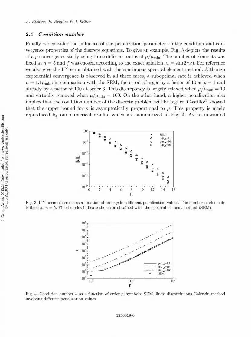
Finally we consider the influence of the penalization parameter on the condition and con-vergence properties of the discrete equations. To give an example, Fig. 3 depicts the resultsof a p-convergence study using three different ratios of µ/µmin. The number of elements wasfixed at n = 5 and f was chosen according to the exact solution, u = sin(2πx). For referencewe also give the L∞ error obtained with the continuous spectral element method. Althoughexponential convergence is observed in all three cases, a suboptimal rate is achieved whenµ = 1.1µmin: in comparison with the SEM, the error is larger by a factor of 10 at p = 1 andalready by a factor of 100 at order 6. This discrepancy is largely relaxed when µ/µmin = 10and virtually removed when µ/µmin = 100. On the other hand, a higher penalization alsoimplies that the condition number of the discrete problem will be higher. Castillo25 showedthat the upper bound for κ is asymptotically proportional to µ. This property is nicelyreproduced by our numerical results, which are summarized in Fig. 4. As an unwanted

Fig. 3. L∞ norm of error ε as a function of order p for different penalization values. The number of elementsis fixed at n = 5. Filled circles indicate the error obtained with the spectral element method (SEM).

Fig. 4. Condition number κ as a function of order p; symbols: SEM, lines: discontinuous Galerkin methodinvolving different penalization values.

1250019-6

J. C

omp.

Aco

us. 2

013.

21. D

ownl

oade

d fr

om w

ww

.wor

ldsc

ient

ific

.com

by 1

15.2

9.18

0.17

3 on

06/

22/1

4. F

or p

erso

nal u

se o

nly.

2nd Reading



side effect of stabilization, the increased condition can degrade the performance of iterativesolvers. Since the growth is related to an increase in the largest eigenvalue, one also hasto consider potential implications for the stability of time integration in applications tounsteady problems.

3. Accuracy and Stability as a Function of Penalization

3.1. Basic equations

The findings in the one-dimensional case suggest that there should be further investigationinto the influence of penalization in the discontinuous Galerkin method applied to morecomplex cases, here the two-dimensional compressible, unsteady Navier–Stokes equations.Considered in the conservative form these equations are

∂tU + ∇ · F = ∇ ·D + S, (2)

where U = (ρ, ρvx, ρvy, ρe)T are the conservative variables, F = (Fx,Fy)T and D =(Dx,Dy)T with

Fi = viU + p

0ei

vi

, Di =

0ei · τ

(τ · v)i + λ∂iT

T

, i = x, y

the convective and diffusive fluxes, respectively, and S the vector of volume forces withthe density ρ, the velocity v = (vx, vy)T, the pressure p, the total energy per unit masse = 1

γ−1pρ + ekin, the kinetic energy per unit mass ekin = 1

2 (v2x + v2

y), the heat conductivityλ, the temperature T , the dynamic viscosity η, and the tensor of viscous stresses

τ = η(∇v + (∇v)T) − 23η(∇ · v)I.

3.2. High-order SIP-DG method in two dimensions

For the spatial discretization, the computational domain Ω is partitioned into a set ofnonoverlapping elements Ωe. Conforming or nonconforming elements of arbitrary shapecan be employed. In the following, we constrain ourselves to quadrilateral elements, possiblywith curved sides. Corresponding to the one-dimensional case, we denote the interior andexterior traces of a scalar or vector function ϕ on the boundary Γe of an element Ωe withϕ− and ϕ+, respectively. With the outer normal n the average · and jump [[·]] of ϕ acrossΓe are defined as ϕ = 1

2 (ϕ− + ϕ+) and [[ϕ]] = n(ϕ− − ϕ+). On element boundary partsthat coincide with the domain boundary of Ω, the exterior values ϕ+ are not availableand an additional boundary treatment is necessary to compute the average and jump. Anappropriate definition of this treatment is crucial for the conservation properties of thesystem, as discussed for wall boundaries in Sec. 4.

1250019-7

J. C

omp.

Aco

us. 2

013.

21. D

ownl

oade

d fr

om w

ww

.wor

ldsc

ient

ific

.com

by 1

15.2

9.18

0.17

3 on

06/

22/1

4. F

or p

erso

nal u

se o

nly.

2nd Reading



In order to derive the semi-discrete DG formulation, the Navier–Stokes equations (2)are rewritten in the quasi-linear form

∂tU + ∇ · F = ∇ · (C∇Π) + S

introducing the primitive variables Π = (vx, vy, T )T and the diffusivity tensor C = C(Π).A similar approach using the entropy variables was given by Pesch.26

The major steps are now the conversion of (2) into a two-equation system of first-orderdifferential equations, the derivation of the weak formulation with test functions φe, partialintegration and conversion back to a one-equation system using appropriate substitutions.A detailed derivation is given by Richter et al.18 This leads to the following primal DGformulation of the Navier–Stokes equations (2) related to one element Ωe∫

Ωe

φe∂tUedΩe =∫

Ωe

∇φe · (F(Ue) − D(Πe,∇Πe))dΩe

−∫

Γe

φe(Hc(U±e ,n) − Hd(Π±

e ,∇Π±e ,n))dΓe

+12

∫Γe

∇φe ·Cn(Π−e )∆ΠedΓe +

∫Ωe

φeSedΩe (3)

with Cn = Cn and ∆Π = (Π− − Π+). The first right-hand side term in (3) considersthe convective and diffusive fluxes in Ωe and the second one the numerical convective anddiffusive fluxes over the discontinuous element boundary Γe. The third right-hand side termcharacterizes the symmetric interior penalty version of the DG (SIP-DG) method and thefourth right-hand side term accounts for the source terms. Special attention has to be paidto the numerical convective and diffusive fluxes Hc and Hd, since they have to be consistentand keep the transport properties of the system.

For the numerical convective flux the Roe flux27,28

Hc(U±,n) =12[Fn(U−) + Fn(U+) − |An(U)|(U+ − U−)] (4)

is used, with the Jacobian An = F′n of the normal convective flux Fn and the Roe average

U. The numerical diffusive flux is defined as

Hd(Π±,∇Π±,n) = (D − µ [[Π]]) · n (5)

with the physically consistent penalization matrix

µ =cipδ

Cnn ,

where δ is the minimal distance between two quadrature points normal to the bound-ary within an element and with the diffusivity matrix Cnn = n · Cn. The new approachconsidered here in contrast to Hartmann and Houston2 or Pesch26 is the use of a penal-ization matrix instead of a constant value. A constant value µ = µ would result in anidentical penalization always using the complete set of primitive variables vx, vy and T in

1250019-8

J. C

omp.

Aco

us. 2

013.

21. D

ownl

oade

d fr

om w

ww

.wor

ldsc

ient

ific

.com

by 1

15.2

9.18

0.17

3 on

06/

22/1

4. F

or p

erso

nal u

se o

nly.

2nd Reading



the numerical diffusive fluxes of continuity, momentum and energy. The advantage of apenalization matrix µ made up of a diffusivity matrix Cnn is a physical penalization ofthe numerical diffusive fluxes; e.g. for momentum only jumps in vx and vy are considered,whereas for energy all three variables are taken into account. The influence of µ, i.e. thepenalization parameter cip , on the stability and accuracy of the SIP-DG method for thetwo-dimensional Navier–Stokes equations, is the subject of the following sections.

The discrete equations are integrated over time using a three-stage TVD Runge–Kuttamethod as described by Shu and Osher,29 with embedded slope limiting and boundarycorrection. As discussed by Cockburn et al.,30 the time integration should be of the sameorder as the spatial discretization. According to the works,7,31,32 the time step size wassufficiently small, so the error in time is negligible compared with spatial errors. Furthermorethe results of the following studies depend only slightly on the transient behavior, so in thissense the time-integration scheme can be interpreted as a steady-state solver.

Introducing the concatenated element coefficients Uh = Uij,e and Lh(Uh) =Uij,e(Uh), the method can be written as

(1) Set U(0)h = Un

h;(2) For i = 1, . . . , k compute the intermediate solutions

U∗h =

i−1∑l=0

αilU(l)h + βlLh(U(l)

h ),

U(i)h = ShBhU∗

h;

(3) Set Un+1h = U(k)

h ;

where for k = 3, α0l = 1, α1l = 34 , 1

4, α2l = 13 , 0, 2

3 and βl = 1, 14 , 2

3. Further, Bh

represents the boundary correction (see Sec. 4) and Sh the slope limiter that is necessary toavoid spurious oscillations in the vicinity of large gradients or jumps in the solution field.Details of the limiting scheme are given by Richter et al.17 In regions that contain a smoothsolution field, the limiter is disabled to preserve the accuracy of the underlying scheme. Forthat a shock detection criterion is applied, which is adapted for high-order methods.19

3.3. Convergence as a function of the wave number kh

The following section is devoted to verifying the order of convergence for the SIP-DG schemediscussed in the previous section. A study into how the penalization parameter influencesthe convergence is given in Sec. 3.4.

DG methods formally converge at a rate of p+ 12 in general, and at p+1 in some special

cases.33 Contrary to standard Galerkin schemes, DG methods can provide super-convergentsolutions at a rate of 2p + 1 or higher. For example, Hu and Atkins34 examined the one-dimensional, scalar advection equation for the case kh → 0. They conjectured that thedispersion error decays locally at a rate of 2p+3 in kh, and the dissipation error at a rate of2p + 2. Ainsworth35 investigated the relation between p and kh and found that for p kh

1250019-9

J. C

omp.

Aco

us. 2

013.

21. D

ownl

oade

d fr

om w

ww

.wor

ldsc

ient

ific

.com

by 1

15.2

9.18

0.17

3 on

06/

22/1

4. F

or p

erso

nal u

se o

nly.

2nd Reading



the solution converges at a super-exponential rate and for 2p + 1 ≈ ckh at an exponentialrate (c as a fixed constant > 1). Furthermore Atkins and Helenbrook33 investigated the flowaround a cylinder and demonstrated that flow parameters can exhibit super convergencewithout additional post-processing techniques.

In Ref. 36, Lomtev et al. suggested Taylor–Green vortices as a test case to approve theconvergence for viscous flows. The initial solution in the domain Ω = [−1, 1]2 is definedusing

ρ = 1 +110

sin(πx),

vx =125

cos(πx) sin(πy),

vy = 0,

T = 84 + 28y,

(6)

with the viscosity equal to 1. The left and right boundaries are defined as periodic, thelower and upper boundaries are isothermal walls. An appropriate additional force term onthe right-hand side of the Navier–Stokes equations compensates the dissipative losses so thatEq. (6) describes a steady-state solution. We defined three equidistant and orthogonal grids,which consist of 5, 10 and 15 elements in each direction. With k = 1

λwas the corresponding

integer wave number and λw = 2 the wave length, the resultant nondimensional wavenumbers kh are 0.2, 0.1 and 0.067, respectively. The stabilization parameter is set by cip = 3,which is close to cip,min and approved in different practical applications.

In order to investigate the convergence rate, we varied the polynomial degree between 2and 8. The maximum norm of the numerical error ε is defined as

ε =√

ε2ρ + ε2

vx+ ε2

vy+ ε2

T ,

with the relative errors ερ = (ρh − ρex)/ρref (εvx , εvy and εT similarly) and the referencevalues ρref = 1, vref = 0.04, Tref = 84, where “ex” indicates the exact solution.

Figure 5 gives the convergence rate as a function of kh. As reported by Hu and Atkins,34

the convergence rate rises in the case kh → 0. This fact is also pointed out in Fig. 5. FromFig. 5 it can be seen that the convergence rate diverges for kh ≤ 0.1 and p > 7. This decreasedepends on the condition number, which is too large, amplifying the influence of roundofferrors.

Table 1 compares the maximum error norm ‖ε‖∞ and the order of convergence O. Thepolynomial degree and the grid resolution are identical to the values used in Fig. 5. In thiscontext, the convergence order is defined as

O =log

(‖ε‖∞,h2

‖ε‖∞,h1

)

log(

h2

h1

)

1250019-10

J. C

omp.

Aco

us. 2

013.

21. D

ownl

oade

d fr

om w

ww

.wor

ldsc

ient

ific

.com

by 1

15.2

9.18

0.17

3 on

06/

22/1

4. F

or p

erso

nal u

se o

nly.

2nd Reading



Fig. 5. L∞ norm of error ε as a function of order p for kh = 0.067 . . . 0.2.

Table 1. L∞ norm of error ε and order of conver-gence O as a function of polynomial order p for kh =0.067 . . . 0.2. The penalization term cip is equal to 3.

p kh Nel ‖ε‖∞ O2 0.2 25 1.573 · 101 2.5

3 0.2 25 1.096 · 100 4.3

4 0.2 25 6.888 · 10−2 3.5

5 0.2 25 3.554 · 10−3 6.0

6 0.2 25 1.527 · 10−4 4.3

7 0.2 25 5.986 · 10−6 8.1

8 0.2 25 2.009 · 10−7 6.4

2 0.1 100 1.496 · 100 3.4

3 0.1 100 6.644 · 10−2 4.0

4 0.1 100 1.678 · 10−3 5.4

5 0.1 100 5.061 · 10−5 6.1

6 0.1 100 8.012 · 10−7 7.6

7 0.1 100 1.980 · 10−8 8.2

8 0.1 100 1.380 · 10−9 7.2

2 0.067 225 4.324 · 10−1 3.1

3 0.067 225 1.211 · 10−2 4.2

4 0.067 225 1.893 · 10−4 5.4

5 0.067 225 3.911 · 10−5 6.3

6 0.067 225 3.738 · 10−8 7.7

7 0.067 225 6.526 · 10−10 8.3

8 0.067 225 3.864 · 10−11 8.8

with h the element size. The calculation of the convergence rate for one mesh depends ondata for the next coarser mesh, so for example the convergence rates for kh = 0.1 are basedon data for kh = 0.2, and so on. Additional post-processing techniques are not applied. Forthe case kh = 0.2, calculations with a mesh kh = 0.5 (Nel = 4) were performed. The results

1250019-11

J. C

omp.

Aco

us. 2

013.

21. D

ownl

oade

d fr

om w

ww

.wor

ldsc

ient

ific

.com

by 1

15.2

9.18

0.17

3 on

06/

22/1

4. F

or p

erso

nal u

se o

nly.

2nd Reading



for this mesh are not listed in Table 1. As displayed in Table 1, for kh = 0.1 and kh = 0.067,the order of convergence is nearly p + 1. On the other hand, with kh = 0.2 the expectedorder of convergence could not be achieved for each polynomial degree. This behavior isdue to an under-resolved physical problem, which means that the grid resolution is not fineenough to sufficiently capture local minima or maxima of the solution. Consequently, thedeviations from the expected rates drop as kh decreases. As discussed above, larger valuesof p lead to larger condition numbers, which amplifies roundoff errors and reduces the rateof convergence. This can be seen in Table 1 for p = 8.

3.4. Influence of penalization on accuracy and time step size

As discussed in Sec. 2.3 for the one-dimensional diffusion equation, a lower bound µmin =cip,min/δ for the penalization µ is derived from a stability analysis using the system eigen-values. Negative eigenvalues, which indicate an unstable system, occur when µ is reducedbeyond this threshold. In this section, the correlation between penalization, overall accuracyand critical time step size is investigated for the two-dimensional DG formulation of theNavier–Stokes equations. The test case is identical to that discussed in the previous section.

In Fig. 6 the normalized maximum norm of the error ε as a function of the penalizationparameter cip is depicted for different wave numbers kh and polynomial orders p. In order toachieve a better comparison between the different combinations of kh and p, for every casethe L∞ norm of ε is normalized by the maximum error. This maximum error is typicallyachieved at cip,min and here denoted as ‖ε‖∞,max. Two distinct regions independent of thediscretization parameter kh can be identified: For cip,min ≤ cip ≤ 1000, the error decreasesasymptotically with a maximum factor of 5. For cip > 1000, the error remains constant.Interestingly, the correlation between kh, p, cip and the error is not consistent: For kh = 0.5,an increased polynomial degree accounts for a decreased convergence rate as a function ofcip . For kh = 0.2, the situation is changed; now an increased polynomial degree also causesan increased convergence rate. Comparing the results with the convergence properties listed

Fig. 6. L∞ norm of the error ε as a function of the penalization parameter cip . Separately for every curve,‖ε‖∞ was normalized by the maximum norm of the error estimated for cip = cip,min, denoted as ‖ε‖∞,max.For that reason all curves start at the point (cip,min, 1).

1250019-12

J. C

omp.

Aco

us. 2

013.

21. D

ownl

oade

d fr

om w

ww

.wor

ldsc

ient

ific

.com

by 1

15.2

9.18

0.17

3 on

06/

22/1

4. F

or p

erso

nal u

se o

nly.

2nd Reading



in Table 1 reveals that increasing p improves the accuracy better than increasing cip by anarbitrary factor.

However, increasing cip in the range from cip,min to 1000 results, as shown, in improvedaccuracy. But it also results in a loss of stability in such a way, that the largest possibletime step size ∆tc, for which the system remains stable, is also reduced. To investigatethe correlation between the penalization parameter cip and the time step size, the criticaltime step ∆tc was determined empirically in a numerical study, where the time step sizewas varied systematically for different combinations of cip and kh until the system becomesunstable. The results of the study suggest the following inverse proportionality

∆tc =δ2Recip

(7)

with the Reynolds number Re (for the given example Re = ρrefvrefkη ). As illustrated in Fig. 7,

the theoretical curve (7) and the numerical experiments are in good agreement. For cip →cip,min the value ∆tc is below the theoretically predicted value. In this region the influenceof the convective time step size, identified by the CFL number, becomes dominant. Thecritical time-step size was estimated using a three-stage Runge–Kutta method, but it is

Fig. 7. Numerical study of critical time step size ∆tc size as a function of penalization parameter cip ;

kh = 0.1 . . . 0.5; dashed line: numerical study, solid line: ∆tc = δ2Recip

; upper figure: p = 2, lower figure: p = 4.

1250019-13

J. C

omp.

Aco

us. 2

013.

21. D

ownl

oade

d fr

om w

ww

.wor

ldsc

ient

ific

.com

by 1

15.2

9.18

0.17

3 on

06/

22/1

4. F

or p

erso

nal u

se o

nly.

2nd Reading



very likely that this estimate remains valid for explicit time-integration schemes offering ahigher order of accuracy. It is worth noting that, if the condition ∆t < ∆tc is fulfilled in thenumerical experiments, the error ε is nearly independent of the time step size.

4. Influence of Wall Treatment on Conservation Properties

4.1. Strategies

In addition to the discretization technique, the boundary treatment significantly influencesthe accuracy and thereby the quality of the solution. In general, different strategies exist:

(1) Strict enforcement of the solution field. This approach strictly keeps the boundaryvalue but leads to instabilities, because it does not respect the type of the underlyingdifferential equation.

(2) Direct definition of fluxes at the boundary considered. This is only possible if the exactflux is known, e.g. at walls.

(3) Alternatively, the outer values at the corresponding edge can be defined in such a waythat the resulting numerical flux meets the exact flux (see e.g. Jacobs et al.37).

(4) Characteristic treatment. Following Hirsch27 or Polifke et al.,38 the solution can bedivided into variables that propagate along characteristic directions. This quasi one-dimensional approach respects the hyperbolic character of the differential equation, butmay fail at more complex geometries.

(5) Buffer zone techniques such as Perfectly Matched Layers (PML) extend the computa-tional domain by additional zones, in which the solution is damped to a homogeneousmean flow.

Which of these strategies is a good choice depends on the boundary type. In the contextof DG schemes, the boundary conditions are typically defined via the corresponding con-vective and diffusive fluxes. Following this, appropriate flux formulations are necessary thatrespect both the given Dirichlet and Neumann conditions and the discretization scheme. Forconvective and diffusive fluxes, a combination of the strategies listed or a different strategyaltogether may be useful or necessary. Due to the inherent simplicity of adiabatic wallswe focus on test problems that involve adiabatic boundaries to investigate the influence ofboundary treatment on conservation properties.

4.2. Advective flux treatment

For adiabatic and solid walls, the characteristic formulation denotes the reflection of char-acteristics running outwards at the wall considered. With the time derivative of the char-acteristic variables Z, linearized in the form

∂tZ = R−1U ≈ ∆tZ∆t

=Zn+1 − Zn

tn+1 − tn,

1250019-14

J. C

omp.

Aco

us. 2

013.

21. D

ownl

oade

d fr

om w

ww

.wor

ldsc

ient

ific

.com

by 1

15.2

9.18

0.17

3 on

06/

22/1

4. F

or p

erso

nal u

se o

nly.

2nd Reading



and R a matrix containing the eigenvectors of the system, the incoming characteristic Z1

is defined by the outgoing characteristic Z4 in the form

∆tZ1 = ∆tZ4.

Due to the linearization, oscillations can be produced that disturb the solution, so thisstrategy shall not be pursued further.

Another possibility is to directly prescribe the boundary flux in the form

Hbc = Hbc(Ubc(U−)).

The boundary function Ubc(U) has to be consistent, which means that Ubc(U) = U, whereU is the exact solution. This condition leads to the boundary flux

Hbc =

0

pbcn

0

. (8)

Several definitions for Ubc(U) are feasible. The choice

Ubc,1 (U) =

U1

0

0

U4 − 12ρ|v|2

results in the simple relation pbc,1 = p−. As an alternative, the boundary functionUbc,2 (U) = (U1, 0, 0, U4)T leads to pbc,2 = p− + 1

2(γ − 1)ρ−|v−|2.39 A third approachconsidered here is based on the solution of a modified Riemann problem at the wall. Forthis we test the implementation proposed by Gottlieb and Groth,40 denoted in the followingas pbc,3.

A different strategy to implement adiabatic walls is to define the outer state U+ in sucha way that the correct boundary flux is achieved

U+ =

ρ−

v− − α1nv−nρe− + β1e

−kin

α1 = 1 . . . 2, β1 = −1 . . . 1. (9)

The actual values of α1 and β1 will be specified later. For frictionless systems such as theEuler equations, at stationary walls, the total energy outside of the boundary is determinedfully by the fluid’s internal energy at the wall. For systems with friction, different choicesfor the kinetic energy may be possible.

1250019-15

J. C

omp.

Aco

us. 2

013.

21. D

ownl

oade

d fr

om w

ww

.wor

ldsc

ient

ific

.com

by 1

15.2

9.18

0.17

3 on

06/

22/1

4. F

or p

erso

nal u

se o

nly.

2nd Reading



4.3. Diffusive flux treatment

As described in Sec. 3, the diffusive fluxes are based on the primitive variables Π and theirgradients ∇Π, thus Π and ∇Π have to be defined properly. In contrast to the boundarytreatment for the advective flux the treatment of Π and ∇Π affects two different terms inEq. (3). As the velocity gradients are unknown at the wall, only an incomplete data set isavailable to define the exact diffusive flux. Alternatively the outer state can be constructedby setting the velocity field to zero or by mirroring the velocity. The outer temperaturehas to meet the inner temperature because no temperature gradients are allowed. Theconstruction scheme follows

Π+ =(v− − α2v−

T−

), (10)

with α2 equal to one in terms of setting the velocity to the boundary value, or two formirroring. Gradients can be treated similarly to diffusive fluxes. Only the temperaturegradient is given to construct the outer state, while the wall shear stress is not defined apriori. This leads to

(∇v)+ = (∇v)−,

∂nT+ = ∂nT− − β2∂nT−,(11)

where β2 is a constant taking the values one or two.It is worth noting that the characteristic formulation to treat the diffusive flux is also

based on the linearization of the time derivatives and is therefore not discussed here.

4.4. Test case

In summary, the four free parameters, α1, α2, β1, β2, have to be specified clearly. For thatpurpose, a lid-driven cavity is investigated as a common test case (see e.g. Jacobs et al.37).The test case is divided into two steps. First, the flow is driven by a moving isothermal wallon the top. Then, all walls are defined as stationary and adiabatic and the development ofmass and total energy inside the container is measured, as well as the temperature gradientsat the boundaries. The domain is divided into 4 × 4 elements of polynomial order 8, theReynolds number during the start-up process is 400 (Fig. 8) and the penalization parameteris defined as cip = 3.

4.5. Mass and energy conservation

In order to consider the influence of both the convective and the diffusive flux on theglobal conservation properties of mass and energy, different strategies were applied for theconvective and the diffusive flux. The convective flux is defined by Eq. (8), with differentchoices for pbc, or based on Eq. (4) in conjunction with Eq. (9), for the latter with differentconstants α1 and β1. The diffusive flux, on the other hand, is defined following Eq. (5), withEqs. (10) and (11) the underlying primitive variables and gradients. Here, α2 and β2 areunknown constants that were varied systematically.

1250019-16

J. C

omp.

Aco

us. 2

013.

21. D

ownl

oade

d fr

om w

ww

.wor

ldsc

ient

ific

.com

by 1

15.2

9.18

0.17

3 on

06/

22/1

4. F

or p

erso

nal u

se o

nly.

2nd Reading



Fig. 8. Lid-driven cavity: snapshots of flow field. Left: start up phase, right: runout phase.

Table 2 displays global mass and energy conservation as a function of advective and dif-fusive flux treatment. Three results emerge: First, depending on α1 and β1, the conservationof mass varies by several orders of magnitude. From Table 2 it is recommendable to chooseα1 = 2 and β1 = 0 or Hbc with any pbc in order to achieve the maximum mass conservation.No influence of the diffusive-flux treatment on mass conservation was measurable. Second,unlike mass conservation, the total energy depends mainly on the treatment of the diffusiveterms and only slightly on the advective flux. Only one configuration — the combinationof mirrored temperature gradients (β2 = 2) and mirrored velocities (α2 = 2) — pushesthe energy losses two orders downward. Finally, a comparison of different boundary fluxesHbc shows that the special choice of pbc has no impact on the conservation of energy andmass. In Table 2 the preferred combinations of convective and diffusive flux treatment aremarked.

4.6. Error in boundary values

In addition to the global mass and energy conservation, the enforcement of given boundaryconditions may also influence the accuracy of the numerical scheme. In order to estimatethe relation between different formulations for the convective and the diffusive fluxes andthe error in the boundary values, the maximum errors in the velocity components and thetemperature gradient are measured. Due to the adiabatic walls, the temperature gradientnormal to the wall should be equal to zero, as are the wall-tangential and normal componentsof the velocity vector.

Table 3 lists the error in boundary values for different convective fluxes. Different conclu-sions can be drawn: The error in vt is approximately independent of the boundary treatment,but may be a function of the penalty term cip . The special choice of pbc does not influencethe boundary errors, so the results in Table 3 are nearly identical for different pbc . Thisstatement holds true for different choices of the diffusive flux. The influence of β1 is alsonegligible. From the examination of mass and energy conservation β1 should be equal tozero. The impact of α1 on ‖εvn‖∞ is small, but surprisingly large for ‖ε∂nT ‖∞, i.e. one order

1250019-17

J. C

omp.

Aco

us. 2

013.

21. D

ownl

oade

d fr

om w

ww

.wor

ldsc

ient

ific

.com

by 1

15.2

9.18

0.17

3 on

06/

22/1

4. F

or p

erso

nal u

se o

nly.

2nd Reading



Table 2. Mass and total energy conservation as a function of adiabaticand viscous fluxes.

α1 β1 α2 β2 ‖εm‖∞ ‖εe‖∞1 −1 1 1 4.099 · 10−7 1.320 · 10−6

1 −1 1 2 5.042 · 10−7 4.246 · 10−6

1 −1 2 1 6.876 · 10−7 1.023 · 10−5

1 −1 2 2 7.184 · 10−7 4.754 · 10−7

1 0 1 1 4.852 · 10−7 1.292 · 10−6

1 0 1 2 5.766 · 10−7 4.218 · 10−6

1 0 2 1 7.748 · 10−7 1.026 · 10−5

1 0 2 2 7.999 · 10−7 5.051 · 10−7

1 1 1 1 5.606 · 10−7 1.264 · 10−6

1 1 1 2 6.490 · 10−7 4.191 · 10−6

1 1 2 1 8.620 · 10−7 1.029 · 10−5

1 1 2 2 8.814 · 10−7 5.347 · 10−7

2 −1 1 1 8.286 · 10−9 1.638 · 10−6

2 −1 1 2 8.284 · 10−9 4.538 · 10−6

2 −1 2 1 8.791 · 10−9 9.825 · 10−6

2 −1 2 2 8.775 · 10−9 7.496 · 10−8

2 0 1 1 7.320 · 10−12 1.635 · 10−6

2 0 1 2 7.320 · 10−12 4.535 · 10−6

2 0 2 1 7.320 · 10−12 9.828 · 10−6

2 0 2 2 7.312 · 10−12 7.835 · 10−8

2 1 1 1 8.301 · 10−9 1.632 · 10−6

2 1 1 2 8.298 · 10−9 4.531 · 10−6

2 1 2 1 8.806 · 10−9 9.832 · 10−6

2 1 2 2 8.790 · 10−9 8.174 · 10−8

Hbc,1 1 1 7.320 · 10−12 1.629 · 10−6

Hbc,1 1 2 7.320 · 10−12 4.443 · 10−6

Hbc,1 2 1 7.320 · 10−12 9.818 · 10−6

Hbc,1 2 2 7.320 · 10−12 7.844 · 10−8

Hbc,2 1 1 7.324 · 10−12 1.785 · 10−6

Hbc,2 1 2 7.323 · 10−12 4.402 · 10−6

Hbc,2 2 1 7.320 · 10−12 9.745 · 10−6

Hbc,2 2 2 7.318 · 10−12 7.734 · 10−8

Hbc,3 1 1 7.323 · 10−12 1.629 · 10−6

Hbc,3 1 2 7.319 · 10−12 4.443 · 10−6

Hbc,3 2 1 7.320 · 10−12 9.82 · 10−6

Hbc,3 2 2 7.319 · 10−12 7.84 · 10−8

of magnitude. For that reason α1 should be equal to two, which is consistent with previousfindings for mass and energy conservation. The situation changes, if the diffusive flux treat-ment is considered. In Table 3 combinations are marked that are advantageous in terms ofsmall boundary errors. The most promising combination is α2 = 1 and β2 = 2. If Eqs. (4)and (9) are used, α2 = 1 and β2 = 1 is also possible. A comparison with Table 2 reveals

1250019-18

J. C

omp.

Aco

us. 2

013.

21. D

ownl

oade

d fr

om w

ww

.wor

ldsc

ient

ific

.com

by 1

15.2

9.18

0.17

3 on

06/

22/1

4. F

or p

erso

nal u

se o

nly.

2nd Reading



Table 3. Error in boundary conditions for different choices ofconvective and diffusive fluxes.

α1 β1 α2 β2 ‖εvn‖∞ ‖εvt‖∞ ‖ε∂nT ‖∞1 0 2 2 9.696 · 10−8 3.258 · 10−7 4.368 · 10−7

2 0 1 1 7.817 · 10−9 4.618 · 10−7 1.978 · 10−8

2 0 1 2 7.866 · 10−9 4.620 · 10−7 1.389 · 10−8

2 0 2 1 2.294 · 10−8 3.064 · 10−7 6.735 · 10−8

2 0 2 2 2.304 · 10−8 2.759 · 10−7 4.452 · 10−8

2 1 2 2 2.303 · 10−8 2.764 · 10−7 4.482 · 10−8

Hbc,1 1 1 1.096 · 10−7 4.306 · 10−7 1.222 · 10−8

Hbc,1 1 2 1.102 · 10−7 4.310 · 10−7 6.343 · 10−9

Hbc,1 2 1 9.811 · 10−8 3.464 · 10−7 4.734 · 10−8

Hbc,1 2 2 8.803 · 10−8 3.170 · 10−7 3.033 · 10−8

Hbc,2 2 2 8.801 · 10−8 3.169 · 10−7 3.035 · 10−8

Hbc,3 2 2 8.803 · 10−8 3.170 · 10−7 3.031 · 10−8

that no combination exists which minimizes both the error in mass and energy conservationand the error in boundary values.

The listed results reveal that a minimized error in boundary values reduces the conserva-tion properties of the scheme, and vice versa. From adjoint consistency analysis it is knownthat Eq. (8) should be preferred.39 For this reason we recommend that the advective fluxHbc should be used. Since the special choice of pbc does not influence conservation proper-ties and boundary values, we propose the usage of pbc = pbc,1 = p−. This choice minimizeswork on implementation and calculation, especially in comparison with the solution of aRiemann problem at the wall. The values α2 and β2 have to be equal to two. This definitionincreases the energy conservation accuracy by two orders of magnitude, with a moderateaccuracy loss in vn and ∂nT at the wall. If one may choose Eq. (4) together with Eq. (9) forthe advective flux, α1 = 2 and β1 = 0 are superior to any other combinations. It is worthnoting that in Table 3 only a selection of all possible combinations are listed. Of course wehave considered every combination of advective and diffusive flux, so all statements givenhere holds true for parameters that are not listed in Table 3.

5. Conclusion

This article is devoted to the influence of penalization and boundary treatment on the stabil-ity and accuracy of high-order discontinuous Galerkin schemes for the compressible Navier–Stokes equations. For this purpose, a high-order interior penalty discontinuous Galerkinmethod for the compressible Navier–Stokes equations was introduced; it can be interpretedas a modification of the scheme given by Hartmann and Houston.2

To investigate the stability of the scheme, we first estimated lower bounds for the penal-ization term µ by observing the eigenvalues and condition numbers for one-dimensionalconvection–diffusion problems. We were able to demonstrate that the stability threshold

1250019-19

J. C

omp.

Aco

us. 2

013.

21. D

ownl

oade

d fr

om w

ww

.wor

ldsc

ient

ific

.com

by 1

15.2

9.18

0.17

3 on

06/

22/1

4. F

or p

erso

nal u

se o

nly.

2nd Reading



µmin is inversely proportional to δ, with cip the proportionality factor and δ the minimaldistance between quadrature points normal to the edge of the element. The analysis of thesystem’s eigenvalues yields a lower bound of cip at 1.85, at which the solution is stable.

Next, by studying two-dimensional convection–diffusion problems, we investigated rela-tions between the accuracy of the scheme and cip . In fact increasing the factor cip reducesthe overall error, but the reduction is on a moderate level only. At the same time, increas-ing cip reduces the admissible time step size, at which the explicit time integration schemeremains stable. Thereby we found the relation ∆tc = δ2Re

cip, which means ∆tc is inversely

proportional to the penalization parameter cip . In this relation a constant is introducedwhich is denoted as the Reynolds number. This fact is approved only for one test case andshould be tested for other flow problems in further studies. The given relation allows theconclusion that in terms of a minimized discretization error and a minimum computationaleffort the approximation order and/or the spatial discretization should be increased whilecip should remain at the lower bound given by the stability criteria.

Finally, different strategies for enforcing boundary conditions were tested in termsof minimized global mass and energy losses and minimized approximation errors at theboundaries. We were able to demonstrate that different boundary treatments influence theaccuracy by various orders of magnitude, and propose reasonable strategies to improve con-servation properties. This investigation was restricted to adiabatic walls. Further studiesshould be performed in order to respect different types of boundary conditions, e.g. inflowand outflow conditions, as well as isothermal walls.

Acknowledgments

This work was supported by the German National Science Foundation (DeutscheForschungsgemeinschaft, DFG) within the project Gr 1388/18-1, Numerical simulation ofthe sound spectrum and the sound radiation in and around a recorder (Numerische Simu-lation des Klangspektrums und der Schallausbreitung in und um eine Blockflote).

References

1. T. Lahivaara, M. Malinen, J. P. Kaipio and T. Huttunen, Computational aspects of the discon-tinuous Galerkin method for the wave equation, J. Comp. Acoust. 16 (2008) 507–530.

2. R. Hartmann and P. Houston, An optimal order interior penalty discontinuous Galerkin dis-cretization of the compressible Navier–Stokes equations, J. Comput. Phys. 227 (2008) 9670–9685.

3. D. N. Arnold, F. Brezzi, B. Cockburn and L. D. Marini, Unified analysis of discontinuousGalerkin methods for elliptic problems, SIAM J. Numer. Anal. 39 (2001) 1749–1779.

4. R. M. Kirby and G. E. Karniadakis, Selecting the numerical flux in discontinuous Galerkinmethods for diffusion problems, J. Sci. Comput. 22/23 (2005) 385–411.

5. G. Gassner, F. Lorcher and C.-D. Munz, A contribution to the construction of diffusion fluxesfor finite volume and discontinuous Galerkin schemes, J. Comput. Phys. 224 (2007) 1049–1063.

6. B. Cockburn and B. Dong, An analysis of the minimal dissipation local discontinuous Galerkinmethod for convection–diffusion problems, J. Sci. Comput. 32 (2007) 233–262.

1250019-20

J. C

omp.

Aco

us. 2

013.

21. D

ownl

oade

d fr

om w

ww

.wor

ldsc

ient

ific

.com

by 1

15.2

9.18

0.17

3 on

06/

22/1

4. F

or p

erso

nal u

se o

nly.

2nd Reading



7. B. Cockburn and C.-W. Shu, The local discontinuous Galerkin method for time-dependentconvection–diffusion systems, SIAM J. Numer. Anal. 35 (1998) 2440–2463.

8. O. C. Zienkiewicz, R. L. Taylor, S. J. Sherwin and J. Peiro, On discontinuous Galerkin methods,Int. J. Numer. Meth. Eng. 58 (2003) 1119–1148.

9. B. Landmann, M. Kessler, S. Wagner and E. Kramer, A parallel, high-order discontinuousGalerkin code for laminar and turbulent flows, Comp. Fluids 37 (2008) 427–438.

10. H. Liu and K. Xu, A Runge-Kutta discontinuous Galerkin method for viscous flow equations,J. Comput. Phys. 224 (2007) 1223–1242.

11. G. Gassner, F. Lorcher and C.-D. Munz, A discontinuous Galerkin scheme based on a space-timeexpansion II. Viscous flow equations in multi dimensions, J. Sci. Comput. 34 (2008) 260–286.

12. J. W. Kim and D. J. Lee, Implementation of boundary conditions for optimized high-ordercompact schemes, J. Comp. Acoust. 5 (1997) 177–191.

13. C. K. W. Tam, Advances in numerical boundary conditions for computational aeroacoustics,J. Comp. Acoust. 6 (1998) 377–402.

14. T. Hagstrom, M. L. De Castro, D. Givoli and D. Tzemach, Local high-order absorbing boundaryconditions for time-dependent waves in guides, J. Comp. Acoust. 15 (2007) 1–22.

15. C. M. Klaij, J. J. W. van der Vegt and H. van der Ven, Space-time discontinuous Galerkinmethod for the compressible Navier–Stokes equations, J. Comput. Phys. 217 (2006) 589–611.

16. M. Feistauer and V. Kucera, On a robust discontinuous Galerkin technique for the solution ofcompressible flow, J. Comput. Phys. 224 (2007) 208–221.

17. A. Richter, J. Stiller and R. Grundmann, Stabilized discontinuous Galerkin methods for flow-sound interaction, J. Comp. Acoust. 15 (2007) 123–143.

18. A. Richter, E. Brußies, J. Stiller and R. Grundmann, Aeroacoustics investigation of wood-wind instruments based on discontinuous Galerkin methods, in Computational Fluid DynamicsReview, eds. M. Hafez, K. Oshima and D. Kwak (World Scientific, 2010), pp. 399–419.

19. L. Krivodonova, J. Xin, J.-F. Remacle, N. Chevaugeon and J. E. Flaherty, Shock detection andlimiting with discontinuous Galerkin methods for hyperbolic conservation laws, Appl. Numer.Math. 48 (2004) 323–338.

20. K. Shahbazi, An explicit expression for the penalty parameter of the interior penalty method,J. Comput. Phys. 205 (2005) 401–407.

21. Y. Epshteyn and B. Riviere, Estimation of penalty parameters for symmetric interior penaltyGalerkin methods, J. Comput. Appl. Math. 206 (2007) 843–872.

22. D. Sarmany, F. Izsak and J. van der Vegt, Optimal penalty parameters for symmetric discon-tinuous Galerkin discretisations of the time-harmonic Maxwell equations, J. Sci. Comput. 44(2010) 219–254.

23. M. O. Deville, P. F. Fischer and E. H. Mund, High-Order Methods for Incompressible Fluid Flow,Cambridge Monographs on Applied and Computational Mathematics (Cambridge UniversityPress, 2002).

24. G. E. Karniadakis and S. Sherwin, Spectral/hp Element Methods for Computational FluidDynamics, 2nd edn. (Oxford University Press Inc., New York, 2005).

25. P. Castillo, Performance of discontinuous Galerkin methods for elliptic PDE’s, SIAM J. Sci.Comput. 24 (2002) 524–547.

26. L. Pesch, Discontinuous Galerkin finite element methods for the Navier–Stokes equations inentropy variable formulation, PhD thesis, University of Twente (2007).

27. C. Hirsch, Numerical Computation of Internal and External Flows, Vol. 1 & 2 (Wiley-Interscience Publication, 1990).

28. R. J. Leveque, Finite Volume Methods for Hyperbolic Problems, Cambridge Texts in AppliedMathematics (Cambridge University Press, 2002).

1250019-21

J. C

omp.

Aco

us. 2

013.

21. D

ownl

oade

d fr

om w

ww

.wor

ldsc

ient

ific

.com

by 1

15.2

9.18

0.17

3 on

06/

22/1

4. F

or p

erso

nal u

se o

nly.

2nd Reading



29. C.-W. Shu and S. Osher, Efficient implementation of essentially non-oscillatory shock-capturingschemes, J. Comput. Phys. 77 (1998) 439–471.

30. B. Cockburn, S.-Y. Lin and C.-W. Shu, The Runge-Kutta discontinuous Galerkin finite ele-ment method for conservation laws V: Multidimensional systems, J. Comput. Phys. 141 (1998)199–224.

31. H. L. Atkins and C.-W. Shu, Quadrature-free implementation of discontinuous Galerkin methodfor hyperbolic equations, AIAA J. 36 (1998) 775–782.

32. A. Burbeau, P. Sagaut and C.-H. Bruneau, A problem-independent limiter for high-order Runge–Kutta discontinuous Galerkin methods, J. Comput. Phys. 169 (2001) 111–150.

33. H. Atkins and B. Helenbrook, Super-convergence of discontinuous Galerkin method applied tothe Navier–Stokes equations, AIAA J. 3787 (2009) 1–13.

34. F. Q. Hu and H. L. Atkins, Eigensolution analysis of the discontinuous Galerkin method withnonuniform grids: I. One space dimension, J. Comput. Phys. 182 (2002) 516–545.

35. M. Ainsworth, Dispersive and dissipative behaviour of high order discontinuous Galerkin finiteelement methods, J. Comput. Phys. 198 (2004) 106–130.

36. I. Lomtev, C. B. Quillen and G. E. Karniadakis, Spectral/hp methods for viscous compressibleflows on unstructured 2D meshes, J. Comput. Phys. 144 (1998) 325–357.

37. G. B. Jacobs, D. A. Kopriva and F. Mashayek, A conservative isothermal wall boundary condi-tion for the compressible Navier–Stokes equations, J. Sci. Comput. 30 (2007) 177–192.

38. W. Polifke, C. Wall and P. Moin, Partially reflecting and non-reflecting boundary conditions forsimulation of compressible viscous flow, J. Comput. Phys. 213 (2006) 437–449.

39. R. Hartmann, Adjoint consistency analysis of discontinuous Galerkin discretizations, SIAM J.Numer. Anal. 45 (2007) 2671–2696.

40. J. J. Gottlieb and C. P. T. Groth, Assessment of Riemann solvers for unsteady one-dimensionalinviscid flows of perfect gases, J. Comput. Phys. 78 (1988) 437–458.

1250019-22

J. C

omp.

Aco

us. 2

013.

21. D

ownl

oade

d fr

om w

ww

.wor

ldsc

ient

ific

.com

by 1

15.2

9.18

0.17

3 on

06/

22/1

4. F

or p

erso

nal u

se o

nly.

Documents

INFLUENCE OF PENALIZATION AND BOUNDARY TREATMENT ON THE STABILITY AND ACCURACY OF HIGH-ORDER DISCONTINUOUS GALERKIN SCHEMES FOR THE COMPRESSIBLE NAVIER-STOKES EQUATIONS