A Parallel, Implicit Reconstructed Discontinuous Galerkin Method for the Compressible Flows on 3D Arbitrary Grids

A Parallel, Implicit Reconstructed Discontinuous

Galerkin Method for the Compressible Flows on 3D

Arbitrary Grids

Yidong Xia∗ , Hong Luo† , Seth Spiegel‡ and Megan Frisbey‡

Department of Mechanical and Aerospace Engineering

North Carolina State University, Raleigh, NC 27695-7910, United States

Robert Nourgaliev§

Thermal Science and Safety Analysis Department

Idaho National Laboratory, Idaho Falls, ID 83415-3840, United States

A Navier-Stokes flow solver RDGFLO based on a third-order accurate reconstructeddiscontinuous Galerkin (RDG) method is presented for modeling the compressible flows on3D arbitrary grids. A remarkable feature of this solver is that the 1D, 2D and 3D flow prob-lems can be simulated with the very same code, thanks to the adopted Taylor basis for thevarious types of elements, i.e., tetrahedron, pyramid, prism, and hexahedron. A quadraticpolynomial (P2) solution is obtained from the underlying linear polynomial (P1) DG so-lution via a hierarchical WENO reconstruction scheme, termed as HWENO(P1P2), whichis designed in order to not only increase the accuracy of the underlying DG method, butalso ensure the non-linear stability of the RDG method. Both multi-stage explicit Runge-Kutta and implicit backward Euler methods are implemented for time advancement inthe RDG method. In the implicit method, the flux Jacobian matrix is well approximatedvia an automatic differentiation engine TAPENADE, which is the key to a robust andefficient linear solver. The approximate system of linear equations arising from Newtonlinearization is solved by an LU-SGS (lower-upper symmetric Gauss-Seidel) preconditionedGMRES (general minimum residual) algorithm, termed as GMRES+LU-SGS. The paral-lelization in the RDG method is based on a message passing interface (MPI) programmingparadigm, where the METIS library is used for the partitioning of a grid into subdomaingrids of approximately the same size. The developed solver is used to compute a varietyof compressible flow problems to demonstrate its accuracy, robustness and scalability. Thenumerical experiments indicate that RDGFLO is able to offer a cost-effective solution tocomplicated flows of practical importance. Overall, the developed RDG method shows agreat potential to become a viable, attractive, competitive and ultimately superior DGmethod over the current state-of-the-art second-order finite volume methods.

I. Introduction

The discontinuous Galerkin (DG) methods16,18,9, 8, 12,19,56,10,35,60,58,59,49,67,66,36,4, 5, 6, 20,28,29,29,55,34,57

have recently become popular for the solution of systems of conservation laws. Originally introduced for thesolution of neutron transport equations,62 nowadays they are widely used in computational fluid dynamics(CFD), computational acoustics, and computational magneto-hydrodynamics (MHD). The DG methodscombine two advantageous features commonly associated to the finite element (FE) methods and finitevolume (FV) methods. As in classical finite element methods, accuracy is obtained by means of high-order

∗Graduate Student, AIAA Student Member. Corresponding Author: [email protected]†Associate Professor, AIAA Senior Member.‡Graduate Student, AIAA Senior Member.§Senior Scientist

1 of 42

American Institute of Aeronautics and Astronautics

polynomial approximation within an element rather than by wide stencils as in the case of finite volumemethods. The physics of wave propagation is, however, accounted for by solving the Riemann problemsthat arise from the discontinuous representation of the solution at element interfaces. In this respect, themethods are therefore similar to finite volume methods. The DG methods have many features: 1) Theyhave several useful mathematical properties with respect to conservation, stability, and convergence; 2) Themethods can be easily extended to higher-order (> 2nd) approximation; 3) The methods are well suited forcomplex geometries since they can be applied on unstructured grids. In addition, the methods can also handlenon-conforming elements, where the grids are allowed to have hanging nodes; 4) The methods are highlyparallelizable, as they are compact and each element is independent. Since the elements are discontinuous,and the inter-element communications are minimal, domain decomposition can be efficiently employed. Thecompactness also allows for structured and simplified coding for the methods; 5) They can easily handleadaptive strategies, since refining or coarsening a grid can be achieved without considering the continuityrestriction commonly associated with the conforming elements. The methods allow easy implementationof hp-refinement, for example, the order of accuracy, or shape, can vary from element to element; 6) Theyhave the ability to compute low Mach number flow problems without recourse to the time-preconditioningtechniques normally required for the finite volume methods. In contrast to the enormous advances in thetheoretical and numerical analysis of the DG methods, the development of a viable, attractive, competitive,and ultimately superior DG method over the more mature and well-established second order finite volumemethods is relatively an untouched area. This is mainly due to the fact that the DG methods have a numberof weaknesses that have yet to be addressed, before they can be robustly used for flow problems of practicalinterest in a complex configuration environment. In particular, how to effectively control spurious oscillationsin the presence of strong discontinuities, and how to reduce the computing costs for the DG methods remainthe two most challenging and unresolved issues in the DG methods. Indeed, compared to the FE and FVmethods, the DG methods require solutions of systems of equations with more unknowns for the same grids.Consequently, these methods have been recognized as expensive in terms of both computational costs andstorage requirements especially in the context of implicit methods, where the memory requirement for theJacobian matrix grows quadratically with the order of the DG methods, thus leading to a significant increasein computational cost.

In order to reduce the high costs associated with the DG methods, Dumbser et al.23,22,24 have introduceda new family of reconstructed DG methods, termed PnPm schemes and referred to as RDG(PnPm) in thispaper, where Pn indicates that a piecewise polynomial of degree of n is used to represent a DG solution,and Pm represents a reconstructed polynomial solution of degree of m (m ≥ n) that is used to computethe fluxes. The RDG(PnPm) schemes are designed to enhance the accuracy of the discontinuous Galerkinmethod by increasing the order of the underlying polynomial solution. The beauty of RDG(PnPm) schemesis that they provide a unified formulation for both the FV and DG methods, and contain both classical FVand standard DG methods as two special cases of RDG(PnPm) schemes, and thus allow for a direct efficiencycomparison. When n = 0, i.e., a piecewise constant polynomial is used to represent a numerical solution,RDG(P0Pm) is nothing but the classical high order FV schemes, where a polynomial solution of degree m(m ≥ 1) is reconstructed from a piecewise constant solution. When m = n, the reconstruction reduces tothe identity operator, and RDG(PnPn) scheme yields a standard DG method.

Obviously, the construction of an accurate and efficient reconstruction operator is crucial to the successof the RDG(PnPm) schemes. In Dumbser’s work, a higher-order polynomial solution is reconstructed usingan L2 projection, requiring it indistinguishable from the underlying DG solutions in the contributing cells inthe weak sense. The resulting over-determined system is then solved by using a least-squares method thatguarantees exact conservation, not only of the cell averages but also of all higher-order moments in the re-constructed cell itself, such as slopes and curvatures. However, this conservative least-squares reconstructionapproach is computationally expensive, as the L2 projection, i.e., the operation of integration, is required toobtain the resulting over-determined system. Furthermore, the reconstruction might be problematic for aboundary cell, where the number of the adjacent face-neighboring cells might not be enough to provide thenecessary information to recover a polynomial solution of a desired order. Fortunately, the projection-basedreconstruction is not the only way to obtain a polynomial solution of higher order from the underlying dis-continuous Galerkin solutions. In the reconstructed DG method using a Taylor basis47,48,45,51,53 developedby Luo et al. for the solution of the compressible Euler and Navier-Stokes equations on 2D arbitrary gridsand 3D tetrahedral grids, a higher-order polynomial solution is reconstructed by using a strong interpolation,requiring point values and derivatives to be interpolated on the adjacent face-neighboring cells. The result-

2 of 42


ing over-determined linear system of equations is then solved in the least-squares sense. This reconstructionscheme only involves the von Neumann neighborhood, and thus is compact, simple, robust, and flexible.Like the projection-based reconstruction, the strong reconstruction scheme guarantees exact conservation,not only of the cell averages but also of their slopes due to a judicious choice of the Taylor basis. Morerecently, Zhang et al.75,76 presented a class of hybrid DG/FV methods for the conservation laws, where thesecond derivatives in a cell are obtained from the first derivatives in the cell itself and its neighboring cellsusing a Green-Gauss reconstruction widely used in the FV methods. This also provides a fast, simple, androbust way to obtain higher-order polynomial solutions. More recently, Luo et al.52,54 have conducted acomparative study for these three reconstructed discontinuous Galerkin methods RDG(P1P2) for solving the2D Euler equations on arbitrary grids. It is found that all the three reconstructed discontinuous Galerkinmethods can deliver the desired third-order accuracy and significantly improve the accuracy of the underlyingsecond-order DG method, although the least-squares reconstruction method provides the best performancein terms of both accuracy and robustness.

However, the attempt to directly extend the RDG method to solve the 3D Euler equations on tetrahedralgrids is not successful. Like the second-order cell-centered FV methods, i.e., RDG(P0P1), the resultantRDG(P1P2) method is numerically unstable. Although the RDG(P0P1) methods are in general stable in 2Dand on Cartesian or structured grids in 3D, they suffer from the so-called linear instability on unstructuredtetrahedral grids, when the reconstruction stencils only involve von Neumann neighborhood, i.e., adjacentface-neighboring cells.27 The RDG(P1P2) method exhibits the same linear instability, which can be overcomeby using extended reconstruction stencils. However, this is achieved at the expense of sacrificing the com-pactness of the underlying DG methods. Furthermore, these linear reconstruction-based DG methods willsuffer from the non-physical oscillations in the vicinity of strong discontinuities for the compressible Eulerequations. Alternatively, the ENO, WENO and HWENO schemes can be used to reconstruct a higher-orderpolynomial solution, which can not only enhance the order of accuracy of the underlying DG method butalso achieve both the linear and non-linear stability. This type of hybrid HWENO + DG schemes has beendeveloped on 1D and 2D structured grids by Balsara et al.,7 where the HWENO reconstruction is relativelysimple and straightforward. Recently, Luo et al. developed a Hermite-WENO reconstruction, termed asWENO(P1P2) in this paper, using a Taylor basis42 for the solution of the compressible Euler equations on3D unstructured tetrahedral grids. In this WENO(P1P2) scheme, a quadratic solution is reconstructed toenhance the accuracy of the underlying DG(P1) method in two steps: 1) all second derivatives on each cell arefirst reconstructed using the solution variables and their first derivatives from adjacent face-neighboring cellsvia a strong interpolation; 2) the final second derivatives on each cell are then obtained using a WENO re-construction based on the reconstructed second derivatives on the cell itself and its adjacent face-neighboringcells. This WENO(P1P2) scheme, by taking advantage of handily available and yet valuable informationnamely the gradients in the context of the DG methods, only involves von Neumann neighborhood andthus is compact, simple, robust, and flexible. As the underlying DG method is second order, and the ba-sis functions are at most linear functions, fewer quadrature points are then required for both volume andface integrals, and the number of unknowns (the number of degrees of freedom) remains the same as forDG(P1). Consequently, this RDG method is more efficient than its third-order DG(P2) counterpart. Xia etal.69 further extended this WENO(P1P2) scheme to the compressible Navier-Stokes equations on 3D hybridgrids. More recently, Luo et al. developed a two-step hierarchical WENO scheme HWENO(P1P2)53 for thecompressible Euler equations on unstructured tetrahedral grids, in which the first step is nothing but theWENO(P1P2) reconstruction, and the gradients of the quadratic polynomial solutions are then modified us-ing a WENO reconstruction in the second step in order to eliminate non-physical oscillations in the vicinityof strong discontinuities, thus ensuring the non-linear stability of the RDG method.

In contrast to the enormous advances in spatial discretization of the DG methods, the temporal discretiza-tion methods have lagged far behind. Usually, explicit temporal discretizations such as multi-stage TVD(total variation diminishing) Runge-Kutta schemes16,9, 8, 19,18 are adopted to advance the solution in time.Explicit schemes and their boundary conditions are easy to implement, vectorize and parallelize, and requireonly limited memory storage. However, for large-scale simulations and especially for higher-order solutions,the rate of convergence slows down dramatically, resulting in inefficient solution techniques. To accelerateconvergence, an implicit strategy is required. In general, the implicit DG methods11,10,61,12,26,35,56,74,21

require the solution of a linear system of equations arising from the linearization of a fully implicit schemeat each timestep. Unfortunately, they all require a considerable amount of memory to store the Jacobianmatrix. Even for the so-called “matrix-free” methods where only a block diagonal matrix is required to

3 of 42


store, the memory requirement can still be demanding. The block diagonal matrix requires a storage of(Ndegr×Netot)×(Ndegr×Netot) ×Nelem, where Ndegr is the number of degree of freedom (DOFs) forthe polynomial (3 for P1, 6 for P2, and 10 for P3 for a triangular element in 2D; 4 for P1, 10 for P2, and20 for P3 for a tetrahedral element in 3D), Netot is the number of equations (4 for 2D, and 5 for 3D in theNavier-Stokes equations), and Nelem is the number of elements for the grid. Take a 4th-order (cubic poly-nomial finite element approximation P3) DG method in 3D for example, the storage of this block diagonalmatrix alone requires 10,000 words per element. Indeed, it is our belief that a lack of efficient solvers is oneof the reasons that the application of the DG methods for engineering-type problems does not exist.

Recently, Xia et al.70,72 developed an efficient implicit method for the RDG(P1P2) method for thecompressible Euler equations on tetrahedral grids. A remarkable feature of this implicit method is that thelinearization of the RDG(P1P2) scheme is based only on the underlying DG(P1) scheme, and the resultingstructure of the Jacobian matrix remains the same as for DG(P1), which is a huge saving in both computingtime and memory requirements in contrast to the one of DG(P2). In fact, the exact Jacobian matrix of theRDG method is practically not accessible in a closed form, e.g., when linearization involves HWENO(P1P2)which is highly nonlinear in nature. More recently, Xia et al.71 presented an automatic differentiation basedimplicit RDG(P1P2) method for the compressible Navier-Stokes equations on unstructured tetrahedral grids,where the Jacobian matrix is well approximated via an automatic differentiation engine TAPENADE,3 andleads to a highly robust and efficient linear solver. Automatic differentiation (AD)15,14 is a set of techniquesbased on the mechanical application of the chain rule to obtain derivatives of a function given as a computerprogram. With the aid of AD tools, the labor for a programmer can be significantly released from manualimplementation, which can be quite complicated, tedious and error-prone if done by hand or symbolicarithmetic software, depending on the complexity of the functions. In addition, the workload for codemaintenance can also be greatly relieved in case the numerical schemes are updated.

The objective of the effort discussed in this paper is to develop a Navier-Stokes flow solver RDGFLO basedon a third-order accurate reconstructed discontinuous Galerkin (RDG) method for modeling the compressibleflows on 3D arbitrary grids. A remarkable feature of this solver is that the 1D, 2D and 3D flow problems canbe simulated with the very same code, thanks to the adopted Taylor basis for the various types of elements,i.e., tetrahedron, pyramid, prism, and hexahedron. A quadratic polynomial (P2) solution is obtained fromthe underlying linear polynomial (P1) DG solution via a hierarchical WENO reconstruction scheme, termedas HWENO(P1P2), which is designed in order to not only increase the accuracy of the underlying DGmethod, but also ensure the non-linear stability of the RDG method. Both multi-stage explicit Runge-Kutta and implicit backward Euler methods are implemented for time advancement in the RDG method.In the implicit method, the flux Jacobian matrix is well approximated via an automatic differentiationengine TAPENADE, which is the key to a robust and efficient linear solver. The approximate system oflinear equations arising from Newton linearization is solved by an LU-SGS (lower-upper symmetric Gauss-Seidel) preconditioned GMRES (general minimum residual) algorithm, termed as GMRES+LU-SGS. Theparallelization in the RDG method is based on a message passing interface (MPI) programming paradigm,where the METIS library is used for the partitioning of a grid into subdomain grids of approximately thesame size. The developed solver is used to compute a variety of compressible flow problems to demonstrateits accuracy, robustness and scalability. The numerical experiments indicate that RDGFLO is able to offera cost-effective solution to complicated flows of practical importance. Overall, the developed RDG methodshows a great potential to become a viable, attractive, competitive and ultimately superior DG method overthe current state-of-the-art second-order finite volume methods. The remainder of this paper is organizedas follows. The governing equations are described in Section II. The discontinuous Galerkin discretizationand the reconstruction schemes are presented in Section III and IV. The implicit time integration methodsare discussed in Section V. The parallelization strategy is illustrated in Section VI. Extensive numericalexperiments are reported in Section VII. Concluding remarks are given in Section VIII.

II. Governing equations

The Navier-Stokes equations governing unsteady compressible viscous flows can be expressed as

∂U(x, t)

∂t+∂Fk(U(x, t))

∂xk=∂Gk(U(x, t))

∂xk(1)

4 of 42


where the summation convention has been used. The conservative variable vector U, advective (inviscid)flux vector F, and viscous flux vector G are defined by

U =

ρ

ρui

ρe

Fj =

ρuj

ρuiuj + pδij

uj(ρe+ p)

Gj =

0

σij

ulσij + qj

(2)

Here ρ, p, and e denote the density, pressure, and specific total energy of the fluid, respectively, and ui isthe velocity of the flow in the coordinate direction xi. The pressure can be computed from the equation ofstate

p = (γ − 1)ρ

(e− 1

2(u2 + v2 + w2)

)(3)

which is valid for perfect gas. The ratio of the specific heats γ is assumed to be constant and equal to 1.4.The viscous stress tensor τ and heat flux vector qj are given by

σij = µ

(∂ui∂xj

+∂uj∂xi

)− 2

3µ∂uk∂xk

δij qj =1

γ − 1

µ

Pr

∂T

∂xj(4)

In the above equations, T is the temperature of the fluid, Pr the laminar Prandtl number, which is takenas 0.7 for air. µ represents the molecular viscosity, which can be determined through Sutherlands law

µ

µ0=

(T

T0

) 32 T0 + S

T + S(5)

µ0 denotes the viscosity at the reference temperature T0, and S is a constant which for assumes the valueS = 110K. The temperature of the fluid T is determined by

T = γP

ρ(6)

Neglecting viscous effects, the left-hand-side of Eq. (1) represents the Euler equations governing unsteadycompressible inviscid flows.

III. Discontinuous Galerkin discretization

The governing equation Eq. (1) is discretized using a discontinuous Galerkin finite element formulation.To formulate the discontinuous Galerkin method, we first introduce the following weak formulation, whichis obtained by multiplying the above conservation law by a test function W, integrating over the domain Ω,and then performing an integration by parts,∫

Ω

∂U

∂tW dΩ +

∫Γ

Fknk dΓ−∫

Ω

Fk∂W

∂xkdΩ =

∫Γ

Gknk dΓ−∫

Ω

Gk∂W

∂xkdΩ (7)

where Γ(= ∂Ω) denotes the boundary of Ω, and nj the unit outward normal vector to the boundary. Weassume that the domain Ω is subdivided into a collection of non-overlapping arbitrary elements Ωe in 3D.We introduce the following broken Sobolev space V ph

V ph =vh ∈

[L2(Ω)

]m: vh|Ωe

∈[V mp]∀Ωe ∈ Ω

(8)

which consists of discontinuous vector-values polynomial functions of degree p, and where m is the dimensionof the unknown vector and

V mp = span∏

xαii : 0 ≤ αi ≤ p, 0 ≤ i ≤ d

(9)

where α denotes a multi-index and d is the dimension of space. Then, we can obtain the following semi-discrete form by applying weak formulation on each element Ωe, find U ∈ V ph such as

d

dt

∫Ωe

UhWh dΩ +

∫Γe

Fk(Uh)nkWh dΓ−∫

Ωe

Fk(Uh)∂Wh

∂xkdΩ

=

∫Γe

Gk(Uh)nkWh dΓ−∫

Ωe

Gk(Uh)∂Wh

∂xkdΩ ∀Wh ∈ V ph

(10)

5 of 42


where Uh and Wh represent the finite element approximations to the analytical solution U and the testfunction W respectively, and they are approximated by a piecewise polynomial function of degrees p, whichare discontinuous between the cell interfaces. Assume that B is the basis of polynomial function of degreesp, this is then equivalent to the following system of N equations,

d

dt

∫Ωe

UhBi dΩ +

∫Γe

Fk(Uh)nkBi dΓ−∫

Ωe

Fk(Uh)∂Bi∂xk

dΩ

=

∫Γe

Gk(Uh)nkBi dΓ−∫

Ωe

Gk(Uh)∂Bi∂xk

dΩ 1 ≤ i ≤ N(11)

where N is the dimension of the polynomial space. Since the numerical solution Uh is discontinuous betweenelement interfaces, the interface fluxes are not uniquely defined. The flux function Fk(Uh)nk appearing inthe second terms of Eq. (11) is replaced by a numerical Riemann flux function Hk(UL

h ,URh ,nk) where UL

h

and URh are the conservative state vectors at the left and right side of the element boundary. This scheme is

called discontinuous Galerkin method of degree p, or in short notation DG(P) method. By simply increasingthe degree p of the polynomials, the DG methods of corresponding higher order are obtained. In the presentwork, the inviscid flux is evaluated by the HLLC13 scheme and the viscous flux by the Bassi-Rebay IIscheme,12 respectively. In the traditional DG method, numerical polynomial solutions Uh in each elementare expressed using either standard Lagrange finite element or hierarchical node-based basis as following

Uh =

N∑i=1

UiBi(x) (12)

where Bi is the finite element basis function. The resulting unknowns to be solved are the variables atthe nodes Ui. In the DG method of our work, the numerical polynomial solutions are represented usinga Taylor series expansion at the cell centroid and normalized in order to improve the conditioning of thesystem matrix Eq. (11). The quadratic polynomial solutions, which consist of cell-averaged values and theirderivatives at the center of the cell, can be expressed as follows

Uh = U +∂U

∂x|c∆xB2 +

∂U

∂y|c∆yB3 +

∂U

∂z|c∆xB4 +

∂2U

∂x2|c∆x2B5 +

∂2U

∂y2|c∆y2B6 +

∂2U

∂z2|c∆z2B7

+∂2U

∂x∂y|c∆x∆xB8 +

∂2U

∂x∂z|c∆x∆zB9 +

∂2U

∂y∂z|c∆y∆zB10

(13)

where U is the mean value of U in this cell and the ten basis functions are as below. The unknowns to besolved in this formulation are the cell-averaged variables and their normalized derivatives at the cell center.The dimension of the polynomial space is ten and the ten basis functions are

B1 = 1 B2 =x− xc

∆xB3 =

y − yc∆y

B4 =z − zc

∆z

B5 =B2

2

2− 1

Ωe

∫Ωe

B22

2dΩ B6 =

B23

2− 1

Ωe

∫Ωe

B23

2dΩ B7 =

B27

2− 1

Ωe

∫Ωe

B27

2dΩ

B8 = B2B3 −1

Ωe

∫Ωe

B2B3 dΩ B9 = B2B4 −1

Ωe

∫Ωe

B2B4 dΩ B10 = B3B4 −1

Ωe

∫Ωe

B3B4 dΩ

(14)

where ∆x = 0.5(xmax − xmin), ∆y = 0.5(ymax − ymin), ∆z = 0.5(zmax − zmin) and xmax, ymax, zmax andxmin, ymin, zmin are the maximum and minimum coordinates in the cell Ωe in x−, y− and z− directions,respectively. The above normalization is especially important to alleviate the stiffness of the system matrixfor higher-order discontinuous Galerkin approximations.

The discontinuous Galerkin formulation then leads to the following ten equations

d

dt

∫Ωe

U dΩ +

∫Γe

Fk(Uh)nk dΓ = 0 i = 1

M 9×9d

dt

(∂U

∂x|c

∂U

∂y|c

∂U

∂z|c

∂2U

∂x2|c

∂2U

∂y2|c

∂2U

∂z2|c

∂2U

∂x∂y|c

∂2U

∂x∂z|c

∂2U

∂y∂z|c)T

+ R9×1 = 0

(15)

6 of 42


Note that in this formulation, equations for the cell-averaged variables are decoupled from equations for theirderivatives due to the judicial choice of the basis functions and the fact that∫

Ωe

B1Bi dΩ = 0 2 ≤ i ≤ 10 (16)

This formulation has a number of attractive, distinct, and useful features. First, cell-averaged variables andtheir derivatives are handily available in this formulation. This makes the implementation of both in-celland inter-cell reconstruction schemes straightforward and simple.48,45,46,76,52 Secondly, the Taylor basisis hierarchic, which greatly facilitates the implementation of p-multigrid methods39,40 and p-refinement.Thirdly, the same basis functions are used for any shapes of elements: tetrahedron, pyramid, prism, andhexahedron. This makes the implementation of DG methods on arbitrary grids straightforward.

IV. Reconstructed discontinuous Galerkin methods

A hierarchical Hermite WENO reconstruction-based RDG method, is designed for the 3D arbitrary shapesof grids not only to reduce the high computing costs of the DG methods, but also to avoid spurious oscillationsin the vicinity of strong discontinuities, thus ensuring the nonlinear stability of the RDG method. Similarto moment limiters, the hierarchical reconstruction methods73 reconstruct the derivatives in a hierarchicalmanner. In the case of the RDG(P1P2) method, the second derivatives (curvatures) are first reconstructedand the first derivatives (gradients) are then reconstructed, which are describes in the next two subsections.

IV.A. WENO reconstruction at P2: WENO(P1P2)

The reconstruction of the second derivatives consists of two steps: a quadratic polynomial solution (P2) isfirst reconstructed using a least-squares method from the underlying linear polynomial (P1) discontinuousGalerkin solution, and the final quadratic polynomial solution is then obtained using a WENO reconstruction,which is necessary to ensure the linear stability of the RDG method.51 The resulting RDG method is referredto as WENO (P1P2) in this paper.

IV.A.1. Least-squares reconstruction

By using the underlying linear polynomial DG(P1) solution in the neighboring cells, one can reconstruct aquadratic polynomial solution UR

i as follows:

Ui = URi +UR

x,iB2 +URy,iB3 +UR

z,iB4 +URxx,iB5 +UR

yy,iB6 +URzz,iB7 +UR

xy,iB8 +URxz,iB9 +UR

yz,iB10 (17)

In order to maintain the compactness of the DG methods, the reconstruction is required to involve onlyvon Neumann neighborhood, i.e., the adjacent cells that share a face with the cell i under consideration, asshown in Fig. 1. There are 10 DOFs, and therefore 10 unknowns must be determined. The first 4 unknowns

(a) 4 cells surrounding a tetrahedron (b) 6 cells surrounding a hexahedron

Figure 1: Representation of the von Neumann neighborhood

can be trivially obtained by requiring the consistency of the RDG with the underlying DG(P1) method: 1)

7 of 42


the reconstruction scheme must be conservative, and 2) the values of the reconstructed first derivatives areequal to the ones of the first derivatives of the underlying DG(P1) solution at the centroid i. Due to thejudicious choice of Taylor basis in our DG formulation, these 4 DOFs simply coincide with the ones fromthe underlying DG(P1) solution, i.e.,

URi = Ui UR

x,i = Ux,i URy,i = Uy,i UR

z,i = Uz,i (18)

As a result, only 6 second derivatives need to be determined. This can be accomplished by requiring that thepoint-wise values and first derivatives of the reconstructed solution are equal to these of the underlying DGsolution at the cell centers for all the adjacent face neighboring cells. Considering an adjacent neighboringcell j, one obtains

Uj = URi + UR

x,iBj2 + UR

y,iBj3 + UR

z,iBj4 + UR

xx,iBj5 + UR

yy,iBj6 + UR

zz,iBj7 + UR

xy,iBj8 + UR

xz,iBj9 + UR

yz,iBj10

∂U

∂x

∣∣∣j

= URx,i

1

∆xi+ UR

xx,i

Bj2∆xi

+ URxy,i

Bj3∆xi

+ URxz,i

Bj4∆xi

∂U

∂y

∣∣∣j

= URy,i

1

∆yi+ UR

yy,i

Bj3∆yi

+ URxy,i

Bj2∆yi

+ URyz,i

Bj4∆yi

∂U

∂z

∣∣∣j

= URz,i

1

∆zi+ UR

zz,i

Bj4∆zi

+ URxz,i

Bj2∆zi

+ URyz,i

Bj3∆zi

(19)where the basis functions B are evaluated at the center of cell j, i.e., B = B(xj , yj , zj). This can be writtenin a matrix form as follows:

Bj5 Bj6 Bj7 Bj8 Bj9 Bj10

Bj2 0 0 Bj3 Bj4 0

0 Bj3 0 Bj2 0 Bj40 0 Bj4 0 Bj2 Bj3

URxx,i

URyy,i

URzz,i

URxy,i

URxz,i

URyz,i

=

Uj −(URi + UR

x,iBj2 + UR

y,iBj3 + UR

z,iBj4

)∆xi∆xj

Ux,j − Ux,i

∆yi∆yj

Uy,j − Uy,i

∆zi∆zj

Uz,j − Uz,i

=

Rj

1

Rj2

Rj3

Rj4

(20)

where R is used to represent the right-hand-side (RHS) for simplicity. Similar equations can be written forall the cells connected to the cell i with a common face, which leads to a non-square matrix. The numbers ofthe face-neighboring cells Nes for a tetrahedron, a pyramid, a prism and a hexahedron are Nes = 4, 5, 5 and6, respectively. This over-determined linear system is solved in the least-squares sense to obtain the secondderivatives of the reconstructed quadratic polynomial solution. One can easily verify that this least-squaresreconstruction satisfies the so-called 2-exactness, i.e., it can reconstruct a quadratic polynomial functionexactly.

IV.A.2. WENO reconstruction

This least-squares reconstructed discontinuous Galerkin method: RDG (P1P2) has been successfully usedto solve the 2D compressible Euler equations for smooth flows on arbitrary grids48,45,46,76,52 and is ableto achieve the designed third order of accuracy and significantly improve the accuracy of the underlyingsecond-order DG(P1) method. However, when extended to solve the 3D compressible Euler equations onunstructured tetrahedral grids, this RDG method suffers from the so-called linear instability, which is alsoobserved in the second-order cell-centered finite volume methods, i.e., RDG(P0P1).27 This linear instability isattributed to the fact that the reconstruction stencils only involve von Neumann neighborhood, i.e., adjacentface-neighboring cells.27 The linear stability can be achieved using extended stencils, which will unfortunatelysacrifice the compactness of the underlying DG methods. Furthermore, such a linear reconstruction-basedDG method cannot maintain the non-linear instability, leading to non-physical oscillations in the vicinityof strong discontinuities. Alternatively, ENO/WENO can be used to reconstruct a higher-order polynomialsolution, which can not only enhance the order of accuracy of the underlying DG method but also achieve

8 of 42


both linear and non-linear stability. Specifically,the WENO scheme introduced by Dumber et al.22 is adoptedin this work, where an entire quadratic polynomial solution on cell i is obtained using a non-linear WENOreconstruction as a convex combination of the least-squares reconstructed second derivatives at the cell itselfand its face-neighboring cells,

∂2U

∂xm∂xn

∣∣∣WENO

i=

1+Nes∑k=1

wk∂2U

∂xm∂xn

∣∣∣k

(21)

and the normalized nonlinear weights wk are computed as

wk =wk

1+Nes∑i=1

wi

(22)

The non-normalized nonlinear weights wi are functions of the linear weights λi and the so-called oscillationindicator oi

wk =λi

(ε+ oi)γ(23)

where ε is a small positive number used to avoid division by zero, and γ an integer parameter to control howfast the non-linear weights decay for non-smooth stencils. The oscillation indicator ok for the reconstructedsecond order polynomials is simply defined as

ok =

[(∂2U

∂xm∂xn

∣∣∣k

)2] 1

2

(24)

The linear weights λi can be chosen to balance the accuracy and the non-oscillatory property of the RDGmethod. Note that the least-squares reconstructed polynomial at the cell itself serves as the central stenciland the least-squares reconstructed polynomials on its face-neighboring cells act as biased stencils in thisWENO reconstruction. This reconstructed quadratic polynomial solution is then used to compute the do-main and boundary integrals of the underlying DG(P1) method in Eq.11. As demonstrated by Luo et al.,51

the resulting WENO(P1P2) method is able to achieve the designed third order of accuracy, maintain thelinear stability, and significantly improve the accuracy of the underlying second-order DG method withoutsignificant increase in computing costs and storage requirements. Note that this RDG method is not compactanymore, as neighbors neighbors are used in the solution update. However, the stencil used in the recon-struction is compact, involving only von Neumann neighbors. Consequently, the resultant RDG method canbe implemented in a compact manner.

IV.B. WENO reconstruction at P1: HWENO(P1P2)

Although the WENO(P1P2) method does not introduce any new oscillatory behavior for the reconstructedcurvature terms (second derivatives) due to the WENO reconstruction, it cannot remove inherent oscillationsin the underlying DG(P1) solutions. Consequently, the WENO(P1P2) method still suffers from the non-linear instability for flows with strong discontinuities. In order to eliminate non-physical oscillations in thevicinity of strong discontinuities and thus maintain the non-linear stability, the first derivatives need to bereconstructed using a WENO reconstruction. The resulting RDG method based on this Hierarchical WENOreconstruction is termed as HWENO(P1P2),53 where a hierarchical reconstruction (successively from highorder to low order) strategy73 is adopted.

The WENO reconstruction for the first derivatives is based on the reconstructed quadratic polynomialsolutions of the flow variables for each cell in the grid. The stencils are only chosen in the von Neumannneighborhood. Take a tetrahedral cell i for example, the following four stencils (i, j1, j2, j3), (i, j1, j2, j4),(i, j1, j3, j4) and (i, j2, j3, j4), where j1, j2, j3 and j4 designate the four adjacent face-neighboring cells of thecell i are chosen to construct a Lagrange polynomial such that

Uj = URi +UR

x,iBj2 +UR

y,iBj3 +UR

z,iBj4 +UR

xx,iBj5 +UR

yy,iBj6 +UR

zz,iBj7 +UR

xy,iBj8 +UR

xz,iBj9 +UR

yz,iBj10 (25)

where Uj refers to the point-wise value of the reconstructed polynomial solution at centroid of cell j andthe basis functions B are evaluated at the center of cell j, i.e., B = B(xj , yj , zj). In addition, the following

9 of 42


four stencils (i, j1), (i, j2), (i, j3) and (i, j4) are chosen to construct a Hermite polynomial such that

∂U

∂x

∣∣∣j

= URx,i

1

∆xi+ UR

xx,i

Bj2∆xi

+ URxy,i

Bj3∆xi

+ URxz,i

Bj4∆xi

∂U

∂y

∣∣∣j

= URy,i

1

∆yi+ UR

yy,i

Bj3∆yi

+ URxy,i

Bj2∆yi

+ URyz,i

Bj4∆yi

∂U

∂z

∣∣∣j

= URz,i

1

∆zi+ UR

zz,i

Bj4∆zi

+ URxz,i

Bj2∆zi

+ URyz,i

Bj3∆zi

(26)

These eight reconstructed gradients (URx,i, UR

y,i, and URz,i) serving as the biased stencils and the gradient

from the DG solution itself at cell i (Ux,i, Uy,i, and Uz,i) acting as the central stencil are used to modifythe first derivatives based on the WENO reconstruction as a convex combination of these nine derivatives

∂U

∂xm

∣∣∣WENO

i=

Nsten∑k=1

wk∂U

∂xm

∣∣∣k

(27)

where, Nsten = 2Nes+1 denotes the number of reconstruction stencils. (9 for a tetrahedron, 11 for a pyramidand prism, and 13 for a hexahedron). The normalized nonlinear weights wk are computed as

wk =wk

Nsten∑i=1

wi

(28)

The non-normalized nonlinear weights wi are functions of the linear weights λi and oscillation indicator oi

wk =λi

(ε+ oi)γ(29)

where ε is a small positive number used to avoid division by zero, and γ an integer parameter to control howfast the non-linear weights decay for non-smooth stencils. The oscillation indicator ok for the reconstructedfirst order polynomials is simply defined as

ok =

[(∂U

∂xm

∣∣∣k

)2] 1

2

(30)

The present choice of stencils is symmetric, and compact, as only van Neumann neighbors are involved in thereconstruction. This means that no additional data structure is required for our HWENO(P1P2) method.As demonstrated by Luo et al.,53 this HWENO(P1P2) method is also able to achieve the designed third orderof accuracy for smooth flows. Note that this WENO reconstruction at P1 is the extension of a HWENOlimiter developed for the DG (P1).41 From the perspective of both computing cost and solution accuracy,the above WENO reconstruction at P1 should only be used in the regions where strong discontinuities exist.This can be accomplished using the so-called discontinuity detectors, which are helpful to distinguish regionswhere solutions are smooth and discontinuous. The beauty of this WENO reconstruction is that in casethat the reconstruction is mistakenly applied in the smooth cells, the uniform high-order accuracy can stillbe maintained, unlike the slope limiters, which, when applied near smooth extrema, will have a profoundlyadverse impact on solution in the smooth region, leading to the loss of the original high-order accuracy.This remarkable feature of the WENO reconstruction in turn alleviates the burden on the discontinuitydetectors, as no discontinuity detectors can really either in theory or in practice make a distinction betweena stagnation point and a shock wave, as flow gradients near the stagnation point are even larger than theones near the shock wave in some cases.

IV.C. Curved solid wall boundary

A quadratic representation of the solid wall boundary, i.e., 6-node curvilinear triangle and 8-node curvilinearquadrilateral as shown in Fig 2, is adopted in our RDGFLO code in accordance with the quadratic spatial

10 of 42


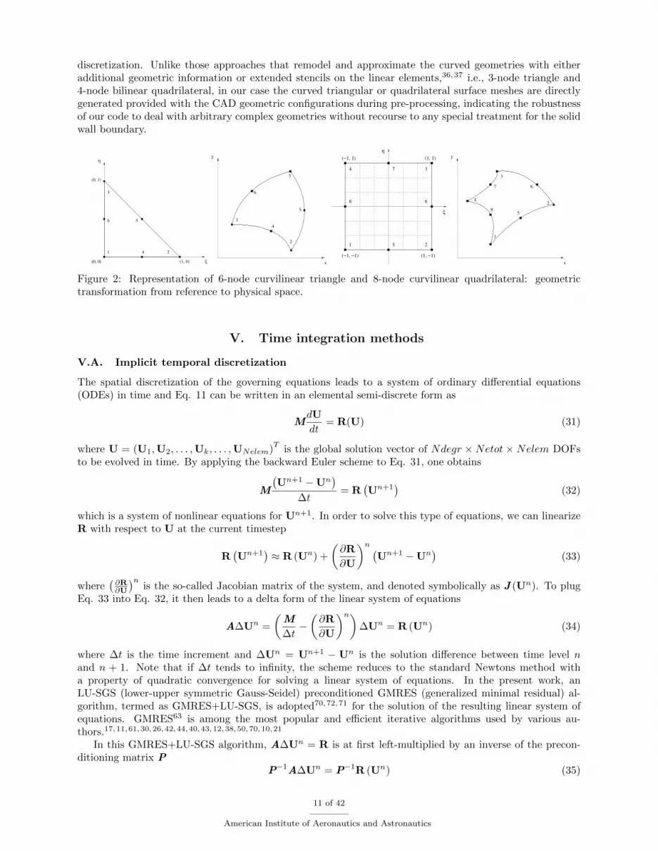
discretization. Unlike those approaches that remodel and approximate the curved geometries with eitheradditional geometric information or extended stencils on the linear elements,36,37 i.e., 3-node triangle and4-node bilinear quadrilateral, in our case the curved triangular or quadrilateral surface meshes are directlygenerated provided with the CAD geometric configurations during pre-processing, indicating the robustnessof our code to deal with arbitrary complex geometries without recourse to any special treatment for the solidwall boundary.

ξ

η

(0, 0) (1, 0)

(0, 1)

1 2

3

4

56

x

y

1

2

4

3

5

6

(1, 1)

(1, −1)(−1, −1)

(−1, 1)

ξ

η

1 2

34

5

6

7

8

x

y

1

2

3

4

5

67

8

Figure 2: Representation of 6-node curvilinear triangle and 8-node curvilinear quadrilateral: geometrictransformation from reference to physical space.

V. Time integration methods

V.A. Implicit temporal discretization

The spatial discretization of the governing equations leads to a system of ordinary differential equations(ODEs) in time and Eq. 11 can be written in an elemental semi-discrete form as

MdU

dt= R(U) (31)

where U = (U1,U2, . . . ,Uk, . . . ,UNelem)T

is the global solution vector of Ndegr ×Netot ×Nelem DOFsto be evolved in time. By applying the backward Euler scheme to Eq. 31, one obtains

M

(Un+1 −Un

)∆t

= R(Un+1

)(32)

which is a system of nonlinear equations for Un+1. In order to solve this type of equations, we can linearizeR with respect to U at the current timestep

R(Un+1

)≈ R (Un) +

(∂R

∂U

)n (Un+1 −Un

)(33)

where(∂R∂U

)nis the so-called Jacobian matrix of the system, and denoted symbolically as J (Un). To plug

Eq. 33 into Eq. 32, it then leads to a delta form of the linear system of equations

A∆Un =

(M

∆t−(∂R

∂U

)n)∆Un = R (Un) (34)

where ∆t is the time increment and ∆Un = Un+1 − Un is the solution difference between time level nand n + 1. Note that if ∆t tends to infinity, the scheme reduces to the standard Newtons method witha property of quadratic convergence for solving a linear system of equations. In the present work, anLU-SGS (lower-upper symmetric Gauss-Seidel) preconditioned GMRES (generalized minimal residual) al-gorithm, termed as GMRES+LU-SGS, is adopted70,72,71 for the solution of the resulting linear system ofequations. GMRES63 is among the most popular and efficient iterative algorithms used by various au-thors.17,11,61,30,26,42,44,40,43,12,38,50,70,10,21

In this GMRES+LU-SGS algorithm, A∆Un = R is at first left-multiplied by an inverse of the precon-ditioning matrix P

P−1A∆Un = P−1R (Un) (35)

11 of 42


where the matrix P consists of the strict upper U, lower L and diagonal D matrices

P = (D + L)D−1 (D + U) (36)

where L and U are stored via an face-based data structure. In order to construct an elemental Jacobianmatrix for cell i, the contributions from U, L and D in face integrals are computed as below

U =

∫Γij

∂Hinv (Ui,Uj ,nij)Bd,ij∂Uj

dΓ−∫

Γij

∂Hvis (Ui,Uj ,nij)Bd,ij∂Uj

dΓ (37)

L =

∫Γij

−∂Hinv (Ui,Uj ,nij)Bd,ij∂Ui

dΓ +

∫Γij

∂Hvis (Ui,Uj ,nij)Bd,ij∂Ui

dΓ (38)

DΓ =

i<j∪i>j∑Γij

(∫Γij

∂Hinv (Ui,Uj ,nij)Bd,ij∂Ui

dΓ−∫

Γij

∂Hvis (Ui,Uj ,nij)Bd,ij∂Ui

dΓ

)(39)

The contribution to D from volume integrals is

DΩ = −∫

Ωi

∂Fk (Ui)∂Bd,i∂xk

∂UidΩ +

∫Ωi

∂Gk (Ui)∂Bd,i∂xk

∂UidΩ (40)

In Eq. 37–40, the subscript d denotes the index of DOFs, 1 ≤ d ≤ Ndegr; i and j denote cell i and itsadjacent face-neighboring cell j, respectively. Finally, the time derivative term M

∆t is added to the D, andthe elemental block diagonal matrix is as below

Di =Mi

∆t+ DΓi

+ DΩi=

Mi

∆t− Ji (41)

in which the crucial part is the assembly of the Jacobian matrix Ji. The global block diagonal matrix requiresa storage of Nelem×(Ndegr ×Netot)×(Ndegr ×Netot) units. Both the upper and lower matrices requirea storage of Nafac×(Ndegr ×Netot)×(Ndegr ×Netot) units, where Nafac is the number of faces.

The LU-SGS preconditioned linear system of equations is then solved iteratively in the GMRES algorithm,which requires one RHS evaluation in each subiteration, plus one RHS evaluation in each timestep. Theprimary static storage is dictated by LU-SGS preconditioning, which requires the upper, lower and diagonalmatrices to be stored for every non-zero element of the left-hand-side (LHS) matrix A in Eq. 34. Theadditional storage associated to the GMRES algorithm is an array of size (k+2)×Nelem×(Ndegr×Netot),where k is the number of search directions.

V.B. Jacobians

In general, four approaches are widely adopted for the linearization (or differentiation) of a set of complicatedfunctions, e.g., upwind numerical flux functions: 1) Analytical differentiation: manual implementation of an-alytic derivative formulae typically results in very efficient derivative code. However, the implementation istedious and error-prone; 2) Symbolic differentiation: computer algebra packages manipulate expressions byrepeatedly applying the chain rule so that there is no truncation error. However, the resulting expressionfor the derivative involves the parameters with respect to which one is differentiating. This can lead toan excessive growth of the length of the expression; 3) Numerical differentiation: or divided differencing(DD), is based on some truncation of the Taylor series. It is easy to implement by evaluating the underlyingfunction using perturbations of the input parameters. However, a suitable perturbation is often hard tofind because a small perturbation decreasing the truncation error will increase the cancellation error; and 4)Automatic differentiation (AD): also called algorithmic differentiation, is a technology for automatically aug-menting computer programs, including arbitrarily complex simulations, with statements for the computationof derivatives, also known as sensitivities.

Usually, the exact Jacobian matrix J is practically not accessible in a closed form, e.g., when linearizationinvolves the HWENO(P1P2) reconstruction process that is highly nonlinear in nature. Even for a high-order standard DG method, exact linearization of the viscous flux functions, e.g., the BR2 scheme or CDGscheme,56 is not trivial work, as the computing time and storage requirement would still be very demanding.

12 of 42


Thus more than usual, approximate Jacobians are formulated instead of the exact ones for the implicitFV and DG methods.13,38,50,10,61,30,26,12,40,68,42,25,21,70 In the present work, the Jacobian matrix J isevaluated as the differentiation of the underlying residual vector RP1

, i.e., JP1= ∂RP1

/∂U, instead of thereconstruction-based residual vector RP1P2

. With this approximation, Eq. 34 can be rewritten as follows:(M

∆t− JP1

)∆Un = RP1P2 (42)

Due to the inexact representation of the LHS matrix in Eq. 42, the quadratic convergence of the Newton’smethod can no longer be achieved. But in return, this implicit third-order RDG(P1P2) method requires onlya DG(P1)-like linear system, which is a significant reduction in both memory requirement and computingtime compared with the standard implicit third-order DG(P2) method.

Several approaches introduced above, i.e., analytical differentiation, divided differencing (DD), and au-tomatic differentiation (AD), were accessed and compared for computing the approximate Jacobian matrixon the tetrahedral grids JP1 by the authors,71 where the linear solver achieved relatively the best robustnessand efficiency provided with the AD-based Jacobians. Indeed, by using an automatic differentiation tool,e.g., TAPENADE3 as adopted in the present work for computing the Jacobians on 3D arbitrary shapes ofelements, the labor of a programmer can be released from manual implementation, which can be especiallycomplicated, tedious and error-prone in the discontinuous Galerkin context if done either by hand or withsymbolic arithmetic software, depending on the complexity of the numerical functions. In addition, theworkload for code maintenance can also be largely reduced in case the underlying numerical flux functionsare changed and updated. Just like divided differencing, automatic differentiation requires only the sourceprogram C. But instead of executing C on different sets of inputs, it builds a new, augmented code C, thatcomputes theanalytical derivatives along with the source program. This new program is called the differ-entiated program. Each time the source program holds some value v, the differentiated program holds anadditional value dv, which is the differentialof v. In principle, arbitrarily complex functions can be differen-tiated. An incomplete list of AD tools can be found at Community Portal for Automatic Differentiation.2

VI. Parallelization

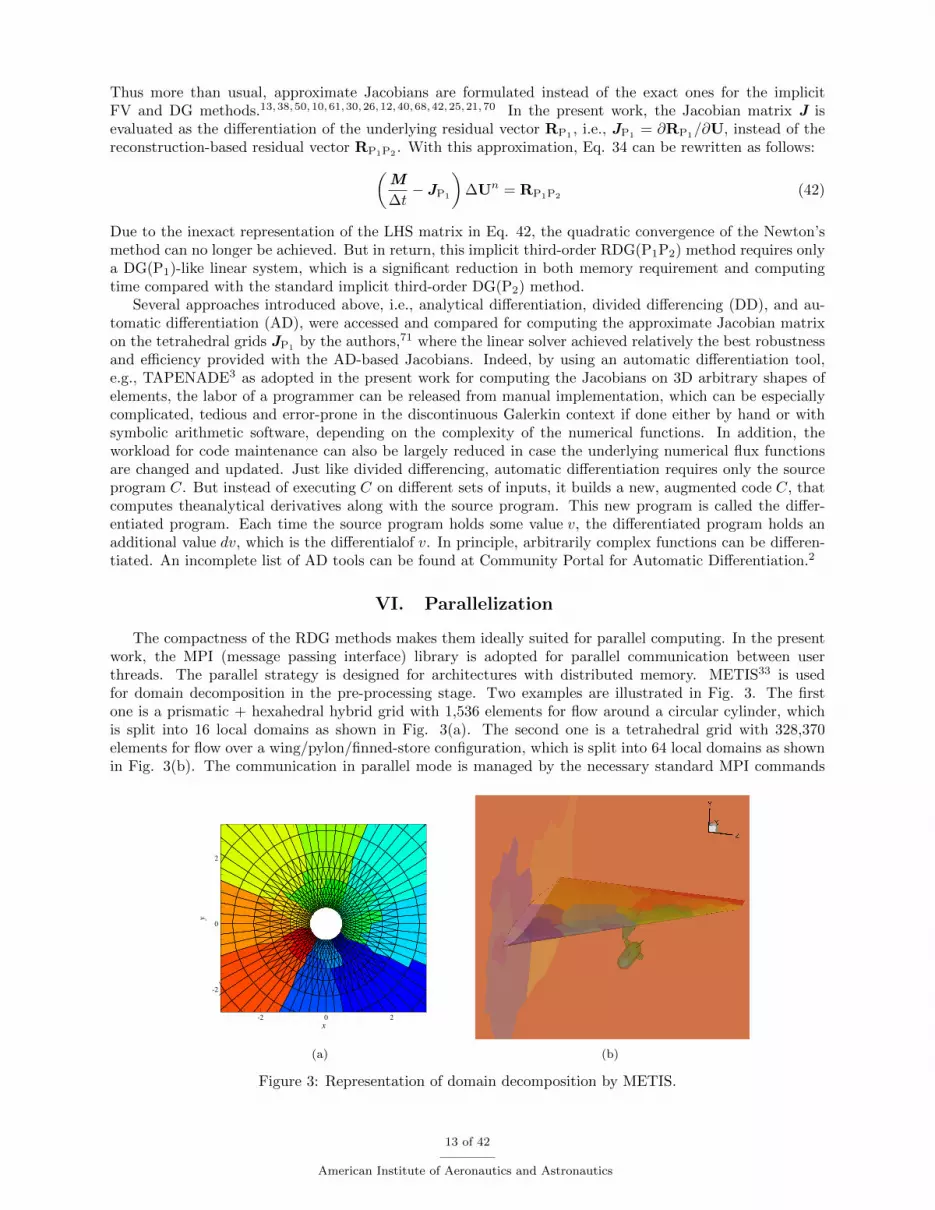
The compactness of the RDG methods makes them ideally suited for parallel computing. In the presentwork, the MPI (message passing interface) library is adopted for parallel communication between userthreads. The parallel strategy is designed for architectures with distributed memory. METIS33 is usedfor domain decomposition in the pre-processing stage. Two examples are illustrated in Fig. 3. The firstone is a prismatic + hexahedral hybrid grid with 1,536 elements for flow around a circular cylinder, whichis split into 16 local domains as shown in Fig. 3(a). The second one is a tetrahedral grid with 328,370elements for flow over a wing/pylon/finned-store configuration, which is split into 64 local domains as shownin Fig. 3(b). The communication in parallel mode is managed by the necessary standard MPI commands

x

y

2 0 2

2

0

2

(a) (b)

Figure 3: Representation of domain decomposition by METIS.

13 of 42


like nonblocking send, nonblocking receive and wait commands. Parallelization is implemented for both theexplicit and implicit methods.

VII. Numerical examples

Computations on a series of well-documented V&V (Verification & Validation) test cases for the com-pressible Euler and Navier-Stokes equations are carried out on a Dell Precision T7400 personal workstationcomputer (2.98 GHz Xeon CPU with 18 GBytes memory) using openSUSE 12.2 Linux operating systemwith the Intel FORTRAN compiler. A set of parallel scaling test cases are conducted on the ARC1 clusterrunning the Red Hat 4.1.2-51 Linux operating system at North Carolina State University, with the codecompiled by the PGI FORTRAN.

The following L2 norm of the entropy production is used as the error measurement for the steady-stateinviscid flow problems

‖ε‖L2(Ω) =

√∫Ω

ε2 dΩ =

√√√√Nelem∑i=1

∫Ωi

ε2 dΩ

where the entropy production ε is defined as

ε =S − S∞S∞

=p

p∞

(ρ∞ρ

)γ− 1

Note that the entropy production, where the entropy is defined as S = (p/ρ)γ , is a very good criterion tomeasure accuracy of the numerical solutions, since the flow under consideration is isentropic.

The residual convergence rate for the implicit method is assessed and compared with the baseline resultsobtained by the three-stage explicit Runge-Kutta (RK3) time stepping scheme. The RK3 scheme is also usedfor computing unsteady flows, e.g., Sod shock tube problem. For 2D demonstration of a cluster of variableson the surface of solid body, e.g., extracted surface pressure coefficients by a cut plane, the variables arecomputed at the two nodes of each face that intersect with the cut plane, and plotted by a straight line.This is the most accurate way to represent the P1 solution for profile plotting, as the solution is linear oneach face and multiple values exist for a vertex due to the discontinuous representation of DG solution.

Some phrase abbreviations for describing a computational grid are defined as follows: Nelem – numberof total elements of a grid; Ntetr – number of tetrahedral elements; Npyra – number of pyramidal elements;Npris – number of prismatic elements; Nhexa – number of hexahedral elements; Nafac – number of totalboundary faces; Ntria – number of boundary triangular faces; Nquad – number of boundary quadrilateralfaces; Npoin – number of grid vertex node.

VII.A. Sod shock tube

The shock tube problem constitutes a particularly interesting and difficult test case, since it presents anexact solution to the full system of one-dimensional Euler equations containing simultaneously a shock wave,a contact discontinuity, and expansion fan. This test case is chosen to validate the implementation of theHLLC Riemann solver and demonstrate the robustness of the RDG methods. The initial conditions in thepresent computation are the following: ρL = 1.000, uL = 0, pL = 1.0 for 0.0 ≤ x ≤ 0.5, ρR = 0.125,uR = 0, pR = 0.1 for 0.5 ≤ x ≤ 1.0. This is a 3D simulation of the 1D problem. Fig. 4 shows thehexahedral grid used in computation. The grid consists of 50 cells in the x-direction, 1 cell in y-directionand 1 cell in z-direction. Fig. 5(a), Fig. 5(b) and Fig. 5(c) show the computed density, Mach number, andpressure profiles respectively, where each is obtained by the unlimited RDG(P1P1), WENO(P1P2)-basedand HWENO(P1P2)-based RDG(P1P2) and compared with the exact solutions. As expected, the unlimitedRDG(P1P1) and WENO(P1P2) solutions exhibit small oscillations in the vicinity of discontinuities andyield a sharp resolution for both contact and discontinuity and shock wave, whereas the HWENO(P1P2)reconstruction is able to eliminate the spurious oscillations in the shock wave region. In the rest region ofdomain, the HWENO(P1P2) solutions are not as good as those obtained by the underlying RDG(P1P1)solutions, indicating that the HWENO reconstruction does increase slightly the absolute error, although itcan keep the designed order of accuracy of the original DG method as shown in the following subsections.Most importantly, the reconstruction scheme used in the DG method does not create negative density, and

14 of 42


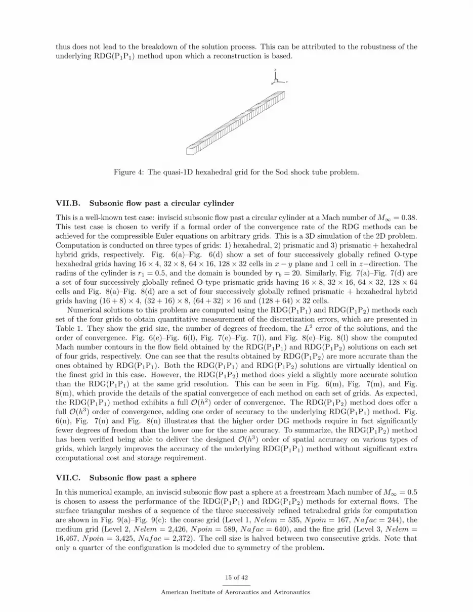
thus does not lead to the breakdown of the solution process. This can be attributed to the robustness of theunderlying RDG(P1P1) method upon which a reconstruction is based.

XY

Z

Figure 4: The quasi-1D hexahedral grid for the Sod shock tube problem.

VII.B. Subsonic flow past a circular cylinder

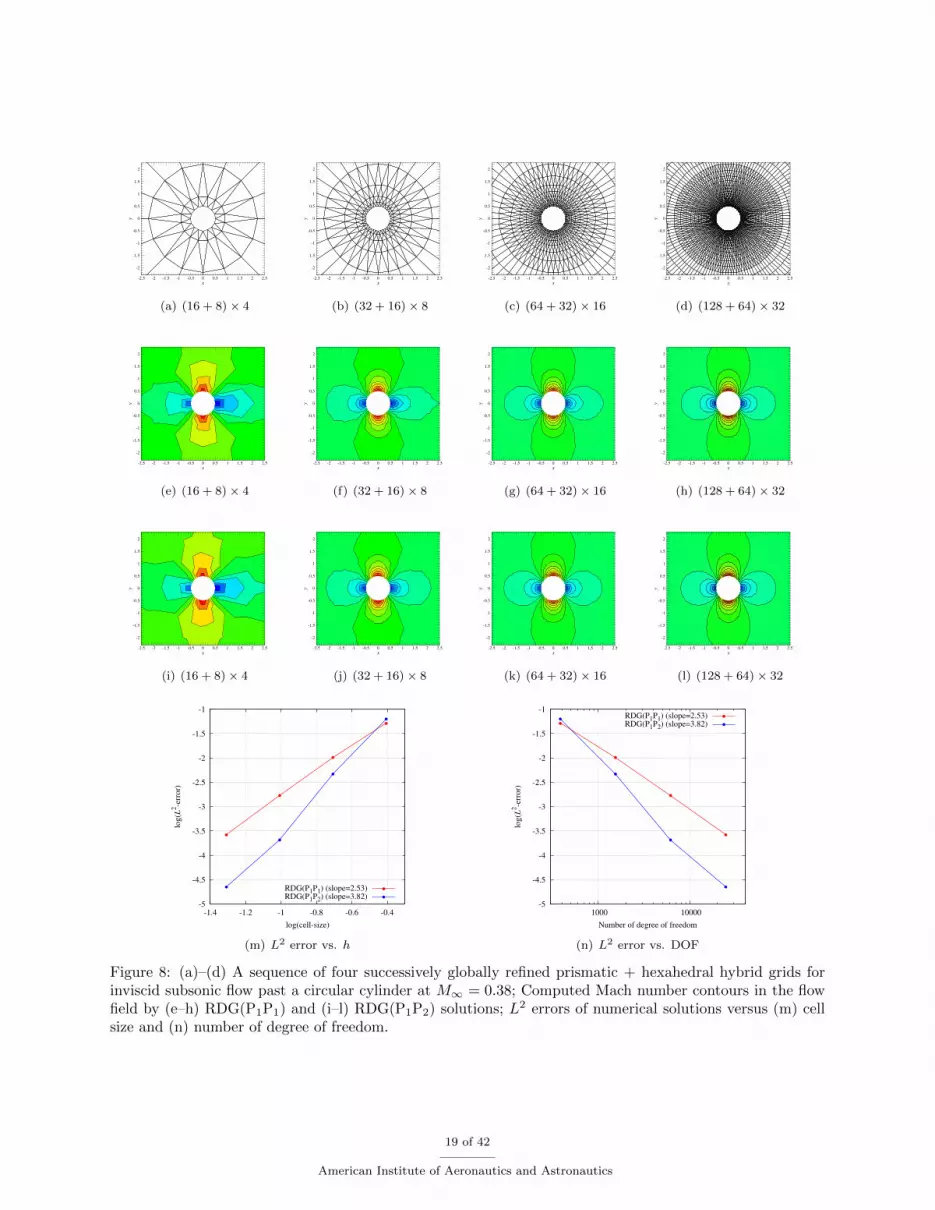
This is a well-known test case: inviscid subsonic flow past a circular cylinder at a Mach number of M∞ = 0.38.This test case is chosen to verify if a formal order of the convergence rate of the RDG methods can beachieved for the compressible Euler equations on arbitrary grids. This is a 3D simulation of the 2D problem.Computation is conducted on three types of grids: 1) hexahedral, 2) prismatic and 3) prismatic + hexahedralhybrid grids, respectively. Fig. 6(a)–Fig. 6(d) show a set of four successively globally refined O-typehexahedral grids having 16× 4, 32× 8, 64× 16, 128× 32 cells in x− y plane and 1 cell in z−direction. Theradius of the cylinder is r1 = 0.5, and the domain is bounded by rb = 20. Similarly, Fig. 7(a)–Fig. 7(d) area set of four successively globally refined O-type prismatic grids having 16 × 8, 32 × 16, 64 × 32, 128 × 64cells and Fig. 8(a)–Fig. 8(d) are a set of four successively globally refined prismatic + hexahedral hybridgrids having (16 + 8)× 4, (32 + 16)× 8, (64 + 32)× 16 and (128 + 64)× 32 cells.

Numerical solutions to this problem are computed using the RDG(P1P1) and RDG(P1P2) methods eachset of the four grids to obtain quantitative measurement of the discretization errors, which are presented inTable 1. They show the grid size, the number of degrees of freedom, the L2 error of the solutions, and theorder of convergence. Fig. 6(e)–Fig. 6(l), Fig. 7(e)–Fig. 7(l), and Fig. 8(e)–Fig. 8(l) show the computedMach number contours in the flow field obtained by the RDG(P1P1) and RDG(P1P2) solutions on each setof four grids, respectively. One can see that the results obtained by RDG(P1P2) are more accurate than theones obtained by RDG(P1P1). Both the RDG(P1P1) and RDG(P1P2) solutions are virtually identical onthe finest grid in this case. However, the RDG(P1P2) method does yield a slightly more accurate solutionthan the RDG(P1P1) at the same grid resolution. This can be seen in Fig. 6(m), Fig. 7(m), and Fig.8(m), which provide the details of the spatial convergence of each method on each set of grids. As expected,the RDG(P1P1) method exhibits a full O(h2) order of convergence. The RDG(P1P2) method does offer afull O(h3) order of convergence, adding one order of accuracy to the underlying RDG(P1P1) method. Fig.6(n), Fig. 7(n) and Fig. 8(n) illustrates that the higher order DG methods require in fact significantlyfewer degrees of freedom than the lower one for the same accuracy. To summarize, the RDG(P1P2) methodhas been verified being able to deliver the designed O(h3) order of spatial accuracy on various types ofgrids, which largely improves the accuracy of the underlying RDG(P1P1) method without significant extracomputational cost and storage requirement.

VII.C. Subsonic flow past a sphere

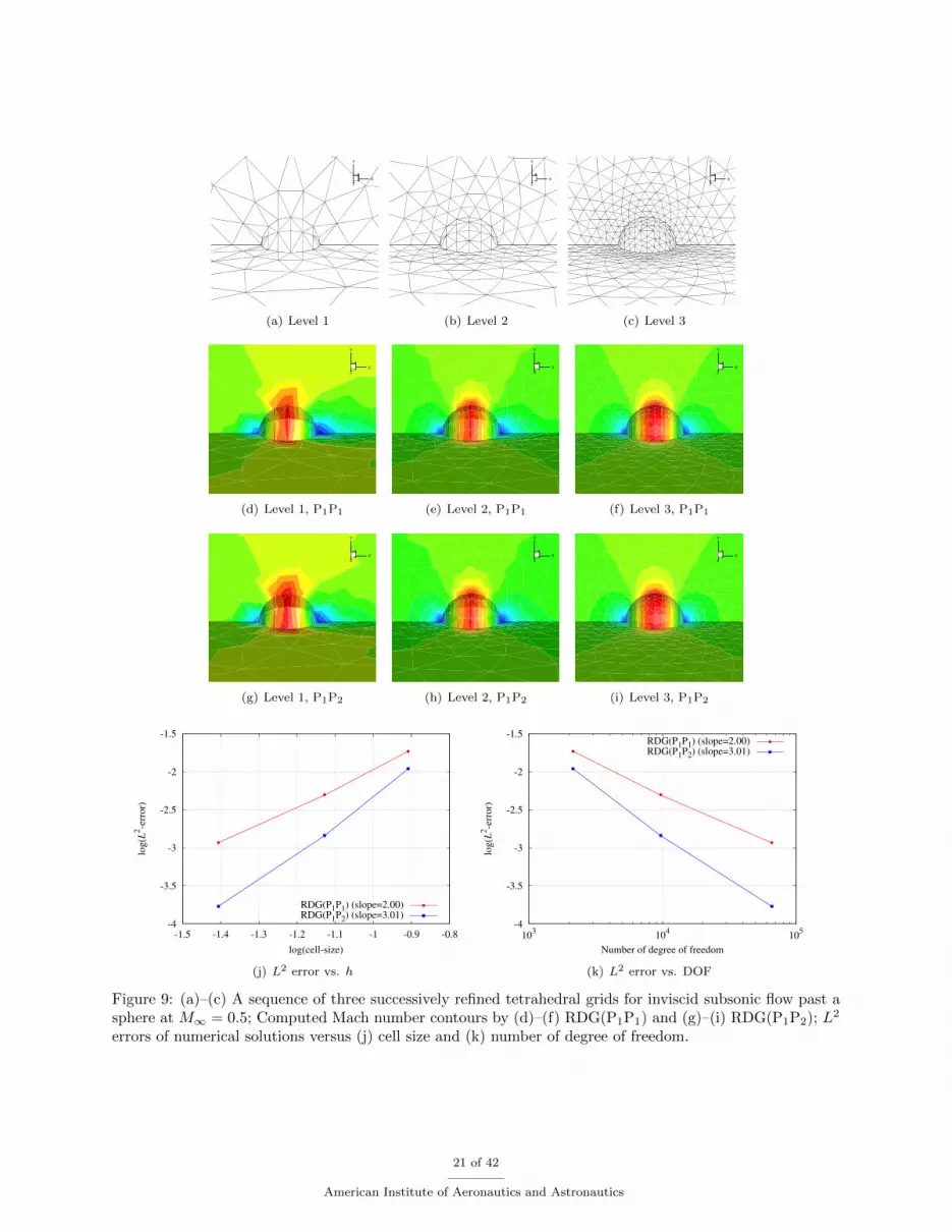
In this numerical example, an inviscid subsonic flow past a sphere at a freestream Mach number of M∞ = 0.5is chosen to assess the performance of the RDG(P1P1) and RDG(P1P2) methods for external flows. Thesurface triangular meshes of a sequence of the three successively refined tetrahedral grids for computationare shown in Fig. 9(a)–Fig. 9(c): the coarse grid (Level 1, Nelem = 535, Npoin = 167, Nafac = 244), themedium grid (Level 2, Nelem = 2,426, Npoin = 589, Nafac = 640), and the fine grid (Level 3, Nelem =16,467, Npoin = 3,425, Nafac = 2,372). The cell size is halved between two consecutive grids. Note thatonly a quarter of the configuration is modeled due to symmetry of the problem.

15 of 42


0

0.1

0.2

0.3

0.4

0.5

0.6

0.7

0.8

0.9

1

1.1

0 0.2 0.4 0.6 0.8 1

Den

sity

x-coordinate

Exact SolutionRDG(P1P1)

WENO(P1P2)HWENO(P1P2)

(a) Density

0

0.1

0.2

0.3

0.4

0.5

0.6

0.7

0.8

0.9

1

0 0.2 0.4 0.6 0.8 1

Mach

num

ber

x-coordinate



(b) Mach number

0

0.1

0.2

0.3

0.4

0.5

0.6

0.7

0.8

0.9

1

1.1

0 0.2 0.4 0.6 0.8 1

Pre

ssure

x-coordinate



(c) Pressure

Figure 5: Comparison of computed variable profiles for the Sod shock tube problem obtained by theRDG(P1P1), WENO(P1P2), and HWENO(P1P2) solutions with the analytical solution.

16 of 42


x

y

2.5 2 1.5 1 0.5 0 0.5 1 1.5 2 2.5

2

1.5

1

0.5

0

0.5

1

1.5

2

(a) 16× 4

x

y

2.5 2 1.5 1 0.5 0 0.5 1 1.5 2 2.5

2

1.5

1

0.5

0

0.5

1

1.5

2

(b) 32× 8

x

y

2.5 2 1.5 1 0.5 0 0.5 1 1.5 2 2.5

2

1.5

1

0.5

0

0.5

1

1.5

2

(c) 64× 16

x

y

2.5 2 1.5 1 0.5 0 0.5 1 1.5 2 2.5

2

1.5

1

0.5

0

0.5

1

1.5

2

(d) 128× 32

x

y

2.5 2 1.5 1 0.5 0 0.5 1 1.5 2 2.5

2

1.5

1

0.5

0

0.5

1

1.5

2

(e) 16× 4

x

y

2.5 2 1.5 1 0.5 0 0.5 1 1.5 2 2.5

2

1.5

1

0.5

0

0.5

1

1.5

2

(f) 32× 8

x

y

2.5 2 1.5 1 0.5 0 0.5 1 1.5 2 2.5

2

1.5

1

0.5

0

0.5

1

1.5

2

(g) 64× 16

x

y

2.5 2 1.5 1 0.5 0 0.5 1 1.5 2 2.5

2

1.5

1

0.5

0

0.5

1

1.5

2

(h) 128× 32

x

y

2.5 2 1.5 1 0.5 0 0.5 1 1.5 2 2.5

2

1.5

1

0.5

0

0.5

1

1.5

2

(i) 16× 4

x

y

2.5 2 1.5 1 0.5 0 0.5 1 1.5 2 2.5

2

1.5

1

0.5

0

0.5

1

1.5

2

(j) 32× 8

x

y

2.5 2 1.5 1 0.5 0 0.5 1 1.5 2 2.5

2

1.5

1

0.5

0

0.5

1

1.5

2

(k) 64× 16

xy

2.5 2 1.5 1 0.5 0 0.5 1 1.5 2 2.5

2

1.5

1

0.5

0

0.5

1

1.5

2

(l) 128× 32

-4

-3.5

-3

-2.5

-2

-1.5

-1

-0.5

-1.4 -1.2 -1 -0.8 -0.6 -0.4

log

(L2-e

rror)

log(cell-size)

RDG(P1P1) (slope=2.19)RDG(P1P2) (slope=3.54)

(m) L2 error vs. h

-4

-3.5

-3

-2.5

-2

-1.5

-1

-0.5

1000 10000

log

(L2-e

rror)

Number of degree of freedom


(n) L2 error vs. DOF

Figure 6: (a)–(d) A sequence of four successively globally refined hexahedral grids for inviscid subsonicflow past a circular cylinder at M∞ = 0.38; Computed Mach number contours in the flow field by (e–h)RDG(P1P1) and (i–l) RDG(P1P2) solutions; L2 errors of numerical solutions versus (m) cell size and (n)number of degree of freedom.

17 of 42


x

y

2.5 2 1.5 1 0.5 0 0.5 1 1.5 2 2.5

2

1.5

1

0.5

0

0.5

1

1.5

2

(a) 16× 8

x

y

2.5 2 1.5 1 0.5 0 0.5 1 1.5 2 2.5

2

1.5

1

0.5

0

0.5

1

1.5

2

(b) 32× 16

x

y

2.5 2 1.5 1 0.5 0 0.5 1 1.5 2 2.5

2

1.5

1

0.5

0

0.5

1

1.5

2

(c) 64× 32

x

y

2.5 2 1.5 1 0.5 0 0.5 1 1.5 2 2.5

2

1.5

1

0.5

0

0.5

1

1.5

2

(d) 128× 64

x

y

2.5 2 1.5 1 0.5 0 0.5 1 1.5 2 2.5

2

1.5

1

0.5

0

0.5

1

1.5

2

(e) 16× 4

x

y

2.5 2 1.5 1 0.5 0 0.5 1 1.5 2 2.5

2

1.5

1

0.5

0

0.5

1

1.5

2

(f) 32× 8

x

y

2.5 2 1.5 1 0.5 0 0.5 1 1.5 2 2.5

2

1.5

1

0.5

0

0.5

1

1.5

2

(g) 64× 16

x

y

2.5 2 1.5 1 0.5 0 0.5 1 1.5 2 2.5

2

1.5

1

0.5

0

0.5

1

1.5

2

(h) 128× 32

x

y

2.5 2 1.5 1 0.5 0 0.5 1 1.5 2 2.5

2

1.5

1

0.5

0

0.5

1

1.5

2

(i) 16× 4

x

y

2.5 2 1.5 1 0.5 0 0.5 1 1.5 2 2.5

2

1.5

1

0.5

0

0.5

1

1.5

2

(j) 32× 8

x

y

2.5 2 1.5 1 0.5 0 0.5 1 1.5 2 2.5

2

1.5

1

0.5

0

0.5

1

1.5

2

(k) 64× 16

xy

2.5 2 1.5 1 0.5 0 0.5 1 1.5 2 2.5

2

1.5

1

0.5

0

0.5

1

1.5

2

(l) 128× 32

-5.5

-5

-4.5

-4

-3.5

-3

-2.5

-2

-1.5

-1

-1.6 -1.4 -1.2 -1 -0.8 -0.6

log

(L2-e

rror)

log(cell-size)


(m) L2 error vs. h

-5.5

-5

-4.5

-4

-3.5

-3

-2.5

-2

-1.5

-1

1000 10000

log

(L2-e

rror)




Figure 7: (a)–(d) A sequence of four successively globally refined prismatic grids for inviscid subsonic flow pasta circular cylinder at M∞ = 0.38; Computed Mach number contours in the flow field by (e–h) RDG(P1P1)and (i–l) RDG(P1P2) solutions; L2 errors of numerical solutions versus (m) cell size and (n) number of degreeof freedom.

18 of 42


x

y

2.5 2 1.5 1 0.5 0 0.5 1 1.5 2 2.5

2

1.5

1

0.5

0

0.5

1

1.5

2

(a) (16 + 8)× 4

x

y

2.5 2 1.5 1 0.5 0 0.5 1 1.5 2 2.5

2

1.5

1

0.5

0

0.5

1

1.5

2

(b) (32 + 16)× 8

x

y

2.5 2 1.5 1 0.5 0 0.5 1 1.5 2 2.5

2

1.5

1

0.5

0

0.5

1

1.5

2

(c) (64 + 32)× 16

x

y

2.5 2 1.5 1 0.5 0 0.5 1 1.5 2 2.5

2

1.5

1

0.5

0

0.5

1

1.5

2

(d) (128 + 64)× 32

x

y

2.5 2 1.5 1 0.5 0 0.5 1 1.5 2 2.5

2

1.5

1

0.5

0

0.5

1

1.5

2

(e) (16 + 8)× 4

x

y

2.5 2 1.5 1 0.5 0 0.5 1 1.5 2 2.5

2

1.5

1

0.5

0

0.5

1

1.5

2

(f) (32 + 16)× 8

x

y

2.5 2 1.5 1 0.5 0 0.5 1 1.5 2 2.5

2

1.5

1

0.5

0

0.5

1

1.5

2

(g) (64 + 32)× 16

x

y

2.5 2 1.5 1 0.5 0 0.5 1 1.5 2 2.5

2

1.5

1

0.5

0

0.5

1

1.5

2

(h) (128 + 64)× 32

x

y

2.5 2 1.5 1 0.5 0 0.5 1 1.5 2 2.5

2

1.5

1

0.5

0

0.5

1

1.5

2

(i) (16 + 8)× 4

x

y

2.5 2 1.5 1 0.5 0 0.5 1 1.5 2 2.5

2

1.5

1

0.5

0

0.5

1

1.5

2

(j) (32 + 16)× 8

x

y

2.5 2 1.5 1 0.5 0 0.5 1 1.5 2 2.5

2

1.5

1

0.5

0

0.5

1

1.5

2

(k) (64 + 32)× 16

xy

2.5 2 1.5 1 0.5 0 0.5 1 1.5 2 2.5

2

1.5

1

0.5

0

0.5

1

1.5

2

(l) (128 + 64)× 32

-5

-4.5

-4

-3.5

-3

-2.5

-2

-1.5

-1

-1.4 -1.2 -1 -0.8 -0.6 -0.4

log(L

2-e

rro

r)

log(cell-size)


(m) L2 error vs. h

-5

-4.5

-4

-3.5

-3

-2.5

-2

-1.5

-1

1000 10000

log(L

2-e

rro

r)




Figure 8: (a)–(d) A sequence of four successively globally refined prismatic + hexahedral hybrid grids forinviscid subsonic flow past a circular cylinder at M∞ = 0.38; Computed Mach number contours in the flowfield by (e–h) RDG(P1P1) and (i–l) RDG(P1P2) solutions; L2 errors of numerical solutions versus (m) cellsize and (n) number of degree of freedom.

19 of 42


Table 1: Discretization errors and convergence rates of the RDG methods obtained on various types of gridsfor an inviscid subsonic flow past a circular cylinder at M∞ = 0.38.

Hexahedral grids

Grid No. DOFs L2-error-P1P1 Order-P1P1 L2-error-P1P2 Order-P1P2

16× 4 256 -0.86941E+00 - -0.80491E+00 -

32× 8 1,024 -0.13597E+01 1.629 -0.15768E+01 2.193

64× 16 4,096 -0.20821E+01 2.400 -0.27377E+01 3.746

128× 32 16,384 -0.28501E+01 2.551 -0.39997E+01 3.548

Prismatic grids


16× 8 512 -0.12456E+01 - -0.14009E+01 -

32× 16 2,048 -0.19753E+01 2.424 -0.25497E+01 3.816

64× 32 8,192 -0.28013E+01 2.744 -0.38685E+01 4.381

128× 64 32,768 -0.36030E+01 2.663 -0.50007E+01 3.761

Prismatic + hexahedral hybrid grids


(16 + 8)× 4 384 -0.12907E+01 - -0.12000E+01 -

(32 + 16)× 8 1,536 -0.19912E+01 2.326 -0.23306E+01 3.762

(64 + 32)× 16 6,144 -0.27710E+01 2.593 -0.36842E+01 4.500

(128 + 64)× 32 24,576 -0.35798E+01 2.697 -0.46498E+01 3.219

Computation is conducted on these grids by using the RDG(P1P1) and RDG(P1P2) methods to obtaina quantitative measurement of the discretization errors as shown in Table 2. Fig. 9(d)–9(f) and Fig. 9(g)–9(i) show the computed Mach number contours in the flow field by RDG(P1P1) and RDG(P1P2) solutions,respectively. One can see that the results obtained by RDG(P1P2) are more accurate than the ones obtainedby RDG(P1P1). Both RDG(P1P1) and RDG(P1P2) have achieved a formal order of accuracy of convergence,being 2.00 and 3.01, respectively, as Fig. 9(j) and 9(k) show the L2 errors of numerical solutions versus cellsize and DOFs respectively for the RDG methods, convincingly demonstrating the benefits of using thereconstructed RDG(P1P2) method. Fig. 10(a) and 10(b) show the RDG(P1P2) convergence history oflogarithmic density residual with respect to timestep and CPU time on the set of grids. In comparison, theimplicit method is about four orders of magnitude faster than its explicit counterpart, indicating a significantsaving in terms of computing time. A decreased convergence rate with respect to timestep is observed ongrids of higher level for the implicit RDG(P1P2) methods, due to the use of approximated Jacobians.

Table 2: Discretization errors and convergence rates of the RDG methods obtained on the three successivelyrefined tetrahedral grids for an inviscid subsonic flow past a sphere at M∞ = 0.5.


Level 1 2,140 -0.1732E+01 - -0.196E+01 -

Level 2 9,704 -0.2302E+01 1.895 -0.284E+01 2.924

Level 3 65,868 -0.2933E+01 2.094 -0.377E+01 3.094

20 of 42


X

Y

Z

(a) Level 1

X

Y

Z

(b) Level 2

X

Y

Z

(c) Level 3

X

Y

Z

(d) Level 1, P1P1

X

Y

Z

(e) Level 2, P1P1

X

Y

Z

(f) Level 3, P1P1

X

Y

Z

(g) Level 1, P1P2

X

Y

Z

(h) Level 2, P1P2

X

Y

Z

(i) Level 3, P1P2

-4

-3.5

-3

-2.5

-2

-1.5

-1.5 -1.4 -1.3 -1.2 -1.1 -1 -0.9 -0.8

log

(L2-e

rror)

log(cell-size)


(j) L2 error vs. h

-4

-3.5

-3

-2.5

-2

-1.5

103

104

105

log

(L2-e

rror)



(k) L2 error vs. DOF

Figure 9: (a)–(c) A sequence of three successively refined tetrahedral grids for inviscid subsonic flow past asphere at M∞ = 0.5; Computed Mach number contours by (d)–(f) RDG(P1P1) and (g)–(i) RDG(P1P2); L2

errors of numerical solutions versus (j) cell size and (k) number of degree of freedom.

21 of 42


-10

-8

-6

-4

-2

0

0 50 100 150 200

Log

(Res

idual

)

Time Step

RK3, Level 1RK3, Level 2RK3, Level 3

GMRES, Level 1GMRES, Level 2GMRES, Level 3

(a)

-10

-8

-6

-4

-2

0

0 100 200 300 400 500 600

Log

(Res

idual

)

CPU Time, Second



(b)

Figure 10: Convergence history for logarithmic density residual with respect to (a) timestep and (b) CPUtime respectively for inviscid subsonic flow past a sphere at M∞ = 0.5 on tetrahedral grids, by RDG(P1P2).

VII.D. Subsonic flow through a channel with a smooth bump

In this numerical example, an inviscid subsonic flow through a channel with a smooth bump on the lowersurface at a freestream Mach number of M∞ = 0.5 is chosen to assess the RDG(P1P1) and RDG(P1P2)methods for internal flows. This is a 3D simulation of the 2D problem. Two types of grids: 1) prismatic and2) tetrahedral grids are used respectively.

Firstly, computation is conducted on a sequence of four successively globally refined prismatic grids,having 128 (Level 1), 512 (Level 2), 2048 (Level 3) and 8192 (Level 4) cells as shown in x-y plane and 1 cellin z-direction as shown in Fig. 11(a)–11(d). A quantitative measurement of discretization errors is obtainedand presented in Tabel 3. As expected, the RDG(P1P1) method exhibits a full O(h2) order of accuracy, being2.469, and the RDG(P1P2) method does offer a full O(h3) order of accuracy, being 3.223. Fig. 12(a), 12(c),12(e), 12(g) and Fig. 12(b), 12(d), 12(f), 12(h) display the computed Mach number contours in the flow fieldobtained by RDG(P1P1) and RDG(P1P2) solutions on these four prismatic grids, respectively. One can seethat the results obtained by RDG(P1P2) are more accurate than the ones obtained by RDG(P1P1). Boththe RDG(P1P1) and RDG(P1P2) solutions are virtually identical on the finest grid in this case. However,the RDG(P1P2) method does yield a slightly more accurate solution than the RDG(P1P1) at the same gridresolution. This can be seen in Fig. 12(i) and 12(j) which provide the details of spatial convergence of eachmethod on these four grids.

Table 3: Discretization errors and convergence rates of the RDG methods obtained on the four successivelyglobally refined prismatic grids for an inviscid subsonic flow through a channel with a bump at M∞ = 0.5.


128 512 -0.28947E+01 - -0.33689E+01 -

512 2,048 -0.35941E+01 2.323 -0.43314E+01 3.197

2,048 8,192 -0.43592E+01 2.542 -0.53343E+01 3.332

8,192 32,768 -0.51240E+01 2.541 -0.62793E+01 3.139

Secondly, Fig. 13(a)–13(c) display the surface triangular meshes of a sequence of three successively refinedtetrahedral grids: the coarse grid (Level 1, Nelem = 889, Npoin = 254, Nafac = 171), the medium grid(Level 2, Nelem = 6,986, Npoin = 1,555, Nafac = 691) and the fine grid (Level 3, Nelem = 55,703, Npoin= 10,822, Nafac = 2,711). Computation is conducted on these grids to obtain a quantitative measurementof the discretization errors as displayed in Tabel 4. The RDG(P1P1) and RDG(P1P2) methods achievedan averaged order of 1.89 and 2.80, respectively. Consider the fact that this is a 3D simulation of a 2Dproblem, and the unstructured tetrahedral grids are not symmetric by nature, thus causing errors in the

22 of 42


x

y

1.5 1 0.5 0 0.5 1 1.50

0.5

(a) Level 1

x

y

1.5 1 0.5 0 0.5 1 1.50

0.5

(b) Level 2

x

y

1.5 1 0.5 0 0.5 1 1.50

0.5

(c) Level 3

x

y

1.5 1 0.5 0 0.5 1 1.50

0.5

(d) Level 4

Figure 11: A sequence of four successively globally refined prismatic grids for inviscid subsonic flow througha channel with a smooth bump at M∞ = 0.5

z-direction. If the RDG(P1P1) method can be considered to deliver the designed O(h2) order of accuracy,the RDG(P1P2) method offers a full O(h3) order of convergence, adding one order of accuracy to theunderlying RDG(P1P1) method. Fig. 13(d) and 13(e) display the computed Mach number contours inthe flow field obtained by RDG(P1P1) and RDG(P1P2) solutions on the fine grid, respectively. They arevisually very similar to each other. However the RDG(P1P2) method yields a slightly more accurate solutionthan RDG(P1P1) as demonstrated in Fig. 13(f) and 13(g). Fig. 14(a) and 14(b) illustrate the RDG(P1P2)convergence history of logarithmic density residual with respect to timestep and CPU time on the threegrids, respectively. In comparison, the implicit method is over four orders of magnitude faster than itsexplicit counterpart, indicating a superior advantage. A gradually decreased convergence rate with respectto timestep is observed on grids of higher level for the implicit RDG(P1P2) methods, due to the use ofinexact Jacobians.

Table 4: Discretization errors and convergence rates of the RDG methods obtained on the three successivelyrefined tetrahedral grids for an inviscid subsonic flow through a channel with a bump at M∞ = 0.5.


889 3,556 -0.26129E+01 - -0.26709E+01 -

6,986 27,944 -0.31333E+01 1.730 -0.356436E+01 2.968

55,703 222,812 -0.37430E+01 2.026 -0.435115E+01 2.614

VII.E. Transonic flow over the ONERA M6 wing

An inviscid transonic flow over the ONERA M6 wing is considered in this case. This test case is cho-sen in order to assess and validate the performance of WENO(P1P2) reconstruction and HWENO(P1P2)reconstruction of the implicit RDG(P1P2) method at the presence of weak and strong discontinuities.

The DG method is not only linear stable but also has the ability to obtain a stable solution for weakdiscontinuities in spite of the over- and under-shots in the vicinity of shock waves. Firstly, a weak-shockcondition is computed at a freestream Mach number of M∞ = 0.699 and an attack angle of α = 3.06 on acoarse tetrahedral grid (Nelem = 41,440, Npoin = 8,325, Nafac = 5,146) as the surface triangular meshesare shown in Fig. 15(a). The computed pressure contours obtained by the WENO(P1P2) solutions on thewing surface are shown in Fig. 15(b). Fig. 16 compares the pressure coefficient distributions at six span-wise locations on the wing surface between the numerical results and experimental data.64 As expected,

23 of 42


x

y

1.5 1 0.5 0 0.5 1 1.50

0.5

(a) Level 1, P1P1

x

y

1.5 1 0.5 0 0.5 1 1.50

0.5

(b) Level 1, P1P2

x

y

1.5 1 0.5 0 0.5 1 1.50

0.5

(c) Level 2, P1P1

x

y

1.5 1 0.5 0 0.5 1 1.50

0.5

(d) Level 2, P1P2

x

y

1.5 1 0.5 0 0.5 1 1.50

0.5

(e) Level 3, P1P1

xy

1.5 1 0.5 0 0.5 1 1.50

0.5

(f) Level 3, P1P2

x

y

1.5 1 0.5 0 0.5 1 1.50

0.5

(g) Level 4, P1P1

x

y

1.5 1 0.5 0 0.5 1 1.50

0.5

(h) Level 4, P1P2

-6.5

-6

-5.5

-5

-4.5

-4

-3.5

-3

-2.5

-2.4 -2.2 -2 -1.8 -1.6 -1.4 -1.2 -1

log

(L2-e

rro

r)

log(cell-size)


(i) L2 error vs. h

-6.5

-6

-5.5

-5

-4.5

-4

-3.5

-3

-2.5

100 1000 10000 100000

log

(L2-e

rro

r)



(j) L2 error vs. DOF

Figure 12: Computed Mach number contours in the flow field by (a, c, e, f) RDG(P1P1) and (b, d, f, h)RDG(P1P2) solutions for inviscid subsonic flow through a channel with a smooth bump at M∞ = 0.5; L2

errors of numerical solutions versus (i) cell size and (j) number of degree of freedom on four successivelyglobally refined prismatic grids.

24 of 42


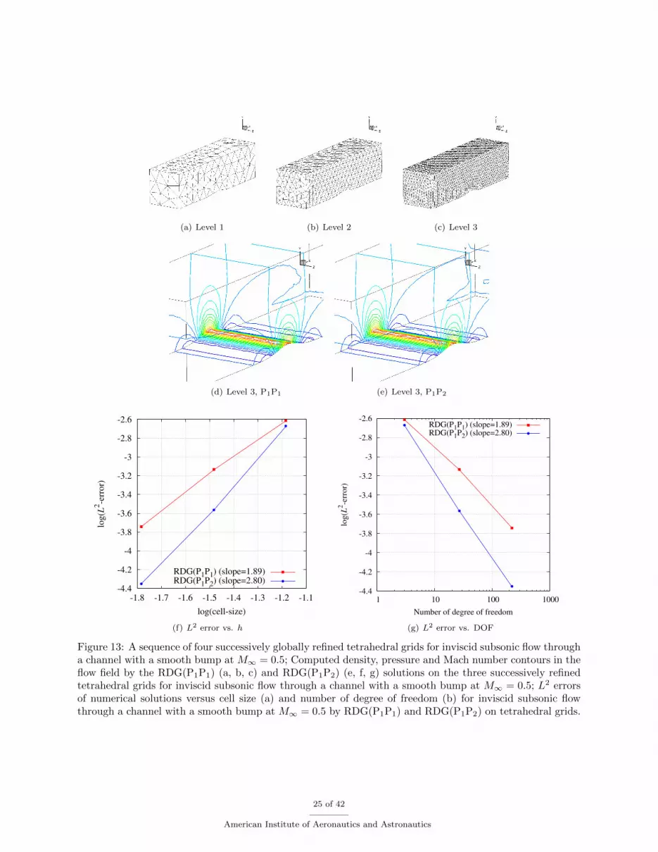
(a) Level 1 (b) Level 2 (c) Level 3

(d) Level 3, P1P1 (e) Level 3, P1P2

-4.4

-4.2

-4

-3.8

-3.6

-3.4

-3.2

-3

-2.8

-2.6

-1.8 -1.7 -1.6 -1.5 -1.4 -1.3 -1.2 -1.1

log(L

2-e

rror)

log(cell-size)


(f) L2 error vs. h

-4.4

-4.2

-4

-3.8

-3.6

-3.4

-3.2

-3

-2.8

-2.6

1 10 100 1000

log

(L2-e

rro

r)



(g) L2 error vs. DOF

Figure 13: A sequence of four successively globally refined tetrahedral grids for inviscid subsonic flow througha channel with a smooth bump at M∞ = 0.5; Computed density, pressure and Mach number contours in theflow field by the RDG(P1P1) (a, b, c) and RDG(P1P2) (e, f, g) solutions on the three successively refinedtetrahedral grids for inviscid subsonic flow through a channel with a smooth bump at M∞ = 0.5; L2 errorsof numerical solutions versus cell size (a) and number of degree of freedom (b) for inviscid subsonic flowthrough a channel with a smooth bump at M∞ = 0.5 by RDG(P1P1) and RDG(P1P2) on tetrahedral grids.

25 of 42


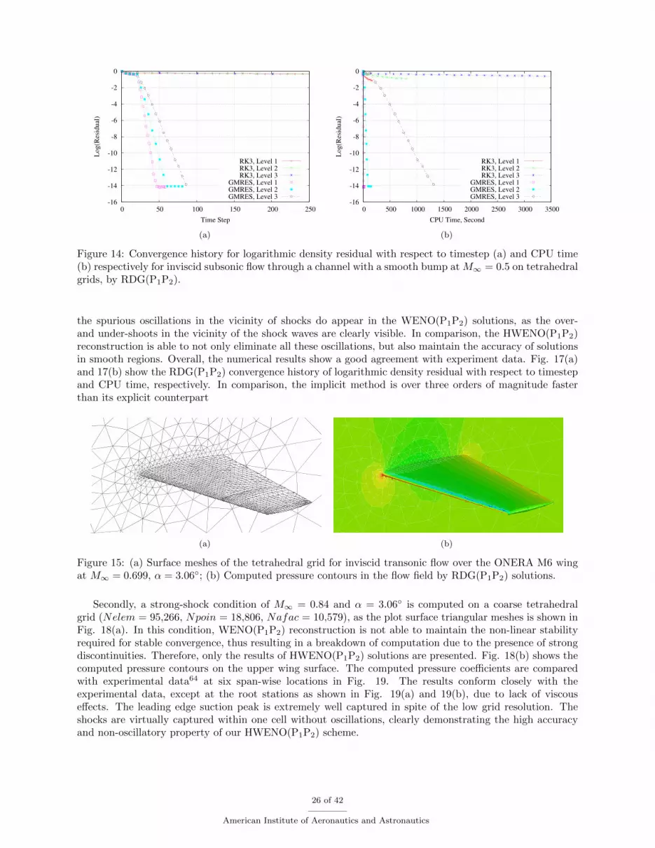
-16

-14

-12

-10

-8

-6

-4

-2

0

0 50 100 150 200 250

Log

(Res

idual

)

Time Step



(a)

-16

-14

-12

-10

-8

-6

-4

-2

0

0 500 1000 1500 2000 2500 3000 3500

Log

(Res

idual

)

CPU Time, Second



(b)

Figure 14: Convergence history for logarithmic density residual with respect to timestep (a) and CPU time(b) respectively for inviscid subsonic flow through a channel with a smooth bump at M∞ = 0.5 on tetrahedralgrids, by RDG(P1P2).

the spurious oscillations in the vicinity of shocks do appear in the WENO(P1P2) solutions, as the over-and under-shoots in the vicinity of the shock waves are clearly visible. In comparison, the HWENO(P1P2)reconstruction is able to not only eliminate all these oscillations, but also maintain the accuracy of solutionsin smooth regions. Overall, the numerical results show a good agreement with experiment data. Fig. 17(a)and 17(b) show the RDG(P1P2) convergence history of logarithmic density residual with respect to timestepand CPU time, respectively. In comparison, the implicit method is over three orders of magnitude fasterthan its explicit counterpart

(a) (b)

Figure 15: (a) Surface meshes of the tetrahedral grid for inviscid transonic flow over the ONERA M6 wingat M∞ = 0.699, α = 3.06; (b) Computed pressure contours in the flow field by RDG(P1P2) solutions.

Secondly, a strong-shock condition of M∞ = 0.84 and α = 3.06 is computed on a coarse tetrahedralgrid (Nelem = 95,266, Npoin = 18,806, Nafac = 10,579), as the plot surface triangular meshes is shown inFig. 18(a). In this condition, WENO(P1P2) reconstruction is not able to maintain the non-linear stabilityrequired for stable convergence, thus resulting in a breakdown of computation due to the presence of strongdiscontinuities. Therefore, only the results of HWENO(P1P2) solutions are presented. Fig. 18(b) shows thecomputed pressure contours on the upper wing surface. The computed pressure coefficients are comparedwith experimental data64 at six span-wise locations in Fig. 19. The results conform closely with theexperimental data, except at the root stations as shown in Fig. 19(a) and 19(b), due to lack of viscouseffects. The leading edge suction peak is extremely well captured in spite of the low grid resolution. Theshocks are virtually captured within one cell without oscillations, clearly demonstrating the high accuracyand non-oscillatory property of our HWENO(P1P2) scheme.

26 of 42


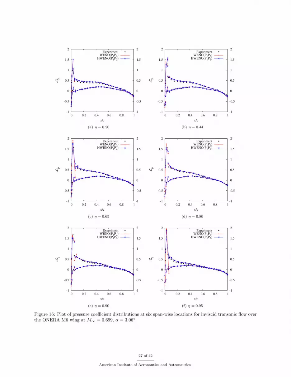
-1

-0.5

0

0.5

1

1.5

2

0 0.2 0.4 0.6 0.8 1-1

-0.5

0

0.5

1

1.5

2

-Cp

x/c

ExperimentWENO(P1P2)

HWENO(P1P2)

(a) η = 0.20

-1

-0.5

0

0.5

1

1.5

2

0 0.2 0.4 0.6 0.8 1-1

-0.5

0

0.5

1

1.5

2

-Cp

x/c


HWENO(P1P2)

(b) η = 0.44

-1

-0.5

0

0.5

1

1.5

2

0 0.2 0.4 0.6 0.8 1-1

-0.5

0

0.5

1

1.5

2

-Cp

x/c


HWENO(P1P2)

(c) η = 0.65

-1

-0.5

0

0.5

1

1.5

2

0 0.2 0.4 0.6 0.8 1-1

-0.5

0

0.5

1

1.5

2

-Cp

x/c


HWENO(P1P2)

(d) η = 0.80

-1

-0.5

0

0.5

1

1.5

2

0 0.2 0.4 0.6 0.8 1-1

-0.5

0

0.5

1

1.5

2

-Cp

x/c


HWENO(P1P2)

(e) η = 0.90

-1

-0.5

0

0.5

1

1.5

2

0 0.2 0.4 0.6 0.8 1-1

-0.5

0

0.5

1

1.5

2

-Cp

x/c


HWENO(P1P2)

(f) η = 0.95

Figure 16: Plot of pressure coefficient distributions at six span-wise locations for inviscid transonic flow overthe ONERA M6 wing at M∞ = 0.699, α = 3.06

27 of 42


-7

-6

-5

-4

-3

-2

-1

0

0 200 400 600 800 1000

Log

(Res

idual

)

Time Step

RK3GMRES

(a)

-7

-6

-5

-4

-3

-2

-1

0

0 1000 2000 3000 4000 5000 6000

Log

(Res

idual

)

CPU Time, Second

RK3GMRES

(b)

Figure 17: Logarithmic density residual versus timestep (a) and CPU time (b) respectively for inviscidtransonic flow over the ONERA M6 wing at M∞ = 0.699, α = 3.06, by RDG(P1P2).

(a) (b)

Figure 18: (a) Surface meshes of the tetrahedral grid for inviscid transonic flow over the ONERA M6 wingat M∞ = 0.84, α = 3.06; (b) Computed pressure contours in the flow field by RDG(P1P2) solutions.

VII.F. Transonic flow over the wing/pylon/finned-store configuration

An inviscid transonic flow over the wing/pylon/finned-store configuration at a freestream Mach number ofM∞ = 0.95 and attack angle of α = 0 is considered in this test case, in order to assess and verify theimplementation of HWENO(P1P2) for complex geometric configurations. The detailed description of thisconfiguration is reported by IIleim et al.32 The configuration consists of a clipped delta wing with a 45

sweep comprised from a constant NACA 64010 symmetric airfoil section. The wing has a root chord of 15inches, a semispan of 13 inches, and a taper ratio of 0.134. The pylon is located at the midspan station andhas a cross-section characterized by a flat plate closed at the leading and trailing edges by a symmetrical oliveshape. The width of the pylon is 0.294 inches. The four fins on the store are defined by a constant NACA0008 airfoil section with a leading-edge sweep of 45 and a truncated tip. Computation is conducted on atetrahedral grid (Nelem = 319,134, Npoin = 147,289, Nafac = 28,738), as the plot of its surface meshesare shown in Fig. 20(a) and 20(b). Fig. 20(c) and 20(d) show the computed pressure contours on the upperand lower wing surfaces, respectively. The computed pressure coefficient distributions are compared withexperimental data at two span-wise stations in Fig. 21. The comparison with experimental data is excellenton both upper and lower surfaces up to 70% chord. As expected from the Euler solution, the computationpredicts a shock location that is downstream of that measured by the experiment due to the lack of viscouseffect. Again, our HWENO(P1P2) method captures the shock waves very sharply within one cell withoutvisible under- and over-shoots. Fig. 22(a) and 22(b) plot the convergence history of logarithmic densityresidual with respect to timestep and CPU time, respectively. One can see that the implicit method hasachieved a speedup of over three orders of magnitude faster than the explicit method.

28 of 42


-1

-0.5

0

0.5

1

1.5

0 0.2 0.4 0.6 0.8 1-1

-0.5

0

0.5

1

1.5

-Cp

x/c

ExperimentHWENO(P1P2)

(a) η = 0.20

-1

-0.5

0

0.5

1

1.5

0 0.2 0.4 0.6 0.8 1-1

-0.5

0

0.5

1

1.5

-Cp

x/c


(b) η = 0.44

-1

-0.5

0

0.5

1

1.5

0 0.2 0.4 0.6 0.8 1-1

-0.5

0

0.5

1

1.5

-Cp

x/c


(c) η = 0.65

-1

-0.5

0

0.5

1

1.5

0 0.2 0.4 0.6 0.8 1-1

-0.5

0

0.5

1

1.5

-Cp

x/c


(d) η = 0.80

-1

-0.5

0

0.5

1

1.5

0 0.2 0.4 0.6 0.8 1-1

-0.5

0

0.5

1

1.5

-Cp

x/c


(e) η = 0.90

-1

-0.5

0

0.5

1

1.5

0 0.2 0.4 0.6 0.8 1-1

-0.5

0

0.5

1

1.5

-Cp

x/c


(f) η = 0.95

Figure 19: Plot of pressure coefficient distributions at six span-wise locations for inviscid transonic flow overthe ONERA M6 wing at M∞ = 0.84, α = 3.06

29 of 42


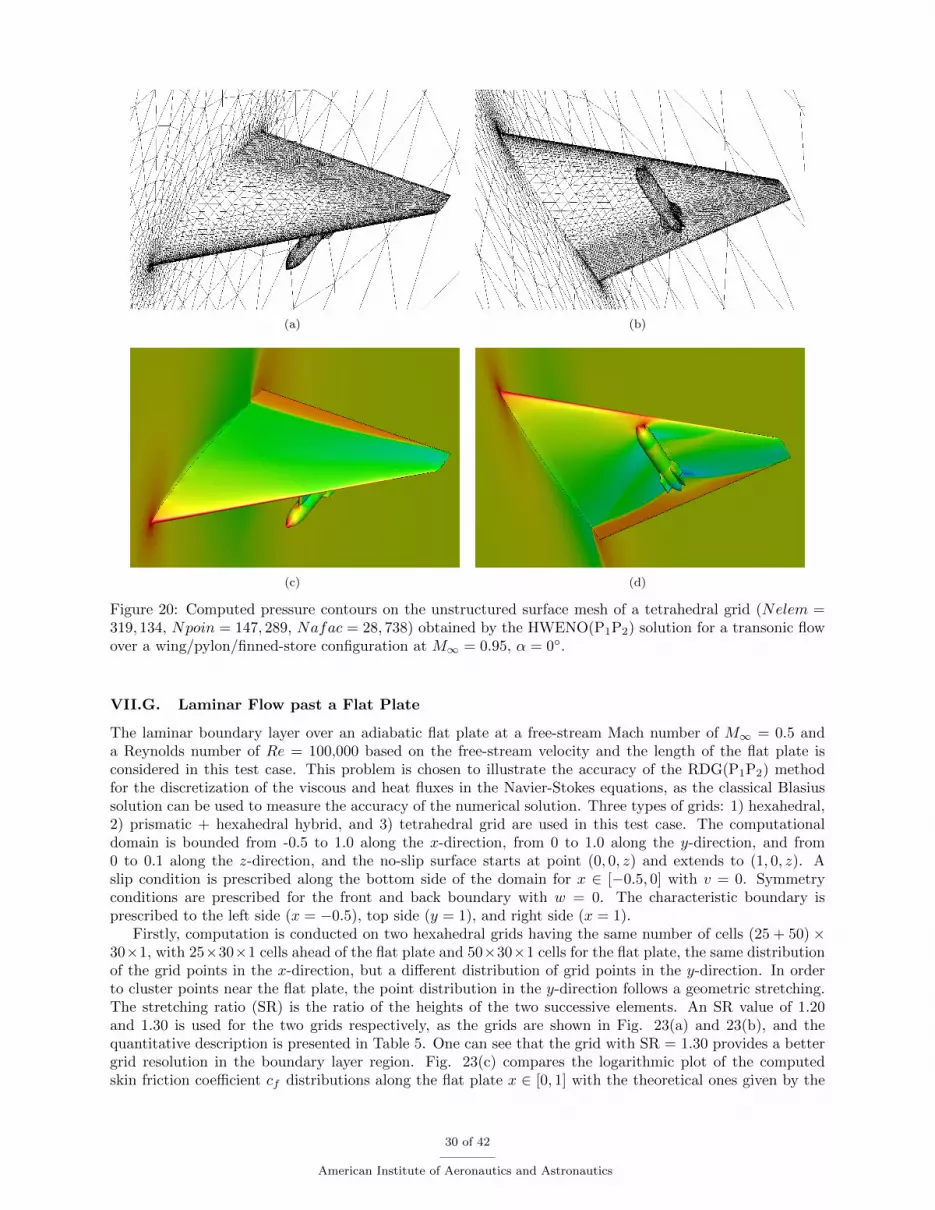
(a) (b)

(c) (d)

Figure 20: Computed pressure contours on the unstructured surface mesh of a tetrahedral grid (Nelem =319, 134, Npoin = 147, 289, Nafac = 28, 738) obtained by the HWENO(P1P2) solution for a transonic flowover a wing/pylon/finned-store configuration at M∞ = 0.95, α = 0.

VII.G. Laminar Flow past a Flat Plate

The laminar boundary layer over an adiabatic flat plate at a free-stream Mach number of M∞ = 0.5 anda Reynolds number of Re = 100,000 based on the free-stream velocity and the length of the flat plate isconsidered in this test case. This problem is chosen to illustrate the accuracy of the RDG(P1P2) methodfor the discretization of the viscous and heat fluxes in the Navier-Stokes equations, as the classical Blasiussolution can be used to measure the accuracy of the numerical solution. Three types of grids: 1) hexahedral,2) prismatic + hexahedral hybrid, and 3) tetrahedral grid are used in this test case. The computationaldomain is bounded from -0.5 to 1.0 along the x-direction, from 0 to 1.0 along the y-direction, and from0 to 0.1 along the z-direction, and the no-slip surface starts at point (0, 0, z) and extends to (1, 0, z). Aslip condition is prescribed along the bottom side of the domain for x ∈ [−0.5, 0] with v = 0. Symmetryconditions are prescribed for the front and back boundary with w = 0. The characteristic boundary isprescribed to the left side (x = −0.5), top side (y = 1), and right side (x = 1).

Firstly, computation is conducted on two hexahedral grids having the same number of cells (25 + 50)×30×1, with 25×30×1 cells ahead of the flat plate and 50×30×1 cells for the flat plate, the same distributionof the grid points in the x-direction, but a different distribution of grid points in the y-direction. In orderto cluster points near the flat plate, the point distribution in the y-direction follows a geometric stretching.The stretching ratio (SR) is the ratio of the heights of the two successive elements. An SR value of 1.20and 1.30 is used for the two grids respectively, as the grids are shown in Fig. 23(a) and 23(b), and thequantitative description is presented in Table 5. One can see that the grid with SR = 1.30 provides a bettergrid resolution in the boundary layer region. Fig. 23(c) compares the logarithmic plot of the computedskin friction coefficient cf distributions along the flat plate x ∈ [0, 1] with the theoretical ones given by the

30 of 42


-0.6

-0.4

-0.2

0

0.2

0.4

0.6

0.8

1

1.2

0 0.2 0.4 0.6 0.8 1

-Cp

x/c

HWENO(P1P2)Experiment (lower)Experiment (upper)

(a) η = 0.4077

-0.4

-0.2

0

0.2

0.4

0.6

0.8

1

1.2

0 0.2 0.4 0.6 0.8 1

-Cp

x/c

HWENO(P1P2)Experiment (lower)Experiment (upper)

(b) η = 0.5900

Figure 21: Comparison of the computed pressure coefficient distributions with experimental data at twospan-wise locations for a transonic flow over a wing/pylon/finned-store configuration at M∞ = 0.95, α = 0.

-8

-7

-6

-5

-4

-3

-2

-1

0

0 200 400 600 800 1000

Lo

g(R

esid

ual

)

Time Step

RK3GMRES

(a)

-8

-7

-6

-5

-4

-3

-2

-1

0

0 5000 10000 15000 20000 25000 30000

Lo

g(R

esid

ual

)

CPU Time, Second

RK3GMRES

(b)

Figure 22: Logarithmic density residual versus timestep (a) and CPU time (b) for inviscid subsonic flow overthe wing/pylon/finned-store configuration at M∞ = 0.95, α = 0

Blasius solution, where one can see that the grid of SR = 1.30 provides a better overall prediction. Near theplate leading edge region, cf was overpredicted evidently on grid of SR = 1.20 due to the insufficient gridresolution. Furthermore, a zoom-in observation in Fig. 23(d) clearly illustrates the improved accuracy ofthe RDG(P1P2) solution over the underlying DG(P1) method for viscous flows. Fig. 23(e) and 23(f) showthe plot of velocity profiles versus similarity variable η for computed x-velocity u and scaled y-velocity v+

along the cells cut through by plane of x = 0.1, x = 0.5 and x = 0.9 in the boundary layer region, amongwhich the cells cut by plane of x = 0.9 are adjacent to the outflow boundary. In Fig. 23(e), one can see thatthe u profiles at all the three locations are highly matched with the analytical solution, which indicates aconsistent convergence and accuracy of numerical solution by RDG methods. Furthermore, one can also seethat the v+ profiles can also match the analytical solution very well in Fig. 23(f), although not so good asthe u profiles, since the y-velocity is relatively a small quantity with respect to the x-velocity.

Secondly, computation is conducted on a hybrid grid (Npris = 977, Nhexa = 358) as shown in Fig. 24(a).A zoom-in observation in Fig. 24(b) shows that the boundary layer region mainly consists of hexahedralelements, except at the leading edge region of the plate, where prismatic elements are filled. Fig. 24(c) showsthe comparison of the computed cf distributions with the analytical solution. A zoom-in observation forx ∈ [0.02, 0.1] in Fig. 24(d) clearly demonstrates a more accurate prediction presented by the RDG(P1P2)method than the underlying RDG(P1P1) on this hybrid grid. Fig. 24(e) and 24(f) compares the computedvelocity profiles with the analytical solutions at the three downstream locations, where the RDG methods

31 of 42


Table 5: Boundary layer grid resolution for laminar flow past a flat plate at Re = 100, 000

Stretching Ratio (SR) Height of the first layer y+ of the first layer

1.20 8.4611× 10−4 4.542

1.30 1.1455× 10−4 0.615

again demonstrate a highly consistent convergence of numerical solutionThirdly, computation is carried out on a tetrahedral grid (Ntetr = 47,536) as shown in Fig. 25(a) Fig.

25(b) renders a closer view at the near-wall region, which depicts the sparsity of the grid resolution in theboundary layer. Fig. 25(c) compares the computed cf distributions with the analytical solution. They arehighly accurate on this grid. The difference is only discernible if one takes a zoom-in observation, e.g., forx ∈ [0.5, 0.6] in Fig. 25(d), where RDG(P1P2) presents a slightly better prediction than the RDG(P1P1)on this grid. Fig. 24(e) and 24(f) comapre computed velocity profiles with the analytical solutions at thethree downstream locations, where the RDG methods again exhibit a consistent convergence of numericalsolution. Fig. 26(a) and 26(b) show the convergence history of logarithmic density residuals for bothexplicit and implicit methods with respect to timestep and CPU time respectively. In comparison, one canobserve that GMRES(P1P2) can deliver a speedup of more than three orders of magnitude over RK3(P1P2),indicating the superior advantage of the developed implicit methods over the baseline explicit methods forviscous flow problems. In conclusion of this test case, our RDG methods are able to offer a consistent andefficient highly accurate solution for computing the compressible viscous flows on various types of grids.

VII.H. Subsonic Flow around a Delta Wing at Re = 0.95× 106

A subsonic flow around a sharp-edged slender delta wing at a freestream Mach number of M∞ = 0.3, angleof attack α = 20.5, and Reynolds number of Re = 0.95× 106 based on a mean cord length of 1 is presentedin this test case in order to assess and verify our RDG(P1P2) method for computing high Reynolds numberflows, as the experimental data is available for the geometric configuration31 considered. The aspect ratio ofthis delta wing is equal to 1, which corresponds to a sweep angle of 75.9638. The upper surface of the wingis flat and the cross section is triangular ahead of x/L = 0.9, with the maximum thickness 0.021L. The crosssection downstream of x/L = 0.9 is trapezoidal, and the trailing edge is sharp. A tetrahedral grid (Nelem= 316,139, Npoin = 58,322, Nafac = 21,712) is used in this test case, as the triangular meshes of the wingsurface are displayed in Fig. 27(a), where the no-slip and adiabatic boundary conditions are prescribed. Fig.27(b) displays a sliced-plane of x/L = 0.9, where one can see the highly stretched anisotropic elements piledon the wing surface. The height of the elements on the first layer is 0.5 × 10−3, with a growth rate of 1.3normal to the surface and 5 layers in total. The rest of the domain is filled with isotropic elements.

Computation is initialized with constant freestream values in the entire domain. The flow filed is assumedto have reached the steady state after a decrease of 8 orders of magnitude for the global density residual inonly 191 timesteps as shown in Fig. 28(a). The convergence history (serial mode) in terms of CPU time isshown in Fig. 28(b). Fig. 29(a)–29(d) show the computed surface pressure coefficient distributions comparedwith the experimental data at four stations along the chord of the geometry. At the forward and middlestations as shown in Fig. 29(a), 29(b), and 29(c), the numerical results agree well with the experimentaldata, However the pressure coefficients are significantly over-predicted on the lower wing surface at stationx/L = 0.9 as shown in Fig. 29(d). Similar results were previously reported by J. Thomas et.al65 and T.Erwin et.al.25 The reason for the disagreement is not clearly known, but it was surmised by J. Thomaset.al65 that the disagreement might be caused by the presence of the pressure tubing that exits from themodel in the lower surface trailing-edge region.

VII.I. Transonic flow over a Boeing 747 aircraft

Finally, a transonic flow past a complete Boeing 747 aircraft at a freestream of Mach number of M∞ = 0.85and an angle of attack of α = 2 is presented in this test case. The B747 aircraft configuration includesthe fuselage, wing, horizontal and vertical tails, under-wing pylons, and flow-through engine nacelle. Atetrahedral grid (Nelem = 253,577, Npoin = 48, 851, Nafac = 23,616) is used for modeling the half-span

32 of 42


x

y

0.5 0 0.5 10

0.2

0.4

0.6

0.8

1

(a)

x

y

0.5 0 0.5 10

0.2

0.4

0.6

0.8

1

(b)

10-3

10-2

10-1

10-3

10-2

10-1

100

cf

x

BlasiusRDG(P1P1) SR 1.2RDG(P1P1) SR 1.3RDG(P1P2) SR 1.2RDG(P1P2) SR 1.3

(c)

10-2

10-1

cf

x

BlasiusRDG(P1P1) SR 1.2RDG(P1P2) SR 1.2

(d)

0

0.2

0.4

0.6

0.8

1

1.2

0 1 2 3 4 5 6 7 8

u

η

BlasiusRDG(P1P1) SR 1.2, x=0.1RDG(P1P1) SR 1.2, x=0.5RDG(P1P1) SR 1.2, x=0.9RDG(P1P2) SR 1.2, x=0.1RDG(P1P2) SR 1.2, x=0.5RDG(P1P2) SR 1.2, x=0.9

(e)

0

0.2

0.4

0.6

0.8

1

0 1 2 3 4 5 6 7 8

v+

η

BlasiusRDG(P1P1) SR 1.2, x=0.1RDG(P1P1) SR 1.2, x=0.5RDG(P1P1) SR 1.2, x=0.9RDG(P1P2) SR 1.2, x=0.1RDG(P1P2) SR 1.2, x=0.5RDG(P1P2) SR 1.2, x=0.9

(f)

Figure 23: Plot of the hexahedral grids for laminar flow past a flat plate at Re = 100, 000: (a) SR = 1.20 iny-direction and (b) SR = 1.30 in y-direction. (c) Logarithmic plot of the computed skin friction cf coefficientdistribution compared with the analytical solution along the flat plate x ∈ [0, 1]. (d) Zoom-in comparisonof cf distribution for x ∈ [0.05, 0.1]. (e) Comparison of computed x-velocity u vs. η with the analyticalsolutions at typical downstream locations. (f) Comparison of scaled y-velocity v+ vs. η with the analyticalsolutions at typical downstream locations.

33 of 42


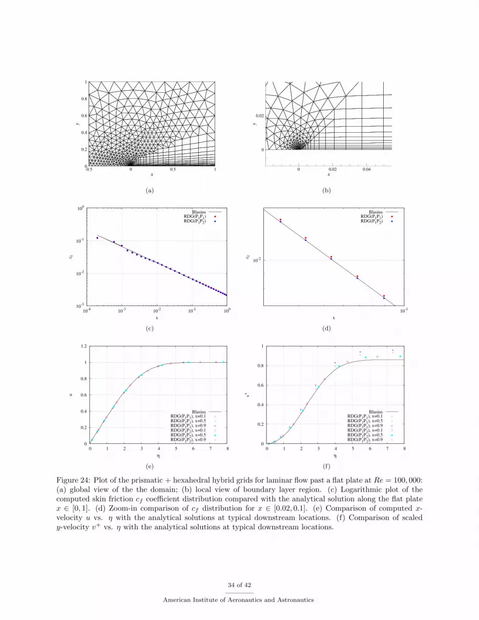
x

y

0.5 0 0.5 10

0.2

0.4

0.6

0.8

1

(a)

x

y

0 0.02 0.04

0

0.02

(b)

10-3

10-2

10-1

100

10-4

10-3

10-2

10-1

100

cf

x

BlasiusRDG(P1P1)RDG(P1P2)

(c)

10-2

10-1

cf

x


(d)

0

0.2

0.4

0.6

0.8

1

1.2

0 1 2 3 4 5 6 7 8

u

η

BlasiusRDG(P1P1), x=0.1RDG(P1P1), x=0.5RDG(P1P1), x=0.9RDG(P1P2), x=0.1RDG(P1P2), x=0.5RDG(P1P2), x=0.9

(e)

0

0.2

0.4

0.6

0.8

1

0 1 2 3 4 5 6 7 8

v+

η


(f)

Figure 24: Plot of the prismatic + hexahedral hybrid grids for laminar flow past a flat plate at Re = 100, 000:(a) global view of the the domain; (b) local view of boundary layer region. (c) Logarithmic plot of thecomputed skin friction cf coefficient distribution compared with the analytical solution along the flat platex ∈ [0, 1]. (d) Zoom-in comparison of cf distribution for x ∈ [0.02, 0.1]. (e) Comparison of computed x-velocity u vs. η with the analytical solutions at typical downstream locations. (f) Comparison of scaledy-velocity v+ vs. η with the analytical solutions at typical downstream locations.

34 of 42


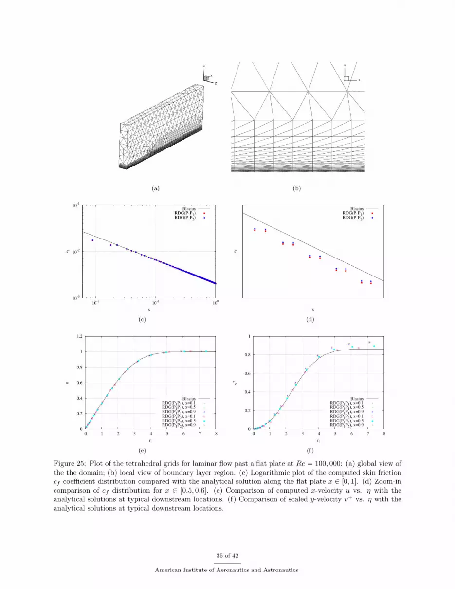
X

Y

Z

(a)

X

Y

Z

(b)

10-3

10-2

10-1

10-2

10-1

100

cf

x


(c)

cf

x


(d)

0

0.2

0.4

0.6

0.8

1

1.2

0 1 2 3 4 5 6 7 8

u

η


(e)

0

0.2

0.4

0.6

0.8

1

0 1 2 3 4 5 6 7 8

v+

η


(f)

Figure 25: Plot of the tetrahedral grids for laminar flow past a flat plate at Re = 100, 000: (a) global view ofthe the domain; (b) local view of boundary layer region. (c) Logarithmic plot of the computed skin frictioncf coefficient distribution compared with the analytical solution along the flat plate x ∈ [0, 1]. (d) Zoom-incomparison of cf distribution for x ∈ [0.5, 0.6]. (e) Comparison of computed x-velocity u vs. η with theanalytical solutions at typical downstream locations. (f) Comparison of scaled y-velocity v+ vs. η with theanalytical solutions at typical downstream locations.

35 of 42


-8

-7

-6

-5

-4

-3

-2

-1

0

1

0 200 400 600 800 1000

Log

(Res

idual

)

Time Step

RK3(P1P1)RK3(P1P2)

GMRES(P1P1)GMRES(P1P2)

(a)

-8

-7

-6

-5

-4

-3

-2

-1

0

1

0 2000 4000 6000 8000 10000 12000 14000

Log

(Res

idual

)

CPU Time, Second

RK3(P1P1)RK3(P1P2)

GMRES(P1P1)GMRES(P1P2)

(b)

Figure 26: Logarithmic density residual versus timestep (a) and CPU time (b) for laminar flow past a flatplate at Re = 100, 000.

(a) (b)

Figure 27: A tetrahedral grid for subsonic flow over a sharp-edged slender delta wing at M∞ = 0.3, α = 20.5

and Re = 0.95× 106: (a) triangular surface meshes; (b) extracted meshes on sliced plane of x/L = 0.9.

airplane. Computation is carried out in parallel mode using 8 compute nodes (equal to 128 CPUs) on NCSU’sARC cluster, which took about 600 steps and 11 minutes to converge the flow field to steady state as Fig.31(a) and 31(b). The computed Mach number contours on the surface of the airplane along with the surfacemesh are shown in Fig. 30. One can see that the shock waves on the upper surface of the wing are capturedwell within one cell, confirming the accuracy, robustness and efficiency of our parallel, implicit RDG(P1P2)method for computing complicated flows of practical importance.

VII.J. Parallel performance

The parallel scalability of our flow solver RDGFLO is assessed through a set of strong scaling experiments bycomputing the test case of subsonic flow past a sphere on NCSU’s ARC cluster, where the finest grid (Nelem= 124,706, equal to 498,824 DOFs) is used and split into up to 128 subdomains. Computation is carriedout with both the explicit and implicit time integration methods. Fig. 32(a) and 32(b) display the parallelspeedup and efficiency obtained on a single compute node (up to 16 CPUs). The parallel efficiency has arrivedaround 78% and 80% for the explicit and implicit methods respectively. Fig. 33(a) and 33(b) demonstratethe parallel speedup and efficiency obtained on multiple compute nodes (up to 8 nodes with 16 CPUs pernode). One can see that the efficiency has a sharp decrease from 1 node (16 CPUs) to 2 nodes (32 CPUs) forthe implicit method but tends to drop slower with more nodes used. This large decrease of efficiency from

36 of 42


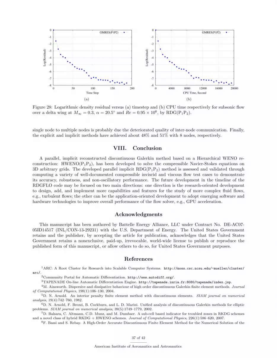
-8

-7

-6

-5

-4

-3

-2

-1

0

0 50 100 150 200

Log(R

esid

ual

)

Time Step

GMRES(P1P2)

(a)

-8

-7

-6

-5

-4

-3

-2

-1

0

0 4000 8000 12000 16000 20000

Log(R

esid

ual

)

CPU Time, Second

GMRES(P1P2)

(b)

Figure 28: Logarithmic density residual versus (a) timestep and (b) CPU time respectively for subsonic flowover a delta wing at M∞ = 0.3, α = 20.5 and Re = 0.95× 106, by RDG(P1P2).

single node to multiple nodes is probably due the deteriorated quality of inter-node communication. Finally,the explicit and implicit methods have achieved about 48% and 51% with 8 nodes, respectively.

VIII. Conclusion

A parallel, implicit reconstructed discontinuous Galerkin method based on a Hierarchical WENO re-construction: HWENO(P1P2), has been developed to solve the compressible Navier-Stokes equations on3D arbitrary grids. The developed parallel implicit RDG(P1P2) method is assessed and validated throughcomputing a variety of well-documented compressible inviscid and viscous flow test cases to demonstrateits accuracy, robustness, and non-oscillatory performance. The future development in the timeline of theRDGFLO code may be focused on two main directions: one direction is the research-oriented developmentto design, add, and implement more capabilities and features for the study of more complex fluid flows,e.g., turbulent flows; the other can be the application-oriented development to adopt emerging software andhardware technologies to improve overall performance of the flow solver, e.g., GPU acceleration.

Acknowledgments

This manuscript has been authored by Battelle Energy Alliance, LLC under Contract No. DE-AC07-05ID14517 (INL/CON-13-29231) with the U.S. Department of Energy. The United States Governmentretains and the publisher, by accepting the article for publication, acknowledges that the United StatesGovernment retains a nonexclusive, paid-up, irrevocable, world-wide license to publish or reproduce thepublished form of this manuscript, or allow others to do so, for United States Government purposes.

References

1ARC: A Root Cluster for Research into Scalable Computer Systems. http://moss.csc.ncsu.edu/~mueller/cluster/

arc/.2Community Portal for Automatic Differentiation. http://www.autodiff.org/.3TAPENADE On-line Automatic Differentiation Engine. http://tapenade.inria.fr:8080/tapenade/index.jsp.4M. Ainsworth. Dispersive and dissipative behaviour of high order discontinuous Galerkin finite element methods. Journal

of Computational Physics, 198(1):106–130, 2004.5D. N. Arnold. An interior penalty finite element method with discontinuous elements. SIAM journal on numerical

analysis, 19(4):742–760, 1982.6D. N. Arnold, F. Brezzi, B. Cockburn, and L. D. Marini. Unified analysis of discontinuous Galerkin methods for elliptic

problems. SIAM journal on numerical analysis, 39(5):1749–1779, 2002.7D. Balsara, C. Altmann, C.D. Munz, and M. Dumbser. A sub-cell based indicator for troubled zones in RKDG schemes

and a novel class of hybrid RKDG + HWENO schemes. Journal of Computational Physics, 226(1):586–620, 2007.8F. Bassi and S. Rebay. A High-Order Accurate Discontinuous Finite Element Method for the Numerical Solution of the

37 of 42


http://moss.csc.ncsu.edu/~mueller/cluster/arc/

http://moss.csc.ncsu.edu/~mueller/cluster/arc/

http://www.autodiff.org/

http://tapenade.inria.fr:8080/tapenade/index.jsp

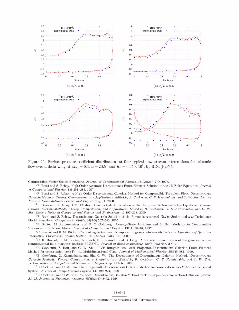
-0.4

-0.2

0

0.2

0.4

0.6

0.8

1

1.2

1.4

1.6

0 0.2 0.4 0.6 0.8 1

-Cp

Semispan

RDG(P1P2)Experimental Data

(a) x/L = 0.3

-0.4

-0.2

0

0.2

0.4

0.6

0.8

1

1.2

1.4

1.6

0 0.2 0.4 0.6 0.8 1

-Cp

Semispan


(b) x/L = 0.5

-0.4

-0.2

0

0.2

0.4

0.6

0.8

1

1.2

0 0.2 0.4 0.6 0.8 1

-Cp

Semispan


(c) x/L = 0.7

-0.2

-0.1

0

0.1

0.2

0.3

0.4

0.5

0.6

0.7

0.8

0 0.2 0.4 0.6 0.8 1

-Cp

Semispan


(d) x/L = 0.9

Figure 29: Surface pressure coefficient distributions at four typical downstream intersections for subsonicflow over a delta wing at M∞ = 0.3, α = 20.5 and Re = 0.95× 106, by RDG(P1P2).

Compressible Navier-Stokes Equations. Journal of Computational Physics, 131(2):267–279, 1997.9F. Bassi and S. Rebay. High-Order Accurate Discontinuous Finite Element Solution of the 2D Euler Equations. Journal

of Computational Physics, 138:251–285, 1997.10F. Bassi and S. Rebay. A High Order Discontinuous Galerkin Method for Compressible Turbulent Flow. Discontinuous

Galerkin Methods, Theory, Computation, and Applications. Edited by B. Cockburn, G. E. Karniadakis, and C. W. Shu. LectureNotes in Computational Science and Engineering, 11, 2000.

11F. Bassi and S. Rebay. GMRES discontinuous Galerkin solution of the Compressible Navier-Stokes Equations. Discon-tinuous Galerkin Methods, Theory, Computation, and Applications. Edited by B. Cockburn, G. E. Karniadakis, and C. W.Shu. Lecture Notes in Computational Science and Engineering, 11:197–208, 2000.

12F. Bassi and S. Rebay. Discontinuous Galerkin Solution of the Reynolds-Averaged Navier-Stokes and κ-ω TurbulenceModel Equations. Computers & Fluids, 34(4-5):507–540, 2005.

13P. Batten, M. A. Leschziner, and U. C. Goldberg. Average-State Jacobians and Implicit Methods for CompressibleViscous and Turbulent Flows. Journal of Computational Physics, 137(1):38–78, 1997.

14C. Bischof and H. M. Bucker. Computing derivatives of computer programs. Modern Methods and Algorithms of QuantumChemistry: Proceedings, Second Edition, NIC Series, 3:315–327, 2000.

15C. H. Bischof, H. M. Bucker, A. Rasch, E. Slusanschi, and B. Lang. Automatic differentiation of the general-purposecomputational fluid dynamics package FLUENT. Journal of fluids engineering, 129(5):652–658, 2007.

16B. Cockburn, S. Hou, and C. W. Shu. TVB Runge-Kutta Local Projection Discontinuous Galerkin Finite ElementMethod for conservation laws IV: the Multidimensional Case. Journal of Mathematical Physics, 55:545–581, 1990.

17B. Cockburn, G. Karniadakis, and Shu C. W. The Development of Discontinuous Galerkin Method. DiscontinuousGalerkin Methods, Theory, Computation, and Applications. Edited by B. Cockburn, G. E. Karniadakis, and C. W. Shu.Lecture Notes in Computational Science and Engineering, 11:5–50, 2000.

18B. Cockburn and C. W. Shu. The Runge-Kutta Discontinuous Galerkin Method for conservation laws V: MultidimensionalSystem. Journal of Computational Physics, 141:199–224, 1998.

19B. Cockburn and C.W. Shu. The Local Discontinuous Galerkin Method for Time-dependent Convection-Diffusion System.SIAM, Journal of Numerical Analysis, 35(6):2440–2463, 1998.

38 of 42


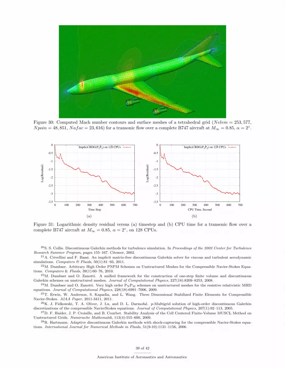
Figure 30: Computed Mach number contours and surface meshes of a tetrahedral grid (Nelem = 253, 577,Npoin = 48, 851, Nafac = 23, 616) for a transonic flow over a complete B747 aircraft at M∞ = 0.85, α = 2.

-3.5

-3

-2.5

-2

-1.5

-1

-0.5

0

0 100 200 300 400 500 600 700

Lo

g(R

esid

ual

)

Time Step

Implicit RDG(P1P2) on 128 CPUs

(a)

-3.5

-3

-2.5

-2

-1.5

-1

-0.5

0

0 100 200 300 400 500 600 700

Lo

g(R

esid

ual

)

CPU Time, Second

Implicit RDG(P1P2) on 128 CPUs

(b)

Figure 31: Logarithmic density residual versus (a) timestep and (b) CPU time for a transonic flow over acomplete B747 aircraft at M∞ = 0.85, α = 2, on 128 CPUs.

20S. S. Collis. Discontinuous Galerkin methods for turbulence simulation. In Proceedings of the 2002 Center for TurbulenceResearch Summer Program, pages 155–167. Citeseer, 2002.

21A. Crivellini and F. Bassi. An implicit matrix-free discontinuous Galerkin solver for viscous and turbulent aerodynamicsimulations. Computers & Fluids, 50(1):81–93, 2011.

22M. Dumbser. Arbitrary High Order PNPM Schemes on Unstructured Meshes for the Compressible Navier-Stokes Equa-tions. Computers & Fluids, 39(1):60–76, 2010.

23M. Dumbser and O. Zanotti. A unified framework for the construction of one-step finite volume and discontinuousGalerkin schemes on unstructured meshes. Journal of Computational Physics, 227(18):8209–8253, 2008.

24M. Dumbser and O. Zanotti. Very high order PNPM schemes on unstructured meshes for the resistive relativistic MHDequations. Journal of Computational Physics, 228(18):6991–7006, 2009.

25T. Erwin, W. Anderson, S. Kapadia, and L. Wang. Three Dimensional Stabilized Finite Elements for CompressibleNavier-Stokes. AIAA Paper, 2011-3411, 2011.

26K. J. Fidkowski, T. A. Oliver, J. Lu, and D. L. Darmofal. p-Multigrid solution of high-order discontinuous Galerkindiscretizations of the compressible NavierStokes equations. Journal of Computational Physics, 207(1):92–113, 2005.

27D. F. Haider, J. P. Croisille, and B. Courbet. Stability Analysis of the Cell Centered Finite-Volume MUSCL Method onUnstructured Grids. Numirische Mathematik, 113(4):555–600, 2009.

28R. Hartmann. Adaptive discontinuous Galerkin methods with shock-capturing for the compressible Navier-Stokes equa-tions. International Journal for Numerical Methods in Fluids, 51(9-10):1131–1156, 2006.

39 of 42


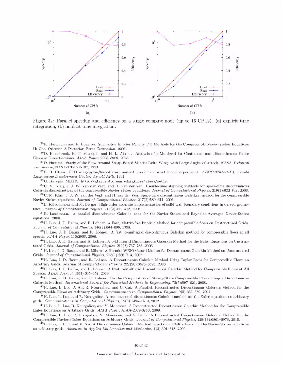
100

101

100

101

0

0.2

0.4

0.6

0.8

1

Sp

eed

up

Eff

icie

ncy

Number of CPUs

IdealReal

Efficiency

(a)

100

101

100

101

0

0.2

0.4

0.6

0.8

1

Sp

eed

up

Eff

icie

ncy

Number of CPUs

IdealReal

Efficiency

(b)

Figure 32: Parallel speedup and efficiency on a single compute node (up to 16 CPUs): (a) explicit timeintegration; (b) implicit time integration.

29R. Hartmann and P. Houston. Symmetric Interior Penalty DG Methods for the Compressible Navier-Stokes EquationsII: Goal-Oriented A Posteriori Error Estimation. 2005.

30D. Helenbrook, B. T. Mavriplis and H. L. Atkins. Analysis of p-Multigrid for Continuous and Discontinuous FiniteElement Discretizations. AIAA Paper, 2003–3989, 2003.

31D. Hummel. Study of the Flow Around Sharp-Edged Slender Delta Wings with Large Angles of Attack. NASA TechnicalTranslation, NASA-TT-F-15107, 1973.

32E. R. IIleim. CFD wing/pylon/finned store mutual interference wind tunnel experiment. AEDC-TSR-91-P4, ArnoldEngineering Development Center, Arnold AFB, 1991.

33G. Karypis. METIS. http://glaros.dtc.umn.edu/gkhome/views/metis.34C. M. Klaij, J. J. W. Van der Vegt, and H. Van der Ven. Pseudo-time stepping methods for space-time discontinuous

Galerkin discretizations of the compressible Navier-Stokes equations. Journal of Computational Physics, 219(2):622–643, 2006.35C. M. Klaij, J. J. W. van der Vegt, and H. van der Ven. Space-time discontinuous Galerkin method for the compressible

Navier-Stokes equations. Journal of Computational Physics, 217(2):589–611, 2006.36L. Krivodonova and M. Berger. High-order accurate implementation of solid wall boundary conditions in curved geome-

tries. Journal of Computational Physics, 211(2):492–512, 2006.37B. Landmann. A parallel discontinuous Galerkin code for the Navier-Stokes and Reynolds-Averaged Navier-Stokes

equations. 2008.38H. Luo, J. D. Baum, and R. Lohner. A Fast, Matrix-free Implicit Method for compressible flows on Unstructured Grids.

Journal of Computational Physics, 146(2):664–690, 1998.39H. Luo, J. D. Baum, and R. Lohner. A fast, p-multigrid discontinuous Galerkin method for compressible flows at all

speeds. AIAA Paper, 110:2006, 2006.40H. Luo, J. D. Baum, and R. Lohner. A p-Multigrid Discontinuous Galerkin Method for the Euler Equations on Unstruc-

tured Grids. Journal of Computational Physics, 211(2):767–783, 2006.41H. Luo, J. D. Baum, and R. Lohner. A Hermite WENO-based Limiter for Discontinuous Galerkin Method on Unstructured

Grids. Journal of Computational Physics, 225(1):686–713, 2007.42H. Luo, J. D. Baum, and R. Lohner. A Discontinuous Galerkin Method Using Taylor Basis for Compressible Flows on

Arbitrary Grids. Journal of Computational Physics, 227(20):8875–8893, 2008.43H. Luo, J. D. Baum, and R. Lohner. A Fast, p-Multigrid Discontinuous Galerkin Method for Compressible Flows at All

Speeds. AIAA Journal, 46(3):635–652, 2008.44H. Luo, J. D. Baum, and R. Lohner. On the Computation of Steady-State Compressible Flows Using a Discontinuous

Galerkin Method. International Journal for Numerical Methods in Engineering, 73(5):597–623, 2008.45H. Luo, L. Luo, A Ali, R. Nourgaliev, and C. Cai. A Parallel, Reconstructed Discontinuous Galerkin Method for the

Compressible Flows on Arbitrary Grids. Communication in Computational Physics, 9(2):363–389, 2011.46H. Luo, L. Luo, and R. Nourgaliev. A reconstructed discontinuous Galerkin method for the Euler equations on arbitrary

grids. Communications in Computational Physics, 12(5):1495–1519, 2012.47H. Luo, L. Luo, R. Nourgaliev, and V. Mousseau. A Reconstructed Discontinuous Galerkin Method for the Compressible

Euler Equations on Arbitrary Grids. AIAA Paper, AIAA-2009-3788, 2009.48H. Luo, L. Luo, R. Nourgaliev, V. Mousseau, and N. Dinh. A Reconstructed Discontinuous Galerkin Method for the

Compressible Navier-STokes Equations on Arbitrary Grids. Journal of Computational Physics, 229(19):6961–6978, 2010.49H. Luo, L. Luo, and K. Xu. A Discontinuous Galerkin Method based on a BGK scheme for the Navier-Stokes equations

on arbitrary grids. Advances in Applied Mathematics and Mechanics, 1(3):301–318, 2009.

40 of 42


http://glaros.dtc.umn.edu/gkhome/views/metis

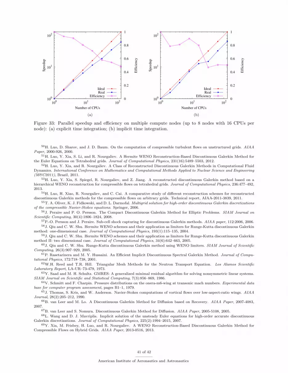
100

101

102

100

101

102

0

0.2

0.4

0.6

0.8

1

Sp

eed

up

Eff

icie

ncy

Number of CPUs

IdealReal

Efficiency

(a)

100

101

102

100

101

102

0

0.2

0.4

0.6

0.8

1

Sp

eed

up

Eff

icie

ncy

Number of CPUs

IdealReal

Efficiency

(b)

Figure 33: Parallel speedup and efficiency on multiple compute nodes (up to 8 nodes with 16 CPUs pernode): (a) explicit time integration; (b) implicit time integration.

50H. Luo, D. Sharov, and J. D. Baum. On the computation of compressible turbulent flows on unstructured grids. AIAAPaper, 2000-926, 2000.

51H. Luo, Y. Xia, S. Li, and R. Nourgaliev. A Hermite WENO Reconstruction-Based Discontinuous Galerkin Method forthe Euler Equations on Tetrahedral grids. Journal of Computational Physics, 231(16):5489–5503, 2012.

52H. Luo, Y. Xia, and R. Nourgaliev. A Class of Reconstructed Discontinuous Galerkin Methods in Computational FluidDynamics. International Conference on Mathematics and Computational Methods Applied to Nuclear Science and Engineering(M&C2011), Brazil, 2011.

53H. Luo, Y. Xia, S. Spiegel, R. Nourgaliev, and Z. Jiang. A reconstructed discontinuous Galerkin method based on ahierarchical WENO reconstruction for compressible flows on tetrahedral grids. Journal of Computational Physics, 236:477–492,2013.

54H. Luo, H. Xiao, R. Nourgaliev, and C. Cai. A comparative study of different reconstruction schemes for reconstructeddiscontinuous Galerkin methods for the compressible flows on arbitrary grids. Technical report, AIAA-2011-3839, 2011.

55T. A. Oliver, K. J. Fidkowski, and D. L. Darmofal. Multigrid solution for high-order discontinuous Galerkin discretizationsof the compressible Navier-Stokes equations. Springer, 2006.

56J. Peraire and P. O. Persson. The Compact Discontinuous Galerkin Method for Elliptic Problems. SIAM Journal onScientific Computing, 30(4):1806–1824, 2008.

57P.-O. Persson and J. Peraire. Sub-cell shock capturing for discontinuous Galerkin methods. AIAA paper, 112:2006, 2006.58J. Qiu and C. W. Shu. Hermite WENO schemes and their application as limiters for Runge-Kutta discontinuous Galerkin

method: one-dimensional case. Journal of Computational Physics, 193(1):115–135, 2004.59J. Qiu and C. W. Shu. Hermite WENO schemes and their application as limiters for Runge-Kutta discontinuous Galerkin

method II: two dimensional case. Journal of Computational Physics, 34(6):642–663, 2005.60J. Qiu and C. W. Shu. Runge-Kutta discontinuous Galerkin method using WENO limiters. SIAM Journal of Scientific

Computing, 26(3):907–929, 2005.61P. Rasetarinera and M. Y. Hussaini. An Efficient Implicit Discontinuous Spectral Galerkin Method. Journal of Compu-

tational Physics, 172:718–738, 2001.62W.H. Reed and T.R. Hill. Triangular Mesh Methods for the Neutron Transport Equation. Los Alamos Scientific

Laboratory Report, LA-UR–73-479, 1973.63Y. Saad and M. H. Schultz. GMRES: A generalized minimal residual algorithm for solving nonsymmetric linear systems.

SIAM Journal on Scientific and Statistical Computing, 7(3):856–869, 1986.64V. Schmitt and F. Charpin. Pressure distributions on the onera-m6-wing at transonic mach numbers. Experimental data

base for computer program assessment, pages B1–1, 1979.65J. Thomas, S. Kris, and W. Anderson. Navier-Stokes computations of vortical flows over low-aspect-ratio wings. AIAA

Journal, 28(2):205–212, 1990.66B. van Leer and M. Lo. A Discontinuous Galerkin Method for Diffusion based on Recovery. AIAA Paper, 2007-4083,

2007.67B. van Leer and S. Nomura. Discontinuous Galerkin Method for Diffusion. AIAA Paper, 2005-5108, 2005.68L. Wang and D. J. Mavriplis. Implicit solution of the unsteady Euler equations for high-order accurate discontinuous

Galerkin discretizations. Journal of Computational Physics, 225(2):1994–2015, 2007.69Y. Xia, M. Frisbey, H. Luo, and R. Nourgaliev. A WENO Reconstruction-Based Discontinuous Galerkin Method for

Compressible Flows on Hybrid Grids. AIAA Paper, 2013-0516, 2013.

41 of 42


70Y. Xia, H. Luo, and R. Nourgaliev. An Implicit Method for a Reconstructed Discontinuous Galerkin Method on Tetra-hedron Grids. AIAA Paper, 2012-2834, 2012.

71Y. Xia, H. Luo, and R. Nourgaliev. An Implicit Reconstructed Discontinuous Galerkin Method Based on AutomaticDifferentiation for the Navier-Stokes Equations on Tetrahedron Grids. AIAA Paper, 2013-0687, 2013.

72Y. Xia and R. Nourgaliev. An Implicit Hermite WENO Reconstruction-Based Discontinuous Galerkin Method on Tetra-hedral Grids. 7th International Conference on Computational Fluid Dynamics, ICCFD7-4205, 2012.

73Z. Xu, Y. Liu, H. Du, G. Lin, and C. W. Shu. Point-wise hierarchical reconstruction for discontinuous Galerkin and finitevolume methods for solving conservation laws. Journal of Computational Physics, 230(17):6843–6865, 2011.

74K. Yasue, M. Furudate, N. Ohnishi, and K. Sawada. Implicit discontinuous Galerkin method for RANS simulationutilizing pointwise relaxation algorithm. Communications in Computational Physics, 7(3):510–533, 2010.

75L. Zhang, L. Wei, L. He, X. Deng, and H. Zhang. A class of hybrid DG/FV methods for conservation laws I: Basicformulation and one-dimensional systems. Journal of Computational Physics, 231(4):1081–1103, 2012.

76L. P. Zhang, W. Liu, L. X. He, X. G. Deng, and H. X. Zhang. A Class of Hybrid DG/FV Methods for ConservationLaws II: Two dimensional Cases. Journal of Computational Physics, 231(4):1104–1120, 2012.

42 of 42


Documents

A Parallel, Implicit Reconstructed Discontinuous Galerkin Method for the Compressible Flows on 3D Arbitrary Grids