arX

iv:c

ond-

mat

/060

7089

v2 [

cond

-mat

.dis

-nn]

5 J

ul 2

006

The Compressible Ising Spin Glass: Simulation Results

Adam H. MarshallThe James Franck Institute and Department of Physics, University of Chicago, Chicago, Illinois 60637

(Dated: February 6, 2008)

This paper reports numerical studies of a compressible version of the Ising spin glass in twodimensions. Compressibility is introduced by adding a term that couples the spin-spin interactionsand local lattice deformations to the standard Edwards-Anderson model. The relative strength ofthis coupling is controlled by a single dimensionless parameter, µ. The timescale associated with thedynamics of the system grows exponentially as µ is increased, and the energy of the compressiblesystem is shifted downward by an amount proportional to µ times the square of the uncoupledenergy. This result leads to the formulation of a simplified model that depends solely on spinvariables; analysis and numerical simulations of the simplified model predict a critical value of thecoupling strength above which the spin-glass transition cannot exist at any temperature.

PACS numbers: 75.10.Nr,75.40.Mg,05.50.+q

I. INTRODUCTION

Much theoretical study has been made of the natureof the spin-glass transition. It is now generally acceptedthat the three-dimesional spin glass undergoes a second-order phase transition at finite temperature,1,2,3,4,5,6,7

and the bulk of the evidence in two dimensions is consis-tent with a zero-temperature phase transition,5,8,9,10,11,12

although recent work suggests that the lower critical di-mension for some spin-glass models is greater than two.13

The continued controversy hints at the delicate and sub-tle nature of the spin-glass transition and suggests thatmodifications to the underlying model, even small ones,could have dramatic effects on the system.

Compressibility has already been shown to have astrong effect on a variety of spin systems. The inclu-sion of compressibility in the Ising ferromagnet modi-fies the standard second-order transition to a first-ordertransition that occurs at the Curie temperature.14,15 The(fully frustrated) 2-D triangular Ising anti-ferromagnetdoes not undergo a phase transition; however, whencompressibility is added to the model, the character-istic frustration is relieved, and the system developsa first-order transition to a “striped” phase at lowtemperatures.16,17,18 Other frustrated spin systems areknown to have their frustration relieved by the presenceof magnetoelastic couplings,19,20 and polaron effects alterthe nature of magnetic transitions in frustrated physicalsystems such as manganites.21,22,23

With the possibility of relieving frustration, the addi-tion of compressibility to spin-glass models could dramat-ically alter the nature of the spin-glass phase and/or thetransition thereto. Furthermore, the fact that all physi-cal systems must possess some (albeit small) spin-latticecoupling provides a physical motivation for such studies.

A previous paper introduced a particular model forthe compressible spin glass with a linear coupling be-tween the spin-spin interactions and the distances be-tween neighboring particles.24 The work described thereinvolved simulations of the compressible spin glass per-formed on two-dimensional systems in which the volume

was held fixed. Results of the direct simulations sug-gest a simplified model, qualitatively equivalent to thefirst, that depends only upon spin degrees of freedom.The presence of compressibility alters the preferred spinconfigurations of the system, so that the transition toa low-temperature spin-glass phase is impossible above acritical value of the coupling. The current paper expandson that previous work as well as provides details of theanalysis. Presented here are results showing the expo-nential slowing down of the time to reach equilibriumas the coupling increases, additional quantitative moti-vation for the simplified model, and a functional formfor the entropy of the spin glass, from which thermody-namic quantities are predicted. Finally, a phase diagramillustrates an approximate boundary separating criticalbehavior from the region where the spin-glass transitioncannot exist.

The structure of this paper is as follows: Section IIdescribes the Hamiltonian of the compressible spin glassand defines the important tuning parameters. The detailsof the computer simulations are discussed in Sec. III, andthe results of the simulations are presented in Sec. IV.A simplified model is introduced in Sec. V, along withresults of numeric simulations and analytic investigationsperformed on the simplified model. Section VI containsthe primary conclusions and some additional points ofdiscussion.

II. THE MODEL

The Hamiltonian for the compressible Ising spin glassis24

H = −∑

〈i,j〉

JijSiSj + α∑

〈i,j〉

JijSiSj (rij − r0) + Ulattice .

(1)The first term is the standard Edwards-Anderson spin-

glass Hamiltonian,25 with the sum performed over pairsof nearest neighbors. The spins Si are dynamic variableswhich may take the values +1 or −1. The interactions Jij

2

are chosen randomly from ±J with equal probabilityand are then held fixed; this collection of interactionsrepresents a single realization of the quenched disordercentral to the nature of the spin glass.

The coupling between the spin interactions and thelattice distortions is contained within the second termof Eq. (1), where the coupling is considered to linearorder with proportionality constant α. This constantmultiplies the change in bond length: rij represents theEuclidean distance between particles i and j, and r0 isthe natural spacing of nearest neighbors on the lattice.This term allows the system to lower the total energyby displacing the particles from their regular lattice po-sitions. Spins with satisfied interactions (i.e., those withJijSiSj = +1) will tend to move closer together in orderto strengthen the effect; similarly, unsatisfied bonds willtend to lengthen as the particles move farther apart to di-minish the negative effect of their interaction on the totalenergy. The inability of all of the bonds in the system todistort simultaneously in the ideal fashion is the mech-anism by which the degeneracy of configurations withequal spin-spin energy is broken.

The final term, Ulattice, stabilizes the lattice by pro-viding a restoring force to counteract the displacementsgenerated by the spin-lattice interactions. The stabiliza-tion is obtained by connecting harmonic springs betweennearest neighbors and between next-nearest neighbors(along the diagonals of the square lattice). Each springhas as its unstretched length the natural spacing of thevertices, so that Ulattice is zero in the absence of spin-lattice coupling when the particles are not displaced.

Two important parameters can be formed. The firstarises due to force balance between the last two terms inEq. (1):

δ ≡Jα

k, (2)

This has dimensions of length and represents the scaleof the typical displacements of the particles from theiruncoupled locations on the square lattice. The secondparameter is

µ ≡Jα2

k, (3)

which is dimensionless; it represents the strength of thespin-lattice coupling, relative to the spin-spin interaction.When µ = 0, there is no spin-lattice coupling, latticedistortions are not energetically favorable, and the modelreduces to the standard Edwards-Anderson spin glass.The interaction strength J serves merely to set the energyscale for the model. In this work, J is set to unity, while αand k are chosen so that δ and µ take the desired values.

III. SIMULATION DETAILS

All simulations were run on square lattices of lineardimension L with periodic boundary conditions in two

dimensions; the size of the system was held constant ineach direction, fixing the total volume. The control pa-rameters were adjusted so that δ was set at ten percentof the natural lattice spacing while µ was varied overthe range 0 ≤ µ ≤ 5. Since the information regardingrelative energy scales is contained within µ, the specificvalue of δ does not affect the qualitative nature of theresults, so long as the displacements are small enough tomaintain the topology of the lattice. As discussed below,however, small nonlinearities do depend on the extent ofthe lattice distortions.

For all values of the control parameters, 100 differentbond configurations (i.e., realizations of the quencheddisorder) were simulated. Calculated quantities werethen averaged over the various runs.

Two different methods of simulation were used to studythe compressible spin glass. For the first method, suitablefor studying the dynamics of the model, states were gen-erated via single-spinflip Monte Carlo steps, with transi-tion probabilities dependent upon the difference in energybetween the two spin states. These energies employed thefull Hamiltonian of Eq. (1), including the componentsthat depend on the particle positions. For purposes ofdetermining transition probabilities, the spins were con-sidered to flip in place, i.e., without any particle motion.The lattice was then relaxed for the new spin configu-ration. The full simulation algorithm is as follows: Thesystem is started in a random spin configuration withthe particles located at the positions which minimize thetotal energy. From a given spin configuration, a particleis chosen at random. This particle is given a chance toflip, in place, from the state with energy E1 to the statewith energy E2. If E2 < E1 the spin is flipped; other-wise the spin flips with probability exp[−(E2 − E1)/T ].After L2 randomly chosen particles have been considered(i.e., one Monte Carlo step), the lattice is relaxed to theminimum of the potential energy for the new spin config-uration using conjugate-gradient minimization. Systemproperties are recorded for analysis, and this process isthen repeated.

In order to ensure proper equilibration, I follow thealgorithm prescribed by Bhatt and Young:1,5 The spin-glass susceptibility

χsg =1

L2

∑

i,j

〈SiSj〉2

,

where 〈·〉 indicates a thermal (time) average, is calculatedby two different methods, each as a function of equilibra-tion time tequil. One method uses the overlap betweenstates of the same system at two different times duringthe run, while the other uses the overlap between statesof two randomly initialized, independently run replicasof the same bond realization. These two computationmethods produce the same value of χsg as tequil → ∞,but the “two-times” method approaches the asymptoticvalue from above, while the “two-replicas” method ap-proaches from below. When the two values are withinstatistical error of one another, the system is equilibrated.

3

The simulations are typically run for several multiples ofthe equilibration time in order to acquire data from un-correlated portions of the time evolution.

Another method of simulation, suitable for studyingstatic properties such as the energy, involves substitut-ing a collection of pre-generated spin states into thecompressible spin-glass Hamiltonian and relaxing eachto the minimum of its total energy with respect to theparticle positions. Typically, the spin states are gener-ated by single-spinflip Monte Carlo simulations using thestandard (incompressible) spin-glass Hamiltonian, whichtakes much less time than simulations of the full Hamilto-nian as described above. In this manner, “typical” statesmay be analyzed to observe the effect of the compressibleterms on quantities of interest; however, these states willnot occur with frequency given by the correct Boltzmannweight, so care must be taken not to draw conclusionsthat would rely on such an assumption. For the small-est system sizes (L = 3, 4, and 5), it was possible to

enumerate all 2L2

possible spin states for a given bondconfiguration.

For all methods of generating spin states, the latticewas relaxed to its minimum using the conjugate-gradientminimization technique.26 Since the distortions of thelattice are kept small by the value of δ, the potential-energy landscape is close to quadratic, and the minimumcan typically be located to reasonable numerical toler-ance within a few conjugate gradient steps. Neverthe-less, because of the computation involved in calculatingthe lattice energy, this portion of the simulation takesapproximately two orders of magnitude more time thanthe Monte Carlo spinflips.

IV. RESULTS

Simulations of the two-dimensional, constant-volumecompressible Ising spin glass were performed for systemsizes ranging from L = 3 to 40 using the techniques de-scribed above. Data from these simulations are presentedand anlayzed below.

A. Dynamics

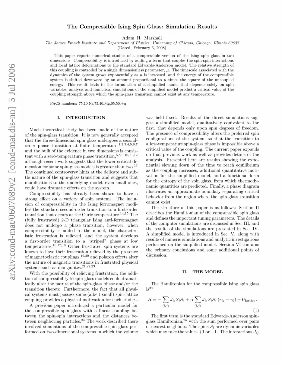
The time required for the system to reach thermal equi-librium is an easily accessible measure of the timescalefor the system dynamics. For each value of µ, a dif-ferent equilibration time is required, and Fig. 1 showsthe dependence of the equilibration time, tequil, on µ forthe L = 10 systems at a relatively high temperature,T = 2.0. As the fit line on the semilog plot demon-strates, the growth of the equilibration time, in MonteCarlo steps (MCS), is exponential in µ; the slope of theexponential fit is 1.8 MCS−1. The rapid growth of theequilibration time as the coupling is increased can beviewed as a growth of energy barriers between states that

101

102

103

0 0.5 1 1.5 2

t equ

il (M

CS

)

µ

FIG. 1: The time to reach equilibrium, tequil, grows expo-nentially as µ increases. The data here are from 100 L = 10systems at T = 2.0, and the slope of the exponential fit line is1.8 MCS−1. The dramatic increase of simulation time makesstraightforward simulation of the dynamics difficult for largevalues of the coupling.

were previously similar in energy. The movement of par-ticles “locks in” the current spin configuration, increasingthe timescale for single-spinflip transitions.

The growth of the equilibration time as a function ofthe coupling is in addition to the usual dramatic growthof dynamic timescales as the temperature is lowered (see,for example, Fig. 3 of Ref. 3). Since the number of simu-lation steps required increases exponentially with µ andthe computation time per step increases in a manner pro-portional to the number of spins, direct simulations of thesystem dynamics at temperatures approaching the tran-sition become prohibitive for large values of the coupling.

B. Energy Analysis

In analyzing the results of the simulations, the vari-ous components of the total energy may be computedindependently for a given spin configuration. Of partic-ular interest is the first term in Eq. (1). This componentrepresents the contribution due solely to spin-spin inter-actions and is denoted E0. It is equivalent to the energyof that spin configuration on an undistorted lattice in theabsence of any spin-lattice coupling.

As shown in Fig. 1 of Ref. 24, the effect of the couplingis to shift the states of the system downward in energy.When µ = 0, the energy levels are δ-functions separatedby constant gaps of 4J , the smallest energy differencebetween states of the incompressible ±J model. As µ isincreased from zero, each energy level (identified by E0)shifts downward in energy and broadens into a Gaussian-shaped band.

For all of the states with a given value of E0, the dis-tribution of energies is characterized by two values: theaverage shift in energy, ∆E(E0, µ) ≡ 〈E(E0, µ)〉 − E0,

4

-40

-30

-20

-10

0

0 1 2 3 4 5

∆E

µ

(a)

E0 = -24-20-16-12

-8-40

0

2

4

6

8

0 1 2 3 4 5

σ

µ

(b)E0 = -24-20-16-12

-8-40

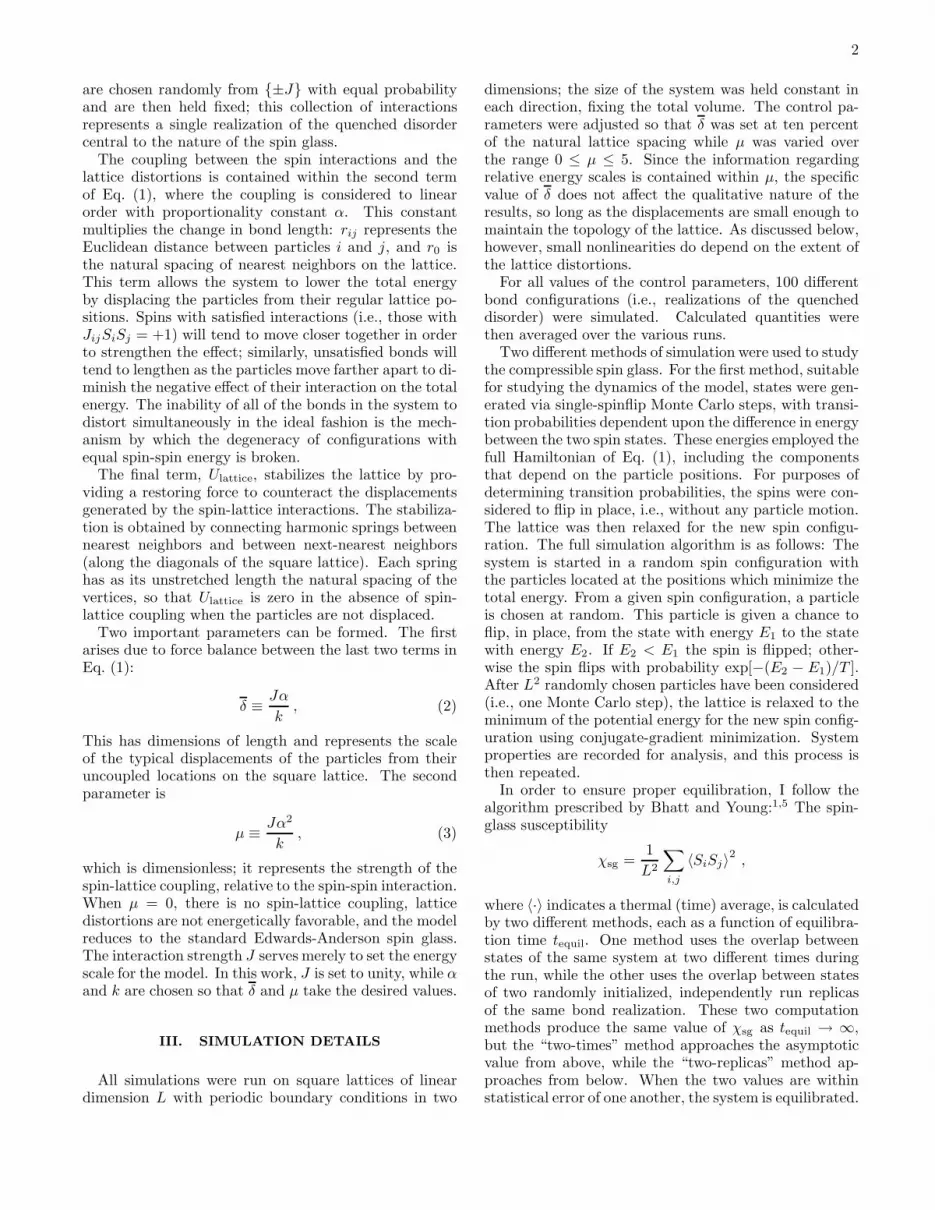
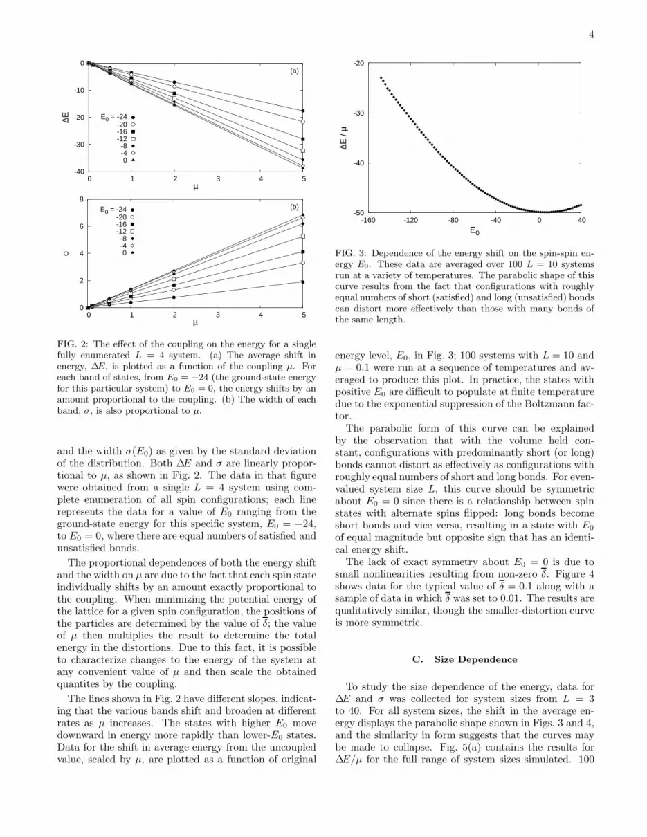
FIG. 2: The effect of the coupling on the energy for a singlefully enumerated L = 4 system. (a) The average shift inenergy, ∆E, is plotted as a function of the coupling µ. Foreach band of states, from E0 = −24 (the ground-state energyfor this particular system) to E0 = 0, the energy shifts by anamount proportional to the coupling. (b) The width of eachband, σ, is also proportional to µ.

and the width σ(E0) as given by the standard deviationof the distribution. Both ∆E and σ are linearly propor-tional to µ, as shown in Fig. 2. The data in that figurewere obtained from a single L = 4 system using com-plete enumeration of all spin configurations; each linerepresents the data for a value of E0 ranging from theground-state energy for this specific system, E0 = −24,to E0 = 0, where there are equal numbers of satisfied andunsatisfied bonds.

The proportional dependences of both the energy shiftand the width on µ are due to the fact that each spin stateindividually shifts by an amount exactly proportional tothe coupling. When minimizing the potential energy ofthe lattice for a given spin configuration, the positions ofthe particles are determined by the value of δ; the valueof µ then multiplies the result to determine the totalenergy in the distortions. Due to this fact, it is possibleto characterize changes to the energy of the system atany convenient value of µ and then scale the obtainedquantites by the coupling.

The lines shown in Fig. 2 have different slopes, indicat-ing that the various bands shift and broaden at differentrates as µ increases. The states with higher E0 movedownward in energy more rapidly than lower-E0 states.Data for the shift in average energy from the uncoupledvalue, scaled by µ, are plotted as a function of original

-50

-40

-30

-20

-160 -120 -80 -40 0 40

∆E /

µ

E0

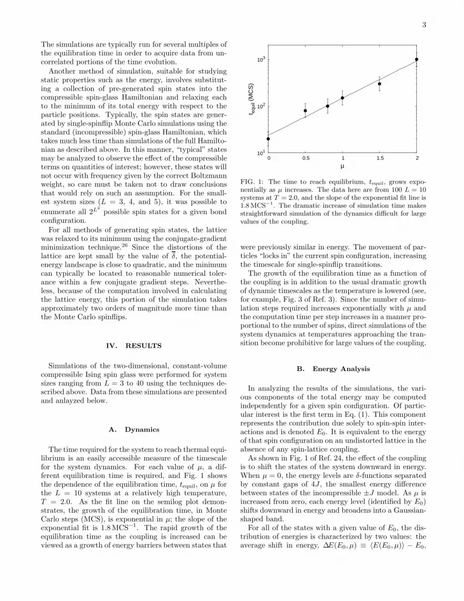
FIG. 3: Dependence of the energy shift on the spin-spin en-ergy E0. These data are averaged over 100 L = 10 systemsrun at a variety of temperatures. The parabolic shape of thiscurve results from the fact that configurations with roughlyequal numbers of short (satisfied) and long (unsatisfied) bondscan distort more effectively than those with many bonds ofthe same length.

energy level, E0, in Fig. 3; 100 systems with L = 10 andµ = 0.1 were run at a sequence of temperatures and av-eraged to produce this plot. In practice, the states withpositive E0 are difficult to populate at finite temperaturedue to the exponential suppression of the Boltzmann fac-tor.

The parabolic form of this curve can be explainedby the observation that with the volume held con-stant, configurations with predominantly short (or long)bonds cannot distort as effectively as configurations withroughly equal numbers of short and long bonds. For even-valued system size L, this curve should be symmetricabout E0 = 0 since there is a relationship between spinstates with alternate spins flipped: long bonds becomeshort bonds and vice versa, resulting in a state with E0

of equal magnitude but opposite sign that has an identi-cal energy shift.

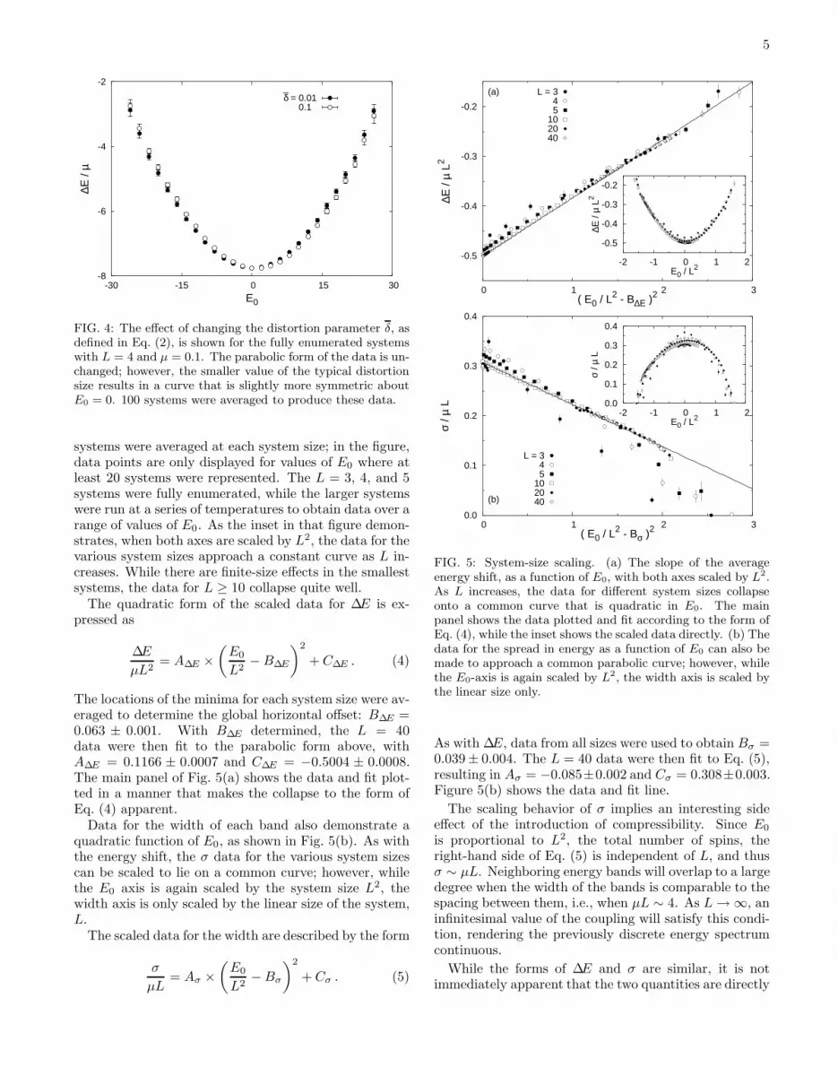
The lack of exact symmetry about E0 = 0 is due tosmall nonlinearities resulting from non-zero δ. Figure 4shows data for the typical value of δ = 0.1 along with asample of data in which δ was set to 0.01. The results arequalitatively similar, though the smaller-distortion curveis more symmetric.

C. Size Dependence

To study the size dependence of the energy, data for∆E and σ was collected for system sizes from L = 3to 40. For all system sizes, the shift in the average en-ergy displays the parabolic shape shown in Figs. 3 and 4,and the similarity in form suggests that the curves maybe made to collapse. Fig. 5(a) contains the results for∆E/µ for the full range of system sizes simulated. 100

5

-8

-6

-4

-2

-30 -15 0 15 30

∆E /

µ

E0

_δ = 0.01

0.1

FIG. 4: The effect of changing the distortion parameter δ, asdefined in Eq. (2), is shown for the fully enumerated systemswith L = 4 and µ = 0.1. The parabolic form of the data is un-changed; however, the smaller value of the typical distortionsize results in a curve that is slightly more symmetric aboutE0 = 0. 100 systems were averaged to produce these data.

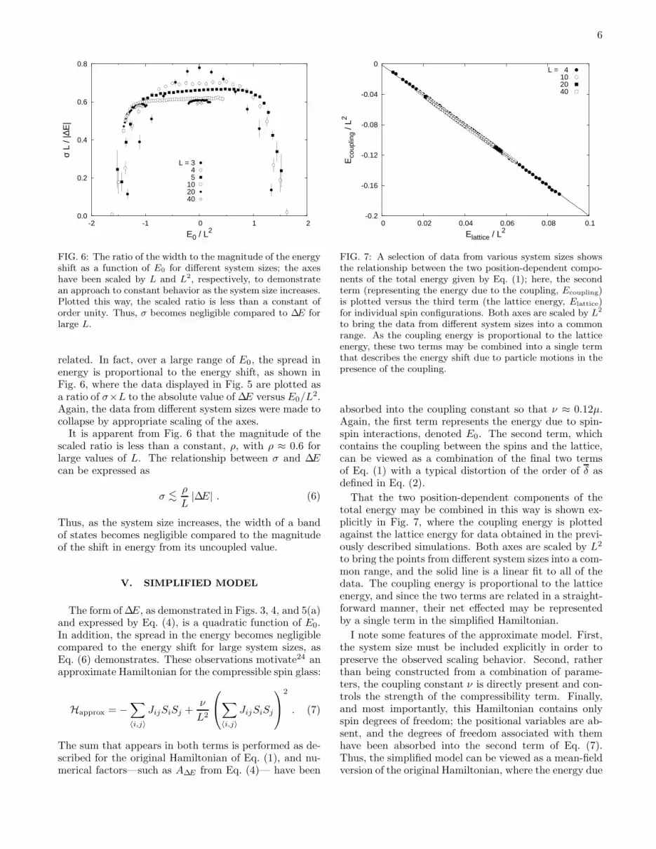
systems were averaged at each system size; in the figure,data points are only displayed for values of E0 where atleast 20 systems were represented. The L = 3, 4, and 5systems were fully enumerated, while the larger systemswere run at a series of temperatures to obtain data over arange of values of E0. As the inset in that figure demon-strates, when both axes are scaled by L2, the data for thevarious system sizes approach a constant curve as L in-creases. While there are finite-size effects in the smallestsystems, the data for L ≥ 10 collapse quite well.

The quadratic form of the scaled data for ∆E is ex-pressed as

∆E

µL2= A∆E ×

(E0

L2− B∆E

)2

+ C∆E . (4)

The locations of the minima for each system size were av-eraged to determine the global horizontal offset: B∆E =0.063 ± 0.001. With B∆E determined, the L = 40data were then fit to the parabolic form above, withA∆E = 0.1166 ± 0.0007 and C∆E = −0.5004 ± 0.0008.The main panel of Fig. 5(a) shows the data and fit plot-ted in a manner that makes the collapse to the form ofEq. (4) apparent.

Data for the width of each band also demonstrate aquadratic function of E0, as shown in Fig. 5(b). As withthe energy shift, the σ data for the various system sizescan be scaled to lie on a common curve; however, whilethe E0 axis is again scaled by the system size L2, thewidth axis is only scaled by the linear size of the system,L.

The scaled data for the width are described by the form

σ

µL= Aσ ×

(E0

L2− Bσ

)2

+ Cσ . (5)

-0.5

-0.4

-0.3

-0.2

0 1 2 3

∆E /

µ L2

( E0 / L2 - B∆E )2

(a) L = 345

102040

-0.5

-0.4

-0.3

-0.2

-2 -1 0 1 2

∆E /

µ L2

E0 / L2

0.0

0.1

0.2

0.3

0.4

0 1 2 3

σ / µ

L

( E0 / L2 - Bσ )2

(b)

L = 345

102040

0.0

0.1

0.2

0.3

0.4

-2 -1 0 1 2

σ / µ

L

E0 / L2

FIG. 5: System-size scaling. (a) The slope of the averageenergy shift, as a function of E0, with both axes scaled by L2.As L increases, the data for different system sizes collapseonto a common curve that is quadratic in E0. The mainpanel shows the data plotted and fit according to the form ofEq. (4), while the inset shows the scaled data directly. (b) Thedata for the spread in energy as a function of E0 can also bemade to approach a common parabolic curve; however, whilethe E0-axis is again scaled by L2, the width axis is scaled bythe linear size only.

As with ∆E, data from all sizes were used to obtain Bσ =0.039± 0.004. The L = 40 data were then fit to Eq. (5),resulting in Aσ = −0.085±0.002 and Cσ = 0.308±0.003.Figure 5(b) shows the data and fit line.

The scaling behavior of σ implies an interesting sideeffect of the introduction of compressibility. Since E0

is proportional to L2, the total number of spins, theright-hand side of Eq. (5) is independent of L, and thusσ ∼ µL. Neighboring energy bands will overlap to a largedegree when the width of the bands is comparable to thespacing between them, i.e., when µL ∼ 4. As L → ∞, aninfinitesimal value of the coupling will satisfy this condi-tion, rendering the previously discrete energy spectrumcontinuous.

While the forms of ∆E and σ are similar, it is notimmediately apparent that the two quantities are directly

6

0.0

0.2

0.4

0.6

0.8

-2 -1 0 1 2

σ L

/ |∆E

|

E0 / L2

L = 345

102040

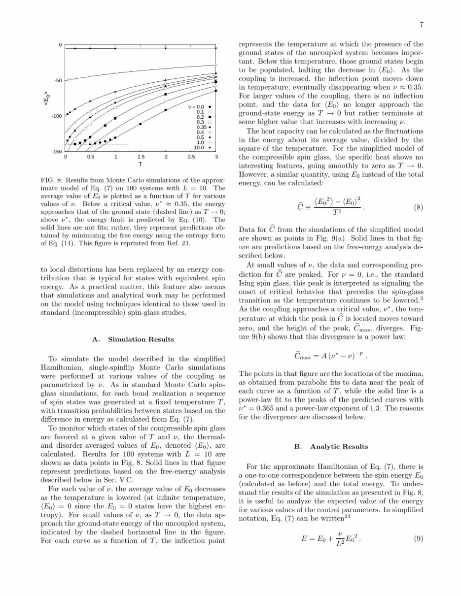
FIG. 6: The ratio of the width to the magnitude of the energyshift as a function of E0 for different system sizes; the axeshave been scaled by L and L2, respectively, to demonstratean approach to constant behavior as the system size increases.Plotted this way, the scaled ratio is less than a constant oforder unity. Thus, σ becomes negligible compared to ∆E forlarge L.

related. In fact, over a large range of E0, the spread inenergy is proportional to the energy shift, as shown inFig. 6, where the data displayed in Fig. 5 are plotted asa ratio of σ×L to the absolute value of ∆E versus E0/L2.Again, the data from different system sizes were made tocollapse by appropriate scaling of the axes.

It is apparent from Fig. 6 that the magnitude of thescaled ratio is less than a constant, ρ, with ρ ≈ 0.6 forlarge values of L. The relationship between σ and ∆Ecan be expressed as

σ <∼

ρ

L|∆E| . (6)

Thus, as the system size increases, the width of a bandof states becomes negligible compared to the magnitudeof the shift in energy from its uncoupled value.

V. SIMPLIFIED MODEL

The form of ∆E, as demonstrated in Figs. 3, 4, and 5(a)and expressed by Eq. (4), is a quadratic function of E0.In addition, the spread in the energy becomes negligiblecompared to the energy shift for large system sizes, asEq. (6) demonstrates. These observations motivate24 anapproximate Hamiltonian for the compressible spin glass:

Happrox = −∑

〈i,j〉

JijSiSj +ν

L2

∑

〈i,j〉

JijSiSj

2

. (7)

The sum that appears in both terms is performed as de-scribed for the original Hamiltonian of Eq. (1), and nu-merical factors—such as A∆E from Eq. (4)— have been

-0.2

-0.16

-0.12

-0.08

-0.04

0

0 0.02 0.04 0.06 0.08 0.1

Eco

uplin

g / L

2

Elattice / L2

L = 4102040

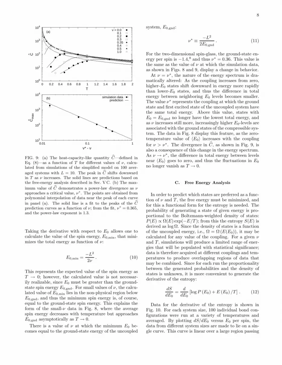
FIG. 7: A selection of data from various system sizes showsthe relationship between the two position-dependent compo-nents of the total energy given by Eq. (1); here, the secondterm (representing the energy due to the coupling, Ecoupling)is plotted versus the third term (the lattice energy, Elattice)for individual spin configurations. Both axes are scaled by L2

to bring the data from different system sizes into a commonrange. As the coupling energy is proportional to the latticeenergy, these two terms may be combined into a single termthat describes the energy shift due to particle motions in thepresence of the coupling.

absorbed into the coupling constant so that ν ≈ 0.12µ.Again, the first term represents the energy due to spin-spin interactions, denoted E0. The second term, whichcontains the coupling between the spins and the lattice,can be viewed as a combination of the final two termsof Eq. (1) with a typical distortion of the order of δ asdefined in Eq. (2).

That the two position-dependent components of thetotal energy may be combined in this way is shown ex-plicitly in Fig. 7, where the coupling energy is plottedagainst the lattice energy for data obtained in the previ-ously described simulations. Both axes are scaled by L2

to bring the points from different system sizes into a com-mon range, and the solid line is a linear fit to all of thedata. The coupling energy is proportional to the latticeenergy, and since the two terms are related in a straight-forward manner, their net effected may be representedby a single term in the simplified Hamiltonian.

I note some features of the approximate model. First,the system size must be included explicitly in order topreserve the observed scaling behavior. Second, ratherthan being constructed from a combination of parame-ters, the coupling constant ν is directly present and con-trols the strength of the compressibility term. Finally,and most importantly, this Hamiltonian contains onlyspin degrees of freedom; the positional variables are ab-sent, and the degrees of freedom associated with themhave been absorbed into the second term of Eq. (7).Thus, the simplified model can be viewed as a mean-fieldversion of the original Hamiltonian, where the energy due

7

-150

-100

-50

0

0 0.5 1 1.5 2 2.5 3

<E

0>

T

ν = 0.00.10.20.30.350.40.51.0

10.0

FIG. 8: Results from Monte Carlo simulations of the approx-imate model of Eq. (7) on 100 systems with L = 10. Theaverage value of E0 is plotted as a function of T for variousvalues of ν. Below a critical value, ν∗

≈ 0.35, the energyapproaches that of the ground state (dashed line) as T → 0;above ν∗, the energy limit is predicted by Eq. (10). Thesolid lines are not fits; rather, they represent predictions ob-tained by minimizing the free energy using the entropy formof Eq. (14). This figure is reprinted from Ref. 24.

to local distortions has been replaced by an energy con-tribution that is typical for states with equivalent spinenergy. As a practical matter, this feature also meansthat simulations and analytical work may be performedon the model using techniques identical to those used instandard (incompressible) spin-glass studies.

A. Simulation Results

To simulate the model described in the simplifiedHamiltonian, single-spinflip Monte Carlo simulationswere performed at various values of the coupling asparametrized by ν. As in standard Monte Carlo spin-glass simulations, for each bond realization a sequenceof spin states was generated at a fixed temperature T ,with transition probabilities between states based on thedifference in energy as calculated from Eq. (7).

To monitor which states of the compressible spin glassare favored at a given value of T and ν, the thermal-and disorder-averaged values of E0, denoted 〈E0〉, arecalculated. Results for 100 systems with L = 10 areshown as data points in Fig. 8. Solid lines in that figurerepresent predictions based on the free-energy analysisdescribed below in Sec. VC.

For each value of ν, the average value of E0 decreasesas the temperature is lowered (at infinite temperature,〈E0〉 = 0 since the E0 = 0 states have the highest en-tropy). For small values of ν, as T → 0, the data ap-proach the ground-state energy of the uncoupled system,indicated by the dashed horizontal line in the figure.For each curve as a function of T , the inflection point

represents the temperature at which the presence of theground states of the uncoupled system becomes impor-tant. Below this temperature, those ground states beginto be populated, halting the decrease in 〈E0〉. As thecoupling is increased, the inflection point moves downin temperature, eventually disappearing when ν ≈ 0.35.For larger values of the coupling, there is no inflectionpoint, and the data for 〈E0〉 no longer approach theground-state energy as T → 0 but rather terminate atsome higher value that increases with increasing ν.

The heat capacity can be calculated as the fluctuationsin the energy about its average value, divided by thesquare of the temperature. For the simplified model ofthe compressible spin glass, the specific heat shows nointeresting features, going smoothly to zero as T → 0.However, a similar quantity, using E0 instead of the totalenergy, can be calculated:

C ≡

⟨E0

2⟩− 〈E0〉

2

T 2. (8)

Data for C from the simulations of the simplified modelare shown as points in Fig. 9(a). Solid lines in that fig-ure are predictions based on the free-energy analysis de-scribed below.

At small values of ν, the data and corresponding pre-

diction for C are peaked. For ν = 0, i.e., the standardIsing spin glass, this peak is interpreted as signaling theonset of critical behavior that precedes the spin-glasstransition as the temperature continues to be lowered.3

As the coupling approaches a critical value, ν∗, the tem-

perature at which the peak in C is located moves toward

zero, and the height of the peak, Cmax, diverges. Fig-ure 9(b) shows that this divergence is a power law:

Cmax = A (ν∗ − ν)−p .

The points in that figure are the locations of the maxima,as obtained from parabolic fits to data near the peak ofeach curve as a function of T , while the solid line is apower-law fit to the peaks of the predicted curves withν∗ = 0.365 and a power-law exponent of 1.3. The reasonsfor the divergence are discussed below.

B. Analytic Results

For the approximate Hamiltonian of Eq. (7), there isa one-to-one correspondence between the spin energy E0

(calculated as before) and the total energy. To under-stand the results of the simulation as presented in Fig. 8,it is useful to analyze the expected value of the energyfor various values of the control parameters. In simplifiednotation, Eq. (7) can be written24

E = E0 +ν

L2E0

2 . (9)

8

100

101

102

103

104

0 0.2 0.4 0.6 0.8 1 1.2 1.4 1.6 1.8 2

C

T

(a)^

ν = 0.00.10.20.30.350.40.51.0

101

102

103

104

0.01 0.1 1

Cm

ax

ν* - ν

(b)

^

simulation dataprediction

FIG. 9: (a) The heat-capacity-like quantity C—defined inEq. (8)—as a function of T for different values of ν, calcu-lated from simulations of the simplified model on 100 aver-

aged systems with L = 10. The peak in C shifts downwardin T as ν increases. The solid lines are predictions based onthe free-energy analysis described in Sec. V C. (b) The max-

imum value of C demonstrates a power-law divergence as ν

approaches a critical value, ν∗. The points are obtained frompolynomial interpolation of data near the peak of each curve

in panel (a). The solid line is a fit to the peaks of the C

prediction curves as a function of ν; from the fit, ν∗ = 0.365,and the power-law exponent is 1.3.

Taking the derivative with respect to E0 allows one tocalculate the value of the spin energy, E0,min, that mini-mizes the total energy as function of ν:

E0,min =−L2

2ν. (10)

This represents the expected value of the spin energy asT → 0; however, the calculated value is not necessar-ily realizable, since E0 must be greater than the ground-state spin energy E0,gnd. For small values of ν, the calcu-lated value of E0,min lies in the non-physical region belowE0,gnd, and thus the minimum spin energy is, of course,equal to the ground-state spin energy. This explains theform of the small-ν data in Fig. 8, where the averagespin energy decreases with temperature but approachesE0,gnd asymptotically as T → 0.

There is a value of ν at which the minimum E0 be-comes equal to the ground-state energy of the uncoupled

system, E0,gnd:

ν∗ ≡−L2

2E0,gnd

. (11)

For the two-dimensional spin-glass, the ground-state en-ergy per spin is −1.4,8 and thus ν∗ = 0.36. This value isthe same as the value of ν at which the simulation data,as shown in Figs. 8 and 9, display a change in behavior.

At ν = ν∗, the nature of the energy spectrum is dra-matically altered: As the coupling increases from zero,higher-E0 states shift downward in energy more rapidlythan lower-E0 states, and thus the difference in totalenergy between neighboring E0 levels becomes smaller.The value ν∗ represents the coupling at which the groundstate and first excited state of the uncoupled system havethe same total energy. Above this value, states withE0 = E0,gnd no longer have the lowest total energy, andas ν increases still more, increasingly higher E0-levels areassociated with the ground states of the compressible sys-tem. The data in Fig. 8 display this feature, as the zero-temperature value of 〈E0〉 increases with the coupling

for ν > ν∗. The divergence in C, as shown in Fig. 9, isalso a consequence of this change in the energy spectrum.As ν → ν∗, the difference in total energy between levelsnear 〈E0〉 goes to zero, and thus the fluctuations in E0

no longer vanish as T → 0.

C. Free Energy Analysis

In order to predict which states are preferred as a func-tion of ν and T , the free energy must be minimized, andfor this a functional form for the entropy is needed. Theprobability of generating a state of given energy is pro-portional to the Boltzmann-weighted density of states:P (E) ∝ Ω(E) exp(−E/T ); from this the entropy S(E) isderived as log Ω. Since the density of states is a functionof the uncoupled energy, i.e., Ω = Ω (E(E0)), it may becalculated for any value of the coupling. For a given νand T , simulations will produce a limited range of ener-gies that will be populated with statistical significance;data is therefore acquired at different couplings and tem-peratures to produce overlapping regions of data thatmay be combined. Since for each run the proportionalitybetween the generated probabilities and the density ofstates is unknown, it is more convenient to generate thederivative of the entropy:

dS

dE0

=d

dE0

[log P (E0) + E (E0) /T ] . (12)

Data for the derivative of the entropy is shown inFig. 10. For each system size, 100 individual bond con-figurations were run at a variety of temperatures andaveraged. By plotting dS/dE0 versus E0 per spin, thedata from different system sizes are made to lie on a sin-gle curve. This curve is linear over a large region passing

9

-2

-1

0

1

2

-1.5 -1 -0.5 0 0.5 1 1.5

dS/d

E0

E0 / L2

L = 4102040fit

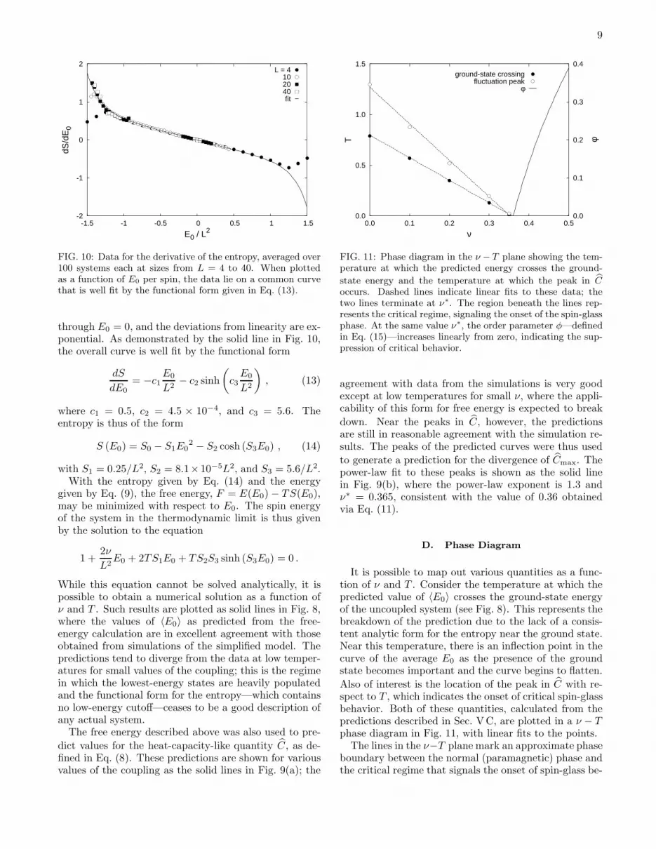
FIG. 10: Data for the derivative of the entropy, averaged over100 systems each at sizes from L = 4 to 40. When plottedas a function of E0 per spin, the data lie on a common curvethat is well fit by the functional form given in Eq. (13).

through E0 = 0, and the deviations from linearity are ex-ponential. As demonstrated by the solid line in Fig. 10,the overall curve is well fit by the functional form

dS

dE0

= −c1

E0

L2− c2 sinh

(c3

E0

L2

), (13)

where c1 = 0.5, c2 = 4.5 × 10−4, and c3 = 5.6. Theentropy is thus of the form

S (E0) = S0 − S1E02 − S2 cosh (S3E0) , (14)

with S1 = 0.25/L2, S2 = 8.1×10−5L2, and S3 = 5.6/L2.With the entropy given by Eq. (14) and the energy

given by Eq. (9), the free energy, F = E(E0) − TS(E0),may be minimized with respect to E0. The spin energyof the system in the thermodynamic limit is thus givenby the solution to the equation

1 +2ν

L2E0 + 2TS1E0 + TS2S3 sinh (S3E0) = 0 .

While this equation cannot be solved analytically, it ispossible to obtain a numerical solution as a function ofν and T . Such results are plotted as solid lines in Fig. 8,where the values of 〈E0〉 as predicted from the free-energy calculation are in excellent agreement with thoseobtained from simulations of the simplified model. Thepredictions tend to diverge from the data at low temper-atures for small values of the coupling; this is the regimein which the lowest-energy states are heavily populatedand the functional form for the entropy—which containsno low-energy cutoff—ceases to be a good description ofany actual system.

The free energy described above was also used to pre-

dict values for the heat-capacity-like quantity C, as de-fined in Eq. (8). These predictions are shown for variousvalues of the coupling as the solid lines in Fig. 9(a); the

0.0

0.5

1.0

1.5

0.0 0.1 0.2 0.3 0.4 0.50.0

0.1

0.2

0.3

0.4

T φ

ν

ground-state crossingfluctuation peak

φ

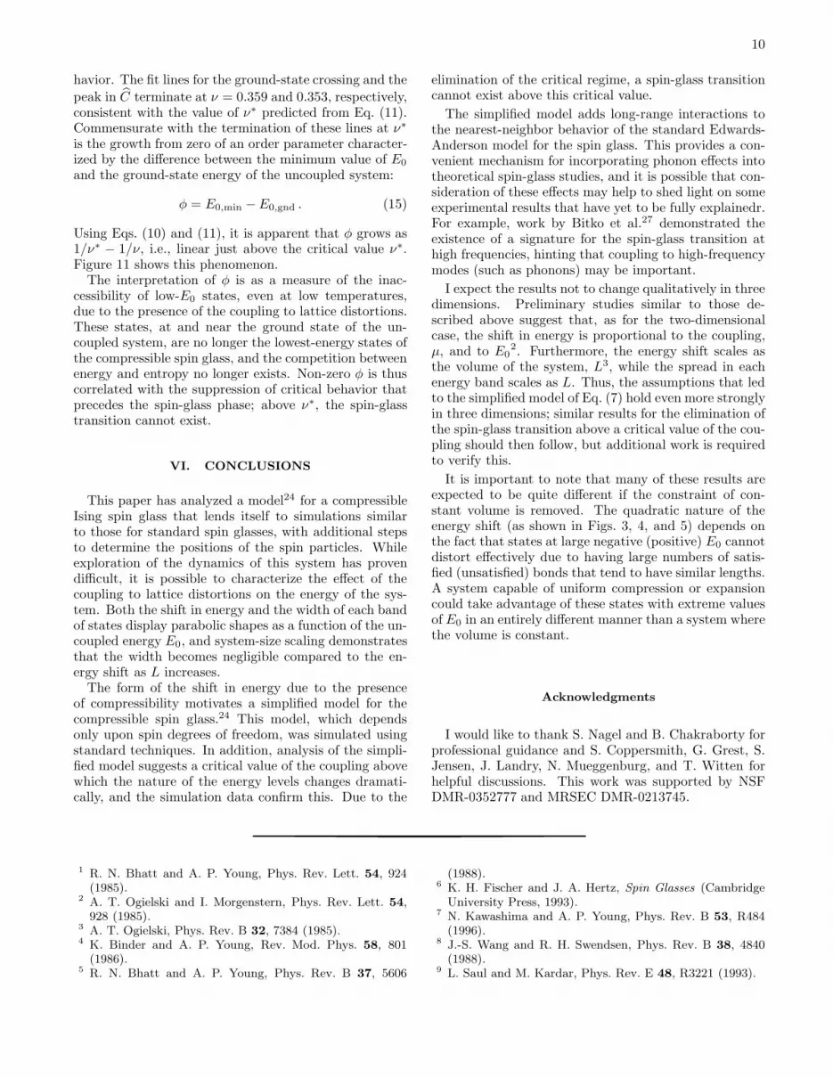
FIG. 11: Phase diagram in the ν − T plane showing the tem-perature at which the predicted energy crosses the ground-

state energy and the temperature at which the peak in C

occurs. Dashed lines indicate linear fits to these data; thetwo lines terminate at ν∗. The region beneath the lines rep-resents the critical regime, signaling the onset of the spin-glassphase. At the same value ν∗, the order parameter φ—definedin Eq. (15)—increases linearly from zero, indicating the sup-pression of critical behavior.

agreement with data from the simulations is very goodexcept at low temperatures for small ν, where the appli-cability of this form for free energy is expected to break

down. Near the peaks in C, however, the predictionsare still in reasonable agreement with the simulation re-sults. The peaks of the predicted curves were thus used

to generate a prediction for the divergence of Cmax. Thepower-law fit to these peaks is shown as the solid linein Fig. 9(b), where the power-law exponent is 1.3 andν∗ = 0.365, consistent with the value of 0.36 obtainedvia Eq. (11).

D. Phase Diagram

It is possible to map out various quantities as a func-tion of ν and T . Consider the temperature at which thepredicted value of 〈E0〉 crosses the ground-state energyof the uncoupled system (see Fig. 8). This represents thebreakdown of the prediction due to the lack of a consis-tent analytic form for the entropy near the ground state.Near this temperature, there is an inflection point in thecurve of the average E0 as the presence of the groundstate becomes important and the curve begins to flatten.

Also of interest is the location of the peak in C with re-spect to T , which indicates the onset of critical spin-glassbehavior. Both of these quantities, calculated from thepredictions described in Sec. VC, are plotted in a ν − Tphase diagram in Fig. 11, with linear fits to the points.

The lines in the ν−T plane mark an approximate phaseboundary between the normal (paramagnetic) phase andthe critical regime that signals the onset of spin-glass be-

10

havior. The fit lines for the ground-state crossing and the

peak in C terminate at ν = 0.359 and 0.353, respectively,consistent with the value of ν∗ predicted from Eq. (11).Commensurate with the termination of these lines at ν∗

is the growth from zero of an order parameter character-ized by the difference between the minimum value of E0

and the ground-state energy of the uncoupled system:

φ = E0,min − E0,gnd . (15)

Using Eqs. (10) and (11), it is apparent that φ grows as1/ν∗ − 1/ν, i.e., linear just above the critical value ν∗.Figure 11 shows this phenomenon.

The interpretation of φ is as a measure of the inac-cessibility of low-E0 states, even at low temperatures,due to the presence of the coupling to lattice distortions.These states, at and near the ground state of the un-coupled system, are no longer the lowest-energy states ofthe compressible spin glass, and the competition betweenenergy and entropy no longer exists. Non-zero φ is thuscorrelated with the suppression of critical behavior thatprecedes the spin-glass phase; above ν∗, the spin-glasstransition cannot exist.

VI. CONCLUSIONS

This paper has analyzed a model24 for a compressibleIsing spin glass that lends itself to simulations similarto those for standard spin glasses, with additional stepsto determine the positions of the spin particles. Whileexploration of the dynamics of this system has provendifficult, it is possible to characterize the effect of thecoupling to lattice distortions on the energy of the sys-tem. Both the shift in energy and the width of each bandof states display parabolic shapes as a function of the un-coupled energy E0, and system-size scaling demonstratesthat the width becomes negligible compared to the en-ergy shift as L increases.

The form of the shift in energy due to the presenceof compressibility motivates a simplified model for thecompressible spin glass.24 This model, which dependsonly upon spin degrees of freedom, was simulated usingstandard techniques. In addition, analysis of the simpli-fied model suggests a critical value of the coupling abovewhich the nature of the energy levels changes dramati-cally, and the simulation data confirm this. Due to the

elimination of the critical regime, a spin-glass transitioncannot exist above this critical value.

The simplified model adds long-range interactions tothe nearest-neighbor behavior of the standard Edwards-Anderson model for the spin glass. This provides a con-venient mechanism for incorporating phonon effects intotheoretical spin-glass studies, and it is possible that con-sideration of these effects may help to shed light on someexperimental results that have yet to be fully explainedr.For example, work by Bitko et al.27 demonstrated theexistence of a signature for the spin-glass transition athigh frequencies, hinting that coupling to high-frequencymodes (such as phonons) may be important.

I expect the results not to change qualitatively in threedimensions. Preliminary studies similar to those de-scribed above suggest that, as for the two-dimensionalcase, the shift in energy is proportional to the coupling,µ, and to E0

2. Furthermore, the energy shift scales asthe volume of the system, L3, while the spread in eachenergy band scales as L. Thus, the assumptions that ledto the simplified model of Eq. (7) hold even more stronglyin three dimensions; similar results for the elimination ofthe spin-glass transition above a critical value of the cou-pling should then follow, but additional work is requiredto verify this.

It is important to note that many of these results areexpected to be quite different if the constraint of con-stant volume is removed. The quadratic nature of theenergy shift (as shown in Figs. 3, 4, and 5) depends onthe fact that states at large negative (positive) E0 cannotdistort effectively due to having large numbers of satis-fied (unsatisfied) bonds that tend to have similar lengths.A system capable of uniform compression or expansioncould take advantage of these states with extreme valuesof E0 in an entirely different manner than a system wherethe volume is constant.

Acknowledgments

I would like to thank S. Nagel and B. Chakraborty forprofessional guidance and S. Coppersmith, G. Grest, S.Jensen, J. Landry, N. Mueggenburg, and T. Witten forhelpful discussions. This work was supported by NSFDMR-0352777 and MRSEC DMR-0213745.

1 R. N. Bhatt and A. P. Young, Phys. Rev. Lett. 54, 924(1985).

2 A. T. Ogielski and I. Morgenstern, Phys. Rev. Lett. 54,928 (1985).

3 A. T. Ogielski, Phys. Rev. B 32, 7384 (1985).4 K. Binder and A. P. Young, Rev. Mod. Phys. 58, 801

(1986).5 R. N. Bhatt and A. P. Young, Phys. Rev. B 37, 5606

(1988).6 K. H. Fischer and J. A. Hertz, Spin Glasses (Cambridge

University Press, 1993).7 N. Kawashima and A. P. Young, Phys. Rev. B 53, R484

(1996).8 J.-S. Wang and R. H. Swendsen, Phys. Rev. B 38, 4840

(1988).9 L. Saul and M. Kardar, Phys. Rev. E 48, R3221 (1993).

11

10 H. Kitatani and A. Sinada, J. Phys. A 33, 3545 (2000).11 J. Houdayer, Eur. Phys. J. B 22, 479 (2001).12 H. G. Katzgraber and L. W. Lee, Phys. Rev. B 71, 134404

(2005).13 C. Amoruso, E. Marinari, O. C. Martin, and A. Pagnani,

Phys. Rev. Lett. 91, 087201 (2003).14 C. P. Bean and D. S. Rodbell, Phys. Rev. 126, 104 (1962).15 D. J. Bergman and B. I. Halperin, Phys. Rev. B 13, 2145

(1976).16 Z.-Y. Chen and M. Kardar, J. Phys. C 19, 6825 (1986).17 L. Gu, B. Chakraborty, P. L. Garrido, M. Phani, and J. L.

Lebowitz, Phys. Rev. B 53, 11985 (1996).18 A. Dhar, P. Chaudhuri, and C. Dasgupta, Phys. Rev. B

61, 6227 (2000).19 F. Becca, F. Mila, and D. Poilblanc, Phys. Rev. Lett. 91,

067202 (2003).20 A. B. Sushkov, O. Tchernyshyov, W. Ratcliff II, S.-W.

Cheong, and H. D. Drew, Phys. Rev. Lett. 94, 137202(2005).

21 M. B. Salamon and M. Jaime, Rev. Mod. Phys. 73, 583(2001).

22 R. Laiho, E. Lahderanta, J. Salminen, K. G. Lisunov, andV. S. Zakhvalinskii, Phys. Rev. B 63, 094405 (2001).

23 C. P. Adams, J. W. Lynn, V. N. Smolyaninova, A. Biswas,R. L. Greene, W. Ratcliff II, S.-W. Cheong, Y. M.Mukovskii, and D. A. Shulyatev, Phys. Rev. B 70, 134414(2004).

24 A. H. Marshall, B. Chakraborty, and S. R. Nagel, Euro-phys. Lett. 74, 699 (2006).

25 S. F. Edwards and P. W. Anderson, J. Phys. F 5, 965(1975).

26 W. H. Press, S. A. Teukolsky, W. T. Vetterling, and B. P.Flannery, Numerical Recipes in C (Cambridge UniversityPress, 1997), 2nd ed.

27 D. Bitko, N. Menon, S. R. Nagel, T. F. Rosenbaum, andG. Aeppli, Europhys. Lett. 33, 489 (1996).