1

Incorporating Large Photovoltaic Farms in Power

Generation System Adequacy Assessment

A. Ghaedia, A. Abbaspour

a, M. Fotuhi-Friuzabad

a* and M. Parvania

a

a Center of Excellence in Power System Control and Management, Department of Electrical Engineering,

Sharif University of Technology, Tehran, Iran,

E-mail: ghaedi@ee.sharif.edu; abbaspour@sharif.edu; fotuhi@shairf.edu; parvania@ee.sharif.edu

*Corresponding author address: Room 621 West, Electrical Engineering Department, Sharif University of

Technology, Azadi Ave., Tehran, Iran; Tel:+982166165921; Postal Code: 11365-11155.

Abstract–Recent advancements in photovoltaic (PV) system technologies have decreased their investment

cost and enabled the construction of large PV farms for bulk power generations.The output power of PV farms is

affected by both failure of composed components and solar radiation variability. These two factors cause the

output power of PV farms be random and different from that of conventional units. Therefore, suitable models

and methods should be developed to assess different aspects of PV farms integrationinto power systems,

particularly from the system reliability viewpoint. In this context a reliability model has been developed for PV

farms with considering both the uncertainties associated with solar radiation and components outages. The

proposed model represents a PV farm by a multi-state generating unit which is suitable for the generation system

assessment. Utilizing the developed reliability model, an analytical method is proposed for adequacy assessment

of power generation systems including large PV farms. Real solar radiation data is used from Jask region in Iran

which are utilized in the studies performed on the RBTS and the IEEE-RTS. Several different analyses are

conducted to analyze the reliability impacts of PV farms integration and to estimate the capacity value of large

PV farms in power generation systems.

Keywords:Adequacy assessment, photovoltaic farm, reliability model, solar radiation uncertainty

1. Introduction

Renewable generations, specially, wind power and photovoltaic (PV) systems are increasingly used in power

systems in recent years. The non-exhausted nature of renewable resources, along with negligible operating costs

2

and benign environmental effects are their primary derivers in power system applications. Recent advancements

in PV system technologies have decreased the investments costs of PV systems. Although the cost of power

produced by PV systems is still higher than the same size conventional generationsand they normally require

additional facilities to integrate and transfer the power to the grid,they are supported strongly by governmental

policies in order to reduce the emissions. The renewable portfolio standards (RPSs), renewable energy

certificates (RECs) [1], regional greenhouse gas emission control schemes [2] in the US, and the 20/20/20 targets

in the European Union [3], are examples of such policies.The ultimate target of these policies is to increase the

use of renewable energy and reduce the environmental emissions. The 250 MW Agua Caliente Solar plant in

USA,214 MW PV Charanka powerplant in India and the 200 MW Yuma County PV power plant in USA are

examples of such PV farms constructed around the world in the past two years [4].

The intermittent nature of solar radiation, along with the probabilistic behavior of PV farms component

outages, makes output power of PV farms completely random and different from conventional generation units.

Therefore, new models and methods are required to be developed to assess the different aspects of PV farms

integration in power systems, particularly from the system reliability point of view. Very little attentions have

been devoted to assess the power system reliability impacts of PV farms integration. In [5], the hourly mean solar

radiation and standard deviation is applied as inputs to simulate the solar radiation over a year. Then, the Monte

Carlo simulation technique is utilized for reliability analysis of small isolated power system containing solar

photovoltaic. A time sequential simulation method is proposed in [6] for generating capacity adequacy evaluation

of small stand-alone power systems containing solar energy operating in parallel with battery storage.The system

considered in [6] is composed of a diesel generator, a PV system and battery storage. In [7] and [8] the reliability

evaluation of the isolated power systems containing PV system and wind generation is studied. In those papers,

the capacity of renewable resources is assumed to be small and the Monte Carlo method is used for uncertainty

modeling of wind speed and solar radiation. In [9], the reliability study of a hybrid system containing wind and

solar generation in off-grid applications of a real system is performed. Various reliability indices such asloss of

load expectation, expected energy not served, energy index of reliability and expected customer interruption cost

are evaluated through probabilistic approach using analytical method. In [10], the reliability analysis of hybrid

wind and solar system based on the well-being approach which is the combination of probabilistic and

deterministic techniques is performed thorough Monte Carlo simulation technique. Monte Carlo Simulation

method is used in [11] for reliability evaluation of a hybrid system containing wind and PV systems connected to

the multi micro storage systems.All the references have considered the reliability impacts of PV farms

integration in isolated power systems.In this context an analytical method is proposed in this paper for adequacy

3

assessment of power generation systems including large PV farms. A reliability model is first developed for PV

farms which consider both the uncertainties associated with solar radiation and components outages. The

proposed reliability model represents a PV farm by a multi-state generating unit which makes it easy to be

utilized in the generation system reliability assessment. The developed multi-state reliability model is utilized to

form a capacity outage probability table (COPT) of the PV farm(s). The obtained COPT is then added to the

equivalent COPT of the conventional generating units to form the total generation capacity model of the system.

Finally, convolution of the load model with the final COPT provides the risk model of generation system

including PV farms, and the reliability indices can be calculated using the obtained risk model. The proposed

analytic approach overcomes some of the difficulties associated with the simulation-based methods in terms of

both computational burden and volume of data needed in such methods. Besides, the proposed analytic model

can be used in generation system expansion planning including large PV farms.

The rest of the paper is organized as follows. The typical structure of a PV farm considered in the paper is

presented in section 2. In section 3 the proposed component reliability model for PV farms is presented. The

model proposed in section 3 is then modified in section 4 in order to consider the effect of solar radiation

uncertainties. The real solar radiation data in the southern part of Iran are utilized in section 4. The proposed

analytic method for adequacy assessment of power systems including PV farms is presented in section 5. The

proposed model is applied to the RBTS and the IEEE-RTS in section 6 to analyze the reliability impacts of PV

farms integration in power systems. Finally, conclusions are given in section 7.

2. PV Farm Structure

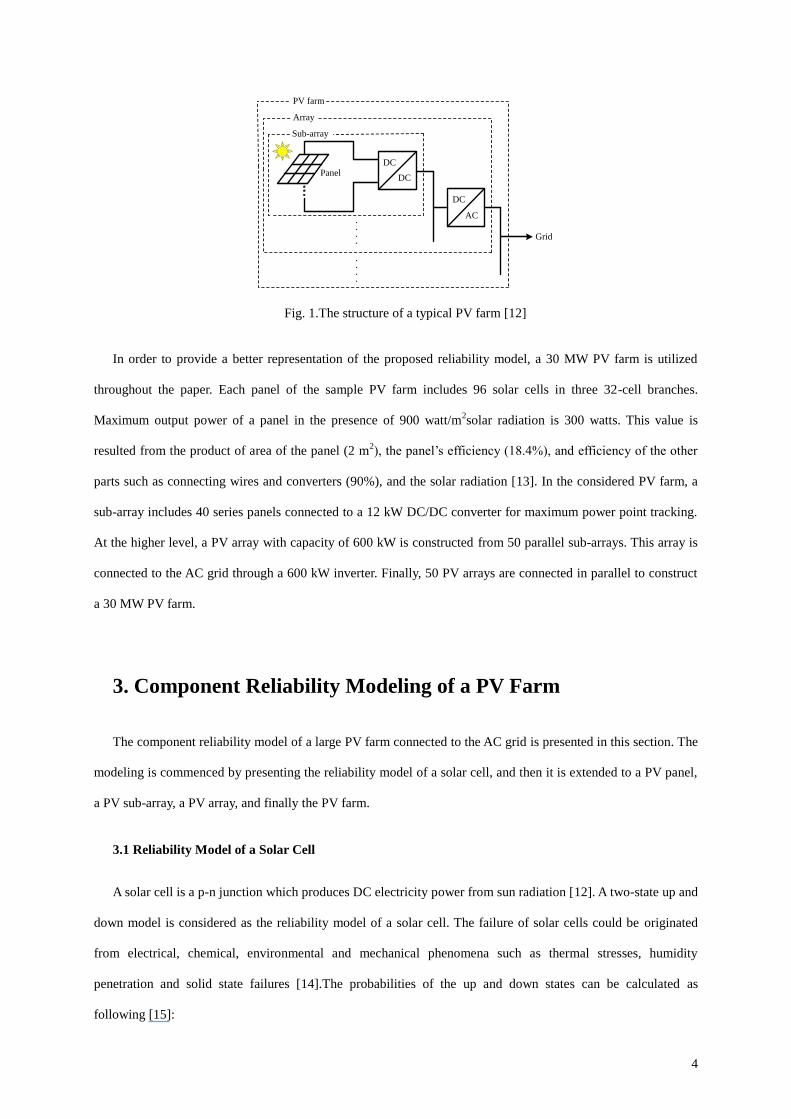
The structure of a typical PV farm is shown in Fig. 1 [12]. The smallest building block of a PV farm is solar

cell which absorbs the solar radiation and converts it to the DC electric power. A number of solar cells are

connected in series and parallel to construct a PV panel and achieve larger current-voltage characteristics. The

output power of a solar panel is maximized in a point named maximum power point (MPP). A number of solar

panels are then connected to a DC/DC converter to target the MPP and yield the maximum power produced by

the panels. This DC/DC converter is usually known as MPP tracker (MPPT) [12]. Such a structure consisted of

solar panels connected to a DC/DC converter is usually known as a PV sub-array. The power produced by a sub-

array is still DC. In order to connect the PV farm to the AC grid, some sub-arrays are then connected to a DC/AC

converter to construct a PV array which is the largest building block of a PV farm.

4

DC

DC

Sub-array

DC

AC

Array

PV farm

Panel

Grid

Fig. 1.The structure of a typical PV farm [12]

In order to provide a better representation of the proposed reliability model, a 30 MW PV farm is utilized

throughout the paper. Each panel of the sample PV farm includes 96 solar cells in three 32-cell branches.

Maximum output power of a panel in the presence of 900 watt/m2solar radiation is 300 watts. This value is

resulted from the product of area of the panel (2 m2), the panel’s efficiency (18.4%), and efficiency of the other

parts such as connecting wires and converters (90%), and the solar radiation [13]. In the considered PV farm, a

sub-array includes 40 series panels connected to a 12 kW DC/DC converter for maximum power point tracking.

At the higher level, a PV array with capacity of 600 kW is constructed from 50 parallel sub-arrays. This array is

connected to the AC grid through a 600 kW inverter. Finally, 50 PV arrays are connected in parallel to construct

a 30 MW PV farm.

3. Component Reliability Modeling of a PV Farm

The component reliability model of a large PV farm connected to the AC grid is presented in this section. The

modeling is commenced by presenting the reliability model of a solar cell, and then it is extended to a PV panel,

a PV sub-array, a PV array, and finally the PV farm.

3.1 Reliability Model of a Solar Cell

A solar cell is a p-n junction which produces DC electricity power from sun radiation [12]. A two-state up and

down model is considered as the reliability model of a solar cell. The failure of solar cells could be originated

from electrical, chemical, environmental and mechanical phenomena such as thermal stresses, humidity

penetration and solid state failures [14].The probabilities of the up and down states can be calculated as

following [15]:

5

,UP DOWNc c

c c

c c c c

P P

(1)

where, c and c are failure rate and repair/replacement rate of a solar cell, respectively. Failure rate and

repair time of the p-n junction of a solar cell of the considered 30MW PV farm are considered to be 0.005

failures in 106 hours (0.00004 f/yr) and 40 hours, respectively [16].

3.2 Reliability Model of a PV Panel

A PV panel is constructed by Mparallelbranches, each with N series solar cells. If a solar cell fails, the

associated branch would go out of service. Accordingly, the failure rate of a branch is sum of the failure rate of

the series solar cells [17]. Thus, the probabilities of the up and down states of a panel branch can be calculated by

(2), respectively:

, 1N

UP UP DOWN UPb b

b c b b

b b b b

P P P P

(2)

where, b and b are failure rate and repair/replacement rate of a branch, respectively. Using the principles of

series systems [15], b and b are equal to cN and c , respectively.

3.3 Reliability Model of a PV Sub-array

In a PV panel with M parallel branches, the failure of a branch reduces the output power of the panel to (M-

1)/M of maximum power output of the panel. As the direct consequence of this failure and based on the

Kirchhoff’scurrent law, the current of the other panelsmust be reduced by the factor of (M-1)/M. Thus, the total

output power of the sub-array would be reduced to (M-1)/Mtimes of the nominal power. The reliability model of

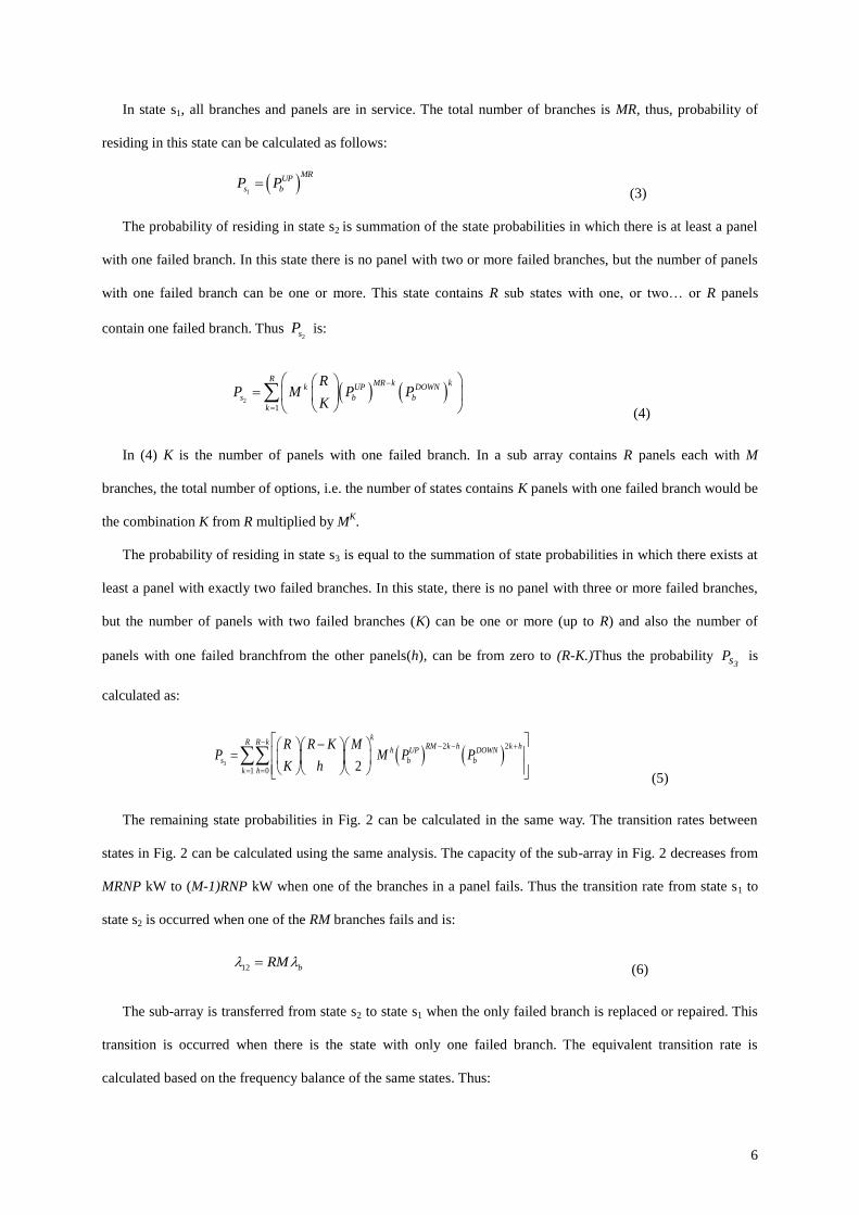
a PV sub-array can be shown as Fig. 2, with (M+1) states. In Fig. 2, P is the power produced by each solar cell,N

is the number of series cells in a branch, M is the number of parallel branches in a panel, and R is the number of

series PV panels in a sub-array.

MRNP

KW0 KW

(M-1)RNP

KW

s1 s2 sM+1

21

12(M-2)RNP

KW

s3

32

23

Fig. 2. Reliability model of a PV sub-array

The state probabilities in Fig. 2 can be calculated as follows:

6

In state s1, all branches and panels are in service. The total number of branches is MR, thus, probability of

residing in this state can be calculated as follows:

1

MRUP

s bP P (3)

The probability of residing in state s2 is summation of the state probabilities in which there is at least a panel

with one failed branch. In this state there is no panel with two or more failed branches, but the number of panels

with one failed branch can be one or more. This state contains R sub states with one, or two… or R panels

contain one failed branch. Thus 2sP is:

2

1

RMR k k

k UP DOWN

s b b

k

RP M P P

K

(4)

In (4) K is the number of panels with one failed branch. In a sub array contains R panels each with M

branches, the total number of options, i.e. the number of states contains K panels with one failed branch would be

the combination K from R multiplied by MK.

The probability of residing in state s3 is equal to the summation of state probabilities in which there exists at

least a panel with exactly two failed branches. In this state, there is no panel with three or more failed branches,

but the number of panels with two failed branches (K) can be one or more (up to R) and also the number of

panels with one failed branchfrom the other panels(h), can be from zero to (R-K.)Thus the probability 3sP is

calculated as:

3

2 2

1 0 2

kR R k

RM k h k hh UP DOWN

s b b

k h

R R K MP M P P

K h

(5)

The remaining state probabilities in Fig. 2 can be calculated in the same way. The transition rates between

states in Fig. 2 can be calculated using the same analysis. The capacity of the sub-array in Fig. 2 decreases from

MRNP kW to (M-1)RNP kW when one of the branches in a panel fails. Thus the transition rate from state s1 to

state s2 is occurred when one of the RM branches fails and is:

12 bRM (6)

The sub-array is transferred from state s2 to state s1 when the only failed branch is replaced or repaired. This

transition is occurred when there is the state with only one failed branch. The equivalent transition rate is

calculated based on the frequency balance of the same states. Thus:

7

2

1

21

MRUP DOWN

b b b

s

RM P P

P

(7)

In (7), DOWN

b1MRUP

b P)P(RM is the probability of the state with only one failed branch.

The sub-array in state s2 has at least one panel with one failed branch. If one another branch of the panel(s)

with one failed branch are failed, the sub-array would go to state s3. It is considered to in state s2, there are K

panels with one failed branch. In a one, if a branch of remaining (M-1) perfect branches fails, the transition is

occurred. Accordingly, using the rule of combining failure rate of the same states [15], transition rate from state

s2 to state s3 can be calculated by:

2

1

23

1R

MR k kk UP DOWN

b b b

k

s

RM k M P P

K

P

(8)

In (8), bK)1M( is the transition rate associated to the states containingK panels with one failed branch

andKDOWN

bKMRUP

bK )P()P(

K

RM

is the probability of these states.

The sub-array in state s3 has one or more panels with two failed branches. But, the sub-array can go from

state s3 to state s2, if and only if it has one panel with two failed branches. By repairing/replacing one of the failed

branches of the panel, the sub-array would be transferred to state s2. Thus:

3

12 2

0

32

12

2

RRM k k

k UP DOWN

b b b

k

s

M RR M P P

K

P

(9)

In (9), b2 is the transition rate associated to the states containing one panel with two failed branches. In

these states the remaining panels may have one failed branch or not, i.e. the number of panels with one failed

branch may be 0, 1… (R-1). In (9), R is the number of options, determining a panel with two failed branch,

2

M

is the number of options, determining two failed branches from M branches of a panel and

2KDOWNb

2KMRUPb

K )P()P(K

1RM

is the probability of states containing one panel with two failed

branches incorporating K panels with one failed branch.

The remaining transition rates in Fig. 2 can be calculated in the same way. For example, in the considered 30

MW PV farm, when a branch of a panel –consisting of three branches– fails, the output power of the panel

8

reduces to 2/3 of maximum output power of the panel. Accordingly, the output power of the sub-array would

have four states, i.e., 12, 8, 4 and 0 kW. The state probabilities and the associated transition rates can be

calculated using the above procedure. Besides the failures originated by the solar cells failures, the panels and the

associated sub-arrays may also fail due to a common mode failure. In such failures which normally happen due

to storm, snow, wind blowing, panel basement breaking, etc., the whole panel and thus the whole sub-array

would fail. Considering the common mode failures, the reliability model of the sub-array shown in Fig. 2, would

be extended to the model in which a transition is made from each state to 0 KW capacity state which denotes a

common mode failure of the panel. The common mode failure states probabilities can be calculated using the

frequency balance principle [15].

As shown in Fig. 1, the panels in a sub-array are connected to a DC/DC converter for maximum power point

tracking. The next step in reliability modeling of a sub-array is to consider failure of the DC/DC converter. From

the reliability modeling point of view, the DC/DC converter is in series with all the panels in a sub-array and its

failure results in failure of the whole sub-array. Hence, failure of the DC/DC converter can be considered as a

common mode failure and can be evaluated using the same procedure utilized above to model the common mode

failures. The DC/DC converter can be modeled using a simple two-state up and down reliability model.

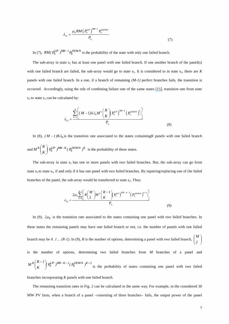
Accordingly, the reliability model of a sub-array of the sample 30 MW PV farmwhich accounts for common

mode failures and failure of the DC/DC converter is shown in Fig. 3. The new state probabilities and transition

rates are also shown in this figure.

12 KW

0.1536

4 KW8 KW

0.0026

218.9 438

P=0.998583 P=0.00069 P=3.98e-9

0 KW

P=0.00078

218.8

0.170.

1713

8.76

e-7

0.150.17

Fig. 3.Reliability model of a sub-array of the 30 MW PV farm

The common mode failure rate and repair/replacement rate of a panelof the 30 MW PV farm are assumed to

be 0.004f/yr and 219r/yr, respectively. The failure rate and repair/replacement rate of theDC/DC converter are

also considered to be 0.01f/yr and 219r/yr, respectively.

9

3.4 Reliability Model of a PV Array

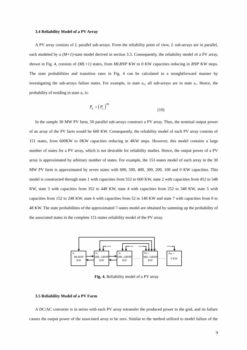
A PV array consists of L parallel sub-arrays. From the reliability point of view, L sub-arrays are in parallel,

each modeled by a (M+1)-state model derived in section 3.3. Consequently, the reliability model of a PV array,

shown in Fig. 4, consists of (ML+1) states, from MLRNP KW to 0 KW capacities reducing in RNP KW steps.

The state probabilities and transition rates in Fig. 4 can be calculated in a straightforward manner by

investigating the sub-arrays failure states. For example, in state a1, all sub-arrays are in state s1. Hence, the

probability of residing in state a1 is:

1 1

ML

a sP P (10)

In the sample 30 MW PV farm, 50 parallel sub-arrays construct a PV array. Thus, the nominal output power

of an array of the PV farm would be 600 KW. Consequently, the reliability model of each PV array consists of

151 states, from 600KW to 0KW capacities reducing in 4KW steps. However, this model contains a large

number of states for a PV array, which is not desirable for reliability studies. Hence, the output power of a PV

array is approximated by arbitrary number of states. For example, the 151-states model of each array in the 30

MW PV farm is approximated by seven states with 600, 500, 400, 300, 200, 100 and 0 KW capacities. This

model is constructed through state 1 with capacities from 552 to 600 KW, state 2 with capacities from 452 to 548

KW, state 3 with capacities from 352 to 448 KW, state 4 with capacities from 252 to 348 KW, state 5 with

capacities from 152 to 248 KW, state 6 with capacities from 52 to 148 KW and state 7 with capacities from 0 to

48 KW. The state probabilities of the approximated 7-states model are obtained by summing up the probability of

the associated states in the complete 151-states reliability model of the PV array.

MLRNP

KW0 KW

(ML-1)RNP

KW

a1 a2 aML+1

(ML-2)RNP

KW

a3

M(L-1)RNP

KW

aM+1

Fig. 4. Reliability model of a PV array

3.5 Reliability Model of a PV Farm

A DC/AC converter is in series with each PV array totransfer the produced power to the grid, and its failure

causes the output power of the associated array to be zero. Similar to the method utilized to model failure of the

10

DC\DC converter in each sub-array, failure of the DC/AC converter can be considered as a common mode failure

and can be evaluated using the same procedure. Accordingly, a transition is made from each state of Fig. 4 to 0

KW capacity state which denotes the failure of the DC/AC converter. The transition rates to/from the new states

with 0 KW capacities are failure rate/repair rate of the DC/AC converter. The resulting reliability model of each

array considering the DC/AC converter is similar to the model shown in Fig. 4 with (ML+1) states in which the

state probabilities and transition rates are updated.

Consider a PV farm with G parallel arrays. From the reliability point of view, G arrays (each in series with a

DC/AC converter), are in parallel, and each are modeled by a (ML+1)-state model. Accordingly, the reliability

model of a PV farm consists of (MLG+1) states, from MLGRNP KW to 0KW capacities reducing by RNP KW

steps. In this regard, based on the 7-states reliability model of each array of the sample 30MW PV farm, derived

in section 3.4, which further manipulated to include the failure of DC/AC converter, the reliability model of the

30MW PV farm consisting of 50 parallel arrays would have301 states. However, this large number of states is

not suitable for reliability analysis of power systems. Investigating the 7-states model derived in section 3.4

reveals that the probabilities associated with states of 500, 400, 300, 200, 100 and 0 kW capacities are

respectively3.174e-9, 1.567e-29, 3.58e-52, 7.36e-79, 1.088e-107 and 2.497e-138, which are almost zeroand can

be omitted from the model. Thus, without losing the precision of calculations, the reliability model of a PV array

of the 30 MW PV farm can be best approximated by only one state having 600 kW capacity and unity

probability.

Considering the two-state reliability model for the DC/AC converters, we can derive a 51-states reliability

model for the sample 30 MW PV farm. The failure and repair rates of the DC/AC converters are 0.5f/yr

and50r/yr, respectively. We can simplify the model by clustering the states into 4 states with 30, 20, 10 and 0

MW capacities. This model is constructed through state 1 with capacities from 25.2 to 30 MW, state 2 with

capacities from 15 to 24.6 MW, state 3 with capacities from 5.4 to 14.4 MW, and state 4 with capacities from 0 to

4.8 MW.

4. Solar Radiation Uncertainty Considerations in Reliability

Model of PV Farms

Besides the random nature of components in a PV farm, the solar radiation, is also uncertain and can

considerably affect the output power of the farm. Every physical event such as solar radiation that changes

11

continuously and randomly in time and space is considered a stochastic process and can be modeled

approximately as a process with discrete state space and relevant parameters [18]. Markov chain may be used to

model the alteration of a stochastic process as transitions between states, where each state represents a discrete

value of the process. As a basic characteristic of a Markov process, it should be stationary, i.e. the transition rates

between different states should remain constant through the study period [19]. Modeling a stochastic process by

a stationary Markov process demands that the state residence time follows an exponential distribution [17]. In

this paper, exponential state residence time is assumed for all applications. In Exponential distribution a constant

transition rate between states i and j is used, which is defined by[17]

i

ijij

T

N

(11)

where, λij is the transition rate (occurs per hour), Nij is the number of observed transitions from state i to state

j, and Tiis the duration of state i (in hours) calculated during the whole period. If the departure rate from state i to

the upper and lower states are denoted as λ+i and λ−i, respectively, then [17]

ij

iji

(12)

ij

iji

(13)

The probability of occurrence of state i, Pi, is given by[17]

T

TP i

i (14)

where, T is the entire period of observation (in hours).The frequency of occurrence of state i, fi (in

occurrences per hour), is then given by [17]

)( iiii Pf (15)

The output power of aPV farm at a definite time can be estimated using the solar radiation data. We have

utilized a yearly solar radiation data ofJask region in the southern part of Iran [20], to obtain the output power of

the considered 30 MW PV farm for a year-long horizon. However, the number ofsolar radiation data and the

associated output power states of PV farmsis too large,that is not suitable for analytical reliability evaluation of a

power system, unless the number of data is reduced by a clustering method.

To attain a proper Markov model for PV farm, its output power should be split up to some finite states. To

12

find the number and range of these steps, an efficient clustering method which simultaneously could guarantee

the model accuracy and its generality have to be employed. Clustering is a process for classifying patterns or

objects in a way that samples of the same group are more similar to one another than samples belonging to

different groups. Many clustering approacheswith special characteristics,such as the hard clustering and the

fuzzy clustering scheme,have been introduced in the literature. The conventional hard clustering approach

restricts each point of the data set to exclusively just one cluster. As a consequence, with this technique the

segmentation results are often very crisp. However, in many real situations, issues such as limited spatial

resolution, poor contrast and overlapping intensities make this hard segmentation a difficult task. The other

clustering approach, i.e. the fuzzy clustering as a soft segmentation method has been widely studied and

successfully applied in image segmentation. Among the fuzzy clustering methods, fuzzy c-means (FCM)

algorithm is the most popular method used in image segmentation due to the robust characteristics for ambiguity

and capable of retaining much more information than hard segmentation methods [21].

In this paper,we have employed fuzzy c-means (FCM) clustering method as a robust method in dealing with

structure identification of unlabeled data [22]. Employing this method, object data X=[x1,x2,…,xn] can be

categorized into m clusters minimizing the following objective function [22].

kk

m

1i

n

1k

fikm vxU)v,U(J

(16)

where,f, vkand Uikare respectively fuzzification parameter, center of the ith

cluster and fuzzy degree between xk

and the ith

cluster. This FCM technique is implemented on the historical output power data of the sample 30MW

PV farm and then the number and probability of the cluster centersare specified, which represent the various

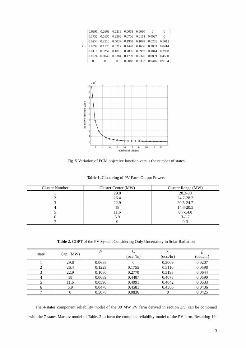
states associated with the PV farm generation levels. With increasing the number of associated clusters, the value

of the objective function, decreases. As shown in Fig. 5, decrement in the objective function becomes

insignificant when the number of considered clusters is seven or more. So, it can be concluded that a seven-

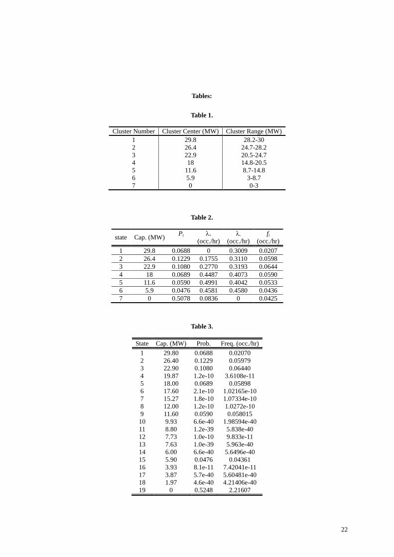
cluster model can be regarded as a proper one for the PV farm. The resulting seven clusters are presented in

Table 1. Once the output power has been split into finite steps by FCM, the various attribute associated with

these states, i.e. transition rates between different states and state probabilities and frequencies can be calculated.

Consequently, the reliability model of the 30 MW PV farm considering variability in the solar radiation can be

obtained which is presented in Table. 2.The transition rates between states in the model can be calculated by (11)

to develop the following transition matrix:

13

0.6991 0.2663 0.0213 0.0053 0.0080 0 0

0.1755 0.5135 0.2266 0.0706 0.0111 0.0027 0

0.0254 0.2516 0.4037 0.1903 0.1078 0.0201 0.0011

0.0099 0.1176 0.3212 0.1440 0.1656 0.2003 0.0414

0.0116 0.0252 0.1818 0.2805 0.0967 0.1044 0.2998

0.0

024 0.0048 0.0384 0.1799 0.2326 0.0839 0.4580

0 0 0 0.0083 0.0337 0.0416 0.9164

2 4 6 8 10 12 14 16 18 20

0

1

2

3

4

5

6

7

8

9

10x 10

6

number of clusters

ob

ject

ive

fun

ctio

n v

alu

e

Fig. 5.Variation of FCM objective function versus the number of states

Table 1. Clustering of PV Farm Output Powers

Cluster Number Cluster Center (MW) Cluster Range (MW)

1 29.8 28.2-30

2 26.4 24.7-28.2

3 22.9 20.5-24.7

4 18 14.8-20.5

5 11.6 8.7-14.8

6 5.9 3-8.7

7 0 0-3

Table 2. COPT of the PV System Considering Only Uncertainty in Solar Radiation

state Cap. (MW) Pi

λ+

(occ./hr)

λ-

(occ./hr)

fi

(occ./hr)

1 29.8 0.0688 0 0.3009 0.0207

2 26.4 0.1229 0.1755 0.3110 0.0598

3 22.9 0.1080 0.2770 0.3193 0.0644

4 18 0.0689 0.4487 0.4073 0.0590

5 11.6 0.0590 0.4991 0.4042 0.0533

6 5.9 0.0476 0.4581 0.4580 0.0436

7 0 0.5078 0.0836 0 0.0425

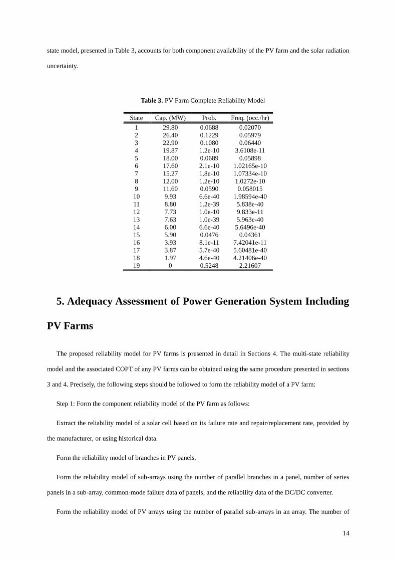
The 4-states component reliability model of the 30 MW PV farm derived in section 3.5, can be combined

with the 7-states Markov model of Table. 2 to form the complete reliability model of the PV farm. Resulting 19-

14

state model, presented in Table 3, accounts for both component availability of the PV farm and the solar radiation

uncertainty.

Table 3. PV Farm Complete Reliability Model

5. Adequacy Assessment of Power Generation System Including

PV Farms

The proposed reliability model for PV farms is presented in detail in Sections 4. The multi-state reliability

model and the associated COPT of any PV farms can be obtained using the same procedure presented in sections

3 and 4. Precisely, the following steps should be followed to form the reliability model of a PV farm:

Step 1: Form the component reliability model of the PV farm as follows:

Extract the reliability model of a solar cell based on its failure rate and repair/replacement rate, provided by

the manufacturer, or using historical data.

Form the reliability model of branches in PV panels.

Form the reliability model of sub-arrays using the number of parallel branches in a panel, number of series

panels in a sub-array, common-mode failure data of panels, and the reliability data of the DC/DC converter.

Form the reliability model of PV arrays using the number of parallel sub-arrays in an array. The number of

State Cap. (MW) Prob. Freq. (occ./hr)

1 29.80 0.0688 0.02070

2 26.40 0.1229 0.05979

3 22.90 0.1080 0.06440

4 19.87 1.2e-10 3.6108e-11

5 18.00 0.0689 0.05898

6 17.60 2.1e-10 1.02165e-10

7 15.27 1.8e-10 1.07334e-10

8 12.00 1.2e-10 1.0272e-10

9 11.60 0.0590 0.058015

10 9.93 6.6e-40 1.98594e-40

11 8.80 1.2e-39 5.838e-40

12 7.73 1.0e-10 9.833e-11

13 7.63 1.0e-39 5.963e-40

14 6.00 6.6e-40 5.6496e-40

15 5.90 0.0476 0.04361

16 3.93 8.1e-11 7.42041e-11

17 3.87 5.7e-40 5.60481e-40

18 1.97 4.6e-40 4.21406e-40

19 0 0.5248 2.21607

15

states of the arrays model can be reduced by clustering.

Form the PV farm component reliability model considering failure of the DC/AC converter and the number

of parallel arrays in a farm. Clustering method can be utilized in this step to reduce the number of states in the

PV farm model.

Step 2: Model the uncertainty associated with the solar radiation:

Determine the output power of the PV farm using the solar radiation data.

Cluster the output power of the PV farm as segments of the rated power, and calculate the associated state

probabilities and transition rates.

Step 3: Form the complete reliability model of the PV farm by combining the component reliability model

obtained in Step1with the Markov model associated with the uncertainty of solar radiation formed in Step 2.

Using the proposed reliability model, the PV farms can be modeled as a conventional unit with de-rated

power states. Therefore, the analytical generation reliability assessment methods [17] can be utilized for

adequacy assessment of the system. In the first stage, the PV farm(s) of the system are modeled and the

associated COPT is formed. The obtained COPT is then added to the equivalent COPT of the conventional

generating units to form the total generation capacity model of the system. Finally, convolution of the load model

with the final COPT provides the risk model of generation system, and the reliability indices can be calculated.

6. Study Results

In this chapter we present the result of studies performed on two test systems, RBTS [23] and IEEE-RTS

[24]. Both systems are modified by adding PV farms and reliability indices are calculated to investigate the

impacts of implementing PV farms. In addition, numerous sensitivity analyses are conducted to investigate the

effects of solar radiation average, penetration level of solar generation and peak load value on the reliability

indices.

6.1 Reliability Analysis of the RBTS

In this study, the RBTS with 11 generating units is considered [23]. The system load duration curve is

modeled by a straight line from %100 to %60 of the peak load. Three case studies are conducted on the system.

In case 1, the basic RBTS is considered. In case 2, a 30 MW PV farm with the model presented in Section 4 is

16

added to the RBTS. In this case, the 19-state model of Table 3 is simplified to a 7-state model by omitting all the

states which their probability is less than 10-5

. In case 3, a 30 MW conventional generating unit with FOR of 0.02

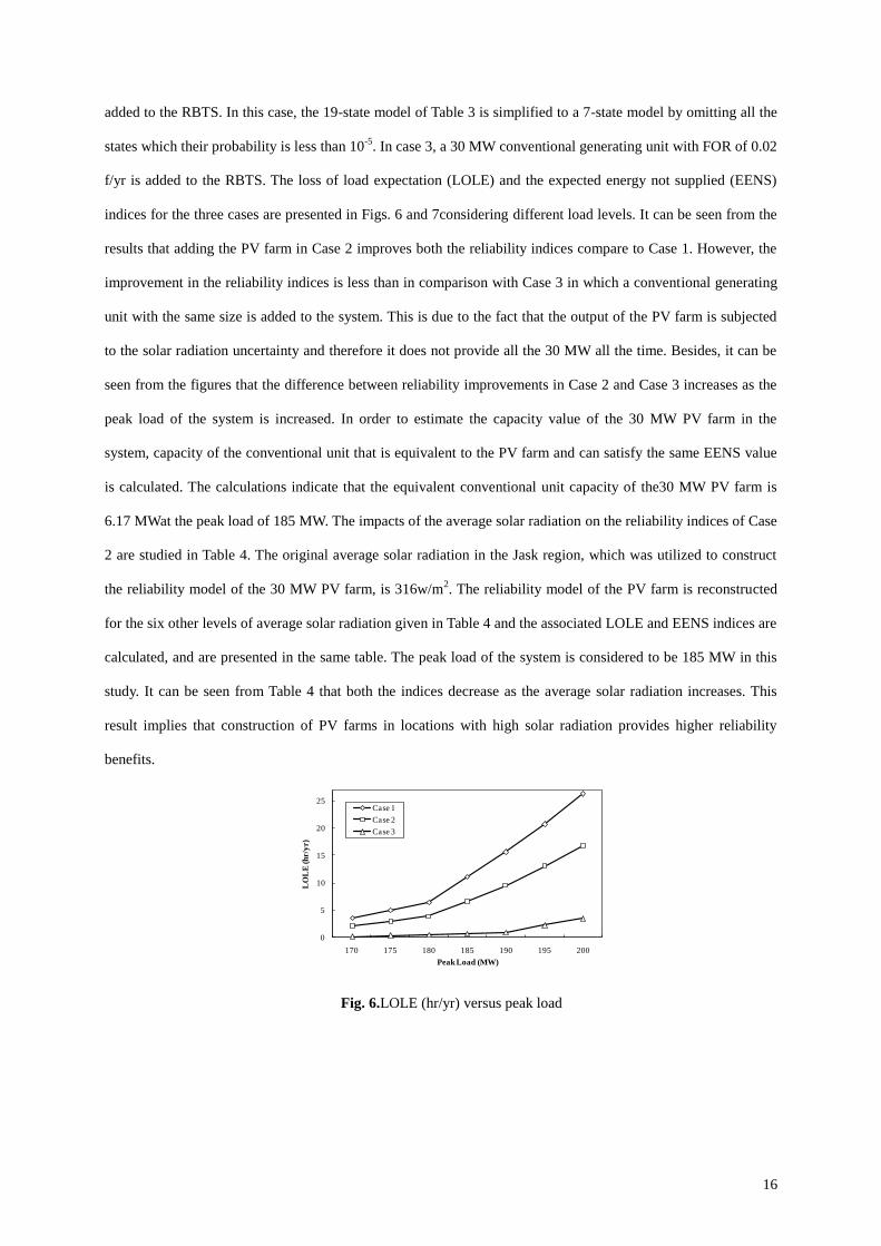
f/yr is added to the RBTS. The loss of load expectation (LOLE) and the expected energy not supplied (EENS)

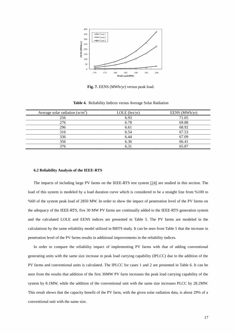
indices for the three cases are presented in Figs. 6 and 7considering different load levels. It can be seen from the

results that adding the PV farm in Case 2 improves both the reliability indices compare to Case 1. However, the

improvement in the reliability indices is less than in comparison with Case 3 in which a conventional generating

unit with the same size is added to the system. This is due to the fact that the output of the PV farm is subjected

to the solar radiation uncertainty and therefore it does not provide all the 30 MW all the time. Besides, it can be

seen from the figures that the difference between reliability improvements in Case 2 and Case 3 increases as the

peak load of the system is increased. In order to estimate the capacity value of the 30 MW PV farm in the

system, capacity of the conventional unit that is equivalent to the PV farm and can satisfy the same EENS value

is calculated. The calculations indicate that the equivalent conventional unit capacity of the30 MW PV farm is

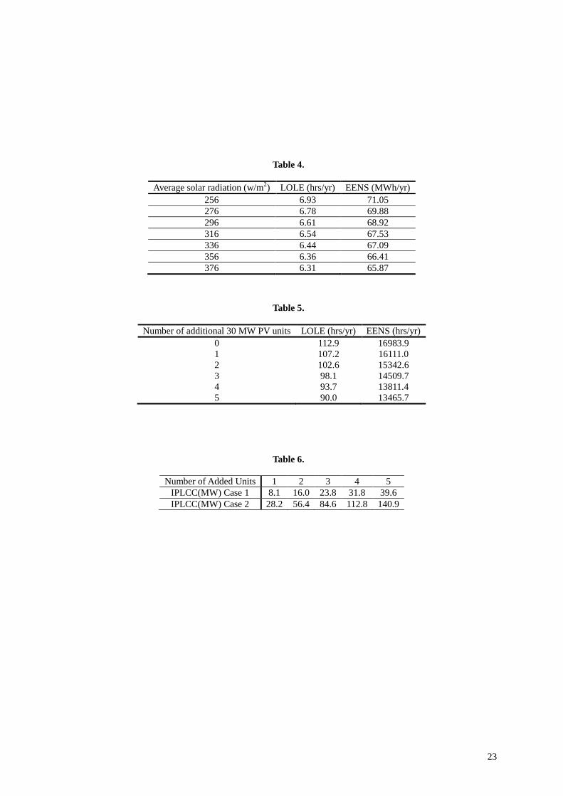
6.17 MWat the peak load of 185 MW. The impacts of the average solar radiation on the reliability indices of Case

2 are studied in Table 4. The original average solar radiation in the Jask region, which was utilized to construct

the reliability model of the 30 MW PV farm, is 316w/m2. The reliability model of the PV farm is reconstructed

for the six other levels of average solar radiation given in Table 4 and the associated LOLE and EENS indices are

calculated, and are presented in the same table. The peak load of the system is considered to be 185 MW in this

study. It can be seen from Table 4 that both the indices decrease as the average solar radiation increases. This

result implies that construction of PV farms in locations with high solar radiation provides higher reliability

benefits.

0

5

10

15

20

25

170 175 180 185 190 195 200

LO

LE

(h

r/y

r)

Peak Load (MW)

Case 1

Case 2

Case 3

Fig. 6.LOLE (hr/yr) versus peak load

17

0

50

100

150

200

250

300

350

400

170 175 180 185 190 195 200

EE

NS

(M

Wh

/yr)

Peak Load (MW)

Case 1

Case 2

Case 3

Fig. 7. EENS (MWh/yr) versus peak load.

Table 4. Reliability Indices versus Average Solar Radiation

Average solar radiation (w/m2) LOLE (hrs/yr) EENS (MWh/yr)

256 6.93 71.05

276 6.78 69.88

296 6.61 68.92

316 6.54 67.53

336 6.44 67.09

356 6.36 66.41

376 6.31 65.87

6.2 Reliability Analysis of the IEEE-RTS

The impacts of including large PV farms on the IEEE-RTS test system [24] are studied in this section. The

load of this system is modeled by a load duration curve which is considered to be a straight line from %100 to

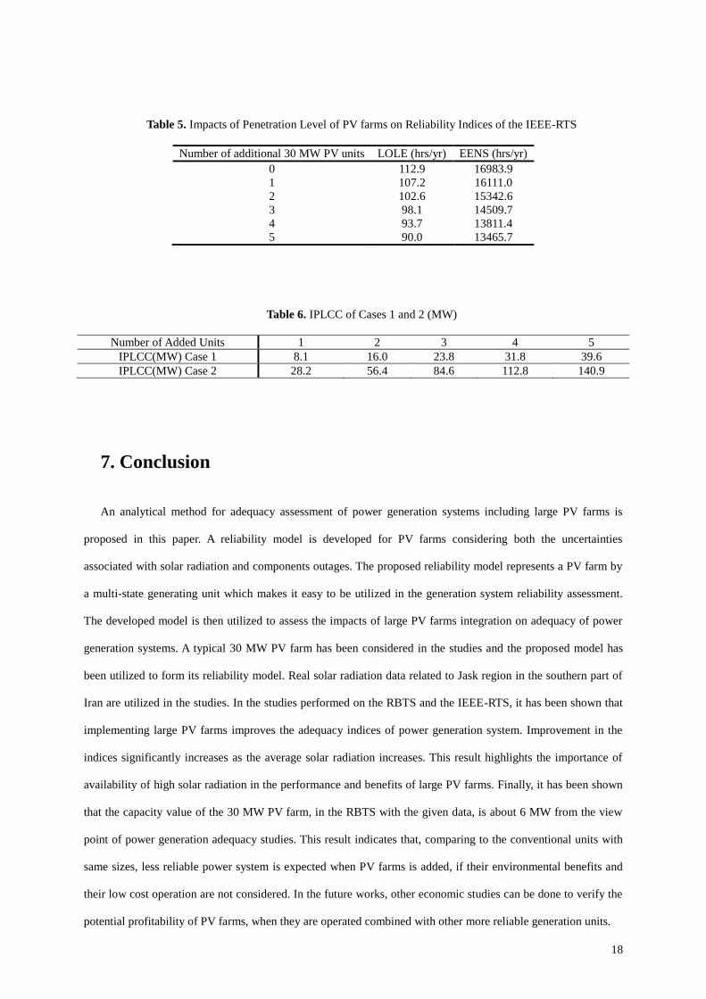
%60 of the system peak load of 2850 MW. In order to show the impact of penetration level of the PV farms on

the adequacy of the IEEE-RTS, five 30 MW PV farms are continually added to the IEEE-RTS generation system

and the calculated LOLE and EENS indices are presented in Table 5. The PV farms are modeled in the

calculations by the same reliability model utilized in RBTS study. It can be seen from Table 5 that the increase in

penetration level of the PV farms results in additional improvements in the reliability indices.

In order to compare the reliability impact of implementing PV farms with that of adding conventional

generating units with the same size increase in peak load carrying capability (IPLCC) due to the addition of the

PV farms and conventional units is calculated. The IPLCC for cases 1 and 2 are presented in Table 6. It can be

seen from the results that addition of the first 30MW PV farm increases the peak load carrying capability of the

system by 8.1MW, while the addition of the conventional unit with the same size increases PLCC by 28.2MW.

This result shows that the capacity benefit of the PV farm, with the given solar radiation data, is about 29% of a

conventional unit with the same size.

18

Table 5. Impacts of Penetration Level of PV farms on Reliability Indices of the IEEE-RTS

Number of additional 30 MW PV units LOLE (hrs/yr) EENS (hrs/yr)

0 112.9 16983.9

1 107.2 16111.0

2 102.6 15342.6

3 98.1 14509.7

4 93.7 13811.4

5 90.0 13465.7

Table 6. IPLCC of Cases 1 and 2 (MW)

Number of Added Units 1 2 3 4 5

IPLCC(MW) Case 1 8.1 16.0 23.8 31.8 39.6

IPLCC(MW) Case 2 28.2 56.4 84.6 112.8 140.9

7. Conclusion

An analytical method for adequacy assessment of power generation systems including large PV farms is

proposed in this paper. A reliability model is developed for PV farms considering both the uncertainties

associated with solar radiation and components outages. The proposed reliability model represents a PV farm by

a multi-state generating unit which makes it easy to be utilized in the generation system reliability assessment.

The developed model is then utilized to assess the impacts of large PV farms integration on adequacy of power

generation systems. A typical 30 MW PV farm has been considered in the studies and the proposed model has

been utilized to form its reliability model. Real solar radiation data related to Jask region in the southern part of

Iran are utilized in the studies. In the studies performed on the RBTS and the IEEE-RTS, it has been shown that

implementing large PV farms improves the adequacy indices of power generation system. Improvement in the

indices significantly increases as the average solar radiation increases. This result highlights the importance of

availability of high solar radiation in the performance and benefits of large PV farms. Finally, it has been shown

that the capacity value of the 30 MW PV farm, in the RBTS with the given data, is about 6 MW from the view

point of power generation adequacy studies. This result indicates that, comparing to the conventional units with

same sizes, less reliable power system is expected when PV farms is added, if their environmental benefits and

their low cost operation are not considered. In the future works, other economic studies can be done to verify the

potential profitability of PV farms, when they are operated combined with other more reliable generation units.

19

References

[1] Wiser R.BarboseG “Renewables Portfolio Standards in the United States: A Status Report with Data

through 2007”, Lawrence Berkeley National Laboratory, Report LBNL 154-E.(2008)

[2] Regional Greenhouse Gas Initiative (RGGI), “Overview of RGGI CO2 Budget Trading Program,”

October 2007. (2007)

[3] European Union (EU), “Climate change: Commission welcomes final adoption of Europe's climate and

energy package,” Press Release, EU, Dec. 17, 2008. (2008)

[4] PV-resources,“Large-Scale Photovoltaic Power Plants Ranking 1-

50”,http://www.pvresources.com/PVPowerPlants/Top50.aspx, Accessed 4April 2013 (2013)

[5] Moharil RM, KulkarniPS “Reliability analysis of solar photovoltaic system using hourly mean solar

radiation data”, Solar Energy, vol. 84, no. 4, pp. 691-702, April 2010.(2010)

[6] Billinton R, Bagen, B.“Generating capacity adequacy evaluation of small stand-alone power systems

containing solar energy”Reliability Engineering & System Safety, vol. 91, no. 4, pp. 438-443, April

2006(2006)

[7] Billinton R, Karki R. “Capacity Expansion of Small Isolated Power Systems Using PV and Wind

Energy”,IEEE Trans. Power Syst., vol. 16, no. 4, Nov. 2001.(2001)

[8] Karki R, Billinton R. “Reliability/Cost Implications of PV and Wind Energy Utilization in Small Isolated

Power Systems”,IEEE Trans. Energy Conversion, vol. 16, no. 4, Dec. 2001(2001)

[9] Pradhan, N. Karki, N.R. “Probabilistic reliability evaluation of off-grid small hybrid solar PV-wind power

system for the rural electrification in Nepal” North American Power Symposium (NAPS), 2012

[10] Kishore, L.N. Fernandez, E. “Reliability well-being assessment of PV-wind hybrid system using Monte

Carlo simulation” International Conference on Emerging Trends in Electrical and Computer Technology

(ICETECT), 2011

[11] Burgio. A, Menniti. D, Pinnarelli. A, Sorrentino. N, “Reliability studies of a PV-WG hybrid system in

presence of multi-micro storage systems” IEEE conference on Power Technology, Bucharest, 2009

[12] Khaligh A, OnarOC “Energy Harvesting, Solar, Wind and Ocean Energy Conversion Systems”, CRC

Press.(2010)

[13] Ramon S “A guide to photovoltaic system design and installation”, prepared by California Energy

Commission, Energy Technology Development Division, EndeconEngineering,Version 1.0, June 14,

20

2001(2001)

[14] Wenham SR, Green MA, Watt ME, CorkishR “Applied Photovoltaics”, ARC Centre for Advanced Silicon

Photovoltaics and Photonics, UK and USA, 2007.(2007)

[15] Billinton R, AllanRN “Reliability Evaluation of Engineering Systems”, 2nd

edition, plenum press,

1992.(1992)

[16] Military handbook reliability prediction of electronic equipment, MIL-HDBK 217F NOTICE

2,February1995.

[17] Billinton R, Allan RN “Reliability Evaluation of Power Systems”, Plenum Press, New York and London,

2nd Edition, 1994.(1994)

[18] SayasFC, Allan RN “Generation availability assessment of wind farms”,Proc. IEE Gen., Trans., Dist., vol.

143, no. 5, pp. 507-518, Sep. 1996(1996)

[19] Leite AP, Borges CLT, Falc˜aoDM “Probabilistic wind farms generationmodel for reliability studies

applied to Brazilian sites”,IEEE Trans. Power Syst., vol. 21, no. 4, pp. 1493-1501, Nov. 2006(2006)

[20] Suna sun data of Jask. http://www.suna.org.ir/fa/ationoffice/windenergyoffice/windamar. Accessed 21

June 2012, (2012)

[21] Yong Yung, Shuying Huang, “image segmentation by fuzzy c means clustering algorithm with a novel

penalty term” Journal on computing and informatics, Vol. 26, 2007

[22] Cannon RL, Jitendra VD, BezdekJC “Efficient Implementation of the Fuzzy c-Means Clustering

Algorithms”,IEEE Trans. Pattern Analysis and Machine Intelligence, vol. PAMI-8, no. 2, pp. 248-255,

March 1986.(1986)

[23] Billinton R, Li W “Reliability assessment of electric power systems using Monte Carlo methods”. IEEE

Press, New York, 1991(1991)

[24] Grigg C. “The IEEE reliability test system- 1996,” IEEE Trans. Power Syst., vol. 14, no. 3, pp. 1010–

1020, Aug. 1999.(1999)

Amir Ghaedi was born in Shiraz, Iran in 1984. He received his B.Sc. degree in power

engineering from Shiraz University in 2007, and the M.S. and Ph.D. degree in Electrical

Engineering from Sharif University of Technology, Tehran, Iran, in 2008, and 2013,

respectively. His main research interest is renewable energies, reliability studies and power

system operation.

Ali Abbaspour received B.Sc. and M.Sc. degrees in Electrical Engineering from Amir

Kabir University of Technology and Tehran University respectively and Ph.D. Degree in

Electrical Engineering from the Massachusetts Institute of Technology (MIT), USA. Presently

21

he is an associate professor in the Department of Electrical Engineering, Sharif University of

Technology, Tehran, Iran. Dr. Abbaspour is a member of center of excellence in power system

control and management.

Mahmud Fotuhi-Firuzabad (SM’ 99) received B.Sc. and M.Sc. degrees in Electrical

Engineering from Sharif University of Technology and Tehran University in 1986 and 1989

respectively and M.Sc. and Ph.D. Degrees in Electrical Engineering from the University of

Saskatchewan, Canada, in 1993 and 1997 respectively. Presently he is a professor and Head of

the Department of Electrical Engineering, Sharif University of Technology, Tehran, Iran. Dr.

Fotuhi-Firuzabad is a member of center of excellence in power system control and

management. He serves as the Editor of the IEEE TRANSACTIONS ON SMART GRID.

Masood Parvania (S’09) received the B.S. degree in Electrical Engineering from Iran

University of Science and Technology (IUST), Tehran, Iran, in 2007, and the M.S. and Ph.D.

degree in Electrical Engineering from Sharif University of Technology, Tehran, Iran, in 2009,

and 2013, respectively.

Since 2012, he has been a Research Associate in the Robert W. Galvin Center for

Electricity Innovation at Illinois Institute of Technology, Chicago, IL, USA. He is currently a

Postdoctoral Research Fellow at the Electrical Engineering Department, Sharif University of

Technology, Tehran, Iran. His research interests include power system reliability and security

assessment, as well as operation and optimization of smart electricity grids. He received the

Nation-wide Distinguished Ph.D. Student Award from the Ministry of Science, Research and

Technology of Iran in 2013.

List of Figures

Fig. 1. The structure of a typical PV farm

Fig. 2. Reliability model of a PV sub-array

Fig. 3. Reliability model of a sub-array of the 30 MW PV farm

Fig. 4. Reliability model of a PV array

Fig. 5. The value of the FCM objective function with respect to the number of states

Fig. 6. LOLE (hr/yr) versus peak load

Fig. 7. EENS (MWh/yr) versus peak load.

List of Tables

Table 1. Clustering of PV Farm Output Powers

Table 2. COPT of the PV System Considering Only Uncertainty in Solar Radiation

Table 3. PV Farm Complete Reliability Model

Table 4. Reliability Indices versus Average Solar Radiation

Table 5. Impacts of Penetration Level of PV farms on Reliability Indices of the IEEE-RTS

Table 6. IPLCC of Cases 1 and 2 (MW)

22

Tables:

Table 1.

Cluster Number Cluster Center (MW) Cluster Range (MW)

1 29.8 28.2-30

2 26.4 24.7-28.2

3 22.9 20.5-24.7

4 18 14.8-20.5

5 11.6 8.7-14.8

6 5.9 3-8.7

7 0 0-3

Table 2.

state Cap. (MW) Pi

λ+

(occ./hr)

λ-

(occ./hr)

fi

(occ./hr)

1 29.8 0.0688 0 0.3009 0.0207

2 26.4 0.1229 0.1755 0.3110 0.0598

3 22.9 0.1080 0.2770 0.3193 0.0644

4 18 0.0689 0.4487 0.4073 0.0590

5 11.6 0.0590 0.4991 0.4042 0.0533

6 5.9 0.0476 0.4581 0.4580 0.0436

7 0 0.5078 0.0836 0 0.0425

Table 3.

State Cap. (MW) Prob. Freq. (occ./hr)

1 29.80 0.0688 0.02070

2 26.40 0.1229 0.05979

3 22.90 0.1080 0.06440

4 19.87 1.2e-10 3.6108e-11

5 18.00 0.0689 0.05898

6 17.60 2.1e-10 1.02165e-10

7 15.27 1.8e-10 1.07334e-10

8 12.00 1.2e-10 1.0272e-10

9 11.60 0.0590 0.058015

10 9.93 6.6e-40 1.98594e-40

11 8.80 1.2e-39 5.838e-40

12 7.73 1.0e-10 9.833e-11

13 7.63 1.0e-39 5.963e-40

14 6.00 6.6e-40 5.6496e-40

15 5.90 0.0476 0.04361

16 3.93 8.1e-11 7.42041e-11

17 3.87 5.7e-40 5.60481e-40

18 1.97 4.6e-40 4.21406e-40

19 0 0.5248 2.21607

23

Table 4.

Average solar radiation (w/m2) LOLE (hrs/yr) EENS (MWh/yr)

256 6.93 71.05

276 6.78 69.88

296 6.61 68.92

316 6.54 67.53

336 6.44 67.09

356 6.36 66.41

376 6.31 65.87

Table 5.

Number of additional 30 MW PV units LOLE (hrs/yr) EENS (hrs/yr)

0 112.9 16983.9

1 107.2 16111.0

2 102.6 15342.6

3 98.1 14509.7

4 93.7 13811.4

5 90.0 13465.7

Table 6.

Number of Added Units 1 2 3 4 5

IPLCC(MW) Case 1 8.1 16.0 23.8 31.8 39.6

IPLCC(MW) Case 2 28.2 56.4 84.6 112.8 140.9