Energy Policy 52 (2013) 402–416

Contents lists available at SciVerse ScienceDirect

Energy Policy

0301-42

http://d

n Corr

E-m1 ht

journal homepage: www.elsevier.com/locate/enpol

Incorporating experience curves in appliance standards analysis

Louis-Benoit Desroches n, Karina Garbesi, Colleen Kantner, Robert Van Buskirk, Hung-Chia Yang

Environmental Energy Technologies Division, Lawrence Berkeley National Laboratory, 1 Cyclotron Road, Berkeley, CA 94720, USA

H I G H L I G H T S

c Past appliance standards analyses have assumed constant equipment prices.c There is considerable evidence of consistent real price declines.c We incorporate experience curves for several large appliances into the analysis.c The revised analyses demonstrate larger net present values of potential standards.c The results imply that past standards analyses may have undervalued benefits.

a r t i c l e i n f o

Article history:

Received 1 November 2011

Accepted 18 September 2012Available online 16 October 2012

Keywords:

Efficiency standards

Experience curves

Large appliances

15/$ - see front matter & 2012 Elsevier Ltd. A

x.doi.org/10.1016/j.enpol.2012.09.066

esponding author. Tel.: þ1 510 486 5833.

ail address: ldesroches@lbl.gov (L.-B. Desroch

tp://www1.eere.energy.gov/buildings/applian

a b s t r a c t

There exists considerable evidence that manufacturing costs and consumer prices of residential

appliances have decreased in real terms over the last several decades. This phenomenon is generally

attributable to manufacturing efficiency gained with cumulative experience producing a certain good,

and is modeled by an empirical experience curve. The technical analyses conducted in support of U.S.

energy conservation standards for residential appliances and commercial equipment have, until

recently, assumed that manufacturing costs and retail prices remain constant during the projected

30-year analysis period. This assumption does not reflect real market price dynamics. Using price data

from the Bureau of Labor Statistics, we present U.S. experience curves for room air conditioners, clothes

dryers, central air conditioners, furnaces, and refrigerators and freezers. These experience curves were

incorporated into recent energy conservation standards analyses for these products. Including

experience curves increases the national consumer net present value of potential standard levels. In

some cases a potential standard level exhibits a net benefit when considering experience, whereas

without experience it exhibits a net cost. These results highlight the importance of modeling more

representative market prices.

& 2012 Elsevier Ltd. All rights reserved.

1. Introduction

The U.S. Department of Energy (DOE) develops energy con-servation standards for residential appliances and commercialequipment.1 Improved energy efficiency is generally assumed toincrease initial purchase costs, but decrease operating costs. Insupport of any new proposed standard, DOE conducts an analysisof the consumer life-cycle costs (LCCs) and savings of a givenproduct meeting the new standard, in addition to a nationalimpact analysis (NIA) that calculates the economic and energy-savings impact on the nation over a 30-year time period. Animportant input to these calculations is the engineering analysis,which determines the incremental appliance purchase cost as a

ll rights reserved.

es).

ce_standards/

function of incremental energy efficiency improvement. As codi-fied in the statute, standards may be promulgated if and only ifthey are shown to be technically feasible and economicallyjustified. To date, these analyses have assumed that the manu-facturing costs and retail prices of appliances and commercialequipment (hereafter referred to generally as ‘‘appliances’’) arefixed during the typical 30-year analysis period.

There is, however, considerable historical evidence of consis-tent declines in appliance prices. Dale et al. (2009) have notedthat U.S. appliance efficiency regulation does not address trendsin real market prices and energy efficiency improvements. Theystudied historical price trends of room air conditioners (ACs),central AC, refrigerators, and clothes washers, and had four majorfindings: (1) for the past several decades, the retail price ofappliances has been steadily falling while efficiency has beenincreasing; (2) past retail price predictions made in the analysesof efficiency standards, assuming constant prices over time, havetended to overestimate retail prices; (3) the average incremental

L.-B. Desroches et al. / Energy Policy 52 (2013) 402–416 403

price to increase appliance efficiency has declined over time,and the analyses of efficiency standards have typically over-estimated this incremental price and retail prices; and (4) changesin retail markups and economies of scale in production of moreefficient appliances may have contributed to declines in prices ofefficient appliances. This problem of not addressing real marketprices is not limited to the U.S. Appliance standards and labelingprograms in Australia, Japan, and Europe suffer from similaroverestimations of the cost of increased efficiency (Ellis et al.,2007).

There is an extensive literature, applicable to a broad range ofapplications and industries, documenting how real productioncosts and prices of goods tend to fall in a relatively predictableway as cumulative production increases. This phenomenon isgenerally referred to as learning or experience. Wright (1936)pioneered the concept when studying the falling unit cost ofaircraft production (a topic revisited by Alchian, 1963). Earlyapplications continued to focus on manufacturing (Hirsh, 1952;Arrow, 1962), but since then the concept has been widely appliedto such diverse products and services as semiconductors (Gruber,1992), building envelopes (Jakob and Madlener, 2004), nuclearreactors (Joskow and Rozanski, 1979; Zimmerman, 1982), lique-fied natural gas (Greaker and Sagen, 2008), solar photovoltaics(Masini and Frankl, 2002; van der Zwaan and Rabl, 2003; Nemet,2006; van Benthem et al., 2008), wind power (Ibenholt, 2002;Junginger et al., 2005; Klaassen et al., 2005), renewable energytechnologies (Neij, 1997; Papineau, 2006), energy generationtechnologies (Jamasb, 2007), and electric utility investments(Laitner and Sanstad, 2004). Management consulting firms havestudied experience for a diverse set of clients and products (e.g.,BCG, 1972, 1980). To date, however, the study of experience forappliances and commercial equipment has been limited (Bass,1980; Newell, 2000; Laitner and Sanstad, 2004; Jardot et al., 2009;Weiss et al., 2010a,b). A thorough review of the extensivehistorical work on learning and experience, across many disci-plines, is provided by Fusfeld (1973), Yelle (1979), Day andMontgomery (1983), Dutton and Thomas (1984), Argote andEpple (1990), Newell (2000), IEA (2000), McDonald andSchrattenholzer (2001), and Weiss et al. (2010a) (and referencestherein). In addition, Baumol (1967) and Baumol et al. (1985)established the framework of unbalanced growth in the economy,explaining why certain sectors of the economy may have distinctreal price trends from other sectors.

The empirical phenomenon of falling prices is typically mod-eled by a learning curve or an experience curve, depending on thescope of the analysis and the nature and breadth of causal factors.Learning and experience curves are functions relating the cost ofproduction to quantity produced (typically cumulative produc-tion). Learning curve analysis tends to focus more narrowly onrelatively well-characterized and localized factors of productionthat result in price reductions of a single standardized product(e.g., learning by workers and management that reduces laborhours needed for production), while experience curve analysisfocuses on entire industries (often operating globally) and aggre-gates over many causal factors that may not be well character-ized. The two main causal factors typically associated withlearning curves are labor-based learning and investment in newcapital equipment (Dutton and Thomas, 1984). In its broadestsense, however, experience curve analysis implicitly includesfactors such as efficiencies in labor, capital investment, automa-tion, materials prices, and distribution at an industry-wide level(Newell, 2000). Since market competition is very effective, learn-ing in one plant or firm rapidly diffuses to other firms as well,leading to industry-wide effects. Learning and experience curveshave been empirically demonstrated at both the microeconomicand macroeconomic levels. It should be noted, however, that the

literature seldom distinguishes between the use of these twoterms, and they are often used interchangeably.

Various studies have examined the conditions under whichexperience (and learning) curve analysis could be used in supportof policy to escalate commercialization of emerging technologies,and as a mechanism of assessment (IEA, 2000; Neij et al., 2003;van Benthem et al., 2008; Jamasb and Kohler, 2008; Ferioli et al.,2009). Experience is already incorporated into the Energy Infor-mation Administration’s (EIA) National Energy Modeling System(NEMS; Newell, 2000), a model that is utilized for energy policyanalysis. Some previous studies of energy-saving potentialsachievable through standards have included modest experienceparameters (e.g., Rosenquist et al., 2006).

There is therefore a potential bias in past estimates of the costof efficiency for appliances. However, experience curves haverecently been incorporated into the analysis of energy conserva-tion standards for residential clothes dryers, room air condi-tioners, central air conditioners and heat pumps, furnaces,refrigerators and freezers (US Department of Energy, 2001a,b,c).In this paper, we describe how those experience curves weredetermined and how the standards analysis was modified toinclude them (Section 2), calculate the appropriate experiencerates and the effects on the national net present value for theseappliances (Section 3), and provide some discussion on themethodology and considerations for future analyses (Section 4).Finally, we summarize our results (Section 5).

2. Methodology and data sources

This section describes the methodology and data sources usedto determine the experience curve and experience rates for recentDOE energy conservation standards. In addition, we describe howexperience rates were incorporated into the existing analysisframework. For more details on data sources and methods usedto determine experience, as well as a full description of theappliance standards analysis process, see the energy conservationstandards Technical Support Documents (TSDs; US Department ofEnergy, 2001a–c).

2.1. Experience curves

The conventional functional relationship for both learning andexperience is given by

PðXÞ ¼ P0X

X0

� ��b

, ð1Þ

where Po is an initial price (or cost), b is a constant known as theexperience rate parameter, Xo is the initial cumulative production,X is cumulative production, and P is the price as a function ofcumulative production. The experience rate is defined as thefractional reduction in price/cost that results from each doublingin cumulative production,

ER¼ 1�2�b: ð2Þ

For example, an experience rate of 0.25 implies a 25% costreduction for each doubling of cumulative production.

Cumulative production is generally considered to be an appro-priate proxy for knowledge accumulated. Production-driven mod-els are generally better predictors of learning and experienceeffects than time-driven models (Newell, 2000; Bailey et al.,2012), since production-driven models implicitly account forvariations in production resulting from macroeconomic condi-tions such as recessions. Despite these advantages, however, itis important to remember that cumulative production is a proxymeasure for the underlying (and related) causal factors.

L.-B. Desroches et al. / Energy Policy 52 (2013) 402–416404

Furthermore, learning and experience curves are empirical rela-tionships, though they are readily accepted due to the strengthand robustness of the empirical evidence.

The final experience curves were obtained from a linearregression in log–log space as opposed to real space. This isreasonable if we assume: (1) the true errors in the price index areproportional to the value of the index; and (2) the errors arerelatively small so that asymmetries in log space are minimal.

2.2. Product prices

Direct manufacturing costs are very difficult to obtain, as thesedata are often proprietary. As a proxy for manufacturing costs, weuse price indices from the Bureau of Labor Statistics (BLS), inparticular the Producer Price Index (PPI).2 The PPI is an indicatorof wholesale distributor price, adjusted for quality changes overtime, and is available for a wide variety of specific industries (e.g.,refrigerator manufacturing) organized by the North AmericanIndustry Classification System (NAICS) code. Since we are onlyinterested in changes in producer prices and not in absoluteprices, the indices, once inflation-adjusted, are suitable for theanalysis. Annually averaged PPI data were adjusted for inflationusing the Consumer Price Index—All Items Index,3 a broadindicator of inflation in the economy.4 Table 1 summarizes thePPI series used in the subsequent analysis. The household laundryequipment series was assumed to represent both clothes dryersand clothes washers because more detailed data were unavail-able. A PPI series is available for heat pumps, but includes only afew years of data. As a result, the experience curve for heat pumpswas assumed to be the same as for central air conditioners.

In the special case of refrigerators and freezers, a seconddiscontinued price index exists from 1947 to 1997 as part of theConsumer Price Index (such a series does not exist for other homeappliances). Given the important leverage that 30 extra years ofdata can provide, the discontinued CPI series and the PPI series forrefrigerators were combined to form a unified price index. Theyears of overlap (1977–1997) for refrigerator and freezer datawere examined for differences, and a regression was performed toallow normalization of the PPI data to the CPI data.

2.3. Cumulative production

Annual shipment data were provided as part of the energyconservation standard rulemaking process by several industrytrade associations, including the Association of Home ApplianceManufacturers (AHAM), Gas Appliance Manufacturers Association(GAMA), and the Air-conditioning, Heating, and RefrigerationInstitute (AHRI). Annual shipment data were also available frompublications such as Appliance Magazine and the AHAM FactBook. In most cases, the data exist all the way back to the firstyear of production. For furnaces, shipments prior to 1953 wereextrapolated backward based on a linear trend to the historicalshipments (back to 1937). For compact freezers, an exponential fitwas used to extrapolate back to 1951. In some cases, decadal

2 http://www.bls.gov/ppi/3 http://www.bls.gov/cpi/4 For refrigerators and freezers, the methodology was adjusted such that the

Chained GDP Price Index (http://www.gpoaccess.gov/usbudget/fy11/hist.html)

was used to correct for inflation (US Department of Energy, 2011c). This was

done to better align with the electricity price forecasts used in the model, which

are deflated using a projected Chained GDP Price Index. There is an approximately

0.3% per year cumulative difference in the inflation adjustment between the two

indices (e.g., for 1980, this corresponds to an approximately 10% difference in

inflation adjustment to 2010 dollars). The CPI index is the larger correction factor.

The results presented here for refrigerators and freezers use the Chained GDP

Price Index.

shipments are available from the first decade of productiononward, and were used when annual shipment data from thefirst year of production were not available. Projected shipments,used to project the experience curves to future years, wereobtained from the base case projections in the energy conserva-tion standards analyses. See Fig. 1 and Table 2 for a summary ofthe annual shipments used. The annual shipments data were thenused to calculate cumulative production.

2.4. Amending appliance standards analyses

The analyses performed in support of federal appliance energyconservation standards rulemakings include a consumer life-cyclecost analysis (for the first year of compliance) and 30-yearcumulative national impacts analysis. Both sets of analysesconsider various trial standard levels (TSLs), which are potentialnew energy conservation standards above the current minimumstandard. The convention is to name TSL 1 the lowest potentialnew standard, TSL 2 the next lowest, and so on.

Both the LCC and NIA analyses rely on an engineering analysisthat establishes the incremental cost of improved efficiency foreach appliance. The main engineering analysis outputs are cost-efficiency curves (relationships of the increase in cost for a givenincrease in efficiency). These costs are then marked up to includemanufacturer and retailer margins, resulting in final consumerprices. These final prices as a function of efficiency are maininputs into the LCC and NIA analyses.

The LCC analysis uses Monte Carlo simulations to determinethe distribution of consumer impacts for various TSLs, in the firstyear of compliance. For each TSL, the LCC indicates what percen-tage of current consumers would experience a positive economicimpact, negative impact, or no impact if they replaced theircurrent appliance with new standards in place. The LCC considersboth the initial purchase price and the life-cycle operating costs.LCC inputs include distributions of households (e.g., with varyingsize and location), usage patterns, equipment lifetimes, energyprices, and discount rates.

The NIA models the aggregate impacts across the nation over30 years, using a forecast for annual shipments, average energyprices, and baseline improvements in efficiency. The NIA includesmonetized values for emissions reduction (CO2 and NOX). Keyoutputs of the NIA are the total energy savings (in quadrillion Btu)and the net present value (NPV) of those savings, for each TSL (seeFig. 2 for an illustrative NIA result). The NPV is the discountedsum of total costs and savings over the 30-year period, discountedto the year of the analysis. Based on these results, the Secretary ofEnergy then determines which TSL will become the next federalappliance standard, weighing a number of factors (e.g., energysavings, consumer impacts, manufacturer impacts). Ultimately,the chosen standard should achieve significant energy (andwater) savings, while being technologically feasible and econom-ically justified.5

Incorporating experience curves into the LCC analysis portionof the appliance energy conservation standard analysis is straight-forward. The LCC is only calculated for the first year of compli-ance, and the compliance year is typically 3–5 years afterpublication of a Final Rule by DOE. Thus, the input prices thatare fed into the LCC model are simply deflated by a single value,representing the experience gained between the date of theengineering analysis in support of the rulemaking to the firstyear of compliance. For the national impact analysis, the averagepurchase prices (in real dollars) for all efficiency levels are

5 These criteria for prescribing new standards are required by statute. See 42

U.S.C. 6295(o)(2).

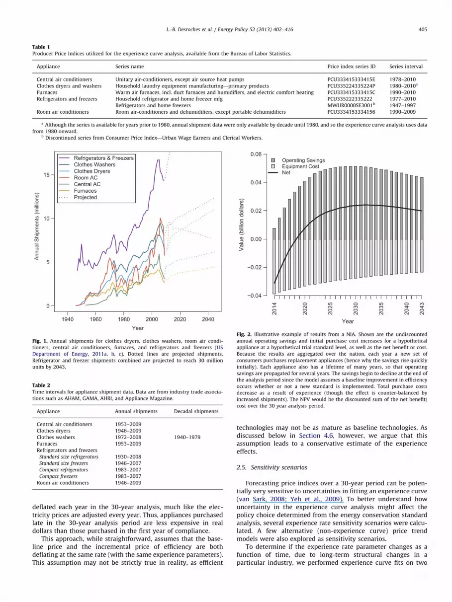
Table 1Producer Price Indices utilized for the experience curve analysis, available from the Bureau of Labor Statistics.

Appliance Series name Price index series ID Series interval

Central air conditioners Unitary air-conditioners, except air source heat pumps PCU333415333415E 1978–2010

Clothes dryers and washers Household laundry equipment manufacturing—primary products PCU335224335224P 1980–2010a

Furnaces Warm air furnaces, incl. duct furnaces and humidifiers, and electric comfort heating PCU333415333415C 1990–2010

Refrigerators and freezers Household refrigerator and home freezer mfg PCU335222335222 1977–2010

Refrigerators and home freezers MWUR0000SE3001b 1947–1997

Room air conditioners Room air-conditioners and dehumidifiers, except portable dehumidifiers PCU3334153334156 1990–2009

a Although the series is available for years prior to 1980, annual shipment data were only available by decade until 1980, and so the experience curve analysis uses data

from 1980 onward.b Discontinued series from Consumer Price Index—Urban Wage Earners and Clerical Workers.

1940 1960 1980 2000 2020 2040

0

5

10

15

Year

Ann

ual S

hipm

ents

(mill

ions

)

Refrigerators & FreezersClothes WashersClothes DryersRoom ACCentral ACFurnacesProjected

Fig. 1. Annual shipments for clothes dryers, clothes washers, room air condi-

tioners, central air conditioners, furnaces, and refrigerators and freezers (US

Department of Energy, 2011a, b, c). Dotted lines are projected shipments.

Refrigerator and freezer shipments combined are projected to reach 30 million

units by 2043.

Table 2Time intervals for appliance shipment data. Data are from industry trade associa-

tions such as AHAM, GAMA, AHRI, and Appliance Magazine.

Appliance Annual shipments Decadal shipments

Central air conditioners 1953–2009

Clothes dryers 1946–2009

Clothes washers 1972–2008 1940–1979

Furnaces 1953–2009

Refrigerators and freezers

Standard size refrigerators 1930–2008

Standard size freezers 1946–2007

Compact refrigerators 1983–2007

Compact freezers 1983–2007

Room air conditioners 1946–2009

Year

Val

ue (b

illio

n do

llars

)

2014

2020

2025

2030

2035

2040

2043

−0.04

−0.02

0.00

0.02

0.04

0.06Operating SavingsEquipment CostNet

Fig. 2. Illustrative example of results from a NIA. Shown are the undiscounted

annual operating savings and initial purchase cost increases for a hypothetical

appliance at a hypothetical trial standard level, as well as the net benefit or cost.

Because the results are aggregated over the nation, each year a new set of

consumers purchases replacement appliances (hence why the savings rise quickly

initially). Each appliance also has a lifetime of many years, so that operating

savings are propagated for several years. The savings begin to decline at the end of

the analysis period since the model assumes a baseline improvement in efficiency

occurs whether or not a new standard is implemented. Total purchase costs

decrease as a result of experience (though the effect is counter-balanced by

increased shipments). The NPV would be the discounted sum of the net benefit/

cost over the 30 year analysis period.

L.-B. Desroches et al. / Energy Policy 52 (2013) 402–416 405

deflated each year in the 30-year analysis, much like the elec-tricity prices are adjusted every year. Thus, appliances purchasedlate in the 30-year analysis period are less expensive in realdollars than those purchased in the first year of compliance.

This approach, while straightforward, assumes that the base-line price and the incremental price of efficiency are bothdeflating at the same rate (with the same experience parameters).This assumption may not be strictly true in reality, as efficient

technologies may not be as mature as baseline technologies. Asdiscussed below in Section 4.6, however, we argue that thisassumption leads to a conservative estimate of the experienceeffects.

2.5. Sensitivity scenarios

Forecasting price indices over a 30-year period can be poten-tially very sensitive to uncertainties in fitting an experience curve(van Sark, 2008; Yeh et al., 2009). To better understand howuncertainty in the experience curve analysis might affect thepolicy choice determined from the energy conservation standardanalysis, several experience rate sensitivity scenarios were calcu-lated. A few alternative (non-experience curve) price trendmodels were also explored as sensitivity scenarios.

To determine if the experience rate parameter changes as afunction of time, due to long-term structural changes in aparticular industry, we performed experience curve fits on two

2010 2015 2020 2025 2030 2035 2040

0.2

0.4

0.6

0.8

1.0

Year

Rea

l Pric

e In

dex

Constant PriceAEO 2011 PCE FurnitureExperience Curve (low)Experience Curve (mid)Experience Curve (high)PPI Exp Fit (low)PPI Exp Fit (mid)PPI Exp Fit (high)

Fig. 3. Illustration of the various sensitivity scenarios for the case of residential

refrigerators and freezers. Included are the experience curve, the exponential

model, and the price trend from AEO2011. All scenarios are normalized such that

the price index in 2010 equals 1. Prior analyses assumed a constant price.

Table 3Experience curve fitting results with 95% confidence limits.

Appliance Experience rate

parameter b

Experience

rate (%)

R2

Central air conditioners and

heat pumps

0.28870.021 18:1þ1:2�1:2

0.960

Clothes dryers 0.77570.034 41:6þ1:3�1:4

0.987

Furnaces 0.52770.056 30:6þ2:6�2:7

0.954

Refrigerators and freezers 0.75570.027 40:7þ1:1�1:1

0.983

Room air conditioners 0.71070.062 38:9þ2:6�2:7

0.970

L.-B. Desroches et al. / Energy Policy 52 (2013) 402–416406

or more component periods in the historical data (roughlysplitting the time series in half). For several appliances, the yearsplitting the two components was chosen to be the complianceyear for the first federal energy conservation standard for thatproduct. For refrigerators, several fits were performed to variousCPI and PPI subseries.

In the clothes dryer case, the PPI series that was used representeda more aggregate product category than the appliance analyzed (e.g.,household laundry equipment vs. clothes dryers or washers). In thisinstance, an additional sensitivity scenario was calculated. Price datawere collected from Consumer Reports and market research firmssuch as NPD on clothes dryers and clothes washers. Using thesedata, an experience rate was calculated for clothes dryers only, usingcumulative shipments for that appliance only. Although this experi-ence rate is more representative than the rate based on theaggregate PPI category, the clothes dryer price data cover only ahandful of years. As a result, the fit is not nearly as robust as thatbased on the PPI of the aggregate category.

In the case of refrigerators and freezers, we also considered analternative exponential model (e.g., similar to Moore’s law;Moore, 1965) to extrapolate the price trend. An exponentialmodel uses time as an explanatory variable, instead of cumulativeshipments. If annual (and cumulative) shipments are exponentialwith time, the experience curve and the exponential model areequivalent

P¼ P0X

X0

� ��b

¼ P0X0eat

X0

� ��b

¼ P0e�at , ð3Þ

where P is the price, Po is the initial price, t is the time variable whichequals the year difference between the base year and any given year,and a is the exponential parameter of the time variable. This modelcan be alternatively expressed as a percentage decline/increase inprice per year. Although time-driven models are generally not asaccurate as production-driven models (based on hindcast studies;e.g., Bailey et al., 2012), several recent studies of technologicalprogress have utilized them (Koh and Magee, 2006, 2008), so weconsidered them here for completeness.

EIA uses the NEMS model when publishing their AnnualEnergy Outlooks (AEOs).6 NEMS incorporates a macroeconomicmodel that forecasts national energy use and productivity out to2035. NEMS produces a set of intermediate outputs, includingchained price indices for various sectors of the economy. In thecase of refrigerators and freezers, we also examined a forecastbased on the Personal Consumption Expenditures—Furniture indexthat was forecasted for AEO 2011. This index is the mostdisaggregated category that includes appliances. To develop aninflation-adjusted index, we normalized the above index with theforecasted GDP deflator from AEO 2011. To extend the adjustedindex past 2035, we used the average annual growth rate in2026–2035. This price trend has a long-term real price decline ofapproximately 2.6% per year.

Fig. 3 illustrates the full range of price trends for the case ofrefrigerators and freezers, including the experience curve, theexponential model, and the AEO 2011 forecast. The experienceand exponential model were fit to various subsets of the data. The95% confidence limits on the experience curve and exponentialmodel are not shown, but were also considered as part of thesensitivity analysis. Of all these trends, the trend with the largestprice decline was considered as a high sensitivity scenario in oursensitivity analysis, and the smallest price decline was consideredas a low sensitivity scenario. The experience curve was the defaultmodel in all cases.

6 http://www.eia.gov/forecasts/aeo/

The default, high, and low sensitivity scenarios were used inthe national impacts analysis (for clothes dryers, we also used theclothes-dryer-only experience rate scenario). These sensitivityscenarios were not considered for the life-cycle cost analysis.Since the life-cycle analysis is based on the first year of compli-ance only, typically only a few years from publication of a FinalRule, the difference in price deflators amongst the variousscenarios will be minimal. Over a 30-year time period, however,the difference can grow to become substantial.

3. Experience rates and national impacts analysis results

Tables 3 and 4 summarize the experience curve and sensitivityresults for all the appliances considered in recent energy con-servation standards, and Fig. 4 illustrates the historical PPI seriesand the default projections. The default scenario is used through-out the energy conservation standard analysis (consumer LCC,NIA, manufacturer impact analysis, etc.), whereas the varioussensitivities are used to analyze impacts in the NIA only. As theseexperience rates are derived using domestic shipments only, theyrepresent apparent experience rates in the U.S. (see Section 4.2 forfurther discussion). The majority of these appliances have experi-ence rates above 30%, with only central air conditioners below20% (in the default scenario).

Table 4Results from default, high, low, and special sensitivity scenarios. Clothes dryers included an extra scenario based on market data for clothes

dryers only. The other clothes dryer scenarios are based on the household laundry PPI (which includes both clothes washers and dryers).

The high and low scenarios for refrigerators and freezers are exponential models instead of experience curves.

Appliance Default (%) High Low Special (%)

Central air conditioners and heat pumps ER¼18.1 ER¼20.5% ER¼11.5%

Clothes dryers ER¼41.6 ER¼42.9% ER¼33.9% ER¼52.2

Furnaces ER¼30.6 ER¼33.3% ER¼19.2%

Refrigerators and freezers ER¼40.7 3.12%/yr 1.14%/yr

Room air conditioners ER¼38.9 ER¼41.1% ER¼31.0%

1980 1990 2000 2010 2020 2030 2040

0.5

1.0

1.5

2.0

Year

Rea

l Pric

e In

dex

Central ACFurnacesRoom ACHousehold LaundryRefrigerators

Fig. 4. The historical PPI series with the default forecast scenario. All series are

normalized such that the price index in 2010 equals 1. Solid lines are historical PPI

data. Dashed lines are forecasted trends. Prior analyses assumed a constant price

in the forecast. For clothes dryers, the Household Laundry PPI was used.

Clothes Dryers

Trial Standard Level

Net

Pre

sent

Val

ue (b

illio

n 20

09$)

0.00

0.02

0.04

0.06

0.08

0.10

0.12

1 2 3 4

Constant PriceLow ScenarioDefault ExperienceHigh ScenarioSpecial Scenario

Fig. 5. Net present values (NPVs) for a variety of trial standard levels (TSLs) for

residential clothes dryers. The NPV is aggregated across the nation and summed

over a 30-year analysis period, discounted at 7% per year. Positive NPVs indicate

that consumer benefits of potential standards exceed costs. See Section 2.4 for an

overview of the appliance standards analysis. Results are from the National Impact

Analysis of the recent Direct Final Rule (US Department of Energy, 2011a). Not all

TSLs are shown, as some TSLs are significantly negative (not cost-effective). Shown

are the NIA results using the previous constant price assumption, a low price trend

sensitivity scenario, the default price trend based on an experience curve, and a

high price trend sensitivity scenario. Also included is a scenario using clothes-

dryer-only price data, as opposed to the household laundry equipment PPI series.

The LCC analysis and all downstream analyses use the default price trend only.

See Section 2.5 for the definition of the various scenarios. The inclusion of

experience has a modest effect on the NPV for clothes dryers.

L.-B. Desroches et al. / Energy Policy 52 (2013) 402–416 407

The inclusion of experience curves can significantly affect theNPV of the aggregated national economic impacts for a potentialstandard. Figs. 5–9 demonstrate the results of including experi-ence curves in the NIA, with the NPV discounted at 7% per year.For most appliances, the NPV rises significantly compared to theconstant price assumption, indicating a larger national benefitfrom potential standards. The effect is more dramatic for higherTSLs (i.e., more stringent potential standards), where the costpremium is larger. This is realistic—in reality newer (and there-fore more expensive) technologies will undergo more rapidexperience than more mature technologies, therefore one intui-tively expects the higher TSLs to show a more pronouncedexperience effect. In a few cases (such as refrigerators and HVACequipment) the NPV actually changes sign for some TSLs.A previously uneconomical potential standard level becomeseconomical when incorporating experience curves.

It is important to note that the NIA includes many otherfactors than simply purchase price and operating cost. The modelincludes installation costs, repair costs, purchase price elasticities,early replacement effects, fuel switching (for certain products),and other effects. None of these are affected by experience asderived above. Nevertheless, the purchase price is usually thedominant factor, and thus including experience curves in theanalysis is important (though installation can be significant forsome appliances).

Given that experience curves are more representative of actualmarket behavior than a constant price assumption, our resultsimply that previous appliance standards analyses, guided by theolder methodology, may have undervalued the potential benefitsof proposed standard levels. This may have led to settling on alower standard level as a result. For example, suppose the policychoice is based on the maximum TSL with a positive NPV, thenincorporating experience curves can result in choosing a higherTSL for HVAC equipment and refrigerators. If the policy choice isbased on the TSL with the maximum NPV, however, the effect onthe policy choice is much more limited, and potentially onlyaffects refrigerators. It is also important to note that the policychoice is based on many other factors in addition to the nationalNPV (e.g., manufacturer impacts). Nevertheless, the final consu-mer NPV estimates are much larger than when assuming constant

HVAC Equipment

Trial Standard Level

Net

Pre

sent

Val

ue (b

illio

n 20

09$)

1 2 3 4 5 6

−0.3

−0.2

−0.1

0

0.1

0.2

0.3

0.4

0.5Constant PriceLow ScenarioDefault ExperienceHigh Scenario

Fig. 6. Net present values (NPVs) for a variety of trial standard levels (TSLs) for

residential central air conditioners, central heat pumps, and furnaces, collectively

referred to as heating, ventilation, and air-conditioning (HVAC) equipment. The

NPV is aggregated across the nation and summed over a 30-year analysis period,

discounted at 7% per year. Positive NPVs indicate that consumer benefits of

potential standards exceed costs. See Section 2.4 for an overview of the appliance

standards analysis. Results are from the National Impact Analysis of the recent

Final Rule (US Department of Energy, 2011b). Not all TSLs are shown, as some TSLs

are significantly negative (not cost-effective). Shown are the NIA results using the

previous constant price assumption, a low price trend sensitivity scenario, the

default price trend based on an experience curve, and a high price trend sensitivity

scenario. The LCC analysis and all downstream analyses use the default price trend

only. See Section 2.5 for the definition of the various scenarios. The inclusion of

experience has a substantial effect on the NPV of the more stringent TSLs. TSL

6 was previously considered to be cost-negative, but the revised analysis

demonstrates a benefit.

Refrigerators

Trial Standard LevelN

et P

rese

nt V

alue

(bill

ion

2009

$)

1 2 3 4−0.4

0

0.4

0.8

1.2

Constant PriceLow ScenarioDefault ExperienceHigh Scenario

Fig. 7. Net present values (NPVs) for a variety of trial standard levels (TSLs) for

residential refrigerators and refrigerator-freezers. The NPV is aggregated across

the nation and summed over a 30-year analysis period, discounted at 7% per year.

Positive NPVs indicate that consumer benefits of potential standards exceed costs.

See Section 2.4 for an overview of the appliance standards analysis. Results are

from the National Impact Analysis of the recent Final Rule (US Department of

Energy, 2011c). Not all TSLs are shown for each product class, as some TSLs are

significantly negative (not cost-effective). Shown are the NIA results using the

previous constant price assumption, a low price trend sensitivity scenario, the

default price trend based on an experience curve, and a high price trend sensitivity

scenario. The LCC analysis and all downstream analyses use the default price trend

only. See Section 2.5 for the definition of the various scenarios. The inclusion of

experience has a substantial effect on the NPV of the more stringent TSLs. Some

TSLs were previously considered to be cost-negative, but the revised analysis

demonstrates a significant benefit.

L.-B. Desroches et al. / Energy Policy 52 (2013) 402–416408

prices, and thus the cumulative economic benefits of the appli-ance standards program have likely been significantly under-estimated in the past.

4. Discussion

4.1. General methodology comments

The ideal implementation of experience curve analysis wouldinclude detailed cost data for each efficiency level, for each indivi-dual product. Such data are virtually impossible to obtain for theU.S., however, and so we must rely on lower resolution data such asthe PPI. Furthermore, past trends are no guarantee of futureperformance. Nevertheless, the PPI data show persistent, significant,and lengthy historical trends, and are therefore a more rationalindicator of future trends than an assumption of no changes. Thesensitivity analysis looks at the effects of historical fluctuations,recent trends, fitting variations, and data variations (e.g., looking atlower quality but more product-specific data). The 30-year forecastmay be sensitive to errors in the experience curve analysis, but suchforecast errors are diminished by the discounting adopted in theNIA. Ultimately, in the cases discussed here, the policy choice basedon the NPV results is the same regardless of whether the low,default, or high scenario is considered.

The experience model utilized in our analysis is straightfor-ward and is a proxy for a variety of underlying casual factors.

We recognize the limitations of such a simple model, and acknowl-edge that future work is needed in assessing the reliability andapplicability of experience curves in policy analysis (Jamasb andKohler, 2008; Ferioli et al., 2009). Adopting a more complexexperience model, however, is not justified by the relatively limitedand low resolution data, as any model with additional parametersmay overfit the data. We additionally do not have data for high-efficiency and baseline products separately. It is also plausible thatappliance experience is in reality driven by component-level inno-vations, and that a component-level model is perhaps a betterindication of true experience (Ferioli et al., 2009). Our adoptedexperience curve model is therefore simple and conservative, but isultimately more representative of real-world dynamics than thepreviously used constant price assumption.

4.2. Apparent experience

Since the focus of this work is domestic, we rely only ondomestic shipments (i.e., cumulative production intended fordomestic consumption). The analyses conducted for DOE energyconservation standards are similarly restricted to domestic con-sumption. Appliance manufacturing is concentrated in a fewmultinational corporations, however, and major changes in onemarket can impact other markets substantially. True experience isa dynamic of global production and distribution, with differentregional factors having more or less influence on product price.A manufacturer will learn from all production lines and apply

Freezers

Trial Standard Level

Net

Pre

sent

Val

ue (b

illio

n 20

09$)

0.0

0.1

0.2

0.3

0.4

0.5

0.6

1 2 3 4 5

Constant PriceLow ScenarioDefault ExperienceHigh Scenario

Fig. 8. Net present values (NPVs) for a variety of trial standard levels (TSLs) for

residential freezers. The NPV is aggregated across the nation and summed over a

30-year analysis period, discounted at 7% per year. Positive NPVs indicate that

consumer benefits of potential standards exceed costs. See Section 2.4 for an

overview of the appliance standards analysis. Results are from the National Impact

Analysis of the recent Final Rule (US Department of Energy, 2011c). Not all TSLs

are shown for each product class, as some TSLs are significantly negative (not cost-

effective). Shown are the NIA results using the previous constant price assump-

tion, a low price trend sensitivity scenario, the default price trend based on an

experience curve, and a high price trend sensitivity scenario. The LCC analysis and

all downstream analyses use the default price trend only. See Section 2.5 for the

definition of the various scenarios. The inclusion of experience has a substantial

effect on the NPV of the more stringent TSLs. Some TSLs were previously

considered to be cost-negative or cost-neutral, but the revised analysis demon-

strates a significant benefit.

Room Air Conditioners

Trial Standard Level

Net

Pre

sent

Val

ue (b

illio

n 20

09$)

0.00

0.02

0.04

0.06

0.08

1 2 3 4 5

Constant PriceLow ScenarioDefault ExperienceHigh Scenario

Fig. 9. Net present values (NPVs) for a variety of trial standard levels (TSLs) for

residential room air conditioners. The NPV is aggregated across the nation and

summed over a 30-year analysis period, discounted at 7% per year. Positive NPVs

indicate that consumer benefits of potential standards exceed costs. See Section

2.4 for an overview of the appliance standards analysis. Results are from the

National Impact Analysis of the recent Direct Final Rule (US Department of Energy,

2011a). Not all TSLs are shown, as some TSLs are significantly negative (not cost-

effective). Shown are the NIA results using the previous constant price assump-

tion, a low price trend sensitivity scenario, the default price trend based on an

experience curve, and a high price trend sensitivity scenario. The LCC analysis and

all downstream analyses use the default price trend only. See Section 2.5 for the

definition of the various scenarios. The inclusion of experience has a substantial

effect on the NPV of the more stringent TSLs. TSL 5 was previously considered to

be cost-neutral, but the revised analysis demonstrates a significant benefit.

7 BLS Handbook of Methods, Chapter 14. http://www.bls.gov/opub/hom/

homch14.htm

L.-B. Desroches et al. / Energy Policy 52 (2013) 402–416 409

improvements globally. This is especially true for new technolo-gies incorporated into appliance designs. New premium andefficient features are introduced predominantly in one marketat first, and then diffuse into the remaining global markets.

Costs as perceived in the U.S. are likely changing faster thanwould be driven by domestic shipments alone, because domesticshipments are only a fraction of total shipments. The fraction ofU.S. shipments relative to global production is also changing, andhas diminished with time. We therefore distinguish an experiencerate calculated using only domestic shipments as an apparent

experience rate. Nevertheless, utilizing the apparent experiencerate makes sense from a domestic energy policy context. Manda-tory efficiency standards, for example, focus only on domesticenergy-saving impacts. When calculating the national net presentvalue of a possible minimum efficiency standard, the apparentexperience rate is the correct value to use. Domestic consumersbenefit fully from global production experience, despite purchas-ing only a fraction of total global production. It is for this reasonthat our experience values differ from those in Weiss et al.(2010b), and from other historical studies of experience inappliance manufacturing.

We note that this distinction confounds the experience curveliterature in general, not just its application to energy efficiencystandards. For example, the impressive review of Weiss et al.(2010a) documents the results of 75 different experiencecurve analyses. There is no consistency in the independent anddependent variables for each, however, with some studies pairing

domestic prices with global production, others pairing domesticprices with domestic production, and others not specifying. Thereis good reason for this confusion, with mixed markets and majorshifts in the relative influences of those markets through thedecades. Domestic appliance energy policy, however, is based ondomestic shipments and domestic economic benefits, and thus inthis instance, the data needs are clear.

4.3. Characteristics of PPI as a cost indicator

The producer prices on which the PPI is based are only a closeapproximation of manufacturing costs. True manufacturing costs,both fixed and variable, are generally not available in a time series(indeed they are often proprietary). Therefore, even though experi-ence curves are strictly a (mostly variable) manufacturing anddistribution cost effect, we must rely on the producer prices for ouranalysis. Nevertheless, PPI is based on a wholesale price, not a retailprice, so it is not subject to factors that affect retail prices. The use ofPPI indicates long-term declining real price trends for many products.

The PPI also includes a quality adjustment, which attempts tofactor out physical changes (such as capacity, premium features,government-mandated features, etc.) in the product that affectthe price.7 The BLS uses a variety of methods to determine thisquality adjustment, including comparing similar models from

MonthR

elat

ive

Nom

inal

Pric

e

Jan−07 May−07 Sep−07 Jan−08 May−08 Sep−08

nominal PPINPD (a)NPD (b)0.90

0.95

1.00

1.05

1.10

0.90

0.95

1.00

1.05

1.10

Rel

ativ

e N

omin

al P

rice

Fig. 10. Comparison of the historical monthly refrigerator-only PPI series with

refrigerator market data from NPD. Shown are both the sales-weighted average price

(a) and the average model price (b) of all units sold in a given month. The PPI series and

both NPD series are normalized such that the 2-year average equals 1. Error bars

represent 1 standard deviation from the mean (the width of the distribution is much

larger).

Table 5Correlation coefficients between PPI and market price data.

Appliance Series pair Pearson correlation

coefficient

P-value

Refrigerators Monthly PPI–NPD (a) 0.66 6.3�10�4

Monthly PPI–NPD (b) 0.77 1.8�10�5

Freezers Monthly PPI–NPD (a) 0.68 3.4�10�4

Monthly PPI–NPD (b) 0.79 6.6�10�6

Refrigerators and

freezers

Yearly PPI–Dale et al.

(2009)

0.92 1.3�10�4

Clothes washers Yearly PPIa–Dale

et al. (2009)

0.86 7.6�10�5

a The PPI series applicable for clothes washers is the household laundry

equipment series, which also includes clothes dryers.

L.-B. Desroches et al. / Energy Policy 52 (2013) 402–416410

year to year, asking manufacturers to explicitly separate outvalue-added cost increases, and potentially using a hedonicmodel. For this reason, the PPI is a better measure of experiencecurve effects than actual wholesale prices would be, sincechanges in PPI should reflect production cost changes due toindustrial productivity improvements and other advances intechnology rather than changes driven by enhanced features.

The BLS does not explicitly correct for changing product efficiencyin the CPI, but the PPI likely accounts for improvements in the energyefficiency of the device because such changes are generally physicalchanges. This quality adjustment is exactly what the appliancestandards analysis, based on an engineering cost-efficiency curve,requires. Although experience curve analysis has been applied toresidential appliances for decades, and many analyses account forvariability or changes in the service delivered per unit, in general thechange in the energy efficiency of appliances is not accounted for,except in cases in which energy delivery or conservation is the endservice delivered. Weiss et al. (2010a,b) document numerous cases ofcapacity-related normalizations. For example, clothes washers anddryers, dishwashers, and refrigerators are frequently, though notalways, normalized with respect for volume, and computer memoryis consistently normalized for megabytes of DRAM. In cases whereenergy efficiency and delivery are not the end-use service delivered,however, efficiency is generally not accounted for. Yet applianceshave significantly reduced their energy consumption over the timeperiod considered in these experience curve analyses (e.g., refrigera-tors currently use approximately 70% less energy than in the 1970s).In contrast, energy service technologies like photovoltaics, lighting,heating, building insulation, advanced glazing, and electricity gen-erators are usually (though not always) normalized for the energydelivered or conserved. Usage of the PPI to analyze experience curveeffects is therefore advantageous since energy efficiency is likelyincluded as part of the quality adjustment. This yields a fairer, morerealistic experience rate estimate that is not biased toward lowervalues due to constantly improving efficiency.

The PPI is based only on domestic manufacturing. Althougha majority of appliance manufacturing is now performed over-seas, there are still some appliance models manufactured domes-tically, and historically the share of appliances produceddomestically was much larger. Thus the PPI is still a meaningfulindicator. Labor costs can be an important component of variablemanufacturing costs, however, and since outsourcing is notreflected in the PPI time series, using it results in a conservativeestimate of the experience rate. We do not attempt to forecast theimpact of future outsourcing of production (or increase in importsgenerally) in our forecasts of appliance manufacturing costs.

Finally, we note that producer prices will include the effects oftaxes, import tariffs, and other non-tariff import barriers. This istrue even if products are manufactured domestically, as compo-nent parts may be imported. Such barriers may significantly affectthe production cost and consumer price (without physicallychanging the product), and are likely to substantially change overthe long time periods considered here. The experience curvespresented here therefore implicitly include such effects, in addi-tion to changes in manufacturing efficiency.

4.4. Comparison of PPI to market data and previous studies

In order to address some of the potential issues relevant tousing the PPI, we performed a cross-check of PPI data with actualmarket data. We used market price data gathered as part of therefrigerator and freezer rulemaking activity, obtained from themarket research firm NPD.8 The data include monthly units sold

8 http://www.npd.com

and total price at the point of sale (retail) over a period of 24months, and we compared this to the monthly refrigerator-onlyand freezer-only PPI series9 over the same time period. NPDincludes many large retailers and covers a significant fraction ofthe market; we therefore assume it is representative of the wholemarket. The NPD data are actual point-of-sale prices paid byconsumers, and therefore include all possible sales, promotions,and discounts. Using only 2 years worth of data limits the extentof any physical changes that might have occurred in refrigeratorsand freezers, enabling a cleaner comparison of PPI and marketdata, and yet provides 23 monthly data points (January 2007 toNovember 2008 inclusive).

We derived the following monthly series from the NPD data,for both refrigerators and freezers: (a) the sales-weighted averageprice of all units sold; and (b) the average model price of all

9 Series ID PCU3352223352221 and PCU3352223352222.

1960 1980 2000

1.0

1.5

2.0

2.5

3.0

Clothes Washers/HH Laundry

Year

Rea

l Pric

e In

dex

PPIDale et al. (2009)

1980 1990 2000 2010

1.0

1.5

2.0

Room AC

Year

Rea

l Pric

e In

dex

PPIDale et al. (2009)

1960 1980 2000

1.0

1.2

1.4

1.6

1.8

Central AC

Year

Rea

l Pric

e In

dex

PPIDale et al. (2009)

1980 1990 2000 2010

1.0

1.5

2.0

Refrigerators

Year

Rea

l Pric

e In

dex

PPIDale et al. (2009)

Fig. 11. Comparison of historical PPI trends with retail market price data from Dale et al. (2009) for refrigerators, room air conditioners, clothes washers, and central air

conditioners. These data were obtained from various catalogues and Consumer Reports. The clothes washer data are compared to the household laundry equipment PPI

series. The PPI series are normalized to 1 in 2010. The market price data are normalized such that average over the period of overlap with the PPI series is equal to the

average PPI over the same period.

10 Note that there is no strong competition for appliance energy use as there is

for purchase price. As a result, cumulative production is unlikely to be an

explanatory variable for changing energy use as it is for purchase price.

L.-B. Desroches et al. / Energy Policy 52 (2013) 402–416 411

models sold. The NPD market data are inherently variable, asconsumer spending habits fluctuate and retailers offer discounts.NPD also does not cover 100% of the market. Nevertheless, there isgood agreement in the general price trend between the PPI andthe series derived from NPD data, as illustrated in Fig. 10 forrefrigerators. Since the time period is only 2 years, the modelsavailable for purchase are likely to remain relatively constant,which is why we include the derived series (b). Table 5 lists thePearson correlation coefficients of the PPI series with the NPDseries. All are significantly correlated and the null hypothesis isrejected with over 99% confidence, even given the relativelyshallow trend over the 2-year time period (correlation tests arenot possible with a constant function). This provides reassuranceand verification that the PPI series are representative of changesin product prices. The correlations will not be perfect because thePPI is quality-adjusted but the NPD data are not. The adjustmentover a 2-year period will be small but not necessarily zero.

In addition, we also compared the PPI series used in determin-ing the experience rates with trends and market price data in theliterature. Fig. 11 compares data from Dale et al. (2009), originallyobtained from catalogues and Consumer Reports. Dale et al. (2009)restricted the price data to specific capacities and types ofappliances (e.g., an 18 ft3 top-mount refrigerator), so these dataare partially quality-adjusted. For all appliances except perhapscentral air conditioners, the trends in the PPI series qualitativelycorrelate very well with market price data. The market price datagathered by Dale et al. for central air conditioners may not berepresentative of actual prices. Central air conditioners are gen-erally contractor purchased and installed appliances, and arerarely purchased by consumers directly through retail, leadingto a potential discrepancy between catalogue prices and prices

actually paid by the contractor. This may explain some of thediscrepancy between Dale et al. (2009) and the PPI series. Table 5lists the Pearson correlation coefficients for refrigerators andfreezers and clothes washers, the only two appliance categorieswith sufficient overlapping years to calculate a correlation coeffi-cient. In addition, it has been shown that in the last few decades,the PPI data track reasonably well with quality-corrected pricesobtained from consumer catalogues (Gordon, 1990). The pricetrends derived in this study for all appliances are consistent withother previous domestic and international studies (see Table 6).

4.5. Cost reductions at constant efficiency

As described in Section 4.3, it is important to consider pricechanges at constant efficiency, especially given the remarkableprogress in appliance efficiency in the last 30 years due to strongenergy policy drivers. Prices and energy use have both fallensignificantly over a long period of time.10 In a few cases, data existthat can be used to illustrate the reductions in appliance produc-tion cost at constant efficiencies. The appliances covered herehave all had recent updates of their energy conservation stan-dards. The TSDs published by DOE in support of these rulemak-ings include an engineering analysis, which establishes the cost-efficiency curve for a given appliance (i.e., the incrementalmanufacturing costs for a given incremental efficiency improve-ment). The TSDs are available for both the recent rulemakings as

Table 6Comparison of long-term real price trends derived in this study with values from the literature. This study relies on PPI data, whereas previous studies obtained market

price data from market research firms. All price data have been deflated to real dollars using a consumer index appropriate for the region analyzed.

Study Region Time period Appliance Approximate real price decline (%/year)

Household laundry equipment

This study USA 1980–2010 Clothes washers and dryers 1.9

Bass (1980) USA 1950–1974 Electric clothes dryers 2.2

Laitner and Sanstad (2004) USA 1980–1998 Clothes washers 3.4

Electric clothes dryers 3.2

Gas clothes dryers 2.9

Dale et al. (2009) USA 1983–2001 Clothes washers 2.4

EES (2006) Australia 1993–2005 Clothes washers 2.6

Clothes dryers 1.1

Weiss et al. (2010b) Netherlands 1965–2008 Clothes washers 2.4

1969–2003 Clothes dryers 2.1

HVAC equipment

This study USA 1990–2009 Room AC 1.7

1978–2010 Central AC 0.8

Bass (1980) USA 1946–1974 Room AC 2.5

Laitner and Sanstad (2004) USA 1980–1998 Room AC 4.0

Dale et al. (2009) USA 1975–1994 Room AC 1.5

1965–1986 Central AC 1.0a

Refrigerators and freezers

This study USA 1951–2007 Refrigerators and freezers 2.5

Bass (1980) USA 1922–1940 Refrigerators 2.6

Laitner and Sanstad (2004) USA 1980–1998 Refrigerators 3.2

Freezers 5.3

Dale et al. (2009) USA 1980–2001 Refrigerators 2.5

Schiellerup (2002) UK 1992–1999 Refrigerators 6.3

Freezers 5.0–5.1

EES (2006) Australia 1993–2005 Refrigerators 1.7

Freezers 2.5

Weiss et al. (2010b) Netherlands 1964–2008 Refrigerators 1.2

1970–2003 Freezers 1.1–1.5

a The central AC time series in Dale et al. (2009) is very noisy. The real price decline presented here uses the average of the first two years of data and the average of the

last two years of data as endpoints.

9 10 11 12 13

200

300

400

500

600

700

800

900

Room ACs

Energy Efficiency Ratio (Btu/W−hr)

Man

ufac

turin

g C

ost (

2009

$)

19972011

Fig. 12. Comparison of past and recent cost-efficiency curves for room air

conditioners. Results are from the engineering analyses in support of appliance

efficiency standards (US Department of Energy, 1997, Volume 2, Table 1.12; US

Department of Energy, 2011a, Appendix 5D, Table 5-D.2.3). These cost-efficiency

curves represent averaged or interpolated costs for a typical 12,000 Btu/h louvered

room air conditioner. Prices have been deflated using the CPI.

L.-B. Desroches et al. / Energy Policy 52 (2013) 402–416412

well as past rulemakings, complete with an older engineeringanalysis and cost-efficiency relationship. (The last standard forclothes dryers was issued in 1991, and its engineering analysis isunavailable.)

The manufacturing costs used in these analyses are obtainedvia confidentially submitted manufacturing data and/or frommanufacturer interviews, as well as by detailed tear-down ana-lysis. By comparing the older and newer cost-efficiency relation-ships, it is possible to determine how manufacturing costs havechanged for a given efficiency, in the time separating the tworulemakings. The update frequency is typically once every 6–10years (potentially longer) during which time technologies canchange substantially. Given this large time span, there is oftenonly limited overlap between older and newer cost-efficiencyrelationships. In some cases there is no overlap at all. Never-theless, these cost-efficiency curves provide an important quali-tative insight. A design option that was once considered veryefficient and carried a significant cost premium can becometoday’s baseline option.

Figs. 12–15 show the cost-efficiency curves for room airconditioners, central air conditioners (including split ACs, pack-aged ACs, split heat pumps, and packaged HPs), furnaces, refrig-erators, and freezers. Calculating experience rates by efficiencylevels is not possible, since shipment data by efficiency level arenot available, although we can make qualitative comparisons.

In all cases, the manufacturing cost for a given efficiency levelhas declined significantly, by as much as 60% over 14 yearsfor room air conditioners, 30% over 11 years for central airconditioners, 55% over 4 years for furnaces, and 40% over 15years for refrigerators. This is compared to a decline in PPI of

10 12 14 16 18

400

600

800

1000

1200

Coil−Only Split ACs

SEER

Man

ufac

turin

g C

ost (

2009

$) 19992011

10 15 20 25

400

600

800

1000

1200

1400

1600

Blower−Coil Split ACs

SEER

Man

ufac

turin

g C

ost (

2009

$)

10 12 14 16 18 20 22

800

1000

1200

1400

1600

Split HPs

SEER

Man

ufac

turin

g C

ost (

2009

$)

Fig. 13. Comparison of past and recent cost-efficiency curves for central air conditioners and heat pumps. Results are from the engineering analyses in support of appliance

efficiency standards (US Department of Energy, 1999, Chapter 4, Table 4.7; US Department of Energy, 2011b, Chapter 5, Tables 5.13.4, 5.13.7, and 5.13.10). These cost-

efficiency curves represent averaged or interpolated costs for a typical two-ton central air conditioner or heat pump. Prices have been deflated using the CPI.

75 80 85 90 95 100

200

400

600

800

1000

1200

Furnaces

Annual Fuel Utilization Efficiency (%)

Man

ufac

turin

g C

ost (

2009

$)

20072011

Fig. 14. Comparison of past and recent cost-efficiency curves for residential

furnaces. Results are from the engineering analyses in support of appliance

efficiency standards (US Department of Energy, 2007, Appendix E, Table E.1.1;

US Department of Energy, 2011b, Chapter 5, Table 5.13.1). These cost-efficiency

curves represent averaged or interpolated costs for a typical 75,000–80,000 Btu/h

non-weatherized furnace. Prices have been deflated using the CPI.

L.-B. Desroches et al. / Energy Policy 52 (2013) 402–416 413

approximately 25%, 5%, and 33% for room air conditioners, centralair conditioner, and refrigerators respectively, over the same timeperiods (using the default experience rate). The PPI for furnaces is

essentially flat in the last 4 years. This highlights the differencebetween high-efficiency units vs. average units, in that costsassociated with high-efficiency units (often with small or zeromarket share at the time of the analysis) will likely decline muchfaster than an average unit. This is especially true in the case offurnaces, for which only 4 years separate the two engineeringanalyses, and yet we see a 55% drop in manufacturing costs forthe most efficient units. In the case of packaged heat pumps, therewas no overlapping efficiency level in the two engineeringanalyses. It is worth noting, however, that the maximum levelanalyzed and deemed viable in 1999 was 12 SEER (seasonalenergy efficiency ratio), whereas the baseline packaged heatpump was 13 SEER in 2010.

This comparison of bottom-up engineering analysis fromsuccessive appliance standards rulemakings underscores the needto include experience in the standards analysis. The cost deflatorsused in our experience curve analysis likely underestimate theactual decline in manufacturing costs, especially for the high-efficiency TSLs. Including even a conservative estimate of experi-ence, however, is an improvement over the previous constantprice assumption that is inconsistent with historical data.

4.6. Considerations for future analyses

The methodology outlined here treats baseline models andhighly efficient models in the same way. The PPI does notdistinguish between the two, and the calculated experience ratesare applied to both equally. In reality, because the baselinemodels and the highly efficient models are at different maturitystages, their experience rates are likely not the same. High-efficiency models tend to incorporate newer technology, and wewould expect such models to experience faster cost declines thanmore mature technology since the time period required to double

300 400 500 600 700 800

250

300

350

400

450

500

550

Top−mount Refrigerators

Annual Energy Use (kWh/yr)

Man

ufac

turin

g C

ost (

2009

$)

400 500 600 700

400

500

600

700

800

Bottom−mount Refrigerators

Annual Energy Use (kWh/yr)

Man

ufac

turin

g C

ost (

2009

$)

500 600 700 800 900

500

600

700

800

900

1000

1100

Side−mount Refrigerators

Annual Energy Use (kWh/yr)

Man

ufac

turin

g C

ost (

2009

$)

200 250 300 350 400

200

250

300

350

400

Chest Freezers

Annual Energy Use (kWh/yr)

Man

ufac

turin

g C

ost (

2009

$) 19952010

Fig. 15. Comparison of past and recent cost-efficiency curves for residential refrigerators and freezers. Results are from the engineering analyses in support of appliance

efficiency standards (US Department of Energy, 1995, Chapter 3, Tables 3.6, 3.8, 3.9, and 3.12; US Department of Energy, 2011c, Chapter 5, Tables 5.9.1 and 5.9.2). These

cost-efficiency curves represent averaged or interpolated costs for a typical 18 ft3 top-mount auto-defrost refrigerator, 22 ft3 side-mount auto-defrost refrigerator with

through-the-door ice service, 20 ft3 bottom-mount auto-defrost refrigerator, and 15 ft3 manual-defrost chest freezer. Annual energy use values from the older engineering

analysis have been adjusted to the revised test procedure (with new compartment temperatures), as described in US Department of Energy (2011c). Prices have been

deflated using the CPI.

L.-B. Desroches et al. / Energy Policy 52 (2013) 402–416414

the cumulative production of newer technology is shorter than fortechnology long on the market. The use of the PPI to determine theexperience curve for the product as a whole will tend to under-value the potential economic benefits for higher efficiency models.Ideally, we would utilize appliance price histories broken down byefficiency class, and if at all feasible, by important components(e.g., compressors, heat exchangers, vacuum panels, etc.).

Unfortunately, at this time we are not aware of robust datasufficient to separately analyze baseline models and efficientmodels. Such data are virtually non-existent in the U.S., thoughthese data are collected in Europe and Australia in support of theirefficiency standards. Future analyses would benefit from an insti-tution or agency implementing a program to make such dataavailable in the U.S. These data could then be used to develop moresophisticated experience curves for baseline and efficient models.

A few appliances and some commercial equipment are heavilyaffected by volatile commodity prices. For some, such as trans-formers and motors, a significant fraction of the manufacturingcost is in obtaining the raw materials such as copper, aluminum,and steel. This is confirmed by the PPI series for these products,which are not monotonic and correlate strongly with the histor-ical prices of commodity metals. The prices of these commoditiesdepend on many factors and cannot be easily forecasted. Forfuture analyses, historical commodity data could be used todetermine whether commodity price volatility is a concern forestimating an experience rate for specific products. In such cases,and with sufficient cost and/or price data, it might be possible tofactor out commodity price volatility and determine an experi-ence rate for the non-commodity component of the manufactur-ing cost/producer price.

In cases with limited or no data, it is worth considering usingdata at a higher level of aggregation to determine a range ofexperience rates. This approach has already been adopted to somedegree with household laundry equipment. For some productcategories, there may not be suitable PPI data to properly char-acterize the experience curve. In such instances, using the AEOprice trend as a default scenario is perhaps the best approach, andis more representative of actual markets than assuming a priori

that costs remain constant in the 30-year analysis period.The improvements outlined above will enhance the statistical

certainty of the experience curve estimate and the completenessof any future model. Additional data should enable an improvedevaluation of the potential impacts and of all the factors that caninfluence equipment cost and price trends over time. Such datawill also enable a more sophisticated sensitivity analysis.

5. Summary

Historically, technical analyses performed in support of nationalenergy efficiency appliance standards have forecasted equipmentprices to be constant over the analysis period. This assumption-based approach of a constant real price trend is not consistent withthe historical data for many products, including consumer durablegoods. Inflation-adjusted producer price data for appliances exhibitpersistent price declines over several decades. The constant costassumption used in previous energy efficiency standards analysesmay therefore underestimate the consumer benefits of more strin-gent standards.

L.-B. Desroches et al. / Energy Policy 52 (2013) 402–416 415

Experience curve analysis can be used to obtain more repre-sentative price forecasts for appliances, as was done for theanalyses in support of recent appliance energy efficiency stan-dards (for clothes dryers, room air conditioners, central airconditioners and heat pumps, furnaces, refrigerators, and free-zers). This is an approach with a strong theoretical and empiricalfoundation, utilized across many disciplines, and is advocated foruse in energy technology policy by the Organization for EconomicCooperation and Development and the International EnergyAgency (IEA, 2000). When incorporating experience curves, therecent appliance standards analyses yielded significantly largernet present values than when using the constant price assump-tion. For some trial standard levels, the net present value changedsign, suggesting that previous rulemakings may have undervaluedthe consumer benefits of appliance efficiency standards.

In recognition of the uncertainty in experience curve analysis,we adopted several sensitivity scenarios. The scenarios were usedin the national impact analysis to examine the dependence of theresults on different assumptions about experience. While thereare some differences between high and low sensitivity scenarios,the policy choice generally remains unchanged. There is, however,a drastic difference compared to the constant price assumption.

Although incorporating experience curves in appliance stan-dards analysis represents a significant step forward, furtherresearch is needed to properly account for several other factors,including commodity price volatility and differences betweenbaseline and high-efficiency products. Cost reductions are oftenmore pronounced in newer-technology products. The currentimplementation described here is therefore conservative, but isultimately a more representative projection of future prices thanthe constant price assumption.

Acknowledgments

We wish to thank Katie Coughlin, Larry Dale, Jeffery Green-blatt, and two anonymous reviewers for helpful comments. Wealso thank Arpi Kupelian, who assisted us on a previous iterationof this work. The Energy Efficiency Standards group at LawrenceBerkeley National Laboratory is supported by the U.S. Departmentof Energy’s Office of Energy Efficiency and Renewable Energy,Building Technologies Program under Contract no. DE-AC02-05CH11231.

References

Alchian, A., 1963. Reliability of progress curves in airframe production. Econome-trica 31 (4), 679–693.

Argote, L., Epple, D., 1990. Learning curves in manufacturing. Science 247 (4945),920–924.

Arrow, K., 1962. The economic implications of learning-by-doing. Review ofEconomic Studies 29 (3), 155–173.

Bailey, A.G., Bui, Q.M., Farmer, J.D., Margolis, R., Ramamoorthy, R., 2012. Forecastingtechnological progress. In: Proceedings of the International Workshop on Com-plex Sciences in the Engineering of Computing Systems.

Bass, F.M., 1980. The relationship between diffusion rates, experience curves, anddemand elasticities for consumer durable technological innovations. Journal ofBusiness 53 (3), S51–67.

Baumol, W.J., 1967. Macroeconomics of unbalanced growth: the anatomy of urbancrisis. The American Economic Review 57 (3), 415–426.

Baumol, W.J., Blackman, S.A.B., Wolff, E.N., 1985. Unbalanced growth revisited:asymptotic stagnancy and new evidence. The American Economic Review 75(4), 806–817.

BCG, 1972. Perspectives on Experience. Boston Consulting Group, Boston.BCG, 1980. The Experience Curve Revisited. Boston Consulting Group, Boston.Dale, L., Antinori, C., McNeil, M., McMahon, J.E., Fujita, K.S., 2009. Retrospective

evaluation of appliance price trends. Energy Policy 37, 597–605.Day, G.S., Montgomery, D.B., 1983. Diagnosing the experience curve. Journal of

Marketing 47 (2), 22–58.Dutton, J.M., Thomas, A., 1984. Treating progress functions as a managerial

opportunity. Academy of Management Review 9 (2), 235–247.

EES, 2006. Greening white goods: a report into the energy efficiency trends ofmajor household appliances in Australia from 1993–2005. Prepared by EnergyEfficiency Strategies for Equipment Energy Efficiency (E3) Committee.

Ellis, M., Jollands, N., Harrington, L., Meier, A., 2007. Do energy efficient appliancescost more? In: Proceedings of 2007 ECEEE Summer Study.

Ferioli, F., Schoots, K., van der Zwaan, B.C.C., 2009. Use and limitations of learningcurves for energy technology policy: a component-learning hypothesis.Energy Policy 37, 2525–2535.

Fusfeld, A.R., 1973. The technological progress function. Technology Review(February), 29–38.

Gordon, R.J., 1990. Electrical appliances. In: The Measurement of Durable GoodsPrices. University of Chicago Press, Chicago, pp. 241–320.

Greaker, M., Sagen, E.L., 2008. Explaining experience curves for new energy technol-ogies: a case study of liquefied natural gas. Energy Economics 30, 2899–2911.

Gruber, H., 1992. The learning curve in the production of semiconductor memorychips. Applied Economics 24 (8), 885–894.

Hirsh, W.Z., 1952. Manufacturing progress functions. Review of Economics andStatistics 34 (2), 143–155.

IEA, 2000. Experience Curves for Energy Technology Policy. International EnergyAgency, Paris.

Ibenholt, K., 2002. Explaining learning curves for wind power. Energy Policy 30,1181–1189.

Jakob, M., Madlener, R., 2004. Riding down the experience curve for energy-efficient building envelopes: the swiss case for 1970–2020. InternationalJournal of Energy Technology and Policy 2 (1–2), 153–178.

Jamasb, T., 2007. Technical change theory and learning curves: patterns ofprogress in electricity generation technologies. Energy Journal 28 (3), 51–72.

Jamasb, T., Kohler, J., 2008. Learning curves for energy technology and policyanalysis: a critical assessment. In: Grubb, M., Jamasb, T., Pollitt, M.G. (Eds.),Delivering a Low Carbon Electricity System Technologies Economics andPolicy. Cambridge University Press, Cambridge, pp. 314–332.

Jardot, D., Eichhammer, W., Fleiter, T., 2009. Effects of economies of scale andexperience on the costs of energy-efficient technologies—case study of electricmotors. In: Proceedings of 2009 ECEEE Summer Study.

Joskow, P.L., Rozanski, G.A., 1979. The effects of learning by doing on nuclear plantoperating reliability. Review of Economics and Statistics 61 (2), 161–168.

Junginger, M., Faaij, A., Turkenburg, W.C., 2005. Global experience curves for windfarms. Energy Policy 33, 133–150.

Klaassen, G., Miketa, A., Larsen, K., Sundqvist, T., 2005. The impact of R&D oninnovation for wind energy in Denmark, Germany and the United Kingdom.Ecological Economics 54 (2), 227–240.

Koh, H., Magee, C.L., 2006. A functional approach for studying technologicalprogress: application to information technology. Technological Forecastingand Social Change 73 (9), 1061–1083.

Koh, H., Magee, C.L., 2008. A functional approach for studying technologicalprogress: extension to energy technology. Technological Forecasting andSocial Change 75 (6), 735–758.

Laitner, J.A., Sanstad, A.H., 2004. Learning-by-doing on both the demand and thesupply sides: implications for electric utility investments in a heuristic model.International Journal of Energy Technology and Policy 2 (1–2), 142–152.

Masini, A., Frankl, P., 2002. Forecasting the diffusion of photovoltaic systems insouthern Europe: a learning curve approach. Technological Forecasting andSocial Change 70, 39–65.

McDonald, A., Schrattenholzer, L., 2001. Learning rates for energy technologies.Energy Policy 29, 255–261.

Moore, G.E., 1965. Cramming more components onto integrated circuits. Electro-nics 38 (8), 114–117.

Neij, L., 1997. Use of experience curves to analyze the prospects for diffusion andadoption of renewable energy technology. Energy Policy 23, 1099–1107.

Neij, L., Andersen, P.D., Durstewitz, M., 2003. The use of experience curves forassessing energy policy programs. In: Proceedings of the EU/IEA Workshop onExperience Curves: A Tool for Energy Policy Analysis and Design, Paris.

Nemet, G.F., 2006. Beyond the learning curve: factors influencing cost reductionsin photovoltaics. Energy Policy 34, 3218–3232.

Newell, R.G., 2000. Incorporation of Technological Learning into NEMS BuildingsModules. US Department of Energy, Energy Information Administration,Washington, DC.

Papineau, M., 2006. An economic perspective on experience curves and dynamiceconomies in renewable energy technologies. Energy Policy 34, 422–432.

Rosenquist, G., McNeil, M., Iyer, M., Meyers, S., McMahon, J., 2006. Energyefficiency standards for equipment: additional opportunities in the residentialand commercial sectors. Energy Policy 34, 3257–3267.

Schiellerup, P., 2002. An examination of the effectiveness of the EU minimumstandard on cold appliances: the British case. Energy Policy 30, 327–333.

US Department of Energy, 1995. Technical Support Document: Energy EfficiencyStandards for Consumer Products: Refrigerators, Refrigerator-Freezers, andFreezers (Final Rule), Washington, DC.

US Department of Energy, 1997. Technical Support Document for EnergyConservation Standards for Room Air Conditioners: Volume 2 Detailed Ana-lysis of Efficiency Levels (Final Rule), Washington, DC.

US Department of Energy, 1999. Technical Support Document: Energy EfficiencyStandards for Consumer Products: Residential Central Air Conditioners andHeat Pumps (Advanced Notice of Proposed Rulemaking), Washington, DC.

US Department of Energy, 2007. Technical Support Document: Energy EfficiencyProgram for Consumer Products: Energy Conservation Standards for ResidentialFurnaces and Boilers (Final Rule), Washington, DC.

L.-B. Desroches et al. / Energy Policy 52 (2013) 402–416416

US Department of Energy, 2011a. Technical Support Document: Energy EfficiencyProgram for Consumer Products: Residential Clothes Dryers and Room AirConditioner (Direct Final Rule), Washington, DC.

US Department of Energy, 2011b. Technical Support Document: Energy EfficiencyProgram for Consumer Products: Residential Central Air Conditioners, HeatPumps, and Furnaces (Direct Final Rule), Washington, DC.

US Department of Energy, 2011c. Technical Support Document: Energy EfficiencyProgram for Consumer Products: Residential Refrigerators, Refrigerator-Free-zers, and Freezers (Final Rule), Washington, DC.

van Benthem, A., Gillingham, K., Sweeney, J., 2008. Learning-by-doing and theoptimal solar policy in California. The Energy Journal 29, 131–151.

van der Zwaan, B., Rabl, A., 2003. Prospects for PV: a learning curve analysis.Solar Energy 74, 19–31.

van Sark, W.G.J.H.M., 2008. Introducing errors in progress ratios determinedfrom experience curves. Technological Forecasting and Social Change 75,405–415.

Weiss, M., Junginger, M., Patel, M.K., Blok, K., 2010a. A review of experience curveanalyses for energy demand technologies. Technological Forecasting andSocial Change 77, 411–428.

Weiss, M., Patel, M.K., Junginger, M., Blok, K., 2010b. Analyzing price and efficiencydynamics of large appliances with the experience curve approach. EnergyPolicy 38, 770–783.

Wright, T.P., 1936. Factors affecting the cost of airplanes. Journal of AeronauticalSciences 3, 122–128.

Yeh, S., Rubin, E., Hounshell, D.A., Taylor, M.R., 2009. Uncertainties in technologyexperience curves for integrated assessment models. Environmental Scienceand Technology 43 (18), 6907–6914.

Yelle, L.E., 1979. The learning curve: historical review and comprehensive survey.Decision Science 10, 302–328.

Zimmerman, M.B., 1982. Learning effects and the commercialization of newenergy technologies: the case of nuclear power. Bell Journal of Economics 13(2), 297–310.