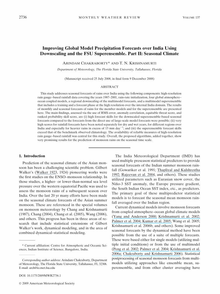
Improving Global Model Precipitation Forecasts over India UsingDownscaling and the FSU Superensemble. Part II: Seasonal Climate

ARINDAM CHAKRABORTY* AND T. N. KRISHNAMURTI

Department of Meteorology, The Florida State University, Tallahassee, Florida

(Manuscript received 25 July 2008, in final form 9 December 2008)

ABSTRACT

This study addresses seasonal forecasts of rains over India using the following components: high-resolution

rain gauge–based rainfall data covering the years 1987–2001, rain-rate initialization, four global atmosphere–

ocean coupled models, a regional downscaling of the multimodel forecasts, and a multimodel superensemble

that includes a training and a forecast phase at the high resolution over the internal India domain. The results

of monthly and seasonal forecasts of rains for the member models and for the superensemble are presented

here. The main findings, assessed via the use of RMS error, anomaly correlation, equitable threat score, and

ranked probability skill score, are (i) high forecast skills for the downscaled superensemble-based seasonal

forecasts compared to the forecasts from the direct use of large-scale model forecasts were possible; (ii) very

high scores for rainfall forecasts have been noted separately for dry and wet years, for different regions over

India and especially for heavier rains in excess of 15 mm day21; and (iii) the superensemble forecast skills

exceed that of the benchmark observed climatology. The availability of reliable measures of high-resolution

rain gauge–based rainfall was central for this study. Overall, the proposed algorithms, added together, show

very promising results for the prediction of monsoon rains on the seasonal time scale.

1. Introduction

Prediction of the seasonal climate of the Asian mon-

soon has been a challenging scientific problem. Gilbert

Walker’s (Walker 1923, 1924) pioneering works were

the first studies on the ENSO–monsoon relationship. In

those studies, a higher- or lower-than-normal sea level

pressure over the western equatorial Pacific was used to

assess the monsoon rains of a subsequent season over

India. Over the last 20 yr many efforts have been made

on the seasonal climate forecasts of the Asian summer

monsoon. These are referenced in the special volumes

on monsoon meteorology by Chang and Krishnamurti

(1987), Chang (2004), Chang et al. (2005), Wang (2006),

and others. This progress has been in three areas of re-

search that include statistical extensions of Gilbert

Walker’s work, dynamical modeling, and in the area of

combined dynamical–statistical modeling.

The India Meteorological Department (IMD) has

used multiple preseason statistical predictors to provide

seasonal forecasts of the Indian summer monsoon rain-

fall (Gowariker et al. 1991; Thapliyal and Kulshrestha

1992; Rajeevan et al. 2004, and others). These studies

utilized parameters such as Eurasian snow cover, the

Nino-3 SST anomaly, the Europe pressure gradient,

the South Indian Ocean SST index, etc., as predictors.

The primary goal of these multipredictor statistical

models is to forecast the seasonal mean monsoon rain-

fall averaged over the Indian region.

Current dynamical models involve monsoon forecasts

from coupled atmosphere–ocean global climate models

(Yang and Anderson 2000; Krishnamurti et al. 2002;

Palmer et al. 2004; Kumar et al. 2005; Wang et al. 2005;

Krishnamurti et al. 2006b, and others). Some improved

seasonal forecasts by the dynamical method have been

possible from the use of a suite of multiple forecasts.

These were based either for single models (utilizing mul-

tiple initial conditions) or from the use of multimodel

(Peng et al. 2002; Palmer et al. 2004; Krishnamurti et al.

2006a; Chakraborty and Krishnamurti 2006). Statistical

postprocessing of seasonal monsoon forecasts from multi-

models utilizing approaches like ensemble mean, su-

perensemble, and from other cluster averaging have

* Current affiliation: Centre for Atmospheric and Oceanic Sci-

ences, Indian Institute of Science, Bangalore, India.

Corresponding author address: Arindam Chakraborty, Department

of Meteorology, The Florida State University, Tallahassee, FL 32306.

E-mail: arch@io.met.fsu.edu

2736 M O N T H L Y W E A T H E R R E V I E W VOLUME 137

DOI: 10.1175/2009MWR2736.1

� 2009 American Meteorological Society

defined the current state of art in this area. These

statistical–dynamical combinations have provided im-

provements over those possible for the use of single

atmosphere–ocean coupled climate models (Brankovic

et al. 1990; Brankovic and Palmer 1997; Sperber and

Palmer 1996; Stephenson et al. 2005). The horizontal

resolution used in most of these models has generally

been of the order of 100–250 km. This had the limitation

for predicting the regional climate needed for the

provinces of India (Gadgil and Kumar 2006).

Categorical forecasts using ensemble of simulations

(either from a single model with multiple initial condition

or from multiple models) is one approach for forecasting

extreme events. Rajagopalan et al. (2002) used this ap-

proach to forecast precipitation and temperature over the

globe on a seasonal time scale. Regonda et al. (2006)

initiated a new approach for categorical streamflow fore-

cast using leading modes of principle components of the

flow and large-scale climate variables. Logistic regres-

sion between different parameters is another approach

for forecasting extreme events (e.g., Hamill et al. 2004).

Higher-resolution forecasts of monsoon climate can

be approached from the direct use of a suite of meso-

scale models (Ji and Vernekar 1997; Vernekar and Ji

1999) or from the deployment of downscaling strategies

(e.g., Misra and Kanamitsu 2004; Tripathi et al. 2006;

Anandhi et al. 2008). A direct use of observed high-

resolution precipitation estimates is possible in the con-

text of downscaling for coupled climate modeling. This

is the main objective of this study. Krishnamurti et al.

(2009, hereafter Part I) used a suite of atmospheric models

for medium-range numerical weather prediction. In this

study we propose a two-step approach for the prediction

of monthly to seasonal monsoon precipitation in a re-

gional scale over the Indian domain. At first, a down-

scaling strategy is used to obtain precipitation forecasts

from coupled climate models at the resolution of a new

rain gauge–based dataset. The next step is to use the

superensemble methodology (Krishnamurti et al. 1999)

to construct a consensus forecast from these downscaled

model forecasts that usually provides higher skills than

the individual member models and their ensemble mean

for seasonal climate prediction (Krishnamurti et al.

2000b; Stefanova and Krishnamurti 2002; Chakraborty

and Krishnamurti 2006). The next section describes the

models and datasets used in this study. The downscaling

strategy is detailed in section 3. The superensemble

methodology and the coupled assimilation procedure

are described in sections 4 and 5, respectively. Section 6

outlines the seasonal forecast experiments. The results

are illustrated in section 7. The main findings of this

study are summarized in section 8 with a note about

future work.

2. Models and datasets

Four versions of the coupled Florida State University

(FSU) General Spectral Model (GSM) were used in our

study. These models vary from each other in the pa-

rameterization of radiation and convection. Two radia-

tion schemes, one based on band model (referred as

new in this paper) and the other based on emissivity–

absorptivity (Krishnamurti et al. 2002, referred to as old

in this paper) were used in combination with two dif-

ferent convection schemes (viz., the Arakawa–Schubert

and the Kuo). The Arakawa–Schubert scheme is a sim-

plified version of the original scheme (Arakawa and

Schubert 1974) by Grell (1993). The Kuo convection

scheme used in our study was based on Krishnamurti

et al. (1980) and Krishnamurti and Bedi (1988), which is

a modified version of the parameterization introduced

by Anthes (1977). Table 1 lists these features of the four

models and their nomenclature used in this paper. De-

tails of the FSU coupled model are given in Larow and

Krishnamurti (1998).

The atmospheric component of the model has a

spectral triangular truncation at wavenumber 63 (T63),

which corresponds to a horizontal grid spacing of roughly

1.8758. It has 14 vertical sigma levels with more closely

spaced levels near the surface and tropopause. The ocean

model is a version of the Hamburg Ocean Primitive

Equation global (HOPE-G) model (Wolff et al. 1997),

which uses the Arakawa E grid. The horizontal resolu-

tion of the ocean model is 58 in longitude and 0.58–5.08 in

latitude with higher resolution near the equator. The

ocean was first spun up for 11 yr with observed wind and

SST. Next, a coupled assimilation procedure was used to

create oceanic initial conditions for the coupled forecast

by the FSU–GSM. Details of this assimilation procedure

is provided in section 5.

The primary observational dataset that is used in this

study was prepared by the National Climate Centre of the

IMD, Pune, India. As many as 2140 rain gauge–based

precipitation observations over India were used to obtain

a 1.08 3 1.08 gridded datasets (Rajeevan et al. 2006). The

TABLE 1. Four versions of the FSU global coupled climate models

and their nomenclature used in this paper.

Model Radiation scheme Convection scheme

ANR New, based on

band model

Arakawa–Schubert

(Grell 1993)

AOR Old, based on

emissivity–absorptivity

Arakawa–Schubert

(Grell 1993)

KNR New, based on

band model

Modified Kuo

(Krishnamurti et al. 1980)

KOR Old, based on

emissivity–absorptivity

Modified Kuo

(Krishnamurti et al. 1980)

SEPTEMBER 2009 C H A K R A B O R T Y A N D K R I S H N A M U R T I 2737

spatial interpolation procedure from the irregularly spaced

rain gauge network to equal angle grid was adapted from

Shepard (1968). The temporal resolution of this pre-

cipitation dataset is 1 day, and available from 1950 to

2004. This is a long and comprehensive dataset available

for studies of monsoons over the Indian region at dif-

ferent time scales (Rajeevan et al. 2006). In this study,

we have created a monthly mean dataset for the period

1987–2001 from this daily IMD observations. This pe-

riod was constrained by the availability of the coupled

model datasets. However, there were 6 yr during this

15-yr period when the Indian region experienced sea-

sonal precipitation far from the normal. And the years

1987, 1988, 1994, and 2000 were extreme among those

6 yr. We have shown, in this manuscript, the forecast

skill during all individual extreme years.

The coarse-resolution (2.58 3 2.58) monthly mean pre-

cipitation was obtained from the Climate Prediction

Center (CPC) Merged Analysis of Precipitation (CMAP;

Xie and Arkin 1997). Forecasts from member models

were averaged to the CMAP grid to calculate their skills

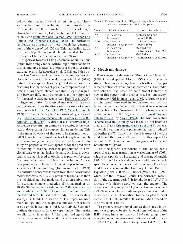
before downscaling. Figure 1 shows the comparison

between these two observational datasets used in our

study. In Fig. 1a, the grid-by-grid relationship between

CMAP and IMD precipitation over the Indian region

(7.58–27.58N, 67.58–97.58E) is shown for all the months

during 1987–2001. Since CMAP and IMD grids are

different in resolution, the IMD grid (higher resolution)

was regrided to the CMAP grid (lower resolution) using

a box averaging procedure (averages over all the frac-

tional grids of IMD those fall within a CMAP grid). It is

to be noted that IMD precipitation is slightly higher

compared to CMAP precipitation over most of the

precipitation ranges. This could be due to differences in

observational sources as well as the resolution between

these two datasets. CMAP uses satellite, radar, and rain

gauge observations to construct their monthly mean

precipitation product (Xie and Arkin 1997). However,

IMD-based precipitation is only based on dense rain

gauge observations (Rajeevan et al. 2006). The linear

relationship between these two datasets is indicated in-

side Fig. 1a, which shows that there is almost no constant

bias between precipitation obtained from CMAP and

IMD (intercept 5 0.07 mm day21). On the other hand,

the CMAP precipitation has to be scaled by a factor of

1.17 to match the IMD rainfall on the same grid.

Figures 1b–e show the climatology of January and

July precipitation over the Indian region from CMAP

and IMD observations. The spatial correlation between

these two datasets is indicated inside the respective

panels. During January, CMAP shows higher precipi-

tation at the southernmost tip of the Indian peninsula

compared to the IMD datasets. On the other hand,

during July, the IMD datasets show higher precipitation

over the west coast of India and over the northeast

Indian region compared to the CMAP. However, the

overall spatial pattern between these two datasets is

similar during both the months (spatial correlations of

0.77 and 0.67, respectively, during January and July).

Therefore, it can be concluded that these two datasets

are close enough to compare skill scores between coarse

resolution and downscaled model forecasts.

3. The downscaling strategy

Our downscaling strategy is as follows. We started

with monthly mean datasets at 2.58 3 2.58 resolution

from four FSU models, and monthly mean datasets at

1.08 3 1.08 resolution from IMD observations. The

common time period of these datasets is 1987–2001.

Now, the coarse-resolution model precipitation over the

Indian monsoon region was bilinearly interpolated to

FIG. 1. (a) Grid-by-grid relationship between CMAP and IMD precipitation over 7.58–27.58N, 67.58–97.58E during all the months of

1987–2001. The linear relationship between these two datasets is indicated. (b),(c),(d) January and July climatology of CMAP and IMD

precipitation during 1987–2001. The spatial correlation between these two datasets is indicated for IMD.

2738 M O N T H L Y W E A T H E R R E V I E W VOLUME 137

the higher-resolution grid of the observed IMD precip-

itation:

M9 5 Interp(M), (1)

where Interp() is the bilinear interpolation operator and

M is the model forecast field. This provided 1.08 3 1.08

resolution interpolated datasets from the four models

during each month of 1987–2001 (15 yr). Next, all the 12

months of the first year of model forecasts were kept

aside and the rest of the 14 yr of data, once for each

month and each grid, were used to calculate coefficients

of the following equation:

O 5 aM9 1 b 1 �, (2)

where O and M9 are the observed and interpolated

model forecast of rainfall on that grid, respectively; a

and b are regression coefficients (the slope and intercept

of the linear fit, respectively); and � is the error term. The

regression procedure is a least squares linear fit that

minimizes the absolute value of the error term (j�j).

Once these regression coefficients (a and b) are ob-

tained, they are used in the forecast year to calculate

downscaled model precipitation:

M99 5 aM9 1 b, (3)

where M0 is the downscaled forecast of the model [other

symbols are same as in Eq. (2)]. Note that, in the above

equation, the values of a and b are obtained from the

least squares linear regression described by Eq. (2).

Hence, one set of coefficients are calculated for every

grid point and for every month of the year. The entire

procedure is repeated for every year of the 15 yr of da-

tasets (cross validation; Deque 1997). This spatial and

seasonal dependency in regression coefficients is nec-

essary to take into account the regional and seasonal

variation of the model skills in predicting monthly pre-

cipitation over India. This downscaling strategy, when

applied to every grid in the domain of interest, corrects

model bias over numerous regions such as orography,

vegetation, land–sea boundary, etc. This is mainly pos-

sible because the observed precipitation datasets is rain

gauge based and is free from any error arising from those

factors.

4. Superensemble methodology

The superensemble methodology (Krishnamurti et al.

1999, 2000b) combines multiple model forecasts based

on their past performance to make a consensus forecast.

To obtain the past performance, the forecast time series

is divided into a training period and a forecast period.

The model forecasts are regressed in the training period

with the observed counterpart to obtain weights:

G 5 �Ntrain

t51(S9

t�O9

t)2, (4)

where G is the error term that is minimized to obtain the

weights, Ntrain is the length of the training dataset, and

St9 and Ot9 are the superensemble and observed field

anomalies, respectively, at training time t. The outcome

of this regression is statistical weights ai (i 5 1, 2, . . . , N;

N being the number of models) assigned to every model

in the suite. These weights are then passed on to the

forecast phase to construct superensemble forecast:

S 5 O 1 �N

i51a

i(F

i� F

i), (5)

where O is the climatology of the observed field, and Fi

and Fi are the forecasts and forecast climatology, re-

spectively, for the ith model. The summation is taken

over the N-member models in the suite. The observed

and model climatology fields are the mean over the

training period during every calendar month. The co-

efficients are estimated my minimizing the error term of

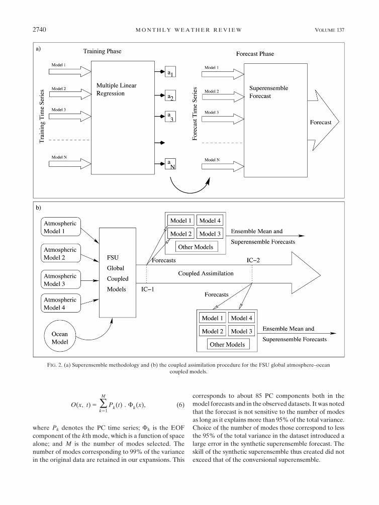
Eq. (4). This method is illustrated in Fig. 2a. The su-

perensemble differs from the conventional bias-removed

forecasts in the assignment of weights to the member

models. In the bias-removed forecast, an equal weight of

1/N is assigned to every model where N is the total

number of models. For the superensemble, model

weights are based on their performance in the training

phase, and can even attain a negative value if the model

anomalies are negatively correlated with that of the

observation in the training phase (Chakraborty et al.

2007). Moreover, for the superensemble, the weights vary

geographically, which takes into account the regional

variation of skills of the member models. This varied

weights leads to a better forecast by the superensemble

compared to the bias-removed ensemble mean forecasts

(Stefanova and Krishnamurti 2002; Chakraborty and

Krishnamurti 2006).

The seasonal climate forecasts of the superensemble

uses a variation of the above, which was shown to have

performed better than the conventional superensemble

methodology (Yun et al. 2005). In this variation, syn-

thetic forecasts for each of the member models are

created from their original forecast time series using

linear regression with their observed counterpart in the

EOF space. This methodology is as follows.

The observed time series are expanded in terms of

principal component (PC; in time) and empirical or-

thogonal function (EOF; in space):

SEPTEMBER 2009 C H A K R A B O R T Y A N D K R I S H N A M U R T I 2739

O(x, t) 5 �M

k51P

k(t) . F

k(x), (6)

where Pk denotes the PC time series; Fk is the EOF

component of the kth mode, which is a function of space

alone; and M is the number of modes selected. The

number of modes corresponding to 99% of the variance

in the original data are retained in our expansions. This

corresponds to about 85 PC components both in the

model forecasts and in the observed datasets. It was noted

that the forecast is not sensitive to the number of modes

as long as it explains more than 95% of the total variance.

Choice of the number of modes those correspond to less

the 95% of the total variance in the dataset introduced a

large error in the synthetic superensemble forecast. The

skill of the synthetic superensemble thus created did not

exceed that of the conversional superensemble.

FIG. 2. (a) Superensemble methodology and (b) the coupled assimilation procedure for the FSU global atmosphere–ocean

coupled models.

2740 M O N T H L Y W E A T H E R R E V I E W VOLUME 137

Similar to the observed, the model datasets are also

expanded:

Fi(x, t) 5 �

M

k51F

i,k(t) f

i,k(x), (7)

where i denotes the ith model in the suite, Fi,k is the PC

time series for the kth mode of the ith model, and fi,k is

the EOF.

Now, every mode of the PC time series of the models

are regressed against the corresponding observed coun-

terpart to obtain weights for each model. In this proce-

dure, the kth mode of the PC time series of the

observation is written as a linear combination of that of

the member models:

Pk(t) 5 �

N

i51a

i,kF

i,k(t) 1 �

i,k, (8)

where i is the ith member in the ensemble, ai,k is the

weight to the ith model for mode k, and �i,k is the error

term. The weights (ai,k) are estimated using multiple

linear regression that minimizes the variance of the er-

ror E(�2i,k). The regression-obtained PC time series thus

obtained can be written as

Fregi,k (t) 5 a

i,kF

i,k(t).

These, when combined with the spatial EOF, provides

the synthetic forecast dataset:

Fregi (x, t) 5 �

M

k51F

regi,k (t)F

k(x), (9)

where Fk(x) denotes the EOF components of the ob-

servation. The above exercise is repeated for every

model in the ensemble. To forecast a particular year, we

have used the entire model forecast time series. How-

ever, the observational data for that year was substituted

by the ensemble mean of the member models. This was

required to remove any dependency of the results with

available observation during the forecast year. The syn-

thetic dataset thus obtained is sent to the original super-

ensemble algorithm for final superensemble forecast.

Further details of this methodology are provided in Yun

et al. (2005), Krishnamurti et al. (2006b), and Chakraborty

and Krishnamurti (2006). It has been shown in these

studies that for seasonal climate forecasts the synthetic

superensemble methodology performs better than the

conventional superensemble methodology. In this paper

we will use the term superensemble to refer to synthetic

superensemble.

5. Coupled assimilation

Prior to the start of each seasonal forecast we in-

clude a coupled assimilation. This procedure, based on

Krishnamurti et al. (2000a) is outlined in Fig. 2b. This

includes the following steps.

a. Oceanic spinup

The ocean state undergoes a spinup where 11 yr

(1976–86) of monthly mean observed surface winds

[obtained from the 40-yr European Centre for Medium-

Range Weather Forecasts (ECMWF) Re-Analysis

(ERA-40)] and monthly mean SSTs (based on Reynolds

and Smith 1994 datasets) were used. This component of

ocean data assimilation is carried out using a continuous

Newtonian relaxation technique (Krishnamurti et al.

2000a). This spinup generates ocean currents, oceanic

temperature, and distributes the salinity fields in three

dimensions that acquire an equilibrium, with respect to

the prescribed surface wind stress and the SSTs. This

feature of the modeling does not assure an equilibration

for the deeper oceans that may require much longer time

scales (compared to 11 yr). Because the upper oceans are

considered more important for seasonal forecasts (of

monsoon), this may not be a major limitation.

b. Coupled assimilation

Daily coupled assimilation follows the 11-yr spin-up

phase. This is a continuous assimilation that covers the

period 1987–2001. The atmospheric part of the coupled

assimilation follows our previous study Krishnamurti

et al. (1991). Here we include a physical initialization of

observed rainfall based on Tropical Rainfall Measuring

Mission (TRMM) data files from Kummerow et al.

(1998). The ECMWF datasets provides all of the gridded

initial variables such as the wind components u, y, and _s,

and the temperature, humidity, and surface pressure

distributions. The atmospheric spinup is done using a

Newtonian relaxation of these base variables con-

strained to the physical initialization of the improved

rain rates. The Newtonian relaxation calls for hard and

soft nudging for different variables to enable the model

to essentially retain the rotational part of the wind from

the ECMWF data analysis at the end of our assimilation.

However, it permits the other fields such as humidity,

surface pressure, vertical motions, and diabatic heating

to adjust to the imposed rains. This coupled assimilation

is shared by all of the member models of our suite.

6. Seasonal forecast experiments

Seasonal forecasts with the four FSU coupled models

are performed for the years 1987–2001. Two forecasts

SEPTEMBER 2009 C H A K R A B O R T Y A N D K R I S H N A M U R T I 2741

per month, one starting at the middle and the other

starting at the end of each month were carried out for

each of the four member models. This study uses the

model outputs that started only at the end of a month

during our study period. The oceanic initial condition

was taken from the output of the coupled assimilation

phase. The atmospheric initial condition was obtained

from ECMWF 0.58 3 0.58 analysis datasets. The length

of each forecast was 90 days. Forecast fields averaged

from days 1 through 30 is termed as month 1 in this

study. Months 2 and 3 of forecasts follow similarly. The

string of all month-1 forecasts from January 1987 to

December 2001 (180 time points) constitute the month-1

forecast time series in our study. Similarly, month-2

forecast time series start on February 1987 and end on

January 2002, and month-3 forecasts start on March

1987 and end on February 2002.

In this paper we will illustrate forecast skills of the

models, their ensemble mean, and the superensemble

before and after downscaling. All model forecasts

before downscaling were interpolated to a common

2.58 3 2.58 grid to compare with the CMAP datasets.

The ensemble mean and the superensemble forecasts

were created from these 2.58 horizontal resolution,

monthly forecast time series. These forecast prod-

ucts are referred as coarse resolution or CRes in this

paper.

To construct downscaled forecasts, the monthly mean

datasets from every model were first downscaled using

the proposed algorithm to the 1.08 horizontal resolution

grid. Next, this downscaled forecast time series from

the models were used to calculate downscaled ensemble

mean and superensemble forecasts. The downscaled

forecasts are termed DScl in this paper.

7. Results

a. Skills of uninterpolated and interpolated rainfall

Prior to the statistical downscaling we bilinearly inter-

polated the model forecast rains from a 2.58 3 2.58

longitude–latitude grid to a 1.08 3 1.08 longitude–latitude

grid. These two products, the uninterpolated and the

interpolated rains, were compared with the CMAP- and

IMD-based precipitation estimates, respectively. The

15 yr (1987–2001) climatology of coarse resolution (2.58)

and interpolated (1.08) forecasts of precipitation for

month 2 during July and December from the four

member models are illustrated in Figs. 3a–t. The RMS

errors (in mm day21) of the precipitation climatology

for this month along with months 1 and 3 of forecasts are

shown in Figs. 3u–z. The RMS errors were calculated

using the following equation:

RMS error 5

ffiffiffiffiffiffiffiffiffiffiffiffiffiffiffiffiffiffiffiffiffiffiffiffiffiffiffiffiffiffiffiffiffi

1

N�N

i51(F

i�O

i)2

v

u

u

t

, (10)

where Fi and Oi are forecast and observed fields, re-

spectively, at the ith grid point. Here N is the total number

of grid points in the domain. There are some obvious

model to model differences in these 15-yr averages. The

uninterpolated model precipitation has RMS errors in the

range of 1.4–6.4 (1.9–6.1 for month 2) mm day21 (when

verified against the CMAP rains). The interpolated rains

are essentially the same fields as the uninterpolated ones

and these have RMS errors of the order of 1.5–13.6

(1.9–13.4 for month 2) mm day21 for months 1, 2, and 3

of forecasts. The IMD rains were used here as the bench-

mark for this higher resolution. These large errors arise

because the IMD rain gauges measure extreme local

rains (e.g., high along the west coast and low in the rain

shadow region of south-central India). Those levels of

high or low local rains are not predicted by large-scale

models. When this large-scale-averaged precipitation by

the coarse-resolution models is interpolated to finer

grids, it leads to higher RMS errors because the spatial

variability of high-resolution precipitation within the

large-scale grid is not captured by the interpolation

procedure. The reason why we are presenting these is to

show in a later section of the paper that this same prod-

uct that carries these large local errors can be very much

improved by deploying a statistical downscaling and a

multimodel superensemble based on these downscaled

member models.

b. Spatial distribution of downscaling coefficients

The coefficients a and b of the linear regression [Eq. (2)]

that relates interpolated model-predicted rainfall against

the high-resolution observed IMD counterpart provide

useful information for the systematic errors of each

model. A slope of 1.0 would imply that the large-scale

model has rain equal to the high-resolution rain of IMD

at all rainfall rates after removing the constant bias (the

intercept b). The slope of 1.0 also conveys that the rate

of change of model rain is consistent with that of the

observed. A faster (slower) rate of change of rain by the

model implies a slope 0 , a , 1 (a . 1). A negative value

of a indicates that model rain is lower (higher) then

observation in the high (low) observed precipitation

range. On the other hand, b implies the constant bias of

the model compared to the observation at any precipi-

tation range. A positive (negative) value of b indicates

that the model rain was lower (higher) compared to the

observation.

The spatial distribution of the slope and intercept

(a and b) during July and December for month 2 of

2742 M O N T H L Y W E A T H E R R E V I E W VOLUME 137

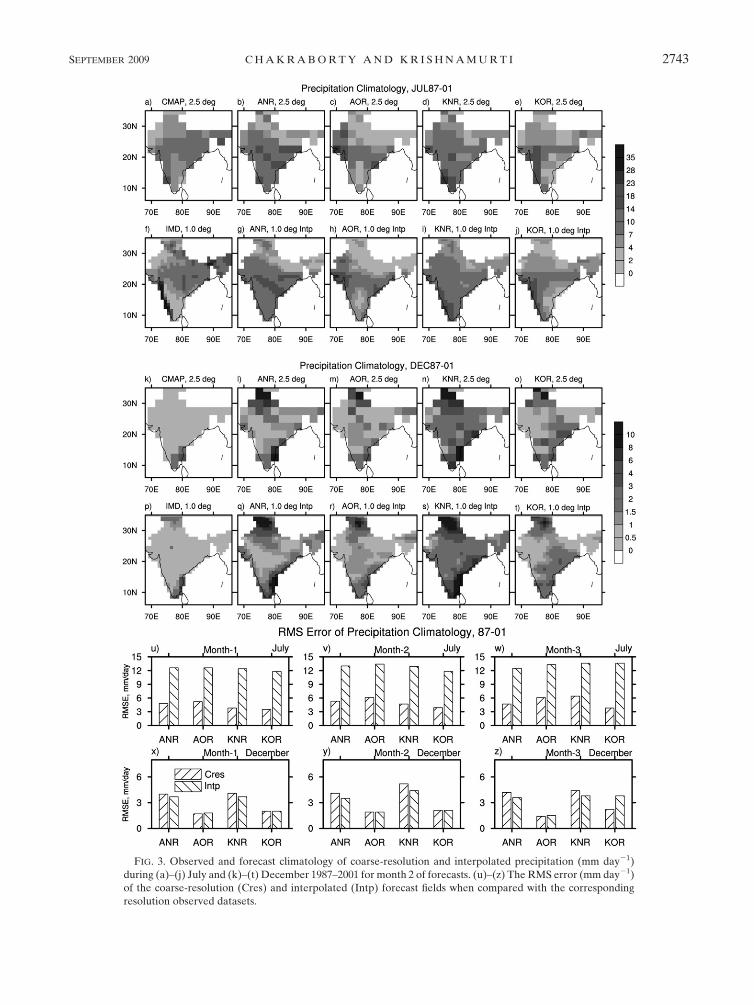
FIG. 3. Observed and forecast climatology of coarse-resolution and interpolated precipitation (mm day21)

during (a)–(j) July and (k)–(t) December 1987–2001 for month 2 of forecasts. (u)–(z) The RMS error (mm day21)

of the coarse-resolution (Cres) and interpolated (Intp) forecast fields when compared with the corresponding

resolution observed datasets.

SEPTEMBER 2009 C H A K R A B O R T Y A N D K R I S H N A M U R T I 2743

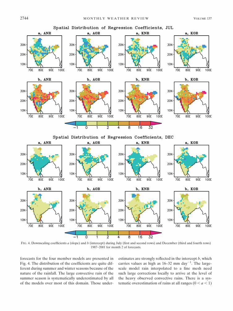
forecasts for the four member models are presented in

Fig. 4. The distribution of the coefficients are quite dif-

ferent during summer and winter seasons because of the

nature of the rainfall. The large convective rain of the

summer season is systematically underestimated by all

of the models over most of this domain. Those under-

estimates are strongly reflected in the intercept b, which

carries values as high as 16–32 mm day21. The large-

scale model rain interpolated to a fine mesh need

such large corrections locally to arrive at the level of

the heavy observed convective rains. There is a sys-

tematic overestimation of rains at all ranges (0 , a , 1)

FIG. 4. Downscaling coefficients a (slope) and b (intercept) during July (first and second rows) and December (third and fourth rows)

1987–2001 for month 2 of forecasts.

2744 M O N T H L Y W E A T H E R R E V I E W VOLUME 137

over south-central India by the model that utilized the

Arakawa–Schubert cumulus parameterization scheme

for its convection and a band model for its radiative

transfer (ANR). This feature is less pronounced in the

other models. There are many smaller-scale features in

the slope alternating between 61. This arises because of

the smoother larger scales of model rains and heavier

mesoscale features of the observed rains. In the steep

orographic regions of the Himalayas, some models carry

large errors of the order of 16–32 units for the slope

parameter, these are indicative of underestimates of

heavy orographic rains by the large-scale models where

the observed rains have been much larger intensity.

The four models carry somewhat different fields of the

slope a during December (Fig. 4, third and fourth rows).

The ANR model carries a positive slope (0 to 11) over

north of 308N and a negative slope (0 to 21) south of

308N. This, along with the fact the value of intercept b is

small positive south of 308N latitude, implies that this

model overestimates low rains and underestimates

heavier rains over this region. North of 308N, in the

winter season, most of the rains occur from western

disturbances. That is similar to precold frontal rains and

is largely stratiform in nature. The combination of

Arakawa–Schubert cumulus parameterization and the

band model for the radiative transfer (ANR) appears to

underestimate stratiform rains. The other models seem

to carry less bias in this region. Such inferences, how-

ever, need to be taken with a word of caution. It was

noted in Krishnamurti and Sanjay (2003) that a physical

parameterization scheme within two different models

can show different behavior even if all other physics and

initial datasets were kept identical. A physical parame-

terization scheme’s behavior also depends strongly on

the rest of the model within which it resides. Large-scale

global model and regional model can differ in resolu-

tion, advective algorithm, and boundary conditions and

can thus affect the behavior of a cumulus parameteri-

zation quite differently. Most models carry values for

the intercept b between 0 and 1 over most of India,

implying that this systematic error (underestimate) for

rainfall is of the order of 0–1 mm day21. However, all

models underestimate rainfall by 2–8 mm day21 near the

southeastern coast of India where winter monsoon

dominates over summer monsoon. Similar underesti-

mation of precipitation is noticed over the mountainous

regions north of 308N.

The coefficients shown in Fig. 4 are not sensitive to the

number of years (data points) chosen for the regression.

Figure 5 shows how the values of a and b changes with

the number of years used in the least squares linear re-

gression procedure at a location near the southwest

coast of India (13.58N, 75.58E). At first, 3 yr of data were

taken and coefficients were calculated. Addition of

more years to the regression database changes the

values of the coefficients wildly at first. However, when

the number of years crosses 10, both the values stabilize

and does not show large sensitivity to the number of data

points. This is true during both winter (December) and

summer (July), except for coefficient b during July.

During this month, the value of b was not as stable as

was seen during December. However, the variation

during July after the number of months cross 7 was much

less as compared to that when less than 7 months were

considered to calculated the regression coefficients. The

above result shows that our choice of 14 yr of training to

calculate the downscaling coefficients for the forecast

year is adequate for this study.

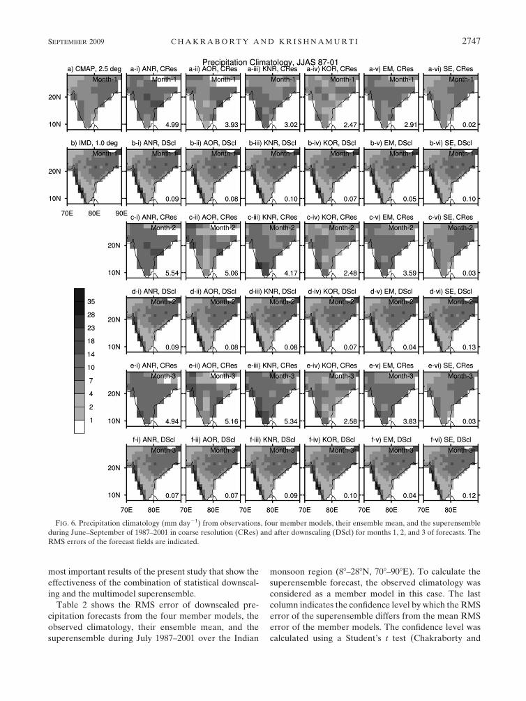
c. Downscaled climatology

Each of the model forecasts for months 1, 2, and 3 were

downscaled using the observed IMD high-resolution

rains for the respective months. Figure 6 shows the June–

September climatology of coarse- and high-resolution

(downscaled) precipitation from CMAP- and IMD-based

observations along with the forecasts from member

models, their ensemble mean, and the superensemble

before and after downscaling for months 1, 2, and 3 of

forecasts. Within each forecast panel, we have shown the

RMS error of the climatology fields when compared with

the respective resolution observation. We note that both

the observed (CMAP) and the coarse-resolution models

fail to show the strong west coastal heavy rains in their

climatology; furthermore, the southern India rains (south

of 158N) were absent in these climatologies. The RMS

errors for the climatology of large-scale models carry

values from 2.47 to 5.54 mm day21. The superensemble

based on these large-scale models is able to reduce these

errors. The climatology of the downscaled models, when

compared with the high-resolution IMD-based precipi-

tation observation, show much higher skills compared to

their coarse-resolution counterpart. It was possible to

obtain the RMS error of monthly climatology of the

member models of the order of 0.01–0.10 mm day21. This

is one of the promising aspects of the proposed down-

scaling. Both the ensemble means and the large-scale

downscaled models provide the climatology of precipi-

tation that shows much higher skills compared to the

corresponding coarse-resolution counterpart. The RMS

error of the climatology field from the superensemble was

of the same order as that of the large-scale models and

their ensemble mean.

d. Forecast skills over a seasonal time scale

In this section the skills of forecasts over seasonal time

scales are measured using RMS error and equitable

SEPTEMBER 2009 C H A K R A B O R T Y A N D K R I S H N A M U R T I 2745

threat score (ETS). The ETS is defined as (Rogers et al.

1996):

ETS 5H � E

F 1 A�H � E, (11)

where F and A are the number of grids where forecast

and observed fields exceed a specified threshold, re-

spectively; and H is the number of grids that correctly

forecast more than the specified threshold (also termed

as ‘‘hit’’). In other words, H is the number of grids where

both the observed and forecasted field cross the

threshold; and E 5 F 3 A/T, T being the total number

of grids over the region. ETS values can range from 21/3

to 1. The higher the ETS, the better the forecast. An

ETS value of 1 indicates perfect forecast skill.

The ETS for months 1, 2, and 3 of forecasts for the

southwest Indian domain during June–September of

1987–2001 are shown in Fig. 7. ETS from both coarse-

resolution and downscaled forecasts are shown to illus-

trate the marked improvements obtained from the

downscaling methodology. The threat scores of the rains

were less than 0.1 for the large-scale models for all the

months 1, 2, and 3 of the forecasts. The downscaled

versions of these models show ETS values as high as

0.4–0.6. The member models and the superensemble per-

form the best (ETS values reach peak) for precipitation

thresholds of 15 and 20 mm day21. The threat scores for

rains in excess of 35 mm day21 are as high as 0.4, which is

not well predicted by the large-scale models. Similar

improvements are obtained for the ensemble mean

forecasts as well. It is interesting to note that the ETS

score for the superensemble based on forecasts of the

large-scale models follow closely to that of the down-

scaled superensemble for rain rates #10 mm day21. This

shows that the superensemble based on large-scale

models is able to predict low rains (,15 mm day21) as

well as the downscaled higher-resolution superensemble.

However, at higher rain rates (.15 mm day21) the skill of

the superensemble falls sharply. Figure 7 conveys the

FIG. 5. Dependence of the downscaling coefficients a (slope) and b (intercept) on the number of years in the

training period during (a),(b) December and (c),(d) July for month 3 of forecasts at 13.58N, 75.58E (near the

southwest coast of India). The values of the regression coefficients get stabilized when more than about 10 yr of data

are used in the training period.

2746 M O N T H L Y W E A T H E R R E V I E W VOLUME 137

most important results of the present study that show the

effectiveness of the combination of statistical downscal-

ing and the multimodel superensemble.

Table 2 shows the RMS error of downscaled pre-

cipitation forecasts from the four member models, the

observed climatology, their ensemble mean, and the

superensemble during July 1987–2001 over the Indian

monsoon region (88–288N, 708–908E). To calculate the

superensemble forecast, the observed climatology was

considered as a member model in this case. The last

column indicates the confidence level by which the RMS

error of the superensemble differs from the mean RMS

error of the member models. The confidence level was

calculated using a Student’s t test (Chakraborty and

FIG. 6. Precipitation climatology (mm day21) from observations, four member models, their ensemble mean, and the superensemble

during June–September of 1987–2001 in coarse resolution (CRes) and after downscaling (DScl) for months 1, 2, and 3 of forecasts. The

RMS errors of the forecast fields are indicated.

SEPTEMBER 2009 C H A K R A B O R T Y A N D K R I S H N A M U R T I 2747

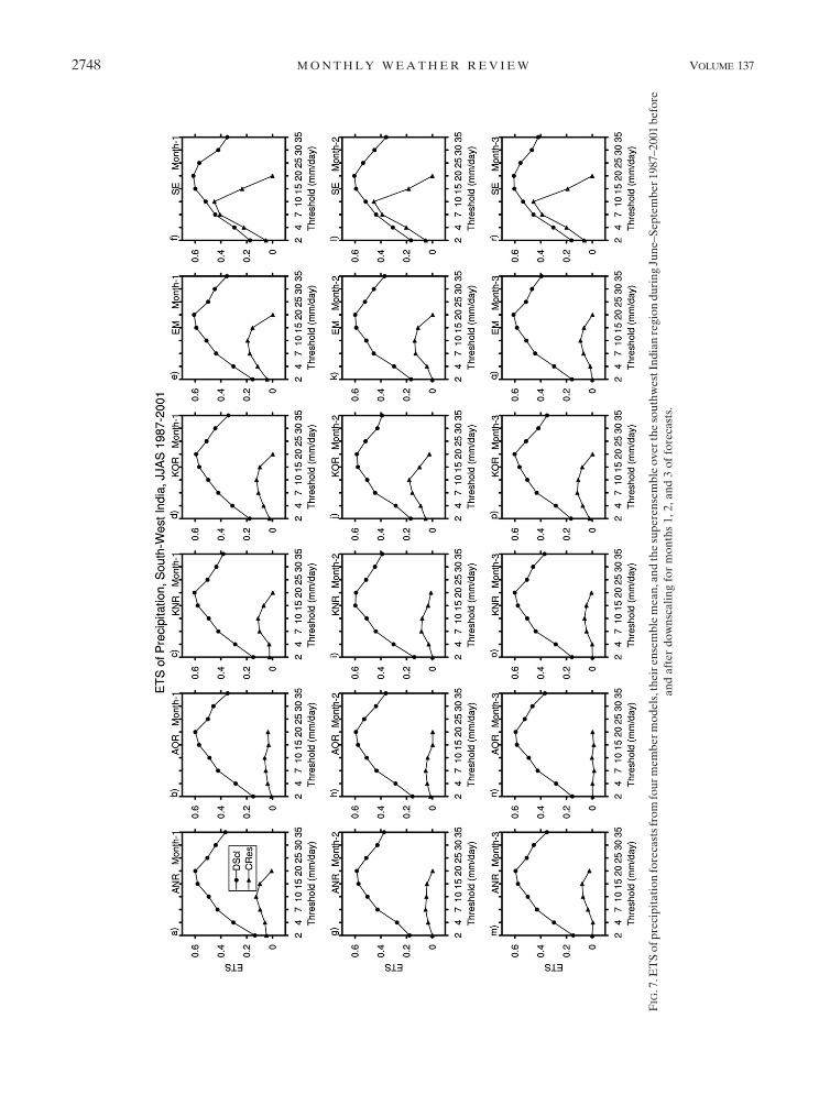
FIG

.7.E

TS

of

pre

cip

ita

tio

nfo

reca

sts

fro

mfo

ur

me

mb

er

mo

de

ls,t

he

ire

nse

mb

lem

ea

n,a

nd

the

sup

ere

nse

mb

leo

ver

the

sou

thw

est

Ind

ian

reg

ion

du

rin

gJu

ne

–S

ep

tem

be

r1

98

7–2

001

be

fore

an

da

fte

rd

ow

nsc

ali

ng

for

mo

nth

s1

,2

,a

nd

3o

ffo

reca

sts.

2748 M O N T H L Y W E A T H E R R E V I E W VOLUME 137

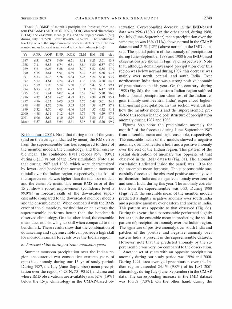
Krishnamurti 2006). Note that during most of the years

(and on the average, indicated by mean) the RMS error

from the superensemble was less compared to those of

the member models, the climatology, and their ensem-

ble mean. The confidence level exceeds 95% (90%)

during 6 (11) yr out of the 15-yr simulation. Note also

that during 1987 and 1988, which were characterized

by lower- and heavier-than-normal summer monsoon

rainfall over the Indian region, respectively, the skill of

the superensemble was higher than the member models

and the ensemble mean. The mean RMS error of the

15 yr show a robust improvement (confidence level is

99.9%) in forecast skills of the downscaled super-

ensemble compared to the downscaled member models

and the ensemble mean. When compared with the RMS

error of the climatology, we find that on an average the

superensemble performs better than the benchmark

observed climatology. On the other hand, the ensemble

mean does not show higher skill when compared to this

benchmark. These results show that the combination of

downscaling and superensemble can provide a high skill

for monsoon rainfall forecasts over the Indian region.

e. Forecast skills during extreme monsoon years

Summer monsoon precipitation over the Indian re-

gion encountered two consecutive extreme years of

opposite anomaly during our 15 yr of study period.

During 1987, the July (June–September) mean precipi-

tation over the region 88–288N, 708–908E (land area and

where IMD observations are available) was 32% (19%)

below the 15-yr climatology in the CMAP-based ob-

servation. Corresponding decrease in the IMD-based

data was 25% (18%). On the other hand, during 1988,

the July (June–September) mean precipitation over the

same region was 16% (11%) above normal in the CMAP

datasets and 21% (12%) above normal in the IMD data-

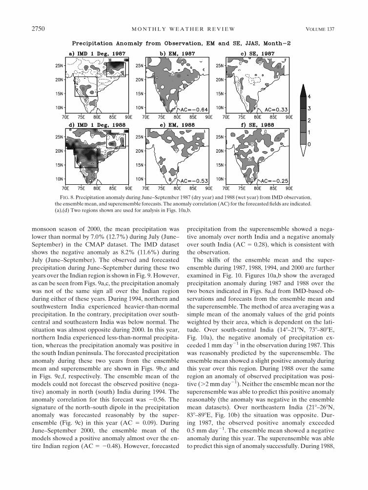
sets. The spatial pattern of the anomaly of precipitation

during June–September 1987 and 1988 from IMD-based

observations are shown in Figs. 8a,d, respectively. Note

that, although domain-averaged precipitation over this

region was below normal during 1987, this decrease was

mainly over north, central, and south India. Over

northeastern India there was a strong positive anomaly

of precipitation in this year. On the contrary, during

1988 (Fig. 8d), the northeastern Indian region suffered

below-normal precipitation when rest of the Indian re-

gion (mainly south-central India) experienced higher-

than-normal precipitation. In this section we illustrate

how the member models and the superensemble pre-

dicted this seesaw in the dipole structure of precipitation

anomaly during 1987 and 1988.

Figures 8b,c show the precipitation anomaly for

month 2 of the forecasts during June–September 1987

from ensemble mean and superensemble, respectively.

The ensemble mean of the models showed a negative

anomaly over northeastern India and a positive anomaly

over the rest of the Indian region. This pattern of the

spatial distribution of anomaly was opposite of that

observed in the IMD datasets (Fig. 8a). The anomaly

correlation (indicated inside the panel) was 20.64 for

the ensemble mean forecasts. The superensemble suc-

cessfully forecasted the observed positive anomaly over

northeastern India and a negative anomaly over central

and south India during this year. The anomaly correla-

tion from the superensemble was 0.33. During 1988

(Figs. 8e,f), the ensemble mean of the member models

predicted a slightly negative anomaly over south India

and a positive anomaly over eastern and northern India.

This pattern was opposite to that observed (Fig. 8d).

During this year, the superensemble performed slightly

better than the ensemble mean in predicting the spatial

pattern of precipitation anomaly over the Indian region.

The signature of positive anomaly over south India and

patches of the positive and negative anomaly over

eastern India is present in the superensemble datasets.

However, note that the predicted anomaly by the su-

perensemble was very low compared to the observation.

Another set of years with an opposite precipitation

anomaly during our study period was 1994 and 2000.

During 1994, area-averaged precipitation over the In-

dian region exceeded 24.4% (9.8%) of its 1987–2001

climatology during July (June–September) in the CMAP

data. The corresponding increase in the IMD dataset

was 16.5% (7.0%). On the other hand, during the

TABLE 2. RMSE of month-3 precipitation forecasts from the

four FSUGSMs (ANR, AOR, KNR, KOR), observed climatology

(CLM), the ensemble mean (EM), and the superensemble (SE)

during July 1987–2001 over 88–288N, 708–908E. The confidence

level by which the superensemble forecast differs from the en-

semble mean forecast is indicated in the last column (clev).

Yr ANR AOR KNR KOR CLM EM SE clev

1987 6.31 6.78 5.99 6.71 6.11 6.23 5.91 93.8

1988 7.11 6.87 6.74 6.81 6.84 6.80 6.57 97.0

1989 5.61 6.07 5.58 5.65 5.70 5.57 5.55 77.9

1990 5.75 5.64 5.91 5.39 5.32 5.39 5.36 93.5

1991 5.33 5.78 5.26 5.34 5.25 5.24 5.08 93.9

1992 5.52 4.64 4.24 4.73 4.38 4.56 4.28 84.3

1993 5.59 5.98 5.74 5.60 5.35 5.47 5.07 99.4

1994 6.93 6.90 6.71 6.73 6.71 6.70 6.47 99.1

1995 5.81 5.44 6.02 6.34 5.52 5.67 5.20 96.6

1996 4.32 4.51 4.62 4.89 4.28 4.38 4.19 95.4

1997 4.96 6.12 6.03 5.69 5.76 5.48 5.61 24.5

1998 4.48 4.76 5.96 5.03 4.33 4.58 4.37 87.8

1999 5.32 4.70 4.65 4.46 4.53 4.57 4.32 91.1

2000 4.48 5.11 5.12 4.99 4.76 4.71 4.29 97.5

2001 6.06 5.80 6.10 5.79 5.86 5.80 5.71 92.9

Mean 5.57 5.67 5.64 5.61 5.38 5.41 5.20 99.9

SEPTEMBER 2009 C H A K R A B O R T Y A N D K R I S H N A M U R T I 2749

monsoon season of 2000, the mean precipitation was

lower than normal by 7.0% (12.7%) during July (June–

September) in the CMAP dataset. The IMD dataset

shows the negative anomaly as 8.2% (11.6%) during

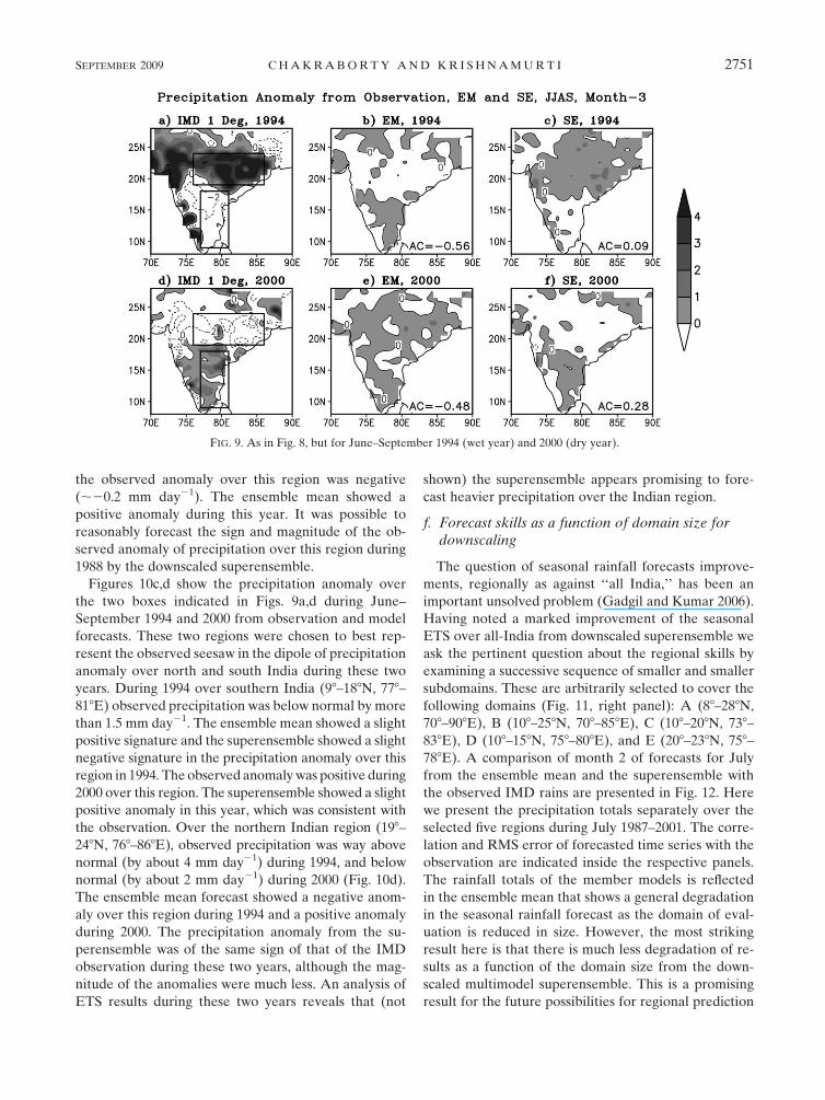
July (June–September). The observed and forecasted

precipitation during June–September during these two

years over the Indian region is shown in Fig. 9. However,

as can be seen from Figs. 9a,c, the precipitation anomaly

was not of the same sign all over the Indian region

during either of these years. During 1994, northern and

southwestern India experienced heavier-than-normal

precipitation. In the contrary, precipitation over south-

central and southeastern India was below normal. The

situation was almost opposite during 2000. In this year,

northern India experienced less-than-normal precipita-

tion, whereas the precipitation anomaly was positive in

the south Indian peninsula. The forecasted precipitation

anomaly during these two years from the ensemble

mean and superensemble are shown in Figs. 9b,c and

in Figs. 9e,f, respectively. The ensemble mean of the

models could not forecast the observed positive (nega-

tive) anomaly in north (south) India during 1994. The

anomaly correlation for this forecast was 20.56. The

signature of the north–south dipole in the precipitation

anomaly was forecasted reasonably by the super-

ensemble (Fig. 9c) in this year (AC 5 0.09). During

June–September 2000, the ensemble mean of the

models showed a positive anomaly almost over the en-

tire Indian region (AC 5 20.48). However, forecasted

precipitation from the superensemble showed a nega-

tive anomaly over north India and a negative anomaly

over south India (AC 5 0.28), which is consistent with

the observation.

The skills of the ensemble mean and the super-

ensemble during 1987, 1988, 1994, and 2000 are further

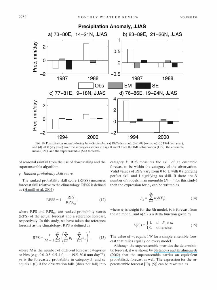
examined in Fig. 10. Figures 10a,b show the averaged

precipitation anomaly during 1987 and 1988 over the

two boxes indicated in Figs. 8a,d from IMD-based ob-

servations and forecasts from the ensemble mean and

the superensemble. The method of area averaging was a

simple mean of the anomaly values of the grid points

weighted by their area, which is dependent on the lati-

tude. Over south-central India (148–218N, 738–808E,

Fig. 10a), the negative anomaly of precipitation ex-

ceeded 1 mm day21 in the observation during 1987. This

was reasonably predicted by the superensemble. The

ensemble mean showed a slight positive anomaly during

this year over this region. During 1988 over the same

region an anomaly of observed precipitation was posi-

tive (.2 mm day21). Neither the ensemble mean nor the

superensemble was able to predict this positive anomaly

reasonably (the anomaly was negative in the ensemble

mean datasets). Over northeastern India (218–268N,

838–898E, Fig. 10b) the situation was opposite. Dur-

ing 1987, the observed positive anomaly exceeded

0.5 mm day21. The ensemble mean showed a negative

anomaly during this year. The superensemble was able

to predict this sign of anomaly successfully. During 1988,

FIG. 8. Precipitation anomaly during June–September 1987 (dry year) and 1988 (wet year) from IMD observation,

the ensemble mean, and superensemble forecasts. The anomaly correlation (AC) for the forecasted fields are indicated.

(a),(d) Two regions shown are used for analysis in Figs. 10a,b.

2750 M O N T H L Y W E A T H E R R E V I E W VOLUME 137

the observed anomaly over this region was negative

(;20.2 mm day21). The ensemble mean showed a

positive anomaly during this year. It was possible to

reasonably forecast the sign and magnitude of the ob-

served anomaly of precipitation over this region during

1988 by the downscaled superensemble.

Figures 10c,d show the precipitation anomaly over

the two boxes indicated in Figs. 9a,d during June–

September 1994 and 2000 from observation and model

forecasts. These two regions were chosen to best rep-

resent the observed seesaw in the dipole of precipitation

anomaly over north and south India during these two

years. During 1994 over southern India (98–188N, 778–

818E) observed precipitation was below normal by more

than 1.5 mm day21. The ensemble mean showed a slight

positive signature and the superensemble showed a slight

negative signature in the precipitation anomaly over this

region in 1994. The observed anomaly was positive during

2000 over this region. The superensemble showed a slight

positive anomaly in this year, which was consistent with

the observation. Over the northern Indian region (198–

248N, 768–868E), observed precipitation was way above

normal (by about 4 mm day21) during 1994, and below

normal (by about 2 mm day21) during 2000 (Fig. 10d).

The ensemble mean forecast showed a negative anom-

aly over this region during 1994 and a positive anomaly

during 2000. The precipitation anomaly from the su-

perensemble was of the same sign of that of the IMD

observation during these two years, although the mag-

nitude of the anomalies were much less. An analysis of

ETS results during these two years reveals that (not

shown) the superensemble appears promising to fore-

cast heavier precipitation over the Indian region.

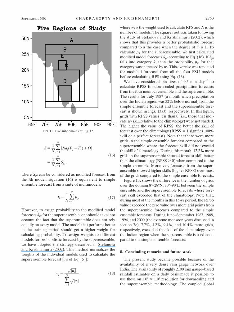
f. Forecast skills as a function of domain size fordownscaling

The question of seasonal rainfall forecasts improve-

ments, regionally as against ‘‘all India,’’ has been an

important unsolved problem (Gadgil and Kumar 2006).

Having noted a marked improvement of the seasonal

ETS over all-India from downscaled superensemble we

ask the pertinent question about the regional skills by

examining a successive sequence of smaller and smaller

subdomains. These are arbitrarily selected to cover the

following domains (Fig. 11, right panel): A (88–288N,

708–908E), B (108–258N, 708–858E), C (108–208N, 738–

838E), D (108–158N, 758–808E), and E (208–238N, 758–

788E). A comparison of month 2 of forecasts for July

from the ensemble mean and the superensemble with

the observed IMD rains are presented in Fig. 12. Here

we present the precipitation totals separately over the

selected five regions during July 1987–2001. The corre-

lation and RMS error of forecasted time series with the

observation are indicated inside the respective panels.

The rainfall totals of the member models is reflected

in the ensemble mean that shows a general degradation

in the seasonal rainfall forecast as the domain of eval-

uation is reduced in size. However, the most striking

result here is that there is much less degradation of re-

sults as a function of the domain size from the down-

scaled multimodel superensemble. This is a promising

result for the future possibilities for regional prediction

FIG. 9. As in Fig. 8, but for June–September 1994 (wet year) and 2000 (dry year).

SEPTEMBER 2009 C H A K R A B O R T Y A N D K R I S H N A M U R T I 2751

of seasonal rainfall from the use of downscaling and the

superensemble algorithm.

g. Ranked probability skill score

The ranked probability skill score (RPSS) measures

forecast skill relative to the climatology. RPSS is defined

as (Hamill et al. 2004)

RPSS 5 1� RPS

RPSref

, (12)

where RPS and RPSref are ranked probability scores

(RPS) of the actual forecast and a reference forecast,

respectively. In this study, we have taken the reference

forecast as the climatology. RPS is defined as

RPS 51

M � 1�M

m51�m

k51p

k��

m

k51o

k

!2

, (13)

where M is the number of different forecast categories

or bins (e.g., 0.0–0.5, 0.5–1.0, . . ., 49.5–50.0 mm day21),

pk is the forecasted probability in category k, and ok

equals 1 (0) if the observation falls (does not fall) into

category k. RPS measures the skill of an ensemble

forecast to be within the category of the observation.

Valid values of RPS vary from 0 to 1, with 0 signifying

perfect skill and 1 signifying no skill. If there are N

number of models in an ensemble (N 5 4 for this study)

then the expression for pk can be written as

pk

5 �N

i51w

id(F

i), (14)

where wi is weight for the ith model, Fi is forecast from

the ith model, and d(Fi) is a delta function given by

d(Fi) 5

1, if Fi2 k;

0, otherwise.

�

(15)

The value of wi equals 1/N for a simple ensemble fore-

cast that relies equally on every model.

Although the superensemble provides the determinis-

tic forecast, it was shown by Stefanova and Krishnamurti

(2002) that the superensemble carries an equivalent

probabilistic forecast as well. The expression for the su-

perensemble forecast [Eq. (5)] can be rewritten as

FIG. 10. Precipitation anomaly during June–September (a) 1987 (dry year), (b) 1988 (wet year), (c) 1994 (wet year),

and (d) 2000 (dry year) over the subregions shown in Figs. 8 and 9 from the IMD observation (Obs), the ensemble

mean (EM), and the superensemble (SE) forecasts.

2752 M O N T H L Y W E A T H E R R E V I E W VOLUME 137

S 51

N�N

i51[Na

i(F

i� F

i) 1 O]

51

N�N

i51S

pi,

(16)

where Spi can be considered as modified forecast from

the ith model. Equation (16) is equivalent to simple

ensemble forecast from a suite of multimodels:

E 51

N�N

i51F

i. (17)

However, to assign probability to the modified model

forecasts Spi for the superensemble, one should take into

account the fact that the superensemble does not rely

equally on every model. The model that performs better

in the training period should get a higher weight for

calculating probability. To assign weights to different

models for probabilistic forecast by the superensemble,

we have adopted the strategy described in Stefanova

and Krishnamurti (2002). This method normalizes the

weights of the individual models used to calculate the

superensemble forecast [ais of Eq. (5)]:

wi5

ffiffiffiffiffiffiffi

jaij

p

�N

i51

ffiffiffiffiffiffiffi

jaij

p

, (18)

where wi is the weight used to calculate RPS and N is the

number of models. The square root was taken following

the study of Stefanova and Krishnamurti (2002), which

shows that this provides a better probabilistic forecast

compared to a the case when the degree of ai is 1. To

calculate pk for the superensemble, we first calculated

modified model forecasts Spi according to Eq. (16). If Spi

falls into category k, then the probability pk for that

category was increased by wi. This exercise was repeated

for modified forecasts from all the four FSU models

before calculating RPS using Eq. (13).

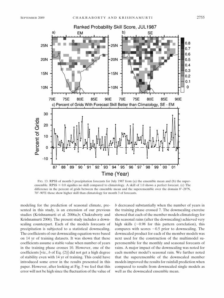
We have considered bin sizes of 0.5 mm day21 to

calculate RPSS for downscaled precipitation forecasts

from the four member ensemble and the superensemble.

The results for July 1987 (a month when precipitation

over the Indian region was 32% below normal) from the

simple ensemble forecast and the superensemble fore-

cast is shown in Figs. 13a,b, respectively. In this figure,

grids with RPSS values less than 0 (i.e., those that indi-

cate no skill relative to the climatology) were not shaded.

The higher the value of RPSS, the better the skill of

forecast over the climatology (RPSS 5 1 signifies 100%

skill or a perfect forecast). Note that there were more

grids in the simple ensemble forecast compared to the

superensemble where the forecast skill did not exceed

the skill of climatology. During this month, 12.2% more

grids in the superensemble showed forecast skill better

than the climatology (RPSS . 0) when compared to the

simple ensemble. Moreover, forecasts from the super-

ensemble showed higher skills (higher RPSS) over most

of the grids compared to the simple ensemble forecasts.

Figure 13c shows the difference in the number of grids

over the domain 88–288N, 708–908E between the simple

ensemble and the superensemble forecasts where fore-

cast skill exceeded that of the climatology. Note that,

during most of the months in this 15-yr period, the RPSS

value exceeded the zero value over more grid points from

the superensemble forecasts compared to the simple

ensemble forecasts. During June–September 1987, 1988,

1994, and 2000 (the extreme monsoon years discussed in

section 7e), 7.7%, 4.2%, 9.4%, and 10.4% more grids,

respectively, exceeded the skill of the climatology over

the Indian region when the superensemble is used com-

pared to the simple ensemble forecasts.

8. Concluding remarks and future work

The present study became possible because of the

availability of a very dense rain gauge network over

India. The availability of roughly 2100 rain gauge–based

rainfall estimates on a daily basis made it possible to

use these on 1.08 3 1.08 resolution for downscaling and

the superensemble methodology. The coupled global

FIG. 11. Five subdomains of Fig. 12.

SEPTEMBER 2009 C H A K R A B O R T Y A N D K R I S H N A M U R T I 2753

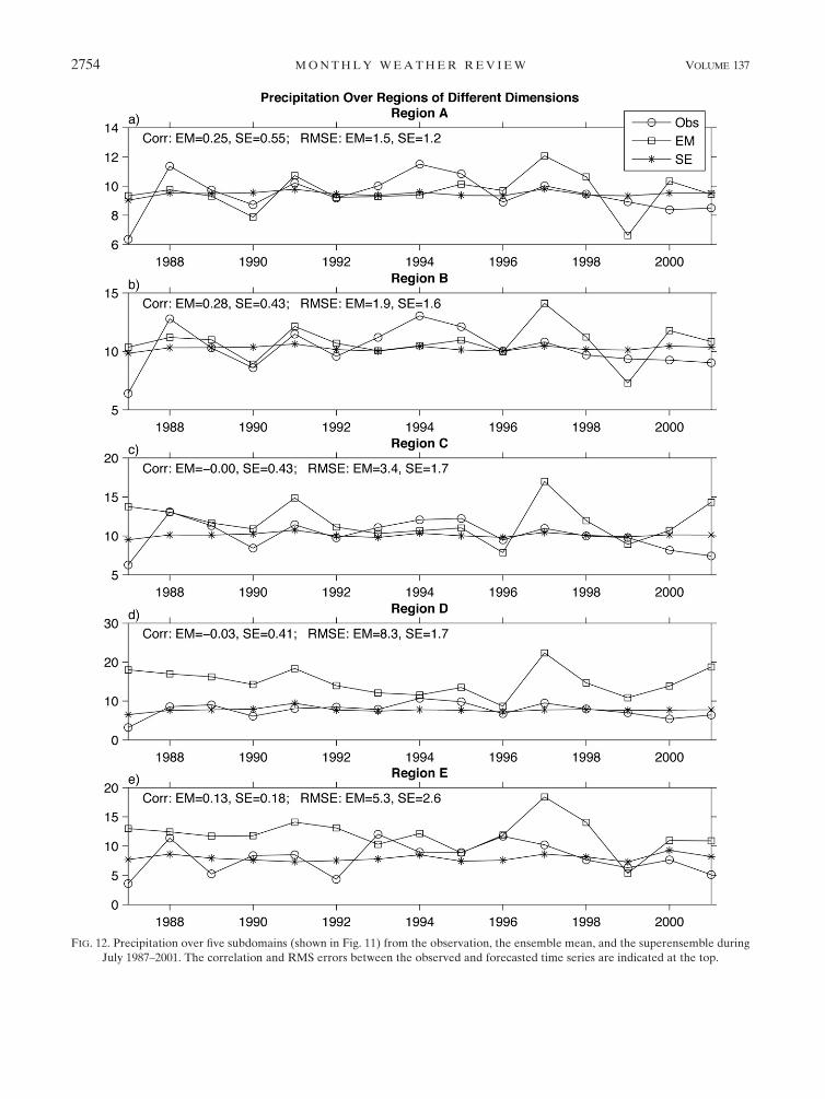
FIG. 12. Precipitation over five subdomains (shown in Fig. 11) from the observation, the ensemble mean, and the superensemble during

July 1987–2001. The correlation and RMS errors between the observed and forecasted time series are indicated at the top.

2754 M O N T H L Y W E A T H E R R E V I E W VOLUME 137

modeling for the prediction of seasonal climate, pre-

sented in this study, is an extension of our previous

studies (Krishnamurti et al. 2006a,b; Chakraborty and

Krishnamurti 2006). The present study includes a down-

scaling counterpart. Each of the models forecasts of

precipitation is subjected to a statistical downscaling.

The coefficients of our downscaling equation were based

on 14 yr of training datasets. It was shown that these

coefficients assume a stable value when number of years

in the training phase crosses 10. However, one of the

coefficients [viz., b of Eq. (2)] did not get a high degree

of stability even with 14 yr of training. This could have

introduced some error in the results presented in this

paper. However, after looking at Fig. 5 we feel that this

error will not be high since the fluctuation of the value of

b decreased substantially when the number of years in

the training phase crossed 7. The downscaling exercise

showed that each of the member models climatology for

the seasonal rains (after the downscaling) achieved very

high skills (;0.98 for this pattern correlation), this

compares with scores ;0.5 prior to downscaling. The

downscaled product for each of the member models was

next used for the construction of the multimodel su-

perensemble for the monthly and seasonal forecasts of

rains. A major impact of the downscaling was noted for

each member model’s seasonal rain. We further noted

that the superensemble of the downscaled member

models improved the results for rainfall prediction when

compared to results from downscaled single models as

well as the downscaled ensemble mean.

FIG. 13. RPSS of month-3 precipitation forecasts for July 1987 from (a) the ensemble mean and (b) the super-

ensemble. RPSS # 0.0 signifies no skill compared to climatology. A skill of 1.0 shows a perfect forecast. (c) The

difference in the percent of grids between the ensemble mean and the superensemble over the domain 88–288N,

708–908E those show higher skill than climatology for month 3 of forecasts.

SEPTEMBER 2009 C H A K R A B O R T Y A N D K R I S H N A M U R T I 2755

A measure of the level of improvement for the sea-

sonal precipitation forecasts is illustrated in Fig. 7. We

can see a vast improvement on the 1.08 3 1.08 latitude–

longitude resolution. In Fig. 1 we have seen that the

coarse-resolution (CMAP) and higher-resolution (IMD)

observed precipitation datasets are somewhat different

in their spatial patterns. This difference between the two

observed datasets can have some consequences when

coarse-resolution and downscaled model results are in-

tercompared. However, it is shown in the manuscript

that we get a huge improvement in the forecast skill with

the proposed downscaling methodology compared to the

coarse-resolution models. Therefore, it can be said that

the results presented in this manuscript are robust and

the improvement of forecast skill due to downscaling is

not dependent on the quality of the observed datasets.

The downscaling algorithm for each member model

corrects the slope and intercept of the rainfall history of

each model based on the training period. The slope is a

measure of the rate of increase of model rains as com-

pared to those of the observations. The intercept error is

an overall systematic underestimation or overestimation

of the model rains. These errors were corrected by our

downscaling algorithm. The use of multimodel super-

ensembles on these downscaled model precipitation esti-

mates further improves the skill of the forecast compared

to the individual models or their ensemble mean.

Although in this study we used only 15 yr of datasets,

there were 6 yr during this period when the precipitation

over the Indian region was far from normal. This includes

four extreme years [viz., 1987 (below normal), 1988

(above normal), 1994 (above normal), and 2000 (below

normal)]. We have shown, in this manuscript that during

these 4 yr the skill of the downscaled superensemble was

better than the corresponding ensemble mean forecast.

One of the limitations of this downscaling strategy could

be that it cannot capture the dynamically varying relation-

ship between the model output and observation that can

arise due to climate change. We plan to extend our meth-

odology in the future to be able to capture the observed

changes in the value of the parameters being downscaled.

Recently, a huge rain gauge–based precipitation data-

base is being compiled under the Asian Precipitation

Highly Resolved Observational Data Integration to-

wards Evaluation of Water Resources (APHRODITE)

project (Xie et al. 2007). This covers nearly 50 yr of daily

rainfall datasets. This covers the regions of the Asian

summer monsoon, the Middle East, and Africa. It would

be possible to expand the downscaling and the multi-

model superensemble forecasts of seasonal climate to

cover this entire domain. It would also be possible to

carry out the downscaling and the construction of the

superensemble using a site-specific (instead of grid point

based) downscaling and superensemble constructions.

Thus, these rain gauge sites would replace the grid points.

This approach calls for the interpolation of the model

output rains from their spectral transform grid locations

to these rain gauge locations, thereafter, the entire

downscaling and the superensemble would be carried out

at the rain gauge sites. This is worth exploring in the

context of seasonal climate forecasts at high resolution.

REFERENCES

Anandhi, A., V. V. Srinivas, R. S. Nanjundiah, and D. N. Kumar,

2008: Downscaling precipitation to a river basin in India for

IPCC SRES scenarios using the support vector machine. Int.

J. Climatol., 28, 401–420.

Anthes, R. A., 1977: A cumulus parameterization scheme utilizing a

one-dimensional cloud model. Mon. Wea. Rev., 105, 270–286.

Arakawa, A., and W. H. Schubert, 1974: Interaction of a cumulus

cloud ensemble with the large-scale environment, Part I.

J. Atmos. Sci., 31, 674–701.

Brankovic, C., and T. N. Palmer, 1997: Atmospheric seasonal

predictability and estimates of ensemble size. Mon. Wea. Rev.,

125, 859–874.

——, ——, F. Molenti, S. Tibaldi, and U. Cubasch, 1990: Extended

range predictions with ECMWF models: Time lagged en-

semble forecasting. Quart. J. Roy. Meteor. Soc., 116, 867–912.

Chakraborty, A., and T. N. Krishnamurti, 2006: Improved seasonal

climate forecasts of the south Asian summer monsoon using

a suite of 13 coupled ocean–atmosphere models. Mon. Wea.

Rev., 134, 1697–1721.

——, ——, and C. Gnanaseelan, 2007: Prediction of the diurnal

cycle using a multimodel superensemble. Part II: Clouds. Mon.

Wea. Rev., 135, 4097–4116.

Chang, C. P., Ed., 2004: East Asian Monsoon. World Scientific, 564 pp.

——, and T. N. Krishnamurti, Eds., 1987: Monsoon Meteorology.

Oxford University Press, 560 pp.

——, B. Wang, and N.-C. G. Lau, 2005: The global monsoon sys-

tem: Research and forecast. World Meteorological Organi-

zation, WMO/TD 1266, 28 pp.

Deque, M., 1997: Ensemble size for numerical seasonal forecasts.

Tellus, 49A, 74–78.

Gadgil, S., and K. R. Kumar, 2006: Agriculture and economy. The

Asian Monsoon, B. Wang, Ed., Springer-Verlag, 203–257.

Gowariker, V., V. Thapliyal, S. M. Kulshrestha, G. S. Mandal,

N. Sen Roy, and D. R. Sikka, 1991: A power regression model

for long range forecast of southwest monsoon rainfall over

India. Mausam, 42, 125–130.

Grell, G. A., 1993: Prognostic evaluation of assumptions used by

cumulus parameterization. Mon. Wea. Rev., 121, 764–787.

Hamill, T. M., J. S. Whitaker, and X. Wei, 2004: Ensemble refore-

casting: Improving medium-range forecast skill using retro-

spective forecasts. Mon. Wea. Rev., 132, 1434–1447.

Ji, Y., and A. D. Vernekar, 1997: Simulation of the Asian summer

monsoons of 1987 and 1988 with a regional model nested in a

global GCM. J. Climate, 10, 1965–1979.

Krishnamurti, T. N., and H. S. Bedi, 1988: Cumulus parameteri-

zation and rainfall rates: Part III. Mon. Wea. Rev., 116, 583–599.

——, and J. Sanjay, 2003: A new approach to the cumulus pa-

rameterization issue. Tellus, 55, 275–300.

——, Y. Ramanathan, H. L. Pan, R. J. Pasch, and J. Molinary, 1980:

Cumulus parameterization and rainfall rates: Part I. Mon.

Wea. Rev., 108, 465–472.

2756 M O N T H L Y W E A T H E R R E V I E W VOLUME 137

——, J. Xue, H. S. Bedi, K. Ingles, and D. Oosterhof, 1991: Physical

initialization for numerical weather prediction over the

tropics. Tellus, 43, 53–81.

——, C. M. Kishtawal, T. E. LaRow, D. R. Bachiochi, Z. Zhang,

C. E. Williford, S. Gadgil, and S. Surendran, 1999: Improved

weather and seasonal climate forecasts from multimodel su-

perensemble. Science, 285, 1548–1550.

——, D. Bachiochi, T. LaRow, B. Jha, M. Tewari, D. Chakraborty,

R. Correa-Torres, and D. Oosterhof, 2000a: Coupled

atmosphere–ocean modeling of the El Nino of 1997–98.

J. Climate, 13, 2428–2459.

——, C. M. Kishtawal, Z. Zhang, T. E. LaRow, D. R. Bachiochi,

C. E. Williford, S. Gadgil, and S. Surendran, 2000b: Multi-

model superensemble forecasts for weather and seasonal cli-

mate. J. Climate, 13, 4196–4216.

——, L. Stefanova, A. Chakraborty, T. S. V. V. Kumar, S. Cocke,

D. Bachiochi, and B. Mackey, 2002: Seasonal forecasts of

precipitation anomalies for North American and Asian mon-

soons. J. Meteor. Soc. Japan, 80, 1415–1426.

——, A. Chakraborty, R. Krishnamurti, W. K. Dewar, and

C. A. Clayson, 2006a: Seasonal prediction of sea surface tem-

perature anomalies using a suite of 13 coupled atmosphere–

ocean models. J. Climate, 19, 6069–6088.

——, A. K. Mitra, W.-T. Yun, and T. S. V. V. Kumar, 2006b:

Seasonal climate forecasts of the Asian monsoon using mul-

tiple coupled models. Tellus, 58A, 487–507.

——, A. K. Mishra, A. Chakraborty, and M. Rajeevan, 2009: Im-

proving global model precipitation forecasts over India using

downscaling and the FSU superensemble. Part I: 1–5-day

forecasts. Mon. Wea. Rev., 137, 2713–2735.

Kumar, K. K., M. Hoerling, and B. Rajagopalan, 2005: Advancing

dynamical prediction of Indian monsoon rainfall. Geophys.

Res. Lett., 32, L08704, doi:10.1029/2004GL021979.

Kummerow, C., W. Barnes, T. Kozu, J. Shiue, and J. Simpson, 1998:

The Tropical Rainfall Measuring Mission (TRMM) sensor

package. J. Atmos. Oceanic Technol., 15, 809–817.

Larow, T. E., and T. N. Krishnamurti, 1998: Initial conditions and

ENSO prediction using a coupled ocean-atmosphere model.

Tellus, 50, 76–94.

Misra, V., and M. Kanamitsu, 2004: Anomaly nesting: A meth-

odology to downscale seasonal climate simulations from

AGCMs. J. Climate, 17, 3249–3262.

Palmer, T. N., and Coauthors, 2004: Development of a European

Multimodel Ensemble System for Seasonal to Interannual

Prediction (DEMETER). Bull. Amer. Meteor. Soc., 85,853–872.

Peng, P., A. Kumar, A. H. van den Dool, and A. G. Barnston, 2002:

An analysis of multimodel ensemble predictions for seasonal

climate anomalies. J. Geophys. Res., 107, 4710, doi:10.1029/

2002JD002712.

Rajagopalan, B., U. Lall, and S. Zebiak, 2002: Categorical climate

forecasts through regularization and optimal combination of

multiple GCM ensembles. Mon. Wea. Rev., 130, 1792–1811.

Rajeevan, M., D. S. Pai, S. K. Dikshit, and R. R. Kelkar, 2004:

IMD’s new operational models for long-range forecast of

southwest monsoon rainfall over India and their verification

for 2003. Curr. Sci., 86, 422–431.

——, J. Bhate, J. Kale, and B. Lal, 2006: High resolution daily

gridded rainfall data for the Indian region: Analysis of break

and active monsoon spells. Curr. Sci., 91, 296–306.

Regonda, S. K., B. Rajagopalan, and M. Clark, 2006: A new

method to produce categorical streamflow forecasts. Water

Resour. Res., 42, W09501, doi:10.1029/2006WR004984.

Reynolds, R. W., and T. M. Smith, 1994: Improved global sea

surface temperature analysis using optimum interpolation.

J. Climate, 7, 929–948.

Rogers, E., T. Black, D. Deaven, G. DiMego, Q. Zhao,

M. Baldwin, N. Junker, and Y. Lin, 1996: Changes to the op-

erational early ETA analysis/forecast system at the National

Centers for Environmental Prediction. Wea. Forecasting, 11,

391–413.

Shepard, D., 1968: A two-dimensional interpolation function for

irregularly spaced data. Proc. 1968 ACM National Conf.,

Princeton, NJ, ACM, 517–524.

Sperber, K. R., and T. N. Palmer, 1996: Interannual tropical rain-

fall variability in general circulation model simulations asso-

ciated with the Atmospheric Model Intercomparison Project.

J. Climate, 9, 2727–2750.

Stefanova, L., and T. N. Krishnamurti, 2002: Interpretation of

seasonal climate forecast using Brier skill score, FSU super-

ensemble, and the AMIP-I dataset. J. Climate, 15, 537–544.

Stephenson, D. B., C. A. S. Coelho, F. J. Doblas-Reyes, and

M. Balmaseda, 2005: Forecast assimilation: A unified frame-

work for the combination of multi-model weather and climate

predictions. Tellus, 57, 253–264.

Thapliyal, V., and S. M. Kulshrestha, 1992: Recent models for long-

range forecasting of south–west monsoon rainfall over India.

Mausam, 43, 239–248.

Tripathi, S., V. V. Srinivas, and R. S. Nanjundiah, 2006: Down-

scaling of precipitation for climate change scenarios: A sup-

port vector machine approach. J. Hydrol., 330, 621–640.

Vernekar, A. D., and Y. Ji, 1999: Simulation of the onset and in-

traseasonal variability of two contrasting summer monsoons.

J. Climate, 12, 1707–1725.

Walker, G. T., 1923: Correlation in seasonal variations of weather.

VIII: A preliminary study of world weather. IMD Memo.

XXIII, Part IV, 75–131.

——, 1924: Correlation in seasonal variations of weather. IX: A

further study of world weather. IMD Memo. XXIV, Part IX,

75–131.

Wang, B., Ed., 2006: The Asian Monsoon. Springer-Verlag, 844 pp.

——, Q. Ding, X. Fu, I.-S. Kang, K. Jin, J. Shukla, and F. Doblas-

Reyes, 2005: Fundamental challenge in simulation and pre-

diction of summer monsoon rainfall. Geophys. Res. Lett., 32,

L15711, doi:10.1029/2005Gl022734.

Wolff, J.-O., E. Maier-Reimer, and S. Legutke, 1997: The Hamburg

Ocean Primitive Equation Model HOPE. DKRZ Tech. Rep.

13, Modellberatungsgruppe, 98 pp.

Xie, P., and P. A. Arkin, 1997: A 17-year monthly analysis based on

gauge observations, satellite estimates, and numerical model

outputs. Bull. Amer. Meteor. Soc., 78, 2539–2558.

——, M. Chen, S. Yang, A. Yatagai, T. Hayasaka, Y. Fukushima,

and C. Liu, 2007: A gauge-based analysis of daily precipitation

over East Asia. J. Hydrometeor., 8, 607–626.

Yang, X.-Q., and J. L. Anderson, 2000: Correction of systematic

errors in coupled GCM forecasts. J. Climate, 13, 2072–2085.

Yun, W.-T., L. Stefanova, A. K. Mitra, T. S. V. V. Kumar,

W. Dewar, and T. N. Krishnamurti, 2005: Multimodel syn-

thetic superensemble algorithm for seasonal climate predic-

tion using DEMETER forecasts. Tellus, 57, 280–289.

SEPTEMBER 2009 C H A K R A B O R T Y A N D K R I S H N A M U R T I 2757