INTERNATIONAL JOURNAL OF CLIMATOLOGY

Int. J. Climatol. 24: 161–180 (2004)

Published online in Wiley InterScience (www.interscience.wiley.com). DOI: 10.1002/joc.997

A STATISTICAL DOWNSCALING METHOD FOR MONTHLY TOTALPRECIPITATION OVER TURKEY

HASAN TATLI,a,* H. NUZHET DALFES b and S SIBEL MENTESa

a Meteorology Department, Istanbul Technical University, Maslak, 34469 Istanbul, Turkeyb Eurasia Institute of Earth Sciences, Istanbul Technical University, Maslak, 34469 Istanbul, Turkey

Received 10 August 2003Revised 12 November 2003

Accepted 12 November 2003

ABSTRACT

Researchers are aware of certain types of problems that arise when modelling interconnections between general circulationand regional processes, such as prediction of regional, local-scale climate variables from large-scale processes, e.g. bymeans of general circulation model (GCM) outputs. The problem solution is called downscaling. In this paper, a statisticaldownscaling approach to monthly total precipitation over Turkey, which is an integral part of system identificationfor analysis of local-scale climate variables, is investigated. Based on perfect prognosis, a new computationallyeffective working method is introduced by the proper predictors selected from the National Centers for EnvironmentalPrediction–National Center for Atmospheric Research reanalysis data sets, which are simulated as perfectly as possibleby GCMs during the period of 1961–98. The Sampson correlation ratio is used to determine the relationships betweenthe monthly total precipitation series and the set of large-scale processes (namely 500 hPa geopotential heights, 700 hPageopotential heights, sea-level pressures, 500 hPa vertical pressure velocities and 500–1000 hPa geopotential thicknesses).In the study, statistical preprocessing is implemented by independent component analysis rather than principal componentanalysis or principal factor analysis. The proposed downscaling method originates from a recurrent neural network modelof Jordan that uses not only large-scale predictors, but also the previous states of the relevant local-scale variables. Finally,some possible improvements and suggestions for further study are mentioned. Copyright 2004 Royal MeteorologicalSociety.

KEY WORDS: independent component analysis; precipitation; recurrent neural networks; sampson correlation; statistical downscaling;Turkey

1. INTRODUCTION

The introduction of the concept of downscaling has opened a wide spectrum of applications in many fields(e.g. Klein, 1982; Kim et al., 1984; Wilks, 1989; Karl et al., 1990; Wigley et al., 1990; Giorgi and Mearns,1991; Zorita et al., 1992; von Storch et al., 1993; Bardossy, 1994; Matyasovsky et al., 1994; Noguer, 1994;von Storch, 1995; Cubasch et al., 1996; Hewitson and Crane, 1996; Schubert and Henderson-Sellers, 1997;Conway and Jones, 1998; Heimann and Sept, 1998; Kidson and Thomson, 1998; Murphy, 1999, 2000; Sailorand Li, 1999; Smith, 1999; von Storch and Zwiers, 1999; Fuentes and Heimann, 2000; Wilby and Wigley,2000; Stein et al., 2001; Watson, 2002; Geerts, 2003). The logic behind downscaling and representation ofregional climate in nested models (known as dynamical downscaling) may be found in Giorgi and Mearns(1991) and McGregor et al. (1993; McGregor, 1997).

In those studies, the methods, large-scale predictors and local-scale predictands were various. For example,in the work of Kim et al. (1984) the predictors were large-scale monthly mean temperature and precipitation.On other hand, monthly surface temperature and precipitation were selected as local-scale predictors. The

∗ Correspondence to: Hasan Tatlı, Aeronautics and Astronautics Faculty, Meteorology Department, Istanbul Technical University,Maslak, 34469 Istanbul, Turkey; e-mail: tatli@itu.edu.tr

Copyright 2004 Royal Meteorological Society

162 H. TATLI, H. NUZHET DALFES AND S. SIBEL MENTES

methods they applied were principal component analysis (PCA) and linear regression. For downscaling Iberianwinter precipitation, Zorita et al. (1992) and von Storch et al. (1993) selected gridded North Atlantic sea-level pressure (SLP) as a large-scale predictor, and the downscaling method was simple regression based oncanonical correlation analysis (CCA). The other very interesting application is the work of Heimann and Sept(1998), who employed both statistical and dynamical downscaling techniques in order to analyse the climaticchange of summer temperature and precipitation in the Alpine region.

Statistical downscaling methods may be sorted into three groups: model output statistics (predictorsfrom global circulation models (GCMs)); perfect prognosis (predictors from large-scale free atmosphericobservations or free atmospheric reanalysis data sets); and, downscaling with surface variables (predictorsfrom large-scale surface observations).

Perfect prognosis, based on multivariate regression, is gaining considerable acceptance in downscaling ofGCMs in view of its inherent simplicity and flexibility. This technique provides an external description ofthe system under study and leads to a parsimonious representation of the process. The accurate determinationof the predictors is a necessary first step in downscaling, and this continues to be a subject of extensivecontemporary research. A literature review reveals that many statistical methods are available for findingthe relations between large-scale predictors and local-scale predictands (von Storch and Zwiers, 1999). Theselection of a reliable and efficient criterion has been elusive, since most criteria are sensitive to the statisticalproperties of the processes. Validation of most of the available criteria has generally been through simulatedGCMs. More precisely, in the traditional methods, downscaling of surface variables from large-scale processesis thought of as a static map (regression equation). However, the unsolved problem is that the downscalingprocess has to satisfy constraints. These constraints can be seen as ‘mathematical objects used to make explicitthe logic behind of the downscaling problem’. In this study, the constraints of the downscaling process aresummarized thus:

1. The key assumption is that there is growing evidence of local-scale patterns being driven by large-scaleclimatic fluctuations.

2. Classical, linear methods may be inappropriate for downscaling local-scale processes from large-scaleprocesses. Here, we consider the local-scale observations as the outcome of a finite-dimensional, nonlineardynamical system and use recurrent neural networks to recover the nonlinear, ‘causal and naıve skeleton’of the underlying static relations and dynamics from the large-scale processes and the previous states ofthe system.

Based on these constraints, the model is not thought of as a curve-fitting problem. Rather, the statisticalmodel must satisfy the probability assumptions, e.g. homogeneity of dependence is the first requirement indistinguishing a model from the curve-fitting transformation.

For example, predictions of the local variables from large-scale processes by well-known linear timeseries techniques (Bras and Rodriguez-Iturbe, 1993; Box et al., 1994; Hipel and Mcleod 1994; von Storchand Zwiers, 1999), such as autoregressive (AR) and autoregressive moving average (ARMA) techniques, arepossible ways in modelling to satisfy ‘locality features’. On the other hand, to predict the same local processesfrom large-scale processes by means of regression equations is another possible approach (based on staticrelations). However, this paper suggests a method of combining these two approaches.

Since the suggested method offers a statistical model, the predictors should be independent in the sense ofthe statistical framework. Details are given in the following sections, but instead of the PCA (also known asempirical orthogonal functions in meteorology literature), which is based on second-order statistics (Diaz andFulbright, 1981; Preisendorfer, 1988), a new method known as independent component analysis (ICA) basedon high-order statistics is employed (Jutten and Herault, 1991; Comon, 1994; Everson and Roberts, 1999;Hyvarinen et al., 2001).

A number of studies regarding the spatial and temporal properties of precipitation or rainfall in Turkey havebeen published (Kutiel et al., 1996, 2001; Turkes 1996, 1998; Kadıoslu, 2000; Turkes et al., 2002; Touchanet al., 2003). However, this paper is the first study regarding statistical downscaling of local variables inTurkey. In this paper, the monthly total precipitation data of 31 stations have been selected as an application

Copyright 2004 Royal Meteorological Society Int. J. Climatol. 24: 161–180 (2004)

STATISTICAL DOWNSCALING OF TURKISH RAINFALL 163

of the proposed approach. It is demonstrated that the proposed method can suppress well the increase of thedownscaling error due to nonlinearities, improving greatly the accuracy of the downscaling compared withthe conventional regression-based techniques.

In Section 2, the features of the precipitation climate of Turkey are summarized. In Section 3, the proposedmethod is described in detail: a new idea in statistical downscaling techniques is discussed along with analgorithm; it represents the main ideas behind the proposed method. In the same section, we also brieflydiscuss the concept of ICA, which is then used in Section 4 to build a downscaling model for monthly totalprecipitation series over Turkey. Some comments and conclusions are provided in Section 5.

2. A GENERAL LOOK AT THE PRECIPITATION CLIMATE OF TURKEY

In general terms, Turkey is associated with a subtropical climatic regime that is referred to as Mediterranean.Because of its geographic location, the air masses that shape the weather regimes affecting Turkey have bothpolar and tropical origins, which are dominant in the winter and summer respectively. During the autumnsand winters, polar fronts have a determining effect on the mid-latitudes.

Large-scale atmospheric motions are translated into local weather conditions due to different landcharacteristics. These local conditions have both thermal and dynamical features. On the other hand, thedifferent local conditions have sparse local-climate features due to the land–sea distribution, elevation andsuch other local physical–geographical properties that make those macro-climate features highly variable.Turkey (despite being surrounded by the sea on three sides), because of its coastal regions characterized byhigh topography, includes a rather large inland area (central Anatolia) that has a quite continental climatecharacter (Taha et al., 1981; Erinc, 1984; Kadıoglu, 2000). The topography causes strong variations in theclimate. The coastal sides of the mountains receive heavy precipitation, but there are also thermal effects dueto topographic height differences coupled with other factors.

Summer. Since the maritime-polar (MP) and continental-polar (CP) air masses move towards northernregions, the tropical air masses have a dominant effect on mid-latitudes in this season. The southern andsoutheastern parts of the country are under the influence of a continental tropical air mass (due to the Arabiclow) which is quite dry. The marine air mass that travels from the Atlantic towards Turkey (a northwesterlymotion) gets heated and loses most of its relative humidity during its passage across the mainland andpresents a stable structure. The Azores high-pressure centre locates over Europe during its northward andeastward displacement, and this situation affects the characteristic motions, especially for the western parts ofTurkey. The interaction between the marine and continental systems causes strong winds, especially during theJune–August period. Both these air masses have stable structures characterized by hot and dry conditions, andcloudless summers are quite typical for Turkey. Exceptions do occur, as sometimes the western, and especiallynorthwestern, parts of the country get heavy precipitation. The precipitation is the result of frontal systemsforming as the Atlantic polar marine air mass interacts with the tropical marine air mass. The northern partof the country, having high topography along the Black Sea coast, also experiences some heavy precipitationof orographic origin. In the west, the mountains are not parallel to the coast; as a result, the orographicprecipitation has a more local character. The mountains also divert the air flow in various ways, causingcentral Turkey to possess a peculiar wind regime.

Winter. The Mediterranean basin, which includes all the European countries having a coast on theMediterranean, becomes an active frontogenesis region at the beginning of autumn. The Azores high shifts tothe south and the Siberian high-pressure system starts to affect northern and eastern Europe (due to thermalreasons); the Mediterranean belt becomes a convergence zone. The frontal systems that travel along varioustrajectories towards the east affect Turkey. These cyclonic depressions have two main paths across Turkey.The first affects the western and southern parts of the country and then continues towards the southeasternparts. The second has a trajectory towards the northeast and is the cause of most of the precipitation in thenorthwestern, northern and central parts of the country.

The other trajectory of the polar front that affects Turkey is felt when the Azores high becomes strong enoughto affect western Europe. When this comes onto the scene the depressions travel from the Thrace–Marmara

Copyright 2004 Royal Meteorological Society Int. J. Climatol. 24: 161–180 (2004)

164 H. TATLI, H. NUZHET DALFES AND S. SIBEL MENTES

and western part of the Black Sea region towards southeastern Turkey by northerly and northwesterly flows;most of Turkey is affected by those motions. The effect is more pronounced when the mechanisms related tothe Azores high create northerly and northwesterly winds over the Anatolian Plateau.

The principal effects of the Mediterranean cyclones on Turkey are southwesterly winds on the TurkishMediterranean coast. Topography creates important local effects in the western and Black Sea coasts ofTurkey: the seaward sides of the mountains are washed by heavy precipitation and the precipitation decreasestowards the inner parts of Asia Minor. There exists a very sharp negative orographic precipitation gradientfrom the coastal regions towards central Anatolia. In central Anatolia, there is a plateau effect rather than asharp topography effect.

During the winter, a convergence zone also forms in the eastern part of the Black Sea. This is a consequenceof the interaction between the northerly currents created by the Asian high (Siberian high) and the localsoutherly currents created by the small-scale high-pressure centres due to thermal effects in eastern Anatolia.Foehn winds and rain shadows are, therefore, common in this region during cold, winter periods. In thewinter the passage of the fronts and related cyclones causes precipitation in the coastal regions, but centraland eastern Anatolia remain largely continental in terms of climatic features and become a divergence field.During the spring, depressions gradually decrease over Turkey, due to the heating of the land surface and thedepression frequencies reaching a minimum during the summer (Tatlı et al., 2003). The depressions that areseen during the summer mainly affect the northern part of the Marmara region and over the Black Sea coast.Spring and summer are seasons that are dominated mainly by local effects. The mountains that run parallel tothe Black Sea coast of Turkey prevent the northerly currents from penetrating inland. However, the situationin the west is different, as the mountains run perpendicular to the coast, so they cannot block the westerlycurrents very effectively, and Mediterranean depressions penetrate into the mid-western parts of the countrythrough the gaps between these mountains.

3. METHODS

A key assumption that constitutes the foundation of downscaling is that local climate is controlled by large-scale processes. For simplicity, consider first the case of two different multivariate random variables: Xoriginates from large-scale physical processes (such as a large-scale SLP series) and Y represents localvariables (could be surface precipitation series). Mathematically, the statistical downscaling may be definedin terms a multivariate regression equation. The multivariate random variables X and Y are said to be dependentif and only if

Y (t) = F [X (t)] + e(t) (1)

exists, where F is an operator to be determined and e(t) is the multivariate error term. In other words, the jointprobability density P(X , Y ) cannot be factorized into a product of their marginal densities P(X ) and P(Y ).In practice, the probability densities are generally unknown. Therefore, particularly to distinguish betweenpredictor and predictand variables, some generalization of the multiple correlation coefficients may be of use.One such possibility, according to Sampson (1984), is

RS =√

Tr(CYX C −1XX CXY )

Tr(CYY )(2)

where CXY , CXX and CYY indicate multivariate cross-covariance and covariance matrices and Tr denotesthe trace of the related matrices respectively. Another important special case of this approach concernsthe correlation between the multivariate X and Y, called CCA. CCA is a multivariate linear technique forportraying the relationship between multiple sets of multivariate data (Glahn, 1968; Nicholls, 1987; Chen et al.,1994; Chen and Chang, 1994), and it is based on symmetrical Pearson correlation. That is, CCA transformsthe predictors and predictands into new variables (canonical correlation variates: CCVs) by maximizing the

Copyright 2004 Royal Meteorological Society Int. J. Climatol. 24: 161–180 (2004)

STATISTICAL DOWNSCALING OF TURKISH RAINFALL 165

correlation between two CCVs. In words, CCA does not recognize predictor and predictand variables as inthe case of Sampson correlation (Jackson, 1991), because the correlation between predictors and predictandsmay not be symmetrical, i.e. correlation (X , Y )

?= correlation(Y, X).If we put a single grid time series of each large-scale variable (X is now a vector in Equation (2)) and

multiple stations’ time series set (Y is now a matrix in Equation (2)) in Equation (2), then the map of computedSampson correlations is termed the RS correlation pattern in this study. The interpretation of the RS patternsis similar to the canonical correlation patterns with respect to their statistical properties. Although there isonly one RS correlation pattern, CCA extracts a number up to the rank of {X , Y } correlation patterns (rank(X,Y) = min[rank(X), rank(Y)]).

Before model building, the application of statistical preprocessing of data sets is required (Rummukainen,1997). In the study, we employ ICA based on PCA, and followed by CCA. First, the data sets are decomposedinto their significant principal components (PCs) according to the maximum-likelihood criterion of Joreskopand Sorbom (1989); second, these uncorrelated PCs are transformed into independent components (ICs) bythe FastICA technique, which is an ICA approach of Hyvarinen and Oja (1997).

PCA and the closely related principal factor analysis techniques are widely applied in meteorology orclimatology literature. Without going into details, assume the first- and second-order statistics of a multivariateX is known or can be estimated from the sample. In PCA transform, the variables of X are centred bysubtracting their means, and then the covariance matrix of X is defined as the expected value of the minorproducts of its variables. In this paper, all matrices are organized such that rows represent simultaneousobservations and columns are observed variables at different sites.

SXX = E(X T X ) (3)

One has to keep in mind that PCs are not invariant under scaling. Without loss of generality, an orthogonaldecomposition of SXX is given as follows.

SXX = EX DX E TX (4)

where EX is a matrix of the orthonormal eigenvectors of SXX and D = diag(λ1, . . . , λk) is the diagonalmatrix of the eigenvalues of SXX in a decreasing magnitude order (Preisendorfer, 1988). The PCs are thencomputed by

VX = XE X (5)

where VX illustrates the PCs and the reconstruction of X follows

X = VX E TX (6)

The PCA model was discussed above as a distribution-free method with no underlying statistical model, butin the case of principal factor analysis (FA) the multivariate X is reconstructed as in the following:

X = FX AX + GX (7)

where FX and GX are called common factors (CFs; or latent variables) and white noise components (orspecific components), respectively. AX is called a factor loading, defined as

SXX = AX ATX = EX D1/2D1/2E T

X (8)

There are no statistical constraints on PCs, but CFs must be Gaussian in an FA model. Furthermore, PCsare easily calculated in a unique way, whereas there is no unique method for CFs; however, a possible wayaccording to Reyment and Joreskog (1993) is

FX = XS −1XX AT

X (9)

Copyright 2004 Royal Meteorological Society Int. J. Climatol. 24: 161–180 (2004)

166 H. TATLI, H. NUZHET DALFES AND S. SIBEL MENTES

The CFs may be rotated for easier interpretation of the patterns (Richman, 1985), e.g. by the varimax method(Kaiser, 1959).

On the other hand, ICA may be seen as a special kind of rotation of CFs (or PCs), but using high-orderstatistics rather the second-order statistics. If the data series have Gaussian density then FA and ICA areidentical, because the high-order statistics of Gaussian variables are all zero (assume the variables have zeromean and unit variance). ICA has been widely used in data analysis and decomposition in recent years (Juttenand Herault, 1991; Comon, 1994; Everson and Roberts, 1999; Hyvarinen et al., 2001). ICA typically aims tosolve the blind source separation problem in which a set of unknown sources is mixed in some way to formthe data. An ICA model assumes that the multivariate data set X is a mixing of the ICs as

X = SA (10)

or in terms of PCA as

S = XW = VX E TX W (11)

where A = W −1 is called mixing matrix, and S (like PCs or CFs) represents ICs, respectively. The startingpoint for ICA is the very simple assumption that all the ICs are statistically independent based on a non-Gaussian distribution. However, the basic model of ICA does not assume this distribution is known. Afterdetermining the matrix A, its inverse W is then computed to obtain the ICs by Equation (11) from PCs.

The restriction in a PCA is that all PCs are mutually uncorrelated, but the restriction in an ICA is that allthe ICs are statistically independent. Uncorrelatedness is a weaker form of independence. That is, two randomvariables are uncorrelated if their covariance is zero. On the other hand, if the variables are independent thenthey are uncorrelated, from which it follows that uncorrelatedness does not imply independence (Comon,1994). Let us define independency according to Hyvarinen et al. (2001). Two random variables y1 and y2

are said to be mutually independent if, given two arbitrary functions h1(y1) and h2(y2), they satisfy thefollowing condition:

E{h1(y1)h2(y2)} = E{h1(y1)}E{h2(y2)} (12)

where E represents the expected value. According to the definition of statistical independency, ICA has astronger definition than the uncorrelatedness concerning PCA. ICA uses high-order statistics and can separatethe data into true sources, unlike PCA or FA, and so guarantees true sources in data. In this study, the ICs arecomputed via a fixed-point algorithm called FastICA, introduced by Hyvarinen and Oja (1997). The FastICAalgorithm is based on maximizing the absolute value of kurtosis of the variable by using an ‘informationmeasure’ or negative of entropy:

J (y) = 1

12E{y3}2 + 1

48kurt(y)2 (13)

where J (y) ∈ [0, 1] indicates information measure, and the kurtosis of y is illustrated by kurt(y) defined as:

kurt(y) = E{y4} − 3(E{y2})2 (14)

Since the ‘information measure’ of Gaussian variables among equivalent variances is zero, the informationcan be used as an indicator of the measure of the degree of normality in the data series.

There are some basic ambiguities that hold in an ICA model:

1. The variances of ICs cannot be determined, whereas the variances are explained by eigenvalues of PCs(or CFs) in a PCA (or FA) approach.

2. The order of ICs cannot be determined.

Copyright 2004 Royal Meteorological Society Int. J. Climatol. 24: 161–180 (2004)

STATISTICAL DOWNSCALING OF TURKISH RAINFALL 167

A detailed introduction to ICA for practitioners may be found in Hyvarinen et al. (2001).A downscaling model may be divided into a naıve (e.g. AR, ARMA) and causal (e.g. regression)

components. One must distinguish between causal models and naıve models. A naıve model approach involvesusing only historical data. Thus, it assumes that the trend of the dependent variables, which in this studyare the monthly total precipitations, remains constant over time, and the value of the dependent variablesY(t + k), where t is the present month and k is the number of the month to predict, can be extrapolated fromhistorical data.

On the other hand, a causal model approach assumes that there are some (causal) variables (e.g. GCMoutputs) that are responsible for changes in the dependent variables. In the causal models, previous informationis available from GCMs; therefore, this information should be considered in the process of the model buildingfor downscaling purposes (i.e. a Bayesian approach).

Assuming now that �t illustrates the prediction time step and G is an unknown transformation (such asAR coefficients in an AR model), then prediction of the multivariate Y from its own finite countable previousstates can be illustrated as in the following:

Y (t + �t) = G[∑

Y (t − k�t)]

+ e(t) k = 0, 1 . . . , n (15)

Let Y1(t) and Y2(t) denote the outputs of the causal model and the naive model respectively, and in order todistinguish and separate the models. Assume that the static transformation (causal) is linear and the dynamicprediction model (naive) is first order (Richardson, 1981); then these two separated prediction models can bewritten as

Y1(t + �t) = A[X (t + �t)] (causal model) (16)

Y2(t + �t) = B [Y (t)](naıve model) (17)

where X(t) represents causal variables and, for simplification, we omit the error term e(t). The main problemarises in selecting the best outputs from these models. However, it is not clear which of the model outputs isimportant for local-scale processes, but one may propose a multivariate difference equation as in the following(Bras and Rodriguez-Iturbe, 1993):

Y (t) = M1[Y (t − �t)] + M2[X (t)] + M3[e(t)] (18)

where M1, M2 and M3 are linear operators and the vector e(t) consists of uncorrelated white noise. The vectorcovariance of e(t) is a diagonal matrix:

De = E(e(t)Te(t)) (19)

where E illustrates the expected value operator, which in practice is generally taken as the sample average.The definition of Equation (18) forms a possible way for accommodating the naive and the causal modelsinto a new model with linear structure. Meteorological or climate processes are generally expected to behavenonlinearly, whereas the process represented by Equation (18) has a linear static part and a linear dynamicpart; one can claim that it represents a linearization approximation. Therefore, Equation (18) may not beenough to satisfy the nonlinearity constraint. Hence, we develop here a more sophisticated approximateapproach for solving this problem. If the two downscaled sets from Equations (16) and (17) are combined asZ (t) = [Y1(t), Y2(t)], then the suggested model can be written as

Y (t) = M [H [Z (t)]] + e(t) (20)

where e(t) is the multivariate Gaussian noise. M is a linear operator in the case of Equation (1) and itpredicts local variables from the {H [Z (t)]} basis functions, and H is a nonlinear scalar function given byEquation (21) that can generate the basis functions. So we now have a new version of the downscaling method

Copyright 2004 Royal Meteorological Society Int. J. Climatol. 24: 161–180 (2004)

168 H. TATLI, H. NUZHET DALFES AND S. SIBEL MENTES

that constitutes both the knowledge from the static model of the causal large-scale variables in the case inEquation (16) and the knowledge from the first-order local linear dynamic model in the case of Equation (17).

However, the regression equation in Equation (16) may be applied as long as one assumes homogeneity inthe sets of predictors and predictands for which the regression is evaluated. Obviously, linear regression ofEquation (16) may not directly be applied due to heterogeneity, since heterogeneity may be introduced in thedependence. In this study, the ‘homogeneity of dependence’ is an assumption that describes the invariance ofthe relation (deterministic rule) between predictors and predictands. Hence, a method is proposed to solve thisproblem. First, using CCA, which may be seen as a classification of predictors and predictands, the significantCCVs are determined. Second, the so-called causal model is evaluated between these CCVs. In this study,CCA is employed after ICA where it has been briefly described in the paper.

Now we can determine the structure of the scalar function H. It should be nonlinear in its structure tosatisfy the constraint of nonlinearity. So, we transform Z(t) element by element to generate the basis variablesof the system in Equation (20) with one of a nonlinear H function (Equation (21)); thereafter, the degreesof problem may be reduced. Two such possible nonlinear functions from neural network applications are(Connor et al., 1994; Haykin, 1999, 2001):

H1(y) = tan h(αy)

H2(y) = 11 + exp(−αy)

}(21)

where α is a scalar constant. The proposed method algorithm stages are summarized in Table I, and a flowchart diagram that describes the model components is also shown in Figure 1. The proposed approach is,indeed, an originating form of a recurrent neural network (RNN) model (Jordan, 1986; Elman, 1990; Robinsonand Fallside, 1991; Puskorius and Feldkamp, 1994; Connor et al., 1994; Pearlmutter, 1995; Haykin, 1999,2001; Hochreiter et al., 2001). In the conventional RNN models, the training process is based on minimizingthe variance of the error between estimated and observed values. Hence, the structure of an RNN is sensitiveto the dynamics of the process. The RNN model of Jordan (1986) can be represented as

Z (t + �t) = H [M1Y (t) + M2X (t + �t)]Y (t + �t) = M3Z (t + �t)

}(22)

where H is a nonlinear scalar function defined in Equation (21), Z illustrates the states of the system (outputsof hidden neurons), and M1, M2 and M3 are linear operators. In the proposed RNN, the initial weights (as givenby M1 and M2 in Equation (22)) between inputs and hidden neurons are selected as A given in Equation (16)and as B given in Equation (17). If the initial weights are selected randomly, then the conventional RNN may

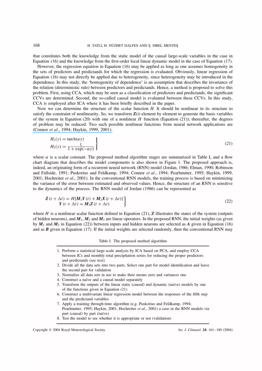
Table I. The proposed method algorithm

1. Perform a statistical large-scale analysis by ICA based on PCA, and employ CCAbetween ICs and monthly total precipitation series for reducing the proper predictorsand predictands (see text)

2. Divide all the data sets into two parts. Select one part for model identification and leavethe second part for validation

3. Normalize all data sets in use to make their means zero and variances one4. Construct a naıve and a causal model separately5. Transform the outputs of the linear static (causal) and dynamic (naıve) models by one

of the functions given in Equation (21)6. Construct a multivariate linear regression model between the responses of the fifth step

and the predictand variables7. Apply a training through-time algorithm (e.g. Puskorius and Feldkamp, 1994;

Pearlmutter, 1995; Haykin, 2001; Hochreiter et al., 2001) a case in the RNN models viapart (causal) by part (naıve)

8. Test the model to see whether it is appropriate or not (validation)

Copyright 2004 Royal Meteorological Society Int. J. Climatol. 24: 161–180 (2004)

STATISTICAL DOWNSCALING OF TURKISH RAINFALL 169

Feed Back

Basis Functions

PCA

ICA

PCs

ICs

CCVs

CCVsRNN

Statistical Preprocessing

CCA

Large-scale

Causal Model

(Eq.16)

Validation

Y (t )

Y (t )

Z (t )

Y1 (t )

Y2 (t )

X (t )

X (t )

Y (t−1)

Y (t−1)

Local-scale

Naive Model (Eq.17)

Linear Model

Figure 1. The flow chart of the components in the proposed downscaling approach

capture only the dynamical features of the local-scale process. To solve this problem, the training processis employed part by part. The elements of A (naıve) are kept constant while updating the elements of B(causal); similarly, the elements of A are updated while keeping constant the elements of recently updated B.Consequently, the proposed RNN can satisfy not only the nonlinearity, such as in the case of a conventionalRNN; it also satisfies and distinguishes the naıve and the causal relationships (linear or nonlinear). In thispaper, the well-known training process algorithms of RNN are not described, but one may, find the effectivealgorithms in Puskorius and Feldkamp (1994), Pearlmutter (1995), Haykin (2001) and Hochreiter et al. (2001),for example.

4. RESULTS

The basic data consists of monthly total precipitation of 31 stations over Turkey (Table II) with a recordlength of 38 years, during the period 1961–98. The weather stations selected have no missing data in theprescribed period, and represent the characteristics of precipitation of Turkey.

In order to perform a successful statistical large-scale analysis (Rummukainen, 1997), National Centersfor Environmental Prediction–National Center for Atmospheric (NCEP–NCAR) reanalysis data sets (Kalnayet al., 1996) are used between 10–50 °E and 30–60 °N, since this area is large enough to represent the large-scale climate or synoptic features that affect the monthly total precipitation series over Turkey. The followinglarge-scale data sets from NCEP–NCAR reanalysis data sets were used as predictors in this study:

1. The interactions of long (Rossby) and short waves are identified at the 500 hPa level. At this level, the longwaves generally show a barotropic character, whereas the short waves are baroclinic. Therefore, the shortwaves at this level have determining effects on the development of surface cyclonic and anticyclonicsystems. The cyclonic and anticyclonic vorticity at all high levels is a result of the interactions ofshort waves of high-level currents and surface systems. As a consequence of these arguments, 500 hPageopotential heights are considered as predictors.

Copyright 2004 Royal Meteorological Society Int. J. Climatol. 24: 161–180 (2004)

170 H. TATLI, H. NUZHET DALFES AND S. SIBEL MENTES

Table II. The stations of Turkey used in the application

Station name Latitude(°N)

Longitude(°E)

Internationalstation number

Zonguldak 41.27 31.48 17 022Sinop 42.01 35.10 17 026Samsun 41.17 36.18 17 030Trabzon 41.00 39.43 17 037Rize 41.02 40.31 17 040Edirne 41.40 26.34 17 050Goztepe (Istanbul) 40.58 29.05 17 062Bolu 40.44 31.31 17 070Kastamonu 41.22 33.47 17 074Sivas 41.00 39.43 17 090Erzurum 37.18 40.44 17 096Kars 41.27 31.48 17 098Igdir 42.01 35.10 17 100Canakkale 40.09 26.25 17 112Bursa 40.11 29.04 17 116Ankara 39.55 44.03 17 130Van 41.40 26.34 17 172Afyon 38.45 30.32 17 190Kayseri 41.17 36.18 17 196Malatya 39.45 37.01 17 199Izmir 38.26 27.10 17 220Isparta 40.58 29.05 17 240Konya 41.02 40.31 17 244Gaziantep 40.11 29.04 17 261Sanliurfa 40.37 43.06 17 270Mardin 40.44 31.31 17 275Diyarbakir 39.55 41.16 17 280Mugla 37.13 28.22 17 292Antalya 36.53 30.42 17 300Mersin 36.48 34.36 17 340Adana 37.00 35.20 17 351

2. 700 hPa geopotential heights have also been considered as predictors. Cloud and precipitation occur byvertical motions in regions with short waves. In particular, local precipitation is significantly related to theshort waves at the 700 and 500 hPa levels.

3. Owing to the thermal effects of the troposphere, 500–1000 hPa geopotential thicknesses are considered.4. In order to represent surface weather systems features, SLP (a prognostic variable in GCMs) is considered.

SLP is the most important causal variable of the proposed model, since Kutiel et al. (2001) have recentlystudied the relationships of SLP patterns associated with dry or wet monthly rainfall conditions in Turkey.

5. The diagnostic predictor is the 500 hPa pressure vertical-velocity (omega), since this is considered torepresent the vertical dynamics of the troposphere (Holton, 1992; Bluestein, 1993), where vertical dynamicsproperties are associated with the occurrence of the precipitation process.

In order to represent jet streams in the troposphere, one may take the 200 and 300 hPa wind speeds (e.g.Xoplaki et al., 2003); but, as seen below, while preprocessing large-scale variables, 500 hPa vertical pressurevelocities can satisfactorily represent the vertical dynamics characteristics.

The significant CCVs are selected such that the CCV can explain the maximum variance of the monthlytotal precipitation series over Turkey. The significant PCs and CCVs are shown in Tables III and IV; and

Copyright 2004 Royal Meteorological Society Int. J. Climatol. 24: 161–180 (2004)

STATISTICAL DOWNSCALING OF TURKISH RAINFALL 171

Figure 2 displays the contrast between the PCs and the ICs. In fact, a true statistical downscaling may bedone within the data sets with similar power spectra. Indeed, the CCVs of the large-scale processes andthe CCVs of the local-scale processes show similar spectral densities. As a consequence, the downscalingprocess is said to be in conformance with the constraint of ‘homogeneity of dependence’. As a result, thelow-frequency large-scale predictors induce instabilities in the prediction of the high-frequency local-scalepredictands, and vice versa. The first three spectral densities of the CCVs of the large-scale and the local-scaledata sets are computed using the Climlab2000 Software Package (Tourre, 2000), and the results are shownin Figure. 3.

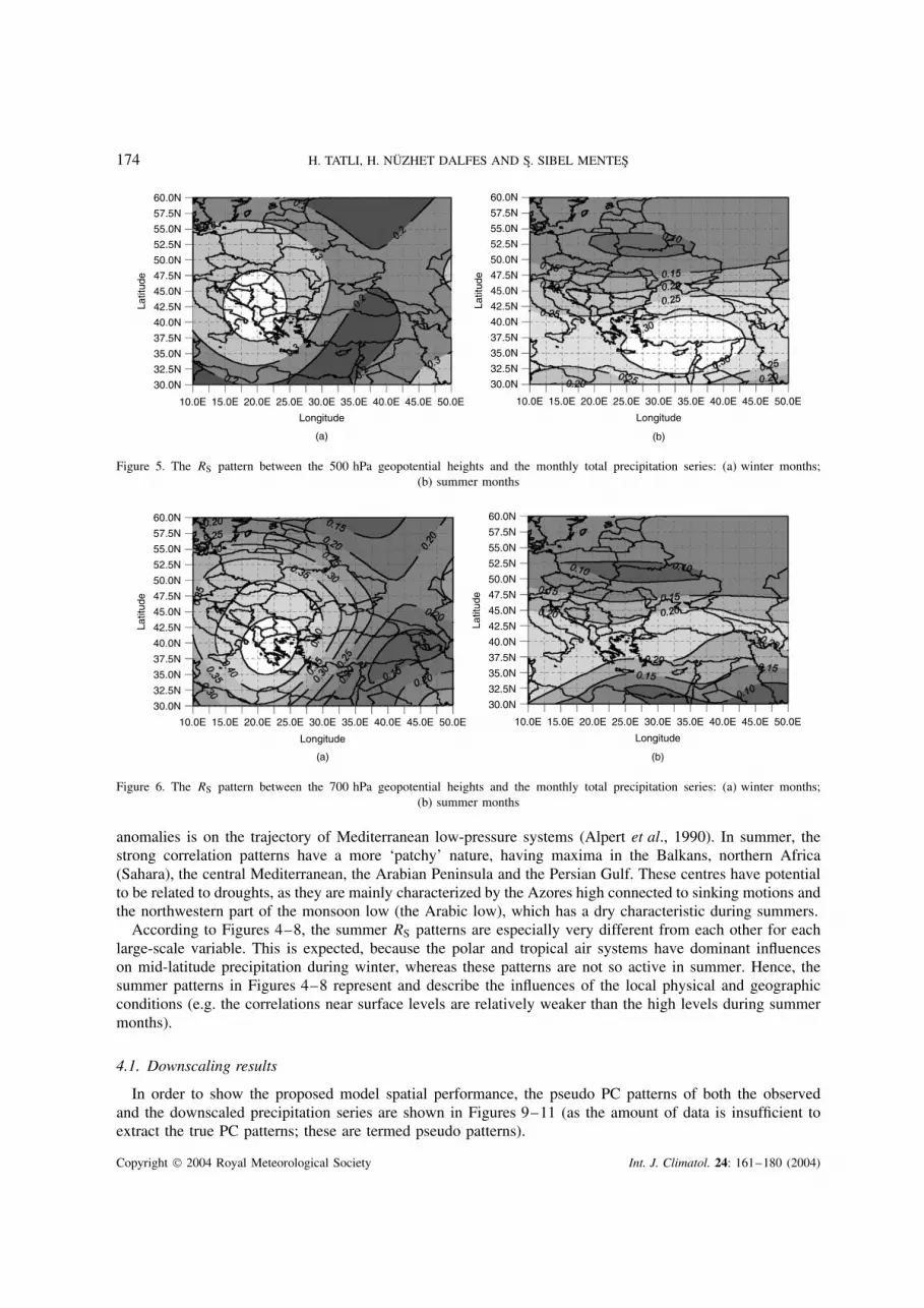
In order to analyse the relationships between the large-scale data predictors and the monthly totalprecipitation series, Sampson correlation (RS) patterns are computed, using Equation (2), between theindividual large-scale variables (namely 500 hPa geopotential heights, 700 hPa geopotential heights, SLPs,500 hPa vertical pressure velocities and 500–1000 hPa geopotential thicknesses) and the precipitation seriesfor four seasons; however, in this paper, only the results for winter and summer are shown in Figures 4–8.In these figures, the significance of the RS correlations (based on α-level statistics) is shown in grey scalefrom light to dark to represent the decreasing order of significance.

Figure 4 shows the Sampson correlation coefficients between the seasonal sea-level atmospheric pressures(wet and dry seasons being characterized by the winter and the summer respectively) and the precipitationseries of Turkey. The most important correlations are observed in the region that encompasses Italy, the entireBalkans region, Turkey and the eastern Mediterranean. This explains the effect of the low-pressure anomalieson the Turkish precipitation regimes during the winter. These correlations are in agreement with the workof Kutiel et al., (2001). The strongest correlations are observed in the central and southern Aegean. For thesummer, weaker correlations exist in the eastern Mediterranean.

As seen in Figure 5, there is an important correlation between the values of the 500 hPa geopotentialheights and the winter precipitation series. The correlation pattern in the area that includes the western part

Table III. The significant PC of the large-scale variables according to the criterionof Joreskop and Sorbom (1989)

Large-scale predictors Sum of explainedvariance (%)

Numberof PCs

500 hPa geopotential heights 96.4 3700 hPa geopotential heights 94.8 3SLP 90.4 3500–1000 hPa thicknesses 96.6 2500 hPa vertical pressure velocities 69.7 6

Table IV. The CCVs of the large-scale variables (seventh CCVis more significant than the sixth CCV)

CCVs ofthe large-scale

variables

Explained variance (%) of themonthly total

precipitation series

CCV1 46.213CCV2 18.931CCV3 10.375CCV4 7.748CCV5 2.934CCV7 1.581Sum 87.782

Copyright 2004 Royal Meteorological Society Int. J. Climatol. 24: 161–180 (2004)

172 H. TATLI, H. NUZHET DALFES AND S. SIBEL MENTES

0

4

50 100 150 200 250

PCs of SLP

300 350 400 450 500−4

−2

0

2

ICs of SLP

0 50 100 150 200 250 300 350 400 450 500

5

−5

0

0 50 100 150 200 250 300 350 400 450 500

4

−4

−2

0

2

0 50 100 150 200 250 300 350 400 450 500

4

−4

−2

0

2

0 50 100 150 200 250 300 350 400 450 500

4

−4

−2

0

2

0 50 100 150 200 250 300 350 400 450 500

5

−5

0

Figure 2. The plots of the first three PC and ICs of SLP

of Turkey, the Adriatic Sea, the Balkans and the eastern part of Italy is at an appreciable level. In winter, thegeopotential low centre at 500 hPa affects Turkey from the northwest. Such conditions are observed at highlevels (500 hPa) when low-pressure centres and related frontal systems are observed at the surface. Significantcorrelations for the summer occur in the eastern Mediterranean (namely southern Turkey and Cyprus). Duringthe summers, Turkey is under the influence of warm air masses (systems) of tropical origin, which is visible interms of positive anomalies for the 500 hPa geopotential heights. Spring and autumn form transitions betweenthe above mentioned regimes.

In Figure 6, the 700 hPa geopotential height data set gives a similar result to that of 500 hPa in terms ofits correlations with the precipitation regimes during the winter. In this figure, the significant correlations areseen over western parts. However, no such significant correlation pattern exists for the summer (according to95% statistical α level).

The anomalies related to the geopotential thicknesses of 500–1000 hPa (in a similar way to the 500 hPageopotential heights themselves) in central Europe have a correlation with the Turkish precipitation regimes,as can be seen in Figure 7. It can be postulated that, especially during the winter, the negative thicknessanomalies are related to cold advection, because the thickness itself is an indicator of thermal advection.As can be seen from the contours, a similar correlation is valid for the Caucasus and the Caspian regionas well (this correlation is related to the positive thickness anomalies that indicate the lack of precipitationduring winter, i.e. winter with dry conditions). As discussed for Figure 4, Turkey is under the influence ofIceland and Mediterranean lows in winter; therefore, those regions are characterized by convergent fields.That is, upward motions are effective. The pronounced nature of such cold advection at high levels (from1000 hPa to 500 hPa) has a determining effect on the occurrence of precipitation. In winter, the eastern partof Turkey (especially the eastern Black Sea part of Turkey) is an important convergent field (see Section 2).The existing cold advection over these upward motions has important effects on the formation of clouds and

Copyright 2004 Royal Meteorological Society Int. J. Climatol. 24: 161–180 (2004)

STATISTICAL DOWNSCALING OF TURKISH RAINFALL 173

0.00

140

120

100

80

60

40

20

0.05 0.10 0.15 0.20 0.250

0.00 0.05 0.10 0.15 0.20 0.25

160

140

120

100

80

60

40

20

0

0.00 0.05 0.10 0.15 0.20 0.300.25

9080706050403020100

0.00 0.05 0.10 0.15 0.20 0.300.25

1009080706050403020100

0.00 0.05 0.10 0.15 0.20 0.500.30 0.35 0.40 0.450.25

(a)

12

10

8

6

4

2

00.00 0.05 0.10 0.15 0.20 0.500.30 0.35 0.40 0.450.25

(b)

14

12

10

8

6

4

2

0

Figure 3. The spectral densities of the first three CCVs. The horizontal and vertical axes represent frequency (month−1) and spectraldensity respectively: (a) the large-scale variables (on left), (b) the local-scale variables (on right)

60.0N

57.5N

55.0N

52.5N

50.0N

47.5N

45.0N

42.5N

40.0N

37.5N

35.0N

32.5N

30.0N

10.0E 15.0E 20.0E 25.0E

Longitude

Latit

ude

(a)

30.0E 35.0E 40.0E 45.0E 50.0E

60.0N

57.5N

55.0N

52.5N

50.0N

47.5N

45.0N

42.5N

40.0N

37.5N

35.0N

32.5N

30.0N

10.0E 15.0E 20.0E 25.0E

Longitude

Latit

ude

(b)

30.0E 35.0E 40.0E 45.0E 50.0E

Figure 4. The RS pattern between the SLP and the monthly total precipitation series: (a) winter months; (b) summer months

precipitation. In summer, the effect of the air system originating from the Sahara (dry and warm) is clearlyseen in Figure 7(b). This period indicates the dry period for Turkey.

Correlation patterns between the 500 hPa vertical pressure velocity (omega) series and the precipitationseries can be observed in Figure 8. For both seasons, there is a strong correlation pattern for the area thatincludes the east of Greece, the entire Black Sea and the entire eastern Mediterranean. There is also a strongcorrelation pattern for the southwest corner of Turkey and Cyprus. During the winter, the area of omega

Copyright 2004 Royal Meteorological Society Int. J. Climatol. 24: 161–180 (2004)

174 H. TATLI, H. NUZHET DALFES AND S. SIBEL MENTES

60.0N

57.5N

55.0N

52.5N

50.0N

47.5N

45.0N

42.5N

40.0N

37.5N

35.0N

32.5N

30.0N

10.0E 15.0E 20.0E 25.0E

Longitude

Latit

ude

(a)

30.0E 35.0E 40.0E 45.0E 50.0E

60.0N

57.5N

55.0N

52.5N

50.0N

47.5N

45.0N

42.5N

40.0N

37.5N

35.0N

32.5N

30.0N

10.0E 15.0E 20.0E 25.0E

Longitude

Latit

ude

(b)

30.0E 35.0E 40.0E 45.0E 50.0E

Figure 5. The RS pattern between the 500 hPa geopotential heights and the monthly total precipitation series: (a) winter months;(b) summer months

60.0N

57.5N

55.0N

52.5N

50.0N

47.5N

45.0N

42.5N

40.0N

37.5N

35.0N

32.5N

30.0N

10.0E 15.0E 20.0E 25.0E

Longitude

Latit

ude

(a)

30.0E 35.0E 40.0E 45.0E 50.0E

60.0N

57.5N

55.0N

52.5N

50.0N

47.5N

45.0N

42.5N

40.0N

37.5N

35.0N

32.5N

30.0N

10.0E 15.0E 20.0E 25.0E

Longitude

Latit

ude

(b)

30.0E 35.0E 40.0E 45.0E 50.0E

Figure 6. The RS pattern between the 700 hPa geopotential heights and the monthly total precipitation series: (a) winter months;(b) summer months

anomalies is on the trajectory of Mediterranean low-pressure systems (Alpert et al., 1990). In summer, thestrong correlation patterns have a more ‘patchy’ nature, having maxima in the Balkans, northern Africa(Sahara), the central Mediterranean, the Arabian Peninsula and the Persian Gulf. These centres have potentialto be related to droughts, as they are mainly characterized by the Azores high connected to sinking motions andthe northwestern part of the monsoon low (the Arabic low), which has a dry characteristic during summers.

According to Figures 4–8, the summer RS patterns are especially very different from each other for eachlarge-scale variable. This is expected, because the polar and tropical air systems have dominant influenceson mid-latitude precipitation during winter, whereas these patterns are not so active in summer. Hence, thesummer patterns in Figures 4–8 represent and describe the influences of the local physical and geographicconditions (e.g. the correlations near surface levels are relatively weaker than the high levels during summermonths).

4.1. Downscaling results

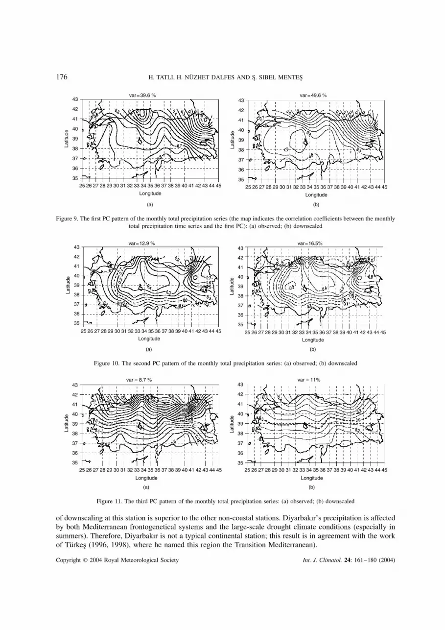
In order to show the proposed model spatial performance, the pseudo PC patterns of both the observedand the downscaled precipitation series are shown in Figures 9–11 (as the amount of data is insufficient toextract the true PC patterns; these are termed pseudo patterns).

Copyright 2004 Royal Meteorological Society Int. J. Climatol. 24: 161–180 (2004)

STATISTICAL DOWNSCALING OF TURKISH RAINFALL 175

60.0N

57.5N

55.0N

52.5N

50.0N

47.5N

45.0N

42.5N

40.0N

37.5N

35.0N

32.5N

30.0N

10.0E 15.0E 20.0E 25.0E

Longitude

Latit

ude

(a)

30.0E 35.0E 40.0E 45.0E 50.0E

60.0N

57.5N

55.0N

52.5N

50.0N

47.5N

45.0N

42.5N

40.0N

37.5N

35.0N

32.5N

30.0N

10.0E 15.0E 20.0E 25.0E

Longitude

Latit

ude

(b)

30.0E 35.0E 40.0E 45.0E 50.0E

Figure 7. The RS pattern between the 500–1000 hPa thicknesses and the monthly total precipitation series: (a) winter months;(b) summer months

60.0N

57.5N

55.0N

52.5N

50.0N

47.5N

45.0N

42.5N

40.0N

37.5N

35.0N

32.5N

30.0N

10.0E 15.0E 20.0E 25.0E

Longitude

Latit

ude

(a)

30.0E 35.0E 40.0E 45.0E 50.0E

60.0N

57.5N

55.0N

52.5N

50.0N

47.5N

45.0N

42.5N

40.0N

37.5N

35.0N

32.5N

30.0N

10.0E 15.0E 20.0E 25.0E

Longitude

Latit

ude

(b)

30.0E 35.0E 40.0E 45.0E 50.0E

Figure 8. The RS pattern between the 500 hPa vertical pressure velocities and the monthly total precipitation series: (a) winter months;(b) summer months

The scatter plots of the downscaled versus the observed monthly total precipitation time series for Goztepe(Istanbul), Ankara, Diyarbakır, Izmir, Rize, Adana and Erzurum are selected from rainfall regions accordingto Turkes (1996, 1998) and are shown in Figure 12. In order to distinguish the performance for validation,the correlation coefficients (r1, r2) between the observed and the downscaled data sets are computed. Inthis figure, r1 and r2 represent the correlation coefficients for the training part of the data (the data part foridentifying the model) and the non-training part of the data (validation part) respectively. The performanceof the proposed model increases from the continental regions of Turkey to the coastal regions of Turkeyexcept in the eastern part of the Black Sea (Rize) and in southern Anatolia (Diyarbakır) region. Thisresult is expected, because the precipitation conditions over the western and the southern coastal regions(including mainly the Marmara Transition and the Mediterranean rainfall regions of Turkey) are dominantlycontrolled by large-scale systems, whereas in the continental parts the added precipitation is due to localconditions.

In the Black Sea region, the added precipitation is due to the topographical and rain-shadow characteristicsthat the large-scale processes may not capture. The other unexpected result is for Diyarbakır. The performance

Copyright 2004 Royal Meteorological Society Int. J. Climatol. 24: 161–180 (2004)

176 H. TATLI, H. NUZHET DALFES AND S. SIBEL MENTES

25 26 27 28 29 30 31 32 33 34 35 36 37 38 39 40 41 42 43 44 45

35

36

37

38

39

40

41

42

43

Longitude

Latit

ude

25 26 27 28 29 30 31 32 33 34 35 36 37 38 39 40 41 42 43 44 45

35

36

37

38

39

40

41

42

43

Longitude

Latit

ude

var=39.6 % var= 49.6 %

(a) (b)

Figure 9. The first PC pattern of the monthly total precipitation series (the map indicates the correlation coefficients between the monthlytotal precipitation time series and the first PC): (a) observed; (b) downscaled

25 26 27 28 29 30 31 32 33 34 35 36 37 38 39 40 41 42 43 44 45

35

36

37

38

39

40

41

42

43

Longitude

Latit

ude

25 26 27 28 29 30 31 32 33 34 35 36 37 38 39 40 41 42 43 44 45

35

36

37

38

39

40

41

42

43

Longitude

Latit

ude

var=12.9 % var=16.5%

(a) (b)

Figure 10. The second PC pattern of the monthly total precipitation series: (a) observed; (b) downscaled

25 26 27 28 29 30 31 32 33 34 35 36 37 38 39 40 41 42 43 44 45

35

36

37

38

39

40

41

42

43

Longitude

Latit

ude

25 26 27 28 29 30 31 32 33 34 35 36 37 38 39 40 41 42 43 44 4535

36

37

38

39

40

41

42

43

Longitude

Latit

ude

var = 8.7 % var = 11%

(a) (b)

Figure 11. The third PC pattern of the monthly total precipitation series: (a) observed; (b) downscaled

of downscaling at this station is superior to the other non-coastal stations. Diyarbakır’s precipitation is affectedby both Mediterranean frontogenetical systems and the large-scale drought climate conditions (especially insummers). Therefore, Diyarbakır is not a typical continental station; this result is in agreement with the workof Turkes (1996, 1998), where he named this region the Transition Mediterranean).

Copyright 2004 Royal Meteorological Society Int. J. Climatol. 24: 161–180 (2004)

STATISTICAL DOWNSCALING OF TURKISH RAINFALL 177

350

300

250

200

150

100

Dow

nsca

led

(in m

m)

50

00 50 100 150

Observed (in mm)

(a)

200 250 300

r1 = 0.78r2 = 0.74

175

150

125

100

75

50

25

0

Dow

nsca

led

(in m

m)

Observed (in mm)

(b)

0 25 50 75 100 125

r1 = 0.79r2 = 0.73

Dow

nsca

led

(in m

m)

300

250

200

150

100

50

00 50 100 150

Observed (in mm)200

(c)

r1 = 0.86r2 = 0.83

Dow

nsca

led

(in m

m)

500

400

300

200

100

00 100 200 300 400 500

Observed (in mm)

(d)

r1 = 0.90r2 = 0.84

Dow

nsca

led

(in m

m)

175

150

125

100

75

50

25

00 25 50 75 100 125 150

Observed (in mm)

(g)

r1 = 0.85r2 = 0.82

Dow

nsca

led

(in m

m)

600

500

400

300

200

100

00 100 200 300 400 500

Observed (in mm)

(f)

r1 = 0.85r2 = 0.82

Dow

nsca

led

(in m

m)

700

600

500

400

300

200

100

00 100 200 300 400 500 600

Observed (in mm)

(e)

r1 = 0.77r2 = 0.71

Figure 12. The scatter plots of the identified model outputs versus the actual monthly total precipitation series. The correlation coefficientsbetween the observed and the model outputs are abbreviated as r1 for the training part and r2 for non-training part respectively:

(a) Goztepe (Istanbul); (b) Ankara; (c) Diyarbakır; (d) Izmir; (e) Rize; (f) Adana; (g) Erzurum

5. DISCUSSION AND CONCLUSIONS

In this study, a new method for downscaling regional climate processes has been presented. The model resultsshow that the precipitation regime (both wet and dry periods) of the coastal regions of Turkey (Mediterranean,

Copyright 2004 Royal Meteorological Society Int. J. Climatol. 24: 161–180 (2004)

178 H. TATLI, H. NUZHET DALFES AND S. SIBEL MENTES

Aegean, Marmara, western Black Sea) is under the influence of large-scale pressure systems and upper-aircirculations. On the other hand, especially in the Black Sea region, in addition to the large-scale processes, thelocal features (namely topography and rain-shadows) determine the likelihood and intensity of precipitation.For inland regions, the local processes are more effective than the large-scale processes. The southeastern partof the country (particularly Diyarbakır) is affected by both Mediterranean and monsoon lows. Therefore, thisregion can be called a Transition Mediterranean precipitation regime, which is in agreement with the workof Turkes (1996, 1998).

Before model building, a large-scale analysis is needed because of relationships between large-scaleprocesses and local processes based on meaningful statistical linkages. However, according to Nicholls (1987),other climate indices, such as North Atlantic oscillation index, may be considered to relate remote effects onthe local precipitation series.

The model is constructed following a three-stage process. In the first stage, the potential predictors arepreprocessed with PCA based on the maximum likelihood criterion of Joreskop and Sorbom (1989). In thisway, 1105 time series (five type predictors on 221 grid points) are reduced to 17 time series of PCs (Table III).

If the data in use do not have a Gaussian distribution, as is the case for precipitation series, then CCAafter PCA may not able to produce true correlated components; therefore, the significant PCs are transformedinto ICs by the ICA procedure to satisfy the probability distribution constraint. Since a prediction technique’sperformance is sensitive to the independence of the predictors; a better performance of CCA with ICs is not asurprising result according to this study. After employing CCA, six significant CCVs of ICs of the predictortime series are produced based on their explanatory performance of maximum variances in the precipitationseries (Table IV). In the second stage, a causal model is identified between the monthly total precipitationseries and the CCVs of ICs of the large-scale data sets. Thereafter, a naıve model is identified as a first-order model (Richardson, 1981). In this step, the causal and the naıve models are run in parallel (or online),and the outputs of the models are transformed into the basis functions by the hyperbolic tangent function(Equation (21)) to satisfy nonlinearity requirements. In the third stage, a classical multivariate regressionmodel is built between the extracted basis functions in the second stage and the set of the monthly totalprecipitation. Finally, for the proposed RNN, the training through time process is applied to the naıve andthe causal components of the model separately. The method is equivalent to a Jordan-type recurrent neuralnetwork in terms of its structure. The final model is so simple in its structure that it can easily be updatedwhen new data sets are available.

Generally, we have two types of knowledge about large-scale processes: those coming from models andthose inferred from observations. Knowledge from observations may be divided into three parts: physical-based linkages, such as weather types (Lamb, 1972; Conway and Jones, 1998); ‘summarized’ knowledge,such as climate indices; and time series of large-scale observations or GCM-generated fields. In this study,we only developed statistical linkages based on large-scale NCEP–NCAR reanalysis data sets.

Finally, one has to emphasize that the performance of the resulting prediction scheme (grey = white +black) depends not only on the performance of the statistical (black-box) downscaling techniques, but alsoon the GCM’s (white-box) performance in simulating large-scale fields.

ACKNOWLEDGEMENTS

We wish to thank Dr Murat Turkes of the Turkish State Meteorological Service and the referees for theirhelpful comments and suggestions.

REFERENCES

Alpert P, Neeman BU, Shah-El Y. 1990. Intermonthly variability of cyclone tracks in the Mediterranean. Journal of Climate 3:1474–1478.

Bardossy A. 1994. Downscaling from GCMs to local climate through stochastic linkages. In Climate Change, Uncertainty and DecisionMaking, Paoli G (ed.). Institute for Risk Research: Waterloo; 33–46.

Bluestein HB. 1993. Synoptic–Dynamic Meteorology in Midlatitudes, Vol. II. Oxford University Press.Box GEP, Jenkins GM, Reinsel GC. 1994. Time Series Analysis: Forecasting and Control, 3rd edn. Prentice Hall.Bras RL, Rodriguez-Iturbe I. 1993. Random Functions and Hydrology. Dover Publications.

Copyright 2004 Royal Meteorological Society Int. J. Climatol. 24: 161–180 (2004)

STATISTICAL DOWNSCALING OF TURKISH RAINFALL 179

Chen JM, Chang CP. 1994. A technique for analyzing optimal relationships among multiple sets of data fields. Part II: reliability casestudy. Monthly Weather Review 122: 2494–2505.

Chen JM, Chang CP, Harr P. 1994. A technique for analyzing optimal relationships among multiple sets of data fields. Part I: themethod. Monthly Weather Review 122: 2482–2493.

Comon P. 1994. Independent component analysis — a new concept? Signal Processing 36: 287–314.Connor J, Martin R, Atlas L. 1994. Recurrent neural networks and robust time series prediction. IEEE Transactions on Neural Networks

5: 240–253.Conway D, Jones PD. 1998. The use of weather types and air flow indices for GCM downscaling. Journal of Hydrology 212–213:

348–361.Cubasch U, von Storch H, Waszkewitz J, Zorita E. 1996. Estimates of climate change in southern Europe using different downscaling

techniques. Max Planck Institute fur Meteorologie, report no. 183.Diaz HF, Fulbright DC. 1981. Eigenvector analysis of seasonal temperature, precipitation and synoptic-scale system frequency over the

contiguous United States. Part I: winter. Monthly Weather Review 109: 1267–1284.Elman J. 1990. Finding structure in time. Cognitive Science 14: 179–221.Erinc S. 1984. Climatology and Its Methods. Istanbul University Press, Marine Science, Institute of Geography: Istanbul (in Turkish).Everson R, Roberts S. 1999. Independent component analysis: a flexible non-linearity and decorrelating manifold approach. Neural

Computing 11: 1957–1984.Fuentes U, Heimann D. 2000. An improved statistical–dynamical downscaling scheme and its application to the Alpine precipitation

climatology. Theoretical and Applied Climatology 65: 119–135.Geerts B. 2003. Empirical estimation of the monthly-mean daily temperature range. Theoretical and Applied Climatology 74: 145–165.Giorgi F, Mearns LO. 1991. Approaches to the simulation of regional climate change: a review. Review of Geophysics 29: 191–216.Glahn HR. 1968. Canonical correlation and its relationship to discriminant analysis and multiple regression. Journal of Atmospheric

Science 25: 23–31.Haykin S. 1999. Neural Networks: A Comprehensive Foundation, 2nd edn. Prentice-Hall: New Jersey.Haykin S. 2001. Kalman Filtering and Neural Networks. Wiley: New York.Heimann D, Sept V. 1998. Climatic change of summer temperature and precipitation in the Alpine region. A statistical–dynamical

assessment. Institute fur Physik der Atmosphere, report no. 112.Hewitson BC, Crane RG. 1996. Climate downscaling: techniques and application. Climate Research 7: 85–95.Hipel KW, Mcleod AI. 1994. Developments in Water Sciences: Time Series Modeling of Water Resources and Environmental Systems.

Elsevier.Hochreiter S, Younger AS, Conwell PR. 2001. Learning to learn using gradient descent. In Proceeding of the International Conference

on Artificial Neural Networks. Springer: Berlin; 87–94.Holton JR. 1992. An Introduction to Dynamic Meteorology, 3rd edn. Academic Press.Hyvarinen A, Oja E. 1997. A fast fixed-point algorithm for independent component analysis. Neural Computing 9: 1483–1492.Hyvarinen A, Karhunen J, Oja E. 2001. Independent Component Analysis. John Wiley.Jackson JE. 1991. A Users Guide to Principle Components. John Wiley.Jordan MI. 1986. Attractor dynamics and parallelism in a connectionist sequential machine. In Proceedings of 1986 Cognitive Science

Conference; 531–546.Joreskop KG, Sorbom D. 1989. LISREL-7 A Guide to the Program and Applications, 2nd edn. SPSS Publications. Chicago.Jutten C, Herault J. 1991. Blind separation of sources. Part I: an adaptive algorithm based on neuromimetic architecture. Signal

Processing 24: 1–10.Kadıoglu M. 2000. Regional variability of seasonal precipitation over Turkey. International Journal of Climatology 20: 1743–1760.Kaiser HF. 1959. Computer program for varimax rotation in factor analysis. Educational and Psychological Measurement 19: 413–420.Kalnay E, Kanamitsu M, Kistler R, Collins W, Deaven D, Gandin L, Iredell M, Saha S, White G, Woollen J, Zhu Y, Chelliah M,

Ebisuzaki W, Higgins W, Janowiak J, Mo KC, Ropelewski C, Wang J, Leetmaa A, Reynolds R, Jenne R, Joseph D. 1996. TheNCEP/NCAR reanalysis 40-year project. Bulletin of the American Meteorology Society 77: 437–471.

Karl TR, Wang WC, Schlesinger ME, Knight RW, Portman D. 1990. A method of relating general circulation model simulated climateto the observed local climate. Part I: seasonal statistics. Journal of Climate 3: 1053–1079.

Kidson JW, Thompson CS. 1998. Comparison of statistical and model-based downscaling techniques for estimating local climatevariations. Journal of Climate 11: 735–753.

Kim JW, Chang JT, Baker NL, Wilks DS, Gates WL. 1984. The statistical problem of climate inversion. Determination of therelationship between local and large-scale climate. Monthly Weather Review 112: 2069–2077.

Klein WH. 1982. Statistical weather forecasting on different time scales. Bulletin of the American Meteorology Society 63: 170–177.Kutiel H, Maheras P, Guika P. 1996. Circulation and extreme rainfall conditions in the eastern Mediterranean during the last century.

International Journal of Climatology 16: 73–92.Kutiel H, Hirsch-Eshkol TR, Turkes M. 2001. Sea level pressure patterns associated with dry or wet monthly rainfall conditions in

Turkey. Theoretical and Applied Climatology 69: 39–67.Lamb HH. 1972. British Isles Weather Types and a Register of Daily Sequence of Circulation Patterns, 1861–1971. Geophysical Memoir

116. HMSO: London.Matyasovsky I, Bogardi A, Duckstein L. 1994. Local temperature estimation under climate change. Theoretical and Applied Climatology

50: 1–13.McGregor JL. 1997. Regional climate modelling. Meteorology and Atmospheric Physics 63: 105–117.McGregor JL, Walsh KJ, Katzfey JJ. 1993. Nested modelling for regional climate studies. In Modelling Change in Environmental

Systems, Jakeman AJ, Beck MB, McAleer MJ (eds). John Wiley and Sons; 367–386.Murphy JM. 1999. An evaluation of statistical and dynamical techniques for downscaling local climate. Journal of Climate 12:

2256–2284.Murphy JM. 2000. Predictions of climate change over Europe using statistical and dynamical downscaling techniques. International

Journal of Climatology 20: 489–501.

Copyright 2004 Royal Meteorological Society Int. J. Climatol. 24: 161–180 (2004)

180 H. TATLI, H. NUZHET DALFES AND S. SIBEL MENTES

Nicholls N. 1987. The use of canonical correlations to study teleconnections. Monthly Weather Review 115: 393–399.Noguer M. 1994. Using statistical techniques to deduce local climate distributions: an application for model validation. Meteorological

Applications 1: 277–287.Pearlmutter BA. 1995. Gradient calculations for dynamic recurrent neural networks: a survey. IEEE Transactions on Neural Networks

6: 1212–1228.Preisendorfer RW. 1988. Principle Component Analysis in Meteorology and Oceanography. Elsevier.Puskorius GV, Feldkamp LA. 1994. Neurocontrol of nonlinear dynamical systems with Kalman filter trained recurrent networks. IEEE

Transactions on Neural Networks 5: 279–297.Reyment R, Joreskog KG. 1993. Applied Factor Analysis in the Natural Sciences, 2nd edn. Cambridge University Press.Richardson CW. 1981. Stochastic simulation of daily precipitation, temperature and solar radiation. Water Resources Research 17:

182–190.Richman MB. 1985. Rotation of principle components. Journal of Climatology 6: 293–335.Robinson AJ, Fallside F. 1991. A recurrent error propagation speech recognition system. Computer Speech and Language 5: 259–274.Rummukainen M. 1997. Methods for statistical downscaling of GCM simulation. SWECLIM (Swedish Regional Climate Modelling

Programme), Reports Meteorology and Climatology, no. 80.Sailor DJ, Li XA. 1999. A semi-empirical downscaling approach for predicting regional temperature impacts associated with climate

change. Journal of Climate 12: 103–114.Sampson AR. 1984. A multivariate correlation ratio. Statistics and Probability Letters 2: 77–81.Schubert A, Henderson-Sellers A. 1997. A statistical model to downscale local daily temperature extremes from synoptic scale

atmospheric circulation patterns in the Australian region. Climate Dynamics 13: 223–234.Smith J. 1999. Models and scale: up and downscaling. In Data and Models in Action, Stein A, Penning de Vries FWT (eds). Kluwer

Academic: Dordrecht; 81–98.Stein A, Riley J, Halberg N. 2001. Issues of scale for environmental indicators. Agriculture, Ecosystem and Environment 87: 215–232.Taha MF, Harb SA, Nagib MK, Tantawy AH. 1981. Climate of southern and western Asia. In The Climate of the Near East, Takahashi K,

Arakawa H (eds). World Survey of Climatology Series, vol. 9. Elsevier: Amsterdam; chapter 3.Tatlı H, Dalfes HN, Mentes SS. 2003. Principle factor and canonical correlation analysis of sea level pressures associated with

precipitation series in Turkey. In III. Atmospheric Science Symposium, Istanbul Technical University Istanbul, Turkey Sen O, Saylan L,Kocak K, Toros H (eds); 150–160 (in Turkish).

Touchan R, Garfin GM, Meko DM, Funkhouser G, Erkan N, Hughes MK, Wallin B. 2003. Preliminary reconstructions of springprecipitation in southwestern Turkey from tree-ring width. International Journal of Climatology 23: 157–171.

Tourre YM. 2000. Climlab2000: A Statistical Software Package for Climate Applications. IRI, International Research Institute for ClimatePrediction. http://iri.columbia.edu/outreach/training/climlab2000, 2003, version 1.10. [December 2003].

Turkes M. 1996. Spatial and temporal analysis of annual rainfall variations in Turkey. International Journal of Climatology 16:1057–1076.

Turkes M. 1998. Influence of geopotential heights, cyclone frequency and southern oscillation on rainfall variations in Turkey.International Journal of Climatology 18: 649–680.

Turkes M, Sumer UM, Kılıc G. 2002. Persistence and periodicity in the precipitation series of Turkey and associations with 500 hPageopotential heights. Climate Research 21: 59–81.

Von Storch H. 1995. Inconsistencies at the interface of climate impact studies and global climate research. Meteorologie Zeitschrift 4:72–80.

Von Storch H, Zwiers FW. 1999. Statistical Analysis in Climate Research. Springer/Cambridge University Press: Cambridge, UK.Von Storch H, Zorita E, Cubash U. 1993. Downscaling of global climate change estimates to regional scales: an application to Iberian

rainfall in wintertime. Journal of Climate 6: 1161–1171.Watson RT (ed.). 2002. Climate Change 2001. Synthesis Report. Third Assessment Report of the Intergovernmental Panel on Climate

Change. Cambridge University Press: Cambridge.Wigley TML, Jones PD, Briffa KR, Smith G. 1990. Obtaining sub-grid-scale information from coarse-resolution general circulation

model output. Journal of Geophysical Research 95: 1943–1953.Wilby RL, Wigley TML. 2000. Precipitation predictors for downscaling: observed and general circulation model relationships.

International Journal of Climatology 20: 641–661.Wilks DS. 1989. Statistical specification of local surface weather elements from large-scale information. Theoretical and Applied

Climatology 40: 119–134.Xoplaki E, Gonzales-Rouco JF, Luterbacher J, Wanner H. 2003. Mediterranean summer air temperature variability and its connection

to the large-scale atmospheric circulation and SSTs. Climate Dynamics 20: 723–739.Zorita E, Kharin V, von Storch H. 1992. The atmospheric circulation and sea surface temperature in the North Atlantic area in winter:

their interaction and relevance for Iberain precipitation. Journal of Climate 5: 1097–1108.

Copyright 2004 Royal Meteorological Society Int. J. Climatol. 24: 161–180 (2004)