POLITECNICO DI MILANO

Corso di Laurea MAGISTRALE in Ingegneria InformaticaDipartimento di Elettronica, Informazione e Bioingegneria

Importance-Weighted Methods inReal-World Applications

AI & R LabArtificial Intelligence and RoboticsLaboratory at Politecnico di Milano

Advisor: Prof. Matteo MatteucciCo-Advisors: Prof. Masashi Sugiyama

Dr. Florian Yger

Master’s Thesis by:Alessandro Balzi

matr. 818196

Academic Year 2014-2015

I dedicate this thesis to my parents,for their endless love, support

and encouragement.

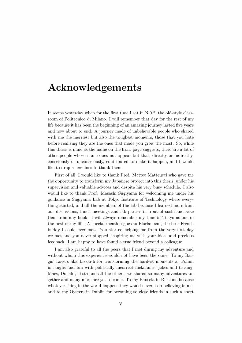
Acknowledgements

It seems yesterday when for the first time I sat in N.0.2, the old-style class-room of Politecnico di Milano. I will remember that day for the rest of mylife because it has been the beginning of an amazing journey lasted five yearsand now about to end. A journey made of unbelievable people who sharedwith me the merriest but also the toughest moments, those that you hatebefore realizing they are the ones that made you grow the most. So, whilethis thesis is mine as the name on the front page suggests, there are a lot ofother people whose name does not appear but that, directly or indirectly,consciously or unconsciously, contributed to make it happen, and I wouldlike to drop a few lines to thank them.

First of all, I would like to thank Prof. Matteo Matteucci who gave methe opportunity to transform my Japanese project into this thesis, under hissupervision and valuable advices and despite his very busy schedule. I alsowould like to thank Prof. Masashi Sugiyama for welcoming me under hisguidance in Sugiyama Lab at Tokyo Institute of Technology where every-thing started, and all the members of the lab because I learned more fromour discussions, lunch meetings and lab parties in front of sushi and sakethan from any book. I will always remember my time in Tokyo as one ofthe best of my life. A special mention goes to Florian-san, the best Frenchbuddy I could ever met. You started helping me from the very first daywe met and you never stopped, inspiring me with your ideas and preciousfeedback. I am happy to have found a true friend beyond a colleague.

I am also grateful to all the peers that I met during my adventure andwithout whom this experience would not have been the same. To my Bar-gis’ Lovers aka Lizzardi for transforming the hardest moments at Polimiin laughs and fun with politically incorrect nicknames, jokes and teasing.Macs, Donald, Testa and all the others, we shared so many adventures to-gether and many more are yet to come. To my Bauscia in Riccione becausewhatever thing in the world happens they would never stop believing in me,and to my Oysters in Dublin for becoming so close friends in such a short

V

time. To my dear friend Eni for our long conversations about our brokensentimental lives, and to the unpredictable Teo, our extra roommate andmy worthiest substitute in the house.

Yes the house, that cozy old-style apartment in viale Piceno 36 where Ishared my life with Loris and Marti. Our crazy adventures and trips, piadaand beer parties, late night conversations and NBA fights will always have aspecial place in my heart, together with our “comfy” couch. I do not thinkyou can find many others trios living together for five years, and this tellyou more than any word how I felt home being with you.

Last but not least, my family. Starting from my younger brother Mogiofor being the best pal in my trips around the world and for filling my thesisbreaks watching Lost and Fargo together. I am so curious to see what willbe the next. And thanks also to my parents for always being with me, givingme the strength to overcome the toughest and most frustrating periods ofthese five years. I cannot say how much I am lucky that I can count on youand if I became the person that I am, the credit (or the blame!) is onlyyours. This thesis is dedicated to you.

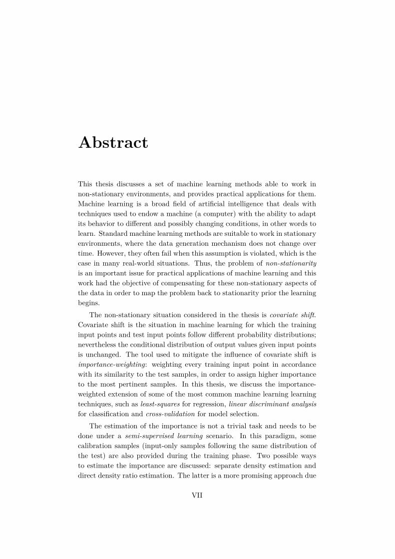
Abstract

This thesis discusses a set of machine learning methods able to work innon-stationary environments, and provides practical applications for them.Machine learning is a broad field of artificial intelligence that deals withtechniques used to endow a machine (a computer) with the ability to adaptits behavior to different and possibly changing conditions, in other words tolearn. Standard machine learning methods are suitable to work in stationaryenvironments, where the data generation mechanism does not change overtime. However, they often fail when this assumption is violated, which is thecase in many real-world situations. Thus, the problem of non-stationarityis an important issue for practical applications of machine learning and thiswork had the objective of compensating for these non-stationary aspects ofthe data in order to map the problem back to stationarity prior the learningbegins.

The non-stationary situation considered in the thesis is covariate shift.Covariate shift is the situation in machine learning for which the traininginput points and test input points follow different probability distributions;nevertheless the conditional distribution of output values given input pointsis unchanged. The tool used to mitigate the influence of covariate shift isimportance-weighting: weighting every training input point in accordancewith its similarity to the test samples, in order to assign higher importanceto the most pertinent samples. In this thesis, we discuss the importance-weighted extension of some of the most common machine learning learningtechniques, such as least-squares for regression, linear discriminant analysisfor classification and cross-validation for model selection.

The estimation of the importance is not a trivial task and needs to bedone under a semi-supervised learning scenario. In this paradigm, somecalibration samples (input-only samples following the same distribution ofthe test) are also provided during the training phase. Two possible waysto estimate the importance are discussed: separate density estimation anddirect density ratio estimation. The latter is a more promising approach due

VII

to its higher accuracy and efficiency.The core of the thesis are the real-world applications of importance-

weighted methods. Among all the possible choices, brain-computer inter-faces and image analysis are investigated, two fields that are prone to non-stationary phenomena. In brain-computer interfaces, importance-weightingis applied to the feature extraction phase and to the classification phase. Theexperiments performed show that the application of importance-weightingin both phases strongly enhances the results. In image analysis, we con-sider the problems of texture classification and traffic sign classification.For both of them, the experiments give evidence of the positive effects ofusing importance-weighted classification methods. The results obtained inall these cases allow us to claim the effectiveness of importance-weightedmethods in real-world applications.

The contributions brought by this thesis to the machine learning com-munity are multiple:

• The problem of non-stationarity is addressed, both from a theoreticaland from a practical point of view.

• An exhaustive theoretical discussion about importance-weighting isprovided. Importance-weighted extensions of some of the most com-mon machine learning methods are derived and techniques to estimatethe importance are explained.

• Robust to non-stationarity classification methods are provided for twoimportant real-world applications of machine learning: brain-computerinterfaces and images analysis.

• The concept of importance-weighting is applied in the phase of featureextraction. The IWCSP method, which allows to produce robust tonon-stationarity features for brain-computer interfaces, is introduced.

• The concept of importance-weighting is applied in the computation ofthe covariance matrices. A Robust to non-stationarity estimation ofthe covariance matrix is provided.

The latest two points are particularly meaningful because they are novel-ties introduced by the author of this thesis. While the importance-weightedcommon spatial pattern (IWCSP) has already been material for a scientificarticle, the application of the importance-weighting in the estimation ofcovariance matrices is a promising topic that still requires further investiga-tions. The expectations are to find enough interesting material for anotherscientific publication.

Sommario

Questa tesi discute un insieme di metodi di machine learning in grado di op-erare in ambienti non stazionari, e ne fornisce alcune applicazioni pratiche. Ilmachine learning e un ampio campo dell’intelligenza artificiale che riguardatecniche per dotare macchine (computer) della capacita di adattare il pro-prio comportamento a condizioni operative diverse e variabili, in altre paroledi apprendere. I metodi standard di machine learning sono pensati per la-vorare in condizioni stazionarie, dove il meccanismo di generazione dei datinon cambia nel tempo. Tuttavia, tali metodi falliscono quando questa as-sunzione e violata, cosa che accade in molte situazioni reali. Il problemadella non stazionarieta e percio di rilievo in molte applicazioni pratiche dimachine learning. Questo lavoro ha l’obiettivo di proporre tecniche per lacompensazione di non stazionarieta nei dati, cosı da riportare il problemaal caso stazionario prima di iniziare l’apprendimento.

La non stazionarieta considerata nella tesi e quella di covariate shift. Co-variate shift e la situazione per cui i campioni di training e i campioni di testseguono diverse distribuzioni di probabilita, ma la distribuzione condizionatadei valori in output rispetto a quelli in input e invariata. Lo strumento uti-lizzato per mitigare l’influenza della covariate shift e l’importance-weighting:pesare ogni campione di training in accordo con la sua similarita rispettoai campioni di test, in modo da attribuire maggiore importanza ai cam-pioni piu pertinenti. In questa tesi, discuteremo l’estensione del metododi importance-weighting ad alcune delle piu comuni tecniche di machinelearning, come least-squares in regressione, linear discriminant analysis inclassificazione e cross-validation in model selection.

Stimare il valore dell’importanza (in inglese importance) non e un prob-lema banale e necessita di operare in uno scenario di semi-supervised learn-ing. In questo paradigma, alcuni campioni di calibrazione (campioni disolo input che seguono la stessa distribuzione del test) sono forniti in fasedi training. Due possibili modi per stimare il valore dell’importanza sonodiscussi: stima separata delle densita e stima diretta del rapporto tra le den-

IX

sita. Quest’ultimo e un approccio piu promettente grazie alla sua maggioreaccuratezza ed efficienza.

La tesi e incentrata sulle applicazioni reali dell’importance-weighting.Tra tutte le possibili scelte, vengono investigati brain-computer interfacesed image analysis, due campi che sono soggetti a fenomeni non stazionari.Nel caso delle brain-computer interfaces, l’importance-weighting e appli-cata sia nella fase di feature extraction, sia nella fase di classificazione. Gliesperimenti svolti mostrano che entrambe le applicazioni di importance-weighting migliorano notevolmente i risultati. In image analysis, consid-eriamo il problema di classificazione di texture e di segnali stradali. Perentrambi, gli esperimenti evidenziano gli effetti positivi portati dall’utilizzodell’importance-weighting in fase di classificazione. I risultati ottenuti cipermetto di affermare l’efficacia dei metodi di importance-weighting in ap-plicazioni reali.

I contributi portati da questa tesi alla comunita di machine learning sonomolteplici:

• Viene trattato il problema della non stazionarieta, sia dal punto divista teorico che da quello pratico.

• Viene fornita un’eusastiva discussione teorica riguardo l’importance-weigthing. Sono derivate estensioni al caso di importance-weightingdi alcuni dei metodi di machine learning piu comuni e sono spiegatetecniche per stimare il valore dell’importanza.

• Vengono forniti metodi di classificazione robusti alla non stazionar-ieta per due importanti applicazioni reali di machine learning: brain-computer interfaces e image analysis.

• Il concetto di importance-weighting e applicato nella fase di feature ex-traction. Viene introdotto il metodo IWCSP che permette di produrrefeatures robuste alla non stazionarieta per brain-computer interfaces.

• Il concetto di importance-weighting e applicato nel calcolo delle matricidi covarianza. Viene fornita una stima della matrice di covarianzarobusta alla non stazionarieta.

Gli ultimi due punti sono particolarmente significativi perche sono novitaintrodotte dall’autore di questa tesi. Mentre IWCSP e gia stato materialeper un articolo scientifico, l’utilizzo dell’importance-weighting nella stimadelle matrici di covarianza e un argomento promettente che richiede ulteri-ori ricerche. Le aspettative sono quelle di raccogliere abbastanza materialeinteressante per un’altra pubblicazione scientifica.

Contents

Acknowledgements V

Abstract VII

Sommario IX

1 Introduction 11.1 Machine Learning under Covariate Shift . . . . . . . . . . . . 11.2 Problem Formulation . . . . . . . . . . . . . . . . . . . . . . . 41.3 Thesis Structure . . . . . . . . . . . . . . . . . . . . . . . . . 8

2 Learning with Importance-Weighting 112.1 Importance-Weighting . . . . . . . . . . . . . . . . . . . . . . 112.2 Importance-Weighted Methods . . . . . . . . . . . . . . . . . 14

2.2.1 Regression . . . . . . . . . . . . . . . . . . . . . . . . . 142.2.2 Classification . . . . . . . . . . . . . . . . . . . . . . . 16

2.3 Model Selection . . . . . . . . . . . . . . . . . . . . . . . . . . 202.4 Numerical Experiments . . . . . . . . . . . . . . . . . . . . . 21

2.4.1 Regression Example . . . . . . . . . . . . . . . . . . . 212.4.2 Classification Example . . . . . . . . . . . . . . . . . . 23

3 Importance Estimation 273.1 Density Estimation Approach . . . . . . . . . . . . . . . . . . 283.2 Direct Importance Estimation Approach . . . . . . . . . . . . 29

3.2.1 Kullback-Leibler Importance Estimation Procedure . . 303.2.2 Least-Squares Importance Fitting . . . . . . . . . . . . 32

3.3 Numerical Comparison . . . . . . . . . . . . . . . . . . . . . . 34

4 Importance-Weighted Methods for BCI 374.1 Motor Imagery in BCI . . . . . . . . . . . . . . . . . . . . . . 384.2 Method . . . . . . . . . . . . . . . . . . . . . . . . . . . . . . 40

XI

4.2.1 General Framework . . . . . . . . . . . . . . . . . . . 404.2.2 Common Spatial Pattern . . . . . . . . . . . . . . . . 424.2.3 Linear Discriminant Analysis . . . . . . . . . . . . . . 454.2.4 K-Nearest Neighbors on Covariance Matrices . . . . . 45

4.3 Real-Life Experiment . . . . . . . . . . . . . . . . . . . . . . . 484.3.1 Dataset . . . . . . . . . . . . . . . . . . . . . . . . . . 494.3.2 Procedure . . . . . . . . . . . . . . . . . . . . . . . . . 504.3.3 Results . . . . . . . . . . . . . . . . . . . . . . . . . . 51

5 Importance-Weighted Methods for Image Analysis 555.1 Texture Classification . . . . . . . . . . . . . . . . . . . . . . 56

5.1.1 The Brodatz Texture Images . . . . . . . . . . . . . . 575.1.2 Procedure . . . . . . . . . . . . . . . . . . . . . . . . . 585.1.3 Results . . . . . . . . . . . . . . . . . . . . . . . . . . 62

5.2 Traffic Sign Recognition . . . . . . . . . . . . . . . . . . . . . 645.2.1 The German Traffic Sign Recognition Benchmark . . . 655.2.2 Procedure . . . . . . . . . . . . . . . . . . . . . . . . . 675.2.3 Results . . . . . . . . . . . . . . . . . . . . . . . . . . 70

6 Conclusions and Future Directions 73

A BCI Paper 77

Chapter 1

Introduction

I propose to consider the question,“Can machines think?”

Alan TuringComputing Machinery and Intelligence, 1950

This first chapter is a general introduction to machine learning. We firstgive an overview of the learning problem, then we proceed with a moreformal formulation of the main concepts and notation. The focus is on aparticular situation of non-stationary environments called covariate shift,which is common in real-world applications and for which standard machinelearning techniques fail to produce accurate results. The chapter thereforesuggests the need of a different technique to cope with this problem that isdiscussed in the next chapters.

1.1 Machine Learning under Covariate Shift

Learning is the act of inferring new knowledge starting from some knownspecific facts. This activity can be performed by humans, animals and somemachines. In the latter case, we call it machine learning. In a more sci-entific fashion, machine learning is an interdisciplinary field of science andengineering aimed at analyzing and developing learning systems. We might,for instance, be interested in systems that learn to complete a task, or tomake accurate predictions, or to behave intelligently.

Learning is done automatically without human intervention and it isusually based on some sort of data (i.e., the specific facts). Dependingon the type of data and on the purpose of the analysis, various scenarios ofmachine learning can be identified. In this thesis, we will focus on supervised

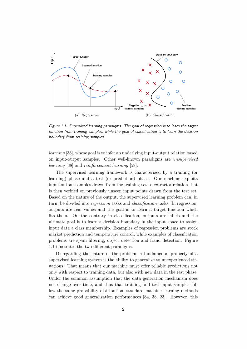
(a) Regression (b) Classification

Figure 1.1: Supervised learning paradigms. The goal of regression is to learn the targetfunction from training samples, while the goal of classification is to learn the decisionboundary from training samples.

learning [38], whose goal is to infer an underlying input-output relation basedon input-output samples. Other well-known paradigms are unsupervisedlearning [38] and reinforcement learning [58].

The supervised learning framework is characterized by a training (orlearning) phase and a test (or prediction) phase. Our machine exploitsinput-output samples drawn from the training set to extract a relation thatis then verified on previously unseen input points drawn from the test set.Based on the nature of the output, the supervised learning problem can, inturn, be divided into regression tasks and classification tasks. In regression,outputs are real values and the goal is to learn a target function whichfits them. On the contrary in classification, outputs are labels and theultimate goal is to learn a decision boundary in the input space to assigninput data a class membership. Examples of regression problems are stockmarket prediction and temperature control, while examples of classificationproblems are spam filtering, object detection and fraud detection. Figure1.1 illustrates the two different paradigms.

Disregarding the nature of the problem, a fundamental property of asupervised learning system is the ability to generalize to unexperienced sit-uations. That means that our machine must offer reliable predictions notonly with respect to training data, but also with new data in the test phase.Under the common assumption that the data generation mechanism doesnot change over time, and thus that training and test input samples fol-low the same probability distribution, standard machine learning methodscan achieve good generalization performances [84, 38, 23]. However, this

2

Figure 1.2: Semi-supervised learning scenario. The training and calibration datasetsare used to learn the model that will then be tested on the test dataset.

fundamental assumption is often violated in real-world applications, suchas robot control [35], brain signal analysis [46], image analysis [83], speechrecognition [85], natural language processing [80], and bioinformatics [6].Therefore, there is a strong need for theories and algorithms of supervisedlearning able to deal with such a changing environment.

The framework this thesis deals with is the one of covariate shift [68]. Inthis setting, the training input points and the test input points can followdifferent probability distributions, but the conditional distribution of outputvalues given the input points does not change. This means that the targetfunction we want to learn is unchanged between the training phase and thetest phase, but the distributions of input points are different for trainingand test data. The aim of this thesis is to discuss a set of techniques ableto extend standard machine learning methods in order to improve the gen-eralization performance under covariate shift. In the following, we will referto these techniques as covariate shift adaptation techniques.

The covariate shift adaptation techniques covered in this thesis fall intothe category of semi-supervised learning [18], which in recent years is gain-ing strong attention from the machine learning community. In this scenario,input-only samples drawn from the test are available in addition to the stan-dard input-output samples drawn from the training. In other words, we willconsider the standard training and test datasets plus a third dataset, calledcalibration, which contains input-only samples from the same distributionof the test. The idea is to use this extra knowledge about the test duringthe learning phase, in order to learn a model able to perform well in the pre-diction phase also when a change in the input distribution occurs. Figure

3

1.2 shows the semi-supervised learning paradigm.The effectiveness of the proposed method will be verified through some

experiments in Brain-Computer Interfaces (see Chapter 4) and Image Anal-ysis (see Chapter 5), with the purpose to stress its utility in real-worldapplications.

1.2 Problem Formulation

The standard supervised learning problem of estimating an unknown input-output dependency, can be formalized in the following way. Let

(xtri , ytri )ntri=1

be the training samples, where the training input points

xtri ∈ Rd, i = 1, 2, . . . ntr

are independent and identically distributed (i.i.d.) samples following a prob-ability distribution Ptr(x) with density ptr(x):

xtri ∼ Ptr(x).

The training output values1

ytri ∈ R, i = 1, 2, . . . ntr

follow a conditional probability distribution P (y|x) with conditional densityp(y|x):

ytri ∼ P (y|x = xtri ).

In a similar way, let(xtei , ytei )ntei=1

be the test samples which are not given in the training phase, but will begiven in the test phase. xtei ∈ Rd is a test input point following a probabilitydistribution Pte(x) with density pte(x), and ytei ∈ R is a test output valuewith conditional probability distribution P (y|x = xte) and density p(y|x =xte). The goal of supervised learning is to exploit the training samples toextract an estimate y of the true output value y which performs well for thetraining, but is able to generalize also on samples from the test.

1For the sake of simplicity, here it is shown the general regression case. All the con-siderations made apply also to the classification scenario, for instance ytri ∈ Ω whereΩ = +1,−1.

4

To evaluate the goodness of our estimation, we need a measure of discrep-ancy between the true output value and the estimated one. This discrepancyis called loss function

loss(x, y, y).

The loss function quantifies the amount by which the prediction deviatesfrom the actual values, mapping it onto a real number intuitively represent-ing some “cost” associated with the wrong estimation. For this reason itis also called cost function and it is usually aimed at being minimized. Inthe literature, various loss functions have been proposed [38] and the choicedepends on the type of problem (e.g., regression or classification) and on theneeds of the specific application.

The basic assumption of supervised learning is that it is possible toestimate the output value y through a parameterized function f(x; θ) where

θ = (θ1, θ2, . . . , θd)T ∈ Rd.

The most simple parametric model for function f is called linear modelbecause it is linear with respect to the parameter θ:

f(x; θ) =d∑i=1

θiϕi(x) (1.1)

where ϕi(x)di=1 are fixed, linearly independent functions known as basisfunctions (e.g., polynomials functions or trigonometric functions). Anotherimportant and slightly more complex model is the so called kernel model:

f(x; θ) =ntr∑i=1

θik(x, xtri ), (1.2)

where k is the kernel function. The kernel function can be seen as a non-linear similarity measure generalizing the concept of scalar product. Morein detail, given two vectors u, v ∈ RN , k(u, v) implicitly computes the dotproduct between u and v in a higher-dimensional RM without explicitlytransforming u and v to RM .

Since a linear algorithm for the learning of a target function (or of a de-cision boundary in case of classification) can usually be expressed in termsof scalar product, replacing it with the kernel we obtain non-linear algo-rithm in the original RN which corresponds to a linear algorithm in RM .The procedure goes under the name of kernel trick and it is a powerful toolto exploit the advantages of a non-linear model while keeping the computa-tional burden of a linear one, as shown in an example in Figure 1.32. Among

2Figure taken from “Everything You Wanted to Know about the Kernel Trick”, EricKim, 2013 (http://www.eric-kim.net/).

5

Figure 1.3: Example of kernel trick in a classification scenario: the decision boundarythat is linear in R3, when transformed back to R2 is non-linear.

the many possible kernel functions, one of the most popular is the Gaussiankernel:

k(x, x′) = exp(−‖x− x

′‖2

2h2

)with h > 0 being the bandwidth of the Gaussian. It is worth noting that thekernel and the linear model, which are both widely used in machine learningapplications, present a crucial difference. The linear model is simpler butthe number of parameters depends on the input dimensionality d. On thecontrary, in the kernel model the number of parameters is related only to thenumber of training samples ntr and it is independent from the dimensionalityof the problem. This important property makes the kernel model much moresuitable when dealing with high dimensional data [59].

As shown above, our estimate is a function of the input points and of aparameter θ which has to be learned. A standard way to to do that is theempirical risk minimization (ERM) (e.g., [84]):

θERM := argminθ

[1ntr

ntr∑i=1

loss(xtri , ytri , f(xtri ; θ))]. (1.3)

The idea of ERM is to find θ such that the previously defined loss function isminimized. However, from Equation (1.3) we notice that the parameter θ islearned considering only the training samples, without using any informationabout the test. Although this approach provides a consistent3 estimator in

3We say that an estimator is “consistent” if it converges to the optimal parameter in

6

(a) Training and test data (b) Input data densities

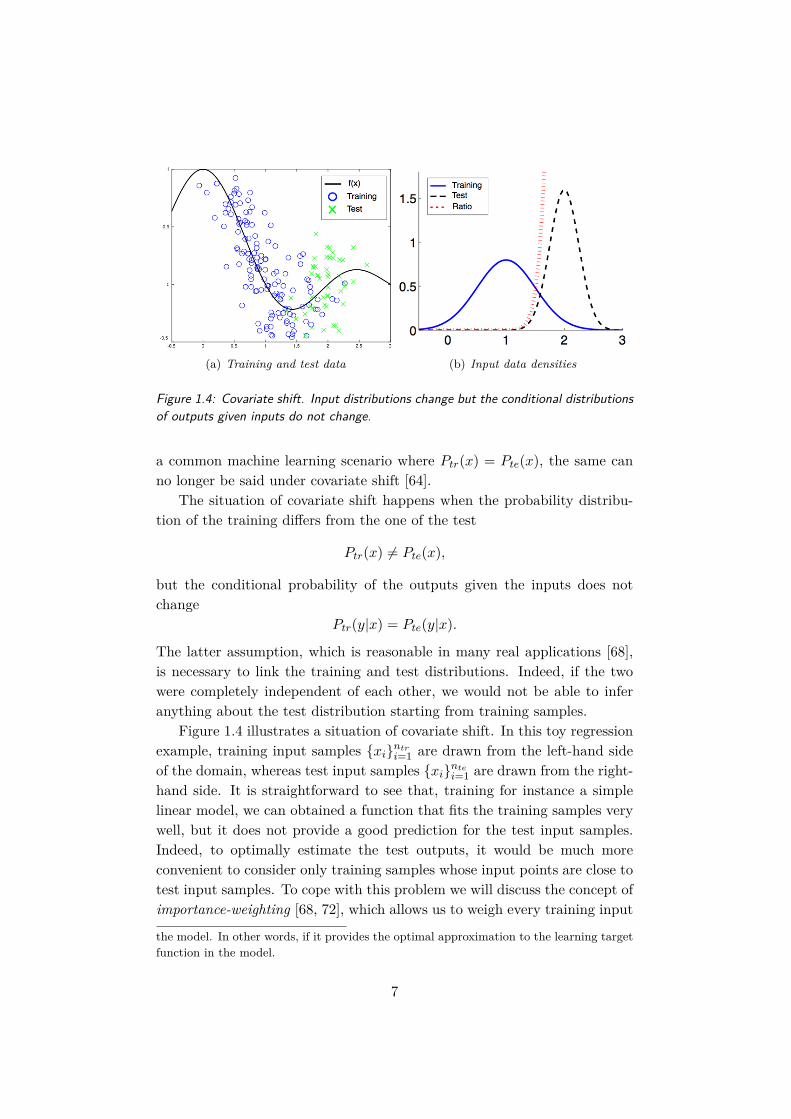
Figure 1.4: Covariate shift. Input distributions change but the conditional distributionsof outputs given inputs do not change.

a common machine learning scenario where Ptr(x) = Pte(x), the same canno longer be said under covariate shift [64].

The situation of covariate shift happens when the probability distribu-tion of the training differs from the one of the test

Ptr(x) 6= Pte(x),

but the conditional probability of the outputs given the inputs does notchange

Ptr(y|x) = Pte(y|x).

The latter assumption, which is reasonable in many real applications [68],is necessary to link the training and test distributions. Indeed, if the twowere completely independent of each other, we would not be able to inferanything about the test distribution starting from training samples.

Figure 1.4 illustrates a situation of covariate shift. In this toy regressionexample, training input samples xintri=1 are drawn from the left-hand sideof the domain, whereas test input samples xintei=1 are drawn from the right-hand side. It is straightforward to see that, training for instance a simplelinear model, we can obtained a function that fits the training samples verywell, but it does not provide a good prediction for the test input samples.Indeed, to optimally estimate the test outputs, it would be much moreconvenient to consider only training samples whose input points are close totest input samples. To cope with this problem we will discuss the concept ofimportance-weighting [68, 72], which allows us to weigh every training input

the model. In other words, if it provides the optimal approximation to the learning targetfunction in the model.

7

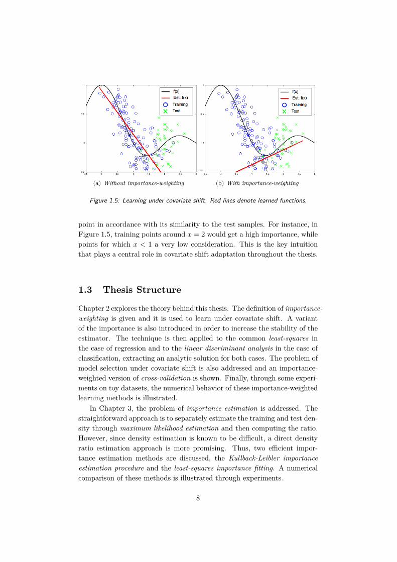
(a) Without importance-weighting (b) With importance-weighting

Figure 1.5: Learning under covariate shift. Red lines denote learned functions.

point in accordance with its similarity to the test samples. For instance, inFigure 1.5, training points around x = 2 would get a high importance, whilepoints for which x < 1 a very low consideration. This is the key intuitionthat plays a central role in covariate shift adaptation throughout the thesis.

1.3 Thesis Structure

Chapter 2 explores the theory behind this thesis. The definition of importance-weighting is given and it is used to learn under covariate shift. A variantof the importance is also introduced in order to increase the stability of theestimator. The technique is then applied to the common least-squares inthe case of regression and to the linear discriminant analysis in the case ofclassification, extracting an analytic solution for both cases. The problem ofmodel selection under covariate shift is also addressed and an importance-weighted version of cross-validation is shown. Finally, through some experi-ments on toy datasets, the numerical behavior of these importance-weightedlearning methods is illustrated.

In Chapter 3, the problem of importance estimation is addressed. Thestraightforward approach is to separately estimate the training and test den-sity through maximum likelihood estimation and then computing the ratio.However, since density estimation is known to be difficult, a direct densityratio estimation approach is more promising. Thus, two efficient impor-tance estimation methods are discussed, the Kullback-Leibler importanceestimation procedure and the least-squares importance fitting. A numericalcomparison of these methods is illustrated through experiments.

8

Chapter 4 presents a real application of covariate shift adaptation. Thefield is motor imagery in Brain-Computer Interfaces, which is by naturestrongly affected by non-stationary phenomena. First, the standard frame-work constituted by feature extraction and classification is explained. Then,the importance-weighting adaptation is applied to both phases. In partic-ular, the importance-weighted common spatial patterns is used in the fea-ture extraction step while importance-weighted linear discriminant analysisand k-nearest neighbors on importance-weighted covariance matrices are em-ployed as classification techniques. Finally, the improvements obtained areillustrated and discussed.

In Chapter 5, we present another real application of covariate shift adap-tation, this time in the field of image analysis. In fact, images are subjectto environment changes such as variations in illumination, rotations, scalingand presence of noise and it is reasonable to apply importance-weightingto compensate for them. The chapter addresses two important problems ofimage analysis: texture classification and traffic sign recognition. For bothof them, the datasets used and the feature extraction and classification tech-niques employed are described and the improvements obtained thanks to theuse of the importance are reported and commented.

Chapter 6 concludes the thesis and offers some directions for possiblefuture works.

9

10

Chapter 2

Learning withImportance-Weighting

The question of whether Machines Can Thinkis about as relevant as the questionof whether Submarines Can Swim.

Edsger W. DijkstraThe threats to computing science, 1984

This thesis is focused mainly in the use of importance-weighted methods tocope with covariate shift. In this chapter, we explore the theory behind themethod and we see how it can be plugged into the most common machinelearning techniques. We start by giving a formal definition of the impor-tance. Then we use it to learn both in the case of regression and in thecase of classification. We also address the problem of model selection undercovariate shift. Finally, we show the improvements obtained using the pro-posed method with respect to the standard one through some experimentson toy datasets.

2.1 Importance-Weighting

In Section 1.2 we showed that the ERM method for a generic loss functiondoes not provide a consistent estimator under covariate shift. The failurecomes from the fact that the training input distribution is different from thetest input distribution. The idea of importance sampling [26] to compensatefor this difference of distribution is derived from the following equation. For

a generic function g,

Exte [g(xte)] =∫g(x)pte(x)dx =

∫g(x)pte(x)

ptr(x)ptr(x)dx = Extr

[g(xtr)pte(x)

ptr(x)

]where Extr and Exte denote the expectation over x drawn from ptr(x) andpte(x) respectively. The quantity

w(x) = pte(x)ptr(x)

is called the importance. The identity above shows that the expectation of ageneric function over the test can be computed as the importance-weightedexpectation of the same function over the train. Thus, the difference ofdistributions can be systematically adjusted by importance-weighting.

With this result in mind, under covariate shift the Equation (1.3) canbe rewritten as

θIWERM := argminθ

[1ntr

ntr∑i=1

w(xtri )loss(xtri , y

tri , f(xtri ; θ)

)].

The above learning method is called importance-weighted empirical risk min-imization (IWERM), and it has been proved to be consistent even undercovariate shift [64].

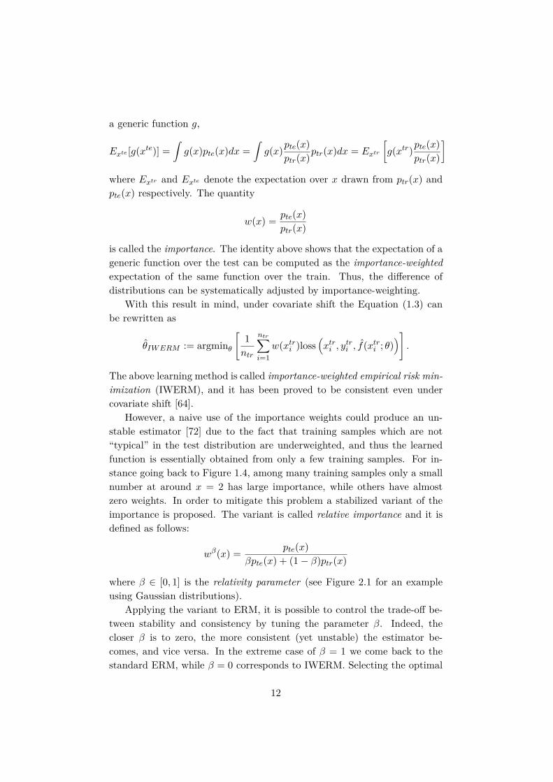
However, a naive use of the importance weights could produce an un-stable estimator [72] due to the fact that training samples which are not“typical” in the test distribution are underweighted, and thus the learnedfunction is essentially obtained from only a few training samples. For in-stance going back to Figure 1.4, among many training samples only a smallnumber at around x = 2 has large importance, while others have almostzero weights. In order to mitigate this problem a stabilized variant of theimportance is proposed. The variant is called relative importance and it isdefined as follows:

wβ(x) = pte(x)βpte(x) + (1− β)ptr(x)

where β ∈ [0, 1] is the relativity parameter (see Figure 2.1 for an exampleusing Gaussian distributions).

Applying the variant to ERM, it is possible to control the trade-off be-tween stability and consistency by tuning the parameter β. Indeed, thecloser β is to zero, the more consistent (yet unstable) the estimator be-comes, and vice versa. In the extreme case of β = 1 we come back to thestandard ERM, while β = 0 corresponds to IWERM. Selecting the optimal

12

(a) Probability densities (b) Relative importance wβ(x)

Figure 2.1: Relative importance. pte(x) is the normal distribution with mean 0 andvariance 1, and ptr(x) is the normal distribution with mean 0.5 and variance 1.

value for β is not a trivial task because it depends on many (usually un-known) factors, such as the learning target function, the noise level, etc. Arough approximation is to use a small β when the number of training sam-ples ntr is large and a large β when ntr is small. However, a more precisemethod for the estimation will be presented in Section 2.3.

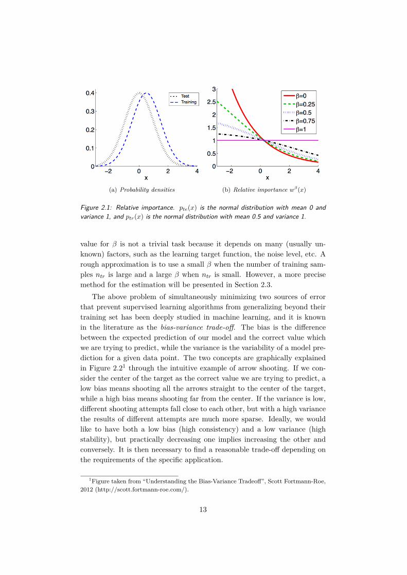
The above problem of simultaneously minimizing two sources of errorthat prevent supervised learning algorithms from generalizing beyond theirtraining set has been deeply studied in machine learning, and it is knownin the literature as the bias-variance trade-off. The bias is the differencebetween the expected prediction of our model and the correct value whichwe are trying to predict, while the variance is the variability of a model pre-diction for a given data point. The two concepts are graphically explainedin Figure 2.21 through the intuitive example of arrow shooting. If we con-sider the center of the target as the correct value we are trying to predict, alow bias means shooting all the arrows straight to the center of the target,while a high bias means shooting far from the center. If the variance is low,different shooting attempts fall close to each other, but with a high variancethe results of different attempts are much more sparse. Ideally, we wouldlike to have both a low bias (high consistency) and a low variance (highstability), but practically decreasing one implies increasing the other andconversely. It is then necessary to find a reasonable trade-off depending onthe requirements of the specific application.

1Figure taken from “Understanding the Bias-Variance Tradeoff”, Scott Fortmann-Roe,2012 (http://scott.fortmann-roe.com/).

13

Figure 2.2: Graphical illustration of bias and variance. Low bias is shooting straight tothe center of the target, high bias is shooting far from the center. With low variancedifferent attempts fall close to each other, with high variance they fall far.

2.2 Importance-Weighted Methods

In this section, we show how importance-weighting can be plugged into themost common machine learning techniques to improve the learning perfor-mance under covariate shift. We will consider first a framework of regressionand then of classification.

2.2.1 Regression

In the regression scenario, a common choice of the loss function to use is theleast squares (LS) (e.g., [38, 63]):

loss(x, y, y) = (y − y)2.

Basically, the discrepancy between the real output y and the estimated oney is computed as the square of the values distance.

To cope with covariate shift, we can introduce an importance-weightingmethod for the squared loss, called importance-weighted least squares (IWLS).

14

Our learning procedure is now given by2

θIWLS := argminθ

[1ntr

ntr∑i=1

w(xtri )(f(xtri ; θ)− ytri

)2]. (2.1)

The interesting thing about least squares, which is also the reason for itsextensive use, is that we can easily derive an analytic solution to the problemof determine θ both using a linear model and a kernel model.

In a linear model (see Equation (1.1)), let Xtr be the design matrix, thatis the ntr × d matrix (where d is the dimensionality of the input) with the(i, j)-th element

Xtri,j = ϕj(xtri ),

such thatf(xtr; θ) = Xtrθ.

Then, Equation (2.1) can be expressed in a matrix form as

1ntr

(Xtrθ − ytr)TW tr(Xtrθ − ytr)

where W tr is the diagonal matrix having the i-th diagonal element as

W tri,i = w(xtri ) = pte(xtri )

ptr(xtri ) .

Now, to find the minimum, we have to take the derivative with respect toθ and equate it to zero. After some simple algebra and assuming that theinverse of XtrTW trXtr exists, we reach the analytic solution

θ = Lytr,

whereL = (XtrTW trXtr)−1XtrTW tr

is the so called learning matrix.The procedure for the kernel model (see Equation (1.2)) is very similar.

The design matrix Xtr becomes the ntr × ntr kernel matrix Ktr having the(i, j)-th element as

Ktri,j = k(xtri , xtrj ),

and, exploiting the fact that the kernel matrix is symmetric, we obtain thelearning matrix:

L = (KtrW trKtr)−1KtrW tr.

2For the sake of simplicity, in the following the standard version of IW is used. However,the extension to the case of relative IW is straightforward.

15

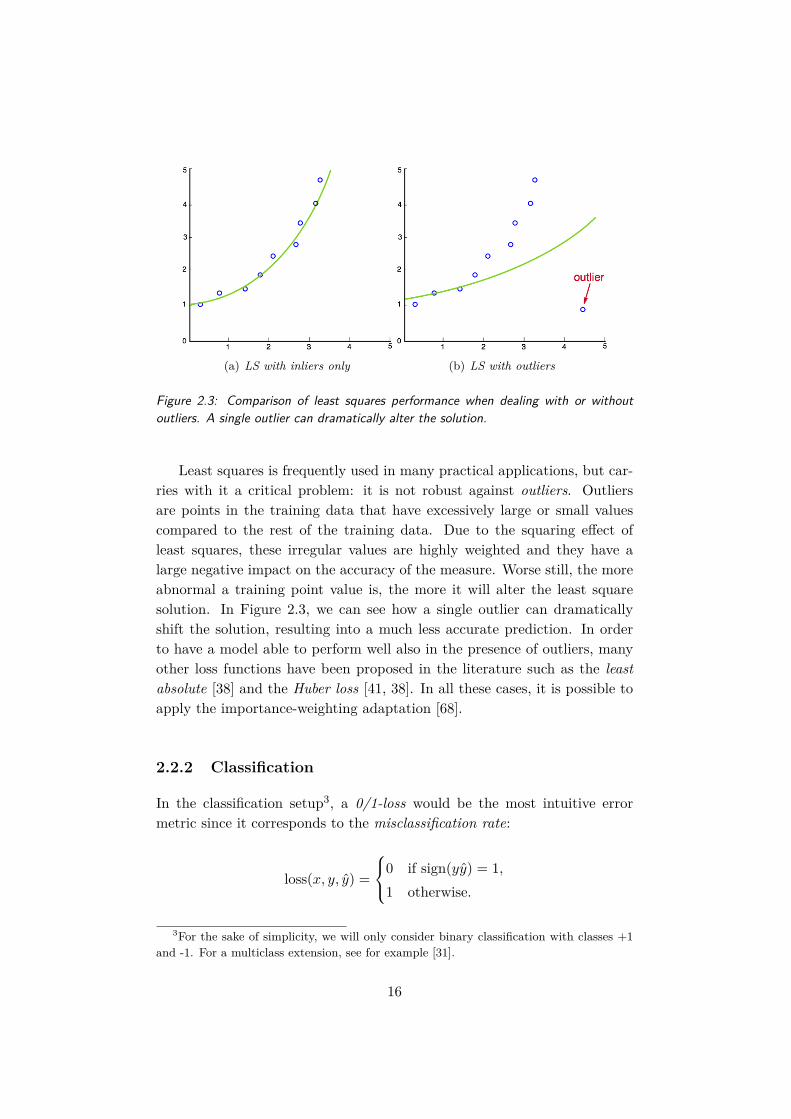
(a) LS with inliers only (b) LS with outliers

Figure 2.3: Comparison of least squares performance when dealing with or withoutoutliers. A single outlier can dramatically alter the solution.

Least squares is frequently used in many practical applications, but car-ries with it a critical problem: it is not robust against outliers. Outliersare points in the training data that have excessively large or small valuescompared to the rest of the training data. Due to the squaring effect ofleast squares, these irregular values are highly weighted and they have alarge negative impact on the accuracy of the measure. Worse still, the moreabnormal a training point value is, the more it will alter the least squaresolution. In Figure 2.3, we can see how a single outlier can dramaticallyshift the solution, resulting into a much less accurate prediction. In orderto have a model able to perform well also in the presence of outliers, manyother loss functions have been proposed in the literature such as the leastabsolute [38] and the Huber loss [41, 38]. In all these cases, it is possible toapply the importance-weighting adaptation [68].

2.2.2 Classification

In the classification setup3, a 0/1-loss would be the most intuitive errormetric since it corresponds to the misclassification rate:

loss(x, y, y) =

0 if sign(yy) = 1,1 otherwise.

3For the sake of simplicity, we will only consider binary classification with classes +1and -1. For a multiclass extension, see for example [31].

16

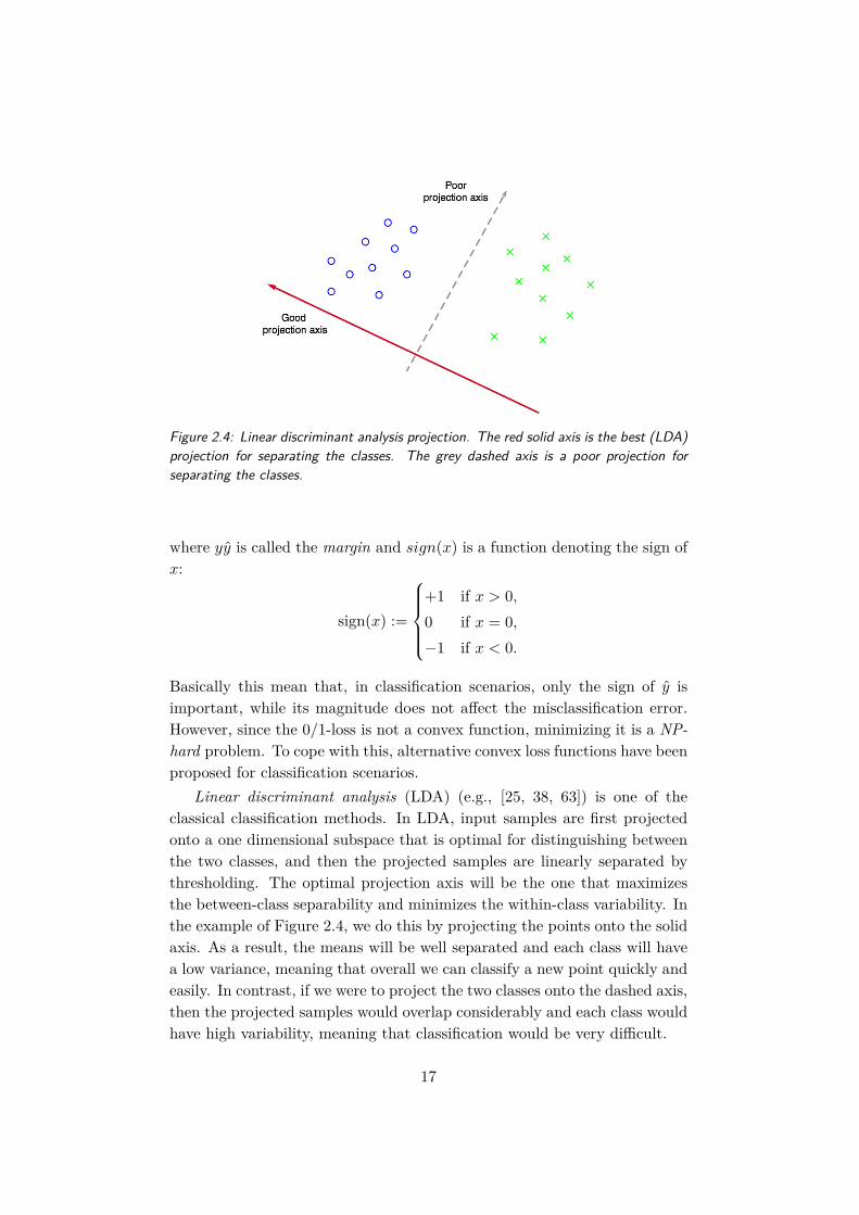
Figure 2.4: Linear discriminant analysis projection. The red solid axis is the best (LDA)projection for separating the classes. The grey dashed axis is a poor projection forseparating the classes.

where yy is called the margin and sign(x) is a function denoting the sign ofx:

sign(x) :=

+1 if x > 0,0 if x = 0,−1 if x < 0.

Basically this mean that, in classification scenarios, only the sign of y isimportant, while its magnitude does not affect the misclassification error.However, since the 0/1-loss is not a convex function, minimizing it is a NP-hard problem. To cope with this, alternative convex loss functions have beenproposed for classification scenarios.

Linear discriminant analysis (LDA) (e.g., [25, 38, 63]) is one of theclassical classification methods. In LDA, input samples are first projectedonto a one dimensional subspace that is optimal for distinguishing betweenthe two classes, and then the projected samples are linearly separated bythresholding. The optimal projection axis will be the one that maximizesthe between-class separability and minimizes the within-class variability. Inthe example of Figure 2.4, we do this by projecting the points onto the solidaxis. As a result, the means will be well separated and each class will havea low variance, meaning that overall we can classify a new point quickly andeasily. In contrast, if we were to project the two classes onto the dashed axis,then the projected samples would overlap considerably and each class wouldhave high variability, meaning that classification would be very difficult.

17

Formally, let µ+ and µ− be the means of classes +1 and −1 respectively:

µ+ = 1n+tr

∑i:ytri =+1

xtri ,

µ− = 1n−tr

∑i:ytri =−1

xtri ,

where n±tr is the number of training samples of class ±1 and∑i:ytri =±1 de-

notes the summation over index i such that ytri = ±1. We can then definethe between-class scatter matrix

Sb = (µ+ − µ−)(µ+ − µ−)T ,

and the within-class scatter matrix

Sw =∑

i:ytri =+1(xtri − µ+)(xtri − µ+)T +

∑i:ytri =−1

(xtri − µ−)(xtri − µ−)T .

The objective of LDA is to find a projection direction ΦLDA that maximizesthe ratio of between-class scatter to within-class scatter

ΦLDA = argmaxΦ|ΦTSbΦ||ΦTSwΦ| .

This ratio is known as Rayleigh quotient and, provided that Sw is not sin-gular, it has a simple analytic solution in

ΦLDA = S−1w (µ+ − µ−).

Once the optimal projection is found, all the data points can be transformedto the new axis system and the classification is performed by simply applyinga threshold.

In order to facilitate the extension of LDA with the importance-weightingframework, it is convenient to consider an alternative, yet equivalent4, for-mulation of the method under a least squares regression framework. Theidea is to consider the training output values ytri

ntri=1 as

ytri =

1/n+tr if xtri belongs to class +1,

−1/n−tr if xtri belongs to class -1.

4LDA in the binary class case has been shown to be equivalent to linear regression withthe class label as the output [87].

18

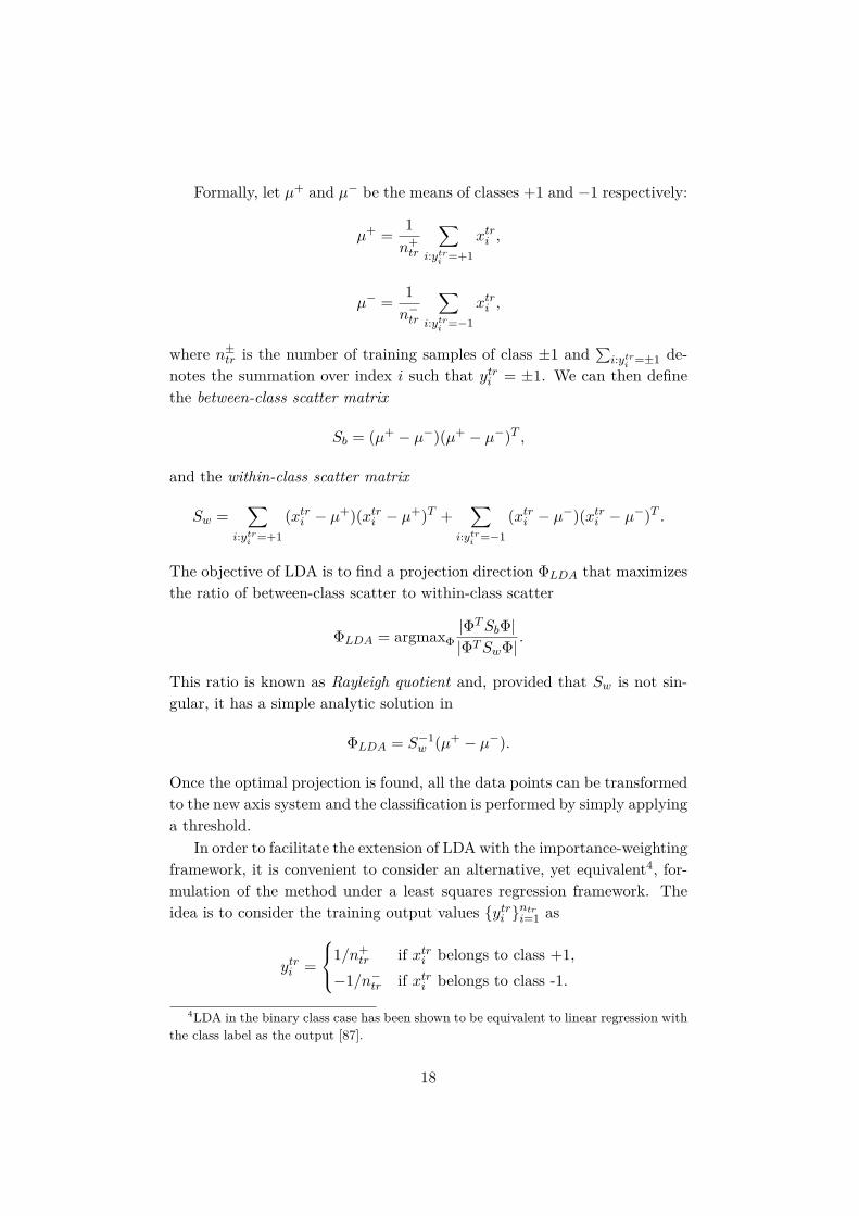
Figure 2.5: Approximation of the 0/1-loss through linear discriminant analysis.

Using a linear model (Equation (1.1)) for learning, the classification resultyte, of a test sample xte, is obtained by the sign of the output of the learnedfunction

yte = sign(f(xte; θ)),

where the parameter θ is learned using LS as loss function.In this setting, the covariate shift adaptation follows the regression case.

The importance-weighted linear discriminant analysis (IWLDA) is given by

θIWLS := argminθ

[1ntr

ntr∑i=1

w(xtri )(1− ytri f(xtri ; θ)

)2]

(2.2)

which has analytic solution in

θ = Lytr = (XtrTW trXtr)−1XtrTW trytr.

The approximation achieved through the least squares formulation of LDAwith respect to the ideal 0/1-loss is illustrated in Figure 2.5, showing thatthe former is a convex upper bound of the latter. Therefore, minimizing theerror under the squared loss corresponds to minimize the upper bound ofthe 0/1-loss error, although the bound is rather loose.

Linear discriminant analysis is just one of the various classification meth-ods proposed in the literature. Other popular ones are logistic regres-sion [38], support vector machine [15, 84] and boosting [29, 30]. For theimportance-weighting adaptation of these methods, see [68].

19

2.3 Model Selection

In the learning processes presented above, we fixed some model parameterssuch as the relative parameter β of the IW, the basis function ϕ(·) of thelinear model, and the bandwidth h of the Gaussian kernel model. Thechoice of these parameters can heavily affect the performance of the learningmethod, therefore an appropriate procedure should be carried out in orderto select their optimal values. This procedure is known under the name ofmodel selection [2, 3].

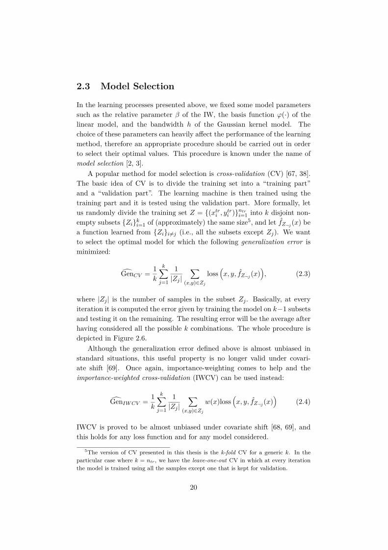
A popular method for model selection is cross-validation (CV) [67, 38].The basic idea of CV is to divide the training set into a “training part”and a “validation part”. The learning machine is then trained using thetraining part and it is tested using the validation part. More formally, letus randomly divide the training set Z = (xtri , ytri )ntri=1 into k disjoint non-empty subsets Ziki=1 of (approximately) the same size5, and let fZ¬j (x) bea function learned from Zii 6=j (i.e., all the subsets except Zj). We wantto select the optimal model for which the following generalization error isminimized:

GenCV = 1k

k∑j=1

1|Zj |

∑(x,y)∈Zj

loss(x, y, fZ¬j (x)

), (2.3)

where |Zj | is the number of samples in the subset Zj . Basically, at everyiteration it is computed the error given by training the model on k−1 subsetsand testing it on the remaining. The resulting error will be the average afterhaving considered all the possible k combinations. The whole procedure isdepicted in Figure 2.6.

Although the generalization error defined above is almost unbiased instandard situations, this useful property is no longer valid under covari-ate shift [69]. Once again, importance-weighting comes to help and theimportance-weighted cross-validation (IWCV) can be used instead:

GenIWCV = 1k

k∑j=1

1|Zj |

∑(x,y)∈Zj

w(x)loss(x, y, fZ¬j (x)

)(2.4)

IWCV is proved to be almost unbiased under covariate shift [68, 69], andthis holds for any loss function and for any model considered.

5The version of CV presented in this thesis is the k-fold CV for a generic k. In theparticular case where k = ntr, we have the leave-one-out CV in which at every iterationthe model is trained using all the samples except one that is kept for validation.

20

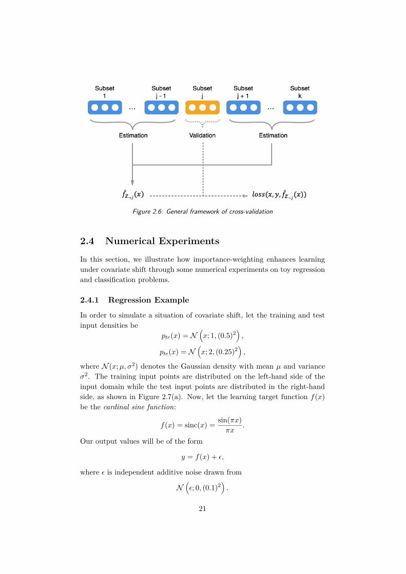
Figure 2.6: General framework of cross-validation

2.4 Numerical Experiments

In this section, we illustrate how importance-weighting enhances learningunder covariate shift through some numerical experiments on toy regressionand classification problems.

2.4.1 Regression Example

In order to simulate a situation of covariate shift, let the training and testinput densities be

ptr(x) = N(x; 1, (0.5)2

),

pte(x) = N(x; 2, (0.25)2

),

where N (x;µ, σ2) denotes the Gaussian density with mean µ and varianceσ2. The training input points are distributed on the left-hand side of theinput domain while the test input points are distributed in the right-handside, as shown in Figure 2.7(a). Now, let the learning target function f(x)be the cardinal sine function:

f(x) = sinc(x) = sin(πx)πx

.

Our output values will be of the form

y = f(x) + ε,

where ε is independent additive noise drawn from

N(ε; 0, (0.1)2

).

21

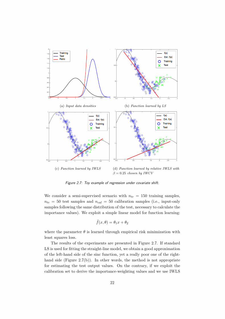
(a) Input data densities (b) Function learned by LS

(c) Function learned by IWLS (d) Function learned by relative IWLS withβ = 0.25 chosen by IWCV

Figure 2.7: Toy example of regression under covariate shift.

We consider a semi-supervised scenario with ntr = 150 training samples,nte = 50 test samples and ncal = 50 calibration samples (i.e., input-onlysamples following the same distribution of the test, necessary to calculate theimportance values). We exploit a simple linear model for function learning:

f(x, θ) = θ1x+ θ2

where the parameter θ is learned through empirical risk minimization withleast squares loss.

The results of the experiments are presented in Figure 2.7. If standardLS is used for fitting the straight-line model, we obtain a good approximationof the left-hand side of the sinc function, yet a really poor one of the right-hand side (Figure 2.7(b)). In other words, the method is not appropriatefor estimating the test output values. On the contrary, if we exploit thecalibration set to derive the importance-weighting values and we use IWLS

22

to estimate the optimal parameter θ, the obtained model manages to predictthe behavior of the right-hand side of the sinc function, and thus to estimatethe test output values properly (Figure 2.7(c)). The problem in this case isrepresented by instability. The relative version of IWLS should be then used,and the relativity parameter β can be selected using importance-weightedCV. In our case, the optimal value is found in β = 0.25. This low value(which makes the relative IWLS be closer to IWLS rather than to standardLS) was expectable, since train and test input densities vary significantly.Figure 2.7(d) depicts the learned function obtained in this latter case, whichyields a better estimation than in the former ones.

Overall, the above toy regression problem shows that importance-weightingtends to improve the prediction performance under covariate shift in regres-sion scenarios.

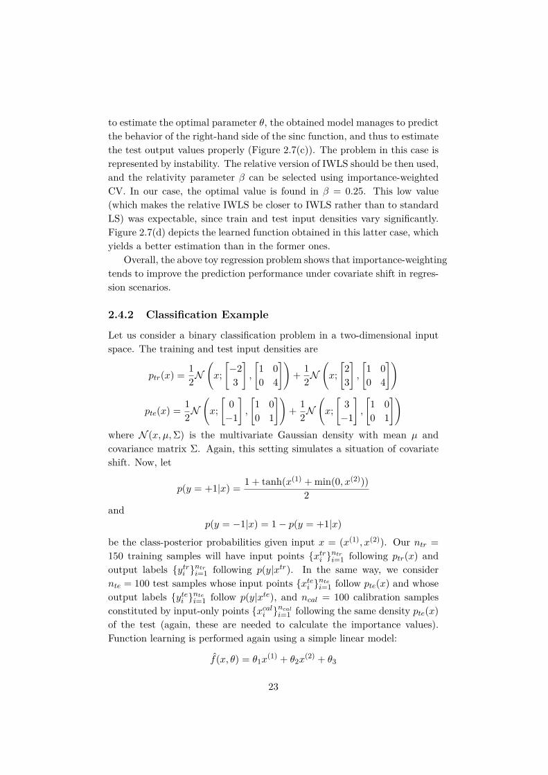
2.4.2 Classification Example

Let us consider a binary classification problem in a two-dimensional inputspace. The training and test input densities are

ptr(x) = 12N

(x;[−23

],

[1 00 4

])+ 1

2N(x;[23

],

[1 00 4

])

pte(x) = 12N

(x;[

0−1

],

[1 00 1

])+ 1

2N(x;[

3−1

],

[1 00 1

])where N (x, µ,Σ) is the multivariate Gaussian density with mean µ andcovariance matrix Σ. Again, this setting simulates a situation of covariateshift. Now, let

p(y = +1|x) = 1 + tanh(x(1) + min(0, x(2)))2

andp(y = −1|x) = 1− p(y = +1|x)

be the class-posterior probabilities given input x = (x(1), x(2)). Our ntr =150 training samples will have input points xtri

ntri=1 following ptr(x) and

output labels ytri ntri=1 following p(y|xtr). In the same way, we consider

nte = 100 test samples whose input points xtei ntei=1 follow pte(x) and whose

output labels ytei ntei=1 follow p(y|xte), and ncal = 100 calibration samples

constituted by input-only points xcali ncali=1 following the same density pte(x)

of the test (again, these are needed to calculate the importance values).Function learning is performed again using a simple linear model:

f(x, θ) = θ1x(1) + θ2x

(2) + θ3

23

(a) Optimal boundary (b) Boundary learned by LDA

(c) Boundary learned by IWLDA (d) Boundary learned by relative IWLDAwith β = 0.20 chosen by IWCV

Figure 2.8: Toy example of classification under covariate shift.

where the parameter θ is learned through linear discriminant analysis.Figure 2.8 illustrates the results of the experiment. In particular, in

Figure 2.8(a) is shown the optimal decision boundary, while in the othersthe boundaries learned using standard LDA, IWLDA and relative IWLDA(with β = 0.2 chosen by IWCV) respectively. Once again, it is evident thatstandard LDA produces a good boundary with respect to the train, yet areally poor one with respect to the test reaching a classification precision onthe test of only 58%. Importance-weighting allows us to obtain an acceptableestimation of the test output labels, increasing the classification precisionto 74% in the case of IWLDA and to 80% in the case of relative IWLDA.Comparing Figure 2.8(c) and 2.8(d), we can notice that the difference isminimal because the relative parameter β is close to zero. Also in this case,the reason is to be found in the significant difference between train and testinput densities.

24

Overall, the above toy classification problem shows that importance-weighting tends to improve the prediction performance under covariate shiftin classification scenarios.

25

26

Chapter 3

Importance Estimation

Essentially, all models are wrong,but some are useful.

George E. P. BoxEmpirical Model-Building and Response Surfaces, 1987

In Chapter 2 we have seen that the importance can be used to enhance theperformance of standard regression and classification methods under covari-ate shift. More in general, the use of density ratios allows us to solve a widerange of machine learning problems (e.g., mutual information estimation,multi-task learning, outlier detection, two-sample test) in a unified manner[71]. However, the true importance is usually unknown in practice and needsto be estimated from data. This chapter is devoted to showcasing some ofthe possible algorithms for estimating the density ratio w(x) between theprobability densities pte(x) and ptr(x):

w(x) = pte(x)ptr(x) .

The setup to be considered is semi-supervised learning. Indeed, in or-der to perform the estimation, we need not only training input samplesxtri

ntri=1, but also input samples drawn from the test, called calibration

samples xcali ncali=1 .

It is important to remark that calibration samples are input-only sam-ples, hence they do not carry any sort of information about the value ofthe output. In the following, we first discuss a naive approach based on theseparate estimation of the densities and successive calculation of the ratiobetween them. Then we analyze two more complex, yet effective, methodswhich directly estimate the density ratio. Numerical experiments concludethe chapter, comparing the accuracy of the presented algorithms.

3.1 Density Estimation Approach

The most straightforward, yet naive, approach for density ratio estimationconsists in first obtaining density estimators pte(x) and ptr(x) separatelyfrom xcali

ncali=1 and xtri

ntri=1, and then computing the density ratio by plug-

ging the density estimators into the ratio

w(x) = pte(x)ptr(x) .

To approximate the true density p(x), we can use a parametric model ofprobability density functions p(x; θ), where θ is a parameter to be estimated.Being p(x; θ) a probability density function, it will satisfy p(x; θ) ≥ 0 and∫p(x; θ)dx = 1 for all θ. The challenge, in this scenario, is to learn the

optimal parameter θ for which the true density is accurately approximated.One common method to do that is the maximum likelihood estimation [38].

The principle of maximum likelihood estimation (MLE) is to determinethe parameter θ that most likely generates the given data. To this end, theprobability of obtaining xi, i = 1 . . . n from the model p(x, θ) needs to beevaluated as a function of θ. Under the assumption that xi, i = 1 . . . n areindependent and identically distributed (i.i.d.) samples, the probability ofobserving all the samples is expressed by the following product:

L(θ) =n∏i=1

p(xi; θ).

This is called the likelihood. In ML estimation, the parameter θ is learnedso that the likelihood L(θ) is maximized:

θMLE = argmaxθ L(θ).

Hence, the MLE of the density p(x) will be pMLE(x) = p(x; θMLE).However, since the above likelihood is the product of numbers less than or

equal to 1, when the number n of samples is large, it tends to zero. To avoidany numerical instability that can be caused by working with extremelysmall values, the log-likelihood is often used:

logL(θ) =n∑i=1

log p(xi; θ),

where the previous product has become a summation due to the simple rulelog xy = log x+ log y. Because the log function is monotone increasing, theprocedure to learn the optimal parameter θ consists again in maximizingthe log-likelihood:

θMLE = argmaxθ logL(θ).

28

This formulation is equivalent to the previous one, but with the advantageof being numerically more stable.

The MLE approach is a classical and convenient method for densityestimation but it is not so accurate when the number of available samplesis limited. This is an issue considering that our objective is to compute theratio between two densities, hence even a small approximation error in theestimation of a single density can lead to a big total error. For instance, ifwe make a small error in the estimation of pte(x), this would be magnified bythe division for ptr(x), making the whole estimator unreliable. To overcomethe limitation of this two-step approach, a one-shot procedure of directlyestimating the density ratio without going through the separate estimationof densities seems more promising. Methods following this idea are describedin the next section.

3.2 Direct Importance Estimation Approach

In this section, we consider directly estimating the importance without go-ing through the separate estimation of the test and training densities. Theintuitive advantage of this approach is that knowing the densities pte(x) andptr(x) implies knowing the importance w(x), but not viceversa. The impor-tance w(x) cannot be uniquely decomposed into the two densities pte(x) andptr(x) (see Figure 3.1). In other words, directly estimating the importanceis a simpler and more promising approach.

This intuitive idea is supported by the famous principle advocated bythe Russian mathematician Vladimir Vapnik1:

One should avoid solving more difficult intermediateproblems when solving a target problem.

This statement is sometimes referred to as Vapnik’s principle (1998) and inthe context of density ratio estimation may be interpreted as follows:

One should avoid estimating the two densitiespte(x) and ptr(x) when estimating the ratio w(x).

Following this idea, two direct density ratio estimation methods will bediscussed, and their performance in terms of estimation accuracy are shownin Section 3.3.

1Vladimir Vapnik is the creator of one of the most successful classification algorithms,the support vector machine [15, 84].

29

Figure 3.1: Knowing the two densities pte(x) and ptr(x) implies knowing the importancew(x). However, the importance w(x) cannot be uniquely decomposed into the twodensities pte(x) and ptr(x).

3.2.1 Kullback-Leibler Importance Estimation Procedure

The Kullback-Leibler importance estimation procedure (KLIEP) [70, 71] di-rectly gives an estimate of the importance function without going throughseparate density estimations. The procedure is based on the use of theKullback-Leibler (KL) divergence [44] as a measure of discrepancy betweentwo densities. More specifically, the KL divergence of a probability distribu-tion Q from a probability distribution P, denoted KL(P ‖ Q), is a measureof the information lost when Q is used to approximate P. Our objectivewill then be to minimize the KL divergence from the true importance func-tion w(x) to a modeled importance function w(x), so as to obtain the mostaccurate possible approximation.

In order to apply this concept to our problem, let us employ a simplelinear model (see Equation (1.1)) for the importance estimation:

w(x) =d∑i=1

θiϕi(x),

with θidi=1 being the parameters to be learned from data samples, andϕi(x)di=1 the fixed and linearly independent basis functions. Since thetrue importance function is defined as

w(x) = pte(x)ptr(x) ,

then the density pte(x) may be modeled by

pte(x) = w(x)ptr(x).

From the definition, the KL divergence from pte(x) to pte(x) is expressed asfollows:

KL(pte ‖ pte) =∫pte(x) log pte(x)

pte(x)dx ,

30

which gives an indication of the information lost when pte(x) is used toapproximate pte(x). Thus, our goal is to minimize the above KL divergence.

It is possible to show that, after few mathematical steps2, the aboveoptimization problem becomes:

maxθ1nte

nte∑i=1

log w(xtei ) (3.1)

subject to 1ntr

ntr∑i=1

w(xtri ) = 1 and θ1, θ2, . . . θd ≥ 0 (3.2)

Now, substituting w(x) with the proposed linear model, we obtain:

maxθnte∑i=1

log

d∑j=1

θjϕj(xtei )

subject to 1

ntr

ntr∑i=1

d∑j=1

θjϕj(xtri ) = 1 and θ1, θ2, . . . θd ≥ 0

This formulation is the Kullback-Leibler importance estimation procedurein the case of a linear model. Because the KLIEP optimization problemis convex, there exists a unique global optimal solution. However, since anonlinear optimization problem has to be solved, the computation resultsrather expensive. This is only in part mitigated by the fact that the KLIEPsolution tends to be sparse, meaning that many parameters take exactlyvalue zero. Such sparsity would contribute to reduce the computation timewhen computing the estimated importance values.

It is worth noting that Equations (3.1) and (3.2) depend only on w(x),the model used to approximate the true importance function. Thus, alter-natives to the linear model could be used. An example would be the alreadydiscussed Gaussian kernel model (see Equation (1.2)). The advantages of us-ing a kernel model rather than a linear model are all those already discussedin Section 1.2.

To summarize, KLIEP is an accurate way to avoid single density esti-mation when estimating the importance. Furthermore, it is applicable toa variety of different models depending on the requirements needed. Theonly drawback is represented by the computational efficiency, which can be-come critical when dealing with high dimensional data due to the nonlinearoptimization problem involved. A MATLAB implementation of KLIEP isavailable at http://www.ms.k.u-tokyo.ac.jp/software.html#KLIEP.

2For the sake of simplicity, these steps are not presented in this thesis. The reasonis that the main interest is not to go into the mathematical details of the derivation,yet instead to provide the reader with a general idea of importance estimation. For acomprehensive discussion see [71].

31

3.2.2 Least-Squares Importance Fitting

If KLIEP employed the Kullback-Leibler divergence for measuring the dis-crepancy between two densities, the least-squares importance fitting (LSIF)[42, 71] uses the squared loss for importance function fitting. In other words,LSIF formulates the direct importance estimation problem as a least-squaresfunction fitting problem. The great advantage of this approach is that it iscomputationally very efficient.

Assuming that w(x) is a model that approximate the true importancefunction w(x). The idea behind LSIF is to determine the optimal modelw(x) so that the following squared error J is minimized:

J(w) = 12

∫(w(x)− w(x))2 ptr(x)dx,

which is basically an analogous formulation of the already discussed least-squares (see Section 2.2). As in the case of KLIEP, applying a few mathe-matical rules to the optimization problem above, it is possible to reach theleast-squares importance fitting formulation:

minw

12ntr

ntr∑i=1

w2(xtri )− 1nte

nte∑j=1

w(xtej )

. (3.3)

Now, suppose we use the usual linear model3 (see Equation (1.1)) toestimate the importance function:

w(x) =d∑i=1

θiϕi(x),

with θidi=1 being the parameters to be learned from data samples, andϕi(x)di=1 the fixed and linearly independent basis functions. Substitut-ing it into Equation (3.3), we obtain the least-squares importance fittingformulation for the linear model:

minθ[1

2θT Hθ − hT θ

]subject to θ1, θ2, . . . θd ≥ 0, (3.4)

where θ = (θ1, θ2, . . . θd), H is the d × d matrix with the (k, k′)-th elementas

Hk,k′ = 1ntr

ntr∑i=1

ϕk(xtri )ϕk′(xtri ),

3Again, we consider a linear model just for the sake of simplicity. Other more complexmodels could be used, such as Gaussian kernel model (see Equation (1.2)).

32

and h is the d-dimensional vector with the k-th element as

hk = 1nte

nte∑j=1

ϕk(xtej ).

This optimization problem is a convex quadratic programming problem.Therefore, the unique global optimal solution exists and can be computedefficiently by a standard optimization software (e.g., quadprog function inMATLAB).

LSIF is a computationally very efficient way to directly estimate the im-portance function. However, it sometimes suffers from numerical problems,and therefore it may not be reliable in practice. For this reasons, a slightlydifferent version still based on squared loss for importance function fitting isusually preferred. This version goes under the name of unconstrained least-squares importance fitting (uLSIF) and, beyond the fact of being numericallystable, it also has a solution that can be computed analytically.

The idea behind uLSIF is very simple. As the name suggests, we approx-imate LSIF by dropping the non-negativity constraint in the optimizationproblem (Equation (3.4)). Without the non-negativity constraint, it is nec-essary to introduce a penalty term λ

2 θT θ for regularization purposes, where

λ (≥ 0) is the regularization parameter. The new optimization problem willthen be:

minθ[1

2θT Hθ − hT θ + λ

2 θT θ

]. (3.5)

Equation (3.5) is an unconstrained convex quadratic programming problem,and the solution can be computed analytically by solving a system of linearequations:

θ = (H + λId)−1h,

where Id is the d-dimensional identity matrix. Finally, because the non-negative constraint θ1, θ2, . . . θd ≥ 0 was dropped, some of the learned pa-rameters, and consequently the estimated importance values, could be nega-tive. To compensate for this approximation error, negative parameters maybe rounded up to zero as follows:

θi = max(0, θi) for i = 1, 2 . . . d.

The great advantage of uLSIF is that it allows us to obtain a closed-formsolution that can be computed just by solving a system of linear equations.Therefore, the computation is fast and numerically stable. Furthermore, thesimple approximation performed does not prevent uLSIF to exhibit all thegood properties of the other methods. For these reasons, uLSIF is a prefer-able method for importance estimation. A MATLAB implementation ofuLSIF is available at http://www.ms.k.u-tokyo.ac.jp/software.html#uLSIF.

33

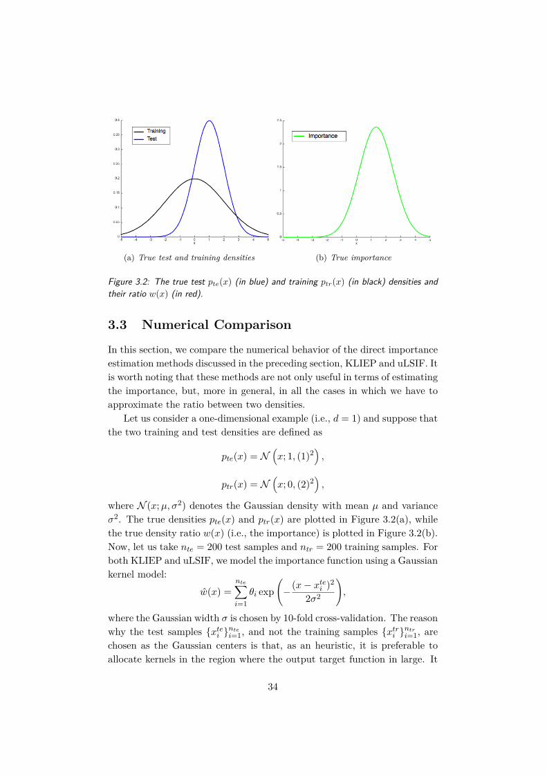
(a) True test and training densities (b) True importance

Figure 3.2: The true test pte(x) (in blue) and training ptr(x) (in black) densities andtheir ratio w(x) (in red).

3.3 Numerical Comparison

In this section, we compare the numerical behavior of the direct importanceestimation methods discussed in the preceding section, KLIEP and uLSIF. Itis worth noting that these methods are not only useful in terms of estimatingthe importance, but, more in general, in all the cases in which we have toapproximate the ratio between two densities.

Let us consider a one-dimensional example (i.e., d = 1) and suppose thatthe two training and test densities are defined as

pte(x) = N(x; 1, (1)2

),

ptr(x) = N(x; 0, (2)2

),

where N (x;µ, σ2) denotes the Gaussian density with mean µ and varianceσ2. The true densities pte(x) and ptr(x) are plotted in Figure 3.2(a), whilethe true density ratio w(x) (i.e., the importance) is plotted in Figure 3.2(b).Now, let us take nte = 200 test samples and ntr = 200 training samples. Forboth KLIEP and uLSIF, we model the importance function using a Gaussiankernel model:

w(x) =nte∑i=1

θi exp(−(x− xtei )2

2σ2

),

where the Gaussian width σ is chosen by 10-fold cross-validation. The reasonwhy the test samples xtei

ntei=1, and not the training samples xtri

ntri=1, are

chosen as the Gaussian centers is that, as an heuristic, it is preferable toallocate kernels in the region where the output target function in large. It

34

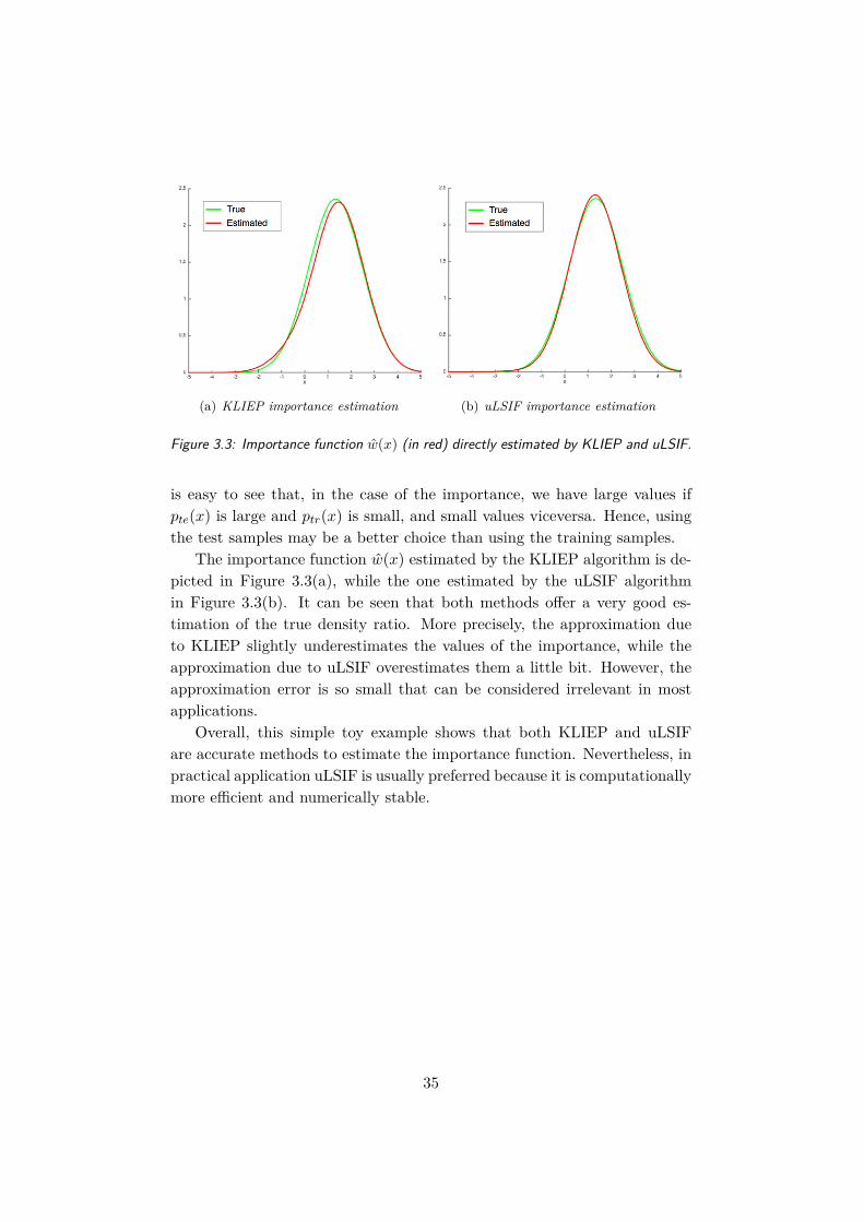
(a) KLIEP importance estimation (b) uLSIF importance estimation

Figure 3.3: Importance function w(x) (in red) directly estimated by KLIEP and uLSIF.

is easy to see that, in the case of the importance, we have large values ifpte(x) is large and ptr(x) is small, and small values viceversa. Hence, usingthe test samples may be a better choice than using the training samples.

The importance function w(x) estimated by the KLIEP algorithm is de-picted in Figure 3.3(a), while the one estimated by the uLSIF algorithmin Figure 3.3(b). It can be seen that both methods offer a very good es-timation of the true density ratio. More precisely, the approximation dueto KLIEP slightly underestimates the values of the importance, while theapproximation due to uLSIF overestimates them a little bit. However, theapproximation error is so small that can be considered irrelevant in mostapplications.

Overall, this simple toy example shows that both KLIEP and uLSIFare accurate methods to estimate the importance function. Nevertheless, inpractical application uLSIF is usually preferred because it is computationallymore efficient and numerically stable.

35

36

Chapter 4

Importance-WeightedMethods for BCI

There is a real danger that computerswill develop intelligence and take over.We urgently need to develop direct connections to the brainso that computers can add to human intelligencerather than be in opposition.

Stephen Hawking

As we said in Chapter 1, the stationary assumption of standard machinelearning is often violated in real-world problems, in which non-stationaryphenomena are usually experienced. Consequently, the concept of importance-weighting gains particular relevance in many practical situations that can bedescribed by covariance shift. This chapter presents a first real-world appli-cation of importance-weighting for covariate shift adaptation. The paradigmconsidered is motor imagery in Brain-Computer Interfaces (BCI), which isby nature strongly affected by non-stationary phenomena. In the following,we formulate the problem and we show how importance-weighted methodscan be applied to enhance the performance of a BCI system1.

1The chapter is inspired by the paper “Importance-weighted covariance estimation forrobust common spatial pattern” written by the author of this thesis in collaboration withDr. Florian Yger and Prof. Masashi Sugiyama and published in Pattern RecognitionLetters journal, volume 68, part 1, pages 139-145, on December 15, 2015. The originalversion of the paper is reported in Appendix A.

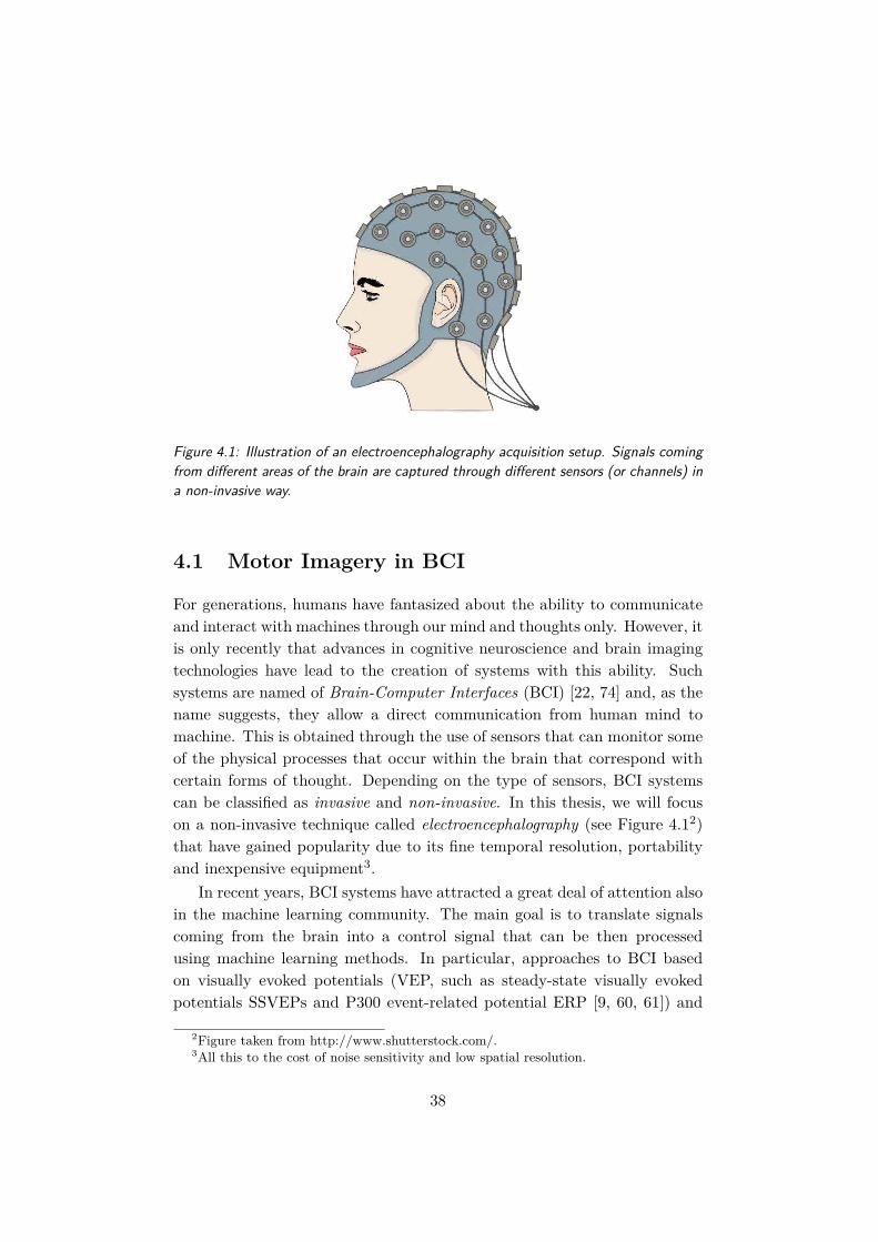
Figure 4.1: Illustration of an electroencephalography acquisition setup. Signals comingfrom different areas of the brain are captured through different sensors (or channels) ina non-invasive way.

4.1 Motor Imagery in BCI

For generations, humans have fantasized about the ability to communicateand interact with machines through our mind and thoughts only. However, itis only recently that advances in cognitive neuroscience and brain imagingtechnologies have lead to the creation of systems with this ability. Suchsystems are named of Brain-Computer Interfaces (BCI) [22, 74] and, as thename suggests, they allow a direct communication from human mind tomachine. This is obtained through the use of sensors that can monitor someof the physical processes that occur within the brain that correspond withcertain forms of thought. Depending on the type of sensors, BCI systemscan be classified as invasive and non-invasive. In this thesis, we will focuson a non-invasive technique called electroencephalography (see Figure 4.12)that have gained popularity due to its fine temporal resolution, portabilityand inexpensive equipment3.

In recent years, BCI systems have attracted a great deal of attention alsoin the machine learning community. The main goal is to translate signalscoming from the brain into a control signal that can be then processedusing machine learning methods. In particular, approaches to BCI basedon visually evoked potentials (VEP, such as steady-state visually evokedpotentials SSVEPs and P300 event-related potential ERP [9, 60, 61]) and

2Figure taken from http://www.shutterstock.com/.3All this to the cost of noise sensitivity and low spatial resolution.

38

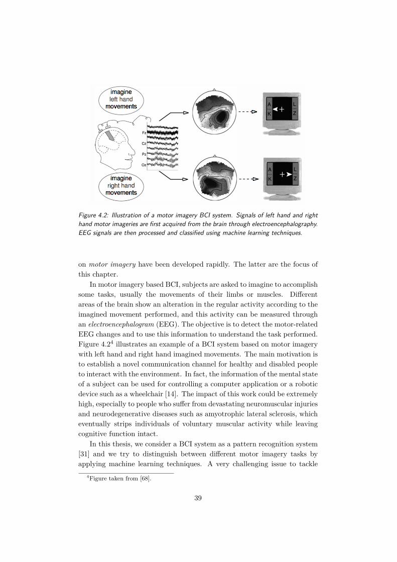
Figure 4.2: Illustration of a motor imagery BCI system. Signals of left hand and righthand motor imageries are first acquired from the brain through electroencephalography.EEG signals are then processed and classified using machine learning techniques.

on motor imagery have been developed rapidly. The latter are the focus ofthis chapter.

In motor imagery based BCI, subjects are asked to imagine to accomplishsome tasks, usually the movements of their limbs or muscles. Differentareas of the brain show an alteration in the regular activity according to theimagined movement performed, and this activity can be measured throughan electroencephalogram (EEG). The objective is to detect the motor-relatedEEG changes and to use this information to understand the task performed.Figure 4.24 illustrates an example of a BCI system based on motor imagerywith left hand and right hand imagined movements. The main motivation isto establish a novel communication channel for healthy and disabled peopleto interact with the environment. In fact, the information of the mental stateof a subject can be used for controlling a computer application or a roboticdevice such as a wheelchair [14]. The impact of this work could be extremelyhigh, especially to people who suffer from devastating neuromuscular injuriesand neurodegenerative diseases such as amyotrophic lateral sclerosis, whicheventually strips individuals of voluntary muscular activity while leavingcognitive function intact.

In this thesis, we consider a BCI system as a pattern recognition system[31] and we try to distinguish between different motor imagery tasks byapplying machine learning techniques. A very challenging issue to tackle

4Figure taken from [68].

39

in this setting is the presence of non-stationarity and outliers. The sourcesof these could be changes in user attention level, fatigue or artifacts (e.g.,eye blinks, loose electrodes, etc.) that corrupt the acquired brain signals,and the intrinsic non-stationarity of EEG signals. These non-stationaryphenomena are particularly evident between the training and test sessions ofan experiment, being these usually separated by a significant span of time.As a consequence, training input points and test input points are likelyto have different distributions and this cause standard machine learningtechniques performance to be far from being optimal. A situation of thiskind can be well approximated by covariate shift, thus importance-weightedmethods become useful to improve the BCI recognition accuracy.

4.2 Method

In this section, we explore the machine learning methods used for motorimagery BCI classification. We start by providing a general framework,then we go into the details of the single techniques with their extension tothe importance-weighted case.

4.2.1 General Framework

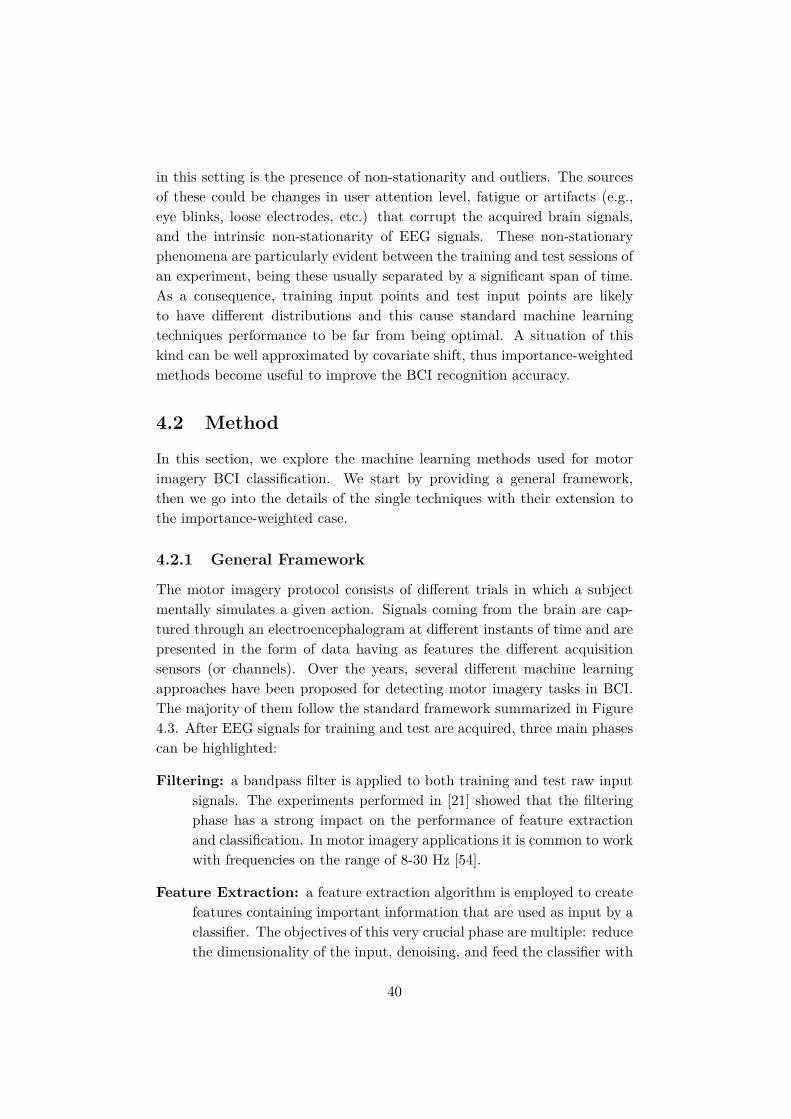
The motor imagery protocol consists of different trials in which a subjectmentally simulates a given action. Signals coming from the brain are cap-tured through an electroencephalogram at different instants of time and arepresented in the form of data having as features the different acquisitionsensors (or channels). Over the years, several different machine learningapproaches have been proposed for detecting motor imagery tasks in BCI.The majority of them follow the standard framework summarized in Figure4.3. After EEG signals for training and test are acquired, three main phasescan be highlighted:

Filtering: a bandpass filter is applied to both training and test raw inputsignals. The experiments performed in [21] showed that the filteringphase has a strong impact on the performance of feature extractionand classification. In motor imagery applications it is common to workwith frequencies on the range of 8-30 Hz [54].

Feature Extraction: a feature extraction algorithm is employed to createfeatures containing important information that are used as input by aclassifier. The objectives of this very crucial phase are multiple: reducethe dimensionality of the input, denoising, and feed the classifier with

40

Figure 4.3: Standard framework for the classification of motor imagery tasks in BCI.Raw signals go into the phases of filtering, feature extraction and finally classification.

only the relevant features. A popular algorithm for feature extractionin BCI application is common spatial pattern (CSP) [31], followed bythe extraction of the log-variance of the spatially filtered signals.

Classification: a classification algorithm is used to separate different mo-tor imagery tasks. In [48] the authors gave experimental evidence ofthe fact that in BCI applications linear algorithms such as linear dis-criminant analysis (LDA) [38] often outperform more complex ones.Another valid option could be adopting a basic K-nearest neighbors(k-NN) [4, 38] classifier.

Although this standard framework is widely used in the machine learningBCI community, it does not take in consideration the eventuality of changesbetween the train and test distributions, which are instead very frequentin BCI experiments. Thus, in order to deal with such dataset shift, theabove framework needs to be slightly modified. First of all, it is necessaryto consider a semi-supervised learning scenario for the importance-weightingextension. To do so, a calibration set composed of unlabeled data followingthe same distribution of the test is provided in addition to the standardtraining and test sets. Once the values of the importance are calculated (e.g.,

41

Figure 4.4: Robust framework for the classification of motor imagery tasks in BCI.Unlabeled calibration data following the same distribution of the test are providedin addition to training and test data. Importance-weighted feature extraction andclassification phases lead to a robust decision rule.

using one of the methods discussed in Chapter 3), these can be applied tothe feature extraction step as well as to the classification step, with the aimof increasing the robustness of the model. Indeed, having a robust featureextraction and classification phase will result in a more accurate model forprediction under covariate shift, as it is proved by the experiment discussedin Section 4.3. The new obtained framework is illustrated in the flowchartof Figure 4.4. Finally, it is important to remark that, while the importance-weighting extension in the classification phase has been already proposed in[46], the one in the feature extraction step is a novel technique introducedby the author of this thesis (see appendix A).

4.2.2 Common Spatial Pattern

The Common Spatial Pattern (CSP) method was first introduced by K.Fukunaga in 1990 [31]. Nowadays it is one the most popular algorithm forspatial filtering in motor imagery experiments. The main idea is to use a

42

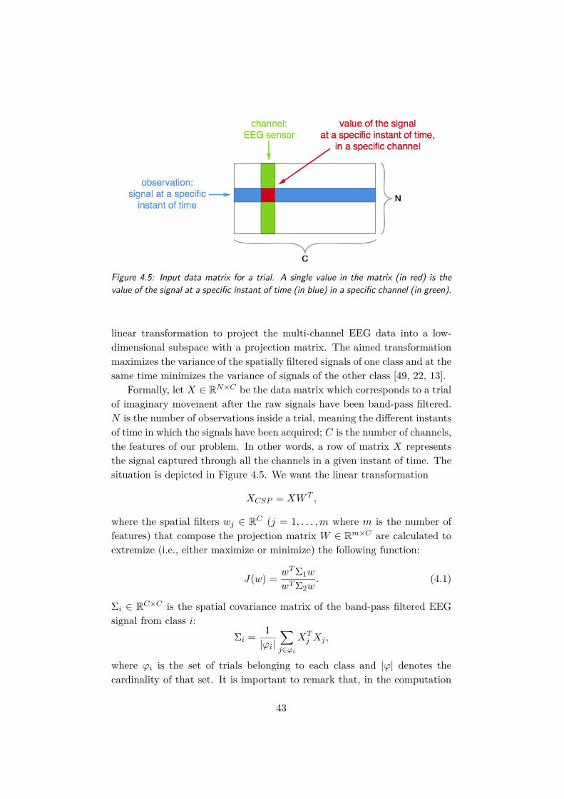
Figure 4.5: Input data matrix for a trial. A single value in the matrix (in red) is thevalue of the signal at a specific instant of time (in blue) in a specific channel (in green).

linear transformation to project the multi-channel EEG data into a low-dimensional subspace with a projection matrix. The aimed transformationmaximizes the variance of the spatially filtered signals of one class and at thesame time minimizes the variance of signals of the other class [49, 22, 13].

Formally, let X ∈ RN×C be the data matrix which corresponds to a trialof imaginary movement after the raw signals have been band-pass filtered.N is the number of observations inside a trial, meaning the different instantsof time in which the signals have been acquired; C is the number of channels,the features of our problem. In other words, a row of matrix X representsthe signal captured through all the channels in a given instant of time. Thesituation is depicted in Figure 4.5. We want the linear transformation

XCSP = XW T ,

where the spatial filters wj ∈ RC (j = 1, . . . ,m where m is the number offeatures) that compose the projection matrix W ∈ Rm×C are calculated toextremize (i.e., either maximize or minimize) the following function:

J(w) = wTΣ1w

wTΣ2w. (4.1)

Σi ∈ RC×C is the spatial covariance matrix of the band-pass filtered EEGsignal from class i:

Σi = 1|ϕi|

∑j∈ϕi

XTj Xj ,

where ϕi is the set of trials belonging to each class and |ϕ| denotes thecardinality of that set. It is important to remark that, in the computation

43

of the covariance matrices, we assume the EEG signals to have a zero mean.However, this assumption is generally met if EEG signals have been formerlyband-pass filtered.

An alternative, yet equivalent way, to express Equation 4.1 is to use theRayleigh quotient5 as follows:

J(W ) = Trace(W TΣ1W )Trace(W TΣ2W ) .

Various possible approaches to solve this optimization problem have beendeveloped. The most straightforward one seems the one proposed in [49],however in the literature [22] it is more often solved by jointly diagonalizingthe two covariance matrices in a way that the eigenvalues of Σ1 and Σ2 sumto 1:

W TΣ1W = D,

W T (Σ1 + Σ2)W = Im,

where Im is the identity matrix of size m×m and D is the diagonal matrixcontaining the eigenvalues of Σ1. Using the Lagrangian of the constrainedproblem

L(λ,w) = wTΣ1w − λ(wT (Σ1 + Σ2)w − 1),

we can calculate the derivative with respect to W and then, setting it to 0,we obtain a standard eigenvalue problem:

(Σ1 + Σ2)−1Σ1w = λw.

In BCI applications it is common [13] to select the dimension of W as m = 6and therefore the spatial filters extremizing Equation 4.1 are the eigenvectorsof (Σ1 + Σ2)−1Σ1 associated to the 3 largest and the 3 lowest eigenvalues.

CSP has been proven to be one of the most effective algorithms forfeatures extraction in BCI applications [12]. However, one of its main draw-backs, inherited from the weakness of the covariance matrix estimation, is tobe highly sensitive to noise and outliers [34, 56] and therefore it is not robustunder covariate shift. To cope with this problem, the importance-weightingadaptation6 is applied to every observation of the training dataset during theconstruction of the covariance matrix. Thanks to this adjustment eventualinput distribution shifts between the training and test phase are taken intoaccount. In practice this is obtained by down-weighting the non-pertinent

5The Rayleigh quotient has been already introduced in Section 2.2.2 when talkingabout the optimization problem of LDA.

6In this chapter, we will indicate the importance with the notation r(x) (and not w(x)as it was presented in Chapter 2) to avoid confusion with the spatial filters w.

44

training samples in favor of the pertinent ones. Mathematically speaking,the covariance matrix Σi for class i is now calculated as it follows:

Σi =∑j∈ϕi X

Tj RjXj

Trace(Rj),

where Rj is the diagonal matrix7 containing the density ratio ri (with i =1, . . . , N) for all the N observations of trial

Rj =

r

(j)1 0

. . .0 r

(j)N

.Provided that a robust estimation of the covariance matrix of every epochis derived, the CSP would become effective even in presence of covariateshift. The discussed extension goes under the name of importance-weightedcommon spatial pattern (IWCSP) and it is a novel technique introduced bythe author of this thesis (see appendix A).

4.2.3 Linear Discriminant Analysis

After the feature extraction step, data is ready to be fed into a classifier.As already pointed out in Section 4.2.1, when dealing with the classificationof motor imagery tasks in BCI, linear algorithms often outperform morecomplex ones. A common choice is therefore to use linear discriminantanalysis (LDA), already introduced in Section 2.2.2. Once again, takinginto account the non-stationarity of the motor imagery paradigm in BCIand modeling the situation as covariate shift, it seems straightforward toapply the importance-weighting adaptation. Hence, importance-weightedLDA (IWLDA, Equation 2.2) is a robust and effective classification methodfor motor imagery BCI.

4.2.4 K-Nearest Neighbors on Covariance Matrices

A different approach in motor imagery BCI classification consists in lookingat the “similarity” of the covariance matrices of training and test samples.The idea of using the covariance matrices as features is receiving a greatamount of attention recently [7, 8, 39, 89, 91], due to their ability to carrymeaningful information keeping a low dimension. In this scenario, classifica-tion can be performed using a simple, yet efficient, non-parametric algorithm

7Note that the Maximum Likelihood Estimator can be written in this way with Rjbeing the identity matrix. This case should occur when the data is stationary.

45

called k-nearest neighbors (k-NN) [4, 38]. k-NN assigns a label to a test sam-ple by looking at the k samples in the training set (called neighbors) thathave the most similar features to it and picking the label by majority votingamong them.

Mathematically speaking, let Z ∈ RN×m be the data matrix which cor-responds to a trial of imaginary movement after that the feature extractionphase has been performed. The situation is the same that was already de-picted in Figure 4.5, with the only difference that the number of featureshas been reduced from C to m (with m = 6 in the case of CSP). We wantto represent each trial in terms of its covariance matrix:

Σ = ZTZ, (4.2)

where Σ is the m×m covariance matrix. Now, the idea of k-NN is that giventhe covariance matrix of a test trial Σte

i , we find the k training covariancematrices Σtr

j , j = 1, . . . k closest in distance to Σtei and then classify using

majority voting among the k neighbors. In other words, the test trial isassigned to the most common class among its k nearest neighbors, wherethe parameter k is a positive integer, typically small.

The best choice of k depends upon the data. Generally, larger values ofk reduce the effect of noise on the classification [24], but make boundariesbetween classes less distinct. In the special case where k = 1, the the testtrial label is simply assigned to the class of the closest training trial (i.e.,the single nearest neighbor). In binary classification problems, it is helpfulto choose k to be an odd number as this avoids tied votes and, hence,ambiguity in the correct label to assign. More generally, in the literaturevarious techniques have been proposed to select a good value for k, such ascross-validation or the bootstrap method [36].

As previously explained, k-NN evaluates the “similarity” for featurematching. A crucial passage is therefore to choose a meaningful measureof the distance between two covariance matrices Σ1 and Σ2. The most clas-sical one would be to use the Euclidean distance δe [20], defined as:

δe(Σ1,Σ2) =‖ Σ1 − Σ2 ‖F ,

where ‖ . ‖F denotes the Frobenius norm [33, 40]. However, since the spaceof covariance matrices is not a Euclidean space [81], the Euclidean distancemay result deformed and hence inadequate for our purposes. A better so-lution is to employ the distance measured proposed in [28] and sometimesreferred to as the Riemannian distance8. The Riemannian distance δr be-

8An alternative, yet equivalent, formulation of the Riemannian distance is given in [10]as: δr(Σ1,Σ2) =‖ log (Σ−

12

1 Σ2Σ−12

1 ) ‖F .

46

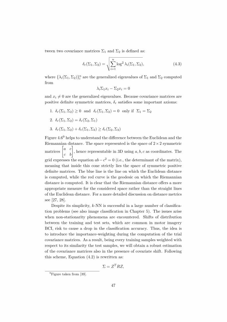
tween two covariance matrices Σ1 and Σ2 is defined as:

δr(Σ1,Σ2) =

√√√√ n∑i=1

log2 λi(Σ1,Σ2), (4.3)

where λi(Σ1,Σ2)ni are the generalized eigenvalues of Σ1 and Σ2 computedfrom

λiΣ1xi − Σ2xi = 0

and xi 6= 0 are the generalized eigenvalues. Because covariance matrices arepositive definite symmetric matrices, δr satisfies some important axioms:

1. δr(Σ1,Σ2) ≥ 0 and δr(Σ1,Σ2) = 0 only if Σ1 = Σ2

2. δr(Σ1,Σ2) = δr(Σ2,Σ1)

3. δr(Σ1,Σ2) + δr(Σ1,Σ3) ≥ δr(Σ2,Σ3)

Figure 4.69 helps to understand the difference between the Euclidean and theRiemannian distance. The space represented is the space of 2×2 symmetric

matrices[a c

c b

], hence representable in 3D using a, b, c as coordinates. The

grid expresses the equation ab− c2 = 0 (i.e., the determinant of the matrix),meaning that inside this cone strictly lies the space of symmetric positivedefinite matrices. The blue line is the line on which the Euclidean distanceis computed, while the red curve is the geodesic on which the Riemanniandistance is computed. It is clear that the Riemannian distance offers a moreappropriate measure for the considered space rather than the straight linesof the Euclidean distance. For a more detailed discussion on distance metricssee [27, 28].

Despite its simplicity, k-NN is successful in a large number of classifica-tion problems (see also image classification in Chapter 5). The issues arisewhen non-stationarity phenomena are encountered. Shifts of distributionbetween the training and test sets, which are common in motor imageryBCI, risk to cause a drop in the classification accuracy. Thus, the idea isto introduce the importance-weighting during the computation of the trialcovariance matrices. As a result, being every training samples weighted withrespect to its similarity the test samples, we will obtain a robust estimationof the covariance matrices also in the presence of covariate shift. Followingthis scheme, Equation (4.2) is rewritten as:

Σ = ZTRZ,

9Figure taken from [39].

47

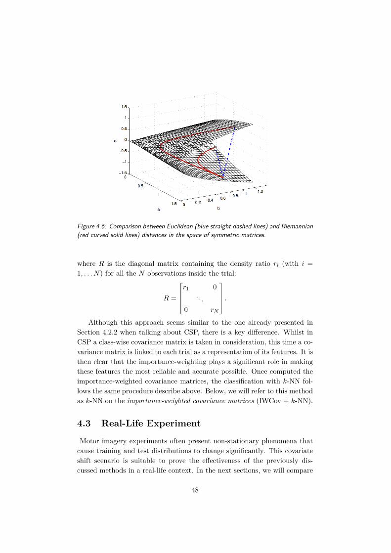
Figure 4.6: Comparison between Euclidean (blue straight dashed lines) and Riemannian(red curved solid lines) distances in the space of symmetric matrices.

where R is the diagonal matrix containing the density ratio ri (with i =1, . . . N) for all the N observations inside the trial:

R =

r1 0

. . .0 rN

.Although this approach seems similar to the one already presented in

Section 4.2.2 when talking about CSP, there is a key difference. Whilst inCSP a class-wise covariance matrix is taken in consideration, this time a co-variance matrix is linked to each trial as a representation of its features. It isthen clear that the importance-weighting plays a significant role in makingthese features the most reliable and accurate possible. Once computed theimportance-weighted covariance matrices, the classification with k-NN fol-lows the same procedure describe above. Below, we will refer to this methodas k-NN on the importance-weighted covariance matrices (IWCov + k-NN).

4.3 Real-Life Experiment

Motor imagery experiments often present non-stationary phenomena thatcause training and test distributions to change significantly. This covariateshift scenario is suitable to prove the effectiveness of the previously dis-cussed methods in a real-life context. In the next sections, we will compare

48

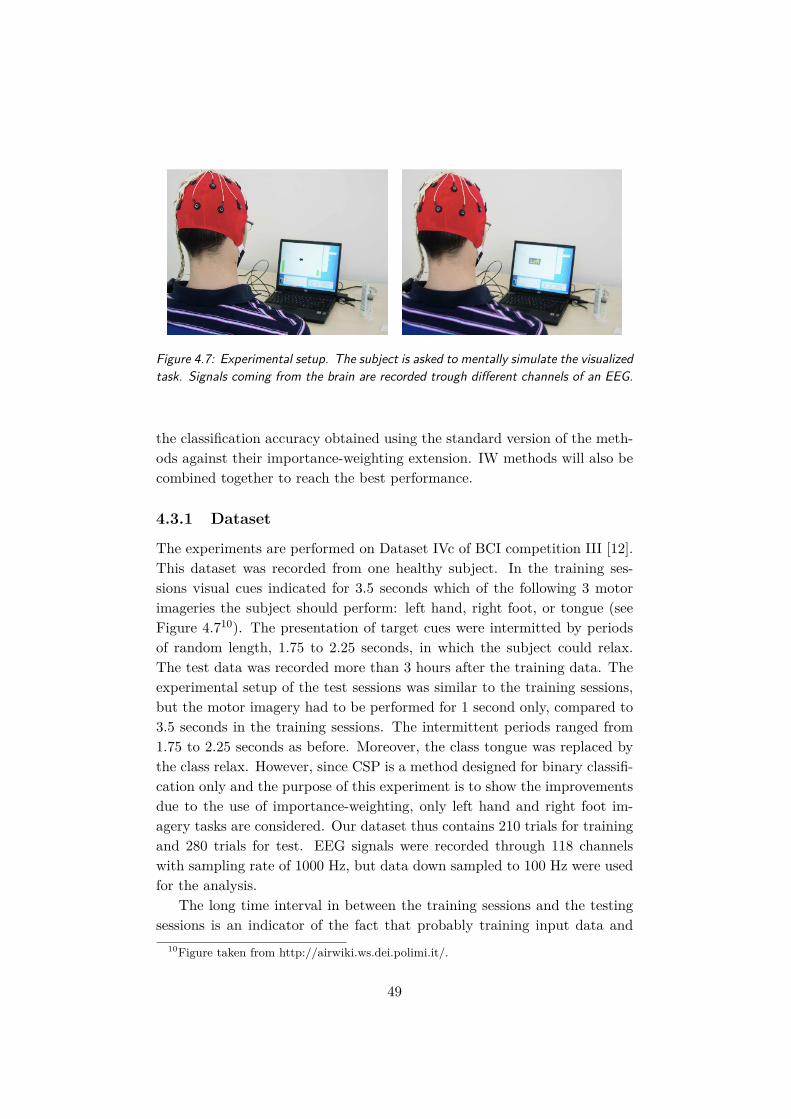
Figure 4.7: Experimental setup. The subject is asked to mentally simulate the visualizedtask. Signals coming from the brain are recorded trough different channels of an EEG.

the classification accuracy obtained using the standard version of the meth-ods against their importance-weighting extension. IW methods will also becombined together to reach the best performance.

4.3.1 Dataset

The experiments are performed on Dataset IVc of BCI competition III [12].This dataset was recorded from one healthy subject. In the training ses-sions visual cues indicated for 3.5 seconds which of the following 3 motorimageries the subject should perform: left hand, right foot, or tongue (seeFigure 4.710). The presentation of target cues were intermitted by periodsof random length, 1.75 to 2.25 seconds, in which the subject could relax.The test data was recorded more than 3 hours after the training data. Theexperimental setup of the test sessions was similar to the training sessions,but the motor imagery had to be performed for 1 second only, compared to3.5 seconds in the training sessions. The intermittent periods ranged from1.75 to 2.25 seconds as before. Moreover, the class tongue was replaced bythe class relax. However, since CSP is a method designed for binary classifi-cation only and the purpose of this experiment is to show the improvementsdue to the use of importance-weighting, only left hand and right foot im-agery tasks are considered. Our dataset thus contains 210 trials for trainingand 280 trials for test. EEG signals were recorded through 118 channelswith sampling rate of 1000 Hz, but data down sampled to 100 Hz were usedfor the analysis.

The long time interval in between the training sessions and the testingsessions is an indicator of the fact that probably training input data and

10Figure taken from http://airwiki.ws.dei.polimi.it/.

49

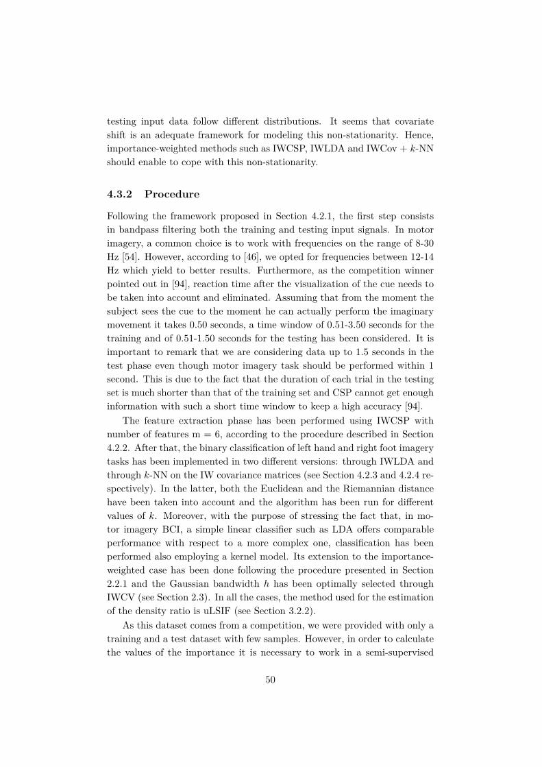
testing input data follow different distributions. It seems that covariateshift is an adequate framework for modeling this non-stationarity. Hence,importance-weighted methods such as IWCSP, IWLDA and IWCov + k-NNshould enable to cope with this non-stationarity.

4.3.2 Procedure

Following the framework proposed in Section 4.2.1, the first step consistsin bandpass filtering both the training and testing input signals. In motorimagery, a common choice is to work with frequencies on the range of 8-30Hz [54]. However, according to [46], we opted for frequencies between 12-14Hz which yield to better results. Furthermore, as the competition winnerpointed out in [94], reaction time after the visualization of the cue needs tobe taken into account and eliminated. Assuming that from the moment thesubject sees the cue to the moment he can actually perform the imaginarymovement it takes 0.50 seconds, a time window of 0.51-3.50 seconds for thetraining and of 0.51-1.50 seconds for the testing has been considered. It isimportant to remark that we are considering data up to 1.5 seconds in thetest phase even though motor imagery task should be performed within 1second. This is due to the fact that the duration of each trial in the testingset is much shorter than that of the training set and CSP cannot get enoughinformation with such a short time window to keep a high accuracy [94].

The feature extraction phase has been performed using IWCSP withnumber of features m = 6, according to the procedure described in Section4.2.2. After that, the binary classification of left hand and right foot imagerytasks has been implemented in two different versions: through IWLDA andthrough k-NN on the IW covariance matrices (see Section 4.2.3 and 4.2.4 re-spectively). In the latter, both the Euclidean and the Riemannian distancehave been taken into account and the algorithm has been run for differentvalues of k. Moreover, with the purpose of stressing the fact that, in mo-tor imagery BCI, a simple linear classifier such as LDA offers comparableperformance with respect to a more complex one, classification has beenperformed also employing a kernel model. Its extension to the importance-weighted case has been done following the procedure presented in Section2.2.1 and the Gaussian bandwidth h has been optimally selected throughIWCV (see Section 2.3). In all the cases, the method used for the estimationof the density ratio is uLSIF (see Section 3.2.2).

As this dataset comes from a competition, we were provided with only atraining and a test dataset with few samples. However, in order to calculatethe values of the importance it is necessary to work in a semi-supervised

50

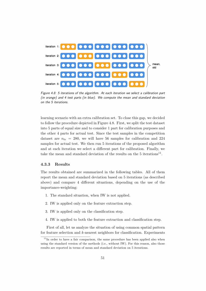
Figure 4.8: 5 iterations of the algorithm. At each iteration we select a calibration part(in orange) and 4 test parts (in blue). We compute the mean and standard deviationon the 5 iterations.

learning scenario with an extra calibration set. To close this gap, we decidedto follow the procedure depicted in Figure 4.8. First, we split the test datasetinto 5 parts of equal size and to consider 1 part for calibration purposes andthe other 4 parts for actual test. Since the test samples in the competitiondataset are nte = 280, we will have 56 samples for calibration and 224samples for actual test. We then run 5 iterations of the proposed algorithmand at each iteration we select a different part for calibration. Finally, wetake the mean and standard deviation of the results on the 5 iterations11.

4.3.3 Results

The results obtained are summarized in the following tables. All of themreport the mean and standard deviation based on 5 iterations (as describedabove) and compare 4 different situations, depending on the use of theimportance-weighting:

1. The standard situation, when IW is not applied.

2. IW is applied only on the feature extraction step.

3. IW is applied only on the classification step.

4. IW is applied to both the feature extraction and classification step.

First of all, let us analyze the situation of using common spatial patternfor feature selection and k-nearest neighbors for classification. Experiments

11In order to have a fair comparison, the same procedure has been applied also whenusing the standard version of the methods (i.e., without IW). For this reason, also thoseresults are reported in terms of mean and standard deviation on 5 iterations.

51

k-NN CSP + Cov IWCSP + Cov CSP + IWCov IWCSP + IWCov

E R E R E R E R

k = 1 mean 86.43 86.43 87.23 87.68 87.41 87.14 87.41 88.66std 1.40 1.28 1.89 1.40 1.82 2.27 1.63 1.34

k = 3 mean 85.71 87.14 85.54 87.95 86.34 86.61 85.98 88.12std 1.52 1.28 1.61 1.16 1.51 1.81 2.14 1.71

k = 5 mean 83.93 87.14 84.73 87.59 84.73 86.52 84.55 87.68std 1.76 0.95 1.82 0.95 2.30 1.88 2.32 1.97

Table 4.1: Results obtained using CSP for feature extraction and k-NN on covariancematrices for classification (denoted with Cov and IWCov for the sake of brevity). TheMean and standard deviation over 5 iterations are reported for different values of k usingboth the Euclidean distance (E) and the Riemannian distance (R). The classificationaccuracy increases with the use of the IW.

have been run for 3 different values of k (k = 1, 3, 5, all odds so that we avoidtied votes and hence ambiguity in the classification) and using as distancemetrics both the Euclidean (E) and Riemannian (R) distances. Table 4.1reports the results. The first thing to notice is that the Riemannian distanceoffers in general better performance than the Euclidean distance. If this wasexpected from the considerations made above, more surprising is the factthat the smaller is the values of k, the better are the results. This soundsa bit counterintuitive considering the non-stationarity of the dataset andmore experiments would be needed to draw conclusions. In all the cases, itis clear to see that IW brings to an increase of performance. For instance,looking at the Riemannian distance for k = 1, the mean accuracy risesfrom 86.43% with the standard method (CSP + Cov) to 88.66% with theimportance-weighted method (IWCSP + IWCov) without any significantchange in the standard deviation. At the same time, the hybrid methods(IWCSP + Cov and CSP + IWCov) offer intermediate results, meaningthat one layer of IW already improves the performance but two layers areeven better. This pattern is followed also in all the other cases, with only avery few exceptions. As a consequence, we can state that IW significantlyimproves the classification results of CSP and k-NN on covariance matriceswhen dealing with a non-stationary environment.

The second experiment was to use common spatial pattern for featureextraction and linear discriminant analysis for classification. Table 4.2 com-pares the results obtained in this framework. It is immediate to notice thatthe full covariate shift adaptation (IWCSP + IWLDA) outperforms the stan-

52

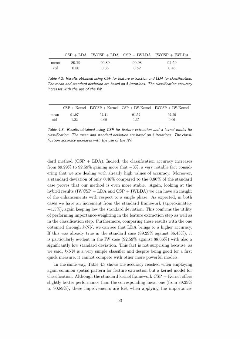
CSP + LDA IWCSP + LDA CSP + IWLDA IWCSP + IWLDA

mean 89.29 90.89 90.98 92.59std 0.80 0.36 0.82 0.46

Table 4.2: Results obtained using CSP for feature extraction and LDA for classification.The mean and standard deviation are based on 5 iterations. The classification accuracyincreases with the use of the IW.

CSP + Kernel IWCSP + Kernel CSP + IW-Kernel IWCSP + IW-Kernel

mean 91.97 92.41 91.52 92.50std 1.22 0.69 1.35 0.66

Table 4.3: Results obtained using CSP for feature extraction and a kernel model forclassification. The mean and standard deviation are based on 5 iterations. The classi-fication accuracy increases with the use of the IW.

dard method (CSP + LDA). Indeed, the classification accuracy increasesfrom 89.29% to 92.59% gaining more that +3%, a very notable fact consid-ering that we are dealing with already high values of accuracy. Moreover,a standard deviation of only 0.46% compared to the 0.80% of the standardcase proves that our method is even more stable. Again, looking at thehybrid results (IWCSP + LDA and CSP + IWLDA) we can have an insightof the enhancements with respect to a single phase. As expected, in bothcases we have an increment from the standard framework (approximately+1.5%), again keeping low the standard deviation. This confirms the utilityof performing importance-weighting in the feature extraction step as well asin the classification step. Furthermore, comparing these results with the oneobtained through k-NN, we can see that LDA brings to a higher accuracy.If this was already true in the standard case (89.29% against 86.43%), itis particularly evident in the IW case (92.59% against 88.66%) with also asignificantly low standard deviation. This fact is not surprising because, aswe said, k-NN is a very simple classifier and despite being good for a firstquick measure, it cannot compete with other more powerful models.

In the same way, Table 4.3 shows the accuracy reached when employingagain common spatial pattern for feature extraction but a kernel model forclassification. Although the standard kernel framework CSP + Kernel offersslightly better performance than the corresponding linear one (from 89.29%to 90.89%), these improvements are lost when applying the importance-

53

weighting. Indeed, the importance-weighted kernel framework IWCSP +IW-Kernel results in a lower accuracy than IWCSP + IWLDA (92.50%against 92.59%) and also to a higher standard deviation (0.66% against0.46%). This proves the aforementioned statement that in motor imageryBCI a linear algorithm often outperforms more complex ones.

In conclusion, importance-weighted common spatial pattern combinedwith importance-weighted linear discriminant analysis (IWCSP + IWLDA)seems the method of choice for motor imagery classification under covariateshift. More generally, the results shown above allow us to claim that, everytime we need to deal with non-stationary environments that can be mod-eled with covariate shift, importance-weighting is able to provide us with arobust model.

54

Chapter 5

Importance-WeightedMethods for Image Analysis

Any A.I. smart enough to pass a Turing testis smart enough to know to fail it.

Ian McDonaldRiver of Gods, 2004

Image analysis is a field of computer science developed with the advent ofdigital images in the 1950s at academic institutions such as the MIT A.I.Lab, originally as a branch of artificial intelligence and robotics. The ideais to process a digital image by means of statistical techniques in order toextract meaningful information. In this chapter we offer a machine learningapproach to image analysis and, in particular, we focus on supervised imageclassification, in which, given a set of images with known labels, a system canpredict the classification of new images. This scenario is receiving a greatdeal of attention in recent years due to its large number of applications.Examples of these can be found in the field of healthcare, where we areinterested in the classification of benign or malignant tumor from fine needleaspirate (FNA) images of breast masses, or, more on a daily basis, in theclassification of faces in Facebook pictures.

For the purpose of this thesis, images analysis is particularly interestingbecause of the different conditions in which images are analyzed. Indeed,among different images representing the same subject, changes in illumi-nation [5], rotations and scaling [37] or the simple presence of noise [47]are frequent. For instance, consider satellite images which can capture im-ages of same landscape at different time intervals; the images captured at

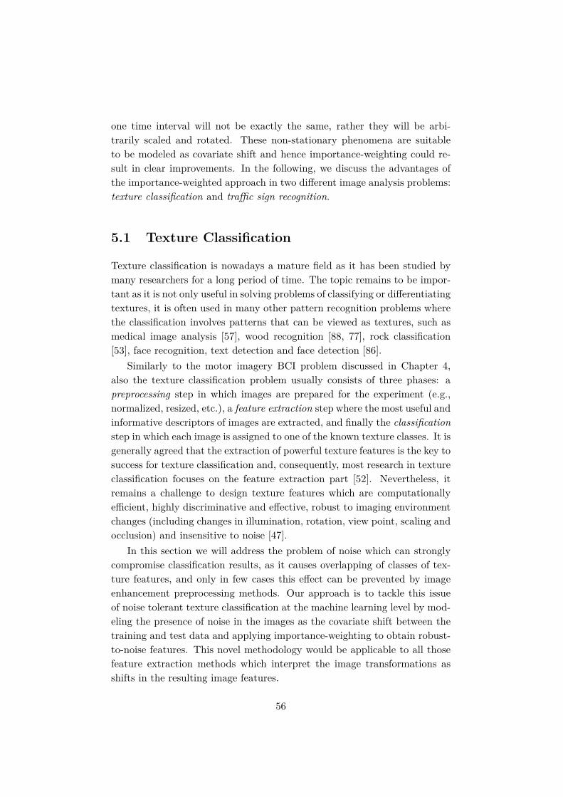
one time interval will not be exactly the same, rather they will be arbi-trarily scaled and rotated. These non-stationary phenomena are suitableto be modeled as covariate shift and hence importance-weighting could re-sult in clear improvements. In the following, we discuss the advantages ofthe importance-weighted approach in two different image analysis problems:texture classification and traffic sign recognition.

5.1 Texture Classification

Texture classification is nowadays a mature field as it has been studied bymany researchers for a long period of time. The topic remains to be impor-tant as it is not only useful in solving problems of classifying or differentiatingtextures, it is often used in many other pattern recognition problems wherethe classification involves patterns that can be viewed as textures, such asmedical image analysis [57], wood recognition [88, 77], rock classification[53], face recognition, text detection and face detection [86].

Similarly to the motor imagery BCI problem discussed in Chapter 4,also the texture classification problem usually consists of three phases: apreprocessing step in which images are prepared for the experiment (e.g.,normalized, resized, etc.), a feature extraction step where the most useful andinformative descriptors of images are extracted, and finally the classificationstep in which each image is assigned to one of the known texture classes. It isgenerally agreed that the extraction of powerful texture features is the key tosuccess for texture classification and, consequently, most research in textureclassification focuses on the feature extraction part [52]. Nevertheless, itremains a challenge to design texture features which are computationallyefficient, highly discriminative and effective, robust to imaging environmentchanges (including changes in illumination, rotation, view point, scaling andocclusion) and insensitive to noise [47].

In this section we will address the problem of noise which can stronglycompromise classification results, as it causes overlapping of classes of tex-ture features, and only in few cases this effect can be prevented by imageenhancement preprocessing methods. Our approach is to tackle this issueof noise tolerant texture classification at the machine learning level by mod-eling the presence of noise in the images as the covariate shift between thetraining and test data and applying importance-weighting to obtain robust-to-noise features. This novel methodology would be applicable to all thosefeature extraction methods which interpret the image transformations asshifts in the resulting image features.

56

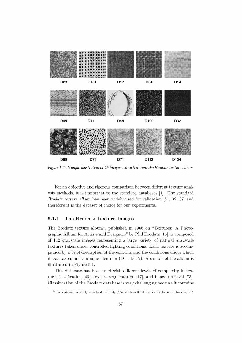
Figure 5.1: Sample illustration of 15 images extracted from the Brodatz texture album.

For an objective and rigorous comparison between different texture anal-ysis methods, it is important to use standard databases [1]. The standardBrodatz texture album has been widely used for validation [81, 32, 37] andtherefore it is the dataset of choice for our experiments.

5.1.1 The Brodatz Texture Images

The Brodatz texture album1, published in 1966 on “Textures: A Photo-graphic Album for Artists and Designers” by Phil Brodatz [16], is composedof 112 grayscale images representing a large variety of natural grayscaletextures taken under controlled lighting conditions. Each texture is accom-panied by a brief description of the contents and the conditions under whichit was taken, and a unique identifier (D1 - D112). A sample of the album isillustrated in Figure 5.1.

This database has been used with different levels of complexity in tex-ture classification [43], texture segmentation [17], and image retrieval [73].Classification of the Brodatz database is very challenging because it contains

1The dataset is freely available at http://multibandtexture.recherche.usherbrooke.ca/

57

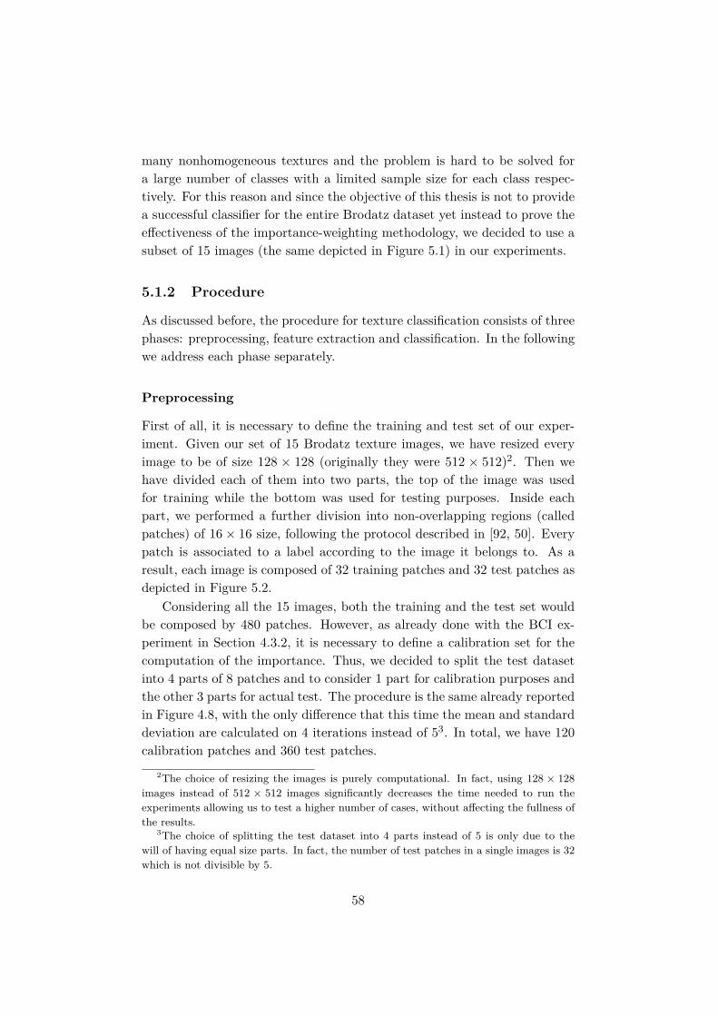
many nonhomogeneous textures and the problem is hard to be solved fora large number of classes with a limited sample size for each class respec-tively. For this reason and since the objective of this thesis is not to providea successful classifier for the entire Brodatz dataset yet instead to prove theeffectiveness of the importance-weighting methodology, we decided to use asubset of 15 images (the same depicted in Figure 5.1) in our experiments.

5.1.2 Procedure

As discussed before, the procedure for texture classification consists of threephases: preprocessing, feature extraction and classification. In the followingwe address each phase separately.

Preprocessing

First of all, it is necessary to define the training and test set of our exper-iment. Given our set of 15 Brodatz texture images, we have resized everyimage to be of size 128 × 128 (originally they were 512 × 512)2. Then wehave divided each of them into two parts, the top of the image was usedfor training while the bottom was used for testing purposes. Inside eachpart, we performed a further division into non-overlapping regions (calledpatches) of 16× 16 size, following the protocol described in [92, 50]. Everypatch is associated to a label according to the image it belongs to. As aresult, each image is composed of 32 training patches and 32 test patches asdepicted in Figure 5.2.

Considering all the 15 images, both the training and the test set wouldbe composed by 480 patches. However, as already done with the BCI ex-periment in Section 4.3.2, it is necessary to define a calibration set for thecomputation of the importance. Thus, we decided to split the test datasetinto 4 parts of 8 patches and to consider 1 part for calibration purposes andthe other 3 parts for actual test. The procedure is the same already reportedin Figure 4.8, with the only difference that this time the mean and standarddeviation are calculated on 4 iterations instead of 53. In total, we have 120calibration patches and 360 test patches.

2The choice of resizing the images is purely computational. In fact, using 128 × 128images instead of 512 × 512 images significantly decreases the time needed to run theexperiments allowing us to test a higher number of cases, without affecting the fullness ofthe results.

3The choice of splitting the test dataset into 4 parts instead of 5 is only due to thewill of having equal size parts. In fact, the number of test patches in a single images is 32which is not divisible by 5.

58

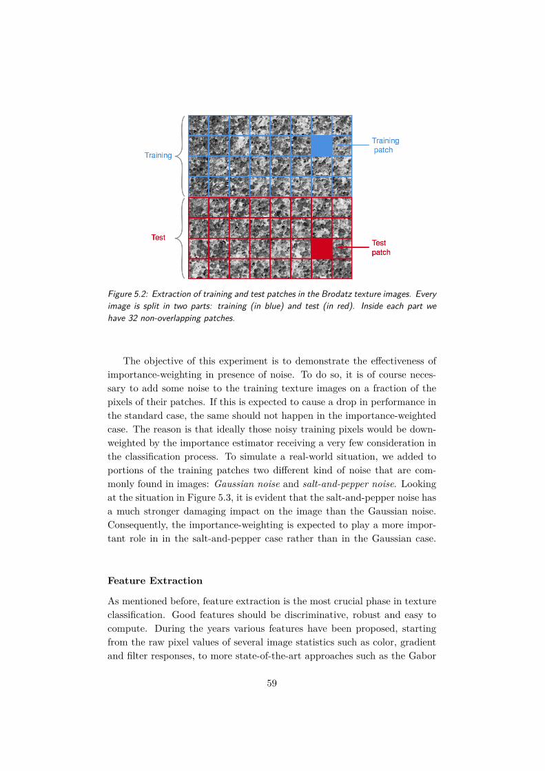
Figure 5.2: Extraction of training and test patches in the Brodatz texture images. Everyimage is split in two parts: training (in blue) and test (in red). Inside each part wehave 32 non-overlapping patches.

The objective of this experiment is to demonstrate the effectiveness ofimportance-weighting in presence of noise. To do so, it is of course neces-sary to add some noise to the training texture images on a fraction of thepixels of their patches. If this is expected to cause a drop in performance inthe standard case, the same should not happen in the importance-weightedcase. The reason is that ideally those noisy training pixels would be down-weighted by the importance estimator receiving a very few consideration inthe classification process. To simulate a real-world situation, we added toportions of the training patches two different kind of noise that are com-monly found in images: Gaussian noise and salt-and-pepper noise. Lookingat the situation in Figure 5.3, it is evident that the salt-and-pepper noise hasa much stronger damaging impact on the image than the Gaussian noise.Consequently, the importance-weighting is expected to play a more impor-tant role in in the salt-and-pepper case rather than in the Gaussian case.

Feature Extraction

As mentioned before, feature extraction is the most crucial phase in textureclassification. Good features should be discriminative, robust and easy tocompute. During the years various features have been proposed, startingfrom the raw pixel values of several image statistics such as color, gradientand filter responses, to more state-of-the-art approaches such as the Gabor

59

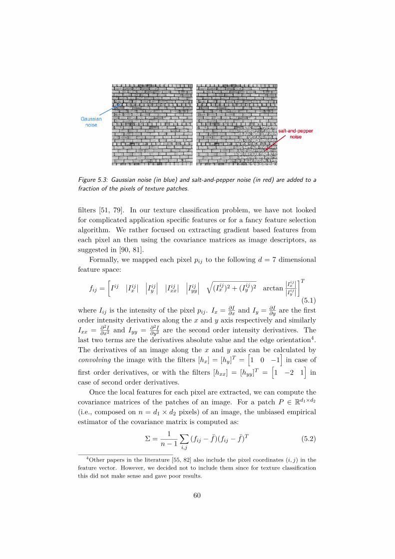
Figure 5.3: Gaussian noise (in blue) and salt-and-pepper noise (in red) are added to afraction of the pixels of texture patches.

filters [51, 79]. In our texture classification problem, we have not lookedfor complicated application specific features or for a fancy feature selectionalgorithm. We rather focused on extracting gradient based features fromeach pixel an then using the covariance matrices as image descriptors, assuggested in [90, 81].

Formally, we mapped each pixel pij to the following d = 7 dimensionalfeature space:

fij =[Iij

∣∣Iijx ∣∣ ∣∣∣Iijy ∣∣∣ ∣∣Iijxx∣∣ ∣∣∣Iijyy∣∣∣ √(Iijx )2 + (Iijy )2 arctan |I

ijx ||Iijy |

]T(5.1)

where Iij is the intensity of the pixel pij . Ix = ∂I∂x and Iy = ∂I

∂y are the firstorder intensity derivatives along the x and y axis respectively and similarlyIxx = ∂2I

∂x2 and Iyy = ∂2I∂y2 are the second order intensity derivatives. The

last two terms are the derivatives absolute value and the edge orientation4.The derivatives of an image along the x and y axis can be calculated byconvolving the image with the filters [hx] = [hy]T =

[1 0 −1

]in case of

first order derivatives, or with the filters [hxx] = [hyy]T =[1 −2 1

]in

case of second order derivatives.Once the local features for each pixel are extracted, we can compute the

covariance matrices of the patches of an image. For a patch P ∈ Rd1×d2

(i.e., composed on n = d1 × d2 pixels) of an image, the unbiased empiricalestimator of the covariance matrix is computed as:

Σ = 1n− 1

∑i,j

(fij − f)(fij − f)T (5.2)

4Other papers in the literature [55, 82] also include the pixel coordinates (i, j) in thefeature vector. However, we decided not to include them since for texture classificationthis did not make sense and gave poor results.

60

with f being the empirical mean of f . Note that this estimator will beaccurate provided that the number of samples is large enough compared tothe number of features. Covariance matrices have been studied as imagedescriptors in wide variety of applications from license plate detection [55]to pedestrian detection [82] and there are several advantages of using them.For instance, the fact that a single covariance matrix extracted from a patchis usually enough to match the region in different views and poses (assumingthat the covariance of a distribution is enough to discriminate it from otherdistributions), and that covariance matrices are low-dimensional comparedto other region descriptors.

However, the proposed covariance matrix estimator is well-known for itssensitivity to noise. To overcome this issue, we modeled the presence of noiseas covariate shift between the train and test and we applied the importance-weighting to obtain a robust estimation of the covariance matrices. Equation(5.2) is then rewritten as follows:

Σ = 1n− 1

∑i,j

wij(fij − f)(fij − f)T (5.3)

where wij is the importance-weighting for pixel pij computed by looking atthe similarity of its feature vector fij with respect to the feature vectors of agiven calibration set. Doing so, only the feature vectors not affected by noisewill receive strong consideration during the computation of the covariancematrix, while the noisy ones will have importance close to zero. All this willresult in a robust-to-noise estimation of the covariance matrix. Once again,the values of the importance can be estimated with any of the techniquesdiscussed in Section 3.2.2 but the more convenient approach is uLSIF, whichis the one used in this experiment.

In the following we will refer to this extension as importance-weightedcovariance matrix (IWCov), a novelty introduced by the author of this thesisand for which a scientific paper is planned in the near future.

Classification

Finally, after having extracted robust covariance matrices for each patch,we are ready to perform the actual classification. Among all the possibleclassification methods, we decided to use a k−nearest neighbors algorithmon covariance matrices, following the suggestion of various paper on textureclassification [81, 78, 79]. The procedure is the same already described inSection 4.2.4 when talking about the motor imagery BCI experiment. Thus,the considerations made about the Euclidean and Riemannian distances as

61

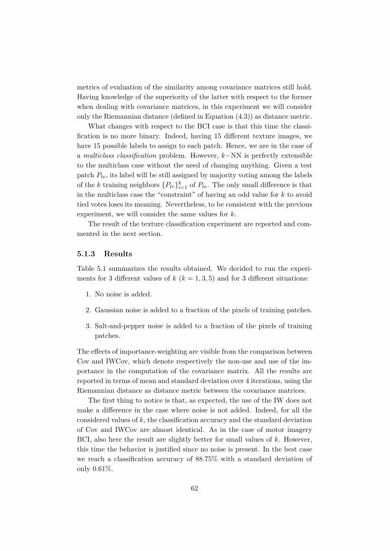
metrics of evaluation of the similarity among covariance matrices still hold.Having knowledge of the superiority of the latter with respect to the formerwhen dealing with covariance matrices, in this experiment we will consideronly the Riemannian distance (defined in Equation (4.3)) as distance metric.

What changes with respect to the BCI case is that this time the classi-fication is no more binary. Indeed, having 15 different texture images, wehave 15 possible labels to assign to each patch. Hence, we are in the case ofa multiclass classification problem. However, k−NN is perfectly extensibleto the multiclass case without the need of changing anything. Given a testpatch Pte, its label will be still assigned by majority voting among the labelsof the k training neighbors Ptrki=1 of Pte. The only small difference is thatin the multiclass case the “constraint” of having an odd value for k to avoidtied votes loses its meaning. Nevertheless, to be consistent with the previousexperiment, we will consider the same values for k.

The result of the texture classification experiment are reported and com-mented in the next section.

5.1.3 Results

Table 5.1 summarizes the results obtained. We decided to run the experi-ments for 3 different values of k (k = 1, 3, 5) and for 3 different situations:

1. No noise is added.

2. Gaussian noise is added to a fraction of the pixels of training patches.

3. Salt-and-pepper noise is added to a fraction of the pixels of trainingpatches.

The effects of importance-weighting are visible from the comparison betweenCov and IWCov, which denote respectively the non-use and use of the im-portance in the computation of the covariance matrix. All the results arereported in terms of mean and standard deviation over 4 iterations, using theRiemannian distance as distance metric between the covariance matrices.

The first thing to notice is that, as expected, the use of the IW does notmake a difference in the case where noise is not added. Indeed, for all theconsidered values of k, the classification accuracy and the standard deviationof Cov and IWCov are almost identical. As in the case of motor imageryBCI, also here the result are slightly better for small values of k. However,this time the behavior is justified since no noise is present. In the best casewe reach a classification accuracy of 88.75% with a standard deviation ofonly 0.61%.

62

k-NN No Noise Gaussian Salt&Pepper

Cov IWCov Cov IWCov Cov IWCov

k = 1 mean 88.75 88.47 83.61 83.54 72.64 84.10std 0.61 0.64 0.44 0.63 1.40 1.55

k = 3 mean 87.08 87.29 82.64 83.54 75.35 83.89std 1.01 1.06 1.01 1.26 1.05 1.32

k = 5 mean 86.60 87.36 82.71 83.54 75.83 82.29std 0.41 0.50 0.97 1.25 1.02 0.91

Table 5.1: Results obtained using k-NN with Riemannian distance on covariance ma-trices. Cov and IWCov denote the non-use and use of the importance respectively. Themean and standard deviation over 4 iterations are reported for different values of k.The classification accuracy increases with the use of the IW.

More surprising is the fact that, in the case in which Gaussian noise isadded to the training patches, the results obtained with Cov and IWCov arestill comparable for every values of k. The reason could be found in the factthat the Gaussian noise can be removed by simply subtracting the mean. Itis clear that in both case the results are far from being totally insensitiveto noise, since we lost around 5% accuracy from the case without noise, yetthe drop is not as big as in the salt-and-pepper case.

From our point of view, the most interesting results are obtained whensalt-and-pepper noise is added to the training patches. The effects of thisaddition are dramatic for the standard Cov method, causing the mean clas-sification accuracy to drop until around 75%, with a low peak of 72.64%when k = 1 justified by the fact that, for low values of k, k-NN is moresensitive to noise. On the contrary, the IWCov method seems unaffected bythis change and the mean accuracy is stable around 83% as in the case ofGaussian noise. The case where k = 1 is particularly interesting becausethe classification accuracy reached 84.10%, +11.46% with respect to thestandard method, and the standard deviation is not affected significantly.Also for k = 3 and k = 5 we have an increments using the IW, +8.54%and +6.46% respectively. Being the difference between Cov and IWCov sta-tistically significant5 for all the values of k, we can state that IW stronglyreduces the effects of salt-and-pepper noise on images. This also supportsour previous statement that IW plays a much more important role in in the

5The hypothesis test was performed through a t-test with significance level of 0.05.

63

salt-and-pepper case rather than in the Gaussian case.To summarize, this experiment shows that importance-weighting allows

us to obtain a robust and reliable estimation of the covariance matrices evenin presence of noise and, consequently, the k-NN algorithm leads to resultscomparable with the noise free case. More generally, in all the situationsin which the occurrence of non-stationary phenomena between training andtest images can be modeled as covariate shift, importance-weighting is anuseful and effective tool to compensate for this shift and to map the problemback to stationarity.

5.2 Traffic Sign Recognition

Traffic sign recognition is a technology by which a vehicle is able to recognizethe traffic signs present on the road, such as prohibitory signs (e.g., “speedlimit of 100 Km/h”), warning signs (e.g., “attention, children!”), mandatorysigns (e.g., “turn left”), and temporary signs (e.g., “road works”). Therecent advent of autonomous cars, has lead to a strong interest on thistechnology with many studies published on the subject and multiple systems,which often restrict themselves to a subset of relevant signs, are alreadycommercially available in new high and mid-range vehicles.

From the machine learning point of view, traffic sign recognition cov-ers two problems: traffic sign detection and traffic sign classification. Theformer is meant for the accurate localization of traffic signs in the imagespace, while the latter handles the labeling of such detections into specifictraffic sign types or subcategories. In this thesis, we will focus on traffic signclassification which is a challenging real-world problem of high industrial rel-evance. The interest is driven by the market for intelligent applications suchas autonomous driving [45], advanced driver assistance systems (ADAS) [75],and mobile mapping [76]. Road signals are designed to be easily detectedand recognized by human drivers. Accordingly, humans are capable of recog-nizing the large variety of existing road signs with close to 100% correctnessand no false positives on single images. Can machines catch up with humanperformance?

Traffic sign classification is a challenging multiclass classification prob-lem. The main issue lies in the fact that, even though traffic signs show awide range of variations between classes in terms of color, shape, and thepresence of drawings or text, the classifier has to cope with large variationsin visual appearances due to illumination changes, partial occlusions, rota-tions, weather conditions, scaling, etc. For instance, a “stop” signal maylook very different under the daylight or at night. This is the reason why

64

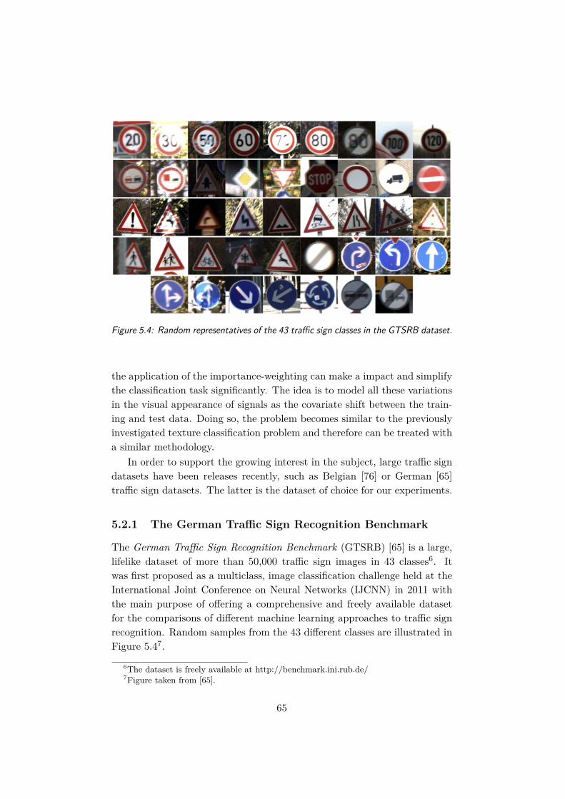
Figure 5.4: Random representatives of the 43 traffic sign classes in the GTSRB dataset.

the application of the importance-weighting can make a impact and simplifythe classification task significantly. The idea is to model all these variationsin the visual appearance of signals as the covariate shift between the train-ing and test data. Doing so, the problem becomes similar to the previouslyinvestigated texture classification problem and therefore can be treated witha similar methodology.

In order to support the growing interest in the subject, large traffic signdatasets have been releases recently, such as Belgian [76] or German [65]traffic sign datasets. The latter is the dataset of choice for our experiments.

5.2.1 The German Traffic Sign Recognition Benchmark

The German Traffic Sign Recognition Benchmark (GTSRB) [65] is a large,lifelike dataset of more than 50,000 traffic sign images in 43 classes6. Itwas first proposed as a multiclass, image classification challenge held at theInternational Joint Conference on Neural Networks (IJCNN) in 2011 withthe main purpose of offering a comprehensive and freely available datasetfor the comparisons of different machine learning approaches to traffic signrecognition. Random samples from the 43 different classes are illustrated inFigure 5.47.

6The dataset is freely available at http://benchmark.ini.rub.de/7Figure taken from [65].

65

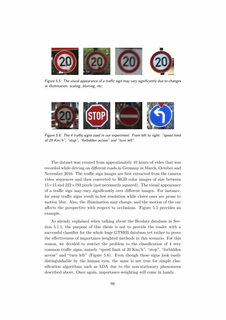
Figure 5.5: The visual appearance of a traffic sign may vary significantly due to changesin illumination, scaling, blurring, etc.

Figure 5.6: The 4 traffic signs used in our experiment. From left to right: “speed limitof 20 Km/h”, “stop”, “forbidden access” and “turn left”.

The dataset was created from approximately 10 hours of video that wasrecorded while driving on different roads in Germany in March, October andNovember 2010. The traffic sign images are first extracted from the cameravideo sequences and then converted to RGB color images of size between15×15 and 222×193 pixels (not necessarily squared). The visual appearanceof a traffic sign may vary significantly over different images. For instance,far away traffic signs result in low resolution while closer ones are prone tomotion blur. Also, the illumination may change, and the motion of the caraffects the perspective with respect to occlusions. Figure 5.5 provides anexample.

As already explained when talking about the Brodatz database in Sec-tion 5.1.1, the purpose of this thesis is not to provide the reader with asuccessful classifier for the whole huge GTSRB database yet rather to provethe effectiveness of importance-weighted methods in this scenario. For thisreason, we decided to restrict the problem to the classification of 4 verycommon traffic signs, namely “speed limit of 20 Km/h”, “stop”, “forbiddenaccess” and “turn left” (Figure 5.6). Even though these signs look easilydistinguishable by the human eyes, the same is not true for simple clas-sification algorithms such as LDA due to the non-stationary phenomenadescribed above. Once again, importance-weighting will come in handy.

66

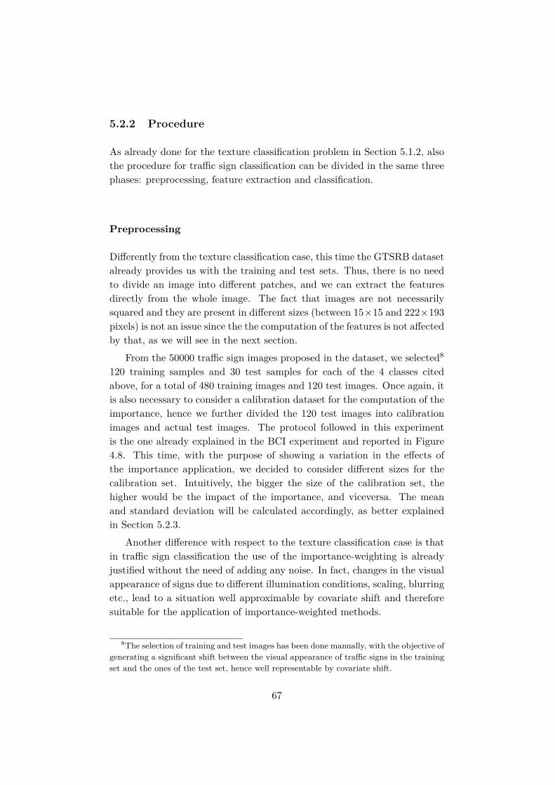
5.2.2 Procedure

As already done for the texture classification problem in Section 5.1.2, alsothe procedure for traffic sign classification can be divided in the same threephases: preprocessing, feature extraction and classification.

Preprocessing

Differently from the texture classification case, this time the GTSRB datasetalready provides us with the training and test sets. Thus, there is no needto divide an image into different patches, and we can extract the featuresdirectly from the whole image. The fact that images are not necessarilysquared and they are present in different sizes (between 15×15 and 222×193pixels) is not an issue since the the computation of the features is not affectedby that, as we will see in the next section.

From the 50000 traffic sign images proposed in the dataset, we selected8

120 training samples and 30 test samples for each of the 4 classes citedabove, for a total of 480 training images and 120 test images. Once again, itis also necessary to consider a calibration dataset for the computation of theimportance, hence we further divided the 120 test images into calibrationimages and actual test images. The protocol followed in this experimentis the one already explained in the BCI experiment and reported in Figure4.8. This time, with the purpose of showing a variation in the effects ofthe importance application, we decided to consider different sizes for thecalibration set. Intuitively, the bigger the size of the calibration set, thehigher would be the impact of the importance, and viceversa. The meanand standard deviation will be calculated accordingly, as better explainedin Section 5.2.3.

Another difference with respect to the texture classification case is thatin traffic sign classification the use of the importance-weighting is alreadyjustified without the need of adding any noise. In fact, changes in the visualappearance of signs due to different illumination conditions, scaling, blurringetc., lead to a situation well approximable by covariate shift and thereforesuitable for the application of importance-weighted methods.

8The selection of training and test images has been done manually, with the objective ofgenerating a significant shift between the visual appearance of traffic signs in the trainingset and the ones of the test set, hence well representable by covariate shift.

67

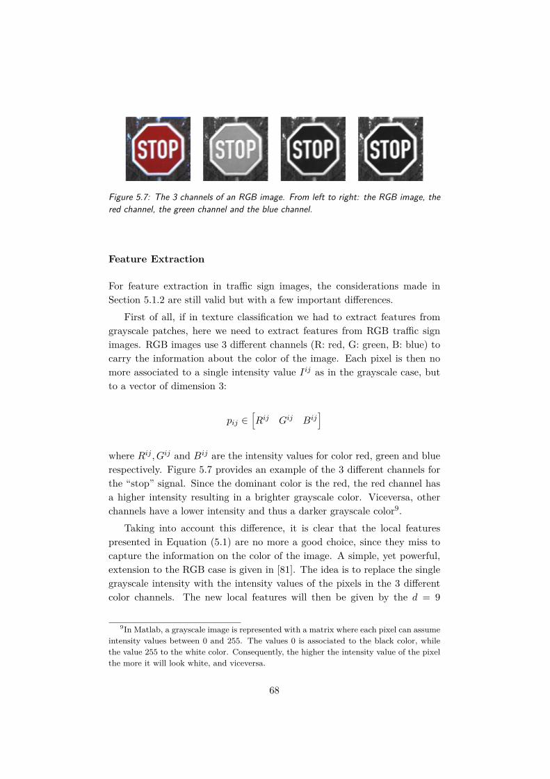
Figure 5.7: The 3 channels of an RGB image. From left to right: the RGB image, thered channel, the green channel and the blue channel.

Feature Extraction

For feature extraction in traffic sign images, the considerations made inSection 5.1.2 are still valid but with a few important differences.

First of all, if in texture classification we had to extract features fromgrayscale patches, here we need to extract features from RGB traffic signimages. RGB images use 3 different channels (R: red, G: green, B: blue) tocarry the information about the color of the image. Each pixel is then nomore associated to a single intensity value Iij as in the grayscale case, butto a vector of dimension 3:

pij ∈[Rij Gij Bij

]

where Rij , Gij and Bij are the intensity values for color red, green and bluerespectively. Figure 5.7 provides an example of the 3 different channels forthe “stop” signal. Since the dominant color is the red, the red channel hasa higher intensity resulting in a brighter grayscale color. Viceversa, otherchannels have a lower intensity and thus a darker grayscale color9.

Taking into account this difference, it is clear that the local featurespresented in Equation (5.1) are no more a good choice, since they miss tocapture the information on the color of the image. A simple, yet powerful,extension to the RGB case is given in [81]. The idea is to replace the singlegrayscale intensity with the intensity values of the pixels in the 3 differentcolor channels. The new local features will then be given by the d = 9

9In Matlab, a grayscale image is represented with a matrix where each pixel can assumeintensity values between 0 and 255. The values 0 is associated to the black color, whilethe value 255 to the white color. Consequently, the higher the intensity value of the pixelthe more it will look white, and viceversa.

68

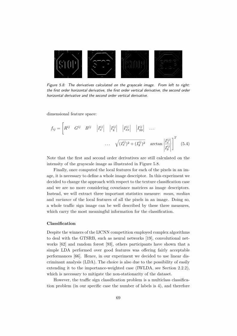
Figure 5.8: The derivatives calculated on the grayscale image. From left to right:the first order horizontal derivative, the first order vertical derivative, the second orderhorizontal derivative and the second order vertical derivative.

dimensional feature space:

fij =[Rij Gij Bij

∣∣∣Iijx ∣∣∣ ∣∣∣Iijy ∣∣∣ ∣∣∣Iijxx∣∣∣ ∣∣∣Iijyy∣∣∣ . . .

. . .√

(Iijx )2 + (Iijy )2 arctan∣∣Iijx ∣∣∣∣∣Iijy ∣∣∣

]T(5.4)

Note that the first and second order derivatives are still calculated on theintensity of the grayscale image as illustrated in Figure 5.8.

Finally, once computed the local features for each of the pixels in an im-age, it is necessary to define a whole image descriptor. In this experiment wedecided to change the approach with respect to the texture classification caseand we are no more considering covariance matrices as image descriptors.Instead, we will extract three important statistics measure: mean, medianand variance of the local features of all the pixels in an image. Doing so,a whole traffic sign image can be well described by these three measures,which carry the most meaningful information for the classification.

Classification

Despite the winners of the IJCNN competition employed complex algorithmsto deal with the GTSRB, such as neural networks [19], convolutional net-works [62] and random forest [93], others participants have shown that asimple LDA performed over good features was offering fairly acceptableperformances [66]. Hence, in our experiment we decided to use linear dis-criminant analysis (LDA). The choice is also due to the possibility of easilyextending it to the importance-weighted case (IWLDA, see Section 2.2.2),which is necessary to mitigate the non-stationarity of the dataset.

However, the traffic sign classification problem is a multiclass classifica-tion problem (in our specific case the number of labels is 4), and therefore

69

it is necessary to extend our classifier to the multiclass case. In the litera-ture [11], various possible approaches to this problem have been proposedbut the most commons are two: one-vs-all and one-vs-one. Given a genericmulticlass classification problem with k different classes, the one-vs-all strat-egy involves training a single classifier per class, with the samples of thatclass as positive samples and all other samples as negatives, for a total of kclassifiers. Instead in the one-vs-one strategy, one trains k(k− 1) classifiers,each of them to distinguish between a pair of classes. There is not a gen-eral better choice between the two approaches, but the decision depends onvarious factors, such as the number of classes k, the base classifier involvedand the requirements of the specific application.

In this thesis we decided to consider the one-vs-all approach. Goingmore into the details of it, we build k = 4 LDA classifiers10, one for eachof the considered classes. For the i-th classifier (i ∈ 1 . . . k), let the positivesamples be all the images belonging to class i, and let the negative samplesbe all the images not belonging to class i. If fi denotes the output of thei-th classifier, the decision y is given by:

y = argmaxi fi(x).

In other word we predict the label i for which the LDA classifier reportsthe highest confidence score. It is important to remark that this strategyrequires the LDA classifier to produce a real-valued confidence score for itsdecision, rather than just a class label. In fact, discrete class labels alonecan lead to ambiguities, where multiple classes are predicted for a singlesample.

Following this procedure, we are now ready to run our traffic sign clas-sification experiment. The results are reported and commented in the nextsection.

5.2.3 Results

Table 5.2 presents the results obtained. As mentioned above, we wanted toinvestigate the effects of the use of the importance for different sizes of thecalibration set. Hence, the experiments have been performed consideringthree different situations:

1. The 120 test images are divided into 40 calibration images and 80actual test images and 3 different iterations are run.

10For the sake of simplicity, here we show the passages for the LDA case. However, theprocedure is valid also for IWLDA and, more generally, for any other binary classificationtechnique.

70

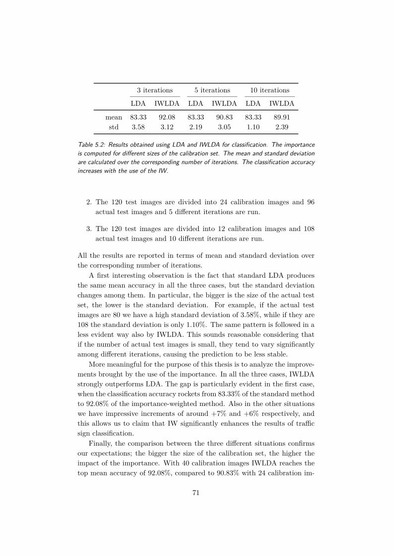
3 iterations 5 iterations 10 iterations

LDA IWLDA LDA IWLDA LDA IWLDA

mean 83.33 92.08 83.33 90.83 83.33 89.91std 3.58 3.12 2.19 3.05 1.10 2.39

Table 5.2: Results obtained using LDA and IWLDA for classification. The importanceis computed for different sizes of the calibration set. The mean and standard deviationare calculated over the corresponding number of iterations. The classification accuracyincreases with the use of the IW.

2. The 120 test images are divided into 24 calibration images and 96actual test images and 5 different iterations are run.

3. The 120 test images are divided into 12 calibration images and 108actual test images and 10 different iterations are run.

All the results are reported in terms of mean and standard deviation overthe corresponding number of iterations.

A first interesting observation is the fact that standard LDA producesthe same mean accuracy in all the three cases, but the standard deviationchanges among them. In particular, the bigger is the size of the actual testset, the lower is the standard deviation. For example, if the actual testimages are 80 we have a high standard deviation of 3.58%, while if they are108 the standard deviation is only 1.10%. The same pattern is followed in aless evident way also by IWLDA. This sounds reasonable considering thatif the number of actual test images is small, they tend to vary significantlyamong different iterations, causing the prediction to be less stable.

More meaningful for the purpose of this thesis is to analyze the improve-ments brought by the use of the importance. In all the three cases, IWLDAstrongly outperforms LDA. The gap is particularly evident in the first case,when the classification accuracy rockets from 83.33% of the standard methodto 92.08% of the importance-weighted method. Also in the other situationswe have impressive increments of around +7% and +6% respectively, andthis allows us to claim that IW significantly enhances the results of trafficsign classification.

Finally, the comparison between the three different situations confirmsour expectations; the bigger the size of the calibration set, the higher theimpact of the importance. With 40 calibration images IWLDA reaches thetop mean accuracy of 92.08%, compared to 90.83% with 24 calibration im-

71

ages and 89.91% with only 12 calibration images. Intuitively, if the numberof calibration images is larger, the computation of the importance can relyon more samples and this results in a more precise estimation.

Overall, this experiment confirmed that importance-weighted methodsare suitable for traffic sign classification. More generally, this holds in allthe situations in which changes in the visual appearance of objects can bemodeled via covariate shift.

72

Chapter 6

Conclusions and FutureDirections

We can only see a short distance ahead,but we can see plenty there that needs to be done.

Alan TuringComputing Machinery and Intelligence, 1950

In this thesis, we addressed the problem of machine learning under covari-ate shift, a particularly common situation in real-world applications. Thekey to success in this scenario is the use of importance-weighted methods,which lead to an impressive enhancement of performance with respect tothe standard machine learning methods.

Conclusions

Through the thesis, we first introduced the general problem of machinelearning in non-stationary environments. We consider a particular non-stationarity environment called covariate shift and we highlighted the dif-ficulties of standard machine learning methods to properly work in thisscenario. In order to cope with this problem, we discussed the conceptof importance-weighting. Then, we extended some of the most commonmachine learning techniques to their importance-weighted version. The es-timation of the importance values is not a trivial problem and requires asemi-supervised learning scenario. We argued that direct density ratio esti-mation techniques are preferable than separate density estimation ones fortheir higher accuracy and efficiency.

The emphasis in the thesis was put mainly in the fact that covariate shiftis representative of various real-world problems and therefore it is not only of

theoretical interest, but also of practical one. For this reason, we focused ourattention in two different real-world applications: brain-computer interfacesand image analysis. Our main objective was to demonstrate the effectivenessof importance-weighted methods when applied to these popular machinelearning contexts.

In brain-computer interfaces, we considered the motor imagery paradigm.The objective was to classify signal coming from the human mind throughcommon machine learning techniques. Due to the non-stationarity of theBCI environment, standard machine learning algorithms performed poorly.However, thanks to importance-weighting, we managed to build robust meth-ods that allowed us to reach a high classification accuracy. The results ofour motor imagery experiment allow us to claim that importance-weightedmethods are powerful in brain-computer interfaces.

In images analysis, we investigated two different classification problems:texture classification and traffic signal classification. In texture classifica-tion, the goal is to classify grayscale texture images. However, when we haveto deal with noise textures, standard machine learning techniques might fail.In our experiment we gave evidence that importance-weighted methods areable to deal with noisy texture images. Instead in traffic sign classification,the objective is to classify RGB images that are already prone to changesin the visual appearance. Also in this case, our experiments confirmed thatimportance-weighted methods outperform standard ones.

In conclusion, in this thesis we gave evidence of importance-weighting asa powerful tool to perform machine learning under covariate shift.

Future Directions

The use of importance-weighted methods opens various possible interestingscenarios that can be addressed and investigated in the future.

While the importance-weighted common spatial pattern (IWCSP) pre-sented in Chapter 4 has already been material for a scientific article (seeAppendix A), the application of the importance-weighting in covariancematrices is an open topic which requires further investigations. In this the-sis, we addressed only few of the potential applications of the method, yetenough to convince us that it is a promising technique that deserves to beanalyzed more in depth. More experiments and theoretical investigationson the subject can lead to a more clear picture, and this will be the nextpriority for the author of this thesis.

Another big challenge would be to apply importance-weighted methodsto other real-world problems that experience a situation similar to covariate

74

shift. Just to name a few of them: image and video processing, speech andmusic analyses, natural language processing, sensory data analysis, web datamining, robot and system control, financial data analysis, bioinformatics,computational chemistry and brain science. We believe that importance-weighted methods could be a key tool in such scenarios.

Finally, beyond the covariate shift adaptation, it has been shown re-cently that the ratio of probability densities can be used for solving variousother machine learning tasks [71]. Examples of these are domain adaptation,multi-task learning, two-sample test, outlier detection, change detection intime series, independence test, feature selection, dimension reduction, inde-pendent component analysis, causal inference, clustering, object matching,conditional probability estimation, probabilistic classification and mutual in-formation estimation. Thus, density ratio estimation is a promising versatiletool for machine learning which needs to be further investigated.

Various implementations of importance-weighted methods are availablefrom http://www.ms.k.u-tokyo.ac.jp/software.html. We believe that thesesoftware packages could be useful for developing new machine learning tech-niques and exploring novel application areas.

75

76

Appendix A

BCI Paper

This appendix reports the original version of the paper “Importance-weightedcovariance estimation for robust common spatial pattern” written by the au-thor of this thesis in collaboration with Dr. Florian Yger and Prof. MasashiSugiyama as it was published in Pattern Recognition Letters journal, volume68, part 1, pages 139-145, on December 15, 2015.

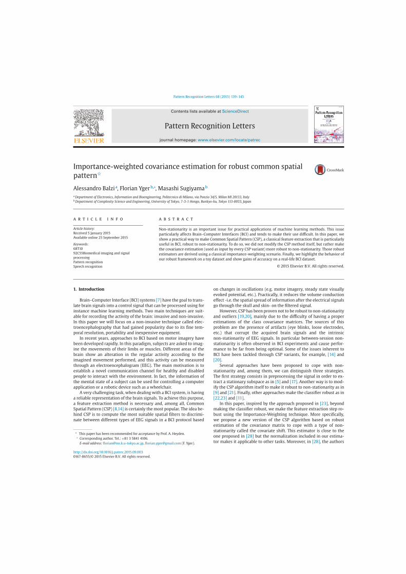
Pattern Recognition Letters 68 (2015) 139–145

Contents lists available at ScienceDirect

Pattern Recognition Letters

journal homepage: www.elsevier.com/locate/patrec

Importance-weighted covariance estimation for robust common spatial

pattern

Alessandro Balzi a, Florian Yger b,∗, Masashi Sugiyama b

a Department of Electronics, Information and Bioengineering, Politecnico di Milano, via Ponzio 34/5, Milan MI 20133, Italyb Department of Complexity Science and Engineering, University of Tokyo, 7-3-1 Hongo, Bunkyo-ku, Tokyo 113-0033, Japan

a r t i c l e i n f o

Article history:

Received 5 January 2015

Available online 25 September 2015

Keywords:

68T10

92C55Biomedical imaging and signal

processing

Pattern recognition

Speech recognition

a b s t r a c t

Non-stationarity is an important issue for practical applications of machine learning methods. This issue

particularly affects Brain–Computer Interfaces (BCI) and tends to make their use difficult. In this paper, we

show a practical way to make Common Spatial Pattern (CSP), a classical feature extraction that is particularly

useful in BCI, robust to non-stationarity. To do so, we did not modify the CSP method itself, but rather make

the covariance estimation (used as input by every CSP variant) more robust to non-stationarity. Those robust

estimators are derived using a classical importance-weighting scenario. Finally, we highlight the behavior of

our robust framework on a toy dataset and show gains of accuracy on a real-life BCI dataset.

© 2015 Elsevier B.V. All rights reserved.

1. Introduction

Brain–Computer Interface (BCI) systems [7] have the goal to trans-

late brain signals into a control signal that can be processed using for

instance machine learning methods. Two main techniques are suit-

able for recording the activity of the brain: invasive and non-invasive.

In this paper we will focus on a non-invasive technique called elec-

troencephalography that had gained popularity due to its fine tem-

poral resolution, portability and inexpensive equipment.

In recent years, approaches to BCI based on motor imagery have

been developed rapidly. In this paradigm, subjects are asked to imag-

ine the movements of their limbs or muscles. Different areas of the

brain show an alteration in the regular activity according to the

imagined movement performed, and this activity can be measured

through an electroencephalogram (EEG). The main motivation is to

establish a novel communication channel for healthy and disabled

people to interact with the environment. In fact, the information of

the mental state of a subject can be used for controlling a computer

application or a robotic device such as a wheelchair.

A very challenging task, when dealing with a BCI system, is having

a reliable representation of the brain signals. To achieve this purpose,

a feature extraction method is necessary and, among all, Common

Spatial Pattern (CSP) [8,14] is certainly the most popular. The idea be-

hind CSP is to compute the most suitable spatial filters to discrimi-

nate between different types of EEG signals in a BCI protocol based

This paper has been recommended for acceptance by Prof. A. Heyden.∗ Corresponding author. Tel.: +81 3 5841 4106.

E-mail address: florian@ms.k.u-tokyo.ac.jp, florian.yger@gmail.com (F. Yger).

on changes in oscillations (e.g. motor imagery, steady state visually

evoked potential, etc.). Practically, it reduces the volume conduction

effect -i.e. the spatial spread of information after the electrical signals

go through the skull and skin- on the filtered signal.

However, CSP has been proven not to be robust to non-stationarity

and outliers [19,20], mainly due to the difficulty of having a proper

estimations of the class covariance matrices. The sources of this

problem are the presence of artifacts (eye blinks, loose electrodes,

etc.) that corrupt the acquired brain signals and the intrinsic

non-stationarity of EEG signals. In particular between-session non-

stationarity is often observed in BCI experiments and cause perfor-

mance to be far from being optimal. Some of the issues inherent to

BCI have been tackled through CSP variants, for example, [14] and

[20].

Several approaches have been proposed to cope with non-

stationarity and, among them, we can distinguish three strategies.

The first strategy consists in preprocessing the signal in order to ex-

tract a stationary subspace as in [5] and [17]. Another way is to mod-

ify the CSP algorithm itself to make it robust to non-stationarity as in

[9] and [21]. Finally, other approaches make the classifier robust as in

[22,23] and [11].

In this paper, inspired by the approach proposed in [23], beyond

making the classifier robust, we make the feature extraction step ro-

bust using the Importance-Weighting technique. More specifically,

we propose a new version of the CSP algorithm based on robust

estimation of the covariance matrix to cope with a type of non-

stationarity called the covariate shift. This estimator is close to the

one proposed in [28] but the normalization included in our estima-

tor makes it applicable to other tasks. Moreover, in [28], the authors

http://dx.doi.org/10.1016/j.patrec.2015.09.003

0167-8655/© 2015 Elsevier B.V. All rights reserved.

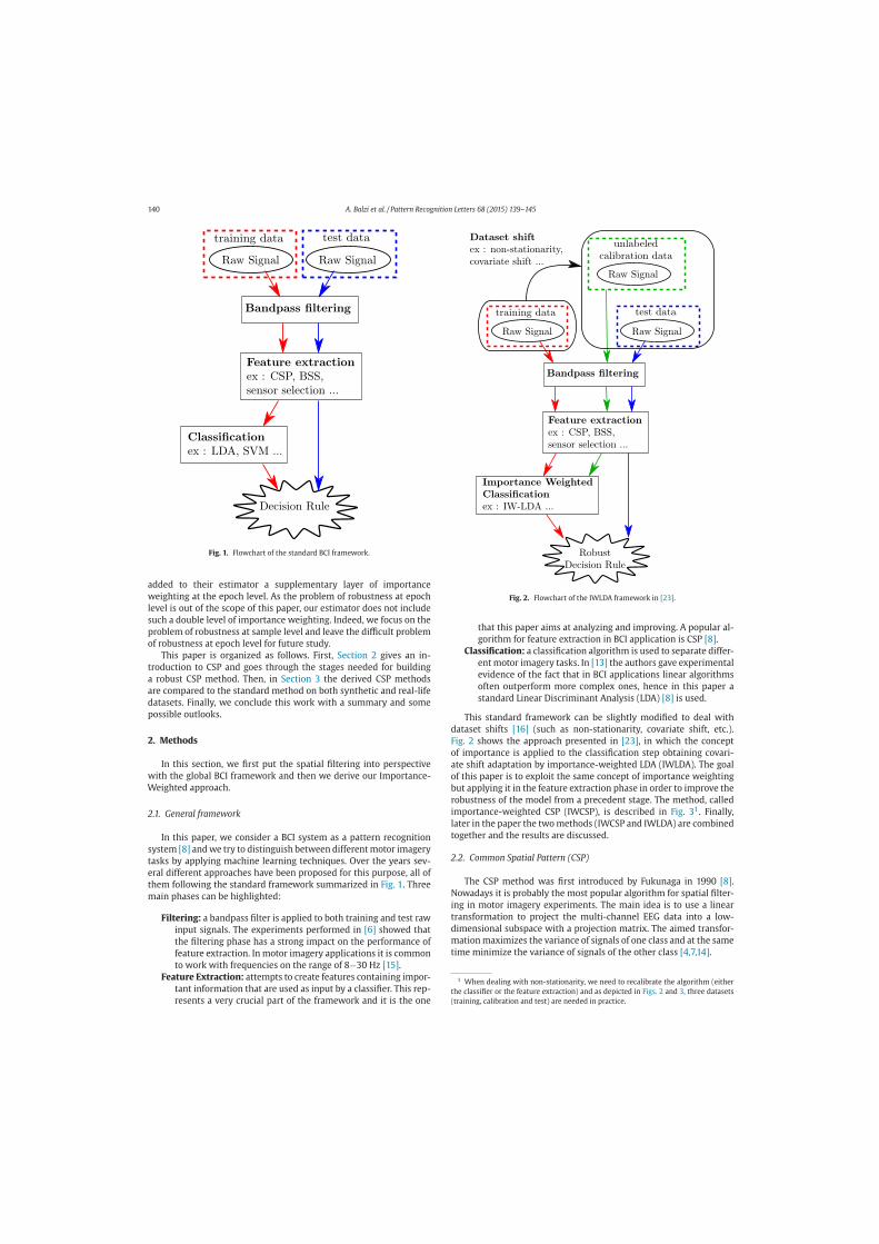
140 A. Balzi et al. / Pattern Recognition Letters 68 (2015) 139–145

Fig. 1. Flowchart of the standard BCI framework.

added to their estimator a supplementary layer of importance

weighting at the epoch level. As the problem of robustness at epoch

level is out of the scope of this paper, our estimator does not include

such a double level of importance weighting. Indeed, we focus on the

problem of robustness at sample level and leave the difficult problem

of robustness at epoch level for future study.

This paper is organized as follows. First, Section 2 gives an in-

troduction to CSP and goes through the stages needed for building

a robust CSP method. Then, in Section 3 the derived CSP methods

are compared to the standard method on both synthetic and real-life

datasets. Finally, we conclude this work with a summary and some

possible outlooks.

2. Methods

In this section, we first put the spatial filtering into perspective

with the global BCI framework and then we derive our Importance-

Weighted approach.

2.1. General framework

In this paper, we consider a BCI system as a pattern recognition

system [8] and we try to distinguish between different motor imagery

tasks by applying machine learning techniques. Over the years sev-

eral different approaches have been proposed for this purpose, all of

them following the standard framework summarized in Fig. 1. Three

main phases can be highlighted:

Filtering: a bandpass filter is applied to both training and test raw

input signals. The experiments performed in [6] showed that

the filtering phase has a strong impact on the performance of

feature extraction. In motor imagery applications it is common

to work with frequencies on the range of 8−30 Hz [15].

Feature Extraction: attempts to create features containing impor-

tant information that are used as input by a classifier. This rep-

resents a very crucial part of the framework and it is the one

Fig. 2. Flowchart of the IWLDA framework in [23].

that this paper aims at analyzing and improving. A popular al-

gorithm for feature extraction in BCI application is CSP [8].

Classification: a classification algorithm is used to separate differ-

ent motor imagery tasks. In [13] the authors gave experimental

evidence of the fact that in BCI applications linear algorithms

often outperform more complex ones, hence in this paper a

standard Linear Discriminant Analysis (LDA) [8] is used.

This standard framework can be slightly modified to deal with

dataset shifts [16] (such as non-stationarity, covariate shift, etc.).

Fig. 2 shows the approach presented in [23], in which the concept

of importance is applied to the classification step obtaining covari-

ate shift adaptation by importance-weighted LDA (IWLDA). The goal

of this paper is to exploit the same concept of importance weighting

but applying it in the feature extraction phase in order to improve the

robustness of the model from a precedent stage. The method, called

importance-weighted CSP (IWCSP), is described in Fig. 31. Finally,

later in the paper the two methods (IWCSP and IWLDA) are combined

together and the results are discussed.

2.2. Common Spatial Pattern (CSP)

The CSP method was first introduced by Fukunaga in 1990 [8].

Nowadays it is probably the most popular algorithm for spatial filter-

ing in motor imagery experiments. The main idea is to use a linear

transformation to project the multi-channel EEG data into a low-

dimensional subspace with a projection matrix. The aimed transfor-

mation maximizes the variance of signals of one class and at the same

time minimize the variance of signals of the other class [4,7,14].

1 When dealing with non-stationarity, we need to recalibrate the algorithm (either

the classifier or the feature extraction) and as depicted in Figs. 2 and 3, three datasets

(training, calibration and test) are needed in practice.

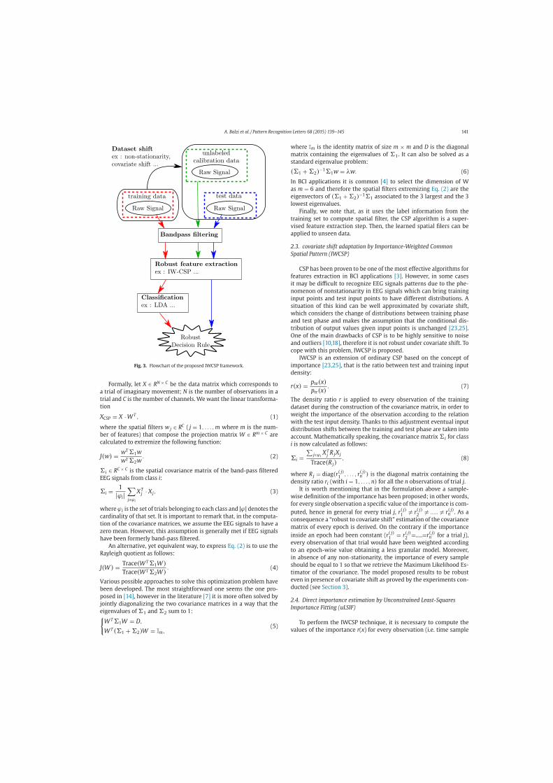
A. Balzi et al. / Pattern Recognition Letters 68 (2015) 139–145 141

Fig. 3. Flowchart of the proposed IWCSP framework.

Formally, let X ∈ RN × C be the data matrix which corresponds to

a trial of imaginary movement; N is the number of observations in a

trial and C is the number of channels. We want the linear transforma-

tion

XCSP = X · W T , (1)

where the spatial filters w j ∈ RC ( j = 1, . . . , m where m is the num-

ber of features) that compose the projection matrix W ∈ Rm × C are

calculated to extremize the following function:

J(w) = wT 1w

wT 2w. (2)

i ∈ RC × C is the spatial covariance matrix of the band-pass filtered

EEG signals from class i:

i = 1

|ϕi|∑j∈ϕi

XTj · Xj, (3)

where ϕi is the set of trials belonging to each class and |ϕ| denotes the

cardinality of that set. It is important to remark that, in the computa-

tion of the covariance matrices, we assume the EEG signals to have a

zero mean. However, this assumption is generally met if EEG signals

have been formerly band-pass filtered.

An alternative, yet equivalent way, to express Eq. (2) is to use the

Rayleigh quotient as follows:

J(W) = Trace(W T 1W)

Trace(W T 2W). (4)

Various possible approaches to solve this optimization problem have

been developed. The most straightforward one seems the one pro-

posed in [14], however in the literature [7] it is more often solved by

jointly diagonalizing the two covariance matrices in a way that the

eigenvalues of 1 and 2 sum to 1:W T 1W = D,

W T (1 + 2)W = Im,(5)

where Im is the identity matrix of size m × m and D is the diagonal

matrix containing the eigenvalues of 1. It can also be solved as a

standard eigenvalue problem:

(1 + 2)−11w = λw. (6)

In BCI applications it is common [4] to select the dimension of W

as m = 6 and therefore the spatial filters extremizing Eq. (2) are the

eigenvectors of (1 + 2)−11 associated to the 3 largest and the 3

lowest eigenvalues.

Finally, we note that, as it uses the label information from the

training set to compute spatial filter, the CSP algorithm is a super-

vised feature extraction step. Then, the learned spatial filers can be

applied to unseen data.

2.3. covariate shift adaptation by Importance-Weighted Common

Spatial Pattern (IWCSP)

CSP has been proven to be one of the most effective algorithms for

features extraction in BCI applications [3]. However, in some cases

it may be difficult to recognize EEG signals patterns due to the phe-

nomenon of nonstationarity in EEG signals which can bring training

input points and test input points to have different distributions. A

situation of this kind can be well approximated by covariate shift,

which considers the change of distributions between training phase

and test phase and makes the assumption that the conditional dis-

tribution of output values given input points is unchanged [23,25].

One of the main drawbacks of CSP is to be highly sensitive to noise

and outliers [10,18], therefore it is not robust under covariate shift. To

cope with this problem, IWCSP is proposed.

IWCSP is an extension of ordinary CSP based on the concept of

importance [23,25], that is the ratio between test and training input

density:

r(x) = pte(x)

ptr(x). (7)

The density ratio r is applied to every observation of the training

dataset during the construction of the covariance matrix, in order to

weight the importance of the observation according to the relation

with the test input density. Thanks to this adjustment eventual input

distribution shifts between the training and test phase are taken into

account. Mathematically speaking, the covariance matrix i for class

i is now calculated as follows:

i =∑

j∈ϕiXT

jR jXj

Trace(Rj), (8)

where R j = diag(r( j)1

, . . . , r( j)n ) is the diagonal matrix containing the

density ratio ri (with i = 1, . . . , n) for all the n observations of trial j.

It is worth mentioning that in the formulation above a sample-

wise definition of the importance has been proposed; in other words,

for every single observation a specific value of the importance is com-

puted, hence in general for every trial j, r( j)1

= r( j)2

= ..... = r( j)n . As a

consequence a “robust to covariate shift” estimation of the covariance

matrix of every epoch is derived. On the contrary if the importance

inside an epoch had been constant (r( j)1

= r( j)2

=.....=r( j)n for a trial j),

every observation of that trial would have been weighted according

to an epoch-wise value obtaining a less granular model. Moreover,

in absence of any non-stationarity, the importance of every sample

should be equal to 1 so that we retrieve the Maximum Likelihood Es-

timator of the covariance. The model proposed results to be robust

even in presence of covariate shift as proved by the experiments con-

ducted (see Section 3).

2.4. Direct importance estimation by Unconstrained Least-Squares

Importance Fitting (uLSIF)

To perform the IWCSP technique, it is necessary to compute the

values of the importance r(x) for every observation (i.e. time sample

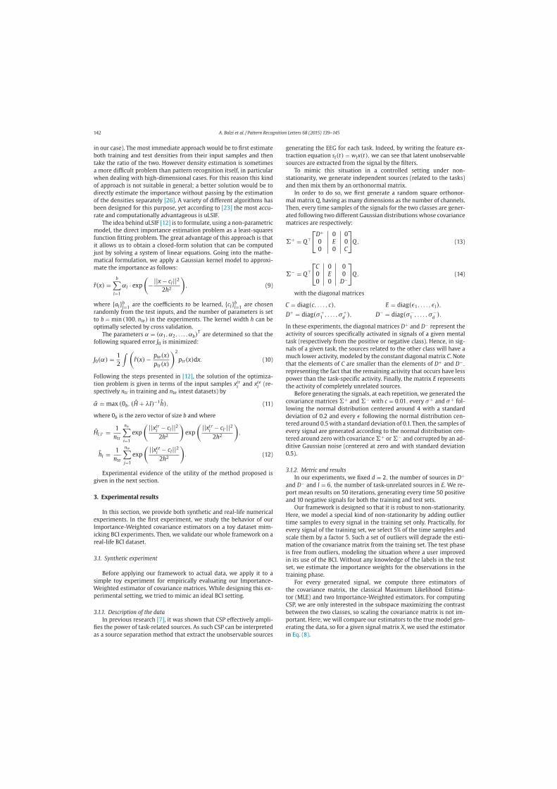
142 A. Balzi et al. / Pattern Recognition Letters 68 (2015) 139–145

in our case). The most immediate approach would be to first estimate

both training and test densities from their input samples and then

take the ratio of the two. However density estimation is sometimes

a more difficult problem than pattern recognition itself, in particular

when dealing with high-dimensional cases. For this reason this kind

of approach is not suitable in general; a better solution would be to

directly estimate the importance without passing by the estimation

of the densities separately [26]. A variety of different algorithms has

been designed for this purpose, yet according to [23] the most accu-

rate and computationally advantageous is uLSIF.

The idea behind uLSIF [12] is to formulate, using a non-parametric

model, the direct importance estimation problem as a least-squares

function fitting problem. The great advantage of this approach is that

it allows us to obtain a closed-form solution that can be computed

just by solving a system of linear equations. Going into the mathe-

matical formulation, we apply a Gaussian kernel model to approxi-

mate the importance as follows:

r(x) =b∑

l=1

αl · exp

(−||x − cl||2

2h2

), (9)

where albl=1

are the coefficients to be learned, clbl=1

are chosen

randomly from the test inputs, and the number of parameters is set

to b = min (100, nte) in the experiments. The kernel width h can be

optimally selected by cross validation.

The parameters α = (α1, α2, . . . , αb)T

are determined so that the

following squared error J0 is minimized:

J0(α) = 1

2

∫ (r(x) − pte(x)

ptr(x)

)2

ptr(x)dx. (10)

Following the steps presented in [12], the solution of the optimiza-

tion problem is given in terms of the input samples xtri

and xtei

(re-

spectively ntr in training and nte intest datasets) by

α = max (0b, (H + λI)−1h), (11)

where 0b is the zero vector of size b and where

Hl,l′ = 1

ntr

ntr∑i=1

exp

( ||xtri

− cl||2

2h2

)exp

( ||xtri

− cl′ ||2

2h2

),

hl = 1

nte

nte∑j=1

exp

( ||xtei

− cl||2

2h2

). (12)

Experimental evidence of the utility of the method proposed is

given in the next section.

3. Experimental results

In this section, we provide both synthetic and real-life numerical

experiments. In the first experiment, we study the behavior of our

Importance-Weighted covariance estimators on a toy dataset mim-

icking BCI experiments. Then, we validate our whole framework on a

real-life BCI dataset.

3.1. Synthetic experiment

Before applying our framework to actual data, we apply it to a

simple toy experiment for empirically evaluating our Importance-

Weighted estimator of covariance matrices. While designing this ex-

perimental setting, we tried to mimic an ideal BCI setting.

3.1.1. Description of the data

In previous research [7], it was shown that CSP effectively ampli-

fies the power of task-related sources. As such CSP can be interpreted

as a source separation method that extract the unobservable sources

generating the EEG for each task. Indeed, by writing the feature ex-

traction equation sl(t) = wlx(t), we can see that latent unobservable

sources are extracted from the signal by the filters.

To mimic this situation in a controlled setting under non-

stationarity, we generate independent sources (related to the tasks)

and then mix them by an orthonormal matrix.

In order to do so, we first generate a random square orthonor-

mal matrix Q, having as many dimensions as the number of channels.

Then, every time samples of the signals for the two classes are gener-

ated following two different Gaussian distributions whose covariance

matrices are respectively:

+ = Q

[D+ 0 00 E 00 0 C

]Q, (13)

− = Q

[C 0 00 E 00 0 D−

]Q, (14)

with the diagonal matrices

C = diag(c, . . . , c), E = diag(ε1, . . . , εl),

D+ = diag(σ+1 , . . . , σ+

d), D− = diag(σ−

1 , . . . , σ−d).

In these experiments, the diagonal matrices D+ and D− represent the

activity of sources specifically activated in signals of a given mental

task (respectively from the positive or negative class). Hence, in sig-

nals of a given task, the sources related to the other class will have a

much lower activity, modeled by the constant diagonal matrix C. Note

that the elements of C are smaller than the elements of D+ and D−,

representing the fact that the remaining activity that occurs have less

power than the task-specific activity. Finally, the matrix E represents

the activity of completely unrelated sources.

Before generating the signals, at each repetition, we generated the

covariance matrices + and − with c = 0.01, every σ+ and σ+ fol-

lowing the normal distribution centered around 4 with a standard

deviation of 0.2 and every ε following the normal distribution cen-

tered around 0.5 with a standard deviation of 0.1. Then, the samples of

every signal are generated according to the normal distribution cen-

tered around zero with covariance + or − and corrupted by an ad-

ditive Gaussian noise (centered at zero and with standard deviation

0.5).

3.1.2. Metric and results

In our experiments, we fixed d = 2, the number of sources in D+

and D− and l = 6, the number of task-unrelated sources in E. We re-

port mean results on 50 iterations, generating every time 50 positive

and 10 negative signals for both the training and test sets.

Our framework is designed so that it is robust to non-stationarity.

Here, we model a special kind of non-stationarity by adding outlier

time samples to every signal in the training set only. Practically, for

every signal of the training set, we select 5% of the time samples and

scale them by a factor 5. Such a set of outliers will degrade the esti-

mation of the covariance matrix from the training set. The test phase

is free from outliers, modeling the situation where a user improved

in its use of the BCI. Without any knowledge of the labels in the test

set, we estimate the importance weights for the observations in the

training phase.

For every generated signal, we compute three estimators of

the covariance matrix, the classical Maximum Likelihood Estima-

tor (MLE) and two Importance-Weighted estimators. For computing

CSP, we are only interested in the subspace maximizing the contrast

between the two classes, so scaling the covariance matrix is not im-

portant. Here, we will compare our estimators to the true model gen-

erating the data, so for a given signal matrix X, we used the estimator

in Eq. (8).

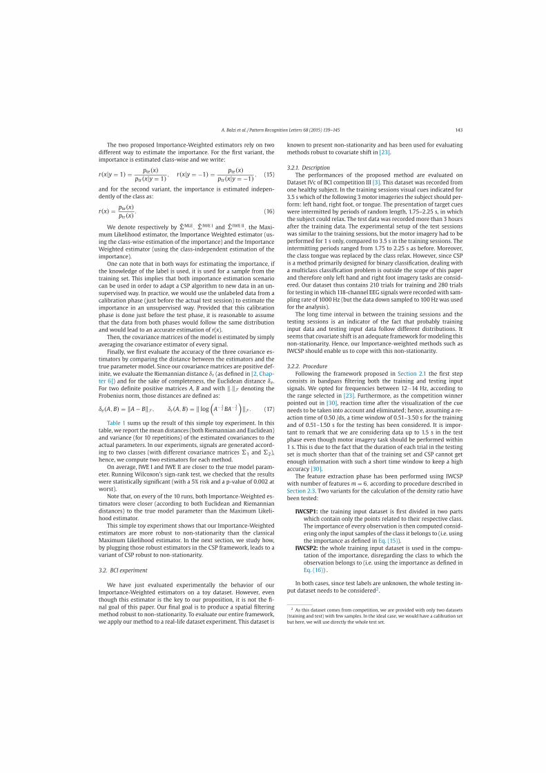
A. Balzi et al. / Pattern Recognition Letters 68 (2015) 139–145 143

The two proposed Importance-Weighted estimators rely on two

different way to estimate the importance. For the first variant, the

importance is estimated class-wise and we write:

r(x|y = 1) = pte(x)

ptr(x|y = 1), r(x|y = −1) = pte(x)

ptr(x|y = −1), (15)

and for the second variant, the importance is estimated indepen-

dently of the class as:

r(x) = pte(x)

ptr(x). (16)

We denote respectively by MLE, IWE I and IWE II, the Maxi-

mum Likelihood estimator, the Importance Weighted estimator (us-

ing the class-wise estimation of the importance) and the Importance

Weighted estimator (using the class-independent estimation of the

importance).

One can note that in both ways for estimating the importance, if

the knowledge of the label is used, it is used for a sample from the

training set. This implies that both importance estimation scenario

can be used in order to adapt a CSP algorithm to new data in an un-

supervised way. In practice, we would use the unlabeled data from a

calibration phase (just before the actual test session) to estimate the

importance in an unsupervised way. Provided that this calibration

phase is done just before the test phase, it is reasonable to assume

that the data from both phases would follow the same distribution

and would lead to an accurate estimation of r(x).

Then, the covariance matrices of the model is estimated by simply

averaging the covariance estimator of every signal.

Finally, we first evaluate the accuracy of the three covariance es-

timators by comparing the distance between the estimators and the

true parameter model. Since our covariance matrices are positive def-

inite, we evaluate the Riemannian distance δr (as defined in [2, Chap-

ter 6]) and for the sake of completeness, the Euclidean distance δe.

For two definite positive matrices A, B and with ‖.‖F denoting the

Frobenius norm, those distances are defined as:

δe(A, B) = ‖A − B‖F , δr(A, B) = ‖ log

(A− 1

2 BA− 12

)‖F . (17)

Table 1 sums up the result of this simple toy experiment. In this

table, we report the mean distances (both Riemannian and Euclidean)

and variance (for 10 repetitions) of the estimated covariances to the

actual parameters. In our experiments, signals are generated accord-

ing to two classes (with different covariance matrices 1 and 2),

hence, we compute two estimators for each method.

On average, IWE I and IWE II are closer to the true model param-

eter. Running Wilcoxon’s sign-rank test, we checked that the results

were statistically significant (with a 5% risk and a p-value of 0.002 at

worst).

Note that, on every of the 10 runs, both Importance-Weighted es-

timators were closer (according to both Euclidean and Riemannian

distances) to the true model parameter than the Maximum Likeli-

hood estimator.

This simple toy experiment shows that our Importance-Weighted

estimators are more robust to non-stationarity than the classical

Maximum Likelihood estimator. In the next section, we study how,

by plugging those robust estimators in the CSP framework, leads to a

variant of CSP robust to non-stationarity.

3.2. BCI experiment

We have just evaluated experimentally the behavior of our

Importance-Weighted estimators on a toy dataset. However, even

though this estimator is the key to our proposition, it is not the fi-

nal goal of this paper. Our final goal is to produce a spatial filtering

method robust to non-stationarity. To evaluate our entire framework,

we apply our method to a real-life dataset experiment. This dataset is

known to present non-stationarity and has been used for evaluating

methods robust to covariate shift in [23].

3.2.1. Description

The performances of the proposed method are evaluated on

Dataset IVc of BCI competition III [3]. This dataset was recorded from

one healthy subject. In the training sessions visual cues indicated for

3.5 s which of the following 3 motor imageries the subject should per-

form: left hand, right foot, or tongue. The presentation of target cues

were intermitted by periods of random length, 1.75–2.25 s, in which

the subject could relax. The test data was recorded more than 3 hours

after the training data. The experimental setup of the test sessions

was similar to the training sessions, but the motor imagery had to be

performed for 1 s only, compared to 3.5 s in the training sessions. The

intermitting periods ranged from 1.75 to 2.25 s as before. Moreover,

the class tongue was replaced by the class relax. However, since CSP

is a method primarily designed for binary classification, dealing with

a multiclass classification problem is outside the scope of this paper

and therefore only left hand and right foot imagery tasks are consid-

ered. Our dataset thus contains 210 trials for training and 280 trials

for testing in which 118-channel EEG signals were recorded with sam-

pling rate of 1000 Hz (but the data down sampled to 100 Hz was used

for the analysis).

The long time interval in between the training sessions and the

testing sessions is an indicator of the fact that probably training

input data and testing input data follow different distributions. It

seems that covariate shift is an adequate framework for modeling this

non-stationarity. Hence, our Importance-weighted methods such as

IWCSP should enable us to cope with this non-stationarity.

3.2.2. Procedure

Following the framework proposed in Section 2.1 the first step

consists in bandpass filtering both the training and testing input

signals. We opted for frequencies between 12−14 Hz, according to

the range selected in [23]. Furthermore, as the competition winner

pointed out in [30], reaction time after the visualization of the cue

needs to be taken into account and eliminated; hence, assuming a re-

action time of 0.50 /ds, a time window of 0.51–3.50 s for the training

and of 0.51–1.50 s for the testing has been considered. It is impor-

tant to remark that we are considering data up to 1.5 s in the test

phase even though motor imagery task should be performed within

1 s. This is due to the fact that the duration of each trial in the testing

set is much shorter than that of the training set and CSP cannot get

enough information with such a short time window to keep a high

accuracy [30].

The feature extraction phase has been performed using IWCSP

with number of features m = 6, according to procedure described in

Section 2.3. Two variants for the calculation of the density ratio have

been tested:

IWCSP1: the training input dataset is first divided in two parts

which contain only the points related to their respective class.

The importance of every observation is then computed consid-

ering only the input samples of the class it belongs to (i.e. using

the importance as defined in Eq. (15)).

IWCSP2: the whole training input dataset is used in the compu-

tation of the importance, disregarding the class to which the

observation belongs to (i.e. using the importance as defined in

Eq. (16)) .

In both cases, since test labels are unknown, the whole testing in-

put dataset needs to be considered2.

2 As this dataset comes from competition, we are provided with only two datasets

(training and test) with few samples. In the ideal case, we would have a calibration set

but here, we will use directly the whole test set.

144 A. Balzi et al. / Pattern Recognition Letters 68 (2015) 139–145

Table 1

Distance from the estimator to the true model.

δr(1,1) δr(2,2) δe(1,1) δe(2,2)

mean var mean var mean var mean var

MLE 5.1433 0.0014 2.189 0.0122 5.1507 8.37e − 4 2.1129 0.0134

IWE I 4.815 7.69e − 4 0.8606 2.47e − 4 4.6748 3.67e − 4 1.5356 0.01

IWE II 4.8154 7.66e − 4 0.8618 2.54e − 4 4.8277 6.81e − 4 0.8544 3.22e − 4

Table 2

Results of CSP + LDA, IWCSP1 + LDA, and

IWCSP2 + LDA measured in terms of accuracy

(mean and standard deviation).

Method CSP IWCSP1 IWCSP2

mean 89.29 90.11 90.46

std – 0.66 0.58

Table 3

Results of CSP + IWLDA, IWCSP1 + IWLDA,

and IWCSP2 + IWLDA measured in terms of

accuracy (mean and standard deviation).

Method CSP IWCSP1 IWCSP2

mean 91.79 93.61 93.71

std – 0.41 0.36

Finally, Linear Discriminant Analysis (LDA) has been used as a

classifier. A version with importance (IWLDA) has also been imple-

mented according to the model proposed in [23] which suggests

also the introduction of a regularizer. In this latter case the method

used for the estimation of the density ratio is a variant of the com-

mon uLSIF, called Relative Unconstrained Least-Squares Importance

Fitting (RuLSIF) [27]. The difference is the introduction of the rel-

ativity parameter β ∈ [0, 1] with the purpose of controlling the

trade off between bias and variance. The Eq. (7) is now rewritten as

follows:

r(β)(x) = pte(x)

βpte(x) + (1 − β)ptr(x). (18)

Both the regularizer and the relativity parameter are chosen

through Importance-Weighted Cross Validation (IWCV) [24], in

which a part of the test set is used as calibration for training the

model during cross validation.

3.2.3. Results

We report in Table 2 the results obtained applying covariate shift

adaptation in the feature extraction phase and using LDA as classifier.

The mean and standard deviation are based on 10 iteration of testing.

It is immediate to notice that both the IWCSP algorithms outper-

form the standard CSP version in terms of accuracy, therefore we

can claim the efficacy of our method under a situation of covariate

shift. Furthermore, IWCSP2 results to be slightly more accurate than

IWCSP1, reaching an accuracy of 90.46% against 90.11% for the other.

This may probably be due to the fact that uLSIF in IWCSP2 can benefit

of the knowledge of the whole training input dataset, hence it can

exploit this information to compute more adequate values for the

importance.

Applying the covariate shift adaptation also in the classification

phase we obtain some interesting results that are summarized in

Table 3. As expected, the use of importance weighting in the clas-

sification phase also improves the results. We experience already a

significant increment in the case CSP + IWLDA, passing from 89.29

to 91.79% of accuracy. However, it is the combination of IWCSP and

IWLDA that offers the best result. In particular the case IWCSP2 +IWLDA (which, as in Table 2, is slightly more accurate than IWCSP1 +

IWLDA) brings an increase of the 4 points with respect to the standard

case, a very notable fact considering that we are dealing with already

high values of accuracy. These results confirm the utility of perform-

ing importance weighting in the feature extraction step as well as in

the classification step, in order to obtain a robust model that is able

to deal with covariate shift.

4. Conclusions and future works

In this paper, we proposed a practical way to make Common

Spatial Pattern robust to non-stationarity. Compared to previous ap-

proaches tackling this problem, we did not modify the CSP algo-

rithm itself. Instead, we focused on making the covariance estimation

(feeded to the CSP algorithm) robust to non-stationarity by weight-

ing samples with their importance. This makes our approach generic

enough so that it could be applied to other CSP variants [14,20].

We showed the utility of our method on a real-life datasets and

we empirically studied our re-weighted covariance estimator on a toy

dataset. However, the theoretical study of the consistency of this es-

timator is an interesting open question and constitute a non-trivial

future works of this project.

We showed empirically, on a toy experiment mimicking BCI set-

ting, that the two proposed Importance-Weighted estimators are

more robust than a standard Maximum Likelihood estimator. Then

we showed on a real-life BCI dataset that the use of Importance-

Weighted estimators improves the performance of a CSP based BCI

system. To sum up, our whole idea has been to robustify the feature

extraction step in order to cope with non-stationarity, but we also

showed that using an Importance-Weighted classifier in robust fea-

tures improved even more the performances.

Finally, we applied our Importance-Weighted estimator for CSP

and showed that such an estimator brings to CSP more robustness

to non-stationarity. However, CSP is not the only feature extraction

based on covariance estimators and we plan to apply those estima-

tors to other approaches such as the one described in [1,29]. More-

over, as suggested in [28], our work could be extended in order to use

the importance to bring robustness at the epoch level.

Acknowledgments

AB was supported by a JASSO fellowship through the YSEP pro-

gramm. FY was supported by a JSPS fellowship (KAKENHI 26.04730)

and MS was supported by KAKENHI 26280054. The authors would

like to thank Dr. Du Plessis, Dr. Kawanabe and Dr. Lotte for fruitful

discussions.

References

[1] A. Barachant, S. Bonnet, M. Congedo, C. Jutten, Classification of covariance matri-

ces using a riemannian-based kernel for BCI applications, Neurocomputing 112(2013) 172–178.

[2] R. Bhatia, Positive Definite Matrices, Princeton University Press, 2009.[3] B. Blankertz, K.-R. Müller, G.S. Dean Krusienski, J.R. Wolpaw, A. Schlögl,

G. Pfurtscheller, J. del R.Millán, M. Schroder, N. Birbaumer, The BCI competition

iii:validating alternative approaches to actual BCI problems, IEEE Trans. NeuralSyst. Rehabil. Eng. 14 (2) (2006) 153–159.

[4] B. Blankertz, R. Tomioka, S. Lemm, M. Kawanabe, K.-R. Müller, Optimizing spatialfilters for robust eeg single-trial analysis, IEEE Signal Process. Mag. 25 (1) (2008)

41–56.

A. Balzi et al. / Pattern Recognition Letters 68 (2015) 139–145 145

[5] P. von Bünau, F.C. Meinecke, F.C. Király, K.-R. Müller, Finding stationary subspacesin multivariate time series, Phys. Rev. Lett. 103 (21) (2009) 214101.

[6] G. Dornhege, B. Blankertz, M. Krauledat, F. Losch, G. Curio, K.-R. Müller, Combinedoptimization of spatial and temporal filters for improving BCI, IEEE Trans. Biomed.

Eng. 53 (11) (2008) 2274–2281.[7] G. Dornhege, J. del R.Millán, T. Hinterberger, D.J. McFarland, K.-R. Müller, Toward

Brain-Computer Interfacing, The MIT Press, 2007.[8] K. Fukunaga, Introduction to Statistical Pattern Recognition, Academic Press,

1990.

[9] C. Gouy-Pailler, M. Congedo, C. Brunner, C. Jutten, G. Pfurtscheller, Nonstationarybrain source separation for multiclass motor imagery, IEEE Trans. Biomed. Eng. 57

(2) (2010) 469–478.[10] M. Grosse-Wentrup, C. Liefhold, K. Gramann, M. Buss, Beamforming in non-

invasive brain-computer interfaces, IEEE Trans. Biomed. Eng. 56 (4) (2009) 1209–1219.

[11] A. Hassan, I. Niazi, M. Jochumsen, F. Riaz, K. Dremstrup, Classification of kinet-

ics of movement for lower limb using covariate shift method for brain computerinterface, in: Proceedings of IEEE International Conference on Acoustics, Speech

and Signal Processing (ICASSP), 2014, pp. 5854–5858.[12] T. Kanamori, S. Hido, M. Sugiyama, A least-squares approach to direct importance

estimation, J. Mach. Learn. Res. 10 (2009) 1391–1445.[13] F. Lotte, M. Congedo, A. Lécuyer, F. Lamarche, B. Arnaldi, A review of classification

algorithms for eeg-based brain-computer interfaces, J. Neural Eng. 4 (2) (2007)

R1–R13.[14] F. Lotte, C. Guan, Regularizing common spatial patterns to improve BCI designs:

unified theory and new algorithms, IEEE Trans. Biomed. Eng. 58 (2) (2010) 355–362.

[15] G. Pfurtscheller, F.L. da Silva, Event-related eeg/meg synchronization and desyn-chronization: basic principles, Clin. Neurophysiol. 110 (11) (1999).

[16] J. Quinonero-Candela, M. Sugiyama, A. Schwaighofer, N.D. Lawrence, Dataset Shift

in Machine Learning, MIT Press, 2009.[17] B. Reuderink, J. Farquhar, M. Poel, Slow sphering to suppress non-stationaries in

the EEG, Int. J. Bioelectromagn. 13 (2) (2011) 78–79.

[18] B. Reuderink, M. Poel, Robustness of the common spatial patterns algorithm inthe bci-pipeline, HMI, University of Twente, 2008.

[19] W. Samek, On Robust Spatial Filtering of EEG in Nonstationary Environments,Technische Universität Berlin, 2014 Ph.D. thesis.

[20] W. Samek, M. Kawanabe, K.-R. Müller, Divergence-based framework for commonspatial patterns algorithms, IEEE Rev. Biomed. Eng. 7 (2014) 50–72.

[21] W. Samek, C. Vidaurre, K.-R. Müller, M. Kawanabe, Stationary common spatialpatterns for brain–computer interfacing, J. Neural Eng. 9 (2) (2012) 026013.

[22] A. Satti, C. Guan, D. Coyle, G. Prasad, A covariate shift minimisation method to

alleviate non-stationarity effects for an adaptive brain-computer interface, in:Proceedings of International Conference on Pattern Recognition (ICPR), 2010,

pp. 105–108.[23] M. Sugiyama, T. Kanamori, T. Suzuki, S. Hido, J. Sese, I. Takeuchi, L. Wang, A

density-ratio framework for statistical data processing, IPSJ Trans. Comput. Vis.Appl. 1 (2009) 183–208.

[24] M. Sugiyama, M. Krauledat, K.-R. Müller, Covariate shift adaptation by importance

weighted cross validation, J. Mach. Learn. Res. 8 (2007) 985–1005.[25] M. Sugiyama, T. Suzuki, T. Kanamori, Density Ratio Estimation in Machine Learn-

ing, Cambridge University Press, 2012.[26] M. Sugiyama, T. Suzuki, S. Nakajima, H. Kashima, P. von Bünau, M. Kawanabe, Di-

rect importance estimation for covariate shift adaptation, The Inst. Stat. Math. 60(4) (2008) 699–746.

[27] M. Sugiyama, M. Yamada, M.C. du Plessis, Learning under non-stationarity: co-

variate shift and class-balance change, WIREs Comput. Stat. 5 (6) (2013) 465–477.[28] W. Tu, S. Sun, Semi-supervised feature extraction for eeg classification, Pattern

Anal. Appl. 16 (2) (2013) 213–222.[29] F. Yger, A review of kernels on covariance matrices for BCI applications, in: Pro-

ceedings of IEEE International Workshop on Machine Learning for Signal Process-ing (MLSP), 2013, pp. 1–6.

[30] D. Zhang, Y. Wang, X. Gao, B. Hong, S. Gao, An algorithm for idle-state detection in

motor-imagery-based brain-computer interface, Comput. Intell. Neurosci. 2007(2007) 9.

Bibliography

[1] S. Abdelmounaime and H. Dong-Chen. New brodatz-based imagedatabases for grayscale color and multiband texture analysis. ISRNMachine Vision, 2013.

[2] H. Akaike. Statistical predictor identification. Annals of the Instituteof Statistical Mathematics, 1970.

[3] H. Akaike. A new look at the statistical model identification. IEEETransactions on Automatic Control, 1974.

[4] N. S. Altman. An introduction to kernel and nearest-neighbor nonpara-metric regression. The American Statistician, 1992.

[5] F. Anzani, D. Bosisio, M. Matteucci, and D. G. Sorrenti. On-line colorcalibration in non-stationary environments. RoboCup 2005: Robot Soc-cer World Cup IX, 2006.

[6] P. Baldi and S. Brunak. Bioinformatics: The Machine Learning Ap-proach. MIT Press, 1998.

[7] A. Barachant, S. Bonnet, M. Congedo, and C. Jutten. Classificationof covariance matrices using a riemannian-based kernel for bci applica-tions. Neurocomputing, 2013.

[8] A. Barachant, S. Bonnet, M. Congedo, and C. Jutten. Multi-classbrain computer interface classification by riemannian geometry. IEEETransactions on Biomedical Engineering, 2014.

[9] F. Beverina, G. Palmas, S. Silvoni, F. Piccione, and S. Giove. Useradaptive bcis: Ssvep and p300 based interfaces. PsychNology Journal,2003.

[10] R. Bhatia. Positive Definite Matrices. Princeton University Press, 2009.

85

[11] C. M. Bishop. Pattern Recognition and Machine Learning. Springer,2006.

[12] B. Blankertz, K.R. Muller, G. Shalk, D. J. Krusienski, J. R. Wolpaw,A. Schlogl, G. Pfurtscheller, J. del R. Millan, M. Schroder, and N. Bir-baumer. The bci competition iii:validating alternative approaches toactual bci problems. IEEE Transactions on Neural Systems and Reha-bilitation Engineering, 2006.

[13] B. Blankertz, R. Tomioka, S. Lemm, M. Kawanabe, and K.R. Muller.Optimizing spatial filters for robust eeg single-trial analysis. IEEE Sig-nal Processing Magazine, 2008.

[14] R. Blatt, S. Ceriani, B. Dal Seno, G. Fontana, M. Matteucci, andD. Migliore. Brain control of a smart wheelchair. 10th internationalconference on intelligent autonomous systems, 2008.

[15] B. E. Boser, I. M. Guyon, and V. N. Vapnik. A training algorithm foroptimal margin classifiers. ACM, 1992.

[16] P. Brodatz. Textures: A Photographic Album for Artists and Designers.Dover Publications, 1966.

[17] B. M. Carvalho, T. S. Souza, and E. Garduno. Texture fuzzy segmen-tation using adaptive a nity functions. Proceedings of the 27th AnnualACM Symposium on Applied Computing, 2012.

[18] O. Chapelle, B. Scholkopf, and A. Zien. Semi-Supervised Learning. MITPress, 2006.

[19] D. Ciresan, U. Meier, J. Masci, and J. Schmidhuber. Multi-column deepneural network for traffic sign classification. Neural Networks, 2012.

[20] M. Deza and E. Deza. Encyclopedia of Distances. Springer, 2009.

[21] G. Dornhege, B. Blankertz, M. Krauledat, F. Losch, G. Curio, andK.R. Muller. Combined optimization of spatial and temporal filters forimproving bci. IEEE Transactions on Biomedical Engineering, 2008.

[22] G. Dornhege, J. del R. Millan, T. Hinterberger, D. J. McFarland, andK.R. Muller. Toward Brain-Computer Interfacing. The MIT Press,2007.

[23] R. O. Duda, P. E. Hart, and D. G. Stork. Pattern Classification. Wiley,2000.

86

[24] B. S. Everitt, S. Landau, M. Leese, and D. Stahl. Cluster Analysis.John Wiley and Sons, 2011.

[25] R. A. Fisher. The use of multiple measurements in taxonomic problems.Annals of Eugenics, 1936.

[26] G. S. Fishman. Monte Carlo: Concepts, Algorithms, and Applications.Springer, 1996.

[27] P. T. Fletcher and S. Joshi. Principal geodesic analysis on symmetricspaces: Statistics of diffusion tensors. Proceedings of Computer VisionApproaches to Medical Image Analysis, 2004.

[28] W. Forstner and B. Moonen. A metric for covariance matrices. Tech-nical report, Department of Geodesy and Geoinformatics, StuttgartUniversity, 1999.

[29] Y. Freund and R. E. Schapire. Experiments with a New Boosting Algo-rithm. Machine Learning: Proceedings of the Thirteenth InternationalConference, 1996.

[30] J. Friedman, T. Hastie, and R. Tibshirani. Additive logistic regression:a statistical view of boosting. The Annals of Statistics, 2000.

[31] K. Fukunaga. Introduction to Statistical Pattern Recognition. AcademicPress, 1990.

[32] B. Georgescu, I. Shimshoni, and P. Meer. Mean shift based clusteringin high dimensions: A texture classification example. Proceedings ofthe 9th IEEE International Conference on Computer Vision, 2003.

[33] G. H. Golub and C. F. Van Loan. Matrix Computations. Johns HopkinsUniversity Press, 1996.

[34] M. Grosse-Wentrup, C. Liefhold, K. Gramann, and M. Buss. Beam-forming in non-invasive brain-computer interfaces. IEEE Transactionson Biomedi- cal Engineering, 2009.

[35] H. Hachiya, T. Akiyama, M. Sugiyama, and J. Peters. Adaptive im-portance sampling for value function approximation in off-policy rein-forcement learning. Neural Networks, 2009.

[36] P. Hall, B. U. Park, and R. J. Samworth. Choice of neighbor order innearest-neighbor classification. Annals of Statistics, 2008.

87

[37] A. Hassan and A. Shaukat. Covariate shift approach for invariant tex-ture classification. IEEE International Workshop on Machine Learningfor Signal Processing, 2013.

[38] T. Hastie, R. Tibshirani, and J. Friedman. The Elements of StatisticalLearning: Data Mining, Inference, and Prediction. Springer, 2009.

[39] I. Horev, F. Yger, and M. Sugiyama. Geometry-aware principal compo-nent analysis for symmetric positive definite matrices. JMLR: Workshopand Conference Proceedings, 2015.

[40] R. A. Horn and C. R. Johnson. Matrix Analysis. Cambridge UniversityPress, 1990.

[41] P. J. Huber. Robust Statistics. Wiley-Interscience, 1981.

[42] T. Kanamori, S. Hido, and M. Sugiyama. A least-squares approach todirect importance estimation. Journal of Machine Learning Research,2009.

[43] F. M. Khellah. Texture classification using dominant neighborhoodstructure. IEEE Transactions on Image Processing, 2011.

[44] S. Kullback and R. A. Leibler. On information and sufficiency. Annalsof Mathematical Statistics, 1951.

[45] J. Levinson, J. Askeland, J. Becker, J. Dolson, D. Held, S. Kammel,J. Z. Kolter, D. Langer, O. Pink, V. Pratt, M. Sokolsky, G. Stanek,D. Stavens, A. Teichman, M. Werling, and S. Thrun. Towards fully au-tonomous driving: Systems and algorithms. Intelligent Vehicles Sym-posium (IV), 2011.

[46] Y. Li, H. Kambara, Y. Koike, and M. Sugiyama. Application of co-variate shift adaptation techniques in brain computer interfaces. IEEETransactions on Biomedical Engineering, 2010.

[47] L. Liu, Y. Long, P. Fieguth, S. Lao, and Guoying Zhao. Brint: Bi-nary rotation invariant and noise tolerant texture classification. IEEETransactions on Image Processing, 2014.

[48] F. Lotte, M. Congedo, A. Lecuyer, F. Lamarche, and B. Arnaldi. Areview of classification algorithms for eeg-based brain-computer inter-faces. Journal of Neural Engineering, 2007.

88

[49] F. Lotte and C. Guan. Regularizing common spatial patterns to im-prove bci designs: Unified theory and new algorithms. IEEE Transac-tions on Biomedical Engineering, 2010.

[50] J. Mairal, F. Bach, J. Ponce, G. Sapiro, and A. Zisserman. Super-vised dictionary learning. Advances in Neural Information ProcessingSystems, 2008.

[51] B. S. Manjunath and W. Y. Ma. Texture features for browsing andretrieval of image data. IEEE Transactions on Pattern Analysis andMachine Intelligence, 1996.

[52] M. Mirmehdi, X. Xie, and J. S. Suri. Handbook of Texture Analysis.Imperial College Press, 2008.

[53] M. Partio, B. Cramariuc, M. Gabboui, and M. Visa. Rock texture re-trieval using gray level co-occurrence matrix. Proceedings of 5th NordicSignal Processing Symposium, 2002.

[54] G. Pfurtscheller and F. L. da Silva. Event-related eeg/meg synchroniza-tion and desynchronization: basic principles. Clinical Neurophysiology,1999.

[55] F. Porikli and T. Kocak. Robust license plate detection using covariancedescriptor in a neural network framework. Proceedings of the IEEE In-ternational Conference on Video and Signal Based Surveillance (AVSS),2006.

[56] B. Reuderink and M. Poel. Robustness of the common spatial patternsalgorithm in the bci-pipeline. Technical report, University of Twente,2008.

[57] F. Riaz, F. Silva, M. Ribeiro, and M. Coimbra. Invariant gabor texturedescriptors for classification of gastroenterology images. IEEE Trans-actions on Biomedical Engineering, 2012.

[58] S. Russel and P. Norvig. Artificial Intelligence: A Modern Approach.Pearson, 2010.

[59] B. Scholkopf and A. J. Smola. Learning with Kernels. MIT Press, 2001.

[60] B. Dal Seno. Toward An Integrated P300- And ErrP-Based Brain-Computer Interface. PhD thesis, Politecnico di Milano, 2009.

89

[61] B. Dal Seno, M. Matteucci, and L. Mainardi. Online detection of p300and error potentials in a bci speller. Computational intelligence andneuroscience, 2010.

[62] P. Sermanet and Y. LeCun. Traffic sign recognition with multi-scaleconvolutional networks. International Joint Conference on Neural Net-works (IJCNN), 2011.

[63] A. Shashua. Introduction to Machine Learning. School of ComputerScience and Engineering: The Hebrew University of Jerusalem, 2008.

[64] H. Shimodaira. Improving predictive inference under covariate shift byweighting the log-likelihood function. Journal of Statistical Planningand Inference, 2000.

[65] J. Stallkamp, M. Schlipsing, and J. Salmen. The german traffic signrecognition benchmark: A multi-class classification competition. Pro-ceedings of International Joint Conference on Neural Networks, 2011.

[66] J. Stallkamp, M. Schlipsing, J. Salmen, and C. Igel. Man vs computer:Benchmarking machine learning algorithms for traffic sign recognition.Neural Networks, 2012.

[67] M. Stone. Cross-validatory choice and assessment of statistical predic-tions. Journal of the Royal Statistical Society, 1974.

[68] M. Sugiyama and M. Kawanabe. Machine Learning in Non-StationaryEnvironments: Introduction to Covariate Shift Adaptation. The MITPress, 2012.

[69] M. Sugiyama, M. Krauledat, and K.-R. Muller. Covariate shift adap-tation by importance weighted cross validation. Journal of MachineLearning Research, 2007.

[70] M. Sugiyama, S. Nakajima, H. Kashima, P. von Bunau, and M. Kawan-abe. Direct importance estimation with model selection and its appli-cation to covariate shift adaptation. Advances in Neural InformationProcessing Systems, 2008.

[71] M. Sugiyama, T. Suzuki, and T. Kanamori. Density Ratio Estimationin Machine Learning. Cambridge University Press, 2012.

[72] M. Sugiyama, M. Yamada, and M. Christoffel du Plessis. Learning un-der non-stationarity: Covariate shift and class-balance change. WIREsComputational Statistics, 2013.

90

[73] I. J. Sumana, G. Lu, and D. Zhang. Comparison of curvelet and wavelettexture features for content based image retrieval. Proceedings of theIEEE International Conference on Multimedia and Expo, 2012.

[74] D. S. Tan and A. Nijholt. Brain-Computer Interfaces - Applying ourMinds to Human-Computer Interaction. Springer, 2010.

[75] R. Timofte, V. A. Prisacariu, L. J. Van Gool, and I. Reid. Emerg-ing Topics in Computer Vision and its Applications. World ScientificPublishing, 2011.

[76] R. Timofte, K. Zimmermann, and L. Van Gool. Multi-view trafficsign detection, recognition, and 3d localisation. Machine Vision andApplications, 2011.

[77] J. Y. Tou, P. Y. Lau, and Y. H. Tay. Computer vision based woodrecognition system. Proceedings of the International Workshop on Ad-vanced Image Technology, 2007.

[78] J. Y. Tou, Y. H. Tay, and P. Y. Lau. One-dimensional grey-level co-occurrence matrices for texture classification. International Symposiumon Information Technology (ITSim), 2008.

[79] J. Y. Tou, Y. H. Tay, and P. Y. Lau. Gabor filters as feature imagesfor covariance matrix on texture classification problem. Advances inNeuro-Information Processing, 2009.

[80] Y. Tsuboi, H. Kashima, S. Hido, S. Bickel, and M. Sugiyama. Di-rect density ratio estimation for large-scale covariate shift adaptation.Journal of Information Processing, 2009.

[81] O. Tuzel, F. Porikli, and P. Meer. Region covariance: A fast descrip-tor for detection and classification. Proceedings of the 9th EuropeanConference on Computer Vision, 2006.

[82] O. Tuzel, F. Porikli, and P. Meer. Human detection via classification onriemannian manifolds. Proceedings of the IEEE Conference on Com-puter Vision and Pattern Recognition (CVPR), 2007.

[83] K. Ueki, M. Sugiyama, and Y. Ihara. A semi-supervised approachto perceived age prediction from face images. IEICE Transactions onInformation and Systems, 2010.

[84] V. N. Vapnik. Statistical Learning Theory. Wiley-Interscience, 1998.

91

[85] M. Yamada, M. Sugiyama, and T. Matsui. Semi-supervised speakeridentification under covariate shift. Signal Processing, 2010.

[86] W. H. Yap, M. Khalid, and R. Yusof. Face verification with gaborrepresentation and support vector machines. IEEE Proceedings of theFirst Asia International Conference on Modeling and Simulation, 2007.

[87] J. Ye. Least squares linear discriminant analysis. Proceedings of the24th international conference on Machine learning, 2007.

[88] Y. L. Yew. Design of an intelligent wood recognition system for theclassification of tropical wood species. Technical report, UniversitiTeknologi Malaysia, 2005.

[89] F. Yger. A review of kernels on covariance matrices for bci applica-tions. IEEE International Workshop on Machine Learning for SignalProcessing, 2013.

[90] F. Yger. Application of covariance matrices and wavelet marginals.Challenge IEEE-ISBI/TCB, 2014.

[91] F. Yger, F. Lotte, and M. Sugiyama. Averaging covariance matricesfor eeg signal classification based on the csp: an empirical study. EU-SIPCO, 2015.

[92] F. Yger and A. Rakotomamonjy. Wavelet kernel learning. 2010.

[93] F. Zaklouta, B. Stanciulescu, and O. Hamdoun. Traffic sign classifica-tion using k-d trees and random forests. International Joint Conferenceon Neural Networks (IJCNN), 2011.

[94] D. Zhang, Y. Wang, X. Gao, B. Hong, and S. Gao. An algorithm foridle-state detection in motor-imagery-based brain-computer interface.Computational Intelligence and Neuroscience, 2007.

92