A Weighted Regularity Lemma with Applications

arX

iv:0

907.

0245

v1 [

mat

h.C

O]

1 J

ul 2

009

WEIGHTED REGULARITY LEMMA WITH APPLICATIONS

BELA CSABA AND ANDRAS PLUHAR

Abstract. We prove an extension of the Regularity Lemma with vertex and edgeweights, which can be applied for a large class of sparse graphs.

1. Introduction

Let G = G(A, B) be a bipartite graph. For X, Y ⊂ A ∪ B let eG(X, Y ) denotethe number of edges with one endpoint in X and the other in Y. We say that the(A, B)-pair is ε-regular if

∣

∣

∣

∣

eG(A′, B′)

|A′||B′| − eG(A, B)

|A||B|

∣

∣

∣

∣

< ε

for every A ⊂ A, |A′| > ε|A| and B′ ⊂ B, |B′| > ε|B|.This definition plays a crucial role in the celebrated Regularity Lemma of Sze-

meredi, see [8, 9]. Szemeredi invented the lemma for proving his famous theoremon arithmetic progression of dense subsets of the natural numbers. The RegularityLemma is a very powerful tool when applied to a dense graph. It has found lots ofapplications in several areas of mathematics and computer science, for applicationsin graph theory see e.g. [7]. However, it does not tell us anything useful when appliedfor a sparse graph (i.e., a graph on n vertices having o(n2) edges).

There has been significant interest to find widely applicable versions for sparsegraphs. This turns out to be a very hard task. Kohayakawa [5] proved a sparseregularity lemma, and with Rodl and Luczak [6] they applied it for finding arith-metic progressions of length 3 in dense subsets of a random set. In their sparseregularity lemma dense graphs are substituted by dense subgraphs of a random (orquasi-random) graph. Naturally, a new definition of ε-regularity was needed, belowwe formulate a slightly different version from theirs:

Let F (A, B) and G(A, B) be two bipartite graphs such that F ⊂ G. We say thatthe (A, B)-pair is ε-regular in F relative to G if

∣

∣

∣

∣

eF (A′, B′)

eG(A′, B′)− eF (A, B)

eG(A, B)

∣

∣

∣

∣

< ε

Key words and phrases. Regularity lemma, sparse graphs.The authors were partially supported by the grants OTKA T049398 and OTKA K76099. The

first author was partially supported by a New Faculty Scholarship Grant of the Office of SponsoredPrograms at Western Kentucky University.

1

http://arxiv.org/abs/0907.0245v1

2 CSABA AND PLUHAR

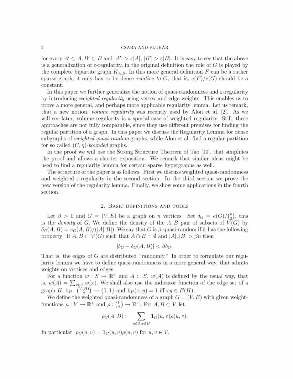
for every A′ ⊂ A, B′ ⊂ B and |A′| > ε|A|, |B′| > ε|B|. It is easy to see that the aboveis a generalization of ε-regularity, in the original definition the role of G is played bythe complete bipartite graph KA,B. In this more general definition F can be a rathersparse graph, it only has to be dense relative to G, that is, e(F )/e(G) should be aconstant.

In this paper we further generalize the notion of quasi-randomness and ε-regularityby introducing weighted regularity using vertex and edge weights. This enables us toprove a more general, and perhaps more applicable regularity lemma. Let us remark,that a new notion, volume regularity was recently used by Alon et al. [2]. As wewill see later, volume regularity is a special case of weighted regularity. Still, theseapproaches are not fully comparable, since they use different premises for finding theregular partition of a graph. In this paper we discuss the Regularity Lemma for densesubgraphs of weighted quasi-random graphs, while Alon et al. find a regular partitionfor so called (C, η)-bounded graphs.

In the proof we will use the Strong Structure Theorem of Tao [10], that simplifiesthe proof and allows a shorter exposition. We remark that similar ideas might beused to find a regularity lemma for certain sparse hypergraphs as well.

The structure of the paper is as follows. First we discuss weighted quasi-randomnessand weighted ε-regularity in the second section. In the third section we prove thenew version of the regularity lemma. Finally, we show some applications in the fourthsection.

2. Basic definitions and tools

Let β > 0 and G = (V, E) be a graph on n vertices. Set δG = e(G)/(

n

2

)

, thisis the density of G. We define the density of the A, B pair of subsets of V (G) byδG(A, B) = eG(A, B)/(|A||B|). We say that G is β-quasi-random if it has the followingproperty: If A, B ⊂ V (G) such that A ∩ B = ∅ and |A|, |B| > βn then

|δG − δG(A, B)| < βδG.

That is, the edges of G are distributed “randomly.” In order to formulate our regu-larity lemma we have to define quasi-randomness in a more general way, that admitsweights on vertices and edges.

For a function w : S → R+ and A ⊂ S, w(A) is defined by the usual way, that

is, w(A) =∑

x∈A w(x). We shall also use the indicator function of the edge set of a

graph H. 1H :(

V (H)2

)

→ {0, 1} and 1H(x, y) = 1 iff xy ∈ E(H).We define the weighted quasi-randomness of a graph G = (V, E) with given weight-

functions µ : V → R+ and ρ :

(

V

2

)

→ R+. For A, B ⊂ V let

ρG(A, B) :=∑

u∈A,v∈B

1G(u, v)ρ(u, v).

In particular, ρG(u, v) = 1G(u, v)ρ(u, v) for u, v ∈ V.

WEIGHTED REGULARITY LEMMA WITH APPLICATIONS 3

Definition 1. A graph G = (V, E) is weighted β-quasi-random with weight-functionsµ and ρ if for any A, B ⊂ V (G) such A ∩ B = ∅ and µ(A) ≥ βµ(V ), µ(B) ≥ βµ(V )we have

∣

∣

∣

∣

ρG(A, B)

µ(A)µ(B)− ρG(V, V )

µ(V )µ(V )

∣

∣

∣

∣

< β.

Observe that choosing µ ≡ 1 and ρ ≡ 1/δG gives back the first definition of quasi-randomness. There is another, weaker notion of quasi-randomness, which we will alsouse.

Definition 2. Let D > 1 be an absolute constant. A graph G = (V, E) is weighted(D, β)-quasi-random with weight-functions µ and ρ if for any A, B ⊂ V (G) suchA ∩ B = ∅ and µ(A) ≥ βµ(V ), µ(B) ≥ βµ(V ) we have

1

D

ρG(V, V )

µ(V )µ(V )≤ ρG(A, B)

µ(A)µ(B)≤ D

ρG(V, V )

µ(V )µ(V ).

Clearly, if a graph is β-quasi-random, then it is (D, β)-quasi-random unless D isvery close to one. Now we need to describe the weighted version of relative regularity.

Definition 3. Let G and F be graphs such that F ⊂ G and µ, ρ weight functionsdefined as above. For A, B ⊂ V (G) and A ∩ B = ∅ the pair (A, B) in F is µ − ρ-weighted ǫ-regular relative to G, or briefly weighted ǫ-regular, if

∣

∣

∣

∣

ρF (A′, B′)

µ(A′)µ(B′)− ρF (A, B)

µ(A)µ(B)

∣

∣

∣

∣

< ǫ

for every A′ ⊂ A and B′ ⊂ B provided that µ(A′) ≥ ǫµ(A), µ(B′) ≥ ǫµ(B). Here

ρF (A, B) =∑

u∈A,v∈B

1F (u, v)ρ(u, v).

Remark. Note that weighted ǫ-regularity is nothing but the well-known ǫ-regularitywhen G = KA,B and µ ≡ 1 and ρ is chosen to be identically the reciprocal of thedensity of G as before.

Next we define weighted regular partitions.

Definition 4. Let G = (V, E) and F ⊂ G be graphs, and µ and ρ weight functions.F has a weighted ǫ-regular partition relative to G if its vertex set V can be partitionedinto ℓ + 1 clusters W0, W1, . . . , Wℓ such that

• µ(W0) ≤ ǫµ(V ),• |µ(Wi) − µ(Wj)| ≤ maxx∈V {µ(x)} for every 1 ≤ i, j ≤ ℓ,• all but at most ǫℓ2 of the pairs (Wi, Wj) for 1 ≤ i < j ≤ ℓ are weighted

ǫ-regular in F relative to G.

4 CSABA AND PLUHAR

In order to show our main result we will use the Strong Structure Theorem ofTao, that allows a short exposition. In fact we will closely follow his proof for theRegularity Lemma as discussed in [10]. First we have to introduce some definitions.

Let H be a real finite-dimensional Hilbert space, and let S be a set of basic functionsor basic structured vectors of H of norm at most 1. The function g ∈ H is (M, K)-structured with the positive integers M, K if one has a decomposition

g =∑

1≤i≤M

cisi

with si ∈ S and ci ∈ [−K, K] for 1 ≤ i ≤ M. We say that g is β-pseudorandom forsome β > 0 if |〈g, s〉| ≤ β for all s ∈ S. Then we have the following

Theorem 1 (Strong Structure Theorem - T. Tao). Let H and S be as above, let ε > 0,and let J : Z+ → R

+ be an arbitrary function. Let f ∈ H be such that ‖f‖H ≤ 1. Thenwe can find an integer M = MJ,ε and a decomposition f = fstr + fpsd + ferr where (i)fstr is (M, M)-structured, (ii) fpsd is 1/J(M)-pseudorandom, and (iii) ‖ferr‖H ≤ ε.

3. Weighted Regularity Lemma relative to a quasi-random graph G

First we define the Hilbert space H , and S. We generalize Example 2.3 of [10] toweighted graphs. Let G = (V, E) be a β-quasi-random graph on n vertices with weightfunctions µ and ρ. Let H be the

(

n

2

)

-dimensional space of functions g :(

V

2

)

→ R,endowed with the inner product

〈g, h〉 =1(

n

2

)

∑

(u,v)∈(V

2)

g(u, v)h(u, v)ρG(u, v).

It is useful to normalize the vertex and edge weight functions, we assume thatµ(V ) = n and 〈1, 1〉 = 1. We also assume, that µ(v) = o(|V |) for every v ∈ V.Observe, that if F ⊂ G then ‖1F‖ ≤ 1. We let S to be the collection of 0,1-valuedfunctions γA,B for A, B ⊂ V (G), A∩B = ∅, where γA,B(u, v) = 1 if and only if u ∈ Aand v ∈ B. We have the following

Theorem 2 (Weighted Regularity Lemma). Let D > 1 and β, ε ∈ (0, 1), such that0 < β ≪ ε ≪ 1/D and let L ≥ 1. If G = (V, E) is a weighted (D, β)-quasi-randomgraph on n vertices with n sufficiently large depending on ε and L and F ⊂ G,then F admits a weighted ε-regular partition relative to G into the partition setsW0, W1, . . . , Wℓ such that L ≤ ℓ ≤ Cε,L for some constant Cε,L.

Proof: Let us apply Theorem 1 to the function 1F with parameters η and functionJ to be chosen later. We get the decomposition

1F = fstr + fpsd + ferr,

where fstr is (M, M)-structured, fpsd is 1/J(M)-pseudorandom, and ‖ferr‖ ≤ η withM = MJ,η = MJ,ε.


The function fstr is the combination of at most M basic functions:

fstr =∑

1≤k≤M

αkγAk,Bk

where Ak,Bk are subsets of V and γAk,Bkagrees with the indicator function of the

edges of G in between Ak and Bk. Any (Ak,Bk) pair partitions V into at most 4subsets. Overall we get a partitioning of V into at most 4M subsets, we will refer tothem as atoms. Divide every atom into subsets of total vertex weight εn

L+4M , exceptpossibly one smaller subset. The small subsets will be put into W0, the others giveW1, W2, . . . , Wℓ, with ℓ = L+4M

ε. We refer to the sets Wi for i = 1, . . . ℓ as clusters.

If n is sufficiently large then this partitioning is non-trivial. From the constructionit follows that each Wi is entirely contained within an atom. It is also clear thatµ(W0) ≤ εn and µ(Wi) ≈ m = Θ(n

ℓ) for every 1 ≤ i ≤ ℓ.

We have that

‖ferr‖2 =1(

n

2

)

∑

(u,v)∈(V

2)

|ferr(u, v)|2ρG(u, v) ≤ η2.

From this and the normalization of ρ it follows that

1(

ℓ

2

)

∑

1≤i<j≤ℓ

1

ρG(Wi, Wj)

∑

u∈Wi,v∈Wj

|ferr(u, v)|2ρG(u, v) = O(η2).

Clearly,1

ρG(Wi, Wj)

∑

u∈Wi,v∈Wj

|ferr(u, v)|2ρG(u, v) = O(η)

for all but at most O(ηℓ2) pairs (i, j). If the above is satisfied for a pair (i, j) thenwe call it a good pair. We will apply the Cauchy-Schwarz inequality. For that leta(u, v) = |ferr(u, v)|

√

ρG(u, v) and b(u, v) =√

ρG(u, v), then

∑

u∈Wi,v∈Wja(u, v)b(u, v)

√

∑

u∈Wi,v∈Wjb2(u, v)

≤√

∑

u∈Wi,v∈Wj

a2(u, v).

Since√

∑

u∈Wi,v∈Wj

a2(u, v) = O(√

η)√

ρG(Wi, Wj),

we get that1

ρG(Wi, Wj)

∑

u∈Wi,v∈Wj

|ferr(u, v)|ρG(u, v) = O(√

η)

if (i, j) is a good pair.

6 CSABA AND PLUHAR

Assume that (i, j) is a good pair. From the pseudorandomness of fpsd we have that

|〈fpsd, γA,B〉| =1(

n

2

)

∣

∣

∣

∣

∣

∑

u∈A,v∈B

fpsd(u, v)ρG(u, v)

∣

∣

∣

∣

∣

≤ 1

J(M)

for every A ⊂ Wi and B ⊂ Wj .

We will show that every good pair is weighted ε-regular in F relative to G. Let(i, j) be a good pair, and assume that A ⊂ Wi, µ(A) > εµ(Wi) and B ⊂ Wj ,µ(B) > εµ(Wj). If (Wi, Wj) is weighted ε-regular, then

∣

∣

∣

∣

ρF (A, B)

µ(A)µ(B)− ρF (Wi, Wj)

µ(Wi)µ(Wj)

∣

∣

∣

∣

< ε.

Recall that

ρF (A, B) =∑

u∈A,v∈B

1F (u, v)ρ(u, v) =∑

u∈A,v∈B

1F (u, v)ρG(u, v),

since F ⊂ G.Substituting fstr+fpsd+ferr for 1F it is sufficient to verify the following inequalities.

(1)

∣

∣

∣

∣

∣

∑

u∈A,v∈B fstr(u, v)ρG(u, v)

µ(A)µ(B)−∑

u∈Wi,v∈Wjfstr(u, v)ρG(u, v)

µ(Wi)µ(Wj)

∣

∣

∣

∣

∣

< ε/3,

(2)

∣

∣

∣

∣

∣

∑

u∈A,v∈B fpsd(u, v)ρG(u, v)

µ(A)µ(B)−∑

u∈Wi,v∈Wjfpsd(u, v)ρG(u, v)

µ(Wi)µ(Wj)

∣

∣

∣

∣

∣

< ε/3

and

(3)

∣

∣

∣

∣

∣

∑

u∈A,v∈B ferr(u, v)ρG(u, v)

µ(A)µ(B)−∑

u∈Wi,v∈Wjferr(u, v)ρG(u, v)

µ(Wi)µ(Wj)

∣

∣

∣

∣

∣

< ε/3.

For proving (1) recall that fstr is constant on Wi × Wj and (M, M)-structured.Since the γX,Y basic functions are 0, 1-valued, we get, that |fstr| ≤ M2. Moreover,G is (D, β)-quasi-random, where 0 < β ≪ ε. Therefore, (1) ≤ DM2β < ε/3, sinceβ ≪ ǫ.

The proof of (2) goes as follows. The first term is∣

∣

∣

∣

∑

u∈A,v∈B fpsd(u, v)ρG(u, v)

µ(A)µ(B)

∣

∣

∣

∣

=

(

n

2

)

|〈fpsd, γA,B〉| ≤(

n

2

)

J(M)µ(A)µ(B)

the second is

∣

∣

∣

∣

∣

∑

u∈Wi,v∈Wjfpsd(u, v)ρG(u, v)

µ(Wi)µ(Wj)

∣

∣

∣

∣

∣

=

(

n

2

)

|〈fpsd, γWi,Wj〉| ≤

(

n

2

)

J(M)µ(Wi)µ(Wj).


Noting that µ(Wk) = Θ(n/ℓ) for k ≥ 1 we get that the sum of the above terms is atmost

ℓ2

2J(M)

(

1 +1

ε2

)

<ε

3,

if J(M) ≫ ℓ2

ε3 .For (3) first notice that it is upper bounded by

O(√

η)

(

ρG(Wi, Wj)

µ(Wi)µ(Wj)+

ρG(Wi, Wj)

µ(A)µ(B)

)

≤ O(√

η)ρG(Wi, Wj)

ε2µ(Wi)µ(Wj).

We also have thatρG(Wi, Wj)

µ(Wi)µ(Wj)= O(1)

by the normalization of µ and ρ and from the fact that G is quasi-random. From thisit is easy to see that if η ≪ ε6 then (3) is at most ε/3. This finishes the proof of thetheorem. �

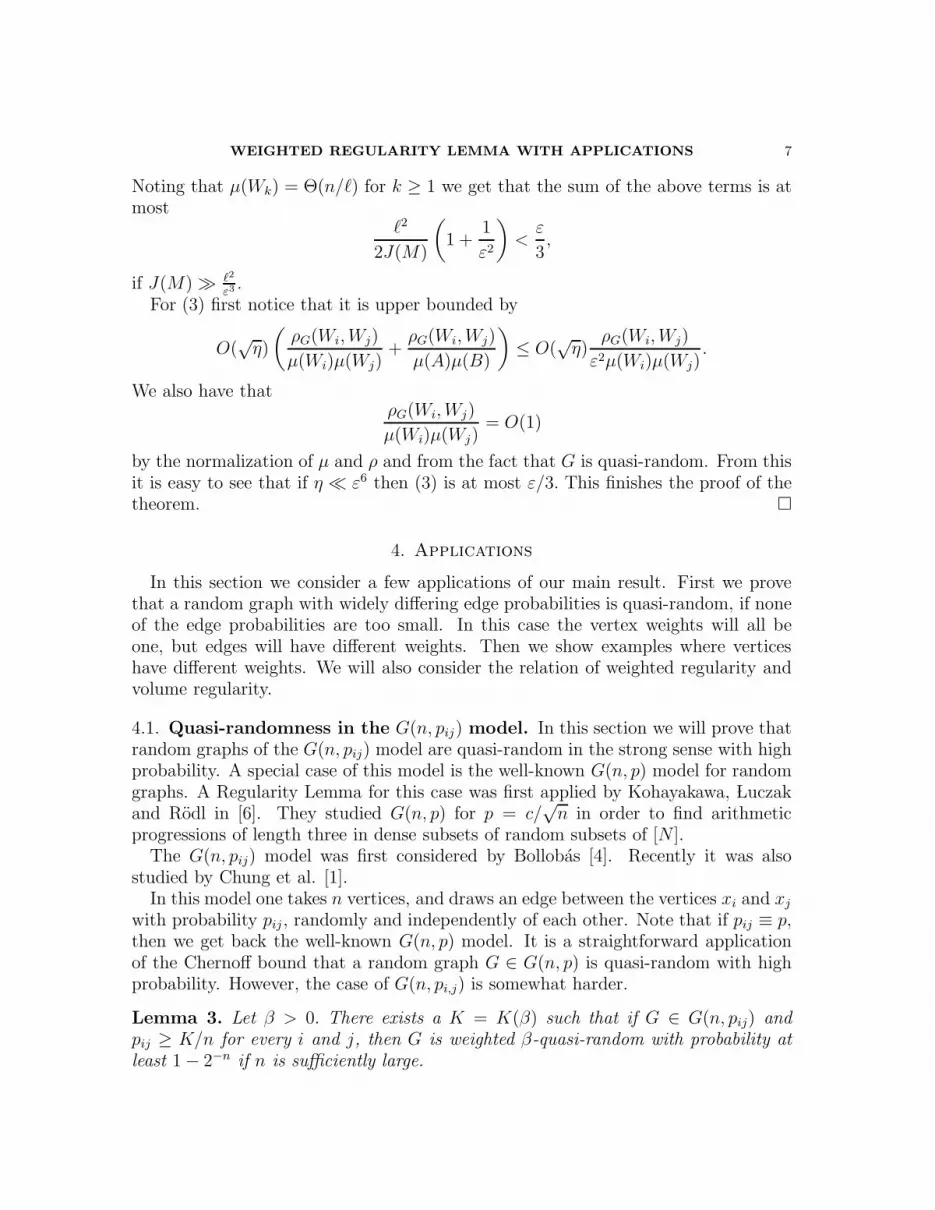
4. Applications

In this section we consider a few applications of our main result. First we provethat a random graph with widely differing edge probabilities is quasi-random, if noneof the edge probabilities are too small. In this case the vertex weights will all beone, but edges will have different weights. Then we show examples where verticeshave different weights. We will also consider the relation of weighted regularity andvolume regularity.

4.1. Quasi-randomness in the G(n, pij) model. In this section we will prove thatrandom graphs of the G(n, pij) model are quasi-random in the strong sense with highprobability. A special case of this model is the well-known G(n, p) model for randomgraphs. A Regularity Lemma for this case was first applied by Kohayakawa, Luczakand Rodl in [6]. They studied G(n, p) for p = c/

√n in order to find arithmetic

progressions of length three in dense subsets of random subsets of [N ].The G(n, pij) model was first considered by Bollobas [4]. Recently it was also

studied by Chung et al. [1].In this model one takes n vertices, and draws an edge between the vertices xi and xj

with probability pij , randomly and independently of each other. Note that if pij ≡ p,then we get back the well-known G(n, p) model. It is a straightforward applicationof the Chernoff bound that a random graph G ∈ G(n, p) is quasi-random with highprobability. However, the case of G(n, pi,j) is somewhat harder.

Lemma 3. Let β > 0. There exists a K = K(β) such that if G ∈ G(n, pij) andpij ≥ K/n for every i and j, then G is weighted β-quasi-random with probability atleast 1 − 2−n if n is sufficiently large.

8 CSABA AND PLUHAR

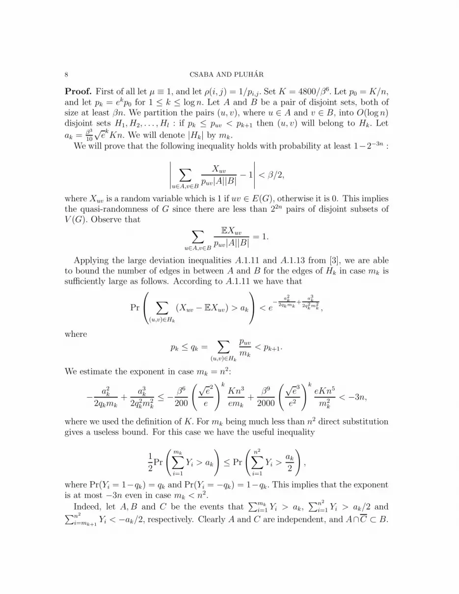
Proof. First of all let µ ≡ 1, and let ρ(i, j) = 1/pi,j. Set K = 4800/β6. Let p0 = K/n,and let pk = ekp0 for 1 ≤ k ≤ log n. Let A and B be a pair of disjoint sets, both ofsize at least βn. We partition the pairs (u, v), where u ∈ A and v ∈ B, into O(log n)disjoint sets H1, H2, . . . , Hl : if pk ≤ puv < pk+1 then (u, v) will belong to Hk. Let

ak = β3

10

√e

kKn. We will denote |Hk| by mk.

We will prove that the following inequality holds with probability at least 1−2−3n :

∣

∣

∣

∣

∣

∑

u∈A,v∈B

Xuv

puv|A||B| − 1

∣

∣

∣

∣

∣

< β/2,

where Xuv is a random variable which is 1 if uv ∈ E(G), otherwise it is 0. This impliesthe quasi-randomness of G since there are less than 22n pairs of disjoint subsets ofV (G). Observe that

∑

u∈A,v∈B

EXuv

puv|A||B| = 1.

Applying the large deviation inequalities A.1.11 and A.1.13 from [3], we are ableto bound the number of edges in between A and B for the edges of Hk in case mk issufficiently large as follows. According to A.1.11 we have that

Pr

∑

(u,v)∈Hk

(Xuv − EXuv) > ak

< e−

a2k

2qkmk+

a3k

2q2k

m2k ,

where

pk ≤ qk =∑

(u,v)∈Hk

puv

mk

< pk+1.

We estimate the exponent in case mk = n2:

− a2k

2qkmk

+a3

k

2q2km

2k

≤ − β6

200

(√e2

e

)k

Kn3

emk

+β9

2000

(√e3

e2

)k

eKn5

m2k

< −3n,

where we used the definition of K. For mk being much less than n2 direct substitutiongives a useless bound. For this case we have the useful inequality

1

2Pr

(

mk∑

i=1

Yi > ak

)

≤ Pr

(

n2∑

i=1

Yi >ak

2

)

,

where Pr(Yi = 1−qk) = qk and Pr(Yi = −qk) = 1−qk. This implies that the exponentis at most −3n even in case mk < n2.

Indeed, let A, B and C be the events that∑mk

i=1 Yi > ak,∑n2

i=1 Yi > ak/2 and∑n2

i=mk+1Yi < −ak/2, respectively. Clearly A and C are independent, and A∩C ⊂ B.


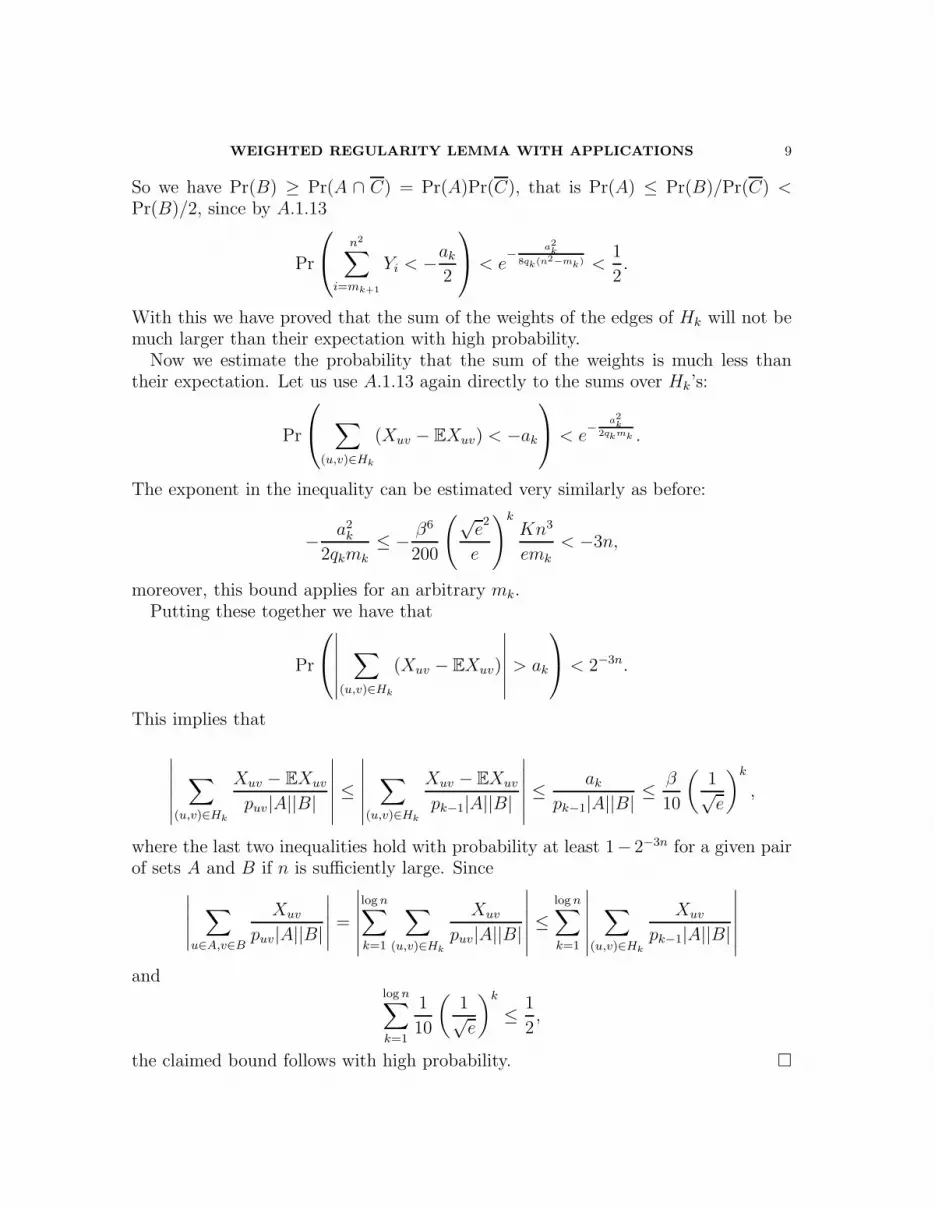
So we have Pr(B) ≥ Pr(A ∩ C) = Pr(A)Pr(C), that is Pr(A) ≤ Pr(B)/Pr(C) <Pr(B)/2, since by A.1.13

Pr

n2∑

i=mk+1

Yi < −ak

2

< e−

a2k

8qk(n2−mk) <

1

2.

With this we have proved that the sum of the weights of the edges of Hk will not bemuch larger than their expectation with high probability.

Now we estimate the probability that the sum of the weights is much less thantheir expectation. Let us use A.1.13 again directly to the sums over Hk’s:

Pr

∑

(u,v)∈Hk

(Xuv − EXuv) < −ak

< e−

a2k

2qkmk .

The exponent in the inequality can be estimated very similarly as before:

− a2k

2qkmk

≤ − β6

200

(√e2

e

)k

Kn3

emk

< −3n,

moreover, this bound applies for an arbitrary mk.Putting these together we have that

Pr

∣

∣

∣

∣

∣

∣

∑

(u,v)∈Hk

(Xuv − EXuv)

∣

∣

∣

∣

∣

∣

> ak

< 2−3n.

This implies that

∣

∣

∣

∣

∣

∣

∑

(u,v)∈Hk

Xuv − EXuv

puv|A||B|

∣

∣

∣

∣

∣

∣

≤

∣

∣

∣

∣

∣

∣

∑

(u,v)∈Hk

Xuv − EXuv

pk−1|A||B|

∣

∣

∣

∣

∣

∣

≤ ak

pk−1|A||B| ≤β

10

(

1√e

)k

,

where the last two inequalities hold with probability at least 1− 2−3n for a given pairof sets A and B if n is sufficiently large. Since

∣

∣

∣

∣

∣

∑

u∈A,v∈B

Xuv

puv|A||B|

∣

∣

∣

∣

∣

=

∣

∣

∣

∣

∣

∣

log n∑

k=1

∑

(u,v)∈Hk

Xuv

puv|A||B|

∣

∣

∣

∣

∣

∣

≤log n∑

k=1

∣

∣

∣

∣

∣

∣

∑

(u,v)∈Hk

Xuv

pk−1|A||B|

∣

∣

∣

∣

∣

∣

andlog n∑

k=1

1

10

(

1√e

)k

≤ 1

2,

the claimed bound follows with high probability. �

10 CSABA AND PLUHAR

Remark. It is very similar to prove that with high probability |∑i,j ρG(i, j)−(

n

2

)

| =

o(n), we omit the details. From this it follows that rescaling the above edge weightsby a factor of (1+o(1)) and letting µ ≡ 1 provides us β-quasi-random weights for mostgraphs from G(n, pij) such that µ(V ) = n and ρG(V, V ) = 2

(

n

2

)

. That is, with highprobability we can apply the Regularity Lemma for any F ⊂ G, where G ∈ G(n, pij).

4.2. Other examples for defining vertex and edge weights. When defining thenotion of weighted quasi-randomness and weighted regularity, we mentioned, thatchoosing µ ≡ 1 and ρ ≡ 1/δG gives back the old definitions of quasi-randomness andregularity. In the previous section we saw an example when we needed different edgeweights, but µ was identically one.

Let us consider a simple example in which µ has to take more than one value. LetG be a star on n vertices, that is, the vertex v1 is adjacent to the vertices v2, . . . , vn,and vi has degree 1 for i ≥ 2. We let µ(v1) = 1/2 and µ(vi) = 1/(2(n − 1)) fori ≥ 2, and choose ρG ≡ n/2. With these choices G is easily seen to be quasi-random,moreover, it is weighted regular.

A more sophisticated example relates weighted regularity with volume regularity,the latter introduced by Alon et al [2]. Given a graph G, the volume of a set S ⊂ V (G)is defined as vol(S) =

∑

v∈S deg(v). For disjoint sets A, B ⊂ V (G), the (A, B) pair is ε-volume regular if ∀X ⊂ A, Y ⊂ B satisfying vol(X) ≥ ε·vol(A) and vol(Y ) ≥ ε·vol(B)we have

∣

∣

∣

∣

e(X, Y ) − e(A, B)

vol(A)vol(B)vol(X)vol(Y )

∣

∣

∣

∣

< ε · vol(A)vol(B)/vol(V ).

In order to show that volume regularity is a special case of weighted regularity, wemay choose edge and vertex weights as follows: for all A, B ⊂ V let

ρ(A, B) = e(A, B)n2

vol(V )

and

µ(A) =n · vol(A)

vol(V ).

It is easy to see that if the (A, B) pair is µ − ρ-weighted ε-regular with the abovechoice for µ and ρ, then it is also ε-volume regular.

In certain cases it can be more useful to apply the notion of weighted regularitythan volume regularity. As an example, consider a bipartite graph G(A, B), whereA = A1 ∪ A2, B = B1 ∪ B2 and A1 ∩ A2 = B1 ∩ B2 = ∅. We assume that |A1| =|A2| = |B1| = |B2| = n/4. Further assume that G(A1, B) and G(A, B1) are completebipartite graphs, and G(A2, B2) is a random bipartite graph with edge probability1/√

n.Letting X = A2 and Y = B2, it is easy to see that G(A, B) is not ε-volume regular,

if ε is small, no matter how large n is. On the other hand, the result of the previoussection implies that G is weighted regular, even with a very small ε.


Acknowledgment The authors thank Peter Hajnal and Endre Szemeredi for thehelpful discussions.

References

[1] W. Aiello, F. Chung and L. Lu, A random graph model for massive graphs, Proceedings of the

Thirty-Second Annual ACM Symposium on Theory of Computing, (2000) 171-180.[2] N. Alon, A. Coja-Oghlan, H. Han, M. Kang, V. Rodl and M. Schacht, Quasi-Randomness and

Algorithmic Regularity for Graphs with General Degree Distributions, Proc. ICALP 2007,789–800.

[3] N. Alon and J. Spencer, The Probabilistic Method. Wiley-Interscience, New York, 2000.[4] B. Bollobas, Random Graphs. Second edition. Cambridge Studies in Advanced Mathematics,

73. Cambridge University Press, Cambridge, 2001.[5] Y. Kohayakawa, Szemeredi’s Regularity Lemma for sparse graphs, in Foundations of compu-

tational mathematics (1997) 216–230.[6] Y. Kohayakawa, T. Luczak and V. Rodl, Arithmetic progressions of length three in subsets of

a random set, Acta Arith. 75 (1996), no. 2, 133–163[7] J. Komlos, M. Simonovits, Szemeredi’s Regularity Lemma and its Applications in Graph

Theory, Combinatorics, Paul Erdos is eighty, Vol. 2 (Keszthely, 1993), 295–352.[8] E. Szemeredi, On sets of integers containing no k elements in arithmetic progressions, Acta

Arithmetica 27 (1975), 299–345.[9] E. Szemeredi, Regular Partitions of Graphs, Colloques Internationaux C.N.R.S No 260 -

Problemes Combinatoires et Theorie des Graphes, Orsay (1976), 399-401.[10] T. Tao, Structure and randomness in combinatorics, FOCS’07

Department of Mathematics, Western Kentucky University

E-mail address : [email protected]

University of Szeged, Department of Computer Science, Arpad ter 2., Szeged,

H-6720

E-mail address : [email protected]

Documents

A Weighted Regularity Lemma with Applications