Working Paper

* Professor of Marketing, IESE** Ph. D. Student, The Anderson School at UCLA*** The Bud Knapp Professor of Management, The Anderson School at UCLA

IESE Business School - Universidad de NavarraAvda. Pearson, 21 - 08034 Barcelona. Tel.: (+34) 93 253 42 00 Fax: (+34) 93 253 43 43Camino del Cerro del Águila, 3 (Ctra. de Castilla, km. 5,180) - 28023 Madrid. Tel.: (+34) 91 357 08 09 Fax: (+34) 91 357 29 13

Copyright© 2003, IESE Business School. Do not quote or reproduce without permission

WP No 516

August, 2003

THE IMPACT OF ACQUISITION CHANNELSON CUSTOMER EQUITY

Julián Villanueva*Shijin Yoo**

Dominique M. Hanssens****

THE IMPACT OF ACQUISITION CHANNELS ON CUSTOMER EQUITY

Abstract

Customer equity (CE henceforth) is a powerful new paradigm to evaluate the firm’svalue and to optimally allocate marketing resources. This paper is focused on therelationship between customer acquisition and CE. We attempt to answer the following fourquestions: 1) How should customer acquisition channels be categorized to make themmeaningful to managers and academics?; 2) How do we measure the effects of differentacquisition channels on the firm’s performance?; 3) How do we disentangle short-run effectand long-run effects?; and 4) How should the manager allocate a limited budget among theacquisition channels so as to maximize customer equity?

We first propose a way of categorizing customer acquisition channels according totheir level of contact and intrusiveness. A vector-autoregressive (VAR) model is usedto examine the dynamics of acquisition channels and the firm’s performance, and anempirical illustration on a surviving Internet company will be provided. The results show thateach cohort (i.e., customers from different acquisition channels) has different short-run andlong-run effects on the firm’s performance by the subsequent login and purchasing behavior.

Building on previous research on optimal resource allocation, we develop aMarketing Decision Support System (MDSS) to help managers allocate the acquisitionbudget among different channels with the objective of maximizing customer equity. Weillustrate the consequences of naively maximizing the short-term profit and not accountingfor differences in the margin contribution of different cohorts.

Keywords: customer equity; customer acquisition; VAR; long-run modeling

THE IMPACT OF ACQUISITION CHANNELS ON CUSTOMER EQUITY

Introduction

Customers are valuable assets for the firm, but they can be costly to acquire and toretain. Customers’ heterogeneity in the course of their relationship with the firm is reflectedin their price sensitivity, lifetime duration, purchase volume, and even word-of-mouthgeneration. This heterogeneity causes differences in customers’ lifetime value (CLV,hereafter), defined as the discounted stream of cash flows generated over the lifetime of acustomer. To the extent that different acquisition strategies will bring different “qualities” ofcustomers, the acquisition effort will have an important influence on the long-termprofitability of the firm1. Indeed, both practitioners and scholars have emphasized that firmsshould not spend to acquire just any customer, but the “right” kind of customer (Reichheld1993; Blattberg and Deighton 1996; Hansotia and Wang 1997; Blattberg, Getz, and Thomas2001). Therefore, the customer acquisition process plays an important role in the newly-emerging paradigm of customer equity (CE)2.

Optimizing the acquisition budget for long-term profitability is particularly relevantfor start-ups and for firms competing in growth markets, where acquisition spending is themost important expense in the marketing budget. In these scenarios, the firm could have anillusion of profitable growth, when in fact it is acquiring unprofitable customers. Thisoccurred for many Internet start-ups that spent aggressively on acquisition in an effort tomaximize ‘eyeballs’, with the hope of locking-in customer revenue later. For manycompanies, however, that revenue never came, either because their value proposition was notcompelling enough or because the underlying linkage between acquisition spending andlong-term profitability was poorly understood.

In order to grow their businesses, companies acquire customers using a variety ofchannels. In this paper, we define an acquisition channel as any vehicle that initially drives aprospect to the firm. While broadcast media and direct marketing are the most traditionalacquisition channels, firms also acquire customers through other vehicles such as public

1 Moreover, models that do not account for the effect that acquisition has on customer retention will result inbiased estimates (Thomas 2001).

2 For a general discussion of the CE concept, see Blattberg, Getz, and Thomas (2001), and Rust, Zeithaml, andLemon (2000).

NOTE: The authors thank an anonymous collaborating company for providing the data used in this paper. Theythank seminar participants at UCLA, UC Riverside, University of Iowa and Dartmouth College for helpfulcomments.

Research support from the Harold Price Center for Entrepreneurial Studies at UCLA is gratefully acknowledged

relations and word-of-mouth. Thus, it is important to understand the relative effectiveness ofthese acquisition channels.

In a recent survey of marketing managers of Internet firms, it was found thatmanagers do not predominantly use the channels that they believe are the most effective(Forrester Research 2001). For example, in this study affiliate programs was said to be a veryeffective channel, but it was rarely used. This suggests that managers are unclear about theeffectiveness of different channels of acquisition. For example, online ad banners have beencriticized as ineffective since they drive few click-throughs and exhibit small conversionrates. However, some authors have warned that media that appear ineffective in the short runmay generate consumer awareness and become effective in the long run (Briggs and Hollis1997; Drèze and Zufryden 1998). Consequently, acquisition-channel effectiveness should bemeasured with models that can quantify short-run as well as long-run response to marketingstimuli.

The distinction between short and long-run effects is not new in the marketingliterature, and several statistical models or experiments capable of capturing this distinctionhave been proposed3. Nevertheless, managers are often criticized as myopic when makingspending decisions in that they tend to maximize the short-term and neglect the long-termprofitability of the firm. This may occur because the managers’ incentives are linked to short-term metrics such as market-share movements. On other occasions managers lack thenecessary tools to measure the long-run effects of their decisions. The inability to measurethe future consequences of current decisions increases the uncertainty of future payoffs,especially in turbulent markets that are difficult to forecast. By contrast, short-run metricssuch as current market share have a strong credibility at all levels of management and areeasy to justify (Keil, Reibstein, and Wittink 2001). Nonetheless, neglecting the long-termeffects of current actions can lead to suboptimal spending decisions, resulting in inferiorlong-run profitability and shareholder value creation (Doyle 2000).

Hence, there is an urgent need to develop models capable of measuring the long-runeffects of different acquisition strategies, and provide systems to help managers optimallyallocate their acquisition spending among different channels. These models should be able todisentangle the long-run from the short-run effects, incorporate the risk associated with futurepayoffs, and take into account the costs associated with different acquisition channels. This isthe main objective of the current paper. Moreover, we depart from “soft” metrics ofcommunication effectiveness (e.g., brand awareness) to “hard” metrics of profitability(Greyser and Root 1999), in that we measure the effectiveness of each acquisition channelwith respect to its contribution to the CE of the firm4. Once these long-run effects have beenmeasured, we can optimally allocate the acquisition budget among the various channels. Indoing so, we do not measure the expected CLV of a customer, but rather her CE contribution.In this way a customer is worth not only her own expected CLV but also all the indirectimpacts that she has on the firm’s performance over time (e.g., by bringing new customers tothe firm through word-of-mouth).

2

3 For example, streams of research include the use of multivariate time-series techniques (e.g., Dekimpe andHanssens 1995a, 1995b, 1999; Bronnenberg, Mahajan, and Vanhonacker 2000; Pauwels, Hanssens, andSiddarth 2002; Nijs et al. 2001), varying-parameters approaches (e.g., Mela, Gupta, and Lehman 1997;Jedidi, Mela, and Gupta 1999), and experiments (e.g., Lodish et al. 1995; Anderson and Simester 2001). Fora review of long-run marketing modeling, see Dekimpe and Hanssens (2000). This paper fits into theemerging literature of linking marketing spending to long-run shareholder value (e.g., Pauwels et al. 2003).

4 Though there exist various definitions of customer equity (CE), it is defined in this paper as the sum of allexisting and expected customers’ CLVs. Here CE is used as a metric to show the long-run performance ofthe firm.

The paper is organized as follows. First, we categorize customer acquisitionchannels to investigate their short-run and long-run differences with respect to the impact onCE. Second, we propose a VAR model to estimate the long-run effect of a customer acquiredfrom each channel on the long-term performance of the company. Third, we provide anempirical illustration using data from an Internet start-up. Lastly, we develop a marketingdecision support system to help the manager allocate her acquisition budget among thedifferent channels.

Research Development

Our study differs from previous literature on media selection in at least three ways.First, we consider important yet under-researched acquisition channels, such as word-of-mouthand public relations. Second, we study long-run effects of the different acquisition channels onthe firm’s performance, as separate from short-run effects. Third, we specify the long-runeffects of acquisition in a customer-equity framework. Thus, our research is particularlyrelevant for relationship businesses in which the firm spends aggressively on acquiringcustomers, in the hope of deriving a substantial future revenue stream. Examples include thewireless telephone industry, broadband Internet service providers, and cable television.

Classification of Customer Acquisition Channels

Our focus on customer acquisition includes all possible channels that drive newcustomers to a firm, including those that are difficult to control, such as word-of-mouth. Anincreasing number of firms uses such channels. For instance, BMG Music Service not onlyspends on online ad banners and direct mail, but also gives referral incentives (in the form offree CDs) to existing customers. Netflix, an online DVD rental firm, spends on online adbanners, places free trial coupons in the DVD-player cartons of some manufacturers, mailsother free-trial coupons to targeted audiences and encourages referrals, although without amonetary incentive.

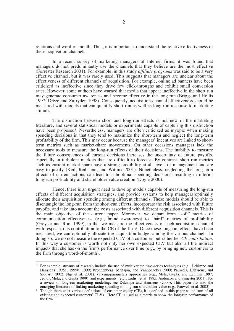
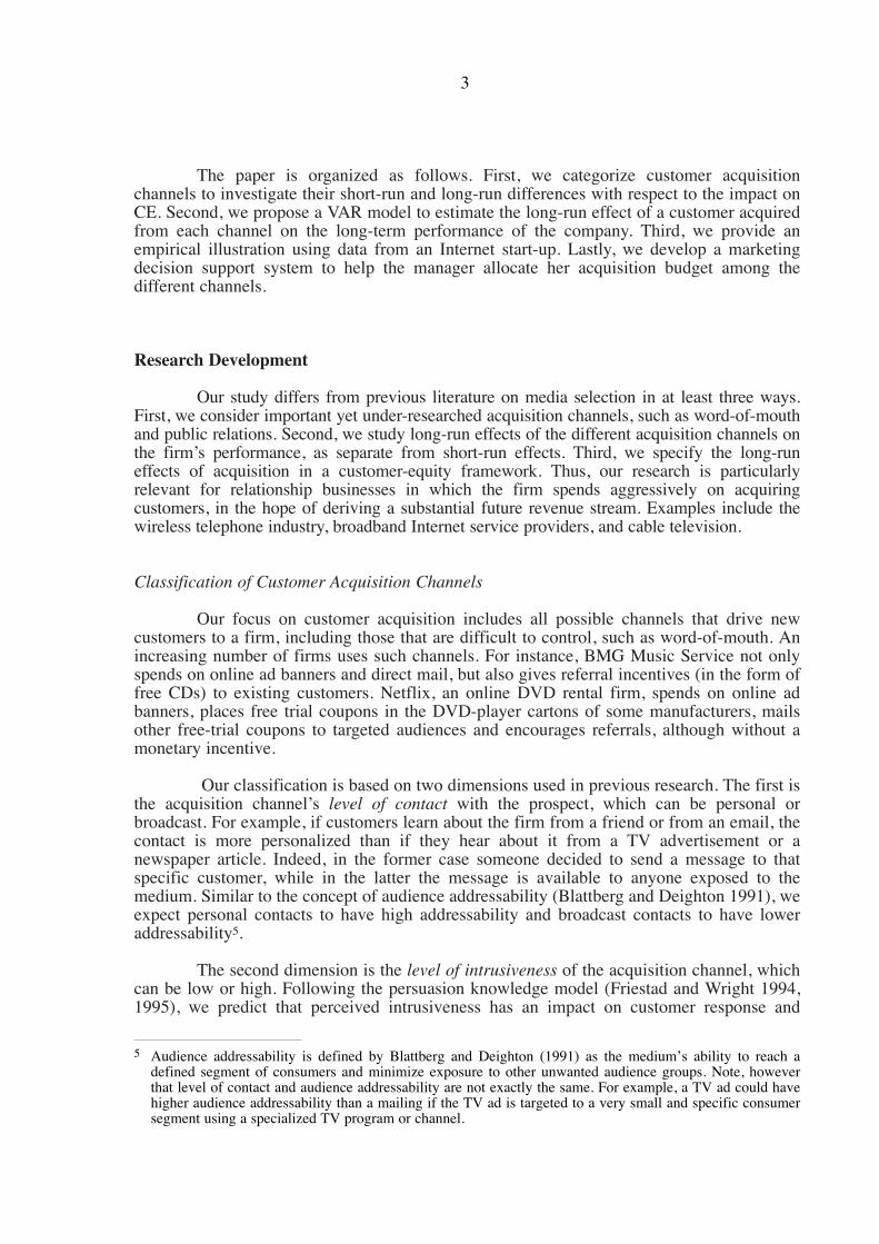
Our classification is based on two dimensions used in previous research. The first isthe acquisition channel’s level of contact with the prospect, which can be personal orbroadcast. For example, if customers learn about the firm from a friend or from an email, thecontact is more personalized than if they hear about it from a TV advertisement or anewspaper article. Indeed, in the former case someone decided to send a message to thatspecific customer, while in the latter the message is available to anyone exposed to themedium. Similar to the concept of audience addressability (Blattberg and Deighton 1991), weexpect personal contacts to have high addressability and broadcast contacts to have loweraddressability5.

The second dimension is the level of intrusiveness of the acquisition channel, whichcan be low or high. Following the persuasion knowledge model (Friestad and Wright 1994,1995), we predict that perceived intrusiveness has an impact on customer response and

3

5 Audience addressability is defined by Blattberg and Deighton (1991) as the medium’s ability to reach adefined segment of consumers and minimize exposure to other unwanted audience groups. Note, howeverthat level of contact and audience addressability are not exactly the same. For example, a TV ad could havehigher audience addressability than a mailing if the TV ad is targeted to a very small and specific consumersegment using a specialized TV program or channel.

subsequent behavior. Indeed, consumers interpret and cope with marketers’ communicationattempts (e.g., advertising) based on contingent persuasion knowledge. They understand thatthe main goal of marketing communications is to influence their own beliefs and/or attitudesabout the firm’s products or services. Thus, we argue that visibly commercial acquisitionchannels such as direct marketing or mass advertising will be perceived as more intrusivethan channels such as public relations or word-of-mouth6.

Our classification of acquisition channels based on the level of contact and level ofintrusiveness results in four categories, namely, word-of-mouth (WOM), direct marketing(DM), advertising (AD), and public relations (PR). A wide array of acquisition tactics can beassigned to one or other of these categories, and we present some of them as an illustration inFigure 1. This classification is managerially relevant, as it includes many non-traditional butwidely used acquisition tactics in a comprehensive way. Moreover, it is based on existingconsumer behavior theory and therefore we expect these four categories to differ both in theirshort and in their long-run effectiveness7.

Figure 1. Classification of Acquisition Channels

Measuring Acquisition Effectiveness

In this research we develop a metric that helps us link acquisition efforts toshareholder value by measuring the impact of the acquisition spending on customer equity,which has been suggested as a powerful metric for the value of a firm (Gupta, Lehman, andStuart 2002). Hence, models capable of maximizing customer equity should help managersmaximize shareholder value.

4

6 Word-of-mouth communication has been said to be more persuasive than conventional advertising (e.g.,Herr, Kardes, and Kim 1991; Brown and Reingen 1987).

7 Nevertheless, the development and testing of formal hypotheses on how level of contact and intrusivenessaffect short and long-run effectiveness are beyond the scope of this paper. With our particular dataset(introduced below), we cannot control for personal differences among groups, so we do not know whetherthose differences are caused by the nature of the medium, or by individual characteristics. We ran amultivariate discriminant analysis of group membership on some personal demographics and found that thereare statistically significant differences in the demographics across groups. Therefore, it can be tentativelyconcluded that different acquisition channels bring different kinds of customers to the firm.

Level ofIntrusiveness

High

Low

•• CataloguesCatalogues•• EmailEmail•• Promotion callsPromotion calls

•• TV adTV ad•• Radio adRadio ad•• Print adPrint ad•• Online ad bannerOnline ad banner

•• WordWord--ofof--mouth frommouth fromfriendsfriends

•• Referral from searchReferral from searchenginesengines

•• Print articlesPrint articles•• Online articlesOnline articles

DM AD

WOM PR

Level of ContactPersonal Broadcast

Unlike previous CLV models, our model investigates cross-sectional heterogeneityat the acquisition channel level8. For example, previous work has assumed that customers arehomogeneous in their expected future value (e.g., Blattberg and Deighton 1996), orlongitudinally heterogeneous depending only on the period of acquisition (e.g., Gupta,Lehman, and Stuart 2002). However, we expect different acquisition channels to yieldcustomers that are unequal in their contribution to customer equity. This heterogeneity ofacquisition channels has important implications for optimal resource allocation, as firms wantto allocate their limited acquisition budget among the different acquisition channels so thatthey maximize their customer equity and therefore shareholder value. We shall emphasize thedifferences between the short and the long-run effectiveness to illustrate the importance ofmaximizing the latter when allocating marketing resources.

Methodology

Linkage between Acquisition and Long-Run Performance

The acquisition process and its link with the firm’s performance should be examinedas a complex system in which many interactions could take place over time. For example,when computing the marginal contribution of one new customer to CE, we want to measurenot only her expected CLV but also all the indirect influences that this acquisition will causein the firm’s performance.

We propose a vector-autoregressive (VAR) model to investigate these interactionswhich we characterize as follows: (1) Direct effects of acquisition on the performance of thefirm. We are interested in measuring the impact on the firm’s performance (e.g., profits) of aperson being acquired from a given acquisition channel; (2) Cross-effects among channels.For instance, we are interested in how different acquisition channels affect future word-of-mouth. As an illustration, customers acquired through public relations may generate morereferrals than those acquired from direct marketing; (3) Feedback effects. The firm’s currentperformance may affect differently the number of customers acquired through differentchannels in the future. For instance, firms that develop stronger reputations may increasefuture customer acquisitions through public relations; (4) Reinforcement effects. Both firmperformance and customer acquisitions will have an effect on each other in the future. Forinstance, there may be some inertia in the firm that prompts it to use certain channels moreand others less if it believes some are more effective than others.

For ease of exposition, assume a three-variable system that captures the dynamicinterrelationships among the number of customers acquired at time t through massadvertising (ADt), the number of customers acquired at time t through word-of-mouth(WOMt), and a proxy variable for the firm’s performance at time t (Vt). The VAR(p) modelwould be specified as9,

5

8 We will investigate how each acquisition channel contributes to the firm’s customer equity and studyheterogeneity for our four categories of acquisition channels. Our measurement approach could neverthelessbe used for any particular acquisition channel or for any other categorization. There could also beheterogeneity at different levels, for instance due to demographic characteristics of the individuals attractedby each channel.

9 A deterministic trend, seasonal dummy variables, and exogenous variables can also be included in this VAR.Instantaneous effects are not included directly in this VAR, but they are reflected in the variance-covariancematrix of the residuals (Σ).

(1)

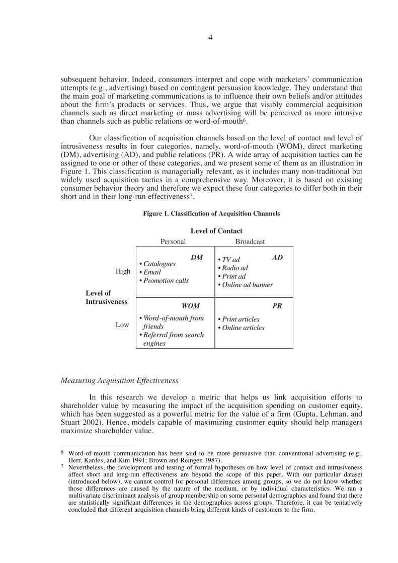
For this VAR model of order p, where (e1t, e2t, e3t)’ are white-noise disturbancesfollowing N (0, Σ), the direct effects are captured by a31, a32, cross effects by a12, a21,feedback effects by a13, a23 and, finally, reinforcement effects by a11, a22, a33. The researchercould, of course, include additional acquisition channels and even impose restrictions onsome of these parameters if there is an a priori reason for doing so. VAR models can beheavily parameterized, depending on the number of variables and time lags in the model.Therefore, long time series are desirable. Note that we do not include marketing activity data(e.g., advertising expenditures, price promotions) since at this point we are not interested inmeasuring how these marketing efforts lead to number of customers acquired. Instead, wewant to measure how much a specific customer contributes to the firm’s performance nowand in the future. The function linking the number of customers acquired to the contributionto the firm’s customer equity will be called the value generating function. The interactionsbetween marketing spending and number of acquisitions is captured by an acquisitionresponse function (see Figure 2). We will join these two functions later.

Figure 2. Value Generation through Customer Acquisition

Impulse Response Functions and Customer Equity

Given data availability, a VAR model not only captures all the previous effects (i.e.,direct, cross, feedback and reinforcement), it also measures the time dynamics of each effect.We are interested in disentangling the immediate and the long-run effects, and in determiningthe total cumulative effects. This is accomplished by Impulse Response Functions (IRFs) thattrace the present and future response of a variable to an unexpected shock in another variable.VAR models and IRFs have been introduced to the marketing literature in a marketing-mixcontext (e.g., Dekimpe and Hanssens 1995a, 1995b, 1999; Bronnenberg, Mahajan, andVanhonacker 2000; Nijs et al. 2001; Srinivasan, Bass, and Popkowski 2000). They are usedhere to assess how one unexpected customer acquisition, for example from the advertising

6

Marketing(channel )

Acquisition(channel k )

Value(firm )

Acquisitionresponsefunction

Valuegeneratingfunction

e.g., AD, DM, PR, +

Acquisition effort Value generation

AD

WOM

V

a

a

a

AD

WOM

V

e

e

e

t

t

t

t l

t l

t l

t

t

t

11 12 13

21 22 23

31 32 33

=1 +

=

=

∑

10

20

30

1

2

3

a a a

a a a

a a a

l l l

l l l

l l ll

p ±

±

±

channel, impacts customer equity over time. To the best of our knowledge, this is the first useof the VAR method to measure the financial contribution of newly acquired customers.

Assuming data stationarity, we can rewrite the VAR model in equation (1) as amoving-average representation (see Enders 1995):

(2)

The coefficients φjk(i) are called impact multipliers and measure the impact of a one-unit change in εk(t-i) on the jth variable. The different sets of coefficients φjk(i) for i = {0,...,∞}are called impulse response functions and are usually plotted to visualize the dynamicbehavior of the variables of interest as a function of shocks in other variables. We cancalculate the cumulative long-run effect of unit impulses in any error shock on anothervariable by accumulating the impact multipliers,

(3)

When variables are stationary, the impact multipliers tend to be zero for sufficientlyhigh numbers of i and therefore the total effect is finite10.

In order to estimate the effect of one new customer acquisition from a specificchannel on the long-run performance of the firm we take the following steps: (1) estimate theimpulse response functions defined as the effect of a one-person shock in the acquisitionchannel on the firms’ performance (Vt); (2) select the impact multipliers that are significantlydifferent from zero; and (3) accumulate significant impact multipliers using a discount rate.Thus, the long-run impact multiplier for a direct effect is obtained as

(4)

where r is the discount rate11, m is the number of periods to include in the calculation, andφvk(i) is the impact multiplier measuring the response of the V variable to the shock of the kth

variable i time units ago.

So long as Vt is a good proxy for the contribution of each customer to the firm’sprofits, this impact multiplier can be interpreted as the contribution of one customer acquiredthrough a specific channel to the firm’s customer equity before accounting for differences inacquisition costs12. On other occasions, however, Vt may not be expressed in monetary value.In such cases the impact multiplier needs to be translated to profit contribution, for example,

(5) λk = τ(γk)

7

Total Effect k j ii

( ( )→ ==

∞

∑) φ jk0

10 When variables are evolving, the standard procedure is to estimate the VAR model with variables in firstdifferences. In those cases, the IRFs should be accumulated to measure the impact on level forms.

11 The discount rate should incorporate the risk associated with the specific investment. For example, factorssuch as expected future competition or the urgent need to raise money might affect this rate.

12 Note that γk does not take into account that a person acquired from a given acquisition channel, sayadvertising, could be more expensive to acquire than a person acquired through for instance word-of-mouth.We shall come back to this issue later.

γ δ φ δki=0

m

ir

= ( ), = 1

1 + i

vk∑

AD

WOM

V

t

t

t

=0

1

2

3

+

( ) ( ) ( )

( ) ( ) ( )

( ) ( ) ( )

=

∞

∑AD

WOM

V

i i

i i

i i

11 12 13

21 22 23

31 32 33

i

l – i

l – i

l – i

φ φ φφ φ φφ φ φ

εεε

i

i

i

where τ(γk) is a function that translates the direct effects (as measured by the impactmultipliers) on the firm’s profits. This approach may be necessary, for example, for an onlinenewspaper that generates revenue from advertising but can only observe its users’ loginbehavior13. This login behavior would presumably be highly correlated with advertisingexposure and, therefore, with the firm’s financial performance.

In conclusion, we have developed a metric that is capable of measuring the long-runCE contribution of a newly acquired customer. This metric captures not only the expectedCLV of a new customer, but also all indirect effects that affect the firm’s value through thatparticular customer acquisition.

Empirical Illustration

Data Description

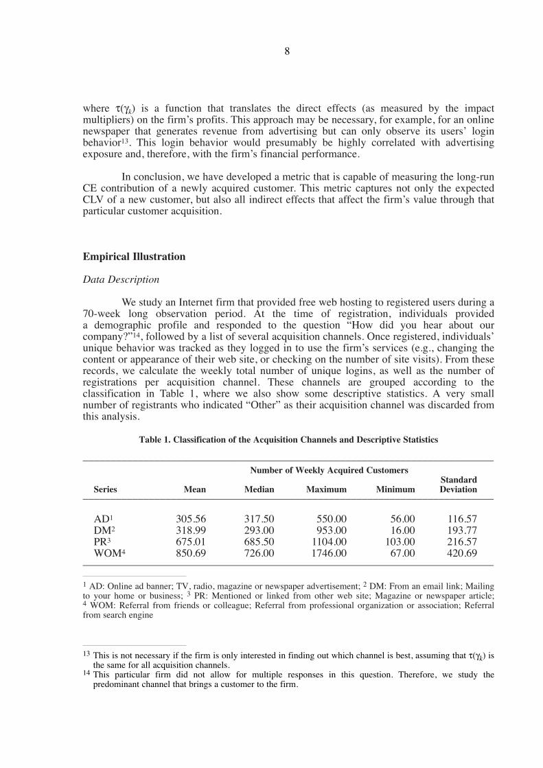
We study an Internet firm that provided free web hosting to registered users during a70-week long observation period. At the time of registration, individuals provideda demographic profile and responded to the question “How did you hear about ourcompany?”14, followed by a list of several acquisition channels. Once registered, individuals’unique behavior was tracked as they logged in to use the firm’s services (e.g., changing thecontent or appearance of their web site, or checking on the number of site visits). From theserecords, we calculate the weekly total number of unique logins, as well as the number ofregistrations per acquisition channel. These channels are grouped according to theclassification in Table 1, where we also show some descriptive statistics. A very smallnumber of registrants who indicated “Other” as their acquisition channel was discarded fromthis analysis.

Table 1. Classification of the Acquisition Channels and Descriptive Statistics

–––––––––––––––––––––––––––––––––––––––––––––––––––––––––––––––––––––––––––Number of Weekly Acquired Customers

StandardSeries Mean Median Maximum Minimum Deviation

–––––––––––––––––––––––––––––––––––––––––––––––––––––––––––––––––––––––––––

AD1 305.56 317.50 550.00 56.00 116.57DM2 318.99 293.00 953.00 16.00 193.77PR3 675.01 685.50 1104.00 103.00 216.57WOM4 850.69 726.00 1746.00 67.00 420.69

–––––––––––––––––––––––––––––––––––––––––––––––––––––––––––––––––––––––––––

1 AD: Online ad banner; TV, radio, magazine or newspaper advertisement; 2 DM: From an email link; Mailingto your home or business; 3 PR: Mentioned or linked from other web site; Magazine or newspaper article;4 WOM: Referral from friends or colleague; Referral from professional organization or association; Referralfrom search engine

8

13 This is not necessary if the firm is only interested in finding out which channel is best, assuming that τ(γk) isthe same for all acquisition channels.

14 This particular firm did not allow for multiple responses in this question. Therefore, we study thepredominant channel that brings a customer to the firm.

The number of logins is a good proxy for the firm’s performance given thecharacteristics of this business15. Most free-service Internet companies generate advertisingrevenue based on logins or click-throughs. Furthermore, once a sufficient number ofregistrations was achieved, the company switched to a fee-for-service revenue model. Asexplained in detail in Appendix A, intensity of login behavior was found to have a positiveand statistically significant correlation with customers’ willingness to pay. Therefore,acquisition channels that yield customers with high usage (login) intensity and therefore ahigher probability of converting to a fee-based service, will be considered as the mosteffective.

The variables are defined as follows:

ADt: number of new registrations at time t from mass advertisingDMt: number of new registrations at time t from direct marketingPRt: number of new registrations at time t from public relationsWOMt: number of new registrations at time t from word-of-mouthVt: total number of unique logins at time t

VAR Estimation

The VAR estimation begins with a unit-root test to determine whether the series isevolving or stationary (see Dekimpe & Hanssens 1995 for a detailed explanation). We use theaugmented Dickey-Fuller (ADF) unit root test (e.g., Enders 1995, p. 257), in which the nullhypothesis of unit root corresponds to Ho : ρ = 0 in

(6)

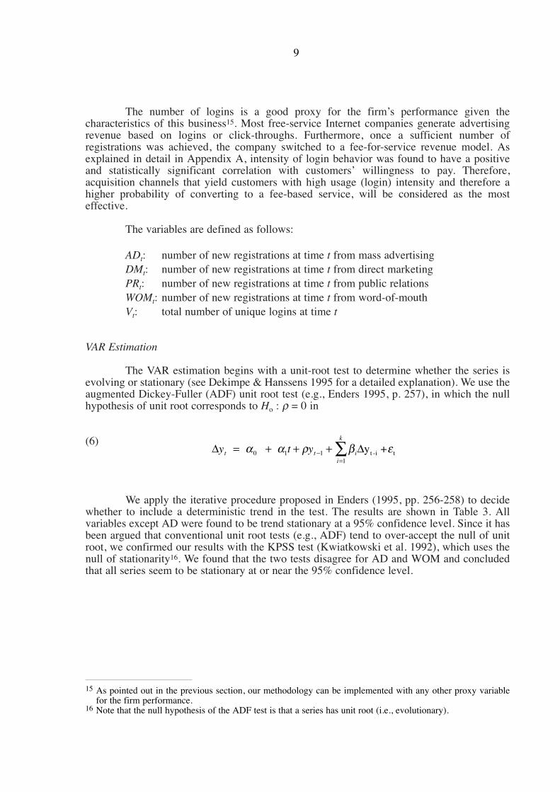
We apply the iterative procedure proposed in Enders (1995, pp. 256-258) to decidewhether to include a deterministic trend in the test. The results are shown in Table 3. Allvariables except AD were found to be trend stationary at a 95% confidence level. Since it hasbeen argued that conventional unit root tests (e.g., ADF) tend to over-accept the null of unitroot, we confirmed our results with the KPSS test (Kwiatkowski et al. 1992), which uses thenull of stationarity16. We found that the two tests disagree for AD and WOM and concludedthat all series seem to be stationary at or near the 95% confidence level.

9

15 As pointed out in the previous section, our methodology can be implemented with any other proxy variablefor the firm performance.

16 Note that the null hypothesis of the ADF test is that a series has unit root (i.e., evolutionary).

∆ ∆y t yt t ii

k

0 1 t -i t y += + + +−=

∑α α ρ β ε11

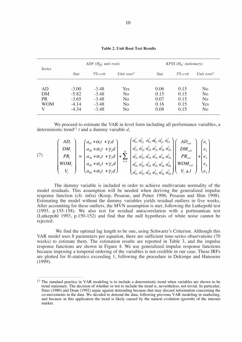
Table 2. Unit Root Test Results

–––––––––––––––––––––––––––––––––––––––––––––––––––––––––––––––––––––––––––ADF (H0: unit root) KPSS (H0: stationary)

SeriesStat 5%-crit Unit root? Stat 5%-crit Unit root?

–––––––––––––––––––––––––––––––––––––––––––––––––––––––––––––––––––––––––––

AD -3.00 -3.48 Yes 0.06 0.15 NoDM -5.82 -3.48 No 0.15 0.15 NoPR -3.65 -3.48 No 0.07 0.15 NoWOM -4.14 -3.48 No 0.16 0.15 YesV -4.34 -3.48 No 0.08 0.15 No

–––––––––––––––––––––––––––––––––––––––––––––––––––––––––––––––––––––––––––

We proceed to estimate the VAR in level form including all performance variables, adeterministic trend17 t and a dummy variable d,

(7)

The dummy variable is included in order to achieve multivariate normality of themodel residuals. This assumption will be needed when deriving the generalized impulseresponse function (cfr. infra) (Koop, Pesaran, and Potter 1996; Pesaran and Shin 1998).Estimating the model without the dummy variables yields residual outliers in five weeks,After accounting for these outliers, the MVN assumption is met, following the Lutkepohl test(1993, p.155-158). We also test for residual autocorrelation with a portmanteau test(Lutkepohl 1993, p.150-152) and find that the null hypothesis of white noise cannot berejected.

We find the optimal lag length to be one, using Schwartz’s Criterion. Although thisVAR model uses 8 parameters per equation, there are sufficient time-series observations (70weeks) to estimate them. The estimation results are reported in Table 3, and the impulseresponse functions are shown in Figure 4. We use generalized impulse response functionsbecause imposing a temporal ordering of the variables is not credible in our case. These IRFsare plotted for |t|-statistics exceeding 1, following the procedure in Dekimpe and Hanssens(1999).

10

17 The standard practice in VAR modeling is to include a deterministic trend when variables are shown to betrend stationary. The decision of whether or not to include the trend is, nevertheless, not trivial. In particular,Sims (1980) and Doan (1992) argue against detrending because that may discard information concerning theco-movements in the data. We decided to detrend the data, following previous VAR modeling in marketing,and because in this application the trend is likely caused by the natural evolution (growth) of the internetmarket.

AD

DM

PR

WOM

V

t

t

t

t

t

10 1 1

20 2 2

30 3 3

40 4 4

50 5 5

=l

p

11 12 13

=

+ +

+ +

+ +

+ +

+ +

+

∑

a t d

a t d

a t d

a t d

a t d

a a a

l

l l lα γα γα γα γα γ

aa a a

a a a a a a

a a a a a a

a a a a a a

a a a a a a

l l l

l l l l l l

l l l l l l

l l l l l l

l l l l l l

11 14 15

21 22 23 21 24 25

31 32 33 31 34 35

41 42 43 41 44 45

51 52 53 51 54 55

+

1

2

3

4

5

AD

DM

PR

WOM

V l

t l

t l

t l

t l

t

±

±

±

±

±

e

e

e

e

e

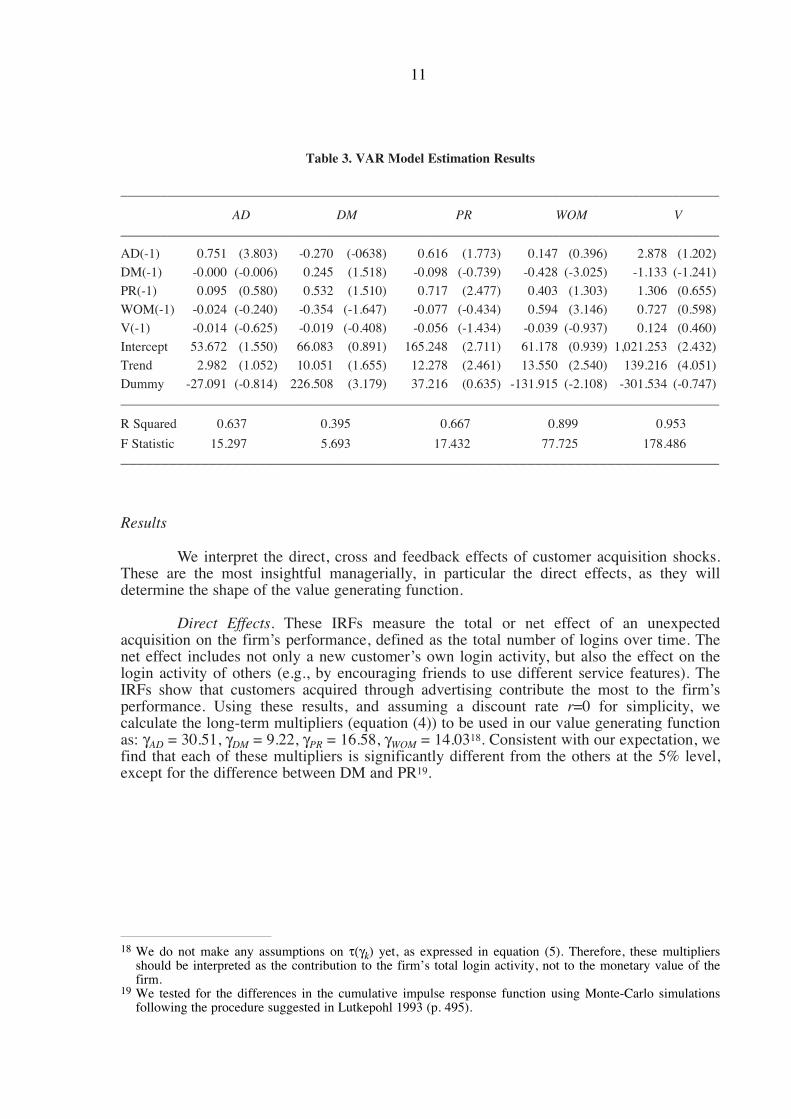
Table 3. VAR Model Estimation Results

––––––––––––––––––––––––––––––––––––––––––––––––––––––––––––––––––––––––––––––––––––––––––

AD DM PR WOM V

––––––––––––––––––––––––––––––––––––––––––––––––––––––––––––––––––––––––––––––––––––––––––

AD(-1) 0.751 (3.803) -0.270 (-0638) 0.616 (1.773) 0.147 (0.396) 2.878 (1.202)

DM(-1) -0.000 (-0.006) 0.245 (1.518) -0.098 (-0.739) -0.428 (-3.025) -1.133 (-1.241)

PR(-1) 0.095 (0.580) 0.532 (1.510) 0.717 (2.477) 0.403 (1.303) 1.306 (0.655)

WOM(-1) -0.024 (-0.240) -0.354 (-1.647) -0.077 (-0.434) 0.594 (3.146) 0.727 (0.598)

V(-1) -0.014 (-0.625) -0.019 (-0.408) -0.056 (-1.434) -0.039 (-0.937) 0.124 (0.460)

Intercept 53.672 (1.550) 66.083 (0.891) 165.248 (2.711) 61.178 (0.939) 1,021.253 (2.432)

Trend 2.982 (1.052) 10.051 (1.655) 12.278 (2.461) 13.550 (2.540) 139.216 (4.051)

Dummy -27.091 (-0.814) 226.508 (3.179) 37.216 (0.635) -131.915 (-2.108) -301.534 (-0.747)

––––––––––––––––––––––––––––––––––––––––––––––––––––––––––––––––––––––––––––––––––––––––––

R Squared 0.637 0.395 0.667 0.899 0.953

F Statistic 15.297 5.693 17.432 77.725 178.486

–––––––––––––––––––––––––––––––––––––––––––––––––––––––––––––––––––––––––––

Results

We interpret the direct, cross and feedback effects of customer acquisition shocks.These are the most insightful managerially, in particular the direct effects, as they willdetermine the shape of the value generating function.

Direct Effects. These IRFs measure the total or net effect of an unexpectedacquisition on the firm’s performance, defined as the total number of logins over time. Thenet effect includes not only a new customer’s own login activity, but also the effect on thelogin activity of others (e.g., by encouraging friends to use different service features). TheIRFs show that customers acquired through advertising contribute the most to the firm’sperformance. Using these results, and assuming a discount rate r=0 for simplicity, wecalculate the long-term multipliers (equation (4)) to be used in our value generating functionas: γAD = 30.51, γDM = 9.22, γPR = 16.58, γWOM = 14.0318. Consistent with our expectation, wefind that each of these multipliers is significantly different from the others at the 5% level,except for the difference between DM and PR19.

11

18 We do not make any assumptions on τ(γk) yet, as expressed in equation (5). Therefore, these multipliersshould be interpreted as the contribution to the firm’s total login activity, not to the monetary value of thefirm.

19 We tested for the differences in the cumulative impulse response function using Monte-Carlo simulationsfollowing the procedure suggested in Lutkepohl 1993 (p. 495).

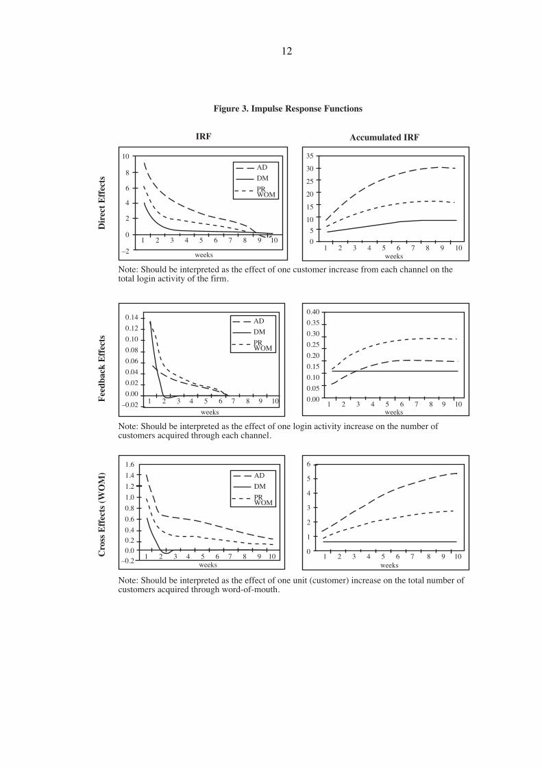
Figure 3. Impulse Response Functions

12

0.14

0.12

0.10

0.08

0.06

0.04

0.02

0.00

–0.02 1 2 3 4 5 6 7 8 9 10

AD

DM

PRWOM

weeks

35

30

25

20

15

10

5

01 2 3 4 5 6 7 8 9 10

weeks

0.40

0.35

0.30

0.25

0.20

0.15

0.10

0.05

0.001 2 3 4 5 6 7 8 9 10

weeks

1.6

1.4

1.2

1.0

0.8

0.6

0.4

0.2

0.0

–0.21 2 3 4 5 6 7 8 9 10

AD

DM

PRWOM

weeks

6

5

4

3

2

1

01 2 3 4 5 6 7 8 9 10

weeks

Note: Should be interpreted as the effect of one customer increase from each channel on thetotal login activity of the firm.

Note: Should be interpreted as the effect of one login activity increase on the number ofcustomers acquired through each channel.

10

8

6

4

2

0

–2

1 2 3 4 5 6 7 8 9 10

AD

DM

PRWOM

weeks

Note: Should be interpreted as the effect of one unit (customer) increase on the total number ofcustomers acquired through word-of-mouth.

IRF Accumulated IRF

Cro

ss E

ffec

ts (

WO

M)

Fee

dbac

k E

ffec

tsD

irec

t E

ffec

ts

Feedback Effects. Here we investigate how many new customer acquisitions can begenerated by an unexpected one-login increase. Indeed, increased usage of the Internetservice may lead to higher customer satisfaction and reliance on the service, which can createa diffusion effect in the form of additional customer generation. The results show thatincreased login activity has the strongest feedback effect on public relations and word-of-mouth channels, i.e., as customers become more involved with the service, the firm enjoyshigher word-of-mouth generation and also higher media coverage. By contrast, theperformance feedback effect is weakest for the direct marketing and advertising channels (seeFigure 4).

Cross Effects. We investigate only the cross effects of the different acquisitionchannels on the word-of-mouth channel, i.e., how effective the different acquisition channelsare at generating future acquisitions through word-of-mouth. Figure 4 shows that customersacquired through advertising are better at word-of-mouth generation than those acquired inother ways. For example, each customer acquired through advertising is expected to bringaround 5.4 new customers, while a customer acquired from direct marketing is expected tobring only about 0.6 customers. Surprisingly, customers acquired through word-of-mouth areless likely to generate referral customers than those acquired by advertising. Thesedifferences are managerially important and require separate research to determine theirunderlying causes.

Cost-Benefit Analysis

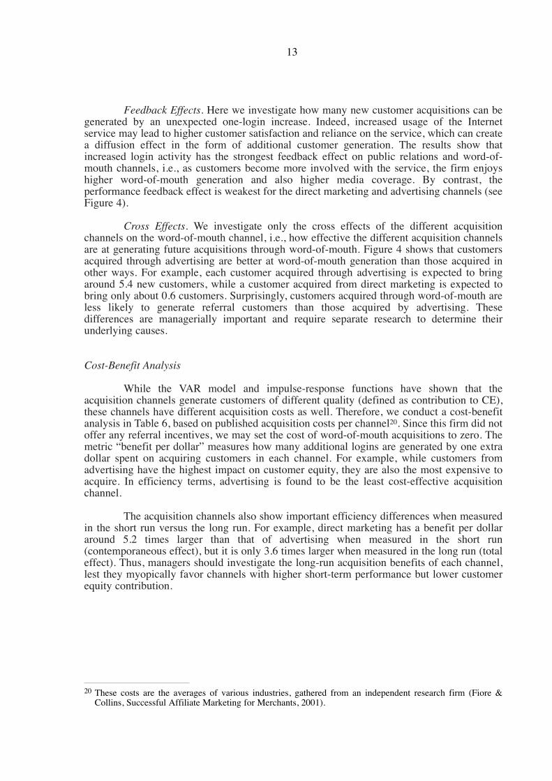
While the VAR model and impulse-response functions have shown that theacquisition channels generate customers of different quality (defined as contribution to CE),these channels have different acquisition costs as well. Therefore, we conduct a cost-benefitanalysis in Table 6, based on published acquisition costs per channel20. Since this firm did notoffer any referral incentives, we may set the cost of word-of-mouth acquisitions to zero. Themetric “benefit per dollar” measures how many additional logins are generated by one extradollar spent on acquiring customers in each channel. For example, while customers fromadvertising have the highest impact on customer equity, they are also the most expensive toacquire. In efficiency terms, advertising is found to be the least cost-effective acquisitionchannel.

The acquisition channels also show important efficiency differences when measuredin the short run versus the long run. For example, direct marketing has a benefit per dollararound 5.2 times larger than that of advertising when measured in the short run(contemporaneous effect), but it is only 3.6 times larger when measured in the long run (totaleffect). Thus, managers should investigate the long-run acquisition benefits of each channel,lest they myopically favor channels with higher short-term performance but lower customerequity contribution.

13

20 These costs are the averages of various industries, gathered from an independent research firm (Fiore &Collins, Successful Affiliate Marketing for Merchants, 2001).

Table 4. Cost-Benefit Analysis

–––––––––––––––––––––––––––––––––––––––––––––––––––––––––––––––––––––––––––AD DM PR WOM

–––––––––––––––––––––––––––––––––––––––––––––––––––––––––––––––––––––––––––Cost of Acquiring One More Customer ($) 323 27 82 -

Benefit: Increased Number of LoginsContemporaneous Effect 9.07 3.98 6.21 5.52Lagged Effect 21.43 5.24 10.37 8.51Total Effect 30.51 9.22 16.58 14.03

Benefit per DollarContemporaneous Effect 0.03 0.15 0.08Lagged Effect 0.07 0.19 0.13Total Effect 0.09 0.34 0.20

Maximum WOM incentives ($)Contemporaneous Effect 197 37 73 - Total Effect 149 41 69 - –––––––––––––––––––––––––––––––––––––––––––––––––––––––––––––––––––––––––––

Source of cost data: Fiore & Collins, Successful Affiliate Marketing for Merchants, 2001

When word-of-mouth acquisition of customers is costless, their benefit per dollar isinfinite. However, some firms implement strategies to actively boost word-of-mouthgeneration by referral incentives, so the question arises: What is the maximum amount a firmshould be willing to pay for referrals. Table 6 provides an answer to this question bycalculating the referral incentive that equates the CE contribution to that of other channels.For instance, given that the total effect of word-of-mouth on the firm’s customer equity is14.03, the firm could spend $149 per referral to obtain the same net benefit per dollar as theone exhibited by a customer acquired through advertising21.

A Marketing Decision Support System for Optimal Resource Allocation

The previous cost-benefit analysis rank-ordered the different acquisition channels interms of benefit per dollar (see Table 6). This approach, while managerially insightful, hasthree limitations. First, it assumes that, for each channel, the acquisition cost per customerdoes not change with the number of customers acquired. This is equivalent to assuming thatthe acquisition response function is linear with no intercept. Second, it does not address thequestion of how much to spend on acquisition, nor does it reveal how the budget should beallocated among the different acquisition channels.

In this section, we develop a marketing decision support system (MDSS) todetermine the optimal acquisition budget and its allocation across the different acquisition

14

21 This reasoning assumes that customers acquired through incentivized WOM will behave in the same way asthose acquired through spontaneous WOM.

channels. We have argued earlier that the objective should be to maximize customer equity,which is different from maximizing “eyeballs” or customer counts. We will show that, if themanager uses a different objective, the resulting allocation will be suboptimal. Our MDSS issimilar to that of Mantrala, Sinha, and Zoltners (1992), in that we use submarket (in our case,channel) acquisition response functions to derive optimal spending and allocation acrosssubmarkets. Assuming four acquisition channels k = {AD, DM, PR, WOM}, we define aconcave acquisition response function for each in the form22,

(8) ck = αk + (Sk – αk)(1– exp(–βkxk))

where ck is the number of customers acquired, xk is the amount of money spent, Sk is themaximum number of customers that can be acquired (saturation level), βk represents the rateat which the number of customers approaches the saturation level, and αk is an intercept thatcaptures the number of customers acquired when no investment is made.

These acquisition response functions can be parameterized for each channel usingdecision calculus (see Blattberg and Deighton 1996 for a similar approach)23. The optimalresource allocation finds the best investment for each acquisition channel , given afixed budget B. It is also possible to determine the optimal acquisition budget B* and thenderive . The allocation problem can be expressed as

(9)

s.t. Σkxk ≤ B, xk ≥ 0, k = {AD, DM, PR, WOM}

where mk is the contribution margin for each customer acquired from a specific acquisitionchannel, and B is the acquisition budget. We further assume that firms exhaust their entirebudget, that is Σxk = B.

Incorporating Differences in the Contribution to the Firm’s Profitability

Allocations that maximize aggregate acquisitions (i.e., Σck) do not necessarilymaximize aggregate profits, because customers differ in their customer equity contribution.In contrast to Mantrala, Sinha, and Zoltners (1992), we incorporate the possibility of differentcontribution margins mk for the different submarkets (i.e., acquisition channels). If themanager’s objective is to maximize customer equity, mk should represent the expectedcontribution of a new customer acquired through channel k as explained in previous sections.

15

22 We assume that there are no cross-effects of acquisition responses among channels. This assumption could berelaxed by incorporating in each acquisition response function the effect that a certain spending in anotherchannel will have on the number of customers acquired in that specific channel. See Rangaswamy, Sinha,and Zoltners (1990).

23 An estimation alternative to decision calculus would be using a statistical model on historical data. This maypresent several challenges. First, it may prove difficult to collect data on some channels such as publicrelations and word-of-mouth. Second, a sufficient number of data points with enough variability are required.Third, the data generation process should be able to predict future behavior. If these requirements are notmet, decision calculus may be superior to statistical modeling. An example of a successful implementation ofdecision calculus may be found in Lodish et al. (1988).

xk* ( )B

xk* ( )B*

Max B m Bx (B)

kk

k k k k kk

( ) = ( +(S - )(1- exp(- x ))) -Π ∑ α α β

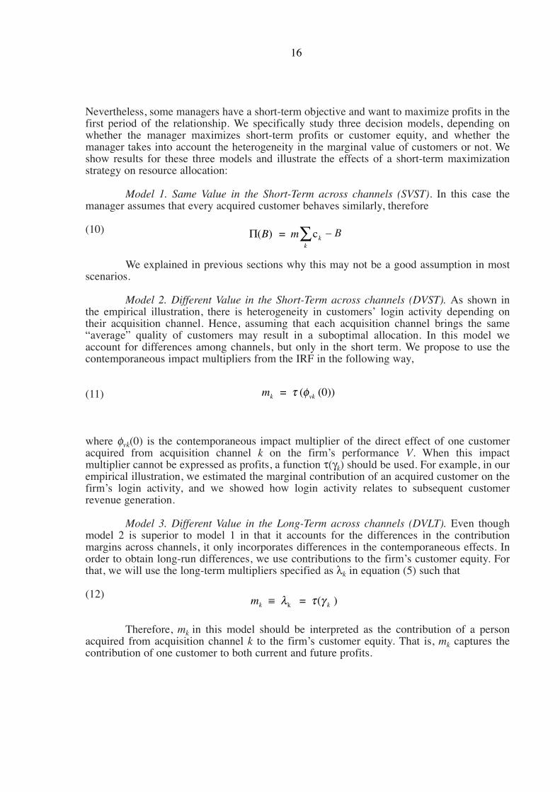
Nevertheless, some managers have a short-term objective and want to maximize profits in thefirst period of the relationship. We specifically study three decision models, depending onwhether the manager maximizes short-term profits or customer equity, and whether themanager takes into account the heterogeneity in the marginal value of customers or not. Weshow results for these three models and illustrate the effects of a short-term maximizationstrategy on resource allocation:

Model 1. Same Value in the Short-Term across channels (SVST). In this case themanager assumes that every acquired customer behaves similarly, therefore

(10) – B

We explained in previous sections why this may not be a good assumption in mostscenarios.

Model 2. Different Value in the Short-Term across channels (DVST). As shown inthe empirical illustration, there is heterogeneity in customers’ login activity depending ontheir acquisition channel. Hence, assuming that each acquisition channel brings the same“average” quality of customers may result in a suboptimal allocation. In this model weaccount for differences among channels, but only in the short term. We propose to use thecontemporaneous impact multipliers from the IRF in the following way,

(11)

where φvk(0) is the contemporaneous impact multiplier of the direct effect of one customeracquired from acquisition channel k on the firm’s performance V. When this impactmultiplier cannot be expressed as profits, a function τ(γk) should be used. For example, in ourempirical illustration, we estimated the marginal contribution of an acquired customer on thefirm’s login activity, and we showed how login activity relates to subsequent customerrevenue generation.

Model 3. Different Value in the Long-Term across channels (DVLT). Even thoughmodel 2 is superior to model 1 in that it accounts for the differences in the contributionmargins across channels, it only incorporates differences in the contemporaneous effects. Inorder to obtain long-run differences, we use contributions to the firm’s customer equity. Forthat, we will use the long-term multipliers specified as λk in equation (5) such that

(12)

Therefore, mk in this model should be interpreted as the contribution of a personacquired from acquisition channel k to the firm’s customer equity. That is, mk captures thecontribution of one customer to both current and future profits.

16

Π( )B = cm kk

∑

mk = ( (0))τ φvk

mk = ( ) ≡ λ τ γk k

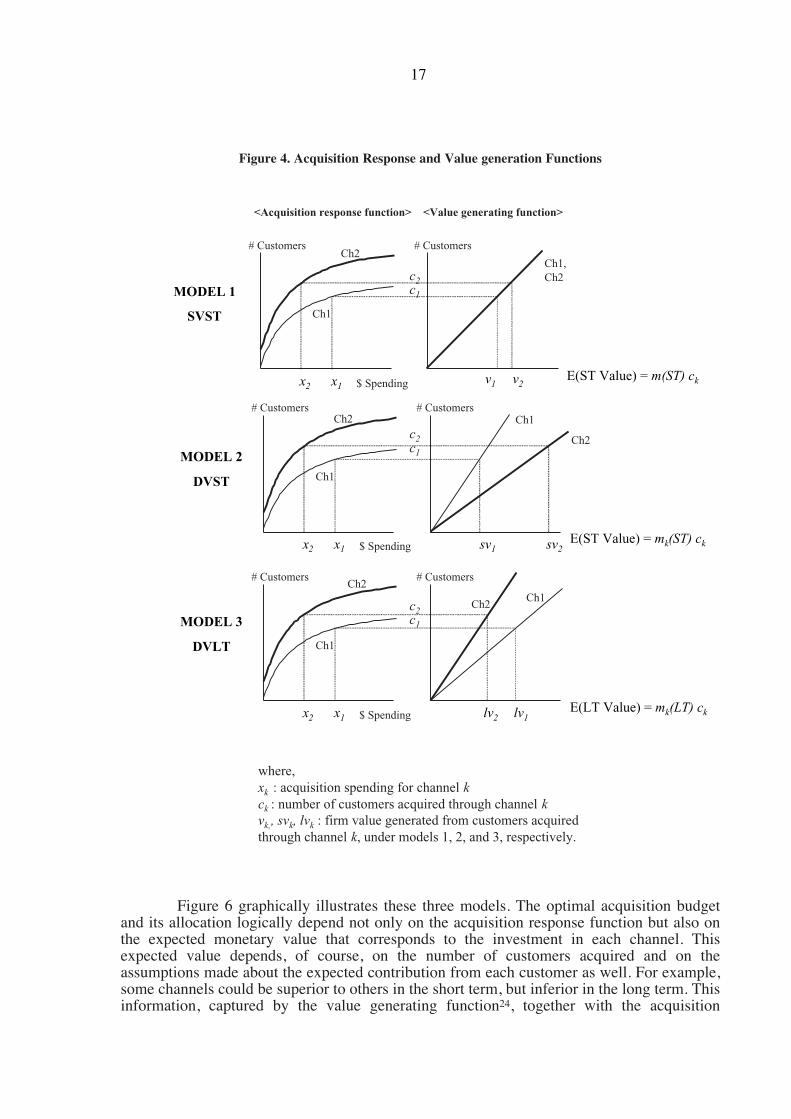
Figure 4. Acquisition Response and Value generation Functions

Figure 6 graphically illustrates these three models. The optimal acquisition budgetand its allocation logically depend not only on the acquisition response function but also onthe expected monetary value that corresponds to the investment in each channel. Thisexpected value depends, of course, on the number of customers acquired and on theassumptions made about the expected contribution from each customer as well. For example,some channels could be superior to others in the short term, but inferior in the long term. Thisinformation, captured by the value generating function24, together with the acquisition

17

$ SpendingE(ST Value) = mk(ST) ck

Ch1

Ch2 Ch1

Ch2

x2 x1 sv1 sv2

<Acquisition response function> <Value generating function>

$ Spending

# Customers

E(LT Value) = mk(LT) ck

# Customers

Ch1

Ch2Ch1

Ch2

x2 x1 lv1lv2

$ SpendingE(ST Value) = m(ST) ck

Ch1

Ch2Ch1,Ch2

x2 x1v1 v2

c1

c2MODEL 1

SVST

MODEL 2

DVST

MODEL 3

DVLT

c1

c2

c1

c2

# Customers # Customers

# Customers # Customers

where,xk : acquisition spending for channel kck : number of customers acquired through channel kvk,, svk, lvk : firm value generated from customers acquiredthrough channel k, under models 1, 2, and 3, respectively.

response functions, is sufficient to derive the optimal resource allocation. Since the objectiveof the firm should be to maximize customer equity, we argue that model 3 (DVLT) should besuperior.

Numerical Illustration

We provide an illustration using the results from our VAR model25 on four differentacquisition channels. For the parameterization of the value generating functions we use thecontemporaneous and the long-term multipliers as reported in Table 6 and we derivecustomer profitability based on equations (11) and (12). Therefore, the values γAD = 30.51,γDM = 9.22, γPR = 16.58, γWOM = 14.03, φv,AD (0) = 9.07, φv,DM (0) = 3.98, φv,PR (0) = 6.21, andφv,WOM (0) = 5.52 are used. For the short-term effect of model 1, we calculate the average ofthe immediate multipliers, which is 6.2026. To calculate the acquisition response function foreach channel, we use equation (8)27.

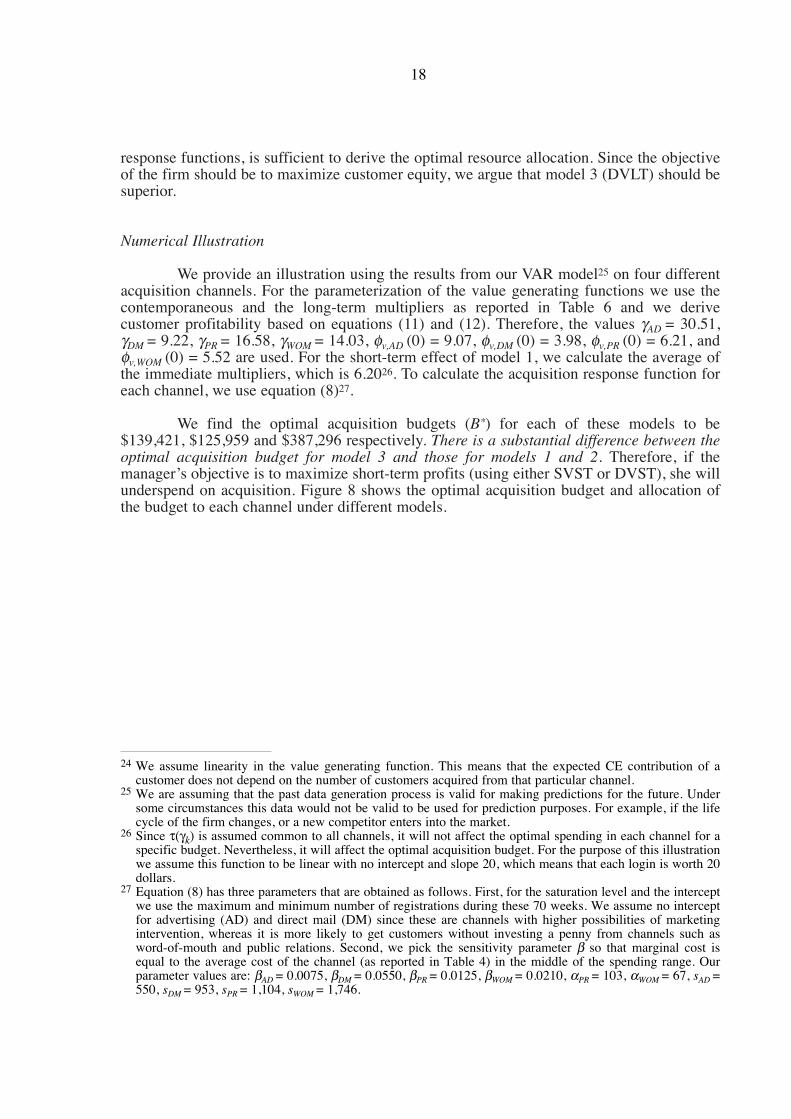
We find the optimal acquisition budgets (B*) for each of these models to be$139,421, $125,959 and $387,296 respectively. There is a substantial difference between theoptimal acquisition budget for model 3 and those for models 1 and 2. Therefore, if themanager’s objective is to maximize short-term profits (using either SVST or DVST), she willunderspend on acquisition. Figure 8 shows the optimal acquisition budget and allocation ofthe budget to each channel under different models.

18

24 We assume linearity in the value generating function. This means that the expected CE contribution of acustomer does not depend on the number of customers acquired from that particular channel.

25 We are assuming that the past data generation process is valid for making predictions for the future. Undersome circumstances this data would not be valid to be used for prediction purposes. For example, if the lifecycle of the firm changes, or a new competitor enters into the market.

26 Since τ(γk) is assumed common to all channels, it will not affect the optimal spending in each channel for aspecific budget. Nevertheless, it will affect the optimal acquisition budget. For the purpose of this illustrationwe assume this function to be linear with no intercept and slope 20, which means that each login is worth 20dollars.

27 Equation (8) has three parameters that are obtained as follows. First, for the saturation level and the interceptwe use the maximum and minimum number of registrations during these 70 weeks. We assume no interceptfor advertising (AD) and direct mail (DM) since these are channels with higher possibilities of marketingintervention, whereas it is more likely to get customers without investing a penny from channels such asword-of-mouth and public relations. Second, we pick the sensitivity parameter β so that marginal cost isequal to the average cost of the channel (as reported in Table 4) in the middle of the spending range. Ourparameter values are: βAD = 0.0075, βDM = 0.0550, βPR = 0.0125, βWOM = 0.0210, αPR = 103, αWOM = 67, sAD =550, sDM = 953, sPR = 1,104, sWOM = 1,746.

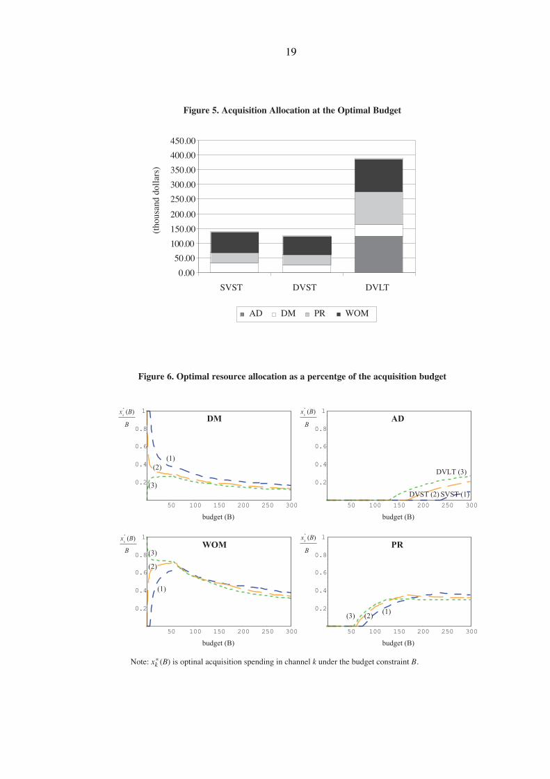
Figure 5. Acquisition Allocation at the Optimal Budget

Figure 6. Optimal resource allocation as a percentge of the acquisition budget

19

0.00

50.00

100.00

150.00

200.00

250.00

300.00

350.00

400.00

450.00

SVST DVST DVLT

(tho

usan

d do

llars

)

AD DM PR WOM

50 100 150 200 250 300

0.2

0.4

0.6

0.8

1

50 100 150 200 250 300

0.2

0.4

0.6

0.8

1

50 100 150 200 250 300

0.2

0.4

0.6

0.8

1

50 100 150 200 250 300

0.2

0.4

0.6

0.8

1

budget (B)

DM

budget (B)

AD

budget (B)

PR

budget (B)

WOM

DVLT (3)

SVST (1)DVST (2)

(3)(1)

(2)

(3)

(1)

(2)

(3)

(1)(2)

B

BB

B

Note: xk (B) is optinal acquisition spending in channel k under the budget constraint B.*

*

kx (B)

*

kx (B)

*

kx (B)*

kx (B)

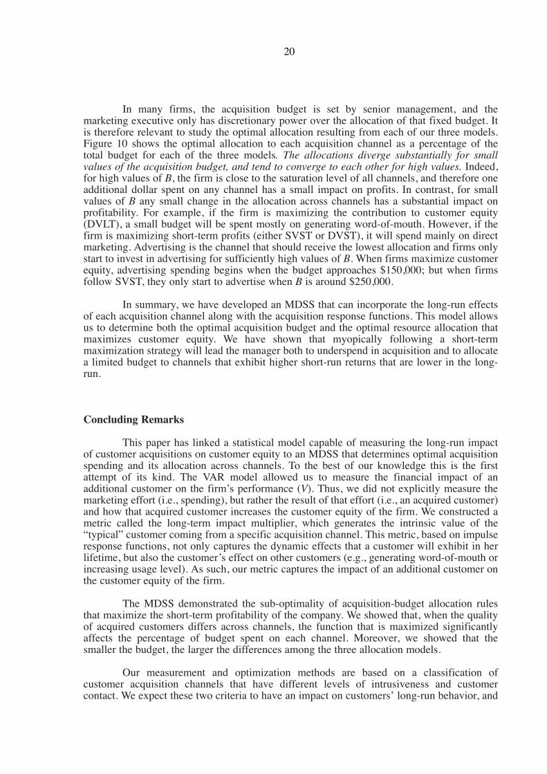
In many firms, the acquisition budget is set by senior management, and themarketing executive only has discretionary power over the allocation of that fixed budget. Itis therefore relevant to study the optimal allocation resulting from each of our three models.Figure 10 shows the optimal allocation to each acquisition channel as a percentage of thetotal budget for each of the three models. The allocations diverge substantially for smallvalues of the acquisition budget, and tend to converge to each other for high values. Indeed,for high values of B, the firm is close to the saturation level of all channels, and therefore oneadditional dollar spent on any channel has a small impact on profits. In contrast, for smallvalues of B any small change in the allocation across channels has a substantial impact onprofitability. For example, if the firm is maximizing the contribution to customer equity(DVLT), a small budget will be spent mostly on generating word-of-mouth. However, if thefirm is maximizing short-term profits (either SVST or DVST), it will spend mainly on directmarketing. Advertising is the channel that should receive the lowest allocation and firms onlystart to invest in advertising for sufficiently high values of B. When firms maximize customerequity, advertising spending begins when the budget approaches $150,000; but when firmsfollow SVST, they only start to advertise when B is around $250,000.

In summary, we have developed an MDSS that can incorporate the long-run effectsof each acquisition channel along with the acquisition response functions. This model allowsus to determine both the optimal acquisition budget and the optimal resource allocation thatmaximizes customer equity. We have shown that myopically following a short-termmaximization strategy will lead the manager both to underspend in acquisition and to allocatea limited budget to channels that exhibit higher short-run returns that are lower in the long-run.

Concluding Remarks

This paper has linked a statistical model capable of measuring the long-run impactof customer acquisitions on customer equity to an MDSS that determines optimal acquisitionspending and its allocation across channels. To the best of our knowledge this is the firstattempt of its kind. The VAR model allowed us to measure the financial impact of anadditional customer on the firm’s performance (V). Thus, we did not explicitly measure themarketing effort (i.e., spending), but rather the result of that effort (i.e., an acquired customer)and how that acquired customer increases the customer equity of the firm. We constructed ametric called the long-term impact multiplier, which generates the intrinsic value of the“typical” customer coming from a specific acquisition channel. This metric, based on impulseresponse functions, not only captures the dynamic effects that a customer will exhibit in herlifetime, but also the customer’s effect on other customers (e.g., generating word-of-mouth orincreasing usage level). As such, our metric captures the impact of an additional customer onthe customer equity of the firm.

The MDSS demonstrated the sub-optimality of acquisition-budget allocation rulesthat maximize the short-term profitability of the company. We showed that, when the qualityof acquired customers differs across channels, the function that is maximized significantlyaffects the percentage of budget spent on each channel. Moreover, we showed that thesmaller the budget, the larger the differences among the three allocation models.

Our measurement and optimization methods are based on a classification ofcustomer acquisition channels that have different levels of intrusiveness and customercontact. We expect these two criteria to have an impact on customers’ long-run behavior, and

20

our empirical results confirm this expectation. Nevertheless, we do not test formal hypotheseson these relationships, which we leave as an important area for future research.

Other limitations of our work offer areas for future exploration. First, more researchis needed to understand the dynamics of word-of-mouth generation. Estimating an acquisitionresponse function could be especially difficult for word-of-mouth for two reasons: (1) forsome firms it may be difficult to “incentivize” word-of-mouth and to know which is the bestway to do so (e.g., offering monetary incentives to the source or to the target of word-of-mouth, or to both); (2) it may be difficult to predict customer reaction, especially when firmshave never encouraged word-of-mouth before and when customers behave strategically.Second, we do not consider the resource allocation between acquisition and retention. OurMDSS could be extended to include both criteria simultaneously. We hope that this researchwill enhance an appreciation for the differences in customers’ lifetime value and itsimplication for designing effective customer acquisition strategies.

21

Appendix A

The relationship between login activity and willingness to pay for a fee-based service

The empirical example offers an unusual opportunity to study the relationshipbetween customer usage levels of a free service and their willingness to pay when the servicebecomes fee-based. During the 70 weeks of our observation period, customers were notcharged for the web-hosting service and did not know the firm intended to change that policylater on. Two weeks after the end of our observation period, the firm announced by emailthat, in two months’ time, users would either agree to pay subscription fees for differentservice levels, or face the termination of their accounts. We obtained data on whichcustomers declined the fee for service and which ones paid fees for at least one year after theregime switch. We entertain and test the hypothesis that free-usage levels are an indication ofinherent customer utility for the service and therefore predict subsequent willingness to pay.

The hypothesis is tested using a binary logit model of customer choice, usingindividual data on login behavior and various demographic characteristics as independentvariables. Formally, we define

1 if customer paysPAY =

0 if customer abandons

The logit model includes the following covariates:

(1) LOG20: total binary logins during the first 20 weeks of a relationship. Sincewe observe customers joining the firm at different points in time, we accumulate loginsduring their first 20 weeks of the relationship1. This time period is sufficient to capture acustomer’s level of use and interest in the service. Furthermore, it allows us to study the loginbehavior of a large number of customers, i.e., those who registered between week 1 and week50 of the observation period.

(2) WEEK: week in which the customer registered. This variable allows us to testwhether early adopters (customers who joined early) have a higher conversion probabilitythan late adopters.

(3) RETAILER: 1 if retailer, 0 otherwise. Most of the firm’s customers are smallcompanies trying to advertise or sell through the Internet. Retailers are the most commonbusiness type and constituted the main target of the firm, so a priori we expect the retailercategory to have higher conversion rates than others.

(4) COUNTRY: 1 if US, 0 otherwise. Although most of the firm’s customers werebased in the US, some were international, so this dummy variable tests for a difference in

22

1 Using total logins for each customer during the 70-week period would increase sample size, but makeinterpretation more difficult. Indeed, a sizeable percentage of registrants do not return to the site past theinitial week. In the full sample we could observe, for example, a customer registering in week 70 with anaverage weekly login of 1, even though (s)he never returned to the site.

Appendix (continued)

conversion probability between these nationalities. Since the US was the pioneer in thecommercialization of the Internet, we expect this indicator to have a positive impact.

(5) EMP: number of employees. The firm expected their service to be most suitedto the needs of small firms, because of the ease of use and simplicity of its offering.Therefore, we expect larger firms to have a smaller conversion probability.

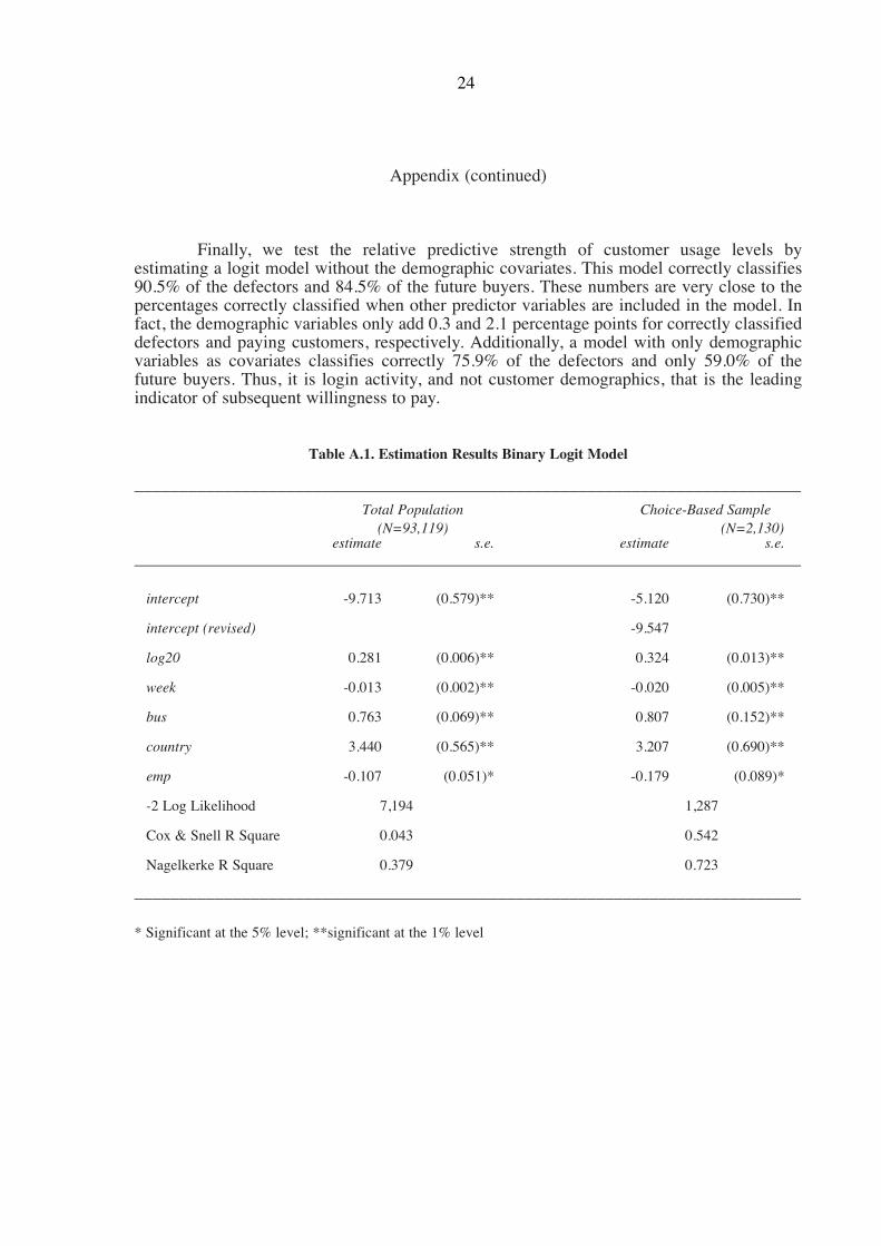
We first estimate a binary logit model on the total sample of customers whoregistered between weeks 1 and 50 of the observation period. Of these free-service users,only 1,030 (1.1%) chose to stay with the company after the fees were initiated. Thus, theoccurrence of PAY=1 in our sample is a rare event and the logit model logically predicts thateveryone will abandon the service, which results in a 98.9% correct classification rate.Nevertheless, all parameter estimates are found to be statistically significant, and our focalconstruct LOG20 has a positive impact on the probability of paying (see Table A.1.).

We also estimated the model with a choice-based sampling method that balances thenumber of paying customers and defectors (see Ben-Akiva and Lerman 1985). Thistechnique does not yield consistent maximum-likelihood estimates of the intercept.Following Manski and Lerman (1977), we adjust the estimated intercepts for each alternativeby substracting from the exogeneous maximum likelihood estimates of the intercept theconstant 1n(Sg/Pg), where Sg is the percentage of observations for alternative g in the sample,and Pg is the percentage of observations for alternative g in the population2.

The estimation results using the choice-based sample are reported in Table A1. Themodel correctly classifies 90.8% of those who terminate and 86.5% of those who agree topay. The average predicted probability of retention for our choice-based sample is 0.475,which is very similar to the observed 0.484. Using the revised intercept, the predictedaverage retention probability for the population is 0.0107, which is also very close to theobserved value of 0.0111.

The results support our hypothesis of a significant and positive effect of acustomer’s login activity on her subsequent willingness to pay. Therefore, acquisitionchannels with a higher level of subsequent usage (login) activity will increase the subsequentaverage conversion rates. The logit results are also consistent with our demographichypotheses: customers who registered earlier, retailers, US-based firms and firms with feweremployees are more likely to be retained than others.

23

2 Hence, for our particular estimation results, where we find an estimated intercept of –5.120, we have torevise this intercept through the following steps. We have Sg = 1,030 / 2,130 = 0.4836, and Pg = 1,030 /93,119 = 0.00111. Thus we have to subtract from the estimated intercept 1n(Sg/Pg). Similarly, we have Sg =1,100 / 2,130 = 0.5164, and Pg = 92,089 / 93,119 = 0.9889. Therefore, we should subtract from the interceptof alternative 0 the constant 1n(Sg/Pg) = –0.6497. The estimated new constants will be -5.12 - 3.77 = -8.90for alternative 1, and 0 – (-0.65) = 0.65 for alternative 0. Finally, since we want to keep alternative 0normalized to be 0, we should add the constant -0.65 to both alternatives. The resulting revised intercept willbe -9.55. For an example implementing this approach for the Multinomial Logit Model see Ben-Akiva andLerman (1985, p. 238).

Appendix (continued)

Finally, we test the relative predictive strength of customer usage levels byestimating a logit model without the demographic covariates. This model correctly classifies90.5% of the defectors and 84.5% of the future buyers. These numbers are very close to thepercentages correctly classified when other predictor variables are included in the model. Infact, the demographic variables only add 0.3 and 2.1 percentage points for correctly classifieddefectors and paying customers, respectively. Additionally, a model with only demographicvariables as covariates classifies correctly 75.9% of the defectors and only 59.0% of thefuture buyers. Thus, it is login activity, and not customer demographics, that is the leadingindicator of subsequent willingness to pay.

Table A.1. Estimation Results Binary Logit Model

–––––––––––––––––––––––––––––––––––––––––––––––––––––––––––––––––––––––––––Total Population Choice-Based Sample

(N=93,119) (N=2,130)estimate s.e. estimate s.e.

–––––––––––––––––––––––––––––––––––––––––––––––––––––––––––––––––––––––––––

intercept -9.713 (0.579)** -5.120 (0.730)**

intercept (revised) -9.547

log20 0.281 (0.006)** 0.324 (0.013)**

week -0.013 (0.002)** -0.020 (0.005)**

bus 0.763 (0.069)** 0.807 (0.152)**

country 3.440 (0.565)** 3.207 (0.690)**

emp -0.107 (0.051)* -0.179 (0.089)*

-2 Log Likelihood 7,194 1,287

Cox & Snell R Square 0.043 0.542

Nagelkerke R Square 0.379 0.723

–––––––––––––––––––––––––––––––––––––––––––––––––––––––––––––––––––––––––––

* Significant at the 5% level; **significant at the 1% level

24

REFERENCES

Anderson, Eric, and Duncan Simester (2002), “Evidence and Explanation of Long-Run PriceEffects,” Paper Presented at the Marketing Science Conference, Edmonton, Canada,2002.

Ben-Akiva, Moshe, and Steven R. Lerman (1985), Discrete Choice Models. MIT Press.

Blattberg, Robert C., and John Deighton (1991), “Interactive Marketing: Exploiting the Ageof Addressability,” Sloan Management Review, 33 (1), 5-14.

—— (1996), “Manage Marketing by the Customer Equity Test,” Harvard Business Review,74 (4), 136-44.

Blattberg, Robert C., Gary Getz, and Jacquelyn S. Thomas (2001), Customer Equity:Building and Managing Relationships As Valued Assets. Boston, Massachusetts:Harvard Business School Press.

Briggs, Rex, and Nigel Hollis (1997), “Advertising on the Web: Is There Response BeforeClick-Through?,” Journal of Advertising Research, 37 (2), 33-45.

Bronnenberg, Bart J., Vijay Mahajan, and Wilfried R. Vanhonacker (2000), “The Emergenceof Market Structure in New Repeat Purchase Categories: The Interplay of Market Shareand Retailer Distribution,” Journal of Marketing Research, 37 (1).

Brown, Jacqueline Johnson, and Peter H. Reingen (1987), “Social Ties and Word-of-MouthReferral Behavior,” Journal of Consumer Research, 14 (3), 350-362.

Dekimpe, M. G., and Dominique M. Hanssens (2000), “Time-Series Models in Marketing:Past, Present, and Future,” International Journal of Research in Marketing, 17, 183-93.

Dekimpe, Marnik G., and Dominique M. Hanssens (1995a), “Empirical GeneralizationsAbout Market Evolution and Stationarity,” Marketing Science, 14 (3), G109-G121.

—— (1995b), “The Persistence of Marketing Effects on Sales,” Marketing Science, 14 (1), 1-21.

—— (1999), “Sustained Spending and Persistent Response: A New Look at Long-TermMarketing Profitability,” Journal of Marketing Research, 36 (4), 397-412.

Doan, Thomas (1992), RATS User’s Manual. Evanston, Ill: Estima.

Doyle, Peter (2000), Value-Based Marketing Strategies for Corporate Growth andShareholder Value. New York: Wiley.

Dreze, Xavier, and Fred Zufryden (1998), “Is Internet Advertising Ready for Prime Time?,”Journal of Advertising Research, 38 (3), 7-18.

Enders, Walter (1994), Applied Econometric Times Series. New York: John Wiley & Sons.

Forrester (2001), “Effective Email Marketing,” hhtp://www.forrester.com.

25

Friestad, Marian, and Peter Wright (1995), “Persuasion Knowledge: Lay People’s andResearchers’ Beliefs About the Psychology of Advertising,” Journal of ConsumerResearch, 22 (1), 62-74.

—— (1994), “The Persuasion Knowledge Model: How People Cope With PersuasionAttempts,” Journal of Consumer Research, 21 (1), 1-31.

Greyser, Stephen A., and H. Paul Root (1999), “Improving Advertising Budgeting,” MSIWorking Paper, Report No. 00-126.

Gupta, Sunil, Donald R. Lehman, and Jennifer Ames Stuart (2002), “Valuing Customers,”Working Paper at The Teradata Center for Customer Relationship Management.

Hansotia, Behram J., and Paul Wang (1997), “Analytical Challenges in CustomerAcquisition,” Journal of Direct Marketing, 11 (2), 7-19.

Herr, Paul M., Frank R. Kardes, and John Kim (1991), “Effects of Word-of-Mouth andProduct-Attribute Information on Persuasion: An Accessibility-DiagnosticityPerspective,” Journal of Consumer Research, 17 (4), 454-62.

Jedidi, Kamel, Carl F. Mela, and Sunil Gupta (1999), “Managing Advertising and Promotionfor Long-Run Profitability,” Marketing Science, 18 (1), 1-22.

Keil, Sev K., David Reibstein, and Dick R. Wittink (2001), “The Impact of businessobjectives and the time horizon of performance evaluation on pricing behavior,”International Journal of Research in Marketing, (18), 67-81.

Kwiatkowski, Denis, Peter C.B. Phillips, Peter Schmidt, and Yongcheol Shin (1992),“Testing the Null Hypothesis of Stationarity Against the Alternative of a Unit Root,”Journal of Econometrics, (54), 159-178.`

Koop, Gary, M. Hashem Pesaran, and Simon M. Potter (1996), “Impulse Response Analysisin Nonlinear Multivariate Models,” Journal of Econometrics, 74 (1), 119-47.

Lodish, Leonard M., Magid M. Abraham, Jeanne Livelsberger, Beth Lubetkin, and others(1995), “A Summary of Fifty-Five In-Market Experimental Estimates of the Long-TermEffect of TV Advertising,” Marketing Science, 14 (3), G133-G140.

Lutkepohl, Helmut (1993), Introduction to Multiple Time Series Analysis. Heidelberg:Springer-Verlag.

Manski, Charles, and S. Lerman (1977), “The Estimation of Choice Probabilities fromChoice-Based Samples,” Econometrica, 45, 1977-88.

Mantrala, Murali K., Prabhakant Sinha, and Andris A. Zoltners (1992), “Impact of ResourceAllocation Rules on Marketing Investment-Level Decisions and Profitability,” Journalof Marketing Research, 29 (2), 162-75.

Mela, Carl F., Sunil Gupta, and Donald R. Lehmann (1997), “The Long-Term Impact ofPromotion and Advertising on Consumer Brand Choice,” Journal of MarketingResearch, 34 (2), 248-61.

26

Nijs, Vincent R., Marnik G. Dekimpe, Jan-Benedict E. M. Steenkamp, and Dominque M.Hanssens (2001), “The Category-Demand Effects of Price Promotions,” MarketingScience, 20 (1), 1-22.

Pauwels, Koen, Dominique M. Hanssens, and S. Siddarth (2002), “The Long-Term Effects ofPrice Promotions on Category Incidence, Brand Choice and Purchase Quantity,”Journal of Marketing Research, 39, 421-39.

Pauwels, Koen, Jorge Silva-Risso, Shuba Srinivasan, and Dominique M. Hanssens (2003),“The Long-Term Impact of New-Product Introductions and Promotions On FinancialPerformance and Firm Value,” Working Paper at The Anderson School at UCLA.

Pesaran, H. Hashem, and Youngcheol Shin (1998), “Generalized Impulse Response Analysisin Linear Multivariate Models,” Economic Letters, 58 (1), 17-29.

Rangaswamy, Arvind, Prabhakant Sinha, and Andris Zoltners (1990), “An Integrated Model-Based Approach for Sales Force Structuring,” Marketing Science, 9 (4), 279-98.

Reichheld, Frederick F. (1993), “Loyalty-Based Management,” Harvard Business Review, 71(2), 64-73.

Rust, Roland T., Valarie A. Zeithaml, and Katherine N. Lemon (2000), Driving CustomerEquity: How Customer Lifetime Value Is Reshaping Corporate Strategy. New York:Free Press.

Sims, Christopher (1980 ), “Macroeconomics and Reality,” Econometrica, 48, 1-49.

Srinivasan, Shuba, Frank M. Bass, and Peter Popkowski (2000), “Market Share Responseand Competitive Interaction: The Impact of Temporary, Evolving and StructuralChanges in Prices,” International Journal of Research in Marketing, 17 (4), 281-305.

Thomas, Jacquelyn S. (2001), “A Methodology for Linking Customer Acquisition toCustomer Retention,” Journal of Marketing Research, 38 (2), 262-68.

27