Image Display Algorithmsfor High and Low Dynamic Range Display Devices

Erik Reinhard1,2,3 Timo Kunkel1 Yoann Marion2 Jonathan Brouillat2 Remi Cozot2

Kadi Bouatouch2

Abstract

With interest in high dynamic range imaging mounting, techniquesfor displaying such images on conventional display devices aregaining in importance. Conversely, high dynamic range displayhardware is creating the need for display algorithms that prepareimages for such displays. In this paper, the current state-of-the-artin dynamic range reduction and expansion is reviewed, and in par-ticular we assess the theoretical and practical need to structure tonereproduction as a combination of a forward and a reverse pass.

1 Introduction

Real-world environments typically contain a range of illuminationmuch larger than can be represented by conventional 8-bit images.For instance, sunlight at noon may be as much as 100 milliontimes brighter than starlight [Spillmann and Werner 1990; Ferw-erda 2001]. The human visual system is able to detect 4 or 5 logunits of illumination simultaneously, and can adapt to a range ofaround 10 orders of magnitude over time [Ferwerda 2001].

On the other hand, conventional 8-bit images with values be-tween 0 and 255, have a useful dynamic range of around 2 ordersof magnitude. Such images are represented typically by one byteper pixel for each of the red, green and blue channels. The lim-ited dynamic range afforded by 8-bit images is well-matched to thedisplay capabilities of CRTs. Their range, while being larger than2 orders of magnitude, lies partially in the dark end where humanvision has trouble discerning very small differences under normalviewing circumstances. Hence, CRTs have a useful dynamic rangeof 2 log units of magnitude. Currently, very few display deviceshave a dynamic range that significantly exceeds this range.

The notable exception are LCD displays with an LED back-panelwhere each of the LEDs is separately addressable [Seetzen et al.2003; Seetzen et al. 2004]. With the pioneering start-up BrightSidebeing taken over by Dolby, and both Philips and Samsung demon-strating their own displays with spatially varying back-lighting,hardware developments are undeniably moving towards higher dy-namic ranges.

It is therefore reasonable to anticipate that the variety in displaycapabilities will increase. Some displays will have a much higherdynamic range than others, whereas differences in mean luminancewill also increase due to a greater variety in back-lighting technol-ogy. As a result, the burden on general purpose display algorithmswill change. High dynamic range (HDR) image acquisition hasalready created the need for tone reproduction operators, which re-duce the dynamic range of images prior to display [Reinhard et al.2005; Reinhard 2007]. The advent of HDR display devices willadd to this the need to sometimes expand the dynamic range of im-ages. In particular the enormous number of conventional eight-bit

1University of Bristol, Bristol, e-mail: reinhard@cs.bris.ac.uk2Institut de Recherche en Informatique et Systemes Aleatoires (IRISA),

Rennes3University of Central Florida, USA

Figure 1:With conventional photography, some parts of the scenemay be under- or over-exposed (left). Capture of this scene with 9exposures, and assemblage of these into one high dynamic rangeimage followed by tone reproduction, affords the result shown onthe right.

Figure 2:Linear scaling of high dynamic range images to fit a givendisplay device may cause significant detail to be lost (left). Forcomparison, the right image is tone-mapped, allowing details inboth bright and dark regions to be visible.

images may have to be expanded in range prior to display on suchdevices. Algorithms for dynamic range expansion are commonlycalled inverse tone reproduction operators.

In this paper we survey the state-of-the-art in tone reproductionas well as inverse tone reproduction. In addition, we will summa-rize desirable features of tone reproduction and inverse tone repro-duction algorithms.

2 Dynamic Range Reduction

Capturing the full dynamic range of a scene implies that in manyinstances the resulting high dynamic range (HDR) image cannotbe directly displayed, as its range is likely to exceed the 2 ordersof magnitude range afforded by conventional display devices. Fig-ure 1 (left) shows a scene with a dynamic range far exceeding thecapabilities a conventional display. By capturing the full dynamicrange of this scene, followed by tone mapping the image, an accept-able rendition of this scene may be obtained (Figure 1, right).

A simple compressive function would be to normalize an image(see Figure 2 (left)). This constitutes a linear scaling which is suffi-cient only if the dynamic range of the image is slightly higher thanthe dynamic range of the display. For images with a significantlyhigher dynamic range, small intensity differences will be quantized

to the same display value such that visible details are lost. For com-parison, the right image in Figure 2 is tone-mapped non-linearlyshowing detail in both the light and dark regions.

In general linear scaling will not be appropriate for tone repro-duction. The key issue in tone reproduction is then to compress animage while at the same time preserving one or more attributes ofthe image. Different tone reproduction algorithms focus on differ-ent attributes such as contrast, visible detail, brightness, or appear-ance. Ideally, displaying a tone-mapped image on a low dynamicrange display device would recreate the same visual response inthe observer as the original scene. Given the limitations of displaydevices, this is in general not achievable, although we may approx-imate this goal as closely as possible.

3 Spatial operators

In the following sections we discuss tone reproduction operatorswhich apply compression directly on pixels. Often global and lo-cal operators are distinguished. Tone reproduction operators in theformer class change each pixel’s luminance values according to acompressive function which is the same for each pixel [Miller et al.1984; Tumblin and Rushmeier 1993; Ward 1994; Ferwerda et al.1996; Drago et al. 2003; Ward et al. 1997; Schlick 1994]. Theterm global stems from the fact that many such functions need tobe anchored to some values that are computed by analyzing the fullimage. In practice most operators use the geometric averageLv tosteer the compression:

Lv = exp

1

N

X

x,y

log(δ + Lv(x, y)

!

(1)

The small constantδ is introduced to prevent the average to becomezero in the presence of black pixels. The luminance of each pixelis indicated withLv , which can be computed from RGB values ifthe color space is known. If the color space in which the image isspecified is unknown, then the second best alternative would be toassume that the image uses sRGB primaries and white point, so thatthe luminance of a pixel is given by:

Lv(x, y) = 0.2125 R(x, y) + 0.7154 G(x, y) + 0.0721 B(x, y)(2)

The geometric averageLv is normally mapped to a predefined dis-play value. The main challenge faced in the design of a globaloperator lies in the choice of compressive function. Many func-tions are possible, which are for instance based on the image’s his-togram (Section 4.2) [Ward et al. 1997] or on data gathered frompsychophysics (Section 4.3).

On the other hand, local operators compress each pixel accordingto a specific compression function which is modulated by informa-tion derived from a selection of neighboring pixels, rather than thefull image [Chiu et al. 1993; Jobson et al. 1995; Rahman et al. 1996;Rahman et al. 1997; Pattanaik et al. 1998; Fairchild and Johnson2002; Ashikhmin 2002; Reinhard et al. 2002; Pattanaik and Yee2002; Oppenheim et al. 1968; Durand and Dorsey 2002; Choud-hury and Tumblin 2003]. The rationale is that the brightness ofa pixel in a light neighborhood is different than the brightness ofa pixel in a dark neighborhood. Design challenges for local opera-tors involve choosing the compressive function, the size of the localneighborhood for each pixel, and the manner in which local pixelvalues are used. In general, local operators are able to achieve bet-ter compression than global operators (Figure 3), albeit at a highercomputational cost.

Both global and local operators are often inspired by the humanvisual system. Most operators employ one of two distinct com-pressive functions, which is orthogonal to the distinction between

Figure 3: A local tone reproduction operator (left) and a globaltone reproduction operator (right) [Reinhard et al. 2002]. The localoperator shows more detail, as for instance seen in the insets.

local and global operators. Display valuesLd(x, y) are most com-monly derived from image luminancesLv(x, y) by the followingtwo functional forms:

Ld(x, y) =Lv(x, y)

f(x, y)(3a)

Ld(x, y) =Ln

v (x, y)

Lnv (x, y) + gn(x, y)

(3b)

In these equations,f(x, y) andg(x, y) may either be constant, ora function which varies per pixel. In the former case, we have aglobal operator, whereas a spatially varying function results in alocal operator. The exponentn is a constant which is either fixed,or set differently per image.

Equation 3a divides each pixel’s luminance by a value derivedfrom either the full image or a local neighborhood. As an exam-ple, the substitutionf(x, y) = Lmax/255 in (3a) yields a linearscaling such that values may be directly quantized into a byte, andcan therefore be displayed. A different approach would be to sub-stitutef(x, y) = Lblur(x, y), i.e. divide each pixel by a weightedlocal average, perhaps obtained by applying a Gaussian filter to theimage [Chiu et al. 1993]. While this local operator yields a dis-playable image, it highlights a classical problem whereby areas nearbright spots are reproduced too dark. This is often seen as halos, asdemonstrated in Figure 4.

The cause of halos stems from the fact that Gaussian filters bluracross sharp contrast edges in the same way that they blur small andlow contrast details. If there is a high contrast gradient in the neigh-borhood of the pixel under consideration, this causes the Gaussianblurred pixel to be significantly different from the pixel itself. Byusing a very large filter kernel in a division-based approach suchlarge contrasts are averaged out, and the occurrence of halos canbe minimized. However, very large filter kernels tend to compute alocal average that is not substantially different from the global av-erage. In the limit that the size of the filter kernel tends to infinity,the local average becomes identical to the global average and there-fore limits the compressive power of the operator to be no betterthan a global operator. Thus, the size of the filter kernel in division-based operators presents a trade-off between the ability to reducethe dynamic range, and the visibility of artifacts.

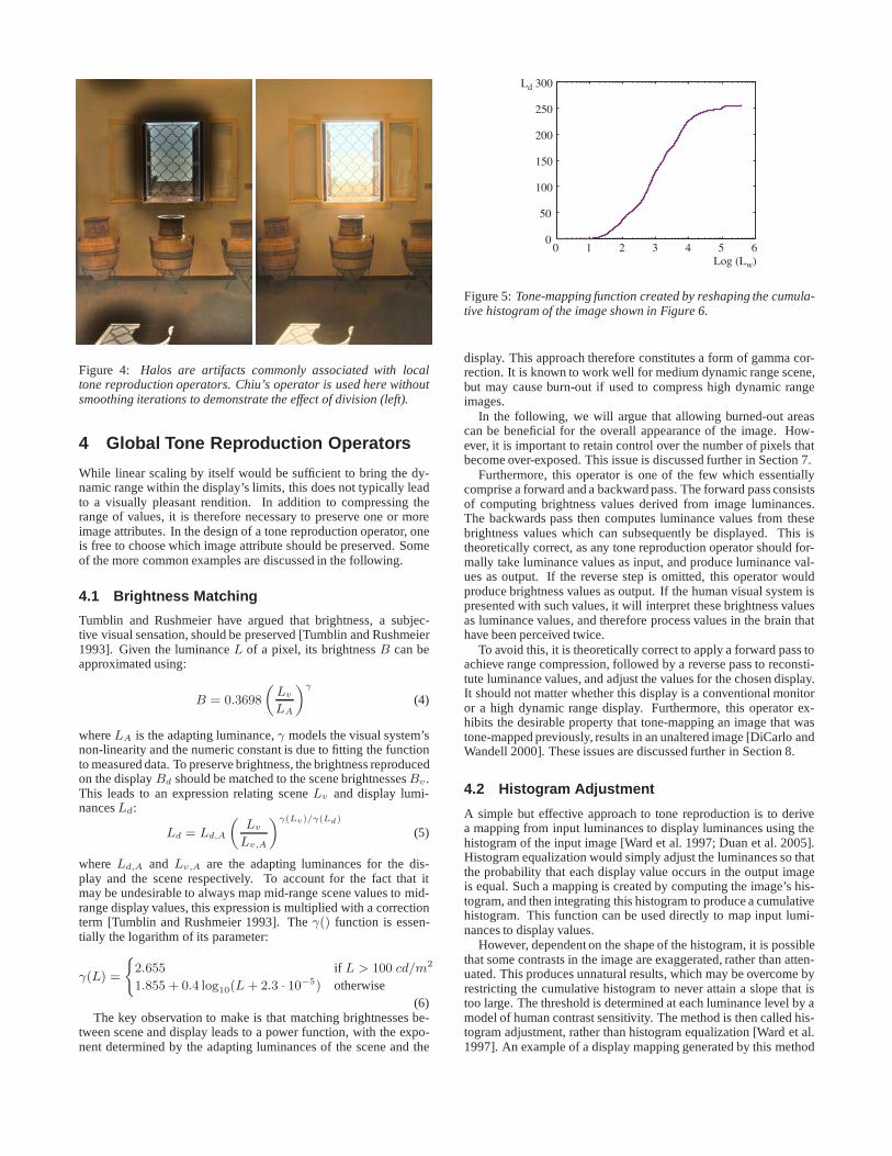
Figure 4: Halos are artifacts commonly associated with localtone reproduction operators. Chiu’s operator is used here withoutsmoothing iterations to demonstrate the effect of division (left).

4 Global Tone Reproduction Operators

While linear scaling by itself would be sufficient to bring the dy-namic range within the display’s limits, this does not typically leadto a visually pleasant rendition. In addition to compressing therange of values, it is therefore necessary to preserve one or moreimage attributes. In the design of a tone reproduction operator, oneis free to choose which image attribute should be preserved. Someof the more common examples are discussed in the following.

4.1 Brightness Matching

Tumblin and Rushmeier have argued that brightness, a subjec-tive visual sensation, should be preserved [Tumblin and Rushmeier1993]. Given the luminanceL of a pixel, its brightnessB can beapproximated using:

B = 0.3698

„

Lv

LA

«γ

(4)

whereLA is the adapting luminance,γ models the visual system’snon-linearity and the numeric constant is due to fitting the functionto measured data. To preserve brightness, the brightness reproducedon the displayBd should be matched to the scene brightnessesBv .This leads to an expression relating sceneLv and display lumi-nancesLd:

Ld = Ld,A

„

Lv

Lv,A

«γ(Lv)/γ(Ld)

(5)

where Ld,A and Lv,A are the adapting luminances for the dis-play and the scene respectively. To account for the fact that itmay be undesirable to always map mid-range scene values to mid-range display values, this expression is multiplied with a correctionterm [Tumblin and Rushmeier 1993]. Theγ() function is essen-tially the logarithm of its parameter:

γ(L) =

(

2.655 if L > 100 cd/m2

1.855 + 0.4 log10(L + 2.3 · 10−5) otherwise(6)

The key observation to make is that matching brightnesses be-tween scene and display leads to a power function, with the expo-nent determined by the adapting luminances of the scene and the

0 1 2 3 4 5 60

50

100

150

200

250

300Ld

Log (Lw)

Figure 5:Tone-mapping function created by reshaping the cumula-tive histogram of the image shown in Figure 6.

display. This approach therefore constitutes a form of gamma cor-rection. It is known to work well for medium dynamic range scene,but may cause burn-out if used to compress high dynamic rangeimages.

In the following, we will argue that allowing burned-out areascan be beneficial for the overall appearance of the image. How-ever, it is important to retain control over the number of pixels thatbecome over-exposed. This issue is discussed further in Section 7.

Furthermore, this operator is one of the few which essentiallycomprise a forward and a backward pass. The forward pass consistsof computing brightness values derived from image luminances.The backwards pass then computes luminance values from thesebrightness values which can subsequently be displayed. This istheoretically correct, as any tone reproduction operator should for-mally take luminance values as input, and produce luminance val-ues as output. If the reverse step is omitted, this operator wouldproduce brightness values as output. If the human visual system ispresented with such values, it will interpret these brightness valuesas luminance values, and therefore process values in the brain thathave been perceived twice.

To avoid this, it is theoretically correct to apply a forward pass toachieve range compression, followed by a reverse pass to reconsti-tute luminance values, and adjust the values for the chosen display.It should not matter whether this display is a conventional monitoror a high dynamic range display. Furthermore, this operator ex-hibits the desirable property that tone-mapping an image that wastone-mapped previously, results in an unaltered image [DiCarlo andWandell 2000]. These issues are discussed further in Section 8.

4.2 Histogram Adjustment

A simple but effective approach to tone reproduction is to derivea mapping from input luminances to display luminances using thehistogram of the input image [Ward et al. 1997; Duan et al. 2005].Histogram equalization would simply adjust the luminances so thatthe probability that each display value occurs in the output imageis equal. Such a mapping is created by computing the image’s his-togram, and then integrating this histogram to produce a cumulativehistogram. This function can be used directly to map input lumi-nances to display values.

However, dependent on the shape of the histogram, it is possiblethat some contrasts in the image are exaggerated, rather than atten-uated. This produces unnatural results, which may be overcome byrestricting the cumulative histogram to never attain a slope that istoo large. The threshold is determined at each luminance level by amodel of human contrast sensitivity. The method is then called his-togram adjustment, rather than histogram equalization [Ward et al.1997]. An example of a display mapping generated by this method

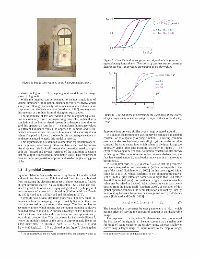
Figure 6:Image tone-mapped using histogram adjustment.

is shown in Figure 5. This mapping is derived from the imageshown in Figure 6.

While this method can be extended to include simulations ofveiling luminance, illumination dependent color sensitivity, visualacuity, and although knowledge of human contrast sensitivity is in-corporated into the basic operator [Ward et al. 1997], we may viewthis operator as a refined form of histogram equalization.

The importance of this observation is that histogram equaliza-tion is essentially rooted in engineering principles, rather than asimulation of the human visual system. It is therefore natural to re-gard this operator as “unit-less” — it transforms luminance valuesto different luminance values, as opposed to Tumblin and Rush-meier’s operator which transforms luminance values to brightnessvalues if applied in forward mode only. As a consequence there isno theoretical need to apply this model in reverse.

This argument can be extended to other tone reproduction opera-tors. In general, when an algorithm simulates aspects of the humanvisual system, this by itself creates the theoretical need to applyboth the forward and inverse versions of the algorithm to ensurethat the output is measured in radiometric units. This requirementdoes not necessarily exist for approachesbased on engineering prin-ciples.

4.3 Sigmoidal Compression

Equation 3b has an S-shaped curve on a log-linear plot, and is calleda sigmoid for that reason. This functional form fits data obtainedfrom measuring the electrical response of photo-receptors to flashesof light in various species [Naka and Rushton 1966]. It has also pro-vided a good fit to other electro-physiological and psychophysicalmeasurements of human visual function [Kleinschmidt and Dowl-ing 1975; Hood et al. 1979; Hood and Finkelstein 1979].

Sigmoids have several desirable properties. For very small lu-minance values the mapping is approximately linear, so that con-trast is preserved in dark areas of the image. The function has anasymptote at one, which means that the output mapping is alwaysbounded between0 and1. A further advantage of this function isthat for intermediate values, the function affords an approximatelylogarithmic compression. This can be seen for instance in Figure 7,where the middle section of the curve is approximately linear ona log-linear plot. To illustrate, bothLd = Lw/(Lw + 1) andLd = 0.25 log(Lw) + 0.5 are plotted in this figure4, showing that

4The constants 0.25 and 0.5 were determined by equating the values as

-2 -1 0 1 20.0

0.5

1.0

log (Lw)

Ld Ld = Lw / (Lw + 1)

Ld = 0.25 log (Lw) + 0.5

Ld = Lw / (Lw + 10)

Ld = Lw / (Lw + 0.1)

Figure 7:Over the middle range values, sigmoidal compression isapproximately logarithmic. The choice of semi-saturation constantdetermines how input values are mapped to display values.

-2 -1 0 1 20.0

0.5

1.0

log (Lw)

Ld Ld = Lw / (Lw + gn)

n = 0.5

n = 1.0

n = 2.0

g = 1

nn

Figure 8: The exponentn determines the steepness of the curve.Steeper slopes map a smaller range of input values to the displayrange.

these functions are very similar over a range centered around1.In Equation 3b, the functiong(x, y) may be computed as a global

constant, or as a spatially varying function. Following commonpractice in electro-physiology, we callg(x, y) thesemi-saturationconstant. Its value determines which values in the input image areoptimally visible after tone mapping, as shown in Figure 7. Theeffect of choosing different semi-saturation constants is also shownin this figure. The name semi-saturation constant derives from thefact that when the inputLv reaches the same value asg(), the outputbecomes0.5.

In its simplest form,g(x, y) is set toLv/k, so that the geometricaverage is mapped to user parameterk (which corresponds to thekeyof the scene) [Reinhard et al. 2002]. In this case, a good initialvalue fork is 0.18, which conforms to the photographic equiva-lent of middle gray (although some would argue that 0.13 ratherthan 0.18 is neutral gray). For particularly light or dark scenes thisvalue may be raised or lowered. Alternatively, its value may be es-timated from the image itself [Reinhard 2003]. A variation of thisglobal operator computes the semi-saturation constant by linearlyinterpolating between the geometric average and each pixel’s lumi-nance [Reinhard and Devlin 2005].

g(x, y) = a Lv(x, y) + (1− a) Lv (7)

The interpolation is governed by user parametera ∈ [0, 1] whichhas the effect of varying the amount of contrast in the displayableimage.

The exponentn in Equation 3b determines how pronouncedthe S-shape of the sigmoid is. Steeper curves map a smaller use-ful range of scene values to the display range, whereas shallowercurves map a larger range of input values to the display range.

well as the derivatives of both functions forx = 1.

Studies in electro-physiology report values betweenn = 0.2 andn = 0.9 [Hood et al. 1979].

5 Local Tone Reproduction Operators

The several different variants of sigmoidal compression shownabove are all global in nature. This has the advantage that theyare fast to compute, and they are very suitable for medium to highdynamic range images. Their simplicity makes these operators suit-able for implementation on graphics hardware as well. For veryhigh dynamic range images, however, it may be necessary to resortto a local operator since this may give somewhat better compres-sion.

5.1 Local Sigmoidal Operators

A straightforward method to extend sigmoidal compression re-places the global semi-saturation constant by a spatially varyingfunction, which once more can be computed in several differentways. Thus,g(x, y) then becomes a function of a spatially local-ized average. Perhaps the simplest way to accomplish this is toonce more use a Gaussian blurred image. Each pixel in a blurredimage represents a locally averaged value which may be viewed asa suitable choice for the semi-saturation constant5.

As with division-based operators discussed in the previous sec-tion, we have to consider haloing artifacts. If sigmoids are usedwith a spatially varying semi-saturation constant, the Gaussian fil-ter kernel is typically chosen to be very small to minimize artifacts.In practice filter kernels of only a few pixels wide are sufficient tosuppress significant artifacts while at the same time producing morelocal contrast in the tone-mapped images. Such small filter kernelscan be conveniently computed in the spatial domain without los-ing too much performance. There are, however, several differentapproaches to compute a local average, which are discussed in thefollowing section.

5.2 Local Neighborhoods

In local operators, halo artifacts occur when the local average iscomputed over a region that contains sharp contrasts with respectto the pixel under consideration. It is therefore important that thelocal average is computed over pixel values that are not significantlydifferent from the pixel that is being filtered.

This suggests a strategy whereby an image is filtered such thatno blurring over such edges occurs. A simple, but computationallyexpensive way is to compute a stack of Gaussian blurred imageswith different kernel sizes, i.e. animage pyramid. For each pixel,we may choose the largest Gaussian which does not overlap with asignificant gradient. The scale at which this happens can be com-puted as follows.

In a relatively uniform neighborhood, the value of a Gaussianblurred pixel should be the same regardless of the filter kernel size.Thus, in this case the difference between a pixel filtered with twodifferent Gaussians should be around zero. This difference willonly change significantly if the wider filter kernel overlaps with aneighborhood containing a sharp contrast step, whereas the smallerfilter kernel does not. A difference of Gaussians (DoG) signalLDoG

i (x, y) at scalei can be computed as follows:

LDoGi (x, y) = Ri σ(x, y) − R2 i σ(x, y) (8)

5Althoughg(x, y) is now no longer a constant, we continue to refer toit as the semi-saturationconstant.

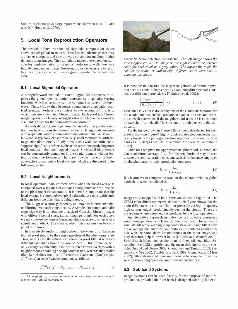
Figure 9: Scale selection mechanism. The left image shows thetone-mapped result. The image on the right encodes the selectedscale for each pixel as a gray value. The darker the pixel, thesmaller the scale. A total of eight different scales were used tocompute this image.

It is now possible to find the largest neighborhood around a pixelthat does not contain sharp edges by examining differences of Gaus-sians at different kernel sizesi [Reinhard et al. 2002]:

˛

˛

˛

˛

LDoGi (x, y)

Ri σ(x, y) + α

˛

˛

˛

˛

> t i = 1 . . . 8 (9)

Here, the DoG filter is divided by one of the Gaussians to normalizethe result, and thus enable comparison against the constant thresh-old t which determines if the neighborhood at scalei is consideredto have significant detail. The constantα is added to avoid divisionby zero.

For the image shown in Figure 9 (left), the scale selected for eachpixel is shown in Figure 9 (right). Such a scale selection mechanismis employed by the photographic tone reproduction operator [Rein-hard et al. 2002] as well as in Ashikhmin’s operator [Ashikhmin2002].

Once for each pixel the appropriate neighborhood is known, theGaussian blurred averageLblur for this neighborhood may be usedto steer the semi-saturation constant, such as for instance employedby the photographic tone reproduction operator:

Ld =Lw

1 + Lblur(10)

It is instructive to compare the result of this operator with its globalequivalent, which is defined as:

Ld =Lw

1 + Lw(11)

Images tone-mapped with both forms are shown in Figure 10. TheCIE94 color difference metric shown in this figure shows that themain differences occur near (but not precisely at) high-frequencyhigh-contrast edges, predominantly seen in the clouds. These arethe regions where more detail is produced by the local operator.

An alternative approach includes the use of edge preservingsmoothing operators, which are designed specifically for removingsmall details while keeping sharp contrasts in tact. Such filters havethe advantage that sharp discontinuities in the filtered result coin-cide with the same sharp discontinuities in the input image, andmay therefore help to prevent halos [DiCarlo and Wandell 2000].Several such filters, such as the bilateral filter, trilateral filter, Su-san filter, the LCIS algorithm and the mean shift algorithm are suit-able [Durand and Dorsey 2002; Choudhury and Tumblin 2003; Pat-tanaik and Yee 2002; Tumblin and Turk 1999; Comaniciu and Meer2002], although some of them are expensive to compute. Edge pre-serving smoothing operators are discussed Section 5.4.

5.3 Sub-band Systems

Image pyramids can be used directly for the purpose of tone re-production, provided the filter bank is designed carefully [Li et al.

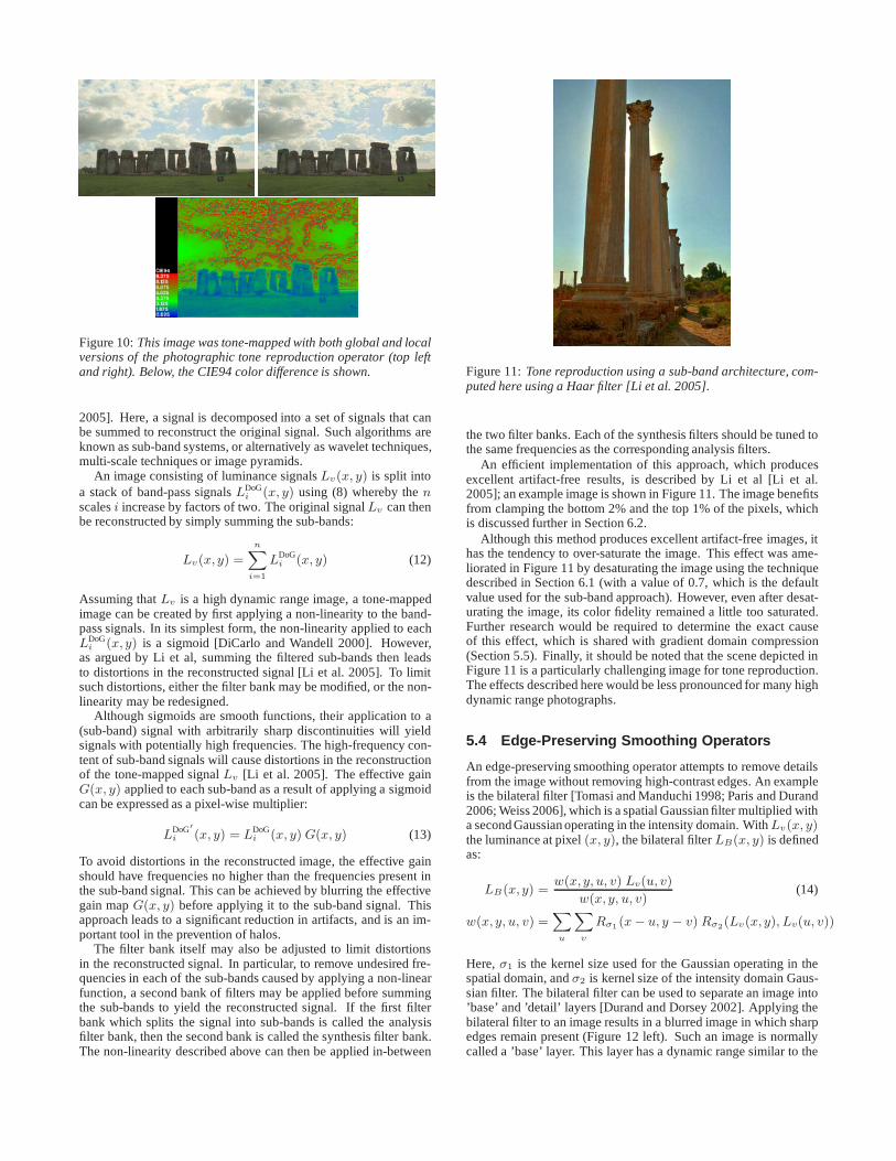
Figure 10:This image was tone-mapped with both global and localversions of the photographic tone reproduction operator (top leftand right). Below, the CIE94 color difference is shown.

2005]. Here, a signal is decomposed into a set of signals that canbe summed to reconstruct the original signal. Such algorithms areknown as sub-band systems, or alternatively as wavelet techniques,multi-scale techniques or image pyramids.

An image consisting of luminance signalsLv(x, y) is split intoa stack of band-pass signalsLDoG

i (x, y) using (8) whereby thenscalesi increase by factors of two. The original signalLv can thenbe reconstructed by simply summing the sub-bands:

Lv(x, y) =

nX

i=1

LDoGi (x, y) (12)

Assuming thatLv is a high dynamic range image, a tone-mappedimage can be created by first applying a non-linearity to the band-pass signals. In its simplest form, the non-linearity applied to eachLDoG

i (x, y) is a sigmoid [DiCarlo and Wandell 2000]. However,as argued by Li et al, summing the filtered sub-bands then leadsto distortions in the reconstructed signal [Li et al. 2005]. To limitsuch distortions, either the filter bank may be modified, or the non-linearity may be redesigned.

Although sigmoids are smooth functions, their application to a(sub-band) signal with arbitrarily sharp discontinuities will yieldsignals with potentially high frequencies. The high-frequency con-tent of sub-band signals will cause distortions in the reconstructionof the tone-mapped signalLv [Li et al. 2005]. The effective gainG(x, y) applied to each sub-band as a result of applying a sigmoidcan be expressed as a pixel-wise multiplier:

LDoG′

i (x, y) = LDoGi (x, y) G(x, y) (13)

To avoid distortions in the reconstructed image, the effective gainshould have frequencies no higher than the frequencies present inthe sub-band signal. This can be achieved by blurring the effectivegain mapG(x, y) before applying it to the sub-band signal. Thisapproach leads to a significant reduction in artifacts, and is an im-portant tool in the prevention of halos.

The filter bank itself may also be adjusted to limit distortionsin the reconstructed signal. In particular, to remove undesired fre-quencies in each of the sub-bands caused by applying a non-linearfunction, a second bank of filters may be applied before summingthe sub-bands to yield the reconstructed signal. If the first filterbank which splits the signal into sub-bands is called the analysisfilter bank, then the second bank is called the synthesis filter bank.The non-linearity described above can then be applied in-between

Figure 11:Tone reproduction using a sub-band architecture, com-puted here using a Haar filter [Li et al. 2005].

the two filter banks. Each of the synthesis filters should be tuned tothe same frequencies as the corresponding analysis filters.

An efficient implementation of this approach, which producesexcellent artifact-free results, is described by Li et al [Li et al.2005]; an example image is shown in Figure 11. The image benefitsfrom clamping the bottom 2% and the top 1% of the pixels, whichis discussed further in Section 6.2.

Although this method produces excellent artifact-free images, ithas the tendency to over-saturate the image. This effect was ame-liorated in Figure 11 by desaturating the image using the techniquedescribed in Section 6.1 (with a value of 0.7, which is the defaultvalue used for the sub-band approach). However, even after desat-urating the image, its color fidelity remained a little too saturated.Further research would be required to determine the exact causeof this effect, which is shared with gradient domain compression(Section 5.5). Finally, it should be noted that the scene depicted inFigure 11 is a particularly challenging image for tone reproduction.The effects described here would be less pronounced for many highdynamic range photographs.

5.4 Edge-Preserving Smoothing Operators

An edge-preserving smoothing operator attempts to remove detailsfrom the image without removing high-contrast edges. An exampleis the bilateral filter [Tomasi and Manduchi 1998; Paris and Durand2006; Weiss 2006], which is a spatial Gaussian filter multiplied witha second Gaussian operating in the intensity domain. WithLv(x, y)the luminance at pixel(x, y), the bilateral filterLB(x, y) is definedas:

LB(x, y) =w(x, y, u, v) Lv(u, v)

w(x, y, u, v)(14)

w(x, y, u, v) =X

u

X

v

Rσ1(x − u, y − v) Rσ2

(Lv(x, y), Lv(u, v))

Here,σ1 is the kernel size used for the Gaussian operating in thespatial domain, andσ2 is kernel size of the intensity domain Gaus-sian filter. The bilateral filter can be used to separate an image into’base’ and ’detail’ layers [Durand and Dorsey 2002]. Applying thebilateral filter to an image results in a blurred image in which sharpedges remain present (Figure 12 left). Such an image is normallycalled a ’base’ layer. This layer has a dynamic range similar to the

Figure 12:Bilateral filtering removes small details, but preservessharp gradients (left). The associated detail layer is shown on theright.

Figure 13: An image tone-mapped using bilateral filtering. Thebase and detail layers shown in Figure 12 are recombined aftercompressing the base layer.

input image. The high dynamic range image may be divided pixel-wise by the base layer, obtaining a ’detail’ layerLD(x, y) whichcontains all the high frequency detail, but typically does not have avery high dynamic range (Figure 12 right):

LD(x, y) = Lv(x, y)/LB(x, y) (15)

By compressing the base layer before recombining into a com-pressed image, a displayable low dynamic range image may be cre-ated (Figure 13). Compression of the base layer may be achieved bylinear scaling. Tone reproduction on the basis of bilateral filteringis executed in the logarithmic domain.

Edge-preserving smoothing operators may be used to computea local adaptation level for each pixel, to be applied in a spatiallyvarying or local tone reproduction operator. A local operator basedon sigmoidal compression can for instance be created by substitut-ing Lblur(x, y) = LB(x, y) in (10).

Alternatively, the semi-saturation constantg(x, y) in (3b) maybe seen as a local adaptation constant, and can therefore be locallyapproximated withLB(x, y) [Ledda et al. 2004], or with any of theother filters mentioned above. As shown in Figure 7, the choiceof semi-saturation constant shifts the curve horizontally such thatits middle portion lies over a desirable range of values. In a localoperator, this shift is determined by the values of a local neighbor-hood of pixels, and is thus different for each pixel. This leads toa potentially better compression mechanism than a constant valuecould afford.

5.5 Gradient-Domain Operators

Local adaptation provides a measure of how different a pixel is fromits immediate neighborhood. If a pixel is very different from itsneighborhood, it typically needs to be attenuated more. Such a dif-ference may also be expressed in terms of contrast, which could be

Figure 14: The image on the left is tone-mapped using gradientdomain compression. The magnitude of the gradients‖∇L‖ ismapped to a grey scale in the right image (white is a gradient of0; black is the maximum gradient in the image).

represented with image gradients (in log space):

∇L = (L(x + 1, y) − L(x, y), L(x, y + 1) − L(y)) (16)

Here,∇L is a vector-valued gradient field. By attenuating largegradients more than small gradients, a tone reproduction operatormay be constructed [Fattal et al. 2002]. Afterwards, an image canbe reconstructed by integrating the gradient field to form a tone-mapped image. Such integration must be approximated by numer-ical techniques, which is achieved by solving a Poisson equationusing the Full Multi-grid Method [Press et al. 1992]. The resultingimage then needs to be linearly scaled to fit the range of the tar-get display device. An example of gradient domain compression isshown in Figure 14.

5.6 Lightness Perception

The theory of lightness perception, provides a model for the per-ception of surface reflectances6. To cast this into a computa-tional model, the image needs to be automatically decomposedinto frameworks, i.e. regions of common illumination. As an ex-ample, the window in the right-most image of Figure 17 wouldconstitute a separate framework from the remainder of the interior.The influence of each framework on the total lightness needs tobe estimated, and the anchors within each framework must be com-puted [Krawczyk et al. 2004; Krawczyk et al. 2005; Krawczyk et al.2006].

It is desirable to assign a probability to each pixel of belonging toa particular framework. This leaves the possibility of a pixel havingnon-zero participation in multiple frameworks, which is somewhatdifferent from standard segmentation algorithms that assign a pixelto at most one segment. To compute frameworks and probabilitiesfor each pixel, a standard K-means clustering algorithm may beapplied.

For each framework, the highest luminance rule may now be ap-plied to find an anchor. This means that within a framework, thepixel with the highest luminance would determine how all the pixelsin this framework are likely to be perceived. However, direct appli-cation of this rule may result in the selection of a luminance value ofa patch that is perceived as self-luminous. As the anchor should bethe highest luminance value that is not perceived as self-luminous,

6Lightness is defined as relative perceived surface reflectance.

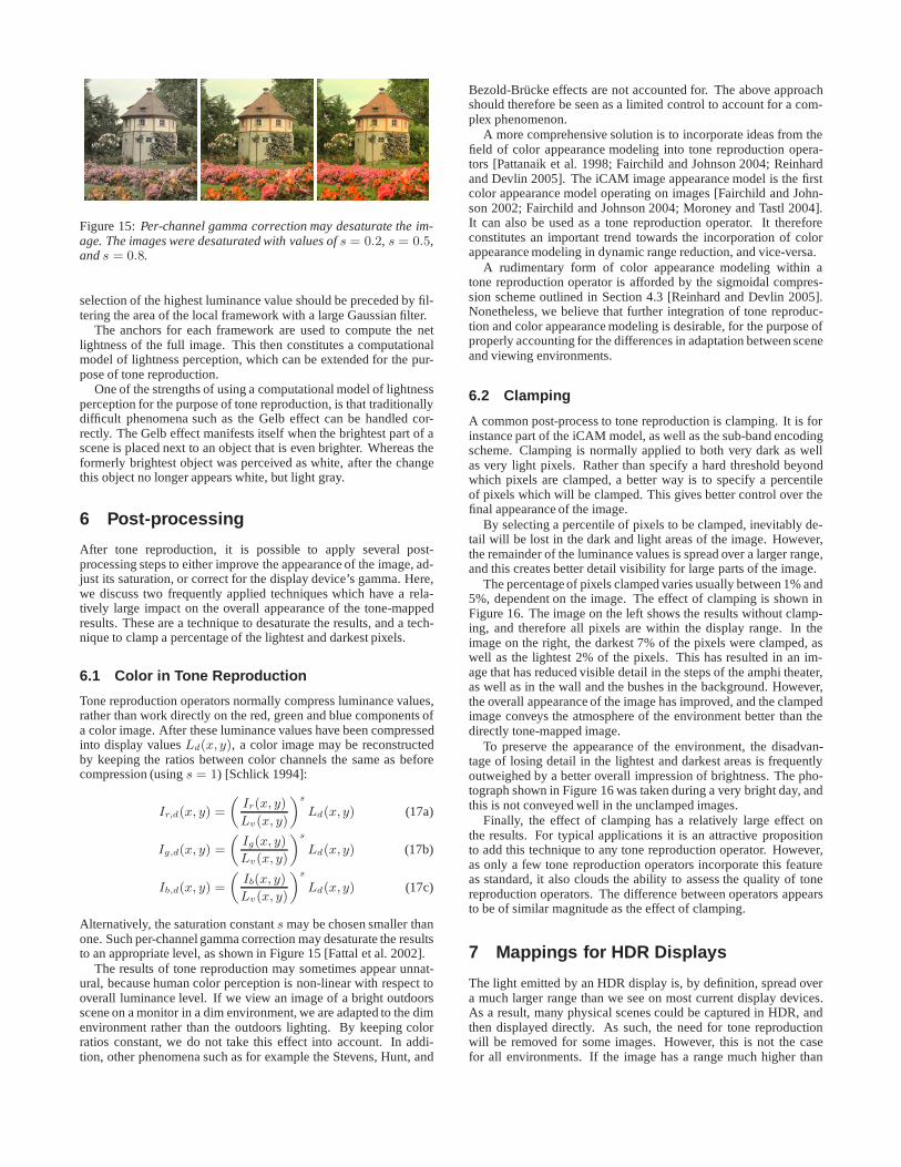
Figure 15:Per-channel gamma correction may desaturate the im-age. The images were desaturated with values ofs = 0.2, s = 0.5,ands = 0.8.

selection of the highest luminance value should be preceded by fil-tering the area of the local framework with a large Gaussian filter.

The anchors for each framework are used to compute the netlightness of the full image. This then constitutes a computationalmodel of lightness perception, which can be extended for the pur-pose of tone reproduction.

One of the strengths of using a computational model of lightnessperception for the purpose of tone reproduction, is that traditionallydifficult phenomena such as the Gelb effect can be handled cor-rectly. The Gelb effect manifests itself when the brightest part of ascene is placed next to an object that is even brighter. Whereas theformerly brightest object was perceived as white, after the changethis object no longer appears white, but light gray.

6 Post-processing

After tone reproduction, it is possible to apply several post-processing steps to either improve the appearance of the image, ad-just its saturation, or correct for the display device’s gamma. Here,we discuss two frequently applied techniques which have a rela-tively large impact on the overall appearance of the tone-mappedresults. These are a technique to desaturate the results, and a tech-nique to clamp a percentage of the lightest and darkest pixels.

6.1 Color in Tone Reproduction

Tone reproduction operators normally compress luminance values,rather than work directly on the red, green and blue components ofa color image. After these luminance values have been compressedinto display valuesLd(x, y), a color image may be reconstructedby keeping the ratios between color channels the same as beforecompression (usings = 1) [Schlick 1994]:

Ir,d(x, y) =

„

Ir(x, y)

Lv(x, y)

«s

Ld(x, y) (17a)

Ig,d(x, y) =

„

Ig(x, y)

Lv(x, y)

«s

Ld(x, y) (17b)

Ib,d(x, y) =

„

Ib(x, y)

Lv(x, y)

«s

Ld(x, y) (17c)

Alternatively, the saturation constants may be chosen smaller thanone. Such per-channel gamma correction may desaturate the resultsto an appropriate level, as shown in Figure 15 [Fattal et al. 2002].

The results of tone reproduction may sometimes appear unnat-ural, because human color perception is non-linear with respect tooverall luminance level. If we view an image of a bright outdoorsscene on a monitor in a dim environment, we are adapted to the dimenvironment rather than the outdoors lighting. By keeping colorratios constant, we do not take this effect into account. In addi-tion, other phenomena such as for example the Stevens, Hunt, and

Bezold-Brucke effects are not accounted for. The above approachshould therefore be seen as a limited control to account for a com-plex phenomenon.

A more comprehensive solution is to incorporate ideas from thefield of color appearance modeling into tone reproduction opera-tors [Pattanaik et al. 1998; Fairchild and Johnson 2004; Reinhardand Devlin 2005]. The iCAM image appearance model is the firstcolor appearance model operating on images [Fairchild and John-son 2002; Fairchild and Johnson 2004; Moroney and Tastl 2004].It can also be used as a tone reproduction operator. It thereforeconstitutes an important trend towards the incorporation of colorappearance modeling in dynamic range reduction, and vice-versa.

A rudimentary form of color appearance modeling within atone reproduction operator is afforded by the sigmoidal compres-sion scheme outlined in Section 4.3 [Reinhard and Devlin 2005].Nonetheless, we believe that further integration of tone reproduc-tion and color appearance modeling is desirable, for the purpose ofproperly accounting for the differences in adaptation between sceneand viewing environments.

6.2 Clamping

A common post-process to tone reproduction is clamping. It is forinstance part of the iCAM model, as well as the sub-band encodingscheme. Clamping is normally applied to both very dark as wellas very light pixels. Rather than specify a hard threshold beyondwhich pixels are clamped, a better way is to specify a percentileof pixels which will be clamped. This gives better control over thefinal appearance of the image.

By selecting a percentile of pixels to be clamped, inevitably de-tail will be lost in the dark and light areas of the image. However,the remainder of the luminance values is spread over a larger range,and this creates better detail visibility for large parts of the image.

The percentage of pixels clamped varies usually between 1% and5%, dependent on the image. The effect of clamping is shown inFigure 16. The image on the left shows the results without clamp-ing, and therefore all pixels are within the display range. In theimage on the right, the darkest 7% of the pixels were clamped, aswell as the lightest 2% of the pixels. This has resulted in an im-age that has reduced visible detail in the steps of the amphi theater,as well as in the wall and the bushes in the background. However,the overall appearance of the image has improved, and the clampedimage conveys the atmosphere of the environment better than thedirectly tone-mapped image.

To preserve the appearance of the environment, the disadvan-tage of losing detail in the lightest and darkest areas is frequentlyoutweighed by a better overall impression of brightness. The pho-tograph shown in Figure 16 was taken during a very bright day, andthis is not conveyed well in the unclamped images.

Finally, the effect of clamping has a relatively large effect onthe results. For typical applications it is an attractive propositionto add this technique to any tone reproduction operator. However,as only a few tone reproduction operators incorporate this featureas standard, it also clouds the ability to assess the quality of tonereproduction operators. The difference between operators appearsto be of similar magnitude as the effect of clamping.

7 Mappings for HDR Displays

The light emitted by an HDR display is, by definition, spread overa much larger range than we see on most current display devices.As a result, many physical scenes could be captured in HDR, andthen displayed directly. As such, the need for tone reproductionwill be removed for some images. However, this is not the casefor all environments. If the image has a range much higher than

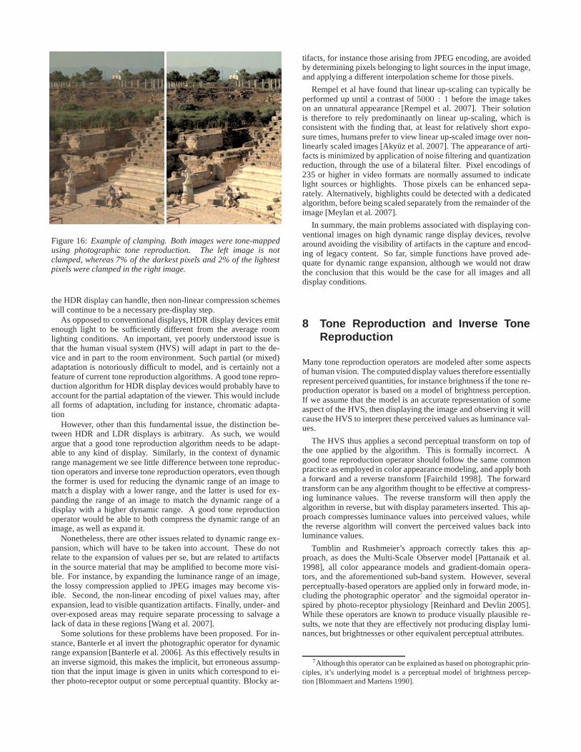
Figure 16:Example of clamping. Both images were tone-mappedusing photographic tone reproduction. The left image is notclamped, whereas 7% of the darkest pixels and 2% of the lightestpixels were clamped in the right image.

the HDR display can handle, then non-linear compression schemeswill continue to be a necessary pre-display step.

As opposed to conventional displays, HDR display devices emitenough light to be sufficiently different from the average roomlighting conditions. An important, yet poorly understood issue isthat the human visual system (HVS) will adapt in part to the de-vice and in part to the room environment. Such partial (or mixed)adaptation is notoriously difficult to model, and is certainly not afeature of current tone reproduction algorithms. A good tone repro-duction algorithm for HDR display devices would probably have toaccount for the partial adaptation of the viewer. This would includeall forms of adaptation, including for instance, chromatic adapta-tion

However, other than this fundamental issue, the distinction be-tween HDR and LDR displays is arbitrary. As such, we wouldargue that a good tone reproduction algorithm needs to be adapt-able to any kind of display. Similarly, in the context of dynamicrange management we see little difference between tone reproduc-tion operators and inverse tone reproduction operators, even thoughthe former is used for reducing the dynamic range of an image tomatch a display with a lower range, and the latter is used for ex-panding the range of an image to match the dynamic range of adisplay with a higher dynamic range. A good tone reproductionoperator would be able to both compress the dynamic range of animage, as well as expand it.

Nonetheless, there are other issues related to dynamic range ex-pansion, which will have to be taken into account. These do notrelate to the expansion of values per se, but are related to artifactsin the source material that may be amplified to become more visi-ble. For instance, by expanding the luminance range of an image,the lossy compression applied to JPEG images may become vis-ible. Second, the non-linear encoding of pixel values may, afterexpansion, lead to visible quantization artifacts. Finally, under- andover-exposed areas may require separate processing to salvage alack of data in these regions [Wang et al. 2007].

Some solutions for these problems have been proposed. For in-stance, Banterle et al invert the photographic operator for dynamicrange expansion [Banterle et al. 2006]. As this effectively results inan inverse sigmoid, this makes the implicit, but erroneous assump-tion that the input image is given in units which correspond to ei-ther photo-receptor output or some perceptual quantity. Blocky ar-

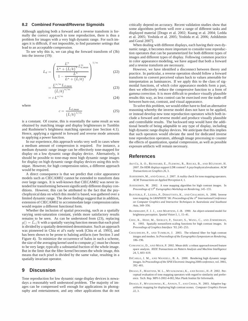
tifacts, for instance those arising from JPEG encoding, are avoidedby determining pixels belonging to light sources in the input image,and applying a different interpolation scheme for those pixels.

Rempel et al have found that linear up-scaling can typically beperformed up until a contrast of5000 : 1 before the image takeson an unnatural appearance [Rempel et al. 2007]. Their solutionis therefore to rely predominantly on linear up-scaling, which isconsistent with the finding that, at least for relatively short expo-sure times, humans prefer to view linear up-scaled image over non-linearly scaled images [Akyuz et al. 2007]. The appearance of arti-facts is minimized by application of noise filtering and quantizationreduction, through the use of a bilateral filter. Pixel encodings of235 or higher in video formats are normally assumed to indicatelight sources or highlights. Those pixels can be enhanced sepa-rately. Alternatively, highlights could be detected with a dedicatedalgorithm, before being scaled separately from the remainder of theimage [Meylan et al. 2007].

In summary, the main problems associated with displaying con-ventional images on high dynamic range display devices, revolvearound avoiding the visibility of artifacts in the capture and encod-ing of legacy content. So far, simple functions have proved ade-quate for dynamic range expansion, although we would not drawthe conclusion that this would be the case for all images and alldisplay conditions.

8 Tone Reproduction and Inverse ToneReproduction

Many tone reproduction operators are modeled after some aspectsof human vision. The computed display values therefore essentiallyrepresent perceived quantities, for instance brightness if the tone re-production operator is based on a model of brightness perception.If we assume that the model is an accurate representation of someaspect of the HVS, then displaying the image and observing it willcause the HVS to interpret these perceived values as luminance val-ues.

The HVS thus applies a second perceptual transform on top ofthe one applied by the algorithm. This is formally incorrect. Agood tone reproduction operator should follow the same commonpractice as employed in color appearance modeling, and apply botha forward and a reverse transform [Fairchild 1998]. The forwardtransform can be any algorithm thought to be effective at compress-ing luminance values. The reverse transform will then apply thealgorithm in reverse, but with display parameters inserted. This ap-proach compresses luminance values into perceived values, whilethe reverse algorithm will convert the perceived values back intoluminance values.

Tumblin and Rushmeier’s approach correctly takes this ap-proach, as does the Multi-Scale Observer model [Pattanaik et al.1998], all color appearance models and gradient-domain opera-tors, and the aforementioned sub-band system. However, severalperceptually-based operators are applied only in forward mode, in-cluding the photographic operator7 and the sigmoidal operator in-spired by photo-receptor physiology [Reinhard and Devlin 2005].While these operators are known to produce visually plausible re-sults, we note that they are effectively not producing display lumi-nances, but brightnesses or other equivalent perceptual attributes.

7Although this operator can be explained as based on photographicprin-ciples, it’s underlying model is a perceptual model of brightness percep-tion [Blommaert and Martens 1990].

8.1 Sigmoids Revisited

Here we discuss the implications of adding a reverse step to sig-moidal compression. Recall that equation (3b) can be rewritten as:

V (x, y) =Ln

v (x, y)

Lnv (x, y) + gn(x, y)

(18)

whereV is a perceived value (for instance a voltage, if this equationis thought of as a simple model of photoreceptor physiology). Thefunctiong continues to return either a globally or locally computedadaptation value, which is based on the image values.

To convert these perceived values back to luminance values, thisequation then needs to be inverted, wherebyg is replaced with a dis-play adaptation value (see also Section 4.1). For instance, we couldtry to replaceg with the mean display luminanceLd,mean. The otheruser parameter in this model is the exponentn, which for the re-verse model we will replace with a display related exponentm. Bymaking these substitutions, we have replaced all the image-relateduser parameters (n andg) with their display-related equivalents (mand Ld,mean). The resulting inverse equation, computing displayvaluesLd from previously computed perceived valuesV is then:

Ld(x, y) =

„

V (x, y)Lmd,mean

1 − V (x, y)

«1/m

(19)

For a conventional display, we would setLd,mean to 128. The expo-nentm is also a display related parameter and determines how dis-play values are spread around the mean display luminance. For lowdynamic range display devices, this value can be set to 1, therebysimplifying the above equation to:

Ld(x, y) =V (x, y) Ld,mean

1 − V (x, y)(20)

The computation of display values is now driven entirely by themean luminance of the image (through the computation ofg), themean display luminanceLd,mean, as well as the exponentn whichspecifies how large a range of values around the mean image lu-minance will be visualized. As a result, the inverse transform maycreate display values that are outside the display range. These willhave to be clamped.

As for most display devices the peak luminanceLd,max as wellas the black levelLd,min are known, it is attractive to use thesenatural boundaries to clamp the display values against. This is ar-guably a more natural choice than clamping against a percentile, asdiscussed in Section 6.2.

Given that we will gamma correct the image afterwards, we mayassume that the display range ofLd is linear. As such, we can nowcompute the mean display luminance as the average of the display’sblack level and peak luminance:

Ld,mean =1

2(Ld,min + Ld,max) (21)

As there is no good theoretical ground for choosing any specificvalue for the exponentm, we will set this parameter to1 for now.As a result, all display related parameters are fixed, leaving onlythe image-dependent parametersn as well as the choice of semi-saturation constantg(). For our example, we will follow Reinhardet al, and setg() = Lv/k, where the user parameterk determineshow overall light or dark the image should be reproduced (see Sec-tion 4.3) [Reinhard et al. 2002]. The exponentn can be thought ofas a measure of how much contrast there is in the image.

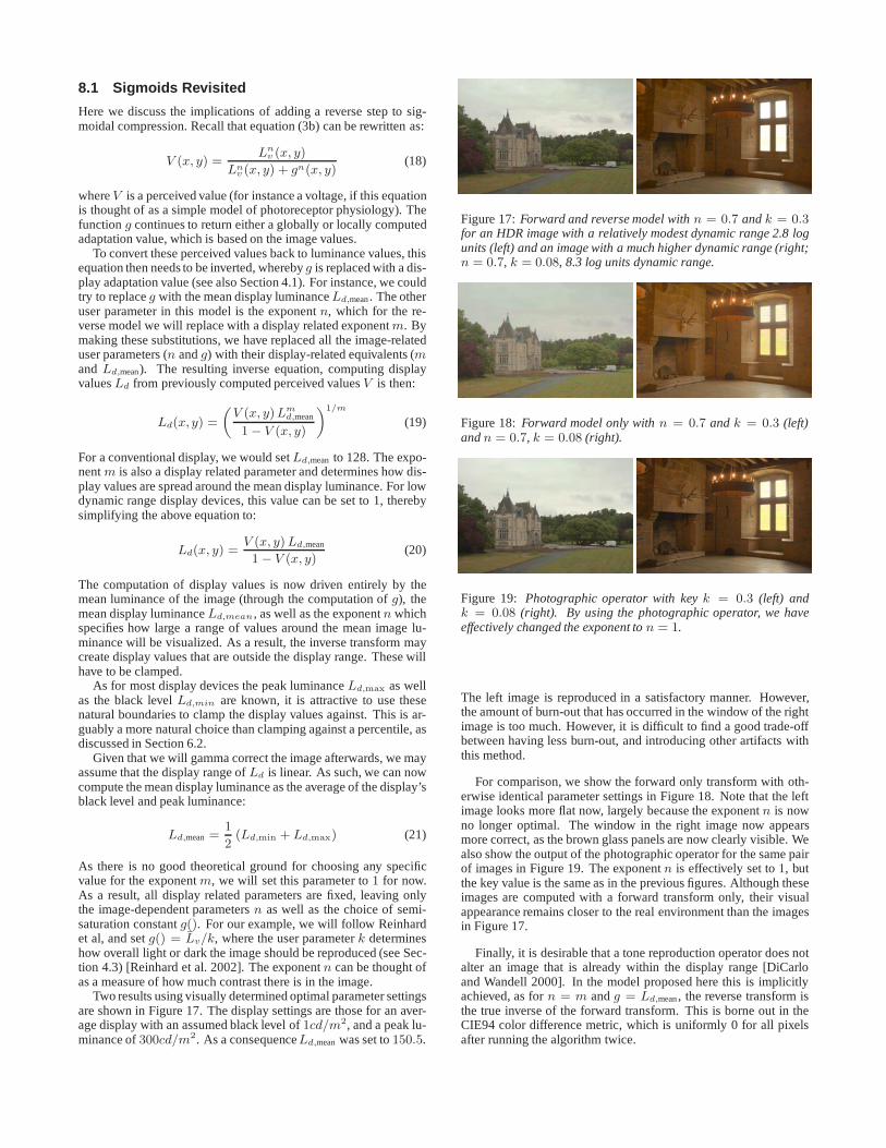
Two results using visually determined optimal parameter settingsare shown in Figure 17. The display settings are those for an aver-age display with an assumed black level of1cd/m2, and a peak lu-minance of300cd/m2. As a consequenceLd,meanwas set to150.5.

Figure 17:Forward and reverse model withn = 0.7 andk = 0.3for an HDR image with a relatively modest dynamic range 2.8 logunits (left) and an image with a much higher dynamic range (right;n = 0.7, k = 0.08, 8.3 log units dynamic range.

Figure 18:Forward model only withn = 0.7 andk = 0.3 (left)andn = 0.7, k = 0.08 (right).

Figure 19: Photographic operator with keyk = 0.3 (left) andk = 0.08 (right). By using the photographic operator, we haveeffectively changed the exponent ton = 1.

The left image is reproduced in a satisfactory manner. However,the amount of burn-out that has occurred in the window of the rightimage is too much. However, it is difficult to find a good trade-offbetween having less burn-out, and introducing other artifacts withthis method.

For comparison, we show the forward only transform with oth-erwise identical parameter settings in Figure 18. Note that the leftimage looks more flat now, largely because the exponentn is nowno longer optimal. The window in the right image now appearsmore correct, as the brown glass panels are now clearly visible. Wealso show the output of the photographic operator for the same pairof images in Figure 19. The exponentn is effectively set to1, butthe key value is the same as in the previous figures. Although theseimages are computed with a forward transform only, their visualappearance remains closer to the real environment than the imagesin Figure 17.

Finally, it is desirable that a tone reproduction operator does notalter an image that is already within the display range [DiCarloand Wandell 2000]. In the model proposed here this is implicitlyachieved, as forn = m andg = Ld,mean, the reverse transform isthe true inverse of the forward transform. This is borne out in theCIE94 color difference metric, which is uniformly 0 for all pixelsafter running the algorithm twice.

8.2 Combined Forward/Reverse Sigmoids

Although applying both a forward and a reverse transform is for-mally the correct approach to tone reproduction, there is thus aproblem for images with a very high dynamic range. For such im-ages it is difficult, if not impossible, to find parameter settings thatlead to an acceptable compression.

To see why this is, we can plug the forward transform of (3b)into the inverse (19):

Ld =

0

B

B

@

Ln

Ln +`

L/k´n Lm

d,mean

1 −Ln

Ln +`

L/k´n

1

C

C

A

1/m

(22)

=Ln/mLd,mean`

L/k´n/m

(23)

= c Ln/m (24)

where

c =Ld,mean`

L/k´n/m

(25)

is a constant. Of course, this is essentially the same result as wasobtained by matching image and display brightnesses in Tumblinand Rushmeier’s brightness matching operator (see Section 4.1).Hence, applying a sigmoid in forward and reverse mode amountsto applying a power function.

In our experience, this approach works very well in cases wherea medium amount of compression is required. For instance, amedium dynamic range image can be effectively tone-mapped fordisplay on a low dynamic range display device. Alternatively, itshould be possible to tone-map most high dynamic range imagesfor display on high dynamic range display devices using this tech-nique. However, for high compression ratios, a different approachwould be required.

A direct consequence is that we predict that color appearancemodels such as CIECAM02 cannot be extended to transform dataover large ranges. It is well-known that CIECAM02 was never in-tended for transforming between significantly different display con-ditions. However, this can be attributed to the fact that the psy-chophysical data on which this model is based, was gathered over alimited dynamic range. The above findings suggest that in addition,extension of CIECAM02 to accommodate large compression ratioswould require a different functional form.

Whether the inclusion of spatial processing, such as a spatiallyvarying semi-saturation constant, yields more satisfactory resultsremains to be seen. As can be understood from (23), replacingg() = Lv/k with a spatially varying function means that each pixelis divided by a spatially determined denominator. Such an approachwas pioneered in Chiu et al’s early work [Chiu et al. 1993], andhas been shown to be prone to haloing artifacts (see Section 3 andFigure 4). To minimize the occurrence of halos in such a scheme,the size of the averaging kernel used to computeg() must be chosento be very large; typically a substantial fraction of the whole image.But in the limit that the filter kernel becomes the whole image, thismeans that each pixel is divided by the same value, resulting in aspatially invariant operator.

9 Discussion

Tone reproduction for low dynamic range display devices is nowa-days a reasonably well understood problem. The majority of im-ages can be compressed well enough for applications in photog-raphy and entertainment, and any other applications that do not

critically depend on accuracy. Recent validation studies show thatsome algorithms perform well over a range of different tasks anddisplayed material [Drago et al. 2002; Kuang et al. 2004; Leddaet al. 2005; Yoshida et al. 2005; Yoshida et al. 2006; Ashikhminand Goral 2007].

When dealing with different displays, each having their own dy-namic range, it becomes more important to consider tone reproduc-tion operators that can be parameterized for both different types ofimages and different types of display. Following common practicein color appearance modeling, we have argued that both a forwardand a reverse transform are necessary.

However, we have identified a disconnect between theory andpractice. In particular, a reverse operation should follow a forwardtransform to convert perceived values back to values amenable forinterpretation as luminances. If we apply this to the class of sig-moidal functions, of which color appearance models form a part,then we effectively reduce the compressive function to a form ofgamma correction. It is more difficult to produce visually plausibleresults this way, as less control can be exercised over the trade-offbetween burn-out, contrast, and visual appearance.

To solve this problem, we would either have to find an alternativereasoning whereby the inverse model does not have to be applied,or instead develop new tone reproduction operators which both in-clude a forward and reverse model and produce visually plausibleand controllable results. The backward step would have the addi-tional benefit of being adaptable to any type of display, includinghigh dynamic range display devices. We anticipate that this impliesthat such operators would obviate the need for dedicated inversetone reproduction operators, although image processing to counterthe effects of quantization, spatial compression, as well as possibleexposure artifacts will remain necessary.

ReferencesAKY UZ, A. O., REINHARD, E., FLEMING , R., RIECKE, B., AND BULTHOFF, H.

2007. Do HDR displays support LDR content? A psychophysicalevaluation.ACMTransactions on Graphics 26, 3.

ASHIKHMIN , M., AND GORAL, J. 2007. A reality check for tone mapping operators.ACM Transactions on Applied Perception 4, 1.

ASHIKHMIN , M. 2002. A tone mapping algorithm for high contrast images. InProceedings of 13th Eurographics Workshop on Rendering, 145–155.

BANTERLE, F., LEDDA, P., DEBATTISTA, K., AND CHALMERS, A. 2006. Inversetone mapping. InGRAPHITE ’06: Proceedingsof the4th InternationalConferenceon Computer Graphics and Interactive Techniques in Australasia and SoutheastAsia, 349–356.

BLOMMAERT, F. J. J.,AND M ARTENS, J.-B. 1990. An object-oriented model forbrightness perception.Spatial Vision 5, 1, 15–41.

CHIU , K., HERF, M., SHIRLEY, P., SWAMY, S., WANG, C., AND Z IMMERMAN ,K. 1993. Spatially nonuniform scaling functions for high contrast images. InProceedings of Graphics Interface ’93, 245–253.

CHOUDHURY, P., AND TUMBLIN , J. 2003. The trilateral filter for high contrastimages and meshes. InProceedings of the EurographicsSymposium on Rendering,186–196.

COMANICIU , D., AND M EER, P. 2002. Mean shift: a robust approach toward featurespace analysis.IEEE Transactions on Pattern Analysis and Machine Intelligence24, 5, 603–619.

D ICARLO, J. M., AND WANDELL , B. A. 2000. Rendering high dynamic rangeimages. InProceedingsof the SPIE Electronic Imaging2000 conference, vol. 3965,392–401.

DRAGO, F., MARTENS, W. L., MYSZKOWSKI, K., AND SEIDEL, H.-P. 2002. Per-ceptual evaluation of tone mapping operators with regard to similarity and prefer-ence. Tech. Rep. MPI-I-2002-4-002, Max Plank Institut fur Informatik.

DRAGO, F., MYSZKOWSKI, K., ANNEN, T., AND CHIBA , N. 2003. Adaptive log-arithmic mapping for displaying high contrast scenes.Computer Graphics Forum22, 3.

DUAN , J., QIU , G., AND CHEN, M. 2005. Comprehensive fast tone mapping for highdynamic range image visualization. InProceedings of Pacific Graphics.

DURAND, F., AND DORSEY, J. 2002. Fast bilateral filtering for the display of high-dynamic-range images.ACM Transactions on Graphics 21, 3, 257–266.

FAIRCHILD , M. D., AND JOHNSON, G. M. 2002. Meet iCAM: an image colorappearance model. InIS&T/SID10

th Color Imaging Conference, 33–38.

FAIRCHILD , M. D., AND JOHNSON, G. M. 2004. The iCAM framework for imageappearance, image differences, and image quality.Journal of Electronic Imaging.

FAIRCHILD , M. D. 1998.Color appearance models. Addison-Wesley, Reading, MA.

FATTAL , R., LISCHINSKI, D., AND WERMAN, M. 2002. Gradient domain highdynamic range compression.ACM Transactions on Graphics 21, 3, 249–256.

FERWERDA, J. A., PATTANAIK , S., SHIRLEY, P.,AND GREENBERG, D. P. 1996. Amodel of visual adaptation for realistic image synthesis. InSIGGRAPH 96 Confer-ence Proceedings, 249–258.

FERWERDA, J. A. 2001. Elements of early vision for computer graphics.IEEEComputer Graphics and Applications 21, 5, 22–33.

HOOD, D. C., AND FINKELSTEIN, M. A. 1979. Comparison of changes in sensi-tivity and sensation: implications for the response-intensity function of the humanphotopic system.Journal of Experimental Psychology: Human Perceptual Perfor-mance 5, 3, 391–405.

HOOD, D. C., FINKELSTEIN, M. A., AND BUCKINGHAM , E. 1979. Psychophysicaltests of models of the response function.Vision Research 19, 4, 401–406.

JOBSON, D. J., RAHMAN , Z., AND WOODELL, G. A. 1995. Retinex image pro-cessing: Improved fidelity to direct visual observation. InProceedings of theIS&T Fourth Color Imaging Conference: Color Science, Systems, and Applica-tions, vol. 4, 124–125.

KLEINSCHMIDT, J.,AND DOWLING, J. E. 1975. Intracellular recordings from geckophotoreceptors during light and dark adaptation.Journal of General Physiology66, 5, 617–648.

KRAWCZYK , G., MANTIUK , R., MYSZKOWSKI, K., AND SEIDEL, H.-P. 2004.Lightness perception inspired tone mapping. InProceedings of the1st ACM Sym-posium on Applied Perception in Graphics and Visualization, 172.

KRAWCZYK , G., MYSZKOWSKI, K., AND SEIDEL, H.-P. 2005. Lightness perceptionin tone reproduction for high dynamic range images.Computer Graphics Forum24, 3, 635–645.

KRAWCZYK , G., MYSZKOWSKI, K., AND SEIDEL, H.-P. 2006. Computationalmodel of lightness perception in high dynamic range imaging. InProceedings ofIS&T/SPIE Human Vision and Electronic Imaging, vol. 6057.

KUANG, J., YAMAGUCHI , H., JOHNSON, G. M., AND FAIRCHILD , M. D. 2004.Testing HDR image renderingalgorithms. InProceedingsof IS&T/SID12

th ColorImaging Conference, 315–320.

L EDDA, P., SANTOS, L.-P.,AND CHALMERS, A. 2004. A local model of eye adapta-tion for high dynamic range images. InProceedings of ACM Afrigraph, 151–160.

L EDDA, P., CHALMERS, A., TROSCIANKO, T., AND SEETZEN, H. 2005. Evaluationof tone mapping operators using a high dynamic range display.ACM Transactionson Graphics 24, 3, 640–648.

L I , Y., SHARAN , L., AND ADELSON, E. H. 2005. Compressing and compandinghighdynamic range images with subband architectures.ACM Transactions on Graphics24, 3, 836–844.

M EYLAN , L., DALY , S.,AND SUSSTRUNK, S. 2007. Tone mapping for high dynamicrange displays. InProceedings of IS&T/SPIE Electronic Imaging: Human Visionand Electronic Imaging XII, vol. 6492.

M ILLER , N. J., NGAI , P. Y.,AND M ILLER , D. D. 1984. The application of computergraphics in lighting design.Journal of the IES 14, 6–26.

M ORONEY, N., AND TASTL, I. 2004. A comparison of retinex and iCAM for scenerendering.Journal of Electronic Imaging 13, 1.

NAKA , K. I., AND RUSHTON, W. A. H. 1966. S-potentials from luminosity units inthe retina of fish (cyprinidae).Journal of Physiology (London) 185, 3, 587–599.

OPPENHEIM, A. V., SCHAFER, R., AND STOCKHAM , T. 1968. Nonlinear filteringof multiplied and convolved signals.Proceedings of the IEEE 56, 8, 1264–1291.

PARIS, S.,AND DURAND, F. 2006. A fast approximation of the bilateral filter usinga signal processing approach. InEuropean Conference on Computer Vision.

PATTANAIK , S. N., AND YEE, H. 2002. Adaptive gain control for high dynamicrange image display. InProceedings of Spring Conference in Computer Graphics(SCCG2002), 24–27.

PATTANAIK , S. N., FERWERDA, J. A., FAIRCHILD , M. D., AND GREENBERG, D. P.1998. A multiscale model of adaptation and spatial vision for realistic image dis-play. InSIGGRAPH 98 Conference Proceedings, 287–298.

PRESS, W. H., TEUKOLSKY, S. A., VETTERLING, W. T., AND FLANNERY, B. P.1992.Numerical Recipes in C: The Art of Scientific Computing, 2nd ed. CambridgeUniversity Press.

RAHMAN , Z., JOBSON, D. J., AND WOODELL, G. A. 1996. A multiscale retinexfor color rendition and dynamic range compression. InSPIE Proceedings: Appli-cations of Digital Image Processing XIX, vol. 2847.

RAHMAN , Z., WOODELL, G. A., AND JOBSON, D. J. 1997. A comparison ofthe multiscale retinex with other image enhancement techniques. InIS&T’s 50thAnnual Conference: A Celebration of All Imaging, vol. 50, 426–431.

REINHARD, E., AND DEVLIN , K. 2005. Dynamic range reduction inspired by pho-toreceptor physiology.IEEE Transactions on Visualization and Computer Graphics11, 1, 13–24.

REINHARD, E., STARK , M., SHIRLEY, P.,AND FERWERDA, J. 2002. Photographictone reproduction for digital images.ACM Transactions on Graphics 21, 3, 267–276.

REINHARD, E., WARD, G., PATTANAIK , S., AND DEBEVEC, P. 2005. High Dy-namic Range Imaging: Acquisition, Display and Image-Based Lighting. MorganKaufmann Publishers, San Francisco.

REINHARD, E. 2003. Parameter estimation for photographic tone reproduction.Jour-nal of Graphics Tools 7, 1, 45–51.

REINHARD, E. 2007. Overview of dynamic range reduction. InThe InternationalSymposium of the Society for Information Display (SID 2007).

REMPEL, A., TRENTACOSTE, M., SEETZEN, H., YOUNG, D., HEIDRICH, W.,WHITEHEAD, L., AND WARD, G. 2007. On-the-fly reverse tone mapping oflegacy video and photographics.ACM Transactions on Graphics (Proceedings ofSIGGRAPH 2007) 26, 3.

SCHLICK , C. 1994. Quantization techniques for the visualization of high dynamicrange pictures. InPhotorealistic Rendering Techniques, Springer-Verlag, Berlin,P. Shirley, G. Sakas, and S. Muller, Eds., 7–20.

SEETZEN, H., WHITEHEAD, L. A., AND WARD, G. 2003. A high dynamic rangedisplay using low and high resolution modulators. InThe Society for InformationDisplay International Symposium.

SEETZEN, H., HEIDRICH, W., STUERZLINGER, W., WARD, G., WHITEHEAD, L.,TRENTACOSTE, M., GHOSH, A., AND VOROZCOVS, A. 2004. High dynamicrange display systems.ACM Transactions on Graphics 23, 3, 760–768.

SPILLMANN , L., AND WERNER, J. S., Eds. 1990.Visual perception: the neurologicalfoundations. Academic Press, San Diego.

TOMASI, C., AND M ANDUCHI , R. 1998. Bilateral filtering for gray and color images.In Proceedings of the IEEE International Conference on Computer Vision, 836–846.

TUMBLIN , J.,AND RUSHMEIER, H. 1993. Tone reproduction for computer generatedimages.IEEE Computer Graphics and Applications 13, 6, 42–48.

TUMBLIN , J., AND TURK, G. 1999. LCIS: A boundary hierarchy for detail-preserving contrast reduction. InSIGGRAPH 1999, Computer Graphics Proceed-ings, A. Rockwood, Ed., 83–90.

WANG, L., WEI, L.-Y., ZHOU, K., GUO, B., AND SHUM , H.-Y. 2007. High dy-namic range image hallucination. InEurographics Symposium on Rendering.

WARD, G., RUSHMEIER, H., AND PIATKO , C. 1997. A visibility matching tonereproduction operator for high dynamic range scenes.IEEE Transactions on Visu-alization and Computer Graphics 3, 4.

WARD, G. 1994. A contrast-based scalefactor for luminance display. InGraphicsGems IV, P. Heckbert, Ed. Academic Press, Boston, 415–421.

WEISS, B. 2006. Fast median and bilateral filtering.ACM Transactions on Graphics25, 3.

YOSHIDA, A., BLANZ , V., MYSZKOWSKI, K., AND SEIDEL, H.-P. 2005. Perceptualevaluation of tone mapping operators with real-world scenes. InProceedings ofSPIE Human Vision and Electronic Imaging X, vol. 5666, 192–203.

YOSHIDA, A., MANTIUK , R., MYSZKOWSKI, K., AND SEIDEL, H.-P. 2006. Anal-ysis of reproducing real-world appearance on displays of varying dynamic range.Computer Graphics Forum 25, 3, XXX.