Embed Size (px)
Citation preview

arX
iv:0
711.
1552
v2 [
mat
h.D
S] 9
Sep
200
8
HOMOTOPY METHODS FOR COUNTING REACTION NETWORKEQUILIBRIA
GHEORGHE CRACIUN, J. WILLIAM HELTON, AND RUTH J. WILLIAMS
September 9, 2008
Abstract. Dynamical system models of complex biochemical reaction networks are usu-ally high-dimensional, nonlinear, and contain many unknown parameters. In some casesthe reaction network structure dictates that positive equilibria must be unique for all val-ues of the parameters in the model. In other cases multiple equilibria exist if and only ifspecial relationships between these parameters are satisfied. We describe methods basedon homotopy invariance of degree which allow us to determine the number of equilibriafor complex biochemical reaction networks and how this number depends on parametersin the model.
1

2 CRACIUN, HELTON, AND WILLIAMS
Contents
1. Introduction 3
1.1. Overview 3
1.2. More detail 4
1.3. Organization of the paper 5
2. Examples 6
2.1. Two examples on treating boundary equilibria 6
2.2. The theory of Arcak and Sontag 10
3. Degree and homotopy of maps 10
4. Mass-dissipating dynamical systems 12
5. Dynamics of chemical reaction networks 14
5.1. The general setup 15
5.2. Mass conservation 17
5.3. Main results 18
6. Applications 19
6.1. The determinant expansion, its signs and uses 20
6.2. General reaction rate functions 22
7. Acknowledgements 25
References 26

HOMOTOPY AND COUNTING EQUILIBRIA IN REACTION NETWORKS 3
1. Introduction
Dynamical system models of complex biochemical reaction networks are usually high-dimensional, nonlinear, and contain many unknown parameters. As was shown recentlyin [CTF06], based on the assumption of mass-action kinetics, graph-theoretical propertiesof some biochemical reaction networks can guarantee the uniqueness of positive equilibriumpoints for any values of the reaction rate parameters in the model. On the other hand,relatively simple reaction networks do admit multiple positive equilibria for some values ofthe parameters as shown in [CF05,CF06,CTF06].
The aforementioned results do not address the dependence of the number of equilibria onthe parameter values unless there is a unique equilibrium for every set of parameters. Alsothey do not address the general problem of existence of positive equilibria. Here we describemethods using degree theory to analyze general biochemical dynamics (not only mass-actionkinetics). These methods allow us to determine how the number of positive equilibria fora complex biochemical reaction network depends on the parameters of the model. Theywill often also imply the existence of positive equilibria. Also we obtain uniqueness ofpositive equilibria in various situations under significantly weaker assumptions than in[CF05,CF06,CTF06].
1.1. Overview. We are interested in equilibria for high-dimensional, nonlinear dynamicalsystems that originate from chemical dynamics. These dynamical systems are systems ofordinary differential equations of the form
(1.1)dc
dt= f(c)
where f is a smooth function defined on a subset of the orthant Rn≥0 of vectors c in R
n
having nonnegative components. Such dynamical systems usually have a large number ofstate variables, i.e., n is large. In addition, the parameters defining f are often not wellknown. The focus of this paper is on equilibria for dynamical systems of the form (1.1),that is on c∗ for which f(c∗) = 0.
We consider the dynamical system (1.1) on a subset Ω of Rn≥0 which is the closure of
a domain Ω in Rn>0. We give conditions for the number of equilibria of (1.1) to remain
constant as we “continuously deform” (homotopy) the function f through a family offunctions. A key assumption is that the following condition holds for all members of thefamily:
(DetSign) The determinant of the Jacobian matrix ∂f
∂c(·) of f is either
strictly positive or strictly negative on Ω.
(Recall that the Jacobian ∂f
∂c(c) at c is the matrix
∂fj
∂ci(c), i, j = 1, . . . , n.)
4 CRACIUN, HELTON, AND WILLIAMS
What we observe is that when the condition (DetSign) holds for all f in the family and Ω isbounded, then the number of equilibria for the dynamical system (1.1) is a constant for all fin the family, provided there are no equilibria on the boundary of Ω for any f in the family(see Theorem 1.1). We further indicate how this result extends to unbounded domains suchas Ω = R
n>0 under suitable conditions (see e.g., Theorem 4.1), including those associated
with a mass-conserving reaction network operating in a chemical reactor with inflows andoutflows.
This paper extends previous findings in several ways.
The (DetSign) condition was introduced by Craciun and Feinberg [CF05,CF06] in the con-text of chemistry with Ω = R
n>0 and they observed that many chemical reaction networks
have the property (DetSign). They gave many examples and many tests for this conditionto hold in the case where f is a system of polynomials and Ω is R
n>0. Then they [CF05,CF06]
proved that if the components of f are polynomials corresponding to mass-action kinetics(operating in a continuous flow stirred tank reactor), and if (DetSign) holds on R
n>0 for all
positive “rate constants”, then for each particular choice of rate constant, when an equi-librium exists, it is unique. Here we obtain stronger conclusions with weaker assumptions.In particular the following are features of our approach.
(1) Rather than all positive “rate constants” we can select a (vector valued) rate con-stant k0 of interest at which (DetSign) holds. Then one merely needs a continuouscurve k(λ) of “rate constants” joining k0 to another k1 at which (DetSign) holdsand at which the dynamical system has a unique positive equilibrium.
(2) For a mass-conserving reaction network operating in a chemical reactor with in-flows and outflows, under the (DetSign) assumption in (1), we prove existence anduniqueness of a positive equilibrium, see Theorem 5.8.
(3) In (1) and (2), the function f need not be polynomial, but is required only to becontinuously differentiable. Of practical importance are rational f as one finds inMichaelis-Menten or Hill type chemical models, see §5, §6.
(4) We give methods, see §6, combining the items above to describe large regions ofrate constants where a chemical reaction network has a unique positive equilibrium.
We also point out in this paper that the biochemical reaction network models introducedand analyzed by Arcak and Sontag [AS06,AS08] satisfy (DetSign) and we can also rule outboundary equilibria (where they give enough data). Consequently, under extremely weakhypotheses, we obtain that each of these models has a unique positive equilibrium, see §2.2.The findings of Arcak and Sontag are impressive in that under strong hypotheses they proveglobal asymptotic stability of equilibria, a topic that this paper does not address.
1.2. More detail. Now we give some formal definitions. Let Ω be a domain in Rn, i.e.,
an open, connected set in Rn. We denote the closure of Ω by Ω and the boundary of Ω by
∂Ω. A function f : Ω → Rn is smooth if it is once continuously differentiable on Ω. If Ω

HOMOTOPY AND COUNTING EQUILIBRIA IN REACTION NETWORKS 5
is bounded, for such a smooth function f , the following norm is finite:
‖f‖Ω := supc∈Ω‖f(c)‖
Here ‖ · ‖ denotes the Euclidean norm on Rn. When Ω is bounded, a family fλ : Ω → R
n
for λ ∈ [0, 1], is a continuously varying family of functions provided each fλ is smoothand the mapping λ→ fλ is continuous on [0, 1] with the norm ‖ · ‖Ω on the functions fλ.A zero of f : Ω → R
n is a value c ∈ Ω such that f(c) = 0, where 0 is the zero vector inR
n. A zero of f is an equilibrium point for the dynamical system (1.1).
The following is an immediate consequence of Theorem 3.2 which will be proved in §3.This theorem and examples given in §2 are designed to illustrate our approach; then moretargeted theorems are given in §4 and §5, followed by more examples in §6.
Theorem 1.1. Suppose Ω ⊂ Rn is a bounded domain and fλ : Ω → R
n for λ ∈ [0, 1], isa continuously varying family of smooth functions such that fλ does not have any zeros onthe boundary of Ω for all λ ∈ [0, 1]. If det
(
∂fλ
∂c(c)
)
6= 0 for all c ∈ Ω whenever λ = 0 andwhenever λ = 1, then the number of zeros of f0 in Ω equals the number of zeros of f1 in Ω.
The domain of interest for chemical dynamics (cf. (1.1)) is typically the orthant Rn>0,
but this is not bounded, so it violates the hypothesis “Ω is bounded”. Thus in applyingTheorem 1.1 we must approximate R
n>0 by a large bounded domain Ω and check for the
absence of boundary equilibria. One can think of the boundary ∂Ω in two pieces: thatwhich intersects the boundary of R
n>0, called the sides of Ω, and the outer boundary,
∂Ω ∩ Rn>0. We show that if we assume conservation of mass (e.g., by atomic balance) in
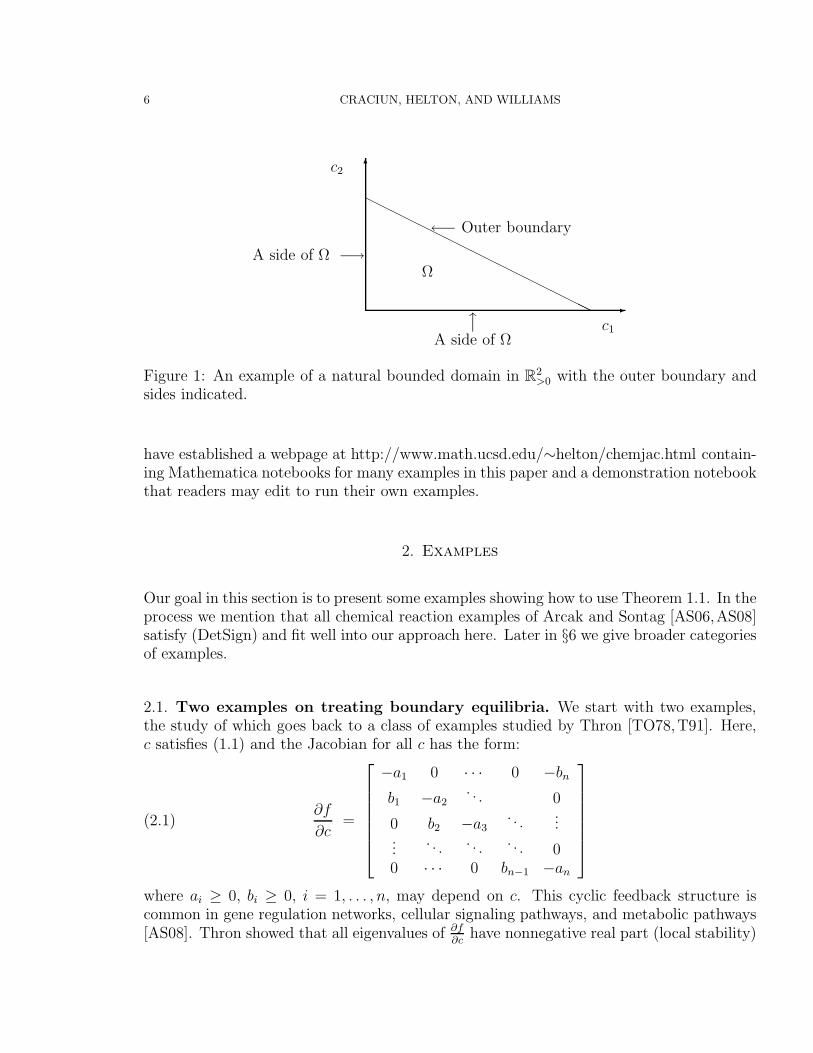
our model and augment with suitable “outflows”, then natural bounded domains Ω canbe chosen which have no equilibria on the outer boundary. An example of such a naturalbounded domain in R
2>0 is shown in Figure 1. Also under assumptions of positive invariance
and augmentation with “inflows”, there are no equilibria on the sides. In these cases weconclude that there is exactly one nonnegative equilibrium c∗ for (1.1) and that it is actuallya positive equilibrium, i.e., it lies in R
n>0. This result is described in detail in §4 and §5.
1.3. Organization of the paper. In this paper we give many examples of widely vary-ing types to illustrate our contention that our method applies broadly and is easy to use.Section 2 gives several examples illustrating Theorem 1.1. Section 3 summarizes degreetheory since our proof is based on this and relies on the observation that when (DetSign)is true, and there are no boundary equilibria, then “the degree of f with respect to 0”equals ± the number of equilibria in a bounded domain. Then in §3 we prove Theorem1.1 and more. Section 4 describes the mathematical benefits of mass dissipation (includingmass conservation) and “inflows” and “outflows”. Section 5 describes a chemical reactionnetwork framework which contains in addition to mass-action kinetics, Michaelis-Mentenand Hill dynamics. We conclude in §6 with more examples and new methods presented inthe context of these examples. For many of our examples, the determinant of the Jacobianof f was computed symbolically using Mathematica. As a complement to this paper, we
6 CRACIUN, HELTON, AND WILLIAMS
-
6
HHHHHHHHHHHHHHHHHH
←− Outer boundary
x
A side of Ωc1
A side of Ω −→
c2
Ω
Figure 1: An example of a natural bounded domain in R2>0 with the outer boundary and
sides indicated.
have established a webpage at http://www.math.ucsd.edu/∼helton/chemjac.html contain-ing Mathematica notebooks for many examples in this paper and a demonstration notebookthat readers may edit to run their own examples.
2. Examples
Our goal in this section is to present some examples showing how to use Theorem 1.1. In theprocess we mention that all chemical reaction examples of Arcak and Sontag [AS06,AS08]satisfy (DetSign) and fit well into our approach here. Later in §6 we give broader categoriesof examples.
2.1. Two examples on treating boundary equilibria. We start with two examples,the study of which goes back to a class of examples studied by Thron [TO78,T91]. Here,c satisfies (1.1) and the Jacobian for all c has the form:
(2.1)∂f
∂c=
−a1 0 · · · 0 −bn
b1 −a2. . . 0
0 b2 −a3. . .
......
. . .. . .
. . . 00 · · · 0 bn−1 −an
where ai ≥ 0, bi ≥ 0, i = 1, . . . , n, may depend on c. This cyclic feedback structure iscommon in gene regulation networks, cellular signaling pathways, and metabolic pathways[AS08]. Thron showed that all eigenvalues of ∂f
∂chave nonnegative real part (local stability)
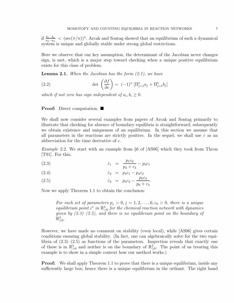
HOMOTOPY AND COUNTING EQUILIBRIA IN REACTION NETWORKS 7
if b1···bn
a1···an< (sec(π/n))n. Arcak and Sontag showed that an equilibrium of such a dynamical
system is unique and globally stable under strong global restrictions.
Here we observe that our key assumption, the determinant of the Jacobian never changessign, is met, which is a major step toward checking when a unique positive equilibriumexists for this class of problem.
Lemma 2.1. When the Jacobian has the form (2.1), we have
(2.2) det
(
∂f
∂c
)
= (−1)n [Πnj=1aj + Πn
j=1bj ]
which if not zero has sign independent of ai, bi ≥ 0.
Proof: Direct computation.
We shall now consider several examples from papers of Arcak and Sontag primarily toillustrate that checking for absence of boundary equilibria is straightforward; subsequentlywe obtain existence and uniqueness of an equilibrium. In this section we assume thatall parameters in the reactions are strictly positive. In the sequel, we shall use c as anabbreviation for the time derivative of c.
Example 2.2. We start with an example from §6 of [AS06] which they took from Thron[T91]. For this,
c1 =p1c0
p2 + c3− p3c1(2.3)
c2 = p3c1 − p4c2(2.4)
c3 = p4c2 −p5c3
p6 + c3
.(2.5)
Now we apply Theorem 1.1 to obtain the conclusion:
For each set of parameters pj > 0, j = 1, 2, . . . , 6, c0 > 0, there is a uniqueequilibrium point c∗ in R
3>0 for the chemical reaction network with dynamics
given by (2.3)–(2.5), and there is no equilibrium point on the boundary ofR
3≥0.
However, we have made no comment on stability (even local), while [AS06] gives certainconditions ensuring global stability. (In fact, one can algebraically solve for the two equi-libria of (2.3)–(2.5) as functions of the parameters. Inspection reveals that exactly oneof these is in R
3>0 and neither is on the boundary of R
3≥0. The point of us treating this
example is to show in a simple context how our method works.)
Proof: We shall apply Theorem 1.1 to prove that there is a unique equilibrium, inside anysufficiently large box; hence there is a unique equilibrium in the orthant. The right hand

8 CRACIUN, HELTON, AND WILLIAMS
side fp,c0(c) of the differential equations (2.3)–(2.5), while a function of c, also depends onpositive parameters (p, c0). One can check that the Jacobian for any of these parametershas the form in (2.1) for all c ∈ R
3>0, and since n = 3 and all parameters are strictly positive,
the Jacobian determinant is strictly negative. Note that for any two values of the positiveparameters, (p∗, c∗0) and (p†, c†0), f
λ(p∗,c∗0)+(1−λ)(p†,c
†0), λ ∈ [0, 1], defines a continuously varying
family of smooth functions on any bounded subset of Rn≥0. We check below that the no
equilibria (i.e., no zeros of f(p,c0)) on the boundary hypothesis holds on any sufficientlylarge box, for all positive parameters (p, c0), and thereby conclude using Theorem 1.1 thatthe number of equilibria of (2.3)–(2.5) in R
n>0 does not depend on (p, c0) provided the
parameters are all strictly positive. Computing the equilibria at one simple “initial” valueof (p∗, c∗0) then finishes the proof.
No equilibria on the boundary of the orthant: Suppose an equilibrium has c2 = 0. Thenequation (2.4) implies c1 = 0 which contradicts (2.3). Likewise if we start by assumingc1 = 0 we get c1 > 0 and a contradiction. On the other hand if c3 = 0, then (2.5) impliesc2 = 0, which reverts to the case considered first. Thus there are no equilibria on theboundary of R
3≥0.
No equilibria on the outer boundary of some big box: Suppose 0 < δ < 12
and 1δ
> pj > δ
for all j and c0 < 1. Pick Ω to be a box Ω := c ∈ R3>0 : cj < (1
δ)4 for j = 1, 2, 3. An
equilibrium on the outer boundary of the box satisfies
(1) c1 = (1δ)4 which by (2.3) implies (1
δ)2 > p1c0
p2+c3= p3c1 > (1
δ)3. A contradiction.
OR(2) c2 = (1
δ)4 which by (2.5) implies 1
δ> p5c3
p6+c3= p4c2 > (1
δ)3. A contradiction.
OR(3) c3 = (1
δ)4 which by adding (2.3), (2.4), (2.5) implies that
δ3 =1δ1δ4
≥p1c0
p2 + c3=
p5c3
p6 + c3≥
δ · 1δ4
1δ
+ 1δ4
=δ
δ3 + 1.
A contradiction.
Initializing: Up to this point, Theorem 1.1 tells us that each choice of parameters yields thesame number of equilibria! It is easy to compute for oneself that there is a simple choice ofparameters which yields a unique positive equilibrium, for example pj = 1 for all j yieldsthe unique equilibrium, c1 = c2 = c0
1+c0, c3 = c0. Thus there is one and only one equilibrium
in R3>0 for each value of the positive parameters (p, c0).
Example 2.3. In Example 1 of §4 in [AS08], the authors describe a simplified modelof mitogen activated protein kinase (MAPK) cascades with inhibitory feedback, proposed

HOMOTOPY AND COUNTING EQUILIBRIA IN REACTION NETWORKS 9
in [K00,SHYDWL01]. For this,
c1 = −b1c1
c1 + a1+
d1(1− c1)
e1 + (1− c1)
µ
1 + kc3(2.6)
c2 = −b2c2
c2 + a2+
d2(1− c2)
e2 + (1− c2)c1(2.7)
c3 = −b3c3
c3 + a3
+d3(1− c3)
e3 + (1− c3)c2.(2.8)
The variables cj ∈ [0, 1], j = 1, 2, 3 denote the concentrations of the active forms ofthe proteins, and the terms 1 − cj , j = 1, 2, 3, indicate the inactive forms (after non-dimensionalization and assuming that the total concentration of each of the proteins is 1).Here the parameters a1, a2, a3, b1, d1, e1, b2, d2, e2, b3, d3, e3, µ, k are strictly positive.
Let Ω := c ∈ R3 : 0 < cj < 1, j = 1, 2, 3 denote the open unit cube, the domain where
this model holds. Now we show how to apply Theorem 1.1 on Ω to conclude that:
There is a unique equilibrium in Ω for any choice of the strictly positiveparameters, a1, a2, a3, b1, d1, e1, b2, d2, e2, b3, d3, e3, µ, k.
Proof: First the Jacobian has the form (2.1). Thus (2.2) implies that the determinant isstrictly negative for all strictly positive parameters and concentrations c ∈ Ω. The prooffollows the same outline as Example 2.2. Now we check the required items:
No equilibria on the boundary of the unit cube: Suppose there is an equilibrium c onthe boundary of Ω. Then the equilibrium equations imply that
(1) If c1 = 0 then (2.6) forces c1 = 1. Contradiction.(2) If c1 = 1 then (2.6) forces c1 = 0. Contradiction.(3) If c2 = 0 then (2.7) forces c1 = 0. Contradiction as above.(4) If c2 = 1 then (2.7) forces c2 = 0. Contradiction.(5) If c3 = 0 then (2.8) forces c2 = 0. Contradiction as above.(6) If c3 = 1 then (2.8) forces c3 = 0. Contradiction.
Initializing: [AS08] proves that there are choices of parameters compatible with this modelfor which there is a unique stable equilibrium point in Ω. Alternatively, one can computefor a simple choice of parameters that there is a unique positive equilibrium.
The discussion exactly as before implies that there is a unique equilibrium for all fixedstrictly positive values of the parameters.

10 CRACIUN, HELTON, AND WILLIAMS
We mention here that the question of how one finds good intializations for the rate constantsmight be a topic for further research. The goal would be to find methods for systemati-cally selecting rate constants that produce systems whose equilibria can be determined byanalytic means. We have not explored this topic at all.
2.2. The theory of Arcak and Sontag. Now we shall make some general commentson [AS06,AS08]. There were four chemical reaction examples presented in the two papers[AS06,AS08]. So far we have treated two of the four here in this section. The third example,Example 2 in §4 of [AS08], is a small variant of Example 2.3 above and it can be treatedin a similar manner to that example. In particular, it has a Jacobian of the form (2.1). Wenow turn to the fourth example of Arcak and Sontag.
Example 2.4. This is Example 3 in §4 of [AS08] which we do not describe in detail, sinceit requires about a page. While its Jacobian does not have the form (2.1), it is easy toanalyze (using Mathematica) and what we found is that the determinant of the Jacobianof f is positive at all strictly positive c. Thus the theory described here applies providedsuitable boundary behavior holds. Boundary behavior was not possible to determine sincethe example was a rather general class whose boundary behavior was not specified. In aparticular case where more information is specified one might expect that this could bedone.
Arcak and Sontag [AS08] present a general theory which contains the examples consideredin this section and which does not match up simply with ours. Their theory assumesan equilibrium exists (we do not). It places global restrictions on the equilibrium whichguarantee that it is a unique globally stable equilibrium (we address uniqueness but notstability). However, while the Arcak-Sontag theory is different than ours, we do point outin this section that all four of their chemical examples have Jacobians whose determinantsign does not depend on chemical concentration, so our approach applies directly, and witha bit of attention to boundary behavior, gives existence of a unique positive equilibrium.However, we do not obtain the very impressive global stability in [AS08].
3. Degree and homotopy of maps
The proof of Theorem 1.1 and other results in this paper is based on classical degree theory.The degree of a function is invariant if we continuously deform (homotopy) the functionand we use that to advantage in this paper.
Now we give the setup. If Ω ⊂ Rn is a bounded domain, and if a smooth (once continuously
differentiable) function f : Ω → Rn has no degenerate zeros, and has no zeros on the
boundary of Ω, then the topological degree with respect to zero of f (or simply the degree

HOMOTOPY AND COUNTING EQUILIBRIA IN REACTION NETWORKS 11
of f) equals
(3.1) deg(f) = deg(f, Ω) =∑
c∈Zf
sgn
(
det
(
∂f
∂c(c)
))
,
where sgn : R → −1, 0, 1 is the sign function, Zf is the set of zeros of f in Ω, and c∗ is
a degenerate point means det(
∂f
∂c(c∗)
)
= 0. The degree of a map naturally extends from
nondegenerate smooth functions to continuous functions f : Ω → Rn. For this, one can
approximate f uniformly with smooth functions Fk that have no degenerate zeros and nozeros on the boundary of Ω, and then define the degree of f as the limit of the degrees ofFk. The key fact is: this construction of the degree of f is independent of the approximatesFk. Fortunately, we shall only need to compute deg(f) on smooth nondegenerate f . For aquick account of this theorem and the main properties of degree, see Ch 1.6A of [B77].
Homotopy invariance of the degree is the following well known property:
Theorem 3.1. Consider some bounded domain Ω ⊂ Rn and a continuously varying family
of smooth functions fλ : Ω→ Rn for λ ∈ [0, 1], such that fλ does not have any zeros on the
boundary of Ω for all λ ∈ [0, 1]. Then deg(fλ) is constant for all λ ∈ [0, 1].
Now we give a slightly more general theorem than Theorem 1.1 stated in the introduction.
Theorem 3.2. Suppose Ω and fλ, λ ∈ [0, 1], are as in Theorem 3.1. Then for any λ ∈ [0, 1]such that det
(
∂fλ
∂c(c)
)
6= 0 for all c ∈ Ω, the number of zeros of fλ in Ω must equal theabsolute value of the degree of fλ in Ω, which equals the absolute value of the degree of fλ′
for any λ′ ∈ [0, 1].
Proof: If λ ∈ [0, 1] is such that the determinant det(∂fλ/∂c) does not vanish in Ω, thensgn (det(∂fλ/∂c)) is independent of c. This implies that the zeros of fλ are nondegenerateand, by the formula for the degree of fλ, that | deg(fλ)| equals the number of zeros of fλ
in Ω. The fact that the degree does not vary with λ is immediate from Theorem 3.1.
Remark 3.3. For | deg(fλ)| to count the number of zeros of fλ in Ω, sgn(
det(
∂fλ
∂c(c∗)
))
needonly be the same for all zeros c∗ in Ω, not for all c ∈ Ω. Sadly this weakening of hypothesesis hard to take advantage of in practice.
Remark 3.4. From the viewpoint of numerical calculation, Theorem 3.2 strongly suggeststhat if the no boundary zeros hypothesis holds, and (DetSign) holds for f = fλ at onevalue of λ = λ1, and if one can calculate all zeros of fλ at some other value of λ = λ2
where (DetSign) also holds, then we can determine the number of zeros at λ = λ1. Indeed,often we can find a λ2 for which fλ2
is “simple” in the sense that all zeros for λ2 arenon-degenerate and the zeros can be readily computed along with the Jacobians there,and consequently deg(fλ2
) can be computed. The import for numerical calculation is thatfinding a single equilibrium is often not so onerous. After finding one equilibrium onetypically makes a new initial guess and tries to find another. Knowing if one has found

12 CRACIUN, HELTON, AND WILLIAMS
all of the equilibria is the truly daunting task, since it is nearly impossible to ensure thisby experiment. Thus theoretical results (hopefully those here) help with this very difficultcomputational question.
4. Mass-dissipating dynamical systems
In this section we consider a general dynamical system model which includes the morespecific dynamics of conservative chemical reaction networks, augmented with inflows andoutflows, as described in the next section. In chemical engineering, the latter is commonlyrefered to as dynamics that goes with a continuous flow stirred tank reactor (CFSTR).In biochemistry, one may view this as a model for intracellular behavior with productionand degradation, or with inflow and outflow across the cell boundary. Here all speciescomponents are subject to inflow and outflow, however, to approximate the conservationof some species such as enzymes, one may take the associated inflow rate value in cin anddegradation factor in Λo to be arbitrarily small, if desired.
In preparation for defining a dynamical system on the orthant Rn≥0, we consider a smooth
function g : Rn≥0 → R
n, where g has the property that for each j ∈ 1, ..., n, the jth
coordinate of g(c) is nonnegative whenever the jth coordinate of c ∈ Rn≥0 is zero. Consider
the dynamical system associated with this function given by
(4.1) c = g(c) for c ∈ Rn≥0.
This dynamical system (4.1) is called positive-invariant because of the condition on g.This guarantees that the dynamics leaves the orthant R
n≥0 invariant. Given m ∈ R
n>0, the
dynamical system (4.1) is called mass-dissipating with respect to m if
(4.2) m · g(c) ≤ 0
for all c ∈ Rn≥0; it is called mass-dissipating if it is mass-dissipating with respect to m for
some m ∈ Rn>0. In this case, on R
n≥0,
(4.3)d(m · c)
dt= m · g(c) ≤ 0.
Now we consider the dynamical system (4.1) augmented with inflows and outflows:
(4.4) c = cin − Λoc + g(c),
where Λo is an n × n diagonal matrix with strictly positive entries on the diagonal. Weinterpret the term cin ∈ R
n>0 as a constant inflow rate, and the term Λoc as an outflow
rate which for each component is proportional to the concentration of that component. Itis easy to check that with this augmentation, the dynamics still leaves the orthant R
n≥0
invariant. However, the mass-dissipating property is only inherited at large values of theconcentration c.

HOMOTOPY AND COUNTING EQUILIBRIA IN REACTION NETWORKS 13
We are now ready to state our main theorem in this context.
Theorem 4.1. Let cin, m ∈ Rn>0, and Λo be an n× n diagonal matrix with strictly positive
diagonal entries. Consider a smooth function g : Rn≥0 → R
n such that the dynamical system(4.1) is positive-invariant and mass-dissipating with respect to m. Define
f(c) := cin − Λoc + g(c) for c ∈ Rn≥0.
Then the augmented system (4.4), with inflows and outflows, has no equilibria on theboundary of R
n≥0, and if det
(
∂f
∂c
)
6= 0 on Rn>0, then there is exactly one equilibrium point
for this system in Rn>0.
Proof. It suffices to prove that f has no zeros on the boundary of Rn≥0 and if det
(
∂f
∂c
)
6= 0on R
n>0, then f has exactly one zero in R
n>0.
Definefλ(c) := cin − Λoc + λg(c), for c ∈ R
n≥0, λ ∈ [0, 1].
Fix M > m · cin and let
ΩM = c ∈ Rn>0 : m · (Λoc) < M.
Then ΩM is a bounded domain and fλ : λ ∈ [0, 1] is a continuously varying family ofsmooth functions on ΩM . For j = 1, . . . , n, consider cj ∈ ΩM such that the jth coordinateof cj is zero. Then the jth coordinate of fλ(c
j) must be strictly positive, because the jth
coordinate of cin is strictly positive, and the jth coordinate of g(cj) is nonnegative, bythe positive-invariance assumption. Therefore fλ has no zeros on the sides of ΩM , i.e., onΩM ∩ ∂R
n≥0. Also, we have
(4.5) m · fλ(c) = m · cin −m · (Λoc) + λm · g(c) ≤ m · cin −m · (Λoc) < 0
for all c ∈ ΩM such that m ·(Λoc) = M . Here we have used the mass-dissipating property ofm for the first inequality and the fact that M > m · cin for the second inequality. It followsthat fλ has no zeros on the outer boundary of ΩM , i.e., on c ∈ R
n>0 : m · (Λoc) = M.
Thus, fλ has no zeros on the boundary of ΩM for all λ ∈ [0, 1]. Then, by Theorem 3.1,the degree of fλ on ΩM , deg(fλ, ΩM), is constant for all λ ∈ [0, 1]. Next we observe
that c∗ = (Λo)−1cin is the unique zero of f0 and is inside ΩM , and ∂f
∂c= −Λo, and so
by (3.1), we obtain deg(f0, ΩM) = sgn(det(−Λo)) = (−1)n. Hence, by Theorem 3.2, ifdet
(
∂f
∂c
)
= det(
∂f1
∂c
)
6= 0 on ΩM , then f = f1 has exactly one zero in ΩM .
Since M > m · cin was arbitrary and the sets ΩM : M > m · cin fill out Rn≥0, it follows that
f has no zeros on the boundary of Rn≥0. If furthermore, det
(
∂f
∂c
)
6= 0 on all of Rn>0, then it
follows that f has exactly one zero in Rn>0.
Remark 4.2. A special case of mass-dissipating is mass-conserving, namely m·g(c) = 0. Fordynamical systems associated to chemical reaction networks this has a natural interpreta-tion. Indeed, the dynamics of chemical concentrations resulting from chemical interactionsamong several types of molecules will be mass-conserving whenever there exists a mass

14 CRACIUN, HELTON, AND WILLIAMS
assignment for each chemical species which is conserved by each reaction, or whenever eachchemical species (or molecule) is made up of atoms that are also conserved by each reaction.More generally, the dynamics will be mass-dissipating whenever no reaction produces moremass than it consumes, respectively, produces more atoms than it consumes. Mass conser-vation implies det(∂g
∂c) = 0, since m · ∂g
∂c= 0 when m ·g = 0. Thus augmenting with outflows
is required to make the hypothesis on the sign of det(∂f
∂c) in our theorems meaningful. The
paper [HKG08], which builds on the current one, introduces a more general determinantthat applies when there are no outflows (or only some outflows). This then helps one countequilibria in a manner generalizing what we have done here.
Remark 4.3. Theorem 4.1 still holds with a much less restrictive definition of mass-dissipating,e.g., by replacing “m” with the gradient “∇L” for an appropriate class of functions L :R
n≥0 → R≥0. Here mass or atom count is behaving like what is called storage function in
engineering systems theory, see [K02]. Indeed the inequality m · fλ(c) ≤ m · cin−m · (Λoc)derived in (4.5) is what is called a dissipation inequality on the storage function c→ m · c,which in fact also plays the role of a “running cost”.
5. Dynamics of chemical reaction networks
We now introduce the standard terminology of Chemical Reaction Network Theory (see[HJ72,F72,F95,CF05]). A chemical reaction network is usually specified by a finite set ofreactions R involving a finite set of chemical species S .
For example, a chemical reaction network with two chemical species A1 and A2 is schemat-ically given in the diagram
(5.1) 2A1/
)
A1 + A2o / 2A2io
The dynamics of the state of this chemical system is defined in terms of functions cA1(t)
and cA2(t) which represent the concentrations of the species A1 and A2 at time t. The
occurrence of a chemical reaction causes changes in concentrations; for instance, wheneverthe reaction A1 +A2 → 2A1 occurs, the net gain is a molecule of A1, whereas one moleculeof A2 is lost. Similarly, the reaction 2A2 → 2A1 results in the creation of two molecules ofA1 and the loss of two molecules of A2.
A common assumption is that the rate of change of the concentration of each speciesis governed by mass-action kinetics [HJ72, F72, F79, F87, F95, S01, CF05, CF06, CTF06],i.e., that each reaction takes place at a rate that is proportional to the product of theconcentrations of the species being consumed in that reaction. For example, under themass-action kinetics assumption, the contribution of the reaction A1 + A2 → 2A1 to therate of change of cA1
has the form kA1+A2→2A1cA1
cA2, where kA1+A2→2A1
is a positive number

HOMOTOPY AND COUNTING EQUILIBRIA IN REACTION NETWORKS 15
called the reaction rate constant. In the same way, the reaction 2A2 → 2A1 contributesthe negative value −2k2A2→2A1
c2A2
to the rate of change of cA2. Collecting the contributions
of all the reactions, we obtain the following dynamical system associated to the chemicalreaction network depicted in (5.1):
cA1= −k2A1→A1+A2
c2A1
+ kA1+A2→2A1cA1
cA2− kA1+A2→2A2
cA1cA2
(5.2)
+ k2A2→A1+A2c2A2− 2k2A1→2A2
c2A1
+ 2k2A2→2A1c2A2
cA2= k2A1→A1+A2
c2A1− kA1+A2→2A1
cA1cA2
+ kA1+A2→2A2cA1
cA2
− k2A2→A1+A2c2A2
+ 2k2A1→2A2c2A1− 2k2A2→2A1
c2A2
The objects on both sides of the reaction arrows (i.e., 2A1, A1 + A2, and 2A2) are calledcomplexes of the reaction network. Note that the complexes are non-negative integer com-binations of the species. On the other hand, we will see later that it is very useful to thinkof the complexes as (column) vectors in R
n, where n is the number of elements of S , via anidentification of the set of species with the standard basis of R
n, given by a fixed ordering of
the species. For example, via this identification, the complexes above become 2A1 =
[
20
]
,
A1 + A2 =
[
11
]
, and 2A2 =
[
02
]
. We can now formulate a general setup which includes
many situations, certainly those above.
5.1. The general setup. Now we present basic definitions and illustrate them.
Definition 5.1. A chemical reaction network is a triple (S , C , R), where S is a set of nchemical species, C is a finite set of vectors in R
n≥0 with nonnegative integer entries called
the set of complexes, and R ⊂ C × C is a finite set of relations between elements of C ,denoted y → y′ which represents the set of reactions in the network. Moreover, the set R
cannot contain elements of the form y → y; for any y ∈ C there exists some y′ ∈ C suchthat either y → y′ or y′ → y; and the union of the supports of all y ∈ C is S , where thesupport of an element α ∈ R
n is supp(α) = j : αj 6= 0. To each reaction y → y′ ∈ R, weassociate a reaction vector given by y′ − y.
The last two constraints of the definition amount to requiring that each complex appearsin at least one reaction, and each species appears in at least one complex. For the system(5.1), the set of species is S = A1, A2, the set of complexes is C = 2A1, A1 + A2, 2A2and the set of reactions is R = 2A1 A1 +A2, A1 +A2 2A2, 2A2 2A1, and consistsof 6 reactions, represented as three reversible reactions.

16 CRACIUN, HELTON, AND WILLIAMS
In examples we will often refer to a chemical reaction network by specifying R only, sinceR encompasses all of the information about the network. In the sequel we shall sometimessimply say reaction network in place of chemical reaction network.
Definition 5.2. A kinetics for a reaction network (S , C , R) is an assignment to eachreaction y → y′ ∈ R of a reaction rate function
Ky→y′ : Rn≥0 → R
n≥0.
By a kinetic system, which we denote by (S , C , R, K), we mean a reaction network takentogether with a kinetics.
For each concentration c ∈ Rn≥0, the nonnegative number Ky→y′(c) is interpreted as the
occurrence rate of the reaction y → y′ when the chemical mixture has concentration c.Hereafter, we suppose that reaction rate functions are smooth on R
n≥0, and that Ky→y′(c) =
0 whenever supp(y) 6⊂ supp(c). Although it will not be important in this article, it is naturalto also require that, for each y → y′ ∈ R the function Ky→y′ is strictly positive preciselywhen supp(y) ⊂ supp(c), i.e., precisely when the concentration c contains at non-zeroconcentrations those species that appear in the reactant complex y.
Definition 5.3. The species formation rate function for a kinetic system (S , C , R, K) isdefined by r : R
n≥0 → R
n where
r(c) =∑
y→y′∈R
Ky→y′(c)(y′ − y) for c ∈ Rn≥0.
The associated dynamical system for the kinetic system (S , C , R, K) is
(5.3) c = r(c) =∑
y→y′∈R
Ky→y′(c)(y′ − y),
where c ∈ Rn≥0 is the nonnegative vector of species concentrations.
The interpretation of r(·) is as follows: if the chemical concentration is c ∈ Rn≥0, then rj(c)
is the production rate of species j due to the occurrence of all chemical reactions. To seethis, note that
rj(c) =∑
y→y′∈R
Ky→y′(c)(y′j − yj),
and that y′j − yj is the net number of molecules of species j produced with each occurrence
of reaction y → y′. Thus, the right hand side of the equation above is the sum of allreaction occurrence rates, each weighted by the net gain in molecules of species j with eachoccurrence of the corresponding reaction. Note that rj(c) could be less than zero, in whichcase |rj(c)| represents the overall rate of consumption of species j.

HOMOTOPY AND COUNTING EQUILIBRIA IN REACTION NETWORKS 17
5.1.1. Special case: Mass-action kinetics.
Definition 5.4. A mass-action system is a quadruple (S , C , R, k), where (S , C , R) is achemical reaction network and k = (ky→y′) is a vector of reaction rate constants, so thatthe reaction rate function Ky→y′ : R
n≥0 → R
n≥0, for each reaction y → y′ ∈ R, is given by
mass-action kinetics :
Ky→y′(c) = ky→y′cy where cy =n
∏
i=1
cyi
i .
(Here we adopt the convention that 00 = 1.) The associated mass-action dynamical systemis
(5.4) c =∑
y→y′∈R
ky→y′cy(y′ − y).
In the vector equation (5.4), the total rate of change of the vector of concentrations c iscomputed by summing the contributions of all the reactions in R. Each reaction y → y′
contributes proportionally to the product of the concentrations of the species in its source y,that is, cy, and also proportional to the number of molecules gained or lost in this reaction.Finally, the proportionality factor is ky→y′. For example, we can rewrite (5.2) in the vectorform (5.4) as
[
c1
c2
]
= k2A1→A1+A2c21
[
−11
]
+ kA1+A2→2A1c1c2
[
1−1
]
+ kA1+A2→2A2c1c2
[
−11
]
(5.5)
+k2A2→A1+A2c22
[
1−1
]
+ k2A1→2A2c21
[
−22
]
+ k2A2→2A1c22
[
2−2
]
.
5.2. Mass conservation. Now we see in terms of this setup how one obtains mass con-servation as defined in §4.
Definition 5.5. The stoichiometric subspace S ⊂ Rn of a reaction network (S , C , R) is
the linear subspace of Rn spanned by the reaction vectors y′−y, for all reactions y → y′ ∈ R.
Note that, according to (5.3), for a given value of c, the vector c is a linear combination ofthe reaction vectors. This implies that each stoichiometric compatibility class (c0+S)∩R
n≥0
is an invariant set for the dynamical system (5.3) with initial condition c0 ∈ Rn≥0.
Definition 5.6. A reaction network (S , C , R) is called conservative if there exists somepositive vector m ∈ R
n>0 which is orthogonal to all its reaction vectors, i.e.,
m · (y′ − y) = 0
for all reactions y → y′ in R. Then m is called a conserved mass vector.
Remark 5.7. Each trajectory of a conservative reaction network is bounded. A conservativereaction network can have no inflows or outflows (see the definition of inflow and outflowin the next section).

18 CRACIUN, HELTON, AND WILLIAMS
5.3. Main results. We now consider conservative reaction networks augmented with in-flow and outflow reactions (for each of the species). An inflow reaction is a reaction of theform 0 → A and an outflow reaction is one of the form A → 0, where A is a species. Thereaction vector y′−y associated with an inflow reaction for species j is the vector containingall zeros, except that it has a one in the jth position. The reaction vector associated withan outflow reaction for species j is the negative of the vector associated with an inflowreaction for that species. Here, for the kinetics associated with the inflows and outflows,we assume that the reaction rate function for each inflow reaction is a positive constantand the value of the reaction rate function for each outflow reaction is a positive constanttimes the concentration of the species flowing out. The latter corresponds to degradationof each species at a rate proportional to its concentration. The following theorem may beused to determine the number of equilibria for conservative reaction networks augmentedby such inflows and outflows. It requires a positive determinant condition and is the analogof Theorem 4.1 in this context.
Theorem 5.8. Consider some conservative reaction network (S , C , R) with conservedmass vector m. Let K be a kinetics for this network with associated species formation ratefunction g. Consider an augmented kinetic system (S , C , R, K ) obtained by adding inflowand outflow reactions for all species so that the associated dynamical system is:
(5.6) c = r(c) := cin − Λoc + g(c),
where cin ∈ Rn>0 and Λo is an n× n diagonal matrix with strictly positive diagonal entries.
Suppose that
det
(
∂r
∂c(c)
)
6= 0,
for all c ∈ Rn>0. Then the dynamical system (5.6) has exactly one equilibrium c∗ in R
n>0
and no equilibria on the boundary of Rn≥0.
Proof. We want to apply Theorem 4.1. The function g is given by the right member of(5.3), where the functions Ky→y′ are all smooth and have the property that Ky→y′(c) = 0whenever supp(y) 6⊂ supp(c). Consequently, g is smooth and, whenever c ∈ R
n≥0 is such
that cj = 0 for some j, then we have
gj(c) ≥∑
y→y′∈R
Ky→y′(c)(−yj) = 0,
because Ky→y′(c) = 0 whenever yj > 0 and cj = 0, by the support property of K. Itfollows that the dynamical system (5.6) is positive-invariant. Furthermore, the system ismass-dissipating, since
m · g(c) =∑
y→y′∈R
Ky→y′(c) m · (y − y′) = 0,
by the assumption that the reaction network (S , C , R) is conservative. The conclusionthen follows immediately from Theorem 4.1.
HOMOTOPY AND COUNTING EQUILIBRIA IN REACTION NETWORKS 19
Remark 5.9. The results described above use the assumption that all species have inflows,in order to conclude that there are no equilibria on the boundary of R
n>0. On the other hand,
for very large classes of chemical reaction networks described in [ADS07], this assumptionis actually not needed in order to rule out the existence of such boundary equilibria (anobservation by David Anderson University of Wisconsin [A]).
Remark 5.10. The paper [BDB07], for the case of “nonautocatalytic reactions”, gives acondition on the “stoichiometric matrix” (in our terminology the matrix whose columnsare the vectors y′−y for y → y′ ∈ R) which is necessary and sufficient for the determinant ofthe Jacobian of r to be of one sign for all concentrations and all Ky→y′ which are monotoneincreasing in each variable. Our theory is less restrictive as illustrated by Example 6.1.
6. Applications
In practice, most dynamical system models of biochemical reaction networks contain a largenumber of unknown parameters. These parameters correspond to reaction rates and otherchemical properties of the reacting species. In this section we treat a variety of examples ofsuch models and illustrate the use of Theorems 4.1 and 5.8. In some of these examples, thedeterminant of the Jacobian det
(
∂r∂c
)
is of one sign everywhere on the open orthant for allparameters and in some it is not. Even in the latter cases we describe ways to find classesof rate functions for which there exists a unique positive equilibrium.
The first subsection assumes mass-action kinetics and defines (reminds) the reader of theCraciun-Feinberg “determinant expansion” via an example. Critical is the sign of eachterm in the expansion and whether all terms have the same sign or miss this by “a little”,namely, only one or two terms in the determinant expansion has a coefficient with ananomalous sign. Here we point out that all examples in [CF05,CF06,CTF06] have at mostone or two anomalous signs. When there are no anomalous signs, these papers show thatany positive equilibrium is unique for all parameter values, and they develop and use graphtheoretical methods for determining when there are no anomalous signs. Here, for cases offew anomalous signs, we propose and illustrate a technique for identifying parameter valuesfor which a positive equilibrium exists and is unique. The paper, [HKG08], subsequent tothis one, gives ways of counting the number of anomalous signs in terms of graphs associatedto a chemical reaction network.
In the second subsection, we continue with the general framework of §5, and move be-yond mass-action kinetics to rate functions satisfying certain monotonicity conditions (seeDefinitions 6.3 and 6.4). The weaker condition, Definition 6.4, holds for many biochem-ical reactions and allows one to make sense of the signs which occur in the determinantexpansion. Hence one can apply the methods in this paper.
The number of anomalous signs can be determined for the examples in this section using:(a) the graph-theoretic methods of Craciun and Feinberg [CF05,CF06] when there are no

20 CRACIUN, HELTON, AND WILLIAMS
anomalous signs and the kinetics are of mass-action type, and (b) symbolic computation ofthe determinant of the Jacobian using Mathematica when there are some anomalous signsor the kinetics are general (not necessarily mass-action). The reader will find Mathematicanotebooks at
http://www.math.ucsd.edu/∼helton/chemjac.html
for many of the examples in this section (including all of those that fall under (b)), aswell as a demonstration notebook that readers may edit to run their own examples. Thissoftware works well when the number of species is small; for larger numbers, the determinantexpansion has too many terms to be handled readily.
We conclude this preamble with some intuition underlying the case when there are anoma-lous signs. In general, we expect that for very small values of the parameters appearing inthe reaction rate functions for a conservative reaction network (and, in the limit, for vanish-ing parameter values), the dynamics of the system augmented by inflows and outflows willbe dominated by the inflow and outflow terms, and det(∂r/∂c) will not vanish; moreover, ifthe inflow and (linear) outflow terms dominate the dynamics, then the equilibrium will beunique. Examples 6.1 and 6.6 illustrate how this observation can be made rigorous and canbe used together with Theorem 5.8 and the proof of Theorem 4.1 to conclude the existenceand uniqueness of an equilibrium for a subset of the parameter space, even if the resultdoes not hold for the entire parameter space.
6.1. The determinant expansion, its signs and uses.
Example 6.1. Consider the mass-action kinetics system given by the chemical reactionnetwork (6.1), which is an irreversible version of the network shown in Table 1.1(i) of [CF05](see Table 1(i) below):
A + B → P
B + C → Q(6.1)
C → 2A
If we add inflow and outflow reactions for all species, the associated dynamical systemmodel for (6.1) is
cA = k0→A − kA→0cA − kA+B→P cAcB + 2kC→2AcC
cB = k0→B − kB→0cB − kA+B→P cAcB − kB+C→QcBcC
cC = k0→C − kC→0cC − kB+C→QcBcC − kC→2AcC(6.2)
cP = k0→P − kP→0cP + kA+B→P cAcB
cQ = k0→Q − kQ→0cQ + kB+C→QcBcC .
According to Remark 4.3 in [CF05] the dynamical system above does have multiple positiveequilibria for some values of the reaction rate parameters.

HOMOTOPY AND COUNTING EQUILIBRIA IN REACTION NETWORKS 21
If we assume that all outflow rate constants kA→0, ..., kQ→0 are equal to 1, then the deter-minant of the Jacobian of the reaction rate function is:
det(∂r/∂c) = −1 − kA+B→P cA − kB+C→QcC − kB+C→QcB
− kB+C→QkA+B→P cAcB − kC→2A − kC→2AkA+B→P cA
− kC→2AkB+C→QcC − kA+B→P cB − kA+B→PkC→2AcB(6.3)
− kA+B→PkB+C→Qc2B − kA+B→PkB+C→QcBcC
+ kA+B→P kB+C→QkC→2AcBcC .
Note that there is only one positive monomial in the expansion in (6.3). The concentrationsin it are cBcC , but there is also a negative monomial with concentrations cBcC , and thetwo combine to give
[− kA+B→P kB+C→Q + kA+B→PkB+C→QkC→2A]cBcC .
Thus if kC→2A ≤ 1, then the positive monomial will be dominated by a negative monomial.Therefore, if kC→2A ≤ 1, then det(∂r/∂c) 6= 0 for this network, everywhere on R
5>0.
Note that (mA, mB, mC , mP , mQ) = (1, 1, 2, 2, 3) is a conserved mass vector for the reactionnetwork (6.1). It follows from Theorem 5.8 that (6.2), the dynamical system for (6.1),augmented with inflows and outflows (with outflow rate constants equal to one), has aunique positive equilibrium for all positive values of the reaction rates such that kC→2A ≤ 1.Note that this uniqueness conclusion would not follow directly from the theory of [CF05,CF06] nor from that in [BDB07], since these works pertain only when the determinant hasthe same sign for all rate constants and species concentrations.
The same method can be applied to conclude that the reversible version of the reactionnetwork (6.1), augmented with inflows and outflows (with outflow rate constants set equalto one), also has a unique positive equilibrium for all positive values of the reaction ratessuch that kC→2A ≤ 1; moreover, even if the (positive) outflow rate constants kA→0, ..., kQ→0
are not necessarily equal to 1, the same conclusion holds if we know that kC→2A ≤ kC→0.
Example 6.2. Here we summarize several examples with mass-action kinetics (in the nextsubsection we consider some of these reactions with more general kinetics). Of the eightexamples in [CF05,CF06], which are chemical reaction networks augmented with inflowsand outflows (with outflow rate constants equal to one), two have the property that thecoefficients of the terms in their Jacobian determinant expansion all have the same sign,and the other six have all but one sign the same. The first observation is from [CF05] andthe second observation, emphasizing that there is only one anomalous sign, is new here. Ananalysis as in Example 6.1 can be applied here. Table 1 is a list of the examples showinghow many “anomalous” signs each determinant expansion has.
A similar accounting holds for examples of reaction networks in [CTF06], see Table 1,page 8699. These reactions involve enzymes which [CTF06] treat with mass-action kineticmodels. They find reaction networks 1,2,3,5,7,9 in this table do not have any anomalous

22 CRACIUN, HELTON, AND WILLIAMS
Reaction Num. of “anomalous” signednetwork terms in det expansion
(i) A + B P B + C Q 1C 2A
(ii) A + B P B + C Q 0C + D R D 2A
(iii) A + B P B + C Q
C + D R D + E S 1E 2A
(iv) A + B P B + C Q 0C A
(v) A + B F A + C G 1C + D B C + E D
(vi) A + B 2A 1
(vii) 2A + B 3A 1
(viii) A + 2B 3A 1
Table 1: Some examples of reaction networks and the signs of coefficients in their Jaco-bian determinant expansion when augmented with inflows and outflows (with outflow rateconstants equal to one).
signs. Here we point out that the remaining reaction networks, 4, 6 and 8 have very fewanomalous signs. The reaction network 4 is
S + E ES → E + P, I + E EI, I + ES ESI EI + S
and has only 1 “anomalous” sign, and the reaction network 6 is
S1+E ES1, S2+E ES2, S2+ES1 ES1S2 S1+ES2, ES1S2→ E +P
and has only 2 “anomalous” signs. Reaction network 8 has 4 anomalous signs out of atotal of over 3000 terms. Here all reactions are augmented by outflows with outflow rateconstants set to one. (For the cases of no anomalous signs these outflow rate constants canbe taken to be arbitrarily small without changing the answer1.) The theory of Sections 4 and5 applies, if there are (arbitrarily small) inflows and outflows, to yield that there is a uniquepositive equilibrium, for reaction networks 1,2,3,5,7,9. It also leaves open the possibilitythat one can apply the technique in Example 6.1 to get a unique positive equilibrium forcertain rate constants in reaction networks 4, 6, 8. These applications of our theory requirefinding a conserved “mass” for the system without inflow and outflow, which is easy to doin all cases.
6.2. General reaction rate functions. In this subsection, we follow the setup in §5 andmove beyond mass-action kinetics to a very general classes of rate functions.
1See [CF06iee] for how one can eliminate outflows for the enzymes.
HOMOTOPY AND COUNTING EQUILIBRIA IN REACTION NETWORKS 23
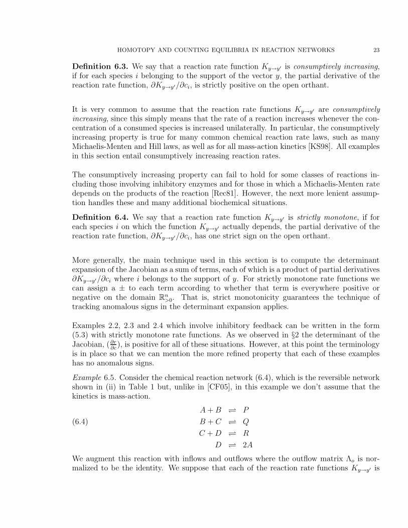
Definition 6.3. We say that a reaction rate function Ky→y′ is consumptively increasing,if for each species i belonging to the support of the vector y, the partial derivative of thereaction rate function, ∂Ky→y′/∂ci, is strictly positive on the open orthant.
It is very common to assume that the reaction rate functions Ky→y′ are consumptivelyincreasing, since this simply means that the rate of a reaction increases whenever the con-centration of a consumed species is increased unilaterally. In particular, the consumptivelyincreasing property is true for many common chemical reaction rate laws, such as manyMichaelis-Menten and Hill laws, as well as for all mass-action kinetics [KS98]. All examplesin this section entail consumptively increasing reaction rates.
The consumptively increasing property can fail to hold for some classes of reactions in-cluding those involving inhibitory enzymes and for those in which a Michaelis-Menten ratedepends on the products of the reaction [Rec81]. However, the next more lenient assump-tion handles these and many additional biochemical situations.
Definition 6.4. We say that a reaction rate function Ky→y′ is strictly monotone, if foreach species i on which the function Ky→y′ actually depends, the partial derivative of thereaction rate function, ∂Ky→y′/∂ci, has one strict sign on the open orthant.
More generally, the main technique used in this section is to compute the determinantexpansion of the Jacobian as a sum of terms, each of which is a product of partial derivatives∂Ky→y′/∂ci where i belongs to the support of y. For strictly monotone rate functions wecan assign a ± to each term according to whether that term is everywhere positive ornegative on the domain R
n>0. That is, strict monotonicity guarantees the technique of
tracking anomalous signs in the determinant expansion applies.
Examples 2.2, 2.3 and 2.4 which involve inhibitory feedback can be written in the form(5.3) with strictly monotone rate functions. As we observed in §2 the determinant of theJacobian, (∂r
∂c), is positive for all of these situations. However, at this point the terminology
is in place so that we can mention the more refined property that each of these exampleshas no anomalous signs.
Example 6.5. Consider the chemical reaction network (6.4), which is the reversible networkshown in (ii) in Table 1 but, unlike in [CF05], in this example we don’t assume that thekinetics is mass-action.
A + B P
B + C Q(6.4)
C + D R
D 2A
We augment this reaction with inflows and outflows where the outflow matrix Λo is nor-malized to be the identity. We suppose that each of the reaction rate functions Ky→y′ is

24 CRACIUN, HELTON, AND WILLIAMS
consumptively increasing as in Definition 6.3. We compute the expansion of det(∂r/∂c) interms of the partial derivatives ∂Ky→y′(c)/∂ci, for i belonging to the support of y. It isa sum of coefficients times monomials in these partial derivatives; the set of coefficients isshown in (6.5).
−1,−1,−1,−1,−1,−1,−1,−1,−1,−1,−1,−1,−1,−1,
−1,−1,−1,−1,−1,−1,−1,−2,−2,−2,−2,−2,−2,−2,
−2,−2,−2,−2,−2,−2,−3,−1,−1,−1,−1,−1,−1,−1,
−3,−1,−1,−1,−1,−1,−1,−1,−1,−1,−1,−1,−1,−1,
−2,−2,−2,−2,−2,−1,−1,−1,−1,−1,−1,−1,−1,−1,(6.5)
−1,−1,−1,−1,−1,−1,−1,−1,−2,−2,−2,−2,−2,−2,
−1,−1,−1,−1,−1,−1,−1,−1,−2,−2,−1,−1,−1,−1,
−1,−1,−1,−1,−1,−1,−1,−2,−2,−2,−2,−2,−2,−2,
−2,−1,−1,−1,−1,−1,−1,−1,−1,−2,−2,−2,−1,−1,
−1,−1,−1,−1,−2,−2,−2,−1,−1,−1,−2,−1
To summarize this list there are 138 terms in the expansion of det(∂r/∂c) and the setof coefficients of these terms contains exactly: 96 minus ones, 40 minus twos, 2 minusthrees and no positive terms. This is more information than we need, since the point isthat all these numbers are negative. This implies that det(∂r/∂c) 6= 0 for this network,for all values of c ∈ R
7>0 and all “consumptively increasing” rate laws. Also, note that
(mA, mB, mC , mD, mP , mQ, mR) = (1, 1, 1, 2, 2, 2, 3) is a conserved mass vector for the reac-tion network (6.4). Therefore, we can apply Theorem 5.8 to conclude that for the reactionnetwork (6.4) with rate laws which are all consumptively increasing, and with inflows andoutflows (with rate constants equal to one), has a unique positive equilibrium.
Example 6.6. This example is exactly parallel to Example 6.5 except that now we considerthe chemical reaction network which is the network shown in (v) in Table 1. Unlike in[CF05], in this example we don’t assume that the kinetics is mass-action. We assume thatthe reaction rate functions are consumptively increasing. Also we augment with inflowsand outflows where the outflow matrix Λo is normalized to be the identity matrix. We findthat there are 167 terms in the expansion of det(∂r/∂c) involving the partial derivativesof ∂Ky→y′/∂ci for i belonging to the support of y and the set of coefficients of these termscontains exactly: 146 minus ones, 20 minus twos and one positive term. The positive termis
K ′B→C+D(cB) K ′
D→C+E(cD) K(0,1)A+C→G(cA, cC) K
(1,0)A+B→F (cA, cB)
Here F (1,0) (resp. F (0,1)) denotes the partial derivative of F with respect to its first (re-spectively second) variable.
One can think of many conditions on the reaction rate functions that make the determinanthave one sign on the open orthant. Typically, the more complicated they look, the more
HOMOTOPY AND COUNTING EQUILIBRIA IN REACTION NETWORKS 25
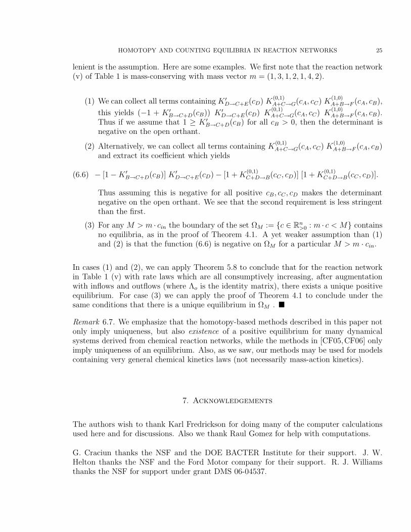
lenient is the assumption. Here are some examples. We first note that the reaction network(v) of Table 1 is mass-conserving with mass vector m = (1, 3, 1, 2, 1, 4, 2).
(1) We can collect all terms containing K ′D→C+E(cD) K
(0,1)A+C→G(cA, cC) K
(1,0)A+B→F (cA, cB),
this yields (−1 + K ′B→C+D(cB)) K ′
D→C+E(cD) K(0,1)A+C→G(cA, cC) K
(1,0)A+B→F (cA, cB).
Thus if we assume that 1 ≥ K ′B→C+D(cB) for all cB > 0, then the determinant is
negative on the open orthant.
(2) Alternatively, we can collect all terms containing K(0,1)A+C→G(cA, cC) K
(1,0)A+B→F (cA, cB)
and extract its coefficient which yields
(6.6) − [1−K ′B→C+D(cB)] K ′
D→C+E(cD)− [1 + K(0,1)C+D→B(cC , cD)] [1 + K
(0,1)C+D→B(cC , cD)].
Thus assuming this is negative for all positive cB, cC , cD makes the determinantnegative on the open orthant. We see that the second requirement is less stringentthan the first.
(3) For any M > m · cin the boundary of the set ΩM := c ∈ Rn>0 : m · c < M contains
no equilibria, as in the proof of Theorem 4.1. A yet weaker assumption than (1)and (2) is that the function (6.6) is negative on ΩM for a particular M > m · cin.
In cases (1) and (2), we can apply Theorem 5.8 to conclude that for the reaction networkin Table 1 (v) with rate laws which are all consumptively increasing, after augmentationwith inflows and outflows (where Λo is the identity matrix), there exists a unique positiveequilibrium. For case (3) we can apply the proof of Theorem 4.1 to conclude under thesame conditions that there is a unique equilibrium in ΩM .
Remark 6.7. We emphasize that the homotopy-based methods described in this paper notonly imply uniqueness, but also existence of a positive equilibrium for many dynamicalsystems derived from chemical reaction networks, while the methods in [CF05,CF06] onlyimply uniqueness of an equilibrium. Also, as we saw, our methods may be used for modelscontaining very general chemical kinetics laws (not necessarily mass-action kinetics).
7. Acknowledgements
The authors wish to thank Karl Fredrickson for doing many of the computer calculationsused here and for discussions. Also we thank Raul Gomez for help with computations.
G. Craciun thanks the NSF and the DOE BACTER Institute for their support. J. W.Helton thanks the NSF and the Ford Motor company for their support. R. J. Williamsthanks the NSF for support under grant DMS 06-04537.

26 CRACIUN, HELTON, AND WILLIAMS
References
[A] Anderson, D. personal communication.[ADS07] Angeli, D., De Leenheer, P. and Sontag, E. D. A Petri net approach to the study of persistence
in chemical reaction networks. Mathematical Biosciences, 210 (2007), 598–618.[AS06] Arcak, M. and Sontag, E. D. Diagonal stability of a class of cyclic systems and its connection with
the secant criterion. Automatica, 42 (2006), 1531–1537.[AS08] Arcak, M. and Sontag, E. D. A passivity-based stability criterion for a class of interconnected
systems and applications to biochemical reaction networks. Mathematical Biosciences and Engineering,5 (2008), 1–19.
[BDB07] Banaji, M., Donnell, P. and Baigent, S. P matrix properties, injectivity and stability in chemicalreaction systems. SIAM Journal on Applied Mathematics, 67 (2007), 1523–1547.
[B77] Berger, M. S. Nonlinearity and Functional Analysis. Academic Press, 1977.[CF05] Craciun, G. and Feinberg, M. Multiple equilibria in complex chemical reaction networks: I. The
injectivity property. SIAM Journal on Applied Mathematics, 65 (2005), 1526–1546.[CF06] Craciun, G. and Feinberg, M. Multiple equilibria in complex chemical reaction networks: II. The
SR Graph. SIAM Journal on Applied Mathematics, 66 (2006), 1321–1338.[CF06iee] Craciun, G. and Feinberg, M. Multiple equilibria in complex chemical reaction networks: exten-
sions to entrapped species models. IEE Proceedings - Systems Biology, 153 (2006), 179–186.[CTF06] Craciun G., Tang Y. and Feinberg, M. Understanding bistability in complex enzyme-driven re-
action networks. Proceedings of the National Academy of Sciences, 103 (2006), 8697–8702.[F72] Feinberg, M. Complex balancing in general kinetic systems. Archive for Rational Mechanics and
Analysis, 49 (1972), 187–194.[F79] Feinberg, M., Lectures on chemical reaction networks. Notes of lectures given
at the Mathematics Research Center of the University of Wisconsin in 1979:http://www.che.eng.ohio-state.edu/∼FEINBERG/LecturesOnReactionNetworks
[F87] Feinberg, M. Chemical reaction network structure and the stability of complex isothermal reactors I.The deficiency zero and deficiency one theorems. Chemical Engineering Science, 42 (1987), 2229–2268.
[F95] Feinberg, M. The existence and uniqueness of steady states for a class of chemical reaction networks.Archive for Rational Mechanics and Analysis, 132 (1995), 311–370.
[HKG08] Helton, J. W., Klep, I. and Gomez, R. Determinant expansions of signed matrices and of certainJacobians, preprint, 2008, http://arxiv.org/abs/0802.4319, 25 pages.
[HJ72] Horn, F. and Jackson, R. General mass-action kinetics. Archive for Rational Mechanics and Anal-
ysis, 47 (1972), 81–116.[KS98] Keener, J. and Sneyd, J. Mathematical Physiology. Springer-Verlag Interdisciplinary Applied Math-
ematics Series, Vol. 8, 1998.[K02] Khalil, H. K. Nonlinear Systems. Prentice Hall, 2002.[K00] Kholodenko, B.N. Negative feedback and ultrasensitivity can bring about oscillations in the mitogen-
activated protein kinase cascades. European Journal of Biochemistry, 267 (2000), 1583–1588.[Rec81] Recommendations of the 1981 NC-IUB panel on enzyme kinetics. Symbolism and terminology
in enzyme kinetics. Biochemical Nomenclature and Related Documents. 2nd edition, Portland Press,1992, pp. 96–106.
[SHYDWL01] Shvartsman, S. Y., Hagan, M. P., Yacoub, A., Dent, P., Wiley, H. S. and Lauffenburger, D.A. Context-dependent signaling in autocrine loops with positive feedback: Modeling and experimentsin the egfr system. American Journal of Physiology - Cell Physiology, 282 (2001), C545–C559.
[S01] Sontag, E.D. Structure and stability of certain chemical networks and applications to the kineticproofreading model of T-cell receptor signal transduction. IEEE Transactions on Automatic Control,46 (2001), 1028–1047.
[S06] Sontag, E. D. Passivity gains and the “secant condition” for stability. Systems and Control Letters,55 (2006), 177–183.

HOMOTOPY AND COUNTING EQUILIBRIA IN REACTION NETWORKS 27
[T91] Thron, C. D. The secant condition for instability in biochemical feedback control - Parts I and II.Bulletin of Mathematical Biology, 53 (1991), 383–424.
[TO78] Tyson, J. J., and Othmer, H. G. The dynamics of feedback control circuits in biochemical pathways.
In R. Rosen and F.M. Snell, editors, Progress in Theoretical Biology, 5, Academic Press, 1978, pp.1–62.
Department of Mathematics and Department of Biomolecular Chemistry, University ofWisconsin-Madison. ([email protected])
Mathematics Department, University of California at San Diego, La Jolla CA 92093-0112([email protected])
Mathematics Department, University of California at San Diego, La Jolla CA 92093-0112([email protected])


