Embed Size (px)
Citation preview
PHASE EQUILIBRIA & THERMODYNAMIC
MODELLING OF THE TERNARY SYSTEM
CO2 + 1-DECANOL + N-TETRADECANE
by
Machelle Ferreira
Dissertation presented for the Degree
of
DOCTOR OF PHILOSOPHY
(CHEMICAL ENGINEERING)
in the Faculty of Engineering
at Stellenbosch University
The financial assistance of the National Research Foundation (NRF) towards this research is hereby
acknowledged. Opinions expressed, and conclusions arrived at, are those of the author and are not
necessarily to be attributed to the NRF.
Supervisor
Prof. C.E. Schwarz
December 2018
i
DECLARATION
By submitting this thesis electronically, I declare that the entirety of the work contained therein is my
own, original work, that I am the sole author thereof (save to the extent explicitly otherwise stated), that
reproduction and publication thereof by Stellenbosch University will not infringe any third-party rights
and that I have not previously in its entirety or in part submitted it for obtaining any qualification.
Please note: In the case of dissertations in format stipulated in 2018 Policies and Rules par. 6.9.5.2
to 6.9.5.4, the following general declaration should be added as a second paragraph, in addition to the
above declaration: refer to the (par 6.11.5.4, page 215). Also refer to additional declarations in par.
6.9.15.
This dissertation includes 1 original paper published in peer-reviewed journals or books and 3
unpublished publications. The development and writing of the papers (published and unpublished) were
the principal responsibility of myself and, for each of the cases where this is not the case, a declaration
is included in the dissertation indicating the nature and extent of the contributions of co-authors.
Date: December 2018
Copyright © 2018 Stellenbosch University
All rights reserved
Stellenbosch University https://scholar.sun.ac.za

ii
Stellenbosch University https://scholar.sun.ac.za
iii
ABSTRACT
Experimental data and predictive process models, tested at various operating conditions, have shown
that supercritical fluid fractionation is a feasible process when aimed at the separation of detergent range
1-alcohols and n-alkanes with similar boiling points. Although this process shows good separation
performance, it was previously found that distinct solute + solute interactions occur that influence the
predictive capability of thermodynamic models. The aim of this study was to obtain a fundamental
understanding of the solute + solute interactions in the CO2 + 1-decanol + n-tetradecane ternary
system; firstly, through the generation of phase equilibria data and secondly, through the evaluation of
thermodynamic models, with solute + solute binary interaction parameters (BIPs) incorporated into
their algorithm, to correlate the new VLE data. The aim was achieved through the following objectives:
(1) Studying the high-pressure phase equilibria of the CO2 + 1-decanol + n-tetradecane ternary system;
(2) Studying the low-pressure phase equilibria of the 1-decanol + n-tetradecane binary system;
(3) Selecting 4 suitable thermodynamic models available within a commercial process simulator and
studying the modelling of the ternary and binary phase equilibria data with new solute + solute BIPs
obtained from the experimental data.
The first objective was met in two parts namely, the measurement of new high-pressure bubble- and
dew-point data (HPBDP) and the measurement of new high-pressure vapour-liquid equilibria data
(HPVLE). The HPBDP experiments were conducted between T = 308 K and T = 358 K using a visual
static synthetic method. CO2 free n-tetradecane mass fractions (wcred) of 0.2405, 0.5000, 0.6399, 0.7698,
0.8162 and 0.9200 g/g were investigated, and the total solute mass fractions were varied between
0.015 g/g and 0.65 g/g. An increase in the solute + solute interactions were observed when increasing
the n-tetradecane composition and decreasing the temperature. The distinct solute + solute interactions
lead to the formation of a liquid-gas hole in the three-phase surface, cosolvency effects and miscibility
windows.
For the HPVLE data, a state of the art high-pressure analytical view cell was used to study four
ternary mixtures at T = 308 K, 328 K and 348 K and pressures between P = 8.0 and 16.4 MPa. The
equipment allowed for equilibrium to be achieved after which samples of the co-existing phases were
taken simultaneously. Phase composition data for four tie lines were obtained and ternary phase
diagrams constructed. A similar outcome to the HPBDP experimental results were observed. In general,
for wcred ≥ 0.9004 g/g, 1-decanol will be the more soluble compound and for wc
red ≤ 0.2403 g/g,
n-tetradecane will be the more soluble compound. Furthermore, within the complex phase behaviour
region (wcred = ± 0.6245 g/g), separation of residual n-tetradecane from 1-decanol in the mixtures are
postulated to be impossible. However, separation experiments are required on a pilot plant setup to
verify this assumption.
Stellenbosch University https://scholar.sun.ac.za
iv
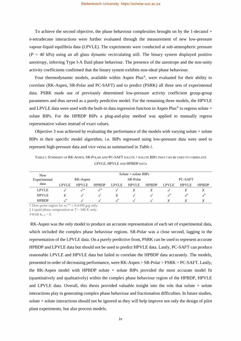
To achieve the second objective, the phase behaviour complexities brought on by the 1-decanol +
n-tetradecane interactions were further evaluated through the measurement of new low-pressure
vapour-liquid equilibria data (LPVLE). The experiments were conducted at sub-atmospheric pressure
(P = 40 kPa) using an all glass dynamic recirculating still. The binary system displayed positive
azeotropy, inferring Type I-A fluid phase behaviour. The presence of the azeotrope and the non-unity
activity coefficients confirmed that the binary system exhibits non-ideal phase behaviour.
Four thermodynamic models, available within Aspen Plus®, were evaluated for their ability to
correlate (RK-Aspen, SR-Polar and PC-SAFT) and to predict (PSRK) all three sets of experimental
data. PSRK made use of previously determined low-pressure activity coefficient group-group
parameters and thus served as a purely predictive model. For the remaining three models, the HPVLE
and LPVLE data were used with the built-in data regression function in Aspen Plus® to regress solute +
solute BIPs. For the HPBDP BIPs a plug-and-play method was applied to manually regress
representative values instead of exact values.
Objective 3 was achieved by evaluating the performance of the models with varying solute + solute
BIPs in their specific model algorithm, i.e. BIPs regressed using low-pressure data were used to
represent high-pressure data and vice versa as summarised in Table i.
TABLE I: SUMMARY OF RK-ASPEN, SR-POLAR AND PC-SAFT SOLUTE + SOLUTE BIPS THAT CAN BE USED TO CORRELATE
LPVLE, HPVLE AND HPBDP DATA
New
Experimental
data
Solute + solute BIPs
RK-Aspen SR-Polar PC-SAFT
LPVLE HPVLE HPBDP LPVLE HPVLE HPBDP LPVLE HPVLE HPBDP
LPVLE ✓ ✓⁕ ✓⁕ ✓ ✗ ✗ ✓ ✗ ✗
HPVLE ✗ ✓ ✓ ✗ ✓ ✓ ✓‡ ✓‡ ✓‡
HPBDP ✓† ✓ ✓ ✓† ✓ ✓ ✗ ✗ ✗
† Dew-point region for wcred ≤ 0.6399 g/g only.
‡ Liquid phase composition at T = 348 K only.
⁕With kb, ij = 0.
RK-Aspen was the only model to produce an accurate representation of each set of experimental data,
which included the complex phase behaviour regions. SR-Polar was a close second, lagging in the
representation of the LPVLE data. On a purely predictive front, PSRK can be used to represent accurate
HPBDP and LPVLE data but should not be used to predict HPVLE data. Lastly, PC-SAFT can produce
reasonable LPVLE and HPVLE data but failed to correlate the HPBDP data accurately. The models,
presented in order of decreasing performance, were RK-Aspen > SR-Polar > PSRK > PC-SAFT. Lastly,
the RK-Aspen model with HPBDP solute + solute BIPs provided the most accurate model fit
(quantitatively and qualitatively) within the complex phase behaviour region of the HPBDP, HPVLE
and LPVLE data. Overall, this thesis provided valuable insight into the role that solute + solute
interactions play in generating complex phase behaviour and fractionation difficulties. In future studies,
solute + solute interactions should not be ignored as they will help improve not only the design of pilot
plant experiments, but also process models.
Stellenbosch University https://scholar.sun.ac.za
v
OPSOMMING
Eksperimentele data en voorspellende prosesmodelle, wat by verskeie bedryfstoestande getoets is, het
getoon dat superkritiese vloeier fraksionering ’n lewensvatbare proses is wanneer dit gemik is op die
skeiding van 1-alkohole en n-alkane met soortgelyke kookpunte. Alhoewel hierdie proses goeie
skeiding toon, is daar voorheen bevind dat opgeloste stof interaksies die voorspellingsvermoë van
termodinamiese modelle beïnvloed. Die doel van hierdie ondersoek was om ’n fundamentele begrip
van die opgeloste stof interaksies in die CO2 + 1-dekanol + n-tetradekaan ternêre sisteem te verkry:
eerstens, deur fase-ewewigsdata te genereer, en tweedens, deur die evaluering van termodinamiese
modelle, wat van binêre interaksie parameters (BIPs) gebruik maak, om die nuwe fase-ewewigsdata te
korreleer. Hierdie doel is deur die volgende doelwitte bereik: (1) Bestudeer die hoë druk fase ewewig
van die CO2 + 1-dekanol + n-tetradekaan ternêre sisteem; (2) Bestudeer die lae druk fase ewewig van
die 1-dekanol + n-tetradekaan binêre sisteem; (3) Kies 4 gepaste termodinamiese modelle wat in ’n
kommersiële proses simulator beskikbaar is en bestudeer die termodinamiese modellering van die
ternêre en binêre fase-ewewigsdata met nuwe opgeloste stof-BIPs bepaal deur die eksperimentele data.
Die eerste doelwit is in twee dele bereik: nuwe hoë druk borrel- en doupunt data (HPBDP) en nuwe
hoë druk damp-vloeistof ewewigsdata (HPVLE) is gemeet. Die HPBDP eksperimente is tussen
T = 308 K en T = 358 K met ’n visuele staties-sintetiese metode uitgevoer. CO2-vry n-tetradekaan
massafraksies (wcred) van 0.2405, 0.5000, 0.6399, 0.7698, 0.8162 en 0.9200 g/g is bestudeer en die totale
opgeloste stof massafraksies is tussen 0.015 g/g en 0.65 g/g varieer. ’n Toename in opgeloste stof
interaksies is met ’n toename in n-tetradekaan samestelling en ’n afname in temperatuur waargeneem.
Die opgeloste stof interaksies het gelei tot die vorming van ’n vloeistof-gas gaping in die drie-fase
gebied, saam-oplosbaarheid, en mengbaarheidsgebiede.
Om die HPVLE data te meet is ’n moderne hoë druk visuele analitiese sel gebruik. Vier mengsels is
by T = 308 K, 328 K en 348 K, en by drukke tussen P = 8.0 en 16.4 MPa bestudeer. In hierdie toerusting
kan monsters van die ekwilibrium fases gelyktydig geneem word. Die fase-samestellingsdata van vier
bindlyne is verkry en ternêre fasediagramme is gekonstrueer. Die HPVLE data het soortgelyke
gevolgtrekkings as die HPBDP data na vore gebring. Oor die algemeen was 1-dekanol meer oplosbaar
vir die wcred ≥ 0.9004 g/g mengsel en n-tetradekaan meer oplosbaar vir die wc
red ≤ 0.2403 g/g mengsel.
In die komplekse fasegedragsgebied (wcred = ± 0.6245 g/g) word daar postuleer dat skeiding van
residuele n-tetradekaan van 1-dekanol onmoontlik is. Skeidingseksperimente op ’n loodsaanleg word
egter benodig om hierdie aanname te bevestig.
Om die tweede doelwit te bereik, is die komplekse fasegedrag wat deur 1-dekanol + n-tetradekaan
interaksies veroorsaak word, verder evalueer. Nuwe lae druk damp-vloeistof ewewigsdata (LPVLE) is
vir hierdie binêre stelsel by sub-atmosferiese druk (P = 40 kPa) in ’n dinamiese hersirkulerende
distilleerder gemeet. Hierdie binêre sisteem toon ’n positiewe aseotroop, wat moontlik Tipe I-A vloeier
Stellenbosch University https://scholar.sun.ac.za
vi
fasegedrag aandui. Die teenwoordigheid van ’n aseotroop en die aktiwiteitskoëffisiënt waardes het
bevestig dat die sisteem nie-ideale fasegedrag uitoefen.
Vier termodinamiese modelle, almal beskikbaar in Aspen Plus®, is evalueer op grond van hul vermoë
om die drie stelle eksperimentele data te korreleer (RK-Aspen, SR-Polar, en PC-SAFT) en te voorspel
(PSRK). PSRK gebruik voorheen bepaalde lae druk aktiwiteitskoëffisiënt groep-groep parameters en
dien dus as ’n suiwer voorspellende model. Vir die ander drie modelle is die HPVLE en LPVLE data
saam met die ingeboude regressiefunksie in Aspen Plus® gebruik om opgeloste stof BIPs te bepaal.
Verteenwoordigende waardes van die HPBDP BIPs is met die hand bepaal.
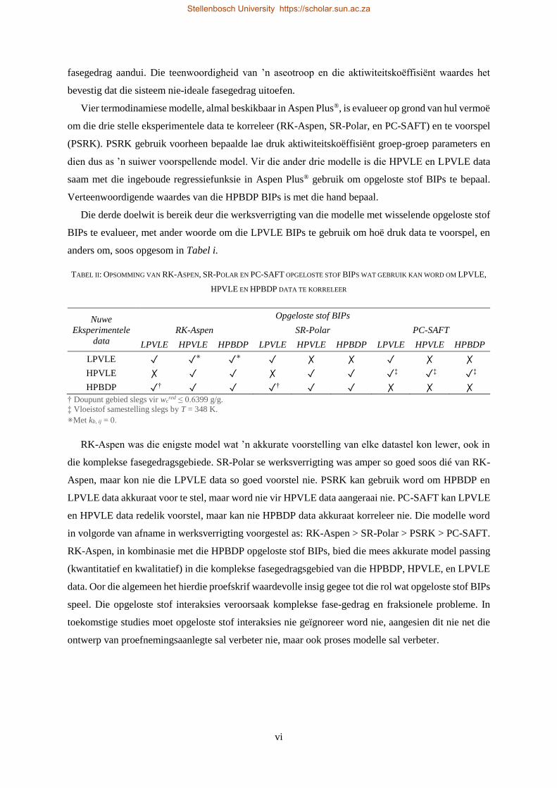
Die derde doelwit is bereik deur die werksverrigting van die modelle met wisselende opgeloste stof
BIPs te evalueer, met ander woorde om die LPVLE BIPs te gebruik om hoë druk data te voorspel, en
anders om, soos opgesom in Tabel i.
TABEL II: OPSOMMING VAN RK-ASPEN, SR-POLAR EN PC-SAFT OPGELOSTE STOF BIPS WAT GEBRUIK KAN WORD OM LPVLE,
HPVLE EN HPBDP DATA TE KORRELEER
Nuwe
Eksperimentele
data
Opgeloste stof BIPs
RK-Aspen SR-Polar PC-SAFT
LPVLE HPVLE HPBDP LPVLE HPVLE HPBDP LPVLE HPVLE HPBDP
LPVLE ✓ ✓⁕ ✓⁕ ✓ ✗ ✗ ✓ ✗ ✗
HPVLE ✗ ✓ ✓ ✗ ✓ ✓ ✓‡ ✓‡ ✓‡
HPBDP ✓† ✓ ✓ ✓† ✓ ✓ ✗ ✗ ✗
† Doupunt gebied slegs vir wcred ≤ 0.6399 g/g.
‡ Vloeistof samestelling slegs by T = 348 K.
⁕Met kb, ij = 0.
RK-Aspen was die enigste model wat ’n akkurate voorstelling van elke datastel kon lewer, ook in
die komplekse fasegedragsgebiede. SR-Polar se werksverrigting was amper so goed soos dié van RK-
Aspen, maar kon nie die LPVLE data so goed voorstel nie. PSRK kan gebruik word om HPBDP en
LPVLE data akkuraat voor te stel, maar word nie vir HPVLE data aangeraai nie. PC-SAFT kan LPVLE
en HPVLE data redelik voorstel, maar kan nie HPBDP data akkuraat korreleer nie. Die modelle word
in volgorde van afname in werksverrigting voorgestel as: RK-Aspen > SR-Polar > PSRK > PC-SAFT.
RK-Aspen, in kombinasie met die HPBDP opgeloste stof BIPs, bied die mees akkurate model passing
(kwantitatief en kwalitatief) in die komplekse fasegedragsgebied van die HPBDP, HPVLE, en LPVLE
data. Oor die algemeen het hierdie proefskrif waardevolle insig gegee tot die rol wat opgeloste stof BIPs
speel. Die opgeloste stof interaksies veroorsaak komplekse fase-gedrag en fraksionele probleme. In
toekomstige studies moet opgeloste stof interaksies nie geïgnoreer word nie, aangesien dit nie net die
ontwerp van proefnemingsaanlegte sal verbeter nie, maar ook proses modelle sal verbeter.
Stellenbosch University https://scholar.sun.ac.za

vii
ACKNOWLEDGEMENTS
This work is based on the research supported in part by the National Research Foundation of South
Africa (Grant specific unique reference number (UID) 103214) and Sasol Technology (Pty) Ltd. The
author acknowledges that opinions, findings and conclusions or recommendations expressed in this
thesis are that of the author, and that of the sponsors accepts no liability whatsoever in this regard.
Aspen Plus® is a registered trademark of aspen Technology Inc.
The author would like to express her personal gratitude to the following people who have contributed
to the completion of this work:
- My supervisor, Prof. C. E. Schwarz, not only for all your valuable guidance and great amount of
help to the successful completion of this work, but for allowing me the honour of learning from
you and always leaving your door open to me for any issues. Thank you for all your time and help,
it truly is appreciated.
- To Sonja Smith, a close friend and honoured colleague for helping me with my Afrikaans abstract.
- To the workshop staff, for always helping to fix an issue when things did not always go according
to plan.
- To Mrs. H Botha, for your guidance and expertise with the gas chromatography work.
- To my fellow colleagues and friends without whom the days would have felt unbearably long.
Thank you for the sun sessions and motivational talks over coffee when needed.
- To by brothers, Alex and Jason, thank you for being there to cheer me up at times of need and for
always understanding when I was unable to attend special moments with you.
- To my parents, Belindie and Johan, who supported me through this time not only emotionally but
at times, financially too. Without you this work would not have been possible and for that I will be
forever grateful.
- To my husband, Janti Kriel for your unwavering patience, love and support throughout this time.
Thank you for not allowing me to give up during times of struggle and always remaining by my
side.
Stellenbosch University https://scholar.sun.ac.za

viii
Stellenbosch University https://scholar.sun.ac.za
ix
NOMENCLATURE & ABBREVIATIONS
List of Symbols
Symbol Description Symbol Description
𝐴 Solvent/CO2 𝑀 Molar value
𝐴 Helmholtz energy 𝑀𝑤 Molecular weight
𝐴 Association site 𝑚 Equation of state parameter
𝐴1 1st order Van der Waals interactions 𝑚 Number of carbon atoms in 1-alcohol chain
𝐴2 2nd order Van der Waals interactions 𝑚 Mean segment number in the fluid
𝐴3 3rd order Van der Waals interactions 𝑁 Number of chemical species
𝑎 Equation of state energy parameter 𝑛 Total moles
𝐵 Solute/1-decanol 𝑛 Number of carbon atoms in n-alkane chain
𝐵 Association site ∆𝑃 Change in pressure
𝐵𝑖𝑖 Virial coefficient 𝑃 Pressure
𝑏 Equation of state co-volume parameter 𝑝1,𝑖 Pure component polar parameter
𝐶 Solute/n-tetradecane 𝑝2,𝑖 Pure component polar parameter
𝐶𝑖 Carbon chain of length i 𝑝3,𝑖 Pure component polar parameter
𝐶1 Compressibility of the hard chain fluid 𝑄 Original Van der Waals surface area
𝑐 Equation of state parameter 𝑄𝑖 Quadrupolar moment
𝑐1,𝑖 Mathias and Copeman parameter 𝑞 Group area
𝑐2,𝑖 Mathias and Copeman parameter 𝑅 Universal gas constant
𝑐3,𝑖 Mathias and Copeman parameter 𝑅 Original Van der Waals volume
𝐶1−9 Extended Antoine equation constant 𝑟 Response factor
𝐷 Parameter in L/W consistency test 𝑟 Group volume
𝑑 Equation of state parameter ∆𝑆𝑠𝑎𝑡 Entropy of vaporisation
𝑑 Segment diameter parameter ∆𝑆 Parameter in L/W consistency test
𝐹 The degrees of freedom 𝑆 Entropy
𝑓 Fugacity of a pure component 𝑇 Temperature
𝑓 Fugacity of a component in solution 𝑇𝐵 Boiling point temperature
𝐺 Gibbs free energy 𝑇𝑀 Melting point temperature
�� Partial molar Gibbs energy 𝑢 Packing fraction
𝑔𝑖𝑖ℎ𝑠(𝑑𝑖𝑖) Radial pair distribution function 𝑉 Volume
∆𝐻𝑠𝑎𝑡 Heat of vaporisation 𝑣 Specific molar volume
𝐻 Enthalpy 𝜐 Number of groups (UNIFAC)
𝐼2 Pure fluid integral of A2 𝑊 Parameter in L/W consistency test
𝐼3 Pure fluid integral of A3 𝑤 Parameter in L/W consistency test
𝐾𝑖 K-value of solute i 𝑤 Mass fraction/composition
Stellenbosch University https://scholar.sun.ac.za
x
Symbol Description Symbol Description
𝐾𝑗 K-value of solute j 𝑤𝑐𝑟𝑒𝑑 Reduced/CO2 free n-tetradecane mass fraction
𝑘𝑖𝑗 Binary interaction parameter 𝑋 Group mole fraction in the liquid
𝑘𝑎,𝑖𝑗 Energy binary interaction parameter 𝑋𝐴𝑖 Mole fraction of molecule i not bonded to site A
𝑘𝑏,𝑖𝑗 Co-volume binary interaction parameter 𝑥 Liquid mass/mole fraction
𝑘 Number of critical points for phase rule 𝑥𝑝 Fraction of dipolar/quadrupolar segment
𝑘 Boltzmann constant 𝑦 Vapour mass/mole fraction
𝐿 Parameter in L/W consistency test 𝑍𝑚 Compressibility factor
𝑙𝑖𝑗 Binary interaction parameter 𝑧 Co-ordination number
�� Partial molar property
List of Greek Symbols
Symbol Description Symbol Description
𝛼(𝑇) Equation of state parameter ∅ Critical points for phase rule
𝛼𝑖𝑗 Relative solubility 𝜑 Fugacity coefficient
𝛾 Activity coefficient �� Fugacity coefficient (species in solution)
𝛤 Activity coefficient of a group Ф Group molecular volume
𝛤(𝑇) Integration constant 𝛩 Group surface fraction
휂 Polar parameter 𝜔 Acentric factor
휂 Packing fraction 𝜌 Density
𝜇 Chemical potential 𝛿 Virial coefficient
𝜇𝑖 Dipole moment 𝜏 Generated function
𝜋 Number of phases 𝜎 Segment diameter parameter
𝜓 Generated function 𝜅𝐴𝑖𝐵𝑗 Effective association volume
휁 Reduced segment density 휀/𝑘 Segment energy parameter
∆𝐴𝐵 Association strength 휀𝐴𝑖𝐵𝑗/𝑘 Association energy parameter
Stellenbosch University https://scholar.sun.ac.za
xi
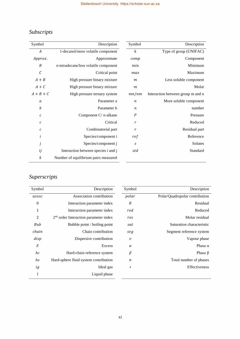
Subscripts
Symbol Description Symbol Description
𝐴 1-decanol/more volatile component 𝑘 Type of group (UNIFAC)
𝐴𝑝𝑝𝑟𝑜𝑥. Approximate 𝑐𝑜𝑚𝑝 Component
𝐵 n-tetradecane/less volatile component 𝑚𝑖𝑛 Minimum
𝐶 Critical point 𝑚𝑎𝑥 Maximum
𝐴 + 𝐵 High pressure binary mixture 𝑚 Less soluble component
𝐴 + 𝐶 High pressure binary mixture 𝑚 Molar
𝐴 + 𝐵 + 𝐶 High pressure ternary system 𝑚𝑛/𝑛𝑚 Interaction between group m and n
𝑎 Parameter a 𝑛 More soluble component
𝑏 Parameter b 𝑛 number
𝑐 Component C/ n-alkane 𝑃 Pressure
𝑐 Critical 𝑟 Reduced
𝑐 Combinatorial part 𝑟 Residual part
𝑖 Species/component i 𝑟𝑒𝑓 Reference
𝑗 Species/component j 𝑠 Solutes
𝑖𝑗 Interaction between species i and j 𝑠𝑡𝑑 Standard
𝑘 Number of equilibrium pairs measured
Superscripts
Symbol Description Symbol Description
𝑎𝑠𝑠𝑜𝑐 Association contribution 𝑝𝑜𝑙𝑎𝑟 Polar/Quadrupolar contribution
0 Interaction parameter index 𝑅 Residual
1 Interaction parameter index 𝑟𝑒𝑑 Reduced
2 2nd order Interaction parameter index 𝑟𝑒𝑠 Molar residual
𝐵𝑢𝑏 Bubble point / boiling point 𝑠𝑎𝑡 Saturation characteristic
𝑐ℎ𝑎𝑖𝑛 Chain contribution 𝑠𝑒𝑔 Segment reference system
𝑑𝑖𝑠𝑝 Dispersive contribution 𝑣 Vapour phase
𝐸 Excess 𝛼 Phase α
ℎ𝑐 Hard-chain reference system 𝛽 Phase β
ℎ𝑠 Hard-sphere fluid system contribution 𝜋 Total number of phases
𝑖𝑔 Ideal gas ∗ Effectiveness
𝑙 Liquid phase
Stellenbosch University https://scholar.sun.ac.za
xii
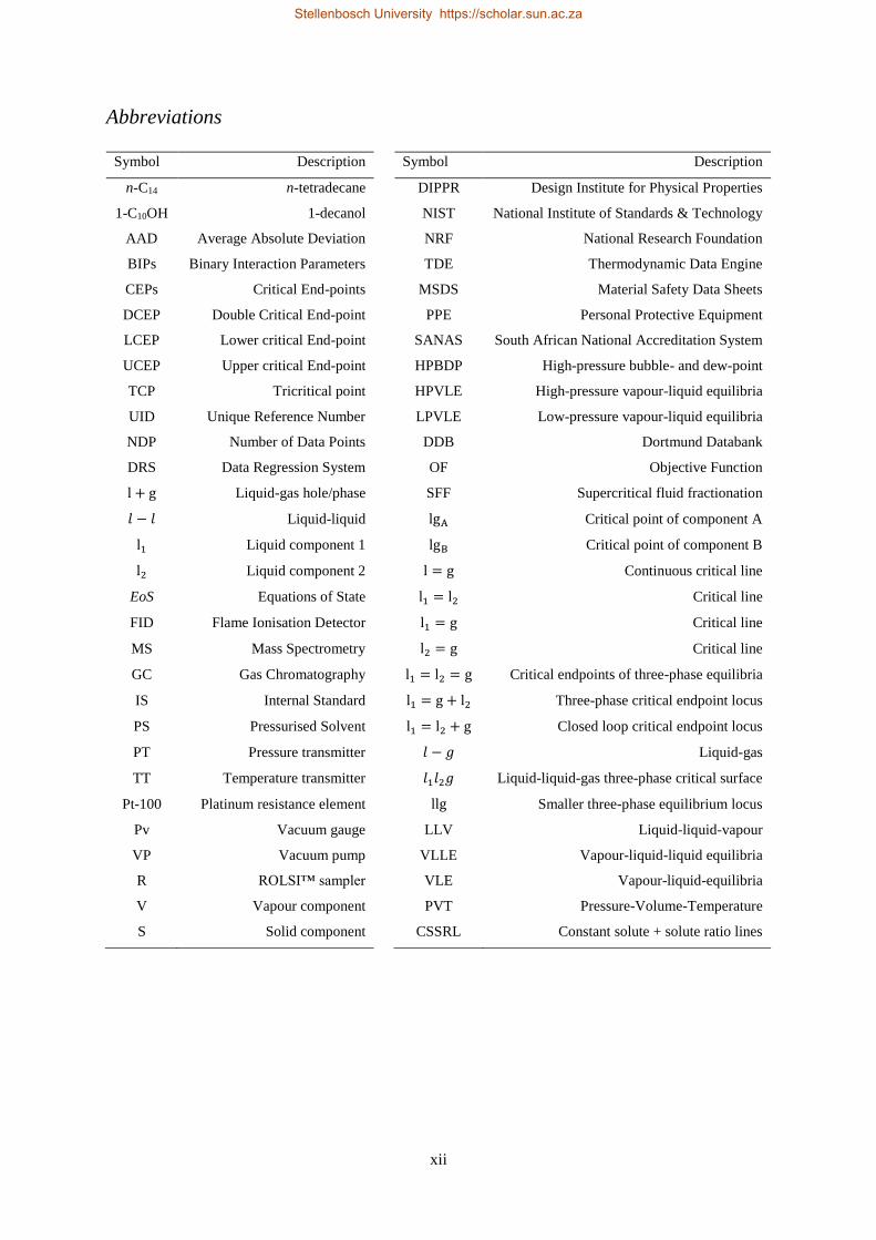
Abbreviations
Symbol Description Symbol Description
n-C14 n-tetradecane DIPPR Design Institute for Physical Properties
1-C10OH 1-decanol NIST National Institute of Standards & Technology
AAD Average Absolute Deviation NRF National Research Foundation
BIPs Binary Interaction Parameters TDE Thermodynamic Data Engine
CEPs Critical End-points MSDS Material Safety Data Sheets
DCEP Double Critical End-point PPE Personal Protective Equipment
LCEP Lower critical End-point SANAS South African National Accreditation System
UCEP Upper critical End-point HPBDP High-pressure bubble- and dew-point
TCP Tricritical point HPVLE High-pressure vapour-liquid equilibria
UID Unique Reference Number LPVLE Low-pressure vapour-liquid equilibria
NDP Number of Data Points DDB Dortmund Databank
DRS Data Regression System OF Objective Function
l + g Liquid-gas hole/phase SFF Supercritical fluid fractionation
𝑙 − 𝑙 Liquid-liquid lgA Critical point of component A
l1 Liquid component 1 lgB Critical point of component B
l2 Liquid component 2 l = g Continuous critical line
EoS Equations of State l1 = l2 Critical line
FID Flame Ionisation Detector l1 = g Critical line
MS Mass Spectrometry l2 = g Critical line
GC Gas Chromatography l1 = l2 = g Critical endpoints of three-phase equilibria
IS Internal Standard l1 = g + l2 Three-phase critical endpoint locus
PS Pressurised Solvent l1 = l2 + g Closed loop critical endpoint locus
PT Pressure transmitter 𝑙 − 𝑔 Liquid-gas
TT Temperature transmitter 𝑙1𝑙2𝑔 Liquid-liquid-gas three-phase critical surface
Pt-100 Platinum resistance element llg Smaller three-phase equilibrium locus
Pv Vacuum gauge LLV Liquid-liquid-vapour
VP Vacuum pump VLLE Vapour-liquid-liquid equilibria
R ROLSI™ sampler VLE Vapour-liquid-equilibria
V Vapour component PVT Pressure-Volume-Temperature
S Solid component CSSRL Constant solute + solute ratio lines
Stellenbosch University https://scholar.sun.ac.za
xiii
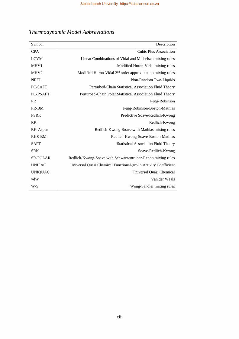
Thermodynamic Model Abbreviations
Symbol Description
CPA Cubic Plus Association
LCVM Linear Combinations of Vidal and Michelsen mixing rules
MHV1 Modified Huron-Vidal mixing rules
MHV2 Modified Huron-Vidal 2nd order approximation mixing rules
NRTL Non-Random Two-Liquids
PC-SAFT Perturbed-Chain Statistical Association Fluid Theory
PC-PSAFT Perturbed-Chain Polar Statistical Association Fluid Theory
PR Peng-Robinson
PR-BM Peng-Robinson-Boston-Mathias
PSRK Predictive Soave-Redlich-Kwong
RK Redlich-Kwong
RK-Aspen Redlich-Kwong-Soave with Mathias mixing rules
RKS-BM Redlich-Kwong-Soave-Boston-Mathias
SAFT Statistical Association Fluid Theory
SRK Soave-Redlich-Kwong
SR-POLAR Redlich-Kwong-Soave with Schwarzentruber-Renon mixing rules
UNIFAC Universal Quasi Chemical Functional-group Activity Coefficient
UNIQUAC Universal Quasi Chemical
vdW Van der Waals
W-S Wong-Sandler mixing rules
Stellenbosch University https://scholar.sun.ac.za

xiv
Stellenbosch University https://scholar.sun.ac.za
xv
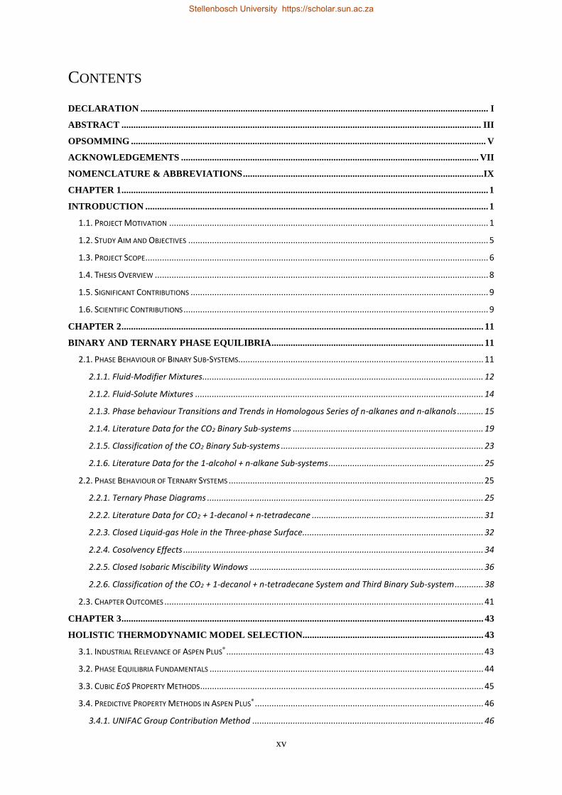
CONTENTS
DECLARATION .................................................................................................................................................. I
ABSTRACT ....................................................................................................................................................... III
OPSOMMING ..................................................................................................................................................... V
ACKNOWLEDGEMENTS ............................................................................................................................. VII
NOMENCLATURE & ABBREVIATIONS ..................................................................................................... IX
CHAPTER 1 .......................................................................................................................................................... 1
INTRODUCTION ................................................................................................................................................ 1
1.1. PROJECT MOTIVATION ...................................................................................................................................... 1
1.2. STUDY AIM AND OBJECTIVES .............................................................................................................................. 5
1.3. PROJECT SCOPE ................................................................................................................................................ 6
1.4. THESIS OVERVIEW ............................................................................................................................................ 8
1.5. SIGNIFICANT CONTRIBUTIONS ............................................................................................................................. 9
1.6. SCIENTIFIC CONTRIBUTIONS ................................................................................................................................ 9
CHAPTER 2 ........................................................................................................................................................ 11
BINARY AND TERNARY PHASE EQUILIBRIA ......................................................................................... 11
2.1. PHASE BEHAVIOUR OF BINARY SUB-SYSTEMS....................................................................................................... 11
2.1.1. Fluid-Modifier Mixtures...................................................................................................................... 12
2.1.2. Fluid-Solute Mixtures ......................................................................................................................... 14
2.1.3. Phase behaviour Transitions and Trends in Homologous Series of n-alkanes and n-alkanols ........... 15
2.1.4. Literature Data for the CO2 Binary Sub-systems ................................................................................ 19
2.1.5. Classification of the CO2 Binary Sub-systems ..................................................................................... 23
2.1.6. Literature Data for the 1-alcohol + n-alkane Sub-systems ................................................................. 25
2.2. PHASE BEHAVIOUR OF TERNARY SYSTEMS ........................................................................................................... 25
2.2.1. Ternary Phase Diagrams .................................................................................................................... 25
2.2.2. Literature Data for CO2 + 1-decanol + n-tetradecane ........................................................................ 31
2.2.3. Closed Liquid-gas Hole in the Three-phase Surface............................................................................ 32
2.2.4. Cosolvency Effects .............................................................................................................................. 34
2.2.5. Closed Isobaric Miscibility Windows .................................................................................................. 36
2.2.6. Classification of the CO2 + 1-decanol + n-tetradecane System and Third Binary Sub-system ............ 38
2.3. CHAPTER OUTCOMES ...................................................................................................................................... 41
CHAPTER 3 ........................................................................................................................................................ 43
HOLISTIC THERMODYNAMIC MODEL SELECTION............................................................................ 43
3.1. INDUSTRIAL RELEVANCE OF ASPEN PLUS® ............................................................................................................ 43
3.2. PHASE EQUILIBRIA FUNDAMENTALS ................................................................................................................... 44
3.3. CUBIC EOS PROPERTY METHODS ....................................................................................................................... 45
3.4. PREDICTIVE PROPERTY METHODS IN ASPEN PLUS® ................................................................................................ 46
3.4.1. UNIFAC Group Contribution Method ................................................................................................. 46
Stellenbosch University https://scholar.sun.ac.za
xvi
3.4.2. EoS-GE Mixing Rules ........................................................................................................................... 48
3.4.3. PSRK and RKSMHV2 Model Predictions of the CO2 Binary Sub-Systems ............................................ 50
3.4.4. Li-Correction for Size-Asymmetric Gas-Alkane Systems ..................................................................... 51
3.4.5. PSRK Model ........................................................................................................................................ 53
3.5. FLEXIBLE PROPERTY METHODS IN ASPEN PLUS® .................................................................................................... 54
3.5.1. RK-Aspen Model ................................................................................................................................. 56
3.5.2. SR-Polar Model ................................................................................................................................... 57
3.6. ASSOCIATION EOS PROPERTY METHODS IN ASPEN PLUS® ....................................................................................... 58
3.6.1. SAFT EoS Framework .......................................................................................................................... 58
3.6.2. SAFT Family Developments ................................................................................................................ 59
3.6.3. PC-SAFT Model ................................................................................................................................... 61
3.6.3.1. Hard-chain Fluids and Chain Connectivity ....................................................................................... 62
3.6.3.2. Association Term – 2B Model .......................................................................................................... 63
3.6.3.3. Dispersion Term .............................................................................................................................. 64
3.6.3.4. Polar/Quadrupolar Terms ............................................................................................................... 65
3.7. SIMULATION APPROACH .................................................................................................................................. 67
3.7.1. Pure Component Parameter Regressions ........................................................................................... 68
3.7.2. Alpha(T) Parameter Regressions ........................................................................................................ 69
3.7.3. Binary Interaction Parameter Regressions ......................................................................................... 69
3.8. CHAPTER OUTCOMES ...................................................................................................................................... 70
CHAPTER 4 ........................................................................................................................................................ 73
EXPERIMENTAL MATERIALS AND METHODS ...................................................................................... 73
4.1. MEASUREMENT TECHNIQUES............................................................................................................................ 73
4.1.1. High-Pressure Phase Equilibria .......................................................................................................... 73
4.1.2. Low-Pressure Phase Equilibria ........................................................................................................... 74
4.2. HPBDP PHASE EQUILIBRIA MEASUREMENTS ....................................................................................................... 76
4.2.1. Experimental Setup and Apparatus ................................................................................................... 76
4.2.2. Experimental Procedure ..................................................................................................................... 77
4.3. HPVLE PHASE EQUILIBRIA MEASUREMENTS ....................................................................................................... 77
4.3.1. Experimental Setup and Apparatus ................................................................................................... 77
4.3.2. Experimental Procedure ..................................................................................................................... 78
4.4. LPVLE PHASE EQUILIBRIA MEASUREMENTS ........................................................................................................ 79
4.4.1. Experimental Setup and Apparatus ................................................................................................... 79
4.4.2. Experimental Procedure ..................................................................................................................... 81
4.4.3. Experimental Error Analysis ............................................................................................................... 81
4.5. ACCURACY OF DATA ........................................................................................................................................ 83
4.5.1. Calibration Curves for GC Analysis ..................................................................................................... 83
4.5.2. High-Pressure Experimental Measurements ...................................................................................... 84
Stellenbosch University https://scholar.sun.ac.za
xvii
4.5.3. Low-Pressure Experimental Measurements ....................................................................................... 85
4.6. MATERIALS ................................................................................................................................................... 85
4.7. CHAPTER OUTCOMES ...................................................................................................................................... 87
CHAPTER 5 ........................................................................................................................................................ 89
SUPER- AND NEAR-CRITICAL PHASE EQUILIBRIA OF THE TERNARY SYSTEM CO2 + 1-
DECANOL + N-TETRADECANE ................................................................................................................... 89
5.1. HPBDP RESULTS AND DISCUSSION .................................................................................................................... 89
5.1.1. Verification of Experimental Setup .................................................................................................... 89
5.1.2. Experimental Results .......................................................................................................................... 90
5.1.3. Comparison to CO2 Binary Sub-systems ............................................................................................. 96
5.1.4. Temperature Inversions and Effects ................................................................................................... 98
5.1.5. Section Outcomes............................................................................................................................. 102
5.2. COMPLEX PHASE BEHAVIOUR ......................................................................................................................... 103
5.2.1. Azeotrope and Cosolvency Effects.................................................................................................... 103
5.2.2. Near-Critical Liquid-gas Hole ........................................................................................................... 107
5.2.3. Closed Isobaric Miscibility Windows ................................................................................................ 109
5.2.4. Section Outcomes............................................................................................................................. 110
5.3. HPVLE RESULTS AND DISCUSSION ................................................................................................................... 111
5.3.1. Verification of Experimental Setup .................................................................................................. 111
5.3.2. Experimental Results ........................................................................................................................ 113
5.3.3. Relative Solubility of the Ternary System ......................................................................................... 117
5.3.4. Section Outcomes............................................................................................................................. 119
5.4. CLASSIFICATION OF THE TERNARY SYSTEM ......................................................................................................... 120
5.4.1. Transition Sequence of Fluid Phase Behaviour ................................................................................. 120
5.4.2. Binary Sub-systems and the Ternary System ................................................................................... 120
5.4.3. Section Outcomes............................................................................................................................. 121
5.5. CHAPTER OUTCOMES .................................................................................................................................... 122
CHAPTER 6 ...................................................................................................................................................... 123
LOW PRESSURE PHASE EQUILIBRIA OF 1-ALCOHOL + N-ALKANE BINARY SYSTEMS ........ 123
6.1. VERIFICATION OF EXPERIMENTAL SETUP ............................................................................................................ 124
6.1.1. Pure Component Vapour Pressure Data .......................................................................................... 124
6.1.2. Thermodynamic Consistency Tests .................................................................................................. 125
6.1.3. Reproducibility Tests ........................................................................................................................ 126
6.2. LPVLE RESULTS AND DISCUSSION ................................................................................................................... 129
6.2.1. Experimental Difficulties .................................................................................................................. 129
6.2.2. Positive Azeotropy ............................................................................................................................ 135
6.2.3. Phase Behaviour Classification......................................................................................................... 136
6.3. CHAPTER OUTCOMES .................................................................................................................................... 136
Stellenbosch University https://scholar.sun.ac.za
xviii
CHAPTER 7 ...................................................................................................................................................... 139
PURE COMPONENT & BINARY INTERACTION PARAMETER ESTIMATION .............................. 139
7.1. PURE COMPONENT PARAMETERS .................................................................................................................... 139
7.1.1. Critical Properties and Acentric Factors ........................................................................................... 139
7.1.2. Saturated Vapour Pressure Data ..................................................................................................... 140
7.1.3. PSRK ................................................................................................................................................. 142
7.1.4. RK-Aspen and SR-Polar ..................................................................................................................... 143
7.1.5. Alpha(T) Parameter .......................................................................................................................... 144
7.1.6. PC-SAFT ............................................................................................................................................ 145
7.2. BINARY INTERACTION PARAMETERS ................................................................................................................. 146
7.2.1. Group + Group Parameters .............................................................................................................. 146
7.2.2. Solute + Solvent ................................................................................................................................ 150
7.2.3. Solute + Solute.................................................................................................................................. 151
7.2.3.1. Regressions with Bubble- and Dew-point Data ............................................................................. 152
7.2.3.2. Regressions with VLE Data ............................................................................................................ 156
7.3. CHAPTER OUTCOMES .................................................................................................................................... 157
CHAPTER 8 ...................................................................................................................................................... 159
THERMODYNAMIC MODELLING USING ASPEN PLUS® ................................................................... 159
8.1. HIGH-PRESSURE PHASE BEHAVIOUR RESULTS ..................................................................................................... 159
8.1.1. RK-Aspen .......................................................................................................................................... 160
8.1.2. SR-Polar ............................................................................................................................................ 169
8.1.3. PC-SAFT ............................................................................................................................................ 177
8.1.4. PSRK ................................................................................................................................................. 185
8.2. LOW-PRESSURE PHASE BEHAVIOUR RESULTS ...................................................................................................... 190
8.2.1. RK-Aspen .......................................................................................................................................... 190
8.2.2. SR-Polar ............................................................................................................................................ 192
8.2.3. PC-SAFT ............................................................................................................................................ 193
8.2.4. PSRK ................................................................................................................................................. 195
8.3. OPTIMUM THERMODYNAMIC MODEL & SOLUTE + SOLUTE BIPS ........................................................................... 196
8.4. CHAPTER OUTCOMES .................................................................................................................................... 205
CHAPTER 9 ...................................................................................................................................................... 209
CONCLUSIONS AND RECOMMENDATIONS .......................................................................................... 209
9.1. PART 1: ACHIEVEMENT OF KEY OBJECTIVES 1 AND 2 ........................................................................................... 210
9.2. PART 2: ACHIEVEMENT OF KEY OBJECTIVE 3 ...................................................................................................... 213
9.3. RECOMMENDATIONS FOR FUTURE WORK ......................................................................................................... 214
CHAPTER 10 .................................................................................................................................................... 217
REFERENCES ................................................................................................................................................. 217
CHAPTER 11 .................................................................................................................................................... 235
APPENDICES ................................................................................................................................................... 235
Stellenbosch University https://scholar.sun.ac.za
xix
A. SUPPLEMENTARY LITERATURE DATA ....................................................................................................................... II
A1. High-pressure Measurement Techniques ................................................................................................ II
A2. Low-pressure Measurement Techniques ................................................................................................. V
A3. Thermodynamic Consistency Tests ........................................................................................................ VII
B. DETAILED EXPERIMENTAL PROCEDURES ................................................................................................................. XII
B1. HPBDP Experimental Procedure ............................................................................................................. XII
B2. HPVLE Experimental Procedure ........................................................................................................... XVII
B3. LPVLE Experimental Procedure .............................................................................................................. XL
C. CALIBRATION DATA AND CERTIFICATES ................................................................................................................ XLII
C1. High-pressure Calibrations .................................................................................................................. XLIII
C2. Barnett Pressure Calibration .............................................................................................................. XLVII
C3. HPBDP Large Cell Pt-100 Calibration .................................................................................................. XLIX
C4. LPVLE Pt-100 Calibrations ........................................................................................................................ L
C5. Low-Pressure Calibration ...................................................................................................................... LIII
D. PRECAUTIONARY MEASURES .............................................................................................................................. LIV
E. RAW EXPERIMENTAL RESULTS ............................................................................................................................. LVI
E1. HPBDP experimental data ..................................................................................................................... LVI
E2. HPVLE experimental data ...................................................................................................................... LIX
E3. LPVLE experimental data ...................................................................................................................... LXI
F. TERNARY PHASE DIAGRAMS (HPBDP) ................................................................................................................ LXX
G. GAS CHROMATOGRAPHY CALIBRATION CURVES ................................................................................................. LXXVI
H. SUPPLEMENTARY MODELLING RESULTS ........................................................................................................... LXXXII
Stellenbosch University https://scholar.sun.ac.za

xx
Stellenbosch University https://scholar.sun.ac.za
1
Chapter 1
INTRODUCTION
The design of separation processes usually requires thermodynamic data, more specifically, phase
equilibria. As more than 40% of the cost in industrial processes are related to their specific separation
units, the need for accurate thermodynamics is imperative [1]. When commencing with the design of a
separation unit it is often questioned whether sufficient data and/or suitable models are available for the
specific process. The answer to this question varies with respect to the availability of suitable models
in process simulators. Fortunately, several commercial simulators, e.g. Aspen Plus®, have a wide
spectrum of thermodynamic models to choose from [2]. In CO2 systems containing a 1-alcohol with
m ≤ 10 and a n-alkane with n ≤ 16, where m and n represent the number of carbon atoms in the alky-
chains of the 1-alcohol and n-alkane, respectively, complex phase behaviour regions occur near the
critical point of the solvent [3]. These complexities often cause predictive and thermodynamic models
to fail for such systems. Experimental phase equilibria data can contribute to bridging this gap and aid
in the fundamental understanding of the distinct solute + solute binary interactions that occur between
these large, complex molecules when mixed with a third supercritical species.
The aim of this chapter is to introduce the topic of this thesis, define the binary sub-systems and
ternary system to be measured, formulate the aim and key objectives and provide an outline for the
project.
1.1. PROJECT MOTIVATION
Alcohols in the range C8 - C20 are commonly referred to as detergent range alcohols due to their use in
the manufacturing of detergents [4]. These detergent alcohols are further used in the chemical industry
for the manufacturing of surfactants and for the preparation of plasticizers [5], [6]. The Oxo process is
generally applied as a downstream process in the petroleum industry to synthesize alcohols in the range
C3 - C20. At times, the feedstock will be obtained directly from a synthetic fuel manufacturing plant.
The feedstock is predominantly made up of olefins but also n-alkanes and small amounts of oxygenates
[7]. On an industrial scale, the n-alkanes present in the feedstock do not take part in the alcohol
production process. Therefore, the process is often incomplete, resulting in a mixture of unconverted
C10 - C15 n-alkanes and isomeric alcohols [6], [8]. In order for the 1-alcohol to be effective in other
Stellenbosch University https://scholar.sun.ac.za
2
processes, e.g. for the production of alcohol ethoxylate surfactants, the residual n-alkanes will need to
be removed from the alcohol using a suitable post-production separation process [9].
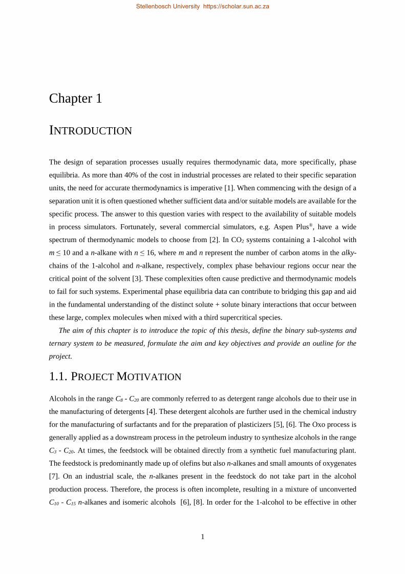
The process of separating the C10 - C15 detergent range 1-alcohols and n-alkanes is complicated by
crossover boiling (TB) and melting points (TM) as shown in Table 1-1. Experimental data and predictive
process models, tested at various operating conditions, have shown that supercritical fluid fractionation
(SFF) is a feasible process for the separation of these similar boiling point and melting point components
[4], [10]–[19]. SFF applications involve the separation of components exhibiting different phase
behaviour after a supercritical solvent is added [13]. The solvent is at conditions exceeding its critical
point and will preferentially dissolve the n-alkane, above the 1-alcohol.
TABLE 1- 1: BOILING AND MELTING POINTS OF 1-ALCOHOLS AND N-ALKANES WITHIN THE RANGE C10 –C15 [20]–[23].
Carbon
number
1-alcohol n-alkane
TB (K) TM (K) TB (K) TM (K)
C10 504 280 447 243
C11 516 292 469 247
C12 532 297 489 264
C13 554 305 509 267
C14 562 313 526 279
C15 583 317 543 289
The unique solvent characteristics of supercritical fluids were discovered over 100 years ago, after
common gases such as CO2 and ethylene were pressurised and found to dissolve complex organic
compounds [24]. Today, the most well-known example is the commercial use of supercritical fluids in
the coffee industry [24], [25]. Here, supercritical CO2 is used in the decaffeination process of coffee,
successfully replacing the organic solvent, dichloromethane, and avoiding the release of volatile organic
compounds. Increased research efforts from both academic and industrial sectors have shown that
supercritical CO2 can further be applied in old and new applications, like extraction, dying, cleaning,
polymer processing and waste water treatment, to name only a few [26]–[28]. The use of CO2 in other
industrial processes such as polymerization and organic synthesis has not yet been fully developed but
shows potential. Thus, improvements on existing separation processes will continue for years to come.
The critical properties of CO2, Tc = 304.2 K and Pc = 7.38 MPa, make it ideal for separating detergent
range alkanes and alcohols [20]. Furthermore, CO2 is non-toxic, non-flammable, inert and easy to
acquire. It is for these reasons that CO2 is the selected solvent for use in this study.
Supercritical CO2 has shown success in separating detergent range alcohols and n-alkanes, amongst
others 1-decanol and n-dodecane [13], [16], [19]. The phase behaviour of the ternary CO2 + 1-decanol +
n-dodecane system revealed significant interactions between the detergent range 1-alcohol and n-alkane
in the presence of supercritical CO2. Another study conducted on the separation of 1-dodecanol and
n-tetradecane in the presence of supercritical CO2 shows similar interactions between the 1-alcohol and
Stellenbosch University https://scholar.sun.ac.za
3
n-alkane [11], [17]. In both studies, components with close boiling points were investigated with the
n-alkane having a slightly lower normal boiling point than the 1-alcohol. To maintain the close boiling
point perspective this project studies the binary interactions between 1-decanol and n-tetradecane in the
presence of supercritical CO2. Here, in this system, the 1-alcohol is more volatile than the n-alkane but
at the same time, the 1-alcohol is less soluble in CO2 than the n-alkane [17], [18]. The physical
properties of the components used in this work are presented in Table 1-2.
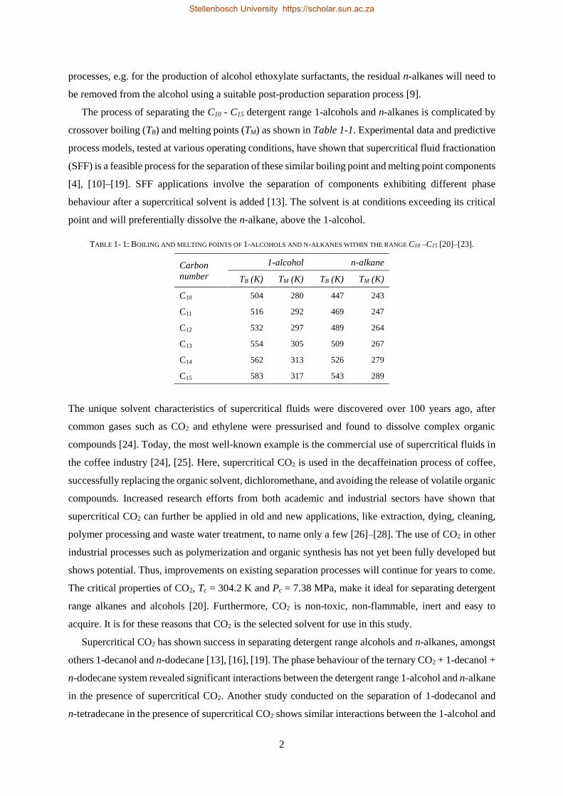
TABLE 1- 2: PHYSICAL PROPERTIES OF CO2, 1-DECANOL AND N-TETRADECANE [20]–[23]. THE 3D STRUCTURES WERE DRAWN
USING CHEMSKETCH [29].
Compound CO2 1-decanol n-tetradecane
3D Structure
Carbon number C C10 C14
Molecular Weight (g/mol) 44.01 158.28 193.39
Normal TB (K) 194.7‡ 504 526
Normal TM (K) 194.7† 280 279
Polarity Quadrupolar Slightly Polar Non-polar
Density (kg/m3) 1.98 829.7 762.8
Critical Temperature (K) 304.2 688 693
Critical Pressure (bar) 7.38 23.1 15.7
† At 1 atm, gas deposits directly to a solid at T < 194.7 K
‡ At 1 atm, the solid sublimes directly to a gat at T > 194.7 K
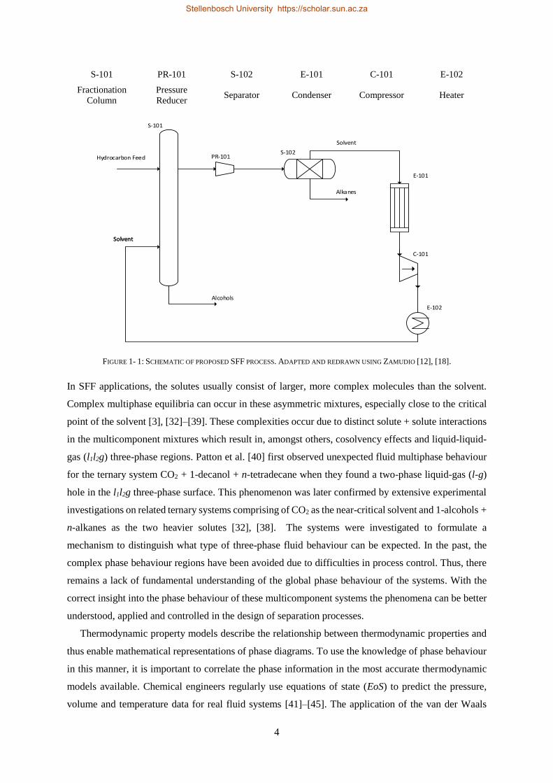
The proposed SFF process for separating the close-boiling detergent range 1-alcohol from its
corresponding n-alkane is shown in Figure 1-1 [12]. The approach involves a feed and solvent stream
to be sent to a fractionation column, S-101. Two phases will then exit S-101, one a liquid product stream
at the bottom (with residual 1-alcohol) and the second the loaded supercritical fluid at the top of S-101.
The supercritical fluid is sent to a pressure reducer, PR-101, before separating the solvent from the
accompanying extract (mainly n-alkanes) in a separator, S-102. Before recycling the solvent back to
S-101 it will first be condensed in E-101, compressed in C-101 and heated in E-102. A history on the
development of supercritical fluid technology and fundamental studies on the application of
supercritical fluids can be found in various publications [1], [24], [26]–[28], [30], [31].
Stellenbosch University https://scholar.sun.ac.za
4
S-101 PR-101 S-102 E-101 C-101 E-102
Fractionation
Column
Pressure
Reducer Separator Condenser Compressor Heater
Hydrocarbon Feed
Solvent
Alcohols
Solvent
Alkanes
Solvent
S-101
PR-101S-102
E-101
C-101
E-102
FIGURE 1- 1: SCHEMATIC OF PROPOSED SFF PROCESS. ADAPTED AND REDRAWN USING ZAMUDIO [12], [18].
In SFF applications, the solutes usually consist of larger, more complex molecules than the solvent.
Complex multiphase equilibria can occur in these asymmetric mixtures, especially close to the critical
point of the solvent [3], [32]–[39]. These complexities occur due to distinct solute + solute interactions
in the multicomponent mixtures which result in, amongst others, cosolvency effects and liquid-liquid-
gas (l1l2g) three-phase regions. Patton et al. [40] first observed unexpected fluid multiphase behaviour
for the ternary system CO2 + 1-decanol + n-tetradecane when they found a two-phase liquid-gas (l-g)
hole in the l1l2g three-phase surface. This phenomenon was later confirmed by extensive experimental
investigations on related ternary systems comprising of CO2 as the near-critical solvent and 1-alcohols +
n-alkanes as the two heavier solutes [32], [38]. The systems were investigated to formulate a
mechanism to distinguish what type of three-phase fluid behaviour can be expected. In the past, the
complex phase behaviour regions have been avoided due to difficulties in process control. Thus, there
remains a lack of fundamental understanding of the global phase behaviour of the systems. With the
correct insight into the phase behaviour of these multicomponent systems the phenomena can be better
understood, applied and controlled in the design of separation processes.
Thermodynamic property models describe the relationship between thermodynamic properties and
thus enable mathematical representations of phase diagrams. To use the knowledge of phase behaviour
in this manner, it is important to correlate the phase information in the most accurate thermodynamic
models available. Chemical engineers regularly use equations of state (EoS) to predict the pressure,
volume and temperature data for real fluid systems [41]–[45]. The application of the van der Waals
Stellenbosch University https://scholar.sun.ac.za
5
(vdW) mixing rules to define the interaction parameters are only applicable to mildly non-ideal systems,
which is not the case for the current study [46]. Several EoS have been developed as an expansion on
the vdW EoS to take into consideration mixture complexities. The most popular EoSs, especially in the
petrochemical industry, include (i) Peng-Robinson (PR) [47] and (ii) Redlich-Kwong (RK) [48] which
forms the basis of (iii) the Soave-Redlich-Kwong (SRK) EoS [49]. Although both the SRK and PR
equations provide highly accurate phase equilibria data for hydrocarbons, the vdW one-fluid mixing
rules restrict their use for correlating the interested system. However, these EoS form the basis of
various flexible and predictive mixing rules as well as statistical thermodynamic models that have
become the focus point in recent years for holistic modelling of complex multiphase equilibria [50].
Several of these thermodynamic models are found in commercial simulators, e.g. Aspen Plus®. They
provide a way for fast and simple calculations of complex multiphase systems and are becoming
increasingly popular compared to in-house developed programs [51]. The reason for selecting models
available within Aspen Plus® is to ultimately allow for the development of a process model within a
process simulator, like the work done by Zamudio et al.[12].
1.2. STUDY AIM AND OBJECTIVES
The CO2 + 1-decanol + n-tetradecane system is an important model system for the separation of
detergent range n-alkanes and 1-alcohols; however, obtaining new equilibria data for the complex
ternary system can be time consuming and costly.
The aim of this study is to obtain a fundamental understanding of the solute + solute interactions in
the CO2 + 1-decanol + n-tetradecane ternary system firstly, through the generation of phase equilibria
data and secondly, through the evaluation of thermodynamic models, with solute + solute BIPs
incorporated into their algorithm. To achieve this aim, the following key objectives need to be met:
1. Study the high-pressure phase equilibria of the CO2 + 1-decanol + n-tetradecane ternary system:
1.1. Measure bubble- and dew-point data for six (1-decanol + n-tetradecane) mixtures in
supercritical CO2.
1.2. Measure vapour-liquid equilibria (VLE) data for four (1-decanol + n-tetradecane) mixtures in
supercritical CO2.
1.3. Characterise the complex phase behaviour of the ternary system.
1.4. Assess the ability of CO2 to separate the solutes, 1-decanol and n-tetradecane.
2. Study the low-pressure phase equilibria of the 1-decanol + n-tetradecane binary system:
2.1. Measure isobaric VLE data of the 1-decanol + n-tetradecane binary system.
2.2. Measure isobaric VLE data of four pertinent binary systems with the same 4 carbon number
difference as the 1-decanol + n-tetradecane system.
2.3. Characterise the phase behaviour of the 1-decanol + n-tetradecane binary system.
Stellenbosch University https://scholar.sun.ac.za
6
3. Study the thermodynamic modelling of the CO2 + 1-decanol + n-tetradecane ternary system and
the 1-decanol + n-tetradecane binary system:
3.1. Select at least 4 suitable thermodynamic models within a commercial process simulator that
can be used to correlate the ternary and binary systems.
3.2. Generate new solute + solute BIPs using the new HPBDP, HPVLE and LPVLE experimental
data.
3.3. Identify whether high-pressure solute + solute BIPs can be used to improve the modelling of
low-pressure data and vice versa.
3.4. Establish the solute + solute parameter set to be used by each of the thermodynamic models
that will result in the overall best representation of the measured equilibrium data.
3.5. Identify the best suited thermodynamic model for representing the experimental HPBDP,
HPVLE and LPVLE data.
1.3. PROJECT SCOPE
The predominant outcome of this research project is to define and understand the interactions between
1-decanol and n-tetradecane and inevitably improve the thermodynamic modelling of the complex
CO2 + 1-decanol + n-tetradecane ternary system. In Chapter 5, the present study provides new high-
pressure bubble- and dew-point (HPBDP) ternary data and inferred critical end-point data to
characterise the complex l1l2g three-phase behaviour. To date, no classification on the type of phase
behaviour of the CO2 + 1-decanol + n-tetradecane ternary system, has been made. Therefore, in Chapter
2, the binary classifications of Van Konynenburg and Scott [52], [53] were adapted to ternary systems
to describe the observed fluid phase behaviour. The VLE data of the CO2 + 1-decanol + n-tetradecane
system can be used to describe and solve problems regarding the design analysis and control of
supercritical fluid processes. Thus, new high-pressure vapour-liquid-equilibrium (HPVLE) data of
the ternary system are provided on ternary phase diagrams, alongside the HPBDP data (see Chapter 5).
The slope of the HPVLE tie lines are used to assess the ability of supercritical CO2 to separate the two
solutes, 1-decanol and n-tetradecane. The HPBDP and HPVLE experiments were conducted within the
temperature range (308 K – 358 K), pressure range (6 MPa – 27 MPa) and solute composition range
(0.015 g/g – 0.7 g/g) at which SFF applications take place.
In addition, non-ideal phase behaviour might be illustrated by systems containing both a polar and
non-polar component. Based on this and the complex phase behaviour phenomena in the ternary system,
a systematic and extensive experimental study of binary 1-alcohol + n-alkane VLE data has been carried
out in Chapter 6. The low-pressure vapour-liquid-equilibrium (LPVLE) phase behaviour of the
(i) 1-pentanol + n-nonane, (ii) 1-hexanol + n-decane, (iii) 1-heptanol + n-undecane, (iv) 1-octanol +
n-dodecane and (v) 1-decanol + n-tetradecane binary systems were measured at a sub-atmospheric
pressure of 40 kPa.
Stellenbosch University https://scholar.sun.ac.za
7
Obtaining binary and ternary phase equilibrium data demands time and resources that are not always
readily available. The development of computerised simulation software aided in this requirement,
making robust and industrial relevant thermodynamic models valuable. In Chapter 3, the property
methods available within the commercial software program, Aspen Plus®, are investigated to select a
minimum of 4 suitable models. The approach for generating high- and low-pressure solute + solute
BIPs are discussed in Chapter 7, followed by an assessment of the ability of BIPs to improve the model
correlations of the new HPBDP, HPVLE and LPVLE data in Chapter 8. Finally, the aim of this study
is addressed in Chapter 9, i.e., what the influence of the solute + solute interactions are on the separation
of 1-decanol and n-tetradecane and how this understanding can be used to improve pilot plant
experiments. Lastly, the conclusions of this research project are summarised and the model system that
resulted in the most accurate representation of the thermodynamic properties of the CO2 + 1-decanol +
n-tetradecane system are discussed that will inevitably be used to improve future process models.
Stellenbosch University https://scholar.sun.ac.za
8
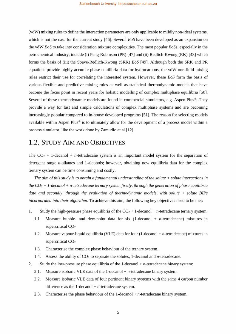
1.4. THESIS OVERVIEW
FIGURE 1- 2: FLOW DIAGRAM PRESENTING AN OVERVIEW OF THIS THESIS AND THE ACHIEVEMENT OF EACH KEY OBJECTIVE.
Aim of thesis
Define and understand the interactions between 1-decanol + n-
tetradecane to improve the thermodynamic modelling of the complex
CO2 + 1-decanol + n-tetradecane ternary system.
Phase equilibria
Thermodynamic modelling
Chapter 2
Chapter 3Literature study
Aspen Plus® to be used.
Cubic EoS
Association EoS Predictive
property methods
Flexible property
methods
PC-SAFT PSRKRK-Aspen
SR-Polar
Classification of ternary system
and binary sub-systems.
Available literature at T and P
of interest to this study
(i) CO2 + 1-decanol
(ii) CO2 + n-tetradecane
(iii) 1-decanol + n-tetradecane
(iv) CO2 + 1-decanol + n-tetradecane
✓
✓
✗
✗
Postulated non-ideal phase behaviour:
* Azeotrope
Identified complex phase behaviour:
* Cosolvency
* Liquid-gas holes
* Miscibility window
Phase equilibria
data required
Materials and methods
Chapter 4
Chapter 1
Binary data
all glass dynamic
recirculating still
Ternary data
analytical and synthetic
high pressure view cells
High-pressure results
Low-pressure results
Chapter 6
Chapter 5
New LPVLE data measured for:
(i) 1-pentanol + n-nonane
(ii) 1-hexanol + n-decane
(iii) 1-heptanol + n-undecane
(iv) 1-octanol + n-dodecane
(v) 1-decanol + n-tetradecane
New HPBDP data measured for:
CO2 + 1-decanol + n-tetradecane
New HPVLE data measured for:
CO2 + 1-decanol + n-tetradecane
&
Achievement of
objective 2
Achievement of
objective 1
Model Parameters
Group + group
BIPs
Solute +
solute BIPs
Achievement of
objective 3
Solute +
solute BIPs
Chapter 7
Newly measured experimental data used to regress
solute + solute binary interaction parameters
LPVLE data for
“LPVLE BIPs”
HPVLE data for
“HPVLE BIPs”
HPBDP data for
“HPBDP BIPs”
For PSRK: group-group parameters regressed using
LPVLE data and compared to DDB interaction parameters
Modelling results
Chapter 8
Achievement of
objective 4
Assessment of the solute + solute BIPs
influence on the thermodynamic model
correlations
i.e. RK-Aspen correlations of
LPVLE data, HPVLE data and
HPBDP data with included:
(i) LPVLE BIPs
(ii) HPVLE BIPs
(iii) HPBDP BIPs
Chapter 9
Project outcome
Conclusion of optimum solute + solute BIPs to be
regressed for best suited thermodynamic model
&
Recommendations for future work
Stellenbosch University https://scholar.sun.ac.za
9
1.5. SIGNIFICANT CONTRIBUTIONS
This research leads to the following significant scientific contributions:
(i) HPBDP data of six (1-decanol + n-tetradecane) mixtures in supercritical CO2 that are used to
classify the ternary system and link the l-g hole and miscibility window to cosolvency effects.
(ii) HPVLE data of four CO2 + 1-decanol + n-tetradecane mixtures that were used to construct tie
lines on ternary phase diagrams and assess the ability of supercritical CO2 to separate the two
solutes, 1-decanol and n-tetradecane.
(iii) LPVLE data of five (1-alcohol + n-alkane) binary systems at sub-atmospheric conditions.
(iv) Solute + solute BIPs obtained for three thermodynamic models using the three different
experimental data sets (HPBDP, HPVLE and LPVLE). The thermodynamic models provide an
outcome for the best approach to quantifying solute + solute interactions.
(v) Assessing the capabilities of one purely predictive thermodynamic model to capture the phase
behaviour of the CO2 + 1-decanol + n-tetradecane mixtures.
1.6. SCIENTIFIC CONTRIBUTIONS
The work presented in this thesis contributed to the following publication:
M. Ferreira and C.E. Schwarz, Super- and near-critical fluid phase behaviour and phenomena of the
ternary system CO2 + 1-decanol + n-tetradecane, The Journal of Chemical Thermodynamics. 111 (2017)
88-99.
The work presented in this thesis contributed to the following papers submitted for publication:
(i) M. Ferreira and C.E. Schwarz, Low-pressure VLE measurements and thermodynamic modelling,
with PSRK and NRTL, of binary 1-alcohol + n-alkane systems, The Journal of Chemical &
Engineering Data, submitted 1 August 2018, manuscript reference number: je-2018-006802.
(ii) M. Ferreira and C.E. Schwarz, High-pressure VLE measurements and PSRK modelling of the
complex CO2 + 1-decanol + n-tetradecane ternary system, The Journal of Supercritical Fluids,
to be submitted 7 September 2018, manuscript reference number: SUPFLU_2018_502.
The work presented in this thesis contributed to the following paper in preparation for publication:
M. Ferreira and C.E. Schwarz, Thermodynamic modelling of the CO2 + 1-decanol + n-tetradecane
system with RK-Aspen, SR-Polar and PC-SAFT in Aspen Plus®, Fluid Phase Equilibria, to be
submitted November 2018
Stellenbosch University https://scholar.sun.ac.za
10
The work presented in this thesis contributed to the following conferences:
(i) M. Ferreira and C.E. Schwarz, Process modelling of the phase behaviour of the CO2 + 1-decanol
+ n-tetradecane systems, Poster presentation at the 15th European Meeting on Supercritical
Fluids, Essen, Germany (May 2016).
(ii) C.E. Schwarz, S.A.M. Smith, M. Ferreira, S.P. Nortjé, High pressure bubble- and dew-point
measurements for ternary solute + supercritical solvent mixtures, Oral presentation at the 24th
IUPAC International Conference on Chemical Thermodynamics, Guilin, China (August 2016).
(iii) M. Ferreira and C.E. Schwarz, High-pressure phase equilibria of the ternary system CO2 +
1-decanol + n-tetradecane, Oral presentation at the 16th European Meeting on Supercritical
Fluids, Lisbon, Portugal (April 2017).
(iv) M. Ferreira and C.E. Schwarz, Obtaining solute + solute binary interaction parameters from
different sources for the ternary system CO2 + 1-decanol + n-tetradecane, Oral presentation at
the 29th European Symposium on Applied Thermodynamics, Bucharest, Romania (May 2017).
(v) M. Ferreira and C. E. Schwarz, Phase Equilibria and Thermodynamic Modelling of the Ternary
System CO2 + 1-decanol + n-tetradecane, Oral presentation at the 10th World Congress of
Chemical Engineering, Spain, Barcelona (October 2017).
Stellenbosch University https://scholar.sun.ac.za
11
Chapter 2
BINARY AND TERNARY PHASE EQUILIBRIA
This chapter introduces the first part of this thesis, which is devoted to the phase behaviour
characteristics of the ternary system and its three binary sub-systems. The solubility behaviour of a
solute in supercritical CO2 is strongly affected when a second low-volatile component is added [54].
Therefore, investigations of the binary and ternary phase behaviour are of considerable interest to
understand the thermodynamic properties of processing with supercritical CO2.
The aim of this chapter is not to review all aspects of binary and ternary phase behaviour, but to
provide a critical analysis of the phase behaviour types, trends, transitions and classes relevant to the
work done in this study.
First, a systematic study on the phase behaviour of the three binary sub-systems: CO2 + 1-decanol,
CO2 + n-tetradecane and 1-decanol + n-tetradecane is conducted in this chapter (which includes a full
literature review of available binary data). The study will aid in the understanding of the solute + solvent
and solute + solute interactions taking place within the ternary system. The unexpected phenomena of
the CO2 + 1-decanol + n-tetradecane system cannot directly be predicted considering only the binary
sub-systems. Therefore, in addition, an extensive literature study is also conducted for the ternary
system. From this knowledge, the thermodynamic phenomena expected in this ternary system at near-
and supercritical conditions are characterised. In so doing, the correct thermodynamic models can be
developed and used to calculate the fluid phase equilibria of the interested system. The chapter will
close with a discussion of the research gaps in open literature for the ternary system CO2 + 1-decanol +
n-tetradecane and how each will be addressed throughout this work.
2.1. PHASE BEHAVIOUR OF BINARY SUB-SYSTEMS
The phase behaviour of pure component and binary mixtures are characterized by the generation of
points and lines. These include:
(i) The location of the three-phase l1l2g equilibria.
(ii) The number and kind of critical endpoints (CEPs).
(iii) The critical lines occurring.
Stellenbosch University https://scholar.sun.ac.za
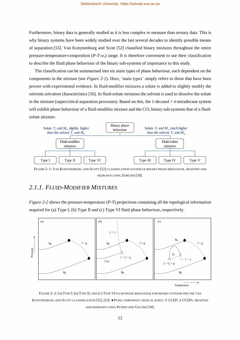
12
Furthermore, binary data is generally studied as it is less complex to measure than ternary data. This is
why binary systems have been widely studied over the last several decades to identify possible means
of separation [55]. Van Konynenburg and Scott [52] classified binary mixtures throughout the entire
pressure-temperature-composition (P-T-ws) range. It is therefore convenient to use their classification
to describe the fluid phase behaviour of the binary sub-systems of importance to this study.
The classification can be summarised into six main types of phase behaviour, each dependent on the
components in the mixture (see Figure 2-1). Here, ‘main types’ simply refers to those that have been
proven with experimental evidence. In fluid-modifier mixtures a solute is added to slightly modify the
solvents solvation characteristics [56]. In fluid-solute mixtures the solvent is used to dissolve the solute
in the mixture (supercritical separation processes). Based on this, the 1-decanol + n-tetradecane system
will exhibit phase behaviour of a fluid-modifier mixture and the CO2 binary sub-systems that of a fluid-
solute mixture.
FIGURE 2- 1: VAN KONYNENBURG AND SCOTT [52] CLASSIFICATION SYSTEM OF BINARY PHASE BEHAVIOUR. ADAPTED AND
REDRAWN USING ZAMUDIO [18].
2.1.1. FLUID-MODIFIER MIXTURES
Figure 2-2 shows the pressure-temperature (P-T) projections containing all the topological information
required for (a) Type I, (b) Type II and (c) Type VI fluid phase behaviour, respectively.
FIGURE 2- 2: (A) TYPE I; (B) TYPE II; AND (C) TYPE VI FLUID PHASE BEHAVIOUR FOR BINARY SYSTEMS PER THE VAN
KONYNENBURG AND SCOTT CLASSIFICATION [52], [53]. ● PURE COMPONENT CRITICAL POINT; ◇ LCEP; Δ UCEPS. ADAPTED
AND REDRAWN USING PETERS AND GAUTER [34].
Binary phase
behaviour
Fluid-solute
mixtures
Fluid-modifier
mixtures
Type I Type II Type VI Type IVType III Type V
Solute Tc and Mw slightly higher
than the solvent Tc and Mw
Solute Tc and Mw much higher
than the solvent Tc and Mw
Pre
ssure
lgA
lgB
l = g lgA
lgB
l = g
l1 = l2
l1 = l2 + g
l1l2g
Temperature
lgA
lgB
l = g
llg
l1 = l2 + g
l1 = l2 + g
(a) (b) (c)
Stellenbosch University https://scholar.sun.ac.za
13
The characteristics of each Type are discussed briefly per the classification by Van Konynenburg and
Scott [52], [53]. Detailed discussions are available in literature elsewhere [34], [36], [37], [57], [58].
Type I fluid phase behaviour is identified in systems exhibiting:
(i) Similar molecular size or diameters
(ii) Similar interaction strengths
(iii) Critical properties of comparable magnitude
l = g Continuous critical line connecting the critical points of the pure components
(lgA and lgB)
Type II fluid phase behaviour is identified in systems exhibiting:
(i) Partial miscibility at subcritical temperatures
(ii) Non-ideal mixtures
(iii) Components with similar sized molecules (solutes)
l1l2g Three-phase equilibrium locus (at lower temperatures)
l = g Continuous critical line connecting the critical points of the pure components
(lgA and lgB)
l1 = l2 + g Upper critical endpoint (UCEP) of the l1l2g locus (the two liquid phases are
critical in the presence of a gaseous phase) – two liquid phases are formed from
one liquid phase
l1 = l2 Critical line at lower temperatures and pressures, which merges with the UCEP
of the l1l2g locus
Type VI fluid phase behaviour is identified in systems exhibiting:
(i) The so-called closed-loop l1 = l2 immiscibility region
(ii) Non-ideal mixtures
(iii) Three-phase region bounded by two CEPs of the same nature
l1 = l2 + g Lower critical endpoint (LCEP) of the llg locus at lower temperatures (the two
liquid phases are critical in the presence of a gaseous phase)
l1 = l2 + g UCEP of the llg locus at higher temperatures
llg Smaller three-phase equilibrium locus connecting LCEP and DCEP to form
three-phase region
l = g Continuous critical line connecting the critical points of the pure components
(lgA and lgB)
Stellenbosch University https://scholar.sun.ac.za
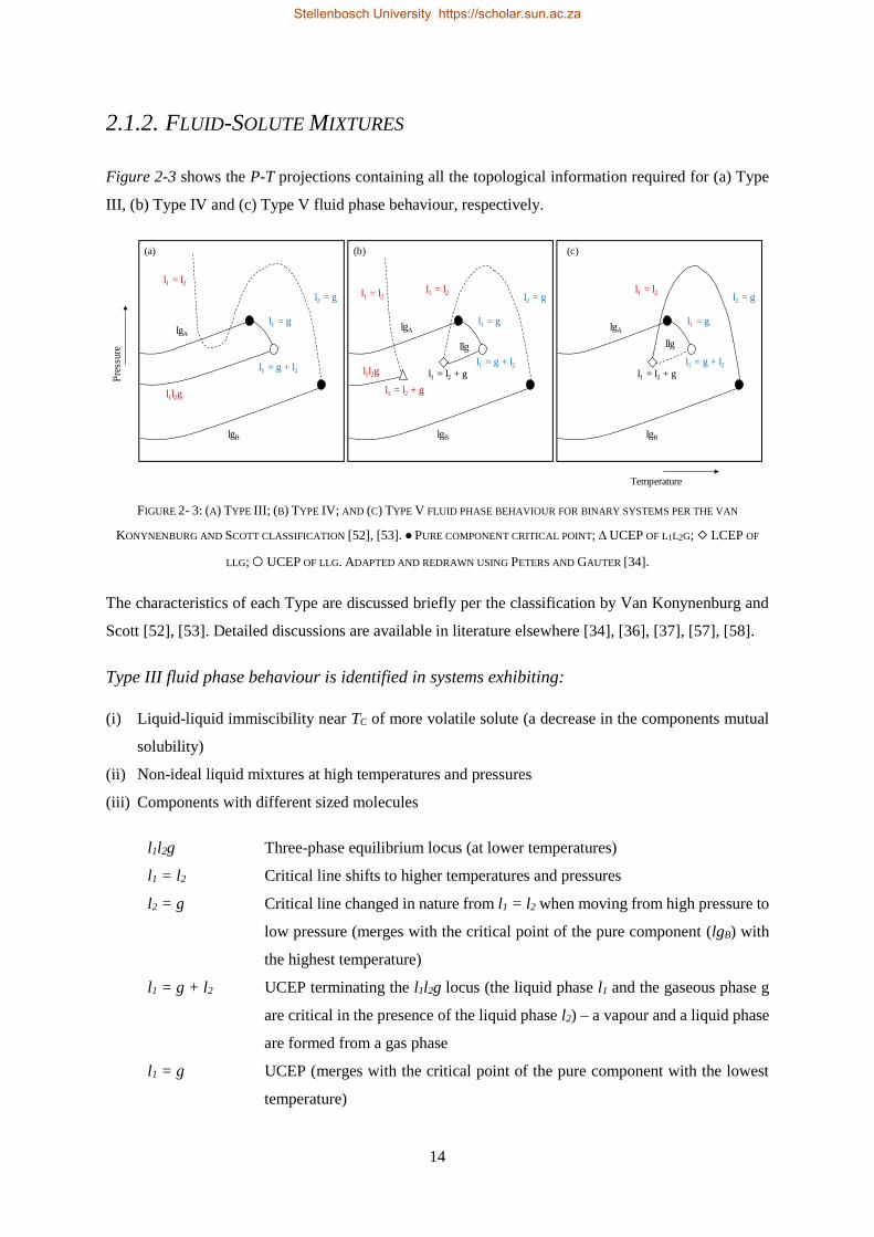
14
2.1.2. FLUID-SOLUTE MIXTURES
Figure 2-3 shows the P-T projections containing all the topological information required for (a) Type
III, (b) Type IV and (c) Type V fluid phase behaviour, respectively.
FIGURE 2- 3: (A) TYPE III; (B) TYPE IV; AND (C) TYPE V FLUID PHASE BEHAVIOUR FOR BINARY SYSTEMS PER THE VAN
KONYNENBURG AND SCOTT CLASSIFICATION [52], [53]. ● PURE COMPONENT CRITICAL POINT; Δ UCEP OF L1L2G; ◇ LCEP OF
LLG; ○ UCEP OF LLG. ADAPTED AND REDRAWN USING PETERS AND GAUTER [34].
The characteristics of each Type are discussed briefly per the classification by Van Konynenburg and
Scott [52], [53]. Detailed discussions are available in literature elsewhere [34], [36], [37], [57], [58].
Type III fluid phase behaviour is identified in systems exhibiting:
(i) Liquid-liquid immiscibility near TC of more volatile solute (a decrease in the components mutual
solubility)
(ii) Non-ideal liquid mixtures at high temperatures and pressures
(iii) Components with different sized molecules
l1l2g Three-phase equilibrium locus (at lower temperatures)
l1 = l2 Critical line shifts to higher temperatures and pressures
l2 = g Critical line changed in nature from l1 = l2 when moving from high pressure to
low pressure (merges with the critical point of the pure component (lgB) with
the highest temperature)
l1 = g + l2 UCEP terminating the l1l2g locus (the liquid phase l1 and the gaseous phase g
are critical in the presence of the liquid phase l2) – a vapour and a liquid phase
are formed from a gas phase
l1 = g UCEP (merges with the critical point of the pure component with the lowest
temperature)
lgA
lgB
l1 = g
l2 = gl1 = l2
l1 = g + l2
llg
l1 = l2
l1 = l2 + gl1l2g
l1 = l2 + g
lgA
lgB
l1 = g
l2 = g
l1 = l2
l1l2g
l1 = g + l2
Pre
ssure
Temperature
lgA
lgB
l1 = g
l2 = g
l1 = g + l2
l1 = l2
l1 = l2 + g
llg
(a) (b) (c)
Stellenbosch University https://scholar.sun.ac.za
15
Type IV fluid phase behaviour is identified in systems exhibiting:
(i) Discontinued liquid-liquid immiscibility at intermediate temperatures
(ii) Non-ideal mixtures
(iii) Components with different sized molecules (but less obvious than Type III)
l1l2g Three-phase equilibrium locus (at lower temperatures)
llg Smaller three-phase equilibrium locus (additional at higher temperatures and
pressures) – interrupts the l = g critical line previously seen in Type II systems.
l1 = g + l2 UCEP terminating the llg locus at higher temperatures and pressures.
l1 = l2 + g LCEP terminating the llg locus at lower temperatures and pressures; and the
UCEP terminating the l1l2g locus at lower temperatures and pressures (see
Type II).
UCEP and LCEP refer to the location of these points relative to the corresponding three-phase locus
(l1l2g or llg).
Type V fluid phase behaviour is identified in systems exhibiting:
(i) Difference in molecular size of components become significant
(ii) Almost ideal system
(iii) Complete miscibility at lower temperatures
llg Smaller three-phase equilibrium locus (additional at higher temperatures and
pressures) – interrupts the l = g critical line previously seen in Type II systems.
l1 = g + l2 UCEP terminating the llg locus at higher temperatures and pressures.
l1 = l2 + g LCEP terminating the llg locus at lower temperatures (at a temperature below
TC of component)
2.1.3. PHASE BEHAVIOUR TRANSITIONS AND TRENDS IN HOMOLOGOUS
SERIES OF N-ALKANES AND N-ALKANOLS
Critical curves will at times form a sequence, i.e. the CEP on a three-phase curve, merges with another
CEP on a different curve. Generally, this is a transition in both homologous series from Type IV to
Type II and Type IV to Type III fluid phase behaviour occurring due to an increase and decrease in the
miscibility of the components, respectively.
Stellenbosch University https://scholar.sun.ac.za
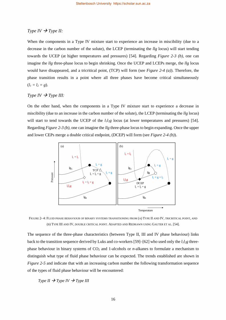
16
Type IV → Type II:
When the components in a Type IV mixture start to experience an increase in miscibility (due to a
decrease in the carbon number of the solute), the LCEP (terminating the llg locus) will start tending
towards the UCEP (at higher temperatures and pressures) [54]. Regarding Figure 2-3 (b), one can
imagine the llg three-phase locus to begin shrinking. Once the UCEP and LCEPs merge, the llg locus
would have disappeared, and a tricritical point, (TCP) will form (see Figure 2-4 (a)). Therefore, the
phase transition results in a point where all three phases have become critical simultaneously
(l1 = l2 = g).
Type IV → Type III:
On the other hand, when the components in a Type IV mixture start to experience a decrease in
miscibility (due to an increase in the carbon number of the solute), the LCEP (terminating the llg locus)
will start to tend towards the UCEP of the l1l2g locus (at lower temperatures and pressures) [54].
Regarding Figure 2-3 (b), one can imagine the llg three-phase locus to begin expanding. Once the upper
and lower CEPs merge a double critical endpoint, (DCEP) will form (see Figure 2-4 (b)).
FIGURE 2- 4: FLUID PHASE BEHAVIOUR OF BINARY SYSTEMS TRANSITIONING FROM (A) TYPE II AND IV, TRICRITICAL POINT, AND
(B) TYPE III AND IV, DOUBLE CRITICAL POINT. ADAPTED AND REDRAWN USING GAUTER ET AL. [54].
The sequence of the three-phase characteristics (between Type II, III and IV phase behaviour) links
back to the transition sequence derived by Luks and co-workers [59]–[62] who used only the l1l2g three-
phase behaviour in binary systems of CO2 and 1-alcohols or n-alkanes to formulate a mechanism to
distinguish what type of fluid phase behaviour can be expected. The trends established are shown in
Figure 2-5 and indicate that with an increasing carbon number the following transformation sequence
of the types of fluid phase behaviour will be encountered:
Type II → Type IV → Type III
Temperature
lgA
lgB
l1 = g
l2 = g
l1 = l2
l1l2gl1 = g + l2
llg
DCEP
l1 = l2 + g
Pre
ssure
lgA
lgB
l1 = g
l1 = l2
l1 = l2 + g
l1l2g
l2 = gTCP
l1 = l2 = g
(a) (b)
Stellenbosch University https://scholar.sun.ac.za
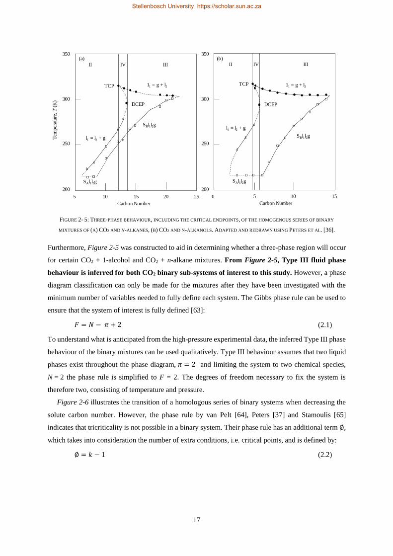
17
FIGURE 2- 5: THREE-PHASE BEHAVIOUR, INCLUDING THE CRITICAL ENDPOINTS, OF THE HOMOGENOUS SERIES OF BINARY
MIXTURES OF (A) CO2 AND N-ALKANES, (B) CO2 AND N-ALKANOLS. ADAPTED AND REDRAWN USING PETERS ET AL. [36].
Furthermore, Figure 2-5 was constructed to aid in determining whether a three-phase region will occur
for certain CO2 + 1-alcohol and CO2 + n-alkane mixtures. From Figure 2-5, Type III fluid phase
behaviour is inferred for both CO2 binary sub-systems of interest to this study. However, a phase
diagram classification can only be made for the mixtures after they have been investigated with the
minimum number of variables needed to fully define each system. The Gibbs phase rule can be used to
ensure that the system of interest is fully defined [63]:
𝐹 = 𝑁 − 𝜋 + 2 (2.1)
To understand what is anticipated from the high-pressure experimental data, the inferred Type III phase
behaviour of the binary mixtures can be used qualitatively. Type III behaviour assumes that two liquid
phases exist throughout the phase diagram, 𝜋 = 2 and limiting the system to two chemical species,
N = 2 the phase rule is simplified to F = 2. The degrees of freedom necessary to fix the system is
therefore two, consisting of temperature and pressure.
Figure 2-6 illustrates the transition of a homologous series of binary systems when decreasing the
solute carbon number. However, the phase rule by van Pelt [64], Peters [37] and Stamoulis [65]
indicates that tricriticality is not possible in a binary system. Their phase rule has an additional term ∅,
which takes into consideration the number of extra conditions, i.e. critical points, and is defined by:
∅ = 𝑘 − 1 (2.2)
Tem
per
ature
, T
(K)
Carbon Number
105 15 20 25
250
200
300
350
IV IIIII
l1 = l2 + g
SBl1l2g
11 = g + l2
SAl1l2g
Carbon Number
0 105 15
250
200
300
350
IV IIIII
11 = g + l2
l1 = l2 + g
SAl1l2g
SBl1l2g
(a) (b)
DCEP DCEP
TCPTCP
Stellenbosch University https://scholar.sun.ac.za
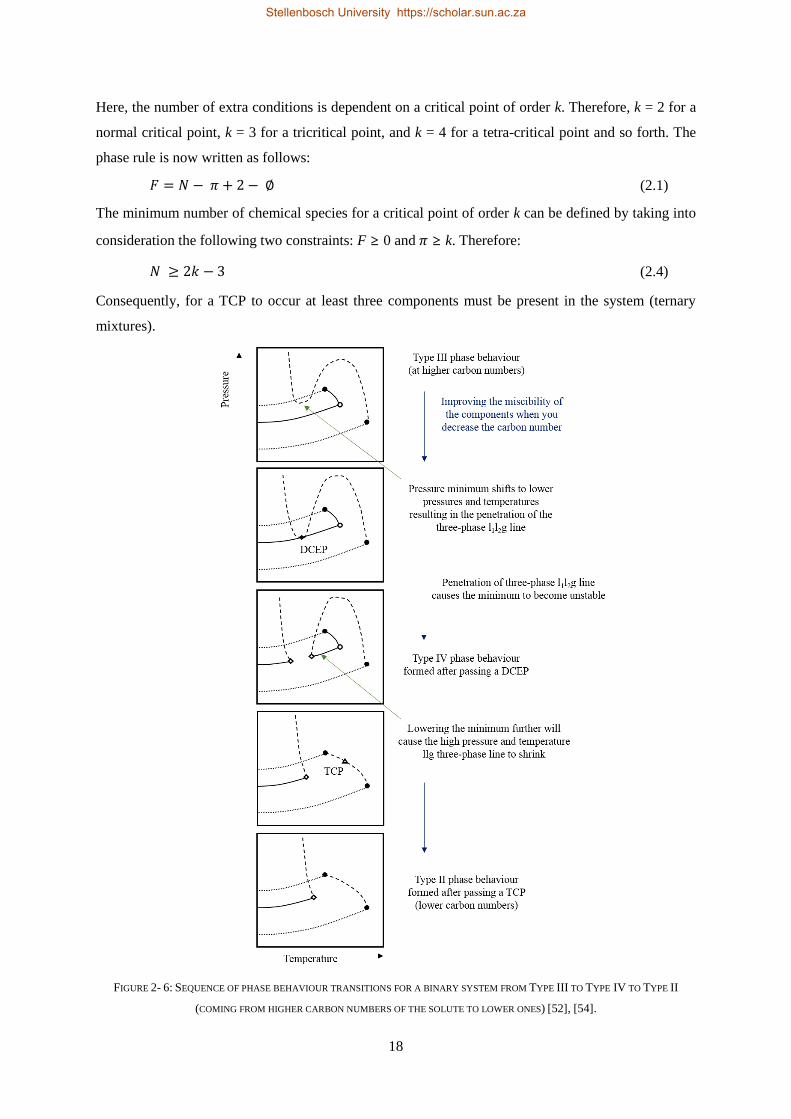
18
Here, the number of extra conditions is dependent on a critical point of order k. Therefore, k = 2 for a
normal critical point, k = 3 for a tricritical point, and k = 4 for a tetra-critical point and so forth. The
phase rule is now written as follows:
𝐹 = 𝑁 − 𝜋 + 2 − ∅ (2.1)
The minimum number of chemical species for a critical point of order k can be defined by taking into
consideration the following two constraints: F ≥ 0 and 𝜋 ≥ k. Therefore:
𝑁 ≥ 2𝑘 − 3 (2.4)
Consequently, for a TCP to occur at least three components must be present in the system (ternary
mixtures).
FIGURE 2- 6: SEQUENCE OF PHASE BEHAVIOUR TRANSITIONS FOR A BINARY SYSTEM FROM TYPE III TO TYPE IV TO TYPE II
(COMING FROM HIGHER CARBON NUMBERS OF THE SOLUTE TO LOWER ONES) [52], [54].
Stellenbosch University https://scholar.sun.ac.za
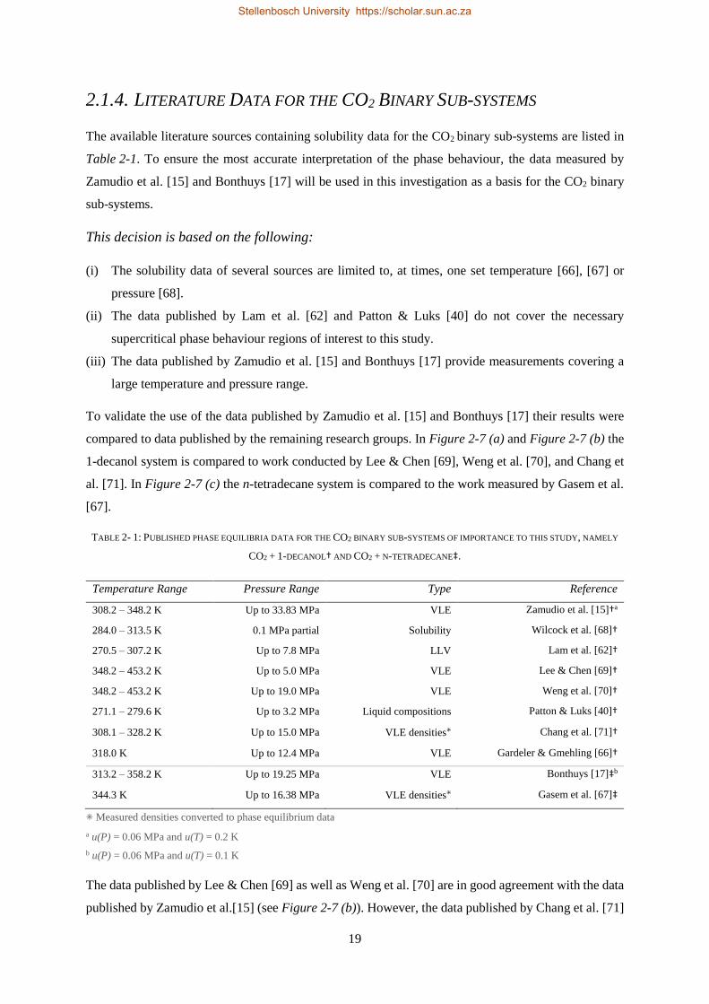
19
2.1.4. LITERATURE DATA FOR THE CO2 BINARY SUB-SYSTEMS
The available literature sources containing solubility data for the CO2 binary sub-systems are listed in
Table 2-1. To ensure the most accurate interpretation of the phase behaviour, the data measured by
Zamudio et al. [15] and Bonthuys [17] will be used in this investigation as a basis for the CO2 binary
sub-systems.
This decision is based on the following:
(i) The solubility data of several sources are limited to, at times, one set temperature [66], [67] or
pressure [68].
(ii) The data published by Lam et al. [62] and Patton & Luks [40] do not cover the necessary
supercritical phase behaviour regions of interest to this study.
(iii) The data published by Zamudio et al. [15] and Bonthuys [17] provide measurements covering a
large temperature and pressure range.
To validate the use of the data published by Zamudio et al. [15] and Bonthuys [17] their results were
compared to data published by the remaining research groups. In Figure 2-7 (a) and Figure 2-7 (b) the
1-decanol system is compared to work conducted by Lee & Chen [69], Weng et al. [70], and Chang et
al. [71]. In Figure 2-7 (c) the n-tetradecane system is compared to the work measured by Gasem et al.
[67].
TABLE 2- 1: PUBLISHED PHASE EQUILIBRIA DATA FOR THE CO2 BINARY SUB-SYSTEMS OF IMPORTANCE TO THIS STUDY, NAMELY
CO2 + 1-DECANOL† AND CO2 + N-TETRADECANE‡.
Temperature Range Pressure Range Type Reference
308.2 – 348.2 K Up to 33.83 MPa VLE Zamudio et al. [15]†a
284.0 – 313.5 K 0.1 MPa partial Solubility Wilcock et al. [68]†
270.5 – 307.2 K Up to 7.8 MPa LLV Lam et al. [62]†
348.2 – 453.2 K Up to 5.0 MPa VLE Lee & Chen [69]†
348.2 – 453.2 K Up to 19.0 MPa VLE Weng et al. [70]†
271.1 – 279.6 K Up to 3.2 MPa Liquid compositions Patton & Luks [40]†
308.1 – 328.2 K Up to 15.0 MPa VLE densities⁕ Chang et al. [71]†
318.0 K Up to 12.4 MPa VLE Gardeler & Gmehling [66]†
313.2 – 358.2 K Up to 19.25 MPa VLE Bonthuys [17]‡b
344.3 K Up to 16.38 MPa VLE densities⁕ Gasem et al. [67]‡
⁕ Measured densities converted to phase equilibrium data
a u(P) = 0.06 MPa and u(T) = 0.2 K
b u(P) = 0.06 MPa and u(T) = 0.1 K
The data published by Lee & Chen [69] as well as Weng et al. [70] are in good agreement with the data
published by Zamudio et al.[15] (see Figure 2-7 (b)). However, the data published by Chang et al. [71]
Stellenbosch University https://scholar.sun.ac.za
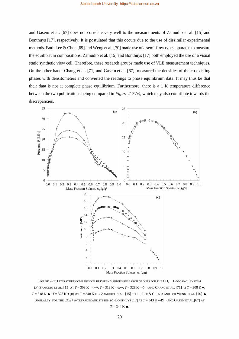
20
and Gasem et al. [67] does not correlate very well to the measurements of Zamudio et al. [15] and
Bonthuys [17], respectively. It is postulated that this occurs due to the use of dissimilar experimental
methods. Both Lee & Chen [69] and Weng et al. [70] made use of a semi-flow type apparatus to measure
the equilibrium compositions. Zamudio et al. [15] and Bonthuys [17] both employed the use of a visual
static synthetic view cell. Therefore, these research groups made use of VLE measurement techniques.
On the other hand, Chang et al. [71] and Gasem et al. [67], measured the densities of the co-existing
phases with densitometers and converted the readings to phase equilibrium data. It may thus be that
their data is not at complete phase equilibrium. Furthermore, there is a 1 K temperature difference
between the two publications being compared in Figure 2-7 (c), which may also contribute towards the
discrepancies.
FIGURE 2- 7: LITERATURE COMPARISONS BETWEEN VARIOUS RESEARCH GROUPS FOR THE CO2 + 1-DECANOL SYSTEM
(A) ZAMUDIO ET AL. [15] AT T = 308 K ⋯○⋯; T = 318 K ⋯∆⋯; T = 328 K ⋯◊⋯ AND CHANG ET AL. [71] AT T = 308 K ●;
T = 318 K ▲; T = 328 K ♦ (B) AT T = 348 K FOR ZAMUDIO ET AL. [15] ⋯⧠⋯; LEE & CHEN ∆ AND FOR WENG ET AL. [70] ▲.
SIMILARLY, FOR THE CO2 + N-TETRADECANE SYSTEM (C) BONTHUYS [17] AT T = 343 K ⋯⧠⋯ AND GASEM ET AL.[67] AT
T = 344 K ∎.
0
5
10
15
20
25
30
35
0.0 0.1 0.2 0.3 0.4 0.5 0.6 0.7 0.8 0.9 1.0
Pre
ssure
, P
(MP
a)
Mass Fraction Solutes, ws (g/g)
0
5
10
15
20
25
0.0 0.1 0.2 0.3 0.4 0.5 0.6 0.7 0.8 0.9 1.0
Mass Fraction Solutes, ws (g/g)
0
2
4
6
8
10
12
14
16
18
20
0.0 0.1 0.2 0.3 0.4 0.5 0.6 0.7 0.8 0.9 1.0
Pre
ssure
, P
(MP
a)
Mass Fraction Solutes, ws (g/g)
(a) (b)
(c)
Stellenbosch University https://scholar.sun.ac.za
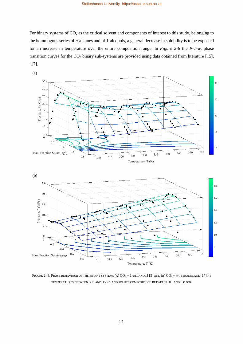
21
For binary systems of CO2 as the critical solvent and components of interest to this study, belonging to
the homologous series of n-alkanes and of 1-alcohols, a general decrease in solubility is to be expected
for an increase in temperature over the entire composition range. In Figure 2-8 the P-T-ws phase
transition curves for the CO2 binary sub-systems are provided using data obtained from literature [15],
[17].
FIGURE 2- 8: PHASE BEHAVIOUR OF THE BINARY SYSTEMS (A) CO2 + 1-DECANOL [15] AND (B) CO2 + N-TETRADECANE [17] AT
TEMPERATURES BETWEEN 308 AND 358 K AND SOLUTE COMPOSITIONS BETWEEN 0.01 AND 0.8 G/G.
(a)
(b)
Stellenbosch University https://scholar.sun.ac.za
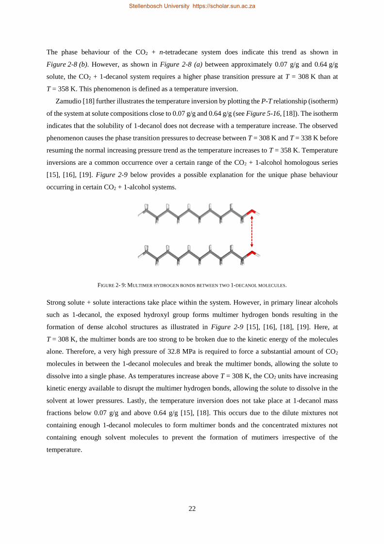
22
The phase behaviour of the CO2 + n-tetradecane system does indicate this trend as shown in
Figure 2-8 (b). However, as shown in Figure 2-8 (a) between approximately 0.07 g/g and 0.64 g/g
solute, the CO2 + 1-decanol system requires a higher phase transition pressure at T = 308 K than at
T = 358 K. This phenomenon is defined as a temperature inversion.
Zamudio [18] further illustrates the temperature inversion by plotting the P-T relationship (isotherm)
of the system at solute compositions close to 0.07 g/g and 0.64 g/g (see Figure 5-16, [18]). The isotherm
indicates that the solubility of 1-decanol does not decrease with a temperature increase. The observed
phenomenon causes the phase transition pressures to decrease between T = 308 K and T = 338 K before
resuming the normal increasing pressure trend as the temperature increases to T = 358 K. Temperature
inversions are a common occurrence over a certain range of the CO2 + 1-alcohol homologous series
[15], [16], [19]. Figure 2-9 below provides a possible explanation for the unique phase behaviour
occurring in certain CO2 + 1-alcohol systems.
FIGURE 2- 9: MULTIMER HYDROGEN BONDS BETWEEN TWO 1-DECANOL MOLECULES.
Strong solute + solute interactions take place within the system. However, in primary linear alcohols
such as 1-decanol, the exposed hydroxyl group forms multimer hydrogen bonds resulting in the
formation of dense alcohol structures as illustrated in Figure 2-9 [15], [16], [18], [19]. Here, at
T = 308 K, the multimer bonds are too strong to be broken due to the kinetic energy of the molecules
alone. Therefore, a very high pressure of 32.8 MPa is required to force a substantial amount of CO2
molecules in between the 1-decanol molecules and break the multimer bonds, allowing the solute to
dissolve into a single phase. As temperatures increase above T = 308 K, the CO2 units have increasing
kinetic energy available to disrupt the multimer hydrogen bonds, allowing the solute to dissolve in the
solvent at lower pressures. Lastly, the temperature inversion does not take place at 1-decanol mass
fractions below 0.07 g/g and above 0.64 g/g [15], [18]. This occurs due to the dilute mixtures not
containing enough 1-decanol molecules to form multimer bonds and the concentrated mixtures not
containing enough solvent molecules to prevent the formation of mutimers irrespective of the
temperature.
Stellenbosch University https://scholar.sun.ac.za
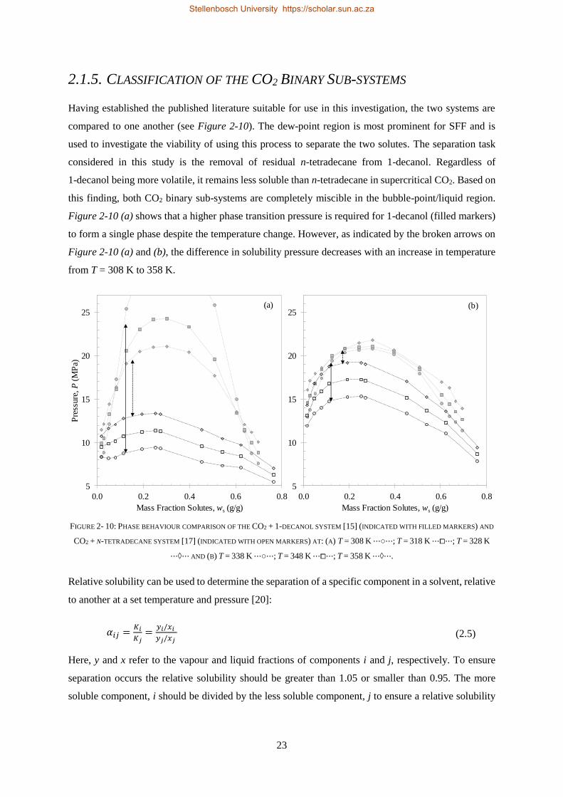
23
2.1.5. CLASSIFICATION OF THE CO2 BINARY SUB-SYSTEMS
Having established the published literature suitable for use in this investigation, the two systems are
compared to one another (see Figure 2-10). The dew-point region is most prominent for SFF and is
used to investigate the viability of using this process to separate the two solutes. The separation task
considered in this study is the removal of residual n-tetradecane from 1-decanol. Regardless of
1-decanol being more volatile, it remains less soluble than n-tetradecane in supercritical CO2. Based on
this finding, both CO2 binary sub-systems are completely miscible in the bubble-point/liquid region.
Figure 2-10 (a) shows that a higher phase transition pressure is required for 1-decanol (filled markers)
to form a single phase despite the temperature change. However, as indicated by the broken arrows on
Figure 2-10 (a) and (b), the difference in solubility pressure decreases with an increase in temperature
from T = 308 K to 358 K.
FIGURE 2- 10: PHASE BEHAVIOUR COMPARISON OF THE CO2 + 1-DECANOL SYSTEM [15] (INDICATED WITH FILLED MARKERS) AND
CO2 + N-TETRADECANE SYSTEM [17] (INDICATED WITH OPEN MARKERS) AT: (A) T = 308 K ⋯○⋯; T = 318 K ⋯⧠⋯; T = 328 K
⋯◊⋯ AND (B) T = 338 K ⋯○⋯; T = 348 K ⋯⧠⋯; T = 358 K ⋯◊⋯.
Relative solubility can be used to determine the separation of a specific component in a solvent, relative
to another at a set temperature and pressure [20]:
𝛼𝑖𝑗 =𝐾𝑖
𝐾𝑗=
𝑦𝑖/𝑥𝑖
𝑦𝑗/𝑥𝑗 (2.5)
Here, y and x refer to the vapour and liquid fractions of components i and j, respectively. To ensure
separation occurs the relative solubility should be greater than 1.05 or smaller than 0.95. The more
soluble component, i should be divided by the less soluble component, j to ensure a relative solubility
5
10
15
20
25
0.0 0.2 0.4 0.6 0.8
Mass Fraction Solutes, ws (g/g)
5
10
15
20
25
0.0 0.2 0.4 0.6 0.8
Pre
ssure
, P
(MP
a)
Mass Fraction Solutes, ws (g/g)
(a) (b)
Stellenbosch University https://scholar.sun.ac.za
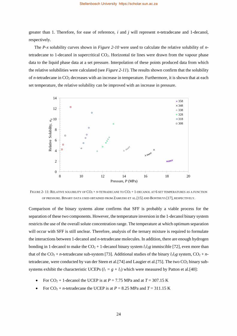
24
greater than 1. Therefore, for ease of reference, i and j will represent n-tetradecane and 1-decanol,
respectively.
The P-x solubility curves shown in Figure 2-10 were used to calculate the relative solubility of n-
tetradecane to 1-decanol in supercritical CO2. Horizontal tie lines were drawn from the vapour phase
data to the liquid phase data at a set pressure. Interpolation of these points produced data from which
the relative solubilities were calculated (see Figure 2-11). The results shown confirm that the solubility
of n-tetradecane in CO2 decreases with an increase in temperature. Furthermore, it is shown that at each
set temperature, the relative solubility can be improved with an increase in pressure.
FIGURE 2- 11: RELATIVE SOLUBILITY OF CO2 + N-TETRADECANE TO CO2 + 1-DECANOL AT 6 SET TEMPERATURES AS A FUNCTION
OF PRESSURE. BINARY DATA USED OBTAINED FROM ZAMUDIO ET AL.[15] AND BONTHUYS [17], RESPECTIVELY.
Comparison of the binary systems alone confirms that SFF is probably a viable process for the
separation of these two components. However, the temperature inversion in the 1-decanol binary system
restricts the use of the overall solute concentration range. The temperature at which optimum separation
will occur with SFF is still unclear. Therefore, analysis of the ternary mixture is required to formulate
the interactions between 1-decanol and n-tetradecane molecules. In addition, there are enough hydrogen
bonding in 1-decanol to make the CO2 + 1-decanol binary system l1l2g immiscible [72], even more than
that of the CO2 + n-tetradecane sub-system [73]. Additional studies of the binary l1l2g system, CO2 + n-
tetradecane, were conducted by van der Steen et al.[74] and Laugier et al.[75]. The two CO2 binary sub-
systems exhibit the characteristic UCEPs (l1 = g + l2) which were measured by Patton et al.[40]:
• For CO2 + 1-decanol the UCEP is at P = 7.75 MPa and at T = 307.15 K
• For CO2 + n-tetradecane the UCEP is at P = 8.25 MPa and T = 311.15 K
0
2
4
6
8
10
12
14
8 10 12 14 16 18 20
Rel
ativ
e S
olu
bili
ty, α
ij
Pressure, P (MPa)
358
348
338
328
318
308
Stellenbosch University https://scholar.sun.ac.za
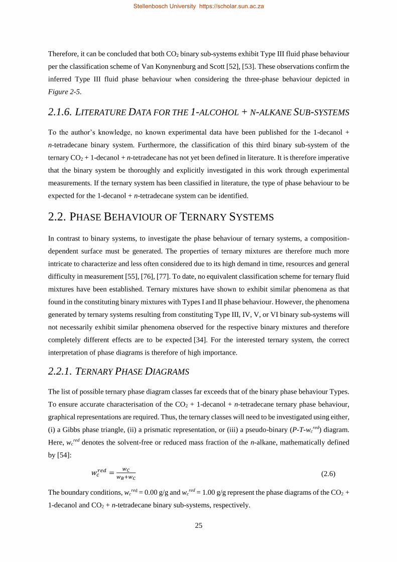
25
Therefore, it can be concluded that both CO2 binary sub-systems exhibit Type III fluid phase behaviour
per the classification scheme of Van Konynenburg and Scott [52], [53]. These observations confirm the
inferred Type III fluid phase behaviour when considering the three-phase behaviour depicted in
Figure 2-5.
2.1.6. LITERATURE DATA FOR THE 1-ALCOHOL + N-ALKANE SUB-SYSTEMS
To the author’s knowledge, no known experimental data have been published for the 1-decanol +
n-tetradecane binary system. Furthermore, the classification of this third binary sub-system of the
ternary CO2 + 1-decanol + n-tetradecane has not yet been defined in literature. It is therefore imperative
that the binary system be thoroughly and explicitly investigated in this work through experimental
measurements. If the ternary system has been classified in literature, the type of phase behaviour to be
expected for the 1-decanol + n-tetradecane system can be identified.
2.2. PHASE BEHAVIOUR OF TERNARY SYSTEMS
In contrast to binary systems, to investigate the phase behaviour of ternary systems, a composition-
dependent surface must be generated. The properties of ternary mixtures are therefore much more
intricate to characterize and less often considered due to its high demand in time, resources and general
difficulty in measurement [55], [76], [77]. To date, no equivalent classification scheme for ternary fluid
mixtures have been established. Ternary mixtures have shown to exhibit similar phenomena as that
found in the constituting binary mixtures with Types I and II phase behaviour. However, the phenomena
generated by ternary systems resulting from constituting Type III, IV, V, or VI binary sub-systems will
not necessarily exhibit similar phenomena observed for the respective binary mixtures and therefore
completely different effects are to be expected [34]. For the interested ternary system, the correct
interpretation of phase diagrams is therefore of high importance.
2.2.1. TERNARY PHASE DIAGRAMS
The list of possible ternary phase diagram classes far exceeds that of the binary phase behaviour Types.
To ensure accurate characterisation of the CO2 + 1-decanol + n-tetradecane ternary phase behaviour,
graphical representations are required. Thus, the ternary classes will need to be investigated using either,
(i) a Gibbs phase triangle, (ii) a prismatic representation, or (iii) a pseudo-binary (P-T-wcred) diagram.
Here, wcred denotes the solvent-free or reduced mass fraction of the n-alkane, mathematically defined
by [54]:
𝑤𝑐𝑟𝑒𝑑 =
𝑤𝐶
𝑤𝐵+𝑤𝐶 (2.6)
The boundary conditions, wcred = 0.00 g/g and wc
red = 1.00 g/g represent the phase diagrams of the CO2 +
1-decanol and CO2 + n-tetradecane binary sub-systems, respectively.
Stellenbosch University https://scholar.sun.ac.za
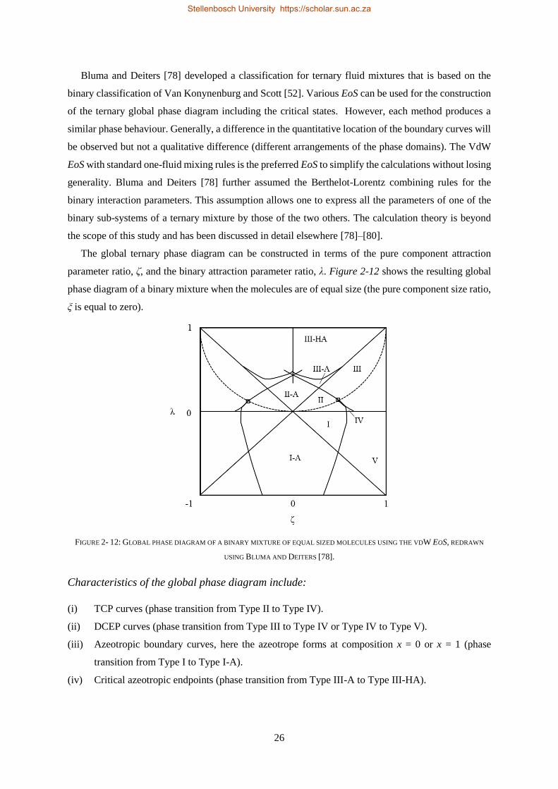
26
Bluma and Deiters [78] developed a classification for ternary fluid mixtures that is based on the
binary classification of Van Konynenburg and Scott [52]. Various EoS can be used for the construction
of the ternary global phase diagram including the critical states. However, each method produces a
similar phase behaviour. Generally, a difference in the quantitative location of the boundary curves will
be observed but not a qualitative difference (different arrangements of the phase domains). The VdW
EoS with standard one-fluid mixing rules is the preferred EoS to simplify the calculations without losing
generality. Bluma and Deiters [78] further assumed the Berthelot-Lorentz combining rules for the
binary interaction parameters. This assumption allows one to express all the parameters of one of the
binary sub-systems of a ternary mixture by those of the two others. The calculation theory is beyond
the scope of this study and has been discussed in detail elsewhere [78]–[80].
The global ternary phase diagram can be constructed in terms of the pure component attraction
parameter ratio, ζ, and the binary attraction parameter ratio, λ. Figure 2-12 shows the resulting global
phase diagram of a binary mixture when the molecules are of equal size (the pure component size ratio,
ξ is equal to zero).
FIGURE 2- 12: GLOBAL PHASE DIAGRAM OF A BINARY MIXTURE OF EQUAL SIZED MOLECULES USING THE VDW EOS, REDRAWN
USING BLUMA AND DEITERS [78].
Characteristics of the global phase diagram include:
(i) TCP curves (phase transition from Type II to Type IV).
(ii) DCEP curves (phase transition from Type III to Type IV or Type IV to Type V).
(iii) Azeotropic boundary curves, here the azeotrope forms at composition x = 0 or x = 1 (phase
transition from Type I to Type I-A).
(iv) Critical azeotropic endpoints (phase transition from Type III-A to Type III-HA).
Stellenbosch University https://scholar.sun.ac.za
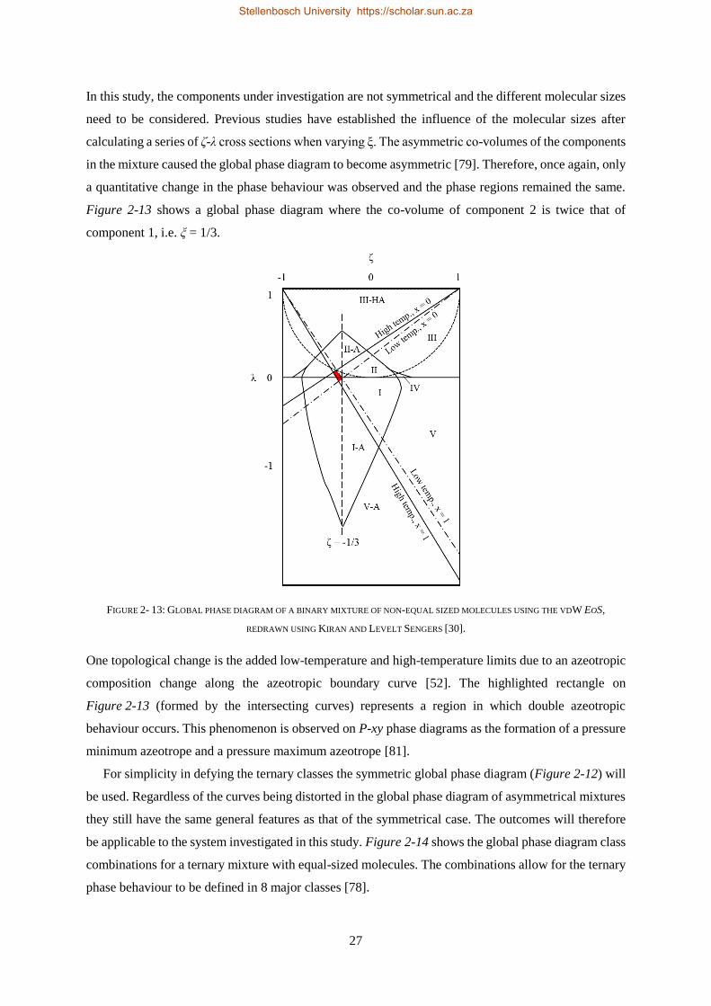
27
In this study, the components under investigation are not symmetrical and the different molecular sizes
need to be considered. Previous studies have established the influence of the molecular sizes after
calculating a series of ζ-λ cross sections when varying ξ. The asymmetric co-volumes of the components
in the mixture caused the global phase diagram to become asymmetric [79]. Therefore, once again, only
a quantitative change in the phase behaviour was observed and the phase regions remained the same.
Figure 2-13 shows a global phase diagram where the co-volume of component 2 is twice that of
component 1, i.e. ξ = 1/3.
FIGURE 2- 13: GLOBAL PHASE DIAGRAM OF A BINARY MIXTURE OF NON-EQUAL SIZED MOLECULES USING THE VDW EOS,
REDRAWN USING KIRAN AND LEVELT SENGERS [30].
One topological change is the added low-temperature and high-temperature limits due to an azeotropic
composition change along the azeotropic boundary curve [52]. The highlighted rectangle on
Figure 2-13 (formed by the intersecting curves) represents a region in which double azeotropic
behaviour occurs. This phenomenon is observed on P-xy phase diagrams as the formation of a pressure
minimum azeotrope and a pressure maximum azeotrope [81].
For simplicity in defying the ternary classes the symmetric global phase diagram (Figure 2-12) will
be used. Regardless of the curves being distorted in the global phase diagram of asymmetrical mixtures
they still have the same general features as that of the symmetrical case. The outcomes will therefore
be applicable to the system investigated in this study. Figure 2-14 shows the global phase diagram class
combinations for a ternary mixture with equal-sized molecules. The combinations allow for the ternary
phase behaviour to be defined in 8 major classes [78].
Stellenbosch University https://scholar.sun.ac.za
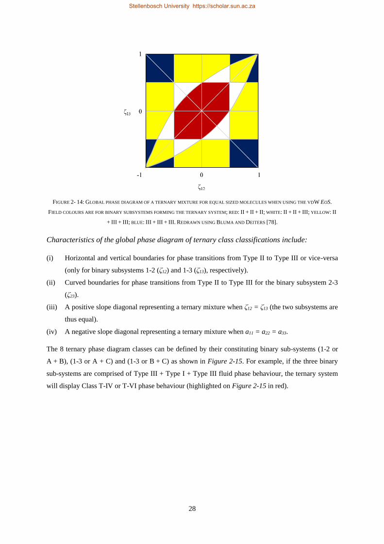
28
FIGURE 2- 14: GLOBAL PHASE DIAGRAM OF A TERNARY MIXTURE FOR EQUAL SIZED MOLECULES WHEN USING THE VDW EOS.
FIELD COLOURS ARE FOR BINARY SUBSYSTEMS FORMING THE TERNARY SYSTEM; RED: II + II + II; WHITE: II + II + III; YELLOW: II
+ III + III; BLUE: III + III + III. REDRAWN USING BLUMA AND DEITERS [78].
Characteristics of the global phase diagram of ternary class classifications include:
(i) Horizontal and vertical boundaries for phase transitions from Type II to Type III or vice-versa
(only for binary subsystems 1-2 (ζ12) and 1-3 (ζ13), respectively).
(ii) Curved boundaries for phase transitions from Type II to Type III for the binary subsystem 2-3
(ζ23).
(iii) A positive slope diagonal representing a ternary mixture when ζ12 = ζ13 (the two subsystems are
thus equal).
(iv) A negative slope diagonal representing a ternary mixture when a11 = a22 = a33.
The 8 ternary phase diagram classes can be defined by their constituting binary sub-systems (1-2 or
A + B), (1-3 or A + C) and (1-3 or B + C) as shown in Figure 2-15. For example, if the three binary
sub-systems are comprised of Type III + Type I + Type III fluid phase behaviour, the ternary system
will display Class T-IV or T-VI phase behaviour (highlighted on Figure 2-15 in red).
Stellenbosch University https://scholar.sun.ac.za
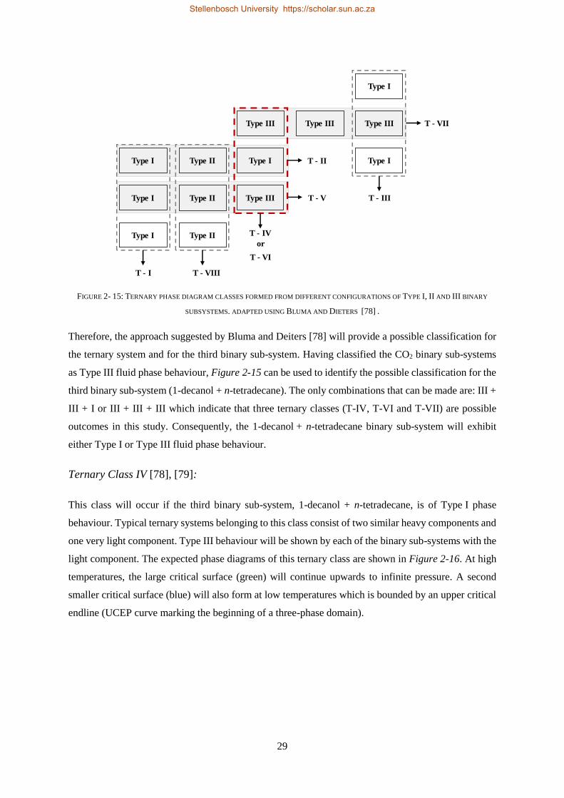
29
FIGURE 2- 15: TERNARY PHASE DIAGRAM CLASSES FORMED FROM DIFFERENT CONFIGURATIONS OF TYPE I, II AND III BINARY
SUBSYSTEMS. ADAPTED USING BLUMA AND DIETERS [78] .
Therefore, the approach suggested by Bluma and Deiters [78] will provide a possible classification for
the ternary system and for the third binary sub-system. Having classified the CO2 binary sub-systems
as Type III fluid phase behaviour, Figure 2-15 can be used to identify the possible classification for the
third binary sub-system (1-decanol + n-tetradecane). The only combinations that can be made are: III +
III + I or III + III + III which indicate that three ternary classes (T-IV, T-VI and T-VII) are possible
outcomes in this study. Consequently, the 1-decanol + n-tetradecane binary sub-system will exhibit
either Type I or Type III fluid phase behaviour.
Ternary Class IV [78], [79]:
This class will occur if the third binary sub-system, 1-decanol + n-tetradecane, is of Type I phase
behaviour. Typical ternary systems belonging to this class consist of two similar heavy components and
one very light component. Type III behaviour will be shown by each of the binary sub-systems with the
light component. The expected phase diagrams of this ternary class are shown in Figure 2-16. At high
temperatures, the large critical surface (green) will continue upwards to infinite pressure. A second
smaller critical surface (blue) will also form at low temperatures which is bounded by an upper critical
endline (UCEP curve marking the beginning of a three-phase domain).
Type I
Type I
Type I
Type I
Type I
Type IType II
Type II
Type II
Type IIIType III Type III
Type III
T - VII
T - III
T - IV
or
T - VIII
T - VI
T - I
T - II
T - V
Stellenbosch University https://scholar.sun.ac.za
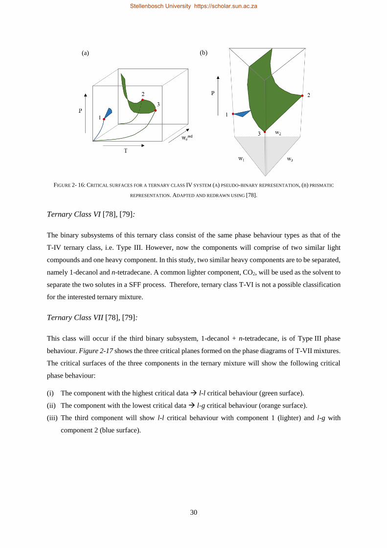
30
FIGURE 2- 16: CRITICAL SURFACES FOR A TERNARY CLASS IV SYSTEM (A) PSEUDO-BINARY REPRESENTATION, (B) PRISMATIC
REPRESENTATION. ADAPTED AND REDRAWN USING [78].
Ternary Class VI [78], [79]:
The binary subsystems of this ternary class consist of the same phase behaviour types as that of the
T-IV ternary class, i.e. Type III. However, now the components will comprise of two similar light
compounds and one heavy component. In this study, two similar heavy components are to be separated,
namely 1-decanol and n-tetradecane. A common lighter component, CO2, will be used as the solvent to
separate the two solutes in a SFF process. Therefore, ternary class T-VI is not a possible classification
for the interested ternary mixture.
Ternary Class VII [78], [79]:
This class will occur if the third binary subsystem, 1-decanol + n-tetradecane, is of Type III phase
behaviour. Figure 2-17 shows the three critical planes formed on the phase diagrams of T-VII mixtures.
The critical surfaces of the three components in the ternary mixture will show the following critical
phase behaviour:
(i) The component with the highest critical data → l-l critical behaviour (green surface).
(ii) The component with the lowest critical data → l-g critical behaviour (orange surface).
(iii) The third component will show l-l critical behaviour with component 1 (lighter) and l-g with
component 2 (blue surface).
(a) (b)
Stellenbosch University https://scholar.sun.ac.za
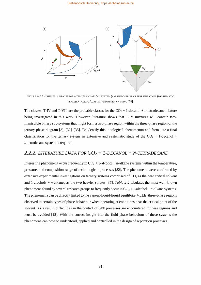
31
FIGURE 2- 17: CRITICAL SURFACES FOR A TERNARY CLASS VII SYSTEM (A) PSEUDO-BINARY REPRESENTATION, (B) PRISMATIC
REPRESENTATION. ADAPTED AND REDRAWN USING [78].
The classes, T-IV and T-VII, are the probable classes for the CO2 + 1-decanol + n-tetradecane mixture
being investigated in this work. However, literature shows that T-IV mixtures will contain two-
immiscible binary sub-systems that might form a two-phase region within the three-phase region of the
ternary phase diagram [3], [32]–[35]. To identify this topological phenomenon and formulate a final
classification for the ternary system an extensive and systematic study of the CO2 + 1-decanol +
n-tetradecane system is required.
2.2.2. LITERATURE DATA FOR CO2 + 1-DECANOL + N-TETRADECANE
Interesting phenomena occur frequently in CO2 + 1-alcohol + n-alkane systems within the temperature,
pressure, and composition range of technological processes [82]. The phenomena were confirmed by
extensive experimental investigations on ternary systems comprised of CO2 as the near critical solvent
and 1-alcohols + n-alkanes as the two heavier solutes [37]. Table 2-2 tabulates the most well-known
phenomena found by several research groups to frequently occur in CO2 + 1-alcohol + n-alkane systems.
The phenomena can be directly linked to the vapour-liquid-liquid equilibria (VLLE) three-phase regions
observed in certain types of phase behaviour when operating at conditions near the critical point of the
solvent. As a result, difficulties in the control of SFF processes are encountered in these regions and
must be avoided [18]. With the correct insight into the fluid phase behaviour of these systems the
phenomena can now be understood, applied and controlled in the design of separation processes.
(a) (b)
Stellenbosch University https://scholar.sun.ac.za
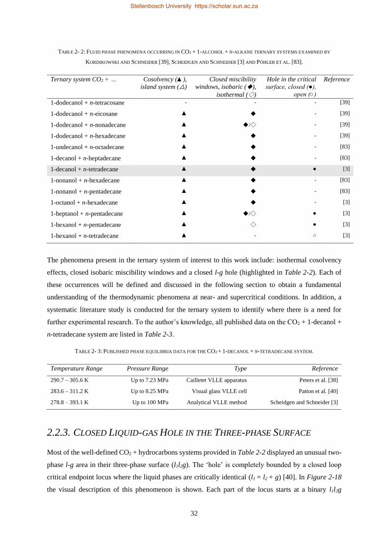
32
TABLE 2- 2: FLUID PHASE PHENOMENA OCCURRING IN CO2 + 1-ALCOHOL + N-ALKANE TERNARY SYSTEMS EXAMINED BY
KORDIKOWSKI AND SCHNEIDER [39], SCHEIDGEN AND SCHNEIDER [3] AND PÖHLER ET AL. [83].
Ternary system CO2 + … Cosolvency (▲),
island system (△)
Closed miscibility
windows, isobaric (◆),
isothermal (◇)
Hole in the critical
surface, closed (●),
open (○)
Reference
1-dodecanol + n-tetracosane - - - [39]
1-dodecanol + n-eicosane ▲ ◆ - [39]
1-dodecanol + n-nonadecane ▲ ◆/◇ - [39]
1-dodecanol + n-hexadecane ▲ ◆ - [39]
1-undecanol + n-octadecane ▲ ◆ - [83]
1-decanol + n-heptadecane ▲ ◆ - [83]
1-decanol + n-tetradecane ▲ ◆ ● [3]
1-nonanol + n-hexadecane ▲ ◆ - [83]
1-nonanol + n-pentadecane ▲ ◆ - [83]
1-octanol + n-hexadecane ▲ ◆ - [3]
1-heptanol + n-pentadecane ▲ ◆/◇ ● [3]
1-hexanol + n-pentadecane ▲ ◇ ● [3]
1-hexanol + n-tetradecane ▲ - ○ [3]
The phenomena present in the ternary system of interest to this work include: isothermal cosolvency
effects, closed isobaric miscibility windows and a closed l-g hole (highlighted in Table 2-2). Each of
these occurrences will be defined and discussed in the following section to obtain a fundamental
understanding of the thermodynamic phenomena at near- and supercritical conditions. In addition, a
systematic literature study is conducted for the ternary system to identify where there is a need for
further experimental research. To the author’s knowledge, all published data on the CO2 + 1-decanol +
n-tetradecane system are listed in Table 2-3.
TABLE 2- 3: PUBLISHED PHASE EQUILIBRIA DATA FOR THE CO2 + 1-DECANOL + N-TETRADECANE SYSTEM.
Temperature Range Pressure Range Type Reference
290.7 – 305.6 K Up to 7.23 MPa Cailletet VLLE apparatus Peters et al. [38]
283.6 – 311.2 K Up to 8.25 MPa Visual glass VLLE cell Patton et al. [40]
278.8 – 393.1 K Up to 100 MPa Analytical VLLE method Scheidgen and Schneider [3]
2.2.3. CLOSED LIQUID-GAS HOLE IN THE THREE-PHASE SURFACE
Most of the well-defined CO2 + hydrocarbons systems provided in Table 2-2 displayed an unusual two-
phase l-g area in their three-phase surface (l1l2g). The ‘hole’ is completely bounded by a closed loop
critical endpoint locus where the liquid phases are critically identical (l1 = l2 + g) [40]. In Figure 2-18
the visual description of this phenomenon is shown. Each part of the locus starts at a binary l1l2g
Stellenbosch University https://scholar.sun.ac.za
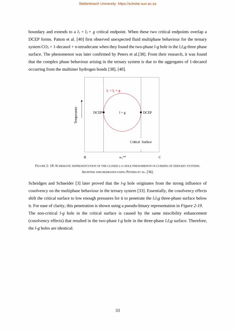
33
boundary and extends to a l1 = l2 + g critical endpoint. When these two critical endpoints overlap a
DCEP forms. Patton et al. [40] first observed unexpected fluid multiphase behaviour for the ternary
system CO2 + 1-decanol + n-tetradecane when they found the two-phase l-g hole in the l1l2g three phase
surface. The phenomenon was later confirmed by Peters et al.[38]. From their research, it was found
that the complex phase behaviour arising in the ternary system is due to the aggregates of 1-decanol
occurring from the multimer hydrogen bonds [38], [40].
FIGURE 2- 18: SCHEMATIC REPRESENTATION OF THE CLOSED L-G HOLE PHENOMENON OCCURRING IN TERNARY SYSTEMS.
ADAPTED AND REDRAWN USING PETERS ET AL. [36].
Scheidgen and Schneider [3] later proved that the l-g hole originates from the strong influence of
cosolvency on the multiphase behaviour in the ternary system [33]. Essentially, the cosolvency effects
shift the critical surface to low enough pressures for it to penetrate the l1l2g three-phase surface below
it. For ease of clarity, this penetration is shown using a pseudo-binary representation in Figure 2-19.
The non-critical l-g hole in the critical surface is caused by the same miscibility enhancement
(cosolvency effects) that resulted in the two-phase l-g hole in the three-phase l1l2g surface. Therefore,
the l-g holes are identical.
DCEP DCEP
l1 = l2 + g
l + g
wcredB C
Tem
per
atur
e
Critical Surface
Stellenbosch University https://scholar.sun.ac.za
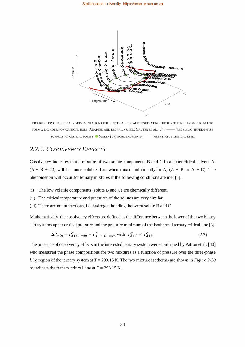
34
FIGURE 2- 19: QUASI-BINARY REPRESENTATION OF THE CRITICAL SURFACE PENETRATING THE THREE-PHASE L1L2G SURFACE TO
FORM A L-G HOLE/NON-CRITICAL HOLE. ADAPTED AND REDRAWN USING GAUTER ET AL. [54]. _______ (RED) L1L2G THREE-PHASE
SURFACE, ○ CRITICAL POINTS, ● (GREEN) CRITICAL ENDPOINTS, ………... METASTABLE CRITICAL LINE.
2.2.4. COSOLVENCY EFFECTS
Cosolvency indicates that a mixture of two solute components B and C in a supercritical solvent A,
(A + B + C), will be more soluble than when mixed individually in A, (A + B or A + C). The
phenomenon will occur for ternary mixtures if the following conditions are met [3]:
(i) The low volatile components (solute B and C) are chemically different.
(ii) The critical temperature and pressures of the solutes are very similar.
(iii) There are no interactions, i.e. hydrogen bonding, between solute B and C.
Mathematically, the cosolvency effects are defined as the difference between the lower of the two binary
sub-systems upper critical pressure and the pressure minimum of the isothermal ternary critical line [3]:
∆𝑃𝑚𝑖𝑛 = 𝑃𝐴+𝐶, 𝑚𝑖𝑛𝑐 − 𝑃𝐴+𝐵+𝐶, 𝑚𝑖𝑛
𝑐 with 𝑃𝐴+𝐶𝑐 < 𝑃𝐴+𝐵
𝑐 (2.7)
The presence of cosolvency effects in the interested ternary system were confirmed by Patton et al. [40]
who measured the phase compositions for two mixtures as a function of pressure over the three-phase
l1l2g region of the ternary system at T = 293.15 K. The two mixture isotherms are shown in Figure 2-20
to indicate the ternary critical line at T = 293.15 K.
wcred
Temperature
Pre
ssure
B
C
Stellenbosch University https://scholar.sun.ac.za
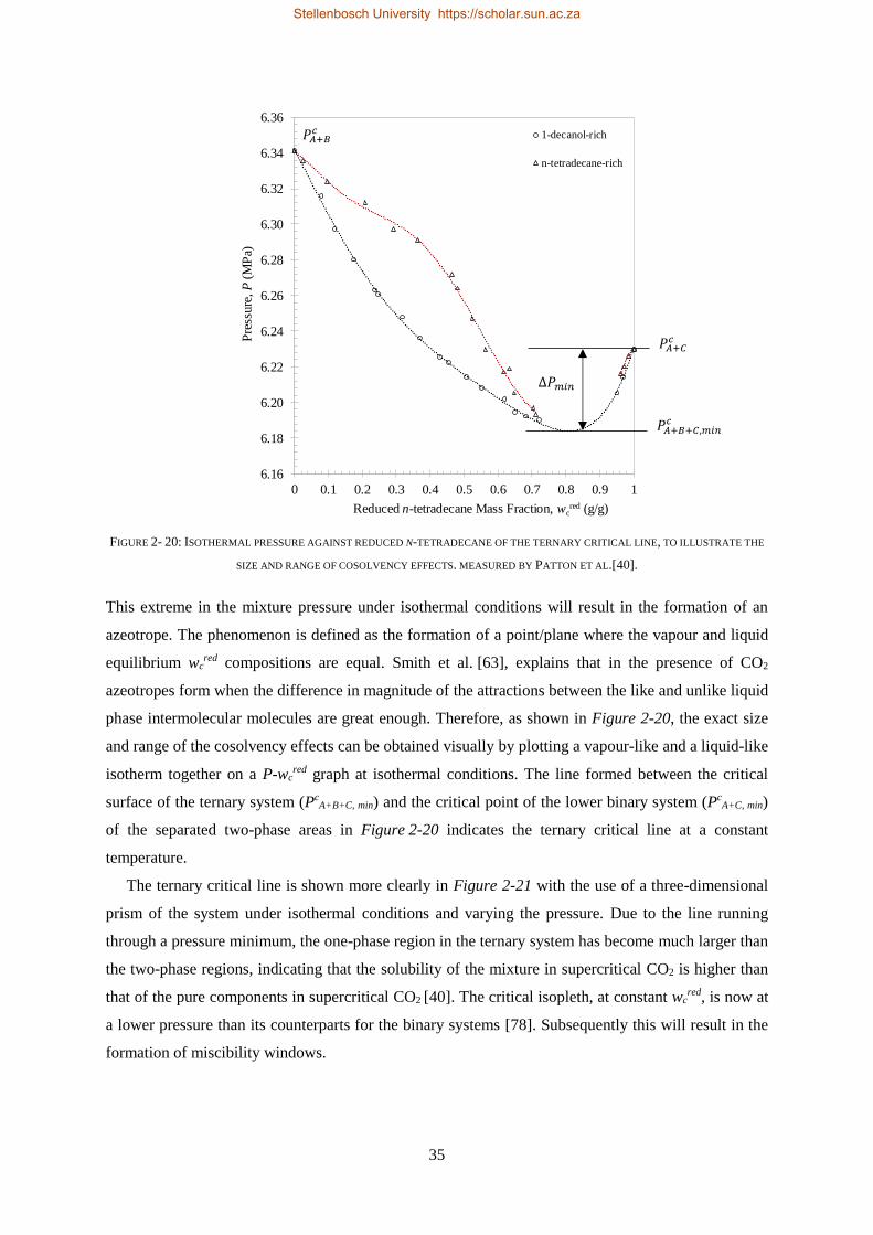
35
FIGURE 2- 20: ISOTHERMAL PRESSURE AGAINST REDUCED N-TETRADECANE OF THE TERNARY CRITICAL LINE, TO ILLUSTRATE THE
SIZE AND RANGE OF COSOLVENCY EFFECTS. MEASURED BY PATTON ET AL.[40].
This extreme in the mixture pressure under isothermal conditions will result in the formation of an
azeotrope. The phenomenon is defined as the formation of a point/plane where the vapour and liquid
equilibrium wcred compositions are equal. Smith et al. [63], explains that in the presence of CO2
azeotropes form when the difference in magnitude of the attractions between the like and unlike liquid
phase intermolecular molecules are great enough. Therefore, as shown in Figure 2-20, the exact size
and range of the cosolvency effects can be obtained visually by plotting a vapour-like and a liquid-like
isotherm together on a P-wcred graph at isothermal conditions. The line formed between the critical
surface of the ternary system (PcA+B+C, min) and the critical point of the lower binary system (Pc
A+C, min)
of the separated two-phase areas in Figure 2-20 indicates the ternary critical line at a constant
temperature.
The ternary critical line is shown more clearly in Figure 2-21 with the use of a three-dimensional
prism of the system under isothermal conditions and varying the pressure. Due to the line running
through a pressure minimum, the one-phase region in the ternary system has become much larger than
the two-phase regions, indicating that the solubility of the mixture in supercritical CO2 is higher than
that of the pure components in supercritical CO2 [40]. The critical isopleth, at constant wcred, is now at
a lower pressure than its counterparts for the binary systems [78]. Subsequently this will result in the
formation of miscibility windows.
6.16
6.18
6.20
6.22
6.24
6.26
6.28
6.30
6.32
6.34
6.36
0 0.1 0.2 0.3 0.4 0.5 0.6 0.7 0.8 0.9 1
Pre
ssure
, P
(MP
a)
Reduced n-tetradecane Mass Fraction, wcred (g/g)
1-decanol-rich
n-tetradecane-rich
𝑃𝐴+𝐶𝑐
𝑃𝐴+𝐵+𝐶,𝑚𝑖𝑛𝑐
𝑃𝐴+𝐵𝑐
∆𝑃𝑚𝑖𝑛
Stellenbosch University https://scholar.sun.ac.za
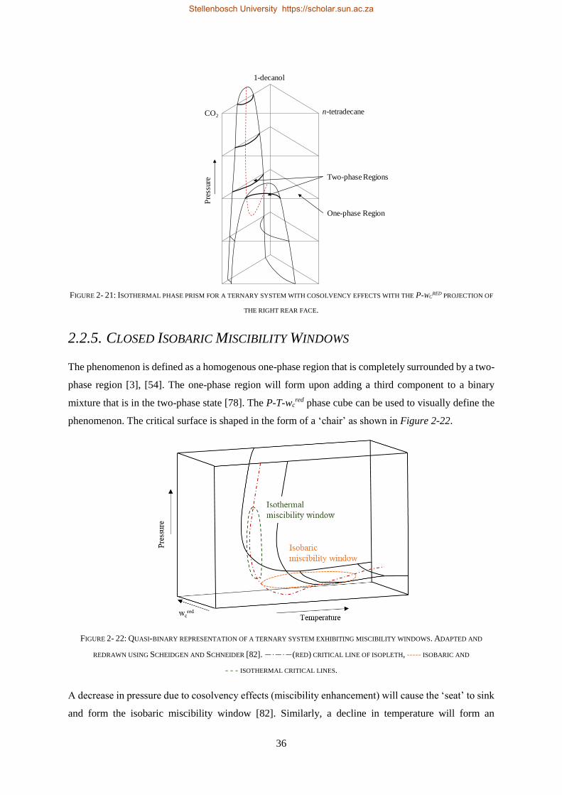
36
FIGURE 2- 21: ISOTHERMAL PHASE PRISM FOR A TERNARY SYSTEM WITH COSOLVENCY EFFECTS WITH THE P-WCRED PROJECTION OF
THE RIGHT REAR FACE.
2.2.5. CLOSED ISOBARIC MISCIBILITY WINDOWS
The phenomenon is defined as a homogenous one-phase region that is completely surrounded by a two-
phase region [3], [54]. The one-phase region will form upon adding a third component to a binary
mixture that is in the two-phase state [78]. The P-T-wcred phase cube can be used to visually define the
phenomenon. The critical surface is shaped in the form of a ‘chair’ as shown in Figure 2-22.
FIGURE 2- 22: QUASI-BINARY REPRESENTATION OF A TERNARY SYSTEM EXHIBITING MISCIBILITY WINDOWS. ADAPTED AND
REDRAWN USING SCHEIDGEN AND SCHNEIDER [82]. ⎯ ⋅⎯ ⋅⎯ (RED) CRITICAL LINE OF ISOPLETH, ----- ISOBARIC AND
- - - ISOTHERMAL CRITICAL LINES.
A decrease in pressure due to cosolvency effects (miscibility enhancement) will cause the ‘seat’ to sink
and form the isobaric miscibility window [82]. Similarly, a decline in temperature will form an
CO2
Pre
ssure
1-decanol
n-tetradecane
One-phase Region
Two-phase Regions
Stellenbosch University https://scholar.sun.ac.za
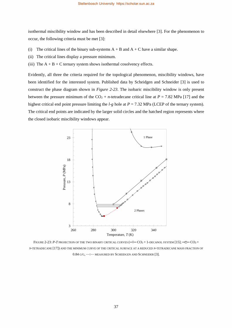
37
isothermal miscibility window and has been described in detail elsewhere [3]. For the phenomenon to
occur, the following criteria must be met [3]:
(i) The critical lines of the binary sub-systems A + B and A + C have a similar shape.
(ii) The critical lines display a pressure minimum.
(iii) The A + B + C ternary system shows isothermal cosolvency effects.
Evidently, all three the criteria required for the topological phenomenon, miscibility windows, have
been identified for the interested system. Published data by Scheidgen and Schneider [3] is used to
construct the phase diagram shown in Figure 2-23. The isobaric miscibility window is only present
between the pressure minimum of the CO2 + n-tetradecane critical line at P = 7.82 MPa [17] and the
highest critical end point pressure limiting the l-g hole at P = 7.32 MPa (LCEP of the ternary system).
The critical end points are indicated by the larger solid circles and the hatched region represents where
the closed isobaric miscibility windows appear.
FIGURE 2-23: P-T PROJECTION OF THE TWO BINARY CRITICAL CURVES (─◊─ CO2 + 1-DECANOL SYSTEM [15]; ─⧠─ CO2 +
N-TETRADECANE [17]) AND THE MINIMUM CURVE OF THE CRITICAL SURFACE AT A REDUCED N-TETRADECANE MASS FRACTION OF
0.84 G/G, ⋯○⋯ MEASURED BY SCHEIDGEN AND SCHNEIDER [3].
3
8
13
18
23
260 280 300 320 340
Pre
ssure
, P
(MP
a)
Temperature, T (K)
1 Phase
2 Phases
Stellenbosch University https://scholar.sun.ac.za
38
2.2.6. CLASSIFICATION OF THE CO2 + 1-DECANOL + N-TETRADECANE
SYSTEM AND THIRD BINARY SUB-SYSTEM
The miscibility window measured by Scheidgen and Schneider [3] within the l1l2g three-phase region
of the CO2 + 1-decanol + n-tetradecane system infers T-IV phase behaviour. Therefore, the ternary
system will have two Type III binary sub-systems (CO2 + 1-decanol and CO2 + n-tetradecane) and one
Type I sub-system (1-decanol + n-tetradecane). Type I behaviour assumes that only one liquid phase
exists throughout the phase diagram. Therefore, the two solutes, 1-decanol and n-tetradecane are
miscible, with close boiling points, possibly resulting in a homogeneous azeotrope. These systems will
be identified as displaying Type I-A fluid phase behaviour [79]. The two main variants of azeotropic
behaviour, i.e. positive and negative, are well defined in literature [79], [84]–[87]:
Positive azeotropy:
Positive azeotropy is most commonly observed for non-polar or weakly polar molecules where the
interactions between the like molecules (solute + solute) are stronger than the interactions between the
unlike molecules (solute + solvent). Thus, a positive deviation from Raoult’s law occurs due to
solvation or association effects, i.e. the vapour pressure of the azeotropic mixture is greater than the
pure component vapour pressures at a constant temperature.
Negative azeotropy:
Negative azeotropy is seldomly observed for non-polar or weakly polar molecules. Therefore, they are
more likely to occur in mixtures where the interactions between the unlike molecules (solute + solvent)
are stronger than those between the like molecules (solute + solute). Thus, a negative deviation from
Raoult’s law will take place due to hydrogen bonding or proton transfers, i.e. the vapour pressure of
the azeotropic mixture is less than the pure component vapour pressures at a constant temperature.
It is postulated that a positive azeotrope (positive deviation from Raoult’s law) will be observed for
the 1-decanol + n-tetradecane binary sub-system. This assumption is based on the following:
(i) The complex phase behaviour identified in the ternary system indicates strong solute + solute
interactions.
(ii) The binary sub-system comprises of non-polar n-tetradecane molecules and weakly polar
1-decanol molecules.
(iii) Pertinent 1-alcohol + n-alkane literature data were gathered and are tabulated in Table 2-4 to
identify the type of phase behaviour to be anticipated for the 1-decanol + n-tetradecane system.
For each of the 1-alcohol + n-alkane binary systems a general trend is identified: in 1-alcohol +
Stellenbosch University https://scholar.sun.ac.za
39
n-alkane systems with m < n, where m and n represent the number of carbon atoms in the alkyl-
chains of the 1-alcohol and n-alkane, respectively, an azeotrope is identified.
Based on the non-ideal phase behaviour illustrated by these polar + non-polar systems and the complex
phase behaviour phenomena in the ternary system, an extensive experimental study of binary
1-alcohol + n-alkane VLE data will be carried out in this work to verify the new 1-decanol +
n-tetradecane phase equilibria data. The binary systems that will be measured for verification include:
1-pentanol + n-nonane, 1-hexanol + n-decane, 1-heptanol + n-undecane and 1-octanol + n-dodecane.
Furthermore, due to the high boiling points of the interested systems, it is preferred to measure the data
at sub-atmospheric conditions. This is in line with literature findings, as Table 2-4 shows that sub-
atmospheric pressures are generally used to measure 1-alcohol + n-alkane binary systems. A suitable
setup that can be operated at sub-atmospheric conditions and high temperatures should therefore also
be considered for the systems of interest to this work.
Stellenbosch University https://scholar.sun.ac.za
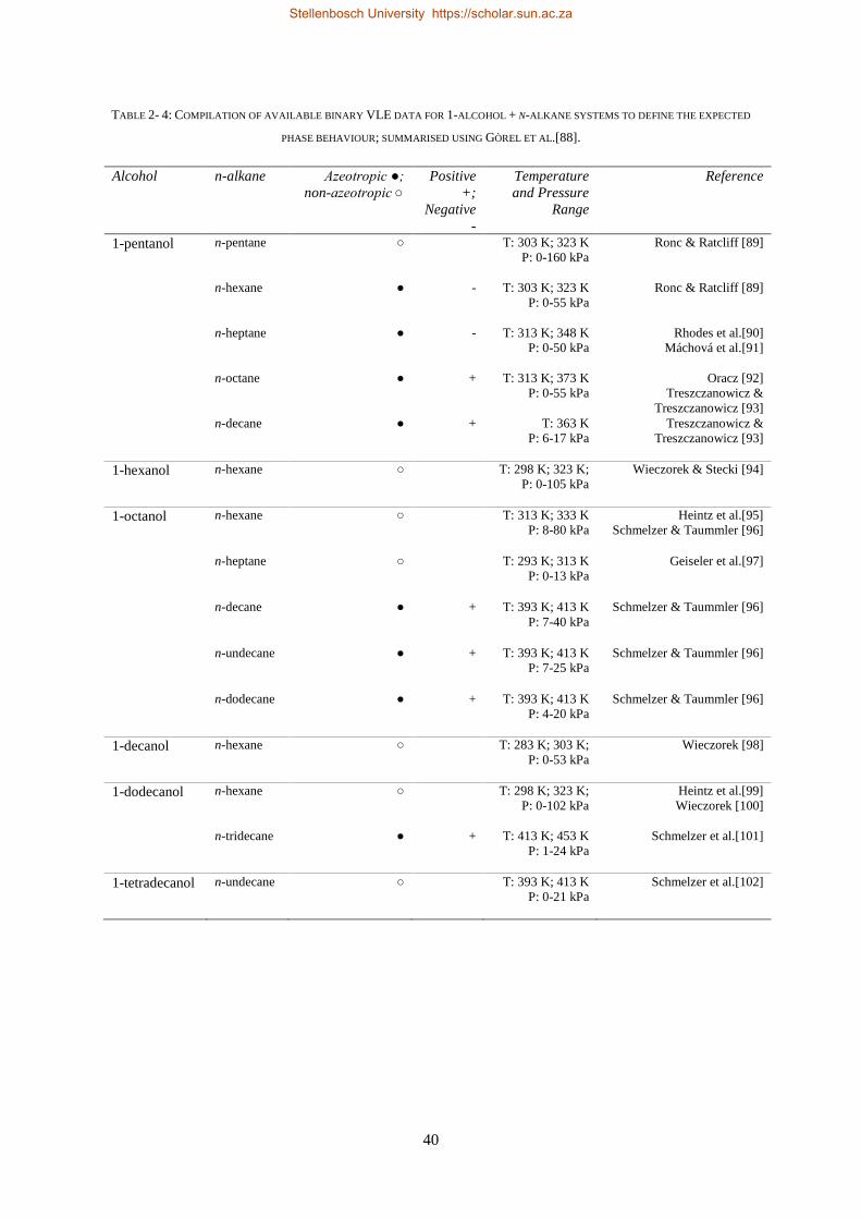
40
TABLE 2- 4: COMPILATION OF AVAILABLE BINARY VLE DATA FOR 1-ALCOHOL + N-ALKANE SYSTEMS TO DEFINE THE EXPECTED
PHASE BEHAVIOUR; SUMMARISED USING GÒREL ET AL.[88].
Alcohol n-alkane Azeotropic ●;
non-azeotropic ○
Positive
+;
Negative
-
Temperature
and Pressure
Range
Reference
1-pentanol n-pentane ○
T: 303 K; 323 K
P: 0-160 kPa
Ronc & Ratcliff [89]
n-hexane ● - T: 303 K; 323 K
P: 0-55 kPa
Ronc & Ratcliff [89]
n-heptane ● - T: 313 K; 348 K
P: 0-50 kPa
Rhodes et al.[90]
Máchová et al.[91]
n-octane ● + T: 313 K; 373 K
P: 0-55 kPa
Oracz [92]
Treszczanowicz &
Treszczanowicz [93]
n-decane ● + T: 363 K
P: 6-17 kPa
Treszczanowicz &
Treszczanowicz [93]
1-hexanol n-hexane ○
T: 298 K; 323 K;
P: 0-105 kPa
Wieczorek & Stecki [94]
1-octanol n-hexane ○
T: 313 K; 333 K
P: 8-80 kPa
Heintz et al.[95]
Schmelzer & Taummler [96]
n-heptane ○
T: 293 K; 313 K
P: 0-13 kPa
Geiseler et al.[97]
n-decane ● + T: 393 K; 413 K
P: 7-40 kPa
Schmelzer & Taummler [96]
n-undecane ● + T: 393 K; 413 K
P: 7-25 kPa
Schmelzer & Taummler [96]
n-dodecane ● + T: 393 K; 413 K
P: 4-20 kPa
Schmelzer & Taummler [96]
1-decanol n-hexane ○
T: 283 K; 303 K;
P: 0-53 kPa
Wieczorek [98]
1-dodecanol n-hexane ○
T: 298 K; 323 K;
P: 0-102 kPa
Heintz et al.[99]
Wieczorek [100]
n-tridecane ● + T: 413 K; 453 K
P: 1-24 kPa
Schmelzer et al.[101]
1-tetradecanol n-undecane ○
T: 393 K; 413 K
P: 0-21 kPa
Schmelzer et al.[102]
Stellenbosch University https://scholar.sun.ac.za
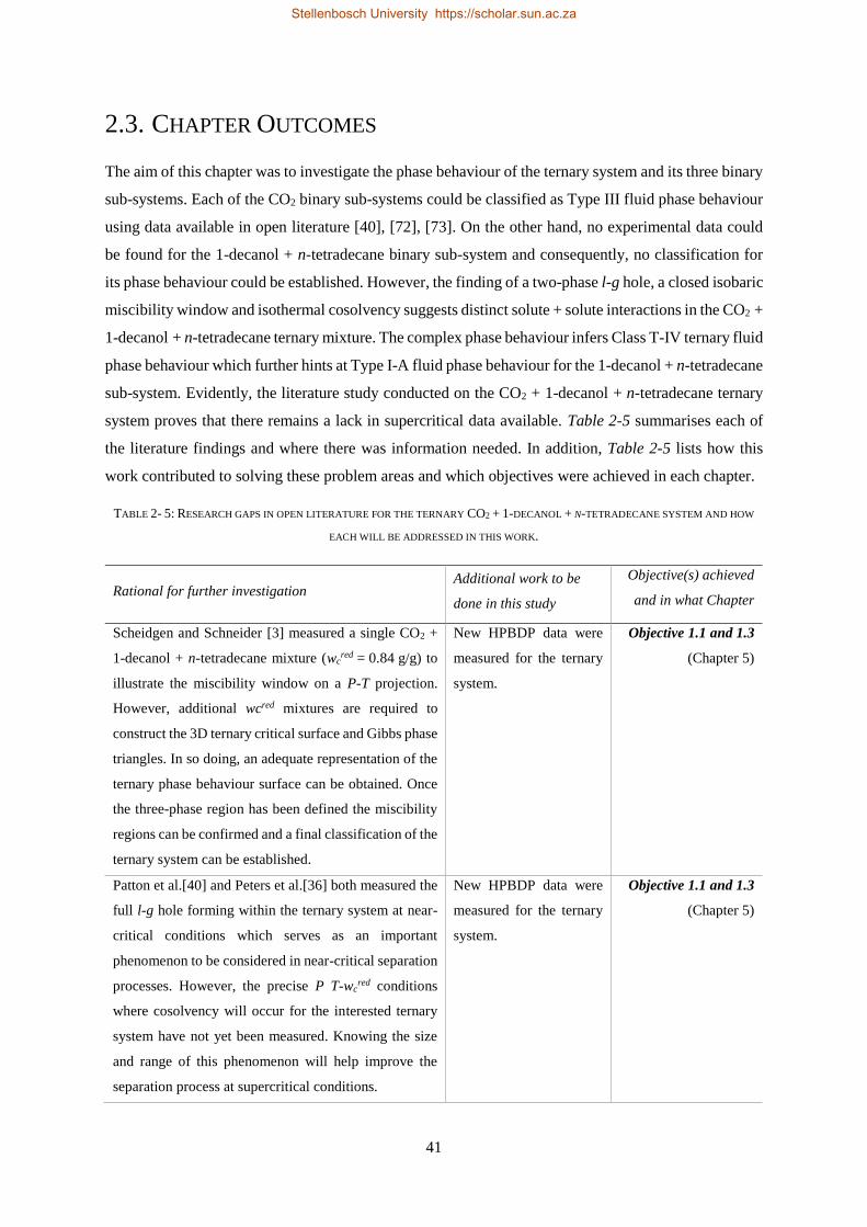
41
2.3. CHAPTER OUTCOMES
The aim of this chapter was to investigate the phase behaviour of the ternary system and its three binary
sub-systems. Each of the CO2 binary sub-systems could be classified as Type III fluid phase behaviour
using data available in open literature [40], [72], [73]. On the other hand, no experimental data could
be found for the 1-decanol + n-tetradecane binary sub-system and consequently, no classification for
its phase behaviour could be established. However, the finding of a two-phase l-g hole, a closed isobaric
miscibility window and isothermal cosolvency suggests distinct solute + solute interactions in the CO2 +
1-decanol + n-tetradecane ternary mixture. The complex phase behaviour infers Class T-IV ternary fluid
phase behaviour which further hints at Type I-A fluid phase behaviour for the 1-decanol + n-tetradecane
sub-system. Evidently, the literature study conducted on the CO2 + 1-decanol + n-tetradecane ternary
system proves that there remains a lack in supercritical data available. Table 2-5 summarises each of
the literature findings and where there was information needed. In addition, Table 2-5 lists how this
work contributed to solving these problem areas and which objectives were achieved in each chapter.
TABLE 2- 5: RESEARCH GAPS IN OPEN LITERATURE FOR THE TERNARY CO2 + 1-DECANOL + N-TETRADECANE SYSTEM AND HOW
EACH WILL BE ADDRESSED IN THIS WORK.
Rational for further investigation Additional work to be
done in this study
Objective(s) achieved
and in what Chapter
Scheidgen and Schneider [3] measured a single CO2 +
1-decanol + n-tetradecane mixture (wcred = 0.84 g/g) to
illustrate the miscibility window on a P-T projection.
However, additional wcred mixtures are required to
construct the 3D ternary critical surface and Gibbs phase
triangles. In so doing, an adequate representation of the
ternary phase behaviour surface can be obtained. Once
the three-phase region has been defined the miscibility
regions can be confirmed and a final classification of the
ternary system can be established.
New HPBDP data were
measured for the ternary
system.
Objective 1.1 and 1.3
(Chapter 5)
Patton et al.[40] and Peters et al.[36] both measured the
full l-g hole forming within the ternary system at near-
critical conditions which serves as an important
phenomenon to be considered in near-critical separation
processes. However, the precise P T-wcred conditions
where cosolvency will occur for the interested ternary
system have not yet been measured. Knowing the size
and range of this phenomenon will help improve the
separation process at supercritical conditions.
New HPBDP data were
measured for the ternary
system.
Objective 1.1 and 1.3
(Chapter 5)
Stellenbosch University https://scholar.sun.ac.za
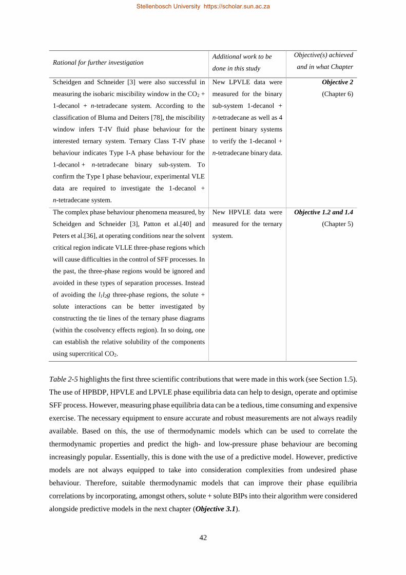
42
Rational for further investigation Additional work to be
done in this study
Objective(s) achieved
and in what Chapter
Scheidgen and Schneider [3] were also successful in
measuring the isobaric miscibility window in the CO2 +
1-decanol + n-tetradecane system. According to the
classification of Bluma and Deiters [78], the miscibility
window infers T-IV fluid phase behaviour for the
interested ternary system. Ternary Class T-IV phase
behaviour indicates Type I-A phase behaviour for the
1-decanol + n-tetradecane binary sub-system. To
confirm the Type I phase behaviour, experimental VLE
data are required to investigate the 1-decanol +
n-tetradecane system.
New LPVLE data were
measured for the binary
sub-system 1-decanol +
n-tetradecane as well as 4
pertinent binary systems
to verify the 1-decanol +
n-tetradecane binary data.
Objective 2
(Chapter 6)
The complex phase behaviour phenomena measured, by
Scheidgen and Schneider [3], Patton et al.[40] and
Peters et al.[36], at operating conditions near the solvent
critical region indicate VLLE three-phase regions which
will cause difficulties in the control of SFF processes. In
the past, the three-phase regions would be ignored and
avoided in these types of separation processes. Instead
of avoiding the l1l2g three-phase regions, the solute +
solute interactions can be better investigated by
constructing the tie lines of the ternary phase diagrams
(within the cosolvency effects region). In so doing, one
can establish the relative solubility of the components
using supercritical CO2.
New HPVLE data were
measured for the ternary
system.
Objective 1.2 and 1.4
(Chapter 5)
Table 2-5 highlights the first three scientific contributions that were made in this work (see Section 1.5).
The use of HPBDP, HPVLE and LPVLE phase equilibria data can help to design, operate and optimise
SFF process. However, measuring phase equilibria data can be a tedious, time consuming and expensive
exercise. The necessary equipment to ensure accurate and robust measurements are not always readily
available. Based on this, the use of thermodynamic models which can be used to correlate the
thermodynamic properties and predict the high- and low-pressure phase behaviour are becoming
increasingly popular. Essentially, this is done with the use of a predictive model. However, predictive
models are not always equipped to take into consideration complexities from undesired phase
behaviour. Therefore, suitable thermodynamic models that can improve their phase equilibria
correlations by incorporating, amongst others, solute + solute BIPs into their algorithm were considered
alongside predictive models in the next chapter (Objective 3.1).
Stellenbosch University https://scholar.sun.ac.za
43
Chapter 3
HOLISTIC THERMODYNAMIC MODEL SELECTION
This chapter introduces the second part of this thesis, which is devoted to the thermodynamic modelling
of the ternary system and its three binary sub-systems. Emphasis will be placed on the use of property
methods available within Aspen Plus®.
The aim of this chapter is twofold: first, to assess both classical and advanced thermodynamic
models; and second, to select suitable methods within Aspen Plus® (Objective 3.1), which can
potentially be used not simply for modelling complex VLE behaviour, but also for industrial
applications.
First, a short-unified presentation of the phase equilibria fundamentals will be given, highlighting
the direction for selecting a suitable model. The flexible and predictive property methods will be
described in separate sections to define their fundamental equations. The chapter will close with a
discussion of the selected association EoS property method and the parameters to be used for correlating
the complex phase behaviour of the CO2 + 1-decanol + n-tetradecane system.
3.1. INDUSTRIAL RELEVANCE OF ASPEN PLUS®
The purpose of evaluating, selecting and improving thermodynamic models found in Aspen Plus® is to
ultimately end with a working process model like that designed by Zamudio et al. [12]. However, the
design of a process model falls beyond the scope of this work. The focus will remain on obtaining a
fundamental understanding of the impact the solute + solute interaction parameters have on the ability
of thermodynamic models to correlate measured equilibrium data. Aspen Plus® is a popular commercial
process simulator that is available to various industrial sectors. Furthermore, it was validated as a
reliable thermodynamic tool in a previous research project conducted by Lombard [51]. Parameters
were regressed for the Redlich-Kwong-Aspen (RK-Aspen) model [103] in Aspen Plus® and the
resultant correlations agreed with those obtained by an in-house developed model with MATLAB
software. Based on the ease of availability and accuracy of Aspen Plus®, the strategies developed in this
work with this commercial simulator can be repeated and implemented in similar separation processes
elsewhere.
Stellenbosch University https://scholar.sun.ac.za
44
3.2. PHASE EQUILIBRIA FUNDAMENTALS
The first step in modelling the measured data is to determine the correct thermodynamic model to use
for the close boiling point detergent range 1-alcohols and n-alkanes. There are two main approaches to
phase equilibria: γ-φ and φ-φ. Here, γ accounts for the deviations from ideality via the activity
coefficient and the deviation of the fluid from ideal solution behaviour. Analogously, φ accounts for
the deviations from ideality via the fugacity coefficient and the deviation from ideal gas behaviour.
The fundamental property determining the equilibrium of a specific component between phases and
chemical reactions is chemical potential. The chemical potential of species 𝑖, can mathematically be
defined using the partial Gibbs energy equation [63]:
𝜇𝑖 = (𝜕(𝑛𝐺)
𝜕𝑥𝑖)
𝑇,𝑃,𝑥𝑗
(3.1)
When the chemical potential of multiple species is the same in all phases, at the same temperature and
pressure, they are said to be in equilibrium with one another [63]:
𝜇𝑖𝛼 = 𝜇𝑖
𝛽= 𝜇𝑖
𝜋 (3.2)
To define the chemical potential of real gasses and liquids the concept of fugacity needs to be utilised.
Fugacity is a representation of the effective or real partial pressure of species 𝑖, in a specific phase and
can mathematically be defined using [63]:
𝜇𝑖 = ��𝑖 = 𝛤𝑖(𝑇) + 𝑅𝑇 ln(𝑓��) (3.3)
Therefore, fugacity will be a function of the temperature, pressure and composition of species 𝑖 in a
solution, at phase equilibrium:
𝑓𝑖𝑙(𝑇, 𝑃, 𝑥) = 𝑓𝑖
𝑣(𝑇, 𝑃, 𝑦) (3.4)
Fugacity can be estimated with either the γ approach or the φ approach. For the γ approach, deviations
from the ideal solution can be calculated using:
𝑓�� = 𝑥𝑖𝛾𝑖𝜑𝑖𝑠𝑎𝑡𝑃𝑖
𝑠𝑎𝑡 exp1
𝑅𝑇∫ 𝑉𝑖
𝑙𝑃𝑖
𝑃𝑖𝑠𝑎𝑡 𝑑𝑃 (3.5)
For the φ approach the deviations from the ideal gas can be calculated using equations (3.6) and (3.7)
for the vapour and liquid phase, respectively.
𝑓𝑖𝑣 = 𝑦𝑖𝑃��𝑖
𝑣 (3.6)
𝑓𝑖𝑙 = 𝑥𝑖𝑃��𝑖
𝑙 (3.7)
Unfortunately, the γ approach requires the calculation of saturation pressures and therefore, all
compounds must remain below their respective critical point. Thus, applications of this method for
critical and supercritical pressures can become rather difficult and inaccurate.
Stellenbosch University https://scholar.sun.ac.za
45
For each component in equilibrium can be expressed using equation (3.8) after the substitution of
equations (3.6) and (3.7) into (3.4).
𝑦𝑖��𝑖𝑣 = 𝑥𝑖��𝑖
𝑙 (3.8)
To solve for the fugacity of component 𝑖 in a mixture, 𝜑�� the residual Gibbs energy equation for a
mixture (3.9) must be used:
ln ��𝑖𝑣 = [
𝜕(𝑛𝐺𝑅)
𝜕𝑥𝑖]
𝑃,𝑇,𝑥𝑗
(3.9)
EoSs can be used to calculate 𝑛𝐺𝑅. Among other techniques, the φ-φ approach is the best method to
use in calculating the fluid phase equilibria of the system of interest. For further details of the φ-φ
approach one is referred to Smith et al. [63].
3.3. CUBIC EOS PROPERTY METHODS
Systematic literature investigations have shown that classical cubic EoS models can, to a certain degree,
accurately represent hydrocarbon + gas and hydrocarbon + hydrocarbon VLE mixtures at low- and
high-pressures [43], [45], [101], [102], [104]–[107]. Thus, the SRK and PR EoS are further investigated
in this work. In general, a cubic EoS can be written using equation (3.10).
𝑃 =𝑅𝑇
𝑉𝑚−𝑏 −
𝑎
(𝑉𝑚+ 𝜆1𝑏)(𝑉𝑚+𝜆2𝑏) (3.10)
Where, λ1 = 1 and λ2 = 0 (SRK); or λ1 = 1 - √2 and λ2 = 1 - √2 (PR).
The current study deals with mixtures and therefore, mixing rules are required. To calculate the
energy parameter and co-volume parameters, the quadratic vdW one fluid mixing rules can be applied
with the cross coefficient written in terms of an inclusive binary interaction parameter. The geometric
mean rule is applied to represent the attractive force between two molecules (equation 3.11) and the
arithmetic mean rule to relate to the volume that a species occupies (equation 3.12) [18], [107], [108].
The pure component parameters can be calculated with equations (3.13 a) and (3.13 b).
𝑎 = ∑ ∑ 𝑥𝑖𝑥𝑗(𝑎𝑖𝑎𝑗)0.5
(1 − 𝑘𝑖𝑗)𝑛𝑗=1
𝑛𝑖=1 (3.11)
𝑏 = ∑ ∑ 𝑥𝑖𝑥𝑗(𝑏𝑖+𝑏𝑗)
2(1 − 𝑙𝑖𝑗)𝑛
𝑗=1𝑛𝑖=1 (3.12)
𝑎𝑖 = 𝛼𝑖(𝑇) ∙ 𝛺𝑎 ∙𝑅2𝑇𝑐,𝑖
2
𝑃𝑐,𝑖
(3.13 a)
𝑏𝑖 = 𝛺𝑏 ∙𝑅𝑇𝑐,𝑖
𝑃𝑐,𝑖
(3.13 b)
Where, Ωa = 0.42747 and Ωb = 0.08664 (SRK); or Ωa = 0.45724 and Ωb = 0.07780 (PR).
The temperature dependent alpha function, αi(T) shown in equation (3.13 a) can be calculated using
equation (3.14) and substituting equation (3.15 a) or (3.15 b) for the SRK or PR EoS, respectively. In
general, these terms were empirically established to best fit experimental data [109].
Stellenbosch University https://scholar.sun.ac.za
46
𝛼𝑖(𝑇) = [1 + 𝑚𝑖(1 − √𝑇𝑟,𝑖)]2 (3.14)
𝑚𝑖 = 0.48 + 1.574𝜔𝑖 − 0.176𝜔𝑖2 (3.15 a)
𝑚𝑖 = 0.37464 + 1.54226𝜔𝑖 − 0.26992𝜔𝑖2 (3.15 b)
Cubic EoS with the classical mixing and combining rules could, to a certain degree, represent polar
mixtures when considering the BIPs. However, regardless of the added BIPs, for highly polar and
hydrogen bonding mixtures, the classical quadratic mixing rules fail to represent the phase equilibria
accurately and false phase splits are calculated [42], [107], [110]. This problem area can partially be
addressed within the framework of cubic EoS with more advanced mixing rules, i.e. the EoS-GE mixing
rules proposed by Huron and Vidal [111].
3.4. PREDICTIVE PROPERTY METHODS IN ASPEN PLUS®
EoS-GE mixing rules permit an expression for the excess Gibbs energy, GE to be incorporated into the
EoS. In so doing, a single model is established which combines the strengths of both the cubic EoS and
the activity coefficient models [107]. The predictive models can be derived from the following equality
at a reference pressure:
(𝐺𝐸
𝑅𝑇)
𝑃
𝐸𝑜𝑆
= (𝐺𝐸
𝑅𝑇)
𝑃
𝑚𝑜𝑑𝑒𝑙,∗
(3.16)
The left-hand side of equation (3.16) represents the GE of the EoS and can be obtained using the fugacity
coefficient as computed by EoS (see equation (3.9)). The right-hand side of equation (3.16) defines the
GE expression of an explicit activity coefficient model. Here, the subscript, * will give reference to, for
example the Wilson [112], NRTL [113] or UNIQUAC [114] model. Any activity coefficient model
with available BIPs can be used.
∴𝐺𝐸
𝑅𝑇= ln 𝜑 − ∑ 𝑥𝑖 ln 𝜑��𝑖 = ∑ 𝑥𝑖 ln 𝛾𝑖𝑖 (3.17)
3.4.1. UNIFAC GROUP CONTRIBUTION METHOD
If low-pressure data are unavailable for the regression of BIPs, a group contribution method can be used
to predict the missing phase equilibria data [115]. With group contribution methods, the mixture is
described using different functional groups (group-group interaction parameters), not molecules, as
shown in Figure 3-1 for 1-decanol and n-tetradecane [116]. In this manner, for example, group
interaction parameters derived from LPVLE experimental data of an available alcohol + alkane system
can be used to predict the real behaviour of the alcohol + alkane system of interest to this work [117]–
[119].
Stellenbosch University https://scholar.sun.ac.za
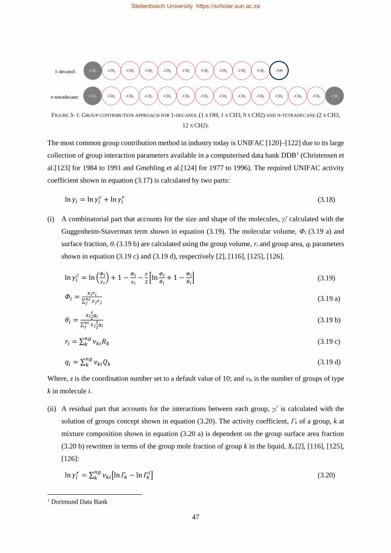
47
FIGURE 3- 1: GROUP CONTRIBUTION APPROACH FOR 1-DECANOL (1 X OH, 1 X CH3, 9 X CH2) AND N-TETRADECANE (2 X CH3,
12 X CH2).
The most common group contribution method in industry today is UNIFAC [120]–[122] due to its large
collection of group interaction parameters available in a computerised data bank DDB1 (Christensen et
al.[123] for 1984 to 1991 and Gmehling et al.[124] for 1977 to 1996). The required UNIFAC activity
coefficient shown in equation (3.17) is calculated by two parts:
ln 𝛾𝑖 = ln 𝛾𝑖𝑐 + ln 𝛾𝑖
𝑟 (3.18)
(i) A combinatorial part that accounts for the size and shape of the molecules, γic calculated with the
Guggenheim-Staverman term shown in equation (3.19). The molecular volume, Φi (3.19 a) and
surface fraction, θi (3.19 b) are calculated using the group volume, ri and group area, qi parameters
shown in equation (3.19 c) and (3.19 d), respectively [2], [116], [125], [126].
ln 𝛾𝑖𝑐 = ln (
𝛷𝑖
𝑥𝑖) + 1 −
𝛷𝑖
𝑥𝑖−
𝑧
2[ln
𝛷𝑖
𝑖+ 1 −
𝛷𝑖
𝑖] (3.19)
𝛷𝑖 =𝑥𝑖𝑟𝑖
∑ 𝑥𝑗𝑟𝑗𝑛𝑐𝑗
(3.19 a)
휃𝑖 =𝑥𝑖
𝑧
2𝑞𝑖
∑ 𝑥𝑗𝑧
2𝑞𝑖
𝑛𝑐𝑗
(3.19 b)
𝑟𝑖 = ∑ 𝜈𝑘𝑖𝑅𝑘𝑛𝑔𝑘 (3.19 c)
𝑞𝑖 = ∑ 𝜈𝑘𝑖𝑄𝑘𝑛𝑔𝑘 (3.19 d)
Where, z is the coordination number set to a default value of 10; and νki is the number of groups of type
k in molecule i.
(ii) A residual part that accounts for the interactions between each group, γir is calculated with the
solution of groups concept shown in equation (3.20). The activity coefficient, Γk of a group, k at
mixture composition shown in equation (3.20 a) is dependent on the group surface area fraction
(3.20 b) rewritten in terms of the group mole fraction of group k in the liquid, Xk [2], [116], [125],
[126]:
ln 𝛾𝑖𝑟 = ∑ 𝜈𝑘𝑖[ln 𝛤𝑘 − ln 𝛤𝑘
𝑖]𝑛𝑔𝑘 (3.20)
1 Dortmund Data Bank
-CH3 -CH2 -CH2 -CH2-CH2-CH2-CH2 -CH2 -CH2 -CH2 -OH1-decanol:
-CH3 -CH2 -CH2 -CH2-CH2-CH2-CH2 -CH2 -CH2 -CH2 -CH2-CH2-CH2 -CH3n-tetradecane:
Stellenbosch University https://scholar.sun.ac.za
48
ln 𝛤𝑘 = 𝑄𝑘 [1 − ln ∑ 휃𝑚𝜏𝑚𝑘𝑛𝑔𝑚 − ∑ ( 𝑚𝜏𝑘𝑚
∑ 𝑛𝜏𝑛𝑚𝑛𝑔𝑛
)𝑛𝑔𝑚 ] (3.20 a)
휃𝑘 =𝑋𝑘
𝑧
2𝑄𝑘
∑ 𝑋𝑚𝑧
2𝑄𝑚
𝑛𝑐𝑗
(3.20 b)
𝑋𝑘 =∑ 𝜈𝑘𝑗𝑥𝑗
𝑛𝑐𝑗
∑ ∑ 𝜈𝑚𝑗𝑥𝑗𝑛𝑔𝑚
𝑛𝑐𝑗
(3.20 c)
Using a generated function, τmn the residual term of the activity coefficient model is corrected with a
temperature independent group interaction parameter, bmn between group m and group n [127], [128]:
𝜏𝑚𝑛 = exp (−𝑏𝑚𝑛
𝑇) (3.21)
3.4.2. EOS-GE MIXING RULES
The EoS-GE mixing rules allows for the advantages of the group contribution models to be directly
connected with the EoS. Subsequently, a strictly predictive tool is available for the prediction of VLE
data at low- and high-pressures, irrespective of the presence of polar compounds [128], [129]. Various
well known EoS-GE models have been developed by different authors to enable VLE predictions at high
and low temperatures or pressures as well as for supercritical compounds. These predictive EoS include,
amongst others:
(i) Huron-Vidal type mixing rules:
o Predictive SRK (PSRK) mixing rule as suggested by Holderbaum and Gmehling [115], [116],
[125], [127], [128], [130]–[136].
o Modified Huron-Vidal second order approximation (MHV2) [115], [137]–[143].
(ii) Linear combinations of Vidal and Michelsen mixing rules (LCVM) [115], [137], [144], [145].
(iii) Wong-Sandler mixing rules (W-S) with an additional kij parameter [115], [119], [137], [142],
[146]–[149].
Of importance to this study are EoS-GE models available within Aspen Plus® and therefore, the LCVM
mixing rules will not be investigated further. Figure 3-2 summarises the predictive EoS-GE property
methods suggested by the Aspen Plus® software guide. For each of the property methods the distinctive
EoS models on which they are based, the activity coefficient models implemented in their algorithm
and some of their mixture characteristics are specified.
Stellenbosch University https://scholar.sun.ac.za

49
FIGURE 3- 2: BREAKDOWN OF THE PREDICTIVE EOS-GE PROPERTY METHODS SUGGESTED BY THE ASPEN PLUS® SOFTWARE GUIDE
TO EVALUATE THEIR APPLICABILITY TO THE TERNARY SYSTEM OF INTEREST TO THIS STUDY.
EoS?
Mixing
rules?
Peng-Robinson
(PR)
Redlich-Kwong-Soave
(RKS)
Mixing
rules?
Wong Sandler (W-S)
Modified Huron-Vidal, 2nd order (MHV2)
Wong Sandler (W-S)
Modified Huron-Vidal, 2nd order (MHV2)
Holderbaum and Gmehling (PSRK)
• Property method name: PRWS
• Activity coefficient model: Original UNIFAC
(Parameter table for gas containing mixtures are not available)
• Mixture types: Non-polar and polar with light gases
• Range: High temperatures and pressures; inaccurate at critical point
* Gas solubilities are not predicted
∴ should be regressed from experimental data
• Property method name: PRMHV2
• Activity coefficient model: Original UNIFAC
(Parameter table does not provide any interaction parameters for light gases)
• Mixture types: Non-polar and polar
• Range: High temperatures and pressures; inaccurate at critical point
• Property method name: PSRK
• Activity coefficient model: Original UNIFAC
(Interaction parameter table extended for special gases)
• Mixture types: Non-polar and polar in combination with light gases
• Range: High temperatures and pressures; inaccurate at critical point
• Property method name: RKSMHV2
• Activity coefficient model: Lyngby modified UNIFAC
(Interaction Parameters table extended for special gases)
• Mixture types: Non-polar and polar with light gases
• Range: High temperatures and pressures; inaccurate at critical point
• Property method name: RKSWS
• Activity coefficient model: Original UNIFAC
(Parameter table for gas containing mixtures are not available)
• Mixture types: Non-polar and polar with light gases
• Range: High temperatures and pressures; inaccurate at critical point
* Gas solubilities are not predicted
∴ should be regressed from experimental data
Stellenbosch University https://scholar.sun.ac.za
50
Based on its predictive capabilities, the original UNIFAC model was chosen by Aspen Plus® for the
PRWS and RKSWS models. Unfortunately, the W-S mixing rules have not been used extensively for
mixtures with light gases. Therefore, no interaction parameter table is available for the gas containing
mixtures of interest to this work when using the PRWS and RKSWS models and will thus be omitted
from further investigation.
The GE model for the PSRK property method is also the original UNIFAC model. However, unlike
the W-S model, selecting the PSRK model in Aspen Plus® activates the new built-in temperature
dependent group interaction parameters to the Aspen Plus® Physical Property System for the gas-
containing mixtures [115]. The original UNIFAC generated function in equation (3.21) is replaced by
[116]:
𝜏𝑚𝑛 = exp (−𝑎𝑚𝑛+𝑏𝑚𝑛𝑇+𝑐𝑚𝑛𝑇2
𝑇) (3.22)
In the case of the RKSMHV2 method, the Lyngby modified UNIFAC model [127], [128], [132], [150]
is used for optimum performance, allowing it to be applied to multiphase equilibria, i.e. VLLE of
difficult mixtures. The group interaction parameters are temperature dependent and the GE model
parameters are calculated using the following generated function:
𝜓𝑚𝑛 = exp (−𝑎𝑚𝑛,1+𝑎𝑚𝑛,2(𝑇−298.15)+𝑎𝑚𝑛,3(𝑇∙𝑙𝑛
298.15
𝑇+𝑇−298.15)
𝑇) (3.23)
For the full mathematical changes made to the original UNIFAC model, see literature elsewhere [150].
This extension has not yet been made for the PRMHV2 property method in Aspen Plus® as it still utilises
the original UNIFAC model. Thus, the model is not suitable for predicting the VLE phase equilibria of
the CO2 binary systems nor the CO2 + 1-decanol + n-tetradecane ternary system of interest to this study.
It is recommended that the model only be applied to non-polar and polar mixtures. Based on these
findings, the PSRK and RKSMHV2 property methods are the only two EoS-GE models, within Aspen
Plus®, that present suitable interaction parameters for the three binary sub-systems of interest to this
work.
3.4.3. PSRK AND RKSMHV2 MODEL PREDICTIONS OF THE CO2 BINARY
SUB-SYSTEMS
A screening process of the PSRK and RKSMHV2 models was done to evaluate their applicability in
predicting the VLE phase equilibria of the CO2 + 1-decanol [15] (Figure 3.3 a, c and e) and CO2 +
n-tetradecane [17] (Figure 3-3 b, d and f) binary systems at T = 308 K, 328 K and 348 K. In so doing,
the thermodynamic model providing the most accurate prediction of the experimental phase behaviour
is identified.
As the temperature conditions of the binary CO2 + 1-decanol system are increased from T = 308 K
(Figure 3-3 e) to 328 K (Figure 3-3 c) and again to T = 348 K (Figure 3-3 a) the trend predicted by the
Stellenbosch University https://scholar.sun.ac.za
51
models move closer towards the literature phase equilibria. The RKSMHV2 model overshoots the phase
split envelope at T = 348 K whereas the PSRK model provides an accurate prediction of the literature
data at T = 348 K. Due to the temperature inversion taking place in the CO2 + 1-decanol system at
T = 308 K, neither of the two group contribution models can predict the VLE phase equilibria. It is for
this reason that other forms of EoS, such as those derived from Statistical thermodynamics, will also be
investigated in this work [151]. The large association effects at temperatures near the critical point of
the solvent are considered in statistical models and might lead to improved correlation of the complex
phase behaviour [42], [107], [152], [153].
For the binary CO2 + n-tetradecane binary system at T = 328 K (Figure 3-3 d) and 348 K
(Figure 3-3 b) the PSRK model under predicts the phase split envelope and the RKSMHV2 model
overpredicts the VLE phase behaviour. Furthermore, at T = 308 K (Figure 3-3 f) neither of the models
can provide an accurate prediction of the CO2 + n-tetradecane system. In fact, the RKSMHV2 predicts
three-phase behaviour at T = 308 K which is not the case for the binary system.
3.4.4. LI-CORRECTION FOR SIZE-ASYMMETRIC GAS-ALKANE SYSTEMS
The PSRK and RKSMHV2 model predictions highlight the poor performance of these mixing rules
when applied to size-asymmetric gas-alkane systems, such as the CO2 + n-tetradecane binary system.
This limitation is addressed for the PSRK model with a modification proposed by Li et al. [130] (further
referred to as the Li-correction). The modified PSRK model makes use of an alkyl-carbon number (nc)
dependent function:
𝑓(𝑛𝑐) = 1 − 0.36983(𝑛𝑐)1
2 + 1.0287(𝑛𝑐)3
4 − 1.0199(𝑛𝑐) + 0.41645(𝑛𝑐)4
3 − 0.05536(𝑛𝑐)3
2 (3.24)
For 𝑛𝑐 < 45.
This function allows one to alter the original VdW volume (Rk) and surface area (Qk) parameters to
effective values of Rk* and Qk
*, respectively:
𝑅𝑘∗ = 𝑓(𝑛𝑐) ∙ 𝑅𝑘 (3.24 a)
𝑄𝑘∗ = 𝑓(𝑛𝑐) ∙ 𝑄𝑘 (3.24 b)
Here, the subscript, k refers to the different alkane subgroups C, CH, CH2 and CH3. The CO2 +
n-tetradecane system, amongst others, was investigated by Yang and Zhong [133] who used literature
data published by Gasem et al. [67] to show how the pressure average absolute deviation (%AADP)2
decreased markedly from 25.8% to 1.4% when applying the Li -correction to the PSRK model. Based
on these observations, the PSRK model with the Li-correction, is the first approach selected to model
2 %𝐴𝐴𝐷𝑃 =100
𝑁𝐷𝑃∑
|𝑃𝑖𝐶𝑎𝑙𝑐𝑢𝑙𝑎𝑡𝑒𝑑−𝑃𝑖
𝐸𝑥𝑝𝑒𝑟𝑖𝑚𝑒𝑛𝑡𝑎𝑙|
𝑃𝑖𝐸𝑥𝑝𝑒𝑟𝑖𝑚𝑒𝑛𝑡𝑎𝑙𝑖 , where NDP is the number of data points.
Stellenbosch University https://scholar.sun.ac.za
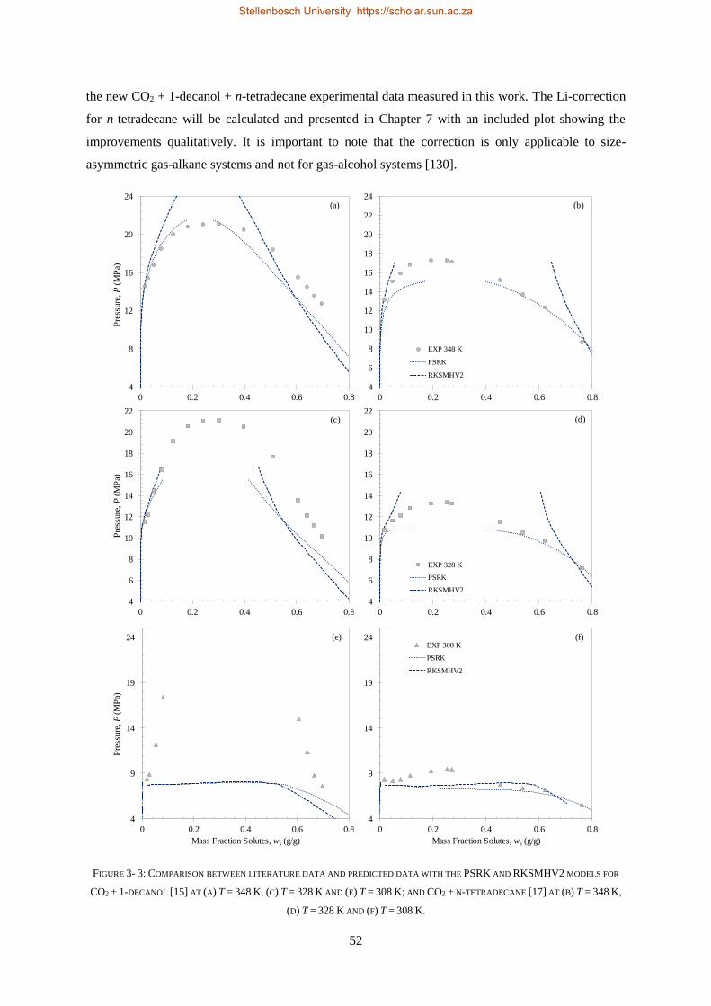
52
the new CO2 + 1-decanol + n-tetradecane experimental data measured in this work. The Li-correction
for n-tetradecane will be calculated and presented in Chapter 7 with an included plot showing the
improvements qualitatively. It is important to note that the correction is only applicable to size-
asymmetric gas-alkane systems and not for gas-alcohol systems [130].
FIGURE 3- 3: COMPARISON BETWEEN LITERATURE DATA AND PREDICTED DATA WITH THE PSRK AND RKSMHV2 MODELS FOR
CO2 + 1-DECANOL [15] AT (A) T = 348 K, (C) T = 328 K AND (E) T = 308 K; AND CO2 + N-TETRADECANE [17] AT (B) T = 348 K,
(D) T = 328 K AND (F) T = 308 K.
4
6
8
10
12
14
16
18
20
22
24
0 0.2 0.4 0.6 0.8
EXP 348 K
PSRK
RKSMHV2
4
8
12
16
20
24
0 0.2 0.4 0.6 0.8
Pre
ssure
, P
(MP
a)
(a) (b)
4
6
8
10
12
14
16
18
20
22
0 0.2 0.4 0.6 0.8
Pre
ssure
, P
(MP
a)
(c)
4
9
14
19
24
0 0.2 0.4 0.6 0.8
Pre
ssure
, P
(M
Pa)
Mass Fraction Solutes, ws (g/g)
(e)
4
6
8
10
12
14
16
18
20
22
0 0.2 0.4 0.6 0.8
EXP 328 K
PSRK
RKSMHV2
(d)
4
9
14
19
24
0 0.2 0.4 0.6 0.8
Mass Fraction Solutes, ws (g/g)
EXP 308 K
PSRK
RKSMHV2
(f)
Stellenbosch University https://scholar.sun.ac.za
53
3.4.5. PSRK MODEL
The PSRK model within Aspen Plus® is based on the RKS EoS and utilises the PSRK mixing rules as
developed by Holderbaum and Gmehling [127]. The PSRK method is an example of the modified
Huron-Vidal mixing rules (MHV1) [111] however, makes use of a thermodynamic relationship between
the excess Helmholtz energy, AE and the SRK EoS [107]:
𝐴𝐸
𝑅𝑇=
𝐴𝑟𝑒𝑠
𝑅𝑇− ∑ 𝑥𝑖
𝐴𝑖𝑟𝑒𝑠
𝑅𝑇𝑖 (3.25)
𝐴𝑟𝑒𝑠 = 𝐴(𝑇, 𝑃) − 𝐴𝑖𝑔(𝑇, 𝑃) = ∫ (𝑅𝑇
𝑉𝑚− 𝑃) 𝑑𝑉𝑚
𝑉𝑚
𝑉𝑚=∞ (3.25 a)
𝐴𝑟𝑒𝑠
𝑅𝑇=
𝑉𝑚
𝑉𝑚−𝑏−
𝑎
𝑏𝑅𝑇ln
𝑉𝑚+𝑏
𝑉𝑚 (3.25 b)
∴𝐴𝐸
𝑅𝑇=
𝑉𝑚𝑏
𝑉𝑚𝑏
−1−
𝑎
𝑏𝑅𝑇ln
𝑉𝑚𝑏
+1
𝑉𝑚𝑏
− ∑ 𝑥𝑖 (
𝑉𝑚,𝑖𝑏𝑖
𝑉𝑚,𝑖𝑏𝑖
−1−
𝑎𝑖
𝑏𝑖𝑅𝑇ln
𝑉𝑚,𝑖𝑏𝑖
+1
𝑉𝑚,𝑖𝑏𝑖
)𝑖 (3.25 c)
The final generalization of the PSRK model, presented in equation (3.26), can be obtained based on the
following assumptions [2], [115]:
(i) A reference state pressure of approximately 1 atmosphere is assumed (p ≈ 1 atm).
(ii) The packing fraction, u = 𝑉𝑚
𝑏= 𝑢𝑖 =
𝑉𝑚,𝑖
𝑏𝑖 is constant, i.e. u = 1.1.
(iii) A linear mixing rule is used to calculate the co-volume parameter of the mixture: 𝑏 = ∑ 𝑥𝑖𝑏𝑖𝑖
(iv) The excess molar volume, ѵE is neglected, i.e. ѵE = 0.
𝐴𝐸
𝑅𝑇= −0.64663 [
𝑎
𝑏𝑅𝑇− ∑ 𝑥𝑖
𝑎𝑖
𝑏𝑖𝑅𝑇𝑖 ] =𝐺𝐸,∗
𝑅𝑇+ ∑ 𝑥𝑖 ln
∑ 𝑥𝑖𝑏𝑖𝑖
𝑏𝑖 𝑖 (3.26)
In the context of this investigation it is favourable to define the fugacity coefficient in terms of the
excess Helmholtz energy. This is made possible by substituting equation (3.26) into (3.17). The species-
specific energy and co-volume parameters are calculated with equation (3.13 a) and (3.13 b),
respectively. For the EoS to predict accurate VLE data of these close boiling systems the temperature
dependent alpha parameters, αi(T) in equation (3.13 a) were calculated with the Mathias and Copeman
expression [154]:
𝛼𝑖(𝑇) = [1 + 𝑐1,𝑖(1 − 𝑇𝑟,𝑖0.5) + 𝑐2,𝑖(1 − 𝑇𝑟,𝑖
0.5)2
+ 𝑐3,𝑖(1 − 𝑇𝑟,𝑖
0.5)3
]2
(3.27)
At subcritical conditions, up to three parameters c1, i, c2, i and c3, i can be used and are regressed using
pure component vapour pressure data. At supercritical conditions the constants c2, i and c3, i are set to
zero and equation (3.27) reduces to the expression provided as equation (3.14).
The excess Gibbs energy, GE, * was obtained using the original UNIFAC model with special-gas
group interaction parameters for the CO2 binary sub-systems. The UNIFAC model was further modified
with the Li-correction for the CO2 + n-tetradecane combinations in the binary and ternary mixtures.
Stellenbosch University https://scholar.sun.ac.za
54
Therefore, this model has five pure component parameters for each subcritical component (Tc, i, Pc, i,
ci,1, ci,2, ci,3) and three for each supercritical component (Tc, i, Pc, i, 𝜔𝑖). Additionally, for the CO2 +
1-decanol and 1-decanol + n-tetradecane binary systems four group interaction parameters are used to
improve the fit (amn, anm, Qk, Rk); whereas for the CO2 + n-tetradecane binary combination six group
interaction parameters and two effective group parameters are used to improve the fit (amn, anm, bmn, bnm,
cmn, cnm, Q*k, R
*k).
3.5. FLEXIBLE PROPERTY METHODS IN ASPEN PLUS®
Two additional thermodynamic models suggested by the Aspen Plus® software guide for the systems
considered in this investigation are:
(i) Redlich-Kwong-Soave with Mathias mixing rules (RK-Aspen) [48], [49], [103]: The extended
classical mixing rules used in this model are especially suited for systems with strong size and
shape asymmetry, i.e. the CO2 + n-tetradecane combinations in the ternary CO2 + 1-decanol +
n-tetradecane system.
(ii) Redlich-Kwong-Soave with Schwarzentruber-Renon mixing rules (SR-Polar) [154]–[157]: The
composition and temperature dependent mixing rules makes this the ideal thermodynamic model
for correlating the complex phase equilibria of the CO2 + 1-decanol + n-tetradecane system at the
required high-temperature and high-pressure ranges.
The RK-Aspen an SR-Polar models have been investigated in multiple studies, conducted on similar
high-pressure systems, which are summarised in Table 3-1. Both methods are selected to model the new
CO2 + 1-decanol + n-tetradecane and 1-decanol + n-tetradecane experimental data measured in this
work based on the following findings:
• Lombard [51] only considered binary systems with ethane and propane as the supercritical
solvents.
• Zamudio and co-workers [12], [13] did not consider the addition of solute + solute BIPs into the
RK-Aspen model algorithm and saw significant deviations between the model correlations and
experimental data.
• Zamudio [18] only considered binary CO2 + n-alkane and CO2 + alcohol systems with the SR-Polar
model.
• Smith and Schwarz [16] continued the work of Zamudio et al.[13] by considering the effects of
solute + solute BIPs and saw improved model predictions by RK-Aspen.
• In more recent studies, conducted by Fourie and co-workers [19], [158], [159], it was shown that
both flexible property methods have the option to include additional BIPs and pure component
polar parameters to improve the accuracy of their fit to experimental data.
Stellenbosch University https://scholar.sun.ac.za
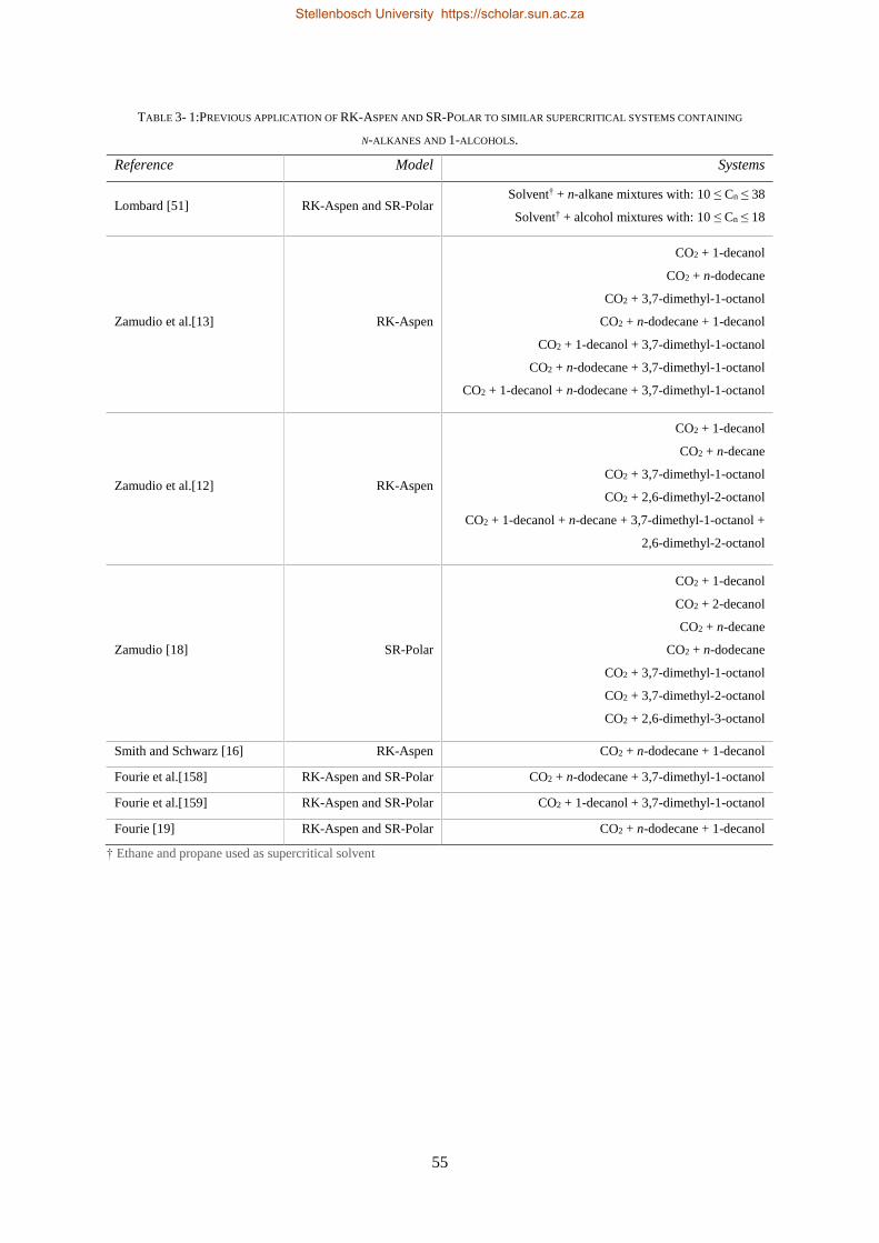
55
TABLE 3- 1:PREVIOUS APPLICATION OF RK-ASPEN AND SR-POLAR TO SIMILAR SUPERCRITICAL SYSTEMS CONTAINING
N-ALKANES AND 1-ALCOHOLS.
Reference Model Systems
Lombard [51] RK-Aspen and SR-Polar Solvent† + n-alkane mixtures with: 10 ≤ Cn ≤ 38
Solvent† + alcohol mixtures with: 10 ≤ Cn ≤ 18
Zamudio et al.[13] RK-Aspen
CO2 + 1-decanol
CO2 + n-dodecane
CO2 + 3,7-dimethyl-1-octanol
CO2 + n-dodecane + 1-decanol
CO2 + 1-decanol + 3,7-dimethyl-1-octanol
CO2 + n-dodecane + 3,7-dimethyl-1-octanol
CO2 + 1-decanol + n-dodecane + 3,7-dimethyl-1-octanol
Zamudio et al.[12] RK-Aspen
CO2 + 1-decanol
CO2 + n-decane
CO2 + 3,7-dimethyl-1-octanol
CO2 + 2,6-dimethyl-2-octanol
CO2 + 1-decanol + n-decane + 3,7-dimethyl-1-octanol +
2,6-dimethyl-2-octanol
Zamudio [18] SR-Polar
CO2 + 1-decanol
CO2 + 2-decanol
CO2 + n-decane
CO2 + n-dodecane
CO2 + 3,7-dimethyl-1-octanol
CO2 + 3,7-dimethyl-2-octanol
CO2 + 2,6-dimethyl-3-octanol
Smith and Schwarz [16] RK-Aspen CO2 + n-dodecane + 1-decanol
Fourie et al.[158] RK-Aspen and SR-Polar CO2 + n-dodecane + 3,7-dimethyl-1-octanol
Fourie et al.[159] RK-Aspen and SR-Polar CO2 + 1-decanol + 3,7-dimethyl-1-octanol
Fourie [19] RK-Aspen and SR-Polar CO2 + n-dodecane + 1-decanol
† Ethane and propane used as supercritical solvent
Stellenbosch University https://scholar.sun.ac.za
56
3.5.1. RK-ASPEN MODEL
The RK-Aspen property method is an extension of the RKS EoS and can be described using equation
(3.10). Furthermore, quadratic Mathias mixing rules are employed in this model for calculating the
energy (3.28) and co-volume (3.29) parameters, each containing a linear temperature-dependent BIP as
shown in equations (3.30) and (3.31), respectively [2], [18].
𝑎 = ∑ ∑ 𝑥𝑖𝑥𝑗(𝑎𝑖𝑎𝑗)0.5
(1 − 𝑘𝑎,𝑖𝑗)𝑛𝑗=1
𝑛𝑖=1 (3.28)
𝑏 = ∑ ∑ 𝑥𝑖𝑥𝑗(𝑏𝑖+𝑏𝑗)
2(1 − 𝑘𝑏,𝑖𝑗)𝑛
𝑗=1𝑛𝑖=1 (3.29)
𝑘𝑎,𝑖𝑗 = 𝑘𝑎,𝑗𝑖 = 𝑘𝑎,𝑖𝑗0 + 𝑘𝑎,𝑖𝑗
1 𝑇
1000 (3.30)
𝑘𝑏,𝑖𝑗 = 𝑘𝑏,𝑗𝑖 = 𝑘𝑏,𝑖𝑗0 + 𝑘𝑏,𝑖𝑗
1 𝑇
1000 (3.31)
To ensure accurate VLE data correlations, the temperature depended αi(T) parameter in equation
(3.13 a) was calculated in one of two ways [103], [156]:
(i) A Mathias alpha function, shown in equation (3.32)
(ii) A Boston-Mathias alpha function, shown in equation (3.33)
The former method is applied for subcritical components (Tr, i < 1) and incorporates a pure component
polar parameter, 휂𝑖 directly into the alpha function; whereas, the latter is applied for supercritical
components (Tr, i > 1) and contains a modified, 𝑑𝑖 parameter (3.33 a) to incorporate the pure component
polar parameter into the alpha function (3.33). The species-specific co-volume parameter, bi remains
temperature independent and can be calculated using equation (3.13 b).
𝛼𝑖(𝑇) = [1 + 𝑚𝑖(1 − 𝑇𝑟,𝑖0.5) − 휂𝑖(1 − 𝑇𝑟,𝑖)(0.7 − 𝑇𝑟,𝑖)]
2 (3.32)
𝑚𝑖 = 0.48508 + 1.55171𝜔𝑖 − 0.15613𝜔𝑖2 (3.32 a)
𝛼𝑖(𝑇) = [exp[𝑐𝑖(1 − 𝑇𝑟,𝑖𝑑𝑖)]]
2 (3.33)
𝑑𝑖 = 1 +𝑚𝑖
2+ 0.3휂𝑖 (3.33 a)
𝑐𝑖 = 1 −1
𝑑𝑖 (3.33 b)
Therefore, this model has four pure component parameters for each subcritical and supercritical
component (Tc, i, Pc, i, 𝜔𝑖, 휂𝑖). Additionally, per binary combination up to four BIPs can be used to
improve the fit (ka, ij0, ka, ij
1, kb, ij0, kb, ij
1).
Stellenbosch University https://scholar.sun.ac.za
57
3.5.2. SR-POLAR MODEL
The Redlich-Kwong-UNIFAC model [109], extended from the RKS EoS [49], [103], forms the basis
of the SR-Polar property method. Once again, equation (3.10) will be applied for the model with the
SRK extension. Like the RK-Aspen model the energy and co-volume BIPs remain temperature
dependent when applying the Schwarzentruber-Renon mixing rules to the EoS. However, a second BIP,
lij is included for the SR-Polar energy parameter as shown in equation (3.34). The co-volume parameter
is calculated using equation (3.29). Temperature dependency can be incorporated for the ka, ij, kb, ij and
lij BIPs as shown in equations (3.35), (3.36) and (3.37), respectively [2], [18].
𝑎 = ∑ ∑ 𝑥𝑖𝑥𝑗(𝑎𝑖𝑎𝑗)0.5
[1 − 𝑘𝑎,𝑖𝑗 − 𝑙𝑖𝑗(𝑥𝑖 − 𝑥𝑗)]𝑛𝑗=1
𝑛𝑖=1 (3.34)
𝑘𝑎,𝑖𝑗 = 𝑘𝑎,𝑗𝑖 = 𝑘𝑎,𝑖𝑗0 + 𝑘𝑎,𝑖𝑗
1 𝑇 +𝑘𝑎,𝑖𝑗
2
𝑇 (3.35)
𝑘𝑏,𝑖𝑗 = 𝑘𝑏,𝑗𝑖 = 𝑘𝑏,𝑖𝑗0 + 𝑘𝑏,𝑖𝑗
1 𝑇 +𝑘𝑏,𝑖𝑗
2
𝑇 (3.36)
𝑙𝑖𝑗 = −𝑙𝑗𝑖 = 𝑙𝑖𝑗0 + 𝑙𝑖𝑗
1 𝑇 +𝑙𝑖𝑗
2
𝑇 (3.37)
For the SR-Polar model, the Extended Mathias alpha function is used to calculate the αi(T) parameter
of subcritical (Tr, i < 1) components. The expression is shown in equation (3.38) which enable the
incorporation of three pure component polar parameters, p1, i, p2, i, and p3, i into the EoS model to improve
the VLE data correlations. A Boston Mathias Extrapolation with a modified di parameter (3.39) is used
to incorporate the three polar parameters into the αi(T) parameter (3.33) of the supercritical components
(Tr, I > 1) [103], [156]. The mi and ci parameters are computed by equation (3.32 a) and equation (3.33 b),
respectively.
𝛼𝑖(𝑇) = [1 + 𝑚𝑖(1 − 𝑇𝑟,𝑖0.5) − 𝑝1,𝑖(1 − 𝑇𝑟,𝑖)(1 + 𝑝2,𝑖𝑇𝑟,𝑖 + 𝑝3,𝑖𝑇𝑟,𝑖
2 )]2 (3.38)
𝑑𝑖 = 1 +𝑚𝑖
2− 𝑝1,𝑖(1 + 𝑝2,𝑖 + 𝑝3,𝑖) (3.39)
Therefore, this model has six pure component parameters for each subcritical and supercritical
component (Tc, i, Pc, i, 𝜔𝑖, p1, i, p2, i, p3, i). Additionally, per binary combination up to nine BIPs can be
used to improve the fit (ka, ij0, ka, ij
1, ka, ij2, kb, ij
0, kb, ij1, kb, ij
2, lij0, lij
1, lij2).
Stellenbosch University https://scholar.sun.ac.za
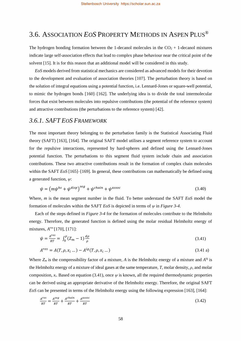
58
3.6. ASSOCIATION EOS PROPERTY METHODS IN ASPEN PLUS®
The hydrogen bonding formation between the 1-decanol molecules in the CO2 + 1-decanol mixtures
indicate large self-association effects that lead to complex phase behaviour near the critical point of the
solvent [15]. It is for this reason that an additional model will be considered in this study.
EoS models derived from statistical mechanics are considered as advanced models for their devotion
to the development and evaluation of association theories [107]. The perturbation theory is based on
the solution of integral equations using a potential function, i.e. Lennard-Jones or square-well potential,
to mimic the hydrogen bonds [160]–[162]. The underlying idea is to divide the total intermolecular
forces that exist between molecules into repulsive contributions (the potential of the reference system)
and attractive contributions (the perturbations to the reference system) [42].
3.6.1. SAFT EOS FRAMEWORK
The most important theory belonging to the perturbation family is the Statistical Associating Fluid
theory (SAFT) [163], [164]. The original SAFT model utilises a segment reference system to account
for the repulsive interactions, represented by hard-spheres and defined using the Lennard-Jones
potential function. The perturbations to this segment fluid system include chain and association
contributions. These two attractive contributions result in the formation of complex chain molecules
within the SAFT EoS [165]–[169]. In general, these contributions can mathematically be defined using
a generated function, ψ:
𝜓 = (𝑚𝜓ℎ𝑠 + 𝜓𝑑𝑖𝑠𝑝)𝑠𝑒𝑔
+ 𝜓𝑐ℎ𝑎𝑖𝑛 + 𝜓𝑎𝑠𝑠𝑜𝑐 (3.40)
Where, m is the mean segment number in the fluid. To better understand the SAFT EoS model the
formation of molecules within the SAFT EoS is depicted in terms of ψ in Figure 3-4.
Each of the steps defined in Figure 3-4 for the formation of molecules contribute to the Helmholtz
energy. Therefore, the generated function is defined using the molar residual Helmholtz energy of
mixtures, Ares [170], [171]:
𝜓 =𝐴𝑟𝑒𝑠
𝑅𝑇= ∫ (𝑍𝑚 − 1)
𝑑𝜌
𝜌
𝜌
0 (3.41)
𝐴𝑟𝑒𝑠 = 𝐴(𝑇, 𝜌, 𝑥𝑖 … ) − 𝐴𝑖𝑔(𝑇, 𝜌, 𝑥𝑖 … ) (3.41 a)
Where Zm is the compressibility factor of a mixture, A is the Helmholtz energy of a mixture and Aig is
the Helmholtz energy of a mixture of ideal gases at the same temperature, T, molar density, ρ, and molar
composition, xi. Based on equation (3.41), once ψ is known, all the required thermodynamic properties
can be derived using an appropriate derivative of the Helmholtz energy. Therefore, the original SAFT
EoS can be presented in terms of the Helmholtz energy using the following expression [163], [164]:
𝐴𝑟𝑒𝑠
𝑅𝑇=
𝐴𝑠𝑒𝑔
𝑅𝑇+
𝐴𝑐ℎ𝑎𝑖𝑛
𝑅𝑇+
𝐴𝑎𝑠𝑠𝑜𝑐
𝑅𝑇 (3.42)
Stellenbosch University https://scholar.sun.ac.za
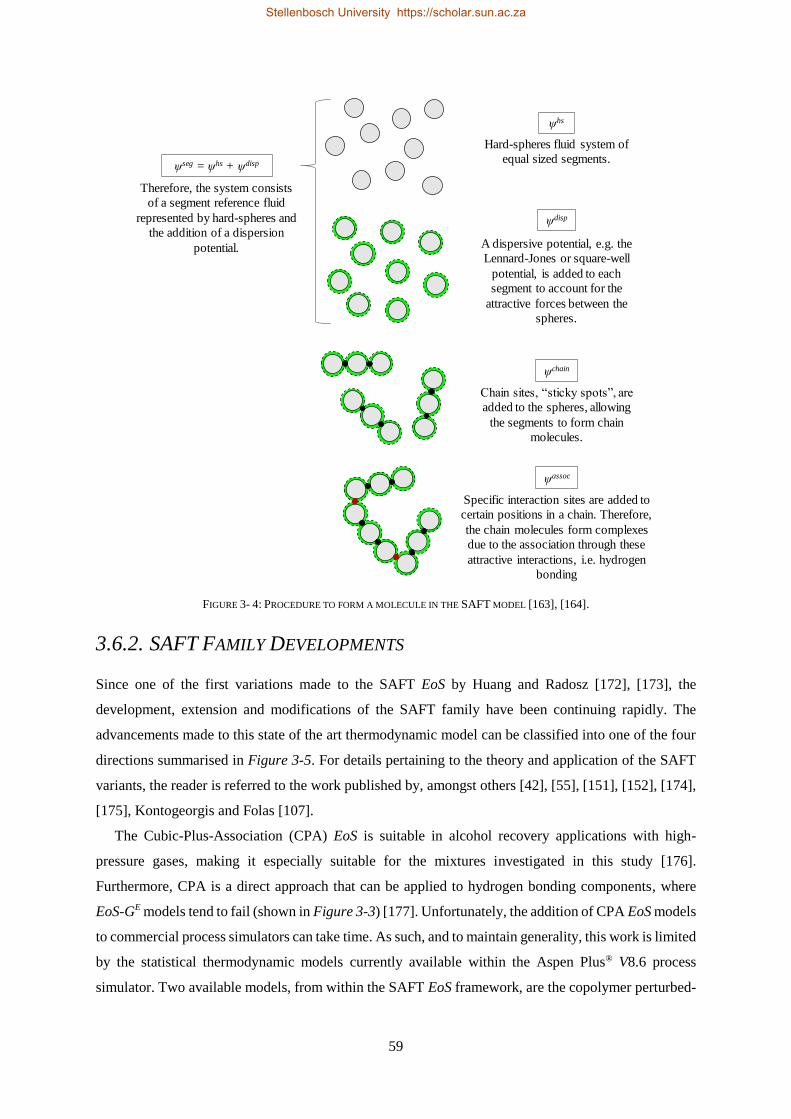
59
FIGURE 3- 4: PROCEDURE TO FORM A MOLECULE IN THE SAFT MODEL [163], [164].
3.6.2. SAFT FAMILY DEVELOPMENTS
Since one of the first variations made to the SAFT EoS by Huang and Radosz [172], [173], the
development, extension and modifications of the SAFT family have been continuing rapidly. The
advancements made to this state of the art thermodynamic model can be classified into one of the four
directions summarised in Figure 3-5. For details pertaining to the theory and application of the SAFT
variants, the reader is referred to the work published by, amongst others [42], [55], [151], [152], [174],
[175], Kontogeorgis and Folas [107].
The Cubic-Plus-Association (CPA) EoS is suitable in alcohol recovery applications with high-
pressure gases, making it especially suitable for the mixtures investigated in this study [176].
Furthermore, CPA is a direct approach that can be applied to hydrogen bonding components, where
EoS-GE models tend to fail (shown in Figure 3-3) [177]. Unfortunately, the addition of CPA EoS models
to commercial process simulators can take time. As such, and to maintain generality, this work is limited
by the statistical thermodynamic models currently available within the Aspen Plus® V8.6 process
simulator. Two available models, from within the SAFT EoS framework, are the copolymer perturbed-
Therefore, the system consists
of a segment reference fluid
represented by hard-spheres and
the addition of a dispersion
potential.
Hard-spheres fluid system of
equal sized segments.
A dispersive potential, e.g. the
Lennard-Jones or square-well
potential, is added to each
segment to account for the
attractive forces between the
spheres.
ψhs
ψdisp
ψseg = ψhs + ψdisp
Chain sites, “sticky spots”, are
added to the spheres, allowing
the segments to form chain
molecules.
ψchain
Specific interaction sites are added to
certain positions in a chain. Therefore,
the chain molecules form complexes
due to the association through these
attractive interactions, i.e. hydrogen
bonding
ψassoc
Stellenbosch University https://scholar.sun.ac.za
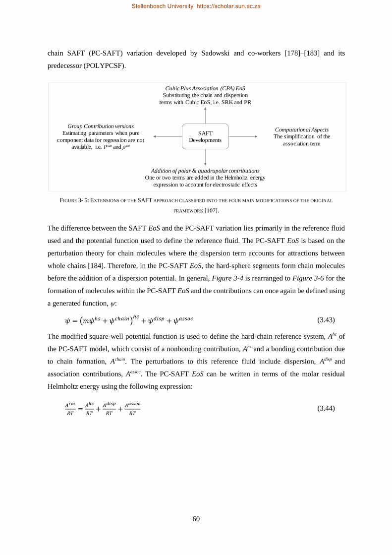
60
chain SAFT (PC-SAFT) variation developed by Sadowski and co-workers [178]–[183] and its
predecessor (POLYPCSF).
FIGURE 3- 5: EXTENSIONS OF THE SAFT APPROACH CLASSIFIED INTO THE FOUR MAIN MODIFICATIONS OF THE ORIGINAL
FRAMEWORK [107].
The difference between the SAFT EoS and the PC-SAFT variation lies primarily in the reference fluid
used and the potential function used to define the reference fluid. The PC-SAFT EoS is based on the
perturbation theory for chain molecules where the dispersion term accounts for attractions between
whole chains [184]. Therefore, in the PC-SAFT EoS, the hard-sphere segments form chain molecules
before the addition of a dispersion potential. In general, Figure 3-4 is rearranged to Figure 3-6 for the
formation of molecules within the PC-SAFT EoS and the contributions can once again be defined using
a generated function, ψ:
𝜓 = (𝑚𝜓ℎ𝑠 + 𝜓𝑐ℎ𝑎𝑖𝑛)ℎ𝑐
+ 𝜓𝑑𝑖𝑠𝑝 + 𝜓𝑎𝑠𝑠𝑜𝑐 (3.43)
The modified square-well potential function is used to define the hard-chain reference system, Ahc of
the PC-SAFT model, which consist of a nonbonding contribution, Ahs and a bonding contribution due
to chain formation, Achain. The perturbations to this reference fluid include dispersion, Adisp and
association contributions, Aassoc. The PC-SAFT EoS can be written in terms of the molar residual
Helmholtz energy using the following expression:
𝐴𝑟𝑒𝑠
𝑅𝑇=
𝐴ℎ𝑐
𝑅𝑇+
𝐴𝑑𝑖𝑠𝑝
𝑅𝑇+
𝐴𝑎𝑠𝑠𝑜𝑐
𝑅𝑇 (3.44)
SAFT
Developments
Cubic Plus Association (CPA) EoS
Substituting the chain and dispersion
terms with Cubic EoS, i.e. SRK and PR
Addition of polar & quadrupolar contributions
One or two terms are added in the Helmholtz energy
expression to account for electrostatic effects
Computational Aspects
The simplification of the
association term
Group Contribution versions
Estimating parameters when pure
component data for regression are not
available, i.e. Psat and ρsat
Stellenbosch University https://scholar.sun.ac.za
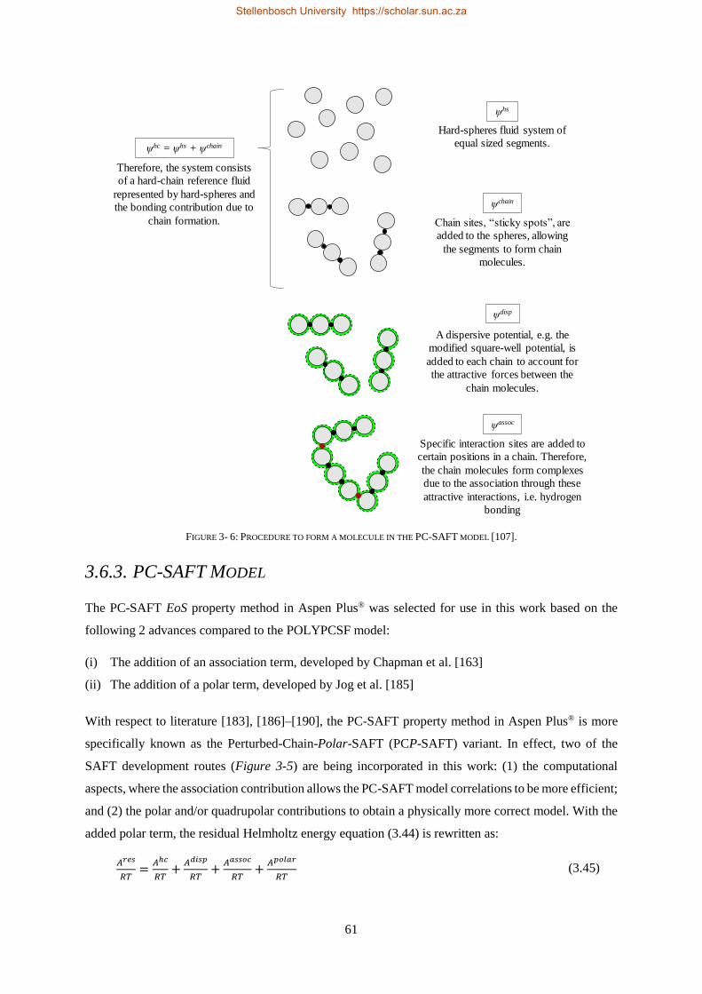
61
FIGURE 3- 6: PROCEDURE TO FORM A MOLECULE IN THE PC-SAFT MODEL [107].
3.6.3. PC-SAFT MODEL
The PC-SAFT EoS property method in Aspen Plus® was selected for use in this work based on the
following 2 advances compared to the POLYPCSF model:
(i) The addition of an association term, developed by Chapman et al. [163]
(ii) The addition of a polar term, developed by Jog et al. [185]
With respect to literature [183], [186]–[190], the PC-SAFT property method in Aspen Plus® is more
specifically known as the Perturbed-Chain-Polar-SAFT (PCP-SAFT) variant. In effect, two of the
SAFT development routes (Figure 3-5) are being incorporated in this work: (1) the computational
aspects, where the association contribution allows the PC-SAFT model correlations to be more efficient;
and (2) the polar and/or quadrupolar contributions to obtain a physically more correct model. With the
added polar term, the residual Helmholtz energy equation (3.44) is rewritten as:
𝐴𝑟𝑒𝑠
𝑅𝑇=
𝐴ℎ𝑐
𝑅𝑇+
𝐴𝑑𝑖𝑠𝑝
𝑅𝑇+
𝐴𝑎𝑠𝑠𝑜𝑐
𝑅𝑇+
𝐴𝑝𝑜𝑙𝑎𝑟
𝑅𝑇 (3.45)
Hard-spheres fluid system of
equal sized segments.
ψhs
Chain sites, “sticky spots”, are
added to the spheres, allowing
the segments to form chain
molecules.
ψchain
Therefore, the system consists
of a hard-chain reference fluid
represented by hard-spheres and
the bonding contribution due to
chain formation.
ψhc = ψhs + ψchain
A dispersive potential, e.g. the
modified square-well potential, is
added to each chain to account for
the attractive forces between the
chain molecules.
ψdisp
Specific interaction sites are added to
certain positions in a chain. Therefore,
the chain molecules form complexes
due to the association through these
attractive interactions, i.e. hydrogen
bonding
ψassoc
Stellenbosch University https://scholar.sun.ac.za
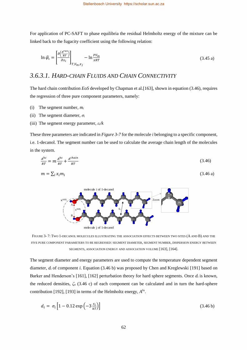
62
For application of PC-SAFT to phase equilibria the residual Helmholtz energy of the mixture can be
linked back to the fugacity coefficient using the following relation:
ln 𝜑�� = [𝜕(
𝐴𝑟𝑒𝑠
𝑅𝑇)
𝜕𝑥𝑖]
𝑇,𝑉𝑚,𝑥𝑗
− ln𝑃𝑉𝑚
𝑥𝑅𝑇 (3.45 a)
3.6.3.1. HARD-CHAIN FLUIDS AND CHAIN CONNECTIVITY
The hard chain contribution EoS developed by Chapman et al.[163], shown in equation (3.46), requires
the regression of three pure component parameters, namely:
(i) The segment number, mi
(ii) The segment diameter, σi
(iii) The segment energy parameter, εi/k
These three parameters are indicated in Figure 3-7 for the molecule i belonging to a specific component,
i.e. 1-decanol. The segment number can be used to calculate the average chain length of the molecules
in the system.
𝐴ℎ𝑐
𝑅𝑇= 𝑚
𝐴ℎ𝑠
𝑅𝑇+
𝐴𝑐ℎ𝑎𝑖𝑛
𝑅𝑇 (3.46)
𝑚 = ∑ 𝑥𝑖𝑚𝑖𝑖 (3.46 a)
FIGURE 3- 7: TWO 1-DECANOL MOLECULES ILLUSTRATING THE ASSOCIATION EFFECTS BETWEEN TWO SITES (A AND B) AND THE
FIVE PURE COMPONENT PARAMETERS TO BE REGRESSED: SEGMENT DIAMETER, SEGMENT NUMBER, DISPERSION ENERGY BETWEEN
SEGMENTS, ASSOCIATION ENERGY AND ASSOCIATION VOLUME [163], [164].
The segment diameter and energy parameters are used to compute the temperature dependent segment
diameter, di of component i. Equation (3.46 b) was proposed by Chen and Kreglewski [191] based on
Barker and Henderson’s [161], [162] perturbation theory for hard sphere segments. Once di is known,
the reduced densities, ζn (3.46 c) of each component can be calculated and in turn the hard-sphere
contribution [192], [193] in terms of the Helmholtz energy, Ahs.
𝑑𝑖 = 𝜎𝑖 [1 − 0.12 exp (−3 𝑖
𝑘𝑇)] (3.46 b)
mi
κAiBj
εAiBj
Zoom
εi
σi
A
B
molecule i of 1-decanol
molecule j of 1-decanol
Stellenbosch University https://scholar.sun.ac.za
63
휁𝑛 =𝜋
6𝜌 ∑ 𝑥𝑖𝑚𝑖𝑑𝑖
𝑛𝑖 𝑛 ∈ {0, 1, , 2, 3} (3.46 c)
𝐴ℎ𝑠
𝑅𝑇=
1
0[
3 1 2
1− 3+ 2
3
3(1− 3)2 + ( 23
32 − 휁0) ln(1 − 휁3)] (3.46 d)
In addition, both the di and ζn parameters are required to compute the radial pair distribution function,
giihs(dii) which is the final requirement to calculate the contribution from the chain connectivity, Achain.
Equation (3.46 e) and equation (3.46 f) are derived for a mixture of hard spheres using the Carnahan-
Starling EoS [194].
𝑔𝑖𝑖ℎ𝑠(𝑑𝑖𝑖) =
1
1− 3+ (
𝑑𝑖𝑑𝑗
𝑑𝑖+𝑑𝑗)
3 2
(1− 3)2 + (𝑑𝑖𝑑𝑗
𝑑𝑖+𝑑𝑗)
22 2
2
(1− 3)3 (3.46 e)
𝐴𝑐ℎ𝑎𝑖𝑛
𝑅𝑇= − ∑ 𝑥𝑖(𝑚𝑖 − 1) ln 𝑔𝑖𝑖
ℎ𝑠(𝑑𝑖𝑖)𝑖 (3.46 f)
3.6.3.2. ASSOCIATION TERM – 2B MODEL
Figure 3-7 indicates how the partially negative charged oxygen on the hydroxyl group of the 1st
1-decanol molecule, i (site A) bonds with the partially positive charged hydrogen atom on the hydroxyl
group of the 2nd 1-decanol molecule, j (site B). This hydrogen bonding between two like molecules
indicates the self-association taking place between the 1-decanol molecules in the mixtures measured
in this work [107], [110], [195], [196].
The following two pure component parameters should be regressed to account for the association
taking place in the fluid system:
(iv) The effective association volume, κAiBj
(v) The association energy parameter, εAiBj/k
In general, the association contribution developed by Chapman et al. [163] can be written in terms of
the Helmholtz energy, Aassoc:
𝐴𝑎𝑠𝑠𝑜𝑐
𝑅𝑇= ∑ 𝑥𝑖 [∑ (ln 𝑋𝐴𝑖 −
𝑋𝐴𝑖
2)𝐴𝑖
+1
2]𝑖 (3.47)
Here, XAi is the mole fraction of a molecule i that are not bonded at site A, and ΔAiBj is the association
strength between two sites A and B belonging to two different molecules i and j [197].
𝑋𝐴𝑖 = [1 + ∑ ∑ 𝜌𝑗𝑋𝐵𝑗∆𝐴𝑖𝐵𝑗𝐵𝑗𝑗 ]
−1 (3.47 a)
∆𝐴𝑖𝐵𝑗= 𝜎𝑖𝑗3 𝑔𝑖𝑗(𝑑𝑖𝑗)
𝑠𝑒𝑔𝜅𝐴𝑖𝐵𝑗 [exp (
𝐴𝑖𝐵𝑗
𝑘𝑇) − 1] (3.47 b)
Stellenbosch University https://scholar.sun.ac.za
64
The cross-association volume and cross-energy parameters can be calculated using mixing rules
suggested by Wolbach and Sandler [195].
휀𝐴𝑖𝐵𝑗 =1
2(휀𝐴𝑖𝐵𝑖 + 휀𝐴𝑗𝐵𝑗) (3.47 c)
𝜅𝐴𝑖𝐵𝑗 = √𝜅𝐴𝑖𝐵𝑖𝜅𝐴𝑗𝐵𝑗 (√𝜎𝑖𝑖𝜎𝑗𝑗
1
2(𝜎𝑖𝑖+𝜎𝑗𝑗)
)
3
(3.47 d)
In pure and binary systems, the XAi fraction can be derived explicitly if the association scheme is known.
To establish the association scheme, the number and type of association sites should be identified.
Fortunately, previous investigations with the use of spectroscopy data and the PC-SAFT EoS model
have been conducted [198], [199]. Distinctions between the 2B and 3B association schemes were not
always possible but, for heavier alcohols, i.e. 1-decanol, the 2B scheme will perform best [172], [179],
[200], [201]. After Huang and Radosz [172] the following two approximations are made for the 2B
bonding type:
∆𝐴𝑖𝐵𝑗= ∆𝐵𝑖𝐴𝑗≠ 0 (3.48)
𝑋𝐴𝑖 = 𝑋𝐵𝑗 (3.49)
Therefore, equation (3.47) and (3.47 a) can be simplified to equation (3.50) and (3.50 a), respectively.
𝐴𝑎𝑠𝑠𝑜𝑐
𝑅𝑇= 2 ∑ 𝑥𝑖 (ln 𝑋𝐴𝑖 −
𝑋𝐴𝑖
2+
1
2)𝑖 (3.50)
𝑋𝐴𝑖 =−1+√1+4𝜌∆
𝐴𝑖𝐵𝑗
2𝜌∆𝐴𝑖𝐵𝑗
(3.50 a)
3.6.3.3. DISPERSION TERM
The contribution term with fundamental differences to the original SAFT EoS is the dispersion term,
Adisp. The Barker and Henderson [160]–[162] perturbation theory is used to compute an equation in
terms of the 1st and 2nd order vdW dispersion interactions between molecules.
𝐴𝑑𝑖𝑠𝑝
𝑘𝑇𝑁=
𝐴1
𝑘𝑇𝑁+
𝐴2
𝑘𝑇𝑁 (3.51)
𝐴1 = −2𝜋𝜌 ∑ 𝑎𝑖(𝑚)휂𝑖6𝑖=0 ∑ 𝑚2 ( 𝑖𝑗
𝑘𝑇) 𝜎𝑖𝑗
3𝑖𝑗 (3.51 a)
𝐴2 = −𝜋𝜌𝑚𝐶1 ∑ 𝑏𝑖(𝑚)휂𝑖6𝑖=0 ∑ 𝑚2 ( 𝑖𝑗
𝑘𝑇)
2𝜎𝑖𝑗
3𝑖𝑗 (3.51 b)
Where, η is the packing fraction and represents a reduced segment density, ζ3, i.e. η = ζ3. The
compressibility of the hard chain fluid, C1 can be calculated using equation (3.51 c) The coefficients
ai(m) and bi(m) as functions of the chain length, were developed using the Lennard-Jones potential and
the radial distribution function of O’Lenick et al. [202]. The model constants are derived from pure
component data of alkane and can be found in literature [107], [202].
Stellenbosch University https://scholar.sun.ac.za
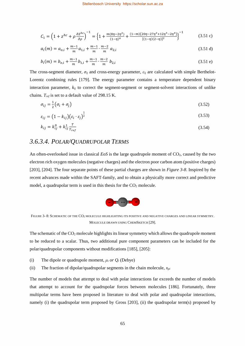
65
𝐶1 = (1 + 𝑧ℎ𝑐 + 𝜌𝜕𝑍ℎ𝑐
𝜕𝜌)
−1
= {1 +𝑚(8 −2 2)
(1− )4 +(1−𝑚)(20 −27 2+12 3−2 4)
[(1− )(2− )]2 }−1
(3.51 c)
𝑎𝑖(𝑚) = 𝑎𝑜,𝑖 +𝑚−1
𝑚𝑎1,𝑖 +
𝑚−1
𝑚∙
𝑚−2
𝑚 𝑎2,𝑖 (3.51 d)
𝑏𝑖(𝑚) = 𝑏𝑜,𝑖 +𝑚−1
𝑚𝑏1,𝑖 +
𝑚−1
𝑚∙
𝑚−2
𝑚 𝑏2,𝑖 (3.51 e)
The cross-segment diameter, σij and cross-energy parameter, εij are calculated with simple Berthelot-
Lorentz combining rules [179]. The energy parameter contains a temperature dependent binary
interaction parameter, kij to correct the segment-segment or segment-solvent interactions of unlike
chains. Tref is set to a default value of 298.15 K.
𝜎𝑖𝑗 =1
2(𝜎𝑖 + 𝜎𝑗) (3.52)
휀𝑖𝑗 = (1 − 𝑘𝑖𝑗)(휀𝑖 ∙ 휀𝑗)1
2 (3.53)
𝑘𝑖𝑗 = 𝑘𝑖𝑗0 + 𝑘𝑖𝑗
1 𝑇
𝑇𝑟𝑒𝑓 (3.54)
3.6.3.4. POLAR/QUADRUPOLAR TERMS
An often-overlooked issue in classical EoS is the large quadrupole moment of CO2, caused by the two
electron rich oxygen molecules (negative charges) and the electron poor carbon atom (positive charges)
[203], [204]. The four separate points of these partial charges are shown in Figure 3-8. Inspired by the
recent advances made within the SAFT-family, and to obtain a physically more correct and predictive
model, a quadrupolar term is used in this thesis for the CO2 molecule.
FIGURE 3- 8: SCHEMATIC OF THE CO2 MOLECULE HIGHLIGHTING ITS POSITIVE AND NEGATIVE CHARGES AND LINEAR SYMMETRY.
MOLECULE DRAWN USING CHEMSKETCH [29].
The schematic of the CO2 molecule highlights its linear symmetry which allows the quadrupole moment
to be reduced to a scalar. Thus, two additional pure component parameters can be included for the
polar/quadrupolar components without modifications [185], [205]:
(i) The dipole or quadrupole moment, μi or Qi (Debye)
(ii) The fraction of dipolar/quadrupolar segments in the chain molecule, xpi
The number of models that attempt to deal with polar interactions far exceeds the number of models
that attempt to account for the quadrupolar forces between molecules [186]. Fortunately, three
multipolar terms have been proposed in literature to deal with polar and quadrupolar interactions,
namely (i) the quadrupolar term proposed by Gross [203], (ii) the quadrupolar term(s) proposed by
++- -
Stellenbosch University https://scholar.sun.ac.za
66
Economou and co-workers [206], [207] and (iii) the quadrupolar term proposed by de Hemptinne and
co-workers [208].
The thermodynamic property method available within Aspen Plus® has been identified as the PCP-
SAFT model that uses a two-centre Lennard-Jones pair potential as the reference fluid and no mixing
rules. Therefore, the thermodynamic model used in this study is that developed by Gross [203], inspired
by the perturbation theory of Stell and co-workers [209]–[212] and Gubbins & Twu [213], [214]. The
new EoS can be employed with an experimental quadrupole moment and contrary to most other EoS
contributions for polar and quadrupolar mixtures it can be used without any additional adjustable
parameters, i.e., BIPs [215]. The quadrupolar term provided in equation (3.55) is written in the Padé
approximate [210], where A2 and A3 represent the 2nd and 3rd order terms of the perturbation expansion
developed by statistical mechanics, respectively (the so called u-expansion by Stell and co-workers
[209]–[212] and Flytzani-Stephanopoulos et al.[216]).
𝐴𝑝𝑜𝑙𝑎𝑟
𝑅𝑇=
𝐴2
1−𝐴3𝐴2
(3.55)
𝐴2 = −2𝜋
9
𝜌𝐼2( )
(𝑘𝑇)2∑ ∑ 𝑥𝑖𝑥𝑗 𝑚𝑖𝑚𝑗𝑥𝑝𝑖𝑥𝑝𝑗
𝑄𝑖2𝑄𝑗
2
𝑑𝑖𝑗2𝑗𝑖 (3.55 a)
𝐴3 = 5𝜋2
162
𝜌𝐼3( )
(𝑘𝑇)3∑ ∑ ∑ 𝑥𝑖𝑥𝑗𝑥𝑘 𝑚𝑖𝑚𝑗𝑚𝑘𝑥𝑝𝑖𝑥𝑝𝑗𝑥𝑝𝑘
𝑄𝑖2𝑄𝑗
2𝑄𝑘2
𝑑𝑖𝑗2 𝑑𝑗𝑘
2 𝑑𝑖𝑘2𝑘𝑗𝑖 (3.55 b)
𝑑𝑖𝑗 =𝑑𝑖+𝑑𝑗
2 (3.55 c)
Rushbrooke et al.[210] have shown that the pure fluid integrals can be written in terms of the packing
fraction, η using the following expressions that are functions of reduced density:
𝐼2(𝜌∗) =1−0.3618𝜌∗−0.3205𝜌∗2
+0.1078𝜌∗3
(1−0.5236𝜌∗)2 (3.56)
𝐼3(𝜌∗) =1+0.62378𝜌∗−0.11658𝜌∗2
1−0.59056𝜌∗+0.20059𝜌∗2 (3.57)
𝜌∗ =6
𝜋 (3.58)
𝐼2(휂) =1−0.69099 −1.16904 2+0.75097 3
(1− )2 (3.59)
𝐼3(휂) =1+1.19133 −0.42523 2
1−1.12789 +0.73166 2 (3.60)
Although 1-decanol is considered slightly polar, the effects of polarity may be small and, in some
instances, overshadowed by the more stringent hydrogen effects (self-association). It is for this reason
that 1-decanol will be considered as a non-polar, self-associating segment in this work, with five unary
parameters specified (m, σ, ε/k, κAB, εAB/k). For the non-association and non-polar segment, n-
tetradecane, three unary parameters are specified (m, σ, ε/k) and for the non-association and quadrupolar
solvent, CO2, 5 unary parameters are specified (m, σ, ε/k, Q, xp). In addition, up to two BIPs can be used
for the segment-segment pair (1-decanol + n-tetradecane) and for each of the segment-solvent pairs (the
Stellenbosch University https://scholar.sun.ac.za
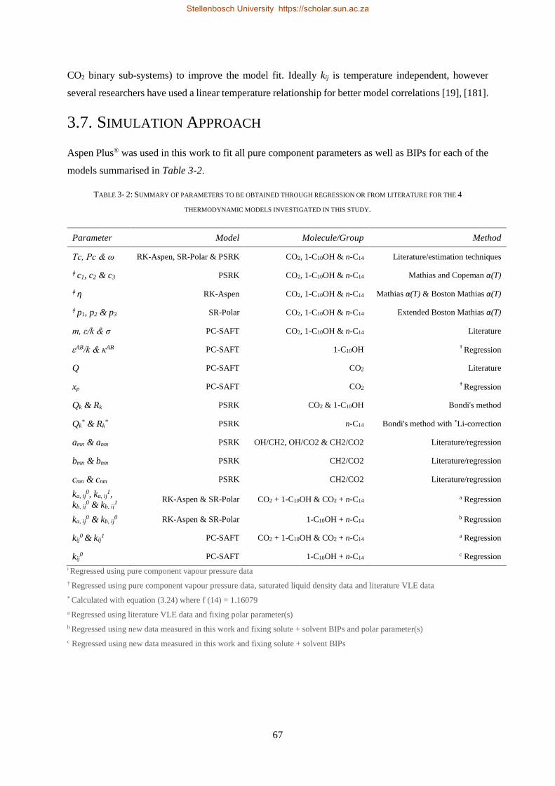
67
CO2 binary sub-systems) to improve the model fit. Ideally kij is temperature independent, however
several researchers have used a linear temperature relationship for better model correlations [19], [181].
3.7. SIMULATION APPROACH
Aspen Plus® was used in this work to fit all pure component parameters as well as BIPs for each of the
models summarised in Table 3-2.
TABLE 3- 2: SUMMARY OF PARAMETERS TO BE OBTAINED THROUGH REGRESSION OR FROM LITERATURE FOR THE 4
THERMODYNAMIC MODELS INVESTIGATED IN THIS STUDY.
Parameter Model Molecule/Group Method
Tc, Pc & ω RK-Aspen, SR-Polar & PSRK CO2, 1-C10OH & n-C14 Literature/estimation techniques
ǂ c1, c2 & c3 PSRK CO2, 1-C10OH & n-C14 Mathias and Copeman α(T)
ǂ η RK-Aspen CO2, 1-C10OH & n-C14 Mathias α(T) & Boston Mathias α(T)
ǂ p1, p2 & p3 SR-Polar CO2, 1-C10OH & n-C14 Extended Boston Mathias α(T)
m, ε/k & σ PC-SAFT CO2, 1-C10OH & n-C14 Literature
εAB/k & κAB PC-SAFT 1-C10OH † Regression
Q PC-SAFT CO2 Literature
xp PC-SAFT CO2 † Regression
Qk & Rk PSRK CO2 & 1-C10OH Bondi's method
Qk* & Rk
* PSRK n-C14 Bondi's method with *Li-correction
amn & anm PSRK OH/CH2, OH/CO2 & CH2/CO2 Literature/regression
bmn & bnm PSRK CH2/CO2 Literature/regression
cmn & cnm PSRK CH2/CO2 Literature/regression
ka, ij0, ka, ij
1,
kb, ij0 & kb, ij
1 RK-Aspen & SR-Polar CO2 + 1-C10OH & CO2 + n-C14 a Regression
ka, ij0 & kb, ij
0 RK-Aspen & SR-Polar 1-C10OH + n-C14 b Regression
kij0
& kij1
PC-SAFT CO2 + 1-C10OH & CO2 + n-C14 a Regression
kij0 PC-SAFT 1-C10OH + n-C14 c Regression
ǂ Regressed using pure component vapour pressure data
† Regressed using pure component vapour pressure data, saturated liquid density data and literature VLE data
* Calculated with equation (3.24) where f (14) = 1.16079
a Regressed using literature VLE data and fixing polar parameter(s)
b Regressed using new data measured in this work and fixing solute + solvent BIPs and polar parameter(s)
c Regressed using new data measured in this work and fixing solute + solvent BIPs
Stellenbosch University https://scholar.sun.ac.za
68
The following conditions are set for the parameters regressed in this work:
1. Only the Aspen Plus® built-in regression function was considered for parameter fitting (see
discussion in section 3.1). The regression analysis adjusts and weighs each variable (T, P, x and
y) by the standard deviation, therefore it assumes the experimental data are not error free.
2. Temperature dependence was evaluated for the solute + solvent BIPs only due to the HPBDP
data limiting the regression procedure (discussed in Chapter 7).
3. For the SR-Polar model, the ka, ij2 and kb, ij
2 parameters were not considered for T-dependence in
this study following the findings by Lombard [51] who showed an improved model performance
with 3 BIPs is not due to the correlation fitting the data but rather the errors.
4. For the SR-Polar model, the lij parameters was not considered in this study due to the HPBDP
data limiting the regression procedure (discussed in Chapter 7).
5. The solute + solvent BIPs are kept fixed while varying the solute + solute BIPs to avoid inter-
correlation of the parameters. Inter-correlation occurs when more than two BIPs are regressed
simultaneously, resulting in the formation of various parameter sets that all satisfy the regression
solution.
6. For the solute + solvent BIPs only the VLE data previously measured [15], [17] at T = 338 K and
T = 348 K were used for regressions. These two temperatures were selected to avoid
inconsistencies caused by, e.g. temperature inversions at temperatures close to the solvent critical
point. Furthermore, at lower temperatures, the HPBDP P-x curve-concavity restricts accurate
interpolation at constant P to generate the binary “VLE data”, i.e. the phase transition curves are
too flat.
7. Regressions near the critical region of the binary literature data [15], [17] and the HPBDP data
measured in this work were excluded.
3.7.1. PURE COMPONENT PARAMETER REGRESSIONS
Most of the pure component parameters are available in literature and were thus used as is.
Unfortunately, not all the required parameters are available and had to be regressed (see Table 3-2). For
the Mathias and Copeman constants regressed, the polar parameter(s) regressed, the xp parameter
regressed (for CO2) and the association parameters regressed (for 1-decanol) the following objective
function (OF) was used for calculating the pure component vapour pressure data and saturated liquid
density data:
𝑂𝐹 = 𝑊1 ∑ [(𝑃𝑠𝑎𝑡,𝑖
𝐸𝑥𝑝−𝑃𝑠𝑎𝑡,𝑖
𝐶𝑎𝑙𝑐)2
(𝑃𝑠𝑎𝑡𝐸𝑥𝑝
)2 ]
0.5
𝑁𝑃𝑖=1 + 𝑊2 ∑ [
(𝜌𝑠𝑎𝑡,𝑖𝐸𝑥𝑝
−𝜌𝑠𝑎𝑡,𝑖𝐶𝑎𝑙𝑐)
2
(𝜌𝑠𝑎𝑡𝐸𝑥𝑝
)2 ]
0.5
𝑁𝑃𝑖=1 (3.61)
Where, NP is the number of data points.
Stellenbosch University https://scholar.sun.ac.za
69
The regression weights (Wn) used for each model are provided in Table 3-3. Therefore, for PSRK,
RK-Aspen and SR-Polar the α(T) parameters were only fitted to saturated vapour pressure data but with
PC-SAFT, the saturated liquid density data was included for the additional CO2 parameter (xp) and
association parameters for 1-decanol (εAB/k and κAB). How each of these parameters were
obtained/regressed has been further discussed in detail in Chapter 7.
TABLE 3- 3: REGRESSION WEIGHTS FOR EACH OF THE 4 MODELS TO BE USED WITH THE OF SHOWN IN EQUATION (3.61).
Model W1 W2
PSRK 1 0
RK-Aspen 1 0
SR-Polar 1 0
PC-SAFT 0.8 0.2
3.7.2. ALPHA(T) PARAMETER REGRESSIONS
The accuracy of the α(T)-function influences not only the model correlations of supercritical VLE phase
equilibria but also the derivation of supercritical thermodynamic properties, e.g. heat capacities and
enthalpies [217]. Therefore, consistency tests (a list of consistent constraints) applicable to any α(T)-
function were developed to ensure accurate correlations of systems with at least one component at
supercritical conditions (here for CO2). These include [217]:
1. A positive, and continuous α(T)-function for any temperature value, i.e. α(T) ≥ 0.
2. The 1st derivative of the α(T)-function must be continuous and monotonically decreasing for any
temperature (including the critical temperature, Tr = 1), i.e. dα(T)/dT ≤ 0.
3. The 2nd derivative of the α(T)-function must be convex and continuous for any temperature
(including the critical temperature, Tr = 1), i.e. d2α(T)/dT2 ≥ 0.
4. To ensure accurate predictions of state functions in the supercritical domain a negativity constraint
is placed on the 3rd derivative of the α(T)-function, i.e. d3α(T)/dT3 ≤ 0.
Therefore, of relevance to this study are the first 3 constraints to ensure accurate correlations of the
VLE data at supercritical conditions. Table 3-2 lists the α(T)-functions applied for the three cubic EoS
investigated in this work. Each of these were evaluated in Chapter 7 after regressing all required pure
component parameters (also provided in Table 3-2).
3.7.3. BINARY INTERACTION PARAMETER REGRESSIONS
New BIPs were regressed in this study to improve the model correlations/calculations. Different
methods can be used to fit BIPs in the model mixing rules to VLE data through regression. However,
in this work the Aspen Plus® Data Regression System (DRS) was used to determine the binary
Stellenbosch University https://scholar.sun.ac.za
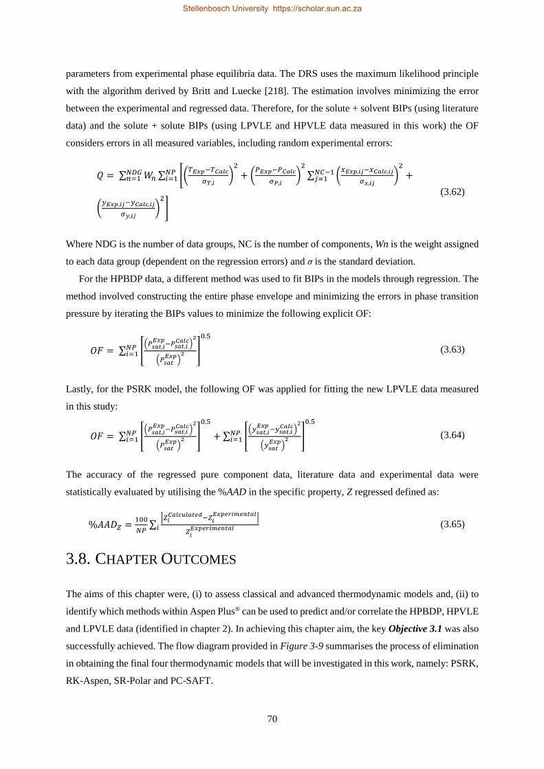
70
parameters from experimental phase equilibria data. The DRS uses the maximum likelihood principle
with the algorithm derived by Britt and Luecke [218]. The estimation involves minimizing the error
between the experimental and regressed data. Therefore, for the solute + solvent BIPs (using literature
data) and the solute + solute BIPs (using LPVLE and HPVLE data measured in this work) the OF
considers errors in all measured variables, including random experimental errors:
𝑄 = ∑ 𝑊𝑛 ∑ [(𝑇𝐸𝑥𝑝−𝑇𝐶𝑎𝑙𝑐
𝜎𝑇,𝑖)
2
+ (𝑃𝐸𝑥𝑝−𝑃𝐶𝑎𝑙𝑐
𝜎𝑃,𝑖)
2
∑ (𝑥𝐸𝑥𝑝,𝑖𝑗−𝑥𝐶𝑎𝑙𝑐,𝑖𝑗
𝜎𝑥,𝑖𝑗)
2
+𝑁𝐶−1𝑗=1
𝑁𝑃𝑖=1
𝑁𝐷𝐺𝑛=1
(𝑦𝐸𝑥𝑝,𝑖𝑗−𝑦𝐶𝑎𝑙𝑐,𝑖𝑗
𝜎𝑦,𝑖𝑗)
2
]
(3.62)
Where NDG is the number of data groups, NC is the number of components, Wn is the weight assigned
to each data group (dependent on the regression errors) and σ is the standard deviation.
For the HPBDP data, a different method was used to fit BIPs in the models through regression. The
method involved constructing the entire phase envelope and minimizing the errors in phase transition
pressure by iterating the BIPs values to minimize the following explicit OF:
𝑂𝐹 = ∑ [(𝑃𝑠𝑎𝑡,𝑖
𝐸𝑥𝑝−𝑃𝑠𝑎𝑡,𝑖
𝐶𝑎𝑙𝑐)2
(𝑃𝑠𝑎𝑡𝐸𝑥𝑝
)2 ]
0.5
𝑁𝑃𝑖=1 (3.63)
Lastly, for the PSRK model, the following OF was applied for fitting the new LPVLE data measured
in this study:
𝑂𝐹 = ∑ [(𝑃𝑠𝑎𝑡,𝑖
𝐸𝑥𝑝−𝑃𝑠𝑎𝑡,𝑖
𝐶𝑎𝑙𝑐)2
(𝑃𝑠𝑎𝑡𝐸𝑥𝑝
)2 ]
0.5
𝑁𝑃𝑖=1 + ∑ [
(𝑦𝑠𝑎𝑡,𝑖𝐸𝑥𝑝
−𝑦𝑠𝑎𝑡,𝑖𝐶𝑎𝑙𝑐)
2
(𝑦𝑠𝑎𝑡𝐸𝑥𝑝
)2 ]
0.5
𝑁𝑃𝑖=1 (3.64)
The accuracy of the regressed pure component data, literature data and experimental data were
statistically evaluated by utilising the %AAD in the specific property, Z regressed defined as:
%𝐴𝐴𝐷𝑍 =100
𝑁𝑃∑
|𝑍𝑖𝐶𝑎𝑙𝑐𝑢𝑙𝑎𝑡𝑒𝑑−𝑍𝑖
𝐸𝑥𝑝𝑒𝑟𝑖𝑚𝑒𝑛𝑡𝑎𝑙|
𝑍𝑖𝐸𝑥𝑝𝑒𝑟𝑖𝑚𝑒𝑛𝑡𝑎𝑙𝑖 (3.65)
3.8. CHAPTER OUTCOMES
The aims of this chapter were, (i) to assess classical and advanced thermodynamic models and, (ii) to
identify which methods within Aspen Plus® can be used to predict and/or correlate the HPBDP, HPVLE
and LPVLE data (identified in chapter 2). In achieving this chapter aim, the key Objective 3.1 was also
successfully achieved. The flow diagram provided in Figure 3-9 summarises the process of elimination
in obtaining the final four thermodynamic models that will be investigated in this work, namely: PSRK,
RK-Aspen, SR-Polar and PC-SAFT.
Stellenbosch University https://scholar.sun.ac.za
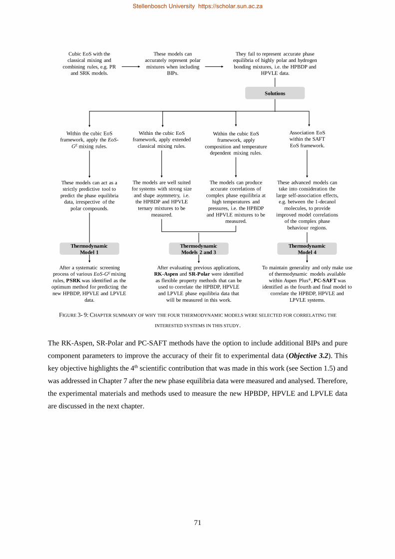
71
FIGURE 3- 9: CHAPTER SUMMARY OF WHY THE FOUR THERMODYNAMIC MODELS WERE SELECTED FOR CORRELATING THE
INTERESTED SYSTEMS IN THIS STUDY.
The RK-Aspen, SR-Polar and PC-SAFT methods have the option to include additional BIPs and pure
component parameters to improve the accuracy of their fit to experimental data (Objective 3.2). This
key objective highlights the 4th scientific contribution that was made in this work (see Section 1.5) and
was addressed in Chapter 7 after the new phase equilibria data were measured and analysed. Therefore,
the experimental materials and methods used to measure the new HPBDP, HPVLE and LPVLE data
are discussed in the next chapter.
These models can
accurately represent polar
mixtures when including
BIPs.
They fail to represent accurate phase
equilibria of highly polar and hydrogen
bonding mixtures, i.e. the HPBDP and
HPVLE data.
Cubic EoS with the
classical mixing and
combining rules, e.g. PR
and SRK models.
Within the cubic EoS
framework, apply the EoS-
GE mixing rules.
Association EoS
within the SAFT
EoS framework.
These models can act as a
strictly predictive tool to
predict the phase equilibria
data, irrespective of the
polar compounds.
After a systematic screening
process of various EoS-GE mixing
rules, PSRK was identified as the
optimum method for predicting the
new HPBDP, HPVLE and LPVLE
data.
These advanced models can
take into consideration the
large self-association effects,
e.g. between the 1-decanol
molecules, to provide
improved model correlations
of the complex phase
behaviour regions.
The models can produce
accurate correlations of
complex phase equilibria at
high temperatures and
pressures, i.e. the HPBDP
and HPVLE mixtures to be
measured.
Within the cubic EoS
framework, apply extended
classical mixing rules.
Within the cubic EoS
framework, apply
composition and temperature
dependent mixing rules.
The models are well suited
for systems with strong size
and shape asymmetry, i.e.
the HPBDP and HPVLE
ternary mixtures to be
measured.
After evaluating previous applications,
RK-Aspen and SR-Polar were identified
as flexible property methods that can be
used to correlate the HPBDP, HPVLE
and LPVLE phase equilibria data that
will be measured in this work.
To maintain generality and only make use
of thermodynamic models available
within Aspen Plus®, PC-SAFT was
identified as the fourth and final model to
correlate the HPBDP, HPVLE and
LPVLE systems.
Solutions
Thermodynamic
Model 1
Thermodynamic
Models 2 and 3
Thermodynamic
Model 4
Stellenbosch University https://scholar.sun.ac.za

72
Stellenbosch University https://scholar.sun.ac.za
73
Chapter 4
EXPERIMENTAL MATERIALS AND METHODS
With a premise of the work presented in this thesis covered in the previous chapters, focus now shifts
to how the work was done. To achieve the first two key objectives of this work, experimental
measurements were to be conducted, namely: HPBDP and HPVLE (Objective 1) and LPVLE
(Objective 2). Various methods are available to measure fluid phase equilibria [219]–[221]. However,
each method is limited with respect to the type of data obtained.
The aim of this chapter is to provide a systematic overview of the experimental materials and
methods employed in this work to measure new high- and low-pressure phase equilibria data.
The materials and apparatus used, methods applied, calibrations conducted, and accuracy of the
experimental results are presented in this chapter.
4.1. MEASUREMENT TECHNIQUES
4.1.1. HIGH-PRESSURE PHASE EQUILIBRIA
There is yet no superior method for measuring high-pressure phase equilibria. The dynamic approach
is used to classify measuring equipment where the system components are continuously circulated
through the equilibrium cell. The second approach, static methods, are used to classify non-flowing
systems [222]. The type of equipment will also depend on whether sampling (analytic) of the phases
takes place or not (synthetic). A summary of the two main techniques employed namely, dynamic and
static methods, are shown in Figure 4-1 and discussed in some detail in Appendix A1 [222], [223].
Each type has its advantages and drawbacks for the measurement of high-pressure phase equilibria data.
The dynamic method will not be used as it is not suitable to measure the critical region of the mixtures
and thermal degradation of the hydrocarbons could occur [18]. Furthermore, experience is required to
ensure the correct quantity of components are added to the equilibrium cell.
Fast, simple and efficient measurements can be achieved using a synthetic method and will thus be
used to measure the bubble- and dew-point data of the ternary system. It is also the most suitable method
for measuring the super and near-critical phenomena of the system. For ternary systems and
multicomponent systems, the only approach suitable to measure data points of phases that are in
equilibrium and construct the tie lines on phase diagrams is the analytical method (synthetic method
Stellenbosch University https://scholar.sun.ac.za
74
only produces P-T-x data). The analytical method will thus be used to measure the high-pressure VLE
data of the CO2 + 1-decanol + n-tetradecane system. However, the number of tests are limited due to
complicated and expensive equipment needed for analysing the samples.
FIGURE 4- 1: CLASSIFICATION OF EXPERIMENTAL HIGH-PRESSURE VLE METHODS. ADAPTED USING [221]–[225].
4.1.2. LOW-PRESSURE PHASE EQUILIBRIA
Over the past few decades, the different techniques to utilise in the measurement of low-pressure phase
equilibria have improved immensely [226], [227]. A brief discussion of the less conventional techniques
can be found in Appendix A2. The only measurement required for the binary system was the pressure,
making the preferred technique isothermal. However, the phase equilibria measurement of the
1-decanol + n-tetradecane binary system will need to be conducted at a sub-atmospheric pressure and
therefore an isobaric technique is required. The Gillespie dynamic still was investigated for measuring
low-pressure phase equilibria due to the suitability of the technique and the isobaric requirement (see
Appendix A2 for a discussion on the use of the Othmer dynamic still).
The Gillespie equilibrium still is effective in establishing phase equilibria, including azeotropic
properties of liquid systems. It was initially pioneered in 1931 by Lee [228] who established a means
of obtaining accurate equilibrium temperature readings using a Platinum resistance element (Pt-100).
Several years later in 1946, Gillespie designed a disengagement chamber to separate the liquid from the
vapour to induce mass transfer effects taking place between phases. The vapour-liquid mixture is
pumped from the boiling chamber to the separation chamber by means of the Cottrell tube/pump. The
Stellenbosch University https://scholar.sun.ac.za
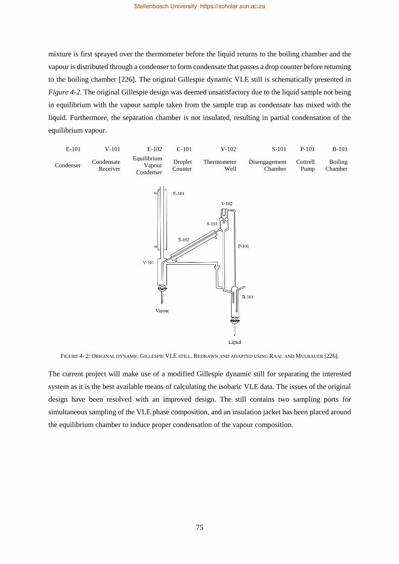
75
mixture is first sprayed over the thermometer before the liquid returns to the boiling chamber and the
vapour is distributed through a condenser to form condensate that passes a drop counter before returning
to the boiling chamber [226]. The original Gillespie dynamic VLE still is schematically presented in
Figure 4-2. The original Gillespie design was deemed unsatisfactory due to the liquid sample not being
in equilibrium with the vapour sample taken from the sample trap as condensate has mixed with the
liquid. Furthermore, the separation chamber is not insulated, resulting in partial condensation of the
equilibrium vapour.
E-101 V-101 E-102 C-101 V-102 S-101 P-101 B-101
Condenser Condensate
Receiver
Equilibrium
Vapour
Condenser
Droplet
Counter
Thermometer
Well
Disengagement
Chamber
Cottrell
Pump
Boiling
Chamber
FIGURE 4- 2: ORIGINAL DYNAMIC GILLESPIE VLE STILL. REDRAWN AND ADAPTED USING RAAL AND MULBAUER [226].
The current project will make use of a modified Gillespie dynamic still for separating the interested
system as it is the best available means of calculating the isobaric VLE data. The issues of the original
design have been resolved with an improved design. The still contains two sampling ports for
simultaneous sampling of the VLE phase composition, and an insulation jacket has been placed around
the equilibrium chamber to induce proper condensation of the vapour composition.
Stellenbosch University https://scholar.sun.ac.za
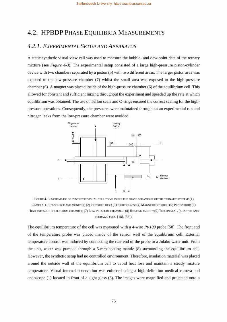
76
4.2. HPBDP PHASE EQUILIBRIA MEASUREMENTS
4.2.1. EXPERIMENTAL SETUP AND APPARATUS
A static synthetic visual view cell was used to measure the bubble- and dew-point data of the ternary
mixture (see Figure 4-3). The experimental setup consisted of a large high-pressure piston-cylinder
device with two chambers separated by a piston (5) with two different areas. The larger piston area was
exposed to the low-pressure chamber (7) whilst the small area was exposed to the high-pressure
chamber (6). A magnet was placed inside of the high-pressure chamber (6) of the equilibrium cell. This
allowed for constant and sufficient mixing throughout the experiment and speeded up the rate at which
equilibrium was obtained. The use of Teflon seals and O-rings ensured the correct sealing for the high-
pressure operations. Consequently, the pressures were maintained throughout an experimental run and
nitrogen leaks from the low-pressure chamber were avoided.
FIGURE 4- 3: SCHEMATIC OF SYNTHETIC VISUAL CELL TO MEASURE THE PHASE BEHAVIOUR OF THE TERNARY SYSTEM: (1)
CAMERA, LIGHT-SOURCE AND MONITOR; (2) PRESSURE DISC; (3) SIGHT GLASS; (4) MAGNETIC STIRRER; (5) PISTON ROD; (6)
HIGH-PRESSURE EQUILIBRIUM CHAMBER; (7) LOW-PRESSURE CHAMBER; (8) HEATING JACKET; (9) TEFLON SEAL. (ADAPTED AND
REDRAWN FROM [18], [58]).
The equilibrium temperature of the cell was measured with a 4-wire Pt-100 probe [58]. The front end
of the temperature probe was placed inside of the sensor well of the equilibrium cell. External
temperature control was induced by connecting the rear end of the probe to a Julabo water unit. From
the unit, water was pumped through a 5-mm heating mantle (8) surrounding the equilibrium cell.
However, the synthetic setup had no controlled environment. Therefore, insulation material was placed
around the outside wall of the equilibrium cell to avoid heat loss and maintain a steady mixture
temperature. Visual internal observation was enforced using a high-definition medical camera and
endoscope (1) located in front of a sight glass (3). The images were magnified and projected onto a
Stellenbosch University https://scholar.sun.ac.za
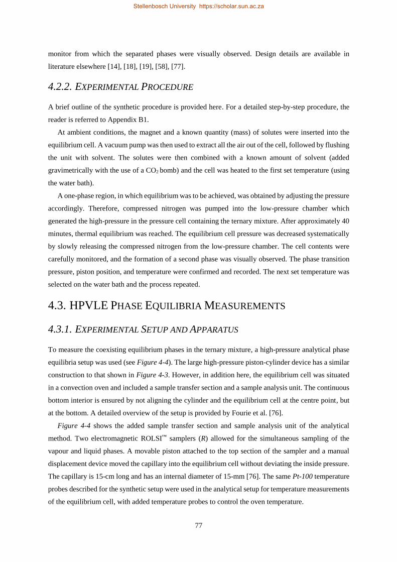
77
monitor from which the separated phases were visually observed. Design details are available in
literature elsewhere [14], [18], [19], [58], [77].
4.2.2. EXPERIMENTAL PROCEDURE
A brief outline of the synthetic procedure is provided here. For a detailed step-by-step procedure, the
reader is referred to Appendix B1.
At ambient conditions, the magnet and a known quantity (mass) of solutes were inserted into the
equilibrium cell. A vacuum pump was then used to extract all the air out of the cell, followed by flushing
the unit with solvent. The solutes were then combined with a known amount of solvent (added
gravimetrically with the use of a CO2 bomb) and the cell was heated to the first set temperature (using
the water bath).
A one-phase region, in which equilibrium was to be achieved, was obtained by adjusting the pressure
accordingly. Therefore, compressed nitrogen was pumped into the low-pressure chamber which
generated the high-pressure in the pressure cell containing the ternary mixture. After approximately 40
minutes, thermal equilibrium was reached. The equilibrium cell pressure was decreased systematically
by slowly releasing the compressed nitrogen from the low-pressure chamber. The cell contents were
carefully monitored, and the formation of a second phase was visually observed. The phase transition
pressure, piston position, and temperature were confirmed and recorded. The next set temperature was
selected on the water bath and the process repeated.
4.3. HPVLE PHASE EQUILIBRIA MEASUREMENTS
4.3.1. EXPERIMENTAL SETUP AND APPARATUS
To measure the coexisting equilibrium phases in the ternary mixture, a high-pressure analytical phase
equilibria setup was used (see Figure 4-4). The large high-pressure piston-cylinder device has a similar
construction to that shown in Figure 4-3. However, in addition here, the equilibrium cell was situated
in a convection oven and included a sample transfer section and a sample analysis unit. The continuous
bottom interior is ensured by not aligning the cylinder and the equilibrium cell at the centre point, but
at the bottom. A detailed overview of the setup is provided by Fourie et al. [76].
Figure 4-4 shows the added sample transfer section and sample analysis unit of the analytical
method. Two electromagnetic ROLSI™ samplers (R) allowed for the simultaneous sampling of the
vapour and liquid phases. A movable piston attached to the top section of the sampler and a manual
displacement device moved the capillary into the equilibrium cell without deviating the inside pressure.
The capillary is 15-cm long and has an internal diameter of 15-mm [76]. The same Pt-100 temperature
probes described for the synthetic setup were used in the analytical setup for temperature measurements
of the equilibrium cell, with added temperature probes to control the oven temperature.
Stellenbosch University https://scholar.sun.ac.za
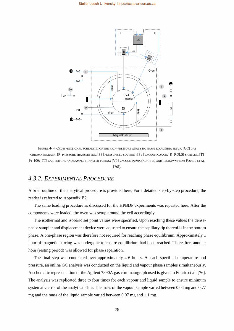
78
FIGURE 4- 4: CROSS-SECTIONAL SCHEMATIC OF THE HIGH-PRESSURE ANALYTIC PHASE EQUILIBRIA SETUP: [GC] GAS
CHROMATOGRAPH; [P] PRESSURE TRANSMITTER; [PS] PRESSURISED SOLVENT; [PV] VACUUM GAUGE; [R] ROLSI SAMPLER; [T]
PT-100; [TT] CARRIER GAS AND SAMPLE TRANSFER TUBING; [VP] VACUUM PUMP, (ADAPTED AND REDRAWN FROM FOURIE ET AL.
[76]).
4.3.2. EXPERIMENTAL PROCEDURE
A brief outline of the analytical procedure is provided here. For a detailed step-by-step procedure, the
reader is referred to Appendix B2.
The same loading procedure as discussed for the HPBDP experiments was repeated here. After the
components were loaded, the oven was setup around the cell accordingly.
The isothermal and isobaric set point values were specified. Upon reaching these values the dense-
phase sampler and displacement device were adjusted to ensure the capillary tip thereof is in the bottom
phase. A one-phase region was therefore not required for reaching phase equilibrium. Approximately 1
hour of magnetic stirring was undergone to ensure equilibrium had been reached. Thereafter, another
hour (resting period) was allowed for phase separation.
The final step was conducted over approximately 4-6 hours. At each specified temperature and
pressure, an online GC analysis was conducted on the liquid and vapour phase samples simultaneously.
A schematic representation of the Agilent 7890A gas chromatograph used is given in Fourie et al. [76].
The analysis was replicated three to four times for each vapour and liquid sample to ensure minimum
systematic error of the analytical data. The mass of the vapour sample varied between 0.04 mg and 0.77
mg and the mass of the liquid sample varied between 0.07 mg and 1.1 mg.
Stellenbosch University https://scholar.sun.ac.za
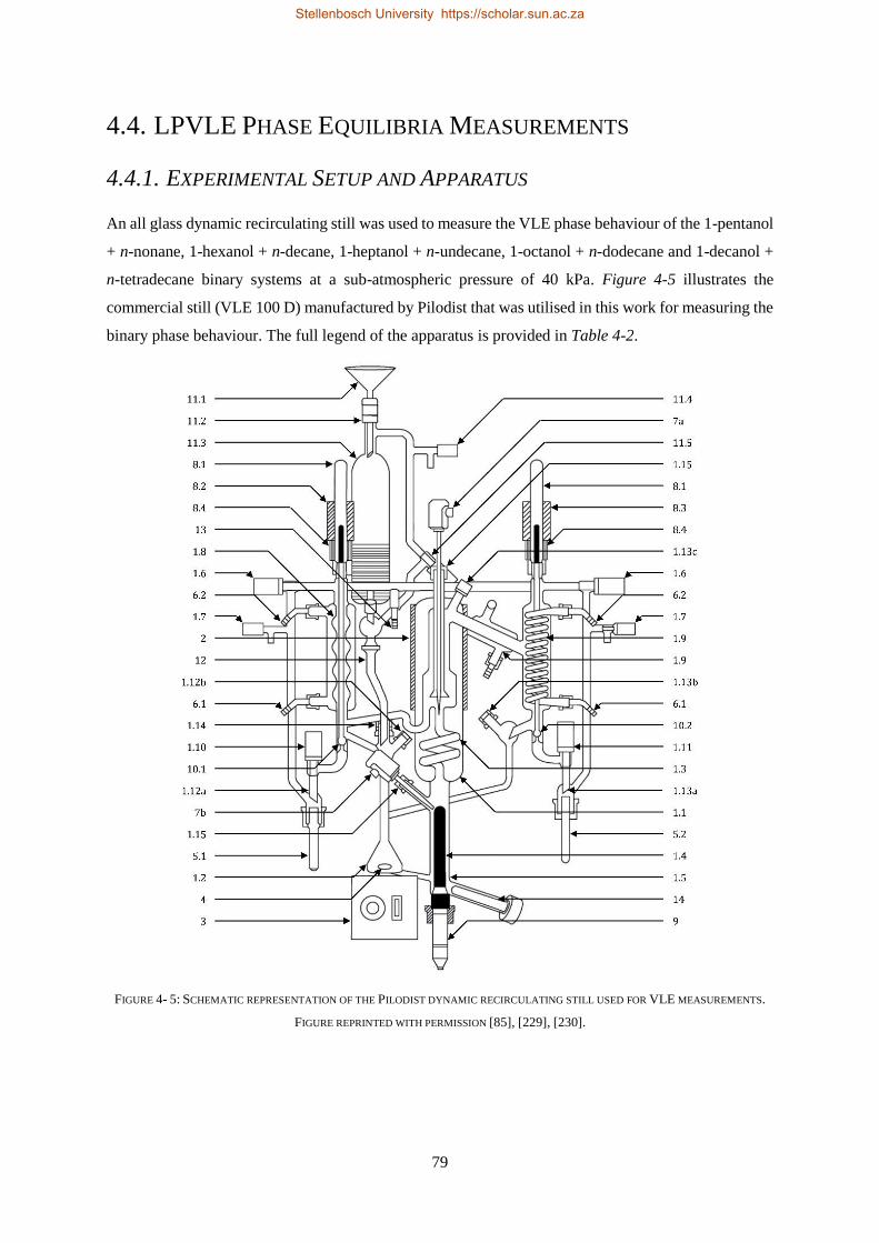
79
4.4. LPVLE PHASE EQUILIBRIA MEASUREMENTS
4.4.1. EXPERIMENTAL SETUP AND APPARATUS
An all glass dynamic recirculating still was used to measure the VLE phase behaviour of the 1-pentanol
+ n-nonane, 1-hexanol + n-decane, 1-heptanol + n-undecane, 1-octanol + n-dodecane and 1-decanol +
n-tetradecane binary systems at a sub-atmospheric pressure of 40 kPa. Figure 4-5 illustrates the
commercial still (VLE 100 D) manufactured by Pilodist that was utilised in this work for measuring the
binary phase behaviour. The full legend of the apparatus is provided in Table 4-2.
FIGURE 4- 5: SCHEMATIC REPRESENTATION OF THE PILODIST DYNAMIC RECIRCULATING STILL USED FOR VLE MEASUREMENTS.
FIGURE REPRINTED WITH PERMISSION [85], [229], [230].
Stellenbosch University https://scholar.sun.ac.za
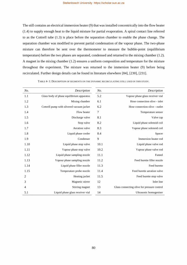
80
The still contains an electrical immersion heater (9) that was installed concentrically into the flow heater
(1.4) to supply enough heat to the liquid mixture for partial evaporation. A spiral contact line referred
to as the Cottrell tube (1.3) is place before the separation chamber to enable the phase change. The
separation chamber was modified to prevent partial condensation of the vapour phase. The two-phase
mixture can therefore be sent over the thermometer to measure the bubble-point (equilibrium
temperature) before the two phases are separated, condensed and returned to the mixing chamber (1.2).
A magnet in the mixing chamber (1.2) ensures a uniform composition and temperature for the mixture
throughout the experiment. The mixture was returned to the immersion heater (9) before being
recirculated. Further design details can be found in literature elsewhere [84], [230], [231].
TABLE 4- 1: DESCRIPTION OF SEGMENTS ON THE DYNAMIC RECIRCULATING STILL USED IN THIS STUDY.
No. Description No. Description
1.1 Glass body of phase equilibrium apparatus 5.2 Vapour phase glass receiver vial
1.2 Mixing chamber 6.1 Hose connection olive - inlet
1.3 Cottrell pump with silvered vacuum jacket 6.2 Hose connection olive - outlet
1.4 Flow heater 7 Temperature sensor
1.5 Discharge valve 8.1 Valve cap
1.6 Stop valve 8.2 Liquid phase solenoid coil
1.7 Aeration valve 8.3 Vapour phase solenoid coil
1.8 Liquid phase cooler 8.4 Spacer
1.9 Condenser 9 Immersion heater rod
1.10 Liquid phase stop valve 10.1 Liquid phase valve rod
1.11 Vapour phase stop valve 10.2 Vapour phase valve rod
1.12 Liquid phase sampling nozzle 11.1 Funnel
1.13 Vapour phase sampling nozzle 11.2 Feed burette filler nozzle
1.14 Liquid phase filler nozzle 11.3 Feed burette
1.15 Temperature probe nozzle 11.4 Feed burette aeration valve
2 Heating jacket 11.5 Feed burette stop valve
3 Magnetic stirrer 12 Inlet line
4 Stirring magnet 13 Glass connecting olive for pressure control
5.1 Liquid phase glass receiver vial 14 Ultrasonic homogeniser
Stellenbosch University https://scholar.sun.ac.za
81
4.4.2. EXPERIMENTAL PROCEDURE
All numerical references in the procedure provided below refers to those illustrated in Figure 4-5. For
a detailed step-by-step procedure, the reader is referred to Appendix B3.
The still was initially dried with compressed air. The nitrogen cylinder was opened, and the cooling
water system switched on to pass through the cooler for the liquid phase (1.8) and two condensers on
the vapour side (1.9). The still was switched on and the controlling software opened.
The still was prepared by selecting the operation to be performed, securing the ultrasonic
homogenizer probe (14), closing the discharge valve (1.5) and adding approximately 110 ml of the feed
mixture to the mixing chamber (1.2). Once the immersion heater rod (9) was completely submerged in
mixture, the magnetic stirrer (3) was switched on. The heater power is important as it established the
feed mixture temperature (inserted as a percentage). The pressure was also set accordingly and balanced
using nitrogen gas.
After approximately 1-hour equilibrium was achieved and confirmed with a steady vapour
temperature on the display unit. When at least 30 drops per minute was observed at the droplet point of
the vapour condensation side, in combination with the constant temperature equilibrium, a large enough
sample of both phases were taken. Thereafter, a vapour and liquid sample was collected through the
two sampling ports and prepared for GC analysis on an Agilent 7820A gas chromatograph. Each of the
samples were prepared by adding a known mass amount of the analyte to 1.5 ml of solvent in a vial. In
addition, approximately 30 mg of internal standard (IS) was also added to the solvent mixture and
measured accurately to 10-5 g.
Once enough samples had been obtained the apparatus was stopped and allowed to cool down. The
components were drained from the still and discarded into the appropriate waste container.
Approximately 110 ml of acetone was fed into the mixing chamber (1.2) to wash out the still by boiling
the acetone. After another 40 minutes, the acetone was drained and the still dried with compressed air.
4.4.3. EXPERIMENTAL ERROR ANALYSIS
Two user-controlled, dependent variables need to be considered with respect to the outcome of the
experimental runs, namely (1) the heater power (%), and (2) isobaric pressure (kPa).
The first input does not require alternation while running the still and was thus not considered as a
variable factor. The influence of the heater power on the equilibrium composition is considered
negligible in this study. The pressure fluctuations present during the experiment cannot be regarded in
the same light. For investigating the effect of pressure fluctuations on the equilibrium composition, the
PSRK model, in Aspen Plus®, will be used. It produces an excellent prediction of the 1-octanol +
n-dodecane VLE data as will be presented later (see section 7.2.1) but has been produced in Figure 4-6
for analysis here.
Stellenbosch University https://scholar.sun.ac.za
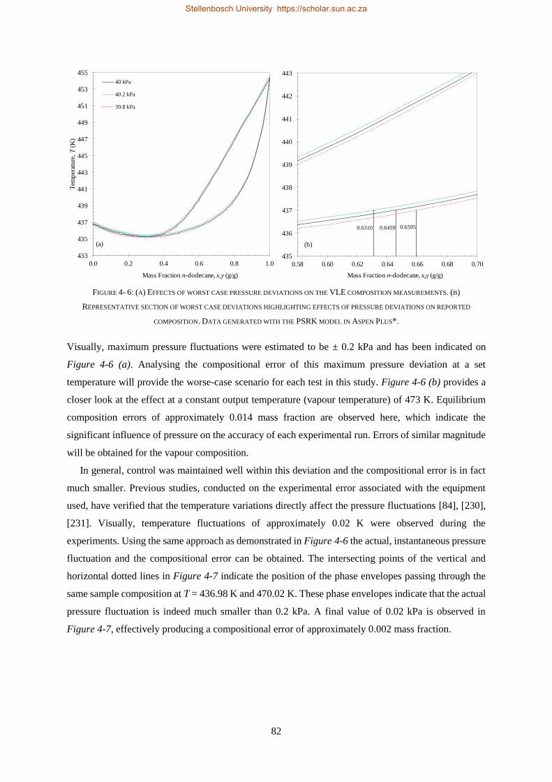
82
FIGURE 4- 6: (A) EFFECTS OF WORST CASE PRESSURE DEVIATIONS ON THE VLE COMPOSITION MEASUREMENTS. (B)
REPRESENTATIVE SECTION OF WORST CASE DEVIATIONS HIGHLIGHTING EFFECTS OF PRESSURE DEVIATIONS ON REPORTED
COMPOSITION. DATA GENERATED WITH THE PSRK MODEL IN ASPEN PLUS®.
Visually, maximum pressure fluctuations were estimated to be ± 0.2 kPa and has been indicated on
Figure 4-6 (a). Analysing the compositional error of this maximum pressure deviation at a set
temperature will provide the worse-case scenario for each test in this study. Figure 4-6 (b) provides a
closer look at the effect at a constant output temperature (vapour temperature) of 473 K. Equilibrium
composition errors of approximately 0.014 mass fraction are observed here, which indicate the
significant influence of pressure on the accuracy of each experimental run. Errors of similar magnitude
will be obtained for the vapour composition.
In general, control was maintained well within this deviation and the compositional error is in fact
much smaller. Previous studies, conducted on the experimental error associated with the equipment
used, have verified that the temperature variations directly affect the pressure fluctuations [84], [230],
[231]. Visually, temperature fluctuations of approximately 0.02 K were observed during the
experiments. Using the same approach as demonstrated in Figure 4-6 the actual, instantaneous pressure
fluctuation and the compositional error can be obtained. The intersecting points of the vertical and
horizontal dotted lines in Figure 4-7 indicate the position of the phase envelopes passing through the
same sample composition at T = 436.98 K and 470.02 K. These phase envelopes indicate that the actual
pressure fluctuation is indeed much smaller than 0.2 kPa. A final value of 0.02 kPa is observed in
Figure 4-7, effectively producing a compositional error of approximately 0.002 mass fraction.
433
435
437
439
441
443
445
447
449
451
453
455
0.0 0.2 0.4 0.6 0.8 1.0
Tem
per
ature
, T
(K)
Mass Fraction n-dodecane, x,y (g/g)
40 kPa
40.2 kPa
39.8 kPa
(a)
0.6310 0.6459 0.6595
435
436
437
438
439
440
441
442
443
0.58 0.60 0.62 0.64 0.66 0.68 0.70
Mass Fraction n-dodecane, x,y (g/g)
(b)
Stellenbosch University https://scholar.sun.ac.za
83
FIGURE 4- 7: EFFECTS OF ANTICIPATED PRESSURE DEVIATIONS ON THE VLE COMPOSITION MEASUREMENTS. PHASE ENVELOPES
INDICATED ARE FOR THE LIQUID PHASE. AN EQUIVALENT ANALYSIS CAN BE MADE FOR THE VAPOUR PHASE. DATA GENERATED
WITH THE PSRK MODEL IN ASPEN PLUS®.
4.5. ACCURACY OF DATA
4.5.1. CALIBRATION CURVES FOR GC ANALYSIS
To ensure accurate and precise qualitative determinations of any analyte it is essential to consider good
calibration and the sensitivity of the instrumental analysis. The solvents and ISs used for the GC
calibration are provided in Table 4-1. The IS used to quantify the results depend on the system being
investigated and has been indicated for each chemical. GC calibration curves were constructed to enable
replicate injections within a relative standard deviation of 1%. The linear curves have a regression
coefficient equal to or greater than 0.9995 and can be found in Appendix G.
For HPVLE, the calibration procedure involved 3 to 8 manual injections of known mass amounts
for the liquids (1-decanol + n-tetradecane) and the gas (CO2). The liquid analytes were diluted with 2-
ethyl-1-hexanol (solvent) prior to injections. Linear relationships between injected mass (of analyte)
and detector response were obtained with a slow plunger depression rate. The rate of change of response
with the amount of analyte defines the sensitivity of the analysis. However, the response factors (the
slope of the curves) are dependent on the amount of analyte and is therefore a numerical representation
of the sensitivity of the analysis.
0.6310 0.65950.6442 0.6471
436.3
436.4
436.5
436.6
436.7
436.8
436.9
437.0
437.1
437.2
437.3
0.60 0.61 0.62 0.63 0.64 0.65 0.66 0.67 0.68
Tem
per
ature
, T
(K)
Mass Fraction n-dodecane, x, y (g/g)
40 kPa
40.2 kPa
39.8 kPa
40.02 kPa
39.98 kPa
Stellenbosch University https://scholar.sun.ac.za
84
For LPVLE calibrations, the procedure involved 5 injections of known mass amounts for the liquids
(each analyte of interest) and an internal standard. The analyte + IS mixture were diluted with n-hexane
(solvent) prior to injections. The linear curves were constructed using the response of each analyte
relative to its respective IS response at separate points all along the composition spectrum. Therefore,
the linear curves indicate constant sensitivity in each system because the slopes were constant.
4.5.2. HIGH-PRESSURE EXPERIMENTAL MEASUREMENTS
The measurement uncertainty are as follows:
For the HPBDP measurements, two calibrated analytical balances with a precision of 0.0001 g and 0.01
g were used to weigh the solutes and solvent, respectively. The maximum relative uncertainties in the
mass fraction is 0.01 times the value, i.e. u(w) = 0.01w.
For the HPVLE measurements, the simultaneous analysis of the two phases (composition) will show
an estimated relative uncertainty of 0.5 mass % for the species-specific data measured in this work and
should not exceed a maximum of 0.9 mass %, i.e. u(wi) = ± 0.005 g/g with u(wi) ≤ 0.009 g/g.
ONEhalf20 Melt pressure transducers were used for both high-pressure experimental procedures.
An in-house calibration was conducted for each transducer using a Barnet Instruments dead-weight
tester. The calibration data used for HPBDP and HPVLE pressure corrections are tabulated in
Appendix C1. The Barnet pressure balance was calibrated by the South African National Accreditation
System (SANAS) to take into consideration the weight of each plate used. After suitable corrections for
gravity, temperature and air buoyancy were made (i.e. the deviation from the nominal value) a
maximum error of 0.04 % was obtained above 2 MPa (see Appendix C2 for the calibration certificates).
(i) HPBDP: The absolute uncertainty of the pressure measurement is no greater than 0.06 MPa, i.e.
u(P) ≤ 0.06 MPa, and includes all contributions towards the error in pressure measurements.
(ii) HPVLE: The absolute uncertainty of the pressure measurement is smaller than or equal to
0.035 MPa, i.e. u(P) ≤ 0.035 MPa, and includes the 0.01 MPa fluctuation during the sampling
process.
The temperature for both experimental methods were measured with 4-wire Pt-100 probes. The most
recent temperature calibration certificates can be found in Appendix C3.
(i) HPBDP: A calibration was conducted by Wika Instruments (Pty) Ltd, South Africa, with a
maximum absolute uncertainty of 0.1 K, i.e. u(T) = 0.1 K.
(ii) HPVLE: Calibrations were conducted by a SANAS accredited institute (InterCal) for 12 Pt-100
probes (4 x in the equilibrium cell block, 4 x in the heating fluid inlets and outlets, and 4 x inside
the oven environment). The probe-, controller-, and logger-inaccuracies were taken into
Stellenbosch University https://scholar.sun.ac.za
85
consideration and a total absolute uncertainty of 0.1 K was measured, i.e. u(T) = 0.1 K, which
includes the 0.01 K fluctuation during the sampling process.
4.5.3. LOW-PRESSURE EXPERIMENTAL MEASUREMENTS
The measurement uncertainties are as follows:
The Pt-100 temperature probes were calibrated by Thermon South Africa (SANAS accredited). After
completing a temperature calibration, the Pt-100 temperature probe connected to a digital Hart
Scientific thermometer measured the equilibrium temperature of the mixture with an accuracy of 0.1 K.
Fluctuations of 0.03 K in the temperature were observed during sampling. However, the deviation never
exceeded 0.1 K. The maximum absolute uncertainty of the temperature is no greater than 0.2 K, i.e.
u(T) ≤ 0.2 K. The latest calibration certificates for the vapour and evaporator temperature probes are
provided in Appendix C4.
A Wika UT-10 unit with a maximum operating pressure of 160 kPa absolute and a quoted accuracy
of 0.1 % (0.16 kPa) of full scale output per the most recent calibration certificate (see Appendix C5)
was utilized to measure the pressure. Furthermore, pressure fluctuations of up to 0.2 kPa were observed
during sampling. Therefore, the absolute uncertainty of the pressure transducer is no greater than
0.36 kPa, i.e. u(P) ≤ 0.36 kPa.
Manual repeatability tests were completed on the GC for samples with a known mass composition.
A maximum uncertainty of 0.022 g/g for the analysis was calculated, i.e. u(x) = u(y) = 0.022 g/g.
4.6. MATERIALS
Table 4-1 contains the list of components with their respective suppliers, CAS numbers, purity, and
chemical structures. Each of the components were used for either the low-pressure and/or the high-
pressure experimental measurements. Technical grade air and high purity helium, supplied by Afrox,
were used for the gas chromatography (GC) analysis. Nitrogen, also supplied by Afrox was used for
overpressure control in the phase equilibrium still and high-pressure equilibrium cells. An additional
GC-Mass Spectrometry (GC-MS) analysis was conducted for the two main solutes of interest to this
study, namely 1-decanol and n-tetradecane for which purity values of 99.5% and 99.7% were obtained,
respectively. For each of the components used in the LPVLE systems Karl-Fischer titrations were
conducted and showed negligible amounts of water. Based on these tests, the purity of the chemicals
given in Table 4-1 were confirmed and all components were used without further purification.
Stellenbosch University https://scholar.sun.ac.za
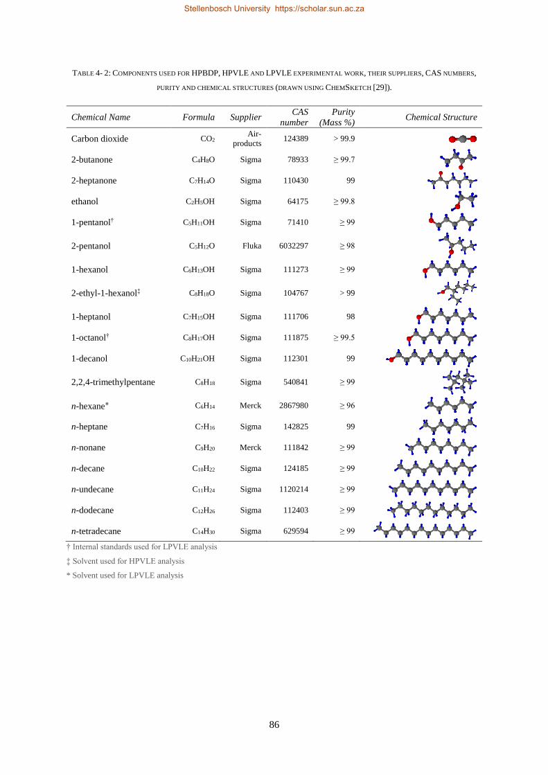
86
TABLE 4- 2: COMPONENTS USED FOR HPBDP, HPVLE AND LPVLE EXPERIMENTAL WORK, THEIR SUPPLIERS, CAS NUMBERS,
PURITY AND CHEMICAL STRUCTURES (DRAWN USING CHEMSKETCH [29]).
Chemical Name Formula Supplier CAS
number
Purity
(Mass %) Chemical Structure
Carbon dioxide CO2 Air-
products 124389 > 99.9
2-butanone C4H8O Sigma 78933 ≥ 99.7
2-heptanone C7H14O Sigma 110430 99
ethanol C2H5OH Sigma 64175 ≥ 99.8
1-pentanol† C5H11OH Sigma 71410 ≥ 99
2-pentanol C5H12O Fluka 6032297 ≥ 98
1-hexanol C6H13OH Sigma 111273 ≥ 99
2-ethyl-1-hexanol‡ C8H18O Sigma 104767 > 99
1-heptanol C7H15OH Sigma 111706 98
1-octanol† C8H17OH Sigma 111875 ≥ 99.5
1-decanol C10H21OH Sigma 112301 99
2,2,4-trimethylpentane C8H18 Sigma 540841 ≥ 99
n-hexane⁕ C6H14 Merck 2867980 ≥ 96
n-heptane C7H16 Sigma 142825 99
n-nonane C9H20 Merck 111842 ≥ 99
n-decane C10H22 Sigma 124185 ≥ 99
n-undecane C11H24 Sigma 1120214 ≥ 99
n-dodecane C12H26 Sigma 112403 ≥ 99
n-tetradecane C14H30 Sigma 629594 ≥ 99
† Internal standards used for LPVLE analysis
‡ Solvent used for HPVLE analysis
* Solvent used for LPVLE analysis
Stellenbosch University https://scholar.sun.ac.za
87
4.7. CHAPTER OUTCOMES
This chapter provided an overview of the materials and methods used for the three experimental studies
conducted in this work, namely:
(i) A static synthetic equilibrium cell to measure the HPBDP phase transition points of six CO2 +
1-decanol + n-tetradecane mixtures at 6 set temperatures and 12 varying solute concentrations.
(ii) A static analytical equilibrium cell to measure the HPVLE of four CO2 + 1-decanol + n-tetradecane
mixtures at 40 different isothermal and isobaric conditions.
(iii) An all-glass dynamic recirculating still to measure the LPVLE of the 1-decanol + n-tetradecane
system and 4 pertinent binary systems (1-pentanol + n-nonane, 1-hexanol + n-decane, 1-heptanol +
n-undecane and 1-octanol + n-dodecane) to help verify the 1-decanol + n-tetradecane binary data.
The HPBDP and HPVLE results are presented and discussed in Chapter 5 after first verifying the setup
of each equilibrium cell with reproducibility tests. Similarly, the LPVLE results of all 5 1-alcohol +
n-alkane binary systems are presented and discussed in Chapter 6 after verifying the setup of the still
with, amongst others, reproducibility tests.
Stellenbosch University https://scholar.sun.ac.za

88
Stellenbosch University https://scholar.sun.ac.za
89
Chapter 5
SUPER- AND NEAR-CRITICAL PHASE EQUILIBRIA OF THE
TERNARY SYSTEM CO2 + 1-DECANOL + N-TETRADECANE
The literature study conducted in Chapter 2 indicates a lack of ternary data available for the system of
interest to this work (see Table 2-5).
The aim of this chapter is to address these shortcomings by studying the high-pressure phase
equilibria of the CO2 + 1-decanol + n-tetradecane ternary system (Objective 1).
The materials and high-pressure phase equilibria methods discussed in Chapter 4 were used to
measure new HPBDP and HPVLE data for the ternary system. The phase equilibria data were used to:
(i) Construct the necessary phase diagrams for investigating where the solute + solute interactions are
most prominent (Objective 1.1);
(ii) Construct the tie lines on the ternary phase diagrams (Objective 1.2);
(iii) Visually identifying the topological phenomena (Objective 1.3);
(iv) Establish the relative solubility and separation potential of the components when using
supercritical CO2 (Objective 1.4).
5.1. HPBDP RESULTS AND DISCUSSION
5.1.1. VERIFICATION OF EXPERIMENTAL SETUP
The synthetic setup has been verified several times by previous researchers through comparisons of
data to literature [14], [15], [56]. Table 5-1 provides a select few of the errors obtained by the researchers
involved in the design and construction of the equipment being used in this investigation. The
experimental setup has therefore been proven accurate through comparisons to literature data.
TABLE 5- 1: VALIDATION OF THE SYNTHETIC EXPERIMENTAL SETUP THROUGH COMPARISONS OF LITERATURE DATA.
System Measured Error Reference
Ethane + nC24 ≤ 0.02 MPa Schwarz and Nieuwoudt [56] with [232], [233]
CO2 + 1-octanol ≤ 0.02 MPa Fourie et al. [14] with [71], [234], [235]
Stellenbosch University https://scholar.sun.ac.za
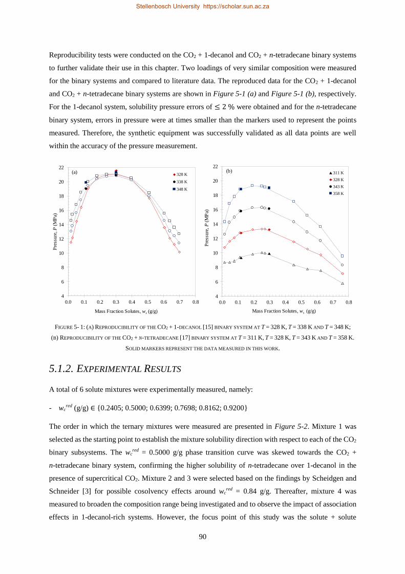
90
Reproducibility tests were conducted on the CO2 + 1-decanol and CO2 + n-tetradecane binary systems
to further validate their use in this chapter. Two loadings of very similar composition were measured
for the binary systems and compared to literature data. The reproduced data for the CO2 + 1-decanol
and CO2 + n-tetradecane binary systems are shown in Figure 5-1 (a) and Figure 5-1 (b), respectively.
For the 1-decanol system, solubility pressure errors of ≤ 2 % were obtained and for the n-tetradecane
binary system, errors in pressure were at times smaller than the markers used to represent the points
measured. Therefore, the synthetic equipment was successfully validated as all data points are well
within the accuracy of the pressure measurement.
FIGURE 5- 1: (A) REPRODUCIBILITY OF THE CO2 + 1-DECANOL [15] BINARY SYSTEM AT T = 328 K, T = 338 K AND T = 348 K;
(B) REPRODUCIBILITY OF THE CO2 + N-TETRADECANE [17] BINARY SYSTEM AT T = 311 K, T = 328 K, T = 343 K AND T = 358 K.
SOLID MARKERS REPRESENT THE DATA MEASURED IN THIS WORK.
5.1.2. EXPERIMENTAL RESULTS
A total of 6 solute mixtures were experimentally measured, namely:
- wcred (g/g) ∈ {0.2405; 0.5000; 0.6399; 0.7698; 0.8162; 0.9200}
The order in which the ternary mixtures were measured are presented in Figure 5-2. Mixture 1 was
selected as the starting point to establish the mixture solubility direction with respect to each of the CO2
binary subsystems. The wcred = 0.5000 g/g phase transition curve was skewed towards the CO2 +
n-tetradecane binary system, confirming the higher solubility of n-tetradecane over 1-decanol in the
presence of supercritical CO2. Mixture 2 and 3 were selected based on the findings by Scheidgen and
Schneider [3] for possible cosolvency effects around wcred = 0.84 g/g. Thereafter, mixture 4 was
measured to broaden the composition range being investigated and to observe the impact of association
effects in 1-decanol-rich systems. However, the focus point of this study was the solute + solute
4
6
8
10
12
14
16
18
20
22
0.0 0.1 0.2 0.3 0.4 0.5 0.6 0.7 0.8
Pre
ssure
, P
(MP
a)
Mass Fraction Solutes, ws (g/g)
311 K
328 K
343 K
358 K
(b)
4
6
8
10
12
14
16
18
20
22
0.0 0.1 0.2 0.3 0.4 0.5 0.6 0.7 0.8
Pre
ssure
, P
(MP
a)
Mass Fraction Solutes, ws (g/g)
328 K
338 K
348 K
(a)
Stellenbosch University https://scholar.sun.ac.za
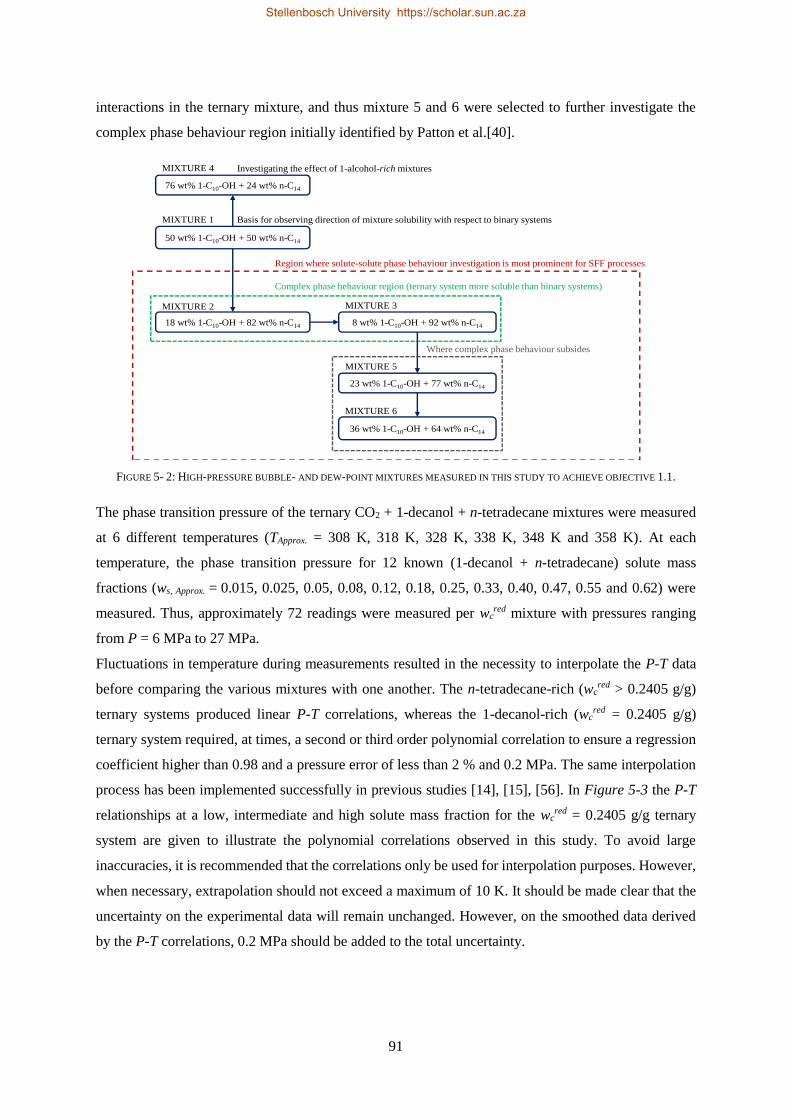
91
interactions in the ternary mixture, and thus mixture 5 and 6 were selected to further investigate the
complex phase behaviour region initially identified by Patton et al.[40].
FIGURE 5- 2: HIGH-PRESSURE BUBBLE- AND DEW-POINT MIXTURES MEASURED IN THIS STUDY TO ACHIEVE OBJECTIVE 1.1.
The phase transition pressure of the ternary CO2 + 1-decanol + n-tetradecane mixtures were measured
at 6 different temperatures (TApprox. = 308 K, 318 K, 328 K, 338 K, 348 K and 358 K). At each
temperature, the phase transition pressure for 12 known (1-decanol + n-tetradecane) solute mass
fractions (ws, Approx. = 0.015, 0.025, 0.05, 0.08, 0.12, 0.18, 0.25, 0.33, 0.40, 0.47, 0.55 and 0.62) were
measured. Thus, approximately 72 readings were measured per wcred mixture with pressures ranging
from P = 6 MPa to 27 MPa.
Fluctuations in temperature during measurements resulted in the necessity to interpolate the P-T data
before comparing the various mixtures with one another. The n-tetradecane-rich (wcred > 0.2405 g/g)
ternary systems produced linear P-T correlations, whereas the 1-decanol-rich (wcred = 0.2405 g/g)
ternary system required, at times, a second or third order polynomial correlation to ensure a regression
coefficient higher than 0.98 and a pressure error of less than 2 % and 0.2 MPa. The same interpolation
process has been implemented successfully in previous studies [14], [15], [56]. In Figure 5-3 the P-T
relationships at a low, intermediate and high solute mass fraction for the wcred = 0.2405 g/g ternary
system are given to illustrate the polynomial correlations observed in this study. To avoid large
inaccuracies, it is recommended that the correlations only be used for interpolation purposes. However,
when necessary, extrapolation should not exceed a maximum of 10 K. It should be made clear that the
uncertainty on the experimental data will remain unchanged. However, on the smoothed data derived
by the P-T correlations, 0.2 MPa should be added to the total uncertainty.
76 wt% 1-C10-OH + 24 wt% n-C14
50 wt% 1-C10-OH + 50 wt% n-C14
18 wt% 1-C10-OH + 82 wt% n-C14 8 wt% 1-C10-OH + 92 wt% n-C14
23 wt% 1-C10-OH + 77 wt% n-C14
36 wt% 1-C10-OH + 64 wt% n-C14
MIXTURE 1
MIXTURE 2
MIXTURE 4
MIXTURE 3
MIXTURE 5
MIXTURE 6
Complex phase behaviour region (ternary system more soluble than binary systems)
Where complex phase behaviour subsides
Region where solute-solute phase behaviour investigation is most prominent for SFF processes
Basis for observing direction of mixture solubility with respect to binary systems
Investigating the effect of 1-alcohol-rich mixtures
Stellenbosch University https://scholar.sun.ac.za
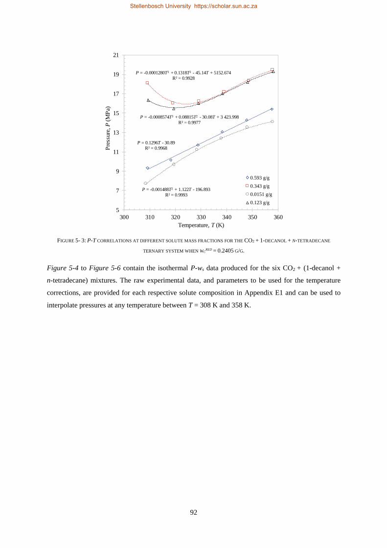
92
FIGURE 5- 3: P-T CORRELATIONS AT DIFFERENT SOLUTE MASS FRACTIONS FOR THE CO2 + 1-DECANOL + N-TETRADECANE
TERNARY SYSTEM WHEN WCRED = 0.2405 G/G.
Figure 5-4 to Figure 5-6 contain the isothermal P-ws data produced for the six CO2 + (1-decanol +
n-tetradecane) mixtures. The raw experimental data, and parameters to be used for the temperature
corrections, are provided for each respective solute composition in Appendix E1 and can be used to
interpolate pressures at any temperature between T = 308 K and 358 K.
P = 0.1296T - 30.89R² = 0.9968
P = -0.0001280T3 + 0.1318T2 - 45.14T + 5152.674R² = 0.9928
P = -0.001488T2 + 1.122T - 196.893R² = 0.9993
P = -0.0008574T3 + 0.08815T2 - 30.08T + 3 423.998R² = 0.9977
5
7
9
11
13
15
17
19
21
300 310 320 330 340 350 360
Pre
ssure
, P
(MP
a)
Temperature, T (K)
0.593 g/g
0.343 g/g
0.0151 g/g
0.123 g/g
Stellenbosch University https://scholar.sun.ac.za
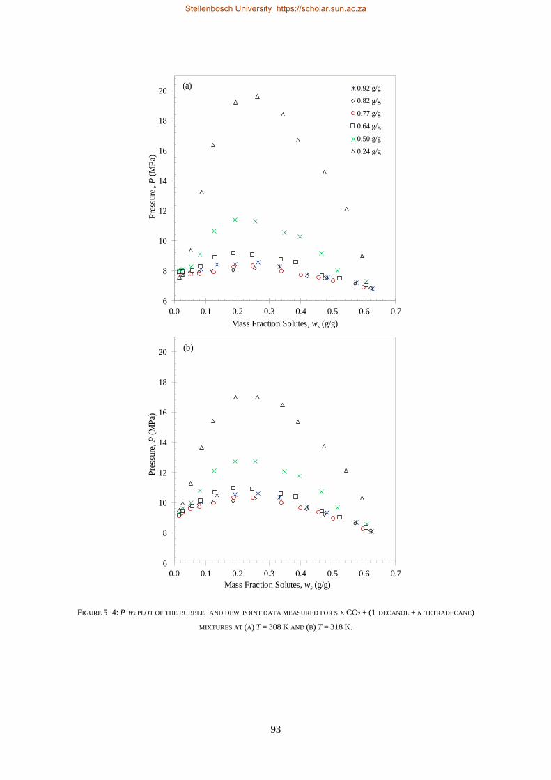
93
FIGURE 5- 4: P-WS PLOT OF THE BUBBLE- AND DEW-POINT DATA MEASURED FOR SIX CO2 + (1-DECANOL + N-TETRADECANE)
MIXTURES AT (A) T = 308 K AND (B) T = 318 K.
6
8
10
12
14
16
18
20
0.0 0.1 0.2 0.3 0.4 0.5 0.6 0.7
Pre
ssure
, P
(MP
a)
Mass Fraction Solutes, ws (g/g)
0.92 g/g
0.82 g/g
0.77 g/g
0.64 g/g
0.50 g/g
0.24 g/g
(a)
6
8
10
12
14
16
18
20
0.0 0.1 0.2 0.3 0.4 0.5 0.6 0.7
Pre
ssure
, P
(MP
a)
Mass Fraction Solutes, ws (g/g)
(b)
Stellenbosch University https://scholar.sun.ac.za
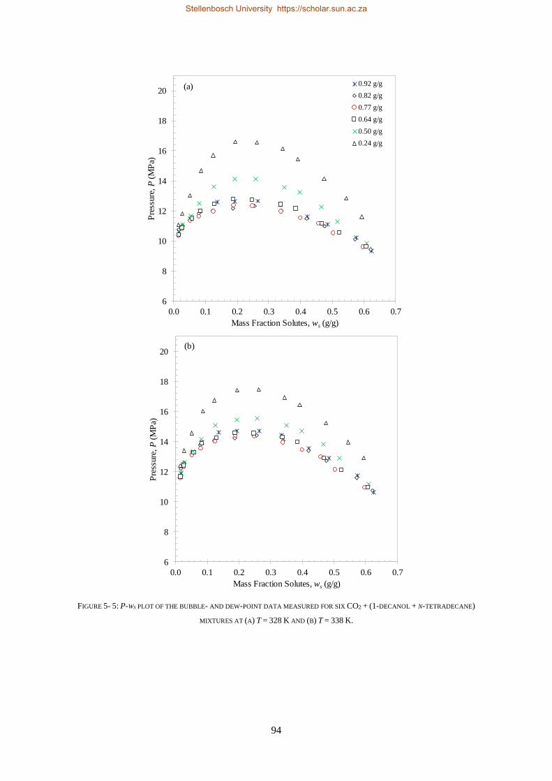
94
FIGURE 5- 5: P-WS PLOT OF THE BUBBLE- AND DEW-POINT DATA MEASURED FOR SIX CO2 + (1-DECANOL + N-TETRADECANE)
MIXTURES AT (A) T = 328 K AND (B) T = 338 K.
6
8
10
12
14
16
18
20
0.0 0.1 0.2 0.3 0.4 0.5 0.6 0.7
Pre
ssure
, P
(MP
a)
Mass Fraction Solutes, ws (g/g)
0.92 g/g
0.82 g/g
0.77 g/g
0.64 g/g
0.50 g/g
0.24 g/g
(a)
6
8
10
12
14
16
18
20
0.0 0.1 0.2 0.3 0.4 0.5 0.6 0.7
Pre
ssure
, P
(MP
a)
Mass Fraction Solutes, ws (g/g)
(b)
Stellenbosch University https://scholar.sun.ac.za
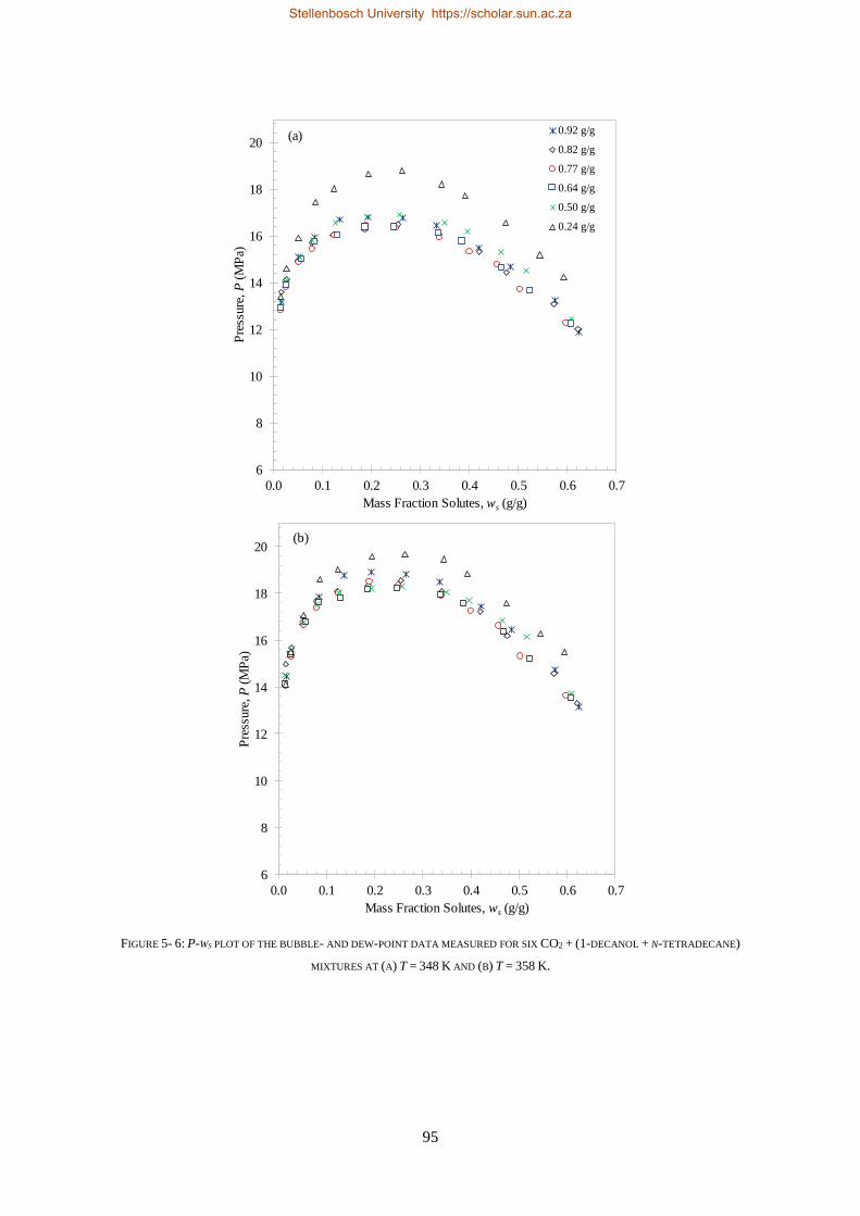
95
FIGURE 5- 6: P-WS PLOT OF THE BUBBLE- AND DEW-POINT DATA MEASURED FOR SIX CO2 + (1-DECANOL + N-TETRADECANE)
MIXTURES AT (A) T = 348 K AND (B) T = 358 K.
6
8
10
12
14
16
18
20
0.0 0.1 0.2 0.3 0.4 0.5 0.6 0.7
Pre
ssure
, P
(MP
a)
Mass Fraction Solutes, ws (g/g)
0.92 g/g
0.82 g/g
0.77 g/g
0.64 g/g
0.50 g/g
0.24 g/g
(a)
6
8
10
12
14
16
18
20
0.0 0.1 0.2 0.3 0.4 0.5 0.6 0.7
Pre
ssure
, P
(MP
a)
Mass Fraction Solutes, ws (g/g)
(b)
Stellenbosch University https://scholar.sun.ac.za
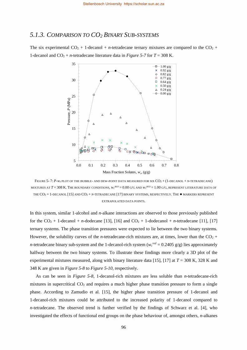
96
5.1.3. COMPARISON TO CO2 BINARY SUB-SYSTEMS
The six experimental CO2 + 1-decanol + n-tetradecane ternary mixtures are compared to the CO2 +
1-decanol and CO2 + n-tetradecane literature data in Figure 5-7 for T = 308 K.
FIGURE 5- 7: P-WS PLOT OF THE BUBBLE- AND DEW-POINT DATA MEASURED FOR SIX CO2 + (1-DECANOL + N-TETRADECANE)
MIXTURES AT T = 308 K. THE BOUNDARY CONDITIONS, WCRED = 0.00 G/G AND WC
RED = 1.00 G/G, REPRESENT LITERATURE DATA OF
THE CO2 + 1-DECANOL [15] AND CO2 + N-TETRADECANE [17] BINARY SYSTEMS, RESPECTIVELY. THE ● MARKERS REPRESENT
EXTRAPOLATED DATA POINTS.
In this system, similar 1-alcohol and n-alkane interactions are observed to those previously published
for the CO2 + 1-decanol + n-dodecane [13], [16] and CO2 + 1-dodecanol + n-tetradecane [11], [17]
ternary systems. The phase transition pressures were expected to lie between the two binary systems.
However, the solubility curves of the n-tetradecane-rich mixtures are, at times, lower than the CO2 +
n-tetradecane binary sub-system and the 1-decanol-rich system (wcred = 0.2405 g/g) lies approximately
halfway between the two binary systems. To illustrate these findings more clearly a 3D plot of the
experimental mixtures measured, along with binary literature data [15], [17] at T = 308 K, 328 K and
348 K are given in Figure 5-8 to Figure 5-10, respectively.
As can be seen in Figure 5-8, 1-decanol-rich mixtures are less soluble than n-tetradecane-rich
mixtures in supercritical CO2 and requires a much higher phase transition pressure to form a single
phase. According to Zamudio et al. [15], the higher phase transition pressure of 1-decanol and
1-decanol-rich mixtures could be attributed to the increased polarity of 1-decanol compared to
n-tetradecane. The observed trend is further verified by the findings of Schwarz et al. [4], who
investigated the effects of functional end groups on the phase behaviour of, amongst others, n-alkanes
5
10
15
20
25
30
35
0.0 0.1 0.2 0.3 0.4 0.5 0.6 0.7 0.8
Pre
ssure
, P
(MP
a)
Mass Fraction Solutes, ws, (g/g)
1.00 g/g
0.92 g/g
0.82 g/g
0.77 g/g
0.64 g/g
0.50 g/g
0.24 g/g
0.00 g/g
Stellenbosch University https://scholar.sun.ac.za
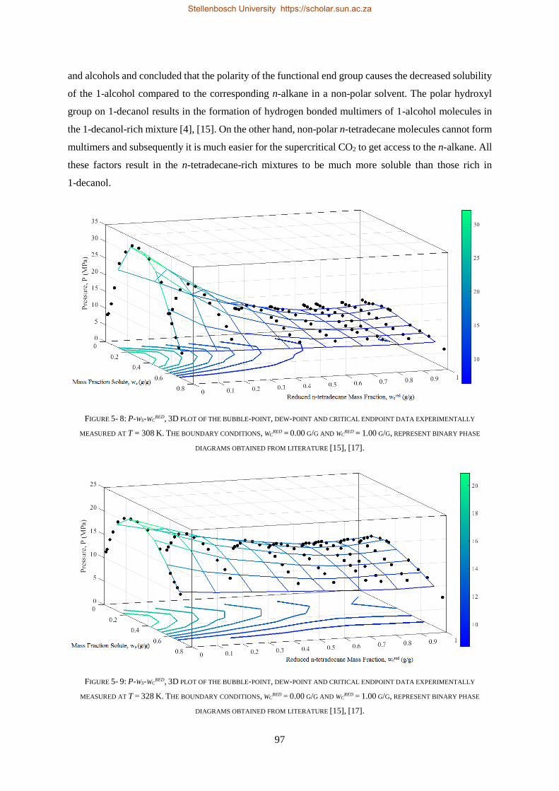
97
and alcohols and concluded that the polarity of the functional end group causes the decreased solubility
of the 1-alcohol compared to the corresponding n-alkane in a non-polar solvent. The polar hydroxyl
group on 1-decanol results in the formation of hydrogen bonded multimers of 1-alcohol molecules in
the 1-decanol-rich mixture [4], [15]. On the other hand, non-polar n-tetradecane molecules cannot form
multimers and subsequently it is much easier for the supercritical CO2 to get access to the n-alkane. All
these factors result in the n-tetradecane-rich mixtures to be much more soluble than those rich in
1-decanol.
FIGURE 5- 8: P-WS-WCRED, 3D PLOT OF THE BUBBLE-POINT, DEW-POINT AND CRITICAL ENDPOINT DATA EXPERIMENTALLY
MEASURED AT T = 308 K. THE BOUNDARY CONDITIONS, WCRED = 0.00 G/G AND WC
RED = 1.00 G/G, REPRESENT BINARY PHASE
DIAGRAMS OBTAINED FROM LITERATURE [15], [17].
FIGURE 5- 9: P-WS-WCRED, 3D PLOT OF THE BUBBLE-POINT, DEW-POINT AND CRITICAL ENDPOINT DATA EXPERIMENTALLY
MEASURED AT T = 328 K. THE BOUNDARY CONDITIONS, WCRED = 0.00 G/G AND WC
RED = 1.00 G/G, REPRESENT BINARY PHASE
DIAGRAMS OBTAINED FROM LITERATURE [15], [17].
Stellenbosch University https://scholar.sun.ac.za
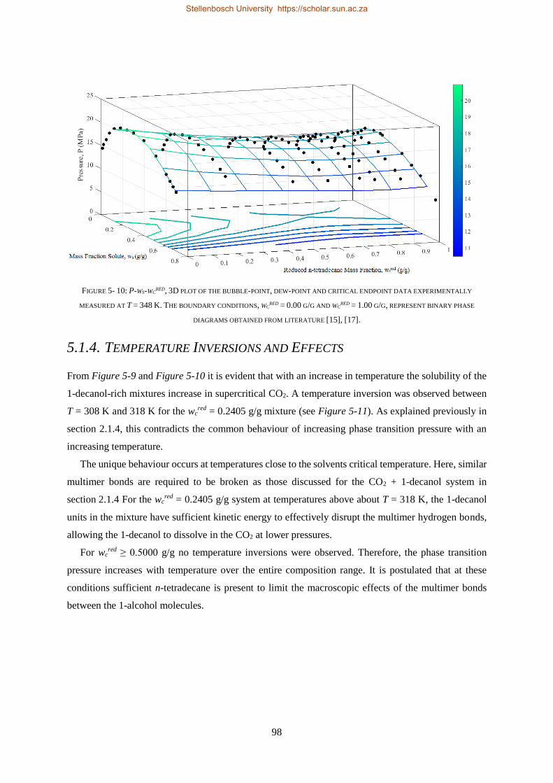
98
FIGURE 5- 10: P-WS-WCRED, 3D PLOT OF THE BUBBLE-POINT, DEW-POINT AND CRITICAL ENDPOINT DATA EXPERIMENTALLY
MEASURED AT T = 348 K. THE BOUNDARY CONDITIONS, WCRED = 0.00 G/G AND WC
RED = 1.00 G/G, REPRESENT BINARY PHASE
DIAGRAMS OBTAINED FROM LITERATURE [15], [17].
5.1.4. TEMPERATURE INVERSIONS AND EFFECTS
From Figure 5-9 and Figure 5-10 it is evident that with an increase in temperature the solubility of the
1-decanol-rich mixtures increase in supercritical CO2. A temperature inversion was observed between
T = 308 K and 318 K for the wcred = 0.2405 g/g mixture (see Figure 5-11). As explained previously in
section 2.1.4, this contradicts the common behaviour of increasing phase transition pressure with an
increasing temperature.
The unique behaviour occurs at temperatures close to the solvents critical temperature. Here, similar
multimer bonds are required to be broken as those discussed for the CO2 + 1-decanol system in
section 2.1.4 For the wcred = 0.2405 g/g system at temperatures above about T = 318 K, the 1-decanol
units in the mixture have sufficient kinetic energy to effectively disrupt the multimer hydrogen bonds,
allowing the 1-decanol to dissolve in the CO2 at lower pressures.
For wcred ≥ 0.5000 g/g no temperature inversions were observed. Therefore, the phase transition
pressure increases with temperature over the entire composition range. It is postulated that at these
conditions sufficient n-tetradecane is present to limit the macroscopic effects of the multimer bonds
between the 1-alcohol molecules.
Stellenbosch University https://scholar.sun.ac.za
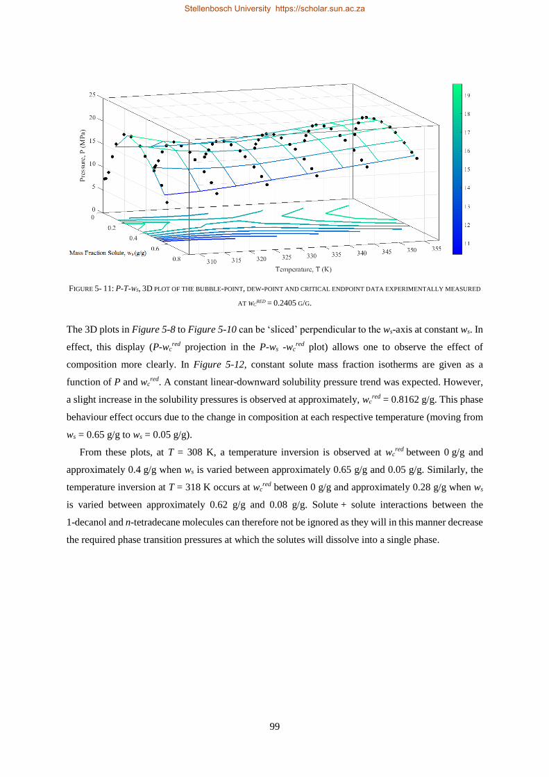
99
FIGURE 5- 11: P-T-WS, 3D PLOT OF THE BUBBLE-POINT, DEW-POINT AND CRITICAL ENDPOINT DATA EXPERIMENTALLY MEASURED
AT WCRED = 0.2405 G/G.
The 3D plots in Figure 5-8 to Figure 5-10 can be ‘sliced’ perpendicular to the ws-axis at constant ws. In
effect, this display (P-wcred projection in the P-ws -wc
red plot) allows one to observe the effect of
composition more clearly. In Figure 5-12, constant solute mass fraction isotherms are given as a
function of P and wcred. A constant linear-downward solubility pressure trend was expected. However,
a slight increase in the solubility pressures is observed at approximately, wcred = 0.8162 g/g. This phase
behaviour effect occurs due to the change in composition at each respective temperature (moving from
ws = 0.65 g/g to ws = 0.05 g/g).
From these plots, at T = 308 K, a temperature inversion is observed at wcred between 0 g/g and
approximately 0.4 g/g when ws is varied between approximately 0.65 g/g and 0.05 g/g. Similarly, the
temperature inversion at T = 318 K occurs at wcred between 0 g/g and approximately 0.28 g/g when ws
is varied between approximately 0.62 g/g and 0.08 g/g. Solute + solute interactions between the
1-decanol and n-tetradecane molecules can therefore not be ignored as they will in this manner decrease
the required phase transition pressures at which the solutes will dissolve into a single phase.
Stellenbosch University https://scholar.sun.ac.za
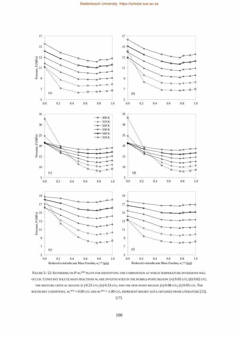
100
FIGURE 5- 12: ISOTHERMS ON P-WCRED PLOTS FOR IDENTIFYING THE COMPOSITION AT WHICH TEMPERATURE INVERSIONS WILL
OCCUR. CONSTANT SOLUTE MASS FRACTIONS WS ARE INVESTIGATED IN THE BUBBLE-POINT REGION: (A) 0.65 G/G; (B) 0.62 G/G;
THE MIXTURE CRITICAL REGION: (C) 0.25 G/G; (D) 0.33 G/G; AND THE DEW-POINT REGION: (E) 0.08 G/G; (F) 0.05 G/G. THE
BOUNDARY CONDITIONS, WCRED = 0.00 G/G AND WC
RED = 1.00 G/G, REPRESENT BINARY DATA OBTAINED FROM LITERATURE [15],
[17].
5
7
9
11
13
15
17
19
0.0 0.2 0.4 0.6 0.8 1.0
Reduced n-tetradecane Mass Fraction, wcred (g/g)
5
10
15
20
25
30
35
0.0 0.2 0.4 0.6 0.8 1.0
Pre
ssure
, P(M
Pa)
308 K
318 K
328 K
338 K
348 K
358 K
5
7
9
11
13
15
17
19
0.0 0.2 0.4 0.6 0.8 1.0
Pre
ssure
, P(M
Pa)
Reduced n-tetradecane Mass Fraction, wcred (g/g)
5
7
9
11
13
15
17
0.0 0.2 0.4 0.6 0.8 1.0
Pre
ssure
, P (
MP
a)
5
7
9
11
13
15
17
0.0 0.2 0.4 0.6 0.8 1.0
5
10
15
20
25
30
35
0.0 0.2 0.4 0.6 0.8 1.0
(a) (b)
(c) (d)
(e) (f)
Stellenbosch University https://scholar.sun.ac.za
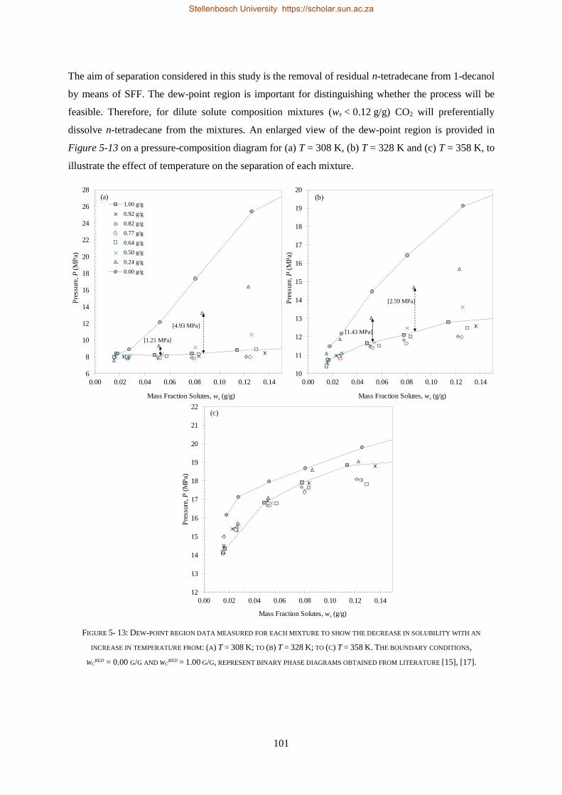
101
The aim of separation considered in this study is the removal of residual n-tetradecane from 1-decanol
by means of SFF. The dew-point region is important for distinguishing whether the process will be
feasible. Therefore, for dilute solute composition mixtures (ws < 0.12 g/g) CO2 will preferentially
dissolve n-tetradecane from the mixtures. An enlarged view of the dew-point region is provided in
Figure 5-13 on a pressure-composition diagram for (a) T = 308 K, (b) T = 328 K and (c) T = 358 K, to
illustrate the effect of temperature on the separation of each mixture.
FIGURE 5- 13: DEW-POINT REGION DATA MEASURED FOR EACH MIXTURE TO SHOW THE DECREASE IN SOLUBILITY WITH AN
INCREASE IN TEMPERATURE FROM: (A) T = 308 K; TO (B) T = 328 K; TO (C) T = 358 K. THE BOUNDARY CONDITIONS,
WCRED = 0.00 G/G AND WC
RED = 1.00 G/G, REPRESENT BINARY PHASE DIAGRAMS OBTAINED FROM LITERATURE [15], [17].
6
8
10
12
14
16
18
20
22
24
26
28
0.00 0.02 0.04 0.06 0.08 0.10 0.12 0.14
Pre
ssure
, P
(M
Pa)
Mass Fraction Solutes, ws (g/g)
1.00 g/g
0.92 g/g
0.82 g/g
0.77 g/g
0.64 g/g
0.50 g/g
0.24 g/g
0.00 g/g
(a)
10
11
12
13
14
15
16
17
18
19
20
0.00 0.02 0.04 0.06 0.08 0.10 0.12 0.14
Pre
ssure
, P
(MP
a)
Mass Fraction Solutes, ws (g/g)
(b)
12
13
14
15
16
17
18
19
20
21
22
0.00 0.02 0.04 0.06 0.08 0.10 0.12 0.14
Pre
ssure
, P
(MP
a)
Mass Fraction Solutes, ws (g/g)
(c)
[4.93 MPa][1.43 MPa]
[1.21 MPa]
[2.59 MPa]
Stellenbosch University https://scholar.sun.ac.za
102
The phase transition pressures for the n-tetradecane-rich mixtures are very similar at the lower
temperature of T = 308 K. The large difference for the wcred = 0.2405 g/g mixture is due to the
temperature inversion at this isothermal condition. Therefore, it is postulated that the separation was
enhanced at temperatures closer to the solvent’s critical temperature. The broken arrows in Figure 5-13
indicate the difference in phase transition pressures between the binary system CO2 + n-tetradecane and
the wcred = 0.2405 g/g mixture at ± ws = 0.08 g/g. The pressure difference of each is indicated in the
square brackets. The pressure difference decreased from P = 4.93 MPa to 2.59 MPa when increasing
the temperature from T = 308 K to 328 K, supporting the observation. However, by diluting the solute
composition to ± ws = 0.05 g/g, the separation was optimised at T = 328 K. Once again, the solubility
pressure differences are shown by the values in the brackets, now indicated by solid arrows. The
pressure difference between the 1-decanol-rich mixture and the CO2 + n-tetradecane binary system
increased from P = 1.21 MPa to 1.43 MPa when increasing the temperature from T = 308 K to 328 K.
The overall composition therefore controls the temperature at which optimum separation with SFF will
occur. Regardless of the temperature inversion at T = 308 K, the phase behaviour differences at
T = 328 K increased, indicating separation with SFF will be enhanced. Therefore, moderate
temperatures such as T = 328 K are advised for the process to be feasible by avoiding temperature
inversion discrepancies and similar phase behavioural properties.
At the highest temperature investigated, T = 358 K (Figure 5-13 (c)) all the mixtures have closer
phase transition pressures and thus exhibit very similar phase behaviour properties. The use of SFF
under these circumstances will prove very difficult and most likely unsuccessful.
5.1.5. SECTION OUTCOMES
New contributions:
(i) New high-pressure bubble- and dew-point data for six CO2 + (1-decanol + n-tetradecane) mixtures
were measured.
(ii) The data successfully defined the range and region in which distinct solute + solute interactions
were occurring when compared to the CO2 + 1-decanol and CO2 + n-tetradecane binary systems.
Key objective(s) achieved: Objective 1.1
The HPBDP phase behaviour of the wcred = 0.2405 g/g mixture differs tremendously from the remaining
5 mixtures at T = 308 K and T = 318 K due to the occurrence of temperature inversions. Separation was
enhanced at temperatures closer to the solvents critical temperature. However, the overall concentration
of the mixture determined the temperature at which optimum separation took place. Regardless of the
temperature inversion, at very dilute solute compositions (ws < 0.07 g/g), where SFF is most prominent,
the separations were believed to be optimised at T = 328 K. In terms of phase behaviour differences,
T = 328 K is the recommended operating temperature for the ternary system.
Stellenbosch University https://scholar.sun.ac.za
103
The HPBDP data can be used to characterise the complex phase behaviour and will be done in the
next section. Furthermore, to confirm the optimum separations conditions, HPVLE phase equilibria
data are required and will be presented and discussed in section 5.3.
5.2. COMPLEX PHASE BEHAVIOUR
5.2.1. AZEOTROPE AND COSOLVENCY EFFECTS
Published literature shows that an azeotrope forms in the CO2 + 1-decanol + n-tetradecane ternary
system (see section 2.2.2) [40]. The azeotropic phase behaviour was expected for the system due to the
close boiling points of the pure components (only 22 K apart) [63].
To identify in which pressure range the azeotrope will form the influence of solute composition on
the ternary system was investigated. The azeotropic point is where the vapour and liquid equilibrium
wcred compositions are equal. Knowing this, one can obtain the approximate location of the azeotrope
graphically by plotting a dew-point and a bubble-point isotherm together on a P-wcred graph under
isothermal conditions. For example, as shown in Figure 5-14 by plotting the P-wcred curves at
ws = 0.245 g/g (liquid-like) and ws = 0.180 g/g (vapour-like) at T = 318 K, 328 K and 338 K, a pressure
minimum occurs within a range surrounding the wcred ≈ 0.8162 g/g mixture. Near this point the ratio of
the solutes in the liquid-like and the vapour-like phases are the same; an azeotrope therefore occurs.
According to the Gibbs phase rule, the azeotrope will be a plane in the temperature and pressure domain
for this ternary system. Figure 5-14 is only illustrative and can be repeated for various temperatures
and solute ratios (wcred).
Figure 5-14 (a), (c) and (e) illustrates that the addition of n-tetradecane to a pure CO2 + 1-decanol
binary system will cause a non-linear decrease in the solubility pressures of the system. The line running
through a pressure minimum indicates that the solubility of the mixture in supercritical CO2 is at times
higher than that of the pure components in supercritical CO2 [40].
Figure 5-14 (b), (d) and (f) show a closer view of the pressure minimum which graphically defines
the cosolvency effect taking place. The line formed between the critical surface of CO2 + 1-decanol +
n-tetradecane ternary system (𝑃𝑐,𝑚𝑖𝑛𝐴+𝐵+𝐶 at wc
red ≈ 0.8162 g/g)3 and the critical point of the CO2 +
n-tetradecane binary system (PcA+C at wc
red ≈ 1.00 g/g) of the separated two-phase areas in
Figure 5-14 (f) indicates the ternary critical line at T = 338 K. Consequently, the finding of the azeotrope
revealed the exact pressure range in which cosolvency will be observed between T = 308 K and 358 K.
3 It is important to note that this is the lowest point measured in this work and not necessarily the minimum.
Stellenbosch University https://scholar.sun.ac.za
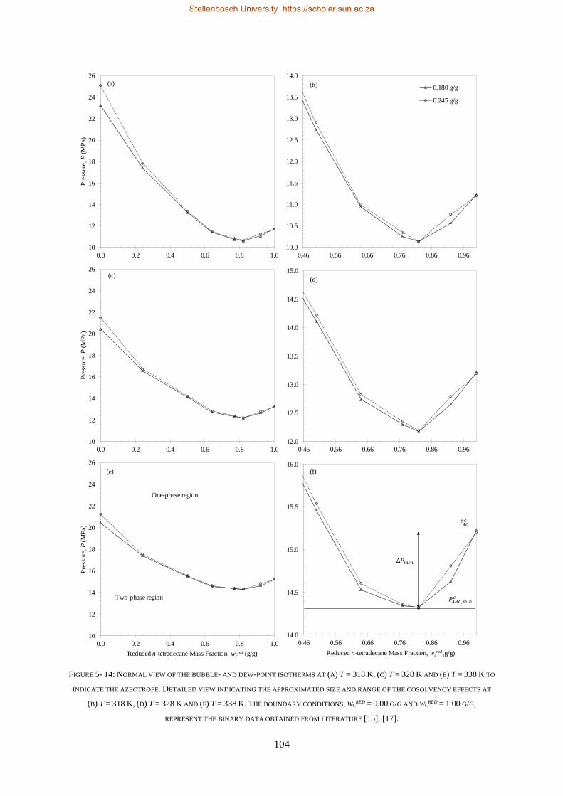
104
FIGURE 5- 14: NORMAL VIEW OF THE BUBBLE- AND DEW-POINT ISOTHERMS AT (A) T = 318 K, (C) T = 328 K AND (E) T = 338 K TO
INDICATE THE AZEOTROPE. DETAILED VIEW INDICATING THE APPROXIMATED SIZE AND RANGE OF THE COSOLVENCY EFFECTS AT
(B) T = 318 K, (D) T = 328 K AND (F) T = 338 K. THE BOUNDARY CONDITIONS, WCRED = 0.00 G/G AND WC
RED = 1.00 G/G,
REPRESENT THE BINARY DATA OBTAINED FROM LITERATURE [15], [17].
14.0
14.5
15.0
15.5
16.0
0.46 0.56 0.66 0.76 0.86 0.96
Reduced n-tetradecane Mass Fraction, wcred
(g/g)
𝑃𝐴𝐶𝑐
𝑃𝐴𝐵𝐶,𝑚𝑖𝑛𝑐
∆𝑃𝑚𝑖𝑛
(f)
10
12
14
16
18
20
22
24
26
0.0 0.2 0.4 0.6 0.8 1.0
Pre
ssure
,P
(M
Pa)
Reduced n-tetradecane Mass Fraction, wcred (g/g)
(e)
One-phase region
Two-phase region
12.0
12.5
13.0
13.5
14.0
14.5
15.0
0.46 0.56 0.66 0.76 0.86 0.96
(d)
10
12
14
16
18
20
22
24
26
0.0 0.2 0.4 0.6 0.8 1.0
Pre
ssure
, P
(MP
a)
(c)
10.0
10.5
11.0
11.5
12.0
12.5
13.0
13.5
14.0
0.46 0.56 0.66 0.76 0.86 0.96
0.180 g/g
0.245 g/g
(b)
10
12
14
16
18
20
22
24
26
0.0 0.2 0.4 0.6 0.8 1.0
Pre
ssure
, P
(MP
a)(a)
Stellenbosch University https://scholar.sun.ac.za
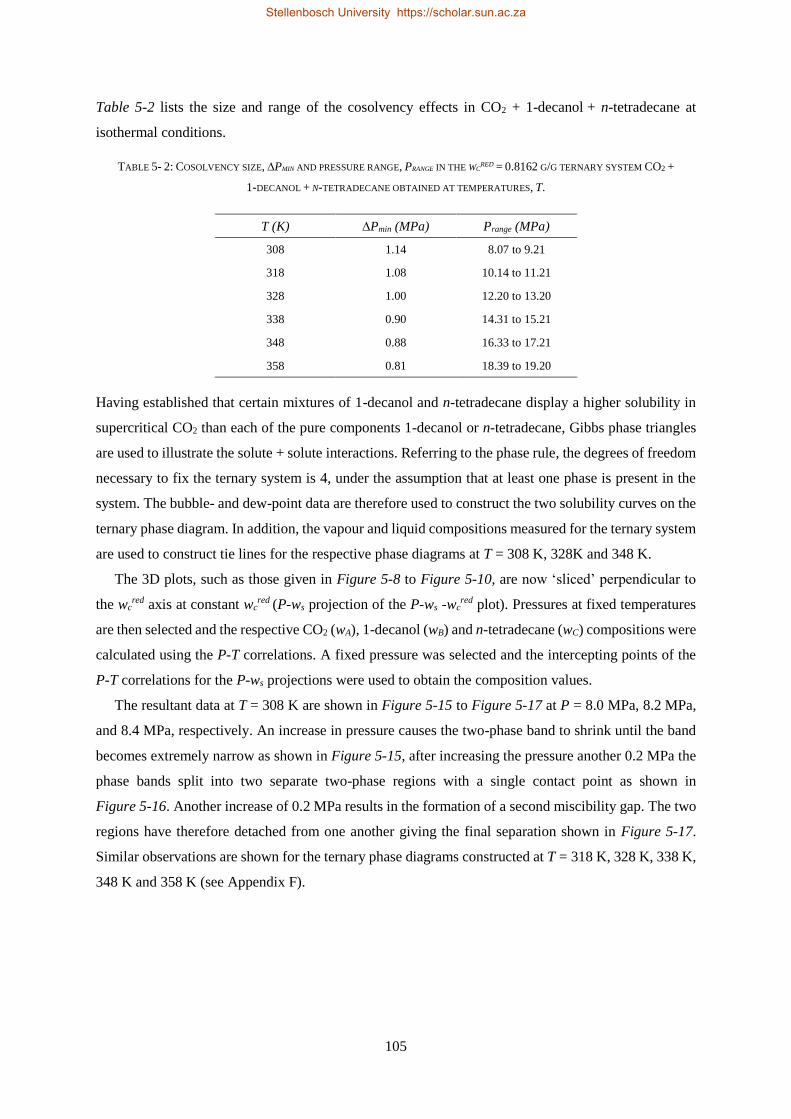
105
Table 5-2 lists the size and range of the cosolvency effects in CO2 + 1-decanol + n-tetradecane at
isothermal conditions.
TABLE 5- 2: COSOLVENCY SIZE, ∆PMIN AND PRESSURE RANGE, PRANGE IN THE WCRED = 0.8162 G/G TERNARY SYSTEM CO2 +
1-DECANOL + N-TETRADECANE OBTAINED AT TEMPERATURES, T.
T (K) ∆Pmin (MPa) Prange (MPa)
308 1.14 8.07 to 9.21
318 1.08 10.14 to 11.21
328 1.00 12.20 to 13.20
338 0.90 14.31 to 15.21
348 0.88 16.33 to 17.21
358 0.81 18.39 to 19.20
Having established that certain mixtures of 1-decanol and n-tetradecane display a higher solubility in
supercritical CO2 than each of the pure components 1-decanol or n-tetradecane, Gibbs phase triangles
are used to illustrate the solute + solute interactions. Referring to the phase rule, the degrees of freedom
necessary to fix the ternary system is 4, under the assumption that at least one phase is present in the
system. The bubble- and dew-point data are therefore used to construct the two solubility curves on the
ternary phase diagram. In addition, the vapour and liquid compositions measured for the ternary system
are used to construct tie lines for the respective phase diagrams at T = 308 K, 328K and 348 K.
The 3D plots, such as those given in Figure 5-8 to Figure 5-10, are now ‘sliced’ perpendicular to
the wcred axis at constant wc
red (P-ws projection of the P-ws -wcred plot). Pressures at fixed temperatures
are then selected and the respective CO2 (wA), 1-decanol (wB) and n-tetradecane (wC) compositions were
calculated using the P-T correlations. A fixed pressure was selected and the intercepting points of the
P-T correlations for the P-ws projections were used to obtain the composition values.
The resultant data at T = 308 K are shown in Figure 5-15 to Figure 5-17 at P = 8.0 MPa, 8.2 MPa,
and 8.4 MPa, respectively. An increase in pressure causes the two-phase band to shrink until the band
becomes extremely narrow as shown in Figure 5-15, after increasing the pressure another 0.2 MPa the
phase bands split into two separate two-phase regions with a single contact point as shown in
Figure 5-16. Another increase of 0.2 MPa results in the formation of a second miscibility gap. The two
regions have therefore detached from one another giving the final separation shown in Figure 5-17.
Similar observations are shown for the ternary phase diagrams constructed at T = 318 K, 328 K, 338 K,
348 K and 358 K (see Appendix F).
Stellenbosch University https://scholar.sun.ac.za
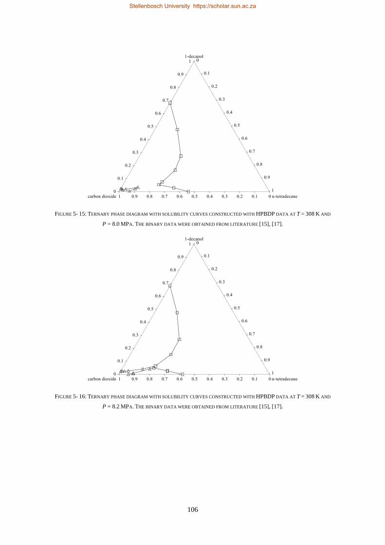
106
FIGURE 5- 15: TERNARY PHASE DIAGRAM WITH SOLUBILITY CURVES CONSTRUCTED WITH HPBDP DATA AT T = 308 K AND
P = 8.0 MPA. THE BINARY DATA WERE OBTAINED FROM LITERATURE [15], [17].
FIGURE 5- 16: TERNARY PHASE DIAGRAM WITH SOLUBILITY CURVES CONSTRUCTED WITH HPBDP DATA AT T = 308 K AND
P = 8.2 MPA. THE BINARY DATA WERE OBTAINED FROM LITERATURE [15], [17].
Stellenbosch University https://scholar.sun.ac.za
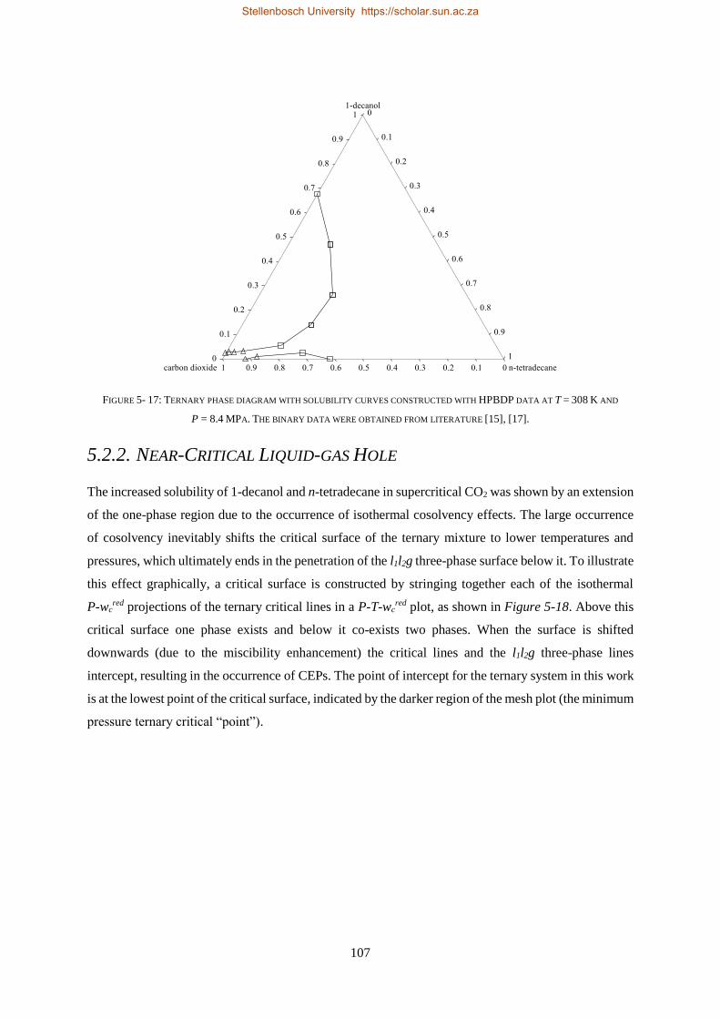
107
FIGURE 5- 17: TERNARY PHASE DIAGRAM WITH SOLUBILITY CURVES CONSTRUCTED WITH HPBDP DATA AT T = 308 K AND
P = 8.4 MPA. THE BINARY DATA WERE OBTAINED FROM LITERATURE [15], [17].
5.2.2. NEAR-CRITICAL LIQUID-GAS HOLE
The increased solubility of 1-decanol and n-tetradecane in supercritical CO2 was shown by an extension
of the one-phase region due to the occurrence of isothermal cosolvency effects. The large occurrence
of cosolvency inevitably shifts the critical surface of the ternary mixture to lower temperatures and
pressures, which ultimately ends in the penetration of the l1l2g three-phase surface below it. To illustrate
this effect graphically, a critical surface is constructed by stringing together each of the isothermal
P-wcred projections of the ternary critical lines in a P-T-wc
red plot, as shown in Figure 5-18. Above this
critical surface one phase exists and below it co-exists two phases. When the surface is shifted
downwards (due to the miscibility enhancement) the critical lines and the l1l2g three-phase lines
intercept, resulting in the occurrence of CEPs. The point of intercept for the ternary system in this work
is at the lowest point of the critical surface, indicated by the darker region of the mesh plot (the minimum
pressure ternary critical “point”).
Stellenbosch University https://scholar.sun.ac.za
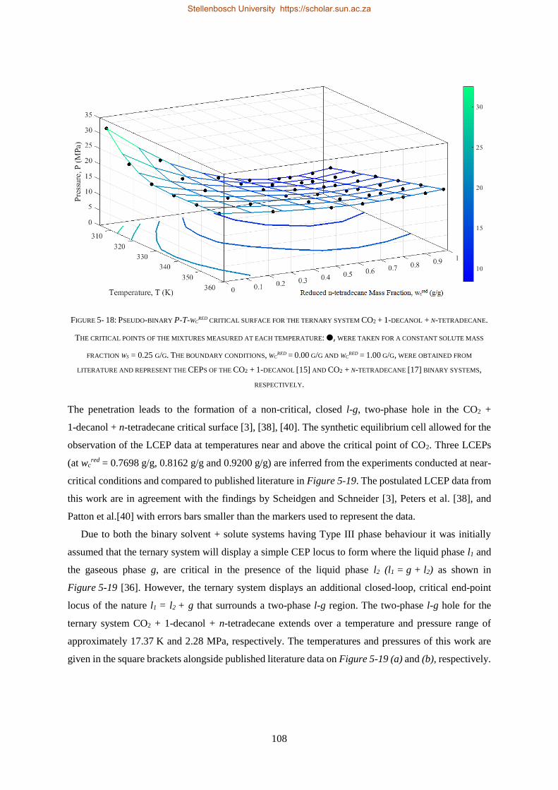
108
FIGURE 5- 18: PSEUDO-BINARY P-T-WCRED CRITICAL SURFACE FOR THE TERNARY SYSTEM CO2 + 1-DECANOL + N-TETRADECANE.
THE CRITICAL POINTS OF THE MIXTURES MEASURED AT EACH TEMPERATURE: ●, WERE TAKEN FOR A CONSTANT SOLUTE MASS
FRACTION WS = 0.25 G/G. THE BOUNDARY CONDITIONS, WCRED = 0.00 G/G AND WC
RED = 1.00 G/G, WERE OBTAINED FROM
LITERATURE AND REPRESENT THE CEPS OF THE CO2 + 1-DECANOL [15] AND CO2 + N-TETRADECANE [17] BINARY SYSTEMS,
RESPECTIVELY.
The penetration leads to the formation of a non-critical, closed l-g, two-phase hole in the CO2 +
1-decanol + n-tetradecane critical surface [3], [38], [40]. The synthetic equilibrium cell allowed for the
observation of the LCEP data at temperatures near and above the critical point of CO2. Three LCEPs
(at wcred = 0.7698 g/g, 0.8162 g/g and 0.9200 g/g) are inferred from the experiments conducted at near-
critical conditions and compared to published literature in Figure 5-19. The postulated LCEP data from
this work are in agreement with the findings by Scheidgen and Schneider [3], Peters et al. [38], and
Patton et al.[40] with errors bars smaller than the markers used to represent the data.
Due to both the binary solvent + solute systems having Type III phase behaviour it was initially
assumed that the ternary system will display a simple CEP locus to form where the liquid phase l1 and
the gaseous phase g, are critical in the presence of the liquid phase l2 (l1 = g + l2) as shown in
Figure 5-19 [36]. However, the ternary system displays an additional closed-loop, critical end-point
locus of the nature l1 = l2 + g that surrounds a two-phase l-g region. The two-phase l-g hole for the
ternary system CO2 + 1-decanol + n-tetradecane extends over a temperature and pressure range of
approximately 17.37 K and 2.28 MPa, respectively. The temperatures and pressures of this work are
given in the square brackets alongside published literature data on Figure 5-19 (a) and (b), respectively.
Stellenbosch University https://scholar.sun.ac.za
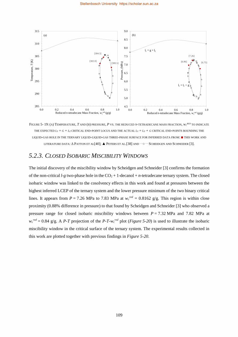
109
FIGURE 5- 19: (A) TEMPERATURE, T AND (B) PRESSURE, P VS. THE REDUCED N-TETRADECANE MASS FRACTION, WCRED TO INDICATE
THE EXPECTED L1 = G + L2 CRITICAL END-POINT LOCUS AND THE ACTUAL L1 = L2 + G CRITICAL END-POINTS BOUNDING THE
LIQUID-GAS HOLE IN THE TERNARY LIQUID-LIQUID-GAS THREE-PHASE SURFACE FOR INFERRED DATA FROM: ■ THIS WORK AND
LITERATURE DATA: Δ PATTON ET AL[40]; ▲ PETERS ET AL.[38] AND . . .○ . . . SCHEIDGEN AND SCHNEIDER [3].
5.2.3. CLOSED ISOBARIC MISCIBILITY WINDOWS
The initial discovery of the miscibility window by Scheidgen and Schneider [3] confirms the formation
of the non-critical l-g two-phase hole in the CO2 + 1-decanol + n-tetradecane ternary system. The closed
isobaric window was linked to the cosolvency effects in this work and found at pressures between the
highest inferred LCEP of the ternary system and the lower pressure minimum of the two binary critical
lines. It appears from P = 7.26 MPa to 7.83 MPa at wcred = 0.8162 g/g. This region is within close
proximity (0.88% difference in pressure) to that found by Scheidgen and Schneider [3] who observed a
pressure range for closed isobaric miscibility windows between P = 7.32 MPa and 7.82 MPa at
wcred = 0.84 g/g. A P-T projection of the P-T-wc
red plot (Figure 5-20) is used to illustrate the isobaric
miscibility window in the critical surface of the ternary system. The experimental results collected in
this work are plotted together with previous findings in Figure 5-20.
[302.0]
[304.5]
[300.5]
285
290
295
300
305
310
315
0.0 0.2 0.4 0.6 0.8 1.0
Tem
per
ature
, T
(K)
Reduced n-tetradecane Mass Fraction, wcred (g/g)
[6.96]
[7.26]
[6.75]
4.5
5.0
5.5
6.0
6.5
7.0
7.5
8.0
8.5
9.0
0.0 0.2 0.4 0.6 0.8 1.0
Pre
ssure
, (M
Pa)
Reduced n-tetradecane Mass Fraction, wcred (g/g)
l1 = g + l2
l1 = l2 + g
(a) (b)
Stellenbosch University https://scholar.sun.ac.za
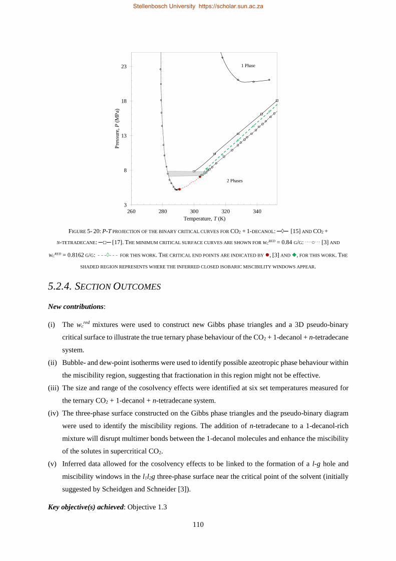
110
FIGURE 5- 20: P-T PROJECTION OF THE BINARY CRITICAL CURVES FOR CO2 + 1-DECANOL: ─◊─ [15] AND CO2 +
N-TETRADECANE: ─□─ [17]. THE MINIMUM CRITICAL SURFACE CURVES ARE SHOWN FOR WCRED = 0.84 G/G: . . . .○. . . [3] AND
WCRED = 0.8162 G/G: - - -◊- - - FOR THIS WORK. THE CRITICAL END POINTS ARE INDICATED BY ●, [3] AND ◆, FOR THIS WORK. THE
SHADED REGION REPRESENTS WHERE THE INFERRED CLOSED ISOBARIC MISCIBILITY WINDOWS APPEAR.
5.2.4. SECTION OUTCOMES
New contributions:
(i) The wcred mixtures were used to construct new Gibbs phase triangles and a 3D pseudo-binary
critical surface to illustrate the true ternary phase behaviour of the CO2 + 1-decanol + n-tetradecane
system.
(ii) Bubble- and dew-point isotherms were used to identify possible azeotropic phase behaviour within
the miscibility region, suggesting that fractionation in this region might not be effective.
(iii) The size and range of the cosolvency effects were identified at six set temperatures measured for
the ternary CO2 + 1-decanol + n-tetradecane system.
(iv) The three-phase surface constructed on the Gibbs phase triangles and the pseudo-binary diagram
were used to identify the miscibility regions. The addition of n-tetradecane to a 1-decanol-rich
mixture will disrupt multimer bonds between the 1-decanol molecules and enhance the miscibility
of the solutes in supercritical CO2.
(v) Inferred data allowed for the cosolvency effects to be linked to the formation of a l-g hole and
miscibility windows in the l1l2g three-phase surface near the critical point of the solvent (initially
suggested by Scheidgen and Schneider [3]).
Key objective(s) achieved: Objective 1.3
3
8
13
18
23
260 280 300 320 340
Pre
ssure
, P
(MP
a)
Temperature, T (K)
1 Phase
2 Phases
Stellenbosch University https://scholar.sun.ac.za
111
5.3. HPVLE RESULTS AND DISCUSSION
5.3.1. VERIFICATION OF EXPERIMENTAL SETUP
The analytical setup has been verified by Fourie et al. [76], the main researcher involved in the design
and construction of the equipment being used in this investigation [19]. Table 5-3 provides a select few
of the errors obtained. The experimental setup has therefore been proven accurate through extensive
comparisons to literature data and repeatability tests.
TABLE 5- 3: VALIDATION OF THE EXPERIMENTAL SETUP THROUGH COMPARISONS OF LITERATURE DATA BY FOURIE ET AL.[76]
AND REPRODUCIBILITY ERRORS CALCULATED IN THIS WORK.
System Measured Species specific mass fraction error Reference
ethane + 1-dodecanol + n-hexadecane
(one-phase region)
a0.004 - 0.007 g/g (ethane)
a0.002 - 0.004 g/g (1-dodecanol)
a0.002 - 0.003 g/g (n-hexadecane)
Fourie et al. [76]
CO2 + 1-octanol b 0.007 - 0.069 g/g (1-octanol) Fourie et al. [76] with [14], [235]
CO2 + 1-dodecanol + n-hexadecane
(two-phase region)
b0 - 0.05 g/g (CO2)
b0 - 0.03 g/g (1-dodecanol)
b0 - 0.02 g/g (n-hexadecane)
Fourie et al. [76] with [39], [236]
CO2 + 1-decanol + n-dodecane
(vapor phase)
c0.26-0.84 % (CO2)
c0.19-0.53 % (1-decanol)
c0.07-0.31 % (n-dodecane)
This work with Fourie [19]
CO2 + 1-decanol + n-dodecane
(liquid phase)
c0.26-0.52 % g/g (CO2)
c0.22-0.32 % (1-decanol)
c0.06-0.34 % (n-dodecane)
This work with Fourie [19]
a Root mean square error b Absolute deviations c Absolute average deviation
To ensure the measurements are correctly conducted, two reproducibility tests (see Figure 5-21) were
conducted in this investigation for the CO2 + (75% 1-decanol + 25% n-dodecane) ternary system at
three isothermal and isobaric conditions: T = 308 K (8.30 MPa), T = 328 K (12.3 MPa) and T = 348 K
(15.7 MPa). The absolute average deviations calculated for each component in comparison to
previously measured data are presented in Table 5-3. Based on these values, the VLE data measured on
two separate occasions for this study both agreed well with literature data [19]. To further determine
the repeatability of the work, a total of 5 samples for the two phases were simultaneously measured at
each set point. Satisfactory standard deviations for each component were obtained that never exceeded
0.005 (CO2), 0.003 (1-decanol) and 0.002 (n-dodecane). Thus, the analytical equipment was
successfully validated as all data points are well within the accuracy of the pressure measurement and
lie within the 2% composition error margin.
Stellenbosch University https://scholar.sun.ac.za

112
FIGURE 5- 21: REPRODUCIBILITY RUN 1 (Ο) AND RUN 2 (Χ) COMPARED TO THE LITERATURE DATA (□) OF FOURIE ET AL.[19] FOR
THE TERNARY SYSTEM CO2 + 1-DECANOL + N-DODECANE AT (A) T = 308 K AND P = 8.3 MPA; (B) T = 328 K AND P = 12.3 MPA;
AND (C) T = 348 K AND P = 15.7 MPA.
(a)
(b)
(c)
Stellenbosch University https://scholar.sun.ac.za
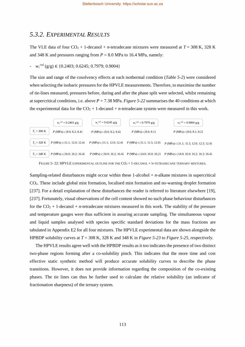
113
5.3.2. EXPERIMENTAL RESULTS
The VLE data of four CO2 + 1-decanol + n-tetradecane mixtures were measured at T = 308 K, 328 K
and 348 K and pressures ranging from P = 8.0 MPa to 16.4 MPa, namely:
- wcred (g/g) ∈ {0.2403; 0.6245; 0.7979; 0.9004}
The size and range of the cosolvency effects at each isothermal condition (Table 5-2) were considered
when selecting the isobaric pressures for the HPVLE measurements. Therefore, to maximise the number
of tie-lines measured, pressures before, during and after the phase split were selected, whilst remaining
at supercritical conditions, i.e. above P = 7.38 MPa. Figure 5-22 summarises the 40 conditions at which
the experimental data for the CO2 + 1-decanol + n-tetradecane system were measured in this work.
FIGURE 5- 22: HPVLE EXPERIMENTAL OUTLINE FOR THE CO2 + 1-DECANOL + N-TETRADECANE TERNARY MIXTURES.
Sampling-related disturbances might occur within these 1-alcohol + n-alkane mixtures in supercritical
CO2. These include global mist formation, localised mist formation and no-warning droplet formation
[237]. For a detail explanation of these disturbances the reader is referred to literature elsewhere [19],
[237]. Fortunately, visual observations of the cell content showed no such phase behaviour disturbances
for the CO2 + 1-decanol + n-tetradecane mixtures measured in this work. The stability of the pressure
and temperature gauges were thus sufficient in assuring accurate sampling. The simultaneous vapour
and liquid samples analysed with species specific standard deviations for the mass fractions are
tabulated in Appendix E2 for all four mixtures. The HPVLE experimental data are shown alongside the
HPBDP solubility curves at T = 308 K, 328 K and 348 K in Figure 5-23 to Figure 5-25, respectively.
The HPVLE results agree well with the HPBDP results as it too indicates the presence of two distinct
two-phase regions forming after a co-solubility pinch. This indicates that the more time and cost
effective static synthetic method will produce accurate solubility curves to describe the phase
transitions. However, it does not provide information regarding the composition of the co-existing
phases. The tie lines can thus be further used to calculate the relative solubility (an indicator of
fractionation sharpness) of the ternary system.
T1 = 308 K
T2 = 328 K
T3 = 348 K
wcred = 0.2403 g/g wc
red = 0.6245 g/g wcred = 0.7979 g/g wc
red = 0.9004 g/g
P (MPa) ϵ{8.0; 8.2; 8.4}
P (MPa) ϵ{11.1; 12.0; 12.4}
P (MPa) ϵ{16.0; 16.2; 16.4}
P (MPa) ϵ{8.0; 8.2; 8.4}
P (MPa) ϵ{11.1; 12.0; 12.4}
P (MPa) ϵ{16.0; 16.2; 16.4}
P (MPa) ϵ{8.0; 8.1}
P (MPa) ϵ{11.1; 11.5; 12.0}
P (MPa) ϵ{14.0; 16.0; 16.2}
P (MPa) ϵ{8.0; 8.1; 8.2}
P (MPa) ϵ{11.1; 11.5; 12.0; 12.3; 12.4}
P (MPa) ϵ{14.0; 16.0; 16.2; 16.3; 16.4}
Stellenbosch University https://scholar.sun.ac.za
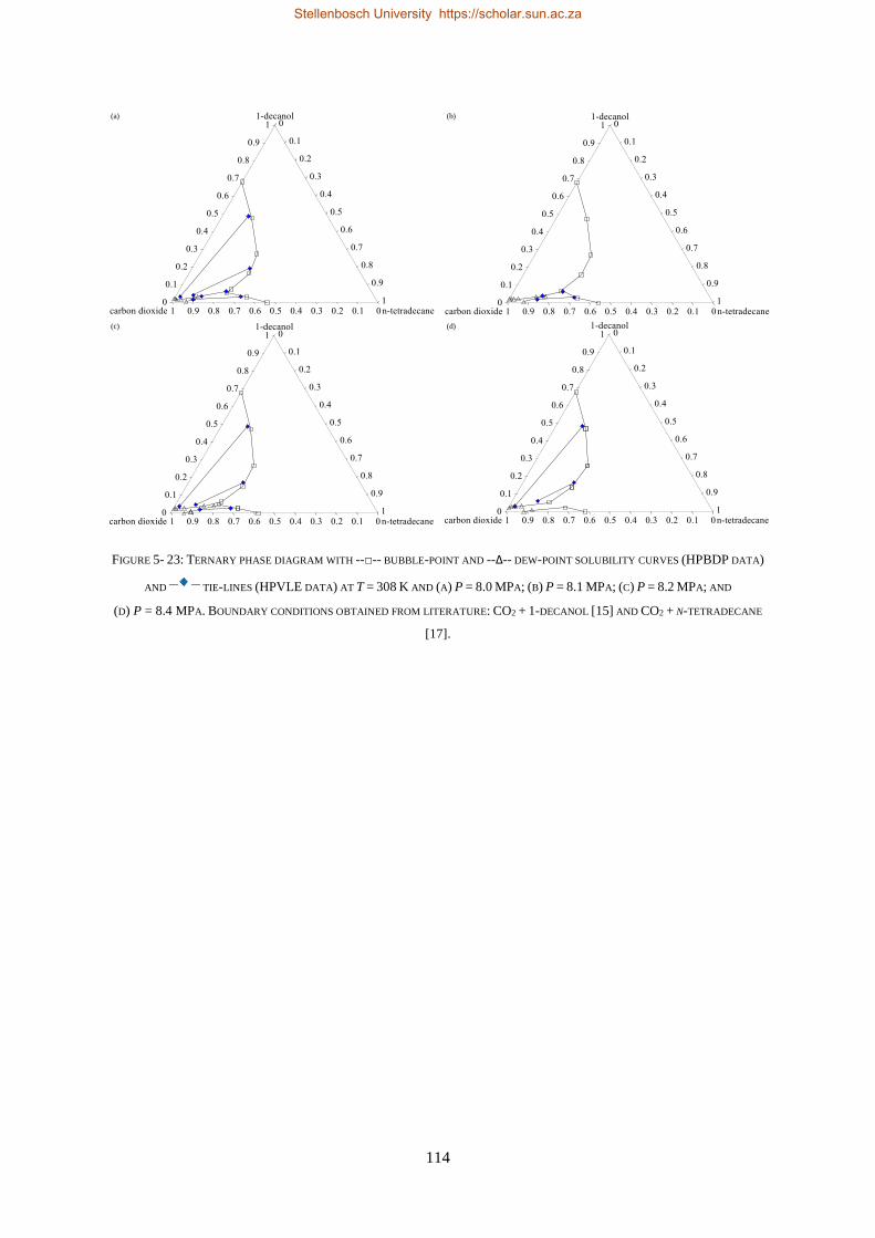
114
FIGURE 5- 23: TERNARY PHASE DIAGRAM WITH --□-- BUBBLE-POINT AND --Δ-- DEW-POINT SOLUBILITY CURVES (HPBDP DATA)
AND ── ── TIE-LINES (HPVLE DATA) AT T = 308 K AND (A) P = 8.0 MPA; (B) P = 8.1 MPA; (C) P = 8.2 MPA; AND
(D) P = 8.4 MPA. BOUNDARY CONDITIONS OBTAINED FROM LITERATURE: CO2 + 1-DECANOL [15] AND CO2 + N-TETRADECANE
[17].
(a) (b)
(c) (d)
Stellenbosch University https://scholar.sun.ac.za
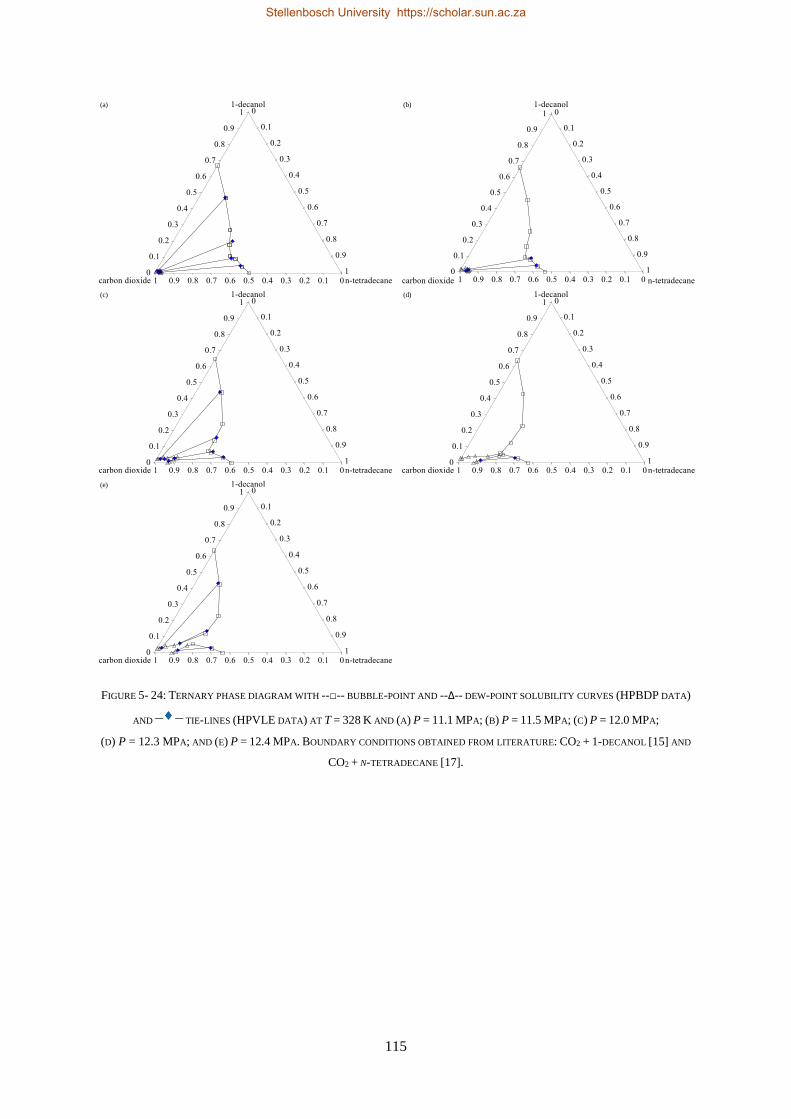
115
FIGURE 5- 24: TERNARY PHASE DIAGRAM WITH --□-- BUBBLE-POINT AND --Δ-- DEW-POINT SOLUBILITY CURVES (HPBDP DATA)
AND ── ── TIE-LINES (HPVLE DATA) AT T = 328 K AND (A) P = 11.1 MPA; (B) P = 11.5 MPA; (C) P = 12.0 MPA;
(D) P = 12.3 MPA; AND (E) P = 12.4 MPA. BOUNDARY CONDITIONS OBTAINED FROM LITERATURE: CO2 + 1-DECANOL [15] AND
CO2 + N-TETRADECANE [17].
(e)
(c) (d)
(a) (b)
Stellenbosch University https://scholar.sun.ac.za
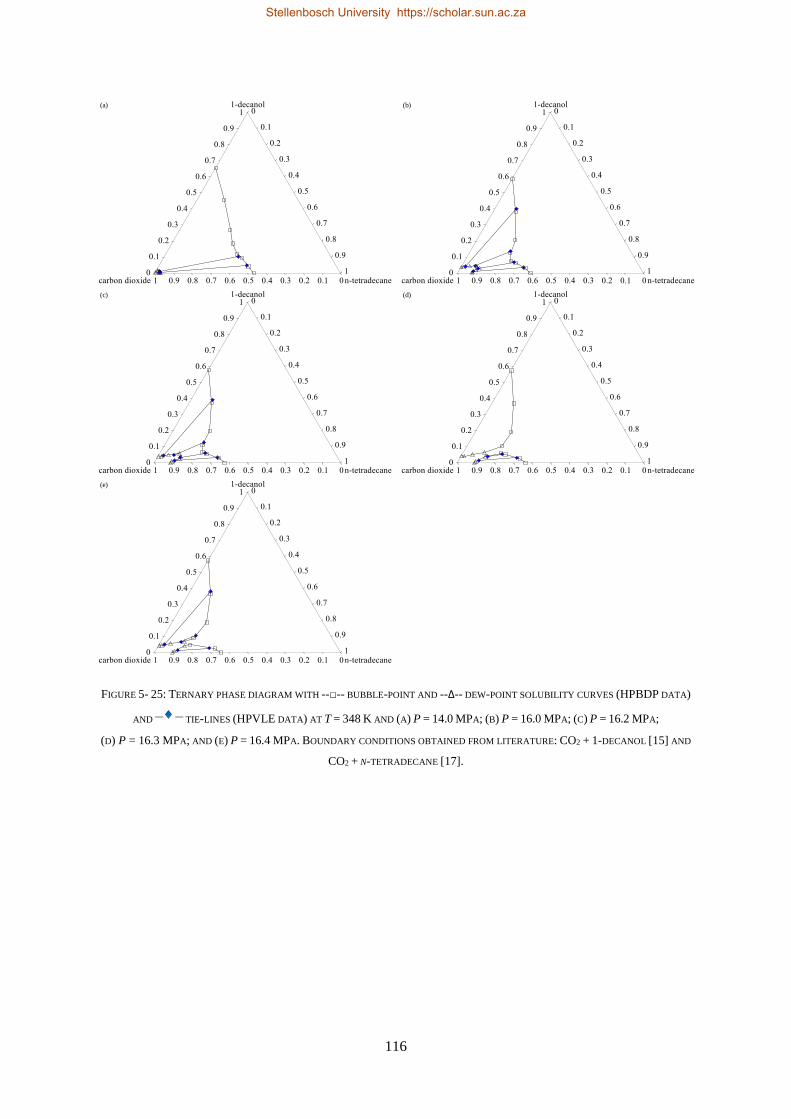
116
FIGURE 5- 25: TERNARY PHASE DIAGRAM WITH --□-- BUBBLE-POINT AND --Δ-- DEW-POINT SOLUBILITY CURVES (HPBDP DATA)
AND ── ── TIE-LINES (HPVLE DATA) AT T = 348 K AND (A) P = 14.0 MPA; (B) P = 16.0 MPA; (C) P = 16.2 MPA;
(D) P = 16.3 MPA; AND (E) P = 16.4 MPA. BOUNDARY CONDITIONS OBTAINED FROM LITERATURE: CO2 + 1-DECANOL [15] AND
CO2 + N-TETRADECANE [17].
(e)
(c) (d)
(a) (b)
Stellenbosch University https://scholar.sun.ac.za
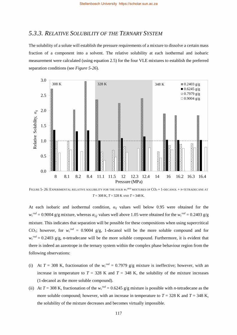
117
5.3.3. RELATIVE SOLUBILITY OF THE TERNARY SYSTEM
The solubility of a solute will establish the pressure requirements of a mixture to dissolve a certain mass
fraction of a component into a solvent. The relative solubility at each isothermal and isobaric
measurement were calculated (using equation 2.5) for the four VLE mixtures to establish the preferred
separation conditions (see Figure 5-26).
FIGURE 5- 26: EXPERIMENTAL RELATIVE SOLUBILITY FOR THE FOUR WCRED MIXTURES OF CO2 + 1-DECANOL + N-TETRADECANE AT
T = 308 K, T = 328 K AND T = 348 K.
At each isobaric and isothermal condition, αij values well below 0.95 were obtained for the
wcred = 0.9004 g/g mixture, whereas 𝛼𝑖𝑗 values well above 1.05 were obtained for the wc
red = 0.2403 g/g
mixture. This indicates that separation will be possible for these compositions when using supercritical
CO2; however, for wcred = 0.9004 g/g, 1-decanol will be the more soluble compound and for
wcred = 0.2403 g/g, n-tetradecane will be the more soluble compound. Furthermore, it is evident that
there is indeed an azeotrope in the ternary system within the complex phase behaviour region from the
following observations:
(i) At T = 308 K, fractionation of the wcred = 0.7979 g/g mixture is ineffective; however, with an
increase in temperature to T = 328 K and T = 348 K, the solubility of the mixture increases
(1-decanol as the more soluble compound).
(ii) At T = 308 K, fractionation of the wcred = 0.6245 g/g mixture is possible with n-tetradecane as the
more soluble compound; however, with an increase in temperature to T = 328 K and T = 348 K,
the solubility of the mixture decreases and becomes virtually impossible.
0.0
0.5
1.0
1.5
2.0
2.5
3.0
8 8.1 8.2 8.4 11.1 11.5 12 12.3 12.4 14 16 16.2 16.3 16.4
Rel
ativ
e S
olu
bili
ty, α
ij
Pressure (MPa)
0.2403 g/g
0.6245 g/g
0.7979 g/g
0.9004 g/g
328 K308 K 348 K
Stellenbosch University https://scholar.sun.ac.za
118
It is postulated that this occurs due to the l1l2g three-phase behaviour in this composition range, caused
by the miscibility enhancement. Therefore, to overcome these difficulties in fractionation, a pressure-
temperature swing is required, analogous to pressure swing distillation.
Considering a constant temperature of T = 308 K, no clear trend in the pressure for each mixture can
be established. This is not uncommon due to the relative solubility at these low pressures being severely
sensitive to the vapour phase composition [158] as well as the temperature inversion. At a constant
temperature of T = 328 K, a positive correlation between the relative solubility and pressure for each
mixture is observed. However, for the T = 348 K isothermal condition in the low-pressure region, the
αij-P correlation will change depending on wcred:
(i) For the wcred = 0.9004 g/g and wc
red = 0.7979 g/g mixtures the correlation will change from negative
to positive; this indicates that an increase in pressure will favour the less soluble component,
1-decanol.
(ii) For the wcred = 0.2403 g/g mixture the correlation changes from positive to negative; this indicates
that an increase in pressure will increase the solubility of n-tetradecane
The slope of the tie lines constructed on the ternary phase diagrams are another indication of the degree
of separability that is occuring in the mixtures. The steeper the slope, the higher the relative solubility
and the more effective the separation in the mixture. As an example, Figure 5-27 shows the constant
solute:solute ratio lines (CSSRL) in comparison to the HPVLE results at T = 328 K and P = 11.1 MPa.
The CSSRL are to aid in establishing how effective fractionation will be for the system at a constant
temperature and pressure and only varying the wcred value. Similar to what was shown by the calculated
αij values, the wcred = 0.6245 g/g mixture is either ineffective or virtually impossible to fractionate as its
tie line runs parallel to the CSSRL.
Stellenbosch University https://scholar.sun.ac.za
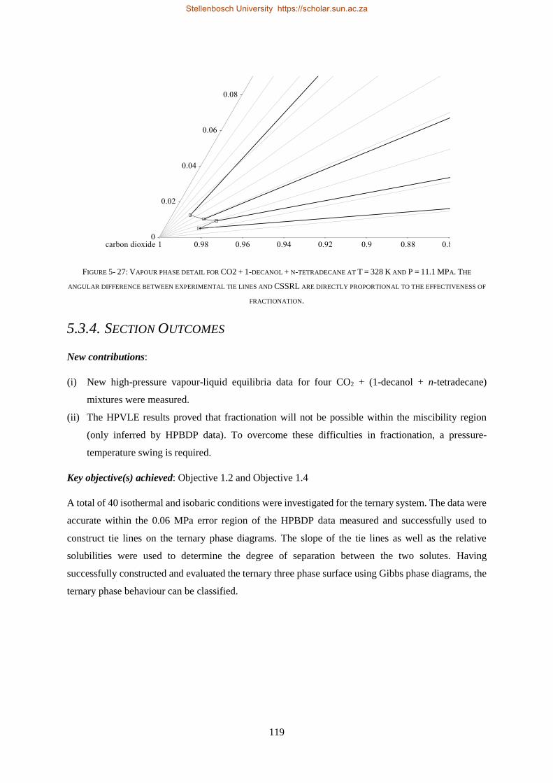
119
FIGURE 5- 27: VAPOUR PHASE DETAIL FOR CO2 + 1-DECANOL + N-TETRADECANE AT T = 328 K AND P = 11.1 MPA. THE
ANGULAR DIFFERENCE BETWEEN EXPERIMENTAL TIE LINES AND CSSRL ARE DIRECTLY PROPORTIONAL TO THE EFFECTIVENESS OF
FRACTIONATION.
5.3.4. SECTION OUTCOMES
New contributions:
(i) New high-pressure vapour-liquid equilibria data for four CO2 + (1-decanol + n-tetradecane)
mixtures were measured.
(ii) The HPVLE results proved that fractionation will not be possible within the miscibility region
(only inferred by HPBDP data). To overcome these difficulties in fractionation, a pressure-
temperature swing is required.
Key objective(s) achieved: Objective 1.2 and Objective 1.4
A total of 40 isothermal and isobaric conditions were investigated for the ternary system. The data were
accurate within the 0.06 MPa error region of the HPBDP data measured and successfully used to
construct tie lines on the ternary phase diagrams. The slope of the tie lines as well as the relative
solubilities were used to determine the degree of separation between the two solutes. Having
successfully constructed and evaluated the ternary three phase surface using Gibbs phase diagrams, the
ternary phase behaviour can be classified.
Stellenbosch University https://scholar.sun.ac.za
120
5.4. CLASSIFICATION OF THE TERNARY SYSTEM
5.4.1. TRANSITION SEQUENCE OF FLUID PHASE BEHAVIOUR
The three-phase fluid behaviour has been discussed previously in chapter 2 to allow for the proper
characterising of the types of phase behaviour transitions taking place in the ternary system.
In a quasi-binary mixture comprised of mostly n-tetradecane and a small amount of 1-decanol, the
multimer hydrogen bonds are negligible due to the low 1-alcohol concentration preventing the
formation of aggregates. The ternary system shows the same Type III fluid phase behaviour as that of
the binary CO2 + n-tetradecane system. A continuation of replacing incremental amounts of
n-tetradecane with 1-decanol results in the average carbon number of the system to decrease. The nature
and fluid phase behaviour of the CO2 + n-tetradecane system starts to change to that of the binary CO2 +
n-tridecane system [36]. When the overall carbon number of the CO2 + (1-decanol + n-tetradecane)
ternary system is equivalent to that of the CO2 + n-tridecane binary system, the LCEP and UCEP tends
towards each other with mutual deteriorating solubility of the system and forms a DCEP, as shown in
Figure 5-19. The formation of a DCEP indicates a phase transition from Type III to Type IV (see section
2.1.3). Therefore, the ternary system now shows Type IV fluid phase behaviour. This finding has been
confirmed through previous studies by Fall and Luks [59] who proved that the CO2 + n-tridecane system
shows Type IV fluid phase behaviour.
With increasing concentrations of 1-decanol the contribution of the 1-alcohol and the formation of
multimers becomes prominent. The system returns to the Type III fluid phase behaviour depicted by
both the CO2 + n-tetradecane and CO2 + 1-decanol systems. The critical endpoint locus l1 = l2 + g closes
to form another DCEP and due to the CO2 + 1-decanol displaying Type III phase behaviour, the
replacement of n-tetradecane with 1-decanol no longer alters the fluid phase behaviour [17]. The
sequence of types of fluid phase behaviour encountered for the ternary system CO2 + 1-decanol +
n-tetradecane takes place through a DCEP and is thus:
Type III → Type IV → Type III
5.4.2. BINARY SUB-SYSTEMS AND THE TERNARY SYSTEM
According to the classification by Van Konynenburg and Scott [52], published literature shows Type
III phase behaviour for each of the sub-systems with CO2. This type of fluid phase behaviour is common
in systems, like these, when the components have different sized molecules and different interactions.
If n-tetradecane is added to the CO2 + 1-decanol system, it will lead to a decrease in their mutual
miscibility and form the pressure minimum in the critical locus as shown on the P-T phase diagram
(Figure 5-20). These findings confirm the non-ideal phase behaviour when operating at high
temperatures and pressures which agrees with Type III fluid phase behaviour.
Stellenbosch University https://scholar.sun.ac.za
121
The inferred data measured in this investigation confirmed the miscibility window in the ternary
three-phase surface. This phenomenon is shown in Figure 5-20 and was established to occur due to a
miscibility enhancement (cosolvency effects). Therefore, according to the findings by Bluma and
Deiters [78], the ternary system can be classified as Class T-IV phase behaviour. This is a viable
classification of the system as it consists of two similar heavy components (1-decanol and
n-tetradecane) and one very light component (CO2).
The critical surface of the ternary system is like that of Class T-IV, as shown by the Gibbs phase
diagrams. The three-phase l1l2g domain was identified in full by the HPBDP data and HPVLE data
forming the solubility curves and the tie lines, respectively. Near the critical point of the solvent liquid-
liquid immiscibility resulted in the formation of a two-phase l-g hole in the three-phase surface (see
Figure 5-19). A phase transition sequence from Type III to Type IV to Type III phase behaviour occurs
across the hole due to the decrease in miscibility. Therefore, several LCEPs and UCEP were identified,
including the two DCEP between the phase behaviour changes. Consequently, the l1l2g and llg critical
lines occurring were identified.
The 1-decanol + n-tetradecane binary subsystem can be classified by the parameters of the other two
binary subsystems. Having confirmed the ternary system as Class T-IV phase behaviour (Type III +
Type III + Type I) it is postulated that the final sub-system will fall under Type I fluid phase behaviour.
5.4.3. SECTION OUTCOMES
New contributions:
(i) A phase transition across the two-phase region was confirmed from Type III → Type IV → Type
III fluid phase behaviour.
(ii) The miscibility enhancement (cosolvency effects) lead to the occurrence of simultaneous isobaric
miscibility windows. This peculiar phenomenon was linked to ternary Class T-IV phase behaviour
according to the classification by Bluma and Deiters [78].
Key objective(s) achieved: Objective 1.3
Stellenbosch University https://scholar.sun.ac.za
122
5.5. CHAPTER OUTCOMES
The aim of this chapter was to study the high-pressure phase equilibria of the CO2 + 1-decanol +
n-tetradecane ternary system and address the literature gaps identified in Chapter 2 (Objective 1).
Several new contributions to science are made in achieving this key objective and have been listed as
outcomes to each section discussed in this chapter. Because of these contributions, one article has been
published in a peer reviewed journal:
M. Ferreira and C.E. Schwarz, Super- and near-critical fluid phase behaviour and phenomena of the
ternary system CO2 + 1-decanol + n-tetradecane, The Journal of Chemical Thermodynamics. 111
(2017) 88-99.
The manuscript covers the new HPBDP data (Objective 1.1) and complex phase behaviour
(Objective 1.3) presented and discussed in this work. A second manuscript has been submitted for
publication in a second peer reviewed journal that covers the HPVLE data (Objective 1.2) and the
relative solubility (Objective 1.4) presented and discussed in this chapter:
High-pressure VLE measurements and PSRK modelling of the complex CO2 + 1-decanol +
n-tetradecane ternary system, The Journal of Supercritical Fluids, manuscript reference number:
SUPFL_2018_502.
The identification of the ternary system as Class T-IV fluid phase behaviour infers that the third
binary sub-system, 1-decanol + n-tetradecane, belongs to Type I-A fluid phase behaviour [52], [53].
This assumption needs to be verified by means of experimental work (Objective 2). Thus, the next
chapter deals with the 1-decanol + n-tetradecane binary system in more detail.
Stellenbosch University https://scholar.sun.ac.za
123
Chapter 6
LOW PRESSURE PHASE EQUILIBRIA OF 1-ALCOHOL +
N-ALKANE BINARY SYSTEMS
The high-pressure phase equilibria data measured in this work confirmed the significant solute + solute
interactions taking place between 1-decanol and n-tetradecane in the presence of near- and supercritical
CO2. In fact, the solute + solute interactions are directly connected to the phenomena that lead to the
complex phase behaviour regions. An additional method to obtain a fundamental understanding of the
distinct solute + solute binary interactions that occur between these large, complex molecules is to study
the binary 1-decanol + n-tetradecane VLE data (Objective 2). In measuring the LPVLE data the
following contributions will be made in this work:
(i) The binary sub-system comprised of non-polar n-tetradecane molecules and weakly polar
1-decanol molecules has not yet been published (T-xy data at constant P). New LPVLE data will
help bridge this gap in open literature.
(ii) The complex ternary phase behaviour infers Class T-IV ternary fluid phase behaviour which
further hints at Type I-A fluid phase behaviour for the 1-decanol + n-tetradecane sub-system. If
the new binary data displays non-ideal, azeotropic phase behaviour this assumption can be
confirmed.
(iii) The new LPVLE data can be used as an additional means for regressing solute + solute BIPs. These
parameters can then be used to achieve key Objective 3 of this study.
The aim of this chapter is to measure and study new LPVLE data of the 1-decanol + n-tetradecane
binary system. Reproducibility tests can be used to verify the experimental setup, however, 1-decanol
and n-tetradecane both have high, cross-over boiling points that might lead to unforeseen experimental
difficulties. It is for this reason that the following four pertinent systems will also be measured in this
work to serve as additional verification of the new LPVLE data: (i) 1-pentanol + n-nonane,
(ii) 1-hexanol + n-decane, (iii) 1-heptanol + n-undecane and (iv) 1-octanol + n-dodecane. To maintain
generality, verification systems with the same 4 carbon number difference between the 1-alcohol and
n-alkane molecules were selected. Furthermore, lower systems were chosen to avoid too high boiling
point temperatures.
Stellenbosch University https://scholar.sun.ac.za
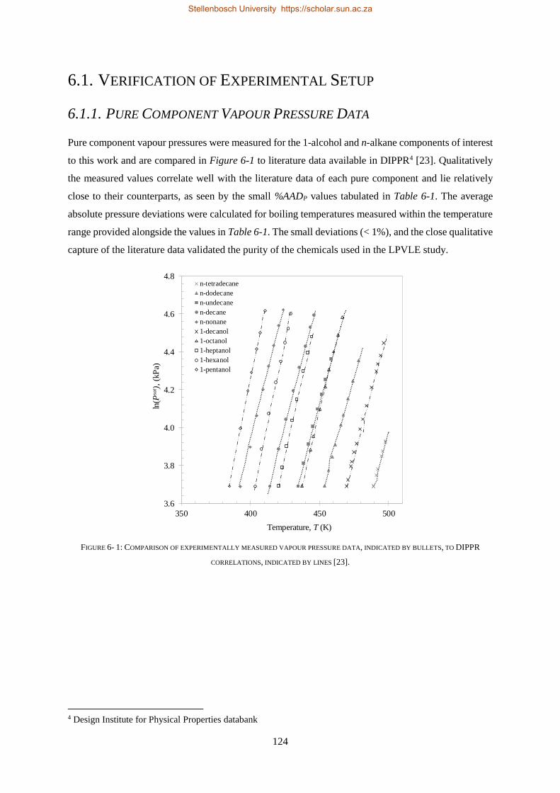
124
6.1. VERIFICATION OF EXPERIMENTAL SETUP
6.1.1. PURE COMPONENT VAPOUR PRESSURE DATA
Pure component vapour pressures were measured for the 1-alcohol and n-alkane components of interest
to this work and are compared in Figure 6-1 to literature data available in DIPPR4 [23]. Qualitatively
the measured values correlate well with the literature data of each pure component and lie relatively
close to their counterparts, as seen by the small %AADP values tabulated in Table 6-1. The average
absolute pressure deviations were calculated for boiling temperatures measured within the temperature
range provided alongside the values in Table 6-1. The small deviations (< 1%), and the close qualitative
capture of the literature data validated the purity of the chemicals used in the LPVLE study.
FIGURE 6- 1: COMPARISON OF EXPERIMENTALLY MEASURED VAPOUR PRESSURE DATA, INDICATED BY BULLETS, TO DIPPR
CORRELATIONS, INDICATED BY LINES [23].
4 Design Institute for Physical Properties databank
3.6
3.8
4.0
4.2
4.4
4.6
4.8
350 400 450 500
ln(P
sat )
,(k
Pa)
Temperature, T (K)
n-tetradecane
n-dodecane
n-undecane
n-decane
n-nonane
1-decanol
1-octanol
1-heptanol
1-hexanol
1-pentanol
Stellenbosch University https://scholar.sun.ac.za
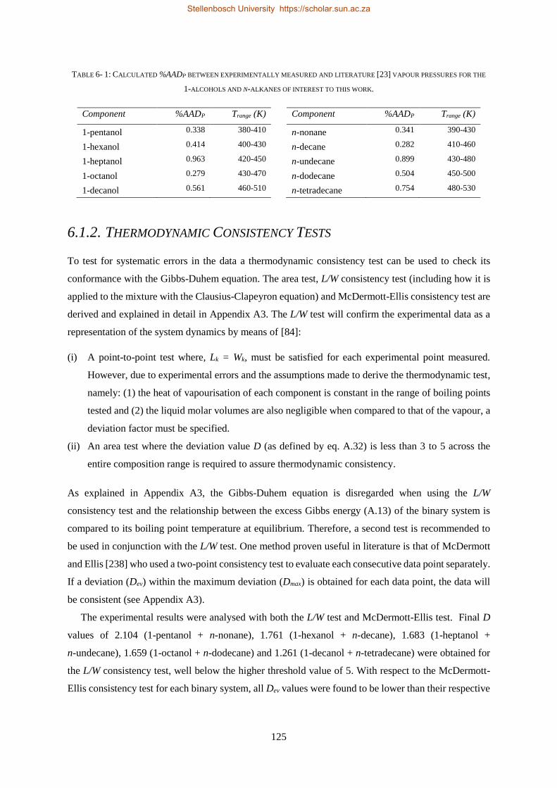
125
TABLE 6- 1: CALCULATED %AADP BETWEEN EXPERIMENTALLY MEASURED AND LITERATURE [23] VAPOUR PRESSURES FOR THE
1-ALCOHOLS AND N-ALKANES OF INTEREST TO THIS WORK.
Component %AADP Trange (K) Component %AADP Trange (K)
1-pentanol 0.338 380-410 n-nonane 0.341 390-430
1-hexanol 0.414 400-430 n-decane 0.282 410-460
1-heptanol 0.963 420-450 n-undecane 0.899 430-480
1-octanol 0.279 430-470 n-dodecane 0.504 450-500
1-decanol 0.561 460-510 n-tetradecane 0.754 480-530
6.1.2. THERMODYNAMIC CONSISTENCY TESTS
To test for systematic errors in the data a thermodynamic consistency test can be used to check its
conformance with the Gibbs-Duhem equation. The area test, L/W consistency test (including how it is
applied to the mixture with the Clausius-Clapeyron equation) and McDermott-Ellis consistency test are
derived and explained in detail in Appendix A3. The L/W test will confirm the experimental data as a
representation of the system dynamics by means of [84]:
(i) A point-to-point test where, Lk = Wk, must be satisfied for each experimental point measured.
However, due to experimental errors and the assumptions made to derive the thermodynamic test,
namely: (1) the heat of vapourisation of each component is constant in the range of boiling points
tested and (2) the liquid molar volumes are also negligible when compared to that of the vapour, a
deviation factor must be specified.
(ii) An area test where the deviation value D (as defined by eq. A.32) is less than 3 to 5 across the
entire composition range is required to assure thermodynamic consistency.
As explained in Appendix A3, the Gibbs-Duhem equation is disregarded when using the L/W
consistency test and the relationship between the excess Gibbs energy (A.13) of the binary system is
compared to its boiling point temperature at equilibrium. Therefore, a second test is recommended to
be used in conjunction with the L/W test. One method proven useful in literature is that of McDermott
and Ellis [238] who used a two-point consistency test to evaluate each consecutive data point separately.
If a deviation (Dev) within the maximum deviation (Dmax) is obtained for each data point, the data will
be consistent (see Appendix A3).
The experimental results were analysed with both the L/W test and McDermott-Ellis test. Final D
values of 2.104 (1-pentanol + n-nonane), 1.761 (1-hexanol + n-decane), 1.683 (1-heptanol +
n-undecane), 1.659 (1-octanol + n-dodecane) and 1.261 (1-decanol + n-tetradecane) were obtained for
the L/W consistency test, well below the higher threshold value of 5. With respect to the McDermott-
Ellis consistency test for each binary system, all Dev values were found to be lower than their respective
Stellenbosch University https://scholar.sun.ac.za
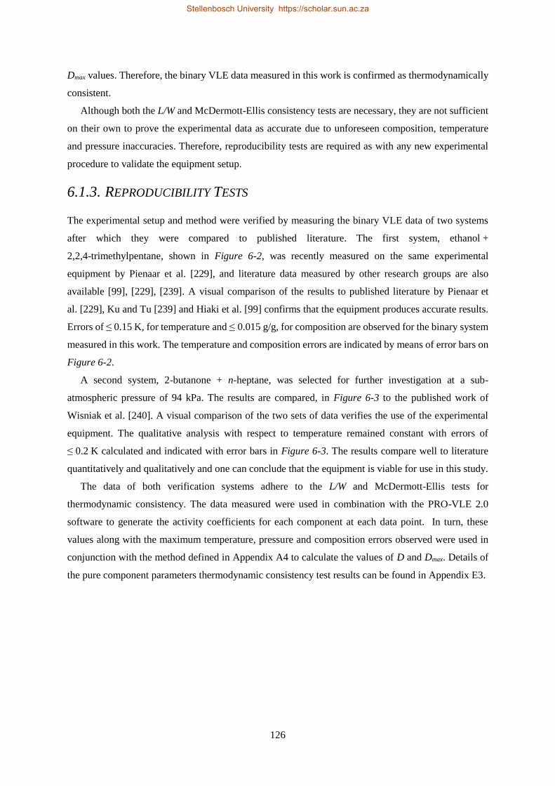
126
Dmax values. Therefore, the binary VLE data measured in this work is confirmed as thermodynamically
consistent.
Although both the L/W and McDermott-Ellis consistency tests are necessary, they are not sufficient
on their own to prove the experimental data as accurate due to unforeseen composition, temperature
and pressure inaccuracies. Therefore, reproducibility tests are required as with any new experimental
procedure to validate the equipment setup.
6.1.3. REPRODUCIBILITY TESTS
The experimental setup and method were verified by measuring the binary VLE data of two systems
after which they were compared to published literature. The first system, ethanol +
2,2,4-trimethylpentane, shown in Figure 6-2, was recently measured on the same experimental
equipment by Pienaar et al. [229], and literature data measured by other research groups are also
available [99], [229], [239]. A visual comparison of the results to published literature by Pienaar et
al. [229], Ku and Tu [239] and Hiaki et al. [99] confirms that the equipment produces accurate results.
Errors of ≤ 0.15 K, for temperature and ≤ 0.015 g/g, for composition are observed for the binary system
measured in this work. The temperature and composition errors are indicated by means of error bars on
Figure 6-2.
A second system, 2-butanone + n-heptane, was selected for further investigation at a sub-
atmospheric pressure of 94 kPa. The results are compared, in Figure 6-3 to the published work of
Wisniak et al. [240]. A visual comparison of the two sets of data verifies the use of the experimental
equipment. The qualitative analysis with respect to temperature remained constant with errors of
≤ 0.2 K calculated and indicated with error bars in Figure 6-3. The results compare well to literature
quantitatively and qualitatively and one can conclude that the equipment is viable for use in this study.
The data of both verification systems adhere to the L/W and McDermott-Ellis tests for
thermodynamic consistency. The data measured were used in combination with the PRO-VLE 2.0
software to generate the activity coefficients for each component at each data point. In turn, these
values along with the maximum temperature, pressure and composition errors observed were used in
conjunction with the method defined in Appendix A4 to calculate the values of D and Dmax. Details of
the pure component parameters thermodynamic consistency test results can be found in Appendix E3.
Stellenbosch University https://scholar.sun.ac.za
127
FIGURE 6- 2: (A) T-XY AND (B) X-Y REPRESENTATION OF EXPERIMENTAL VLE DATA FOR THE VALIDATION SYSTEM ETHANOL +
2,2,4-TRIMETHYLPENTANE AT P = 101.3 KPA AGAINST LITERATURE DATA: □ PIENAAR ET AL.[229]; Δ KU AND TU [239] AND
◊ HIAKI ET AL.[99].
0.0
0.1
0.2
0.3
0.4
0.5
0.6
0.7
0.8
0.9
1.0
0.0 0.1 0.2 0.3 0.4 0.5 0.6 0.7 0.8 0.9 1.0
Vap
our
Mas
s F
ractio
n e
than
ol, y
(g/g
)
Liquid Mass Fraction ethanol, x (g/g)
Day 1
Day 2
Day 3
Day 4
340
345
350
355
360
365
370
375
0.0 0.1 0.2 0.3 0.4 0.5 0.6 0.7 0.8 0.9 1.0
Tem
per
ature
, T
(K)
Mass Fraction ethanol, x, y (g/g)
Liquid
Vapour
(a)
(b)
Stellenbosch University https://scholar.sun.ac.za
128
FIGURE 6- 3: (A) T-XY AND (B) X-Y REPRESENTATION OF EXPERIMENTAL VLE DATA FOR THE VALIDATION SYSTEM 2-BUTANONE +
N-HEPTANE AT P = 94 KPA AGAINST LITERATURE DATA: Δ WISNIAK ET AL. [240].
345
350
355
360
365
370
375
0.0 0.1 0.2 0.3 0.4 0.5 0.6 0.7 0.8 0.9 1.0
Tem
per
ature
, T
(K)
Mass Fraction 2-butanone , x,y (g/g)
Liquid
Vapour
(a)
0.0
0.1
0.2
0.3
0.4
0.5
0.6
0.7
0.8
0.9
1.0
0.0 0.1 0.2 0.3 0.4 0.5 0.6 0.7 0.8 0.9 1.0
Vap
our
Mas
s F
ractio
n 2
-buta
no
ne,
y(g
/g)
Liquid Mass Fraction 2-butanone, x (g/g)
Day 1
Day 2
Day 3
Day 4
(b)
Stellenbosch University https://scholar.sun.ac.za
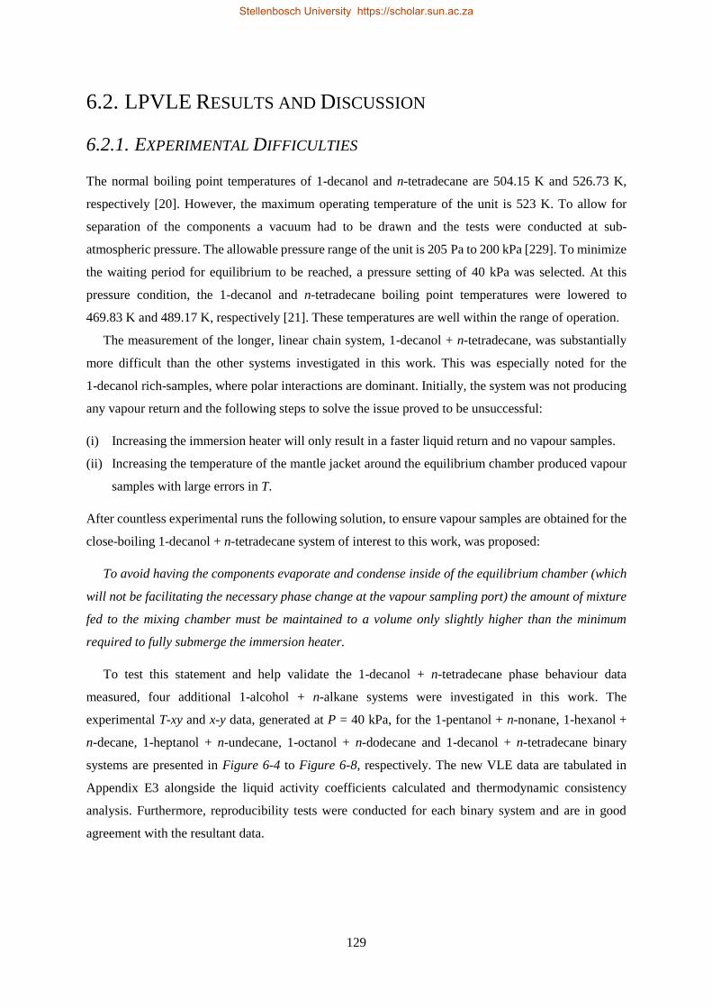
129
6.2. LPVLE RESULTS AND DISCUSSION
6.2.1. EXPERIMENTAL DIFFICULTIES
The normal boiling point temperatures of 1-decanol and n-tetradecane are 504.15 K and 526.73 K,
respectively [20]. However, the maximum operating temperature of the unit is 523 K. To allow for
separation of the components a vacuum had to be drawn and the tests were conducted at sub-
atmospheric pressure. The allowable pressure range of the unit is 205 Pa to 200 kPa [229]. To minimize
the waiting period for equilibrium to be reached, a pressure setting of 40 kPa was selected. At this
pressure condition, the 1-decanol and n-tetradecane boiling point temperatures were lowered to
469.83 K and 489.17 K, respectively [21]. These temperatures are well within the range of operation.
The measurement of the longer, linear chain system, 1-decanol + n-tetradecane, was substantially
more difficult than the other systems investigated in this work. This was especially noted for the
1-decanol rich-samples, where polar interactions are dominant. Initially, the system was not producing
any vapour return and the following steps to solve the issue proved to be unsuccessful:
(i) Increasing the immersion heater will only result in a faster liquid return and no vapour samples.
(ii) Increasing the temperature of the mantle jacket around the equilibrium chamber produced vapour
samples with large errors in T.
After countless experimental runs the following solution, to ensure vapour samples are obtained for the
close-boiling 1-decanol + n-tetradecane system of interest to this work, was proposed:
To avoid having the components evaporate and condense inside of the equilibrium chamber (which
will not be facilitating the necessary phase change at the vapour sampling port) the amount of mixture
fed to the mixing chamber must be maintained to a volume only slightly higher than the minimum
required to fully submerge the immersion heater.
To test this statement and help validate the 1-decanol + n-tetradecane phase behaviour data
measured, four additional 1-alcohol + n-alkane systems were investigated in this work. The
experimental T-xy and x-y data, generated at P = 40 kPa, for the 1-pentanol + n-nonane, 1-hexanol +
n-decane, 1-heptanol + n-undecane, 1-octanol + n-dodecane and 1-decanol + n-tetradecane binary
systems are presented in Figure 6-4 to Figure 6-8, respectively. The new VLE data are tabulated in
Appendix E3 alongside the liquid activity coefficients calculated and thermodynamic consistency
analysis. Furthermore, reproducibility tests were conducted for each binary system and are in good
agreement with the resultant data.
Stellenbosch University https://scholar.sun.ac.za
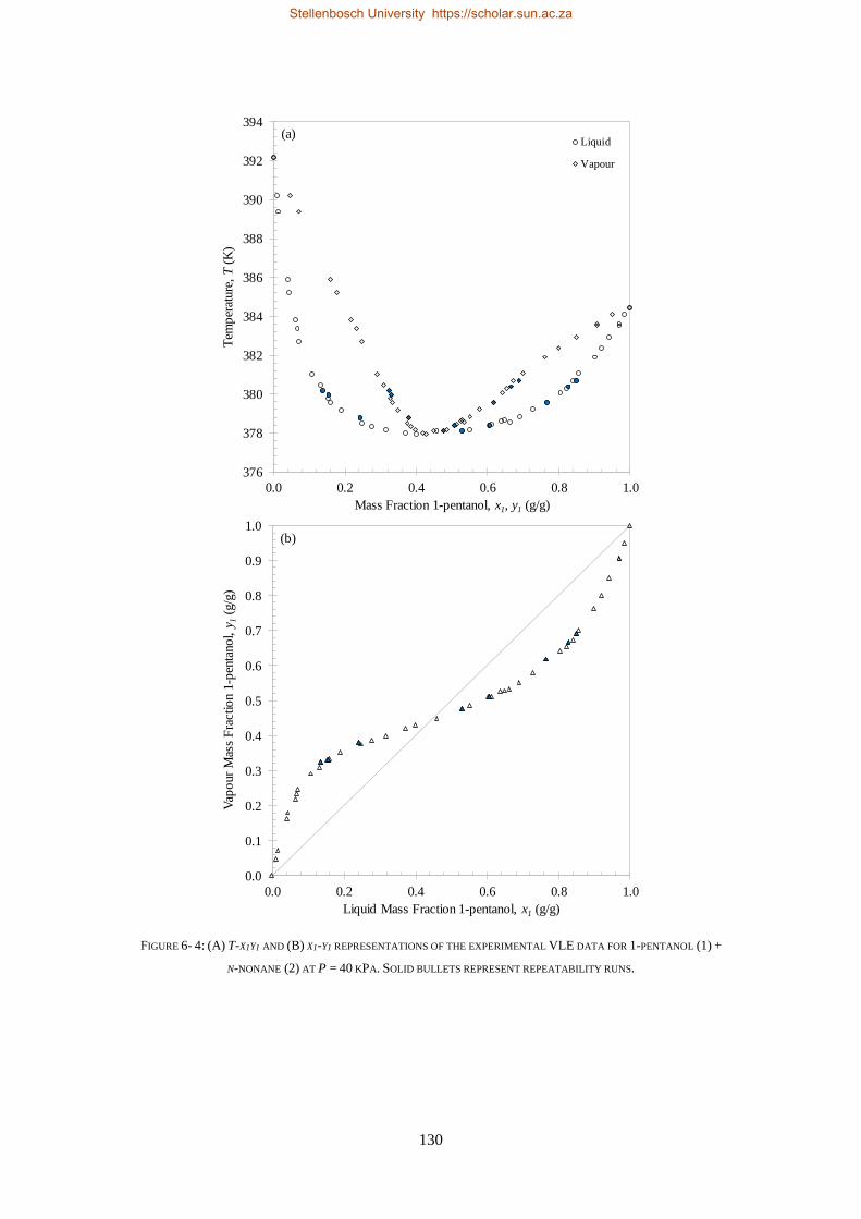
130
FIGURE 6- 4: (A) T-X1Y1 AND (B) X1-Y1 REPRESENTATIONS OF THE EXPERIMENTAL VLE DATA FOR 1-PENTANOL (1) +
N-NONANE (2) AT P = 40 KPA. SOLID BULLETS REPRESENT REPEATABILITY RUNS.
376
378
380
382
384
386
388
390
392
394
0.0 0.2 0.4 0.6 0.8 1.0
Tem
per
ature
, T
(K)
Mass Fraction 1-pentanol, x1, y1 (g/g)
Liquid
Vapour
0.0
0.1
0.2
0.3
0.4
0.5
0.6
0.7
0.8
0.9
1.0
0.0 0.2 0.4 0.6 0.8 1.0
Vap
our
Mas
s F
ractio
n 1
-pen
tano
l, y
1(g
/g)
Liquid Mass Fraction 1-pentanol, x1 (g/g)
(a)
(b)
Stellenbosch University https://scholar.sun.ac.za
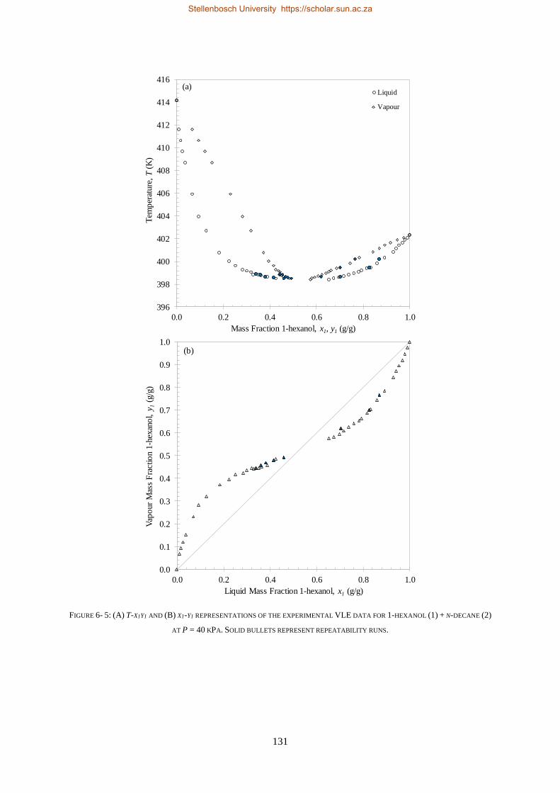
131
FIGURE 6- 5: (A) T-X1Y1 AND (B) X1-Y1 REPRESENTATIONS OF THE EXPERIMENTAL VLE DATA FOR 1-HEXANOL (1) + N-DECANE (2)
AT P = 40 KPA. SOLID BULLETS REPRESENT REPEATABILITY RUNS.
396
398
400
402
404
406
408
410
412
414
416
0.0 0.2 0.4 0.6 0.8 1.0
Tem
per
ature
, T
(K)
Mass Fraction 1-hexanol, x1, y1 (g/g)
Liquid
Vapour
0.0
0.1
0.2
0.3
0.4
0.5
0.6
0.7
0.8
0.9
1.0
0.0 0.2 0.4 0.6 0.8 1.0
Vap
our
Mas
s F
ractio
n 1
-hex
ano
l, y
1(g
/g)
Liquid Mass Fraction 1-hexanol, x1 (g/g)
(a)
(b)
Stellenbosch University https://scholar.sun.ac.za
132
FIGURE 6- 6: (A) T-X1Y1 AND (B) X1-Y1 REPRESENTATIONS OF THE EXPERIMENTAL VLE DATA FOR 1-HEPTANOL (1) +
N-UNDECANE (2) AT P = 40 KPA. SOLID BULLETS REPRESENT REPEATABILITY RUNS.
414
416
418
420
422
424
426
428
430
432
434
436
0.0 0.2 0.4 0.6 0.8 1.0
Tem
per
ature
, T
(K)
Mass Fraction 1-heptanol, x1, y1 (g/g)
Liquid
Vapour
0.0
0.1
0.2
0.3
0.4
0.5
0.6
0.7
0.8
0.9
1.0
0.0 0.2 0.4 0.6 0.8 1.0
Vap
our
Mas
s F
ractio
n 1
-hep
tano
l, y
1(g
/g)
Liquid Mass Fraction 1-heptanol, x1 (g/g)
(a)
(b)
Stellenbosch University https://scholar.sun.ac.za
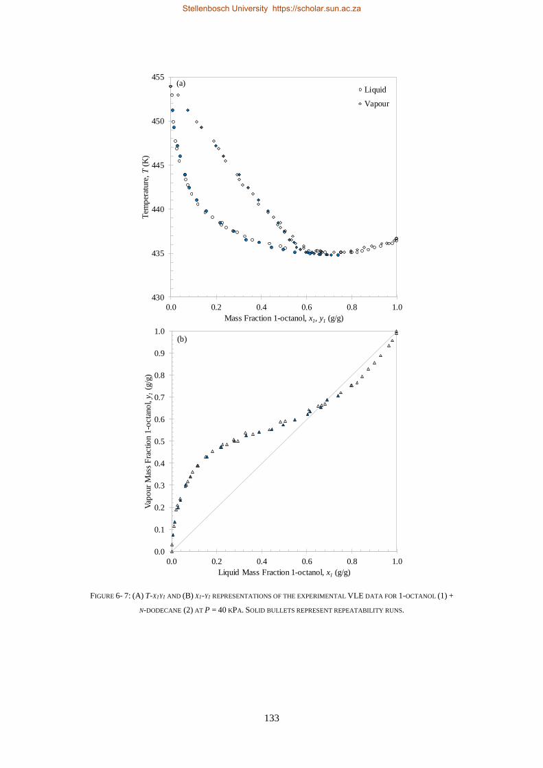
133
FIGURE 6- 7: (A) T-X1Y1 AND (B) X1-Y1 REPRESENTATIONS OF THE EXPERIMENTAL VLE DATA FOR 1-OCTANOL (1) +
N-DODECANE (2) AT P = 40 KPA. SOLID BULLETS REPRESENT REPEATABILITY RUNS.
430
435
440
445
450
455
0.0 0.2 0.4 0.6 0.8 1.0
Tem
per
ature
, T
(K)
Mass Fraction 1-octanol, x1, y1 (g/g)
Liquid
Vapour
0.0
0.1
0.2
0.3
0.4
0.5
0.6
0.7
0.8
0.9
1.0
0.0 0.2 0.4 0.6 0.8 1.0
Vap
our
Mas
s F
ractio
n 1
-octa
no
l, y
1(g
/g)
Liquid Mass Fraction 1-octanol, x1 (g/g)
(a)
(b)
Stellenbosch University https://scholar.sun.ac.za
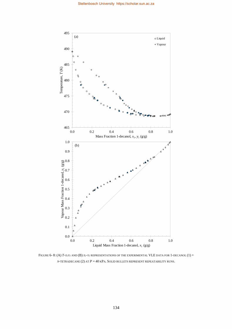
134
FIGURE 6- 8: (A) T-X1Y1 AND (B) X1-Y1 REPRESENTATIONS OF THE EXPERIMENTAL VLE DATA FOR 1-DECANOL (1) +
N-TETRADECANE (2) AT P = 40 KPA. SOLID BULLETS REPRESENT REPEATABILITY RUNS.
465
470
475
480
485
490
495
0.0 0.2 0.4 0.6 0.8 1.0
Tem
per
ature
, T
(K)
Mass Fraction 1-decanol, x1, y1 (g/g)
Liquid
Vapour
0.0
0.1
0.2
0.3
0.4
0.5
0.6
0.7
0.8
0.9
1.0
0.0 0.2 0.4 0.6 0.8 1.0
Vap
our
Mas
s F
ractio
n 1
-dec
ano
l, y
1(g
/g)
Liquid Mass Fraction 1-decanol, x1 (g/g)
(a)
(b)
Stellenbosch University https://scholar.sun.ac.za
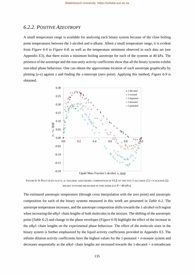
135
6.2.2. POSITIVE AZEOTROPY
A small temperature range is available for analysing each binary system because of the close boiling
point temperatures between the 1-alcohol and n-alkane. Albeit a small temperature range, it is evident
from Figure 6-4 to Figure 6-8, as well as the temperature minimum observed in each data set (see
Appendix E3), that there exists a minimum boiling azeotrope for each of the systems at 40 kPa. The
presence of the azeotrope and the non-unity activity coefficients show that all the binary systems exhibit
non-ideal phase behaviour. One can obtain the approximate location of each azeotrope graphically by
plotting (y-x) against x and finding the x-intercept (zero point). Applying this method, Figure 6-9 is
obtained.
FIGURE 6- 9: PLOT OF (Y1-X1) VS. X1 YIELDING AZEOTROPIC COMPOSITION IN VLE OF THE FIVE 1-ALCOHOL (1) + N-ALKANE (2)
BINARY SYSTEMS MEASURED IN THIS WORK (AT P = 40 KPA).
The estimated azeotropic temperature (through cross interpolation with the zero point) and azeotropic
composition for each of the binary systems measured in this work are presented in Table 6-2. The
azeotrope temperature increases, and the azeotrope composition shifts towards the 1-alcohol-rich region
when increasing the alkyl- chain lengths of both molecules in the mixture. The shifting of the azeotropic
point (Table 6-2) and change in the phase envelopes (Figure 6-9) highlight the effect of the increase in
the alkyl- chain lengths on the experimental phase behaviour. The effect of the molecule sizes in the
binary system is further emphasized by the liquid activity coefficients provided in Appendix E3. The
infinite dilution activity coefficients have the highest values for the 1-pentanol + n-nonane system and
decreases sequentially as the alkyl- chain lengths are increased towards the 1-decanol + n-tetradecane
-0.20
-0.15
-0.10
-0.05
0.00
0.05
0.10
0.15
0.20
0.25
0.30
0.0 0.2 0.4 0.6 0.8 1.0
y 1-
x 1,
(g/g
)
Liquid Mass Fraction 1-alcohol, x1 (g/g)
1-decanol
1-octanol
1-heptanol
1-hexanol
1-pentanol
Stellenbosch University https://scholar.sun.ac.za
136
binary system. These observations support the idea that the degree of association is dependent on the
size of the 1-alcohol molecule: the shorter the chain length, the more polar the molecule becomes.
TABLE 6- 2: SUMMARY OF EXPERIMENTALLY ESTIMATED AZEOTROPIC TEMPERATURES AND COMPOSITIONS IN THE FIVE
1-ALCOHOL (1) + N-ALKANE (2) BINARY SYSTEMS.
Azeotropic
Temperature, T (K)
Azeotropic
Composition, x1 (g/g)
1-pentanol (1) + n-nonane (2) 378.05 0.445
1-hexanol (1) + n-decane (2) 398.47 0.516
1-heptanol (1) + n-undecane (2) 416.78 0.625
1-octanol (1) + n-dodecane (2) 435.19 0.664
1-decanol (1) + n-tetradecane (2) 468.66 0.864
6.2.3. PHASE BEHAVIOUR CLASSIFICATION
Each of the five binary systems infer Type I-A fluid phase behaviour due to their positive deviations
from ideality and the formation of a minimum boiling homogenous azeotrope. Whether the system
displays Type I fluid phase behaviour per the classification of Van Konynenburg and Scott [52] can
only be established using a P-T plot to rule out possible liquid-liquid equilibria regions. Consequently,
the system should be measured at several isobaric conditions to form the required phase curve and
confirm the ternary system as Class T-IV (Type III + Type III + Type I-A) fluid phase behaviour.
6.3. CHAPTER OUTCOMES
The aim of this chapter was to present and discuss new LPVLE data of the 1-decanol + n-tetradecane
binary system (Objective 2). Due to the low vapour pressures of the components, initial difficulties in
the measurement of the LPVLE data were experienced. After overcoming the difficulties, new
1-decanol + n-tetradecane data were measured. Additionally, to verify the new 1-decanol +
n-tetradecane data, additional LPVLE of 4 pertinent binary systems, all with similar relative volatility
and cross-over boiling point characteristics as that of the 1-decanol + n-tetradecane system, were
measured. Consequently, the following new contributions were made in this chapter:
(i) New LPVLE data for the 1-decanol + n-tetradecane system were measured at P = 40 kPa.
(ii) New LPVLE data for the 1-pentanol + n-nonane, 1-hexanol + n-decane, 1-heptanol + n-undecane
and 1-octanol + n-dodecane systems were measured at P = 40 kPa.
(iii) Each of the binary systems displayed positive azeotropy, inferring Type I-A fluid phase behaviour
per the classification of Van Konynenburg and Scott [52]. Therefore, the ternary system is
postulated to consist of binary sub-systems belonging to Type III + Type III + Type I phase
behaviour.
Stellenbosch University https://scholar.sun.ac.za
137
A third manuscript has been submitted for publication in a peer reviewed journal that covers the LPVLE
data (Objective 2) presented and discussed in this chapter:
Low-pressure VLE measurements and thermodynamic modelling, with PSRK and NRTL, of binary
1-alcohol + n-alkane systems, The Journal of Chemical and Engineering Data, manuscript reference
number: je-2018-006802.
Experimental data are required to obtain BIPs that can be incorporated into thermodynamic models
for improved model correlations. However, as shown in this chapter, the measurement of sub-
atmospheric VLE data for 1-alcohol + n-alkane systems, with crossover boiling point characteristics,
becomes increasingly difficult as the chain length of these linear molecules increase. It is for this reason
that predictive models have become increasingly popular, not only for modelling the phase behaviour
of complex systems, but to ensure robust and industrial relevant modelling for when there is a lack in
available experimental data. Based on this, the LPVLE data of all 5 binary systems measured in this
work were used to investigate the predictive capability of the PSRK model in the next chapter.
Furthermore, the LPVLE data of the 1-decanol + n-tetradecane system were used to regress new solute
+ solute BIPs for the RK-Aspen, SR-Polar and PC-SAFT thermodynamic models (Chapter 7). The
LPVLE BIPs were evaluated alongside the HPBDP and HPVLE BIPs to see which set can improve the
model correlations and help achieve key Objective 3 of this study (Chapter 8).
Stellenbosch University https://scholar.sun.ac.za

138
Stellenbosch University https://scholar.sun.ac.za
139
Chapter 7
PURE COMPONENT & BINARY INTERACTION PARAMETER
ESTIMATION
New high-pressure (Objective 1) and low-pressure (Objective 2) phase equilibria data have been
measured and discussed in Chapter 5 and 6 of this thesis, respectively. Furthermore, four suitable
thermodynamic models to correlate the experimental data (Objective 3.1) were identified in Chapter 3.
Therefore, focus can now shift to the second step in modelling the new phase equilibria data measured
in this work.
The aim of this chapter is to gather pure component parameters from literature and regress the
necessary interaction parameters (Objective 3.2).
Three of the thermodynamic models, RK-Aspen, SR-Polar and PC-SAFT, have the option to include
additional BIPs and pure component parameters to improve the accuracy of their fit to experimental
data. The fourth model, PSRK can act as a purely predictive model through the implementation of
group-group UNIFAC parameters found in literature. Thus, the chapter will include an evaluation of
PSRK and its ability to correlate the 5 binary LPVLE systems measured in this work with: (i) literature
interaction parameters (from DDB) and (ii) newly regressed interaction parameters. The chapter will
close with a summary of the optimum parameters to be used for correlating (RK-Aspen, SR-Polar and
PC-SAFT) and predicting (PSRK) the complex phase behaviour of the CO2 + 1-decanol + n-tetradecane
ternary system and 1-decanol + n-tetradecane binary system.
7.1. PURE COMPONENT PARAMETERS
7.1.1. CRITICAL PROPERTIES AND ACENTRIC FACTORS
The PSRK, RK-Aspen and SR-Polar property methods make use of the RKS EoS and therefore, require
the estimation of pure component states parameters to calculate the species-specific energy and co-
volume parameters. Accurate critical temperatures (Tc), critical pressures (Pc), and acentric factors (𝜔𝑖)
are not always readily available in literature. However, several estimation techniques have been
established of which more detail can be found elsewhere [241]–[246]. These estimation techniques are
generally incorporated into process simulation software such as Aspen Plus®. The techniques have a
Stellenbosch University https://scholar.sun.ac.za
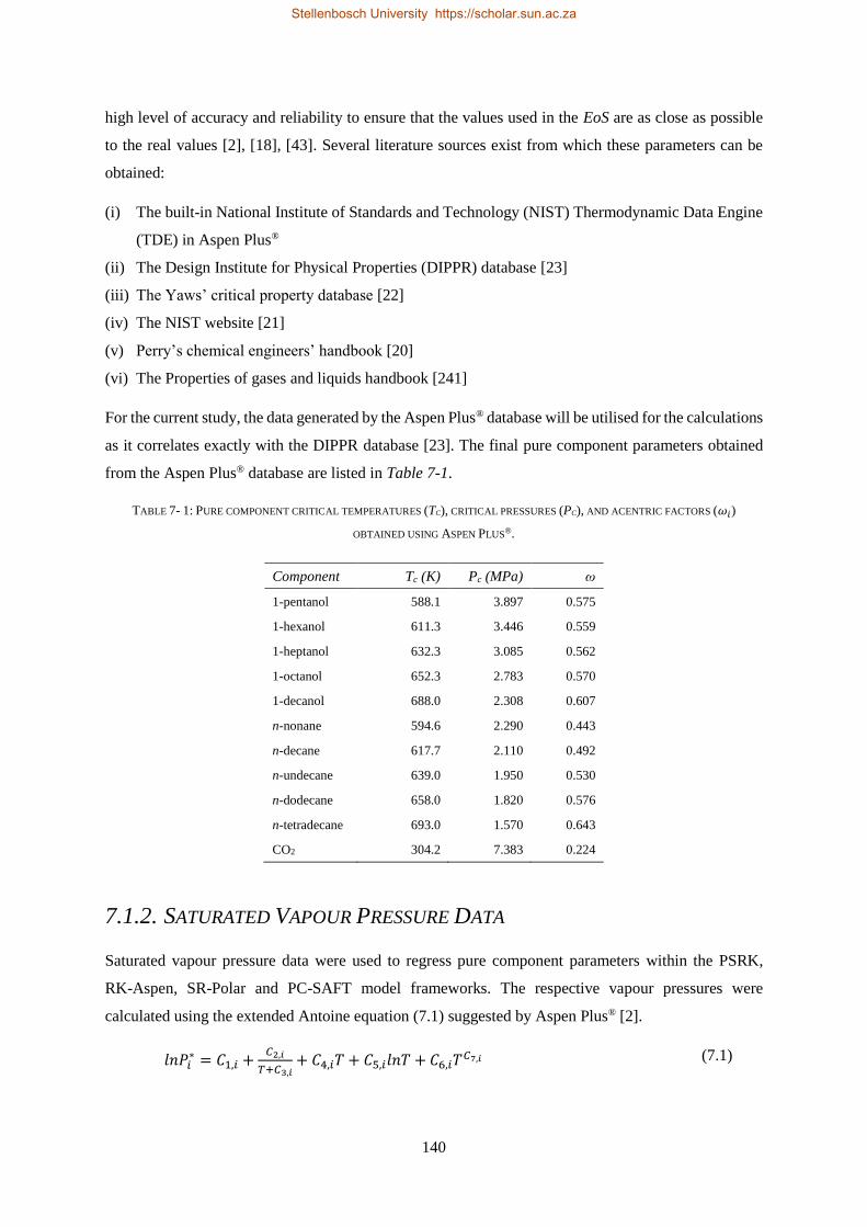
140
high level of accuracy and reliability to ensure that the values used in the EoS are as close as possible
to the real values [2], [18], [43]. Several literature sources exist from which these parameters can be
obtained:
(i) The built-in National Institute of Standards and Technology (NIST) Thermodynamic Data Engine
(TDE) in Aspen Plus®
(ii) The Design Institute for Physical Properties (DIPPR) database [23]
(iii) The Yaws’ critical property database [22]
(iv) The NIST website [21]
(v) Perry’s chemical engineers’ handbook [20]
(vi) The Properties of gases and liquids handbook [241]
For the current study, the data generated by the Aspen Plus® database will be utilised for the calculations
as it correlates exactly with the DIPPR database [23]. The final pure component parameters obtained
from the Aspen Plus® database are listed in Table 7-1.
TABLE 7- 1: PURE COMPONENT CRITICAL TEMPERATURES (TC), CRITICAL PRESSURES (PC), AND ACENTRIC FACTORS (𝜔𝑖)
OBTAINED USING ASPEN PLUS®.
Component Tc (K) Pc (MPa) ω
1-pentanol 588.1 3.897 0.575
1-hexanol 611.3 3.446 0.559
1-heptanol 632.3 3.085 0.562
1-octanol 652.3 2.783 0.570
1-decanol 688.0 2.308 0.607
n-nonane 594.6 2.290 0.443
n-decane 617.7 2.110 0.492
n-undecane 639.0 1.950 0.530
n-dodecane 658.0 1.820 0.576
n-tetradecane 693.0 1.570 0.643
CO2 304.2 7.383 0.224
7.1.2. SATURATED VAPOUR PRESSURE DATA
Saturated vapour pressure data were used to regress pure component parameters within the PSRK,
RK-Aspen, SR-Polar and PC-SAFT model frameworks. The respective vapour pressures were
calculated using the extended Antoine equation (7.1) suggested by Aspen Plus® [2].
𝑙𝑛𝑃𝑖∗ = 𝐶1,𝑖 +
𝐶2,𝑖
𝑇+𝐶3,𝑖+ 𝐶4,𝑖𝑇 + 𝐶5,𝑖𝑙𝑛𝑇 + 𝐶6,𝑖𝑇𝐶7,𝑖 (7.1)
Stellenbosch University https://scholar.sun.ac.za
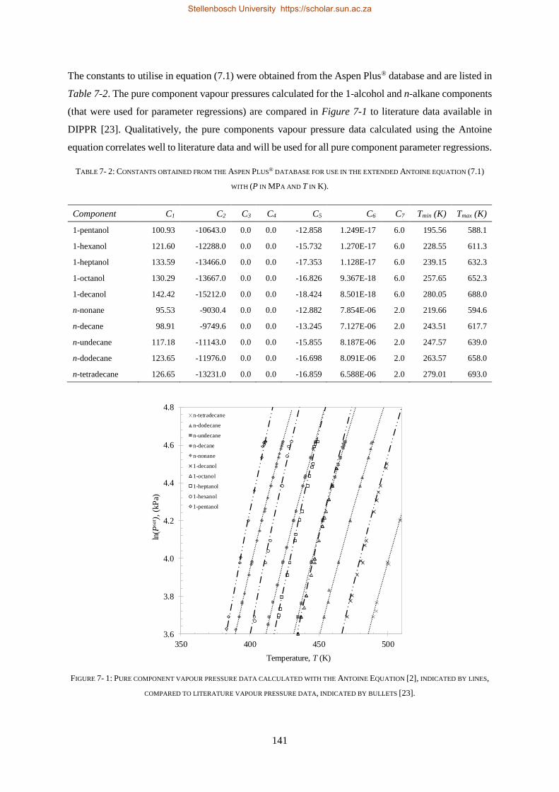
141
The constants to utilise in equation (7.1) were obtained from the Aspen Plus® database and are listed in
Table 7-2. The pure component vapour pressures calculated for the 1-alcohol and n-alkane components
(that were used for parameter regressions) are compared in Figure 7-1 to literature data available in
DIPPR [23]. Qualitatively, the pure components vapour pressure data calculated using the Antoine
equation correlates well to literature data and will be used for all pure component parameter regressions.
TABLE 7- 2: CONSTANTS OBTAINED FROM THE ASPEN PLUS® DATABASE FOR USE IN THE EXTENDED ANTOINE EQUATION (7.1)
WITH (P IN MPA AND T IN K).
Component C1 C2 C3 C4 C5 C6 C7 Tmin (K) Tmax (K)
1-pentanol 100.93 -10643.0 0.0 0.0 -12.858 1.249E-17 6.0 195.56 588.1
1-hexanol 121.60 -12288.0 0.0 0.0 -15.732 1.270E-17 6.0 228.55 611.3
1-heptanol 133.59 -13466.0 0.0 0.0 -17.353 1.128E-17 6.0 239.15 632.3
1-octanol 130.29 -13667.0 0.0 0.0 -16.826 9.367E-18 6.0 257.65 652.3
1-decanol 142.42 -15212.0 0.0 0.0 -18.424 8.501E-18 6.0 280.05 688.0
n-nonane 95.53 -9030.4 0.0 0.0 -12.882 7.854E-06 2.0 219.66 594.6
n-decane 98.91 -9749.6 0.0 0.0 -13.245 7.127E-06 2.0 243.51 617.7
n-undecane 117.18 -11143.0 0.0 0.0 -15.855 8.187E-06 2.0 247.57 639.0
n-dodecane 123.65 -11976.0 0.0 0.0 -16.698 8.091E-06 2.0 263.57 658.0
n-tetradecane 126.65 -13231.0 0.0 0.0 -16.859 6.588E-06 2.0 279.01 693.0
FIGURE 7- 1: PURE COMPONENT VAPOUR PRESSURE DATA CALCULATED WITH THE ANTOINE EQUATION [2], INDICATED BY LINES,
COMPARED TO LITERATURE VAPOUR PRESSURE DATA, INDICATED BY BULLETS [23].
3.6
3.8
4.0
4.2
4.4
4.6
4.8
350 400 450 500
ln(P
sat )
,(k
Pa)
Temperature, T (K)
n-tetradecane
n-dodecane
n-undecane
n-decane
n-nonane
1-decanol
1-octanol
1-heptanol
1-hexanol
1-pentanol
Stellenbosch University https://scholar.sun.ac.za
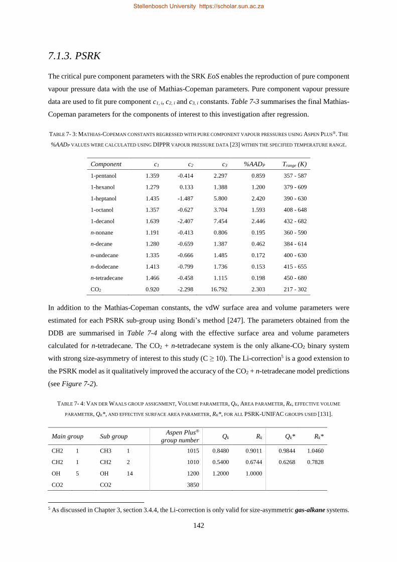
142
7.1.3. PSRK
The critical pure component parameters with the SRK EoS enables the reproduction of pure component
vapour pressure data with the use of Mathias-Copeman parameters. Pure component vapour pressure
data are used to fit pure component c1, i, c2, i and c3, i constants. Table 7-3 summarises the final Mathias-
Copeman parameters for the components of interest to this investigation after regression.
TABLE 7- 3: MATHIAS-COPEMAN CONSTANTS REGRESSED WITH PURE COMPONENT VAPOUR PRESSURES USING ASPEN PLUS®. THE
%AADP VALUES WERE CALCULATED USING DIPPR VAPOUR PRESSURE DATA [23] WITHIN THE SPECIFIED TEMPERATURE RANGE.
Component c1 c2 c3 %AADP Trange (K)
1-pentanol 1.359 -0.414 2.297 0.859 357 - 587
1-hexanol 1.279 0.133 1.388 1.200 379 - 609
1-heptanol 1.435 -1.487 5.800 2.420 390 - 630
1-octanol 1.357 -0.627 3.704 1.593 408 - 648
1-decanol 1.639 -2.407 7.454 2.446 432 - 682
n-nonane 1.191 -0.413 0.806 0.195 360 - 590
n-decane 1.280 -0.659 1.387 0.462 384 - 614
n-undecane 1.335 -0.666 1.485 0.172 400 - 630
n-dodecane 1.413 -0.799 1.736 0.153 415 - 655
n-tetradecane 1.466 -0.458 1.115 0.198 450 - 680
CO2 0.920 -2.298 16.792 2.303 217 - 302
In addition to the Mathias-Copeman constants, the vdW surface area and volume parameters were
estimated for each PSRK sub-group using Bondi’s method [247]. The parameters obtained from the
DDB are summarised in Table 7-4 along with the effective surface area and volume parameters
calculated for n-tetradecane. The CO2 + n-tetradecane system is the only alkane-CO2 binary system
with strong size-asymmetry of interest to this study (C ≥ 10). The Li-correction5 is a good extension to
the PSRK model as it qualitatively improved the accuracy of the CO2 + n-tetradecane model predictions
(see Figure 7-2).
TABLE 7- 4: VAN DER WAALS GROUP ASSIGNMENT, VOLUME PARAMETER, QK, AREA PARAMETER, RK, EFFECTIVE VOLUME
PARAMETER, QK*, AND EFFECTIVE SURFACE AREA PARAMETER, RK*, FOR ALL PSRK-UNIFAC GROUPS USED [131].
Main group Sub group Aspen Plus®
group number Qk Rk Qk* Rk*
CH2 1 CH3 1 1015 0.8480 0.9011 0.9844 1.0460
CH2 1 CH2 2 1010 0.5400 0.6744 0.6268 0.7828
OH 5 OH 14 1200 1.2000 1.0000
CO2 CO2 3850
5 As discussed in Chapter 3, section 3.4.4, the Li-correction is only valid for size-asymmetric gas-alkane systems.
Stellenbosch University https://scholar.sun.ac.za
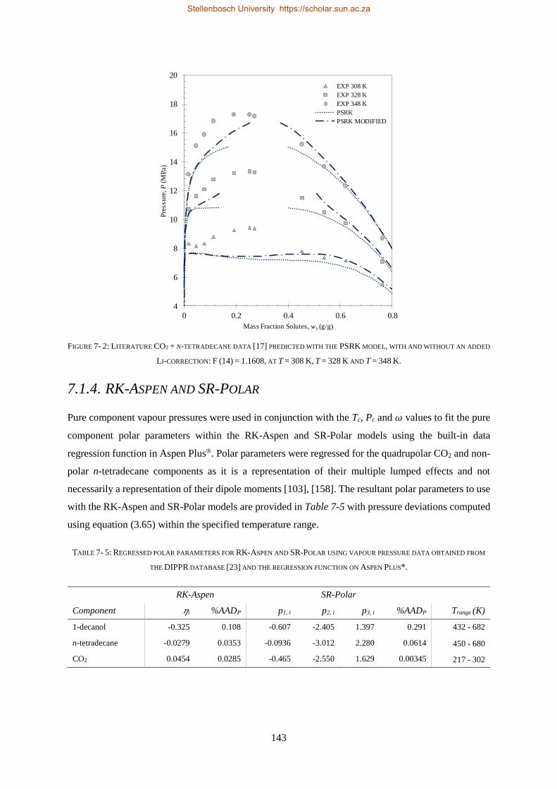
143
FIGURE 7- 2: LITERATURE CO2 + N-TETRADECANE DATA [17] PREDICTED WITH THE PSRK MODEL, WITH AND WITHOUT AN ADDED
LI-CORRECTION: F (14) = 1.1608, AT T = 308 K, T = 328 K AND T = 348 K.
7.1.4. RK-ASPEN AND SR-POLAR
Pure component vapour pressures were used in conjunction with the Tc, Pc and 𝜔 values to fit the pure
component polar parameters within the RK-Aspen and SR-Polar models using the built-in data
regression function in Aspen Plus®. Polar parameters were regressed for the quadrupolar CO2 and non-
polar n-tetradecane components as it is a representation of their multiple lumped effects and not
necessarily a representation of their dipole moments [103], [158]. The resultant polar parameters to use
with the RK-Aspen and SR-Polar models are provided in Table 7-5 with pressure deviations computed
using equation (3.65) within the specified temperature range.
TABLE 7- 5: REGRESSED POLAR PARAMETERS FOR RK-ASPEN AND SR-POLAR USING VAPOUR PRESSURE DATA OBTAINED FROM
THE DIPPR DATABASE [23] AND THE REGRESSION FUNCTION ON ASPEN PLUS®.
RK-Aspen SR-Polar
Component 휂i %AADP p1, i p2, i p3, i %AADP Trange (K)
1-decanol -0.325 0.108 -0.607 -2.405 1.397 0.291 432 - 682
n-tetradecane -0.0279 0.0353 -0.0936 -3.012 2.280 0.0614 450 - 680
CO2 0.0454 0.0285 -0.465 -2.550 1.629 0.00345 217 - 302
4
6
8
10
12
14
16
18
20
0 0.2 0.4 0.6 0.8
Pre
ssu
re, P
(MP
a)
Mass Fraction Solutes, ws (g/g)
EXP 308 K
EXP 328 K
EXP 348 K
PSRK
PSRK MODIFIED
Stellenbosch University https://scholar.sun.ac.za
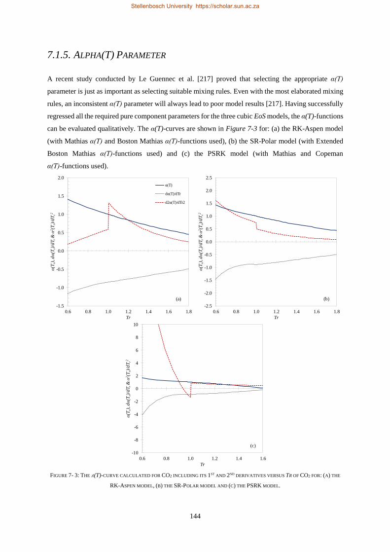
144
7.1.5. ALPHA(T) PARAMETER
A recent study conducted by Le Guennec et al. [217] proved that selecting the appropriate α(T)
parameter is just as important as selecting suitable mixing rules. Even with the most elaborated mixing
rules, an inconsistent α(T) parameter will always lead to poor model results [217]. Having successfully
regressed all the required pure component parameters for the three cubic EoS models, the α(T)-functions
can be evaluated qualitatively. The α(T)-curves are shown in Figure 7-3 for: (a) the RK-Aspen model
(with Mathias α(T) and Boston Mathias α(T)-functions used), (b) the SR-Polar model (with Extended
Boston Mathias α(T)-functions used) and (c) the PSRK model (with Mathias and Copeman
α(T)-functions used).
FIGURE 7- 3: THE Α(T)-CURVE CALCULATED FOR CO2 INCLUDING ITS 1ST AND 2ND DERIVATIVES VERSUS TR OF CO2 FOR: (A) THE
RK-ASPEN MODEL, (B) THE SR-POLAR MODEL AND (C) THE PSRK MODEL.
-10
-8
-6
-4
-2
0
2
4
6
8
10
0.6 0.8 1.0 1.2 1.4 1.6
α(T
r), dα
(Tr)
/dT
r&
α2(T
r)/d
Tr2
Tr
-1.5
-1.0
-0.5
0.0
0.5
1.0
1.5
2.0
0.6 0.8 1.0 1.2 1.4 1.6 1.8
α(T
r), dα
(Tr)
/dT
r&
α2(T
r)/d
Tr2
Tr
α(T)
dα(T)/dTr
d2α(T)/dTr2
-2.5
-2.0
-1.5
-1.0
-0.5
0.0
0.5
1.0
1.5
2.0
2.5
0.6 0.8 1.0 1.2 1.4 1.6 1.8
α(T
r), dα
(Tr)
/dT
r&
α2(T
r)/d
Tr2
Tr
(a) (b)
(c)
Stellenbosch University https://scholar.sun.ac.za
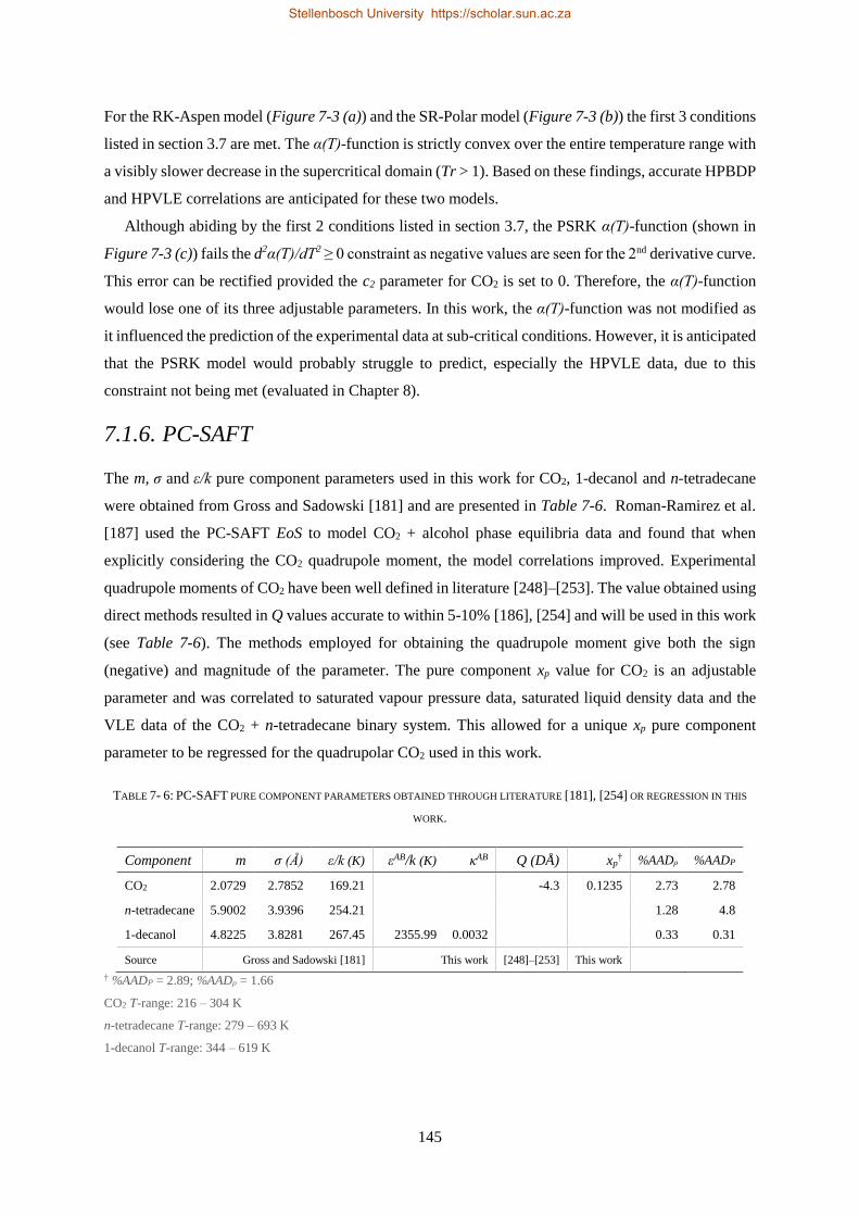
145
For the RK-Aspen model (Figure 7-3 (a)) and the SR-Polar model (Figure 7-3 (b)) the first 3 conditions
listed in section 3.7 are met. The α(T)-function is strictly convex over the entire temperature range with
a visibly slower decrease in the supercritical domain (Tr > 1). Based on these findings, accurate HPBDP
and HPVLE correlations are anticipated for these two models.
Although abiding by the first 2 conditions listed in section 3.7, the PSRK α(T)-function (shown in
Figure 7-3 (c)) fails the d2α(T)/dT2 ≥ 0 constraint as negative values are seen for the 2nd derivative curve.
This error can be rectified provided the c2 parameter for CO2 is set to 0. Therefore, the α(T)-function
would lose one of its three adjustable parameters. In this work, the α(T)-function was not modified as
it influenced the prediction of the experimental data at sub-critical conditions. However, it is anticipated
that the PSRK model would probably struggle to predict, especially the HPVLE data, due to this
constraint not being met (evaluated in Chapter 8).
7.1.6. PC-SAFT
The m, σ and ε/k pure component parameters used in this work for CO2, 1-decanol and n-tetradecane
were obtained from Gross and Sadowski [181] and are presented in Table 7-6. Roman-Ramirez et al.
[187] used the PC-SAFT EoS to model CO2 + alcohol phase equilibria data and found that when
explicitly considering the CO2 quadrupole moment, the model correlations improved. Experimental
quadrupole moments of CO2 have been well defined in literature [248]–[253]. The value obtained using
direct methods resulted in Q values accurate to within 5-10% [186], [254] and will be used in this work
(see Table 7-6). The methods employed for obtaining the quadrupole moment give both the sign
(negative) and magnitude of the parameter. The pure component xp value for CO2 is an adjustable
parameter and was correlated to saturated vapour pressure data, saturated liquid density data and the
VLE data of the CO2 + n-tetradecane binary system. This allowed for a unique xp pure component
parameter to be regressed for the quadrupolar CO2 used in this work.
TABLE 7- 6: PC-SAFT PURE COMPONENT PARAMETERS OBTAINED THROUGH LITERATURE [181], [254] OR REGRESSION IN THIS
WORK.
Component m σ (Å) ε/k (K) εAB/k (K) κAB Q (DÅ) xp† %AADρ %AADP
CO2 2.0729 2.7852 169.21 -4.3 0.1235 2.73 2.78
n-tetradecane 5.9002 3.9396 254.21 1.28 4.8
1-decanol 4.8225 3.8281 267.45 2355.99 0.0032 0.33 0.31
Source Gross and Sadowski [181] This work [248]–[253] This work
† %AADP = 2.89; %AADρ = 1.66
CO2 T-range: 216 – 304 K
n-tetradecane T-range: 279 – 693 K
1-decanol T-range: 344 – 619 K
Stellenbosch University https://scholar.sun.ac.za
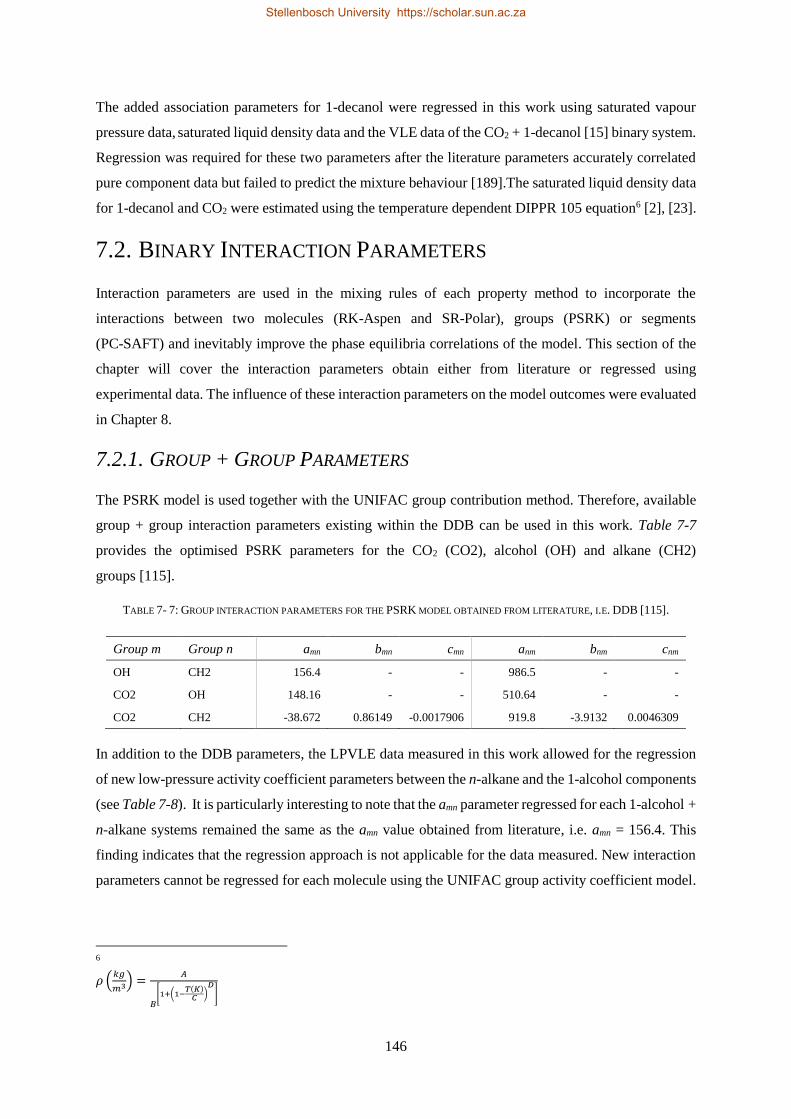
146
The added association parameters for 1-decanol were regressed in this work using saturated vapour
pressure data, saturated liquid density data and the VLE data of the CO2 + 1-decanol [15] binary system.
Regression was required for these two parameters after the literature parameters accurately correlated
pure component data but failed to predict the mixture behaviour [189].The saturated liquid density data
for 1-decanol and CO2 were estimated using the temperature dependent DIPPR 105 equation6 [2], [23].
7.2. BINARY INTERACTION PARAMETERS
Interaction parameters are used in the mixing rules of each property method to incorporate the
interactions between two molecules (RK-Aspen and SR-Polar), groups (PSRK) or segments
(PC-SAFT) and inevitably improve the phase equilibria correlations of the model. This section of the
chapter will cover the interaction parameters obtain either from literature or regressed using
experimental data. The influence of these interaction parameters on the model outcomes were evaluated
in Chapter 8.
7.2.1. GROUP + GROUP PARAMETERS
The PSRK model is used together with the UNIFAC group contribution method. Therefore, available
group + group interaction parameters existing within the DDB can be used in this work. Table 7-7
provides the optimised PSRK parameters for the CO2 (CO2), alcohol (OH) and alkane (CH2)
groups [115].
TABLE 7- 7: GROUP INTERACTION PARAMETERS FOR THE PSRK MODEL OBTAINED FROM LITERATURE, I.E. DDB [115].
Group m Group n amn bmn cmn anm bnm cnm
OH CH2 156.4 - - 986.5 - -
CO2 OH 148.16 - - 510.64 - -
CO2 CH2 -38.672 0.86149 -0.0017906 919.8 -3.9132 0.0046309
In addition to the DDB parameters, the LPVLE data measured in this work allowed for the regression
of new low-pressure activity coefficient parameters between the n-alkane and the 1-alcohol components
(see Table 7-8). It is particularly interesting to note that the amn parameter regressed for each 1-alcohol +
n-alkane systems remained the same as the amn value obtained from literature, i.e. amn = 156.4. This
finding indicates that the regression approach is not applicable for the data measured. New interaction
parameters cannot be regressed for each molecule using the UNIFAC group activity coefficient model.
6
𝜌 (𝑘𝑔
𝑚3) =𝐴
𝐵[1+(1−
𝑇(𝐾)𝐶 )
𝐷]
Stellenbosch University https://scholar.sun.ac.za
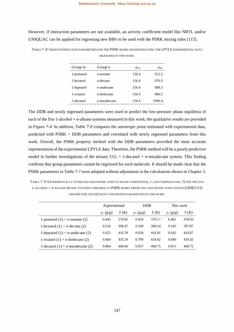
147
However, if interaction parameters are not available, an activity coefficient model like NRTL and/or
UNIQUAC can be applied for regressing new BIPs to be used with the PSRK mixing rules [115].
TABLE 7- 8: GROUP INTERACTION PARAMETERS FOR THE PSRK MODEL REGRESSED USING THE LPVLE EXPERIMENTAL DATA
MEASURED IN THIS WORK.
Group m Group n amn anm
1-pentanol n-nonane 156.4 912.2
1-hexanol n-decane 156.4 976.5
1-heptanol n-undecane 156.4 888.3
1-octanol n-dodecane 156.4 986.5
1-decanol n-tetradecane 156.4 1096.4
The DDB and newly regressed parameters were used to predict the low-pressure phase equilibria of
each of the five 1-alcohol + n-alkane systems measured in this work; the qualitative results are provided
in Figure 7-4. In addition, Table 7-9 compares the azeotropic point estimated with experimental data,
predicted with PSRK + DDB parameters and correlated with newly regressed parameters from this
work. Overall, the PSRK property method with the DDB parameters provided the most accurate
representation of the experimental LPVLE data. Therefore, the PSRK method will be a purely predictive
model in further investigations of the ternary CO2 + 1-decanol + n-tetradecane system. This finding
confirms that group parameters cannot be regressed for each molecule. It should be made clear that the
PSRK parameters in Table 7-7 were adopted without adjustment in the calculations shown in Chapter 3.
TABLE 7- 9: EXPERIMENTALLY ESTIMATED AZEOTROPIC POINT (VAPOUR COMPOSITION, Y1 AND TEMPERATURE, T) FOR THE FIVE
1-ALCOHOL + N-ALKANE BINARY SYSTEMS COMPARED TO PSRK MODEL PREDICTED AZEOTROPIC POINT WITH (A) DDB [115]
PARAMETERS AND (B) NEWLY REGRESSED PARAMETERS IN THIS WORK.
Experimental DDB This work
y1 (g/g) T (K) y1 (g/g) T (K) y1 (g/g) T (K)
1-pentanol (1) + n-nonane (2) 0.445 378.05 0.450 378.17 0.461 378.03
1-hexanol (1) + n-decane (2) 0.516 398.47 0.549 398.24 0.545 397.87
1-heptanol (1) + n-undecane (2) 0.625 416.78 0.630 416.81 0.642 416.87
1-octanol (1) + n-dodecane (2) 0.664 435.19 0.709 434.82 0.680 434.35
1-decanol (1) + n-tetradecane (2) 0.864 468.66 0.837 468.75 0.811 468.75
Stellenbosch University https://scholar.sun.ac.za
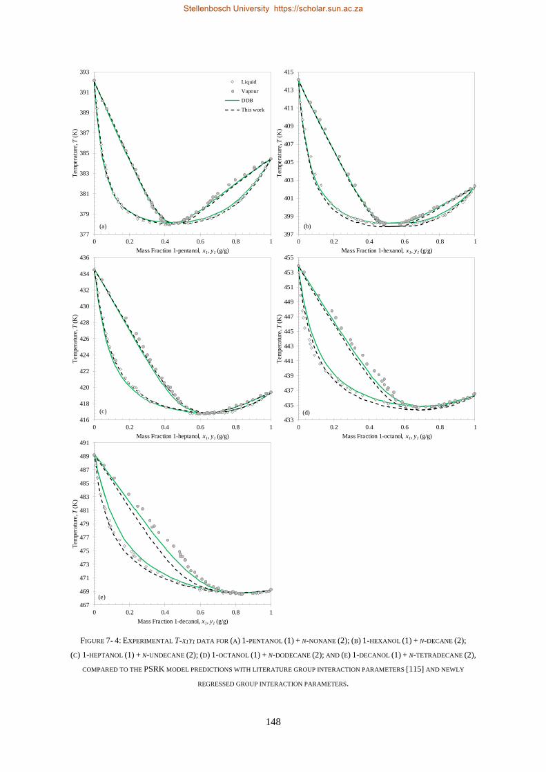
148
FIGURE 7- 4: EXPERIMENTAL T-X1Y1 DATA FOR (A) 1-PENTANOL (1) + N-NONANE (2); (B) 1-HEXANOL (1) + N-DECANE (2);
(C) 1-HEPTANOL (1) + N-UNDECANE (2); (D) 1-OCTANOL (1) + N-DODECANE (2); AND (E) 1-DECANOL (1) + N-TETRADECANE (2),
COMPARED TO THE PSRK MODEL PREDICTIONS WITH LITERATURE GROUP INTERACTION PARAMETERS [115] AND NEWLY
REGRESSED GROUP INTERACTION PARAMETERS.
377
379
381
383
385
387
389
391
393
0 0.2 0.4 0.6 0.8 1
Tem
pera
ture
, T(K
)
Mass Fraction 1-pentanol, x1, y1 (g/g)
Liquid
Vapour
DDB
This work
(a)
397
399
401
403
405
407
409
411
413
415
0 0.2 0.4 0.6 0.8 1
Tem
pera
ture
, T(K
)
Mass Fraction 1-hexanol, x1, y1 (g/g)
(b)
416
418
420
422
424
426
428
430
432
434
436
0 0.2 0.4 0.6 0.8 1
Tem
pera
ture
, T(K
)
Mass Fraction 1-heptanol, x1, y1 (g/g)
(c)
433
435
437
439
441
443
445
447
449
451
453
455
0 0.2 0.4 0.6 0.8 1
Tem
pera
ture
, T(K
)
Mass Fraction 1-octanol, x1, y1 (g/g)
(d)
467
469
471
473
475
477
479
481
483
485
487
489
491
0 0.2 0.4 0.6 0.8 1
Tem
pera
ture
, T(K
)
Mass Fraction 1-decanol, x1, y1 (g/g)
(e)
Stellenbosch University https://scholar.sun.ac.za
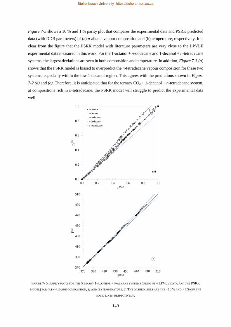
149
Figure 7-5 shows a 10 % and 1 % parity plot that compares the experimental data and PSRK predicted
data (with DDB parameters) of (a) n-alkane vapour composition and (b) temperature, respectively. It is
clear from the figure that the PSRK model with literature parameters are very close to the LPVLE
experimental data measured in this work. For the 1-octanol + n-dodecane and 1-decanol + n-tetradecane
systems, the largest deviations are seen in both composition and temperature. In addition, Figure 7-3 (a)
shows that the PSRK model is biased to overpredict the n-tetradecane vapour composition for these two
systems, especially within the low 1-decanol region. This agrees with the predictions shown in Figure
7-2 (d) and (e). Therefore, it is anticipated that for the ternary CO2 + 1-decanol + n-tetradecane system,
at compositions rich in n-tetradecane, the PSRK model will struggle to predict the experimental data
well.
FIGURE 7- 5: PARITY PLOTS FOR THE 5 BINARY 1-ALCOHOL + N-ALKANE SYSTEMS (USING NEW LPVLE DATA AND THE PSRK
MODEL) FOR (A) N-ALKANE COMPOSITION, Y2 AND (B) TEMPERATURE, T. THE DASHED LINES ARE THE +10 % AND + 1% OFF THE
SOLID LINES, RESPECTIVELY.
0.0
0.2
0.4
0.6
0.8
1.0
0.0 0.2 0.4 0.6 0.8 1.0
y 2E
xp
y2DDB
n-nonane
n-decane
n-undecane
n-dodecane
n-tetradecane
370
390
410
430
450
470
490
510
370 390 410 430 450 470 490 510
TE
xp
TDDB
(b)
(a)
Stellenbosch University https://scholar.sun.ac.za
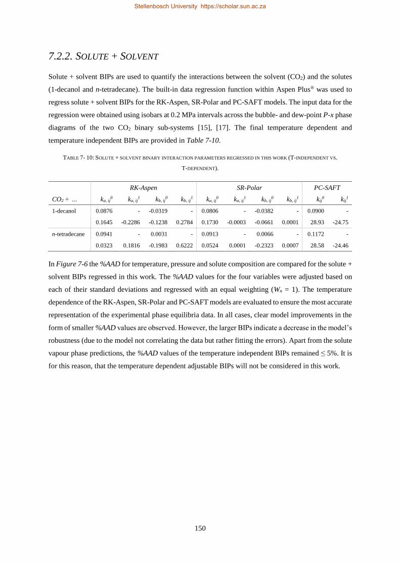
150
7.2.2. SOLUTE + SOLVENT
Solute + solvent BIPs are used to quantify the interactions between the solvent (CO2) and the solutes
(1-decanol and n-tetradecane). The built-in data regression function within Aspen Plus® was used to
regress solute + solvent BIPs for the RK-Aspen, SR-Polar and PC-SAFT models. The input data for the
regression were obtained using isobars at 0.2 MPa intervals across the bubble- and dew-point P-x phase
diagrams of the two CO2 binary sub-systems [15], [17]. The final temperature dependent and
temperature independent BIPs are provided in Table 7-10.
TABLE 7- 10: SOLUTE + SOLVENT BINARY INTERACTION PARAMETERS REGRESSED IN THIS WORK (T-INDEPENDENT VS.
T-DEPENDENT).
RK-Aspen SR-Polar PC-SAFT
CO2 + … ka, ij0 ka, ij
1 kb, ij0 kb, ij
1 ka, ij0 ka, ij
1 kb, ij0 kb, ij
1 kij0 kij
1
1-decanol 0.0876 - -0.0319 - 0.0806 - -0.0382 - 0.0900 -
0.1645 -0.2286 -0.1238 0.2784 0.1730 -0.0003 -0.0661 0.0001 28.93 -24.75
n-tetradecane 0.0941 - 0.0031 - 0.0913 - 0.0066 - 0.1172 -
0.0323 0.1816 -0.1983 0.6222 0.0524 0.0001 -0.2323 0.0007 28.58 -24.46
In Figure 7-6 the %AAD for temperature, pressure and solute composition are compared for the solute +
solvent BIPs regressed in this work. The %AAD values for the four variables were adjusted based on
each of their standard deviations and regressed with an equal weighting (Wn = 1). The temperature
dependence of the RK-Aspen, SR-Polar and PC-SAFT models are evaluated to ensure the most accurate
representation of the experimental phase equilibria data. In all cases, clear model improvements in the
form of smaller %AAD values are observed. However, the larger BIPs indicate a decrease in the model’s
robustness (due to the model not correlating the data but rather fitting the errors). Apart from the solute
vapour phase predictions, the %AAD values of the temperature independent BIPs remained ≤ 5%. It is
for this reason, that the temperature dependent adjustable BIPs will not be considered in this work.
Stellenbosch University https://scholar.sun.ac.za
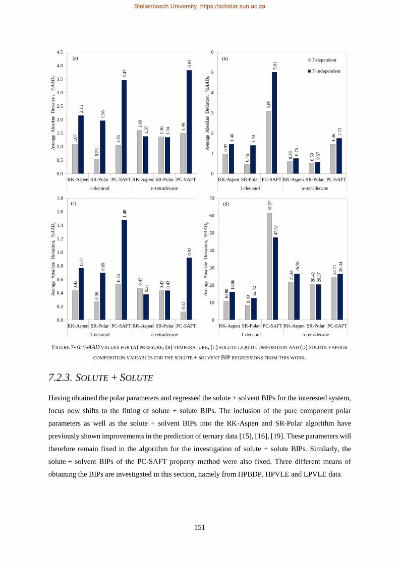
151
FIGURE 7- 6: %AAD VALUES FOR (A) PRESSURE, (B) TEMPERATURE, (C) SOLUTE LIQUID COMPOSITION AND (D) SOLUTE VAPOUR
COMPOSITION VARIABLES FOR THE SOLUTE + SOLVENT BIP REGRESSIONS FROM THIS WORK.
7.2.3. SOLUTE + SOLUTE
Having obtained the polar parameters and regressed the solute + solvent BIPs for the interested system,
focus now shifts to the fitting of solute + solute BIPs. The inclusion of the pure component polar
parameters as well as the solute + solvent BIPs into the RK-Aspen and SR-Polar algorithm have
previously shown improvements in the prediction of ternary data [15], [16], [19]. These parameters will
therefore remain fixed in the algorithm for the investigation of solute + solute BIPs. Similarly, the
solute + solvent BIPs of the PC-SAFT property method were also fixed. Three different means of
obtaining the BIPs are investigated in this section, namely from HPBDP, HPVLE and LPVLE data.
1.0
7
0.5
5
1.0
5
1.6
0
1.3
6 1.4
9
2.1
5
1.9
6
3.4
7
1.3
7
1.3
4
3.8
3
0.0
0.5
1.0
1.5
2.0
2.5
3.0
3.5
4.0
4.5
RK-Aspen SR-Polar PC-SAFT RK-Aspen SR-Polar PC-SAFT
1-decanol n-tetradecane
Ave
rage
Abso
lute
D
evia
tion,
%
AA
DT
0.9
7
0.4
6
3.0
9
0.5
9
0.5
0
1.4
6
1.4
6
1.4
0
5.0
1
0.7
5
0.5
7
1.7
3
0
1
2
3
4
5
6
RK-Aspen SR-Polar PC-SAFT RK-Aspen SR-Polar PC-SAFT
1-decanol n-tetradecane
Ave
rage
Abso
lute
D
evia
tion,
%
AA
DP
T-dependent
T-independent0.4
3
0.2
6
0.5
3
0.4
7
0.4
3
0.1
2
0.7
7
0.6
9
1.4
8
0.3
7 0.4
3
0.9
2
0.0
0.2
0.4
0.6
0.8
1.0
1.2
1.4
1.6
1.8
RK-Aspen SR-Polar PC-SAFT RK-Aspen SR-Polar PC-SAFT
1-decanol n-tetradecane
Ave
rage
Abso
lute
D
evia
tion,
%
AA
Dx
10.8
0
8.4
0
61.5
7
21.4
4
20.4
2 24.7
1
16.0
6
12.4
2
47.3
2
26.5
8
20.3
7
26.3
4
0
10
20
30
40
50
60
70
RK-Aspen SR-Polar PC-SAFT RK-Aspen SR-Polar PC-SAFT
1-decanol n-tetradecane
Ave
rage
Abso
lute
D
evia
tion,
%
AA
Dy
(a) (b)
(c) (d)
Stellenbosch University https://scholar.sun.ac.za
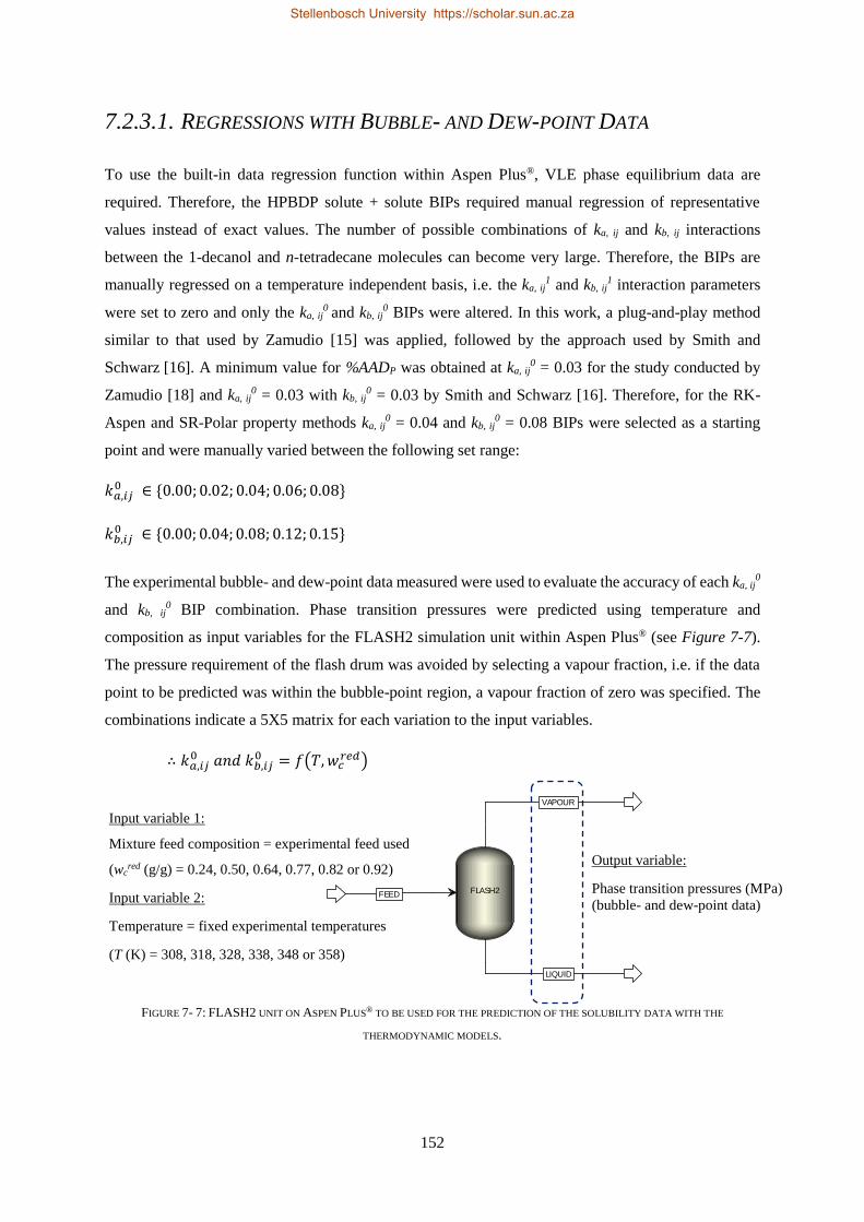
152
7.2.3.1. REGRESSIONS WITH BUBBLE- AND DEW-POINT DATA
To use the built-in data regression function within Aspen Plus®, VLE phase equilibrium data are
required. Therefore, the HPBDP solute + solute BIPs required manual regression of representative
values instead of exact values. The number of possible combinations of ka, ij and kb, ij interactions
between the 1-decanol and n-tetradecane molecules can become very large. Therefore, the BIPs are
manually regressed on a temperature independent basis, i.e. the ka, ij1 and kb, ij
1 interaction parameters
were set to zero and only the ka, ij0 and kb, ij
0 BIPs were altered. In this work, a plug-and-play method
similar to that used by Zamudio [15] was applied, followed by the approach used by Smith and
Schwarz [16]. A minimum value for %AADP was obtained at ka, ij0 = 0.03 for the study conducted by
Zamudio [18] and ka, ij0 = 0.03 with kb, ij
0 = 0.03 by Smith and Schwarz [16]. Therefore, for the RK-
Aspen and SR-Polar property methods ka, ij0 = 0.04 and kb, ij
0 = 0.08 BIPs were selected as a starting
point and were manually varied between the following set range:
𝑘𝑎,𝑖𝑗0 ∈ {0.00; 0.02; 0.04; 0.06; 0.08}
𝑘𝑏,𝑖𝑗0 ∈ {0.00; 0.04; 0.08; 0.12; 0.15}
The experimental bubble- and dew-point data measured were used to evaluate the accuracy of each ka, ij0
and kb, ij0 BIP combination. Phase transition pressures were predicted using temperature and
composition as input variables for the FLASH2 simulation unit within Aspen Plus® (see Figure 7-7).
The pressure requirement of the flash drum was avoided by selecting a vapour fraction, i.e. if the data
point to be predicted was within the bubble-point region, a vapour fraction of zero was specified. The
combinations indicate a 5X5 matrix for each variation to the input variables.
∴ 𝑘𝑎,𝑖𝑗0 𝑎𝑛𝑑 𝑘𝑏,𝑖𝑗
0 = 𝑓(𝑇, 𝑤𝑐𝑟𝑒𝑑)
FIGURE 7- 7: FLASH2 UNIT ON ASPEN PLUS® TO BE USED FOR THE PREDICTION OF THE SOLUBILITY DATA WITH THE
THERMODYNAMIC MODELS.
FLASH2FEED
VAPOUR
LIQUID
Input variable 1:
Mixture feed composition = experimental feed used
(wcred (g/g) = 0.24, 0.50, 0.64, 0.77, 0.82 or 0.92)
Input variable 2:
Temperature = fixed experimental temperatures
(T (K) = 308, 318, 328, 338, 348 or 358)
Output variable:
Phase transition pressures (MPa)
(bubble- and dew-point data)
Stellenbosch University https://scholar.sun.ac.za
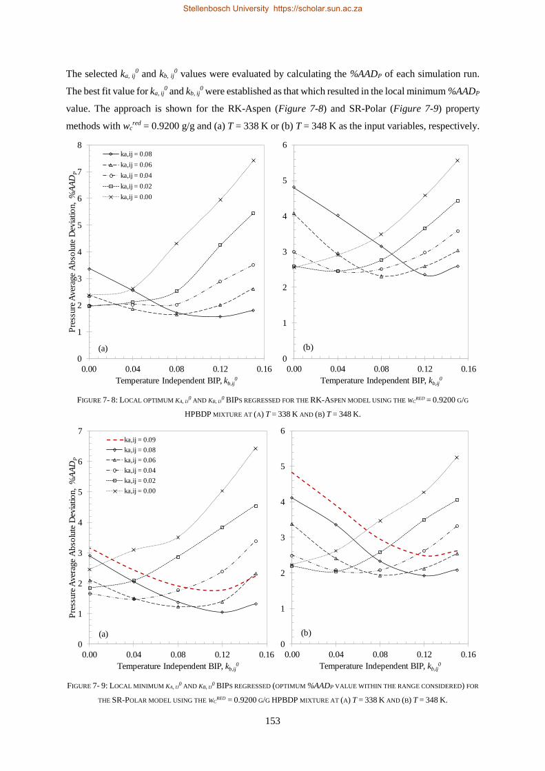
153
The selected ka, ij0 and kb, ij
0 values were evaluated by calculating the %AADP of each simulation run.
The best fit value for ka, ij0 and kb, ij
0 were established as that which resulted in the local minimum %AADP
value. The approach is shown for the RK-Aspen (Figure 7-8) and SR-Polar (Figure 7-9) property
methods with wcred = 0.9200 g/g and (a) T = 338 K or (b) T = 348 K as the input variables, respectively.
FIGURE 7- 8: LOCAL OPTIMUM KA, IJ0 AND KB, IJ
0 BIPS REGRESSED FOR THE RK-ASPEN MODEL USING THE WCRED = 0.9200 G/G
HPBDP MIXTURE AT (A) T = 338 K AND (B) T = 348 K.
FIGURE 7- 9: LOCAL MINIMUM KA, IJ0 AND KB, IJ
0 BIPS REGRESSED (OPTIMUM %AADP VALUE WITHIN THE RANGE CONSIDERED) FOR
THE SR-POLAR MODEL USING THE WCRED = 0.9200 G/G HPBDP MIXTURE AT (A) T = 338 K AND (B) T = 348 K.
0
1
2
3
4
5
6
7
8
0.00 0.04 0.08 0.12 0.16
Pre
ssure
Aver
age
Ab
solu
te D
evia
tio
n,
%A
AD
P
Temperature Independent BIP, kb,ij0
ka,ij = 0.08
ka,ij = 0.06
ka,ij = 0.04
ka,ij = 0.02
ka,ij = 0.00
0
1
2
3
4
5
6
0.00 0.04 0.08 0.12 0.16
Temperature Independent BIP, kb,ij0
(b)(a)
0
1
2
3
4
5
6
7
0.00 0.04 0.08 0.12 0.16
Pre
ssure
Aver
age
Ab
solu
te D
evia
tio
n,
%A
AD
P
Temperature Independent BIP, kb,ij0
ka,ij = 0.09
ka,ij = 0.08
ka,ij = 0.06
ka,ij = 0.04
ka,ij = 0.02
ka,ij = 0.00
0
1
2
3
4
5
6
0.00 0.04 0.08 0.12 0.16
Temperature Independent BIP, kb,ij0
(b)(a)
Stellenbosch University https://scholar.sun.ac.za
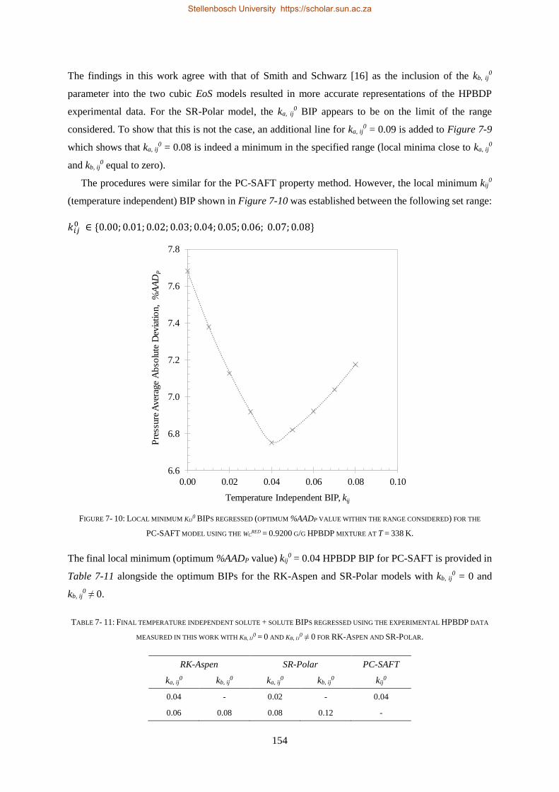
154
The findings in this work agree with that of Smith and Schwarz [16] as the inclusion of the kb, ij0
parameter into the two cubic EoS models resulted in more accurate representations of the HPBDP
experimental data. For the SR-Polar model, the ka, ij0 BIP appears to be on the limit of the range
considered. To show that this is not the case, an additional line for ka, ij0 = 0.09 is added to Figure 7-9
which shows that ka, ij0 = 0.08 is indeed a minimum in the specified range (local minima close to ka, ij
0
and kb, ij0 equal to zero).
The procedures were similar for the PC-SAFT property method. However, the local minimum kij0
(temperature independent) BIP shown in Figure 7-10 was established between the following set range:
𝑘𝑖𝑗0 ∈ {0.00; 0.01; 0.02; 0.03; 0.04; 0.05; 0.06; 0.07; 0.08}
FIGURE 7- 10: LOCAL MINIMUM KIJ0 BIPS REGRESSED (OPTIMUM %AADP VALUE WITHIN THE RANGE CONSIDERED) FOR THE
PC-SAFT MODEL USING THE WCRED = 0.9200 G/G HPBDP MIXTURE AT T = 338 K.
The final local minimum (optimum %AADP value) kij0 = 0.04 HPBDP BIP for PC-SAFT is provided in
Table 7-11 alongside the optimum BIPs for the RK-Aspen and SR-Polar models with kb, ij0 = 0 and
kb, ij0 ≠ 0.
TABLE 7- 11: FINAL TEMPERATURE INDEPENDENT SOLUTE + SOLUTE BIPS REGRESSED USING THE EXPERIMENTAL HPBDP DATA
MEASURED IN THIS WORK WITH KB, IJ0 = 0 AND KB, IJ
0 ≠ 0 FOR RK-ASPEN AND SR-POLAR.
RK-Aspen SR-Polar PC-SAFT
ka, ij0 kb, ij
0 ka, ij0 kb, ij
0 kij0
0.04 - 0.02 - 0.04
0.06 0.08 0.08 0.12 -
6.6
6.8
7.0
7.2
7.4
7.6
7.8
0.00 0.02 0.04 0.06 0.08 0.10
Pre
ssure
Aver
age
Ab
solu
te D
evia
tio
n,
%A
AD
P
Temperature Independent BIP, kij
Stellenbosch University https://scholar.sun.ac.za
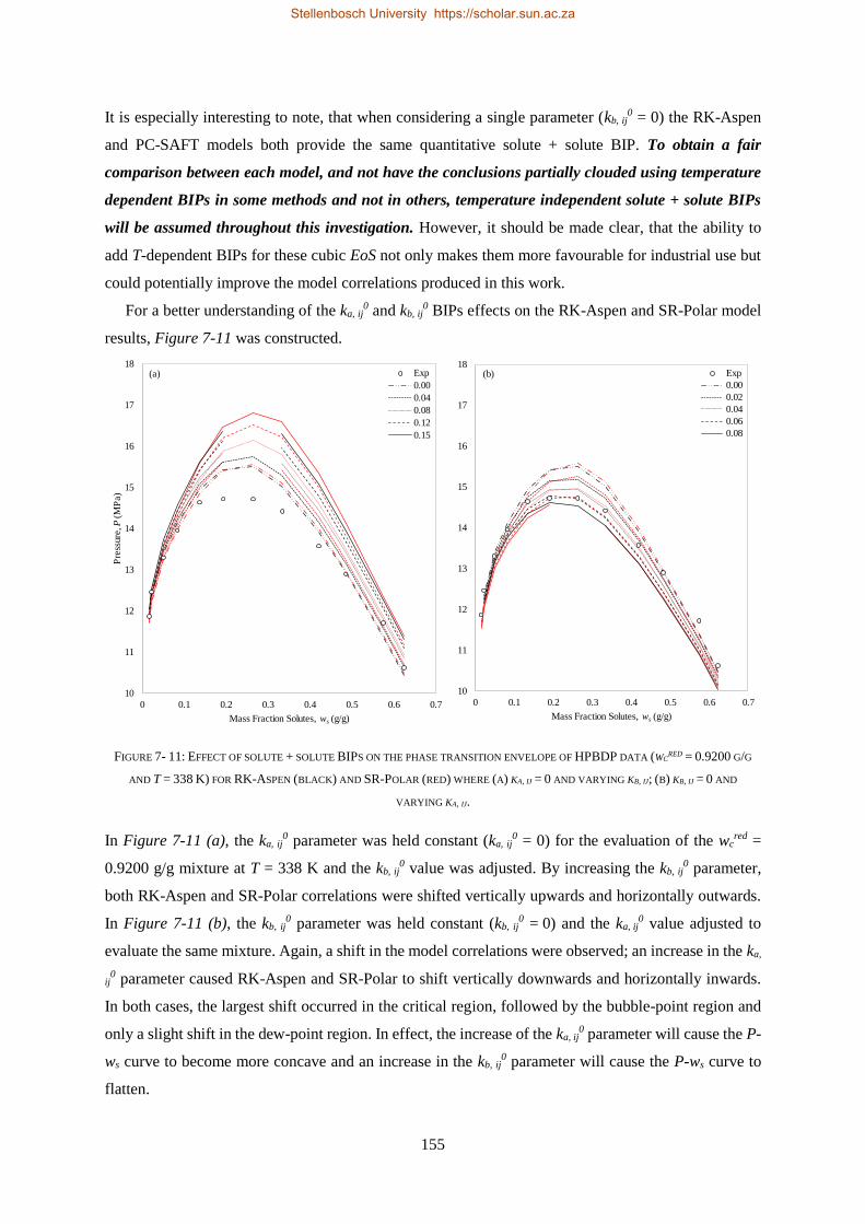
155
It is especially interesting to note, that when considering a single parameter (kb, ij0 = 0) the RK-Aspen
and PC-SAFT models both provide the same quantitative solute + solute BIP. To obtain a fair
comparison between each model, and not have the conclusions partially clouded using temperature
dependent BIPs in some methods and not in others, temperature independent solute + solute BIPs
will be assumed throughout this investigation. However, it should be made clear, that the ability to
add T-dependent BIPs for these cubic EoS not only makes them more favourable for industrial use but
could potentially improve the model correlations produced in this work.
For a better understanding of the ka, ij0 and kb, ij
0 BIPs effects on the RK-Aspen and SR-Polar model
results, Figure 7-11 was constructed.
FIGURE 7- 11: EFFECT OF SOLUTE + SOLUTE BIPS ON THE PHASE TRANSITION ENVELOPE OF HPBDP DATA (WCRED = 0.9200 G/G
AND T = 338 K) FOR RK-ASPEN (BLACK) AND SR-POLAR (RED) WHERE (A) KA, IJ = 0 AND VARYING KB, IJ; (B) KB, IJ = 0 AND
VARYING KA, IJ.
In Figure 7-11 (a), the ka, ij0 parameter was held constant (ka, ij
0 = 0) for the evaluation of the wcred =
0.9200 g/g mixture at T = 338 K and the kb, ij0 value was adjusted. By increasing the kb, ij
0 parameter,
both RK-Aspen and SR-Polar correlations were shifted vertically upwards and horizontally outwards.
In Figure 7-11 (b), the kb, ij0 parameter was held constant (kb, ij
0 = 0) and the ka, ij0 value adjusted to
evaluate the same mixture. Again, a shift in the model correlations were observed; an increase in the ka,
ij0 parameter caused RK-Aspen and SR-Polar to shift vertically downwards and horizontally inwards.
In both cases, the largest shift occurred in the critical region, followed by the bubble-point region and
only a slight shift in the dew-point region. In effect, the increase of the ka, ij0 parameter will cause the P-
ws curve to become more concave and an increase in the kb, ij0 parameter will cause the P-ws curve to
flatten.
10
11
12
13
14
15
16
17
18
0 0.1 0.2 0.3 0.4 0.5 0.6 0.7
Pre
ssure
, P(M
Pa)
Mass Fraction Solutes, ws (g/g)
Exp
0.00
0.04
0.08
0.12
0.15
10
11
12
13
14
15
16
17
18
0 0.1 0.2 0.3 0.4 0.5 0.6 0.7
Mass Fraction Solutes, ws (g/g)
Exp
0.00
0.02
0.04
0.06
0.08
(b)(a)
Stellenbosch University https://scholar.sun.ac.za
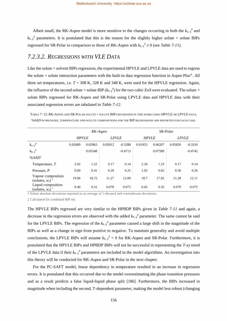
156
Albeit small, the RK-Aspen model is more sensitive to the changes occurring in both the ka, ij0 and
kb, ij0 parameters. It is postulated that this is the reason for the slightly higher solute + solute BIPs
regressed for SR-Polar in comparison to those of RK-Aspen with kb, ij0 ≠ 0 (see Table 7-11).
7.2.3.2. REGRESSIONS WITH VLE DATA
Like the solute + solvent BIPs regression, the experimental HPVLE and LPVLE data are used to regress
the solute + solute interaction parameters with the built-in data regression function in Aspen Plus®. All
three set temperatures, i.e. T = 308 K, 328 K and 348 K, were used for the HPVLE regression. Again,
the influence of the second solute + solute BIP (kb, ij0) for the two cubic EoS were evaluated. The solute +
solute BIPs regressed for RK-Aspen and SR-Polar using LPVLE data and HPVLE data with their
associated regression errors are tabulated in Table 7-12.
TABLE 7- 12: RK-ASPEN AND SR-POLAR SOLUTE + SOLUTE BIPS REGRESSED IN THIS WORK USING HPVLE OR LPVLE DATA.
%AAD IN PRESSURE, TEMPERATURE AND SOLUTE COMPOSITIONS FOR THE BIP REGRESSIONS ARE REPORTED FOR EACH CASE.
RK-Aspen SR-Polar
HPVLE LPVLE HPVLE LPVLE
ka, ij0 0.02689 0.05963 0.05812 -0.3288 0.01953 0.06207 0.05820 -0.3310
kb, ij0 0.05548 -0.4713 0.07589 -0.4742
%AAD‡
Temperature, T 2.02 1.22 0.17 0.14 2.24 1.23 0.17 0.14
Pressure, P 0.69 0.41 0.29 0.25 1.02 0.65 0.30 0.26
Vapour composition
(solutes, ws) † 19.96 18.72 11.27 12.09 18.7 17.92 11.28 12.11
Liquid composition
(solutes, ws) † 0.40 0.31 0.078 0.075 0.45 0.35 0.079 0.075
† Solute absolute deviations reported as an average of 1-decanol and n-tetradecane deviations.
‡ Calculated for combined BIP set.
The HPVLE BIPs regressed are very similar to the HPBDP BIPs given in Table 7-11 and again, a
decrease in the regression errors are observed with the added kb, ij0 parameter. The same cannot be said
for the LPVLE BIPs. The regression of the kb, ij0 parameter caused a large shift in the magnitude of the
BIPs as well as a change in sign from positive to negative. To maintain generality and avoid multiple
conclusions, the LPVLE BIPs will assume kb, ij0 = 0 for RK-Aspen and SR-Polar. Furthermore, it is
postulated that the HPVLE BIPs and HPBDP BIPs will not be successful in representing the T-xy trend
of the LPVLE data if their kb, ij0 parameters are included in the model algorithms. An investigation into
this theory will be conducted for RK-Aspen and SR-Polar in the next chapter.
For the PC-SAFT model, linear dependency in temperature resulted in an increase in regression
errors. It is postulated that this occurred due to the model overestimating the phase transition pressures
and as a result predicts a false liquid-liquid phase split [186]. Furthermore, the BIPs increased in
magnitude when including the second, T-dependent parameter, making the model less robust (changing
Stellenbosch University https://scholar.sun.ac.za
157
its fundamental characteristics). Therefore, in this study, the use of a single temperature independent
interaction parameter is preferred since it allows the thermodynamic model to retain its predictive
qualities, rather than just fitting the experimental data. The temperature independent kij parameters used
for the 1-decanol + n-tetradecane interactions are listed in Table 7-13 with their associated regression
errors.
TABLE 7- 13: PC-SAFT SOLUTE + SOLUTE BIPS REGRESSED IN THIS WORK USING HPVLE OR LPVLE DATA. %AAD IN
PRESSURE, TEMPERATURE AND SOLUTE COMPOSITIONS FOR THE BIP REGRESSIONS ARE REPORTED FOR EACH CASE.
HPVLE LPVLE
kij0 0.04454 0.02467
%AAD
Temperature 10.78 0.37
Pressure 7.34 0.56
Vapour composition (solutes, ws) † 44.32 21.86
Liquid composition (solutes, ws) † 1.44 0.12
† Solute absolute deviations reported as an average of 1-decanol and n-tetradecane deviations.
7.3. CHAPTER OUTCOMES
The aim of this chapter was to achieve Objective 3.2 by gathering pure component parameters from
literature and regressing the necessary interaction parameters for the four thermodynamic models using
(i) HPBDP, (ii) HPVLE and (iii) LPVLE data. The key conclusions drawn from this chapter are the
following:
• The HPBDP data were used to manually obtain solute + solute BIPs with the use of a flash drum
simulation in Aspen Plus®.
• The intercorrelation of the parameters with the two cubic EoS restricted the HPBDP BIPs to a
maximum of 2 solute + solute interaction parameters namely, ka, ij0 and kb, ij
0. Therefore, only
temperature independent BIPs were investigated in this study. PC-SAFT required the regression
of only one kij parameter to maintain the temperature independent trend. The accuracy of this fitting
procedure is limited by the technique used for obtaining the solute + solute BIPs. The values did
not represent the true interactions between the solutes, but rather enabled the most accurate fit of
the thermodynamic models to the experimental data.
• HPVLE data for the ternary system and LPVLE data for the binary system were used to regress
the second and third set of BIPs, respectively. Like the solute + solvent regression procedure, the
built-in data regression function in Aspen Plus® was applied.
• To maintain generality and not have one method produce a biased outcome, the HPVLE and
LPVLE BIPs were regressed on a temperature independent basis.
Stellenbosch University https://scholar.sun.ac.za
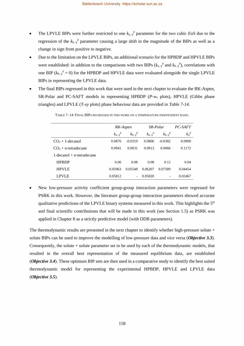
158
• The LPVLE BIPs were further restricted to one ka, ij0 parameter for the two cubic EoS due to the
regression of the kb, ij0 parameter causing a large shift in the magnitude of the BIPs as well as a
change in sign from positive to negative.
• Due to the limitation on the LPVLE BIPs, an additional scenario for the HPBDP and HPVLE BIPs
were established: in addition to the comparisons with two BIPs (ka, ij0 and kb, ij
0), correlations with
one BIP (kb, ij0 = 0) for the HPBDP and HPVLE data were evaluated alongside the single LPVLE
BIPs in representing the LPVLE data.
• The final BIPs regressed in this work that were used in the next chapter to evaluate the RK-Aspen,
SR-Polar and PC-SAFT models in representing HPBDP (P-ws plots), HPVLE (Gibbs phase
triangles) and LPVLE (T-xy plots) phase behaviour data are provided in Table 7-14.
TABLE 7- 14: FINAL BIPS REGRESSED IN THIS WORK ON A TEMPERATURE INDEPENDENT BASIS.
RK-Aspen SR-Polar PC-SAFT
ka, ij0 kb, ij
0 ka, ij0 kb, ij
0 kij0
CO2 + 1-decanol 0.0876 -0.0319 0.0806 -0.0382 0.0900
CO2 + n-tetradecane 0.0941 0.0031 0.0913 0.0066 0.1172
1-decanol + n-tetradecane
HPBDP 0.06 0.08 0.08 0.12 0.04
HPVLE 0.05963 0.05548 0.06207 0.07589 0.04454
LPVLE 0.05812 - 0.05820 - 0.02467
• New low-pressure activity coefficient group-group interaction parameters were regressed for
PSRK in this work. However, the literature group-group interaction parameters showed accurate
qualitative predictions of the LPVLE binary systems measured in this work. This highlights the 5th
and final scientific contributions that will be made in this work (see Section 1.5) as PSRK was
applied in Chapter 8 as a strictly predictive model (with DDB parameters).
The thermodynamic results are presented in the next chapter to identify whether high-pressure solute +
solute BIPs can be used to improve the modelling of low-pressure data and vice versa (Objective 3.3).
Consequently, the solute + solute parameter set to be used by each of the thermodynamic models, that
resulted in the overall best representation of the measured equilibrium data, are established
(Objective 3.4). These optimum BIP sets are then used in a comparative study to identify the best suited
thermodynamic model for representing the experimental HPBDP, HPVLE and LPVLE data
(Objective 3.5).
Stellenbosch University https://scholar.sun.ac.za
159
Chapter 8
THERMODYNAMIC MODELLING USING ASPEN PLUS®
With the parameters required for the thermodynamic models of interest to this work successfully
generated in the previous chapter (Objective 3.2), focus now shifts to their influence on representing
HPBDP, HPVLE and LPVLE phase equilibria data.
The aim of this chapter is to provide a comprehensive overview of the current capabilities of
thermodynamic models, within Aspen Plus®, in correlating the phase behaviour of the asymmetric
CO2 + 1-decanol + n-tetradecane system and 1-decanol + n-tetradecane binary system. The
performance of these models (RK-Aspen, SR-Polar, PC-SAFT and PSRK) will be determined over a
temperature range of T = 308 K to 358 K and a pressure range of P = 8.0 MPa to 27.0 MPa for the
ternary system; and at a sub-atmospheric pressure of 40 kPa for the binary system.
To identify shortcomings in the models and to provide a fair comparison between them, the solute +
solute BIPs regressed from the LPVLE data are used in a consistent way for HPVLE and HPBDP
calculations and vice versa (Objective 3.3). In so doing, better insight into the applicability of these
models are gained. Furthermore, the specific strengths and weaknesses of each model family are
highlighted to establish the best suited model (Objective 3.5) and its optimum solute + solute BIPs set
(Objective 3.4) for the complex CO2 + 1-decanol + n-tetradecane system.
8.1. HIGH-PRESSURE PHASE BEHAVIOUR RESULTS
Model evaluation at high-pressure was conducted via two means:
(i) Using experimental temperatures and compositions (from HPBDP results) as inputs to predict
the equilibrium pressures of the bubble- and dew-point phases. These results are represented on
%AADP plots and P-ws plots.
(ii) Using experimental temperatures and pressures (from HPVLE results) as inputs to predict the
equilibrium compositions of the liquid and vapour phases. These results are represented on a
%AADws plot and Gibbs phase triangles.
Stellenbosch University https://scholar.sun.ac.za
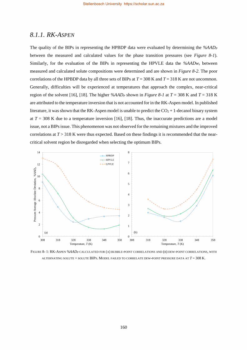
160
8.1.1. RK-ASPEN
The quality of the BIPs in representing the HPBDP data were evaluated by determining the %AADP
between the measured and calculated values for the phase transition pressures (see Figure 8-1).
Similarly, for the evaluation of the BIPs in representing the HPVLE data the %AADws between
measured and calculated solute compositions were determined and are shown in Figure 8-2. The poor
correlations of the HPBDP data by all three sets of BIPs at T = 308 K and T = 318 K are not uncommon.
Generally, difficulties will be experienced at temperatures that approach the complex, near-critical
region of the solvent [16], [18]. The higher %AADP shown in Figure 8-1 at T = 308 K and T = 318 K
are attributed to the temperature inversion that is not accounted for in the RK-Aspen model. In published
literature, it was shown that the RK-Aspen model is unable to predict the CO2 + 1-decanol binary system
at T = 308 K due to a temperature inversion [16], [18]. Thus, the inaccurate predictions are a model
issue, not a BIPs issue. This phenomenon was not observed for the remaining mixtures and the improved
correlations at T > 318 K were thus expected. Based on these findings it is recommended that the near-
critical solvent region be disregarded when selecting the optimum BIPs.
FIGURE 8- 1: RK-ASPEN %AADP CALCULATED FOR (A) BUBBLE-POINT CORRELATIONS AND (B) DEW-POINT CORRELATIONS, WITH
ALTERNATING SOLUTE + SOLUTE BIPS. MODEL FAILED TO CORRELATE DEW-POINT PRESSURE DATA AT T = 308 K.
0
2
4
6
8
10
12
14
308 318 328 338 348 358
Pre
ssure
Aver
age
Ab
solu
te D
evia
tio
n,
%A
AD
P
Temperature, T (K)
HPBDP
HPVLE
LPVLE
0
1
2
3
4
5
6
7
8
308 318 328 338 348 358
Temperature, T (K)
(a) (b)
Stellenbosch University https://scholar.sun.ac.za
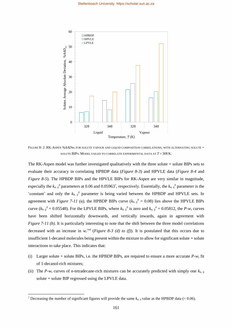
161
FIGURE 8- 2: RK-ASPEN %AADWS FOR SOLUTE VAPOUR AND LIQUID COMPOSITION CORRELATIONS, WITH ALTERNATING SOLUTE +
SOLUTE BIPS. MODEL FAILED TO CORRELATE EXPERIMENTAL DATA AT T = 308 K.
The RK-Aspen model was further investigated qualitatively with the three solute + solute BIPs sets to
evaluate their accuracy in correlating HPBDP data (Figure 8-3) and HPVLE data (Figure 8-4 and
Figure 8-5). The HPBDP BIPs and the HPVLE BIPs for RK-Aspen are very similar in magnitude,
especially the ka, ij0 parameters at 0.06 and 0.059637, respectively. Essentially, the ka, ij
0 parameter is the
‘constant’ and only the kb, ij0 parameter is being varied between the HPBDP and HPVLE sets. In
agreement with Figure 7-11 (a), the HPBDP BIPs curve (kb, ij0 = 0.08) lies above the HPVLE BIPs
curve (kb, ij0 = 0.05548). For the LPVLE BIPs, where kb, ij
0 is zero and ka, ij0 = 0.05812, the P-ws curves
have been shifted horizontally downwards, and vertically inwards, again in agreement with
Figure 7-11 (b). It is particularly interesting to note that the shift between the three model correlations
decreased with an increase in wcred (Figure 8-3 (d) to (f)). It is postulated that this occurs due to
insufficient 1-decanol molecules being present within the mixture to allow for significant solute + solute
interactions to take place. This indicates that:
(i) Larger solute + solute BIPs, i.e. the HPBDP BIPs, are required to ensure a more accurate P-ws fit
of 1-decanol-rich mixtures;
(ii) The P-ws curves of n-tetradecane-rich mixtures can be accurately predicted with simply one ka, ij
solute + solute BIP regressed using the LPVLE data.
7 Decreasing the number of significant figures will provide the same ka, ij value as the HPBDP data (≈ 0.06).
0
10
20
30
40
50
60
328 348 328 348
Liquid Vapour
So
lute
s A
ver
age
Ab
solu
te D
evia
tio
n,
%A
AD
ws
Temperature, T (K)
HPBDP
HPVLE
LPVLE
Stellenbosch University https://scholar.sun.ac.za
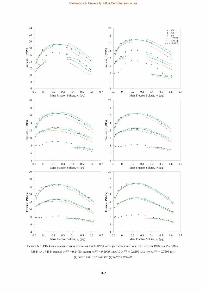
162
FIGURE 8- 3: RK-ASPEN MODEL CORRELATIONS OF THE HPBDP DATA (WITH VARYING SOLUTE + SOLUTE BIPS) AT T = 308 K,
328 K AND 348 K FOR (A) WCRED = 0.2405 G/G; (B) WC
RED = 0.5000 G/G; (C) WCRED = 0.6399 G/G; (D) WC
RED = 0.7698 G/G;
(E) WCRED = 0.8162 G/G; AND (F) WC
RED = 0.9200.
6
8
10
12
14
16
18
20
22
24
0.0 0.1 0.2 0.3 0.4 0.5 0.6 0.7
Pre
ssure
, P
(M
Pa)
Mass Fraction Solutes, ws (g/g)
4
6
8
10
12
14
16
18
20
0.0 0.1 0.2 0.3 0.4 0.5 0.6 0.7
Pre
ssure
, P
(M
Pa)
Mass Fraction Solutes, ws (g/g)
308328348HPBDPHPVLELPVLE
4
6
8
10
12
14
16
18
20
0.0 0.1 0.2 0.3 0.4 0.5 0.6 0.7
Pre
ssure
, P
(M
Pa)
Mass Fraction Solutes, ws (g/g)
4
6
8
10
12
14
16
18
20
0.0 0.1 0.2 0.3 0.4 0.5 0.6 0.7
Pre
ssure
, P
(M
Pa)
Mass Fraction Solutes, ws (g/g)
4
6
8
10
12
14
16
18
20
0.0 0.1 0.2 0.3 0.4 0.5 0.6 0.7
Pre
ssure
, P
(M
Pa)
Mass Fraction Solutes, ws (g/g)
4
6
8
10
12
14
16
18
20
0.0 0.1 0.2 0.3 0.4 0.5 0.6 0.7
Pre
ssure
, P
(M
Pa)
Mass Fraction Solutes, ws (g/g)
Stellenbosch University https://scholar.sun.ac.za
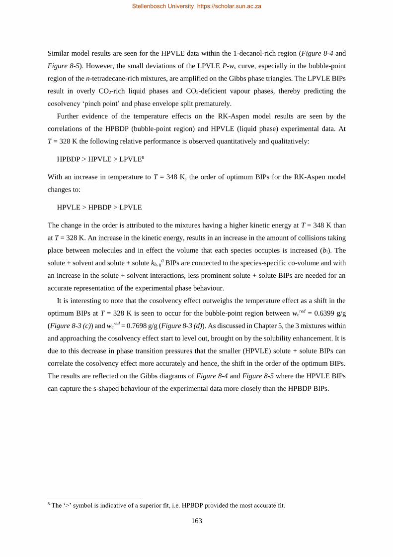
163
Similar model results are seen for the HPVLE data within the 1-decanol-rich region (Figure 8-4 and
Figure 8-5). However, the small deviations of the LPVLE P-ws curve, especially in the bubble-point
region of the n-tetradecane-rich mixtures, are amplified on the Gibbs phase triangles. The LPVLE BIPs
result in overly CO2-rich liquid phases and CO2-deficient vapour phases, thereby predicting the
cosolvency ‘pinch point’ and phase envelope split prematurely.
Further evidence of the temperature effects on the RK-Aspen model results are seen by the
correlations of the HPBDP (bubble-point region) and HPVLE (liquid phase) experimental data. At
T = 328 K the following relative performance is observed quantitatively and qualitatively:
HPBDP > HPVLE > LPVLE8
With an increase in temperature to T = 348 K, the order of optimum BIPs for the RK-Aspen model
changes to:
HPVLE > HPBDP > LPVLE
The change in the order is attributed to the mixtures having a higher kinetic energy at T = 348 K than
at T = 328 K. An increase in the kinetic energy, results in an increase in the amount of collisions taking
place between molecules and in effect the volume that each species occupies is increased (bi). The
solute + solvent and solute + solute kb, ij0 BIPs are connected to the species-specific co-volume and with
an increase in the solute + solvent interactions, less prominent solute + solute BIPs are needed for an
accurate representation of the experimental phase behaviour.
It is interesting to note that the cosolvency effect outweighs the temperature effect as a shift in the
optimum BIPs at T = 328 K is seen to occur for the bubble-point region between wcred = 0.6399 g/g
(Figure 8-3 (c)) and wcred = 0.7698 g/g (Figure 8-3 (d)). As discussed in Chapter 5, the 3 mixtures within
and approaching the cosolvency effect start to level out, brought on by the solubility enhancement. It is
due to this decrease in phase transition pressures that the smaller (HPVLE) solute + solute BIPs can
correlate the cosolvency effect more accurately and hence, the shift in the order of the optimum BIPs.
The results are reflected on the Gibbs diagrams of Figure 8-4 and Figure 8-5 where the HPVLE BIPs
can capture the s-shaped behaviour of the experimental data more closely than the HPBDP BIPs.
8 The ‘>’ symbol is indicative of a superior fit, i.e. HPBDP provided the most accurate fit.
Stellenbosch University https://scholar.sun.ac.za
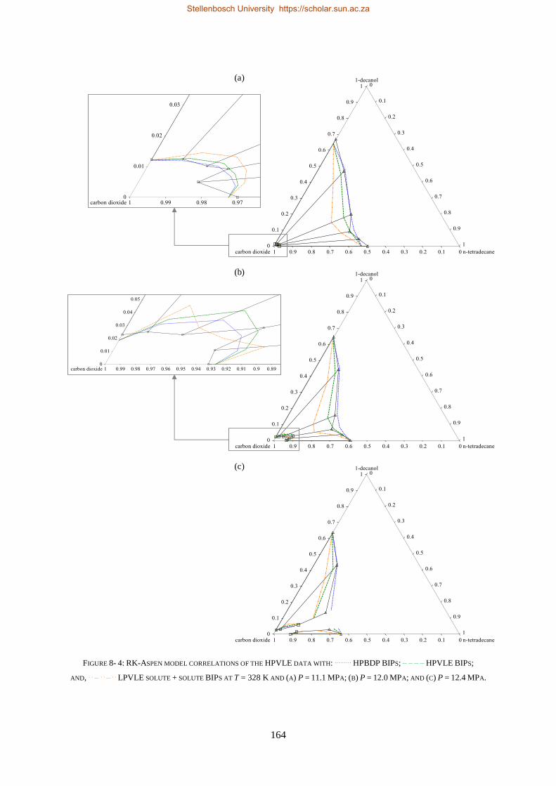
164
FIGURE 8- 4: RK-ASPEN MODEL CORRELATIONS OF THE HPVLE DATA WITH: ……… HPBDP BIPS; – – – – HPVLE BIPS;
AND, . . – . . – . . LPVLE SOLUTE + SOLUTE BIPS AT T = 328 K AND (A) P = 11.1 MPA; (B) P = 12.0 MPA; AND (C) P = 12.4 MPA.
(a)
(b)
(c)
Stellenbosch University https://scholar.sun.ac.za
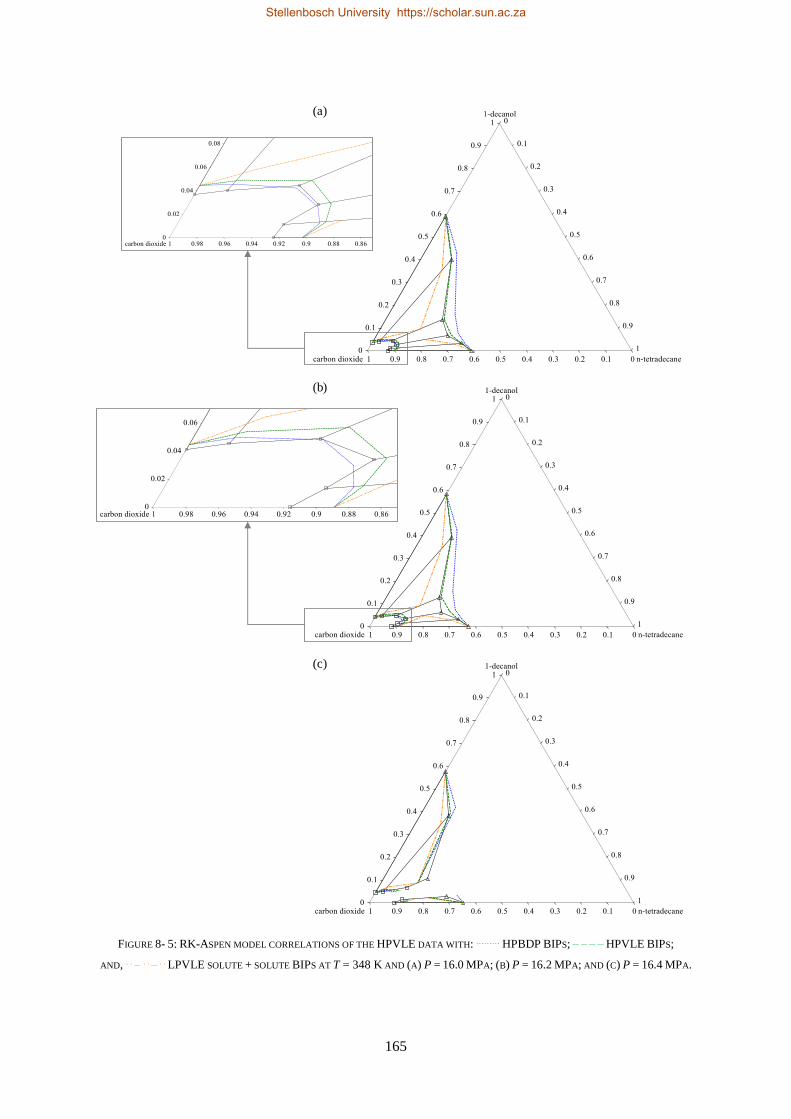
165
FIGURE 8- 5: RK-ASPEN MODEL CORRELATIONS OF THE HPVLE DATA WITH: ……… HPBDP BIPS; – – – – HPVLE BIPS;
AND, . . – . . – . . LPVLE SOLUTE + SOLUTE BIPS AT T = 348 K AND (A) P = 16.0 MPA; (B) P = 16.2 MPA; AND (C) P = 16.4 MPA.
(a)
(b)
(c)
Stellenbosch University https://scholar.sun.ac.za
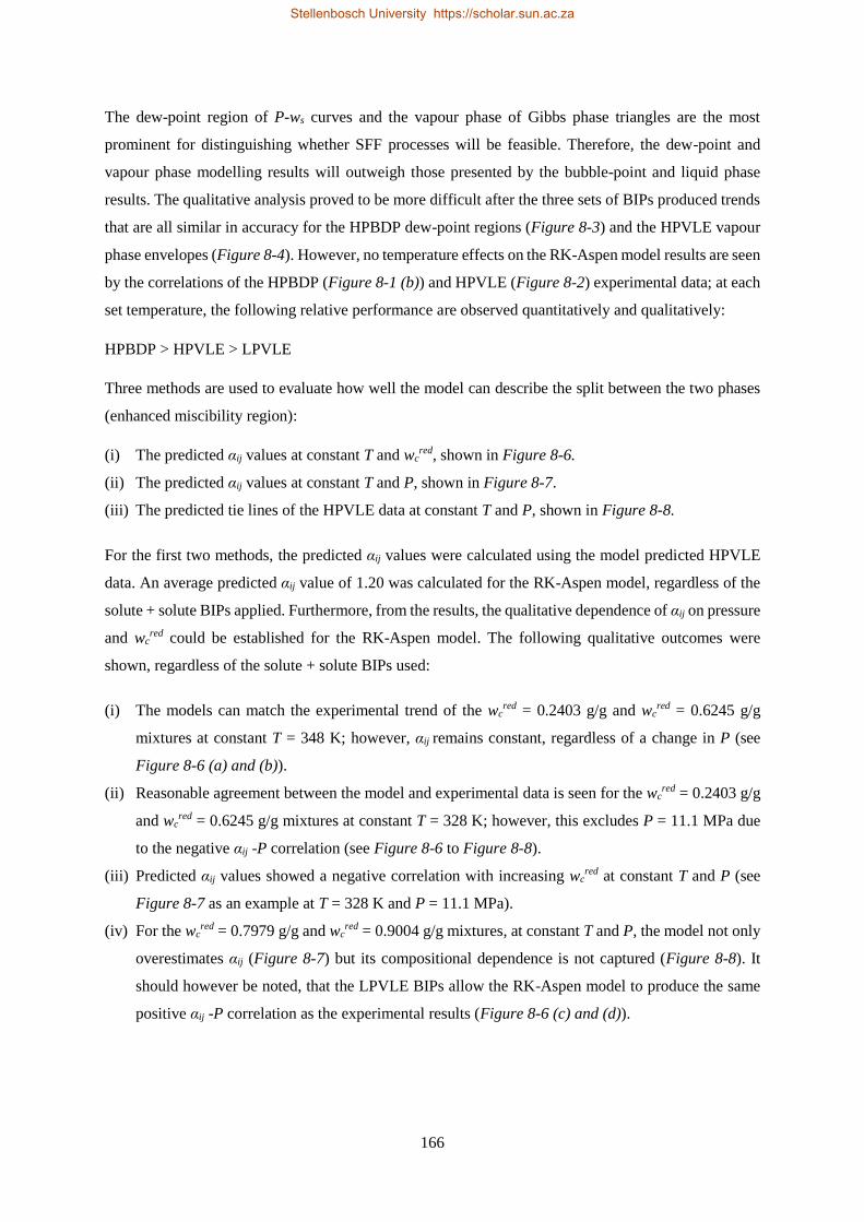
166
The dew-point region of P-ws curves and the vapour phase of Gibbs phase triangles are the most
prominent for distinguishing whether SFF processes will be feasible. Therefore, the dew-point and
vapour phase modelling results will outweigh those presented by the bubble-point and liquid phase
results. The qualitative analysis proved to be more difficult after the three sets of BIPs produced trends
that are all similar in accuracy for the HPBDP dew-point regions (Figure 8-3) and the HPVLE vapour
phase envelopes (Figure 8-4). However, no temperature effects on the RK-Aspen model results are seen
by the correlations of the HPBDP (Figure 8-1 (b)) and HPVLE (Figure 8-2) experimental data; at each
set temperature, the following relative performance are observed quantitatively and qualitatively:
HPBDP > HPVLE > LPVLE
Three methods are used to evaluate how well the model can describe the split between the two phases
(enhanced miscibility region):
(i) The predicted αij values at constant T and wcred, shown in Figure 8-6.
(ii) The predicted αij values at constant T and P, shown in Figure 8-7.
(iii) The predicted tie lines of the HPVLE data at constant T and P, shown in Figure 8-8.
For the first two methods, the predicted αij values were calculated using the model predicted HPVLE
data. An average predicted αij value of 1.20 was calculated for the RK-Aspen model, regardless of the
solute + solute BIPs applied. Furthermore, from the results, the qualitative dependence of αij on pressure
and wcred could be established for the RK-Aspen model. The following qualitative outcomes were
shown, regardless of the solute + solute BIPs used:
(i) The models can match the experimental trend of the wcred = 0.2403 g/g and wc
red = 0.6245 g/g
mixtures at constant T = 348 K; however, αij remains constant, regardless of a change in P (see
Figure 8-6 (a) and (b)).
(ii) Reasonable agreement between the model and experimental data is seen for the wcred = 0.2403 g/g
and wcred = 0.6245 g/g mixtures at constant T = 328 K; however, this excludes P = 11.1 MPa due
to the negative αij -P correlation (see Figure 8-6 to Figure 8-8).
(iii) Predicted αij values showed a negative correlation with increasing wcred at constant T and P (see
Figure 8-7 as an example at T = 328 K and P = 11.1 MPa).
(iv) For the wcred = 0.7979 g/g and wc
red = 0.9004 g/g mixtures, at constant T and P, the model not only
overestimates αij (Figure 8-7) but its compositional dependence is not captured (Figure 8-8). It
should however be noted, that the LPVLE BIPs allow the RK-Aspen model to produce the same
positive αij -P correlation as the experimental results (Figure 8-6 (c) and (d)).
Stellenbosch University https://scholar.sun.ac.za
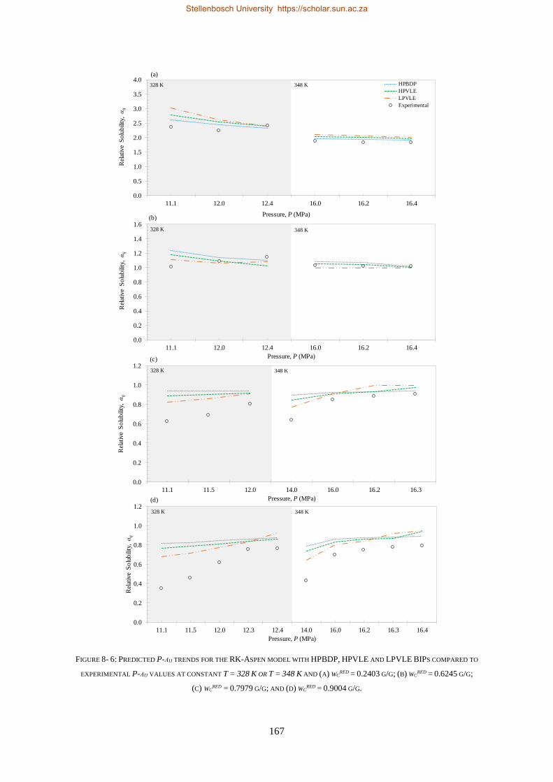
167
FIGURE 8- 6: PREDICTED P-ΑIJ TRENDS FOR THE RK-ASPEN MODEL WITH HPBDP, HPVLE AND LPVLE BIPS COMPARED TO
EXPERIMENTAL P-ΑIJ VALUES AT CONSTANT T = 328 K OR T = 348 K AND (A) WCRED = 0.2403 G/G; (B) WC
RED = 0.6245 G/G;
(C) WCRED = 0.7979 G/G; AND (D) WC
RED = 0.9004 G/G.
328 K 348 K
0.0
0.2
0.4
0.6
0.8
1.0
1.2
11.1 11.5 12.0 12.3 12.4 14.0 16.0 16.2 16.3 16.4
Rel
ativ
e S
olu
bili
ty, α
ij
Pressure, P (MPa)
0.0
0.5
1.0
1.5
2.0
2.5
3.0
3.5
4.0
11.1 12.0 12.4 16.0 16.2 16.4
Rel
ativ
e S
olu
bili
ty, α
ij
Pressure, P (MPa)
HPBDP
HPVLE
LPVLE
Experimental
348 K328 K
328 K 348 K
0.0
0.2
0.4
0.6
0.8
1.0
1.2
11.1 11.5 12.0 14.0 16.0 16.2 16.3
Rel
ativ
e S
olu
bili
ty, α
ij
Pressure, P (MPa)
0.0
0.2
0.4
0.6
0.8
1.0
1.2
1.4
1.6
11.1 12.0 12.4 16.0 16.2 16.4
Rel
ativ
e S
olu
bili
ty, α
ij
Pressure, P (MPa)
328 K 348 K
(a)
(b)
(c)
(d)
Stellenbosch University https://scholar.sun.ac.za
168
FIGURE 8- 7: PREDICTED WCRED -ΑIJ TRENDS FOR THE RK-ASPEN MODEL WITH HPBDP, HPVLE AND LPVLE BIPS COMPARED TO
EXPERIMENTAL ΑIJ VALUES AT CONSTANT T = 328 K AND P = 11.1 MPA.
FIGURE 8- 8: VAPOUR PHASE DETAIL FOR CO2 + 1-DECANOL + N-TETRADECANE PREDICTED TIE LINES WITH THE RK-ASPEN
MODEL USING ……… HPBDP BIPS; – – – – HPVLE BIPS; AND, . . – . . – . . LPVLE SOLUTE + SOLUTE BIPS COMPARED TO
EXPERIMENTAL TIE LINES AT CONSTANT T = 328 K AND P = 11.1 MPA.
0.0
0.5
1.0
1.5
2.0
2.5
3.0
3.5
0.0 0.2 0.4 0.6 0.8 1.0
Pre
dic
ted
Rel
ativ
e S
olu
bili
ty, α
ij
Reduced n-tetradecane Mass Fraction, wcred (g/g)
HPBDP
LPVLE
HPVLE
Experimental
Stellenbosch University https://scholar.sun.ac.za
169
8.1.2. SR-POLAR
The SR-Polar model was investigated with the three solute + solute BIPs sets to evaluate their accuracy
in correlating HPBDP data (Figure 8-9). The HPBDP and the HPVLE BIPs for SR-Polar are not as
similar in magnitude as that seen for RK-Aspen, especially the kb, ij0 parameters at 0.12 and 0.07589,
respectively. As expected, the HPBDP BIPs curves lie above the HPVLE BIPs curves (Figure 8-9)
which agrees with Figure 7-11 (a). However, the shift between the two curves within the bubble-point
region were much smaller than anticipated and were almost non-existent within the dew-point region.
It is postulated that this occurred because the effects of the three, pure component, polar parameters
within the SR-Polar algorithm overpowered those of the BIPs.
For the LPVLE BIPs, where kb, ij0 is zero and ka, ij
0 = 0.05820, the P-ws curves have been shifted
horizontally downwards, and vertically inwards, again in agreement with Figure 7-11 (b). It is
particularly interesting to note that the shift of the LPVLE curves were much more prominent than the
HPVLE and HPBDP curves. This finding indicates that, by only considering the attractive forces in the
system (ka, ij0) the polar parameters are not sufficient to still allow for an accurate overall model fit.
Stellenbosch University https://scholar.sun.ac.za
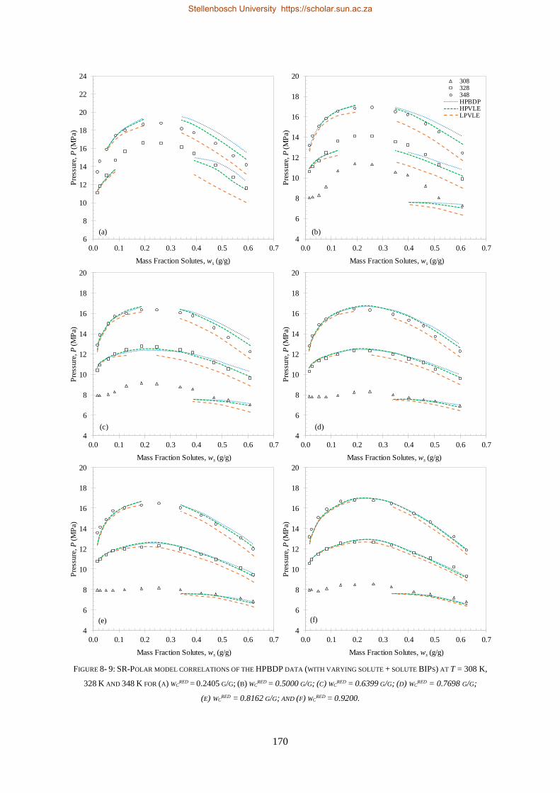
170
FIGURE 8- 9: SR-POLAR MODEL CORRELATIONS OF THE HPBDP DATA (WITH VARYING SOLUTE + SOLUTE BIPS) AT T = 308 K,
328 K AND 348 K FOR (A) WCRED = 0.2405 G/G; (B) WC
RED = 0.5000 G/G; (C) WCRED = 0.6399 G/G; (D) WC
RED = 0.7698 G/G;
(E) WCRED = 0.8162 G/G; AND (F) WC
RED = 0.9200.
4
6
8
10
12
14
16
18
20
0.0 0.1 0.2 0.3 0.4 0.5 0.6 0.7
Pre
ssure
, P
(M
Pa)
Mass Fraction Solutes, ws (g/g)
308328348HPBDPHPVLELPVLE
6
8
10
12
14
16
18
20
22
24
0.0 0.1 0.2 0.3 0.4 0.5 0.6 0.7
Pre
ssure
, P
(M
Pa)
Mass Fraction Solutes, ws (g/g)
4
6
8
10
12
14
16
18
20
0.0 0.1 0.2 0.3 0.4 0.5 0.6 0.7
Pre
ssure
, P
(M
Pa)
Mass Fraction Solutes, ws (g/g)
4
6
8
10
12
14
16
18
20
0.0 0.1 0.2 0.3 0.4 0.5 0.6 0.7
Pre
ssure
, P
(M
Pa)
Mass Fraction Solutes, ws (g/g)
4
6
8
10
12
14
16
18
20
0.0 0.1 0.2 0.3 0.4 0.5 0.6 0.7
Pre
ssure
, P
(M
Pa)
Mass Fraction Solutes, ws (g/g)
4
6
8
10
12
14
16
18
20
0.0 0.1 0.2 0.3 0.4 0.5 0.6 0.7
Pre
ssure
, P
(M
Pa)
Mass Fraction Solutes, ws (g/g)
(a) (b)
(c) (d)
(e) (f)
Stellenbosch University https://scholar.sun.ac.za
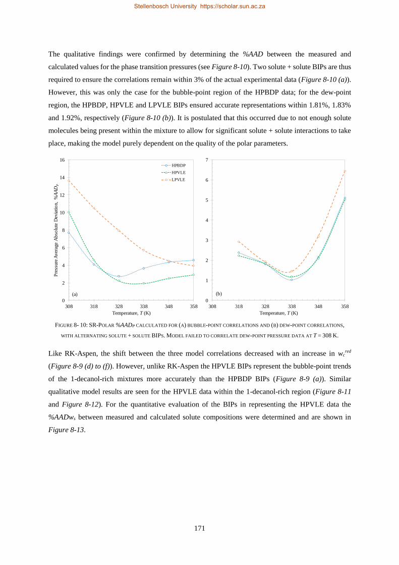
171
The qualitative findings were confirmed by determining the %AAD between the measured and
calculated values for the phase transition pressures (see Figure 8-10). Two solute + solute BIPs are thus
required to ensure the correlations remain within 3% of the actual experimental data (Figure 8-10 (a)).
However, this was only the case for the bubble-point region of the HPBDP data; for the dew-point
region, the HPBDP, HPVLE and LPVLE BIPs ensured accurate representations within 1.81%, 1.83%
and 1.92%, respectively (Figure 8-10 (b)). It is postulated that this occurred due to not enough solute
molecules being present within the mixture to allow for significant solute + solute interactions to take
place, making the model purely dependent on the quality of the polar parameters.
FIGURE 8- 10: SR-POLAR %AADP CALCULATED FOR (A) BUBBLE-POINT CORRELATIONS AND (B) DEW-POINT CORRELATIONS,
WITH ALTERNATING SOLUTE + SOLUTE BIPS. MODEL FAILED TO CORRELATE DEW-POINT PRESSURE DATA AT T = 308 K.
Like RK-Aspen, the shift between the three model correlations decreased with an increase in wcred
(Figure 8-9 (d) to (f)). However, unlike RK-Aspen the HPVLE BIPs represent the bubble-point trends
of the 1-decanol-rich mixtures more accurately than the HPBDP BIPs (Figure 8-9 (a)). Similar
qualitative model results are seen for the HPVLE data within the 1-decanol-rich region (Figure 8-11
and Figure 8-12). For the quantitative evaluation of the BIPs in representing the HPVLE data the
%AADws between measured and calculated solute compositions were determined and are shown in
Figure 8-13.
0
2
4
6
8
10
12
14
16
308 318 328 338 348 358
Pre
ssure
Aver
age
Ab
solu
te D
evia
tio
n,
%A
AD
P
Temperature, T (K)
HPBDP
HPVLE
LPVLE
0
1
2
3
4
5
6
7
308 318 328 338 348 358
Temperature, T (K)
(a) (b)
Stellenbosch University https://scholar.sun.ac.za
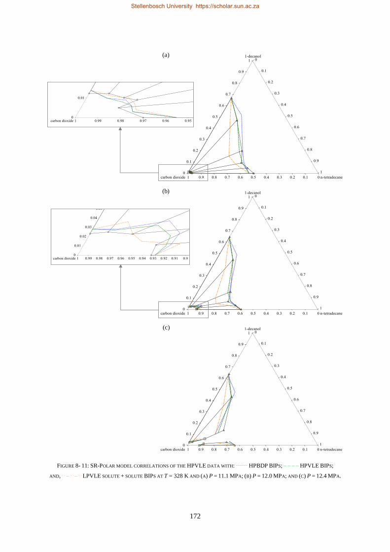
172
FIGURE 8- 11: SR-POLAR MODEL CORRELATIONS OF THE HPVLE DATA WITH: ……… HPBDP BIPS; – – – – HPVLE BIPS;
AND, . . – . . – . . LPVLE SOLUTE + SOLUTE BIPS AT T = 328 K AND (A) P = 11.1 MPA; (B) P = 12.0 MPA; AND (C) P = 12.4 MPA.
(a)
(b)
(c)
Stellenbosch University https://scholar.sun.ac.za
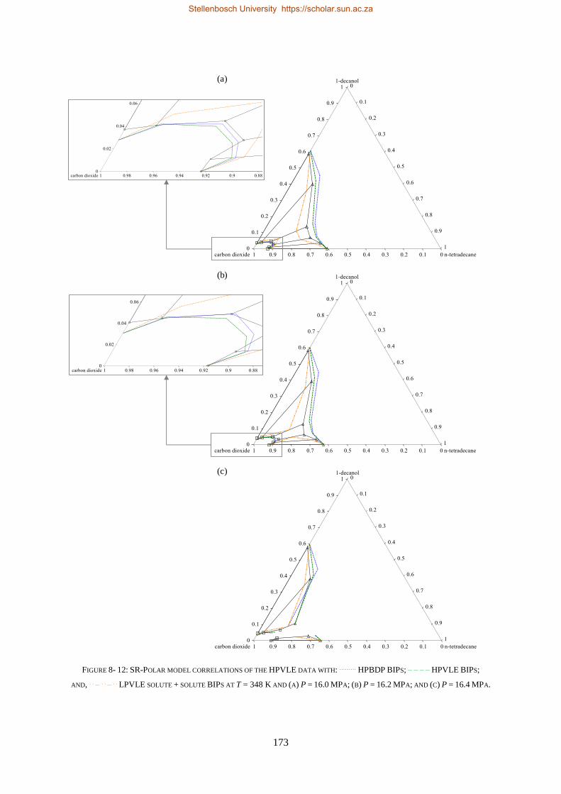
173
FIGURE 8- 12: SR-POLAR MODEL CORRELATIONS OF THE HPVLE DATA WITH: ……… HPBDP BIPS; – – – – HPVLE BIPS;
AND, . . – . . – . . LPVLE SOLUTE + SOLUTE BIPS AT T = 348 K AND (A) P = 16.0 MPA; (B) P = 16.2 MPA; AND (C) P = 16.4 MPA.
(a)
(b)
(c)
Stellenbosch University https://scholar.sun.ac.za
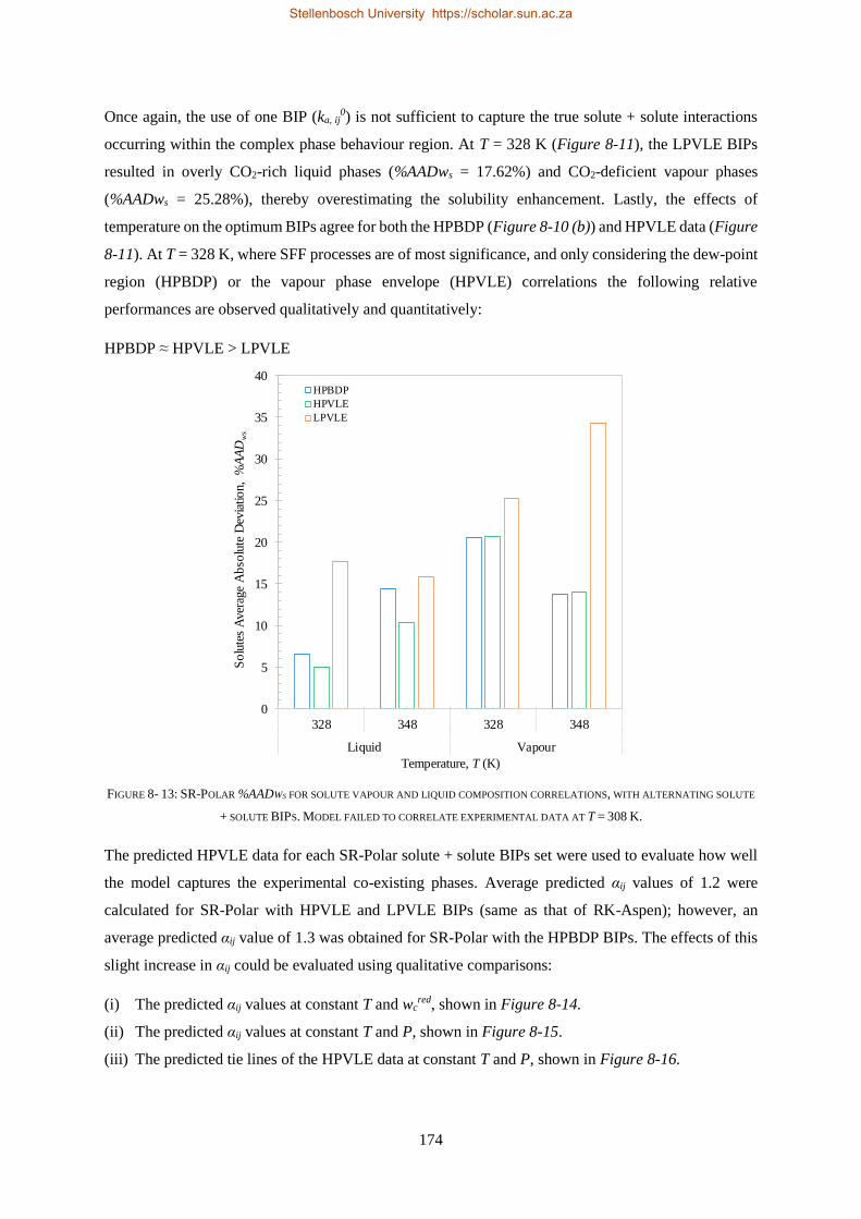
174
Once again, the use of one BIP (ka, ij0) is not sufficient to capture the true solute + solute interactions
occurring within the complex phase behaviour region. At T = 328 K (Figure 8-11), the LPVLE BIPs
resulted in overly CO2-rich liquid phases (%AADws = 17.62%) and CO2-deficient vapour phases
(%AADws = 25.28%), thereby overestimating the solubility enhancement. Lastly, the effects of
temperature on the optimum BIPs agree for both the HPBDP (Figure 8-10 (b)) and HPVLE data (Figure
8-11). At T = 328 K, where SFF processes are of most significance, and only considering the dew-point
region (HPBDP) or the vapour phase envelope (HPVLE) correlations the following relative
performances are observed qualitatively and quantitatively:
HPBDP ≈ HPVLE > LPVLE
FIGURE 8- 13: SR-POLAR %AADWS FOR SOLUTE VAPOUR AND LIQUID COMPOSITION CORRELATIONS, WITH ALTERNATING SOLUTE
+ SOLUTE BIPS. MODEL FAILED TO CORRELATE EXPERIMENTAL DATA AT T = 308 K.
The predicted HPVLE data for each SR-Polar solute + solute BIPs set were used to evaluate how well
the model captures the experimental co-existing phases. Average predicted αij values of 1.2 were
calculated for SR-Polar with HPVLE and LPVLE BIPs (same as that of RK-Aspen); however, an
average predicted αij value of 1.3 was obtained for SR-Polar with the HPBDP BIPs. The effects of this
slight increase in αij could be evaluated using qualitative comparisons:
(i) The predicted αij values at constant T and wcred, shown in Figure 8-14.
(ii) The predicted αij values at constant T and P, shown in Figure 8-15.
(iii) The predicted tie lines of the HPVLE data at constant T and P, shown in Figure 8-16.
0
5
10
15
20
25
30
35
40
328 348 328 348
Liquid Vapour
So
lute
s A
ver
age
Ab
solu
te D
evia
tio
n,
%A
AD
ws
Temperature, T (K)
HPBDP
HPVLE
LPVLE
Stellenbosch University https://scholar.sun.ac.za
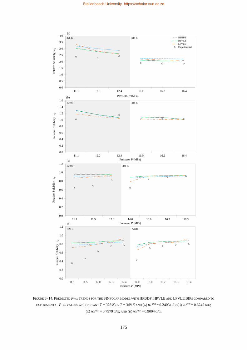
175
FIGURE 8- 14: PREDICTED P-ΑIJ TRENDS FOR THE SR-POLAR MODEL WITH HPBDP, HPVLE AND LPVLE BIPS COMPARED TO
EXPERIMENTAL P-ΑIJ VALUES AT CONSTANT T = 328 K OR T = 348 K AND (A) WCRED = 0.2403 G/G; (B) WC
RED = 0.6245 G/G;
(C) WCRED = 0.7979 G/G; AND (D) WC
RED = 0.9004 G/G.
328 K 348 K
0.0
0.2
0.4
0.6
0.8
1.0
1.2
11.1 11.5 12.0 12.3 12.4 14.0 16.0 16.2 16.3 16.4
Rel
ativ
e S
olu
bili
ty, α
ij
Pressure, P (MPa)
0.0
0.5
1.0
1.5
2.0
2.5
3.0
3.5
4.0
11.1 12.0 12.4 16.0 16.2 16.4
Rel
ativ
e S
olu
bili
ty, α
ij
Pressure, P (MPa)
HPBDP
HPVLE
LPVLE
Experimental
348 K328 K
328 K 348 K
0.0
0.2
0.4
0.6
0.8
1.0
1.2
11.1 11.5 12.0 14.0 16.0 16.2 16.3
Rel
ativ
e S
olu
bili
ty, α
ij
Pressure, P (MPa)
0.0
0.2
0.4
0.6
0.8
1.0
1.2
1.4
1.6
11.1 12.0 12.4 16.0 16.2 16.4
Rel
ativ
e S
olu
bili
ty, α
ij
Pressure, P (MPa)
328 K 348 K
(a)
(b)
(c)
(d)
Stellenbosch University https://scholar.sun.ac.za
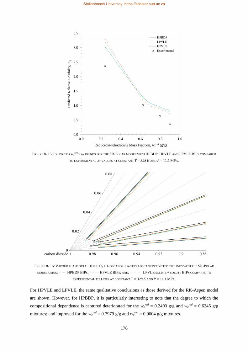
176
FIGURE 8- 15: PREDICTED WCRED -ΑIJ TRENDS FOR THE SR-POLAR MODEL WITH HPBDP, HPVLE AND LPVLE BIPS COMPARED
TO EXPERIMENTAL ΑIJ VALUES AT CONSTANT T = 328 K AND P = 11.1 MPA.
FIGURE 8- 16: VAPOUR PHASE DETAIL FOR CO2 + 1-DECANOL + N-TETRADECANE PREDICTED TIE LINES WITH THE SR-POLAR
MODEL USING: ……… HPBDP BIPS; – – – – HPVLE BIPS; AND, . . – . . – . . LPVLE SOLUTE + SOLUTE BIPS COMPARED TO
EXPERIMENTAL TIE LINES AT CONSTANT T = 328 K AND P = 11.1 MPA.
For HPVLE and LPVLE, the same qualitative conclusions as those derived for the RK-Aspen model
are shown. However, for HPBDP, it is particularly interesting to note that the degree to which the
compositional dependence is captured deteriorated for the wcred = 0.2403 g/g and wc
red = 0.6245 g/g
mixtures; and improved for the wcred = 0.7979 g/g and wc
red = 0.9004 g/g mixtures.
0.0
0.5
1.0
1.5
2.0
2.5
3.0
3.5
0.0 0.2 0.4 0.6 0.8 1.0
Pre
dic
ted
Rel
ativ
e S
olu
bili
ty, α
ij
Reduced n-tetradecane Mass Fraction, wcred (g/g)
HPBDP
LPVLE
HPVLE
Experimental
Stellenbosch University https://scholar.sun.ac.za
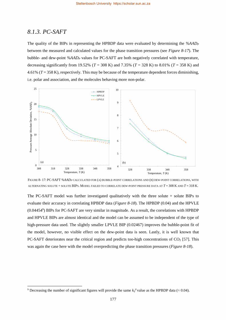
177
8.1.3. PC-SAFT
The quality of the BIPs in representing the HPBDP data were evaluated by determining the %AADP
between the measured and calculated values for the phase transition pressures (see Figure 8-17). The
bubble- and dew-point %AADP values for PC-SAFT are both negatively correlated with temperature,
decreasing significantly from 19.52% (T = 308 K) and 7.35% (T = 328 K) to 8.01% (T = 358 K) and
4.61% (T = 358 K), respectively. This may be because of the temperature dependent forces diminishing,
i.e. polar and association, and the molecules behaving more non-polar.
FIGURE 8- 17: PC-SAFT %AADP CALCULATED FOR (A) BUBBLE-POINT CORRELATIONS AND (B) DEW-POINT CORRELATIONS, WITH
ALTERNATING SOLUTE + SOLUTE BIPS. MODEL FAILED TO CORRELATE DEW-POINT PRESSURE DATA AT T = 308 K AND T = 318 K.
The PC-SAFT model was further investigated qualitatively with the three solute + solute BIPs to
evaluate their accuracy in correlating HPBDP data (Figure 8-18). The HPBDP (0.04) and the HPVLE
(0.044549) BIPs for PC-SAFT are very similar in magnitude. As a result, the correlations with HPBDP
and HPVLE BIPs are almost identical and the model can be assumed to be independent of the type of
high-pressure data used. The slightly smaller LPVLE BIP (0.02467) improves the bubble-point fit of
the model, however, no visible effect on the dew-point data is seen. Lastly, it is well known that
PC-SAFT deteriorates near the critical region and predicts too-high concentrations of CO2 [57]. This
was again the case here with the model overpredicting the phase transition pressures (Figure 8-18).
9 Decreasing the number of significant figures will provide the same kij
0 value as the HPBDP data (≈ 0.04).
0
5
10
15
20
25
308 318 328 338 348 358
Pre
ssure
Aver
age
Ab
solu
te D
evia
tio
n,
%A
AD
P
Temperature, T (K)
HPBDP
HPVLE
LPVLE
4
5
6
7
8
9
10
328 338 348 358
Temperature, T (K)
(a) (b)
Stellenbosch University https://scholar.sun.ac.za
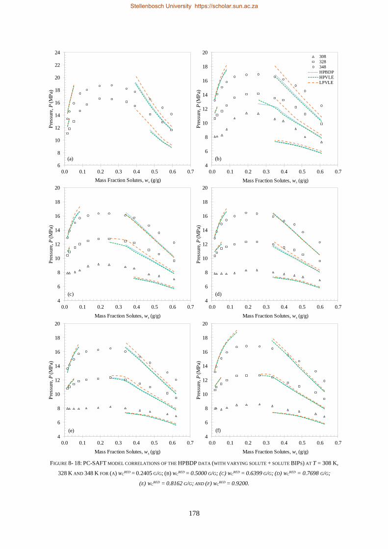
178
FIGURE 8- 18: PC-SAFT MODEL CORRELATIONS OF THE HPBDP DATA (WITH VARYING SOLUTE + SOLUTE BIPS) AT T = 308 K,
328 K AND 348 K FOR (A) WCRED = 0.2405 G/G; (B) WC
RED = 0.5000 G/G; (C) WCRED = 0.6399 G/G; (D) WC
RED = 0.7698 G/G;
(E) WCRED = 0.8162 G/G; AND (F) WC
RED = 0.9200.
4
6
8
10
12
14
16
18
20
0.0 0.1 0.2 0.3 0.4 0.5 0.6 0.7
Pre
ssure
, P
(M
Pa)
Mass Fraction Solutes, ws (g/g)
4
6
8
10
12
14
16
18
20
0.0 0.1 0.2 0.3 0.4 0.5 0.6 0.7
Pre
ssure
, P
(M
Pa)
Mass Fraction Solutes, ws (g/g)
4
6
8
10
12
14
16
18
20
0.0 0.1 0.2 0.3 0.4 0.5 0.6 0.7
Pre
ssure
, P
(M
Pa)
Mass Fraction Solutes, ws (g/g)
308
328
348
HPBDP
HPVLE
LPVLE
6
8
10
12
14
16
18
20
22
24
0.0 0.1 0.2 0.3 0.4 0.5 0.6 0.7
Pre
ssure
, P
(M
Pa)
Mass Fraction Solutes, ws (g/g)
4
6
8
10
12
14
16
18
20
0.0 0.1 0.2 0.3 0.4 0.5 0.6 0.7
Pre
ssure
, P
(M
Pa)
Mass Fraction Solutes, ws (g/g)
4
6
8
10
12
14
16
18
20
0.0 0.1 0.2 0.3 0.4 0.5 0.6 0.7
Pre
ssure
, P
(M
Pa)
Mass Fraction Solutes, ws (g/g)
(a) (b)
(c) (d)
(e) (f)
Stellenbosch University https://scholar.sun.ac.za
179
With respect to the HPVLE data correlations shown in Figure 8-19 and Figure 8-20, PC-SAFT can
capture the liquid phase trend to some extent at T = 348 K (Figure 8-20). This is somewhat expected,
since the system is influenced greatly by molecular association and this model explicitly accounts for
them, i.e. the Wertheim’s association term [110], [181], [255] (Chapter 3, section 3.6). However,
problems with the model are still encountered in representing the vapour phase composition data
(Figure 8-19 and Figure 8-20). The qualitative results are confirmed with the %AADws values
calculated for PC-SAFT (see Figure 8-21). The %AADws values calculated for the liquid phase at
T = 328 K and T = 348 K are approximately one-half of those obtained from the vapour phase.
The shortcomings in the model could originate from the polar forces that are not explicitly accounted
for in the ternary system. The concentration of hydrogen bonding segments in each mixture are high
and lead to hydrogen bond co-operativity forming [174], [256]–[258]. Wertheim’s association term
cannot account for these effects which have led to the poor CO2-rich model correlations.
The following factors are postulated to be cause for the poor representations at T = 328 K
(Figure 8-19):
(i) Cross-association [197].
(ii) Steric hindrances in hydrogen bonding.
(iii) The influence of mixture composition with respect to the number of bonding sites on
molecules [201].
It is particularly interesting to note that all three sets of BIPs can produce the s-shaped curve within the
complex phase behaviour region of the system. This finding is contradicting to the model correlations
of a similar ternary system, CO2 + 1-decanol + n-dodecane [19], [158]. Whether the improved
correlations are attributed to the inclusion of the quadrupole moment of the CO2 molecule can only be
established if all the model factors remained the same, i.e. the temperature dependence and the
components in the system. Quantitatively the HPBDP (Figure 8-17) and HPVLE (Figure 8-21)
correlations agree. For the dew-point region/vapour phase compositions, at T = 328 K the following
relative performances are observed qualitatively and quantitatively:
HPBDP ≈ HPVLE > LPVLE
Stellenbosch University https://scholar.sun.ac.za
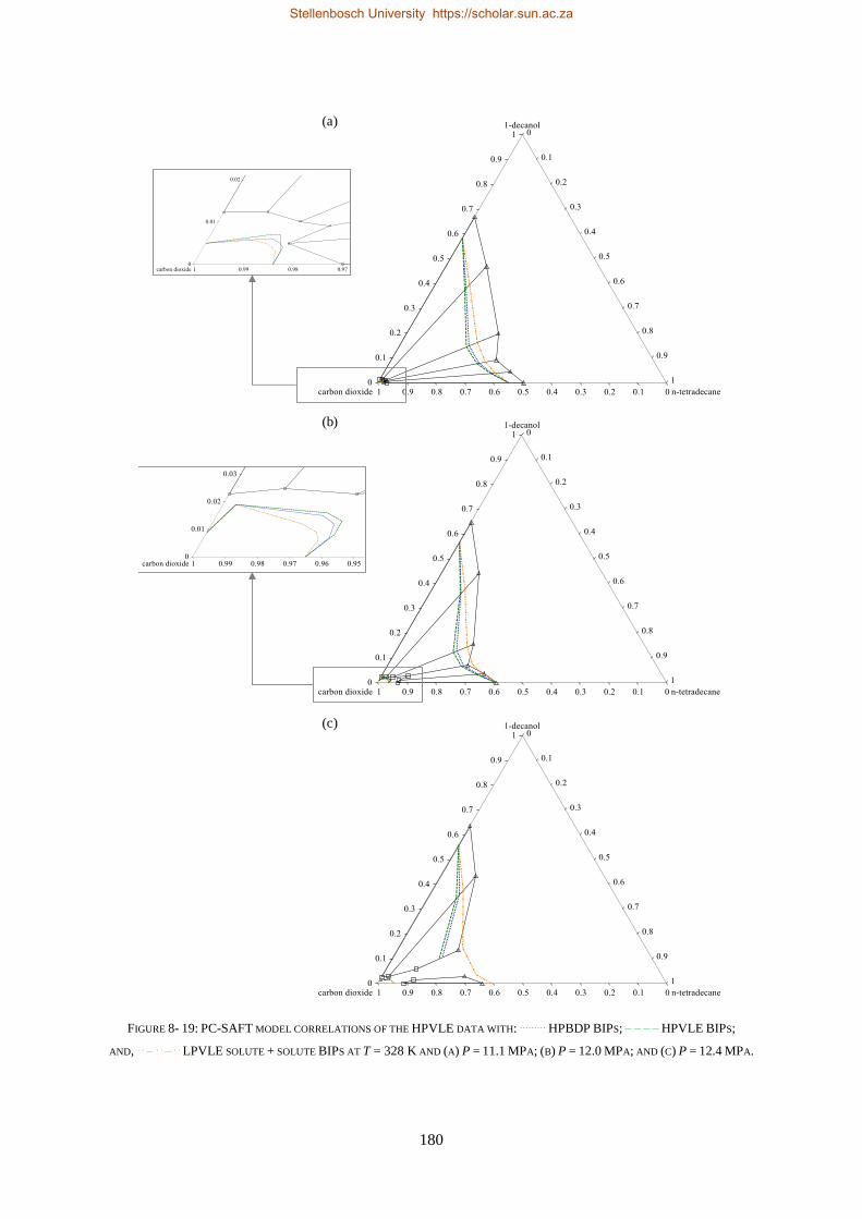
180
FIGURE 8- 19: PC-SAFT MODEL CORRELATIONS OF THE HPVLE DATA WITH: ……… HPBDP BIPS; – – – – HPVLE BIPS;
AND, . . – . . – . . LPVLE SOLUTE + SOLUTE BIPS AT T = 328 K AND (A) P = 11.1 MPA; (B) P = 12.0 MPA; AND (C) P = 12.4 MPA.
(a)
(b)
(c)
Stellenbosch University https://scholar.sun.ac.za
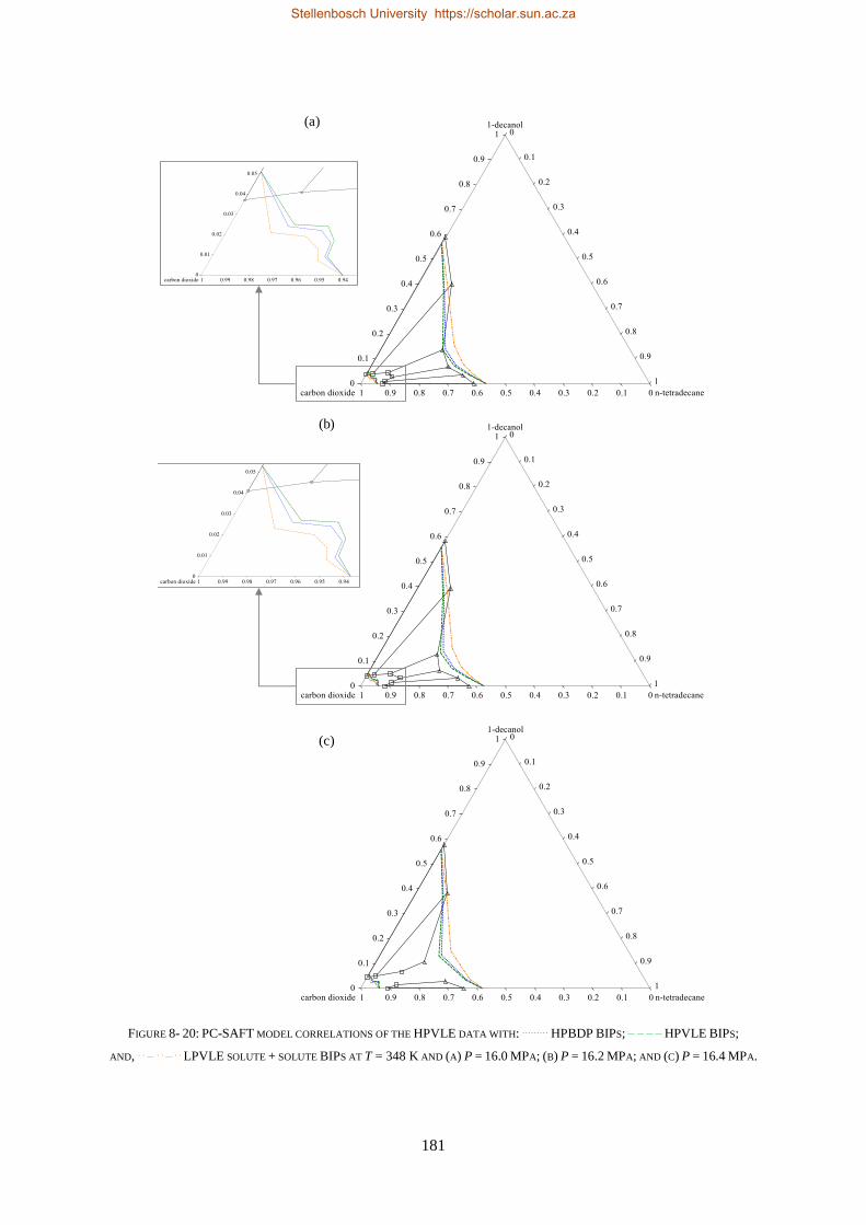
181
FIGURE 8- 20: PC-SAFT MODEL CORRELATIONS OF THE HPVLE DATA WITH: ……… HPBDP BIPS; – – – – HPVLE BIPS;
AND, . . – . . – . . LPVLE SOLUTE + SOLUTE BIPS AT T = 348 K AND (A) P = 16.0 MPA; (B) P = 16.2 MPA; AND (C) P = 16.4 MPA.
(a)
(b)
(c)
Stellenbosch University https://scholar.sun.ac.za
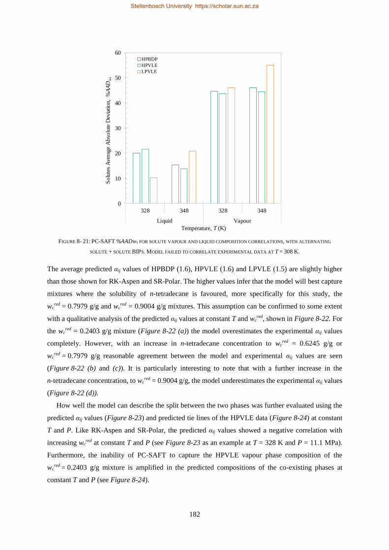
182
FIGURE 8- 21: PC-SAFT %AADWS FOR SOLUTE VAPOUR AND LIQUID COMPOSITION CORRELATIONS, WITH ALTERNATING
SOLUTE + SOLUTE BIPS. MODEL FAILED TO CORRELATE EXPERIMENTAL DATA AT T = 308 K.
The average predicted αij values of HPBDP (1.6), HPVLE (1.6) and LPVLE (1.5) are slightly higher
than those shown for RK-Aspen and SR-Polar. The higher values infer that the model will best capture
mixtures where the solubility of n-tetradecane is favoured, more specifically for this study, the
wcred = 0.7979 g/g and wc
red = 0.9004 g/g mixtures. This assumption can be confirmed to some extent
with a qualitative analysis of the predicted αij values at constant T and wcred, shown in Figure 8-22. For
the wcred = 0.2403 g/g mixture (Figure 8-22 (a)) the model overestimates the experimental αij values
completely. However, with an increase in n-tetradecane concentration to wcred = 0.6245 g/g or
wcred = 0.7979 g/g reasonable agreement between the model and experimental αij values are seen
(Figure 8-22 (b) and (c)). It is particularly interesting to note that with a further increase in the
n-tetradecane concentration, to wcred = 0.9004 g/g, the model underestimates the experimental αij values
(Figure 8-22 (d)).
How well the model can describe the split between the two phases was further evaluated using the
predicted αij values (Figure 8-23) and predicted tie lines of the HPVLE data (Figure 8-24) at constant
T and P. Like RK-Aspen and SR-Polar, the predicted αij values showed a negative correlation with
increasing wcred at constant T and P (see Figure 8-23 as an example at T = 328 K and P = 11.1 MPa).
Furthermore, the inability of PC-SAFT to capture the HPVLE vapour phase composition of the
wcred = 0.2403 g/g mixture is amplified in the predicted compositions of the co-existing phases at
constant T and P (see Figure 8-24).
0
10
20
30
40
50
60
328 348 328 348
Liquid Vapour
So
lute
s A
ver
age
Ab
solu
te D
evia
tio
n,
%A
AD
ws
Temperature, T (K)
HPBDP
HPVLE
LPVLE
Stellenbosch University https://scholar.sun.ac.za
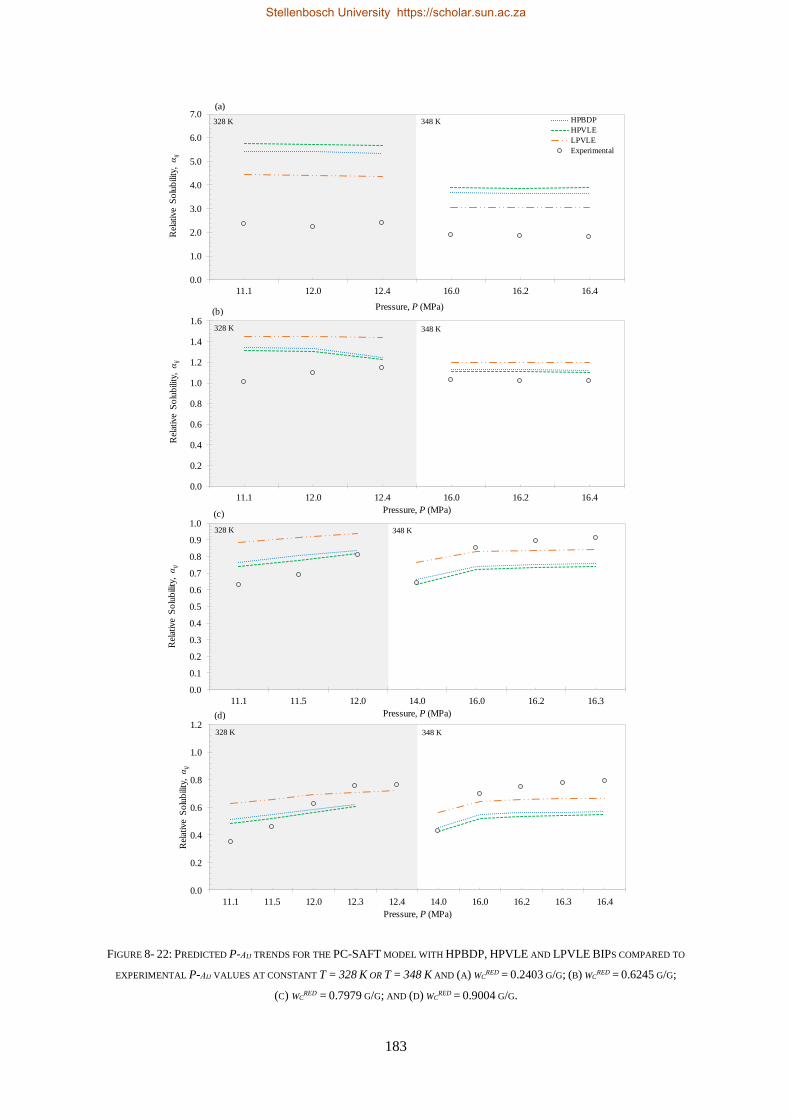
183
FIGURE 8- 22: PREDICTED P-ΑIJ TRENDS FOR THE PC-SAFT MODEL WITH HPBDP, HPVLE AND LPVLE BIPS COMPARED TO
EXPERIMENTAL P-ΑIJ VALUES AT CONSTANT T = 328 K OR T = 348 K AND (A) WCRED = 0.2403 G/G; (B) WC
RED = 0.6245 G/G;
(C) WCRED = 0.7979 G/G; AND (D) WC
RED = 0.9004 G/G.
328 K 348 K
0.0
0.2
0.4
0.6
0.8
1.0
1.2
11.1 11.5 12.0 12.3 12.4 14.0 16.0 16.2 16.3 16.4
Rel
ativ
e S
olu
bili
ty, α
ij
Pressure, P (MPa)
0.0
1.0
2.0
3.0
4.0
5.0
6.0
7.0
11.1 12.0 12.4 16.0 16.2 16.4
Rel
ativ
e S
olu
bili
ty, α
ij
Pressure, P (MPa)
HPBDP
HPVLE
LPVLE
Experimental
348 K328 K
328 K 348 K
0.0
0.1
0.2
0.3
0.4
0.5
0.6
0.7
0.8
0.9
1.0
11.1 11.5 12.0 14.0 16.0 16.2 16.3
Rel
ativ
e S
olu
bili
ty, α
ij
Pressure, P (MPa)
0.0
0.2
0.4
0.6
0.8
1.0
1.2
1.4
1.6
11.1 12.0 12.4 16.0 16.2 16.4
Rel
ativ
e S
olu
bili
ty, α
ij
Pressure, P (MPa)
328 K 348 K
(a)
(b)
(c)
(d)
Stellenbosch University https://scholar.sun.ac.za
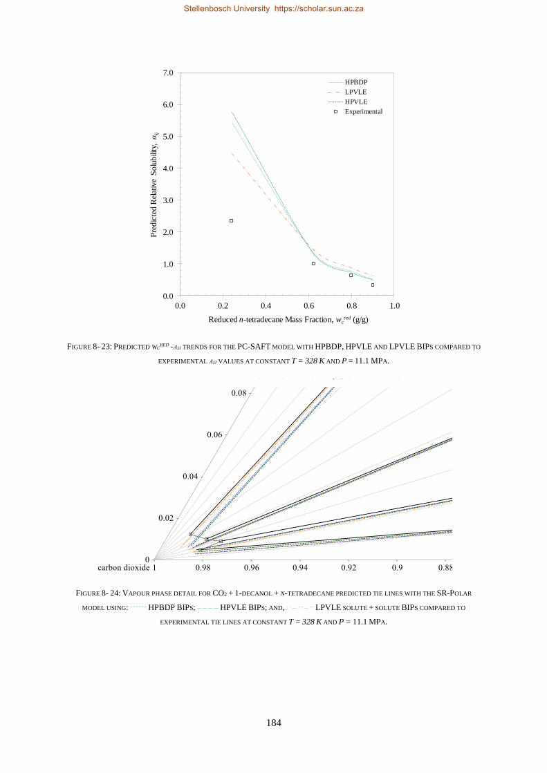
184
FIGURE 8- 23: PREDICTED WCRED -ΑIJ TRENDS FOR THE PC-SAFT MODEL WITH HPBDP, HPVLE AND LPVLE BIPS COMPARED TO
EXPERIMENTAL ΑIJ VALUES AT CONSTANT T = 328 K AND P = 11.1 MPA.
FIGURE 8- 24: VAPOUR PHASE DETAIL FOR CO2 + 1-DECANOL + N-TETRADECANE PREDICTED TIE LINES WITH THE SR-POLAR
MODEL USING: ……… HPBDP BIPS; – – – – HPVLE BIPS; AND, . . – . . – . . LPVLE SOLUTE + SOLUTE BIPS COMPARED TO
EXPERIMENTAL TIE LINES AT CONSTANT T = 328 K AND P = 11.1 MPA.
0.0
1.0
2.0
3.0
4.0
5.0
6.0
7.0
0.0 0.2 0.4 0.6 0.8 1.0
Pre
dic
ted
Rel
ativ
e S
olu
bili
ty, α
ij
Reduced n-tetradecane Mass Fraction, wcred (g/g)
HPBDP
LPVLE
HPVLE
Experimental
Stellenbosch University https://scholar.sun.ac.za
185
8.1.4. PSRK
The PSRK model was investigated to evaluate its ability to predict:
(i) HPBDP data (Figure 8-25).
(ii) HPVLE data (Figure 8-26).
(iii) The tie lines (compositional dependence) at constant T and P (Figure 8-27).
(iv) The relative solubility at constant T and P (Figure 8-28).
(v) The relative solubility at constant T and wcred (Figure 8-29).
With respect to Figure 8-25, PSRK strictly enforces the use of the linear mixing rule for the co-volume
parameter, which limited the accuracy of the predictions, especially in the bubble-point region of the
HPBDP data. Further exclusions occurred in the critical region of each mixture (Figure 8-25). However,
of more importance to the success of SFF processes are the model’s capabilities in predicting the dew-
point region/vapour phase composition of the mixtures. PSRK showed remarkable results in predicting
the dew-point HPBDP experimental data, especially for the mixtures within the complex phase
behaviour region (Figure 8-25 (d), (e) and (f)).
Quantitatively, the PSRK results at T = 328 K are reasonably accurate in predicting the HPBDP data
with bubble- and dew-point pressure deviations within 5.70% and 3.38%, respectively. Unfortunately,
the same cannot be said for the HPVLE %AADws values which were calculated at 19.4% and 34.1%
for the liquid and vapour phase envelopes, respectively.
PSRK predictions of the HPVLE data (Figure 8-26) are too rich in solutes, i.e., lower CO2 solubility,
regardless of a change in temperature or pressure. Thus, the model is unable to capture the vapour or
liquid phase transition curves nor predict the co-solubility pinch.
The model can to a certain degree predict the vapour phase composition of the wcred = 0.2403 g/g
mixture (see Figure 8-26); which is also evident from the great predictability of the coexisting
concentrations (tie line) of the wcred = 0.2403 g/g mixture shown in Figure 8-27. However, the
compositional dependence of the complex phase behaviour region and the n-tetradecane-rich region
could not be captured.
An average relative solubility of 1.6 was calculated from the PSRK predicted VLE data, much higher
than the average experimental αij value of 1.1. The overestimation of the experimentally derived αij
values are further evident from the wcred- αij correlations (Figure 8-28) and P- αij correlations
(Figure 8-29). Apart from the wcred = 0.2403 g/g mixture, it is particularly interesting to note that the
predicted αij values are negatively correlated with pressure, contradicting the positive P- αij correlations
shown by the experimental results (Figure 8-29). Therefore, PSRK is unable to capture the trend of the
data and the advantage of using regressed parameters with real data is prominent.
Stellenbosch University https://scholar.sun.ac.za
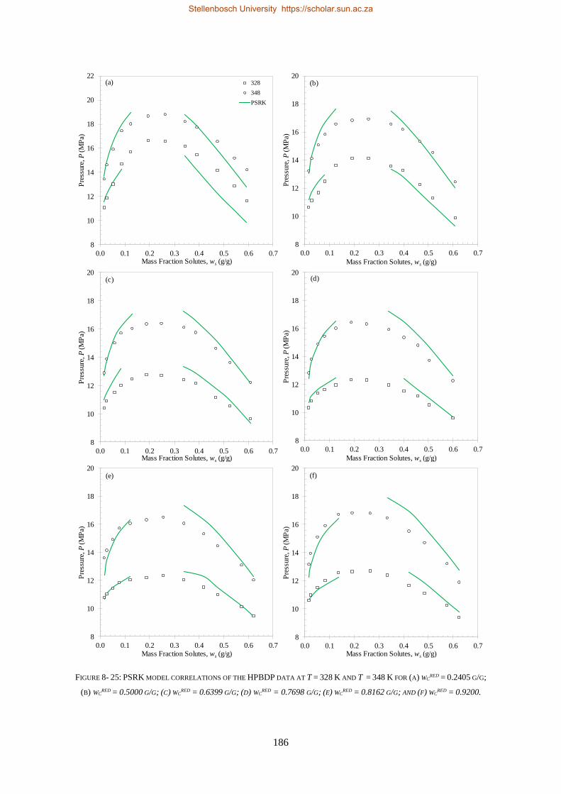
186
FIGURE 8- 25: PSRK MODEL CORRELATIONS OF THE HPBDP DATA AT T = 328 K AND T = 348 K FOR (A) WCRED = 0.2405 G/G;
(B) WCRED = 0.5000 G/G; (C) WC
RED = 0.6399 G/G; (D) WCRED = 0.7698 G/G; (E) WC
RED = 0.8162 G/G; AND (F) WCRED = 0.9200.
8
10
12
14
16
18
20
0.0 0.1 0.2 0.3 0.4 0.5 0.6 0.7
Pre
ssure
, P
(M
Pa)
Mass Fraction Solutes, ws (g/g)
8
10
12
14
16
18
20
0.0 0.1 0.2 0.3 0.4 0.5 0.6 0.7
Pre
ssure
, P
(M
Pa)
Mass Fraction Solutes, ws (g/g)
8
10
12
14
16
18
20
0.0 0.1 0.2 0.3 0.4 0.5 0.6 0.7
Pre
ssure
, P
(M
Pa)
Mass Fraction Solutes, ws (g/g)
8
10
12
14
16
18
20
22
0.0 0.1 0.2 0.3 0.4 0.5 0.6 0.7
Pre
ssure
, P
(M
Pa)
Mass Fraction Solutes, ws (g/g)
328
348
PSRK
8
10
12
14
16
18
20
0.0 0.1 0.2 0.3 0.4 0.5 0.6 0.7
Pre
ssure
, P
(M
Pa)
Mass Fraction Solutes, ws (g/g)
8
10
12
14
16
18
20
0.0 0.1 0.2 0.3 0.4 0.5 0.6 0.7
Pre
ssure
, P
(M
Pa)
Mass Fraction Solutes, ws (g/g)
(f)(e)
(d)(c)
(a) (b)
Stellenbosch University https://scholar.sun.ac.za
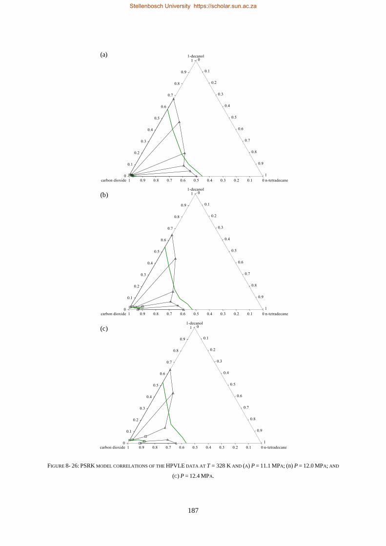
187
FIGURE 8- 26: PSRK MODEL CORRELATIONS OF THE HPVLE DATA AT T = 328 K AND (A) P = 11.1 MPA; (B) P = 12.0 MPA; AND
(C) P = 12.4 MPA.
(a)
(b)
(c)
Stellenbosch University https://scholar.sun.ac.za
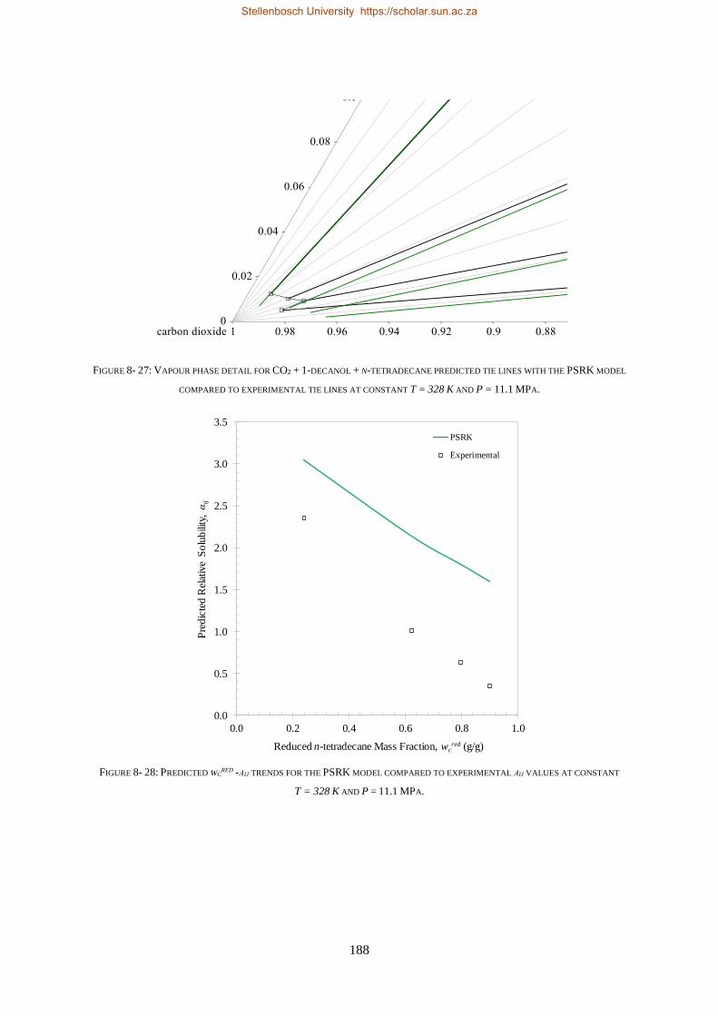
188
FIGURE 8- 27: VAPOUR PHASE DETAIL FOR CO2 + 1-DECANOL + N-TETRADECANE PREDICTED TIE LINES WITH THE PSRK MODEL
COMPARED TO EXPERIMENTAL TIE LINES AT CONSTANT T = 328 K AND P = 11.1 MPA.
FIGURE 8- 28: PREDICTED WCRED -ΑIJ TRENDS FOR THE PSRK MODEL COMPARED TO EXPERIMENTAL ΑIJ VALUES AT CONSTANT
T = 328 K AND P = 11.1 MPA.
0.0
0.5
1.0
1.5
2.0
2.5
3.0
3.5
0.0 0.2 0.4 0.6 0.8 1.0
Pre
dic
ted
Rel
ativ
e S
olu
bili
ty, α
ij
Reduced n-tetradecane Mass Fraction, wcred (g/g)
PSRK
Experimental
Stellenbosch University https://scholar.sun.ac.za
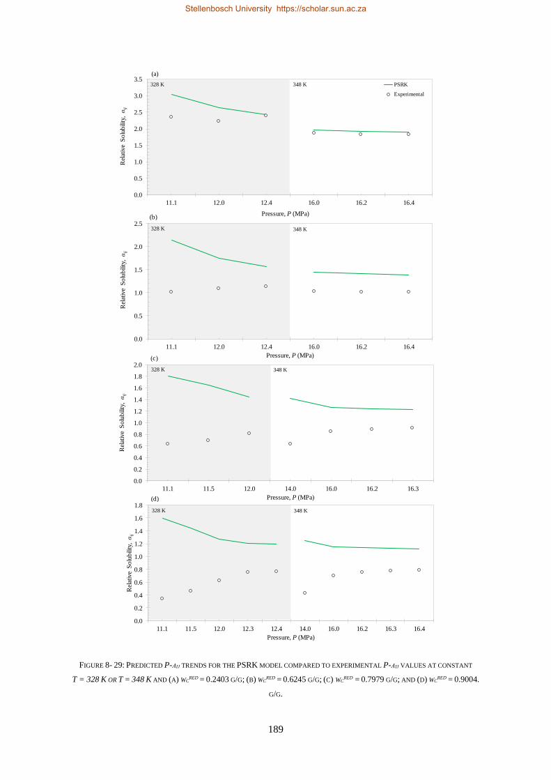
189
FIGURE 8- 29: PREDICTED P-ΑIJ TRENDS FOR THE PSRK MODEL COMPARED TO EXPERIMENTAL P-ΑIJ VALUES AT CONSTANT
T = 328 K OR T = 348 K AND (A) WCRED = 0.2403 G/G; (B) WC
RED = 0.6245 G/G; (C) WCRED = 0.7979 G/G; AND (D) WC
RED = 0.9004.
G/G.
328 K 348 K
0.0
0.2
0.4
0.6
0.8
1.0
1.2
1.4
1.6
1.8
11.1 11.5 12.0 12.3 12.4 14.0 16.0 16.2 16.3 16.4
Rel
ativ
e S
olu
bili
ty, α
ij
Pressure, P (MPa)
0.0
0.5
1.0
1.5
2.0
2.5
3.0
3.5
11.1 12.0 12.4 16.0 16.2 16.4
Rel
ativ
e S
olu
bili
ty, α
ij
Pressure, P (MPa)
PSRK
Experimental
348 K328 K
328 K 348 K
0.0
0.2
0.4
0.6
0.8
1.0
1.2
1.4
1.6
1.8
2.0
11.1 11.5 12.0 14.0 16.0 16.2 16.3
Rel
ativ
e S
olu
bili
ty, α
ij
Pressure, P (MPa)
0.0
0.5
1.0
1.5
2.0
2.5
11.1 12.0 12.4 16.0 16.2 16.4
Rel
ativ
e S
olu
bili
ty, α
ij
Pressure, P (MPa)
328 K 348 K
(a)
(b)
(c)
(d)
Stellenbosch University https://scholar.sun.ac.za
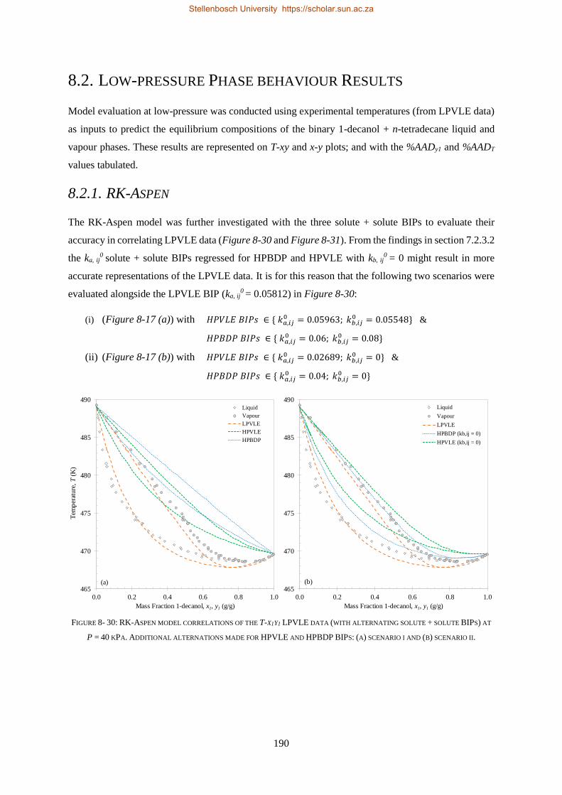
190
8.2. LOW-PRESSURE PHASE BEHAVIOUR RESULTS
Model evaluation at low-pressure was conducted using experimental temperatures (from LPVLE data)
as inputs to predict the equilibrium compositions of the binary 1-decanol + n-tetradecane liquid and
vapour phases. These results are represented on T-xy and x-y plots; and with the %AADy1 and %AADT
values tabulated.
8.2.1. RK-ASPEN
The RK-Aspen model was further investigated with the three solute + solute BIPs to evaluate their
accuracy in correlating LPVLE data (Figure 8-30 and Figure 8-31). From the findings in section 7.2.3.2
the ka, ij0 solute + solute BIPs regressed for HPBDP and HPVLE with kb, ij
0 = 0 might result in more
accurate representations of the LPVLE data. It is for this reason that the following two scenarios were
evaluated alongside the LPVLE BIP (ka, ij0 = 0.05812) in Figure 8-30:
(i) (Figure 8-17 (a)) with 𝐻𝑃𝑉𝐿𝐸 𝐵𝐼𝑃𝑠 ∈ { 𝑘𝑎,𝑖𝑗0 = 0.05963; 𝑘𝑏,𝑖𝑗
0 = 0.05548} &
𝐻𝑃𝐵𝐷𝑃 𝐵𝐼𝑃𝑠 ∈ { 𝑘𝑎,𝑖𝑗0 = 0.06; 𝑘𝑏,𝑖𝑗
0 = 0.08}
(ii) (Figure 8-17 (b)) with 𝐻𝑃𝑉𝐿𝐸 𝐵𝐼𝑃𝑠 ∈ { 𝑘𝑎,𝑖𝑗0 = 0.02689; 𝑘𝑏,𝑖𝑗
0 = 0} &
𝐻𝑃𝐵𝐷𝑃 𝐵𝐼𝑃𝑠 ∈ { 𝑘𝑎,𝑖𝑗0 = 0.04; 𝑘𝑏,𝑖𝑗
0 = 0}
FIGURE 8- 30: RK-ASPEN MODEL CORRELATIONS OF THE T-X1Y1 LPVLE DATA (WITH ALTERNATING SOLUTE + SOLUTE BIPS) AT
P = 40 KPA. ADDITIONAL ALTERNATIONS MADE FOR HPVLE AND HPBDP BIPS: (A) SCENARIO I AND (B) SCENARIO II.
465
470
475
480
485
490
0.0 0.2 0.4 0.6 0.8 1.0
Tem
per
ature
, T
(K)
Mass Fraction 1-decanol, x1, y1 (g/g)
Liquid
Vapour
LPVLE
HPVLE
HPBDP
465
470
475
480
485
490
0.0 0.2 0.4 0.6 0.8 1.0
Mass Fraction 1-decanol, x1, y1 (g/g)
Liquid
Vapour
LPVLE
HPBDP (kb,ij = 0)
HPVLE (kb,ij = 0)
(a) (b)
Stellenbosch University https://scholar.sun.ac.za
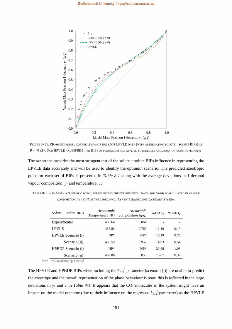
191
FIGURE 8- 31: RK-ASPEN MODEL CORRELATIONS OF THE X1-Y1 LPVLE DATA (WITH ALTERNATING SOLUTE + SOLUTE BIPS) AT
P = 40 KPA. FOR HPVLE AND HPBDP, THE BIPS OF SCENARIO II ARE APPLIED TO INDICATE ACCURACY OF AZEOTROPIC POINT.
The azeotrope provides the most stringent test of the solute + solute BIPs influence in representing the
LPVLE data accurately and will be used to identify the optimum scenario. The predicted azeotropic
point for each set of BIPs is presented in Table 8-1 along with the average deviations in 1-decanol
vapour composition, y1 and temperature, T.
TABLE 8- 1: RK-ASPEN AZEOTROPIC POINT, REPRESENTING THE EXPERIMENTAL DATA AND %AAD CALCULATED IN VAPOUR
COMPOSITION, Y1 AND T OF THE 1-DECANOL (1) + N-TETRADECANE (2) BINARY SYSTEM.
Solute + solute BIPs Azeotropic
Temperature (K)
Azeotropic
composition (g/g) %AADy1 %AADT
Experimental 468.66 0.864 - -
LPVLE 467.83 0.765 11.19 0.19
HPVLE Scenario (i) NP* NP* 18.19 0.77
Scenario (ii) 469.59 0.957 14.03 0.54
HPBDP Scenario (i) NP* NP* 21.88 1.08
Scenario (ii) 469.09 0.855 13.07 0.32
NP* - No azeotrope predicted
The HPVLE and HPBDP BIPs when including the kb, ij0 parameter (scenario (i)) are unable to predict
the azeotrope and the overall representation of the phase behaviour is poor; this is reflected in the large
deviations in y1 and T in Table 8-1. It appears that the CO2 molecules in the system might have an
impact on the model outcome (due to their influence on the regressed kb, ij0
parameter) as the HPVLE
0.0
0.1
0.2
0.3
0.4
0.5
0.6
0.7
0.8
0.9
1.0
0.0 0.2 0.4 0.6 0.8 1.0
Vap
our
Mas
s F
ractio
n 1
-dec
ano
l, y
1(g
/g)
Liquid Mass Fraction 1-decanol, x1 (g/g)
Exp
HPBDP (kb,ij = 0)
HPVLE (kb,ij = 0)
LPVLE
Stellenbosch University https://scholar.sun.ac.za
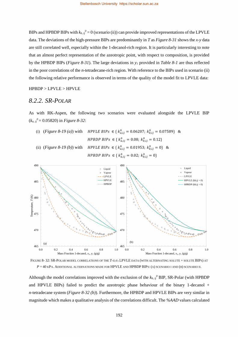
192
BIPs and HPBDP BIPs with kb, ij0 = 0 (scenario (ii)) can provide improved representations of the LPVLE
data. The deviations of the high-pressure BIPs are predominantly in T as Figure 8-31 shows the x-y data
are still correlated well, especially within the 1-decanol-rich region. It is particularly interesting to note
that an almost perfect representation of the azeotropic point, with respect to composition, is provided
by the HPBDP BIPs (Figure 8-31). The large deviations in y1 provided in Table 8-1 are thus reflected
in the poor correlations of the n-tetradecane-rich region. With reference to the BIPs used in scenario (ii)
the following relative performance is observed in terms of the quality of the model fit to LPVLE data:
HPBDP > LPVLE > HPVLE
8.2.2. SR-POLAR
As with RK-Aspen, the following two scenarios were evaluated alongside the LPVLE BIP
(ka, ij0
= 0.05820) in Figure 8-32:
(i) (Figure 8-19 (a)) with 𝐻𝑃𝑉𝐿𝐸 𝐵𝐼𝑃𝑠 ∈ { 𝑘𝑎,𝑖𝑗0 = 0.06207; 𝑘𝑏,𝑖𝑗
0 = 0.07589} &
𝐻𝑃𝐵𝐷𝑃 𝐵𝐼𝑃𝑠 ∈ { 𝑘𝑎,𝑖𝑗0 = 0.08; 𝑘𝑏,𝑖𝑗
0 = 0.12}
(ii) (Figure 8-19 (b)) with 𝐻𝑃𝑉𝐿𝐸 𝐵𝐼𝑃𝑠 ∈ { 𝑘𝑎,𝑖𝑗0 = 0.01953; 𝑘𝑏,𝑖𝑗
0 = 0} &
𝐻𝑃𝐵𝐷𝑃 𝐵𝐼𝑃𝑠 ∈ { 𝑘𝑎,𝑖𝑗0 = 0.02; 𝑘𝑏,𝑖𝑗
0 = 0}
FIGURE 8- 32: SR-POLAR MODEL CORRELATIONS OF THE T-X1Y1 LPVLE DATA (WITH ALTERNATING SOLUTE + SOLUTE BIPS) AT
P = 40 KPA. ADDITIONAL ALTERNATIONS MADE FOR HPVLE AND HPBDP BIPS: (A) SCENARIO I AND (B) SCENARIO II.
Although the model correlations improved with the exclusion of the kb, ij0 BIP, SR-Polar (with HPBDP
and HPVLE BIPs) failed to predict the azeotropic phase behaviour of the binary 1-decanol +
n-tetradecane system (Figure 8-32 (b)). Furthermore, the HPBDP and HPVLE BIPs are very similar in
magnitude which makes a qualitative analysis of the correlations difficult. The %AAD values calculated
465
470
475
480
485
490
0.0 0.2 0.4 0.6 0.8 1.0
Tem
per
ature
, T
(K)
Mass Fraction 1-decanol, x1, y1 (g/g)
Liquid
Vapour
LPVLE
HPVLE
HPBDP
465
470
475
480
485
490
0.0 0.2 0.4 0.6 0.8 1.0
Mass Fraction 1-decanol, x1, y1 (g/g)
Liquid
Vapour
LPVLE
HPVLE (kb,ij = 0)
HPBDP (kb,ij = 0)
(a)(b)
Stellenbosch University https://scholar.sun.ac.za
193
for each BIP set and scenario are provided in Table 8-2. With reference to the BIPs used in scenario (ii)
the following relative performance is observed in terms of the quality of the model fit to LPVLE data:
LPVLE > HPBDP > HPVLE
TABLE 8- 2: SR-POLAR %AAD CALCULATED IN VAPOUR COMPOSITION, Y1 AND T OF THE 1-DECANOL (1) + N-TETRADECANE (2)
BINARY SYSTEM.
Solute + solute BIPs %AADy1 %AADT
LPVLE 11.35 0.19
HPVLE Scenario (i) 21.28 1.01
Scenario (ii) 15.25 0.66
HPBDP Scenario (i) 25.97 1.31
Scenario (ii) 15.13 0.65
8.2.3. PC-SAFT
The predicted azeotropic point for each of the PC-SAFT temperature independent kij parameters are
presented in Table 8-3 along with the average deviations in 1-decanol vapour composition, y1 and
temperature, T. The large deviations in y1 and T are due to the inability of PC-SAFT to accurately
account for the azeotropic behaviour in the 1-decanol + n-tetradecane system when using BIPs regressed
from high-pressure phase equilibria data. It is interesting to note that the nature of the deviations is very
similar, especially within the 1-decanol-rich region. As seen in Figure 8-33 and Figure 8-34, the
strength of the positive deviations in the binary mixture are overestimated, causing the azeotropic
temperature to be underpredicted. The following relative performance is observed in terms of the quality
of the model fit to LPVLE data:
LPVLE > HPBDP > HPVLE
TABLE 8- 3: PC-SAFT AZEOTROPIC POINT, REPRESENTING THE EXPERIMENTAL DATA AND %AAD CALCULATED IN VAPOUR
COMPOSITION, Y1 AND T OF THE 1-DECANOL (1) + N-TETRADECANE (2) BINARY SYSTEM.
Solute + solute BIPs Azeotropic
Temperature (K)
Azeotropic
composition (g/g) %AADy1 %AADT
Experimental 468.66 0.864 - -
LPVLE 467.73 0.776 10.16 0.20
HPVLE 464.01 0.676 15.44 0.84
HPBDP 464.91 0.694 13.08 0.66
Stellenbosch University https://scholar.sun.ac.za
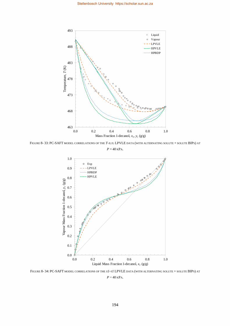
194
FIGURE 8- 33: PC-SAFT MODEL CORRELATIONS OF THE T-X1Y1 LPVLE DATA (WITH ALTERNATING SOLUTE + SOLUTE BIPS) AT
P = 40 KPA.
FIGURE 8- 34: PC-SAFT MODEL CORRELATIONS OF THE X1-Y1 LPVLE DATA (WITH ALTERNATING SOLUTE + SOLUTE BIPS) AT
P = 40 KPA.
463
468
473
478
483
488
493
0.0 0.2 0.4 0.6 0.8 1.0
Tem
per
ature
, T
(K)
Mass Fraction 1-decanol, x1, y1 (g/g)
Liquid
Vapour
LPVLE
HPVLE
HPBDP
0.0
0.1
0.2
0.3
0.4
0.5
0.6
0.7
0.8
0.9
1.0
0.0 0.2 0.4 0.6 0.8 1.0
Vap
our
Mas
s F
ractio
n 1
-dec
ano
l, y
1(g
/g)
Liquid Mass Fraction 1-decanol, x1 (g/g)
Exp
LPVLE
HPBDP
HPVLE
Stellenbosch University https://scholar.sun.ac.za
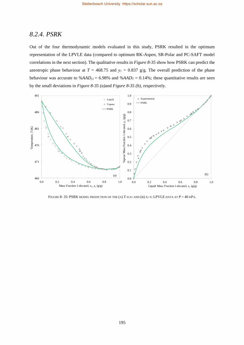
195
8.2.4. PSRK
Out of the four thermodynamic models evaluated in this study, PSRK resulted in the optimum
representation of the LPVLE data (compared to optimum RK-Aspen, SR-Polar and PC-SAFT model
correlations in the next section). The qualitative results in Figure 8-35 show how PSRK can predict the
azeotropic phase behaviour at T = 468.75 and y1 = 0.837 g/g. The overall prediction of the phase
behaviour was accurate to %AADy1 = 6.98% and %AADT = 0.14%; these quantitative results are seen
by the small deviations in Figure 8-35 (a)and Figure 8-35 (b), respectively.
FIGURE 8- 35: PSRK MODEL PREDICTION OF THE (A) T-X1Y1 AND (B) X1-Y1 LPVLE DATA AT P = 40 KPA.
466
471
476
481
486
491
0.0 0.2 0.4 0.6 0.8 1.0
Tem
per
ature
, T
(K)
Mass Fraction 1-decanol, x1, y1 (g/g)
Liquid
Vapour
PSRK
(a)0.0
0.1
0.2
0.3
0.4
0.5
0.6
0.7
0.8
0.9
1.0
0.0 0.2 0.4 0.6 0.8 1.0
Vap
our
Mas
s F
ractio
n 1
-dec
ano
l, y
1(g
/g)
Liquid Mass Fraction 1-decanol, x1 (g/g)
Experimental
PSRK
(b)
Stellenbosch University https://scholar.sun.ac.za
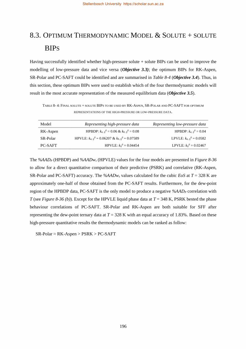
196
8.3. OPTIMUM THERMODYNAMIC MODEL & SOLUTE + SOLUTE
BIPS
Having successfully identified whether high-pressure solute + solute BIPs can be used to improve the
modelling of low-pressure data and vice versa (Objective 3.3); the optimum BIPs for RK-Aspen,
SR-Polar and PC-SAFT could be identified and are summarised in Table 8-4 (Objective 3.4). Thus, in
this section, these optimum BIPs were used to establish which of the four thermodynamic models will
result in the most accurate representation of the measured equilibrium data (Objective 3.5).
TABLE 8- 4: FINAL SOLUTE + SOLUTE BIPS TO BE USED BY RK-ASPEN, SR-POLAR AND PC-SAFT FOR OPTIMUM
REPRESENTATIONS OF THE HIGH-PRESSURE OR LOW-PRESSURE DATA.
Model Representing high-pressure data Representing low-pressure data
RK-Aspen HPBDP: ka, ij0 = 0.06 & kb, ij
0 = 0.08 HPBDP: ka, ij0 = 0.04
SR-Polar HPVLE: ka, ij0 = 0.06207 & kb, ij
0 = 0.07589 LPVLE: ka, ij0 = 0.0582
PC-SAFT HPVLE: kij0 = 0.04454 LPVLE: kij
0 = 0.02467
The %AADP (HPBDP) and %AADws (HPVLE) values for the four models are presented in Figure 8-36
to allow for a direct quantitative comparison of their predictive (PSRK) and correlative (RK-Aspen,
SR-Polar and PC-SAFT) accuracy. The %AADws values calculated for the cubic EoS at T = 328 K are
approximately one-half of those obtained from the PC-SAFT results. Furthermore, for the dew-point
region of the HPBDP data, PC-SAFT is the only model to produce a negative %AADP correlation with
T (see Figure 8-36 (b)). Except for the HPVLE liquid phase data at T = 348 K, PSRK bested the phase
behaviour correlations of PC-SAFT. SR-Polar and RK-Aspen are both suitable for SFF after
representing the dew-point ternary data at T = 328 K with an equal accuracy of 1.83%. Based on these
high-pressure quantitative results the thermodynamic models can be ranked as follow:
SR-Polar ≈ RK-Aspen > PSRK > PC-SAFT
Stellenbosch University https://scholar.sun.ac.za
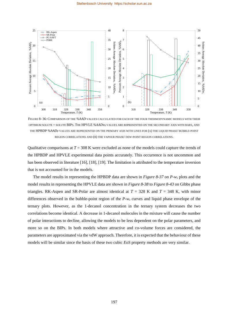
197
FIGURE 8- 36: COMPARISON OF THE %AAD VALUES CALCULATED FOR EACH OF THE FOUR THERMODYNAMIC MODELS WITH THEIR
OPTIMUM SOLUTE + SOLUTE BIPS. THE HPVLE %AADWS VALUES ARE REPRESENTED ON THE SECONDARY AXIS WITH BARS, AND
THE HPBDP %AADP VALUES ARE REPRESENTED ON THE PRIMARY AXIS WITH LINES FOR (A) THE LIQUID PHASE/ BUBBLE-POINT
REGION CORRELATIONS AND (B) THE VAPOUR PHASE/ DEW-POINT REGION CORRELATIONS.
Qualitative comparisons at T = 308 K were excluded as none of the models could capture the trends of
the HPBDP and HPVLE experimental data points accurately. This occurrence is not uncommon and
has been observed in literature [16], [18], [19]. The limitation is attributed to the temperature inversion
that is not accounted for in the models.
The model results in representing the HPBDP data are shown in Figure 8-37 on P-ws plots and the
model results in representing the HPVLE data are shown in Figure 8-38 to Figure 8-43 on Gibbs phase
triangles. RK-Aspen and SR-Polar are almost identical at T = 328 K and T = 348 K, with minor
differences observed in the bubble-point region of the P-ws curves and liquid phase envelope of the
ternary plots. However, as the 1-decanol concentration in the ternary system decreases the two
correlations become identical. A decrease in 1-decanol molecules in the mixture will cause the number
of polar interactions to decline, allowing the models to be less dependent on the polar parameters, and
more so on the BIPs. In both models where attractive and co-volume forces are considered, the
parameters are approximated via the vdW approach. Therefore, it is expected that the behaviour of these
models will be similar since the basis of these two cubic EoS property methods are very similar.
0
5
10
15
20
25
30
35
40
0
5
10
15
20
25
308 318 328 338 348 358
So
lutes A
verag
e Ab
solu
te Dev
iation,
%A
AD
wsP
ress
ure
Aver
age
Ab
solu
te D
evia
tio
n,
%A
AD
P
Temperature, T (K)
RK-AspenSR-PolarPC-SAFTPSRK
0
5
10
15
20
25
30
35
40
45
50
0
1
2
3
4
5
6
7
8
318 328 338 348 358
So
lutes A
verag
e Ab
solu
te Dev
iation,
%A
AD
wsP
ress
ure
Aver
age
Ab
solu
te D
evia
tio
n,
%A
AD
P
Temperature, T (K)
(a) (b)
Stellenbosch University https://scholar.sun.ac.za
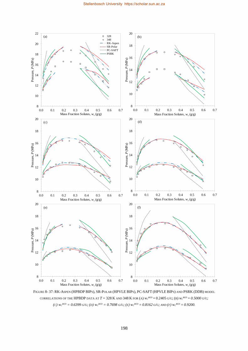
198
FIGURE 8- 37: RK-ASPEN (HPBDP BIPS), SR-POLAR (HPVLE BIPS), PC-SAFT (HPVLE BIPS) AND PSRK (DDB) MODEL
CORRELATIONS OF THE HPBDP DATA AT T = 328 K AND 348 K FOR (A) WCRED = 0.2405 G/G; (B) WC
RED = 0.5000 G/G;
(C) WCRED = 0.6399 G/G; (D) WC
RED = 0.7698 G/G; (E) WCRED = 0.8162 G/G; AND (F) WC
RED = 0.9200.
8
10
12
14
16
18
20
0.0 0.1 0.2 0.3 0.4 0.5 0.6 0.7
Pre
ssure
, P
(M
Pa)
Mass Fraction Solutes, ws (g/g)
8
10
12
14
16
18
20
0.0 0.1 0.2 0.3 0.4 0.5 0.6 0.7
Pre
ssure
, P
(M
Pa)
Mass Fraction Solutes, ws (g/g)
8
10
12
14
16
18
20
0.0 0.1 0.2 0.3 0.4 0.5 0.6 0.7
Pre
ssure
, P
(M
Pa)
Mass Fraction Solutes, ws (g/g)
8
10
12
14
16
18
20
22
0.0 0.1 0.2 0.3 0.4 0.5 0.6 0.7
Pre
ssure
, P
(M
Pa)
Mass Fraction Solutes, ws (g/g)
328
348
RK-Aspen
SR-Polar
PC-SAFT
PSRK
8
10
12
14
16
18
20
0.0 0.1 0.2 0.3 0.4 0.5 0.6 0.7
Pre
ssure
, P
(M
Pa)
Mass Fraction Solutes, ws (g/g)
8
10
12
14
16
18
20
0.0 0.1 0.2 0.3 0.4 0.5 0.6 0.7
Pre
ssure
, P
(M
Pa)
Mass Fraction Solutes, ws (g/g)
(f)(e)
(d)(c)
(a) (b)
Stellenbosch University https://scholar.sun.ac.za
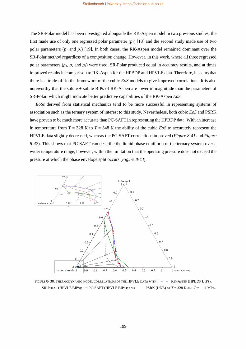
199
The SR-Polar model has been investigated alongside the RK-Aspen model in two previous studies; the
first made use of only one regressed polar parameter (p1) [18] and the second study made use of two
polar parameters (p1 and p2) [19]. In both cases, the RK-Aspen model remained dominant over the
SR-Polar method regardless of a composition change. However, in this work, where all three regressed
polar parameters (p1, p2 and p3) were used, SR-Polar produced equal in accuracy results, and at times
improved results in comparison to RK-Aspen for the HPBDP and HPVLE data. Therefore, it seems that
there is a trade-off in the framework of the cubic EoS models to give improved correlations. It is also
noteworthy that the solute + solute BIPs of RK-Aspen are lower in magnitude than the parameters of
SR-Polar, which might indicate better predictive capabilities of the RK-Aspen EoS.
EoSs derived from statistical mechanics tend to be more successful in representing systems of
association such as the ternary system of interest to this study. Nevertheless, both cubic EoS and PSRK
have proven to be much more accurate than PC-SAFT in representing the HPBDP data. With an increase
in temperature from T = 328 K to T = 348 K the ability of the cubic EoS to accurately represent the
HPVLE data slightly decreased, whereas the PC-SAFT correlations improved (Figure 8-41 and Figure
8-42). This shows that PC-SAFT can describe the liquid phase equilibria of the ternary system over a
wider temperature range, however, within the limitation that the operating pressure does not exceed the
pressure at which the phase envelope split occurs (Figure 8-43).
FIGURE 8- 38: THERMODYNAMIC MODEL CORRELATIONS OF THE HPVLE DATA WITH: . . – . . – . . RK-ASPEN (HPBDP BIPS);
– – – – SR-POLAR (HPVLE BIPS); …… PC-SAFT (HPVLE BIPS); AND ––––– PSRK (DDB) AT T = 328 K AND P = 11.1 MPA.
Stellenbosch University https://scholar.sun.ac.za
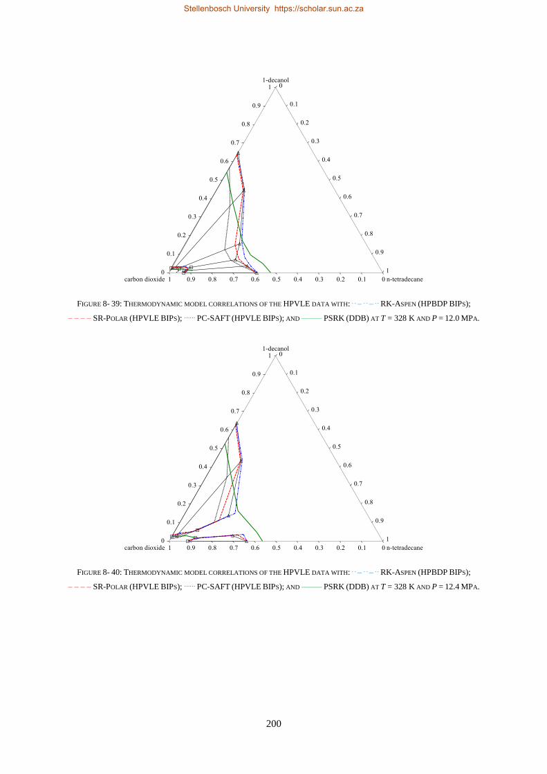
200
FIGURE 8- 39: THERMODYNAMIC MODEL CORRELATIONS OF THE HPVLE DATA WITH: . . – . . – . . RK-ASPEN (HPBDP BIPS);
– – – – SR-POLAR (HPVLE BIPS); …… PC-SAFT (HPVLE BIPS); AND ––––– PSRK (DDB) AT T = 328 K AND P = 12.0 MPA.
FIGURE 8- 40: THERMODYNAMIC MODEL CORRELATIONS OF THE HPVLE DATA WITH: . . – . . – . . RK-ASPEN (HPBDP BIPS);
– – – – SR-POLAR (HPVLE BIPS); …… PC-SAFT (HPVLE BIPS); AND ––––– PSRK (DDB) AT T = 328 K AND P = 12.4 MPA.
Stellenbosch University https://scholar.sun.ac.za
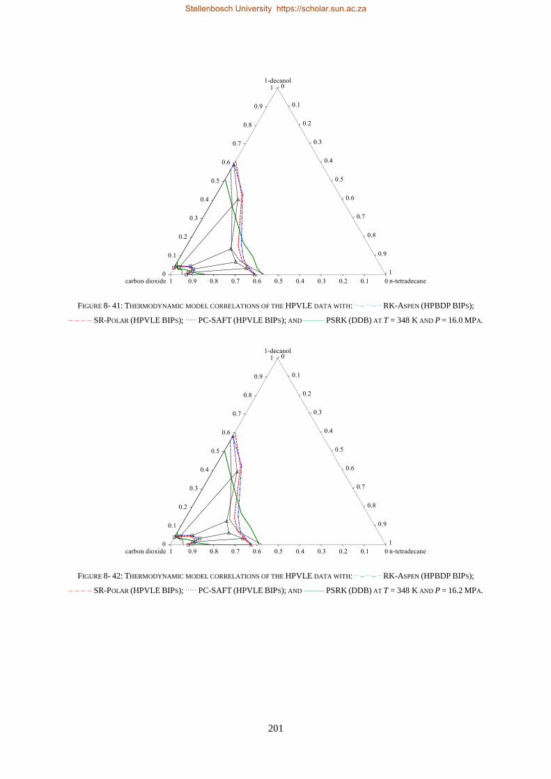
201
FIGURE 8- 41: THERMODYNAMIC MODEL CORRELATIONS OF THE HPVLE DATA WITH: . . – . . – . . RK-ASPEN (HPBDP BIPS);
– – – – SR-POLAR (HPVLE BIPS); …… PC-SAFT (HPVLE BIPS); AND ––––– PSRK (DDB) AT T = 348 K AND P = 16.0 MPA.
FIGURE 8- 42: THERMODYNAMIC MODEL CORRELATIONS OF THE HPVLE DATA WITH: . . – . . – . . RK-ASPEN (HPBDP BIPS);
– – – – SR-POLAR (HPVLE BIPS); …… PC-SAFT (HPVLE BIPS); AND ––––– PSRK (DDB) AT T = 348 K AND P = 16.2 MPA.
Stellenbosch University https://scholar.sun.ac.za
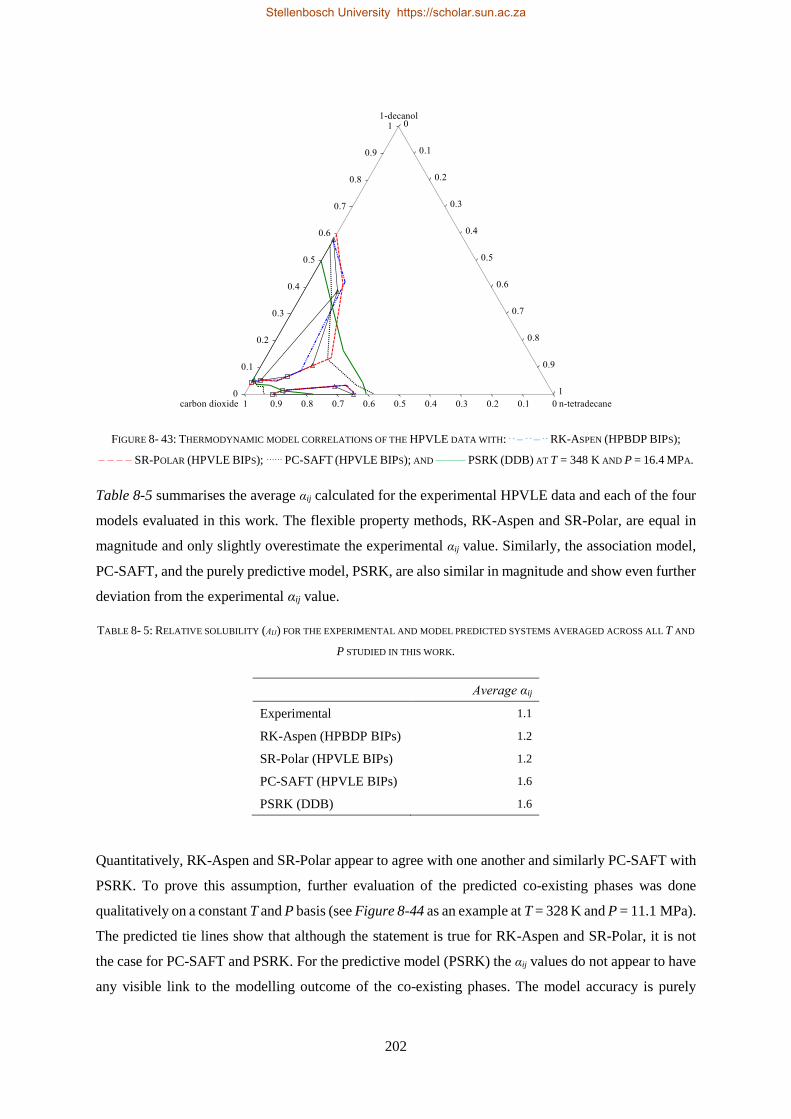
202
FIGURE 8- 43: THERMODYNAMIC MODEL CORRELATIONS OF THE HPVLE DATA WITH: . . – . . – . . RK-ASPEN (HPBDP BIPS);
– – – – SR-POLAR (HPVLE BIPS); …… PC-SAFT (HPVLE BIPS); AND ––––– PSRK (DDB) AT T = 348 K AND P = 16.4 MPA.
Table 8-5 summarises the average αij calculated for the experimental HPVLE data and each of the four
models evaluated in this work. The flexible property methods, RK-Aspen and SR-Polar, are equal in
magnitude and only slightly overestimate the experimental αij value. Similarly, the association model,
PC-SAFT, and the purely predictive model, PSRK, are also similar in magnitude and show even further
deviation from the experimental αij value.
TABLE 8- 5: RELATIVE SOLUBILITY (ΑIJ) FOR THE EXPERIMENTAL AND MODEL PREDICTED SYSTEMS AVERAGED ACROSS ALL T AND
P STUDIED IN THIS WORK.
Average αij
Experimental 1.1
RK-Aspen (HPBDP BIPs) 1.2
SR-Polar (HPVLE BIPs) 1.2
PC-SAFT (HPVLE BIPs) 1.6
PSRK (DDB) 1.6
Quantitatively, RK-Aspen and SR-Polar appear to agree with one another and similarly PC-SAFT with
PSRK. To prove this assumption, further evaluation of the predicted co-existing phases was done
qualitatively on a constant T and P basis (see Figure 8-44 as an example at T = 328 K and P = 11.1 MPa).
The predicted tie lines show that although the statement is true for RK-Aspen and SR-Polar, it is not
the case for PC-SAFT and PSRK. For the predictive model (PSRK) the αij values do not appear to have
any visible link to the modelling outcome of the co-existing phases. The model accuracy is purely
Stellenbosch University https://scholar.sun.ac.za
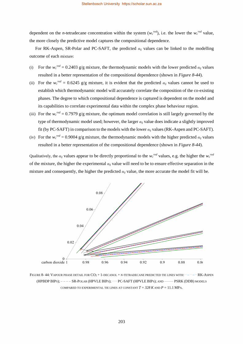
203
dependent on the n-tetradecane concentration within the system (wcred), i.e. the lower the wc
red value,
the more closely the predictive model captures the compositional dependence.
For RK-Aspen, SR-Polar and PC-SAFT, the predicted αij values can be linked to the modelling
outcome of each mixture:
(i) For the wcred = 0.2403 g/g mixture, the thermodynamic models with the lower predicted αij values
resulted in a better representation of the compositional dependence (shown in Figure 8-44).
(ii) For the wcred = 0.6245 g/g mixture, it is evident that the predicted αij values cannot be used to
establish which thermodynamic model will accurately correlate the composition of the co-existing
phases. The degree to which compositional dependence is captured is dependent on the model and
its capabilities to correlate experimental data within the complex phase behaviour region.
(iii) For the wcred = 0.7979 g/g mixture, the optimum model correlation is still largely governed by the
type of thermodynamic model used; however, the larger αij value does indicate a slightly improved
fit (by PC-SAFT) in comparison to the models with the lower αij values (RK-Aspen and PC-SAFT).
(iv) For the wcred = 0.9004 g/g mixture, the thermodynamic models with the higher predicted αij values
resulted in a better representation of the compositional dependence (shown in Figure 8-44).
Qualitatively, the αij values appear to be directly proportional to the wcred values, e.g. the higher the wc
red
of the mixture, the higher the experimental αij value will need to be to ensure effective separation in the
mixture and consequently, the higher the predicted αij value, the more accurate the model fit will be.
FIGURE 8- 44: VAPOUR PHASE DETAIL FOR CO2 + 1-DECANOL + N-TETRADECANE PREDICTED TIE LINES WITH: . . – . . – . . RK-ASPEN
(HPBDP BIPS); – – – – SR-POLAR (HPVLE BIPS); …… PC-SAFT (HPVLE BIPS); AND ––––– PSRK (DDB) MODELS
COMPARED TO EXPERIMENTAL TIE LINES AT CONSTANT T = 328 K AND P = 11.1 MPA.
Stellenbosch University https://scholar.sun.ac.za
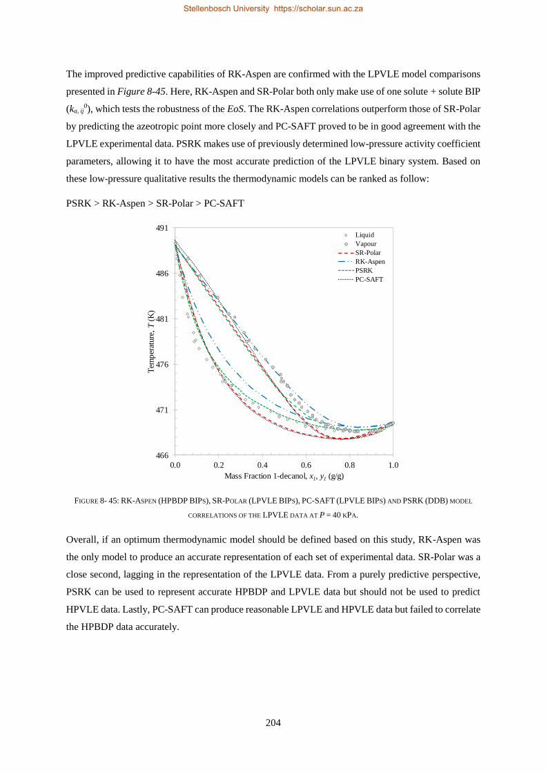
204
The improved predictive capabilities of RK-Aspen are confirmed with the LPVLE model comparisons
presented in Figure 8-45. Here, RK-Aspen and SR-Polar both only make use of one solute + solute BIP
(ka, ij0), which tests the robustness of the EoS. The RK-Aspen correlations outperform those of SR-Polar
by predicting the azeotropic point more closely and PC-SAFT proved to be in good agreement with the
LPVLE experimental data. PSRK makes use of previously determined low-pressure activity coefficient
parameters, allowing it to have the most accurate prediction of the LPVLE binary system. Based on
these low-pressure qualitative results the thermodynamic models can be ranked as follow:
PSRK > RK-Aspen > SR-Polar > PC-SAFT
FIGURE 8- 45: RK-ASPEN (HPBDP BIPS), SR-POLAR (LPVLE BIPS), PC-SAFT (LPVLE BIPS) AND PSRK (DDB) MODEL
CORRELATIONS OF THE LPVLE DATA AT P = 40 KPA.
Overall, if an optimum thermodynamic model should be defined based on this study, RK-Aspen was
the only model to produce an accurate representation of each set of experimental data. SR-Polar was a
close second, lagging in the representation of the LPVLE data. From a purely predictive perspective,
PSRK can be used to represent accurate HPBDP and LPVLE data but should not be used to predict
HPVLE data. Lastly, PC-SAFT can produce reasonable LPVLE and HPVLE data but failed to correlate
the HPBDP data accurately.
466
471
476
481
486
491
0.0 0.2 0.4 0.6 0.8 1.0
Tem
per
ature
, T
(K)
Mass Fraction 1-decanol, x1, y1 (g/g)
Liquid
Vapour
SR-Polar
RK-Aspen
PSRK
PC-SAFT
Stellenbosch University https://scholar.sun.ac.za
205
8.4. CHAPTER OUTCOMES
The aim of this chapter was to evaluate the capabilities of the RK-Aspen, SR-Polar, PC-SAFT and
PSRK thermodynamic models within Aspen Plus® to correlate the phase behaviour of the CO2 +
1-decanol + n-tetradecane ternary system and the 1-decanol + n-tetradecane binary system. In achieving
this aim, key Objective 3.3, Objective 3.4 and Objective 3.5 were successfully achieved.
On the off chance that no experimental data for parameter regression is available, the PSRK model
can be used to predict semi-accurate HPBDP data and good LPVLE data but should not be used to
predict HPVLE data. Thus, the PSRK model is not equipped to take into consideration the complexities
from the undesired phase behaviour. The specific strengths and weaknesses of each suitable model that
could incorporate, amongst others, solute + solute BIPs to improve their correlations are summarised
through answering the following questions (Objective 3.3):
(i) Can solute + solute BIPs regressed from LPVLE 1-decanol + n-tetradecane data be used to
correlate HPBDP CO2 + 1-decanol + n-tetradecane data?
Cubic EoS: Although being outperformed by the HPBDP and HPVLE BIPs, the LPVLE BIPs can
represent the dew-point region of the mixtures at T = 328 K within 2.62% (RK-Aspen) and 1.92% (SR-
Polar) of the actual data. Furthermore, qualitative trends of the dew-point region are equal in accuracy
to those obtained by both HPBDP and HPVLE BIPs. For the bubble-point region, the effects of a single
BIP (kb, ij0 = 0) are more prominent as the P-ws curves have been shifted horizontally downwards, and
vertically inwards. Quantitatively, the LPVLE BIPs represent the bubble-point region of the mixtures
at T = 328 K within 7.97% (RK-Aspen) and 7.92% (SR-Polar) of the actual data. However, the values
calculated are simply a representation of the data points predicted, and not the actual fit of the models.
For n-tetradecane-rich mixtures somewhat accurate correlations of the bubble-point region were
maintained.
PC-SAFT: Quantitatively the LPVLE BIPs can represent the bubble- and dew-point regions of the
mixtures at T = 328 K within 8.90% and 9.16% of the actual data, respectively. However, the model fit
to the experimental data remained poor. It is noteworthy that this finding for the LPVLE BIPs was not
the exception, but the norm, as similar correlations of the HPBDP data were obtained with HPBDP and
HPVLE BIPs too.
(ii) Can solute + solute BIPs regressed from LPVLE 1-decanol + n-tetradecane data be used to
correlate HPVLE CO2 + 1-decanol + n-tetradecane data?
Cubic EoS: Within the complex phase behaviour region of the ternary system, where solute + solute
interactions are prominent, the cosolvency ‘pinch point’ and phase envelope split were predicted
prematurely. The poor fit of the models with the LPVLE BIPs were mirrored in the %AAD values
calculated for the solute compositions. At T = 328 K, overly CO2-rich liquid phases (AADws = 17.35%
Stellenbosch University https://scholar.sun.ac.za
206
for RK-Aspen; 17.62% for SR-Polar) and CO2-deficient vapour phases (AADws = 37.64% for
RK-Aspen; 25.28% for SR-Polar) were obtained. Therefore, the use of LPVLE BIPs are not
recommended for representing the HPVLE data.
PC-SAFT: The LPVLE BIPs can produce the s-shaped curve within the complex phase behaviour
region of the system. However, problems with the model are still encountered in representing the vapour
phase composition data. At T = 328 K, slightly CO2-deficient liquid phases (AADws = 10.37%) and
overly CO2-rich vapour phases (AADws = 46.14%) were obtained. Therefore, like the cubic EoS, the
use of LPVLE BIPs are not recommended for representing the HPVLE data.
(iii) Can solute + solute BIPs regressed from HPBDP and HPVLE CO2 + 1-decanol + n-tetradecane
data be used to correlate LPVLE 1-decanol + n-tetradecane data?
Cubic EoS: The assessment of high-pressure BIPs in representing low-pressure VLE data raises a
further important point in the context of this study namely, the problem with parameter degeneracy.
The addition of the kb, ij0 parameter did not only affect the predictability of the system, but the ability of
the models to correlate the system as well. Therefore, HPBDP and HPVLE BIPs can be used to represent
the LPVLE data if the condition of kb, ij0 = 0 is maintained. Overall, for RK-Aspen, the HPBDP BIP
(ka, ij0 = 0.04) resulted in the most accurate representation of the azeotropic point. For SR-Polar, the
azeotropic phase behaviour could still not be predicted, regardless of setting kb, ij0 = 0. Therefore, for
SR-Polar, HPBDP and HPVLE BIPs are not recommended for correlating LPVLE data.
PC-SAFT: With HPBDP and HPVLE BIPs the strength of the positive deviations in the binary
mixture are overestimated, causing the azeotropic temperature to be underpredicted. Therefore, HPBDP
and HPVLE BIPs are not recommended for correlating LPVLE data.
(iv) Can solute + solute BIPs regressed from HPVLE CO2 + 1-decanol + n-tetradecane data be used
to correlate HPBDP CO2 + 1-decanol + n-tetradecane data and vice versa?
Cubic EoS: Quantitatively and qualitatively both sets of high-pressure BIPs resulted in accurate
representations of the true thermodynamic properties of the CO2 + 1-decanol + n-tetradecane system.
This conclusion is not unexpected, as the ka, ij0 and kb, ij
0 parameters of the two are very similar. However,
with respect to the optimum set of BIPs to be used in SFF processes, the HPBDP BIPs are recommended
for RK-Aspen and the HPVLE BIPs are recommended for SR-Polar.
PC-SAFT: It is well known that PC-SAFT deteriorates near the critical region of HPBDP data and
predicts too-high concentrations of CO2 (decreased solubility). In this work, neither the HPBDP nor the
HPVLE BIPs can improve the model fit to the HPBDP data. With respect to the HPVLE data, both sets
of BIPs can capture the liquid phase trend accurately at T = 348 K. However, the vapour composition
correlation remained poor (like the results of the LPVLE BIPs).
Stellenbosch University https://scholar.sun.ac.za
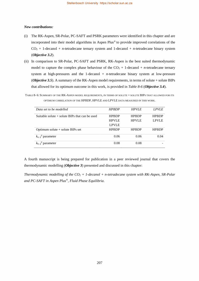
207
New contributions:
(i) The RK-Aspen, SR-Polar, PC-SAFT and PSRK parameters were identified in this chapter and are
incorporated into their model algorithms in Aspen Plus® to provide improved correlations of the
CO2 + 1-decanol + n-tetradecane ternary system and 1-decanol + n-tetradecane binary system
(Objective 3.2).
(ii) In comparison to SR-Polar, PC-SAFT and PSRK, RK-Aspen is the best suited thermodynamic
model to capture the complex phase behaviour of the CO2 + 1-decanol + n-tetradecane ternary
system at high-pressures and the 1-decanol + n-tetradecane binary system at low-pressure
(Objective 3.5). A summary of the RK-Aspen model requirements, in terms of solute + solute BIPs
that allowed for its optimum outcome in this work, is provided in Table 8-6 (Objective 3.4).
TABLE 8- 6: SUMMARY OF THE RK-ASPEN MODEL REQUIREMENTS, IN TERMS OF SOLUTE + SOLUTE BIPS THAT ALLOWED FOR ITS
OPTIMUM CORRELATION OF THE HPBDP, HPVLE AND LPVLE DATA MEASURED IN THIS WORK.
Data set to be modelled HPBDP HPVLE LPVLE
Suitable solute + solute BIPs that can be used HPBDP
HPVLE
LPVLE
HPBDP
HPVLE
HPBDP
LPVLE
Optimum solute + solute BIPs set HPBDP HPBDP HPBDP
ka, ij0 parameter 0.06 0.06 0.04
kb, ij0 parameter 0.08 0.08 -
A fourth manuscript is being prepared for publication in a peer reviewed journal that covers the
thermodynamic modelling (Objective 3) presented and discussed in this chapter:
Thermodynamic modelling of the CO2 + 1-decanol + n-tetradecane system with RK-Aspen, SR-Polar
and PC-SAFT in Aspen Plus®, Fluid Phase Equilibria.
Stellenbosch University https://scholar.sun.ac.za

208
Stellenbosch University https://scholar.sun.ac.za
209
Chapter 9
CONCLUSIONS AND RECOMMENDATIONS
The aim of this thesis was to obtain a fundamental understanding of the solute + solute interactions in
the CO2 + 1-decanol + n-tetradecane ternary system. The aim was achieved in two main parts, namely:
(i) Experimental measurement of new high-pressure and low-pressure phase equilibria data (key
Objective 1 and Objective 2).
(ii) Thermodynamic modelling of the new experimental phase equilibria data (key Objective 3).
Complex phase behavior regions within the CO2 + 1-decanol + n-tetradecane system, i.e. cosolvency
effects, were identified with both the HPBDP and HPVLE data measured in this work. The complex
phase behaviour was found to occur due to distinct solute + solute interactions taking place with the
ternary system. The interactions further lead to a fractionation gap within the complex phase behaviour
region, i.e. wcred = ± 0.6245 g/g, that can only be overcome through a pressure-temperature swing
distillation. The complexities between the two larger solutes were confirmed with LPVLE
measurements of the 1-decanol + n-tetradecane binary system. Thermodynamic modelling in this study
showed that knowledge of the co-existing phases (HPVLE and LPVLE data) are not necessary to ensure
their compositions are correlated well. The HPBDP data is not only less expensive and easier to
measure, but when combined with the RK-Aspen property method in Aspen Plus®, it will allow for
excellent correlations of the CO2 + 1-decanol + n-tetradecane system, especially within the complex
phase behaviour region where solute + solute interactions were most prominent. Therefore, it is
recommended that separation experiments be conducted on a pilot plant setup to confirm the
fractionation gap occurring due to the solute + solute interactions. Once the final feed ratio and reflux
settings are obtained, the RK-Aspen model with HPBDP solute + solute BIPs should be used to improve
the accuracy of a working process model setup within Aspen Plus®.
The conclusions of each part are discussed separately in this chapter, followed by recommendations
for possible future work. Each chapter in this study contains a separate conclusions section, the content
of which are to be treated as supplemental to chapter 9.
Stellenbosch University https://scholar.sun.ac.za
210
9.1. PART 1: ACHIEVEMENT OF KEY OBJECTIVES 1 AND 2
Table 9-1 summarises the main experimental shortcomings in open literature that were identified in
Chapter 2 and how each were addressed through new contributions made in Chapter 5 (HPBDP and
HPVLE data) and Chapter 6 (LPVLE data) of this work. Studying the ternary system at high-pressures
helped to identify:
(i) The type of complex phase behaviour occurring within the ternary system, e.g. cosolvency, l-g
hole and miscibility windows.
(ii) How each phenomenon is connected to the next, e.g. cosolvency lead to l-g hole and the
simultaneous formation of miscibility windows.
(iii) The influence of solute + solute interactions on the fractionation of the systems.
(iv) The relative solubility of the components to identify the fractionation gap.
(v) The types of phase transitions occurring within the complex phase behaviour region.
Given the scarcity of HPVLE ternary data, the experimental data measured in this work represents a
valuable academic contribution. However, the measurement of new HPVLE ternary data is a timely and
tedious process. It is for this reason that a synthetic setup was an alternative method used to measure
HPBDP data. The measurement of new HPBDP solubility pressures were far less complex and time
consuming. The third and final method entailed the use of an all-glass dynamic still to measure new
LPVLE data of the binary 1-decanol + n-tetradecane system. Measuring the binary system served to:
(i) Confirm that non-ideal phase behaviour does arise between the two solutes.
(ii) Help gain further insight into the distinct solute + solute interactions.
(iii) Classify the binary 1-decanol + n-tetradecane system.
(iv) Confirm Class T-IV phase behaviour for the CO2 + 1-decanol + n-tetradecane system.
Stellenbosch University https://scholar.sun.ac.za
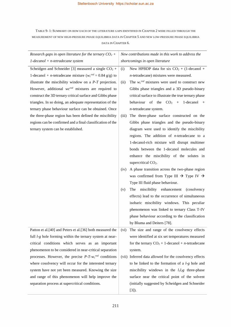
211
TABLE 9- 1: SUMMARY ON HOW EACH OF THE LITERATURE GAPS IDENTIFIED IN CHAPTER 2 WERE FILLED THROUGH THE
MEASUREMENT OF NEW HIGH-PRESSURE PHASE EQUILIBRIA DATA IN CHAPTER 5 AND NEW LOW-PRESSURE PHASE EQUILIBRIA
DATA IN CHAPTER 6.
Research gaps in open literature for the ternary CO2 +
1-decanol + n-tetradecane system
New contributions made in this work to address the
shortcomings in open literature
Scheidgen and Schneider [3] measured a single CO2 +
1-decanol + n-tetradecane mixture (wcred = 0.84 g/g) to
illustrate the miscibility window on a P-T projection.
However, additional wcred mixtures are required to
construct the 3D ternary critical surface and Gibbs phase
triangles. In so doing, an adequate representation of the
ternary phase behaviour surface can be obtained. Once
the three-phase region has been defined the miscibility
regions can be confirmed and a final classification of the
ternary system can be established.
(i) New HPBDP data for six CO2 + (1-decanol +
n-tetradecane) mixtures were measured.
(ii) The wcred mixtures were used to construct new
Gibbs phase triangles and a 3D pseudo-binary
critical surface to illustrate the true ternary phase
behaviour of the CO2 + 1-decanol +
n-tetradecane system.
(iii) The three-phase surface constructed on the
Gibbs phase triangles and the pseudo-binary
diagram were used to identify the miscibility
regions. The addition of n-tetradecane to a
1-decanol-rich mixture will disrupt multimer
bonds between the 1-decanol molecules and
enhance the miscibility of the solutes in
supercritical CO2.
(iv) A phase transition across the two-phase region
was confirmed from Type III → Type IV →
Type III fluid phase behaviour.
(v) The miscibility enhancement (cosolvency
effects) lead to the occurrence of simultaneous
isobaric miscibility windows. This peculiar
phenomenon was linked to ternary Class T-IV
phase behaviour according to the classification
by Bluma and Deiters [78].
Patton et al.[40] and Peters et al.[36] both measured the
full l-g hole forming within the ternary system at near-
critical conditions which serves as an important
phenomenon to be considered in near-critical separation
processes. However, the precise P-T-wcred conditions
where cosolvency will occur for the interested ternary
system have not yet been measured. Knowing the size
and range of this phenomenon will help improve the
separation process at supercritical conditions.
(vi) The size and range of the cosolvency effects
were identified at six set temperatures measured
for the ternary CO2 + 1-decanol + n-tetradecane
system.
(vii) Inferred data allowed for the cosolvency effects
to be linked to the formation of a l-g hole and
miscibility windows in the l1l2g three-phase
surface near the critical point of the solvent
(initially suggested by Scheidgen and Schneider
[3]).
Stellenbosch University https://scholar.sun.ac.za
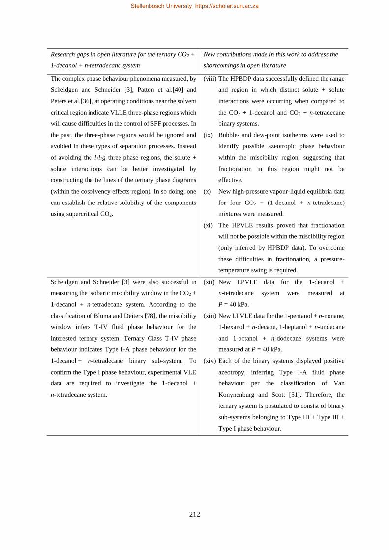
212
Research gaps in open literature for the ternary CO2 +
1-decanol + n-tetradecane system
New contributions made in this work to address the
shortcomings in open literature
The complex phase behaviour phenomena measured, by
Scheidgen and Schneider [3], Patton et al.[40] and
Peters et al.[36], at operating conditions near the solvent
critical region indicate VLLE three-phase regions which
will cause difficulties in the control of SFF processes. In
the past, the three-phase regions would be ignored and
avoided in these types of separation processes. Instead
of avoiding the l1l2g three-phase regions, the solute +
solute interactions can be better investigated by
constructing the tie lines of the ternary phase diagrams
(within the cosolvency effects region). In so doing, one
can establish the relative solubility of the components
using supercritical CO2.
(viii) The HPBDP data successfully defined the range
and region in which distinct solute + solute
interactions were occurring when compared to
the CO2 + 1-decanol and CO2 + n-tetradecane
binary systems.
(ix) Bubble- and dew-point isotherms were used to
identify possible azeotropic phase behaviour
within the miscibility region, suggesting that
fractionation in this region might not be
effective.
(x) New high-pressure vapour-liquid equilibria data
for four CO2 + (1-decanol + n-tetradecane)
mixtures were measured.
(xi) The HPVLE results proved that fractionation
will not be possible within the miscibility region
(only inferred by HPBDP data). To overcome
these difficulties in fractionation, a pressure-
temperature swing is required.
Scheidgen and Schneider [3] were also successful in
measuring the isobaric miscibility window in the CO2 +
1-decanol + n-tetradecane system. According to the
classification of Bluma and Deiters [78], the miscibility
window infers T-IV fluid phase behaviour for the
interested ternary system. Ternary Class T-IV phase
behaviour indicates Type I-A phase behaviour for the
1-decanol + n-tetradecane binary sub-system. To
confirm the Type I phase behaviour, experimental VLE
data are required to investigate the 1-decanol +
n-tetradecane system.
(xii) New LPVLE data for the 1-decanol +
n-tetradecane system were measured at
P = 40 kPa.
(xiii) New LPVLE data for the 1-pentanol + n-nonane,
1-hexanol + n-decane, 1-heptanol + n-undecane
and 1-octanol + n-dodecane systems were
measured at P = 40 kPa.
(xiv) Each of the binary systems displayed positive
azeotropy, inferring Type I-A fluid phase
behaviour per the classification of Van
Konynenburg and Scott [51]. Therefore, the
ternary system is postulated to consist of binary
sub-systems belonging to Type III + Type III +
Type I phase behaviour.
Stellenbosch University https://scholar.sun.ac.za
213
9.2. PART 2: ACHIEVEMENT OF KEY OBJECTIVE 3
Chapter 3 provided a systematic investigation on available thermodynamic models in Aspen Plus® and
their applicability to correlate/predict the complex ternary and binary data. To improve the correlative
capabilities of 3 suitable thermodynamic models, new solute + solute BIPs were regressed in Chapter
7. In addition to the RK-Aspen, SR-Polar and PC-SAFT models, 1 purely predictive model, PSRK, was
also assessed in Chapter 8 to fit the new HPBDP, HPVLE and LPVLE data.
A key question that arose was if it would be possible to improve/maintain the performance of the
models by using different solute + solute BIPs in their specific model algorithm, i.e. can BIPs regressed
using low-pressure data be used to represent high-pressure data accurately and vice versa. Although
the RK-Aspen model (with HPBDP BIPs) and SR-Polar model (with HPVLE BIPs) resulted in the most
accurate representations of the ternary system, the following alternatives were also found in this study:
(i) The use of binary VLE data to regress LPVLE BIPs did improve the RK-Aspen and SR-Polar
thermodynamic model correlations for HPBDP data where distinct solute + solute interactions
were prominent, i.e. wcred ≥ 0.6399 g/g.
(ii) LPVLE BIPs can be used for the two cubic EoS to identify the cosolvency effect in HPVLE data
(s-shaped phase behaviour). However, the LPVLE BIPs should not be used to identify the ‘pinch
point’ where the phase split takes place.
(iii) LPVLE BIPs can be used for PC-SAFT (T-independent basis) to produce model correlations of
the HPVLE data. However, the PC-SAFT model, regardless of the BIPs applied, did not provide
accurate correlations of the HPBDP data.
(iv) The PSRK model can be used without the need for experimental data as the group-group
(UNIFAC) interactions allowed for accurate predictions of the HPBDP data (dew-point region).
However, the PSRK model failed to provide accurate predictions of the HPVLE data.
With regards to correlating the LPVLE data the following alternatives were found in this study:
(i) The PSRK model can be used without the need for experimental data as the group-group
interactions allowed for accurate predictions of the LPVLE data.
(ii) HPBDP BIPs (kb, ij0 = 0) can be used with the RK-Aspen model to produce accurate correlations
of the LPVLE data.
In general, the performance of the thermodynamic models can be ranked as follow:
RK-Aspen > SR-Polar > PSRK > PC-SAFT
However, after the evaluation of all three techniques for obtaining solute + solute BIPs the incorporation
of the HPBDP BIPs into the RK-Aspen model resulted in the most accurate representation of ternary
Stellenbosch University https://scholar.sun.ac.za
214
HPBDP and HPVLE data and binary LPVLE data. Therefore, RK-Aspen was the preferred model to
produce an accurate representation of each set of experimental data, namely:
(i) The dew-point and bubble-point regions of HPBDP mixtures were accurately correlated
regardless of a change in wcred and T.
(ii) The trend of the vapour phase envelope for HPVLE data on Gibbs phase triangles were
exceptionally well correlated at T = 328 K and T = 348 K.
(iii) The HPVLE s-shape behaviour seen by the liquid phase envelopes on Gibbs phase triangles as
well as the two-phase split after the cosolvency ‘pinch point’ were represented well.
(iv) The use of ka, ij0 and kb, ij
0 HPBDP BIPs to correlate the LPVLE data failed to predict the azeotropic
phase behaviour. However, with kb, ij0 = 0, the HPBDP ka, ij
0 BIP allowed for an accurate prediction
of the azeotropic point.
From this research it follows that RK-Aspen with HPBDP solute + solute BIPs should be used for the
most accurate model fit within the complex phase behaviour region of the HPBDP, HPVLE and LPVLE
data. However, PSRK will be more suitable for use if a purely predictive trend of the HPBDP ternary
data and LPVLE binary data is required.
9.3. RECOMMENDATIONS FOR FUTURE WORK
(i) Many data points have been measured for most of the systems listed in Table 2-2. These include
near-critical and super-critical conditions. Therefore, it would be interesting to see whether a
group contribution EoS can be developed to predict these CO2 + hydrocarbon systems.
(ii) The CPA EoS has shown success in representing alcohol recovery applications with
high-pressure gases, making it especially suitable for the mixtures investigated in this study.
Furthermore, CPA is a direct approach that can be applied to hydrogen bonding components,
where EoS-GE models tend to fail. The thermodynamic model was recently added to Aspen Plus®
V8.8 and should be evaluated in correlating the experimental data measured in this work.
(iii) By improving the design and analysis through controlled experiments, the modelling of the
system could be enhanced. Factors based on qualitative assumptions can thus be ruled out, i.e.
design of experiments on STATISTICA®.
(iv) Experimental pilot plant testing of the ternary system should be conducted (like that done by
Bonthuys [17]). The data can be used to verify the separation of residual n-tetradecane from
1-decanol using supercritical CO2.
(v) The experimental pilot plant data can be used in collaboration with the process model developed
in Aspen Plus® by Zamudio [18]. The process model is ideal for the system of interest here as it
was specifically designed for detergent range alkanes and alcohols with cross-over boiling points.
Stellenbosch University https://scholar.sun.ac.za
215
The models and solute + solute BIPs regressed in this work should be used to evaluate the
performance of a SFF process for the separation of the ternary mixtures.
(vi) For RK-Aspen and SR-Polar, the use of high-pressure BIPs to predict LPVLE data showed the
use of only the ka, ij0 parameter produces an accurate fit (including kb, Ij
0 decreases the model
accuracy). Based on this finding, it is recommended that a third scenario be investigated in future
studies, where: ka, ij0 and ka, ij
1 high-pressure BIPs are used to fit the model to LPVLE data. Due
to the LPVLE data measured in this work being at much higher temperatures than the HPVLE
data and HPBDP data measured, it is anticipated that taking T-dependence into consideration in
this manner might improve the model fit.
(vii) The HPBDP BIP regression approach limited the number of parameters that could be used to
improve the SR-Polar model fit. It is recommended that the influence of the lij parameter be
investigated using the HPVLE data and LPVLE data, e.g. see if HPVLE BIPs with 3 BIPs can
improve the model fit to LPVLE data and vice versa.
(viii) In addition to the objective functions used in this study to fit the solute + solute BIPs, it could be
interesting to assess if including the relative solubility (using the K-Value) in the OF would
improve the results, e.g. 𝑂𝐹 = ∑ [(𝑃𝑠𝑎𝑡,𝑖
𝐸𝑥𝑝−𝑃𝑠𝑎𝑡,𝑖
𝐶𝑎𝑙𝑐)2
(𝑃𝑠𝑎𝑡𝐸𝑥𝑝
)2 ]
0.5
𝑁𝑃𝑖=1 + ∑ ∑ [
(𝐾𝑖𝐸𝑥𝑝
−𝐾𝑖𝐶𝑎𝑙𝑐)
2
(𝐾𝑖𝐸𝑥𝑝
)2 ]
0.5
𝑁𝐶𝑖=1
𝑁𝑃𝑖=1 .
(ix) Having identified which models can correlate the interested systems accurately with no
T-dependent BIPs in this work, it is recommended that the influence of T-dependent BIPs be
evaluated in future studies.
Stellenbosch University https://scholar.sun.ac.za

216
Stellenbosch University https://scholar.sun.ac.za
217
Chapter 10
REFERENCES
[1] E. Kiran and J. F. Brennecke, “Supercritical Fluid Engineering Science: Fundamentals and
Applications,” in ACS Symposium Series No. 514, 1993.
[2] Aspen Technology, “Aspen Physical Property System,” Softw. Guid. - Phys. Prop. Model., vol.
7.3.2, pp. 69–70, 2012.
[3] A. L. Scheidgen and G. M. Schneider, “Fluid phase equilibria of (carbon dioxide + a 1-alkanol+
an alkane) up to 100 MPa and T = 393 K: cosolvency effect, miscibility windows, and holes in
the critical surface,” J. Chem. Thermodyn., vol. 32, no. 9, pp. 1183–1201, 2000.
[4] C. E. Schwarz, G. J. K. Bonthuys, J. H. Knoetze, and A. J. Burger, “The influence of functional
end groups on the high-pressure phase equilibria of long chain molecules in supercritical
propane,” J. Supercrit. Fluids, vol. 46, no. 3, pp. 233–237, 2008.
[5] H. A. Mills, “Alcohols, Fatty (via Hydrogenation),” Chemical and Process Technology. 1974.
[6] J. Falbe, W. Lipps, and D. Mayer, Alcohols, Aliphatic, Ullmann’s Encyclopaedia of Industrial
Chemistry. 2012.
[7] J. C. Crause, “Supercritical Fluid Extraction of Paraffin Wax,” P.h.D Thesis, Stellenbosch
University, 2001.
[8] A. J. Lundeen, “Alcohols,” Chemical and Process Technology. 1974.
[9] D. A. McKensie, “Nonionic Surfactants in: Chemical Society,” J. Am. Oil, vol. 55, pp. 93–97,
1978.
[10] G. J. K. Bonthuys, C. E. Schwarz, A. J. Burger, and J. H. Knoetze, “Separation of alkanes and
alcohols with supercritical fluids. Part I: Phase equilibria and viability study,” J. Supercrit.
Fluids, vol. 57, no. 2, pp. 101–111, 2011.
[11] C. E. Schwarz, G. J. K. Bonthuys, R. F. Van Schalkwyk, D. L. Laubscher, A. J. Burger, and J.
H. Knoetze, “Separation of alkanes and alcohols with supercritical fluids. Part II. Influence of
process parameters and size of operating range,” J. Supercrit. Fluids, vol. 58, no. 3, pp. 352–
359, 2011.
[12] M. Zamudio, C. E. Schwarz, and J. H. Knoetze, “Methodology for process modelling of
supercritical fluid fractionation processes illustrated for the separation of alkane/alcohol isomer
mixtures using CO2,” J. Supercrit. Fluids, vol. 104, pp. 272–280, 2015.
Stellenbosch University https://scholar.sun.ac.za
218
[13] M. Zamudio, C. E. Schwarz, and J. H. Knoetze, “Experimental measurement and modelling with
Aspen Plus® of the phase behaviour of supercritical CO2+(n-dodecane+1-decanol+3,7-
dimethyl-1-octanol),” J. Supercrit. Fluids, vol. 84, pp. 132–145, 2013.
[14] F. C. v N. Fourie, C. E. Schwarz, and J. H. Knoetze, “Phase equilibria of alcohols in supercritical
fluids. Part I. The effect of the position of the hydroxyl group for linear C8 alcohols in
supercritical carbon dioxide,” J. Supercrit. Fluids, vol. 47, no. 2, pp. 161–167, 2008.
[15] M. Zamudio, C. E. Schwarz, and J. H. Knoetze, “Phase equilibria of branched isomers of C10-
alcohols and C10-alkanes in supercritical carbon dioxide,” J. Supercrit. Fluids, vol. 59, no. 3,
pp. 14–26, 2011.
[16] S. A. M. Smith and C. E. Schwarz, “High pressure phase behaviour of the CO2+1-decanol+n-
dodecane system,” Fluid Phase Equilib., vol. 406, pp. 1–9, 2015.
[17] G. J. K. Bonthuys, “Separation of 1-dodecanol and n-tetradecane through supercritical
extraction,” Masters Thesis, Stellenbosch University, 2008.
[18] M. Zamudio, “The Separation of Detergent Range Alkanes and Alcohol Isomers with
Supercritical Carbon Dioxide,” P.h.D Thesis, Stellenbosch University, 2014.
[19] F. C. v N. Fourie, “The high pressure phase behaviour of detergent range alcohols and alkanes,”
P.h.D Thesis, Stellenbosch University, 2018.
[20] R. H. Perry and D. W. Green, Perry’s chemical engineers’ handbook, 7th ed. New York:
McGraw-Hill, 1997.
[21] NIST Chemistry WebBook, “National Institute of Standards and Technology: Available from:
http://webbook.nist.gov/chemistry/.” .
[22] C. L. Yaws, “Yaws’ Thermophysical Properties of Chemicals and Hydrocarbons.” Knovel,
2010.
[23] DIPPR 801 Database, “Design Institute for Physical Properties. Sponsored by AIChe: Available
from: http://www.aiche.org/dippr.” .
[24] G. Brunner, Gas Extraction: An Introduction to Fundamentals of Supercritical Fluids and the
Application to Separation Processes, Vol. 4. Darmstadt: Steinkopf; New York: Springer, 1994.
[25] G. Brunner, “Decaffeination of raw coffee by means of compressed nitrous oxide,” in
International Symposium on Supercritical Fluids, Vol. 2, 1987, pp. 691–698.
[26] M. McHugh and V. Krukonis, Supercritical Fluid Extraction. London: Butterworths, 1986.
[27] L. T. Taylor, Supercritical Fluid Extraction: Techniques in Analytical Chemistry. John Wiley
& Sons, Inc., 1996.
[28] F. V Bright and M. E. P. McNally, “Supercritical Fluid Technology: Theoretical and Applied
Approaches in Analytical Chemistry,” in ACS Symposium Series No. 488, 1992.
[29] V. 15. 0. ACD/ChemSketch (Freeware), “Advanced Chemistry Development, Inc.” Toronto,
ON, Canada, Available from: www.acdlabs.com, 2016.
Stellenbosch University https://scholar.sun.ac.za
219
[30] T. J. Bruno and J. F. Ely, Supercritical Fluid Technology: Reviews in Modern Theory and
Applications. CRC Press, 1991.
[31] E. Kiran and J. M. H. Levelt Sengers, Supercritical Fluids: Fundamentals for Application.
Dordrecht, The Netherlands: Kluwer Academic Publishers, 1994.
[32] K. Gauter, “Fluid multiphase behavior in ternary systems of near-critical CO2: Measurements,
modeling and computation,” P.h.D thesis, Delft University, 1999.
[33] C. J. Gauter, K.; Peters, “Phase equilibria in near-critical solutions: Binary and ternary mixtures
of carbon dioxide and certain solutes and the occurence of two-phase holes,” in Supercritical
Fluids: Fundamentals for Applications, Series E., C. J. Kiran, E; Debenedetti, P. G; Peters, Ed.
Turkey: Kluwer Academic, 2000, pp. 69–89.
[34] C. J. Peters and K. Gauter, “Occurrence of Holes in Ternary Fluid Multiphase Systems of Near-
Critical Carbon Dioxide and Certain Solutes.,” Chem. Rev., vol. 99, no. 2, pp. 419–432, 1999.
[35] G. M. Schneider, A. L. Scheidgen, and D. Klante, “Complex phase equilibrium phenomena in
fluid mixtures up to 2 GPa - Cosolvency, holes, windows, closed loops, high-pressure
immiscibility, barotropy, and related effects,” Ind. Eng. Chem. Res., vol. 39, no. 12, pp. 4476–
4480, 2000.
[36] C. J. Peters, L. . Florusse, S. Hähre, and J. de Swaan Arons, “Fluid multiphase equilibrla and
critical phenomena in binary and ternary mixtures of carbon dioxide, certain n-alkanols and n-
tetradecane,” Fluid Phase Equilib., vol. 110, pp. 157–173, 1995.
[37] C. J. Peters, “Multiphase equilibria in near-critical solvents,” in Supercritical Fluids:
Fundamentals for Applications, E. Kiran and J. M. H. Levelt Sengers, Eds. Netherlands: Kluwer
Academic, 1994, pp. 117–145.
[38] C. J. Peters, L. J. Florusse, and S. Hähre, “Measurements on Fluid Multiphase Equilibria in
Ternary Mixtures of Carbon Dioxide , Tetradecane , and Certain N -Alkanols,” J. Supercrit.
Fluids, vol. 9, no. 3, pp. 135–140, 1996.
[39] A. Kordikowski and G. M. Schneider, “Fluid phase equilibria of binary and ternary mixtures of
supercritical carbon dioxide with low-volatility organic substances up to 100 MPa and 393 K:
cosolvency effects and miscibility windows,” Fluid Phase Equilib., vol. 90, pp. 149–162, 1993.
[40] C. L. Patton, S. H. Kisler, and K. D. Luks, “Multiphase equilibrium behaviour of a mixture of
carbon dioxide, 1-decanol, and n-tetradecane,” in Supercritical Fluid Engineering: Science-
Fundamentals and Applications, E. Kiran and J. F. Brennecke, Eds. Washington D. C: American
Chemical Society, 1993, pp. 55–65.
[41] E. H. Benmekki and G. A. Mansoori, “Phase equilibrium calculations of highly polar systems,”
Fluid Phase Equilib., vol. 32, pp. 139–149, 1987.
[42] G. M. Kontogeorgis and I. G. Economou, “Equations of state: From the ideas of van der Waals
to association theories,” J. Supercrit. Fluids, vol. 55, no. 2, pp. 421–437, 2010.
Stellenbosch University https://scholar.sun.ac.za
220
[43] S. Stamataki and D. Tassios, “Performance of cubic EoS at high pressures,” Oil Gas Sci.
Technol., vol. 53, pp. 367–377, 1998.
[44] J. O. Valderrama, “The State of the Cubic Equations of State,” Ind. Eng. Chem. Res., vol. 42,
no. 8, pp. 1603–1618, 2003.
[45] C. Tsonopoulos and J. L. Heidman, “High-pressure vapor-liquid equilibria with cubic equations
of state,” Fluid Phase Equilib., vol. 29, no. C, pp. 391–414, 1986.
[46] J. D. van der Waals, “Over de constinuiteit van den gas- en vloeistoftoestand (On the continuity
of the gaseous and liquid states),” P.h.D Thesis, University of Leiden, 1873.
[47] D. Y. Peng and D. B. Robinson, “A new two-constant equation of state,” Ind. Eng. Chem.
Fundam., vol. 15, pp. 59–64, 1976.
[48] O. Redlich and J. N. S. Kwong, “On the Thermodynamics of Solutions V. An Equation-of-state.
Fugacities of Gaseous Solutions,” Chem. Rev., vol. 44, pp. 223–244, 1979.
[49] G. Soave, “Equilibrium constants from a modified Redlich-Kwong equation of state,” Chem.
Eng. Sci., vol. 27, pp. 1197–1203, 1972.
[50] K. E. Gubbins, “Perturbation theories of the thermodynamics of polar and associating liquids:
A historical perspective,” Fluid Phase Equilib., vol. 416, pp. 3–17, 2016.
[51] J. E. Lombard, “Thermodynamic modelling of hydrocarbon-chains and light-weight
supercritical solvents by,” Masters Thesis, Stellenbosch University, 2015.
[52] P. H. Van Konynenburg and R. L. Scott, “Critical Lines and Phase Equilibria in Binary Van Der
Waals Mixtures,” in Mathematical and Physical Sciences, vol. 298, no. 1442, J. S. Rowlinson,
Ed. London: Royal Society, 1980, pp. 495–540.
[53] R. L. Scott and P. H. Van Konynenburg, “Van der Waals and related models for hydrocarbon
mixtures,” Discuss. Faraday Soc., vol. 49, pp. 87–97, 1970.
[54] K. Gauter, C. J. Peters, A. L. Scheidgen, and G. M. Schneider, “Cosolvency effects, miscibility
windows and two-phase lg holes in three-phase llg surfaces in ternary systems: A status report,”
Fluid Phase Equilib., vol. 171, no. 1–2, pp. 127–149, 2000.
[55] Y. S. Wei and R. J. Sadus, “Phase behaviour of ternary mixtures: a theoretical investigation of
the critical properties of mixtures with equal size components,” Phys. Chem. Chem. Phys., vol.
1, no. 18, pp. 4329–4336, 1999.
[56] C. E. Schwarz and I. Nieuwoudt, “Phase equilibrium of propane and alkanes. Part I:
Experimental procedures, dotriacontane equilibrium and EOS modelling,” J. Supercrit. Fluids,
vol. 27, no. 3, pp. 133–144, 2003.
[57] C. E. Schwarz, “The processing of wax and wax additives with supercritical fluids,” P.h.D
Thesis, Stellenbosch University, 2005.
[58] C. E. Schwarz, “The phase equilibrium of alkanes and supercritical fluids,” Masters Thesis,
Stellenbosch University, 2001.
Stellenbosch University https://scholar.sun.ac.za
221
[59] D. J. Fall and K. D. Luks, “Liquid-liquid-vapor phase equilibria of the binary system carbon
dioxide + n-tridecane.,” J. Chem. Eng. Data, vol. 30, no. 3, pp. 276–279, 1985.
[60] D. J. Fall, J. L. Fall, and K. D. Luks, “Liquid-Liquid-Vapor Immiscibility Limits in Carbon
Dioxide + n-Paraffin Mixtures,” J. Chem. Eng. Data, vol. 30, pp. 82–88, 1985.
[61] M. M. Miller and K. D. Luks, “Observations on the multiphase equilibria behavior of CO2-rich
and ethane-rich mixtures,” Fluid Phase Equilib., vol. 44, no. 3, pp. 295–304, 1989.
[62] D. H. Lam, A. Jangkamolkulchai, and K. D. Luks, “Liquid-liquid-vapor phase equilibrium
behavior of certain binary nitrous oxide + n-alkanol mixtures,” Fluid Phase Equilib., vol. 60,
no. 1–2, pp. 131–141, 1990.
[63] J. M. Smith, H. C. Van Ness, and M. M. Abbott, Introduction to chemical engineering
thermodynamics, 7th ed. New York: McGraw-Hill, 2005.
[64] A. van Pelt, “Critical phenomena in binary fluid mixtures, Classification of phase equilibria with
the simplified-perturbed-hard-chain theory,” Delft University of Technology, 1992.
[65] D. Stamoulis, “Patterns of fluid phase behavior in binary and quasi-binary mixtures,” Ph.D
Thesis, Delft University of Technology, 1994.
[66] H. Gardeler and J. Gmehling, “Experimental determination of phase equilibria and
comprehensive examination of the predictive capabilities of group contribution equations of
state with a view to the synthesis of supercritical extraction processes,” in Supercritical Fluids
as Solvents and Reaction Media, G. Brunner, Ed. Amsterdam: Elsevier B.V., 2004, pp. 3–38.
[67] K. A. M. Gasem, K. B. Dickson, P. B. Dulcamara, N. Nagarajan, and R. L. J. Robinson,
“Equilibrium Phase Compositions, Phase Densities, and Interfacial Tensions for CO2 +
Hydrocarbon Systems. 5. CO2 + n-Tetradecane,” J. Chem. Eng. Data, vol. 34, no. 2, pp. 191–
195, 1989.
[68] R. J. Wilcock, R. Battino, W. F. Danforth, and E. Wilhelm, “Solubilities of gases in liquids II.
The solubilities of He, Ne, Ar, Kr, O2, N2, CO, CO2, CH4, CF4, and SF6 in n-octane 1-octanol,
n-decane, and 1-decanol,” J. Chem. Thermodyn., vol. 10, no. 9, pp. 817–822, 1978.
[69] M.-J. Lee and J.-T. Chen, “Vapor-liquid equilibrium for carbon dioxide/alcohol systems,” Fluid
Phase Equilib., vol. 92, pp. 215–231, 1994.
[70] W.-L. Weng, J.-T. Chen, and M.-J. Lee, “High-pressure vapor-liquid equilibria for mixtures
containing a supercritical fluid,” Ind. Eng. Chem. Res., vol. 33, no. 8, pp. 1955–1961, 1994.
[71] C. J. Chang, K.-L. Chiu, and C.-Y. Day, “A new apparatus for the determination of P–x–y
diagrams and Henry’s constants in high pressure alcohols with critical carbon dioxide,” J.
Supercrit. Fluids, vol. 12, pp. 223–237, 1998.
[72] D. H. Lam, A. Jangkamolkulchai, and K. D. Luks, “Liquid—liquid—vapor phase equilibrium
behavior of certain binary nitrous oxide + n-alkanol mixtures,” Fluid Phase Equilib., vol. 60,
pp. 119–130, 1990.
Stellenbosch University https://scholar.sun.ac.za
222
[73] J. D. Hottovy, K. D. Luks, and J. P. Kohn, “Three-phase liquid–liquid–vapor equilibriums
behavior of certain binary carbon dioxide–n-paraffin systems,” J. Chem. Eng. Data, vol. 26, pp.
256–258, 1981.
[74] J. van der steen, T. W. de Loos, and J. de Swaan Arons, “The Volumetric analysis and Prediction
of Liquid-Liquid-Vapour Equilibria in Certain Carbon Dioxide + n-Alkane Systems,” Fluid
Phase Equilib., vol. 51, pp. 353–367, 1989.
[75] S. Laugier, D. Richon, and H. Renon, “Simultaneous determination of vapor—liquid equilibria
and volumetric properties of ternary systems with a new experimental apparatus,” Fluid Phase
Equilib., vol. 54, pp. 19–34, 1990.
[76] F. C. v. N. Fourie, C. E. Schwarz, and J. H. Knoetze, “Analytic Setup for Multicomponent High-
Pressure Phase Equilibria via Dual Online Gas Chromatography,” Chem. Eng. Technol., vol. 38,
no. 7, pp. 1165–1172, 2015.
[77] F. C. v. N. Fourie, C. E. Schwarz, and J. H. Knoetze, “Considerations for the design of high-
pressure phase equilibrium and solubility measurements equipment,” in Supercritical Fluids, M.
R. Belinsky, Ed. Stellenbosch: Nova Science, 2009, pp. 1–42.
[78] M. Bluma and U. K. Deiters, “A classification of phase diagrams of ternary fluid systems,” Phys.
Chem. Chem. Phys., vol. 1, no. 18, pp. 4307–4313, 1999.
[79] U. K. Deiters and T. Kraska, High-pressure fluid-phase equilibria: Phenomenology and
computation, 1st ed. Amsterdam: Elsevier, 2012.
[80] T. Kraska and U. K. Deiters, “Systematic investigation of the phase behaviour in binary fluid
mixtures. II. Calculations based on the Canahan-Starling-Redlich-Kwong equation of state,” J.
Chem. Phys., vol. 96, no. 1, pp. 539–547, 1992.
[81] F. J. Gaw and F. L. Swinton, “Occurrence of a double azeotrope in the binary system
hexafluorobenzene + benzene,” Nature, vol. 212, pp. 283–284, 1966.
[82] A. L. Scheidgen and G. M. Schneider, “New phase phenomena in ternary systems at high
pressures - Cosolvency and miscibility windows up to 100 MPa,” Phys. Chem. Chem. Phys.,
vol. 4, no. 6, pp. 963–967, 2002.
[83] H. Pöhler, A. L. Scheidgen, and G. M. Schneider, “Fluid phase equilibria of binary and ternary
mixtures of supercritical carbon dioxide with a 1-alkanol and an n-alkane up to 100 MPa and
393 K--cosolvency effect and miscibility windows ( Part II ),” Fluid Phase Equilib., vol. 115,
pp. 165–177, 1996.
[84] J. T. Cripwell, “Assessment of the Capabilities of Two Polar sPC-SAFT Terms Through
Application To Measured Ketone-alkane Phase Equilibria Data,” Masters Thesis, Stellenbosch
University, 2014.
[85] S. A. M. Smith, “Measurement and modelling of the vapour-liquid equilibria of binary mixtures
of water and alkanols,” Masters Thesis, Stellenbosch University, 2017.
Stellenbosch University https://scholar.sun.ac.za
223
[86] K. Tochigi, H. Inoue, and K. Kojima, “Determination of azeotropes in binary systems at reduced
pressures,” Fluid Phase Equilib., vol. 22, no. 3, pp. 343–352, 1985.
[87] W. Malesinski, Azeotropy and Other Theoretical Problems. Canada: John Wiley & Sons, 1965.
[88] M. Góral, P. Oracz, A. Skrzecz, A. Bok, and A. Maczyñski, “Recommended vapor-liquid
equilibrium data. Part 1: Binary n-alkanol-n-alkane systems,” J. Phys. Chem. Ref. Data, vol. 31,
no. 3, pp. 701–748, 2002.
[89] M. Ronc and G. R. Ratcliff, “Measurement of vapor-liquid equilibria using a semi-continuous
total pressure static equilibrium still,” Can. J. Chem. Eng., vol. 54, no. 4, pp. 326–332, 1976.
[90] J. M. Rhodes, T. A. Griffin, M. J. Lazzaroni, V. R. Bhethanabotla, and S. W. Campbell, “Total
pressure measurements for benzene with 1-propanol, 2-propanol, 1-pentanol, 3-pentanol, and 2-
methyl-2-butanol at 313.15 K,” Fluid Phase Equilib., vol. 179, pp. 217–229, 2001.
[91] I. Máchová, J. Linek, and I. Wichterle, “Vapour—liquid equilibria in the heptane - 1-pentanol
and heptane - 3-methyl-1-butanol systems at 75, 85 and 95 °C,” Fluid Phase Equilib., vol. 41,
no. 3, pp. 257–267, 1988.
[92] P. Oracz, “Recommendations for VLE data on binary 1-alkanol+ n-alkane systems,” Warsaw
University, 1976.
[93] T. Treszczanowicz and A. . Treszczanowicz, “Vapor-liquid-equilibria of non-electrolyte
mixtures. 3. Vapor-liquid phase equilibria of binary-systems formed by pentane -1-ol and
alkanes.,” Bull. Acad. Pol. Sci., Ser. Sci. Chim., vol. 27, pp. 689–695, 1979.
[94] S. A. Wieczorek and J. A. N. Stecki, “Vapour pressures and thermodynamic properties of hexan-
1-ol + n-hexane between 298 . 230 and 342 . 824 K,” J. Chem. Thermodyn., vol. 10, pp. 177–
186, 1978.
[95] A. Heintz, E. Dolch, and R. N. Lichtenthaler, “New experimental VLE-data for alkanol/alkane
mixtures and their description by an extended real association (ERAS) model,” Fluid Phase
Equilib., vol. 27, pp. 61–79, 1986.
[96] J. Schmelzer and H. Taummler, “Binary VLE data of 1-alcohol + alkane systems,” Leipzig,
1984.
[97] G. Geiseler, K. Quitzsch, H. G. Vogel, D. Pilz, and H. Sachse, “Thermodynamische
Untersuchungen an Mischsystemen aus stellungsisomeren hydroxygruppenhaltigen n-
Alkanderivaten und n-Heptan,” Z. Phys. Chem., vol. 56, pp. 288–302, 1967.
[98] S. A. Wieczorek, “Vapour pressures and thermodynamic properties of decan-1-ol + n-hexane
between 283.160 and 333.151 K,” J. Chem. Thermodyn., vol. 11, no. 3, pp. 239–245, 1979.
[99] T. Hiaki, K. Takahashi, T. Tsuji, M. Hongo, and K. Kojima, “Vapor-liquid equilibria of ethanol
with 2,2,4-trimethylpentane or octane at 101.3 kPa,” J. Chem. Eng. Data, vol. 39, pp. 720–722,
1994.
[100] S. A. Wieczorek, “Vapour pressure and thermodynamic properties of dodecan-1-ol + n-hexane
Stellenbosch University https://scholar.sun.ac.za
224
between 298.230 and 342.824 K,” J. Chem. Thermodyn., vol. 10, no. 2, pp. 187–194, 1978.
[101] J. Schmelzer, V. Creutziger, I. Lieberwirth, and R. Pfestorf, “Vapour-liquid equilibria and heats
of mixing in n-alkane-1-alcohol systems. III. Vapour-liquid equilibria in n-alkane-1-dodecanol
systems,” Fluid Phase Equilib., vol. 15, pp. 107–119, 1983.
[102] J. Schmelzer, I. Lieberwirth, M. Krug, and R. Pfestorf, “Vapor-Liquid Equilibria and Heats of
Mixing in Alkane-Alcohol(1) Systems. I. Vapour-Liquid Equilibria in 1-Alcohol-Undecane
Systems,” Fluid Phase Equilib., vol. 11, no. 2, pp. 187–200, 1983.
[103] P. M. Mathias, “A Versatile Phase Equilibrium Equation-of-state,” Ind. Eng. Chem. Process
Des. Dev., vol. 22, pp. 385–391, 1983.
[104] A. R. Heidemann, “Combined excess free energy models and equations of state,” Fluid Phase
Equilib., vol. 56, pp. 17–37, 1990.
[105] M. Solorzano-Zavala, F. Barragan-Aroche, and E. R. Bazua, “Comparative study of mixing rules
for cubic equations of state in the prediction of multicomponent vapor-liquid equilibria,” Fluid
Phase Equilib., vol. 122, pp. 99–116, 1996.
[106] S. Ionita, V. Feroiu, and D. Geana, “Phase Equilibria of the Carbon Dioxide + 1-Decanol System
at High Pressures,” J. Chem. Eng. Data, vol. 58, pp. 3069–3077, 2013.
[107] G. M. Kontogeorgis and G. K. Folas, Thermodynamic Models for Industrial Aplications: from
classical and advanced mixing rules to association theories. United Kingdom: John Wiley &
Sons, 2010.
[108] M. D. Koretsky, Engineering and Chemical Thermodynamics, 2nd ed. New Jersey: Wiley, 2004.
[109] J. Schwartzentruber and H. Renon, “Extension of UNIFAC to High Pressures and Temperatures
by the Use of a Cubic-Equation-of-State,” Ind. Eng. Chem. Res., vol. 28, pp. 1049–1955, 1989.
[110] C. Panayiotou and I. C. Sanchez, “Hydrogen bonding in fluids: An equation-of-state approach,”
J. Phys. Chem., vol. 95, no. 24, pp. 10090–10097, 1991.
[111] M.-J. Huron and J. Vidal, “New mixing rules in simple equations of state for representing
vapour-liquid equilibria of strongly non-ideal mixtures,” Fluid Phase Equilib., vol. 3, pp. 255–
271, 1979.
[112] G. M. Wilson, “A New Expression for the Excess Free Energy of Mixing,” J. Am. Chem. Soc.,
vol. 86, no. 2, pp. 127–130, 1964.
[113] H. Renon and J. M. Prausnitz, “Local Compositions in Thermodynamic Excess Functions for
Liquid Mixtures,” AIChe J., vol. 14, no. 1, pp. 135–144, 1968.
[114] D. S. Abrams and J. M. Prausnitz, “Statistical Thermodynamics of liquid mixtures: A new
expression for the Excess Gibbs Energy of Partly or Completely Miscible Systems,” AIChe J.,
vol. 21, p. 116, 1975.
[115] K. Fischer and J. Gmehling, “Further development , status and results of the PSRK method for
the prediction of vapor-liquid equilibria and gas solubilities,” Fluid Phase Equilib., vol. 121, pp.
Stellenbosch University https://scholar.sun.ac.za
225
185–206, 1996.
[116] J. Gmehling, “From UNIFAC to modified UNIFAC to PSRK with the help of DDB,” Fluid
Phase Equilib., vol. 107, pp. 1–29, 1995.
[117] P. A. Gupte and T. E. Daubert, “Extension of UNIFAC to high pressure VLE using Vidal mixing
rules,” Fluid Phase Equilib., vol. 28, pp. 155–170, 1986.
[118] S. Hirohama, D. Bluck, and M. Sasaki, “Direct prediction of the binary parameters of a cubic
equation of state from those of a low-pressure gE model,” Fluid Phase Equilib., vol. 302, no. 1–
2, pp. 305–309, 2011.
[119] H. Orbey, S. I. Sandler, D. Shan, and H. Wong, “Accurate equation of state predictions at high
temperatures and pressures using the existing UNIFAC model,” Fluid Phase Equilib., vol. 85,
pp. 41–54, 1993.
[120] A. Fredenslund, J. Gmehling, and P. Rasmussen, Vapor-Liquid Equilibria using UNIFAC.
Amsterdam: Elsevier, 1977.
[121] A. Fredenslund, R. L. Jones, and J. M. Prausnitz, “Group‐contribution estimation of activity
coefficients in nonideal liquid mixtures,” AIChE J., vol. 21, no. 6, pp. 1086–1099, 1975.
[122] H. K. Hansen, P. Rasmussen, A. Fredenslund, M. Schiller, and J. Gmehling, “Vapor-Liquid
Equilibria by UNIFAC Group Contribution. 5 Revision and Extension,” Ind. Eng. Chem. Res.,
vol. 30, pp. 2352–2355, 1991.
[123] C. Christensen, J. Gmehling, P. Rasmussen, U. Weidlich, and T. Holderbaum, “Heats of Mixing
Data Collection,” in DECHEMA Chemistry Data Series, Frankfurt.
[124] J. Gmehling, U. Onken, W. Arlt, P. Grenzheuser, B. Kolbe, J. Rarey, and U. Weidlich, “Vapor-
Liquid equilibrium Data Collection,” in DECHEMA Chemistry Data Series, Frankfurt.
[125] P. Kolar and K. Kojima, “Prediction of critical points in multicomponent systems using the
PSRK group contribution equation of state,” Fluid Phase Equilib., vol. 118, pp. 175–200, 1996.
[126] G. M. Kontogeorgis and G. K. Folas, Thermodynamic Models for Industrial Applications: From
Classical and Advanced Mixing Rules to Association Theories. 2009.
[127] T. Holderbaum and J. Gmehling, “PSRK: A Group Contribution Equation of State Based on
UNIFAC,” Fluid Phase Equilib., vol. 70, pp. 251–265, 1991.
[128] S. Horstmann, K. A. I. Fischer, and J. Gmehling, “Application of PSRK for Process Design,”
Chem. Eng. Commun., no. 192, pp. 336–350, 2005.
[129] J. Gmehling, “Potential of group contribution methods for the prediction of phase equilibria and
excess properties of complex mixtures *,” Pure Appl. Chem., vol. 75, no. 7, pp. 875–888, 2003.
[130] J. Li, K. Fischer, and J. Gmehling, “Prediction of vapor – liquid equilibria for asymmetric
systems at low and high pressures with the PSRK model,” Fluid Phase Equilib., vol. 143, pp.
71–82, 1998.
[131] S. Horstmann, A. Jabłoniec, J. Krafczyk, K. Fischer, and J. Gmehling, “PSRK group
Stellenbosch University https://scholar.sun.ac.za
226
contribution equation of state: comprehensive revision and extension IV , including critical
constants and alpha-function parameters for 1000 components,” Fluid Phase Equilib., vol. 227,
pp. 157–164, 2005.
[132] J. Gmehling, J. Li, and K. Fischer, “Further development of the PSRK model for the prediction
of gas solubilities and vapor-liquid -equilibria at low and high pressures II,” Fluid Phase
Equilib., vol. 141, pp. 113–127, 1997.
[133] Q. Yang and C. Zhong, “A modified PSRK model for the prediction of the vapor-liquid
equilibria of asymmetric systems,” Fluid Phase Equilib., vol. 192, no. 1–2, pp. 103–120, 2001.
[134] L. Min, W. Lisheng, and J. Gmehling, “A modified mixing rule for PSRK model and application
for the predicton of vapor-liquid equilibria of polymer solutions,” Chinese J. Chem. Eng., vol.
12, no. 3, pp. 454–457, 2004.
[135] J. Chen, K. Fischer, and J. Gmehling, “Modification of PSRK mixing rules and results for vapor
– liquid equilibria, enthalpy of mixing and activity coefficients at infinite dilution,” Fluid Phase
Equilib., vol. 200, pp. 411–429, 2002.
[136] J. Kiepe, S. Horstmann, H. Gardeler, K. Fischer, J. Ahlers, J. Gmehling, M. Topphoff, and J.
Gmehling, “Predictive Soave-Redlich-Kwong Equation of State ( PSRK ),” p. 27.
[137] E. C. Voutsas, C. J. Boukouvalas, N. S. Kalospiros, and D. P. Tassios, “The performance of
EoS/GE models in the prediction of vapor-liquid equilibria in asymmetric systems,” Fluid Phase
Equilib., vol. 116, pp. 480–487, 1996.
[138] A. U. Burman and K. H. U. Strom, “Excess Enthalpy and Vapor-Liquid Equilibria with the
MHV2 and Soave Mixing Rules,” Chem. Eng. Commun., vol. 198, pp. 1435–1452, 2011.
[139] M. L. Michelsen, “A modified Huron-Vidal mixing rule for cubic equations of state,” Fluid
Phase Equilib., vol. 60, pp. 213–219, 1990.
[140] S. Dahl, A. Dunalewicz, A. Fredenslund, and P. Rasmussen, “The MHV2 Model: Prediction of
Phase Equilibria at Sub- and Supercritical Conditions,” J. Supercrit. Fluids, no. 5, pp. 42–47,
1992.
[141] S. Dahl and M. L. Michelsen, “High-Pressure Vapor-Liquid Equilibrium with a UNIFAC-based
Equation-of-state,” AIChe J., vol. 36, pp. 1829–1836, 1990.
[142] W. Wang, Y. Qu, C. H. Twu, and J. E. Coon, “Comprehensive comparison and evaluation of
the mixing rules of WS, MHV2 and Twu et al.,” Fluid Phase Equilib., vol. 116, pp. 488–494,
1996.
[143] M. L. Michelsen, “A method for incorporating excess Gibbs energy models in equations of
state,” Fluid Phase Equilib., vol. 60, pp. 47–58, 1990.
[144] C. Lermite and J. Vidal, “A group contribution equation of state for polar and non-polar
compounds,” Fluid Phase Equilib., vol. 72, pp. 111–130, 1992.
[145] C. Boukouvalas, N. Spiliotis, P. Coutsikos, N. Tzouvaras, and D. Tassios, “Prediction of vapor-
Stellenbosch University https://scholar.sun.ac.za
227
liquid equilibrium with the LCVM model: a linear combination of the Vidal and Michelsen
mixing rules coupled with the original UNIFAC and the t-mPR equation of state,” Fluid Phase
Equilib., vol. 92, pp. 75–106, 1994.
[146] P. Kolar and K. Kojima, “Determination of the binary cross virial coefficient in the Wong-
Sandler mixing rule for cubic equations of state,” J. Chem. Eng. Japan, vol. 27, no. 4, pp. 460–
465, 1994.
[147] A. Naderifar, B. Khodakarami, and I. Zanganeh, “New approach for the prediction of vapor –
liquid equilibria in asymmetric systems using GE – EOS mixing rules,” Fluid Phase Equilib.,
vol. 271, pp. 38–42, 2008.
[148] D. S. Wong, H. Orbey, and S. I. Sandler, “Equation-of-state Mixing Rule for Non-ideal Mixtures
Using Available Activity Coefficient Model Parameters and That Allows Extrapolation over
Large Ranges of Temperature and Pressure,” Ind. Eng. Chem. Res., vol. 31, pp. 2033–2039,
1992.
[149] D. S. Wong and S. I. Sandler, “A Theoretically Correct New Mixing Rule for Cubic Equations
of State for Both Highly and Slightly Non-ideal Mixtures,” AIChe J., vol. 38, pp. 671–680, 1992.
[150] B. Larsen, P. Rasmussen, and A. Fredenslund, “A Modified UNIFAC Group-Contribution
Model for Prediction of Phase Equilibria and Heats of Mixing,” Ind. Eng. Chem. Res., vol. 26,
pp. 2274–2286, 1987.
[151] E. A. Muller and K. E. Gubbins, “Molecular-based equations of state for associating fluids: A
review of SAFT and related approaches,” Ind. Eng. Chem. Res., vol. 40, no. 10, pp. 2193–2211,
2001.
[152] G. M. Kontogeorgis, “Association theories for complex thermodynamics,” Chem. Eng. Res.
Des., vol. 91, no. 10, pp. 1840–1858, 2013.
[153] G. M. Kontogeorgis, E. C. Voutsas, I. V Yakoumis, and D. P. Tassios, “An equation of state for
associating fluids,” Ind. Eng. Chem. Res., vol. 35, no. 11, pp. 4310–4318, 1996.
[154] P. M. Mathias and T. W. Copeman, “Extension of the Peng-Robinson equation of state to
complex mixtures: Evaluation of the various forms of the local composition concept,” Fluid
Phase Equilib., vol. 13, pp. 91–108, 1983.
[155] A. Peneloux, E. Rauzy, and R. Freze, “A Consistent Correction For Redlich-Kwong-Soave
Volumes,” Fluid Phase Equilib., vol. 8, pp. 7–23, 1982.
[156] J. F. Boston and P. M. Mathias, “Phase Equilibria in a Third- Generation Process Simulator,” in
2nd International Conference on Phase Equilibria and Fluid Properties in the Chemical Process
Industries, 1980, pp. 823–849.
[157] J. Schwartzentruber, H. Renon, and S. Watanasiri, “K-values for Non-Ideal Systems:An Easier
Way,” Chem. Eng., no. March, pp. 118–124, 1990.
[158] F. C. v. N. Fourie, C. E. Schwarz, and J. H. Knoetze, “CO2 + n-dodecane + 3,7-dimethyl-1-
Stellenbosch University https://scholar.sun.ac.za
228
octanol: high-pressure experimental phase equilibria data and thermodynamic modelling,” J.
Supercrit. Fluids, vol. 130, pp. 105–117, 2017.
[159] F. C. v. N. Fourie, C. E. Schwarz, and J. H. Knoetze, “CO2 + 3,7-dimethyl-1-octanol + 1-
decanol: High pressure experimental phase equilibria data and thermodynamic modelling,” J.
Supercrit. Fluids, vol. 136, pp. 82–94, 2018.
[160] J. A. Barker and D. Henderson, “What is ‘liquid’? Understanding the states of matter,” Rev.
Mod. Phys., vol. 48, no. 4, pp. 587–671, 1976.
[161] J. A. Barker and D. Henderson, “Perturbation theory and equation of state for fluids: the square-
well potential,” J. Chem. Phys., vol. 47, no. 8, pp. 2856–2861, 1967.
[162] J. A. Barker and D. Henderson, “Perturbation theory and equation of state for fluids. II. A
successful theory of liquids,” J. Chem. Phys., vol. 47, no. 11, pp. 4714–4721, 1967.
[163] W. G. Chapman, K. E. Gubbins, G. Jackson, and M. Radosz, “New reference equation of state
for associating liquids,” Ind. Eng. Chem. Res., vol. 29, no. 8, pp. 1709–1721, 1990.
[164] W. G. Chapman, K. E. Gubbins, G. Jackson, and M. Radosz, “SAFT: Equation-of-state solution
model for associating fluids. Fluid Phase Equilibria,” Fluid Phase Equilib., vol. 52, pp. 31–38,
1989.
[165] M. S. Wertheim, “Thermodynamic perturbation theory of polymerization,” J. Chem. Phys., vol.
87, no. 12, pp. 7323–7331, 1987.
[166] M. S. Wertheim, “Fluids with highly directional attractive forces. I. Statistical
thermodynamics.,” J. Stat. Phys., vol. 35, no. 1, pp. 19–34, 1984.
[167] M. S. Wertheim, “Fluids with highly directional attractive forces. II. Thermodynamic
perturbation theory and integral equations,” J. Stat. Phys., vol. 35, no. 1, pp. 35–47, 1984.
[168] M. S. Wertheim, “Fluids with highly directional attractive forces. III. Multiple attraction sites,”
J. Stat. Phys., vol. 42, no. 3, pp. 459–476, 1986.
[169] M. S. Wertheim, “Fluids with highly directional attractive forces. IV. Equilibrium
polymerization,” J. Stat. Phys., vol. 42, no. 3, pp. 477–492, 1986.
[170] M. L. Michelsen and J. M. Mollerup, Thermodynamic models: Fundamentals and computational
aspects, 2nd ed. Copenhagen: Tie line publications, 2007.
[171] N. von Solms, M. L. Michelsen, and G. M. Kontogeorgis, “Computational and physical
performance of a modefied PC-SAFT equation of state for highly asymmetricand associating
mixtures,” Ind. Eng. Chem. Res., vol. 42, no. 5, pp. 1098–1105, 2003.
[172] S. H. Huang and M. Radosz, “Equation of state for small, large, polydisperse, and associating
molecules,” Ind. Eng. Chem. Res., vol. 29, no. 11, pp. 2284–2294, 1990.
[173] S. H. Huang and M. Radosz, “Equation of State for Small, Large, Polydisperse, and Associating
Molecules: Extension to Fluid Mixtures,” Ind. Eng. Chem. Res., vol. 30, no. 8, pp. 1994–2005,
1991.
Stellenbosch University https://scholar.sun.ac.za
229
[174] I. G. Economou and M. D. Donohue, “Equations of state for hydrogen bonding systems,” Fluid
Phase Equilib., vol. 116, pp. 518–529, 1996.
[175] S. P. Tan, H. Adidharma, and M. Radosz, “Recent advances and applications of Statistical
Associating Fluid Theory,” Ind. Eng. Chem. Res., vol. 47, no. 21, pp. 8063–8082, 2008.
[176] E. C. Voutsas, G. M. Kontogeorgis, and I. V Yakoumis, “Correlation of liquid-liquid equilibria
for alcohol/hydrocarbon mixtures using the CPA equation of state,” Fluid Phase Equilib., vol.
132, no. 1, pp. 61–75, 1997.
[177] E. Voutsas, C. Perakis, G. Pappa, and D. Tassios, “An evaluation of the performance of the
Cubic-Plus-Association equation of state in mixtures of non-polar, polar and associating
compounds: Towards a single model for non-polymeric systems,” Fluid Phase Equilib., vol.
261, no. 1, pp. 343–350, 2007.
[178] J. Gross and G. Sadowski, “Modeling polymer systems using the perturbed-chain statistical
associating fluid theory equation of state,” Ind. Eng. Chem. Res., vol. 41, pp. 1084–1093, 2002.
[179] J. Gross and G. Sadowski, “Application of the Perturbed-Chain SAFT Equation of State to
Associating Systems,” Ind. Eng. Chem. Res., vol. 41, no. 22, pp. 5510–5515, 2002.
[180] J. Gross, O. Spuhl, F. Tumakaka, and G. Sadowski, “Modeling Copolymer Systems Using the
Perturbed-Chain SAFT Equation of State,” Ind. Eng. Chem. Res., vol. 42, pp. 1266–1274, 2003.
[181] J. Gross and G. Sadowski, “Perturbed-chain SAFT: An equation of state based on a perturbation
theory for chain molecules,” Ind. Eng. Chem. Res., vol. 40, no. 4, pp. 1244–1260, 2001.
[182] F. Becker, M. Buback, H. Latz, G. Sadowski, and F. Tumakaka, “Cloud-Point Curves of
Ethylene-(Meth)acrylate Copolymers in Fluid Ethene up to High Pressures and Temperatures –
Experimental Study and PC-SAFT Modeling,” Fluid Phase Equilib., vol. 215, pp. 263–282,
2004.
[183] M. Kleiner, F. Tumakaka, G. Sadowski, H. Latz, and M. Buback, “Phase Equilibria in
Polydisperse and Associating Copolymer Solutions: Poly(ethaneco-( meth)acrylic acid) –
Monomer Mixtures,” Fluid Phase Equilib., vol. 241, pp. 113–123, 2006.
[184] J. Gross and G. Sadowski, “Application of perturbation theory to a hard-chain reference fluid:
An equation of state for square-well chains,” Fluid Phase Equilib., vol. 168, no. 2, pp. 183–199,
2000.
[185] P. K. Jog, S. G. Sauer, J. Blaesing, and W. G. Chapman, “Application of dipolar chain theory to
the phase behavior of polar fluids and mixtures,” Ind. Eng. Chem. Res., vol. 40, no. 21, pp. 4641–
4648, 2001.
[186] M. G. Bjørner, “Thermodynamic modeling of CO2 mixtures,” Technical University of
Denmark, 2016.
[187] L. A. Roman-Ramirez, F. Garcia-Sanchez, C. H. Ortiz-Estrada, and D. N. Justo-Garcia,
“Modeling of Vapor−Liquid Equilibria for CO2 + 1-Alkanol Binary Systems with the PC-SAFT
Stellenbosch University https://scholar.sun.ac.za
230
Equation of State Using Polar Contributions,” Ind. Eng. Chem. Res., vol. 49, no. 23, pp. 12276–
12283, 2010.
[188] X. Tang and J. Gross, “Modeling the phase equilibria of hydrogen sulfide and carbon dioxide in
mixture with hydrocarbons and water using the PCP-SAFT equation of state,” Fluid Phase
Equilib., vol. 293, no. 1, pp. 11–21, 2010.
[189] A. Dominik, W. G. Chapman, M. Kleiner, and G. Sadowski, “Modeling of polar systems with
the Perturbed-Chain SAFT equation of state. Investigation of the performance of two polar
terms,” Ind. Eng. Chem. Res., vol. 44, no. 17, pp. 6928–6938, 2005.
[190] S. G. Sauer and W. G. Chapman, “A Parametric Study of Dipolar Chain Theory with
Applications to Ketone Mixtures,” Ind. Eng. Chem. Res., vol. 42, p. 5687, 2003.
[191] S. S. Chen and A. Kreglewski, “Applications of the augmented van der Waals Theory of fluids.:
I. Pure fluids,” Berichte der Bunsengesellschaft fur Phys. Chemie, vol. 81, no. 10, pp. 1048–
1052, 1977.
[192] T. Boublik, “Hard-sphere equation of state,” J. Chem. Phys., vol. 53, no. 1, pp. 471–472, 1970.
[193] G. A. Mansoori, N. F. Carnahan, K. E. Starling, and T. W. J. Leland, “Equilibrium
thermodynamic properties of the mixture of hard spheres,” J. Chem. Phys., vol. 54, no. 4, pp.
1523–1525, 1971.
[194] N. F. Carnahan and K. E. Starling, “Equation of state for nonattracting rigid spheres,” J. Chem.
Phys., vol. 51, no. 2, pp. 635–636, 1969.
[195] J. P. Wolbach and S. I. Sandler, “Using Molecular Orbital Calculations To Describe the Phase
Behavior of Hydrogen-Bonding Fluids,” Ind. Eng. Chem. Res., vol. 36, no. 10, pp. 4041–4051,
1997.
[196] W. A. Fouad, L. Wang, A. Haghmoradi, S. K. Gupta, and W. G. Chapman, “Understanding the
Thermodynamics of Hydrogen Bonding in Alcohol-Containing Mixtures: Self-Association,” J.
Phys. Chem. B, vol. 119, no. 13, pp. 14086–14101, 2015.
[197] W. A. Fouad, L. Wang, A. Haghmoradi, D. Asthagiri, and W. G. Chapman, “Understanding the
Thermodynamics of Hydrogen Bonding in Alcohol-Containing Mixtures: Cross-Association,”
J. Phys. Chem. B, vol. 120, no. 13, pp. 3388–3402, 2016.
[198] N. von Solms, M. L. Michelsen, C. P. Passos, S. O. Derawi, and G. M. Kontogeorgis,
“Investigating models for associating fluids using spectroscopy,” Ind. Eng. Chem. Res., vol. 45,
no. 15, pp. 5368–5374, 2006.
[199] N. Asprion, H. Hasse, and G. Maurer, “FT-IR spectroscopic investigations of hydrogen bonding
in alcohol-hydrocarbon solutions,” Fluid Phase Equilib., vol. 186, no. 1, pp. 1–25, 2001.
[200] N. M. Al-Saifi, E. Z. Hamad, and P. Englezos, “Prediction of vapor-liquid equilibrium in water-
alcohol-hydrocarbon systems with the dipolar Perturbed-Chain SAFT equation of state,” Fluid
Phase Equilib., vol. 271, no. 1, pp. 82–93, 2008.
Stellenbosch University https://scholar.sun.ac.za
231
[201] A. J. De Villiers, “Evaluation and improvement of the sPC-SAFT equation of state for complex
mixtures,” P.h.D Thesis, Stellenbosch University, 2011.
[202] R. O’Lenick, X. J. Li, and Y. C. Chiew, “Correlation functions of hard-sphere chain mixtures:
integral equation theory and simulation results,” Mol. Phys., vol. 86, p. 1123, 1995.
[203] J. Gross, “An equation-of-state contribution for polar components: Quadrupolar molecules.,”
AIChe J., vol. 51, no. 9, pp. 2556–2568, 2005.
[204] F. Tumakaka and G. Sadowski, “Application of the Perturbed-Chain SAFT equation of state to
polar systems,” Fluid Phase Equilib., vol. 217, no. 2, pp. 233–239, 2004.
[205] P. K. Jog and W. G. Chapman, “Application of Wertheim’s thermodynamic perturbation theory
to dipolar hard sphere chains,” Mol. Phys., vol. 97, no. 3, pp. 307–319, 1999.
[206] E. K. Karakatsani and I. G. Economou, “Perturbed chain-statistical associating fluid theory
extended to dipolar and quadrupolar molecular fluids,” J. Phys. Chem. B, vol. 110, no. 18, pp.
9252–9261, 2006.
[207] E. K. Karakatsani, G. M. Kontogeorgis, and I. G. Economou, “Evaluation of the Truncated
Perturbed Chain-Polar Statistical Associating Fluid Theory for Complex Mixture Fluid Phase
Equilibria,” Ind. Eng. Chem. Res., vol. 45, no. 17, pp. 6063–6074, 2006.
[208] D. NguyenHuynh, J.-P. Passarello, P. Tobaly, and J.-C. de Hemptinne, “Application of GC-
SAFT EOS to polar systems using a segment approach,” Fluid Phase Equilib., vol. 264, no. 1–
2, pp. 62–75, 2008.
[209] B. Larsen, J. C. Rasaiah, and G. Stell, “Thermodynamic perturbation theory for multipolar and
ionic liquids,” Mol. Phys., vol. 33, no. 4, pp. 987–1027, 1977.
[210] G. S. Rushbrooke, G. Stell, and J. S. Hove, “Theory of polar liquids. I. Dipolar hard spheres,”
Mol. Phys., vol. 26, no. 5, pp. 1199–1215, 1973.
[211] G. Stell, J. C. Rasaiah, and H. Narang, “Thermodynamic perturbation theory for simple polar
fluids, I,” Mol. Phys., vol. 23, no. 2, pp. 393–406, 1972.
[212] G. Stell, J. C. Rasaiah, and H. Narang, “Thermodynamic perturbation theory for simple polar
fluids. II,” Mol. Phys., vol. 27, no. 5, pp. 1393–1414, 1974.
[213] C. H. Twu and K. E. Gubbins, “Thermodynamics of polyatomic fluid mixtures—II: Polar,
quadrupolar and octopolar molecules,” Chem. Eng. Sci., vol. 33, no. 7, pp. 879–887, 1978.
[214] K. E. Gubbins and C. H. Twu, “Thermodynamics of polyatomic fluid mixtures—I theory.,”
Chem. Eng. Sci., vol. 33, no. 7, pp. 863–878, 1978.
[215] J. Stoll, J. Vrabec, H. Hasse, and J. Fischer, “Comprehensive study of the vapour–liquid
equilibria of the pure two-centre Lennard–Jones plus pointquadrupole fluid,” Fluid Phase
Equilib., vol. 179, no. 1–2, pp. 339–362, 2001.
[216] M. Flytzani-Stephanopoulos, K. E. Gubbins, and C. G. Gray, “Thermodynamics of mixtures of
nonspherical molecules II. Strong polar, quadrupolar, and overlap forces,” Mol. Phys., vol. 30,
Stellenbosch University https://scholar.sun.ac.za
232
no. 6, pp. 1649–1676, 1975.
[217] Y. Le Guennec, S. Lasala, R. Privat, and J.-N. Jaubert, “A consistency test for α-functions of
cubic equations of state,” Fluid Phase Equilib., vol. 427, pp. 513–538, 2016.
[218] H. I. Britt and R. H. Luecke, “The Estimation of Parameters in Nonlinear, Implicit Models,”
Technometrics, vol. 15, pp. 233–247, 1973.
[219] R. E. Fornari, P. Alessi, and I. Kikic, “High-pressure fluid-phase equilibria: Experimental
methods and systems investigated (1978-1987),” Fluid Phase Equilib., vol. 57, pp. 1–33, 1990.
[220] J. M. S. Fonseca, R. Dohrn, and S. Peper, “High-pressure fluid-phase equilibria : Experimental
methods and systems investigated ( 2005 – 2008 ),” Fluid Phase Equilib., vol. 300, pp. 1–69,
2011.
[221] M. Christov and R. Dohrn, “High-pressure fluid phase equilibria Experimental methods and
systems investigated ( 1994 – 1999 ),” Fluid Phase Equilib., vol. 202, pp. 153–218, 2002.
[222] J. Raal and A. Mühlbauer, “The Measurement of High Pressure Vapour-Liquid Equilibria: Part
II: Static Methods,” Dev. Chem. Eng. Miner. Process., vol. 2, no. 2–3, pp. 88–104, 1994.
[223] J. Raal and A. Mühlbauer, “The Measurement of High Pressure Vapour-Liquid Equilibria: Part
I: Dynamic Methods,” Dev. Chem. Eng. Miner. Process., vol. 2, no. 2–3, pp. 69–87, 1994.
[224] R. Dohrn, S. Peper, and J. M. S. Fonseca, “High-pressure fluid-phase equilibria: Experimental
methods and systems investigated (2000-2004),” Fluid Phase Equilib., vol. 288, pp. 1–54, 2010.
[225] R. Dohrn and G. Brunner, “High-pressure fluid-phase equilibria: experimental methods and
systems investigated (1988-1993),” Fluid Phase Equilib., vol. 106, pp. 213–282, 1995.
[226] J. D. Raal and A. L. Mulbauer, Phase Equilibria: Measurement and Computation. Washington
D. C: Taylor & Francis, 1998.
[227] M. M. Abbott, “Low-pressure phase equilibria: Measurement of VLE,” Fluid Phase Equilib.,
vol. 29, no. C, pp. 193–207, 1986.
[228] S. C. Lee, “Partial pressure isotherms. II,” J. Phys. Chem., vol. 1452, pp. 3558–3582, 1931.
[229] C. Pienaar, C. E. Schwarz, J. H. Knoetze, and A. J. Burger, “Vapor-liquid-liquid equilibria
measurements for the dehydration of ethanol, isopropanol, and n-propanol via azeotropic
distillation using DIPE and isooctane as entrainers,” J. Chem. Eng. Data, vol. 58, no. 3, pp. 537–
550, 2013.
[230] C. Pienaar, “Evaluation of entrainers for the dehydration of C2 and C3 alcohols via azeotropic
distillation,” Masters Thesis, Stellenbosch University, 2012.
[231] L. Brits, “Vapour-liquid-liquid equilibria measurements for the dehydration of low molecular
weight alcohols via heterogeneous azeotropic distillation,” Masters Thesis, 2015.
[232] M. du Rand and I. Nieuwoudt, “Measurement of phase equilibria of supercritical carbon dioxide
and paraffins,” J. Supercrit. Fluids, vol. 21, no. 3, pp. 181–193, 2001.
[233] C. J. Peters, H. J. Van Der Kooi, and J. De Swaan Arons, “Measurements and calculations of
Stellenbosch University https://scholar.sun.ac.za
233
phase equilibria for (ethane + tetracosane) and (p, Vm*, T) of liquid tetracosane,” J. Chem.
Thermodyn., vol. 19, no. 4, pp. 395–405, 1987.
[234] W. L. Weng and M. J. Lee, “Phase equilibrium measurements for the binary mixtures of 1-
octanol plus CO2, C2H6 and C2H4,” Fluid Phase Equilib., vol. 73, no. 1–2, pp. 117–127, 1992.
[235] H.-S. Byun and C. Kwak, “High pressure phase behavior for carbon dioxide-1-butanol and
carbon dioxide-1-octanol systems,” Korean J. Chem. Eng., vol. 19, no. 6, pp. 1007–1013, 2002.
[236] I. F. Hölscher, M. Spee, and G. M. Schneider, “Fluid-phase equilibria of binary and ternary
mixtures of CO2 with hexadecane, 1-dodecanol, 1-hexadecanol and 2-ethoxy-ethanol at 333.2
and 393.2 K and at pressures up to 33 MPa,” Fluid Phase Equilib., vol. 49, no. C, pp. 103–113,
1989.
[237] F. C. v N. Fourie, C. E. Schwarz, and J. H. Knoetze, “Analytic High-pressure phase equilibria
part II: gas chromatography and sampling method development,” Chem. Eng. Technol., vol. 39,
pp. 1475–1482, 2016.
[238] C. McDermott and S. R. M. Ellis, “A multicomponent consistency test,” Chem. Eng. Sci., vol.
20, no. September 1964, pp. 293–296, 1965.
[239] H. C. Ku and C. H. Tu, “Isobaric vapor-liquid equilibria for mixtures of acetone, ethanol, and
2,2,4-trimethylpentane at 101.3 kPa,” Fluid Phase Equilib., vol. 231, no. 1, pp. 99–108, 2005.
[240] J. Wisniak, E. Fishman, and R. Shaulitch, “Isobaric Vapor−Liquid Equilibria in the Systems 2-
Butanone + Heptane and 2-Butanone + Oxolane,” J. Chem. Eng. Data, vol. 43, no. 4, pp. 537–
540, 1998.
[241] B. E. Poling, J. M. Prausnitz, and J. P. O’Connell, The Properties of Gases and Liquids, 5th ed.
United States of America: McGraw-Hill Companies Inc., 2001.
[242] K. G. Joback, “A unified approach to physical property estimation using multivariate statistical
techniques,” Massachusetts Institute of Technology, 1984.
[243] K. G. Joback and R. C. Reid, “Estimation of pure-component properties from group-
contributions,” Chem. Eng. Commun., vol. 57, pp. 233–243, 1987.
[244] L. Constantinou and R. Gani, “New group contribution method for estimating properties of pure
compounds,” AIChe, vol. 40, pp. 1697 – 1710, 1994.
[245] G. M. Wilson and L. V. Jasperson, Critical constants Tc, Pc, estimation based on zero first and
second order methods. New Orleans, LA, 1996.
[246] J. Marerro-Morejon and E. Radillo-Fontdevila, “Estimation of pure compound properties using
group-interaction contributions,” AIChe, vol. 45, pp. 615–621, 1999.
[247] A. Bondi, Physical properties of molecular liquids, crystals, and glasses. New York: Wiley,
1968.
[248] A. D. Buckingham, “Molecular quadrupole moments,” Q. Rev. Chem. Soc., vol. 13, pp. 183–
214, 1959.
Stellenbosch University https://scholar.sun.ac.za
234
[249] A. D. Buckingham and R. L. Disch, “The quadrupole moment of the carbon dioxide molecule,”
Proc. R. Soc. London, vol. 273, no. 1353, pp. 275–289, 1963.
[250] A. D. Buckingham, R. L. Disch, and D. A. Dunmur, “The quadrupole moments of some simple
molecules,” J. Am. Chem. Soc., vol. 90, no. 12, pp. 3104–3107, 1968.
[251] D. E. Stogryn and A. P. Stogryn, “Molecular multipole moments,” Mol. Phys., vol. 11, no. 4,
pp. 371–393, 1966.
[252] J. E. Harries, “The quadrupole moment of CO2, measured from the far infrared spectrum,” J.
Phys. B At. Mol. Phys., vol. 3, no. 12, p. L150, 1970.
[253] C. Graham, J. Pierrus, and R. E. Raab, “Measurement of the electric quadrupole moments of
CO2, CO and N2,” Mol. Phys., vol. 67, no. 4, pp. 939–955, 1989.
[254] C. G. Gray and K. E. Gubbins, Theory of Molecular Fluids: I: Fundamentals, Internatio. New
York: Oxford University Press, 1984.
[255] K. Mejbri, A. Tsieb, and A. Bellagi, “Phase equilibria calculation of binary and ternary mixtures
of associating fluids applying PC-SAFT equation of state,” J. Supercrit. Fluids, vol. 104, pp.
132–144, 2015.
[256] G. V Yukhnevich, “Hydrogen-bond cooperativity,” J. Mol. Liq., vol. 46, pp. 211–219, 1990.
[257] R. B. Gupta and R. L. Brinkley, “Hydrogen-bond cooperativity in 1-alkanol plus n-alkane binary
mixtures,” AIChe J., vol. 44, no. 1, pp. 207–213, 1998.
[258] R. P. Sear and G. Jackson, “Thermodynamic perturbation theory for association with bond
cooperativity,” J. Chem. Phys., vol. 105, no. 3, pp. 1113–1120, 1996.
[259] J. Wisniak, “A new test for the thermodynamic consistency of vapor-liquid equilibrium,” Ind.
Eng. Chem. Res., vol. 32, pp. 1531–1533, 1993.
[260] J. T. Cripwell, C. E. Schwarz, and A. J. Burger, “Vapor–Liquid Equilibria Measurements for the
Nine n -Alkane/Ketone Pairs Comprising 2-, 3-, and 4-Heptanone with n -Octane, n -Nonane,
and n -Decane,” J. Chem. Eng. Data, vol. 60, no. 3, pp. 602–611, 2015.
[261] S. I. Sandler, Chemical, biochemical, and engineering thermodynamics. John Wiley and Sons,
Inc., 2006.
[262] J. Wisniak and A. Tamir, “Vapor-liquid equilibria in the ternary systems water-formic acidacetic
Acid., acid and water-acetic acid-propionic,” J. Chem. Eng. Data, vol. 22, no. 3, pp. 253–260,
1977.
Stellenbosch University https://scholar.sun.ac.za
235
Chapter 11
APPENDICES
A. SUPPLEMENTARY LITERATURE DATA ....................................................................................................................... II
A1. High-pressure Measurement Techniques ................................................................................................ II
A2. Low-pressure Measurement Techniques ................................................................................................. V
A3. Thermodynamic Consistency Tests ........................................................................................................ VII
B. DETAILED EXPERIMENTAL PROCEDURES ................................................................................................................. XII
B1. HPBDP Experimental Procedure ............................................................................................................. XII
B2. HPVLE Experimental Procedure ........................................................................................................... XVII
B3. LPVLE Experimental Procedure .............................................................................................................. XL
C. CALIBRATION DATA AND CERTIFICATES ................................................................................................................ XLII
C1. High-pressure Calibrations .................................................................................................................. XLIII
C2. Barnett Pressure Calibration .............................................................................................................. XLVII
C3. HPBDP Large Cell Pt-100 Calibration .................................................................................................. XLIX
C4. LPVLE Pt-100 Calibrations ........................................................................................................................ L
C5. Low-Pressure Calibration ...................................................................................................................... LIII
D. PRECAUTIONARY MEASURES .............................................................................................................................. LIV
E. RAW EXPERIMENTAL RESULTS ............................................................................................................................. LVI
E1. HPBDP experimental data ..................................................................................................................... LVI
E2. HPVLE experimental data ...................................................................................................................... LIX
E3. LPVLE experimental data ...................................................................................................................... LXI
F. TERNARY PHASE DIAGRAMS (HPBDP) ................................................................................................................ LXX
G. GAS CHROMATOGRAPHY CALIBRATION CURVES ................................................................................................. LXXVI
H. SUPPLEMENTARY MODELLING RESULTS ........................................................................................................... LXXXII
Stellenbosch University https://scholar.sun.ac.za

I
Stellenbosch University https://scholar.sun.ac.za
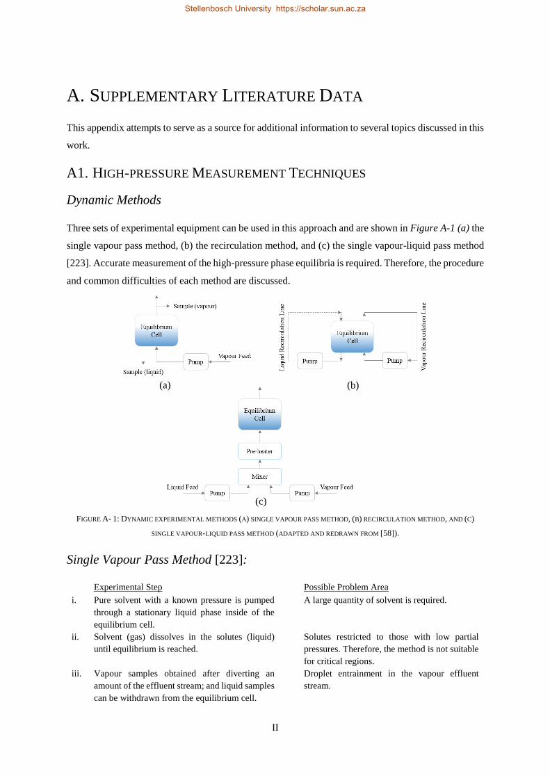
II
A. SUPPLEMENTARY LITERATURE DATA
This appendix attempts to serve as a source for additional information to several topics discussed in this
work.
A1. HIGH-PRESSURE MEASUREMENT TECHNIQUES
Dynamic Methods
Three sets of experimental equipment can be used in this approach and are shown in Figure A-1 (a) the
single vapour pass method, (b) the recirculation method, and (c) the single vapour-liquid pass method
[223]. Accurate measurement of the high-pressure phase equilibria is required. Therefore, the procedure
and common difficulties of each method are discussed.
FIGURE A- 1: DYNAMIC EXPERIMENTAL METHODS (A) SINGLE VAPOUR PASS METHOD, (B) RECIRCULATION METHOD, AND (C)
SINGLE VAPOUR-LIQUID PASS METHOD (ADAPTED AND REDRAWN FROM [58]).
Single Vapour Pass Method [223]:
Experimental Step Possible Problem Area
i. Pure solvent with a known pressure is pumped
through a stationary liquid phase inside of the
equilibrium cell.
A large quantity of solvent is required.
ii. Solvent (gas) dissolves in the solutes (liquid)
until equilibrium is reached.
Solutes restricted to those with low partial
pressures. Therefore, the method is not suitable
for critical regions.
iii. Vapour samples obtained after diverting an
amount of the effluent stream; and liquid samples
can be withdrawn from the equilibrium cell.
Droplet entrainment in the vapour effluent
stream.
(a) (b)
(c)
Stellenbosch University https://scholar.sun.ac.za
III
iv. Isobaric and isothermal VLE data generated by
controlling the vapour pressure and the liquid
temperature.
The solvent flowrate must be regulated to
ensure the correct amount of contact time and
avoid gas bubbles.
Phase Recirculation Method [223]:
Experimental Step Possible Problem Area
i. All the components are charged into the
equilibrium cell.
Maintaining a constant liquid level inside of the
cell is difficult.
ii. The pressure and temperature of the system is
controlled while either one or both phases are
continuously withdrawn from the equilibrium
cell and recirculated.
Droplet entrainment in the vapour effluent
stream;
Pumps may result in the contamination of the
equilibrium mixture.
iii. Sampling done by isolating a quantity of the
circulating phases.
Partial condensation of the vapour stream being
recirculated;
Vapourisation of the recirculating liquid
stream.
iv. Circulation of the phases will ensure enough
mixing inside of the cell for equilibrium to be
reached. No added stirring of the liquid phase
is required.
The circulating pumps may cause undesired
pressure gradients to form across the
equilibrium cell.
Single Vapour-liquid Pass Method [223]:
Experimental Step Possible Problem Area
i. The separate liquid and vapour streams are
contacted co-currently before entering the
preheater.
Pumps might result in contaminations of the
equilibrium mixture.
ii. Temperature and pressure controlled in the
mixing unit.
Undesirable pressure gradient still observed
across the equilibrium cell.
iii. The combined mixture will pass into the
equilibrium cell after being heated.
The vapour and liquid phases will separate
inside of the cell.
Difficult to achieve complete phase separation.
Equilibrium must be achieved after 1 pass.
iv. After being separated, the vapour and liquid
phases will exit the cell separately.
Difficult to ensure a steady liquid level inside
of the equilibrium cell.
v. Sampling can be done once the effluent streams
have been separated.
Droplet entrainment in the vapour effluent
stream.
Static Methods
The experimental equipment used for a typical analytical approach is shown in Figure A-2. For the
synthetic approach, a similar set of equipment is used. The only difference is the added equipment
needed for analysing the samples [222]. The experimental procedure and common difficulties of each
static method are discussed below.
Stellenbosch University https://scholar.sun.ac.za
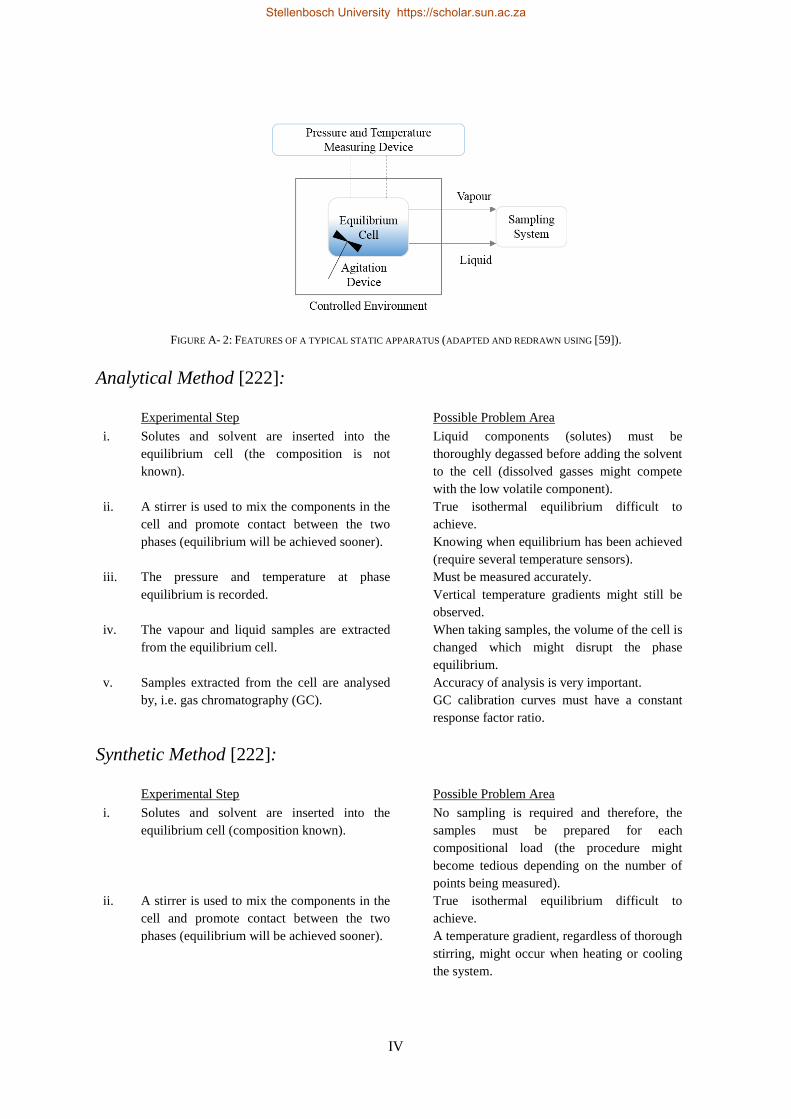
IV
FIGURE A- 2: FEATURES OF A TYPICAL STATIC APPARATUS (ADAPTED AND REDRAWN USING [59]).
Analytical Method [222]:
Experimental Step Possible Problem Area
i. Solutes and solvent are inserted into the
equilibrium cell (the composition is not
known).
Liquid components (solutes) must be
thoroughly degassed before adding the solvent
to the cell (dissolved gasses might compete
with the low volatile component).
ii. A stirrer is used to mix the components in the
cell and promote contact between the two
phases (equilibrium will be achieved sooner).
True isothermal equilibrium difficult to
achieve.
Knowing when equilibrium has been achieved
(require several temperature sensors).
iii. The pressure and temperature at phase
equilibrium is recorded.
Must be measured accurately.
Vertical temperature gradients might still be
observed.
iv. The vapour and liquid samples are extracted
from the equilibrium cell.
When taking samples, the volume of the cell is
changed which might disrupt the phase
equilibrium.
v. Samples extracted from the cell are analysed
by, i.e. gas chromatography (GC).
Accuracy of analysis is very important.
GC calibration curves must have a constant
response factor ratio.
Synthetic Method [222]:
Experimental Step Possible Problem Area
i. Solutes and solvent are inserted into the
equilibrium cell (composition known).
No sampling is required and therefore, the
samples must be prepared for each
compositional load (the procedure might
become tedious depending on the number of
points being measured).
ii. A stirrer is used to mix the components in the
cell and promote contact between the two
phases (equilibrium will be achieved sooner).
True isothermal equilibrium difficult to
achieve.
A temperature gradient, regardless of thorough
stirring, might occur when heating or cooling
the system.
Stellenbosch University https://scholar.sun.ac.za
V
iii. Pressure and temperature are manually
controlled to achieve phase separation of the
homogenous phase.
The pressure and temperature at the phase
transition point is recorded.
Information obtained for mixtures with more
than two components is limited (usually
bubble, dew and critical point data).
iv. Once the second phase has been noted, the
pressure and temperature are manually
controlled again to achieve a homogenous
phase.
De-mixing and layering of the phases can occur
if the mixture is not adjusted back to a
homogenous phase.
v A T(P) isopleth (the pressure is varied while the
temperature is kept constant) is formed when
continuously adjusting the temperature and
noting the phase transition pressures (while
keeping a constant composition).
It is easy to overlook the dew point phase
transitions (liquid phase might condense as this
film on the cell wall).
A2. LOW-PRESSURE MEASUREMENT TECHNIQUES
Special techniques include:
i. Dew point/ bubble point (DPBP) methods:
A calibrated piston/ cylinder assembly that is submerged in a bath that is kept under isothermal
conditions. The composition is known beforehand, and the pressures are measured in turn as a function
of volume. This technique can be hindered by small amounts of dissolved gasses that complicate the
accuracy at which bubble point pressures are measured.
ii. An Isopiestic method:
This method is more suitable for mixtures that are comprised of a single volatile component which is
not the case for the system being investigated in this study [227].
iii. Semi-micro techniques:
In instances when the chemicals being measured are expensive and therefore limited the Semi-micro
technique is useful as high volumes for phase equilibria measurement is not required [84].
iv. Measurement of infinitely dilute activity coefficients
The measurement of infinitely dilute activity coefficients provides an indication of the non-ideality of
the system in the highly dilute composition area. This method is extremely expensive and does not
cover the entire composition range. It is for this reason that one of the most comprehensive low-pressure
measurement techniques should be utilised for this project. These techniques include [227]:
• Dynamic circulation stills; and
• Static cells
Stellenbosch University https://scholar.sun.ac.za
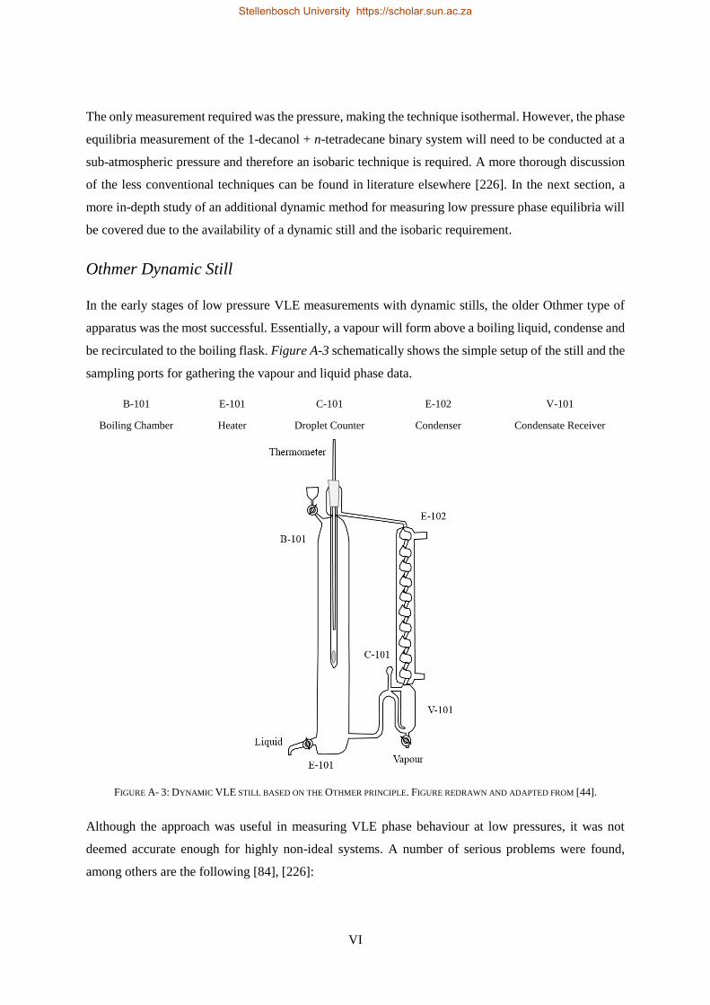
VI
The only measurement required was the pressure, making the technique isothermal. However, the phase
equilibria measurement of the 1-decanol + n-tetradecane binary system will need to be conducted at a
sub-atmospheric pressure and therefore an isobaric technique is required. A more thorough discussion
of the less conventional techniques can be found in literature elsewhere [226]. In the next section, a
more in-depth study of an additional dynamic method for measuring low pressure phase equilibria will
be covered due to the availability of a dynamic still and the isobaric requirement.
Othmer Dynamic Still
In the early stages of low pressure VLE measurements with dynamic stills, the older Othmer type of
apparatus was the most successful. Essentially, a vapour will form above a boiling liquid, condense and
be recirculated to the boiling flask. Figure A-3 schematically shows the simple setup of the still and the
sampling ports for gathering the vapour and liquid phase data.
B-101 E-101 C-101 E-102 V-101
Boiling Chamber Heater Droplet Counter Condenser Condensate Receiver
FIGURE A- 3: DYNAMIC VLE STILL BASED ON THE OTHMER PRINCIPLE. FIGURE REDRAWN AND ADAPTED FROM [44].
Although the approach was useful in measuring VLE phase behaviour at low pressures, it was not
deemed accurate enough for highly non-ideal systems. A number of serious problems were found,
among others are the following [84], [226]:
Stellenbosch University https://scholar.sun.ac.za
VII
• The vapour condensate receiver is too large, preventing true equilibrium from being attained as
well as errors in the composition measurements.
• Due to the boiling chamber walls being too large, partial condensation of the equilibrium vapour
will occur.
• A lack of stirring will result in uneven boiling and minimum fluctuations in temperature.
• Poor contact between the temperature probe and both equilibrium phases will cause inaccuracies
in measurements. The Othmer still only takes the vapour phase measurement and therefore the
temperature readings are unsatisfactory.
Based on these complications the Othmer still was deemed unusable for the generation of accurate VLE
data. The Gillespie still [226] that utilises a Cottrell vapour lift pump to circulate not only the vapour
phase but also the liquid phase is a good alternative for generating accurate VLE data.
A3. THERMODYNAMIC CONSISTENCY TESTS
The experimental data will need to be validated by checking its conformance with the Gibbs/Duhem
equation. The variable M will be used as the molar value to represent any extensive thermodynamic
property throughout the derivation. Therefore, knowing that [63]:
𝑛𝑀 = 𝑓(𝑇, 𝑃, 𝑛𝑖) (A.1)
We can formulate the differential:
𝑑(𝑛𝑀) = [𝜕(𝑛𝑀)
𝜕𝑃]
𝑇,𝑛𝑖
𝑑𝑃 + [𝜕(𝑛𝑀)
𝜕𝑇]
𝑃,𝑛𝑖
𝑑𝑇 + ∑ [𝜕(𝑛𝑀)
𝜕𝑛𝑖]
𝑇,𝑃,𝑛𝑖
𝑑𝑛𝑖𝑖 (A.2)
Where a simplification can be made for the partial property of species i in (A.2):
[𝜕(𝑛𝑀)
𝜕𝑛𝑖]
𝑇,𝑃,𝑛𝑖
= 𝑀𝑖 (A.3)
Furthermore, with constant total moles, (A.2) can be simplified to:
𝑑(𝑛𝑀) = 𝑛 [𝜕𝑀
𝜕𝑃]
𝑇,𝑥𝑖
𝑑𝑃 + 𝑛 [𝜕𝑀
𝜕𝑇]
𝑃,𝑥𝑖
𝑑𝑇 + ∑ 𝑀𝑖 𝑑𝑛𝑖𝑖 (A.4)
Applying the product rule the following simplifications can be made to (A.4):
𝑑𝑛𝑖 = 𝑥𝑖𝑑𝑛 + 𝑛𝑑𝑥𝑖 (A.5)
𝑑(𝑛𝑀) = 𝑛𝑑𝑀 + 𝑀𝑑𝑛 (A.6)
Once (A.5) and (A.6) have been substituted into (A.4), simplifying will result in:
0 = 𝑛 [(𝜕𝑀
𝜕𝑃)
𝑇,𝑥𝑖
𝑑𝑃 + (𝜕𝑀
𝜕𝑇)
𝑃,𝑥𝑖
𝑑𝑇 + ∑ 𝑀𝑖 𝑑𝑥𝑖𝑖 − 𝑑𝑀] + [∑ 𝑀𝑖
𝑥𝑖𝑖 − 𝑀]𝑑𝑛 (A.7)
By equating both sections bringing together (A.7) to zero and applying summability relations to the
second part, the mixture properties can be calculated from the partial properties and differentiated to
form:
Stellenbosch University https://scholar.sun.ac.za
VIII
𝑑𝑀 = (𝜕𝑀
𝜕𝑃)
𝑇,𝑥𝑖
𝑑𝑃 + (𝜕𝑀
𝜕𝑇)
𝑃,𝑥𝑖
𝑑𝑇 + ∑ 𝑀𝑖 𝑑𝑥𝑖𝑖 (A.8)
𝑑𝑀 = ∑ 𝑥𝑖𝑑𝑀𝑖
𝑖 + ∑ 𝑀𝑖
𝑖 𝑑𝑥𝑖 (A.9)
Finally, the Gibbs/Duhem equation can be constructed by substituting (A.9) into (A.8) and simplifying:
0 = (𝜕𝑀
𝜕𝑃)
𝑇,𝑥𝑖
𝑑𝑃 + (𝜕𝑀
𝜕𝑇)
𝑃,𝑥𝑖
𝑑𝑇 − ∑ 𝑥𝑖𝑑𝑀𝑖 𝑖 (A.10)
To formulate the two king-pin equations for the performance of thermodynamic consistency tests, at an
assumed constant temperature and pressure, the Excess Gibbs Energy equation can be used. Knowing
from fundamentals the first relationship to be satisfied can be defined:
��𝐸𝑖 = 𝑅𝑇𝑙𝑛𝛾𝑖 (A.11)
The definition of partial molar properties can now be used to define:
𝐺𝐸 = ∑ 𝑥𝑖��𝐸𝑖𝑖 (A.12)
By incorporating (A.11) into (A.12), the excess Gibbs equation for a multicomponent system can be
constructed based on summability:
𝐺𝐸 = 𝑅𝑇 ∑ 𝑥𝑖𝑙𝑛𝛾𝑖𝑖 (A.13)
Replacing the thermodynamic variable M in (A.10) with the Gibbs Energy thermodynamic property, G
and taking into consideration the assumed constant temperature and pressure, the Gibbs/Duhem
equation can be simplified to:
∑ 𝑥𝑖𝑑𝐺𝑖𝐸 𝑖 = 0 (A.14)
Lastly, by incorporating (A.11) into (A.14) the second relationship to be satisfied by the measured data
can be defined:
∑ 𝑥𝑖𝑑𝑙𝑛𝛾𝑖 𝑖 = 0 (A.15)
If the measured data for 𝛾𝑖 are not satisfying both (A.11) and (A.15) it will be considered as inconsistent
and therefore not useful for modelling the system.
Area Test
During the experimental procedure for testing the phase behaviour of the 1-decanol + n-tetradecane
binary system, samples of both the vapour and liquid phase will be taken for analyses at a set
temperature and pressure. Therefore, the activity coefficient for each component in the mixture can be
determined. Equation (A.15) therefore reduces to:
0 = 𝑥1𝑑 𝑙𝑛 𝛾1
𝑑𝑥1+ 𝑥2
𝑑 𝑙𝑛 𝛾2
𝑥1 (A.16)
Stellenbosch University https://scholar.sun.ac.za
IX
Unfortunately, (A.16) is not linked to the Gibbs/Duhem equation and cannot be used to verify
consistency. The two-component system can therefore be substituted into (A.11) to give:
𝐺𝐸 = 𝑅𝑇[𝑥1𝑙𝑛𝛾1 + (1 − 𝑥1)𝑙𝑛𝛾2] (A.17)
∴𝑑𝐺𝐸
𝑑𝑥1= 𝑅𝑇 (𝑙𝑛𝛾1 − 𝑙𝑛𝛾2 +
𝑥1𝑑𝑙𝑛𝛾1+𝑥2𝑑𝑙𝑛𝛾2
𝑑𝑥1) (A.18)
Now substituting (A.15) into (A.18) and simplifying:
𝑑𝐺𝐸 = 𝑅𝑇 𝑙𝑛 (𝛾1
𝛾2) 𝑑𝑥1 (A.19)
Integrating (A.19) from pure 1-decanol to pure n-tetradecane:
∫ 𝑑𝐺𝐸 =𝑝𝑢𝑟𝑒 𝑛−𝐶14
𝑝𝑢𝑟𝑒 1−𝐶10𝑂𝐻𝑅𝑇 ∫ ln (
𝛾1
𝛾2) 𝑑𝑥1
𝑥1=1
𝑥1=0 (A.20)
Furthermore, due to GE being a state property, the pure Gibbs energy of each component will tend to
zero as that component tends to unity resulting in the activity coefficient of that component similarly
tending to unity:
∴ 𝐺𝑖𝐸 → 0 𝑤ℎ𝑒𝑛 𝑥𝑖 → 0, 𝑠𝑖𝑛𝑐𝑒 𝛾𝑖 → 1 (A.21)
The left-hand side of (A.20) is zero and at constant temperature and pressure simplifies to:
∫ ln (𝛾1
𝛾2) 𝑑𝑥1
𝑥1=1
𝑥1=0= 0 (A.22)
This equation is therefore used to formulate the thermodynamic consistency test, as a plot of ln (𝛾1
𝛾2)
versus 𝑥1 will produce a curve crossing the x-axis at an arbitrary point. The total area under the curve
should be close to zero for the data to be considered as thermodynamically consistent with (A.11) and
(A.15). In the generation of true vapour-liquid data sets (A.22) will unfortunately not be viable as either
the temperature or pressure must be altered to effect a change in the equilibrium composition.
The activity coefficients are strongly dependent on temperature and only slightly dependent on
pressure. Therefore, under isothermal conditions the activity coefficient will remain constant and (A.22)
will be valid for testing the thermodynamic consistency. However, in the isobaric case as is with the
present study (A.22) should be modified to compensate for the temperature effects. It is for this reason
that a different approach needs to be considered where the experimental data can be tested under
isobaric conditions. One such approach was developed in 1993 by Wisniak [259], namely the L/W
consistency test.
L/W Consistency Test
Wisniak [259] proposed an approach where the relationship between the excess Gibbs energy (A.13) of
the binary system is compared to its boiling point temperature at equilibrium and the Gibbs/Duhem
equation is disregarded in this case. Assuming all the non-ideality of the pure components are
Stellenbosch University https://scholar.sun.ac.za
X
concentrated in the liquid phase the vapour phase will behave like an ideal gas. An approximation of
the activity coefficients can be calculated at low pressures using [259]:
𝛾𝑖 ≈𝑦𝑖𝑃
𝑥𝑖𝑃𝑖𝑠𝑎𝑡 (A.23)
To calculate the 𝑃
𝑃𝑖𝑠𝑎𝑡 ratio in (A.23) the Clausius-Clapeyron equation can be used:
ln
𝑃
𝑃𝑖𝑠𝑎𝑡 =
∆𝐻𝑖𝑠𝑎𝑡(𝑇𝑖
𝑠𝑎𝑡−𝑇)
𝑅𝑇𝑖𝑠𝑎𝑡𝑇
(A.24)
However, in order to use (A.24), the heat of vaporization of each component is assumed to be constant
in the range of boiling points tested and the liquid molar volumes are also assumed negligible when
compared to that of the vapour [259]. Therefore, (A.24) can be further simplified to:
ln
𝑃
𝑃𝑖𝑠𝑎𝑡 =
∆𝑆𝑖𝑠𝑎𝑡(𝑇𝑖
𝑠𝑎𝑡−𝑇)
𝑅𝑇 (A.25)
Combining (A.25) with (A.23) and then substituting the result into (A.13) will yield:
𝐺𝐸 = ∑ 𝑥𝑖∆𝑆𝑖𝑠𝑎𝑡(𝑇𝑖
𝑠𝑎𝑡 − 𝑇)𝑖 + 𝑅𝑇 ∑ 𝑥𝑖 ln (𝑦𝑖
𝑥𝑖)𝑖 (A.26)
Furthermore, Wisniak [259] defined two equations that can be utilised with (A.26) to construct the
expression for determining the bubble-point temperature of the binary mixture. The two equations along
with the final bubble-point temperature expression are:
∆𝑆 = ∑ 𝑥𝑖∆𝑆𝑖𝑠𝑎𝑡
𝑖 (A.27)
𝑤 = ∑ 𝑥𝑖 ln (𝑦𝑖
𝑥𝑖)𝑖 (A.28)
𝑇𝐵𝑢𝑏 = ∑𝑇𝑖
𝑠𝑎𝑡𝑥𝑖∆𝑆𝑖𝑠𝑎𝑡
∆𝑆𝑖 −𝐺𝐸
∆𝑆+
𝑅𝑇𝑤
∆𝑆 (A.29)
The bubble-point temperature expression of the mixture (A.29) is rearranged to construct a
thermodynamic consistency test:
𝐿𝑘 = ∑𝑇𝑖
𝑠𝑎𝑡𝑥𝑖∆𝑆𝑖𝑠𝑎𝑡
∆𝑆𝑘 − 𝑇𝐵𝑢𝑏 =𝐺𝐸
∆𝑆−
𝑅𝑇𝑤
∆𝑆= 𝑊𝑘 (A.30)
𝐿𝑘 will always be positive except in the case where there is an azeotrope formed, as is expected for this
study, in which case the left hand side of (A.30) will be negative [259]. The right-hand side of (A.30),
𝑊𝑘 , will be consistent with the 𝐿𝑘 value. Lastly, 𝐺𝐸 can be calculated using (A.13) and will be positive
or negative based on the deviations from ideality. The test is applied to each of the vapour-liquid
equilibrium data pairs, 𝑘, experimentally measured and integration over this entire range will therefore
provide the final values of L and W:
𝐿 = ∫ 𝐿𝑘𝑑𝑥11
0= ∫ 𝑊𝑘𝑑𝑥1
1
0= 𝑊 (A.31)
Stellenbosch University https://scholar.sun.ac.za
XI
If equal values for both L and W, are obtained using (A.31), the data will be verified as
thermodynamically consistent. Unfortunately, due to experimental errors and the assumptions made to
derive the thermodynamic test, a deviation factor must be defined. Wisniak [259] proposed the
following:
𝐷 =100|𝐿−𝑊|
𝐿+𝑊 (A.32)
To assure thermodynamic consistency, the value calculated using (A.32) should be less than 3 to 5. The
lower limit is specified in order to abide by the Herrington test for consistency and the upper limit for
cases when the heat of vaporization is unknown and requires estimating [259], [260].
The L/W test will confirm the experimental data as a representation of the system dynamics by means
of [84]:
i. An area test where the D value (A.32) is within reason across the entire composition range.
ii. A point-to-point test where (A.30) must be satisfied for each experimental point measured.
As mentioned previously, the Gibbs-Duhem equation is disregarded when using this consistency
test. Therefore, a second test is recommended to be used in conjunction with the L/W test. One
consistency test proven useful in literature is the McDermott-Ellis test.
McDermott-Ellis Consistency Test
With reference to (A.16) and applying the trapezoidal rule, the two-point consistency test can be derived
through integration for, i.e. points c and d [238]:
0 = ∑ (𝑥𝑖𝑐 + 𝑥𝑖𝑑)(ln 𝛾𝑖𝑑 − ln 𝛾𝑖𝑐)𝑁𝑖=1 (A.33)
Consistency of each consecutive data point is thus evaluated separately. McDermott and Ellis [238]
judged the data as consistent or inconsistent depending on a constant deviation of 0.01 for (A.33).
therefore, the vapour and liquid fractions had to lie within a maximum composition deviation of ± 0.001
[261].
Several years later it was argued that the inaccuracies of the parameters should be considered within
the criteria of the consistency test. Therefore, the maximum deviation would no longer be a constant,
but rather a function of the measured composition (∆𝑥), temperature (∆𝑇) and pressure (∆𝑃)
accuracies. Wisniak and Tamir [262] redefined (A.33) to:
0 = ∑ (𝑥𝑖𝑐 + 𝑥𝑖𝑑) (1
𝑥𝑖𝑐+
1
𝑥𝑖𝑑+
1
𝑦𝑖𝑐+
1
𝑦𝑖𝑑) ∆𝑥𝑁
𝑖=1 + 2 ∑ |ln 𝛾𝑖𝑑 −𝑁𝑖=1
ln 𝛾𝑖𝑐|∆𝑥 + ∑ (𝑥𝑖𝑐 + 𝑥𝑖𝑑)∆𝑃
𝑃𝑁𝑖=1 + ∑ (𝑥𝑖𝑐 + 𝑥𝑖𝑑)𝛽𝑖 (
1
|𝑇𝑐+ 𝛿𝑖|2 +1
|𝑇𝑑+ 𝛿𝑖|2 ) ∆𝑇 𝑁𝑖=1
(A.34)
Where, 𝛽𝑖 = Bi and 𝛿𝑖 = Ci constants for the components being evaluated.
Stellenbosch University https://scholar.sun.ac.za
XII
B. DETAILED EXPERIMENTAL PROCEDURES
The following section will cover the details regarding the experimental work conducted in this work.
Schematic diagrams are provided for each of the experimental setups followed by a step-by-step
description of the procedure to follow.
B1. HPBDP EXPERIMENTAL PROCEDURE
Loading procedure
No. Step
1 The cell should be carefully turned vertically
2 The magnetic stirrer can be inserted into the cell
3 The equilibrium cell valve is closed
4 Measure the correct amount of solute mixture as per the mass fraction specified can now be insert it
into the cell using a pipette
5 The piston head piece should then be screwed onto the cell
6 The piston should be tightened to avoid variations in volume
7 The cell should then be turned horizontally
8 The four-way section is to be connected onto the equilibrium cell outlet/ inlet
9 All valves should be closed
10 The vacuum pump is switched on
11 One can collect the carbon dioxide using the gas cylinder provided
12 The carbon dioxide gas cylinder can then be connected to the four-way valve
13 Once secured correctly onto the cell, the vacuum valve can be opened slightly
14 The equilibrium cell valve can now also be opened fractionally to evacuate as much air as possible
from the cell (careful not to remove any solute)
15 The valves should again be closed
16 The television monitor is switched on and the medical camera with the endoscope is inserted in front
of the sapphire window
17 The cell is now flushed 6 times with carbon dioxide (solvent) to remove any residual air in the
equilibrium cell
18 The carbon dioxide cylinder is opened and closed to flush solvent into the four-way section
19 The equilibrium valve is then opened a quarter of a way slowly to allow the solvent into the cell
20 The valve to atmosphere on the four-way connection is opened to flush the solvent out of the cell
21 After the final flush, the cell can remain open and all the other valves should be closed.
Stellenbosch University https://scholar.sun.ac.za

XIII
22 The magnetic stirrer and hot plate can now be placed under the cell and switched on to remove air
bubbles from pressure build-up in the cell
23 Release the last bit of built up pressure to atmosphere
24 Close the equilibrium cell valve and all the valves on the four-way connector
25 The carbon dioxide gas cylinder should now be removed from the four-way connector and weighed
26 If enough solvent is left in the cylinder to load into the cell no more should be collected
27 The solvent should be gravimetrically measured to the specified amount
28 If too little solvent remained in the cylinder more should be collected
29 The cylinder is placed back onto the four-way connector
30 The vacuum is opened once more to air out the four-way connection
31 The solvent in the cylinder should be heated with the hair-dryer
32 The vacuum valve can be closed
33 Once hot enough the equilibrium cell inlet/ outlet valve can be opened 100 %
34 The cylinder is then opened, and the solvent released into the cell
35 The four-way connector should also be heated with the hair-dryer to remove solvent from the piping
network
36 Once all the solvent has been loaded the cell can be closed
37 The four-way connector valve to the atmosphere is opened to relief the pressure in the piping network
38 The solvent cylinder can now be removed from the four-way connector and weighed
39 The total mass of the components in the cell can now be measured
40 If the mass fraction is incorrect the solvent loading should be repeated
41 If correct, the vacuum can be switched off and the four-way connector can be removed from the
equilibrium cell
42 The Julabo circulating liquid bath can now be switched on and the first temperature set point entered
43 A metal container containing the insulation material is placed around the equilibrium cell to conserve
heat
44 The magnetic plate is positioned below the equilibrium cell and secures the container around the cell
45 The magnetic stirrer can be switched on
46 The temperature Pt-100 probe can be inserted inside the cell wall
47 The piston ruler is attached to the cell and zeroed
48 The nitrogen gas line is connected to the piston head (low pressure region) and the pressure
systematically increased in the high-pressure chamber
49 A cap is placed on the equilibrium cell inlet/outlet port
50 The cell can now be left to achieve thermal equilibrium (approximately 30min)
Stellenbosch University https://scholar.sun.ac.za

XIV
Testing Procedure
No. Step
1 Once thermal equilibrium has been reached and the pressure is high enough to ensure a single phase
the measurements can be taken
2 The components are observed on the TV monitor
3 If a single phase has not been attained, additional nitrogen gas should be added to the cell
4 Nitrogen gas is then to be slowly released from the chamber to decrease the pressure until the first sign
of vapour bubbles
5 An extrapolation method can then be applied to iteratively take readings until the exact phase transition
point is obtained with an accuracy of 0.2 bar
6 The phase transition will occur at the highest possible pressure before the single phase is converted
into two phases
7 The pressure, temperature, piston position and phase criteria must be recorded
8 The next set temperature should now be selected
9 The nitrogen gas can be increased to create a pressure increase and allow for equilibrium to be attained
once more in a single phase
Stellenbosch University https://scholar.sun.ac.za
XV
Unloading Procedure
No. Step
1 The nitrogen cylinder can be closed once all the tests have been completed
2 The nitrogen from the cell can be drained
3 The heating bath can be switched off
4 The medical camera and endoscope can be removed and switched off
5 The Pt-100 probe and the piston ruler can be removed from the cylinder
6 The magnetic plate can be switched off and removed
7 The insulation material and the container can be removed
8 The cell can now be left to cool down (cooling water system switched on)
9 All the correct protection clothing should now be worn
10 The cap on the equilibrium cell inlet/ outlet port can now be removed
11 The cell should be turned at an angle and the nozzle pointing downwards
12 An Erlenmeyer flask can be used to capture the exiting components when opening the equilibrium cell
valve
13 The cell can be turned vertically, and the piston loosened
14 A three-point test needs to be conducted to make sure it is safe before removing the head of the
cylinder.
- The piston rod should be loosened to move down when force is applied onto it. This gives an
indication that there is not a lot of pressure inside the cell.
- The equilibrium cell valve should be open
- The reading of the pressure transmitter should be close to the initial zero point.
Stellenbosch University https://scholar.sun.ac.za

XVI
Cleaning Procedure
No. Step
1 The cell can now be angled with the open end slanted downwards at a 45°
2 The magnetic stirrer can be removed
3 The cell is first thoroughly washed out with xylene
4 The chemicals are captured in a waste bucket
5 The nozzle should also be cleaned with xylene
6 The cell can now be rinsed using methanol to remove the xylene
7 Pressurised air can then be used to dry the cell
8 Paper towel is also used to ensure the cell is completely dry and clean
9 The cooling system can now be switched off
10 The heating batch can be switched off
11 The magnetic stirrer should also be cleaned with xylene, followed by methanol
12 Ensure everything is returned to the correct place
13 The chemicals should be disposed in the correct waste bin
Stellenbosch University https://scholar.sun.ac.za
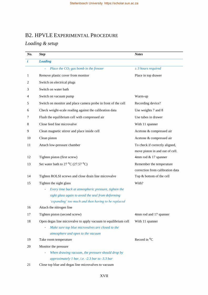
XVII
B2. HPVLE EXPERIMENTAL PROCEDURE
Loading & setup
No. Step Notes
i Loading
- Place the CO2 gas bomb in the freezer ± 3 hours required
1 Remove plastic cover from monitor Place in top drawer
2 Switch on electrical plugs
3 Switch on water bath
4 Switch on vacuum pump Warm-up
5 Switch on monitor and place camera probe in front of the cell Recording device?
6 Check weight-scale reading against the calibration data Use weights 7 and 8
7 Flush the equilibrium cell with compressed air Use tubes in drawer
8 Close feed line microvalve With 11 spanner
9 Clean magnetic stirrer and place inside cell Acetone & compressed air
10 Clean piston Acetone & compressed air
11 Attach low-pressure chamber To check if correctly aligned,
move piston in and out of cell.
12 Tighten piston (first screw) 4mm rod & 17 spanner
13 Set water bath to 27 ⁰C (27.57 ⁰C) Remember the temperature
correction from calibration data
14 Tighten ROLSI screws and close drain line microvalve Top & bottom of the cell
15 Tighten the sight glass
- Every time back at atmospheric pressure, tighten the
sight glass again to avoid the seal from deforming
‘expanding’ too much and then having to be replaced
With?
16 Attach the nitrogen line
17 Tighten piston (second screw) 4mm rod and 17 spanner
18 Open degas line microvalve to apply vacuum to equilibrium cell
- Make sure top blue microvalves are closed to the
atmosphere and open to the vacuum
With 11 spanner
19 Take room temperature Record in ⁰C
20 Monitor the pressure
- When drawing vacuum, the pressure should drop by
approximately 1 bar, i.e. -2.3 bar to -3.3 bar
21 Close top blue and degas line microvalves to vacuum
Stellenbosch University https://scholar.sun.ac.za
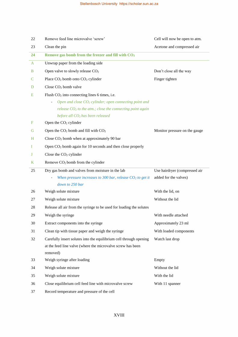
XVIII
22 Remove feed line microvalve ‘screw’ Cell will now be open to atm.
23 Clean the pin Acetone and compressed air
24 Remove gas bomb from the freezer and fill with CO2
A Unwrap paper from the loading side
B Open valve to slowly release CO2 Don’t close all the way
C Place CO2 bomb onto CO2 cylinder Finger tighten
D Close CO2 bomb valve
E Flush CO2 into connecting lines 6 times, i.e.
- Open and close CO2 cylinder; open connecting point and
release CO2 to the atm.; close the connecting point again
before all CO2 has been released
F Open the CO2 cylinder
G Open the CO2 bomb and fill with CO2 Monitor pressure on the gauge
H Close CO2 bomb when at approximately 90 bar
I Open CO2 bomb again for 10 seconds and then close properly
J Close the CO2 cylinder
K Remove CO2 bomb from the cylinder
25 Dry gas bomb and valves from moisture in the lab
- When pressure increases to 300 bar, release CO2 to get it
down to 250 bar
Use hairdryer (compressed air
added for the valves)
26 Weigh solute mixture With the lid, on
27 Weigh solute mixture Without the lid
28 Release all air from the syringe to be used for loading the solutes
29 Weigh the syringe With needle attached
30 Extract components into the syringe Approximately 23 ml
31 Clean tip with tissue paper and weigh the syringe With loaded components
32 Carefully insert solutes into the equilibrium cell through opening
at the feed line valve (where the microvalve screw has been
removed)
Watch last drop
33 Weigh syringe after loading Empty
34 Weigh solute mixture Without the lid
35 Weigh solute mixture With the lid
36 Close equilibrium cell feed line with microvalve screw With 11 spanner
37 Record temperature and pressure of the cell
Stellenbosch University https://scholar.sun.ac.za
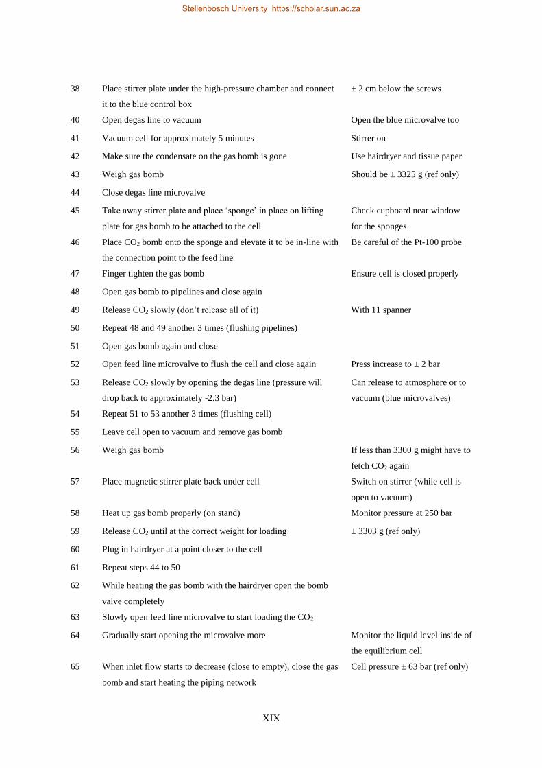
XIX
38 Place stirrer plate under the high-pressure chamber and connect
it to the blue control box
± 2 cm below the screws
40 Open degas line to vacuum Open the blue microvalve too
41 Vacuum cell for approximately 5 minutes Stirrer on
42 Make sure the condensate on the gas bomb is gone Use hairdryer and tissue paper
43 Weigh gas bomb Should be ± 3325 g (ref only)
44 Close degas line microvalve
45 Take away stirrer plate and place ‘sponge’ in place on lifting
plate for gas bomb to be attached to the cell
Check cupboard near window
for the sponges
46 Place CO2 bomb onto the sponge and elevate it to be in-line with
the connection point to the feed line
Be careful of the Pt-100 probe
47 Finger tighten the gas bomb Ensure cell is closed properly
48 Open gas bomb to pipelines and close again
49 Release CO2 slowly (don’t release all of it) With 11 spanner
50 Repeat 48 and 49 another 3 times (flushing pipelines)
51 Open gas bomb again and close
52 Open feed line microvalve to flush the cell and close again Press increase to ± 2 bar
53 Release CO2 slowly by opening the degas line (pressure will
drop back to approximately -2.3 bar)
Can release to atmosphere or to
vacuum (blue microvalves)
54 Repeat 51 to 53 another 3 times (flushing cell)
55 Leave cell open to vacuum and remove gas bomb
56 Weigh gas bomb If less than 3300 g might have to
fetch CO2 again
57 Place magnetic stirrer plate back under cell Switch on stirrer (while cell is
open to vacuum)
58 Heat up gas bomb properly (on stand) Monitor pressure at 250 bar
59 Release CO2 until at the correct weight for loading ± 3303 g (ref only)
60 Plug in hairdryer at a point closer to the cell
61 Repeat steps 44 to 50
62 While heating the gas bomb with the hairdryer open the bomb
valve completely
63 Slowly open feed line microvalve to start loading the CO2
64 Gradually start opening the microvalve more Monitor the liquid level inside of
the equilibrium cell
65 When inlet flow starts to decrease (close to empty), close the gas
bomb and start heating the piping network
Cell pressure ± 63 bar (ref only)
Stellenbosch University https://scholar.sun.ac.za
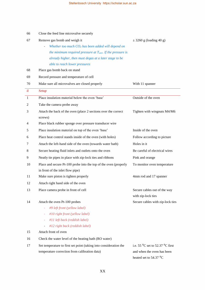
XX
66 Close the feed line microvalve securely
67 Remove gas bomb and weigh it
- Whether too much CO2 has been added will depend on
the minimum required pressure at Tset1. If the pressure is
already higher, then must degas at a later stage to be
able to reach lower pressures
± 3260 g (loading 40 g)
68 Place gas bomb back on stand
69 Record pressure and temperature of cell
70 Make sure all microvalves are closed properly With 11 spanner
ii Setup
1 Place insulation material below the oven ‘base’ Outside of the oven
2 Take the camera probe away
3 Attach the back of the oven (place 2 sections over the correct
screws)
Tighten with wingnuts M4/M6
4 Place black rubber sponge over pressure transducer wire
5 Place insulation material on top of the oven ‘base’ Inside of the oven
6 Place heat control stands inside of the oven (with holes) Follow according to picture
7 Attach the left-hand side of the oven (towards water bath) Holes in it
8 Secure heating fluid inlets and outlets onto the oven Be careful of electrical wires
9 Neatly tie pipes in place with zip-lock ties and ribbons Pink and orange
10 Place and secure Pt-100 probe into the top of the oven (properly
in front of the inlet flow pipe)
To monitor oven temperature
11 Make sure piston is tighten properly 4mm rod and 17 spanner
12 Attach right hand side of the oven
13 Place camera probe in front of cell Secure cables out of the way
with zip-lock ties
14 Attach the oven Pt-100 probes
- #9 left front (yellow label)
- #10 right front (yellow label)
- #11 left back (reddish label)
- #12 right back (reddish label)
Secure cables with zip-lock ties
15 Attach front of oven
16 Check the water level of the heating bath (RO water)
17 Set temperature to first set point (taking into consideration the
temperature correction from calibration data)
i.e. 55 ⁰C set to 52.37 ⁰C first
and when the oven has been
heated set to 54.37 ⁰C
Stellenbosch University https://scholar.sun.ac.za
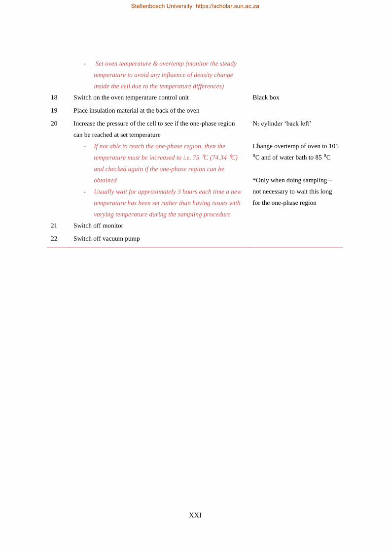
XXI
- Set oven temperature & overtemp (monitor the steady
temperature to avoid any influence of density change
inside the cell due to the temperature differences)
18 Switch on the oven temperature control unit Black box
19 Place insulation material at the back of the oven
20 Increase the pressure of the cell to see if the one-phase region
can be reached at set temperature
- If not able to reach the one-phase region, then the
temperature must be increased to i.e. 75 ⁰C (74.34 ⁰C)
and checked again if the one-phase region can be
obtained
- Usually wait for approximately 3 hours each time a new
temperature has been set rather than having issues with
varying temperature during the sampling procedure
N2 cylinder ‘back left’
Change overtemp of oven to 105
⁰C and of water bath to 85 ⁰C
*Only when doing sampling –
not necessary to wait this long
for the one-phase region
21 Switch off monitor
22 Switch off vacuum pump
Stellenbosch University https://scholar.sun.ac.za

XXII
Measurements
Terminology:
i. Purge series = pre-pre-purge (to clean capillary)
ii. Slow purge = pre-purge (until peaks level out → liquid peaks are larger due to more solutes)
iii. Fast purge = purge (before each sample series, i.e. alternating)
iv. Sample series = analysis A1, A2, A3 and A4
Important to know:
i. Front ROLSI (#2) inlet at the back of GC; therefore, on computer = SSL Back
ii. Back ROLSI (#1) inlet at the front of GC; therefore, on computer = SSL Front
iii. When sampling at a pressure close to the one phase region:
- Do the purge series 1st.
- Then set the cell pressure higher to reach the one-phase region before taking the system back
down to the required isobaric condition.
- Once all droplets in the capillary cone are gone (high solute vapour phase it will disappear; and
low solute vapour phase it will drop down).
- Start the slow purge series
- Alternate between the fast purge and the sample series (total of 4 samples)
iv. The slow purge series will require different timer settings for the vapour and the liquid phases to
clear the capillaries properly:
- Vapour: Multiple, smaller purge extractions (less disruptive)
- Liquid: Can be much more vigorous due to no dew interferences; therefore, use small number
of large extractions at 30 secs apart
v. The pressure sensitivity increases as the total solubility pressure is approached (the pressure at
which the mixture enters a one-phase region).
vi. For measurements close to the phase transition point increase the pressure to the one-phase region
first and then decrease to the set pressure;
For measurements, further away from the transition point, start at lower pressures in the two-
phase region and increase to the set pressure.
vii. It is helpful to sync up both computers with a watch; therefore, when observing something odd
in the equilibrium cell, the videos and recorded temperatures/pressures can be referred to per the
logged time of the occurrence (data is logged on each day).
viii. Make sure to always monitor the pressure and keep it as constant as possible throughout each
measurement.
ix. At higher temperature measurements, the viscosity of the vapour phase is more vapour intensive
than liquid intensive which creates small drops with lower surface areas (global mist formation)
Stellenbosch University https://scholar.sun.ac.za
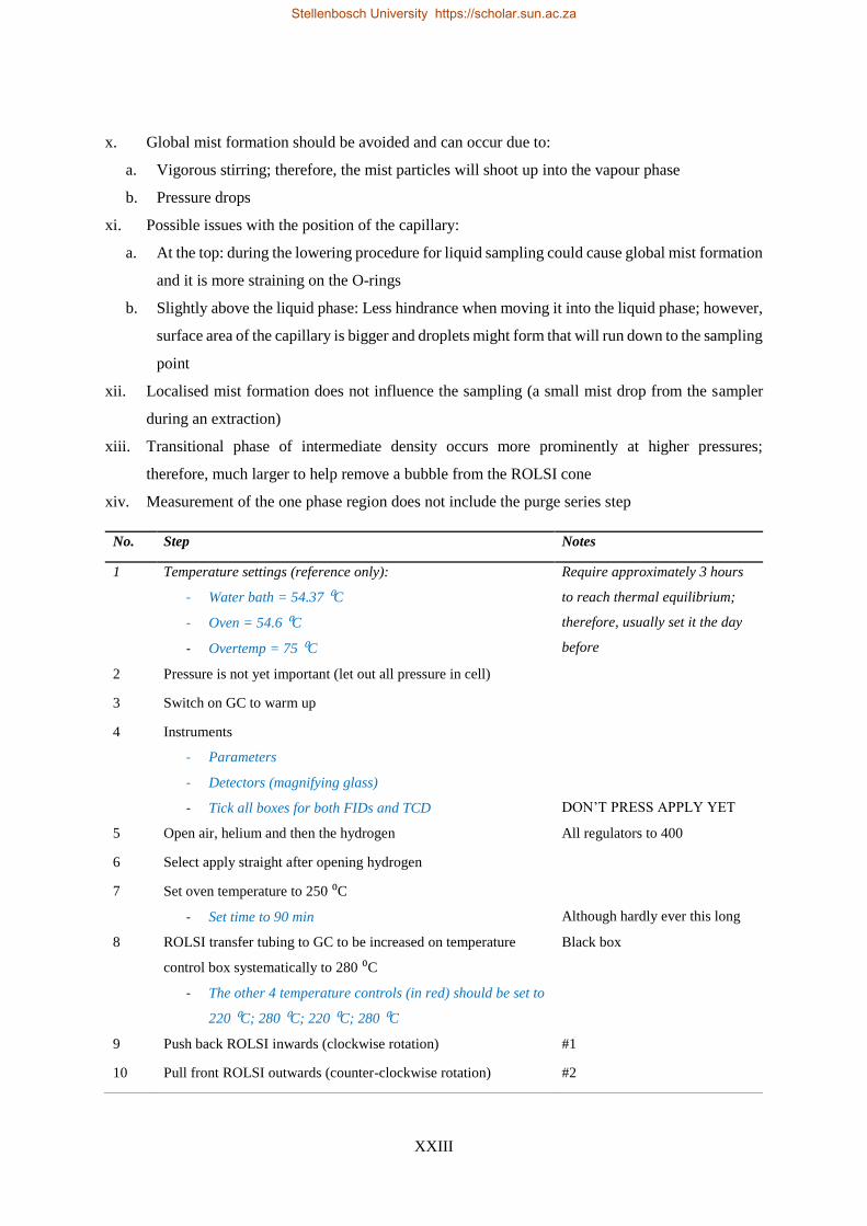
XXIII
x. Global mist formation should be avoided and can occur due to:
a. Vigorous stirring; therefore, the mist particles will shoot up into the vapour phase
b. Pressure drops
xi. Possible issues with the position of the capillary:
a. At the top: during the lowering procedure for liquid sampling could cause global mist formation
and it is more straining on the O-rings
b. Slightly above the liquid phase: Less hindrance when moving it into the liquid phase; however,
surface area of the capillary is bigger and droplets might form that will run down to the sampling
point
xii. Localised mist formation does not influence the sampling (a small mist drop from the sampler
during an extraction)
xiii. Transitional phase of intermediate density occurs more prominently at higher pressures;
therefore, much larger to help remove a bubble from the ROLSI cone
xiv. Measurement of the one phase region does not include the purge series step
No. Step Notes
1 Temperature settings (reference only):
- Water bath = 54.37 ⁰C
- Oven = 54.6 ⁰C
- Overtemp = 75 ⁰C
Require approximately 3 hours
to reach thermal equilibrium;
therefore, usually set it the day
before
2 Pressure is not yet important (let out all pressure in cell)
3 Switch on GC to warm up
4 Instruments
- Parameters
- Detectors (magnifying glass)
- Tick all boxes for both FIDs and TCD
DON’T PRESS APPLY YET
5 Open air, helium and then the hydrogen All regulators to 400
6 Select apply straight after opening hydrogen
7 Set oven temperature to 250 ⁰C
- Set time to 90 min
Although hardly ever this long
8 ROLSI transfer tubing to GC to be increased on temperature
control box systematically to 280 ⁰C
- The other 4 temperature controls (in red) should be set to
220 ⁰C; 280 ⁰C; 220 ⁰C; 280 ⁰C
Black box
9 Push back ROLSI inwards (clockwise rotation) #1
10 Pull front ROLSI outwards (counter-clockwise rotation) #2
Stellenbosch University https://scholar.sun.ac.za
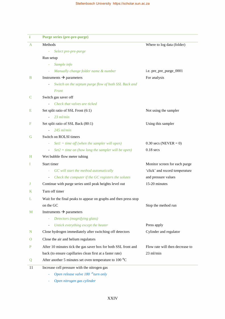
XXIV
i Purge series (pre-pre-purge)
A Methods
- Select pre-pre-purge
Run setup
- Sample info
- Manually change folder name & number
Where to log data (folder)
i.e. pre_pre_purge_0001
B Instruments → parameters
- Switch on the septum purge flow of both SSL Back and
Front
For analysis
C Switch gas saver off
- Check that valves are ticked
E Set split ratio of SSL Front (6:1)
- 23 ml/min
Not using the sampler
F Set split ratio of SSL Back (80:1)
- 245 ml/min
Using this sampler
G Switch on ROLSI timers
- Set1 = time off (when the sampler will open)
- Set2 = time on (how long the sampler will be open)
0.30 secs (NEVER = 0)
0.18 secs
H Wet bubble flow meter tubing
I Start timer
- GC will start the method automatically
- Check the computer if the GC registers the solutes
Monitor screen for each purge
‘click’ and record temperature
and pressure values
J Continue with purge series until peak heights level out 15-20 minutes
K Turn off timer
L Wait for the final peaks to appear on graphs and then press stop
on the GC
Stop the method run
M Instruments → parameters
- Detectors (magnifying glass)
- Untick everything except the heater
Press apply
N Close hydrogen immediately after switching off detectors Cylinder and regulator
O Close the air and helium regulators
P After 10 minutes tick the gas saver box for both SSL front and
back (to ensure capillaries clean first at a faster rate)
Flow rate will then decrease to
23 ml/min
Q After another 5 minutes set oven temperature to 100 ⁰C
11 Increase cell pressure with the nitrogen gas
- Open release valve 180 ⁰ turn only
- Open nitrogen gas cylinder
Stellenbosch University https://scholar.sun.ac.za
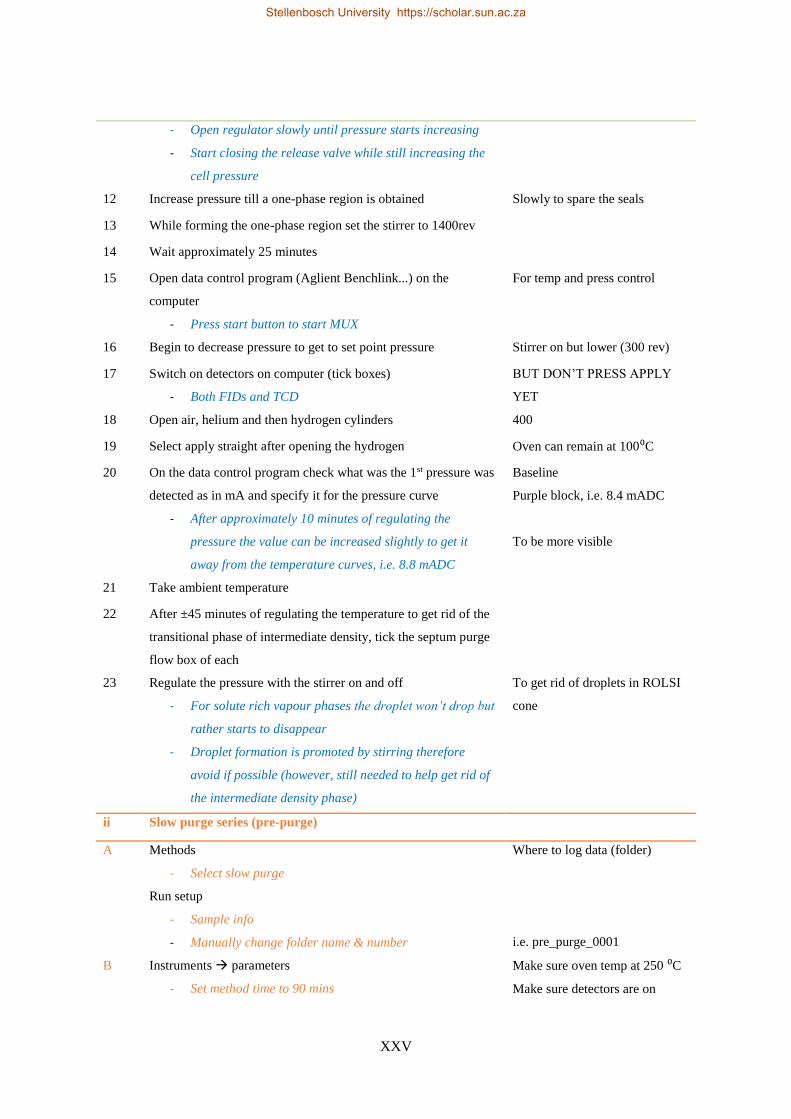
XXV
- Open regulator slowly until pressure starts increasing
- Start closing the release valve while still increasing the
cell pressure
12 Increase pressure till a one-phase region is obtained Slowly to spare the seals
13 While forming the one-phase region set the stirrer to 1400rev
14 Wait approximately 25 minutes
15 Open data control program (Aglient Benchlink...) on the
computer
- Press start button to start MUX
For temp and press control
16 Begin to decrease pressure to get to set point pressure Stirrer on but lower (300 rev)
17 Switch on detectors on computer (tick boxes)
- Both FIDs and TCD
BUT DON’T PRESS APPLY
YET
18 Open air, helium and then hydrogen cylinders 400
19 Select apply straight after opening the hydrogen Oven can remain at 100⁰C
20 On the data control program check what was the 1st pressure was
detected as in mA and specify it for the pressure curve
- After approximately 10 minutes of regulating the
pressure the value can be increased slightly to get it
away from the temperature curves, i.e. 8.8 mADC
Baseline
Purple block, i.e. 8.4 mADC
To be more visible
21 Take ambient temperature
22 After ±45 minutes of regulating the temperature to get rid of the
transitional phase of intermediate density, tick the septum purge
flow box of each
23 Regulate the pressure with the stirrer on and off
- For solute rich vapour phases the droplet won’t drop but
rather starts to disappear
- Droplet formation is promoted by stirring therefore
avoid if possible (however, still needed to help get rid of
the intermediate density phase)
To get rid of droplets in ROLSI
cone
ii Slow purge series (pre-purge)
A Methods
- Select slow purge
Run setup
- Sample info
- Manually change folder name & number
Where to log data (folder)
i.e. pre_purge_0001
B Instruments → parameters
- Set method time to 90 mins
Make sure oven temp at 250 ⁰C
Make sure detectors are on
Stellenbosch University https://scholar.sun.ac.za
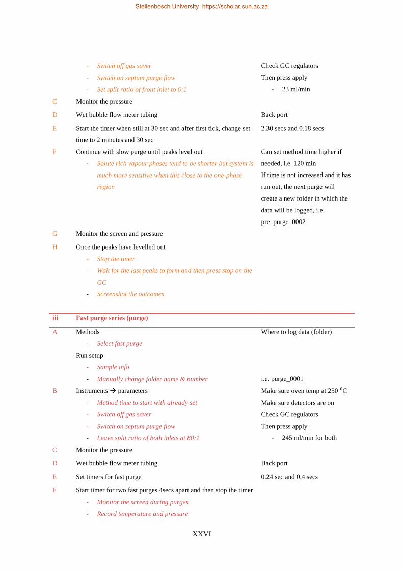
XXVI
- Switch off gas saver
- Switch on septum purge flow
- Set split ratio of front inlet to 6:1
Check GC regulators
Then press apply
- 23 ml/min
C Monitor the pressure
D Wet bubble flow meter tubing Back port
E Start the timer when still at 30 sec and after first tick, change set
time to 2 minutes and 30 sec
2.30 secs and 0.18 secs
F Continue with slow purge until peaks level out
- Solute rich vapour phases tend to be shorter but system is
much more sensitive when this close to the one-phase
region
Can set method time higher if
needed, i.e. 120 min
If time is not increased and it has
run out, the next purge will
create a new folder in which the
data will be logged, i.e.
pre_purge_0002
G Monitor the screen and pressure
H Once the peaks have levelled out
- Stop the timer
- Wait for the last peaks to form and then press stop on the
GC
- Screenshot the outcomes
iii Fast purge series (purge)
A Methods
- Select fast purge
Run setup
- Sample info
- Manually change folder name & number
Where to log data (folder)
i.e. purge_0001
B Instruments → parameters
- Method time to start with already set
- Switch off gas saver
- Switch on septum purge flow
- Leave split ratio of both inlets at 80:1
Make sure oven temp at 250 ⁰C
Make sure detectors are on
Check GC regulators
Then press apply
- 245 ml/min for both
C Monitor the pressure
D Wet bubble flow meter tubing Back port
E Set timers for fast purge 0.24 sec and 0.4 secs
F Start timer for two fast purges 4secs apart and then stop the timer
- Monitor the screen during purges
- Record temperature and pressure
Stellenbosch University https://scholar.sun.ac.za
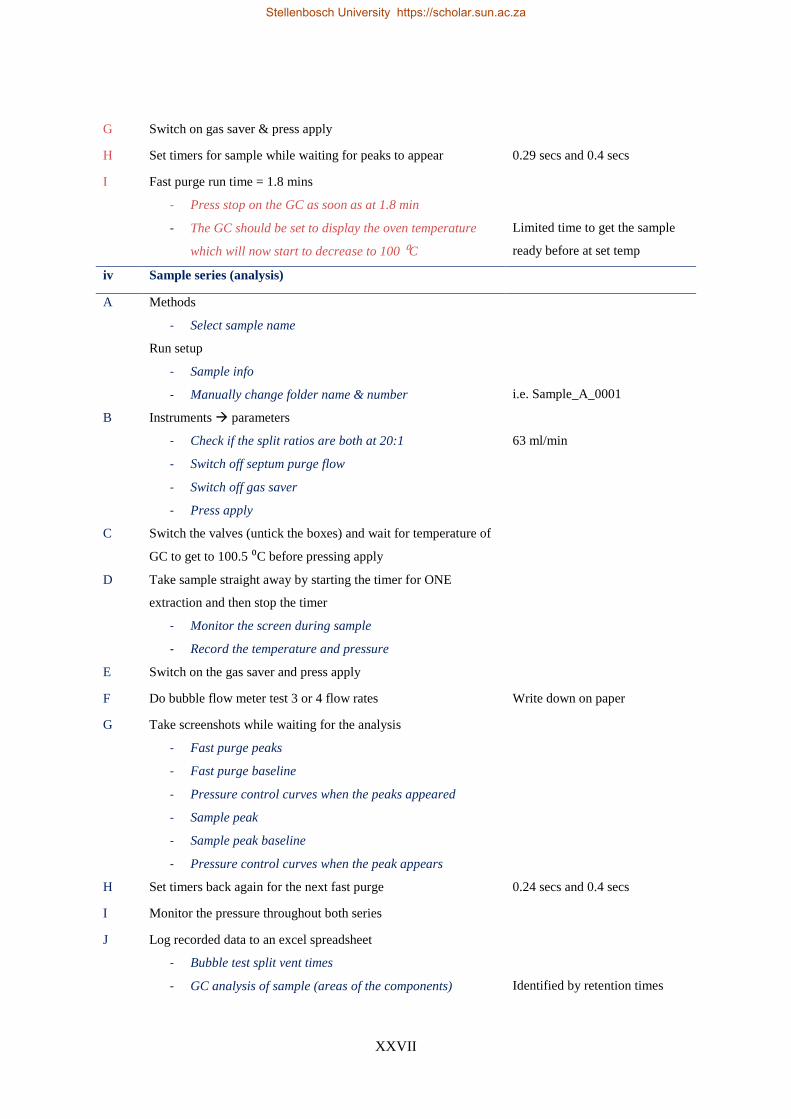
XXVII
G Switch on gas saver & press apply
H Set timers for sample while waiting for peaks to appear 0.29 secs and 0.4 secs
I Fast purge run time = 1.8 mins
- Press stop on the GC as soon as at 1.8 min
- The GC should be set to display the oven temperature
which will now start to decrease to 100 ⁰C
Limited time to get the sample
ready before at set temp
iv Sample series (analysis)
A Methods
- Select sample name
Run setup
- Sample info
- Manually change folder name & number
i.e. Sample_A_0001
B Instruments → parameters
- Check if the split ratios are both at 20:1
- Switch off septum purge flow
- Switch off gas saver
- Press apply
63 ml/min
C Switch the valves (untick the boxes) and wait for temperature of
GC to get to 100.5 ⁰C before pressing apply
D Take sample straight away by starting the timer for ONE
extraction and then stop the timer
- Monitor the screen during sample
- Record the temperature and pressure
E Switch on the gas saver and press apply
F Do bubble flow meter test 3 or 4 flow rates Write down on paper
G Take screenshots while waiting for the analysis
- Fast purge peaks
- Fast purge baseline
- Pressure control curves when the peaks appeared
- Sample peak
- Sample peak baseline
- Pressure control curves when the peak appears
H Set timers back again for the next fast purge 0.24 secs and 0.4 secs
I Monitor the pressure throughout both series
J Log recorded data to an excel spreadsheet
- Bubble test split vent times
- GC analysis of sample (areas of the components)
Identified by retention times
Stellenbosch University https://scholar.sun.ac.za

XXVIII
K After 7 mins the oven temperature should be back to 250 ⁰C
- Set the temperature of the oven to 250 ⁰C under
parameters
- Change the method time to 10 minutes
- Press tab to observe change
- Switch back valves (tick the boxes again)
- Press apply and ok
Replace 5 min with 7 min
L After 10 minutes the run is completed; close the PDF document
that will pop up
24 Repeat the
- iii. Fast purge series and
- iv. Sample series
Another 3 times to have a total of 4 fast purges and 4 samples of
the vapour phase
25 End off as if a 5 fast purge would need to be done
- set method to fast purge after sample A4
- Rename, i.e. purge_0005
- Switch on septum purge flow
- Switch off gas saver
Depends on the outcome of the
data
26 ROLSI now has to be moved into the liquid phase
- For large space gaps between vapour and liquid it will
be better to first switch off the detectors
- For high pressure tests close to the one phase region this
the distance is small enough to leave them on
27 The back ROLSI will be rotated out of the cell (counter
clockwise) while the front ROLSI is being rotated into the cell
(clockwise)
To keep the pressure constant
28 Use the data control curves to know which ROLSIs to adjust
- When the pressure curve is below the centre line the
pressure has decreased; therefore, the volume can be
decreased to counter for it
- i.e. two rotations at the back & one rotation at the front
or one rotation of each
Vice versa
29 Once the ROLSI is in the liquid phase, switch on the stirrer for a
few minutes to check for miscibility waves/ vapour bubbles in
the sampler cone
At low revs
30 Repeat the slow purge, fast purge and sample series steps again
but now for the liquid phase
- Slow purge timer setting is now 30 secs and 0.2 secs
Stellenbosch University https://scholar.sun.ac.za

XXIX
- With a front inlet split ratio of 7:1
- Fast purge timer setting is now 0.4 secs and 0.28 secs
- Sample series timer settings are also 0.4 secs and 0.28
secs
31 End the last sample as if a 5 fast purge should be done
32 After the last scan of the control program stop the MUX by
selecting the top stop button
- Screenshot final curve outcomes
Turn off MUX power button
33 Take note of anything strange inside of the equilibrium cell
34 Switch off timers (properly)
35 Switch off detectors under parameters Leave the heaters on
36 Close hydrogen cylinder followed by the air and helium
cylinders
The cylinders and regulators
37 Switch on the stirrer to 700 revs and push the pressure up to the
one phase region
38 Set the temperature of the transfer tubes to the GC to 300 ⁰C
- And the other 4 thermal regulators to 240 ⁰C; 300 ⁰C;
240 ⁰C and 300 ⁰C, respectively
To help clean out the GC tubes
properly
39 Leave the gas saver off to have a faster flow rate through the
tubes for cleaning
40 After approximately 10 minutes switch off the thermal regulators
(all 5)
41 Measure the phase transition point of the ternary mixture at the
set temperature
Same as synthetic method
42 Copy work logged for the day to a flash drive
43 Methods
- Select the sleep method
44 Release the cell pressure and set the water bath to the next
isothermal condition
Stellenbosch University https://scholar.sun.ac.za
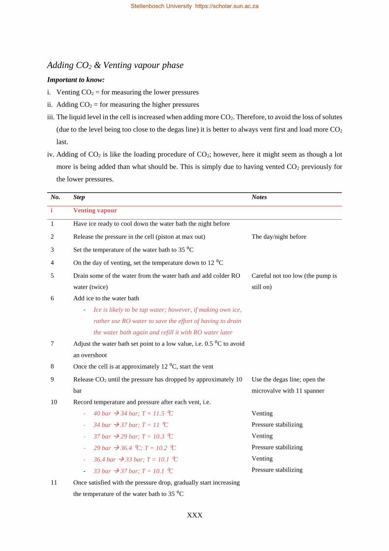
XXX
Adding CO2 & Venting vapour phase
Important to know:
i. Venting CO2 = for measuring the lower pressures
ii. Adding CO2 = for measuring the higher pressures
iii. The liquid level in the cell is increased when adding more CO2. Therefore, to avoid the loss of solutes
(due to the level being too close to the degas line) it is better to always vent first and load more CO2
last.
iv. Adding of CO2 is like the loading procedure of CO2; however, here it might seem as though a lot
more is being added than what should be. This is simply due to having vented CO2 previously for
the lower pressures.
No. Step Notes
i Venting vapour
1 Have ice ready to cool down the water bath the night before
2 Release the pressure in the cell (piston at max out) The day/night before
3 Set the temperature of the water bath to 35 ⁰C
4 On the day of venting, set the temperature down to 12 ⁰C
5 Drain some of the water from the water bath and add colder RO
water (twice)
Careful not too low (the pump is
still on)
6 Add ice to the water bath
- Ice is likely to be tap water; however, if making own ice,
rather use RO water to save the effort of having to drain
the water bath again and refill it with RO water later
7 Adjust the water bath set point to a low value, i.e. 0.5 ⁰C to avoid
an overshoot
8 Once the cell is at approximately 12 ⁰C, start the vent
9 Release CO2 until the pressure has dropped by approximately 10
bar
Use the degas line; open the
microvalve with 11 spanner
10 Record temperature and pressure after each vent, i.e.
- 40 bar → 34 bar; T = 11.5 ⁰C
- 34 bar → 37 bar; T = 11 ⁰C
- 37 bar → 29 bar; T = 10.3 ⁰C
- 29 bar → 36.4 ⁰C; T = 10.2 ⁰C
- 36.4 bar → 33 bar; T = 10.1 ⁰C
- 33 bar → 37 bar; T = 10.1 ⁰C
Venting
Pressure stabilizing
Venting
Pressure stabilizing
Venting
Pressure stabilizing
11 Once satisfied with the pressure drop, gradually start increasing
the temperature of the water bath to 35 ⁰C
Stellenbosch University https://scholar.sun.ac.za
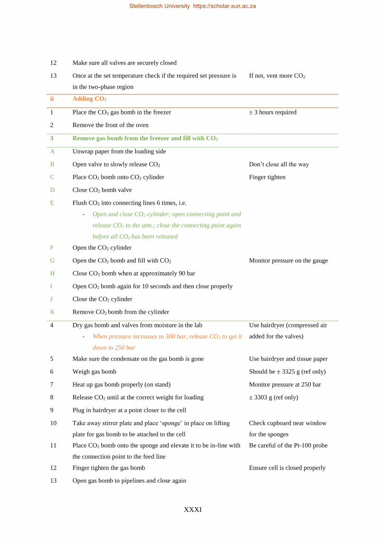
XXXI
12 Make sure all valves are securely closed
13 Once at the set temperature check if the required set pressure is
in the two-phase region
If not, vent more CO2
ii Adding CO2
1 Place the CO2 gas bomb in the freezer ± 3 hours required
2 Remove the front of the oven
3 Remove gas bomb from the freezer and fill with CO2
A Unwrap paper from the loading side
B Open valve to slowly release CO2 Don’t close all the way
C Place CO2 bomb onto CO2 cylinder Finger tighten
D Close CO2 bomb valve
E Flush CO2 into connecting lines 6 times, i.e.
- Open and close CO2 cylinder; open connecting point and
release CO2 to the atm.; close the connecting point again
before all CO2 has been released
F Open the CO2 cylinder
G Open the CO2 bomb and fill with CO2 Monitor pressure on the gauge
H Close CO2 bomb when at approximately 90 bar
I Open CO2 bomb again for 10 seconds and then close properly
J Close the CO2 cylinder
K Remove CO2 bomb from the cylinder
4 Dry gas bomb and valves from moisture in the lab
- When pressure increases to 300 bar, release CO2 to get it
down to 250 bar
Use hairdryer (compressed air
added for the valves)
5 Make sure the condensate on the gas bomb is gone Use hairdryer and tissue paper
6 Weigh gas bomb Should be ± 3325 g (ref only)
7 Heat up gas bomb properly (on stand) Monitor pressure at 250 bar
8 Release CO2 until at the correct weight for loading ± 3303 g (ref only)
9 Plug in hairdryer at a point closer to the cell
10 Take away stirrer plate and place ‘sponge’ in place on lifting
plate for gas bomb to be attached to the cell
Check cupboard near window
for the sponges
11 Place CO2 bomb onto the sponge and elevate it to be in-line with
the connection point to the feed line
Be careful of the Pt-100 probe
12 Finger tighten the gas bomb Ensure cell is closed properly
13 Open gas bomb to pipelines and close again
Stellenbosch University https://scholar.sun.ac.za
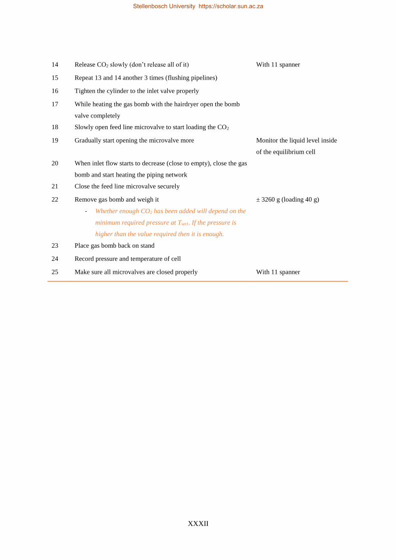
XXXII
14 Release CO2 slowly (don’t release all of it) With 11 spanner
15 Repeat 13 and 14 another 3 times (flushing pipelines)
16 Tighten the cylinder to the inlet valve properly
17 While heating the gas bomb with the hairdryer open the bomb
valve completely
18 Slowly open feed line microvalve to start loading the CO2
19 Gradually start opening the microvalve more Monitor the liquid level inside
of the equilibrium cell
20 When inlet flow starts to decrease (close to empty), close the gas
bomb and start heating the piping network
21 Close the feed line microvalve securely
22 Remove gas bomb and weigh it
- Whether enough CO2 has been added will depend on the
minimum required pressure at Tset1. If the pressure is
higher than the value required then it is enough.
± 3260 g (loading 40 g)
23 Place gas bomb back on stand
24 Record pressure and temperature of cell
25 Make sure all microvalves are closed properly With 11 spanner
Stellenbosch University https://scholar.sun.ac.za
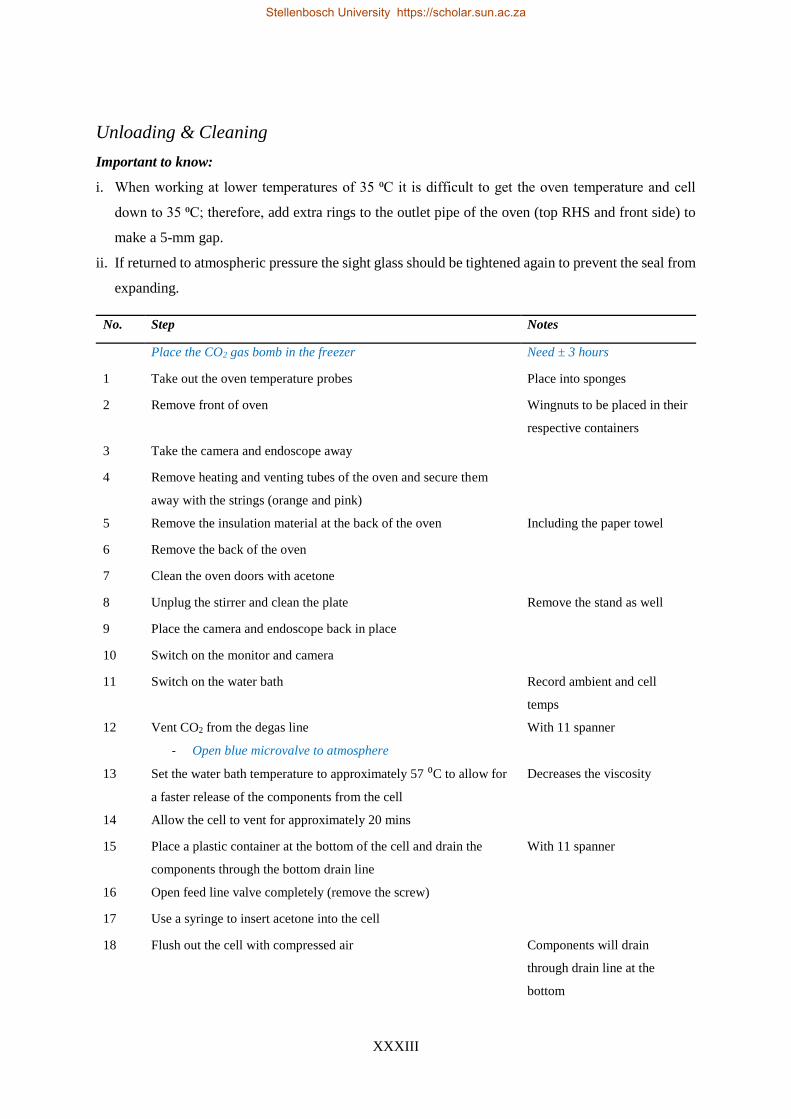
XXXIII
Unloading & Cleaning
Important to know:
i. When working at lower temperatures of 35 ⁰C it is difficult to get the oven temperature and cell
down to 35 ⁰C; therefore, add extra rings to the outlet pipe of the oven (top RHS and front side) to
make a 5-mm gap.
ii. If returned to atmospheric pressure the sight glass should be tightened again to prevent the seal from
expanding.
No. Step Notes
Place the CO2 gas bomb in the freezer Need ± 3 hours
1 Take out the oven temperature probes Place into sponges
2 Remove front of oven Wingnuts to be placed in their
respective containers
3 Take the camera and endoscope away
4 Remove heating and venting tubes of the oven and secure them
away with the strings (orange and pink)
5 Remove the insulation material at the back of the oven Including the paper towel
6 Remove the back of the oven
7 Clean the oven doors with acetone
8 Unplug the stirrer and clean the plate Remove the stand as well
9 Place the camera and endoscope back in place
10 Switch on the monitor and camera
11 Switch on the water bath Record ambient and cell
temps
12 Vent CO2 from the degas line
- Open blue microvalve to atmosphere
With 11 spanner
13 Set the water bath temperature to approximately 57 ⁰C to allow for
a faster release of the components from the cell
Decreases the viscosity
14 Allow the cell to vent for approximately 20 mins
15 Place a plastic container at the bottom of the cell and drain the
components through the bottom drain line
With 11 spanner
16 Open feed line valve completely (remove the screw)
17 Use a syringe to insert acetone into the cell
18 Flush out the cell with compressed air Components will drain
through drain line at the
bottom
Stellenbosch University https://scholar.sun.ac.za

XXXIV
19 Repeat 17 and 18 another three times Use 90⁰ angle tube
20 Loosen the piston 4 mm rod and 17 spanner
21 Unscrew the low pressure chamber of the cell
22 Clean the piston with acetone and paper towels Remove piston and clean
each part separately
23 Place blue waste container underneath the cell in front of the
opening (upright)
24 Place paper towel around the bottom and sides of the outlet to
avoid splashing the components everywhere
25 Cover he GC with the black cloth
26 Close the drain line
- To avoid excess solutes in that line
27 Remove the stirrer from the cell with the magnet
28 Clean the stirrer with acetone and paper towel
29 Wash the cell with acetone and flush with compressed air
- Until satisfied
- Leave bottom drain line open
Use curved tube to place
inside of opening
30 Flush through the bottom drain line with compressed air Short, curvy tube
31 Add acetone to the cell through the feel line With syringe
32 Flush out the cell with compressed air through the bottom drain line
33 Repeat 31 and 32 another three times and then close the bottom
drain line
34 Open degas line and top blue microvalve to the atmosphere
35 Wash the degas line by spraying acetone into the top ‘vent line’ and
flushing it out with compressed air
Repeat three times
36 Once satisfied close the degas line microvalve at the top to
atmosphere and at the back
37 Use syringe to add acetone to the cell through the feed line
38 Flush out with compressed air through the port where CO2 is added Use 90⁰ tube
39 Repeat 37 and 38 another three times
40 Place back the T screw for the feed line once satisfied
41 Take out syringe with metal line (extract acetone) In the cupboard below the cell
42 Attach to the feed line used for adding solvents to the cell
43 Spray the acetone into the cell and then remove the syringe
44 Flush out with compressed air until well dry Use small curvy tube
45 Close the feed line microvalve properly
Stellenbosch University https://scholar.sun.ac.za

XXXV
- All microvalves have been washed out and closed
46 Wash out the cell once more through the opening on the RHS Acetone and compressed air
47 Switch off the water bath
48 Continue washing the cell until visibly clean
- Look for viscous drops on the sight glass
49 Lower the ROLSI samplers all the way into the cell in order to
wash the shaft of each
At lower pressures there will
be less strain on the O-rings
50 Fold paper towel ± 9 times (arm length), wet the tip and then wipe
out the high pressure chamber
- Don’t push the paper towel in all the way
Careful of the temperature
and pressure probes on the
inside
51 Discard the waste into the respective containers
i Load cell with ‘dirty’ CO2
1.1 Place stirrer inside of the cell
1.2 Place low pressure chamber back onto cell
1.3 Tighten the piston 4 mm rod and 17 spanner
1.4 Repeat the adding CO2 procedure (described in section 3)
- No need to flush the connecting pipelines/cell this time as
the air inside the cell is irrelevant ‘dirty CO2’
1.5 Once the CO2 has been loaded switch on the water bath and set it to
57 ⁰C
Place the CO2 gas bomb in the freezer
- Will need to use it for a second loading
Need ± 3 hours
1.6 Place magnetic stirrer plate back underneath the cell and switch it
on
1.7 Push up the pressure to the one-phase region
- Allow a waiting period of approximately 20 min
1.8 Switch off the water bath and stirrer
1.9 Remove the stirring plate
1.10 Slowly vent the CO2 to the atmosphere with a collecting bottle at
the outlet of the vent line to capture any solutes
52 Remove the feed line T microvalve screw
53 Loosen the piston 4 mm rod and 17 spanner
54 Remove the low pressure chamber
55 Remove stirrer with the magnet
56 Flush out the vent line used with compressed air Small, curvy tube
57 Close the degas line microvalve
Stellenbosch University https://scholar.sun.ac.za
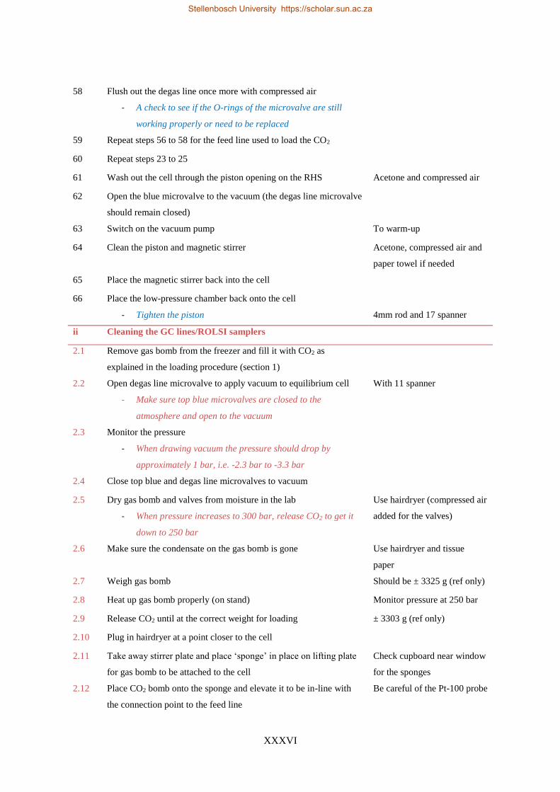
XXXVI
58 Flush out the degas line once more with compressed air
- A check to see if the O-rings of the microvalve are still
working properly or need to be replaced
59 Repeat steps 56 to 58 for the feed line used to load the CO2
60 Repeat steps 23 to 25
61 Wash out the cell through the piston opening on the RHS Acetone and compressed air
62 Open the blue microvalve to the vacuum (the degas line microvalve
should remain closed)
63 Switch on the vacuum pump To warm-up
64 Clean the piston and magnetic stirrer Acetone, compressed air and
paper towel if needed
65 Place the magnetic stirrer back into the cell
66 Place the low-pressure chamber back onto the cell
- Tighten the piston
4mm rod and 17 spanner
ii Cleaning the GC lines/ROLSI samplers
2.1 Remove gas bomb from the freezer and fill it with CO2 as
explained in the loading procedure (section 1)
2.2 Open degas line microvalve to apply vacuum to equilibrium cell
- Make sure top blue microvalves are closed to the
atmosphere and open to the vacuum
With 11 spanner
2.3 Monitor the pressure
- When drawing vacuum the pressure should drop by
approximately 1 bar, i.e. -2.3 bar to -3.3 bar
2.4 Close top blue and degas line microvalves to vacuum
2.5 Dry gas bomb and valves from moisture in the lab
- When pressure increases to 300 bar, release CO2 to get it
down to 250 bar
Use hairdryer (compressed air
added for the valves)
2.6 Make sure the condensate on the gas bomb is gone Use hairdryer and tissue
paper
2.7 Weigh gas bomb Should be ± 3325 g (ref only)
2.8 Heat up gas bomb properly (on stand) Monitor pressure at 250 bar
2.9 Release CO2 until at the correct weight for loading ± 3303 g (ref only)
2.10 Plug in hairdryer at a point closer to the cell
2.11 Take away stirrer plate and place ‘sponge’ in place on lifting plate
for gas bomb to be attached to the cell
Check cupboard near window
for the sponges
2.12 Place CO2 bomb onto the sponge and elevate it to be in-line with
the connection point to the feed line
Be careful of the Pt-100 probe
Stellenbosch University https://scholar.sun.ac.za
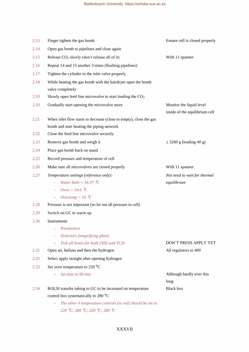
XXXVII
2.13 Finger tighten the gas bomb Ensure cell is closed properly
2.14 Open gas bomb to pipelines and close again
2.15 Release CO2 slowly (don’t release all of it) With 11 spanner
2.16 Repeat 14 and 15 another 3 times (flushing pipelines)
2.17 Tighten the cylinder to the inlet valve properly
2.18 While heating the gas bomb with the hairdryer open the bomb
valve completely
2.19 Slowly open feed line microvalve to start loading the CO2
2.20 Gradually start opening the microvalve more Monitor the liquid level
inside of the equilibrium cell
2.21 When inlet flow starts to decrease (close to empty), close the gas
bomb and start heating the piping network
2.22 Close the feed line microvalve securely
2.23 Remove gas bomb and weigh it ± 3260 g (loading 40 g)
2.24 Place gas bomb back on stand
2.25 Record pressure and temperature of cell
2.26 Make sure all microvalves are closed properly With 11 spanner
2.27 Temperature settings (reference only):
- Water bath = 34.37 ⁰C
- Oven = 34.6 ⁰C
- Overtemp = 55 ⁰C
Not need to wait for thermal
equilibrium
2.28 Pressure is not important (so let out all pressure in cell)
2.29 Switch on GC to warm up
2.30 Instruments
- Parameters
- Detectors (magnifying glass)
- Tick all boxes for both FIDs and TCD
DON’T PRESS APPLY YET
2.31 Open air, helium and then the hydrogen All regulators to 400
2.32 Select apply straight after opening hydrogen
2.33 Set oven temperature to 250 ⁰C
- Set time to 90 min
Although hardly ever this
long
2.34 ROLSI transfer tubing to GC to be increased on temperature
control box systematically to 280 ⁰C
- The other 4 temperature controls (in red) should be set to
220 ⁰C; 280 ⁰C; 220 ⁰C; 280 ⁰C
Black box
Stellenbosch University https://scholar.sun.ac.za
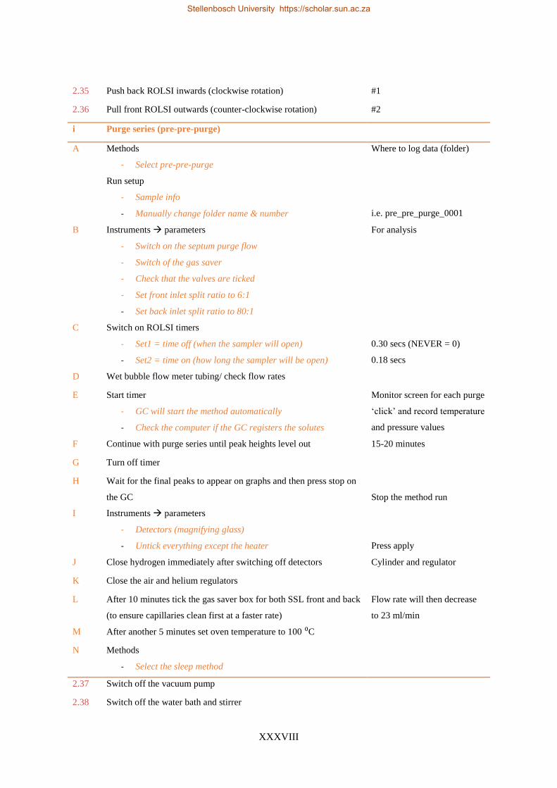
XXXVIII
2.35 Push back ROLSI inwards (clockwise rotation) #1
2.36 Pull front ROLSI outwards (counter-clockwise rotation) #2
i Purge series (pre-pre-purge)
A Methods
- Select pre-pre-purge
Run setup
- Sample info
- Manually change folder name & number
Where to log data (folder)
i.e. pre_pre_purge_0001
B Instruments → parameters
- Switch on the septum purge flow
- Switch of the gas saver
- Check that the valves are ticked
- Set front inlet split ratio to 6:1
- Set back inlet split ratio to 80:1
For analysis
C Switch on ROLSI timers
- Set1 = time off (when the sampler will open)
- Set2 = time on (how long the sampler will be open)
0.30 secs (NEVER = 0)
0.18 secs
D Wet bubble flow meter tubing/ check flow rates
E Start timer
- GC will start the method automatically
- Check the computer if the GC registers the solutes
Monitor screen for each purge
‘click’ and record temperature
and pressure values
F Continue with purge series until peak heights level out 15-20 minutes
G Turn off timer
H Wait for the final peaks to appear on graphs and then press stop on
the GC
Stop the method run
I Instruments → parameters
- Detectors (magnifying glass)
- Untick everything except the heater
Press apply
J Close hydrogen immediately after switching off detectors Cylinder and regulator
K Close the air and helium regulators
L After 10 minutes tick the gas saver box for both SSL front and back
(to ensure capillaries clean first at a faster rate)
Flow rate will then decrease
to 23 ml/min
M After another 5 minutes set oven temperature to 100 ⁰C
N Methods
- Select the sleep method
2.37 Switch off the vacuum pump
2.38 Switch off the water bath and stirrer
Stellenbosch University https://scholar.sun.ac.za
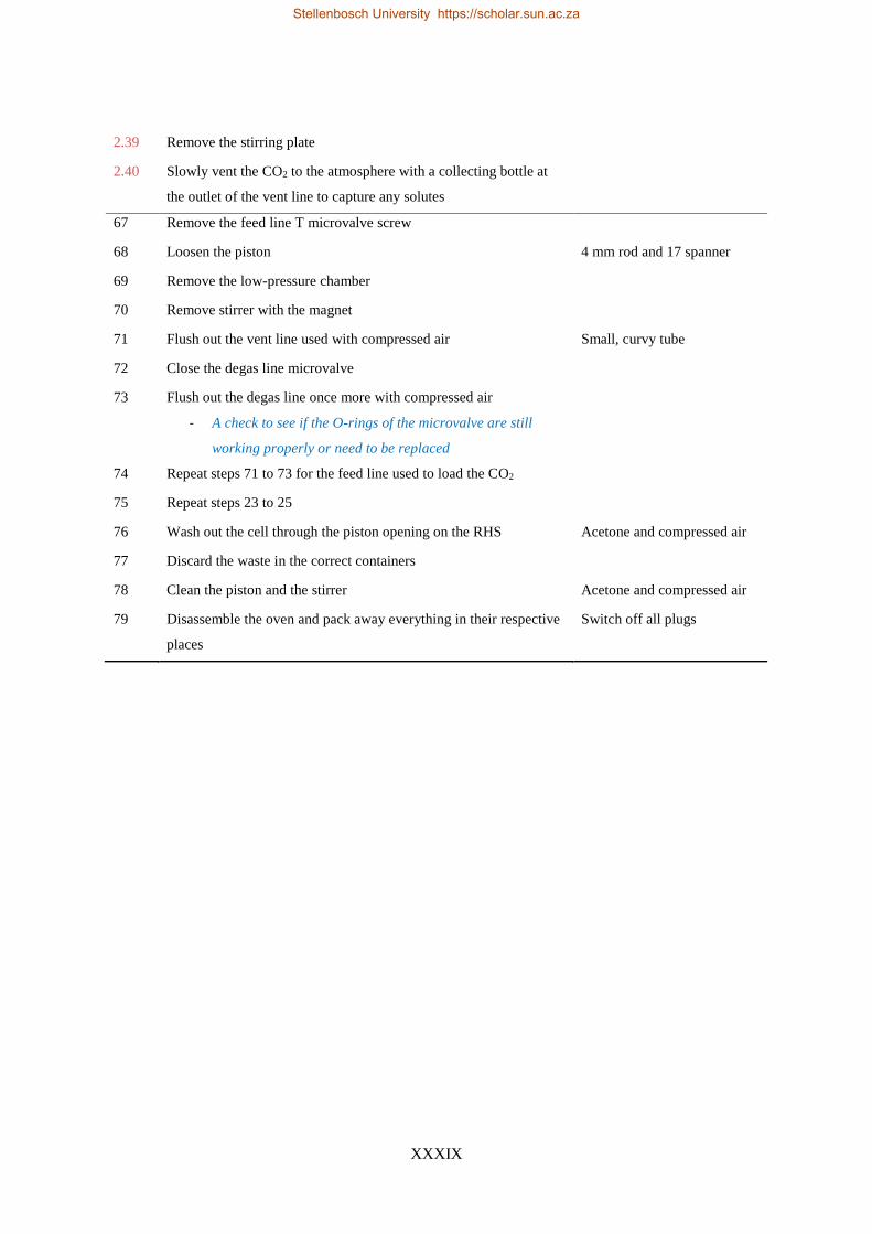
XXXIX
2.39 Remove the stirring plate
2.40 Slowly vent the CO2 to the atmosphere with a collecting bottle at
the outlet of the vent line to capture any solutes
67 Remove the feed line T microvalve screw
68 Loosen the piston 4 mm rod and 17 spanner
69 Remove the low-pressure chamber
70 Remove stirrer with the magnet
71 Flush out the vent line used with compressed air Small, curvy tube
72 Close the degas line microvalve
73 Flush out the degas line once more with compressed air
- A check to see if the O-rings of the microvalve are still
working properly or need to be replaced
74 Repeat steps 71 to 73 for the feed line used to load the CO2
75 Repeat steps 23 to 25
76 Wash out the cell through the piston opening on the RHS Acetone and compressed air
77 Discard the waste in the correct containers
78 Clean the piston and the stirrer Acetone and compressed air
79 Disassemble the oven and pack away everything in their respective
places
Switch off all plugs
Stellenbosch University https://scholar.sun.ac.za
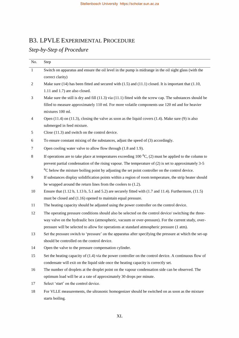
XL
B3. LPVLE EXPERIMENTAL PROCEDURE
Step-by-Step of Procedure
No. Step
1 Switch on apparatus and ensure the oil level in the pump is midrange in the oil sight glass (with the
correct clarity)
2 Make sure (14) has been fitted and secured with (1.5) and (11.1) closed. It is important that (1.10,
1.11 and 1.7) are also closed.
3 Make sure the still is dry and fill (11.3) via (11.1) fitted with the screw cap. The substances should be
filled to measure approximately 110 ml. For more volatile components use 120 ml and for heavier
mixtures 100 ml.
4 Open (11.4) on (11.3), closing the valve as soon as the liquid covers (1.4). Make sure (9) is also
submerged in feed mixture.
5 Close (11.3) and switch on the control device.
6 To ensure constant mixing of the substances, adjust the speed of (3) accordingly.
7 Open cooling water valve to allow flow through (1.8 and 1.9).
8 If operations are to take place at temperatures exceeding 100 ⁰C, (2) must be applied to the column to
prevent partial condensation of the rising vapour. The temperature of (2) is set to approximately 3-5
⁰C below the mixture boiling point by adjusting the set point controller on the control device.
9 If substances display solidification points within a region of room temperature, the strip heater should
be wrapped around the return lines from the coolers to (1.2).
10 Ensure that (1.12 b, 1.13 b, 5.1 and 5.2) are securely fitted with (1.7 and 11.4). Furthermore, (11.5)
must be closed and (1.16) opened to maintain equal pressure.
11 The heating capacity should be adjusted using the power controller on the control device.
12 The operating pressure conditions should also be selected on the control device/ switching the three-
way valve on the hydraulic box (atmospheric, vacuum or over-pressure). For the current study, over-
pressure will be selected to allow for operations at standard atmospheric pressure (1 atm).
13 Set the pressure switch to ‘pressure’ on the apparatus after specifying the pressure at which the set-up
should be controlled on the control device.
14 Open the valve to the pressure compensation cylinder.
15 Set the heating capacity of (1.4) via the power controller on the control device. A continuous flow of
condensate will exit on the liquid side once the heating capacity is correctly set.
16 The number of droplets at the droplet point on the vapour condensation side can be observed. The
optimum load will be at a rate of approximately 30 drops per minute.
17 Select ‘start’ on the control device.
18 For VLLE measurements, the ultrasonic homogenizer should be switched on as soon as the mixture
starts boiling.
Stellenbosch University https://scholar.sun.ac.za
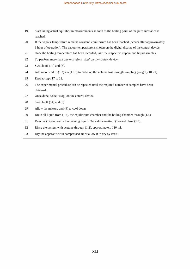
XLI
19 Start taking actual equilibrium measurements as soon as the boiling point of the pure substance is
reached.
20 If the vapour temperature remains constant, equilibrium has been reached (occurs after approximately
1 hour of operation). The vapour temperature is shown on the digital display of the control device.
21 Once the boiling temperature has been recorded, take the respective vapour and liquid samples.
22 To perform more than one test select ‘stop’ on the control device.
23 Switch off (14) and (3).
24 Add more feed to (1.2) via (11.3) to make up the volume lost through sampling (roughly 10 ml).
25 Repeat steps 17 to 21.
26 The experimental procedure can be repeated until the required number of samples have been
obtained.
27 Once done, select ‘stop’ on the control device.
28 Switch off (14) and (3).
29 Allow the mixture and (9) to cool down.
30 Drain all liquid from (1.2), the equilibrium chamber and the boiling chamber through (1.5).
31 Remove (14) to drain all remaining liquid. Once done reattach (14) and close (1.5).
32 Rinse the system with acetone through (1.2), approximately 110 ml.
33 Dry the apparatus with compressed air or allow it to dry by itself.
Stellenbosch University https://scholar.sun.ac.za
XLII
C. CALIBRATION DATA AND CERTIFICATES
The following appendix contains the certificates issued by companies that performed the necessary
calibration tests on the experimental equipment used in this study. The in-house HPBDP and HPVLE
pressure calibrations performed by the author are also included in this chapter.
C1. High-pressure experimental equipment
(i) Pressure calibration
(ii) Deadweight tester calibration
(iii) Temperature calibration
C2. Low-pressure experimental equipment
(i) Temperature calibration (vapour and evaporator)
(ii) Pressure calibration
Stellenbosch University https://scholar.sun.ac.za
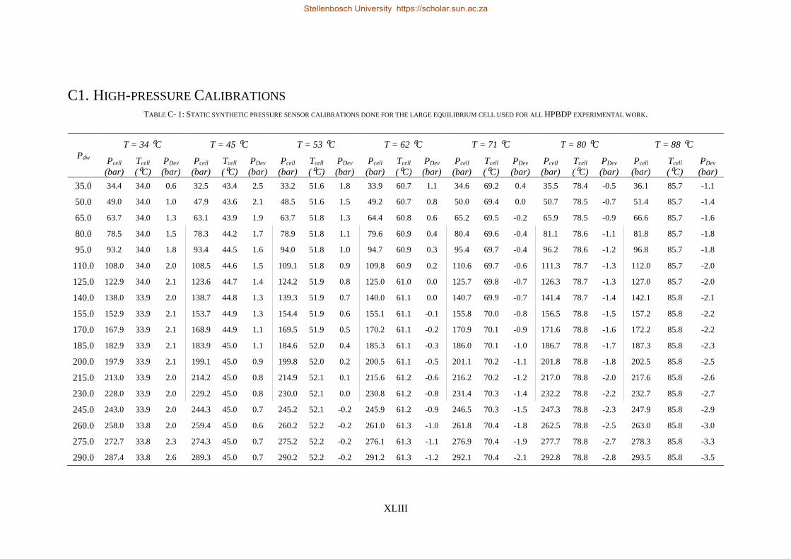
XLIII
C1. HIGH-PRESSURE CALIBRATIONS TABLE C- 1: STATIC SYNTHETIC PRESSURE SENSOR CALIBRATIONS DONE FOR THE LARGE EQUILIBRIUM CELL USED FOR ALL HPBDP EXPERIMENTAL WORK.
Pdw
T = 34 ⁰C T = 45 ⁰C T = 53 ⁰C T = 62 ⁰C T = 71 ⁰C T = 80 ⁰C T = 88 ⁰C
Pcell
(bar)
Tcell
(⁰C)
PDev
(bar)
Pcell
(bar)
Tcell
(⁰C)
PDev
(bar)
Pcell
(bar)
Tcell
(⁰C)
PDev
(bar)
Pcell
(bar)
Tcell
(⁰C)
PDev
(bar)
Pcell
(bar)
Tcell
(⁰C)
PDev
(bar)
Pcell
(bar)
Tcell
(⁰C)
PDev
(bar)
Pcell
(bar)
Tcell
(⁰C)
PDev
(bar)
35.0 34.4 34.0 0.6 32.5 43.4 2.5 33.2 51.6 1.8 33.9 60.7 1.1 34.6 69.2 0.4 35.5 78.4 -0.5 36.1 85.7 -1.1
50.0 49.0 34.0 1.0 47.9 43.6 2.1 48.5 51.6 1.5 49.2 60.7 0.8 50.0 69.4 0.0 50.7 78.5 -0.7 51.4 85.7 -1.4
65.0 63.7 34.0 1.3 63.1 43.9 1.9 63.7 51.8 1.3 64.4 60.8 0.6 65.2 69.5 -0.2 65.9 78.5 -0.9 66.6 85.7 -1.6
80.0 78.5 34.0 1.5 78.3 44.2 1.7 78.9 51.8 1.1 79.6 60.9 0.4 80.4 69.6 -0.4 81.1 78.6 -1.1 81.8 85.7 -1.8
95.0 93.2 34.0 1.8 93.4 44.5 1.6 94.0 51.8 1.0 94.7 60.9 0.3 95.4 69.7 -0.4 96.2 78.6 -1.2 96.8 85.7 -1.8
110.0 108.0 34.0 2.0 108.5 44.6 1.5 109.1 51.8 0.9 109.8 60.9 0.2 110.6 69.7 -0.6 111.3 78.7 -1.3 112.0 85.7 -2.0
125.0 122.9 34.0 2.1 123.6 44.7 1.4 124.2 51.9 0.8 125.0 61.0 0.0 125.7 69.8 -0.7 126.3 78.7 -1.3 127.0 85.7 -2.0
140.0 138.0 33.9 2.0 138.7 44.8 1.3 139.3 51.9 0.7 140.0 61.1 0.0 140.7 69.9 -0.7 141.4 78.7 -1.4 142.1 85.8 -2.1
155.0 152.9 33.9 2.1 153.7 44.9 1.3 154.4 51.9 0.6 155.1 61.1 -0.1 155.8 70.0 -0.8 156.5 78.8 -1.5 157.2 85.8 -2.2
170.0 167.9 33.9 2.1 168.9 44.9 1.1 169.5 51.9 0.5 170.2 61.1 -0.2 170.9 70.1 -0.9 171.6 78.8 -1.6 172.2 85.8 -2.2
185.0 182.9 33.9 2.1 183.9 45.0 1.1 184.6 52.0 0.4 185.3 61.1 -0.3 186.0 70.1 -1.0 186.7 78.8 -1.7 187.3 85.8 -2.3
200.0 197.9 33.9 2.1 199.1 45.0 0.9 199.8 52.0 0.2 200.5 61.1 -0.5 201.1 70.2 -1.1 201.8 78.8 -1.8 202.5 85.8 -2.5
215.0 213.0 33.9 2.0 214.2 45.0 0.8 214.9 52.1 0.1 215.6 61.2 -0.6 216.2 70.2 -1.2 217.0 78.8 -2.0 217.6 85.8 -2.6
230.0 228.0 33.9 2.0 229.2 45.0 0.8 230.0 52.1 0.0 230.8 61.2 -0.8 231.4 70.3 -1.4 232.2 78.8 -2.2 232.7 85.8 -2.7
245.0 243.0 33.9 2.0 244.3 45.0 0.7 245.2 52.1 -0.2 245.9 61.2 -0.9 246.5 70.3 -1.5 247.3 78.8 -2.3 247.9 85.8 -2.9
260.0 258.0 33.8 2.0 259.4 45.0 0.6 260.2 52.2 -0.2 261.0 61.3 -1.0 261.8 70.4 -1.8 262.5 78.8 -2.5 263.0 85.8 -3.0
275.0 272.7 33.8 2.3 274.3 45.0 0.7 275.2 52.2 -0.2 276.1 61.3 -1.1 276.9 70.4 -1.9 277.7 78.8 -2.7 278.3 85.8 -3.3
290.0 287.4 33.8 2.6 289.3 45.0 0.7 290.2 52.2 -0.2 291.2 61.3 -1.2 292.1 70.4 -2.1 292.8 78.8 -2.8 293.5 85.8 -3.5
Stellenbosch University https://scholar.sun.ac.za
Stellenbosch University https://scholar.sun.ac.za
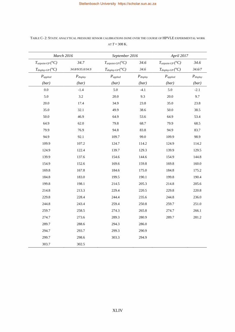
XLIV
TABLE C- 2: STATIC ANALYTICAL PRESSURE SENSOR CALIBRATIONS DONE OVER THE COURSE OF HPVLE EXPERIMENTAL WORK
AT T = 308 K.
March 2016 September 2016 April 2017
Tsetpoint-GP (°C) 34.7 Tsetpoint-GP (°C) 34.6 Tsetpoint-GP (°C) 34.6
Tdisplay-GP (°C) 34.8/9/35.0/34.9 Tdisplay-GP (°C) 34.6 Tdisplay-GP (°C) 34.6/7
Papplied Pdisplay Papplied Pdisplay Papplied Pdisplay
(bar) (bar) (bar) (bar) (bar) (bar)
0.0 -1.4 5.0 -4.1 5.0 -2.1
5.0 3.2 20.0 9.3 20.0 9.7
20.0 17.4 34.9 23.8 35.0 23.8
35.0 32.1 49.9 38.6 50.0 38.5
50.0 46.9 64.9 53.6 64.9 53.4
64.9 62.0 79.8 68.7 79.9 68.5
79.9 76.9 94.8 83.8 94.9 83.7
94.9 92.1 109.7 99.0 109.9 98.9
109.9 107.2 124.7 114.2 124.9 114.2
124.9 122.4 139.7 129.3 139.9 129.5
139.9 137.6 154.6 144.6 154.9 144.8
154.9 152.6 169.6 159.8 169.8 160.0
169.8 167.8 184.6 175.0 184.8 175.2
184.8 183.0 199.5 190.1 199.8 190.4
199.8 198.1 214.5 205.3 214.8 205.6
214.8 213.3 229.4 220.5 229.8 220.8
229.8 228.4 244.4 235.6 244.8 236.0
244.8 243.4 259.4 250.8 259.7 251.0
259.7 258.5 274.3 265.8 274.7 266.1
274.7 273.6 289.3 280.9 289.7 281.2
289.7 288.6 294.3 286.0
294.7 293.7 299.3 290.9
299.7 298.6 303.3 294.9
303.7 302.5
Stellenbosch University https://scholar.sun.ac.za
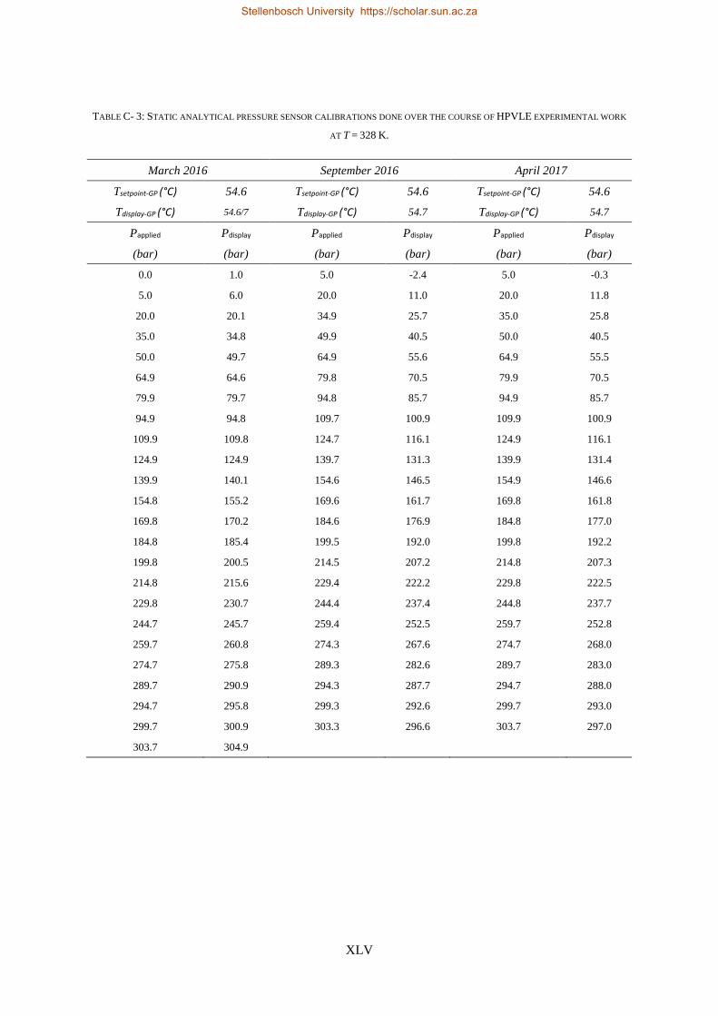
XLV
TABLE C- 3: STATIC ANALYTICAL PRESSURE SENSOR CALIBRATIONS DONE OVER THE COURSE OF HPVLE EXPERIMENTAL WORK
AT T = 328 K.
March 2016 September 2016 April 2017
Tsetpoint-GP (°C) 54.6 Tsetpoint-GP (°C) 54.6 Tsetpoint-GP (°C) 54.6
Tdisplay-GP (°C) 54.6/7 Tdisplay-GP (°C) 54.7 Tdisplay-GP (°C) 54.7
Papplied Pdisplay Papplied Pdisplay Papplied Pdisplay
(bar) (bar) (bar) (bar) (bar) (bar)
0.0 1.0 5.0 -2.4 5.0 -0.3
5.0 6.0 20.0 11.0 20.0 11.8
20.0 20.1 34.9 25.7 35.0 25.8
35.0 34.8 49.9 40.5 50.0 40.5
50.0 49.7 64.9 55.6 64.9 55.5
64.9 64.6 79.8 70.5 79.9 70.5
79.9 79.7 94.8 85.7 94.9 85.7
94.9 94.8 109.7 100.9 109.9 100.9
109.9 109.8 124.7 116.1 124.9 116.1
124.9 124.9 139.7 131.3 139.9 131.4
139.9 140.1 154.6 146.5 154.9 146.6
154.8 155.2 169.6 161.7 169.8 161.8
169.8 170.2 184.6 176.9 184.8 177.0
184.8 185.4 199.5 192.0 199.8 192.2
199.8 200.5 214.5 207.2 214.8 207.3
214.8 215.6 229.4 222.2 229.8 222.5
229.8 230.7 244.4 237.4 244.8 237.7
244.7 245.7 259.4 252.5 259.7 252.8
259.7 260.8 274.3 267.6 274.7 268.0
274.7 275.8 289.3 282.6 289.7 283.0
289.7 290.9 294.3 287.7 294.7 288.0
294.7 295.8 299.3 292.6 299.7 293.0
299.7 300.9 303.3 296.6 303.7 297.0
303.7 304.9
Stellenbosch University https://scholar.sun.ac.za
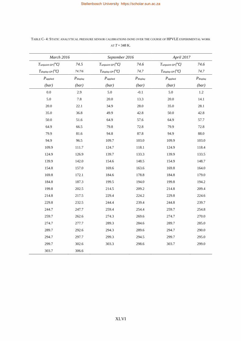
XLVI
TABLE C- 4: STATIC ANALYTICAL PRESSURE SENSOR CALIBRATIONS DONE OVER THE COURSE OF HPVLE EXPERIMENTAL WORK
AT T = 348 K.
March 2016 September 2016 April 2017
Tsetpoint-GP (°C) 74.5 Tsetpoint-GP (°C) 74.6 Tsetpoint-GP (°C) 74.6
Tdisplay-GP (°C) 74.7/6 Tdisplay-GP (°C) 74.7 Tdisplay-GP (°C) 74.7
Papplied Pdisplay Papplied Pdisplay Papplied Pdisplay
(bar) (bar) (bar) (bar) (bar) (bar)
0.0 2.9 5.0 -0.1 5.0 1.2
5.0 7.8 20.0 13.3 20.0 14.1
20.0 22.1 34.9 28.0 35.0 28.1
35.0 36.8 49.9 42.8 50.0 42.8
50.0 51.6 64.9 57.6 64.9 57.7
64.9 66.5 79.8 72.8 79.9 72.8
79.9 81.6 94.8 87.8 94.9 88.0
94.9 96.5 109.7 103.0 109.9 103.0
109.9 111.7 124.7 118.1 124.9 118.4
124.9 126.9 139.7 133.3 139.9 133.5
139.9 142.0 154.6 148.5 154.9 148.7
154.8 157.0 169.6 163.6 169.8 164.0
169.8 172.1 184.6 178.8 184.8 179.0
184.8 187.3 199.5 194.0 199.8 194.2
199.8 202.5 214.5 209.2 214.8 209.4
214.8 217.5 229.4 224.2 229.8 224.6
229.8 232.5 244.4 239.4 244.8 239.7
244.7 247.7 259.4 254.4 259.7 254.8
259.7 262.6 274.3 269.6 274.7 270.0
274.7 277.7 289.3 284.6 289.7 285.0
289.7 292.6 294.3 289.6 294.7 290.0
294.7 297.7 299.3 294.5 299.7 295.0
299.7 302.6 303.3 298.6 303.7 299.0
303.7 306.6
Stellenbosch University https://scholar.sun.ac.za
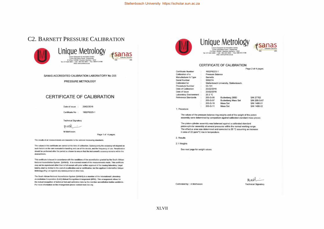
XLVII
C2. BARNETT PRESSURE CALIBRATION
Stellenbosch University https://scholar.sun.ac.za
Stellenbosch University https://scholar.sun.ac.za
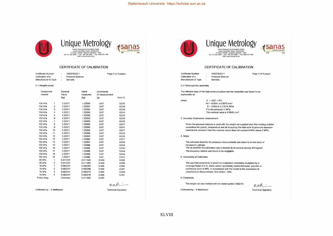
XLVIII
Stellenbosch University https://scholar.sun.ac.za
Stellenbosch University https://scholar.sun.ac.za
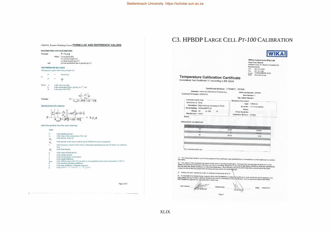
XLIX
C3. HPBDP LARGE CELL PT-100 CALIBRATION
Stellenbosch University https://scholar.sun.ac.za
Stellenbosch University https://scholar.sun.ac.za
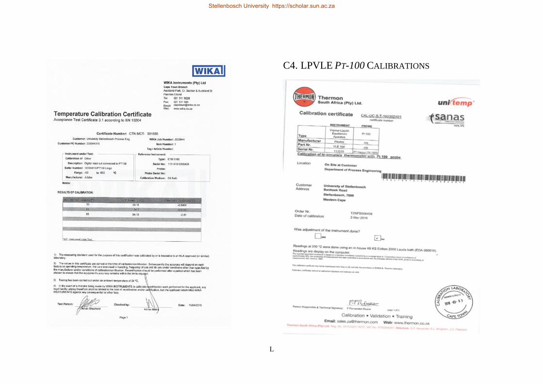
L
C4. LPVLE PT-100 CALIBRATIONS
Stellenbosch University https://scholar.sun.ac.za
Stellenbosch University https://scholar.sun.ac.za
LI
Stellenbosch University https://scholar.sun.ac.za
Stellenbosch University https://scholar.sun.ac.za
LII
Stellenbosch University https://scholar.sun.ac.za
Stellenbosch University https://scholar.sun.ac.za
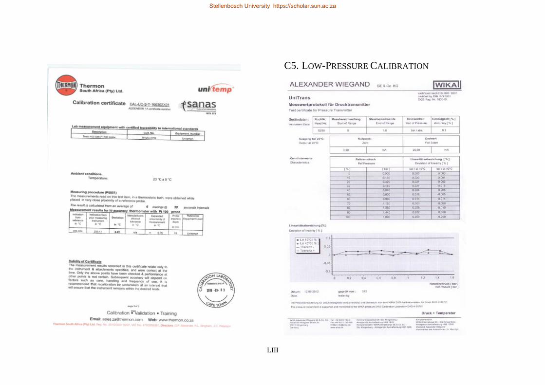
LIII
C5. LOW-PRESSURE CALIBRATION
Stellenbosch University https://scholar.sun.ac.za
Stellenbosch University https://scholar.sun.ac.za
LIV
D. PRECAUTIONARY MEASURES
Take note of several aspects during each of the experimental procedures to ensure the operator is always
safe when working with the equipment. The first is the different chemicals used during testing. It is
advised that latex gloves, safety glasses and a lab coat be worn at all times when working with the
chemicals. Closed shoes should also be worn to avoid spills on open skin.
It is required to study the potential harm that can be inflicted on the operator by not only the alcohols
and n-alkanes used in this work but also the chemicals used for cleaning. The operator should study the
material Safety Data Sheets (MSDS) for the respective components that will be utilized in this project
before starting. CO2 and nitrogen were also utilised in the experimental procedures of this work. If the
operator is exposed to large amounts of these gases he/ she might experience weakness, dizziness and
in some instances a loss of consciousness. These symptoms develop due to a decline in oxygen in the
body. It is advised that the room be evacuated immediately in such instances.
The all glass dynamic recirculating still has been installed inside and extraction cabinet for safety
with respect to the flammable nature of the chemicals being tested. Maximum operating levels have
also been enforced for protection:
• The pressure should remain within a 2.5 mbar to 3 bar range
• The temperature should not exceed 250 °C
The high pressure analytical phase equilibria setup contains the following upper operating limits:
• The pressure should not exceed 300 bar
• The temperature should not be increased over 150 °C
The high-pressure visual synthetic method has the following constraints specified:
• Low pressure chamber maximum pressure of 15 bar
• High pressure chamber maximum pressure of 500 bar
• Working pressure inside cell at a maximum of 275 bar
• Sight glass operating temperature limit of 200 °C
Stellenbosch University https://scholar.sun.ac.za

LV
Stellenbosch University https://scholar.sun.ac.za
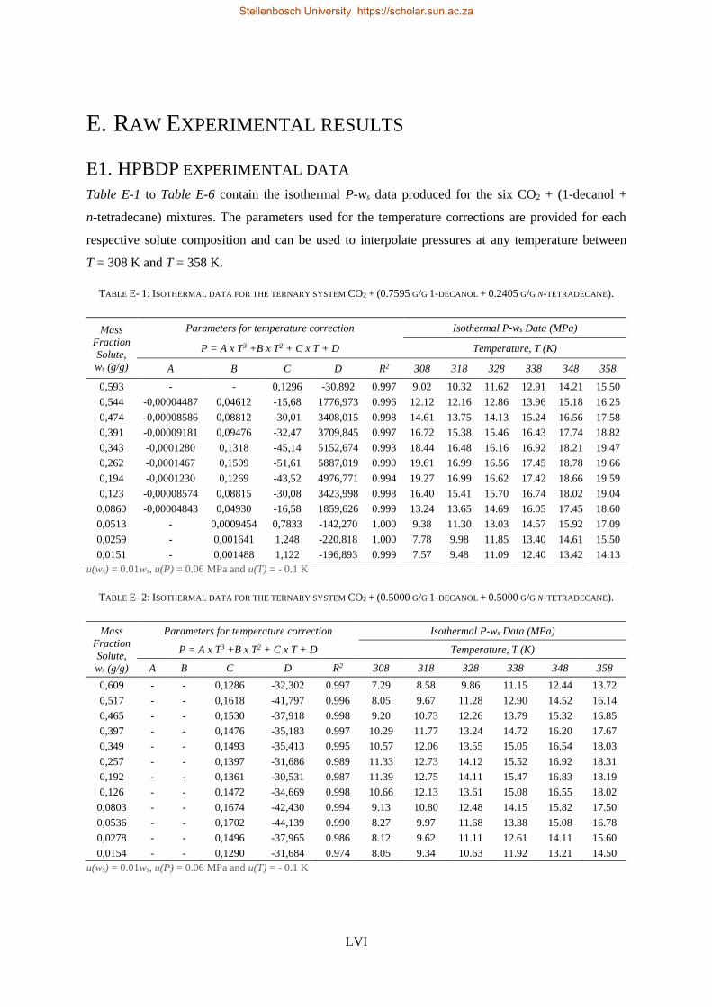
LVI
E. RAW EXPERIMENTAL RESULTS
E1. HPBDP EXPERIMENTAL DATA
Table E-1 to Table E-6 contain the isothermal P-ws data produced for the six CO2 + (1-decanol +
n-tetradecane) mixtures. The parameters used for the temperature corrections are provided for each
respective solute composition and can be used to interpolate pressures at any temperature between
T = 308 K and T = 358 K.
TABLE E- 1: ISOTHERMAL DATA FOR THE TERNARY SYSTEM CO2 + (0.7595 G/G 1-DECANOL + 0.2405 G/G N-TETRADECANE).
Mass
Fraction
Solute,
ws (g/g)
Parameters for temperature correction Isothermal P-ws Data (MPa)
P = A x T3 +B x T2 + C x T + D Temperature, T (K)
A B C D R2 308 318 328 338 348 358
0,593 - - 0,1296 -30,892 0.997 9.02 10.32 11.62 12.91 14.21 15.50
0,544 -0,00004487 0,04612 -15,68 1776,973 0.996 12.12 12.16 12.86 13.96 15.18 16.25
0,474 -0,00008586 0,08812 -30,01 3408,015 0.998 14.61 13.75 14.13 15.24 16.56 17.58
0,391 -0,00009181 0,09476 -32,47 3709,845 0.997 16.72 15.38 15.46 16.43 17.74 18.82
0,343 -0,0001280 0,1318 -45,14 5152,674 0.993 18.44 16.48 16.16 16.92 18.21 19.47
0,262 -0,0001467 0,1509 -51,61 5887,019 0.990 19.61 16.99 16.56 17.45 18.78 19.66
0,194 -0,0001230 0,1269 -43,52 4976,771 0.994 19.27 16.99 16.62 17.42 18.66 19.59
0,123 -0,00008574 0,08815 -30,08 3423,998 0.998 16.40 15.41 15.70 16.74 18.02 19.04
0,0860 -0,00004843 0,04930 -16,58 1859,626 0.999 13.24 13.65 14.69 16.05 17.45 18.60
0,0513 - 0,0009454 0,7833 -142,270 1.000 9.38 11.30 13.03 14.57 15.92 17.09
0,0259 - 0,001641 1,248 -220,818 1.000 7.78 9.98 11.85 13.40 14.61 15.50
0,0151 - 0,001488 1,122 -196,893 0.999 7.57 9.48 11.09 12.40 13.42 14.13
u(ws) = 0.01ws, u(P) = 0.06 MPa and u(T) = - 0.1 K
TABLE E- 2: ISOTHERMAL DATA FOR THE TERNARY SYSTEM CO2 + (0.5000 G/G 1-DECANOL + 0.5000 G/G N-TETRADECANE).
Mass
Fraction
Solute,
ws (g/g)
Parameters for temperature correction Isothermal P-ws Data (MPa)
P = A x T3 +B x T2 + C x T + D Temperature, T (K)
A B C D R2 308 318 328 338 348 358
0,609 - - 0,1286 -32,302 0.997 7.29 8.58 9.86 11.15 12.44 13.72
0,517 - - 0,1618 -41,797 0.996 8.05 9.67 11.28 12.90 14.52 16.14
0,465 - - 0,1530 -37,918 0.998 9.20 10.73 12.26 13.79 15.32 16.85
0,397 - - 0,1476 -35,183 0.997 10.29 11.77 13.24 14.72 16.20 17.67
0,349 - - 0,1493 -35,413 0.995 10.57 12.06 13.55 15.05 16.54 18.03
0,257 - - 0,1397 -31,686 0.989 11.33 12.73 14.12 15.52 16.92 18.31
0,192 - - 0,1361 -30,531 0.987 11.39 12.75 14.11 15.47 16.83 18.19
0,126 - - 0,1472 -34,669 0.998 10.66 12.13 13.61 15.08 16.55 18.02
0,0803 - - 0,1674 -42,430 0.994 9.13 10.80 12.48 14.15 15.82 17.50
0,0536 - - 0,1702 -44,139 0.990 8.27 9.97 11.68 13.38 15.08 16.78
0,0278 - - 0,1496 -37,965 0.986 8.12 9.62 11.11 12.61 14.11 15.60
0,0154 - - 0,1290 -31,684 0.974 8.05 9.34 10.63 11.92 13.21 14.50
u(ws) = 0.01ws, u(P) = 0.06 MPa and u(T) = - 0.1 K
Stellenbosch University https://scholar.sun.ac.za
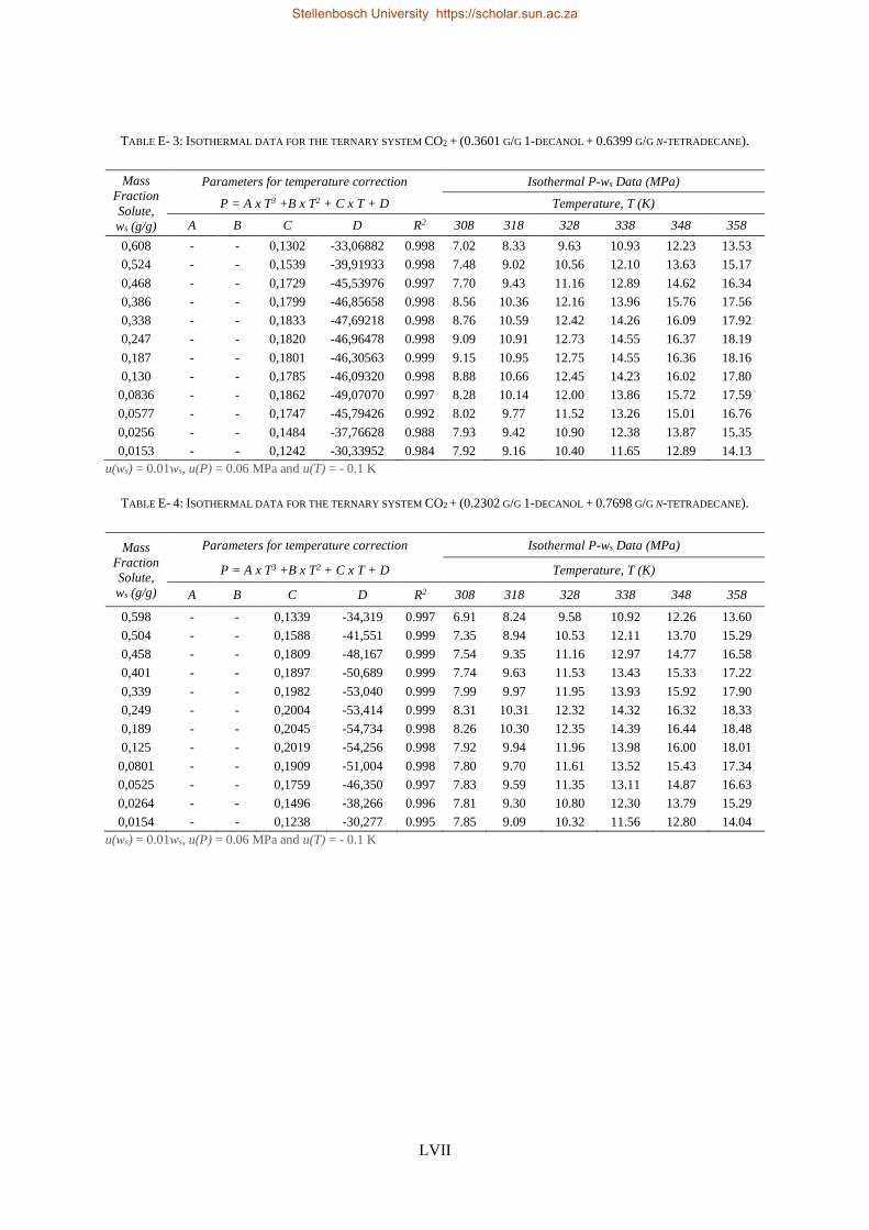
LVII
TABLE E- 3: ISOTHERMAL DATA FOR THE TERNARY SYSTEM CO2 + (0.3601 G/G 1-DECANOL + 0.6399 G/G N-TETRADECANE).
Mass
Fraction
Solute,
ws (g/g)
Parameters for temperature correction Isothermal P-ws Data (MPa)
P = A x T3 +B x T2 + C x T + D Temperature, T (K)
A B C D R2 308 318 328 338 348 358
0,608 - - 0,1302 -33,06882 0.998 7.02 8.33 9.63 10.93 12.23 13.53
0,524 - - 0,1539 -39,91933 0.998 7.48 9.02 10.56 12.10 13.63 15.17
0,468 - - 0,1729 -45,53976 0.997 7.70 9.43 11.16 12.89 14.62 16.34
0,386 - - 0,1799 -46,85658 0.998 8.56 10.36 12.16 13.96 15.76 17.56
0,338 - - 0,1833 -47,69218 0.998 8.76 10.59 12.42 14.26 16.09 17.92
0,247 - - 0,1820 -46,96478 0.998 9.09 10.91 12.73 14.55 16.37 18.19
0,187 - - 0,1801 -46,30563 0.999 9.15 10.95 12.75 14.55 16.36 18.16
0,130 - - 0,1785 -46,09320 0.998 8.88 10.66 12.45 14.23 16.02 17.80
0,0836 - - 0,1862 -49,07070 0.997 8.28 10.14 12.00 13.86 15.72 17.59
0,0577 - - 0,1747 -45,79426 0.992 8.02 9.77 11.52 13.26 15.01 16.76
0,0256 - - 0,1484 -37,76628 0.988 7.93 9.42 10.90 12.38 13.87 15.35
0,0153 - - 0,1242 -30,33952 0.984 7.92 9.16 10.40 11.65 12.89 14.13
u(ws) = 0.01ws, u(P) = 0.06 MPa and u(T) = - 0.1 K
TABLE E- 4: ISOTHERMAL DATA FOR THE TERNARY SYSTEM CO2 + (0.2302 G/G 1-DECANOL + 0.7698 G/G N-TETRADECANE).
Mass
Fraction
Solute,
ws (g/g)
Parameters for temperature correction Isothermal P-ws Data (MPa)
P = A x T3 +B x T2 + C x T + D Temperature, T (K)
A B C D R2 308 318 328 338 348 358
0,598 - - 0,1339 -34,319 0.997 6.91 8.24 9.58 10.92 12.26 13.60
0,504 - - 0,1588 -41,551 0.999 7.35 8.94 10.53 12.11 13.70 15.29
0,458 - - 0,1809 -48,167 0.999 7.54 9.35 11.16 12.97 14.77 16.58
0,401 - - 0,1897 -50,689 0.999 7.74 9.63 11.53 13.43 15.33 17.22
0,339 - - 0,1982 -53,040 0.999 7.99 9.97 11.95 13.93 15.92 17.90
0,249 - - 0,2004 -53,414 0.999 8.31 10.31 12.32 14.32 16.32 18.33
0,189 - - 0,2045 -54,734 0.998 8.26 10.30 12.35 14.39 16.44 18.48
0,125 - - 0,2019 -54,256 0.998 7.92 9.94 11.96 13.98 16.00 18.01
0,0801 - - 0,1909 -51,004 0.998 7.80 9.70 11.61 13.52 15.43 17.34
0,0525 - - 0,1759 -46,350 0.997 7.83 9.59 11.35 13.11 14.87 16.63
0,0264 - - 0,1496 -38,266 0.996 7.81 9.30 10.80 12.30 13.79 15.29
0,0154 - - 0,1238 -30,277 0.995 7.85 9.09 10.32 11.56 12.80 14.04
u(ws) = 0.01ws, u(P) = 0.06 MPa and u(T) = - 0.1 K
Stellenbosch University https://scholar.sun.ac.za
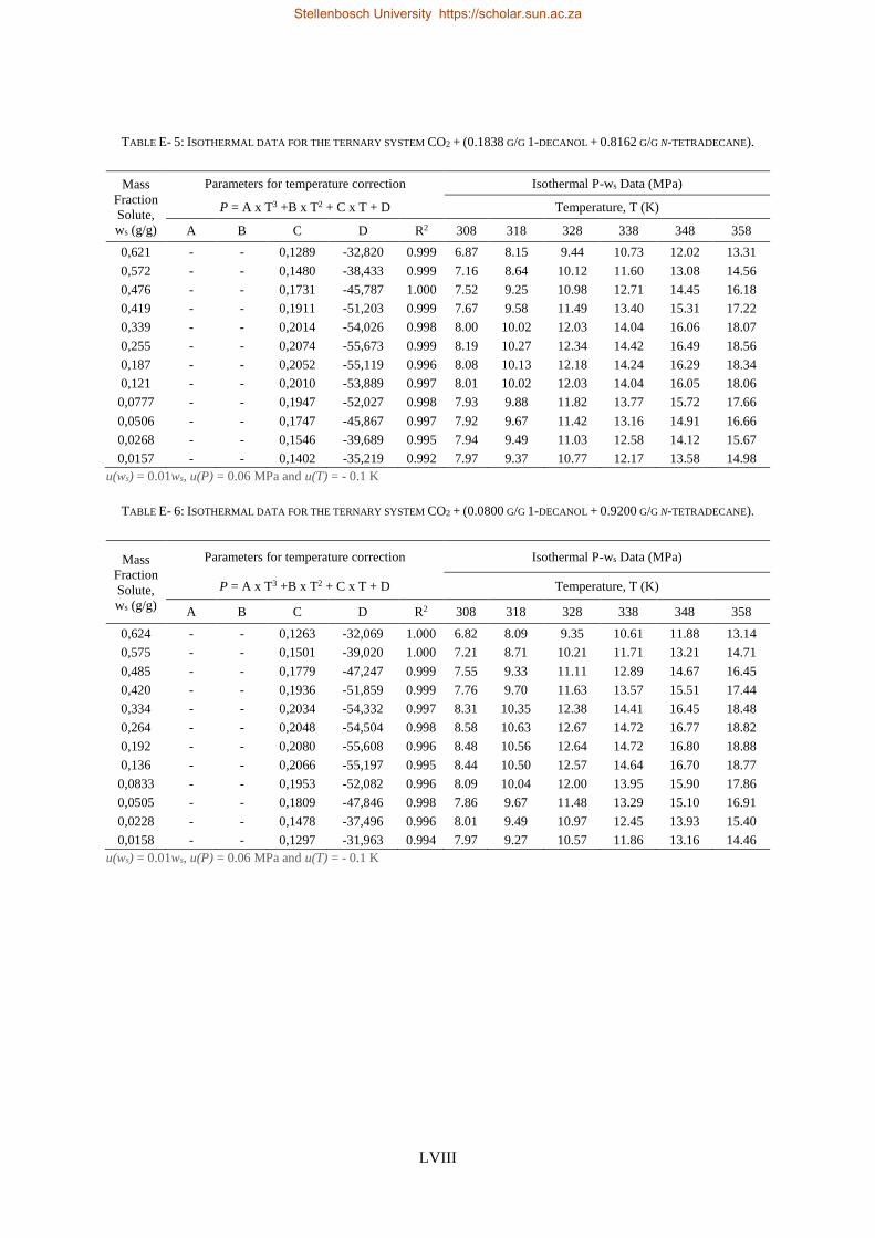
LVIII
TABLE E- 5: ISOTHERMAL DATA FOR THE TERNARY SYSTEM CO2 + (0.1838 G/G 1-DECANOL + 0.8162 G/G N-TETRADECANE).
Mass
Fraction
Solute,
ws (g/g)
Parameters for temperature correction Isothermal P-ws Data (MPa)
P = A x T3 +B x T2 + C x T + D Temperature, T (K)
A B C D R2 308 318 328 338 348 358
0,621 - - 0,1289 -32,820 0.999 6.87 8.15 9.44 10.73 12.02 13.31
0,572 - - 0,1480 -38,433 0.999 7.16 8.64 10.12 11.60 13.08 14.56
0,476 - - 0,1731 -45,787 1.000 7.52 9.25 10.98 12.71 14.45 16.18
0,419 - - 0,1911 -51,203 0.999 7.67 9.58 11.49 13.40 15.31 17.22
0,339 - - 0,2014 -54,026 0.998 8.00 10.02 12.03 14.04 16.06 18.07
0,255 - - 0,2074 -55,673 0.999 8.19 10.27 12.34 14.42 16.49 18.56
0,187 - - 0,2052 -55,119 0.996 8.08 10.13 12.18 14.24 16.29 18.34
0,121 - - 0,2010 -53,889 0.997 8.01 10.02 12.03 14.04 16.05 18.06
0,0777 - - 0,1947 -52,027 0.998 7.93 9.88 11.82 13.77 15.72 17.66
0,0506 - - 0,1747 -45,867 0.997 7.92 9.67 11.42 13.16 14.91 16.66
0,0268 - - 0,1546 -39,689 0.995 7.94 9.49 11.03 12.58 14.12 15.67
0,0157 - - 0,1402 -35,219 0.992 7.97 9.37 10.77 12.17 13.58 14.98
u(ws) = 0.01ws, u(P) = 0.06 MPa and u(T) = - 0.1 K
TABLE E- 6: ISOTHERMAL DATA FOR THE TERNARY SYSTEM CO2 + (0.0800 G/G 1-DECANOL + 0.9200 G/G N-TETRADECANE).
Mass
Fraction
Solute,
ws (g/g)
Parameters for temperature correction Isothermal P-ws Data (MPa)
P = A x T3 +B x T2 + C x T + D Temperature, T (K)
A B C D R2 308 318 328 338 348 358
0,624 - - 0,1263 -32,069 1.000 6.82 8.09 9.35 10.61 11.88 13.14
0,575 - - 0,1501 -39,020 1.000 7.21 8.71 10.21 11.71 13.21 14.71
0,485 - - 0,1779 -47,247 0.999 7.55 9.33 11.11 12.89 14.67 16.45
0,420 - - 0,1936 -51,859 0.999 7.76 9.70 11.63 13.57 15.51 17.44
0,334 - - 0,2034 -54,332 0.997 8.31 10.35 12.38 14.41 16.45 18.48
0,264 - - 0,2048 -54,504 0.998 8.58 10.63 12.67 14.72 16.77 18.82
0,192 - - 0,2080 -55,608 0.996 8.48 10.56 12.64 14.72 16.80 18.88
0,136 - - 0,2066 -55,197 0.995 8.44 10.50 12.57 14.64 16.70 18.77
0,0833 - - 0,1953 -52,082 0.996 8.09 10.04 12.00 13.95 15.90 17.86
0,0505 - - 0,1809 -47,846 0.998 7.86 9.67 11.48 13.29 15.10 16.91
0,0228 - - 0,1478 -37,496 0.996 8.01 9.49 10.97 12.45 13.93 15.40
0,0158 - - 0,1297 -31,963 0.994 7.97 9.27 10.57 11.86 13.16 14.46
u(ws) = 0.01ws, u(P) = 0.06 MPa and u(T) = - 0.1 K
Stellenbosch University https://scholar.sun.ac.za
LIX
E2. HPVLE EXPERIMENTAL DATA
TABLE E- 7: HIGH-PRESSURE VLE DATA MEASURED FOR THE CO2 + 1-DECANOL + N-TETRADECANE TERNARY MIXTURES AT
T = 308 K. LIQUID AND VAPOUR COMPOSITIONS GIVEN AS AVERAGE MASS FRACTIONS AFTER 4 SAMPLES.
Pressure, CO2 n-tetradecane 1-decanol CO2 n-tetradecane 1-decanol
P (MPa) liquid vapour
8.0
0.384 0.129 0.487 0.942 0.0240 0.0335
0.526 0.282 0.192 0.875 0.0832 0.0417
0.704 0.232 0.0635 0.838 0.126 0.0353
0.648 0.318 0.0335 0.889 0.0944 0.0166
0.320 0.000 0.680 0.977 0.000 0.023
8.1 0.697 0.239 0.0643 0.807 0.151 0.0414
0.658 0.310 0.0314 0.843 0.137 0.0198
8.2
0.385 0.126 0.489 0.942 0.0198 0.0381
0.566 0.262 0.173 0.857 0.0948 0.0478
0.697 0.275 0.0271 0.852 0.129 0.0196
8.4 0.389 0.126 0.485 0.944 0.0244 0.0317
0.589 0.245 0.166 0.817 0.121 0.0613
u(wi) = ± 0.005 g/g with u(wi) ≤ 0.009 g/g, u(P) ≤ 0.035 MPa and u(T) = 0.1 K
TABLE E- 8: HIGH-PRESSURE VLE DATA MEASURED FOR THE CO2 + 1-DECANOL + N-TETRADECANE TERNARY MIXTURES AT
T = 328 K. LIQUID AND VAPOUR COMPOSITIONS GIVEN AS AVERAGE MASS FRACTIONS AFTER 4 SAMPLES.
Pressure, CO2 n-tetradecane 1-decanol CO2 n-tetradecane 1-decanol
P (MPa) liquid vapour
11.1
0.389 0.142 0.470 0.979 0.00881 0.0124
0.484 0.317 0.199 0.973 0.0165 0.0102
0.544 0.364 0.0917 0.968 0.0230 0.00919
0.519 0.436 0.0453 0.978 0.0167 0.00496
11.5 0.566 0.347 0.0877 0.946 0.0394 0.0144
0.559 0.399 0.0412 0.962 0.0308 0.00689
12.0
0.430 0.128 0.442 0.959 0.0162 0.0249
0.591 0.252 0.157 0.937 0.0398 0.0228
0.653 0.277 0.0697 0.881 0.0911 0.0283
0.614 0.350 0.0359 0.922 0.0673 0.0111
12.3 0.679 0.291 0.0299 0.872 0.113 0.0154
12.4
0.444 0.122 0.434 0.949 0.0207 0.0305
0.653 0.211 0.136 0.837 0.104 0.0590
0.685 0.284 0.0305 0.869 0.115 0.0162
u(wi) = ± 0.005 g/g with u(wi) ≤ 0.009 g/g, u(P) ≤ 0.035 MPa and u(T) = 0.1 K
Stellenbosch University https://scholar.sun.ac.za
LX
TABLE E- 9: HIGH-PRESSURE VLE DATA MEASURED FOR THE CO2 + 1-DECANOL + N-TETRADECANE TERNARY MIXTURES AT
T = 348 K. LIQUID AND VAPOUR COMPOSITIONS GIVEN AS AVERAGE MASS FRACTIONS AFTER 4 SAMPLES.
Pressure, CO2 n-tetradecane 1-decanol CO2 n-tetradecane 1-decanol
P (MPa) liquid vapour
14.0 0.499 0.398 0.102 0.968 0.0231 0.00933
0.481 0.471 0.0479 0.973 0.0220 0.00523
16.0
0.483 0.116 0.401 0.937 0.0222 0.0407
0.649 0.216 0.136 0.883 0.0729 0.0445
0.663 0.270 0.0675 0.877 0.0952 0.0280
0.628 0.338 0.0339 0.911 0.0783 0.0112
16.2
0.493 0.114 0.393 0.931 0.0241 0.0453
0.671 0.201 0.127 0.873 0.0785 0.0487
0.698 0.241 0.0610 0.847 0.119 0.0339
0.647 0.320 0.0326 0.887 0.0995 0.0135
16.3 0.734 0.212 0.0543 0.818 0.142 0.0399
0.666 0.303 0.0311 0.879 0.107 0.0142
16.4
0.508 0.109 0.383 0.923 0.0264 0.0505
0.726 0.168 0.106 0.825 0.108 0.0665
0.693 0.278 0.0286 0.869 0.116 0.0150
u(wi) = ± 0.005 g/g with u(wi) ≤ 0.009 g/g, u(P) ≤ 0.035 MPa and u(T) = 0.1 K
Stellenbosch University https://scholar.sun.ac.za
LXI
E3. LPVLE EXPERIMENTAL DATA
The L/W thermodynamic consistency tests were performed with the use of a PRO-VLE software that
required the use of component specific parameters. All values were obtained from the DIPPR database
[23] unless otherwise stated.
TABLE E- 10: REPRODUCIBILITY COMPONENT PARAMETERS USED FOR THE L/W THERMODYNAMIC CONSISTENCY TESTS [23].
Parameters Symbol Units Components
Ethanol Iso-octane 2-butanone n-heptane
A
mmHg and ⁰C
8.112 6.888 6.613 6.509
B 1592.864 1319.529 1010.546 1041.244
C 226.184 211.625 191.244 188.569
Critical Temperature Tc K 514.0 559.7 536.8 540.3
Critical Pressure Pc atm 60.567 24.673 41.549 27.042
Critical Volume Vc cm³/mol 168 488 267 432
Normal Boiling Point Tb K 351.44 390.80 350.35 371.60
Liquid Molar Volume VL cm³/mol 58.620 164.401 98.230 158.855
Acentric Factor w 0.644 0.380 0.320 0.349
Dipole Moment D (Debye) 1.691 0.000 2.780 0.000
Heat of Vapourisation Hv cal/mol 9359 8030 7589 9096
Antoine equation as log10(mmHg) = A-(B/(T(⁰C) + C))
TABLE E- 11: 1-ALCOHOL COMPONENT PARAMETERS USED FOR THE L/W THERMODYNAMIC CONSISTENCY TESTS [23].
Parameters Symbol Units Components
1-pentanol 1-hexanol 1-heptanol 1-octanol 1-decanol
A
mmHg and ⁰C
7.771 7.462 7.350 7.274 8.153
B 1695.022 1572.478 1573.510 1601.290 2658.552
C 204.976 183.114 172.836 167.617 255.725
Critical Temperature Tc K 588.1 611.3 632.3 652.3 688
Critical Pressure Pc atm 38.490 34.049 30.496 27.466 22.778
Critical Volume Vc cm³/mol 326 382 444 509 645
Normal Boiling Point Tb K 410.90 429.90 448.60 467.10 503.00
Liquid Molar Volume VL cm³/mol 108.500 125.200 141.500 157.700 192.800
Acentric Factor w 0.575 0.559 0.562 0.570 0.607
Dipole Moment D (Debye) 1.700 1.649 1.739 1.649 1.619
Heat of Vapourisation Hv cal/mol 10485 10865 11183 11447 11915
Antoine equation as log10(mmHg) = A-(B/(T(⁰C) + C))
Stellenbosch University https://scholar.sun.ac.za
LXII
TABLE E- 12: N-ALKANE COMPONENT PARAMETERS USED FOR THE L/W THERMODYNAMIC CONSISTENCY TESTS [23].
Parameters Symbol Units Components
n-nonane n-decane n-undecane n-dodecane n-tetradecane
A
mmHg and ⁰C
7.141 7.143 7.152 7.184 6.257
B 1559.556 1631.047 1694.395 1772.573 1929.961
C 215.025 207.968 200.346 195.283 186.791
Critical Temperature Tc K 594.6 617.7 639 658 693
Critical Pressure Pc atm 22.601 20.824 19.245 17.962 15.495
Critical Volume Vc cm³/mol 551 617 685 755 894
Normal Boiling Point Tb K 423.97 447.31 469.08 489.47 526.00
Liquid Molar Volume VL cm³/mol 178.890 195.827 212.243 228.605 260.166
Acentric Factor w 0.443 0.492 0.530 0.576 0.643
Dipole Moment D (Debye) 0.000 0.000 0.000 0.000 0.000
Heat of Vapourisation Hv cal/mol 8904 9424 10013 10546 11509
Antoine equation as log10(mmHg) = A-(B/(T(⁰C) + C))
Stellenbosch University https://scholar.sun.ac.za
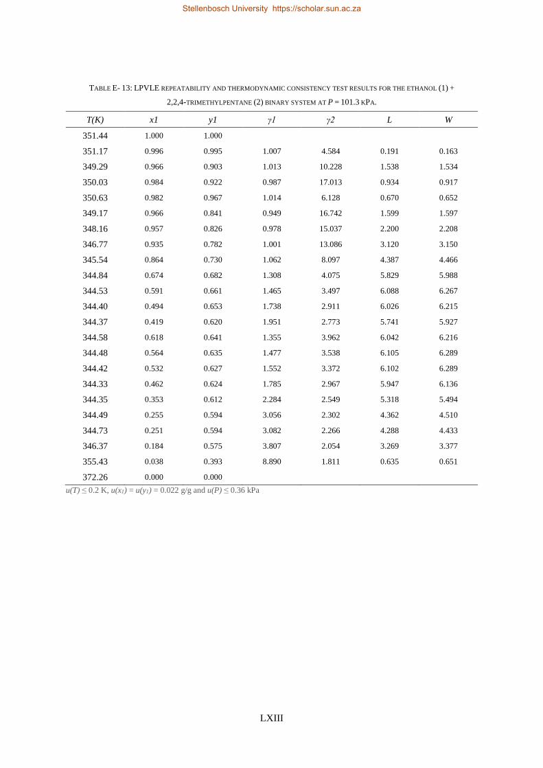
LXIII
TABLE E- 13: LPVLE REPEATABILITY AND THERMODYNAMIC CONSISTENCY TEST RESULTS FOR THE ETHANOL (1) +
2,2,4-TRIMETHYLPENTANE (2) BINARY SYSTEM AT P = 101.3 KPA.
T(K) x1 y1 γ1 γ2 L W
351.44 1.000 1.000
351.17 0.996 0.995 1.007 4.584 0.191 0.163
349.29 0.966 0.903 1.013 10.228 1.538 1.534
350.03 0.984 0.922 0.987 17.013 0.934 0.917
350.63 0.982 0.967 1.014 6.128 0.670 0.652
349.17 0.966 0.841 0.949 16.742 1.599 1.597
348.16 0.957 0.826 0.978 15.037 2.200 2.208
346.77 0.935 0.782 1.001 13.086 3.120 3.150
345.54 0.864 0.730 1.062 8.097 4.387 4.466
344.84 0.674 0.682 1.308 4.075 5.829 5.988
344.53 0.591 0.661 1.465 3.497 6.088 6.267
344.40 0.494 0.653 1.738 2.911 6.026 6.215
344.37 0.419 0.620 1.951 2.773 5.741 5.927
344.58 0.618 0.641 1.355 3.962 6.042 6.216
344.48 0.564 0.635 1.477 3.538 6.105 6.289
344.42 0.532 0.627 1.552 3.372 6.102 6.289
344.33 0.462 0.624 1.785 2.967 5.947 6.136
344.35 0.353 0.612 2.284 2.549 5.318 5.494
344.49 0.255 0.594 3.056 2.302 4.362 4.510
344.73 0.251 0.594 3.082 2.266 4.288 4.433
346.37 0.184 0.575 3.807 2.054 3.269 3.377
355.43 0.038 0.393 8.890 1.811 0.635 0.651
372.26 0.000 0.000
u(T) ≤ 0.2 K, u(x1) = u(y1) = 0.022 g/g and u(P) ≤ 0.36 kPa
Stellenbosch University https://scholar.sun.ac.za
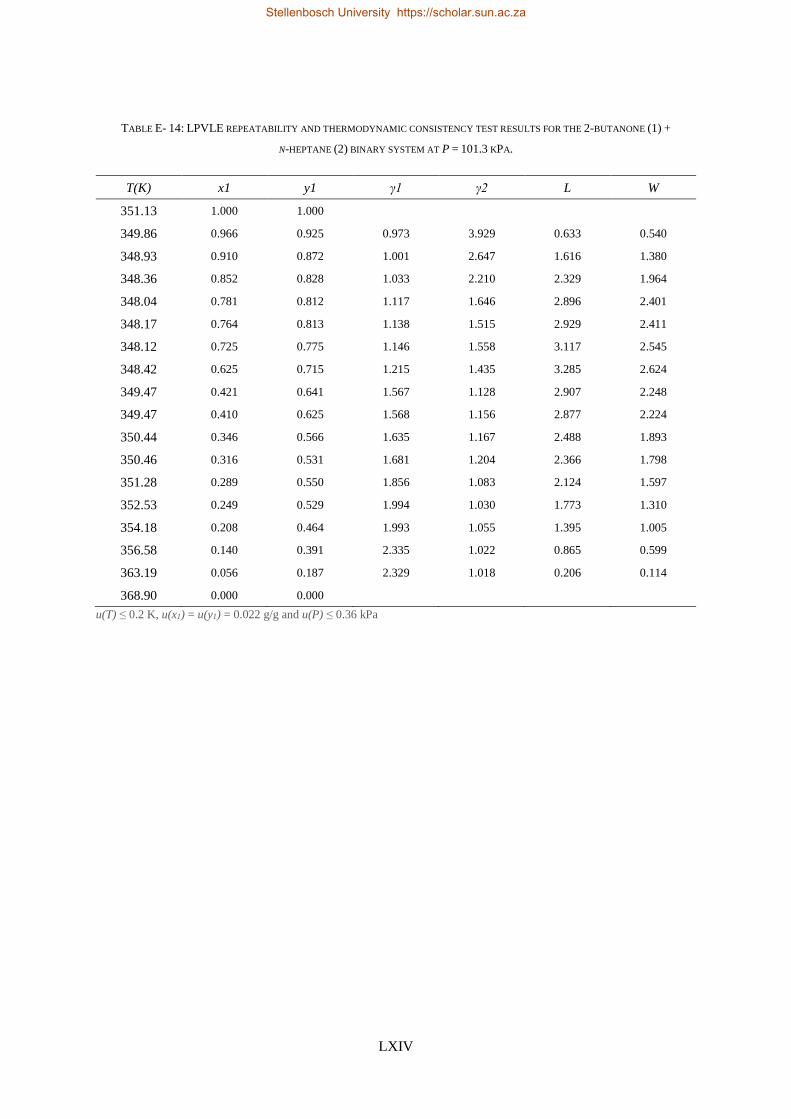
LXIV
TABLE E- 14: LPVLE REPEATABILITY AND THERMODYNAMIC CONSISTENCY TEST RESULTS FOR THE 2-BUTANONE (1) +
N-HEPTANE (2) BINARY SYSTEM AT P = 101.3 KPA.
T(K) x1 y1 γ1 γ2 L W
351.13 1.000 1.000
349.86 0.966 0.925 0.973 3.929 0.633 0.540
348.93 0.910 0.872 1.001 2.647 1.616 1.380
348.36 0.852 0.828 1.033 2.210 2.329 1.964
348.04 0.781 0.812 1.117 1.646 2.896 2.401
348.17 0.764 0.813 1.138 1.515 2.929 2.411
348.12 0.725 0.775 1.146 1.558 3.117 2.545
348.42 0.625 0.715 1.215 1.435 3.285 2.624
349.47 0.421 0.641 1.567 1.128 2.907 2.248
349.47 0.410 0.625 1.568 1.156 2.877 2.224
350.44 0.346 0.566 1.635 1.167 2.488 1.893
350.46 0.316 0.531 1.681 1.204 2.366 1.798
351.28 0.289 0.550 1.856 1.083 2.124 1.597
352.53 0.249 0.529 1.994 1.030 1.773 1.310
354.18 0.208 0.464 1.993 1.055 1.395 1.005
356.58 0.140 0.391 2.335 1.022 0.865 0.599
363.19 0.056 0.187 2.329 1.018 0.206 0.114
368.90 0.000 0.000
u(T) ≤ 0.2 K, u(x1) = u(y1) = 0.022 g/g and u(P) ≤ 0.36 kPa
Stellenbosch University https://scholar.sun.ac.za
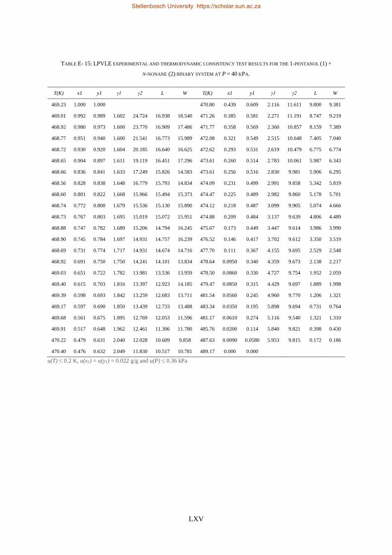
LXV
TABLE E- 15: LPVLE EXPERIMENTAL AND THERMODYNAMIC CONSISTENCY TEST RESULTS FOR THE 1-PENTANOL (1) +
N-NONANE (2) BINARY SYSTEM AT P = 40 KPA.
T(K) x1 y1 γ1 γ2 L W T(K) x1 y1 γ1 γ2 L W
469.23 1.000 1.000 470.80 0.439 0.609 2.116 11.611 9.800 9.381
469.01 0.992 0.989 1.602 24.724 16.938 18.540 471.26 0.385 0.581 2.271 11.191 8.747 9.219
468.92 0.980 0.973 1.600 23.770 16.909 17.486 471.77 0.358 0.569 2.360 10.857 8.159 7.389
468.77 0.951 0.940 1.600 21.541 16.773 15.989 472.08 0.321 0.549 2.515 10.648 7.405 7.040
468.72 0.930 0.920 1.604 20.185 16.640 16.625 472.62 0.293 0.531 2.619 10.479 6.775 6.774
468.65 0.904 0.897 1.611 19.119 16.451 17.296 473.61 0.260 0.514 2.783 10.061 5.987 6.343
468.66 0.836 0.841 1.633 17.249 15.826 14.583 473.61 0.256 0.516 2.830 9.981 5.906 6.295
468.56 0.828 0.838 1.648 16.779 15.793 14.834 474.09 0.231 0.499 2.991 9.858 5.342 5.819
468.60 0.801 0.822 1.668 15.966 15.494 15.373 474.47 0.225 0.489 2.982 9.860 5.178 5.701
468.74 0.772 0.800 1.679 15.536 15.130 15.890 474.12 0.218 0.487 3.099 9.905 5.074 4.666
468.73 0.767 0.803 1.695 15.019 15.072 15.951 474.88 0.209 0.484 3.137 9.639 4.806 4.489
468.88 0.747 0.782 1.689 15.206 14.794 16.245 475.67 0.173 0.449 3.447 9.614 3.986 3.990
468.90 0.745 0.784 1.697 14.931 14.757 16.239 476.52 0.146 0.417 3.702 9.612 3.350 3.519
468.69 0.731 0.774 1.717 14.931 14.674 14.716 477.70 0.111 0.367 4.155 9.695 2.529 2.548
468.92 0.691 0.750 1.750 14.241 14.101 13.834 478.64 0.0950 0.340 4.359 9.673 2.138 2.217
469.03 0.651 0.722 1.782 13.981 13.536 13.959 478.50 0.0860 0.330 4.727 9.754 1.952 2.059
469.40 0.615 0.703 1.816 13.397 12.923 14.185 479.47 0.0850 0.315 4.429 9.697 1.889 1.998
469.39 0.598 0.693 1.842 13.259 12.683 13.711 481.54 0.0560 0.245 4.960 9.770 1.206 1.321
469.17 0.597 0.690 1.850 13.439 12.733 13.488 483.34 0.0350 0.195 5.898 9.694 0.731 0.764
469.68 0.561 0.675 1.895 12.769 12.053 11.596 481.17 0.0610 0.274 5.116 9.540 1.321 1.310
469.91 0.517 0.648 1.962 12.461 11.306 11.780 485.76 0.0200 0.114 5.840 9.821 0.398 0.430
470.22 0.479 0.631 2.040 12.028 10.609 9.858 487.63 0.0090 0.0580 5.953 9.815 0.172 0.186
470.40 0.476 0.632 2.049 11.830 10.517 10.781 489.17 0.000 0.000
u(T) ≤ 0.2 K, u(x1) = u(y1) = 0.022 g/g and u(P) ≤ 0.36 kPa
Stellenbosch University https://scholar.sun.ac.za
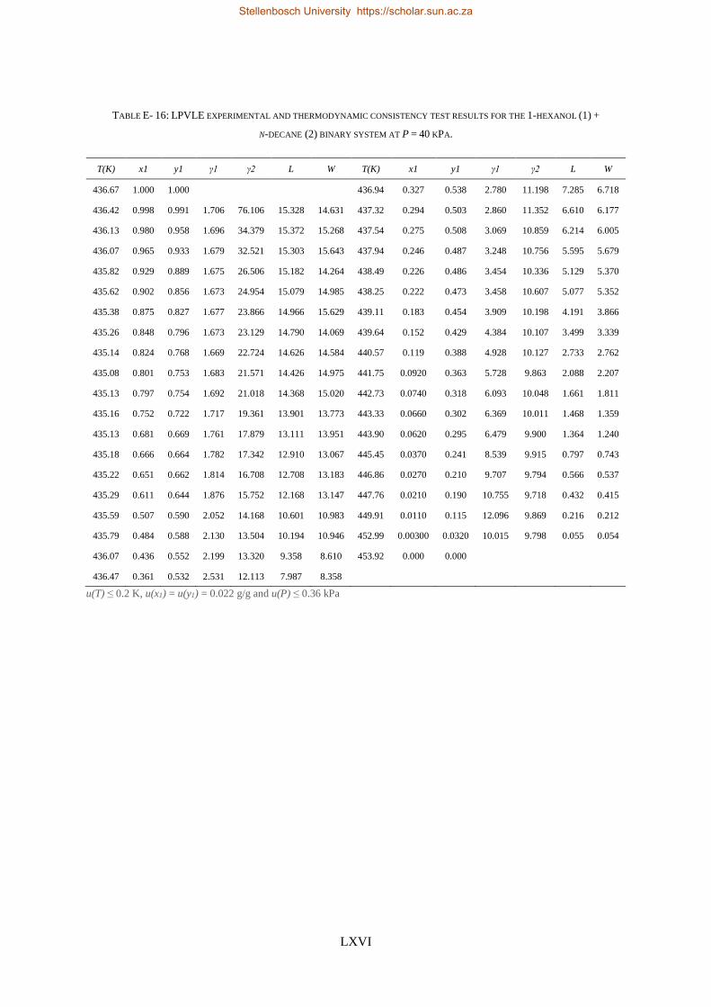
LXVI
TABLE E- 16: LPVLE EXPERIMENTAL AND THERMODYNAMIC CONSISTENCY TEST RESULTS FOR THE 1-HEXANOL (1) +
N-DECANE (2) BINARY SYSTEM AT P = 40 KPA.
T(K) x1 y1 γ1 γ2 L W T(K) x1 y1 γ1 γ2 L W
436.67 1.000 1.000 436.94 0.327 0.538 2.780 11.198 7.285 6.718
436.42 0.998 0.991 1.706 76.106 15.328 14.631 437.32 0.294 0.503 2.860 11.352 6.610 6.177
436.13 0.980 0.958 1.696 34.379 15.372 15.268 437.54 0.275 0.508 3.069 10.859 6.214 6.005
436.07 0.965 0.933 1.679 32.521 15.303 15.643 437.94 0.246 0.487 3.248 10.756 5.595 5.679
435.82 0.929 0.889 1.675 26.506 15.182 14.264 438.49 0.226 0.486 3.454 10.336 5.129 5.370
435.62 0.902 0.856 1.673 24.954 15.079 14.985 438.25 0.222 0.473 3.458 10.607 5.077 5.352
435.38 0.875 0.827 1.677 23.866 14.966 15.629 439.11 0.183 0.454 3.909 10.198 4.191 3.866
435.26 0.848 0.796 1.673 23.129 14.790 14.069 439.64 0.152 0.429 4.384 10.107 3.499 3.339
435.14 0.824 0.768 1.669 22.724 14.626 14.584 440.57 0.119 0.388 4.928 10.127 2.733 2.762
435.08 0.801 0.753 1.683 21.571 14.426 14.975 441.75 0.0920 0.363 5.728 9.863 2.088 2.207
435.13 0.797 0.754 1.692 21.018 14.368 15.020 442.73 0.0740 0.318 6.093 10.048 1.661 1.811
435.16 0.752 0.722 1.717 19.361 13.901 13.773 443.33 0.0660 0.302 6.369 10.011 1.468 1.359
435.13 0.681 0.669 1.761 17.879 13.111 13.951 443.90 0.0620 0.295 6.479 9.900 1.364 1.240
435.18 0.666 0.664 1.782 17.342 12.910 13.067 445.45 0.0370 0.241 8.539 9.915 0.797 0.743
435.22 0.651 0.662 1.814 16.708 12.708 13.183 446.86 0.0270 0.210 9.707 9.794 0.566 0.537
435.29 0.611 0.644 1.876 15.752 12.168 13.147 447.76 0.0210 0.190 10.755 9.718 0.432 0.415
435.59 0.507 0.590 2.052 14.168 10.601 10.983 449.91 0.0110 0.115 12.096 9.869 0.216 0.212
435.79 0.484 0.588 2.130 13.504 10.194 10.946 452.99 0.00300 0.0320 10.015 9.798 0.055 0.054
436.07 0.436 0.552 2.199 13.320 9.358 8.610 453.92 0.000 0.000
436.47 0.361 0.532 2.531 12.113 7.987 8.358
u(T) ≤ 0.2 K, u(x1) = u(y1) = 0.022 g/g and u(P) ≤ 0.36 kPa
Stellenbosch University https://scholar.sun.ac.za
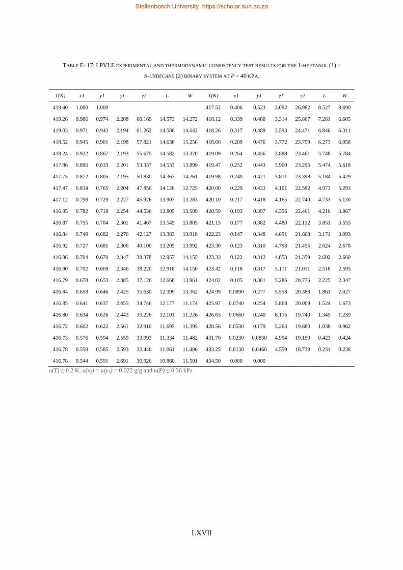
LXVII
TABLE E- 17: LPVLE EXPERIMENTAL AND THERMODYNAMIC CONSISTENCY TEST RESULTS FOR THE 1-HEPTANOL (1) +
N-UNDECANE (2) BINARY SYSTEM AT P = 40 KPA.
T(K) x1 y1 γ1 γ2 L W T(K) x1 y1 γ1 γ2 L W
419.40 1.000 1.000 417.52 0.406 0.523 3.092 26.982 8.527 8.690
419.26 0.986 0.974 2.208 60.169 14.573 14.272 418.12 0.339 0.480 3.314 25.867 7.261 6.605
419.03 0.971 0.943 2.194 61.262 14.586 14.642 418.26 0.317 0.489 3.593 24.471 6.846 6.311
418.52 0.945 0.901 2.198 57.821 14.638 15.256 418.66 0.289 0.476 3.772 23.759 6.273 6.058
418.24 0.922 0.867 2.193 55.675 14.582 13.370 419.09 0.264 0.456 3.888 23.461 5.748 5.784
417.86 0.896 0.833 2.201 53.337 14.533 13.899 419.47 0.252 0.443 3.900 23.296 5.474 5.618
417.75 0.872 0.805 2.195 50.830 14.367 14.261 419.98 0.240 0.421 3.811 23.398 5.184 5.429
417.47 0.834 0.765 2.204 47.856 14.128 12.725 420.00 0.229 0.433 4.101 22.582 4.973 5.293
417.12 0.798 0.729 2.227 45.926 13.907 13.283 420.10 0.217 0.418 4.165 22.740 4.733 5.130
416.95 0.782 0.718 2.254 44.536 13.805 13.509 420.59 0.193 0.397 4.356 22.461 4.216 3.867
416.87 0.755 0.704 2.301 41.467 13.545 13.805 421.15 0.177 0.382 4.480 22.112 3.851 3.555
416.84 0.740 0.682 2.276 42.127 13.383 13.918 422.23 0.147 0.348 4.691 21.668 3.171 3.093
416.92 0.727 0.681 2.306 40.100 13.205 13.992 423.30 0.123 0.310 4.798 21.455 2.624 2.678
416.86 0.704 0.670 2.347 38.378 12.957 14.155 423.33 0.122 0.312 4.853 21.359 2.602 2.660
416.90 0.702 0.669 2.346 38.220 12.918 14.150 423.42 0.118 0.317 5.111 21.011 2.518 2.595
416.79 0.678 0.653 2.385 37.126 12.666 13.961 424.02 0.105 0.301 5.286 20.776 2.225 2.347
416.84 0.658 0.646 2.425 35.630 12.399 13.362 424.99 0.0890 0.277 5.558 20.388 1.861 2.027
416.85 0.641 0.637 2.455 34.746 12.177 11.174 425.97 0.0740 0.254 5.868 20.009 1.524 1.673
416.80 0.634 0.626 2.443 35.226 12.101 11.226 426.63 0.0660 0.240 6.116 19.740 1.345 1.239
416.72 0.602 0.622 2.561 32.910 11.695 11.395 428.56 0.0530 0.179 5.263 19.680 1.038 0.962
416.73 0.576 0.594 2.559 33.093 11.334 11.482 431.70 0.0230 0.0830 4.994 19.159 0.423 0.424
416.78 0.558 0.585 2.593 32.446 11.061 11.486 433.25 0.0130 0.0460 4.559 18.739 0.231 0.238
416.78 0.544 0.591 2.691 30.926 10.860 11.501 434.50 0.000 0.000
u(T) ≤ 0.2 K, u(x1) = u(y1) = 0.022 g/g and u(P) ≤ 0.36 kPa
Stellenbosch University https://scholar.sun.ac.za
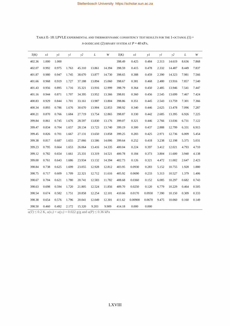
LXVIII
TABLE E- 18: LPVLE EXPERIMENTAL AND THERMODYNAMIC CONSISTENCY TEST RESULTS FOR THE 1-OCTANOL (1) +
N-DODECANE (2) BINARY SYSTEM AT P = 40 KPA.
T(K) x1 y1 γ1 γ2 L W T(K) x1 y1 γ1 γ2 L W
402.36 1.000 1.000 398.49 0.425 0.484 2.313 14.619 8.636 7.868
402.07 0.992 0.975 1.763 45.310 13.861 14.394 398.59 0.415 0.478 2.332 14.487 8.449 7.837
401.87 0.980 0.947 1.745 38.670 13.877 14.730 398.65 0.388 0.459 2.390 14.323 7.981 7.566
401.66 0.968 0.919 1.727 37.188 13.894 15.060 398.67 0.381 0.468 2.480 13.916 7.857 7.540
401.43 0.956 0.895 1.716 35.321 13.916 12.999 398.79 0.364 0.450 2.485 13.946 7.541 7.447
401.16 0.944 0.871 1.707 34.395 13.952 13.366 398.81 0.360 0.456 2.545 13.699 7.467 7.424
400.83 0.929 0.844 1.701 33.161 13.987 13.804 398.86 0.351 0.445 2.543 13.759 7.301 7.366
400.34 0.893 0.786 1.676 30.670 13.904 12.853 398.92 0.340 0.446 2.625 13.478 7.096 7.287
400.21 0.870 0.766 1.684 27.719 13.754 12.865 398.87 0.330 0.442 2.685 13.395 6.926 7.225
399.84 0.861 0.745 1.676 28.597 13.830 13.176 399.07 0.321 0.446 2.766 13.036 6.731 7.122
399.47 0.834 0.704 1.657 28.134 13.723 13.740 399.19 0.300 0.437 2.888 12.799 6.331 6.915
399.45 0.826 0.701 1.667 27.131 13.650 13.858 399.25 0.283 0.425 2.971 12.736 6.009 5.454
399.38 0.817 0.687 1.655 27.066 13.586 14.006 399.64 0.252 0.418 3.238 12.198 5.375 5.031
399.23 0.795 0.664 1.653 26.064 13.416 14.335 400.04 0.224 0.397 3.412 12.021 4.793 4.710
399.12 0.782 0.654 1.661 25.331 13.319 14.521 400.78 0.184 0.373 3.804 11.600 3.940 4.138
399.00 0.761 0.643 1.686 23.934 13.132 14.394 402.73 0.126 0.321 4.472 11.002 2.647 2.423
398.84 0.738 0.625 1.699 23.055 12.928 12.812 403.95 0.0930 0.283 5.152 10.755 1.928 1.880
398.75 0.717 0.609 1.709 22.321 12.712 11.616 405.92 0.0690 0.233 5.313 10.527 1.379 1.406
398.67 0.704 0.621 1.780 20.741 12.583 11.782 408.68 0.0360 0.152 6.085 10.297 0.682 0.743
398.63 0.698 0.594 1.720 21.805 12.524 11.856 409.70 0.0250 0.120 6.779 10.229 0.464 0.505
398.54 0.674 0.582 1.751 20.858 12.254 12.101 410.66 0.0170 0.0930 7.390 10.150 0.309 0.333
398.38 0.654 0.576 1.796 20.041 12.049 12.301 411.62 0.00900 0.0670 9.475 10.060 0.160 0.149
398.50 0.460 0.492 2.172 15.320 9.203 9.909 414.18 0.000 0.000
u(T) ≤ 0.2 K, u(x1) = u(y1) = 0.022 g/g and u(P) ≤ 0.36 kPa
Stellenbosch University https://scholar.sun.ac.za
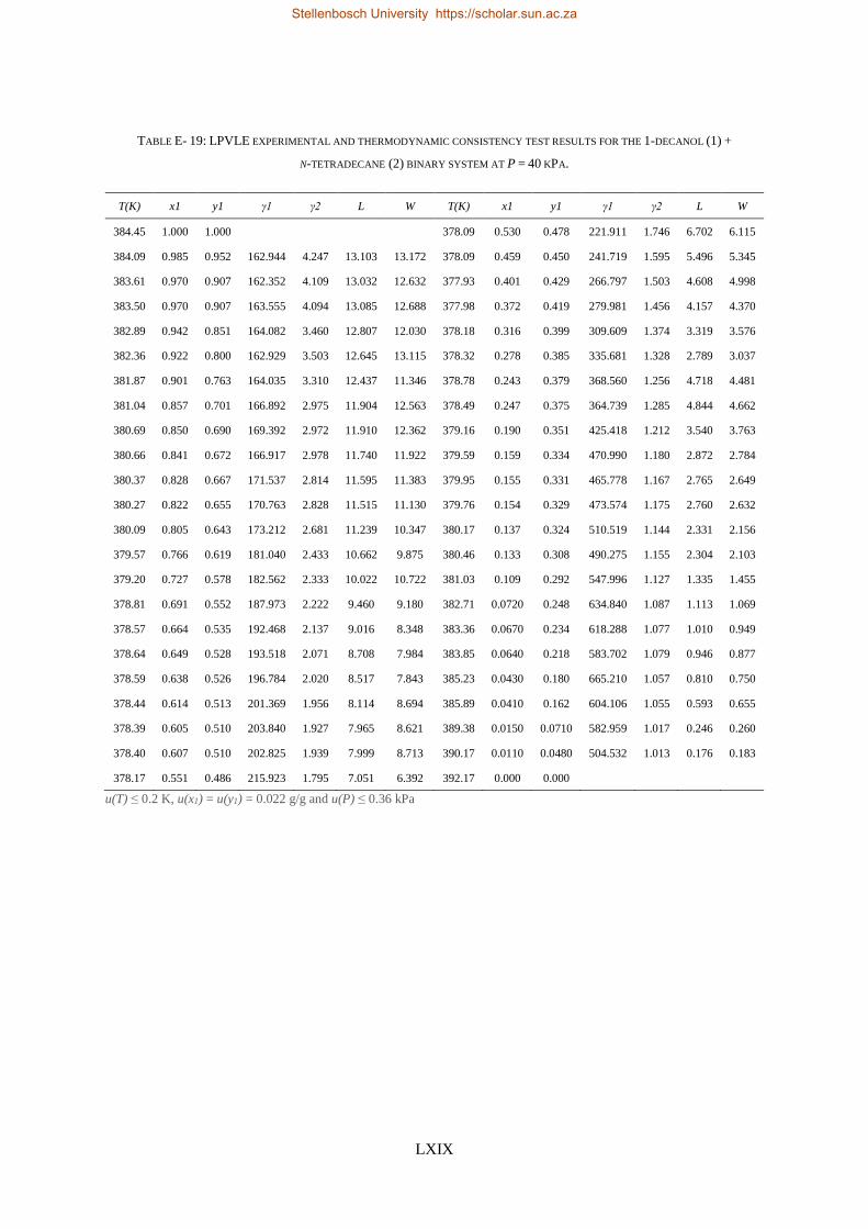
LXIX
TABLE E- 19: LPVLE EXPERIMENTAL AND THERMODYNAMIC CONSISTENCY TEST RESULTS FOR THE 1-DECANOL (1) +
N-TETRADECANE (2) BINARY SYSTEM AT P = 40 KPA.
T(K) x1 y1 γ1 γ2 L W T(K) x1 y1 γ1 γ2 L W
384.45 1.000 1.000 378.09 0.530 0.478 221.911 1.746 6.702 6.115
384.09 0.985 0.952 162.944 4.247 13.103 13.172 378.09 0.459 0.450 241.719 1.595 5.496 5.345
383.61 0.970 0.907 162.352 4.109 13.032 12.632 377.93 0.401 0.429 266.797 1.503 4.608 4.998
383.50 0.970 0.907 163.555 4.094 13.085 12.688 377.98 0.372 0.419 279.981 1.456 4.157 4.370
382.89 0.942 0.851 164.082 3.460 12.807 12.030 378.18 0.316 0.399 309.609 1.374 3.319 3.576
382.36 0.922 0.800 162.929 3.503 12.645 13.115 378.32 0.278 0.385 335.681 1.328 2.789 3.037
381.87 0.901 0.763 164.035 3.310 12.437 11.346 378.78 0.243 0.379 368.560 1.256 4.718 4.481
381.04 0.857 0.701 166.892 2.975 11.904 12.563 378.49 0.247 0.375 364.739 1.285 4.844 4.662
380.69 0.850 0.690 169.392 2.972 11.910 12.362 379.16 0.190 0.351 425.418 1.212 3.540 3.763
380.66 0.841 0.672 166.917 2.978 11.740 11.922 379.59 0.159 0.334 470.990 1.180 2.872 2.784
380.37 0.828 0.667 171.537 2.814 11.595 11.383 379.95 0.155 0.331 465.778 1.167 2.765 2.649
380.27 0.822 0.655 170.763 2.828 11.515 11.130 379.76 0.154 0.329 473.574 1.175 2.760 2.632
380.09 0.805 0.643 173.212 2.681 11.239 10.347 380.17 0.137 0.324 510.519 1.144 2.331 2.156
379.57 0.766 0.619 181.040 2.433 10.662 9.875 380.46 0.133 0.308 490.275 1.155 2.304 2.103
379.20 0.727 0.578 182.562 2.333 10.022 10.722 381.03 0.109 0.292 547.996 1.127 1.335 1.455
378.81 0.691 0.552 187.973 2.222 9.460 9.180 382.71 0.0720 0.248 634.840 1.087 1.113 1.069
378.57 0.664 0.535 192.468 2.137 9.016 8.348 383.36 0.0670 0.234 618.288 1.077 1.010 0.949
378.64 0.649 0.528 193.518 2.071 8.708 7.984 383.85 0.0640 0.218 583.702 1.079 0.946 0.877
378.59 0.638 0.526 196.784 2.020 8.517 7.843 385.23 0.0430 0.180 665.210 1.057 0.810 0.750
378.44 0.614 0.513 201.369 1.956 8.114 8.694 385.89 0.0410 0.162 604.106 1.055 0.593 0.655
378.39 0.605 0.510 203.840 1.927 7.965 8.621 389.38 0.0150 0.0710 582.959 1.017 0.246 0.260
378.40 0.607 0.510 202.825 1.939 7.999 8.713 390.17 0.0110 0.0480 504.532 1.013 0.176 0.183
378.17 0.551 0.486 215.923 1.795 7.051 6.392 392.17 0.000 0.000
u(T) ≤ 0.2 K, u(x1) = u(y1) = 0.022 g/g and u(P) ≤ 0.36 kPa
Stellenbosch University https://scholar.sun.ac.za
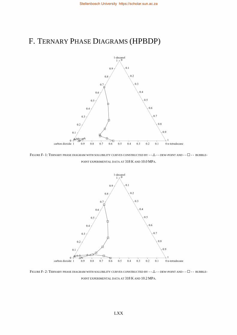
LXX
F. TERNARY PHASE DIAGRAMS (HPBDP)
FIGURE F- 1: TERNARY PHASE DIAGRAM WITH SOLUBILITY CURVES CONSTRUCTED BY - - △ - - DEW-POINT AND - - □ - - BUBBLE-
POINT EXPERIMENTAL DATA AT 318 K AND 10.0 MPA.
FIGURE F- 2: TERNARY PHASE DIAGRAM WITH SOLUBILITY CURVES CONSTRUCTED BY - - △ - - DEW-POINT AND - - □ - - BUBBLE-
POINT EXPERIMENTAL DATA AT 318 K AND 10.2 MPA.
Stellenbosch University https://scholar.sun.ac.za
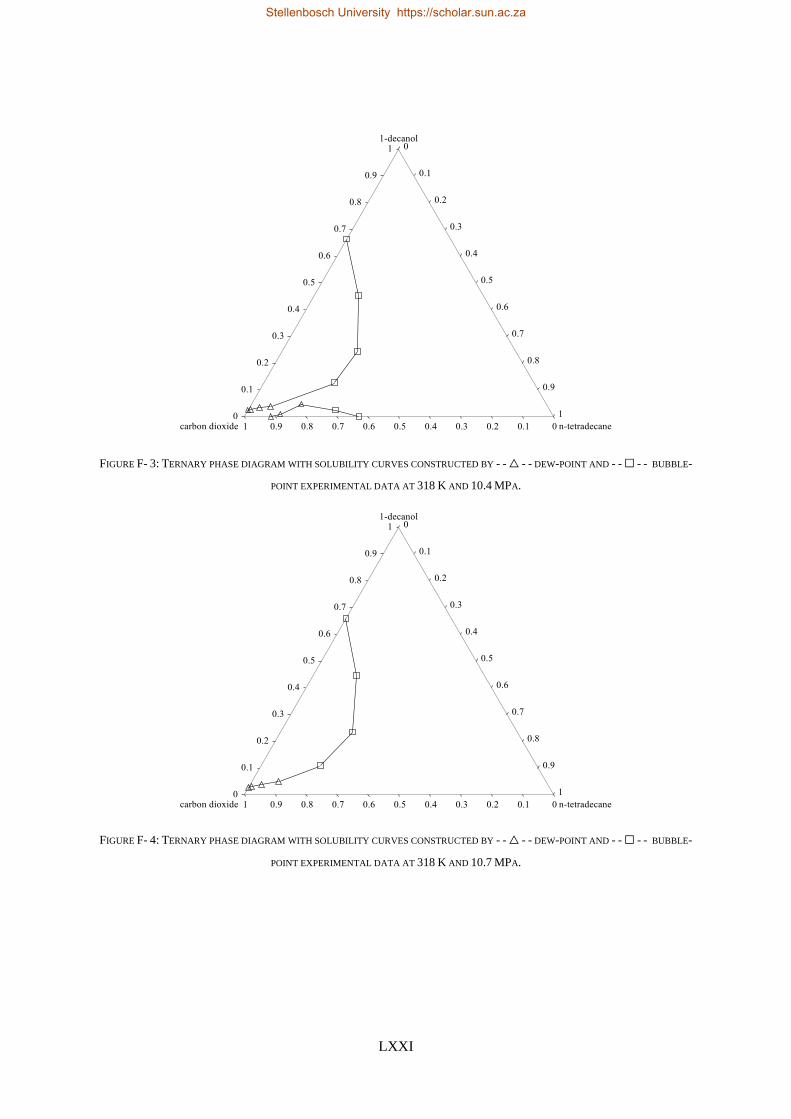
LXXI
FIGURE F- 3: TERNARY PHASE DIAGRAM WITH SOLUBILITY CURVES CONSTRUCTED BY - - △ - - DEW-POINT AND - - □ - - BUBBLE-
POINT EXPERIMENTAL DATA AT 318 K AND 10.4 MPA.
FIGURE F- 4: TERNARY PHASE DIAGRAM WITH SOLUBILITY CURVES CONSTRUCTED BY - - △ - - DEW-POINT AND - - □ - - BUBBLE-
POINT EXPERIMENTAL DATA AT 318 K AND 10.7 MPA.
Stellenbosch University https://scholar.sun.ac.za
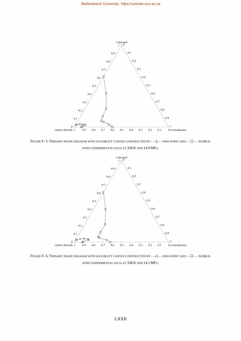
LXXII
FIGURE F- 5: TERNARY PHASE DIAGRAM WITH SOLUBILITY CURVES CONSTRUCTED BY - - △ - - DEW-POINT AND - - □ - - BUBBLE-
POINT EXPERIMENTAL DATA AT 338 K AND 14.0 MPA.
FIGURE F- 6: TERNARY PHASE DIAGRAM WITH SOLUBILITY CURVES CONSTRUCTED BY - - △ - - DEW-POINT AND - - □ - - BUBBLE-
POINT EXPERIMENTAL DATA AT 338 K AND 14.2 MPA.
Stellenbosch University https://scholar.sun.ac.za
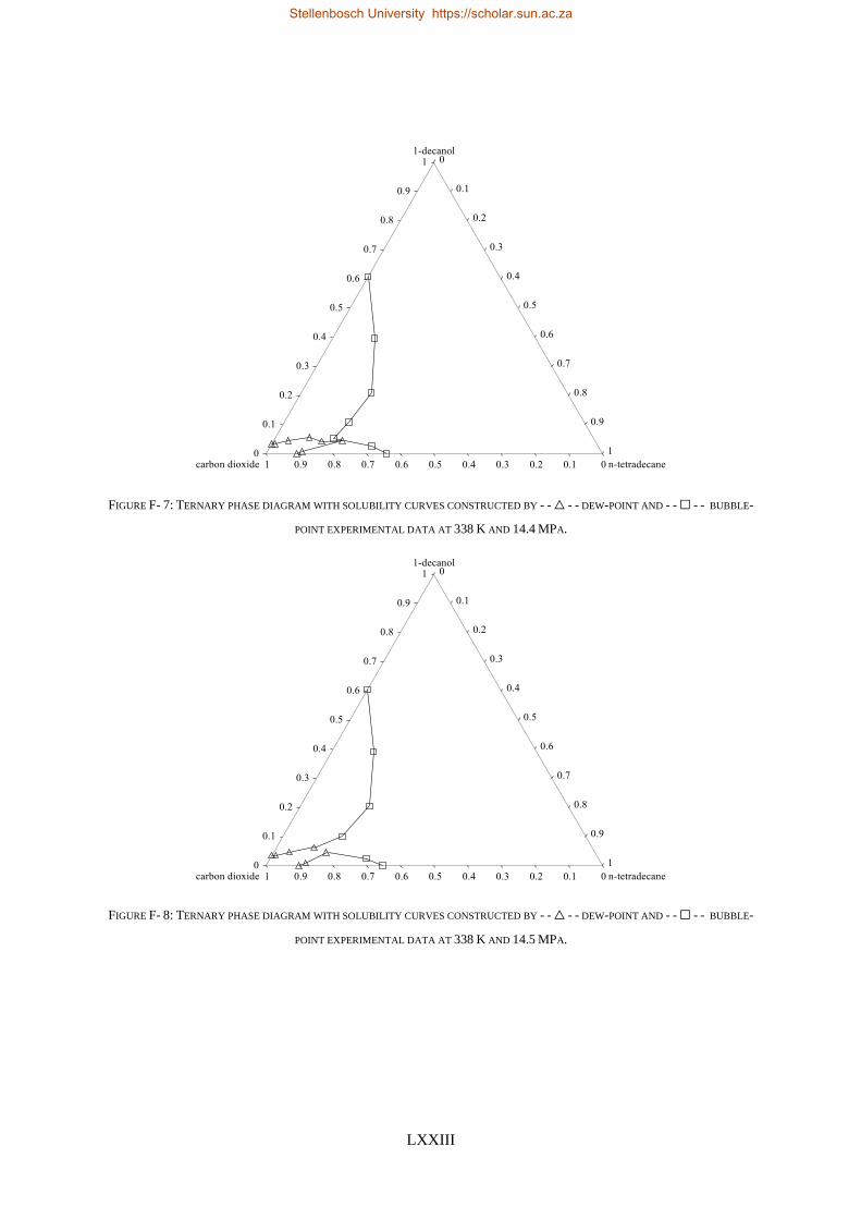
LXXIII
FIGURE F- 7: TERNARY PHASE DIAGRAM WITH SOLUBILITY CURVES CONSTRUCTED BY - - △ - - DEW-POINT AND - - □ - - BUBBLE-
POINT EXPERIMENTAL DATA AT 338 K AND 14.4 MPA.
FIGURE F- 8: TERNARY PHASE DIAGRAM WITH SOLUBILITY CURVES CONSTRUCTED BY - - △ - - DEW-POINT AND - - □ - - BUBBLE-
POINT EXPERIMENTAL DATA AT 338 K AND 14.5 MPA.
Stellenbosch University https://scholar.sun.ac.za
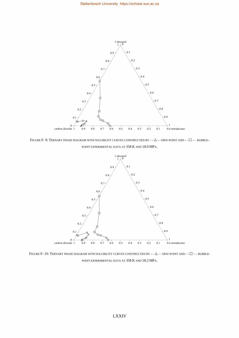
LXXIV
FIGURE F- 9: TERNARY PHASE DIAGRAM WITH SOLUBILITY CURVES CONSTRUCTED BY - - △ - - DEW-POINT AND - - □ - - BUBBLE-
POINT EXPERIMENTAL DATA AT 358 K AND 18.0 MPA.
FIGURE F- 10: TERNARY PHASE DIAGRAM WITH SOLUBILITY CURVES CONSTRUCTED BY - - △ - - DEW-POINT AND - - □ - - BUBBLE-
POINT EXPERIMENTAL DATA AT 358 K AND 18.2 MPA.
Stellenbosch University https://scholar.sun.ac.za
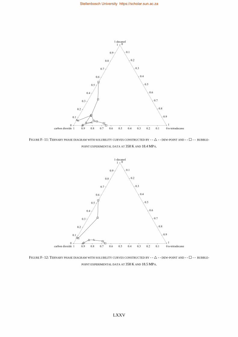
LXXV
FIGURE F- 11: TERNARY PHASE DIAGRAM WITH SOLUBILITY CURVES CONSTRUCTED BY - - △ - - DEW-POINT AND - - □ - - BUBBLE-
POINT EXPERIMENTAL DATA AT 358 K AND 18.4 MPA.
FIGURE F- 12: TERNARY PHASE DIAGRAM WITH SOLUBILITY CURVES CONSTRUCTED BY - - △ - - DEW-POINT AND - - □ - - BUBBLE-
POINT EXPERIMENTAL DATA AT 358 K AND 18.5 MPA.
Stellenbosch University https://scholar.sun.ac.za
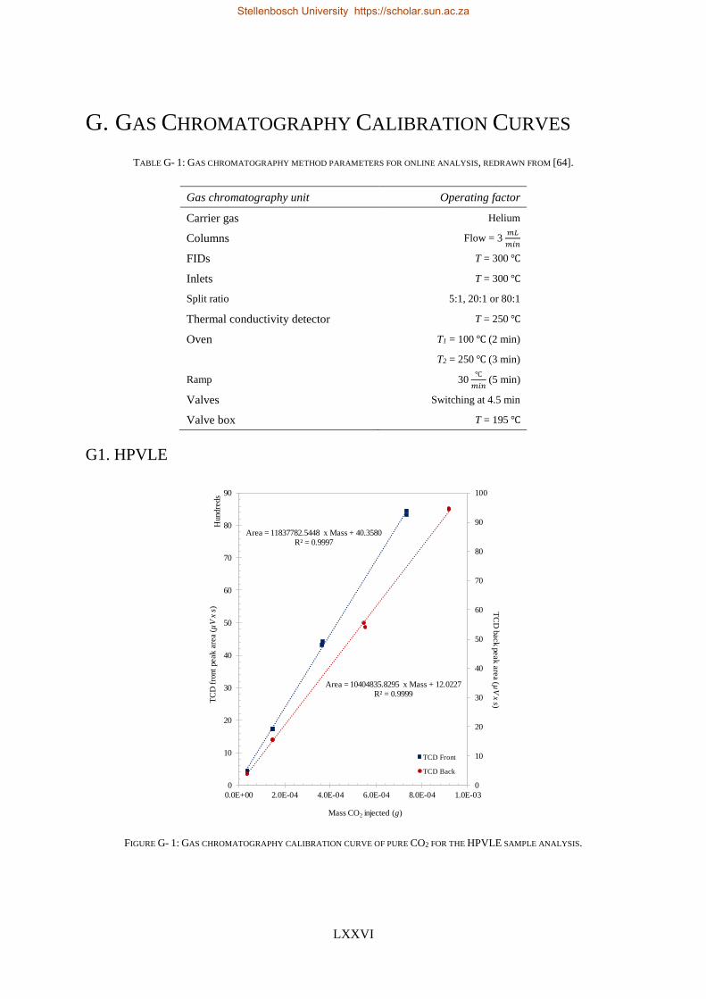
LXXVI
G. GAS CHROMATOGRAPHY CALIBRATION CURVES
TABLE G- 1: GAS CHROMATOGRAPHY METHOD PARAMETERS FOR ONLINE ANALYSIS, REDRAWN FROM [64].
Gas chromatography unit Operating factor
Carrier gas Helium
Columns Flow = 3 𝑚𝐿
𝑚𝑖𝑛
FIDs T = 300 ℃
Inlets T = 300 ℃
Split ratio 5:1, 20:1 or 80:1
Thermal conductivity detector T = 250 ℃
Oven T1 = 100 ℃ (2 min)
T2 = 250 ℃ (3 min)
Ramp 30 ℃
𝑚𝑖𝑛 (5 min)
Valves Switching at 4.5 min
Valve box T = 195 ℃
G1. HPVLE
FIGURE G- 1: GAS CHROMATOGRAPHY CALIBRATION CURVE OF PURE CO2 FOR THE HPVLE SAMPLE ANALYSIS.
Area = 10404835.8295 x Mass + 12.0227R² = 0.9999
Area = 11837782.5448 x Mass + 40.3580R² = 0.9997
0
10
20
30
40
50
60
70
80
90
100
0
10
20
30
40
50
60
70
80
90
0.0E+00 2.0E-04 4.0E-04 6.0E-04 8.0E-04 1.0E-03
TC
D b
ack p
eak a
rea (µ
V x
s)TC
D f
ront
peak a
rea (
µV
x s
)H
undre
ds
Mass CO2 injected (g)
TCD Front
TCD Back
Stellenbosch University https://scholar.sun.ac.za
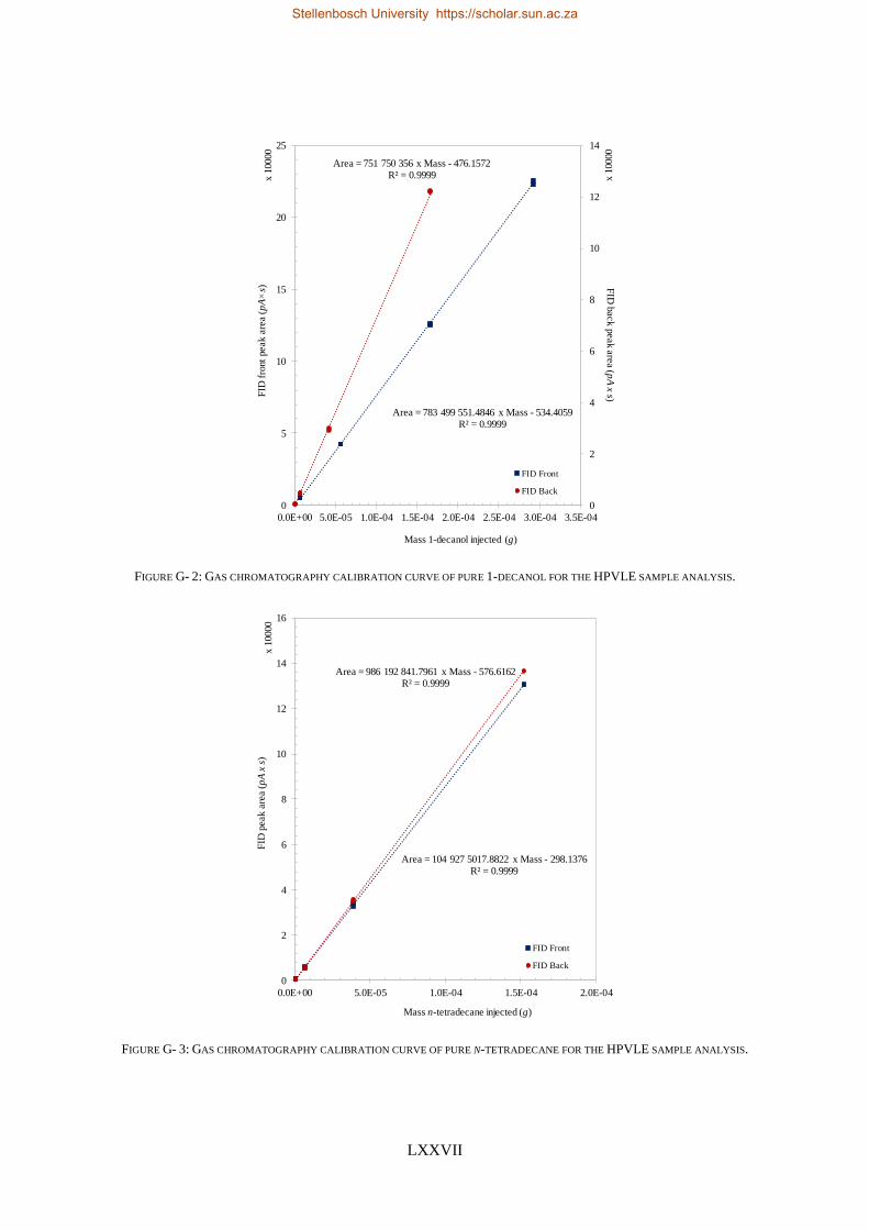
LXXVII
FIGURE G- 2: GAS CHROMATOGRAPHY CALIBRATION CURVE OF PURE 1-DECANOL FOR THE HPVLE SAMPLE ANALYSIS.
FIGURE G- 3: GAS CHROMATOGRAPHY CALIBRATION CURVE OF PURE N-TETRADECANE FOR THE HPVLE SAMPLE ANALYSIS.
Area = 783 499 551.4846 x Mass - 534.4059R² = 0.9999
Area = 751 750 356 x Mass - 476.1572R² = 0.9999
0
2
4
6
8
10
12
14
0
5
10
15
20
25
0.0E+00 5.0E-05 1.0E-04 1.5E-04 2.0E-04 2.5E-04 3.0E-04 3.5E-04
FID
back p
eak a
rea (p
A x
s)
x 1
0000
FID
fro
nt
peak a
rea (
pA
s)x 1
0000
Mass 1-decanol injected (g)
FID Front
FID Back
Area = 104 927 5017.8822 x Mass - 298.1376R² = 0.9999
Area = 986 192 841.7961 x Mass - 576.6162R² = 0.9999
0
2
4
6
8
10
12
14
16
0.0E+00 5.0E-05 1.0E-04 1.5E-04 2.0E-04
FID
peak a
rea (
pA
x s
)x 1
0000
Mass n-tetradecane injected (g)
FID Front
FID Back
Stellenbosch University https://scholar.sun.ac.za
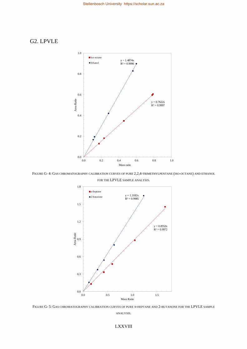
LXXVIII
G2. LPVLE
FIGURE G- 4: GAS CHROMATOGRAPHY CALIBRATION CURVES OF PURE 2,2,4-TRIMETHYLPENTANE (ISO-OCTANE) AND ETHANOL
FOR THE LPVLE SAMPLE ANALYSIS.
FIGURE G- 5: GAS CHROMATOGRAPHY CALIBRATION CURVES OF PURE N-HEPTANE AND 2-BUTANONE FOR THE LPVLE SAMPLE
ANALYSIS.
y = 0.7622xR² = 0.9997
y = 1.4874xR² = 0.9996
0.0
0.2
0.4
0.6
0.8
1.0
0.0 0.2 0.4 0.6 0.8 1.0
Are
a R
atio
Mass ratio
Iso-octane
Ethanol
y = 0.8552xR² = 0.9972
y = 1.3182xR² = 0.9985
0.0
0.3
0.6
0.9
1.2
1.5
1.8
0.0 0.5 1.0 1.5
Are
a R
atio
Mass Ratio
n-heptane
2-butanone
Stellenbosch University https://scholar.sun.ac.za
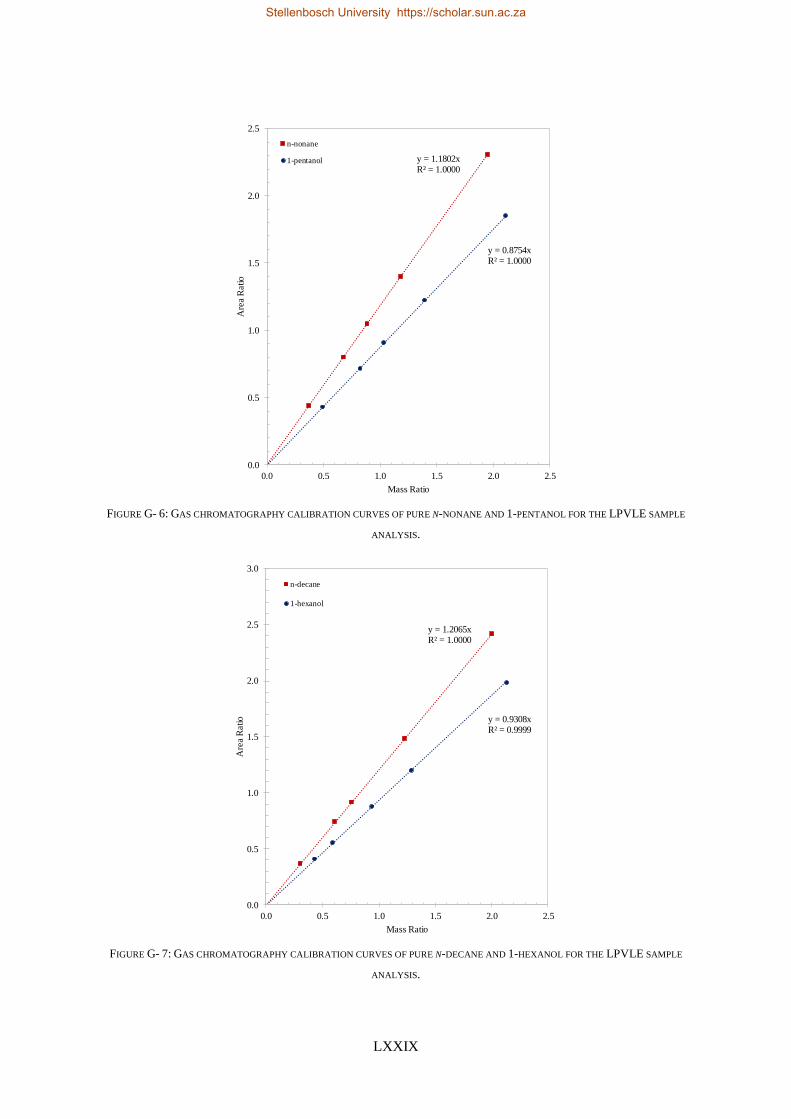
LXXIX
FIGURE G- 6: GAS CHROMATOGRAPHY CALIBRATION CURVES OF PURE N-NONANE AND 1-PENTANOL FOR THE LPVLE SAMPLE
ANALYSIS.
FIGURE G- 7: GAS CHROMATOGRAPHY CALIBRATION CURVES OF PURE N-DECANE AND 1-HEXANOL FOR THE LPVLE SAMPLE
ANALYSIS.
y = 1.1802xR² = 1.0000
y = 0.8754xR² = 1.0000
0.0
0.5
1.0
1.5
2.0
2.5
0.0 0.5 1.0 1.5 2.0 2.5
Are
a R
atio
Mass Ratio
n-nonane
1-pentanol
y = 1.2065xR² = 1.0000
y = 0.9308xR² = 0.9999
0.0
0.5
1.0
1.5
2.0
2.5
3.0
0.0 0.5 1.0 1.5 2.0 2.5
Are
a R
atio
Mass Ratio
n-decane
1-hexanol
Stellenbosch University https://scholar.sun.ac.za
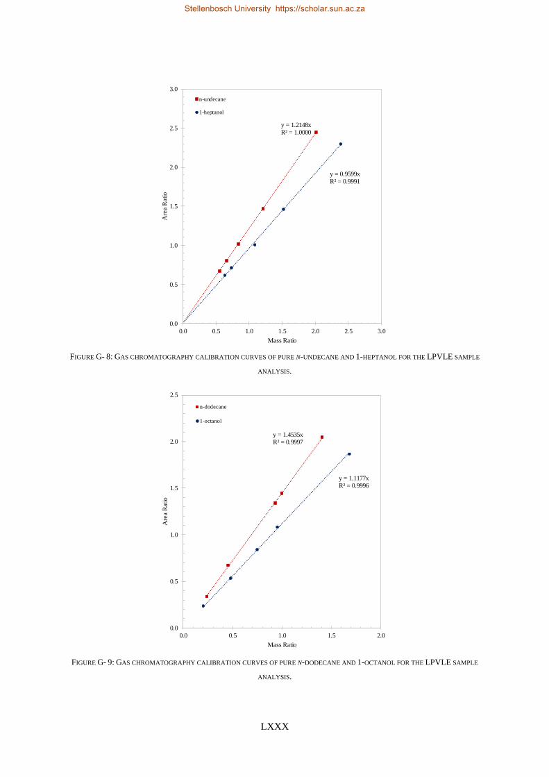
LXXX
FIGURE G- 8: GAS CHROMATOGRAPHY CALIBRATION CURVES OF PURE N-UNDECANE AND 1-HEPTANOL FOR THE LPVLE SAMPLE
ANALYSIS.
FIGURE G- 9: GAS CHROMATOGRAPHY CALIBRATION CURVES OF PURE N-DODECANE AND 1-OCTANOL FOR THE LPVLE SAMPLE
ANALYSIS.
y = 1.2148xR² = 1.0000
y = 0.9599xR² = 0.9991
0.0
0.5
1.0
1.5
2.0
2.5
3.0
0.0 0.5 1.0 1.5 2.0 2.5 3.0
Are
a R
atio
Mass Ratio
n-undecane
1-heptanol
y = 1.4535xR² = 0.9997
y = 1.1177xR² = 0.9996
0.0
0.5
1.0
1.5
2.0
2.5
0.0 0.5 1.0 1.5 2.0
Are
a R
atio
Mass Ratio
n-dodecane
1-octanol
Stellenbosch University https://scholar.sun.ac.za
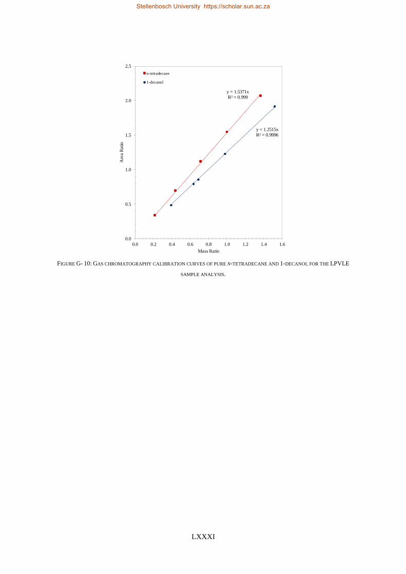
LXXXI
FIGURE G- 10: GAS CHROMATOGRAPHY CALIBRATION CURVES OF PURE N-TETRADECANE AND 1-DECANOL FOR THE LPVLE
SAMPLE ANALYSIS.
y = 1.5371xR² = 0.999
y = 1.2515xR² = 0.9996
0.0
0.5
1.0
1.5
2.0
2.5
0.0 0.2 0.4 0.6 0.8 1.0 1.2 1.4 1.6
Are
a R
atio
Mass Ratio
n-tetradecane
1-decanol
Stellenbosch University https://scholar.sun.ac.za
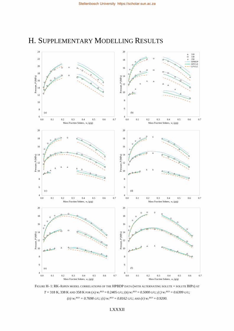
LXXXII
H. SUPPLEMENTARY MODELLING RESULTS
FIGURE H- 1: RK-ASPEN MODEL CORRELATIONS OF THE HPBDP DATA (WITH ALTERNATING SOLUTE + SOLUTE BIPS) AT
T = 318 K, 338 K AND 358 K FOR (A) WCRED = 0.2405 G/G; (B) WC
RED = 0.5000 G/G; (C) WCRED = 0.6399 G/G;
(D) WCRED = 0.7698 G/G; (E) WC
RED = 0.8162 G/G; AND (F) WCRED = 0.9200.
4
6
8
10
12
14
16
18
20
0.0 0.1 0.2 0.3 0.4 0.5 0.6 0.7P
ress
ure
, P (
MP
a)
Mass Fraction Solutes, ws (g/g)
318
338
358
HPBDP
HPVLE
LPVLE
6
8
10
12
14
16
18
20
22
24
0.0 0.1 0.2 0.3 0.4 0.5 0.6 0.7
Pre
ssure
, P (
MP
a)
Mass Fraction Solutes, ws (g/g)
4
6
8
10
12
14
16
18
20
0.0 0.1 0.2 0.3 0.4 0.5 0.6 0.7
Pre
ssure
, P (
MP
a)
Mass Fraction Solutes, ws (g/g)
4
6
8
10
12
14
16
18
20
0.0 0.1 0.2 0.3 0.4 0.5 0.6 0.7
Pre
ssure
, P (
MP
a)
Mass Fraction Solutes, ws (g/g)
4
6
8
10
12
14
16
18
20
0.0 0.1 0.2 0.3 0.4 0.5 0.6 0.7
Pre
ssure
, P (
MP
a)
Mass Fraction Solutes, ws (g/g)
4
6
8
10
12
14
16
18
20
0.0 0.1 0.2 0.3 0.4 0.5 0.6 0.7
Pre
ssure
, P (
MP
a)
Mass Fraction Solutes, ws (g/g)
(a) (b)
(c) (d)
(e) (f)
Stellenbosch University https://scholar.sun.ac.za
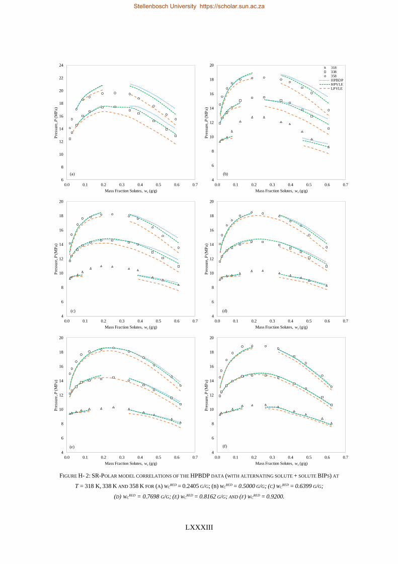
LXXXIII
FIGURE H- 2: SR-POLAR MODEL CORRELATIONS OF THE HPBDP DATA (WITH ALTERNATING SOLUTE + SOLUTE BIPS) AT
T = 318 K, 338 K AND 358 K FOR (A) WCRED = 0.2405 G/G; (B) WC
RED = 0.5000 G/G; (C) WCRED = 0.6399 G/G;
(D) WCRED = 0.7698 G/G; (E) WC
RED = 0.8162 G/G; AND (F) WCRED = 0.9200.
6
8
10
12
14
16
18
20
22
24
0.0 0.1 0.2 0.3 0.4 0.5 0.6 0.7
Pre
ssure
, P (
MP
a)
Mass Fraction Solutes, ws (g/g)
4
6
8
10
12
14
16
18
20
0.0 0.1 0.2 0.3 0.4 0.5 0.6 0.7
Pre
ssure
, P (
MP
a)
Mass Fraction Solutes, ws (g/g)
318338358HPBDPHPVLELPVLE
4
6
8
10
12
14
16
18
20
0.0 0.1 0.2 0.3 0.4 0.5 0.6 0.7
Pre
ssure
, P (
MP
a)
Mass Fraction Solutes, ws (g/g)
4
6
8
10
12
14
16
18
20
0.0 0.1 0.2 0.3 0.4 0.5 0.6 0.7
Pre
ssure
, P (
MP
a)
Mass Fraction Solutes, ws (g/g)
4
6
8
10
12
14
16
18
20
0.0 0.1 0.2 0.3 0.4 0.5 0.6 0.7
Pre
ssure
, P (
MP
a)
Mass Fraction Solutes, ws (g/g)
4
6
8
10
12
14
16
18
20
0.0 0.1 0.2 0.3 0.4 0.5 0.6 0.7
Pre
ssure
, P (
MP
a)
Mass Fraction Solutes, ws (g/g)
(a) (b)
(c) (d)
(e) (f)
Stellenbosch University https://scholar.sun.ac.za
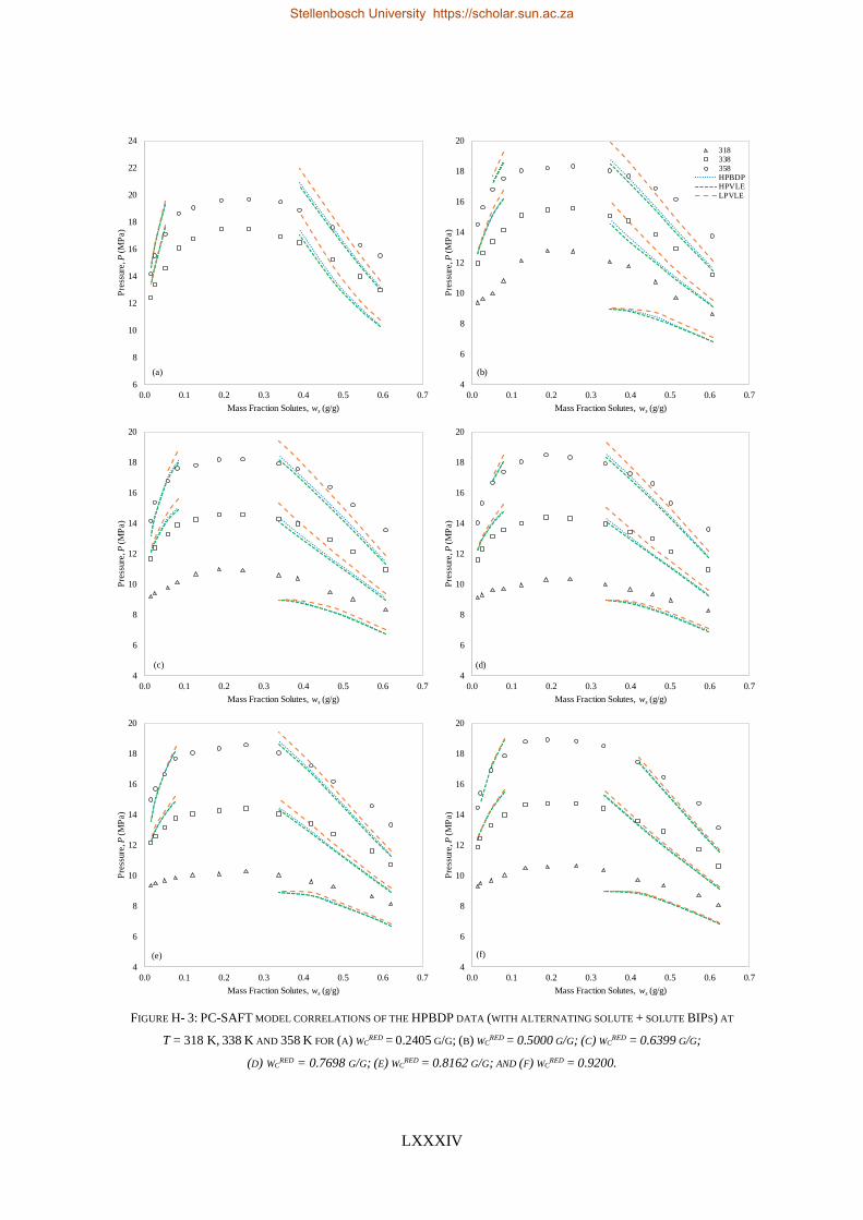
LXXXIV
FIGURE H- 3: PC-SAFT MODEL CORRELATIONS OF THE HPBDP DATA (WITH ALTERNATING SOLUTE + SOLUTE BIPS) AT
T = 318 K, 338 K AND 358 K FOR (A) WCRED = 0.2405 G/G; (B) WC
RED = 0.5000 G/G; (C) WCRED = 0.6399 G/G;
(D) WCRED = 0.7698 G/G; (E) WC
RED = 0.8162 G/G; AND (F) WCRED = 0.9200.
4
6
8
10
12
14
16
18
20
0.0 0.1 0.2 0.3 0.4 0.5 0.6 0.7
Pre
ssure
, P (
MP
a)
Mass Fraction Solutes, ws (g/g)
4
6
8
10
12
14
16
18
20
0.0 0.1 0.2 0.3 0.4 0.5 0.6 0.7
Pre
ssure
, P (
MP
a)
Mass Fraction Solutes, ws (g/g)
4
6
8
10
12
14
16
18
20
0.0 0.1 0.2 0.3 0.4 0.5 0.6 0.7
Pre
ssure
, P (
MP
a)
Mass Fraction Solutes, ws (g/g)
318
338
358
HPBDPHPVLE
LPVLE
6
8
10
12
14
16
18
20
22
24
0.0 0.1 0.2 0.3 0.4 0.5 0.6 0.7
Pre
ssure
, P (
MP
a)
Mass Fraction Solutes, ws (g/g)
4
6
8
10
12
14
16
18
20
0.0 0.1 0.2 0.3 0.4 0.5 0.6 0.7
Pre
ssure
, P (
MP
a)
Mass Fraction Solutes, ws (g/g)
4
6
8
10
12
14
16
18
20
0.0 0.1 0.2 0.3 0.4 0.5 0.6 0.7
Pre
ssure
, P (
MP
a)
Mass Fraction Solutes, ws (g/g)
(a) (b)
(c) (d)
(e) (f)
Stellenbosch University https://scholar.sun.ac.za
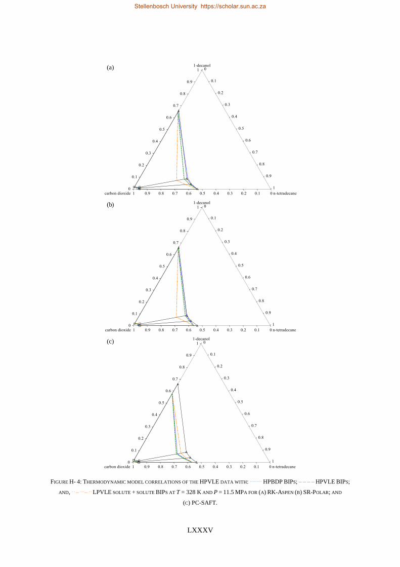
LXXXV
FIGURE H- 4: THERMODYNAMIC MODEL CORRELATIONS OF THE HPVLE DATA WITH: ……… HPBDP BIPS; – – – – HPVLE BIPS;
AND, . . – . . – . . LPVLE SOLUTE + SOLUTE BIPS AT T = 328 K AND P = 11.5 MPA FOR (A) RK-ASPEN (B) SR-POLAR; AND
(C) PC-SAFT.
(a)
(b)
(c)
Stellenbosch University https://scholar.sun.ac.za
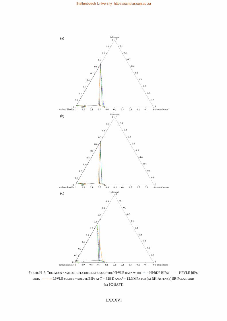
LXXXVI
FIGURE H- 5: THERMODYNAMIC MODEL CORRELATIONS OF THE HPVLE DATA WITH: ……… HPBDP BIPS; – – – – HPVLE BIPS;
AND, . . – . . – . . LPVLE SOLUTE + SOLUTE BIPS AT T = 328 K AND P = 12.3 MPA FOR (A) RK-ASPEN (B) SR-POLAR; AND
(C) PC-SAFT.
(a)
(b)
(c)
Stellenbosch University https://scholar.sun.ac.za
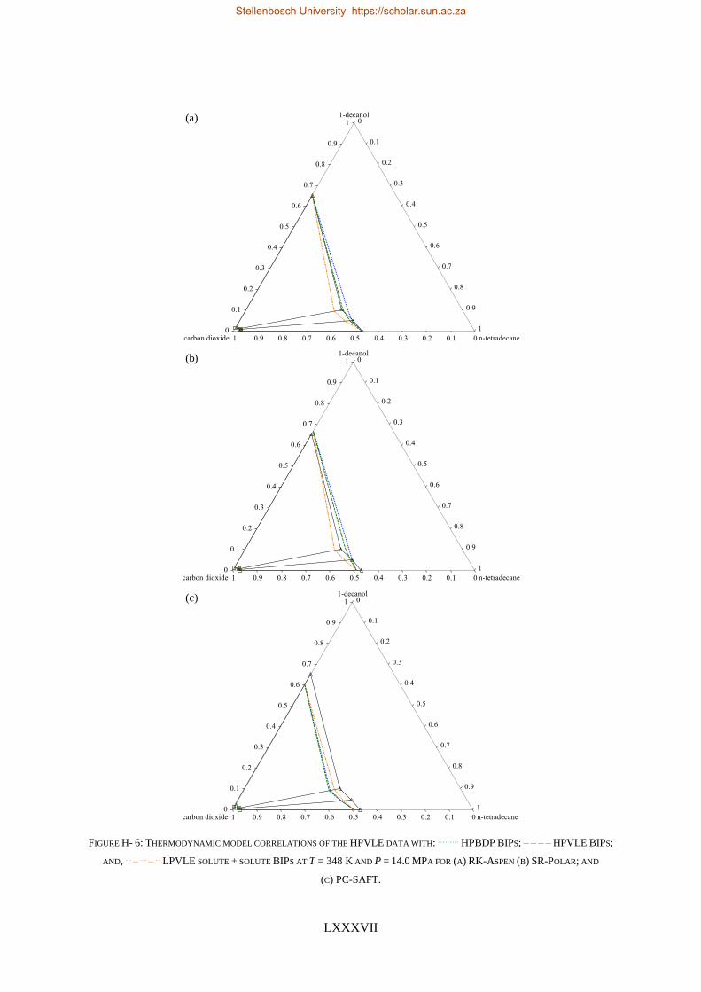
LXXXVII
FIGURE H- 6: THERMODYNAMIC MODEL CORRELATIONS OF THE HPVLE DATA WITH: ……… HPBDP BIPS; – – – – HPVLE BIPS;
AND, . . – . . – . . LPVLE SOLUTE + SOLUTE BIPS AT T = 348 K AND P = 14.0 MPA FOR (A) RK-ASPEN (B) SR-POLAR; AND
(C) PC-SAFT.
(a)
(b)
(c)
Stellenbosch University https://scholar.sun.ac.za
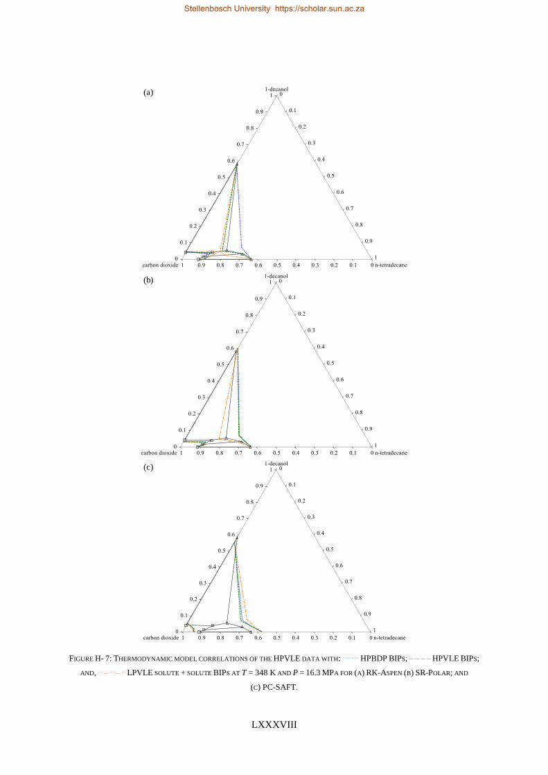
LXXXVIII
FIGURE H- 7: THERMODYNAMIC MODEL CORRELATIONS OF THE HPVLE DATA WITH: ……… HPBDP BIPS; – – – – HPVLE BIPS;
AND, . . – . . – . . LPVLE SOLUTE + SOLUTE BIPS AT T = 348 K AND P = 16.3 MPA FOR (A) RK-ASPEN (B) SR-POLAR; AND
(C) PC-SAFT.
(a)
(b)
(c)
Stellenbosch University https://scholar.sun.ac.za


