Embed Size (px)
Citation preview
STUDY OF VAPOR – LIQUID EQUILIBRIA OF
PETROLEUM FRACTIONS
A Thesis Submitted to the College of Engineering
of Nahrain University in Partial Fulfillment of the Requirements for the Degree of
Doctor of Philosophy in
Chemical Engineering
by AUDAY AMER FADHEL AL-ZUBAIDY
B. Sc. 1995 M. Sc. 1998
Daul-Qa'da 1427 November 2006
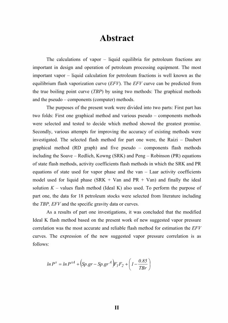
Abstract
The calculations of vapor – liquid equilibria for petroleum fractions are important in design and operation of petroleum processing equipment. The most important vapor – liquid calculation for petroleum fractions is well known as the equilibrium flash vaporization curve (EFV). The EFV curve can be predicted from the true boiling point curve (TBP) by using two methods: The graphical methods and the pseudo – components (computer) methods. The purposes of the present work were divided into two parts: First part has two folds: First one graphical method and various pseudo – components methods were selected and tested to decide which method showed the greatest promise. Secondly, various attempts for improving the accuracy of existing methods were investigated. The selected flash method for part one were, the Raizi – Daubert graphical method (RD graph) and five pseudo – components flash methods including the Soave – Redlich, Kowng (SRK) and Peng – Robinson (PR) equations of state flash methods, activity coefficients flash methods in which the SRK and PR equations of state used for vapor phase and the van – Laar activity coefficients model used for liquid phase (SRK + Van and PR + Van) and finally the ideal solution K – values flash method (Ideal K) also used. To perform the purpose of part one, the data for 18 petroleum stocks were selected from literature including the TBP, EFV and the specific gravity data or curves. As a results of part one investigations, it was concluded that the modified Ideal K flash method based on the present work of new suggested vapor pressure correlation was the most accurate and reliable flash method for estimation the EFV curves. The expression of the new suggested vapor pressure correlation is as follows:
( )
−+−+=
TBr85.01FFgr.Spgr.SpPlnPln 21
AsAs
II
The average absolute deviation (AAD%) for the modified Ideal K is 15.62% as compared to 23.51%, 24.98%, 23.40%, 25.18%, 23.73% and 21.81% for unmodified SRK, SRK + Van, PR + Van, Ideal K and RD graph methods respectively. Using the modified Ideal K flash method had improved the values of AAD% for 10 petroleum stocks (out of 18 petroleum stocks used) by more than 30%. Improvement was limited by inaccurate in experimental data (TBP curve) and characterization parameters (Tc, Pc, ω, …etc).
For part two of the present work, the modified Ideal K flash method was used for predicting the EFV curves and the flash zone temperatures for Kirkuk, Basrah, Jambur and Bai – Hassan Iraqi crude oils. The TBP and the specific gravity curves for these crude oils were obtained experimentally at laboratory distillation unit in Daura refinery. The predicted flash zone temperatures were 318 °C, 327 °C, 335 °C and 290 °C for Kirkuk, Basrah, Jambur and Bai – Hassan crude oils respectively. These values of the flash zone temperatures must be considered as primary values and must be adjusted to the temperature, pressure and the amount of the stripping steam that usually used with crude oil tower.
III
List of contents Contents Page Abstract II List of contents IV Notations IX List of Tables XVII List of Figures XXII Chapter One : Introduction 1 Chapter Two : Literature survey 4 2.1 Crude oil 4 2.1.2 Composition of crude oil 4 2.1.2.1 Hydrocarbon compounds 5 2.1.2.2 Non – hydrocarbon compounds 6 2.2 Physical properties of petroleum fractions 7 2.2.1 Boiling point 7 2.2.2 Specific gravity and API gravity 8 2.2.3 Viscosity 9 2.2.4 Refractive index 10 2.3 Distillation and distillation curve 10 2.3.1 Types of distillation 10 2.3.1.1 True boiling point distillation (TBP) 10 2.3.1.2 Equilibrium flash vaporization distillation (EFV) 11 2.3.1.3 Non – fractionating distillation (ASTM distillation) 12 2.3.1.4 Semi – fractionating distillation 12 2.4 Characterization of petroleum fractions 12 2.5 Vapor – liquid equilibrium of petroleum fractions 14
(undefined mixtures) 2.5.1 Definitions 14 2.5.1.1 Graphical or empirical methods for predicting (EFV) curve 15 2.5.1.2 Pseudo – component (computer) methods for predicting 17
the EFV curve
IV
Contents Page
Chapter Three : The theory 21 3.1 Graphical methods 21 3.2 Raizi – Daubert graphical method 22 3.3 Pseudo – component (computer) methods 24 3.4 Divided the TBP curve into fractions or cuts 25 3.5 Estimation of the basic characterization parameters 27
for the fractions or cuts 3.6 Prediction of vapor – liquid equilibrium constants 34
(K – values) for fractions 3.7 Thermodynamic of equilibrium 34 3.7.1 Fugacity and fugacity coefficient 34 3.7.2 Activity and activity coefficients 37 3.7.3 K – values formulation 38 3.8 Equation of state forms for prediction the K – values 39
(φ – φ forms)
3.8.1 Soave – Relich – Kowng equation of state (SRK) 42 3.8.2 Peng – Robinson equation of state (PR) 45 3.8.3 Improvement of SRK and PR equation of state for 48
petroleum fraction 3.8.3.1 Sim – Dauber modification for SRK equation of state 48 3.8.3.2 Twu et al. modification for PR equation of state 49 3.9 Activity models for prediction K – values (γ – φ models) 50
3.9.1 The pure liquid fugacity coefficient (φ ) 51 Li
3.9.2 The liquid phase activity coefficient γ 56 Li
3.9.2.1 Regular solution models 59 3.9.2.2 van Laar models 61 3.10 Working formula for activity coefficient model for 63
predicting the K – values 3.11 Ideal solution models for prediction K – values 63 3.12 Calculation of flash volume by flash calculations 67
V
Contents Page 3.12.1 Constant temperature and pressure (isothermal flash) 68 Chapter Four : Experimental work 73 4.1 Aim of the experimental work 73 4.2 Feed stocks 73 4.3 Distillation unit 74 4.3.1 Laboratory distillation unit 75 4.4 Density and specific gravity 80 Chapter Five : Selected data and estimation methods 81 5.1 Data sources 81 5.1.1 Data sources for part one (testing and improving part) 81 5.1.2 Data sources for part two (application part) 102 5.2 Part one: Testing and developing part 107 5.2.1 Calculational methods 107 5.2.1.1 Estimation the TBP and specific gravity curves 107 5.2.1.2 Graphical method 109 5.2.1.3 Pseudo – component (computer) methods 110 5.2.1.4 Algorithms (procedures) for performing isothermal flash 115
(P – T) calculations 5.2.1.4.1 Isothermal flash calculation algorithm using ideal K – values 116
models 5.2.1.4.2 Isothermal flash calculations algorithm using equation of state 117
(EOS) models 5.2.1.4.3 Isothermal flash calculation algorithm using activity 120
coefficients models 5.2.1.5 Statistical measurement and analysis dispersion 125 5.2.1.6 Improvement on the existing thermodynamic models used 126
with pseudo – component methods 5.2.1.6.1 Unmodified models mode 127 5.2.1.6.2 Modified models No.1 mode 127 Chapter Six : Present work suggested modification 128 6.1 Suggested modification mode (modified model No. 2 mode) 128
VI
Contents Page 6.2 Computer implementation 132 6.2.1 Input part 132 6.2.2 Calculational part 133 6.2.3 Printout part 134 Chapter Seven : Results and discussion 137 7.1 Discussion of results 137 7.1.1 Selected data for part one and part two of the present work 137 7.1.2 Estimated physical properties and material balance for 139
cuts or fractions 7.1.3 Part one (testing and developing part) 145 7.1.3.1 Estimated EFV curve using unmodified models 145 7.1.3.2 Estimated EFV curve using modified models No. 1 150
(existing in literature) 7.1.3.3 Estimated EFV curve using the present work of suggested 153
modifications mode (modified models No. 2) 7.1.3.4 Effect of measured or calculated parameters on the predicted 160
flash volumes 7.1.4 Part two (Application part) 161 7.2 Conclusions 166 7.3 Recommendations for further work 169 References 170 Appendix A : Example of calculation A.1
Appendix B : Numerical technique B.1 B.1 Newton – Raphson method B.1 B.2 Newton – Raphson method for estimation the compressibility B.2
factor from equation of state B.3 Newton – Raphson method for estimation the vapor fraction B.3
vaporized (β) in flash calculations Appendix C : Laboratory equipments specifications C.1 C.1 Thermocouple specifications C.1 C.2 Helipak packing materials specifications C.1
VII
Contents Page C.3 Fractionating column components C.2 C.4 Utility requirements C.3 Appendix D : Literature data for 18 petroleum stocks D.1 Appendix E : Material balance and Sp.gr data for four types of E.1 Iraqi crude oils Appendix F : Constants for TBP and Sp.gr equations F.1 Appendix G : List of computer program G.1 Appendix H : Physical properties and material balances for petroleum H.1 stocks for parts one and two of present work Appendix I : Predicted flash volumes and error analysis for part one I.1 of present work Appendix J : Comparison between modified and unmodified acentric J.1 factors
VIII
Notations
Symbols Symbol Meaning a Attractive term (parameter) of cubic equation of state a, b, c Parameters in equation (2.6) ai Activity of species i Parameter in equations (3.84) and (3.97) a1, a2, a3 Constants in equation (3.1) a4, a5, a6 Constants in equation (3.2) A Mixture temperature dependent term defined in
equations (3.80) and (3.93) A', B', C' Antonine's equation constants {equation (3.112)} Ac, Bc Adjustable parameters in equation (6.6) Ai Pure species combining parameters defined in
equations (3.83) and (3.96) Aij Interaction parameter for van – Laar
equation {equation (3.145)} A0, A1, A2, A4, A5 Constants in equation (B.122) A6, A7, A8, A9 A10, A11, A12, A14 Constants in equation (3.123) A1', B1', C1' Constants of working TBP equation {equation (5.2)} D1', E1' A2', B2' Constants of working Sp.gr equation {equation (5.3)} A12', A21' Constants in van – Laar equation ASTM D86 10% ASTM temperature at 10% volume percent distilled, °R ASTM D86 50% ASTM temperature at 50% volume percent distilled , °R b Co volume term (parameter) of cubic equation of state bi Pure species parameter defined in equations (3.84) and (3.97) bm Mixing rule parameters defined in equations (3.82) and (3.95) b1, b2 Constants in equation (3.3)
IX
Symbol Meaning B Mixture volume dependent term defined in
equations (3.81) and (3.94) Bi Pure species combining parameters defined in
equations (3.83) and (3.96) c1, c2, c3 Constants in equation (3.4) C Constant in equations (3.45) and (6.4) CF Correction factor EFV 10% EFV temperature at 10% volume percent distilled, °R EFV 50% EFV temperature at 50% volume percent distilled, °R EFV 50% Temperature at which 50% of petroleum stock vaporized
idif Ideal fugacity for pure species
if Partial fugacity coefficient
Vif , Fugacity for pure species in vapor and liquid phase L
if
Vif , L
if Partial fugacity of species i in mixture for
vapor and liquid phase F Feed molar rate, mole/s FM Parameter in equation (3.26) FP Parameter in equation (3.28) FT Parameter in equation (3.27) FL Liquid molar rate, mole/s FV Vapor molar rate, mole/s F(0), F(1) Functions defined in equation (3.177) F1, F2 Constants in equation (6.3)
iG Molar free energy for pure species
iG Partial molar Gibbs free energy EiG Partial molar Gibbs excess free energy
Kij Interaction parameters K Parameter in equation (3.90) Ki Equilibrium ratio or K – values
X
Symbol Meaning Ki(ideal) Ideal K – values
KUOP Characterization factor defined as gr.SpTB3
AiK Initial value of K - values
L(0),L(1) Parameters in equations (3.104) and (3.105) m Parameter in equation (3.76) M Intensive real property, M(0),M(1) Parameters in equations (3.104) and (3.105) Mid Intensive ideal property ME Intensive excess property
M Intensive real partial property idM Intensive ideal partial property EM Intensive partial excess property
MW Molecular weight N (0), N (1) Parameter in equations (3.104) and (3.105) N Number of experimental points Nc Total number of species Ni Number of moles of cut or fraction Nt Total estimated moles NP Number of phases P Total pressure PsA Vapor pressure for n – alkane species Pc Critical pressure, kPa, psia Pi Partial pressure of species i Pr Reduced pressure (Pr=P/Pc) Pr* Reduced vapor pressure (Pr*=P*/Pc)
siP Vapor pressure of species i
R Universal gas constant Sp.gr Specific gravity measured @ (15 °C/15 °C) (60 °F/60 °F)
XI
Symbol Meaning Sp.grA Specific gravity of n - alkane measured
@ (15 °C/15 °C) (60 °F/60 °F) t TBP temperature at equation (2.6), R T Temperature Tr Reduced temperature (Tr=T/Tc) Tc Critical temperature, °C, R TB True boiling point temperature, °C, R TBF True boiling point temperature, °F TBr Reduced true boiling temperature (TBr=TB/Tc) TBP 50% Temperature at which 50% of petroleum stock distilled TMEP Parameter in equation (3.102) V Volume, volume percent distilled in equations (5.2) and (5.3) VL Molar volume, cm3/gmol Vc Critical volume Vi Flash volume given in equations (5.14) and (5.15) VF Molal volume in feed stream VV Molal volume in vapor stream V1, V2 Volume percent distilled in equation (2.5) Wf Feed total weight Wi Weight of cut or fraction Wt Total estimated weight IxI Parameter in equation (3.35) xi Liquid phase mole fraction of species i, independent variable in equation (6.1) Xm Mid volume percent yi Vapor phase mole fraction of species i Z Compressibility factor for cubic equation of state ZL Liquid phase compressibility factor
XII
Symbol Meaning ZV Vapor phase compressibility factor ZRA Rackett equation constant Zi Molar feed compositions
Greek litters Symbol Meaning α Alfa function term of cubic equation of state Parameter defined in equation (3.40) α' Original alfa function term of SRK equation of state defined in equation (3.76) β Vapor fraction in mole basis βV Vapor fraction in volume basis γ Kinematic viscosity, c. stock
Liγ liquid phase activity coefficient for species i
Viγ Vapor phase activity coefficient for species i
δi Solubility parameter of species i in mixture, J/cm3 δj Solubility parameter of species j in mixture, J/cm3 ζi Cavet equation constant θ Temperature in equation (2.6),and any physical property in equation (6.1) θref Reference physical properties in equation (6.1) θi First partial deviation in equation (6.1) θij Second partial deviation in equation (6.1) θ1, θ2 First order deviation in equation (6.2) λi Heat of vaporization of species i µ Dynamic viscosity, Ns/m2 µi Chemical potential of species i ρ Density @ 15 °C (60 °F), g/cm3
XIII
Σ Summation Symbol Meaning
Liφ Liquid phase fugacity coefficient of pure species i
Viφ Vapor phase fugacity coefficient of pure species i
Liφ Liquid phase partial fugacity coefficient of species i in mixture
Viφ Vapor phase partial fugacity coefficient of species i in mixture
Φi Volume fraction of species i in mixture Φj Volume fraction of species j in mixture ω Acentric factor ωA Acentric factor of n – alkane Є Tolerance error
Super scripts Symbol Meaning - Partial properties A n – alkane, initial estimated values given in equation (5.11) calcd Calculated exp Experimental L liquid phase LK Lee – Kasler correlation s Saturation conditions V Vapor phase 0 Measured at ω = 0 1 Measured at ω = 1 1, 2 Number of phases in equilibrium 15 Measured at 15 °C (60 °F) 25 Measured at 25 °C (77 °F)
XIV
Sub scripts Symbol Meaning f Feed i Species i in mixture j Species j in mixture M Molecular weight in equations (3.29) and (3.32) P Critical pressure in equations (3.31) and (3.34) r Reduced conditions t Total T Critical temperature in equations (3.30) and (3.33) V Vapor phase and volume basis in equation (3.181)
Abbreviations
Symbol Meaning API American petroleum institute ASTM American society for testing and materials Cal Calculation C.S Chao – Sender EFV Equilibrium vaporization curve Eq. Equation Ideal K Ideal solution K – values model PR Peng – Robinson equation of state PR + Van PR equation of state for vapor phase and
van – Laar activity model for liquid phase RD graph Raizi – Daubert graphical method RK Redlich Kowng equation of state SEFV Slop of EFV curve SRK Soave Redlich Kowng equation of state SRK + Van SRK equation of state for vapor phase and
van – Laar activity model for liquid phase
XV

Symbol Meaning STBP Slop of TBP curve TBP True boiling point curve Van van – Laar model VLE Vapor – liquid equilibrium
XVI
List of Tables Table Title Page 2-1 Types of average boiling point with proper physical properties 8 2-2 Some of correlations that have been developed for estimation 13
basic parameters for petroleum fractions 3-1 Equation (3.3) constants 23 3-2 Equation (3.4) constants 24 3-3 Summary of characterization correlations 29 3-4 The L, M and N data bank of the generalized alpha function for 50
equations (3.104) and (3.105) with the PR equation of state 3-5 Constants of equations (3.122) and (3.123) 56 4-1 Properties of Kirkuk, Basrah, Jambour and Bai – Hassan crude oils 74 5-1 Literature sources and characterization of flash data 82 7-1 Physical properties for petroleum stock No. 1 141 7-2 Material balance for petroleum stock No. 1 142 7-3 Physical properties for Kirkuk crude oil 143 7-4 Material balance for Kirkuk crude oil 144 7-5 Error analysis for 18 petroleum stocks using unmodified models 146
mode flash methods 7-6 AAD% for 18 petroleum stocks that used in part one of the 148
present work (for all flash volumes regions) 7-7 AD% for 18 petroleum stocks that used in part one of the 149
present work (for all flash volumes regions) 7-8 TMEP values, 20% TBP and AD% values for five petroleum 151
stocks that satisfy the Sim – Daubert requirements 7-9 Error analysis for the five petroleum stocks using unmodified 151
models mode 7-10 Error analysis for the five petroleum stocks using modified 151
models No. 1 7-11 Error analysis for the 18 petroleum stocks using modified 153
models mode
XVII
Table Title Page 7-12 Error analysis for the 18 petroleum stocks using modified 153
models No. 1 mode 7-13 TEMP values and 20% TBP temperature for ten petroleum stocks 154
that satisfy the suggested vapor pressure correlation requirements 7-14 Error analysis for ten petroleum stocks using unmodified 155
models mode 7-15 Error analysis for ten petroleum stocks using the present work 155
suggested modification mode (modified models No. 2 mode) 7-16 Comparison between Lee – Kasler acentric factors and modified 159
acentric factors for petroleum stock No. 1 7-17 TEMP values and 20% TBP temperature for four Iraqi crude oils 162 7-18 Predicted flash volumes (EFV curves) for Kirkuk crude oil 162 7-19 Predicted flash volumes (EFV curves) for Basrah crude oil 163 7-20 Predicted flash volumes (EFV curves) for Jambour crude oil 163 7-21 Predicted flash volumes (EFV curves) for Bai – Hassan crude oil 163 C-1 Thermocouple specifications C.1 C-2 Helipak packing materials specifications C.2 C-3 Power requirements C.3 D-1 TBP, EFV and Sp.gr data for Santa fe spring crude D.1 D-2 TBP, EFV and Sp.gr data for Eldwood crude D.1 D-3 TBP, EFV and Sp.gr data for Columbian crude D.1 D-4 TBP, EFV and Sp.gr data for Ranger crude D.2 D-5 TBP, EFV and Sp.gr data for Lulting crude D.2 D-6 TBP, EFV and Sp.gr data for 50% COL. OH crude D.2 D-7 TBP, EFV and Sp.gr data for Kansas crude D.3 D-8 TBP, EFV and Sp.gr data for Mid – continent crude D.3 D-9 TBP, EFV and Sp.gr data for Magnoland crude D.3 D-10 TBP, EFV and Sp.gr data for Mid – continent crude D.4 D-11 TBP, EFV and Sp.gr data for Hendricks crude D.4 D-12 TBP, EFV and Sp.gr data for Mid – continent crude D.4 D-13 TBP, EFV and Sp.gr data for Naphtha – kerosene blend D.5
XVIII
Table Title Page D-14 TBP, EFV and Sp.gr data for California research stock 7 D.5 D-15 TBP, EFV and Sp.gr data for Middle east crude D.5 D-16 TBP, EFV and Sp.gr data for Intermediate – paraffin base crude D.6 D-17 TBP, EFV and Sp.gr data for Asphaltic – naphthene base crude D.6 D-18 TBP, EFV and Sp.gr data for Paraffin base crude D.7 E-1 Material balance of Kirkuk crude oil E.1 E-2 Material balance of Basrah crude oil E.2 E-3 Material balance of Jambur crude oil E.3 E-4 Material balance of Bai – Hassan crude oil E.4 E-5 Specific gravity and API of distillate fractions from Kirkuk crude oil E.5 E-6 Specific gravity and API of distillate fractions from Basrah crude oil E.6 E-7 Specific gravity and API of distillate fractions from Jambur crude oil E.7 E-8 Specific gravity and API of distillate fractions from Bai – Hassan E.8
crude oil F-1 Constants for working TBP and Sp.gr equations for data sources of F.1
part one F-2 Constants for working TBP and Sp.gr equations for data sources of F.2
part two H-1 Physical properties for petroleum stock No. 2 H.1 H-2 Physical properties for petroleum stock No. 3 H.2 H-3 Physical properties for petroleum stock No. 4 H.3 H-4 Physical properties for petroleum stock No. 5 H.4 H-5 Physical properties for petroleum stock No. 6 H.5 H-6 Physical properties for petroleum stock No. 7 H.6 H-7 Physical properties for petroleum stock No. 8 H.7 H-8 Physical properties for petroleum stock No. 9 H.8 H-9 Physical properties for petroleum stock No. 10 H.9 H-10 Physical properties for petroleum stock No. 11 H.10 H-11 Physical properties for petroleum stock No. 12 H.11 H-12 Physical properties for petroleum stock No. 13 H.12 H-13 Physical properties for petroleum stock No. 14 H.13
XIX
Table Title Page H-14 Physical properties for petroleum stock No. 15 H.14 H-15 Physical properties for petroleum stock No. 16 H.15 H-16 Physical properties for petroleum stock No. 17 H.16 H-17 Physical properties for petroleum stock No. 18 H.17 H-18 Material balance for petroleum stock No. 2 H.18 H-19 Material balance for petroleum stock No. 3 H.19 H-20 Material balance for petroleum stock No. 4 H.20 H-21 Material balance for petroleum stock No. 5 H.21 H-22 Material balance for petroleum stock No. 6 H.22 H-23 Material balance for petroleum stock No. 7 H.23 H-24 Material balance for petroleum stock No. 8 H.24 H-25 Material balance for petroleum stock No. 9 H.25 H-26 Material balance for petroleum stock No. 10 H.26 H-27 Material balance for petroleum stock No. 11 H.27 H-28 Material balance for petroleum stock No. 12 H.28 H-29 Material balance for petroleum stock No. 13 H.29 H-30 Material balance for petroleum stock No. 14 H.30 H-31 Material balance for petroleum stock No. 15 H.31 H-32 Material balance for petroleum stock No. 16 H.32 H-33 Material balance for petroleum stock No. 17 H.33 H-34 Material balance for petroleum stock No. 18 H.34 H-35 Physical properties for Basrah crude oil H.35 H-36 Physical properties for Jambur crude oil H.36 H-37 Physical properties for Bai – Hassan crude oil H.37 H-38 Material balance for Basrah crude oil H.38 H-39 Material balance for Jambur crude oil H.39 H-40 Material balance for Bai – Hassan crude oil H.40 I-1 Predicted flash volumes for 106 flash data points I.1
(18 petroleum stocks) using unmodified models mode flash methods I-2 ADD% values for 106 flash data points I.4
(18 petroleum stocks) using unmodified models mode flash methods
XX
Table Title Page I-3 AD% for 106 flash data points I.7
(18 petroleum stocks) using unmodified models mode flash methods I-4 Predicted flash volumes for 45 flash data points I.10
(5 petroleum stocks) using modified models No. 1 mode flash methods I-5 ADD% values for 45 flash data points I.11
(5 petroleum stocks) using modified models No. 1 mode flash methods I-6 AD% values for 45 flash data points I.12
(5 petroleum stocks) using modified models No. 1 mode flash methods I-7 Predicted flash volumes for 106 flash data points I.13
(18 petroleum stocks) using modified models No. 1 mode flash methods I-8 AAD% for 106 flash data points I.16
(18 petroleum stocks) using modified models No. 1 mode flash methods I-9 AD% for 106 flash data points I.19
(18 petroleum stocks) using modified models No. 1 mode flash methods I-10 Predicted flash volumes for 61 flash data points I.22
(10 petroleum stocks) using modified models No. 2 mode flash methods I-11 ADD% for 61 flash data points I.24
(10 petroleum stocks) using modified models No. 2 mode flash methods I-12 AD% for 61 flash data points I.26
(10 petroleum stocks) using modified models No. 2 mode flash methods J-1 Acentric factor Comparison for petroleum stoke No. 2 J.1 J-2 Acentric factor Comparison for petroleum stoke No. 3 J.2 J-3 Acentric factor Comparison for petroleum stoke No. 6 J.3 J-4 Acentric factor Comparison for petroleum stoke No. 7 J.4 J-5 Acentric factor Comparison for petroleum stoke No. 9 J.5 J-6 Acentric factor Comparison for petroleum stoke No. 13 J.6 J-7 Acentric factor Comparison for petroleum stoke No. 14 J.7 J-8 Acentric factor Comparison for petroleum stoke No. 16 J.8 J-9 Acentric factor Comparison for petroleum stoke No. 18 J.9
XXI
List of Figures Figure Title Page 2-1 Types of distillation curves 11 3-1 The mid boiling point concept 26 3-2 P – T flash unit 69 4-1 Photographic picture of the laboratory distillation unit 77 4-2 Schematic diagram of the laboratory distillation unit 78 5-1 TBP curve for petroleum stock number 1 83 5-2 TBP curve for petroleum stock number 2 83 5-3 TBP curve for petroleum stock number 3 84 5-4 TBP curve for petroleum stock number 4 84 5-5 TBP curve for petroleum stock number 5 85 5-6 TBP curve for petroleum stock number 6 85 5-7 TBP curve for petroleum stock number 7 86 5-8 TBP curve for petroleum stock number 8 86 5-9 TBP curve for petroleum stock number 9 87 5-10 TBP curve for petroleum stock number 10 87 5-11 TBP curve for petroleum stock number 11 88 5-12 TBP curve for petroleum stock number 12 88 5-13 TBP curve for petroleum stock number 13 89 5-14 TBP curve for petroleum stock number 14 89 5-15 TBP curve for petroleum stock number 15 90 5-16 EFV curve for petroleum stock number 1 90 5-17 EFV curve for petroleum stock number 2 91 5-18 EFV curve for petroleum stock number 3 91 5-19 EFV curve for petroleum stock number 4 92 5-20 EFV curve for petroleum stock number 5 92 5-21 EFV curve for petroleum stock number 6 93 5-22 EFV curve for petroleum stock number 7 93 5-23 EFV curve for petroleum stock number 8 94 5-24 EFV curve for petroleum stock number 9 94
XXII
Figure Title Page 5-25 EFV curve for petroleum stock number 10 95 5-26 EFV curve for petroleum stock number 11 95 5-27 EFV curve for petroleum stock number 12 96 5-28 EFV curve for petroleum stock number 13 96 5-29 EFV curve for petroleum stock number 14 97 5-30 EFV curve for petroleum stock number 15 97 5-31 TBP curve for petroleum stock number 16 98 5-32 TBP curve for petroleum stock number 17 98 5-33 TBP curve for petroleum stock number 18 99 5-34 EFV curve for petroleum stock number 16 99 5-35 EFV curve for petroleum stock number 17 100 5-36 EFV curve for petroleum stock number 18 100 5-37 Sp.gr curve for petroleum stock number 16 101 5-38 Sp.gr curve for petroleum stock number 17 101 5-39 Sp.gr curve for petroleum stock number 18 102 5-40 TBP curve for Kirkuk crude oil 103 5-41 TBP curve for Basrah crude oil 103 5-42 TBP curve for Jambur crude oil 104 5-43 TBP curve for Bai-Hassan crude oil 104 5-44 Sp.gr curve for Kirkuk crude oil 105 5-45 Sp.gr curve for Basrah crude oil 105 5-46 Sp.gr curve for Jambur crude oil 106 5-47 Sp.gr curve for Bai-Hassan crude oil 106 5-48 Flow sheet for algorithm of Raizi – Daubert graphical method 110
(RD – graph) 5-49 Flow sheet for algorithm of characterization steps of pseudo – 114
components methods 5-50 Flow sheet for algorithm for Rachford – Rice algorithm for 118
isothermal flash calculations using ideal K – values equation 5-51 Flow sheet algorithm for isothermal flash calculations using EOS 121
models (SRK or PR)
XXIII
Figure Title Page 5-52 Flow sheet algorithm for isothermal flash calculations using activity 124
coefficient models (SRK + Van or PR + Van) 6-1 Flow diagram for the computer program 136 7-1 EFV curve for Kirkuk crude oil 164 7-2 EFV curve for Basrah crude oil 164 7-3 EFV curve for Jambur crude oil 165 7-4 EFV curve for Bai – Hassan crude oil 165 A-1 Graphical form of equation (3.3) A.3 A-2 Graphical form of equation (3.4) A.4 C-1 Calibration curves for the thermocouples C.2 C-2 Fractionating column components C.4
XXIV
Chapter One
Introduction
Since virtually all phase of petroleum refining involve the separation of petroleum fractions (or undefined mixtures) into liquid and vapor phases, a reliable vapor – liquid calculations are essential perquisite for efficient design and operation of petroleum processing equipment [1]. The most important vapor – liquid equilibrium calculations for petroleum fractions are the flash calculations, in which the flash vaporization curve (EFV) is estimated. The flash vaporization curve (EFV) is defined as plot of temperature against percent by volume of liquid distilled, with the total vapor in equilibrium with the non vaporized liquid at constant pressure. Each point of the EFV curve represents a separate equilibrium experiment. Normally at least five such experiments are required to establish the EFV curve [2, 3]. The costly of operations and tedious procedures necessary to obtain experimental EFV curves have given impetus to development of methods for predicting EFV curves from some other distillation curves such as true boiling point curves (TBP) [4]. For complex mixtures such as the crude oil or petroleum fractions must have their compositions defined by empirical means because the identity of the hundreds or thousands of different hydrocarbons present are not known. A common method used for this is the true boiling point distillation curve (TBP). A TBP curve then is a plot of boiling point temperature of each small increment of volume and is obtained by measuring the volume percent distilled and the top temperature of high efficiency batch distillation column. TBP distillation is performed in column has the efficiency of 15 to 100 theoretical plates at relatively high reflux ratio (i.e. 5 to 1 or greater) [5, 6]. Two important impacts of the accurate prediction of the EFV curve from the TBP curve can be obtained. The first impact; the designer needs to know how much vapor is going up to the feed zone of the crude tower, the later can be accomplished
1
by knowing the flash zone temperature. The flash zone temperature is obtained from the EFV curve. Knowing the flash zone temperature and the amount of the vaporization have great rule in the design of the auxiliary crude oil tower (e.g. furnace, pre heater exchangers, …etc) [6]. The second impact; the accurate prediction of the EFV curve means that the accurate and reliable K – values predictions for each of petroleum fraction or cut are performed. The accurate predictions of the K – values have greater effect on the relative volatility of each cut, that used for estimation of the number of theoretical plates of crude oil tower. Error in the relative volatility can generate as much as 100% error in the number of theoretical plates. This means that for a column with 20 actual plates, the designer may design a column with 40 plates doubling the cost of investment [7]. Two methods are used for predicting the EFV curve from available TBP curve, these are: a) Graphical methods. b) Pseudo – components (computer) methods.
The graphical methods are the oldest methods for predicting the EFV curves from the TBP curves. They are also known as empirical correlations because they relate the TBP curve with the EFV curve using a rather limited amount of data for both curves, consequently, the graphical methods are developed from published experimental data for both TBP and EFV curves [4, 8]. The most famous graphical methods that used for predicting the EFV curve from TBP curves are the Maxwell method [9] and the Raizi – Daubert method [10], which is adopted by the API – technical data book [11].
The pseudo – components methods (also known as computer methods) based on several types of thermodynamic models for predicting the K – values, have been proposed to replace the classical graphical methods for predicting the EFV curve from the available TBP curve. In the pseudo – components methods there are four main steps must be performed to obtain the EFV curve, these steps can be summarized as follows [1, 6]: a) In the first step the TBP curve must be divided into a suitable number of cuts. Each cut has its average boiling point (TB) and specific gravity (Sp.gr).
2
b) In the second step, the (TB) and (Sp.gr) for each cut are used for estimation the basic characterization parameters using a suitable characterization correlations published in literatures [12, 13]. Basic characterization parameters including the molecular weight (MW), critical temperatures (Tc), critical pressures (Pc), acentric factors (ω), …etc. At this step the compositions of feed can be obtained. c) In the third step, the K – values for each cut are estimated using available thermodynamic models such as equation of state models, activity coefficient models, …etc. d) The final step including the estimation of the flash volumes or EFV curve by using the isothermal flash calculation.
The scope of the present work can be divided into two parts: 1. The first part has two folds, first the graphical methods, and the pseudo – components methods were tested to decide which method shows the greatest promise, secondly various attempts were tried to investigate the possibility for improving and increasing the accuracy of the existing flash method. To perform the purpose of part one of the present work, the data for 18 petroleum stocks were selected from literature including TBP, EFV and specific gravity data or curves. 2. Using the most accurate flash method suggested and developed in part one, the EFV curves for four Iraqi crude oils were predicted from their TBP curves. These crude oils are Kirkuk, Basrah, Jambour and Bai – Hassan. The TBP and specific gravity curves for these crude oils were obtained from the laboratory distillation unit in the Duara refinery laboratory.
Using the predicted EFV curves for the Kirkuk, Basrah, Jambour and Bai – Hassan crude oils, the flash zone temperatures were also predicted using the Nelson procedure [3].
3
Chapter Two
Literature survey
2.1 Crude oil
Crude oil (also known as Petroleum), is the product of natural changes to organic debris over millennia. It is water white to black liquid which may vary from free flowing to having difficulty in being mobile at room temperature [14]. The crude oil consists almost entirely of compounds of carbon and hydrogen, with varying amount of organic and these elements can vary only between very narrow limits. The elementary analysis of crude oil shows that crude oils contain 83 – 86.9wt% carbon, 11.4 – 14.0wt% hydrogen, 0.04 – 8.0wt% of sulfur, 0.11 – 1.70wt% nitrogen, 0.5wt% oxygen and about 0.03wt% metals [15]. Crudes contain high proportion of individual hydrocarbons so they vary from a thin (mobile), nearly colorless liquid to a thick (viscous), almost black oil. The specific gravity at 60°F (15.6°C) varies correspondingly from about 0.75 to 1.00 (57 – 10°API), with the specific gravity of most crude oils falling in range from 0.80 to 0.95 (45 - 17°API) thus, it is not surprising that crude oils vary in composition from one oil field to another, from one well to another in the same field. This variation can be in both molecular weight and types of molecules present in petroleum, thus crude oil may well be described as a mixture of organic molecules drawn from a wide distribution of molecular types that lie within a wide distribution of molecular weights, so that crude oil can be categorized based on the molecular weight distribution as light, medium and heavy crude oil [14, 16].
2.1.2 Composition of crude oil
Crude oil is very complex mixture consisting of hydrocarbons and non – hydrocarbons compounds. There are many studies that have been applied as a mean of evaluating petroleum composition. In fact, these studies are so numerous as to be
4
subject matter of several books and articles (Rostler [17], Altgeft and Gouw [18] and Speight [15]). As a results of these studies, it was realized that the hydrocarbons in petroleum belong to several series of paraffins, naphthene (cyclo paraffin), branched paraffins and aromatics hydrocarbons. Non hydrocarbon such as nitrogen, oxygen, sulfur and traces of variety of metal – containing (vanadium and nickel) compounds are also present in crude oils. The amounts of these non hydrocarbon compounds increase with boiling point and also with increase of molecular weight [14].
2.1.2.1 Hydrocarbon compounds
Hydrocarbons are the principal constituents of the petroleum. The hydrocarbon series are grouped into paraffins, naphthenes and aromatics [3].
a- Paraffins
Normal paraffins are found in most petroleums and particularly in light types. The member of paraffins C1 – C35 group (molecular weight (16 – 492)) have been found in several crude oils [16]. Normal paraffins series (type formula CnH2n+2) is characterized by great stability, the name of each member ends in (ane), methane, ethane, hexane etc [3]. Branched – chain paraffins also have been found in light and middle point fractions [14].
b- Naphthenes (cyclo paraffins)
Naphthenes (also known as cyclo paraffins) are widely found in crude oils and petroleum fractions. The characteristic of naphthenic hydrocarbons is the fact they contain saturated rings which have 5 or 6 carbon atoms [20]. Naphthenes has the formula of CnH2n and its presence in the petroleum all over the world varies from 30 to 60% with quantities increasing in the heavy fractions, and decreasing in the light fractions [3].
5
c- Aromatics
Aromatics form the third main type of hydrocarbon compounds found in crude oils. Aromatic series have general type formula of CnH2n-6, and they differ chemically and physically from paraffin and naphthene compounds, i.e., aromatics are unsaturated hydrocarbons and have relatively high specific gravity possessing good solvent properties [3, 17, 20].
2.1.2.2 Non – hydrocarbon compounds
The non – hydrocarbon compounds can be summarized as follows:
a- Sulfur compounds
Sulfur compounds are among the most important of non hydrocarbon compounds of crude oils. Four types of sulfur compounds occur in crude oils and petroleum fractions, they are hydrogen sulfide, mercaptans, sulfide and thiocyclic compounds (containing sulfur ring) [16, 21]. Difficulties with oil that contains sulfur compounds arise in only three main ways: corrosion, color and poor explosion characteristic of gasoline fuels [3].
b- Nitrogen compounds
The nitrogen compounds content of crude oils and petroleum fractions are much lower than the sulfur content. The typical nitrogen compounds found in crude oils are generally divided into two groups, basic and non basic compounds. The basic nitrogen compounds cause difficulty with many acid – catalyzed processes used in petroleum (e.g. reforming units) [14, 20].
6
c- Oxygen compounds
The oxygen compounds found in crude oil and petroleum fractions are often products of exposure to air. The most common oxygen compounds are naphthenic acids which are organic acids found in some crudes, and phenol derivatives, which can appear in cracking units [14].
e- Metals compounds
The metal compounds (essentially nickel and vanadium) present in small quantities in crude oils and petroleum fractions. The metal content increases regularly with increasing the molecular weight of distillate fraction, and reaches maximum in residue. The crude oils also contain other non organic compounds such as water, sediments and mineral salts [20].
2.2 Physical properties of petroleum fractions
When dealing with the complex mixtures of hydrocarbons normally found in petroleum fractions, the average physical properties of the mixtures are often of greater importance than a knowledge of exact chemical compositions and of the physical properties of individual compounds [22]. A more important measurable physical properties will be discussed in the next sections.
2.2.1 Boiling point
The temperature at which a pure component boils at atmospheric pressure is an invariable property of the substance and is in fact a useful guide to the identity of the material. Mixtures (including petroleum fractions) do not have single boiling point, but they boil over a range of temperatures depending on pressure, composition and nature of the apparatus used to carry out the experiment [22].
7
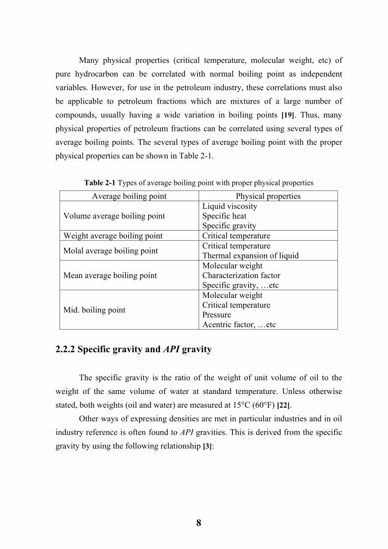
Many physical properties (critical temperature, molecular weight, etc) of pure hydrocarbon can be correlated with normal boiling point as independent variables. However, for use in the petroleum industry, these correlations must also be applicable to petroleum fractions which are mixtures of a large number of compounds, usually having a wide variation in boiling points [19]. Thus, many physical properties of petroleum fractions can be correlated using several types of average boiling points. The several types of average boiling point with the proper physical properties can be shown in Table 2-1.
Table 2-1 Types of average boiling point with proper physical properties
Average boiling point Physical properties
Volume average boiling point Liquid viscosity Specific heat Specific gravity
Weight average boiling point Critical temperature
Molal average boiling point Critical temperature Thermal expansion of liquid
Mean average boiling point Molecular weight Characterization factor Specific gravity, …etc
Mid. boiling point
Molecular weight Critical temperature Pressure Acentric factor, …etc
2.2.2 Specific gravity and API gravity
The specific gravity is the ratio of the weight of unit volume of oil to the weight of the same volume of water at standard temperature. Unless otherwise stated, both weights (oil and water) are measured at 15°C (60°F) [22]. Other ways of expressing densities are met in particular industries and in oil industry reference is often found to API gravities. This is derived from the specific gravity by using the following relationship [3]:
8
( )
−= 5.131
6060gr.Sp5.141API …(2.1)
The API scale allows representation of specific gravity of oils to vary only from less than 0 (heavy residual oils) to 340 (methane) [5]. Density gives an indication of the crude oil quality. In fact under the same boiling point, paraffinic hydrocarbons have less densities (higher API), followed in order by naphthenic and aromatic hydrocarbons, with gradually greater density (lower API) [23].
2.2.3 Viscosity
Viscosity is a measure of the ability of a fluid to resist shear. Dynamic viscosity is defined as the shear stress at a point divided by the velocity gradient at that point. The unit of dynamic viscosity in S.I. units is Ns/m2 and in c.g.s. units is poise [24]. The kinematic viscosity is defined as the ratio of the dynamic viscosity to the density, both at the same temperature. The unit of kinematic viscosity in S.I. units is m2/s and c.g.s. units is stock [25]. The relation between the dynamic viscosity and kinematic viscosity is given by the following equation:
ρµ
γ = …(2.2)
where: γ = kinematic viscosity µ = dynamic viscosity ρ = density at °C (60 °F)
9
2.2.4 Refractive index
Refractive index is defined as the ratio of the velocity of light in vacuum to the velocity of the same wave light in the substance. The value of refractive index varies with the wave length of light used, and also with temperature and both must be specified [22].
2.3 Distillation and distillation curve
Distillation is a widely used method for separating liquid mixtures into their components and had been called the workhorse separation of petroleum, petrochemical, chemical and related industries. It is old in the art, having been practiced for crudes for many decades [26]. Distillation is a separation process that differentiate between the component of a mixture through their volatility. The difference in volatility between the component of a mixture is often characterized by the difference between their boiling points or their vapor pressures [20]. Distillation curve is a plot that relates the percentage distillate (volume or mass basis) of the component or fraction with the corresponding boiling temperature. The distillation curve gives information about initial boiling point temperature, final boiling point temperature and the temperature of any particulate cut or fraction, such as 10%, 20%, …etc [27]. The most important types of distillations will be discussed in the next sections.
2.3.1 Types of distillation
2.3.1.1 True boiling point distillation (TBP)
It is also called "fractionating" distillation. This method of distillation is basically a batch distillation using 15 – 100 theoretical plates (or packed bed), with
10
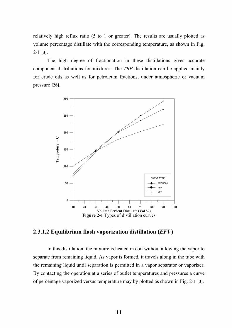
relatively high reflux ratio (5 to 1 or greater). The results are usually plotted as volume percentage distillate with the corresponding temperature, as shown in Fig. 2-1 [3]. The high degree of fractionation in these distillations gives accurate component distributions for mixtures. The TBP distillation can be applied mainly for crude oils as well as for petroleum fractions, under atmospheric or vacuum pressure [28].
Figure 2-1 Types of distillation curves
10 20 30 40 50 60 70 80 90 100Volume Percent Distillate (Vol %)
0
50
100
150
200
250
300
Tem
pret
ure
C
0
CURVE TYPE
ASTMD86
TBP
EFV
2.3.1.2 Equilibrium flash vaporization distillation (EFV)
In this distillation, the mixture is heated in coil without allowing the vapor to separate from remaining liquid. As vapor is formed, it travels along in the tube with the remaining liquid until separation is permitted in a vapor separator or vaporizer. By contacting the operation at a series of outlet temperatures and pressures a curve of percentage vaporized versus temperature may by plotted as shown in Fig. 2-1 [3].
11
Each point on the EFV curve represents a separate equilibrium experiment. The number of equilibrium experiments needed to define all portions of the EFV curve varies with the shape of the curve. The EFV curve can be applied under atmospheric pressure (or higher) and under vacuum pressure [28].
2.3.1.3 Non – fractionating distillation (ASTM distillation)
It is best known as ASTM distillation or Engler distillation. ASTM distillations are run in Engler flask. No packing is employed and the reflux results only from heat loss through the neck of the flask. ASTM distillation are more widely used than TBP distillation because ASTM distillations are simpler, less expensive, require less sample and take only approximately one – tenth as much time [28]. ASTM distillation methods in use are: i. ASTM method D 86. ii. ASTM method D 216. iii. ASTM method D 1160.
2.3.1.4 Semi – fractionating distillation
In this method of distillation, a mid degree of fractionating is attained by use of a section of packed column between the flask and the condenser. The best known method is the Hample distillation of the U.S. bureau of mines and ASTM D 285 for crude petroleum. The crude oil curves obtained by these methods are nearly the same form as TBP distillation curve [3].
2.4 Characterization of petroleum fractions
Characterization of hydrocarbons and petroleum fractions (also known as undefined mixtures), involves with use of available bulk parameters such as boiling point, specific gravity, viscosity or refractive index to estimate the basic properties such as molecular weight (MW), acentric factor (ω) and critical constant (critical
12
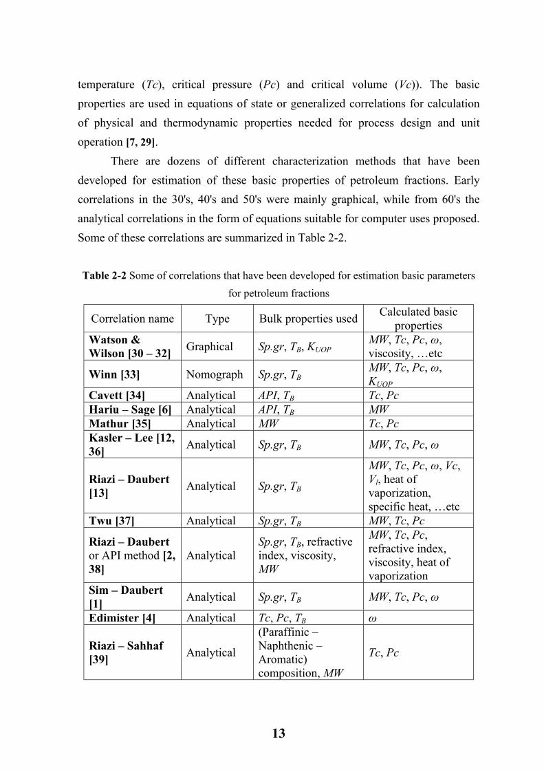
temperature (Tc), critical pressure (Pc) and critical volume (Vc)). The basic properties are used in equations of state or generalized correlations for calculation of physical and thermodynamic properties needed for process design and unit operation [7, 29]. There are dozens of different characterization methods that have been developed for estimation of these basic properties of petroleum fractions. Early correlations in the 30's, 40's and 50's were mainly graphical, while from 60's the analytical correlations in the form of equations suitable for computer uses proposed. Some of these correlations are summarized in Table 2-2. Table 2-2 Some of correlations that have been developed for estimation basic parameters
for petroleum fractions
Correlation name Type Bulk properties used Calculated basic properties
Watson & Wilson [30 – 32] Graphical Sp.gr, TB, KUOP MW, Tc, Pc, ω,
viscosity, …etc
Winn [33] Nomograph Sp.gr, TB MW, Tc, Pc, ω, KUOP
Cavett [34] Analytical API, TB Tc, Pc Hariu – Sage [6] Analytical API, TB MW Mathur [35] Analytical MW Tc, Pc Kasler – Lee [12, 36] Analytical Sp.gr, TB MW, Tc, Pc, ω
Riazi – Daubert [13] Analytical Sp.gr, TB
MW, Tc, Pc, ω, Vc, Vl, heat of vaporization, specific heat, …etc
Twu [37] Analytical Sp.gr, TB MW, Tc, Pc
Riazi – Daubert or API method [2, 38]
Analytical Sp.gr, TB, refractive index, viscosity, MW
MW, Tc, Pc, refractive index, viscosity, heat of vaporization
Sim – Daubert [1] Analytical Sp.gr, TB MW, Tc, Pc, ω
Edimister [4] Analytical Tc, Pc, TB ω
Riazi – Sahhaf [39] Analytical
(Paraffinic – Naphthenic – Aromatic) composition, MW
Tc, Pc
13
2.5 Vapor – liquid equilibrium of petroleum fractions (undefined mixtures)
2.5.1 Definitions
Vapor – liquid equilibria (or phase equilibria) and fluid properties are required in the design of separation process, and analysis of petroleum operations. The separation of multi component mixtures into pure components (or fractions) of desired compositions is of great interest in the petroleum industry [40]. A number of important industrial processes, such as distillation bring two phases (vapor and liquid) into contact, when the phases are not in equilibrium, mass transfer occurs between the phases. The rate of mass transfer of each component depends on the departure of the system from equilibrium. Quantitative treatment of mass transfer rates requires knowledge of the equilibrium states (temperature T, pressure P and compositions) of the system [41]. For the system of NP phases, the temperature, pressure, and partial molal
fugacities if for each component are the same in all phases, and the equilibrium
conditions can be stated as followed [42]:
( ) ( ) ( )NP21 TTT ==
( ) ( ) ( )NP21 PPP ==
( ) ( ) (NPi
2i
1i fff == ) where i = 1, 2, 3, …NP …(2.3)
For vapor – liquid system of N components:
VL TT =
VL PP =
14
Vi
Li ff = where i = 1, 2, 3, …N …(2.4)
Since virtually all phases of petroleum refining involves the separation of petroleum fractions into liquid and vapor phases, a reliable estimate of equilibrium flash vaporization curve (EFV) (or data) is an essential prerequisite for efficient design and operation of petroleum processing equipment [1]. The EFV curve (data) can be obtained experimentally by determining flash vaporization on the stock in question at desired temperature and pressure. Unfortunately this procedure generally so complex and requires a considerable amount of time and money. As a result several methods were developed to predict the (EFV) curve or data from simpler analytical true boiling point distillations (TBP) [4]. The methods presented in the literatures for predicting the flash vaporization curve are of two general types:
• Graphical or empirical methods.
• Pseudo – component (computer) methods.
2.5.1.1 Graphical or empirical methods for predicting (EFV) curve
Graphical methods are the oldest methods that were used for predicting the equilibrium flash vaporization curve or data. They are also known as empirical correlations because they relate the true boiling point and equilibrium flash vaporization curves using a rather limited amount of data for both curves [6, 8]. In 1929 Pirmoov and Beiwenger [43], developed the first such graphical method using experimental EFV distillation data on crude oils. In this method, the EFV curve is assumed to be straight line on the temperature versus percent volume vaporized scale. Also the relation between the slope of the TBP curve (STBP) and the slope of EFV curve (SEFV) are established using the temperature of 50% distillate of the TBP (TBP 50%) and the temperature of 50% distillate of the EFV (EFV 50%). The slope of the TBP curve and EFV curve can be defined as follows:
15
12
12VVTTSEFVorSTBP
−−
= …(2.5)
where T2, T1 and V2, V1 are the temperatures and their corresponding volume percent vaporized (or distillate), respectively. Nelson and Souders [43], Pakie [44], Nelson – Harvey [45], Edmister and
Merien [46] developed several correlations for relating the STBP, SEFV, TBP 50% and EFV 50%, based on the assumption of straight line EFV curve. In their 1948 correlation, Edmister and Pollock [47], avoided the assumption of straight line EFV curve and developed a new correlation for predicting the EFV curve using the experimental data on fractions of mid – continent crude oils, the workable scale charts of this correlation was published later by Edmister [48]. Maxwell [9], proposed an empirical method for estimating the EFV curve from the TBP curve. The Maxwell method is a modification of the Packi [44] method that based on the assumption of the straight line EFV. The Maxwell method is a correction for the curvature effect of the EFV curve. In 1966 House et al. [1] evaluated the above mentioned flash methods using the same data base as that used to develop the original correlations and methods. The evaluation indicated that the Maxwell [9] correlation gave the best results, with an average error of 14.9%, while the errors of the other methods all exceeded 20%. For this reason, only the Maxwell method was considered in API – technical data book (in their 1977 and 1982 editions) [28, 49]. Arnold [50], computerized the Maxwell method through a set of nth order polynomials equations. Riazi – Daubert [10], proposed a new method for estimating the EFV curve from the TBP curve. The experimental data on TBP and EFV distillation of fractions were collected from Edmister Pollock [47], Chu and Staffel [11] and Edmister [4]. Using this data set the following equation was found to be the best simple form for conversion of TBP curve to EFV curve:
…(2.6) cb gr.Spat θ=
16
where t and θ are the EFV and TBP temperature at the same Vol.% vaporized, Sp. gr. Is the specific gravity, and a, b and c are constants. The graphical forms of equation (2.6) are also available for convenience and quick conversions. Riazi – Daubert [10] evaluated and compared their method with the best method of API – technical data book (Maxwell method). The result of their evaluations was superior as compared to the Maxwell method. In addition their method is simpler, requires less time, and can be used on desk calculators as well as in large computers. For these reasons, their method was included in the API – technical data book (1988) [12], and in various process simulators such as PRO/II and Hysys. plant [51, 52].
2.5.1.2 Pseudo – component (computer) methods for predicting the EFV curve
The pseudo – component methods (also known as computer methods) have been proposed to replace the existing graphical method for predicting the EFV curves from the TBP curves. Graphical methods have several problems and limitations because of their empirical nature and they can not be yield by themselves the properties of the vapor and liquid phases such as molecular weight, specific gravity, …etc [1, 6]. In pseudo – component method, the TBP curve of the crude oil or petroleum stock must first be divided into narrow fractions or cuts, with approximately (5 – 50 °C) boiling range (no sharp definition of narrow fractions or cuts boiling range). The narrow fractions then can be handled as pure components [7, 53, 54]. Using the narrow fraction boiling range it is essential to ensure that pseudo – component can accurately be represented by an average boiling point (also known as mid – boiling point) and specific gravity. The average boiling point and the specific gravity of the pseudo – component can be used then to estimate the other characterization parameters or constants such as molecular weight, critical temperature, critical pressure, the acentric factor, …etc, by using the proper characterization correlations [1].
17
The characterization constants can be used with the suitable thermodynamic models (such as equation of state models) to predict the flash volume, with vapor and liquid composition for the gas phase and liquid phase. The flash volume and the gas and liquid compositions can be obtained by performing the flash calculation based on the following material balance [6, 42]:
( )( )1−
−=
ii
ii
KxxZF
V …(2.7)
and, where (i = 1, 2, …N) …(2.8) 1xi =∑
i
ii x
yK = …(2.9)
The Ki in equation (2.7) is well known as phase equilibrium constant or sometimes as K – value. It is the function of the system temperature, pressure and composition [42, 55]. Several thermodynamic models have been developed for predicting the Ki of the equation (2.7), and for performing the flash calculations for estimating the flash volume and the vapor and liquid composition, for the gas and liquid phases of the petroleum fractions [1]. Chao – Sender (C. S.) [56] proposed a semi – empirical correlation for predicting the K – value and the flash volume. Their correlation was based on the using of the equation of state model for gas phase, and the activity model for liquid phase. They proposed the Redlich Kwong [57] equation of state (RK) for the gas phase, and the regular solution model of Scatchard and Hilderband [58], for the liquid phase. The Chao – Seader model was widely used during the 60's in petroleum refining industry. Grayson and Streed [59], extended the original constants of the Chao – Seader model for application to higher temperatures and pressures. Their improvement gave more accuracy for the prediction of the K – value at higher temperatures and pressures.
18
Hoffman [60] and Hariu and Sage [6], had used the ideal solution model for predicting the K – value and flash volume for petroleum fractions. They suggested the ideal gas law for gas phase and the Raoult's law for the liquid phase. The K – value can be predicted using the following equation:
P
PK
si
i = …(2.10)
equation (2.8) is well known as the Raoult's law K – value [55]. The Hariu – Sage
[6] proposed the Esso chart [64] for calculation the vapor pressure ( ) in equation
(2.8).
siP
Starling and Han [62], had proposed a generalized correlation for predicting the K – value. The proposed correlation was based on their equation of state. They suggested an iterative flash calculation procedure for estimation the flash volume by using equation (2.7). Their generalized correlation was applicable for virtually all mixture and conditions encountered in the hydrocarbons and petroleum industries. Lee, Erbar and Edmister [63], developed their own equation of state. They suggested to use their equation of state for the gas phase, while they used the regular solution theory by Scatchard – Hilderbrand for the liquid phase. Lion and Edmister [64], evaluated the Lee – Erbar and Ebmister method, and found it to be inferior to the Chao – Seader and Grayson Streed methods for calculating the flash volumes of petroleum fractions. In 1978, Grabaski and Daubert [65, 66], indicated that the Soave Redlich
Kwong (SRK) [67] equation of state worked well for the estimation of the vapor – liquid equilibrium behavior of a wide variety of technically important hydrocarbon mixtures. They presented the finished form of the (SRK) equation of state for treating mixtures of hydrocarbons of importance to the natural gas and petroleum refining industries. The complete correlation was generalized, requiring only the readily available characterization constants (Tc, Pc and ω) to make equilibrium calculations for petroleum fraction and pure hydrocarbon components.
19
Daubert et al. [68] tested the SRK, Peng – Robinson (PR) [69], and Starling – Han methods on hydrocarbon mixtures and found that the (SRK) and (PR) equations of state gave nearly equivalent results, while the Starling – Han method is considerably less accurate for predicting flash volumes. As a result of their evaluation the SRK equation of state was adapted in the API – technical data book, as the best method for predicting the flash volume for the petroleum fractions and hydrocarbon mixtures [70]. Sim and Daubert [1], evaluated the SRK, Chao – Seaders and Maxwell models for predicting the vapor – liquid equilibria of petroleum fractions. The flash data examined in their work come from the chemical engineering literature and industrial data. As a result of their investigation, it was concluded that the unmodified SRK model was the most accurate and reliable method for flash calculations. While the unmodified SRK model was satisfactory for simulating flash data in the 25 to 90 vol.% range, it predicts low flash volume less accurately. For that reason they proposed a modification on the SRK model to reduce the overall error in the low flash volume data (< 25 vol.%). Improvement was limited by inaccuracies in the experimental data (TBP curve), and characterizing constants (Tc, Pc and ω). In its 1982, 1988, 1992 and 1997 editions [71 – 74], the API – technical data book included the Sim – Daubert [1], modified SRK model and procedure for predicting vapor – liquid equilibria calculations for petroleum fraction. Numerous investigators [75 – 77], had been tried to improve the Peng – Robinson (PR) equation of state for predicting the flash volume of petroleum fractions. Recently Twu, Wayne and Vince Tassone [78], developed a generalized method to improve the accuracy of PR equation of state in prediction the flash volume for hydrocarbon mixtures including the petroleum fractions. The suggested improvement allowed accurate prediction of the vapor pressure data from the triple point to the critical point.
20
Chapter Three
Correlations, theories and vapor-liquid
equilibrium relations
Knowledge of vapor-liquid phase equilibria conditions of petroleum fractions is essential for the design of most petroleum equipment. This information can be obtained by determining an equilibrium flash vaporization curve(EFV).. The methods currently available for estimation the EFV curves are mainly divided into two types: i. Graphical methods ii. Pseudo – component (or computer) methods
Both methods are based on the conversation of the available true boiling point curves (TBP) to the EFV curves.
3.1 Graphical methods
Graphical methods that relating TBP curves and EFV curves have been developed from laboratory distillations and flashes of a number of petroleum fractions [4]. The graphical methods of Maxwell [9] and Edmister [4], are the oldest methods for estimation the EFV curves from the TBP curves. These methods consist essentially of predicting the 50% temperature of EFV (EFV 50%) from the 50% temperature of TBP (TBP 50%), then predicting the differences in the EFV temperatures, in both direction from the 50% point, this is based on the equivalent temperature differences on the TBP curve. Maxwell method predicts the 760 mmHg EFV from 760 mmHg TBP. Edmister method predicts the 760 mmHg EFV and the super and sub – atmospheric EFV. The Maxwell method had been included in the API – technical data book [28].
21
The Raizi – Daubert [20] graphical method is probably the most popular graphical method for estimation the EFV curve from TBP curve. Their method included in the API – technical data book [2]. The Raizi – Daubert method will be considered only because it is simpler, requires less time and easily can be used on desk calculators as well as on large computers.
3.2 Raizi – Daubert graphical method
For cases in which one type of distillation data for a fraction is available, development of correlations for conversions to other distillation types is necessary. In most cases the EFV data should be predicted from any available ASTM D86 or TBP data. This can be achieved by using the number of empirical correlations. The success of any empirical correlation depends, to a large extent, upon the extent of data employed for its development. In Raizi – Daubert method [10], the experimental data on TBP, ASTM D86 and EFV distillation of fractions were collected from Edmister and Pollock [47], Chu and Staffel [79] and Lenoir and
Hipkin [80]. Using these data sets, Raizi – Daubert suggested the following general equation for inter conversion of distillation data:
…(3.1) 32 aa1 gr.Spat θ=
where t and θ are temperatures (in °R) at the same volume percent (vol. %) vaporized, Sp.gr is the specific gravity, and a1, a2 and a3 are constants. For example, for conversion of ASTM 10% to TBP 10% boiling point, θ is the ASTM 10% and t is the corresponding TBP boiling temperature at 10% volume distilled. The Raizi – Daubert method for converting TBP curve to EFV curve can be summarized in the following steps: Step 1: The available TBP data must be converted to the corresponding ASTM D86 data by using the following equation:
22
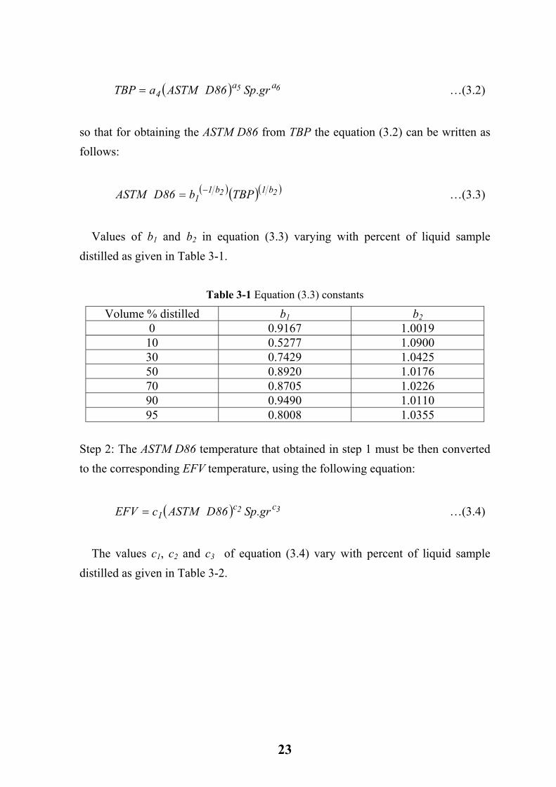
…(3.2) ( ) 65 aa4 gr.Sp86DASTMaTBP =
so that for obtaining the ASTM D86 from TBP the equation (3.2) can be written as follows:
( )( )( 22 b1b11 TBPb86DASTM −= ) …(3.3)
Values of b1 and b2 in equation (3.3) varying with percent of liquid sample distilled as given in Table 3-1.
Table 3-1 Equation (3.3) constants
Volume % distilled b1 b2 0 0.9167 1.0019
10 0.5277 1.0900 30 0.7429 1.0425 50 0.8920 1.0176 70 0.8705 1.0226 90 0.9490 1.0110 95 0.8008 1.0355
Step 2: The ASTM D86 temperature that obtained in step 1 must be then converted to the corresponding EFV temperature, using the following equation:
…(3.4) ( ) 32 cc1 gr.Sp86DASTMcEFV =
The values c1, c2 and c3 of equation (3.4) vary with percent of liquid sample distilled as given in Table 3-2.
23
Table 3-2 Equation (3.4) constants
Volume % distilled c1 c2 c3 0 3.2555 0.8466 0.4208
10 1.4881 0.9511 0.1287 30 0.8330 1.0315 0.0817 50 3.617 0.8274 0.6214 70 9.9607 0.6871 0.9340 90 13.0316 0.6529 1.1025 100 9.5654 0.6949 1.0737
If the values of specific gravity needed for equation (3.4) are unknown Raizi – Daubert developed two equations for predicting the specific gravity using the 10% and 50% ASTM D86 temperature (ASTM D86 10% and ASTM D 86 50%) of the fraction or 10% and 50% EFV temperature (EFV 10% and EFV 50%). These equations are:
…(3.5) ( ) ( 3684.010731.0 %5086DASTM%1086DASTM06711.0gr.Sp = )
( ) ( ) 3684.001334.0 %50EFV%10EFV074251.0gr.Sp −= …(3.6)
Step 3: The EFV curve can be obtained by plotting the EFV temperature against the corresponding volume percent distilled (vol.%). Example, A.1, in Appendix, illustrates the using of Raizi – Daubert method for predicting the EFV curve from the TBP curve.
For convenience and quick conversion of TBP curve to EFV curve, equations (3.3) and (3.4) are graphically represented by Figs. A-1 and A-2 in Appendix, A.
3.3 Pseudo – component (computer) methods
The pseudo – component methods, based on several thermodynamic models that have been proposed to replace the graphical methods for predicting the EFV curve from available TBP curve. The most important resource of the limitations of graphical methods are [6]:
24
• The empirical nature of these methods make them limited to the data set that were used to develop them.
• The graphical methods do not by themselves, yield properties of vapor and liquid phases such as, molecular weight, specific gravity, …etc.
The pseudo – component methods are also known as computer methods, because the electronic computers are used to do the tedious nature of trial and error multi component flash vaporization calculation to estimate the flash vaporization volume of petroleum cuts or fractions. To obtain the EFV curve from the TBP curve using the pseudo – component methods, there are four main important steps that must be followed: First, the TBP curve must be divided into suitable number of fractions or cuts. Each of these fractions have their average boiling point (TB), and specific gravity (Sp.gr). In the second step, the average boiling point and the specific gravity for each fractions must be used for estimation the basic characterization parameters or constants such as critical temperature (Tc), critical pressure (Pc), the acentric factor (ω) and the molecular weight (MW), …etc. These constants can be estimated by using suitable characterization correlations (as mentioned in Chapter, 2). Steps one and two can be considered as characterization steps. The third step includes the estimation of the vapor – liquid equilibrium constants (K – values) for each fractions using the available thermodynamic models. Finally, in the fourth step, the flash volume, and thus, the EFV curve can be provided by performing the flash calculations. The above steps will be discussed in details in the next sections.
3.4 Divided the TBP curve into fractions or cuts
The approach that, the pseudo – component methods have been taken in the dividing the crude oils TBP curves into fractions or cuts, where these fractions are well known as pseudo – components and then they can be handled as pure components.
25
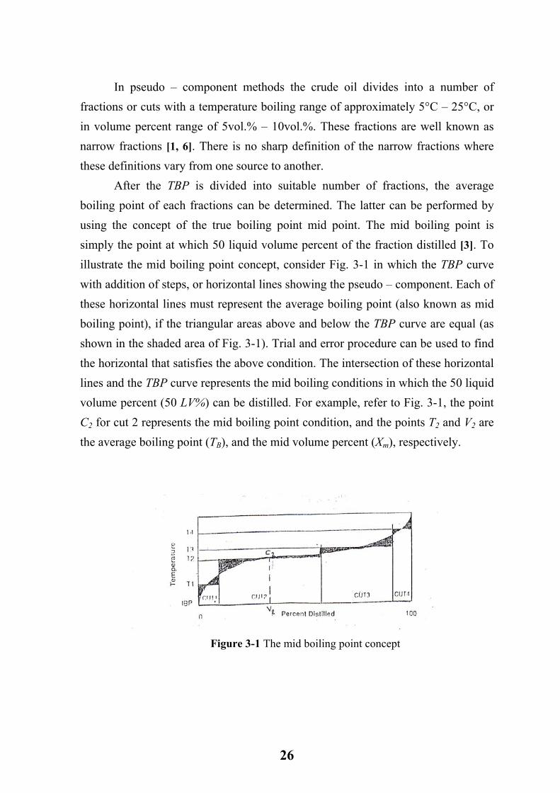
In pseudo – component methods the crude oil divides into a number of fractions or cuts with a temperature boiling range of approximately 5°C – 25°C, or in volume percent range of 5vol.% – 10vol.%. These fractions are well known as narrow fractions [1, 6]. There is no sharp definition of the narrow fractions where these definitions vary from one source to another. After the TBP is divided into suitable number of fractions, the average boiling point of each fractions can be determined. The latter can be performed by using the concept of the true boiling point mid point. The mid boiling point is simply the point at which 50 liquid volume percent of the fraction distilled [3]. To illustrate the mid boiling point concept, consider Fig. 3-1 in which the TBP curve with addition of steps, or horizontal lines showing the pseudo – component. Each of these horizontal lines must represent the average boiling point (also known as mid boiling point), if the triangular areas above and below the TBP curve are equal (as shown in the shaded area of Fig. 3-1). Trial and error procedure can be used to find the horizontal that satisfies the above condition. The intersection of these horizontal lines and the TBP curve represents the mid boiling conditions in which the 50 liquid volume percent (50 LV%) can be distilled. For example, refer to Fig. 3-1, the point C2 for cut 2 represents the mid boiling point condition, and the points T2 and V2 are the average boiling point (TB), and the mid volume percent (Xm), respectively.
Figure 3-1 The mid boiling point concept
26
For straight line TBP curve the mid boiling point for each cuts can be determined by averaging the initial cut boiling point (IBP), and the final cut boiling point (FBP) {i.e. TB=(IBP+FBP)/2}. This is not true for curvature TBP curve [81]. The mid boiling point concept, is also true with other physical properties curve such as specific gravity, viscosity …etc. In some cases in which the specific gravity curve is not available, but just the bulk specific gravity is given, the specific gravity of each fractions can be determined by the Katz – Firoozabadi correlation [82]:
…(3.7) 1605.0BT3067.0gr.Sp =
Where TB is the mid boiling point temperature of fraction in °F. It must be known here that for any available specific gravity input data {curves or using equation (3.7)}, the specific gravity of each cuts must be adjusted to satisfy the given petroleum stock specific gravity. For most crude oils the TBP curve and the specific gravity curve are not available in full range of percent distilled (i.e. 0 – 100 LV%). In such cases these curves must be interpolated and extrapolated as necessary to complete the full range of the curves. The extrapolation and interpolation can be performed using a suitable numerical techniques [83]. These full range curves are known as the working curves which must be used in the mid boiling point concept for obtaining the pseudo – components or fractions of the TBP curve.
3.5 Estimation of the basic characterization parameters for the fractions or cuts
Characterization of petroleum fractions involves estimation of the basic parameters needed in thermodynamic models from readily measurable properties such as the specific gravity and average boiling point (mid boiling point). The basic characterization parameters include the critical properties (critical temperature (Tc) and critical pressure (Pc)), acentric factor (ω) and molecular weight (MW).
27
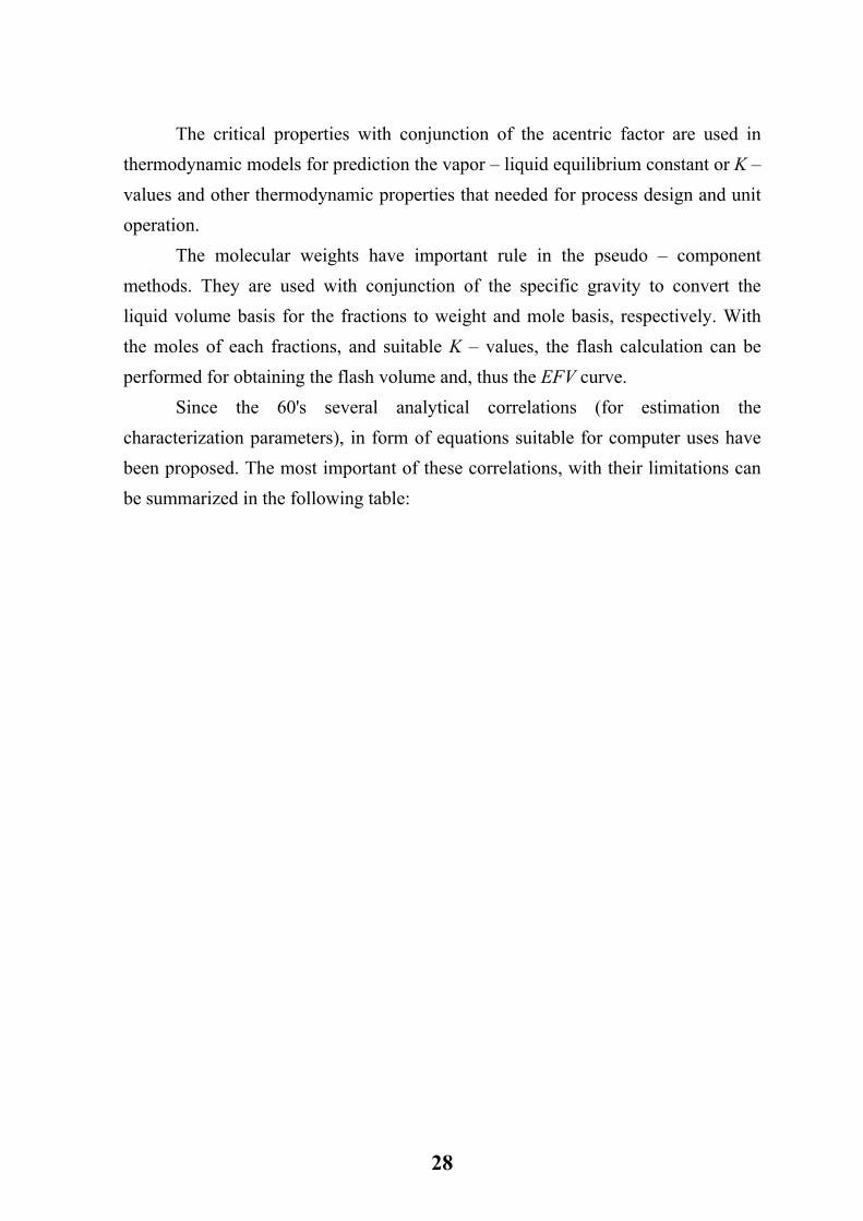
The critical properties with conjunction of the acentric factor are used in thermodynamic models for prediction the vapor – liquid equilibrium constant or K – values and other thermodynamic properties that needed for process design and unit operation. The molecular weights have important rule in the pseudo – component methods. They are used with conjunction of the specific gravity to convert the liquid volume basis for the fractions to weight and mole basis, respectively. With the moles of each fractions, and suitable K – values, the flash calculation can be performed for obtaining the flash volume and, thus the EFV curve. Since the 60's several analytical correlations (for estimation the characterization parameters), in form of equations suitable for computer uses have been proposed. The most important of these correlations, with their limitations can be summarized in the following table:
28
2. Lee –
Kasler [36]
1. Cavett
[34]
Correlation
name
Tc, Pc, ω,
MW
Tc, Pc
Estimated
parameter
Tc=341.7+
811Sp.gr+(0.42
4+0.1174Sp.gr)T
B +
(0.4669–3.2623Sp.gr)×10 45/T
B (3.9) ln Pc=
8.3634–0.0566/Sp.gr –(0.24244+
2.2898/Sp.gr+0.11857/Sp.gr 2)×
10-3T
B 0
77p
+(1.4685+
3.648/Sp.gr+.472
/S.gr 2)×
10-7T
B 2 (0.42019+
1.6977/Sp.gr–
2)×10
-10TB 3 (3.10)
Sp.gr)T
MW
=–12272.6+
9486.4Sp.gr+(4.6523–3.3287
g0
B +
(1–0.77084Sp.r–
.020585Sp.gr)×
(1.3437 2
–720.79/TB ) ×
10/T
+(1–
.882Sp.gr+
0.02226Sp.gr)
×(1.8828–181.96/T
B )×10
12/TB 3 (3.11)
7B
008
2
Tc=768.071
1.734TB–0.1083
×10
T+
14
-2B
2 +
0.3889×10
B0.89213×
10TBA
I +
0.53095×10 -6T
3–-2
P-6TB
2API+0.32712×
10-7TB
2API 2 (3.7)
+log Pc=
2.8290.9412×
10TB
-3
–0.30475×10
TB+
0.-5
215141×
10-8TB
3 –0.20876×
10TB
PI +
0.11048×10
-7TB2API+
0.32712×10
-7TB2API 2 (3.8)
-4A
Equation
Sp.gr, Tc, Pc, TB, K
UO
P
TB, API
Function of
Tc (R), Pc (psia)
Limitations: M
W
60≤ ≤650
TB<677°C (1250°F)
TB, Tc (°Pc (psia) F),
Limitations: not
mentioned
Limitations and
comm
ents
Table 3-3 Sum
mary of characterization correlations
29
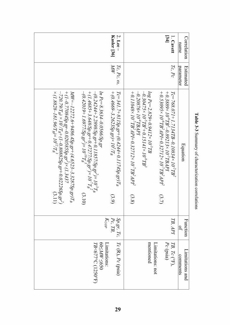
5. Pen – State [84]
4. Adm
ister [4]
3. Mathur et
al. [35]
2. Lee –
Kasler [36]
Correlation
name
MW
, Tc, Pc
ω
Tc, Pc
Tc, Pc, ω,
MW
Estimated
parameter
MW
=1.435×
10–5(TB
2.3776/Sp.gr) 0.9371 (3.17)
c=Exp(3.9935TB
T0.8615Sp.gr 0.04614) (3.18)
Pc=3.4824×
109Sp.gr 2.4853/TB
2.3177 (3.19)
ω=
3/7[logPc/(Tc/TB–1)] (3.16)
Tc=87.5(M
W) 0.4495 (3.14)
Pc=4532(M
W) –0.979 (3.15)
ω=
(ln PB r–5.9
714+6.09648/TBr+
1.2882
62lnTBr –0.169347TBr
)/(15.2518–15.6875/T–13.4721lnTBr+
0.43577TBr6
Br
6)
TBr<0.8 (3.12)
ω=
7.904+0.1352K
UO
P – 0.007465K
.
–1063)/TBr
TBr>0.8 (3.13)
UO
P 2
+8.359TBr+
(1408
0.0TBr=
TB/Tc; PB r=
PB /Pc Equation
TB, Sp.gr
Tc, Pc, TB
TB, API
Sp.gr, Tc, Pc, TB, K
UO
P
Function of
TB, Tc (R), Pc (psia)
Limitations:
40°C≤TB≤457°C
(100°F≤ TB≤850°F)
Tc, TB (K), Pc (atm
) Lim
itations: TB<
343°C (650°F)
Tc (K), Pc (atm
) Lim
itations: not m
entioned
Tc (R), Pc (psia)
Limitations:
60≤MW
≤650 TB<677°C
(1250°F)
Limitations and
comm
ents
Continue, T
able 3-3 Summ
ary of characterization correlations
30
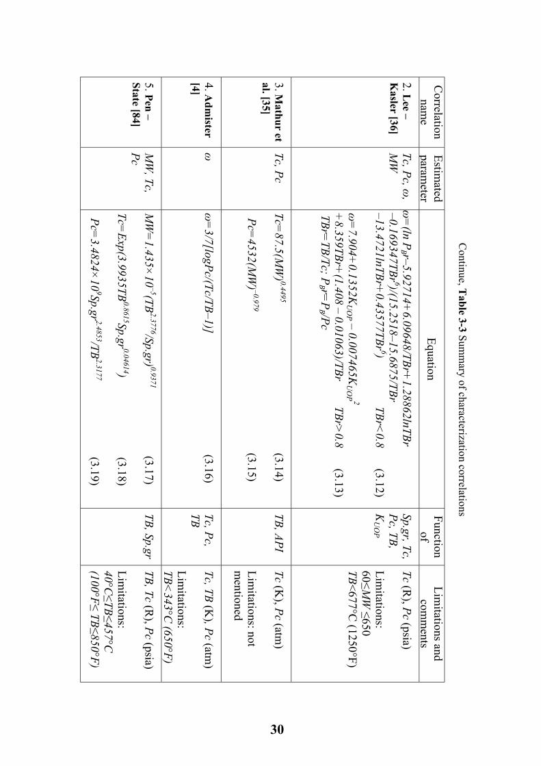
8. Tw
u [37]
7. Sim –
Winn [1]
6. Raizi –
Daubert
1980 [13]
Correlation
name
MW
, Tc, Pc
MW
, Tc, Pc
MW
, Tc, Pc
Estimated
parameter
lnMW
=lnM
WA [(1+
2FM )/(1–2F
M )] 2 (3.26) Tc=
Tc
A [(1+2F
T )/(1–2FT )] 2 (3.27)
Pc=Pc
A [(1+
2FP )/(1–2F
P )] 2 (3.28) F
M =∆Sp.grM +׀x׀]
(–0.01756+0.193168/TB
)∆Sp.gr (3.29)
0.5
B
FT =∆Sp.grT [–0.36245/T
+
(0.03982–0.94812/TB0.5
0.5)]∆Sp.grT (3.30)
MW
=5.805×
10–5[TB
2.3776/Sp.gr 0.9371] (3.23) Tc=
[Exp(4.2009TB
0.08615/Sp.gr 0.04614)]/1.8 (3.24) Pc=
6.1483×10
12TB–2.3177Sp.gr 2.4853 (3.25)
MW
=4.5673×
10–5TB
2.1962Sp.gr –1.0164 (3.20) Tc=
24.2787TB
0.5885Sp.gr 0.3596 (3.21)
Pc=3.1181×
109TB
–2.3125Sp.gr 2.301 (3.22)
Equation
TB, S.
gr pgr
Sp.TB
A A
TB, Sp.gr
TB, Sp.gr
Function of
Pc, PcA (
psia),
TB(R),
TBF (°F)
Limitations: 6
Sp.gr≤1.43TB≤704°C
(TB≤1300°F) Expansion from
n - alkane
TB, Tc (K), Pc (Pa)
Limitations:
80≤ MW≤650
TB, Tc (K), Pc (Pa)
Limitations:
80≤ MW≤650
Limitations and
comm
ents
Continue, T
able 3-3 Summ
ary of characterization correlations
31
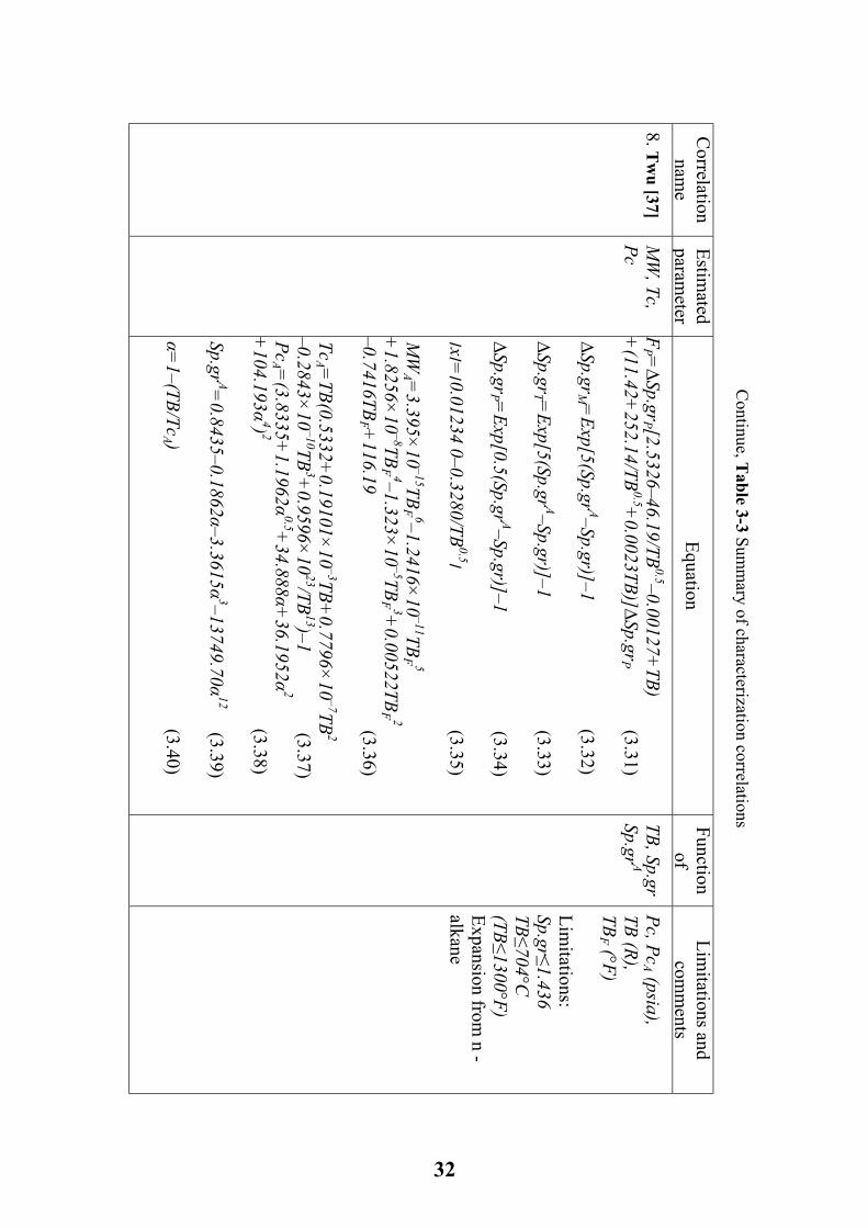
8. Tw
u [37]
Correlation
name
MW
, Tc, Pc
Estimated
parameter
FP =∆Sp.grP [2.5326–46.19/TB
0.5–0.00127+TB)
+(11.42+
252.14/TB0.5+
0.0023TB)]∆Sp.grP (3.31) ∆Sp.gr
M =Exp[5(Sp.gr A–Sp.gr)]–1 (3.32)
∆Sp.gr
T =Exp[5(Sp.gr A–Sp.gr)]–1 (3.33)
∆Sp.gr
P =Exp[0.5(Sp.gr A–Sp.gr)]–1 (3.34)
=׀x׀ TB/0.3280–0 0.01234׀
(3.35) ׀0.5
×
MW
A =3.395
105TB
F 6–1.246×
–11TBF 5
1.323×10
–11
10+
1.8256×10
–8TBF 4–
FF
0.7416TB–5TB
3+0.00522TB
2 –
F +116.19 (3.36)
33
TcA =
TB(0.52+
0.19101×10
TB+.7796×
10TB
2
–30
–72
–0.843×
10TB
+0.9
6×10
/TB)–1
35 –103
5923
13
(3.37) Pc
A =(3.83
+1.1962α
+34.888α+
36.1952α
+104.193α
0.52
4) 2 (3.38) Sp.gr
A=0.8435–0.1862α–3.3615α
3–13749.70α12 (3.39)
=
1–(TB/Tcα
A ) (3.40)
Equation
TB, S.
Sp.gr pgr
A
Function of
Pc, PcA (
psia),
TB(R),
TBF (°F)
Limitations: 6
Sp.gr≤1.43TB≤704°C
(TB≤1300°F) Expansion from
n - alkane
Limitations and
comm
ents
Continue, T
able 3-3 Summ
ary of characterization correlations
32
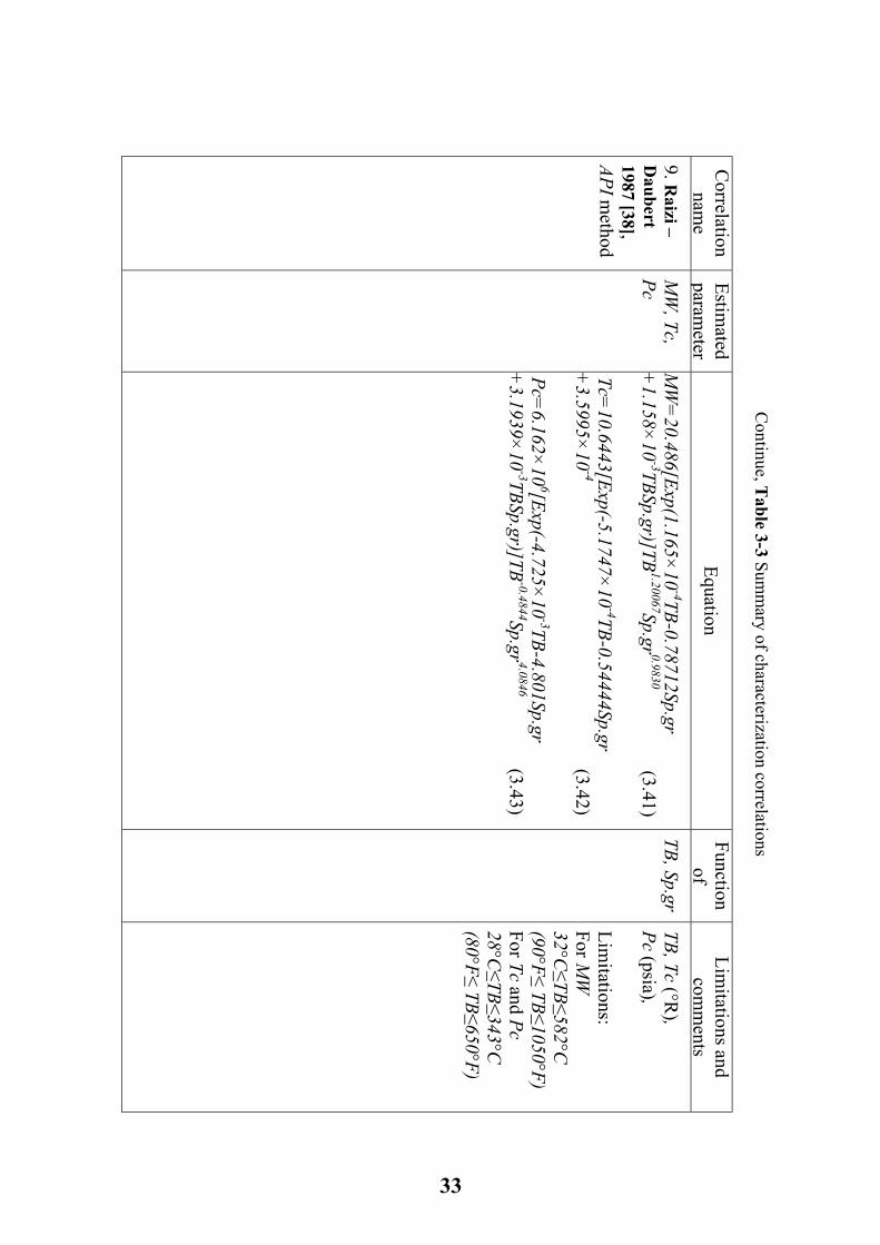
9. Raizi –
Daubert
1987 [38], API m
ethod
Correlation
name
MW
, Tc, Pc
Estimated
parameter
MW
=20.48
[Exp(1.165×B-0.7
Sp.gr +
1.158×10 6
10-4T
8712-3TBSp.gr)]TB
1.20067Sp.gr 0.9830 (3.41)
[ Tc=
10.6443Exp(-5.1747×
10TB-0.54444Sp.gr
+3.5995×
10-4
-4 (3.42)
1×
10 Pc=
6.162×0
6[Exp(-4.7253TB-4
+3.1939×
10-3TBSp.gr)]TB
-0.4844Sp.gr 4.0846 (3.43) -
.801Sp.gr
Equation
TB, Sp.gr
Function of
TB, Tc (°RPc (psia), ),
ns:
Limitatio
For MW
32°C
≤TB≤582°C
(90° TB
50°F) F≤
≤10For Tc and Pc 28°C
≤TB≤343°C
80°F≤ TB≤650°F) (
Limitations and
comm
ents
Continue, T
able 3-3 Summ
ary of characterization correlations
33
The API – technical data book [2, 11] recommended the following correlations for estimation the basic characterization parameters:
• The Raizi – Dauber 1987, for estimation the critical temperature, critical pressure and molecular weight.
• The Lee – Kasler correlations for estimation the acentric factor.
3.6 Prediction of vapor – liquid equilibrium constants (K – values) for fractions
The term "vapor – liquid equilibrium" (VLE), refers to systems in which a single liquid phase is in equilibrium with its vapor. In studies of phase equilibrium, however, the phase containing gradients is not considered. Whenever gradient exists there is a tendency for change with time, hence there is no equilibrium. On other hand, there can be two or more phases, each of which is homogenous throughout, with no tendency for any change in properties with time, even though the phases are in intimate physical contact with one another. The latter is the condition that is denoted by the term "phase equilibrium". In a condition of phase equilibrium there are some properties that are drastically different between the phases, and others that must be identical for all phases to prevent a change of properties within individual phases from change. The thermodynamic equilibrium determines how components in mixture are distributed between phases [85, 86].
3.7 Thermodynamic of equilibrium
3.7.1 Fugacity and fugacity coefficient
The starting point for a phase equilibrium calculation is the thermodynamic requirement that the temperature, pressure, and chemical potential of each species be the same in all phases in which the species is present, that is:
(i = 1, 2, 3, …Nc) ..(3.44) ...21 Phi
Phi == µµ
34
where µ is the chemical potential of species i, Ph1 and Ph2 represent the phases in equilibrium. Chemical potential can be expressed as an absolute quantity, and the numerical values of chemical potential are difficult to relate to more easily understood physical quantities. Furthermore, the chemical potential approaches an infinite negative value as pressure approaches zero. For these reasons, the chemical potential is not favored for phase equilibria calculations. Instead, fugacity invented by G. N. Lewis in 1901, is employed as a surrogate. The partial fugacity of species i in the mixture is like a pseudo – pressure, defined in terms of the chemical potential by [42]:
=RT
expCf ii
µ ..(3.45)
where C is a temperature – dependent constant. Regardless of the value of C, it is shown by Prausintz, Liehtenthaler and Azevedo [87] that equation (3.40) can be replaced with:
...ff 21 Phi
Phi == (i = 1, 2, 3, …Nc) ..(3.46)
thus, at equilibrium, a given species has the same partial molal fugacity in each existing phases. This equality together with equality of phase temperatures and pressures, thus:
..(2.47) (NPPhPh T...TT 21 == )
)
and ..(2.48) (NPPhPh P...PP 21 ==
where NP is the number of phases. Equations (3.46) – (3.48) constitute the required conditions for phase equilibria. For vapor – liquid equilibrium the above equations are reduced to:
35

Li
Vi ff = ..(3.49)
..(3.50) LV TT =
..(3.51) LV PP =
Because of the close relationship between fugacity and pressure, it is convenient to define their ratio for pure species [55]:
Pfi
i =φ ..(3.52)
where φ , is the pure species fugacity coefficient, and it represents the departure of
fugacity due to pressure. i
For a mixture, partial molal fugacity coefficient represents the departure of fugacity due to pressure and the partial molal fugacity coefficient can be defined for vapor and liquid phases as follows [88]:
Py
f
i
ViV
i =φ ..(3.53)
Px
f
i
LiL
i =φ ..(3.54)
For a pure ideal gas, fugacity is equal to the pressure (fi = P) (i.e. φ = 1), and
for a species in the ideal gas mixture, the partial fugacity is equal to its partial
pressure (P
i
i = yi P), (i.e. φ = 1). Vi
36
3.7.2 Activity and activity coefficients
At a given temperature, the ratio of the partial molal fugacity of a component in mixture to its fugacity in some standard state is defined as activity. If the standard state is selected as the pure species at same pressure and temperature as the mixture, then the activity is equal [89]:
i
ii f
fa = ..(3.55)
To represent the departure to partial fugacity due to composition, the activity coefficients based on concentration in mole fractions are defined by [42]:
i
ViV
i ya
=γ ..(3.56)
i
LiL
i xa
=γ ..(3.57)
substituting ai in equations (3.56) and (3.57), gives:
i
Vi
ViV
iyf
f=γ ..(3.58)
i
Li
LiL
ixf
f=γ ..(3.59)
37
3.7.3 K – values formulation
In the multi component system, the K – value of a given species is defined as the ratio of the mole fraction of the species in the vapor phase (yi), to the mole fraction of the species in the liquid phase (xi). Mathematically the relationship is expressed as [89]:
i
ii x
yK = ..(3.60)
To form the K – values, fugacities are replaced by equivalent expressions involving mole fractions. Two common pairs derived from equations (3.53), (3.54), (3.58) and (3.59), are: Pair 1:
Pyf iVi
Vi φ= ..(3.61)
and Pxf iLi
Li φ= ..(3.62)
Pair 2:
iVi
Vi
Vi yff γ= ..(3.63)
and iL
iLi
Li xff γ= ..(3.64)
If equations (3.61) and (3.62) are used with equation (3.49), a so called equation of state form of K – value (or φ – φ K – value form) [90] is obtained:
38
Vi
Li
iKφ
φ= ..(3.65)
If equations (3.61) and (3.64) are used with equation (3.49), a so called activity coefficient form of K – value (or φ – γ K – value form) [89], is obtained:
Vi
Li
Li
Vi
Li
Li
iP
fK
φ
φγ
φ
γ== ..(3.66)
If equations (3.63) and (3.64) is used with equation (3.49) with conjunction
of the ideal solution concept in which γ = =1, a so called ideal solution K –
value form [73, 88] is obtained:
Li
Vi γ
Vi
Li
Vi
Li
iff
Kφ
φ== ..(3.67)
The three forms of the K – value will be discussed in the next sections.
3.8 Equation of state forms for prediction the K – values (φ – φ
forms)
Equation of state are widely used in the prediction of thermodynamic properties of pure fluid and fluid mixtures (including petroleum fractions), in part because they provide a thermodynamically consistent route to the configurationally properties of both vapor and liquid phases. Consequently, equation of state model may be used to determine phase equilibrium conditions as well as other properties. The term equation of state (also refers to P – V – T relationship) is used to describe an empirically – derived function which provides a relation between, pressure, density, temperature and composition of the system. Of all types of equations of state, a most popular class is formed by the so called "cubic equation of
39
state" (CEQS), so named because when usually written in pressure – explicit form, and the volume is given in cubic form [86, 91], thus: ..(3.68) ( ...n,V,TPP 1= ) An equation of state is always used to obtain the partial molal fugacity
coefficient in the vapor and sometimes in the liquid phases ( Viφ , L
iφ ) in terms of the
pressure, temperature and composition of the system thus:
( ...y,P,TF iVi =φ ) ..(3.69)
( ...x,P,TF iLi =φ ) ..(3.70)
A rigorous relation exists between the partial molal fugacity coefficient of a component in a phase and the volumetric properties of that phase. This relation is conveniently expressed in the form of equation of state. In order to obtain the partial molal fugacity coefficient by using equation of state, the following expression is used [88]:
∫∞
−
−
∂∂
=≠V n,V,Ti
i ZlndVVRT
nP
RT1ln
ij
φ ..(3.71)
where ni is the number of moles of component i. Equation (3.71) is exact if the information needed to evaluate the integrals is at hand. These P – V – T information can be obtained from suitable cubic equation of states. The oldest, simplest and best known cubic equation of state is that proposed by van der Waals in 1873, his equation is:
40
2Va
bVRTP −−
= ..(3.72)
where P, T, V are the pressure, temperature and molar volume, respectively. a and b are two constants and they can be obtained from the critical temperature and critical
pressure. The first term of equation (3.72), (bV
RT−
) expresses the effect of repulsion
between molecules, assimilated to hard spheres, while the second term ( 2Va )
expresses the attraction forces due to the van der Waals forces. The first term is also known as repulsive pressure term and the second term is also known as attractive pressure term. It should be mentioned that the van der Waals equation is not accurate for representation the P – V – T behavior of species in the liquid and vapor states, but is historically important and useful for qualitative investigations [89]. The modern development of cubic equation of state started in (1949), with publication of the Redlich – Kowng equation of state (RK) [57]:
( )bVVTa
bVRTP 21 +
−−
= ..(3.73)
Redlich – Kwong demonstrated that by a simple adjustment the van der
Waals attractive pressure term ( 2Va ) could considerably improve the prediction of
the P – V – T behavior and physical properties of the vapor phase. They replaced the
attractive pressure term ( 2Va ) with a generalized temperature dependence term
( 21Ta ) or alpha function (α). Their equation has the form:
( )bVVbVRTP
+−
−=
α ..(3.74)
41
a and b are also obtained from critical temperature and critical pressure. Redlich states that there was no particular theoretical basis for the equation, rather it is considered as an effective empirical modification of its predecessors. More than 110 modification to the Ridlich – Kowng equation of state have been proposed to date to improve its representation of volumetric behavior and physical properties. These modifications including the widely used Soave (also known as Soave – Redlich – Kowng (SRK)) equation of state and Peng – Robinson (PR) equation of state. The SRK and PR equations of state today are the most important and popular equations of state, which are used for prediction the volumetric behavior and physical properties including the vapor – liquid equilibrium calculations for both polar and non polar mixtures including the petroleum fractions.
3.8.1 Soave – Relich – Kowng equation of state (SRK)
One of the most significant milestones in the development of cubic equation of state was the publication by Soave [67], of a modification to the evaluation of parameter a in the attractive pressure term of the Redlich – Kowng (RK) equation of
state {equation (3.73)}. Soave replaced the term ( 21Ta ) in equation (3.73) with a
more generalized temperature dependent term, as denoted by (aα) to give:
( )bVVa
bVRTP
+−
−=
α ..(3.75)
where, α is a dimensionless factor that become unity at T = Tc (α is also known as alpha function), α is a function of the reduced temperature and acentric factor ω (i.e. α = f(Tr, ω)) to overcome the difficulty of inability of equation of state to represent the entire fluid range which prevent their use for the vapor – liquid equilibria calculation. Soave back – calculated the α for various hydrocarbon species over a range of reduced temperature using vapor pressure data to obtain the following correlation for α:
42
..(3.76) ([ 25.0rT1m1 −+=α )]
where ..(3.77) 2176.0574.148.0m ωω −+=
The ω in equation (3.77) is the acentric factor, which can be obtained by Pitzer et al. [44] as follows:
( )[ ] 1Plog 7.0Tr r−−= =
∗ω ..(3.78)
where is the reduced vapor pressure (P∗rP s/P).
All equations of state are generally developed for pure species first, and then extended to mixtures through the use of mixing rules. These mixing rules are simply means of calculating mixture parameters equivalent to those of pure species. The most conventional mixing rules is given by van der Waals. Equation (3.75) of Soave – Redlich in polynomial form of Z will thus be:
( ) ( ) 0ABZBBAZB1Z 223 =−−−+−− ..(3.79)
Where the mixing rules:
( )∑∑= =
−=N
i
N
jjiijji AAkxxA
1 11 ..(3.80)
..(3.81) ∑=
=N
1iii BxB
..(3.82) ∑=
=N
1iiim bxb
43
and, 2i
iii
TrPr
42747.0A α= i
ii Tr
Pr08664.0B = ..(3.83)
( )
i
2i
i PcRTc
42747.0a = i
ii Pc
RTc08664.0b = ..(3.84)
xi, is the mole fraction of species i. The roots of equation (3.79) are obtained by numerical technique such as Newton – Raphson technique [83]. The latter is discussed in Appendix, B. In two phases region, three real roots are exist. The liquid root is smallest of the three, and it represents the compressibility factor for liquid phase (ZL), while the largest root is the compressibility factor for the vapor phase (ZV). A non physical root exists between them. In solving equation (3.79) for the compressibility factor of the liquid phase (ZL), the composition of the liquid xi is used to calculate the coefficient A and B of equations (3.80) and (3.81), through the use of the mixing rules. For determining the compressibility factor for the vapor phase (ZV), the above outlined procedure is used with composition of the vapor phase yi replacing xi. By combining the SRK equation of state equation (3.75) into the thermodynamic definition of the partial molal fugacity coefficient, equation (3.71), Soave proposed the following expression for the partial molal fugacity coefficient
of the species in liquid mixture Liφ :
( ) ( ) ( )
( ) ( )( )
+
−−+
−−−=
∑=
Ljjiiij
Nc
jj
i
LLiL
i
ZBaaKx
aBB
BA
BZZBB
1ln12
ln1ln
1αα
α
φ
..(3.85)
where ( ) ( )( )∑∑= =
−=N
1i
N
1jjjiiijji aaK1xxa ααα ..(3.86)
44
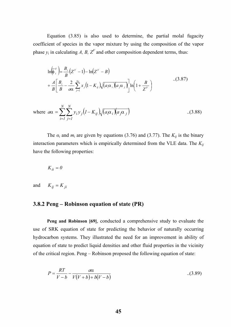
Equation (3.85) is also used to determine, the partial molal fugacity coefficient of species in the vapor mixture by using the composition of the vapor phase yi in calculating A, B, ZV and other composition dependent terms, thus:
( ) ( ) ( )
( ) ( )( )
+
−−+
−−−=
∑=
Vjjiiij
Nc
jj
i
VViV
i
ZBaaKx
aBB
BA
BZZBB
1ln12
ln1ln
1αα
α
φ
..(3.87)
where ( ) ( )( )∑∑= =
−=N
1i
N
1jjjiiijji aaK1yya ααα ..(3.88)
The αi and mi are given by equations (3.76) and (3.77). The Kij is the binary interaction parameters which is empirically determined from the VLE data. The Kij have the following properties: 0Kii =
and jiij KK =
3.8.2 Peng – Robinson equation of state (PR)
Peng and Robinson [69], conducted a comprehensive study to evaluate the use of SRK equation of state for predicting the behavior of naturally occurring hydrocarbon systems. They illustrated the need for an improvement in ability of equation of state to predict liquid densities and other fluid properties in the vicinity of the critical region. Peng – Robinson proposed the following equation of state:
( ) ( )bVbbVVa
bVRTP
−++−
−=
α ..(3.89)
45
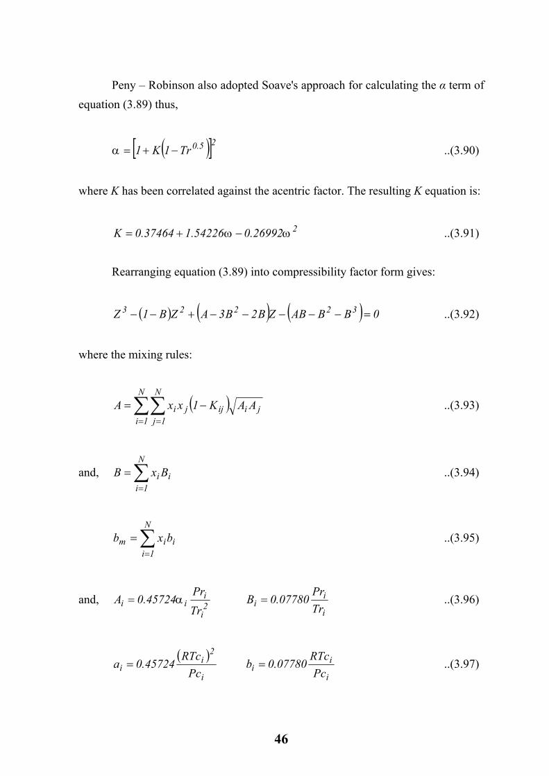
Peny – Robinson also adopted Soave's approach for calculating the α term of equation (3.89) thus,
( )[ ]25.0Tr1K1 −+=α ..(3.90)
where K has been correlated against the acentric factor. The resulting K equation is:
..(3.91) 226992.054226.137464.0K ωω −+=
Rearranging equation (3.89) into compressibility factor form gives:
( ) ( ) ( ) 0BBABZB2B3AZB1Z 32223 =−−−−−+−− ..(3.92)
where the mixing rules:
( )∑∑= =
−=N
1i
N
1jjiijji AAK1xxA ..(3.93)
and, ..(3.94) ∑=
=N
1iii BxB
..(3.95) ∑=
=N
1iiim bxb
and, 2i
iii
TrPr
45724.0A α= i
ii Tr
Pr07780.0B = ..(3.96)
( )
i
2i
i PcRTc
45724.0a = i
ii Pc
RTc07780.0b = ..(3.97)
46
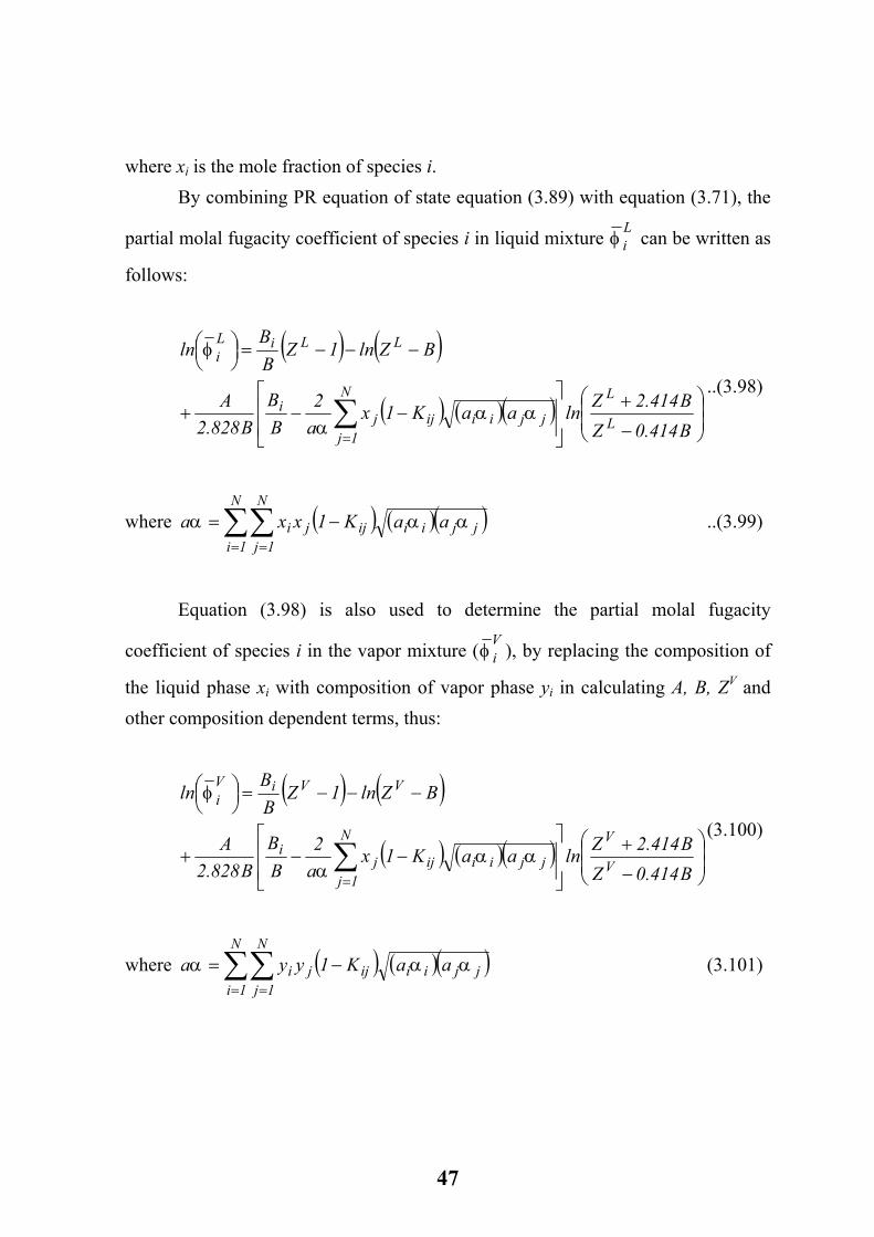
where xi is the mole fraction of species i. By combining PR equation of state equation (3.89) with equation (3.71), the
partial molal fugacity coefficient of species i in liquid mixture Liφ can be written as
follows:
( ) ( )
( ) ( )( )
−
+
−−+
−−−=
∑= B414.0Z
B414.2ZlnaaK1xa2
BB
B828.2A
BZln1ZBB
ln
L
LN
1jjjiiijj
i
LLiLi
ααα
φ
..(3.98)
where ( ) ( )( )∑∑= =
−=N
1i
N
1jjjiiijji aaK1xxa ααα ..(3.99)
Equation (3.98) is also used to determine the partial molal fugacity
coefficient of species i in the vapor mixture ( Viφ ), by replacing the composition of
the liquid phase xi with composition of vapor phase yi in calculating A, B, ZV and other composition dependent terms, thus:
( ) ( )
( ) ( )( )
−
+
−−+
−−−=
∑= B414.0Z
B414.2ZlnaaK1xa2
BB
B828.2A
BZln1ZBB
ln
V
VN
1jjjiiijj
i
VViVi
ααα
φ
(3.100)
where ( ) ( )( )∑∑= =
−=N
1i
N
1jjjiiijji aaK1yya ααα (3.101)
47
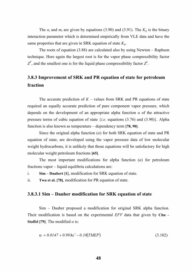
The αi and mi are given by equations (3.90) and (3.91). The Kij is the binary interaction parameter which is determined empirically from VLE data and have the same properties that are given in SRK equation of state Kij. The roots of equation (3.88) are calculated also by using Newton – Raphson technique. Here again the largest root is for the vapor phase compressibility factor ZV, and the smallest one is for the liquid phase compressibility factor ZL.
3.8.3 Improvement of SRK and PR equation of state for petroleum fraction
The accurate prediction of K – values from SRK and PR equations of state required an equally accurate prediction of pure component vapor pressure, which depends on the development of an appropriate alpha function α of the attractive pressure terms of cubic equation of state {i.e. equations (3.76) and (3.90)}. Alpha function is also known as temperature – dependency term [78, 90]. Since the original alpha function (α) for both SRK equation of state and PR equation of state, are developed using the vapor pressure data of low molecular weight hydrocarbons, it is unlikely that those equations will be satisfactory for high molecular weight petroleum fractions [65]. The most important modifications for alpha function (α) for petroleum fractions vapor – liquid equilibria calculations are: i. Sim – Daubert [1], modification for SRK equation of state. ii. Twu et al. [78], modification for PR equation of state.
3.8.3.1 Sim – Dauber modification for SRK equation of state
Sim – Dauber proposed a modification for original SRK alpha function. Their modification is based on the experimental EFV data that given by Chu –
Staffel [79]. The modified α is: (3.102) (TMEP10.0993.00147.0 −′+= αα )
48
where, α' is the original SRK equation of state α {equation (3.76)}, and TMEP is constant calculated as follows:
TMEP = 10 – The calculated flash volume when 20% TBP temperature is used as the flash temperature
The modified α is only applicable if the (TMEP) is negative. The Sim – Daubert modification for alpha function of SRK equation of state is recommended by the API – technical data book [74].
3.8.3.2 Twu et al. modification for PR equation of state
For PR equation of state Twu et al., suggested the generalized alpha function (α) form, that replaced the original PR alpha function {i.e. equation (3.90)}. The generalized α has the following form:
( ) ( )( )010 ααωαα += − (3.103)
where α (3.104) ( ) ( ) ( )( )( ) ( ) ( )
−
−=
0M0N000 Tr1L
1MN0 eTr
(3.105) ( ) ( ) ( )( )( ) ( ) ( )
−
−=
1M1N111 Tr1L
1MN1 eTrα
The superscripts (0) and (1) in equations (3.103) – (3.105) are consistent with the definition of acentric factor at ω = 0, and ω = 1, respectively. In other words, these two alpha functions (α(0) and α(1)) are forced to pass through the saturated pressure at Tr = 0.7 for ω = 0, and ω = 1, respectively. The constants L, M and N for α(0) and α(1), are given in Table 3-4, for supercritical region (Tr > 1), and sub critical region (Tr ≤ 1).
49
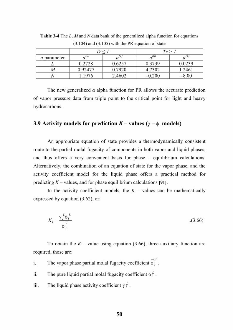
Table 3-4 The L, M and N data bank of the generalized alpha function for equations (3.104) and (3.105) with the PR equation of state
Tr ≤ 1 Tr > 1 α parameter α(0) α(1) α(0) α(1)
L 0.2728 0.6257 0.3739 0.0239 M 0.92477 0.7920 4.7302 1.2461 N 1.1976 2.4602 –0.200 –8.00
The new generalized α alpha function for PR allows the accurate prediction of vapor pressure data from triple point to the critical point for light and heavy hydrocarbons.
3.9 Activity models for prediction K – values (γ – φ models)
An appropriate equation of state provides a thermodynamically consistent route to the partial molal fugacity of components in both vapor and liquid phases, and thus offers a very convenient basis for phase – equilibrium calculations. Alternatively, the combination of an equation of state for the vapor phase, and the activity coefficient model for the liquid phase offers a practical method for predicting K – values, and for phase equilibrium calculations [91]. In the activity coefficient models, the K – values can be mathematically expressed by equation (3.62), or:
Vi
Li
Li
iKφ
φγ= ..(3.66)
To obtain the K – value using equation (3.66), three auxiliary function are required, those are:
i. The vapor phase partial molal fugacity coefficient Viφ .
ii. The pure liquid partial molal fugacity coefficient φ . Li
iii. The liquid phase activity coefficient γ . Li
50
The first auxiliary function, the vapor phase partial molal fugacity coefficient can be obtained using any of the suitable equation of state models, such as SRK and PR equation of state (as discussed in previous section). The other two auxiliary functions will be discussed hereafter.
3.9.1 The pure liquid fugacity coefficient (φ ) Li
The second important auxiliary function of equation (3.66) is the pure liquid
fugacity coefficient (φ ). From the classical thermodynamic relation [88], the pure
species fugacity coefficient:
Li
−= ∫
P
0i dP
PRTV
RT1lnlnφ (3.106)
By integrating equation (3.106) from 0 to , and to P, siP s
iP
dPVRT1
PPlnlnln
P
P
Lis
i
Vsi
Li
si
∫+
−= φφ (3.107)
where V is the liquid molar volume at system temperature and pressure. The last
term of equation (3.107) is known as the Poynting factor (PF) [55]. If the liquid is incompressible, equation (3.107) reduces to:
Li
( )
−
=
RTPPV
expP
P si
LiVs
i
siL
i φφ (3.108)
where is the vapor phase pure species fugacity coefficient at saturated
conditions.
Vsiφ
51
The Poynting factor can not be negligible at high pressure or when the vapor pressure of species is higher than the system pressure. For special case of ideal gas law, where the pressure is low so the Poynting factor is negligible and the equation (3.108) reduces to:
Vsi
siL
i PP
φφ
= (3.109)
The molar liquid volume V of species i can be calculated using modified
Rackett equation of Spencer – Danner [93], thus:
Li
( )[ ]72Tr11RA
Li Z
PcRTcV −+
= (3.110)
where, ZRA is the Rackett constant and must be back – calculated from measured molal volume at known temperature. For pure species, the values of the liquid molal volume can be found in many literatures measured usually at 25 °C (77 °F). For petroleum fraction, the specific gravity at 15.6 °C (60 °F) can be used to calculate the ZRA for equation (3.110). Equation (3.110) can be used for estimation the molar liquid volume up to the critical temperature of species. For the supercritical region, the Cavett [88] equation can be used. The mathematical form of Cavett equation is :
(3.111) ( iiL
i Tr37.5V += ζ ) where, ζi, is the Cavett constant, and can be back – calculated using the same way that described for obtaining ZRA for equation (3.110).
The vapor pressure of species i ( P ), can be estimated from a widely used
empirical correlations. By far the most well known empirical correlations for calculation of vapor pressure data for pure species is Antonine's equation:
si
52
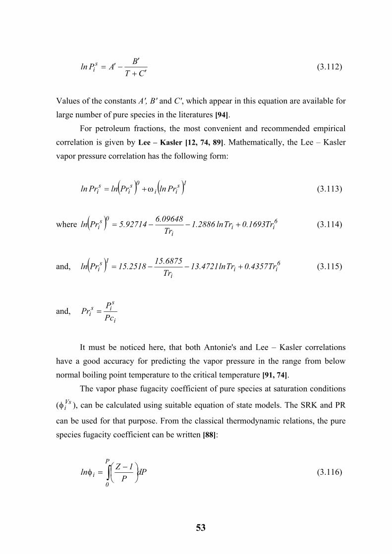
CT
BAPln si ′+
′−′= (3.112)
Values of the constants A', B' and C', which appear in this equation are available for large number of pure species in the literatures [94]. For petroleum fractions, the most convenient and recommended empirical correlation is given by Lee – Kasler [12, 74, 89]. Mathematically, the Lee – Kasler vapor pressure correlation has the following form:
(3.113) ( ) ( 1sii
0si
si PrlnPrlnPrln ω+= )
where ( ) 6ii
i
0si Tr1693.0Trln2886.1
Tr09648.692714.5Prln +−−= (3.114)
and, ( ) 6ii
i
1si Tr4357.0Trln4721.13
Tr6875.152518.15Prln +−−= (3.115)
and, i
sis
i PcP
Pr =
It must be noticed here, that both Antonie's and Lee – Kasler correlations have a good accuracy for predicting the vapor pressure in the range from below normal boiling point temperature to the critical temperature [91, 74]. The vapor phase fugacity coefficient of pure species at saturation conditions
(φ ), can be calculated using suitable equation of state models. The SRK and PR
can be used for that purpose. From the classical thermodynamic relations, the pure species fugacity coefficient can be written [88]:
Vsi
dPP
1ZlnP
0i ∫
−
=φ (3.116)
53
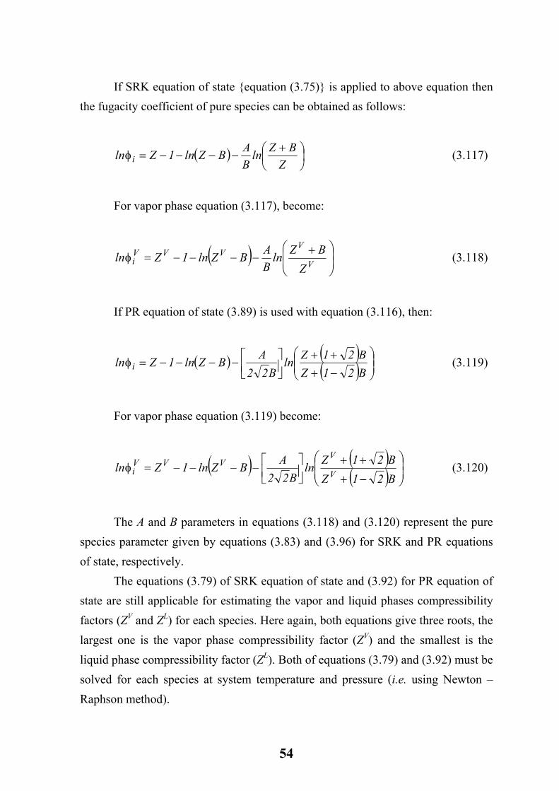
If SRK equation of state {equation (3.75)} is applied to above equation then the fugacity coefficient of pure species can be obtained as follows:
( )
+
−−−−=Z
BZlnBABZln1Zln iφ (3.117)
For vapor phase equation (3.117), become:
( )
+−−−−= V
VVVV
iZ
BZlnBABZln1Zlnφ (3.118)
If PR equation of state (3.89) is used with equation (3.116), then:
( ) ( )( )
−+++
−−−−=B21ZB21Zln
B22ABZln1Zln iφ (3.119)
For vapor phase equation (3.119) become:
( ) ( )( )
−+
++
−−−−=B21ZB21Zln
B22ABZln1Zln V
VVVV
iφ (3.120)
The A and B parameters in equations (3.118) and (3.120) represent the pure species parameter given by equations (3.83) and (3.96) for SRK and PR equations of state, respectively. The equations (3.79) of SRK equation of state and (3.92) for PR equation of state are still applicable for estimating the vapor and liquid phases compressibility factors (ZV and ZL) for each species. Here again, both equations give three roots, the largest one is the vapor phase compressibility factor (ZV) and the smallest is the liquid phase compressibility factor (ZL). Both of equations (3.79) and (3.92) must be solved for each species at system temperature and pressure (i.e. using Newton – Raphson method).
54
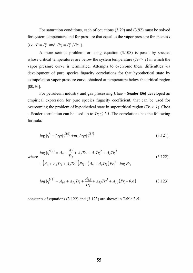
For saturation conditions, each of equations (3.79) and (3.92) must be solved for system temperature and for pressure that equal to the vapor pressure for species i
(i.e. and siPP = i
sii PcPPr = ).
A more serious problem for using equation (3.108) is posed by species whose critical temperatures are below the system temperature (Tri > 1) in which the vapor pressure curve is terminated. Attempts to overcome these difficulties via development of pure species fugacity correlations for that hypothetical state by extrapolation vapor pressure curve obtained at temperature below the critical region [88, 94]. For petroleum industry and gas processing Chao – Seader [56] developed an empirical expression for pure species fugacity coefficient, that can be used for overcoming the problem of hypothetical state in supercritical region (Tri > 1). Choa – Seader correlation can be used up to Tri ≤ 1.3. The correlations has the following formula:
(3.121) ( ) ( )1Lii
0Li
Li logloglog φωφφ +=
where ( )
( ) ( ) i2
ii98i2
i2i63
3i4
2i3i2
i
10
0Li
PrlogPrTrAAPrTrATrAA
TrATrATrATrAAlog
−+++++
++++=φ (3.122)
( ) ( 6.0PrATrATrA
TrAAlog i143i13
i
12i1110
1Li −++++=φ ) (3.123)
constants of equations (3.122) and (3.123) are shown in Table 3-5.
55
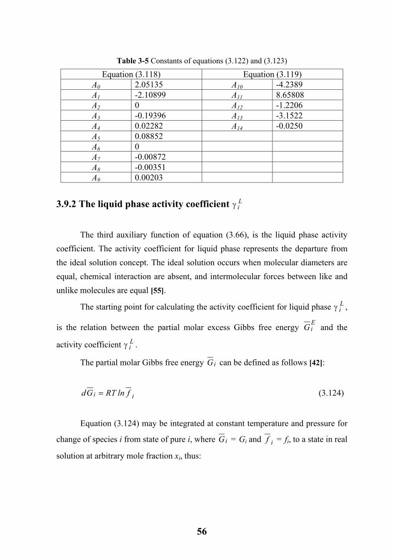
Table 3-5 Constants of equations (3.122) and (3.123)
Equation (3.118) Equation (3.119) A0 2.05135 A10 -4.2389 A1 -2.10899 A11 8.65808 A2 0 A12 -1.2206 A3 -0.19396 A13 -3.1522 A4 0.02282 A14 -0.0250 A5 0.08852 A6 0 A7 -0.00872 A8 -0.00351 A9 0.00203
3.9.2 The liquid phase activity coefficient γ Li
The third auxiliary function of equation (3.66), is the liquid phase activity
coefficient. The activity coefficient for liquid phase represents the departure from the ideal solution concept. The ideal solution occurs when molecular diameters are equal, chemical interaction are absent, and intermolecular forces between like and unlike molecules are equal [55].
The starting point for calculating the activity coefficient for liquid phase γ ,
is the relation between the partial molar excess Gibbs free energy
Li
EiG and the
activity coefficient γ . Li
The partial molar Gibbs free energy iG can be defined as follows [42]:
ii flnRTGd = (3.124)
Equation (3.124) may be integrated at constant temperature and pressure for
change of species i from state of pure i, where iG = Gi and if = fi, to a state in real
solution at arbitrary mole fraction xi, thus:
56
i
iii
ff
lnRTGG =− (3.125)
For ideal solution, the partial fugacity for species i can be written as follows:
iiidi fxf = (3.126)
Equation (3.126) known as Lewis / Randall rule, id denotes to ideal solution. Applying equation (3.125) for ideal solution:
i
idi
iidi
ff
lnRTGG =− (3.127)
Where, iiidi fxf = , thus equation (3.127) becomes:
iiidi xlnRTGG =− (3.128)
If M represents the molar value of an extensive thermodynamic properties for example (V, u, G, …etc), then an excess property ME is defined as the difference between the actual property value of a solution and the value it would have if it is an ideal solution at the same temperature, pressure and composition [39], thus:
(3.129) idE MMM −=
or in partial molal term:
idE MMM −= (3.130) If the above definition is applied to partial excess Gibbs energy, then:
57
idii
Ei GGG −= (3.131)
If equation (3.125) is subtracted from equation (3.128), the result is:
=
ii
iEi
fxf
lnRTG (3.132)
Where the term
ii
ifx
f is the definition of the activity coefficient given by
equation (3.58), thus:
( Li
Ei lnRTG γ= ) (3.133)
or: ( Li
Ei ln
RTG
γ= )
)
(3.134)
It is clear from equation (3.134) that the (γ ) is strongly depended upon the
system temperature, pressure and composition or:
Li
(3.135) ( N21Li x,...x,x,P,TF=γ
Several models have been proposed for predicting the activity coefficient
(γ ) from the excess Gibbs free energy, depending on the type of the liquid
mixtures.
Li
The liquid mixtures that contain dissimilar polar species, particularly those that can form or break hydrogen bonds, such mixtures can be classified as highly non ideal mixtures. Examples of those mixtures are the mixtures that contain water, alcohols, esters, …etc [95]. For such mixtures the most convenient activity models,
58
that widely used are, the Wilson model [96], the non – random two – liquid model (NRTL) [97, 98], and the universal qusi – chemical model (UNIQUAC) [99]. For non polar liquid mixtures, such as the hydrocarbons mixtures, the relatively simple activity models are recommended [100]. The latter is true for crude oils and petroleum fractions, because the bulk of them are consisting of hydrocarbon compounds (as discussed in Chapter 1 typically the hydrocarbon compounds representing more than 97% of crude oil or petroleum fractions). The other polar compounds such as sulfur, nitrogen, metals …etc. representing the miner constituents of crude oil or petroleum fractions. The most relatively simple activity coefficient models that are widely used for predicting the activity coefficients for petroleum fractions and hydrocarbon mixtures are: i. Regular solution models. ii. van Laar models.
3.9.2.1 Regular solution models
Chao – Seader [56] and Paul – Lachman [101] proposed and extended the simple regular models that based on the regular solution theory of Seatchard and
Hilderbrand [58] for predicting the (γ ) for hydrocarbon mixtures and petroleum
fractions. The regular solution theory is based on the premise that the non ideality in the liquid phase mixture is due to differences in van der Walls forces of attraction among the species present. Regular solutions have an endothermic heat of mixing and all activity coefficient are greater than unity (i.e. positive deviation from Raoult's law).
Li
For a multi component regular solution, the partial molal excess free energy is:
( ) (∑ ∑∑= = =
−=
N
1i
N
1i
N
1j
2jiji
Lii
Ei
21VxG δδΦΦ ) (3.136)
59
where Φ is the volume fraction, assuming additive molar volumes (VL), given as:
L
Ljj
N
1i
Ljj
Ljj
jV
Vx
Vx
Vx==
∑=
Φ (3.137)
and δ is the solubility parameter that can be evaluated by:
( )
Li
21i
iVRT−
=λ
δ (3.138)
where λ is the heat of vaporization. Relating equations (3.134) and (3.136) and with some arrangement an expression for the activity coefficient of regular solution theory can be obtained as:
RT
V
ln
2N
1iiii
Li
Li
−
=∑=
δΦδ
γ (3.139)
The calculation of γ by regular solution model involves only pure species
constants and δ
Li
LiV i. Frequently, these constants are taken at some convenient
reference temperature, such as 25 °C (77 °F). For petroleum fraction, the heat of vaporization (λ) can be calculated using the Raizi – Daubert correlation [13]:
(3.140) 0214.01347.1B gr.SpT4885.8=λ
60
3.9.2.2 van Laar models
The excess Gibbs energy is a function of the temperature, pressure and composition of system (P, T, x), but for liquid at low to moderate pressures, it is a very weak function of P. Under these conditions, its pressure dependence or in other word, the pressure dependence of activity coefficients is usually neglected. Thus, a constant temperature is achieved [55]:
( N21
Ei x,...x,xF
RTG
= ) (3.141)
In 1913 van Laar suggested a power series for representation equation (3.141). His proposed model for excess Gibbs energy for binary mixture:
221112
211221Ei
xAxAAAxx
RTG
′+′′′
= (3.142)
The activity coefficients for binary mixtures are given by substituting equation (3.141) into equation (3.134), thus:
2
212
121
12L1
AxAx
1
Aln
′′
+
′=γ (3.143)
and 2
121
212
21L2
AxAx
1
Aln
′′
+
′=γ (3.144)
where A'12 and A'21 are known as the binary interaction parameters and must be back – calculated from experimental data. These parameters are, in theory constants only
61
for a particular binary pair at a given temperature. In practice, they are frequently computed from isobaric data covering a range of temperature. Null [102], extended the van Laar model for a multi component mixture and the resulting expression for activity coefficient in this model depends only on composition and binary interaction parameters and is given by:
( ) ( )
( ) ( ) ( )
2
N
1jjiji
N
1jijji
N
1jijji
i
N
1jijj
Li
Axx1Axx
Axx
1x1
Ax
ln
−+
−−
=
∑∑
∑∑
==
==γ (3.145)
The interaction parameters Aij and Aji have the following properties: 1. Aii = Ajj = 0. 2. Aij = Aji 3. For non polar hydrocarbon pairs Aij and Aji can be estimated as follows:
( 2ji
Li
ij RTV
A δδ −= ) (3.146)
4. For polar pairs, the interaction parameters pairs Aij and Aji can be back calculated from experimental data. 5. If no useful data exist, a procedure based on estimation the binary activity coefficient at infinite dilution suggested by Null can be employed.
Because of the van Laar model, simplicity, flexibility and ability to fit many
systems that have both positive (γ >1) and negative (γ <1) deviations from
Raoult's law, it is widely used in practice [39].
Li
Li
62
3.10 Working formula for activity coefficient model for predicting the K – values
The working formula for activity coefficient model for predicting the K – values can be obtained by combining equations (3.66) and (3.108), thus:
( )
−
=
RTPPV
ExpP
PK
si
LiL
iVi
Vsi
si
i γφ
φ (3.147)
3.11 Ideal solution models for prediction K – values
Separation operations are frequently conducted under or at vacuum pressure (e.g. crude oil tower). In such process, the ideal solution concept is more reliable, and applicable. The ideal solution concept has another important requirement that is the species in the mixture have essentially identical molecular size and intermolecular forces. Thus, a mixture of isomers, such as ortho, meta and para conforms very closely to ideal solution behavior. So do mixtures of adjacent members of a homologous series such the hydrocarbon mixtures [55, 88]. If the ideal K – value equation (3.67) is recalled:
Vi
Li
iff
K = ..(3.67)
or in fugacity coefficient term:
Vi
Li
iKφ
φ= (3.148)
In equation (3.148), both the vapor and liquid phases obey the ideal solution
behavior. Substituting equation (3.108) for φ , the following equation is obtained: Li
63
( )
−
=
RTPPV
ExpP
PK
si
Li
Vi
Vsi
si
iφ
φ (3.149)
Equation (3.149), represents the working formula for ideal solution K – value. For special case at low pressure in which the vapor phase obeys the ideal gas law, and the species vapor pressures are close to system pressure, the ratio
( Vi
Vsi φφ ) will be unity and the Poynting factor (exponent term) may be neglected,
thus equation (3.149) reduces to:
P
PK
si
i = (3.150)
Equation (3.150) is well known as Raoult's law K – value formula.
For the case in which the ideal gas law is valid and the ratio of ( Vi
Vsi φ
sVi
φ ) is
not unity, and the species vapor pressures are widely differ from system pressure, so
the Poynting factor can not be negligible. For such case, the φ and φ must be
obtained using a suitable equation of state models.
Vi
A more serious problem in using equation (3.140) is posed for species whose critical temperatures are below the system temperature (Tr > 1), where the hypothetical region occurs. For ideal solution mixture, only limited extrapolation of pure fugacity coefficients into hypothetical region are required. Henly [88], suggested a simple procedure, that can be utilized for determining the pure species fugacity coefficient whether hypothetical region occurs or not. In Henly procedure, the pure species fugacity coefficient can be determined using equation (3.116) as:
∫
−
=P
0i dP
P1Zlnφ (3.116)
64
At low to moderate pressures of the ideal solution mixture, the integration of equation (3.116) is approximately constant, for a given temperature. The integration is thus readily performed, with the following result in reduced form:
−=
=0Prii
Vi
iPr
1ZPrExpφ (3.151)
The term (Z – 1/Pri) at Pri = 0 is determined from appropriate equation of state models. If the SRK equation of state is used, a reduced form is convenient. It is derived as follows, recalling SRK equation of state {equation (3.75)}.
( )bVVa
bVRTP
+−
−=
α (3.75)
Equation (3.175) can be written in Z term, as:
++
+=
h11
RTVa
h11Z α (3.152)
where Z
BPh = and RTb
=B
Multiplying and dividing equation (3.152) by b, so the following equation is obtained:
++
+=
h1h
RTba
h11Z α (3.153)
The a and b can be obtained from equation (3.83), and h can be written as follows:
65
i
iZTr
Pr08664.0RTbh == (3.154)
Substituting equations (3.83) and (3.154) into equation (3.153) to obtain the following equation:
+−
+=
i
i2i
i
i
iZTr
Pr08664.01
1ZTr
Pr4274.0
ZTrPr08664.0
1
1Zα
(3.155)
If equation (3.155) is rearranged in form of (Z – 1)/Pri and in the limit of Pri = 0 where Z → 1, then:
2ii
1Z0Pri Tr
4274.0Tr
08664.0Pr
1Zi
α−=
−
→=
(3.156)
Substituting equation (3.156) into equation (3.151) gives:
−= 2
i
i
i
iVi
TrPr4274.0
TrPr08664.0
Expα
φ (3.157)
or in the saturation conditions:
−= 2
i
si
i
siVs
iTr
Pr4274.0Tr
Pr08664.0Exp
αφ (3.158)
where: PcPPr si
si =
Substituting equations (3.157) and (3.158) into equation (3.149) gives:
66
−×
−
−
=
RTPP(V
Exp
TrPr4274.0
TrPr08664.0
Exp
TrPr4274.0
TrPr08664.0
Exp
PP
Ks
iL
i
2i
i
i
i
2i
si
i
si
si
iα
α
(3.159)
Rearranging equation (3.159), with Pri = P/Pci and is
is
i PcPPr = , thus the
following working formula is obtained for the ideal K – value as follows:
( ) ( )
−
−−
= PP
RTV
PcTr4278.0
PcTr08664.0Exp
PP
K si
Li
i2
i
i
ii
si
idealiα
(3.160)
Equation (3.160) has the following properties: 1. It is applicable for ideal solution at low to moderate pressures. 2. The exponential term is the correlation for the simple Raoult's law K – value. 3. The ideal K – value is depending only on temperature and pressure of the system and it is independent of the composition of the system or,
( ) ( P,TFK ideali = )
)
(3.161)
For the equation of state model and activity coefficient model where the solution is not ideal solution or the pressure is high, the K – value depends on temperature, pressure and composition of the system as: (3.162) ( x,P,TFKi =
3.12 Calculation of flash volume by flash calculations
One further vapor – liquid equilibrium is the flash calculation. The origin of the name comes when the change occurs when a liquid under pressure passes
67

through a valve to a pressure low enough so that some of liquid vaporizes (flashes) producing a two phase stream of vapor and liquid in equilibrium [55]. The same idea is used in crude oil tower, but instead of using the valve for reducing the pressure, the heated crude oil stream is flashed at the flash zone area in the tower. The pressure in flash zone area is approximately atmospheric pressure [3]. The other important factor in vaporization of crude oil in the flash zone is the flash zone temperature. The flash zone temperature must be fixed in such way to ensure all economically markable range of products from the complex mixtures of crude oil are vaporized [22, 103]. Three types of flash vaporization process depending on the conditions of operation, that can be found in literatures [91], those are: 1. Constant temperature and pressure (isothermal flash). 2. Constant enthalpy and pressure (isenthalpic flash). 3. Constant entropy and pressure (isentropic flash).
The constant temperature and pressure (isothermal flash) are considered here because it is widely used in petroleum refinery operations.
3.12.1 Constant temperature and pressure (isothermal flash)
It is also known as (P – T) flash process which refers to any flash calculation of system in equilibrium at known temperature and pressure (T, P) and overall feed composition [55]. Consider Fig. 3-2, that illustrates schematically the (P – T) flash process. The feed, at temperature T and pressure P, passes through at throttle and enters flash tower or vessel, where liquid and vapor phases may separate. The heat is supplied or removed at a rate of Q through a heat exchanger, so as to maintain isothermal conditions at temperature T. The molar rate of the feed to the unit is specified, together with the overall composition (mole fraction Zi), and the temperature and pressure at which the unit operates. The objectives of the calculation are to determine the compositions (yi and xi), and the molar flow rate (FV and FL) of the vapor and liquid streams leaving the unit.
68
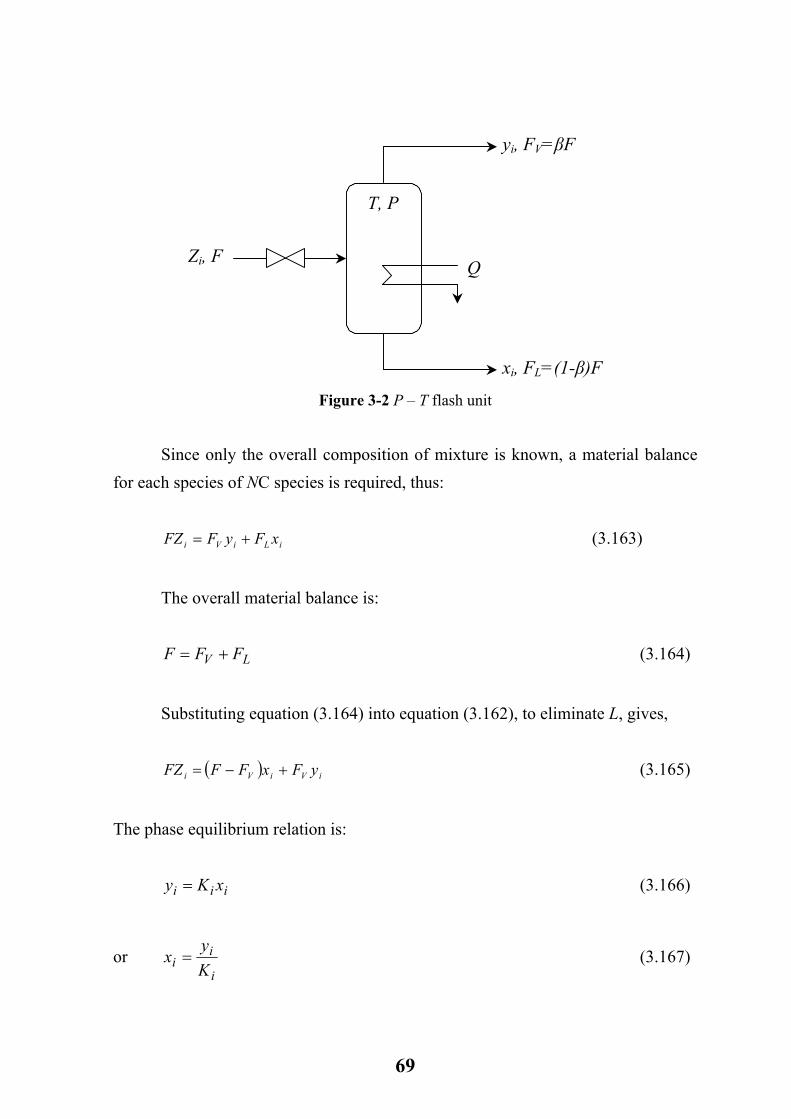
yi, FV=βF
Q
T, P
Zi, F
xi, FL=(1-β)F Figure 3-2 P – T flash unit
Since only the overall composition of mixture is known, a material balance for each species of NC species is required, thus: (3.163) iLiVi xFyFFZ +=
The overall material balance is: (3.164) LV FFF +=
Substituting equation (3.164) into equation (3.162), to eliminate L, gives, (3.165) ( ) iViVi yFxFFFZ +−=
The phase equilibrium relation is: (3.166) iii xKy =
or i
ii K
yx = (3.167)
69
Combining equation (3.166) with equation (3.165) to eliminate the yi or, (3.168) ( ) iiViVi xKFxFFFZ =−=
Or if equation (3.167) is used with equation (3.165) to eliminate xi, yields:
( ) iVi
iVi yF
Ky
FFFZ +
−= (3.169)
Rearranging equations (3.168) and (3.169) to obtain the expression for yi and xi, as:
( )11 −+=
i
ii K
Zx
β (3.170)
and ( )11 −+=
i
iii K
KZy
β (3.171)
where β = FV/F, and it is the vapor fraction for multi component system of NC species, since:
(3.172) 1zN
1ii =∑
=
(3.173) 1yN
1ii =∑
=
(3.174) 1xN
1ii =∑
=
And from overall material balance, is:
70
(3.175) 0xyN
1ii
N
1ii =− ∑∑
==
Substituting equations (3.170) and (3.171) into equation (3.175) gives:
( )∑= −+
−N
i i
iii
KzKZ
1 11 β =0 (3.176)
or, ( ) ( )( )∑
= −+−
=N
i i
ii
KKZ
F1 11
1β
β =0 (3.177)
Equation (3.177) is nonlinear in β only, and it can be solved by trial and error by guessing values of β between 0 and 1, until the F(β) = 0. The most widely employed method for solving equation (3.177) is the Newton – Raphson method [83]. The latter is discussed in Appendix B. It must be noted; that before proceeding in flash calculation, it is be sure that the input feed at a given temperature and pressure is in the two phase region. The latter can be accomplished using equation (3.177) with the following conditions [42]: 1. If F(0) > 0, the mixture is below its bubble point (sub cooled liquid). 2. If F(1) < 0, the mixture is above the dew point (super heated vapor). 3. If F(0) < 0 and F(1) > 0, the mixture in the two phase region, and the flash calculation can be proceeded (i.e. β between 0 and 1).
The EFV curve is usually obtained by plotting the volume percent vaporized against the temperature. As a result of that the vapor fraction β in mole percent must be converted to volume percent. The latter can be done by using the following equation [29]:
100F
FVV V
F
VV ×
⋅
=β (3.178)
71
Where: VF = Molal volume of the feed stream V = Molal volume of the vapor stream The molal volume of the vapor stream can be obtained by the following equation:
∑=
=N
1i i
iiV
MWyV
ρ (3.179)
Where: MWi is the species i molecular weight ρi is the species i liquid density at 15 °C (60 °F) The molal volume of the feed stream can be obtained as follows:
∑=
=N
1i i
iiF
MWzV
ρ (3.180)
Because of (FV / F) represents the vapor vaporized β, so that equation (3.178) can be written as follows:
100VV
F
VV ×
= ββ (3.181)
72
Chapter Four
Experimental work
4.1 Aim of the experimental work 1. Kirkuk, Basrah, Jambour and Bai – Hassan crude oils fractionating into approximately 10 °C narrow fractions in the range of IBP – 370 °C (IBP – 698 °F). 2. Construction of TBP curve for each of crude oils by plotting total cumulative volume (or weight) percent distilled against measured boiling point temperature. 3. Specific gravities determination for all narrow fractions distillate from Kirkuk, Basrah, Jambour and Bai – Hassan crude oils. 4. Construction of specific gravity curve by plotting total cumulative volume (or weight) percent distilled against measured specific gravity. 5. The exponential work were performed in laboratory of Dura refinery.
4.2 Feed stocks
The feed stocks used in this experimental work were Kirkuk, Basrah, Jambour and Bai – Hassan crude oils. The properties of Kirkuk, Basrah, Jambour and Bai – Hassan crude oils are given in Table 4-1. All properties were made at the laboratory of Dura refinery.
73
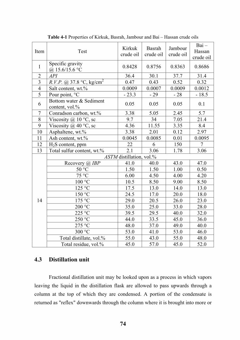
Table 4-1 Properties of Kirkuk, Basrah, Jambour and Bai – Hassan crude oils
Item Test Kirkuk crude oil
Basrah crude oil
Jambour crude oil
Bai – Hassan
crude oil
1 Specific gravity @ 15.6/15.6 °C 0.8428 0.8756 0.8363 0.8686
2 API 36.4 30.1 37.7 31.4 3 R.V.P. @ 37.8 °C, kg/cm2 0.47 0.43 0.52 0.32 4 Salt content, wt.% 0.0009 0.0007 0.0009 0.0012 5 Pour point, °C - 23.3 - 29 - 28 - 18.5
6 Bottom water & Sediment content, vol.% 0.05 0.05 0.05 0.1
7 Conradson carbon, wt.% 3.38 5.05 2.45 5.7 8 Viscosity @ 10 °C, sc 9.7 34 7.05 21.4 9 Viscosity @ 40 °C, sc 4.36 11.55 3.35 8.4 10 Asphaltene, wt.% 3.38 2.01 0.12 2.97 11 Ash content, wt.% 0.0045 0.0085 0.01 0.0095 12 H2S content, ppm 22 6 150 7 13 Total sulfur content, wt.% 2.1 3.06 1.78 3.06
ASTM distillation, vol.% Recovery @ IBP 41.0 40.0 43.0 47.0
50 °C 1.50 1.50 1.00 0.50 75 °C 6.00 4.50 4.00 4.20
100 °C 10.5 8.50 9.00 8.50 125 °C 17.5 13.0 14.0 13.0 150 °C 24.5 17.0 20.0 18.0 175 °C 29.0 20.5 26.0 23.0 200 °C 35.0 25.0 33.0 28.0 225 °C 39.5 29.5 40.0 32.0 250 °C 44.0 33.5 45.0 36.0 275 °C 48.0 37.0 49.0 40.0 300 °C 53.0 41.0 53.0 46.0
Total distillate, vol.% 55.0 43.0 55.0 48.0
14
Total residue, vol.% 45.0 57.0 45.0 52.0
4.3 Distillation unit
Fractional distillation unit may be looked upon as a process in which vapors leaving the liquid in the distillation flask are allowed to pass upwards through a column at the top of which they are condensed. A portion of the condensate is returned as "reflex" downwards through the column where it is brought into more or
74
less intimate contact with the ascending vapors. Here a heat interchange takes place between the relatively cooler liquid and warmer vapors so that more volatile part of the liquid is vaporized, while the more easily condensable part of the vapors is condensed. The net result is a concentration of more volatile material in the top of the column with increasing concentration of less volatile material as the bottom of the column is approached [3, 104].
4.3.1 Laboratory distillation unit
Distillation process was achieved on laboratory distillation apparatus (according to ASTM D2892 – 87). The main parts of the laboratory distillation apparatus are; the distillation flask, heating mantle, distillation column, reflux condenser, timer, distillate condenser, vacuum system, instrumentations for measuring the temperature and pressure of the system, fraction receiver, variable resistance for heat input controlling and simple control panel. Fig. 4-1 shows a photographs picture for the laboratory distillation unit, and Fig. 4-2 shows the schematic diagram of the laboratory distillation unit. Referring to Fig. 4-2, size of distillation flask (1), is 5 liters and provided with two side streams, first side stream used to change the crude oil, and the second side stream contains glass bulb for thermocouple type J, (2), for measurement of the bottom temperature. The specifications of thermocouple type J is given in Table C-1. The distillation flask mounted with 3kW heating mantels (3), connecting with variable resistance to control the heat input to the flask. The flask equipped with semi ball joint for connection with column. The semi ball joint was lubricated with a paste of silicone to insure a good sealing between the column and the flask. Distillation column consisted of a packed bed (4), of 25mm inside diameter and 910mm length. The packed bed consists with Helipak type packing materials, the length of the packed bed was selected to satisfy the requirement of ASTM D2892 – 87 (i.e. the length of packed bed ensures that fractionating column having an efficiency of 14 to 18 theoretical plate). The column was isolated by highly vacuum jacket containing multiple metallic reflectors (5), to minimize the heat loss. The specification of Helipak materials is given in Table C-2.
75
The top of the packed bed column was connected with a glass reflux condenser (6), of 290mm high and 50mm inside diameter and isolated by highly vacuum jacket containing multiple metallic reflectors. The glass reflux condenser was used to condense and cool the distillate. Ethylene glycol alcohol with temperature below –20°C introduced into the condenser by circulating pump of cooling machine. The use of low temperature cooling medium is essential for reducing the light hydrocarbons (mainly C4). Two side streams (7), were used for introducing the cooling medium (i.e. ethylene glycol alcohol) into the reflux condenser. The cooling by ethylene glycol alcohol continued until the temperature of the vapor reached to 75 °C, after that the cooling medium was replaced or turned to ordinary tap water. The temperature of the vapor in the head of reflux condenser was recorded by a thermocouple type J (8). The reflux ratio was controlled by using magnetic solenoid valve (a), connected with reflux timer (10). The reflux ratio of 5:1 was used for atmospheric distillation and 3:1 for vacuum distillation. The bottom of the packed bed was connected to double expansion coil (11) of height 250mm, this expansion coil was used for introducing the vapor from distillation flask into the packed bed column. The expansion coil is also ensures the suitable velocity and good distillation of the vapor through the bed column. For more details of the packed bed column, reflux condenser and the expansion coil are shown in Fig. C-2. The vapor trap (12) was connected to the top of the reflux condenser and it was isolated by vacuum jacket. The vapor trap was maintained at the temperature below –58 °C by using a mixture of solid ice and NaCl salt as cooling medium or refrigerant (13). The using of vapor trap is useful for reducing the light hydrocarbons loss.
76
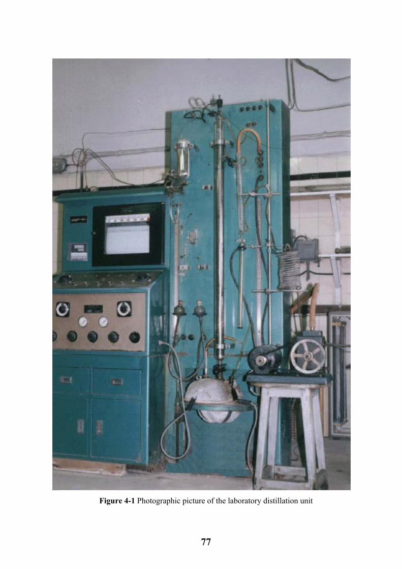
77
Figure 4-1 Photographic picture of the laboratory distillation unit
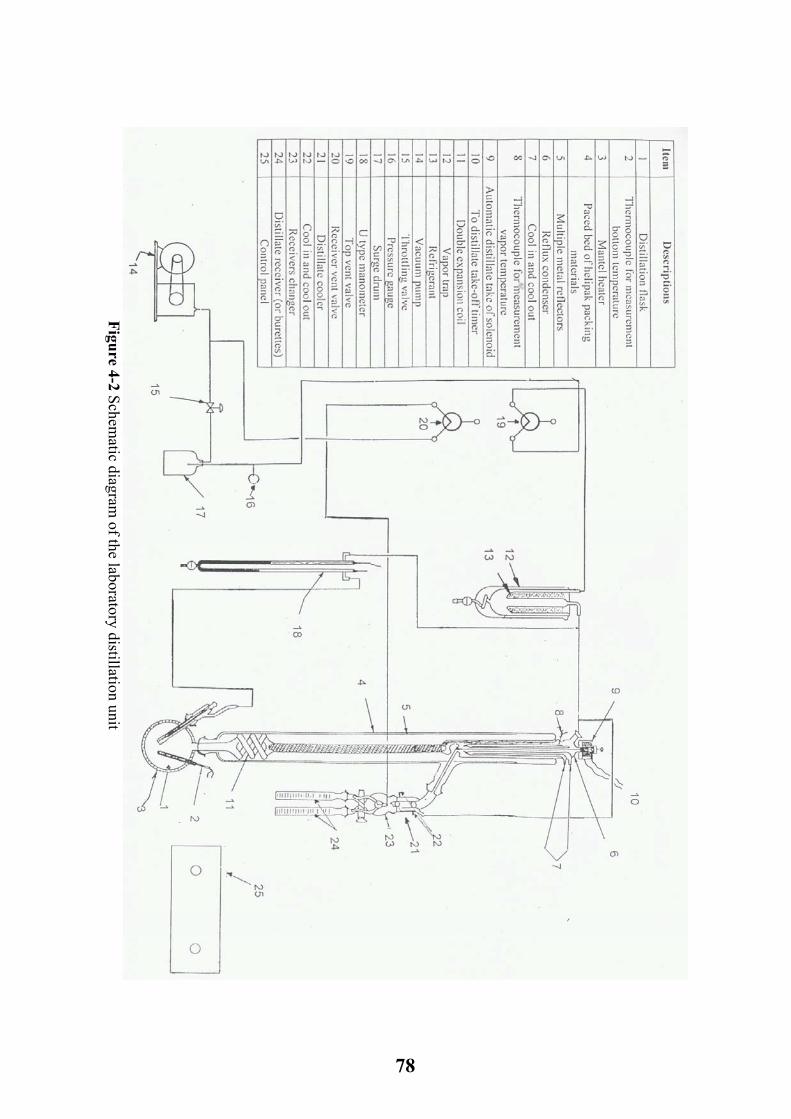
Figure 4-2 Schematic diagram
of the laboratory distillation unit
78
When the temperature of crude oil inside distillation flask reached 300 °C, the distillation column was then connected to the vacuum system for producing the suitable vacuum pressure. The vacuum system was consisted of the vacuum pump (14), throttling valve (15), pressure gauge (16), surge drum (17), U – tube manometer (18), top vent valve (19) and receiver vent valve (20). The vacuum pressure was achieved by using 1/3 HP vacuum pump of general electric type. The vacuum pump can provide a vacuum pressure of 60mmHg. The liquid distillate from reflux condenser was collected by distillate cooler (21). The distillate cooler was furthermore cooled the distillate fraction {i.e. by side streams (22)} by using ethylene glycol alcohol or ordinary trap water (the same as the cooling method that described in the reflux condenser). The aim of cooling the distillate in the distillate cooler is to reduce the light hydrocarbons loss from the light fractions (i.e. those cuts that have temperature less than 75 °C). The vacuum line of the distillate cooler, and reflux condenser were gathered by T shape joint to produce 60mmHg pressure. The bottom of the distillate cooler was connected to receiver changer valve (22), which can be opened in two positions, the first position (the normal position) in which the distillate can be collected in one distillate receiver (23), while in the second position two distillate receivers can be used. The distillate receiver has a capacity of 200ml. When the distillation unit is operated at vacuum pressure, the distillate receiver must be vented to avoid interrupting column equilibrium during taking the samples. The distillate receiver can be vented by using receiver vent valve (20). When the operation under vacuum is finished all distillation unit can be vented by using top vent valve (19). The distillation column was mounted in the column panel of 2.20m length and 0.71m width as shown in Fig. 4-1. The simple control panel (25), of 1.72m length and 0.726m width was mounted besides the column panel (as shown in Fig. 4-1) and consisting of the following items: 1. Selector switch with small screen for reading the vapor and bottom temperatures that measured by using thermocouples.
79
2. Electronic recording potentiometer for measuring the vapor temperature (not used). 3. Starting and off electrical switches for heating mantel and vacuum pump. 4. Variable resistance for controlling the input heat to heating mantel. 5. The solenoid valve timer for controlling the reflux ratio for atmospheric and vacuum distillation operations. 6. Gauge pressure for reading the vacuum pressure of the system.
The connection lines between the distillation column and other parts of distillation unit was achieved by using the double coated rubber tubing suitable for high temperature operations. The utility requirement of the distillation units can be given in Table C-4.
4.4 Density and specific gravity
Density and specific gravity of all distillation fractions from Kirkuk, Basrah, Jambour and Bai – Hassan crude oils were determined according to ASTM D12980 – 80 by using 25cm3 pycnometer. The calibration of pycnometer was performed according to ASTM D12980 – 80.
80
Chapter Five
Selected data and estimation methods The calculation of vapor – liquid equilibria for petroleum fractions is important because of the difficulty of obtaining experimental values or data. The most important vapor – liquid equilibria calculation for petroleum fractions is well known as the equilibrium flash vaporization curve (EFV) calculation. The applicability and limitations of the prediction of the EFV curve for petroleum fractions by means of graphical methods, and the pseudo – component (computer) methods had been studied. Both methods are based on converting the true boiling point curve (TBP) into the EFV curve. In the present work, the results were divided into two parts. The first part has two folds, firstly, the graphical methods and pseudo – component (computer) methods were tested to decide, which approach shows the greatest promise. Secondly, various methods for improving existing methods were investigated. The first part can be considered as testing and improving part. In the second part of the present work, the improved methods were used for predicting or calculating the EFV curves for four types of Iraqi crude oils (Kirkuk, Basrah, Jambur and Bai – Hassan). The second part can be considered as an application part.
5.1 Data sources
5.1.1 Data sources for part one (testing and improving part) For the first part of the present work, the flash data examined which come from chemical engineering literatures. Table 5-1 gives the general characterization of these data. For simplicity, the petroleum stock name will be eliminated and just the stocks number will be used. Petroleum stocks of number 1 to 15 of Table 5-1 are presented with incomplete TBP curves and overall specific gravity. The TBP
81
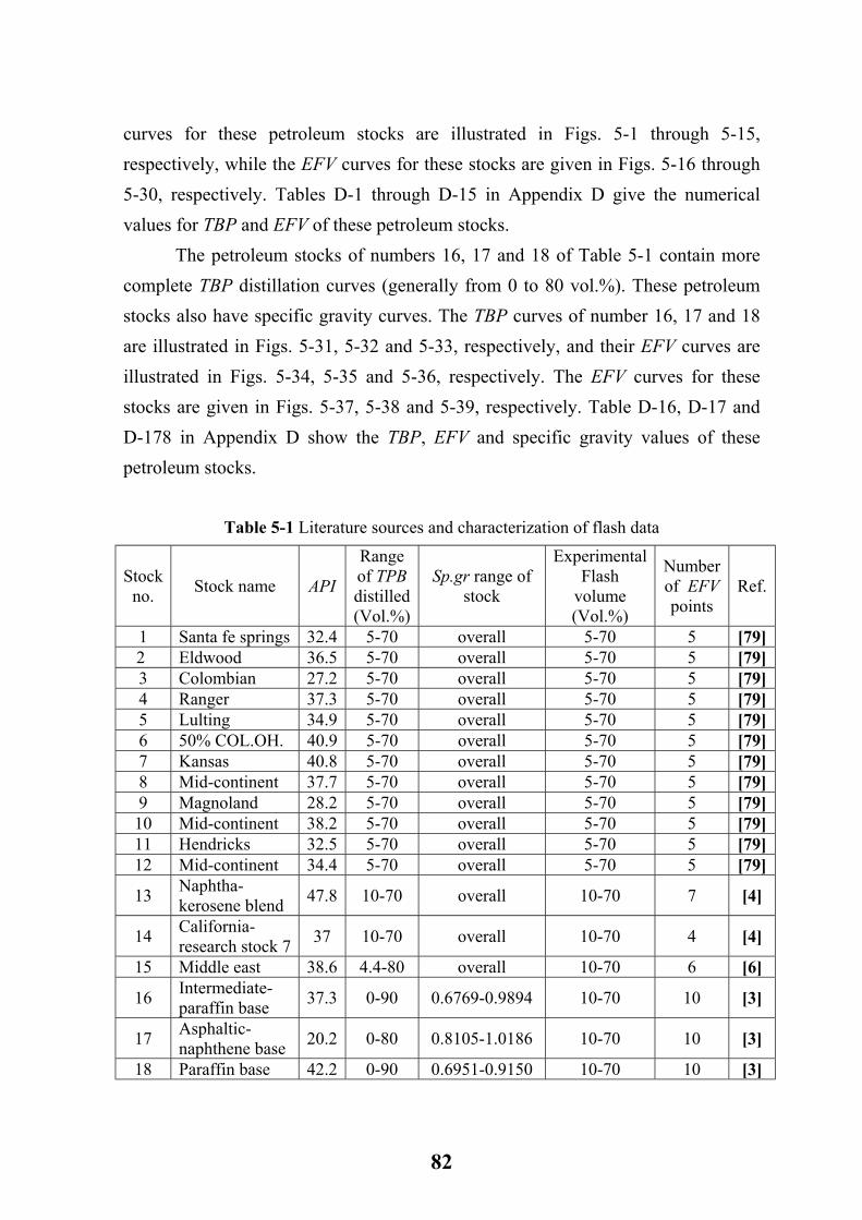
curves for these petroleum stocks are illustrated in Figs. 5-1 through 5-15, respectively, while the EFV curves for these stocks are given in Figs. 5-16 through 5-30, respectively. Tables D-1 through D-15 in Appendix D give the numerical values for TBP and EFV of these petroleum stocks. The petroleum stocks of numbers 16, 17 and 18 of Table 5-1 contain more complete TBP distillation curves (generally from 0 to 80 vol.%). These petroleum stocks also have specific gravity curves. The TBP curves of number 16, 17 and 18 are illustrated in Figs. 5-31, 5-32 and 5-33, respectively, and their EFV curves are illustrated in Figs. 5-34, 5-35 and 5-36, respectively. The EFV curves for these stocks are given in Figs. 5-37, 5-38 and 5-39, respectively. Table D-16, D-17 and D-178 in Appendix D show the TBP, EFV and specific gravity values of these petroleum stocks.
Table 5-1 Literature sources and characterization of flash data
Stock no. Stock name API
Range of TPB distilled(Vol.%)
Sp.gr range of stock
Experimental Flash
volume (Vol.%)
Number of EFV points
Ref.
1 Santa fe springs 32.4 5-70 overall 5-70 5 [79] 2 Eldwood 36.5 5-70 overall 5-70 5 [79]
3 Colombian 27.2 5-70 overall 5-70 5 [79] 4 Ranger 37.3 5-70 overall 5-70 5 [79] 5 Lulting 34.9 5-70 overall 5-70 5 [79] 6 50% COL.OH. 40.9 5-70 overall 5-70 5 [79] 7 Kansas 40.8 5-70 overall 5-70 5 [79] 8 Mid-continent 37.7 5-70 overall 5-70 5 [79] 9 Magnoland 28.2 5-70 overall 5-70 5 [79] 10 Mid-continent 38.2 5-70 overall 5-70 5 [79] 11 Hendricks 32.5 5-70 overall 5-70 5 [79] 12 Mid-continent 34.4 5-70 overall 5-70 5 [79]
13 Naphtha-kerosene blend 47.8 10-70 overall 10-70 7 [4]
14 California-research stock 7 37 10-70 overall 10-70 4 [4]
15 Middle east 38.6 4.4-80 overall 10-70 6 [6]
16 Intermediate-paraffin base 37.3 0-90 0.6769-0.9894 10-70 10 [3]
17 Asphaltic-naphthene base 20.2 0-80 0.8105-1.0186 10-70 10 [3]
18 Paraffin base 42.2 0-90 0.6951-0.9150 10-70 10 [3]
82

0 10 20 30 40 50 60 70 80 90 1
Volume Percent Distillate (Vol %)
0
50
100
150
200
250
300
350
400
450
500
550
600
650
700
750
Tem
pret
ure
C
0
00
Figure 5-1 TBP curve for petroleum stock number 1
0 10 20 30 40 50 60 70 80 90 1
Volume Percent Distillate (Vol %)
0
50
100
150
200
250
300
350
400
450
500
550
600
650
700
750
Tem
pret
ure
C
0
00
Figure 5-2 TBP curve for petroleum stock number 2
83
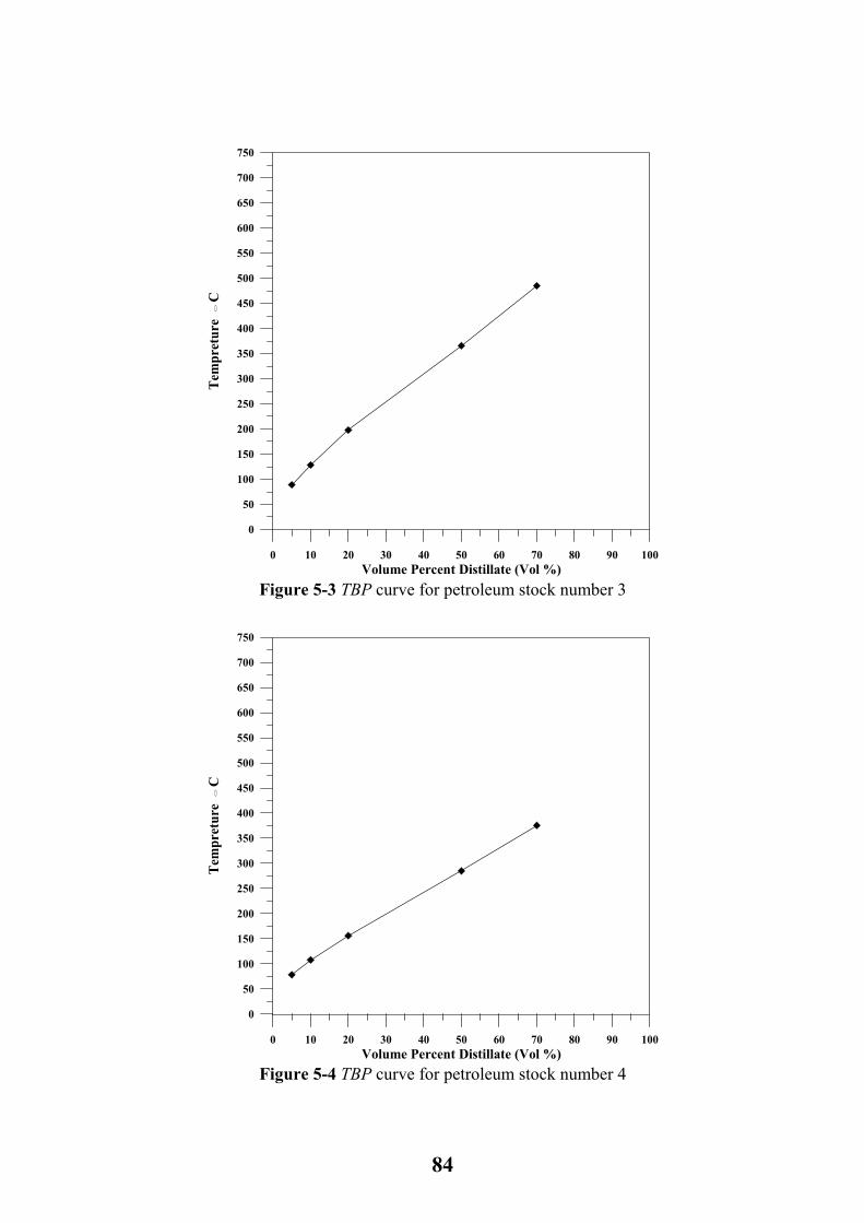
0 10 20 30 40 50 60 70 80 90 1
Volume Percent Distillate (Vol %)
0
50
100
150
200
250
300
350
400
450
500
550
600
650
700
750
Tem
pret
ure
C
0
00
Figure 5-3 TBP curve for petroleum stock number 3
0 10 20 30 40 50 60 70 80 90 1
Volume Percent Distillate (Vol %)
0
50
100
150
200
250
300
350
400
450
500
550
600
650
700
750
Tem
pret
ure
C
0
00
Figure 5-4 TBP curve for petroleum stock number 4
84
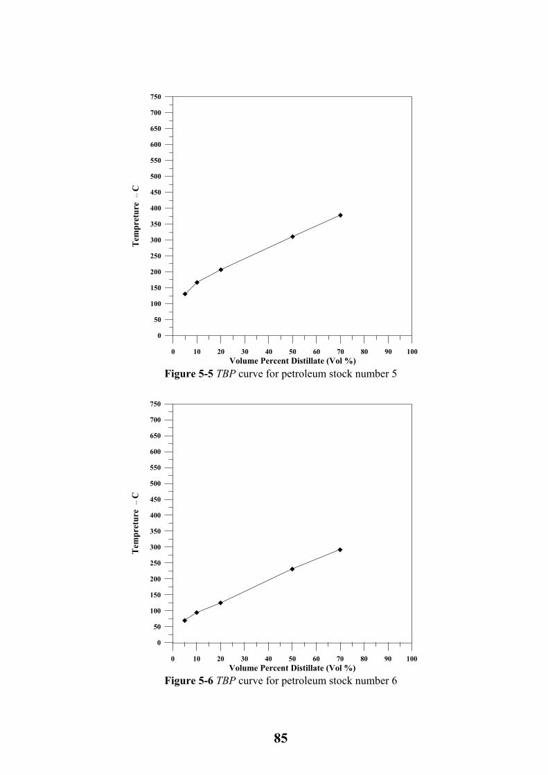
0 10 20 30 40 50 60 70 80 90 1
Volume Percent Distillate (Vol %)
0
50
100
150
200
250
300
350
400
450
500
550
600
650
700
750
Tem
pret
ure
C
0
00
Figure 5-5 TBP curve for petroleum stock number 5
0 10 20 30 40 50 60 70 80 90 1
Volume Percent Distillate (Vol %)
0
50
100
150
200
250
300
350
400
450
500
550
600
650
700
750
Tem
pret
ure
C
0
00
Figure 5-6 TBP curve for petroleum stock number 6
85

0 10 20 30 40 50 60 70 80 90 1
Volume Percent Distillate (Vol %)
0
50
100
150
200
250
300
350
400
450
500
550
600
650
700
750
Tem
pret
ure
C
0
00
Figure 5-7 TBP curve for petroleum stock number 7
0 10 20 30 40 50 60 70 80 90 1
Volume Percent Distillate (Vol %)
0
50
100
150
200
250
300
350
400
450
500
550
600
650
700
750
Tem
pret
ure
C
0
00
Figure 5-8 TBP curve for petroleum stock number 8
86
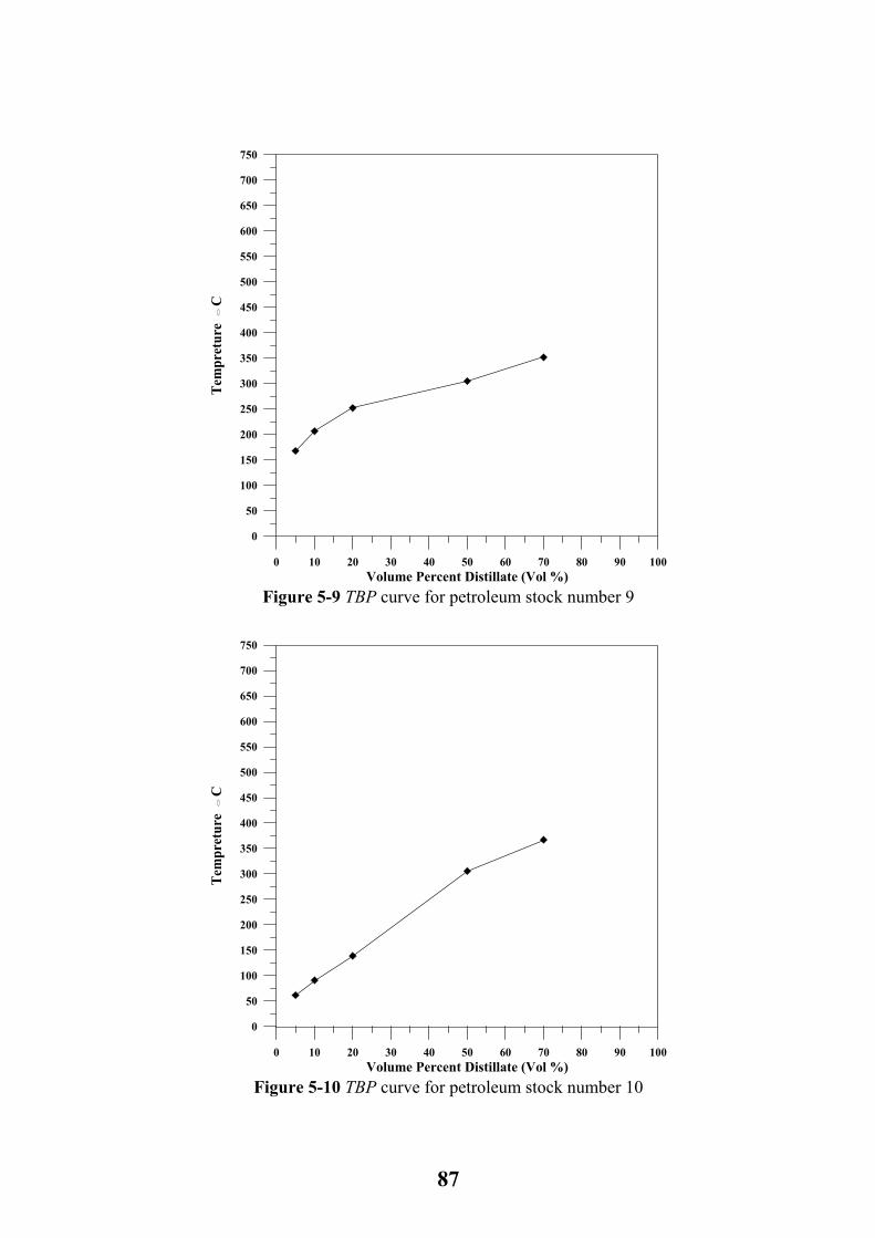
0 10 20 30 40 50 60 70 80 90 1
Volume Percent Distillate (Vol %)
0
50
100
150
200
250
300
350
400
450
500
550
600
650
700
750
Tem
pret
ure
C
0
00
Figure 5-9 TBP curve for petroleum stock number 9
0 10 20 30 40 50 60 70 80 90 1
Volume Percent Distillate (Vol %)
0
50
100
150
200
250
300
350
400
450
500
550
600
650
700
750
Tem
pret
ure
C
0
00
Figure 5-10 TBP curve for petroleum stock number 10
87
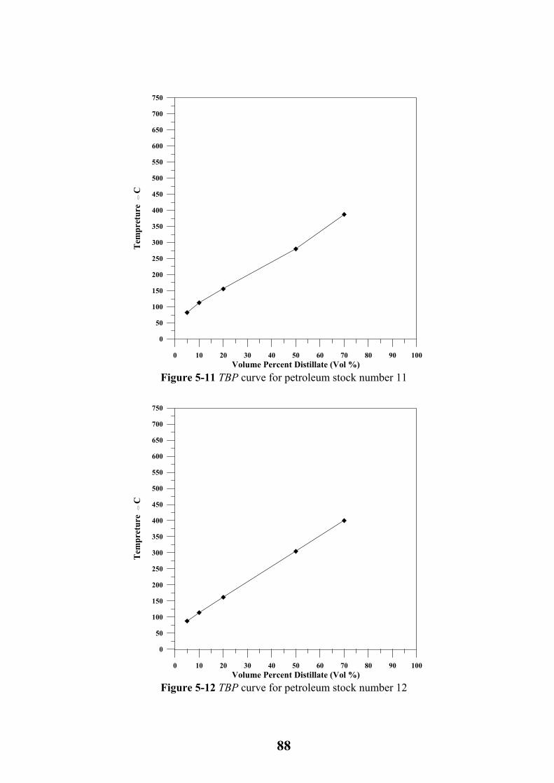
0 10 20 30 40 50 60 70 80 90 1
Volume Percent Distillate (Vol %)
0
50
100
150
200
250
300
350
400
450
500
550
600
650
700
750
Tem
pret
ure
C
0
00
Figure 5-11 TBP curve for petroleum stock number 11
0 10 20 30 40 50 60 70 80 90 1
Volume Percent Distillate (Vol %)
0
50
100
150
200
250
300
350
400
450
500
550
600
650
700
750
Tem
pret
ure
C
0
00
Figure 5-12 TBP curve for petroleum stock number 12
88

0 10 20 30 40 50 60 70 80 90 1
Volume Percent Distillate (Vol %)
0
50
100
150
200
250
300
350
400
450
500
550
600
650
700
750
Tem
pret
ure
C
0
00
Figure 5-13 TBP curve for petroleum stock number 13
0 10 20 30 40 50 60 70 80 90 1
Volume Percent Distillate (Vol %)
0
50
100
150
200
250
300
350
400
450
500
550
600
650
700
750
Tem
pret
ure
C
0
00
Figure 5-14 TBP curve for petroleum stock number 14
89

0 10 20 30 40 50 60 70 80 90 1
Volume Percent Distillate (Vol %)
0
50
100
150
200
250
300
350
400
450
500
550
600
650
700
750
Tem
pret
ure
C
0
00
Figure 5-15 TBP curve for petroleum stock number 15
0 10 20 30 40 50 60 70 80 90 1
Volume Percent Distillate (Vol %)
0
50
100
150
200
250
300
350
400
450
500
550
600
650
700
750
Tem
pret
ure
C
0
00
Figure 5-16 EFV curve for petroleum stock number 1
90
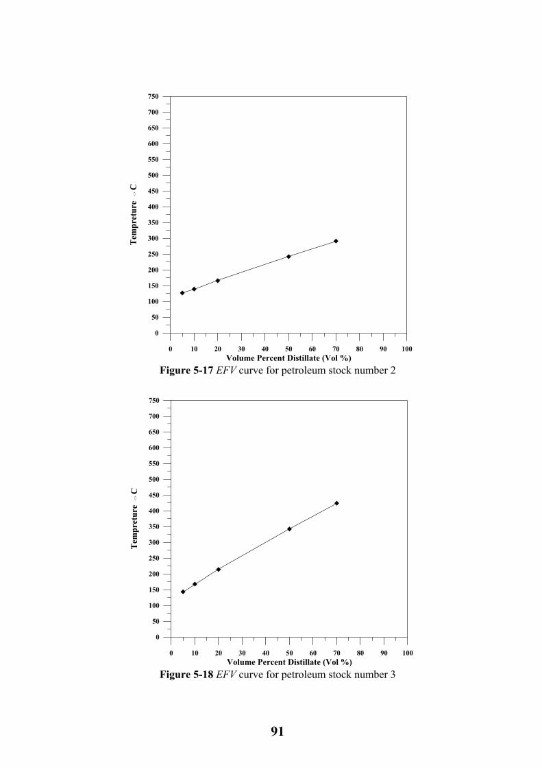
0 10 20 30 40 50 60 70 80 90 1
Volume Percent Distillate (Vol %)
0
50
100
150
200
250
300
350
400
450
500
550
600
650
700
750
Tem
pret
ure
C
0
00
Figure 5-17 EFV curve for petroleum stock number 2
0 10 20 30 40 50 60 70 80 90 1
Volume Percent Distillate (Vol %)
0
50
100
150
200
250
300
350
400
450
500
550
600
650
700
750
Tem
pret
ure
C
0
00
Figure 5-18 EFV curve for petroleum stock number 3
91

0 10 20 30 40 50 60 70 80 90 1
Volume Percent Distillate (Vol %)
0
50
100
150
200
250
300
350
400
450
500
550
600
650
700
750
Tem
pret
ure
C
0
00
Figure 5-19 EFV curve for petroleum stock number 4
0 10 20 30 40 50 60 70 80 90 1
Volume Percent Distillate (Vol %)
0
50
100
150
200
250
300
350
400
450
500
550
600
650
700
750
Tem
pret
ure
C
0
00
Figure 5-20 EFV curve for petroleum stock number 5
92

0 10 20 30 40 50 60 70 80 90 1
Volume Percent Distillate (Vol %)
0
50
100
150
200
250
300
350
400
450
500
550
600
650
700
750
Tem
pret
ure
C
0
00
Figure 5-21 EFV curve for petroleum stock number 6
0 10 20 30 40 50 60 70 80 90 1
Volume Percent Distillate (Vol %)
0
50
100
150
200
250
300
350
400
450
500
550
600
650
700
750
Tem
pret
ure
C
0
00
Figure 5-22 EFV curve for petroleum stock number 7
93

0 10 20 30 40 50 60 70 80 90 1
Volume Percent Distillate (Vol %)
0
50
100
150
200
250
300
350
400
450
500
550
600
650
700
750
Tem
pret
ure
C
0
00
Figure 5-23 EFV curve for petroleum stock number 8
0 10 20 30 40 50 60 70 80 90 1
Volume Percent Distillate (Vol %)
0
50
100
150
200
250
300
350
400
450
500
550
600
650
700
750
Tem
pret
ure
C
0
00
Figure 5-24 EFV curve for petroleum stock number 9
94
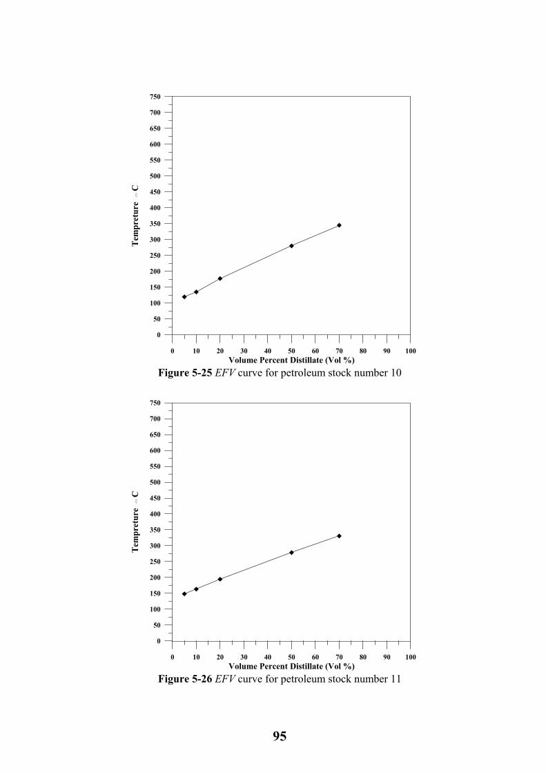
0 10 20 30 40 50 60 70 80 90 1
Volume Percent Distillate (Vol %)
0
50
100
150
200
250
300
350
400
450
500
550
600
650
700
750
Tem
pret
ure
C
0
00
Figure 5-25 EFV curve for petroleum stock number 10
0 10 20 30 40 50 60 70 80 90 1
Volume Percent Distillate (Vol %)
0
50
100
150
200
250
300
350
400
450
500
550
600
650
700
750
Tem
pret
ure
C
0
00
Figure 5-26 EFV curve for petroleum stock number 11
95
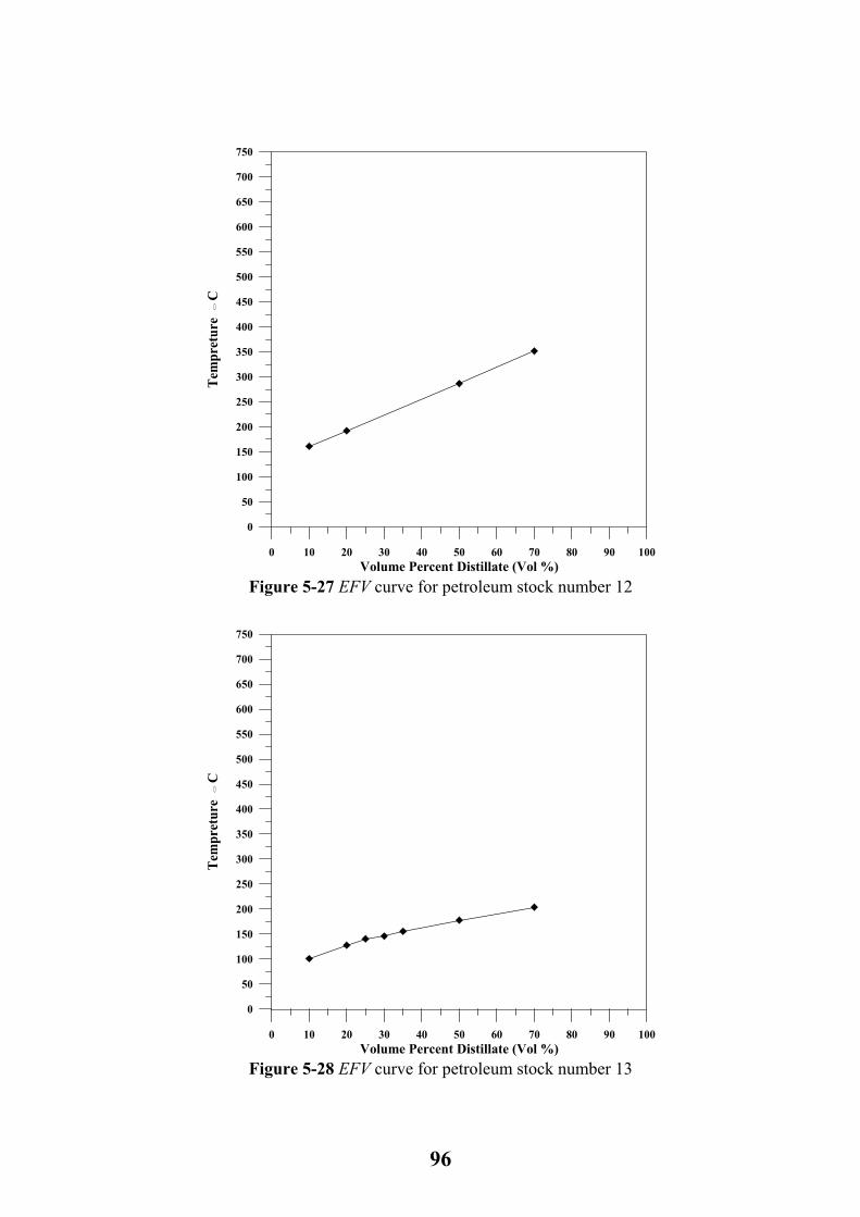
0 10 20 30 40 50 60 70 80 90 1
Volume Percent Distillate (Vol %)
0
50
100
150
200
250
300
350
400
450
500
550
600
650
700
750
Tem
pret
ure
C
0
00
Figure 5-27 EFV curve for petroleum stock number 12
0 10 20 30 40 50 60 70 80 90 1
Volume Percent Distillate (Vol %)
0
50
100
150
200
250
300
350
400
450
500
550
600
650
700
750
Tem
pret
ure
C
0
00
Figure 5-28 EFV curve for petroleum stock number 13
96
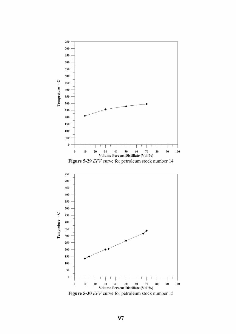
0 10 20 30 40 50 60 70 80 90 1
Volume Percent Distillate (Vol %)
0
50
100
150
200
250
300
350
400
450
500
550
600
650
700
750
Tem
pret
ure
C
0
00
Figure 5-29 EFV curve for petroleum stock number 14
0 10 20 30 40 50 60 70 80 90 1
Volume Percent Distillate (Vol %)
0
50
100
150
200
250
300
350
400
450
500
550
600
650
700
750
Tem
pret
ure
C
0
00
Figure 5-30 EFV curve for petroleum stock number 15
97
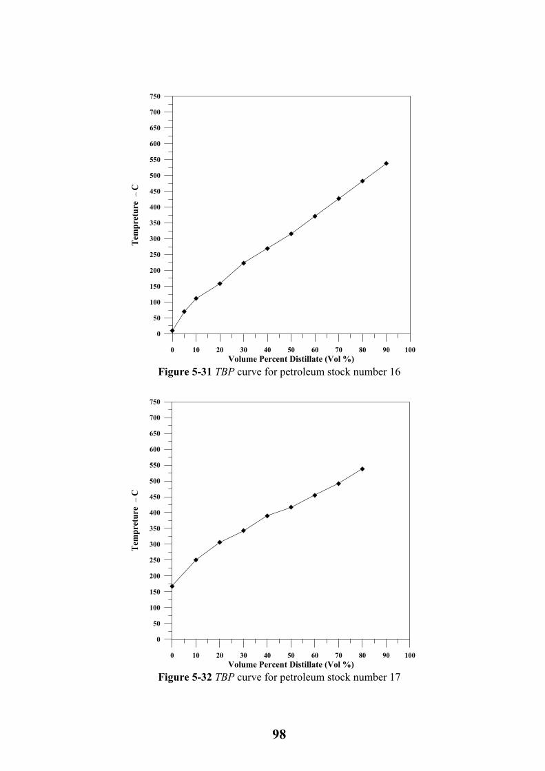
0 10 20 30 40 50 60 70 80 90 1
Volume Percent Distillate (Vol %)
0
50
100
150
200
250
300
350
400
450
500
550
600
650
700
750
Tem
pret
ure
C
0
00
Figure 5-31 TBP curve for petroleum stock number 16
0 10 20 30 40 50 60 70 80 90 1
Volume Percent Distillate (Vol %)
0
50
100
150
200
250
300
350
400
450
500
550
600
650
700
750
Tem
pret
ure
C
0
00
Figure 5-32 TBP curve for petroleum stock number 17
98
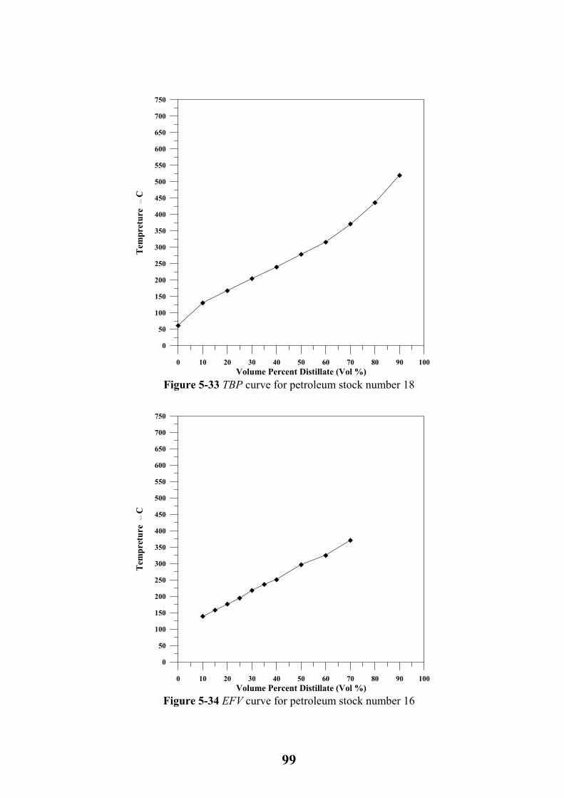
0 10 20 30 40 50 60 70 80 90 1
Volume Percent Distillate (Vol %)
0
50
100
150
200
250
300
350
400
450
500
550
600
650
700
750
Tem
pret
ure
C
0
00
Figure 5-33 TBP curve for petroleum stock number 18
0 10 20 30 40 50 60 70 80 90 1
Volume Percent Distillate (Vol %)
0
50
100
150
200
250
300
350
400
450
500
550
600
650
700
750
Tem
pret
ure
C
0
00
Figure 5-34 EFV curve for petroleum stock number 16
99
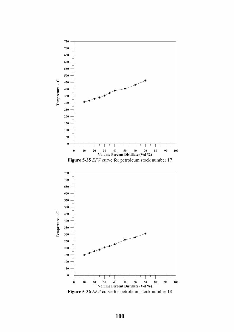
0 10 20 30 40 50 60 70 80 90 1Volume Percent Distillate (Vol %)
0
50
100
150
200
250
300
350
400
450
500
550
600
650
700
750
Tem
pret
ure
C
0
00
Figure 5-35 EFV curve for petroleum stock number 17
0 10 20 30 40 50 60 70 80 90 1
Volume Perce t Distillate (Vol %)
0
50
100
150
200
250
300
350
400
450
500
550
600
650
700
750
Tem
pret
ure
C
0
00
Figure 5-36 EFV curve for petroleum stock number 18 n
100
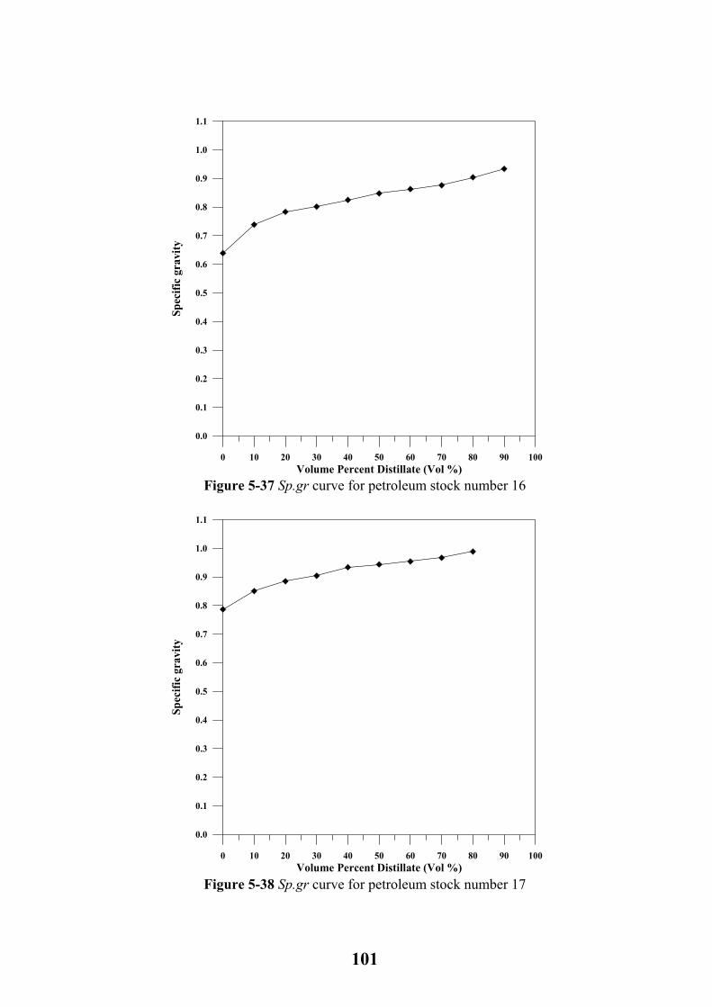
0 10 20 30 40 50 60 70 80 90 1
Volume Percent Distillate (Vol %)
0.0
0.1
0.2
0.3
0.4
0.5
0.6
0.7
0.8
0.9
1.0
1.1
Spec
ific
grav
ity
00
Figure 5-37 Sp.gr curve for petroleum stock number 16
0 10 20 30 40 50 60 70 80 90 1
Volume Percent Distillate (Vol %)
0.0
0.1
0.2
0.3
0.4
0.5
0.6
0.7
0.8
0.9
1.0
1.1
Spec
ific
grav
ity
00
Figure 5-38 Sp.gr curve for petroleum stock number 17
101
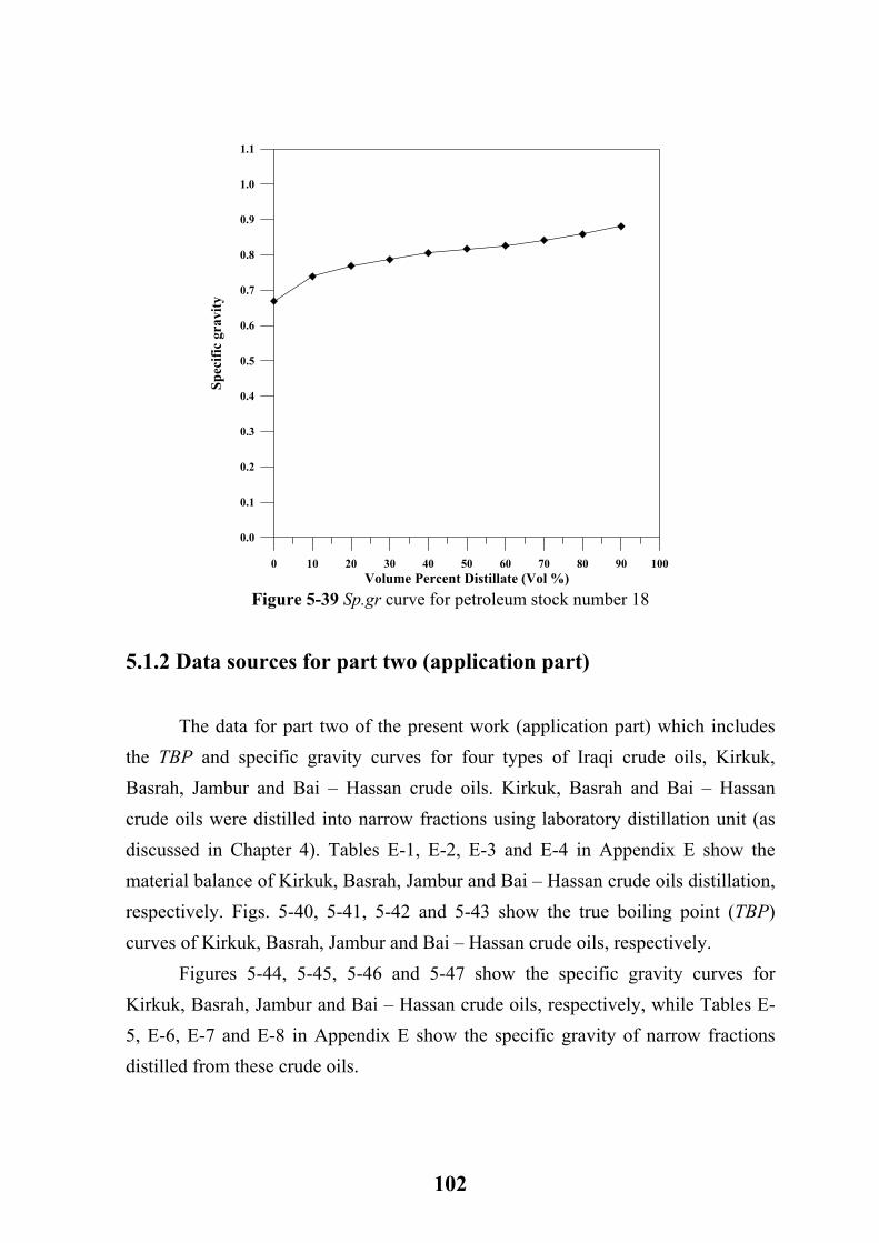
0 10 20 30 40 50 60 70 80 90 1Volume Percent Distillate (Vol %)
0.0
0.1
0.2
0.3
0.4
0.5
0.6
0.7
0.8
0.9
1.0
1.1
Spec
ific
grav
ity
00
Figure 5-39 Sp.gr curve for petroleum stock number 18
5.1.2 Data sources for part two (application part)
The data for part two of the present work (application part) which includes the TBP and specific gravity curves for four types of Iraqi crude oils, Kirkuk, Basrah, Jambur and Bai – Hassan crude oils. Kirkuk, Basrah and Bai – Hassan crude oils were distilled into narrow fractions using laboratory distillation unit (as discussed in Chapter 4). Tables E-1, E-2, E-3 and E-4 in Appendix E show the material balance of Kirkuk, Basrah, Jambur and Bai – Hassan crude oils distillation, respectively. Figs. 5-40, 5-41, 5-42 and 5-43 show the true boiling point (TBP) curves of Kirkuk, Basrah, Jambur and Bai – Hassan crude oils, respectively. Figures 5-44, 5-45, 5-46 and 5-47 show the specific gravity curves for Kirkuk, Basrah, Jambur and Bai – Hassan crude oils, respectively, while Tables E-5, E-6, E-7 and E-8 in Appendix E show the specific gravity of narrow fractions distilled from these crude oils.
102
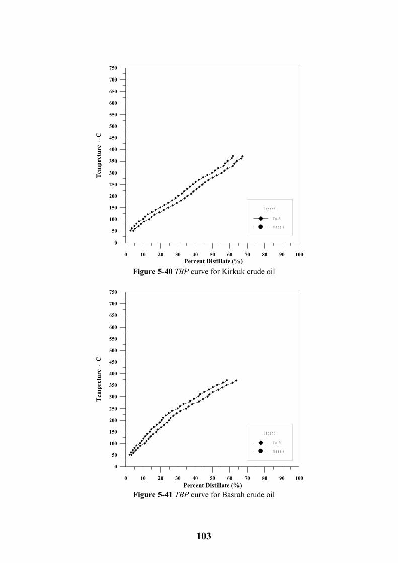
0 10 20 30 40 50 60 70 80 90 1
Percent Distillate (%)
0
50
100
150
200
250
300
350
400
450
500
550
600
650
700
750
Tem
pret
ure
C
0
Legend
V ol %
M ass %
00
Figure 5-40 TBP curve for Kirkuk crude oil
0 10 20 30 40 50 60 70 80 90 1
Percent Distillate (%)
0
50
100
150
200
250
300
350
400
450
500
550
600
650
700
750
Tem
pret
ure
C
0
Legend
V ol %
M ass %
00
Figure 5-41 TBP curve for Basrah crude oil
103
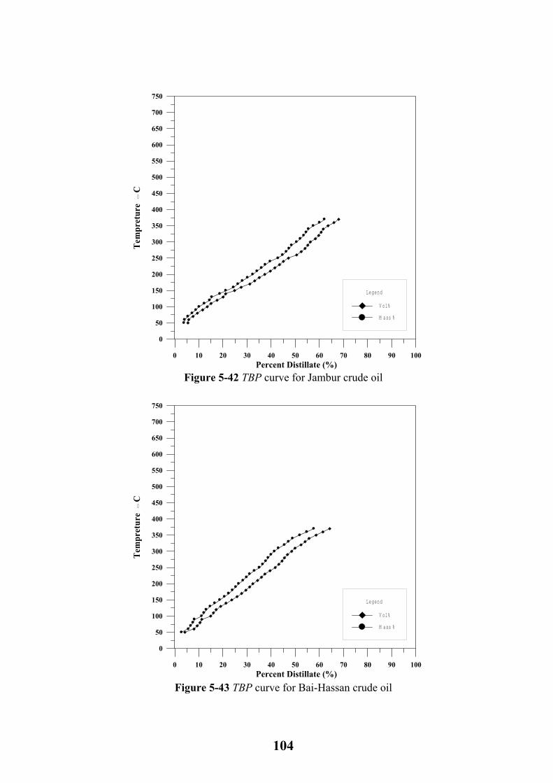
0 10 20 30 40 50 60 70 80 90 1
Percent Distillate (%)
0
50
100
150
200
250
300
350
400
450
500
550
600
650
700
750
Tem
pret
ure
C
0
Legend
V ol %
M ass %
00
Figure 5-42 TBP curve for Jambur crude oil
0 10 20 30 40 50 60 70 80 90 1
Percent Distillate (%)
0
50
100
150
200
250
300
350
400
450
500
550
600
650
700
750
Tem
pret
ure
C
0
Legend
V ol %
M ass %
00
Figure 5-43 TBP curve for Bai-Hassan crude oil
104
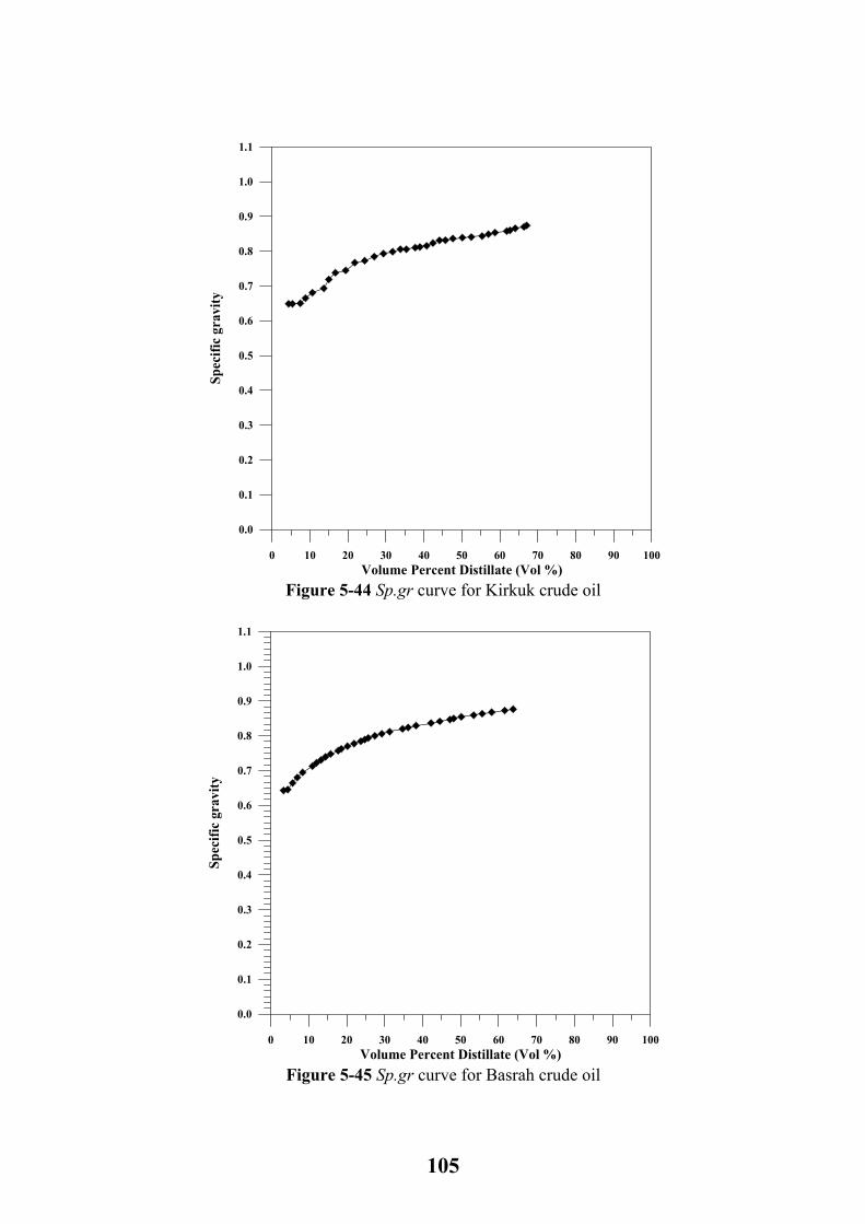
0 10 20 30 40 50 60 70 80 90 1
Volume Percent Distillate (Vol %)
0.0
0.1
0.2
0.3
0.4
0.5
0.6
0.7
0.8
0.9
1.0
1.1
Spec
ific
grav
ity
00
Figure 5-44 Sp.gr curve for Kirkuk crude oil
0 10 20 30 40 50 60 70 80 90 1
Volume Percent Distillate (Vol %)
0.0
0.1
0.2
0.3
0.4
0.5
0.6
0.7
0.8
0.9
1.0
1.1
Spec
ific
grav
ity
00
Figure 5-45 Sp.gr curve for Basrah crude oil
105
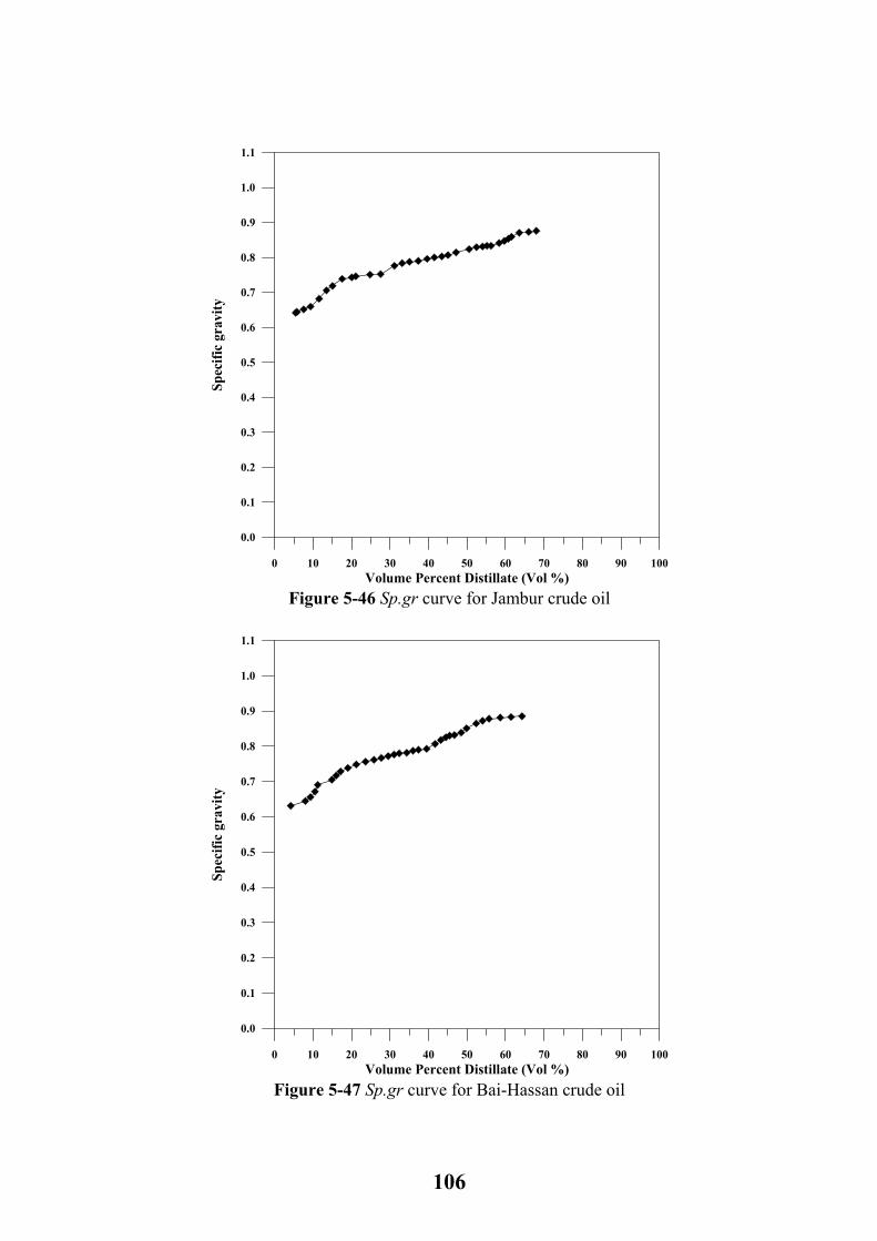
0 10 20 30 40 50 60 70 80 90 1
Volume Percent Distillate (Vol %)
0.0
0.1
0.2
0.3
0.4
0.5
0.6
0.7
0.8
0.9
1.0
1.1
Spec
ific
grav
ity
00
Figure 5-46 Sp.gr curve for Jambur crude oil
0 10 20 30 40 50 60 70 80 90 1
Volume Percent Distillate (Vol %)
0.0
0.1
0.2
0.3
0.4
0.5
0.6
0.7
0.8
0.9
1.0
1.1
Spec
ific
grav
ity
00
Figure 5-47 Sp.gr curve for Bai-Hassan crude oil
106
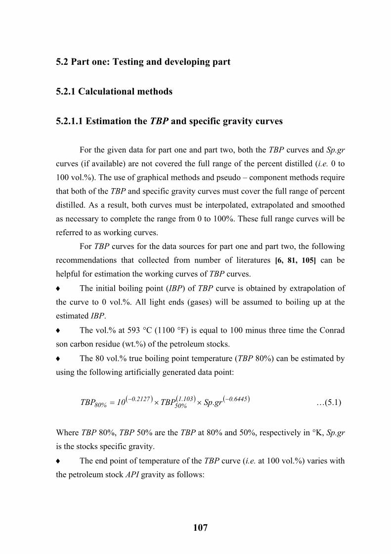
5.2 Part one: Testing and developing part
5.2.1 Calculational methods
5.2.1.1 Estimation the TBP and specific gravity curves
For the given data for part one and part two, both the TBP curves and Sp.gr curves (if available) are not covered the full range of the percent distilled (i.e. 0 to 100 vol.%). The use of graphical methods and pseudo – component methods require that both of the TBP and specific gravity curves must cover the full range of percent distilled. As a result, both curves must be interpolated, extrapolated and smoothed as necessary to complete the range from 0 to 100%. These full range curves will be referred to as working curves. For TBP curves for the data sources for part one and part two, the following recommendations that collected from number of literatures [6, 81, 105] can be helpful for estimation the working curves of TBP curves.
♦
♦
♦
)
♦
The initial boiling point (IBP) of TBP curve is obtained by extrapolation of the curve to 0 vol.%. All light ends (gases) will be assumed to boiling up at the estimated IBP.
The vol.% at 593 °C (1100 °F) is equal to 100 minus three time the Conrad son carbon residue (wt.%) of the petroleum stocks.
The 80 vol.% true boiling point temperature (TBP 80%) can be estimated by using the following artificially generated data point:
( ) ( ) ( 6445.0103.1%50
2127.0%80 gr.SpTBP10TBP −− ××= …(5.1)
Where TBP 80%, TBP 50% are the TBP at 80% and 50%, respectively in °K, Sp.gr is the stocks specific gravity.
The end point of temperature of the TBP curve (i.e. at 100 vol.%) varies with the petroleum stock API gravity as follows:
107
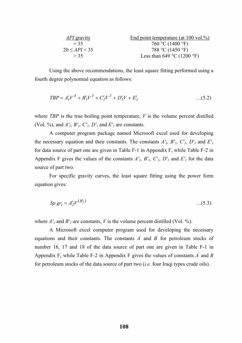
API gravity End point temperature (at 100 vol.%) = 35 760 °C (1400 °F)
20 ≤ API < 35 788 °C (1450 °F) > 35 Less than 649 °C (1200 °F)
Using the above recommendations, the least square fitting performed using a fourth degree polynomial equation as follows:
…(5.2) 112
13
14
1 EVDVCVBVATBP ′+′+′+′+′=
where TBP is the true boiling point temperature, V is the volume percent distilled (Vol. %), and A'1, B'1, C'1, D'1 and E'1 are constants. A computer program package named Microsoft excel used for developing the necessary equation and their constants. The constants A'1, B'1, C'1, D'1 and E'1 for data source of part one are given in Table F-1 in Appendix F, while Table F-2 in Appendix F gives the values of the constants A'1, B'1, C'1, D'1 and E'1 for the data source of part two. For specific gravity curves, the least square fitting using the power form equation gives:
…(5.3) ( 2B2i VAgr.Sp ′′= )
where A'2 and B'2 are constants, V is the volume percent distilled (Vol. %). A Microsoft excel computer program used for developing the necessary equations and their constants. The constants A' and B' for petroleum stocks of number 16, 17 and 18 of the data source of part one are given in Table F-1 in Appendix F, while Table F-2 in Appendix F gives the values of constants A' and B for petroleum stocks of the data source of part two (i.e. four Iraqi types crude oils).
108
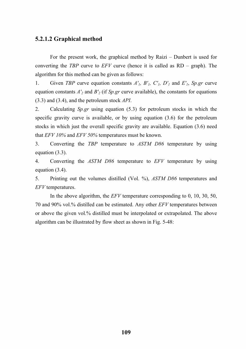
5.2.1.2 Graphical method
For the present work, the graphical method by Raizi – Dunbert is used for converting the TBP curve to EFV curve (hence it is called as RD – graph). The algorithm for this method can be given as follows: 1. Given TBP curve equation constants A'1, B'1, C'1, D'1 and E'1, Sp.gr curve equation constants A'2 and B'2 (if Sp.gr curve available), the constants for equations (3.3) and (3.4), and the petroleum stock API. 2. Calculating Sp.gr using equation (5.3) for petroleum stocks in which the specific gravity curve is available, or by using equation (3.6) for the petroleum stocks in which just the overall specific gravity are available. Equation (3.6) need that EFV 10% and EFV 50% temperatures must be known. 3. Converting the TBP temperature to ASTM D86 temperature by using equation (3.3). 4. Converting the ASTM D86 temperature to EFV temperature by using equation (3.4). 5. Printing out the volumes distilled (Vol. %), ASTM D86 temperatures and EFV temperatures.
In the above algorithm, the EFV temperature corresponding to 0, 10, 30, 50, 70 and 90% vol.% distilled can be estimated. Any other EFV temperatures between or above the given vol.% distilled must be interpolated or extrapolated. The above algorithm can be illustrated by flow sheet as shown in Fig. 5-48:
109
Print vol.%, ASTM D86, EFV
Estimate EFV temperature Corresponding to 0, 10, 30, 50, 70, 90 vol.%
Estimate ASTM D86 temperature
Calculate Sp.gr {equation (5.3) or (3.6)}
Given A'1, B'1, C'1, D'1 and E'1 for TBP curve A'2 and B'2 for Sp.gr curve
a, b, c for equations (3.3) and (3.4)
Figure 5-48 Flow sheet for algorithm of Raizi – Daubert graphical method (RD – graph)
5.2.1.3 Pseudo – component (computer) methods
Pseudo – component (computer) methods based on three thermodynamic models for predicting K – values used in the present work. These thermodynamic models are; equation of state model (EOS), activity coefficient models and the ideal solution K – value model. All these models discussed in details in Chapter three. To obtain the EFV curve from TBP curve using the pseudo – component (computer) methods, there are four important steps that must be achieved. These steps were discussed previously in Chapter three, but because of their importance, they summarized here again to show the present work handling and treatments of the estimation. These steps are:
110
Step one: The TBP curve is divided into a suitable number of fractions or cuts. In the present work the available working TBP curves were divided into 40 cuts with volumes distilled range of 2.5% for each cuts. This suggested method of splitting the TBP curve into 40 cuts will ensure that the boiling point range of each cut has a good agreement with the literature boiling range of 5 – 25 °C (41 – 77 °F). Step two: Using the mid – boiling point (TB) and specific gravity (Sp.gr), the basic characterization parameters for each cut can be estimated. The basic parameter including the critical properties (critical temperatures and critical pressures), acentric factor (ω) and the molecular weight (MW). In the present work the Raizi – Daubert correlations (API – method) was used for estimation the molecular weight (MW), critical temperature (Tc), critical pressure (Pc) (i.e. equations (3.41), (3.42) and (3.43) respectively of Table 3-3), while the Lee – Kesler correlations was used for estimation the acentric factor (ω) (i.e. equations (3.12) and (3.13) in Table 3-3). The Raizi – Daubert correlations for estimation the critical properties (Tc, Pc) have a maximum TB limitation of 343 °C (650 °F). For the TB greater than 343 °C (650 °F), the present work suggested that using the Lee – Kesler correlations for estimation Tc and Pc for each cut (i.e. equations (3.9) and (3.10) respectively of Table 3-3). The Lee – Kesler correlations give a good accuracy for estimation the Tc and Pc for heavy cuts (i.e. TB ≥ 343 °C (650 °F)) [7]. The liquid volume basis for the cuts can then be converted to weight basis and finally to mole basis. The conversion procedure needs the specific gravity and molecular weight of each cut. The specific gravities for the given data in the present work were of two types, first type for those petroleum stocks in which just the overall specific gravities were available (petroleum stocks of number 1 to 15 in Table 5-1). In such case, the specific gravity for each cut can be estimated by using the Katz – Firoozabadi correlation {i.e. equation (3.7)}. For petroleum stocks in which the specific gravity curves were available, the specific gravity for each cut can be obtained by using the equation form of (5.3). The latter is true for petroleum stocks of number 16, 17 and 18 in Table 5-1, and also for four types of Iraqi crude oils. Using any input type of specific gravity, the specific gravity for each cuts must be adjusted to satisfy of the petroleum stocks the overall specific gravity. The latter must be done before estimation of the basic characterization constants (i.e. MW, Tc,
111
Pc, ω …etc). Using the adjusted specific gravity and the molecular weight for each cut, the feed compositions in mole basis can be obtained by performing the material balance (i.e. converting volume basis of TBP curve to weight and mole basis respectively). Steps one and two of pseudo – component methods can be considered as characterization steps and they must be performed before proceeding in flash calculations for obtaining the flash volume at system temperature and pressure. In the present work the following algorithm used for performing the characterization steps: 1. Given TBP curve in form of equation (5.2), API gravity of petroleum stocks, overall feed volume basis (Vt). 2. Splitting the TBP curve into 40 cuts or pseudo – components. Each cut has a volume percent range of 2.5%. Estimate the TB for each cut by using the mid – boiling point concept. 3. Obtaining the specific gravity for each cut (Sp.gri) by using equation (3.7) for overall specific gravity type, or equations (5.3) and (5.4) for available specific gravity curve type. If equation (5.3) is used, the mid – point specific gravity can be obtained using mid – point concept. 4. Estimation of weight of each cut by the following equations:
iii Vgr.SpW ×= …(5.4)
…(5.5) ∑=
=N
1iit WW
where, Wi is the weight for each cut, Vi is the volume of each cut and Wt is the total estimated weight. For the present work, a basis of 4000 cm3 of petroleum stock used for obtaining the material balance, thus each cut has a volume of 100 cm3 (i.e. Vi = 100 cm3). The overall petroleum weight (Wf) is obtained by using the petroleum stock specific gravity (i.e. Wf = 4000 × Sp.gr of feed).
112
5. Comparing the total estimated weight (Wt), with the overall petroleum stock weight (Wf). If Wt differs from Wf then the specific gravity for each cut must be adjusted to satisfy the overall. 6. Estimation of molecular weight (MW) and critical properties (Tc, Pc) and acentric factor (ω) using Raizi – Daubert and Lee – kasler correlations for material balance and the overall petroleum stock specific gravity. 7. If there is no differences between Wf and Wt, then the moles of each fraction can be estimated using the following equations:
i
ii MW
WN = …(5.6)
…(5.7) ∑=
=N
1iit NN
8. Estimation of the feed compositions in mole basis as follows:
t
ii N
NZ = …(5.8)
The characterization algorithm can be illustrated also by the flow sheet diagram shown in Fig. 5-49. Step three: In the third step, the K – values for cuts can be estimated using suitable thermodynamic models. In the present work, different types of thermodynamic models are used. Each of these thermodynamic models will be treated as a separate pseudo – component method. These different types of thermodynamic models can be summarized as follows: 1. SPK and PR equations of state (EOS) are used in both vapor and liquid phases. The working equation for estimation the K – values by using equation of state models is given by equation (3.65).
113
Print out Ni, Nt and Zfi
Estimation of Ni, Nt and Zfi for each cuts {equations (5.6) – (5.8)}
Estimation of MW, Tc, Pc, ω for each cuts (Raizi – Daubert and Lee – Kasler correlations)
Yes
No Adjust Sp.gr Wt = Wf
Estimation of Wi, Wt {equation (5.4) and (5.5)}, Wf
Estimation of TB, Sp.gri for each cuts {equation (3.7)}
Dividing TBP, Sp.gr curves into 40 cuts of 2.5% (i.e. 2.5, 5, 7.5, …etc)
Given TBP curve {equation (5.2)} Specific gravity curve {equation (5.3)}
Estimation of TB for each cuts, Sp.gri {equation (3.7)}
Dividing TBP curve into 40 cuts of 2.5% (i.e. 2.5, 5, 7.5, …etc)
Given TBP curve {equation (5.2)} Overall specific gravity of petroleum stocks
Figure 5-49 Flow sheet for algorithm of characterization steps of pseudo – components
methods
114
2. The SRK EOS are used for vapor phase and the activity coefficient model by van – Laar {equation (3.145)} used for liquid phase (this model henceforth called as SRK + Van). Also the PR EOS is used for the vapor phase and the activity coefficient model by van – Laar used for the liquid phase (this model henceforth called as RP + Van). The working equation for prediction the K – values using the activity coefficient models is given by equation (3.147). 3. The ideal solution model is used in the present work, where both phases (vapor and liquid phases) are considered to form ideal solution. The working equation for estimation the K – values by ideal solution model is given by equation (3.160) (henceforth this model is called as Ideal K). Step four: In this step, the flash volume at a given temperature, pressure and compositions can be estimated by performing the isothermal flash calculations (P – T flash process). The latter can be done by solving equation (3.177) for β by Newton – Raphson method. The β can then be converted to volume basis by using equation (3.181). The algorithm for performing (P – T) flash calculations will be summarized in the next sections.
5.2.1.4 Algorithms (procedures) for performing isothermal flash (P – T) calculations
Many algorithms or procedures for performing isothermal flash calculation can be found in literatures [88, 89 and 91]. All these algorithms can be divided into two categories, the first category in which the K – values of species are not depending on the system compositions. The ideal solution K – value equation {equation (3.160)} falls in such category. In the second category, the K – values are depending on the system compositions, the EOS and activity coefficient models {equations (3.65) and (3.147)} fall into such category. For the present work and since dealing with the bulk of petroleum fractions and hydrocarbons (more than 98% vol. %), the following two assumptions will be adopted: a. All the interaction parameters (Kij) for both SRK and PR EOS mixing rules assumed to be zero.
115
b. Testing the two phase region will be achieved using the ideal K – values only (i.e. using equation (3.177) for β = 1 and 0) and there is no need to perform the bubble and dew point calculations.
5.2.1.4.1 Isothermal flash calculation algorithm using ideal K – values models
The Rachford – Rice [42, 88] algorithm for isothermal flash calculations where the K – values are independent of the system compositions (first category) was adopted in the present work. The Rachford – Rice algorithm can be summarized as follows: 1. Input flash temperature (T) and flash pressure (P), feed molar rate (F), feed compositions (Zfi), petroleum stock API, cut critical properties (Tci, Pci), acentric
factors (ωi), alfa functions (αi), vapor pressures and molar volumes at system
temperature (V ) for Tr < 1 and Tr > 1.
siP
Li
2. Calculating of K – values for each cut (Ki), using equation (3.160). 3. Testing for two phase by solution of equation (3.177) for β = 0 and β = 1 {i.e. F(0) and F(1)}. If F(0) < 0 and F(1) > 0, then the flash calculation can be achieved or if not the given feed composition is at the bubble point conditions and β = 0. Go to step 10. 4. If the flash calculation is achieved, equation (3.177) can be solved for β using Newton – Raphson method (see Appendix D). 5. Calculation of vapor flow rate (FV) and liquid flow rate (FL) by using the following equations:
FFV ×= β …(5.9)
VL FFF −= ..(5.10)
6. Calculation of vapor and liquid phases compositions (yi, xi) using equations (3.171) and (3.170), respectively.
116
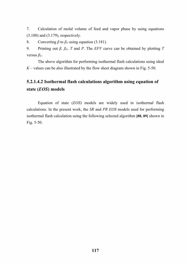
7. Calculation of molal volume of feed and vapor phase by using equations (3.180) and (3.179), respectively. 8. Converting β to βV using equation (3.181). 9. Printing out β, βV, T and P. The EFV curve can be obtained by plotting T versus βV.
The above algorithm for performing isothermal flash calculations using ideal K – values can be also illustrated by the flow sheet diagram shown in Fig. 5-50.
5.2.1.4.2 Isothermal flash calculations algorithm using equation of state (EOS) models
Equation of state (EOS) models are widely used in isothermal flash calculations. In the present work, the SR and PR EOS models used for performing isothermal flash calculation using the following selected algorithm [88, 89] shown in Fig. 5-50.
117
Convert β to βV {equation (3.181)}
Calculate Vf, VV {equations (3.180) and (3.179)}
Calculate FV, FL {equations (5.9) and (5.10)} xi, yi {equations (3.170) and (3.171)}
Print out β, βV, T, P
Solve F(β) of equation (3.177) for β (Newton – Raphson method)
Yes
No β = 0, βV = 0 F(0) < 0 and F(1) > 1
Given T, P, Zfi, F, Tci, Pci, ω, αi, Pis, ViL
Solve equation (3.177) for β = 0 and β = 1 (two phase region testing)
Calculate Ki {equation (3.160)}
Figure 5-50 Flow sheet for algorithm for Rachford – Rice algorithm for isothermal flash calculations using ideal K – values equation
118
1. Input the flash temperature (T), flash pressure (P), feed rate (F), feed compositions (Zfi), critical properties (Tci, Pci), acentric factors (ωi), vapor
pressures ( ), alfa functions (αsiP i) and molar volumes (V ) at system temperature
for Tr > 1 and Tr < 1.
Li
2. Assuming an initial value of K – values for each cut at a given flash temperature and flash pressure (T, P). The ideal K – values given by equation
(3.160) can provide the initial K – values ( ). AiK
3. Testing for two phase region by solving equation (3.175) {F(β)} with β = 0, and β = 1. If F(0) < 0 and F(1) > 0, then the flash calculation can be performed and proceeding to step 4. If the above conditions are not satisfied, then β = 0 and βV = 0 and proceeding to step 12. 4. Performing flash calculations by solving equation (3.175) for β by Newton – Raphson method (as shown in Appendix D). 5. Calculation of vapor and liquid compositions (yi, xi) using equations (3.170) and (3.171), respectively. 6. Calculation of liquid and vapor phase compressibility factors (ZV, ZL) using equation (3.79) for SRK EOS or equation (3.92) for PR EOS {using Newton – Raphson method (as shown in Appendix D)}. Calculation of partial molal fugacity
coefficients for liquid and vapor phases ( Liφ , V
iφ ) using equations (3.85) and (3.87)
for SRK EOS, or equations (3.98) and (3.100) for PR EOS. 7. Calculation of new K – values (Ki), using equation (3.65). 8. Checking for the solution by applying the following constraint:
≤
−∑=
N
1i
2
Ai
i
1KK
Є ..(5.11)
where Є is the preset error tolerance (e.g. 0.0001), and N is the number of components or cuts in the system.
119
9. If the constraint of equation (5.11) is satisfied, then the solution has been reached for both (β) and (Ki) and then proceeding to step 10. If not steps 2 through 7 must be repeated using the calculated K – values (Ki) as initial values. 10. Calculation of FV and FL using equations (5.9) and (5.10). Also calculation of vapor and liquid phase compositions (yi and xi) using equations (3.171) and (3.170). 11. Calculation of molar density for feed and vapor phase streams by using equations (3.180) and (3.179). 12. Calculation of βV using equation (3.181). 13. Printing out β, βV, T and P. The EFV curve can be obtained by plotting T versus βV.
The above algorithm can be also illustrated in the flow sheet diagram shown in Fig. 5-51.
5.2.1.4.3 Isothermal flash calculation algorithm using activity coefficients models
Activity coefficients models are widely used in isothermal flash calculations. In the present work, the SRK and PR EOS used for vapor phase, while the van – Laar activity coefficient model used for the liquid phase. The following algorithm used in the present work for performing isothermal flash calculations [88, 91]:
120
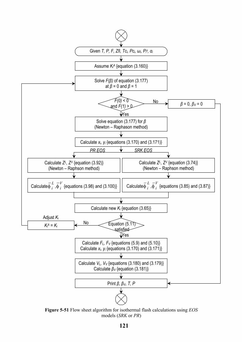
121
Li
Vi
Li
Vi
Print β, βV, T, P
Calculate VL, VV {equations (3.180) and (3.179)} Calculate βV {equation (3.181)}
Calculate FL, FV {equations (5.9) and (5.10)} Calculate xi, yi {equations (3.170) and (3.171)}
Adjust KiNo KiA = Ki
Yes
Equation (5.11) satisfied
Calculate new Ki {equation (3.65)}
Calculateφ ,φ {equations (3.85) and (3.87)} Calculateφ ,φ {equations (3.98) and (3.100)}
SRK EOS PR EOS
Calculate ZL, ZV {equation (3.74)} (Newton – Raphson method)
Calculate ZL, ZV {equation (3.92)} (Newton – Raphson method)
Calculate xi, yi {equations (3.170) and (3.171)}
Solve equation (3.177) for β (Newton – Raphason method)
Yes
No β = 0, βV = 0 F(0) < 0 and F(1) > 0
Given T, P, F, Zfi, Tci, Pci, ωi, Pis, αi
Solve F(β) of equation (3.177) at β = 0 and β = 1
Assume KiA {equation (3.160)}
Figure 5-51 Flow sheet algorithm for isothermal flash calculations using EOS models (SRK or PR)
1. Given flash temperature (T), flash pressure (P), feed rate (F), feed compositions (Zfi), critical properties (Tci, Pci), acentric factors (ωi), vapor
pressures ( ), alfa functions (αsiP i), solubility parameters (δi) and molar volume
(V ) at a system temperature for Tr > 1 and Tr < 1. Li
2. Assuming initial values of K – values for each cuts ( ) at a given flash
temperature (T), and flash pressures (P). The latter can be done using equation (3.160).
AiK
3. Testing for two phase region by solving equation (3.177) {F(β)} with β = 0 and β = 1. If F(0) < 0 and F(1) > 0, then the flash calculation can be performed and proceeding to step 4. If the above conditions are not satisfied then β = 0, βV = 0 and proceeding to step ?. 4. Performing flash calculations, by solving equation (3.177) for β using Newton – Raphson method (as shown in Appendix D). 5. Calculation of vapor and liquid phases compositions (yi and xi) using equations (3.170) and (3.171).
6. Calculation of activity coefficient (γ ) using van – Laar model {equation
(3.145)}.
Li
7. Calculation of vapor phase compressibility factor (ZV) by using equation (3.79) for SRK EOS or (3.92) for PR EOS (Newton – Raphson method, as shown in
Appendix D). partial molal fugacity coefficients Viφ can be estimated using
equation (3.87) for SRK EOS or equation (3.98) for PR EOS. 8. Checking of supercritical region (Tr > 1). If Tri > 1, the new K – values for each species (Ki), can be calculated by using equation (3.68). The liquid phase
partial molal fugacity coefficients (φ ) of equation (3.66) can be estimated by
using Choa – Sender correlation {equations (3.121) – (3.123)}. For the case of Tr < 1 proceeding to step 9.
Li
9. For Tri < 1, the new K – values can be estimated by using equation (3.147).
The saturated fugacity coefficients (φ ) for equation (3.147) can be obtained from
equation (3.118) for SRK EOS, or (3.120) for PR EOS. The saturated
Vsi
122
compressibility factor ( ) can be estimated by solving equation (3.79) for SRK
EOS or (3.92) for PR EOS (using Newton – Raphson method).
VsiZ
10. Checking for solution by applying equation (5.11). If the constraint of (5.11) (Є ≤ 0.0001) is reached then the solutions for both β and Ki are achieved and proceeding to step 11. If not, then steps 2 through 10 must be repeated using the calculated (Ki) as initial values. 11. When the solutions for (β) and (Ki) are achieved, then calculation of vapor and liquid compositions (xi, yi) can be done using equations (3.171) and (3.170). FV and FL also can be obtained using equations (5.9) and (5.10). 12. Calculation of molar volumes for feed stream (Vf) and vapor phase stream (VL) using equations (3.180) and (3.179). 13. Calculation of βV using equation (3.181). 14. Printing out β, βV, T and P. The EFV curve can be obtained by plotting T versus βV.
The above mentioned algorithm for isothermal flash calculations using the activity coefficients models can be illustrated by the following flow sheet diagram:
123
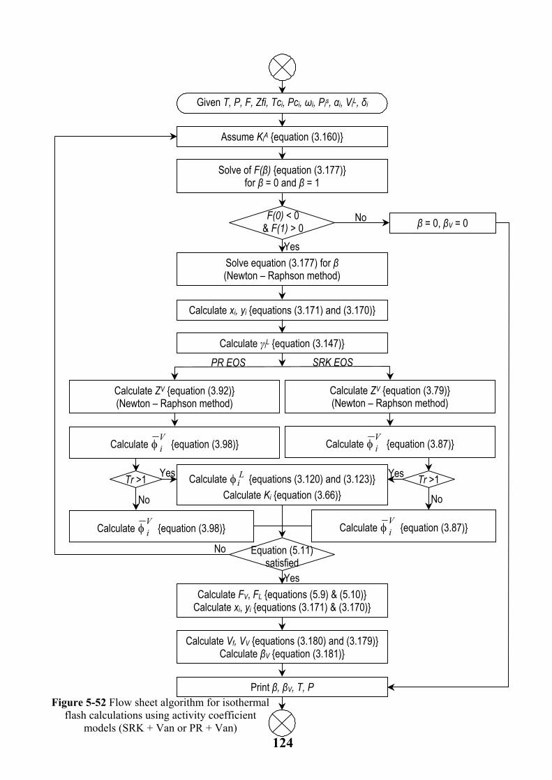
124
Calculate φ {equation (3.98)}
Vi
Vi
Li
Vi
Vi
Figure 5-52 Flow sheet algorithm for isothermal flash calculations using activity coefficient
models (SRK + Van or PR + Van)
Print β, βV, T, P
Calculate Vf, VV {equations (3.180) and (3.179)} Calculate βV {equation (3.181)}
No
Yes
Equation (5.11) satisfied
No No
Calculate φ {equation (3.87)}
Yes Yes Calculate φ {equations (3.120) and (3.123)} Calculate Ki {equation (3.66)}
Tr >1 Tr >1
Calculate γiL {equation (3.147)}
Calculate FV, FL {equations (5.9) & (5.10)} Calculate xi, yi {equations (3.171) & (3.170)}
Calculate φ {equation (3.87)} Calculate φ {equation (3.98)}
SRK EOS PR EOS
Calculate ZV {equation (3.79)} (Newton – Raphson method)
Calculate ZV {equation (3.92)} (Newton – Raphson method)
Calculate xi, yi {equations (3.171) and (3.170)}
Solve equation (3.177) for β (Newton – Raphson method)
Yes
No β = 0, βV = 0 F(0) < 0 & F(1) > 0
Given T, P, F, Zfi, Tci, Pci, ωi, Pis, αi, ViL, δi
Solve of F(β) {equation (3.177)} for β = 0 and β = 1
Assume KiA {equation (3.160)}
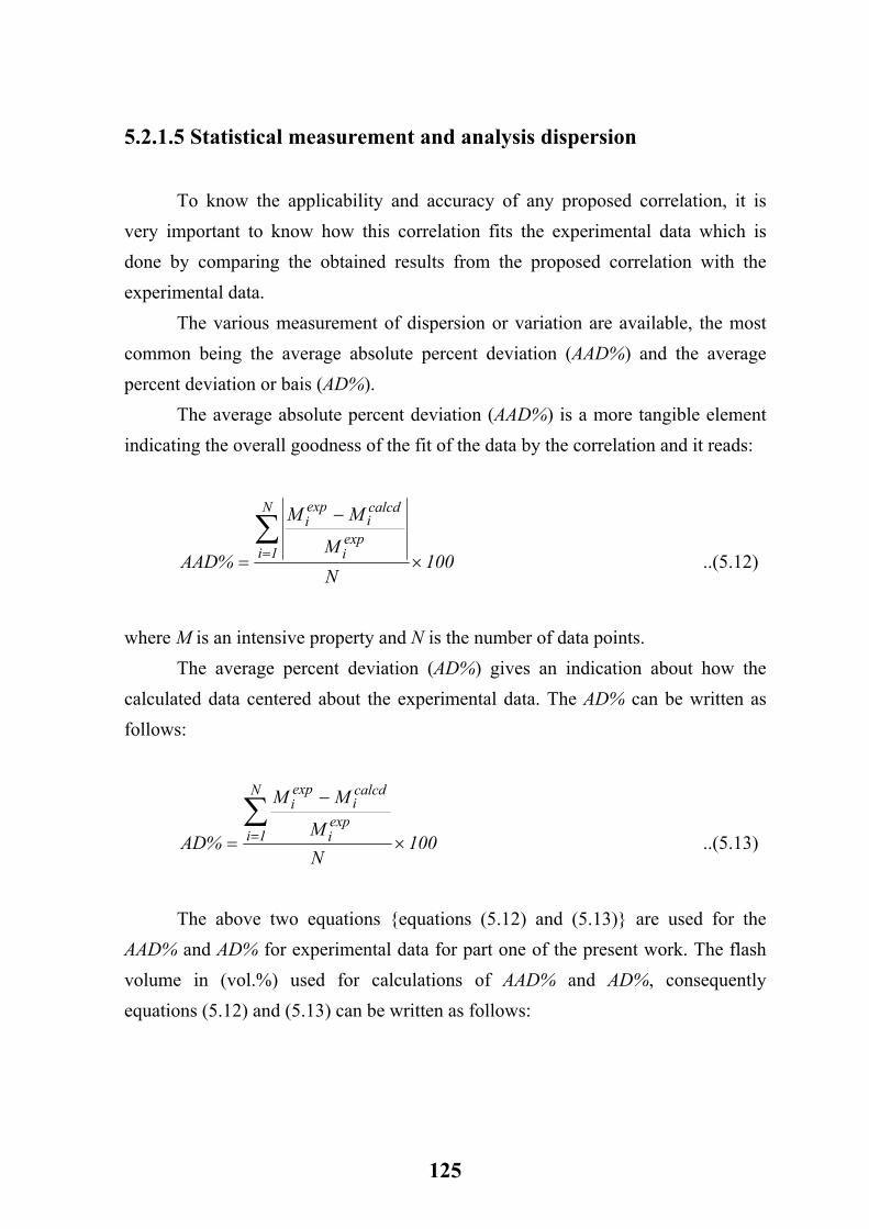
5.2.1.5 Statistical measurement and analysis dispersion
To know the applicability and accuracy of any proposed correlation, it is very important to know how this correlation fits the experimental data which is done by comparing the obtained results from the proposed correlation with the experimental data. The various measurement of dispersion or variation are available, the most common being the average absolute percent deviation (AAD%) and the average percent deviation or bais (AD%). The average absolute percent deviation (AAD%) is a more tangible element indicating the overall goodness of the fit of the data by the correlation and it reads:
100NM
MM
%AAD
N
1iexpi
calcdi
expi
×
−
=∑= ..(5.12)
where M is an intensive property and N is the number of data points. The average percent deviation (AD%) gives an indication about how the calculated data centered about the experimental data. The AD% can be written as follows:
100NM
MM
%AD
N
1iexpi
calcdi
expi
×
−
=∑= ..(5.13)
The above two equations {equations (5.12) and (5.13)} are used for the AAD% and AD% for experimental data for part one of the present work. The flash volume in (vol.%) used for calculations of AAD% and AD%, consequently equations (5.12) and (5.13) can be written as follows:
125
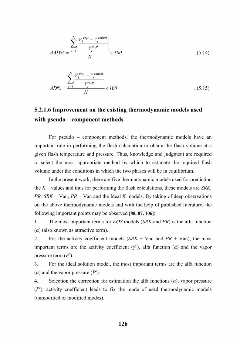
100NV
VV
%AAD
N
1iexp
i
calcdi
expi
×
−
=∑= ..(5.14)
100NV
VV
%AD
N
1iexp
i
calcdi
expi
×
−
=∑= ..(5.15)
5.2.1.6 Improvement on the existing thermodynamic models used with pseudo – component methods
For pseudo – component methods, the thermodynamic models have an important rule in performing the flash calculation to obtain the flash volume at a given flash temperature and pressure. Thus, knowledge and judgment are required to select the most appropriate method by which to estimate the required flash volume under the conditions in which the two phases will be in equilibrium. In the present work, there are five thermodynamic models used for prediction the K – values and thus for performing the flash calculations, these models are SRK, PR, SRK + Van, PR + Van and the Ideal K models. By taking of deep observations on the above thermodynamic models and with the help of published literature, the following important points may be observed [88, 87, 106]: 1. The most important terms for EOS models (SRK and PR) is the alfa function (α) (also known as attractive term). 2. For the activity coefficient models (SRK + Van and PR + Van), the most important terms are the activity coefficient (γL), alfa function (α) and the vapor pressure term (Ps). 3. For the ideal solution model, the most important terms are the alfa function (α) and the vapor pressure (Ps). 4. Selection the correction for estimation the alfa functions (α), vapor pressure (Ps), activity coefficient leads to fix the mode of used thermodynamic models (unmodified or modified modes).
126
Based on the above observation, the present work suggested three modes of thermodynamic models based on the selection of the alfa function (α), vapor
pressure (Ps) and activity coefficient (γ ) terms, these modes are: Li
a. Unmodified models mode. b. Modified models No. 1 mode (existing in the literature). c. Present work suggested modification mode (modified models No. 2 mode).
The above mentioned thermodynamic modes are tested and investigated for obtaining the EFV curve from TBP curve using 18 petroleum stock of Table 5-1. The total number of EFV data points that tested were 106 points.
5.2.1.6.1 Unmodified models mode
In this mode, the following correlations for alfa functions (α), vapor pressure (Ps) and activity coefficients model (γL) are used:
−
−
−
−
−
−
−
The original alfa functions correlations for SRK and PR EOS used {equations (3.76) and (3.90) for SRK and PR EOS respectively}.
The Lee – Kasler correlations {equations (113 – 115)}.
The van – Laar model for activity coefficient model {equation (3.145)}.
5.2.1.6.2 Modified models No.1 mode
In this mode, the following correlations for alfa functions (α), vapor pressure (Ps) and activity coefficient model (γL), are used:
For SRK EOS, the modified alfa function given by Sim – Daubert is used {equation (3.102)}.
For PR EOS, the modified alfa function given by Twa et al. is used {equations (3.103) – (3.105)}.
The Lee – Kasler correlation is used for estimation the vapor pressure (Ps).
The van – Laar model is used for estimation the activity coefficient (γL). The present work suggested a modification (modified models No. 2 mode)
and will be discussed in the next chapter.
127
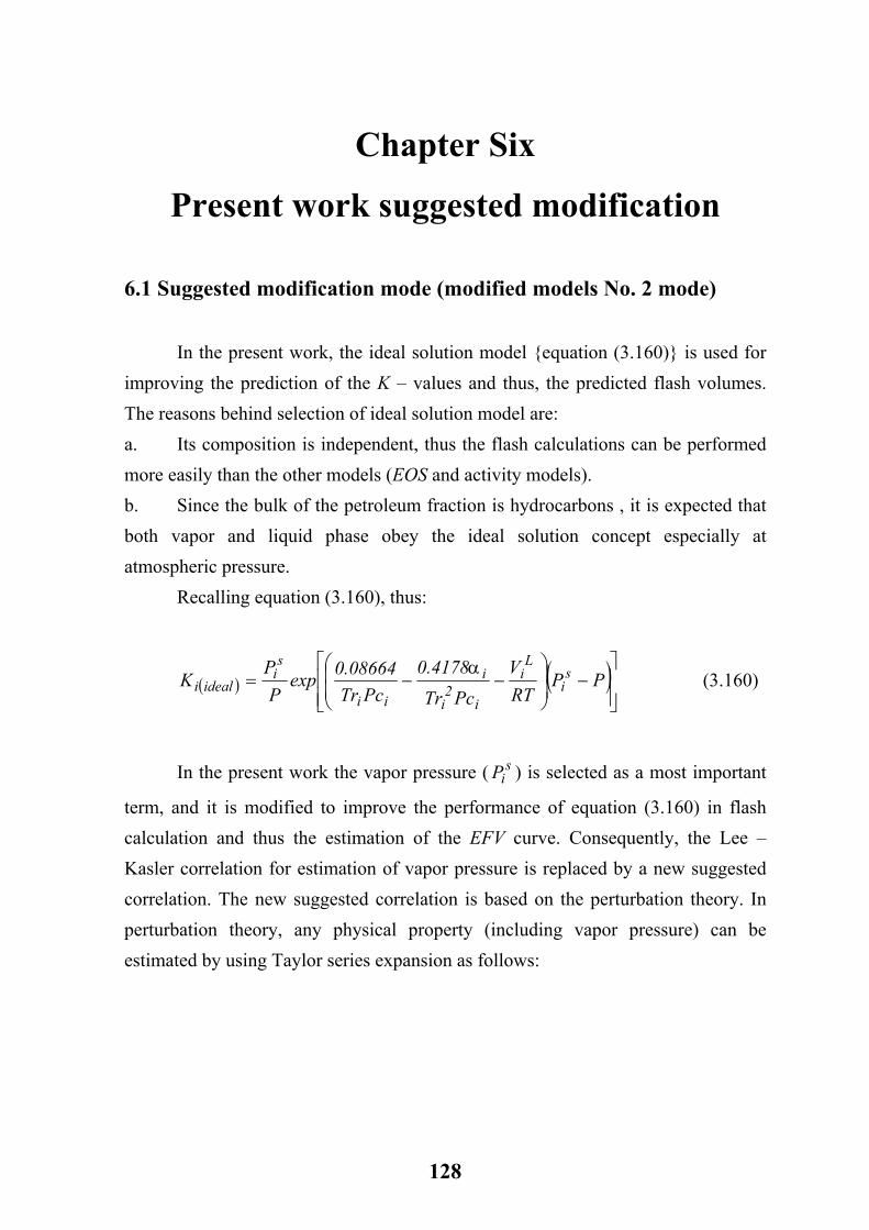
Chapter Six
Present work suggested modification
6.1 Suggested modification mode (modified models No. 2 mode)
In the present work, the ideal solution model {equation (3.160)} is used for improving the prediction of the K – values and thus, the predicted flash volumes. The reasons behind selection of ideal solution model are: a. Its composition is independent, thus the flash calculations can be performed more easily than the other models (EOS and activity models). b. Since the bulk of the petroleum fraction is hydrocarbons , it is expected that both vapor and liquid phase obey the ideal solution concept especially at atmospheric pressure.
Recalling equation (3.160), thus:
( ) (
−
−−= PP
RTV
PcTr4178.0
PcTr08664.0exp
PP
K si
Li
i2
i
i
ii
si
idealiα ) (3.160)
In the present work the vapor pressure ( ) is selected as a most important
term, and it is modified to improve the performance of equation (3.160) in flash calculation and thus the estimation of the EFV curve. Consequently, the Lee – Kasler correlation for estimation of vapor pressure is replaced by a new suggested correlation. The new suggested correlation is based on the perturbation theory. In perturbation theory, any physical property (including vapor pressure) can be estimated by using Taylor series expansion as follows:
siP
128
( ) ( ) ( )( )( )( )( )ref
jjrefii
ijn1ij
i
refiin1in1
refn1
xxxxx,...,x
xxx,...,xx,...,xx,...,x
−−+
−+=
∑
∑θ
θθθ
…(6.1)
where θ is any physical properties, (x1, …,xn) are the independent variable such as TB, Sp.gr …etc, θi, θij are the first and second partial derivatives with respect to the difference variables (xi – xi
ref) evaluated for the reference system, the superscript (ref) denotes the reference system properties. Equation (6.1) represents the general form of Taylor series expansion of the property θ about its value in some reference state. The normal alkane hydrocarbons are widely used as a reference property (θref) [37]. For the purpose of empirically correlating the deviations between n – alkane and non – alkane hydrocarbons Lee and Kasler and Sandler [107] suggested the following simpler, first order perturbation expansion:
( ) ( ) ( )( )
( )( )A2
A1
As
TB
gr.Spgr.SpTBTB,gr.Sp,Tb
ωωθ
θθωθ
−+
−+= …(6.2)
where (Sp.gr – Sp.grA) is the difference between the non – hydrocarbon specific gravity and n – alkane specific gravity measured at same TB of non – alkane hydrocarbons and (ω – ωA) is the difference between the acentric factor of non – alkane hydrocarbons and the acentric factor of n – alkane hydrocarbons measured at same non – alkane hydrocarbons TB. θ1 and θ2 are derivations and must be calculated by back calculation from experimental data. For the vapor pressure property they suggested to terminate equation (6.2) to second term and they obtain the following equation:
( ) 21AsAs FFPlnPln ωω −+= …(6.3)
129
where Ps and PsA are the vapor pressure in (atm) for non – alkane and n – alkane hydrocarbons and F1 and F2 are functions and have the following forms:
( )
+−
++=
TBrC1
1C1TBr8.321864.1F1 (6.3a)
and ( )( 85.0TBrTB10197.30953.0C 4 −×+= − )
)
…(6.4)
(
−×−+= −
TBr85.01TB103574.42532.16828.0F 3
2 …(6.5)
with TBr = T/TB Equation (6.3) is limited to pure components non – alkane hydrocarbons, and it is expected to be useful for calculation the petroleum fractions vapor pressures [107]. In the present work, equation (6.3) is modified and extended for petroleum fractions by achieving the following modifications: 1. The term (ω – ωA) is replaced by (Sp.gr – Sp.grA) terms, since Sp.gr can be measured easily for petroleum fraction rather than ω. 2. The correction term (CF) is used for extending equation (6.3) for petroleum fractions. The correction factor term is given as follows:
TBrBcAcCF −= …(6.6)
where Ac and Bc are the adjustable parameters that must be calculated using experimental data. Consequently, the modified form of equation (6.3) can be written as follows:
( )
−+−+=
TBrBcAcFFgr.Spgr.SpPlnPln 21
AsAs …(6.7)
130
The PsA and Sp.grA of equation (6.7) can be obtained by using the following equation [107]:
1273sA F
TB301.89TB104728.5TB103021.29665.0Pln ×
+×−×+= −−
…(6.8)
TB
605.144TB105328.4TB1042922.625386.1gr.Sp 274A −×+×−= −−
…(6.9) The adjustable parameters Ac and Bc of equation (6.7) are calculated by using optimization technique using the EFV data for 18 petroleum stocks (106 data points). The optimization technique performed by using the solver program of Microsoft excel package. The optimization technique including the following two steps: 1. The flash calculation using equation (3.160) with conjunction of equation (6.7) is performed to obtain the flash volume. 2. The adjustable parameters are selected in such a way that the AAD% of flash volume be in a minimum case {equation (5.14)}.
Consequently, the value of Ac was 1.0202 (≈ 1) and Bc was 0.8498 (≈ 0.85). The working form of equation (6.3) is:
( )
−+−+=
TBr85.01FFgr.Spgr.SpPlnPln 21
AsAs ..(6.10)
The constants F1 and F2 ( equations 6.3a-6.5 )were also used ,since the max. abslute diffreince between(ω – ωA) ,and(Sp.gr – Sp.grA) did not exceed than 10-3
It must be noted here, that the improved vapor pressure correlation can be applied under the following two conditions: a. When the TMEP is negative, the TMEP can be defined as follows:
TMEP = 10 – The calculated flash volume {using equation (3.160)} when 20% TBP temperature is used as flash temperature
131
b. When the TMEP is positive and has the value of greater than 4 (TMEP > 4). The TMEP term suggested by Sim – Daubert [1] for improving the alfa function (α) of SRK EOS model. It is extended in the present work for improving the ideal K model.
The improved vapor pressure correlation with the above conditions can also be used for improving the EOS models (SRK and PR), and the activity coefficient models (SRK + Van and PR + Van) as follows: 1. for SRK and PR models, the improved vapor pressure correlations {equation (5.126)} can be used for improving the acentric factor (ω) prediction by replacing the Lee – Kasler correlations {equations (3.12) and (3.13)} by Pitzer et al. equation (3.78) with using the improved vapor pressure correlation for calculation the vapor pressure at Tr = 0.7. The latter will improve the alfa function (α) {i.e. α = f (Tr, ω)}. 2. For (SRK + Van) and (PR +Van) models, the improved vapor pressure correlation is used instead of Lee – Kasler correlation.
6.2 Computer implementation
A computer program is designed and developed by using quick basic language for the purpose of this work. The computer program is designed to obtain the EFV curve from the input TBP curve using the graphical method by Raizi – Daubert and the SRK, PR, SRK + Van, PR + Van and Ideal K pseudo – components methods. The remark statements are available at the beginning, and throughout the computer program. These statements help the user to understand the calculations used in the program. The computer program consists of three main parts. These parts are, input part, calculational part and printout part.
6.2.1 Input part
In this part all the necessary data for estimation the EFV curve from the TBP curve must be supplied. These data includes the following items:
132
a. Flash temperature (T), flash pressure (P), petroleum stocks API, constants for TBP (A1', B1', C1', D1' and E1') and specific gravity equations (A2' and B2'), constants for Raizi – Daubert graphical method, total feed volume, and feed molar rate. b. Type of specific gravity input data. There are two choices of specific gravity data input:
−
−
−
−
−
−
−
Overall data input type (choice number 1).
Specific gravity equation input type (choice number 2). c. Type of vapor pressure correlations. There are two choices of vapor pressure correlations:
Lee – Kasler correlation (choice number 1).
Modified method suggested by the present work (choice number 2). The modified method will be discussed later.
d. Modes of thermodynamic models used with pseudo – components methods. There are three choices for modes of thermodynamic models used in computer program, those are:
Unmodified models (choice number 1).
Modified models No. 1 (choice number 2).
Present work suggested modification (modified models No. 2).
6.2.2 Calculational part
This part of computer program is responsible for the calculations used for estimation the EFV curve from TBP curve. It is consisted of the following items: a. Graphical methods for estimation the EFV curve from TBP curve. The latter can be achieved using the Raizi – Daubert algorithm (Fig. 5-48). b. Pseudo – components methods for estimation the EFV curve from TBP curve. It consists of the following items:
1. Characterization steps using characterization algorithm (Fig. 5-49).
2. Calculation of molar volume (V ) using Rackett equation {equation
(3.110) for Tr < 1 and Cavett equation (3.111) for Tr > 1}.
Li
133
3. Calculation of vapor pressure ( ) depending on the choices of vapor
pressure correlations. For choice 1, the vapor pressure ( ) is calculated using
Lee – Kasler correlation {equations (3.113) – (3.115)}, while for choice 2, the modified method suggested by the present work is used.
siP
siP
4. Calculation of alfa functions (αi) for EOS models depending on the choices of thermodynamic modes. Since there are three modes of thermodynamic models, thus there are three types of alfa functions (αi) that can be used in computer program, these models are:
Unmodified models {equations (3.76) for SRK and (3.90) for PR}. −
−
−
−
−
−
−
−
Modified models No. 1 {equations (3.102) for SRK and (3.103) for PR}.
Modified models No. 2 {equations (3.76) for SRK and (3.90) for PR}. 5. Calculation of flash volume by performing flash calculations using the flash calculations algorithms that discussed previously and with conjunction of the five thermodynamic models as follows:
SRK thermodynamic model using EOS model algorithm (Fig. 5-51).
PR thermodynamic model using EOS model algorithm (Fig. 5-51).
SRK + Van thermodynamic model using activity coefficient model algorithm (Fig. 5-52).
PR + Van thermodynamic model using activity coefficient model algorithm (Fig. 5-52).
Ideal K thermodynamic model using Rachford – Rice model algorithm (Fig. 5-50).
6. Calculation of AAD% and AD% using equations (5.14) and (5.15).
6.2.3 Printout part
This part of computer program is responsible on the printing of the calculated results that performed by computer program. It consists of the following items:
134
1. Printing of flash temperature (T), flash pressure (P) and flash volume (Vol.%) for each pseudo – components methods. 2. Printing of error analysis (i.e. AAD% and AD%). 3. Printing of physical properties for each cuts including the critical properties (Tci, Pci), molecular weights (MWi), acentric factors (ωi), molar volumes at 15.5 °C
(60 °F) (V ), solubility parameters at 25 °C (77 °F) (δLi i), specific gravity (Sp.gri),
…etc. 4. Printing of material balance (MB) for each cut including volumes (Vi), weights (Wi), moles (Ni) and the feed compositions (Zfi) in mole basis. 5. Printing of Raizi – Daubert graphical method EFV temperatures at a corresponding volume percent (Vol.%). 6. Printing of vapor and liquid phases compositions for each cut (xi and yi) using the five thermodynamic models (SRK, PR, SRK + Van, PR + Van and Ideal K). 7. Printing of K – values for each components (Ki) using the five thermodynamic models.
For items 3 – 7, the printing results is converted to data files. These data files can be opened with other computer package such as Microsoft excel, and Microsoft grapher.
Items 6 – 7 can be considered as optional choices since the present work interested in EFV data rather than other calculated data.
The list of the computer program is given in Appendix G, while its flow sheet diagram is given in Fig. 6-1.
135
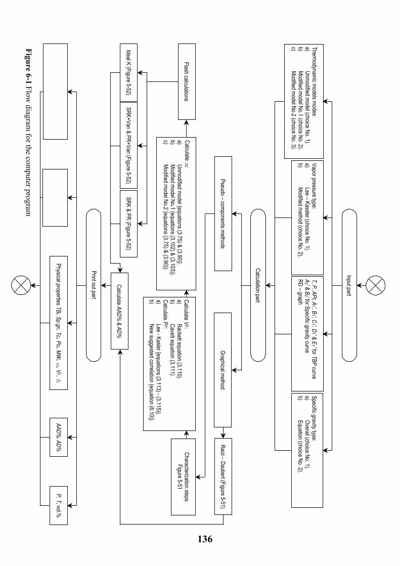
136
xi , yi , Ki , for
do methods each pseu(optional)
Matnce
erial BalaV
i , Ni , Zfi
i i
ii
i
ii
i
%, AD
Raizi – Daubert (Figure 5-51)
Figure 6-1 Flow diagram
for the computer program
P, T, vol.%
AAD%
Physical properties TB , Sp.gr, Tc, Pc, M
W, ω
, VL, δ
Print out part
SRK & PR (Figure 5-52) SRK+Van & PR+Van (Figure 5-52)
Ideal K (Figure 5-52)
Charteps
acterization sFigure 5-51
CaV
i L: .
lculate a)
Rackett equation (3.110)C
vett equation (3.111). b)
alculate
CaP
i s: a)
Lee - Kasler {equations (3.113) - (3.115)}. b )
New suggested correlation {equation (6.10)}.
Caα
i : lculate
a) Unmodified model {equations (3.75) & (3.90)}.
)}. b)
Modified model No.1 {equations (3.102) & (3.103c)
Modified model No.2 {equations (3.75) & (3.90)}.
Flash calculations
Calculate AAD% & AD%
Graphical method Pseudo – components methods
Calculation part
T P, A
I, A1 ', B
1 ', C1 ', D
1 ' & E1 ' for
Specific gravity curve ,
P TBP curve
A2 ' & B
2 ' for RD – graph
Spavity type:
ecific gra)
Overall (choice No. 1). b)
Equation (choice No. 2).
Vasure type:
por presa)
Lee – Kassler (choice No. 1). b)
Modified method (choice No. 2).
Thnamic models modes:
ermodya)
Unmodified model (choice No. 1). b)
Modified model No.1 (choice No. 2). c)
Modified model No.2 (choice No. 3).
Input part
Chapter Seven
Results and discussion
7.1 Discussion of results
7.1.1 Selected data for part one(testing & developing part) and part two (application part)of the present work
For part one of the present work, 18 petroleum stocks are used for estimation the EFV curve from TBP curve. As shown in Table 5-1, the API gravity of these petroleum stocks were varies from 20.2 to 47.8. Petroleum stocks of number 1 to 15 were available with just overall specific gravity and TBP curve, while petroleum stocks number 16, 17 and 18 were available with specific gravity curve and TBP curve, consequently these petroleum stocks can be considered as industrial data type, while the first 15 petroleum stocks can be considered as a classical chemical engineering literature data type. Both data types were available with EFV curves. Figures 5-1 – 5-15 illustrate the TBP curves for petroleum stocks of number 1 through 15, while Figs. 5-31 – 5-33 illustrate the TBP curves for petroleum stocks of number 16, 17 and 18, respectively. As shown by these figures, volume percent distilled (vol.%) of cuts or fractions increase with increasing the temperature of the fractions. This is due to the increase of the aromatic content and decrease of paraffinic content of the fractions( i.e. increasing the TB, and MW of cuts). Petroleum stocks that have low API gravity have much flatter distillation curves than those petroleum stocks of high API gravity. This is due to the highly naphthenic contents of low API petroleum stocks that characterized by their high boiling point, while the high API petroleum stocks have highly contents of paraffinic that can be characterized as low boiling point materials. Because of the close relations between the TBP curves and EFV curves. It is expected that the behavior of the TBP curves that mentioned above for the 18 petroleum stocks are also true for the EFV curves for these petroleum stocks. This is shown by Figs. 5-16 – 5-30 for EFV curves for petroleum stocks of number 1 to 15, and Figs. 5-33 – 5-
137
36 for EFV curves for petroleum stocks of number 16, 17 and 18. It is also noted that the EFV curves have flatter slopes, than the TBP curves. For petroleum stocks of number 16, 17 and 18, Figs. 5-37 – 5-39 illustrate the specific gravity curves for these petroleum stocks. As shown by these curves, the specific gravity for each cut or fraction increases with increasing the volume percent distilled and the TBP of the fractions. This is due to the increase of the aromatic content and decrease of the paraffinic content of the fractions(i.e increasing the MW of cuts). Usually, the specific gravity of aromatic and naphthenic hydrocarbons are higher than those for paraffinic hydrocarbons having the same number of atoms (and also the same molecular weight). For data of part two of the present work, four Iraqi crude oils were used for obtaining the TBP and specific gravity curves. These crudes are Kirkuk, Basrah, Jambour and Bai – Hassan crude oils. The API gravity of these crudes were 36.1, 30.1, 37.7 and 31.4, respectively. These crudes oil can be considered as paraffinic class [22]. Figures 5-40 – 5-43 illustrate the TBP for Kirkuk, Basrah, Jambour and Bai – Hassan crude oils. As shown by these figures, that the total distillate from Kirkuk, Basrah, Jambour and Bai – Hassan (for IBP-370 0C)were 67.07 vol.% (63 wt. %), 63.93 vol.% (57.94 wt. %), 67.76 vol.% (62.19 wt. %) and 64.28 vol.% (57.34 wt. %), respectively. Also the figures show that the volume percent distilled increases with increasing the vapor temperature of each fraction, this is due to the increasing of the aromatic and naphthenic contents and decreasing of paraffinic contents. The TBP curves for these crudes have also a steepest distillation slopes due to the highly content of paraffin compounds. The slope of distillation curve usually measured at 10% and 70% distillation temperatures. The general shapes of the obtained TBP curves for the four Iraqi crude oils have a good agreement with the general shapes of TBP curves given by literature [3, 22]. Figures 5-44 – 5-47 illustrate the specific gravity curves for Kirkuk, Basrah, Jambour and Bai – Hassan crude oils. As shown by the above figures, that the specific gravity for each cut or fraction increases with increasing the volume percent distilled (or TB &MW), this is due the increasing of aromatic and naphthenic contents and decreasing the paraffinic contents. The specific gravity of
138
aromatic and naphthenic hydrocarbons are higher than those for paraffinic hydrocarbons having the same number of atoms (or molecular weight). The obtained specific gravity curve shapes for the four Iraqi crude oils have a good agreement with the general shapes of specific gravity curves observed in literature [22].
7.1.2 Estimated physical properties and material balance for cuts or fractions
For pseudo – components methods, the physical properties and material balance must be obtained. Both physical properties and material balance are performed in the characterization steps that discussed previously. The physical properties including the estimation of basic properties such as molecular weight (MW), critical temperatures (Tc), critical pressures (Pc), acentric factor (ω) and other physical properties such as molar volume (VL) and solubility parameters (δ). The material balance includes the conversion of the volume for each cut to weight and finally to moles. The number of cuts were 40. Table 7-1 gives the physical properties for the 40 cuts of petroleum stock of number 1, while Tables H-1 – H-17 in Appendix H give the physical properties of the 40 cuts of the petroleum stocks of number 2 to 18. As shown in Table 7-1 and Tables H-1 – H-17 that the molecular weight (MW), critical temperature (Tc), acentric factors (ω) and molal volumes VL for each cut increase with increasing the TB and the specific gravity for each cut, while the critical pressures (Pc) and solubility parameters (δ) for each cut decrease with increasing the TB and specific gravity of each cut. The reason behind this behavior is that when the TB and the specific gravity are increase the aromatic and naphthenic contents are increased and the paraffinic contents are decreased. The latter behavior for the cuts have a good agreement with the published physical properties for pure hydrocarbons of different family types (paraffins, aromatics, …etc) [88, 91]. Table 7-2 gives the material balance for 40 cuts of the petroleum stock of number 1, while Tables H-18 – H-34 in Appendix H give the material balance for 40 cuts of the petroleum stocks of number 2 to 18. As shown in Table 7-2 and
139
Tables H-18 – H-34, that the weight of each cut increases due to increasing the specific gravity and TB of each cut. This is due to the proportional relations between the specific gravity and the estimated weight for each cut {as indicated by equation (5.4)}. The estimated moles for each cut decreases with the increasing of the specific gravity and weight for each cut, this is due to reverse proportional between the specific gravity and weight with the estimated moles for each cut {as indicated by equation (5.6)}. The volume percent (vol.%), weight percent (wt.%) and mole percent (mol.%) also are given in these tables. The volume percent (vol.%) for each cut remains constant since each petroleum stock is divided into 40 cuts of equal volume percent of 2.5% (100 cm3). The weight percent (wt.%) and mole percent (mol.%) have the same behavior of estimated weights and moles for each cut that discussed above. For the four Iraqi crude oils (data for part two of the present work), the above mentioned behaviors of the physical properties and the material balance for each cut are also observed. Table 7-3 gives the physical properties for Kirkuk crude oil, while Tables H-35 – H-37 of Appendix H give the physical properties for Basrah, Jambour and Bai – Hassan crude oils respectively, while Table 7-4 gives the material balance for Kirkuk crude oil and Tables H-38 – H-40 give the material balance for Basrah, Jambour and Bai – Hassan crude oils respectively.
140
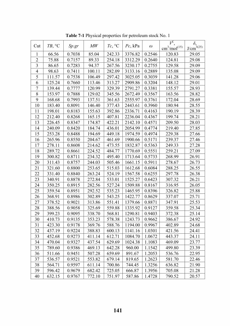
Table 7-1 Physical properties for petroleum stock No. 1
Cut TB, °C Sp.gr MW Tc, °C Pc, kPa ω VL, cm3/mol(15)
δ, J/cm3(25)
1 66.56 0.7038 85.04 242.33 3376.82 0.2546 120.83 29.05 2 75.88 0.7157 89.33 254.18 3312.29 0.2640 124.81 29.08 3 86.65 0.7283 94.37 267.56 3230.17 0.2755 129.58 29.09 4 98.63 0.7411 100.11 282.09 3133.16 0.2889 135.08 29.09 5 111.57 0.7538 106.49 297.42 3025.05 0.3039 141.28 29.06 6 125.24 0.7660 113.46 313.27 2909.86 0.3204 148.12 29.01 7 139.44 0.7777 120.99 329.39 2791.27 0.3381 155.57 28.93 8 153.97 0.7888 129.02 345.56 2672.49 0.3567 163.56 28.82 9 168.68 0.7993 137.51 361.63 2555.97 0.3761 172.04 28.69 10 183.40 0.8091 146.40 377.43 2443.61 0.3960 180.94 28.55 11 198.01 0.8183 155.63 392.86 2336.71 0.4163 190.19 28.39 12 212.40 0.8268 165.15 407.81 2236.04 0.4367 199.74 28.21 13 226.45 0.8347 174.87 422.21 2142.10 0.4571 209.50 28.03 14 240.09 0.8420 184.74 436.01 2054.99 0.4774 219.40 27.85 15 253.28 0.8488 194.69 449.18 1974.59 0.4974 229.38 27.66 16 265.96 0.8550 204.67 461.69 1900.66 0.5171 239.37 27.46 17 278.11 0.8608 214.62 473.55 1832.87 0.5363 249.33 27.28 18 289.72 0.8661 224.52 484.77 1770.69 0.5551 259.21 27.09 19 300.82 0.8711 234.32 495.40 1713.64 0.5733 268.99 26.91 20 311.43 0.8757 244.03 505.46 1661.15 0.5911 278.67 26.73 21 321.60 0.8800 253.65 515.03 1612.68 0.6084 288.25 26.55 22 331.40 0.8840 263.24 524.19 1567.58 0.6255 297.78 26.38 23 340.91 0.8878 272.84 533.01 1525.27 0.6423 307.32 26.21 24 350.25 0.8915 282.56 527.24 1509.88 0.8167 316.95 26.05 25 359.54 0.8951 292.52 535.23 1465.95 0.8396 326.82 25.88 26 368.91 0.8986 302.89 543.25 1422.77 0.8629 337.07 25.71 27 378.52 0.9021 313.86 551.41 1379.66 0.8871 347.91 25.53 28 388.56 0.9058 325.69 559.88 1335.92 0.9127 359.58 25.34 29 399.23 0.9095 338.70 568.81 1290.81 0.9403 372.38 25.14 30 410.73 0.9135 353.23 578.38 1243.73 0.9662 386.67 24.92 31 423.30 0.9178 369.76 588.76 1194.00 0.9967 402.89 24.68 32 437.19 0.9224 388.83 600.13 1141.16 1.0301 421.56 24.41 33 452.68 0.9273 411.14 612.71 1084.70 1.0672 443.37 24.11 34 470.04 0.9327 437.54 629.69 1024.38 1.1083 469.09 23.77 35 789.60 0.9386 469.13 642.28 960.00 1.1542 499.80 23.39 36 511.66 0.9451 507.28 659.69 891.67 1.2053 536.76 22.95 37 536.57 0.9521 553.82 679.14 819.65 1.2623 581.70 22.46 38 564.71 0.9597 611.14 700.86 744.45 1.3256 636.82 21.90 39 596.42 0.9679 682.42 725.05 666.87 1.3956 705.08 21.28 40 632.15 0.9767 772.10 751.97 587.86 1.4728 790.52 20.57
141
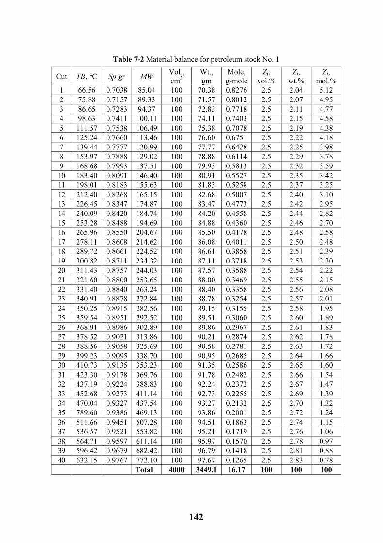
Table 7-2 Material balance for petroleum stock No. 1
Cut TB, °C Sp.gr MW Vol., cm3
Wt., gm
Mole, g-mole
Zi, vol.%
Zi, wt.%
Zi, mol.%
1 66.56 0.7038 85.04 100 70.38 0.8276 2.5 2.04 5.12 2 75.88 0.7157 89.33 100 71.57 0.8012 2.5 2.07 4.95 3 86.65 0.7283 94.37 100 72.83 0.7718 2.5 2.11 4.77 4 98.63 0.7411 100.11 100 74.11 0.7403 2.5 2.15 4.58 5 111.57 0.7538 106.49 100 75.38 0.7078 2.5 2.19 4.38 6 125.24 0.7660 113.46 100 76.60 0.6751 2.5 2.22 4.18 7 139.44 0.7777 120.99 100 77.77 0.6428 2.5 2.25 3.98 8 153.97 0.7888 129.02 100 78.88 0.6114 2.5 2.29 3.78 9 168.68 0.7993 137.51 100 79.93 0.5813 2.5 2.32 3.59 10 183.40 0.8091 146.40 100 80.91 0.5527 2.5 2.35 3.42 11 198.01 0.8183 155.63 100 81.83 0.5258 2.5 2.37 3.25 12 212.40 0.8268 165.15 100 82.68 0.5007 2.5 2.40 3.10 13 226.45 0.8347 174.87 100 83.47 0.4773 2.5 2.42 2.95 14 240.09 0.8420 184.74 100 84.20 0.4558 2.5 2.44 2.82 15 253.28 0.8488 194.69 100 84.88 0.4360 2.5 2.46 2.70 16 265.96 0.8550 204.67 100 85.50 0.4178 2.5 2.48 2.58 17 278.11 0.8608 214.62 100 86.08 0.4011 2.5 2.50 2.48 18 289.72 0.8661 224.52 100 86.61 0.3858 2.5 2.51 2.39 19 300.82 0.8711 234.32 100 87.11 0.3718 2.5 2.53 2.30 20 311.43 0.8757 244.03 100 87.57 0.3588 2.5 2.54 2.22 21 321.60 0.8800 253.65 100 88.00 0.3469 2.5 2.55 2.15 22 331.40 0.8840 263.24 100 88.40 0.3358 2.5 2.56 2.08 23 340.91 0.8878 272.84 100 88.78 0.3254 2.5 2.57 2.01 24 350.25 0.8915 282.56 100 89.15 0.3155 2.5 2.58 1.95 25 359.54 0.8951 292.52 100 89.51 0.3060 2.5 2.60 1.89 26 368.91 0.8986 302.89 100 89.86 0.2967 2.5 2.61 1.83 27 378.52 0.9021 313.86 100 90.21 0.2874 2.5 2.62 1.78 28 388.56 0.9058 325.69 100 90.58 0.2781 2.5 2.63 1.72 29 399.23 0.9095 338.70 100 90.95 0.2685 2.5 2.64 1.66 30 410.73 0.9135 353.23 100 91.35 0.2586 2.5 2.65 1.60 31 423.30 0.9178 369.76 100 91.78 0.2482 2.5 2.66 1.54 32 437.19 0.9224 388.83 100 92.24 0.2372 2.5 2.67 1.47 33 452.68 0.9273 411.14 100 92.73 0.2255 2.5 2.69 1.39 34 470.04 0.9327 437.54 100 93.27 0.2132 2.5 2.70 1.32 35 789.60 0.9386 469.13 100 93.86 0.2001 2.5 2.72 1.24 36 511.66 0.9451 507.28 100 94.51 0.1863 2.5 2.74 1.15 37 536.57 0.9521 553.82 100 95.21 0.1719 2.5 2.76 1.06 38 564.71 0.9597 611.14 100 95.97 0.1570 2.5 2.78 0.97 39 596.42 0.9679 682.42 100 96.79 0.1418 2.5 2.81 0.88 40 632.15 0.9767 772.10 100 97.67 0.1265 2.5 2.83 0.78 Total 4000 3449.1 16.17 100 100 100
142
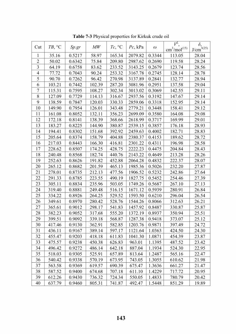
Table 7-3 Physical properties for Kirkuk crude oil
Cut TB, °C Sp.gr MW Tc, °C Pc, kPa ω VL, cm3/mol(15)
δ, J/cm3(25)
1 35.16 0.5217 58.97 165.34 2079.82 0.3344 113.05 28.04 2 50.02 0.6342 75.84 209.80 2987.62 0.2690 119.58 28.24 3 64.19 0.6758 83.62 233.52 3143.25 0.2679 123.74 28.56 4 77.72 0.7043 90.24 253.32 3167.78 0.2745 128.14 28.78 5 90.70 0.7262 96.42 270.98 3137.89 0.2841 132.77 28.94 6 103.21 0.7442 102.39 287.20 3081.96 0.2951 137.58 29.04 7 115.31 0.7595 108.27 302.34 3013.02 0.3069 142.55 29.11 8 127.09 0.7729 114.13 316.67 2937.56 0.3192 147.67 29.14 9 138.59 0.7847 120.03 330.33 2859.06 0.3318 152.95 29.14 10 149.90 0.7954 126.01 343.48 2779.21 0.3448 158.41 29.12 11 161.08 0.8052 132.11 356.23 2699.09 0.3580 164.08 29.08 12 172.18 0.8141 138.39 368.66 2618.99 0.3717 169.99 29.01 13 183.27 0.8225 144.90 380.87 2539.15 0.3857 176.18 28.93 14 194.41 0.8302 151.68 392.92 2459.63 0.4002 182.71 28.83 15 205.64 0.8374 158.79 404.88 2380.37 0.4153 189.62 28.72 16 217.03 0.8443 166.30 416.81 2301.22 0.4311 196.98 28.58 17 228.62 0.8507 174.25 428.75 2222.23 0.4475 204.84 28.43 18 240.48 0.8568 182.74 440.76 2143.22 0.4649 213.28 28.26 19 252.63 0.8626 191.82 452.88 2064.28 0.4832 222.37 28.07 20 265.12 0.8682 201.59 465.13 1985.36 0.5026 232.20 27.87 21 278.01 0.8735 212.13 477.56 1906.52 0.5232 242.86 27.64 22 291.33 0.8785 223.55 490.19 1827.75 0.5452 254.46 27.39 23 305.11 0.8834 235.96 503.05 1749.26 0.5687 267.10 27.13 24 319.40 0.8881 249.48 516.15 1671.12 0.5939 280.91 26.84 25 334.22 0.8926 264.25 529.52 1593.50 0.6210 296.04 26.54 26 349.61 0.8970 280.42 528.76 1544.26 0.8066 312.63 26.21 27 365.61 0.9012 298.17 541.83 1457.92 0.8487 330.87 25.87 28 382.23 0.9052 317.68 555.20 1372.19 0.8937 350.94 25.51 29 399.51 0.9092 339.18 568.87 1287.38 0.9418 373.07 25.12 30 417.46 0.9130 362.91 582.85 1203.76 0.9871 397.49 24.72 31 436.11 0.9167 389.14 597.17 1121.64 1.0363 424.50 24.30 32 455.47 0.9203 418.18 611.83 1041.30 1.0871 454.39 23.87 33 475.57 0.9238 450.38 626.83 963.01 1.1395 487.52 23.42 34 496.42 0.9272 486.14 642.18 887.04 1.1934 524.30 22.95 35 518.03 0.9305 525.91 657.89 813.64 1.2487 565.16 22.47 36 540.42 0.9338 570.19 673.95 743.05 1.3055 610.62 21.98 37 563.58 0.9369 619.57 690.39 675.47 1.3636 661.27 21.47 38 587.52 0.9400 674.68 707.18 611.10 1.4229 717.72 20.95 39 612.26 0.9430 736.32 724.34 550.05 1.4833 780.79 20.42 40 637.79 0.9460 805.31 741.87 492.47 1.5448 851.29 19.89
143

Table 7-4 Material balance for Kirkuk crude oil
Cut TB, °C Sp.gr MW Vol., cm3
Wt., gm
Mole, g-mole
Zi, vol.%
Zi, wt.%
Zi, mol.%
1 35.16 0.5217 58.97 100 52.17 0.8846 2.5 1.54 5.01 2 50.02 0.6342 75.84 100 63.42 0.8362 2.5 1.88 4.73 3 64.19 0.6758 83.62 100 67.58 0.8082 2.5 2.00 4.57 4 77.72 0.7043 90.24 100 70.43 0.7804 2.5 2.09 4.42 5 90.70 0.7262 96.42 100 72.62 0.7532 2.5 2.15 4.26 6 103.21 0.7442 102.39 100 74.42 0.7268 2.5 2.20 4.11 7 115.31 0.7595 108.27 100 75.95 0.7015 2.5 2.25 3.97 8 127.09 0.7729 114.13 100 77.29 0.6772 2.5 2.29 3.83 9 138.59 0.7847 120.03 100 78.47 0.6538 2.5 2.32 3.70 10 149.90 0.7954 126.01 100 79.54 0.6313 2.5 2.36 3.57 11 161.08 0.8052 132.11 100 80.52 0.6095 2.5 2.38 3.45 12 172.18 0.8141 138.39 100 81.41 0.5883 2.5 2.41 3.33 13 183.27 0.8225 144.90 100 82.25 0.5676 2.5 2.44 3.21 14 194.41 0.8302 151.68 100 83.02 0.5473 2.5 2.46 3.10 15 205.64 0.8374 158.79 100 83.74 0.5274 2.5 2.48 2.99 16 217.03 0.8443 166.30 100 84.43 0.5077 2.5 2.50 2.87 17 228.62 0.8507 174.25 100 85.07 0.4882 2.5 2.52 2.76 18 240.48 0.8568 182.74 100 85.68 0.4689 2.5 2.54 2.65 19 252.63 0.8626 191.82 100 86.26 0.4497 2.5 2.55 2.55 20 265.12 0.8682 201.59 100 86.82 0.4307 2.5 2.57 2.44 21 278.01 0.8735 212.13 100 87.35 0.4118 2.5 2.59 2.33 22 291.33 0.8785 223.55 100 87.85 0.3930 2.5 2.60 2.22 23 305.11 0.8834 235.96 100 88.34 0.3744 2.5 2.62 2.12 24 319.40 0.8881 249.48 100 88.81 0.3560 2.5 2.63 2.02 25 334.22 0.8926 264.25 100 89.26 0.3378 2.5 2.64 1.91 26 349.61 0.8970 280.42 100 89.70 0.3199 2.5 2.66 1.81 27 365.61 0.9012 298.17 100 90.12 0.3022 2.5 2.67 1.71 28 382.23 0.9052 317.68 100 90.52 0.2849 2.5 2.68 1.61 29 399.51 0.9092 339.18 100 90.92 0.2680 2.5 2.69 1.52 30 417.46 0.9130 362.91 100 91.30 0.2516 2.5 2.70 1.42 31 436.11 0.9167 389.14 100 91.67 0.2356 2.5 2.71 1.33 32 455.47 0.9203 418.18 100 92.03 0.2201 2.5 2.73 1.25 33 475.57 0.9238 450.38 100 92.38 0.2051 2.5 2.74 1.16 34 496.42 0.9272 486.14 100 92.72 0.1907 2.5 2.75 1.08 35 518.03 0.9305 525.91 100 93.05 0.1769 2.5 2.76 1.00 36 540.42 0.9338 570.19 100 93.38 0.1638 2.5 2.77 0.93 37 563.58 0.9369 619.57 100 93.69 0.1512 2.5 2.77 0.86 38 587.52 0.9400 674.68 100 94.00 0.1393 2.5 2.78 0.79 39 612.26 0.9430 736.32 100 94.30 0.1281 2.5 2.79 0.72 40 637.79 0.9460 805.31 100 94.60 0.1175 2.5 2.80 0.66 Total 4000 3377.1 17.67 100 100 100
144
7.1.3 Part one (testing and developing part)
7.1.3.1 Estimated EFV curve using unmodified models mode
The EFV curve (or flash volumes) for 18 petroleum stocks estimated by using the Raizi – Daubert graphical method and five pseudo – component methods using unmodified thermodynamic models mode. These models are SRK, PR, SPK + Van, PR + Van and Ideal K models. The total number of examined points were 106. The error analysis results are performed by using the AAD% and AD%, respectively (as shown by equation (5.14) for AAD% and (5.15) for AD%). The results of error analysis (ADD% and AD%) are divided into three regions, first region for the flash volume that are below or equal 25% vol.% (low flash volumes region) and the second region for the flash volumes that are above than 25% vol.% (high flash volumes region). Finally, the third region represents all flash volumes (including both low and high flash volumes). The reason behind this divisions of error analysis results, is to show the performance of all flash methods in prediction the EFV curves for each of these three regions. Each of Raizi – Daubert (RD graph) method and the five pseudo – components methods (SRK, PR, SRK + Van, PR + Van and Ideal K) have been handled as a separate flash method that are used for predication the EFV curve from the TBP curve. The above mentioned division of error analysis results will be used also with the other thermodynamic models modes (modified models No. 1 mode and the present work suggested modifications mode). Table 7-5 gives the error analysis for 18 petroleum stocks using the ADD% and AD% for the three regions of the flash volumes. A more details including the predicted flash volumes, ADD% and AD% for each petroleum stock and for the three regions of the flash volumes are given in Tables I-1, I-2 and I-3 in Appendix I, respectively.
145
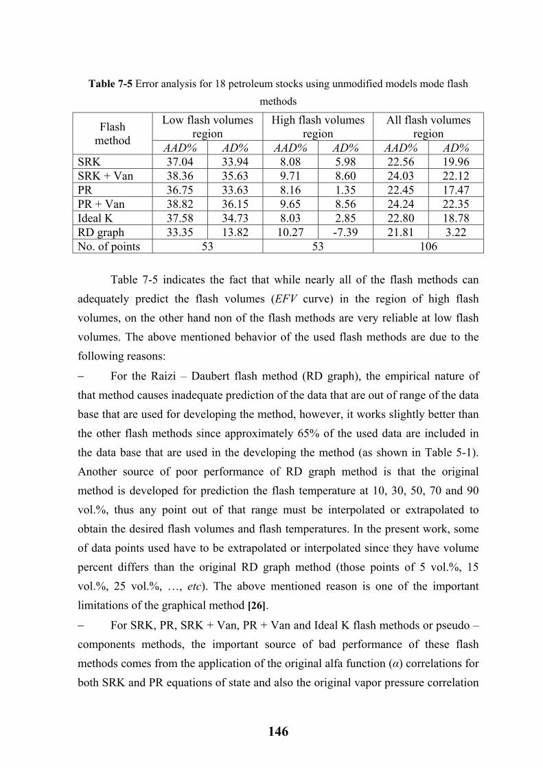
Table 7-5 Error analysis for 18 petroleum stocks using unmodified models mode flash methods
Low flash volumes region
High flash volumes region
All flash volumes region Flash
method AAD% AD% AAD% AD% AAD% AD% SRK 37.04 33.94 8.08 5.98 22.56 19.96 SRK + Van 38.36 35.63 9.71 8.60 24.03 22.12 PR 36.75 33.63 8.16 1.35 22.45 17.47 PR + Van 38.82 36.15 9.65 8.56 24.24 22.35 Ideal K 37.58 34.73 8.03 2.85 22.80 18.78 RD graph 33.35 13.82 10.27 -7.39 21.81 3.22 No. of points 53 53 106 Table 7-5 indicates the fact that while nearly all of the flash methods can adequately predict the flash volumes (EFV curve) in the region of high flash volumes, on the other hand non of the flash methods are very reliable at low flash volumes. The above mentioned behavior of the used flash methods are due to the following reasons:
−
−
For the Raizi – Daubert flash method (RD graph), the empirical nature of that method causes inadequate prediction of the data that are out of range of the data base that are used for developing the method, however, it works slightly better than the other flash methods since approximately 65% of the used data are included in the data base that are used in the developing the method (as shown in Table 5-1). Another source of poor performance of RD graph method is that the original method is developed for prediction the flash temperature at 10, 30, 50, 70 and 90 vol.%, thus any point out of that range must be interpolated or extrapolated to obtain the desired flash volumes and flash temperatures. In the present work, some of data points used have to be extrapolated or interpolated since they have volume percent differs than the original RD graph method (those points of 5 vol.%, 15 vol.%, 25 vol.%, …, etc). The above mentioned reason is one of the important limitations of the graphical method [26].
For SRK, PR, SRK + Van, PR + Van and Ideal K flash methods or pseudo – components methods, the important source of bad performance of these flash methods comes from the application of the original alfa function (α) correlations for both SRK and PR equations of state and also the original vapor pressure correlation
146
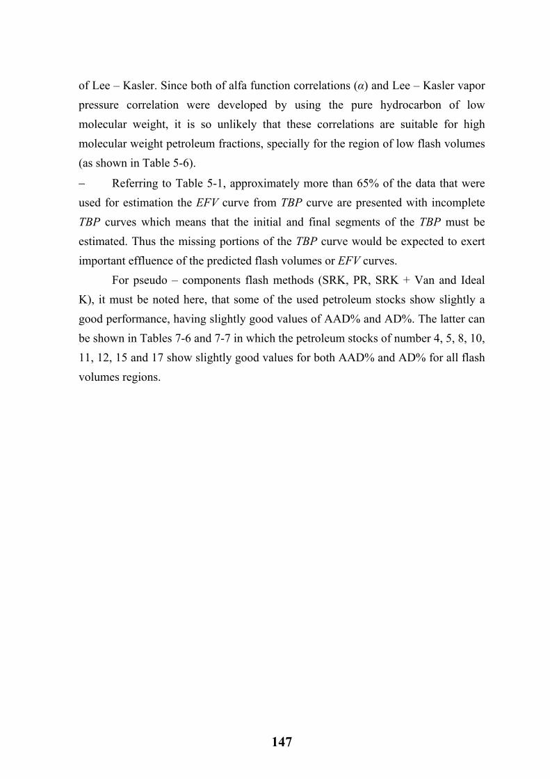
of Lee – Kasler. Since both of alfa function correlations (α) and Lee – Kasler vapor pressure correlation were developed by using the pure hydrocarbon of low molecular weight, it is so unlikely that these correlations are suitable for high molecular weight petroleum fractions, specially for the region of low flash volumes (as shown in Table 5-6).
− Referring to Table 5-1, approximately more than 65% of the data that were used for estimation the EFV curve from TBP curve are presented with incomplete TBP curves which means that the initial and final segments of the TBP must be estimated. Thus the missing portions of the TBP curve would be expected to exert important effluence of the predicted flash volumes or EFV curves.
For pseudo – components flash methods (SRK, PR, SRK + Van and Ideal K), it must be noted here, that some of the used petroleum stocks show slightly a good performance, having slightly good values of AAD% and AD%. The latter can be shown in Tables 7-6 and 7-7 in which the petroleum stocks of number 4, 5, 8, 10, 11, 12, 15 and 17 show slightly good values for both AAD% and AD% for all flash volumes regions.
147
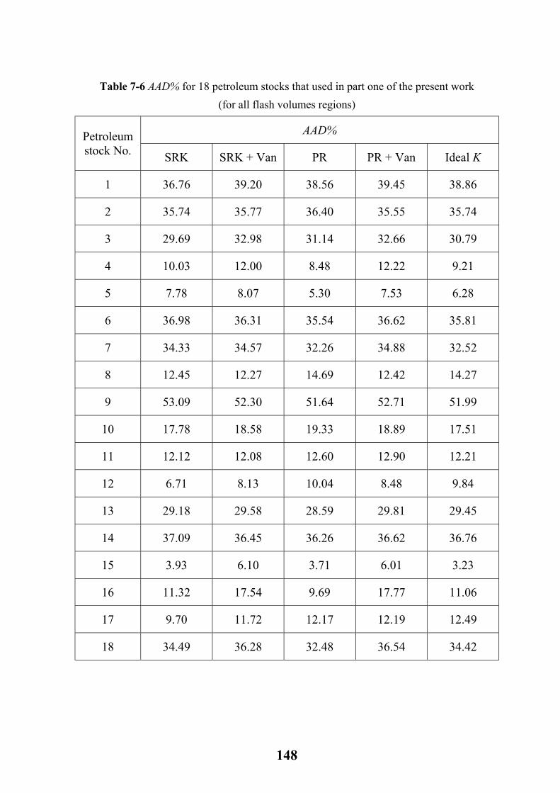
Table 7-6 AAD% for 18 petroleum stocks that used in part one of the present work (for all flash volumes regions)
AAD% Petroleum stock No. SRK SRK + Van PR PR + Van Ideal K
1 36.76 39.20 38.56 39.45 38.86
2 35.74 35.77 36.40 35.55 35.74
3 29.69 32.98 31.14 32.66 30.79
4 10.03 12.00 8.48 12.22 9.21
5 7.78 8.07 5.30 7.53 6.28
6 36.98 36.31 35.54 36.62 35.81
7 34.33 34.57 32.26 34.88 32.52
8 12.45 12.27 14.69 12.42 14.27
9 53.09 52.30 51.64 52.71 51.99
10 17.78 18.58 19.33 18.89 17.51
11 12.12 12.08 12.60 12.90 12.21
12 6.71 8.13 10.04 8.48 9.84
13 29.18 29.58 28.59 29.81 29.45
14 37.09 36.45 36.26 36.62 36.76
15 3.93 6.10 3.71 6.01 3.23
16 11.32 17.54 9.69 17.77 11.06
17 9.70 11.72 12.17 12.19 12.49
18 34.49 36.28 32.48 36.54 34.42
148
Table 7-7 AD% for 18 petroleum stocks that used in part one of the present work (for all flash volumes regions)
AD% Petroleum stock No. SRK SRK + Van PR PR + Van Ideal K
1 36.53 39.20 34.64 39.45 34.88
2 29.45 29.55 28.52 29.52 28.54
3 29.41 32.98 26.44 32.66 27.83
4 10.03 12.00 7.70 12.22 8.89
5 7.74 8.07 4.42 7.53 6.04
6 36.98 36.31 35.54 36.62 35.81
7 34.33 34.57 32.26 34.88 32.52
8 -2.77 -0.59 -5.49 1.20 -4.11
9 53.09 52.30 51.64 52.71 51.99
10 13.98 14.78 8.31 15.63 7.65
11 -2.35 -0.33 -4.60 -0.42 -3.65
12 5.79 8.13 3.18 8.48 4.06
13 29.18 29.58 28.59 29.81 29.45
14 37.09 36.45 36.26 36.62 36.76
15 -0.21 2.07 -3.60 2.28 -2.80
16 11.32 17.54 8.36 17.77 10.47
17 5.13 10.86 1.03 11.36 5.81
18 34.49 36.28 32.48 36.54 34.42
149
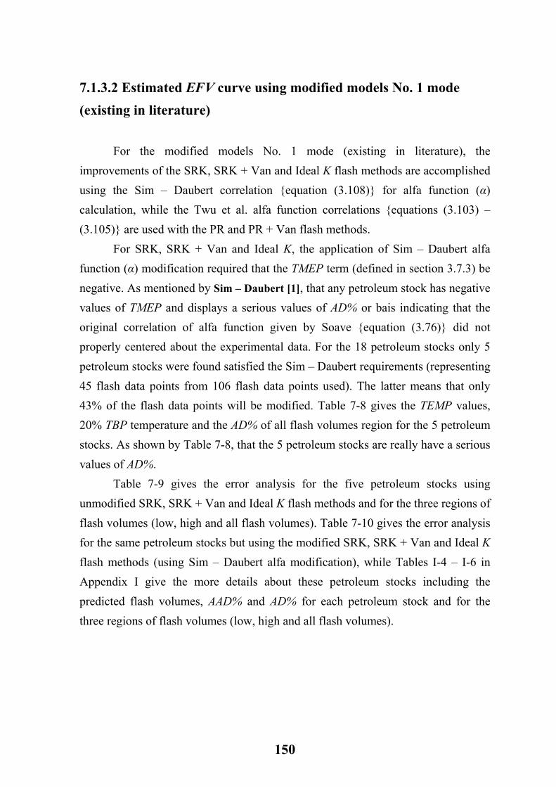
7.1.3.2 Estimated EFV curve using modified models No. 1 mode (existing in literature)
For the modified models No. 1 mode (existing in literature), the improvements of the SRK, SRK + Van and Ideal K flash methods are accomplished using the Sim – Daubert correlation {equation (3.108)} for alfa function (α) calculation, while the Twu et al. alfa function correlations {equations (3.103) – (3.105)} are used with the PR and PR + Van flash methods. For SRK, SRK + Van and Ideal K, the application of Sim – Daubert alfa function (α) modification required that the TMEP term (defined in section 3.7.3) be negative. As mentioned by Sim – Daubert [1], that any petroleum stock has negative values of TMEP and displays a serious values of AD% or bais indicating that the original correlation of alfa function given by Soave {equation (3.76)} did not properly centered about the experimental data. For the 18 petroleum stocks only 5 petroleum stocks were found satisfied the Sim – Daubert requirements (representing 45 flash data points from 106 flash data points used). The latter means that only 43% of the flash data points will be modified. Table 7-8 gives the TEMP values, 20% TBP temperature and the AD% of all flash volumes region for the 5 petroleum stocks. As shown by Table 7-8, that the 5 petroleum stocks are really have a serious values of AD%. Table 7-9 gives the error analysis for the five petroleum stocks using unmodified SRK, SRK + Van and Ideal K flash methods and for the three regions of flash volumes (low, high and all flash volumes). Table 7-10 gives the error analysis for the same petroleum stocks but using the modified SRK, SRK + Van and Ideal K flash methods (using Sim – Daubert alfa modification), while Tables I-4 – I-6 in Appendix I give the more details about these petroleum stocks including the predicted flash volumes, AAD% and AD% for each petroleum stock and for the three regions of flash volumes (low, high and all flash volumes).
150
Table 7-8 TMEP values, 20% TBP and AD% values for five petroleum stocks that satisfy the Sim – Daubert requirements
AD% Petroleum stock No.
20% TBP temperature,
°C
20% TBP temperature,
°F TEMP SRK SRK +
Van Ideal K
3 197.78 388 -4.01 29.41 32.98 27.83 4 156.11 313 -0.01 10.03 12.00 8.89 9 252.22 486 -0.39 33.09 52.30 51.99
16 158.33 317 -1.9 11.32 17.54 10.07 18 177.22 351 -0.45 34.44 36.28 34.42
Table 7-9 Error analysis for the five petroleum stocks using unmodified models mode
Low flash volumes region
High flash volumes region
All flash volumes region Flash
method AAD% AD% AAD% AD% AAD% AD% SRK 44.06 44.06 6.18 6.13 26.35 26.31 SRK + Van 46.21 46.21 8.54 8.54 29.28 29.28 Ideal - K 45.07 45.07 5.30 4.51 26.14 25.50 RD graph 30.65 -3.80 5.69 -4.85 15.12 -4.5 No. of points 17 28 45
Table 7-10 Error analysis for the five petroleum stocks using modified models No. 1
Low flash volumes region
High flash volumes region
All flash volumes region Flash
method AAD% AD% AAD% AD% AAD% AD% SRK 28.54 12.61 1.95 0.99 15.40 6.91 SRK + Van 45.49 45.49 8.48 8.48 28.88 28.88 Ideal K 44.29 44.29 5.28 4.51 25.73 25.12 No. of points 17 28 45 As shown by Tables 7-9 and 7-10, that the modified SRK flash method has a reliable ability for prediction of flash volumes for the three regions of flash volumes (low, high and all flash volumes regions). Using the modified SRK flash method improves the values for AAD% and AD% for the three regions of flash volumes by more than 30% and 60% for AAD% and AD% respectively (especially for the low flash volumes regions) as compared with Tables 7-10 and 7-9. Also, it indicates that the performance of the modified SRK flash method was some what the same as the RD graph flash method.
151
It can be seen also from above mentioned error analysis of Tables 7-9 and 7-10, that the modified Sim – Daubert alfa function correlation has slightly little effect on the performance of SRK + Van and Ideal K flash methods as compared with unmodified flash methods. This is due to the following reasons:
− For the SRK + Van flash method, and since the flash pressure used was atmospheric pressure, it is expected that the ratio of the partial vapor fugacity coefficient to the saturation vapor fugacity coefficient of equation (3.147) for each
cut ( Vsi
Vi φφ ) is approximately closer to unity, consequently this makes the effect
of the modified alfa function correlation given by Sim – Daubert has a slightly little effect on the performance of the SRK + Van flash method.
− For the Ideal K flash method, the vapor pressure term ( ) of equation
(3.160) is the most important term, thus the other terms of equation (3.160) including the alfa function term have a miner effect. Consequently, the modified alfa function correlation given by Sim – Daubert has a slightly little effect on the performance of the Ideal K flash method.
siP
For the PR and PR + Van flash methods, the Twu et al. modified alfa function correlation is used. All the 18 petroleum stocks are included in the Twn et al. modification of the alfa function (i.e. 106 flash data points used).
Table 7-11 gives the error analysis using AAD% and AD% for the 18 petroleum stocks using the unmodified PR and PR + Van flash methods and for the three categories of flash volumes (low, high and all flash volumes regions respectively).
Table 7-12 gives the error analysis using the AAD% and the AD% for the 18 petroleum stocks using the modified PR and PR + Van flash methods (i.e. using Twu alfa function modification) and for the three regions of the flash volumes. A complete error analysis for each of the 18 petroleum stocks, including the predicted flash volumes, AAD% and AD% are given in Tables I-7, I-8 and I-9 in Appendix I. As shown in Tables 7-11 and 7-12 show that there is no significant improvement of the modified Twu et al. alfa function correlation on the performance of PR and PR + Van flash methods as compared to unmodified flash methods. This is due to the following reasons:
152
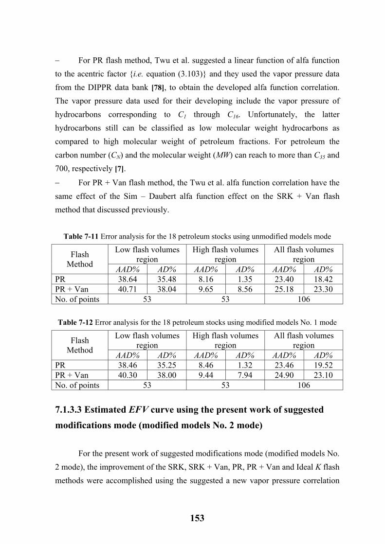
−
−
For PR flash method, Twu et al. suggested a linear function of alfa function to the acentric factor {i.e. equation (3.103)} and they used the vapor pressure data from the DIPPR data bank [78], to obtain the developed alfa function correlation. The vapor pressure data used for their developing include the vapor pressure of hydrocarbons corresponding to C1 through C16. Unfortunately, the latter hydrocarbons still can be classified as low molecular weight hydrocarbons as compared to high molecular weight of petroleum fractions. For petroleum the carbon number (CN) and the molecular weight (MW) can reach to more than C35 and 700, respectively [7].
For PR + Van flash method, the Twu et al. alfa function correlation have the same effect of the Sim – Daubert alfa function effect on the SRK + Van flash method that discussed previously.
Table 7-11 Error analysis for the 18 petroleum stocks using unmodified models mode
Low flash volumes region
High flash volumes region
All flash volumes region Flash
Method AAD% AD% AAD% AD% AAD% AD% PR 38.64 35.48 8.16 1.35 23.40 18.42 PR + Van 40.71 38.04 9.65 8.56 25.18 23.30 No. of points 53 53 106 Table 7-12 Error analysis for the 18 petroleum stocks using modified models No. 1 mode
Low flash volumes region
High flash volumes region
All flash volumes region Flash
Method AAD% AD% AAD% AD% AAD% AD% PR 38.46 35.25 8.46 1.32 23.46 19.52 PR + Van 40.30 38.00 9.44 7.94 24.90 23.10 No. of points 53 53 106
7.1.3.3 Estimated EFV curve using the present work of suggested modifications mode (modified models No. 2 mode)
For the present work of suggested modifications mode (modified models No. 2 mode), the improvement of the SRK, SRK + Van, PR, PR + Van and Ideal K flash methods were accomplished using the suggested a new vapor pressure correlation
153
{i.e. equation (6.10)}. The application of the suggested new vapor pressure required that the TEMP for the interested petroleum stocks be negative or positive higher or equal to 4. For the 18 petroleum stocks investigated, only 10 petroleum stocks (represented 61 flash data points out of 106 flash data points) were found to satisfy the above requirements. The latter means that 58% of the used flash data points will be modified. The TEMP values and the 20% TBP temperatures for these petroleum stocks are given in Table 7-13.
Table 7-13 TEMP values and 20% TBP temperature for ten petroleum stocks that satisfy the suggested vapor pressure correlation requirements
AD% Petroleum stock No.
20% TBP temperature, °C
20% TBP temperature, °F TEMP Ideal K
1 148.89 300.0 4.80 34.88 2 132.22 270.0 10.00 28.54 3 197.78 388.0 -4.01 27.83 6 125.00 257.0 10.00 35.81 7 127.78 262.0 6.50 32.52 9 252.22 486.0 -0.39 51.99 13 108.00 226.4 9.21 29.45 14 232.78 451.0 10.00 36.76 16 158.33 317.0 -1.59 10.47 18 177.22 351.0 -0.14 34.42
Table 7-14 gives the error analysis for the ten petroleum stocks using the unmodified flash methods (i.e. SRK, SRK + Van, PR, PR + Van and Ideal K flash methods). While Table 7-15 gives the error analysis for the same ten petroleum stocks using the present work of suggested modifications (modified models No. 2) with the SRK, SRK + Van, PR, PR + Van and Ideal K flash methods. The complete information about the predicted flash volumes and error analysis (including AAD% and AD%) for each petroleum stock are given in details in Tables I-10, I-11 and I-12 in Appendix I.
154
Table 7-14 Error analysis for ten petroleum stocks using unmodified models mode
Low flash volumes region
High flash volumes region
All flash volumes region Flash
Method AAD% AD% AAD% AD% AAD% AD% SRK 53.90 53.59 10.53 9.74 23.51 31.31 SRK + Van 55.30 55.07 12.51 11.73 24.98 33.04 PR 53.76 53.48 9.08 6.27 23.40 29.49 PR + Van 55.55 55.34 12.62 11.85 25.18 33.24 Ideal K 54.59 54.35 9.64 7.40 23.75 30.49 RD graph 25.95 -5.69 10.92 -7.83 21.81 -7.42 No. of points 30 31 61
Table 7-15 Error analysis for ten petroleum stocks using the present work suggested
modification mode (modified models No. 2 mode)
Low flash volumes region
High flash volumes region
All flash volumes region Flash
method AAD% AD% AAD% AD% AAD% AD% SRK 35.35 32.96 8.48 7.26 21.69 19.90 SRK + Van 24.33 21.16 8.68 4.95 16.38 12.92 PR 35.40 33.69 6.89 3.42 20.91 18.31 PR + Van 25.03 22.20 8.79 5.09 17.00 13.50 Ideal K 23.42 20.08 8.07 0.12 15.62 9.94 No. of points 30 31 61 As shown in Tables 7-14 and 7-15, the performance of the modified flash method (using the suggested vapor pressure correlation) were improved significantly as compared with the unmodified flash methods and the RD graph method using the same data points. The most improvement occurred in the low region of flash volumes, in which the values of AAD% and AD% improved by more than 30% for SRK and PR flash methods and by more than 50% for SRK + Van, PR + Van flash methods. Improvements can be also shown in the high region of flash volumes, in which the values of AAD% and AD% improved by more than 20% for SRK and PR flash methods and by more than 30% for the SRK + Van and PR + Van flash methods (however the AD% showed more than 45% improvement for SRK + Van). For the region of all flash volumes, the improvements of AAD% and AD% were by more than 10% and 30% respectively for both SRK and PR flash
155
methods, while the improvements of the AAD% and AD% were by more than 30% and 50% respectively for both SRK + Van and PR + Van flash methods. The important improvement in AAD% and AD% values occurred by using the modified Ideal K flash method (as compared with unmodified flash methods and RD graph method). The improvements include the three regions of flash volumes. Using the modified Ideal K flash method, the AAD% and AD% values improved by more than 50% for the low flash volumes region. For the high flash volumes region the improvements in AAD% and AD% values were by more than 10% and 70% respectively, while for the all flash volumes region, the improvement of AAD% and AD% values were by more than 30% and 60% respectively. The above mentioned error analysis indicates that the Ideal K flash method was most accurate method for estimation the EFV curves as compared with the other unmodified flash methods (SRK, PR, SRK + Van, PR + Van and Ideal K) and the RD graph flash method. The reasons behind the above mentioned improvements in the values of AAD% and AD% for the modified flash methods (SRK, PR, SRK + Van, PR + Van and Ideal K) can be summarized as follows:
−
−
For the Ideal K flash method, the ideal solution K – value equation is used with this method {equation (3.160)}. The vapor pressure term of equation (3.160) is the most important term of that equation. For the unmodified Ideal K flash method, the Lee – Kasler correlation {equation (3.113)}, the Lee – Kasler correlation was developed by using the vapor pressure of pure low molecular weight hydrocarbons, consequently it is expected that this correlation will not be suitable for the high molecular weight petroleum fractions. In the suggested new vapor pressure correlation, the flash data points of the 106 petroleum stocks were used with conjunction of the Ideal K solution equation for developing the coefficients of the new vapor pressure correlation {equation (6.10)}, consequently this methodology improved the performance of the correlation for high molecular weight petroleum fractions.
For SRK and PR flash methods, the SRK and PR EOS were used for estimation the K – values by using equation (3.60). As mentioned previously that the most important term of SRK and PR EOS is the alfa function term. For the unmodified SRK and PR flash method, the alfa function terms were calculated by
156
using equations (3.76) and (3.90) respectively. The m terms for the above mentioned equations were correlated by using the acentric factor for each cut, that estimated by using the Lee – Kasler correlations {equations (3.12) and (3.13)}. Both equations (3.12) and (3.13) are correlated by using the vapor pressure of the low molecular weight hydrocarbons, consequently, it is expected that the m terms for original alfa functions (α) (and thus the alfa function terms) for both SRK and PR EOS will not be suitable for high molecular weight petroleum fractions. For modified SRK and PR flash methods the m terms for the alfa functions of the SRK and PR EOS were calculated using the suggested modified acentric factors for each cut (ω). The suggested modified acentric factor (ω) was calculated using Pitzer et al. equation {equation (3.78)} with the using of the suggested new vapor pressure correlation {equation (6.10)}. Table 7-16 gives the comparison between the Lee – Kasler acentric factors and the modified acentric factors for petroleum stock No. 1, while Tables J-1 to J-9 in Appendix J give the same comparison for the petroleum stocks of Table 7-13. Tables 7-16 and J-1 to J-9 indicate that the using of suggested new vapor pressure correlation improved the estimation of the acentric factors for each cut by reducing their values (comparing to Lee – Kasler correlation for ω) for those cuts that have approximately of 450 °C (≈ 842 °F), while it increases their values for heavier cuts {above 450 °C (842 °F)}. The heavier cuts have the values of acentric factor greater than 1, the latter is expected for petroleum fractions [20].
−
−
For SRK + Van and PR + Van flash methods, since the flash calculation was accomplished at atmospheric pressure, and as discussed in section 5.4.4.2, the most important term that affects the performance of the calculated K – values using equation (3.147) of the vapor pressure. Since the suggested new vapor pressure correlation was used instead of Lee – Kasler correlation the performance for both flash methods for estimation the flash volumes improved.
For all modified flash methods, the above mentioned improvements in the values of AAD% and AD% represent the resultant of the addition of the second condition of the TEMP term that used in the improving the suggested new vapor pressure correlation in which the positive values of the TEMP term were also included (not just the negative values of TEMP term). To understand the reason behind the addition of the positive TEMP term in the present work which includes
157
the developing the vapor pressure correlation, it must first understood that the philosophy of the TEMP term that originally used by Sim – Daubert alfa function developing. As mentioned by Sim – Daubert [1], that any petroleum stocks that have negative values of TEMP displays a serious value of AD% or bais. This fact is extended by the present work to cover also the positive values of TEMP (which have values of more than 4) because in spite of the petroleum stock has positive TEMP values it is still has a serious value of AD% or bais. The latter fact can be shown by referring to Table 7-13 which is including the TEMP and AD% values for the ten petroleum stocks that satisfy the present work of suggested modifications requirements. Table 7-13 indicates that the Ideal K flash method shows a serious AD% with the positive and negative values of TEMP term (not just negative values as suggested by Sim – Daubert modification).
158
Table 7-16 Comparison between Lee – Kasler acentric factors and modified acentric factors for petroleum stock No. 1
Cut TB, °C TB, °F Lee – Kasler ωLK Modified ω 1 66.56 151.81 0.2540 0.1622 2 75.87 168.57 0.2634 0.1729 3 86.65 187.96 0.2749 0.1861 4 98.62 209.52 0.2883 0.2016 5 111.56 232.81 0.3033 0.2192 6 125.23 257.41 0.3197 0.2388 7 139.43 282.97 0.3374 0.2599 8 153.96 309.13 0.3560 0.2825 9 168.66 335.60 0.3753 0.3061 10 183.39 362.10 0.3952 0.3307 11 197.99 388.39 0.4154 0.3559 12 212.38 414.28 0.4358 0.3816 13 226.43 439.57 0.4562 0.4074 14 240.07 464.13 0.4764 0.4333 15 253.26 487.86 0.4964 0.4590 16 265.94 510.68 0.5160 0.4843 17 278.08 532.54 0.5352 0.5092 18 289.70 553.45 0.5538 0.5336 19 300.79 573.42 0.5720 0.5574 20 311.40 592.52 0.5898 0.5807 21 321.57 610.82 0.6071 0.6034 22 331.36 628.46 0.6240 0.6257 23 340.88 645.58 0.6408 0.6478 24 350.21 662.39 0.8150 0.8024 25 359.50 679.10 0.8378 0.8282 26 368.87 695.96 0.8610 0.8546 27 378.48 713.27 0.8852 0.8820 28 388.52 731.34 0.9108 0.9109 29 399.19 750.54 0.9382 0.9419 30 410.68 771.23 0.9643 0.9759 31 423.26 793.86 0.9947 1.0135 32 437.14 818.86 1.0281 1.0556 33 452.63 846.73 1.0651 1.1033 34 469.99 877.98 1.1062 1.1576 35 489.54 913.18 1.1520 1.2199 36 511.60 952.89 1.2031 1.2914 37 536.52 997.73 1.2601 1.3737 38 564.65 1048.37 1.3233 1.4683 39 596.37 1105.46 1.3933 1.5769 40 632.09 1169.76 1.4704 1.7010
159
7.1.3.4 Effect of measured or calculated parameters on the predicted flash volumes
It can be seen that even with the modification on the flash methods, there is a considerable AAD% and AD% (more than 25%) persist in the low flash volume predictions (first category of the flash volumes), while an acceptable AAD% and AD% (less than 10%) persist in the high flash volume predictions (second category of flash volumes). The considerable high AAD% and AD% persist in the low flash volume predictions arise the question whether any further improvement can be reached. In order to answer this question, it is first necessary to ensure that the accuracy of the flash methods used in the investigation are not limited by errors in the measured or calculated parameters. Sim – Daubert [1] achieved a useful study on the effect of the error of the measured or calculated parameters on the performance of the SRK flash method for prediction the EFV curve from the TBP curve. According to that study, the error in the prediction of flash volumes using SRK flash method can come from two sources, first the error in calculated basic characterization parameters such as molecular weight (MW), critical properties (Tc, Pc), acentric factor (ω) …etc. For petroleum fractions it is not possible to determine the error introduced through the uses of the characterization parameter correlations since experimental values for the molecular weight (MW), critical properties (Tc, Pc), acentric factors (ω) are unknowns. The estimated characterization parameters from the characterization correlations are usually compared to heavy n – alkane compared such as n – heptane and n – octane. The other sources of error in the prediction of the flash volume can be introduced through the use of the measuring experimental parameter including flash temperature, flash pressure and the TBP curve. According to the ASTM standards part 18 (1971), the uncertainty in the thermocouple measurement is approximately ± 0.5 °C, while error in the recorded pressure ± 1%. What is more significant, however is that the repeatability of the TBP curve. According to ASTM D 287 – 82, the repeatability is defined as the difference between successive tests results obtained by the same operator with the same apparatus under constant operating conditions on identical test material, would in the long run. The sensitivity of the
160
SRK flash method to slight errors in the measured parameter was evaluated and the results indicate that at low flash volumes (first category of flash volumes) a 0.5 °C error in the flash temperature can alter the SRK flash method predicted flash volume by 15%, while a 1% error in the pressure alters the predicted flash volume by 11%. The major source of error is the TBP curve. For low flash volume (first category of the flash volumes) a 5 °C error in TBP curve will result in a 100% error in the predicted flash volumes, while the 2.5 °C error in TBP can alter the predicted flash volume by more than 50% (> 50%). For the high flash volumes (second category), the error resulting from in accuracies in TBP curve is approximately 8%. The effect of errors in the flash temperature and flash pressure are negligible at high flash volumes (second category of flash volumes). Sim – Daubert expected that the above error analysis of the input parameter can be extended to other flash methods including the graphical methods. For the present work, the repeatability for the TBP curves for the 18 petroleum stocks that used in part one investigations was ± 5 °C, while for the TBP curve for part two (four Iraqi crude oils) was ± 2.3 °C. While it is not possible to demonstrate conclusively that the inconsistencies in the flash method results are due to experimental errors, it is at least reasonable to conclude that the error in the basic characterization parameters (MW, Tc, Pc, ω, …etc), and experimental parameters are capable of fully explaining the behavior of the flash methods used in present work investigations. It must be noted here, and because of the sensitivity of the error in TBP curve on the performance of the used flash methods in the low flash volumes region, one must be careful when the working TBP curves were obtained by using the interpolation and extrapolation techniques. For the present work the latter curves were obtained using a minimum equation factor values (R2) of 0.9888, to ensure a good accuracy for the working TBP curve.
7.1.4 Part two (Application part)
In part two of the present work, the EFV curves for four Iraqi crude oils are estimated from the TBP curves. These crude oils are Kirkuk, Basrah, Jambour and
161
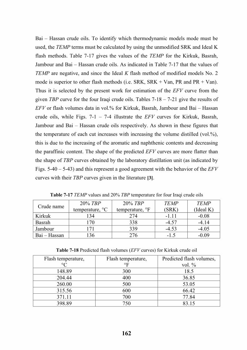
Bai – Hassan crude oils. To identify which thermodynamic models mode must be used, the TEMP terms must be calculated by using the unmodified SRK and Ideal K flash methods. Table 7-17 gives the values of the TEMP for the Kirkuk, Basrah, Jambour and Bai – Hassan crude oils. As indicated in Table 7-17 that the values of TEMP are negative, and since the Ideal K flash method of modified models No. 2 mode is superior to other flash methods (i.e. SRK, SRK + Van, PR and PR + Van). Thus it is selected by the present work for estimation of the EFV curve from the given TBP curve for the four Iraqi crude oils. Tables 7-18 – 7-21 give the results of EFV or flash volumes data in vol.% for Kirkuk, Basrah, Jambour and Bai – Hassan crude oils, while Figs. 7-1 – 7-4 illustrate the EFV curves for Kirkuk, Basrah, Jambour and Bai – Hassan crude oils respectively. As shown in these figures that the temperature of each cut increases with increasing the volume distilled (vol.%), this is due to the increasing of the aromatic and naphthenic contents and decreasing the paraffinic content. The shape of the predicted EFV curves are more flatter than the shape of TBP curves obtained by the laboratory distillation unit (as indicated by Figs. 5-40 – 5-43) and this represent a good agreement with the behavior of the EFV curves with their TBP curves given in the literature [3].
Table 7-17 TEMP values and 20% TBP temperature for four Iraqi crude oils
Crude name 20% TBP temperature, °C
20% TBP temperature, °F
TEMP (SRK)
TEMP (Ideal K)
Kirkuk 134 274 -1.11 -0.08 Basrah 170 338 -4.57 -4.14 Jambour 171 339 -4.53 -4.05 Bai – Hassan 136 276 -1.5 -0.09
Table 7-18 Predicted flash volumes (EFV curves) for Kirkuk crude oil
Flash temperature, °C
Flash temperature, °F
Predicted flash volumes, vol. %
148.89 300 18.5 204.44 400 36.85 260.00 500 53.05 315.56 600 66.42 371.11 700 77.84 398.89 750 83.15
162
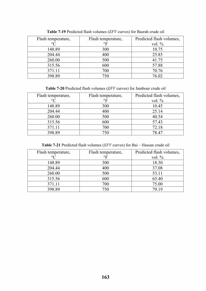
Table 7-19 Predicted flash volumes (EFV curves) for Basrah crude oil
Flash temperature, °C
Flash temperature, °F
Predicted flash volumes, vol. %
148.89 300 10.75 204.44 400 25.85 260.00 500 41.75 315.56 600 57.88 371.11 700 70.76 398.89 750 76.02
Table 7-20 Predicted flash volumes (EFV curves) for Jambour crude oil
Flash temperature, °C
Flash temperature, °F
Predicted flash volumes, vol. %
148.89 300 10.45 204.44 400 25.14 260.00 500 40.54 315.56 600 57.43 371.11 700 72.18 398.89 750 78.47
Table 7-21 Predicted flash volumes (EFV curves) for Bai – Hassan crude oil
Flash temperature, °C
Flash temperature, °F
Predicted flash volumes, vol. %
148.89 300 18.30 204.44 400 37.08 260.00 500 53.11 315.56 600 65.40 371.11 700 75.00 398.89 750 79.19
163
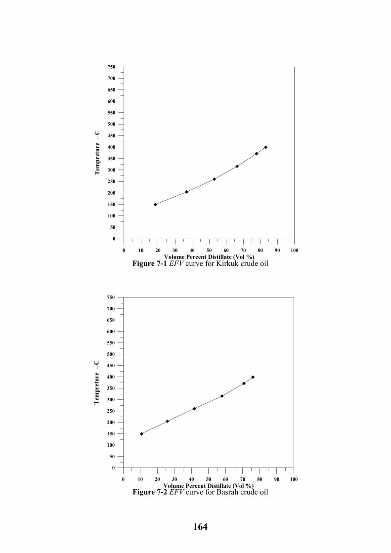
Figure 7-1 EFV curve for Kirkuk crude oil
0 10 20 30 40 50 60 70 80 90 1Volume Percent Distillate (Vol %)
0
50
100
150
200
250
300
350
400
450
500
550
600
650
700
750
Tem
pret
ure
C
0
00
Figure 7-2 EFV curve for Basrah crude oil
0 10 20 30 40 50 60 70 80 90 1Volume Percent Distillate (Vol %)
0
50
100
150
200
250
300
350
400
450
500
550
600
650
700
750
Tem
pret
ure
C
0
00
164
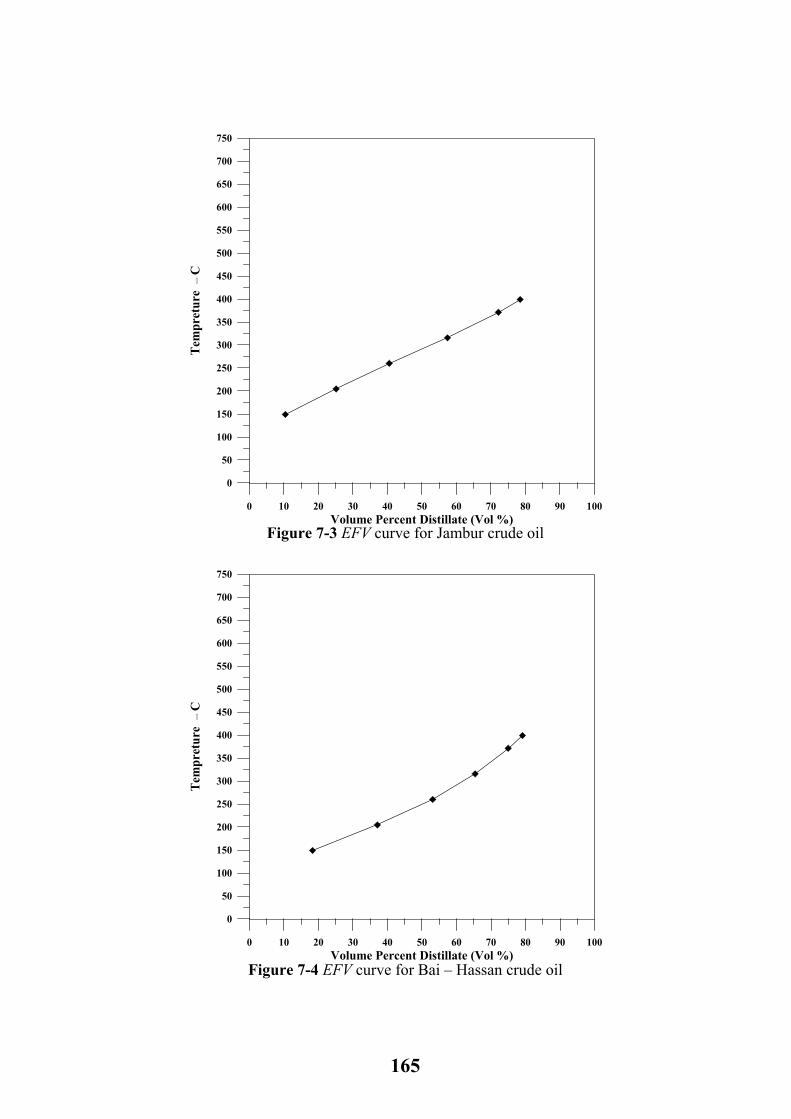
Figure 7-3 EFV curve for Jambur crude oil
0 10 20 30 40 50 60 70 80 90 1Volume Percent Distillate (Vol %)
0
50
100
150
200
250
300
350
400
450
500
550
600
650
700
750
Tem
pret
ure
C
0
00
Figure 7-4 EFV curve for Bai – Hassan crude oil
0 10 20 30 40 50 60 70 80 90 1Volume Percent Distillate (Vol %)
0
50
100
150
200
250
300
350
400
450
500
550
600
650
700
750
Tem
pret
ure
C
0
00
165
After the EFV curves for Kirkuk, Basrah, Jambour and Bai – Hassan crude oils were predicted, the flash zone temperatures of these crude oils can also be predicted. This can be performed by using Nelson procedure [3], and as follows: 1. The volume percent distilled for each crude oil at the end point of atmospheric gas oil. Usually this end point takes at 350 °C (≈ 660 °F) [81, 103]. The volume percent distilled at 350 °C can be obtained from the TBP curve. The values of volume distilled for Kirkuk, Basrah, Jambour and Bai – Hassan crude oils at 350 °C are 64.1%, 58.3%, 63.4% and 58.62% respectively. 2. The flash zone temperature can be read from the EFV curve by using the volume percent distilled at 350 °C. Consequently, the flash zone temperatures for Kirkuk, Basrah, Jambour and Bai – Hassan crude oils are 318 °C, 327 °C, 335 °C and 290 °C respectively. The predicted flash zone temperatures are reliable because they are under the cracking temperature. Usually the cracking temperature of petroleum stocks that have the range of 350 °C to 370 °C (662 °F – 698 °F) [5, 22,
3]. It must be noted here that the predicted flash zone temperatures for Kirkuk, Basrah, Jambour and Bai – Hassan crude oils must be considered as primary values. They are of the flash zone temperatures and they must be adjusted to the crude oil tower pressure and to the temperature, pressure and the amount of the stripping steam that usually used with the atmospheric crude oil tower [3].
7.2 Conclusions The purposes of the present work were divided into two parts: part one has two folds, the first one involves taking data of TBP, EFV and specific gravity for 18 petroleum stocks from literature and investigated the graphical method, and also the pseudo – component methods using three thermodynamic models modes to predict the EFV curve from TBP curve. Secondly, various attempts for improving the accuracy of the existing pseudo – component methods were investigated. In part two of this work, the most promised (greatest accuracy) method which was developed in this work was applied to four Iraqi crude oils in which their TBP and specific gravity data or curves were obtained experimentally to predict their EFV curves and flash zone temperature.
166
The conclusions are as follows: For part one of this work, the Raizi – Daubert (RD graph) flash method was
selected as a graphical method, also three thermodynamic models namely unmodified models, modified models No. 1, and suggested modified model that was developed in this work were selected to predict the EFV curve from the TBP and specific gravity curves or data. Each one of these thermodynamic models consists of five flash methods namely SRK, SRK + Van, PR, PR + Van and Ideal K.
From the present work, the following conclusions are indicated: 1. For unmodified models mode, while nearly all flash methods can adequately predicted the flash volumes or EFV curves in high flash volumes region, non of these flash methods were reliable for prediction the flash volumes at low flash volumes regions. 2. For modified models No. 1 mode, which involves two models, the first one suggested by Sim – Daubert, and was used with the SRK, SRK + Van, and Ideal K flash methods, and the second models suggested by Twu et al. was used with PR, PR + Van flash methods. The results indicate the following points:
a. For the Sim – Daubert modification, only 5 petroleum stocks out of 18 petroleum stocks satisfied this model, this means that only 45 flash data points out of 106 flash data points used were modified (representing 43% from the total flash data points used). For those petroleum stocks that were satisfied by this modification, the results showed that when using with SRK flash method, the AAD% and AD% were improved by more than 30% and for all flash volumes regions as compared with unmodified flash methods and with RD Graph flash method. However, this modification had a little effect on improving the AAD% and AD%, when it is used with SRK + Van and Ideal K flash method, as compared with unmodified flash methods. b. The second modification that suggested by Twu et al. showed no significant improvements on AAD% and AD% when used with PR and PR + Van flash methods as compared with unmodified flash methods.
3. For the modified model suggested in this work using the new suggested vapor pressure correlation, 10 petroleum stocks out of 18 petroleum stocks were
167
satisfied by this suggested modification. This mean, that 61 flash data points out of 106 flash data points were modified. The results indicate the following points:
a. This modification when used with Ideal K flash method, the AAD% and AD% were improved by more than 50% for low flash volumes region, and more than 30% for all flash volumes region as compared with the unmodified flash methods, and RD graph method. b. When the acentric factor was calculated using the vapor pressure correlation suggested in this work, and then this acentric factor was used with SRK and PR flash methods (using their original alfa function correlation), the AAD% and AD% were improved specially in the low flash region by more than 45%, while the improvements in the other regions relatively much less. c. When using the new suggested vapor pressure correlation with the SRK + Van and PR + Van, the AAD% and AD% were improved more than 50% for low flash volumes region and more than 30% for all flash volumes region, as compared with the unmodified flash methods and RD Graph method. d. Results showed that the Ideal K flash method was superior to other flash methods used in this investigation (having less values of AAD% and AD%).
4. A computer program was developed using Quick Basic language for estimation the EFV curve from available TBP and specific gravity curves, the computer program can estimate the EFV curve using any one of the three thermodynamic models. 5. For part two of this work, the Ideal K flash method which was developed in this work and was the most accurate prediction method for performing the following items:
a. Estimation of the EFV curves for four Iraqi crude oils (Kirkuk, Basrah, Jambur, and Bai – Hassan), from TBP and specific gravity data. b. Using the EFV of these crude oils, the flash zone temperature were estimated. The values for these flash zone temperatures were 318 °C, 327 °C, 335 °C and 290 °C for Kirkuk, Basrah, Jambur and Bai – Hassan respectively. These flash zone temperatures were below their cracking temperatures and can
168
be considered good values in view of design point procedures. However, these values of flash zone temperatures must be considered as primary values and must be adjusted to the temperature, pressure, and the amount of stripping steam that usually used with crude oil tower.
7.3 Recommendations for further work
Based on the conclusions presented, the following recommendations may be made for further work: 1. Improving the Lee – Kasler perturbation equation by extended it to cover another ready measurable physical properties such as viscosity, refractive index, …etc. 2. Because of the sensitivity of the pseudo – components flash methods to error in measured TBP curve the following points may be recommended:
a) Using the ASTM curve instead of TBP curve for estimation EFV curve. b) Developing a new approach which utilizes only accessible fundamental properties of petroleum fractions (e.g. viscosity, specific gravity, refractive index, …etc) for estimation the basic characterization parameters (MW, Tc, Pc, ω, …etc), instead of using the existing correlations which used the TBP as a basic input parameters.
3. Study the estimation of the EFV curves for sub atmospheric and super atmospheric pressures from available TBP or ASTM curves.
169
References
[1] Sim W.J. and Daubert T.E., Ind. Eng. Chem. Process Des. Dev., 19, 386 (1980).
[2] American petroleum institute, "Technical data book – petroleum refining", Vol. 1, Ch. 4, Washington D.C. (1988).
[3] Nelson W.L., "Petroleum refining engineering", 4th ed., Mc Graw – Hill book company (1958).
[4] Edmister W.C., "Applied hydrocarbon thermodynamics", Vol. 1, Gulf publishing company, Texas (1967).
[5] Gary J.H. and Handwerk G.E., "Petroleum refining technology and economics", 2nd ed., Marcel Dakker Inc. (1984).
[6] Hariu O. and Sage R.C., Hydrocarbon processing, 48 (4), 143 (1969). [7] Raizi M.R., Aladwani H.A. and Marouf R., "Selection of a characterization
scheme for hydrocarbon systems", Internet resource available at (http: \\www. OilIndustry. pdf. htm) 2003.
[8] Lion A.R. and Edmister W.C., Hydrocarbon processing, 58 (8), 119 (1975). [9] Maxwell J.B., "Data book of hydrocarbons", 8th ed., Van Nostrand company
Inc. (1950). [10] Raizi M.R. and Daubert T.E., Oil and Gas J., 25 (8), 50 (1986). [11] American petroleum institute, "API – Technical data book – petroleum
refining", Vol. 1, Ch. 3, Washington D.C. (1988). [12] Kasler M.G. and Lee B.I., AIChE J., 21, 510 (1975). [13] Raizi M.R. and Daubert T.E., Hydrocarbon processing, 59 (3), 115 (1980). [14] Long R.B. and Speight J.G., "Petroleum chemistry and refining", 1st ed.,
Taylor and Eronics Inc. (2000). [15] Speight J.G., "The chemistry and technology of petroleum", 2nd ed., Marcel
Dakker Inc., New York (1991). [16] Bestougeff M., "Fundamental aspects of petroleum geochemistry", Elsevier
publishing company (1967).
170
[17] Rostler F.S., "Bituminous materials, asphalts, tars and pitches", Vol. 2, Hoibrg Editer Int., New York (1965).
[18] Altgelt K.H. and Gouw T.H., "Chromatography in petroleum analysis", Marcell Dekker Inc., New York (1976).
[19] Haak F.A. and Van Nes K., "Investigation into the olefinic components of Pennsylvania crude oil", Inst. Petrol. J., 37, 245 (1951).
[20] "Refining – petrochemicals engineering", rev. 4, ENSPM formation industries (2000).
[21] Marian P. and Gueret C., "Hydrocracking technology – latest advances", a paper presented by IFP industrial division (1995).
[22] Hobson G.D., "Modern petroleum technology", 4th ed., Applied science publisher LTD. (1973).
[23] "Managerial seminar on oil refining documentation", Dietsmann group comerint, S.P. Agip Petroli (2001).
[24] American petroleum institute, "Technical data book – petroleum refining", Vol. 1, Ch. 11, Washington D.C. (1985).
[25] Streeter V.L. and Benjamin W.E., "Fluid mechanics", Mc Graw – Hill book Co. (1983).
[26] Stichlmair J.G. and Fair J.R., "Distillation principles and practices", Wiley – Liss publication (1998).
[27] Attiya H.G., "A method for characterization of petroleum fractions", M.Sc. Thesis, College of Engineering, Baghdad University (2005).
[28] American petroleum institute, "Technical data book – petroleum refining", Vol. 1, Ch. 3, Washington D.C. (1977).
[29] Okamoto K.K. and Van Winkele M., Petroleum Refiner, 28 (8), 113 (1949). [30] Smith R.L. and Watson K.M., Ind. Eng. Chem., 25, 808 (1933). [31] Watson K.M., Nelson E.F. and Murphy G.B., Ind. Eng. Chem., 27, 1460
(1935). [32] Smith R.L. and Watson K.M., Ind. Eng. Chem., 29, 1408 (1937). [33] Winn F.W., Petroleum Refiner, 57 (2), 157 (1957). [34] Schou K. and Fredenslund A., Ind. Eng. Chem. Process Des. Dev., 23, 163
(1984).
171
[35] Mathur B.C., Ibrahim S.H. and Kuloor N.R., Chem. Eng., 76 (6), 182 (1969). [36] Kasler M.G. and Lee B.I., Hydrocarbon processing, 3, 153 (1976). [37] Twu C.H., Fluid Phase Equilibrium, 16, 137 (1984). [38] Raizi M.R. and Daubert T.E., Ind. Eng. Chem. Res., 26, 755 (1987). [39] Raizi M.R. and Shahhaf T.A., Ind. Eng. Chem., 34, 4145 (1995). [40] Walas S.M., "Phase equilibrium in chemical engineering", Butterworth
publisher, London (1985). [41] Campbell J.M., "Gas conditioning and processing", Vol. 1, Gulf publishing
company (1975). [42] Seader J.D. and Henly E.J., "Separation process principles", John Wiley and
Sons Inc. (1998). [43] Nelson W.L. and Souders M., Jr. Pet. Eng., 3 (1), 131 (1931). [44] Packie J.W., Trans. AIChE J., 37, 51 (1941). [45] Nelson W.C. Harvey R.J., Oil and Gas J., 47 (7), 71 (1948). [46] Edmister, Riedel and Marien, Trans. AIChE J., 39 (4), 157 (1943). [47] Edmister W.C. and Pollock D.H., Chem. Eng. Prog., 44, 905 (1948). [48] Edmister W.C., Petroleum Refiner, 45 (10, 11, 12), (1949). [49] American petroleum institute, "API – Technical data book – petroleum
refining", Vol. 1, Ch. 3, Washington D.C. (1982). [50] Arnold V.E., Oil and Gas J., 11 (12), 55 (1985). [51] PRO/ II, Key ward manual, Simulation science Inc., Fullerton, California
(1992). [52] Hysys. Plant, Version 2.0, "Simulation basis", Hyprotech Ltd., Alberta,
Canada (1998). [53] Katz D.L. and Brown G.G., Ind. Eng. Chem., 28 (7), 1373 (1933). [54] Pottman F.H. and Mayland J.B., Petroleum Refiner, 28 (7), 101 (1949). [55] Smith J.M. and Van Ness H.C., "Introduction to chemical engineering
thermodynamics", 4th ed., Mc Graw – Hill book company (1987). [56] Chao K.C. and Seader J.D., AIChE J., 7, 598 (1961). [57] Redlich D. and Kwong N.S., Chem. Rev., 44, 232 (1949). [58] Hilderbrand J.H., Prausnitz J.M. and Scott R.L., "Regular and related
solution", Van Nostrand Reinold company, New York (1970).
172
[59] Grayson H.G. and Streed C.W., "Sixth world petroleum congress", Frankfurt (1963).
[60] Hoffman H.G., Chem. Eng. Sci., 23, 957 (1968). [61] Linden N.J., "Vapor pressure charts for petroleum hydrocarbon", Esso
engineering and research company, April (1955). [62] Starling K.E. and Han M.S., Hydrocarbon Processing, 51 (6), 107 (1972). [63] Lee B.I., Erbar J.H. and Edmister W.C., AIChE J., 19 (2), 349 (1973). [64] Lion A.R. and Edmister W.C., Hydrocarbon Processing, 54 (8), 119 (1975). [65] Graboski M.S. and Daubert T.E., Ind. Eng. Chem. Process Des. Dev., 17,
443 (1978a), 448 (1978b). [66] Ibid, 18, 3001 (1979). [67] Soave G., Chem. Eng. Sci., 27, 1197 (1972). [68] Daubert T.E., Graboski M.S. and Danner R.P., "Documintation of the basis
for selection of contents of chapter 8 – vapor – liquid equilibrium K – values", American petroleum institute, Dept. of refining, Washington D.C. (1978).
[69] Peng D.Y. and Robinson D.B., Ind. Eng. Chem. Fundam., 15, 59 (1976). [70] American petroleum institute, "API – Technical data book – petroleum
refining", Ch. 8, Washington D.C. (1978). [71] American petroleum institute, "API – Technical data book – petroleum
refining", Vol. 1, Ch. 8, Washington D.C. (1982). [72] Ibid, Vol. 1, Ch. 3 (1988). [73] Ibid, Vol. 1, Ch. 8 (1992). [74] Ibid, Vol. 1, Ch. 8 (1997). [75] Mathias P.M., Ind. Eng. Chem. Process Des. Dev., 22, 385 (1983). [76] Methem G.A. et al., Fluid Phase Equilibrium, 47, 189 (1989). [77] Twu C.H. et al., Fluid Phase Equilibrium, 69, 33 (1991). [78] Chorng H.T., Wayne D.S. and Tasson V., "Getting a handle on advance
cubic equation of state", Internet resource available at (http: www. cepmagazine. org) (2002).
[79] Chu J.C. and Staffel E.J., J. Indst. Petrol., 41, 95 (1955). [80] Lenoir J.M. and Hipkin H.G., J. Chem. Eng. Data, 18, 18 (1973).
173
[81] OPEC world oil and energy study, Battele Geneva research center, Switzerland (1989).
[82] Katz D.L. and firoozabadi A., Petroleum Technology, 20, 160 (1989). [83] Gerald C.F. and Wheaty P.O., "Applied numerical analysis", 4th ed., Addison
Wesley publishing company, 1982. [84] Newman S.A., Hydrocarbon Processing, 10, 133 (1981). [85] Harold R.N., "Phase equilibrium in process design", Wiley – Interscience
publisher, New York (1970). [86] Chasib K.f., "Vapor – liquid equilibrium of ternary systems involving
experimental and theoretical correlations using cubic equation of state", Ph.D. Thesis, College of Engineering, Saddam University (2001).
[87] Prausintz J.M., Liehtenthaler R.N. and De Azevedo E.G., "Molecular thermodynamics of fluid phase equilibria", 2nd ed., Prentice – Hall, Englewood Cliffs, N.J. (1986).
[88] Seader J.D. and Henley E.J., "Equilibrium – stage separation operations in chemical engineering", John Wiley and Sons Inc. (1981).
[89] Ahmed T., "Reservoir engineering handbook", 2nd ed., Gulf professional publishing (2001).
[90] Hasan O. and Sandler S.I., "Modeling vapor – liquid equilibria – cubic equation of state and their mixing rules", 1st ed., Cambridge University press (1998).
[91] Marc J.A., Martin J.P. and Thomas F.T., "Thermophysical properties of fluid: An introduction to thin prediction", Imperial college press, 1st ed. (1998).
[92] Pitzer K.S., Lippman D.Z., Curl R.F. and Huggins C.M., J. Amer. Chem. Soc., 77, 3433 (1955).
[93] Spencer C.F. and Danner R.P., Chem. Eng. Data, 17, 236 (1972). [94] Ried R.C., Prausnitz J.M. and Poling B.E., "The properties of gases and
liquids", Mc Graw – Hill Prentice, Singapore (1988). [95] Ewell R.H., Harrison J.M. and Berg L., Ind. Eng. Chem., 36, 871 (1944). [96] Wilson G.M., J. Amer. Chem. Soc., 86, 127 (1964). [97] Renon H. and Prausnitz J.M., AIChE J., 19, 135 (1968).
174
[98] Renon H. and Prausnitz J.M., Ind. Eng. Chem. Process Des. Dev., 8, 413 (1969).
[99] Abram D. and Prausnitz J.M., AIChE J., 21, 116 (1975). [100] Prausnitz J.M., Edmister W.C. and Chao K.C., AIChE J., 6, 214 (1960). [101] Paul G. and Lachhman D., AIChE J., 17, 343 (1971). [102] Null H.R., "Phase equilibrium in process design", Interscience publisher
Inc., New York (1970). [103] Mechanical catalog for crude distillation unit, Vol. 1, Howe – Baker
Engineers Inc., Tyler – Texas (1973). [104] Norris F.A. and Terry D.E., Oil and Soup, 2, 41 (1945). [105] Poderson K.S., Thomas P. and Fredenslund A.G., Ind. Eng. Chem. Process
Des. Dev., 24, 948 (1985). [106] Valderrama J.O., Ind. Eng. Chem. Res., 42, 1603 (2003). [107] Kasler M.G., Lee B.I. and Sandler S.I., Ind. Eng. Chem. Fundam., 18, 49
(1979).
175
Appendix A
Example of calculation Example, A.1: Estimate the atmospheric EFV curve for petroleum fraction having the following atmospheric TBP curve and API = 32 °.
Distillation, vol.% 10 30 50 70 90 Temperature, °F 150 200 240 275 320
Solution: The Raizi – Dubert method is used with the following steps: Step 1: Converting the TBP temperature to ASTM D86 temperature using equation (3.3) as follows:
( )( )( 22 b1b11 TBPb86DASTM −= ) …(3.3)
Where ASTM D86 and TBP are in °R, b1 and b2 obtained from Table 3-1. For ASTM D86 10%: From Table 3-1, b1 = 0.5277 and b2 = 1.090. Using equation (3.3), thus:
( ) ( )( )( )09.1109.11 4601505277.0%1086DASTM += −
F55.185orR68.645%1086DASTM °°=
Or by using Fig. A-1, the ASTM D86 10% = 200 °F. Using equation (3.3) with other vol.% distilled, the remaining ASTM D86 temperature are obtained as follows:
Distillation, vol.% 10 30 50 70 90 ASTM D86, °F 185.5 213.4 239.2 267 304
Step 2: Obtaining the specific gravity (Sp.gr), using equation (3.5) or:
A.1
( ) ( 26288.010731.0 %5086DASTM%1086DASTM06711.0gr.Sp ⋅= )
)
so, ( ) ( ) 26288.010731.0 4602.2394605.18506711.0gr.Sp +⋅+=
°≈= API57or7517.0gr.Sp
Step 3: Converting the ASTM D86 temperature to EFV temperature using equation (3.4):
…(3.4) ( ) ( 32 cc1 gr.Sp86DASTMcEFV =
Where c1, c2 and c3 are obtained from Table 3-2. For EFV 10%: From Table 3-2, c1 = 3.2555, c2 = 0.8466 and c3 = 0.4208. Using equation (3.4):
( ) ( ) 4208.08466.0 7517.04605.1852555.3%10EFV +=
F8.214orR8.674%10EFV °°=
Or by using Fig. A-2, the EFV 10% = 220 °F
Using equation (3.4), with other vol.% distilled, the remaining ASTM D86 temperatures are obtained as follows:
Distillation, vol.% 10 30 50 70 90 EFV, °F 214.8 214.4 223.8 245.8 265.6
A.2
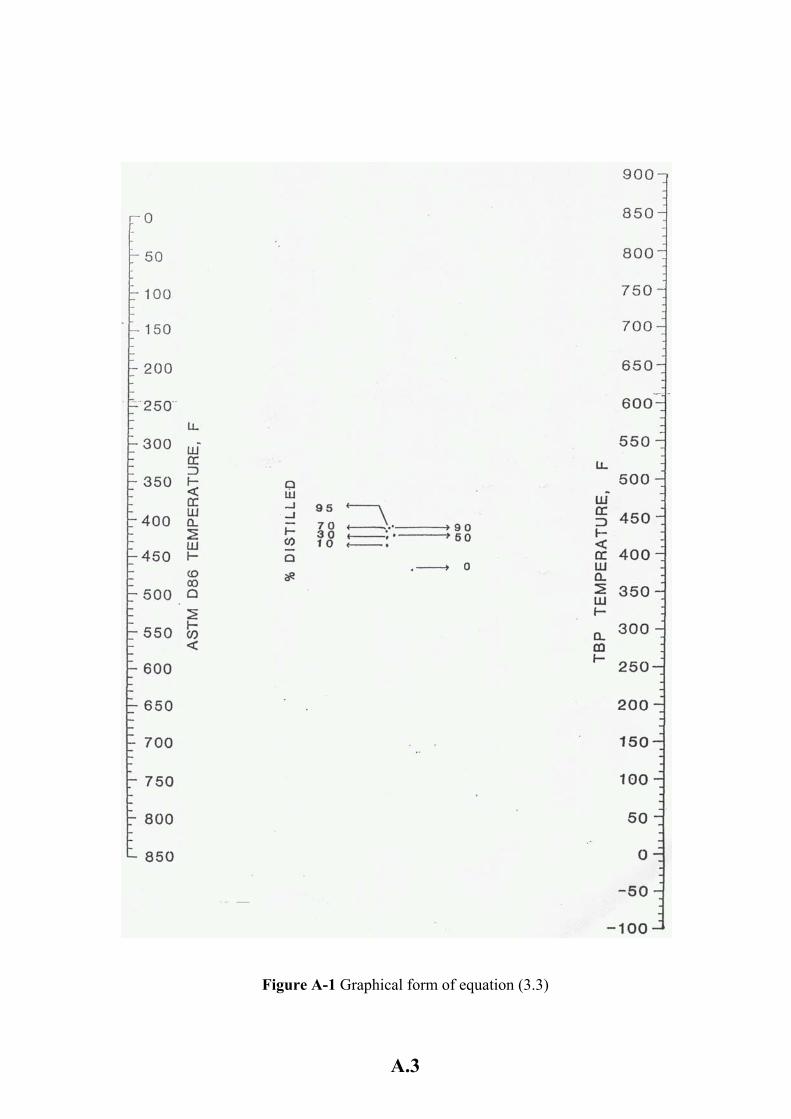
Figure A-1 Graphical form of equation (3.3)
A.3
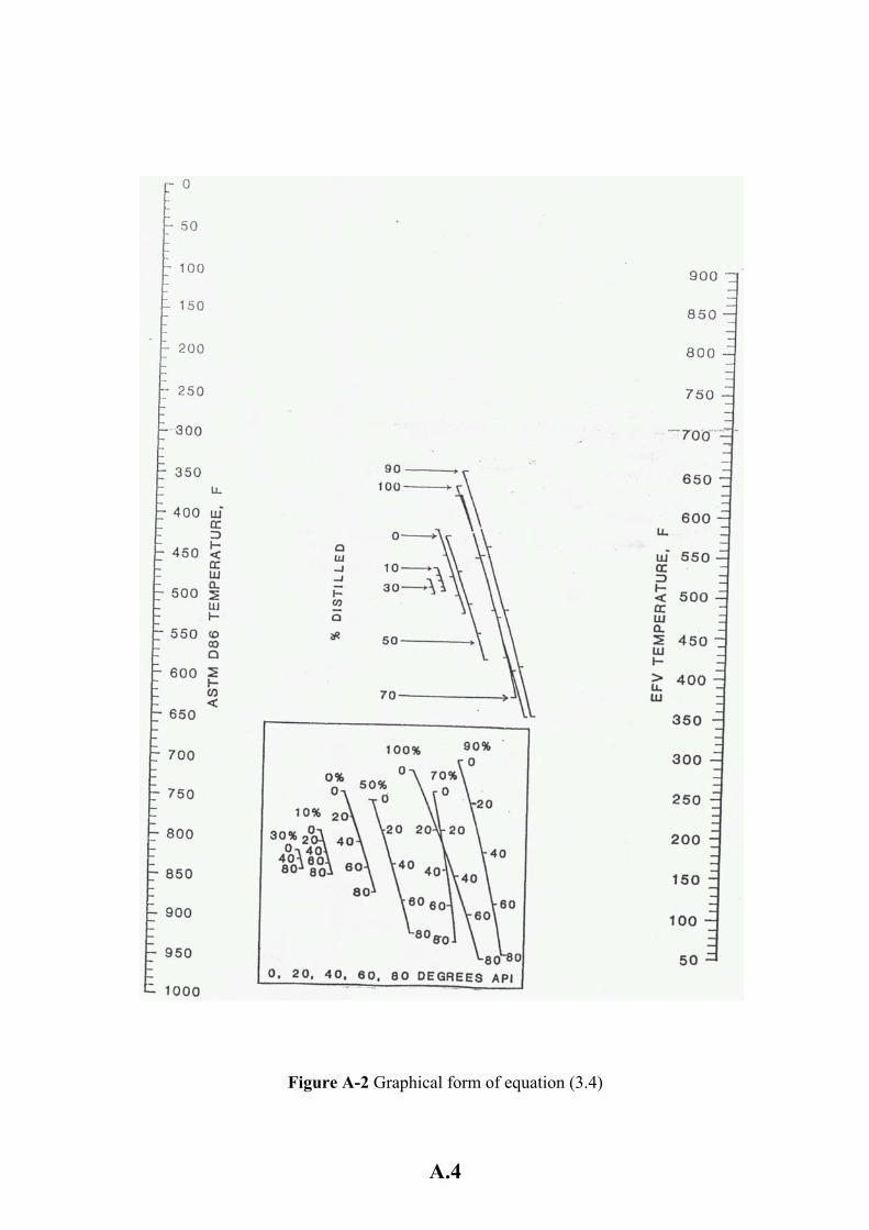
Figure A-2 Graphical form of equation (3.4)
A.4
Appendix B
Numerical technique
B.1 Newton – Raphson method
Numerical techniques are sometimes required in the solution of thermodynamics problems. Particularly useful is an iteration procedure that generates a sequence of approximations which rapidly converges on the exact solution of an equation. One of the most widely used methods of solving equations is the Newton – Raphson method, a technique for finding a root x = xr of the following equation [55, 83]. F(x) = 0 …(B.1) The general form of Newton – Raphson method can be written as follows:
( )( )j
jj1j xF
xFxx +=+ ,
( )( )j
jjj xF
xFxx += …(B.2)
where F(xj) is a nonlinear equation in xj and ( jxF ) is the derivative of F(xj) with
respect to xj. Equation (B.2) is the mathematical statement of Newton – Raphson method. Given estimate xj to the solution of equation (B.1), it provides a better estimate xj+1. The procedure is repeated until computed xj+1 differs from xj by less than some preset tolerance error Є (e.g. Є = 0.0001), where:
Єj
j1j
xxx −
= + …(B.3)
B.1
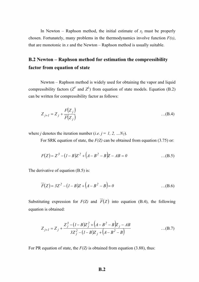
In Newton – Raphson method, the initial estimate of xj must be properly chosen. Fortunately, many problems in the thermodynamics involve function F(x), that are monotonic in x and the Newton – Raphson method is usually suitable.
B.2 Newton – Raphson method for estimation the compressibility factor from equation of state
Newton – Raphson method is widely used for obtaining the vapor and liquid compressibility factors (ZV and ZL) from equation of state models. Equation (B.2) can be written for compressibility factor as follows:
( )( )j
jj1j ZF
ZFZZ +=+ …(B.4)
where j denotes the iteration number (i.e. j = 1, 2, …NT). For SRK equation of state, the F(Z) can be obtained from equation (3.75) or:
( ) ( ) ( ) 0ABZBBAZB1ZZF 223 =−−−+−−= …(B.5)
The derivative of equation (B.5) is:
( ) ( ) ( ) 0BBAZB1Z3ZF 22 =−−+−−= …(B.6)
Substituting expression for F(Z) and (ZF ) into equation (B.4), the following
equation is obtained:
( ) ( )
( ) ( )BBAZB1Z3
ABZBBAZB1ZZZ 2
j2j
j22
j3j
j1j−−+−−
−−−+−−+=+ …(B.7)
For PR equation of state, the F(Z) is obtained from equation (3.88), thus:
B.2
( ) ( ) ( ) ( ) 0BBABZB2B3AZB1ZZF 32223 =−−−−−−−−= …(B.8)
Its derivative is :
( ) ( ) ( ) 0B2B3AB1Z2Z3ZF 22 =−−−−−= …(B.9)
Substituting expression for F(Z) and (ZF ) in equation (B.4), gives:
( ) ( ) ( )
( ) ( )B2B3AB1Z2Z3
BBABZB2B3AZB1ZZZ 2
j2j
32j
22j
3j
j1j−−+−−
−−−−−+−−+=+ ..(B.10)
Equations (B.7) and (B.10), now can be solved iteratively for ZV and ZL, with the following recommendations:
1. For ZV, the initial guess is preferred to be 1, (i.e. = 1). V0Z
2. For ZL, the initial guess is preferred to be 0, (i.e. = 0). L0Z
3. The iteration procedure must be continued until the percent tolerance error {defined by equation (B.3)} not be less than 0.0001, (i.e. Є ≤ 0.0001).
B.3 Newton – Raphson method for estimation the vapor fraction vaporized (β) in flash calculations
Newton – Raphson method is frequently used for estimating the vapor fraction vaporized (β) in flash. Equation (B.3) can be written for β as follows:
( )( )j
jj1j F
F
β
βββ +=+ ..(B.11)
where j denotes iteration number (i.e. j = 1, 2, …NT). The function F(βj) can be obtained from equation (3.175), as:
B.3
( ) ( )( )∑
= −+−
=N
1i i
ii1K1
K1ZF
ββ ..(B.12)
The derivative of equation (B.12) is:
( ) ( )( )[ ]∑
= −+
−=
N
1i2
i
2ii
1K1
K1ZF
ββ ..(B.13)
Substituting expressions for F(β) and ( )βF in equation (B.11), gives:
( )( )
( )( )[ ]∑
∑
=
=+
−+
−
−+−
+= N
1i2
ij
2ii
N
1i ij
ii
j1j
1K1K1Z
1K1K1Z
β
βββ ..(B.14)
Equation (B.14) can be solved iteratively for βi with the following recommendations: 1. The initial guess for βj is preferred to be 0.5 (i.e. β0 = 0.5). 2. The iteration procedure must be continued until the percent tolerance error {defined by equation (B.3)} must not be less than 0.0001 (i.e. Є ≤ 0.0001).
B.4
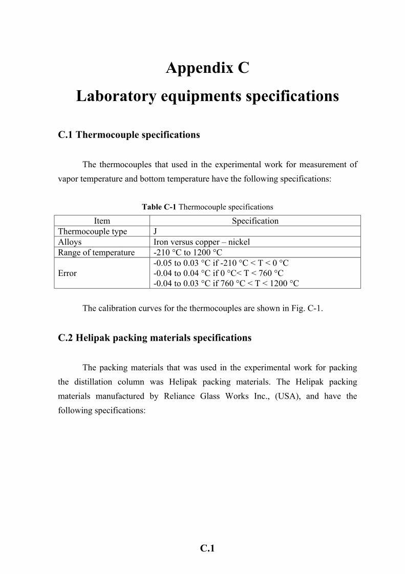
Appendix C
Laboratory equipments specifications
C.1 Thermocouple specifications
The thermocouples that used in the experimental work for measurement of vapor temperature and bottom temperature have the following specifications:
Table C-1 Thermocouple specifications
Item Specification Thermocouple type J Alloys Iron versus copper – nickel Range of temperature -210 °C to 1200 °C
Error -0.05 to 0.03 °C if -210 °C < T < 0 °C -0.04 to 0.04 °C if 0 °C< T < 760 °C -0.04 to 0.03 °C if 760 °C < T < 1200 °C
The calibration curves for the thermocouples are shown in Fig. C-1.
C.2 Helipak packing materials specifications
The packing materials that was used in the experimental work for packing the distillation column was Helipak packing materials. The Helipak packing materials manufactured by Reliance Glass Works Inc., (USA), and have the following specifications:
C.1

Table C-2 Helipak packing materials specifications
Item Specification Dimensions, mm 1.27×2.54×2.54 Model number 2917 Materials Nichrome Porosity (volume%) 0.85 Specific area (m2/m3) 1200 Height equivalent to theoretical plate for operating pressure range of 50 – 760 mmHg, mm 23 – 61
Figure C-1 Calibration curves for the thermocouples
C.3 Fractionating column components
The fractionating column that used in the experimental work consists of three main parts; these parts are: a. Reflux condenser of 290mm high and 50mm inside diameter. b. Packed bed column of 910mm high and 25mm inside diameter. c. Double expansion coil of 250mm high.
C.2
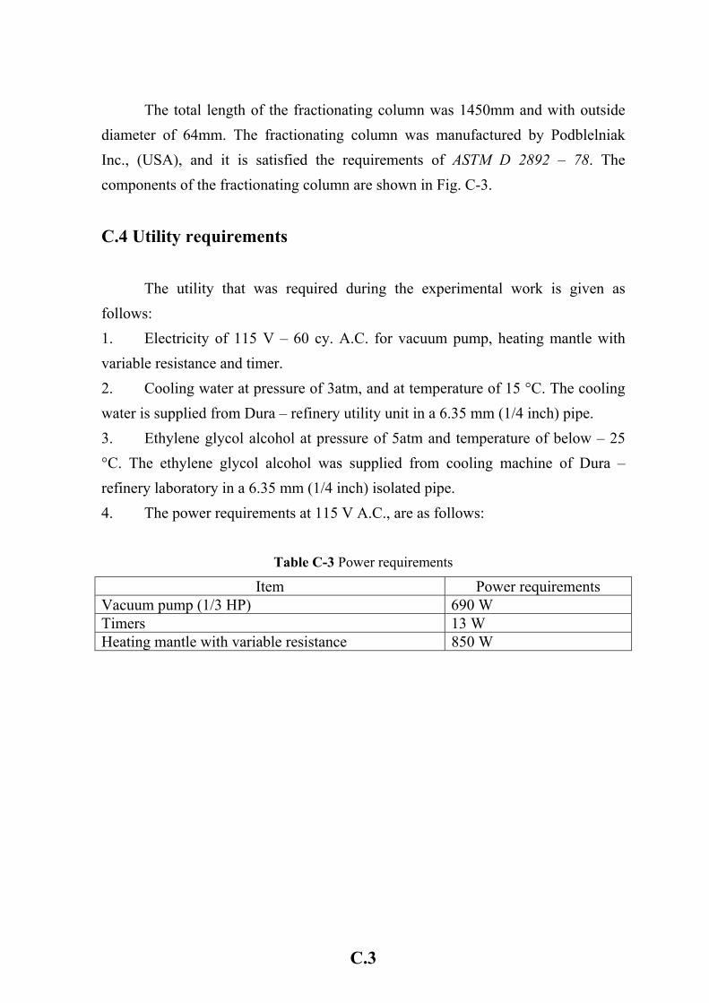
The total length of the fractionating column was 1450mm and with outside diameter of 64mm. The fractionating column was manufactured by Podblelniak Inc., (USA), and it is satisfied the requirements of ASTM D 2892 – 78. The components of the fractionating column are shown in Fig. C-3.
C.4 Utility requirements
The utility that was required during the experimental work is given as follows: 1. Electricity of 115 V – 60 cy. A.C. for vacuum pump, heating mantle with variable resistance and timer. 2. Cooling water at pressure of 3atm, and at temperature of 15 °C. The cooling water is supplied from Dura – refinery utility unit in a 6.35 mm (1/4 inch) pipe. 3. Ethylene glycol alcohol at pressure of 5atm and temperature of below – 25 °C. The ethylene glycol alcohol was supplied from cooling machine of Dura – refinery laboratory in a 6.35 mm (1/4 inch) isolated pipe. 4. The power requirements at 115 V A.C., are as follows:
Table C-3 Power requirements
Item Power requirements Vacuum pump (1/3 HP) 690 W Timers 13 W Heating mantle with variable resistance 850 W
C.3
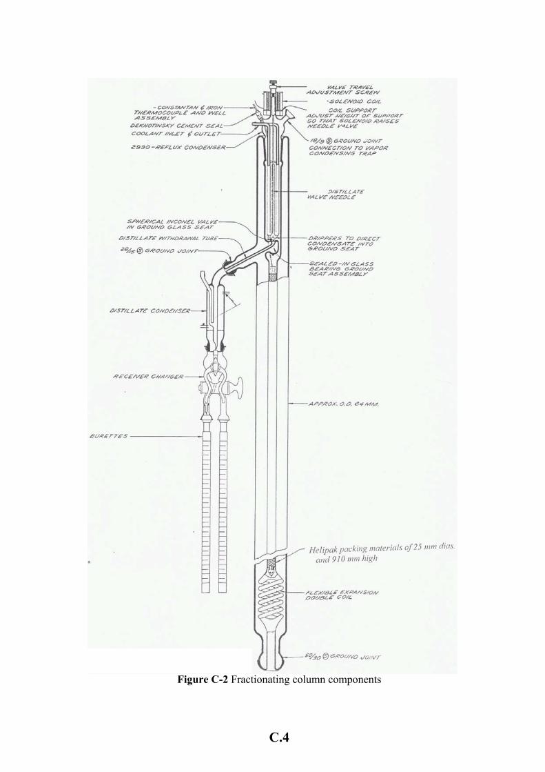
C.4
Figure C-2 Fractionating column components
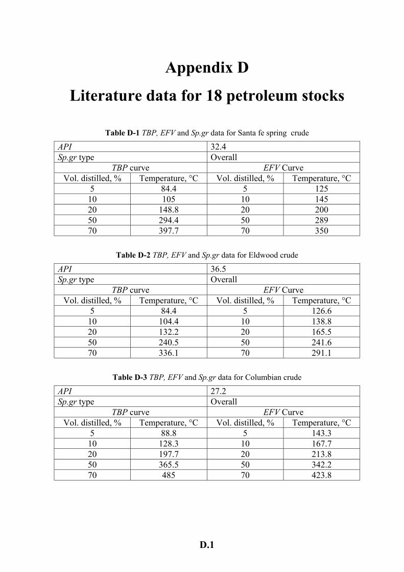
Appendix D
Literature data for 18 petroleum stocks
Table D-1 TBP, EFV and Sp.gr data for Santa fe spring crude
API 32.4 Sp.gr type Overall
TBP curve EFV Curve Vol. distilled, % Temperature, °C Vol. distilled, % Temperature, °C
5 84.4 5 125 10 105 10 145 20 148.8 20 200 50 294.4 50 289 70 397.7 70 350
Table D-2 TBP, EFV and Sp.gr data for Eldwood crude
API 36.5 Sp.gr type Overall
TBP curve EFV Curve Vol. distilled, % Temperature, °C Vol. distilled, % Temperature, °C
5 84.4 5 126.6 10 104.4 10 138.8 20 132.2 20 165.5 50 240.5 50 241.6 70 336.1 70 291.1
Table D-3 TBP, EFV and Sp.gr data for Columbian crude
API 27.2 Sp.gr type Overall
TBP curve EFV Curve Vol. distilled, % Temperature, °C Vol. distilled, % Temperature, °C
5 88.8 5 143.3 10 128.3 10 167.7 20 197.7 20 213.8 50 365.5 50 342.2 70 485 70 423.8
D.1
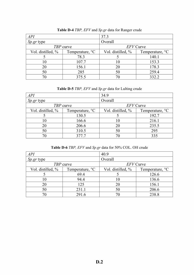
Table D-4 TBP, EFV and Sp.gr data for Ranger crude
API 37.3 Sp.gr type Overall
TBP curve EFV Curve Vol. distilled, % Temperature, °C Vol. distilled, % Temperature, °C
5 78.3 5 140.1 10 107.7 10 153.3 20 156.1 20 178.3 50 285 50 259.4 70 375.5 70 332.2
Table D-5 TBP, EFV and Sp.gr data for Lulting crude
API 34.9 Sp.gr type Overall
TBP curve EFV Curve Vol. distilled, % Temperature, °C Vol. distilled, % Temperature, °C
5 130.5 5 192.7 10 166.6 10 216.1 20 206.6 20 235.5 50 310.5 50 295 70 377.7 70 335
Table D-6 TBP, EFV and Sp.gr data for 50% COL. OH crude
API 40.9 Sp.gr type Overall
TBP curve EFV Curve Vol. distilled, % Temperature, °C Vol. distilled, % Temperature, °C
5 69.4 5 126.6 10 94.4 10 136.6 20 125 20 156.1 50 231.1 50 206.6 70 291.6 70 238.8
D.2
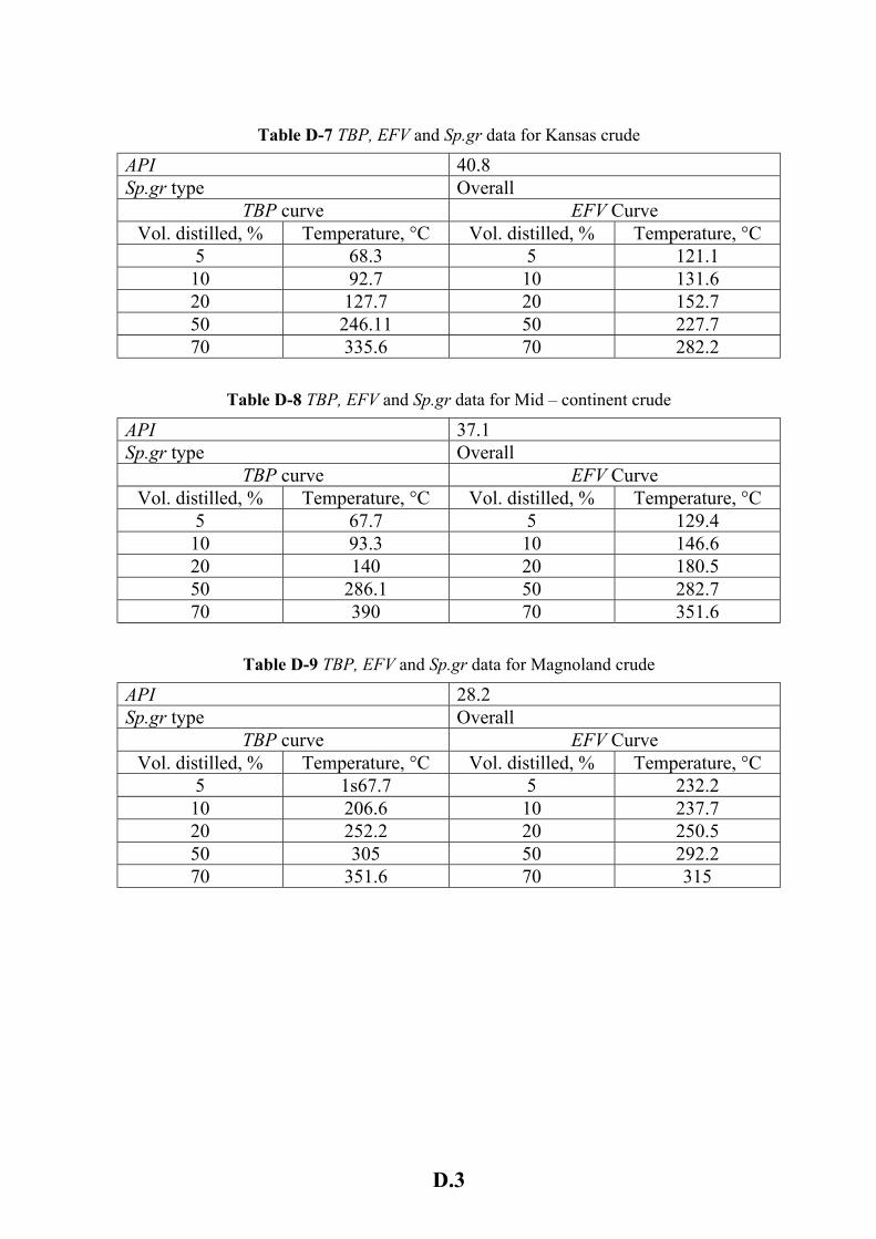
Table D-7 TBP, EFV and Sp.gr data for Kansas crude
API 40.8 Sp.gr type Overall
TBP curve EFV Curve Vol. distilled, % Temperature, °C Vol. distilled, % Temperature, °C
5 68.3 5 121.1 10 92.7 10 131.6 20 127.7 20 152.7 50 246.11 50 227.7 70 335.6 70 282.2
Table D-8 TBP, EFV and Sp.gr data for Mid – continent crude
API 37.1 Sp.gr type Overall
TBP curve EFV Curve Vol. distilled, % Temperature, °C Vol. distilled, % Temperature, °C
5 67.7 5 129.4 10 93.3 10 146.6 20 140 20 180.5 50 286.1 50 282.7 70 390 70 351.6
Table D-9 TBP, EFV and Sp.gr data for Magnoland crude
API 28.2 Sp.gr type Overall
TBP curve EFV Curve Vol. distilled, % Temperature, °C Vol. distilled, % Temperature, °C
5 1s67.7 5 232.2 10 206.6 10 237.7 20 252.2 20 250.5 50 305 50 292.2 70 351.6 70 315
D.3
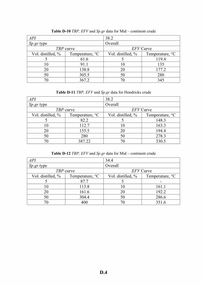
Table D-10 TBP, EFV and Sp.gr data for Mid – continent crude
API 38.2 Sp.gr type Overall
TBP curve EFV Curve Vol. distilled, % Temperature, °C Vol. distilled, % Temperature, °C
5 61.6 5 119.4 10 91.1 10 135 20 138.8 20 177.2 50 305.5 50 280 70 367.2 70 345
Table D-11 TBP, EFV and Sp.gr data for Hendricks crude
API 38.2 Sp.gr type Overall
TBP curve EFV Curve Vol. distilled, % Temperature, °C Vol. distilled, % Temperature, °C
5 82.2 5 148.3 10 112.7 10 163.3 20 155.5 20 194.4 50 280 50 278.3 70 387.22 70 330.5
Table D-12 TBP, EFV and Sp.gr data for Mid – continent crude
API 34.4 Sp.gr type Overall
TBP curve EFV Curve Vol. distilled, % Temperature, °C Vol. distilled, % Temperature, °C
5 87.7 5 - 10 113.8 10 161.1 20 161.6 20 192.2 50 304.4 50 286.6 70 400 70 351.6
D.4
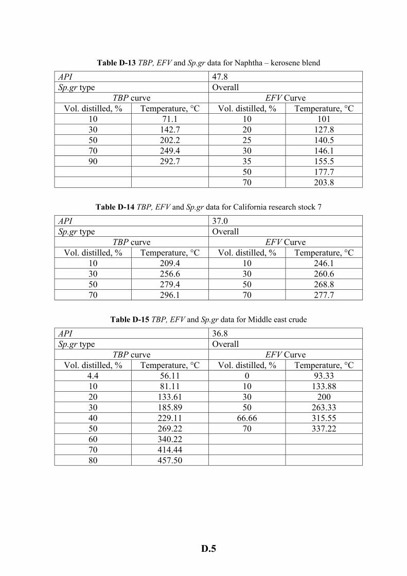
Table D-13 TBP, EFV and Sp.gr data for Naphtha – kerosene blend
API 47.8 Sp.gr type Overall
TBP curve EFV Curve Vol. distilled, % Temperature, °C Vol. distilled, % Temperature, °C
10 71.1 10 101 30 142.7 20 127.8 50 202.2 25 140.5 70 249.4 30 146.1 90 292.7 35 155.5
50 177.7 70 203.8
Table D-14 TBP, EFV and Sp.gr data for California research stock 7
API 37.0 Sp.gr type Overall
TBP curve EFV Curve Vol. distilled, % Temperature, °C Vol. distilled, % Temperature, °C
10 209.4 10 246.1 30 256.6 30 260.6 50 279.4 50 268.8 70 296.1 70 277.7
Table D-15 TBP, EFV and Sp.gr data for Middle east crude
API 36.8 Sp.gr type Overall
TBP curve EFV Curve Vol. distilled, % Temperature, °C Vol. distilled, % Temperature, °C
4.4 56.11 0 93.33 10 81.11 10 133.88 20 133.61 30 200 30 185.89 50 263.33 40 229.11 66.66 315.55 50 269.22 70 337.22 60 340.22 70 414.44 80 457.50
D.5
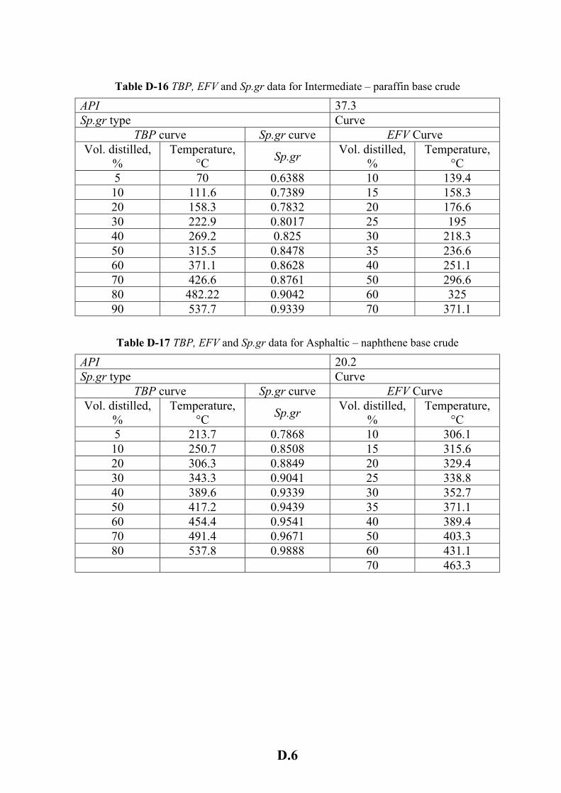
Table D-16 TBP, EFV and Sp.gr data for Intermediate – paraffin base crude
API 37.3 Sp.gr type Curve
TBP curve Sp.gr curve EFV Curve Vol. distilled,
% Temperature,
°C Sp.gr Vol. distilled, %
Temperature, °C
5 70 0.6388 10 139.4 10 111.6 0.7389 15 158.3 20 158.3 0.7832 20 176.6 30 222.9 0.8017 25 195 40 269.2 0.825 30 218.3 50 315.5 0.8478 35 236.6 60 371.1 0.8628 40 251.1 70 426.6 0.8761 50 296.6 80 482.22 0.9042 60 325 90 537.7 0.9339 70 371.1
Table D-17 TBP, EFV and Sp.gr data for Asphaltic – naphthene base crude
API 20.2 Sp.gr type Curve
TBP curve Sp.gr curve EFV Curve Vol. distilled,
% Temperature,
°C Sp.gr Vol. distilled, %
Temperature, °C
5 213.7 0.7868 10 306.1 10 250.7 0.8508 15 315.6 20 306.3 0.8849 20 329.4 30 343.3 0.9041 25 338.8 40 389.6 0.9339 30 352.7 50 417.2 0.9439 35 371.1 60 454.4 0.9541 40 389.4 70 491.4 0.9671 50 403.3 80 537.8 0.9888 60 431.1
70 463.3
D.6
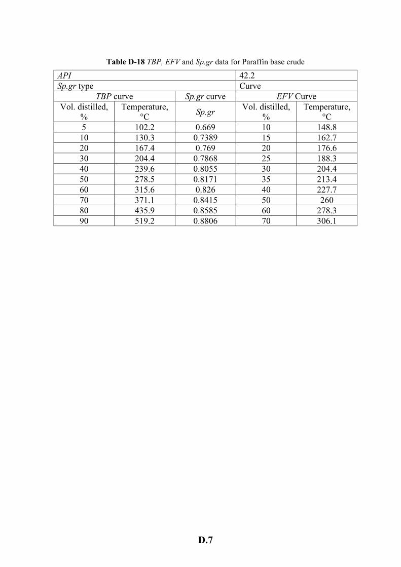
Table D-18 TBP, EFV and Sp.gr data for Paraffin base crude
API 42.2 Sp.gr type Curve
TBP curve Sp.gr curve EFV Curve Vol. distilled,
% Temperature,
°C Sp.gr Vol. distilled, %
Temperature, °C
5 102.2 0.669 10 148.8 10 130.3 0.7389 15 162.7 20 167.4 0.769 20 176.6 30 204.4 0.7868 25 188.3 40 239.6 0.8055 30 204.4 50 278.5 0.8171 35 213.4 60 315.6 0.826 40 227.7 70 371.1 0.8415 50 260 80 435.9 0.8585 60 278.3 90 519.2 0.8806 70 306.1
D.7
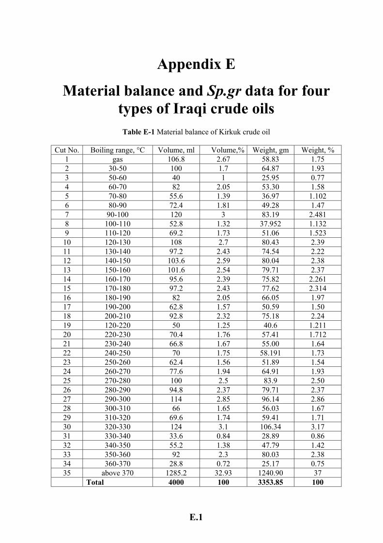
Appendix E
Material balance and Sp.gr data for four types of Iraqi crude oils
Table E-1 Material balance of Kirkuk crude oil
Cut No. Boiling range, °C Volume, ml Volume,% Weight, gm Weight, %
1 gas 106.8 2.67 58.83 1.75 2 30-50 100 1.7 64.87 1.93 3 50-60 40 1 25.95 0.77 4 60-70 82 2.05 53.30 1.58 5 70-80 55.6 1.39 36.97 1.102 6 80-90 72.4 1.81 49.28 1.47 7 90-100 120 3 83.19 2.481 8 100-110 52.8 1.32 37.952 1.132 9 110-120 69.2 1.73 51.06 1.523 10 120-130 108 2.7 80.43 2.39 11 130-140 97.2 2.43 74.54 2.22 12 140-150 103.6 2.59 80.04 2.38 13 150-160 101.6 2.54 79.71 2.37 14 160-170 95.6 2.39 75.82 2.261 15 170-180 97.2 2.43 77.62 2.314 16 180-190 82 2.05 66.05 1.97 17 190-200 62.8 1.57 50.59 1.50 18 200-210 92.8 2.32 75.18 2.24 19 120-220 50 1.25 40.6 1.211 20 220-230 70.4 1.76 57.41 1.712 21 230-240 66.8 1.67 55.00 1.64 22 240-250 70 1.75 58.191 1.73 23 250-260 62.4 1.56 51.89 1.54 24 260-270 77.6 1.94 64.91 1.93 25 270-280 100 2.5 83.9 2.50 26 280-290 94.8 2.37 79.71 2.37 27 290-300 114 2.85 96.14 2.86 28 300-310 66 1.65 56.03 1.67 29 310-320 69.6 1.74 59.41 1.71 30 320-330 124 3.1 106.34 3.17 31 330-340 33.6 0.84 28.89 0.86 32 340-350 55.2 1.38 47.79 1.42 33 350-360 92 2.3 80.03 2.38 34 360-370 28.8 0.72 25.17 0.75 35 above 370 1285.2 32.93 1240.90 37
Total 4000 100 3353.85 100
E.1
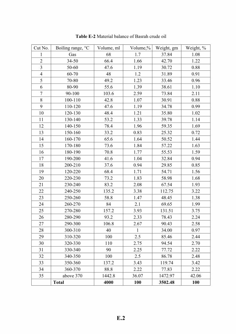
Table E-2 Material balance of Basrah crude oil
Cut No. Boiling range, °C Volume, ml Volume,% Weight, gm Weight, % 1 Gas 68 1.7 37.84 1.08 2 34-50 66.4 1.66 42.70 1.22 3 50-60 47.6 1.19 30.72 0.88 4 60-70 48 1.2 31.89 0.91 5 70-80 49.2 1.23 33.46 0.96 6 80-90 55.6 1.39 38.61 1.10 7 90-100 103.6 2.59 73.84 2.11 8 100-110 42.8 1.07 30.91 0.88 9 110-120 47.6 1.19 34.78 0.99 10 120-130 48.4 1.21 35.80 1.02 11 130-140 53.2 1.33 39.78 1.14 12 140-150 78.4 1.96 59.35 1.69 13 150-160 33.2 0.83 25.32 0.72 14 160-170 65.6 1.64 50.52 1.44 15 170-180 73.6 1.84 57.22 1.63 16 180-190 70.8 1.77 55.53 1.59 17 190-200 41.6 1.04 32.84 0.94 18 200-210 37.6 0.94 29.85 0.85 19 120-220 68.4 1.71 54.71 1.56 20 220-230 73.2 1.83 58.98 1.68 21 230-240 83.2 2.08 67.54 1.93 22 240-250 135.2 3.38 112.75 3.22 23 250-260 58.8 1.47 48.45 1.38 24 260-270 84 2.1 69.65 1.99 25 270-280 157.2 3.93 131.51 3.75 26 280-290 93.2 2.33 78.43 2.24 27 290-300 106.8 2.67 90.43 2.58 28 300-310 40 1 34.00 0.97 29 310-320 100 2.5 85.46 2.44 30 320-330 110 2.75 94.54 2.70 31 330-340 90 2.25 77.72 2.22 32 340-350 100 2.5 86.78 2.48 33 350-360 137.2 3.43 119.74 3.42 34 360-370 88.8 2.22 77.83 2.22 35 above 370 1442.8 36.07 1472.97 42.06 Total 4000 100 3502.48 100
E.2
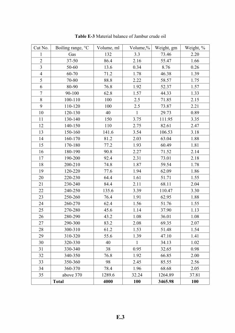
Table E-3 Material balance of Jambur crude oil
Cut No. Boiling range, °C Volume, ml Volume,% Weight, gm Weight, % 1 Gas 132 3.3 73.46 2.20 2 37-50 86.4 2.16 55.47 1.66 3 50-60 13.6 0.34 8.76 0.26 4 60-70 71.2 1.78 46.38 1.39 5 70-80 88.8 2.22 58.57 1.75 6 80-90 76.8 1.92 52.37 1.57 7 90-100 62.8 1.57 44.33 1.33 8 100-110 100 2.5 71.85 2.15 9 110-120 100 2.5 73.87 2.21 10 120-130 40 1 29.73 0.89 11 130-140 150 3.75 111.95 3.35 12 140-150 110 2.75 82.61 2.47 13 150-160 141.6 3.54 106.53 3.18 14 160-170 81.2 2.03 63.04 1.88 15 170-180 77.2 1.93 60.49 1.81 16 180-190 90.8 2.27 71.52 2.14 17 190-200 92.4 2.31 73.01 2.18 18 200-210 74.8 1.87 59.54 1.78 19 120-220 77.6 1.94 62.09 1.86 20 220-230 64.4 1.61 51.71 1.55 21 230-240 84.4 2.11 68.11 2.04 22 240-250 135.6 3.39 110.47 3.30 23 250-260 76.4 1.91 62.95 1.88 24 260-270 62.4 1.56 51.76 1.55 25 270-280 45.6 1.14 37.90 1.13 26 280-290 43.2 1.08 36.01 1.08 27 290-300 83.2 2.08 69.35 2.07 28 300-310 61.2 1.53 51.48 1.54 29 310-320 55.6 1.39 47.10 1.41 30 320-330 40 1 34.13 1.02 31 330-340 38 0.95 32.65 0.98 32 340-350 76.8 1.92 66.85 2.00 33 350-360 98 2.45 85.55 2.56 34 360-370 78.4 1.96 68.68 2.05 35 above 370 1289.6 32.24 1264.89 37.81 Total 4000 100 3465.98 100
E.3
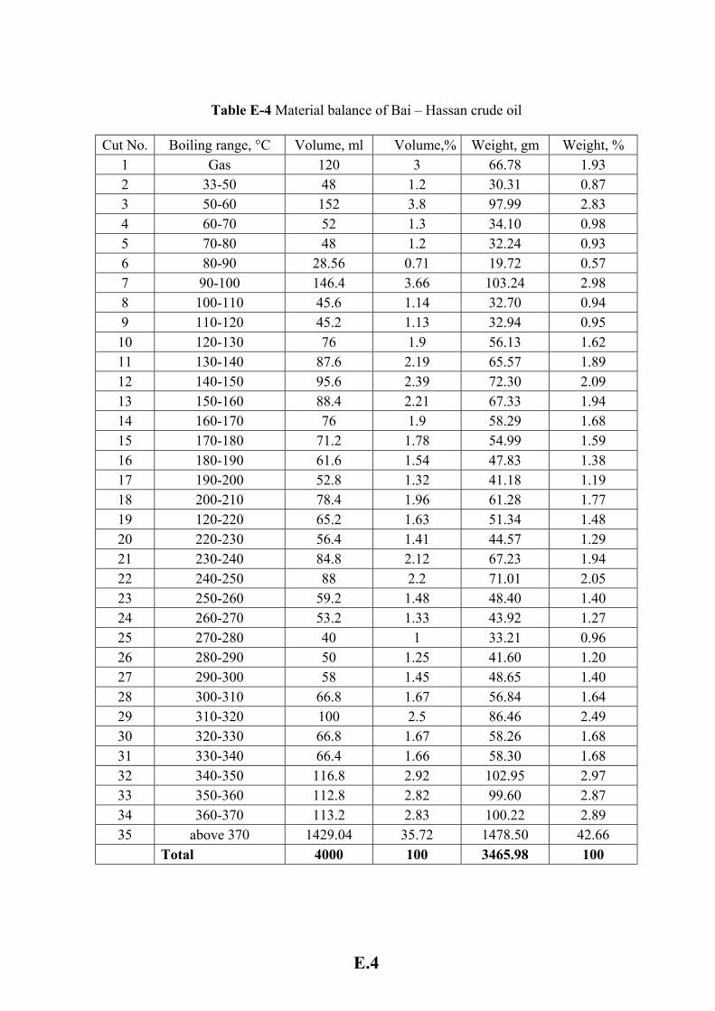
Table E-4 Material balance of Bai – Hassan crude oil
Cut No. Boiling range, °C Volume, ml Volume,% Weight, gm Weight, % 1 Gas 120 3 66.78 1.93 2 33-50 48 1.2 30.31 0.87 3 50-60 152 3.8 97.99 2.83 4 60-70 52 1.3 34.10 0.98 5 70-80 48 1.2 32.24 0.93 6 80-90 28.56 0.71 19.72 0.57 7 90-100 146.4 3.66 103.24 2.98 8 100-110 45.6 1.14 32.70 0.94 9 110-120 45.2 1.13 32.94 0.95 10 120-130 76 1.9 56.13 1.62 11 130-140 87.6 2.19 65.57 1.89 12 140-150 95.6 2.39 72.30 2.09 13 150-160 88.4 2.21 67.33 1.94 14 160-170 76 1.9 58.29 1.68 15 170-180 71.2 1.78 54.99 1.59 16 180-190 61.6 1.54 47.83 1.38 17 190-200 52.8 1.32 41.18 1.19 18 200-210 78.4 1.96 61.28 1.77 19 120-220 65.2 1.63 51.34 1.48 20 220-230 56.4 1.41 44.57 1.29 21 230-240 84.8 2.12 67.23 1.94 22 240-250 88 2.2 71.01 2.05 23 250-260 59.2 1.48 48.40 1.40 24 260-270 53.2 1.33 43.92 1.27 25 270-280 40 1 33.21 0.96 26 280-290 50 1.25 41.60 1.20 27 290-300 58 1.45 48.65 1.40 28 300-310 66.8 1.67 56.84 1.64 29 310-320 100 2.5 86.46 2.49 30 320-330 66.8 1.67 58.26 1.68 31 330-340 66.4 1.66 58.30 1.68 32 340-350 116.8 2.92 102.95 2.97 33 350-360 112.8 2.82 99.60 2.87 34 360-370 113.2 2.83 100.22 2.89 35 above 370 1429.04 35.72 1478.50 42.66 Total 4000 100 3465.98 100
E.4
Table E-5 Specific gravity and API of distillate fractions from Kirkuk crude oil
Cut No. Boiling range, °C Sp.gr API 1 gas - - 2 30-50 0.6487 86.63 3 50-60 0.6488 86.59 4 60-70 0.6501 86.16 5 70-80 0.665 81.28 6 80-90 0.6808 76.34 7 90-100 0.6933 72.60 8 100-110 0.7188 65.36 9 110-120 0.738 60.23 10 120-130 0.7448 58.48 11 130-140 0.7669 53.01 12 140-150 0.7726 51.65 13 150-160 0.7846 48.85 14 160-170 0.7932 46.89 15 170-180 0.7986 45.69 16 180-190 0.8056 44.15 17 190-200 0.8056 44.15 18 200-210 0.8102 43.15 19 120-220 0.812 42.76 20 220-230 0.8156 41.99 21 230-240 0.8234 40.35 22 240-250 0.8313 38.72 23 250-260 0.8317 38.63 24 260-270 0.8365 37.66 25 270-280 0.8390 37.15 26 280-290 0.8409 36.77 27 290-300 0.8434 36.27 28 300-310 0.8490 35.17 29 310-320 0.8536 34.27 30 320-330 0.8576 33.50 31 330-340 0.8601 33.02 32 340-350 0.8658 31.93 33 350-360 0.8699 31.16 34 360-370 0.8740 30.40
E.5
Table E-6 Specific gravity and API of distillate fractions from Basrah crude oil
Cut No. Boiling range, °C Sp.gr API 1 gas - - 2 30-50 0.6430 88.56 3 50-60 0.6623 82.16 4 60-70 0.6782 77.14 5 70-80 0.6914 73.15 6 80-90 0.7039 69.52 7 90-100 0.7201 65.01 8 100-110 0.7285 62.74 9 110-120 0.7367 60.56 10 120-130 0.7445 58.55 11 130-140 0.7522 56.61 12 140-150 0.7611 54.42 13 150-160 0.7665 53.10 14 160-170 0.7737 51.39 15 170-180 0.7806 49.76 16 180-190 0.7873 48.23 17 190-200 0.7922 47.12 18 200-210 0.7967 46.10 19 120-220 0.8025 44.82 20 220-230 0.8082 43.58 21 230-240 0.8141 42.31 22 240-250 0.8216 40.73 23 250-260 0.8260 39.80 24 260-270 0.8311 38.75 25 270-280 0.8383 37.29 26 280-290 0.8432 36.30 27 290-300 0.8484 35.29 28 300-310 0.8515 34.68 29 310-320 0.8556 33.88 30 320-330 0.8609 32.87 31 330-340 0.8649 32.10 32 340-350 0.8691 31.31 33 350-360 0.8740 30.40 34 360-370 0.8777 29.72
E.6
Table E-7 Specific gravity and API of distillate fractions from Jambur crude oil
Cut No. Boiling range, °C Sp.gr API 1 gas - - 2 30-50 0.642 88.90 3 50-60 0.6444 88.08 4 60-70 0.6514 85.72 5 70-80 0.6596 83.02 6 80-90 0.6819 76.01 7 90-100 0.7059 68.95 8 100-110 0.7185 65.44 9 110-120 0.7387 60.05 10 120-130 0.7432 58.89 11 130-140 0.7463 58.10 12 140-150 0.7510 56.92 13 150-160 0.7523 56.59 14 160-170 0.7763 50.77 15 170-180 0.7835 49.10 16 180-190 0.7877 48.14 17 190-200 0.7901 47.59 18 200-210 0.7960 46.26 19 120-220 0.8001 45.35 20 220-230 0.8030 44.71 21 230-240 0.8070 43.84 22 240-250 0.8147 42.18 23 250-260 0.8239 40.24 24 260-270 0.8295 39.08 25 270-280 0.8311 38.76 26 280-290 0.8335 38.27 27 290-300 0.8336 38.25 28 300-310 0.8412 36.71 29 310-320 0.8472 35.52 30 320-330 0.8532 34.35 31 330-340 0.8592 33.19 32 340-350 0.8705 31.05 33 350-360 0.8730 30.58 34 360-370 0.8760 30.03
E.7
Table E-8 Specific gravity and API of distillate fractions from Bai – Hassan crude oil
Cut No. Boiling range, °C Sp.gr API 1 gas - - 2 30-50 0.6314 92.61 3 50-60 0.6447 87.98 4 60-70 0.6558 84.27 5 70-80 0.6717 79.16 6 80-90 0.6906 73.39 7 90-100 0.7052 69.15 8 100-110 0.7170 65.85 9 110-120 0.7287 62.68 10 120-130 0.7386 60.08 11 130-140 0.7485 57.54 12 140-150 0.7563 55.60 13 150-160 0.7616 54.29 14 160-170 0.7670 52.99 15 170-180 0.7723 51.72 16 180-190 0.7765 50.73 17 190-200 0.7800 49.91 18 200-210 0.7816 49.54 19 120-220 0.7874 48.21 20 220-230 0.7903 47.55 21 230-240 0.7928 46.98 22 240-250 0.8069 43.86 23 250-260 0.8176 41.57 24 260-270 0.8255 39.91 25 270-280 0.8303 38.92 26 280-290 0.8319 38.59 27 290-300 0.8388 37.19 28 300-310 0.8509 34.79 29 310-320 0.8646 32.16 30 320-330 0.8722 30.73 31 330-340 0.8780 29.66 32 340-350 0.8814 29.04 33 350-360 0.8830 28.75 34 360-370 0.8853 28.33
E.8
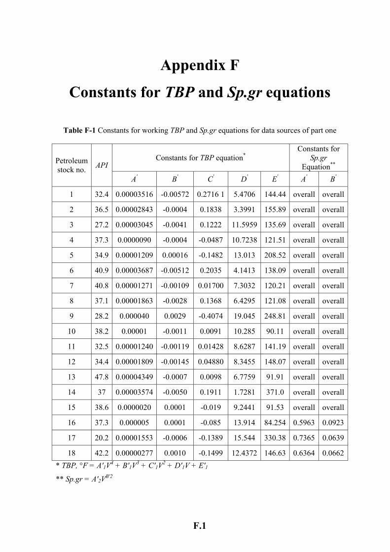
Appendix F
Constants for TBP and Sp.gr equations
Table F-1 Constants for working TBP and Sp.gr equations for data sources of part one
Constants for TBP equation* Constants for
Sp.gr Equation** Petroleum
stock no. API
A' B' C' D' E' A' B'
1 32.4 0.00003516 -0.00572 0.2716 1 5.4706 144.44 overall overall
2 36.5 0.00002843 -0.0004 0.1838 3.3991 155.89 overall overall
3 27.2 0.00003045 -0.0041 0.1222 11.5959 135.69 overall overall
4 37.3 0.0000090 -0.0004 -0.0487 10.7238 121.51 overall overall
5 34.9 0.00001209 0.00016 -0.1482 13.013 208.52 overall overall
6 40.9 0.00003687 -0.00512 0.2035 4.1413 138.09 overall overall
7 40.8 0.00001271 -0.00109 0.01700 7.3032 120.21 overall overall
8 37.1 0.00001863 -0.0028 0.1368 6.4295 121.08 overall overall
9 28.2 0.000040 0.0029 -0.4074 19.045 248.81 overall overall
10 38.2 0.00001 -0.0011 0.0091 10.285 90.11 overall overall
11 32.5 0.00001240 -0.00119 0.01428 8.6287 141.19 overall overall
12 34.4 0.00001809 -0.00145 0.04880 8.3455 148.07 overall overall
13 47.8 0.00004349 -0.0007 0.0098 6.7759 91.91 overall overall
14 37 0.00003574 -0.0050 0.1911 1.7281 371.0 overall overall
15 38.6 0.0000020 0.0001 -0.019 9.2441 91.53 overall overall
16 37.3 0.000005 0.0001 -0.085 13.914 84.254 0.5963 0.0923
17 20.2 0.00001553 -0.0006 -0.1389 15.544 330.38 0.7365 0.0639
18 42.2 0.00000277 0.0010 -0.1499 12.4372 146.63 0.6364 0.0662 * TBP, °F = A'1V4 + B'1V3 + C'1V2 + D'1V + E'1
** Sp.gr = A'2VB'2
F.1
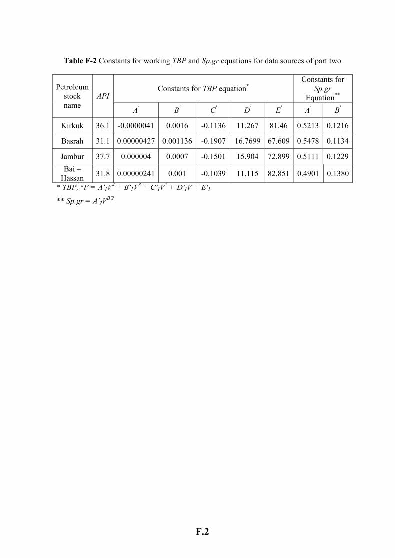
Table F-2 Constants for working TBP and Sp.gr equations for data sources of part two
Constants for TBP equation* Constants for
Sp.gr Equation**
Petroleum stock name
API
A' B' C' D' E' A' B'
Kirkuk 36.1 -0.0000041 0.0016 -0.1136 11.267 81.46 0.5213 0.1216
Basrah 31.1 0.00000427 0.001136 -0.1907 16.7699 67.609 0.5478 0.1134
Jambur 37.7 0.000004 0.0007 -0.1501 15.904 72.899 0.5111 0.1229 Bai –
Hassan 31.8 0.00000241 0.001 -0.1039 11.115 82.851 0.4901 0.1380
* TBP, °F = A'1V4 + B'1V3 + C'1V2 + D'1V + E'1
** Sp.gr = A'2VB'2
F.2
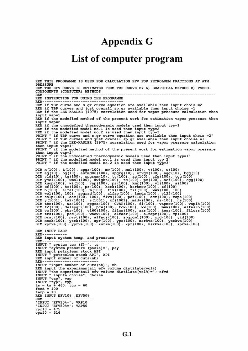
Appendix G
List of computer program
REM THIS PROGRAMME IS USED FOR CALCULATION EFV FOR PETROLUEM FRACTIONS AT ATM PRESSURE REM THE EFV CURVE IS ESTIMATED FROM TBP CURVE BY A) GRAPHICAL METHOD B) PSEDO-COMPONENTS (COMPUTER) METHODS
---------------------------------------- REM-------------------------------------REM INSTRUCTION FOR USING THE PROGRAMME REM------------------------------------
=2 REM if TBP curve and s.gr curve equation are available then input chois REM if TBP curves and just overall sp.gr available then input choise =1 REM if the LEE-KASLER (1975) correlation used for vapor pressure calculation then input vap=1 REM if the modefied method of the present work for eatimation vapor pressure then input vap=2
ut typ=1 REM if the unmodefied thermodynamic models used then inpREM if the modefied model no.1 is used then input typ=2 REM if the modefied model no.2 is used then input typ=3
2" PRINT " if TBP curve and s.gr curve equation are available then input chois =PRINT " if TBP curves and just overall sp.gr available then input choise =1" PRINT " if the LEE-KASLER (1975) correlation used for vapor pressure calculation then input vap=1" PRINT " if the modefied method of the present work for eatimation vapor pressure then input vap=2"
t typ=1" PRINT " if the unmodefied thermodynamic models used then inpuPRINT " if the modefied model no.1 is used then input typ=2" RINT " if the modefied model no.2 is used then input typ=3" P DIM x(100), t(100), spgr(100), mw(100), mol(100), v(100), w(100)
0) DIM ag(10), bg(10), astmd86(100), spgrg(10), efvgm(100), agg(10), bgg(1DIM vld(10), tg(100), spgrgm(10), tv(100), ac(100), zfg(100), tgg(100)
g(100) DIM ymol(100), xmol(100), xwight(100), tc(100), pc(100), acf(100), cg100) DIM kuop(100), wi(100), vap(100), ps(100), kmr(100), vl(100), a(
DIM cf(100), tr(100), pr(100), ksrk(100), ksrknew(100), zf(100) DIM b(100), alfa1(100), m(100), fiv(100), fil(100), wwv(100, 100) DIM wwl(100, 100), spgrad(100), alfao(100), lamda(100), vl25(100) DIM solp(100), aac(100, 100), fivs(100), pof(100), act(100), vapa(100) DIM y(1001), ta2(1001), s(1001), xf(1001), midv(100), ms(100), ns(100) DIM tbr(100), wa(100), spgra(100), CVAP(100), f1(100), vapnew(100), vaplk(100) DIM f2(100), delspgr(100), pcw(100), tcw(100), ww(100), mww(100), alfasro(100)
lcss(100) DIM vc(100), pbr(100), vl60(100), filcs(100), zar(100), tess(100), fiDIM trs(100), pcc(100), wnew(100), alfasr(100), alfapr(100), mp(100)
DIM prst(100), prpt(100), alfaos(100), spgrgm1(100), xid(100), yid(100)DIM xsrk(100), ysrk(100), xpr(100), ypr(100), xsrkva(100), ysrkva(100) IM xprva(100), yprva(100), ksrkm(100), kpr(100), ksrkva(100), kprva(100) D REM INPUT PART REM----------- REM input system temp. and pressure
------ REM--------------------------INPUT " system tem (f)=", ts
=", psy INPUT "system pressure (pasia)REM input petroleum stock API
API INPUT " petroelum stock API",REM input number of cuts(nb) REM------------------------- INPUT "input number of cuts(nb)", nb REM input the experimantail efv volume distilate(vol%)
lume distilate(vol%)="; efvd INPUT "the experimantail efv vooise", choise INPUT " inpute ch
INPUT "vap", vap INPUT "typ", typ
60: tco = 60 ts = ts + 4 feed = 100
temp = 10 REM INPUT EFV10% ,EFV50%
-- REM---------------------'INPUT "EFV10%="; VRP10
0%="; VAP50 'INPUT "EFV5vpr10 = 475 vpr50 = 516
G.1
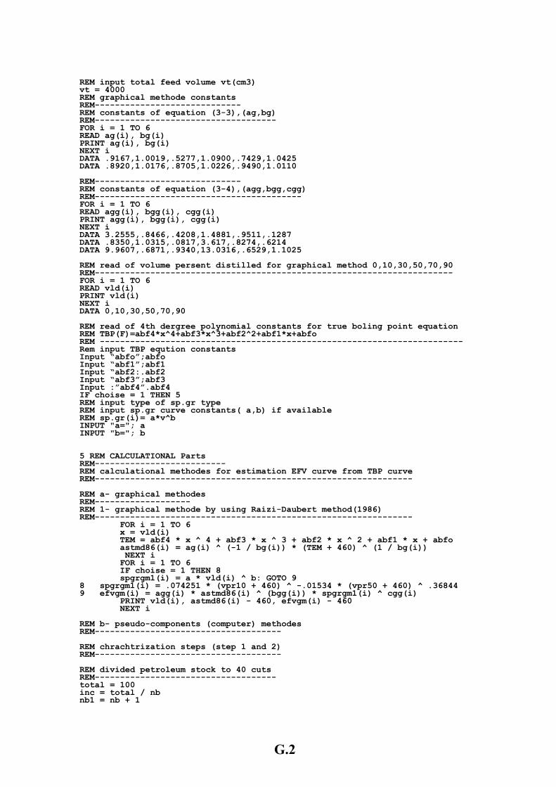
REM input total feed volume vt(cm3) vt = 4000 REM graphical methode constants REM----------------------------- REM constants of equation (3-3),(ag,bg)
------------------------ REM------------FOR i = 1 TO 6 READ ag(i), bg(i)
g(i), bg(i) PRINT aNEXT i DATA .9167,1.0019,.5277,1.0900,.7429,1.0425 ATA .8920,1.0176,.8705,1.0226,.9490,1.0110 D REM-----------------------------
REM constants of equation (3-4),(agg,bgg,cgg)----------------------------- REM------------
FOR i = 1 TO 6 READ agg(i), bgg(i), cgg(i)
gg(i), bgg(i), cgg(i) PRINT aNEXT i
DATA 3.2555,.8466,.4208,1.4881,.9511,.1287DATA .8350,1.0315,.0817,3.617,.8274,.6214 ATA 9.9607,.6871,.9340,13.0316,.6529,1.1025 D REM read of volume persent distilled for graphical method 0,10,30,50,70,90
----------------------------------------------------------- REM------------ 6 FOR i = 1 TO
READ vld(i) ld(i) PRINT v
NEXT i ATA 0,10,30,50,70,90 D
true boling point equation REM read of 4th dergree polynomial constants forREM TBP(F)=abf4*x^4+abf3*x^3+abf2^2+abf1*x+abfo
-------------------------------------------- REM ----------------------------ion constants Rem input TBP equt
Input “abfo”;abfo Input “abf1”;abf1 Input “abf2:.abf2 Input “abf3”;abf3 Input :”abf4”.abf4 IF choise = 1 THEN 5 REM input type of sp.gr type
e constants( a,b) if available REM input sp.gr curva*v^b REM sp.gr(i)=
INPUT "a="; a NPUT "b="; b I 5 REM CALCULATIONAL Parts REM-------------------------- REM calculational methodes for estimation EFV curve from TBP curve EM--------------------------------------------------------------- R
es REM a- graphical methodREM------------------- REM 1- graphical methode by using Raizi-Daubert method(1986)
------------------------------------------- REM--------------------O 6 FOR i = 1 T
x = vld(i) abfo TEM = abf4 * x ^ 4 + abf3 * x ^ 3 + abf2 * x ^ 2 + abf1 * x +
i) = ag(i) ^ (-1 / bg(i)) * (TEM + 460) ^ (1 / bg(i)) astmd86( NEXT i FOR i = 1 TO 6 IF choise = 1 THEN 8 spgrgm1(i) = a * vld(i) ^ b: GOTO 9
.36844 8 spgrgm1(i) = .074251 * (vpr10 + 460) ^ -.01534 * (vpr50 + 460) ^(i) ^ cgg(i) 9 efvgm(i) = agg(i) * astmd86(i) ^ (bgg(i)) * spgrgm1
ld(i), astmd86(i) - 460, efvgm(i) - 460 PRINT v NEXT i
des REM b- pseudo-components (computer) methoEM------------------------------------- R REM chrachtrization steps (step 1 and 2) EM------------------------------------- R REM divided petroleum stock to 40 cuts
--------------------------- REM---------total = 100
nb inc = total /nb1 = nb + 1
G.2
FOR i = 1 TO nb1 : GOTO 10 IF i = 1 THEN x(i) = 0
c x(i) = x(i - 1) + inNT x(i), inc 10 PRI
EXT i N REM calculation of sp.gr of petroleum stock
--------------- REM-------------------------po = 141.5 / (API + 131.5) s REM estimation tbp curve by four degree polynomial equation
* X ^ 3 + abf2 * X ^ 2 + abf1 * X + abfo REM tbp=abf4 * X ^ 4 + abf3 distilled REM X is the vol%
TO nb1 FOR i = 1x = x(i)
* x ^ 4 + abf3 * x ^ 3 + abf2 * x ^ 2 + abf1 * x + abfo TEM = abf4 t(i) = TEM tgg(i) = TEM
(i), t(i) PRINT x i NEXT
REM calculation of mid boiling point temp.
----------------------------------- REM------u = .001 FOR i = 1 TO nb1 - 1
) + inc) STEP u FOR xo = x(i) TO (x(iEN 40 IF xo = x(i) TH
w = x(i) + inc m = (xo + x(i)) / 2
(i + 1) + xo) / 2 m2 = (xx = xo
4 * x ^ 4 + abf3 * x ^ 3 + abf2 * x ^ 2 + abf1 * x + abfo TEM = abfEM yo = T
x = w ^ 4 + abf3 * x ^ 3 + abf2 * x ^ 2 + abf1 * x + abfo TEM = abf4 * x
= TEM y(i + 1) x = x(i)
* x ^ 4 + abf3 * x ^ 3 + abf2 * x ^ 2 + abf1 * x + abfo TEM = abf4 TEM y(i) =
x = m 4 * x ^ 4 + abf3 * x ^ 3 + abf2 * x ^ 2 + abf1 * x + abfo TEM = abf
M ym = TEx = m2
* x ^ 4 + abf3 * x ^ 3 + abf2 * x ^ 2 + abf1 * x + abfo TEM = abf4ym2 = TEM
ym + y(i)) a1 = ((xo - x(i)) / 6) * (yo + 4 * x(i)) a2 = (y(i + 1) - yo) * (xo -
(i + 1) at = (xo - x(i)) * ya3 = at - (a1 + a2)
* (yo + y(i + 1) + 4 * ym2) a11 = ((w - xo) / 6) yo a22 = (w - xo) *
a33 = a11 - a22 er = ((a3 - a33) / a3) * 100: PRINT ABS(er), xo
<= 1 THEN ta2(i) = yo: midv(i) = xo: GOTO 30 IF ABS(er) 40 NEXT xo
NT ta2(i), ABS(er): 30 PRINEXT i
b FOR i = 1 TO nt(i) = ta2(i)
, t(i) PRINT iNEXT i
EN 50 IF choise = 2 TH FOR i = 1 TO nb
= .3067 * t(i) ^ .1605 spgr(i) NEXT i GOTO 60
r 50 REM calculation of mid sp.g-------------------- REM------
u = .001 FOR i = 1 TO nb1 - 1
) + inc) STEP u FOR xo = x(i) TO (x(iEN 55 IF xo = x(i) TH
w = x(i) + inc m = (xo + x(i)) / 2
+ 1) + xo) / 2 m2 = (x(i x = xo
x ^ b TEM = a *EM yo = T
x = w TEM = a * x ^ b
y(i + 1) = TEM
G.3
x = x(i) ^ b TEM = a * x
TEM y(i) = x = m
x ^ b TEM = a * M ym = TE
x = m2 ^ b TEM = a * x
ym2 = TEM ym + y(i)) a1 = ((xo - x(i)) / 6) * (yo + 4 *
x(i)) a2 = (y(i + 1) - yo) * (xo -(i + 1) at = (xo - x(i)) * y
a3 = at - (a1 + a2) * (yo + y(i + 1) + 4 * ym2) a11 = ((w - xo) / 6)
yo a22 = (w - xo) * a33 = a11 - a22 er = ((a3 - a33) / a3) * 100: PRINT ABS(er), xo
= 1 THEN ta2(i) = yo: xf(i) = xo: GOTO 54 IF ABS(er) <55 NEXT xo:
T ta2(i), ABS(er): 54 PRIN NEXT i FOR i = 1 TO nb spgr(i) = ta2(i)
xf(i), spgr(i), t(i) 'PRINT NEXT i 60 REM calculation of ajusted sp.gr
---------------------- REM---------- spgrca = 0 FOR i = 1 TO nb
a + (inc / 100) * spgr(i) spgrca = spgrcpgr(i) PRINT s
EXT i N wf = spo * vt
pgrca, spo, wf PRINT s wt = 0 FOR i = 1 TO nb
v(i) = (inc / 100) * vtpgr(i) wi(i) = v(i) * s
+ wi(i) wt = wtEXT i N
REM ajust the spgr for material balance
-------------------- REM------------------- FOR i = 1 TO nb
wi(i) = wi(i) * (wf / wt)/ v(i) spgrad(i) = wi(i)
sum = sum + wi(i) sum2 + (inc / 100) * spgrad(i) sum2 =
NEXT i po, sum2 PRINT sum, wf, s
FOR i = 1 TO nb spgr(i) = spgrad(i)
pgr(i), t(i) PRINT i, s NEXT i
REM calculation of critical properties of crude oil
------------------------------------- REM ------------FOR i = 1 TO nb REM RAZIE DUBERT (1987) REM---------------------- mw(i) = 20.468 * (t(i) + 460) ^ 1.26007 * spgr(i) ^ 4.98308 * (EXP(1.165 * 10 ^ -4 * (t(i) + 460) - 7.78712 * spgr(i) + 1.1582 * 10 ^ -3 * (t(i) + 460) * spgr(i))) IF t(i) > 650 THEN 61 tc(i) = 10.6443 * (t(i) + 460) ^ .81067 * spgr(i) ^ .53691 * (EXP(-5.1747 * 10 ^ -4 * (t(i) + 460) - .54444 * spgr(i) + 3.5995 * 10 ^ -4 * (t(i) + 460) * pgr(i))) s pc(i) = 6.162 * 10 ^ 6 * (t(i) + 460) ^ -.4844 * spgr(i) ^ 4.0846 * (EXP(-4.725 * 10 ^ -3 * (t(i) + 460) - 4.8014 * spgr(i) + 3.1939 * 10 ^ -3 * (t(i) + 460) * pgr(i))) s GOTO 62 61 REM LEE KASLER (1975) REM---------------------- tc(i) = 341.7 + 811 * spgr(i) + (.4244 + .1174 * spgr(i)) * (t(i) + 460) + (.4669
(t(i) + 460)) - 3.2623 * spgr(i)) * (10 ^ 5 / a1 = 8.3634 - (.0566 / spgr(i)) a2 = (.24244 + 2.2898 * spgr(i) ^ -1 + .11857 * spgr(i) ^ -2) * (t(i) + 460) * 10 ^ -3
G.4
a3 = (1.4685 + 3.648 * spgr(i) ^ -1 + .47227 * spgr(i) ^ -2) * (t(i) + 460) ^ 2 * 10 ^ -7
-2) * (t(i) + 460) ^ 3 * 10 ^ -10 a4 = (.42019 + 1.6977 * spgr(i) ^pc(i) = EXP((a1 - a2 + a3 - a4))
60) / tc(i) 62 tbr(i) = (t(i) + 4pbr(i) = psy / pc(i)
) ^ .3333 / spgr(i) kuop(i) = ((t(i) + 460)IF tbr(i) < .8 THEN 63 w(i) = -7.904 + .1352 * kuop(i) - .007465 * kuop(i) ^ 2 + 8.359 * tbr(i) + (1.408
uop(i)) * tbr(i) ^ -1 - .01063 * k GOTO 64 63 a1 = LOG(pbr(i)) - 5.92714 + 6.09648 * tbr(i) ^ -1 + 1.28862 * LOG(tbr(i)) - .169347 * tbr(i) ^ 6 a2 = 15.2518 - 15.6875 * tbr(i) ^ -1 - 13.4721 * LOG(tbr(i)) + .4377 * tbr(i) ^ 6 w(i) = a1 / a2
T t(i), tc(i), pc(i), mw(i), w(i) 64 PRINNEXT i REM calculation of feed compostions in mole basis (ZFi)
-------------------------------------------- REM--------summol = 0 FOR i = 1 TO nb mol(i) = wi(i) / mw(i)
= summol + mol(i) summol NEXT i FOR i = 1 TO nb
i) / summol zf(i) = mol(f(i) PRINT z
NEXT i
. REM calculation of molar density (Vl)at 15.5 C(60 F),25 C (77 F),and system tempREM ---------------------------------------------------------------------------
ract equation is used,while for tr>1 then cavvt equation is used REM for tr<1 theFOR i = 1 TO nb
/ spgr(i)) * mw(i) vl60(i) = (1 r = 10.73 trs(i) = ts / tc(i) IF trs(i) >= 1 THEN vl60(i) = vl60(i) * .01601: cf(i) = vl60(i) / (5.7 + 3 * ((tco + 460) / tc(i))): vl(i) = cf(i) * (5.7 + (3 * (ts / tc(i)))): vl25(i) =
: GOTO 56 cf(i) * (5.7 + (3 * (77 / tc(i)))) vl60(i) = vl60(i) * .01601
60) / tc(i))) ^ .2857) mr60 = (1 + (1 - ((tco + 4 arc = (r * tc(i)) / pc(i)
rc)) / mr60) zar(i) = EXP((LOG(vl60(i)) - LOG(a2857) mrts = (1 + (1 - trs(i)) ^ .
vl(i) = arc * zar(i) ^ mrts tc(i))) ^ .2857) mr25 = (1 + (1 - ((77 + 460) /
rc * zar(i) ^ mr25 vl25(i) = a 56 PRINT trs(i);
NEXT i REM calculation of cuts vapor pressures using LEE-KASLER method (1975)or developted method
------------------------------------------------- REM ----------------------- 'IF vap = 2 THEN GOTO 34
HOD (1975) REM LEE-KASLER MET FOR i = 1 TO nb trk = ts / tc(i)
PRO = 5.92714 - 6.09648 / trk - 1.28862 * LOG(trk) + .169347 * trk ^ 65 / trk - 13.4721 * LOG(trk) + .43577 * trk ^ 6 PR1 = 15.2518 - 15.687
pr = PRO + w(i) * PR1 * pc(i) vaplk(i) = EXP(pr)
= vaplk(i) 'vap(i) NEXT i 'GOTO 33 34 REM CALCULATION OF VAPOR PRESSURE USING DEVELOPTED LEE KASLER METHODE
------------------------------------------- REM-------------------------- REM VAP IN ATM,T IN KELVIEN REM VAP PRES IS CALCULATED BY VAP=A+B*TB+C*TB^2+D/TB
CONSTANT,FOR CALCULATION SPGR,VAP,W REM RED OF ALKAN FOR i = 1 TO nb
460 - 32) / 1.8 + 273.15)) tsyw = .7 * (((tc(i) - pcc(i) = pc(i) / 14.7
/ 1.8 + 273.15 tv(i) = ((t(i)) - 32) tbr(i) = tsyw / tv(i) spgra(i) = 1.2539 - 6.4292 * 10 ^ -4 * tv(i) + 4.5328 * 10 ^ -7 * tv(i) ^ 2 - 1.4461 * 10 ^ 2 / tv(i) wa(i) = -1.1435 + 3.3716 * 10 ^ -3 * tv(i) - 8.0152 * 10 ^ -7 * tv(i) ^ 2 + (1.3079 * 10 ^ 2) / tv(i)
9 * 10 ^ -4 * tv(i)) * (tbr(i) - .85) CVAP(i) = (.0953 + 3.17 AA = 1 / (CVAP(i) + 1)
P(i) + tbr(i)) BB = 1 / (CVA CC = AA - BB
G.5
f1(i) = 1.21864 * (3.8 + tbr(i)) * CC f2(i) = .6828 + (1.2532 - 4.3574 * 10 ^ -3 * tv(i)) * (1 - .85 / tbr(i) ^ 2) vapa(i) = (.9665 + 2.3021 * 10 ^ -3 * tv(i) - 5.4728 * 10 ^ -7 * tv(i) ^ 2 + 89.301 / tv(i)) * f1(i)
elspgr(i) = spgr(i) - spgra(i) d anew = 1: bnew = .85
(i) * f1(i) * f2(i) + (anew - bnew / tbr(i)) vapnew(i) = vapa(i) + delspgrpnew(i))) vapnew(i) = (EXP(va
vap(i) = vapnew(i) pcc(i)): a11 = -a11 / 2.3025 a11 = LOG(vap(i) /
wnew(i) = a11 - 1 / 1.8 + 273.15 tsy = (ts - 460 - 32)
tbr(i) = tsy / tv(i) spgra(i) = 1.2539 - 6.4292 * 10 ^ -4 * tv(i) + 4.5328 * 10 ^ -7 * tv(i) ^ 2 - 1.4461 * 10 ^ 2 / tv(i) wa(i) = -1.1435 + 3.3716 * 10 ^ -3 * tv(i) - 8.0152 * 10 ^ -7 * tv(i) ^ 2 + (1.3079 * 10 ^ 2) / tv(i)
9 * 10 ^ -4 * tv(i)) * (tbr(i) - .85) CVAP(i) = (.0953 + 3.17AA = 1 / (CVAP(i) + 1)
P(i) + tbr(i)) BB = 1 / (CVACC = AA - BB f1(i) = 1.21864 * (3.8 + tbr(i)) * CC f2(i) = .6828 + (1.2532 - 4.3574 * 10 ^ -3 * tv(i)) * (1 - .85 / tbr(i)) vapa(i) = (.9665 + 2.3021 * 10 ^ -3 * tv(i) - 5.4728 * 10 ^ -7 * tv(i) ^ 2 + 89.301 / tv(i)) * f1(i)
- spgra(i) delspgr(i) = spgr(i) anew = 1: bnew = .85
1(i) * f2(i) + (anew - bnew / tbr(i)) vapnew(i) = vapa(i) + delspgr(i) * fnew(i))) * 14.7 vapnew(i) = (EXP(vap
ew(i) 'vap(i) = vapnnew(i) PRINT w
i NEXT
------------------------------------- 33 REM ---REM step 3 REM selection of types of thermodynamics models for performing flash calculations(mode of operation)
--------------------------------------------------------------- REM-------------FOR i = 1 TO nb tr(i) = ts / tc(i) pr(i) = psy / pc(i) IF typ = 2 THEN GOTO 143
TO 141 IF typ = 3 THEN GOvap(i) = vaplk(i) ms(i) = .48 + 1.574 * w(i) - .176 * w(i) ^ 2
2 mp(i) = .37646 + 1.5422 * w(i) - .26992 * w(i) ^alfasr(i) = (1 + ms(i) * (1 - tr(i) ^ .5)) ^ 2:
= (1 + mp(i) * (1 - tr(i) ^ .5)) ^ 2: alfapr(i)GOTO 146 141 w(i) = wnew(i): vap(i) = vapnew(i) ms(i) = .48 + 1.574 * w(i) - .176 * w(i) ^ 2
2 mp(i) = .37646 + 1.5422 * w(i) - .26992 * w(i) ^alfasr(i) = (1 + ms(i) * (1 - tr(i) ^ .5)) ^ 2:
= (1 + mp(i) * (1 - tr(i) ^ .5)) ^ 2: alfapr(i)GOTO 146 143 vap(i) = vaplk(i)
w(i) - .176 * w(i) ^ 2 ms(i) = .48 + 1.574 *IF temp < 0 THEN 130
= (1 + ms(i) * (1 - tr(i) ^ .5)) ^ 2: alfasr(i)GOTO 144 130 alfasro(i) = (1 + ms(i) * (1 - tr(i) ^ .5)) ^ 2 alfasr(i) = .0147 + (alfasro(i) * .939) - (.01 * temp)
alfa function using TWU method (2002) 144 REM ping-robinson > 1 THEN 142 IF tr(i)
REM tr<1 lo = .272838: mo = .924779: no = 1.19764: l1 = .625701: m1 = .792014: n1 = 2.46022 alfao(i) = tr(i) ^ (no * (mo - 1)) * EXP(lo * (1 - tr(i) ^ (no * mo)))
r(i) ^ (n1 * m1))) alfa1(i) = tr(i) ^ (n1 * (m1 - 1)) * EXP(l1 * (1 - t = alfao(i) + w(i) * (alfa1(i) - alfao(i)) alfapr(i)
GOTO 146 142 REM tr>1
lo = .373949: mo = 4.7302: no = -.2: l1 = .0239035: m1 = 1.24615: n1 = -8alfao(i) = trs(i) ^ (no * (mo - 1)) * EXP(lo * (1 - trs(i) ^ (no * mo)))
trs(i) ^ (n1 * m1))) alfa1(i) = trs(i) ^ (n1 * (m1 - 1)) * EXP(l1 * (1 - w(i) * (alfa1(i) - alfao(i)) alfapr(i) = alfao(i) +
INT alfapr(i); 146 PRNEXT i REM supercritical fivs estimation using grayson-streed method(1962) REM----------------------------------------------------------------
G.6
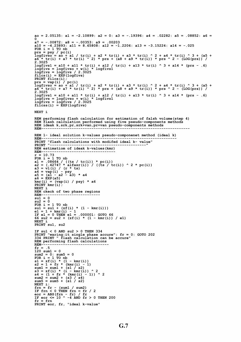
ao = 2.05135: a1 = -2.10899: a2 = 0: a3 = -.19396: a4 = .02282: a5 = .08852: a6 = 0 a7 = -.00872: a8 = -.00353: a9 = .00203
a11 = 8.65808: a12 = -1.2206: a13 = -3.15224: a14 = -.025 a10 = -4.23893: FOR i = 1 TO nb prs = psy / pc(i) logfivso = ao + a1 / tr(i) + a2 * tr(i) + a3 * tr(i) ^ 2 + a4 * tr(i) ^ 3 + (a5 + a6 * tr(i) + a7 * tr(i) ^ 2) * prs + (a8 + a9 * tr(i)) * prs ^ 2 - (LOG(prs)) / 2.3025
tr(i) + a13 * tr(i) ^ 3 + a14 * (prs - .6) logfivs1 = a10 + a11 * tr(i) + a12 / logfivs1 logfivs = logfivso + w(i) *
25 logfivs = logfivs / 2.30ogfivs) filcs(i) = EXP(l
PRINT filcs(i); prs = vap(i) / pc(i) logfivso = ao + a1 / tr(i) + a2 * tr(i) + a3 * tr(i) ^ 2 + a4 * tr(i) ^ 3 + (a5 + a6 * tr(i) + a7 * tr(i) ^ 2) * prs + (a8 + a9 * tr(i)) * prs ^ 2 - (LOG(prs)) / 2.3025
tr(i) + a13 * tr(i) ^ 3 + a14 * (prs - .6) logfivs1 = a10 + a11 * tr(i) + a12 / logfivs1 logfivs = logfivso + w(i) *
5 logfivs = logfivs / 2.302ilcss(i) = EXP(logfivs) f EXT i N
4) REM performing flash calculation for estimation of falsh volume(step methods REM flash calculation performed using five pseudo-components
REM ideak k,srk,pr,srk+van,pr+van pseudo-components methods EM-------------------------------------------------------------------- R REM 1- ideal solution k-values pseudo-componenet method (ideal k)
---------- REM----------------------------------------------------" PRINT "flash calculations with modifed ideal k- value
-------------" PRINT "-------------------------------REM estimatiom of ideak k-values(kmr)
--------------------------- REM-------r = 10.73 FOR i = 1 TO nb a1 = .08664 / ((ts / tc(i)) * pc(i))
i)) / ((ts / tc(i)) ^ 2 * pc(i)) a2 = (.42747 * alfasr(ts) a3 = vl(i) / (r *
a4 = vap(i) - psy - a3) * a4 a5 = (a1 - a2
a6 = EXP(a5) i) / psy) * a6 kmr(i) = (vap(
mr(i); PRINT kNEXT i REM ckeck of two phase regions
---------------------- REM-----su1 = 0 su2 = 0 FOR i = 1 TO nb
(1 - kmr(i))) su1 = su1 + (zf(i) *e1 = 1 + kmr(i) - 1 IF e1 = 0 THEN e1 = .000001: GOTO 66
= su2 + (zf(i) * (1 - kmr(i)) / e1) 66 su2 NEXT i PRINT su1, su2 IF su1 < 0 AND su2 > 0 THEN 334
: GOTO 202 PRINT "waring:it single phase accure": fr = 0be accure" 334 PRINT " flash calculation can
REM performing flash calculations -------------------------- REM-----
fr = .5 120 sum1 = 0
0 sum2 = 0: sum5 =FOR i = 1 TO nb s1 = zf(i) * (1 - kmr(i))
1) s2 = 1 + fr * (kmr(i) - sum1 = sum1 + (s1 / s2) s3 = zf(i) * (i - kmr(i)) ^ 2
1)) ^ 2 s4 = (1 + fr * (kmr(i) -sum2 = sum2 + (s3 / s4)
um5 + (s1 / s2) sum5 = sNEXT i: frn = fr - (sum1 / sum2)
/ 2 IF frn < 0 THEN frn = fr eor = ABS(frn - fr) / fr
10 ^ -4 AND fr > 0 THEN 200 IF eor <=fr = frn PRINT eor, fr, "ideal k-value"
G.7
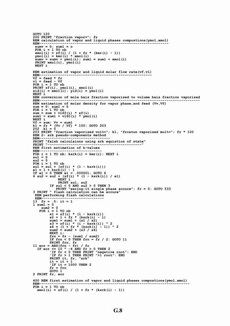
GOTO 120 200 PRINT "fraction vapor="; fr REM calculation of vapor and liquid phases compostions(ymol,xmol)
--------------------------------------------- REM----------------- o sumv = 0: suml =
FOR i = 1 TO nb (kmr(i) - 1)) xmol(i) = zf(i) / (1 + fr *
ymol(i) = kmr(i) * xmol(i) suml = suml + xmol(i) sumv = sumv + ymol(i):
mol(i), ymol(i) PRINT xNEXT i REM estimation of vapor and liquid molar flow rate(vf,vl)
------------------------------------------ REM------------Vf = feed * fr vl = feed - Vf FOR i = 1 TO nb PRINT zf(i), ymol(i), xmol(i)
= xmol(i): yid(i) = ymol(i) xid(i) NEXT i REM conversion of mole bais fraction vaporized to volume bais fraction vaporized
--------------- REM--------------------------------------------------------------molar density for vapor phase,and feed (Vv,Vf) REM estimation of
0 sum = 0: sum1 = FOR i = 1 TO nb sum = sum + vl60(i) * zf(i)
sum1 + vl60(i) * ymol(i) sum1 = NEXT i Vf = sum: Vv = sum1
v / Vf) * 100: GOTO 203 k1 = fr * (V202 k1 = 0
; k1, "frcaton vaporized mol%="; fr * 100 203 PRINT "fraction vaporized vol%="REM 2- srk pseudo-components method REM----------------------------------
PRINT "falsh calculaions using srk equistion of state"-------------------" PRINT "--------------------------
REM first estimation of k-values REM------------------------------
1 TO nb: ksrk(i) = kmr(i): NEXT i FOR i = su1 = 0 su2 = 0 FOR i = 1 TO nb
(1 - ksrk(i))) su1 = su1 + (zf(i) * e1 = 1 + ksrk(i) - 1 IF e1 = 0 THEN e1 = .000001: GOTO 6
) * (1 - ksrk(i)) / e1) 6 su2 = su2 + (zf(i NEXT i PRINT su1, su2 IF su1 < 0 AND su2 > 0 THEN 3
cure": fr = 0: GOTO 533 PRINT "waring:it single phase acaccure" 3 PRINT " flash calculation can be
REM performing flash calculations -------------- REM----------------
: it = 1 13 fr = .51 sum1 = 0 sum2 = 0 FOR i = 1 TO nb s1 = zf(i) * (1 - ksrk(i))
1) s2 = 1 + fr * (ksrk(i) - sum1 = sum1 + (s1 / s2) s3 = zf(i) * (i - ksrk(i)) ^ 2
- 1)) ^ 2 s4 = (1 + fr * (ksrk(i) um2 + (s3 / s4) sum2 = s
NEXT i: frn = fr - (sum1 / sum2)
N frn = fr / 2: GOTO 11 IF frn < 0 THE PRINT frn, fr 11 eor = ABS(frn - fr) / fr IF eor <= 10 ^ -4 AND fr > 0 THEN 2
: END 'IF fr < 0 THEN PRINT "negative root"T ">1 root": END 'IF fr > 1 THEN PRIN
, "srk" PRINT it, fr it = it + 1
1000 THEN 2 'IF it = n fr = fr
GOTO 1 eor 2 PRINT fr,
400 REM first estimation of vapor and liquid phases compostions(ymol,xmol)
----------------------------------------------------------- REM-------------FOR i = 1 TO nb xmol(i) = zf(i) / (1 + fr * (ksrk(i) - 1))
G.8
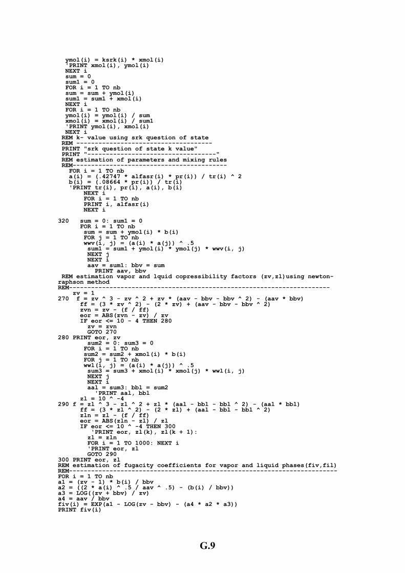
ymol(i) = ksrk(i) * xmolxmol(i), ymol(i)
(i) 'PRINT NEXT i sum = 0 sum1 = 0 FOR i = 1 TO nb sum = sum + ymol(i)
sum1 + xmol(i) sum1 = NEXT i FOR i = 1 TO nb ymol(i) = ymol(i) / sum
xmol(i) = xmol(i) / sum1ymol(i), xmol(i) 'PRINT
NEXT i REM k- value using srk question of state
--- REM ---------------------------------- PRINT "srk question of state k value" PRINT "-----------------------------------" REM estimation of parameters and mixing rules
--------------------------- REM--------------- FOR i = 1 TO nb
i)) / tr(i) ^ 2 a(i) = (.42747 * alfasr(i) * pr( b(i) = (.08664 * pr(i)) / tr(i)
), pr(i), a(i), b(i) 'PRINT tr(i NEXT i FOR i = 1 TO nb
, alfasr(i) PRINT iXT i NE
0 320 sum = 0: sum1 =
FOR i = 1 TO nb (i) * b(i) sum = sum + ymol
FOR j = 1 TO nb wwv(i, j) = (a(i) * a(j)) ^ .5
sum1 + ymol(i) * ymol(j) * wwv(i, j) sum1 = NEXT j NEXT i
sum aav = sum1: bbv = PRINT aav, bbv REM estimation vapor and lquid copressibility factors (zv,zl)using newton-raphson method
--------------------------------------------------------------- REM-------- zv = 1
v * bbv) 270 f = zv ^ 3 - zv ^ 2 + zv * (aav - bbv - bbv ^ 2) - (aa(2 * zv) + (aav - bbv - bbv ^ 2) ff = (3 * zv ^ 2) -
zvn = zv - (f / ff) eor = ABS(zvn - zv) / zv
0 - 4 THEN 280 IF eor <= 1 zv = zvn GOTO 270 280 PRINT eor, zv
= 0 sum2 = 0: sum3 FOR i = 1 TO nb
ol(i) * b(i) sum2 = sum2 + xm FOR j = 1 TO nb wwl(i, j) = (a(i) * a(j)) ^ .5
sum3 + xmol(i) * xmol(j) * wwl(i, j) sum3 = NEXT j NEXT i
sum2 aal = sum3: bbl = l, bbl 'PRINT aa
zl = 10 ^ -4 * bbl) 290 f = zl ^ 3 - zl ^ 2 + zl * (aal - bbl - bbl ^ 2) - (aal
(2 * zl) + (aal - bbl - bbl ^ 2) ff = (3 * zl ^ 2) - zln = zl - (f / ff) eor = ABS(zln - zl) / zl IF eor <= 10 ^ -4 THEN 300
or, zl(k), zl(k + 1): 'PRINT e zl = zln
00: NEXT i FOR i = 1 TO 10r, zl 'PRINT eo
GOTO 290 300 PRINT eor, zl REM estimation of fugacity coefficients for vapor and liquid phases(fiv,fil)
------------------------------------------------------------ REM-------------FOR i = 1 TO nb a1 = (zv - 1) * b(i) / bbv
^ .5) - (b(i) / bbv)) a2 = ((2 * a(i) ^ .5 / aavbbv) / zv) a3 = LOG((zv +
a4 = aav / bbv a1 - LOG(zv - bbv) - (a4 * a2 * a3)) fiv(i) = EXP(
PRINT fiv(i)
G.9
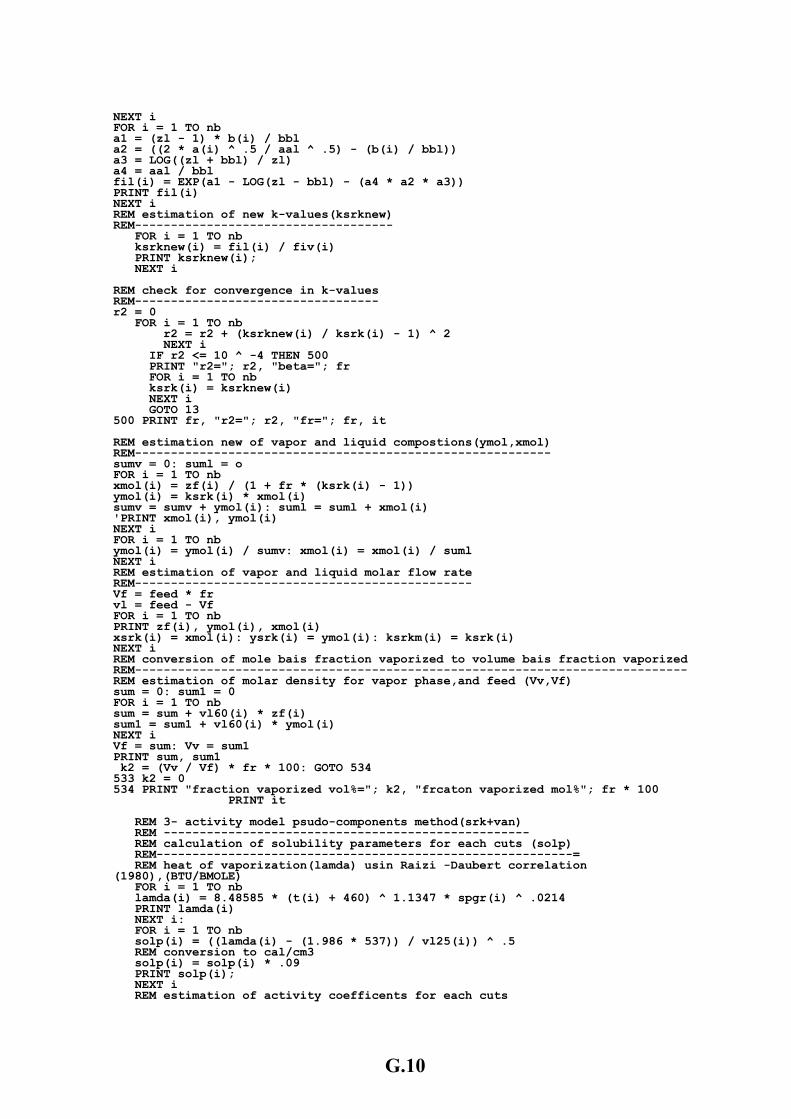
NEXT i FOR i = 1 TO nb a1 = (zl - 1) * b(i) / bbl
^ .5) - (b(i) / bbl)) a2 = ((2 * a(i) ^ .5 / aalbbl) / zl) a3 = LOG((zl +
a4 = aal / bbl a1 - LOG(zl - bbl) - (a4 * a2 * a3)) fil(i) = EXP(
il(i) PRINT fNEXT i REM estimation of new k-values(ksrknew)
-------------------- REM---------------- FOR i = 1 TO nb
) / fiv(i) ksrknew(i) = fil(isrknew(i); PRINT k
NEXT i REM check for convergence in k-values
------------------------------ REM----r2 = 0 FOR i = 1 TO nb
+ (ksrknew(i) / ksrk(i) - 1) ^ 2 r2 = r2 NEXT i IF r2 <= 10 ^ -4 THEN 500
"beta="; fr PRINT "r2="; r2, FOR i = 1 TO nb
= ksrknew(i) ksrk(i) NEXT i GOTO 13
, it 500 PRINT fr, "r2="; r2, "fr="; fr REM estimation new of vapor and liquid compostions(ymol,xmol)
------------------------------------------ REM---------------- o sumv = 0: suml =
FOR i = 1 TO nb (ksrk(i) - 1)) xmol(i) = zf(i) / (1 + fr *
ymol(i) = ksrk(i) * xmol(i) uml = suml + xmol(i) sumv = sumv + ymol(i): s
xmol(i), ymol(i) 'PRINT NEXT i FOR i = 1 TO nb
= ymol(i) / sumv: xmol(i) = xmol(i) / suml ymol(i)NEXT i REM estimation of vapor and liquid molar flow rate
----------------------------------- REM------------Vf = feed * fr vl = feed - Vf FOR i = 1 TO nb PRINT zf(i), ymol(i), xmol(i)
= xmol(i): ysrk(i) = ymol(i): ksrkm(i) = ksrk(i) xsrk(i)NEXT i REM conversion of mole bais fraction vaporized to volume bais fraction vaporized
--------------- REM--------------------------------------------------------------molar density for vapor phase,and feed (Vv,Vf) REM estimation of
0 sum = 0: sum1 = FOR i = 1 TO nb sum = sum + vl60(i) * zf(i)
sum1 + vl60(i) * ymol(i) sum1 = NEXT i
um1 Vf = sum: Vv = sPRINT sum, sum1
Vf) * fr * 100: GOTO 534 k2 = (Vv /533 k2 = 0
ized vol%="; k2, "frcaton vaporized mol%"; fr * 100 534 PRINT "fraction vapor it PRINT
REM 3- activity model psudo-components method(srk+van) REM --------------------------------------------------- REM calculation of solubility parameters for each cuts (solp) REM----------------------------------------------------------= REM heat of vaporization(lamda) usin Raizi -Daubert correlation (1980),(BTU/BMOLE) FOR i = 1 TO nb
585 * (t(i) + 460) ^ 1.1347 * spgr(i) ^ .0214 lamda(i) = 8.48mda(i) PRINT la
NEXT i: FOR i = 1 TO nb
986 * 537)) / vl25(i)) ^ .5 solp(i) = ((lamda(i) - (1.3 REM conversion to cal/cm
i) * .09 solp(i) = solp(olp(i); PRINT s
NEXT i REM estimation of activity coefficents for each cuts
G.10
REM-------------------------------------------------- REM estimation of interaction parameters (aac)
------------------------------------- REM------------- FOR i = 1 TO nb FOR j = 1 TO nb
j) = ((vl25(i) * (solp(i) - solp(j)))) / (1.976 * ts) aac(i, NEXT j NEXT i FOR i = 1 TO nb FOR j = 1 TO nb
ac(i, j); PRINT a NEXT j NEXT i
r REM calculation of pointing facto---------------- REM-------------
FOR i = 1 TO nb ts) a1 = vl(i) / (r *
p(i) a2 = psy - va a3 = a1 * a2
a3) pof(i) = EXP(T pof(i) PRIN
NEXT i REM estimation of vapor phase fugacity coffecients(fiv)
--------------------- REM-------------------------------- REM flash caculation using srk EOS
---- REM--------------------------- REM test for two phase region
-------------- REM------------- FOR i = 1 TO nb
= kmr(i) ksrk(i) NEXT i su1 = 0 su2 = 0 FOR i = 1 TO nb
(1 - ksrk(i))) su1 = su1 + (zf(i) * e1 = 1 + ksrk(i) - 1 IF e1 = 0 THEN e1 = .000001: GOTO 700
= su2 + (zf(i) * (1 - ksrk(i)) / e1) 700 su2 NEXT i PRINT su1, su2 IF su1 < 0 AND su2 > 0 THEN 800
: k3 = 0: GOTO 3001 PRINT "waring:it single phase accure"be accure" 800 PRINT " flash calculation can
REM performing flash calculations ------------- REM-----------------
t = 1 950 fr = .5: i 1000 sum1 = 0
sum2 = 0 FOR i = 1 TO nb s1 = zf(i) * (1 - ksrk(i))
1) s2 = 1 + fr * (ksrk(i) - sum1 = sum1 + (s1 / s2) s3 = zf(i) * (i - ksrk(i)) ^ 2
- 1)) ^ 2 s4 = (1 + fr * (ksrk(i) um2 + (s3 / s4) sum2 = s
NEXT i: frn = fr - (sum1 / sum2)
/ 2 IF frn < 0 THEN frn = fr eor = ABS(frn - fr) / fr
F eor <= 10 ^ -4 AND fr > 0 THEN 1100 I it = it + 1
1000 THEN 1100 'IF it = fr = frn GOTO 1000 100 PRINT fr, eor: 1
y,x) 1200 REM estimation vapor and liquid compostions(-------------------------------- REM-------------
FOR i = 1 TO nb (ksrk(i) - 1)) xmol(i) = zf(i) / (1 + fr *
l(i) ymol(i) = ksrk(i) * xmomol(i), ymol(i) PRINT x
NEXT i sum = 0 sum1 = 0 FOR i = 1 TO nb sum = sum + ymol(i)
sum1 + xmol(i) sum1 = NEXT i FOR i = 1 TO nb ymol(i) = ymol(i) / sum
G.11
xmol(i) = xmol(i) / summol(i), xmol(i)
1 PRINT y NEXT i
REM calculation of actvity coefficints (act)------------------------- REM---------------
0 sum = 0: sum1 = FOR i = 1 TO nb FOR j = 1 TO nb sum = sum + xmol(j) * aac(j, i)
sum1 + xmol(j) * aac(i, j) sum1 = NEXT j a1 = sum1 / (1 - xmol(i))
xmol(i) * sum1) / ((xmol(i) * sum1) + (1 - xmol(i) * sum))))) ^ 2 a2 = ((1 - ((a3 = a1 * a2
a3) act(i) = EXP(ct(i) PRINT a
NEXT i REM calculation of vapor phase fugacity coefficints(fiv) REM----------------------------------------------------
REM calculation of srk EOS parameters and mixing rules ------------------------------------ REM----------------
FOR i = 1 TO nb i)) / tr(i) ^ 2 a(i) = (.42747 * alfasr(i) * pr(
b(i) = (.08664 * pr(i)) / tr(i) , pr(i), a(i), b(i): PRINT tr(i)
NEXT i = 0 sum = 0: sum1
FOR i = 1 TO nb (i) * b(i) sum = sum + ymol
FOR j = 1 TO nb wwv(i, j) = (a(i) * a(j)) ^ .5
sum1 + ymol(i) * ymol(j) * wwv(i, j) sum1 = NEXT j NEXT i aav = sum1: bbv = sum REM estimation vapor phase copressibility factors (zv)using newton-raphson method
------------------------------------------------------------------ REM---------- zv = 1
v * bbv) 1500 f = zv ^ 3 - zv ^ 2 + zv * (aav - bbv - bbv ^ 2) - (aa(2 * zv) + (aav - bbv - bbv ^ 2) ff = (3 * zv ^ 2) -
zvn = zv - (f / ff) eor = ABS(zvn - zv) / zv
0 ^ -4 THEN 1400 IF eor <= 1 zv = zvn
, zv(k) 'PRINT eor500 GOTO 1
1400 PRINT zv REM calculation of fugacity coefficients for vapor phase(fiv)
--------------------------------------------- REM-------------FOR i = 1 TO nb a1 = (zv - 1) * b(i) / bbv
^ .5) - (b(i) / bbv)) a2 = ((2 * a(i) ^ .5 / aavbbv) / zv) a3 = LOG((zv +
a4 = aav / bbv a1 - LOG(zv - bbv) - (a4 * a2 * a3)) fiv(i) = EXP(
v(i) PRINT fiNEXT i
REM calculation of saturation fugacity coffcients (fivs)REM---------------------------------------------------- REM if tr>1 then the fugacity coefficints can be calculated using chao-seader correlation
-------------------- REM----------------------------------------------------REM calculation of srk EOS parameters and mixing rules
------------------------------------ REM---------------- FOR i = 1 TO nb prst(i) = vap(i) / pc(i)
i)) / tr(i) ^ 2 a(i) = (.42747 * alfasr(i) * prst(i) b(i) = (.08664 * prst(i)) / tr(
r(i), pr(i), a(i), b(i) PRINT t NEXT i
0 sum = 0: sum1 = FOR i = 1 TO nb
(i) * b(i) sum = sum + ymol FOR j = 1 TO nb wwv(i, j) = (a(i) * a(j)) ^ .5
+ ymol(i) * ymol(j) * wwv(i, j) sum1 = sum1 NEXT j NEXT i FOR i = 1 TO nb aav = a(i): bbv = b(i)
G.12
IF tr(i) > 1 THEN fil(i) = filcs(i): ksrknew(i) = (act(i) * fil(i)) / fiv(i): GOTO 2101 REM estimation vapor copressibility factors at saturated conditions(zvs)using newton-raphson method
---------------------------------------------------------------- REM--------- zvs = 1
av * bbv) 2000 f = zvs ^ 3 - zvs ^ 2 + zvs * (aav - bbv - bbv ^ 2) - (a2 * zvs) + (aav - bbv - bbv ^ 2) ff = (3 * zvs ^ 2) - (
zvsn = zvs - (f / ff) eor = ABS(zvsn - zvs) / zvs
^ -4 THEN 2100 IF eor <= 10 zvs = zvsn
zvs PRINT eor,00 GOTO 20
2100 PRINT zvs fivs(i) = filcss(i): GOTO 2102 IF zvs < 0 THEN
a1 = (zvs - 1) bbv) / zvs) a3 = LOG((zvs +
a4 = aav / bbv LOG(zvs - bbv) - (a4 * a3)) fivs(i) = EXP(a1 -
RINT "zvs="; zvs P REM calculation of new k-values(ksrknew) REM-------------------------------------
(i) = (act(i) * fivs(i) * vap(i) * pof(i)) / (fiv(i) * psy) 2102 ksrknew01 NEXT i 21
FOR i = 1 TO nb
srknew(i) PRINT kEXT i N REM check for convergence in k-values
--------------------------------- REM-REM r2 = 0 FOR i = 1 TO nb
+ (ksrknew(i) / ksrk(i) - 1) ^ 2 r2 = r2NEXT i IF r2 <= .0001 THEN 3000
"beta="; fr PRINT "r2="; r2,FOR i = 1 TO nb
rknew(i): NEXT i ksrk(i) = ksit = it + 1
r2 PRINT it,GOTO 950 000 PRINT fr 3 REM calculation of vapor and lquid phase compostions(ymol,xmol)
-------------------------------------------- REM---------------- o sumv = 0: suml =
FOR i = 1 TO nb (ksrk(i) - 1)) xmol(i) = zf(i) / (1 + fr *
ymol(i) = ksrk(i) * xmol(i) suml = suml + xmol(i) sumv = sumv + ymol(i):
mol(i), ymol(i) PRINT xEXT i N REM estimation of vapor and liquid molar flow rate (vf,vl)
------------------------------------------- REM------------Vf = feed * fr vl = feed - Vf FOR i = 1 TO nb PRINT zf(i), ymol(i), xmol(i)
i) = ymol(i): xsrkva(i) = xmol(i): ksrkva(i) = ksrk(i) ysrkva(NEXT i
d REM conversion of mole bais fraction vaporized to volume bais fraction vaporize------------- REM--------------------------------------------------------------
molar density for vapor phase,and feed (Vv,Vf) REM estimation of 0 sum = 0: sum1 =
FOR i = 1 TO nb sum = sum + vl60(i) * zf(i)
sum1 + vl60(i) * ymol(i) sum1 = NEXT i Vv = sum1: Vf = sum
) * fr * 100: GOTO 3002 k3 = (Vv / Vf3001 k3 = 0
k3, " frcaton vaporized mol%="; fr * 100 3002 PRINT "fraction vaporized vol%= ";REM 4- PR EOS pseudo-components method REM ------------------------------------ PRINT "falsh calculaions using pr equistion of state"
-------------------" PRINT "--------------------------REM first estimation of k-values
G.13
REM------------------------------ 1 TO nb: ksrk(i) = kmr(i) FOR i =
NEXT i REM ckeck of two phase regions
-------------------- REM------- su1 = 0 su2 = 0 FOR i = 1 TO nb
(1 - ksrk(i))) su1 = su1 + (zf(i) * e1 = 1 + ksrk(i) - 1 IF e1 = 0 THEN e1 = .000001: GOTO 336
(i) * (1 - ksrk(i)) / e1) 336 su2 = su2 + (zf NEXT i
u1, su2 PRINT s IF su1 < 0 AND su2 > 0 THEN 333
INT "waring:it single phase accure": fr = 0: GOTO 5503 PR 33 PRINT " flash calculation can be accure" 3 REM performing flash calculations
------------ REM------------------ it = 1 1333 fr = .5: 1113 sum1 = 0
sum2 = 0 FOR i = 1 TO nb s1 = zf(i) * (1 - ksrk(i))
1) s2 = 1 + fr * (ksrk(i) - sum1 = sum1 + (s1 / s2) s3 = zf(i) * (i - ksrk(i)) ^ 2
- 1)) ^ 2 s4 = (1 + fr * (ksrk(i) um2 + (s3 / s4) sum2 = s
NEXT i: frn = fr - (sum1 / sum2)
fr / 2: GOTO 1133 IF frn < 0 THEN frn = 1133 eor = ABS(frn - fr) / fr IF eor <= 10 ^ -4 AND fr > 0 THEN 2333
: END 'IF fr < 0 THEN PRINT "negative root"HEN PRINT ">1 root": END 'IF fr > 1 T
it = it + 1 1000 THEN 2333 'IF it =
fr = frn fr, it, "pr" PRINT eor,
GOTO 1113 2333 PRINT fr, eor
REM calculation of vapor and liquid phase compostions(y,x)----------------------------------- REM-------------------
4400 FOR i = 1 TO nb (ksrk(i) - 1)) xmol(i) = zf(i) / (1 + fr *
l(i) ymol(i) = ksrk(i) * xmomol(i), ymol(i) PRINT x
NEXT i sum = 0 sum1 = 0 FOR i = 1 TO nb sum = sum + ymol(i)
sum1 + xmol(i) sum1 = NEXT i FOR i = 1 TO nb ymol(i) = ymol(i) / sum
xmol(i) = xmol(i) / sum1ymol(i), xmol(i) 'PRINT
NEXT i REM k- value using PR question of state REM ------------------------------------- PRINT "-----------------------------------" REM estimation of parameters and mixing rules
- REM----------------------------------------- PRINT "k- value using PR question of state "
---" PRINT "-------------------------------- 0: sum3 = 0: sum4 = 0 sum = 0: sum1 =
FOR i = 1 TO nb (i)) / tr(i) ^ 2 a(i) = (.45724 * alfapr(i) * pr
b(i) = (.0778 * pr(i)) / tr(i) (.45724 * (10.73 * tc(i)) ^ 2) / pc(i) ac(i) =
NEXT i sum11 = 0 FOR i = 1 TO nb
(i) * b(i) sum = sum + ymolFOR j = 1 TO nb wwv(i, j) = (a(i) * a(j)) ^ .5
G.14
sum1 = sum1 + ymol(i) * ymol(j) * wwv(i, j) sum3 + ymol(i) * ymol(j) * (ac(i) * alfapr(i) * ac(j) * alfapr(j)) ^ .5 sum3 =
NEXT j NEXT i av = sum1: bbv = sum: aaj = sum3 a REM estimation vapor and lquid copressibility factors (zv,zl)using newton-raphson method
----------------------------------------------------------------- REM----zv = 1 2230 f = zv ^ 3 - zv ^ 2 * (1 - bbv) + zv * (aav - 2 * bbv - 3 * bbv ^ 2) - (aav * bbv - bbv ^ 2 - bbv ^ 3)
* zv * (1 - bbv) + (aav - 3 * bbv ^ 2 - 2 * bbv) ff = 3 * zv ^ 2 - 2 zvn = zv - (f / ff) eor = ABS(zvn - zv) / zv
10 ^ -4 THEN 2550 IF eor <=zv = zvn
zv PRINT eor,GOTO 2230 2550 PRINT eor, zv
0: sum4 = 0 sum2 = 0: sum3 =FOR i = 1 TO nb
ol(i) * b(i) sum2 = sum2 + xmFOR j = 1 TO nb wwl(i, j) = (a(i) * a(j)) ^ .5 sum3 = sum3 + xmol(i) * xmol(j) * wwl(i, j)
sum4 + xmol(i) * xmol(j) * (ac(i) * alfapr(i) * ac(j) * alfapr(j)) ^ .5 sum4 = NEXT j NEXT i
bl = sum2: bbj = sum4 aal = sum3: bzl = 10 ^ -4 2240 f = zl ^ 3 - zl ^ 2 * (1 - bbl) + zl * (aal - 2 * bbl - 3 * bbl ^ 2) - (aal * bbl - bbl ^ 2 - bbl ^ 3)
* zl * (1 - bbl) + (aal - 3 * bbl ^ 2 - 2 * bbl) ff = 3 * zl ^ 2 - 2 zln = zl - (f / ff) eor = ABS(zln - zl) / zl
THEN 2260 IF eor <= 10 ^ -4 r, zl(k) 'PRINT eo
zl = zln zl PRINT eor,
GOTO 2240 , zl 2260 PRINT eor
PRINT zv, zl 1 TO nb FOR i =
sum = 0 FOR j = 1 TO nb
um + ymol(j) * (ac(i) * alfapr(i) * ac(j) * alfapr(j)) ^ .5 sum = sNEXT j a1 = (zv - 1) * (b(i) / bbv) a2 = (((2 * sum) * (1 / aaj)) - b(i) / bbv)
/ bbv) 'a2 = (((2 * a(i) ^ .5) * (1 / aav ^ .5)) - b(i) 4) / (zv - bbv * .414)) a3 = LOG((zv + bbv * 2.41
(2.828 * bbv) a4 = aav /'PRINT a1 'PRINT a2 'PRINT a3 'PRINT a4
a1 - LOG(zv - bbv) - (a2 * a3 * a4)) fiv(i) = EXP(v(i) PRINT fi
NEXT i REM estimation of fugacity coefficients for vapor and liquid phases(fiv,fil)
------------------------------------------------------------ REM-------------1 TO nb FOR i =
sum = 0 FOR j = 1 TO nb
um + xmol(j) * (ac(i) * alfapr(i) * ac(j) * alfapr(j)) ^ .5 sum = sNEXT j a1 = (zl - 1) * (b(i) / bbl) a2 = (((2 * sum) * (1 / bbj)) - b(i) / bbl)
/ bbl) 'a2 = (((2 * a(i) ^ .5) * (1 / aal ^ .5)) - b(i) 4) / (zl - bbl * .414)) a3 = LOG((zl + bbl * 2.41
a4 = aal / (2.828 * bbl) LOG(zl - bbl) - (a2 * a3 * a4)) fil(i) = EXP(a1 -
PRINT fil(i), zl fil(i)="; fil(i) PRINT "
EXT i N REM estimation of new k-values(ksrknew)
----------------------- REM-------------FOR i = 1 TO nb ksrknew(i) = fil(i) / fiv(i)
G.15
PRINT ksrknew(i) NEXT i REM check for convergence in k-values
------------------------------ REM----r2 = 0 FOR i = 1 TO nb
knew(i) / ksrk(i) - 1) ^ 2 r2 = r2 + (ksr NEXT i IF r2 <= .0001 THEN 5500
"beta="; fr PRINT "r2="; r2, FOR i = 1 TO nb
ksrknew(i): NEXT i ksrk(i) = GOTO 1333 500 PRINT fr, r2 5 REM calculation of vapor and lquid phase compostions(ymol,xmol)
---------------------------------------------- REM---------------- o sumv = 0: suml =
FOR i = 1 TO nb (ksrk(i) - 1)) xmol(i) = zf(i) / (1 + fr *
ymol(i) = ksrk(i) * xmol(i) sumv + ymol(i): suml = suml + xmol(i) sumv =
EXT i N REM estimation of vapor and liquid molar flow rate(vf,vl)
------------------------------------------- REM------------Vf = feed * fr vl = feed - Vf FOR i = 1 TO nb PRINT zf(i), ymol(i), xmol(i)
= xmol(i): ypr(i) = ymol(i): kpr(i) = ksrk(i) xpr(i) NEXT i REM conversion of mole bais fraction vaporized to volume bais fraction vaporized
--------------- REM--------------------------------------------------------------of molar density for vapor phase,and feed (Vv,Vf) REM estimation
Vf = 0: Vv = 0 FOR i = 1 TO nb Vf = Vf + vl60(i) * zf(i)
+ vl60(i) * ymol(i) Vv = VvNEXT i
/ Vf) * fr * 100: GOTO 5504 k4 = (Vv 5503 k4 = 0
RINT "fraction vaporized vol%"; k4, "frcaton vaporized mol%"; fr * 100 5504 P
REM 5- activity model psudo-components method(pr+van)
- REM --------------------------------------------------PRINT "falsh calculaions using pr equistion of state" REM ------------------------------------------------- REM heat of vaporization(lamda) usin Raizi -Daubert correlation
E) (1980),(BTU/BMOLFOR i = 1 TO nb
585 * (t(i) + 460) ^ 1.1347 * spgr(i) ^ .0214 lamda(i) = 8.48amda(i) PRINT l
EXT i N REM calculation of solubilty paramter(solp)
--------------------------- REM-------------FOR i = 1 TO nb
986 * 537)) / vl25(i)) ^ .5 solp(i) = ((lamda(i) - (1.3 REM conversion to cal/cm
(i) * .09 solp(i) = solpolp(i) PRINT s
EXT i N REM calculation of interaction parameters(aac)
------------------------------ REM-------------FOR i = 1 TO nb FOR j = 1 TO nb
j) = ((vl25(i) * (solp(i) - solp(j)))) / (1.976 * ts) aac(i, NEXT j NEXT i FOR i = 1 TO nb FOR j = 1 TO nb
ac(i, j); PRINT aNEXT j EXT i N REM calculation of pointing factor(pof)
------------------------ REM-------------FOR i = 1 TO nb a1 = vl(i) / (r * ts)
G.16
a2 = psy - vap(i) a3 = a1 * a2
a3) pof(i) = EXP(of(i) PRINT p
i NEXT
REM calculation of vapor phase fugacity coefficints(fiv)- REM---------------------------------------------------
PRINT "falsh calculaions using PR equistion of state" ------------------" PRINT "---------------------------
REM first estimation for k-values REM------------------------------- OR i = 1 TO nb: ksrk(i) = kmr(i): NEXT i F REM test for two phase region
----------------------- REM----su1 = 0 su2 = 0 FOR i = 1 TO nb
(1 - ksrk(i))) su1 = su1 + (zf(i) * e1 = 1 + ksrk(i) - 1 IF e1 = 0 THEN e1 = .000001: GOTO 3700
2 = su2 + (zf(i) * (1 - ksrk(i)) / e1) 3700 suNEXT i PRINT su1, su2 IF su1 < 0 AND su2 > 0 THEN 3800
GOTO 330001 PRINT "waring:it single phase accure": fr = 0:800 PRINT " flash calculation can be accure" 3 REM performing flash calculations
-------------- REM------------------t = 1 3950 fr = .5: i
1 = 0 31000 sumsum2 = 0 FOR i = 1 TO nb s1 = zf(i) * (1 - ksrk(i))
1) s2 = 1 + fr * (ksrk(i) -sum1 = sum1 + (s1 / s2) s3 = zf(i) * (i - ksrk(i)) ^ 2
- 1)) ^ 2 s4 = (1 + fr * (ksrk(i) sum2 + (s3 / s4) sum2 =
NEXT i frn = fr - (sum1 / sum2)
/ 2 IF frn < 0 THEN frn = fr eor = ABS(frn - fr) / fr
^ -4 AND fr > 0 THEN 31100 IF eor <= 10it = it + 1
1000 THEN 31100 'IF it = fr = frn
fr, it, "pr+gam" PRINT eor, GOTO 31000 1100 PRINT fr, eor 3 REM calculation of vapor and liquid phases compostions(ymol,xmol)
------------------------------------------ REM--------------------31200 FOR i = 1 TO nb
(ksrk(i) - 1)) xmol(i) = zf(i) / (1 + fr * l(i) ymol(i) = ksrk(i) * xmo
mol(i), ymol(i) PRINT xNEXT i sum = 0 sum1 = 0 FOR i = 1 TO nb sum = sum + ymol(i)
sum1 + xmol(i) sum1 = NEXT i FOR i = 1 TO nb ymol(i) = ymol(i) / sum
1 xmol(i) = xmol(i) / summol(i), xmol(i) PRINT y
EXT i N
REM calculation of actvity coefficints (act)------------------------- REM---------------
0 sum = 0: sum1 = FOR i = 1 TO nb FOR j = 1 TO nb sum = sum + xmol(j) * aac(j, i)
sum1 + xmol(j) * aac(i, j) sum1 = NEXT j a1 = sum1 / (1 - xmol(i)) a2 = ((1 - ((xmol(i) * sum1) / ((xmol(i) * sum1) + (1 - xmol(i) * sum))))) ^ 2
G.17
a3 = a1 * a2 a3) act(i) = EXP(
ct(i) PRINT aEXT i N REM estimation of vapor phase fugacity coffecients(fiv)
-- REM---------------------------------------------------REM calculation of srk EOS parameters and mixing rules
-------------------------- REM--------------------------0: r = 10.73 sum = 0: sum1 =
FOR i = 1 TO nb ac(i) = .457235 * ((r * tc(i)) ^ 2 / pc(i))
(i)) / tr(i) ^ 2 a(i) = (.45724 * alfapr(i) * prb(i) = (.0778 * pr(i)) / tr(i)
r(i), pr(i), a(i), b(i): PRINT tNEXT i sum11 = 0 FOR i = 1 TO nb
(i) * b(i) sum = sum + ymolFOR j = 1 TO nb wwv(i, j) = (a(i) * a(j)) ^ .5 sum1 = sum1 + ymol(i) * ymol(j) * wwv(i, j)
sum11 + ymol(i) * ymol(j) * (ac(i) * ac(j) * alfapr(i) * alfapr(j)) ^ .5 sum11 =NEXT j NEXT i av = sum1: bbv = sum: aavv = sum1: aaj = sum11 a REM estimation of vapor phase compessbility factores (zv)using newtone- raphsone method
------------------------------------------------------------------- REM----zv = 1 33231 f = zv ^ 3 - zv ^ 2 * (1 - bbv) + zv * (aav - 2 * bbv - 3 * bbv ^ 2) - (aav * bbv - bbv ^ 2 - bbv ^ 3)
* zv * (1 - bbv) + (aav - 3 * bbv ^ 2 - 2 * bbv) ff = 3 * zv ^ 2 - 2 zvn = zv - (f / ff) eor = ABS(zvn - zv) / zv
10 ^ -4 THEN 33251 IF eor <=zv = zvn
zv PRINT eor, GOTO 33231 33251 PRINT eor, zv REM estimation of vapor phase fugacity coeffidcients(fiv)
----------------------------------------- REM-------------1 TO nb FOR i =
sum = 0 FOR j = 1 TO nb
um + ymol(j) * (ac(i) * ac(j) * alfapr(i) * alfapr(j)) ^ .5 sum = sNEXT j a1 = (zv - 1) * (b(i) / bbv) a2 = (((2 * sum) * (1 / aaj)) - b(i) / bbv)
/ bbv) 'a2 = (((2 * a(i) ^ .5) * (1 / aav ^ .5)) - b(i) 4) / (zv - bbv * .414)) a3 = LOG((zv + bbv * 2.41
a4 = aav / (2.828 * bbv) - LOG(zv - bbv) - (a2 * a3 * a4)) fiv(i) = EXP(a1
fiv(i); 'PRINT NEXT i REM calculation of saturation fugacity coffecient(fivs)
---------------------------------------- REM-------------FOR i = 1 TO nb prpt(i) = vap(i) / pc(i)
(i)) / tr(i) ^ 2 a(i) = (.45724 * alfapr(i) * prptb(i) = (.0778 * prpt(i)) / tr(i)
(.45724 * (10.73 * tc(i)) ^ 2) / pc(i) ac(i) =NEXT i FOR i = 1 TO nb aav = a(i): bbv = b(i) IF tr(i) > 1 THEN fil(i) = filcs(i): ksrknew(i) = (act(i) * fil(i)) / fiv(i): GOTO 32101 REM calcultion of saturates copressibily factores at saturation conditions
------------------------------------------------------------------ REM-----zvs = 1 32000 f = zvs ^ 3 - zvs ^ 2 * (1 - bbv) + zvs * (aav - 2 * bbv - 3 * bbv ^ 2) - (aav * bbv - bbv ^ 2 - bbv ^ 3)
zvs * (1 - bbv) + (aav - 3 * bbv ^ 2 - 2 * bbv) ff = 3 * zvs ^ 2 - 2 *zvsn = zvs - (f / ff) eor = ABS(zvsn - zvs) / zvs
0 ^ -4 THEN 32100 IF eor <= 1zvs = zvsn GOTO 32000 2100 PRINT 3 REM calculation of saturted fugacity coefficinents(fivs)
G.18
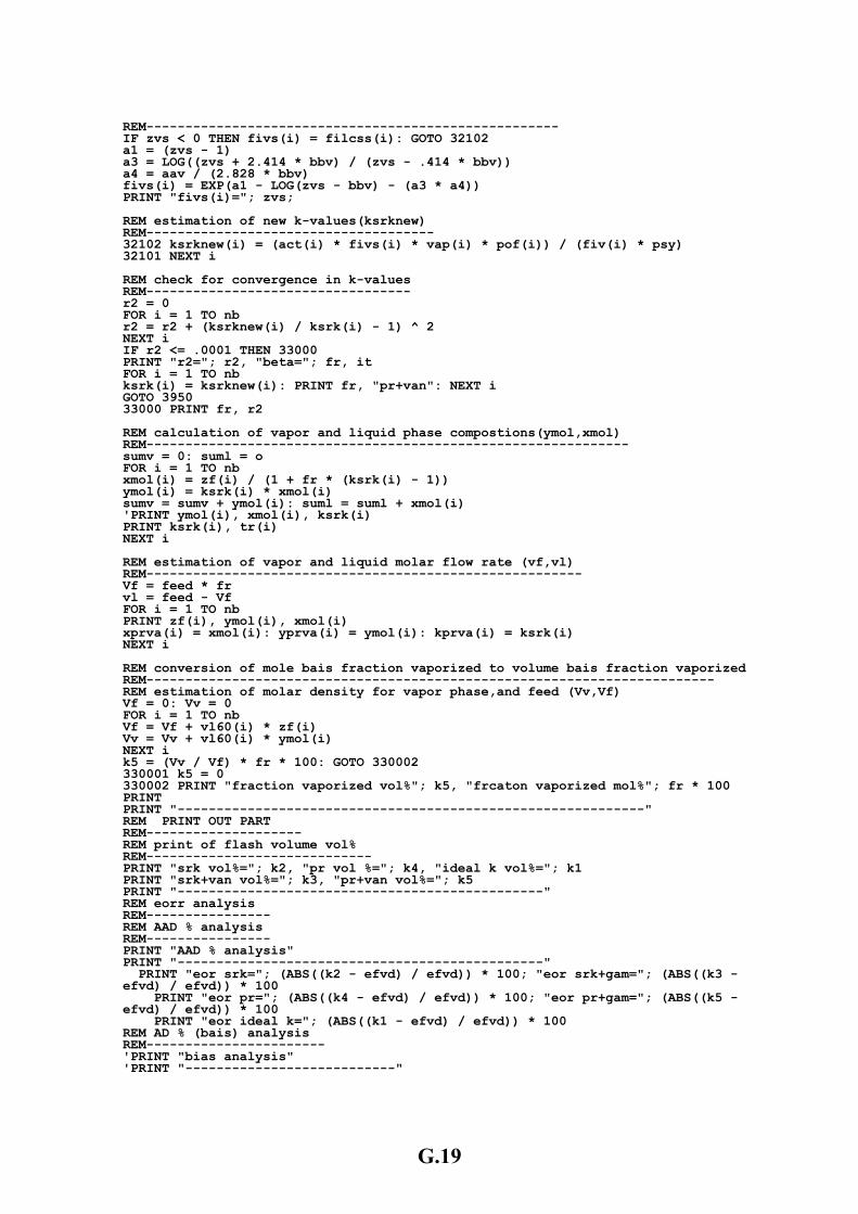
REM--------------------------------------------- fivs(i) = filcss(i): GOTO 32102
-------- IF zvs < 0 THENa1 = (zvs - 1)
bv) / (zvs - .414 * bbv)) a3 = LOG((zvs + 2.414 * ba4 = aav / (2.828 * bbv)
zvs - bbv) - (a3 * a4)) fivs(i) = EXP(a1 - LOG(T "fivs(i)="; zvs; PRIN
REM estimation of new k-values(ksrknew) REM-------------------------------------
(i) = (act(i) * fivs(i) * vap(i) * pof(i)) / (fiv(i) * psy) 32102 ksrknew101 NEXT i 32
REM check for convergence in k-values
------------------------------ REM----r2 = 0 FOR i = 1 TO nb
+ (ksrknew(i) / ksrk(i) - 1) ^ 2 r2 = r2NEXT i IF r2 <= .0001 THEN 33000
"beta="; fr, it PRINT "r2="; r2,FOR i = 1 TO nb
ksrknew(i): PRINT fr, "pr+van": NEXT i ksrk(i) = GOTO 3950 3000 PRINT fr, r2 3 REM calculation of vapor and liquid phase compostions(ymol,xmol)
---------------------------------------------- REM---------------- o sumv = 0: suml =
FOR i = 1 TO nb (ksrk(i) - 1)) xmol(i) = zf(i) / (1 + fr *
ymol(i) = ksrk(i) * xmol(i) l + xmol(i) sumv = sumv + ymol(i): suml = sum
i), ksrk(i) 'PRINT ymol(i), xmol(srk(i), tr(i) PRINT k
T i NEX REM estimation of vapor and liquid molar flow rate (vf,vl)
-------------------------------------------- REM------------Vf = feed * fr vl = feed - Vf FOR i = 1 TO nb PRINT zf(i), ymol(i), xmol(i)
) = xmol(i): yprva(i) = ymol(i): kprva(i) = ksrk(i) xprva(iEXT i N
zed REM conversion of mole bais fraction vaporized to volume bais fraction vapori----------- REM--------------------------------------------------------------
of molar density for vapor phase,and feed (Vv,Vf) REM estimation Vf = 0: Vv = 0 FOR i = 1 TO nb Vf = Vf + vl60(i) * zf(i)
+ vl60(i) * ymol(i) Vv = VvNEXT i
* fr * 100: GOTO 330002 k5 = (Vv / Vf)330001 k5 = 0
PRINT "fraction vaporized vol%"; k5, "frcaton vaporized mol%"; fr * 100 330002PRINT
-----------------------------------------------" PRINT "-------------REM PRINT OUT PART REM-------------------- REM print of flash volume vol% REM-----------------------------
k vol%="; k1 PRINT "srk vol%="; k2, "pr vol %="; k4, "idealPRINT "srk+van vol%="; k3, "pr+van vol%="; k5
------------------------------------" PRINT "-----------REM eorr analysis
REM----------------REM AAD % analysis REM---------------- PRINT "AAD % analysis" PRINT "-----------------------------------------------" PRINT "eor srk="; (ABS((k2 - efvd) / efvd)) * 100; "eor srk+gam="; (ABS((k3 - efvd) / efvd)) * 100 PRINT "eor pr="; (ABS((k4 - efvd) / efvd)) * 100; "eor pr+gam="; (ABS((k5 - efvd) / efvd)) * 100
(ABS((k1 - efvd) / efvd)) * 100 PRINT "eor ideal k=";REM AD % (bais) analysis
--- REM--------------------'PRINT "bias analysis" 'PRINT "---------------------------"
G.19

'PRINT "bias srk="; (((k2 - efvd) / efvd)) * 100; "bias srk+gam="; (((k3 - efvd) / efvd)) * 100 'PRINT "bias pr="; (((k4 - efvd) / efvd)) * 100; "bias pr+gam="; (((k5 - efvd) / efvd)) * 100
- efvd) / efvd)) * 100 'PRINT "bias ideal k="; (((k1 REM system pressure and temp REM----------------------------- PRINT "system tem in F="; ts - 460 REM graphical method efv results REM-------------------------------- PRINT "graphical method EFV estimation using Raizi-Daubert (1986)"
--------------------------------" PRINT "-------------------------- PRINT " vpl %", "astmd86", "efv"
----------------------" PRINT "-------- FOR i = 1 TO 6
ld(i), astmd86(i) - 460, efvgm(i) - 460 PRINT v i NEXT
END REM physical proprties for 40 cuts
REM-------------------------------- OPEN "C:\C1neww.dat" FOR OUTPUT AS #1 REM print out physical properties for cuts
--------------------------- REM------------- FOR i = 1 TO nb PRINT i, t(i), w(i)
1, i, t(i), w(i) PRINT #i NEXT
CLOSE #1 END REM marerial balance for petroleum stock
------- REM-------------------------------OPEN "C:\C22mb.dat" FOR OUTPUT AS #2 REM print out material balance for petroleum stocks
----------------------------------- REM-------------- FOR i = 1 TO nb PRINT i, t(i), spgr(i), v(i), wi(i), mol(i), zf(i)
2, i, t(i), spgr(i), mw(i), v(i), wi(i), mol(i), zf(i) PRINT # NEXT i
E #2 CLOS END
REM vapor and liquid compostions using five pseudo-components methodsREM-----------------------------------------------------------------
REM liquid compostions REM--------------------
" FOR OUTPUT AS #3 OPEN "C:\C6x.dat FOR i = 1 TO nb PRINT i, xid(i), xsrk(i), xpr(i), xsrkva(i), xprva(i)
3, i, xid(i), xsrk(i), xpr(i), xsrkva(i), xprva(i) PRINT # NEXT i REM vapor compostions REM-------------------
" FOR OUTPUT AS #4 OPEN "C:\C6y.dat FOR i = 1 TO nb PRINT i, yid(i), ysrk(i), ypr(i), ysrkva(i), yprva(i)
4, i, yid(i), ysrk(i), ypr(i), ysrkva(i), yprva(i) PRINT # NEXT i REM vapor and liquid k-values using five pseudo-components methods
--------------------------------- REM--------------------------------" FOR OUTPUT AS #5 OPEN "C:\C6k.dat
FOR i = 1 TO nb PRINT i, kmr(i), ksrkm(i), kpr(i), ksrkva(i), kprva(i)
5, i, kmr(i), ksrkm(i), kpr(i), ksrkva(i), kprva(i) PRINT #NEXT i
ND E
G.20
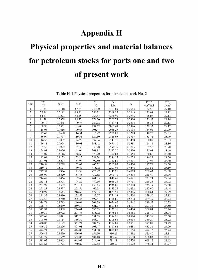
H.1
Appendix H
Physical properties and material balances
for petroleum stocks for parts one and two
of present work
Table H-1 Physical properties for petroleum stock No. 2
Cut TB, °C Sp.gr MW Tc,
°C Pc, kPa ω VL(15),
cm3/mol δ(25), J/cm3
1 71.39 0.7118 87.24 248.90 3361.69 0.2583 122.56 29.10 2 77.26 0.7192 89.95 256.32 3319.27 0.2643 125.08 29.12 3 84.13 0.7273 93.15 264.87 3266.90 0.2716 128.08 29.13 4 91.79 0.7358 96.77 274.26 3205.79 0.2800 131.52 29.14 5 100.10 0.7445 100.76 284.28 3137.44 0.2894 135.35 29.13 6 108.90 0.7531 105.08 294.72 3063.69 0.2996 139.53 29.12 7 118.06 0.7616 109.68 305.44 2986.27 0.3104 144.01 29.09 8 127.45 0.7698 114.51 316.27 2906.87 0.3218 148.75 29.05 9 136.99 0.7777 119.55 327.10 2826.95 0.3337 153.72 28.99 10 146.56 0.7852 124.75 337.84 2747.71 0.3458 158.87 28.93 11 156.11 0.7924 130.08 348.42 2670.10 0.3581 164.16 28.86 12 165.58 0.7992 135.52 358.78 2594.75 0.3705 169.58 28.78 13 174.91 0.8056 141.04 368.88 2522.20 0.3830 175.08 28.69 14 184.09 0.8116 146.62 378.70 2452.63 0.3954 180.66 28.60 15 193.09 0.8173 152.25 388.24 2386.15 0.4078 186.29 28.50 16 201.91 0.8227 157.93 397.50 2322.69 0.4201 191.97 28.40 17 210.58 0.8278 163.67 406.52 2262.05 0.4324 197.71 28.30 18 219.12 0.8327 169.47 415.32 2203.93 0.4446 203.52 28.19 19 227.57 0.8374 175.38 423.97 2147.96 0.4569 209.43 28.08 20 236.00 0.8420 181.43 432.52 2093.70 0.4694 215.49 27.96 21 244.49 0.8464 187.69 441.05 2040.65 0.4821 221.74 27.84 22 253.11 0.8508 194.22 449.66 1988.28 0.4951 228.28 27.72 23 261.99 0.8552 201.14 458.45 1936.01 0.5088 235.19 27.58 24 271.23 0.8597 208.56 467.53 1883.26 0.5232 242.60 27.44 25 280.97 0.8643 216.63 477.03 1829.50 0.5386 250.64 27.29 26 291.37 0.8690 225.52 487.07 1774.13 0.5554 259.50 27.12 27 302.58 0.8740 235.45 497.81 1716.66 0.5738 269.39 26.94 28 314.78 0.8793 246.69 509.39 1656.62 0.5942 280.55 26.73 29 328.18 0.8849 259.54 521.97 1593.68 0.6171 293.31 26.50 30 342.97 0.8908 274.41 535.73 1527.51 0.6430 308.04 26.24 31 359.39 0.8972 291.78 535.92 1478.53 0.8358 325.19 25.94 32 377.68 0.9041 312.25 551.53 1394.91 0.8814 345.38 25.60 33 398.08 0.9114 336.57 568.71 1306.68 0.9334 369.29 25.22 34 420.86 0.9192 365.74 587.63 1214.08 0.9871 397.87 24.79 35 446.32 0.9276 401.01 608.47 1117.62 1.0481 432.31 24.29 36 474.74 0.9365 444.02 631.38 1018.07 1.1154 474.12 23.74 37 506.45 0.9459 496.98 656.56 916.29 1.1892 525.40 23.11 38 541.77 0.9559 562.85 684.18 813.52 1.2698 588.83 22.41 39 581.05 0.9663 645.63 714.40 711.11 1.3574 668.12 21.63 40 624.64 0.9773 750.89 747.42 610.59 1.4522 768.34 20.77
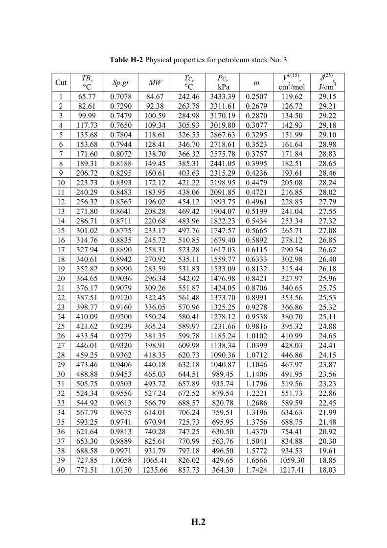
H.2
Table H-2 Physical properties for petroleum stock No. 3
Cut TB, °C Sp.gr MW Tc,
°C Pc, kPa ω VL(15),
cm3/mol δ(25), J/cm3
1 65.77 0.7078 84.67 242.46 3433.39 0.2507 119.62 29.15 2 82.61 0.7290 92.38 263.78 3311.61 0.2679 126.72 29.21 3 99.99 0.7479 100.59 284.98 3170.19 0.2870 134.50 29.22 4 117.73 0.7650 109.34 305.93 3019.80 0.3077 142.93 29.18 5 135.68 0.7804 118.61 326.55 2867.63 0.3295 151.99 29.10 6 153.68 0.7944 128.41 346.70 2718.61 0.3523 161.64 28.98 7 171.60 0.8072 138.70 366.32 2575.78 0.3757 171.84 28.83 8 189.31 0.8188 149.45 385.31 2441.05 0.3995 182.51 28.65 9 206.72 0.8295 160.61 403.63 2315.29 0.4236 193.61 28.46 10 223.73 0.8393 172.12 421.22 2198.95 0.4479 205.08 28.24 11 240.29 0.8483 183.95 438.06 2091.85 0.4721 216.85 28.02 12 256.32 0.8565 196.02 454.12 1993.75 0.4961 228.85 27.79 13 271.80 0.8641 208.28 469.42 1904.07 0.5199 241.04 27.55 14 286.71 0.8711 220.68 483.96 1822.23 0.5434 253.34 27.32 15 301.02 0.8775 233.17 497.76 1747.57 0.5665 265.71 27.08 16 314.76 0.8835 245.72 510.85 1679.40 0.5892 278.12 26.85 17 327.94 0.8890 258.31 523.28 1617.03 0.6115 290.54 26.62 18 340.61 0.8942 270.92 535.11 1559.77 0.6333 302.98 26.40 19 352.82 0.8990 283.59 531.83 1533.09 0.8132 315.44 26.18 20 364.65 0.9036 296.34 542.02 1476.98 0.8421 327.97 25.96 21 376.17 0.9079 309.26 551.87 1424.05 0.8706 340.65 25.75 22 387.51 0.9120 322.45 561.48 1373.70 0.8991 353.56 25.53 23 398.77 0.9160 336.05 570.96 1325.25 0.9278 366.86 25.32 24 410.09 0.9200 350.24 580.41 1278.12 0.9538 380.70 25.11 25 421.62 0.9239 365.24 589.97 1231.66 0.9816 395.32 24.88 26 433.54 0.9279 381.35 599.78 1185.24 1.0102 410.99 24.65 27 446.01 0.9320 398.91 609.98 1138.34 1.0399 428.03 24.41 28 459.25 0.9362 418.35 620.73 1090.36 1.0712 446.86 24.15 29 473.46 0.9406 440.18 632.18 1040.87 1.1046 467.97 23.87 30 488.88 0.9453 465.03 644.51 989.45 1.1406 491.95 23.56 31 505.75 0.9503 493.72 657.89 935.74 1.1796 519.56 23.23 32 524.34 0.9556 527.24 672.52 879.54 1.2221 551.73 22.86 33 544.92 0.9613 566.79 688.57 820.78 1.2686 589.59 22.45 34 567.79 0.9675 614.01 706.24 759.51 1.3196 634.63 21.99 35 593.25 0.9741 670.94 725.73 695.95 1.3756 688.75 21.48 36 621.64 0.9813 740.28 747.25 630.50 1.4370 754.41 20.92 37 653.30 0.9889 825.61 770.99 563.76 1.5041 834.88 20.30 38 688.58 0.9971 931.79 797.18 496.50 1.5772 934.53 19.61 39 727.85 1.0058 1065.41 826.02 429.65 1.6566 1059.30 18.85 40 771.51 1.0150 1235.66 857.73 364.30 1.7424 1217.41 18.03
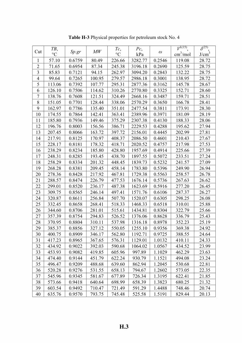
H.3
Table H-3 Physical properties for petroleum stock No. 4
Cut TB, °C Sp.gr MW Tc,
°C Pc, kPa ω VL(15),
cm3/mol δ(25), J/cm3
1 57.10 0.6759 80.49 226.66 3282.77 0.2546 119.08 28.72 2 71.65 0.6954 87.34 245.38 3196.18 0.2690 125.59 28.75 3 85.83 0.7121 94.15 262.97 3094.20 0.2843 132.22 28.75 4 99.64 0.7265 100.95 279.57 2986.18 0.3001 138.95 28.72 5 113.06 0.7392 107.77 295.31 2877.36 0.3162 145.78 28.67 6 126.10 0.7506 114.62 310.26 2770.80 0.3325 152.71 28.60 7 138.76 0.7608 121.51 324.49 2668.16 0.3487 159.71 28.51 8 151.05 0.7701 128.44 338.06 2570.29 0.3650 166.78 28.41 9 162.97 0.7786 135.40 351.01 2477.54 0.3811 173.91 28.30 10 174.55 0.7864 142.41 363.41 2389.96 0.3971 181.09 28.19 11 185.80 0.7936 149.46 375.29 2307.38 0.4130 188.33 28.06 12 196.76 0.8003 156.56 386.71 2229.53 0.4288 195.62 27.94 13 207.45 0.8066 163.72 397.72 2156.01 0.4445 202.99 27.81 14 217.91 0.8125 170.97 408.37 2086.50 0.4601 210.43 27.67 15 228.17 0.8181 178.32 418.71 2020.52 0.4757 217.98 27.53 16 238.29 0.8234 185.80 428.80 1957.69 0.4914 225.66 27.39 17 248.31 0.8285 193.45 438.70 1897.55 0.5072 233.51 27.24 18 258.29 0.8334 201.32 448.45 1839.73 0.5232 241.57 27.09 19 268.28 0.8381 209.45 458.14 1783.80 0.5396 249.90 26.94 20 278.36 0.8428 217.92 467.81 1729.38 0.5563 258.57 26.78 21 288.57 0.8474 226.79 477.53 1676.14 0.5736 267.63 26.62 22 299.01 0.8520 236.17 487.38 1623.69 0.5916 277.20 26.45 23 309.75 0.8565 246.14 497.41 1571.76 0.6106 287.37 26.27 24 320.87 0.8611 256.84 507.70 1520.07 0.6305 298.25 26.08 25 332.45 0.8658 268.41 518.33 1468.33 0.6518 310.01 25.88 26 344.60 0.8706 281.01 515.61 1434.81 0.8304 322.79 25.66 27 357.39 0.8754 294.83 526.52 1376.06 0.8628 336.79 25.43 28 370.95 0.8804 310.11 537.98 1316.18 0.8978 352.23 25.19 29 385.37 0.8856 327.12 550.05 1255.10 0.9356 369.38 24.92 30 400.75 0.8909 346.17 562.80 1192.71 0.9725 388.55 24.64 31 417.23 0.8965 367.65 576.31 1129.01 1.0132 410.11 24.33 32 434.92 0.9022 392.03 590.68 1064.02 1.0567 434.52 23.99 33 453.93 0.9082 419.85 605.96 997.89 1.1029 462.29 23.63 34 474.40 0.9144 451.79 622.24 930.79 1.1521 494.08 23.24 35 496.47 0.9209 488.68 639.60 862.94 1.2045 530.68 22.81 36 520.28 0.9276 531.55 658.13 794.67 1.2602 573.05 22.35 37 545.96 0.9345 581.67 677.89 726.34 1.3195 622.41 21.85 38 573.66 0.9418 640.64 698.99 658.39 1.3823 680.25 21.32 39 603.54 0.9492 710.47 721.49 591.29 1.4488 748.46 20.74 40 635.76 0.9570 793.75 745.48 525.58 1.5191 829.44 20.13
H.4
Table H-4 Physical properties for petroleum stock No. 5
Cut TB, °C Sp.gr MW Tc,
°C Pc, kPa ω VL(15),
cm3/mol δ(25), J/cm3
1 106.91 0.7265 104.74 286.41 2866.20 0.3136 144.18 28.53 2 123.97 0.7416 113.71 306.01 2729.02 0.3349 153.33 28.44 3 140.01 0.7544 122.52 323.98 2600.72 0.3558 162.40 28.32 4 155.06 0.7655 131.16 340.46 2483.00 0.3761 171.33 28.19 5 169.16 0.7752 139.61 355.60 2376.07 0.3956 180.09 28.05 6 182.33 0.7838 147.83 369.50 2279.56 0.4144 188.62 27.91 7 194.61 0.7913 155.80 382.27 2192.72 0.4323 196.89 27.76 8 206.05 0.7980 163.50 394.01 2114.67 0.4493 204.89 27.62 9 216.70 0.8040 170.92 404.81 2044.50 0.4655 212.60 27.48 10 226.62 0.8093 178.06 414.76 1981.30 0.4809 220.01 27.35 11 235.87 0.8142 184.92 423.94 1924.20 0.4954 227.13 27.22 12 244.53 0.8186 191.53 432.47 1872.36 0.5093 233.99 27.09 13 252.68 0.8226 197.91 440.41 1825.02 0.5225 240.60 26.97 14 260.39 0.8263 204.11 447.89 1781.40 0.5352 247.02 26.85 15 267.76 0.8298 210.18 454.98 1740.80 0.5476 253.30 26.74 16 274.89 0.8331 216.19 461.78 1702.56 0.5596 259.51 26.63 17 281.87 0.8362 222.21 468.41 1666.00 0.5716 265.72 26.52 18 288.82 0.8393 228.33 474.96 1630.52 0.5837 272.04 26.40 19 295.85 0.8424 234.67 481.55 1595.50 0.5961 278.58 26.29 20 303.09 0.8455 241.34 488.29 1560.37 0.6091 285.45 26.17 21 310.65 0.8486 248.49 495.29 1524.61 0.6228 292.81 26.04 22 318.69 0.8519 256.27 502.68 1487.68 0.6376 300.81 25.91 23 327.33 0.8554 264.86 510.56 1449.15 0.6538 309.64 25.76 24 336.72 0.8591 274.48 519.08 1408.58 0.6717 319.50 25.59 25 347.02 0.8631 285.37 514.64 1378.41 0.8488 330.65 25.41 26 358.39 0.8673 297.82 524.27 1327.48 0.8781 343.38 25.21 27 370.98 0.8719 312.15 534.86 1273.03 0.9111 358.01 24.98 28 384.99 0.8769 328.79 546.52 1214.87 0.9464 374.95 24.72 29 400.57 0.8822 348.21 559.37 1152.94 0.9856 394.69 24.44 30 417.92 0.8880 371.03 573.53 1087.32 1.0289 417.82 24.11 31 437.23 0.8942 397.97 589.12 1018.24 1.0766 445.04 23.75 32 458.70 0.9009 429.96 606.26 946.04 1.1290 477.28 23.34 33 482.53 0.9079 468.17 625.05 871.25 1.1865 515.64 22.89 34 508.93 0.9155 514.08 645.62 794.52 1.2492 561.55 22.38 35 538.10 0.9234 569.60 668.06 716.65 1.3174 616.84 21.82 36 570.29 0.9318 637.26 692.52 638.49 1.3911 683.90 21.21 37 605.72 0.9406 720.33 719.08 561.06 1.4704 765.83 20.53 38 644.62 0.9498 823.19 747.88 485.41 1.5554 866.73 19.80 39 687.21 0.9593 951.68 779.01 412.66 1.6459 992.04 19.01 40 733.79 0.9692 1113.94 812.62 343.84 1.7418 1149.32 18.15
H.5
Table H-5 Physical properties for petroleum stock No. 6
Cut TB, °C Sp.gr MW Tc,
°C Pc, kPa ω VL(15),
cm3/mol δ(25), J/cm3
1 62.03 0.6875 82.87 234.17 3303.46 0.2563 120.54 28.83 2 69.05 0.6969 86.15 243.19 3259.98 0.2633 123.62 28.84 3 77.10 0.7069 89.95 253.33 3204.47 0.2717 127.25 28.85 4 85.96 0.7171 94.18 264.27 3138.41 0.2813 131.34 28.85 5 95.42 0.7272 98.78 275.73 3064.12 0.2920 135.84 28.84 6 105.29 0.7370 103.68 287.46 2984.12 0.3035 140.68 28.82 7 115.40 0.7464 108.83 299.26 2900.90 0.3157 145.80 28.78 8 125.60 0.7553 114.16 310.98 2816.70 0.3283 151.14 28.72 9 135.76 0.7636 119.61 322.45 2733.42 0.3411 156.63 28.66 10 145.75 0.7714 125.14 333.59 2652.44 0.3541 162.22 28.59 11 155.51 0.7786 130.69 344.31 2574.85 0.3670 167.84 28.51 12 164.93 0.7853 136.20 354.54 2501.41 0.3797 173.44 28.42 13 173.97 0.7914 141.64 364.25 2432.50 0.3920 178.98 28.33 14 182.60 0.7970 146.97 373.41 2368.29 0.4040 184.41 28.24 15 190.79 0.8021 152.17 382.02 2308.76 0.4156 189.71 28.15 16 198.54 0.8068 157.22 390.11 2253.68 0.4267 194.85 28.06 17 205.90 0.8112 162.11 397.71 2202.70 0.4374 199.84 27.97 18 212.87 0.8152 166.86 404.87 2155.39 0.4476 204.69 27.88 19 219.54 0.8189 171.50 411.67 2111.16 0.4575 209.42 27.80 20 225.98 0.8225 176.08 418.19 2069.37 0.4672 214.08 27.71 21 232.29 0.8258 180.65 424.53 2029.30 0.4768 218.74 27.62 22 238.58 0.8291 185.30 430.82 1990.18 0.4864 223.48 27.53 23 244.99 0.8324 190.14 437.18 1951.16 0.4964 228.41 27.44 24 251.68 0.8358 195.29 443.79 1911.35 0.5069 233.66 27.34 25 258.82 0.8393 200.92 450.79 1869.87 0.5182 239.38 27.24 26 266.61 0.8431 207.20 458.38 1825.79 0.5307 245.77 27.12 27 275.26 0.8471 214.37 466.74 1778.24 0.5448 253.05 26.98 28 285.00 0.8516 222.68 476.08 1726.40 0.5610 261.49 26.83 29 296.08 0.8565 232.46 486.62 1669.56 0.5797 271.41 26.65 30 308.78 0.8620 244.12 498.57 1607.10 0.6016 283.20 26.44 31 323.38 0.8681 258.12 512.16 1538.71 0.6274 297.36 26.19 32 340.21 0.8748 275.09 527.62 1464.24 0.6581 314.47 25.89 33 359.57 0.8822 295.82 530.56 1397.64 0.8593 335.31 25.54 34 381.82 0.8904 321.30 549.35 1299.88 0.9165 360.86 25.14 35 407.34 0.8993 352.88 570.55 1195.37 0.9791 392.41 24.66 36 436.51 0.9089 392.34 594.38 1085.19 1.0504 431.67 24.11 37 469.71 0.9192 442.07 621.03 970.84 1.1303 480.91 23.47 38 507.41 0.9303 505.45 650.74 854.05 1.2192 543.32 22.74 39 550.00 0.9420 587.08 683.70 737.02 1.3173 623.23 21.91 40 598.00 0.9544 693.71 720.16 622.02 1.4247 726.89 20.97
H.6
Table H-6 Physical properties for petroleum stock No. 7
Cut TB, °C Sp.gr MW Tc,
°C Pc, kPa ω VL(15),
cm3/mol δ(25), J/cm3
1 54.08 0.6696 79.02 222.22 3277.44 0.2530 118.02 28.68 2 64.31 0.6840 83.85 235.59 3223.39 0.2627 122.58 28.70 3 74.58 0.6971 88.73 248.61 3157.06 0.2733 127.28 28.71 4 84.86 0.7090 93.68 261.30 3082.85 0.2845 132.13 28.71 5 95.08 0.7199 98.70 273.66 3004.06 0.2962 137.11 28.69 6 105.24 0.7299 103.81 285.69 2922.99 0.3082 142.22 28.65 7 115.31 0.7392 108.99 297.40 2841.35 0.3205 147.45 28.61 8 125.27 0.7478 114.25 308.79 2760.31 0.3329 152.78 28.55 9 135.11 0.7558 119.59 319.86 2680.69 0.3455 158.22 28.48 10 144.82 0.7633 125.00 330.65 2603.00 0.3583 163.76 28.41 11 154.41 0.7704 130.50 341.15 2527.55 0.3711 169.40 28.33 12 163.88 0.7770 136.09 351.41 2454.47 0.3840 175.14 28.24 13 173.27 0.7833 141.78 361.43 2383.74 0.3971 180.99 28.14 14 182.58 0.7893 147.59 371.28 2315.26 0.4102 186.98 28.04 15 191.84 0.7951 153.53 380.96 2248.89 0.4235 193.10 27.94 16 201.09 0.8006 159.64 390.53 2184.39 0.4371 199.40 27.83 17 210.38 0.8060 165.96 400.05 2121.47 0.4509 205.92 27.71 18 219.76 0.8112 172.53 409.56 2059.87 0.4650 212.68 27.59 19 229.27 0.8163 179.39 419.11 1999.28 0.4796 219.75 27.46 20 238.98 0.8214 186.61 428.77 1939.36 0.4948 227.19 27.32 21 248.97 0.8264 194.27 438.60 1879.82 0.5106 235.07 27.17 22 259.30 0.8315 202.46 448.67 1820.36 0.5273 243.49 27.02 23 270.05 0.8366 211.28 459.07 1760.67 0.5451 252.54 26.85 24 281.33 0.8418 220.85 469.85 1700.49 0.5640 262.37 26.67 25 293.22 0.8470 231.33 481.10 1639.63 0.5844 273.10 26.48 26 305.82 0.8525 242.89 492.90 1577.84 0.6066 284.92 26.27 27 319.25 0.8580 255.72 505.33 1515.04 0.6308 298.03 26.04 28 333.62 0.8638 270.09 518.48 1451.08 0.6574 312.67 25.79 29 349.04 0.8698 286.28 518.52 1400.98 0.8452 329.14 25.52 30 365.65 0.8760 304.64 532.60 1326.54 0.8879 347.77 25.22 31 383.59 0.8824 325.61 547.63 1250.17 0.9335 368.99 24.90 32 403.00 0.8892 349.71 563.68 1172.02 0.9820 393.31 24.54 33 424.02 0.8961 377.60 580.86 1092.30 1.0341 421.36 24.14 34 446.81 0.9034 410.05 599.25 1011.39 1.0899 453.90 23.71 35 471.54 0.9110 448.08 618.93 929.69 1.1496 491.88 23.24 36 498.36 0.9188 492.94 640.01 847.69 1.2134 536.50 22.72 37 527.46 0.9269 546.22 662.57 765.97 1.2815 589.28 22.16 38 559.00 0.9353 609.95 686.72 685.21 1.3539 652.13 21.55 39 593.20 0.9440 686.83 712.56 606.05 1.4308 727.56 20.89 40 630.23 0.9530 780.29 740.18 529.28 1.5122 818.79 20.18
H.7
Table H-7 Physical properties for petroleum stock No. 8
Cut TB, °C Sp.gr MW Tc,
°C Pc, kPa ω VL(15),
cm3/mol δ(25), J/cm3
1 54.10 0.6746 79.15 223.39 3329.41 0.2498 117.34 28.77 2 63.89 0.6885 83.72 236.23 3277.05 0.2591 121.60 28.80 3 74.43 0.7021 88.68 249.63 3208.29 0.2698 126.31 28.82 4 85.59 0.7151 94.01 263.45 3126.43 0.2819 131.47 28.82 5 97.25 0.7274 99.71 277.53 3034.99 0.2951 137.06 28.80 6 109.30 0.7392 105.75 291.76 2937.11 0.3094 143.07 28.76 7 121.65 0.7503 112.13 306.04 2835.54 0.3245 149.46 28.71 8 134.20 0.7607 118.85 320.28 2732.66 0.3403 156.23 28.63 9 146.89 0.7706 125.87 334.40 2630.20 0.3568 163.35 28.54 10 159.63 0.7798 133.20 348.35 2529.64 0.3738 170.80 28.43 11 172.39 0.7886 140.81 362.08 2431.89 0.3912 178.57 28.30 12 185.09 0.7968 148.70 375.55 2337.73 0.4090 186.62 28.17 13 197.72 0.8046 156.84 388.75 2247.49 0.4270 194.94 28.02 14 210.23 0.8119 165.24 401.64 2161.45 0.4453 203.53 27.87 15 222.60 0.8188 173.88 414.23 2079.66 0.4638 212.36 27.71 16 234.84 0.8253 182.75 426.52 2002.04 0.4824 221.43 27.54 17 246.93 0.8316 191.87 438.53 1928.44 0.5012 230.74 27.36 18 258.89 0.8375 201.25 450.26 1858.62 0.5202 240.30 27.19 19 270.73 0.8431 210.89 461.76 1792.28 0.5394 250.12 27.00 20 282.49 0.8486 220.83 473.05 1729.09 0.5589 260.25 26.82 21 294.20 0.8538 231.12 484.19 1668.75 0.5787 270.70 26.63 22 305.91 0.8589 241.80 495.21 1610.84 0.5989 281.54 26.43 23 317.68 0.8638 252.96 506.18 1555.06 0.6197 292.84 26.23 24 329.58 0.8686 264.67 517.17 1500.99 0.6412 304.70 26.03 25 341.68 0.8734 277.06 528.23 1448.30 0.6635 317.21 25.82 26 354.07 0.8782 290.26 525.16 1412.41 0.8483 330.52 25.59 27 366.86 0.8830 304.44 536.02 1354.80 0.8809 344.80 25.36 28 380.14 0.8878 319.81 547.20 1297.20 0.9153 360.24 25.12 29 394.02 0.8927 336.61 558.78 1239.34 0.9493 377.08 24.86 30 408.65 0.8977 355.15 570.87 1180.90 0.9855 395.62 24.59 31 424.15 0.9029 375.78 583.56 1121.67 1.0236 416.21 24.29 32 440.66 0.9082 398.93 596.95 1061.51 1.0638 439.26 23.98 33 458.36 0.9137 425.16 611.16 1000.25 1.1066 465.30 23.64 34 477.38 0.9195 455.10 626.30 937.90 1.1521 494.95 23.27 35 497.92 0.9255 489.57 642.48 874.46 1.2006 528.97 22.88 36 520.17 0.9318 529.60 659.82 810.03 1.2525 568.36 22.44 37 544.30 0.9384 576.42 678.44 744.86 1.3080 614.26 21.97 38 570.52 0.9453 631.64 698.47 679.23 1.3674 668.20 21.46 39 599.05 0.9525 697.33 720.03 613.54 1.4309 732.11 20.91 40 630.11 0.9600 776.13 743.25 548.27 1.4987 808.43 20.31
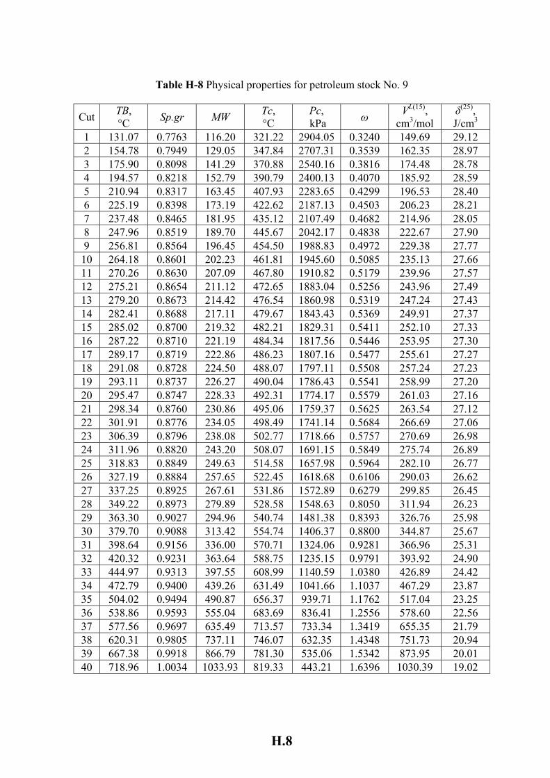
H.8
Table H-8 Physical properties for petroleum stock No. 9
Cut TB, °C Sp.gr MW Tc,
°C Pc, kPa ω VL(15),
cm3/mol δ(25), J/cm3
1 131.07 0.7763 116.20 321.22 2904.05 0.3240 149.69 29.12 2 154.78 0.7949 129.05 347.84 2707.31 0.3539 162.35 28.97 3 175.90 0.8098 141.29 370.88 2540.16 0.3816 174.48 28.78 4 194.57 0.8218 152.79 390.79 2400.13 0.4070 185.92 28.59 5 210.94 0.8317 163.45 407.93 2283.65 0.4299 196.53 28.40 6 225.19 0.8398 173.19 422.62 2187.13 0.4503 206.23 28.21 7 237.48 0.8465 181.95 435.12 2107.49 0.4682 214.96 28.05 8 247.96 0.8519 189.70 445.67 2042.17 0.4838 222.67 27.90 9 256.81 0.8564 196.45 454.50 1988.83 0.4972 229.38 27.77 10 264.18 0.8601 202.23 461.81 1945.60 0.5085 235.13 27.66 11 270.26 0.8630 207.09 467.80 1910.82 0.5179 239.96 27.57 12 275.21 0.8654 211.12 472.65 1883.04 0.5256 243.96 27.49 13 279.20 0.8673 214.42 476.54 1860.98 0.5319 247.24 27.43 14 282.41 0.8688 217.11 479.67 1843.43 0.5369 249.91 27.37 15 285.02 0.8700 219.32 482.21 1829.31 0.5411 252.10 27.33 16 287.22 0.8710 221.19 484.34 1817.56 0.5446 253.95 27.30 17 289.17 0.8719 222.86 486.23 1807.16 0.5477 255.61 27.27 18 291.08 0.8728 224.50 488.07 1797.11 0.5508 257.24 27.23 19 293.11 0.8737 226.27 490.04 1786.43 0.5541 258.99 27.20 20 295.47 0.8747 228.33 492.31 1774.17 0.5579 261.03 27.16 21 298.34 0.8760 230.86 495.06 1759.37 0.5625 263.54 27.12 22 301.91 0.8776 234.05 498.49 1741.14 0.5684 266.69 27.06 23 306.39 0.8796 238.08 502.77 1718.66 0.5757 270.69 26.98 24 311.96 0.8820 243.20 508.07 1691.15 0.5849 275.74 26.89 25 318.83 0.8849 249.63 514.58 1657.98 0.5964 282.10 26.77 26 327.19 0.8884 257.65 522.45 1618.68 0.6106 290.03 26.62 27 337.25 0.8925 267.61 531.86 1572.89 0.6279 299.85 26.45 28 349.22 0.8973 279.89 528.58 1548.63 0.8050 311.94 26.23 29 363.30 0.9027 294.96 540.74 1481.38 0.8393 326.76 25.98 30 379.70 0.9088 313.42 554.74 1406.37 0.8800 344.87 25.67 31 398.64 0.9156 336.00 570.71 1324.06 0.9281 366.96 25.31 32 420.32 0.9231 363.64 588.75 1235.15 0.9791 393.92 24.90 33 444.97 0.9313 397.55 608.99 1140.59 1.0380 426.89 24.42 34 472.79 0.9400 439.26 631.49 1041.66 1.1037 467.29 23.87 35 504.02 0.9494 490.87 656.37 939.71 1.1762 517.04 23.25 36 538.86 0.9593 555.04 683.69 836.41 1.2556 578.60 22.56 37 577.56 0.9697 635.49 713.57 733.34 1.3419 655.35 21.79 38 620.31 0.9805 737.11 746.07 632.35 1.4348 751.73 20.94 39 667.38 0.9918 866.79 781.30 535.06 1.5342 873.95 20.01 40 718.96 1.0034 1033.93 819.33 443.21 1.6396 1030.39 19.02
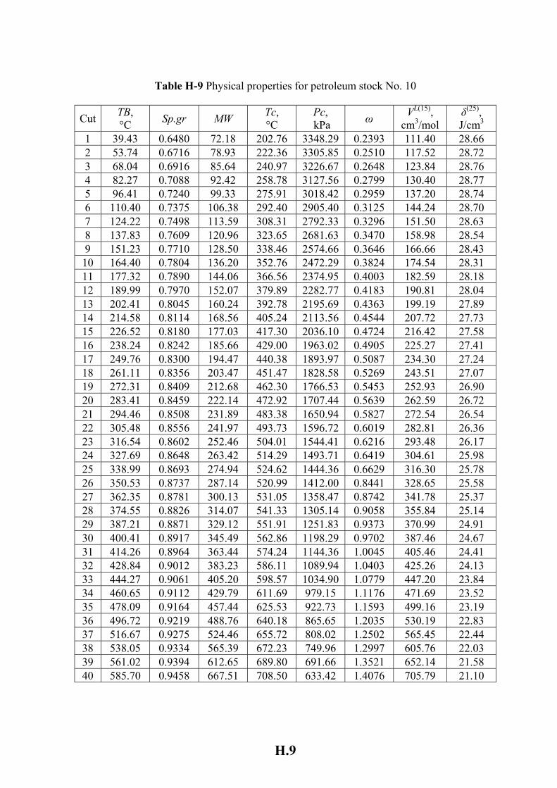
H.9
Table H-9 Physical properties for petroleum stock No. 10
Cut TB, °C Sp.gr MW Tc,
°C Pc, kPa ω VL(15),
cm3/mol δ(25), J/cm3
1 39.43 0.6480 72.18 202.76 3348.29 0.2393 111.40 28.66 2 53.74 0.6716 78.93 222.36 3305.85 0.2510 117.52 28.72 3 68.04 0.6916 85.64 240.97 3226.67 0.2648 123.84 28.76 4 82.27 0.7088 92.42 258.78 3127.56 0.2799 130.40 28.77 5 96.41 0.7240 99.33 275.91 3018.42 0.2959 137.20 28.74 6 110.40 0.7375 106.38 292.40 2905.40 0.3125 144.24 28.70 7 124.22 0.7498 113.59 308.31 2792.33 0.3296 151.50 28.63 8 137.83 0.7609 120.96 323.65 2681.63 0.3470 158.98 28.54 9 151.23 0.7710 128.50 338.46 2574.66 0.3646 166.66 28.43 10 164.40 0.7804 136.20 352.76 2472.29 0.3824 174.54 28.31 11 177.32 0.7890 144.06 366.56 2374.95 0.4003 182.59 28.18 12 189.99 0.7970 152.07 379.89 2282.77 0.4183 190.81 28.04 13 202.41 0.8045 160.24 392.78 2195.69 0.4363 199.19 27.89 14 214.58 0.8114 168.56 405.24 2113.56 0.4544 207.72 27.73 15 226.52 0.8180 177.03 417.30 2036.10 0.4724 216.42 27.58 16 238.24 0.8242 185.66 429.00 1963.02 0.4905 225.27 27.41 17 249.76 0.8300 194.47 440.38 1893.97 0.5087 234.30 27.24 18 261.11 0.8356 203.47 451.47 1828.58 0.5269 243.51 27.07 19 272.31 0.8409 212.68 462.30 1766.53 0.5453 252.93 26.90 20 283.41 0.8459 222.14 472.92 1707.44 0.5639 262.59 26.72 21 294.46 0.8508 231.89 483.38 1650.94 0.5827 272.54 26.54 22 305.48 0.8556 241.97 493.73 1596.72 0.6019 282.81 26.36 23 316.54 0.8602 252.46 504.01 1544.41 0.6216 293.48 26.17 24 327.69 0.8648 263.42 514.29 1493.71 0.6419 304.61 25.98 25 338.99 0.8693 274.94 524.62 1444.36 0.6629 316.30 25.78 26 350.53 0.8737 287.14 520.99 1412.00 0.8441 328.65 25.58 27 362.35 0.8781 300.13 531.05 1358.47 0.8742 341.78 25.37 28 374.55 0.8826 314.07 541.33 1305.14 0.9058 355.84 25.14 29 387.21 0.8871 329.12 551.91 1251.83 0.9373 370.99 24.91 30 400.41 0.8917 345.49 562.86 1198.29 0.9702 387.46 24.67 31 414.26 0.8964 363.44 574.24 1144.36 1.0045 405.46 24.41 32 428.84 0.9012 383.23 586.11 1089.94 1.0403 425.26 24.13 33 444.27 0.9061 405.20 598.57 1034.90 1.0779 447.20 23.84 34 460.65 0.9112 429.79 611.69 979.15 1.1176 471.69 23.52 35 478.09 0.9164 457.44 625.53 922.73 1.1593 499.16 23.19 36 496.72 0.9219 488.76 640.18 865.65 1.2035 530.19 22.83 37 516.67 0.9275 524.46 655.72 808.02 1.2502 565.45 22.44 38 538.05 0.9334 565.39 672.23 749.96 1.2997 605.76 22.03 39 561.02 0.9394 612.65 689.80 691.66 1.3521 652.14 21.58 40 585.70 0.9458 667.51 708.50 633.42 1.4076 705.79 21.10
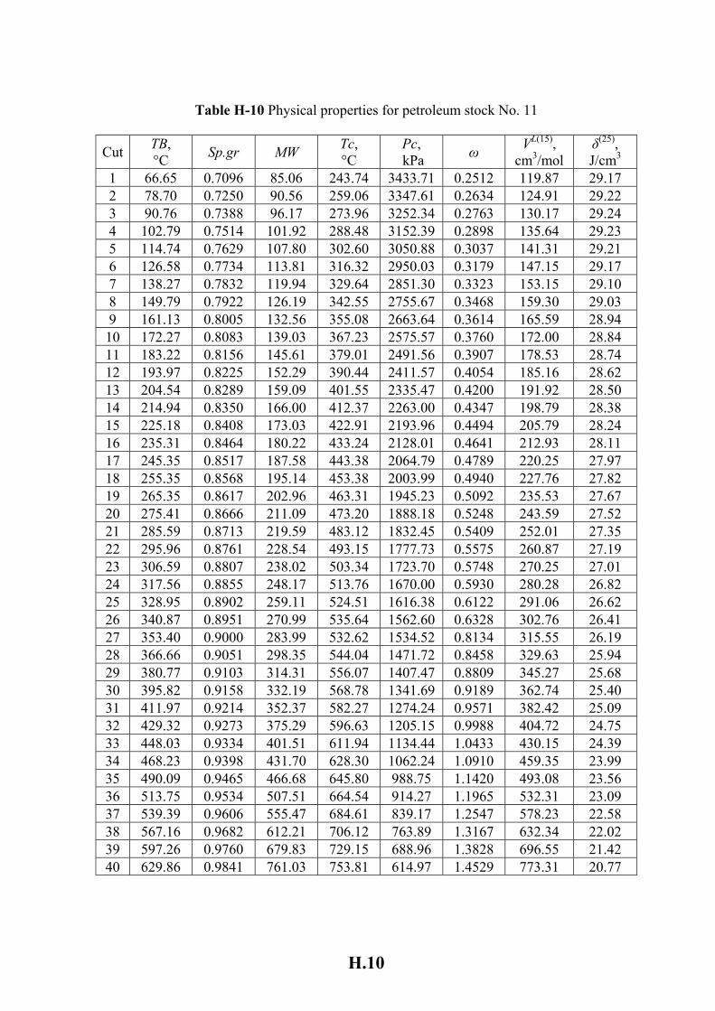
H.10
Table H-10 Physical properties for petroleum stock No. 11
Cut TB, °C Sp.gr MW Tc,
°C Pc, kPa ω VL(15),
cm3/mol δ(25), J/cm3
1 66.65 0.7096 85.06 243.74 3433.71 0.2512 119.87 29.17 2 78.70 0.7250 90.56 259.06 3347.61 0.2634 124.91 29.22 3 90.76 0.7388 96.17 273.96 3252.34 0.2763 130.17 29.24 4 102.79 0.7514 101.92 288.48 3152.39 0.2898 135.64 29.23 5 114.74 0.7629 107.80 302.60 3050.88 0.3037 141.31 29.21 6 126.58 0.7734 113.81 316.32 2950.03 0.3179 147.15 29.17 7 138.27 0.7832 119.94 329.64 2851.30 0.3323 153.15 29.10 8 149.79 0.7922 126.19 342.55 2755.67 0.3468 159.30 29.03 9 161.13 0.8005 132.56 355.08 2663.64 0.3614 165.59 28.94 10 172.27 0.8083 139.03 367.23 2575.57 0.3760 172.00 28.84 11 183.22 0.8156 145.61 379.01 2491.56 0.3907 178.53 28.74 12 193.97 0.8225 152.29 390.44 2411.57 0.4054 185.16 28.62 13 204.54 0.8289 159.09 401.55 2335.47 0.4200 191.92 28.50 14 214.94 0.8350 166.00 412.37 2263.00 0.4347 198.79 28.38 15 225.18 0.8408 173.03 422.91 2193.96 0.4494 205.79 28.24 16 235.31 0.8464 180.22 433.24 2128.01 0.4641 212.93 28.11 17 245.35 0.8517 187.58 443.38 2064.79 0.4789 220.25 27.97 18 255.35 0.8568 195.14 453.38 2003.99 0.4940 227.76 27.82 19 265.35 0.8617 202.96 463.31 1945.23 0.5092 235.53 27.67 20 275.41 0.8666 211.09 473.20 1888.18 0.5248 243.59 27.52 21 285.59 0.8713 219.59 483.12 1832.45 0.5409 252.01 27.35 22 295.96 0.8761 228.54 493.15 1777.73 0.5575 260.87 27.19 23 306.59 0.8807 238.02 503.34 1723.70 0.5748 270.25 27.01 24 317.56 0.8855 248.17 513.76 1670.00 0.5930 280.28 26.82 25 328.95 0.8902 259.11 524.51 1616.38 0.6122 291.06 26.62 26 340.87 0.8951 270.99 535.64 1562.60 0.6328 302.76 26.41 27 353.40 0.9000 283.99 532.62 1534.52 0.8134 315.55 26.19 28 366.66 0.9051 298.35 544.04 1471.72 0.8458 329.63 25.94 29 380.77 0.9103 314.31 556.07 1407.47 0.8809 345.27 25.68 30 395.82 0.9158 332.19 568.78 1341.69 0.9189 362.74 25.40 31 411.97 0.9214 352.37 582.27 1274.24 0.9571 382.42 25.09 32 429.32 0.9273 375.29 596.63 1205.15 0.9988 404.72 24.75 33 448.03 0.9334 401.51 611.94 1134.44 1.0433 430.15 24.39 34 468.23 0.9398 431.70 628.30 1062.24 1.0910 459.35 23.99 35 490.09 0.9465 466.68 645.80 988.75 1.1420 493.08 23.56 36 513.75 0.9534 507.51 664.54 914.27 1.1965 532.31 23.09 37 539.39 0.9606 555.47 684.61 839.17 1.2547 578.23 22.58 38 567.16 0.9682 612.21 706.12 763.89 1.3167 632.34 22.02 39 597.26 0.9760 679.83 729.15 688.96 1.3828 696.55 21.42 40 629.86 0.9841 761.03 753.81 614.97 1.4529 773.31 20.77

H.11
Table H-11 Physical properties for petroleum stock No. 12
Cut TB, °C Sp.gr MW Tc,
°C Pc, kPa ω VL(15),
cm3/mol δ(25), J/cm3
1 70.32 0.7035 86.77 245.95 3300.25 0.2615 123.34 28.95 2 82.20 0.7179 92.34 260.84 3214.53 0.2740 128.62 28.97 3 94.32 0.7312 98.15 275.62 3119.44 0.2874 134.23 28.96 4 106.58 0.7435 104.19 290.24 3018.93 0.3016 140.13 28.94 5 118.95 0.7549 110.46 304.66 2915.96 0.3164 146.33 28.89 6 131.36 0.7655 116.97 318.85 2812.71 0.3318 152.81 28.83 7 143.76 0.7754 123.71 332.77 2710.85 0.3476 159.55 28.74 8 156.10 0.7846 130.66 346.40 2611.55 0.3637 166.53 28.65 9 168.36 0.7932 137.82 359.72 2515.55 0.3801 173.75 28.54 10 180.50 0.8013 145.17 372.73 2423.39 0.3966 181.17 28.42 11 192.49 0.8089 152.72 385.40 2335.35 0.4134 188.80 28.28 12 204.32 0.8160 160.44 397.73 2251.56 0.4302 196.62 28.15 13 215.97 0.8227 168.33 409.73 2172.04 0.4471 204.60 28.00 14 227.45 0.8291 176.39 421.41 2096.64 0.4641 212.76 27.85 15 238.74 0.8351 184.62 432.77 2025.21 0.4811 221.08 27.69 16 249.85 0.8408 193.02 443.84 1957.51 0.4982 229.56 27.53 17 260.80 0.8462 201.58 454.62 1893.34 0.5153 238.21 27.37 18 271.60 0.8514 210.33 465.17 1832.39 0.5325 247.04 27.20 19 282.28 0.8564 219.29 475.49 1774.37 0.5498 256.07 27.03 20 292.87 0.8612 228.49 485.64 1718.95 0.5673 265.32 26.86 21 303.40 0.8658 237.95 495.64 1665.88 0.5850 274.83 26.69 22 313.92 0.8703 247.73 505.54 1614.81 0.6031 284.65 26.51 23 324.48 0.8747 257.88 515.40 1565.44 0.6215 294.84 26.33 24 335.13 0.8790 268.49 525.26 1517.48 0.6405 305.46 26.14 25 345.93 0.8832 279.63 521.13 1494.71 0.8159 316.59 25.95 26 356.95 0.8875 291.41 530.61 1442.76 0.8432 328.35 25.75 27 368.27 0.8917 303.94 540.25 1391.15 0.8717 340.85 25.55 28 379.96 0.8960 317.39 550.14 1339.56 0.9015 354.23 25.33 29 392.11 0.9003 331.93 560.33 1287.78 0.9330 368.67 25.10 30 404.81 0.9048 347.75 570.90 1235.60 0.9626 384.35 24.87 31 418.16 0.9093 365.10 581.92 1182.77 0.9953 401.52 24.61 32 432.27 0.9140 384.27 593.46 1129.19 1.0295 420.45 24.34 33 447.24 0.9188 405.62 605.61 1074.68 1.0656 441.48 24.05 34 463.19 0.9238 429.53 618.44 1019.21 1.1038 464.98 23.74 35 480.25 0.9289 456.52 632.04 962.71 1.1442 491.44 23.41 36 498.54 0.9343 487.18 646.51 905.20 1.1871 521.43 23.05 37 518.20 0.9399 522.24 661.91 846.79 1.2327 555.61 22.67 38 539.36 0.9458 562.59 678.34 787.59 1.2812 594.83 22.25 39 562.18 0.9519 609.35 695.89 727.82 1.3328 640.12 21.80 40 586.82 0.9583 663.88 714.66 667.73 1.3876 692.77 21.32
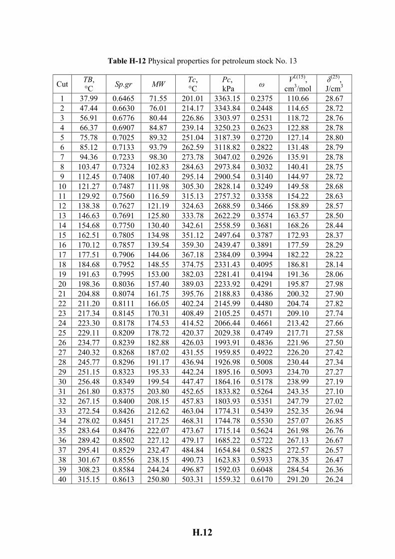
H.12
Table H-12 Physical properties for petroleum stock No. 13
Cut TB, °C Sp.gr MW Tc,
°C Pc, kPa ω VL(15),
cm3/mol δ(25), J/cm3
1 37.99 0.6465 71.55 201.01 3363.15 0.2375 110.66 28.67 2 47.44 0.6630 76.01 214.17 3343.84 0.2448 114.65 28.72 3 56.91 0.6776 80.44 226.86 3303.97 0.2531 118.72 28.76 4 66.37 0.6907 84.87 239.14 3250.23 0.2623 122.88 28.78 5 75.78 0.7025 89.32 251.04 3187.39 0.2720 127.14 28.80 6 85.12 0.7133 93.79 262.59 3118.82 0.2822 131.48 28.79 7 94.36 0.7233 98.30 273.78 3047.02 0.2926 135.91 28.78 8 103.47 0.7324 102.83 284.63 2973.84 0.3032 140.41 28.75 9 112.45 0.7408 107.40 295.14 2900.54 0.3140 144.97 28.72 10 121.27 0.7487 111.98 305.30 2828.14 0.3249 149.58 28.68 11 129.92 0.7560 116.59 315.13 2757.32 0.3358 154.22 28.63 12 138.38 0.7627 121.19 324.63 2688.59 0.3466 158.89 28.57 13 146.63 0.7691 125.80 333.78 2622.29 0.3574 163.57 28.50 14 154.68 0.7750 130.40 342.61 2558.59 0.3681 168.26 28.44 15 162.51 0.7805 134.98 351.12 2497.64 0.3787 172.93 28.37 16 170.12 0.7857 139.54 359.30 2439.47 0.3891 177.59 28.29 17 177.51 0.7906 144.06 367.18 2384.09 0.3994 182.22 28.22 18 184.68 0.7952 148.55 374.75 2331.43 0.4095 186.81 28.14 19 191.63 0.7995 153.00 382.03 2281.41 0.4194 191.36 28.06 20 198.36 0.8036 157.40 389.03 2233.92 0.4291 195.87 27.98 21 204.88 0.8074 161.75 395.76 2188.83 0.4386 200.32 27.90 22 211.20 0.8111 166.05 402.24 2145.99 0.4480 204.74 27.82 23 217.34 0.8145 170.31 408.49 2105.25 0.4571 209.10 27.74 24 223.30 0.8178 174.53 414.52 2066.44 0.4661 213.42 27.66 25 229.11 0.8209 178.72 420.37 2029.38 0.4749 217.71 27.58 26 234.77 0.8239 182.88 426.03 1993.91 0.4836 221.96 27.50 27 240.32 0.8268 187.02 431.55 1959.85 0.4922 226.20 27.42 28 245.77 0.8296 191.17 436.94 1926.98 0.5008 230.44 27.34 29 251.15 0.8323 195.33 442.24 1895.16 0.5093 234.70 27.27 30 256.48 0.8349 199.54 447.47 1864.16 0.5178 238.99 27.19 31 261.80 0.8375 203.80 452.65 1833.82 0.5264 243.35 27.10 32 267.15 0.8400 208.15 457.83 1803.93 0.5351 247.79 27.02 33 272.54 0.8426 212.62 463.04 1774.31 0.5439 252.35 26.94 34 278.02 0.8451 217.25 468.31 1744.78 0.5530 257.07 26.85 35 283.64 0.8476 222.07 473.67 1715.14 0.5624 261.98 26.76 36 289.42 0.8502 227.12 479.17 1685.22 0.5722 267.13 26.67 37 295.41 0.8529 232.47 484.84 1654.84 0.5825 272.57 26.57 38 301.67 0.8556 238.15 490.73 1623.83 0.5933 278.35 26.47 39 308.23 0.8584 244.24 496.87 1592.03 0.6048 284.54 26.36 40 315.15 0.8613 250.80 503.31 1559.32 0.6170 291.20 26.24
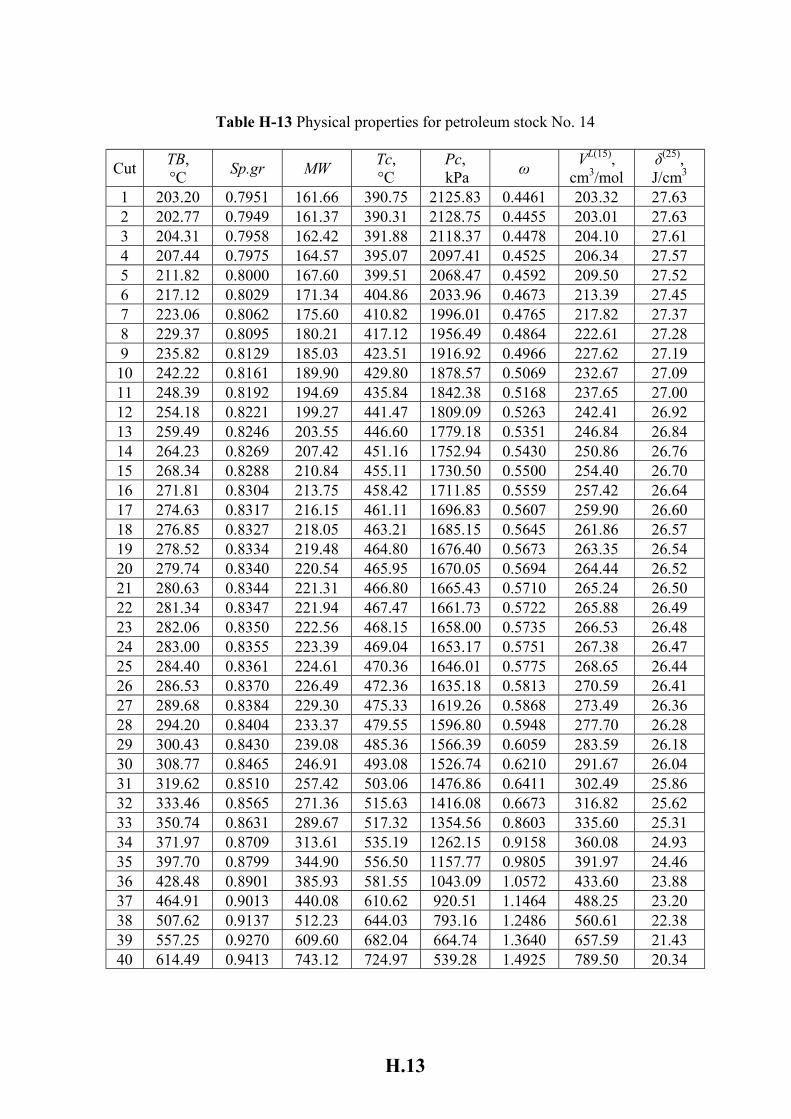
H.13
Table H-13 Physical properties for petroleum stock No. 14
Cut TB, °C Sp.gr MW Tc,
°C Pc, kPa ω VL(15),
cm3/mol δ(25), J/cm3
1 203.20 0.7951 161.66 390.75 2125.83 0.4461 203.32 27.63 2 202.77 0.7949 161.37 390.31 2128.75 0.4455 203.01 27.63 3 204.31 0.7958 162.42 391.88 2118.37 0.4478 204.10 27.61 4 207.44 0.7975 164.57 395.07 2097.41 0.4525 206.34 27.57 5 211.82 0.8000 167.60 399.51 2068.47 0.4592 209.50 27.52 6 217.12 0.8029 171.34 404.86 2033.96 0.4673 213.39 27.45 7 223.06 0.8062 175.60 410.82 1996.01 0.4765 217.82 27.37 8 229.37 0.8095 180.21 417.12 1956.49 0.4864 222.61 27.28 9 235.82 0.8129 185.03 423.51 1916.92 0.4966 227.62 27.19 10 242.22 0.8161 189.90 429.80 1878.57 0.5069 232.67 27.09 11 248.39 0.8192 194.69 435.84 1842.38 0.5168 237.65 27.00 12 254.18 0.8221 199.27 441.47 1809.09 0.5263 242.41 26.92 13 259.49 0.8246 203.55 446.60 1779.18 0.5351 246.84 26.84 14 264.23 0.8269 207.42 451.16 1752.94 0.5430 250.86 26.76 15 268.34 0.8288 210.84 455.11 1730.50 0.5500 254.40 26.70 16 271.81 0.8304 213.75 458.42 1711.85 0.5559 257.42 26.64 17 274.63 0.8317 216.15 461.11 1696.83 0.5607 259.90 26.60 18 276.85 0.8327 218.05 463.21 1685.15 0.5645 261.86 26.57 19 278.52 0.8334 219.48 464.80 1676.40 0.5673 263.35 26.54 20 279.74 0.8340 220.54 465.95 1670.05 0.5694 264.44 26.52 21 280.63 0.8344 221.31 466.80 1665.43 0.5710 265.24 26.50 22 281.34 0.8347 221.94 467.47 1661.73 0.5722 265.88 26.49 23 282.06 0.8350 222.56 468.15 1658.00 0.5735 266.53 26.48 24 283.00 0.8355 223.39 469.04 1653.17 0.5751 267.38 26.47 25 284.40 0.8361 224.61 470.36 1646.01 0.5775 268.65 26.44 26 286.53 0.8370 226.49 472.36 1635.18 0.5813 270.59 26.41 27 289.68 0.8384 229.30 475.33 1619.26 0.5868 273.49 26.36 28 294.20 0.8404 233.37 479.55 1596.80 0.5948 277.70 26.28 29 300.43 0.8430 239.08 485.36 1566.39 0.6059 283.59 26.18 30 308.77 0.8465 246.91 493.08 1526.74 0.6210 291.67 26.04 31 319.62 0.8510 257.42 503.06 1476.86 0.6411 302.49 25.86 32 333.46 0.8565 271.36 515.63 1416.08 0.6673 316.82 25.62 33 350.74 0.8631 289.67 517.32 1354.56 0.8603 335.60 25.31 34 371.97 0.8709 313.61 535.19 1262.15 0.9158 360.08 24.93 35 397.70 0.8799 344.90 556.50 1157.77 0.9805 391.97 24.46 36 428.48 0.8901 385.93 581.55 1043.09 1.0572 433.60 23.88 37 464.91 0.9013 440.08 610.62 920.51 1.1464 488.25 23.20 38 507.62 0.9137 512.23 644.03 793.16 1.2486 560.61 22.38 39 557.25 0.9270 609.60 682.04 664.74 1.3640 657.59 21.43 40 614.49 0.9413 743.12 724.97 539.28 1.4925 789.50 20.34
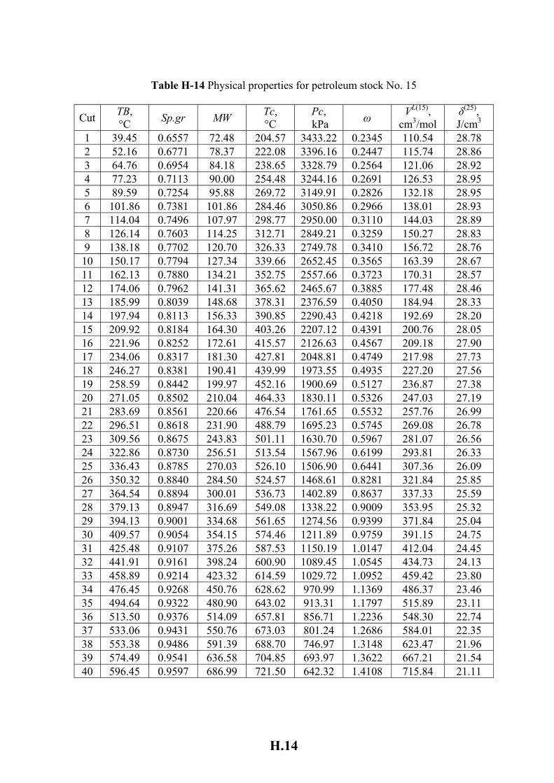
H.14
Table H-14 Physical properties for petroleum stock No. 15
Cut TB, °C Sp.gr MW Tc,
°C Pc, kPa ω VL(15),
cm3/mol δ(25), J/cm3
1 39.45 0.6557 72.48 204.57 3433.22 0.2345 110.54 28.78 2 52.16 0.6771 78.37 222.08 3396.16 0.2447 115.74 28.86 3 64.76 0.6954 84.18 238.65 3328.79 0.2564 121.06 28.92 4 77.23 0.7113 90.00 254.48 3244.16 0.2691 126.53 28.95 5 89.59 0.7254 95.88 269.72 3149.91 0.2826 132.18 28.95 6 101.86 0.7381 101.86 284.46 3050.86 0.2966 138.01 28.93 7 114.04 0.7496 107.97 298.77 2950.00 0.3110 144.03 28.89 8 126.14 0.7603 114.25 312.71 2849.21 0.3259 150.27 28.83 9 138.18 0.7702 120.70 326.33 2749.78 0.3410 156.72 28.76 10 150.17 0.7794 127.34 339.66 2652.45 0.3565 163.39 28.67 11 162.13 0.7880 134.21 352.75 2557.66 0.3723 170.31 28.57 12 174.06 0.7962 141.31 365.62 2465.67 0.3885 177.48 28.46 13 185.99 0.8039 148.68 378.31 2376.59 0.4050 184.94 28.33 14 197.94 0.8113 156.33 390.85 2290.43 0.4218 192.69 28.20 15 209.92 0.8184 164.30 403.26 2207.12 0.4391 200.76 28.05 16 221.96 0.8252 172.61 415.57 2126.63 0.4567 209.18 27.90 17 234.06 0.8317 181.30 427.81 2048.81 0.4749 217.98 27.73 18 246.27 0.8381 190.41 439.99 1973.55 0.4935 227.20 27.56 19 258.59 0.8442 199.97 452.16 1900.69 0.5127 236.87 27.38 20 271.05 0.8502 210.04 464.33 1830.11 0.5326 247.03 27.19 21 283.69 0.8561 220.66 476.54 1761.65 0.5532 257.76 26.99 22 296.51 0.8618 231.90 488.79 1695.23 0.5745 269.08 26.78 23 309.56 0.8675 243.83 501.11 1630.70 0.5967 281.07 26.56 24 322.86 0.8730 256.51 513.54 1567.96 0.6199 293.81 26.33 25 336.43 0.8785 270.03 526.10 1506.90 0.6441 307.36 26.09 26 350.32 0.8840 284.50 524.57 1468.61 0.8281 321.84 25.85 27 364.54 0.8894 300.01 536.73 1402.89 0.8637 337.33 25.59 28 379.13 0.8947 316.69 549.08 1338.22 0.9009 353.95 25.32 29 394.13 0.9001 334.68 561.65 1274.56 0.9399 371.84 25.04 30 409.57 0.9054 354.15 574.46 1211.89 0.9759 391.15 24.75 31 425.48 0.9107 375.26 587.53 1150.19 1.0147 412.04 24.45 32 441.91 0.9161 398.24 600.90 1089.45 1.0545 434.73 24.13 33 458.89 0.9214 423.32 614.59 1029.72 1.0952 459.42 23.80 34 476.45 0.9268 450.76 628.62 970.99 1.1369 486.37 23.46 35 494.64 0.9322 480.90 643.02 913.31 1.1797 515.89 23.11 36 513.50 0.9376 514.09 657.81 856.71 1.2236 548.30 22.74 37 533.06 0.9431 550.76 673.03 801.24 1.2686 584.01 22.35 38 553.38 0.9486 591.39 688.70 746.97 1.3148 623.47 21.96 39 574.49 0.9541 636.58 704.85 693.97 1.3622 667.21 21.54 40 596.45 0.9597 686.99 721.50 642.32 1.4108 715.84 21.11
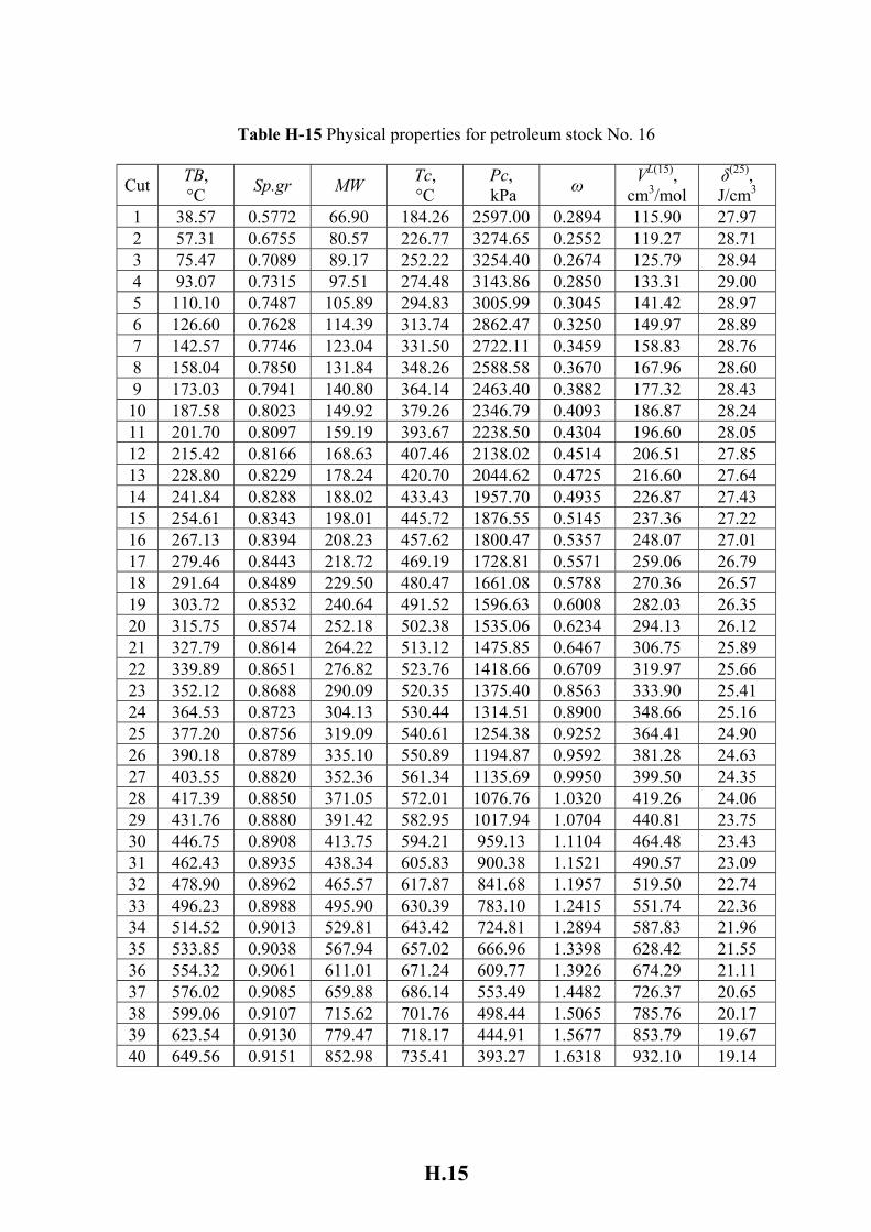
H.15
Table H-15 Physical properties for petroleum stock No. 16
Cut TB, °C Sp.gr MW Tc,
°C Pc, kPa ω VL(15),
cm3/mol δ(25), J/cm3
1 38.57 0.5772 66.90 184.26 2597.00 0.2894 115.90 27.97 2 57.31 0.6755 80.57 226.77 3274.65 0.2552 119.27 28.71 3 75.47 0.7089 89.17 252.22 3254.40 0.2674 125.79 28.94 4 93.07 0.7315 97.51 274.48 3143.86 0.2850 133.31 29.00 5 110.10 0.7487 105.89 294.83 3005.99 0.3045 141.42 28.97 6 126.60 0.7628 114.39 313.74 2862.47 0.3250 149.97 28.89 7 142.57 0.7746 123.04 331.50 2722.11 0.3459 158.83 28.76 8 158.04 0.7850 131.84 348.26 2588.58 0.3670 167.96 28.60 9 173.03 0.7941 140.80 364.14 2463.40 0.3882 177.32 28.43 10 187.58 0.8023 149.92 379.26 2346.79 0.4093 186.87 28.24 11 201.70 0.8097 159.19 393.67 2238.50 0.4304 196.60 28.05 12 215.42 0.8166 168.63 407.46 2138.02 0.4514 206.51 27.85 13 228.80 0.8229 178.24 420.70 2044.62 0.4725 216.60 27.64 14 241.84 0.8288 188.02 433.43 1957.70 0.4935 226.87 27.43 15 254.61 0.8343 198.01 445.72 1876.55 0.5145 237.36 27.22 16 267.13 0.8394 208.23 457.62 1800.47 0.5357 248.07 27.01 17 279.46 0.8443 218.72 469.19 1728.81 0.5571 259.06 26.79 18 291.64 0.8489 229.50 480.47 1661.08 0.5788 270.36 26.57 19 303.72 0.8532 240.64 491.52 1596.63 0.6008 282.03 26.35 20 315.75 0.8574 252.18 502.38 1535.06 0.6234 294.13 26.12 21 327.79 0.8614 264.22 513.12 1475.85 0.6467 306.75 25.89 22 339.89 0.8651 276.82 523.76 1418.66 0.6709 319.97 25.66 23 352.12 0.8688 290.09 520.35 1375.40 0.8563 333.90 25.41 24 364.53 0.8723 304.13 530.44 1314.51 0.8900 348.66 25.16 25 377.20 0.8756 319.09 540.61 1254.38 0.9252 364.41 24.90 26 390.18 0.8789 335.10 550.89 1194.87 0.9592 381.28 24.63 27 403.55 0.8820 352.36 561.34 1135.69 0.9950 399.50 24.35 28 417.39 0.8850 371.05 572.01 1076.76 1.0320 419.26 24.06 29 431.76 0.8880 391.42 582.95 1017.94 1.0704 440.81 23.75 30 446.75 0.8908 413.75 594.21 959.13 1.1104 464.48 23.43 31 462.43 0.8935 438.34 605.83 900.38 1.1521 490.57 23.09 32 478.90 0.8962 465.57 617.87 841.68 1.1957 519.50 22.74 33 496.23 0.8988 495.90 630.39 783.10 1.2415 551.74 22.36 34 514.52 0.9013 529.81 643.42 724.81 1.2894 587.83 21.96 35 533.85 0.9038 567.94 657.02 666.96 1.3398 628.42 21.55 36 554.32 0.9061 611.01 671.24 609.77 1.3926 674.29 21.11 37 576.02 0.9085 659.88 686.14 553.49 1.4482 726.37 20.65 38 599.06 0.9107 715.62 701.76 498.44 1.5065 785.76 20.17 39 623.54 0.9130 779.47 718.17 444.91 1.5677 853.79 19.67 40 649.56 0.9151 852.98 735.41 393.27 1.6318 932.10 19.14
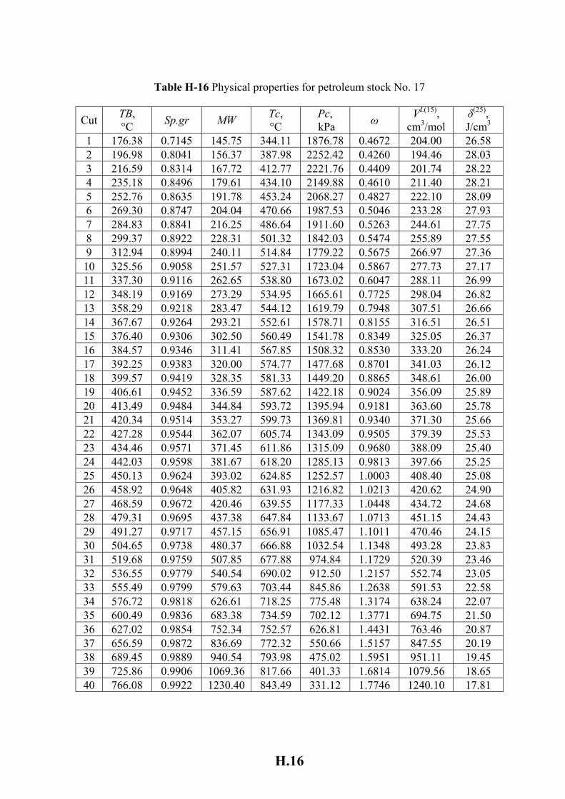
H.16
Table H-16 Physical properties for petroleum stock No. 17
Cut TB, °C Sp.gr MW Tc,
°C Pc, kPa ω VL(15),
cm3/mol δ(25), J/cm3
1 176.38 0.7145 145.75 344.11 1876.78 0.4672 204.00 26.58 2 196.98 0.8041 156.37 387.98 2252.42 0.4260 194.46 28.03 3 216.59 0.8314 167.72 412.77 2221.76 0.4409 201.74 28.22 4 235.18 0.8496 179.61 434.10 2149.88 0.4610 211.40 28.21 5 252.76 0.8635 191.78 453.24 2068.27 0.4827 222.10 28.09 6 269.30 0.8747 204.04 470.66 1987.53 0.5046 233.28 27.93 7 284.83 0.8841 216.25 486.64 1911.60 0.5263 244.61 27.75 8 299.37 0.8922 228.31 501.32 1842.03 0.5474 255.89 27.55 9 312.94 0.8994 240.11 514.84 1779.22 0.5675 266.97 27.36 10 325.56 0.9058 251.57 527.31 1723.04 0.5867 277.73 27.17 11 337.30 0.9116 262.65 538.80 1673.02 0.6047 288.11 26.99 12 348.19 0.9169 273.29 534.95 1665.61 0.7725 298.04 26.82 13 358.29 0.9218 283.47 544.12 1619.79 0.7948 307.51 26.66 14 367.67 0.9264 293.21 552.61 1578.71 0.8155 316.51 26.51 15 376.40 0.9306 302.50 560.49 1541.78 0.8349 325.05 26.37 16 384.57 0.9346 311.41 567.85 1508.32 0.8530 333.20 26.24 17 392.25 0.9383 320.00 574.77 1477.68 0.8701 341.03 26.12 18 399.57 0.9419 328.35 581.33 1449.20 0.8865 348.61 26.00 19 406.61 0.9452 336.59 587.62 1422.18 0.9024 356.09 25.89 20 413.49 0.9484 344.84 593.72 1395.94 0.9181 363.60 25.78 21 420.34 0.9514 353.27 599.73 1369.81 0.9340 371.30 25.66 22 427.28 0.9544 362.07 605.74 1343.09 0.9505 379.39 25.53 23 434.46 0.9571 371.45 611.86 1315.09 0.9680 388.09 25.40 24 442.03 0.9598 381.67 618.20 1285.13 0.9813 397.66 25.25 25 450.13 0.9624 393.02 624.85 1252.57 1.0003 408.40 25.08 26 458.92 0.9648 405.82 631.93 1216.82 1.0213 420.62 24.90 27 468.59 0.9672 420.46 639.55 1177.33 1.0448 434.72 24.68 28 479.31 0.9695 437.38 647.84 1133.67 1.0713 451.15 24.43 29 491.27 0.9717 457.15 656.91 1085.47 1.1011 470.46 24.15 30 504.65 0.9738 480.37 666.88 1032.54 1.1348 493.28 23.83 31 519.68 0.9759 507.85 677.88 974.84 1.1729 520.39 23.46 32 536.55 0.9779 540.54 690.02 912.50 1.2157 552.74 23.05 33 555.49 0.9799 579.63 703.44 845.86 1.2638 591.53 22.58 34 576.72 0.9818 626.61 718.25 775.48 1.3174 638.24 22.07 35 600.49 0.9836 683.38 734.59 702.12 1.3771 694.75 21.50 36 627.02 0.9854 752.34 752.57 626.81 1.4431 763.46 20.87 37 656.59 0.9872 836.69 772.32 550.66 1.5157 847.55 20.19 38 689.45 0.9889 940.54 793.98 475.02 1.5951 951.11 19.45 39 725.86 0.9906 1069.36 817.66 401.33 1.6814 1079.56 18.65 40 766.08 0.9922 1230.40 843.49 331.12 1.7746 1240.10 17.81
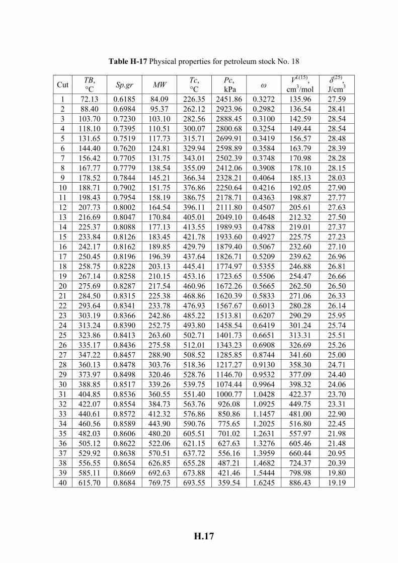
H.17
Table H-17 Physical properties for petroleum stock No. 18
Cut TB, °C Sp.gr MW Tc,
°C Pc, kPa ω VL(15),
cm3/mol δ(25), J/cm3
1 72.13 0.6185 84.09 226.35 2451.86 0.3272 135.96 27.59 2 88.40 0.6984 95.37 262.12 2923.96 0.2982 136.54 28.41 3 103.70 0.7230 103.10 282.56 2888.45 0.3100 142.59 28.54 4 118.10 0.7395 110.51 300.07 2800.68 0.3254 149.44 28.54 5 131.65 0.7519 117.73 315.71 2699.91 0.3419 156.57 28.48 6 144.40 0.7620 124.81 329.94 2598.89 0.3584 163.79 28.39 7 156.42 0.7705 131.75 343.01 2502.39 0.3748 170.98 28.28 8 167.77 0.7779 138.54 355.09 2412.06 0.3908 178.10 28.15 9 178.52 0.7844 145.21 366.34 2328.21 0.4064 185.13 28.03 10 188.71 0.7902 151.75 376.86 2250.64 0.4216 192.05 27.90 11 198.43 0.7954 158.19 386.75 2178.71 0.4363 198.87 27.77 12 207.73 0.8002 164.54 396.11 2111.80 0.4507 205.61 27.63 13 216.69 0.8047 170.84 405.01 2049.10 0.4648 212.32 27.50 14 225.37 0.8088 177.13 413.55 1989.93 0.4788 219.01 27.37 15 233.84 0.8126 183.45 421.78 1933.60 0.4927 225.75 27.23 16 242.17 0.8162 189.85 429.79 1879.40 0.5067 232.60 27.10 17 250.45 0.8196 196.39 437.64 1826.71 0.5209 239.62 26.96 18 258.75 0.8228 203.13 445.41 1774.97 0.5355 246.88 26.81 19 267.14 0.8258 210.15 453.16 1723.65 0.5506 254.47 26.66 20 275.69 0.8287 217.54 460.96 1672.26 0.5665 262.50 26.50 21 284.50 0.8315 225.38 468.86 1620.39 0.5833 271.06 26.33 22 293.64 0.8341 233.78 476.93 1567.67 0.6013 280.28 26.14 23 303.19 0.8366 242.86 485.22 1513.81 0.6207 290.29 25.95 24 313.24 0.8390 252.75 493.80 1458.54 0.6419 301.24 25.74 25 323.86 0.8413 263.60 502.71 1401.73 0.6651 313.31 25.51 26 335.17 0.8436 275.58 512.01 1343.23 0.6908 326.69 25.26 27 347.22 0.8457 288.90 508.52 1285.85 0.8744 341.60 25.00 28 360.13 0.8478 303.76 518.36 1217.27 0.9130 358.30 24.71 29 373.97 0.8498 320.46 528.76 1146.70 0.9532 377.09 24.40 30 388.85 0.8517 339.26 539.75 1074.44 0.9964 398.32 24.06 31 404.85 0.8536 360.55 551.40 1000.77 1.0428 422.37 23.70 32 422.07 0.8554 384.73 563.76 926.08 1.0925 449.75 23.31 33 440.61 0.8572 412.32 576.86 850.86 1.1457 481.00 22.90 34 460.56 0.8589 443.90 590.76 775.65 1.2025 516.80 22.45 35 482.03 0.8606 480.20 605.51 701.02 1.2631 557.97 21.98 36 505.12 0.8622 522.06 621.15 627.63 1.3276 605.46 21.48 37 529.92 0.8638 570.51 637.72 556.16 1.3959 660.44 20.95 38 556.55 0.8654 626.85 655.28 487.21 1.4682 724.37 20.39 39 585.11 0.8669 692.63 673.88 421.46 1.5444 798.98 19.80 40 615.70 0.8684 769.75 693.55 359.54 1.6245 886.43 19.19
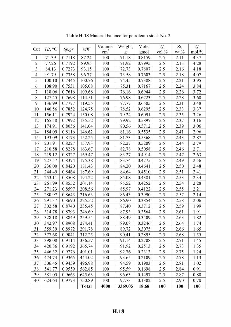
H.18
Table H-18 Material balance for petroleum stock No. 2
Cut TB, °C Sp.gr MW Volume, cm3
Weight, g
Mole, gmol
Zf, vol.%
Zf, wt.%
Zf, mol.%
1 71.39 0.7118 87.24 100 71.18 0.8159 2.5 2.11 4.37 2 77.26 0.7192 89.95 100 71.92 0.7995 2.5 2.13 4.28 3 84.13 0.7273 93.15 100 72.73 0.7807 2.5 2.16 4.18 4 91.79 0.7358 96.77 100 73.58 0.7603 2.5 2.18 4.07 5 100.10 0.7445 100.76 100 74.45 0.7388 2.5 2.21 3.95 6 108.90 0.7531 105.08 100 75.31 0.7167 2.5 2.24 3.84 7 118.06 0.7616 109.68 100 76.16 0.6944 2.5 2.26 3.72 8 127.45 0.7698 114.51 100 76.98 0.6723 2.5 2.28 3.60 9 136.99 0.7777 119.55 100 77.77 0.6505 2.5 2.31 3.48 10 146.56 0.7852 124.75 100 78.52 0.6295 2.5 2.33 3.37 11 156.11 0.7924 130.08 100 79.24 0.6091 2.5 2.35 3.26 12 165.58 0.7992 135.52 100 79.92 0.5897 2.5 2.37 3.16 13 174.91 0.8056 141.04 100 80.56 0.5712 2.5 2.39 3.06 14 184.09 0.8116 146.62 100 81.16 0.5535 2.5 2.41 2.96 15 193.09 0.8173 152.25 100 81.73 0.5368 2.5 2.43 2.87 16 201.91 0.8227 157.93 100 82.27 0.5209 2.5 2.44 2.79 17 210.58 0.8278 163.67 100 82.78 0.5058 2.5 2.46 2.71 18 219.12 0.8327 169.47 100 83.27 0.4914 2.5 2.47 2.63 19 227.57 0.8374 175.38 100 83.74 0.4775 2.5 2.49 2.56 20 236.00 0.8420 181.43 100 84.20 0.4641 2.5 2.50 2.48 21 244.49 0.8464 187.69 100 84.64 0.4510 2.5 2.51 2.41 22 253.11 0.8508 194.22 100 85.08 0.4381 2.5 2.53 2.34 23 261.99 0.8552 201.14 100 85.52 0.4252 2.5 2.54 2.28 24 271.23 0.8597 208.56 100 85.97 0.4122 2.5 2.55 2.21 25 280.97 0.8643 216.63 100 86.43 0.3990 2.5 2.57 2.14 26 291.37 0.8690 225.52 100 86.90 0.3854 2.5 2.58 2.06 27 302.58 0.8740 235.45 100 87.40 0.3712 2.5 2.59 1.99 28 314.78 0.8793 246.69 100 87.93 0.3564 2.5 2.61 1.91 29 328.18 0.8849 259.54 100 88.49 0.3409 2.5 2.63 1.82 30 342.97 0.8908 274.41 100 89.08 0.3246 2.5 2.64 1.74 31 359.39 0.8972 291.78 100 89.72 0.3075 2.5 2.66 1.65 32 377.68 0.9041 312.25 100 90.41 0.2895 2.5 2.68 1.55 33 398.08 0.9114 336.57 100 91.14 0.2708 2.5 2.71 1.45 34 420.86 0.9192 365.74 100 91.92 0.2513 2.5 2.73 1.35 35 446.32 0.9276 401.01 100 92.76 0.2313 2.5 2.75 1.24 36 474.74 0.9365 444.02 100 93.65 0.2109 2.5 2.78 1.13 37 506.45 0.9459 496.98 100 94.59 0.1903 2.5 2.81 1.02 38 541.77 0.9559 562.85 100 95.59 0.1698 2.5 2.84 0.91 39 581.05 0.9663 645.63 100 96.63 0.1497 2.5 2.87 0.80 40 624.64 0.9773 750.89 100 97.73 0.1302 2.5 2.90 0.70 Total 4000 3369.05 18.68 100 100 100
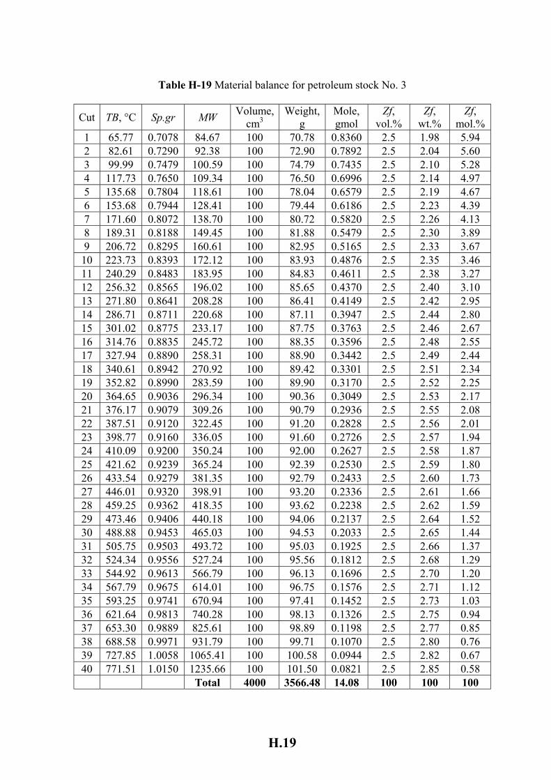
H.19
Table H-19 Material balance for petroleum stock No. 3
Cut TB, °C Sp.gr MW Volume, cm3
Weight, g
Mole, gmol
Zf, vol.%
Zf, wt.%
Zf, mol.%
1 65.77 0.7078 84.67 100 70.78 0.8360 2.5 1.98 5.94 2 82.61 0.7290 92.38 100 72.90 0.7892 2.5 2.04 5.60 3 99.99 0.7479 100.59 100 74.79 0.7435 2.5 2.10 5.28 4 117.73 0.7650 109.34 100 76.50 0.6996 2.5 2.14 4.97 5 135.68 0.7804 118.61 100 78.04 0.6579 2.5 2.19 4.67 6 153.68 0.7944 128.41 100 79.44 0.6186 2.5 2.23 4.39 7 171.60 0.8072 138.70 100 80.72 0.5820 2.5 2.26 4.13 8 189.31 0.8188 149.45 100 81.88 0.5479 2.5 2.30 3.89 9 206.72 0.8295 160.61 100 82.95 0.5165 2.5 2.33 3.67 10 223.73 0.8393 172.12 100 83.93 0.4876 2.5 2.35 3.46 11 240.29 0.8483 183.95 100 84.83 0.4611 2.5 2.38 3.27 12 256.32 0.8565 196.02 100 85.65 0.4370 2.5 2.40 3.10 13 271.80 0.8641 208.28 100 86.41 0.4149 2.5 2.42 2.95 14 286.71 0.8711 220.68 100 87.11 0.3947 2.5 2.44 2.80 15 301.02 0.8775 233.17 100 87.75 0.3763 2.5 2.46 2.67 16 314.76 0.8835 245.72 100 88.35 0.3596 2.5 2.48 2.55 17 327.94 0.8890 258.31 100 88.90 0.3442 2.5 2.49 2.44 18 340.61 0.8942 270.92 100 89.42 0.3301 2.5 2.51 2.34 19 352.82 0.8990 283.59 100 89.90 0.3170 2.5 2.52 2.25 20 364.65 0.9036 296.34 100 90.36 0.3049 2.5 2.53 2.17 21 376.17 0.9079 309.26 100 90.79 0.2936 2.5 2.55 2.08 22 387.51 0.9120 322.45 100 91.20 0.2828 2.5 2.56 2.01 23 398.77 0.9160 336.05 100 91.60 0.2726 2.5 2.57 1.94 24 410.09 0.9200 350.24 100 92.00 0.2627 2.5 2.58 1.87 25 421.62 0.9239 365.24 100 92.39 0.2530 2.5 2.59 1.80 26 433.54 0.9279 381.35 100 92.79 0.2433 2.5 2.60 1.73 27 446.01 0.9320 398.91 100 93.20 0.2336 2.5 2.61 1.66 28 459.25 0.9362 418.35 100 93.62 0.2238 2.5 2.62 1.59 29 473.46 0.9406 440.18 100 94.06 0.2137 2.5 2.64 1.52 30 488.88 0.9453 465.03 100 94.53 0.2033 2.5 2.65 1.44 31 505.75 0.9503 493.72 100 95.03 0.1925 2.5 2.66 1.37 32 524.34 0.9556 527.24 100 95.56 0.1812 2.5 2.68 1.29 33 544.92 0.9613 566.79 100 96.13 0.1696 2.5 2.70 1.20 34 567.79 0.9675 614.01 100 96.75 0.1576 2.5 2.71 1.12 35 593.25 0.9741 670.94 100 97.41 0.1452 2.5 2.73 1.03 36 621.64 0.9813 740.28 100 98.13 0.1326 2.5 2.75 0.94 37 653.30 0.9889 825.61 100 98.89 0.1198 2.5 2.77 0.85 38 688.58 0.9971 931.79 100 99.71 0.1070 2.5 2.80 0.76 39 727.85 1.0058 1065.41 100 100.58 0.0944 2.5 2.82 0.67 40 771.51 1.0150 1235.66 100 101.50 0.0821 2.5 2.85 0.58 Total 4000 3566.48 14.08 100 100 100
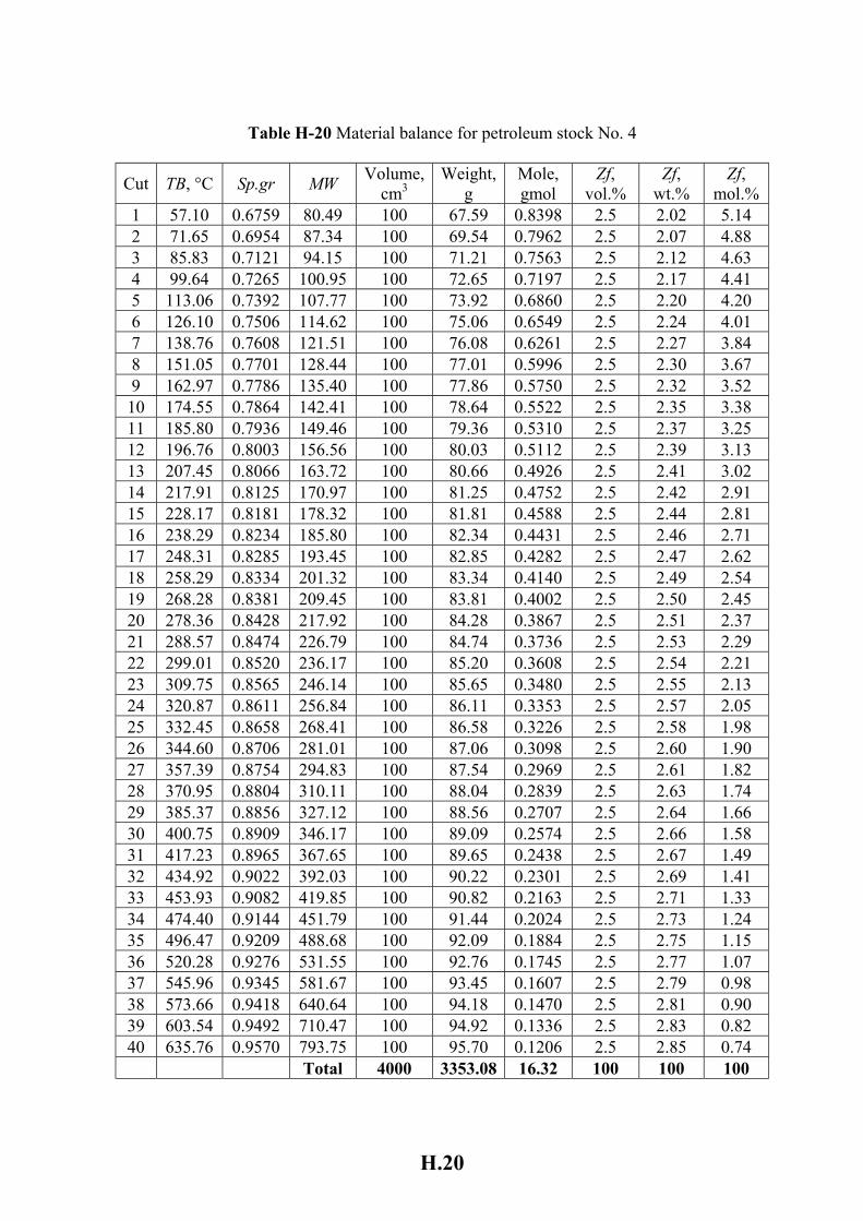
H.20
Table H-20 Material balance for petroleum stock No. 4
Cut TB, °C Sp.gr MW Volume, cm3
Weight, g
Mole, gmol
Zf, vol.%
Zf, wt.%
Zf, mol.%
1 57.10 0.6759 80.49 100 67.59 0.8398 2.5 2.02 5.14 2 71.65 0.6954 87.34 100 69.54 0.7962 2.5 2.07 4.88 3 85.83 0.7121 94.15 100 71.21 0.7563 2.5 2.12 4.63 4 99.64 0.7265 100.95 100 72.65 0.7197 2.5 2.17 4.41 5 113.06 0.7392 107.77 100 73.92 0.6860 2.5 2.20 4.20 6 126.10 0.7506 114.62 100 75.06 0.6549 2.5 2.24 4.01 7 138.76 0.7608 121.51 100 76.08 0.6261 2.5 2.27 3.84 8 151.05 0.7701 128.44 100 77.01 0.5996 2.5 2.30 3.67 9 162.97 0.7786 135.40 100 77.86 0.5750 2.5 2.32 3.52 10 174.55 0.7864 142.41 100 78.64 0.5522 2.5 2.35 3.38 11 185.80 0.7936 149.46 100 79.36 0.5310 2.5 2.37 3.25 12 196.76 0.8003 156.56 100 80.03 0.5112 2.5 2.39 3.13 13 207.45 0.8066 163.72 100 80.66 0.4926 2.5 2.41 3.02 14 217.91 0.8125 170.97 100 81.25 0.4752 2.5 2.42 2.91 15 228.17 0.8181 178.32 100 81.81 0.4588 2.5 2.44 2.81 16 238.29 0.8234 185.80 100 82.34 0.4431 2.5 2.46 2.71 17 248.31 0.8285 193.45 100 82.85 0.4282 2.5 2.47 2.62 18 258.29 0.8334 201.32 100 83.34 0.4140 2.5 2.49 2.54 19 268.28 0.8381 209.45 100 83.81 0.4002 2.5 2.50 2.45 20 278.36 0.8428 217.92 100 84.28 0.3867 2.5 2.51 2.37 21 288.57 0.8474 226.79 100 84.74 0.3736 2.5 2.53 2.29 22 299.01 0.8520 236.17 100 85.20 0.3608 2.5 2.54 2.21 23 309.75 0.8565 246.14 100 85.65 0.3480 2.5 2.55 2.13 24 320.87 0.8611 256.84 100 86.11 0.3353 2.5 2.57 2.05 25 332.45 0.8658 268.41 100 86.58 0.3226 2.5 2.58 1.98 26 344.60 0.8706 281.01 100 87.06 0.3098 2.5 2.60 1.90 27 357.39 0.8754 294.83 100 87.54 0.2969 2.5 2.61 1.82 28 370.95 0.8804 310.11 100 88.04 0.2839 2.5 2.63 1.74 29 385.37 0.8856 327.12 100 88.56 0.2707 2.5 2.64 1.66 30 400.75 0.8909 346.17 100 89.09 0.2574 2.5 2.66 1.58 31 417.23 0.8965 367.65 100 89.65 0.2438 2.5 2.67 1.49 32 434.92 0.9022 392.03 100 90.22 0.2301 2.5 2.69 1.41 33 453.93 0.9082 419.85 100 90.82 0.2163 2.5 2.71 1.33 34 474.40 0.9144 451.79 100 91.44 0.2024 2.5 2.73 1.24 35 496.47 0.9209 488.68 100 92.09 0.1884 2.5 2.75 1.15 36 520.28 0.9276 531.55 100 92.76 0.1745 2.5 2.77 1.07 37 545.96 0.9345 581.67 100 93.45 0.1607 2.5 2.79 0.98 38 573.66 0.9418 640.64 100 94.18 0.1470 2.5 2.81 0.90 39 603.54 0.9492 710.47 100 94.92 0.1336 2.5 2.83 0.82 40 635.76 0.9570 793.75 100 95.70 0.1206 2.5 2.85 0.74 Total 4000 3353.08 16.32 100 100 100
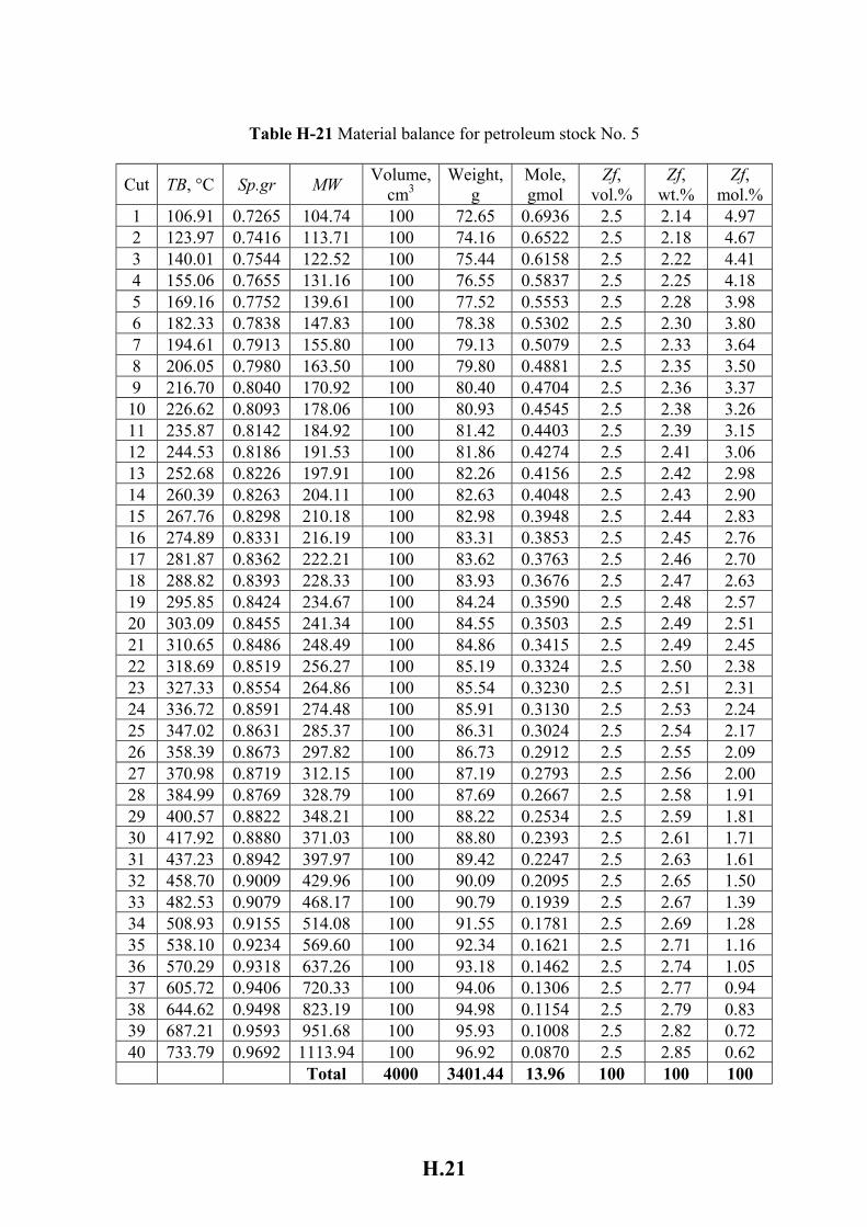
H.21
Table H-21 Material balance for petroleum stock No. 5
Cut TB, °C Sp.gr MW Volume, cm3
Weight, g
Mole, gmol
Zf, vol.%
Zf, wt.%
Zf, mol.%
1 106.91 0.7265 104.74 100 72.65 0.6936 2.5 2.14 4.97 2 123.97 0.7416 113.71 100 74.16 0.6522 2.5 2.18 4.67 3 140.01 0.7544 122.52 100 75.44 0.6158 2.5 2.22 4.41 4 155.06 0.7655 131.16 100 76.55 0.5837 2.5 2.25 4.18 5 169.16 0.7752 139.61 100 77.52 0.5553 2.5 2.28 3.98 6 182.33 0.7838 147.83 100 78.38 0.5302 2.5 2.30 3.80 7 194.61 0.7913 155.80 100 79.13 0.5079 2.5 2.33 3.64 8 206.05 0.7980 163.50 100 79.80 0.4881 2.5 2.35 3.50 9 216.70 0.8040 170.92 100 80.40 0.4704 2.5 2.36 3.37 10 226.62 0.8093 178.06 100 80.93 0.4545 2.5 2.38 3.26 11 235.87 0.8142 184.92 100 81.42 0.4403 2.5 2.39 3.15 12 244.53 0.8186 191.53 100 81.86 0.4274 2.5 2.41 3.06 13 252.68 0.8226 197.91 100 82.26 0.4156 2.5 2.42 2.98 14 260.39 0.8263 204.11 100 82.63 0.4048 2.5 2.43 2.90 15 267.76 0.8298 210.18 100 82.98 0.3948 2.5 2.44 2.83 16 274.89 0.8331 216.19 100 83.31 0.3853 2.5 2.45 2.76 17 281.87 0.8362 222.21 100 83.62 0.3763 2.5 2.46 2.70 18 288.82 0.8393 228.33 100 83.93 0.3676 2.5 2.47 2.63 19 295.85 0.8424 234.67 100 84.24 0.3590 2.5 2.48 2.57 20 303.09 0.8455 241.34 100 84.55 0.3503 2.5 2.49 2.51 21 310.65 0.8486 248.49 100 84.86 0.3415 2.5 2.49 2.45 22 318.69 0.8519 256.27 100 85.19 0.3324 2.5 2.50 2.38 23 327.33 0.8554 264.86 100 85.54 0.3230 2.5 2.51 2.31 24 336.72 0.8591 274.48 100 85.91 0.3130 2.5 2.53 2.24 25 347.02 0.8631 285.37 100 86.31 0.3024 2.5 2.54 2.17 26 358.39 0.8673 297.82 100 86.73 0.2912 2.5 2.55 2.09 27 370.98 0.8719 312.15 100 87.19 0.2793 2.5 2.56 2.00 28 384.99 0.8769 328.79 100 87.69 0.2667 2.5 2.58 1.91 29 400.57 0.8822 348.21 100 88.22 0.2534 2.5 2.59 1.81 30 417.92 0.8880 371.03 100 88.80 0.2393 2.5 2.61 1.71 31 437.23 0.8942 397.97 100 89.42 0.2247 2.5 2.63 1.61 32 458.70 0.9009 429.96 100 90.09 0.2095 2.5 2.65 1.50 33 482.53 0.9079 468.17 100 90.79 0.1939 2.5 2.67 1.39 34 508.93 0.9155 514.08 100 91.55 0.1781 2.5 2.69 1.28 35 538.10 0.9234 569.60 100 92.34 0.1621 2.5 2.71 1.16 36 570.29 0.9318 637.26 100 93.18 0.1462 2.5 2.74 1.05 37 605.72 0.9406 720.33 100 94.06 0.1306 2.5 2.77 0.94 38 644.62 0.9498 823.19 100 94.98 0.1154 2.5 2.79 0.83 39 687.21 0.9593 951.68 100 95.93 0.1008 2.5 2.82 0.72 40 733.79 0.9692 1113.94 100 96.92 0.0870 2.5 2.85 0.62 Total 4000 3401.44 13.96 100 100 100
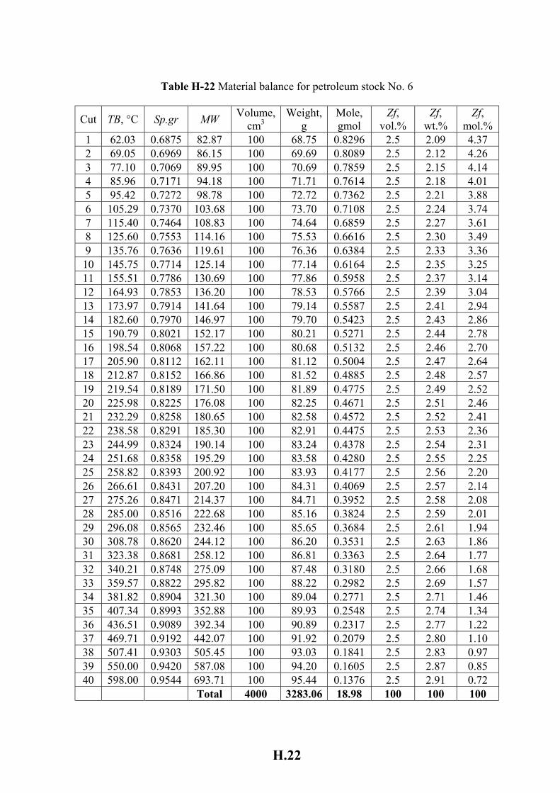
H.22
Table H-22 Material balance for petroleum stock No. 6
Cut TB, °C Sp.gr MW Volume, cm3
Weight, g
Mole, gmol
Zf, vol.%
Zf, wt.%
Zf, mol.%
1 62.03 0.6875 82.87 100 68.75 0.8296 2.5 2.09 4.37 2 69.05 0.6969 86.15 100 69.69 0.8089 2.5 2.12 4.26 3 77.10 0.7069 89.95 100 70.69 0.7859 2.5 2.15 4.14 4 85.96 0.7171 94.18 100 71.71 0.7614 2.5 2.18 4.01 5 95.42 0.7272 98.78 100 72.72 0.7362 2.5 2.21 3.88 6 105.29 0.7370 103.68 100 73.70 0.7108 2.5 2.24 3.74 7 115.40 0.7464 108.83 100 74.64 0.6859 2.5 2.27 3.61 8 125.60 0.7553 114.16 100 75.53 0.6616 2.5 2.30 3.49 9 135.76 0.7636 119.61 100 76.36 0.6384 2.5 2.33 3.36 10 145.75 0.7714 125.14 100 77.14 0.6164 2.5 2.35 3.25 11 155.51 0.7786 130.69 100 77.86 0.5958 2.5 2.37 3.14 12 164.93 0.7853 136.20 100 78.53 0.5766 2.5 2.39 3.04 13 173.97 0.7914 141.64 100 79.14 0.5587 2.5 2.41 2.94 14 182.60 0.7970 146.97 100 79.70 0.5423 2.5 2.43 2.86 15 190.79 0.8021 152.17 100 80.21 0.5271 2.5 2.44 2.78 16 198.54 0.8068 157.22 100 80.68 0.5132 2.5 2.46 2.70 17 205.90 0.8112 162.11 100 81.12 0.5004 2.5 2.47 2.64 18 212.87 0.8152 166.86 100 81.52 0.4885 2.5 2.48 2.57 19 219.54 0.8189 171.50 100 81.89 0.4775 2.5 2.49 2.52 20 225.98 0.8225 176.08 100 82.25 0.4671 2.5 2.51 2.46 21 232.29 0.8258 180.65 100 82.58 0.4572 2.5 2.52 2.41 22 238.58 0.8291 185.30 100 82.91 0.4475 2.5 2.53 2.36 23 244.99 0.8324 190.14 100 83.24 0.4378 2.5 2.54 2.31 24 251.68 0.8358 195.29 100 83.58 0.4280 2.5 2.55 2.25 25 258.82 0.8393 200.92 100 83.93 0.4177 2.5 2.56 2.20 26 266.61 0.8431 207.20 100 84.31 0.4069 2.5 2.57 2.14 27 275.26 0.8471 214.37 100 84.71 0.3952 2.5 2.58 2.08 28 285.00 0.8516 222.68 100 85.16 0.3824 2.5 2.59 2.01 29 296.08 0.8565 232.46 100 85.65 0.3684 2.5 2.61 1.94 30 308.78 0.8620 244.12 100 86.20 0.3531 2.5 2.63 1.86 31 323.38 0.8681 258.12 100 86.81 0.3363 2.5 2.64 1.77 32 340.21 0.8748 275.09 100 87.48 0.3180 2.5 2.66 1.68 33 359.57 0.8822 295.82 100 88.22 0.2982 2.5 2.69 1.57 34 381.82 0.8904 321.30 100 89.04 0.2771 2.5 2.71 1.46 35 407.34 0.8993 352.88 100 89.93 0.2548 2.5 2.74 1.34 36 436.51 0.9089 392.34 100 90.89 0.2317 2.5 2.77 1.22 37 469.71 0.9192 442.07 100 91.92 0.2079 2.5 2.80 1.10 38 507.41 0.9303 505.45 100 93.03 0.1841 2.5 2.83 0.97 39 550.00 0.9420 587.08 100 94.20 0.1605 2.5 2.87 0.85 40 598.00 0.9544 693.71 100 95.44 0.1376 2.5 2.91 0.72 Total 4000 3283.06 18.98 100 100 100
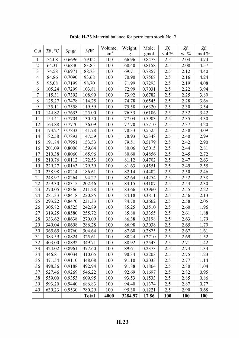
H.23
Table H-23 Material balance for petroleum stock No. 7
Cut TB, °C Sp.gr MW Volume, cm3
Weight, g
Mole, gmol
Zf, vol.%
Zf, wt.%
Zf, mol.%
1 54.08 0.6696 79.02 100 66.96 0.8473 2.5 2.04 4.74 2 64.31 0.6840 83.85 100 68.40 0.8158 2.5 2.08 4.57 3 74.58 0.6971 88.73 100 69.71 0.7857 2.5 2.12 4.40 4 84.86 0.7090 93.68 100 70.90 0.7568 2.5 2.16 4.24 5 95.08 0.7199 98.70 100 71.99 0.7293 2.5 2.19 4.08 6 105.24 0.7299 103.81 100 72.99 0.7031 2.5 2.22 3.94 7 115.31 0.7392 108.99 100 73.92 0.6782 2.5 2.25 3.80 8 125.27 0.7478 114.25 100 74.78 0.6545 2.5 2.28 3.66 9 135.11 0.7558 119.59 100 75.58 0.6320 2.5 2.30 3.54 10 144.82 0.7633 125.00 100 76.33 0.6106 2.5 2.32 3.42 11 154.41 0.7704 130.50 100 77.04 0.5903 2.5 2.35 3.30 12 163.88 0.7770 136.09 100 77.70 0.5710 2.5 2.37 3.20 13 173.27 0.7833 141.78 100 78.33 0.5525 2.5 2.38 3.09 14 182.58 0.7893 147.59 100 78.93 0.5348 2.5 2.40 2.99 15 191.84 0.7951 153.53 100 79.51 0.5179 2.5 2.42 2.90 16 201.09 0.8006 159.64 100 80.06 0.5015 2.5 2.44 2.81 17 210.38 0.8060 165.96 100 80.60 0.4856 2.5 2.45 2.72 18 219.76 0.8112 172.53 100 81.12 0.4702 2.5 2.47 2.63 19 229.27 0.8163 179.39 100 81.63 0.4551 2.5 2.49 2.55 20 238.98 0.8214 186.61 100 82.14 0.4402 2.5 2.50 2.46 21 248.97 0.8264 194.27 100 82.64 0.4254 2.5 2.52 2.38 22 259.30 0.8315 202.46 100 83.15 0.4107 2.5 2.53 2.30 23 270.05 0.8366 211.28 100 83.66 0.3960 2.5 2.55 2.22 24 281.33 0.8418 220.85 100 84.18 0.3811 2.5 2.56 2.13 25 293.22 0.8470 231.33 100 84.70 0.3662 2.5 2.58 2.05 26 305.82 0.8525 242.89 100 85.25 0.3510 2.5 2.60 1.96 27 319.25 0.8580 255.72 100 85.80 0.3355 2.5 2.61 1.88 28 333.62 0.8638 270.09 100 86.38 0.3198 2.5 2.63 1.79 29 349.04 0.8698 286.28 100 86.98 0.3038 2.5 2.65 1.70 30 365.65 0.8760 304.64 100 87.60 0.2875 2.5 2.67 1.61 31 383.59 0.8824 325.61 100 88.24 0.2710 2.5 2.69 1.52 32 403.00 0.8892 349.71 100 88.92 0.2543 2.5 2.71 1.42 33 424.02 0.8961 377.60 100 89.61 0.2373 2.5 2.73 1.33 34 446.81 0.9034 410.05 100 90.34 0.2203 2.5 2.75 1.23 35 471.54 0.9110 448.08 100 91.10 0.2033 2.5 2.77 1.14 36 498.36 0.9188 492.94 100 91.88 0.1864 2.5 2.80 1.04 37 527.46 0.9269 546.22 100 92.69 0.1697 2.5 2.82 0.95 38 559.00 0.9353 609.95 100 93.53 0.1533 2.5 2.85 0.86 39 593.20 0.9440 686.83 100 94.40 0.1374 2.5 2.87 0.77 40 630.23 0.9530 780.29 100 95.30 0.1221 2.5 2.90 0.68 Total 4000 3284.97 17.86 100 100 100
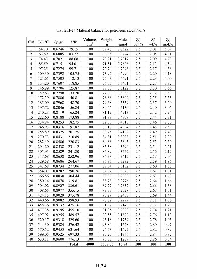
H.24
Table H-24 Material balance for petroleum stock No. 8
Cut TB, °C Sp.gr MW Volume, cm3
Weight, g
Mole, gmol
Zf, vol.%
Zf, wt.%
Zf, mol.%
1 54.10 0.6746 79.15 100 67.46 0.8522 2.5 2.01 5.09 2 63.89 0.6885 83.72 100 68.85 0.8224 2.5 2.05 4.91 3 74.43 0.7021 88.68 100 70.21 0.7917 2.5 2.09 4.73 4 85.59 0.7151 94.01 100 71.51 0.7606 2.5 2.13 4.54 5 97.25 0.7274 99.71 100 72.74 0.7296 2.5 2.17 4.36 6 109.30 0.7392 105.75 100 73.92 0.6990 2.5 2.20 4.18 7 121.65 0.7503 112.13 100 75.03 0.6691 2.5 2.23 4.00 8 134.20 0.7607 118.85 100 76.07 0.6401 2.5 2.27 3.82 9 146.89 0.7706 125.87 100 77.06 0.6122 2.5 2.30 3.66 10 159.63 0.7798 133.20 100 77.98 0.5855 2.5 2.32 3.50 11 172.39 0.7886 140.81 100 78.86 0.5600 2.5 2.35 3.35 12 185.09 0.7968 148.70 100 79.68 0.5359 2.5 2.37 3.20 13 197.72 0.8046 156.84 100 80.46 0.5130 2.5 2.40 3.06 14 210.23 0.8119 165.24 100 81.19 0.4913 2.5 2.42 2.94 15 222.60 0.8188 173.88 100 81.88 0.4709 2.5 2.44 2.81 16 234.84 0.8253 182.75 100 82.53 0.4516 2.5 2.46 2.70 17 246.93 0.8316 191.87 100 83.16 0.4334 2.5 2.48 2.59 18 258.89 0.8375 201.25 100 83.75 0.4162 2.5 2.49 2.49 19 270.73 0.8431 210.89 100 84.31 0.3998 2.5 2.51 2.39 20 282.49 0.8486 220.83 100 84.86 0.3843 2.5 2.53 2.30 21 294.20 0.8538 231.12 100 85.38 0.3694 2.5 2.54 2.21 22 305.91 0.8589 241.80 100 85.89 0.3552 2.5 2.56 2.12 23 317.68 0.8638 252.96 100 86.38 0.3415 2.5 2.57 2.04 24 329.58 0.8686 264.67 100 86.86 0.3282 2.5 2.59 1.96 25 341.68 0.8734 277.06 100 87.34 0.3152 2.5 2.60 1.88 26 354.07 0.8782 290.26 100 87.82 0.3026 2.5 2.62 1.81 27 366.86 0.8830 304.44 100 88.30 0.2900 2.5 2.63 1.73 28 380.14 0.8878 319.81 100 88.78 0.2776 2.5 2.64 1.66 29 394.02 0.8927 336.61 100 89.27 0.2652 2.5 2.66 1.58 30 408.65 0.8977 355.15 100 89.77 0.2528 2.5 2.67 1.51 31 424.15 0.9029 375.78 100 90.29 0.2403 2.5 2.69 1.44 32 440.66 0.9082 398.93 100 90.82 0.2277 2.5 2.71 1.36 33 458.36 0.9137 425.16 100 91.37 0.2149 2.5 2.72 1.28 34 477.38 0.9195 455.10 100 91.95 0.2020 2.5 2.74 1.21 35 497.92 0.9255 489.57 100 92.55 0.1890 2.5 2.76 1.13 36 520.17 0.9318 529.60 100 93.18 0.1759 2.5 2.78 1.05 37 544.30 0.9384 576.42 100 93.84 0.1628 2.5 2.80 0.97 38 570.52 0.9453 631.64 100 94.53 0.1497 2.5 2.82 0.89 39 599.05 0.9525 697.33 100 95.25 0.1366 2.5 2.84 0.82 40 630.11 0.9600 776.13 100 96.00 0.1237 2.5 2.86 0.74 Total 4000 3357.06 16.74 100 100 100
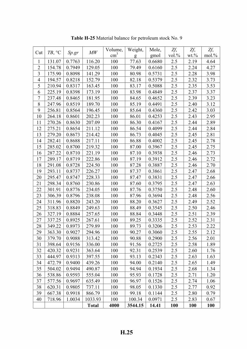
H.25
Table H-25 Material balance for petroleum stock No. 9
Cut TB, °C Sp.gr MW Volume, cm3
Weight, g
Mole, gmol
Zf, vol.%
Zf, wt.%
Zf, mol.%
1 131.07 0.7763 116.20 100 77.63 0.6680 2.5 2.19 4.64 2 154.78 0.7949 129.05 100 79.49 0.6160 2.5 2.24 4.27 3 175.90 0.8098 141.29 100 80.98 0.5731 2.5 2.28 3.98 4 194.57 0.8218 152.79 100 82.18 0.5379 2.5 2.32 3.73 5 210.94 0.8317 163.45 100 83.17 0.5088 2.5 2.35 3.53 6 225.19 0.8398 173.19 100 83.98 0.4849 2.5 2.37 3.37 7 237.48 0.8465 181.95 100 84.65 0.4652 2.5 2.39 3.23 8 247.96 0.8519 189.70 100 85.19 0.4491 2.5 2.40 3.12 9 256.81 0.8564 196.45 100 85.64 0.4360 2.5 2.42 3.03 10 264.18 0.8601 202.23 100 86.01 0.4253 2.5 2.43 2.95 11 270.26 0.8630 207.09 100 86.30 0.4167 2.5 2.44 2.89 12 275.21 0.8654 211.12 100 86.54 0.4099 2.5 2.44 2.84 13 279.20 0.8673 214.42 100 86.73 0.4045 2.5 2.45 2.81 14 282.41 0.8688 217.11 100 86.88 0.4002 2.5 2.45 2.78 15 285.02 0.8700 219.32 100 87.00 0.3967 2.5 2.45 2.75 16 287.22 0.8710 221.19 100 87.10 0.3938 2.5 2.46 2.73 17 289.17 0.8719 222.86 100 87.19 0.3912 2.5 2.46 2.72 18 291.08 0.8728 224.50 100 87.28 0.3887 2.5 2.46 2.70 19 293.11 0.8737 226.27 100 87.37 0.3861 2.5 2.47 2.68 20 295.47 0.8747 228.33 100 87.47 0.3831 2.5 2.47 2.66 21 298.34 0.8760 230.86 100 87.60 0.3795 2.5 2.47 2.63 22 301.91 0.8776 234.05 100 87.76 0.3750 2.5 2.48 2.60 23 306.39 0.8796 238.08 100 87.96 0.3694 2.5 2.48 2.56 24 311.96 0.8820 243.20 100 88.20 0.3627 2.5 2.49 2.52 25 318.83 0.8849 249.63 100 88.49 0.3545 2.5 2.50 2.46 26 327.19 0.8884 257.65 100 88.84 0.3448 2.5 2.51 2.39 27 337.25 0.8925 267.61 100 89.25 0.3335 2.5 2.52 2.31 28 349.22 0.8973 279.89 100 89.73 0.3206 2.5 2.53 2.22 29 363.30 0.9027 294.96 100 90.27 0.3060 2.5 2.55 2.12 30 379.70 0.9088 313.42 100 90.88 0.2900 2.5 2.56 2.01 31 398.64 0.9156 336.00 100 91.56 0.2725 2.5 2.58 1.89 32 420.32 0.9231 363.64 100 92.31 0.2539 2.5 2.60 1.76 33 444.97 0.9313 397.55 100 93.13 0.2343 2.5 2.63 1.63 34 472.79 0.9400 439.26 100 94.00 0.2140 2.5 2.65 1.49 35 504.02 0.9494 490.87 100 94.94 0.1934 2.5 2.68 1.34 36 538.86 0.9593 555.04 100 95.93 0.1728 2.5 2.71 1.20 37 577.56 0.9697 635.49 100 96.97 0.1526 2.5 2.74 1.06 38 620.31 0.9805 737.11 100 98.05 0.1330 2.5 2.77 0.92 39 667.38 0.9918 866.79 100 99.18 0.1144 2.5 2.80 0.79 40 718.96 1.0034 1033.93 100 100.34 0.0971 2.5 2.83 0.67 Total 4000 3544.15 14.41 100 100 100
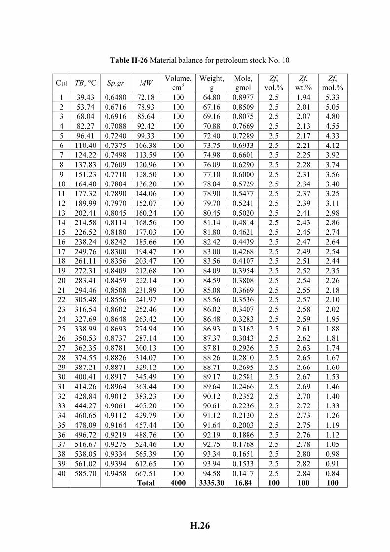
H.26
Table H-26 Material balance for petroleum stock No. 10
Cut TB, °C Sp.gr MW Volume, cm3
Weight, g
Mole, gmol
Zf, vol.%
Zf, wt.%
Zf, mol.%
1 39.43 0.6480 72.18 100 64.80 0.8977 2.5 1.94 5.33 2 53.74 0.6716 78.93 100 67.16 0.8509 2.5 2.01 5.05 3 68.04 0.6916 85.64 100 69.16 0.8075 2.5 2.07 4.80 4 82.27 0.7088 92.42 100 70.88 0.7669 2.5 2.13 4.55 5 96.41 0.7240 99.33 100 72.40 0.7289 2.5 2.17 4.33 6 110.40 0.7375 106.38 100 73.75 0.6933 2.5 2.21 4.12 7 124.22 0.7498 113.59 100 74.98 0.6601 2.5 2.25 3.92 8 137.83 0.7609 120.96 100 76.09 0.6290 2.5 2.28 3.74 9 151.23 0.7710 128.50 100 77.10 0.6000 2.5 2.31 3.56 10 164.40 0.7804 136.20 100 78.04 0.5729 2.5 2.34 3.40 11 177.32 0.7890 144.06 100 78.90 0.5477 2.5 2.37 3.25 12 189.99 0.7970 152.07 100 79.70 0.5241 2.5 2.39 3.11 13 202.41 0.8045 160.24 100 80.45 0.5020 2.5 2.41 2.98 14 214.58 0.8114 168.56 100 81.14 0.4814 2.5 2.43 2.86 15 226.52 0.8180 177.03 100 81.80 0.4621 2.5 2.45 2.74 16 238.24 0.8242 185.66 100 82.42 0.4439 2.5 2.47 2.64 17 249.76 0.8300 194.47 100 83.00 0.4268 2.5 2.49 2.54 18 261.11 0.8356 203.47 100 83.56 0.4107 2.5 2.51 2.44 19 272.31 0.8409 212.68 100 84.09 0.3954 2.5 2.52 2.35 20 283.41 0.8459 222.14 100 84.59 0.3808 2.5 2.54 2.26 21 294.46 0.8508 231.89 100 85.08 0.3669 2.5 2.55 2.18 22 305.48 0.8556 241.97 100 85.56 0.3536 2.5 2.57 2.10 23 316.54 0.8602 252.46 100 86.02 0.3407 2.5 2.58 2.02 24 327.69 0.8648 263.42 100 86.48 0.3283 2.5 2.59 1.95 25 338.99 0.8693 274.94 100 86.93 0.3162 2.5 2.61 1.88 26 350.53 0.8737 287.14 100 87.37 0.3043 2.5 2.62 1.81 27 362.35 0.8781 300.13 100 87.81 0.2926 2.5 2.63 1.74 28 374.55 0.8826 314.07 100 88.26 0.2810 2.5 2.65 1.67 29 387.21 0.8871 329.12 100 88.71 0.2695 2.5 2.66 1.60 30 400.41 0.8917 345.49 100 89.17 0.2581 2.5 2.67 1.53 31 414.26 0.8964 363.44 100 89.64 0.2466 2.5 2.69 1.46 32 428.84 0.9012 383.23 100 90.12 0.2352 2.5 2.70 1.40 33 444.27 0.9061 405.20 100 90.61 0.2236 2.5 2.72 1.33 34 460.65 0.9112 429.79 100 91.12 0.2120 2.5 2.73 1.26 35 478.09 0.9164 457.44 100 91.64 0.2003 2.5 2.75 1.19 36 496.72 0.9219 488.76 100 92.19 0.1886 2.5 2.76 1.12 37 516.67 0.9275 524.46 100 92.75 0.1768 2.5 2.78 1.05 38 538.05 0.9334 565.39 100 93.34 0.1651 2.5 2.80 0.98 39 561.02 0.9394 612.65 100 93.94 0.1533 2.5 2.82 0.91 40 585.70 0.9458 667.51 100 94.58 0.1417 2.5 2.84 0.84 Total 4000 3335.30 16.84 100 100 100
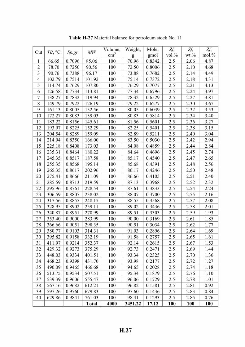
H.27
Table H-27 Material balance for petroleum stock No. 11
Cut TB, °C Sp.gr MW Volume, cm3
Weight, g
Mole, gmol
Zf, vol.%
Zf, wt.%
Zf, mol.%
1 66.65 0.7096 85.06 100 70.96 0.8342 2.5 2.06 4.87 2 78.70 0.7250 90.56 100 72.50 0.8006 2.5 2.10 4.68 3 90.76 0.7388 96.17 100 73.88 0.7682 2.5 2.14 4.49 4 102.79 0.7514 101.92 100 75.14 0.7372 2.5 2.18 4.31 5 114.74 0.7629 107.80 100 76.29 0.7077 2.5 2.21 4.13 6 126.58 0.7734 113.81 100 77.34 0.6796 2.5 2.24 3.97 7 138.27 0.7832 119.94 100 78.32 0.6529 2.5 2.27 3.81 8 149.79 0.7922 126.19 100 79.22 0.6277 2.5 2.30 3.67 9 161.13 0.8005 132.56 100 80.05 0.6039 2.5 2.32 3.53 10 172.27 0.8083 139.03 100 80.83 0.5814 2.5 2.34 3.40 11 183.22 0.8156 145.61 100 81.56 0.5601 2.5 2.36 3.27 12 193.97 0.8225 152.29 100 82.25 0.5401 2.5 2.38 3.15 13 204.54 0.8289 159.09 100 82.89 0.5211 2.5 2.40 3.04 14 214.94 0.8350 166.00 100 83.50 0.5030 2.5 2.42 2.94 15 225.18 0.8408 173.03 100 84.08 0.4859 2.5 2.44 2.84 16 235.31 0.8464 180.22 100 84.64 0.4696 2.5 2.45 2.74 17 245.35 0.8517 187.58 100 85.17 0.4540 2.5 2.47 2.65 18 255.35 0.8568 195.14 100 85.68 0.4391 2.5 2.48 2.56 19 265.35 0.8617 202.96 100 86.17 0.4246 2.5 2.50 2.48 20 275.41 0.8666 211.09 100 86.66 0.4105 2.5 2.51 2.40 21 285.59 0.8713 219.59 100 87.13 0.3968 2.5 2.52 2.32 22 295.96 0.8761 228.54 100 87.61 0.3833 2.5 2.54 2.24 23 306.59 0.8807 238.02 100 88.07 0.3700 2.5 2.55 2.16 24 317.56 0.8855 248.17 100 88.55 0.3568 2.5 2.57 2.08 25 328.95 0.8902 259.11 100 89.02 0.3436 2.5 2.58 2.01 26 340.87 0.8951 270.99 100 89.51 0.3303 2.5 2.59 1.93 27 353.40 0.9000 283.99 100 90.00 0.3169 2.5 2.61 1.85 28 366.66 0.9051 298.35 100 90.51 0.3034 2.5 2.62 1.77 29 380.77 0.9103 314.31 100 91.03 0.2896 2.5 2.64 1.69 30 395.82 0.9158 332.19 100 91.58 0.2757 2.5 2.65 1.61 31 411.97 0.9214 352.37 100 92.14 0.2615 2.5 2.67 1.53 32 429.32 0.9273 375.29 100 92.73 0.2471 2.5 2.69 1.44 33 448.03 0.9334 401.51 100 93.34 0.2325 2.5 2.70 1.36 34 468.23 0.9398 431.70 100 93.98 0.2177 2.5 2.72 1.27 35 490.09 0.9465 466.68 100 94.65 0.2028 2.5 2.74 1.18 36 513.75 0.9534 507.51 100 95.34 0.1879 2.5 2.76 1.10 37 539.39 0.9606 555.47 100 96.06 0.1729 2.5 2.78 1.01 38 567.16 0.9682 612.21 100 96.82 0.1581 2.5 2.81 0.92 39 597.26 0.9760 679.83 100 97.60 0.1436 2.5 2.83 0.84 40 629.86 0.9841 761.03 100 98.41 0.1293 2.5 2.85 0.76 Total 4000 3451.22 17.12 100 100 100
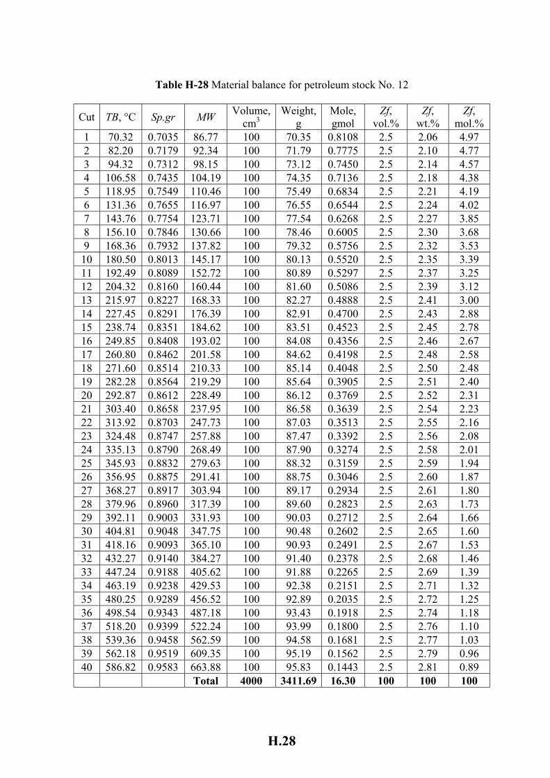
H.28
Table H-28 Material balance for petroleum stock No. 12
Cut TB, °C Sp.gr MW Volume, cm3
Weight, g
Mole, gmol
Zf, vol.%
Zf, wt.%
Zf, mol.%
1 70.32 0.7035 86.77 100 70.35 0.8108 2.5 2.06 4.97 2 82.20 0.7179 92.34 100 71.79 0.7775 2.5 2.10 4.77 3 94.32 0.7312 98.15 100 73.12 0.7450 2.5 2.14 4.57 4 106.58 0.7435 104.19 100 74.35 0.7136 2.5 2.18 4.38 5 118.95 0.7549 110.46 100 75.49 0.6834 2.5 2.21 4.19 6 131.36 0.7655 116.97 100 76.55 0.6544 2.5 2.24 4.02 7 143.76 0.7754 123.71 100 77.54 0.6268 2.5 2.27 3.85 8 156.10 0.7846 130.66 100 78.46 0.6005 2.5 2.30 3.68 9 168.36 0.7932 137.82 100 79.32 0.5756 2.5 2.32 3.53 10 180.50 0.8013 145.17 100 80.13 0.5520 2.5 2.35 3.39 11 192.49 0.8089 152.72 100 80.89 0.5297 2.5 2.37 3.25 12 204.32 0.8160 160.44 100 81.60 0.5086 2.5 2.39 3.12 13 215.97 0.8227 168.33 100 82.27 0.4888 2.5 2.41 3.00 14 227.45 0.8291 176.39 100 82.91 0.4700 2.5 2.43 2.88 15 238.74 0.8351 184.62 100 83.51 0.4523 2.5 2.45 2.78 16 249.85 0.8408 193.02 100 84.08 0.4356 2.5 2.46 2.67 17 260.80 0.8462 201.58 100 84.62 0.4198 2.5 2.48 2.58 18 271.60 0.8514 210.33 100 85.14 0.4048 2.5 2.50 2.48 19 282.28 0.8564 219.29 100 85.64 0.3905 2.5 2.51 2.40 20 292.87 0.8612 228.49 100 86.12 0.3769 2.5 2.52 2.31 21 303.40 0.8658 237.95 100 86.58 0.3639 2.5 2.54 2.23 22 313.92 0.8703 247.73 100 87.03 0.3513 2.5 2.55 2.16 23 324.48 0.8747 257.88 100 87.47 0.3392 2.5 2.56 2.08 24 335.13 0.8790 268.49 100 87.90 0.3274 2.5 2.58 2.01 25 345.93 0.8832 279.63 100 88.32 0.3159 2.5 2.59 1.94 26 356.95 0.8875 291.41 100 88.75 0.3046 2.5 2.60 1.87 27 368.27 0.8917 303.94 100 89.17 0.2934 2.5 2.61 1.80 28 379.96 0.8960 317.39 100 89.60 0.2823 2.5 2.63 1.73 29 392.11 0.9003 331.93 100 90.03 0.2712 2.5 2.64 1.66 30 404.81 0.9048 347.75 100 90.48 0.2602 2.5 2.65 1.60 31 418.16 0.9093 365.10 100 90.93 0.2491 2.5 2.67 1.53 32 432.27 0.9140 384.27 100 91.40 0.2378 2.5 2.68 1.46 33 447.24 0.9188 405.62 100 91.88 0.2265 2.5 2.69 1.39 34 463.19 0.9238 429.53 100 92.38 0.2151 2.5 2.71 1.32 35 480.25 0.9289 456.52 100 92.89 0.2035 2.5 2.72 1.25 36 498.54 0.9343 487.18 100 93.43 0.1918 2.5 2.74 1.18 37 518.20 0.9399 522.24 100 93.99 0.1800 2.5 2.76 1.10 38 539.36 0.9458 562.59 100 94.58 0.1681 2.5 2.77 1.03 39 562.18 0.9519 609.35 100 95.19 0.1562 2.5 2.79 0.96 40 586.82 0.9583 663.88 100 95.83 0.1443 2.5 2.81 0.89 Total 4000 3411.69 16.30 100 100 100
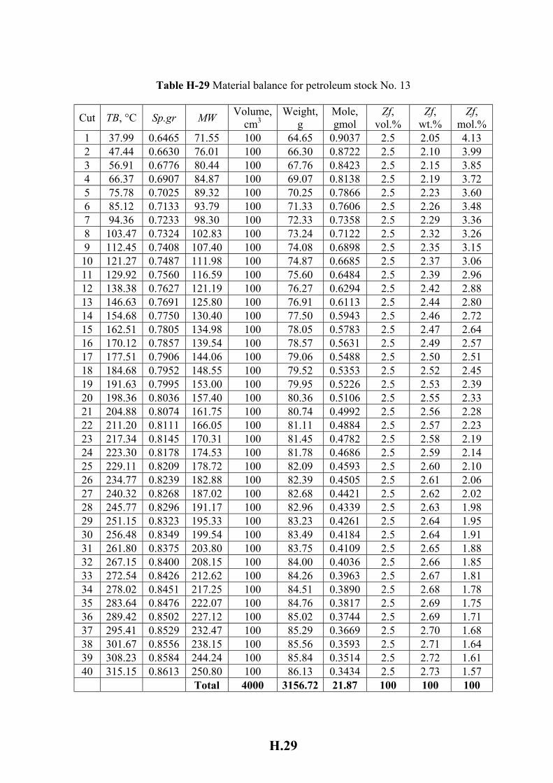
H.29
Table H-29 Material balance for petroleum stock No. 13
Cut TB, °C Sp.gr MW Volume, cm3
Weight, g
Mole, gmol
Zf, vol.%
Zf, wt.%
Zf, mol.%
1 37.99 0.6465 71.55 100 64.65 0.9037 2.5 2.05 4.13 2 47.44 0.6630 76.01 100 66.30 0.8722 2.5 2.10 3.99 3 56.91 0.6776 80.44 100 67.76 0.8423 2.5 2.15 3.85 4 66.37 0.6907 84.87 100 69.07 0.8138 2.5 2.19 3.72 5 75.78 0.7025 89.32 100 70.25 0.7866 2.5 2.23 3.60 6 85.12 0.7133 93.79 100 71.33 0.7606 2.5 2.26 3.48 7 94.36 0.7233 98.30 100 72.33 0.7358 2.5 2.29 3.36 8 103.47 0.7324 102.83 100 73.24 0.7122 2.5 2.32 3.26 9 112.45 0.7408 107.40 100 74.08 0.6898 2.5 2.35 3.15 10 121.27 0.7487 111.98 100 74.87 0.6685 2.5 2.37 3.06 11 129.92 0.7560 116.59 100 75.60 0.6484 2.5 2.39 2.96 12 138.38 0.7627 121.19 100 76.27 0.6294 2.5 2.42 2.88 13 146.63 0.7691 125.80 100 76.91 0.6113 2.5 2.44 2.80 14 154.68 0.7750 130.40 100 77.50 0.5943 2.5 2.46 2.72 15 162.51 0.7805 134.98 100 78.05 0.5783 2.5 2.47 2.64 16 170.12 0.7857 139.54 100 78.57 0.5631 2.5 2.49 2.57 17 177.51 0.7906 144.06 100 79.06 0.5488 2.5 2.50 2.51 18 184.68 0.7952 148.55 100 79.52 0.5353 2.5 2.52 2.45 19 191.63 0.7995 153.00 100 79.95 0.5226 2.5 2.53 2.39 20 198.36 0.8036 157.40 100 80.36 0.5106 2.5 2.55 2.33 21 204.88 0.8074 161.75 100 80.74 0.4992 2.5 2.56 2.28 22 211.20 0.8111 166.05 100 81.11 0.4884 2.5 2.57 2.23 23 217.34 0.8145 170.31 100 81.45 0.4782 2.5 2.58 2.19 24 223.30 0.8178 174.53 100 81.78 0.4686 2.5 2.59 2.14 25 229.11 0.8209 178.72 100 82.09 0.4593 2.5 2.60 2.10 26 234.77 0.8239 182.88 100 82.39 0.4505 2.5 2.61 2.06 27 240.32 0.8268 187.02 100 82.68 0.4421 2.5 2.62 2.02 28 245.77 0.8296 191.17 100 82.96 0.4339 2.5 2.63 1.98 29 251.15 0.8323 195.33 100 83.23 0.4261 2.5 2.64 1.95 30 256.48 0.8349 199.54 100 83.49 0.4184 2.5 2.64 1.91 31 261.80 0.8375 203.80 100 83.75 0.4109 2.5 2.65 1.88 32 267.15 0.8400 208.15 100 84.00 0.4036 2.5 2.66 1.85 33 272.54 0.8426 212.62 100 84.26 0.3963 2.5 2.67 1.81 34 278.02 0.8451 217.25 100 84.51 0.3890 2.5 2.68 1.78 35 283.64 0.8476 222.07 100 84.76 0.3817 2.5 2.69 1.75 36 289.42 0.8502 227.12 100 85.02 0.3744 2.5 2.69 1.71 37 295.41 0.8529 232.47 100 85.29 0.3669 2.5 2.70 1.68 38 301.67 0.8556 238.15 100 85.56 0.3593 2.5 2.71 1.64 39 308.23 0.8584 244.24 100 85.84 0.3514 2.5 2.72 1.61 40 315.15 0.8613 250.80 100 86.13 0.3434 2.5 2.73 1.57 Total 4000 3156.72 21.87 100 100 100
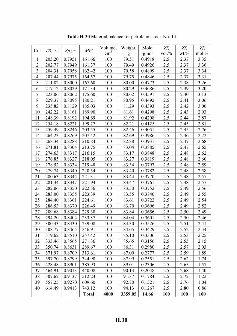
H.30
Table H-30 Material balance for petroleum stock No. 14
Cut TB, °C Sp.gr MW Volume, cm3
Weight, g
Mole, gmol
Zf, vol.%
Zf, wt.%
Zf, mol.%
1 203.20 0.7951 161.66 100 79.51 0.4918 2.5 2.37 3.35 2 202.77 0.7949 161.37 100 79.49 0.4926 2.5 2.37 3.36 3 204.31 0.7958 162.42 100 79.58 0.4899 2.5 2.37 3.34 4 207.44 0.7975 164.57 100 79.75 0.4846 2.5 2.37 3.31 5 211.82 0.8000 167.60 100 80.00 0.4773 2.5 2.38 3.26 6 217.12 0.8029 171.34 100 80.29 0.4686 2.5 2.39 3.20 7 223.06 0.8062 175.60 100 80.62 0.4591 2.5 2.40 3.13 8 229.37 0.8095 180.21 100 80.95 0.4492 2.5 2.41 3.06 9 235.82 0.8129 185.03 100 81.29 0.4393 2.5 2.42 3.00 10 242.22 0.8161 189.90 100 81.61 0.4298 2.5 2.43 2.93 11 248.39 0.8192 194.69 100 81.92 0.4208 2.5 2.44 2.87 12 254.18 0.8221 199.27 100 82.21 0.4125 2.5 2.45 2.81 13 259.49 0.8246 203.55 100 82.46 0.4051 2.5 2.45 2.76 14 264.23 0.8269 207.42 100 82.69 0.3986 2.5 2.46 2.72 15 268.34 0.8288 210.84 100 82.88 0.3931 2.5 2.47 2.68 16 271.81 0.8304 213.75 100 83.04 0.3885 2.5 2.47 2.65 17 274.63 0.8317 216.15 100 83.17 0.3848 2.5 2.48 2.62 18 276.85 0.8327 218.05 100 83.27 0.3819 2.5 2.48 2.60 19 278.52 0.8334 219.48 100 83.34 0.3797 2.5 2.48 2.59 20 279.74 0.8340 220.54 100 83.40 0.3782 2.5 2.48 2.58 21 280.63 0.8344 221.31 100 83.44 0.3770 2.5 2.48 2.57 22 281.34 0.8347 221.94 100 83.47 0.3761 2.5 2.48 2.57 23 282.06 0.8350 222.56 100 83.50 0.3752 2.5 2.49 2.56 24 283.00 0.8355 223.39 100 83.55 0.3740 2.5 2.49 2.55 25 284.40 0.8361 224.61 100 83.61 0.3722 2.5 2.49 2.54 26 286.53 0.8370 226.49 100 83.70 0.3696 2.5 2.49 2.52 27 289.68 0.8384 229.30 100 83.84 0.3656 2.5 2.50 2.49 28 294.20 0.8404 233.37 100 84.04 0.3601 2.5 2.50 2.46 29 300.43 0.8430 239.08 100 84.30 0.3526 2.5 2.51 2.41 30 308.77 0.8465 246.91 100 84.65 0.3429 2.5 2.52 2.34 31 319.62 0.8510 257.42 100 85.10 0.3306 2.5 2.53 2.25 32 333.46 0.8565 271.36 100 85.65 0.3156 2.5 2.55 2.15 33 350.74 0.8631 289.67 100 86.31 0.2980 2.5 2.57 2.03 34 371.97 0.8709 313.61 100 87.09 0.2777 2.5 2.59 1.89 35 397.70 0.8799 344.90 100 87.99 0.2551 2.5 2.62 1.74 36 428.48 0.8901 385.93 100 89.01 0.2306 2.5 2.65 1.57 37 464.91 0.9013 440.08 100 90.13 0.2048 2.5 2.68 1.40 38 507.62 0.9137 512.23 100 91.37 0.1784 2.5 2.72 1.22 39 557.25 0.9270 609.60 100 92.70 0.1521 2.5 2.76 1.04 40 614.49 0.9413 743.12 100 94.13 0.1267 2.5 2.80 0.86 Total 4000 3359.05 14.66 100 100 100
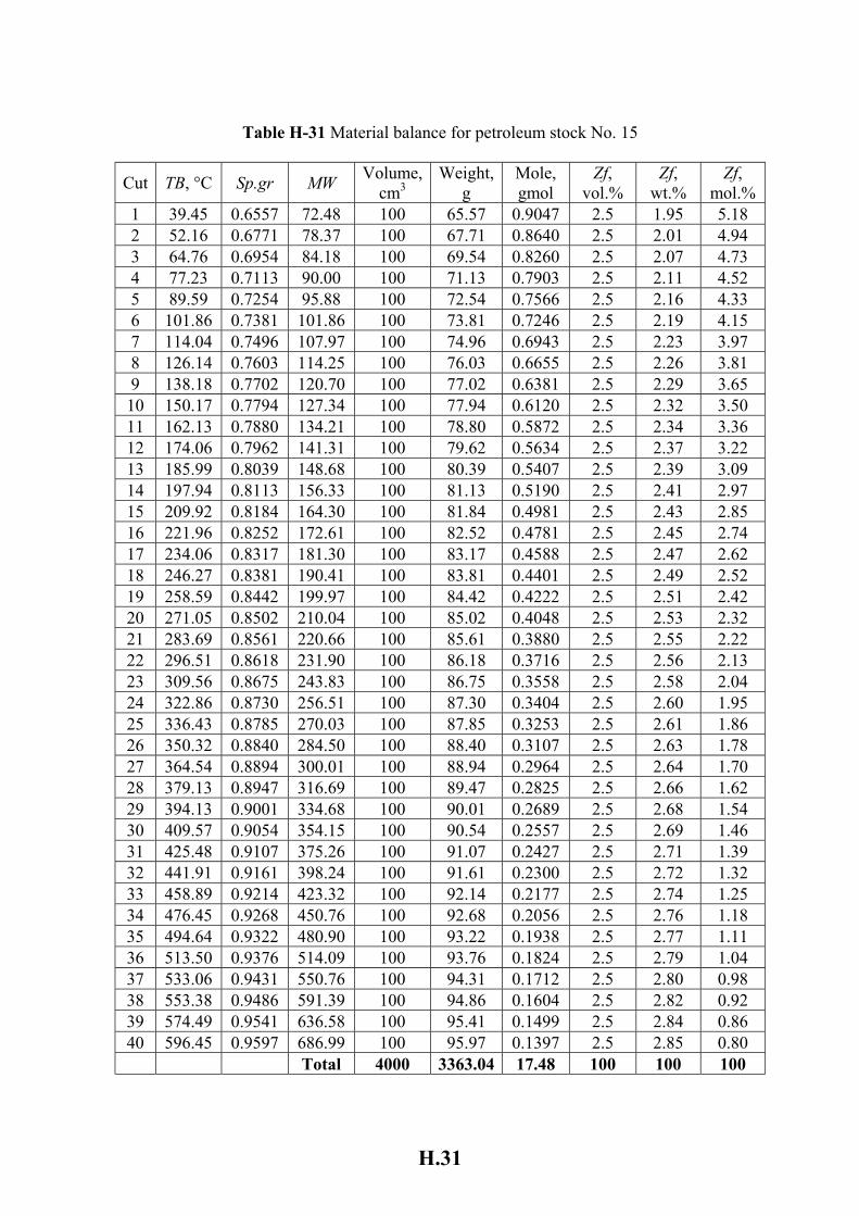
H.31
Table H-31 Material balance for petroleum stock No. 15
Cut TB, °C Sp.gr MW Volume, cm3
Weight, g
Mole, gmol
Zf, vol.%
Zf, wt.%
Zf, mol.%
1 39.45 0.6557 72.48 100 65.57 0.9047 2.5 1.95 5.18 2 52.16 0.6771 78.37 100 67.71 0.8640 2.5 2.01 4.94 3 64.76 0.6954 84.18 100 69.54 0.8260 2.5 2.07 4.73 4 77.23 0.7113 90.00 100 71.13 0.7903 2.5 2.11 4.52 5 89.59 0.7254 95.88 100 72.54 0.7566 2.5 2.16 4.33 6 101.86 0.7381 101.86 100 73.81 0.7246 2.5 2.19 4.15 7 114.04 0.7496 107.97 100 74.96 0.6943 2.5 2.23 3.97 8 126.14 0.7603 114.25 100 76.03 0.6655 2.5 2.26 3.81 9 138.18 0.7702 120.70 100 77.02 0.6381 2.5 2.29 3.65 10 150.17 0.7794 127.34 100 77.94 0.6120 2.5 2.32 3.50 11 162.13 0.7880 134.21 100 78.80 0.5872 2.5 2.34 3.36 12 174.06 0.7962 141.31 100 79.62 0.5634 2.5 2.37 3.22 13 185.99 0.8039 148.68 100 80.39 0.5407 2.5 2.39 3.09 14 197.94 0.8113 156.33 100 81.13 0.5190 2.5 2.41 2.97 15 209.92 0.8184 164.30 100 81.84 0.4981 2.5 2.43 2.85 16 221.96 0.8252 172.61 100 82.52 0.4781 2.5 2.45 2.74 17 234.06 0.8317 181.30 100 83.17 0.4588 2.5 2.47 2.62 18 246.27 0.8381 190.41 100 83.81 0.4401 2.5 2.49 2.52 19 258.59 0.8442 199.97 100 84.42 0.4222 2.5 2.51 2.42 20 271.05 0.8502 210.04 100 85.02 0.4048 2.5 2.53 2.32 21 283.69 0.8561 220.66 100 85.61 0.3880 2.5 2.55 2.22 22 296.51 0.8618 231.90 100 86.18 0.3716 2.5 2.56 2.13 23 309.56 0.8675 243.83 100 86.75 0.3558 2.5 2.58 2.04 24 322.86 0.8730 256.51 100 87.30 0.3404 2.5 2.60 1.95 25 336.43 0.8785 270.03 100 87.85 0.3253 2.5 2.61 1.86 26 350.32 0.8840 284.50 100 88.40 0.3107 2.5 2.63 1.78 27 364.54 0.8894 300.01 100 88.94 0.2964 2.5 2.64 1.70 28 379.13 0.8947 316.69 100 89.47 0.2825 2.5 2.66 1.62 29 394.13 0.9001 334.68 100 90.01 0.2689 2.5 2.68 1.54 30 409.57 0.9054 354.15 100 90.54 0.2557 2.5 2.69 1.46 31 425.48 0.9107 375.26 100 91.07 0.2427 2.5 2.71 1.39 32 441.91 0.9161 398.24 100 91.61 0.2300 2.5 2.72 1.32 33 458.89 0.9214 423.32 100 92.14 0.2177 2.5 2.74 1.25 34 476.45 0.9268 450.76 100 92.68 0.2056 2.5 2.76 1.18 35 494.64 0.9322 480.90 100 93.22 0.1938 2.5 2.77 1.11 36 513.50 0.9376 514.09 100 93.76 0.1824 2.5 2.79 1.04 37 533.06 0.9431 550.76 100 94.31 0.1712 2.5 2.80 0.98 38 553.38 0.9486 591.39 100 94.86 0.1604 2.5 2.82 0.92 39 574.49 0.9541 636.58 100 95.41 0.1499 2.5 2.84 0.86 40 596.45 0.9597 686.99 100 95.97 0.1397 2.5 2.85 0.80 Total 4000 3363.04 17.48 100 100 100
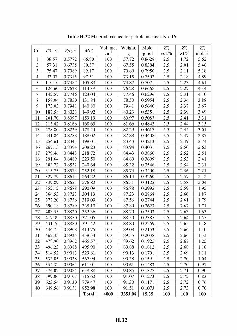
H.32
Table H-32 Material balance for petroleum stock No. 16
Cut TB, °C Sp.gr MW Volume, cm3
Weight, g
Mole, gmol
Zf, vol.%
Zf, wt.%
Zf, mol.%
1 38.57 0.5772 66.90 100 57.72 0.8628 2.5 1.72 5.62 2 57.31 0.6755 80.57 100 67.55 0.8384 2.5 2.01 5.46 3 75.47 0.7089 89.17 100 70.89 0.7950 2.5 2.11 5.18 4 93.07 0.7315 97.51 100 73.15 0.7502 2.5 2.18 4.89 5 110.10 0.7487 105.89 100 74.87 0.7071 2.5 2.23 4.61 6 126.60 0.7628 114.39 100 76.28 0.6668 2.5 2.27 4.34 7 142.57 0.7746 123.04 100 77.46 0.6296 2.5 2.31 4.10 8 158.04 0.7850 131.84 100 78.50 0.5954 2.5 2.34 3.88 9 173.03 0.7941 140.80 100 79.41 0.5640 2.5 2.37 3.67 10 187.58 0.8023 149.92 100 80.23 0.5351 2.5 2.39 3.49 11 201.70 0.8097 159.19 100 80.97 0.5087 2.5 2.41 3.31 12 215.42 0.8166 168.63 100 81.66 0.4842 2.5 2.44 3.15 13 228.80 0.8229 178.24 100 82.29 0.4617 2.5 2.45 3.01 14 241.84 0.8288 188.02 100 82.88 0.4408 2.5 2.47 2.87 15 254.61 0.8343 198.01 100 83.43 0.4213 2.5 2.49 2.74 16 267.13 0.8394 208.23 100 83.94 0.4031 2.5 2.50 2.63 17 279.46 0.8443 218.72 100 84.43 0.3860 2.5 2.52 2.51 18 291.64 0.8489 229.50 100 84.89 0.3699 2.5 2.53 2.41 19 303.72 0.8532 240.64 100 85.32 0.3546 2.5 2.54 2.31 20 315.75 0.8574 252.18 100 85.74 0.3400 2.5 2.56 2.21 21 327.79 0.8614 264.22 100 86.14 0.3260 2.5 2.57 2.12 22 339.89 0.8651 276.82 100 86.51 0.3125 2.5 2.58 2.04 23 352.12 0.8688 290.09 100 86.88 0.2995 2.5 2.59 1.95 24 364.53 0.8723 304.13 100 87.23 0.2868 2.5 2.60 1.87 25 377.20 0.8756 319.09 100 87.56 0.2744 2.5 2.61 1.79 26 390.18 0.8789 335.10 100 87.89 0.2623 2.5 2.62 1.71 27 403.55 0.8820 352.36 100 88.20 0.2503 2.5 2.63 1.63 28 417.39 0.8850 371.05 100 88.50 0.2385 2.5 2.64 1.55 29 431.76 0.8880 391.42 100 88.80 0.2269 2.5 2.65 1.48 30 446.75 0.8908 413.75 100 89.08 0.2153 2.5 2.66 1.40 31 462.43 0.8935 438.34 100 89.35 0.2038 2.5 2.66 1.33 32 478.90 0.8962 465.57 100 89.62 0.1925 2.5 2.67 1.25 33 496.23 0.8988 495.90 100 89.88 0.1812 2.5 2.68 1.18 34 514.52 0.9013 529.81 100 90.13 0.1701 2.5 2.69 1.11 35 533.85 0.9038 567.94 100 90.38 0.1591 2.5 2.70 1.04 36 554.32 0.9061 611.01 100 90.61 0.1483 2.5 2.70 0.97 37 576.02 0.9085 659.88 100 90.85 0.1377 2.5 2.71 0.90 38 599.06 0.9107 715.62 100 91.07 0.1273 2.5 2.72 0.83 39 623.54 0.9130 779.47 100 91.30 0.1171 2.5 2.72 0.76 40 649.56 0.9151 852.98 100 91.51 0.1073 2.5 2.73 0.70 Total 4000 3353.08 15.35 100 100 100
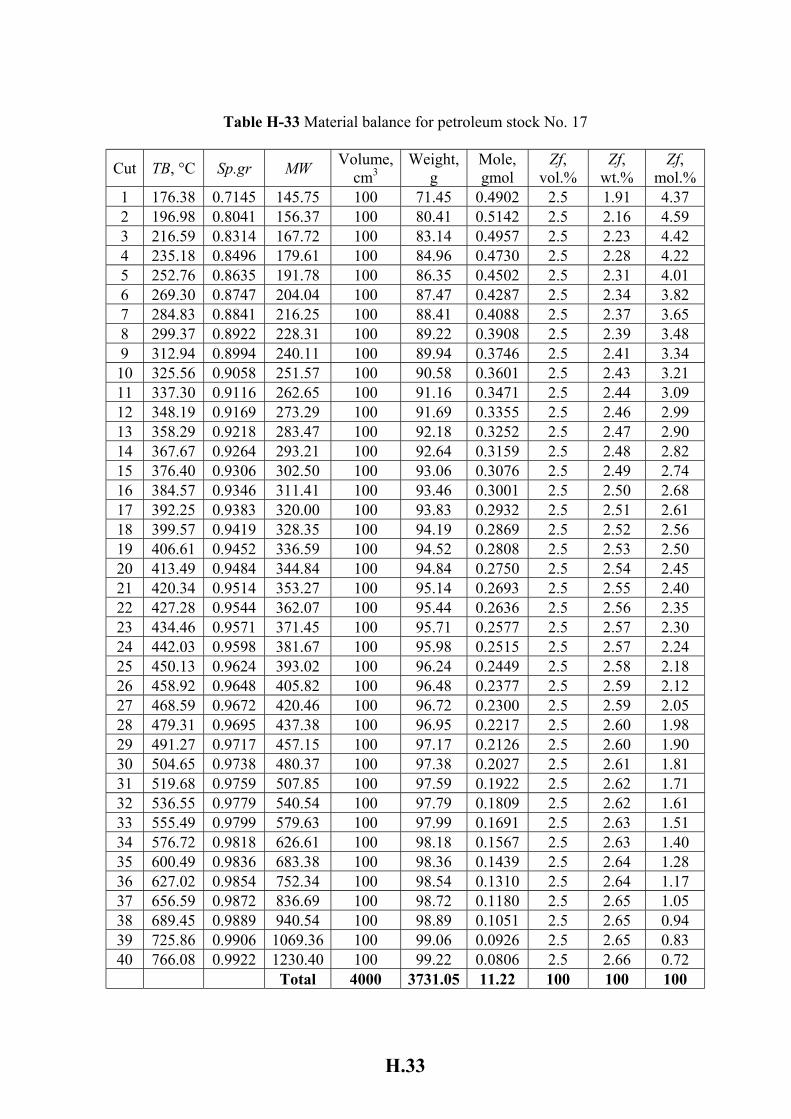
H.33
Table H-33 Material balance for petroleum stock No. 17
Cut TB, °C Sp.gr MW Volume, cm3
Weight, g
Mole, gmol
Zf, vol.%
Zf, wt.%
Zf, mol.%
1 176.38 0.7145 145.75 100 71.45 0.4902 2.5 1.91 4.37 2 196.98 0.8041 156.37 100 80.41 0.5142 2.5 2.16 4.59 3 216.59 0.8314 167.72 100 83.14 0.4957 2.5 2.23 4.42 4 235.18 0.8496 179.61 100 84.96 0.4730 2.5 2.28 4.22 5 252.76 0.8635 191.78 100 86.35 0.4502 2.5 2.31 4.01 6 269.30 0.8747 204.04 100 87.47 0.4287 2.5 2.34 3.82 7 284.83 0.8841 216.25 100 88.41 0.4088 2.5 2.37 3.65 8 299.37 0.8922 228.31 100 89.22 0.3908 2.5 2.39 3.48 9 312.94 0.8994 240.11 100 89.94 0.3746 2.5 2.41 3.34 10 325.56 0.9058 251.57 100 90.58 0.3601 2.5 2.43 3.21 11 337.30 0.9116 262.65 100 91.16 0.3471 2.5 2.44 3.09 12 348.19 0.9169 273.29 100 91.69 0.3355 2.5 2.46 2.99 13 358.29 0.9218 283.47 100 92.18 0.3252 2.5 2.47 2.90 14 367.67 0.9264 293.21 100 92.64 0.3159 2.5 2.48 2.82 15 376.40 0.9306 302.50 100 93.06 0.3076 2.5 2.49 2.74 16 384.57 0.9346 311.41 100 93.46 0.3001 2.5 2.50 2.68 17 392.25 0.9383 320.00 100 93.83 0.2932 2.5 2.51 2.61 18 399.57 0.9419 328.35 100 94.19 0.2869 2.5 2.52 2.56 19 406.61 0.9452 336.59 100 94.52 0.2808 2.5 2.53 2.50 20 413.49 0.9484 344.84 100 94.84 0.2750 2.5 2.54 2.45 21 420.34 0.9514 353.27 100 95.14 0.2693 2.5 2.55 2.40 22 427.28 0.9544 362.07 100 95.44 0.2636 2.5 2.56 2.35 23 434.46 0.9571 371.45 100 95.71 0.2577 2.5 2.57 2.30 24 442.03 0.9598 381.67 100 95.98 0.2515 2.5 2.57 2.24 25 450.13 0.9624 393.02 100 96.24 0.2449 2.5 2.58 2.18 26 458.92 0.9648 405.82 100 96.48 0.2377 2.5 2.59 2.12 27 468.59 0.9672 420.46 100 96.72 0.2300 2.5 2.59 2.05 28 479.31 0.9695 437.38 100 96.95 0.2217 2.5 2.60 1.98 29 491.27 0.9717 457.15 100 97.17 0.2126 2.5 2.60 1.90 30 504.65 0.9738 480.37 100 97.38 0.2027 2.5 2.61 1.81 31 519.68 0.9759 507.85 100 97.59 0.1922 2.5 2.62 1.71 32 536.55 0.9779 540.54 100 97.79 0.1809 2.5 2.62 1.61 33 555.49 0.9799 579.63 100 97.99 0.1691 2.5 2.63 1.51 34 576.72 0.9818 626.61 100 98.18 0.1567 2.5 2.63 1.40 35 600.49 0.9836 683.38 100 98.36 0.1439 2.5 2.64 1.28 36 627.02 0.9854 752.34 100 98.54 0.1310 2.5 2.64 1.17 37 656.59 0.9872 836.69 100 98.72 0.1180 2.5 2.65 1.05 38 689.45 0.9889 940.54 100 98.89 0.1051 2.5 2.65 0.94 39 725.86 0.9906 1069.36 100 99.06 0.0926 2.5 2.65 0.83 40 766.08 0.9922 1230.40 100 99.22 0.0806 2.5 2.66 0.72 Total 4000 3731.05 11.22 100 100 100

H.34
Table H-34 Material balance for petroleum stock No. 18
Cut TB, °C Sp.gr MW Volume, cm3
Weight, g
Mole, gmol
Zf, vol.%
Zf, wt.%
Zf, mol.%
1 72.13 0.6185 84.09 100 61.85 0.7355 2.5 1.90 4.74 2 88.40 0.6984 95.37 100 69.84 0.7324 2.5 2.14 4.72 3 103.70 0.7230 103.10 100 72.30 0.7013 2.5 2.22 4.52 4 118.10 0.7395 110.51 100 73.95 0.6692 2.5 2.27 4.31 5 131.65 0.7519 117.73 100 75.19 0.6387 2.5 2.31 4.11 6 144.40 0.7620 124.81 100 76.20 0.6105 2.5 2.34 3.93 7 156.42 0.7705 131.75 100 77.05 0.5849 2.5 2.36 3.77 8 167.77 0.7779 138.54 100 77.79 0.5615 2.5 2.39 3.62 9 178.52 0.7844 145.21 100 78.44 0.5402 2.5 2.41 3.48 10 188.71 0.7902 151.75 100 79.02 0.5207 2.5 2.42 3.35 11 198.43 0.7954 158.19 100 79.54 0.5028 2.5 2.44 3.24 12 207.73 0.8002 164.54 100 80.02 0.4863 2.5 2.46 3.13 13 216.69 0.8047 170.84 100 80.47 0.4710 2.5 2.47 3.03 14 225.37 0.8088 177.13 100 80.88 0.4566 2.5 2.48 2.94 15 233.84 0.8126 183.45 100 81.26 0.4430 2.5 2.49 2.85 16 242.17 0.8162 189.85 100 81.62 0.4299 2.5 2.50 2.77 17 250.45 0.8196 196.39 100 81.96 0.4173 2.5 2.52 2.69 18 258.75 0.8228 203.13 100 82.28 0.4051 2.5 2.53 2.61 19 267.14 0.8258 210.15 100 82.58 0.3930 2.5 2.53 2.53 20 275.69 0.8287 217.54 100 82.87 0.3810 2.5 2.54 2.45 21 284.50 0.8315 225.38 100 83.15 0.3689 2.5 2.55 2.38 22 293.64 0.8341 233.78 100 83.41 0.3568 2.5 2.56 2.30 23 303.19 0.8366 242.86 100 83.66 0.3445 2.5 2.57 2.22 24 313.24 0.8390 252.75 100 83.90 0.3320 2.5 2.57 2.14 25 323.86 0.8413 263.60 100 84.13 0.3192 2.5 2.58 2.06 26 335.17 0.8436 275.58 100 84.36 0.3061 2.5 2.59 1.97 27 347.22 0.8457 288.90 100 84.57 0.2927 2.5 2.60 1.89 28 360.13 0.8478 303.76 100 84.78 0.2791 2.5 2.60 1.80 29 373.97 0.8498 320.46 100 84.98 0.2652 2.5 2.61 1.71 30 388.85 0.8517 339.26 100 85.17 0.2511 2.5 2.61 1.62 31 404.85 0.8536 360.55 100 85.36 0.2368 2.5 2.62 1.52 32 422.07 0.8554 384.73 100 85.54 0.2223 2.5 2.63 1.43 33 440.61 0.8572 412.32 100 85.72 0.2079 2.5 2.63 1.34 34 460.56 0.8589 443.90 100 85.89 0.1935 2.5 2.64 1.25 35 482.03 0.8606 480.20 100 86.06 0.1792 2.5 2.64 1.15 36 505.12 0.8622 522.06 100 86.22 0.1652 2.5 2.65 1.06 37 529.92 0.8638 570.51 100 86.38 0.1514 2.5 2.65 0.98 38 556.55 0.8654 626.85 100 86.54 0.1381 2.5 2.66 0.89 39 585.11 0.8669 692.63 100 86.69 0.1252 2.5 2.66 0.81 40 615.70 0.8684 769.75 100 86.84 0.1128 2.5 2.66 0.73 Total 4000 3258.49 15.53 100 100 100
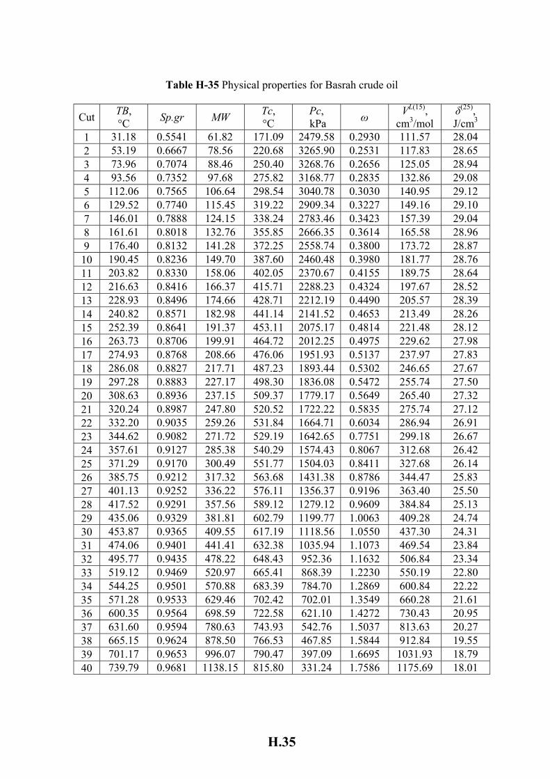
H.35
Table H-35 Physical properties for Basrah crude oil
Cut TB, °C Sp.gr MW Tc,
°C Pc, kPa ω VL(15),
cm3/mol δ(25), J/cm3
1 31.18 0.5541 61.82 171.09 2479.58 0.2930 111.57 28.04 2 53.19 0.6667 78.56 220.68 3265.90 0.2531 117.83 28.65 3 73.96 0.7074 88.46 250.40 3268.76 0.2656 125.05 28.94 4 93.56 0.7352 97.68 275.82 3168.77 0.2835 132.86 29.08 5 112.06 0.7565 106.64 298.54 3040.78 0.3030 140.95 29.12 6 129.52 0.7740 115.45 319.22 2909.34 0.3227 149.16 29.10 7 146.01 0.7888 124.15 338.24 2783.46 0.3423 157.39 29.04 8 161.61 0.8018 132.76 355.85 2666.35 0.3614 165.58 28.96 9 176.40 0.8132 141.28 372.25 2558.74 0.3800 173.72 28.87 10 190.45 0.8236 149.70 387.60 2460.48 0.3980 181.77 28.76 11 203.82 0.8330 158.06 402.05 2370.67 0.4155 189.75 28.64 12 216.63 0.8416 166.37 415.71 2288.23 0.4324 197.67 28.52 13 228.93 0.8496 174.66 428.71 2212.19 0.4490 205.57 28.39 14 240.82 0.8571 182.98 441.14 2141.52 0.4653 213.49 28.26 15 252.39 0.8641 191.37 453.11 2075.17 0.4814 221.48 28.12 16 263.73 0.8706 199.91 464.72 2012.25 0.4975 229.62 27.98 17 274.93 0.8768 208.66 476.06 1951.93 0.5137 237.97 27.83 18 286.08 0.8827 217.71 487.23 1893.44 0.5302 246.65 27.67 19 297.28 0.8883 227.17 498.30 1836.08 0.5472 255.74 27.50 20 308.63 0.8936 237.15 509.37 1779.17 0.5649 265.40 27.32 21 320.24 0.8987 247.80 520.52 1722.22 0.5835 275.74 27.12 22 332.20 0.9035 259.26 531.84 1664.71 0.6034 286.94 26.91 23 344.62 0.9082 271.72 529.19 1642.65 0.7751 299.18 26.67 24 357.61 0.9127 285.38 540.29 1574.43 0.8067 312.68 26.42 25 371.29 0.9170 300.49 551.77 1504.03 0.8411 327.68 26.14 26 385.75 0.9212 317.32 563.68 1431.38 0.8786 344.47 25.83 27 401.13 0.9252 336.22 576.11 1356.37 0.9196 363.40 25.50 28 417.52 0.9291 357.56 589.12 1279.12 0.9609 384.84 25.13 29 435.06 0.9329 381.81 602.79 1199.77 1.0063 409.28 24.74 30 453.87 0.9365 409.55 617.19 1118.56 1.0550 437.30 24.31 31 474.06 0.9401 441.41 632.38 1035.94 1.1073 469.54 23.84 32 495.77 0.9435 478.22 648.43 952.36 1.1632 506.84 23.34 33 519.12 0.9469 520.97 665.41 868.39 1.2230 550.19 22.80 34 544.25 0.9501 570.88 683.39 784.70 1.2869 600.84 22.22 35 571.28 0.9533 629.46 702.42 702.01 1.3549 660.28 21.61 36 600.35 0.9564 698.59 722.58 621.10 1.4272 730.43 20.95 37 631.60 0.9594 780.63 743.93 542.76 1.5037 813.63 20.27 38 665.15 0.9624 878.50 766.53 467.85 1.5844 912.84 19.55 39 701.17 0.9653 996.07 790.47 397.09 1.6695 1031.93 18.79 40 739.79 0.9681 1138.15 815.80 331.24 1.7586 1175.69 18.01
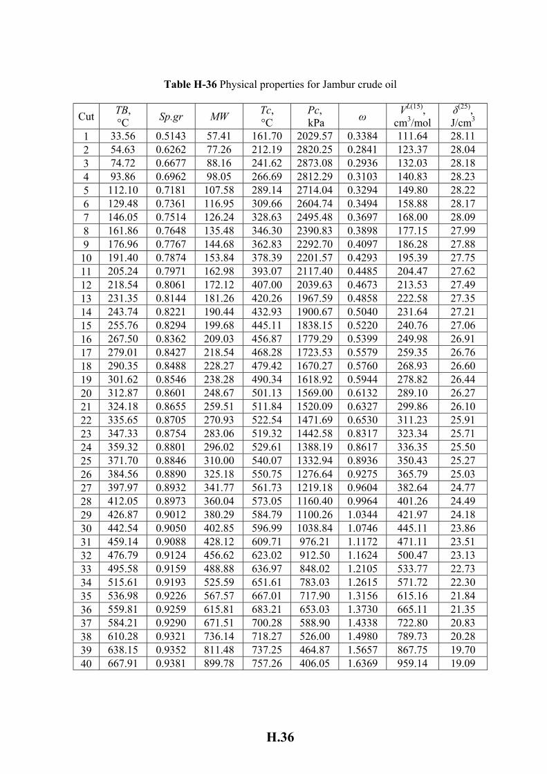
H.36
Table H-36 Physical properties for Jambur crude oil
Cut TB, °C Sp.gr MW Tc,
°C Pc, kPa ω VL(15),
cm3/mol δ(25), J/cm3
1 33.56 0.5143 57.41 161.70 2029.57 0.3384 111.64 28.11 2 54.63 0.6262 77.26 212.19 2820.25 0.2841 123.37 28.04 3 74.72 0.6677 88.16 241.62 2873.08 0.2936 132.03 28.18 4 93.86 0.6962 98.05 266.69 2812.29 0.3103 140.83 28.23 5 112.10 0.7181 107.58 289.14 2714.04 0.3294 149.80 28.22 6 129.48 0.7361 116.95 309.66 2604.74 0.3494 158.88 28.17 7 146.05 0.7514 126.24 328.63 2495.48 0.3697 168.00 28.09 8 161.86 0.7648 135.48 346.30 2390.83 0.3898 177.15 27.99 9 176.96 0.7767 144.68 362.83 2292.70 0.4097 186.28 27.88 10 191.40 0.7874 153.84 378.39 2201.57 0.4293 195.39 27.75 11 205.24 0.7971 162.98 393.07 2117.40 0.4485 204.47 27.62 12 218.54 0.8061 172.12 407.00 2039.63 0.4673 213.53 27.49 13 231.35 0.8144 181.26 420.26 1967.59 0.4858 222.58 27.35 14 243.74 0.8221 190.44 432.93 1900.67 0.5040 231.64 27.21 15 255.76 0.8294 199.68 445.11 1838.15 0.5220 240.76 27.06 16 267.50 0.8362 209.03 456.87 1779.29 0.5399 249.98 26.91 17 279.01 0.8427 218.54 468.28 1723.53 0.5579 259.35 26.76 18 290.35 0.8488 228.27 479.42 1670.27 0.5760 268.93 26.60 19 301.62 0.8546 238.28 490.34 1618.92 0.5944 278.82 26.44 20 312.87 0.8601 248.67 501.13 1569.00 0.6132 289.10 26.27 21 324.18 0.8655 259.51 511.84 1520.09 0.6327 299.86 26.10 22 335.65 0.8705 270.93 522.54 1471.69 0.6530 311.23 25.91 23 347.33 0.8754 283.06 519.32 1442.58 0.8317 323.34 25.71 24 359.32 0.8801 296.02 529.61 1388.19 0.8617 336.35 25.50 25 371.70 0.8846 310.00 540.07 1332.94 0.8936 350.43 25.27 26 384.56 0.8890 325.18 550.75 1276.64 0.9275 365.79 25.03 27 397.97 0.8932 341.77 561.73 1219.18 0.9604 382.64 24.77 28 412.05 0.8973 360.04 573.05 1160.40 0.9964 401.26 24.49 29 426.87 0.9012 380.29 584.79 1100.26 1.0344 421.97 24.18 30 442.54 0.9050 402.85 596.99 1038.84 1.0746 445.11 23.86 31 459.14 0.9088 428.12 609.71 976.21 1.1172 471.11 23.51 32 476.79 0.9124 456.62 623.02 912.50 1.1624 500.47 23.13 33 495.58 0.9159 488.88 636.97 848.02 1.2105 533.77 22.73 34 515.61 0.9193 525.59 651.61 783.03 1.2615 571.72 22.30 35 536.98 0.9226 567.57 667.01 717.90 1.3156 615.16 21.84 36 559.81 0.9259 615.81 683.21 653.03 1.3730 665.11 21.35 37 584.21 0.9290 671.51 700.28 588.90 1.4338 722.80 20.83 38 610.28 0.9321 736.14 718.27 526.00 1.4980 789.73 20.28 39 638.15 0.9352 811.48 737.25 464.87 1.5657 867.75 19.70 40 667.91 0.9381 899.78 757.26 406.05 1.6369 959.14 19.09
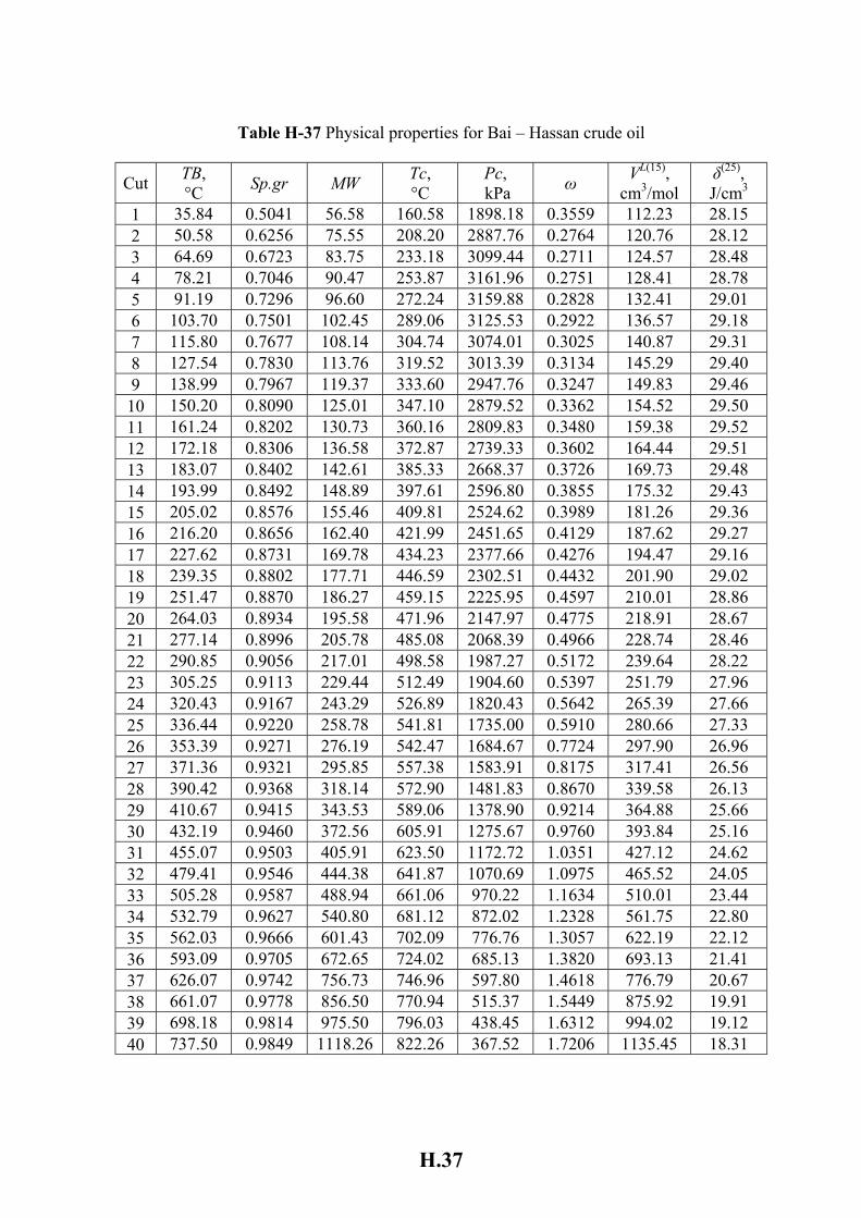
H.37
Table H-37 Physical properties for Bai – Hassan crude oil
Cut TB, °C Sp.gr MW Tc,
°C Pc, kPa ω VL(15),
cm3/mol δ(25), J/cm3
1 35.84 0.5041 56.58 160.58 1898.18 0.3559 112.23 28.15 2 50.58 0.6256 75.55 208.20 2887.76 0.2764 120.76 28.12 3 64.69 0.6723 83.75 233.18 3099.44 0.2711 124.57 28.48 4 78.21 0.7046 90.47 253.87 3161.96 0.2751 128.41 28.78 5 91.19 0.7296 96.60 272.24 3159.88 0.2828 132.41 29.01 6 103.70 0.7501 102.45 289.06 3125.53 0.2922 136.57 29.18 7 115.80 0.7677 108.14 304.74 3074.01 0.3025 140.87 29.31 8 127.54 0.7830 113.76 319.52 3013.39 0.3134 145.29 29.40 9 138.99 0.7967 119.37 333.60 2947.76 0.3247 149.83 29.46 10 150.20 0.8090 125.01 347.10 2879.52 0.3362 154.52 29.50 11 161.24 0.8202 130.73 360.16 2809.83 0.3480 159.38 29.52 12 172.18 0.8306 136.58 372.87 2739.33 0.3602 164.44 29.51 13 183.07 0.8402 142.61 385.33 2668.37 0.3726 169.73 29.48 14 193.99 0.8492 148.89 397.61 2596.80 0.3855 175.32 29.43 15 205.02 0.8576 155.46 409.81 2524.62 0.3989 181.26 29.36 16 216.20 0.8656 162.40 421.99 2451.65 0.4129 187.62 29.27 17 227.62 0.8731 169.78 434.23 2377.66 0.4276 194.47 29.16 18 239.35 0.8802 177.71 446.59 2302.51 0.4432 201.90 29.02 19 251.47 0.8870 186.27 459.15 2225.95 0.4597 210.01 28.86 20 264.03 0.8934 195.58 471.96 2147.97 0.4775 218.91 28.67 21 277.14 0.8996 205.78 485.08 2068.39 0.4966 228.74 28.46 22 290.85 0.9056 217.01 498.58 1987.27 0.5172 239.64 28.22 23 305.25 0.9113 229.44 512.49 1904.60 0.5397 251.79 27.96 24 320.43 0.9167 243.29 526.89 1820.43 0.5642 265.39 27.66 25 336.44 0.9220 258.78 541.81 1735.00 0.5910 280.66 27.33 26 353.39 0.9271 276.19 542.47 1684.67 0.7724 297.90 26.96 27 371.36 0.9321 295.85 557.38 1583.91 0.8175 317.41 26.56 28 390.42 0.9368 318.14 572.90 1481.83 0.8670 339.58 26.13 29 410.67 0.9415 343.53 589.06 1378.90 0.9214 364.88 25.66 30 432.19 0.9460 372.56 605.91 1275.67 0.9760 393.84 25.16 31 455.07 0.9503 405.91 623.50 1172.72 1.0351 427.12 24.62 32 479.41 0.9546 444.38 641.87 1070.69 1.0975 465.52 24.05 33 505.28 0.9587 488.94 661.06 970.22 1.1634 510.01 23.44 34 532.79 0.9627 540.80 681.12 872.02 1.2328 561.75 22.80 35 562.03 0.9666 601.43 702.09 776.76 1.3057 622.19 22.12 36 593.09 0.9705 672.65 724.02 685.13 1.3820 693.13 21.41 37 626.07 0.9742 756.73 746.96 597.80 1.4618 776.79 20.67 38 661.07 0.9778 856.50 770.94 515.37 1.5449 875.92 19.91 39 698.18 0.9814 975.50 796.03 438.45 1.6312 994.02 19.12 40 737.50 0.9849 1118.26 822.26 367.52 1.7206 1135.45 18.31
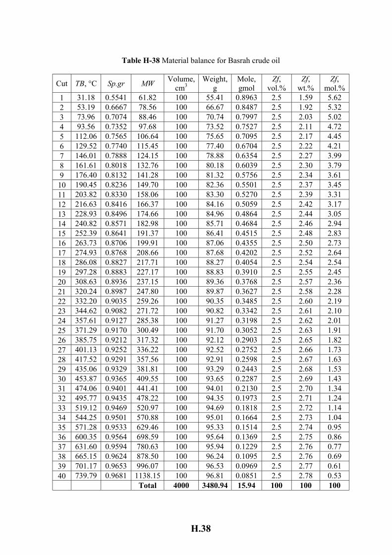
H.38
Table H-38 Material balance for Basrah crude oil
Cut TB, °C Sp.gr MW Volume, cm3
Weight, g
Mole, gmol
Zf, vol.%
Zf, wt.%
Zf, mol.%
1 31.18 0.5541 61.82 100 55.41 0.8963 2.5 1.59 5.62 2 53.19 0.6667 78.56 100 66.67 0.8487 2.5 1.92 5.32 3 73.96 0.7074 88.46 100 70.74 0.7997 2.5 2.03 5.02 4 93.56 0.7352 97.68 100 73.52 0.7527 2.5 2.11 4.72 5 112.06 0.7565 106.64 100 75.65 0.7095 2.5 2.17 4.45 6 129.52 0.7740 115.45 100 77.40 0.6704 2.5 2.22 4.21 7 146.01 0.7888 124.15 100 78.88 0.6354 2.5 2.27 3.99 8 161.61 0.8018 132.76 100 80.18 0.6039 2.5 2.30 3.79 9 176.40 0.8132 141.28 100 81.32 0.5756 2.5 2.34 3.61 10 190.45 0.8236 149.70 100 82.36 0.5501 2.5 2.37 3.45 11 203.82 0.8330 158.06 100 83.30 0.5270 2.5 2.39 3.31 12 216.63 0.8416 166.37 100 84.16 0.5059 2.5 2.42 3.17 13 228.93 0.8496 174.66 100 84.96 0.4864 2.5 2.44 3.05 14 240.82 0.8571 182.98 100 85.71 0.4684 2.5 2.46 2.94 15 252.39 0.8641 191.37 100 86.41 0.4515 2.5 2.48 2.83 16 263.73 0.8706 199.91 100 87.06 0.4355 2.5 2.50 2.73 17 274.93 0.8768 208.66 100 87.68 0.4202 2.5 2.52 2.64 18 286.08 0.8827 217.71 100 88.27 0.4054 2.5 2.54 2.54 19 297.28 0.8883 227.17 100 88.83 0.3910 2.5 2.55 2.45 20 308.63 0.8936 237.15 100 89.36 0.3768 2.5 2.57 2.36 21 320.24 0.8987 247.80 100 89.87 0.3627 2.5 2.58 2.28 22 332.20 0.9035 259.26 100 90.35 0.3485 2.5 2.60 2.19 23 344.62 0.9082 271.72 100 90.82 0.3342 2.5 2.61 2.10 24 357.61 0.9127 285.38 100 91.27 0.3198 2.5 2.62 2.01 25 371.29 0.9170 300.49 100 91.70 0.3052 2.5 2.63 1.91 26 385.75 0.9212 317.32 100 92.12 0.2903 2.5 2.65 1.82 27 401.13 0.9252 336.22 100 92.52 0.2752 2.5 2.66 1.73 28 417.52 0.9291 357.56 100 92.91 0.2598 2.5 2.67 1.63 29 435.06 0.9329 381.81 100 93.29 0.2443 2.5 2.68 1.53 30 453.87 0.9365 409.55 100 93.65 0.2287 2.5 2.69 1.43 31 474.06 0.9401 441.41 100 94.01 0.2130 2.5 2.70 1.34 32 495.77 0.9435 478.22 100 94.35 0.1973 2.5 2.71 1.24 33 519.12 0.9469 520.97 100 94.69 0.1818 2.5 2.72 1.14 34 544.25 0.9501 570.88 100 95.01 0.1664 2.5 2.73 1.04 35 571.28 0.9533 629.46 100 95.33 0.1514 2.5 2.74 0.95 36 600.35 0.9564 698.59 100 95.64 0.1369 2.5 2.75 0.86 37 631.60 0.9594 780.63 100 95.94 0.1229 2.5 2.76 0.77 38 665.15 0.9624 878.50 100 96.24 0.1095 2.5 2.76 0.69 39 701.17 0.9653 996.07 100 96.53 0.0969 2.5 2.77 0.61 40 739.79 0.9681 1138.15 100 96.81 0.0851 2.5 2.78 0.53 Total 4000 3480.94 15.94 100 100 100
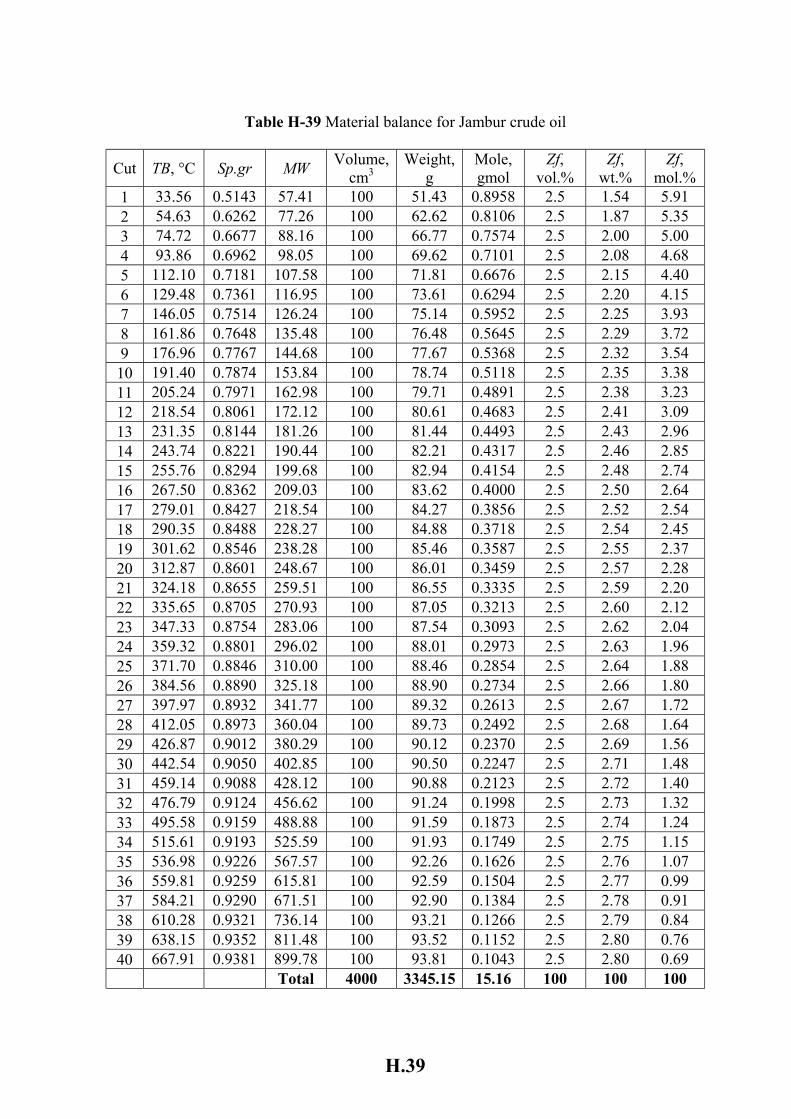
H.39
Table H-39 Material balance for Jambur crude oil
Cut TB, °C Sp.gr MW Volume, cm3
Weight, g
Mole, gmol
Zf, vol.%
Zf, wt.%
Zf, mol.%
1 33.56 0.5143 57.41 100 51.43 0.8958 2.5 1.54 5.91 2 54.63 0.6262 77.26 100 62.62 0.8106 2.5 1.87 5.35 3 74.72 0.6677 88.16 100 66.77 0.7574 2.5 2.00 5.00 4 93.86 0.6962 98.05 100 69.62 0.7101 2.5 2.08 4.68 5 112.10 0.7181 107.58 100 71.81 0.6676 2.5 2.15 4.40 6 129.48 0.7361 116.95 100 73.61 0.6294 2.5 2.20 4.15 7 146.05 0.7514 126.24 100 75.14 0.5952 2.5 2.25 3.93 8 161.86 0.7648 135.48 100 76.48 0.5645 2.5 2.29 3.72 9 176.96 0.7767 144.68 100 77.67 0.5368 2.5 2.32 3.54 10 191.40 0.7874 153.84 100 78.74 0.5118 2.5 2.35 3.38 11 205.24 0.7971 162.98 100 79.71 0.4891 2.5 2.38 3.23 12 218.54 0.8061 172.12 100 80.61 0.4683 2.5 2.41 3.09 13 231.35 0.8144 181.26 100 81.44 0.4493 2.5 2.43 2.96 14 243.74 0.8221 190.44 100 82.21 0.4317 2.5 2.46 2.85 15 255.76 0.8294 199.68 100 82.94 0.4154 2.5 2.48 2.74 16 267.50 0.8362 209.03 100 83.62 0.4000 2.5 2.50 2.64 17 279.01 0.8427 218.54 100 84.27 0.3856 2.5 2.52 2.54 18 290.35 0.8488 228.27 100 84.88 0.3718 2.5 2.54 2.45 19 301.62 0.8546 238.28 100 85.46 0.3587 2.5 2.55 2.37 20 312.87 0.8601 248.67 100 86.01 0.3459 2.5 2.57 2.28 21 324.18 0.8655 259.51 100 86.55 0.3335 2.5 2.59 2.20 22 335.65 0.8705 270.93 100 87.05 0.3213 2.5 2.60 2.12 23 347.33 0.8754 283.06 100 87.54 0.3093 2.5 2.62 2.04 24 359.32 0.8801 296.02 100 88.01 0.2973 2.5 2.63 1.96 25 371.70 0.8846 310.00 100 88.46 0.2854 2.5 2.64 1.88 26 384.56 0.8890 325.18 100 88.90 0.2734 2.5 2.66 1.80 27 397.97 0.8932 341.77 100 89.32 0.2613 2.5 2.67 1.72 28 412.05 0.8973 360.04 100 89.73 0.2492 2.5 2.68 1.64 29 426.87 0.9012 380.29 100 90.12 0.2370 2.5 2.69 1.56 30 442.54 0.9050 402.85 100 90.50 0.2247 2.5 2.71 1.48 31 459.14 0.9088 428.12 100 90.88 0.2123 2.5 2.72 1.40 32 476.79 0.9124 456.62 100 91.24 0.1998 2.5 2.73 1.32 33 495.58 0.9159 488.88 100 91.59 0.1873 2.5 2.74 1.24 34 515.61 0.9193 525.59 100 91.93 0.1749 2.5 2.75 1.15 35 536.98 0.9226 567.57 100 92.26 0.1626 2.5 2.76 1.07 36 559.81 0.9259 615.81 100 92.59 0.1504 2.5 2.77 0.99 37 584.21 0.9290 671.51 100 92.90 0.1384 2.5 2.78 0.91 38 610.28 0.9321 736.14 100 93.21 0.1266 2.5 2.79 0.84 39 638.15 0.9352 811.48 100 93.52 0.1152 2.5 2.80 0.76 40 667.91 0.9381 899.78 100 93.81 0.1043 2.5 2.80 0.69 Total 4000 3345.15 15.16 100 100 100
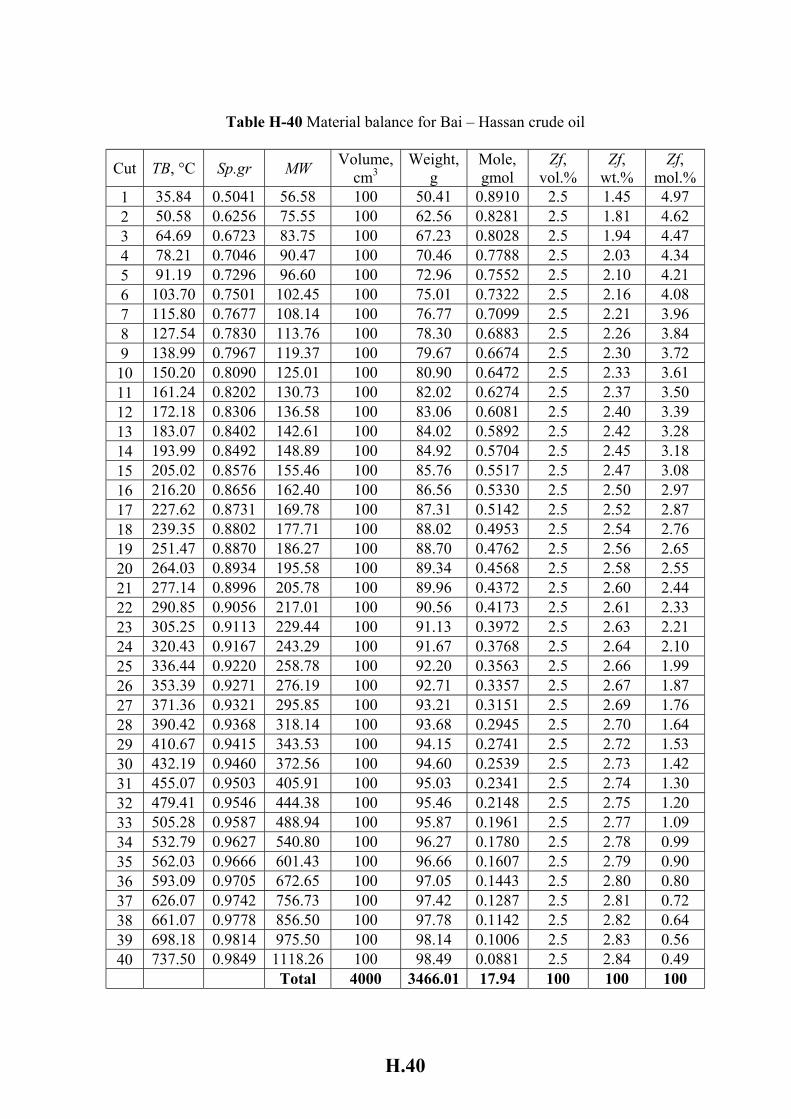
H.40
Table H-40 Material balance for Bai – Hassan crude oil
Cut TB, °C Sp.gr MW Volume, cm3
Weight, g
Mole, gmol
Zf, vol.%
Zf, wt.%
Zf, mol.%
1 35.84 0.5041 56.58 100 50.41 0.8910 2.5 1.45 4.97 2 50.58 0.6256 75.55 100 62.56 0.8281 2.5 1.81 4.62 3 64.69 0.6723 83.75 100 67.23 0.8028 2.5 1.94 4.47 4 78.21 0.7046 90.47 100 70.46 0.7788 2.5 2.03 4.34 5 91.19 0.7296 96.60 100 72.96 0.7552 2.5 2.10 4.21 6 103.70 0.7501 102.45 100 75.01 0.7322 2.5 2.16 4.08 7 115.80 0.7677 108.14 100 76.77 0.7099 2.5 2.21 3.96 8 127.54 0.7830 113.76 100 78.30 0.6883 2.5 2.26 3.84 9 138.99 0.7967 119.37 100 79.67 0.6674 2.5 2.30 3.72 10 150.20 0.8090 125.01 100 80.90 0.6472 2.5 2.33 3.61 11 161.24 0.8202 130.73 100 82.02 0.6274 2.5 2.37 3.50 12 172.18 0.8306 136.58 100 83.06 0.6081 2.5 2.40 3.39 13 183.07 0.8402 142.61 100 84.02 0.5892 2.5 2.42 3.28 14 193.99 0.8492 148.89 100 84.92 0.5704 2.5 2.45 3.18 15 205.02 0.8576 155.46 100 85.76 0.5517 2.5 2.47 3.08 16 216.20 0.8656 162.40 100 86.56 0.5330 2.5 2.50 2.97 17 227.62 0.8731 169.78 100 87.31 0.5142 2.5 2.52 2.87 18 239.35 0.8802 177.71 100 88.02 0.4953 2.5 2.54 2.76 19 251.47 0.8870 186.27 100 88.70 0.4762 2.5 2.56 2.65 20 264.03 0.8934 195.58 100 89.34 0.4568 2.5 2.58 2.55 21 277.14 0.8996 205.78 100 89.96 0.4372 2.5 2.60 2.44 22 290.85 0.9056 217.01 100 90.56 0.4173 2.5 2.61 2.33 23 305.25 0.9113 229.44 100 91.13 0.3972 2.5 2.63 2.21 24 320.43 0.9167 243.29 100 91.67 0.3768 2.5 2.64 2.10 25 336.44 0.9220 258.78 100 92.20 0.3563 2.5 2.66 1.99 26 353.39 0.9271 276.19 100 92.71 0.3357 2.5 2.67 1.87 27 371.36 0.9321 295.85 100 93.21 0.3151 2.5 2.69 1.76 28 390.42 0.9368 318.14 100 93.68 0.2945 2.5 2.70 1.64 29 410.67 0.9415 343.53 100 94.15 0.2741 2.5 2.72 1.53 30 432.19 0.9460 372.56 100 94.60 0.2539 2.5 2.73 1.42 31 455.07 0.9503 405.91 100 95.03 0.2341 2.5 2.74 1.30 32 479.41 0.9546 444.38 100 95.46 0.2148 2.5 2.75 1.20 33 505.28 0.9587 488.94 100 95.87 0.1961 2.5 2.77 1.09 34 532.79 0.9627 540.80 100 96.27 0.1780 2.5 2.78 0.99 35 562.03 0.9666 601.43 100 96.66 0.1607 2.5 2.79 0.90 36 593.09 0.9705 672.65 100 97.05 0.1443 2.5 2.80 0.80 37 626.07 0.9742 756.73 100 97.42 0.1287 2.5 2.81 0.72 38 661.07 0.9778 856.50 100 97.78 0.1142 2.5 2.82 0.64 39 698.18 0.9814 975.50 100 98.14 0.1006 2.5 2.83 0.56 40 737.50 0.9849 1118.26 100 98.49 0.0881 2.5 2.84 0.49 Total 4000 3466.01 17.94 100 100 100

H.41
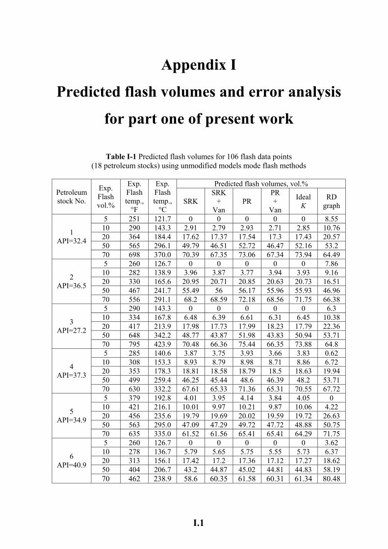
I.1
Appendix I
Predicted flash volumes and error analysis
for part one of present work
Table I-1 Predicted flash volumes for 106 flash data points (18 petroleum stocks) using unmodified models mode flash methods
Predicted flash volumes, vol.%
Petroleum stock No.
Exp. Flash vol.%
Exp. Flash temp.,
°F
Exp. Flash temp.,
°C SRK
SRK +
Van PR
PR +
Van
Ideal K
RD graph
5 251 121.7 0 0 0 0 0 8.55 10 290 143.3 2.91 2.79 2.93 2.71 2.85 10.76 20 364 184.4 17.62 17.37 17.54 17.3 17.43 20.57 50 565 296.1 49.79 46.51 52.72 46.47 52.16 53.2
1 API=32.4
70 698 370.0 70.39 67.35 73.06 67.34 73.94 64.49 5 260 126.7 0 0 0 0 0 7.86
10 282 138.9 3.96 3.87 3.77 3.94 3.93 9.16 20 330 165.6 20.95 20.71 20.85 20.63 20.73 16.51 50 467 241.7 55.49 56 56.17 55.96 55.93 46.96
2 API=36.5
70 556 291.1 68.2 68.59 72.18 68.56 71.75 66.38 5 290 143.3 0 0 0 0 0 6.3
10 334 167.8 6.48 6.39 6.61 6.31 6.45 10.38 20 417 213.9 17.98 17.73 17.99 18.23 17.79 22.36 50 648 342.2 48.77 43.87 51.98 43.83 50.94 53.71
3 API=27.2
70 795 423.9 70.48 66.36 75.44 66.35 73.88 64.8 5 285 140.6 3.87 3.75 3.93 3.66 3.83 0.62
10 308 153.3 8.93 8.79 8.98 8.71 8.86 6.72 20 353 178.3 18.81 18.58 18.79 18.5 18.63 19.94 50 499 259.4 46.25 45.44 48.6 46.39 48.2 53.71
4 API=37.3
70 630 332.2 67.61 65.33 71.36 65.31 70.55 67.72 5 379 192.8 4.01 3.95 4.14 3.84 4.05 0
10 421 216.1 10.01 9.97 10.21 9.87 10.06 4.22 20 456 235.6 19.79 19.69 20.02 19.59 19.72 26.63 50 563 295.0 47.09 47.29 49.72 47.72 48.88 50.75
5 API=34.9
70 635 335.0 61.52 61.56 65.41 65.41 64.29 71.75 5 260 126.7 0 0 0 0 0 3.62
10 278 136.7 5.79 5.65 5.75 5.55 5.73 6.37 20 313 156.1 17.42 17.2 17.36 17.12 17.27 18.62 50 404 206.7 43.2 44.87 45.02 44.81 44.83 58.19
6 API=40.9
70 462 238.9 58.6 60.35 61.58 60.31 61.34 80.48
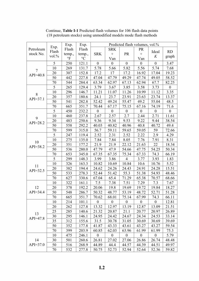
I.2
Continue, Table I-1 Predicted flash volumes for 106 flash data points (18 petroleum stocks) using unmodified models mode flash methods
Predicted flash volumes, vol.%
Petroleum stock No.
Exp. Flash vol.%
Exp. Flash temp.,
°F
Exp. Flash temp.,
°C SRK
SRK +
Van PR
PR +
Van
Ideal K
RD graph
5 250 121.1 0 0 0 0 0 3.47 10 269 131.7 5.78 5.66 5.82 5.56 5.74 7.68 20 307 152.8 17.2 17 17.2 16.92 17.04 19.23 50 442 227.8 47.04 47.79 49.29 47.74 49.05 58.52
7 API=40.8
70 544 284.4 63.34 62.97 67.13 62.94 67.7 82.25 5 265 129.4 3.79 3.67 3.85 3.58 3.73 0 10 296 146.7 11.21 11.07 11.26 10.99 11.12 3.35 20 357 180.6 24.1 23.7 23.91 23.63 23.74 13.37 50 541 282.8 52.42 49.24 55.47 49.2 55.04 48.5
8 API=37.1
70 665 351.7 70.44 67.17 75.15 67.16 74.19 71.6 5 450 232.2 0 0 0 0 0 0 10 460 237.8 2.67 2.57 2.7 2.44 2.71 11.61 20 483 250.6 9.36 9.34 9.53 9.22 9.44 38.54 50 558 292.2 40.03 40.82 40.96 40.8 40.72 49.4
9 API=28.2
70 599 315.0 56.7 59.11 59.65 59.05 59 72.66 5 247 119.4 2.52 2.31 2.52 2.22 2.9 4.29 10 275 135.0 7.84 7.84 8.05 7.76 7.91 8.31 20 351 177.2 21.9 21.9 22.12 21.63 22 18.34 50 536 280.0 47.79 47.9 54.66 47.75 54.25 50.34
10 API=38.2
70 653 345.0 67.35 67.35 75.34 67.33 74.3 66.19 5 299 148.3 3.99 3.86 4 3.77 3.93 1.83 10 326 163.3 10.82 10.69 10.84 10.6 10.76 5.52 20 382 194.4 24.62 24.26 24.43 24.91 24.28 15.51 50 533 278.3 52.44 51.42 55.3 51.38 54.93 48.46
11 API=32.5
70 627 330.6 67.04 65.4 71.29 65.38 70.57 68.66 10 322 161.1 7.5 7.38 7.51 7.29 7.3 7.67 20 378 192.2 20.06 19.8 19.69 19.72 19.84 18.27 50 548 286.7 50.32 48.77 53.19 48.72 52.71 51.28
12 API=34.4
70 665 351.7 70.62 68.01 75.14 67.99 74.3 66.11 10 214 101.1 0 0 0 0 0 12.81 20 262 127.8 13.32 12.97 13.19 12.87 13.09 21.51 25 285 140.6 21.32 20.87 21.1 20.77 20.97 26.89 30 295 146.1 24.95 24.42 24.67 24.34 24.53 33.14 35 312 155.6 31.5 30.78 31.05 30.69 30.69 39.69 50 352 177.8 41.87 43.33 43.61 43.27 43.27 59.54
13 API=47.8
70 399 203.9 60.85 62.03 63.96 61.99 61.99 75.3 10 475 246.1 0 0 0 0 0 5.79 30 501 260.6 26.81 27.02 27.06 26.86 26.74 48.48 50 516 268.9 44.89 44.4 44.57 44.39 44.51 49.97
14 API=37.0
70 532 277.8 50.75 52.73 52.94 52.64 52.36 59.82
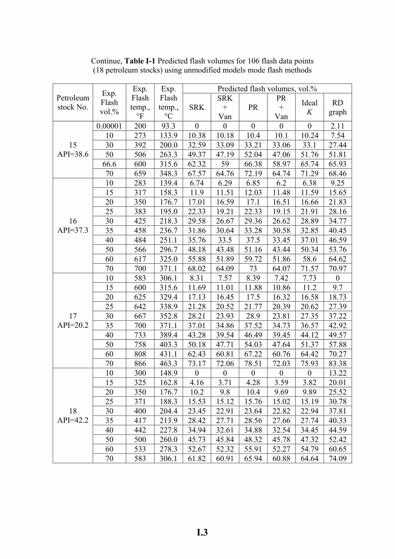
I.3
Continue, Table I-1 Predicted flash volumes for 106 flash data points (18 petroleum stocks) using unmodified models mode flash methods
Predicted flash volumes, vol.%
Petroleum stock No.
Exp. Flash vol.%
Exp. Flash temp.,
°F
Exp. Flash temp.,
°C SRK
SRK +
Van PR
PR +
Van
Ideal K
RD graph
0.00001 200 93.3 0 0 0 0 0 2.11 10 273 133.9 10.38 10.18 10.4 10.1 10.24 7.54 30 392 200.0 32.59 33.09 33.21 33.06 33.1 27.44 50 506 263.3 49.37 47.19 52.04 47.06 51.76 51.81
66.6 600 315.6 62.32 59 66.38 58.97 65.74 65.93
15 API=38.6
70 659 348.3 67.57 64.76 72.19 64.74 71.29 68.46 10 283 139.4 6.74 6.29 6.85 6.2 6.38 9.25 15 317 158.3 11.9 11.51 12.03 11.48 11.59 15.65 20 350 176.7 17.01 16.59 17.1 16.51 16.66 21.83 25 383 195.0 22.33 19.21 22.33 19.15 21.91 28.16 30 425 218.3 29.58 26.67 29.36 26.62 28.89 34.77 35 458 236.7 31.86 30.64 33.28 30.58 32.85 40.45 40 484 251.1 35.76 33.5 37.5 33.45 37.01 46.59 50 566 296.7 48.18 43.48 51.16 43.44 50.34 53.76 60 617 325.0 55.88 51.89 59.72 51.86 58.6 64.62
16 API=37.3
70 700 371.1 68.02 64.09 73 64.07 71.57 70.97 10 583 306.1 8.31 7.57 8.39 7.42 7.73 0 15 600 315.6 11.69 11.01 11.88 10.86 11.2 9.7 20 625 329.4 17.13 16.45 17.5 16.32 16.58 18.73 25 642 338.9 21.28 20.52 21.77 20.39 20.62 27.39 30 667 352.8 28.21 23.93 28.9 23.81 27.35 37.22 35 700 371.1 37.01 34.86 37.52 34.73 36.57 42.92 40 733 389.4 43.28 39.54 46.49 39.45 44.12 49.57 50 758 403.3 50.18 47.71 54.03 47.64 51.37 57.88 60 808 431.1 62.43 60.81 67.22 60.76 64.42 70.27
17 API=20.2
70 866 463.3 73.17 72.06 78.51 72.03 75.93 83.38 10 300 148.9 0 0 0 0 0 13.22 15 325 162.8 4.16 3.71 4.28 3.59 3.82 20.01 20 350 176.7 10.2 9.8 10.4 9.69 9.89 25.52 25 371 188.3 15.53 15.12 15.76 15.02 15.19 30.78 30 400 204.4 23.45 22.91 23.64 22.82 22.94 37.81 35 417 213.9 28.42 27.71 28.56 27.66 27.74 40.33 40 442 227.8 34.94 32.61 34.88 32.54 34.45 44.59 50 500 260.0 45.73 45.84 48.32 45.78 47.32 52.42 60 533 278.3 52.67 52.32 55.91 52.27 54.79 60.65
18 API=42.2
70 583 306.1 61.82 60.91 65.94 60.88 64.64 74.09
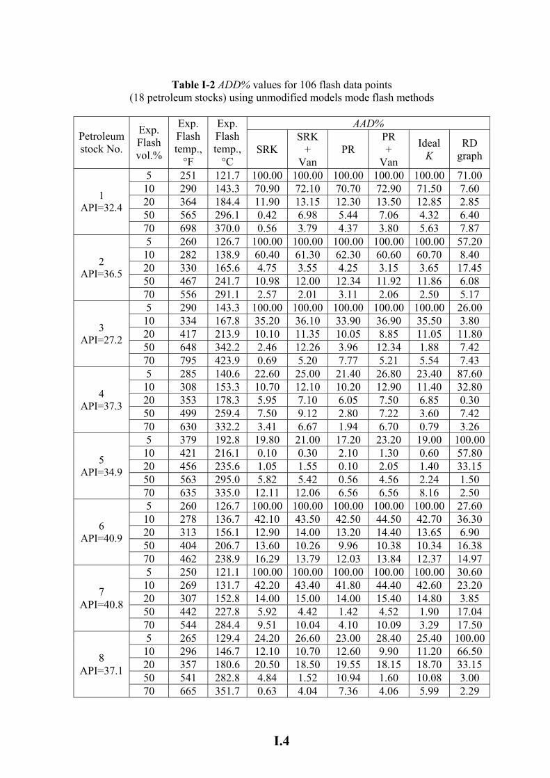
I.4
Table I-2 ADD% values for 106 flash data points (18 petroleum stocks) using unmodified models mode flash methods
AAD%
Petroleum stock No.
Exp. Flash vol.%
Exp. Flash temp.,
°F
Exp. Flash temp.,
°C SRK
SRK +
Van PR
PR +
Van
Ideal K
RD graph
5 251 121.7 100.00 100.00 100.00 100.00 100.00 71.00 10 290 143.3 70.90 72.10 70.70 72.90 71.50 7.60 20 364 184.4 11.90 13.15 12.30 13.50 12.85 2.85 50 565 296.1 0.42 6.98 5.44 7.06 4.32 6.40
1 API=32.4
70 698 370.0 0.56 3.79 4.37 3.80 5.63 7.87 5 260 126.7 100.00 100.00 100.00 100.00 100.00 57.20 10 282 138.9 60.40 61.30 62.30 60.60 60.70 8.40 20 330 165.6 4.75 3.55 4.25 3.15 3.65 17.45 50 467 241.7 10.98 12.00 12.34 11.92 11.86 6.08
2 API=36.5
70 556 291.1 2.57 2.01 3.11 2.06 2.50 5.17 5 290 143.3 100.00 100.00 100.00 100.00 100.00 26.00 10 334 167.8 35.20 36.10 33.90 36.90 35.50 3.80 20 417 213.9 10.10 11.35 10.05 8.85 11.05 11.80 50 648 342.2 2.46 12.26 3.96 12.34 1.88 7.42
3 API=27.2
70 795 423.9 0.69 5.20 7.77 5.21 5.54 7.43 5 285 140.6 22.60 25.00 21.40 26.80 23.40 87.60 10 308 153.3 10.70 12.10 10.20 12.90 11.40 32.80 20 353 178.3 5.95 7.10 6.05 7.50 6.85 0.30 50 499 259.4 7.50 9.12 2.80 7.22 3.60 7.42
4 API=37.3
70 630 332.2 3.41 6.67 1.94 6.70 0.79 3.26 5 379 192.8 19.80 21.00 17.20 23.20 19.00 100.0010 421 216.1 0.10 0.30 2.10 1.30 0.60 57.80 20 456 235.6 1.05 1.55 0.10 2.05 1.40 33.15 50 563 295.0 5.82 5.42 0.56 4.56 2.24 1.50
5 API=34.9
70 635 335.0 12.11 12.06 6.56 6.56 8.16 2.50 5 260 126.7 100.00 100.00 100.00 100.00 100.00 27.60 10 278 136.7 42.10 43.50 42.50 44.50 42.70 36.30 20 313 156.1 12.90 14.00 13.20 14.40 13.65 6.90 50 404 206.7 13.60 10.26 9.96 10.38 10.34 16.38
6 API=40.9
70 462 238.9 16.29 13.79 12.03 13.84 12.37 14.97 5 250 121.1 100.00 100.00 100.00 100.00 100.00 30.60 10 269 131.7 42.20 43.40 41.80 44.40 42.60 23.20 20 307 152.8 14.00 15.00 14.00 15.40 14.80 3.85 50 442 227.8 5.92 4.42 1.42 4.52 1.90 17.04
7 API=40.8
70 544 284.4 9.51 10.04 4.10 10.09 3.29 17.50 5 265 129.4 24.20 26.60 23.00 28.40 25.40 100.0010 296 146.7 12.10 10.70 12.60 9.90 11.20 66.50 20 357 180.6 20.50 18.50 19.55 18.15 18.70 33.15 50 541 282.8 4.84 1.52 10.94 1.60 10.08 3.00
8 API=37.1
70 665 351.7 0.63 4.04 7.36 4.06 5.99 2.29
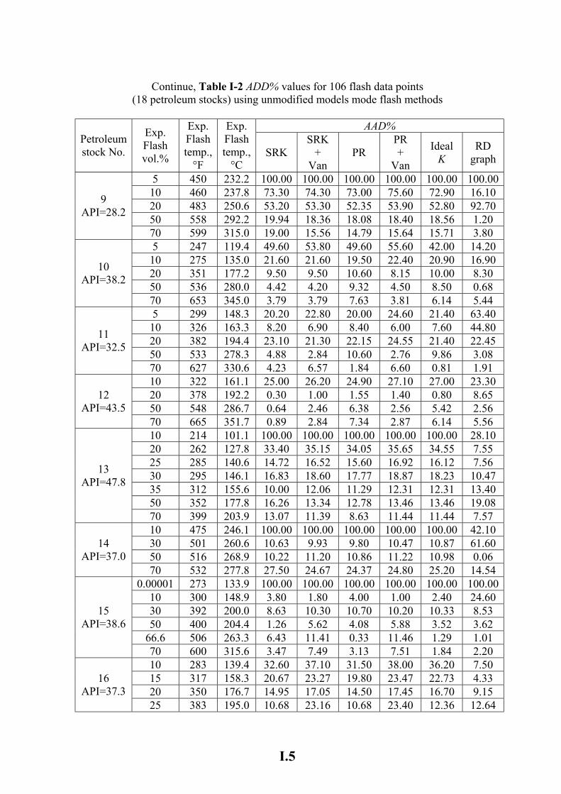
I.5
Continue, Table I-2 ADD% values for 106 flash data points (18 petroleum stocks) using unmodified models mode flash methods
AAD%
Petroleum stock No.
Exp. Flash vol.%
Exp. Flash temp.,
°F
Exp. Flash temp.,
°C SRK
SRK +
Van PR
PR +
Van
Ideal K
RD graph
5 450 232.2 100.00 100.00 100.00 100.00 100.00 100.0010 460 237.8 73.30 74.30 73.00 75.60 72.90 16.10 20 483 250.6 53.20 53.30 52.35 53.90 52.80 92.70 50 558 292.2 19.94 18.36 18.08 18.40 18.56 1.20
9 API=28.2
70 599 315.0 19.00 15.56 14.79 15.64 15.71 3.80 5 247 119.4 49.60 53.80 49.60 55.60 42.00 14.20 10 275 135.0 21.60 21.60 19.50 22.40 20.90 16.90 20 351 177.2 9.50 9.50 10.60 8.15 10.00 8.30 50 536 280.0 4.42 4.20 9.32 4.50 8.50 0.68
10 API=38.2
70 653 345.0 3.79 3.79 7.63 3.81 6.14 5.44 5 299 148.3 20.20 22.80 20.00 24.60 21.40 63.40 10 326 163.3 8.20 6.90 8.40 6.00 7.60 44.80 20 382 194.4 23.10 21.30 22.15 24.55 21.40 22.45 50 533 278.3 4.88 2.84 10.60 2.76 9.86 3.08
11 API=32.5
70 627 330.6 4.23 6.57 1.84 6.60 0.81 1.91 10 322 161.1 25.00 26.20 24.90 27.10 27.00 23.30 20 378 192.2 0.30 1.00 1.55 1.40 0.80 8.65 50 548 286.7 0.64 2.46 6.38 2.56 5.42 2.56
12 API=43.5
70 665 351.7 0.89 2.84 7.34 2.87 6.14 5.56 10 214 101.1 100.00 100.00 100.00 100.00 100.00 28.10 20 262 127.8 33.40 35.15 34.05 35.65 34.55 7.55 25 285 140.6 14.72 16.52 15.60 16.92 16.12 7.56 30 295 146.1 16.83 18.60 17.77 18.87 18.23 10.47 35 312 155.6 10.00 12.06 11.29 12.31 12.31 13.40 50 352 177.8 16.26 13.34 12.78 13.46 13.46 19.08
13 API=47.8
70 399 203.9 13.07 11.39 8.63 11.44 11.44 7.57 10 475 246.1 100.00 100.00 100.00 100.00 100.00 42.10 30 501 260.6 10.63 9.93 9.80 10.47 10.87 61.60 50 516 268.9 10.22 11.20 10.86 11.22 10.98 0.06
14 API=37.0
70 532 277.8 27.50 24.67 24.37 24.80 25.20 14.54 0.00001 273 133.9 100.00 100.00 100.00 100.00 100.00 100.00
10 300 148.9 3.80 1.80 4.00 1.00 2.40 24.60 30 392 200.0 8.63 10.30 10.70 10.20 10.33 8.53 50 400 204.4 1.26 5.62 4.08 5.88 3.52 3.62
66.6 506 263.3 6.43 11.41 0.33 11.46 1.29 1.01
15 API=38.6
70 600 315.6 3.47 7.49 3.13 7.51 1.84 2.20 10 283 139.4 32.60 37.10 31.50 38.00 36.20 7.50 15 317 158.3 20.67 23.27 19.80 23.47 22.73 4.33 20 350 176.7 14.95 17.05 14.50 17.45 16.70 9.15
16 API=37.3
25 383 195.0 10.68 23.16 10.68 23.40 12.36 12.64
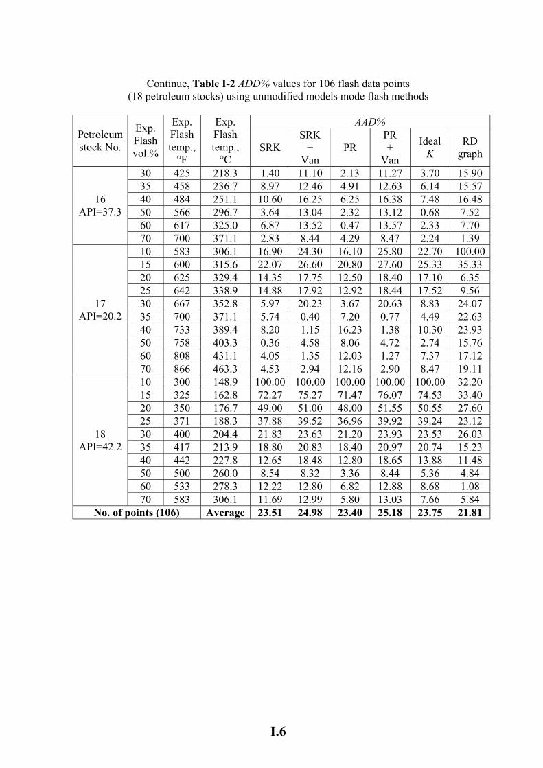
I.6
Continue, Table I-2 ADD% values for 106 flash data points (18 petroleum stocks) using unmodified models mode flash methods
AAD%
Petroleum stock No.
Exp. Flash vol.%
Exp. Flash temp.,
°F
Exp. Flash temp.,
°C SRK
SRK +
Van PR
PR +
Van
Ideal K
RD graph
30 425 218.3 1.40 11.10 2.13 11.27 3.70 15.90 35 458 236.7 8.97 12.46 4.91 12.63 6.14 15.57 40 484 251.1 10.60 16.25 6.25 16.38 7.48 16.48 50 566 296.7 3.64 13.04 2.32 13.12 0.68 7.52 60 617 325.0 6.87 13.52 0.47 13.57 2.33 7.70
16 API=37.3
70 700 371.1 2.83 8.44 4.29 8.47 2.24 1.39 10 583 306.1 16.90 24.30 16.10 25.80 22.70 100.0015 600 315.6 22.07 26.60 20.80 27.60 25.33 35.33 20 625 329.4 14.35 17.75 12.50 18.40 17.10 6.35 25 642 338.9 14.88 17.92 12.92 18.44 17.52 9.56 30 667 352.8 5.97 20.23 3.67 20.63 8.83 24.07 35 700 371.1 5.74 0.40 7.20 0.77 4.49 22.63 40 733 389.4 8.20 1.15 16.23 1.38 10.30 23.93 50 758 403.3 0.36 4.58 8.06 4.72 2.74 15.76 60 808 431.1 4.05 1.35 12.03 1.27 7.37 17.12
17 API=20.2
70 866 463.3 4.53 2.94 12.16 2.90 8.47 19.11 10 300 148.9 100.00 100.00 100.00 100.00 100.00 32.20 15 325 162.8 72.27 75.27 71.47 76.07 74.53 33.40 20 350 176.7 49.00 51.00 48.00 51.55 50.55 27.60 25 371 188.3 37.88 39.52 36.96 39.92 39.24 23.12 30 400 204.4 21.83 23.63 21.20 23.93 23.53 26.03 35 417 213.9 18.80 20.83 18.40 20.97 20.74 15.23 40 442 227.8 12.65 18.48 12.80 18.65 13.88 11.48 50 500 260.0 8.54 8.32 3.36 8.44 5.36 4.84 60 533 278.3 12.22 12.80 6.82 12.88 8.68 1.08
18 API=42.2
70 583 306.1 11.69 12.99 5.80 13.03 7.66 5.84 No. of points (106) Average 23.51 24.98 23.40 25.18 23.75 21.81
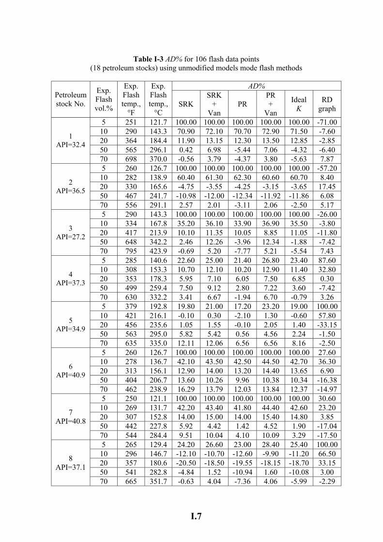
I.7
Table I-3 AD% for 106 flash data points (18 petroleum stocks) using unmodified models mode flash methods
AD%
Petroleum stock No.
Exp. Flash vol.%
Exp. Flash temp.,
°F
Exp. Flash temp.,
°C SRK
SRK +
Van PR
PR +
Van
Ideal K
RD graph
5 251 121.7 100.00 100.00 100.00 100.00 100.00 -71.00 10 290 143.3 70.90 72.10 70.70 72.90 71.50 -7.60 20 364 184.4 11.90 13.15 12.30 13.50 12.85 -2.85 50 565 296.1 0.42 6.98 -5.44 7.06 -4.32 -6.40
1 API=32.4
70 698 370.0 -0.56 3.79 -4.37 3.80 -5.63 7.87 5 260 126.7 100.00 100.00 100.00 100.00 100.00 -57.20 10 282 138.9 60.40 61.30 62.30 60.60 60.70 8.40 20 330 165.6 -4.75 -3.55 -4.25 -3.15 -3.65 17.45 50 467 241.7 -10.98 -12.00 -12.34 -11.92 -11.86 6.08
2 API=36.5
70 556 291.1 2.57 2.01 -3.11 2.06 -2.50 5.17 5 290 143.3 100.00 100.00 100.00 100.00 100.00 -26.00 10 334 167.8 35.20 36.10 33.90 36.90 35.50 -3.80 20 417 213.9 10.10 11.35 10.05 8.85 11.05 -11.80 50 648 342.2 2.46 12.26 -3.96 12.34 -1.88 -7.42
3 API=27.2
70 795 423.9 -0.69 5.20 -7.77 5.21 -5.54 7.43 5 285 140.6 22.60 25.00 21.40 26.80 23.40 87.60 10 308 153.3 10.70 12.10 10.20 12.90 11.40 32.80 20 353 178.3 5.95 7.10 6.05 7.50 6.85 0.30 50 499 259.4 7.50 9.12 2.80 7.22 3.60 -7.42
4 API=37.3
70 630 332.2 3.41 6.67 -1.94 6.70 -0.79 3.26 5 379 192.8 19.80 21.00 17.20 23.20 19.00 100.0010 421 216.1 -0.10 0.30 -2.10 1.30 -0.60 57.80 20 456 235.6 1.05 1.55 -0.10 2.05 1.40 -33.15 50 563 295.0 5.82 5.42 0.56 4.56 2.24 -1.50
5 API=34.9
70 635 335.0 12.11 12.06 6.56 6.56 8.16 -2.50 5 260 126.7 100.00 100.00 100.00 100.00 100.00 27.60 10 278 136.7 42.10 43.50 42.50 44.50 42.70 36.30 20 313 156.1 12.90 14.00 13.20 14.40 13.65 6.90 50 404 206.7 13.60 10.26 9.96 10.38 10.34 -16.38
6 API=40.9
70 462 238.9 16.29 13.79 12.03 13.84 12.37 -14.97 5 250 121.1 100.00 100.00 100.00 100.00 100.00 30.60 10 269 131.7 42.20 43.40 41.80 44.40 42.60 23.20 20 307 152.8 14.00 15.00 14.00 15.40 14.80 3.85 50 442 227.8 5.92 4.42 1.42 4.52 1.90 -17.04
7 API=40.8
70 544 284.4 9.51 10.04 4.10 10.09 3.29 -17.50 5 265 129.4 24.20 26.60 23.00 28.40 25.40 100.0010 296 146.7 -12.10 -10.70 -12.60 -9.90 -11.20 66.50 20 357 180.6 -20.50 -18.50 -19.55 -18.15 -18.70 33.15 50 541 282.8 -4.84 1.52 -10.94 1.60 -10.08 3.00
8 API=37.1
70 665 351.7 -0.63 4.04 -7.36 4.06 -5.99 -2.29
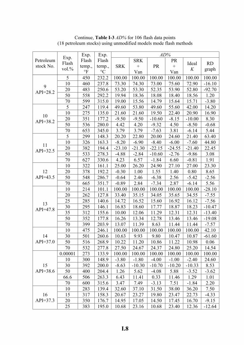
I.8
Continue, Table I-3 AD% for 106 flash data points (18 petroleum stocks) using unmodified models mode flash methods
AD%
Petroleum stock No.
Exp. Flash vol.%
Exp. Flash temp.,
°F
Exp. Flash temp.,
°C SRK
SRK +
Van PR
PR +
Van
Ideal K
RD graph
5 450 232.2 100.00 100.00 100.00 100.00 100.00 100.0010 460 237.8 73.30 74.30 73.00 75.60 72.90 -16.10 20 483 250.6 53.20 53.30 52.35 53.90 52.80 -92.70 50 558 292.2 19.94 18.36 18.08 18.40 18.56 1.20
9 API=28.2
70 599 315.0 19.00 15.56 14.79 15.64 15.71 -3.80 5 247 119.4 49.60 53.80 49.60 55.60 42.00 14.20 10 275 135.0 21.60 21.60 19.50 22.40 20.90 16.90 20 351 177.2 -9.50 -9.50 -10.60 -8.15 -10.00 8.30 50 536 280.0 4.42 4.20 -9.32 4.50 -8.50 -0.68
10 API=38.2
70 653 345.0 3.79 3.79 -7.63 3.81 -6.14 5.44 5 299 148.3 20.20 22.80 20.00 24.60 21.40 63.40 10 326 163.3 -8.20 -6.90 -8.40 -6.00 -7.60 44.80 20 382 194.4 -23.10 -21.30 -22.15 -24.55 -21.40 22.45 50 533 278.3 -4.88 -2.84 -10.60 -2.76 -9.86 3.08
11 API=32.5
70 627 330.6 4.23 6.57 -1.84 6.60 -0.81 1.91 10 322 161.1 25.00 26.20 24.90 27.10 27.00 23.30 20 378 192.2 -0.30 1.00 1.55 1.40 0.80 8.65 50 548 286.7 -0.64 2.46 -6.38 2.56 -5.42 -2.56
12 API=43.5
70 665 351.7 -0.89 2.84 -7.34 2.87 -6.14 5.56 10 214 101.1 100.00 100.00 100.00 100.00 100.00 -28.10 20 262 127.8 33.40 35.15 34.05 35.65 34.55 -7.55 25 285 140.6 14.72 16.52 15.60 16.92 16.12 -7.56 30 295 146.1 16.83 18.60 17.77 18.87 18.23 -10.47 35 312 155.6 10.00 12.06 11.29 12.31 12.31 -13.40 50 352 177.8 16.26 13.34 12.78 13.46 13.46 -19.08
13 API=47.8
70 399 203.9 13.07 11.39 8.63 11.44 11.44 -7.57 10 475 246.1 100.00 100.00 100.00 100.00 100.00 42.10 30 501 260.6 10.63 9.93 9.80 10.47 10.87 -61.60 50 516 268.9 10.22 11.20 10.86 11.22 10.98 0.06
14 API=37.0
70 532 277.8 27.50 24.67 24.37 24.80 25.20 14.54 0.00001 273 133.9 100.00 100.00 100.00 100.00 100.00 100.00
10 300 148.9 -3.80 -1.80 -4.00 -1.00 -2.40 24.60 30 392 200.0 -8.63 -10.30 -10.70 -10.20 -10.33 8.53 50 400 204.4 1.26 5.62 -4.08 5.88 -3.52 -3.62
66.6 506 263.3 6.43 11.41 0.33 11.46 1.29 1.01
15 API=38.6
70 600 315.6 3.47 7.49 -3.13 7.51 -1.84 2.20 10 283 139.4 32.60 37.10 31.50 38.00 36.20 7.50 15 317 158.3 20.67 23.27 19.80 23.47 22.73 -4.33 20 350 176.7 14.95 17.05 14.50 17.45 16.70 -9.15
16 API=37.3
25 383 195.0 10.68 23.16 10.68 23.40 12.36 -12.64
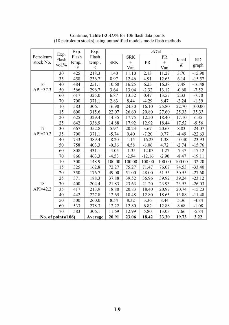
I.9
Continue, Table I-3 AD% for 106 flash data points (18 petroleum stocks) using unmodified models mode flash methods
AD%
Petroleum stock No.
Exp. Flash vol.%
Exp. Flash temp.,
°F
Exp. Flash temp.,
°C SRK
SRK +
Van PR
PR +
Van
Ideal K
RD graph
30 425 218.3 1.40 11.10 2.13 11.27 3.70 -15.90 35 458 236.7 8.97 12.46 4.91 12.63 6.14 -15.57 40 484 251.1 10.60 16.25 6.25 16.38 7.48 -16.48 50 566 296.7 3.64 13.04 -2.32 13.12 -0.68 -7.52 60 617 325.0 6.87 13.52 0.47 13.57 2.33 -7.70
16 API=37.3
70 700 371.1 2.83 8.44 -4.29 8.47 -2.24 -1.39 10 583 306.1 16.90 24.30 16.10 25.80 22.70 100.0015 600 315.6 22.07 26.60 20.80 27.60 25.33 35.33 20 625 329.4 14.35 17.75 12.50 18.40 17.10 6.35 25 642 338.9 14.88 17.92 12.92 18.44 17.52 -9.56 30 667 352.8 5.97 20.23 3.67 20.63 8.83 -24.07 35 700 371.1 -5.74 0.40 -7.20 0.77 -4.49 -22.63 40 733 389.4 -8.20 1.15 -16.23 1.38 -10.30 -23.93 50 758 403.3 -0.36 4.58 -8.06 4.72 -2.74 -15.76 60 808 431.1 -4.05 -1.35 -12.03 -1.27 -7.37 -17.12
17 API=20.2
70 866 463.3 -4.53 -2.94 -12.16 -2.90 -8.47 -19.11 10 300 148.9 100.00 100.00 100.00 100.00 100.00 -32.20 15 325 162.8 72.27 75.27 71.47 76.07 74.53 -33.40 20 350 176.7 49.00 51.00 48.00 51.55 50.55 -27.60 25 371 188.3 37.88 39.52 36.96 39.92 39.24 -23.12 30 400 204.4 21.83 23.63 21.20 23.93 23.53 -26.03 35 417 213.9 18.80 20.83 18.40 20.97 20.74 -15.23 40 442 227.8 12.65 18.48 12.80 18.65 13.88 -11.48 50 500 260.0 8.54 8.32 3.36 8.44 5.36 -4.84 60 533 278.3 12.22 12.80 6.82 12.88 8.68 -1.08
18 API=42.2
70 583 306.1 11.69 12.99 5.80 13.03 7.66 -5.84 No. of points(106) Average 20.91 23.06 18.42 23.30 19.73 3.22
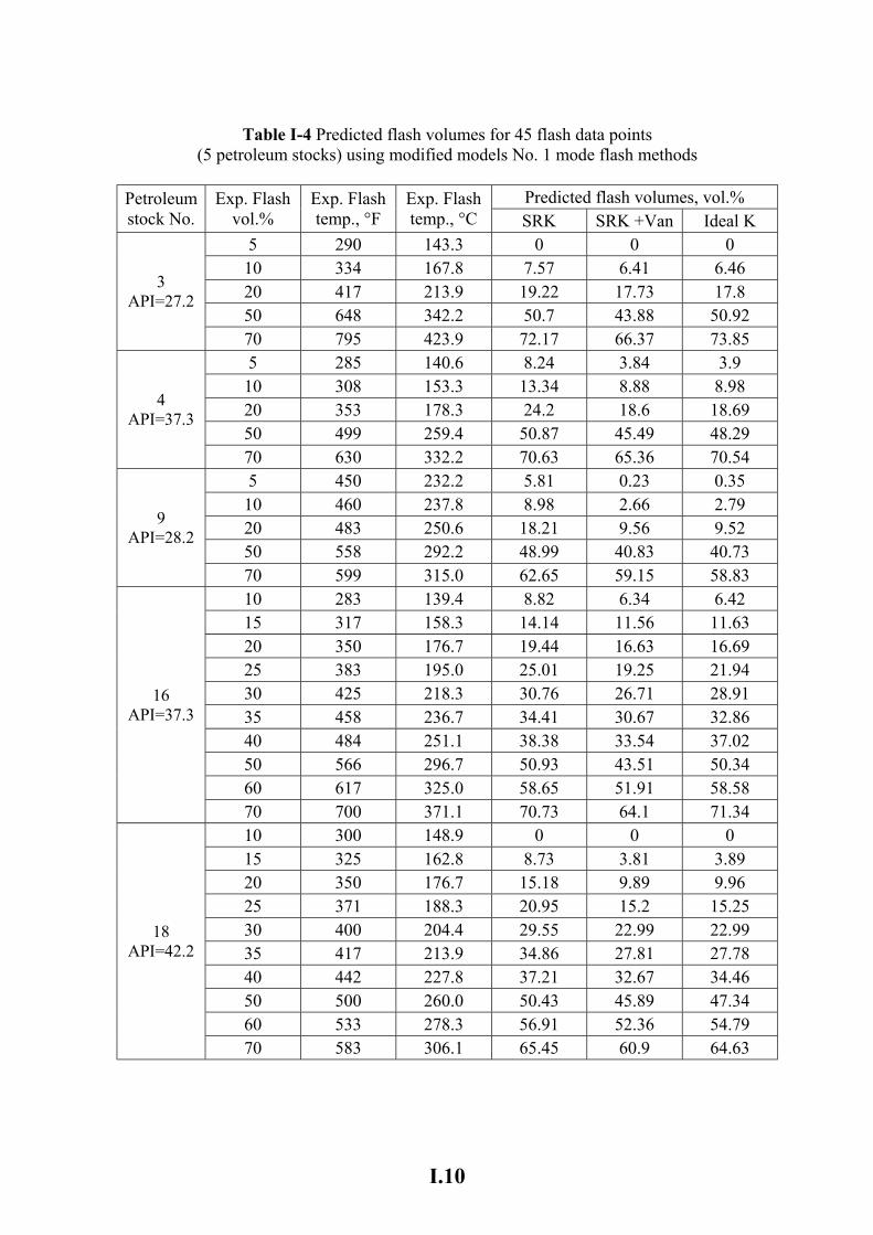
I.10
Table I-4 Predicted flash volumes for 45 flash data points (5 petroleum stocks) using modified models No. 1 mode flash methods
Predicted flash volumes, vol.% Petroleum
stock No. Exp. Flash
vol.% Exp. Flash temp., °F
Exp. Flash temp., °C SRK SRK +Van Ideal K
5 290 143.3 0 0 0 10 334 167.8 7.57 6.41 6.46 20 417 213.9 19.22 17.73 17.8 50 648 342.2 50.7 43.88 50.92
3 API=27.2
70 795 423.9 72.17 66.37 73.85 5 285 140.6 8.24 3.84 3.9 10 308 153.3 13.34 8.88 8.98 20 353 178.3 24.2 18.6 18.69 50 499 259.4 50.87 45.49 48.29
4 API=37.3
70 630 332.2 70.63 65.36 70.54 5 450 232.2 5.81 0.23 0.35 10 460 237.8 8.98 2.66 2.79 20 483 250.6 18.21 9.56 9.52 50 558 292.2 48.99 40.83 40.73
9 API=28.2
70 599 315.0 62.65 59.15 58.83 10 283 139.4 8.82 6.34 6.42 15 317 158.3 14.14 11.56 11.63 20 350 176.7 19.44 16.63 16.69 25 383 195.0 25.01 19.25 21.94 30 425 218.3 30.76 26.71 28.91 35 458 236.7 34.41 30.67 32.86 40 484 251.1 38.38 33.54 37.02 50 566 296.7 50.93 43.51 50.34 60 617 325.0 58.65 51.91 58.58
16 API=37.3
70 700 371.1 70.73 64.1 71.34 10 300 148.9 0 0 0 15 325 162.8 8.73 3.81 3.89 20 350 176.7 15.18 9.89 9.96 25 371 188.3 20.95 15.2 15.25 30 400 204.4 29.55 22.99 22.99 35 417 213.9 34.86 27.81 27.78 40 442 227.8 37.21 32.67 34.46 50 500 260.0 50.43 45.89 47.34 60 533 278.3 56.91 52.36 54.79
18 API=42.2
70 583 306.1 65.45 60.9 64.63
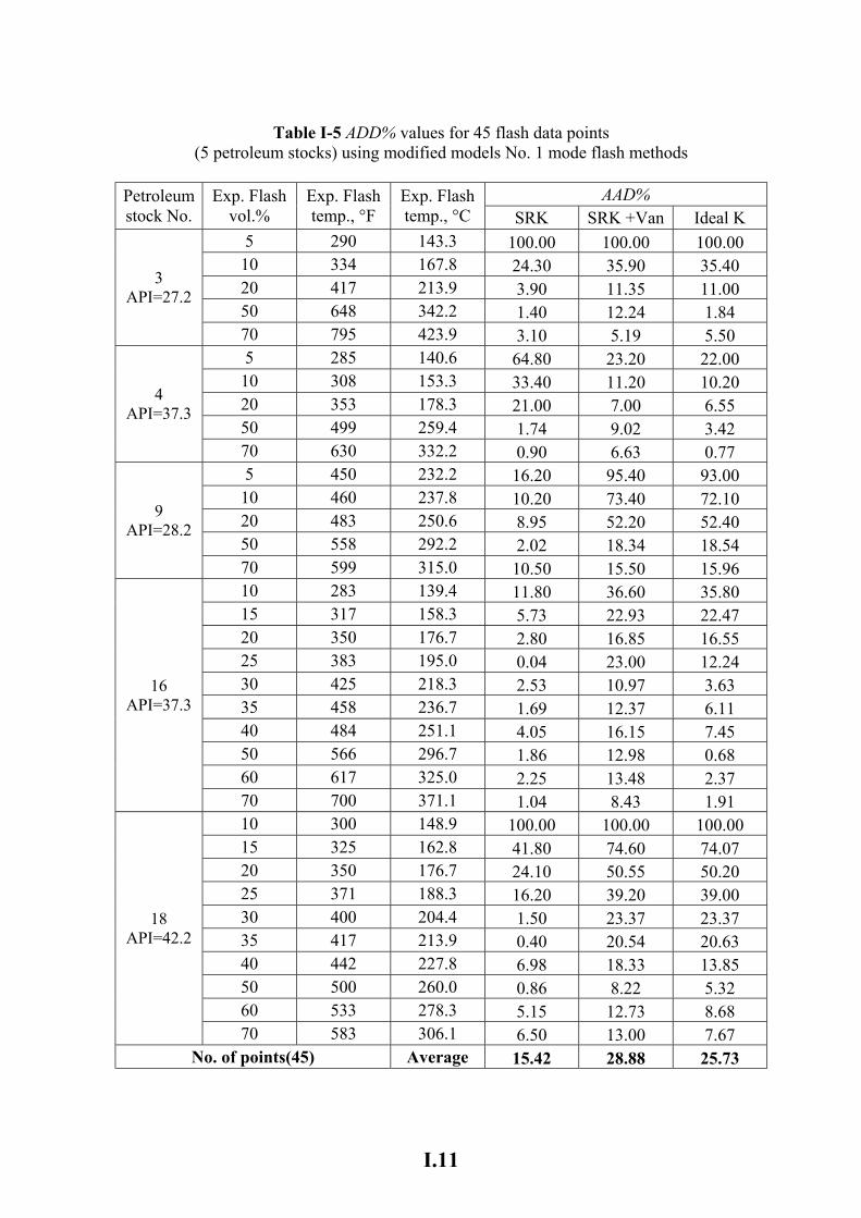
I.11
Table I-5 ADD% values for 45 flash data points (5 petroleum stocks) using modified models No. 1 mode flash methods
AAD% Petroleum
stock No. Exp. Flash
vol.% Exp. Flash temp., °F
Exp. Flash temp., °C SRK SRK +Van Ideal K
5 290 143.3 100.00 100.00 100.00 10 334 167.8 24.30 35.90 35.40 20 417 213.9 3.90 11.35 11.00 50 648 342.2 1.40 12.24 1.84
3 API=27.2
70 795 423.9 3.10 5.19 5.50 5 285 140.6 64.80 23.20 22.00 10 308 153.3 33.40 11.20 10.20 20 353 178.3 21.00 7.00 6.55 50 499 259.4 1.74 9.02 3.42
4 API=37.3
70 630 332.2 0.90 6.63 0.77 5 450 232.2 16.20 95.40 93.00 10 460 237.8 10.20 73.40 72.10 20 483 250.6 8.95 52.20 52.40 50 558 292.2 2.02 18.34 18.54
9 API=28.2
70 599 315.0 10.50 15.50 15.96 10 283 139.4 11.80 36.60 35.80 15 317 158.3 5.73 22.93 22.47 20 350 176.7 2.80 16.85 16.55 25 383 195.0 0.04 23.00 12.24 30 425 218.3 2.53 10.97 3.63 35 458 236.7 1.69 12.37 6.11 40 484 251.1 4.05 16.15 7.45 50 566 296.7 1.86 12.98 0.68 60 617 325.0 2.25 13.48 2.37
16 API=37.3
70 700 371.1 1.04 8.43 1.91 10 300 148.9 100.00 100.00 100.00 15 325 162.8 41.80 74.60 74.07 20 350 176.7 24.10 50.55 50.20 25 371 188.3 16.20 39.20 39.00 30 400 204.4 1.50 23.37 23.37 35 417 213.9 0.40 20.54 20.63 40 442 227.8 6.98 18.33 13.85 50 500 260.0 0.86 8.22 5.32 60 533 278.3 5.15 12.73 8.68
18 API=42.2
70 583 306.1 6.50 13.00 7.67 No. of points(45) Average 15.42 28.88 25.73

I.12
Table I-6 AD% values for 45 flash data points (5 petroleum stocks) using modified models No. 1 mode flash methods
AD% Petroleum
stock No. Exp. Flash
vol.% Exp. Flash temp., °F
Exp. Flash temp., °C SRK SRK +Van Ideal K
5 290 143.3 100.00 100.00 100.00 10 334 167.8 24.30 35.90 35.40 20 417 213.9 3.90 11.35 11.00 50 648 342.2 -1.40 12.24 -1.84
3 API=27.2
70 795 423.9 -3.10 5.19 -5.50 5 285 140.6 -64.80 23.20 22.00 10 308 153.3 -33.40 11.20 10.20 20 353 178.3 -21.00 7.00 6.55 50 499 259.4 -1.74 9.02 3.42
4 API=37.3
70 630 332.2 -0.90 6.63 -0.77 5 450 232.2 -16.20 95.40 93.00 10 460 237.8 10.20 73.40 72.10 20 483 250.6 8.95 52.20 52.40 50 558 292.2 2.02 18.34 18.54
9 API=28.2
70 599 315.0 10.50 15.50 15.96 10 283 139.4 11.80 36.60 35.80 15 317 158.3 5.73 22.93 22.47 20 350 176.7 2.80 16.85 16.55 25 383 195.0 -0.04 23.00 12.24 30 425 218.3 -2.53 10.97 3.63 35 458 236.7 1.69 12.37 6.11 40 484 251.1 4.05 16.15 7.45 50 566 296.7 -1.86 12.98 -0.68 60 617 325.0 2.25 13.48 2.37
16 API=37.3
70 700 371.1 -1.04 8.43 -1.91 10 300 148.9 100.00 100.00 100.00 15 325 162.8 41.80 74.60 74.07 20 350 176.7 24.10 50.55 50.20 25 371 188.3 16.20 39.20 39.00 30 400 204.4 1.50 23.37 23.37 35 417 213.9 0.40 20.54 20.63 40 442 227.8 6.98 18.33 13.85 50 500 260.0 -0.86 8.22 5.32 60 533 278.3 5.15 12.73 8.68
18 API=42.2
70 583 306.1 6.50 13.00 7.67 No. of points(45) Average 6.91 28.88 25.12
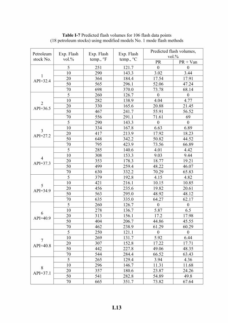
I.13
Table I-7 Predicted flash volumes for 106 flash data points (18 petroleum stocks) using modified models No. 1 mode flash methods
Predicted flash volumes,
vol.% Petroleum stock No.
Exp. Flash vol.%
Exp. Flash temp., °F
Exp. Flash temp., °C PR PR + Van
5 251 121.7 0 0 10 290 143.3 3.02 3.44 20 364 184.4 17.54 17.91 50 565 296.1 52.06 47.24
1 API=32.4
70 698 370.0 73.78 68.14 5 260 126.7 0 0 10 282 138.9 4.04 4.77 20 330 165.6 20.88 21.45 50 467 241.7 55.91 56.52
2 API=36.5
70 556 291.1 71.61 69 5 290 143.3 0 0 10 334 167.8 6.63 6.89 20 417 213.9 17.92 18.23 50 648 342.2 50.82 44.52
3 API=27.2
70 795 423.9 73.56 66.89 5 285 140.6 4.01 4.42 10 308 153.3 9.03 9.44 20 353 178.3 18.77 19.21 50 499 259.4 48.22 46.07
4 API=37.3
70 630 332.2 70.29 65.83 5 379 192.8 4.15 4.82 10 421 216.1 10.15 10.85 20 456 235.6 19.82 20.61 50 563 295.0 48.92 48.12
5 API=34.9
70 635 335.0 64.27 62.17 5 260 126.7 0 0 10 278 136.7 5.87 6.5 20 313 156.1 17.2 17.98 50 404 206.7 44.86 45.55
6 API=40.9
70 462 238.9 61.29 60.29 5 250 121.1 0 0 10 269 131.7 5.92 6.44 20 307 152.8 17.22 17.71 50 442 227.8 49.06 48.35
7 API=40.8
70 544 284.4 66.52 63.43 5 265 129.4 3.94 4.36 10 296 146.7 11.31 11.68 20 357 180.6 23.87 24.26 50 541 282.8 54.89 49.8
8 API=37.1
70 665 351.7 73.82 67.64
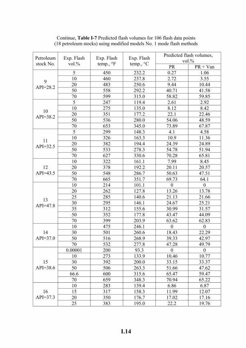
I.14
Continue, Table I-7 Predicted flash volumes for 106 flash data points (18 petroleum stocks) using modified models No. 1 mode flash methods
Predicted flash volumes,
vol.% Petroleum stock No.
Exp. Flash vol.%
Exp. Flash temp., °F
Exp. Flash temp., °C PR PR + Van
5 450 232.2 0.27 1.06 10 460 237.8 2.72 3.55 20 483 250.6 9.44 10.44 50 558 292.2 40.71 41.58
9 API=28.2
70 599 315.0 58.82 59.85 5 247 119.4 2.61 2.92 10 275 135.0 8.12 8.42 20 351 177.2 22.1 22.46 50 536 280.0 54.06 48.59
10 API=38.2
70 653 345.0 73.89 67.87 5 299 148.3 4.1 4.58 10 326 163.3 10.9 11.36 20 382 194.4 24.39 24.89 50 533 278.3 54.78 51.94
11 API=32.5
70 627 330.6 70.28 65.81 10 322 161.1 7.99 8.45 20 378 192.2 20.11 20.57 50 548 286.7 50.63 47.51
12 API=43.5
70 665 351.7 69.73 64.1 10 214 101.1 0 0 20 262 127.8 13.26 13.78 25 285 140.6 21.13 21.66 30 295 146.1 24.67 25.21 35 312 155.6 30.99 31.57 50 352 177.8 43.47 44.09
13 API=47.8
70 399 203.9 63.62 62.83 10 475 246.1 0 0 30 501 260.6 18.43 22.29 50 516 268.9 39.33 42.97
14 API=37.0
70 532 277.8 47.28 49.79 0.00001 200 93.3 0 0
10 273 133.9 10.46 10.77 30 392 200.0 33.15 33.37 50 506 263.3 51.66 47.62
66.6 600 315.6 65.47 59.47
15 API=38.6
70 659 348.3 70.94 65.22 10 283 139.4 6.86 6.87 15 317 158.3 11.99 12.07 20 350 176.7 17.02 17.16
16 API=37.3
25 383 195.0 22.2 19.76
I.15
Continue, Table I-7 Predicted flash volumes for 106 flash data points (18 petroleum stocks) using modified models No. 1 mode flash methods
Predicted flash volumes,
vol.% Petroleum stock No.
Exp. Flash vol.%
Exp. Flash temp., °F
Exp. Flash temp., °C PR PR + Van
30 425 218.3 29.14 27.24 35 458 236.7 33 31.11 40 484 251.1 37.17 34.1 50 566 296.7 50.35 44.07 60 617 325.0 58.52 52.47
16 API=37.3
70 700 371.1 71.18 64.63 10 583 306.1 8.24 8.66 15 600 315.6 11.58 12.1 20 625 329.4 16.93 17.58 25 642 338.9 20.96 21.7 30 667 352.8 27.62 25.09 35 700 371.1 36.69 36.09 40 733 389.4 44.4 40.68 50 758 403.3 51.67 48.81 60 808 431.1 64.65 61.73
17 API=20.2
70 866 463.3 75.93 72.76 10 300 148.9 0 0 15 325 162.8 4.31 4.54 20 350 176.7 10.36 10.61 25 371 188.3 15.65 15.92 30 400 204.4 23.43 23.72 35 417 213.9 28.25 28.56 40 442 227.8 34.67 33.46 50 500 260.0 47.68 46.56 60 533 278.3 55.07 52.99
18 API=42.2
70 583 306.1 64.78 61.5
I.16
Table I-8 AAD% for 106 flash data points (18 petroleum stocks) using modified models No. 1 mode flash methods
AAD% Petroleum
stock No. Exp. Flash
vol.% Exp. Flash temp., °F
Exp. Flash temp., °C PR PR + Van
5 251 121.7 100.00 100.00 10 290 143.3 69.80 65.60 20 364 184.4 12.30 10.45 50 565 296.1 4.12 5.52
1 API=32.4
70 698 370.0 5.40 2.66 5 260 126.7 100.00 100.00 10 282 138.9 59.60 52.30 20 330 165.6 4.40 7.25 50 467 241.7 11.82 13.04
2 API=36.5
70 556 291.1 2.30 1.43 5 290 143.3 100.00 100.00 10 334 167.8 33.70 31.10 20 417 213.9 10.40 8.85 50 648 342.2 1.64 10.96
3 API=27.2
70 795 423.9 5.09 4.44 5 285 140.6 19.80 11.60 10 308 153.3 9.70 5.60 20 353 178.3 6.15 3.95 50 499 259.4 3.56 7.86
4 API=37.3
70 630 332.2 0.41 5.96 5 379 192.8 17.00 3.60 10 421 216.1 1.50 8.50 20 456 235.6 0.90 3.05 50 563 295.0 2.16 3.76
5 API=34.9
70 635 335.0 8.19 11.19 5 260 126.7 100.00 100.00 10 278 136.7 41.30 35.00 20 313 156.1 14.00 10.10 50 404 206.7 10.28 8.90
6 API=40.9
70 462 238.9 12.44 13.87 5 250 121.1 100.00 100.00 10 269 131.7 40.80 35.60 20 307 152.8 13.90 11.45 50 442 227.8 1.88 3.30
7 API=40.8
70 544 284.4 4.97 9.39 5 265 129.4 21.20 12.80 10 296 146.7 13.10 16.80 20 357 180.6 19.35 21.30 50 541 282.8 9.78 0.40
8 API=37.1
70 665 351.7 5.46 3.37
I.17
Continue, Table I-8 AAD% for 106 flash data points (18 petroleum stocks) using modified models No. 1 mode flash methods
AAD% Petroleum
stock No. Exp. Flash
vol.% Exp. Flash temp., °F
Exp. Flash temp., °C PR PR + Van
5 450 232.2 94.60 78.80 10 460 237.8 72.80 64.50 20 483 250.6 52.80 47.80 50 558 292.2 18.58 16.84
9 API=28.2
70 599 315.0 15.97 14.50 5 247 119.4 47.80 41.60 10 275 135.0 18.80 15.80 20 351 177.2 10.50 12.30 50 536 280.0 8.12 2.82
10 API=38.2
70 653 345.0 5.56 3.04 5 299 148.3 18.00 8.40 10 326 163.3 9.00 13.60 20 382 194.4 21.95 24.45 50 533 278.3 9.56 3.88
11 API=32.5
70 627 330.6 0.40 5.99 10 322 161.1 20.10 15.50 20 378 192.2 0.55 2.85 50 548 286.7 1.26 4.98
12 API=43.5
70 665 351.7 0.39 8.43 10 214 101.1 100.00 100.00 20 262 127.8 33.70 31.10 25 285 140.6 15.48 13.36 30 295 146.1 17.77 15.97 35 312 155.6 11.46 9.80 50 352 177.8 13.06 11.82
13 API=47.8
70 399 203.9 9.11 10.24 10 475 246.1 100.00 100.00 30 501 260.6 38.57 25.70 50 516 268.9 21.34 14.06
14 API=37.0
70 532 277.8 32.46 28.87 0.00001 273 133.9 100.00 100.00
10 300 148.9 4.60 7.70 30 392 200.0 10.50 11.23 50 400 204.4 3.32 4.76
66.6 506 263.3 1.70 10.71
15 API=38.6
70 600 315.6 1.34 6.83 10 283 139.4 31.40 31.30 15 317 158.3 20.07 19.53 20 350 176.7 14.90 14.20
16 API=37.3
25 383 195.0 11.20 20.96
I.18
Continue, Table I-8 AAD% for 106 flash data points (18 petroleum stocks) using modified models No. 1 mode flash methods
AAD% Petroleum
stock No. Exp. Flash
vol.% Exp. Flash temp., °F
Exp. Flash temp., °C PR PR + Van
30 425 218.3 2.87 9.20 35 458 236.7 5.71 11.11 40 484 251.1 7.08 14.75 50 566 296.7 0.70 11.86 60 617 325.0 2.47 12.55
16 API=37.3
70 700 371.1 1.69 7.67 10 583 306.1 17.60 13.40 15 600 315.6 22.80 19.33 20 625 329.4 15.35 12.10 25 642 338.9 16.16 13.20 30 667 352.8 7.93 16.37 35 700 371.1 4.83 3.11 40 733 389.4 11.00 1.70 50 758 403.3 3.34 2.38 60 808 431.1 7.75 2.88
17 API=20.2
70 866 463.3 8.47 3.94 10 300 148.9 100.00 100.00 15 325 162.8 71.27 69.73 20 350 176.7 48.20 46.95 25 371 188.3 37.40 36.32 30 400 204.4 21.90 20.93 35 417 213.9 19.29 18.40 40 442 227.8 13.33 16.35 50 500 260.0 4.64 6.88 60 533 278.3 8.22 11.68
18 API=42.2
70 583 306.1 7.46 12.14 No. of points (106) Average 23.40 24.90
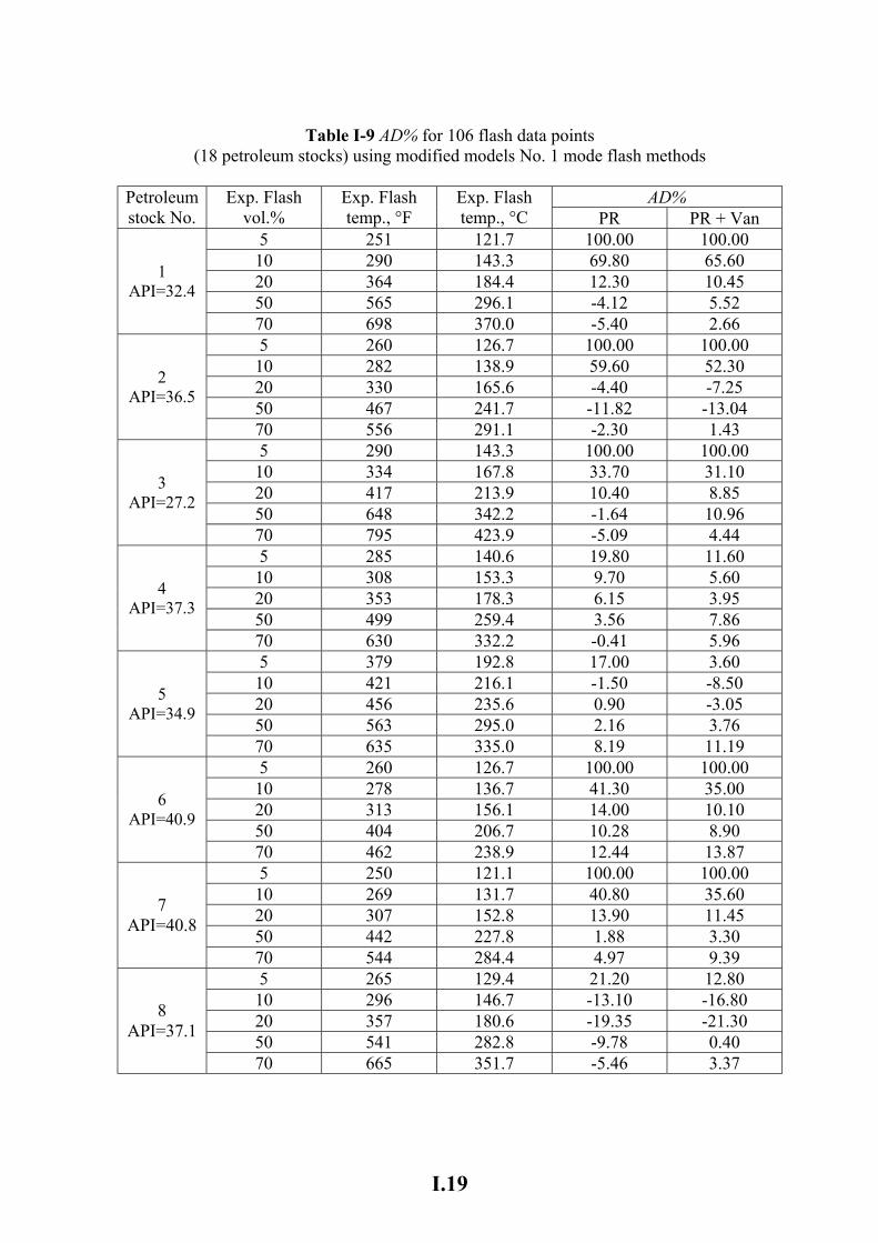
I.19
Table I-9 AD% for 106 flash data points (18 petroleum stocks) using modified models No. 1 mode flash methods
AD% Petroleum
stock No. Exp. Flash
vol.% Exp. Flash temp., °F
Exp. Flash temp., °C PR PR + Van
5 251 121.7 100.00 100.00 10 290 143.3 69.80 65.60 20 364 184.4 12.30 10.45 50 565 296.1 -4.12 5.52
1 API=32.4
70 698 370.0 -5.40 2.66 5 260 126.7 100.00 100.00 10 282 138.9 59.60 52.30 20 330 165.6 -4.40 -7.25 50 467 241.7 -11.82 -13.04
2 API=36.5
70 556 291.1 -2.30 1.43 5 290 143.3 100.00 100.00 10 334 167.8 33.70 31.10 20 417 213.9 10.40 8.85 50 648 342.2 -1.64 10.96
3 API=27.2
70 795 423.9 -5.09 4.44 5 285 140.6 19.80 11.60 10 308 153.3 9.70 5.60 20 353 178.3 6.15 3.95 50 499 259.4 3.56 7.86
4 API=37.3
70 630 332.2 -0.41 5.96 5 379 192.8 17.00 3.60 10 421 216.1 -1.50 -8.50 20 456 235.6 0.90 -3.05 50 563 295.0 2.16 3.76
5 API=34.9
70 635 335.0 8.19 11.19 5 260 126.7 100.00 100.00 10 278 136.7 41.30 35.00 20 313 156.1 14.00 10.10 50 404 206.7 10.28 8.90
6 API=40.9
70 462 238.9 12.44 13.87 5 250 121.1 100.00 100.00 10 269 131.7 40.80 35.60 20 307 152.8 13.90 11.45 50 442 227.8 1.88 3.30
7 API=40.8
70 544 284.4 4.97 9.39 5 265 129.4 21.20 12.80 10 296 146.7 -13.10 -16.80 20 357 180.6 -19.35 -21.30 50 541 282.8 -9.78 0.40
8 API=37.1
70 665 351.7 -5.46 3.37
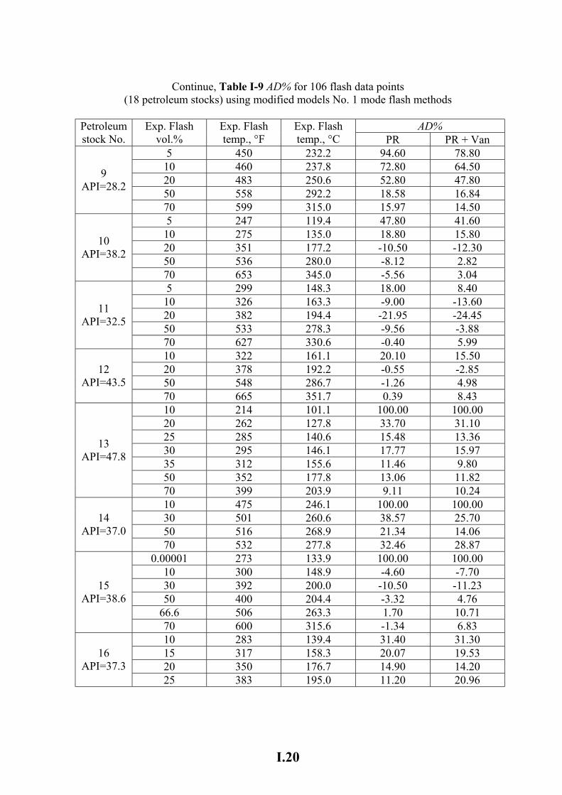
I.20
Continue, Table I-9 AD% for 106 flash data points (18 petroleum stocks) using modified models No. 1 mode flash methods
AD% Petroleum
stock No. Exp. Flash
vol.% Exp. Flash temp., °F
Exp. Flash temp., °C PR PR + Van
5 450 232.2 94.60 78.80 10 460 237.8 72.80 64.50 20 483 250.6 52.80 47.80 50 558 292.2 18.58 16.84
9 API=28.2
70 599 315.0 15.97 14.50 5 247 119.4 47.80 41.60 10 275 135.0 18.80 15.80 20 351 177.2 -10.50 -12.30 50 536 280.0 -8.12 2.82
10 API=38.2
70 653 345.0 -5.56 3.04 5 299 148.3 18.00 8.40 10 326 163.3 -9.00 -13.60 20 382 194.4 -21.95 -24.45 50 533 278.3 -9.56 -3.88
11 API=32.5
70 627 330.6 -0.40 5.99 10 322 161.1 20.10 15.50 20 378 192.2 -0.55 -2.85 50 548 286.7 -1.26 4.98
12 API=43.5
70 665 351.7 0.39 8.43 10 214 101.1 100.00 100.00 20 262 127.8 33.70 31.10 25 285 140.6 15.48 13.36 30 295 146.1 17.77 15.97 35 312 155.6 11.46 9.80 50 352 177.8 13.06 11.82
13 API=47.8
70 399 203.9 9.11 10.24 10 475 246.1 100.00 100.00 30 501 260.6 38.57 25.70 50 516 268.9 21.34 14.06
14 API=37.0
70 532 277.8 32.46 28.87 0.00001 273 133.9 100.00 100.00
10 300 148.9 -4.60 -7.70 30 392 200.0 -10.50 -11.23 50 400 204.4 -3.32 4.76
66.6 506 263.3 1.70 10.71
15 API=38.6
70 600 315.6 -1.34 6.83 10 283 139.4 31.40 31.30 15 317 158.3 20.07 19.53 20 350 176.7 14.90 14.20
16 API=37.3
25 383 195.0 11.20 20.96

I.21
Continue, Table I-9 AD% for 106 flash data points (18 petroleum stocks) using modified models No. 1 mode flash methods
AD% Petroleum
stock No. Exp. Flash
vol.% Exp. Flash temp., °F
Exp. Flash temp., °C PR PR + Van
30 425 218.3 2.87 9.20 35 458 236.7 5.71 11.11 40 484 251.1 7.08 14.75 50 566 296.7 -0.70 11.86 60 617 325.0 2.47 12.55
16 API=37.3
70 700 371.1 -1.69 7.67 10 583 306.1 17.60 13.40 15 600 315.6 22.80 19.33 20 625 329.4 15.35 12.10 25 642 338.9 16.16 13.20 30 667 352.8 7.93 16.37 35 700 371.1 -4.83 -3.11 40 733 389.4 -11.00 -1.70 50 758 403.3 -3.34 2.38 60 808 431.1 -7.75 -2.88
17 API=20.2
70 866 463.3 -8.47 -3.94 10 300 148.9 100.00 100.00 15 325 162.8 71.27 69.73 20 350 176.7 48.20 46.95 25 371 188.3 37.40 36.32 30 400 204.4 21.90 20.93 35 417 213.9 19.29 18.40 40 442 227.8 13.33 16.35 50 500 260.0 4.64 6.88 60 533 278.3 8.22 11.68
18 API=42.2
70 583 306.1 7.46 12.14 No. of points(106) Average 19.50 23.10
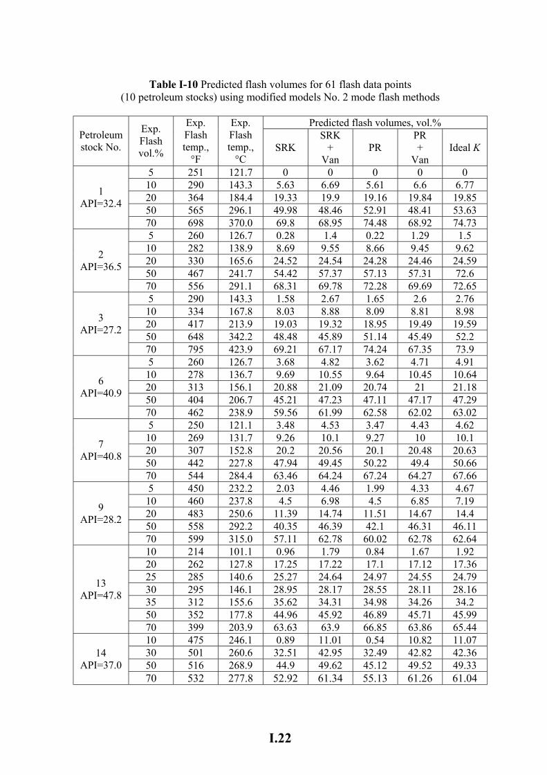
I.22
Table I-10 Predicted flash volumes for 61 flash data points (10 petroleum stocks) using modified models No. 2 mode flash methods
Predicted flash volumes, vol.%
Petroleum stock No.
Exp. Flash vol.%
Exp. Flash temp.,
°F
Exp. Flash temp.,
°C SRK
SRK +
Van PR
PR +
Van Ideal K
5 251 121.7 0 0 0 0 0 10 290 143.3 5.63 6.69 5.61 6.6 6.77 20 364 184.4 19.33 19.9 19.16 19.84 19.85 50 565 296.1 49.98 48.46 52.91 48.41 53.63
1 API=32.4
70 698 370.0 69.8 68.95 74.48 68.92 74.73 5 260 126.7 0.28 1.4 0.22 1.29 1.5 10 282 138.9 8.69 9.55 8.66 9.45 9.62 20 330 165.6 24.52 24.54 24.28 24.46 24.59 50 467 241.7 54.42 57.37 57.13 57.31 72.6
2 API=36.5
70 556 291.1 68.31 69.78 72.28 69.69 72.65 5 290 143.3 1.58 2.67 1.65 2.6 2.76 10 334 167.8 8.03 8.88 8.09 8.81 8.98 20 417 213.9 19.03 19.32 18.95 19.49 19.59 50 648 342.2 48.48 45.89 51.14 45.49 52.2
3 API=27.2
70 795 423.9 69.21 67.17 74.24 67.35 73.9 5 260 126.7 3.68 4.82 3.62 4.71 4.91 10 278 136.7 9.69 10.55 9.64 10.45 10.64 20 313 156.1 20.88 21.09 20.74 21 21.18 50 404 206.7 45.21 47.23 47.11 47.17 47.29
6 API=40.9
70 462 238.9 59.56 61.99 62.58 62.02 63.02 5 250 121.1 3.48 4.53 3.47 4.43 4.62 10 269 131.7 9.26 10.1 9.27 10 10.1 20 307 152.8 20.2 20.56 20.1 20.48 20.63 50 442 227.8 47.94 49.45 50.22 49.4 50.66
7 API=40.8
70 544 284.4 63.46 64.24 67.24 64.27 67.66 5 450 232.2 2.03 4.46 1.99 4.33 4.67 10 460 237.8 4.5 6.98 4.5 6.85 7.19 20 483 250.6 11.39 14.74 11.51 14.67 14.4 50 558 292.2 40.35 46.39 42.1 46.31 46.11
9 API=28.2
70 599 315.0 57.11 62.78 60.02 62.78 62.64 10 214 101.1 0.96 1.79 0.84 1.67 1.92 20 262 127.8 17.25 17.22 17.1 17.12 17.36 25 285 140.6 25.27 24.64 24.97 24.55 24.79 30 295 146.1 28.95 28.17 28.55 28.11 28.16 35 312 155.6 35.62 34.31 34.98 34.26 34.2 50 352 177.8 44.96 45.92 46.89 45.71 45.99
13 API=47.8
70 399 203.9 63.63 63.9 66.85 63.86 65.44 10 475 246.1 0.89 11.01 0.54 10.82 11.07 30 501 260.6 32.51 42.95 32.49 42.82 42.36 50 516 268.9 44.9 49.62 45.12 49.52 49.33
14 API=37.0
70 532 277.8 52.92 61.34 55.13 61.26 61.04
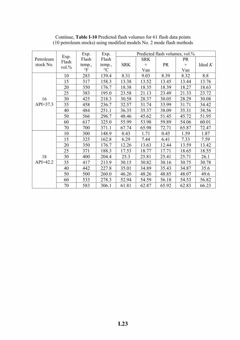
I.23
Continue, Table I-10 Predicted flash volumes for 61 flash data points (10 petroleum stocks) using modified models No. 2 mode flash methods
Predicted flash volumes, vol.%
Petroleum stock No.
Exp. Flash vol.%
Exp. Flash temp.,
°F
Exp. Flash temp.,
°C SRK
SRK +
Van PR
PR +
Van Ideal K
10 283 139.4 8.31 9.03 8.39 8.32 8.8 15 317 158.3 13.38 13.52 13.45 13.44 13.76 20 350 176.7 18.38 18.35 18.39 18.27 18.63 25 383 195.0 23.58 21.13 23.49 21.33 23.72 30 425 218.3 30.58 28.37 30.05 28.29 30.08 35 458 236.7 32.57 31.74 33.99 31.71 34.42 40 484 251.1 36.35 35.37 38.09 35.31 38.56 50 566 296.7 48.46 45.62 51.45 45.72 51.95 60 617 325.0 55.99 53.98 59.89 54.06 60.01
16 API=37.3
70 700 371.1 67.74 65.98 72.71 65.87 72.47 10 300 148.9 0.43 1.71 0.45 1.59 1.87 15 325 162.8 6.29 7.44 6.41 7.33 7.59 20 350 176.7 12.26 13.63 12.44 13.59 13.42 25 371 188.3 17.53 18.77 17.71 18.65 18.55 30 400 204.4 25.3 25.81 25.41 25.71 26.1 35 417 213.9 30.15 30.82 30.16 30.75 30.78 40 442 227.8 35.01 34.89 35.43 34.87 35.6 50 500 260.0 46.26 48.26 48.85 48.07 49.6 60 533 278.3 52.94 54.59 56.18 54.53 56.82
18 API=42.2
70 583 306.1 61.81 62.87 65.92 62.83 66.23
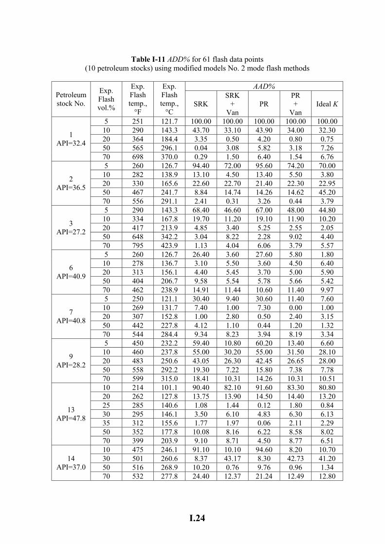
I.24
Table I-11 ADD% for 61 flash data points (10 petroleum stocks) using modified models No. 2 mode flash methods
AAD%
Petroleum stock No.
Exp. Flash vol.%
Exp. Flash temp.,
°F
Exp. Flash temp.,
°C SRK
SRK +
Van PR
PR +
Van Ideal K
5 251 121.7 100.00 100.00 100.00 100.00 100.00 10 290 143.3 43.70 33.10 43.90 34.00 32.30 20 364 184.4 3.35 0.50 4.20 0.80 0.75 50 565 296.1 0.04 3.08 5.82 3.18 7.26
1 API=32.4
70 698 370.0 0.29 1.50 6.40 1.54 6.76 5 260 126.7 94.40 72.00 95.60 74.20 70.00 10 282 138.9 13.10 4.50 13.40 5.50 3.80 20 330 165.6 22.60 22.70 21.40 22.30 22.95 50 467 241.7 8.84 14.74 14.26 14.62 45.20
2 API=36.5
70 556 291.1 2.41 0.31 3.26 0.44 3.79 5 290 143.3 68.40 46.60 67.00 48.00 44.80 10 334 167.8 19.70 11.20 19.10 11.90 10.20 20 417 213.9 4.85 3.40 5.25 2.55 2.05 50 648 342.2 3.04 8.22 2.28 9.02 4.40
3 API=27.2
70 795 423.9 1.13 4.04 6.06 3.79 5.57 5 260 126.7 26.40 3.60 27.60 5.80 1.80 10 278 136.7 3.10 5.50 3.60 4.50 6.40 20 313 156.1 4.40 5.45 3.70 5.00 5.90 50 404 206.7 9.58 5.54 5.78 5.66 5.42
6 API=40.9
70 462 238.9 14.91 11.44 10.60 11.40 9.97 5 250 121.1 30.40 9.40 30.60 11.40 7.60 10 269 131.7 7.40 1.00 7.30 0.00 1.00 20 307 152.8 1.00 2.80 0.50 2.40 3.15 50 442 227.8 4.12 1.10 0.44 1.20 1.32
7 API=40.8
70 544 284.4 9.34 8.23 3.94 8.19 3.34 5 450 232.2 59.40 10.80 60.20 13.40 6.60 10 460 237.8 55.00 30.20 55.00 31.50 28.10 20 483 250.6 43.05 26.30 42.45 26.65 28.00 50 558 292.2 19.30 7.22 15.80 7.38 7.78
9 API=28.2
70 599 315.0 18.41 10.31 14.26 10.31 10.51 10 214 101.1 90.40 82.10 91.60 83.30 80.80 20 262 127.8 13.75 13.90 14.50 14.40 13.20 25 285 140.6 1.08 1.44 0.12 1.80 0.84 30 295 146.1 3.50 6.10 4.83 6.30 6.13 35 312 155.6 1.77 1.97 0.06 2.11 2.29 50 352 177.8 10.08 8.16 6.22 8.58 8.02
13 API=47.8
70 399 203.9 9.10 8.71 4.50 8.77 6.51 10 475 246.1 91.10 10.10 94.60 8.20 10.70 30 501 260.6 8.37 43.17 8.30 42.73 41.20 50 516 268.9 10.20 0.76 9.76 0.96 1.34
14 API=37.0
70 532 277.8 24.40 12.37 21.24 12.49 12.80
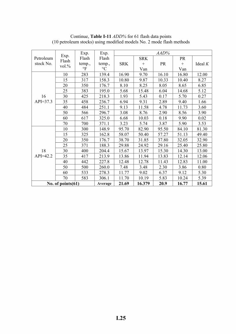
I.25
Continue, Table I-11 ADD% for 61 flash data points (10 petroleum stocks) using modified models No. 2 mode flash methods
AAD%
Petroleum stock No.
Exp. Flash vol.%
Exp. Flash temp.,
°F
Exp. Flash temp.,
°C SRK
SRK +
Van PR
PR +
Van Ideal K
10 283 139.4 16.90 9.70 16.10 16.80 12.00 15 317 158.3 10.80 9.87 10.33 10.40 8.27 20 350 176.7 8.10 8.25 8.05 8.65 6.85 25 383 195.0 5.68 15.48 6.04 14.68 5.12 30 425 218.3 1.93 5.43 0.17 5.70 0.27 35 458 236.7 6.94 9.31 2.89 9.40 1.66 40 484 251.1 9.13 11.58 4.78 11.73 3.60 50 566 296.7 3.08 8.76 2.90 8.56 3.90 60 617 325.0 6.68 10.03 0.18 9.90 0.02
16 API=37.3
70 700 371.1 3.23 5.74 3.87 5.90 3.53 10 300 148.9 95.70 82.90 95.50 84.10 81.30 15 325 162.8 58.07 50.40 57.27 51.13 49.40 20 350 176.7 38.70 31.85 37.80 32.05 32.90 25 371 188.3 29.88 24.92 29.16 25.40 25.80 30 400 204.4 15.67 13.97 15.30 14.30 13.00 35 417 213.9 13.86 11.94 13.83 12.14 12.06 40 442 227.8 12.48 12.78 11.43 12.83 11.00 50 500 260.0 7.48 3.48 2.30 3.86 0.80 60 533 278.3 11.77 9.02 6.37 9.12 5.30
18 API=42.2
70 583 306.1 11.70 10.19 5.83 10.24 5.39 No. of points(61) Average 21.69 16.379 20.9 16.77 15.61
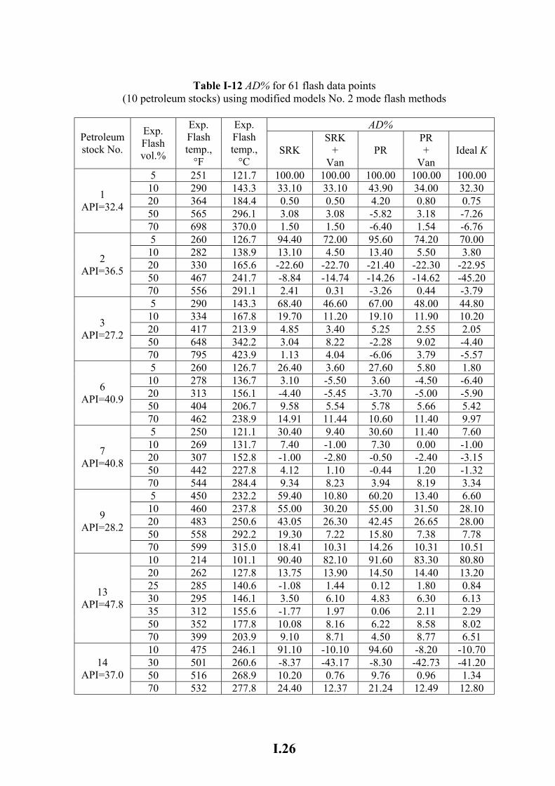
I.26
Table I-12 AD% for 61 flash data points (10 petroleum stocks) using modified models No. 2 mode flash methods
AD%
Petroleum stock No.
Exp. Flash vol.%
Exp. Flash temp.,
°F
Exp. Flash temp.,
°C SRK
SRK +
Van PR
PR +
Van Ideal K
5 251 121.7 100.00 100.00 100.00 100.00 100.00 10 290 143.3 33.10 33.10 43.90 34.00 32.30 20 364 184.4 0.50 0.50 4.20 0.80 0.75 50 565 296.1 3.08 3.08 -5.82 3.18 -7.26
1 API=32.4
70 698 370.0 1.50 1.50 -6.40 1.54 -6.76 5 260 126.7 94.40 72.00 95.60 74.20 70.00 10 282 138.9 13.10 4.50 13.40 5.50 3.80 20 330 165.6 -22.60 -22.70 -21.40 -22.30 -22.95 50 467 241.7 -8.84 -14.74 -14.26 -14.62 -45.20
2 API=36.5
70 556 291.1 2.41 0.31 -3.26 0.44 -3.79 5 290 143.3 68.40 46.60 67.00 48.00 44.80 10 334 167.8 19.70 11.20 19.10 11.90 10.20 20 417 213.9 4.85 3.40 5.25 2.55 2.05 50 648 342.2 3.04 8.22 -2.28 9.02 -4.40
3 API=27.2
70 795 423.9 1.13 4.04 -6.06 3.79 -5.57 5 260 126.7 26.40 3.60 27.60 5.80 1.80 10 278 136.7 3.10 -5.50 3.60 -4.50 -6.40 20 313 156.1 -4.40 -5.45 -3.70 -5.00 -5.90 50 404 206.7 9.58 5.54 5.78 5.66 5.42
6 API=40.9
70 462 238.9 14.91 11.44 10.60 11.40 9.97 5 250 121.1 30.40 9.40 30.60 11.40 7.60 10 269 131.7 7.40 -1.00 7.30 0.00 -1.00 20 307 152.8 -1.00 -2.80 -0.50 -2.40 -3.15 50 442 227.8 4.12 1.10 -0.44 1.20 -1.32
7 API=40.8
70 544 284.4 9.34 8.23 3.94 8.19 3.34 5 450 232.2 59.40 10.80 60.20 13.40 6.60 10 460 237.8 55.00 30.20 55.00 31.50 28.10 20 483 250.6 43.05 26.30 42.45 26.65 28.00 50 558 292.2 19.30 7.22 15.80 7.38 7.78
9 API=28.2
70 599 315.0 18.41 10.31 14.26 10.31 10.51 10 214 101.1 90.40 82.10 91.60 83.30 80.80 20 262 127.8 13.75 13.90 14.50 14.40 13.20 25 285 140.6 -1.08 1.44 0.12 1.80 0.84 30 295 146.1 3.50 6.10 4.83 6.30 6.13 35 312 155.6 -1.77 1.97 0.06 2.11 2.29 50 352 177.8 10.08 8.16 6.22 8.58 8.02
13 API=47.8
70 399 203.9 9.10 8.71 4.50 8.77 6.51 10 475 246.1 91.10 -10.10 94.60 -8.20 -10.70 30 501 260.6 -8.37 -43.17 -8.30 -42.73 -41.20 50 516 268.9 10.20 0.76 9.76 0.96 1.34
14 API=37.0
70 532 277.8 24.40 12.37 21.24 12.49 12.80
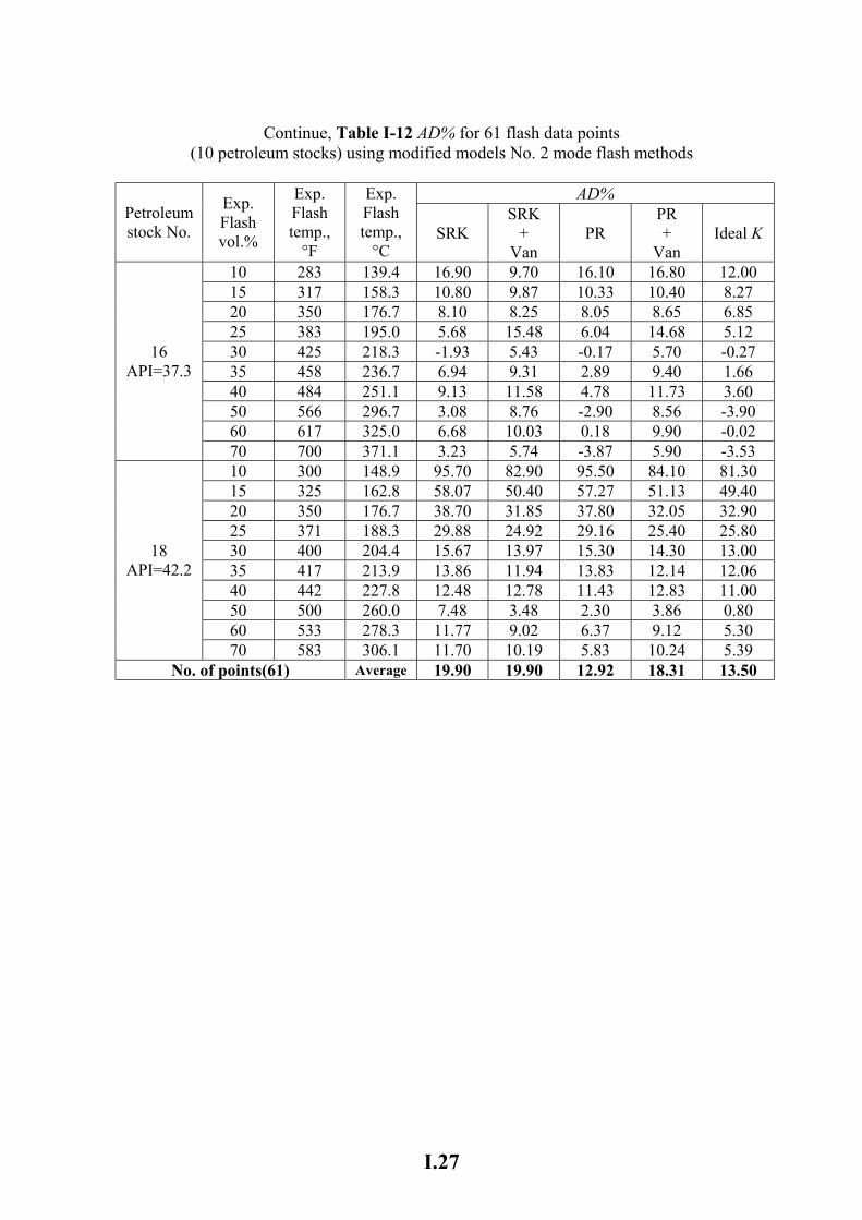
I.27
Continue, Table I-12 AD% for 61 flash data points (10 petroleum stocks) using modified models No. 2 mode flash methods
AD%
Petroleum stock No.
Exp. Flash vol.%
Exp. Flash temp.,
°F
Exp. Flash temp.,
°C SRK
SRK +
Van PR
PR +
Van Ideal K
10 283 139.4 16.90 9.70 16.10 16.80 12.00 15 317 158.3 10.80 9.87 10.33 10.40 8.27 20 350 176.7 8.10 8.25 8.05 8.65 6.85 25 383 195.0 5.68 15.48 6.04 14.68 5.12 30 425 218.3 -1.93 5.43 -0.17 5.70 -0.27 35 458 236.7 6.94 9.31 2.89 9.40 1.66 40 484 251.1 9.13 11.58 4.78 11.73 3.60 50 566 296.7 3.08 8.76 -2.90 8.56 -3.90 60 617 325.0 6.68 10.03 0.18 9.90 -0.02
16 API=37.3
70 700 371.1 3.23 5.74 -3.87 5.90 -3.53 10 300 148.9 95.70 82.90 95.50 84.10 81.30 15 325 162.8 58.07 50.40 57.27 51.13 49.40 20 350 176.7 38.70 31.85 37.80 32.05 32.90 25 371 188.3 29.88 24.92 29.16 25.40 25.80 30 400 204.4 15.67 13.97 15.30 14.30 13.00 35 417 213.9 13.86 11.94 13.83 12.14 12.06 40 442 227.8 12.48 12.78 11.43 12.83 11.00 50 500 260.0 7.48 3.48 2.30 3.86 0.80 60 533 278.3 11.77 9.02 6.37 9.12 5.30
18 API=42.2
70 583 306.1 11.70 10.19 5.83 10.24 5.39 No. of points(61) Average 19.90 19.90 12.92 18.31 13.50
Appendix J
Comparison between modified and
unmodified acentric factors
Table J-1 Acentric factor Comparison for petroleum stoke No. 2
Cut TB, °C Lee – Kasler ω Modified ω 1 160.50 0.2583 0.1669 2 171.08 0.2643 0.1737 3 183.43 0.2716 0.1821 4 197.23 0.2800 0.1918 5 212.18 0.2894 0.2027 6 228.02 0.2996 0.2147 7 244.50 0.3104 0.2275 8 261.42 0.3218 0.2411 9 278.58 0.3337 0.2553
10 295.82 0.3458 0.2700 11 313.01 0.3581 0.2849 12 330.05 0.3705 0.3001 13 346.84 0.3830 0.3155 14 363.36 0.3954 0.3309 15 379.56 0.4078 0.3463 16 395.44 0.4201 0.3618 17 411.04 0.4324 0.3772 18 426.41 0.4446 0.3927 19 441.63 0.4569 0.4084 20 456.81 0.4694 0.4243 21 472.08 0.4821 0.4406 22 487.60 0.4951 0.4574 23 503.58 0.5088 0.4751 24 520.21 0.5232 0.4938 25 537.75 0.5386 0.5139 26 556.46 0.5554 0.5357 27 576.64 0.5738 0.5598 28 598.61 0.5942 0.5866 29 622.71 0.6171 0.6168 30 649.35 0.6430 0.6509 31 678.90 0.8358 0.8263 32 711.82 0.8814 0.8779 33 748.54 0.9334 0.9369 34 789.56 0.9871 1.0044 35 835.38 1.0481 1.0819 36 886.53 1.1154 1.1707 37 943.60 1.1892 1.2725 38 1007.18 1.2698 1.3891 39 1077.88 1.3574 1.5221 40 1156.35 1.4522 1.6728
J.1
Table J-2 Acentric factor Comparison for petroleum stoke No. 3
Cut TB, °C Lee – Kasler ω Modified ω 1 150.39 0.2507 0.1576 2 180.69 0.2679 0.1772 3 211.98 0.2870 0.1994 4 243.92 0.3077 0.2238 5 276.23 0.3295 0.2499 6 308.62 0.3523 0.2775 7 340.87 0.3757 0.3062 8 372.75 0.3995 0.3358 9 404.09 0.4236 0.3661 10 434.72 0.4479 0.3968 11 464.52 0.4721 0.4278 12 493.38 0.4961 0.4588 13 521.25 0.5199 0.4897 14 548.07 0.5434 0.5204 15 573.84 0.5665 0.5507 16 598.57 0.5892 0.5806 17 622.29 0.6115 0.6100 18 645.10 0.6333 0.6389 19 667.08 0.8132 0.8016 20 688.36 0.8421 0.8345 21 709.11 0.8706 0.8670 22 729.52 0.8991 0.8994 23 749.79 0.9278 0.9320 24 770.17 0.9538 0.9652 25 790.92 0.9816 0.9995 26 812.37 1.0102 1.0354 27 834.82 1.0399 1.0735 28 858.65 1.0712 1.1144 29 884.24 1.1046 1.1590 30 911.98 1.1406 1.2079 31 942.36 1.1796 1.2623 32 975.82 1.2221 1.3232 33 1012.86 1.2686 1.3915 34 1054.02 1.3196 1.4686 35 1099.86 1.3756 1.5557 36 1150.96 1.4370 1.6541 37 1207.94 1.5041 1.7649 38 1271.44 1.5772 1.8890 39 1342.14 1.6566 2.0269 40 1420.73 1.7424 2.1779
J.2
Table J-3 Acentric factor Comparison for petroleum stoke No. 6
Cut TB, °C Lee – Kasler ω Modified ω 1 143.66 0.2563 0.1668 2 156.28 0.2633 0.1747 3 170.77 0.2717 0.1842 4 186.72 0.2813 0.1952 5 203.75 0.2920 0.2076 6 221.52 0.3035 0.2210 7 239.72 0.3157 0.2353 8 258.09 0.3283 0.2503 9 276.36 0.3411 0.2656 10 294.36 0.3541 0.2812 11 311.91 0.3670 0.2968 12 328.87 0.3797 0.3123 13 345.15 0.3920 0.3275 14 360.67 0.4040 0.3423 15 375.41 0.4156 0.3566 16 389.38 0.4267 0.3704 17 402.61 0.4374 0.3838 18 415.17 0.4476 0.3967 19 427.18 0.4575 0.4091 20 438.77 0.4672 0.4214 21 450.12 0.4768 0.4335 22 461.44 0.4864 0.4458 23 472.98 0.4964 0.4585 24 485.02 0.5069 0.4719 25 497.87 0.5182 0.4865 26 511.89 0.5307 0.5026 27 527.46 0.5448 0.5208 28 544.99 0.5610 0.5416 29 564.94 0.5797 0.5659 30 587.80 0.6016 0.5943 31 614.09 0.6274 0.6279 32 644.37 0.6581 0.6677 33 679.23 0.8593 0.8490 34 719.28 0.9165 0.9129 35 765.22 0.9791 0.9882 36 817.71 1.0504 1.0769 37 877.48 1.1303 1.1809 38 945.33 1.2192 1.3027 39 1022.00 1.3173 1.4445 40 1108.40 1.4247 1.6085
J.3
Table J-4 Acentric factor Comparison for petroleum stoke No. 7
Cut TB, °C Lee – Kasler ω Modified ω 1 129.35 0.2530 0.1644 2 147.77 0.2627 0.1752 3 166.25 0.2733 0.1872 4 184.74 0.2845 0.2000 5 203.15 0.2962 0.2134 6 221.44 0.3082 0.2274 7 239.56 0.3205 0.2418 8 257.48 0.3329 0.2566 9 275.19 0.3455 0.2716 10 292.67 0.3583 0.2869 11 309.93 0.3711 0.3024 12 326.99 0.3840 0.3181 13 343.88 0.3971 0.3340 14 360.64 0.4102 0.3502 15 377.31 0.4235 0.3667 16 393.97 0.4371 0.3835 17 410.69 0.4509 0.4007 18 427.56 0.4650 0.4185 19 444.68 0.4796 0.4369 20 462.17 0.4948 0.4561 21 480.14 0.5106 0.4763 22 498.73 0.5273 0.4976 23 518.10 0.5451 0.5203 24 538.40 0.5640 0.5447 25 559.79 0.5844 0.5710 26 582.48 0.6066 0.5995 27 606.64 0.6308 0.6307 28 632.51 0.6574 0.6650 29 660.27 0.8452 0.8314 30 690.18 0.8879 0.8787 31 722.46 0.9335 0.9308 32 757.39 0.9820 0.9884 33 795.24 1.0341 1.0521 34 836.27 1.0899 1.1227 35 880.77 1.1496 1.2009 36 929.05 1.2134 1.2877 37 981.42 1.2815 1.3838 38 1038.20 1.3539 1.4900 39 1099.75 1.4308 1.6070 40 1166.42 1.5122 1.7351
J.4
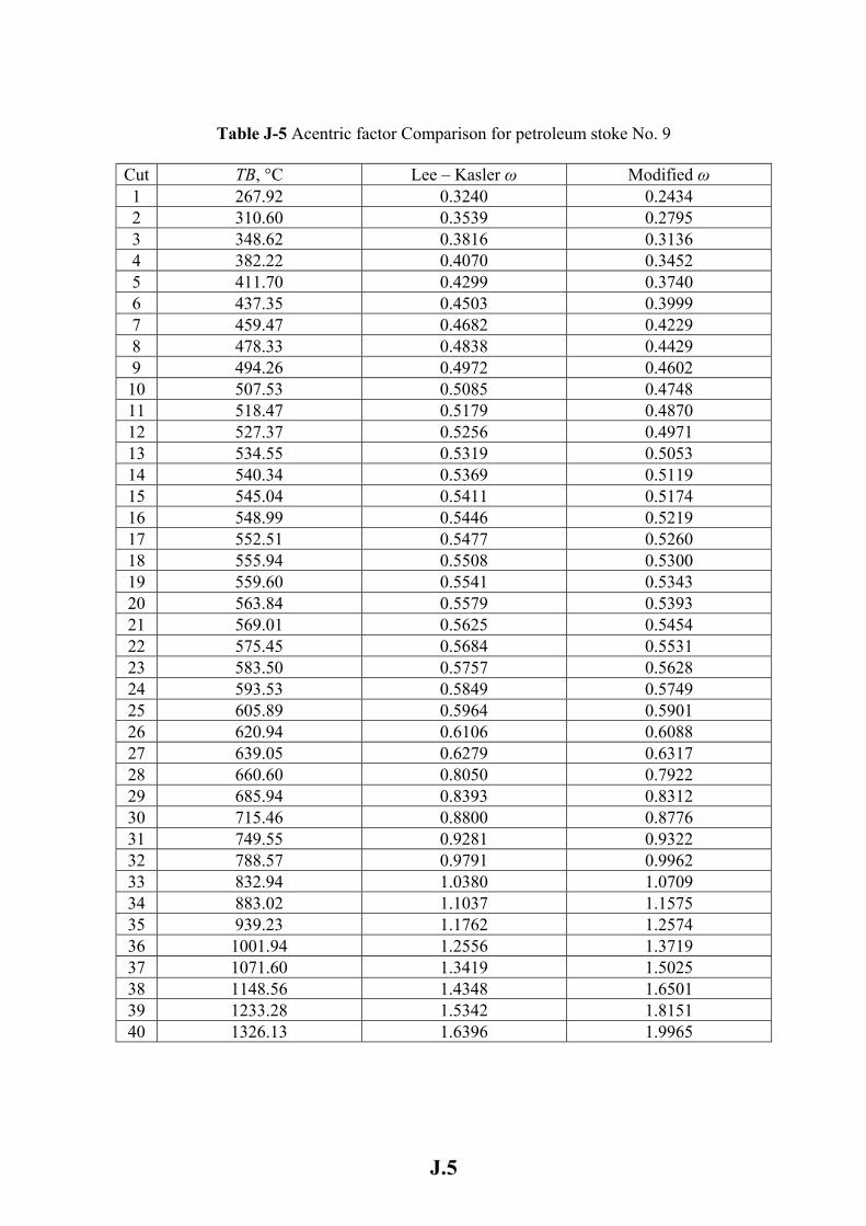
Table J-5 Acentric factor Comparison for petroleum stoke No. 9
Cut TB, °C Lee – Kasler ω Modified ω 1 267.92 0.3240 0.2434 2 310.60 0.3539 0.2795 3 348.62 0.3816 0.3136 4 382.22 0.4070 0.3452 5 411.70 0.4299 0.3740 6 437.35 0.4503 0.3999 7 459.47 0.4682 0.4229 8 478.33 0.4838 0.4429 9 494.26 0.4972 0.4602 10 507.53 0.5085 0.4748 11 518.47 0.5179 0.4870 12 527.37 0.5256 0.4971 13 534.55 0.5319 0.5053 14 540.34 0.5369 0.5119 15 545.04 0.5411 0.5174 16 548.99 0.5446 0.5219 17 552.51 0.5477 0.5260 18 555.94 0.5508 0.5300 19 559.60 0.5541 0.5343 20 563.84 0.5579 0.5393 21 569.01 0.5625 0.5454 22 575.45 0.5684 0.5531 23 583.50 0.5757 0.5628 24 593.53 0.5849 0.5749 25 605.89 0.5964 0.5901 26 620.94 0.6106 0.6088 27 639.05 0.6279 0.6317 28 660.60 0.8050 0.7922 29 685.94 0.8393 0.8312 30 715.46 0.8800 0.8776 31 749.55 0.9281 0.9322 32 788.57 0.9791 0.9962 33 832.94 1.0380 1.0709 34 883.02 1.1037 1.1575 35 939.23 1.1762 1.2574 36 1001.94 1.2556 1.3719 37 1071.60 1.3419 1.5025 38 1148.56 1.4348 1.6501 39 1233.28 1.5342 1.8151 40 1326.13 1.6396 1.9965
J.5
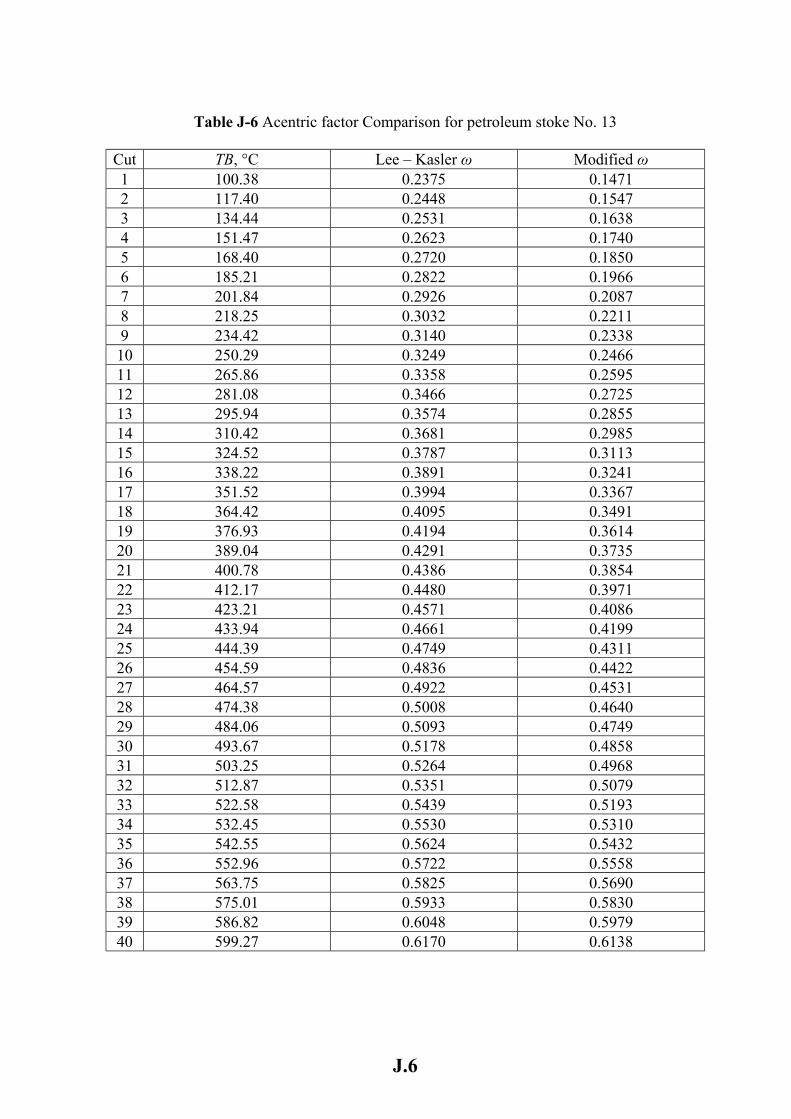
Table J-6 Acentric factor Comparison for petroleum stoke No. 13
Cut TB, °C Lee – Kasler ω Modified ω 1 100.38 0.2375 0.1471 2 117.40 0.2448 0.1547 3 134.44 0.2531 0.1638 4 151.47 0.2623 0.1740 5 168.40 0.2720 0.1850 6 185.21 0.2822 0.1966 7 201.84 0.2926 0.2087 8 218.25 0.3032 0.2211 9 234.42 0.3140 0.2338 10 250.29 0.3249 0.2466 11 265.86 0.3358 0.2595 12 281.08 0.3466 0.2725 13 295.94 0.3574 0.2855 14 310.42 0.3681 0.2985 15 324.52 0.3787 0.3113 16 338.22 0.3891 0.3241 17 351.52 0.3994 0.3367 18 364.42 0.4095 0.3491 19 376.93 0.4194 0.3614 20 389.04 0.4291 0.3735 21 400.78 0.4386 0.3854 22 412.17 0.4480 0.3971 23 423.21 0.4571 0.4086 24 433.94 0.4661 0.4199 25 444.39 0.4749 0.4311 26 454.59 0.4836 0.4422 27 464.57 0.4922 0.4531 28 474.38 0.5008 0.4640 29 484.06 0.5093 0.4749 30 493.67 0.5178 0.4858 31 503.25 0.5264 0.4968 32 512.87 0.5351 0.5079 33 522.58 0.5439 0.5193 34 532.45 0.5530 0.5310 35 542.55 0.5624 0.5432 36 552.96 0.5722 0.5558 37 563.75 0.5825 0.5690 38 575.01 0.5933 0.5830 39 586.82 0.6048 0.5979 40 599.27 0.6170 0.6138
J.6
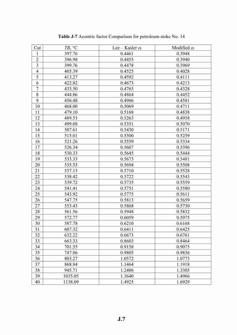
Table J-7 Acentric factor Comparison for petroleum stoke No. 14
Cut TB, °C Lee – Kasler ω Modified ω 1 397.76 0.4461 0.3948 2 396.98 0.4455 0.3940 3 399.76 0.4478 0.3969 4 405.39 0.4525 0.4028 5 413.27 0.4592 0.4111 6 422.82 0.4673 0.4213 7 433.50 0.4765 0.4328 8 444.86 0.4864 0.4452 9 456.48 0.4966 0.4581 10 468.00 0.5069 0.4711 11 479.10 0.5168 0.4838 12 489.53 0.5263 0.4958 13 499.08 0.5351 0.5070 14 507.61 0.5430 0.5171 15 515.01 0.5500 0.5259 16 521.26 0.5559 0.5334 17 526.34 0.5607 0.5396 18 530.33 0.5645 0.5444 19 533.33 0.5673 0.5481 20 535.53 0.5694 0.5508 21 537.13 0.5710 0.5528 22 538.42 0.5722 0.5543 23 539.72 0.5735 0.5559 24 541.41 0.5751 0.5580 25 543.92 0.5775 0.5611 26 547.75 0.5813 0.5659 27 553.43 0.5868 0.5730 28 561.56 0.5948 0.5832 29 572.77 0.6059 0.5975 30 587.78 0.6210 0.6168 31 607.32 0.6411 0.6425 32 632.22 0.6673 0.6761 33 663.33 0.8603 0.8464 34 701.55 0.9158 0.9075 35 747.86 0.9805 0.9836 36 803.27 1.0572 1.0773 37 868.84 1.1464 1.1918 38 945.71 1.2486 1.3305 39 1035.05 1.3640 1.4966 40 1138.09 1.4925 1.6929
J.7
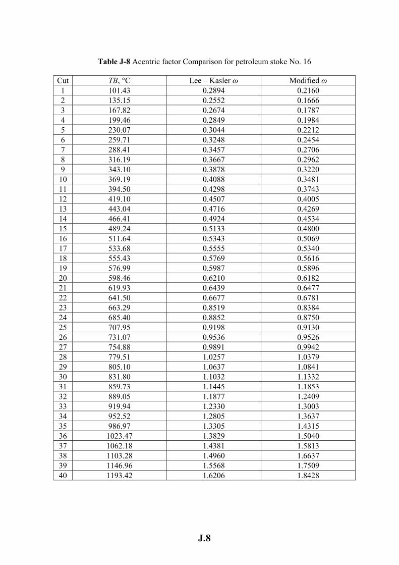
Table J-8 Acentric factor Comparison for petroleum stoke No. 16
Cut TB, °C Lee – Kasler ω Modified ω 1 101.43 0.2894 0.2160 2 135.15 0.2552 0.1666 3 167.82 0.2674 0.1787 4 199.46 0.2849 0.1984 5 230.07 0.3044 0.2212 6 259.71 0.3248 0.2454 7 288.41 0.3457 0.2706 8 316.19 0.3667 0.2962 9 343.10 0.3878 0.3220 10 369.19 0.4088 0.3481 11 394.50 0.4298 0.3743 12 419.10 0.4507 0.4005 13 443.04 0.4716 0.4269 14 466.41 0.4924 0.4534 15 489.24 0.5133 0.4800 16 511.64 0.5343 0.5069 17 533.68 0.5555 0.5340 18 555.43 0.5769 0.5616 19 576.99 0.5987 0.5896 20 598.46 0.6210 0.6182 21 619.93 0.6439 0.6477 22 641.50 0.6677 0.6781 23 663.29 0.8519 0.8384 24 685.40 0.8852 0.8750 25 707.95 0.9198 0.9130 26 731.07 0.9536 0.9526 27 754.88 0.9891 0.9942 28 779.51 1.0257 1.0379 29 805.10 1.0637 1.0841 30 831.80 1.1032 1.1332 31 859.73 1.1445 1.1853 32 889.05 1.1877 1.2409 33 919.94 1.2330 1.3003 34 952.52 1.2805 1.3637 35 986.97 1.3305 1.4315 36 1023.47 1.3829 1.5040 37 1062.18 1.4381 1.5813 38 1103.28 1.4960 1.6637 39 1146.96 1.5568 1.7509 40 1193.42 1.6206 1.8428
J.8
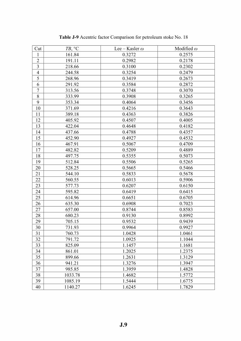
Table J-9 Acentric factor Comparison for petroleum stoke No. 18
Cut TB, °C Lee – Kasler ω Modified ω 1 161.84 0.3272 0.2575 2 191.11 0.2982 0.2178 3 218.66 0.3100 0.2302 4 244.58 0.3254 0.2479 5 268.96 0.3419 0.2673 6 291.92 0.3584 0.2872 7 313.56 0.3748 0.3070 8 333.99 0.3908 0.3265 9 353.34 0.4064 0.3456 10 371.69 0.4216 0.3643 11 389.18 0.4363 0.3826 12 405.92 0.4507 0.4005 13 422.04 0.4648 0.4182 14 437.66 0.4788 0.4357 15 452.90 0.4927 0.4532 16 467.91 0.5067 0.4709 17 482.82 0.5209 0.4889 18 497.75 0.5355 0.5073 19 512.84 0.5506 0.5265 20 528.25 0.5665 0.5466 21 544.10 0.5833 0.5678 22 560.55 0.6013 0.5906 23 577.73 0.6207 0.6150 24 595.82 0.6419 0.6415 25 614.96 0.6651 0.6705 26 635.30 0.6908 0.7023 27 657.00 0.8744 0.8583 28 680.23 0.9130 0.8992 29 705.15 0.9532 0.9439 30 731.93 0.9964 0.9927 31 760.73 1.0428 1.0461 32 791.72 1.0925 1.1044 33 825.09 1.1457 1.1681 34 861.01 1.2025 1.2375 35 899.66 1.2631 1.3129 36 941.21 1.3276 1.3947 37 985.85 1.3959 1.4828 38 1033.78 1.4682 1.5772 39 1085.19 1.5444 1.6775 40 1140.27 1.6245 1.7829
J.9
الخالصة
و التصميم جدا لعمليات مهمة النفطيةحسابات حاله االتزان للبخار و السائل للمقاطع تعتـبر
Flash) أالتزاني هذه الحسابات هو استنباط منحني التقطير أهمو من . النفطيةالتشـغيل للمعـدات
vaporization curve) للنفط الخام الحقيقيةدرجات الغليان منحنيمـن (True boiling point
curve) التخطيطية و هي الطرق األولى: طريقتينبواسـطة و ذلـك (Graphical methods) و
Pseudo – components (ألحاسوبيه الطريقة أو كاذبة مركبات إلى و هي تقسم النفط الخام الثانية
(computer) methods.(
و يتضمن جزئين حيث تم في األولالقسم : قسمين إلى المقدمة الدراسةتم تقسيم الغرض من
مركبات إلىيم النفط الخام واحده و عدد من طرق تقس تخطيطية اختيار و فحص طريقه األول الجزء
تطبيق عدد دراسة بينما يتضمن الجزء الثاني أفضل أداء ذات أيهم لمعرفه ألحاسوبيه الطرق أو كاذبة
لقد تم في القسم . أالتزانيحني التقطير استنباط من في المختارةمن الطرق لغرض تحسين دقه الطرق
و خمسه من Raizi – Daubert (RD graph) لـ التخطيطية الطريقة اختيار الدراسة لهـذه األول
لـ الحالة و تشمل هذه الطرق استخدام طريقه معادله كاذبة مركبات إلىطـرق تقسيم النفوط الخام
Soave – Redlich – Kowng (SRK) لـ لحالةا و طريقه معادلهPeng – Robinson (PR) و
لطور (PR) و (SRK) لـ الحالة و المتضمن استخدام معادلتي الفعاليةطرق استخدام معامل كذلك
و ، SRK + Van)و (PR + Van السائل لطور (van – Laar)تم استخدام نموذج بينما ، الـبخار
األول القسم إنجازو لغرض . (Ideal K) لثابت التوازن المثالية تم استخدام طريقه المحاليل أخـيرا
و تشمل هذه البيانات العلمية المصادر نفط خام من18 لـ الالزمة تم تجميع البيانات الدراسـة مـن
الكثافة و منحنيات أالتزاني و منحنيات التقطير الحقيقية الحرارةدرجات علـى كـال مـن منحنيات
بحثال من هذااألولدلت نتائج القسم لقد . خدمةالمست لهـذه النفوط (Specific gravity) النوعـية
االنموذج الجديد و المقترح في هذ اعتمادا على المطورة (Ideal K) المثالية معادله المحاليل إنعلى
1
طريقه الحتساب منحنى التقطير أفضل هو (Vapor pressure)البخاري لحسـاب الضغط بحـث ال
:اآلتي معادله الضغط البخاري الشكل أخذت حيث المستخدمة للنفوط أالتزاني
( )
−+−+=
TBr85.01FFgr.Spgr.SpPlnPln 21
AsAs
% 15.62يساوي المطورة المثالية لمعادله المحاليل (%AAD)و كـان معـدل االنحـراف المطلق
23.40 و %24.98 و %23.51 البالغة و المعدلةمقارنه بقيم معدل االنحراف المطلق للطرق غير
+ PR و PR و SRK + Van و SRKمن طريقه كل ل% 21.81و % 23.73 و%25.18 و%
Van و Ideal K و RD graph حسب الترتيب و.
تحسين معدل االنحراف المطلق لعشره من إلى أدى المطورة (Ideal K) استخدام معادله إن
حد كبير إلى مرتبط الطريقة هذه أداء التحسينات في إن%. 30 من أكثر و بواقع المستخدمةالـنفوط
و كذلك عدم دقه احتساب الخواص ) الحقيقيةقياس منحني درجات الغليان (ألمختبريهقه النتائج بعدم د
.النفطيةالخ للمقاطع ... ω و الضغط الحرج و الحرجة الحرارةالفيزياويه مثل درجه
الحتساب المطورة (Ideal K) استخدام معادله المقدمة الدراسةالقسـم الثاني من يتضـمن
أنواع ألربعه (Flash zone temperatures)التبخير حرارة و درجات أالتزانيطير منحنـيات التق
ـ الحصول على منحنى درجات و جمبور و باي حسن حيث تم البصرة و هي كركوك و عراقيةط نف
في ألمختبريه التقطير منظومة تجريبيا مستخدما لهذه األنواع النوعية الكثافة و منحنى الحقيقيةالغليان
م و ° 327م و ° 318 التبخير لهذه النفوط كالتالي حرارةلقد كانت نتائج درجات . الـدورة مصـفى
قيم هذه إن. و جمـبور و باي حسن على الترتيب البصـرة ط كـركوك و م لـنف ° 290 و م° 335
و ضغط و كميه بخار حرارة حيث يجب تعديلها وفقا لدرجه أوليه تعتبر أعاله الحراريةالدرجـات
. المستخدم عاده في برج تقطير النفط الخام(Stripping steam)الماء
2
شكر و تقدير
و السالم على سيدنا محمد و اله الطيبين الطاهرين و الصـالة أفضـل و الحمـد هللا رب العالميـن
هذا إنجاز لتيسيره لي أوال اهللا تعالى إلى بالشكر الجميل أتوجه بعد فاني أمـا ، بيـن المنتجصـحابته
:إلى بالشكر أتقدمكما ، البحث
قاسم . د. ا و الطلبة و العلمية للشؤون الكليةمعاون عميد و السيد الهندسة عميد كليه د السـي اشـكر
لمساندتهم لي في قسم الهندسة الكيمياويه نكافه منتسبي و سليمان جبار رئيس قسم الهندسة الكيمياويه
. هذا البحثإنجاز
. ليإشرافه لصبره الجميل خالل فتره محمود عمر عبد اهللا. د. ا العزيز أستاذي اشكر
السيد مدير عام و بالخصوص )الجهة المالكة و الممولة للبحث (الدورة العمل في مصفى فريقاشكر
توفير المصادر و لمساعدتهم المحترمونالعلمية اللجنة أعضاء مختبر التطوير و أعضاءالمصفى و
الجانب العملي لهذا البحث في مختبرات مصفى إنجاز لي خالل العلمـية و االستشـارية الهندسـية
.الدورة
شركه المشاريع (شهالء كمال و الست ) وزاره النفط / الدراسات دائرة ( جواد أميرهالسـت اشـكر
خالل الهندسية االستشارية و العلمية البارز في توفير المصادر الدوريهم) وزاره الـنفط / النفطـية
. البحثإنجاز
تهم و تشجيعهم لي خالل فتره لصبرهم علي و مساند الصغيرةعائلتي و أتوجـه بالشـكر والعرفان ل
. البحثإنجاز
فاضل عامر عدي
سائل للمقاطع النفطية–دراسة اتزان بخار
أطروحة مقدمة إلى كلية الهندسة في جامعة النهرين
جزء من متطلبات نيل درجة دكتوراه فلسفةو هي في الهندسة الكيمياوية
من قبل عدي عامر فاضل الزبيدي
1995 لوريوسابك 1998ماجستير
هـ1427 ذو القعدة مـ2006 تشرين الثاني


