1

HeII Reverberation in AGN Spectra Mark C. Bottorff, Jack A. Baldwin, Gary J. Ferland, Jason W. Ferguson, and

Kirk T. Korista

Abstract This paper compares the observed reverberation response lags and the intensity ratios of the broad line region (BLR) emission lines HeII 1640, HeII 4686 and CIV 1549 with predictions. Published observations indicate that the HeII 1640 lag is three times shorter than the lags of HeII 4686 or CIV 1549. Diverse models however do not reproduce this observation. Extensive improved numerical simulations of the hydrogenic isoelectronic sequence emission show that the HeII spectrum remains especially simple, even in the central regions of a luminous quasar. Line trapping never builds up a significant population of excited states and the emissivities of the two HeII lines are close to simple Case B predictions. Using improved HeII calculations we computed the lags of distributions of clouds concentrated in approximate radius-dependent pressure laws as well as the lags of locally optimally emitting cloud (LOC) distributions. In addition, the effect on lags and intensities due to anisotropic beaming of line emission and observer orientation angle with respect to an obscuring disk is estimated. Comparing our results to observations we do not see how any distribution of clouds can produce intrinsic HeII 1640 and HeII 4686 emission with substantially different responses. Nor do we see how HeII 1640 can vary on a substantially shorter time scale than CIV 1549. Our models suggest that in fact the observed HeII 1640 reverberation time scale is shorter than expected, rather than the observed He II 4686 time scale being longer than expected. We discuss a possible explanation.

1 Introduction The past decade has seen a revolution in our understanding of the emission line regions of AGN due to extensive line-continuum reverberation studies (See Peterson 2001 for a brief review of reverberation mapping applied to AGN). These have shown that the emitting gas is distributed over a wide range of radii and ionization, with significant stratification between species of different ionization potentials. The Broad-Lined Region (BLR) is obviously much more complex than early models that used a single representative cloud at some characteristic radius and density as the basis of studies of BLR properties.

The atomic physics of many of the species present in the BLR is well understood, and it should be straightforward to predict the reverberation behavior of many emission lines. The He+ ion is a particularly simple case. The atomic processes are very well documented, and as we will show below, a clear expectation is that the HeII 1640 and 4686 lines should vary in lockstep with no significant time lag between them. The CIV 1549 line is also produced in a simple situation, and as we will show below, most BLR models predict that the He+ and C+3 ions should coexist closely enough that there should be no more than a modest difference in their reverberation time lags.

2

Yet in all cases where the HeII 1640 and CIV 1549 lag times have both been measured in the same object, it is found that the HeII line varies on a much shorter time scale than CIV. In the one object where both HeII 1640 and 4686 have been measured, the two lines also may vary with significantly different time scales. This paper explores this conundrum. We first review the reliability of the observations, and then discuss the basic simplicity of the He+ ion. Most of this paper is then devoted to working through the predicted reverberation behavior of HeII and CIV lines in a range of models which spans the most frequently suggested structures of the BLR, to see if subtle details can lead to the observed differences in the lag times in spite of the underlying atomic simplicity. Finally, we will offer our best guess at what has been overlooked in the reverberation analysis and must be included in the future in order to explain the observed lag differences.

2 The Observational Situation: HeII and CIV Reverberation We are interested both in the relative intensities and lag times between different HeII lines (λ1640 and λ4686), and in the lag time of the HeII lines relative to lines of other species.

NGC 5548 is by far the best studied AGN, with major optical/UV spectroscopic monitoring campaigns in 1989 (Clavel et al. 1991, hereafter C91; Dietrich et al. 1993, hereafter D93) and then again in 1993 (Korista et al. 1995, hereafter K95). It is also the only object for which λ1640 and λ4686 have both been measured in the same campaigns. In an early study, Wamsteker et al. (1990; W90) measured these two HeII lines from contemporaneous IUE and ground-based observations of modest S/N and spectral resolution spanning 1978-1986 in 29 epochs. Both lines are blended with nearby lines of comparable and much greater strength. HeII 1640 is blended with OIII] 1661, 1666, the red wing of CIV 1549 and perhaps Al II 1670 and emission of uncertain origin near 1600Å (restframe). HeII 4686 is blended with optical FeII (multiplets 37 & 38, others) and the blue wing of Hβ. Figure 1 illustrates each line’s observed-frame spectral regions in representative mean spectra − from the 1993 HST/ground campaign (K95) for λ1640, and from the 1989 IUE/ground campaign (C91, D93)) for λ4686.

After de-blending as best they could the λ1640 and λ4686 lines from the surrounding contaminating emission, removing the narrow line region contributions to the two lines, and correcting the spectra for Galactic foreground extinction (assuming R=3.1, E(B-V) = 0.05), W90 found the broad line flux ratio f(λ1640)/f(λ4686) to have a mean value of 6.9 ± 3.4, which agrees well with the expected recombination value of 6-8 which we will discuss below. However, their results also suggested that this ratio varied from 4 to 10 during the time span of their observations, which if true would indicate different lag times for the two HeII lines.

Further measurements covering both the λ1640 and λ4686 lines in NGC 5548 were made by the AGN Watch group in a 280-day IUE/ground campaign in 1989 (C91; D93). Dumont et al. (1998) recently compared the individual measurements of “λ1640” and “λ4686” from the 1989 campaign for 16 nearly simultaneous observations, and reported ratios that varied from 0.589 to 4.26 with a mean ratio of 2.18 ± 1.22 (their inferred mean

3

broad line spectrum yielded a ratio of 3.15). However, C91 and D93 caution that blending contaminates the measurements of both of these lines. Narrow emission lines, reddening, and (probably in the 1989 IUE data) detector non-linearities are also relevant. When we make our best guesses at the appropriate corrections for these effects (see Appendix I) we find that the mean intensity ratio is more likely be about 5, much closer to the recombination value. Table 1 summarizes the relevant line intensity measurements from the 1989 campaign with these corrections included, and also shows results for CIV 1549 and HeII 1640 from the 1993 campaign (HeII 4686 was not measured in the latter campaign).

However, C91 and D93 may have found substantially different lag times for λ1640 and λ4686 during the 1989 campaign. The most carefully measured values of these lags in the 1989 data are 3.0 (+2.9/-1.1) days for the λ1640 blend and 8.5 (+3.4/-3.4) days for the λ4686 blend, as determined over the full 280-day campaign (Peterson & Wandel 1999). In addition, both the 1989 and 1993 campaigns found that HeII 1640 varied much more rapidly than the adjacent CIV 1549 line (C91; K95).

These lag times are listed in Table 2. The first two columns show the centroid of the lag (in days) of the cross correlation function of the observed emission line light curves for He II 1640, He II 4686, and C IV 1549 with the light curve of the observed continuum at 1350Å as determined from the 1989 and 1993 observing campaigns. The error bars on the lag values are from Peterson & Wandel (1999). The last two columns give line lag ratios. The (estimated) error bars on the lags are not symmetric, with the uncertainty in the longer-lag direction often being larger than in the shorter lag direction. We used a simple square or boxcar uniform distribution of errors. The resulting uncertainty in the lags is conservative, since it puts extra weight on the endpoints of the distribution.

Again, blending with other emission lines is a major source of uncertainty not included in calculating the observed lags or the error bars. All measurements of the HeII 1640 lags in this and other Seyfert 1 AGN have included the light of OIII] 1661,1666 and perhaps other weaker contributions. The λ4686 measurement window (see Figure 1) probably contained a larger contribution from contaminating – and more slowly varying – emission. In addition, the formal error bars on the two lags indicate that they may well be consistent with one another, bearing in mind, too, that the sampling intervals for these two lines were 4 days for the UV line and typically, though unevenly, 1 week for the optical line. However, there is clearly something varying at or very near the wavelengths of these two helium lines in the spectrum of NGC 5548, and the best estimate of the lag times is that the λ1640 feature varies three times more rapidly than λ4686. In this case the intensity ratio of these lines should also change with time, as has been reported by W90.

The ratio of the HeII λ1640 and CIV λ1549 lines is also known for several additional AGN. Table 3 compiles results for all of the objects for which there are reliable lag measurements of both lines. The trend is clear. The HeII 1640 lag times are measured to be several times shorter than those of CIV 1549. This difference has been accepted without much comment because He+ has a significantly higher ionization potential than C+3, and the results from other emission lines show a clear trend of shorter lag times with higher ionization potential. Despite the substantial uncertainties on individual objects and

4

campaigns, all studies show a ratio of lags that are substantially larger than unity, suggesting that this is a true property of these AGN.

3 The Theoretical HeII Spectrum. We have carefully modeled the He+ atomic structure for the calculations presented here. Photoionized models were computed using the development version of the radiative equilibrium code Cloudy, last described by Ferland (2002). This includes many recent improvements to the portions of the code that predicts the intensities of hydrogen and the hydrogen-ion-like isoelectronic sequence. Ferguson & Ferland (1997; hereafter FF) and Ferguson et al. (2002) describe the model of the hydrogen-like isoelectronic sequence, which includes He II, the focus of this paper. These show that the predictions agree with the more extensive calculations of Storey & Hummer (1995) to better than 5% for much lower densities than are considered here. The model atom includes all collisional and radiative effects, including pumping by the continuum and line overlap, collisional excitation and ionization, and line trapping.

We used the continuum shape deduced by Dumont et al. (1998) for NGC 5548, and a solar composition. For simplicity, the hydrogen density was taken to be constant within each cloud, with a column density of 1023 cm-2.

Figures 2a, 2b, and 2c show for CIV 1549, HeII 1640 and He II 4686 the predicted total emission line flux, each normalized to its maximum value, as a function of density n [cm-3] and ionizing radiation flux Φ [cm-2s-1], from 1D slab clouds of column density 1023 cm-2. Contours are logarithmically spaced at 1 dex intervals. Calculations were carried out on a uniformly spaced (0.25 dex) grid in the log(n) vs. log(Φ) plane. The distributions of HeII line emissivities are different from the “peaky” collisionally excited CIV 1549 line. These figures show that the predicted intensities of the HeII lines are comparatively insensitive to assumed details.

The emission planes shown in Figures 2a-2c illustrate the global properties of all possible clouds. The observed spectrum is obtained by integrating over the distribution of the subset of clouds that actually exist. In this work we describe the integration in terms of weighting functions that are power law distribution functions in n and R (the LOC model of Baldwin et al. 1995 and the pressure law models in Goad & O’Brien 1993).

An example of such weighting is the LOC model presented by Korista & Goad (2000), hereafter KG00. This model was chosen from a range of simple LOC models that fit the mean emission line strengths of the stronger UV emission lines of the 1993 HST campaign, with weighting parameters that would produce a wide spread in the lags of the emission lines without exceeding limitations in covering fraction. Figures 2d-2f show the expected emissivity for this model as a function of n and Φ. These are the result of multiplying Figures 2a-2c by the weighting functions in KG00. In each figure the flux is normalized to its maximum, and the contours are now shown on a linear scale with intervals of 0.10. Emission from the HeII lines remains considerably spread out in the log(n)-log(Φ) plane compared to C IV 1549.

Three regions are present in Figures 2d-2f. The declining emission above and to the left of the diagonal from the low to high Φ/n corners corresponds to the coronal phase, where the gas is very highly ionized and produces little UV/optical emission. Temperatures in

5

this region typically lie near 106 K (see Fig. 2 of Korista et al. 1997). Below and to the right of this diagonal, gas is in the nebular phase and temperatures are near 104 K. The equivalent widths of the He II lines change very little in this second region. He II lines form primarily by recombination, so they track the He++ fraction of the cloud, and their emissivity has weak temperature dependence (j ~ T -1). The size of the He II-emitting region inside each individual cloud, which governs the intensity of the He II recombination lines, is determined almost entirely by the shape of the ionizing continuum rather than by cloud parameters, and is in fact a primary stellar temperature indicator for planetary nebulae (Osterbrock 1989). Finally, in the lower right corner of each box there is a region with no emissivity because the weighting functions preclude having any gas with these n-Φ values.

Figure 3 shows the HeII 1640 / HeII 4686 intensity ratio across the log(n)-log(Φ) plane. The ratio is large in the coronal phase, due to both the high temperature and the influence of line pumping by the incident continuum. However, Figure 2 shows that this gas has very small emissivity and can contribute little to the observed lines. The HeII 1640 / HeII 4686 flux ratio falls to 3-4 in the region within the density – flux plane where these lines have their peak emissivities (log(n) ~ 13, log(Φ) ∼ 21). However, this region is comparatively small and emits very little else. Calculations below show that when the emission is integrated over models that predict the other lines, the intensity ratio HeII 1640 / HeII 4686 is in the range 6-8. Thus over most of the region where there is significant emission from the other lines such as CIV (compare to Figs. 2d-2f) the dominate physical situation remains close to the Case B recombination value, ~9 (Hummer & Storey 1995).

He II emission remains very simple because the atom’s resonance lines are effectively destroyed by a combination of Bowen OIII fluorescence (Weymann & Williams 1968) and photoionization of hydrogen in the ground state (MacAlpine 1981). These calculations confirm the long-held suspicion that the He II 1640 / He II 4686 ratio remains close to its optically thin Case B ratio (MacAlpine 1981; MacAlpine et al. 1985). The HeII recombination lines remain optically thin for most conditions where strong lines form. This simplicity makes the He II spectrum a powerful emission line tool – the simulations show that the spectrum should be relatively model independent.

4 Emission line intensity and reverberation In this section we present general expressions for the total line intensity I and the response-weighted radius RRW at which an emission line is formed, in terms of integrations over the variables log(n) and log(Φ). These are needed because I and RRW are measurable quantities, while n and Φ are the physical parameters that we use to describe the distributed geometry required by the reverberation results.

4.1 Observed Line Intensity The observed BLR line intensity is calculated by integrating the differential intensity (the intensity directed toward the observer per unit volume) over the volume of the BLR. Thus we have

6

dVhjIBLR∫ ⋅= )( (1)

where dV is a volume element and the differential intensity per unit volume is symbolized by (j⋅h). It is written as the product of the two functions to separate the total integrated emission power per unit volume (j [erg cm-3s-1]), from the portion of the integrated emission power beamed toward the observer per unit area per steradian (h [cm-2str-1]). The function h depends on µ, the cosine of the angle between the position vector relative to the continuum source, and a unit vector directed from the observer toward the continuum source. This choice puts into h geometric effects such as anisotropic beaming or obscuration by a thick disk. By using this convention j can be estimated from 1D photoionization codes like Cloudy and analytical models may be employed for h. Since emission may arise from an ensemble of clouds of different densities we write j as

dnRnCnFj

n

n∫ ∂∂

∂Φ∝2

1

2

),( (2)

where F [erg cm-2s-1] is the line emission from a cloud with particle density n exposed to ionizing flux Φ, per unit area of cloud surface, and ∂2C/∂n∂R is the differential covering fraction of BLR clouds at radius R as seen from the continuum. The limits of integration range from the smallest cloud density n1 to the largest n2. Substituting equation 2 into equation 1 gives

dVdnhRnCnFI

BLR

n

n∫ ∫ ∂∂

∂Φ=2

1

2

),( (3)

We will calculate I for several spherically symmetric isotropic emission models using a grid of uniformly spaced photoionization calculations in log(n) and log(Φ). Thus h is constant and the volume element is 4πR2dR. It is advantageous to change the integration variables from R and n to log(n) and log(Φ). Since Φ = Lc/4πR2 we have R ∝ Φ-1/2 and

dR ∝ Φ-3/2dΦ. Next changing variables from n and Φ to log(n) and log(Φ) gives dn ∝ n dlogn and dΦ ∝ Φ dlogΦ so we have

∫ ∫Φ

Φ

− ΦΦ∂∂

∂Φ∝)log(

)log(

2/3)log(

)log(

22

1

2

1

loglog),( ndndRnCnFI

n

n

(4)

where Φ1 and Φ2 are the ionizing continuum flux at the maximum radius Rmax (minimum flux) and the minimum integration radius Rmin (maximum flux) respectively. Rmin is taken to be where the gas becomes thermalized and, after weighting by the covering factor and

7

including the effect of geometry, no longer emits significant line radiation. The radius Rmax is taken to be where line emission is truncated due to the onset of dust. We explicitly leave ∂2C/∂n∂R untransformed for easy substitution of its functional forms in section 5 below.

4.2 The responsivity weighted radius The responsivity-weighted radius (RRW) represents the characteristic radial distance from the continuum source to the gas emitting the line in question (Goad et al. 1993). We use a form of RRW that includes anisotropic beaming. It is given by

( )

dVhj

dVRhjR

BLR

BLRRW

∫∫

⋅

+⋅=

)(

1)(

η

µη (5)

The quantity η in Equation 5 is called the responsivity and is defined by

)()(

)()( 00

hjhj

hjhj

⋅Φ

Φ∂⋅∂

=Φ

Φ⋅

⋅⋅

≡δ

δη . (6)

The quantity δ(j⋅h) represents an infinitesimal change in (j⋅h) due to an infinitesimal change δΦ in the ionizing continuum flux from a value Φ0. For model calculations Φ0 is usually taken to be the mean ionizing continuum flux. Since it is assumed that Φ0 ∝ Lc, where Lc is the mean continuum luminosity, Equation 6 may also be written as η = δ(j⋅h)/(j⋅h) ⋅ Lc/δLc or, in the case where there is a unique cloud particle density at each radius, η = δ(j⋅h)/(j⋅h) ⋅Uc/δUc where Uc is the ionization parameter, defined by Uc=Lc/4πR2nc where n is the cloud total hydrogen density at radius R and c is the speed of light (Goad et al. 1993).

The RRW measures the time lag between changes of the ionizing continuum and changes in an emission line. As a result it may be compared to observations. Physically RRW is the characteristic radius at which the response of line emitting gas to temporal changes of the continuum, smeared by light travel time delays, is manifested. The RRW for each emission line will differ because different lines form at different places on the log(n)-log(Φ) plane. Alternatively any two lines that are formed under similar ionization conditions will have similar RRW.

We estimate the effects of non-constant h in section 6 below. Here we calculate RRW when h is a constant and j depends only on R. This means the emission from clouds is isotropic. The assumption simplifies our work and allows us to compare our general definition of RRW with the results in Goad et al. (1993). Using spherical coordinates equation 5 becomes

8

∫

∫

∫

∫== max

min

max

minmax

min

2

max

min

2

)(

)(

4

4

R

R

R

RR

R

R

RRW

dRRL

RdRRL

dRRj

dRRjRR

η

η

πη

πη (7)

where the radial limits of integration are defined in 4.1 and L(R) = j 4πR2 is the line luminosity in a thin shell of radius R. The last expression in equation 7 is exactly the same as in Goad et al. (1993). Since h is set equal to a constant equation 6 becomes

jj 0Φ

Φ∂∂

≡η . (8)

Substitution into equation 7 gives

∫

∫

Φ∂∂Φ∂∂

= max

min

max

minR

R

R

RRW

dRj

RdRj

R (9)

where we have used the fact that 4πR2Φ0 = Lc is independent of R and so the combination may be removed from the integrands of each integral and cancelled. Thus for isotropic emission RRW is the expected value of R weighted by ∂j/∂Φ. Equation 2 indicates that j may be an integration over n. Substituting equation 2 into equation 9 and taking the operator ∂/∂Φ inside the integral over n gives

∫ ∫

∫ ∫

∂∂∂⋅

Φ∂∂

∂∂∂⋅

Φ∂∂

=max

min

2

max

min

2

2

1

2

1

R

R

n

n

R

R

n

nRW

dndRRnCF

RdndRRnCF

R . (10)

We will calculate RRW for several isotropic emission models using a grid of uniformly spaced photoionization calculations in log(n) and log(Φ0). As with the formula for intensity (equation 4) it is advantageous to change the integration variables from R and n to log(n) and log(Φ0). Note we have considered R and Φ as independent quantities because of the dependence of Φ on the time dependant continuum Lc. The quantity ∂F/∂Φ

9

is evaluated at fixed (in time) flux Φ0 and may be traced back to the assumption that emissivity is a linear function of Φ (see Blandford and McKee 1982). Making the same change of variables that leads to equation 4 gives

∫ ∫

∫ ∫Φ

Φ

−

Φ

Φ

−

ΦΦ∂∂

∂⋅Φ∂

∂

ΦΦ∂∂

∂⋅Φ∂

∂

∝ )log(

)log(

)log(

)log(

2/12

)log(

)log(

)log(

)log(

12

2

1

2

1

2

1

2

1

loglog

loglog

n

n

n

nRW

ndndRnCF

ndndRnCF

R . (11)

Both ∂F/∂Φ and ∂2C/∂n∂R is untransformed for easy insertion of photoionization calculations and different covering fraction formulae.

The formula for RRW (equation 11) involves ∂F/∂Φ. For numerical calculations of equation 11 the derivative at each grid point was computed numerically by calculating an additional photoionization grid offset -0.05 dex in log(Φ) from the previous grid and a using a simple first order finite difference scheme. Thus we have

05.0

05.0

10)10,(),(

−

−

⋅Φ−Φ⋅Φ−Φ≈

Φ∂∂ nFnFF . (12)

The derivative approximation in equation 12 is weighted by ∂2C/∂n∂R and inserted into equation 11. Different ∂2C/∂n∂R are described below in sections 5.2 and 5.3 and the corresponding ratios of I and RRW for He II 1640, He II 4686, and C IV 1549 are calculated.

5 The Effect of BLR Cloud Distributions on Reverberation Results We now take the formalism developed above for determining I and RRW, and insert different BLR cloud distributions that span the range of what are currently considered to be realistic models. At one extreme is the very simple, but ad hoc, picture in which the gas is distributed according to a radius-dependent pressure law that is a free parameter (Rees, Netzer, & Ferland 1989; Goad et al. 1993; Kaspi & Netzer 1999). At the opposite end of the range is the “Locally Optimally-emitting Cloud” (LOC) model, in which the clouds have a wide distribution of properties at every radius, but the powerful selection effects introduced by atomic and plasma physics determine the integrated BLR spectrum. It has been shown that in the latter case the overall emitted spectrum is very similar to typical AGN spectra independent of the detailed structure of the BLR (Baldwin et al. 1995; Korista et al. 1997). KG00 used a LOC model to describe the mean UV broad emission line spectrum of NGC 5548.

10

We use these models to see whether it is possible, over this wide range of parameter space, to produce RRW(HeII 1640) / RRW(HeII 4686) and RRW(C IV 1549) / RRW (HeII 1640) values that are consistent with the observed lag ratios. Throughout this section we assume that the BLR geometry is spherical and that individual clouds emit line radiation isotropically. These two assumptions will be relaxed in later sections.

The cloud properties and the continuum they are exposed to are the same as used in section 3 to calculate Figure 2. The range of the computed grid in Figure 2 is 7.0 ≤ log(n) ≤ 14.0 and 17.0 ≤ log(Φ) ≤ 24.0 but integrations in RRW are calculated on the sub-range 7.0 ≤ log(n) ≤ 14.0 and 18.0 ≤ log(Φ) ≤ 22.25. The lower flux limit corresponds to the radius of dust sublimation (Netzer & Laor 1993) where the presence of dust grains diminishes the line emission. The upper flux limit (or inner radius) of integration is set by the onset of line thermalization – dense clouds are primarily continuum emitters, the effect of the covering fraction function and the geometry. These boundaries are shown as dashed white lines in Figure 2d through Figure 2i. Note that the emission of CIV 1549 (Figure 2d), HeII 1640 (Figure 2e), and He II 4686 (Figure 2f) decrease relative to the continuum outside these boundaries for the KG00 LOC model. For an assumed luminosity of NGC 5548 given by KG00 the upper flux limit of integration corresponds to a radius of ~1 light day Between the integration limits the contours of Figure 2e and Figure 2f appear very similar. This suggests that it will be very difficult to create a significant difference between RRW(He II 1640) and RRW(He II 4686) for standard clouds.

5.1 LOC Models The principal of the LOC model (Baldwin et al. 1995) is that clouds are distributed over a wide range in n and Φ, but those located at a density and flux that emit line radiation most effectively tend to dominate the integrated contribution to the observed line flux. The differential covering fraction is written as the product of two functions, ∂2C/∂R∂n ∝ f(R)g(n). The functions f(R) and g(n) describe the physical structure of the BLR and in real situations are likely to be quite complicated. However, the emergent spectrum depends only weakly on the exact structure, so reasonable agreement with the observations is obtained using the simple power-law forms f(R) ∝ Rγ, g(n) ∝ nδ . Thus

δγ nRnRC f ∝∂∂

∂ 2

. (13)

Substituting R ∝ Φ-1/2 into equation 13 and then equation 13 into equation 11 gives

11

∫ ∫

∫ ∫Φ

Φ

++−

Φ

Φ

++

−

ΦΦΦ∂

∂

ΦΦΦ∂

∂

∝ )log(

)log(

)log(

)log(

121

)log(

)log(

)log(

)log(

122

2

1

2

1

2

1

2

1

loglog

loglog

n

n

l

n

n

l

RW

nddnF

nddnF

Rδ

γ

δγ

. (14)

This equation determines the radius where there is significant emission. It has the advantage that it may be compared directly with observations.

How is it that this formula involving ∂F/∂Φis able to trace the spatial distribution of F? To illustrate the connection between the response-weighted approach and the intensity-weighted approach of the LOC model, consider the intensity-weighted radius RIW defined by

∫∫

⋅

⋅=

BLR

BLRIW dVhj

RdVhjR

)(

)( . (15)

For the isotropic LOC model RIW is given by

∫ ∫

∫ ∫Φ

Φ

++

−

Φ

Φ

++

−

ΦΦ

ΦΦ

∝ )log(

)log(

)log(

)log(

123

)log(

)log(

)log(

)log(

124

2

1

2

1

2

1

2

1

loglog

loglog

n

n

n

nIW

nddnF

nddnFR

δγ

δγ

. (16)

Inspection of the integrands in the integrals in the denominators of equation 15 and equation 16 reveals that the weighting of RIW is proportional to FΦ-(γ+3)/2nδ+1. This is the weighting used in the contour plots of Figures 2d-2f for CIV 1549, He II 1640, and He II 4686 respectively (for the adopted LOC model of KG00 that has γ = -1.2 and δ = -1). For comparison, Figures 2g-2i show the weighting of RRW from equation 14 (also using γ = -1.2 and δ = -1), which is proportional to (∂F/∂ Φ)Φ-(γ+1)/2nδ+1. The two sets of contour plots are nearly identical, showing that F ∝ (∂F/∂ Φ)Φ. This confirms that a significant portion of the emitting material responds in a linear way to modest (0.05dex) changes of the continuum, which is a fundamental assumption of standard reverberation mapping theory (Blandford and McKee 1982). Thus it is reasonable, at least for LOC models that use isotropically emitting clouds, that Equation 14 is a good indicator of the relative location of line emitting material.

LOC models are shown in the top six panels of Figure 4. The first row shows the intensity ratios I(CIV 1549)/I(HeII 1640), I(HeII 1640)/I(HeII4686) and I(CIV 1549)/I(HeII 4686). Equation 4 is used for the calculations. The parameter space (–2.0 ≤ δ ≤ 0.0 × –2.0 ≤ γ ≤ 0.0) is considered. The location in parameter space of the LOC

12

model used by KG00 is shown with a cross. The choice of parameters includes the range of the acceptable γ to be –1.6 < γ < -0.5 as found by KG00. In addition, earlier investigations by Baldwin (1997) suggest that δ ≈ –1. We do not consider values significantly outside this range because they give poor fits to the observed reverberation times and intensities of other bright emission lines not studied here.

The intensity ratio contours may be compared with the observed line flux ratios from Table 1. The CIV 1549 / HeII 1640 ratios determined from the 1989 and 1993 observing campaigns overlap with each other and also with the value calculated using the KG00 model. The (very wide) error bars on the CIV 1549 / HeII 4686 measurement from the 1989 campaign also include the KG00 value.

We do not vary the form of the ionizing continuum. The ratio of CIV 1549 to recombination lines depends on the continuum shape, since this is the ratio of a strong coolant to the recombination rate, which is basically the Stoy ratio (Osterbrock 1989). We could have adjusted the continuum shape to reproduce the CIV / HeII intensity ratios, but do not do so here. The second row of the top panels of Figure 4 shows the ratios RRW(CIV 1549) / RRW(HeII 1640), RRW(HeII 1640) / RRW(HeII4686) and RRW(CIV 1549) / RRW(HeII 4686) respectively for the LOC model. Equation 14 is used to calculate the RRW up to a multiplicative constant.

The observed lag ratios in Tables 2 and 3 are contaminated by OIII] 1663 mixed in with the HeII 1640 line. To estimate the correction to the measured lag, we must first estimate the contribution of OIII] to the total intensity. The observed OIII]1663 / HeII1640 intensity ratio is about 0.5, while the LOC model with the KG00 parameters (γ = -1.2, δ = -1) predicts 0.7. Figure 5 shows the expected correction to RRW(HeII 1640) as a function of I(HeII 1640) / I(HeII 1640 + contaminating OIII] 1663), both for the LOC model and for the pressure-law model (labeled Gauss) described below. The ratio I(HeII 1640) / I(HeII 1640 + contaminating OIII] 1663) was found by summing the distributions of OIII] 1663 and HeII 1640 emissivities on the log(n) – log(Φ) plane as predicted by the model, but scaling OIII] 1663 by a factor that varied from 0 to 1. RRW for the resulting HeII-OIII] blend was then calculated and compared to RRW for the HeII line alone to produce the correction.

Figure 5 shows that OIII] contamination should lead to only a ~10% effect (a decrease) in the observed HeII 1640 lag time. The effect is small because, although OIII] emits most strongly from a radius about two times farther out than the peak of the HeII emissivity, the HeII emission is spread out over a broad range extending out to rather large radii.

The model ratios may now be compared to the observed lag ratios in Tables 2 and 3. Due to the large observed errors on the lag ratios definitive claims cannot be made about whether or not LOC models are consistent or inconsistent with observations. The results however are suggestive. Note that whether or not we allow for a small correction for OIII], the observed lag ratio Lag(CIV 1549)/Lag(HeII 1640) ~3.0 (see Tables 2 and Table 3) is not achieved anywhere by the LOC model in the parameter space considered nor is the observed lag ratio Lag(HeII 1640)/Lag(HeII 4686) ~ 0.4. The predicted values are 2.4σ and 0.8σ away from these observed values. On the other hand the observed lag ratio Lag(CIV 1549)/Lag(HeII 4686) ~ 1.1 is achieved by the LOC model in the parameter space considered. This suggests that there is a problem with the HeII 1640 line rather than the HeII 4686 line. The model predicts a response of HeII 1640 roughly

13

contemporaneous with HeII 4686 and CIV 1549. The observations indicate an earlier response, by a factor of about 3.

5.2 Radius-Dependent Pressure Law Models In order to see if the discrepancies with the observations might be just an artifact of the LOC model, we now consider a quite different class of models that are radius-dependant pressure laws (Goad, O’Brien & Gondhalekar 1993). Here

mn )10/(10 5.1810 Φ= (17)

where Equation 17 defines a straight line in the log(n) vs. log(Φ) plane. For reference m = 0 defines a vertical line (constant density). The line is constructed to pass through the point log(n) = 10.0 and log(Φ) = 18.5 to be in accord with the conditions of “standard” BLR cloud conditions (Davidson and Netzer 1979). The ionization parameter along this line is U = Φ/nc ≈ 10-2(Φ/1018.5)1-m. Observations indicate that the BLR of AGN are ionization stratified with lower ionization lines dominating at greater radii (Peterson 1993). Thus if radius-dependant pressure law models apply to the BLR then U must decrease with increasing radius so that m ≤ 1. In addition denser BLR clouds may lie at smaller radii (and therefore higher Φ) (Brotherton et al.1994). We therefore restrict m to 0 ≤ m ≤ 1. As with the LOC model a differential covering factor in the form of a power law in radius is assigned thus

γRRC f ∝∂

∂ . (18)

We normalized the models in the same way as Goad, O’Brien, and Gondhalekar 1993, but unlike them we used a constant column density for simplicity. To facilitate integration on the coarse computed grid we assign a differential cover factor in the form of a Gaussian distribution in log(n) with standard deviation 1.0 centered on equation 17. Thus while not an exact radius-dependant pressure law model (due to the Gaussian width), this distribution is 5 orders of magnitude more restricted in density than the LOC models of section 5.2.

The first row of the bottom six panels of Figure 4 shows the intensity ratios CIV 1549 / HeII 1640, He II 1640 / He II 4686, and CIV 1549 / HeII 4686 respectively for the pressure law model. The parameter space (0.0 ≤ m ≤ 1.0 × –2.0 ≤ γ ≤ 0.0) is considered. A dot at m = 1/2 and γ = -5/6 marks the parameters of an idealized n ∝ R-1 pressure law model from Goad, O’Brien, and Gondhalekar (1993) that predicts reasonably well the reverberation response of the bright emission lines of NGC 5548. As with the LOC model, the intensity ratio contours of the pressure law model may be compared with the observed line ratios C IV 1549 / He II 1640, He II 1640 / He II 4686, and CIV 1549/ HeII 4686 from Table 1. The predicted ratios of the pressure law model

14

fairs less well than the LOC model. For example, when the range of the observed flux ratio CIV 1549 / HeII 1640 from either the 1989 or the 1993 observing campaigns of NGC 5548 are mapped onto the corresponding intensity ratio contours, the idealized pressure law model (m = 1/2 and γ = -5/6) is not included. The predicted OIII] / HeII ratio is 1.5. Other choices of the model parameters could lower this predicted value, by including a different part of the log(n) – log(Φ) plane , but are unlikely to satisfy the many other boundary conditions set by the reverberation results and the strengths of the other emission lines. An alternate possibility is that the abundances of the α-elements are lower, by about a factor of two, than were used in our models. Figure 5 shows the expected correction to the HeII lag time for the pressure law model, calculated in the same way as for the LOC model. Again, the correction to RRW is only about 10%, and therefore will be ignored here.

The second row of the bottom panels of Figure 4 show the ratios RRW(CIV 1549) / RRW(HeII 1640), RRW(HeII 1640) / RRW(HeII 4686) and RRW(CIV 1549) / RRW(HeII 4686) respectively for the pressure law model. The model ratios are compared to the corresponding lag ratios in Tables 2 and 3. Note the observed lag ratio Lag(CIV 1549) / Lag(HeII 1640) ~3.0 is not achieved anywhere by the pressure law model in the parameter space considered nor is the observed lag ratio Lag(CIV 1640) / Lag(HeII 4686) ~ 0.4 or the observed lag ratio Lag(CIV 1549) / Lag(HeII 4686) ~ 1.1. Thus the pressure law model has problems with all three response ratios considered here. The pressure law Model F of Goad et al. (1993) is one of constant density and column density, and so its cloud distribution cuts across the largest number of contours in Figs. 2d-2f and 2g-2i (a vertical line in these plots). It also has the property of having a steeply falling covering fraction distribution with radius (γ = -9/6). Together these conspire to widely separate the emission line lags. However, Table 4 in Goad et al. and the bottom left panel of our Figure 4 indicate that even this model produces a lag ratio Lag(CIV 1549) / Lag(HeII 4686) < 1.8, far short of the observed value ~ 3.

The scatter and error bars in the observed reverberation lag ratios are far too large to make definitive claims about which model is best. For example, based on the above analysis, one cannot conclude that the LOC model is any better or worse than the pressure law model at predicting the intensity or lag ratios considered in this paper. Rather, the important point of these two sections is that that a wide range of models consisting of clouds distributed in density and radius and unique in density with radius are both unable to account for the observed short reverberation time of HeII 1640 relative to CIV 1549 and possibly HeII 4686.

5.3 Effect of Internal Cloud Parameters. We have focused on this pair of He II lines because of their simplicity. Resonance lines of He II occur at energies that can ionize both hydrogen and helium. Either this destruction, or conversion by the Bowen mechanism (Osterbrock 1989), act to prevent large optical depths from building up in He II subordinate lines. As a result the optical and UV lines are formed mainly by recombination and the emission spectrum is mainly determined by the branching ratios from upper levels. There is only a weak (< 20% typically) density and temperature dependence due to details of the atomic physics. In particular the recombination spectrum has no direct dependence on the continuum shape

15

or gas composition. The spectrum will be near "case B" and have no dependence on the column density as long as the column density is large enough to allow the HeII Lyman lines to be optically thick. Ferland (1999) discusses the smaller column density case, and shows that the spectrum goes over to the moderately different "Case C", but that such optically thin clouds are very inefficient radiators and would be nearly invisible. It is hard to imagine realistic conditions where the He II emission would be far from its simplest expectations.

We conclude this section with brief comments on four additional factors that, at first sight, might influence the observed lag times: (1) BLR cloud size, (2) recombination times, (3) negative responsivity clouds, and (4) non-linear response. For each of these, we find that the impact on I and RRW is negligible for the types of models considered here, and therefore are probably not important in any realistic BLR model.

1. Cloud Size

The flux ordinate on the log(n) vs. log(Φ) plane may be converted into a distance scale if a luminosity is assumed. The luminosity of NGC 5548 given by KG00 gives an inner radius of integration of ~1 light day. Spherical clouds with column density ~1023cm-2 with log(n) ≤ 8.0 will completely fill the volume at this radius and cover the continuum source. In general clouds in the upper left hand corner of the log(n) vs. log(Φ) plane will have problems fitting in the BLR at the given normalization of flux with radius. Clouds in this region must therefore be excluded from integrations over the region. In any case clouds in this region are fully ionized and contribute little to the integrated line emission or the reverberation response (for all of the same reasons, KG00 excluded these clouds from consideration).

2. Recombination Time The recombination time is roughly proportional to (nT)-1. The recombination time is always shorter than the variability time except when the gas is heated to the Compton temperature. But this gas is does not contribute to the net emission. The jagged white line superimposed on the contour plots of Figures 2d-2i (and the jagged solid line superimposed on in Figure 3) corresponds to a recombination time of ~1 day. To the right of this line recombination times are shorter. In the region of significant emission (the yellow and orange areas of Figures 2d-2i) the recombination time is only a few minutes. Recombination time delay effects therefore need not be considered in reverberation calculations.

3. Negative Cloud Responsivity

Figures 2a-2c all have regions where ∂F/∂Φ < 0. The region is roughly above a diagonal running from the lower left hand corner to the upper right corner of each figure. Clouds in this region have line emissivities that decrease with an increase in Φ. If this also implies that η < 0 (provided the function f and or ∂2C/∂n∂R does not somehow compensate) then the clouds are said to have “negative responsivity”. Figures 2d-2i shows that the LOC weighting strongly suppresses the contribution to both the emission and emission response of negative responsivity gas. Even if there were a distribution of column densities, it would mainly affect the low-ionization lines, because the high-ionization lines form near the inner edge of the cloud. The region in the log(n) vs. log(Φ)

16

plane where ∂F/∂Φ < 0 (the blue triangular region and purple diagonal strip just above the green, yellow and orange regions of Figures 2g-2i) has very nearly a zero value. Thus the LOC models we computed have little net emission from negative responsivity clouds and the overall effect is that the lines investigated here respond positively. The pressure law models we calculated also do not include any significant contribution from negative responsivity gas.

4. Non-linear emission line response The goal of reverberation analysis is to reconstruct the spatial distribution of line emission or, at the very least, the values of lower order moments such as RRW. Formulae for RRW (equation 5) assume that line emissivity has either a strict linear response to changes in Φ (Blandford and McKee 1982) or that changes in Φ are sufficiently small so that the emissivity is well represented by linearization. Locations on the log(n) – log(Φ) plane where problems may arise if either of the above assumptions are not valid are on the ridge lines of emission where the concavity of emission with increasing Φ is largest. These ridge lines are seen as sharp bends in the contour lines of figure 2a, 2b and 2c and (as mentioned earlier) are where the gas begins to transition to its coronal phase. We note that, when weighted by the representative models discussed in this paper emission from the regions near the ridge lines are suppressed and have little effect on RRW. Figures 2d-2i illustrate that this is the case for the best fit model of KG00 where, near the locations of the respective ridge lines, weighted emission is only ~10% of the maximum and the weighted maximum emission occurs far from the ridges. The result is that the assumption of a linear response is a reasonable one.

The weighting of the models investigated in this paper scale as a power law. As a result a change in the ionizing flux may be interpreted as equivalent to a vertical shift of the log(Φ) limits of integration (the dotted lines in figures 2d-2i). Along the upper boundary the weighted contribution decreases with an increase in log(Φ) whereas along the lower limit the weighted contribution increases. The two effects roughly offset one another as long as neither of the limits approaches the weighted emission peaks. Numerical experiments on the best fit model of KG00, in which the flux limits are changed by a factor of ~5 (a vertical shift of ~0.7dex in the log(n) – log(Φ) plane), have little effect on the relative reverberation response of the CIV 1549, HeII 1640, and HeII 4686 lines. We conclude that even large changes in Φ (a factor of ~5) will have little effect on the relative responses of the system.

6 Beaming and Disk Obscuration The common assumption of all the models of section 5.2 and 5.3 is that emission from clouds is both isotropic and unobscured. Here we investigate whether or not beaming, possibly coupled with obscuration by a disk, can reduce the model ratio RRW(HeII 1640) / RRW (He II 4686) and increase the model ratio RRW (CIV 1549) / RRW (He II 1640) so that the corresponding observed lag ratios are more consistent with the best fit models (e.g. the models corresponding to the crosses in figure 4). For beaming we take the extreme (but computationally tractable) case of “pancake” clouds with the normal of the continuum facing surface pointing directly at the continuum engine. Simulations predict the fraction of the emission, directed toward the source of ionizing radiation. The portion

17

of the emission from the cloud beamed toward the observer (defined in section 2 as h) is then given by

<≤−−≤≤

∝01for10for

µµµµ

I

D

hh

h (19)

where hD is the fraction of the total emission beamed out the back (or dark) side of the cloud, hI is the fraction of the total emission beamed out the front (or illuminated) side of the cloud (so that 1- hD = hI ), and µ = cos(θ) where θ is the angle between a ray from the continuum source to the observer and a ray from the continuum source to a cloud. For simplicity we assume all functions of angle are independent of R. Introducing Equation 19 into equation 5 gives

( )

∫∫

∫∫

Φ∂∂

Ω

Φ∂∂

Ω+

=

Ω

Ω

2

1

2

1

1

R

R

R

RRW

dRj

hd

RdRj

dhR

µ (20)

where we have used the fact that Lc=4πR2Φ may be factored out of the integrals.

We now hypothesize an obscuring disk blocks our view of the far side of the BLR. The disk is oriented at polar angle Θ with respect to the direction to the observer (the Z axis). The integration in angle therefore is not over a full 4π sr but over a smaller unblocked solid angle region that we symbolize by Ω. Part of the solid angle includes the region where the observer views the dark side of the cloud. In the remaining region an observer sees the illuminated side of the cloud. Separating the radial and angular parts of equation 20 gives

isotropicRWRW RGR ,)( ⋅Ω= (21)

where

( )

∫

∫

Ω

Ω

Ω

Ω+=Ω

hd

dhG

µ1)( (22)

18

and RRW,isotropic is RRW as given by equation 9 but with the subscript isotropic is added to remind us that it is the isotropic case. The function G(Ω) multiplying RRW,isotropic is therefore the factor by which the isotropic case is modified to give the anisotropic case (for this simplified scenario).

We now integrate 22.To simplify visualization we consider a unit spherical shell section of the BLR (see Figure 6). Observers see emission from clouds with Z > 0 originating from the dark side of the cloud. Observers see emission from clouds with Z ≤ 0 originating from the illuminated side of the cloud. Any emission originating from below the bisecting plane does not reach the observer. A contour plot of G(Ω) as a function of Θ in degrees from 0° to 90° and hD from 0 to 1 is shown in Figure 7a. The surface cut by Θ = 0° is equivalent to no obscuration. Note that along Θ = 0° we have G(Ω) = 1 at hD = 0.5 as we should have for isotropy and no obscuration. Values of G(Ω) for isotropic emission with an obscuring disk lie on the horizontal line hD = 0.5. The general trend is that increasing hD or Θ results in decreasing G(Ω). The Cloudy computed hD for the lines CIV 1549, HeII 1640, and HeII 4684 are shown in Figures 2j-2l. Isotropic regions (hD ≈ 0.5) appear as light green. Yellow orange shows where hD exceeds the 0.5 contour threshold by a few percent. Successive contours and darker regions correspond to a 0.1 decreases of hD. Over the regions where there is significant emission from CIV 1549, HeII 1640, and HeII 4686 most clouds with column densities ≥ 1023cm-2 have hD ≤ 0.5. To illustrate, the emission weighted average of hD for CIV 1549, HeII 1640, and HeII 4686 is 0.26, 0.33, and 0.41 respectively. These three values are shown as horizontal dashed lines in Figure 7a. Overall the CIV 1549 line is the most anisotropic (smallest hD) followed by the HeII 1640 line and then HeII 4686. To estimate the magnitude of the correction on ratios of RRW the ratios of G(Ω) as a function of Θ are found along lines of emission weighted hD . Based on this the maximum correction to RRW(CIV 1549)/RRW(HeII 1640) is ~1.2 at a disk orientation Θ ≈ 40.5°, the maximum correction to RRW(HeII 1640) / RRW(HeII 4686) is ~1.1 at a disk orientation Θ ≈ 31.5°, and the maximum correction to RRW (CIV 1549) / RRW(HeII 4686) is ~1.3 at a disk orientation Θ ≈ 36.0°. If we apply these corrections to the optimal LOC model (marked by the cross in Figure 4) we see that RRW(CIV 1549) / RRW(HeII 1640) is boosted from ~1.2 to ~1.2×1.2 ≈ 1.4, RRW(HeII 1640) / RRW(HeII 4686) is boosted from ~1.1 to ~1.1×1.1 ≈ 1.2, and RRW(CIV 1549) / RRW(HeII 4686) is boosted from ~1.4 to ~1.4×1.3 ≈ 1.8. These corrections move RRW(CIV 1549) / RRW(HeII 1640) slightly closer to the observed value ~3 (Tables 2 and 3) but move RRW(HeII 1640) / RRW(HeII 4686) and RRW(CIV 1549) / RRW(HeII 4686) away from their observed values of ~0.4 and ~1.1 respectively. There are similar results for the pressure law models. We conclude from this analysis that it is not possible to simultaneously satisfy the observed response ratios with any of the broad range of model types considered here.

A similar analysis was done to estimate the effect of anisotropic emission on line intensity ratios. A contour plot of G(Ω) for intensity is shown in Figure 7b as a function of Θ and hD. The horizontal dashed lines show the same emission weighted hD as in Figure 7a for CIV 1549, HeII 1640, and HeII 4686. Relative differences in G(Ω) from one hD value to another, for obscuring disk angle Θ, give the correction to the intensity ratios for the case of isotropic beaming. We note that hD = 0.5 means symmetry of front versus back surface emission. Because the clouds are pancake shaped however beaming

19

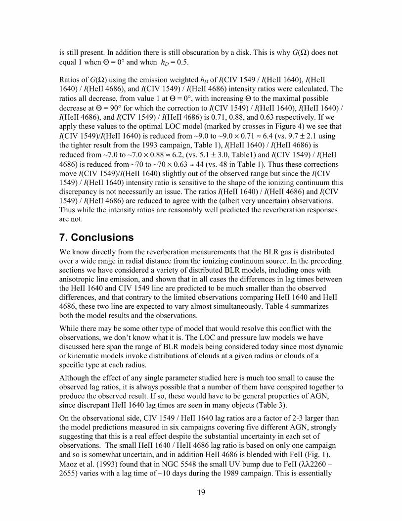
is still present. In addition there is still obscuration by a disk. This is why G(Ω) does not equal 1 when Θ = 0° and when hD = 0.5.

Ratios of G(Ω) using the emission weighted hD of I(CIV 1549 / I(HeII 1640), I(HeII 1640) / I(HeII 4686), and I(CIV 1549) / I(HeII 4686) intensity ratios were calculated. The ratios all decrease, from value 1 at Θ = 0°, with increasing Θ to the maximal possible decrease at Θ = 90° for which the correction to I(CIV 1549) / I(HeII 1640), I(HeII 1640) / I(HeII 4686), and I(CIV 1549) / I(HeII 4686) is 0.71, 0.88, and 0.63 respectively. If we apply these values to the optimal LOC model (marked by crosses in Figure 4) we see that I(CIV 1549)/I(HeII 1640) is reduced from ~9.0 to ~9.0 × 0.71 ≈ 6.4 (vs. 9.7 ± 2.1 using the tighter result from the 1993 campaign, Table 1), I(HeII 1640) / I(HeII 4686) is reduced from ~7.0 to ~7.0 × 0.88 ≈ 6.2, (vs. 5.1 ± 3.0, Table1) and I(CIV 1549) / I(HeII 4686) is reduced from ~70 to ~70 × 0.63 ≈ 44 (vs. 48 in Table 1). Thus these corrections move I(CIV 1549)/I(HeII 1640) slightly out of the observed range but since the I(CIV 1549) / I(HeII 1640) intensity ratio is sensitive to the shape of the ionizing continuum this discrepancy is not necessarily an issue. The ratios I(HeII 1640) / I(HeII 4686) and I(CIV 1549) / I(HeII 4686) are reduced to agree with the (albeit very uncertain) observations. Thus while the intensity ratios are reasonably well predicted the reverberation responses are not.

7. Conclusions We know directly from the reverberation measurements that the BLR gas is distributed over a wide range in radial distance from the ionizing continuum source. In the preceding sections we have considered a variety of distributed BLR models, including ones with anisotropic line emission, and shown that in all cases the differences in lag times between the HeII 1640 and CIV 1549 line are predicted to be much smaller than the observed differences, and that contrary to the limited observations comparing HeII 1640 and HeII 4686, these two line are expected to vary almost simultaneously. Table 4 summarizes both the model results and the observations.

While there may be some other type of model that would resolve this conflict with the observations, we don’t know what it is. The LOC and pressure law models we have discussed here span the range of BLR models being considered today since most dynamic or kinematic models invoke distributions of clouds at a given radius or clouds of a specific type at each radius.

Although the effect of any single parameter studied here is much too small to cause the observed lag ratios, it is always possible that a number of them have conspired together to produce the observed result. If so, these would have to be general properties of AGN, since discrepant HeII 1640 lag times are seen in many objects (Table 3).

On the observational side, CIV 1549 / HeII 1640 lag ratios are a factor of 2-3 larger than the model predictions measured in six campaigns covering five different AGN, strongly suggesting that this is a real effect despite the substantial uncertainty in each set of observations. The small HeII 1640 / HeII 4686 lag ratio is based on only one campaign and so is somewhat uncertain, and in addition HeII 4686 is blended with FeII (Fig. 1). Maoz et al. (1993) found that in NGC 5548 the small UV bump due to FeII (λλ2260 – 2655) varies with a lag time of ~10 days during the 1989 campaign. This is essentially

20

the same as the reported HeII 4686 and CIV lag times, so it may be that the HeII 4686 lag measurement is spurious and that both HeII lines vary on the same (unexpectedly rapid) time scale. However, the HeII spectrum is very simple, and the He II 4686 / C IV 1549 lag ratio is close to the expected value, suggesting again that the 1640 lag is unexpectedly short.

The thrust of this paper has been on HeII and the problems models have in predicting the overly rapid response of the HeII 1640 line. By contrast models do predict the high ionization fast responding line NV 1240 in NGC 5548. To illustrate, the observations yield a CIV 1549 / NV 1240 lag ratio of ~2.4 and ~2.8 for the 1989 and 1993 campaigns respectively of NGC 5548 (with perhaps a 50% error on the lag of the NV λ1240 line) and the KG00 optimal model gives a lag ratio of CIV 1549/ NV 1240 ~ 2.0. This agreement suggests that our results are robust to the details of the high flux, inner region of the BLR where both the HeII lines and NV 1240 peak in emission. This strengthens the argument that it is the HeII 1640 line that is a problem.

The most straight-forward explanation is that we are measuring some other feature blended with HeII 1640. What could this extra feature be?

In principle the HeII 1640 line could be dominated by an extra, rapidly varying component that does not produce much HeII 4686 or CIV 1549. Comparison of Figures 2a and 2b shows that gas with log(n) ~ 12-13, log(Φ) ~ 24 could produce 1640 but little 1549, but figures 2b, 2c and 3 together show that there is no location on the log(n) – log(Φ) plane where large amounts of λ1640 can be produced without also producing lots of λ4686 emission. Even if there were such a situation, then the mean λ1640 / λ4686 intensity ratio should be very large, which does not appear to be the case (albeit with very large observational uncertainties, as is discussed in Appendix 1.).

We suggest that a more likely candidate is a variable absorption feature from the continuum source itself. The ultraviolet continuum source is usually assumed to be dense thermal matter, probably the skin on an accretion disk. Current disk models do not accurately predict the continuum spectrum at the level of detail that would include absorption lines; in fact there is a well-known problem in that hydrogen Lyman continuum absorption is predicted but not seen (Antonucci et al. 1996, Antonucci, Kinney, & Ford 1989). We postulate that an absorption feature due to HeII 1640 or some other nearby line is produced in the skin of the accretion disk and responds immediately to changes in the continuum level coming from the disk. The response of this component would then be mixed with the slower response of HeII emission produced in the BLR to give the observed result. To produce the observed effect, such an absorption feature would have to diminish in equivalent width as the continuum level increased, since the net feature at λ1640 is always observed to have a strong positive response to continuum variations. An obvious difficulty with this interpretation is that no other atmospheric absorption features are known.

The above is at present just speculation. What we actually have found here is that a wide range of models of the BLR indicate that HeII 1640, HeII 4686 and CIV 1549 should all have very similar reverberation lag times. The available observations appear to contradict this, but the uncertainties are large. An obvious next step that we are currently initiating is to re-examine the extensive existing data from AGN reverberation monitoring campaigns, in order to better test whether or not HeII 1640 really does have a several

21

times shorter lag time than CIV, and whether or not the HeII 1640/4686 intensity ratio is consistent with the expected range of 6-8.

If the contradiction between the models and observations persists and is significant, we will then need to more carefully consider what revisions are required in our picture of the BLR.

This work was supported by the NSF and NASA through grants AST-0071180 and NAG5-8212.

Appendix 1. The HeII 1640/4686 intensity ratio in NGC 5548 We discuss here the various corrections that we believe need to be applied to the published λ1640 and λ4686 line strengths from C91 and D93 before they can be used to derive the HeII 1640 / HeII 4686 intensity ratio. To start with, a 3.5% correction of the λ1640 / λ4686 ratio is needed because the fluxes quoted in D93 are in restframe. But more important are the contributions of the contaminants to each line, the uncertainties associated with the absolute flux calibration of the optical spectra, the possibility of non-linear response of the IUE detectors at low light levels (Koratkar et al. 1997), and the possibility of reddening within NGC 5548. C91 reported a mean flux of the HeII 1640 / OIII] 1663 blend of 77.8 in units of 10-14 erg cm-2 s-1 (observed frame) for the 1989 IUE monitoring campaign of NGC 5548. Using the HST/FOS spectrum of NGC 5548 during a very low state in the continuum and broad emission lines, Goad & Koratkar (1998) measured a narrow line flux in HeII 1640 of only 6.0, leaving 71.8 to originate in the BLR. This measurement is consistent with the unreported measurement of narrow HeII emission in HST/FOS data using a much larger aperture (K95).

Based upon IUE spectra from 29 epochs between 1978-1986, W90 reported a mean contribution of OIII] 1663 to the λ1640 blend of just 16%. The higher quality mean HST spectrum of K95 permits us to fit the CIV 1549 profile at the positions of HeII 1640, OIII] 1663 and OIII] 1660.8, 1666.1, which indicates that OIII] contributes about 30% of the flux in the blend. This matches well the results of the unreported line deblending analysis of K95 (see also KG00) that found a contribution of 33% in the mean HST spectrum. Of course, OIII]’s relative contribution to the blend is likely to vary. C91 did not give an estimate of the contribution of OIII] in the 1989 campaign spectra, thus we use the two other estimates to suggest a mean HeII 1640 broad line flux that lay between 50.3 – 60.3 for the 1989 campaign. Corrected for foreground Galactic extinction (R=3.1, E(B-V) = 0.03, the presently accepted value from Murphy et al. 1996), this range is then 62.5 – 74.9.

Finally, there has been some suggestion that weak emission lines in IUE spectra of relatively dim sources may be found to be systematically too faint due to non-linearity of the IUE detectors under low light levels (Koratkar et al.1997). We do not know what role, if any, this played in the measurements of weak lines by C91. However, we do find it

22

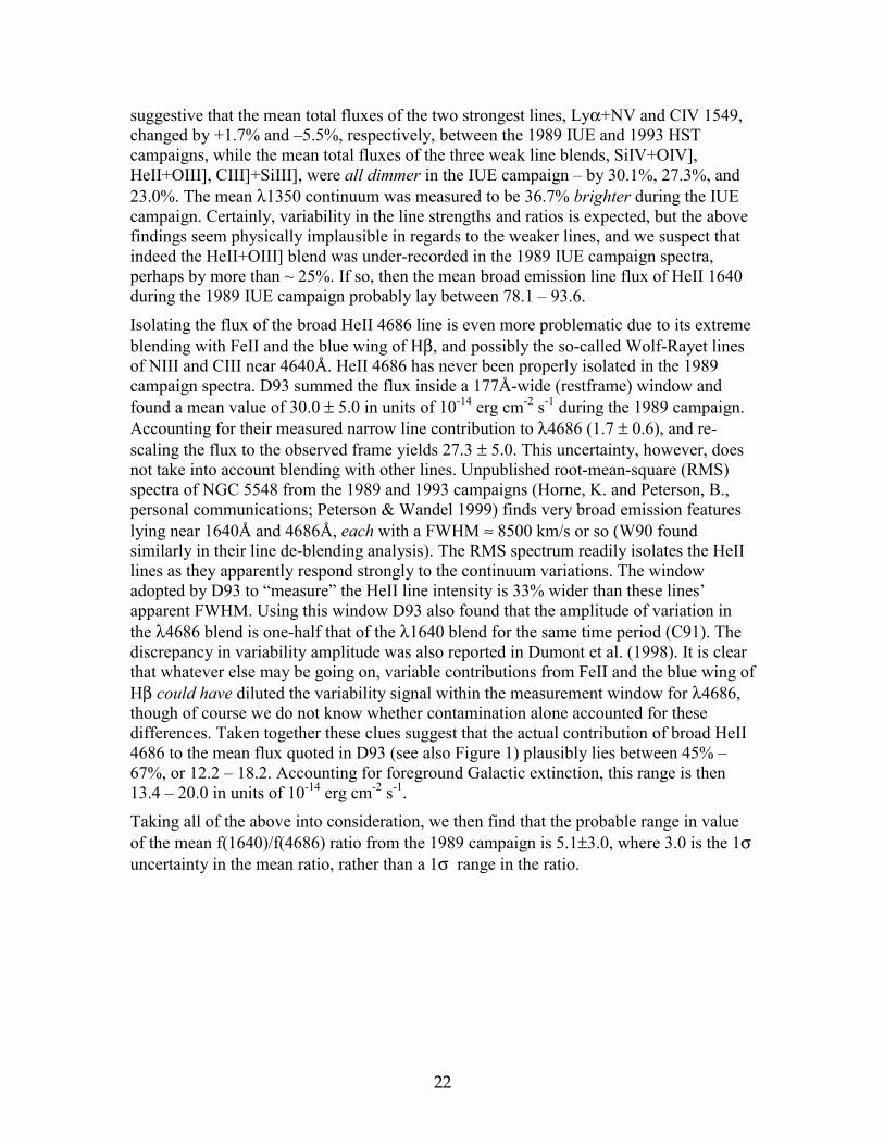
suggestive that the mean total fluxes of the two strongest lines, Lyα+NV and CIV 1549, changed by +1.7% and –5.5%, respectively, between the 1989 IUE and 1993 HST campaigns, while the mean total fluxes of the three weak line blends, SiIV+OIV], HeII+OIII], CIII]+SiIII], were all dimmer in the IUE campaign – by 30.1%, 27.3%, and 23.0%. The mean λ1350 continuum was measured to be 36.7% brighter during the IUE campaign. Certainly, variability in the line strengths and ratios is expected, but the above findings seem physically implausible in regards to the weaker lines, and we suspect that indeed the HeII+OIII] blend was under-recorded in the 1989 IUE campaign spectra, perhaps by more than ~ 25%. If so, then the mean broad emission line flux of HeII 1640 during the 1989 IUE campaign probably lay between 78.1 – 93.6.

Isolating the flux of the broad HeII 4686 line is even more problematic due to its extreme blending with FeII and the blue wing of Hβ, and possibly the so-called Wolf-Rayet lines of NIII and CIII near 4640Å. HeII 4686 has never been properly isolated in the 1989 campaign spectra. D93 summed the flux inside a 177Å-wide (restframe) window and found a mean value of 30.0 ± 5.0 in units of 10-14 erg cm-2 s-1 during the 1989 campaign. Accounting for their measured narrow line contribution to λ4686 (1.7 ± 0.6), and re-scaling the flux to the observed frame yields 27.3 ± 5.0. This uncertainty, however, does not take into account blending with other lines. Unpublished root-mean-square (RMS) spectra of NGC 5548 from the 1989 and 1993 campaigns (Horne, K. and Peterson, B., personal communications; Peterson & Wandel 1999) finds very broad emission features lying near 1640Å and 4686Å, each with a FWHM ≈ 8500 km/s or so (W90 found similarly in their line de-blending analysis). The RMS spectrum readily isolates the HeII lines as they apparently respond strongly to the continuum variations. The window adopted by D93 to “measure” the HeII line intensity is 33% wider than these lines’ apparent FWHM. Using this window D93 also found that the amplitude of variation in the λ4686 blend is one-half that of the λ1640 blend for the same time period (C91). The discrepancy in variability amplitude was also reported in Dumont et al. (1998). It is clear that whatever else may be going on, variable contributions from FeII and the blue wing of Hβ could have diluted the variability signal within the measurement window for λ4686, though of course we do not know whether contamination alone accounted for these differences. Taken together these clues suggest that the actual contribution of broad HeII 4686 to the mean flux quoted in D93 (see also Figure 1) plausibly lies between 45% – 67%, or 12.2 – 18.2. Accounting for foreground Galactic extinction, this range is then 13.4 – 20.0 in units of 10-14 erg cm-2 s-1.

Taking all of the above into consideration, we then find that the probable range in value of the mean f(1640)/f(4686) ratio from the 1989 campaign is 5.1±3.0, where 3.0 is the 1σ uncertainty in the mean ratio, rather than a 1σ range in the ratio.

23

References Antonucci, R.R.J., Geller, R., Goodrich, R.W., Miller, J.S. 1996, ApJ, 472, 502

Antonucci, R.R.J., Kinney, A.L., Ford, H.C. 1989, ApJ 342, 64

Baldwin, J.A. 1997, in Emission Lines in Active Galaxies: New Methods and Techniques IAU Colloquium 159, ASP Conference Series 113, San Francisco: Astronomical Society of the Pacific ed. B.M. Peterson, F.-Z. Cheng, and A. Wilson, 80

Baldwin, J.A., Ferland, Korista, K.T., Ferland, G.J. & Verner, D.A. 1995, ApJ, 455, L119

Blandford, R.D. & McKee, C.F. 1982, ApJ, 255, 419

Brotherton, M.S., Wills, B.J., Francis, P.J., Steidel, C.C. 1994, ApJ, 430, 495

Clavel, J., et al. 1991, ApJ, 366, 64

Davidson, K., & Netzer, H. 1979, Rev. Mod. Phy., 51, 715

Dietrich, M., et al. 1993, ApJ, 408, 416 (D93)

Dumont, A.-M., Collin-Souffrin, S., & Nazarova, L. 1998, A&A, 331, 11

Ferguson, J.W., Korista, K.T., Verner, D.A., & Ferland, G.J. 2002, in Spectroscopic Challenges of Photoionized Plasmas, ASP Conference Series 247, San Francisco: Astronomical Society of the Pacific, ed. Gary J. Ferland & Daniel Wolf Savin, 287

Ferguson, J.W., & Ferland, G.J.1997, ApJ, 479, 363

Ferland, G.J., 1999, PASP, 111, 1524

Ferland, G.J., 2002, Hazy, a Brief Introduction to Cloudy, University of Kentucky Physics Internal Report, http://nimbus.pa.uky.edu/cloudy

Goad, M. R., & Koratkar, A. 1998, ApJ, 495, 718

Goad, M. R., O’Brien, P.T., Gondhalekar, P.M. 1993, MNRAS, 263, 149

Horne, K. personal communication

Kaspi, S., Netzer, H. 1999, ApJ, 524, 71

Koratkar, A., Evans, I, Pesto, S., & Taylor, C. 1997, ApJ, 491, 536

Korista, K. T., et al. 1995, ApJS, 97, 285 (K95)

Korista, K.T., Baldwin, J.A., Ferland, G.J., Verner, D. 1997, ApJS, 108, 401

Korista, K.T., Goad, M. R. 2000, ApJ, 536, 284 (KG00)

MacAlpine, G. M. 1981, ApJ 251, 465

MacAlpine, G. M., Davidson, K., Gull, T., and Wu, C.-C., 1985, 294, 147

Maoz, D. et al. 1993, ApJ, 404, 576

Netzer, H., Laor, A. 1993, ApJ, 404, L51

O'Brien, P.T., et al. 1998, ApJ, 509, 163

24

Osterbrock, D. 1989, Astrophysics Of Gaseous Nebulae and Active Galactic Nuclei, (Mill Valley: University Science Books)

Peterson, B. M., personal communication

Peterson, B.M. & Wandel, A. 1999, ApJ, 521, L95

Peterson, B.M. 2001, in Probing the Physics of Active Galactic Nuclei, ASP Conference Proceedings, Vol. 224. Edited by Bradley M. Peterson, Richard W. Pogge, and Ronald S. Polidan. San Francisco: Astronomical Society of the Pacific, 1

Peterson, B.M. 1993, PASP, 105, 247 Rees, M., Netzer, H., Ferland, G.J. 1989, ApJ, 347, 640

Reichert, G., et al. 1994, ApJ, 425, 582

Rodriguez-Pascual, P.M., et al. 1997, ApJS, 110, 9

Storey, P.J., & Hummer, D.G. 1995, MNRAS, 272, 41 (SH)

Wanders, I., et al. 1997, ApJS, 113, 69

Wamsteker, et al. 1990, ApJ, 354, 446 (W90)

25

Figure Captions

1. The regions around HeII 1640 and HeII 4686 in the spectrum of NGC 5548, on the same velocity scale. Data are from, respectively, K95 and D93. The dashed lines show the approximate continuum level, and the heavy brackets below the continuum show the areas included in the λ4686 and λ1640 flux measurements.

2. Panels a, b, and c show the log of the total (front side plus back side) emission line flux F emergent from 1023 cm-2 column density clouds normalized by the maximum F for CIV 1549, He II 1640, He II 4686, and respectively as a function of log(n) and log(Φ). The contours are 1 dex. Panels d, e, and f shows, on a linear scale, the emission line flux weighted by the covering factor for the optimal LOC model (γ = -1.2 , δ = -1.0), corrected for the log(n) and log(Φ) grid and normalized to the maximum value (orange) on the grid. Panels g, h, and i, also on a linear scale, shows the optimal LOC model weighting of ∂F/∂Φ for the responsivity weighted radius, normalized to the maximum (orange) on the grid. In panels d through i the contours are in steps of 0.1, the region to the left of the jagged near vertical line shows where the recombination time is longer than 1 day, and the horizontal dashed lines show the limits of log(Φ) integration for our models. Note the similarity between panels d, e, and f and g, h, and i respectively. Panels j, k, and l shows the relative flux emergent from the dark sides of the clouds (hD) Light green corresponds to emission isotropy hD = 0.5. Darker (bluer) colors correspond to higher anisotropy (lower hD). Contours are in steps of 0.1.

3. The intensity of HeII 1640 relative to HeII 4686. The ratio is greater than 10 in regions that are highly ionized, the HeII lines optically thin, and continuum pumping of the UV lines is efficient. The lines are very weak in these cases (see previous figure). Over most parameters where the lines have significant equivalent width the intensity ratio lies between 7 and 9 and are close to the case B predictions of Storey and Hummer (1995). The jagged near vertical line shows where the recombination time is longer than 1 day, and the horizontal dashed lines show the limits of log(Φ) integration for our models.

4. Top panel: The first row shows respectively, I(CIV 1549) / I(HeII 1640), I(HeII 1640) / I(HeII 4686), and I(CIV 1549) / I(HeII 4686) and the second row shows respectively RRW(CIV 1549) / RRW(He II 1640), RRW(He II 4686) / RRW(He II 1640) and RRW(C IV 1549) / RRW(He II 4686) for LOC models as functions of the differential covering factor parameters γ and δ. A cross at γ = -1.2 , δ = -1.0 marks the parameters of the optimal LOC solution from KG00. Bottom panel: This is analogous to the top panel except that pressure law models are shown as functions of m and γ. A cross marks the solution m = 1/2 and γ = -5/6 from Goad, O’Brien, and Gondhalekar (1993).

26

5. Plot showing the correction to be applied to the observed reverberation of HeII 1640 when it is contaminated with OIII] 1663 as a function of the fraction of the intensity of HeII 1640 contaminated with OIII] 1663. We caution that in this figure all of the HeII 1640 intensity is included in the blend while only part of the OIII] 1663 is included. The plot therefore shows the effect on reverberation corresponding to varying degrees of OIII] 1663 contamination of HeII 1640. See the text for details.

6. Schematic showing the regions of integration for the calculation of G(Ω). An obscuring disk is viewed edge on. It cuts through the computational sphere at an angle Θ with respect to the observer direction (the Z axis). Clouds below this disk are hidden from the observer. The X axis (corresponding to φ = 0) is to the left and the Y axis (corresponding to φ = π/2) is out of the plane of the page. The observer views the dark side of the clouds if they lie above the X, Y plane and the illuminated sides of the clouds if they are unobscured and lie below the X, Y plane.

7a Contour plot of G(Ω) as a function of fD and Θ. The horizontal lines show the emissivity weighted average of fD for CIV 1549, HeII 1640, and HeII 4686. 7b Contour plot of G(Ω) for intensity. The horizontal lines show the emissivity weighted average of fD for CIV 1549, HeII 1640, and HeII 4686.

27

Tables

Table 1. Observed flux and ratios, NGC 5548 Line Flux (10-14erg cm-2s-1)1 Line Ratio Line Ratio Value

1989 Campaign:

He II 16402 86±30% CIV 1549 / HeII 1640 9.3±3.0

He II 4686 17±50% HeII 1640 / HeII 4686 5.1±3.0

CIV 1549 797±10% CIV 1549 / HeII 4686 48±24

1993 Campaign:

He II 16402 78±20% CIV 1549 / HeII 1640 9.7±2.1

CIV 1549 757±10% 1 In the observed frame, corrected for narrow emission component and de-reddened for the Galaxy; R=3.1, E(B-V) = 0.03. 2 After subtracting of 33% of HeII+OIII] blend to account for OIII] strength, and applying other corrections to 1989 data as described in Appendix 1.

Table 2. Observed time lags and ratios, NGC 5548

Line Lag (days) Lag Ratio Lag Ratio Value

1989 Campaign:

He II 1640+OIII]1663 3.0 +2.9/-1.1 CIV 1549 / HeII 1640+OIII] 3.2 +3.2 / -1.8

He II 4686 8.5 +3.4/-3.4 HeII 1640 / HeII 4686 0.4 +1.0 / -0.2

CIV 1549 9.5 +2.6/-1.0 CIV 1549 / HeII 4686 1.1 +1.3 / -0.4

1993 Campaign:

He II 1640+OIII] 1663 2.0+0.3/-0.4 CIV 1549 / HeII 1640+OIII] 3.4 + 1.5 / -0.9

CIV 1549 6.8+1.1/-1.1

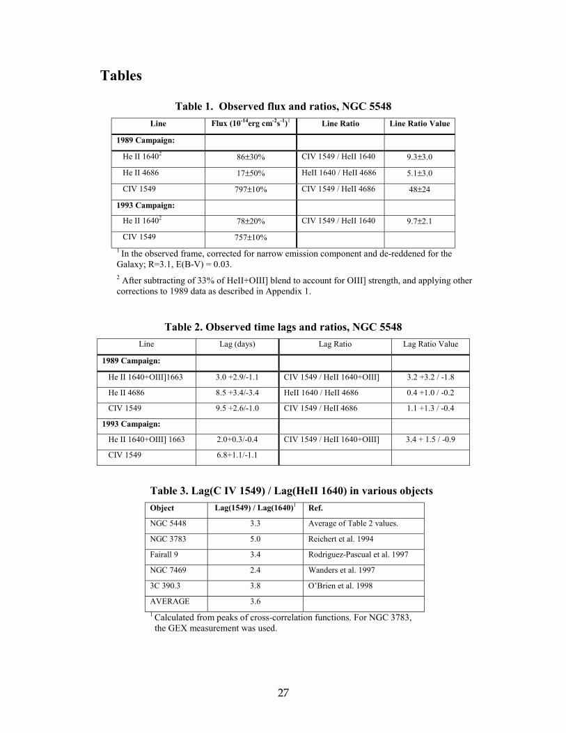
Table 3. Lag(C IV 1549) / Lag(HeII 1640) in various objects Object Lag(1549) / Lag(1640)1 Ref.

NGC 5448 3.3 Average of Table 2 values.

NGC 3783 5.0 Reichert et al. 1994

Fairall 9 3.4 Rodriguez-Pascual et al. 1997

NGC 7469 2.4 Wanders et al. 1997

3C 390.3 3.8 O’Brien et al. 1998

AVERAGE 3.6 1 Calculated from peaks of cross-correlation functions. For NGC 3783, the GEX measurement was used.

28

Table 4. Summary of model results and observations Intensity Ratio Lag Ratio

Model CIV 1549 / HeII 1640

1640/4686 CIV/4686 CIV/1640 1640/4686 CIV/4686

Optimized LOC (γ = -1.2, δ = -1.0) 9 7 70 1.2 1.1 1.4

Pressure Law (m = 1/2, γ = -5/6) 13 7 90 1.3 1.05 1.4

LOC Beamed + Obscuring Disk 1 6 6 44 1.4 1.2 1.8

Observed (NGC 5548) 10 5 48 3.3 0.4 1.1

1The maximal correction, based on the emission weighted hD, applied to the Optimized LOC model.

Figure 1.

Figure 2.

29

Figure 3.

Figure 4.

Figure 5.

Fig. 6

30

Fig. 7a

Fig. 7b