Embed Size (px)
Citation preview

European School for Advanced Studies
in Reduction of Seismic Risk
LESSLOSS Report No. Lessloss-2007/07
Guidelines for Seismic Vulnerability Reduction in the Urban Environment
Editor(s)
Prof. A. Plumier
University of Liege, ARGENCO Department, Structural Engineering Section Institut de Genie Civil-BAT B52/3 B-4000 LIEGE 1, BELGIUM
Reviewer(s)
Dr. G.M. Calvi
ROSE School
c/o EUCENTRE
Via Ferrata 1, 27100 Pavia, Italy
July, 2007


List of Section Contributors
Report Name Institution
1. Seismic safety screening method
M. Hasan Boduroglu, Pinar Ozdemir, Alper İlki, Ergun
Binbir
Istanbul Technical University (ITU), Faculty of Civil
Engineering, Istanbul, Turkey
2. Seismic upgrading of structures using conventional methods
M. Hasan Boduroglu, Engin Orakdogen, Konuralp Girgin, Berna Buyuksisli, Ergun Binbir
Istanbul Technical University (ITU), Faculty of Civil
Engineering, Istanbul, Turkey
3.1. Guidelines for the application of FRP retrofitting
Juan Manuel Mieres, Ignacio Calvo, Javier Bonilla
ACCIONA, Spain
3.2. Integration of knowledge on FRP retrofitted structures
Xavier Martinez, Sergio Oller, Pablo Mata, Alex Barbat
International Center for Numerical Methods in Engineering (CIMNE)
3.3. Experimental data on durability and fatigue resistance
Juan Manuel Mieres, Ignacio Calvo, Javier Bonilla
ACCIONA, Spain
3.4. Computation of the resistance of structural elements considering steel & FRP
Alper Ilki, Cem Demir, Nahit Kumbasar, Onder Peker, Emre
Karamuk, Dogan Akgun
Istanbul Technical University (ITU), Faculty of Civil
Engineering, Istanbul, Turkey
3.5. Urban rehabilitation using FRP
Polat Gülkan, Ahmet Yakut, Barış Binici, Güney Özcebe,
Haluk Sucuoğlu
Middle East Technical University (METU), Turkey
3.6. Design of FRP reinforcement of masonry infill walls against transverse move
Colin Taylor, Luiza Dihoru University of Bristol (UBRIS), Bristol, UK
4.1. RC structures Alex H. Barbat, Sergio Oller M., Pablo Mata A., Xavier Martinez.
International Center for Numerical Methods in Engineering (CIMNE)
4.2. Precast concrete portal frames
Nicolas Hausoul, André Plumier
University of Liege (ULIEGE), Departement ArGEnCo, Liege,
Belgium

ii
4.3. Steel frames with concentric bracings
André Plumier, Hugo Tedoldi, Catherine Doneux
University of Liege (ULIEGE), Departement ArGEnCo, Liege,
Belgium 5.1. Displacement based design models for base isolated historical buildings
Luís Guerreiro Instituto Superior Técnico (IST), Dept. of Civil Engineering,
Lisbon, Portugal 5.2. Non linear method for control of auto adaptative semi active base isolator
Unal Aldemir, Melih Ozdilim, Selcuk Ozbas
Istanbul Technical University (ITU), Faculty of Civil
Engineering, Istanbul, Turkey 6. Mitigation of hammering between buildings
Viviane Warnotte University of Liege (ULIEGE), Departement ArGEnCo, Liege,
Belgium 7. Methodology of analysis for underground structures in soft soils
Mário Lopes, António Brito Instituto Superior Técnico (IST), Dept. of Civil Engineering,
Lisbon, Portugal

ABSTRACT
The aim of Sub-Project 7 is the reduction of the seismic vulnerability of buildings and infrastructures. This can correspond to very different interventions, as there are many types of structures, many materials and many ways to reduce vulnerability. This explains that a variety of topics is treated.
The first chapter deals with the screening of buildings on an urban scale to identify which need retrofitting. In the second chapter, conventional methods for retrofitting are described.
In all the following chapters, new techniques for retrofitting are presented.
The application of Fibre Reinforced Polymers (FRP) on existing structures is a technique which has developed a lot recently. The content of Chapter three is related to the design of FRP solutions: a user friendly design tool, experimental data on durability and fatigue and a design method considering the contribution of steel rebars and FRP to resistance. An effective numerical model for composite is presented. Chapter three also describes experimental studies on masonry infill which FRP can effectively reinforce against transverse move and for their in-plane strength. Rehabilitation using that technique can be applied at an urban scale.
The use of dissipative devices to reduce the vulnerability of structures is the subject of Chapter four. The technique is applied to precast concrete portal frames and to steel frames with concentric bracings. The use of base isolation for seismic upgrading of historical buildings is developed in Chapter five, in which a displacement - based method is applied to a light house. The mitigation of hammering between buildings, with a methodology to face various situations, is the subject of Chapter six. A displacement based methodology of analysis for underground structures in soft soils is presented at Chapter seven.
This Report focuses on practical applications rather than on theory. Detailed information on the research topics can be found in the specific deliverables of the Lessloss project available on the Lessloss website (www.lessloss.org).


ACKNOWLEDGEMENTS
This work has been made possible thanks to the funding by the European Union of the Risk Mitigation for Earthquakes and Landslides project LESSLOSS in the 6th European Community Framework Programme for Research, Technological Development and Demonstration under the programme Integrating and strengthening ERA.


TABLE OF CONTENTS
List of Section Contributors ......................................................................................................................... i
ABSTRACT .................................................................................................................................................. iii
ACKNOWLEDGEMENTS.......................................................................................................................v
TABLE OF CONTENTS.........................................................................................................................vii
LIST OF TABLES...................................................................................................................................xviii
LIST OF FIGURES ..................................................................................................................................xxi
LIST OF SYMBOLS ...............................................................................................................................xxix
1. SEISMIC SAFETY SCREENING METHOD...................................................................................1
1.1 INTRODUCTION..................................................................................................................................1
1.2 SEISMIC SAFETY SCREENING METHOD (SSSM) ............................................................................1
1.2.1 Concept of SSSM...................................................................................................................2
1.3 SEISMIC INDEX, IS..............................................................................................................................3
1.3.1 Seismic Capacity Index, P.....................................................................................................3
1.3.1.1 Strength Index, C ....................................................................................................4
1.3.2 Structural Irregularity Index, D............................................................................................7
1.3.3 Time Dependent Deterioration Index, K...........................................................................8
1.4 REQUIRED SEISMIC CAPACITY INDEX, ID .....................................................................................8
1.5 PILOT REGION STUDY ......................................................................................................................9
1.5.1 Application of SSSM to a Sample Building ......................................................................13

viii
1.6 CONCLUSIONS.................................................................................................................................. 18
2. SEISMIC UPGRADING OF STRUCTURES USING CONVENTIONAL METHODS...... 19
2.1 EVALUATION OF SEISMIC SAFETY OF EXISTING BUILDINGS AND RETROFITTING TECHNIQUES........................................................................................................................................... 19
2.1.1 The Procedure for Determination of the Seismic Safety of Existing Buildings ......... 20
2.2 OBSERVATIONS ON IMPERFECTIONS CAUSING THE COLLAPSE OR DAMAGE IN RESIDENTIAL BUILDINGS AND COMMON STRENGTHENING TECHNIQUES IN TURKEY............ 20
2.2.1 Strengthening the Existing Buildings by Additional Shearwalls ................................... 22
2.2.2 Construction Rules for Additional Shearwalls ................................................................ 23
2.3 NUMERICAL EXAMPLE ................................................................................................................... 24
2.3.1 Performance Evaluations of Strengthened Building According to Non-linear Push-over Analysis Methods of TEC-2006, FEMA-440 and ATC-40.............................................. 27
2.4 CONCLUSIONS.................................................................................................................................. 32
3. SEISMIC UPGRADING OF STRUCTURES USING FIBER REINFORCED POLYMERS33
3.1 GUIDELINES FOR THE APPLICATION OF FRP RETROFITTING............................ 33
3.1.1 Introduction......................................................................................................................... 33
3.1.2 Materials characterisation................................................................................................... 33
3.1.2.1 Fibres...................................................................................................................... 34
3.1.2.2 Resins ..................................................................................................................... 35
3.1.2.3 Lamina and Laminates ......................................................................................... 35
3.1.3 Design of the FRP reinforcement..................................................................................... 36
3.1.4 Adhesiveness........................................................................................................................ 38
3.1.4.1 Structural adhesives.............................................................................................. 38
3.1.4.2 Surface preparation .............................................................................................. 39
3.1.4.3 Adhesion mechanism........................................................................................... 40
ix
3.1.5 Placing on site ......................................................................................................................40
3.1.5.1 Wet lay-up/Hand lay-up ......................................................................................41
3.1.5.2 Vacuum bagging....................................................................................................41
3.1.5.3 Filament winding...................................................................................................41
3.1.5.4 Prepregs..................................................................................................................42
3.1.5.5 Resin Film Infusion (RFI)....................................................................................42
3.1.6 Quality control .....................................................................................................................43
3.1.6.1 Check-points during installation .........................................................................43
3.1.6.2 Site tests..................................................................................................................45
3.1.6.3 Inspection recommendations ..............................................................................45
3.2 INTEGRATION OF KNOWLEDGE ON FRP RETROFITTED STRUCTURES ....................................47
3.2.1 Introduction..........................................................................................................................47
3.2.2 Formulation used to simulate RC structures reinforced and/or retrofitted with CFRP48
3.2.2.1 Simulation of Composite Materials ....................................................................48
3.2.2.2 Other Formulations Developed to Simulate CFRP Reinforcements ............52
3.2.2.3 Efficiency Improvement of the Developed Code ............................................55
3.2.2.4 Making the Code More User Friendly................................................................58
3.2.3 Numerical examples of the formulation proposed. CFRP reinforcements of RC structures...........................................................................................................................................61
3.2.3.1 Code Validation: Bending Reinforcement of a RC Beam ...............................61
3.2.3.2 Code Validation: CFRP Retrofitting of a Beam................................................63
3.2.3.3 Reinforcement of a Framed Structure using CFRP .........................................64
3.2.4 CONCLUSIONS ................................................................................................................71
3.3 EXPERIMENTAL DATA ON DURABILITY AND FATIGUE RESISTANCE..............75
x
3.3.1 Durability.............................................................................................................................. 75
3.3.1.1 Fibres’ environmental degradation..................................................................... 75
3.3.1.2 Accelerated Ageing Models................................................................................. 76
3.3.2 Fatigue of composites......................................................................................................... 80
3.3.2.1 Factors affecting the fatigue life. Damage mechanisms .................................. 81
3.3.2.2 Comparison of the fatigue behaviour in the different types of composites. 83
3.3.2.3 Conclusions ........................................................................................................... 86
3.4 COMPUTATION OF THE RESISTANCE OF STRUCTURAL ELEMENTS CONSIDERING STEEL & FRP 86
3.4.1 Introduction......................................................................................................................... 86
3.4.2 Testing program .................................................................................................................. 88
3.4.2.1 Outline of The Characteristics of The Tested Specimens .............................. 88
3.4.2.2 Loading and Data Acquisition Setup ................................................................. 92
3.4.2.3 Test Results and Discussions.............................................................................. 92
3.4.3 Computation of strength and deformability.................................................................... 97
3.4.4 Verification of proposed computation methodology................................................... 100
3.4.5 Conclusions........................................................................................................................ 101
3.5 URBAN REHABILITATION USING FRP ........................................................................................ 103
3.5.1 Introduction....................................................................................................................... 103
3.5.2 Seismic Performance Assessment Procedures .............................................................. 103
3.5.2.1 The Walkdown Evaluation Procedure............................................................. 104
3.5.2.2 Preliminary Assessment..................................................................................... 105
3.5.2.3 Detailed Assessment Procedure ....................................................................... 107
3.5.3 Application to Zeytinburnu ............................................................................................. 112
xi
3.5.3.1 Walkdown Survey ...............................................................................................112
3.5.3.2 Preliminary Assessment......................................................................................113
3.5.3.3 Detailed Assessment...........................................................................................114
3.5.4 Analysis and Design of FRPs for Seismic Retrofit........................................................115
3.5.4.1 Strengthening with FRP.....................................................................................116
3.5.4.2 Proposed Analytical Model................................................................................117
3.6 DESIGN OF FRP REINFORCEMENT OF MASONRY INFILL WALLS AGAINST TRANSVERSE MOVE....................................................................................................................................................119
3.6.1 Scope of research...............................................................................................................119
3.6.1.1 Objectives and strategy of the present studies ................................................119
3.6.2 Experimental programme.................................................................................................123
3.6.2.1 Materials and panel configuration.....................................................................123
3.6.2.2 Instrumentation...................................................................................................127
3.6.2.3 Seismic tests input motions ...............................................................................127
3.6.2.4 Quasi-static tests – experimental observations ...............................................128
3.6.2.5 Seismic tests .........................................................................................................131
3.6.2.6 Seismic tests – experimental observations and numerical simulations ........133
3.6.2.7 Conclusions from the experimental programme ............................................137
3.6.3 Analytical studies................................................................................................................138
3.6.4 Conclusions ........................................................................................................................140
4. SEISMIC DESIGN AND RETROFIT OF STRUCTURES USING DISSIPATIVE DEVICES ..................................................................................................................................................141
4.1 RC STRUCTURES ..............................................................................................................................141
4.1.1 Introduction........................................................................................................................141

xii
4.1.2 Nonlinear analysis of beam structures............................................................................ 145
4.1.2.1 Finite deformation initially curved beams....................................................... 146
4.1.3 Nonlinear constitutive models ........................................................................................ 149
4.1.3.1 Degrading materials: damage model ................................................................ 150
4.1.3.2 Plastic materials................................................................................................... 152
4.1.3.3 Mixing theory for composites........................................................................... 154
4.1.3.4 Energy Dissipating Devices .............................................................................. 155
4.1.4 Numerical implementation .............................................................................................. 156
4.1.4.1 Tangential stiffness tensors ............................................................................... 156
4.1.4.2 Cross sectional analysis ...................................................................................... 158
4.1.5 Numerical examples.......................................................................................................... 160
4.1.5.1 Nonlinear Seismic Response of Planar Frame ............................................... 160
4.1.5.2 3D Precast concrete building............................................................................ 161
4.1.6 Conclusions........................................................................................................................ 163
4.2 PRECAST CONCRETE PORTAL FRAMES ....................................................................................... 164
4.2.1 Post-earthquake surveys ................................................................................................... 164
4.2.2 INERD pin connection.................................................................................................... 166
4.2.3 Bracings using INERD pin connections........................................................................ 166
4.2.4 Design Model for the systems......................................................................................... 168
4.2.4.1 Definition of the model..................................................................................... 168
4.2.4.2 Plastic hinges at column bases.......................................................................... 170
4.2.4.3 Design of INERD pin connection .................................................................. 171
4.2.4.4 Static non linear analysis (Pushover analysis) ................................................. 175
xiii
4.2.4.5 Dynamic non linear analysis (Time history analysis) ......................................179
4.2.4.6 Analysis of the results.........................................................................................181
4.3 STEEL FRAMES WITH CONCENTRIC BRACINGS. CONNECTIONS...............................................185
4.3.1 Reasons for using dissipative connections in frames with concentric bracings and purpose of the research activity in LESSLOSS. ........................................................................185
4.3.2 The INERD pin connection geometry and properties ................................................186
4.3.3 Code rules for braced frames with pin INERD-connections......................................187
4.3.4 Practical design procedure................................................................................................188
4.3.5 Application of dissipative connections to a tall office building with X bracings ......190
4.3.5.1 Design stage.........................................................................................................190
4.3.5.2 Pushover analysis ................................................................................................192
4.3.5.3 Dynamic Non linear Time History Analyses ..................................................195
4.3.5.4 Conclusions of the application of dissipative connections to a tall office building with X bracings ...................................................................................................198
4.3.6 Application of dissipative connections to a tall industrial building with V bracings 199
4.3.6.1 Reference structure and design conditions......................................................199
4.3.6.2 Comparison of mass of designed structures....................................................201
4.3.6.3 Influence of superstructure design on the dimensions of foundations. ......204
4.3.6.4 Results of the analysis.........................................................................................204
4.3.6.5 Conclusions of the design stage. .......................................................................205
4.3.6.6 Push-over analysis ...............................................................................................206
4.3.6.7 Conclusions from the application of dissipative connections to a tall industrial building with V bracings..................................................................................207
4.3.6.8 Conclusions from the application of dissipative connections to a tall industrial building with V bracings..................................................................................208
xiv
4.3.7 General conclusions on the use of dissipative connections in frames with bracings208
5. SEISMIC UPGRADING OF STRUCTURES USING BASE ISOLATION........................... 211
5.1 DISPLACEMENT BASED DESIGN MODELS FOR BASE ISOLATED HISTORICAL BUILDINGS... 211
5.1.1 Introduction....................................................................................................................... 211
5.1.2 The proposed methodology............................................................................................. 211
5.1.3 The Capelinhos lighthouse............................................................................................... 215
5.1.3.1 Introduction ........................................................................................................ 215
5.1.3.2 The Capelinhos Lighthouse non linear model................................................ 218
5.1.3.3 Capacity curve definition................................................................................... 220
5.1.4 Conclusions........................................................................................................................ 224
5.2 NONLINEAR METHOD FOR CONTROL OF AUTO-ADAPTIVE SEMI ACTIVE BASE ISOLATOR. 224
5.2.1 Structural System............................................................................................................... 224
5.2.2 System Dynamıcs .............................................................................................................. 225
5.2.3 Optimal and Sub-optimal Control .................................................................................. 226
5.2.4 Passive Viscous Damping Control And on-off Cases ................................................. 226
5.2.5 Causal semıactıve control................................................................................................. 227
5.2.6 Numerical application....................................................................................................... 227
5.2.7 Derivation of the Linear Control Law ........................................................................... 229
5.2.8 Conclusions........................................................................................................................ 234
6. MITIGATION OF HAMMERING BETWEEN BUILDINGS................................................ 237
6.1 INTRODUCTION............................................................................................................................. 237
6.2 ANALYSIS OF POUNDING BETWEEN BUILDINGS AND MITIGATION BY LINKING – INTRODUCTION TO THE NUMERICAL STUDY ................................................................................... 238
6.2.1 Assumptions and limitations ........................................................................................... 238
xv
6.2.2 Design of the structures considered in the analysis ......................................................238
6.2.3 On the use of linear or nonlinear analysis to evaluate pounding effects....................240
6.3 OVERVIEW OF POUNDING BETWEEN ADJACENT BUILDINGS..................................................241
6.3.1 Pounding modelling ..........................................................................................................241
6.3.2 Pounding effects ................................................................................................................243
6.3.2.1 Case A: Adjacent buildings with equal height and with aligned floor levels243
6.3.2.2 Case B: Adjacent buildings of unequal height and with aligned floor levels245
6.3.2.3 Case C: Adjacent buildings of similar or different height and with not aligned floor levels .............................................................................................................245
6.3.2.4 Conclusions..........................................................................................................246
6.4 OVERVIEW OF POUNDING MITIGATION BETWEEN ADJACENT BUILDINGS...........................246
6.4.1 The seismic gap..................................................................................................................246
6.4.2 Increasing the stiffness of one or both buildings ..........................................................247
6.4.3 Supplemental energy dissipation......................................................................................247
6.4.4 Strengthening......................................................................................................................248
6.4.5 Alternative load paths........................................................................................................248
6.4.6 Strong shear wall ................................................................................................................248
6.4.7 Primary structure away from property limits .................................................................248
6.4.8 Reconnection......................................................................................................................249
6.5 RECOMMENDATIONS FOR THE MITIGATION OF POUNDING PROBLEMS BETWEEN ADJACENT BUILDINGS..............................................................................................................................................249
6.5.1 Guidance to mitigate pounding with a PRDs ................................................................249
6.5.1.1 Adjacent buildings of equal height, with aligned floor levels and similar structural types, in particular their stiffness....................................................................250
xvi
6.5.1.2 Adjacent buildings of equal height, with aligned floor levels and different structural types................................................................................................................... 251
6.5.1.3 Adjacent buildings of unequal height, with aligned floor levels and same structural types................................................................................................................... 252
6.5.1.4 Adjacent buildings of unequal height, with aligned floor levels and different structural types................................................................................................................... 254
6.5.1.5 Adjacent buildings of similar or different height, with not aligned floor levels and similar or different structural types ......................................................................... 255
6.5.1.6 Buildings with a small seating length (unseating problems) ......................... 256
6.5.2 Some practical indications on the design of Pounding Reduction Devices (PRD's)Choice of the PRD.......................................................................................................... 257
6.5.2.1 Introduction ........................................................................................................ 257
6.5.2.2 Requirements in selecting PRD's ..................................................................... 257
6.5.2.3 Number and location of the devices................................................................ 258
6.5.3 Models and programs for impact zone .......................................................................... 259
6.6 CONCLUSIONS................................................................................................................................ 260
7. METHODOLOGY OF ANALYSIS FOR UNDERGROUND STRUCTURES IN SOFT SOILS......................................................................................................................................................... 263
7.1 HISTORICAL BACKGROUND ......................................................................................................... 263
7.2 ANALYSIS OF THE SEISMIC VULNERABILITY .............................................................................. 264
7.3 SEISMIC BEHAVIOUR ..................................................................................................................... 265
7.4 CONCEPTION ................................................................................................................................. 266
7.5 DESIGN METHODOLOGY ............................................................................................................. 267
7.6 PRACTICAL APPLICATION EXAMPLE ........................................................................................... 269
7.6.1 Structure designed according to current code concepts .............................................. 270
7.6.2 Structure designed according to the proposed methodology...................................... 273

xvii
7.6.2.1 Choice of deformation mechanism ..................................................................273
7.6.2.2 Design of reinforcement ....................................................................................275
7.6.2.3 Results...................................................................................................................279
7.7 SUMMARY AND CONCLUSIONS .....................................................................................................280
REFERENCES.........................................................................................................................................281
LIST OF TABLES
Table 1-1. Classification of vertical members ............................................................................................4
Table 1-2. V/W and P values obtained by pushover analysis and SSSM............................................ 10
Table 1-3. Evaluation of the buildings using SSSM ............................................................................... 12
Table 2-1. Equivalent earthquake loads of strengthened building (TEC-2006)................................. 26
Table 2-2. Comparison of the performance points of the strengthened building with fixed base and at foundation................................................................................................................. 31
Table 3-1. Typical values of fibre properties [FIB-CEB, 2004]............................................................ 34
Table 3-2. Typical values of resin properties with different materials [FIB-CEB, 2004].................. 35
Table 3-3. Effect of fibre orientation on the tensile strength of a laminate depending on the material [ACI 440.2R-02]. ................................................................................................... 36
Table 3-4. Comparative properties of adhesives .................................................................................... 38
Table 3-5. Site test specification................................................................................................................ 45
Table 3-6. Inspection recommendations ................................................................................................. 45
Table 3-7. Mechanical characteristics of the constituent materials used to define the composite materials existing in the framed structure......................................................................... 66
Table 3-8. Characteristics of tested specimens ....................................................................................... 89
Table 3-9. Test Results............................................................................................................................... 93
Table 3-10. Axial Resistance and Deformability Predictions................................................................ 99
Table 3-11. Base Scores and Vulnerability Scores for Concrete Buildings ....................................... 105
Table 3-12. Vulnerability Parameters, (VSM) ....................................................................................... 105

xix
Table 3-13. Values of Equation Parameters for Damage Curves of RC Columns ..........................110
Table 3-14. Values of Equation Parameters for Damage Curves of RC Beams...............................110
Table 3-15. Equation Parameters for the Damage Curves Developed for Brick Infills..................111
Table 3-16. Damage Scores and the Corresponding Performance Levels ........................................112
Table 3-17. Calculated performance scores of RC buildings having 7 storeys or less .....................113
Table 3-18. Results of the Preliminary Assessment Method...............................................................114
Table 3-19. Building Assessment Results..............................................................................................115
Table 3-20 Summary of experimental tests............................................................................................120
Table 3-21 FRP system employed in the tests.......................................................................................124
Table 3-22 Parameters of design response spectrum ...........................................................................127
Table 3-23 Damping corresponding to main modes of vibration in SEU1 (intact wall).................132
Table 3-24 Damping corresponding to main modes of vibration in SER1 (intact wall) .................132
Table 3-25 Evolution of panel’s natural frequency during seismic testing........................................132
Table 3-26 Summary of relevant results from seismic testing.............................................................138
Table 4-1. Parameters of the energy dissipation devices......................................................................162
Table 4-2. Characteristics of the studied INERD pin connection .....................................................173
Table 4-3. Values of “target” displacement Sde(T) corresponding to different Peak Ground accelerations (PGA) ...........................................................................................................177
Table 4-4. Results of dynamic non linear analysis (time history analysis)..........................................180
Table 4-5. Structural typologies and main characteristics for Steel Frames ......................................185
Table 4-6. Design formulae for the connection with 2 internal plates...............................................187
Table 4-7. Eurocode 8 rules for frames with bracings –left, standard – right, with dissipative INERD pin connections. ..................................................................................................188
Table 4-8. Target roof displacements for pushover analyses ..............................................................193
xx
Table 4-9. Drifts at which θ = 0,1 and behaviour factor q from the pushover analysis ................. 194
Table 4-10. Maximum base shear in non linear dynamic analyses ..................................................... 197
Table 4-11. Maximal values of the θ parameter in non linear dynamic analyses.............................. 197
Table 4-12. The 5 design options analysed............................................................................................ 200
Table 4-13. Applied action effect at the foundation, dimension of a pad and volumes of soils to dig out.................................................................................................................................. 205
Table 5-1 Modal frequencies of fixed base solution ............................................................................ 217
Table 5-2 Modal frequencies of base isolated solution........................................................................ 218
Table 5-3 Base isolation solution characteristics .................................................................................. 221
Table 5-4 Equivalent single degree of freedom characteristics .......................................................... 222
Table 5-5. Maximum response quantities for uncontrolled and controlled cases............................ 228
Table 5-6. Maximum response quantities for passive cases ................................................................ 228
Table 6-1. Summary of pounding model.............................................................................................. 242
LIST OF FIGURES
Figure 1-1. Bi-linear model of elasto-plastic response..............................................................................2
Figure 1-2. Displacement compatibility of vertical members..................................................................4
Figure 1-3. The cumulative frequency distribution of the minimum seismic capacity index, Pmin values of 2401RC building in Zeytinburnu.......................................................................10
Figure 1-4. The relation between results obtained by using SSSM and pushover analysis................11
Figure 1-5. Ground floor plan of sample building..................................................................................13
Figure 1-6. Pushover curve of residential building (direction x, y) and bilinear form .......................14
Figure 1-7. Capacity diagram, demand estimation of residential building (direction x, y).................14
Figure 1-8. MS-Excel worksheet for application of SSSM to sample building (direction x, y).........15
Figure 1-9. (Cont.) MS-Excel Worksheet for application of SSSM to sample building (dir. x, y)....16
Figure 1-10. (Cont.) MS-Excel worksheet for application of SSSM to residential building (dir. x, y) .............................................................................................................................................17
Figure 2-1. Normal storey plan of existing building ...............................................................................25
Figure 2-2. Normal storey plan of strengthened building......................................................................25
Figure 2-3. The mathematical model used for the analysis of building with mat foundation...........26
Figure 2-4. Pushover curve of strengthened building with fixed base .................................................27
Figure 2-5. Pushover curve of strengthened building with mat foundation .......................................27
Figure 2-6. Performance graphic of strengthened building with fixed base (TEC-2006) .................28
Figure 2-7. Performance graphic of strengthened building with mat foundation (TEC-2006)........28
Figure 2-8. Performance graphic of strengthened building with fixed base (FEMA-440)................28
xxii
Figure 2-9. Performance graphic of strengthened building with mat foundation (FEMA-440)...... 29
Figure 2-10. Performance graphic of strengthened building with fixed base (ATC-40)................... 29
Figure 2-11. Performance graphic of strengthened building with mat foundation (ATC-40) ......... 30
Figure 2-12. The soil stresses at the performance point and design earthquake load level .............. 30
Figure 2-13. The soil stresses at the performance point and according to FEMA-440 .................... 30
Figure 2-14. The soil stresses at the performance point and according to ATC-40.......................... 31
Figure 3-1. Different distribution of components in a composite material........................................ 50
Figure 3-2. Fibre-matrix system. Fibre behaviour when the composite is compressed.................... 55
Figure 3-3. Assignation, to the different volumes composing the concrete frame to be modelled, of the different composite materials and construction stages ....................................... 59
Figure 3-4. Definition of the different composite materials existing on the structure by the number material constituents and their volumetric participation. Beneath can be seen some material data defined for the simple materials. ............................................. 60
Figure 3-5. Geometry and reinforcement of the beam studied ............................................................ 61
Figure 3-6. Finite element model developed to realize the numerical simulation.............................. 62
Figure 3-7. Force-displacement graph comparing the experimental and the numerical results....... 62
Figure 3-8. Results maps obtained with the finite element model of the beam................................. 63
Figure 3-9. Comparison between the CFRP reinforcement and retrofitting by using capacity curves..................................................................................................................................... 64
Figure 3-10. Geometric definition of the framed structure considered in the simulation................ 65
Figure 3-11. Reinforcements applied to the concrete frame................................................................. 65
Figure 3-12. Capacity curves obtained with the 2D models ................................................................. 67
Figure 3-13. Plastic hinges in the concrete frame. 2D models. a) model without CFRP reinforcement, b) model with upper and lower CFRP, c) model with upper, lower and lateral CFRP.................................................................................................................. 68
Figure 3-14. Capacity curves obtained with the 3D models ................................................................. 69
xxiii
Figure 3-15. Crack evolution in the 3DF-noR model (model without CFRP reinforcement) .........69
Figure 3-16. Crack evolution in the 3DF-R model (model with upper and lower CFRP)................69
Figure 3-17. Plastic hinge in the 3DF-LR model. Lateral view.............................................................70
Figure 3-18. Elements with larger deformations in the 3DF-LR model. Zenith view.......................71
Figure 3-19. S-N curve of a Carbon T300/Epoxi 5208 [0/90/±45]s laminate..................................81
Figure 3-20. Normalised S-N data for different composites systems ..................................................84
Figure 3-21. S-N curves for 0º, 90º and ±45º glass/polyester laminates.............................................84
Figure 3-22. S-N curves for Glass S2/Epoxy 5280 laminates to [0]3 and [±45]2s ............................85
Figure 3-23. S-N curves for carbon T300/epoxy [0]6,, [±45]8t and [90]15 laminates ......................85
Figure 3-24. Cross-sections and Reinforcement Details of the Specimens.........................................91
Figure 3-25. Axial Stress-Strain Relationships for Different Cross-sections.......................................96
Figure 3-26. Axial Stress-Strain Relationships for NSR and LSR Specimens .....................................96
Figure 3-27. Comparison of predictions with available experimental data........................................101
Figure 3-28. Damage Curves Developed for RC Columns .................................................................110
Figure 3-29. FRP strengthening method for reinforced concrete frames with infill walls ..............117
Figure 3-30. Modelling of infill struts and FRP ties..............................................................................118
Figure 3-31 Layout of FRP fabric on the masonry panel (STR1, STR2, SER1)...............................125
Figure 3-32 Layout of FRP fabric on the masonry panel (SER2).......................................................126
Figure 3-33 Layout of FRP fabric on the masonry panel (SER3).......................................................126
Figure 3-34 SER2 panel ready for testing (60% reinforcement).........................................................126
Figure 3-35 Required response spectrum as per Eurocode 8 (Soil B) ...............................................128
Figure 3-36 Experimental rig used for the static tests (STR1, STR2) ................................................128
Figure 3-37 Crack pattern in reinforced walls subjected to out-of-plane monotonic loading (STR1)..................................................................................................................................129
xxiv
Figure 3-38 Loading curves during static testing (STU1 -unreinforced wall, STR1 reinforced wall)130
Figure 3-39 Comparison of deflection profiles for reinforced (STR1) and unreinforced (STU1) walls ..................................................................................................................................... 131
Figure 3-40 Shaking table acceleration in test SEU1_110................................................................... 133
Figure 3-41 Midheight deflection measured in test SEU1_110 (left – general view, right detail) . 134
Figure 3-42 Simulated midheight deflection in test SEU1_110 ......................................................... 134
Figure 3-43 Arching forces measured in test SEU1_110 (left -south face, right –north face)....... 134
Figure 3-44 Simulated arching forces for test SEU1_110................................................................... 135
Figure 3-45 Shaking table and wall accelerations in test SEU1_65.................................................... 135
Figure 3-46 Midheight deflection in test SEU1_65 (left- measured, right-simulated)..................... 135
Figure 3-47 Support acceleration and wall deflection in test SER1_130 (100% reinforcement)... 136
Figure 3-48 Support acceleration and wall deflection in test SER2_120 (60% reinforcement)..... 137
Figure 3-49 Support acceleration and wall deflection in test SER3_80 (40% reinforcement) ....... 137
Figure 3-50 Modelling of top and bottom supported URM panels................................................... 139
Figure 3-51 Fragility curve for a panel height of 4m (t=0.229m, mass density =1950 kg/m³, fc=4.8 MPa, έmax=0.4%, έult=0.45%, viscous damping =5%)...................................... 140
Figure 4-1. Configurational description of the beam........................................................................... 147
Figure 4-2. Cross section showing the composite associated to a material point ............................ 149
Figure 4-3. Discrete fibre like model of the beam element................................................................. 159
Figure 4-4. Columns and beam reinforcements and fibre model of the sections............................ 160
Figure 4-5. Precast industrial building without and with dissipaters.................................................. 161
Figure 4-6. Displacements time history ................................................................................................. 161
Figure 4-7. (1) 3D Frame. (2) Dissipating devices incorporated. (3), (4): Column and beams sections................................................................................................................................ 162

xxv
Figure 4-8. Maximum response for each energy dissipating device. 1: Over–tuning Moment. 2: Top floor displacement. 3: Middle floor displacement. 4: Base shear.........................163
Figure 4-9. General collapse of a precast structure for a one-storey industrial building (Kocaeli earthquake, Turkey, 1999) [Toniolo (2002)] ...................................................................164
Figure 4-10. Damaged half joint between a column and a simple supported beam of precast structure [Toniolo (2002)] .................................................................................................165
Figure 4-11. Example of pinned connections: bolted and dowel connections [FIP, 1994] [Collinet, 2004-2005]..........................................................................................................166
Figure 4-12. Precast reinforced concrete structures braced with INERD pin connections ...........167
Figure 4-13.Implementation of the INERD dissipative connection in a one-storey industrial frame ....................................................................................................................................168
Figure 4-14. Reference structure without bracings ...............................................................................169
Figure 4-15. Studied structure with bracings using INERD pin connection ....................................169
Figure 4-16. Concrete non linear material law at the column base used in the model (3 ductilities : low, average, high) (FEMA Publication 273 [1997]) ..................................................171
Figure 4-17. Detail of the beam-to-column connection with bracings using INERD pin connections .........................................................................................................................172
Figure 4-18. Force-displacement behaviour of the studied INERD pin connection ......................174
Figure 4-19. Equivalent moment-rotation behaviour of the beam column connection with the addition of the studied INERD pin connection ............................................................174
Figure 4-20. Pushover analysis: increasing force F and monitored displacement dr .......................175
Figure 4-21. T = 1,117 s in frame structure without bracings before formation of plastic hinges at the base of the column ..................................................................................................177
Figure 4-22. T = 2,022 s in frame structure with bracings and INERD pin connection, after formation of plastic hinges at the base of the column ..................................................177
Figure 4-23. Pushover curves of reference structure (3 ductility classes), with indication of target displacements corresponding to different ag (PGA)......................................................178
Figure 4-24. Pushover curves of structure with bracings using INERD pin connection (3 Ductility class of column) with indication of target displacement corresponding to different ag (PGA)...............................................................................................................179

xxvi
Figure 4-25. Frame structure without INERD pin connections after formation of plastic hinges at the column bases = Mechanism.................................................................................. 182
Figure 4-26. Frame structure with INERD pin connections after the formation of plastic hinges at the column bases= statically acceptable structure..................................................... 182
Figure 4-27. Perspective and plan views of INERD pin connection. Definition of geometry...... 186
Figure 4-28. Reference structure. Elevation and plan.......................................................................... 190
Figure 4-29. Periods of the analysed structures. ................................................................................... 192
Figure 4-30. Pushover curves of structures (a) drift limit = 0.01h (b) drift limit = 0.005h........... 194
Figure 4-31. Deformed shape at failure (a) with variable pins (b) all other structures .................... 195
Figure 4-32. One artificial accelerogram used in the non linear dynamic analysis........................... 196
Figure 4-33. Base shear-top displacement curves under dynamic analyses. ..................................... 196
Figure 4-34. Force-deformation curves of diagonals. .......................................................................... 197
Figure 4-35. Perspective of the studied structure with its original X bracings (left) and with the studied inverted V bracings (right). ................................................................................ 199
Figure 4-36. Results in terms of periods and spectral ordinates......................................................... 201
Figure 4-37. Mass of structures 1 to 5. Distribution between diagonals, ext. columns, etc, is from top to bottom in the graph. .............................................................................................. 203
Figure 4-38. Volume of soil to dig out to realize the foundation pad. .............................................. 204
Figure 4-39. Push-over curves of structures 1 to 5. ............................................................................. 206
Figure 4-40. Deformed shapes of structures 1 to 5 at θ = 0,1............................................................ 207
Figure 5-1 Vibration modes comparison............................................................................................... 212
Figure 5-2 Example of capacity spectrum with base isolated structure ............................................ 213
Figure 5-3 Capacity spectrum with methodology presentation.......................................................... 215
Figure 5-4 The Capelinhos Lighthouse.................................................................................................. 216
Figure 5-5 Examples of cross section fibre models ............................................................................. 219

xxvii
Figure 5-6 Moment-curvature relation example....................................................................................220
Figure 5-7 Vulnerability functions for shear force................................................................................221
Figure 5-8 Capacity Spectrum with all the base isolation solutions....................................................222
Figure 5-9 Capacity Spectrum with all the base isolation solutions....................................................223
Figure 6-1. The structures studied (dimensions in meters)..................................................................239
Figure 6-2. Traditional Kelvin model .....................................................................................................240
Figure 6-3. Illustration Force-displacement for an elastic and inelastic SDOF systems ................241
Figure 6-4. Typical type of behaviour for case A (same building height, aligned floors) ................244
Figure 6-5. Proposed mitigation for case B ...........................................................................................253
Figure 6-6. Corbels and brackets for bearing supported superstructures..........................................257
Figure 7-1. Collapse of Dakai tube station.............................................................................................263
Figure 7-2. Schematic representation of rigid and flexible alignments ..............................................264
Figure 7-3. Schematic representation of change in the yield moment and curvature by increasing flexural reinforcement (N=0) ...........................................................................................266
Figure 7-4. Example underground structure .........................................................................................269
Figure 7-5. Horizontal displacement profiles ........................................................................................270
Figure 7-6. Reinforcement for maximum displacement according to Direct Design......................272
Figure 7-7. Curvature diagrams at maximum displacement – code design [/1000m]......................273
Figure 7-8. Example structure: global mechanisms ..............................................................................273
Figure 7-9. Mechanism with unavoidable hinges at intermediate locations of walls and columns 275
Figure 7-10. Details of design according to the proposed methodology...........................................277
Figure 7-11. Material constitutive relationships and moment-curvature diagrams at the column base section .........................................................................................................................278
Figure 7-12. Curvatures at maximum displacement - proposed methodology [/1000m] ..............279


LIST OF SYMBOLS
CHAPTER 1
A0 = Effective ground acceleration coefficient
ΣA = Cross sectional area of wall
B = Index for regional seismicity
C = Strength index.
Cc = Strength index of a column
Csc = Strength index of a short column
Cw = Strength index of a shear wall
k C = kth vertical member’s strength index
D = Depth of column
D = Structural irregularity index
I = Building importance factor
ID. = Required seismic index
Is = Seismic index of a building
K = Time dependent deterioration index;
cMu ; wMu = Moment capacity of columns, wall
N = Axial load of a column = Axial load of a wall
Nmax = Axial compressive strength of a column
Nmin = Axial tensile strength of a column
P = Seismic capacity index
P0 = Index for basic seismic demand

xxx
Pg = Seismic capacity index of ground floor
QE = Lateral elastic force
QY = Lateral yield force;
Qg = Lateral load carrying capacity of the ground floor
k Qmu = Flexural strength of kth vertical element
k Qsu = Shear strength of kth vertical element
R = Ductility index
Ra(T) = Seismic load reduction factor
Rc = Ductility index of a column
Rsc = Ductility index of a short column
Rw = Ductility index of a shear wall
S(T) = Spectrum coefficient
T = Natural period of the building
U = Index for usage
Vt = Total Equivalent Seismic Load (base shear),
Z = Index for local soil conditions
W = Total weight of the building
ΣW = Total weight above the storey concerned
a1; a2; a3 = Strength reduction factors due to displacement compatibility
ah = Cross sectional area of lateral reinforcement
at = Area of tension reinforcement of a column
= Area of tensile reinforcement at the wall’s end zone ag = Total area of longitudinal reinforcement
aw = Total cross sectional area of a set of stirrups
aWy = Total area of vertical reinforcement of a wall
b = Width of compressive side of a column
be = Equivalent thickness of wall

xxxi
d = Effective depth of column
fc = Compressive strength of concrete
h0 = Clear height of column
i = Number of the storey concerned
l = Wall length
lW = Distance between center of wall and end zones
n = Number of storeys of a building
s = Spacing of lateral reinforcement
λ = Coefficient for inflection height
µ = Ductility ratio
ρse = Equivalent lateral reinforcement ratio
ρt = Tensile reinforcement ratio(%)
ρte = Equivalent tensile reinforcement ratio of a wall
ρw = Shear reinforcement ratio
σ0 = Axial stress on columns
σ0e = Axial stress on wall
σy = Yield strength of longitudinal reinforcement
σwy = Yield strength of lateral reinforcement, stirrups
CHAPTER 2.
A0 = Effective ground acceleration
I = Building importance factor
PPS-2006 = Performance Point Seeker 2006
T = Characteristic spectral period
ks = Soil modulus

xxxii
q = Allowable soil stress
CHAPTER 3.1 & 3.3
A = Constant of the test conditions and failure of the material
AF = Acceleration factor
CGS = Global safety coefficient
E = Activation energy
nE = Activation energy for the degradation mechanism and for the material
FRP = Fiber Reinforced Polymers
GFRP = Glass Fiber Reinforced Polymers
Md = Design moment
Mr = Section resisting moment
N = Number of cycles
RFI = Resin Film Infusion
S, σ = Stress
T = Temperature in ºK
TS = Time Shift
TSF = Time Shift Factor
ULS = Ultimate Limit State
V = Degradation factor
V = Accelerated stress
k = Boltzmann’s constant
n = Number of layers
t = Exposure time
β' = Degradation rate

xxxiii
β, γ = Constants of the material
δ,ε = Constants of the degradation mechanism
θ = Angle of orientation of the fibres
τ = Life-cycle at the reference temperature T
τ ’ = Life-cycle at the elevated temperature T’
CHAPTER 3.2
ijklAε = Fourth order strain tensor which contain the anisotropy information
ijklAσ = Fourth order stress tensor which contain the anisotropy information
c = Composite material superscript
f = Fibre material superscript
fibNf )( = Nominal fibre strength
matfibNf −)( = Fibre-matrix interface nominal strength
matNf )( = Matrix nominal strength
fibRf )( = New fibre strength
f k = Volumetric participation (parameter) of fibre in the composite
kk = Volumetric participation (parameter) of component k in the composite
mk = Volumetric participation (parameter) matrix in the composite
m = Matrix material superscript
Pε = Parallel component of the stress tensor
Sε = Serial component of the stress tensor c
ijε = Strain tensor for the composite k
ijε = Strain tensor for component k of the composite
jε = Strain variation (perturbation) value
ijσ = Stresses in the real anisotropic space

xxxiv
ijσ = Stresses in the fictitious isotropic space
σ j = Stress variation
Pσ = Parallel component of the strain
Sσ = Serial component of the strain
CHAPTER 3.4
CFRP = Carbon fiber reinforced polymer
Efrp = Elasticity modulus of FRP
FRP = Fiber reinforced polymer
ITR = Internal transverse reinforcement
L.R. = Longitudinal reinforcement
LSR. = Low strength reinforced concrete specimens
NSR = Medium strength reinforced concrete specimens
T.R. = Transverse reinforcement
b = Width of cross-section
f′c = Concrete standard cylinder strength
f′cc = FRP jacketed concrete strength
f′co = Concrete strength of the member
f*fu = Tensile strength of FRP
f′l = Lateral stress of FRP jacket
fs,max = Tensile strength of steel reinforcement
fy = Yield strength of steel reinforcement
h = Height of cross-section
n = Number of plies of FRP
tf = Nominal thickness of FRP

xxxv
εχo = Axial strain corresponding to unconfined concrete strength
εcc = Axial strain corresponding to jacketed member strength
εch = Transverse strain of the FRP jacket
ε*fu = Ultimate rupture strain of FRP
εh,rup = 70% of ε*fu
εy = Yield strain of reinforcement
φl = Diameter of longitudinal bars
κa = Cross-sectional efficiency factor
π = Pi
ρf = Fiber ratio to concrete section
ρl = Longitudinal reinforcement ratio
CHAPTER 3.5
BS = Base score
CFRP = Carbon Fiber Reinforced Polymers
CM = Adjustement factor, which introduce the spatial variation of the ground motion in the evaluation process
CVIO = Cutoff value for IOPC
CVLS = Cutoff value for LSPC
DIIO = Damage score corresponding to IOPC
DILS = Damage index or the damage score corresponding to LSPC
FRP = Fiber Reinforced Polymers
IOCVR = Immediate occupancy coefficient based on the number of storeys above the ground level
IOPC = Immediate Occupancy Performance Classification
LSCVR = Life safety coefficient based on the number of storeys above the ground level

xxxvi
LSPC = Life Safety Performance Classification
PGIO = Performance groupings yield for IOPC
PGLS = Performance groupings yield for LSPC
PS = Seismic performance score
SD1 = Spectral acceleration at the period of 1 sec
SDS = Spectral acceleration at short periods
VS = Vulnerability score
VSM = Vulnerability score multiplier
a, b, and c = Equation parameters
mnlsi = Minimum normalized lateral strength index
mnlstfi = Minimum normalized lateral stiffness index
n = Number of storeys
nrs = Normalized redundancy score
or = Overhang ratio
ssi = Soft storey index
δ = Interstorey drift ratio
δt = Target roof drift ratio under the given elastic spectrum
θ = End rotation of the beam
CHAPTER 4.1
A = Beam cross-section
Ac = Area of the quadrilateral
Aρ0 = Mass density per unit of length of the curved reference beam
xxxvii
Cme = Material form of the elastic constitutive tensor
Cms = Material form of the secant constitutive tensor
Cmt = Material form of the tangent constitutive tensor
Cse = Viscous constitutive tensors in spatial description
Csv = Tangential constitutive tensors in spatial description
Csvij = Spatial forms of the reduced tangential constitutive tensors
Dy = Yielding displacement
EDD = Passive energy dissipating devices
Ed = Energy dissipation due to the addition of EDDs
ED = Energy dissipation due to inelastic behaviour in the structure (including viscous effects)
EK = Absolute kinetic energy
EL = Absolute earthquake energy input
ES = Elastic strain energy
E0 = Young undamaged elastic modulus
F = Damage yield criterion (scalar value)
F = Current beam referred to the straight reference configuration
F0 = Deformation gradients of the curved reference
Fn = Deformation gradient
Fp = Yield function
Fy = Yielding level
G0 = Shear undamaged elastic modulus
Gf = Tensile fracture energy
Gp = Plastic potential function
GPf = Specific plastic fracture energy of the material in tension
G(P) = Scalar monotonic function to be defined in such way to ensure that the energy dissipated by the material on a specific integration point is limited to the specific energy fracture of the material

xxxviii
I = Identity tensor
Iρ0 = Second mass moment density per unit of length of the curved reference beam
Jpq = Jacobian of the transformation between normalized coordinates and cross sectional coordinates
K = Stiffness
Nfiber = Number of quadrilaterals of the beam cross section
Np ,Nq = Number of integration points in the two directions of the normalized geometry of the quadrilateral
P = Asymmetric First Piola Kirchhoff (FPK) stress tensor
Pj = Corresponding FPK stress vector acting on the deformed face in the current beam corresponding to the normal t0j in the curved reference configuration
Pm, Pp = Equivalent (scalar) stress
PRC = Prescast Reinforced Concrete
RC = Reinforced Concrete
SO = Rotation manifold
Sρ0 = First mass moment density per unit of length of the curved reference beam
Wpq = Weighting factors
d = Internal state variable which measures the lack of secant stiffness of the material
fc = Compression strengths
ft = Tension strengths
fp = Hardening function
gf = Fracture energy density
kp = Plastic damage internal variable
lc = Characteristic length of the fractured domain employed in the regularization process
m = Stress couple vector
m,S = Body moment per unit of reference length
n = Stress resultant vector

xxxix
n = Plastic dissipation
n,S = External body force per unit of reference length
n, r = Parameters function of the of the tension and compression strengths fc and ft
t = Time
tβ = Orthogonal local frame
x = Position vector of any material point on the current reference beam
Φp = Hardening parameter
Λ = Current rotation tensor
Λ0 = Orientation tensor
Λn = Rotation tensor relative to the curved reference beam
Ξmaxt = Values of the maximum dissipation in tension
(Ψ0c)L = Parts of the free energy density developed when the compression limits are reached
(Ψ0t)L = Parts of the free energy density developed when the tension limit are reached
χ = Scalar parameter
φ = Current centroid curve
φ0 = Spatially fixed curve
εn = Strain tensor
κ = Parameter
λ = Plastic consistency parameter
ωn = Spatial curvature tensor and the rotation tensor relative to the curved reference beam
= Hardening vector
CHAPTER 4.2
E = Elastic Young’s modulus
F = Force

xl
Ftot = Total seismic force applied to the frame
I = Moment of inertia
L = Length of elements
M = Moment
Mmmf = Total moving mass of the frame
Mp = Plastic moment
MRd = Design value of resisting moment
P = Force
Py = Yield strength of the connection
Pu = Ultimate strength of the connection
Sde(T) = Elastic displacement response spectrum
Se(T) = Elastic response spectrum
T = Period of Vibration
Wpl = Plastic modulus
a = Clear distance between internal and external eye-bars = Distance between the 2 formed plastic hinges
a = Acceleration
ag = Peak ground acceleration (PGA)
b = Width of the pin connection
d = Perpendicular distance between INERD Pin connection system and beam-column node
dr, el = Displacement of the top of the column due to elasticity of the column
dr,pl = Displacement of the top of the column due to plastic rotation of the column
dr = Absolute displacement of the top of the column
dr,max = Maximum absolute displacement of the top of the column
fy = Yield stress
h = Height of the pin connection
xli
= Pin length (axial distance between external eye-bars)
m = Mass
text = Thickness of the external plates of the pin connection
tnt = Thickness of the internal plates of the pin connection
α = Ratio of the clear distance between internal and external eye-bars to the axial distance between external eye-bars
γ = Overstrength factor
δlim = Deformation capacity of the pin connection
δy = Deformation of the pin connection at yield capacity
δII = Deformation of the pin connection at ultimate capacity
π = Pi
θ = Plastic rotation at the base of the column
θmax = Maximum plastic rotation at the base of the column
θυ = Ultimate plastic rotation at the base of the column
CHAPTER 4.3
C0 = Modification factor to relate spectral displacement to the roof
displacement
C1 = Modification factor to relate expected maximum inelastic
displacements to displacements calculated for linear elastic response
C2 = Modification factor to represent the effects of pinched hysteresis
shape, stiffness degradation and strength deterioration on the maximum displacement response
C3 = Modification factor to represent increased displacements due to
P-∆ effects CBF = Concentric braced frames
D = Lateral drift ratio
DCM = Medium ductility class
E = Elastic modulus of pin’s material
FEMA = Federal emergency management agency

xlii
G = Gravity loading
H = Storey height
I = Moment of inertia of the pin
INERD = Innovations for earthquake resistant design
L = Buckling length of the bracing
M = Moment
Mp = Plastic moment
MRF = Moment resisting frames
Nb,Rd = Buckling resistance of the diagonal
NEd = Design force of the diagonal
NEser = Design force of the diagonal at the damage limitation state
P = Vertical load
PEd = Capacity design force
PGA = Peak ground acceleration
Pu = Ultimate strength of the pin
Pu,Rk = Characteristic ultimate strength of the pin
Py = Yield strength of the pin
Py,Rk = Characteristic yield strength of the pin
S = Soil parameter
Sd(T) = Ordinate of the design spectrum for the reference return period
SDe(T) = Elastic displacement response spectrum
T = Period
Wpl = Plastic modulus of pin
a = Clear distance between internal and external eye-bars = foundation slab dimension
ag = Design peak ground acceleration
b = Pin width

xliii
du = Ultimate displacement
dy = Yield displacement
fy = Yield stress of pin
g = Acceleration of gravity
h = Pin height
imin = Minimum radius of gyration
l = Pin length (axial distance between external eye-bars)
q = Behaviour factor
s = Second
text = Thickness of external eye bars
tint = Thickness of internal eye bars
∆ = Horizontal displacement
Ω = Overstrength coefficient
α = Ratio of the clear distance between internal and external eye-bars to
the axial distance between external eye-bars γMser
= Partial safety factor of resistance
γM0 = Partial safety factor of resistance
δlim = Deformation capacity of the pin connection
δII = Deformation of the pin connection at ultimate capacity
δtarget(roof) = Target displacement of roof
δy = Deformation of the pin connection at yield capacity
θ = P-∆ effect parameter
λ−
= Non-dimensional slenderness of the element
ν = Reduction factor for lower return period of seismic action associated with damage limitation
φ = Angle of inclination of diagonal (from horizontal to diagonal)

xliv
CHAPTER 5.1
DBD = Displacement based design
DI = Base isolation deformation
DS = Structures deformation
DT = Total structural deformation of the base isolated structure
E = Modulus of Elasticity
γ = Weight per unit volume
Pga = Peak ground acceleration
Sa = Spectral acceleration
Sd = Spectral displacement
VI = Base shear force
mI = Effective mass value evaluated for the global deformation model
CHAPTER 5.2
ER = Electrorheological dampers
H(u) = Heaviside step function of u
J = Cost function
L = Lagrangian
MR = Magnetorheological dampers
Tv = Response time of the controllable damper
c = Damping coefficient
cd = Describe the post yield behavior
d0 = Constant parameter to describe the pre-yield behavior of the device
f0 = Controllable yield force
fMR = MR damper force

xlv
k = Stiffness
m = Mass
r = Structural relative displacements
t = Time
u(t) = Control function
v0 = Constant parameter to describe the pre-yield behavior of the device
x(t) = State vector
z = Ground displacement
α = Design parameter for the control rule
CHAPTER 6
CR = Coefficient of restitution
DCM = Ductility Classes Medium
FRP = Fibre-reinforced polymers
PRD = Pounding Reduction Device
K = Stiffness
SDOF = Single Degree Of Freedom
VRd = Design value of shear resistance
VSd = Design value of shear action effect
cc = Dashpot constant of the connector modelling
cp = Dashpot constant of the pounding modelling
e = Stand-off distance

xlvi
gp = Static separation between structures
kc = Spring constant of the connector modelling
kp = Spring constant of the pounding modelling
m1 = Mass of the first building
m2 = Mass of the second building
u1 = Displacement of the first building
u2 = Displacement of the second building
ů1 = Velocity of the first impacting body
ů'1 = Final velocity of the first impacting body
ů2 = Velocity of the second impacting body
ů'2 = Final velocity of the second impacting body
∆ = Delta
θ = Interstorey drift sensitivity coefficient
CHAPTER 7
EI = Flexural stiffness
EIsec = Secant flexural stiffness
F = Force
H = Height of the structure
M = Moment
MSd = Design bending moment
MRd = Flexural capacity

xlvii
N = Axial force
dbl = Diameter of longitudinal reinforcement
q = Behaviour factor (q-factor)
s = Spacing of transverse reinforcement
χ = Curvature
δ = Displacement
δu = Maximum displacement
δy = Yield displacement
ε = Strain
γ = Distortion
γmax = Maximum distortion
γo = Overstrength factor
σ = Stress


1.SEISMIC SAFETY SCREENING METHOD
1.1 INTRODUCTION
Turkey is located at the boundary area where the Arabian Plate and African Plate are moving north towards the Eurasian Plate. Many strong earthquakes have occurred along the fault which is called North Anatolian Fault (NAF). Marmara and Duzce Earthquakes in 1999 were two of them which caused catastrophic disaster in Marmara and adjacent regions. Seismologists are pointing out the possibility of another big earthquake hitting Istanbul at the western edge of NAF. When the huge existing stock of buildings in Istanbul is considered, it is clear that it is practically impossible to carry out detailed structural analysis for all of the buildings. In order to cope with the seismic safety evaluation of large number of existing buildings, it is necessary to use simplified techniques, which can predict the seismic safety of the existing buildings in relatively shorter time. The expected outcome from such an analysis is to determine which buildings are at relatively higher risk of collapse.
Seismic Safety Screening Method (SSSM), is an adaptation of the Japanese Seismic Index Method (JSIM) considering the building damages in recent earthquakes and Turkish Earthquake Resistant Design Code 1998 (TERDC-98), “Specification for Structures to be Built in Disaster Areas, Earthquake Disaster Prevention”). The original method have been applied to a number of buildings damaged during 1992 Erzincan, 1998 Adana-Ceyhan and 1999 Marmara and Duzce Earthquakes. These results have been used for adaptation of the original method to Turkey. This rapid seismic safety evaluation method can be applied for structures having a storey number 6 or less with reinforced concrete frame, shear wall or dual frame-shear wall structural systems. The calibration of several coefficients proposed in this method will further be done considering the studies carried out in various pilot areas like Zeytinburnu.
1.2 SEISMIC SAFETY SCREENING METHOD (SSSM)
The structural characteristics of the building are necessary for calculating the seismic capacity index. A large number of the buildings in Istanbul have not received proper civil engineering service and they do not have any civil engineering drawings of the structural system. The inspection of a large number of buildings after recent earthquakes indicated that average concrete compressive strength is as low as 10 MPa and the amount of

2 ITU
longitudinal reinforcement bar is 1% of gross cross sectional area of columns with the tensile strength of 220 MPa. Both longitudinal and transverse bars are generally plain bars with large spacing between stirrups like 20~30 cm. With these facts some assumptions were made to simplify the quick assessment procedure. For obtaining reliable results, the method was applied in a certain geographical pilot region, Zeytinburnu, and the results were then compared with the results of more comprehensive and detailed methods to calibrate several parameters that are used in SSSM.
1.2.1 Concept of SSSM
Basic concept of SSSM and the original JSIM is the equal energy concept. In case of structures with relatively short natural period, dissipation energy is almost equal to maximum potential energy of the elastic system as shown in Figure 1-1.
Figure 1-1. Bi-linear model of elasto-plastic response
Based on this assumption, the below equation can be written:
µ=
−
12 1
QYQE
(1.1)
where QY = lateral yield force; QE = lateral elastic force; and µ = ductility ratio.
When we consider the relation between responses of elastic and elasto-plastic structural systems:
µµ
+= =
−
1 0.05 10.75
2 1
QYQ RE
(1.2)
where R = ductility index.
Sub-Project 7 – 1. Seismic performance assessment methods 3
When we write lateral forces with the term of weight of structure W:
= =Q CxW ; Q C xW Y E E (1.3)
where C = strength index.
Substitution of Equation (1.3) in Equation (1.2), seismic capacity index P is obtained.
= = = =1Q CY ; C CxR PEQ C RE E
(1.4)
It can be assumed that the structures with same seismic capacity index, P value, have similar seismic performance.
1.3 SEISMIC INDEX, IS
Seismic index of a building, Is value, is calculated by using Equation (1.5):
=sI PxDxK (1.5)
where P=seismic capacity index; D=structural irregularity index; and K=time dependent deterioration index.
Seismic index Is should be calculated separately for both earthquake directions for all critical storeys of a building and the most unfavourable result should be compared with the required seismic index ID. Based on this comparison the seismic safety of the building can be estimated. If for any of the comparison cases Is < ID then it is concluded that the behaviour of the structure is at higher risk of collapse and further detailed analysis is necessary.
1.3.1 Seismic Capacity Index, P
During calculation of seismic capacity index, P, the vertical structural members are classified into three groups as columns, short columns and shear walls. The definitions of these groups are given in Table 1-1.
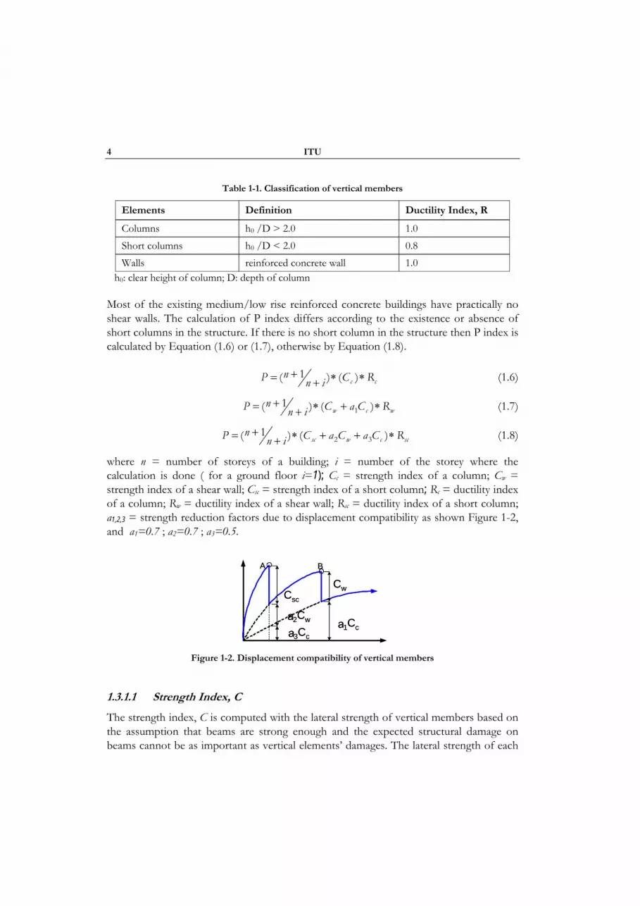
4 ITU
Table 1-1. Classification of vertical members
Elements Definition Ductility Index, R
Columns h0 /D > 2.0 1.0 Short columns h0 /D < 2.0 0.8 Walls reinforced concrete wall 1.0
h0: clear height of column; D: depth of column
Most of the existing medium/low rise reinforced concrete buildings have practically no shear walls. The calculation of P index differs according to the existence or absence of short columns in the structure. If there is no short column in the structure then P index is calculated by Equation (1.6) or (1.7), otherwise by Equation (1.8).
+= ∗ ∗+1( ) ( )c c
nP C Rn i (1.6)
+= ∗ + ∗+ 11( ) ( )w c w
nP C a C Rn i (1.7)
+= ∗ + + ∗+ 2 31( ) ( )sc w c sc
nP C a C a C Rn i (1.8)
where n = number of storeys of a building; i = number of the storey where the calculation is done ( for a ground floor i=1); Cc = strength index of a column; Cw = strength index of a shear wall; Csc = strength index of a short column; Rc = ductility index of a column; Rw = ductility index of a shear wall; Rsc = ductility index of a short column; a1,2,3 = strength reduction factors due to displacement compatibility as shown Figure 1-2, and a1=0.7 ; a2=0.7 ; a3=0.5.
Csc
a2Cw
a3Cc
Cw
a1Cc
A B
Csc
a2Cw
a3Cc
Cw
a1Cc
A B
Figure 1-2. Displacement compatibility of vertical members
1.3.1.1 Strength Index, C
The strength index, C is computed with the lateral strength of vertical members based on the assumption that beams are strong enough and the expected structural damage on beams cannot be as important as vertical elements’ damages. The lateral strength of each
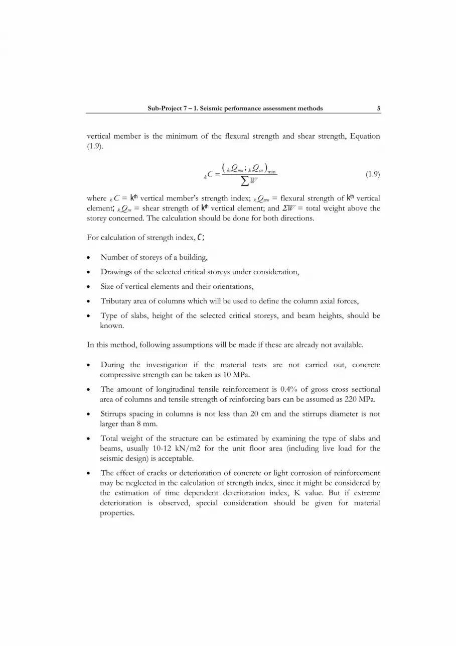
Sub-Project 7 – 1. Seismic performance assessment methods 5
vertical member is the minimum of the flexural strength and shear strength, Equation (1.9).
( )=
∑min;k mu k su
k
Q QC
W (1.9)
where k C = kth vertical member’s strength index; k Qmu = flexural strength of kth vertical element; k Qsu = shear strength of kth vertical element; and ΣW = total weight above the storey concerned. The calculation should be done for both directions.
For calculation of strength index, C;
• Number of storeys of a building,
• Drawings of the selected critical storeys under consideration,
• Size of vertical elements and their orientations,
• Tributary area of columns which will be used to define the column axial forces,
• Type of slabs, height of the selected critical storeys, and beam heights, should be known.
In this method, following assumptions will be made if these are already not available.
• During the investigation if the material tests are not carried out, concrete compressive strength can be taken as 10 MPa.
• The amount of longitudinal tensile reinforcement is 0.4% of gross cross sectional area of columns and tensile strength of reinforcing bars can be assumed as 220 MPa.
• Stirrups spacing in columns is not less than 20 cm and the stirrups diameter is not larger than 8 mm.
• Total weight of the structure can be estimated by examining the type of slabs and beams, usually 10-12 kN/m2 for the unit floor area (including live load for the seismic design) is acceptable.
• The effect of cracks or deterioration of concrete or light corrosion of reinforcement may be neglected in the calculation of strength index, since it might be considered by the estimation of time dependent deterioration index, K value. But if extreme deterioration is observed, special consideration should be given for material properties.
6 ITU
Moment capacity of a member should be known for the calculation of flexural strength for column. The moment capacity of columns can be calculated by using the approximate formulas given in Equation (1.10), (1.11) and (1.12) according to the level of axial load. These equations are the same equations given in the JSIM.
σ
σ
> >
= + − −
= +
max2
max max
max
0.4 ;
(0.8 0.12 )( )/( 0.4 )c
C u t y c c
c g y
N N bDf
M a D bD f N N N bDf
N bDf a
(1.10)
σ> >
= + −0.4 0;
0.8 0.5 (1 / )c
C u t y c
bDf NM a D ND N bDf
(1.11)
σ
σ
> >= +
= −
min
min
0 ;0.8 0.4C u t y
g y
N NM a D ND
N a
(1.12)
where Nmax = axial compressive strength of a column [N]; Nmin = axial tensile strength of a column [N]; N = axial load of a column [N]; at = area of tension reinforcement [mm2]; ag = total area of longitudinal reinforcement [mm2]; b = width of compressive side of a column [mm]; D = cross-sectional depth of a column [mm]; σy = yield strength of longitudinal reinforcement [MPa]; and fc = compressive strength of concrete [MPa].
Ultimate shear strength for column can be calculated by using Equation (1.13) proposed by Arakawa.
ρ ρ σ σ
ρ ρ
⎛ ⎞+= + +⎜ ⎟+⎝ ⎠
= ≤ ≤
= = =
0.23
0
0
0.053 (18 ) 0.85 0.1 ./( . ) 0.12
/ /2 /( . ) 3
100 7 /8. .
t cC su w s wy
t wt w
xfQ b j
M Q dM Q h ; 1 M Q d
a ax ; ; j db d b s
(1.13)
where ρt = tensile reinforcement ratio(%); ρw = shear reinforcement ratio; aw = total cross sectional area of a set of stirrups [mm2]; at = area of tension reinforcement [mm2]; b = width of compressive side of a column [mm]; d = effective depth of column [mm]; s = spacing of stirrups [mm]; sσwy = yield strength of stirrups [MPa]; σ0 = axial stress of columns, 0 < σ0 < 0.5 fc [MPa]; and fc = compressive strength of concrete [MPa].
Ultimate flexure strength for shear wall can be calculated by the following equation.
Sub-Project 7 – 1. Seismic performance assessment methods 7
σ σ= + +∑. 0.5 ( ). 0.5 .W u t y W Wy Wy W WM a l a l N l (1.14)
where N = total axial load of a wall [N]; at = area of tensile reinforcement at the wall’s end zone [mm2]; aWy = total area of vertical reinforcement [mm2]; lW = distance between centre of wall and end zones (wall end zones may be within the wall itself or within an adjoining wall or in an enlarged section at the edge of the wall) [mm]; σy = yield strength of longitudinal reinforcement [MPa]; fc = compressive strength of concrete [MPa].
The flexural strength can be calculated according to moment capacity of a member and the inflection height along the member, Equation (1.15).
( )λ= ∗ /mu u oQ M h (1.15)
where λ is the coefficient for inflection height, and h0 is the clear height of column or wall. If column is not connected to the frame λ is equal to 0. If it is connected then on the strong direction of column λ can be taken as 2 while on the weak direction it is 1.7. When walls are under consideration, coefficient λ becomes 1.
Ultimate shear strength for shear wall can be calculated by Equation (1.16),
ρ ρ σ σ
ρ ρ σ
⎛ ⎞+= + +⎜ ⎟+⎝ ⎠
≤ ≤
= = = = =∑
0.23
00.053 (18 ) 0.85 . 0.1 .
/( . ) 0.12/( . ) 3
100. . .
te cW su se wy e e e
t hte e se 0e e W
e e e
fQ b jM Q l
1 M Q lAa a Nx ; b ; ; ; j l
b l l b s b l
(1.16)
where ρte = equivalent tensile reinforcement ratio(%); at = area of tensile reinforcement at the wall’s end zone [mm2]; be = equivalent thickness of wall [mm]; l = wall length [mm]; ΣA = cross sectional area of wall; ρse = equivalent lateral reinforcement ratio; ah = cross sectional area of lateral reinforcement area [mm2]; s = spacing of lateral reinforcement [mm]; σwy = yield strength of lateral reinforcement [MPa]; σ0e = axial stress of wall, σ0e < 0.5 fc [MPa]; and fc = compressive strength of concrete [MPa].
1.3.2 Structural Irregularity Index, D
Structural irregularity index is related with the irregularities in plan and irregularities in elevation of a building. In the “Specification for Structures to be Built in Disaster Areas, Earthquake Disaster Prevention” (TERDC-98) seven irregularities are described. Four of these are in plan and three in elevation. Since the seismic index, Is is a production of three
8 ITU
sub-indices (eq. 1.5) structural irregularity index is the modification factor for the seismic capacity index, P as well as time dependent deterioration index, K.
If building is an irregular structure, the seismic index, Is could be reduced 40% by the structural irregularity index, D. The details of structural irregularity index, D will not be given in this study. This is an ongoing research project.
1.3.3 Time Dependent Deterioration Index, K
Influence of structural defects such as deflection, cracking, and corrosion is taking into account with time dependent deterioration index, K on the seismic index, Is. Site inspection is necessary for the estimation of the time dependent deterioration index, K.
Since this is an ongoing research project, it is adopted from the JSIM as it is. The seismic index, Is could be reduced 30% by the time dependent deterioration index, K.
1.4 REQUIRED SEISMIC CAPACITY INDEX, ID
The required seismic index, ID should be calculated by Equation (1.17).
= 0DI P xBxZxU (1.17)
where P0 = index for basic seismic demand; B =index for regional seismicity; Z = index for local soil conditions; and U = index for usage. Index B should be taken as 1.0 for high seismicity and never lower than 0.5 in any case. Index Z varies for soil conditions from 0.80(for rock or stiff soil) to 1.00 (soft soil). Usage index, U is 1.0 for residential buildings, 1.5 for buildings to be utilized immediately after the earthquake.
The basic seismic demand index, P0 is the most critical parameter for the method. In TERDC-98, Total Equivalent Seismic Load (base shear), Vt acting on the entire building in the earthquake direction considered will be determined by Equation (1.18).
= ≥00
( ) 0.10( )t
a
WxA xIxS TV xA xIxWR T
(1.18)
where W =total weight of the building (ΣG+nQ); A0 = effective ground acceleration coefficient; I = building importance factor; S(T)= spectrum coefficient, Ra(T) = seismic load reduction factor; and T= natural period of the building.
The lateral load carrying capacity of the ground floor, Qg can be expressed by Equation (1.19) in the SSSM, and it should be greater than the base shear, Vt.
Sub-Project 7 – 1. Seismic performance assessment methods 9
= ≥ ≥ 0 ( )( )g g g t g
a
A xIxS TQ P xW ; Q V ; PR T
(1.19)
where Pg = seismic capacity index of ground floor; and W =total weight of the building.
When a non-ductile (Ra(T)=R=4.0), residential building (I=1.0) is considered, whose natural period is relatively short and nearly matching with soil’s natural period (S(T)=2.5) and located on seismic zone 1 (A0 =0.40), its seismic capacity index of ground floor (Pg) should be equal to or greater than 0.25.
⎛ ⎞≥ =⎜ ⎟⎝ ⎠
0.40 1.00 2.5 0.254g
x x P (1.20)
If we calculate the seismic index, Is for the same case with assuming structural irregularity index, D and time dependent deterioration index, K equal to 1.0 we can say that Is should be equal to or greater than 0.25. Then; the required seismic index, ID value should be equal to 0.25 at least because the seismic index, Is value will be judged against to the required seismic index, ID value. If we repeat the same conditions (B=1; Z=1; U=1) in Equation (1.17) to calculate ID, the result implies that P0 should be equal to 0.25 as the first approach.
( ) ( )≥
= ≥ = 00.25 1.0 1.0 1.0 .1.0 1.0s D
s D
I II x x I P x x x
(1.21)
The value of 0.25 is very conservative as a basic seismic demand index P0 in case of buildings with high ductility. For calibration of this index, a pilot study was carried out in Zeytinburnu, Istanbul.
1.5 PILOT REGION STUDY
The SSSM is applied to 2401 buildings in Zeytinburnu, Istanbul. The cumulative frequency distribution of the seismic capacity index values of these buildings are given in Figure 1-3.

10 ITU
Cumulative Frequency Distrubution
0%
10%
20%
30%
40%
50%
60%
70%
80%
90%
100%
0.00 0.05 0.10 0.15 0.20 0.25 0.30 0.35 0.40 0.45 0.50 0.55
Seismic Capacity Index, P min
Freq
uenc
y ( P
min
)
Figure 1-3. The cumulative frequency distribution of the minimum seismic capacity index, Pmin values of 2401RC building in Zeytinburnu
For the calibration of the SSSM, the results of nonlinear static analysis carried out for 12 of these buildings are utilized. During the nonlinear analyses, actual (as-built) structural characteristics of these buildings are used for input. The value of the seismic capacity index, P has a fundamentally important effect on the decisions about the basic seismic demand index, P0.
During all steps of nonlinear analysis, the displacement profile is taken from the shape of the first mode in the corresponding direction. This assumption does not cause misleading results, because 12 buildings among 2401 buildings were chosen such that the effects of higher modes were minimal. Plastic hinge lengths of columns and beams were assumed as half of the section depth (h/2). From the results of these analyses, base shear force capacities corresponding to collapse prevention performance level were determined for each building. Then the ratios of base shear force capacity to structural weight were calculated. The ratios for x and y directions (Vx/W, Vy/W) and the structural seismic capacity indices (Px, Py), which are the ratios of strength indices to the structural weight determined by SSSM are presented in Table 1-2.
Table 1-2. V/W and P values obtained by pushover analysis and SSSM
Building Code Vx/W Px Vy/W Py
Min
(Vx/W; Vy/W)
Min
(Px,Py)
1597944 0.14 0.21 0.12 0.14 0.12 0.14 1610028 0.10 0.09 0.09 0.11 0.09 0.09 1597778 0.08 0.13 0.12 0.27 0.08 0.13 1597914 0.09 0.13 0.12 0.13 0.09 0.13

Sub-Project 7 – 1. Seismic performance assessment methods 11
Building Code Vx/W Px Vy/W Py
Min
(Vx/W; Vy/W)
Min
(Px,Py)
1597818 0.07 0.06 0.07 0.10 0.07 0.06 1609263 0.07 0.07 0.08 0.08 0.07 0.07 1597776 0.14 0.15 0.15 0.24 0.14 0.15 1599432 0.09 0.10 0.12 0.11 0.09 0.10 1597884 0.10 0.11 0.09 0.13 0.09 0.11 1597799 0.10 0.11 0.10 0.12 0.10 0.11 1610164 0.18 0.28 0.22 0.23 0.18 0.23 1610166 0.11 0.17 0.08 0.12 0.08 0.12
The relationships between V/W and P values are shown in the Figure 1-4, below. As it can be seen from these figures, the results obtained by using SSSM are similar to those obtained by pushover analysis qualitatively. The minimum V/W values obtained by pushover analysis are approximately 80% of the corresponding minimum P values obtained by SSSM.
For the calibration of Po value, the structural performance indices for two principal directions (Px, Py) are compared with the ratios of base shear capacities determined by pushover analysis to the structural weight, (Vx/W, Vy/W). After the calibration, it is determined that the main comparison index ID should be considered as 0.18.
min (Vx/W, Vy/W) and min (Px,Py)
y = 0.80x
00.020.040.060.08
0.10.120.140.160.18
0.2
0 0.05 0.1 0.15 0.2 0.25
min (Px, Py)
min
(Vx/
W, V
y/W
)
Figure 1-4. The relation between results obtained by using SSSM and pushover analysis
During pushover analyses, for seismic demand, the NEHRP acceleration spectrum for 50% exceedence probability in 50 years, is considered. Ss and Sl characteristic spectral acceleration coefficients are determined by Bogazici University based on local seismicity

12 ITU
and ground conditions for each building. This information was used to estimate the index for regional seismicity, B and index for soil-structure behavior (local soil conditions), Z for the calculation of the required seismic index, ID. Usage index was taken as 1.0 since all buildings are employed as residential purposes. Evaluation of the buildings using SSSM is given in Table 1-3.
Table 1-3. Evaluation of the buildings using SSSM
Building Code min(Px,Py)
Irregularity Index D
Time Det. Index K Seismic index,Is
Required seismic index, ID
1597944 0.14 1.00 1.00 0.14 0.15 1610028 0.09 1.00 1.00 0.09 0.15 1597778 0.13 1.00 1.00 0.13 0.14 1597914 0.13 1.00 1.00 0.13 0.15 1597818 0.06 1.00 1.00 0.06 0.15 1609263 0.07 1.00 1.00 0.07 0.15 1597776 0.15 1.00 0.95 0.14 0.15 1599432 0.10 1.00 1.00 0.10 0.14 1597884 0.11 0.95 1.00 0.10 0.14 1597799 0.11 1.00 1.00 0.11 0.14 1610164 0.23 0.90 1.00 0.21 0.15 1610166 0.12 0.90 1.00 0.11 0.18
The estimation of the seismic safety of the building is based on the comparison of the seismic index Is and the required seismic index, ID. It should be noted that the decision on the seismic safety is not based on the seismic capacity index, P and the basic seismic demand index, P0.
According to the evaluation, for only one building out of twelve satisfies Is>ID condition. This shows that for the seismicity of this region, only one building out of examined twelve buildings has sufficient seismic safety. For determining the seismic performance of the remaining 11 buildings, a decision should be given based on a more detailed analysis. It is interesting to note that according to the pushover analyses results, only one building, which was determined as earthquake resistant by the SSSM, had sufficient seismic safety. For other buildings, which had Is values smaller than ID, the results obtained by pushover analysis are also in good agreement with the results obtained by SSSM.

Sub-Project 7 – 1. Seismic performance assessment methods 13
1.5.1 Application of SSSM to a Sample Building
Figure 1-5 shows the ground storey plans of sample building with material quality of C9 concrete and S220 steel.
Figure 1-5. Ground floor plan of sample building
A four storey reinforced concrete building structure having equal storey height of 2.70 m is investigated in details for the purpose of comparing non-linear static analyses results with the SSSM index values. The plan dimensions of the building are 10.10 m x 9.90 m.
The NEHRP acceleration spectrum exceedance probability being 50% in 50 years is considered for seismic demand. Characteristic spectral acceleration coefficients, Ss = 0.692 and Sl = 0.412 are determined by Bogazici University based on local seismicity and ground conditions for the building. Fundamental periods of the building, Tx = 0.766 sec and Ty= 0.602 sec. Pushover analyses of the building were realised by ETABS Nonlinear V.8. (Figure 1-6) then performance level of them according to the NEHRP and TERDC-2006 are determined (Figure 1-7). The ratios of base shear force capacity to structural weight are obtained as 0.135 and 0.149 in directions of X and Y, respectively.

14 ITU
1597776 X_DIRECTION PUSHOVER CURVE
0.0
100.0
200.0
300.0
400.0
500.0
600.0
700.0
0.000 0.050 0.100 0.150 0.200
TOP DISPLACEMENT(M)
BA
SE S
HEA
R (K
N)
X_PUSHOVER CURVE BILINEARIZATION
1597776 Y_DIRECTION PUSHOVER CURVE
0.0
100.0
200.0
300.0
400.0
500.0
600.0
700.0
0.000 0.050 0.100 0.150 0.200 0.250
TOP DISPLACEMENT(M)
BA
SE S
HEA
R (K
N)
Y_PUSHOVER CURVE BILINEARIZATION Figure 1-6. Pushover curve of residential building (direction x, y) and bilinear form
1597776 X DIRECTION CAPACITY DIAGRAM DEMAND ESTIMATION
0.0000
1.0000
2.0000
3.0000
4.0000
5.0000
6.0000
7.0000
8.0000
0.0000 0.0200 0.0400 0.0600 0.0800 0.1000 0.1200 0.1400 0.1600 0.1800 0.2000
SPECTRAL DISPLACEMENT (M)
SPEC
TRA
L A
CC
ELER
ATI
ON
(M/S
N2)
BILINEARIZED X_ PUSHOVER SPECTRUM CORR.LINEAR SYS.
1597776 Y DIRECTION CAPACITY DIAGRAM DEMAND ESTIMATION
0
1
2
3
4
5
6
7
8
0 0.02 0.04 0.06 0.08 0.1 0.12 0.14 0.16 0.18 0.2
SPECTRAL DISPLACEMENT (M)
SPEC
TRA
L A
CC
ELER
ATI
ON
(M/S
N2)
BILINEARIZED Y_ PUSHOVER SPECTRUM CORR.LINEAR SYS. Figure 1-7. Capacity diagram, demand estimation of residential building (direction x, y)
SSSM is applied to the building with the help of MS-Excel. Excel sheet for this building is shown in Figure 1-8. Data input part of the sheet contains number of storeys, height and number of investigated storey, type of slab, areas of ground and normal floors, columns and beams dimensions and effective areas for calculation of axial forces acting on columns. Those data capture from the text file by macros, and then calculation of seismic capacity index, P is started automatically by considering the assumptions and pre-formulated cells. For determination of seismic index Is, structural irregularity index, D and time deterioration index, K should be calculated for the building. Structural irregularity index, D is calculated basically as 1.0 since building has neither irregularity, nor complexity of structural configuration. Time deterioration index, K was considered as 0.95 because evenly corrosion of longitudinal bars inside some columns was reported.

Sub-Project 7 – 1. Seismic performance assessment methods 15
Building ID No 1597776Investigated Floor Ground Story Height (m) 2.70n = number of stories of a building 4 DATA INPUT Type of slab slab-beamArea of ground floor (m2) 99.99Area of Normal Floor (m2) 100.28i =investigated story's number 1
1 2 3 4 5 6 7 8 9
X DirectionY Direction +X-side -X-side +Y-side -Y-sideS1 25.00 40.00 2.70 0.00 50.00 50.00 0.00 0.69S2 40.00 25.00 2.70 0.00 50.00 50.00 0.00 1.69S3 25.00 40.00 2.70 0.00 50.00 50.00 0.00 2.03S4 25.00 40.00 2.70 0.00 50.00 50.00 0.00 1.03S5 25.00 40.00 2.70 0.00 50.00 50.00 0.00 3.12S6 40.00 25.00 2.70 0.00 50.00 50.00 0.00 7.78S7 40.00 25.00 2.70 0.00 50.00 50.00 0.00 9.40S8 35.00 40.00 2.70 0.00 50.00 50.00 0.00 7.19S9 25.00 40.00 2.70 0.00 50.00 50.00 0.00 3.34S10 25.00 40.00 2.70 0.00 50.00 50.00 0.00 10.38S11 25.00 75.00 2.70 0.00 50.00 50.00 0.00 9.79S12 25.00 60.00 2.70 0.00 50.00 50.00 0.00 5.63S13 25.00 60.00 2.70 0.00 50.00 50.00 0.00 13.10S14 25.00 60.00 2.70 0.00 50.00 50.00 0.00 6.20S15 25.00 40.00 2.70 0.00 50.00 50.00 0.00 2.21S16 40.00 25.00 2.70 0.00 50.00 50.00 0.00 5.56S17 25.00 40.00 2.70 0.00 50.00 50.00 0.00 6.67S18 25.00 40.00 2.70 0.00 50.00 50.00 0.00 4.48
Column
No
DIMENSIONS (cm)
Height of
column
(m)
BEAMS' DEPTH (cm)
Tributary
Area (m2)
Figure 1-8. MS-Excel worksheet for application of SSSM to sample building (direction x, y)

16 ITU
10 11 12 13 14 15 16
Table
1.1
Table
1.1σo hox/Dx hoy/Dy Qmux Qmuy Qsux Qsuy
0.3809 8.80 5.50 201.63 322.61 581.59 799.690.9318 5.50 8.80 409.63 256.02 843.76 625.661.1206 8.80 5.50 273.07 436.91 640.76 858.860.5686 8.80 5.50 220.94 353.50 596.60 814.701.7222 8.80 5.50 322.00 515.21 688.90 906.994.2946 5.50 8.80 701.50 438.44 1112.78 894.680.0000 5.50 8.80 1173.17 733.23 769.22 551.122.8349 6.29 5.50 766.01 875.44 1204.44 1295.931.8437 8.80 5.50 330.88 529.41 698.61 916.710.0000 8.80 5.50 733.23 1173.17 551.12 769.222.8822 8.80 2.93 737.11 2211.32 1284.06 2385.352.0718 8.80 3.67 519.99 1247.97 976.44 1639.524.8208 8.80 3.67 665.59 1597.41 1306.32 1969.402.2816 8.80 3.67 540.18 1296.42 1001.62 1664.691.2199 8.80 5.50 281.72 450.75 648.71 866.813.0691 5.50 8.80 642.76 401.72 1014.75 796.653.6818 8.80 5.50 424.35 678.95 845.67 1063.762.4730 8.80 5.50 371.52 594.44 748.96 967.05
w [kN/m2] fc [MPa] σy[MPa] σwy[MPa] ρt ρw d' [cm]12 10 220 220 0.004 0.002 2.5
ASSUMPTIONSHoop diameter (mm) Hoop spacing (cm)
8 20
Eq.(1.10, 1.11,
1.12, 1.15)
Eq. (1.13)
Figure 1-9. (Cont.) MS-Excel Worksheet for application of SSSM to sample building (dir. x, y)

Sub-Project 7 – 1. Seismic performance assessment methods 17
17 18 19 20 21 22 23 24 25 26 27 28
Eq.
(1.19)
Fig
1.2
Eq.
(1.19)
Fig
1.2Cx ax Cy ay Cx ax Cy ay Rx Ry Cx Rx Cy Ry ρw ρw
0.0036 1.0 0.0058 1.0 0.0036 0.0058 1.0 1.0 0.0036 0.0058 0.001 0.0020.0074 1.0 0.0046 1.0 0.0074 0.0046 1.0 1.0 0.0074 0.0046 0.002 0.0010.0049 1.0 0.0079 1.0 0.0049 0.0079 1.0 1.0 0.0049 0.0079 0.001 0.0020.0040 1.0 0.0064 1.0 0.0040 0.0064 1.0 1.0 0.0040 0.0064 0.001 0.0020.0058 1.0 0.0093 1.0 0.0058 0.0093 1.0 1.0 0.0058 0.0093 0.001 0.0020.0127 1.0 0.0079 1.0 0.0127 0.0079 1.0 1.0 0.0127 0.0079 0.002 0.0010.0139 1.0 0.0100 1.0 0.0139 0.0100 1.0 1.0 0.0139 0.0100 0.002 0.0010.0138 1.0 0.0158 1.0 0.0138 0.0158 1.0 1.0 0.0138 0.0158 0.001 0.0010.0060 1.0 0.0096 1.0 0.0060 0.0096 1.0 1.0 0.0060 0.0096 0.001 0.0020.0100 1.0 0.0139 1.0 0.0100 0.0139 1.0 1.0 0.0100 0.0139 0.001 0.0020.0133 1.0 0.0399 1.0 0.0133 0.0399 1.0 1.0 0.0133 0.0399 0.001 0.0020.0094 1.0 0.0225 1.0 0.0094 0.0225 1.0 1.0 0.0094 0.0225 0.001 0.0020.0120 1.0 0.0289 1.0 0.0120 0.0289 1.0 1.0 0.0120 0.0289 0.001 0.0020.0098 1.0 0.0234 1.0 0.0098 0.0234 1.0 1.0 0.0098 0.0234 0.001 0.0020.0051 1.0 0.0081 1.0 0.0051 0.0081 1.0 1.0 0.0051 0.0081 0.001 0.0020.0116 1.0 0.0073 1.0 0.0116 0.0073 1.0 1.0 0.0116 0.0073 0.002 0.0010.0077 1.0 0.0123 1.0 0.0077 0.0123 1.0 1.0 0.0077 0.0123 0.001 0.0020.0067 1.0 0.0107 1.0 0.0067 0.0107 1.0 1.0 0.0067 0.0107 0.001 0.002
∑Cxax ∑Cyay (∑Cxax)*(minRx)0.15 0.24 0.15 0.24
P x P y
Table
1.1
(∑Cyay)*(minRy)
Eq. (1.6, 1.7,
1.8)
Figure 1-10. (Cont.) MS-Excel worksheet for application of SSSM to residential building (dir. x, y)
In this example, seismic capacity index for the “X” direction is found as the minimum value with the score of 0.15. From the results of non-linear analyses, the minimum value of base shear force to weight ratio is obtained as 0.135 for the “X” direction, too. According to TERDC-2006, the building’s performance level is lower than collapse prevention level.
18 ITU
1.6 CONCLUSIONS
A general conclusion after applying Seismic Safety Screening Method (SSSM) to the buildings that are examined by the nonlinear static analysis is that SSSM can be used for estimating the existing seismic safety levels for medium/low rise RC buildings since the results obtained by the screening method and the structural analysis are in good harmony.
The basic seismic demand index, P0 value appeared to be 0.18 in the pilot region. But still much effort is needed to apply this method to a large selection of RC buildings in different seismic regions, and verify the results by the structural analyses.
Future development for improvement of this method will focus on approximate formulas given in Equation (1.10) to (1.16), and adding some experimental studies on sub-structural elements besides to estimate the structural irregularity index, D and time dependent deterioration index, K.
2.SEISMIC UPGRADING OF STRUCTURES USING CONVENTIONAL METHODS
Turkey is located at one of the active earthquake zones of the world and many earthquakes have been occurred in the past resulting the life and property loses. For these reasons, retrofitting or strengthening of existing buildings against the future earthquakes is very important for avoiding the potential life and property loses. The problem is especially important for reinforced concrete buildings which have been built during the last sixty years according to the existing codes of their times. Most of these early codes have considered the seismic loads as some percentage of the total live and dead loads of the building. A linear and approximate method of analysis has been used under this type of seismic load. Experiences from the past earthquakes in Turkey have shown that large earthquakes can severely damage the existing buildings designed according to the old code provisions. The research in this chapter is taken from deliverables 106 which is available from www.lessloss.org. The purpose of Deliverables 106 was to reach the reliability and performance of a low disturbance strengthening technique depending on adding the new shearwalls to the building by using the non-linear analysis which was not applied in common practice after the past four major earthquakes in Turkey. In the report moreover, the non-linear behaviour and seismic performances of the strengthened buildings are also evaluated considering the soil structure interaction using a convenient analysis model.
2.1 EVALUATION OF SEISMIC SAFETY OF EXISTING BUILDINGS AND
RETROFITTING TECHNIQUES
The analytical and experimental studies on real behaviours of structures under seismic loads have led to either revisions in code provisions or more realistic earthquake resistant design of buildings built in seismic zones. On the other hand, It is a reality that there are a number of existing buildings under seismic risk due to constructional problems such as poor concrete quality, insufficient dimensions of structural elements, insufficient and wrong placed reinforcement etc., in Turkey. Thus, first, determination of the seismic safeties of existing buildings and then developing the economical and practical retrofitting techniques for the existing buildings which have insufficient seismic safety are very important.

20 ITU
Pushover analysis method is an effective tool used for determination of seismic safety of existing buildings. In this method, mathematical model of the existing structure is analyzed under the monotonically increasing gravity and earthquake loads, and plastic hinge formations are observed until the structure is collapsed. The results of this type of analysis are very important from the viewpoint of design engineer, since they show the weak parts or potential damage points of the structure and give an idea for existing seismic safety.
2.1.1 The Procedure for Determination of the Seismic Safety of Existing Buildings
The procedure consists of the following steps:
i) Providing and evaluation of the documents of the existing building
ii) Inspections on the existing building.
iii) Preparation of the mathematical model of the existing structure
iv) Pushover analysis of the mathematical model of the existing building.
v) Evaluation of the seismic safety of the building.
vi) Steps of the given procedure is explained in Deliverable-106 in detail.
2.2 OBSERVATIONS ON IMPERFECTIONS CAUSING THE COLLAPSE OR DAMAGE IN
RESIDENTIAL BUILDINGS AND COMMON STRENGTHENING TECHNIQUES IN
TURKEY
Frequently observed imperfections causing the collapse or heavy damages in residential buildings from the past earthquake experiences such as Erzincan (1992), Dinar (1995), Ceyhan (1998), Kocaeli and Düzce (1999), are as follows:
• inappropriate regulation of lateral load carrying structural system elements,
• inadequate reinforcement and poor detailing,
• foundation and geotechnical problems,
• very poor strength of concrete,
• poor workmanship, short columns,
• soft storeys, weak column- strong beam connections,

Sub-Project 7 – 2. Seismic upgrading of structures using conventional methods 21
• lack of construction control organization in Turkey.
As the main part of the building stock in Turkey are suffered from the deficiencies mentioned above, strengthening the existing buildings by an economic, efficient, rapid and low disturbance technique against to the future earthquakes are of great importance. Some common upgrading (retrofitting or strengthening) techniques are summarized as follows:
There are a lot of strengthening techniques have been considered and applied in the actual practice of the existing reinforced concrete structures. Some of them are in the following:
i) reinforced concrete jacketing ,
ii) epoxy bonded steel plates,
iii) steel bracing,
iv) steel frames and trusses,
v) pre-cast reinforced infill walls,
vi) additional cast-in-place concrete concentric or eccentric shear walls and new foundations,
vii) wrapping the existing structural elements with FRP,
vii) application of the base isolation and damping devices.
In Turkey’s experience and practice however, even if it is expensive, upgrading the existing structures by additional cast-in-place RC shearwalls is found to be more effective technique comparing the other alternative upgrading techniques for the following reasons:
i) From the experiences of past earthquakes, the collapsed residential buildings generally had 3-5 storey and collapses were occurred due to the storey mechanism called as pan-cake mechanism.
ii) The most of the buildings do not have a design project prepared by an engineer or an architect.
iii) The concrete strength is very poor due to the non-proportional mixture of water, aggregate and cement. Moreover, the mixture includes sea sand.
iv) The buildings have bad formwork and reinforcement placement workmanship.
v) Lateral load carrying elements have inadequate stirrups and inadequate concrete covers.

22 ITU
vi) The buildings have many irregularities in plan and in view, most of them have short columns and soft storeys.
vii) The columns of the basements are faced the intensive corrosion problem due to the damp, especially in the buildings of İstanbul and its vicinity.
viii) It is the lowest disturbance upgrading method among the other alternatives.
2.2.1 Strengthening the Existing Buildings by Additional Shearwalls
In Turkey most of the low-rise residential RC buildings are not well designed and constructed, thus, lateral rigidities and lateral load carrying capacity of them are not sufficient. Furthermore, as collateral type of construction is very common, the storey drifts should be limited. In order to overcome the mentioned deficiencies above, adding new shear walls to the existing structure has been preferred as the most common upgrading technique in Turkey.
If new added shear walls are selected as an upgrading technique, for the sake of completeness the positive contributions of them to the structural behaviour have been given below:
i) storeydrifts will be reduced, thus, partitioning walls made of brittle material can not be damaged due to excessive storey drifts,
ii) storeymechanism will be diminished,
iii) short column effects can be eliminated,
iv) efficiency of the moment-resistant frames will be reduced so that beam-column connections will not be effective in controlling the lateral load behaviour of the structure,
v) by placing the suitable orientation of the additional shear walls, some of the plain and elevation irregularities of the existing structure can be eliminated as much as possible,
vi) existing lateral load carrying elements of the structure will keep their reserve strengths since the additional shear walls carry the biggest portion of the lateral load.
The major and common difficulty is the integration of the newly added shear walls to the existing structure. In general, since the concrete strength of the existing structures in Turkey is very poor, it becomes very difficult to have shear connectors to join the additional shearwalls to the existing one. In practice, it is very convenient to design the new shear walls as they cover the existing beams and columns for full integration. Epoxy injection may be needed for bonding between the new and existing structural elements. Construction procedure for additional shearwalls will be given in the next chapter. The designing and construction of the foundations of additional shear walls are another
Sub-Project 7 – 2. Seismic upgrading of structures using conventional methods 23
problem since the axial loads transferred to the additional shear walls are not big enough. Rotation of the foundations cannot be restricted, unless they are integrated to the other existing foundations. For this reason, adequate transfer of internal forces must be satisfied by picking up newly added shear walls in order to limit rotation of foundation system.
2.2.2 Construction Rules for Additional Shearwalls
Strengthening by adding the new shearwalls to the existing structure may increase either the seismic safety of the building and also limits the drift ratio. But, as the new shear walls increase the total stiffness of the building, total earthquake load and its distribution over the new and existing structural elements will change. Thus, the existing structural elements should be checked by the new internal force distribution and they should be also retrofitted if necessary.
The following measures should be considered in strengthening by new shear walls:
i) At least two shear walls should be placed in each direction. The dimensions of the shear walls should be selected by considering the total plan area of the building and the number of the storeys. Approximately 80 % of the total seismic base shear should be resisted by the new added shearwalls. Furthermore, wall dimensions should satisfy the minimum requirements imposed by the code.
ii) Shearwalls may be placed at the external axes, blind sides and the stairwell sides of the building. Other internal axes may also be selected as shear wall places if the architectural provisions permit and as not to interfere the building’s function.
iii) New shearwalls should provide sufficient torsional rigidity to the existing structure.
iv) Shear walls should be placed between the two adjacent existing columns and they should also surround the columns for transmitting the existing gravity loads of the structure to the foundation.
v) The connections of the new and existing structural elements such as shear wall-column, shear wall-beam and shear wall-floor connections should be carefully built and the anchorages should be designed for the integration between existing and new structural elements.
vi) The new foundations for the new shear walls should be designed and joined with the existing ones for full integrity.
vii) New shearwalls should also allow for the economical design of the foundation system.
24 ITU
viii) 3D analysis should be performed for the design of strengthened building and actual stiffness properties of existing and new structural elements should be used in the analysis.
2.3 NUMERICAL EXAMPLE
In this chapter, performance levels of a sample strengthened building chosen from the Deliverable-106 are evaluated considering various code provisions including ATC-40, FEMA-440 and TEC-2006 and conclusions on the obtained results are given. Soil-structure interaction is included for the performance analyses using non-linear static analysis by a mat foundation on tensionless Winkler soil model. Non-linear pushover analyses and performance evaluations are performed by SAP2000 computer package. The calculations are performed for two major earthquake directions X and Y, but only the results for the X direction are given for the sake of brevity.
The sample building has a roof storey in 2.5 m, ground storey in 3.15 m height and three normal storeys in 2.75 m heights each one and plan dimensions of the building are 10.20 m x 6.80 m. Typical storey plans for the existing and strengthened buildings are given in Figure 2-1 and Figure 2-2. Two shearwalls are added to the building for strengthening in each direction. 95% of the total base shear is carried by the additional shearwalls and the remaining is carried by the existing elements. The coefficients for the equivalent lateral load calculations are taken as effective ground acceleration, (Ao) = 0.40, intensity factor of design earthquake, E = 1.0, building importance factor, (I) = 1.0, Soil class = Z3, characteristic spectral periods, TA = 0.15 sec, TB = 0.60 sec.
For the performance evaluations of the building with and without soil-structure interaction, two foundation models are considered. For the first model, the foundations of the building are considered as fixed base. At the other hand, the second one is considered that it has a mat foundation on tensionless Winkler foundation. The mathematical model used for the analysis is shown in Figure 2-3. Fundamental period of the fixed base building at the X direction is Tx= 0.343 sec. and the one for the mat foundation model is Tx= 0.414 sec. The total storey weights, masses and the Equivalent Earthquake Loads of the strengthening building calculated according to the TEC-2006 are given in Table 2-1. The Equivalent Earthquake Loads of the strengthening buildings with fixed base and with mat foundation are the same since the spectrum coefficients are equal to 2.5.

Sub-Project 7 – 2. Seismic upgrading of structures using conventional methods 25
Figure 2-1. Normal storey plan of existing building
Figure 2-2. Normal storey plan of strengthened building
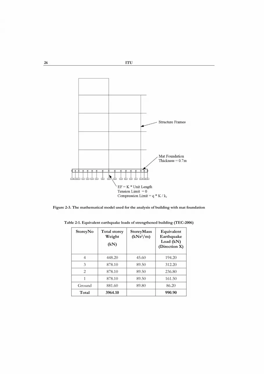
26 ITU
Figure 2-3. The mathematical model used for the analysis of building with mat foundation
Table 2-1. Equivalent earthquake loads of strengthened building (TEC-2006)
StoreyNo Total storey Weight
(kN)
StoreyMass (kNs2/m)
Equivalent Earthquake Load (kN)
(Direction X)
4 448.20 45.60 194.20 3 878.10 89.50 312.20 2 878.10 89.50 236.80 1 878.10 89.50 161.50
Ground 881.60 89.80 86.20 Total 3964.10 990.90
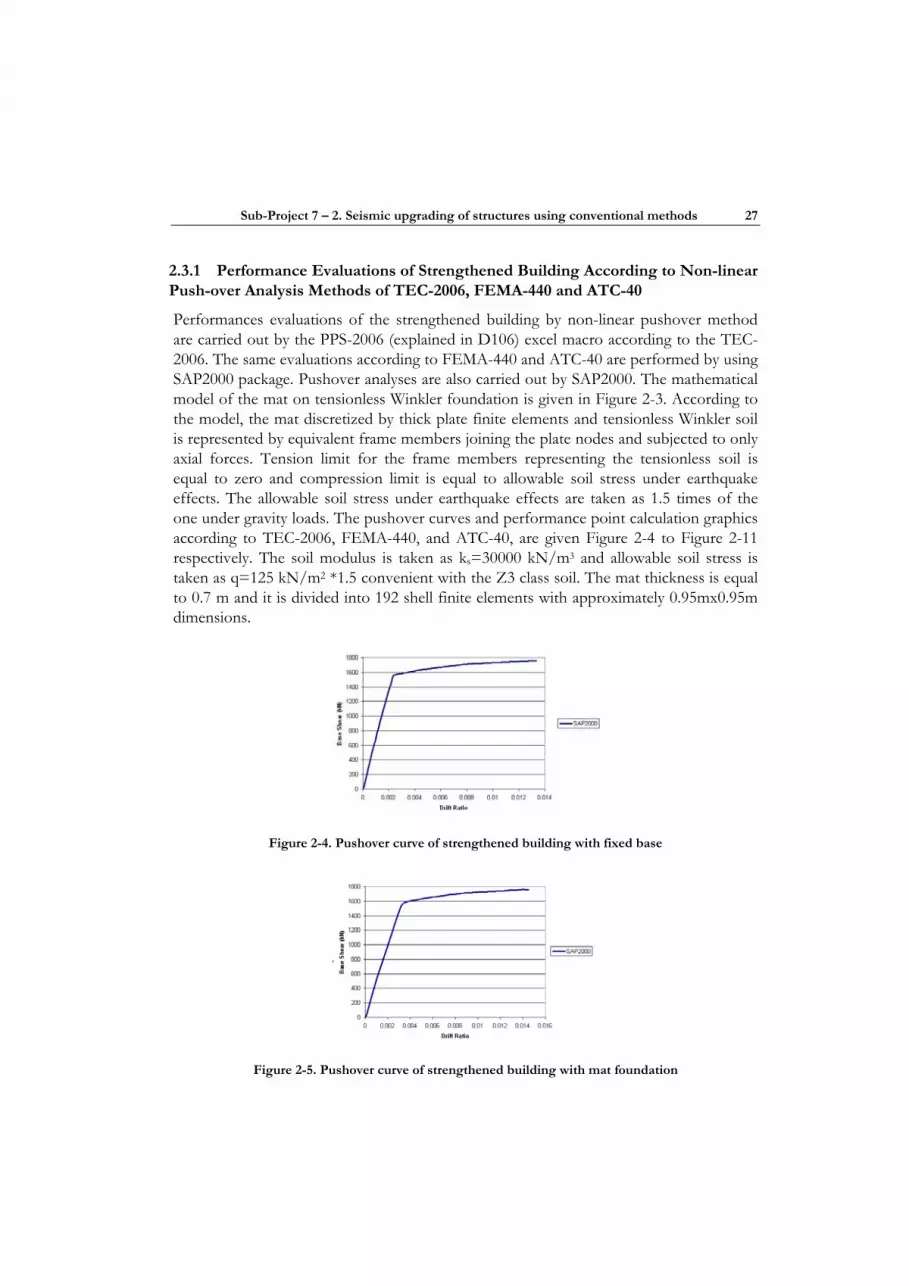
Sub-Project 7 – 2. Seismic upgrading of structures using conventional methods 27
2.3.1 Performance Evaluations of Strengthened Building According to Non-linear Push-over Analysis Methods of TEC-2006, FEMA-440 and ATC-40
Performances evaluations of the strengthened building by non-linear pushover method are carried out by the PPS-2006 (explained in D106) excel macro according to the TEC-2006. The same evaluations according to FEMA-440 and ATC-40 are performed by using SAP2000 package. Pushover analyses are also carried out by SAP2000. The mathematical model of the mat on tensionless Winkler foundation is given in Figure 2-3. According to the model, the mat discretized by thick plate finite elements and tensionless Winkler soil is represented by equivalent frame members joining the plate nodes and subjected to only axial forces. Tension limit for the frame members representing the tensionless soil is equal to zero and compression limit is equal to allowable soil stress under earthquake effects. The allowable soil stress under earthquake effects are taken as 1.5 times of the one under gravity loads. The pushover curves and performance point calculation graphics according to TEC-2006, FEMA-440, and ATC-40, are given Figure 2-4 to Figure 2-11 respectively. The soil modulus is taken as ks=30000 kN/m3 and allowable soil stress is taken as q=125 kN/m2 *1.5 convenient with the Z3 class soil. The mat thickness is equal to 0.7 m and it is divided into 192 shell finite elements with approximately 0.95mx0.95m dimensions.
Figure 2-4. Pushover curve of strengthened building with fixed base
Figure 2-5. Pushover curve of strengthened building with mat foundation
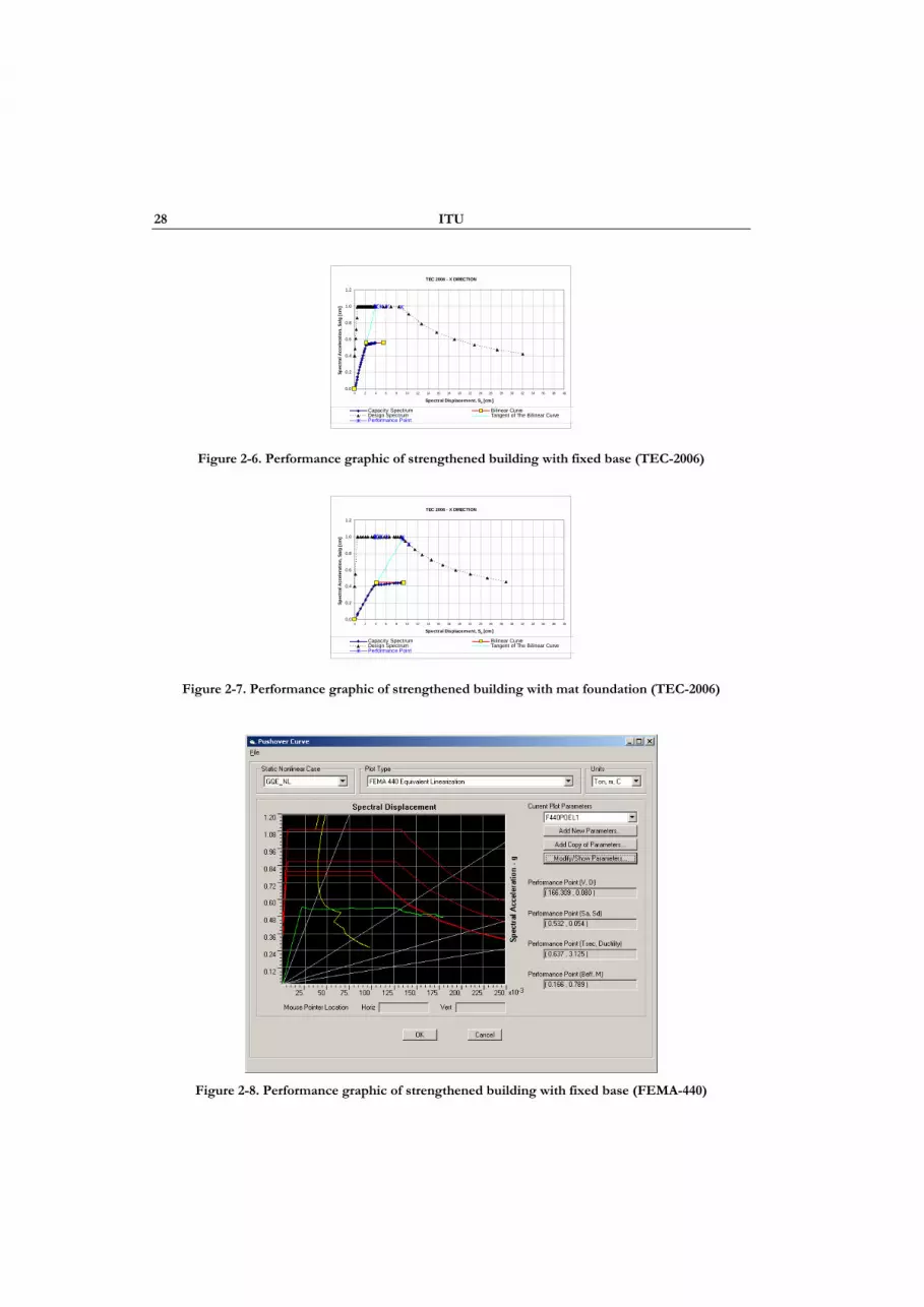
28 ITU
TEC 2006 - X DIRECTION
0.0
0.2
0.4
0.6
0.8
1.0
1.2
0 2 4 6 8 10 12 14 16 18 20 22 24 26 28 30 32 34 36 38 40
Spectral Displacement, Sd [cm]
Spec
tral
Acc
eler
atio
n, S
a/g
[cm
]
Capacity Spectrum Bilinear CurveDesign Spectrum Tangent of The Bilinear CurvePerformance Point
Figure 2-6. Performance graphic of strengthened building with fixed base (TEC-2006)
TEC 2006 - X DIRECTION
0.0
0.2
0.4
0.6
0.8
1.0
1.2
0 2 4 6 8 10 12 14 16 18 20 22 24 26 28 30 32 34 36 38 40
Spectral Displacement, Sd [cm]
Spec
tral
Acc
eler
atio
n, S
a/g
[cm
]
Capacity Spectrum Bilinear CurveDesign Spectrum Tangent of The Bilinear CurvePerformance Point
Figure 2-7. Performance graphic of strengthened building with mat foundation (TEC-2006)
Figure 2-8. Performance graphic of strengthened building with fixed base (FEMA-440)
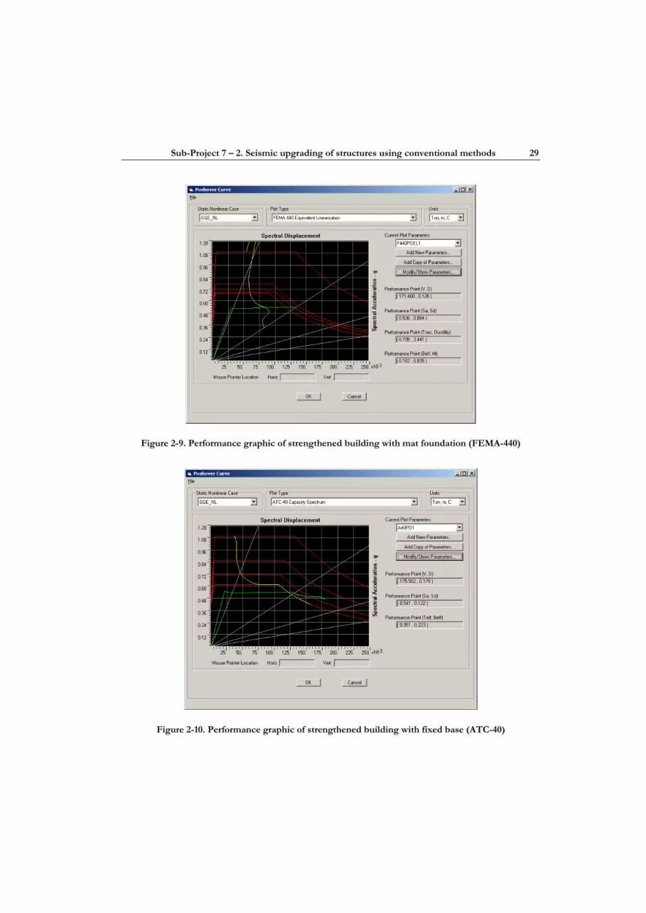
Sub-Project 7 – 2. Seismic upgrading of structures using conventional methods 29
Figure 2-9. Performance graphic of strengthened building with mat foundation (FEMA-440)
Figure 2-10. Performance graphic of strengthened building with fixed base (ATC-40)
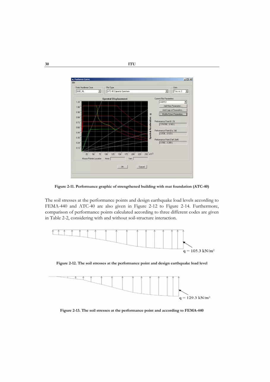
30 ITU
Figure 2-11. Performance graphic of strengthened building with mat foundation (ATC-40)
The soil stresses at the performance points and design earthquake load levels according to FEMA-440 and ATC-40 are also given in Figure 2-12 to Figure 2-14. Furthermore, comparison of performance points calculated according to three different codes are given in Table 2-2, considering with and without soil-structure interaction.
Figure 2-12. The soil stresses at the performance point and design earthquake load level
Figure 2-13. The soil stresses at the performance point and according to FEMA-440
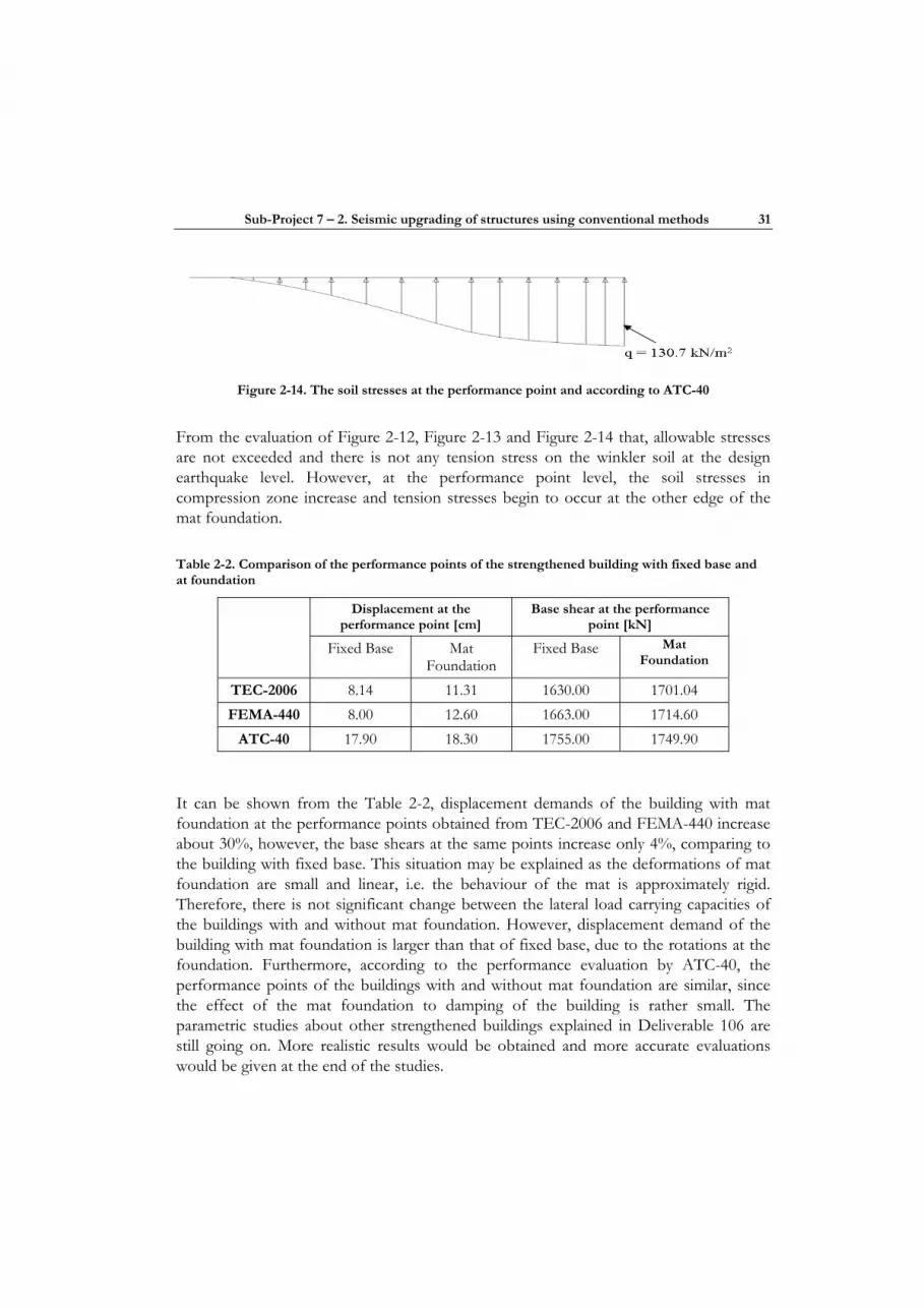
Sub-Project 7 – 2. Seismic upgrading of structures using conventional methods 31
Figure 2-14. The soil stresses at the performance point and according to ATC-40
From the evaluation of Figure 2-12, Figure 2-13 and Figure 2-14 that, allowable stresses are not exceeded and there is not any tension stress on the winkler soil at the design earthquake level. However, at the performance point level, the soil stresses in compression zone increase and tension stresses begin to occur at the other edge of the mat foundation.
Table 2-2. Comparison of the performance points of the strengthened building with fixed base and at foundation
Displacement at the performance point [cm]
Base shear at the performance point [kN]
Fixed Base Mat Foundation
Fixed Base Mat Foundation
TEC-2006 8.14 11.31 1630.00 1701.04 FEMA-440 8.00 12.60 1663.00 1714.60
ATC-40 17.90 18.30 1755.00 1749.90
It can be shown from the Table 2-2, displacement demands of the building with mat foundation at the performance points obtained from TEC-2006 and FEMA-440 increase about 30%, however, the base shears at the same points increase only 4%, comparing to the building with fixed base. This situation may be explained as the deformations of mat foundation are small and linear, i.e. the behaviour of the mat is approximately rigid. Therefore, there is not significant change between the lateral load carrying capacities of the buildings with and without mat foundation. However, displacement demand of the building with mat foundation is larger than that of fixed base, due to the rotations at the foundation. Furthermore, according to the performance evaluation by ATC-40, the performance points of the buildings with and without mat foundation are similar, since the effect of the mat foundation to damping of the building is rather small. The parametric studies about other strengthened buildings explained in Deliverable 106 are still going on. More realistic results would be obtained and more accurate evaluations would be given at the end of the studies.

32 ITU
2.4 CONCLUSIONS
In this section, seismic performance of a sample building strengthened by added shearwalls which is the common strengthening technique in Turkey, experienced from the past earthquakes, is evaluated. The building strengthened by two added shearwalls in each major earthquake direction demonstrates a linear elastic behaviour at the design earthquake level. In this case however, it resists the earthquake loads with minimal damage. Performance evaluations have been comparatively made according to the three current codes TEC-2006, FEMA-440 and ATC-40. The building strengthened by added shearwalls has been in the life safety range given in the codes for design earthquakes considering the drift ratios. From the comparison of the three codes, ATC-40 is found to be more conservative than FEMA-440 and TEC-2006. However, TEC-2006 and FEMA-440 is more realistic as it has been regulated to remedy the criticisms on equivalent linearization method in ATC-40. Soil-structure interaction does not affect the performance point coordinates obtained from ATC-40 when the mat foundation is considered. The reason is that the mat foundation is relatively rigid comparing to soil and there are not significant changes in energy dissipations between the buildings with and without mat foundation due to the linear elastic behaviours of mat and Winkler soil. General design and construction rules for strengthening by added shearwalls are also given in this section. Finally, it is concluded that, the strengthening technique by additional shearwalls is a reasonable and low disturbance technique for the common existing buildings in earthquake risk areas of Turkey.

3.SEISMIC UPGRADING OF STRUCTURES USING FIBER REINFORCED POLYMERS
3.1 GUIDELINES FOR THE APPLICATION OF FRP RETROFITTING
3.1.1 Introduction
Composites materials are defined as the combining of two or more materials physically different and mechanically separable, where the blend is made in such a way that the dispersion of one material in the other may be carried out in a controlled fashion to achieve optimum properties, obtaining as a result a new material with higher and possibly unique properties in some specific aspect, in comparison with the original, separate components.
The fibres and matrices of advanced composite materials may be combined by using a variety of manufacturing processes, according to their destination. Thus, the orientation of the fibres, the number and size of filaments and complexity of the fibres are chosen amongst other things.
The best use possibly known is in the aerospace industry, although they spread their field of application to the automotive, biomedical and sports articles manufacturing industries. Moreover, their mechanical, chemical and physical characteristics have led to their being used in the construction industry as means for rehabilitating, repairing and strengthening structures.
The properties of composite materials depend on the type of materials of which they are made. Reference will be made hereafter to the characteristics of the fibres and resins used and, then to FRPs. Everything described hereafter will focus on the three types of fibre usually used in civil engineering; carbon fibre, glass fibre and aramid fibre.
3.1.2 Materials characterisation
Before defining some general guidelines on the application of FRP retrofitting, it is essential to briefly define the basic characterisation of FRP materials, in order to provide the lecturer with their basic properties. Thus, we will be following distinguishing between types of fibres, resins and the laminates.
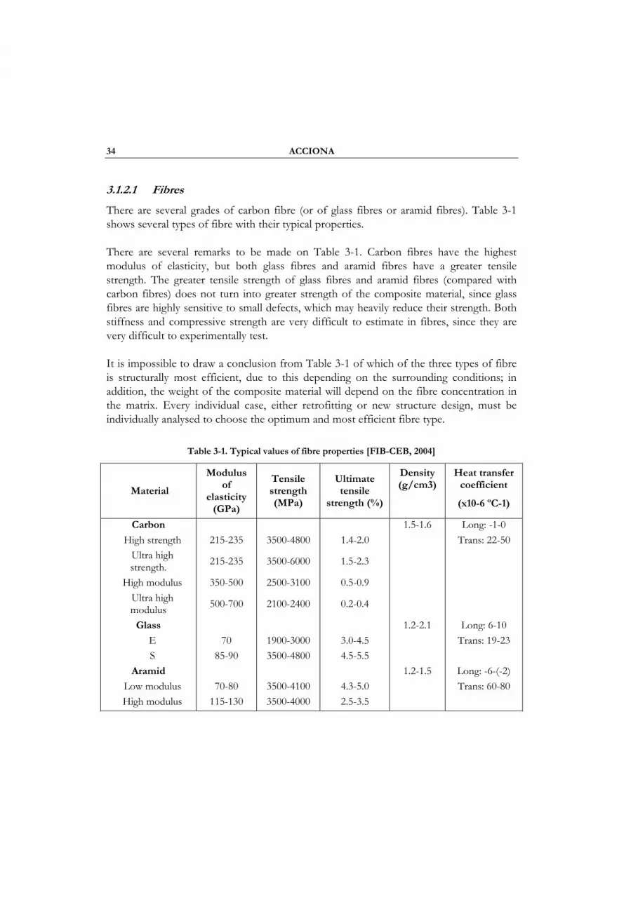
34 ACCIONA
3.1.2.1 Fibres
There are several grades of carbon fibre (or of glass fibres or aramid fibres). Table 3-1 shows several types of fibre with their typical properties.
There are several remarks to be made on Table 3-1. Carbon fibres have the highest modulus of elasticity, but both glass fibres and aramid fibres have a greater tensile strength. The greater tensile strength of glass fibres and aramid fibres (compared with carbon fibres) does not turn into greater strength of the composite material, since glass fibres are highly sensitive to small defects, which may heavily reduce their strength. Both stiffness and compressive strength are very difficult to estimate in fibres, since they are very difficult to experimentally test.
It is impossible to draw a conclusion from Table 3-1 of which of the three types of fibre is structurally most efficient, due to this depending on the surrounding conditions; in addition, the weight of the composite material will depend on the fibre concentration in the matrix. Every individual case, either retrofitting or new structure design, must be individually analysed to choose the optimum and most efficient fibre type.
Table 3-1. Typical values of fibre properties [FIB-CEB, 2004]
Material
Modulus of
elasticity (GPa)
Tensile strength (MPa)
Ultimate tensile
strength (%)
Density (g/cm3)
Heat transfer coefficient
(x10-6 ºC-1)
Carbon 1.5-1.6 Long: -1-0 High strength 215-235 3500-4800 1.4-2.0 Trans: 22-50
Ultra high strength. 215-235 3500-6000 1.5-2.3
High modulus 350-500 2500-3100 0.5-0.9 Ultra high
modulus 500-700 2100-2400 0.2-0.4
Glass 1.2-2.1 Long: 6-10 E 70 1900-3000 3.0-4.5 Trans: 19-23 S 85-90 3500-4800 4.5-5.5
Aramid 1.2-1.5 Long: -6-(-2) Low modulus 70-80 3500-4100 4.3-5.0 Trans: 60-80 High modulus 115-130 3500-4000 2.5-3.5

Sub-Project 7 – 3.1. Guidelines for the application of FRP retrofitting 35
3.1.2.2 Resins
The properties of resins depend on their internal structure. Table 3-2 hereafter shows the properties of some typical resins.
As can be seen by comparing Table 3-1 and Table 3-2, most resins contribute very little to the load capacity of composite materials. In any event, resins may be highly important in the toughness of composite materials; the more ductile the resin is, the more laminate’s toughness will increase. A resin’s function is to transfer a fibre’s load to an adjacent one so that, when a fibre breaks, a ductile resin distributes the force better to several fibres and not only to the adjacent fibre. This means to say that the laminate will resist more broken fibres by increasing the toughness of the composite material
Table 3-2. Typical values of resin properties with different materials [FIB-CEB, 2004]
Property (at 20ºC) Cured epoxy adhesive Concrete Steel
Density (g/cm3) 1100-1700 2350 7800 Modulus of elasticity (GPa) 0.5-20 20-50 205
Shear modulus (GPa) 0.2-8 8-21 80 Poisson ratio 0.3-0.4 0.2 0.3
Tension strength (MPa) 9-30 1-4 200-600 Shear strength (MPa) 10-30 2-5 200-600
Compressive strength (MPa) 55-110 25-150 200-600 Breaking strain (%) 0.5-5 0.015 25
Breaking energy (Jm-2) 200-1000 100 105-106 Coefficient of expansion (x10-6 ºC-1) 25-100 11-13 10-15 Vitreous transition temperature (ºC) 0.1-3 5 0
Water adsorption: 7 days– 25ºC (% w/w) 45-80 - -
3.1.2.3 Lamina and Laminates
A lamina, or ply, is a plane (or curved) layer of unidirectional fibres in a matrix. A laminate is made up of two or more unidirectional laminae or plies stacked together at various orientations. The laminae can be of various thicknesses and consist of different materials.
Most laminates are not single direction but have a variety of orientations in fibres. To illustrate how it affects composite materials, table 5 shows the strengths calculated for a Glass/Polyester laminate with several orientations. The notation used for the type of
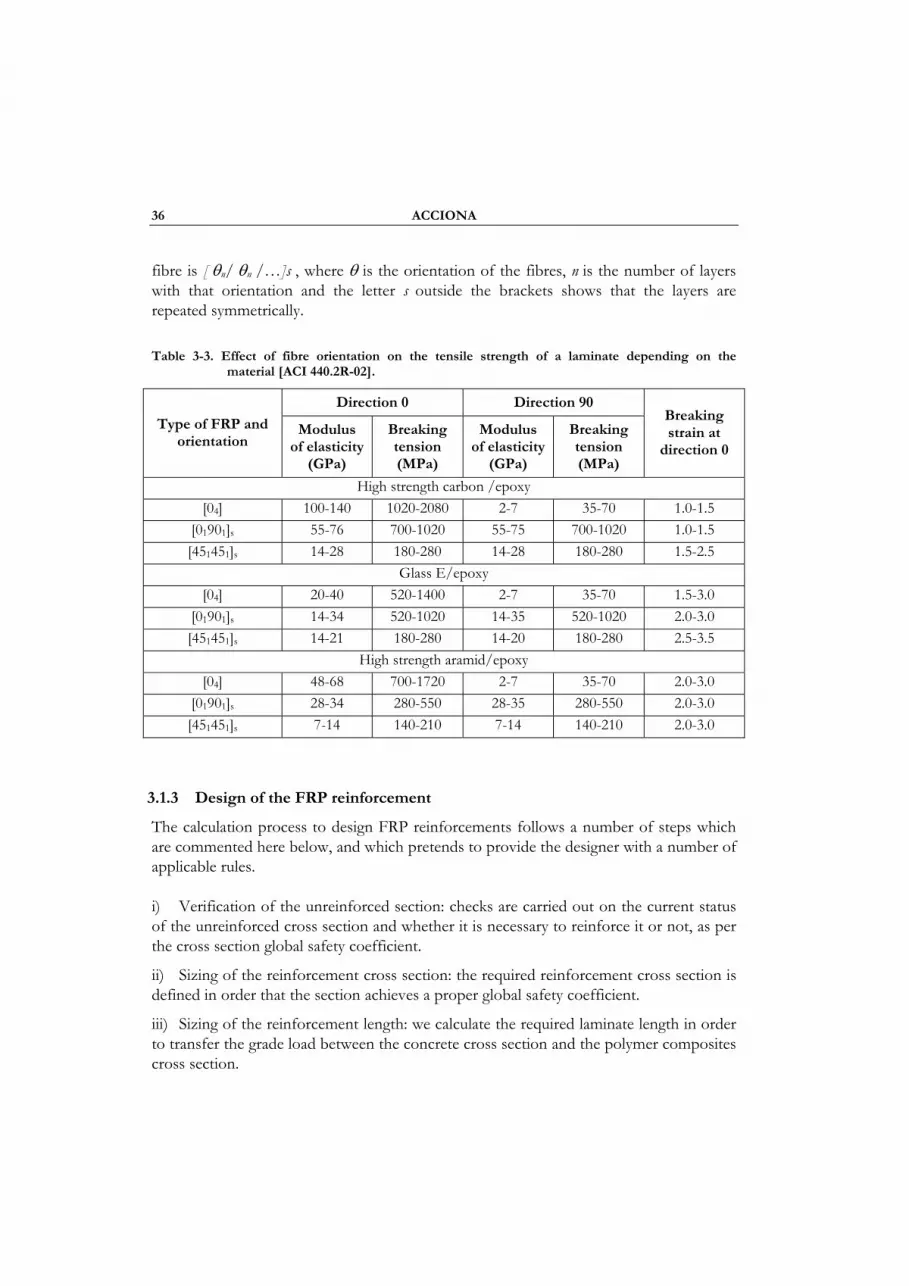
36 ACCIONA
fibre is [ θn/ θn /…]s , where θ is the orientation of the fibres, n is the number of layers with that orientation and the letter s outside the brackets shows that the layers are repeated symmetrically.
Table 3-3. Effect of fibre orientation on the tensile strength of a laminate depending on the material [ACI 440.2R-02].
Direction 0 Direction 90
Type of FRP and orientation
Modulus of elasticity
(GPa)
Breaking tension (MPa)
Modulus of elasticity
(GPa)
Breaking tension (MPa)
Breaking strain at
direction 0
High strength carbon /epoxy[04] 100-140 1020-2080 2-7 35-70 1.0-1.5
[01901]s 55-76 700-1020 55-75 700-1020 1.0-1.5 [451451]s 14-28 180-280 14-28 180-280 1.5-2.5
Glass E/epoxy[04] 20-40 520-1400 2-7 35-70 1.5-3.0
[01901]s 14-34 520-1020 14-35 520-1020 2.0-3.0 [451451]s 14-21 180-280 14-20 180-280 2.5-3.5
High strength aramid/epoxy[04] 48-68 700-1720 2-7 35-70 2.0-3.0
[01901]s 28-34 280-550 28-35 280-550 2.0-3.0 [451451]s 7-14 140-210 7-14 140-210 2.0-3.0
3.1.3 Design of the FRP reinforcement
The calculation process to design FRP reinforcements follows a number of steps which are commented here below, and which pretends to provide the designer with a number of applicable rules.
i) Verification of the unreinforced section: checks are carried out on the current status of the unreinforced cross section and whether it is necessary to reinforce it or not, as per the cross section global safety coefficient.
ii) Sizing of the reinforcement cross section: the required reinforcement cross section is defined in order that the section achieves a proper global safety coefficient.
iii) Sizing of the reinforcement length: we calculate the required laminate length in order to transfer the grade load between the concrete cross section and the polymer composites cross section.
Sub-Project 7 – 3.1. Guidelines for the application of FRP retrofitting 37
Verification of the unreinforced section
To check the unreinforced section of the beam we shall use the ULS theory on the lower part of the unreinforced section. To see if the section is suitable for strengthening, we shall calculate the global safety coefficient (C.G.S.) of the section by means of calculating the depth of the neutral fibre with relation to the upper one and the moment that the section can withstand, as a standard reinforced concrete calculation.
Thus, making use of the safety coefficients of the standard and the resisting moment (Mr), this must be compared with the design moment (Md):
• If Md>Mr : The structure is safe and no strengthening shall be required (C.G.S.>1)
• If Md<Mr : It is necessary to strengthen the structure (C.G.S.<1).
Sizing of the reinforcement cross section
To calculate the size of the strengthening strip we have to insert in the beam lower section we shall use the Ultimate Strength theory of reinforced concrete. We shall assume for all intents and purposes that the strengthening strip placed on the lower part behaves like the reinforcement embedded in the concrete, establishing two possible failure modes:
• Concrete failure
• Strengthening strip failure
The calculation procedure shall be as follows: In both cases, we shall initially calculate the depth of the neutral fibre in the cross section and then the strains in the upper and lower fibres.
If we have assumed that the section undergoes a concrete failure, the strain in the upper fibre shall amount to 3.5 per thousand and the strain in the lower fibre shall be smaller than the strengthening ultimate stress; if we have assumed that a strengthening failure occurs in the section, the strain in the lower fibre shall be the same as the ultimate one in the strengthening and the strain in the upper fibre shall be smaller than the concrete ultimate strain (3.5 per thousand).
Whatever the section failure case, we shall use the following formulation to calculate the depth of the neutral fibre, the fibre strains and finally the section resisting moment.
Consequently, once we have described the general procedure, the sizing procedure is based on the performance of simple iterations, consisting in increasing the thickness of

38 ACCIONA
the strengthening in proportion to the laminate thickness until the calculation moment is greater than the resisting moment, at which time we shall stop the iterations and obtain the required strengthening thickness
3.1.4 Adhesiveness
This section will provide an overview on what a structural adhesive is, the preparation of the surface of the element in needs of reinforcement and the adhesion mechanisms that rule the adhesion process.
3.1.4.1 Structural adhesives
Structural adhesives are used in conjunction with structural materials and operate in such a way as to prevent the joint, or bonding line, from failing when the material is subject to loads of up to its yield strength, while allowing the structure to accommodate its mechanical and physical requirements. In general, these adhesives consist of two polymers, one thermoset (modified or otherwise) and another thermoplastic, including some elastomers.
The border line between structural and non-structural adhesives is not precise, but it is commonly accepted the definition of the structural adhesive being that adhesive which exceeds a tensile load of 10 MPa, at the ambient temperature
The structural systems of the adhesives are variable, each presenting different properties, what makes the choice of the proper adhesive a relevant issue. The following table (Table 3-4) provides a comparison among the most commonly used material-based adhesives.
Table 3-4. Comparative properties of adhesives
STRUCTURAL SYSTEMS – COMPARATIVE ASSESSMENT
SYSTEM ADVANTAGES DISADVANTAGES Epoxy High final bond
Durability Any thickness 2% shrinkage
Surface preparationMix life
Curing cycles Dosing and mixing of components
Polyurethanes Flexibility Better for plastics
Lesser final bond than epoxy Worse for glass and metals
Acrylates Good final bondEase of application
Quick curing Surface preparation
Layer thickness 7% shrinkage
Durability
Sub-Project 7 – 3.1. Guidelines for the application of FRP retrofitting 39
3.1.4.2 Surface preparation
The quality of the bonded union depends both on the quality of the adhesive and on the preparation of the substrata surfaces. The more thorough the cleaning of the surfaces, the greater the saturation of the adhesive, as no grease or dirt is present. When structural bonding is pursued, this cleaning operation is crucial.
However, some metallic materials (due to the presence of rust on the surface) or plastics (due to their apolarity) must be subjected, in addition to the cleaning operation, to a surface treatment.
Generally speaking, these preparations read as follows:
• Mechanical treatment: sanding, steel shot blasting, sandblasting, etc. • Surface chemical treatment (chemical attack). • Miscellaneous treatments: electrical (corona discharge), flaming, priming.
However, the level of cleanliness required before proceeding with a bonding operation depends both on the substrata and on the adhesive used. Thus, some adhesives, such as hotly-applied epoxy-based ones, play a certain dissolving role of the grease that might exist on the substrata surfaces. The same holds true for acrylates cyano-acrylates, which do not contain dissolvents, but their chemical composition is of a dissolvent nature, provided the polluting substance of the substrata does not inhibit curing. Some plastisoles used in the construction industry are directly applied to greased materials, such as steel.
The recommended surface treatment depends upon the surface conditions, which, in turn, is a function of the type of material and of its previous history. As a general rule, the substrata composition is always different from that of the base material.
The simplest of the treatments are based on the cleaning action of dissolvents or abrasives to remove pollution which, otherwise, would prevent the wetting of the base material by the adhesive.
Other treatments have been developed further and tend to increase adhesion by encouraging the process whereby adhesion takes place. That is the case of chemical treatments, which modify the internal structure, from a chemical and physical point of view, to increase the specific adhesion properties. The formation of surface roughness serves to increase the adhesive mechanical adhesion.
40 ACCIONA
Often, the prepared surfaces can be preserved for subsequent use, by covering them with a removable protection layer. Furthermore, it is recommended that the treated substratum is covered with adhesive as soon as possible.
3.1.4.3 Adhesion mechanism
In order to achieve a good bonded union, a free energy reduction must take place when adhesive and substratum come into contact. It shall therefore be necessary for the adhesive to perfectly wet the surface of the material. In this way, we arrive at the interdiffusion of the molecules between the faces of the contact.
Generally speaking, the adhesion can take place in accordance with one or more of the following items:
• Mechanical adhesion: the adhesive enters the pores, inside which it solidifies. Better results are obtained if, on top, surfaces are also rough.
• Electrochemistry: based upon electrostatic phenomena between materials having this type of affinity with the adhesive.
The ideal scenario for a union would be that in which the two types of adhesions take place. This is not always possible with the emergence of a combination of both mechanisms.
It should also be taken into account that, in the case of thin layer structural adhesives, the adhesion forces between adhesive and substrata are greater than the adhesive internal cohesion forces. For this reason, attempts should be made, whenever possible, to look for thin adhesive thicknesses (smaller than 0.2 mm) so that the impact of the former over the latter prevails. In this way, we shall accomplish the transmission of stresses, without cohesive rupture of the adhesive.
There is, however, the case of certain types of adhesives, such as polyurethane-based adhesives which require a given layer thickness (between 3 and 5 mm) to perform its adhesion role. These types of unions lose stiffness and also resistance against the strictly structural ones. However, they are very useful where vibrations, irregularities and noise should be absorbed between faces.
3.1.5 Placing on site
On this section we will summarize the most commonly construction processes for FRP components manufacturing.

Sub-Project 7 – 3.1. Guidelines for the application of FRP retrofitting 41
3.1.5.1 Wet lay-up/Hand lay-up
Resins are impregnated by hand into fibres, which are in the form of woven, knitted, stitched or bonded fabrics. This is usually accomplished by rollers or brushes, with an increasing use of nip-roller type impregnators for forcing resin into the fabrics by means of rotating rollers and a bath of resin. Laminates are left to cure under standard atmospheric conditions.
The main advantage of this method is the facility in use, its wide application along the years and it can be used with most of the fibres.
Its main disadvantages are that the resin mixing, laminate resin contents, and laminate quality are very dependent on the skills of laminators, and it is therefore to count with a team of skilled professionals.
3.1.5.2 Vacuum bagging
Vacuum bagging procedure is an extension of the wet lay-up process described above where pressure is applied to the laminate once laid-up in order to improve its consolidation. This is achieved by sealing a plastic film over the wet laid-up laminate and onto the tool. The air under the bag is extracted by a vacuum pump and thus up to one atmosphere of pressure can be applied to the laminate to consolidate it.
It presents an additional advantage to the above methodology, and it is that higher fibre content laminates can usually be achieved than with standard wet lay-up techniques.
But labour worker must be higher skilled than in the previous process, and it is produced an extra-cost due to the extra-material and equipment required.
The vacuum bagging process is one of the most commonly used processes in the composites industry.
3.1.5.3 Filament winding
This process is primarily used for hollow, generally circular or oval sectioned components, such as pipes and tanks. Fibre tows are passed through a resin bath before being wound onto a mandrel in a variety of orientations, controlled by the fibre feeding mechanism, and rate of rotation of the mandrel.
The main advantages of this method are clear: resin content can be controlled; structural properties of laminates can be very good since straight fibres can be laid in a complex pattern to match the applied loads.

42 ACCIONA
However, it also presents disadvantages, such as the fact that this process is applicable only in convex shaped components, fibre cannot easily be laid exactly along the length of a component and the mandrel cost for large components can be quite high.
3.1.5.4 Prepregs
Fabrics and fibres are pre-impregnated by the materials manufacturer, under heat and pressure or with solvent, with a pre-catalysed resin. The catalyst is largely latent at ambient temperatures giving the materials several weeks, or sometimes months, of useful life when defrosted. However to prolong storage life the materials are stored frozen. The resin is usually a near-solid at ambient temperatures, and so the pre-impregnated materials (prepregs) have a light sticky feel to them, such as that of adhesive tape. Unidirectional materials take fibre direct from a creel, and are held together by the resin alone. The prepregs are laid up by hand or machine onto a mould surface, vacuum bagged and then heated to typically 120-180°C. This allows the resin to initially reflow and eventually to cure. Additional pressure for the moulding is usually provided by an autoclave (effectively a pressurised oven) which can apply up to 5 atmospheres to the laminate.
Main advantages of prepregs are that materials have excellent health and safety characteristics and are clean to work with and fibre cost is minimised in unidirectional tapes since there is no secondary process to convert fibre into fabric prior to use.
Main disadvantages are the cost of the material, which it is usually higher, and that usually autoclaves are required.
3.1.5.5 Resin Film Infusion (RFI)
Dry fabrics are laid up interleaved with layers of semi-solid resin film supplied on a release paper. The lay-up is vacuum bagged to remove air through the dry fabrics, and then heated to allow the resin to first melt and flow into the air-free fabrics, and then after a certain time, to cure.
Main advantages are that high fibre volumes can be accurately achieved with low void contents and good health and safety and a clean lay-up, like prepreg.
Main disadvantages are the fact that this is method is not widely proven outside the aerospace industry and that tooling needs to be able to withstand the process temperatures of the resin film (which if using similar resin to those in low-temperature curing prepregs, is typically 60-100°C).

Sub-Project 7 – 3.1. Guidelines for the application of FRP retrofitting 43
3.1.6 Quality control
Last point on this section deals with the quality control, which not only becomes an important issue, but it can be essential to assure the structural integrity of the designed component or reinforcement.
During the fabrication of the different FRP applications on the projects, a number of control points, to ensure the quality of the methods used, shall have to be considered. These control points are divided into three categories.
• Fabrication procedures of the different structural components. • Workmanship of the unions to the structure. • Testing of the materials used on site to ensure compliance with the design
hypothesis.
3.1.6.1 Check-points during installation
• Materials.
- Compliance with the characteristics required by the project - Quality certificates - Ensure that the handling and delivery of the materials comply with the
recommendations made by both the designer and manufacturer.
• Surface treatment
- Ensure that the concrete surface has been prepared in accordance with the project specifications.
- Check for a regular surface - Always try to obtain rounded corners (with a minimum radius of 3cm
where practicable) - Check that the FRP surface has been properly treated.
• Adhesive
- Determine the right amount of adhesive - Have the different adhesive components been properly mixed - Make sure that the application operations are completed while the
adhesive is workable. The temperature at which the procedure is carried out will have a strong influence.

44 ACCIONA
- See that the adhesive layer thickness is the correct one. - Verify the level of vibration of the structure while the adhesive is curing.
• Plates
- Separation between plate and surface - Plate installation. Check fibre orientation. - Try not to move the plates once they have been bonded to the concrete. - Check for the existence of metallic areas in contact with the carbon fibre
plates.
• Fabrication
- Amount of resin used. Try to comply with the design amounts. - Check that the mixing proportions are the correct ones. - Following compaction, avoid rough or irregular surfaces during site
installation. - Try not to move the materials after the application - Verify the quality of each plate installed before placing the next one.
• Curing
- Verify whether the FRP curing has been properly done
• Tests
- Preparation of specimens in accordance with the specifications
• Inspection
- Assess the best installation method, vacuum, countermold, air drying or other methods.
• Filing of documents
- All the operations shall be documented, or digitally recorded, if deemed necessary for a better understanding of the works performed.

Sub-Project 7 – 3.1. Guidelines for the application of FRP retrofitting 45
3.1.6.2 Site tests
The following table (Table 3-5) describes the possible site tests to be conducted on the materials used on the project in order to check the manufacturer’s specifications, which allow us to assess the feasibility on the on-site element installation.
Table 3-5. Site test specification
Property to be checked Standard Requirements
Young’s modulus in deflection EN ISO 178 > 2000 N/mm2 Young’s modulus in compression EN 13412 > 2000 N/mm2
Shear strength EN 12188 > 12 N/mm2 Maximum overall expansion for any point EN 12617-1
En 12617-3 < 0.1%
Glass transition temperature EN 12614 > 45ºC, or 20ºC above ambient temperature
3.1.6.3 Inspection recommendations
Even though workmanship standards can be very high, there are always factors that are not taken into account, from the workmanship point of view, and that, after some time, they come to the surface.
For this reason, it shall be necessary to set up a number of inspections on the completed work, in order to ascertain that the reinforcements are fulfilling their function and to be able to correct, in time, any eventual problem that might arise.
The ideal inspection frequency could be set up as follows:
Table 3-6. Inspection recommendations
Structure Inspection Detailed Inspection
Bridge Every year Every 6 years, or less Buildings Every year Every 10 years, due to different usage or
structural change Other structures Depending on use Every 10 years or Depending on use
46 ACCIONA
Composite materials, by their very nature, hardly need any maintenance while in operation. Even so, it shall be necessary to conduct a visual inspection to check for cracks, breakages or delaminations that could indicate the level of damage. It shall also be necessary to evaluate eventual damages to the material caused by accidents.
Should the strengthening material have been covered with a protection, this should never be removed. The control, therefore, shall focus on an assessment of the tests conducted on those materials.
In order to prevent future mistakes, checks shall be made on the identification of the materials.
In the event of the covering being of the ultraviolet protection type, said protection shall be monitored in order to control its condition and proceed to their replacement where appropriate. It shall be up to the manufacturer of the materials to determine the best replacement method and its timing.
Detailed inspection
The peeling of the polymer composites fibre from the concrete can be determined either through pressure tests or thermography tests. Nowadays, there are no simple tests that allow us to determine the condition of a joint and its adhesive. The best way to determine this condition is through the pull-off test, when controlling the specimens at regular intervals. However, this requires a number of very frequent tests and a testing period after the execution of the joint.
Another task that has to be performed is the placing of instruments on the bridge to be able to compare the data expected at the beginning to those finally and actually obtained. Should the difference between these data be very great, it shall be necessary to find out why and, on the basis of the results obtained, assess the resisting diagram. Above all, the idea is to try to find out the reason why the model and reality are so different, so that, in this way, eventual similar situations can be assessed in the future.
If during some of the inspections we find out that the condition of the strengthening is not up to expectations, we shall proceed to inject resin or to place reinforcement on top. Should the affected area be a large one, we shall have to remove the FRP and proceed to its reinstatement, always in accordance with all the procedures described so far. In this case, it shall be necessary to install a sufficiently big strengthening to ensure that loads are transferred from the old laminate to the new one we have just laid. The newly installed material should have similar characteristics to those of the old one, particularly with regard to the direction of the fibres, strength, strain and thickness.

Sub-Project 7 – 3.2. Integration of knowledge on FRP retrofitted structures 47
3.2 INTEGRATION OF KNOWLEDGE ON FRP RETROFITTED STRUCTURES
3.2.1 Introduction
The use of carbon fibre reinforced polymers (CFRP) for retrofitting a damaged structure is first reported for the strengthening of the Ibach bridge in 1991, Lucern, Switzerland [Meier, 1995]. Since this first application, the use of this technology has increased exponentially, becoming one of the main applications of composite materials in building and civil engineering. In the case of seismic loads, the improvement provided by CFRP reinforcements in the structural capacity makes them a good solution to increase the ductility of the structure, preventing structural damage in an earthquake situation.
Most of the existing knowledge about structural reinforcement and/or retrofitting of reinforced concrete (RC) structures with fibre reinforced polymers (FRP) is based on experimental simulations, supported and complemented by analytical calculations; and, when the problem is treated using a numerical approach, material nonlinearities are usually linearized and the FRP composite is considered as a single material (i.e. [Rabinovitch and Frostig, 2001]).
On the other hand, the study of composite materials has been one of the major objectives of computational mechanics in the last decade. The numerical simulation of composite materials has been done, traditionally, using orthotropic materials with average properties of their constituents. With this approximation, no model has been found able to work beyond the constituents elastic limit state. Thus, these procedures limit the numerical computation to elastic cases. Different theories have been proposed to solve this problem, taking into account the internal configuration of the composite to predict its behaviour. The two most commonly used are herein remarked.
i) Homogenization theory: This method deals with the global problem of composite material in a two-scale context. The macroscopic scale uses the composite materials to obtain the global response of the structure; composites are treated as homogeneous materials in this scale. The microscopic scale corresponds to an elemental characteristic volume in which the microscopic fields inside the composite are obtained; this scale deals with the component materials. Homogenization theory assumes a periodical configuration of the composite material to relate these two scales [Sanchez-Palencia, 1987; Oller et al., 2005].
ii) Mixing theory: The first formulation of the mixing theory corresponds to Trusdell and Toupín [Trusdell and Toupín, 1960] and it is based in two main hypothesis: 1. All composite constituents have the same strains. 2. Each constituent collaborates to the composite behaviour according to its volumetric participation. The main problem of the mixing theory is the iso-strain condition, which forces a parallel distribution of the
48 CIMNE
constituents in the composite. Some improvements to the original formulation can be found in [Car et al., 2000].
Despite of all existing studies on both subjects, experimental tests of FRP reinforcements and numerical characterization of composite materials, few researches are found in which the structural reinforcement of RC structures using FRP is approached using a numerical point of view. Thus, the main goal of this work is to join both fields, developing a numerical procedure able to compute RC structures reinforced with FRP. The developed formulation based on the finite element method that allows obtaining the structural performance of existing structures when they are reinforced and/or retrofitted with FRP. This structural behaviour is obtained taking into account the material non-linearities. The code also provides the performance of each constituent material in the structure (for example, it is possible to know the stress state of the composite reinforcement when the structure collapses). The code can be used to study the same structure using different FRP configurations, in order to obtain the most suitable for the case considered. It also allows to apply the reinforcement to already damaged structures, reproducing with more accuracy the conditions found in real applications.
In next section, the numerical procedures used to simulate RC structures with carbon fibre reinforced polymers (CFRP) reinforcements are described briefly. Afterwards some simulation examples are exposed, these examples show the validity of the formulation proposed as well as the improvement obtained in the structural capacity when it is reinforced with CFRP. Finally, some conclusions are exposed.
3.2.2 Formulation used to simulate RC structures reinforced and/or retrofitted with CFRP
3.2.2.1 Simulation of Composite Materials
The structural problem of RC structures reinforced with carbon fibre reinforced polymers is solved with PLCd [PLCd, 1991]. This is a finite element code, developed at CIMNE (International Center for Numerical Methods in Engineering) and UPC (Politechnical Univeristy of Catalonia), that works with two and three dimensional solid geometries. It can deal with kinematics and material nonlinearities. It contains various constitutive laws to predict the material behaviour: Von-Mises, Mohr-Coulomb, improved Mohr-Coulomb, Drucker-Prager, etc. [Malvern, 1968; Lubliner et al., 1989]. It uses different integration algorithms to simulate the material: Elastic, visco-elastic, damage, damage-plasticity, etc. [Oller et al., 1990]. Dynamic analysis are developed using the Newmark method, [Barbat et al., 1997].

Sub-Project 7 – 3.2. Integration of knowledge on FRP retrofitted structures 49
To deal with composite materials, of the two main existing theories that take into account composites internal configuration: homogenization and the mixing theory, the one used and presented in this project is based in the last one. The election of the mixing theory instead of a homogenization theory is based in the final aim of the code developed, compute real structures reinforced and or retrofitted with CFRP. A homogenization theory requires a micro-model for each point of the structure that becomes non-linear. The resolution of a real structure with this procedure generates such a big amount of degrees of freedom that the calculation is beyond the computation capabilities of nowadays personal computers or small servers. On the other hand, the mixing theory does not increase the degrees of freedom of the problem, as it is only present in the constitutive section of the finite element code.
a. Classical mixing theory
The classical rule of mixtures was originally developed by Trusdell and Toupin [1960]. It considers that the interaction between the components in a material point of the composite is done according to the following hypothesis: (i) each infinitesimal volume of the composite contains a finite number of material components; (ii) each component contribution to the global behaviour of the composite is proportional to its volumetric participation; (iii) all components suffer the same strains (closing equation); (iv) the volume of each component is significantly smaller than the composite volume.
The third hypothesis, in the case of small strains, can be written as:
1 2c nij ij ij ijε ε ε ε= = = =… (3.2.1)
Where, cijε is the strain tensor for the composite and k
ijε is the strain tensor for component k of the composite. According to second hypothesis, the stresses of the composite can be computed as the proportional (according to the volumetric participation) addition of each component stresses, thus:
1, 1, 1,
k k k k S k k k S cij ij ijkl ij ijkl ij
k n k n k nk k C k Cσ σ ε ε
= = =
= ⋅ = ⋅ ⋅ = ⋅ ⋅∑ ∑ ∑ (3.2.2)
where parameter kk is the volumetric participation of component k in the composite, defined as:
0
k kdVkdV
= (3.2.3)

50 CIMNE
A more detailed explanation of this theory, as well as the extension to the large deformations case and its numerical implementation can be found in [Car, 2000]
b. Serial/Parallel mixing theory
The main problem of the classical mixing theory is the iso-strain condition, which forces a parallel distribution of the constituents in the composite (Figure 3-1, iso-strain case). The serial/parallel rule of mixtures (SP RoM) improves the classical mixing theory replacing the iso-strain hypothesis for an iso-strain condition in the fibre direction and an iso-stress condition in the transversal directions, allowing to simulate all components distribution in the composite shown in Figure 3-1. This theory has been developed by Rastellini and an extensive description of it can be found in [Rastellini, 2006] and in the Deliverable 49 of the LESSLOSS project ( www.lessloss.org ).
Iso-strain Iso-stress Mixed caseIso-strain Iso-stress Mixed case Figure 3-1. Different distribution of components in a composite material
The main hypothesis in which is based the numerical model of the Serial/Parallel mixing theory are:
i) Composite is composed by two component materials: fibre and matrix
ii) Component materials have the same strain in parallel (fibre) direction
iii) Component materials have the same stress in serial direction
iv) Composite material response is in direct relation with the volume fractions of compounding materials
v) Homogeneous distribution of phases is considered in the composite
vi) Perfect bounding between components is also considered
The equations that define the stress equilibrium and establish the strain compatibility between components arise form the analysis of the model hypothesis. Thus,
Parallel behaviour: c m fP P P
c m m f fP P Pk k
ε ε ε
σ σ σ
= =
= + (3.2.4)
Sub-Project 7 – 3.2. Integration of knowledge on FRP retrofitted structures 51
Serial behaviour: c m m f fS S S
c m fS S S
k kε ε ε
σ σ σ
= +
= = (3.2.5)
where, Pε and Sε are the parallel and serial components of the stress tensor respectively, Pσ and Sσ are the parallel and serial components of the strain, the superscripts c , m
and f represent the composite, matrix and fibre materials and mk and f k is the volumetric participation of fibre and matrix in the composite.
In order to verify the compatibility equations, the Serial/Parallel mixing theory proceeds in the following way.
1. First thing to be done is to split the component strain tensor into its serial and parallel parts.
2. Afterwards, a first prediction of the matrix serial strains is computed. With this initial prediction and the strain relation of equation (3.2.3), the fibre serial strains can be also obtained.
3. Using each constituent constitutive law, the stresses for matrix and fibre can be calculated, as well as the actualization of each material internal variable.
4. The stress tensors computed in step 3 are split into their serial and parallel parts and the iso-stress condition defined in equation (3.2.3) is checked. If it is verified, the matrix strain prediction was correct and the composite stress can be obtained using equations (3.2.2) and (3.2.3). If the iso-stress condition is not verified, the initial strain prediction must be corrected and the process must continue in step 3.
The main problem of the Serial/Parallel mixing theory is that the composite material can be composed, only, by two material components. However, this inconvenient is solved with the laminate procedure exposed in the following section.
c. Laminate Composites
Usually fibre reinforced polymers are composed by different layers with different fibre orientations. The orientation of the fibre can be defined by the engineer in order to obtain the better performance of the composite according to its application. In example, if the CFRP application is a flexural reinforcement, fibres will be disposed in the beam axis direction while, if the CFRP is applied as a column wrapping, fibres will be oriented in the cross section plane, following the column perimeter.
Under this scope, the limitation of the Serial/Parallel mixing theory (SP RoM) to only two materials is not such, as the composites used are usually defined by multiple layers composed by only two components: fibre and matrix. Thus, the SP RoM formulation can

52 CIMNE
be applied to each layer of the composite and, afterwards, compute the composite behaviour composing the performance of each constituent layer. To obtain the laminate behaviour, the classical mixing theory is applied to each lamina.
Applying the classical mixing theory to the different layers of the composite implies the assumption that all laminas of the laminate are under the same strain conditions. This assumption can be considered correct, as the different laminas usually have fibre orientation distributions disposed in such a way that provide the laminate with an in-plane homogeneous stiffness.
At this point, it must be said that not all the layers have to behave according to the S/P RoM hypothesis. Sometimes, between fibre oriented layers, a randomly oriented one is disposed. Having random oriented fibres, the layer behaves as an isotropic material and the best theory to be applied to predict its behaviour is the Classical mixing theory. Thus, the composite performance is obtained according to the following procedure:
1. For a given strain of the composite, the strain of each composite layer is obtained applying the Classical mixing theory.
1 2c L L Lnε ε ε ε= = = =… (3.2.6)
2. Each layer stress is obtained using the Serial/Parallel mixing theory in case of fibre oriented layers or the Classical Mixing theory in case of randomly oriented layers (or in other cases of iso-strain behaviour such as single materials layers).
Lk Lkε σ→ ; using Classic mixing theory or SP RoM (3.2.7)
3. The stresses of the composite are obtained composing the stresses obtained in each composite layer.
1
nc Lj Lj
j
kσ σ=
= ∑ (3.2.8)
3.2.2.2 Other Formulations Developed to Simulate CFRP Reinforcements
Having defined the main formulation frame, in which the code works and deals with composite materials, there are other formulations in it that are used to obtain a better performance of the finite element code and that are required to obtain a better approximation of the mechanical behaviour of the RC structures reinforced with CFRP. In this chapter, all of them are briefly described.

Sub-Project 7 – 3.2. Integration of knowledge on FRP retrofitted structures 53
a. Two dimensional and three dimensional elements
The original version of PLCd only dealt with two dimensional problems. Due to the complexity of some geometries required to study CFRP reinforcements, one of the required implementations was to extend all formulations included in PLCd to the three dimensional case. The way in which a finite element code deals with two dimensional and three dimensional cases can be studied in detail in [Oñate, 1995; Zienkiewicz and Taylor, 1991]
b. Anisotropy using a mapping space theory
This theory is based on the transport of all the constitutive parameters and the stress and strain states of the structure, from a real anisotropic space, to a fictitious isotropic space. Once all variables are in the fictitious isotropic space, an isotropic constitutive model can be used to obtain the new structure configuration. This theory allows considering materials with high anisotropy, such as composite materials, using all the techniques and procedures already developed for isotropic materials.
All the anisotropy information is contained in two fourth order tensors. One of them, ijklAσ , relates the stresses in the fictitious isotropic space ( ijσ ) with the stresses in
the real anisotropic space ( ijσ ) and the other one, ijklAε , does the same with the strains. The relation of both spaces for the strains and the stresses is exposed in equations (3.2.9).
:
:ij ijkl ij
ij ijkl ij
A
A
σ
ε
σ σ
ε ε
=
= (3.2.9)
A more detailed description of this methodology, the extension to large strains and its numerical implementation can be obtained in [Car et al., 2001 and Car, 2000]
c. Fibre-matrix debonding
The apparition of matrix cracks in a composite material is usually followed by a relative movement between the fibres and the matrix. This lost of adherence implies a stiffness reduction in the composite material. This phenomenon is introduced in the elastic limit of the material as a modification of its yield surface criterion. The new fibre elastic limit becomes:
[ ] fibmatfibN
matN
fibN
fibR rffff /)(2;)(;)(min)( −⋅= (3.2.10)
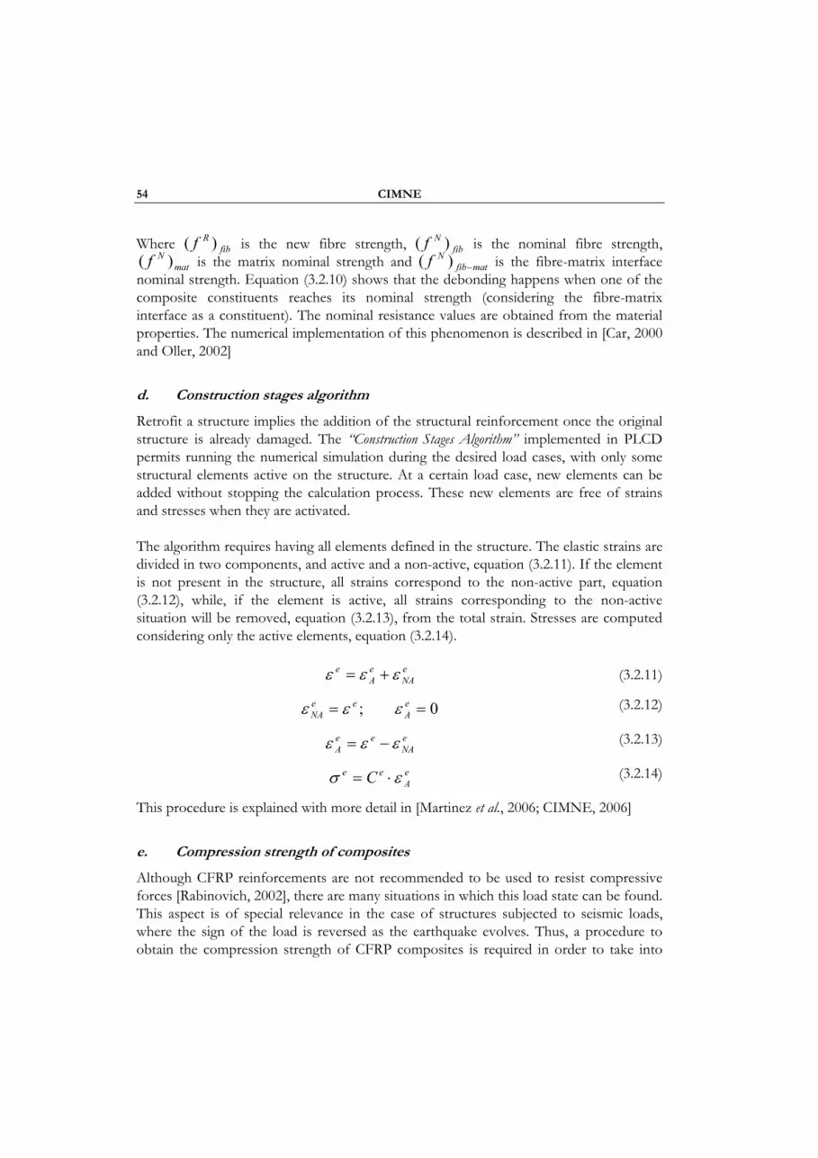
54 CIMNE
Where fibRf )( is the new fibre strength, fib
Nf )( is the nominal fibre strength, mat
Nf )( is the matrix nominal strength and matfibNf −)( is the fibre-matrix interface
nominal strength. Equation (3.2.10) shows that the debonding happens when one of the composite constituents reaches its nominal strength (considering the fibre-matrix interface as a constituent). The nominal resistance values are obtained from the material properties. The numerical implementation of this phenomenon is described in [Car, 2000 and Oller, 2002]
d. Construction stages algorithm
Retrofit a structure implies the addition of the structural reinforcement once the original structure is already damaged. The “Construction Stages Algorithm” implemented in PLCD permits running the numerical simulation during the desired load cases, with only some structural elements active on the structure. At a certain load case, new elements can be added without stopping the calculation process. These new elements are free of strains and stresses when they are activated.
The algorithm requires having all elements defined in the structure. The elastic strains are divided in two components, and active and a non-active, equation (3.2.11). If the element is not present in the structure, all strains correspond to the non-active part, equation (3.2.12), while, if the element is active, all strains corresponding to the non-active situation will be removed, equation (3.2.13), from the total strain. Stresses are computed considering only the active elements, equation (3.2.14).
eNA
eA
e εεε += (3.2.11)
0; == eA
eeNA εεε (3.2.12)
eNA
eeA εεε −= (3.2.13)
eA
ee C εσ ⋅= (3.2.14)
This procedure is explained with more detail in [Martinez et al., 2006; CIMNE, 2006]
e. Compression strength of composites
Although CFRP reinforcements are not recommended to be used to resist compressive forces [Rabinovich, 2002], there are many situations in which this load state can be found. This aspect is of special relevance in the case of structures subjected to seismic loads, where the sign of the load is reversed as the earthquake evolves. Thus, a procedure to obtain the compression strength of CFRP composites is required in order to take into
Sub-Project 7 – 3.2. Integration of knowledge on FRP retrofitted structures 55
account this sort of situations. The main failure cause of compressed CFRP is the fibre buckling phenomenon. Fibres are very slender elements and their second order effects are avoided by the matrix elastic restrain. However, as damage in matrix evolves, fibre restrain becomes weaker and fibre buckling occurs.
In all existing bibliography, the fibre buckling problem is solved by using different methodologies to obtain a general expression for the composite limit compression stress. This expression is only valid for the composite material and is obtained taking into account different characteristics of the composite components. Alternatively, in the present work, the composite material is modelled using the S/P rule of mixtures. Thus, the fibre buckling problem must be solved in terms of the composite components, considering their interaction, and not in terms of the composite by itself.
The interaction between fibres and matrix appears when the composite is compressed: matrix restrain fibres avoiding their transversal movement. Under this approach, matrix can be considered as an elastic restriction of fibres, and the fibre-matrix system can be represented as it is shown in Figure 3-2. In this figure the movement of the fibres in case of compression has been represented in dashed lines. Fibre behaviour is analogous to the response that is obtained in a curved bar under unilateral restrain. This analogy is used to formulate the fibre buckling problem. A detailed explanation of the formulation related to this problem can be found in [Martinez et al., 2007]
Figure 3-2. Fibre-matrix system. Fibre behaviour when the composite is compressed
3.2.2.3 Efficiency Improvement of the Developed Code
Beside the different formulations included in PLCd code to deal with the CFRP reinforcement of RC structures, it is necessary to pay special attention to the code performance in order to improve its computation efficiency. The finite element simulation of a complete structure requires a large number of elements, which requires a lot of memory and computing time. Hence, all effort put in obtain a more efficient code will be recovered when the simulations are performed. Two different code improvements have been developed in this field
56 CIMNE
a. Tangent constitutive stiffness tensor
Depending on the constitutive equation used in a composite constituent material, the tangent constitutive tensor cannot be obtained analytically. One solution is to use, in this material, the initial stiffness matrix, which will lead to the equilibrium state but will require a large amount of structural iterations. Thus, in order to obtain a fast and reliable algorithm, the expression of the tangent constitutive tensor is required. To obtain it, when no analytical expression exists, a numerical derivation using a perturbation method is performed. According to Crisfield [Crisfield, 91], the definition of the tangent constitutive tensor is:
:tσ ε= C (3.2.15)
where,
[ ] [ ]1 2 1 2
11 1
1
; andn n
t tn
t
t tn nn
c c
c c
σ σ σ σ ε ε ε ε= =
⎡ ⎤⎢ ⎥= ⎢ ⎥⎢ ⎥⎣ ⎦
… …
…
…C
(3.2.16)
The definition of the tangent constitutive tensor, equation (3.2.15), shows that the variation of stresses due to an increment in the value of the j element of ε depends on the values of the j column of tC . Thus, writing the j column of tC as,
1 2
Tt t t tj j j njc c c⎡ ⎤= ⎣ ⎦c … (3.2.17)
the stress variation is:
j tj jσ ε= ⋅c (3.2.18)
being tjc the unknown
The perturbation method consists of applying a small perturbation to the strain vector and, using the constitutive equation of the material, determines the variation that will be obtained in the stress tensor due to this perturbation. At this point, the j column of the tangent constitutive tensor can be computed as:
jtj
j
σε
=c (3.2.19)

Sub-Project 7 – 3.2. Integration of knowledge on FRP retrofitted structures 57
The smaller the value applied to the perturbation, the better the approximation obtained for the tangent constitutive tensor. Having defined a perturbation value, jε , the perturbed stress is computed using the constitutive equation of the material applying the following input strain:
1 ˆT
j j nε ε ε ε ε σ⎡ ⎤= + →⎣ ⎦… … (3.2.20)
And the stress variation due to the perturbation is obtained subtracting the original converged stress from the computed one:
j ˆσ σ σ= − (3.2.21)
This procedure must be repeated for all strain components in order to obtain the complete expression of the tangent constitutive tensor. Hence, the numerical cost of using a perturbation method is rather high. However, this procedure allows obtaining an accurate approximation to this tensor for any constitutive equation used, ensuring the convergence of the numerical process in few steps.
b. Improvement of the database system
One of the main advantages of the mixing theory compared to a homogenization theory is that the computational cost is much lower, as the number of degrees of freedom of the problem is not modified by taking into account the composite components. However, taking into account all composite components increase significantly the amount of information that has to be stored for each gauss point.
The information stored, in a finite element code, for each gauss point are the strains, the stresses and the internal variables. If the strain and stress tensors have dimension n and the number of state variables is m, the amount of memory required for each gauss point if only one material is considered in it is: 2n+m real values.
If now, instead of having one single material, the material defined in the gauss point is a composite made by three different layers, and each layer containing two different components, it will be required to save for each layer the strains and stresses and for each component of each layer the strains, stresses and internal variables. This leads to:
3 layers require 3 x (2n) real values = 6n real values
Each layer has two components, each one requiring 2n+m real values
= 3 x (2 x (2n+m)) = 12n + 6m real values
Thus, in total, the amount of real values required for the gauss point is: 18n + 6m
58 CIMNE
This example shows how, with only a three layer composite, the amount of variables that must be stored increase nearly by nine, which increases nearly by nine the amount of memory required to solve the problem.
Being aware of this problem, an optimization of the variables stored by PLDCd code has been performed. PLCd was first developed as a finite element code to compute small structures made of just one material. Thus, the code was not optimized and a lot of useless variables were stored for each gauss point. All these variables have been removed. It have also been removed all variables that, being previously stored, can be computed again when necessary. With these two main measures, the code requirement of memory has been reduced nearly a 70 % in the case of the concrete frame that will be shown in section 3.2.3.3 of present document.
3.2.2.4 Making the Code More User Friendly
a. Pre and post processing using GiD
When solving the structural problem of a RC structure reinforced with CFRP, the amount of information required by the finite element code PLCd is large and complex to define. In the case of the three dimensional framed structure that is exposed in section 3.2.3.3, the input data file has more than 6500 lines. In these cases, is necessary to have a friendly environment to define the input data file.
GiD [GiD, 2007] is a pre and post processor, developed at CIMNE, which can be customized to interact with any existing finite element code. This customization includes two main features, one corresponds to the data that can be defined over the structure and the second one is the writing of the input data file in a format able to be recognized by the finite element code. Both features have been included in the PLCd problem type definition, which allows defining completely the input data file to be used by PLCd code using GiD.
Following figures show some screen captures obtained during the definition of the concrete frame used to obtain the CFRP reinforcement behaviour in a push-over analysis (section 3.2.3.3 of the present document).
Another improvement related to the interaction of PLCd with GiD corresponds to the ouput result file. Initially, PLCd exported each composite material in a layer and each component material was exported in a different layer inside the first layer. This is, if two elements had different composite materials (comp1 and comp2, in example), and both composites have, as a constituent material, polymeric matrix, matrix results of composite comp1 will be stored in the layer mat-comp1 and matrix results of comp2 will be stored in

Sub-Project 7 – 3.2. Integration of knowledge on FRP retrofitted structures 59
mat-comp2. Hence, to see the stresses in matrix materials, different layers must be activated and the results cannot be seen at once.
This way of storing the results has been changed and now all simple materials are stored in the same layer. Doing so it is possible to see the stresses of all matrix material at once, being easier to have a global comprehension of the material behaviour of the structure using the graphical interface provided by GiD. Also, this way of storing results reduces significantly the dimension of the output file.
Figure 3-3. Assignation, to the different volumes composing the concrete frame to be modelled, of
the different composite materials and construction stages

60 CIMNE
Figure 3-4. Definition of the different composite materials existing on the structure by the number
material constituents and their volumetric participation. Beneath can be seen some material data defined for the simple materials.
b. Creation of an ANSYS usermat with the mixing theory
The commercial finite element code ANSYS [ANSYS, Inc, 2007] allows the user definition of material constitutive equations or, as are called by the code, usermats. With this option, ANSYS code becomes more versatile, as it can be customized for some particular applications. With the aim of increase the applicability of the formulation developed to deal with RC structures reinforced with CFRP, a usermat containing the lamination formulation using the rule of mixtures (both, the Classical and the Serial/Parallel) has been programmed.
ANSYS usermat is called when the code is at the gauss point level. The subroutine receives the strains of the gauss point and has to return to the main code the stresses of the gauss point, the tangent constitutive tensor and the internal variables actualized to the new configuration [ANSYS, Inc, 2005].
This application has been already developed and, at this stage of the project, is being tested in order to assure the correct behaviour of the material definition in all possible situations related with composite materials and, more precisely, with the reinforcement of structures using carbon fibre reinforced polymers (CFRP).

Sub-Project 7 – 3.2. Integration of knowledge on FRP retrofitted structures 61
3.2.3 Numerical examples of the formulation proposed. CFRP reinforcements of RC structures
3.2.3.1 Code Validation: Bending Reinforcement of a RC Beam
In this section, a numerical simulation of a bending reinforced beam is presented and used to validate all the formulations proposed and exposed in previous section. This case shows the efficiency of the serial/parallel rule of mixtures to deal with this sort of structural problems, as it is able to reproduce the complex mechanical behaviour found in the beam with an acceptable computational cost. The numerical results are validated with experimental values. The studied beam is defined in the paper by Spadea [Spadea et al. 1998]. Its geometry and the reinforcements applied to it are shown in Figure 3-5.
Figure 3-5. Geometry and reinforcement of the beam studied
The red (thick) line displayed in the bottom of the beam corresponds to the FRP reinforcement. This is made of carbon fibres embedded in a polymeric matrix. The content of fibres is 60 % and the composite thickness is 1.2 mm. The finite element model developed to simulate the beam reinforcement is shown in Figure 3-6. This is a 3D finite element made with linear hexahedrons.
The usage of the S/P rule of mixtures allows considering all the reinforcement details found in the beam using a coarse mesh. In Figure 3-6 it is also included the composite materials composition. As can be seen, a single finite element contains, in this particular case, up to three different component materials. The steel reinforcements are considered as fibres, whose orientation is defined by the bar direction. The FRP reinforcement has been included adding new finite elements to reproduce with more accuracy its position in the beam.

62 CIMNE
MAT-01: Concrete (100 %) MAT-02: Concrete (57 %) Longitudinal Steel (42 %) Vertical Steel (1 %) MAT-03: Concrete (99 %) Vertical Steel (1 %) MAT-04: Concrete (98 %) Vertical Steel (1 %) Horizontal Steel (1 %) MAT-05: Concrete (99 %) Horizontal Steel (1 %) MAT-06: Polymeric Matrix (34 %) Long.Carbon Fibr. (66%)
Figure 3-6. Finite element model developed to realize the numerical simulation
The results obtained with this simulation are compared with the experimental results reported by Spadea [Spadea et al., 1998]. Figure 3-7 shows the capacity curve of the beam for the numerical and the experimental simulations. This is, vertical displacement of the beam, in the point where the force is applied, against the load value. This figure demonstrates the agreement between numerical and experimental results, which proves the ability of the method to perform this sort of simulations. Figure 3-7 also includes the results obtained with a numerical simulation of the same beam without FRP reinforcements. The comparison between the results obtained for the reinforced and for the non-reinforced beam shows the improvement obtained in the beam performance when it is reinforced with FRP.
Figure 3-7. Force-displacement graph comparing the experimental and the numerical results
One of the main advantages of the proposed finite element formulation is that it allows obtaining the structural behaviour of all its components, their failure causes, their strain-stress state, etc. In Figure 3-8 some results maps, corresponding to the final computed step, are represented. These show the most relevant information obtained from the numerical simulation. Figure 3-8a displays the plastic damage in concrete, which shows
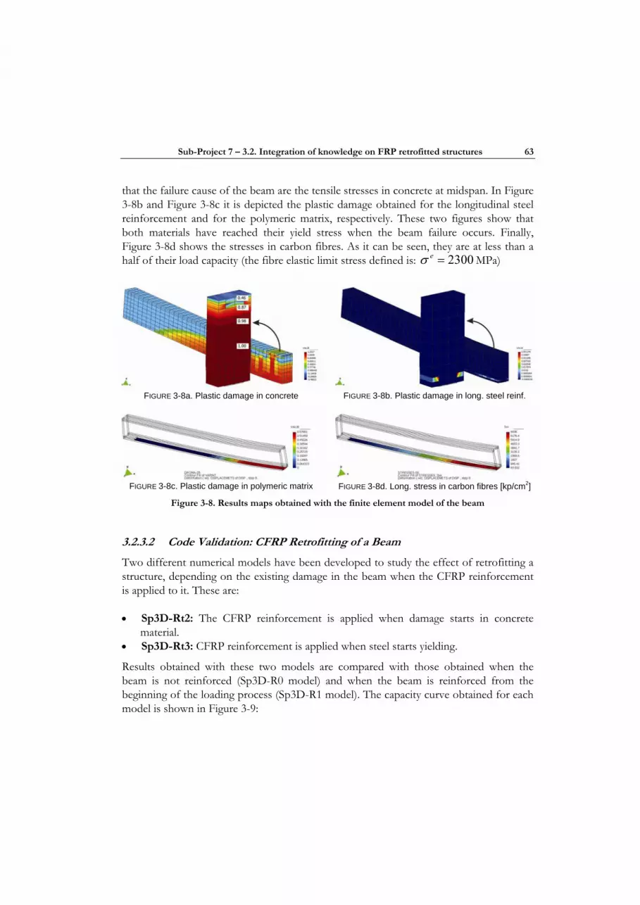
Sub-Project 7 – 3.2. Integration of knowledge on FRP retrofitted structures 63
that the failure cause of the beam are the tensile stresses in concrete at midspan. In Figure 3-8b and Figure 3-8c it is depicted the plastic damage obtained for the longitudinal steel reinforcement and for the polymeric matrix, respectively. These two figures show that both materials have reached their yield stress when the beam failure occurs. Finally, Figure 3-8d shows the stresses in carbon fibres. As it can be seen, they are at less than a half of their load capacity (the fibre elastic limit stress defined is: 2300eσ = MPa)
FIGURE 3-8a. Plastic damage in concrete
FIGURE 3-8b. Plastic damage in long. steel reinf.
FIGURE 3-8c. Plastic damage in polymeric matrix
FIGURE 3-8d. Long. stress in carbon fibres [kp/cm2]
Figure 3-8. Results maps obtained with the finite element model of the beam
3.2.3.2 Code Validation: CFRP Retrofitting of a Beam
Two different numerical models have been developed to study the effect of retrofitting a structure, depending on the existing damage in the beam when the CFRP reinforcement is applied to it. These are:
• Sp3D-Rt2: The CFRP reinforcement is applied when damage starts in concrete material.
• Sp3D-Rt3: CFRP reinforcement is applied when steel starts yielding.
Results obtained with these two models are compared with those obtained when the beam is not reinforced (Sp3D-R0 model) and when the beam is reinforced from the beginning of the loading process (Sp3D-R1 model). The capacity curve obtained for each model is shown in Figure 3-9:
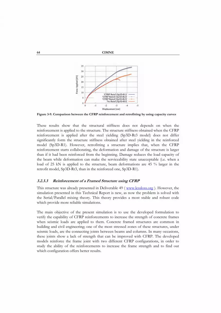
64 CIMNE
Figure 3-9. Comparison between the CFRP reinforcement and retrofitting by using capacity curves
These results show that the structural stiffness does not depends on when the reinforcement is applied to the structure. The structure stiffness obtained when the CFRP reinforcement is applied after the steel yielding (Sp3D-Rt3 model) does not differ significantly form the structure stiffness obtained after steel yielding in the reinforced model (Sp3D-R1). However, retrofitting a structure implies that, when the CFRP reinforcement starts collaborating, the deformation and damage of the structure is larger than if it had been reinforced from the beginning. Damage reduces the load capacity of the beam while deformation can make the serviceability state unacceptable (i.e. when a load of 25 kN is applied to the structure, beam deformations are 45 % larger in the retrofit model, Sp3D-Rt3, than in the reinforced one, Sp3D-R1).
3.2.3.3 Reinforcement of a Framed Structure using CFRP
This structure was already presented in Deliverable 49 ( www.lessloss.org ). However, the simulation presented in this Technical Report is new, as now the problem is solved with the Serial/Parallel mixing theory. This theory provides a most stable and robust code which provide more reliable simulations.
The main objective of the present simulation is to use the developed formulation to verify the capability of CFRP reinforcements to increase the strength of concrete frames when seismic loads are applied to them. Concrete framed structures are common in building and civil engineering; one of the most stressed zones of these structures, under seismic loads, are the connecting joints between beams and columns. In many occasions, these joints show a lack of strength that can be improved with CFRP. The developed models reinforce the frame joint with two different CFRP configurations, in order to study the ability of the reinforcements to increase the frame strength and to find out which configuration offers better results.
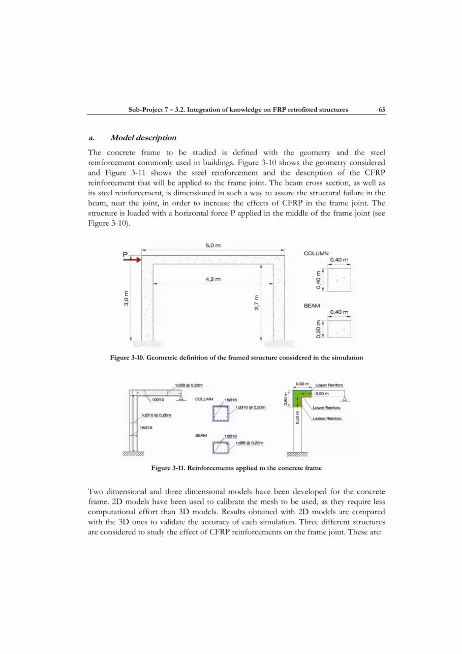
Sub-Project 7 – 3.2. Integration of knowledge on FRP retrofitted structures 65
a. Model description
The concrete frame to be studied is defined with the geometry and the steel reinforcement commonly used in buildings. Figure 3-10 shows the geometry considered and Figure 3-11 shows the steel reinforcement and the description of the CFRP reinforcement that will be applied to the frame joint. The beam cross section, as well as its steel reinforcement, is dimensioned in such a way to assure the structural failure in the beam, near the joint, in order to increase the effects of CFRP in the frame joint. The structure is loaded with a horizontal force P applied in the middle of the frame joint (see Figure 3-10).
Figure 3-10. Geometric definition of the framed structure considered in the simulation
Figure 3-11. Reinforcements applied to the concrete frame
Two dimensional and three dimensional models have been developed for the concrete frame. 2D models have been used to calibrate the mesh to be used, as they require less computational effort than 3D models. Results obtained with 2D models are compared with the 3D ones to validate the accuracy of each simulation. Three different structures are considered to study the effect of CFRP reinforcements on the frame joint. These are:

66 CIMNE
2D-noR and 3D-noR: Two and three dimension concrete frame without CFRP reinforcements
2D-R and 3D-R: Two and three dimension concrete frame with the upper and lower CFRP reinforcements defined in Figure 3-11
2D-LR and 3D-LR: Two and three dimension concrete frame with the upper, lower and lateral CFRP reinforcements
All composite materials existing in the concrete frame are defined by combination of four different basic materials, which are defined in Table 3-7. CFRP reinforcement is 1.2 mm thick and is composed of 66 % of carbon fibres and 34 % of polymeric matrix. In the case of the upper and lower reinforcements, the fibres are oriented following the structure longitudinal axis. In lateral reinforcements, two layers of CFRP are applied to the frame, in which the fibres are oriented at +0º and +90º respect the horizontal.
Table 3-7. Mechanical characteristics of the constituent materials used to define the composite materials existing in the framed structure.
Yield Stres[MPa] Fracture Energy [kPa·m]
Material Yield criterion
Young Modulus [ MPa ]
Poisson Modulus
Compr. Tensile Compr. Tensile
Concrete Mohr-
Coulomb 2.5·104 0.20 30.0 3.0 50.0 0.5
Steel Reinf.
Von-Mises 2.1·105 0.00 270.0 270.0 2000.0 2000.0
Polymeric matrix
Mohr-Coulomb 1.2·104 0.20 87.5 29.2 36.0 3.0
Carbon Fibres
Von-Mises 1.5·105 0.00 2300.0 2300.0 2000.0 2000.0
b. 2D results
The structural behaviour of the frame joint for the different reinforcements applied to the structure is studied using the capacity curves obtained for each model (Figure 3-12). The displacement considered corresponds to the horizontal displacement suffered by the point where the load is applied. This displacement depends on the column, beam and joint stiffness. As the column and the beam are not modified in the different models, if the joint stiffness is increased with the different applied reinforcements, the force--displacement graph will reflect this increment.

Sub-Project 7 – 3.2. Integration of knowledge on FRP retrofitted structures 67
Figure 3-12. Capacity curves obtained with the 2D models
Figure 3-12 shows that the upper and lower CFRP reinforcements (2DF-R model) do not improve significantly the frame behaviour. This improvement is only found when lateral reinforcements are applied to the concrete frame. All three curves present a region where the load reduces, to start increasing again afterwards. These points correspond to the development of a plastic hinge in the structure. At this load step the structure adopts a new strength mechanism and can increase its load capacity. Comparing the load applied to the structure until the development of the plastic hinge, the lateral reinforcements (2DF-LR model) increase in a 25 % the structural load capacity when compared with the non--reinforced model (2DF-noR). This increment is only a 4 % if the structure is reinforced only with upper and lower CFRP.
A better comprehension of the effects of each reinforcement can be obtained studying the points where the plastic hinges are formed. Figure 3-13 shows the longitudinal strains of each model at their last computed step. The cross sections where the plastic hinges are formed are the ones with larger strains.
Figure 3-13 shows that applying only the upper and lower CFRP reinforcements the plastic hinge moves from the beam to the inner part of the joint, where no reinforcements are applied. Thus, the presence of CFRP does not modify substantially the beam behaviour and, once the hinge has been formed, both structures behave similarly (as it can be seen in Figure 3-12). On the other hand, when the lateral reinforcement is applied to the structure, it restrains damage in the frame joint and moves the plastic hinge to the cross section where no CFRP reinforcement is applied, what allows the structure to increase its load capacity and its stiffness.
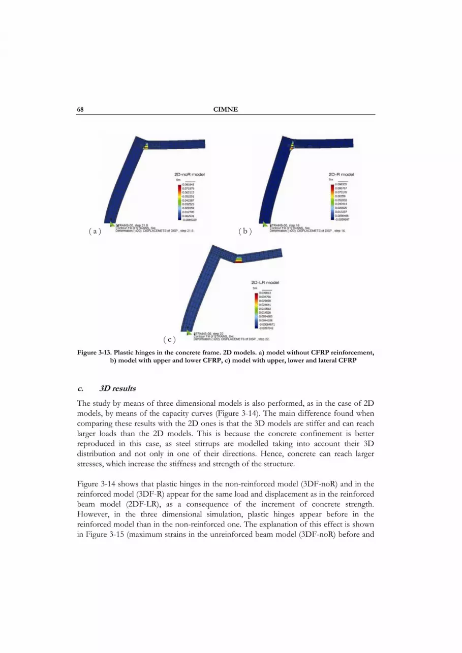
68 CIMNE
( a ) ( b )
( c ) Figure 3-13. Plastic hinges in the concrete frame. 2D models. a) model without CFRP reinforcement,
b) model with upper and lower CFRP, c) model with upper, lower and lateral CFRP
c. 3D results
The study by means of three dimensional models is also performed, as in the case of 2D models, by means of the capacity curves (Figure 3-14). The main difference found when comparing these results with the 2D ones is that the 3D models are stiffer and can reach larger loads than the 2D models. This is because the concrete confinement is better reproduced in this case, as steel stirrups are modelled taking into account their 3D distribution and not only in one of their directions. Hence, concrete can reach larger stresses, which increase the stiffness and strength of the structure.
Figure 3-14 shows that plastic hinges in the non-reinforced model (3DF-noR) and in the reinforced model (3DF-R) appear for the same load and displacement as in the reinforced beam model (2DF-LR), as a consequence of the increment of concrete strength. However, in the three dimensional simulation, plastic hinges appear before in the reinforced model than in the non-reinforced one. The explanation of this effect is shown in Figure 3-15 (maximum strains in the unreinforced beam model (3DF-noR) before and

Sub-Project 7 – 3.2. Integration of knowledge on FRP retrofitted structures 69
after the formation of the plastic hinge) and in Figure 3-16 (the same results in the case of the 3DF-R model).
Figure 3-14. Capacity curves obtained with the 3D models
Figure 3-15. Crack evolution in the 3DF-noR model (model without CFRP reinforcement)
Figure 3-16. Crack evolution in the 3DF-R model (model with upper and lower CFRP)
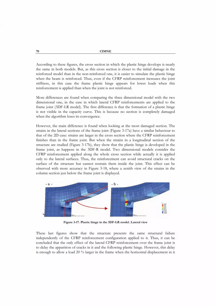
70 CIMNE
According to these figures, the cross section in which the plastic hinge develops is nearly the same in both models. But, as this cross section is closer to the initial damage in the reinforced model than in the non-reinforced one, it is easier to simulate the plastic hinge when the beam is reinforced. Thus, even if the CFRP reinforcement increases the joint stiffness, in this case the frame plastic hinge appears for lower loads when this reinforcement is applied than when the joint is not reinforced.
More differences are found when comparing the three dimensional model with the two dimensional one, in the case in which lateral CFRP reinforcements are applied to the frame joint (3DF-LR model). The first difference is that the formation of a plastic hinge is not visible in the capacity curve. This is because no section is completely damaged when the algorithm loses its convergence.
However, the main difference is found when looking at the most damaged section. The strains in the lateral sections of the frame joint (Figure 3-17a) have a similar behaviour to that of the 2D case: strains are larger in the cross section where the CFRP reinforcement finishes than in the frame joint. But when the strains in a longitudinal section of the structure are studied (Figure 3-17b), they show that the plastic hinge is developed in the frame joint, as happens in the 3DF-R model. Two dimensional models consider the CFRP reinforcement applied along the whole cross section while actually it is applied only to the lateral surfaces. Thus, the reinforcement can avoid structural cracks on the surface of the structure but cannot restrain them inside the joint. This effect can be observed with more accuracy in Figure 3-18, where a zenith view of the strains in the column section just below the frame joint is displayed.
Figure 3-17. Plastic hinge in the 3DF-LR model. Lateral view
These last figures show that the structure presents the same structural failure independently of the CFRP reinforcement configuration applied to it. Thus, it can be concluded that the only effect of the lateral CFRP reinforcement over the frame joint is to delay the apparition of cracks in it and the following plastic hinge. However, this delay is enough to allow a load 20 % larger in the frame when the horizontal displacement in it

Sub-Project 7 – 3.2. Integration of knowledge on FRP retrofitted structures 71
is of 3.0 cm, increment more than sufficient to consider this reinforcement typology the best option to improve concrete framed structures seismic strength.
Figure 3-18. Elements with larger deformations in the 3DF-LR model. Zenith view
The results also show the necessity of using three dimensional elements depending on the simulation to be performed. When the distribution of CFRP reinforcements is not uniform along the whole cross section, 2D simulations can provide incorrect results. However, even if the effectiveness of lateral reinforcements is reduced in the 3D model, the structural strength improvement is significant enough to consider this reinforcement configuration as the best option to reinforce the column-beam joint of RC frame structures.
3.2.4 CONCLUSIONS
In this technical report have been exposed the different numerical procedures developed to solve in a reliable and efficient way the problem of reinforcement and/or retrofitting of reinforced concrete (RC) structures using fibre reinforced polymers (FRP). Due to the complexity of the problem to be solved, efforts have been directed not only to the numerical procedures that allow performing the structural simulation but also to the efficiency of the code and the way the user interacts with it.
Of all the formulations developed to solve the problem of FRP reinforcement of RC structures, is of special relevance the general formulation of the mixing theory to deal with laminated composites. This is, the division of the composite in its different components until reaching the constituent material, which will be the one that will provide the structural behaviour of the composite. This formulation can be understood as a manager of constitutive equations and is the one that allows dealing with the reinforcement problem, taking into account all its particularities, without increasing the problem numerical size beyond the computational limits. The good performance of this theory has been proved with the different simulations presented in section 3.2.3 of the present document.
72 CIMNE
Besides the mixing theory formulation, other numerical procedures have been developed to deal with the particular case of FRP reinforcements. The most relevant of them are the anisotropy using a mapped space theory and the fibre matrix debonding. Special attention must be paid in the construction stages algorithm, which allows performing simulations of retrofitted structures (section 3.2.3.2). These simulations have shown that, even the FRP performance do not vary significantly if it is applied as a reinforcement or as a retrofit, the structural deformations and the stresses are larger if the FRP is applied when the structure is already damaged. Finally, it has to be said that the compression strength formulation has not been tested yet in a FRP reinforcement simulation, however, first results obtained permit be optimistic about its performance and validity.
To improve the code efficiency it has been revised in detail, deleting all data and variables not required to solve the problem. It has also been implemented a numerical derivation procedure, used to obtain the constitutive tangent matrix, in order to reach the structural equilibrium in the fewer number of iterations possible.
The code is now more user friendly as all the problem can be defined using GiD pre-processor, and all output results can be studied with GiD post-processor. Also, to make the developed formulation more accessible, the mixing theory developed to deal with laminate composite will be soon accessible as a usermat for ANSYS users.
The conclusion that all all formulations exposed are valid and useful to solve the FRP reinforcement problem has been obtained form the study of the different simulations performed with them. However, the objective of these simulations was not only to verify the formulations implemented in the finite element code, but also to study in which way the simulations of structural reinforcements of CFRP must be developed to obtain accurate results. The simulation that has provided more information in this aspect has been the framed structure one. This simulation has shown the necessity to work with three dimensional elements to obtain an adequate behaviour of the structure. Two dimensional elements suppose a constant distribution of the materials along the whole cross section. When the structure has not the same composition along its cross section, the supposition that these properties can be extended to the whole section can overestimate the structural performance, as happens with lateral CFRP reinforcements in the frame simulation.
Finally, all simulations have proven the improvement obtained in the structural performance when it is reinforced or retrofitted with fibre reinforced polymers. This improvement depends on the type of reinforcement applied and on the level of existing damage in the structure when the reinforcement is applied. Both aspects can be controlled now, with the formulation described in this work, in order to obtain the best FRP configuration to reinforce the structure considered.

Sub-Project 7 – 3.2. Integration of knowledge on FRP retrofitted structures 73

Sub-Project 7 – 3.3. Experimental data on durability and fatigue resistance 75
3.3 EXPERIMENTAL DATA ON DURABILITY AND FATIGUE
RESISTANCE
This section will deal with a summary on the main factors that have an influence on the durability and the fatigue resistance of composites materials. Thus, the section is divided into two clearly distinct parts, one of them dealing with durability and the second one dealing with the fatigue resistance.
3.3.1 Durability
The durability characteristics of FRP (Fibre Reinforced Polymers) materials have been, and are, the subject of intense review, with special emphasis on the three most common types of fibres, currently used in polymeric composites: glass, carbon and aramid fibres. However, due to their wide application and utilization in Civil Engineering, most of the available information focuses on glass fibre degradation. An up-to-date summary of the main characteristics is given below.
3.3.1.1 Fibres’ environmental degradation
a. Glass fibre
Glass fibres are the most commonly used in Civil Engineering applications, because they are the cheapest (Jamond 2000) and, therefore, it is important that we should understand their behaviour when exposed to hostile environments. Although it is common knowledge that glass fibres degrade in the presence of water and of acid, alkaline or saliferous solutions, the most serious occurs in alkaline solutions (as reported by research work on the subject). A good example is the alkaline water coming from concrete pores, which turns this environment into one of the most critical for glass fibres, due to the hydration of the cement. Therefore, many durability surveys are aimed at determining the alkali resistance of GFRP (Glass Fibre Reinforced Polymers). Additionally, there are debates still raging about the severity of saliferous environments on this type of fibres, which have proved to be more serious than watery and acid environments, but as serious as the degradation in alkaline environments (Chin 1997).
The different glass compositions available on the market read as follows: (1) E-Glass (“Electric Grade Glass”) is the cheapest and more widely used for general purpose jobs; (2) S-Glass (“Strength Glass”) has greater mechanical properties than E-Glass, but costs more; (3) AR-Glass (“Alkali Resistant Glass”) is an improved version of E-Glass, to withstand alkaline attacks through the addition of zirconium.

76 ACCIONA
b. Aramid fibre
Aramid fibres are particularly susceptible to water, as these are organic polymeric fibres and they are known to absorb water (Bank 1995). As happens with glass fibres, the Absorption of water can cause the total degradation of the aramid fibres, mainly thanks to the greater stresses caused by expansion. In addition, solutions such as sodium hydroxide and hydrochloridic acid cause accelerated hydrolysis in the most common aramid fibres (Kevlar 49), especially when temperature and stresses combine (Hunston 2000).
c. Carbon fibre
Studies on carbon fibre reinforced composites are numerous due to their extensive use in the aerospace industry (Bank 1995). Carbon fibres offer higher rigidity and specific strength than glass fibres. In addition, they are resilient, even in chemical environments and do not absorb water. Machida (1995) points out that they are highly resistant to acid, alkaline and organic environments. Due to these characteristics, carbon fibres are being increasingly used in applications where light, high strength, structures are called for. However, carbon fibres exhibit two drawbacks: (1) they are galvanically inactive and, therefore, the cathodic reaction can play an important role in the degradation of the composite, between the polymer and the graphite, that is to say in the interface (Tucker 1990). This can get worse when the carbon fibres come into contact with any metal, such as those present in external reinforcements, or with saliferous water; and (2) they are a lot more expensive than glass fibres.
Many studies have been undertaken to observe the typical degradation, both physical and chemical, of carbon fibres in different environments (acid, alkaline and distil water), but no deterioration mechanism has been found and so none is available (Sen 1998).
3.3.1.2 Accelerated Ageing Models
The accelerated tests main purpose is to predict the system service life; to achieve this, three essential items of information are required: 1) data showing the degradation of the properties of the material, which are going to be predicted in the service life; 2) an analytical or statistical model to extrapolate the data for long term purposes; and 3) a proper definition of the failure mechanism of the test samples; in the event of different failure modes being obtained in the simulated accelerated models, the predictions shall not be valid.
Katsuki & Uomoto (1997) apply Fick’s Law to simulate the degradation of the GFRP rods quantitatively, by predicting the reduction of the tension strength in accelerated tests, where the results coincided well with the measured results. This Law is deemed
Sub-Project 7 – 3.4. Computation of the resistance of structural elements considering steel & FRP 77
adequate to predict the loss of strength of the tendons or rods. Arrhenius’ Law can be used to determine the diffusion rate in “non-accelerated” temperatures and, consequently, the strength reduction rate under non-accelerated conditions.
Valter Dejke et al (2001) in his thesis, assumes that the service life at different temperatures can be derived from Arrhenius’ Law. Using this approximation, it is possible to transform the exposure time under accelerated conditions into real application times, using the time factor (Time Shift Factor, TSF). For example, 1.5 years at 60°C approximately equals 50 years in open air conditions in southern Sweden (which means a yearly temperature of 7°C). In addition, it provides mathematical expressions to calculate the weight gain and the concentration of the profiles of the materials when they are penetrated by a liquid, which can be water, an alkaline solution or any fluid medium. All the above equations assume that the diffusion of the liquid inside the material is distributed in accordance with Fick’s Law.
Different experts have obtained, from several surveys, numerous data about the degradation characteristics of the FRP. However, what the industry needs is a forecast of the service life. The behaviour of the tested materials, together with the degradation characteristics, by themselves, is not sufficient to perform service life predictions. That is the reason why numerous models have been developed to interpret the results from accelerated tests. These models consider the information from the tests as input data and predict the system service life.
a. Degradation models
As the degradation model becomes more complex, so does the model used to describe it. That is the reason why it is so difficult to develop a model of degradation of FRP with very complex durability mechanisms. The lack of knowledge about the true meaning and about the use of the accelerated tests may lead to incorrect conclusions about the tested product and even result in high costs for the development of the product (Nelson 1990).
Although there exist, in the literature, several proposed models, which are widely used, each has its own limitations and assumptions. It must be born in mind that there are no analytical models that take into account the degradation mechanisms and that accurately estimate the service life of the materials subjected to accelerated tests. On the other hand, it is very difficult to simulate in the accelerated tests the actual environmental conditions to which the materials are exposed when they are in operation. Because of this and due to all the aforesaid uncertainties, the service life predicting models must be used with extreme care.

78 ACCIONA
b. Constant Rate Models
These have been established analytical models which link all the variables involved (temperature, saliferous solutions, etc.) under the application of a constant acceleration factor. The close formulation of these models is very hard to obtain, because the degradation models are not well known in most cases. In addition, it is possible that deviations in the model might occur over prolong periods of time.
c. Power Law Models
The Power Law models are the most widely used among the simple speed models of accelerated tests. These models have the degradation rate represented by a Power function of a degradation factor as shown by equation (3.3.1). It must be born in mind that the long-term degradation rate is always the same in these models, as their implies (Nelson 1990).
β β=' V (3.3.1)
Where:
β ' : The degradation rate.
β : A constant of the material.
V : Degradation factor.
d. Exponential Models
These models are very similar to those used with Power’s Law. The degradation rate is represented by an exponential function of the stress, as shown in equation (3.3.2) (Nelson 1990)
β β γ=' exp( )V (3.3.2)
Where:
β ' : Rate of degradation.
β ,γ : Constants of the material.
V : Accelerated stress.
Sub-Project 7 – 3.4. Computation of the resistance of structural elements considering steel & FRP 79
e. Eyring Model
The general formulation of the Eyring model contains two environmental load variables, one of which is the temperature. The other is the load. This can be the mechanical load, the humidity or the existing density. The general formulation of the Eyring model is shown in equation (3.3.3).
γβ β δ ε⎡ ⎤= − − −⎢ ⎥⎣ ⎦' exp VV
T T (3.3.3)
Where:
β ' : Rate of degradation.
β ,γ ,δ ,ε : Constants of the material and of the degradation mechanism.
T : Temperature in °K.
f. Arrhenius Stabilised-Status Temperature Acceleration Model
This model can be used when the temperature is the only acceleration factor and the main concern are the chemical reactions (Caruso 1998). Arrhenius’ degradation rate can be formulated like equation (3.3.4) (Nelson 1990)
β −⎛ ⎞= ⎜ ⎟⎝ ⎠
' ' exp EAkT
(3.3.4)
Where:
β ' : Rate of degradation.
E : Activation energy of the chemical reaction in electron volts.
k : Boltzmann’s constants, 8.617x10⁻⁵ electron volts per °C.
T : Absolute temperature in °K.
A : A constant of the test conditions and failure of the material.
The acceleration factor for this model can be written like equation (3.3.5) to relate the degradations in accelerated environments to those under service conditions (Nelson 1990):
80 ACCIONA
ττ
⎡ ⎤⎛ ⎞⎧ ⎫= = −⎨ ⎬⎜ ⎟⎢ ⎥⎩ ⎭⎝ ⎠⎣ ⎦
1 1exp' '
nEAFk T T
(3.3.5)
Where:
AF : Acceleration factor.
nE : Activation energy for the degradation mechanism and for the material.
τ : life-cycle at the reference temperature T(°K).
τ ' : life-cycle at elevated temperature T’(°K).
k : Boltzmann’s constant.
Arrhenius’ Law models are still being debated and have not been internationally accepted yet. They can only be used to draw comparisons between those materials whose degradation can be simulated with this Law.
The Time Shift (TS) technique is used to represent the ageing effect, using a long-term horizontal Time Shift (Gates 1997). Moreover, by representing the temperature effects along with this technique in accelerated tests, a description is given of the level of acceleration of an environmental exposure which is obtained when the temperature is increased (Valter 2001). However, it does not properly represent ageing, except for short periods of time.
3.3.2 Fatigue of composites
Fatigue is the condition for which a material cracks or it fails as a result of repeated effort (cyclic loading). From an engineered point of view, it should be defined like the permanent, located and progressive structural change that takes place in a material subject to repeated or fluctuating deformations. In general, these deformations are presented to smaller efforts that the last tensile strength of the material in a static test, and they frequently appear for smaller efforts that the fluency limit of the material. The fatigue can affect practically all the engineering materials subject to cyclic efforts. Cyclic efforts include repetitive external loads and thermal efforts that result from heating and alternated cooling.
The fatigue life of a component or material is defined as the total number of necessary effort cycles to cause failure. It is an important concept that one frequently studies in the laboratory, for what the obtained information can apply to designs and components in
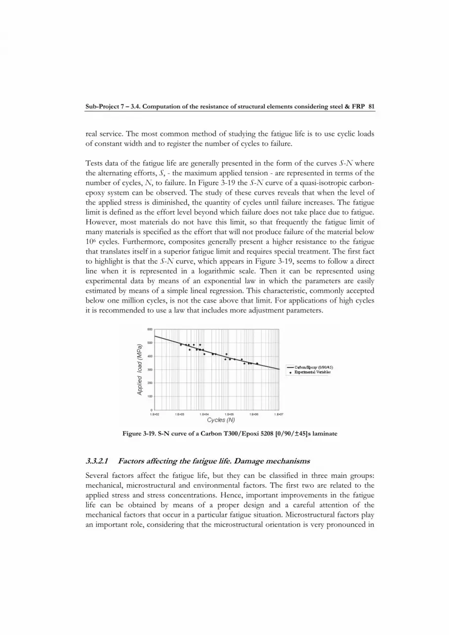
Sub-Project 7 – 3.4. Computation of the resistance of structural elements considering steel & FRP 81
real service. The most common method of studying the fatigue life is to use cyclic loads of constant width and to register the number of cycles to failure.
Tests data of the fatigue life are generally presented in the form of the curves S-N where the alternating efforts, S, - the maximum applied tension - are represented in terms of the number of cycles, N, to failure. In Figure 3-19 the S-N curve of a quasi-isotropic carbon-epoxy system can be observed. The study of these curves reveals that when the level of the applied stress is diminished, the quantity of cycles until failure increases. The fatigue limit is defined as the effort level beyond which failure does not take place due to fatigue. However, most materials do not have this limit, so that frequently the fatigue limit of many materials is specified as the effort that will not produce failure of the material below 106 cycles. Furthermore, composites generally present a higher resistance to the fatigue that translates itself in a superior fatigue limit and requires special treatment. The first fact to highlight is that the S-N curve, which appears in Figure 3-19, seems to follow a direct line when it is represented in a logarithmic scale. Then it can be represented using experimental data by means of an exponential law in which the parameters are easily estimated by means of a simple lineal regression. This characteristic, commonly accepted below one million cycles, is not the case above that limit. For applications of high cycles it is recommended to use a law that includes more adjustment parameters.
Figure 3-19. S-N curve of a Carbon T300/Epoxi 5208 [0/90/±45]s laminate
3.3.2.1 Factors affecting the fatigue life. Damage mechanisms
Several factors affect the fatigue life, but they can be classified in three main groups: mechanical, microstructural and environmental factors. The first two are related to the applied stress and stress concentrations. Hence, important improvements in the fatigue life can be obtained by means of a proper design and a careful attention of the mechanical factors that occur in a particular fatigue situation. Microstructural factors play an important role, considering that the microstructural orientation is very pronounced in
82 ACCIONA
an anisotropic material. As for the environment, they can be considered as special cases of fatigue and include thermal effects, contact fatigue and the effects of corrosion.
In general, the effect of fatigue is the reduction of the strength or the residual stiffness, and the possible failure, after applying a finite number of load cycles. These load cycles are smaller in magnitude than the necessary load to produce failure in a single cycle. Therefore, some process of fatigue damage has to occur that reduces the material strength under load.
In all ways, this damage is not uniform, that is, not all the volume of the material element suffers the same stress reduction. Generally, the damage process consists of a series of discrete events that cause a non-uniform or inhomogeneous response of the material. In fact it is probable that the most universal characteristic in fatigue is the inhomogeneous deformation. According to above-mentioned consequence, the fatigue effect is composed of a series of micro-geometric contributions, such as microcracking that produces local concentrations, which in turn generate additional damage.
A basic physical principle behind any cycle-dependent behaviour is the appearance of non-conservative deformation that modifies the internal nature or the geometry of the material, and its capacity to respond to histories of continuous load. Non-conservative deformation implies that the part of the energy absorbed by the material through the stress or the applied displacements is not stored as energy of deformation, but is dissipated as the driving force of internal processes, as the formation and growth of microcracks, as thermodynamic events, as atomic or molecular redistribution and as chemical events. Although not all the non-conservative processes produce fatigue in the sense that they do not reduce the residual strength, the stiffness or the service life, it is known that the damage processes for fatigue are not conservative; this implies a dependence of the behaviour of the materials on the load history.
For composites of interest in civil engineering applications, especially those with fibres of high modulus, the different micro-events that contribute to the development of the damage process are classified in the following categories:
• Microcrack formation • Chemical damage • Plastic deformation • Delamination • Separation of fibres and matrix • Interface failure
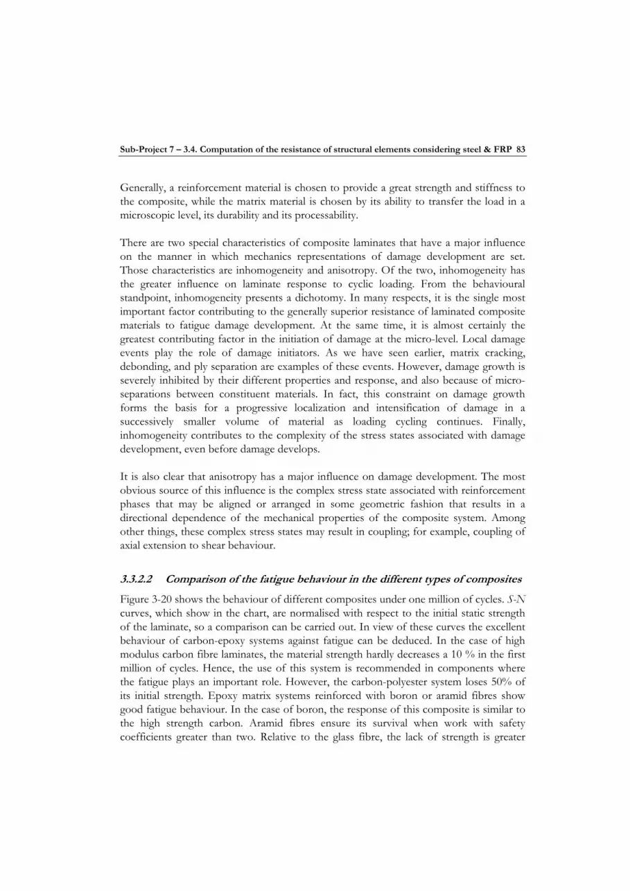
Sub-Project 7 – 3.4. Computation of the resistance of structural elements considering steel & FRP 83
Generally, a reinforcement material is chosen to provide a great strength and stiffness to the composite, while the matrix material is chosen by its ability to transfer the load in a microscopic level, its durability and its processability.
There are two special characteristics of composite laminates that have a major influence on the manner in which mechanics representations of damage development are set. Those characteristics are inhomogeneity and anisotropy. Of the two, inhomogeneity has the greater influence on laminate response to cyclic loading. From the behavioural standpoint, inhomogeneity presents a dichotomy. In many respects, it is the single most important factor contributing to the generally superior resistance of laminated composite materials to fatigue damage development. At the same time, it is almost certainly the greatest contributing factor in the initiation of damage at the micro-level. Local damage events play the role of damage initiators. As we have seen earlier, matrix cracking, debonding, and ply separation are examples of these events. However, damage growth is severely inhibited by their different properties and response, and also because of micro-separations between constituent materials. In fact, this constraint on damage growth forms the basis for a progressive localization and intensification of damage in a successively smaller volume of material as loading cycling continues. Finally, inhomogeneity contributes to the complexity of the stress states associated with damage development, even before damage develops.
It is also clear that anisotropy has a major influence on damage development. The most obvious source of this influence is the complex stress state associated with reinforcement phases that may be aligned or arranged in some geometric fashion that results in a directional dependence of the mechanical properties of the composite system. Among other things, these complex stress states may result in coupling; for example, coupling of axial extension to shear behaviour.
3.3.2.2 Comparison of the fatigue behaviour in the different types of composites
Figure 3-20 shows the behaviour of different composites under one million of cycles. S-N curves, which show in the chart, are normalised with respect to the initial static strength of the laminate, so a comparison can be carried out. In view of these curves the excellent behaviour of carbon-epoxy systems against fatigue can be deduced. In the case of high modulus carbon fibre laminates, the material strength hardly decreases a 10 % in the first million of cycles. Hence, the use of this system is recommended in components where the fatigue plays an important role. However, the carbon-polyester system loses 50% of its initial strength. Epoxy matrix systems reinforced with boron or aramid fibres show good fatigue behaviour. In the case of boron, the response of this composite is similar to the high strength carbon. Aramid fibres ensure its survival when work with safety coefficients greater than two. Relative to the glass fibre, the lack of strength is greater
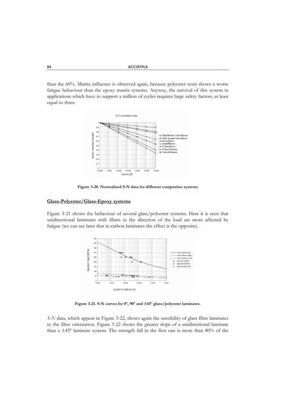
84 ACCIONA
than the 60%. Matrix influence is observed again, because polyester resin shows a worse fatigue behaviour than the epoxy matrix systems. Anyway, the survival of this system in applications which have to support a million of cycles requires large safety factors, at least equal to three.
Figure 3-20. Normalised S-N data for different composites systems
Glass-Polyester/Glass-Epoxy systems
Figure 3-21 shows the behaviour of several glass/polyester systems. Here it is seen that unidirectional laminates with fibres in the direction of the load are more affected by fatigue (we can see later that in carbon laminates the effect is the opposite).
Figure 3-21. S-N curves for 0º, 90º and ±45º glass/polyester laminates.
S-N data, which appear in Figure 3-22, shows again the sensibility of glass fibre laminates to the fibre orientation. Figure 3-22 shows the greater slope of a unidirectional laminate than a ±45º laminate system. The strength fall in the first one is more than 80% of the

Sub-Project 7 – 3.4. Computation of the resistance of structural elements considering steel & FRP 85
initial static strength, whereas in the ±45º laminate is around 30%. Figure 3-22 shows the influence of the fibre orientation in different laminates. Even when the initial strengths are very different, the fatigue causes that all systems reach a strength between 100 and 200 MPa, if the number of cycles overcome the million. Another fact to highlight is when there is 0º plies the strength lack is more significant in the first stages and smooth to a high number of cycles.
Figure 3-22. S-N curves for Glass S2/Epoxy 5280 laminates to [0]3 and [±45]2s
Carbon-epoxi systems
Figure 3-23 compares the behaviour of three laminates: 0º, 90º and ±45º. The reduction of strength in the unidirectional laminate is not more than 30%. Hence unidirectional carbon laminates support fatigue much better than the glass fibre ones, in which the strength loss can reach 80% when the applied load exceeds one million of cycles. Figure 3-23 shows that the presence of 0º laminates diminishes the slope of the S-N curve, contrary to the case of glass fibre laminates.
Figure 3-23. S-N curves for carbon T300/epoxy [0]6,, [±45]8t and [90]15 laminates
86 ACCIONA
3.3.2.3 Conclusions
In this section a large number of S-N data for different fibre reinforced polymer systems, likely to be used in structural components or in FRP strengthening of existing structures are presented. These systems employ epoxy or polyester matrix and glass or carbon fibres. The stress decreasement upon the different types of laminates (constitutive materials) and orientation of the fibres are summarized, shown and discussed.
3.4 COMPUTATION OF THE RESISTANCE OF STRUCTURAL ELEMENTS
CONSIDERING STEEL & FRP
3.4.1 Introduction
Many research works were carried out on strengthening of existing structural members with these materials.
Toutanji [1999], Fam and Rizkalla [2001] and Becque et al. [2003] developed extensive experimental data for cylinder specimens, for a variety of fibre types, orientations and jacket thickness, either for FRP jacketed concrete or concrete filled FRP tubes. Demers and Neale [1999] and Ilki et al. [2004a] tested reinforced concrete columns of circular cross-section with FRP jackets. Rochette and Labossiere [2000], Wang and Restrepo [2001], Shehata et al. [2002] and Ilki et al. [2004b], tested square and rectangular concrete columns confined by FRP composites.
Xiao and Wu [2000] investigated the effect of concrete compressive strength and thickness of CFRP jacket and proposed a simple bilinear stress-strain model for CFRP jacketed concrete. Tan [2002] tested half scale reinforced concrete rectangular columns with a section aspect ratio of 3.65 under axial loads and investigated the effects of fibre type and configuration and fibre anchors on the strength enhancement of the columns. Ilki and Kumbasar [2002] tested both damaged and undamaged cylinder specimens, which were externally confined with different thickness of CFRP jackets, under monotonic increasing and cyclic compressive stresses. Based on experimental results they proposed simple expressions for ultimate strength and corresponding axial strain of CFRP jacketed concrete.
Lam et al. [2004] also performed monotonic and cyclic compression tests on CFRP confined concrete cylinders. Then the tests results were compared with a monotonic stress-strain model proposed by Lam and Teng [2003a], and a cyclic stress-strain model proposed by Shao [2003], for FRP confined concrete. Lam and Teng [2002] carried out an extensive survey of existing studies on FRP confined concrete and proposed a simple model based on a linear relationship between confined concrete strength and lateral confining pressure provided by FRP composites, which was quite similar to the model
Sub-Project 7 – 3.4. Computation of the resistance of structural elements considering steel & FRP 87
proposed by Ilki and Kumbasar [2002] before. Ilki and Kumbasar [2003], after testing CFRP jacketed concrete specimens with square and rectangular cross-sections, modified the expressions that they have proposed before to cover non-circular cross-sections. Lam and Teng [2003a, 2003b] proposed design oriented stress-strain models for both uniformly and non-uniformly confined concrete members. Ilki et al. [2004c] tested FRP jacketed low strength concrete members with circular and rectangular cross-sections, and stated that when the unconfined concrete quality was lower, the efficiency of the FRP jackets was higher.
De Lorenzis and Tepfers [2003], stated that none of the available models could predict the strain at peak stress with reasonable accuracy. Bisby et al. [2005] evaluated and modified available analytical confined concrete models to provide the best fit to the experimental data base. Matthys et al. [2005] tested large scale cylinder columns and observed that most of the available stress-strain models based on small cylinder tests seem to predict the ultimate strength fairly accurately.
Tastani and Pantazopoulou [2004] studied the structural behaviour of FRP confined corrosion damaged square columns with reinforcement details representative of pre-1980s. In the light of the experience obtained on FRP retrofitting techniques, a number of design guidelines and bulletins such as ACI 440.2R-02 [2002], CAN/CSA-S806 [2002], EN 1998-3 [2003] and fib bulletin no.14 [2001] have been published. Most of the experimental studies are on small size cylinders without longitudinal and transverse reinforcement, and the unconfined concrete strengths of almost all of the tested specimens are in the range of medium to high. In this study, uniaxial compressive behaviour of reinforced concrete columns jacketed with CFRP sheets was investigated. The average standard cylinder concrete strength at the time of testing was 15.92 MPa for LSR series, while other specimens had the average standard cylinder concrete strength of 31.00 MPa (NSR series). The main parameters of the experimental work were the thickness of the CFRP jacket, cross-section shape, unconfined concrete strength and corner radius. Additional specimens were included in the test program for determining the effects of existence of pre-damage, cyclic loading, the bonding pattern and anchorage details. After the tests of unconfined and CFRP jacketed specimens, it was observed that the contribution of the CFRP jackets on deformability and/or strength enhancement was remarkable for specimens with circular and non-circular cross-sections. While the strength enhancement was more pronounced for the specimens with circular cross-section, specimens with square and rectangular cross-sections exhibited larger ultimate axial deformations without a substantial loss in strength. Although original specimens without adequate internal transverse reinforcement experienced premature buckling of the longitudinal bars, this phenomenon was delayed significantly after CFRP jacketing. Since the required confining pressure for a certain increase of compressive strength is relatively less in the case of lower strength concrete, CFRP jackets were more effective in
88 ITU
the case of low strength concrete. Rectangular columns with larger corner radius reached relatively higher strengths, while no specific effect of corner radius was observed on deformability. For understanding the effect of pre-damage on the behaviour of retrofitted columns, some of the columns were loaded until the axial strain of 0.003~0.004 before retrofitting. Test results showed that such pre-damage did not have an adverse effect on the performance of the jacketed columns. According to the test results, cyclic loading did not have a remarkable effect on the behaviour of circular and square columns. However, the compressive strength of rectangular columns was slightly less in the case of cyclic loading. For equivalent amount of CFRP, continuous jackets and straps provided similar performances. Application of additional CFRP anchorages into the concrete for increasing the effectively confined area did not improve the behaviour of the retrofitted columns. The compressive strengths and the corresponding axial deformations of the columns were also predicted by the empirical equations proposed before, [Ilki et al. 2004c]. During these predictions, both the contributions of transverse steel reinforcement and CFRP jacket were taken into account. After comparison of the predictions and experimental data, it was seen that these predictions were in reasonable agreement with experimental results. Although satisfactory results were obtained after comparing experimental and predicted strength and ultimate deformation values, another comparative study was also carried out for further verification of the methodology used for computation of strength and deformability of FRP jacketed reinforced concrete members. For this purpose, around 280 specimens of different shapes and concrete strengths tested by different researchers from all over the world were taken into account. This comparative study also showed that the proposed computation methodology gave fairly accurate results.
3.4.2 Testing program
3.4.2.1 Outline of The Characteristics of The Tested Specimens
List of the specimens tested are given in Table 3-8 with main characteristics. The diameter of cylinder columns were 250 mm, and cross-sections of rectangular columns were either 250 mm × 250 mm or 150 mm × 300 mm. The 28 days standard cylinder strength f′c was 10.94 and 23.86 MPa, respectively for low and medium strength concrete. Note that unconfined concrete strength of the member f′co was assumed to be 85% of the standard cylinder strength at the time of testing. Longitudinal reinforcement ratio ρl was around 0.01 and the clear concrete cover was 25 mm for all specimens. For longitudinal reinforcement 6φ10, 4φ14 and 4φ12 bars were used for specimens with circular, square and rectangular cross-sections, respectively. The reinforcement details are given in Figure 3-24. Only plain bars were used both for longitudinal and transverse reinforcement for representing the columns of existing relatively older structures in developing countries. Yield strength fy, yield strain εy and tensile strength fs,max were 367

Sub-Project 7 – 3.4. Computation of the resistance of structural elements considering steel & FRP 89
MPa, 0.0018 and 523 MPa for 10 mm diameter bars, 339 MPa, 0.0017 and 471 MPa for 12 mm diameter bars and 345 MPa, 0.0017 and 477 MPa for 14 mm diameter bars, respectively. Yield strength and yield strain of 8 mm diameter bars were 476 MPa and 0.0024, respectively. The specimens were tested after being jacketed with 1, 3 or 5 plies of CFRP sheets. The tensile strength f*fu, elasticity modulus Efrp, ultimate rupture strain ε∗
fu and nominal thickness tf of CFRP were 3430 MPa, 230 GPa, 1.5% and 0.165 mm, respectively. These properties are taken from the specifications of the manufacturer. To prevent stress concentrations around the corners of the non-circular columns, corners were rounded with a radius of 40 mm, while corners of four specimens were rounded to 10 and 20 mm to examine the effects of corner radius on the behaviour. Four pre-damaged specimens and four specimens with additional anchorage details were included in the test program, as well as nine specimens tested under cyclic loads. Four specimens were wrapped with hoop and spiral type CFRP straps to investigate the effects of the different wrapping patterns. Note that, all these specimens coded LSR-C-3-a-H, LSR-R-2-3-40a-H (with hoop type straps) and LSR-C-3-a-S, LSR-R-2-3-40a-S (with spiral type straps), were wrapped with 50 mm wide straps with 50 mm clear spacing. The general characteristics of the specimens are given in Table 3-8.
Table 3-8. Characteristics of tested specimens
Specimen f′cj L.R. T.R. n f′co
LSR-R-1-0-40a 15.6 4Ø14 Ø8/200 0 13.27 LSR-R-1-0-40b 15.9 4Ø14 Ø8/200 0 13.53
LSR-R-1-1-40a-A 15.9 4Ø14 Ø8/200 1 13.53 LSR-R-1-1-40b-A 15.9 4Ø14 Ø8/200 1 13.53
LSR-R-1-1-40a 15.9 4Ø14 Ø8/200 1 13.53 LSR-R-1-1-40b 15.9 4Ø14 Ø8/200 1 13.53 LSR-R-1-3-40a 15.9 4Ø14 Ø8/200 3 13.53 LSR-R-1-3-40b 15.9 4Ø14 Ø8/200 3 13.53 LSR-R-1-3-10a 15.9 4Ø14 Ø8/200 3 13.53 LSR-R-1-3-10b 15.9 4Ø14 Ø8/200 3 13.53 LSR-R-1-3-20a 15.9 4Ø14 Ø8/200 3 13.53 LSR-R-1-3-20b 15.9 4Ø14 Ø8/200 3 13.53 LSR-R-1-5-40a 15.9 4Ø14 Ø8/200 5 13.53 LSR-R-1-5-40b 15.9 4Ø14 Ø8/200 5 13.53 LSR-R-2-0-40a 14.2 4Ø12 Ø8/175 0 12.09 LSR-R-2-0-40b 14.2 4Ø12 Ø8/175 0 12.09
LSR-R-2-1-40a-A 15.9 4Ø12 Ø8/175 1 13.53 LSR-R-2-1-40b-A 15.9 4Ø12 Ø8/175 1 13.53
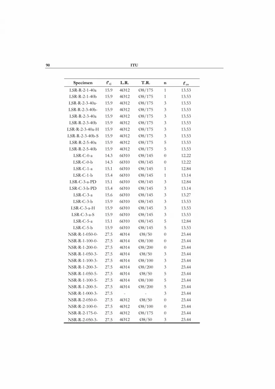
90 ITU
Specimen f′cj L.R. T.R. n f′co
LSR-R-2-1-40a 15.9 4Ø12 Ø8/175 1 13.53 LSR-R-2-1-40b 15.9 4Ø12 Ø8/175 1 13.53 LSR-R-2-3-40a- 15.9 4Ø12 Ø8/175 3 13.53 LSR-R-2-3-40b- 15.9 4Ø12 Ø8/175 3 13.53 LSR-R-2-3-40a 15.9 4Ø12 Ø8/175 3 13.53 LSR-R-2-3-40b 15.9 4Ø12 Ø8/175 3 13.53
LSR-R-2-3-40a-H 15.9 4Ø12 Ø8/175 3 13.53 LSR-R-2-3-40b-S 15.9 4Ø12 Ø8/175 3 13.53 LSR-R-2-5-40a 15.9 4Ø12 Ø8/175 5 13.53 LSR-R-2-5-40b 15.9 4Ø12 Ø8/175 5 13.53
LSR-C-0-a 14.3 6Ø10 Ø8/145 0 12.22 LSR-C-0-b 14.3 6Ø10 Ø8/145 0 12.22 LSR-C-1-a 15.1 6Ø10 Ø8/145 1 12.84 LSR-C-1-b 15.4 6Ø10 Ø8/145 1 13.14
LSR-C-3-a-PD 15.1 6Ø10 Ø8/145 3 12.84 LSR-C-3-b-PD 15.4 6Ø10 Ø8/145 3 13.14
LSR-C-3-a 15.6 6Ø10 Ø8/145 3 13.27 LSR-C-3-b 15.9 6Ø10 Ø8/145 3 13.53
LSR-C-3-a-H 15.9 6Ø10 Ø8/145 3 13.53 LSR-C-3-a-S 15.9 6Ø10 Ø8/145 3 13.53 LSR-C-5-a 15.1 6Ø10 Ø8/145 5 12.84 LSR-C-5-b 15.9 6Ø10 Ø8/145 5 13.53
NSR-R-1-050-0- 27.5 4Ø14 Ø8/50 0 23.44 NSR-R-1-100-0- 27.5 4Ø14 Ø8/100 0 23.44 NSR-R-1-200-0- 27.5 4Ø14 Ø8/200 0 23.44 NSR-R-1-050-3- 27.5 4Ø14 Ø8/50 3 23.44 NSR-R-1-100-3- 27.5 4Ø14 Ø8/100 3 23.44 NSR-R-1-200-3- 27.5 4Ø14 Ø8/200 3 23.44 NSR-R-1-050-5- 27.5 4Ø14 Ø8/50 5 23.44 NSR-R-1-100-5- 27.5 4Ø14 Ø8/100 5 23.44 NSR-R-1-200-5- 27.5 4Ø14 Ø8/200 5 23.44 NSR-R-1-000-3- 27.5 - - 3 23.44 NSR-R-2-050-0- 27.5 4Ø12 Ø8/50 0 23.44 NSR-R-2-100-0- 27.5 4Ø12 Ø8/100 0 23.44 NSR-R-2-175-0- 27.5 4Ø12 Ø8/175 0 23.44 NSR-R-2-050-3- 27.5 4Ø12 Ø8/50 3 23.44

Sub-Project 7 – 3.4. Computation of the resistance of structural elements considering steel & FRP 91
Specimen f′cj L.R. T.R. n f′co
NSR-R-2-100-3- 27.5 4Ø12 Ø8/100 3 23.44 NSR-R-2-175-3- 27.5 4Ø12 Ø8/175 3 23.44 NSR-R-2-050-5- 27.5 4Ø12 Ø8/50 5 23.44 NSR-R-2-100-5- 27.5 4Ø12 Ø8/100 5 23.44 NSR-R-2-175-5- 27.5 4Ø12 Ø8/175 5 23.44 NSR-R-2-175-5- 27.5 4Ø12 Ø8/175 5 23.44
NSR-C-050-0 27.5 6Ø10 Ø8/50 0 23.44 NSR-C-100-0 27.5 6Ø10 Ø8/100 0 23.44 NSR-C-145-0 27.5 6Ø10 Ø8/145 0 23.44 NSR-C-050-3 27.5 6Ø10 Ø8/50 3 23.44 NSR-C-100-3 27.5 6Ø10 Ø8/100 3 23.44 NSR-C-145-3 27.5 6Ø10 Ø8/145 3 23.44 NSR-C-050-5 27.5 6Ø10 Ø8/50 5 23.44 NSR-C-100-5 27.5 6Ø10 Ø8/100 5 23.44 NSR-C-145-5 27.5 6Ø10 Ø8/145 5 23.44
500
145
250
8
R40
8
250
250
250
500
200
R40
Ø12
300
150
300
500
175
Ø14
Ø10
Ø250
2020
TEST
ZO
NE
250
Figure 3-24. Cross-sections and Reinforcement Details of the Specimens
92 ITU
3.4.2.2 Loading and Data Acquisition Setup
The specimens were tested under monotonic or cyclic uniaxial compressive loads by using an Amsler universal testing machine with a capacity of 5000 kN. Two different gauge lengths were used for measurement of average axial strains by displacement transducers. For this purpose, four transducers in the gauge length of 270 mm and six transducers in the gauge length of 500 mm were used. Axial and transverse strains at mid-height were also measured by surface strain gauges with a gauge length of 60 mm for all of the specimens. For specimens with circular cross-section, two vertically and two horizontally bonded strain gauges were used with 180 degree intervals around perimeter, for non-circular specimens vertical strain gauges were bonded on two opposite sides. For specimens with square cross-sections two horizontal strain gauges were bonded on two opposite sides. For rectangular specimens two horizontal strain gauges were bonded on short and long sides. To obtain the deformations of the longitudinal and transverse reinforcement, strain gauges were used with gauge lengths of 5 and 3 mm, respectively. For data acquisition a 50 channel TML-ASW-50C switch box and a TML-TDS-303 data logger were used.
3.4.2.3 Test Results and Discussions
The test results are presented in Table 3-9. As seen in this table for the LSR specimens with circular, square and rectangular cross-sections, the average ratios of confined concrete compressive strength to unconfined concrete member strength f′cc/f′co were 2.3, 1.5 and 1.2 for 1 ply, 4.3, 2.9 and 2.3 for 3 plies and 6.7, 3.7 and 3.3 for 5 plies of CFRP jackets, respectively. For the NSR specimens with circular, square and rectangular cross-sections, f′cc increased 3.2, 1.9 and 1.7 times for 3 plies and 4.0, 2.4 and 2.3 times for 5 plies CFRP jackets, respectively. Note that unconfined concrete strength of member f′co was assumed to be 85% of the standard cylinder strength at the time of testing f′cj. Test results showed that, CFRP jackets were more effective in the case of low concrete strength and strength enhancement was more significant for circular specimens, while only slight difference was observed between the strength enhancements of square and rectangular specimens. The axial strains corresponding to CFRP jacketed concrete strengths εcc for the LSR specimens with circular, square and rectangular cross-sections were 11.5, 10.5 and 8.8 times that of unconfined concrete εco for 1 plies, 24.5, 30.3 and 31.8 for 3 plies and 32.8, 38.5 and 46.5 for 5 plies of CFRP jackets, respectively. For the NSR specimens with circular, square and rectangular cross-sections, εcc increased 16.0, 17.2 and 18.2 times for 3 plies, 21.8, 23.8 and 24.7 times for CFRP jackets of 5 plies, respectively. The axial strain corresponding to unconfined concrete strength εco was assumed to be equal to 0.002. For the LSR specimens the transverse strains on CFRP jackets at failure εch were between 0.007 and 0.018 independent of the jacket thickness, with an average value as 0.012. For the NSR specimens εch were between 0.011 and 0.017, with an average value as 0.013. These average values are about 80-87% of the value given

Sub-Project 7 – 3.4. Computation of the resistance of structural elements considering steel & FRP 93
by the manufacturer. Note that only the strain gauges that could work until failure were taken into consideration. Generally, the failures were sudden fracture of CFRP sheets at the mid-heights of the specimens. For circular, square and rectangular specimens, rupture of CFRP sheets was only one vertical cut with the height of 200-250 mm for the jackets of one ply, 3-4 vertical cuts with the heights of 40-70 mm for the jackets of three plies and more vertical cuts of lower heights for jackets of 5 plies. For square and rectangular specimens, the rupture of sheets was around the corners just after the rounded portion. Damage patterns were similar for LSR and NSR specimens. The axial stiffness of the specimens did not show a tendency to increase with increasing jacket thickness. Note that all stress-strain relationships are given with the non-dimensional vertical axis and while determining the stress-strain relationship of confined concrete, the contribution of longitudinal reinforcing bars was subtracted by considering the stress-strain relationships of these bars. The stress-strain relationships were adapted from coupon tensile tests and strain hardening was also taken into account.
It should also be noted that although the major contribution on strength and deformability enhancement was provided by the external CFRP jacket, the internal transverse reinforcement had also some influence. The contribution of internal transverse reinforcement is minimal for the specimens with square and rectangular cross-section.
Table 3-9. Test Results
Specimen
f′cc exp
(MPa) εcc exp
εch
long side
εch
short side f′cc/f′co εcc/εco
LSR-R-1-0-40a - - - - - - LSR-R-1-0-40b - - - - - -
LSR-R-1-1-40a-A 19.02 0.013 0.008 - 1.4 6.5 LSR-R-1-1-40b-A 20.64 0.014 0.007 - 1.5 7.0
LSR-R-1-1-40a 20.58 0.017 0.011 - 1.5 8.5 LSR-R-1-1-40b 20.33 0.025 0.013 - 1.5 12.5 LSR-R-1-3-40a 37.36 0.055 0.016 - 2.8 27.5 LSR-R-1-3-40b 40.92 0.066 0.014 - 3.0 33.0 LSR-R-1-3-10a 24.74 0.049 0.009 - 1.8 24.5 LSR-R-1-3-10b 26.32 0.078 0.011 - 1.9 39.0 LSR-R-1-3-20a 29.25 0.055 0.014 - 2.2 27.5 LSR-R-1-3-20b 30.83 0.072 0.010* - 2.3 36.0 LSR-R-1-5-40a 51.65 0.069 0.015 - 3.8 34.5 LSR-R-1-5-40b 47.77 0.085 0.012* - 3.5 42.5
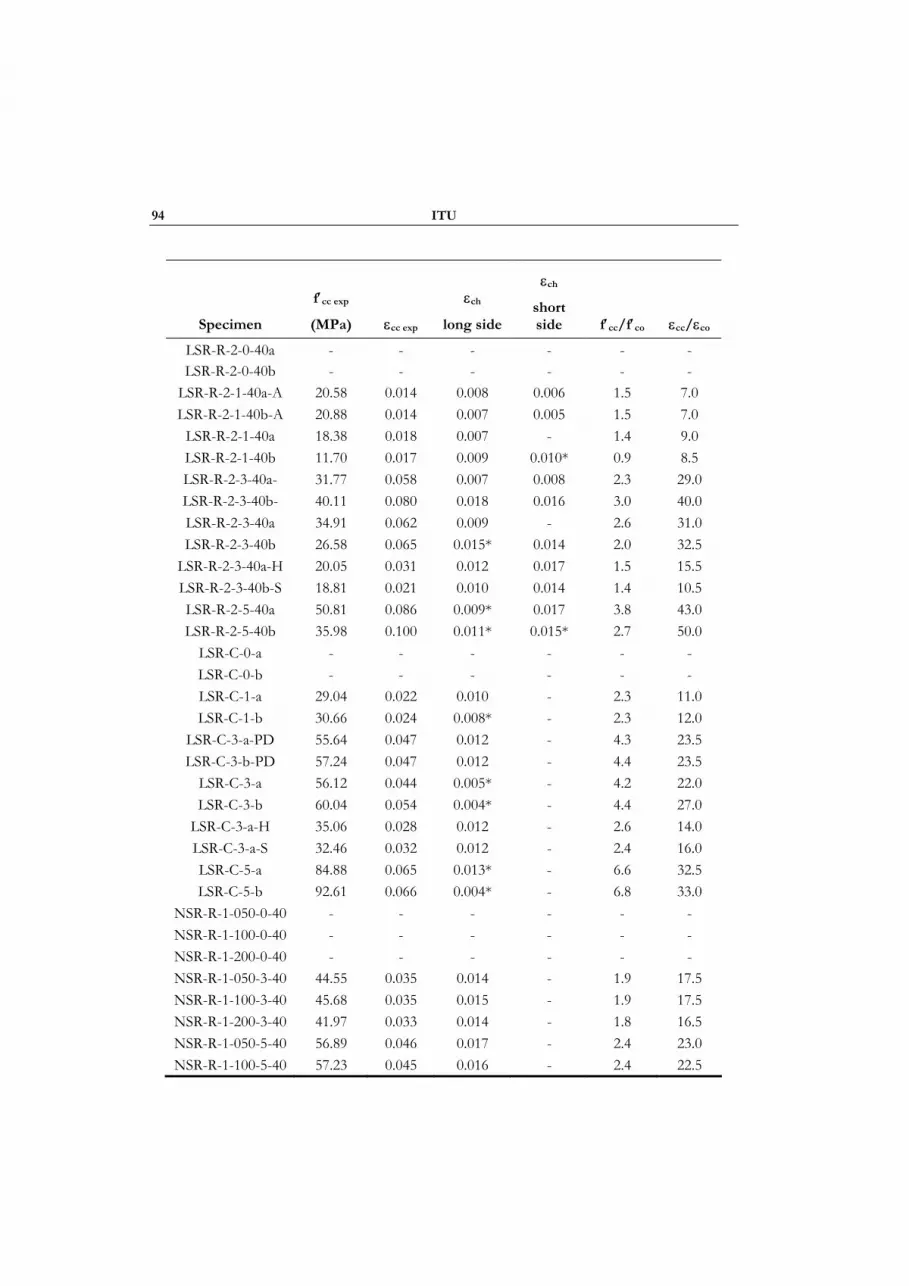
94 ITU
Specimen
f′cc exp
(MPa) εcc exp
εch
long side
εch
short side f′cc/f′co εcc/εco
LSR-R-2-0-40a - - - - - - LSR-R-2-0-40b - - - - - -
LSR-R-2-1-40a-A 20.58 0.014 0.008 0.006 1.5 7.0 LSR-R-2-1-40b-A 20.88 0.014 0.007 0.005 1.5 7.0
LSR-R-2-1-40a 18.38 0.018 0.007 - 1.4 9.0 LSR-R-2-1-40b 11.70 0.017 0.009 0.010* 0.9 8.5 LSR-R-2-3-40a- 31.77 0.058 0.007 0.008 2.3 29.0 LSR-R-2-3-40b- 40.11 0.080 0.018 0.016 3.0 40.0 LSR-R-2-3-40a 34.91 0.062 0.009 - 2.6 31.0 LSR-R-2-3-40b 26.58 0.065 0.015* 0.014 2.0 32.5
LSR-R-2-3-40a-H 20.05 0.031 0.012 0.017 1.5 15.5 LSR-R-2-3-40b-S 18.81 0.021 0.010 0.014 1.4 10.5 LSR-R-2-5-40a 50.81 0.086 0.009* 0.017 3.8 43.0 LSR-R-2-5-40b 35.98 0.100 0.011* 0.015* 2.7 50.0
LSR-C-0-a - - - - - - LSR-C-0-b - - - - - - LSR-C-1-a 29.04 0.022 0.010 - 2.3 11.0 LSR-C-1-b 30.66 0.024 0.008* - 2.3 12.0
LSR-C-3-a-PD 55.64 0.047 0.012 - 4.3 23.5 LSR-C-3-b-PD 57.24 0.047 0.012 - 4.4 23.5
LSR-C-3-a 56.12 0.044 0.005* - 4.2 22.0 LSR-C-3-b 60.04 0.054 0.004* - 4.4 27.0
LSR-C-3-a-H 35.06 0.028 0.012 - 2.6 14.0 LSR-C-3-a-S 32.46 0.032 0.012 - 2.4 16.0 LSR-C-5-a 84.88 0.065 0.013* - 6.6 32.5 LSR-C-5-b 92.61 0.066 0.004* - 6.8 33.0
NSR-R-1-050-0-40 - - - - - - NSR-R-1-100-0-40 - - - - - - NSR-R-1-200-0-40 - - - - - - NSR-R-1-050-3-40 44.55 0.035 0.014 - 1.9 17.5 NSR-R-1-100-3-40 45.68 0.035 0.015 - 1.9 17.5 NSR-R-1-200-3-40 41.97 0.033 0.014 - 1.8 16.5 NSR-R-1-050-5-40 56.89 0.046 0.017 - 2.4 23.0 NSR-R-1-100-5-40 57.23 0.045 0.016 - 2.4 22.5

Sub-Project 7 – 3.4. Computation of the resistance of structural elements considering steel & FRP 95
Specimen
f′cc exp
(MPa) εcc exp
εch
long side
εch
short side f′cc/f′co εcc/εco
NSR-R-1-200-5-40 58.26 0.052 0.015 - 2.5 26.0 NSR-R-1-000-3-40 41.08 0.024 0.013 - 1.8 12.0 NSR-R-2-050-0-40 - - - - - - NSR-R-2-100-0-40 - - - - - - NSR-R-2-175-0-40 - - - - - - NSR-R-2-050-3-40 40.15 0.036 0.012 0.005 1.7 18.0 NSR-R-2-100-3-40 42.84 0.039 0.012 0.013 1.8 19.5 NSR-R-2-175-3-40 40.63 0.034 0.013 0.011 1.7 17.0 NSR-R-2-050-5-40 59.99 0.069 0.014 0.014 2.6 34.5 NSR-R-2-100-5-40 53.63 0.045 0.014 0.014 2.3 22.5 NSR-R-2-175-5-40 47.81 0.034 0.012 0.012 2.0 17.0
NSR-C-050-0 - - - - - - NSR-C-100-0 - - - - - - NSR-C-145-0 - - - - - - NSR-C-050-3 77.46 0.034 0.013 - 3.3 17.0 NSR-C-100-3 72.51 0.029 0.011 - 3.1 14.5 NSR-C-145-3 71.83 0.033 0.012 - 3.1 16.5 NSR-C-050-5 95.07 0.044 0.012 - 4.1 22.0 NSR-C-100-5 94.88 0.043 0.011 - 4.0 21.5 NSR-C-145-5 94.25 0.044 0.013 - 4.0 22.0
In Figure 3-25 the stress–strain relationships of specimens with different cross-section are presented. As seen in these figures, all specimens experienced significant enhancement in strength and deformability after being retrofitted with 5 plies of CFRP jacket. While the strength enhancement was more remarkable for the specimens with circular cross-section, specimens with square and rectangular cross-sections exhibited higher axial deformations. In Figure 3-26 the comparison of LSR and NSR specimens are presented. As seen in these figures, CFRP jackets are more effective in the case of low concrete strength, in terms of strength and deformability.

96 ITU
0
2
4
6
8
-20000 0 20000 40000 60000 80000 100000 120000
Deformation (microstrain)
Axi
al S
tress
( σc/f
' co)
LSR-C-5-aLSR-R-1-5-40aLSR-R-2-5-40aS i 4
Figure 3-25. Axial Stress-Strain Relationships for Different Cross-sections
0
2
4
6
8
0 20000 40000 60000 80000 100000 120000
Axial Deformation (microstrain)
Axi
al S
tress
( σc/f
' co)
LSR-C-5-aNSR-C-5LSR-R-1-5-40aNSR-R-1-5-40LSR-R-2-5-40aNSR-R-2-5-40
Figure 3-26. Axial Stress-Strain Relationships for NSR and LSR Specimens
The following conclusions are derived after axial loading tests of CFRP jacketed low and medium strength circular, square and rectangular brittle reinforced concrete columns. Both for LSR and NSR series CFRP jackets enhanced the compressive strength and corresponding axial strain of the columns with circular, square and rectangular cross-sections. While the strength enhancement was more pronounced for circular cross-sections, deformability enhancement was more for square and rectangular cross-sections. Although in the case of unstrengthened specimens, longitudinal bars buckled
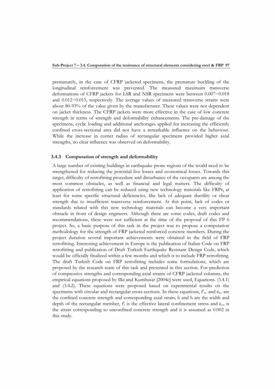
Sub-Project 7 – 3.4. Computation of the resistance of structural elements considering steel & FRP 97
prematurely, in the case of CFRP jacketed specimens, the premature buckling of the longitudinal reinforcement was prevented. The measured maximum transverse deformations of CFRP jackets for LSR and NSR specimens were between 0.007~0.018 and 0.012~0.015, respectively. The average values of measured transverse strains were about 80-93% of the value given by the manufacturer. These values were not dependent on jacket thickness. The CFRP jackets were more effective in the case of low concrete strength in terms of strength and deformability enhancements. The pre-damage of the specimens, cyclic loading and additional anchorages applied for increasing the efficiently confined cross-sectional area did not have a remarkable influence on the behaviour. While the increase in corner radius of rectangular specimens provided higher axial strengths, no clear influence was observed on deformability.
3.4.3 Computation of strength and deformability
A large number of existing buildings in earthquake prone regions of the world need to be strengthened for reducing the potential live losses and economical losses. Towards this target, difficulty of retrofitting procedure and disturbance of the occupants are among the most common obstacles, as well as financial and legal matters. The difficulty of application of retrofitting can be reduced using new technology materials like FRPs, at least for some specific structural deficiencies, like lack of adequate ductility or shear strength due to insufficient transverse reinforcement. At this point, lack of codes or standards related with this new technology materials can become a very important obstacle in front of design engineers. Although there are some codes, draft codes and recommendations, these were not sufficient at the time of the proposal of this FP 6 project. So, a basic purpose of this task in the project was to propose a computation methodology for the strength of FRP jacketed reinforced concrete members. During the project duration several important achievements were obtained in the field of FRP retrofitting. Interesting achievement in Europe is the publication of Italian Code on FRP retrofitting and publication of Draft Turkish Earthquake Resistant Design Code, which would be officially finalized within a few months and which is to include FRP retrofitting. The draft Turkish Code on FRP retrofitting includes some formulations, which are proposed by the research team of this task and presented in this section. For prediction of compressive strengths and corresponding axial strains of CFRP jacketed columns, the empirical equations proposed by Ilki and Kumbasar [2004c] were used, Equations. (3.4.1) and (3.4.2). These equations were proposed based on experimental results on the specimens with circular and rectangular cross-sections. In these equations, f′cc and εcc are the confined concrete strength and corresponding axial strain, b and h are the width and depth of the rectangular member, f′l is the effective lateral confinement stress and εco is the strain corresponding to unconfined concrete strength and it is assumed as 0.002 in this study.

98 ITU
cc l
co coCFRP
f ff f
1.2
1 2.4⎡ ⎤⎡ ⎤ ⎛ ⎞′ ′⎢ ⎥= + ⎜ ⎟⎢ ⎥′ ′⎢ ⎥⎣ ⎦ ⎝ ⎠⎣ ⎦
( 3.4.1 )
cc l
co coCFRP
fhb f
0.5
1 20εε
⎡ ⎤⎡ ⎤ ⎛ ⎞′⎛ ⎞⎢ ⎥= + ⎜ ⎟⎢ ⎥ ⎜ ⎟ ′⎝ ⎠⎢ ⎥⎣ ⎦ ⎝ ⎠⎣ ⎦
( 3.4.2 )
Effective lateral confinement stress, f′l can be obtained by Equation (3.4.3). In this equation, κa is the efficiency factor that is to be determined based on the section geometry as the ratio of effectively confined cross-sectional area to the gross cross-sectional area and can be calculated as given by ACI 440 [2002] or Wang and Restrepo [2001]. Efrp and ρf are the tensile elasticity modulus and ratio of wrapping material to the concrete cross-section, respectively. Ultimate tensile strength of FRP εh,rup is assumed to be 70% of the ultimate strain corresponding to tensile strength of FRP ε∗
fu. According to Lam and Teng [2003b], FRP ruptures around 60% of its ultimate tensile strain determined by the direct tension tests when wrapped around concrete members.
a f h rup frpl
Ef ,
2κ ρ ε
′ = (3.4.3 )
While predicting the confined concrete strength and corresponding axial strain, the contribution of internal transverse reinforcement (ITR) was also taken into account. For this purpose, the empirical equations proposed by Mander et al. [1988] were used for strength and ultimate axial strain, respectively, Equations. (3.4.4) and (3.4.5). After obtaining the strength and deformability enhancements provided by external CFRP jacket and internal transverse reinforcement, the total enhancement in strength and corresponding strain was calculated by using Equations (3.4.6) and (3.4.7). The predictions of confined concrete strength and corresponding axial strain for all specimens are presented in Table 3-10.
cc l l
co co coITR
f f ff f f
7.941.254 2.254 1 2⎡ ⎤⎡ ⎤′ ′ ′
= − + + −⎢ ⎥⎢ ⎥′ ′ ′⎢ ⎥⎣ ⎦ ⎣ ⎦ (3.4.4 )
cc l
co coITR
ff
1 5 1εε
⎡ ⎤⎡ ⎤ ⎛ ⎞′= + −⎢ ⎥⎜ ⎟⎢ ⎥ ′⎢ ⎥⎣ ⎦ ⎝ ⎠⎣ ⎦
(3.4.5 )
cc co cc cc
co co coTOTAL CFRP ITR
f f f ff f f
' ' ' '
' ' '1 1⎡ ⎤ ⎡ ⎤ ⎡ ⎤−
= − + −⎢ ⎥ ⎢ ⎥ ⎢ ⎥⎣ ⎦ ⎣ ⎦ ⎣ ⎦
(3.4.6 )
cc co cc cc
co co coTOTAL CFRP ITR
1 1ε ε ε ε
ε ε ε⎡ ⎤ ⎡ ⎤ ⎡ ⎤−
= − + −⎢ ⎥ ⎢ ⎥ ⎢ ⎥⎣ ⎦ ⎣ ⎦ ⎣ ⎦
(3.4.7 )
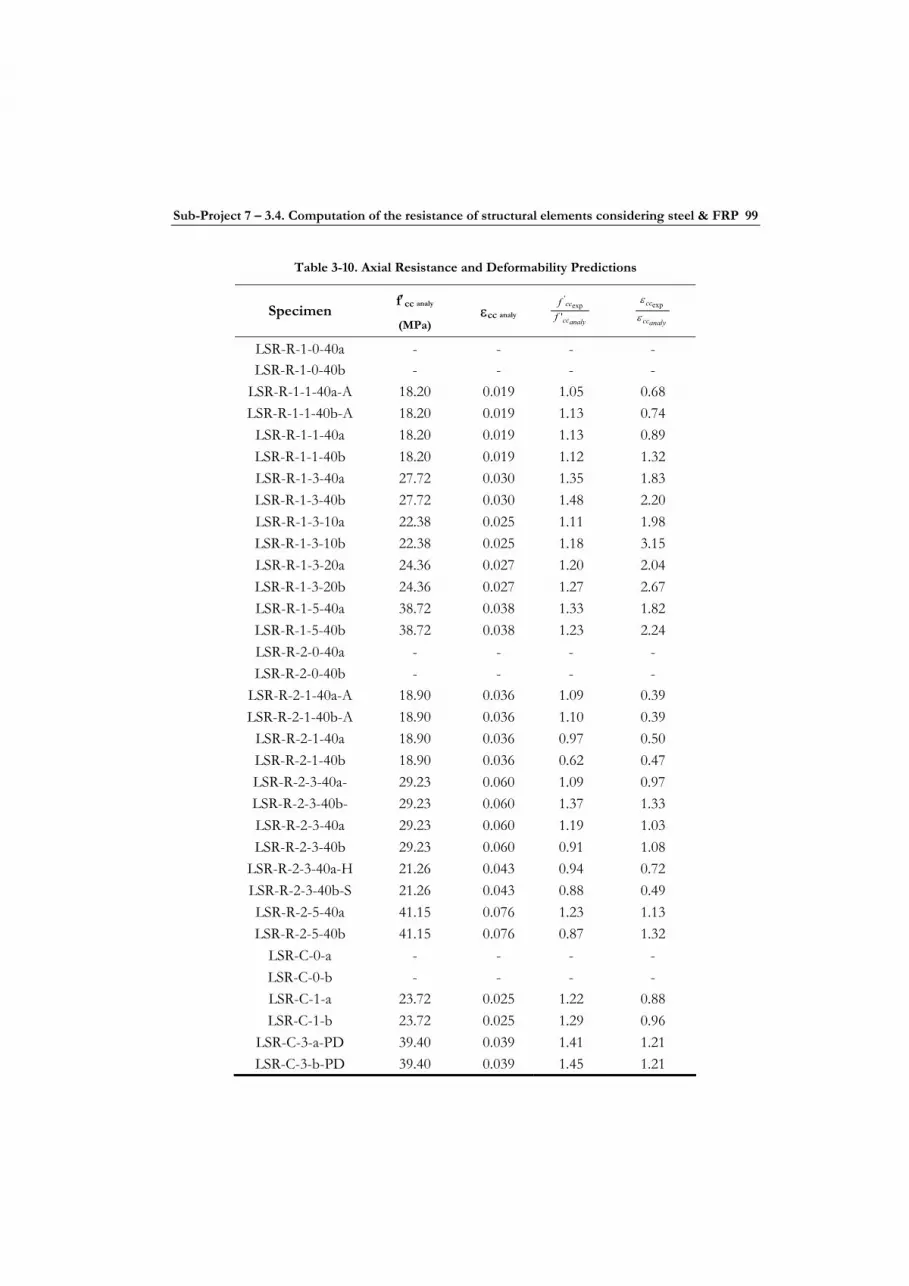
Sub-Project 7 – 3.4. Computation of the resistance of structural elements considering steel & FRP 99
Table 3-10. Axial Resistance and Deformability Predictions
Specimen f′cc analy
(MPa) εcc analy
analycc
cc
ff'
exp'
analycc
cc
ε
ε exp
LSR-R-1-0-40a - - - - LSR-R-1-0-40b - - - -
LSR-R-1-1-40a-A 18.20 0.019 1.05 0.68 LSR-R-1-1-40b-A 18.20 0.019 1.13 0.74
LSR-R-1-1-40a 18.20 0.019 1.13 0.89 LSR-R-1-1-40b 18.20 0.019 1.12 1.32 LSR-R-1-3-40a 27.72 0.030 1.35 1.83 LSR-R-1-3-40b 27.72 0.030 1.48 2.20 LSR-R-1-3-10a 22.38 0.025 1.11 1.98 LSR-R-1-3-10b 22.38 0.025 1.18 3.15 LSR-R-1-3-20a 24.36 0.027 1.20 2.04 LSR-R-1-3-20b 24.36 0.027 1.27 2.67 LSR-R-1-5-40a 38.72 0.038 1.33 1.82 LSR-R-1-5-40b 38.72 0.038 1.23 2.24 LSR-R-2-0-40a - - - - LSR-R-2-0-40b - - - -
LSR-R-2-1-40a-A 18.90 0.036 1.09 0.39 LSR-R-2-1-40b-A 18.90 0.036 1.10 0.39
LSR-R-2-1-40a 18.90 0.036 0.97 0.50 LSR-R-2-1-40b 18.90 0.036 0.62 0.47 LSR-R-2-3-40a- 29.23 0.060 1.09 0.97 LSR-R-2-3-40b- 29.23 0.060 1.37 1.33 LSR-R-2-3-40a 29.23 0.060 1.19 1.03 LSR-R-2-3-40b 29.23 0.060 0.91 1.08
LSR-R-2-3-40a-H 21.26 0.043 0.94 0.72 LSR-R-2-3-40b-S 21.26 0.043 0.88 0.49 LSR-R-2-5-40a 41.15 0.076 1.23 1.13 LSR-R-2-5-40b 41.15 0.076 0.87 1.32
LSR-C-0-a - - - - LSR-C-0-b - - - - LSR-C-1-a 23.72 0.025 1.22 0.88 LSR-C-1-b 23.72 0.025 1.29 0.96
LSR-C-3-a-PD 39.40 0.039 1.41 1.21 LSR-C-3-b-PD 39.40 0.039 1.45 1.21
100 ITU
Specimen f′cc analy
(MPa) εcc analy
analycc
cc
ff'
exp'
analycc
cc
ε
ε exp
LSR-C-3-a 39.40 0.039 1.42 1.13 LSR-C-3-b 39.40 0.039 1.52 1.38
LSR-C-3-a-H 27.31 0.029 1.28 0.97 LSR-C-3-a-S 27.31 0.029 1.19 1.10 LSR-C-5-a 57.51 0.049 1.48 1.33 LSR-C-5-b 57.51 0.049 1.61 1.35
NSR-R-1-0-40 - - - - NSR-R-2-0-40 - - - -
NSR-C-0 - - - - NSR-R-1-3-40 38.94 0.022 1.08 1.50 NSR-R-1-5-40 48.56 0.028 1.20 1.86 NSR-R-2-3-40 38.93 0.043 1.04 0.79 NSR-R-2-5-40 49.37 0.054 0.97 0.74
NSR-C-3 49.80 0.028 1.44 1.18 NSR-C-5 65.65 0.035 1.44 1.29
The empirical equations, proposed by the authors before, predicted the compressive strength and corresponding axial strains of the specimens with a reasonable accuracy.
3.4.4 Verification of proposed computation methodology
For further verification of the proposed equations, more than 200 specimens tested by other researchers were examined and their compressive strength and corresponding deformations were determined using the proposed equations. The comparisons of predictions with experimental data are presented in Figure 3-27.

Sub-Project 7 – 3.4. Computation of the resistance of structural elements considering steel & FRP 101
0.0
10.0
20.0
30.0
40.0
50.0
60.0
70.0
80.0
0.0 10.0 20.0 30.0 40.0 50.0 60.0 70.0 80.0
εcc/εco (Analytical)
ε cc/ ε
co (E
xp.)
Circular-ManufacturerRectangular-ManufacturerCircular-Coupon Rectangular-Coupon
0.0
2.0
4.0
6.0
8.0
10.0
12.0
14.0
16.0
18.0
20.0
0.0 2.0 4.0 6.0 8.0 10.0 12.0 14.0 16.0 18.0 20.0
f'cc/f'co (Analytical)
f' cc/f
' co (E
xp.)
Circular-ManufacturerRectangular-ManufacturerCircular-Coupon Rectangular-Coupon
Figure 3-27. Comparison of predictions with available experimental data
3.4.5 Conclusions
The objective of this sub-task is obtaining experimental results of FRP jacketed reinforced concrete members concerning the effects of different variables such as thickness of the FRP jacket, cross-section shape, unconfined concrete strength, corner radius, loading type, bonding details, pre-damage, etc. and study the methodology of determining the axial resistance of reinforced concrete members considering the contributions of both internal steel reinforcement and external FRP jacket. Naturally, an analytical work is carried out in parallel fashion for predicting the strength and deformability of FRP jacketed members considering the dual effect of internal steel and external CFRP jackets. Totally, 68 specimens were tested under concentric compressive stresses, either by monotonic increasing loading or repeated loading. 40 of the specimens were constructed using low quality of concrete and inadequate transverse reinforcement, while 28 specimens were constructed using medium strength concrete and various amounts of internal transverse reinforcement. Most of the specimens were tested under concentric compression after being jacketed with CFRP, while some specimens were tested as original for representing the reference behaviour. An analytical study is carried out for determining the combined confinement effect of internal and external transverse reinforcement. During this analysis, the contribution of internal reinforcement was taken into account using different models proposed by different researchers, including the authors of this section. The confinement effect of external FRP reinforcement was also taken into account using a model proposed by the authors of this section before. The predicted analytical results were then compared with the experimental data obtained at
102 ITU
the end of this study (for 16 circular and 27 rectangular columns), as well as previous studies of the authors of this section (for 17 circular and 32 rectangular columns). The reason of difference between the number of specimens tested in this study and specimens taken into account for comparison with analytical predictions is; to exclude the specimens, which had special features like additional anchorages, pre-damage or specimens loaded cyclically. Otherwise, it was impossible to propose simple and applicable equations for strength and deformability. For further verification of the proposed equations, more than 200 specimens tested by other researchers were examined and their compressive strength and corresponding deformations were determined using the proposed equations. At the end of this extensive comparison, it was seen that the proposed methodology and design equations are satisfactorily representing the behaviour. The proposed equations for the strength and deformability of FRP jacketed columns, verified with the tests and analytical comparisons carried out during the present project, are included in the draft version of the Turkish Seismic Design Code (2006).

Sub-Project 7 – 3.5. Urban rehabilitation using FRP 103
3.5 URBAN REHABILITATION USING FRP
3.5.1 Introduction
Seismic risk assessment and hazard mitigation for urban infrastructures located in seismic regions is a challenge shared by many countries around the world. The variability and associated uncertainty makes it more difficult to assess and mitigate seismic hazards, and requires development of rapid and cost efficient assessment tools for effective prioritization and timely mitigation. In urban areas, where there is a large stock of existing buildings, most of which have inferior seismic capacities, determining the vulnerable buildings within the existing building stock is a high priority task for taking the necessary remedial measures for disaster mitigation prior to potential seismic events. Limited time, scarcity of funds, and the high variability in seismic resistance of structures in these areas have led to a concentrated research effort towards development of approximate seismic assessment tools that can potentially provide a rapid, efficient, and reliable mitigation strategy. In the following sections, the methods developed for seismic assessment of large building stocks are provided, followed by their implementation on a large group of buildings located in Zeytinburnu, Istanbul (Chapter 1).
Feasible retrofitting solutions have been developed for selected residential mid-rise apartment buildings under high seismic risk in Istanbul. A feasible solution is considered as the optimal combination of cost, downtime, disturbance, technical applicability and social impact. The basic elements of conventional system retrofitting are concrete infilled shear walls (Chapter 2). Recently, new techniques such as the existing masonry partition walls enhanced by applying FRP sheets on their surfaces have been development. Guidelines for the application of this new technique are provided.
3.5.2 Seismic Performance Assessment Procedures
A three tier approach has been developed for seismic vulnerability assessment of buildings located in urban areas. The purpose of three level assessments is to identify likely highly vulnerable buildings by reducing the large building stock into a manageable size so that the mitigation strategies can be investigated. These procedures follow essentially three main stages: (1) walk-down evaluation, (2) preliminary evaluation and (3) detailed evaluation. The first stage, walk-down evaluation, does not require any analysis and it relies on the past performance of similar buildings. The goal in this stage is to rank highly vulnerable buildings that require further investigation. The second stage, preliminary investigation stage generally covers the buildings that are designated to be inadequate in the first stage. In this stage simplified analysis is performed to attain a more detailed and reliable assessment. The final evaluation stage, which is more case oriented, covers an in-depth evaluation through sophisticated structural analysis methods. The
104 METU
need and the scheme for rehabilitation is determined based on the detailed assessment results. These procedures are explained next briefly and the reader is referred to LESSLOSS deliverable reports 47 and 107 for the details ( www.lessloss.org ).
3.5.2.1 The Walkdown Evaluation Procedure
A fast and simple seismic risk assessment procedure is proposed for vulnerable urban building stocks (Sucuoğlu et al. 2007). It is basically a sidewalk survey procedure based on observing selected building parameters from the street side, and calculating a performance score for determining the risk priorities for buildings.
Recent earthquakes in urban environments revealed that building damages increase with the number of storeys when the buildings lack the basic seismic resistant design features. Other factors that have significant contribution to damage are also well established. These are the presence of severe irregularities such as the soft storeys and heavy overhangs, other discontinuities in load paths, poor material quality, detailing and workmanship. It is usually difficult to quantify the sensitivity of damage to each parameter analytically, however statistics can be used. Some of the important parameters stated above that influence damage significantly can be determined quite easily, by visual observation.
According to the procedure proposed here, structural parameters that have to be observed during the field surveys are the number of storeys, soft storeys, heavy overhangs, pounding, topographic effects and the overall apparent quality of the building reflecting the quality of construction. Once the vulnerability parameters of a building are obtained from walkdown surveys and its location is determined, the seismic performance score PS can be calculated by using Equation (3.1.1). The base scores, BS, the vulnerability scores, VS, and the vulnerability score multipliers, VSM, to be used in Equation (3.1.1) are defined in Table 3-11 and Table 3-12, respectively.
= + ∑( ) ( ) ( )PS BS VSM x VS (3.1.1)
The weight of each building vulnerability parameter was evaluated by statistical procedures, based on the Duzce database.

Sub-Project 7 – 3.5. Urban rehabilitation using FRP 105
Table 3-11. Base Scores and Vulnerability Scores for Concrete Buildings
Base Score (BS) Vulnerability Scores (VS) Number of storeys
Zon
e I
Zon
e II
Zon
e II
I
Soft
stor
ey
Hea
vy
Ove
rhan
gs
App
aren
t Q
ualit
y
Shor
t
Colu
mn
Poun
ding
Topo
grap
hic
Eff
ects
1-2 100 130 150 0 -5 -5 -5 0 0 3 90 120 140 -15 -10 -10 -5 -2 0 4 75 100 120 -20 -10 -10 -5 -3 -2 5 65 85 100 -25 -15 -15 -5 -3 -2
6-7 60 80 90 -30 -15 -15 -5 -3 -2
3.5.2.2 Preliminary Assessment
The preliminary assessment procedures are intended to be applied to the vulnerable buildings identified by the walkdown assessment procedures, so the buildings are subjected to a relatively more detailed assessment that require further data. In this context, the discriminant analysis technique (a statistical method) was used to develop a preliminary evaluation methodology for assessing seismic vulnerability of existing low- to medium-rise reinforced concrete buildings (Yakut et al. 2006). The main objective of the procedure outlined below is to identify the buildings that are highly vulnerable to damage. The procedure is developed for structures whose structural system is formed by frames or frames and structural walls. The procedure is applicable for cases where the number of storeys is less than or equal to 7. The structures described above comprise the majority of the existing RC buildings in Turkey.
Table 3-12. Vulnerability Parameters, (VSM)
Parameter Presence
Soft
stor
ey
Hea
vy
Ove
rhan
gs
Ap
par
ent
Qu
alit
y
Shor
t C
olu
mn
Pou
nd
ing T
opog
rap
hic
E
ffec
ts
Does not exist 0 0 0 0 0 Exists 1 1 1 1 1 Good 0
Moderate 1 Poor 2

106 METU
Considering the characteristics of the damaged structures and the huge size of the existing building stock in Turkey, the following parameters were chosen as the basic estimation parameters of the proposed method:
• number of storeys (n), • minimum normalized lateral stiffness index (mnlstfi), • minimum normalized lateral strength index (mnlsi), • normalized redundancy score (nrs), • soft storey index (ssi), • overhang ratio (or)
These parameters take into account the major architectural irregularities in plan and in elevation (ssi, or, nrs), the lateral strength (mnlsi) and stiffness (mnlsi) of the buildings. Lateral strength and stiffness of the building are determined from the sizes of the columns, shear walls and masonry infill walls comprising the structural resistance of the building.
These parameters are calculated for each building to obtain a damage index that is compared with a cutoff value to determine its expected performance. The damage index is computed considering two performance objectives, namely life safety and immediate occupancy. The damage index or the damage score corresponding to the life safety performance classification (DILS) is computed from the discriminant function given in Equation (3.1.3).
= − − − + + −0.620 0.246 0.182 0.699 3.269 2.728 4.905LSDI mnlstfi mnlsi nrs ssi or (3.1.3)
In the case of immediate occupancy performance classification (IOPC), the discriminant function, where DIIO is the damage score corresponding to IOPC, based on these variables is:
= − − − + + −0.808 0.334 0.107 0.687 0.508 3.884 2.868IODI n mnlstfi mnlsi nrs ssi or (3.1.4)
In the proposed classification methodology, buildings are evaluated according to both performance levels. The steps to be followed are listed below.
1. Calculate DILS and DIIO scores by using Eq. (3.1.3) and Eq. (3.1.4), respectively. 2. Determine the cutoff values for each performance classification by using the relationships given in Eq. (3.1.5).
Sub-Project 7 – 3.5. Urban rehabilitation using FRP 107
The LSCVR and IOCVR values in these relationships are obtained based on the number of storeys above the ground level. The CM values are adjustment factors, which introduce the spatial variation of the ground motion in the evaluation process. These values are given in LessLoss Deliverable 107 (www.lessloss.org )
= × = ×LS CVR IO CVRCV CM LS , CV CM IO (3.1.5)
By comparing the CV values with associated DI value calculate performance grouping of the building for life safety performance classification (LSPC) and immediate occupancy performance classification (IOPC) as follows:
If DILS > CVLS take PGLS=1 If DILS < CVLS take PGLS=0 If DIIO > CVLS take PGIO=1 If DIIO < CVLS take PGIO=0
By examining the performance groupings of the building for LSPC and IOPC, make a decision on the probable expected performance level of the building. In this process, if both performance groupings yield PG=0 then the building is classified as having low risk, if PG=1 in both cases then it is classified as having high risk, otherwise it is considered as intermediate needing further analysis.
3.5.2.3 Detailed Assessment Procedure
As mentioned earlier, detailed assessment procedures are applied to individual buildings to determine the need for retrofit as well as verifying the selected retrofit option. A detailed seismic performance assessment procedure has been developed for reinforced concrete frame buildings with masonry in-fill walls (Erduran and Yakut, 2007). The procedure is based on member damage functions developed for the primary components; columns, beams and in-fill walls. Analytical investigations carried out to determine the influence of a number of parameters on the damageability of components were combined with existing experimental data to develop component damage functions expressed in terms of member deformations. The component damage states are combined taking into account their importance to determine the storey and building level damage states that are then used to assess the global performance. The procedure has been calibrated and compared with other procedures by predicting the observed performance of the buildings exposed to recent earthquakes in Turkey. It was observed that the damage experienced by most of the components of these buildings was predicted satisfactorily, and that the observed building damage states were captured.
108 METU
a. Outline of the Procedure
The procedure used in this project is a detailed vulnerability assessment procedure carried out for an individual building under a given ground motion or design spectrum. The outline of the procedure is explained in this part. The response parameters that have been used as pertaining to seismic damage are the interstorey drift ratio for columns and infill walls and the chord rotation for beams.
The steps involved in the procedure developed are summarized below.
Step 1 – Data Collection:
The developed methodology requires a nonlinear analysis, either static or dynamic, of the given building. For this, first of all, some data must be collected about the building at hand. This data includes the design drawings, as-built dimensions of the building, the condition of the building and the material properties, preferably obtained from in-situ tests.
Step 2 – Nonlinear Analysis & Determination of the Member End Deformations:
The computer model developed may be a two dimensional or a three dimensional model, based on the choice of the user. Similarly, the user chooses the type of nonlinear analysis (nonlinear static analysis or nonlinear time history analysis) that will be used. If a nonlinear static analysis is carried out, the capacity curve obtained as a result of this analysis must be used to determine the performance point of the building under the prescribed ground motion or response spectrum, using the procedures available in literature such as the Capacity Spectrum Method summarized in ATC-40, the Displacement Coefficient Method of FEMA-356 or the Constant Ductility Spectrum Method. The member end deformations at this performance point will be recorded and used in the subsequent steps. If a nonlinear time history analysis is carried out, then the maximum member end deformations will be recorded.
Step 3 – Determination of the Member Damage Scores:
The maximum member end deformations obtained as a result of the nonlinear analysis will be input in the damage functions developed to compute the damage score of each member.

Sub-Project 7 – 3.5. Urban rehabilitation using FRP 109
Step 4 – Determination of the storey and Building Damage Scores:
Once the damage score for each member is determined, then the weighted average of these damage scores is computed to determine the damage score of each storey and finally of the entire building. The weighing coefficients used here depend on the contribution of each member in resisting the seismic forces and named as component importance factors. Approximate values for the component importance factors were developed and are given in a tabular format.
The final step of the procedure is the determination of the performance of the building based on the computed building damage score.
The details of these steps are given elsewhere (Erduran and Yakut 2004a, 2004b).
b. Component Damage Functions
For each type of component, numerical analyses and experimental test results have been used to develop damage curves. The functional form for the damage curves is the one given in Eq.3.1.6.
δ
δ δ⎛ ⎞−⎜ ⎟⎝ ⎠
⎡ ⎤⎢ ⎥= −⎢ ⎥⎣ ⎦
( ) 1 ( )
b
aDamage e g (3.1.6)
where
πδδ ⎡ ⎤⎛ ⎞= − ⎜ ⎟⎢ ⎥⎝ ⎠⎣ ⎦( ) 0.5 1 cosg
c if δ≤c
g(δ)=1 if δ>c (3.1.7)
In these equations, δ represents the interstorey drift ratio and a, b, and c are the equation parameters. In case of beams, δ is replaced by θ which represents the end rotation of the beam. The values of these parameters are given in Table 3-13 and Table 3-15 for columns, beams and infill walls. The beams and columns are grouped into theree depending on their ductility level. Infill walls are classified into four based on their material and geometrical properties. To illustrate the shape of damage curves Figure 3-28 displays them for columns.
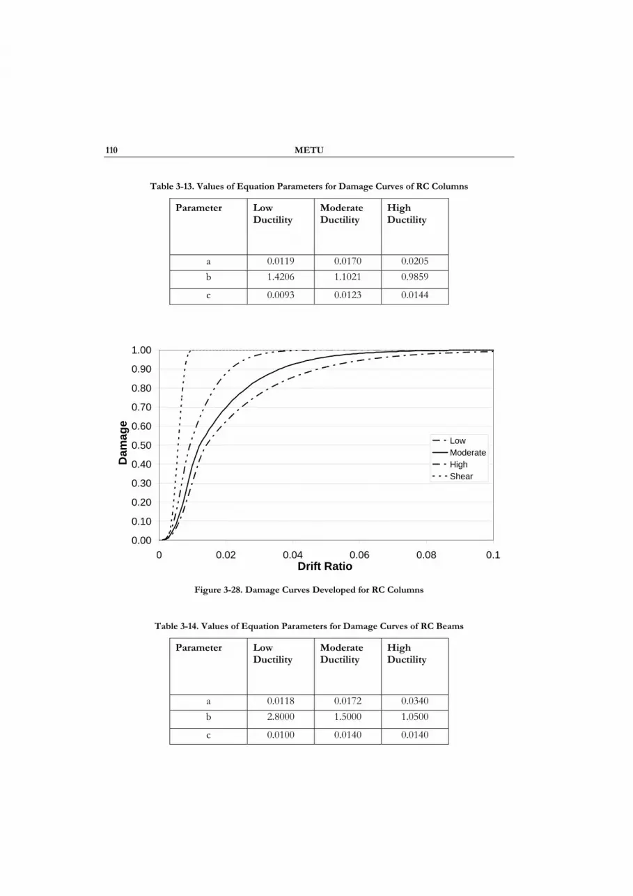
110 METU
Table 3-13. Values of Equation Parameters for Damage Curves of RC Columns
Parameter Low Ductility
Moderate Ductility
High Ductility
a 0.0119 0.0170 0.0205 b 1.4206 1.1021 0.9859
c 0.0093 0.0123 0.0144
0.00
0.10
0.20
0.30
0.40
0.50
0.60
0.70
0.80
0.90
1.00
0 0.02 0.04 0.06 0.08 0.1Drift Ratio
Dam
age
LowModerateHighShear
Figure 3-28. Damage Curves Developed for RC Columns
Table 3-14. Values of Equation Parameters for Damage Curves of RC Beams
Parameter Low Ductility
Moderate Ductility
High Ductility
a 0.0118 0.0172 0.0340 b 2.8000 1.5000 1.0500
c 0.0100 0.0140 0.0140
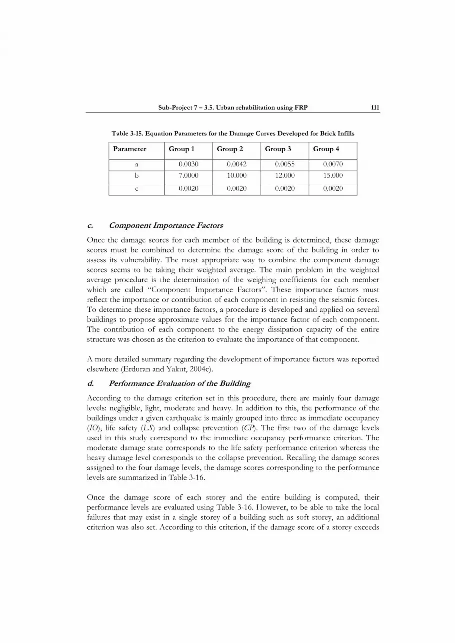
Sub-Project 7 – 3.5. Urban rehabilitation using FRP 111
Table 3-15. Equation Parameters for the Damage Curves Developed for Brick Infills
Parameter Group 1 Group 2 Group 3 Group 4
a 0.0030 0.0042 0.0055 0.0070 b 7.0000 10.000 12.000 15.000
c 0.0020 0.0020 0.0020 0.0020
c. Component Importance Factors
Once the damage scores for each member of the building is determined, these damage scores must be combined to determine the damage score of the building in order to assess its vulnerability. The most appropriate way to combine the component damage scores seems to be taking their weighted average. The main problem in the weighted average procedure is the determination of the weighing coefficients for each member which are called “Component Importance Factors”. These importance factors must reflect the importance or contribution of each component in resisting the seismic forces. To determine these importance factors, a procedure is developed and applied on several buildings to propose approximate values for the importance factor of each component. The contribution of each component to the energy dissipation capacity of the entire structure was chosen as the criterion to evaluate the importance of that component.
A more detailed summary regarding the development of importance factors was reported elsewhere (Erduran and Yakut, 2004c).
d. Performance Evaluation of the Building
According to the damage criterion set in this procedure, there are mainly four damage levels: negligible, light, moderate and heavy. In addition to this, the performance of the buildings under a given earthquake is mainly grouped into three as immediate occupancy (IO), life safety (LS) and collapse prevention (CP). The first two of the damage levels used in this study correspond to the immediate occupancy performance criterion. The moderate damage state corresponds to the life safety performance criterion whereas the heavy damage level corresponds to the collapse prevention. Recalling the damage scores assigned to the four damage levels, the damage scores corresponding to the performance levels are summarized in Table 3-16.
Once the damage score of each storey and the entire building is computed, their performance levels are evaluated using Table 3-16. However, to be able to take the local failures that may exist in a single storey of a building such as soft storey, an additional criterion was also set. According to this criterion, if the damage score of a storey exceeds
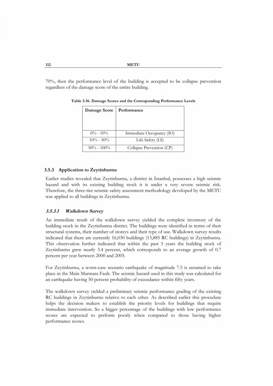
112 METU
70%, then the performance level of the building is accepted to be collapse prevention regardless of the damage score of the entire building.
Table 3-16. Damage Scores and the Corresponding Performance Levels
Damage Score Performance
0% - 10% Immediate Occupancy (IO) 10% - 50% Life Safety (LS)
50% - 100% Collapse Prevention (CP)
3.5.3 Application to Zeytinburnu
Earlier studies revealed that Zeytinburnu, a district in İstanbul, possesses a high seismic hazard and with its existing building stock it is under a very severe seismic risk. Therefore, the three-tier seismic safety assessment methodology developed by the METU was applied to all buildings in Zeytinburnu.
3.5.3.1 Walkdown Survey
An immediate result of the walkdown survey yielded the complete inventory of the building stock in the Zeytinburnu district. The buildings were identified in terms of their structural systems, their number of storeys and their type of use. Walkdown survey results indicated that there are currently 16,030 buildings (13,885 RC buildings) in Zeytinburnu. This observation further indicated that within the past 5 years the building stock of Zeytinburnu grew nearly 3.4 percent, which corresponds to an average growth of 0.7 percent per year between 2000 and 2005.
For Zeytinburnu, a worst-case scenario earthquake of magnitude 7.5 is assumed to take place in the Main Marmara Fault. The seismic hazard used in this study was calculated for an earthquake having 50 percent probability of exceedance within fifty years.
The walkdown survey yielded a preliminary seismic performance grading of the existing RC buildings in Zeytinburnu relative to each other. As described earlier this procedure helps the decision makers to establish the priority levels for buildings that require immediate intervention. So a bigger percentage of the buildings with low performance scores are expected to perform poorly when compared to those having higher performance scores.
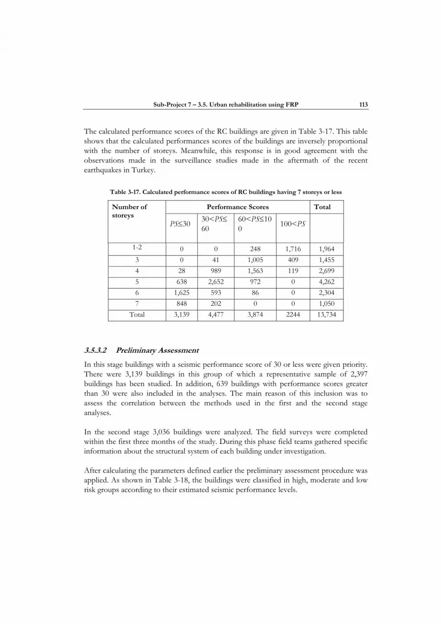
Sub-Project 7 – 3.5. Urban rehabilitation using FRP 113
The calculated performance scores of the RC buildings are given in Table 3-17. This table shows that the calculated performances scores of the buildings are inversely proportional with the number of storeys. Meanwhile, this response is in good agreement with the observations made in the surveillance studies made in the aftermath of the recent earthquakes in Turkey.
Table 3-17. Calculated performance scores of RC buildings having 7 storeys or less
Performance Scores Total Number of storeys
PS≤30 30<PS≤60
60<PS≤100 100<PS
1-2 0 0 248 1,716 1,964 3 0 41 1,005 409 1,455 4 28 989 1,563 119 2,699 5 638 2,652 972 0 4,262 6 1,625 593 86 0 2,304 7 848 202 0 0 1,050
Total 3,139 4,477 3,874 2244 13,734
3.5.3.2 Preliminary Assessment
In this stage buildings with a seismic performance score of 30 or less were given priority. There were 3,139 buildings in this group of which a representative sample of 2,397 buildings has been studied. In addition, 639 buildings with performance scores greater than 30 were also included in the analyses. The main reason of this inclusion was to assess the correlation between the methods used in the first and the second stage analyses.
In the second stage 3,036 buildings were analyzed. The field surveys were completed within the first three months of the study. During this phase field teams gathered specific information about the structural system of each building under investigation.
After calculating the parameters defined earlier the preliminary assessment procedure was applied. As shown in Table 3-18, the buildings were classified in high, moderate and low risk groups according to their estimated seismic performance levels.

114 METU
Table 3-18. Results of the Preliminary Assessment Method
Number of storeys
High risk group
Moderate risk group
Low risk group
Total
≤3 10 18 71 99 4 180 81 71 332 5 713 170 46 929 6 808 262 77 1,147 7 387 119 23 529
Total 2,098 650 288 3,036
Table 3-18 illustrates that 2,098 buildings out of 3,036 (69.1 percent) were classified in the high seismic risk group. Moreover, as can be revealed from Table 3-18, while a smaller percentage of the low-rise buildings were in the high seismic risk group, bigger portions of the mid-rise buildings (i.e. 4-7 storey buildings) were placed in this category. This trend agrees well with the observations made during the reconnaissance studies performed in the aftermath of the recent earthquakes.
3.5.3.3 Detailed Assessment
The procedure developed has been used for assessment of some buildings selected from the Zeytinburnu building inventory. In the assessment of the buildings, the elastic response spectrum proposed in the National Earthquake Hazards Reduction Program (NEHRP) document published in 2000 was used to represent a ground motion with a probability of exceedance of 50% in 50 years. The major parameters in this response spectrum are the spectral acceleration at short periods (SDS) and the spectral acceleration at the period of 1 sec (SD1).
Within the scope of this project, the detailed assessment of five mid-rise buildings (4-6 storeys) with variable material properties was carried out. Table 3-19 presents the SDS and SD1 values determined for each building based on their location.
The target displacement of each building under the specified ground motion was computed using the displacement coefficient method summarized in FEMA 356 (2000). Once the displacement demand is determined, the assessment procedure summarized above was applied on each building to determine expected performance of each member, each storey and the entire building under the given ground motion. Table 3-19 summarizes the target roof drift ratio under the given elastic spectrum (δt), maximum
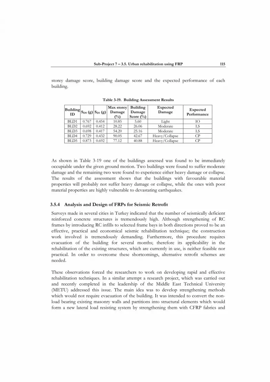
Sub-Project 7 – 3.5. Urban rehabilitation using FRP 115
storey damage score, building damage score and the expected performance of each building.
Table 3-19. Building Assessment Results
Building ID
SDS (g) SD1 (g) Max storey
Damage (%)
Building Damage
Score (%)
Expected Damage
Expected Performance
BLD1 0.767 0.454 10.85 5.60 Light IO BLD2 0.692 0.412 28.22 26.06 Moderate LS BLD3 0.698 0.417 54.20 25.16 Moderate LS BLD4 0.729 0.432 90.05 42.67 Heavy/Collapse CP BLD5 0.873 0.692 77.12 40.88 Heavy/Collapse CP
As shown in Table 3-19 one of the buildings assessed was found to be immediately occupiable under the given ground motion. Two buildings were found to suffer moderate damage and the remaining two were found to experience either heavy damage or collapse. The results of the assessment shows that the buildings with favourable material properties will probably not suffer heavy damage or collapse, while the ones with poor material properties are highly vulnerable to devastating earthquakes.
3.5.4 Analysis and Design of FRPs for Seismic Retrofit
Surveys made in several cities in Turkey indicated that the number of seismically deficient reinforced concrete structures is tremendously high. Although strengthening of RC frames by introducing RC infills to selected frame bays in both directions proved to be an effective, practical and economical seismic rehabilitation technique; the construction work involved is tremendously demanding. Furthermore, this procedure requires evacuation of the building for several months; therefore its applicability in the rehabilitation of the existing structures, which are currently in use, is neither feasible nor practical. In order to overcome these shortcomings, alternative retrofit schemes are needed.
These observations forced the researchers to work on developing rapid and effective rehabilitation techniques. In a similar attempt a research project, which was carried out and recently completed in the leadership of the Middle East Technical University (METU) addressed this issue. The main idea was to develop strengthening methods which would not require evacuation of the building. It was intended to convert the non-load bearing existing masonry walls and partitions into structural elements which would form a new lateral load resisting system by strengthening them with CFRP fabrics and

116 METU
integrating them with the existing structural system. Thus the rehabilitated structure would have adequate lateral stiffness and lateral load carrying capacity.
The main premise of this practical retrofit scheme is to limit inter-storey deformations by FRP strengthened infill walls that are integrated to the boundary frame members through FRP anchors. Based on failure modes and measured deformation limits obtained from a large database of experiments, a diagonal compression-strut and tension-tie model was developed. The estimated envelope load deformation response of frame specimens was compared with the envelope of reversed cyclic test results. A good agreement was observed between analytical and experimental strength and deformation capacity of specimens. Finally a simplified model was proposed for use in displacement based design of FRPs for deficient RC frame buildings. The performance of the FRP retrofit scheme was demonstrated by analyzing an actual deficient RC building with HCT infills. It was observed that prior to FRP retrofit about 75% of the columns are in a total collapse limit state meaning that their deformation capacities are significantly exceeded. Upon FRP retrofit it was observed that a drift control was provided and deformation demands on the structure were significantly reduced.
3.5.4.1 Strengthening with FRP
The idea of the FRP retrofit scheme is to reduce inter-storeydeformation demands by using FRPs to act as tension ties similar to a steel cross-brace configuration. In order to achieve this, diagonal FRPs bonded on the infill wall is tied to the framing members using FRP anchors as shown in Figure 3-29. The tension tie formed in this way provides additional contributions to the load carrying capacity and the lateral stiffness of the existing RC frame structure, in addition to the strength and stiffness provided by the compression strut formed along the infill diagonal. Special embedded fan type FRP anchors formed by rolling FRP sheets are connected in the corner region in order to achieve efficient use of FRP materials (Figure 3-29). To eliminate premature debonding of FRP from plaster surface anchor dowels are used along the thickness of the infill wall (Figure 3-29).
Experiments conducted on FRP strengthened reinforced concrete frames with infill walls revealed that there are two dominant failure modes. First mode initiates with the failure of the FRP anchors in the form of a combined pull-out and slip failure. As soon as the anchors fail, the load carried by the FRP is transferred to the diagonal compression strut and failure of the infill wall occurs due to corner crushing. When three CFRP anchors with a depth of about five times the hole diameter is used per corner on each side of the infill, it has been observed that anchor failure occurs at an average effective diagonal FRP strain of about 0.002-0.003. Second possible failure mode occurs because of FRP debonding from the infill wall surface upon using sufficient number of FRP anchors.
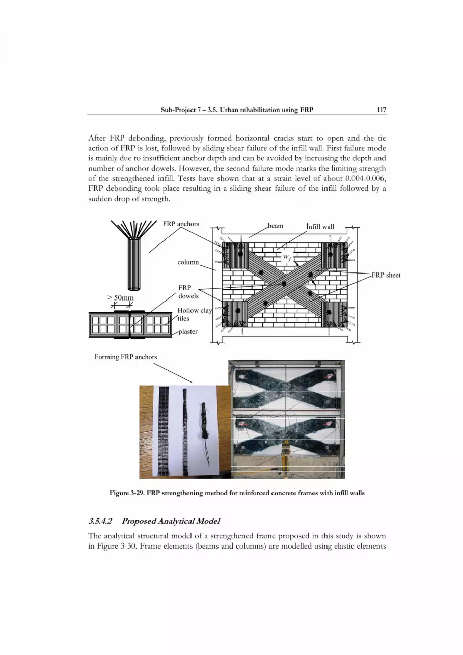
Sub-Project 7 – 3.5. Urban rehabilitation using FRP 117
After FRP debonding, previously formed horizontal cracks start to open and the tie action of FRP is lost, followed by sliding shear failure of the infill wall. First failure mode is mainly due to insufficient anchor depth and can be avoided by increasing the depth and number of anchor dowels. However, the second failure mode marks the limiting strength of the strengthened infill. Tests have shown that at a strain level of about 0.004-0.006, FRP debonding took place resulting in a sliding shear failure of the infill followed by a sudden drop of strength.
FRP anchors
FRP dowels
FRP sheet
beam
column
İnfill wall
fw
Hollow clay tiles
plaster
≥ 50mm
Forming FRP anchors
Figure 3-29. FRP strengthening method for reinforced concrete frames with infill walls
3.5.4.2 Proposed Analytical Model
The analytical structural model of a strengthened frame proposed in this study is shown in Figure 3-30. Frame elements (beams and columns) are modelled using elastic elements
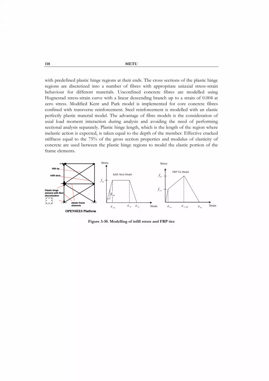
118 METU
with predefined plastic hinge regions at their ends. The cross sections of the plastic hinge regions are discretized into a number of fibres with appropriate uniaxial stress-strain behaviour for different materials. Unconfined concrete fibres are modelled using Hognestad stress-strain curve with a linear descending branch up to a strain of 0.004 at zero stress. Modified Kent and Park model is implemented for core concrete fibres confined with transverse reinforcement. Steel reinforcement is modelled with an elastic perfectly plastic material model. The advantage of fibre models is the consideration of axial load moment interaction during analysis and avoiding the need of performing sectional analysis separately. Plastic hinge length, which is the length of the region where inelastic action is expected, is taken equal to the depth of the member. Effective cracked stiffness equal to the 75% of the gross section properties and modulus of elasticity of concrete are used between the plastic hinge regions to model the elastic portion of the frame elements.
Stress Stress
Strain
crtf
utf
efff ,εcrtε tu ε Strain
us f
soε fsεcrsε
E
Infill Strut Model FRP Tie Model
sm
FRP FRP tietie
InfillInfill strutstrut
PlasticPlastic hingehingeelement element withwith fiber fiber discretizationdiscretization
elasticelastic frameframeelementselements
OPENSEES Platform
FRP FRP tietie
InfillInfill strutstrut
PlasticPlastic hingehingeelement element withwith fiber fiber discretizationdiscretization
elasticelastic frameframeelementselements
OPENSEES Platform
Figure 3-30. Modelling of infill struts and FRP ties

Sub-Project 7 – 3.6. Design of FRP reinforcement of masonry infill walls against transverse move 119
3.6 DESIGN OF FRP REINFORCEMENT OF MASONRY INFILL WALLS AGAINST
TRANSVERSE MOVE
3.6.1 Scope of research
Many buildings in Europe today are of unreinforced masonry (URM) construction and have features, such as infill panels, that could threaten lives under extreme events like high-winds or earthquakes. There is a need to find cheap and effective means of strengthening such structures. This report investigates one particular reinforcing technique, namely the application of fibre reinforced polymer materials to strengthen URM infill panels subjected to out-of-plane loading. There has been an unprecedented growth in research in the area of composites in the last 30 years (Bakis et al. 2002), resulting in a wide range of high-strength, light-weight and environmentally resistant materials available at low costs. Numerous investigators have explored the potential use of fibre reinforced polymer (FRP) strengthening on concrete and on masonry structures under in-plane or out-of-plane monotonic loading. Previous experimental studies have shown increases in capacity and ductility of the FRP reinforced structures (Tikalsky et al. 1995, Velasquez-Dimas et. al. 2000, Tumialan et al. 2003, Krevaikas and Triantafillou 2005). The behaviour under seismic loading has been addressed very little experimentally and mostly tests under ‘simulated earthquake loading’ (large number of cyclic tests) have been reported (Ehsani et al. 1999). Simple analytical methods to assess the out-of-plane behaviour of URM or FRP-reinforced panels were developed based on the flexural theory of masonry present in the building codes (Velasquez-Dimas et. al., II, 2000, Hamilton and Dolan, 2001). The general trend has been to adapt the monotonic loading assessment methods for seismic loading as well, but the developed analytical models have not been validated through dynamic experimentation. A need to evaluate the mechanical behaviour under truly seismic conditions has emerged. The present study is meant to fill the gap in the existing knowledge on the out-of-plane dynamic behaviour of FRP reinforced masonry. Four full-scale quasi-static tests and four full-scale shaking table tests on both unreinforced and reinforced specimens were performed. The experimental observations on pre-cracking and post-cracking behaviour extend understanding on the reinforcement requirements associated with a seismically-sound system. A software tool (CRAMP) capable of predicting the mechanical response of FRP-reinforced masonry walls was developed.
3.6.1.1 Objectives and strategy of the present studies
The research programme at Bristol University investigated the seismic behaviour of FRP-reinforced masonry panels subjected to seismic loading. The specific features and the objectives associated with the tests are presented in Table 3.6.1

120 UBRIS
Table 3-20 Summary of experimental tests
No. Ref. Reinforcement info.
Loading Objectives
1 STU1 Unreinforced
3 cycles of monotonic loading
1. Control specimen for static tests 2. Investigate cracking mechanisms and compare data with Taylor(1998) results and CRAMP simulations 3. Load, deflection, arching force data
2 STU2 Unreinforced
3 cycles of monotonic loading
1. Improvement of boundary conditions 2. Compare data with STU1 results and CRAMP simulations 3. Load, deflection, arching force data
3 STR1 Reinforced (100%) Continuous jacket on tensile face
3 cycles of monotonic loading
1. Investigate quasi-static response 2. Compare response with URM response 3. Inspiration for future FRP layout design 4. Comparison with CRAMP simulations 5. Load, deflection, strain, arching force data
4 STR2 Reinforced (100%) Continuous jacket on tensile face FRP fabric attached to the soffit of the top and bottom beams to prevent sliding
3 cycles of monotonic loading
1. Improvement of boundary conditions 2. Investigate pseudostatic response and data reproducibility 3. Compare response with URM and STR1 response 4. Inspiration for future FRP layout design 5. Comparison with CRAMP simulations 6. Load, deflection, strain, arching force data
Sub-Project 7 – 3.6. Design of FRP reinforcement of masonry infill walls against transverse move121
No. Ref. Reinforcement info.
Loading Objectives
5 SEU1 Unreinforced
Exploratory tests Seismic tests
1. Investigate the modal parameters of URM 2. Investigate seismic response of URM 3. Compare data with Taylor (1998) and CRAMP simulations 4. Load, deflection, arching force data
6 SER1 Reinforced (100%) Continuous jacket on both faces
Exploratory tests Seismic tests
1. Investigate the modal parameters of FRP-URM 2. Investigate seismic response 3.Compare data with SEU1 and CRAMP simulations 4. Load, deflection, strain, arching force, frequency response data 5. Inspiration for future FRP layout design
7 SER2 Reinforced (60%) Vertical strips on both faces
Exploratory tests Seismic tests
1. Lower the stiffness to achieve cracking and better cost / strength ratio 2. Investigate the modal parameters 3. Investigate cracking mechanisms & seismic response 4.Compare data with SER1, SEU1 and CRAMP simulations 5. Load, deflection, arching force, frequency response data 6. Inspiration for future FRP layout design

122 UBRIS
No. Ref. Reinforcement info.
Loading Objectives
8 SER3 Reinforced (40%) Vertical strips on both faces
Exploratory tests Seismic tests
1. Lower the stiffness to achieve cracking and better cost / strength ratio 2. Investigate the modal parameters 3. Investigate cracking mechanisms & seismic response 4.Compare data with SER1, SER2, SEU1 and CRAMP simulations 5. Load, deflection, arching force, frequency response data 6. Conclusions and recommendations for FRP layout design
Note: Test reference codes: STU (static unreinforced panel), STR (static reinforced panel), SEU (seismic unreinforced panel), SER (seismic reinforced panel).
Although both the masonry and the FRP have a brittle type of failure, their combination was expected to show increased load-carrying capacity and ductility favoured by the elastic deformation of fibres and the shear transfer in the resin connection layer. Beside the strength benefits, a slowly-progressing mode of failure has also been pursued. The sudden collapse of unreinforced masonry or the explosive failure of the FRP needed to be substituted by a slow and energy dissipative process that could be the result of the FRP delamination. It was believed that the layout of the FRP and the reinforcement ratios could be used as control factors in triggering the failure mechanisms.
Four full-scale quasi-static tests and four full-scale seismic tests were carried out. The research concentrated on the simplest case of a panel supported at its top and bottom only, with the vertical sides being unrestrained. All specimens were single-wythe, top and bottom supported panels (size 3000 x 2000 x 100 mm) using high density concrete bricks. The latter were chosen so as to maximise the inertia-driven out-of-plane forces.
The tests were intended to give information on the following aspects of mechanical response:
i) mechanisms of the failure modes
ii) crack patterns and strain profiles
Sub-Project 7 – 3.6. Design of FRP reinforcement of masonry infill walls against transverse move123
iii) influence of the FRP lay-out and reinforcement ratio on the mechanical response
iv) influence of the loading characteristics on the mechanical response
v) evolution of panel stiffness and modal parameters under seismic loading
3.6.2 Experimental programme
3.6.2.1 Materials and panel configuration
The following material properties were investigated prior to the masonry panel construction:
i) brickwork density
ii) brick units compression capacity
iii) mortar compression capacity
iv) compressive strength of the brick mortar assemblage (tests on three-brick prisms)
v) modulus of rupture of the brick-mortar assemblage
vi) stress-strain behaviour of the brick-mortar assemblage.
A summary of the material characteristics is given below:
i) concrete facing bricks: to BS6073, size: 215x 102 x 65, density: 2200 kg/m3 (given by the manufacturer), compressive strength: 25 MPa (measured).
ii) mortar: general purpose mortar for masonry, corresponding to group III acc. to BS EN 998-2:2003, composition 1:1:6 (cement: lime: sand) (given by the manufacturer), compressive strength: 6 MPa(measured).
iii) masonry: max. compressive stress = 18 MPa, max. tens. strain = 0.6 % (measured).
a. Masonry panels
The panels were built within a pin-jointed steel frame fabricated from 254x254 universal column sections. The sections were stiffened by thick plates welded longitudinally between the flanges on both sides of the beams in order to prevent the flange flexure. The specimens for the pseudo-static tests were located parallel to the laboratory reaction wall where the hydraulic actuator was mounted. A load distribution beam consisting of a

124 UBRIS
steel square plate and two steel rollers was employed to distribute the load in the central area of the wall.
The specimens for the seismic tests were built off the shaking table and left to cure using standard practices. Each masonry wall was built in two lifts and was top and bottom supported. Mortar was packed on the top side of the wall to fill the gap caused by shrinkage. The walls were left for 21 days to cure. When the specimens were cured, they were bolted down onto the shaking table and instrumented.
b. FRP materials
When selecting the FRP materials for reinforcement of panels, the main parameters that are generally taken into account are the specific strength (tensile strength/specific gravity) or the specific stiffness (modulus of elasticity/specific gravity). The carbon fibre composites exhibit better specific strength and specific stiffness values than their competitors. However, when the seismic behaviour of the retrofitted system comes into play, the systems’ ductility and capacity of energy absorption become important. Fibre ductility increases from carbon to aramid and further to glass. After weighing the benefits and the disadvantages of a large set of FRP materials (both plates and wraps), a glass-fibre fabric system was selected for reinforcement (manufacturer: EXCHEM LTD-UK). Its mechanical properties are given in Table 3.6.2. In particular, the elastic modulus of the applied fabric is closest to that of URM, and therefore strain compatibility and ductility performance are likely to be better than a stiffer fibre material. In addition, glass fibres are significantly cheaper than alternatives.
Table 3-21 FRP system employed in the tests
Fibre Tensile Strength
(MPa)
fibre/ laminate
Modulus of elasticity
(GPa)
fibre/
laminate
Elongation
(%)
Thickness
mm
Weight
g/m2
Wrap Type E (unidirectional
fabric, wet application)
3450
/1099
73
/42
4.5 0.167 432
Discrete strips or continuous jackets of FRP fabric were used. Samples using various reinforcement ratios were tested. Preliminary observations on the first tests led to the
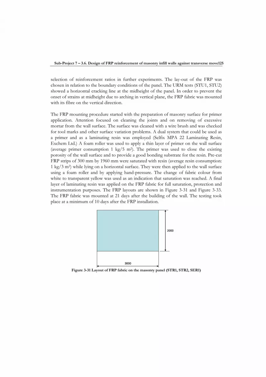
Sub-Project 7 – 3.6. Design of FRP reinforcement of masonry infill walls against transverse move125
selection of reinforcement ratios in further experiments. The lay-out of the FRP was chosen in relation to the boundary conditions of the panel. The URM tests (STU1, STU2) showed a horizontal cracking line at the midheight of the panel. In order to prevent the onset of strains at midheight due to arching in vertical plane, the FRP fabric was mounted with its fibre on the vertical direction.
The FRP mounting procedure started with the preparation of masonry surface for primer application. Attention focused on cleaning the joints and on removing of excessive mortar from the wall surface. The surface was cleaned with a wire brush and was checked for tool marks and other surface variation problems. A dual system that could be used as a primer and as a laminating resin was employed (Selfix MPA 22 Laminating Resin, Exchem Ltd.) A foam roller was used to apply a thin layer of primer on the wall surface (average primer consumption 1 kg/5 m2). The primer was used to close the existing porosity of the wall surface and to provide a good bonding substrate for the resin. Pre-cut FRP strips of 300 mm by 1960 mm were saturated with resin (average resin consumption: 1 kg/3 m2) while lying on a horizontal surface. They were then applied to the wall surface using a foam roller and by applying hand-pressure. The change of fabric colour from white to transparent yellow was used as an indication that saturation was reached. A final layer of laminating resin was applied on the FRP fabric for full saturation, protection and instrumentation purposes. The FRP layouts are shown in Figure 3-31 and Figure 3-33. The FRP fabric was mounted at 21 days after the building of the wall. The testing took place at a minimum of 10 days after the FRP installation.
3000
2000
3000
2000
Figure 3-31 Layout of FRP fabric on the masonry panel (STR1, STR2, SER1)
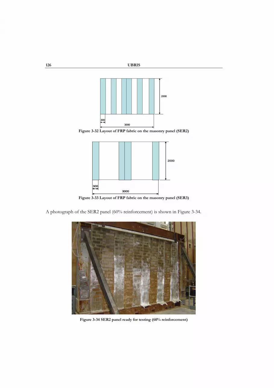
126 UBRIS
3000
300
2000
3000
300
2000
Figure 3-32 Layout of FRP fabric on the masonry panel (SER2)
3000
300
2000
3000
300
3000
300
2000
Figure 3-33 Layout of FRP fabric on the masonry panel (SER3)
A photograph of the SER2 panel (60% reinforcement) is shown in Figure 3-34.
Figure 3-34 SER2 panel ready for testing (60% reinforcement)

Sub-Project 7 – 3.6. Design of FRP reinforcement of masonry infill walls against transverse move127
3.6.2.2 Instrumentation
CELESCO type PT101 displacement transducers measured the out-of-plane deflection. The transducers were placed at mid-height and at positions symmetrically-located about the centre line. Four load cells were incorporated in the four bolts attaching the top beam to the frame columns. The load cells measured the arching forces on the wall. The top beam was separated from the top of the column by washers around the instrumented bolts. Strain gauges recorded the FRP tensile strain at mid-height and at locations symmetrically located about the centreline. The strain gauges were mounted on the FRP fabric in areas located on top of a brick unit. For the monotonic tests only, one 200 kN load cell was mounted on the same axis with the hydraulic actuator to measure the applied load. Three SETRA type 141A accelerometers were installed on the shaking table (X, Y, Z directions) while another three were installed on the panel to measure out-of-plane accelerations. A seventh accelerometer was installed on the frame’s top beam also to measure out-of-plane accelerations.
3.6.2.3 Seismic tests input motions
a. Exploratory tests
The exploratory tests were used for measuring the modal parameters of the specimen. The resonant frequency of the first mode of vibration and the viscous damping of the specimen were the main parameters of interest. The exploratory tests used broadband (0-100) Hz random noise applied on the out-of-plane axis only (Y axis).
b. Seismic tests
An elastic response spectrum for soil type B acc. to Eurocode 8 was used in the tests (Table 3.6.3 and Figure 3-35). Acceleration, velocity and displacement time histories were generated to match the Eurocode 8 response spectrum. The displacement time history was fed into the shaking table control software.
Table 3-22 Parameters of design response spectrum
Ground type S TB(s) TC(s) TD(s)
B 1.2 0.15 0.5 2

128 UBRIS
0
0.5
1
1.5
2
2.5
3
3.5
0.5 2 6.6 40 100
frequency (Hz)
Se/
ag
Figure 3-35 Required response spectrum as per Eurocode 8 (Soil B)
3.6.2.4 Quasi-static tests – experimental observations
a. STU1 and STU2 (quasi-static tests on unreinforced panels)
The URM wall cracked along an horizontal line situated at the midheight of the wall (Figure 3-36) This cracking pattern had been observed by other researchers and it is considered typical for the top-and-bottom-supported masonry panels. The main resistance mechanism was arching of the panel with increasing of contact forces between panel and top and bottom supports.
Figure 3-36 Experimental rig used for the static tests (STR1, STR2)
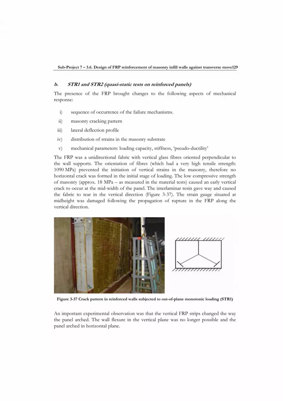
Sub-Project 7 – 3.6. Design of FRP reinforcement of masonry infill walls against transverse move129
b. STR1 and STR2 (quasi-static tests on reinforced panels)
The presence of the FRP brought changes to the following aspects of mechanical response:
i) sequence of occurrence of the failure mechanisms.
ii) masonry cracking pattern
iii) lateral deflection profile
iv) distribution of strains in the masonry substrate
v) mechanical parameters: loading capacity, stiffness, ‘pseudo-ductility’
The FRP was a unidirectional fabric with vertical glass fibres oriented perpendicular to the wall supports. The orientation of fibres (which had a very high tensile strength: 1090 MPa) prevented the initiation of vertical strains in the masonry, therefore no horizontal crack was formed in the initial stage of loading. The low compressive strength of masonry (approx. 18 MPa – as measured in the material tests) caused an early vertical crack to occur at the mid-width of the panel. The interlaminar resin gave way and caused the fabric to tear in the vertical direction (Figure 3-37). The strain gauge situated at midheight was damaged following the propagation of rupture in the FRP along the vertical direction.
Figure 3-37 Crack pattern in reinforced walls subjected to out-of-plane monotonic loading (STR1)
An important experimental observation was that the vertical FRP strips changed the way the panel arched. The wall flexure in the vertical plane was no longer possible and the panel arched in horizontal plane.

130 UBRIS
The main failure modes identified during the STR1 and STR2 tests were: the flexural failure, the shear failure and the FRP debonding. Flexural failure was triggered by the crushing of the masonry in compression and by the rupture of the FRP in tension. Initial cracking occurred at the interface of mortar and masonry. The initial cracking was delayed by the presence of the FRP. Since the tensile strength of the masonry was lower than that of the epoxy resin (55 MPa), the failure line appeared first in the masonry. The vertical crack in the masonry caused the wall to slide while a differential displacement in the shear plane developed. The shear failure mechanism resulted in the FRP debonding alongside the masonry crack. The FRP fabric situated above the opening crack of the masonry started to deform and broke in tension vertically. Debonding of the FRP laminate from the masonry substrate was triggered by the central vertical crack in the masonry and propagated at first vertically, then multiaxially towards the final stages of loading. It was noticed that part of the concrete brick faceshell remained attached to the laminate. This showed that the resin-masonry connection was stronger than the tensile strength of the masonry. End-debonding of the FRP was expected as a main failure mode, but this did not occur.
The strength and stiffness of the STR walls increased dramatically in comparison to the STU specimens. A 2.6 times increase in maximum strength was recorded (see Figure 3-38).
0 10 20 30 40 50 60 70 80
0
5
10
15
20
25
30
35
40
midheight deflection (mm)
out-o
f-pla
ne lo
ad (k
N)
R2
R1
R3
R4
U2 U-collapse
U1
R-collapse
Figure 3-38 Loading curves during static testing (STU1 -unreinforced wall, STR1 reinforced wall)
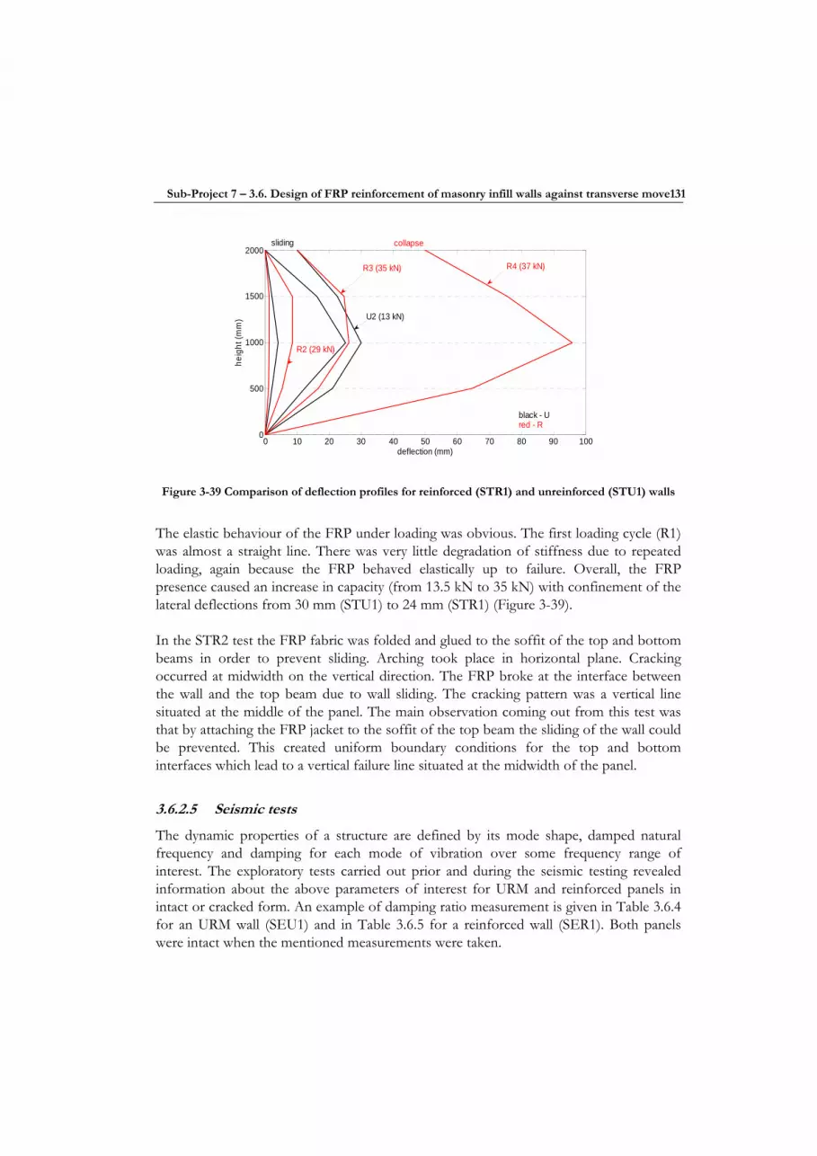
Sub-Project 7 – 3.6. Design of FRP reinforcement of masonry infill walls against transverse move131
0 10 20 30 40 50 60 70 80 90 1000
500
1000
1500
2000
deflection (mm)
heig
ht (m
m)
red - R
sliding collapse
R4 (37 kN)
black - U
U2 (13 kN)
R2 (29 kN)
R3 (35 kN)
Figure 3-39 Comparison of deflection profiles for reinforced (STR1) and unreinforced (STU1) walls
The elastic behaviour of the FRP under loading was obvious. The first loading cycle (R1) was almost a straight line. There was very little degradation of stiffness due to repeated loading, again because the FRP behaved elastically up to failure. Overall, the FRP presence caused an increase in capacity (from 13.5 kN to 35 kN) with confinement of the lateral deflections from 30 mm (STU1) to 24 mm (STR1) (Figure 3-39).
In the STR2 test the FRP fabric was folded and glued to the soffit of the top and bottom beams in order to prevent sliding. Arching took place in horizontal plane. Cracking occurred at midwidth on the vertical direction. The FRP broke at the interface between the wall and the top beam due to wall sliding. The cracking pattern was a vertical line situated at the middle of the panel. The main observation coming out from this test was that by attaching the FRP jacket to the soffit of the top beam the sliding of the wall could be prevented. This created uniform boundary conditions for the top and bottom interfaces which lead to a vertical failure line situated at the midwidth of the panel.
3.6.2.5 Seismic tests
The dynamic properties of a structure are defined by its mode shape, damped natural frequency and damping for each mode of vibration over some frequency range of interest. The exploratory tests carried out prior and during the seismic testing revealed information about the above parameters of interest for URM and reinforced panels in intact or cracked form. An example of damping ratio measurement is given in Table 3.6.4 for an URM wall (SEU1) and in Table 3.6.5 for a reinforced wall (SER1). Both panels were intact when the mentioned measurements were taken.

132 UBRIS
The evolution of panel stiffness during testing takes place in parallel with a measurable shift in panel’s natural frequency. The natural frequency of vibration increased from 12 Hz for the URM panel (SEU1) up to 30.31 Hz for the reinforced panel with maximum reinforcement ratio (SER1). Lowering the reinforcement ratio from 100% to 40% led to a shift in the natural frequency from 30.31 Hz to 15 Hz (Table 3.6.6).
Table 3-23 Damping corresponding to main modes of vibration in SEU1 (intact wall)
Natural Freq (Hz) Damping ratio (%)
12.00 4.30 19.94 1.53 23.38 0.32 29.46 3.81 37.62 4.09
Table 3-24 Damping corresponding to main modes of vibration in SER1 (intact wall)
Natural Freq (Hz)
Damping ratio (%)
30.31 4.87 53.58 2.68
Table 3-25 Evolution of panel’s natural frequency during seismic testing
Test Reinforcement information
Uncracked natural
frequency (Hz)
Cracked natural
frequency (Hz)
Cracking table acceleration or max. table
acceleration
SEU1 unreinforced 12.00 7.50 cracking: 1.175 g (SEU1_60), collapse: 2.4g
SER1 100% reinf. 30.31 uncracked max : 3.53g (SER1_130) SER2 60% reinf. 28.25 uncracked max : 2.28g (SER2_120) SER3 40% reinf. 15.00 8.20 cracking:2.44g (SEU3_80)

Sub-Project 7 – 3.6. Design of FRP reinforcement of masonry infill walls against transverse move133
3.6.2.6 Seismic tests – experimental observations and numerical simulations
Particular attention has been given to tests SEU1_65 that led to the URM wall cracking and SEU1_110 that led to its collapse. The table acceleration reached 2.44g in SEU1_110 (Figure 3-40).
The lateral deflection results collected at midheight on the panel are shown in Figure 3-41.
A simulated evolution of wall displacement in time is presented in Figure Figure 3-42.
The measured and the simulated arching forces are shown in Figure 3-43 and Figure 3-44.
An interesting part of SEU1 test was the SEU1_65, when the imposed seismic input led to cracking. The input motion lasted for 40 s and accelerations up to 1.175 g were recorded by the Y-axis accelerometer mounted on the shaking table (Figure 3-45).
10 15 20 25 30-3
-2
-1
0
1
2
3
time(s)
supp
ort a
ccel
erat
ion(
g)
Expriment, SEU1-110
Figure 3-40 Shaking table acceleration in test SEU1_110
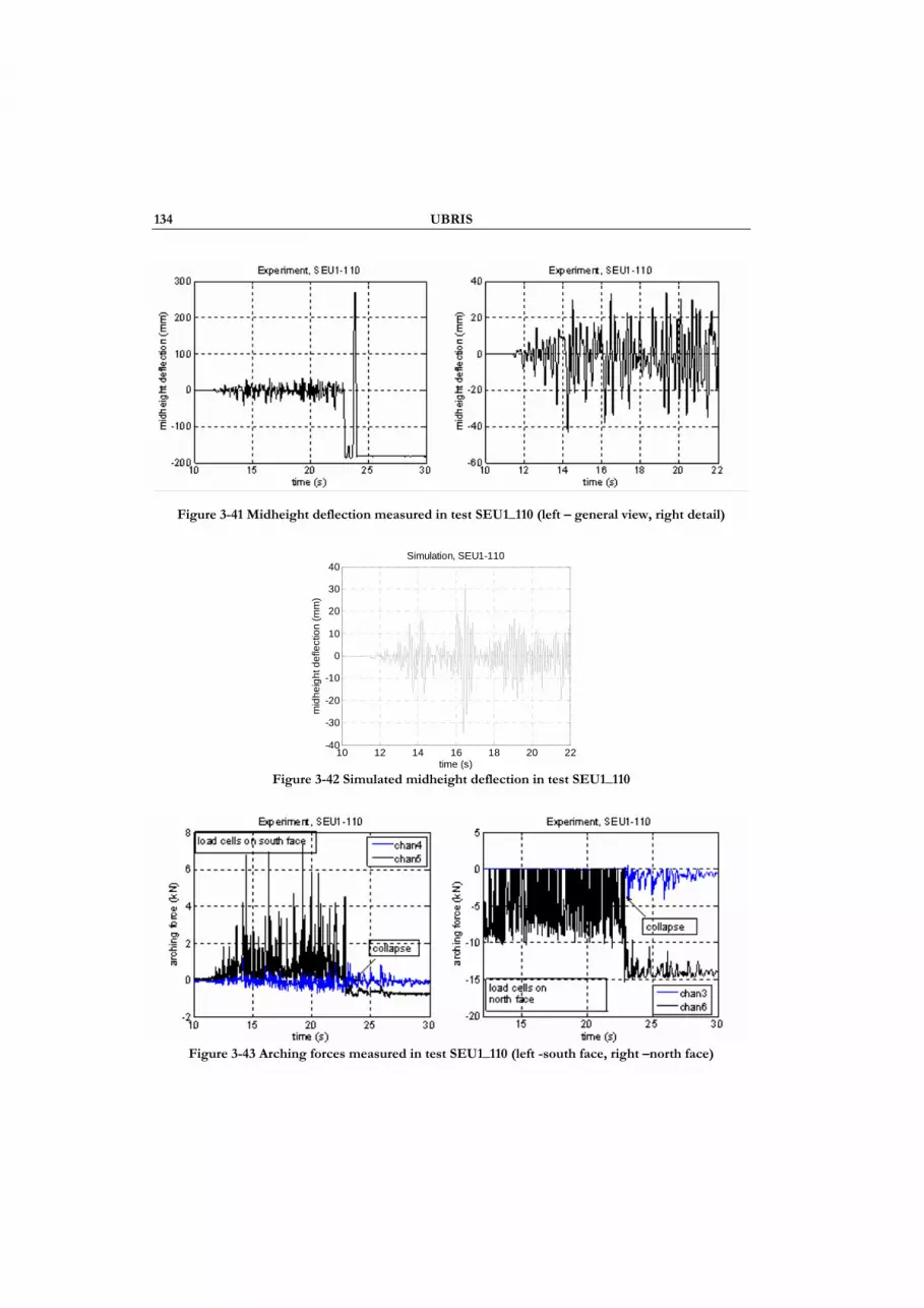
134 UBRIS
Figure 3-41 Midheight deflection measured in test SEU1_110 (left – general view, right detail)
10 12 14 16 18 20 22-40
-30
-20
-10
0
10
20
30
40Simulation, SEU1-110
time (s)
mid
heig
ht d
efle
ctio
n (m
m)
Figure 3-42 Simulated midheight deflection in test SEU1_110
Figure 3-43 Arching forces measured in test SEU1_110 (left -south face, right –north face)
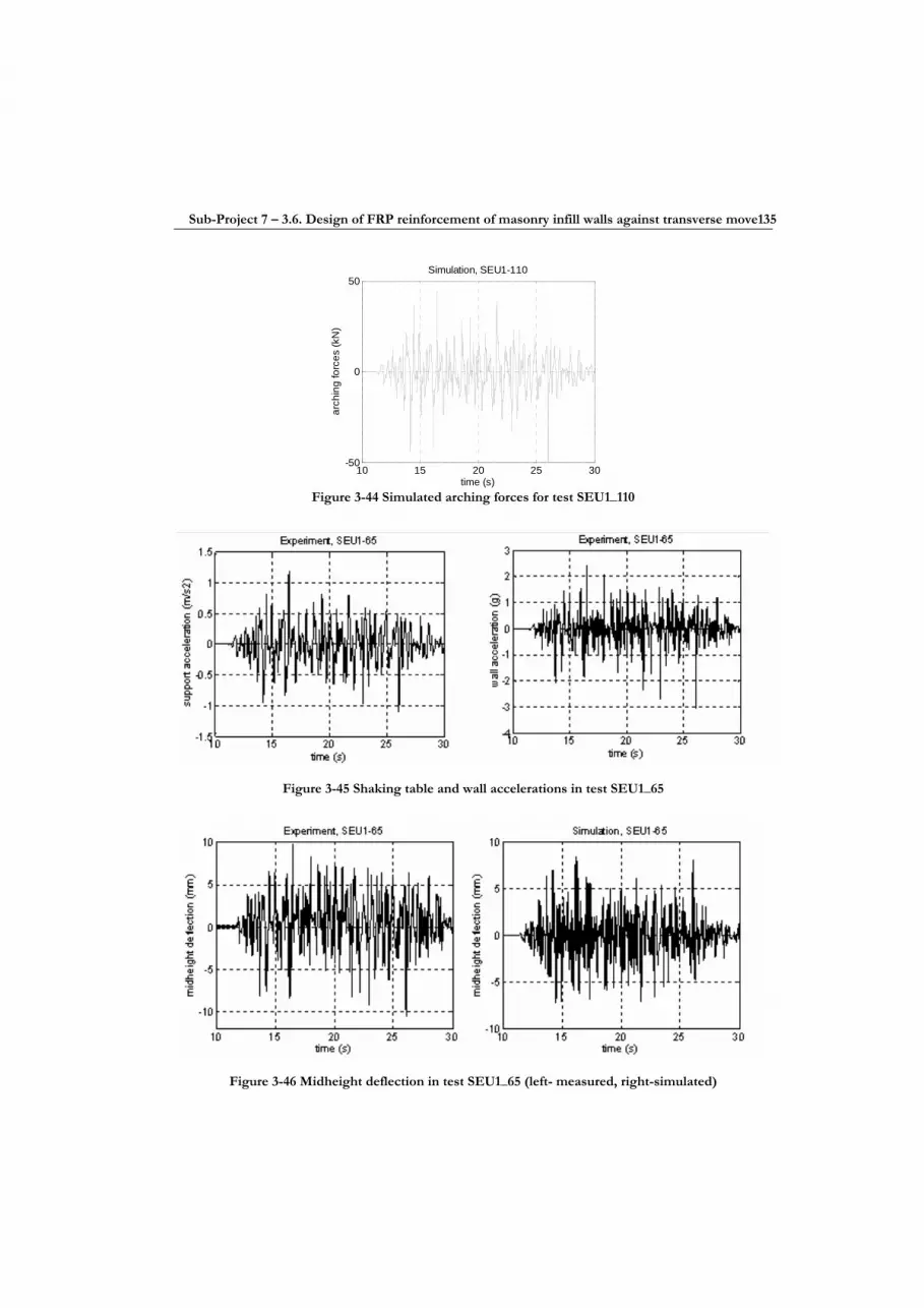
Sub-Project 7 – 3.6. Design of FRP reinforcement of masonry infill walls against transverse move135
10 15 20 25 30-50
0
50Simulation, SEU1-110
time (s)
arch
ing
forc
es (k
N)
Figure 3-44 Simulated arching forces for test SEU1_110
Figure 3-45 Shaking table and wall accelerations in test SEU1_65
Figure 3-46 Midheight deflection in test SEU1_65 (left- measured, right-simulated)
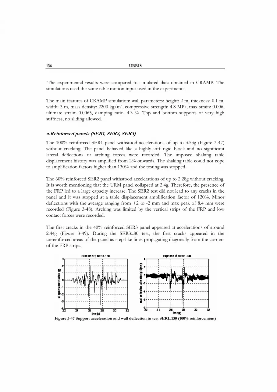
136 UBRIS
The experimental results were compared to simulated data obtained in CRAMP. The simulations used the same table motion input used in the experiments.
The main features of CRAMP simulation: wall parameters: height: 2 m, thickness: 0.1 m, width: 3 m, mass density: 2200 kg/m3, compressive strength: 4.8 MPa, max strain: 0.006, ultimate strain: 0.0065, damping ratio: 4.3 %. Top and bottom supports of very high stiffness, no sliding allowed.
a.Reinforced panels (SER1, SER2, SER3)
The 100% reinforced SER1 panel withstood accelerations of up to 3.53g (Figure 3-47) without cracking. The panel behaved like a highly-stiff rigid block and no significant lateral deflections or arching forces were recorded. The imposed shaking table displacement history was amplified from 2% onwards. The shaking table could not cope to amplification factors higher than 130% and the testing was stopped.
The 60% reinforced SER2 panel withstood accelerations of up to 2.28g without cracking. It is worth mentioning that the URM panel collapsed at 2.4g. Therefore, the presence of the FRP led to a large capacity increase. The SER2 test did not lead to any cracks in the panel and it was stopped at a table displacement amplification factor of 120%. Minor deflections with the average ranging from +2 to -2 mm and max peak of 8.4 mm were recorded (Figure 3-48). Arching was limited by the vertical strips of the FRP and low contact forces were recorded.
The first cracks in the 40% reinforced SER3 panel appeared at accelerations of around 2.44g (Figure 3-49). During the SER3_80 test, the first cracks appeared in the unreinforced areas of the panel as step-like lines propagating diagonally from the corners of the FRP strips.
Figure 3-47 Support acceleration and wall deflection in test SER1_130 (100% reinforcement)
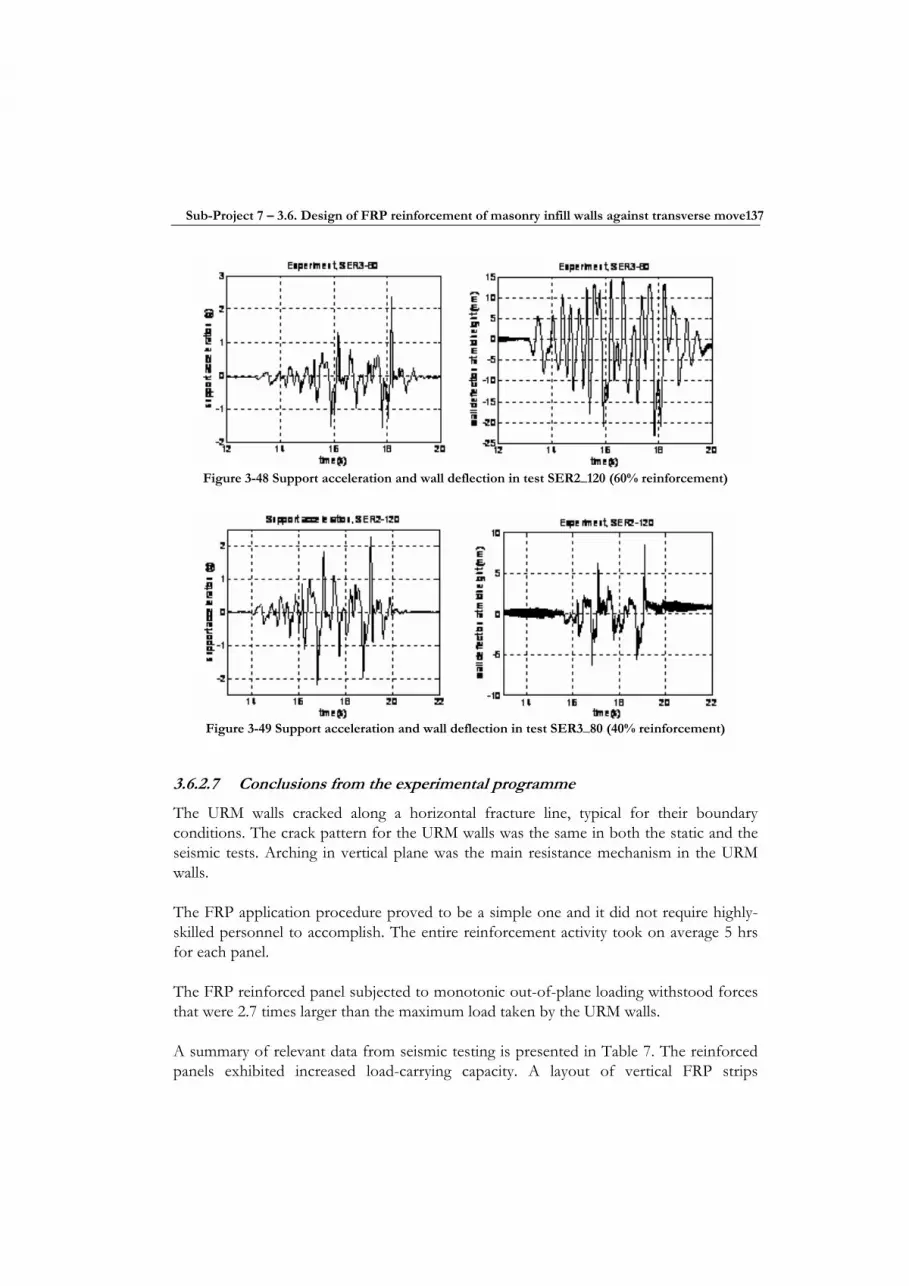
Sub-Project 7 – 3.6. Design of FRP reinforcement of masonry infill walls against transverse move137
Figure 3-48 Support acceleration and wall deflection in test SER2_120 (60% reinforcement)
Figure 3-49 Support acceleration and wall deflection in test SER3_80 (40% reinforcement)
3.6.2.7 Conclusions from the experimental programme
The URM walls cracked along a horizontal fracture line, typical for their boundary conditions. The crack pattern for the URM walls was the same in both the static and the seismic tests. Arching in vertical plane was the main resistance mechanism in the URM walls.
The FRP application procedure proved to be a simple one and it did not require highly-skilled personnel to accomplish. The entire reinforcement activity took on average 5 hrs for each panel.
The FRP reinforced panel subjected to monotonic out-of-plane loading withstood forces that were 2.7 times larger than the maximum load taken by the URM walls.
A summary of relevant data from seismic testing is presented in Table 7. The reinforced panels exhibited increased load-carrying capacity. A layout of vertical FRP strips
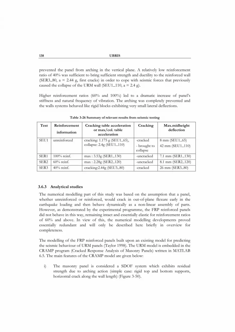
138 UBRIS
prevented the panel from arching in the vertical plane. A relatively low reinforcement ratio of 40% was sufficient to bring sufficient strength and ductility to the reinforced wall (SER3_80, a = 2.44 g, first cracks) in order to cope with seismic forces that previously caused the collapse of the URM wall (SEU1_110, a = 2.4 g).
Higher reinforcement ratios (60% and 100%) led to a dramatic increase of panel’s stiffness and natural frequency of vibration. The arching was completely prevented and the walls systems behaved like rigid blocks exhibiting very small lateral deflections.
Table 3-26 Summary of relevant results from seismic testing
Test Reinforcement
information
Cracking table acceleration or max/col. table
acceleration
Cracking Max.midheight deflection
SEU1 unreinforced cracking: 1.175 g (SEU1_65), collapse: 2.4g (SEU1_110)
-cracked - brought to collapse
8 mm (SEU1_65) 42 mm (SEU1_110)
SER1 100% reinf. max : 3.53g (SER1_130) -uncracked 7.1 mm (SER1_130) SER2 60% reinf. max : 2.28g (SER2_120) -uncracked 8.1 mm (SER2_120) SER3 40% reinf. cracking:2.44g (SEU3_80) -cracked 26 mm (SER3_80)
3.6.3 Analytical studies
The numerical modelling part of this study was based on the assumption that a panel, whether unreinforced or reinforced, would crack in out-of-plane flexure early in the earthquake loading and then behave dynamically as a non-linear assembly of parts. However, as demonstrated by the experimental programme, the FRP reinforced panels did not behave in this way, remaining intact and essentially elastic for reinforcement ratios of 60% and above. In view of this, the numerical modelling developments proved essentially redundant and will only be described here briefly in overview for completeness.
The modelling of the FRP reinforced panels built upon an existing model for predicting the seismic behaviour of URM panels (Taylor 1998). The URM model is embedded in the CRAMP program (Cracked Response Analysis of Masonry Panels) written in MATLAB 6.5. The main features of the CRAMP model are given below:
i) The masonry panel is considered a SDOF system which exhibits residual strength due to arching action (simple case: rigid top and bottom supports, horizontal crack along the wall length) (Figure 3-50).

Sub-Project 7 – 3.6. Design of FRP reinforcement of masonry infill walls against transverse move139
ii) Strip analysis technique (each vertical strip consists of two segments that join at the location of the crack).
iii) Non-linear dynamic analysis. Equation of motion solved using the linear acceleration time-stepping formulation.
iv) Seismic capacity is expressed in the form of fragility curves.
v) Panel segments are assumed to behave non-linear elastically, with the masonry following a simple parabolic stress-strain model. Crushing at the faces of the panel is allowed for.
CRAMP enables multiple time history simulations to be run for a given panel configuration. The outputs of these simulations are then assembled in the form of fragility curves from which the probability of failure relative to, for example, peak input acceleration may be found.
As the CRAMP model involves several significant simplifying assumptions, and the problem is highly non-linear and therefore sensitive to parameter and loading variability, it is unlikely to yield a very close match at a time history level with any given experimental result. However, previous experience with earlier CRAMP models (Taylor, 1998) gave confidence that probability estimates based on CRAMP outputs were meaningful.
arch thrust
arch thrustp
heightcon_length
equivalent compression spring
arch thrust
arch thrustp
heightcon_length
equivalent compression spring
Figure 3-50 Modelling of top and bottom supported URM panels
140 UBRIS
Figure 3-51 Fragility curve for a panel height of 4m (t=0.229m, mass density =1950 kg/m³,
fc=4.8 MPa, έmax=0.4%, έult=0.45%, viscous damping =5%)
Since the FRP material will never reach its max tensile strength (1099 N/mm2), it is fair to say that the FRP membranes behave elastically during testing and that no rupture of fibres takes place.
Figure 3-51 shows a typical fragility curve from CRAMP.
3.6.4 Conclusions
This study has shown the efficacy of a relatively simple method of reinforcing unreinforced masonry infill panels with glass fibre FRP laminates. Provided the reinforcement covers at least 60% of the surface area of the panel (preferably 100%), and the reinforcement overlaps the surrounding frame by at least 75mm, the reinforced panel gains a significant amount of strength to out-of-plane seismic loads. So great are the strength and stiffness increases that, for typical panel configurations, it appears unlikely that a strengthened panel would suffer significant distress during an earthquake due to out-of-plane loads. (Note, however, that this study has not considered combined in-plane and out-of-plane loading.) The evidence derived from this study suggests that this kind of FRP strengthening can simply be specified, rather than requiring detailed engineering calculations for its justification.
The method of application of the FRP reinforcement is very simple, requiring minimal training. It is within the ability of a semi-skilled builder, subject to appropriate supervision. The chosen glass fibre based materials are relatively cheap.

4.SEISMIC DESIGN AND RETROFIT OF STRUCTURES USING DISSIPATIVE DEVICES
4.1 RC STRUCTURES
4.1.1 Introduction Conventional seismic design practice permits designing precast and cast in place reinforced concrete (PRC and RC, respectively) structures for forces lower than those expected from the elastic response on the premise that the structural design assures significant energy dissipation potential and, therefore, the survival of the building when subjected to severe earthquakes. Normally, energy dissipation during seismic actions occurs in critical zones of the structure specially designed to admit large ductility demands. Frequently, these zones are located near the beam-column joints and during earthquakes, several structural members can suffer a great amount of damage with irreversible degradation of the mechanical properties of the materials. Even if a limited level of structural damage dissipates part of the energy offering certain level of protection against seismic actions (Mata et.al. 2006, Lessloss Deliverable report 54, 2005 (www.lessloss.org)), the large displacements required for developing hysteretic cycles in dissipative zones can cause severe damage in those members, but this situation is generally considered economically acceptable if life safety and collapse prevention are achieved.
In the last decades, new concepts for the design of building, based on the manipulation of the energy dissipation, have improved the seismic behaviour of the RC and PRC structures providing higher levels of safety for the occupants, buildings and nonstructural components.
The new techniques are based on adding devices to the buildings with the main objective of dissipating the energy demand imposed by the earthquake alleviating the ductility demand on primary structural elements and decreasing the acceleration response (Soon and Dargush, 1997; Handson et.al. 1993). The purpose is to control the seismic response of the buildings by means of a set of dissipating devices which constitutes the control system, adequately located in the structure.
142 CIMNE
The passive energy dissipating devices (EDD) work dissipating the energy of the earthquake, localizing and concentrating the damage of the structure in the devices without the need of an external energy supply (Soon and Dargush 1997). Today, the passive control of structures is widely accepted by the engineering community.
By one hand, passive EDDs, also called supplemental dampers, are devices located throughout the structure to absorb and dissipate an important part of the energy input induced in the structure by earthquakes. The effectiveness of the implementation of EDDs in RC structures can be analyzed starting from the energy balance equation as:
dDSKI EEEEE +++= (4.1.1)
Where EI is the absolute earthquake energy input, EK is the absolute kinetic energy, ES is the elastic strain energy, ED is the energy dissipation due to inelastic behaviour in the structure (including viscous effects) and Ed is the contribution of energy dissipation due to the addition of EDDs.
Using the assumption that the term Ed has no influence on EI , it is possible to see from Eq. (4.1.1) that increments of the contribution of ED + Ed implies reductions of EK+ES and, therefore, lower responses are obtained when extra energy dissipation is provided (Aiken, 1996; Soon and Dargush, 1997). The main objective of designers when applying passive control in improving the seismic behaviour of PRC structures, is defining appropriately the properties of the EDDs in such way that the inelastic demand on primary structural members ED be transferred to the term Ed. After a sever earthquake, EDDs can be replaced by new ones if necessary. EDDs can be classified according to the nature of their dissipative mechanism in displacement dependent, e.g. friction, metallic and extrusion devices, velocity dependent e.g. viscous, mixed e.g. viscoelastic and others such as tuned liquid and tuned mass dampers. A great amount of works comparing the ability of different passive EDDs in controlling the seismic response of structures is available in the literature (Luck et.al., 1996).
For Aiken (1996) presents the contribution of the extra energy dissipation due to EDDs as an equivalent damping added to the linear bare structure and displacement reduction factors are given as a function of the damping ratio added to buildings. Lin and Copra study the accuracy in estimating the dynamic response of asymmetric one-storeybuildings equipped with EDDs, when the dissipating devices are replaced by their energetic equivalent linear viscous dampers; a correction factor is provided estimating the maximum forces in the EDDs.
Today, only a few countries have design codes for RC buildings with EDDs; in United States, the US Federal Emergency Management Agency (FEMA) proposes code provisions and

Sub-Project 7 – 4.1. RC structures 143
standards pertaining to the design of EDDs devices for use in buildings. The document includes Prestandard and Commentary for the Seismic Rehabilitation of Buildings (FEMA 356, 2000) and NEHRP Recommended Provisions for Seismic Regulations for New Buildings and Other Structures (FEMA 368, 2000).
In the case of Europe, efforts have been focused mainly in developing codes for base isolation. In the case of EDDs the developments have been limited to guidelines rather that codes or official standards.
A great part of the design methods for RC and PRC structures are based on supposing that the behaviour of the bare structure remains elastic, concentrating the energy dissipation demands on the control system. However, even though this assumption can be useful for a preliminary design, experimental and theoretical evidence show that inelastic behaviour will occur in the main structural elements during severe strong motion as noted by Shen and Soong (2005). It is widely recognized that nowadays it is possible to carry out nonlinear time-history analysis, which can provide a most precise evaluation of the response of structural systems incorporating EDDs (see Mata et.al. 2006; Valles et.al. 1996). But it also requires relatively large amounts of computational time. It is also recognized that equivalent linear dynamic procedures are not able to represent the fully complexity of the nonlinear dynamic behaviour of RC and PRC structures.
Independently of the type of analysis chosen, it is clear that the nonlinear time history analysis has gained space in the passive control of RC and PRC structures subjected to earthquakes, therefore, sophisticated numerical tools became more necessary for both academics and practitioners. During the last decades, great efforts have been done in developing numerical formulations and their implementation in computer codes for the simulation of the nonlinear dynamic response of RC and PRC structures, for example a recent state of the art review for the case of concrete structures can be found in reference (Spacone and El-Tawil, 2004).
The engineering community agrees with the fact that the use of general fully 3D numerical techniques, such as nonlinear finite elements (FE), constitutes the most precise tools for the simulation of the behaviour of RC buildings subjected to earthquakes (Soon and Dargush, 1996; Spiliopoulos and Lykidis, 2005). However, usually the computing time required when using full models of real structures became their application unpractical. Considering that most of the elements in RC and PRC buildings are columns or beams, one-dimensional formulations for structural elements, appear as a solution combining both numerical precision and reasonable computational costs (Mata et.al., 2007). Experimental evidence (Bayrak and Sheikh, 2001) shows that nonlinearity in beam elements can be formulated in terms of cross sectional forces and moments (Coleman
144 CIMNE
and Spacone, 2001). Some formulations of this type have been extended to take into account geometric nonlinearities (Sivaselvan et.al., 2002; Vignjevic, 1997).
An additional refinement is obtained considering inhomogeneous distributions of materials on arbitrarily shaped beam cross sections [Kumar et.al., 2004; Valles et.al., 1996]. Specific numerical models based on a secondary discretization of the beam cross sections have been developed allowing to include multiple materials. Using this approach the mechanical behaviour of beams constituted by complex combinations of materials, such it is the case of RC beams, can be simulated (Hajjar, 2000). In general, the engineering community agrees with the fact that although these models are computationally more expensive, they allow estimating more precisely the nonlinear response of RC structures (Davenne et.al., 2003; Taucer et.al., 1991). Formulations of this kind considering both constitutive and geometric nonlinearity are rather scarce (Driemeier et.al., 2005); moreover, most of the geometrically nonlinear models for beams are limited to the elastic range of materials, as it can be consulted for example in references (Reissner, 1972; Simo, 1985) and the treatment of inelasticity has been mainly restricted to plasticity. Recently, Mata et.al. (2007) has extended the geometrically exact formulation for beams due to Reissner-Simo (Reissner, 1972; Simo, 1985; Simo and Vu-Quoc, 1986 and 1988) for considering and arbitrary distribution of composite materials with the cross sections for the static and dynamic cases.
From the numerical point of view, the nonlinear behaviour of EDDs usually has been described in a global sense by means of force–displacement or moment-curvature relationships that intend to capture appropriately the force/moment level and the energy dissipating capacity existing in the devices. That is to say that, a rather simplified description appears to be enough for the mechanical characterization of the EDDs.
The inclusion of EDDs in a software package for the seismic analysis of RC structures is frequently done by means of using link elements equipped with the mentioned nonlinear relationships (Soon and Dargush, 1996). In this way, the link elements connect the different points of the model of structure which represent the anchorage point of the EDDs in the real buildings. During the seismic event the relative displacement and/or rotation between the anchorage points activates the dissipative mechanisms of the devices.
Nowadays, there are several numerical codes available for the study of the nonlinear seismic response of RC structures with EDDs (Valles et.al., 1996, Lessloss Deliverable report 54, 2005 ( www.lessloss.org )). Commercial software has incorporated different kind of inelastic analysis including beam element with plastic–hinges and specific link elements for EDDs.
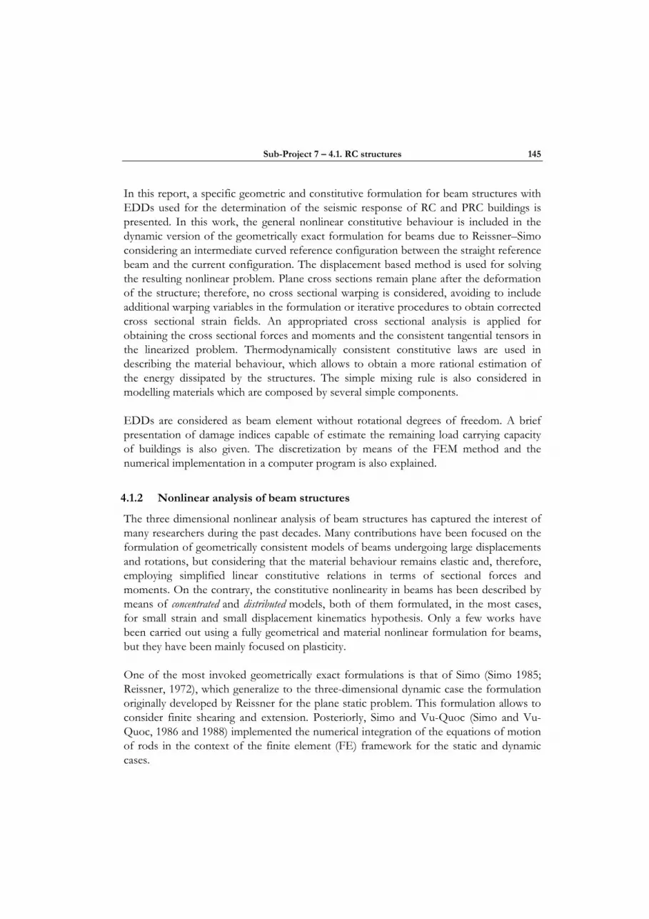
Sub-Project 7 – 4.1. RC structures 145
In this report, a specific geometric and constitutive formulation for beam structures with EDDs used for the determination of the seismic response of RC and PRC buildings is presented. In this work, the general nonlinear constitutive behaviour is included in the dynamic version of the geometrically exact formulation for beams due to Reissner–Simo considering an intermediate curved reference configuration between the straight reference beam and the current configuration. The displacement based method is used for solving the resulting nonlinear problem. Plane cross sections remain plane after the deformation of the structure; therefore, no cross sectional warping is considered, avoiding to include additional warping variables in the formulation or iterative procedures to obtain corrected cross sectional strain fields. An appropriated cross sectional analysis is applied for obtaining the cross sectional forces and moments and the consistent tangential tensors in the linearized problem. Thermodynamically consistent constitutive laws are used in describing the material behaviour, which allows to obtain a more rational estimation of the energy dissipated by the structures. The simple mixing rule is also considered in modelling materials which are composed by several simple components.
EDDs are considered as beam element without rotational degrees of freedom. A brief presentation of damage indices capable of estimate the remaining load carrying capacity of buildings is also given. The discretization by means of the FEM method and the numerical implementation in a computer program is also explained.
4.1.2 Nonlinear analysis of beam structures
The three dimensional nonlinear analysis of beam structures has captured the interest of many researchers during the past decades. Many contributions have been focused on the formulation of geometrically consistent models of beams undergoing large displacements and rotations, but considering that the material behaviour remains elastic and, therefore, employing simplified linear constitutive relations in terms of sectional forces and moments. On the contrary, the constitutive nonlinearity in beams has been described by means of concentrated and distributed models, both of them formulated, in the most cases, for small strain and small displacement kinematics hypothesis. Only a few works have been carried out using a fully geometrical and material nonlinear formulation for beams, but they have been mainly focused on plasticity.
One of the most invoked geometrically exact formulations is that of Simo (Simo 1985; Reissner, 1972), which generalize to the three-dimensional dynamic case the formulation originally developed by Reissner for the plane static problem. This formulation allows to consider finite shearing and extension. Posteriorly, Simo and Vu-Quoc (Simo and Vu-Quoc, 1986 and 1988) implemented the numerical integration of the equations of motion of rods in the context of the finite element (FE) framework for the static and dynamic cases.

146 CIMNE
Works on constitutive nonlinearity have progressed based on a different approach, that’s, lumped and distributed plasticity models. The lumped plasticity models consider linear elastic structural elements equipped with plastic hinges at the ends. This method is recommended by certain authors due to its numerical efficiency when compared with the full three–dimensional (3D) formulation of the problem.
In the case of distributed plasticity models, the constitutive nonlinearity is evaluated at a fixed number of cross sections along the beam axis, allowing to obtain a distributed nonlinear behaviour along the structural elements. These sections are divided into a number of control points corresponding to fibres directed along the beam’s axis. Therefore, this approach is frequently referred as fibre approach (Shao et.al., 2005, Lessloss Deliverable report 54, 2005 (www.lessloss.org)). The employment of fibres allows predicting a more realistic strain–stress state at the cross section level, but it requires the definition of uniaxial constitutive laws for each material point.
Both approaches are affected by the strain localization phenomenon when materials with softening behaviour are employed. In any case, the whole structural response becomes mesh dependent if no appropriate corrections are considered. Hanganu et.al. (2002) and Barbat et.al. (1997) regularize the energy dissipated at material point level, limiting its value to the specific fracture energy of the material (Oliver et.al, 1990). This method ensure that the whole structural response remains objective, but the length of the zone where softening occurs is still mesh dependent.
One of the most common limitations of the distributed formulations lies in the fact that inelasticity is defined for the component of the strain acting in the direction normal to the face of the cross section and, therefore, the shearing components of the stress are treated elastically. This assumption does not allows to simulate the nonlinear coupling between different stress components at constitutive level, resulting in models where sectional shear forces and torsion moments are transmitted elastically across the elements (Davenne et.al., 2003; Neuenhofer and Filippou, 1997).
Works considering both constitutive and geometric nonlinearity are scarce and they have been mainly restricted to plasticity (Saje et.al., 1998). Outstanding works considering warping of arbitrary sections made of rate dependent and rate independent elastic–plastic material are proposed by Simo et.al. (1984) and Gruttmann et.al. (2000), respectively.
4.1.2.1 Finite deformation initially curved beams
The formulation of Simo and Vu Quoc for beams that can undergo large deformations in space is expanded considering an intermediate curved reference configuration between the straight reference beam and the deformed beam in the current configuration.
Sub-Project 7 – 4.1. RC structures 147
The straight reference beam is defined simply by means of straight fixed curve parameterized in terms of its arch-length coordinate. Beam cross-sections are described by means of a local coordinate system contained in the plane of the section. The curved reference beam is defined by means of a spatially fixed curve φ0. Additionally, each point on this curve has rigidly attached an orthogonal local frame, tβ (β=2,3), constructed by means of an orientation tensor Λ0 contained in SO(3). where the rotation manifold is denoted by SO(3). The beam cross-section, A, is defined considering this local coordinate system. The planes of the cross sections are normal to the vector tangent to the reference curve.
The motion deforms the centroid line of the curved reference beam adding a translational displacement and the local orientation frame is simultaneously rotated together with the beam cross section. In general, the normal vector to the cross section does not coincide with the tangent to the current curve because of the shearing. The position vector of any material point on the current reference beam, x, is:
∑=
Λ+=3
2βββξϕ tx (4.1.2)
where curve φ is the current centroid curve, and Λ is the current rotation tensor.
Figure 4-1. Configurational description of the beam
Eq. (4.1.2) implies that the current beam configuration is completely determined by the pairs (φ,Λ).
By the other hand, the deformation gradient (tensor) is defined as the gradient of the deformation mapping and determines the strain measures at any material point of the beam cross section. The deformation gradients of the curved reference beam and of the current beam referred to the straight reference configuration are denoted by F0 and F,

148 CIMNE
respectively. The deformation gradient Fn= FF0−1 relating the differential arch length elements of the curved reference configuration with the current placement is responsible for the development of strains, and can be expressed as
(4.1.3)
Where (.),S denotes partial differentiation with respect to the arc-length parameter S, ωn
and Λn are the spatial curvature tensor and the rotation tensor relative to the curved reference beam. The material representation of Fn is obtained as Fmn= ΛTFnΛ0.
Removing the rigid body component from Fn, it is possible to construct the strain tensor εn = Fn −Λn, conjugated to the asymmetric First Piola Kirchhoff (FPK) stress tensor P, which is referred to the curved reference beam. Pj is the corresponding FPK stress vector acting on the deformed face in the current beam corresponding to the normal t0j in the curved reference configuration. The spatial strain vector acting on the current beam cross section relative to an element of area in the curved reference beam is obtained as εn = εnt01. The spatial form of the stress resultant n and the stress couple m vectors can be estimated from the stress vector P1 as:
(4.1.4)
According to the developments presented by Antman, (1991), the classical form of the equations of motion of the Cosserat beam for the static case are:
(4.1.5)
Where n,S and m,S are the external body force and body moment per unit of reference length at time t. Aρ0, Sρ0 and Iρ0 are the mass density, the first mass moment density and the second mass moment density per unit of length of the curved reference beam, respectively. The terms D1 and D2 appear due to the initial curvature and an inhomogeneous distribution of the material properties; and their contribution to the dynamics can be neglected or added to the external forces and moments.
Considering a kinematically admissible variation, h=(δφ,δθ), of the pair (φ,Λ), taking the dot product with Eq. (4.1.5) and integrating over the length of the curved reference

Sub-Project 7 – 4.1. RC structures 149
beam, we obtain the nonlinear functional G(x,h) corresponding to the virtual work principle, with the following form:
(4.1.6)
4.1.3 Nonlinear constitutive models
Frequently, the material properties have been assumed hyper elastic, isotropic and homogeneous (Ibrahimbegovic, 1995) and, therefore, the reduced constitutive equations became very simple. In this case, realistic studies involve constitutive nonlinearities as well as geometric effects for representing appropriately an adequate combination of strength, ductility and stiffness (Elnashai and Mwafi, 2002). Material points on the beam cross sections are considered as formed by a composite material corresponding to a homogeneous mixture of different simple components, each of them with its own constitutive law (see Figure 4-2). The behaviour of the composite is obtained by means of the mixing theory described in the following sections.
Figure 4-2. Cross section showing the composite associated to a material point
Two kinds of nonlinear constitutive models for simple materials are used in this work: the damage and plasticity models. They correspond to a particular cases of more general formulations, (Barbat et.al. 1997), but formulated in a way such that it is possible to include them in the geometrically exact formulation for beams previously described. The constitutive models are formulated in terms of the material form of the FPK stress and strain vectors, Pm1 and Εn, respectively.
150 CIMNE
4.1.3.1 Degrading materials: damage model
The behaviour of most of the degrading materials is presented attending to the fact that micro–fissuration in geomaterials occurs mainly due to the lack of cohesion between the particles, however a large amount of other processes are also involved as it can be consulted in (Hanganu et.al. 2002). The damage theory employed in this work is based on a special damage yielding function, which differentiates the mechanical response for tension or compression components of the stress vector. In this case, fissuration is interpreted as a local effect depending on the evolution of a set parameters of the material and the corresponding evolution equations. The progress of the damage is based on the evolution of a scalar parameter, which affects all the components of the elastic constitutive tensor and in this sense; it constitutes an isotropic damage model (Oliver et.al. 1990).
a. Constitutive Equation
In the case of thermally stable problems, considering the unconditional fulfilment of the Clausius–Plank inequality and applying the Coleman’s principle, we have the following constitutive relation for the material form of the FPK stress vector acting on each material point of the beam cross section:
(4.1.7)
Where Cme =Diag[E0,G0,G0] is the material form of the elastic constitutive tensor, with E0 and G0 the Young and shear undamaged elastic modulus and Cms=(1 − d)Cme is the material form of the secant constitutive tensor. Eq. (4.1.7) shows that the FPK stress vector is obtained from its elastic (undamaged) counterpart by multiplying it by the degrading factor (1 − d). The internal state variable d measures the lack of secant stiffness of the material.
b. Damage yield criterion By analogy with the developments presented in (Hanganu et.al., 2002; Oller and Barbat, 2006), the damage yield criterion denoted by the scalar value F is defined as a function of the undamaged elastic free energy density and written in terms of the components of the material form of the undamaged principal stresses,
Sub-Project 7 – 4.1. RC structures 151
(4.1.8)
where Pm is the equivalent (scalar) stress and the parameters r and n given in function of the tension and compression strengths fc and ft and the parts of the free energy density developed when the tension or compression limits are reached, (Ψ0t)L and (Ψ0c)L, respectively.
Other kind of damage yield criteria can be used in substitution of P e.g., Mohr–Coulomb, Drucker–Prager, Von Mises etc, according to the mechanical behaviour of the material. A more general expression equivalent to that given in Eq. (4.1.8) is the following:
(4.1.9)
where G(P) is a scalar monotonic function to be defined in such way to ensure that the energy dissipated by the material on a specific integration point is limited to the specific energy fracture of the material (Oliver et.al., 1990).
c. Evolution of the damage variable
The evolution law for the internal damage variable d is given by:
(4.1.10)
A damage yield condition and consistency condition are defined analogously as in plasticity theory. Finally, the Kuhn-Thucker relations have to be employed to derive the unloading–reloading conditions. The following expression is employed for the function G (Oliver et.al., 1990):
(4.1.11)
where the term G(χ) gives the initial yield stress for certain value of the scalar parameter χ. The parameter κ of Eq. (4.1.11) is calibrated to obtain an amount of dissipated energy equal to the specific fracture energy of the material when the entire deformation path is
152 CIMNE
followed. For a uniaxial tension process with a monotonically increasing load, the following expression is obtained for κ:
(4.1.12)
where it has been assumed that the equivalent stress tension is equal to the initial damage stress fc. The values of the maximum dissipation in tension Ξmaxt is a material parameter equal to the corresponding fracture energy density gf , which is derived from the fracture mechanics as gf= Gf/lc
where Gf the tensile fracture energy and lc is the characteristic length of the fractured domain employed in the regularization process (Lubliner et.al., 1989).
d. Tangent constitutive tensor After several algebraic manipulations, which can be reviewed in (Hanganu et.al., 2002, Lessloss Deliverable report 54, 2005 (www.lessloss.org)), we obtain that the material form of the tangent constitutive tensor Cmt can be calculated as where I is the identity tensor. It is worth noting that Cmt is nonsymmetric and it depends on the elastic FPK stress vector.
(4.1.13)
4.1.3.2 Plastic materials
In case of materials which can undergo non–reversible deformations the plasticity model, assuming a thermally stable process and small elastic and finite plastic deformations, formulated in the material configuration is used for predicting their mechanical response.
a. Constitutive equation
Following analogous procedures as those for the damage model i.e. employing the CP inequality and the Coleman’s principle (Lubliner, 1985; Malvern, 1969), the secant constitutive equation and the mechanical dissipation take the following forms
(4.1.14)
where the material description of the secant constitutive tensor Cms coincides with the elastic one and the super script ‘P’ is used to denote plastic strains.

Sub-Project 7 – 4.1. RC structures 153
b. Yield and plastic potential functions
Both, the yield function, Fp, and plastic potential function, Gp, for the plasticity model, are formulated in terms of the material form of the FPK stress vector and the plastic damage internal variable kp as:
(4.1.15)
where Pp is the (scalar) equivalent stress, which is compared with the hardening function fp depending on the damage plastic internal variable kp and the current stress state, and K is a constant value [38,46].
According to the evolution of the plastic damage variable, kp, it is possible to treat materials considering isotropic hardening. However, in this work kp constitutes a measure of the energy dissipated during the plastic process and, therefore, it is well suited for materials with softening. In this case kp is defined (Lubliner et.al., 1989) as:
(4.1.16)
where GPf is the specific plastic fracture energy of the material in tension and lc is the length of the fractured domain defined in analogous manner as for the damage model. The integral term in Eq. (4.1.16) corresponds to the energy dissipated by means of plastic work and, therefore, kp constitutes a measure of the part of the fracture energy that has been consumed during the deformation.
c. Evolution laws for the internal variables
The flow rules for the plastic strain vector and kp are defined as usual for plastic models defined in the material configuration according to
(4.1.17)
where λ is the plastic consistency parameter and is the following hardening vector

154 CIMNE
(4.1.18)
n is the plastic dissipation and r are as for the damage model. It is interesting to note that the proposed evolution rule allows to differentiate between tensile and compressive properties of the material.
As it is a standard practice in plasticity, the loading/unloading conditions are derived in the standard form from the Kuhn-Tucker relations formulated for problems with unilateral restrictions. By other hand, starting from the plastic consistency condition and considering the flow rules it is possible to deduce the explicit form of λ as:
(4.1.19)
d. Tangent constitutive tensor
The material form of the tangent constitutive tensor is calculated taking the time derivative of Eq. (4.1.14), considering the flow rules, replacing the plastic consistency parameter and after several algebraic manipulations, it is obtained as:
(4.1.20)
where Φp is the so-called hardening parameter.
4.1.3.3 Mixing theory for composites
Each material point on the beam cross is treated as a composite material according to the mixing theory considering the following assumptions: (i) Each composite has a finite number of simple components. (ii) Each component participates according to its volumetric participation. (iii) All the components are subjected to the same strain field. Therefore, the interaction between all the components, defines the overall mechanical behaviour of the composite at material point level. The assumption (i) implies that the N different components coexisting in a generic material point are subjected to the same material strain and, therefore, we have the following closing equation:
(4.1.21)

Sub-Project 7 – 4.1. RC structures 155
which imposes the strain compatibility between components. After applying the CP inequality and the Coleman’s principle, it is possible to obtain the material form of the FPK stress vector for the composite in analogous way as for simple materials, i.e.
(4.1.22)
where the FPK stress vector is obtained as a weighted sum, according to the volumetric fraction, of the material form of the stress vectors corresponding to each one of the N components. The material form of the secant constitutive equation, the secant and tangent constitutive tensors, Cms and Cmt, for the composite are obtained as (Oller et.al., 1996)
(4.1.23) where (Cms)q, and (Cmt)q are the material form of the secant and tangent constitutive tensors, respectively. Having calculated the material form of the FPK stress vector, the stress resultant and couples are then calculated employing Eqs. (4.1.4).
The mechanical behaviour of some advanced composed materials are based on a main matrix component which is reinforced with oriented fibres, e.g. epoxy based materials with glass or carbon fibres or even reinforced concrete, where the steel reinforcing bars and stirrups can be seen as embedded reinforcing fibres. The mixing rule provides an appropriated framework to simulate these kinds of composites, associating the one-dimensional version of the described constitutive laws to the reinforcements.
4.1.3.4 Energy Dissipating Devices
The energy dissipating devices are simulated using a rod element with only one Gauss integration point. The rotational degrees of freedom are released in both ends of the beam to obtain only relative displacements in the device. The constitutive law employed for dissipating devices corresponds to a bilinear plasticity, but any other one dimensional description can be employed, for example in Mata et.al. (2006), (Lessloss Deliverable report 54, 2005 (www.lessloss.org)), a constitutive description for elastomers to be employed in energy dissipating devices is given.

156 CIMNE
4.1.4 Numerical implementation
In order to obtain a Newton type numerical solution procedure, the linearized form of the weak form of Eq. (4.1.6) is required, which can be written as L[G(φ,Λ, h)] = G(φ,Λ,h)+DG(,Λ,h)· p where L[G] is the linear part of the functional G(φ,Λ,h) at the configuration defined by (φ,Λ) and p≡ (∆φ, ∆θ) is an admissible variation. The term G(φ,Λ,h) supplies the unbalanced force and the differential DG(φ ,Λ,h)· p, the tangential stiffness, which is calculated as
(4.1.24)
The numerical implementation in a FEM code of the internal, external and inertial terms of G in Eq. (4.1.24) follows standards procedures and it can be consulted in reference (Ibrahimbegovic and Mikdad, 2000).
The employment of nonlinear constitutive equations at material point level implies that the global structural damping is added to the system in the term Gint(x; h) of Eq. (4.1.24) by means of the reduced stress resultant and couples.
4.1.4.1 Tangential stiffness tensors
The discrete counterpart of the term DG(,Λ,h)· p of Eq. (4.1.24) leads to the tangential stiffness matrices, which can be obtained by means of the linearization of the different contributions due to internal, external and inertial terms. The linearization of the internal and external terms and its numerical implementation has been already presented in (Simo, 1986) for the case of linear elastic materials. For the case of an arbitrary distribution of materials within the cross section the linearization of the internal term produces
(4.1.25)
Where the operator [B] relates the linearized increment h and the linearized form of the co-rotated strain measures. The linearized form of the cross sectional force and moment

Sub-Project 7 – 4.1. RC structures 157
vectors takes into account the linearized strain-stress relations existing between P1m, obtained using the mixing theory, and the strain and strain rate vectors and is obtained as
(4.1.26)
Where Csvij is the spatial forms of the reduced tangential constitutive tensors, which are calculated simply replacing Cse within each material point by the tangential Csv and viscous Cse constitutive tensors in spatial description, and integrating over the cross section according the procedure described in (Kapania and Li, 2003) for the linear case. It is interesting to note that in the present formulation the reduced tangential and viscous constitutive tensors are rate dependent. Finally, it is possible to rewrite Eq. (4.1.25) as
(4.1.27)
Where [K]G gives the geometric part of the tangent stiffness matrix, [K]M and [K]V give the constitutive and viscous parts, which consider the contribution of the linearized stresses corresponding to each compounding material.
The inertial contribution of G(x,h) can be rewritten in terms of this material quantities and its linearized form is DGine·h as
(4.1.28)
where
158 CIMNE
(4.1.29)
And then it is possible to rewrite the linearized form of the spatial description of the inertial contribution term as
(4.1.30)
The terms [M], [Cgyr] and [Kcent] of Eq. (4.1.35) correspond to the mass, gyroscopic and centrifugal inertial tangential matrices of the discrete problem. The resulting inertial matrix is nonsymmetric and configuration dependent on the rotational degrees of freedom, as it can be verified from the gyroscopic and centrifugal terms. It is worth to note that all these terms appear coupled in Eq. (4.1.33). Finally, Eq. (4.1.29) can be rewritten as
(4.1.31)
where [K]P corresponds to the part of the tangent stiffness tensor, which is dependent on the loading and can be consulted in (Simo, 1986). The discretization of Eq. (4.1.35) by using the FEM method follows standard procedures and can be reviewed in (Hibrahimbegovic, 1996).
4.1.4.2 Cross sectional analysis
The cross section analysis is carried out expanding each integration point on the beam axis in a set of integration points located on each fibre on cross section. In order to perform this operation, the beam cross section is meshed into a grid of quadrilaterals, each of them corresponding to a fibre oriented along the beam axis (see Figure 4-3). The estimation of the average stress level existing on each quadrilateral is carried out by integrating the constitutive equations of the compounding materials of the composite associated to the corresponding quadrilateral and applying the mixing rule. The geometry

Sub-Project 7 – 4.1. RC structures 159
of each quadrilateral is described by means of normalized bi-dimensional shapes functions and several integration points can be specified in order to estimate more precisely the value of a given function according to a selected integration rule. In the case of the average value of the material form of the FPK stress vector acting on a quadrilateral we have
(4.1.32)
where Ac is the area of the quadrilateral, Np and Nq are the number of integration points in the two directions of the normalized geometry of the quadrilateral, Pm1(yp, zq) is the value of the FPK stress vector existing on a integration point with coordinates (yp, zq) with respect to the reference beam axis, which is obtained from the corresponding material strain vector using the constitutive laws and the mixing rule, Jpq is the Jacobian of the transformation between normalized coordinates and cross sectional coordinates and Wpq are the weighting factors. The coefficients of the tangent constitutive tensors can be estimated in an analogous manner as in Eq. (4.1.32) but replacing Pm1(yp,zq) by Cmt(yp,zq). Finally, having obtained the stress level on each quadrilateral, the cross sectional forces and moments are obtained by means of the discrete form of Eqs. (4.1.6) as
(4.1.33)
were Nfiber is the number of quadrilaterals of the beam cross section, (Ac)k is the area of the k quadrilateral, (Pm1)k is the average value of the material form of the FPK stress vector and k = (0, yk, zk) are the coordinates of the gravity centre of the kth quadrilateral with respect to the local beam reference frame.
Figure 4-3. Discrete fibre like model of the beam element

160 CIMNE
4.1.5 Numerical examples
4.1.5.1 Nonlinear Seismic Response of Planar Frame
In this work the seismic nonlinear response of a typical concrete industrial building is studied. The building has a bay width of 20 m and 24 m of inter–axes length. The storey high is 10 m. The concrete of the beam is H–50, (50 MPa, ultimate compression), with an elastic modulus of 35.000 MPa for the beam and H–30 for the concrete of the columns. It has been assumed a Poison coefficient of 0.2 for both concretes. The steel bar reinforcements considered in the study and the fibre discretization of the sections are those shown in Figure 4-4. The ultimate tensile stress for the steel is 510 MPa. The dimensions of the columns are 60 x 60 cm2. The beam has a variable section with an initial high of 80 cm on the supports and 120 cm in the middle of the span.
Figure 4-4. Columns and beam reinforcements and fibre model of the sections
The permanent loads considered are 2000 N/m2 and the weight of upper half of the closing walls, that is, 270,000xN. The employed acceleration record is the N–S component of the El Centro earthquake, 1940. The section of the energy dissipating devices was designed for yielding with an axial force of 300.000 N and for a relative displacement between the two ending nodes of 1.0 mm. The length of the dissipating devices is of 2.5 m (see Figure 4-5).
In Figure 4-6 it is possible to see the contribution of the dampers to reduce the displacements response. The obtained reduction is the order of 51 % minimizing the P–∆ effects. The maximum acceleration shows a reduction of the order of 30 % compared with the case where no devices are incorporated.

Sub-Project 7 – 4.1. RC structures 161
Figure 4-5. Precast industrial building without and with dissipaters
Figure 4-6. Displacements time history
4.1.5.2 3D Precast concrete building
The nonlinear seismic response of a precast building constructed in urban areas is studied. See Figure 4-7. The building has one bay and two storeys of 6 and 3 m width, respectively. The concrete of the structure is H–25, (25 MPa, ultimate compression), with an elastic modulus of 25,000 Pa. It has been assumed a Poison coefficient of 0.2. The steel bar reinforcements considered in the study are those corresponding to the 8 % of the sectional area for elements near to the joint (25 % of the column or beam length), and 4 % for elements in the middle part of the span. The ultimate tensile stress for the steel is 510 MPa. The dimensions of the columns are 30 x 30 cm2. The beams have a section of 15 x 30 cm2.
The permanent loads considered are the weight of the concrete floors, a live load of 2500 N/m2 and the weight of the closing walls, (432,000 N). The employed acceleration record is the same as before in the direction X and the same record scaled by 0.3 in the orthogonal direction.

162 CIMNE
No accidental or structural eccentricities were considered in this work, but it is possible to do it modifying the mass density of the beams or adding another structural element in the same of the planar frames.
1 2
3
4
Figure 4-7. (1) 3D Frame. (2) Dissipating devices incorporated. (3), (4): Column and beams sections.
Several numerical simulations were carried out to obtain an optimized combination of the characteristic of the energy dissipation devices for knowing what is the yielding level, Fy, stiffness, K, and yielding displacement, Dy, which give a biggest protection level to the structure. The properties of the employed energy dissipating devices are summarized in Table 4-1.
Table 4-1. Parameters of the energy dissipation devices
Device Characteristics Fy, (N) Dy, (mm)
1000 1.250
Fy, (N) Dy, (mm)
2000 1.250
Fy, (N) Dy, (mm)
3000 1.250
Fy, (N) Dy, (mm)
4000 1.250
Fy, (N) Dy, (mm)
5000 1.250
Fy, (N) Dy, (mm)
1000 2.500
Fy, (N) Dy, (mm)
2000 2.500
Fy, (N) Dy, (mm)
3000 2.500
Fy, (N) Dy, (mm)
4000 2.500
Fy, (N) Dy, (mm)
5000 2.500
Fy, (N) Dy, (mm)
1000 5.000
Fy, (N) Dy, (mm)
2000 5.000
Fy, (N) Dy, (mm)
3000 5.000
Fy, (N) Dy, (mm)
4000 5.000
Fy, (N) Dy, (mm)
5000 5.000
The results of the simulation are expressed in terms of maximum top and middle floor displacements; base shear and over-tuning moment are presented simultaneously as function of the type of employed device in Figure 4-8. From this figure it is possible to see that even when the biggest benefits in terms of the selected global variables are attained for different device characteristics, the more advantageous characteristics are related with flexible devices (K = 8000 N/mm) with a medium yielding displacement (approx. 2.5 mm) and yielding force around the 4000 N.
Therefore, the selected properties of the dissipaters were: Plastic yielding for a axial force of 4000 N, relative yielding displacement between the two ending nodes of 2.50 mm. The

Sub-Project 7 – 4.1. RC structures 163
length of the dissipating devices is of 6.7 m. The dissipating devices only were incorporated in the direction where the strongest ground acceleration record is applied.
1 2
3 4
Figure 4-8. Maximum response for each energy dissipating device. 1: Over–tuning Moment. 2: Top
floor displacement. 3: Middle floor displacement. 4: Base shear.
4.1.6 Conclusions
The geometrically exact formulation due to Reissner and Simo for 3D beams is considered in the context of initially curved beams and extended to include arbitrary distribution of composite materials in the cross sections. The resulting formulation is used for studying the constitutive and geometric nonlinear behaviour of framed structures in the static case.
Constitutive laws for the simple materials are based on thermodynamically consistent formulations allowing to obtain more realistic estimations of the energy dissipation in the nonlinear range. The simple mixing rule for composites is used for modelling complex material behaviours at material point level.
A detailed cross sectional analysis, consistent with the kinematics hypothesis is presented. The proposed method, even when inexact from the point of view of the elasticity theory, gives a computationally convenient way of approximating the strain–stress distribution in the section. A mesh independent response is obtained by means of the regularization of

164 CIMNE
the energy dissipated at constitutive level considering the characteristic length of the volume associated to a specific integration point and the fracture energy of the materials.
The seismic behaviour of two typical precast concrete structures is studied employing a numerical code, which incorporate a geometrically exact finite strain formulation for rods using appropriated constitutive laws for materials. The fibre beam model presented in this work provides a useful tool to simulate the earthquake effects on structures. A specific plastic energy dissipating device element is employed in the simulations. The advantages of employing dissipating devices to protect and improve the seismic behaviour of flexible and low damped precast structures with non ductile connecting joints is studied for the 2D and 3D cases presented here. From the results it is possible to see that several numerical simulation are required to validate the best choice for selecting the mechanical characteristics of the control devices to ensure the biggest improvements in the seismic response of the controlled structure.
4.2 PRECAST CONCRETE PORTAL FRAMES
4.2.1 Post-earthquake surveys
Typical damages are observed on precast reinforced concrete structure caused by earthquake: in many cases, beams simply fall down from their support, due to lack of resistance and energy dissipation capacity at the beam-column connections.
Figure 4-9. General collapse of a precast structure for a one-storey industrial building (Kocaeli
earthquake, Turkey, 1999) [Toniolo (2002)]

Sub-Project 7 – 4.2. Precast concrete portal frames 165
Figure 4-10. Damaged half joint between a column and a simple supported beam of precast
structure [Toniolo (2002)]
According to Toniolo [2002], the principal cause of collapses of precast buildings is the loss of bearing of the beam on the column, together with the overturning of beams, under the combined effects of horizontal and vertical actions of earthquake. Bad design corresponds to scanty joint connections with dry bearing supports of beams without adequate structural tie or to a poor detailing of steel reinforcement of critical zones (mainly the pattern and spacing of stirrups).
In the Adana earthquake post survey [AFPS], an industrial collapsed building is analyzed. It seems that the causes of collapse are the underdesign of the dowel connections between beams and columns and the bad implementation of the grouted mortar around these dowels.
Concrete structure prefabricators use habitually pinned connections and particularly the dowel connection (simple to realise) as beam-to-column connection for one-storey structures.

166 ULIEGE
Figure 4-11. Example of pinned connections: bolted and dowel connections [FIP, 1994] [Collinet,
2004-2005]
It is clear that the causes of collapse are complex and result of several parameters. The weak point of precast concrete structures made of linear elements is clearly that they have concentrated connection zones, where the risk of failure is very high if not well designed.
These are generally non redundant connections, sensitive to bad evaluation of the action such as additional axial force in the beam - if differential movement of the columns foundations is present for example.
4.2.2 INERD pin connection
The INERD pin connection consists of two external eye-bars welded or bolted to the adjacent member. It was originally developed in the context of the steel structures and it is presented with detail in section 4.3. of this report. INERD pin connection can be used to solve connection problems in structures made of any material, if capacity design is used in such a way that energy dissipation takes place in the connection, while the structural elements, beams and columns, remain elastic. However the peculiarities of application to other structures than steel structures need to be assessed. This is done in the following for precast concrete structures made of linear elements.
4.2.3 Bracings using INERD pin connections
To reduce the vulnerability of existing precast concrete portal frames, we propose to add 2 short bracings using INERD pin connections at beam-column joints. These bracings should be dissipative. The detailed study on the use of bracings using INERD pin connections in precast reinforced concrete structure is presented in deliverable D55 of the LESSLOSS Project ( www.lessloss.org ).

Sub-Project 7 – 4.2. Precast concrete portal frames 167
Beam
Column Column
Bracing using INERD pin connections
Bracing using INERD pin connections
Figure 4-12. Precast reinforced concrete structures braced with INERD pin connections
The use of the system is suited for new construction as well as for upgrading existing precast RC structures, which is the focus of subproject 7 of the LESSLOSS project. In the case of upgrading existing precast RC structures, bracings using 2 INERD pin connections must be adapted to the characteristics of the beam and column elements: dimensions, position of the reinforcements, type of beam-column connection.
The configuration of the bracing system using 2 INERD pin connections is sketched at Figure 4-13.
Front view Left view
Column
Dowel connection
INERD Pin Connection
Beam
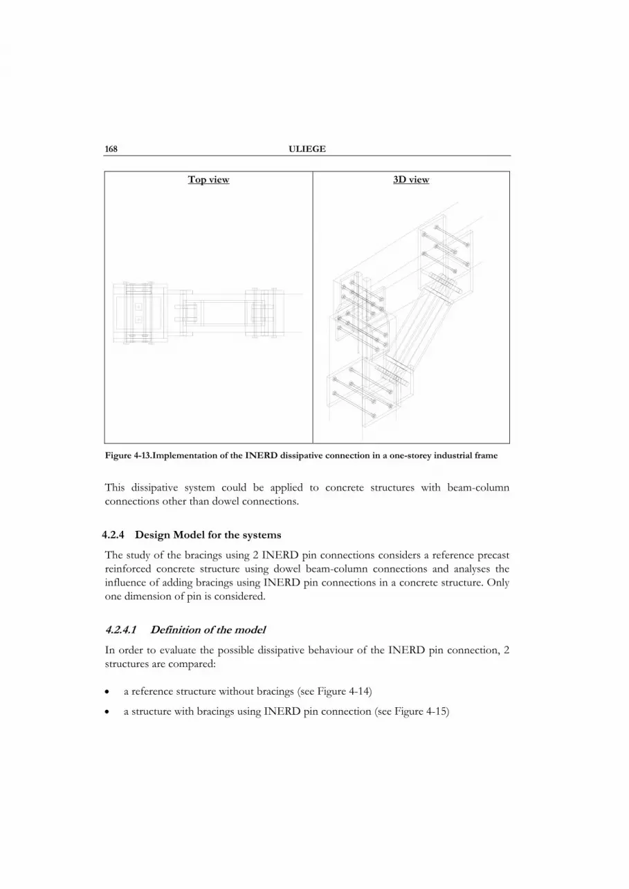
168 ULIEGE
Figure 4-13.Implementation of the INERD dissipative connection in a one-storey industrial frame
This dissipative system could be applied to concrete structures with beam-column connections other than dowel connections.
4.2.4 Design Model for the systems
The study of the bracings using 2 INERD pin connections considers a reference precast reinforced concrete structure using dowel beam-column connections and analyses the influence of adding bracings using INERD pin connections in a concrete structure. Only one dimension of pin is considered.
4.2.4.1 Definition of the model
In order to evaluate the possible dissipative behaviour of the INERD pin connection, 2 structures are compared:
• a reference structure without bracings (see Figure 4-14)
• a structure with bracings using INERD pin connection (see Figure 4-15)
Top view
3D view
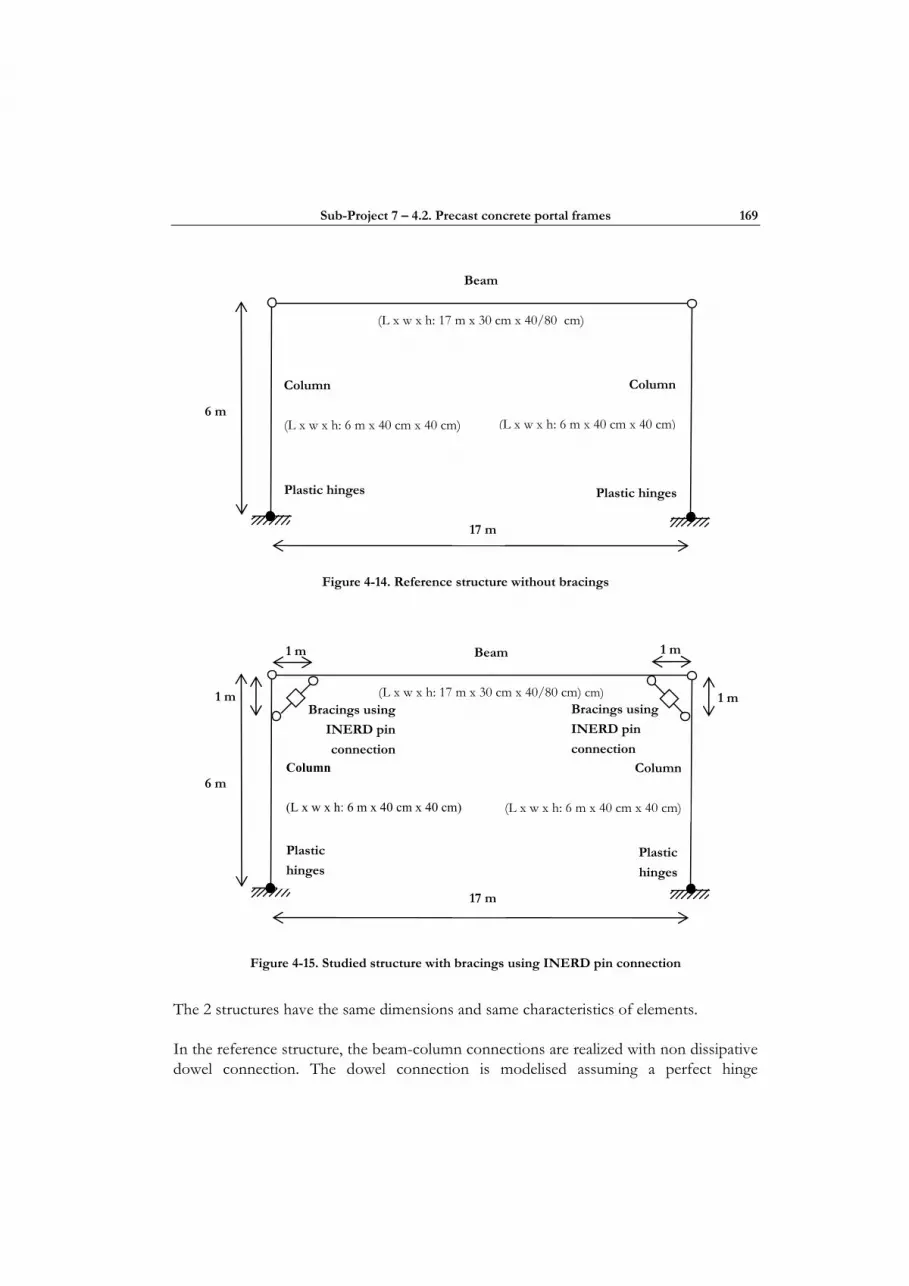
Sub-Project 7 – 4.2. Precast concrete portal frames 169
Figure 4-14. Reference structure without bracings
Figure 4-15. Studied structure with bracings using INERD pin connection
The 2 structures have the same dimensions and same characteristics of elements.
In the reference structure, the beam-column connections are realized with non dissipative dowel connection. The dowel connection is modelised assuming a perfect hinge
6 m
Beam
(L x w x h: 17 m x 30 cm x 40/80 cm) cm)
Column
(L x w x h: 6 m x 40 cm x 40 cm)
Column
(L x w x h: 6 m x 40 cm x 40 cm)
17 m
Plastic
hinges Plastic
hinges
1 m 1 m
1 m Bracings using
INERD pin
connection
Bracings using
INERD pin
connection
1 m
6 m
Beam
(L x w x h: 17 m x 30 cm x 40/80 cm)
Column
(L x w x h: 6 m x 40 cm x 40 cm)
Column
(L x w x h: 6 m x 40 cm x 40 cm)
17 m
Plastic hinges Plastic hinges

170 ULIEGE
behaviour as dowel connection that cannot transmit bending moments between column and beam, but can transmit beam axial force to the column. The second structure has also a dowel connection at the beam-to-column joint to which we add a bracing with an INERD pin connection. The bracing provides a resisting moment at the beam to column connection. Once the INERD pin connection is activated, it can dissipate earthquake energy by hysteretic loops.
Figure 4-15 shows the implementation of the INERD pin connections system in a portal frame structure. Each brace includes 2 INERD pin connections but we consider in the model only one INERD pin connection by bracing with a capacity of deformation twice that of a single pin.
The formation of plastic hinges at the column bases is expected early during the loading. The model integrates the possibility to form plastic hinges at the column base by concentrated plastic hinges at that place.
4.2.4.2 Plastic hinges at column bases
FEMA 273 [1997] gives modelling parameters for non linear procedures in the case of reinforced concrete columns. We use the modelling parameters of columns controlled by flexure. 3 levels of ductility are defined (see Figure 4-16) corresponding to 3 plastic rotation capacities:
• low ductility θ : a = 0,005 rad, b= 0,005 rad
• average ductility θ : a = 0,01 rad, b= 0,015 rad
• high ductility θ : a = 0,02 rad, b = 0,03 rad
The ductility of the flexural plastic region of the column depends on the design of stirrups in this column base region, which influence the concrete containment.
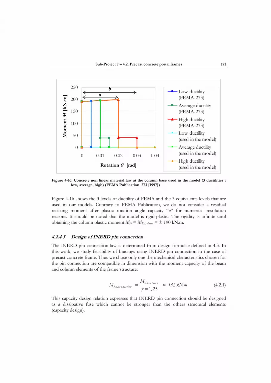
Sub-Project 7 – 4.2. Precast concrete portal frames 171
0
50
100
150
200
250
0 0.01 0.02 0.03 0.04
Rotation θ [rad]
Mom
ent M
[kN
.m]
Low ductility(FEMA-273)Average ductility(FEMA-273)High ductility(FEMA-273)Low ductility (used in the model)Average ductility(used in the model)High ductility (used in the model)
Figure 4-16. Concrete non linear material law at the column base used in the model (3 ductilities :
low, average, high) (FEMA Publication 273 [1997])
Figure 4-16 shows the 3 levels of ductility of FEMA and the 3 equivalents levels that are used in our models. Contrary to FEMA Publication, we do not consider a residual resisting moment after plastic rotation angle capacity “a” for numerical resolution reasons. It should be noted that the model is rigid-plastic. The rigidity is infinite until obtaining the column plastic moment Mpl = MRd,column = ± 190 kN.m.
4.2.4.3 Design of INERD pin connection
The INERD pin connection law is determined from design formulae defined in 4.3. In this work, we study feasibility of bracings using INERD pin connection in the case of precast concrete frame. Thus we chose only one the mechanical characteristics chosen for the pin connection are compatible in dimension with the moment capacity of the beam and column elements of the frame structure:
Rd,c o lum nRd,c on n ec tio n
MM 152 kN.m
1, 25γ = (4.2.1)
This capacity design relation expresses that INERD pin connection should be designed as a dissipative fuse which cannot be stronger than the others structural elements (capacity design).
a b
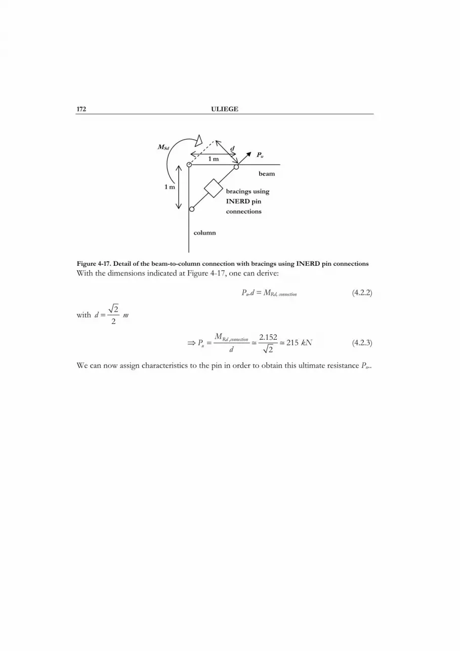
172 ULIEGE
Figure 4-17. Detail of the beam-to-column connection with bracings using INERD pin connections
With the dimensions indicated at Figure 4-17, one can derive:
Pu.d = MRd, connection (4.2.2)
with d m22
=
Rd connectionu
MP kN
d, 2.152 215
2⇒ = (4.2.3)
We can now assign characteristics to the pin in order to obtain this ultimate resistance Pu..
bracings using
INERD pin
connections
1 m
1 m
d
beam
column
Pu MSd

Sub-Project 7 – 4.2. Precast concrete portal frames 173
Table 4-2. Characteristics of the studied INERD pin connection
Force Displacement Force-displacement behaviour
of pin connections
)1,1/(
2
aM
P py
⋅= =
97,44 kN
aM
P pu
⋅=
4=
214,375 kN
( )ααδ 436
5,1 2 −⋅⋅⋅⋅
⋅=IE
M py =
2,68 mm
aII ⋅= 2,0δ = 20 mm
a⋅= 8,0limδ = 80 mm
Geometrical and material data of the pin connection
Geometrical data of the pin connection
yplp fWM ⋅= = 5,36 kN.m
a=α = 0,33
h = 35 mm b = 35 mm (Pin square shape section)
= 300 mm (equal to width of the beam) a = 100 mm
fy = 500 N/mm² Wpl = 10718,75 mm³
I = 125052 mm4 E = 200000 N/mm²
aa
l
text text
h
tint tint
b
Pu
Py
P II
I
δII δy δlim δ

174 ULIEGE
-250-200-150-100-50
050
100150200250
-80 -60 -40 -20 0 20 40 60 80
δ [mm]
P [
kN]
P [kN]
Figure 4-18. Force-displacement behaviour of the studied INERD pin connection
-200
-150
-100
-50
0
50
100
150
200
-0.15 -0.05 0.05 0.15
θ = δ/ d [rad]
M =
P.d
[kN
.m]
M [kN.m]
Figure 4-19. Equivalent moment-rotation behaviour of the beam column connection with the
addition of the studied INERD pin connection

Sub-Project 7 – 4.2. Precast concrete portal frames 175
4.2.4.4 Static non linear analysis (Pushover analysis)
In order to evaluate the effectiveness of bracings connected with INERD pin connections, we consider the 2 structures (see Figure 4-14 and Figure 4-15: structure with and without the studied INERD pin connection) integrating non linear material behaviours (non linear material law for concrete at the column base in all cases and INERD pin connection law whenever it is necessary), and realize several pushover analyses. Considering different levels of ductility (rotation capacity) at column bases (see Figure 4-16.).
The loading is monotonic with the effects of the cyclic behaviour and load reversals being estimated by using a modified monotonic force-deformation criteria and with damping approximations. Static pushover analysis is an attempt by the structural engineering profession to evaluate the real strength of the structure. In our analysis, the increasing load is a horizontal force F applied at the top of the column (near the centre of gravity of the structure) and the monitoring displacement is the top column displacement dr. The pushover is realized with an increasing displacement and a measure of the horizontal force corresponding to this displacement because SAP 2000 requires that the monitored parameter function (displacement in this case) must be strictly monotonous during the pushover. With the increase in the loading, weak links and failure modes of the structure should be found.
Figure 4-20. Pushover analysis: increasing force F and monitored displacement dr
F
dr
θ θ
F/2 F/2
dr
dr,pl dr,el dr,pl
Centre of gravity of the structure
dr,el
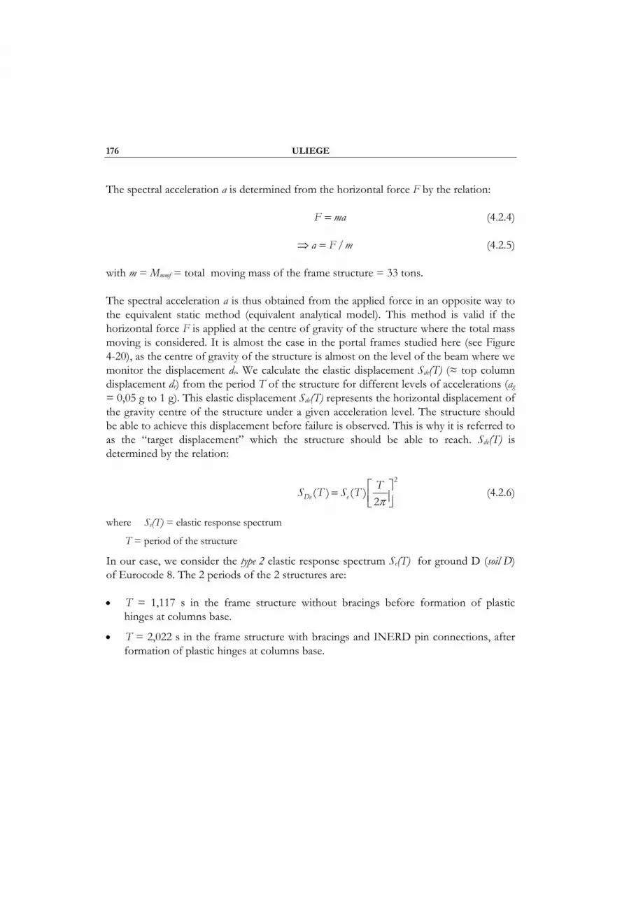
176 ULIEGE
The spectral acceleration a is determined from the horizontal force F by the relation:
F ma= (4.2.4)
a F m/⇒ = (4.2.5)
with m = Mmmf = total moving mass of the frame structure = 33 tons.
The spectral acceleration a is thus obtained from the applied force in an opposite way to the equivalent static method (equivalent analytical model). This method is valid if the horizontal force F is applied at the centre of gravity of the structure where the total mass moving is considered. It is almost the case in the portal frames studied here (see Figure 4-20), as the centre of gravity of the structure is almost on the level of the beam where we monitor the displacement dr. We calculate the elastic displacement Sde(T) (≈ top column displacement dr) from the period T of the structure for different levels of accelerations (ag = 0,05 g to 1 g). This elastic displacement Sde(T) represents the horizontal displacement of the gravity centre of the structure under a given acceleration level. The structure should be able to achieve this displacement before failure is observed. This is why it is referred to as the “target displacement” which the structure should be able to reach. Sde(T) is determined by the relation:
De eTS T S T
2
( ) ( )2π
⎡ ⎤= ⎢ ⎥⎣ ⎦ (4.2.6)
where Se(T) = elastic response spectrum
T = period of the structure
In our case, we consider the type 2 elastic response spectrum Se(T) for ground D (soil D) of Eurocode 8. The 2 periods of the 2 structures are:
• T = 1,117 s in the frame structure without bracings before formation of plastic hinges at columns base.
• T = 2,022 s in the frame structure with bracings and INERD pin connections, after formation of plastic hinges at columns base.
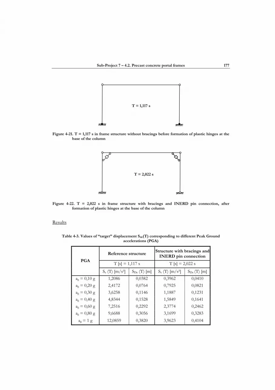
Sub-Project 7 – 4.2. Precast concrete portal frames 177
Figure 4-21. T = 1,117 s in frame structure without bracings before formation of plastic hinges at the
base of the column
Figure 4-22. T = 2,022 s in frame structure with bracings and INERD pin connection, after
formation of plastic hinges at the base of the column
Results
Table 4-3. Values of “target” displacement Sde(T) corresponding to different Peak Ground accelerations (PGA)
Reference structure Structure with bracings and
INERD pin connection
T [s] = 1,117 s T [s] = 2,022 s PGA
Se (T) [m/s²] SDe (T) [m] Se (T) [m/s²] SDe (T) [m] ag = 0,10 g 1,2086 0,0382 0,3962 0,0410 ag = 0,20 g 2,4172 0,0764 0,7925 0,0821 ag = 0,30 g 3,6258 0,1146 1,1887 0,1231 ag = 0,40 g 4,8344 0,1528 1,5849 0,1641 ag = 0,60 g 7,2516 0,2292 2,3774 0,2462 ag = 0,80 g 9,6688 0,3056 3,1699 0,3283
ag = 1 g 12,0859 0,3820 3,9623 0,4104
T = 2,022 s
T = 1,117 s
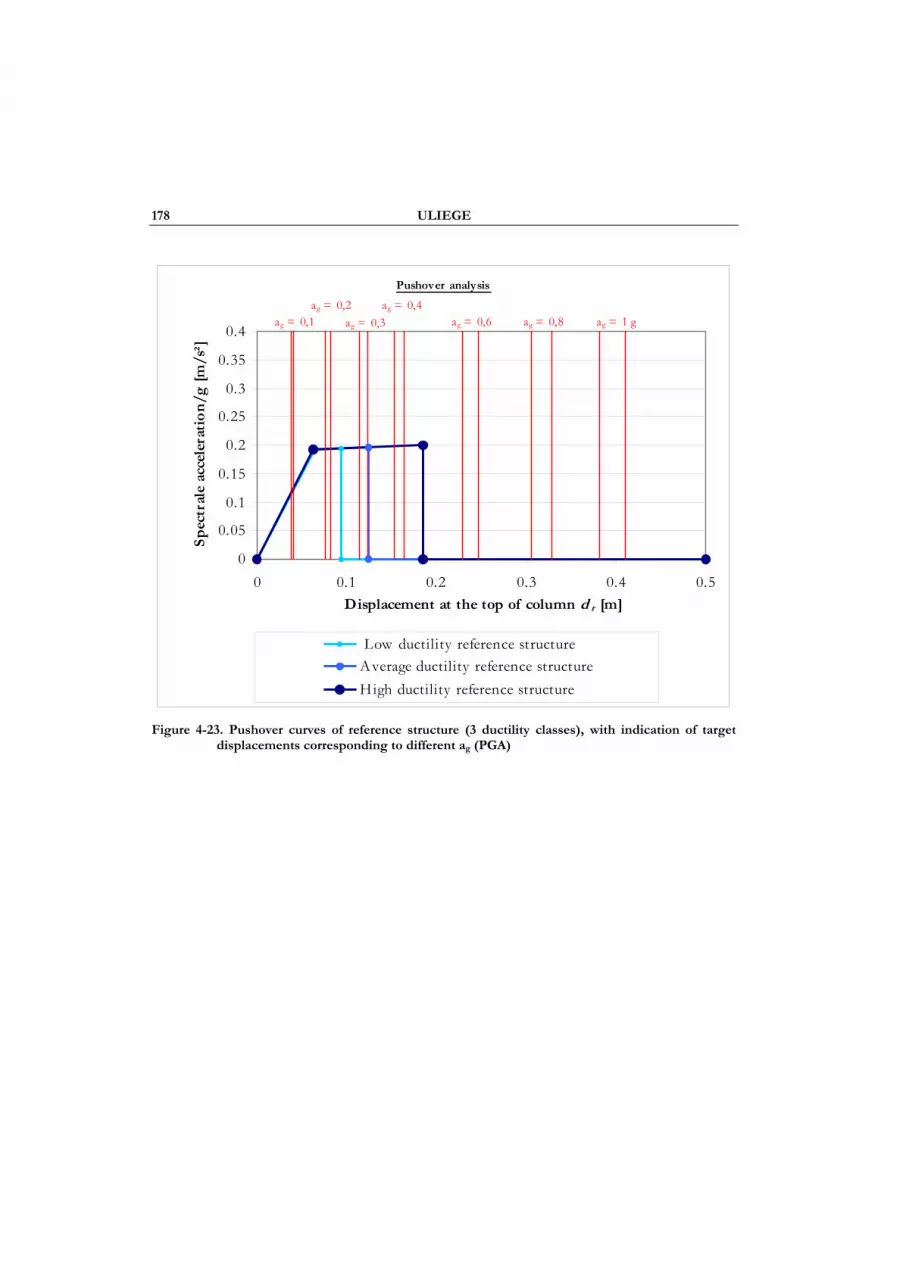
178 ULIEGE
Pushover analysis
0
0.05
0.1
0.15
0.2
0.25
0.3
0.35
0.4
0 0.1 0.2 0.3 0.4 0.5Displacement at the top of column d r [m]
Sp
ectr
ale
acce
lera
tio
n/g
[m
/s²]
Low ductility reference structureAverage ductility reference structureHigh ductility reference structure
ag = 0,8 ag = 1 gag = 0,4
ag = 0,3 ag = 0,2
ag = 0,1 ag = 0,6
Figure 4-23. Pushover curves of reference structure (3 ductility classes), with indication of target
displacements corresponding to different ag (PGA)
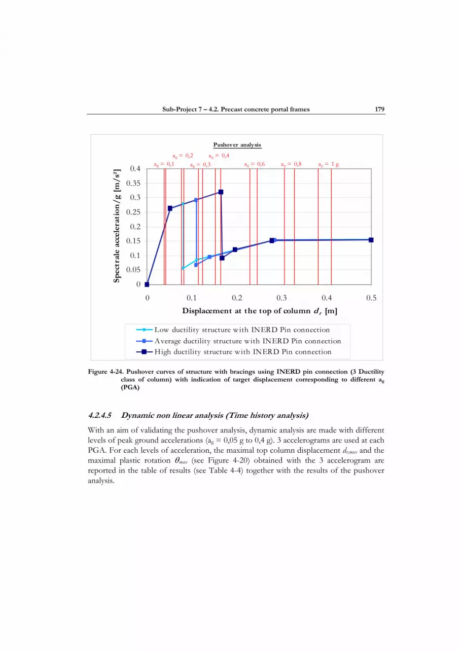
Sub-Project 7 – 4.2. Precast concrete portal frames 179
Pushover analysis
0
0.05
0.1
0.15
0.2
0.25
0.3
0.35
0.4
0 0.1 0.2 0.3 0.4 0.5Displacement at the top of column d r [m]
Spec
tral
e ac
cele
rati
on/g
[m
/s²]
Low ductility structure w ith INERD Pin connectionAverage ductility structure w ith INERD Pin connectionHigh ductility structure w ith INERD Pin connection
ag = 0,8 ag = 1 gag = 0,4
ag = 0,3 ag = 0,2
ag = 0,1 ag = 0,6
Figure 4-24. Pushover curves of structure with bracings using INERD pin connection (3 Ductility class of column) with indication of target displacement corresponding to different ag
(PGA)
4.2.4.5 Dynamic non linear analysis (Time history analysis)
With an aim of validating the pushover analysis, dynamic analysis are made with different levels of peak ground accelerations (ag = 0,05 g to 0,4 g). 3 accelerograms are used at each PGA. For each levels of acceleration, the maximal top column displacement dr,max and the maximal plastic rotation θmax (see Figure 4-20) obtained with the 3 accelerogram are reported in the table of results (see Table 4-4) together with the results of the pushover analysis.
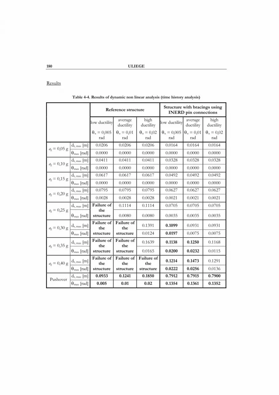
180 ULIEGE
Results
Table 4-4. Results of dynamic non linear analysis (time history analysis)
Reference structure Structure with bracings using
INERD pin connections
low ductility average ductility
high ductility low ductility average
ductility high
ductility
θu = 0,005
rad θu = 0,01
rad θu = 0,02
rad θu = 0,005
rad θu = 0,01
rad θu = 0,02
rad dr, max [m] 0.0206 0.0206 0.0206 0.0164 0.0164 0.0164
ag = 0,05 g θmax [rad] 0.0000 0.0000 0.0000 0.0000 0.0000 0.0000 dr, max [m] 0.0411 0.0411 0.0411 0.0328 0.0328 0.0328
ag = 0,10 g θmax [rad] 0.0000 0.0000 0.0000 0.0000 0.0000 0.0000 dr, max [m] 0.0617 0.0617 0.0617 0.0492 0.0492 0.0492
ag = 0,15 g θmax [rad] 0.0000 0.0000 0.0000 0.0000 0.0000 0.0000 dr, max [m] 0.0795 0.0795 0.0795 0.0627 0.0627 0.0627
ag = 0,20 g θmax [rad] 0.0028 0.0028 0.0028 0.0021 0.0021 0.0021
dr, max [m] 0.1114 0.1114 0.0705 0.0705 0.0705 ag = 0,25 g
θmax [rad]
Failure of the
structure 0.0080 0.0080 0.0035 0.0035 0.0035
dr, max [m] 0.1391 0.1099 0.0931 0.0931 ag = 0,30 g θmax [rad]
Failure of the
structure
Failure of the
structure 0.0124 0.0197 0.0075 0.0075
dr, max [m] 0.1639 0.1138 0.1250 0.1168 ag = 0,35 g
θmax [rad]
Failure of the
structure
Failure of the
structure 0.0165 0.0200 0.0232 0.0115
dr, max [m] 0.1214 0.1473 0.1291 ag = 0,40 g θmax [rad]
Failure of the
structure
Failure of the
structure
Failure of the
structure 0.0222 0.0256 0.0136 dr, max [m] 0.0933 0.1241 0.1850 0.7912 0.7915 0.7900
Pushover θmax [rad] 0.005 0.01 0.02 0.1354 0.1361 0.1352

Sub-Project 7 – 4.2. Precast concrete portal frames 181
4.2.4.6 Analysis of the results
From Figure 4-23 which shows the pushover curve of reference structures, it appears that:
• low ductility reference structures can sustain ag up to 0,24 g;
• medium ductility reference structures can sustain ag up to 0,3 g
• high ductility reference structures can sustain ag up to 0,45 g,
Figure 4-24 shows the pushover curves of structures in which bracings with INERD pin connections are added. It appears that with these bracings, structure of any level of ductility at the column base will survive to all possible ag.
Under a peak ground acceleration or spectral acceleration ag ≤ 0,2 g, there is no failure, even in structures with low plastic rotation capacity at column base. In low seismic area (ag ≤ 0,2 g), bracings with INERD pin connections only bring rigidity at the structure and thus reduce rotation θmax and displacement dr,max (SLS state). Looking the ultimate limit state, bracings using INERD pin connections are not needed in precast concrete structures in low seismicity area
For higher peak ground acceleration ag > 0,2 g, bracings with INERD pin connections show all their effectiveness, especially for low plastic rotation capacity at column bases. The system ensures stability (ULS) and reduces deformations of the structure (SLS).
In a structure without bracings (Figure 4-23), when the plastic rotation capacity at column bases is reached, columns bases behave as real hinges and can be modelled like that. So, the structure becomes a mechanism and the failure of the structure takes place. Then, the structure collapse depends only of the column resisting moment and of the ductility of column at its bases.
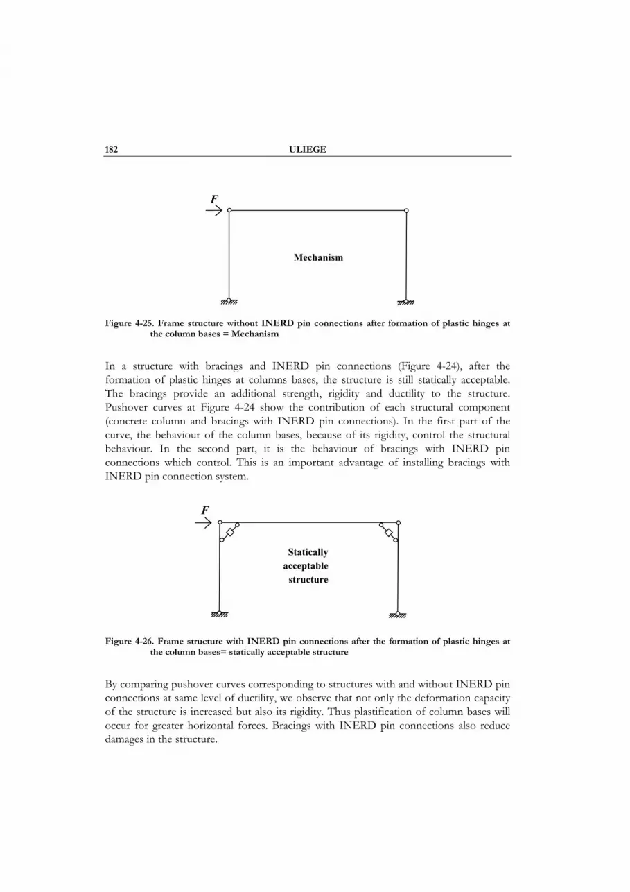
182 ULIEGE
Figure 4-25. Frame structure without INERD pin connections after formation of plastic hinges at
the column bases = Mechanism
In a structure with bracings and INERD pin connections (Figure 4-24), after the formation of plastic hinges at columns bases, the structure is still statically acceptable. The bracings provide an additional strength, rigidity and ductility to the structure. Pushover curves at Figure 4-24 show the contribution of each structural component (concrete column and bracings with INERD pin connections). In the first part of the curve, the behaviour of the column bases, because of its rigidity, control the structural behaviour. In the second part, it is the behaviour of bracings with INERD pin connections which control. This is an important advantage of installing bracings with INERD pin connection system.
Figure 4-26. Frame structure with INERD pin connections after the formation of plastic hinges at
the column bases= statically acceptable structure
By comparing pushover curves corresponding to structures with and without INERD pin connections at same level of ductility, we observe that not only the deformation capacity of the structure is increased but also its rigidity. Thus plastification of column bases will occur for greater horizontal forces. Bracings with INERD pin connections also reduce damages in the structure.
Statically acceptable
structure
F
Mechanism
F
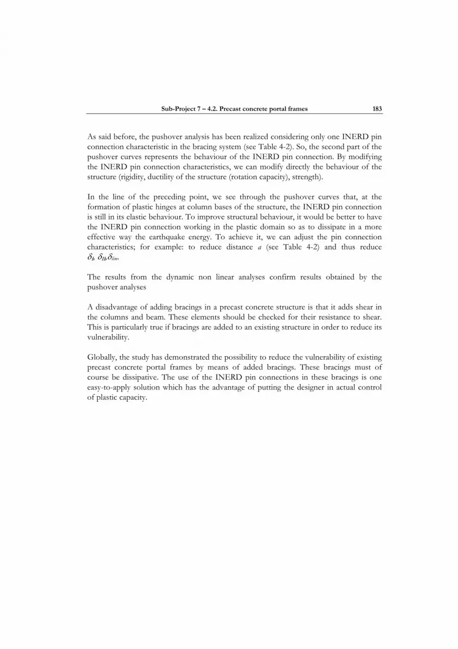
Sub-Project 7 – 4.2. Precast concrete portal frames 183
As said before, the pushover analysis has been realized considering only one INERD pin connection characteristic in the bracing system (see Table 4-2). So, the second part of the pushover curves represents the behaviour of the INERD pin connection. By modifying the INERD pin connection characteristics, we can modify directly the behaviour of the structure (rigidity, ductility of the structure (rotation capacity), strength).
In the line of the preceding point, we see through the pushover curves that, at the formation of plastic hinges at column bases of the structure, the INERD pin connection is still in its elastic behaviour. To improve structural behaviour, it would be better to have the INERD pin connection working in the plastic domain so as to dissipate in a more effective way the earthquake energy. To achieve it, we can adjust the pin connection characteristics; for example: to reduce distance a (see Table 4-2) and thus reduce δΙ, δΙΙ,δlim.
The results from the dynamic non linear analyses confirm results obtained by the pushover analyses
A disadvantage of adding bracings in a precast concrete structure is that it adds shear in the columns and beam. These elements should be checked for their resistance to shear. This is particularly true if bracings are added to an existing structure in order to reduce its vulnerability.
Globally, the study has demonstrated the possibility to reduce the vulnerability of existing precast concrete portal frames by means of added bracings. These bracings must of course be dissipative. The use of the INERD pin connections in these bracings is one easy-to-apply solution which has the advantage of putting the designer in actual control of plastic capacity.


Sub-Project 7 – 4.3. Steel frames with concentric bracings 185
4.3 STEEL FRAMES WITH CONCENTRIC BRACINGS. CONNECTIONS
4.3.1 Reasons for using dissipative connections in frames with concentric bracings and purpose of the research activity in LESSLOSS.
Seismic resistant structures are designed for stiffness, strength and ductility.
Stiffness requirements are imposed in order to limit non-structural damage in case of minor to moderate earthquakes and limit instability effects. Strength is needed to ensure the capacity of the structure to resist safely the action effects. Ductility is a way to dissipate part of the seismic input energy through inelastic deformations and therefore reduce the cost of the structure in a comparison to a non ductile one.
All conventional frames have certain disadvantages in respect to the above design criteria. (Table 4-5). As dissipative connections necessarily bring to a structure more flexibility than “rigid” connections designed for overstrength, their use should not be envisaged in structures which are flexible by nature. It can be shown in the case of moment resisting frames that the loss of rigidity brought by use of dissipative connections must be compensated by deeper beam and column sections.
Table 4-5. Structural typologies and main characteristics for Steel Frames
Moment resisting Frames
(MRF)
Concentric Braced Frames
(CBF)
CBF with dissipative
connections
Stiffness Low High High Ductility High Low High
Dissipative zones
Beam-ends Diagonals Connections
On the contrary, frames with concentric bracings, which are naturally stiff, are a field of application for dissipative connections. Dissipative connections can be designed to be the weak point in the bracing system, while diagonals can be designed to avoid buckling; in that way, both tension and compression diagonals do contribute to the earthquake resistance and are present in the simple models used for design.
Dissipative connections however require research to demonstrate their ability to provide stable cyclic behaviour and to assess their potential for practical applications in structures. In the INERD project –Plumier et al, 2006 - such dissipative connections have been
186 ULIEGE
developed and evaluated experimentally. One of them, the “pin connection”, was demonstrated to possess the required qualities of strength, stiffness and resistance. Their positive input for a good global behaviour of low rise structures with X bracings has been shown in numerical studies. Furthermore, due to the character of “localised fuse” of such connection, the possibility is open to better tune resistance to demand, bringing a more homogeneous and, consequently, more ductile global behaviour of structures.
Further evaluations were needed to assess the practical range of application of frames with bracings and dissipative connections in the range of tall buildings. Those evaluations, which are presented in detail in Deliverable D56 of the LESSLOSS project (www.lessloss.org), are summarised here, together with design guidance for such structures.
4.3.2 The INERD pin connection geometry and properties
An INERD pin connection connect a brace and a columns by means of plates (eye-bars) and a pin running through them (Figure 4-27). The design procedure developed by Vayas & Thanopoulos 2005 is explained in details in Plumier et al. 2006. The behaviour of the pin connection can be modelled by a tri-linear curve. The design expressions are presented in Table 4-6 here under.
Inner plates
Outer plates
Dissipative pin Column
Diagonal bracing
Figure 4-27. Perspective and plan views of INERD pin connection. Definition of geometry.

Sub-Project 7 – 4.3. Steel frames with concentric bracings 187
Table 4-6. Design formulae for the connection with 2 internal plates
Eye-bars in Force Displacement
Point I
“yielding y”
Compression p
y Rk
MP
a,
2
( /1,1)= ( )p
yM
EI21, 5 3 4
6
αδ α−=
Point II
“ultimate u”
Compression p
u Rk
MP
a,
4
( /1,1)= II a0, 2δ =
Points I and II Tension 90% of above values
for Py and Pu
Over-strength for
capacity design checks
30% beyond Pu
Deformation capacity
alim 0,8δ =
Symbols.
p pl yM W f= aα = fy = yield stress of pin
= pin length (axial distance between external eye-bars)
a = clear distance between internal and external eye-bars
Wpl = plastic modulus of pin I = moment of inertia of pin
E = elastic modulus of pin ‘s material
For rectangular pins, Wpl = bh²/4 and I = bh³/12 h = pin height b = pin width
4.3.3 Code rules for braced frames with pin INERD-connections
Frames with bracings and dissipative connections may be designed according to the rules of Eurocode 8, with some modifications justified by the fact that energy dissipation takes place in the connections and not in the tension braces. Table 4-7 presents the original Eurocode 8 rules for frames with dissipative concentric bracing and the modified rules if dissipative INERD pin connections are used.
188 ULIEGE
Table 4-7. Eurocode 8 rules for frames with bracings –left, standard – right, with dissipative INERD pin connections.
Paragraph Dissipative diagonals Dissipative INERD pin connections
6.7.1
Design
criteria
(1)P Concentric braced frames shall be designed so that yielding of the diagonals in tension will take place before failure of the connections and before yielding or buckling of the beams or columns.
(1) P Concentric braced frames with pin INERD connections shall be designed so that: (a) yielding of the pins will take place before compression failure of the diagonals and before yielding or buckling of the beams or columns. (b) failure of the connections precedes buckling failure of the diagonals (c) yielding of the pins is limited at the damage limitation state (d) the other connection elements shall be designed with adequate overstrength relevant to the pins.
(2)P The diagonal elements of bracings shall be placed in such a way that the structure exhibits similar load deflection characteristics at each storey in opposite senses of the same braced direction under load reversals.
(2)P The diagonal elements of bracings and their connections shall be placed in such a way that the structure exhibits similar load deflection characteristics at each storey in opposite senses of the same braced direction under load reversals.
6.7.2 Analysis
(2)P The diagonals shall be taken into account as follows in an elastic analysis of the structure for the seismic action: in frames with diagonal bracings, only the tension diagonals shall be taken into account; (3) ……
(2)P The diagonals shall be taken into account as follows in an elastic analysis of the structure for the seismic action: in frames with diagonal bracings, both the tension and compression diagonals shall be taken into account; (3) Does not apply
6.7.3 Diagonal members
(1) to (9) (1) to (9) Do not apply, except (8)
6.7.4 Beams and columns
(1) … (1) as in the original text, with: Ω is the minimum value of Ωi = Pu,Rd,i/NEd,i over all the connections of the diagonals of the braced frame system; where Pu,Rd,I is the ultimate strength of the pin INERD connection.
4.3.4 Practical design procedure
For practical applications, the following design steps are recommended:
Sub-Project 7 – 4.3. Steel frames with concentric bracings 189
Step 1. Selection of the pin dimensions, according to the following requirements:
DHa
lim
cos0.8
2
ϕδ = ≥ ( 4.3.1 )
Μγ
= ≥,
, ,
y Rk
y Rd E ser
ser
PP N ( 4.3.2 )
Μγ
= ≥,
,
0
u Rk
u Rd Ed
PP N ( 4.3.3 )
a, δlim , Py,Rk , Pu,Rk : see Table 4.3.3 and Figure 4.3.1.
D = lateral drift ratio H = storey height
φ = angle of inclination of diagonal (from horizontal to diagonal)
γΜ0 and γΜser partial safety factor of resistance (=1,0)
NEd design force of the diagonal
NE,ser design force of the diagonal at the damage limitation state
ν=,
EdE ser
NN ( 4.3.4 )
ν reduction factor for lower return period of seismic action associated with damage limitation
Step 2. Verification of the brace dimensions
≤, b,Rdu RkP N ( 4.3.5 )
where: Nb,Rd buckling resistance of the diagonal
Step 3. Dimensioning of eye-bars, welds etc
All connection elements (eye-bars, bolts, welds etc.) shall be verified for the capacity design force, equal to:
= ,1, 3Ed u RkP P ( 4.3.6 )

190 ULIEGE
The thicknesses of the eye bars shall additionally check:
text ≥ 0,75 h tint ≥ 0,5 text a ≥ h
With h = pin height, text = thickness of external eye bars, tint = thickness of internal eye bars
Steel quality of the eye-bars has to be equal to or higher than that of the pin.
4.3.5 Application of dissipative connections to a tall office building with X bracings
4.3.5.1 Design stage
The structure chosen as reference is 15 storey high (Figure 4-28).
52,5
10,5
10,5
10,5
10,5
10,5
3,5
10 10 10
30
28
10 10 10
30
28x28
10
10
10
10
10
10
30
30
Figure 4-28. Reference structure. Elevation and plan.
The study explores parameters. Two interstorey drift limits are considered. Structure design 1 has ductile non structural elements and the interstorey drift limit is 0.01 h. Structure design 2 has fragile non structural elements and the interstorey drift limit is 0.005 h. Design with and without dissipative connections are made. The possibility to
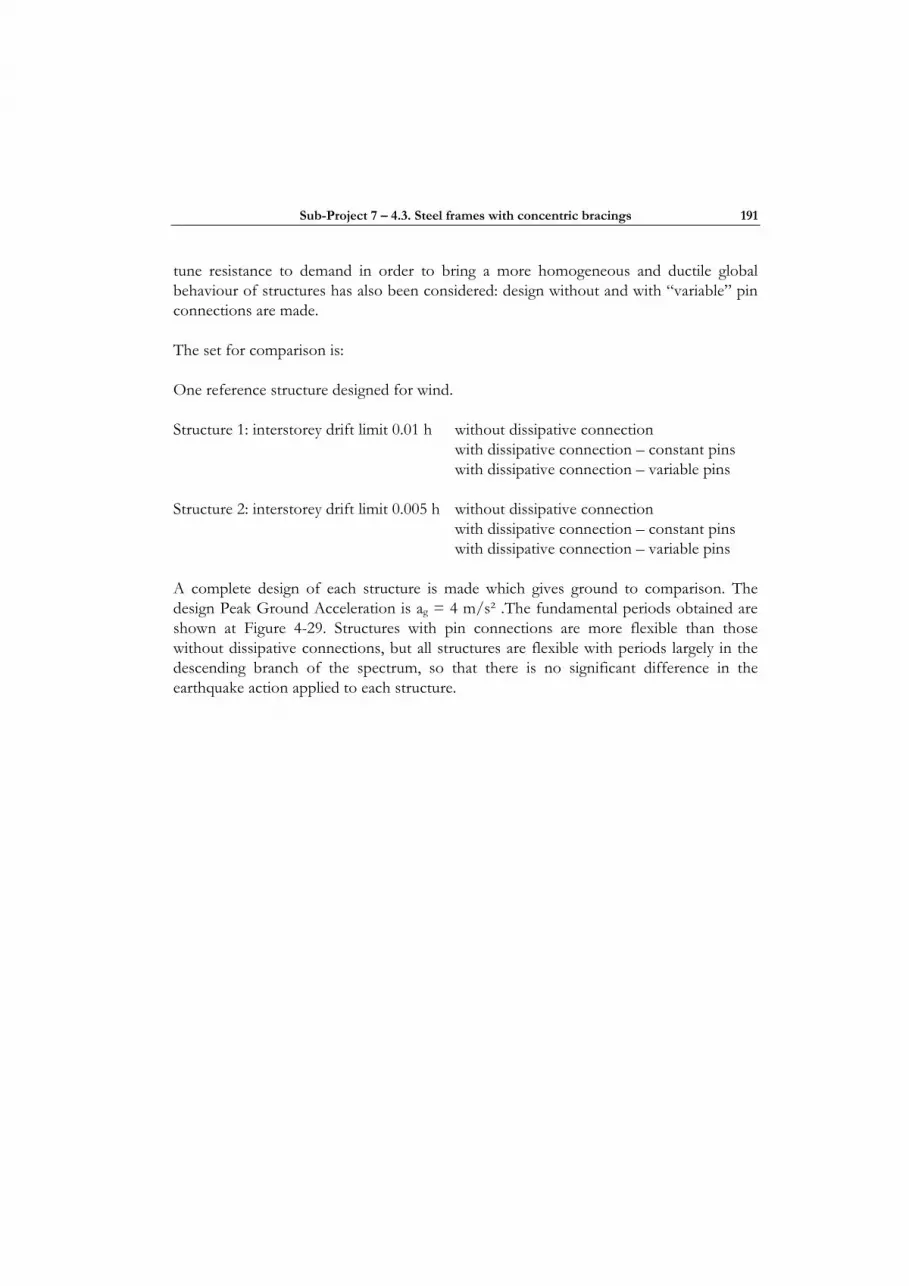
Sub-Project 7 – 4.3. Steel frames with concentric bracings 191
tune resistance to demand in order to bring a more homogeneous and ductile global behaviour of structures has also been considered: design without and with “variable” pin connections are made.
The set for comparison is:
One reference structure designed for wind.
Structure 1: interstorey drift limit 0.01 h without dissipative connection with dissipative connection – constant pins with dissipative connection – variable pins
Structure 2: interstorey drift limit 0.005 h without dissipative connection with dissipative connection – constant pins with dissipative connection – variable pins
A complete design of each structure is made which gives ground to comparison. The design Peak Ground Acceleration is ag = 4 m/s² .The fundamental periods obtained are shown at Figure 4-29. Structures with pin connections are more flexible than those without dissipative connections, but all structures are flexible with periods largely in the descending branch of the spectrum, so that there is no significant difference in the earthquake action applied to each structure.

192 ULIEGE
0
1
2
3
4
5
6
0 0.5 1 1.5 2 2.5 3 3.5 4Periods in seconds
Pseudo-acceleration
(m/s²)
stru
ctur
e 2
with
INER
D p
in c
onne
ctio
ns
stru
ctur
e 1
with
INER
D p
in c
onne
ctio
ns
stru
ctur
e 2
with
out d
issi
pativ
e co
nnec
tion
stru
ctur
e 1
with
out d
issi
pativ
e co
nnec
tion
stru
ctur
e af
ter w
ind
desi
gn
Figure 4-29. Periods of the analysed structures.
In structures Type 1, the column sections are smaller with dissipative connections, but some diagonals are slightly bigger because of the non buckling criteria. The earthquake resistant structures with dissipative connections are 18 % lighter.
In structures Type 2, the interstorey drift criterion under Damage Limit State governs the design, so that no reduction in the sections of columns and diagonals is brought in by the use of dissipative connections. However, a high steel grade is necessary for the structure without dissipative connections (fy ≥ 355 MPa), while a lower steel grade (fy = 235 MPa) can be used in the design with dissipative connections.
The only design fulfilling all the Eurocode 8 criteria are those in which the resistance of the connections was tuned to the required resistance (structure 1 and 2 with “variable” pins).
4.3.5.2 Pushover analysis
The structures without dissipative connections are modelled with diagonals in tension only.
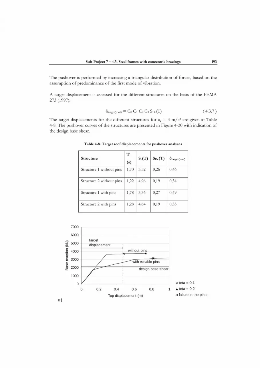
Sub-Project 7 – 4.3. Steel frames with concentric bracings 193
The pushover is performed by increasing a triangular distribution of forces, based on the assumption of predominance of the first mode of vibration.
A target displacement is assessed for the different structures on the basis of the FEMA 273 (1997):
δtarget(roof) = C0 C1 C2 C3 SDe(T) ( 4.3.7 )
The target displacements for the different structures for ag = 4 m/s² are given at Table 4-8. The pushover curves of the structures are presented in Figure 4-30 with indication of the design base shear.
Table 4-8. Target roof displacements for pushover analyses
Structure T
(s) Se(T) SDe(T) δtarget(roof)
Structure 1 without pins 1,70 3,52 0,26 0,46
Structure 2 without pins 1,22 4,96 0,19 0,34
Structure 1 with pins 1,78 3,36 0,27 0,49
Structure 2 with pins 1,28 4,64 0,19 0,35
a)
0
1000
2000
3000
4000
5000
6000
7000
0 0.2 0.4 0.6 0.8 1
Top displacement (m)
Bas
e re
actio
n (k
N)
without pins
with variable pins
target displacement
design base shear
teta = 0.1teta = 0.2failure in the pin co
194 ULIEGE
b)
0
1000
2000
3000
4000
5000
6000
7000
0 0.2 0.4 0.6 0.8 1
Top displacement (m)
Bas
e re
actio
n (k
N)
without pins
with variable pins
with constant pins
target displacement
design base shear
teta = 0.1teta = 0.2failure in the pin co
Figure 4-30. Pushover curves of structures (a) drift limit = 0.01h (b) drift limit = 0.005h
Target displacements are also reported, as well as displacements corresponding to values of the P-∆ effect parameter θ = 0.1 and 0.2 and to pin connections failure.
Table 4-9 reproduces those drifts at θ = 0.1; they are greater for structures with variable pin connections demonstrating a lower sensitivity to second order effects of structures with connections of resistance “tuned” to demand.
Table 4-9 also indicates the behaviour factors q deduced from the pushover curves, computed as: q = ductility = du/dy
For structures with dissipative connections, dy is found at the intersect of the elastic behaviour line with the design shear, in order to avoid the influence of the tri-linear curve used to model pin behaviour and to approach the value which would be found considering a bilinear behaviour. For classical design, dy is found at the intersect of elastic and plastic behaviour. For both type of structures, du is conventionally defined as the point corresponding to the attainment of θ =0.1 in the structure.
Figure 4-31 shows the impact of design conditions on the deformed shapes at θ = 0.1.
Table 4-9. Drifts at which θ = 0,1 and behaviour factor q from the pushover analysis
Structure Drift (%) q
Structure 1 without pins 0,9 1,7Structure 2 without pins 1,2 3,3
Structure 1 with pins 1,6 5,4Structure 2 with pins 0,9 4,0
Structure 2 with variable pins 1,5 6,4

Sub-Project 7 – 4.3. Steel frames with concentric bracings 195
a) b) Figure 4-31. Deformed shape at failure (a) with variable pins (b) all other structures
The pushover curves indicate that some yielding takes place in structures with dissipative INERD pin connections for loads lower than the design base shear. This is due to the tri-linear force-displacement curve used to describe the behaviour of pin connections. In spite of this early yielding, criteria on deflections under service load are satisfied. This design cannot be criticized, because it is similar to what is currently done in the modelling of moment resisting frames: the M-θ curve used to characterize the behaviour of beams in bending is represented by a bilinear law, which is a simplification of a real M-θ curve.
The design using dissipative connections takes fully advantage of the maximum behaviour factor for frames with concentric bracings (q = 4), while classical design result in an overstrength of about 2, so that the value of q really used is in fact 0.5 times the code value. This trend is clearly demonstrated in Table 4-9 in which computed q’s are given.
The only design which generates a global plastic mechanism is the one with pins of variable strength. In the other design, plastic deformations are localized in the bottom bracing.
4.3.5.3 Dynamic Non linear Time History Analyses
Time history analyses are realized with 3 artificial accelerograms, constructed for a type 1 earthquake on soil B, with a PGA of 0.4g and a duration of 15 s. Figure 4-32.

196 ULIEGE
-6
-4
-2
0
2
4
6
0 15
time (sec)
acce
lera
tion
(m/s
²)
Accelerogram 1
Figure 4-32. One artificial accelerogram used in the non linear dynamic analysis.
In the structures without dissipative connections, where the bracings are supposed to work in tension only, both bracings are modelled with a dissymmetric behaviour law. The diagonal in tension has its full plastic capacity while in compression, the diagonal are supposed buckled and keep 33 % of their buckling resistance.
The main result observed is the reduction of shear force at the base of the structures when using dissipative connections. Figure 4-33. In structures with ductile non structural elements, the reduction in base shear is 25 %. In structures with fragile non structural elements, the reduction is nearly 50 % .Table 4-10.
The parameter θ has been assessed in the dynamic analyses. Its maximum values are given in Table 4-11. In the structures were the resistance in the pins is adapted to the needed resistance, the values of θ are quite constant at the different levels. For the structures with overstrength in the upper levels (classical design and structure 2 with constant pins), θ is small for the upper levels and θ is big for the bottom level.
-6000
-4000
-2000
0
2000
4000
6000
-0.5 -0.4 -0.3 -0.2 -0.1 0 0.1 0.2 0.3 0.4 0.5
Top displacement (m)
Bas
e sh
ear (
kN)
w ithout pinsw ith pins
-6000
-4000
-2000
0
2000
4000
6000
-0.5 -0.4 -0.3 -0.2 -0.1 0 0.1 0.2 0.3 0.4 0.5
Top displacement (m)
Bas
e sh
ear (
kN)
w ithout pinsw ith pins
(a) structure 1 (drift < 0.010h) (b) structure 2 (drift < 0.005h)
Figure 4-33. Base shear-top displacement curves under dynamic analyses.
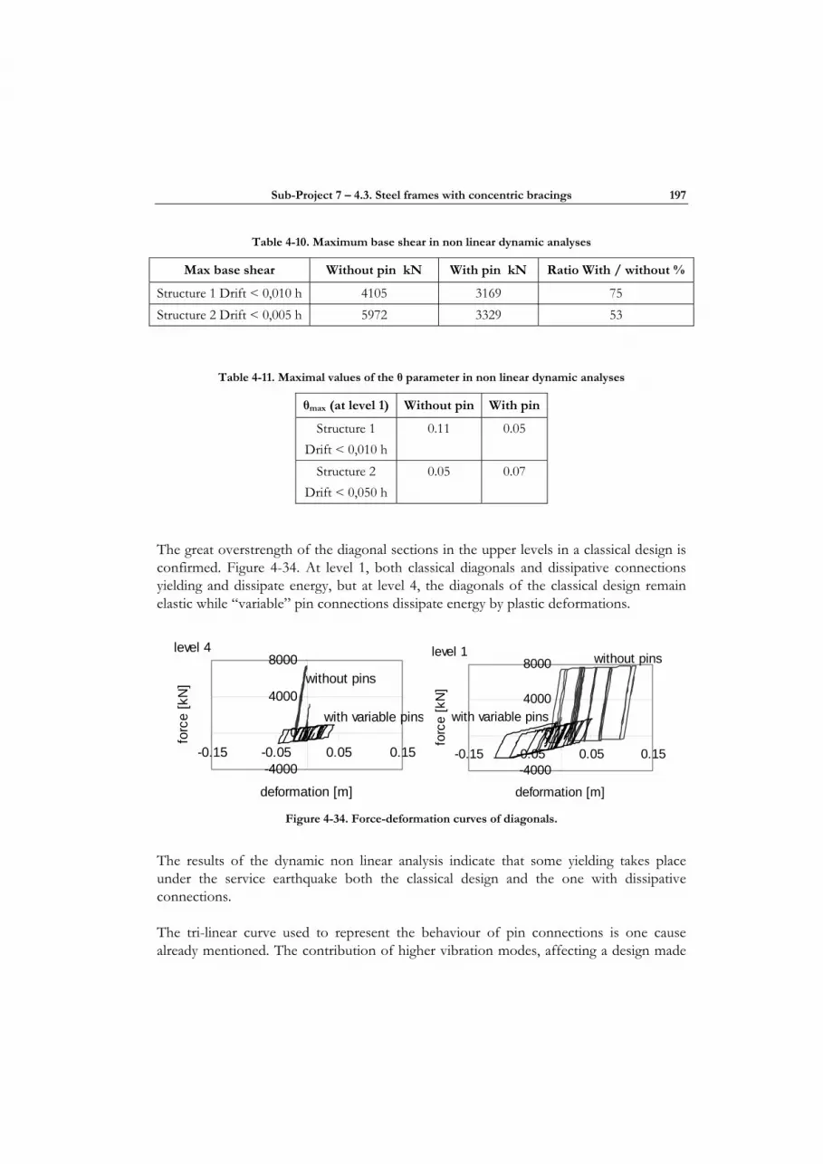
Sub-Project 7 – 4.3. Steel frames with concentric bracings 197
Table 4-10. Maximum base shear in non linear dynamic analyses
Max base shear Without pin kN With pin kN Ratio With / without %
Structure 1 Drift < 0,010 h 4105 3169 75 Structure 2 Drift < 0,005 h 5972 3329 53
Table 4-11. Maximal values of the θ parameter in non linear dynamic analyses
θmax (at level 1) Without pin With pin
Structure 1 Drift < 0,010 h
0.11 0.05
Structure 2 Drift < 0,050 h
0.05 0.07
The great overstrength of the diagonal sections in the upper levels in a classical design is confirmed. Figure 4-34. At level 1, both classical diagonals and dissipative connections yielding and dissipate energy, but at level 4, the diagonals of the classical design remain elastic while “variable” pin connections dissipate energy by plastic deformations.
-4000
0
4000
8000
-0.15 -0.05 0.05 0.15
deformation [m]
forc
e [k
N]
level 4
without pins
with variable pins
-4000
0
4000
8000
-0.15 -0.05 0.05 0.15
deformation [m]
forc
e [k
N]
level 1 without pins
with variable pins
Figure 4-34. Force-deformation curves of diagonals.
The results of the dynamic non linear analysis indicate that some yielding takes place under the service earthquake both the classical design and the one with dissipative connections.
The tri-linear curve used to represent the behaviour of pin connections is one cause already mentioned. The contribution of higher vibration modes, affecting a design made

198 ULIEGE
by the lateral force method (1 mode), is another possible explanation of some yielding, as some peaks of the accelerograms are 25 % above the 4 m/s² PGA.
Plastic deformations are essentially localized in the bottom bracing of the frame, except in the design with pins of variable strength. All design do satisfy the design criteria.
4.3.5.4 Conclusions of the application of dissipative connections to a tall office building with X bracings
Weak points of the classical design of frames with bracings have been set forward. In high rise structure, the Serviceability Limit State (interstorey drift limits under service earthquake) criteria governs the design of braces, leading to a heavy structure. The search for stiffness concludes into large diagonals and capacity design extend large overstrength to the non dissipative elements, columns and beams. The need for heavy diagonal sections is also in opposition with the lower bound limit of slenderness in Eurocode 8 (stockiness limit!). The high stiffness of the structure also results in a higher seismic design action.
Structures designed with dissipative connections of the diagonals eliminate the problem of buckling of the diagonals and the associated uncertainties on the real stiffness of the structure to consider in the design process. The designer is in control of the real plastic resistance of the structure, since the dissipative devices can be calibrated to the needed resistance. The fact that dissipative connections are “calibrated devices” eliminates the uncertainty on the real yield strength limit of the plastic zones and deletes the need to consider material overstrength factors in the design of non dissipative elements adjacent to the dissipative ones.
All designed structures are demonstrated to be able to reach the target displacement.
Structures using INERD pin connections with variable resistance deform plastically at all storey levels. This more uniform distribution of deformations results in an ability to reach greater displacements for a given value of the θ parameter (P-∆ criterion). This means less sensitivity to P-D effects and more available global ductility with the use of dissipative connections. Structures using INERD pin connections can be designed to provide the required resistance and have little overstrength. Classical design always conclude in a significant overstrength, which is of at least 2: resultant base shear is 3000 kN in a design using pin connections; it is 6000 kN in a classical design, which correspond also to much higher forces applied to the foundations and to much higher foundation costs.
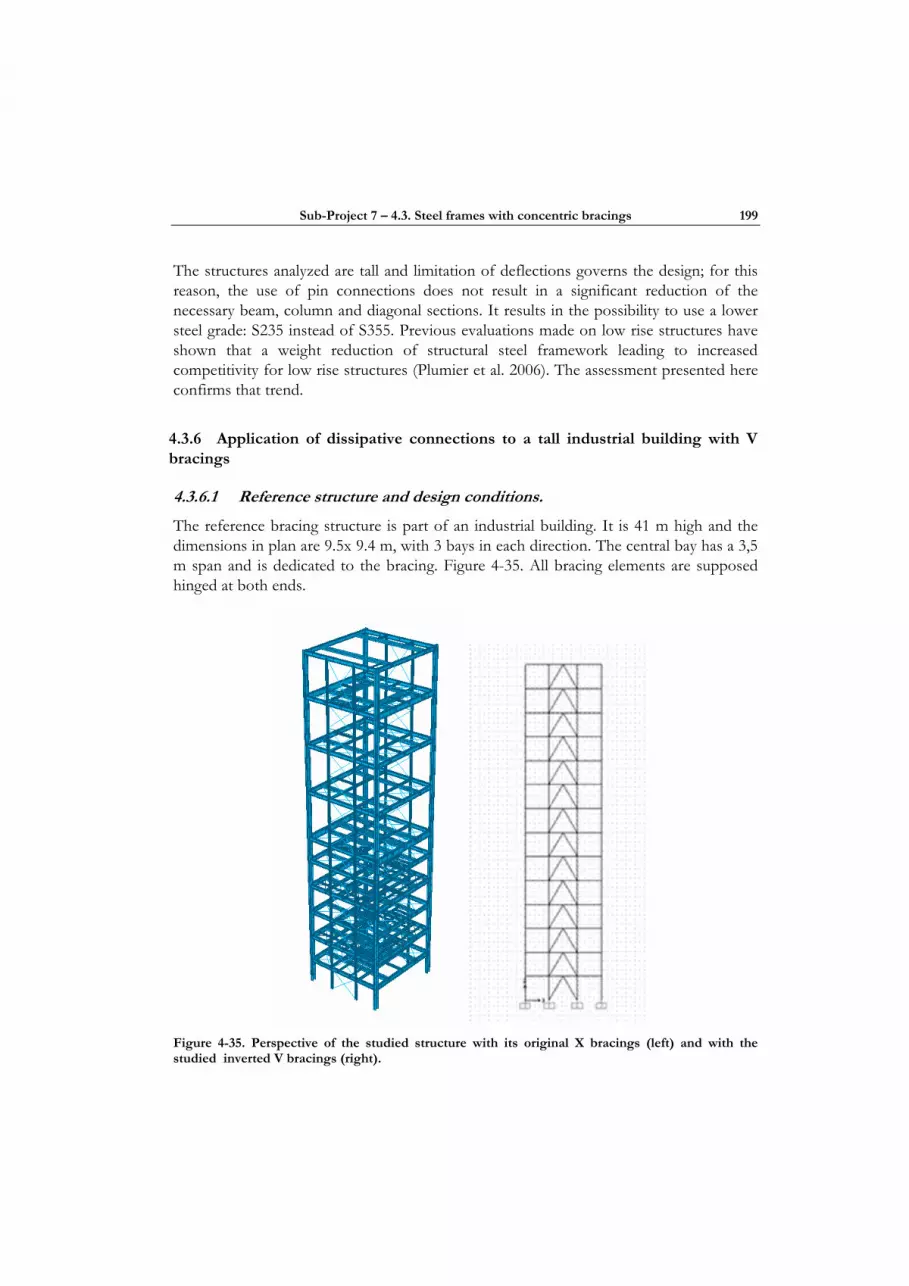
Sub-Project 7 – 4.3. Steel frames with concentric bracings 199
The structures analyzed are tall and limitation of deflections governs the design; for this reason, the use of pin connections does not result in a significant reduction of the necessary beam, column and diagonal sections. It results in the possibility to use a lower steel grade: S235 instead of S355. Previous evaluations made on low rise structures have shown that a weight reduction of structural steel framework leading to increased competitivity for low rise structures (Plumier et al. 2006). The assessment presented here confirms that trend.
4.3.6 Application of dissipative connections to a tall industrial building with V bracings
4.3.6.1 Reference structure and design conditions.
The reference bracing structure is part of an industrial building. It is 41 m high and the dimensions in plan are 9.5x 9.4 m, with 3 bays in each direction. The central bay has a 3,5 m span and is dedicated to the bracing. Figure 4-35. All bracing elements are supposed hinged at both ends.
Figure 4-35. Perspective of the studied structure with its original X bracings (left) and with the studied inverted V bracings (right).
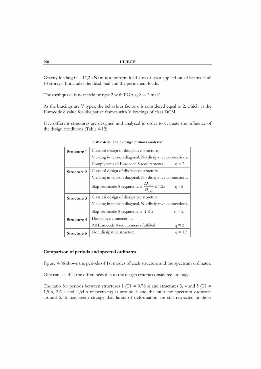
200 ULIEGE
Gravity loading G= 17,2 kN/m is a uniform load / m of span applied on all beams at all 14 storeys. It includes the dead load and the permanent loads.
The earthquake is near field or type 2 with PGA ag S = 2 m/s2.
As the bracings are V types, the behaviour factor q is considered equal to 2, which is the Eurocode 8 value for dissipative frames with V bracings of class DCM.
Five different structures are designed and analysed in order to evaluate the influence of the design conditions (Table 4-12).
Table 4-12. The 5 design options analysed
Structure 1 Classical design of dissipative structure. Yielding in tension diagonal. No dissipative connections. Comply with all Eurocode 8 requirements. q = 2
Structure 2 Classical design of dissipative structure. Yielding in tension diagonal. No dissipative connections.
Skip Eurocode 8 requirement max
min1, 25
ΩΩ
≤ q =2
Structure 3 Classical design of dissipative structure. Yielding in tension diagonal. No dissipative connections.
Skip Eurocode 8 requirement 2λ ≤ q = 2
Structure 4 Dissipative connections. All Eurocode 8 requirements fulfilled. q = 2
Structure 5 Non dissipative structure. q = 1,5
Comparison of periods and spectral ordinates.
Figure 4-36 shows the periods of 1st modes of each structure and the spectrum ordinates.
One can see that the differences due to the design criteria considered are huge.
The ratio for periods between structures 1 (T1 = 0,78 s) and structures 3, 4 and 5 (T1 = 1,5 s, 2,6 s and 2,64 s respectively) is around 3 and the ratio for spectrum ordinates around 5. It may seem strange that limits of deformation are still respected in those
Sub-Project 7 – 4.3. Steel frames with concentric bracings 201
flexible structures, but this is a result of a better distribution of storey drifts in those flexible design, in comparison with classical design, as it is shown later with more details.
Figure 4-36. Results in terms of periods and spectral ordinates.
4.3.6.2 Comparison of mass of designed structures.
Figure 4-37 shows the total mass of each primary resisting structure and the distribution between the various structural elements.
The design process set forward the fact that two criteria of Eurocode 8 lead to huge sections in comparison to wind design:
• criteria 1: 2λ ≤ which leads to
π≥min
12
yfLi
E ( 4.3.8 )
Period T(s)
202 ULIEGE
and prevent the use of sections with a radius of gyration smaller than 18,5 mm
• criteria 2 : ΩΩ
≤max
min
1, 25
The elements which are mostly penalised are diagonals and columns, which represent 80% of the structure weight. Not respecting one of the criteria brings a reduction in mass of the earthquake resisting structure up to 90 %. The most requiring criteria is the limit in slenderness. The simultaneous compliance to criteria 1 and 2 is related to the choice of designing a “dissipative” structure (but with q = 2 only in this case, which does not bring much return on the investment). This choice can be questioned and a non dissipative design (structure 5, q = 1,5) is indeed a more economical option. However, this is normally allowed only in low seismicity area, which is not the case here (ag S = 0,2 g > 0,1 g).
Structure 4 design with dissipative« pin connections » fulfil all Eurocode 8 criteria and also brings a 90% reduction in mass of steel in comparison to a classical dissipative design without dissipative connections complying with all EC8 criteria (structure 1). This impressive influence results from several factors:
• reduction of base shear due to a lower stiffness of the structure
• reduction of overstrength coefficient Ω (1,00 instead of 3,96 and 1,76 in structure 1)
• no unbalance between forces in the tension and the compression diagonals, resulting in no additional action effects in beams
The use of « pin connections » does not create problems with P-∆ effects: the parameter θmax remains smaller than 0,10.
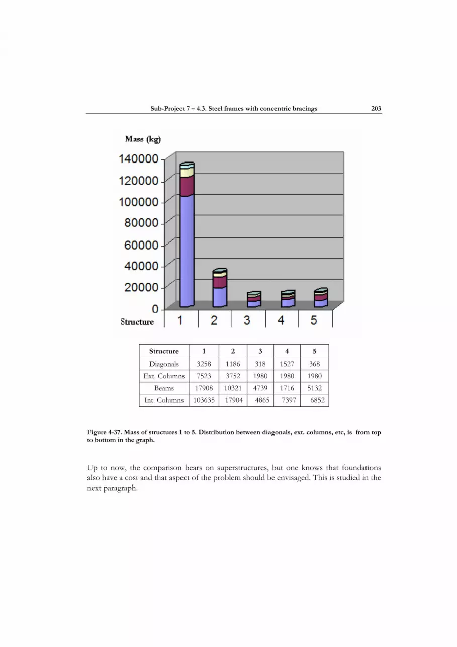
Sub-Project 7 – 4.3. Steel frames with concentric bracings 203
Structure 1 2 3 4 5
Diagonals 3258 1186 318 1527 368 Ext. Columns 7523 3752 1980 1980 1980
Beams 17908 10321 4739 1716 5132 Int. Columns 103635 17904 4865 7397 6852
Figure 4-37. Mass of structures 1 to 5. Distribution between diagonals, ext. columns, etc, is from top to bottom in the graph.
Up to now, the comparison bears on superstructures, but one knows that foundations also have a cost and that aspect of the problem should be envisaged. This is studied in the next paragraph.

204 ULIEGE
4.3.6.3 Influence of superstructure design on the dimensions of foundations.
The assessment considers only the reaction in tension at the base of the bracing. It allows a comparison between various design options for what concerns the anchorage required. The “unit” of comparison is the isolated foundation pad presented at Figure 4-38, which has to resist tension. Two volumes of soils are considered:
• The volume which it is necessary to dig out to realise the foundation pad. Figure 4-38.
• The volume which contributes to the stability.
The mass per unit volume of soil is taken equal to 19 kN/m3.
Figure 4-38. Volume of soil to dig out to realize the foundation pad.
4.3.6.4 Results of the analysis.
The results are presented at Table 4-13. They show that the classical dissipative structure 1 requires foundations which are by far the most expensive one. Very interesting is the difference between design 4 and 5, with 4 involving 25% less soil digging than for structure 5.
Volume of soil to dig out to realize the foundation pad
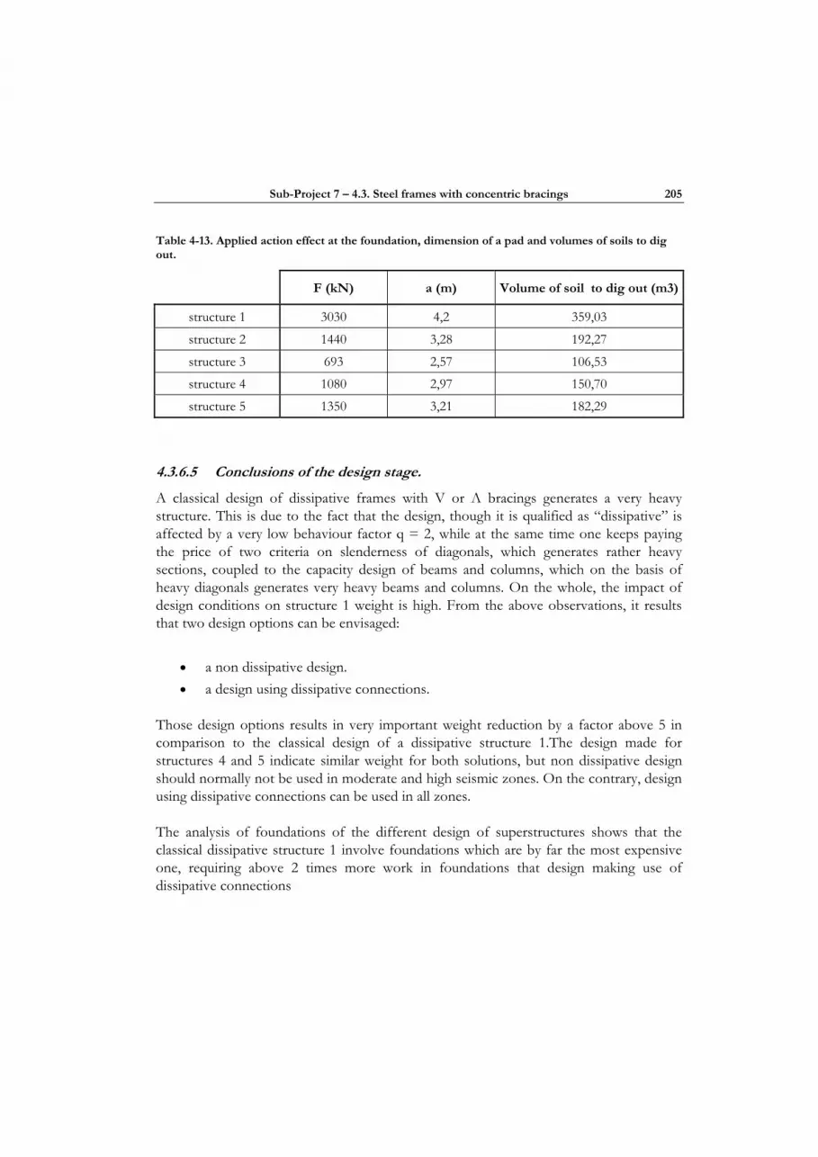
Sub-Project 7 – 4.3. Steel frames with concentric bracings 205
Table 4-13. Applied action effect at the foundation, dimension of a pad and volumes of soils to dig out.
F (kN) a (m) Volume of soil to dig out (m3)
structure 1 3030 4,2 359,03
structure 2 1440 3,28 192,27
structure 3 693 2,57 106,53
structure 4 1080 2,97 150,70
structure 5 1350 3,21 182,29
4.3.6.5 Conclusions of the design stage.
A classical design of dissipative frames with V or Λ bracings generates a very heavy structure. This is due to the fact that the design, though it is qualified as “dissipative” is affected by a very low behaviour factor q = 2, while at the same time one keeps paying the price of two criteria on slenderness of diagonals, which generates rather heavy sections, coupled to the capacity design of beams and columns, which on the basis of heavy diagonals generates very heavy beams and columns. On the whole, the impact of design conditions on structure 1 weight is high. From the above observations, it results that two design options can be envisaged:
• a non dissipative design. • a design using dissipative connections.
Those design options results in very important weight reduction by a factor above 5 in comparison to the classical design of a dissipative structure 1.The design made for structures 4 and 5 indicate similar weight for both solutions, but non dissipative design should normally not be used in moderate and high seismic zones. On the contrary, design using dissipative connections can be used in all zones.
The analysis of foundations of the different design of superstructures shows that the classical dissipative structure 1 involve foundations which are by far the most expensive one, requiring above 2 times more work in foundations that design making use of dissipative connections
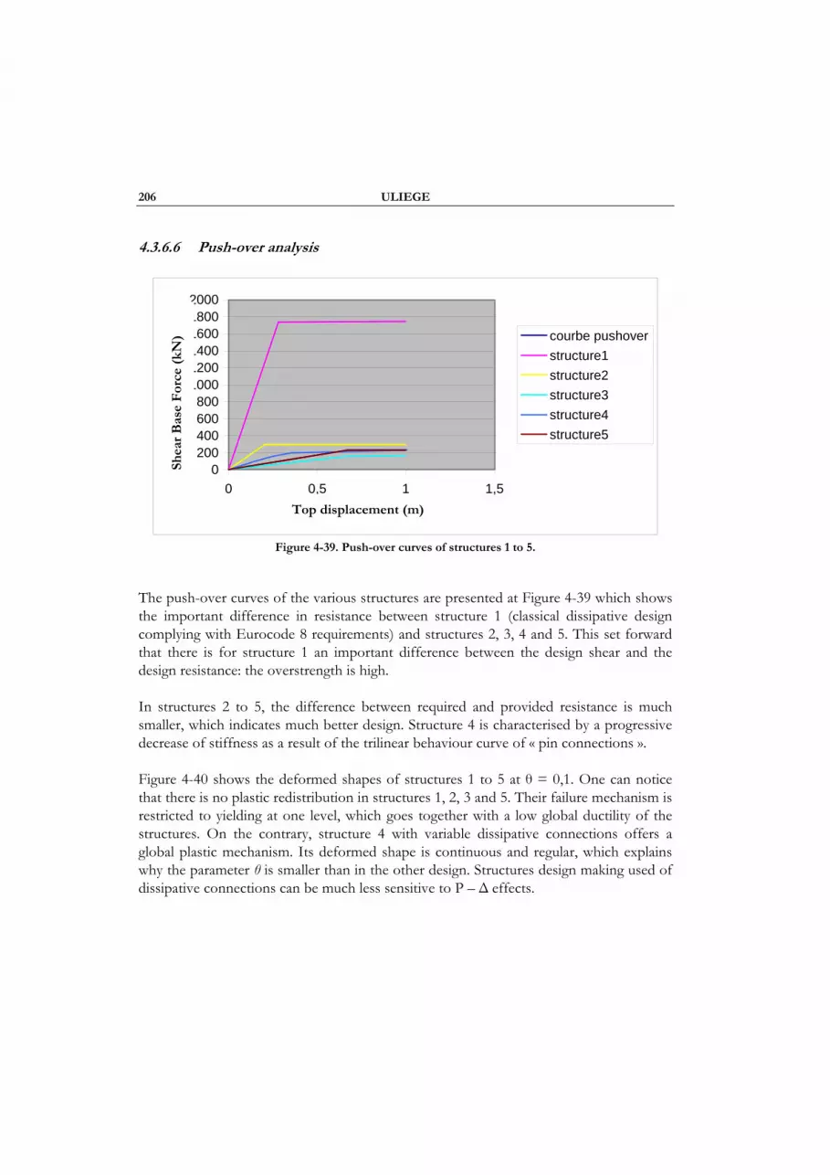
206 ULIEGE
4.3.6.6 Push-over analysis
0200400600800
100012001400160018002000
0 0,5 1 1,5
déplacement en tête (m)
cisa
illem
ent e
n ba
se (k
N)
courbe pushoverstructure1structure2structure3structure4structure5
Figure 4-39. Push-over curves of structures 1 to 5.
The push-over curves of the various structures are presented at Figure 4-39 which shows the important difference in resistance between structure 1 (classical dissipative design complying with Eurocode 8 requirements) and structures 2, 3, 4 and 5. This set forward that there is for structure 1 an important difference between the design shear and the design resistance: the overstrength is high.
In structures 2 to 5, the difference between required and provided resistance is much smaller, which indicates much better design. Structure 4 is characterised by a progressive decrease of stiffness as a result of the trilinear behaviour curve of « pin connections ».
Figure 4-40 shows the deformed shapes of structures 1 to 5 at θ = 0,1. One can notice that there is no plastic redistribution in structures 1, 2, 3 and 5. Their failure mechanism is restricted to yielding at one level, which goes together with a low global ductility of the structures. On the contrary, structure 4 with variable dissipative connections offers a global plastic mechanism. Its deformed shape is continuous and regular, which explains why the parameter θ is smaller than in the other design. Structures design making used of dissipative connections can be much less sensitive to P – ∆ effects.
Shea
r B
ase
For
ce (
kN)
Top displacement (m)
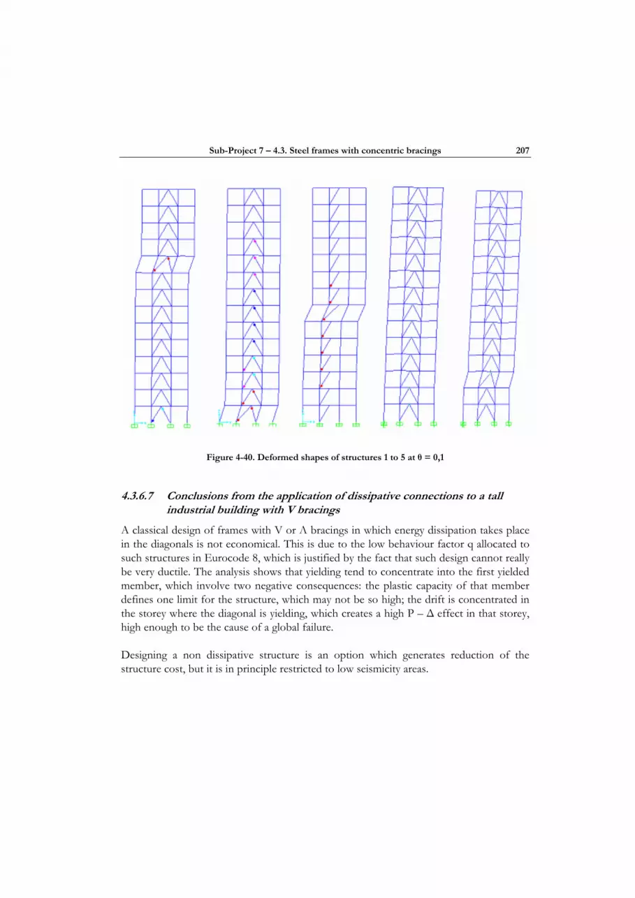
Sub-Project 7 – 4.3. Steel frames with concentric bracings 207
Figure 4-40. Deformed shapes of structures 1 to 5 at θ = 0,1
4.3.6.7 Conclusions from the application of dissipative connections to a tall industrial building with V bracings
A classical design of frames with V or Λ bracings in which energy dissipation takes place in the diagonals is not economical. This is due to the low behaviour factor q allocated to such structures in Eurocode 8, which is justified by the fact that such design cannot really be very ductile. The analysis shows that yielding tend to concentrate into the first yielded member, which involve two negative consequences: the plastic capacity of that member defines one limit for the structure, which may not be so high; the drift is concentrated in the storey where the diagonal is yielding, which creates a high P – ∆ effect in that storey, high enough to be the cause of a global failure.
Designing a non dissipative structure is an option which generates reduction of the structure cost, but it is in principle restricted to low seismicity areas.

208 ULIEGE
4.3.6.8 Conclusions from the application of dissipative connections to a tall industrial building with V bracings
A classical design of frames with V or Λ bracings in which energy dissipation takes place in the diagonals is not economical. This is due to the low behaviour factor q allocated to such structures in Eurocode 8, which is justified by the fact that such design cannot really be very ductile. The analysis shows that yielding tend to concentrate into the first yielded member, which involve two negative consequences: the plastic capacity of that member defines one limit for the structure, which may not be so high; the drift is concentrated in the storey where the diagonal is yielding, which creates a high P – ∆ effect in that storey, high enough to be the cause of a global failure.
Designing a non dissipative structure is an option which generates reduction of the structure cost, but it is in principle restricted to low seismicity areas.
The use of “variable” dissipative connections (the provided resistance meets the required resistance) leads to the best design: a real global plastic mechanism is formed, local exhaustion of plastic capacity of a member is avoided, as well as huge P- ∆ effects due to concentration of ∆ in one single storey over the height. This design option is the most economical in mass of the earthquake primary resisting structure (90% lighter than a “classical” design) and in terms of foundation costs (25% less than for a non dissipative structure).
4.3.7 General conclusions on the use of dissipative connections in frames with bracings
Structures designed with dissipative connections of the diagonals eliminate the problem of buckling of the diagonals and the associated uncertainties on the real stiffness of the structure to consider in the design process. The designer is in control of the real plastic resistance of the structure, since the dissipative devices can be calibrated to the needed resistance. The fact that dissipative connections are “calibrated devices” eliminates the uncertainty on the real yield strength limit of the plastic zones and deletes the need to consider material overstrength factors in the design of non dissipative elements adjacent to the dissipative ones.
Structures using INERD pin connections with resistance calibrated to demand (“variable” pins) deform plastically at all storey levels. It is not the case with classical dissipative design. The more uniform distribution of deformations achieved results in an ability to reach greater displacements for a given value of the θ parameter (P-∆ criterion). This means less sensitivity to P-∆ effects and more available global ductility with the use of dissipative connections. Structures using dissipative connections can be designed to provide the required resistance and have little overstrength. On the contrary, classical

Sub-Project 7 – 4.3. Steel frames with concentric bracings 209
dissipative design always conclude in an overstrength which is of at least 2 and correspond to bigger steel sections and higher forces applied to the foundations, resulting in higher foundation costs.
The flexibility in tuning resistance to a demand pattern is of interest in new design as well as in the retrofitting of existing structures. Such flexibility can only result from the use of specific industrialised components having resistances which are precisely under control.

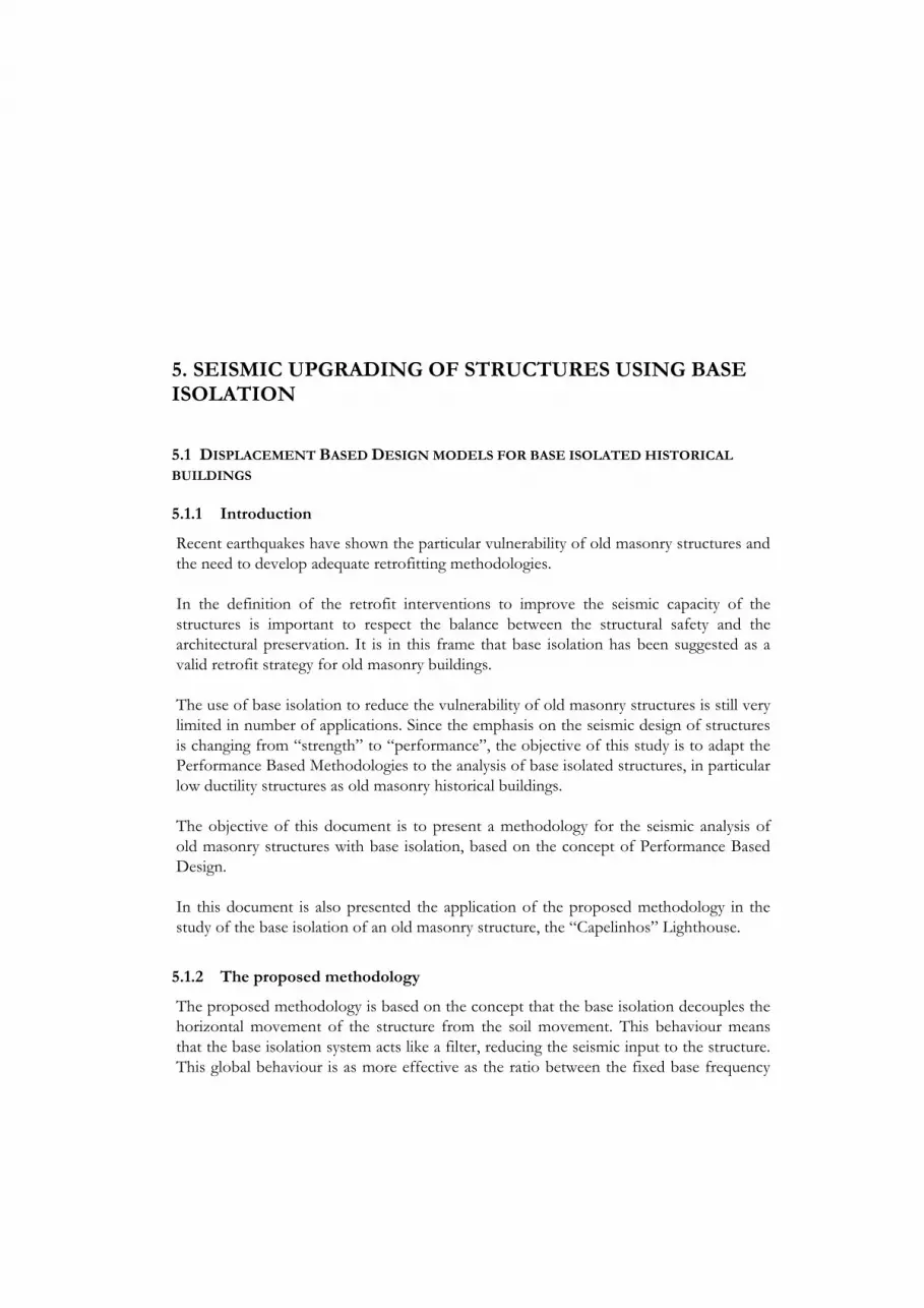
5. SEISMIC UPGRADING OF STRUCTURES USING BASE ISOLATION
5.1 DISPLACEMENT BASED DESIGN MODELS FOR BASE ISOLATED HISTORICAL
BUILDINGS
5.1.1 Introduction
Recent earthquakes have shown the particular vulnerability of old masonry structures and the need to develop adequate retrofitting methodologies.
In the definition of the retrofit interventions to improve the seismic capacity of the structures is important to respect the balance between the structural safety and the architectural preservation. It is in this frame that base isolation has been suggested as a valid retrofit strategy for old masonry buildings.
The use of base isolation to reduce the vulnerability of old masonry structures is still very limited in number of applications. Since the emphasis on the seismic design of structures is changing from “strength” to “performance”, the objective of this study is to adapt the Performance Based Methodologies to the analysis of base isolated structures, in particular low ductility structures as old masonry historical buildings.
The objective of this document is to present a methodology for the seismic analysis of old masonry structures with base isolation, based on the concept of Performance Based Design.
In this document is also presented the application of the proposed methodology in the study of the base isolation of an old masonry structure, the “Capelinhos” Lighthouse.
5.1.2 The proposed methodology
The proposed methodology is based on the concept that the base isolation decouples the horizontal movement of the structure from the soil movement. This behaviour means that the base isolation system acts like a filter, reducing the seismic input to the structure. This global behaviour is as more effective as the ratio between the fixed base frequency

212 IST
and the isolated frequency increases. Ratio values higher than 3 are recommended in order to obtained the desired effect [Skinner et al., 1993].
Since this methodology is supposed to be applied in existent structures is assumed that the behaviour of the structure when base fixed is already known and well defined. In this case is possible to consider a base isolation solution with the characteristics necessary to assure the right isolation.
The vibration mode configurations typical of isolated structures show that, apart the first mode, the other modes present deformation patterns similar to the fixed base modes (Figure 5-1). In the first isolated mode the deformation is concentrated on the isolation system with reduced structural deformation. The deformation on the structure, and consequent stresses are due to the higher modes, with deformation similar to the fixed base structure but with much less intensity since the mode response is reduced due to the isolation.
Figure 5-1 Vibration modes comparison
The assessment of the structure response can be realized using the capacity spectrum definition [e.g. Priestley, 2000]. In Figure 5-2 is presented a typical capacity spectrum for a fixed base structure with non ductile behaviour. In this figure is also represented a typical behaviour curve for an isolated structures. Since the base isolation is consider almost linear and the structural behaviour of the isolated structure is assumed to remain elastic,

Sub-Project 7 – 5.1. Displacement based design models for base isolated historical buildings 213
the behaviour curve of the isolated structure is a radial line starting at the origin, with the slope characteristic of the isolated period.
0.0
1.0
2.0
3.0
4.0
5.0
6.0
0.00 0.02 0.04 0.06 0.08 0.10Displacement (m)
Acc
eler
atio
n (m
/s2 )
ζ = 5%
ζ = 15%
Figure 5-2 Example of capacity spectrum with base isolated structure
It is important to refer that to obtain the capacity curve of the structure is necessary to define the equivalent single degree of freedom oscillator, since the structure behaviour is simplified to a deformation versus an acceleration (or force).
The single degree of freedom behaviour is expressed through effective displacement and mass values. The effective mass definition is used to establish the relation between the base shear and the mass acceleration and the effective displacement is a measure of the structure deformation. According to this consideration and based on the analysis of the mode configurations presented on Figure 5-1, one can assume that the behaviour of the structure on the top of the base isolation layer is similar to the behaviour of the fixed base structure and will be governed by the same capacity curve. Two different equivalent single degree of freedom systems must be considered: one considering the global deformation of the structure, including the base isolation displacement; and a second system considering only the structural deformation.
The total structural deformation of the base isolated structure (DT) must be subdivided in two components: the base isolation deformation (DI) and the structures deformation (DS). For each type of deformation, effective displacement and effective mass are defined using the following equations [Priestley, 2000]:
Fixed Base
Isolated

214 IST
1) Global deformation
n
i Tii
I n
i Tii
m D
m D
2
1
1
( )
( )∆ =
=
=∑
∑ (5.1.1)
n
i Tii
II
m Dm 1
( )
∆==∑
(5.1.2)
2) Structure deformation S T ID D D= − (5.1.3)
n
i Sii
S n
i Sii
m D
m D
2
1
1
( )
( )∆ =
=
=∑
∑ (5.1.4)
n
i Sii
SS
m Dm 1
( )
∆==∑
(5.1.5)
To evaluate the behaviour the base isolated structure is proposed the following methodology. The first step must be the definition of the performance of the isolated structure (Point 1 in the Figure 5-3). This point is defined by the spectral displacement (Sd) and the spectral acceleration (Sa) of the point where the capacity curve of the isolated structure crosses the design capacity spectrum. Using the effective mass value evaluated for the global deformation model (mI) is possible to calculate the base shear force (VI).
I I aV m S= (5.1.6)
Since the global base shear force on the isolating system is the same as the structure base shear, is possible to estimate the equivalent acceleration on the equivalent structure model and define the performance point of the structure itself (Point 2).
S I equivV V ms Sa( )= = (5.1.7)
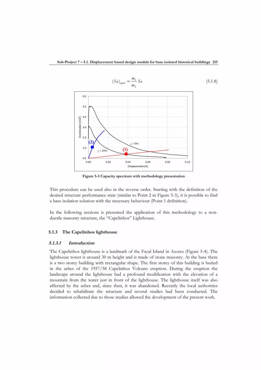
Sub-Project 7 – 5.1. Displacement based design models for base isolated historical buildings 215
Iequiv
S
mSa Sam
( ) = (5.1.8)
0.0
1.0
2.0
3.0
4.0
5.0
6.0
0.00 0.02 0.04 0.06 0.08 0.10Displacement (m)
Acc
eler
atio
n (m
/s2 )
ζ = 5%
ζ = 15%
Figure 5-3 Capacity spectrum with methodology presentation
This procedure can be used also in the reverse order. Starting with the definition of the desired structure performance state (similar to Point 2 in Figure 5-3), it is possible to find a base isolation solution with the necessary behaviour (Point 1 definition).
In the following sections is presented the application of this methodology to a non-ductile masonry structure, the “Capelinhos” Lighthouse.
5.1.3 The Capelinhos lighthouse
5.1.3.1 Introduction
The Capelinhos lighthouse is a landmark of the Fayal Island in Azores (Figure 5-4). The lighthouse tower is around 30 m height and is made of stone masonry. At the base there is a two storey building with rectangular shape. The first storey of this building is buried in the ashes of the 1957/58 Capelinhos Volcano eruption. During the eruption the landscape around the lighthouse had a profound modification with the elevation of a mountain from the water just in front of the lighthouse. The lighthouse itself was also affected by the ashes and, since then, it was abandoned. Recently the local authorities decided to rehabilitate the structure and several studies had been conducted. The information collected due to those studies allowed the development of the present work.
(1)
(2)

216 IST
Figure 5-4 The Capelinhos Lighthouse
The tower cross section is octagonal with a face length of 2.32 m at the base and a face length of approximately 2.00 m at the top. The windows and doors are located in just two opposite faces of the octagon. The structure is composed by regular stone masonry and, in result of an intervention that happened before the Volcano eruption, there is an inside reinforced concrete reinforcement with 0.20 m depth. The RC reinforcement is in poor conditions and is obvious the lack of continuity of the vertical steel bars.
The first step on the process of modelling the Lighthouse was the definition of the 3D elastic model of the fixed base structure. The geometry of the model was based on copies of the original drawings of the structure. For the complete definition of the model it was necessary to assume some characteristics of the materials, such as the weight for unit volume (γ) and the Modulus of Elasticity (E).
As a result of the observation of the masonry type and according to previous experiences with similar materials it was assumed a value of 20 kN/m3 for the weight per unit volume (γ). The definition of the Modulus of Elasticity value was based on the results of a dynamic identification.
The dynamic identification was conducted in order to get the values of the natural frequency of vibration of the tower. Those results were important to calibrate the elastic characteristics of the model. These elastic characteristics were not only the Modulus of Elasticity of the material but also the definition of the restraining at the base, imposed by the soil and by the walls of the structure that exists at the tower base.
The identified frequencies were 2.15 Hz, for the North-South direction, and 2.25 Hz for the East-West direction. The difference of frequency on the two directions is related with
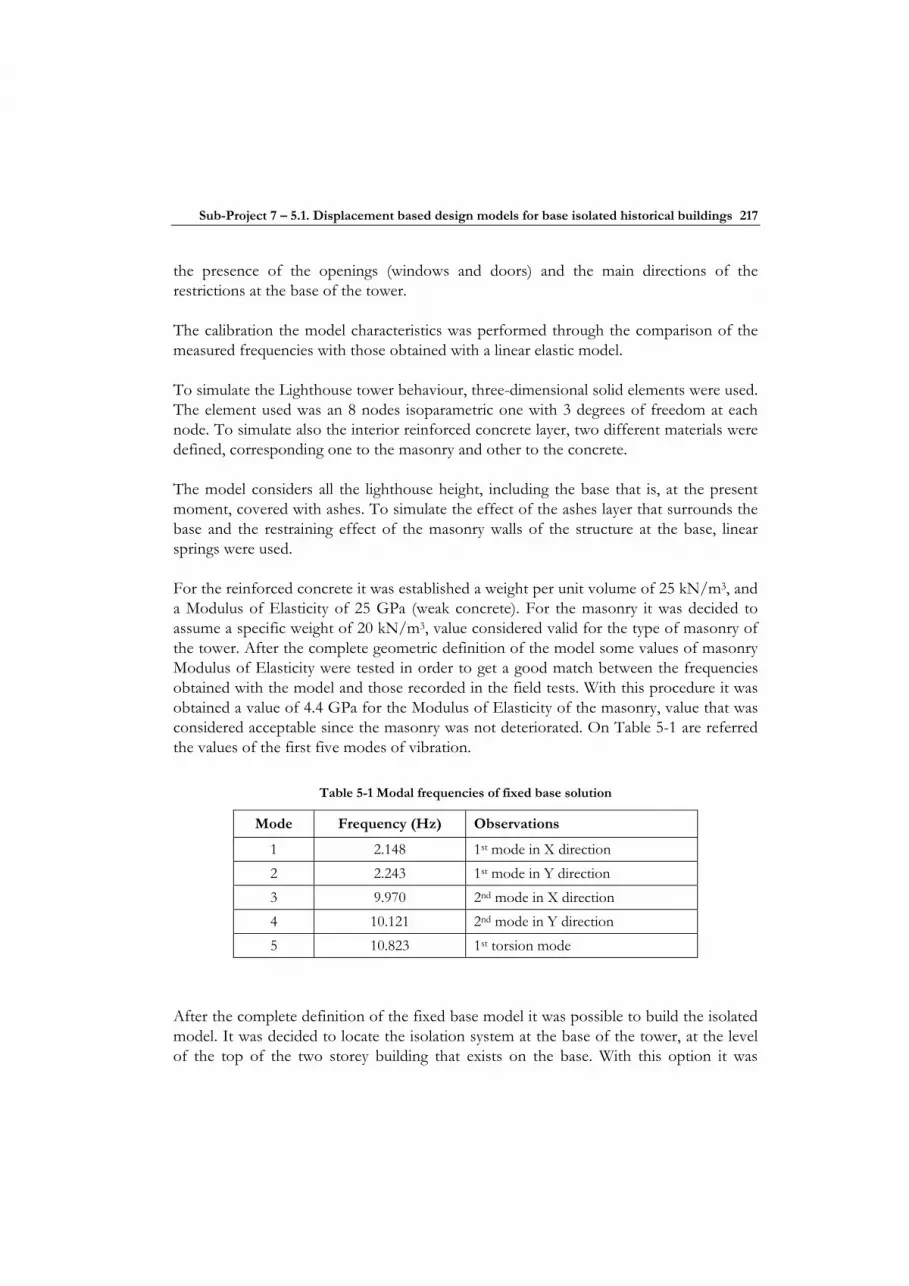
Sub-Project 7 – 5.1. Displacement based design models for base isolated historical buildings 217
the presence of the openings (windows and doors) and the main directions of the restrictions at the base of the tower.
The calibration the model characteristics was performed through the comparison of the measured frequencies with those obtained with a linear elastic model.
To simulate the Lighthouse tower behaviour, three-dimensional solid elements were used. The element used was an 8 nodes isoparametric one with 3 degrees of freedom at each node. To simulate also the interior reinforced concrete layer, two different materials were defined, corresponding one to the masonry and other to the concrete.
The model considers all the lighthouse height, including the base that is, at the present moment, covered with ashes. To simulate the effect of the ashes layer that surrounds the base and the restraining effect of the masonry walls of the structure at the base, linear springs were used.
For the reinforced concrete it was established a weight per unit volume of 25 kN/m3, and a Modulus of Elasticity of 25 GPa (weak concrete). For the masonry it was decided to assume a specific weight of 20 kN/m3, value considered valid for the type of masonry of the tower. After the complete geometric definition of the model some values of masonry Modulus of Elasticity were tested in order to get a good match between the frequencies obtained with the model and those recorded in the field tests. With this procedure it was obtained a value of 4.4 GPa for the Modulus of Elasticity of the masonry, value that was considered acceptable since the masonry was not deteriorated. On Table 5-1 are referred the values of the first five modes of vibration.
Table 5-1 Modal frequencies of fixed base solution
Mode Frequency (Hz) Observations
1 2.148 1st mode in X direction 2 2.243 1st mode in Y direction 3 9.970 2nd mode in X direction 4 10.121 2nd mode in Y direction 5 10.823 1st torsion mode
After the complete definition of the fixed base model it was possible to build the isolated model. It was decided to locate the isolation system at the base of the tower, at the level of the top of the two storey building that exists on the base. With this option it was

218 IST
decided to only isolate the tower, maintaining the base building rigidly connected to the ground.
To define the stiffness of the isolation system the option was to assume an isolated frequency of 0.50 Hz. This frequency is approximately one fourth of the rigid base frequency, ratio that is usually pointed as an optimal value. It must be stressed that the natural frequency of the fixed base model is little above 2.00 Hz and the most important vibration modes involve essentially the tower, element that is going to be isolated.
According to the developed model, the total mass above the isolation level is around 650 tons. With this value and targeting an isolated frequency of 0.50 Hz it was assumed a global horizontal stiffness on the bearings of 6400 kN/m. It was decided to consider a total of 8 bearings, with a horizontal stiffness of 800 kN/m each.
This isolation solution, with a frequency of 0.50 Hz, would be the reference solution in the study. Other solutions, with different horizontal stiffness values would be also analysed.
After the modal analysis of the isolated model there were obtained the results presented on Table 5-2.
Table 5-2 Modal frequencies of base isolated solution
Mode Frequency (Hz) Observations
1 0.475 1st torsion mode 2 0.486 1st mode in Y direction 3 0.487 1st mode in X direction 4 2.879 2nd mode in Y direction 5 2.938 2nd mode in X direction
5.1.3.2 The Capelinhos Lighthouse non linear model
Since the objective of the study is the analysis of the structure behaviour including the non linear range it was necessary to develop a non linear model of analysis. This model will allow evaluating the seismic behaviour of both the fixed base and isolated situations. The only difference would be the introduction of a horizontal flexible layer at the isolation level on the isolated model.

Sub-Project 7 – 5.1. Displacement based design models for base isolated historical buildings 219
In order to allow a large number of numerical analysis it was decided to define a simplified model. This model is composed of vertical linear frame elements connected by joints with nonlinear behaviour. In the model, the nonlinear behaviour would be concentrated on the nodes. The nonlinear characteristics of the joints were obtained through the analysis of fiber models representative of each reference cross section.
To consider the non linear behaviour it was developed a fibre model for each analyzed cross section. There were defined nonlinear cross sections separated at a maximum distance of 1 metre and also at all the irregular cross sections, such as sections with openings. There were considered a total of 31 different cross sections. On Figure 5-5 are presented two different fibre model cross sections as examples.
On the fibre model definition it was admitted the hypothesis of no tension on the masonry and a maximum compression value of 4.0 MPa. For the moment deformation relation definition, there were applied crescent deformation to the section and evaluated the resulting moment. The procedure was conducted at a constant axial force. The axial force considered at each section corresponds to the effect of the dead weight of the tower above the cross section in analysis. With this procedure, the moment-deformation characteristics of all the nonlinear joint elements considered in the model were obtained. On Figure 5-6 is presented an example of moment-deformation relation obtained in the analysis. The relation represented in the figure is representative of the behaviour for just positive moments. In most of the sections the behaviour for negative moments is similar due to the symmetry of the sections. The only exceptions are related with the sections with openings.
Figure 5-5 Examples of cross section fibre models

220 IST
0
2500
5000
7500
10000
12500
15000
17500
0.0E+00 5.0E-04 1.0E-03 1.5E-03 2.0E-03
Curvature
Mom
ent (
kNm
)
Figure 5-6 Moment-curvature relation example
5.1.3.3 Capacity curve definition
For the capacity curve definition there were conducted seismic nonlinear analysis based on the presented simplified model. To test the evolution of the structure behaviour, the seismic action was applied in different levels, starting on 25 % of the reference peak ground acceleration (Pga) and finishing at a maximum of 200 % the reference Pga. It was considered as reference Pga the peak ground acceleration defined in the Portuguese code [RSA, 1983] for the seismic action used in the study.
The result obtained at each level corresponds to the average result of the analysis with all the accelerograms considered in the study. The reference values were: the shear force at the isolation level, the top horizontal displacement, the horizontal displacement at the isolation system and the horizontal relative displacement between the top and the isolation level.
In the analysis of the fixed base situation it was tried the following 6 different seismic levels: 25 %, 50 %, 75 %, 100 %, 125 % and 150 %. Since it was verified that the tower could not support a 150 % seismic level there were conducted analysis at 110 %, 120 %, 130 % and 140 %. It was also verified that the 140 % level was also too strong for the structure. For that reason were considered only the results of the analysis of seismic intensity from 25 % Pga to 130 % Pga.
In the analysis of the isolated solution the study was conducted, without any structural problem, until a 200 % seismic level (200 % of the code defined Pga). In order to obtain more information for the study it was decide to consider 2 different additional isolation solutions, corresponding one to a isolated frequency of 0.40 Hz (more flexible solution)

Sub-Project 7 – 5.1. Displacement based design models for base isolated historical buildings 221
and other to a isolated frequency of 0.60 Hz (more rigid solution). In the study the original isolation solution is referred as “Solution 1”, the softer additional solution as “Solution 2” and the other as “Solution 3”. It was also considered different damping coefficients values for each solution. The basic characteristics of the base isolation cases considered in the study are presented on Table 5-3.
Table 5-3 Base isolation solution characteristics
Solution Frequency (Hz) Damping Coefficient (%)
1 0.50 12.5 2 0.40 15.0 3 0.60 10.0
In the global behaviour there are two main points in analysis: the maximum base shear force on the tower and the maximum displacement at the isolation level. The first is related to the structure capacity and the second to the base isolation system limit state.
On Figure 5-7 are presented the evolution of the shear base with the seismic intensity, for all the tested situations. According to the results the base fixed structure exhibits nonlinear behaviour when the isolated solutions show a linear evolution for the shear base with the seismic intensity, revealing that the structure was always in the elastic range, as expected.
0
200
400
600
800
1000
1200
0.00 0.50 1.00 1.50 2.00
( x PGA )
Bas
e Sh
ear F
orce
(kN
)
Fixed BaseSolution 1Solution 2Solution 3
Figure 5-7 Vulnerability functions for shear force
On Figure 5-8 the obtained results are represented over the capacity spectrum for the seismic action used in the analysis. To mark the seismic response of the fixed base structure and the response of all the three isolation solutions it was necessary to evaluate

222 IST
the effective displacement and the effective mass associated to each case. On Table 5-4 the values of the equivalent single degree of freedom systems are presented. In the Table the effective displacement is presented as a percentage of the top displacement, and the effective mass as a percentage of the total mass.
Table 5-4 Equivalent single degree of freedom characteristics
Solution Effective Displacement Effective Mass
Fixed 0.57 DTOP 0.65 MTOTAL Isolated 0.95 DTOP 1.00 MTOTAL
The results presented on Figure 5-8 show that the fixed base structure could not resist to the seismic action present on the current version of the Portuguese code. With all the base isolation solutions it is possible to sustain a seismic action stronger than the code defined.
As expected, the behaviour of the base isolated situations corresponds to a straight radial lines, each one with the slope characteristic of each isolated period. The Solution 3, that corresponds to the more flexible solution (T=2.5 sec.) presents a higher slope than the other two lines (T=2.0 sec. and T=1.67 sec.).
Figure 5-8 Capacity Spectrum with all the base isolation solutions

Sub-Project 7 – 5.1. Displacement based design models for base isolated historical buildings 223
To confirm the presented methodology is necessary to check if the behaviour of the structure on the top of the base isolation follows the global capacity curve of the fixed base structure. To perform this confirmation it was necessary to evaluate the effective mass (mS), related only to the structural deformation, using equation 5.1.5. The calculations confirmed a result similar to that obtain for the fixed base structure, 65 % of the total mass.
To establish the comparison between the results three pairs of points were marked over the capacity curves diagram. There were chosen three different situations, one for each base isolation solution, corresponding all to the 100 % Pga seismic action level.
The results can be observed on Figure 5-9, where the square marks, (on the right side) refer the performance points on the base isolated structure, and the circle marks (on the left side) represent the corresponding performance points over the capacity curve of the structure. The points marked over the capacity curve of the structure presents the same base shear force of the corresponding points marked over the isolated structure. The higher values of equivalent acceleration result from the lower value of effective mass characteristic of the structure deformation when compared with the base isolated situation.
The presented results show a good agreement between the points obtained from the proposed methodology and the capacity curve obtained directly from the fixed base analysis. It is also possible to conclude about the efficiency of the base isolation solution on the protection of structures.
Figure 5-9 Capacity Spectrum with all the base isolation solutions
224 IST
5.1.4 Conclusions
The main objective of this document was the description of a methodology proposed to adapt the displacement based design concept (DBD) for the analysis of old masonry buildings.
According to the obtained results we can conclude that the proposed methodology may be a useful tool on the design of seismic base isolation to protect an existen structure.
The fixed base capacity curve can be used to characterize the seismic behaviour of the isolated structure over the isolation surface.
The base isolation is an efficient solution to provide seismic protection to structures with non-ductile behaviour.
5.2 NONLINEAR METHOD FOR CONTROL OF AUTO-ADAPTIVE SEMI ACTIVE BASE
ISOLATOR
Civil engineering structures have traditionally been built as passive structures with no adaptability to uncertain dynamic loads. Indeed, ‘solidity’ and ‘massiveness’ have been considered as a measure of the ‘safety’ and ‘reliability’. In recent decades, new alternative approaches such as supplemental damping, passive control, semiactive and active control have been developed to protect structures from earthquakes and severe winds. A detailed and comprehensive literature review for these new approaches has been given in Deliverables 43 (www.lessloss.org ).
One challenge in the use of semiactive controllable fluid dampers is to develop implementable nonlinear control algorithms. In the first annual report of the project, an implementable nonlinear control algorithm has been proposed and its performance has been investigated compared to uncontrolled and exact optimal cases. The comparison results of the proposed control, passive and semiactive cases are given and discussed. Lastly, a new linear optimal control rule is derived, which can be used to obtain semiactive control laws.
5.2.1 Structural System
This study examines the earthquake response of seismically isolated two-degree of freedom (2DOF) structures, in which a controllable fluid device (i.e., an MR damper) is placed at the isolation level. The base isolation system is assumed to be linear and is represented by a spring in parallel with a linear viscous dashpot.

Sub-Project 7 – 5.2. Non linear method for control of auto adaptive semi active base isolator 225
The masses ms and mi represent the superstructure of the building and the mass of the base floor above the isolation system, respectively. The superstructure and the isolation stiffness and damping coefficients are represented by ks, cs, ki and ci, respectively. Structural relative displacements and the ground displacement are denoted by r1, r2 and z, respectively. For the investigated structure; the masses, the stiffness and the damping coefficients are selected as mi=ms=105 kg, ki=16.5 kN/cm, ks=300 kN/cm, ci=1.1 kN/cm/sec and cs=0.3 kN/cm/sec.
The MR damper implemented in the isolation level exhibits controllable stiffness and damping and is modelled by the following algebraic expression with five parameters
MR d df f uH u r d r v k r c r0 1 0 1 0 1 1( )tanh( / / )= + + + (5.2.1)
where the constant parameters d0 and v0 are used to describe the pre-yield behaviour of the device, f0 is a controllable yield force, and kd and cd describe the post yield behaviour and the behaviour when u=0. The control force f is changed optimally via the control decision variable u; H(u) is the Heaviside step function of u. Device parameters used for this case are f0=100 kN, d0=5 cm, v0=4 cm/sec, cd =2 kN/cm/sec and kd =3 kN/cm. These parameters can be used to represent an MR damper, an ER damper, or a controllable valve damper.
5.2.2 System Dynamıcs
The nonlinear system of dynamical equation of a 2DOF base isolated structure with an MR damper defined by (5.2.1) can be expressed as
t t u t t u u z t t0( ) ( ( ), ( ), ) ( , ) ( ), ( )= = + + =x f x Ax g x H x 0 (5.2.2)
where
i s d s i s d s
i i i i
s s s s
s s s s
rr k k k k c c c cr m m m mr k k c c
m m m m
1
2
1
2
0 0 1 00 0 0 1
;
⎡ ⎤⎢ ⎥⎧ ⎫ ⎢ ⎥⎪ ⎪ ⎢ ⎥+ + + +⎪ ⎪ − −= =⎨ ⎬ ⎢ ⎥
⎪ ⎪ ⎢ ⎥⎪ ⎪ ⎢ ⎥⎩ ⎭ − −⎢ ⎥
⎣ ⎦
x A (5.2.3)

226 ITU
iu
f m H u r d r v0 1 0 1 0
0 00 0
( , ) ;( / ) ( )tanh( / / ) 1
0 1
⎧ ⎫ ⎧ ⎫⎪ ⎪ ⎪ ⎪⎪ ⎪ ⎪ ⎪= =⎨ ⎬ ⎨ ⎬− + −⎪ ⎪ ⎪ ⎪⎪ ⎪ ⎪ ⎪−⎩ ⎭ ⎩ ⎭
g x H (5.2.4)
5.2.3 Optimal and Sub-optimal Control
Optimal and sub-optimal control schemes have been given in detail in the first annual report. Optimal control minimizes
f f
f
t t
t t
ts s
st
J L t u t t dt r t z t dt
k r t r t c r t r t dtm
0 0
0
22
21 2 1 2
( ( ), ( ), ) [ ( ) ( )]
[ ( ) ( )] [ ( ) ( )]
= = +
⎧ ⎫− + −= ⎨ ⎬
⎩ ⎭
∫ ∫
∫
x
(5.2.5)
where the Lagrangian )),(),(( ttutL x is the square of the superstructure absolute acceleration. The sub-optimal control trajectory minimizes the integral cost function
t N t
so sot
J L u d( ( ), ( ), )∆
τ τ τ τ+
= ∫ x (5.2.6)
5.2.4 Passive Viscous Damping Control And on-off Cases
Using the previously defined quantities, the basic equations of motion of 2DOF base isolated structure with no control can be modelled by a first-order system of differential equations with constant coefficients. For the passive viscous damping case in which fMR=0 during the earthquake, viscous damping coefficient of the base isolation system was changed as ci=1.1, 2.0, 5.0, 7.0 and 10.0 kN/cm/sec. The selected viscous damping coefficients correspond to first-mode damping ratios of 5.8, 10.6, 16.7, 37.5 and 54.2 percent of critical.
In on-off cases, semiactive damper force is
MR d df k r c r1 1= + (5.2.7)

Sub-Project 7 – 5.2. Non linear method for control of auto adaptive semi active base isolator 227
for u=0 and
MR d df f r d r v k r c r0 1 0 1 0 1 1tanh( / / )= + + + (5.2.8)
for u=1.
5.2.5 Causal semıactıve control
The causal semiactive control system for this case uses the MR damper force (5.2.1) in which the control policy u H(u) is replaced by v, where the delayed control decision v is given by
v MRv T v H f r z1(1/ )[ (( )( ))]= − − + (5.2.9)
for bang-bang control case and
v MRv T v r z H f r z1 1(1/ )[ (( )( ))]α= − − + + (5.2.10)
for continuous control case. The constant Tv is the response time of the controllable damper. The coefficient α is a design parameter for the control rule (5.2.10) which determines the device force level.
5.2.6 Numerical application
Seismic response of 2- degree-of-freedom low-rise base isolated structure with a controllable fluid damper under the May 18, 1940 Imperial Valley earthquake El Centro (NS component) is evaluated in order to examine the performance of the proposed control in comparison to uncontrolled case and the exact optimal case. The calculations are performed for the first 10 sec-duration of the excitation, which includes the peak acceleration values. The damper force is zero for the uncontrolled case. The maximum response quantities for all the investigated cases are given in Table 5-5 and Table 5-6, respectively for comparison purposes.
It ıs clear from the above given results that the optimal control outperforms all the investigated cases. However, it is known that the optimal control is an ideal case and cannot be implemented. Among the passive cases, the case in which the base isolation damping is ci=0.5 kN/cm/sec, is the optimal one in terms of the reduction in absolute acceleration of superstructure and the cost function. It is known that the optimal isolation damping for each earthquake is different. Since the earthquake characteristics are not known a priori, it is almost not possible to determine the optimal isolation damping for that specific earthquake. This is, in fact, one of the reasons of studying the semiactive systems.

228 ITU
Table 5-5. Maximum response quantities for uncontrolled and controlled cases
Table 5-6. Maximum response quantities for passive cases
It is also seen from the tables that the proposed control performs better than all the passive viscous damping and on-off cases in terms of the reduction in absolute acceleration of superstructure and the cost function. Provided that the proposed control is compared to the causal semiactive control rules, it is shown that the proposed sub-optimal control performs better than the causal semiactive bang-bang control while it performs almost the same as the causal semiactive continuous control. These analyses show that the proposed sub-optimal implementable control is promising for the control
Maximum
Values
No control
(f=0)
Proposed control
(implementable)
Optimal control
(nonimplementable)
Bang-bang
control
(BBC)
Continuous control
(CC)
1r (cm) 19.1 10.2 5.0 5.49 7.42
12 rr − (cm) 0.54 0.42 0.3 0.44 0.40
)()(2 tztr +
(cm /sn2)
163.1 125.5 97.5 134.19 119.55
J 41671 18439 16579 25000 18600
Passive linear viscous damping Passive on-off cases
Maximum
Values
ci=1.1
kN/cm/sec
ci=2.0
kN/cm/sec
ci=5.0
kN/cm/sec
ci=7.0
kN/cm/sec
ci=10.0
kN/cm/sec
u=0
u=1
1r (cm) 19.10 15.00 8.28 6.28 4.66 11.04 5.07
12 rr − (cm) 0.54 0.47 0.43 0.50 0.67 0.47 0.74
)()(2 tztr +(cm/sn2)
163.13 140.62 129.67 150.32 200.33 139.09 217.09
J 41600 24900 18700 22300 30200 22542 44888
Sub-Project 7 – 5.2. Non linear method for control of auto adaptive semi active base isolator 229
of earthquake response of base isolated structures. Proposed semiactive control scheme can protect the base isolation system without increasing the superstructure response.
5.2.7 Derivation of the Linear Control Law
To give a brief overview of the active control concept, the governing equations of motion for a general multi-storey shear-beam lumped mass linear building structure are
[ ]t t t f t t t t t t t1 2 0 1 0 0, , ; ( ) ( )+ + = + ∈ = =MX( ) CX( ) KX( ) D ( ) D U( ) X X 0 (5.2.11)
where X(t)=( x1,..., xn )T is the n-dimensional response vector (T indicates the transpose of a vector or a matrix) denoting the relative displacement of the each storey unit with respect to the ground; the superposed dot represents the differentiation with respect to time; M is the (nxn)-dimensional diagonal constant mass matrix with diagonal elements mi = mass of i th storey (i=1,..., n); C and K are the (nxn)-dimensional viscous damping and the stiffness matrices, respectively; D1 is the (nx1)-dimensional location matrix of excitation and given by ),...,( 1
T1 nmm−=D ; D2 is the (nxr)-dimensional location matrix of r
controllers; U(t) is the r-dimensional active control force vector and described as UT(t)=(u1(t),...,ur (t)) and scalar function f(t) is the one dimensional earthquake acceleration. In the state space, equation (5.2.11) becomes
[ ]t t t f t t t t t0 1 0( ) ( ) ( ) ( ), , ; ( )= + + ∈ =Z AZ BU D Z 0 (t) (5.2.12)
in which
nxn1 1− −
⎡ ⎤= ⎢ ⎥
− −⎣ ⎦
0 IA
M K M C ; nxr
12
−
⎡ ⎤= ⎢ ⎥
⎣ ⎦
0 B
M D ; nx1⎡ ⎤
= ⎢ ⎥−⎣ ⎦
0D
η ;
⎡ ⎤= ⎢ ⎥
⎣ ⎦
XZ
X (5.2.13)
such that 0nxm is the (nxm)-dimensional zero matrix; I is the (nxn)-dimensional identity matrix; η= (1,...,1)T is the n-dimensional vector.
In the classical optimal control law; the classical integral type quadratic performance measure
T T1t
C C0
J dt= +∫(Z Q Z U R U) (5.2.14)

230 ITU
is minimized under the constraint imposed by equation(5.2.12), where [0, t1] time interval is the control time and defined to be longer than that of the external excitation duration; QC is a positive semi-definite symmetric weighting matrix ; RC is a positive definite symmetric weighting matrix and the subscript C refers to classical linear optimal control.
It is known that an important property of classical linear optimal control solution is that any selection of the weighting matrices within the constraint of positive semi-definiteness and positive definiteness will preserve asymptotic stability. Provided that the weighting matrices QC and RC are selected as
nxn nxnC C nxn
nxn nxn; ; 0 , 0α β α β
⎡ ⎤= = > >⎢ ⎥
⎣ ⎦
I 0Q R I
0 0 (5.2.15)
in the numerical applications then they satisfy the above-given stability condition. Since the derivation of the necessary conditions of optimality is given in detail by Anderson and Moore, only the results will be given here. Classical linear optimal control law is obtained as
TC t t11( ( ) ( )
2−) = −U R B P Zt (5.2.16)
where P is the solution of the following nonlinear matrix Riccati equation,
T TCCt t t t t t1 1
1( ) ( ) ( ) ( ) ( ) 2 ; ( )2
−+ − + + = =.
P P A P BR B P A P Q 0 P 0 (5.2.17)
In this study, to determine the active control force, we introduce the integral type quadratic functional
t h
Tt h
t
I s s dsT, ( ) ( ) ( ) ( ( min
+
⎡ ⎤= + ) ) ⎯⎯→⎣ ⎦∫U Z Q Z U R Us s (5.2.18)
with two parameters 0and0 >≥ htt , where Q is the (2nx2n)-dimensional positive semi-definite symmetric weighting matrix and R is the (rxr)-dimensional positive definite symmetric weighting matrix; h is the time interval between the successive control instants. The expression given by equation (5.2.18) can be considered as a functional defined for the solutions ],[),( httss +∈Z , of the differential equation
Sub-Project 7 – 5.2. Non linear method for control of auto adaptive semi active base isolator 231
[ ]s s s f s s t t h( ) ( ) ( ) ( ), , ;= + + ∈ +.
Z AZ BU D )(|)( ts ts ZZ == (5.2.19)
with admissible control vectors
[ ]r(s ) PC t t h,∈ +U (5.2.20)
In Eq. (5.2.20), [ ]htt +,PCr is the vector space of r-dimensional column vectors, which have piecewise continuous elements for [ ]htt +∈ ,s . The norm in [ ]htt +,PCr can be defined, for example, as
r
it ht s t h iSup s,
1( )
≤ ≤ + == ∑U U (5.2.21)
It is clear that the problem of minimizing the functional (5.2.18) under the conditions (5.2.19) and (5.2.20) is an optimal control problem with two parameters t and h. Therefore, the exact optimal solution of this problem can be considered as a function of
[ ]htt +∈ ,s while it also depends on the parameters t and h. We denote the exact optimal control of the problem defined by equations (5.2.28-5.2.20) by ],[),(, httssht +∈U . In this study, we will define the value of the active control U(t) at time t as the value of exact optimal control ],[),(, httssht +∈U , at point s=t, that is, as )()( , tt htUU = . For this purpose, we will first obtain the optimality conditions for the problem (5.2.28-5.2.20). For calculation of the first variation of the functional (5.2.28), we consider the following increment of this functional:
t hT T T T
t h t h t ht
I I s s s s ds, , ,( ) ( ) ( )( ) ( ) ( )( ) ( ) ( )δ δ δ η δ+
⎡ ⎤+ − = + + + +⎣ ⎦∫U U U Z Q Q Z U R R U U
(5.2.22)
where )(, Uδη ht is the remainder term given by
t h
Tt h
t
s s dsT, ( ) ( ) ( ) ( (η δ δ δ δ δ
+
⎡ ⎤= + ) )⎣ ⎦∫U Z Q Z U R Us s (5.2.23)
It is clear that )(sZδ represents the solution of the system
s ts s s s s t t h( ) ( ) ( ) , ( )| , [ , ]δ δ δ δ == + = ∈ +Z A Z B U Z 0 (5.2.24)
232 ITU
with [ ]htts +∈ ,PC)( rUδ . The solution of equation (5.2.24) is
[ ]s s t t h( )( ) ( ) , ,τδ δ τ τ−= ∈ +∫ AZ B Us
s
t
e d (5.2.25)
The expression (5.2.23) together with (5.2.25) shows that
t h
t h
,
,
( )0
η δδ
→U
U (5.2.26)
when 0, →htUδ . Consequently, the first variation or differential of the functional (5.2.18) can be written as
t h
Tt h
t
I s s ds' T, 0 0( )( ) ( ) ( ) ( (δ δ δ
+
⎡ ⎤= + ) )⎣ ⎦∫U U Z Q Z U R Us s (5.2.27)
where T0 QQQ += and T
0 RRR += . If we substitute equation (5.2.25) into equation (5.2.27), one obtains )(,
' UhtI as follows:
t hT
t ht
t hT
0t
I s ds
(s ) s d
' ( ) T, 0 0
( ) T0
( )( ) ( ) ( ) ( (
( (
τ
τ
τ
δ δ τ τ δ
τ δ τ τ
+−
+ +−
⎡ ⎤= + ) )⎢ ⎥
⎣ ⎦
⎡ ⎤= + ) )⎢ ⎥
⎣ ⎦
∫ ∫
∫ ∫
A
A
U U Z Q B U U R U
Z Q B U R U
ss
t
t hs
e d s s
e d
(5.2.28)
It is obvious that the necessary condition of optimality for the functional (5.2.28) is
[ ]t h rI s PC t t h', ( )( ) 0 , ( ) ,δ δ= ∀ ∈ +U U U (5.2.29)
The functional (5.2.18) defined for the solutions of the problem given by equations (5.2.19-5.2.20) is convex in the sense that
[ ]t h t h t h rI I I s PC t t h', , ,( ) ( ) ( )( ) , ( ) ,δ δ δ+ ≥ + ∀ ∈ +U U U U U U (5.2.30)
Sub-Project 7 – 5.2. Non linear method for control of auto adaptive semi active base isolator 233
This shows that the condition (5.2.29) is also sufficient condition for optimality. So, the necessary and the sufficient condition of optimality of [ ]htts +∈ ,PC)( rU is
[ ]T s0( ) s s t t h( ) T
0( 0 , ,ττ τ+
− + ) = ∈ +∫ AZ Q B U Rt h
s
e d (5.2.31)
Note that the optimal state vector [ ]httss +∈ ,),(Z , corresponding to the exact optimal control ],[),()( , httsss ht +∈= UU , of the problem (5.2.18-5.2.20) can be easily obtained as
[ ] [ ]s
s t ss t f d s t t h( ) ( )( ) ( ) ( ) ( ) ; ,τ τ τ τ− −= + + ∈ +∫A AZ Z B U Dt
e e (5.2.32)
Consequently, optimal state and control vectors )(and)( ss UZ can be obtained as the solutions of the system of integral equations (5.2.31-5.2.32) in the interval [ ]htts +∈ , . If the earthquake acceleration f(s) can be estimated for [ ]htts +∈ , , then the optimal state and control vectors )(and)( ss UZ can be determined as a unique solution of the equations (5.2.31-5.2.32).
For the purpose of defining the active control, we use the optimality condition (5.2.31), in which the integral term on the left hand-side is continuous for [ ]htts +∈ , . So, equation (5.2.31) is meaningful in special case when s=t. Then, we have
T t0( ) t( ) T
0( 0ττ τ+
− + ) =∫ AZ Q B U Rt h
t
e d (5.2.33)
Using the trapezoidal rule of numerical integration, equation (5.2.33) can be rewritten as
T T T0
h t h t O h30 0( ) ( ) ( ( ) 0
2⎡ ⎤+ + + ) + =⎣ ⎦Z Q K B Z Q B U Rt (5.2.34)
where heAK = and )( 3hO denotes the quantity which satisfies the condition 3
03 )( hChO ≤ with a positive constant C0. Then, U(t) is obtained easily from equation
(5.2.34) as
T Th t t h O h1 30 0 0( ( ) ( ) ( )
2− ⎡ ⎤) = − + + +⎣ ⎦U R B Q Z K Q Zt (5.2.35)
234 ITU
It is noted here that the real time application of the resulting control scheme (5.2.35) requires the estimation of the state vector )( ht +Z at time t. For the sake of simplicity, it is also possible to obtain a simple closed-loop form from equation (5.2.35), which does not require the estimation of )( ht +Z . Due to the space limitations, detailed derivation of optimal U(t) and Z(t) will not be given, only the results will be given here. Ignoring some terms with order O(h2) and O(h3) for symmetric matrices Q and R, optimal U(t) and Z(t) are derived as follows:
Th t1 10( ( )− −) = −U N R B Q Zt (5.2.36)
and
Th ht h f t12
1 10( ( ) ( )
2 2
−− −⎡ ⎤ ⎡ ⎤) = + − +⎢ ⎥ ⎢ ⎥⎣ ⎦⎣ ⎦
Z I B N R B Q y Dt (5.2.37)
where
Th 21
0 4−= +N I R B QB
[ ]Ah Aht h e t h h e t h f t h( ) ( ) ( 2) ( ) ( )− = − + − + −y Z B U D
5.2.8 Conclusions
Exact optimal control resulting from the numerical solution to Euler-Lagrange equations is an idealized case and cannot be implemented since it requires a priori knowledge of earthquake in the control interval. A sub-optimal implementable control rule, which uses the prediction of near-future ground accelerations, is proposed. To evaluate the performance of the proposed control, the real-time control of 2- degree-of-freedom low-rise base isolated structure with a semiactive controllable fluid damper under earthquake excitation is investigated and the results are compared to uncontrolled and exact optimal control cases.
Optimal semiactive controls which use a priori knowledge of the investigated earthquake excitation in the control interval always gives the best performance in terms of the reduction in all structural responses compared to uncontrolled case and the proposed implementable semiactive control. This indicates that with better nonlinear control

Sub-Project 7 – 5.2. Non linear method for control of auto adaptive semi active base isolator 235
methods semiactive control may provide better performance than is achievable by the proposed causal control rules used in this study.
Proposed implementable semiactive control method uses only the 10-step ahead predictions of ground accelerations at the control instant to generate the control forces. However, they show similar behaviour to optimal semiactive control, which uses the complete knowledge of the excitation and follow the optimal trajectories closely.
The controllable fluid damper used in conjunction with the proposed semiactive control can decrease the accelerations and interstorey drifts in the superstructure of base isolated structures. The effectiveness of the proposed control is also shown by the significant reduction in the investigated integral cost function.
A simple integral type quadratic functional is also introduced as the performance index for the purpose of suppressing the seismic vibrations of buildings. The optimal active control force is derived by using the method of calculus of variations based on the minimization of the proposed performance index in the nearest control interval. Although the resulting optimal control law depends on the structural displacements and velocities in the minimization interval, for simplicity in implementing the control system and evaluating the control effectiveness, a simpler control law which depends on the current state of the system is obtained. New semiactive control rules may be developed based on the proposed linear control law.


6.MITIGATION OF HAMMERING BETWEEN BUILDINGS
6.1 INTRODUCTION
Building collision, commonly called ‘pounding’, occurs during an earthquake when, due to their different dynamic characteristics, adjacent buildings vibrate out of phase and the at-rest separation is insufficient to accommodate their relative motions. Pounding means an instance of rapid strong pulsation and sometimes, like hammering, repeated heavy blows. Because building separations in urban areas are often insufficient to preclude pounding, there is a need for safe and economical retrofitting methods to reduce structural pounding.
In the past, major earthquakes affecting large metropolitan areas have induced severe pounding damage. In some cases, the additional forces generated by the impact interactions have led to collapse structural problem. In other cases, the buildings presented minor local damages, but indicating that pounding may be a serious threat to the structures if a stronger earthquake take place. In recent years, research has being done to study the pounding phenomenon. Pounding has been included in the list of important areas to be checked during a seismic evaluation, but in general, the engineer does not have much information on how to evaluate the effects of pounding, nor how to reduce them.
The overall goal of the project is to develop strategies for retrofitting closely spaced buildings to reduce the potential for damage due to seismic pounding, while minimizing the modifications to the existing structural system. Many possibilities of mitigation exist. All of them will be explained in details but special attention is carried on connection between buildings, commonly called Pounding Reduction Devices (PRDs).
More detailed development on the Topic can be found as a Lessloss Project Report listed as Deliverable 46 – Analysis of hammering problems (www.lessloss.org ).
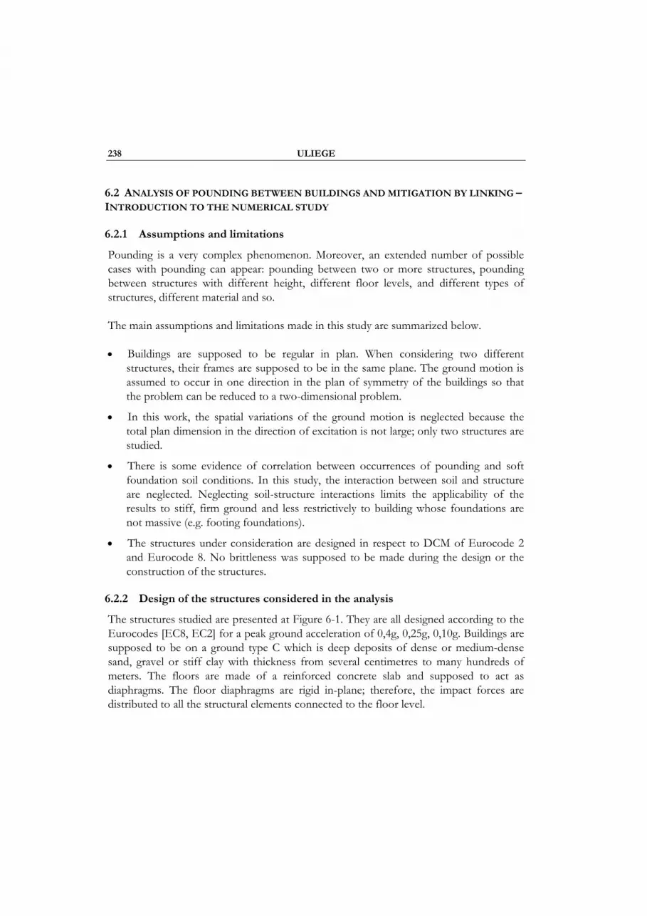
238 ULIEGE
6.2 ANALYSIS OF POUNDING BETWEEN BUILDINGS AND MITIGATION BY LINKING –
INTRODUCTION TO THE NUMERICAL STUDY
6.2.1 Assumptions and limitations
Pounding is a very complex phenomenon. Moreover, an extended number of possible cases with pounding can appear: pounding between two or more structures, pounding between structures with different height, different floor levels, and different types of structures, different material and so.
The main assumptions and limitations made in this study are summarized below.
• Buildings are supposed to be regular in plan. When considering two different structures, their frames are supposed to be in the same plane. The ground motion is assumed to occur in one direction in the plan of symmetry of the buildings so that the problem can be reduced to a two-dimensional problem.
• In this work, the spatial variations of the ground motion is neglected because the total plan dimension in the direction of excitation is not large; only two structures are studied.
• There is some evidence of correlation between occurrences of pounding and soft foundation soil conditions. In this study, the interaction between soil and structure are neglected. Neglecting soil-structure interactions limits the applicability of the results to stiff, firm ground and less restrictively to building whose foundations are not massive (e.g. footing foundations).
• The structures under consideration are designed in respect to DCM of Eurocode 2 and Eurocode 8. No brittleness was supposed to be made during the design or the construction of the structures.
6.2.2 Design of the structures considered in the analysis
The structures studied are presented at Figure 6-1. They are all designed according to the Eurocodes [EC8, EC2] for a peak ground acceleration of 0,4g, 0,25g, 0,10g. Buildings are supposed to be on a ground type C which is deep deposits of dense or medium-dense sand, gravel or stiff clay with thickness from several centimetres to many hundreds of meters. The floors are made of a reinforced concrete slab and supposed to act as diaphragms. The floor diaphragms are rigid in-plane; therefore, the impact forces are distributed to all the structural elements connected to the floor level.
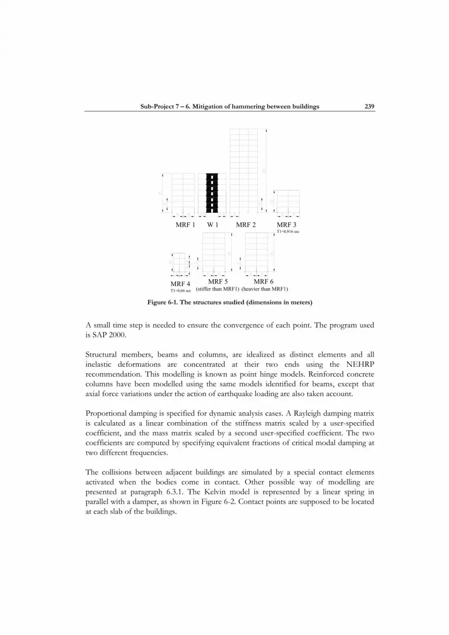
Sub-Project 7 – 6. Mitigation of hammering between buildings 239
MRF 6(heavier than MRF1)
MRF 1 W 1 MRF 2
MRF 5(stiffer than MRF1)
MRF 4 T1=0,66 sec
MRF 3 T1=0,916 sec
Figure 6-1. The structures studied (dimensions in meters)
A small time step is needed to ensure the convergence of each point. The program used is SAP 2000.
Structural members, beams and columns, are idealized as distinct elements and all inelastic deformations are concentrated at their two ends using the NEHRP recommendation. This modelling is known as point hinge models. Reinforced concrete columns have been modelled using the same models identified for beams, except that axial force variations under the action of earthquake loading are also taken account.
Proportional damping is specified for dynamic analysis cases. A Rayleigh damping matrix is calculated as a linear combination of the stiffness matrix scaled by a user-specified coefficient, and the mass matrix scaled by a second user-specified coefficient. The two coefficients are computed by specifying equivalent fractions of critical modal damping at two different frequencies.
The collisions between adjacent buildings are simulated by a special contact elements activated when the bodies come in contact. Other possible way of modelling are presented at paragraph 6.3.1. The Kelvin model is represented by a linear spring in parallel with a damper, as shown in Figure 6-2. Contact points are supposed to be located at each slab of the buildings.
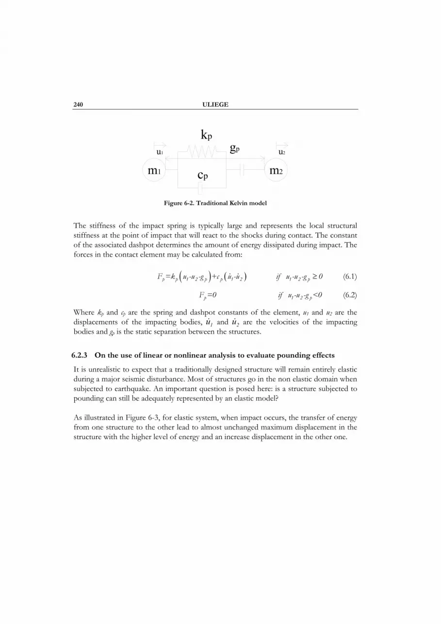
240 ULIEGE
m1
kp
cp m2
u1 u2gp
Figure 6-2. Traditional Kelvin model
The stiffness of the impact spring is typically large and represents the local structural stiffness at the point of impact that will react to the shocks during contact. The constant of the associated dashpot determines the amount of energy dissipated during impact. The forces in the contact element may be calculated from:
( ) ( )p p 1 2 p p 1 2F =k u -u -g +c u -u 1 2 pif u -u -g 0≥ (6.1)
pF =0 1 2 pif u -u -g <0 (6.2)
Where kp and cp are the spring and dashpot constants of the element, u1 and u2 are the displacements of the impacting bodies, 1u and 2u are the velocities of the impacting bodies and gp is the static separation between the structures.
6.2.3 On the use of linear or nonlinear analysis to evaluate pounding effects
It is unrealistic to expect that a traditionally designed structure will remain entirely elastic during a major seismic disturbance. Most of structures go in the non elastic domain when subjected to earthquake. An important question is posed here: is a structure subjected to pounding can still be adequately represented by an elastic model?
As illustrated in Figure 6-3, for elastic system, when impact occurs, the transfer of energy from one structure to the other lead to almost unchanged maximum displacement in the structure with the higher level of energy and an increase displacement in the other one.
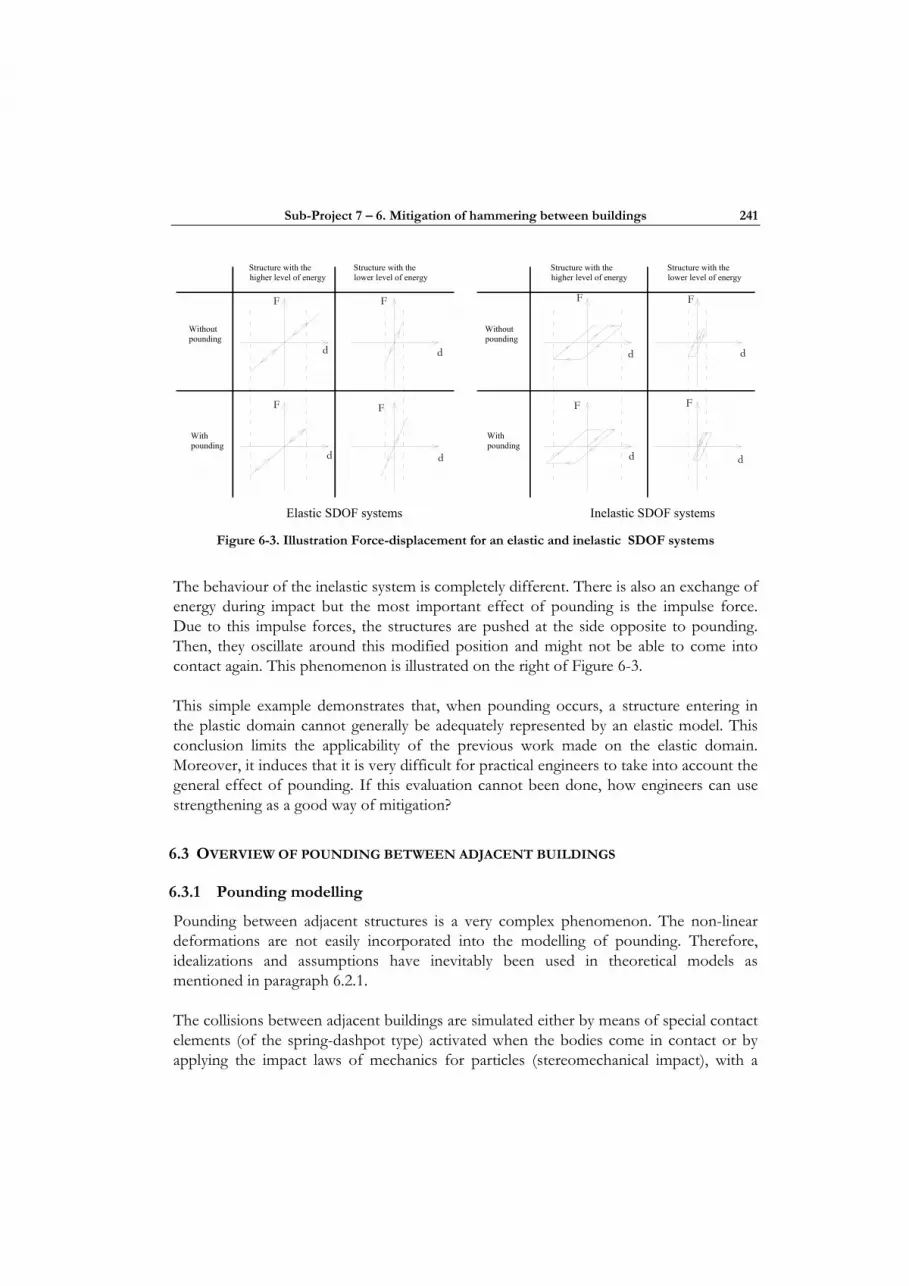
Sub-Project 7 – 6. Mitigation of hammering between buildings 241
F
d
Structure with the higher level of energy
Without pounding
With pounding
F
F F
d
dd
F F
FF
d d
dd
Without pounding
With pounding
Structure with the lower level of energy
Structure with the higher level of energy
Structure with the lower level of energy
Elastic SDOF systems Inelastic SDOF systems Figure 6-3. Illustration Force-displacement for an elastic and inelastic SDOF systems
The behaviour of the inelastic system is completely different. There is also an exchange of energy during impact but the most important effect of pounding is the impulse force. Due to this impulse forces, the structures are pushed at the side opposite to pounding. Then, they oscillate around this modified position and might not be able to come into contact again. This phenomenon is illustrated on the right of Figure 6-3.
This simple example demonstrates that, when pounding occurs, a structure entering in the plastic domain cannot generally be adequately represented by an elastic model. This conclusion limits the applicability of the previous work made on the elastic domain. Moreover, it induces that it is very difficult for practical engineers to take into account the general effect of pounding. If this evaluation cannot been done, how engineers can use strengthening as a good way of mitigation?
6.3 OVERVIEW OF POUNDING BETWEEN ADJACENT BUILDINGS
6.3.1 Pounding modelling
Pounding between adjacent structures is a very complex phenomenon. The non-linear deformations are not easily incorporated into the modelling of pounding. Therefore, idealizations and assumptions have inevitably been used in theoretical models as mentioned in paragraph 6.2.1.
The collisions between adjacent buildings are simulated either by means of special contact elements (of the spring-dashpot type) activated when the bodies come in contact or by applying the impact laws of mechanics for particles (stereomechanical impact), with a

242 ULIEGE
coefficient of restitution (CR) for plastic impacts. Table 6-1 summarizes the existing models and their advantages and disadvantages. The first approach, also called piece-wise impact or simply contact element method, can provide a better approximation to the real problem, under the condition that appropriate values of the impact element properties are used. And while these properties are highly uncertain and hence difficult to determine with accuracy, it turns out that the response is quite insensitive to wide changes in their values.
Table 6-1. Summary of pounding model
Piece-wise model
Model Advantage Disadvantage
Linear spring
gpu1
m1
kp
m2
u2
Easily implemented in software
Energy loss cannot be modelled
Variation: non-linear stiffness
ki kf
Fp
m m2
Stay simple
Some energy dissipation due to hysteretic behaviour
Kelvin-Voight m1
kp
cp m2
u1 u2gp
The constant of the dashpot determines the amount of energy dissipated
The viscous element remains activated when the structures trend to separate
Variation: Impact Kelvin
element
kp
cpm1 m2
gp
The viscous element does not remain activated when the structures trend to separate
Time consuming

Sub-Project 7 – 6. Mitigation of hammering between buildings 243
Piece-wise model
Hertz Contact ( )3/2p p 1 2 pF =k . u -u -g More realistic
Energy loss cannot be modelled easily implemented in software
Hertzdamp model ( ) ( )
3/2p p 1 2 p p 1 2F =k u -u -g +c u -u
The constant of the dashpot determines the amount of energy dissipated
General comment
The piece-wise model can provide a better approximation than stereomechanical to the real problem, under the condition that appropriate values of the impact
element properties are used
Stereomechanical
Model Advantage Disadvantage
Classical formulation of the problem No longer valid if the impact duration is large ( ) ( )2 1 2
1 1 R1 2
m u -uu =u - 1+C .
m +m′
Permanent deformation is accounted by the coefficient of restitution
Difficult to implement in commercial software
An extended review of previous studies on impact between structures is presented in details in the Deliverables 46 Rev (www.lessloss.org).
6.3.2 Pounding effects
The analyses made highlight important effects of pounding. There are summarized below.
6.3.2.1 Case A: Adjacent buildings with equal height and with aligned floor levels
The conclusion is based on the results found in the literature and on the analyses realized in this work. Unfortunately, no general trends in the pounding behaviour could be found. Sometimes the response of the flexible structure increased and sometimes it was the one of the stiffer structure. Many parameters, as the periods of structures, their masses, strength and stiffness and the hypothesis made, interact. However, two distinct types of behaviour can be differentiated:

244 ULIEGE
• If the structure examined is adjacent to another flexible one then pounding amplifies the displacement of both structures at the side opposite to pounding. Figure 6-4 Case A1 shows this type of behaviour.
• When the studied structure is adjacent to a stiffer system, this one acts essentially as a 'stopper' that reduces the motion amplitude of its neighbour (Figure 6-4 Case A2).
Undeformed structure B
Deformed shape of the structure B without pounding
Deformed shape of the structure B with pounding
Case A1 Case A2
Undeformed structure A
Deformed shape of the structure A with pounding
Figure 6-4. Typical type of behaviour for case A (same building height, aligned floors)
Another remarkable result observed is that the flexible structure rebound in the opposite direction so much that they might not be able to come into contact again. This type of behaviour is evidently possible only if the structures are able to act in the plastic domain.
As expected, pounding is found to be more critical for highly out-of-phase systems.
If both structures have the same height and the same floor levels, the designers face generally two problems:
• The displacements are increased in the direction opposite to the side of pounding and this more especially as the stand-off distance decreases. Designers must take care of this effect especially if the P-∆ sensitivity coefficient θ is already high without considering pounding effect.
• The shear action effects in both structures increased, which could lead to shear action effect higher than the shear resistance and generate brittle failure.

Sub-Project 7 – 6. Mitigation of hammering between buildings 245
6.3.2.2 Case B: Adjacent buildings of unequal height and with aligned floor levels
For the case B, two buildings having different height and aligned floor levels, from review of literature, observations and modelling, three kinds of interaction between buildings can be observed:
Interaction 1: The taller structure pushes the smaller one, imposing upon it, in one direction, its own higher amplitude and longer period motion, increasing the plastic deformation of the smaller one, while the displacements of the taller remained almost unchanged. A result of this behaviour is that the plastic deformations of the small building increase and a plastic drift occurs. This type of response happens when the shorter structure is "lighter" than the taller one.
Interaction 2: If the lower building is more massive and stronger, the sway of the taller building is abruptly restricted by the shorter building and it suffers high storey shear forces above the pounding location. With its lower half restrained from moving in one direction, the taller building exhibits a whiplash (the smaller structure blocks the move of the taller one; the free part of the structure moves like a whip) type of behaviour that could have catastrophic consequences. The shorter and heavier building response under pounding is generally less than those from the no-pounding case are. However, near the pounding location, the interstorey drifts and shear action effects increase. These results suggest that pounding has relatively more of an adverse effect on taller but lighter building rather than on the shorter but heavier building.
Interaction 3: The last case is a combination of the two previous ones. The storey shear of the taller building above the pounding level and the storey shear of the shorter building at the pounding level increase significantly.
6.3.2.3 Case C: Adjacent buildings of similar or different height and with not aligned floor levels
It is important to mention that the results presented in this study are based in one case only. However, the lessons of this detail case give already important informations. Moreover, the effects of pounding in case C can be view as the superposition of a global effect, similar to case A or B, and a local effect, the destruction of the impacted column(s). Whatever the stand-off distance is, a column impacted by a slab is destroyed by the impact forces (peak of shears that cause a brittle failure).

246 ULIEGE
6.3.2.4 Conclusions
One point must be kept in mind: where pounding occurs, neglecting its possible effects lead to non-conservative building design.
6.4 OVERVIEW OF POUNDING MITIGATION BETWEEN ADJACENT BUILDINGS
Several methods have been proposed to avoid pounding induced collapse of buildings. The methods may be classified according to their approach to the problem of pounding:
• Methods to avoid pounding or limit pounding problems. This method is used in the majority of the building codes: the joints must have a certain minimum width (seismic gap) to avoid or limit pounding problems. Increasing the stiffness of one or both buildings can also avoid impact. The last technique consists of building the primary structure away from the property limits. This solution conducts to damage of the lateral facades of buildings but not to the structure itself.
• Methods to strengthen structures to withstand pounding. These types of method consist of inserting in building supplemental energy dissipation or conceiving alternative load paths.
• Techniques to improve the behaviour of structures towards pounding effect. For example, by installing a device between structures, commonly called pounding Reduction Device (PRD).
The different solution can be used alone or combined. Typically, the reconnection of two structures can improve the behaviour but does not solve all the problems. In combination with strengthening, the reconnection can resolve the pounding problem.
6.4.1 The seismic gap
The first work for pounding prevention is to establish a good and reliable estimate of the minimum gap required for the design earthquake so that pounding between the structures will not occur. Providing a sufficient gap has been the commonly accepted strategy adopted by building codes throughout the world. The value of the separation distance between two structures that is sufficiently large to prevent pounding is known as the seismic gap or critical gap, gcr. Nevertheless, where it is possible for new buildings to be designed with sufficient gap width, the problem persists in the case of existing buildings designed under older building codes with considerably smaller gap widths than those specified in the current codes.
Although building codes call attention to this problem, building designers are often reluctant to provide the necessary space between buildings to eliminate the problem,
Sub-Project 7 – 6. Mitigation of hammering between buildings 247
principally because the required space would reduce available square footage in the building being developed. Various authors have studied different methods to evaluate the seismic gap that are generally less conservative than the prescriptions of the codes.
The types of foundation and soil have a great importance on the displacements observed in the structures.
Based on the non-linear time history analyses made, few comments on the proposed method to evaluate the seismic gap are made:
• The method proposed in the Eurocode 8 for buildings belonging to the same property and having the same floor elevations is nearly always unsecured. This means that pounding occurs and the buildings must accept the effects produced.
• The method proposed by Kasai is the least conservative one. Whereas, Penzien proposes a method giving an always conservative estimate (in the models studied). Based on the analyses made, the SPD methods are generally not more accurate than the ABS or SRSS rules.
• When the periods of the structures are closed to each other, using the rules of the Eurocode (0,7.ABS) gives good results, similar to the SRSS method. Whereas, for different periods, the ABS rule must be used to obtain secure results.
6.4.2 Increasing the stiffness of one or both buildings
Since the gap between two existing buildings usually cannot be increased, increasing the stiffness of one or both buildings may reduce the seismic deformations to the point where impact is precluded with the existing gap. Increasing the stiffness of the building reduces its period and leads to a decrease of its displacement.
6.4.3 Supplemental energy dissipation
Another method to avoid pounding is the use of supplemental energy dissipation devices in the buildings. Energy dissipation devices are attractive because they improve the overall behaviour of the structure by increasing its internal damping through the energy dissipated by the inelastic deformation of these special devices. The installation in buildings of devices involves distributing them throughout the structures. The seismic response of a damped building would be similar to that of a conventional building.
Another advantage of using energy dissipaters in buildings is that high damping case shows prominent in-phase motion of the two buildings in spite of different periods of the buildings. This occurs, since out-of-phase motion of the buildings caused mainly by free

248 ULIEGE
vibration is damped out due to high damping, and in-phase motion closely following the earthquake excitation history dominates (forced vibration dominates the response). Indeed, structural damping may be defined as an internal energy absorption characteristic of a structural system that acts to attenuate free vibration.
6.4.4 Strengthening
Deficient bending and shear capacity of concrete moment frames can be improved by jacketing with concrete, steel or fibre-reinforced polymers (FRP) in beam and column joints. Strengthening columns to prevent the formation of storey mechanisms may be difficult to accomplish effectively. In addition to strengthening the columns, it is necessary to strengthen the connection between the beams and columns to allow development of the larger moments.
6.4.5 Alternative load paths
A solution proposed is to provide alternative load paths for the vertical load-resisting members that may be damaged or destroyed by the impact. These alternative load paths would include supplementary columns or vertical shoring to support the floor or roof systems. These supplementary supports would be installed at sufficient distance from the vulnerable exterior walls or columns to be protected when the existing elements are damaged. The highest disadvantage of this solution is the loss of space due to the alternative load paths. So, they must be located to minimize any adverse effect on access, egress, or functional circulation within the building.
6.4.6 Strong shear wall
These strong shear walls act as "bumper" elements protecting the rest of the building. Bumpers place at the points of probable contact can help to absorb the blows of pounding. The impact of the bumpers would, however, still transfer some degree of impulsive loading to the structures, which was probably not anticipated in the dynamic design.
6.4.7 Primary structure away from property limits
Due to the high cost of land in metropolitan areas and the small lot sizes in many cities, many owners want to build on the overall property. A solution to allow that while avoiding impact on the earthquake primary resisting structure is by installing the primary structure not on the limit of the property but at a certain distance. When the structures pound each other, the facing is destructed but the building is still stable. After the

Sub-Project 7 – 6. Mitigation of hammering between buildings 249
earthquake, only the facing must be removed and replaced. If a partitioning is necessary then the material has to crash. Its destruction can also dissipate energy.
6.4.8 Reconnection
One method of eliminating dynamic contact between closely spaced buildings is by a connection. The basic motivation for such connection is to provide a relatively simple and cost effective modification to prevent the buildings from hitting without introducing any complexities to the dynamic response or changing the basic characteristics of the building dynamics.
6.5 RECOMMENDATIONS FOR THE MITIGATION OF POUNDING PROBLEMS
BETWEEN ADJACENT BUILDINGS
The basic idea developed in this work to eliminate dynamic contact between closely spaced buildings is by a connection which maintains a minimum separation distance at certain point of the structures. A guidance based on the review of literature and on the models done is presented below for engineers in charge of solving that type of structural problems.
6.5.1 Guidance to mitigate pounding with a PRDs
The basic idea developed in this work to eliminate or reduce dynamic contact between closely spaced buildings is by using a connection that maintains a minimum separation distance at certain point of the structures. The tuned reconnection is envisaged in different ways; it can be made of shock absorbing material placed in the gap, hinge-ended beams, or joint dampers. In some case, installing dampers or damping material in the joint is found to contribute to a solution.
As a result of this study, simplified design guidelines have been established for retrofitting such buildings. A practical guide is presented below to assist engineers in the choice of the appropriate type and properties of the reconnection in view of the characteristics of the structures submitted to pounding and of their stand-off distances.
250 ULIEGE
6.5.1.1 Adjacent buildings of equal height, with aligned floor levels and similar structural types, in particular their stiffness
Recommended intervention:
Using hinge-ended elastic beams as links between structures. For the number and location see § 6.5.2.3.
Comment:
The idea behind the use of permanent linkages is to provide forces to the structures that are continuous and following the height of the buildings. These forces are in-line with the dynamic behaviour of the unlinked frames. The main advantages of these links are the following :
• they prevent the two structures from oscillating out of unison ;
• the forces through the connections are small (due to similar dynamic properties). The requirements on the seismic resistance of the structures are not increased.
Effects:
This system is very effective in some situations, but has some inherent disadvantages. This connection modifies the dynamic behaviour of one or both structures and possibly for the worse. This is particularly important since the coupling is always in effect, even under mild shaking which would not cause pounding of the unconnected structures. Moreover, if the structures are of an asymmetrical geometry, the linkage could increase undesirable torsional response.
• the hinge-ended beams force the structures to behave as if it was only one:
- the shear action effects VEd tend to decrease in the flexible structure and increase in the stiffer one,
- the displacements of the stiffer structure increase. A check of the damage limitation and the P-∆ effect needs to be performed,
• the accelerations peaks observed disappear.
Links properties:
• the stiffness of the links kc must be sufficiently high to preclude pounding, but not too high, to avoid creating too high restraint forces. A starting point of the design of connection can be the stiffness of the building, K, evaluated by a concentred forces applied at the top storey kc=K ;
Sub-Project 7 – 6. Mitigation of hammering between buildings 251
• an important point to note, and mentioned by Plumier et al. [2005], is that in order to be able to predict the response (of the connections and the structures connected) it is desirable to maintain elastic response in the linkage ;
• it is also necessary to place a system that will avoid the buckling of the bars used to connect the structure ;
• if the stand-off distance between the buildings is very small, then the stiffness of the links needs to be higher if in order to preclude pounding. Another possible solution is that the links can have different properties in the compression or tension side.
Other methods:
Other possible methods to avoid or limit pounding problems are summarized at paragraph Erreur ! Source du renvoi introuvable..
6.5.1.2 Adjacent buildings of equal height, with aligned floor levels and different structural types
Recommended intervention:
Using dampers and springs as links between structures. For the number and location see § 6.5.2.3.
Effects:
The advantage of non-elastic links, beside the possible dissipation of energy, is that it limits the link forces to levels that are within the range of the existing lateral load of the adjacent buildings. The use of a spring in addition to the damper prevents the structures from pounding each other.
Links properties:
It is difficult to define adequate properties for the links. An efficient method found is proposed in Zhu and Xu [2005] and in Zhu and Iemura [2000] in which analytical formulas for determining optimum parameters of passive dampers are presented. The recommanded properties are based on the modelling of each structure as a single-degree-of-freedom system. A starting point proposed here in the definition of the properties to use is the computed value found, proposed by those previous researchers, divided by the number of storeys where the connectors are placed. The choice of the connected storeys is made by keeping in mind that
252 ULIEGE
• the upper storeys are more efficient to dissipate energy, due to the higher velocities at those levels;
• the building is kept in service during the retrofitting;
• placing the reconnections only where it is necessary allow to make economy.
If the damper stiffness is above an optimal value, its effectiveness deteriorates rapidly. Indeed, strong damper stiffness reduces the relative velocity and hence the energy absorbing capacity from the dampers decreases. When the damper stiffness is very high, the relative displacement and velocity between the adjacent buildings tends to zero so that the two buildings behave as almost as rigidly connected. As a result, no matter what value the damper coefficient is the damper totally loses its effectiveness. With the decrease of damping coefficient from the optimal value, the performance of the damper deteriorates gradually and as the damping coefficient approaches to zero the two buildings finally return to the unlinked situation. On the other hand, if the damping coefficient is above the optimum value, the performance of the damper also declines and as the damping coefficient becomes very large, therefore the two buildings behave as though almost rigidly connected.
Special comment:
When the stand-off distance is small, then the stiffness of the links must be substantially high to prevent pounding.
Other methods:
Other possible methods to avoid or limit pounding problems are summarized at paragraph 6.4.
6.5.1.3 Adjacent buildings of unequal height, with aligned floor levels and same structural types
Recommended intervention:
Using joint dampers and springs as links between structures. For the number and the location see § 6.5.2.3.

Sub-Project 7 – 6. Mitigation of hammering between buildings 253
Comment:
Various ways of mitigation have been tested but none of them can completely solve the pounding problems. Using joint damper links reduce the shear action effects in both structures. The retrofitting should combine dissipative links with local reinforcement (Figure 6-5), essentially on ductility of beams, to solve the pounding problem. Concrete, steel or composite-materials jacket retrofits can enhance flexural ductility.
Reconnection
Increasing the ductility in the beams of this zone
Figure 6-5. Proposed mitigation for case B
Effects:
The joint dampers dissipate energy and can prevent any impact if they have a sufficiently high stiffness. As the lower part of the tall structure is constrained by the linking to the smaller building, the seismic action effect can be seriously increased in the upper storeys of the tall structure and special attention to the formation of plastic hinges in that one is needed.
Links properties:
As in the paragraph 6.5.1.3, it is suggested to use connectors that can dissipate energy based on Zhu and Xu [2005] or Zhu and Iemura [2000] in combination with local reinforcement in one or both structures.
Other methods: Other possible methods to avoid or limit pounding problems are summarized at paragraph 6.4.

254 ULIEGE
6.5.1.4 Adjacent buildings of unequal height, with aligned floor levels and different structural types
Recommended intervention:
None of the links studied does help. Other type of mitigation must be used to avoid pounding.
Comment:
Connecting the structures does not improve at all the behaviour, because it imposes action effects for which the buildings have not been designed.
The alternative can be:
• For a new building:
- To separate the buildings with an adequate distance to avoid impact.
- To increase the stiffness of one or both buildings.
- To build the primary structure away from the property limits. This solution leads to the degradation of the façade, which needs to be replaced but prevents the damage of the buildings.
• For an existing building:
- To insert supplemental energy dissipation.
- To strengthen the structures.
- To use an alternative load path.
All these methods are presented at paragraph 6.4.

Sub-Project 7 – 6. Mitigation of hammering between buildings 255
6.5.1.5 Adjacent buildings of similar or different height, with not aligned floor levels and similar or different structural types
Recommended intervention:
Two solutions are proposed. The choice depends on the situation met.
The reconnections link each storey level. A reinforced columns connected with a link to the adjacent floor level
Connector
ConnectorReinforced column
Commentary:
The connectors must be placed to transfer the action effects directly from floor to floor in order to prevent any impact within each individual column length.
Commentary:
Strengthen columns of one building in order to increase significantly their shear and bending resistance. Connect the floor levels of the other building to the strengthened columns by means of links.
Effects:
This situation superposes one of the situations described in 6.5.1.1, 0, 6.5.1.3 or 6.5.1.4 to a local potential impact between a slab and a column.
Linking two structures prevent them to pound each other but may also force them to oscillate together. The check of this new type of behaviour is absolutely needed.
Properties to use:
In comparison to the proposed value used in 6.5.1.1 and 0, the stiffness needed is higher due to the inclination of the connectors.
Properties to use:
The proposed solution is to use the links proposed in case 6.5.1.1, 0, 6.5.1.3 or 6.5.1.4 (according to the buildings characteristics).
Other methods: Other possible methods to avoid or limit pounding problems are summarized at paragraph 6.4.
256 ULIEGE
6.5.1.6 Buildings with a small seating length (unseating problems)
Recommended intervention
Restrainers (elastic spring) or non-linear viscous dampers. For the number and the location see § 6.5.2.3.
Comment:
Special attention is needed in the connection design: capacity design of anchorages to avoid brittle failure.
Properties to use:
The proposed linking is essentially based on the study made for unseating in decks of bridges. To design strength and stiffness, 2 methods are proposed:
1. Non-elastic dynamic time-history analysis where the strength and stiffness of the restrainers can be varied until acceptable results are obtained.
2. The second method is based on the hypothesis that the connected frames respond essentially in-phase. This observation has for consequences that the maximum tensile force is equal to the difference between the frame overstrength longitudinal shear capacities.
Effects:
The restrainers reduce the relative displacements between the two parts of the same structure.
Special comment:
Where locking or reducing the relative move of buildings at joints is undesirable or impracticable, another solution is to extend the effective seating length of the expansion joint. The simplest way to increase the support length is by adding corbels or brackets (Figure 6-6).

Sub-Project 7 – 6. Mitigation of hammering between buildings 257
Concrete Block
Concrete cover removed
Anchor bar
Injection of resin
Figure 6-6. Corbels and brackets for bearing supported superstructures
Other methods: Other possible methods to avoid or limit pounding problems are summarized at paragraph 6.4.
6.5.2 Some practical indications on the design of Pounding Reduction Devices (PRD's)Choice of the PRD
6.5.2.1 Introduction
Comments are made in this part to describe the problems raised by the installation of linking devices. The devices are to be placed at some or each storey.
Several criteria need to be examined for screening the most promising PRD. There can be difficulties in placing devices between two buildings.
6.5.2.2 Requirements in selecting PRD's
Paragraph 6.5.1 defines the PRD's to install for various situations of adjacent buildings.
Several criteria need to be examined to define the PRD type
• their ability to sustain large force levels and dissipate large quantities of energy over short displacements;
• their ability to sustain high strain rate;
• their ability to sustain many cycles of loading without degradation of mechanical properties;
• the need for predictable and stable mechanical properties over the range of possible loading amplitudes, displacements and frequencies are needed;

258 ULIEGE
• the possibility to tune the mechanical properties of the device;
• their resistance to weather (if not protected);
• their initial and maintenance cost.
A device must comply with its prescribed hysteresis law during the seismic event for which it has been designed. The device must follow its intended behaviour during the whole installation period, where it might be subjected to a variety of static and dynamic loads. Permanent changes of the basic mechanism of the device may occur with time (e.g. due to creep, crack development,…), however, these changes should not alter the hysteresis law of the device during its life cycle in a substantial manner.
An important point for the effectiveness of the devices is their anchorage. To develop the predicted forces and maybe dissipate energy, the weak point of the devices should not be anchoring. Moreover, the peak link force has to be limited to values compatible with the existing structural system if the installation of the devices is realised without upgrading the existing lateral load carrying systems of the buildings.
6.5.2.3 Number and location of the devices
Intuitively one would conclude that placing PRD at the bottom of the buildings would not be necessary. And actually, Zhang and Xu [1999] found that the sensitivity of the modal frequency and the modal damping ratio of the combined system to the dampers are very small near the bottom of the buildings. This result indicates that there is no need to install viscoelastic dampers near the bottom of two 20-storey buildings. Ni et al. [2001] showed that non-linear hysteretic dampers are effective even if they are placed only on few floor levels. Bhaskararao and Jangid [2005] studied the effect of insert a friction damper. They found that it is not necessary to connect two adjacent structures at all floors but lesser dampers at appropriate locations can significantly reduce the earthquake response of the combined system. The same conclusions were drawn and applied in a practical retrofit by Plumier et al. [2005]. The number of reconnected storey can be reduced but then the magnitudes of the reconnection forces at one storey increases and is more difficult to transmit.
Although placing only few connectors is appealing, designers have to make sure that connectors are able to sustain the design forces.
It is necessary to install a system that will prevent the buckling of the bars used to connect the structure.
Sub-Project 7 – 6. Mitigation of hammering between buildings 259
6.5.3 Models and programs for impact zone
The collisions between adjacent buildings are simulated either by means of special contact elements (of the spring-dashpot type) activated when the bodies come in contact or by applying the impact laws of mechanics for particles (stereomechanical impact), with a coefficient of restitution (CR) for plastic impacts.
Both methods express the fact that, during contact of structures, a transfer of energy is produced. Moreover, an impulse force is transmitted to each structure. This force generates non-elastic structures to rebound in the opposite direction of pounding. The effects of pounding are function of the level of energy in each structure when contact occurs. This is why the use of a gap or the magnitude of the velocities at the moment of impact should be known in order to model adequately the effects of pounding.
The ability to model either piece-wise or stereomechanical methods is limited to a small number of programs. This complex modelling of pounding may force designers to use ad-hoc programming systems with a possible loose of time-efficiency and an increased risk for errors. Some programming systems offering a possibility to model pounding phenomenon are :
• SAP2000 is integrated software for structural analysis and design; which can be used as explained in chapter 6.2. This program has the ability to model pounding effects by the piece-wise method.
• DRAIN-2DX is a static and dynamic analysis of non-elastic plane structures. The element library contains a non-elastic link element that can act in compression/tension with initial gap or axial force. This element can be used to model pounding effects by the piece-wise method. For example, this program is used in the study of pounding by Karayannis at al. [1998].
• ANSR-1 is a general purpose program for analysis of non-linear structural response. It is a non linear program for 3-D structures with a gap-friction element. This element can be used to model pounding effects by the piece-wise method.
• SLAM and SLAM-2, developed by Maison and Kasai [1988], are two micro-computer pounding analysis programs. These programs contain gap element, which have the ability to model piece-wise contact.
• IDARC, developed at the State University of New York at Buffalo, was first introduced in 1987 for analyzing earthquake damage in multi-storey, reinforced concrete buildings. Since then, numerous enhancements have been added, including the ability to analyze a wide variety of structures, structural materials, and, most recently, structural damping devices. This program like the entire previous one has gap element to model piece-wise contact.

260 ULIEGE
• CASTEM 2000 is a computer code for the analysis of structures by the finite element method. This code was developed by the Mechanical Department and Technology (DMT) of the French Police station with Atomic Energy (ECA). The gap element present in the program permits the modelling of pieces-wise contact.
• SEISMOSTRUCT is a Finite Element package capable of predicting the large displacement behaviour of space frames under static or dynamic loading, taking into account both geometric non-linearities and material non-elasticity. Concrete and steel material models are available, together with a large library of 3D elements that may be used with a wide variety of pre-defined steel, concrete and composite section configurations. The gap element present in the program permits the modelling of pieces-wise contact.
6.6 CONCLUSIONS
Analyses of pounding have shown that there is considerable scatter in the amplification of action effects caused by pounding. This study clearly shows the sensitivity of the system response to parameters affecting the pounding phenomenon, i.e. characteristics of buildings, plan layout, structural system and frequency content of the input ground motions. The results depend on the excitation characteristics and the relationship between the buildings fundamental period.
The impulse found when pounding occurs increases suddenly the acceleration and the velocity. These accelerations generated by the impacts may cause significant damage to the structural components, especially in the contact area of pounding. Non-structural components (electrical/mechanical units and architectural features) in some buildings are important to the building's function.
As expected, pounding is found to be more critical for highly out-of-phase systems. For pounding occurring between adjacent buildings having very different dynamic properties, the flexible structure is abruptly stopped by the adjacent one. The pounding phenomenon tends to increase the displacement at the side opposite to pounding. Consequently, the gravity and the subsequent P-∆ effect may cause the collapse of the building. Another problem that could appear due to this increase in displacements is the damage limitation requirement. The interstorey drifts could not fulfil anymore the criterion. Even if this criterion is not as stringent as the P-∆ effect, it might correspond to damage to non-structural elements.
For structures having different height but aligned floors levels, the damage is typically concentrated at the roof level of the shorter building and at the level just above pounding for the taller one. The pounding produced by the adjacent short structure causes the shear failure of the columns in the upper storeys of the tall structure and this for each stand-off distance considered. In addition to this probable shear failure, plastic hinges are

Sub-Project 7 – 6. Mitigation of hammering between buildings 261
formed at the extremities of the upper columns. These hinges conduct to an increase of the interstorey drift and subsequently to problems with the P-∆ effects or to damages to secondary elements. The worst case of pounding occurs when columns are impacted by slabs. Whereas when considering impact between two slabs pounding can sometimes be allowed, possible impact between a slab and a column must be avoided. The shear action effect due to impact in columns is so high that it destroys the element.
This study has established mitigation solutions for the typical problems of pounding between adjacent structures. Each case is different and requires an appropriate way of mitigation. The only method proposed in codes to mitigate pounding is by providing sufficient separation between structures. Various other ways of pounding mitigation exists and are presented in details in Warnotte [2]. The proposed methods can imply one or both structures. They can preclude impact or strengthen structures to withstand pounding effects. The proposed mitigation studied in this work is by linking adjacent structures.
As a result of this study, simplified design guidelines are established for retrofitting buildings. The proposed simplified design guideline can be adopted by practicing engineers and can be used for preliminary design of dampers for retrofitting buildings. This guide indicates mitigation methods which should be successful, with justifications.
Pounding Reduction Devices are efficient to mitigate pounding effects for adjacent structures having same total height. For example, models realized in this work show that using hinge-ended beams as connectors between similar structures can mitigate pounding by preventing them to oscillate out of unison. The connections force the structures to behave as only one structure, which is an intermediate between the two buildings. This method penalizes one of the structures in favour of the other by transferring seismic demands between structures; it might exceed the capacity of the existing lateral system in any of them and require additional retrofits to the lateral resisting system. For adjacent structures with the same total height but with different dynamic characteristics, using an appropriate viscous damper in addition of a spring can mitigate pounding effects. On the contrary, for adjacent buildings of unequal height, connecting the structures does not improve at all the behaviour, because it imposes action effects which are surely different of those for which the buildings were designed. However, linking adjacent structures can be a good and reliable way of mitigation if used in combination with local reinforcement.


7.METHODOLOGY OF ANALYSIS FOR UNDERGROUND STRUCTURES IN SOFT SOILS
In this part of the report the seismic behaviour of large underground reinforced concrete structures in soft soils is analysed. It is shown that code procedures for structures that develop above ground are inadequate and may lead to the design of unsafe structures. A new design methodology and conception criteria are proposed for these structures. A practical example is shown.
7.1 HISTORICAL BACKGROUND
The analysis of damage in large underground structures due to large earthquakes shows that these structures are in general less vulnerable than structures that develop mainly above ground (Gomes, 1999, Hashash et al. 2000). However, recent events have shown that these types of structures may also be vulnerable to earthquake actions. During the Hyogoken-Nanbu earthquake, that in January 1995 hit the town of Kobe in Japan, 6 out 21 tube stations were strongly damaged (Iwatate, 2000). Figure 7-1 shows the example of Dakai tube station, in which collapse was triggered by rupture of the central row of columns. Iwatate et al (2000) attributed this to the large horizontal displacement field imposed to the structure by the surrounding soil in the transverse direction.
Figure 7-1. Collapse of Dakai tube station
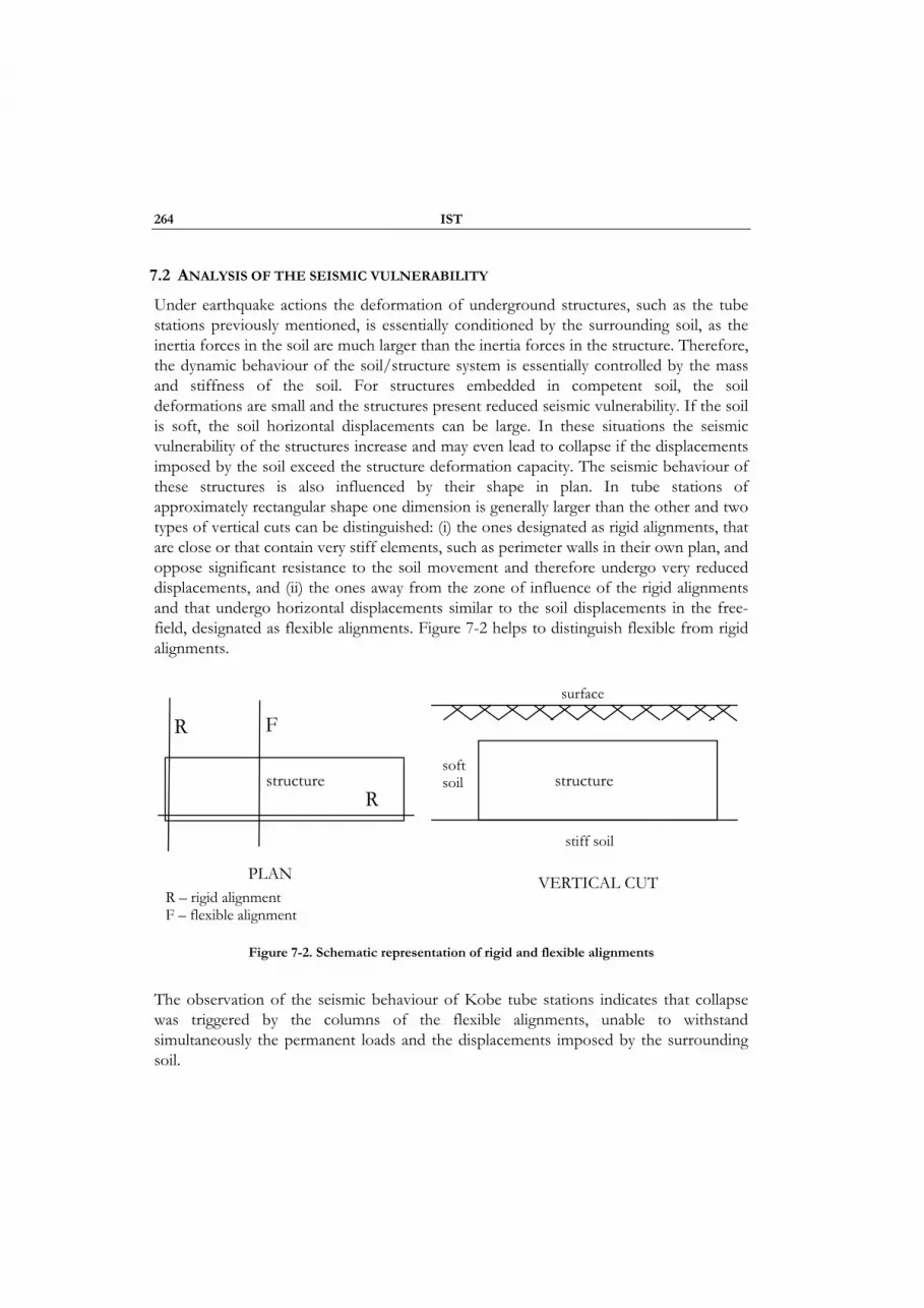
264 IST
7.2 ANALYSIS OF THE SEISMIC VULNERABILITY
Under earthquake actions the deformation of underground structures, such as the tube stations previously mentioned, is essentially conditioned by the surrounding soil, as the inertia forces in the soil are much larger than the inertia forces in the structure. Therefore, the dynamic behaviour of the soil/structure system is essentially controlled by the mass and stiffness of the soil. For structures embedded in competent soil, the soil deformations are small and the structures present reduced seismic vulnerability. If the soil is soft, the soil horizontal displacements can be large. In these situations the seismic vulnerability of the structures increase and may even lead to collapse if the displacements imposed by the soil exceed the structure deformation capacity. The seismic behaviour of these structures is also influenced by their shape in plan. In tube stations of approximately rectangular shape one dimension is generally larger than the other and two types of vertical cuts can be distinguished: (i) the ones designated as rigid alignments, that are close or that contain very stiff elements, such as perimeter walls in their own plan, and oppose significant resistance to the soil movement and therefore undergo very reduced displacements, and (ii) the ones away from the zone of influence of the rigid alignments and that undergo horizontal displacements similar to the soil displacements in the free-field, designated as flexible alignments. Figure 7-2 helps to distinguish flexible from rigid alignments.
Figure 7-2. Schematic representation of rigid and flexible alignments
The observation of the seismic behaviour of Kobe tube stations indicates that collapse was triggered by the columns of the flexible alignments, unable to withstand simultaneously the permanent loads and the displacements imposed by the surrounding soil.
surface
softsoil structure
stiff soil
R
R F
structure
PLAN VERTICAL CUT R – rigid alignmentF – flexible alignment

Sub-Project 7 – 7. Methodology of analysis for underground structures in soft soils 265
7.3 SEISMIC BEHAVIOUR
The seismic performance of an underground structure depends essentially of the ability of the flexible alignments to withstand the imposed displacements. Therefore, an adequate performance can be enforced by means of the following strategies: (i) to treat the soil to control the respective horizontal displacement field along the height during the design earthquake, or (ii) design the structure to withstand the displacements imposed by the soil, while maintaining the ability to resist to the permanent loads.
It results from the above that the design of the structure (always referring to the flexible alignments) aims essentially at providing deformation capacity while it maintains the ability to sustain the permanent loads. Current code procedures, essentially derived for structures that develop mainly above ground, assume that the seismic performance of a structure is a combination of its ability to resist to inertia forces and its ductility and energy dissipation capacity. Since engineers are essentially used to design structures to resist to applied forces, code procedures are usually based on the explicit evaluation of the effects of the inertia forces, the effects of ductility and energy dissipation capacity being accounted for approximately by means of a global factor (q factor in EC 8). The application of this procedure to underground structures is inadequate since these do not need to resist horizontal inertia forces (except for some minor local effects, usually irrelevant) which can be transferred directly to the soil on the sides of the structure and do not need to be transferred to the foundation. Within the usual code framework this would be equivalent to consider the behaviour factor infinite. This highlights the inadequacy of applying code procedures for structures that develop above ground to underground structures. This derives from the fact that providing resistance to horizontal displacements is qualitatively different from the resistance to horizontal forces. The difference between applying displacements and forces can be illustrated in terms of a reinforced concrete section in bending, considering two situations: (i) if a bending moment is applied, the higher the area of flexural reinforcement, the lower will be the respective stresses, the strains and the curvature, which are output of section analysis, (ii) if a curvature is applied the higher the area of reinforcement the higher is the associated bending moment. Note that being the curvature applied by an external source the strains can be evaluated as a function of section geometry, this is, do not depend on the amount of flexural reinforcement (assuming that the position of the neutral axis does not change much with the amount of flexural reinforcement, as generally happens in flexure without axial force).
Another feature that results from the above is that adding flexural reinforcement is useless to prevent yielding, as this depends on the fact that the imposed strain reaches the steel yield strain or not. This clearly contradicts current code concepts according to which a structure can be designed to remain elastic under earthquake actions by designing it

266 IST
with q=1. This is valid in general in structures that develop above ground, but not for structures or elements under applied deformations. Reasoning again at section level, for a given imposed curvature an elastic analysis yields a bending moment. If the amount of flexural reinforcement necessary to resist to that moment (equivalent to consider q=1) or slightly more is provided, the section should remain elastic. The contradiction can be explained with the help of Figure 7-3, as follows: point 1 represents the yield point of a section in bending without axial force. If for instances the flexural reinforcement was duplicated maintaining the same distribution, the flexural capacity would increase in such a way that, if the flexural stiffness was constant as assumed in linear analysis, the new situation would be represented by point 2’. In fact what happens is that the flexural capacity increases but the curvature almost does not increase (as the neutral axis remains in the same position and the steel yield strain does not change) and the point representative of the new situation is point 2 and not 2’. Therefore, the increase in the flexural capacity does not increase the yield curvature and does not avoid yielding.
Figure 7-3. Schematic representation of change in the yield moment and curvature by increasing
flexural reinforcement (N=0)
7.4 CONCEPTION
The conception (in the usual sense of defining the geometry of the structure and its elements) of large underground reinforced concrete structures in soft soils to withstand earthquake actions must aim at ensuring that flexible alignments are provided with the required deformation capacity under horizontal displacement fields without losing the ability to sustain the permanent loads. For this purpose along the flexible alignments the structure must be as flexible and ductile as possible, within the limits associated to the need to resist to all other actions.
Under imposed deformations the larger the cross section dimensions the higher will be the strains imposed both on steel and concrete. Therefore the dimensions of structural elements of the main resisting structure (elements whose collapse would induce irreparable damage or global collapse) in the plan of flexible alignments should be as
χy
M
1
2 2’
EIsec1
EIsec2
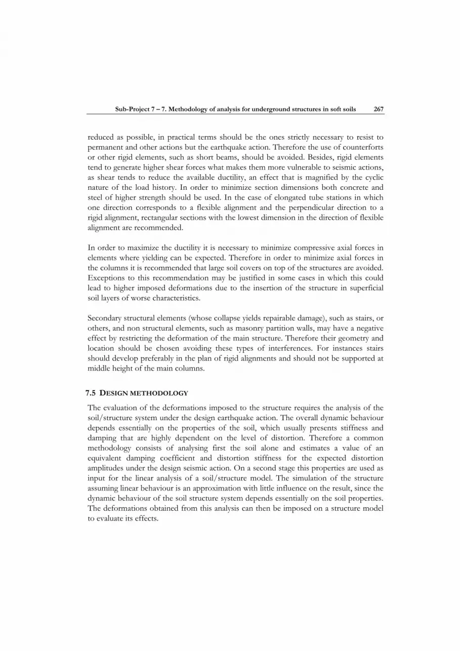
Sub-Project 7 – 7. Methodology of analysis for underground structures in soft soils 267
reduced as possible, in practical terms should be the ones strictly necessary to resist to permanent and other actions but the earthquake action. Therefore the use of counterforts or other rigid elements, such as short beams, should be avoided. Besides, rigid elements tend to generate higher shear forces what makes them more vulnerable to seismic actions, as shear tends to reduce the available ductility, an effect that is magnified by the cyclic nature of the load history. In order to minimize section dimensions both concrete and steel of higher strength should be used. In the case of elongated tube stations in which one direction corresponds to a flexible alignment and the perpendicular direction to a rigid alignment, rectangular sections with the lowest dimension in the direction of flexible alignment are recommended.
In order to maximize the ductility it is necessary to minimize compressive axial forces in elements where yielding can be expected. Therefore in order to minimize axial forces in the columns it is recommended that large soil covers on top of the structures are avoided. Exceptions to this recommendation may be justified in some cases in which this could lead to higher imposed deformations due to the insertion of the structure in superficial soil layers of worse characteristics.
Secondary structural elements (whose collapse yields repairable damage), such as stairs, or others, and non structural elements, such as masonry partition walls, may have a negative effect by restricting the deformation of the main structure. Therefore their geometry and location should be chosen avoiding these types of interferences. For instances stairs should develop preferably in the plan of rigid alignments and should not be supported at middle height of the main columns.
7.5 DESIGN METHODOLOGY
The evaluation of the deformations imposed to the structure requires the analysis of the soil/structure system under the design earthquake action. The overall dynamic behaviour depends essentially on the properties of the soil, which usually presents stiffness and damping that are highly dependent on the level of distortion. Therefore a common methodology consists of analysing first the soil alone and estimates a value of an equivalent damping coefficient and distortion stiffness for the expected distortion amplitudes under the design seismic action. On a second stage this properties are used as input for the linear analysis of a soil/structure model. The simulation of the structure assuming linear behaviour is an approximation with little influence on the result, since the dynamic behaviour of the soil structure system depends essentially on the soil properties. The deformations obtained from this analysis can then be imposed on a structure model to evaluate its effects.

268 IST
The analysis of the deformation capacity of ductile structures involves the analysis of the behaviour in the post-yield range, this is, a physically non-linear analysis. For this purpose, it is necessary to know the yield capacity of structural elements and sections, therefore global structural analysis requires not only the knowledge of the geometry of the structure and its elements but also knowledge of amounts and details of reinforcement. These are necessary to allow the definition of confined concrete constitutive relationships and evaluation of yielding and rupture. The analysis considers flexural and axial deformations but not shear deformations, which are not relevant in well conceived structures. Therefore, the analysis requires as input the definition of the geometry of the structure and its elements and the explicit definition of the flexural reinforcement, including the full monotonic constitutive relationship until rupture. The transverse reinforcement does not need to be defined explicitly, but knowledge of amounts and details of this reinforcement are necessary to evaluate confining stresses and the constitutive relationships for confined concrete. The detailed characterization of the structure allows performing the global structural analysis and the evaluation of axial stresses and strains anywhere in the structure simultaneously. Thus, it allows doing safety verifications at material level by comparing the maximum strain demands with the corresponding acceptable limits.
Global analysis of the structures, linear or nonlinear, are usually performed assuming average material properties. However, safety checkings at element and section level are usually based on design values of material properties to account for the possibility that at some locations in the structure the materials properties are worse than average. In order to follow this analysis and safety verification methodology it is necessary to decouple the global structural analysis from the section or element analysis using separate models. However, since there is an interest in performing both the global analysis and safety verifications with the same model, it is necessary to make a choice of what material properties to use. Since the action upon the structure is represented by imposed displacements, the evaluation of curvatures is essentially a cinematic problem whose result is almost not influenced by material constitutive relationships. Therefore, it is not relevant what material properties are used in the global analysis. Since design values should be used for safety verifications at section or material level, these properties will be used in the analyses that will be presented in the next sections.
Current design practice is usually based on a procedure with the following phases: (i) conception of the structure, (ii) global structural analysis based on a constant stiffness of all structural elements, (iii) safety verification at section or material level. In reinforced concrete structures, the third phase is transformed in the calculation of the amounts of reinforcement necessary to ensure the prescribed safety verification. In the methodology that is proposed in this work the third phase is a really verification phase, as the reinforcement needs to be known before the analysis and safety checkings are done, by
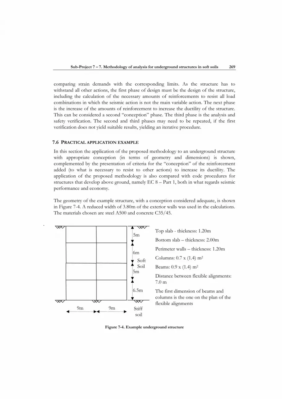
Sub-Project 7 – 7. Methodology of analysis for underground structures in soft soils 269
comparing strain demands with the corresponding limits. As the structure has to withstand all other actions, the first phase of design must be the design of the structure, including the calculation of the necessary amounts of reinforcements to resist all load combinations in which the seismic action is not the main variable action. The next phase is the increase of the amounts of reinforcement to increase the ductility of the structure. This can be considered a second “conception” phase. The third phase is the analysis and safety verification. The second and third phases may need to be repeated, if the first verification does not yield suitable results, yielding an iterative procedure.
7.6 PRACTICAL APPLICATION EXAMPLE
In this section the application of the proposed methodology to an underground structure with appropriate conception (in terms of geometry and dimensions) is shown, complemented by the presentation of criteria for the “conception” of the reinforcement added (to what is necessary to resist to other actions) to increase its ductility. The application of the proposed methodology is also compared with code procedures for structures that develop above ground, namely EC 8 – Part 1, both in what regards seismic performance and economy.
The geometry of the example structure, with a conception considered adequate, is shown in Figure 7-4. A reduced width of 3.80m of the exterior walls was used in the calculations. The materials chosen are steel A500 and concrete C35/45.
Figure 7-4. Example underground structure
9m 9m
5m
6m
5m
6.5m
SoftSoil
Stiffsoil
Top slab - thickness: 1.20m
Bottom slab – thickness: 2.00m
Perimeter walls – thickness: 1.20m
Columns: 0.7 x (1.4) m2
Beams: 0.9 x (1.4) m2
Distance between flexible alignments: 7.0 m
The first dimension of beams and columns is the one on the plan of the flexible alignments
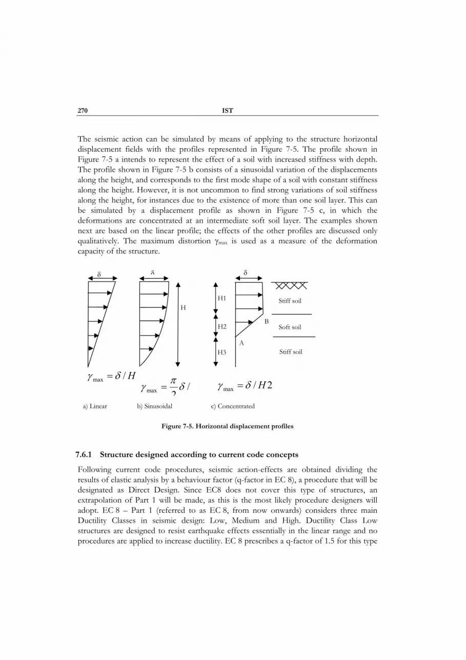
270 IST
The seismic action can be simulated by means of applying to the structure horizontal displacement fields with the profiles represented in Figure 7-5. The profile shown in Figure 7-5 a intends to represent the effect of a soil with increased stiffness with depth. The profile shown in Figure 7-5 b consists of a sinusoidal variation of the displacements along the height, and corresponds to the first mode shape of a soil with constant stiffness along the height. However, it is not uncommon to find strong variations of soil stiffness along the height, for instances due to the existence of more than one soil layer. This can be simulated by a displacement profile as shown in Figure 7-5 c, in which the deformations are concentrated at an intermediate soft soil layer. The examples shown next are based on the linear profile; the effects of the other profiles are discussed only qualitatively. The maximum distortion γmax is used as a measure of the deformation capacity of the structure.
Figure 7-5. Horizontal displacement profiles
7.6.1 Structure designed according to current code concepts
Following current code procedures, seismic action-effects are obtained dividing the results of elastic analysis by a behaviour factor (q-factor in EC 8), a procedure that will be designated as Direct Design. Since EC8 does not cover this type of structures, an extrapolation of Part 1 will be made, as this is the most likely procedure designers will adopt. EC 8 – Part 1 (referred to as EC 8, from now onwards) considers three main Ductility Classes in seismic design: Low, Medium and High. Ductility Class Low structures are designed to resist earthquake effects essentially in the linear range and no procedures are applied to increase ductility. EC 8 prescribes a q-factor of 1.5 for this type
δ δ
H/max δγ =
δ
A
H H1
H2
H3
Stiff soil
Stiff soil
Soft soilB
/2max δπγ = 2/max Hδγ =
a) Linear b) Sinusoidal c) Concentrated

Sub-Project 7 – 7. Methodology of analysis for underground structures in soft soils 271
of structures to account for some levels of overstrength that is assumed is always available in reinforced concrete structures. Structures of Ductility Classes Medium and High are designed to resist earthquake actions by a combination of their resistance to inertia forces with their ductility and energy dissipation capacity. This represents an intermediate type of design between the one associated with Ductility Class Low and the proposed methodology. Therefore, to highlight the differences to the proposed methodology the example structure is designed as a Low Ductility Class structure.
Since in the framework of Direct Design applied displacements result in internal action-effects on the structure (bending moments, shear and axial forces), the maximum displacement the structure can withstand is restricted by the maximum amounts of reinforcement that is possible to place in any structural member. Assuming q=1.5 and that the constant member stiffness assumed in the elastic analysis is half the stiffness of the gross concrete sections as prescribed in EC 8, the maximum allowable distortion associated with the linear profile of imposed displacements is γmax=8.2x10⁻³. The reinforcement corresponding to this distortion is shown in Figure 7-6.
The explicit evaluation of the deformation capacity of this structure was evaluated by means of a static nonlinear analysis imposing the permanent loads and the linear displacement profile. It is assumed that proper detailing ensures the anchorage and effectiveness of all reinforcement, in particular confinement reinforcement after spalling of the concrete cover. The deformability of the nodes and shear deformations were disregarded, only flexural deformations were accounted for. The nonlinear behaviour of concrete and steel were simulated using the constitutive relationships for confined concrete prescribed in EC 8 – Part 2 and constitutive relationships for steel obtained from a large statistical characterization of the Tempcore steels used in Europe (Pipa, 1993). Figure 7-11 shows the constitutive relationship for steel and an example of constitutive relationships for confined concrete. Rupture was defined by the attainment of the maximum axial strain anywhere in the structure. The maximum allowable strain for steel is εmax=7.5%, corresponding to steel type C and for concrete it depends on the level of confinement, according to the equation prescribed in Annex C of EC 8 – Part 2.
The results of this analysis indicate that the maximum average distortion that the structure can withstand is γmax=5.0x10⁻³. Figure 7-7 shows the curvature diagrams at this situation, indicating the yield curvature at some sections and showing that flexural yielding took place at several locations. The maximum tensile strain is ε=27.8 ‰, 13 times the steel yield strain (ε=2.07 ‰). Note that at this stage the maximum distortion was 60% of the distortion evaluated according to EC8 (Low Ductility Class), at which the structure was supposed to be elastic. If the sinusoidal profile had been applied the ductility demand would be higher at the lower part of the structure and it would withstand a lower relative displacement (δ) between the top and bottom slabs.
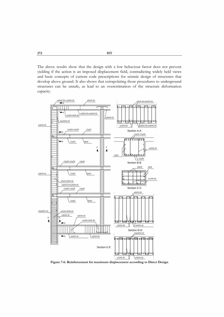
272 IST
The above results show that the design with a low behaviour factor does not prevent yielding if the action is an imposed displacement field, contradicting widely held views and basic concepts of current code prescriptions for seismic design of structures that develop above ground. It also shows that extrapolating those procedures to underground structures can be unsafe, as lead to an overestimation of the structure deformation capacity.
Figure 7-6. Reinforcement for maximum displacement according to Direct Design
Section A-A
Section B-B
Section C-C
Section D-D
Section E-E
2xφ32//0.10
φ32//0.10 φ12//0.20
φ25//0.20+φ20//0.20
φ32//0.20φ32//0.20+ φ32//0.20
11φ32
11φ32 11φ32+11φ25
2xφ25//0.20
φ32//0.20
φ32//0.10
φ32//0.10
φ10//0.20//0.30
φ10//0.20//0.30
φ12//0.20//0.20
φ10//0.20//0.30
A
A
B
B
C C
D
D
E E
11φ32
11φ32 11φ32+11φ25
11φ32
11φ32 11φ32+11φ25
φ25//0.20
2xφ32//0.10
φ32//0.10
φ32//0.20
φ32//0.20
6φ32
6φ32
6φ32
φ32//0.20+φ25//0.20
φ32/0.20+φ32//0.20
φ25//0.20+φ20//0.20 φ10//0.30
φ32//0.20
φ32//0.10 φ10//0.30
16φ32
φ12//0.25
4φ32
11φ32+11φ25
11φ32
φ10//0.20
2φ20
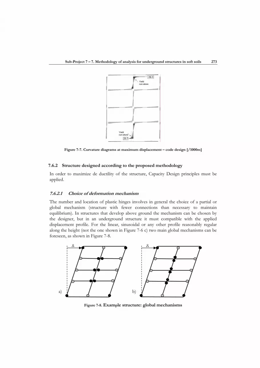
Sub-Project 7 – 7. Methodology of analysis for underground structures in soft soils 273
Figure 7-7. Curvature diagrams at maximum displacement – code design [/1000m]
7.6.2 Structure designed according to the proposed methodology
In order to maximize de ductility of the structure, Capacity Design principles must be applied.
7.6.2.1 Choice of deformation mechanism
The number and location of plastic hinges involves in general the choice of a partial or global mechanism (structure with fewer connections than necessary to maintain equilibrium). In structures that develop above ground the mechanism can be chosen by the designer, but in an underground structure it must compatible with the applied displacement profile. For the linear, sinusoidal or any other profile reasonably regular along the height (not the one shown in Figure 7-6 c) two main global mechanisms can be foreseen, as shown in Figure 7-8.
Figure 7-8. Example structure: global mechanisms
δ δ
a) b)
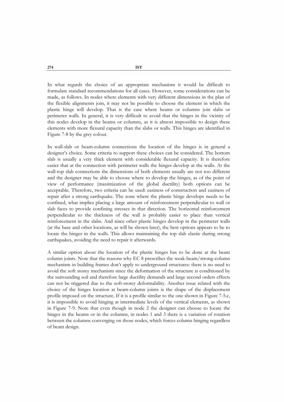
274 IST
In what regards the choice of an appropriate mechanism it would be difficult to formulate standard recommendations for all cases. However, some considerations can be made, as follows. In nodes where elements with very different dimensions in the plan of the flexible alignments join, it may not be possible to choose the element in which the plastic hinge will develop. That is the case where beams or columns join slabs or perimeter walls. In general, it is very difficult to avoid that the hinges in the vicinity of this nodes develop in the beams or columns, as it is almost impossible to design these elements with more flexural capacity than the slabs or walls. This hinges are identified in Figure 7-8 by the grey colour.
In wall-slab or beam-column connections the location of the hinges is in general a designer’s choice. Some criteria to support these choices can be considered. The bottom slab is usually a very thick element with considerable flexural capacity. It is therefore easier that at the connection with perimeter walls the hinges develop at the walls. At the wall-top slab connections the dimensions of both elements usually are not too different and the designer may be able to choose where to develop the hinges, as of the point of view of performance (maximization of the global ductility) both options can be acceptable. Therefore, two criteria can be used: easiness of construction and easiness of repair after a strong earthquake. The zone where the plastic hinge develops needs to be confined, what implies placing a large amount of reinforcement perpendicular to wall or slab faces to provide confining stresses in that direction. The horizontal reinforcement perpendicular to the thickness of the wall is probably easier to place than vertical reinforcement in the slabs. And since other plastic hinges develop in the perimeter walls (at the base and other locations, as will be shown later), the best options appears to be to locate the hinges in the walls. This allows maintaining the top slab elastic during strong earthquakes, avoiding the need to repair it afterwards.
A similar option about the location of the plastic hinges has to be done at the beam column joints. Note that the reasons why EC 8 prescribes the weak-beam/strong-column mechanism in building frames don’t apply to underground structures: there is no need to avoid the soft storey mechanism since the deformation of the structure is conditioned by the surrounding soil and therefore large ductility demands and large second orders effects can not be triggered due to the soft-storey deformability. Another issue related with the choice of the hinges location at beam-column joints is the shape of the displacement profile imposed on the structure. If it is a profile similar to the one shown in Figure 7-5.c, it is impossible to avoid hinging at intermediate levels of the vertical elements, as shown in Figure 7-9. Note that even though in node 2 the designer can choose to locate the hinges in the beams or in the columns, in nodes 1 and 3 there is a variation of rotation between the columns converging on those nodes, which forces column hinging regardless of beam design.
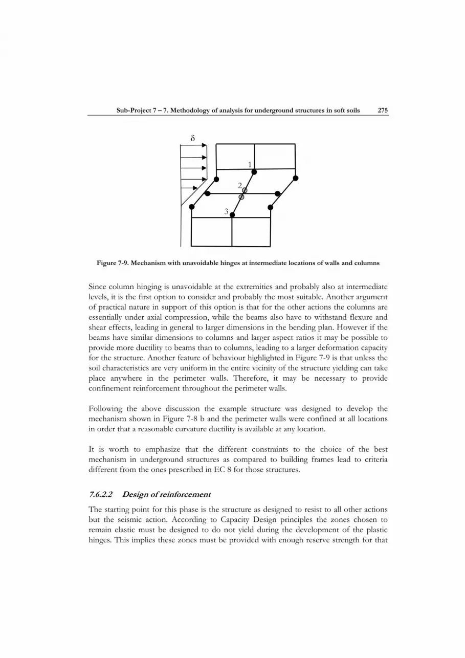
Sub-Project 7 – 7. Methodology of analysis for underground structures in soft soils 275
Figure 7-9. Mechanism with unavoidable hinges at intermediate locations of walls and columns
Since column hinging is unavoidable at the extremities and probably also at intermediate levels, it is the first option to consider and probably the most suitable. Another argument of practical nature in support of this option is that for the other actions the columns are essentially under axial compression, while the beams also have to withstand flexure and shear effects, leading in general to larger dimensions in the bending plan. However if the beams have similar dimensions to columns and larger aspect ratios it may be possible to provide more ductility to beams than to columns, leading to a larger deformation capacity for the structure. Another feature of behaviour highlighted in Figure 7-9 is that unless the soil characteristics are very uniform in the entire vicinity of the structure yielding can take place anywhere in the perimeter walls. Therefore, it may be necessary to provide confinement reinforcement throughout the perimeter walls.
Following the above discussion the example structure was designed to develop the mechanism shown in Figure 7-8 b and the perimeter walls were confined at all locations in order that a reasonable curvature ductility is available at any location.
It is worth to emphasize that the different constraints to the choice of the best mechanism in underground structures as compared to building frames lead to criteria different from the ones prescribed in EC 8 for those structures.
7.6.2.2 Design of reinforcement
The starting point for this phase is the structure as designed to resist to all other actions but the seismic action. According to Capacity Design principles the zones chosen to remain elastic must be designed to do not yield during the development of the plastic hinges. This implies these zones must be provided with enough reserve strength for that
3
1
2
δ
276 IST
purpose. The plastic hinge zones must be designed for ductility as well as to avoid any brittle type of failure. Considering the chosen mechanism the main implications for the different structural elements are as follows:
• perimeter walls: it is not necessary to increase the flexural capacity as hinges are expected to develop at the walls (remind that the proposed methodology is equivalent to consider q=∞). It is necessary to increase the available ductility throughout the walls: for this purpose confinement reinforcement, comprising horizontal links in the direction of the wall thickness and properly anchored at the extremities around the vertical reinforcement must be provided. Figure 7-11 shows the new design of the wall cross sections.
• slabs: the design for the other actions ensures that slabs are stronger then the columns to which they are connected. However the flexural capacity may need to be increased, particularly in the extremities of the top slab, to be higher than the maximum moment at the walls hinges, in order to avoid the formation of plastic hinges at the slab extremities. For this purpose at the extremities the slab is designed for a bending moment which is Msdslab=γ0.Mrdwall, with both moments evaluated by the usual design procedure prescribed in EC 2. A value γ0=1.3, as prescribed in EC 8 for column design, seems appropriate for the first iteration of the proposed design procedure. Figure 7-10 shows a longitudinal cut of the top slab.
• beams: in order to increase the ductility of the extreme sections where plastic hinges are expected to develop, confinement reinforcement must be provided at these zones. Flexural reinforcement on the lower face was also added in order to reduce the size of the compressive zone when the top reinforcement yields at beam extremities. The effectiveness of this extra reinforcement in increasing the curvature ductility can be easily evaluated by section analysis. In what regards interior beam column joints it was decided to develop the plastic hinges in the columns. Therefore in the first iteration the flexural reinforcement on the beams in the vicinity of these nodes provide an excess flexural capacity above the sum of the moments of resistance of the columns converging at the same node of 30%, what also depends on column design. However the analysis showed this was not enough. Figure 7-10 shows the new design of the beams. The beams were provided with more transverse reinforcement at the zones plastic hinges are expected to develop to increase the ductility of confined concrete.
• columns: since the columns are essentially under axial compression for all other loads, can be designed for that purpose with the minimum amounts of flexural and transverse reinforcement. Since the columns are not intended to remain elastic there is no need to increase their flexural capacity (q=∞). However flexural reinforcement may be useful to decrease the ductility demand because of the following reasons: (i) to increase column stiffness relatively to the beams, in order to reduce the

Sub-Project 7 – 7. Methodology of analysis for underground structures in soft soils 277
restrictions that the beams impose to column rotations at beam-column joints, (ii) because large spacing of vertical reinforcement reduces the effectiveness of confinement, (iii) because the spacing of confinement reinforcement should be proportional to the diameter of the flexural reinforcement, therefore this should not be too small.
Figure 7-10. Details of design according to the proposed methodology
Section A-A
Section B-B
Section C-C
Section D-D
Section E-E
2xφ25//0.20
2xφ25//0.20φ12//0.10
φ25//0.20+φ32//0.20
φ25//0.20+φ32//0.20 φ10//0.30
φ25//0.20
φ25//0.20 φ25//0.20+φ20//0.20 φ25//0.20+φ32//0.20
8φ32
8φ32+8φ32 8φ32
8φ32
8φ32
8φ32
8φ32+8φ32 8φ32
2xφ25//0.20
φ32//0.20
φ32//0.20
2xφ25//0.20
2.50
φ12//0.20//0.10
φ10//0.20//0.30
φ10//0.20//0.30
A
A
B
B
C C
D
D
E E
φ25//0.20+φ32//0.20
φ25//0.20+ φ20//0.20
8φ32+2φ32
φ10//0.20
φ10//0.20
8φ32+8φ32
8φ32+2φ32
8φ32+2φ32
φ12//0.10
8φ32
8φ32
2φ20
φ16//0.10
φ12//0.10
8φ32+2φ32
8φ32+2φ32
2φ25
φ16//0.10
φ32//0.20
φ32//0.20φ10//0.30

278 IST
Besides there is the obvious need to provide confinement reinforcement in the plastic hinge zones to increase the available curvature ductility in those zones. The efficiency of the above can be evaluated by section analysis. Figure 7-11 shows the constitutive relationships for steel, confined and unconfined concrete and the moment curvature diagrams at the base of the columns before and after the increase in reinforcement, evaluated considering the axial force at maximum displacement.
σ [MPa]
0
10
20
30
40
50
0 5 10 15
ε [/1000]
σ [MPa]
-600
-400
-200
0
200
400
600
-80 -60 -40 -20 0 20 40 60 80
ε [/1000]
Moment [kNm]
-6000
-4000
-2000
0
2000
4000
6000
-150 -75 0 75 150
Curvature [/1000m]
Without seismic designWith seismic design
a) Concrete b) Steel c) Column moment-curvature diagrams
Figure 7-11. Material constitutive relationships and moment-curvature diagrams at the column base section
It should be emphasized that the process of maximizing the overall structural ductility is an iterative procedure, that starts from the structure as designed to resist to all other actions. Successive analysis and changes were done in order to improve the overall ductility. The following examples highlight this procedure: (i) at each analysis the rupture point and other locations close to rupture were identified and the possibility of increasing the available ductility at those locations was analysed; this was the case at beam extremities that initially were all designed with 6 vertical stirrups φ12, that the analysis showed were not enough to prevent rupture at the beams, limiting the overall ductility of the structure; in the final design, at the extremities the beams were designed with 6φ12+2φ16 vertical stirrups; another change of this type was the use of external stirrups φ16 at the three lower column hinges; (ii) column flexural reinforcement was increased in order to increase its stiffness (according to the concept discussed in section 7.3 and illustrated in Figure 7-3, the amount of flexural reinforcement influences the member stiffness) relatively to the beams, to reduce the ductility demand on the columns; note that the increase in column flexural reinforcement also led to an increase in beam flexural reinforcement to avoid beam hinging but due to the curtailment of reinforcement, the stiffness of the beams increased less than the stiffness of the columns, in which there was no curtailment of flexural reinforcement; (iii) beam overstrength at beam-column joints was increased far above the initial value of γ0=1.3, because the balance between beam moments on both sides of the nodes changed in the non-linear range increasing the moment demand.
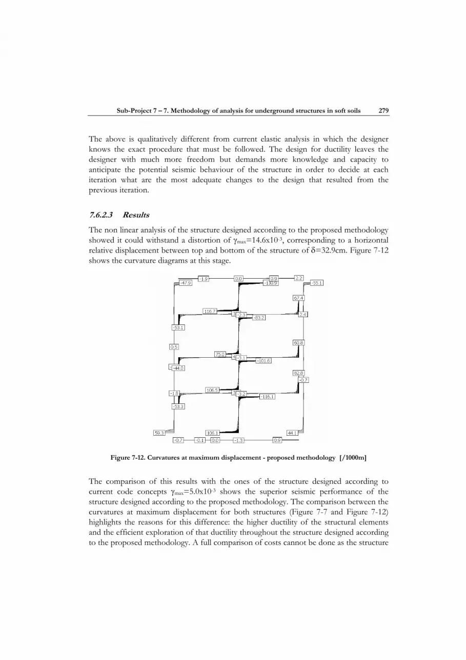
Sub-Project 7 – 7. Methodology of analysis for underground structures in soft soils 279
The above is qualitatively different from current elastic analysis in which the designer knows the exact procedure that must be followed. The design for ductility leaves the designer with much more freedom but demands more knowledge and capacity to anticipate the potential seismic behaviour of the structure in order to decide at each iteration what are the most adequate changes to the design that resulted from the previous iteration.
7.6.2.3 Results
The non linear analysis of the structure designed according to the proposed methodology showed it could withstand a distortion of γmax=14.6x10⁻³, corresponding to a horizontal relative displacement between top and bottom of the structure of δ=32.9cm. Figure 7-12 shows the curvature diagrams at this stage.
Figure 7-12. Curvatures at maximum displacement - proposed methodology [/1000m]
The comparison of this results with the ones of the structure designed according to current code concepts γmax=5.0x10⁻³ shows the superior seismic performance of the structure designed according to the proposed methodology. The comparison between the curvatures at maximum displacement for both structures (Figure 7-7 and Figure 7-12) highlights the reasons for this difference: the higher ductility of the structural elements and the efficient exploration of that ductility throughout the structure designed according to the proposed methodology. A full comparison of costs cannot be done as the structure
280 IST
was not fully defined, neither was the constructive process. However, in terms of materials most of the difference regards the amount of steel in the perimeter walls. The proposed methodology leads to the use of less flexural reinforcement, but needs large amounts of confinement reinforcement, leading to almost equal total amounts of steel spent in the perimeter walls. In the slabs the proposed methodology leads to moderate savings, as the flexural reinforcement is conditioned essentially by the minimum levels prescribed in EC2. In beams and columns the general trend is similar to that observed in the perimeter walls, with some savings for the design of the columns according to the proposed methodology. The above indicates that in general the design according to the proposed methodology does not has a significant influence on the overall costs, and may even lead to slight savings in some elements.
7.7 SUMMARY AND CONCLUSIONS
During earthquakes underground structures do not have to resist to horizontal inertia forces, as structures that develop essentially above ground, but only to withstand the displacements the soil imposes on them without losing the capacity to resist to permanent actions. Therefore reinforced concrete structures must be designed to be flexible and ductile. For instances large underground reinforced concrete structures, such as tube stations, should be designed in the transverse direction with elements whose dimensions must be the ones strictly necessary to resist to other actions but the seismic actions. Stiff elements, such as counterforts or short beams should be avoided, as well as large soil covers. The interference of secondary or non-structural elements with the deformation of the main structure should be avoided.
The structure must be designed by stages: first for all load combinations whose main variable action is not the seismic action; second for the seismic action. Since there are no inertia forces (equivalent to consider the behaviour factor infinite) the designer must choose a suitable deformation mechanism and apply Capacity Design principles, this is, to design the potential plastic hinge zones for ductility and the remaining zones with excess strength to remain elastic. An application example is shown. The proposed procedure tends to lead to considerable savings in flexural reinforcement but more confinement reinforcement. In general terms it leads to structures with better seismic performance than the extrapolation of code procedures derived for structures that develop above ground, that may lead to unsafe underground structures. Therefore it is recommended that EC8 covers explicitly the seismic design of underground structures.

REFERENCES
CHAPTER 1.
Ilki, A., Boduroglu, M.H., Ozdemir, P., Baysan, F., Demir, C., Sirin, S. [2003] “Comparison of the results obtained by seismic index method and structural analysis for existing and retrofitted buildings” Proceedings of 5th National Conference on Earthquake Engineering, Istanbul, Turkey, Paper No. AT-119.
JSIM. [1977]. Standard for evaluation of seismic capacity of existing reinforced concrete buildings. Japan Building Disaster Prevention Association, Ministry of Construction, Tokyo, Japan
Ozdemir, P., Ilki, A., Boduroglu, M.H., Sirin, S., Demir, C., Baysan, F. [2004] “A modified rapid screening procedure for medium rise rc structures“ Proceedings of 13th World Conference on Earthquake Engineering,, Vancouver, Canada, Paper No. 1542.
TERDC-98. [1998]. Specification for structures to be built in disaster areas: Earthquake disaster prevention. Ministry of Settlement and Public-Works, Ankara, Turkey.
TERDC-2006. [2006]. Specification for structures to be built in disaster areas: Earthquake disaster prevention. Ministry of Settlement and Public-Works, Ankara, Turkey.
CHAPTER 2.
ATC-40, [1996], Seismic Evaluation and Retrofit of Concrete Buildings, ATC, California, USA.
FEMA-440, [2004], Improvement of Nonlinear Static Seismic Analysis Procedures, FEMA, Washington DC.
TEC-2006 [2006], Earthquake Code of Turkey, Ministry of Construction, Ankara, (in Turkish).
SAP2000 [2006], Structural Analysis Software, Computers and Structures Inc., Berkeley, CA, USA.

282 Sub-Project 7 - References
SECTIONS 3.1 & 3.3
Amar Khennane; Robert E. Melchers. “Durability of Glass Polymer Composites Subject to Stress Corrosion”. Journal of Composites for Construction, Vol 7, No. 2, May 2003, 10–117.
Bond behaviour of corroded steel reinforcement in concrete wrapped with carbon fiber reinforced polymer sheets. Khaled Soudki, Ted Sherwood [Journal of composites for construccion, ASCE, Julio-Agosto. 2003]
Dowling N.E., Mechanical Behaviour of Materials: Engineering Methods for Deformation, Fracture, and Fatigue, Ed. Prentice Hall,.
Guide for the design and construction of externally bonded FRP systems for strengthening concrete structures. American Concrete Institute (ACI). [ACI 440.2R-02]
Hahn H.T., Fatigue Behaviour of Composite Laminate, J. Composite Materials, Vol. 10, 1976.
Principe, F., Design Requirements, Engineered Materials Handbook
Reifsnider K.L., Fatigue of Composite Materials, Composite Materials Series, Volume 4, Ed. R.B. Pipes, 1991.
Tannous, F. E. and Saadatmanesh, H. (1998). “Environmental Effects on the Mechanical Properties E-Glass FRP Rebars”, ACI Materials Journal, Vol. 95(2), pp 87–100.
Valter Dejke. “Durability of FRP Reinforcement in Concrete–Literature Review and Experiments”. Thesis for the Degree of Licentiate of Engineering, Department of Building Materials, Chalmers University of Technology; Göteborg, Sweden 2001.
CHAPTER 3.2
ANSYS, Inc [2007] ANSYS products, www.ansys.com
ANSYS, Inc [2005] Guide to ANSYS User Programmable Features, ANSYS Release 10.0, Canonsburg, PA,, USA
Barbat, A.H., Oller, S., Oñate, E., Hanganu, A. [1997] “Viscous damage model for Timoshenko beam structures” International Journal of Solids and Structures, Vol.34, No 30, pp. 3953-3976

Sub-Project 7 – References 283
Car, E., Oller, S., Oñate, E. [2001] “A Large Strain Plasticity for Anisotropic Materials – Composite Material Application,” International Journal of Plasticity, Vol. 17, No. 11, pp. 1437-1463.
Car, E., Oller, S., Oñate, E. [2000] “An anisotropic elasto-plastic constitutive model for large strain analysis of fiber reinforced composite materials” Computer Methods in Applied Mechanics and Engineering, Vol.185, No 2-4, pp. 245-277
CIMNE [2006] LessLoss Deriverable 49: Integration of knowledge on FRP retrofitted structures, LessLoss project (GOCE-CT-2003-505488), Sub-Project 7
Crisfield, M.A. [1991], Non-linear finite element analysis of solids and structures. Volume 1. Essentials, John Wiley & Sons, West Sussex, UK
GiD [2007] GiD 8. The personal pre and post processor, www.gidhome.com
Lubliner J., Oliver, J., Oller S., Oñate, E. [1989] “A plastic damage model for concrete” International Journal of Solids and Structures, Vol. 25, No 3, pp. 299-326
Malvern, L. E. [1968] Introduction to the mechanics of a continuous medium, Prentice-Hall, Englewood Cliffs, NJ, USA.
Martinez, X., Oller, S., Barbat, A., Rastellini, F. [2007] “New procedure to calculate compression strength of FRP using the Serial/Parallel mixing theory”, Accepted at 8th FRPRCS-8, Patras, Greece
Martinez, X., Oller, S., Barbat, A. [2006] “Numerical tool to study structural reinforcement of steel reinforced concrete (RC) structures under seismic loads using fibre reinforced polymers (FRP)”, ECEES-1 Proceedings, Geneva, Switzerland
Meier, U. [1995] “Strengthening of structures using carbon fibre/epoxi composites” Construction and Building Materials, Vol.9, No 6, pp.341-351
Oller, S., Miquel, J., Zalamea, F. [2005] “Composite material behaviour using a homogenization double scale method” Journal of Engineering Mechanics, Vol.131, No 1, pp. 65-79
Oller, S. [2002], Análisis y cálculo de estructuras de materiales compuestos, CIMNE, Barcelona, Spain
Oller, S., Oñate, E., Oliver, J., Lubliner, J. [1990] “Finite element non--linear analysis of concrete structures using a plastic-damage model” Engineering Fracture Mechanics, Vol. 35, No 1-3, pp. 219-231
284 Sub-Project 7 - References
Oñate, E. [1995] Cálculo de estructuras por el método de elementos finitos. Análisis estático lineal, CIMNE, Barcelona, Spain
PLCd Manual [1991-now] PLCd. Non-linear thermomechanic finite element code oriented to PhD student education. Code developed at CIMNE
Rabinovitch, O., Frostig, Y. [2001] “Nonlinear high-order analysis of cracked RC beams strengthened with FRP strips” Journal of Structural Engineering, Vol.127, No 4, pp. 381-389
Rastellini, F. [2006] Numerical modelling of the constitutive non-linearity of composite laminates, PhD thesis, Departament de Resistència de Materials i Estructures a l’Enginyeria (RMEE) – UPC, Directors: S. Oller y E. Oñate.
Sánchez-Palencia, E.S. [1987], Homogenization techniques for composite media, Springer-Verlag, Berlin, Germany. Chapter: “Boundary layers and edge effects in composites”, pp. 121-192
Spadea, G., Benicardino F., Swamy, R. [1998] “Structural behaviour of composite RC beams with externally bonded CFRP” Journal of Composites for Construction, Vol.2, No 3, pp. 132-137
Trusdell C., Toupín, R. [1960] The classical field theories, Handbuch der physic iii/I, Edition, Springer-Verlag, Berlin, Germany
Zienkiewicz, O. C., Taylor, L.R., [1991] The finite element method, McGraw-Hill, London, England
CHAPTER 3.4
American Concrete Institute (ACI) Committee 440. (2002). “ACI 440: Guide for the design and construction of externally bonded FRP systems for strengthening concrete structures”, Detroit.
Becque, J., Patnaik, A.K., and Rizkalla, S.H. [2003] “Analytical models for concrete confined with FRP tubes,” J. Compos. Const., Vol. 7, No. 1, pp. 31-38.
Bisby, L.A., Dent, A.J.S., and Green, M.F. [2005] “Comparison of confinement models for fiber-reinforced polymer-wrapped concrete,” ACI Structural Journal, Vol. 102, No. 1, pp. 62-72.
Canadian Standards Association (CSA). (2002). “CAN/CSA-S806: design and construction of building components with fiber-reinforced polymers”, Ottawa.
Sub-Project 7 – References 285
De Lorenzis, L., and Tepfers, R. [2003] “Comparative study of models on confinement of concrete cylinders with fiber-reinforced polymer composites,” J. Compos. Const., Vol. 7, No. 3, pp. 219-237.
Demers, M., and Neale, K.W. [1999] “Confinement of reinforced concrete columns with fibre-reinforced composite sheets-an experimental study,” Can. J. Civ. Eng., Vol. 26, No. 2, pp. 226-241.
Comite Europeen de Normalisation (CEN). (2005). “EN 1998-3: Eurocode 8 part 3: assesment and retrofitting of buildings.”, Brussels.
Fam, A.Z., and Rizkalla, S.H. [2001] “Confinement model for axially loaded concrete confined by circular fiber-reinforced polymer tubes,” ACI Structural Journal, Vol. 98, No. 4, pp. 451-461.
Fédération Internationale du Béton (fib). (2001). “Bulletin no.14: externally bonded FRP reinforcement for rc structures.” Technical Report.
Ilki, A., and Kumbasar, N. [2002] “Behavior of damaged and undamaged concrete strengthened by carbon fiber composite sheets,” Struct. Eng. and Mech., Vol. 13, No. 1, pp. 75-90.
Ilki, A., and Kumbasar, N. [2003] “Compressive behaviour of carbon fibre composite jacketed concrete with circular and non-circular cross-sections,” Journal of Earthquake Engineering, Vol. 7, No. 3, pp. 381-406.
Ilki A., Peker O., Karamuk E., and Kumbasar N. [2004a] “External confinement of low strength brittle reinforced concrete short columns,” Proc., International Symposium on Confined Concrete (CD-ROM), Changsha, China.
Ilki A., Koc V., Peker O., Karamuk E., and Kumbasar N. [2004b] “Strengthening of RC Columns with Inadequate Transverse Reinforcement,” Proc., The Second Int. Conf. on FRP Comps. in Civil Engineering, 8-10 Dec. 2004, Adelaide, Australia, pp. 211-218.
Ilki, A., Kumbasar, N., and Koc, V. [2004c] “Low strength concrete members externally confined with FRP sheets,” Struct. Eng. and Mech., Vol. 18, No. 2, pp. 167-194.
Lam, L., and Teng, J.G. [2002] “Strength models for fiber-reinforced plastic-confined concrete,” J. Struct. Eng., Vol. 128, No. 5, pp. 612-623.
Lam, L., and Teng, J.G. [2003a] “Design-oriented stress-strain model for FRP-confined concrete,” Construction and Building Materials, Vol. 17, pp. 471-489.
286 Sub-Project 7 - References
Lam, L., and Teng, J.G. [2003b] “Design-oriented stress-strain model for FRP-confined concrete in rectangular columns,” Jour. of Reinf. Plast. and Comps., Vol. 22, No. 13, pp. 1149-1186.
Lam, L., Teng, J.G., Cheung, C.H., and Xiao, Y. [2004] “Behavior of FRP-confined concrete under cyclic axial compression,” Proc., International Symposium on Confined Concrete (CD-ROM), Changsha, China.
Mander, J.B., Priestley, M.J.N., and Park, R. [1988]. “Theoretical stress-strain model for confined concrete,” ASCE Jour. of the Struct. Div., Vol. 114, No. 8, pp. 1804-1826.
Matthys, S., Toutanji, H., Audenaert, K., and Taerwe, L. [2005] “Axial load behavior of large-scale columns confined with fiber-reinforced polymer composites,” ACI Structural Journal, Vol. 102, No. 2, pp. 258-267.
Rochette, P., and Labossiere, P. [2000] “Axial testing of rectangular column models confined with composites,” ASCE Jour. of Comp. for Cons., Vol. 4, No. 3, pp. 129-136.
Shehata I.A.E.M., Carneiro L.A.V., and Shehata L.C.D. [2002] “Strength of short concrete columns confined with CFRP sheets,” Mat. and Struct., Vol. 35, No. 245, pp. 50-58.
Tan, K.H. [2002] “Strength enhancement of rectangular reinforced concrete columns using fiber-reinforced polymer,” J. Compos. Const., Vol. 6, No. 3, pp. 175-183.
Tastani, S.P., and Pantazopoulou S.J. [2004] “Experimental evaluation of FRP Jackets upgrading RC corroded columns with substandard detailing,” Engineering Structures, Vol. 26, pp. 817-829.
Toutanji, H.A. [1999] “Stress-strain characteristics of concrete columns externally confined with advanced fiber composite sheets,” ACI Mat. Jour., Vol. 96, No. 3, pp.397-404.
Wang, Y.C., and Restrepo, J.I. [2001] “Investigation of concentrically loaded reinforced concrete columns confined with glass fiber-reinforced polymer jackets,” ACI Structural Journal, Vol. 98, No. 3, pp. 377-385.
Xiao, Y., and Wu, H. [2000] “Compressive behaviour of concrete confined by carbon fiber composite jackets,” ASCE Jour. of Mat. in Civ. Eng., Vol. 12, No. 2, pp. 139-146.
Sub-Project 7 – References 287
CHAPTER 3.5
Applied Technology Council (ATC), [1996], Seismic evaluation and retrofit of concrete buildings, ATC-40, California
Binici, B., and G. Ozcebe, 2005. “Analysis of Infilled Reinforced Concrete Frames Strengthened with FRPs”. Advances in Earthquake Engineering for Urban Risk Reduction, NATO Science Series, Springer, 455-470.
Erduran E. and Yakut A., [2004a], “Drift based damage functions for reinforced concrete columns” Computers and Structures, 82: 121-130
Erduran E. and Yakut A., [2004b], “Drift Based Damage Functions for Components of RC Structures”, 13th World Conference on Earthquake Engineering, Vancouver.
Erduran E. and Yakut A., [2004c], “Development of Component Importance Factors for RC Buildings”, 6th International Congress on Advances in Civil Engineering, 6-8 October, Bogazici University, Istanbul, Turkey.
Erduran E. and Yakut A., [2007], “Vulnerability Assessment Of Reinforced Concrete Moment Resisting Frame Buildings” ASCE, Journal of Structural Engineering (in press).
Federal Emergency Management Agency (FEMA), [2000], Prestandard and commentary for the seismic rehabilitation of buildings, FEMA-356, Washington, DC.
Sucuoglu, H., U. Yazgan, A. Yakut [2007], “A Screening Procedure for Seismic Risk Assessment in Urban Building Stocks”, Earthquake Spectra (in press), EERI, USA, March.
Yakut, A., G. Ozcebe, M.S. Yucemen, [2006],“Seismic Vulnerability Assessment using Regional Empirical Data”, Earthquake Engng Struct. Dyn. 2006; 35:1187–1202, August.
CHAPTER 3.6
Bakis C.E., Bank L.C., Brown V.L., Cosenza E., Davalos J.F., Lesko J.J., Machida A., Rizkalla S.H., Triantafillou T.C. [2002] “Fiber-Reinforced Polymer Composites for Construction – State-of-the-Art Review”, J. Compos. for Constr., Vol. 6, No. 2, pp. 73-87.
Ehsani M.R., Saadatmanesh H, Velasquez-Dimas, J.I. [1999] “Behaviour of retrofitted URM walls under simulated earthquake loading”, J. Compos. for Constr., Vol. 3, No.3, pp. 134-142.
288 Sub-Project 7 - References
Hamilton H.R. , Dolan C.W. [2001] “Flexural Capacity of Glass FRP Strengthened Concrete Masonry Walls”, J. Compos. for Constr., Vol. 5, No. 3, pp. 170-178.
Krevaikas T.D. and Triantafillou T.C. [2005] “Masonry Confinement with Fiber-Reinforced Polymers”, J. Compos. for Constr., Vol. 9, No. 2, pp. 128-135.
Taylor C. [1998] “Seismic performance of masonry panels for Nuclear Electric plc”, EERC Project Report NE395/RP/6, Bristol, United Kingdom.
Tikalsky P.J., Atkinson R.H, Hammons M.I. [1995] Journal of Structural Engineering, Vol. 121, No.2, pp. 283-289.
Tumialan J.G., Galati N., Nanni A. [2003] “Field Assessment of Unreinforced Masonry Walls Strengthened with Fiber Reinforced Polymer Laminates”, Journal of Structural Engineering, Vol. 129, No. 8, pp. 1047-1056.
Velasquez-Dimas J.I., Ehsani M.R., Saadatmanesh H. [2000] “Out of plane behaviour of brick masonry walls strengthened with fiber composites”, ACI Struct. J., Vol. 97, No. 5, pp. 377-387.
Velasquez-Dimas J.I., Ehsani M.R., II. [2000] “Modeling Out-of-Plane Behaviour of URM Walls Retrofitted with Fiber composites”, J. Compos. for Constr., Vol. 4, No.4, pp. 172-18.
CHAPTER 4.1
Aiken I. Passive energy dissipation hardware and applications. Proceedings, Lo Angeles County and Season Symposium on Passive Energy Dissipation Systems for New and Existing Buildings, Los Angeles, July 1996.
Antman S.S., Nonlinear Problems of Elasticity, Springer–Verlag, 1991.
Barbat A.H., Oller S., Hanganu A., O˜nate E., Viscous damage model for Timoshenko beam structures, International Journal for Solids and Structures. 34 (30) (1997) 3953–3976.
Bayrak O. and Sheikh S. A.. Plastic hinge analysis. Journal of Structural Engineering, 2001; 127(9):1092–1100.
Coleman J. and Spacone E.. Localization issues in force-based frame elements. Journal of Structural Engineering, 2001; 127(11):1257–1265.
Davenne L., Ragueneau F., Mazar J., Ibrahimbegovi´c A., Efficient approaches to finite element analysis in earthquake engineering, Computers and Structures. 81 (2003) 1223–1239.

Sub-Project 7 – References 289
Driemeier L., Baroncini S.P. and Alves.M. A contribution to the numerical non-Linear analysis of three-dimensional truss system considering large strains, damage and plasticity. Communications in Nonlinear Science and Numerical Simulation, 2005; 10:515–535.
Elnashai A.S., Mwafi A.M., Overstrength and force reduction factors of multistorey reinforced concrete buildings, The Structural Design of Tall Buildings. 11 (2002) 329–351.
Federal Emergency Management Agency. Prestandard and Commentary for the Seismic Rehabilitation of Buildings, Report 356, Washington, DC: FEMA. 2000.
Federal Emergency Management Agency. NEHRP Recommended Provisions for Seismic Regulations for New Buildings and Other Structures. Report 368, Washington, DC: FEMA. 2000.
Gluck N., Reinhorn A.M. , Gluck J. and Levy R.. Design of supplemental damping for control of structures. Journal fo Structural Engineering, 1996; 122(12):1394–1399.
Gruttmann F., Sauer R. and Wagner W., Theory and numerics of three–dimensional beams with elastoplastic material behaviour, International Journal of Numerical Methods in Engineering. 48 (2000) 1675–1702.
Hanganu A.D., Oñate E., Barbat A.H., Finite element methodology for local/global damage evaluation in civil engineering structures, Computers and Structures. 80 (2002) 1667–1687.
Ibrahimbegovic A., On finite element implementation of geometrically nonlinear Reissner’s beam theory: three-dimensional curved beam elements, Computer Methods in Applied Mechanics and Engineering. 122 (1995) 11–26.
Ibrahimbegovic A., Al Mikdad M., Quadratically convergent direct calculation of critical points for 3D structures undergoing finite rotations, Computer Methods in Applied Mechanics and Engineering. 189 (2000) 107–120.
Ibrahimbegovic A., Shakourzadeh H., Batoz J.L., Mikdad M.A., Guo Y.Q., On the role of geometrically exact and second–order theories in buckling and post–buckling analysis of three–dimensional beam structures, Computers and Structures. 61 (6) (1996) 1101–1114.
Kapania R.K., Li J., On a geometrically exact curved/twisted beam theory under rigid cross–section assumption, Computational Mechanics. 30 (2003) 428–443.
Lubliner J., Thermomechanics of deformable bodies, Department of Civil Engineering, University of California, Berkeley, 1985.
Lubliner J., Oliver J., Oller S., Oñate, A plastic–damage model for concrete, International Journal of Solids and Structures. 25 (3) (1989) 299–326.
Neuenhofer A., Filippou F.C., Evaluation of the nonlinear frame finite–element models, Journal of Structural Engineering. 123 (7) (1997) 958–966.

290 Sub-Project 7 - References
Shao Y., Aval S., Mirmiran A., Fibre–element model for cyclic analysis of concrete–filled fiber reinforced polymer tubes, Journal of Structural Engineering. 131 (2) (2005) 292–303.
Hajjar J.F. Concrete-filled steel tube columns under earthquake loads. Progress in Structural Engineering Materials, 2000; 2:72–81.
Hanson R. D., Aiken I. D., Nims D. K., Ritchter P. J. and Batchman R. E. State of the art and state of the practice in seismic engineering dissipation. Procedings, ATC-17-1. Seminar on seismic isolation, passive energy dissipation and active control. Applied Technology Council, San Francisco, California, March 1993.
Kumar P., Nukala V.V. and White D. W.. A mixed finite element for threedimensional nonlinear analysis of steel frames. Computer Methods in Applied Mechanic and Engineering, 2004; 193(5):2507–2545.
Mata P., Oller S. and Barbat A.H. Static analysis of beam structures under nonlinear geometric and constitutive behaviour. Computer Methods in Applied Mechanic and Engineering, 2007; (Submited).
Mata P., Oller S. and Barbat A.H. Dynamic analysis of beam structures considering geometric and constitutive nonlinearity. Computer Methods in Applied Mechanic and Engineering, 2007; (Submited).
Mata P., Boroschek R., Barbat A.H. and Oller S. High damping rubber model for energy dissipating devices. Journal of Earthquake Engineering, JEE, 2006.
Mata P., Oller S., Barbat A.H., and Boroschek R.. Numerical code for seismic analysis of structures incorporating energy dissipating devices. First European Conference on Earthquake Engineering and Seismology, ECEES, Geneva, Switzerland, 3-8 September 2006.
Mata P., Oller S. and Barbat A.H. and Boroschek R. Evaluation of the seismic behaviour of precast concrete buildings with energy dissipating devices. First European Conference on Earthquake Engineering and Seismology, ECEES, Geneva, Switzerland, 3-8 September 2006.
Oliver J., Cervera M., Oller S., Lubliner J., Isotropic damage models and smeared crack analysis of concrete, Proceedings 2nd ICCAADCS, Zell Am See, Austria, Pineridge Press. 2 (1990) 945–958.
Oller S., Barbat A.H., Moment-curvature damage model for bridges subjected to seismic loads, Computer Methods in Applied Mechanics and Engineering. 195 (2006) 4490–4511.
Oller S., Oñate E., Miquel J., Botello S., A plastic damage constitutive model for composites materials, International Journal of Solids and Structures. 33 (17) (1996) 2501–2518.
Reissner E.. On one-dimensional finite-strain beam theory: the plane problem. Journal of Applied Mathematics and Physics, 1972; 23:795–804.
Shen K.L. and Soong T.T. Design of energy dissipation devices based on concept of damage control. Journal of Structural Engineering, 2005; 122(1):76–82.

Sub-Project 7 – References 291
Simo J.C.. A finite strain beam formulation. The three-dimensional dynamic problem. Part I. Computer Methods in Applied Mechanic and Engineering, 1985; 49:55–70.
Simo J.C. and Vu-Quoc L. A three-dimensional finite-strain rod model. Part II: Computational aspects. Computer Methods in Applied Mechanics and Engineering, 1986; 58:79–116.
Simo J.C. and Vu-Quoc L.. On the dynamics in space of rods undergoing large motions - A geometrically exact approach. Computer Methods in Applied Mechanics and Engineering, 1988; 66:125–161.
Simo J.C., Hjelmstad K.D., Taylor R.L., Numerical simulations of elasto–viscoplastic response of beams accounting for the effect of shear, Computer Methods in Applied Mechanics and Engineering. 42 (1984) 301–330.
Sivaselvan M. V. and Reinhorn A. M. Collapse analysis: large inelastic deformations analysis of planar frames. Journal of Structural Engineering, ASCE, 2002; 128(12):1575–1583.
Soong T.T. and Dargush G.F.. Passive Energy Dissipation Systems in Structural Engineering, 1997; John Wiley & Soms Ltda.
Spacone E.and El-Tawil S. Nonlinear analysis of steel–concrete composite structures: state of the art. Journal of Structural Engineering, ASCE, 2004; 130(2):159–168.
Spiliopoulos K.V. and Lykidis G.Ch.. An eficient three–dimensional solid finite element dynamic analysis of reinforced concrete structures. Earthquake Engineering and Structural Dynamics, 2005.
Taucer F. F., Spacone E. and Filipou F. C.. A fiber beam-column element for seismic response analysis of reinforced concrete structures. Technical report No. UCB/EERC-91/17. Earthquake Engineering Research Center, College of Engineering, University of California, Berkeley; 1991.
Valles R.E., Reinhorn A.M., Kunnath S.K., Li C. and Madan A. IDARC 2D Version 4.0: A Program for the Inelastic Damage Analysis of Buildings, Technical Report NCEER-96- 0010. National center for earthquake engineering research. State University of New York at Buffalo, January 8, 1996.
Vignjevic R. A hybrid approach to the transient collapse analysis of thin walled frameworks II. Computer Methods in Applied Mechanics and Engineering, 1997; 148:423–437.
CHAPTER 4.2
AFPS. “Le séisme de Ceyphan-Misis (Adana, Turquie) du 27 juin 1998”, Rapport de Mission post-sismique. ISBN 2-91179-04-7
Applied Technology Council (ATC-40), November [1996], Report N° SSC 96-01: Seismic Evaluation and Retrofit of Concrete Buildings, Volume 1, California, United States.

292 Sub-Project 7 - References
Biondini, F., Toniolo, G. 1-4 May [2002] “Probabilistic Calibration of Behavior Factors of EC 8 for Cast-In-Situ and Precast Frames”, In the Proc. of the BIBM17th International Congress Of Precast Concrete Industry, Istanbul, Turkey.
Colinet, G.[2005] “Prise en compte de ma déformabilité des différents types d’appuis dans l’analyse et le dimensionnement d’ossatures de bâtiments en béton préfabriqué”, Université de Liège, Master thesis.
CEN - prEN1998-1-1:2003. Eurocode 8: “Design of structures for earthquake resistance”, Part 1: “General rules, seismic actions and rules for buildings”.
CEN - prEN1993-1-1:2002. Eurocode 3: “Design of steel structures”, Part 1: “General structural rules and rules for buildings”.
CEN - prEN1993-1-8:2003. Eurocode 3: “Design of steel structures”, Part 8: “Design of joints”.
de Chefdebien, A. [1998] “Semi-rigidité des assemblages dans les ossatures en béton préfabriqué”, CERIB, Publication Technique n°125.
de Chefdebien, A., Ghavamian, Sh. 1-4 May [2002] “Seismic Behavior of Precast Concrete Industrial Buildings”, In the Proc. of the BIBM17th International Congress Of Precast Concrete Industry, Istanbul, Turkey.
Federal Emergency Management Agency (FEMA Publication 273), octobre [1997], NERHP Guidelines for the Seismic Rehabilitation of Buildings, Washington DC, United States.
FIP (Fédération Internationale de la précontrainte). [1994] “Planning and design handbook on precast concrete building structures”.
FIB (Fédération Internationale du Béton). “Seismic design of precast concrete building structures” bulletin 27.
Lebacq, B. [2005] “Etude d’un assemblage pouter-colonne dans une structure préfabriquée en béton sous charge sismique”, Haute Ecole Léonard de Vinci (ECAM), Master thesis.
New Zealand Concrete Society. “Guidelines for the use of structural precast concrete in buildings”.
Plumier, A., Doneux, C., Castiglioni, C., Brescianini, J., Crespi, A., Dell’Anna, S., Lazzarotto, L., Calado, L., Ferreira, J., Feligioni, S., Bursi, O., Ferrario, F., Sommavilla, M., Vayas, I., Thanopoulos, P., Demarco, T. December [2004] “Two Innovations for earthquake
Sub-Project 7 – References 293
resistance design”, the INERD Project, Final report of research program CECA-7210-PR-316. Partners of INERD project: University Degli Studi di Trento, Politecnico di Milano, National Technical University of Athens, Instituto Superior Técnico, Profil ARBED Recherches and Université de Liège.
Reis, P.R., Lucio, V.J.G. 1-4 May [2002] “Beam - Column Connection for Precast Concrete Structures in Seismic Regions”, In the Proc. of the BIBM17th International Congress Of Precast Concrete Industry, Istanbul, Turkey.
Toniolo, G. 1-4 May [2002] “The Seismic Design of Precast Concrete Structures in the New Eurocode 8”, In the Proc. of the BIBM17th International Congress Of Precast Concrete Industry, Istanbul, Turkey.
Vayas, I. and Thanopoulos, P. “Innovative dissipative ‘INERD’ pin connections for seismic resistant braced frames”, submitted to International Journal of Steel Structures.
Wood, Sh.L. 1-4 May [2002] “Development of Precast Concrete Structural Systems for Resisting Seismic Forces”, In the Proc. of the BIBM17th International Congress Of Precast Concrete Industry, Istanbul, Turkey.
CHAPTER 4.3
CEN - EN1998-1:2004. Eurocode 8: “Design of structures for earthquake resistance. Part 1: General rules, seismic actions and rules for buildings”.
FEMA 273 [1997] – Federal Emergency Management Agency – NEHRP Guidelines for the Seismic Rehabilitation of Buildings, Washington D.C., USA.
Plumier, A., Doneux, C., Castiglioni, C., Brescianini, J., Crespi, A., Dell’Anna, S., Lazzarotto, L., Calado, L., Ferreira, J., Feligioni, S., Bursi, O., Ferrario, F., Sommavilla, M., Vayas, I., Thanopoulos, P., Demarco, T., “Two Innovations for earthquake resistance design, the INERD Project”, Final report of research program CECA-7210-PR-316, Report EUR 22044 EN. ISBN 92-79-01694-6. Office for Official Publications of the European Communities, 2006.
Vayas, I., Thanopoulos, P. 2005 Innovative dissipative ‘INERD’ pin connections for seismic resistant braced frames, International Journal of Steel Structures
294 Sub-Project 7 - References
CHAPTER 5.1
Priestley, MJN [2000] “Performance Based Seismic Design”, Proceedings of 12th World Congress on Earthquake Engineering, Auckland, New Zealand.
RSA [1983] Portuguese National Code for Actions, Portugal.
Skinner, R.I., Robinson, W.H., McVerry, G.H. [1993] An Introduction to Seismic Isolation, John Wiley & Sons, Chichester, England.
CHAPTER 5.2
Aldemir, U., Bakioglu, M., and Akhiev, S. S. (2001). ’’ Optimal control of linear structures.’’, Earthquake Engrg. and Struct. Dyn., 30(6), 835-851.
Aldemir, U., and Bakioglu, M. (2001). ’’ Active structural control based on the prediction and degree of stability.’’, J. Sound and Vibration 247(4), 561-576.
Aldemir, U. and Bakioglu, M. (1997). “Application of Maximum Entropy Method and the Kalman Filtering Technique for the Near-future Prediction of Seismic Excitation,’’ Water and Statistics, A Satellite Meeting to the 51st International Statistical Institue Session, 203-213, Ankara, Turkey.
Aldemir, U., Bakioglu, M. and Cigizoglu, K. (1997). “Prediction of Near-future Earthquake,” First Japan-Turkey Workshop on Earthquake Engineering, 137-147, Istanbul, Turkey.
Bakioglu, M and Aldemir, U. (2001). “A new numerical algorithm for sub-optimal control of earthquake excited structures.“ International Journal For Numerical Methods in Engineering 50(12), 2601-2616.
Gavin, H. P., and Aldemir, U. (2005). “Optimal control of earthquake response using semiactive isolation.” J. Engrg. Mech., ASCE, 131(8), 769-776.
Athans, M., and Falb. P. L. (1966). Optimal Control: An Introduction to the Theory and its Applications, McGraw-Hill Book Company, New York.
Buckle, I. G., and Mayes, R. L. (1990). “Seismic isolation history, application and performance-a world view.” Earthquake Spectra, 6(2), 161-201.
Carlson, J. D., and Weiss, K. D. (1994). “A growing attraction to magnetic fluids.” Machine design, (Aug), 61-64.

Sub-Project 7 – References 295
Carlson, J. D., and Spencer, B. F. (1996). “Magneto-rhelogical fluid dampers for semiactive seismic control.” Proc., Third. Int. Conf. On Motion and Vibration Control, Vol. III, 35-40.
Dyke, S. J., Spencer, B. F., Sain, M. K., and Carlson, J. D. (1996b). “Modeling and control of magnetorhelogical dampers for seismic response reduction.” Smart Mat. and Struct., 5, 565-575.
Dyke, S. J., Spencer, B. F., Sain, M. K., and Carlson, J. D. (1998). “An experimental study of MR dampers for seismic protection.” Smart Mat. and Struct., 7, 693-703.
Ehrgott, R. C., and Masri, S. F. (1994a). “Experimental characterization of an electrorheological material subjected to oscillatory shear strains.” J. Vibration and Accoustics, 116 (Jan.), 53-60.
Garrard, W. L. (1972). “Suboptimal feedback control for nonlinear systems.” Automatica, 8, 219-221.
Gavin, H. P., Hanson, R. D., and Filisko, F. E. (1996a). “Electrorheological dampers, Part I: Analysis and Design.” J. Appl. Mech., ASME, 63, 669-675.
Gavin, H. P., Hanson, R. D., and McClamroch, N. H. (1996b). “Electrorheological dampers, Part II: Testing and Modeling.” J. Appl. Mech., ASME, 63, 676-682.
Gavin, H. P. (2001). “Control of seismically excited vibration using electrorheological materials and Lyapunov methods.” IEEE Trans. On Control Systems Technology, Vol 9, No. 1, January.
Housner G.W., Bergman L. A., Caughey T. K., Chassiakos A. G., Claus R. O., Masri S. F., Skelton R. E., Soong T. T., Spencer B. F., and Yao J. T.P. (1997). “Structural Control: Past, Present and Future.” J. Engrg. Mech., ASCE, 123(9), 897-958.
Jansen, L. M., and Dyke, S. J. (2000). “Semiactive control strategies for MR dampers: Comparative study.” J. Engrg. Mech., ASCE, 126(8), 795-803.
Karnopp, D. (1995). “Active and semiactive vibration isolation.” Transactions of the ASME, Special 50th Anniversary Design Issue, Vol. 117, 177-185.
Kelly, J. M. (1981). “ Aseismic base isolation: its history and prospects.” Proc., First World Congr. on Joints and Bearings, ACI-SP-70, Vol. 1, 549-586.
Kelly, J. M. (1986). “ Aseismic base isolation: review and bibliyography.” Soil Dynamics and Earthquake Engrg., 5(3), 202-216.

296 Sub-Project 7 - References
Kelly, J. M. (1993). Earthquake-resistant design with rubber, Springer, London.
CHAPTER 6
Bhaskararao A.V., Jangid, R.S. [2005] "Seismic analysis of structures connected with friction dampers" Engineering structures, Vol. 28 Issue 5, pp. 690-703.
Karayannis C.G., Fotopoulou M.G. [1998] " Pounding of multi-storey RC structures designed to EC8 & EC2", Proceedings of the 11h European Conference on Earthquake Engineering, Balkena, Rotterdam, pp.1-11.
Lavelle, F.M., Sues, R.H. [1992] "Seismic pounding retrofits for closely spaced buildings," Proceedings of 10th World conference on Earthquake Engineering, Madrid, Spain.
NEHRP, October 1997 "Guidelines for the seismic rehabilitation of buildings," Federal Emergency Management Agency, Washington, DC.
Penzien, J. [1997] "Evaluation of building separation distance required to prevent pounding during strong earthquakes," Earthquake engineering and structural dynamics; Vol.26,pp. 849-858.
Plumier, A., Denoël, V., Sanchez, L., Doneux, C., Warnotte, V., Van Alboom, W. [2005] "Seismic assessment and retrofitting of a S shape building with expansion joints" Seismic Performance Assessment and Rehabilitation of Existing buildings International Workshop, pp. 253-267.
Westermo, B.D. [1989] "The dynamics of interstructural connection to prevent pounding," Earthquake Engineering and Structural dynamics, Vol. 18, pp. 687-699.
Zhang, W.S., Xu, Y.L. [1999] "Dynamic characteristics and seismic response of adjacent buildings linked by discrete dampers," Earthquake Engineering and Structural dynamics, Vol. 28, pp. 1163-1185.
Zhu H., Iemura H. [2000] "A study of response control on the passive coupling element between two parallel structures," Structural Engineering and Mechanics, Vol. 9, No. 4, 383-396.
Zhu, H.P., Xu, Y.L. [2005] "Optimum parameters of Maxwell model-defined dampers used to link adjacent structures," Journal of Sound and Vibration, Vol. 279, pp. 253-274.
Sub-Project 7 – References 297
CHAPTER 7
EC 2 [2004] Design of concrete structures- Part 1-1: General rules and rules for buildings, EN 1992-1-1, Brussels
EC 8 [2005] Design of structures for earthquake resistance – Part 1: General rules, seismic action and rules for buildings, EN 1998-1, Brussels
EC 8 [2005] Design of structures for earthquake resistance – Part 2: Bridges, EN 1998-2, Brussels
EC 8 [2004] Design of structures for earthquake resistance – Part 5: Foundations retaining structures and geotechnical aspects, EN 1998-5, Brussels
Gomes, R.C. [1999] “Behaviour of undeground structures under seismic actions” MSc thesys, IST, Lisbon, Portugal
Hashash, Y.M.A., Hook, J.J., Schmidt, B. [2000] “Seismic design and analysis of underground structures” A state-of-the-art Report sponsored by the International Tunneling association, Working Group Nº2
Iwatate, T., Kobayashi, Y., Kusu, H., Rin, K., [2000] “Investigation and shaking table tests of subway structures of the Hyogoken-Nanbu earthquake” 12th Word Conference Earthquake Engineering, paper 1043, New Zeleand.
Pipa, [1993], “Ductility of reinforced concrete elements under cyclic actions. Influence of the reinforcement mechanical characteristics” (in Portuguese), PhD thesis, IST, Lisbon


