Grain Futures Trading During the Interwar Period: Introducing a New Dataset and Evidence

Elissa Iorgulescu †, Alexander Pütz †, Pierre L. Siklos #

95/2022

† Department of Economics, University of Münster, Germany # Department of Economics, Wilfrid Laurier University, Waterloo, Canada

wissen•leben WWU Münster

Grain Futures Trading During the Interwar Period:Introducing a New Dataset and Evidence

Elissa A.M. Iorgulescu∗, Alexander Pütz and Pierre L. Siklos

Tuesday 4th January, 2022

Abstract

This paper retraces the origins of modern futures trading and provides new data re-searchers can use. This includes an overview of the regulatory and institutional changesduring the interwar period, ones that still inspire present day regimes. To this end, weassemble a new dataset of daily trading information on grain futures contracts tradedat the most dominant exchange in the 20th century, the Chicago Board of Trade. Wethen analyse econometrically the drivers of interwar speculative behaviour and the im-pact of speculators’ positions changes on the volatility of interwar grain futures prices.Our results suggest that speculators significantly adjust their positions following anincrease in corn returns and a decrease in wheat futures returns. Additionally, theirposition changes have no effect on the volatility of prices.

Keywords: Interwar Period, Regulation, Speculation, Grain Futures Markets, Re-turns Volatility

∗Corresponding author: Department of Economics, University of Münster, Am Stadtgraben 9,48143 Münster, Germany, Phone: +49 251 83 25003, Fax: +49 251 83 22846, E-Mail address:elissa.iorgulescu@wiwi.uni-muenster.de

1 Introduction

Organized commodity futures trading in the United States dates back to the founding in

1848 of the most famous futures exchange in existence, the Chicago Board of Trade (CBoT).1

It was established primarily to facilitate standardized transactions for grains and the transfer

of price risk by providing farmers with a central location to transport their crops and sell5

these by contracting, upon delivery, for the delivery of a pre-agreed quantity and pre-agreed

quality of a commodity at a pre-agreed price. The grains futures markets in Chicago, in

particular wheat and corn, experienced rapid development throughout the 19th and 20th

centuries. Together they represent the most important grains futures markets that survive

to the present in terms of volume and monetary value of trading.2 Examining the volume10

of grains traded over the last century one observes a high level of activity during the 1920s,

comparable in scale to levels reached during the 1970s (Hieronymus, 1977, Chapter 2, Table

1, p. 23). During the interwar years, wheat and corn futures at the CBoT were of high

importance for the functioning of world markets, as markets in Liverpool, London, Winnipeg,

Buenos Aires, and elsewhere, set their prices for grain transactions usually based on the15

Chicago’s futures prices (Irwin, 1932).

The interwar period was a time of great economic and political tumult in the United States

and elsewhere around the world, and the era continues to attract considerable interest among

economic historians. In futures markets, the interwar years tell the story of the development

and establishment of many key institutional and regulatory characteristics that still affect20

modern futures markets today. Both industry and government reforms are often reactions

to severe economic crises. Between 1921 and 1938, the U.S. government passed important

1Around the world, earlier documented cases of exchange-based trading of contracts for the delivery ofpre-specified quantities at an agreed-upon price and quality, future delivery date and specific location canbe found: for example, for the rice futures trading at the Dojima exchange in Osaka in the 18th century, seeSchaede (1989) and Wakita (2001), and for the Baltic grain trade in Amsterdam in the late 16th century,see van Tielhof (2002). However, none of these were as dominant as the Board of Trade in Chicago.

2There is some increased interest in the early history of commodity futures markets in Chicago. See, forexample, Santos (2002, 2013).

1

pieces of legislation, namely the ‘Grain Futures Act’, the ‘Commodity Exchange Act’, and

speculative position limits were established to regulate the grains futures market in response

to severe agricultural market disruptions (i.e., heightened volatility and depressed grain25

prices, the Great Depression, Dust Bowl etc.), and a spike in speculative activities observed

during that time. More recently, the heightened volatility in food commodity prices, most

noticeable in 2007/8, and again in 2011, renewed discussions about regulatory failures and

the legitimacy of speculative trading in commodity futures (e.g., Sanders et al., 2010; Irwin

and Sanders, 2012; Kim, 2015; Manera et al., 2016; Brunetti et al., 2016).30

Public concerns about the impact of speculators is a recurring theme in the literature.

Indeed, hostile sentiment towards speculators can be traced back to even before the rise of

organized commodity exchanges in the 19th Century (Jacks, 2007). Futures market spec-

ulators were frequently alleged to have caused severe agricultural price fluctuations. For

instance, when prices rose, as in the early 1920s following an earlier deflation, speculative35

traders were accused of artificially increasing the prices of food commodities. During periods

of low price levels (e.g., early 1930s), grain speculators were blamed for depressing prices

unreasonably (Markham, 1987). Even regulators and industry traders themselves have from

time to time expressed concerns that ‘excessive speculation’ may impact fundamental prices

thereby aggravating price discovery in agricultural commodity futures markets (e.g., U.S.40

Congress, Senate, 1921).

So far, the long held view that speculators are “evil” traders who cause excessive move-

ments in grain prices, is supported only by simple correlation analysis or graphical inspection,

which were the best available tools for scholars at the time these claims were made (see, for

example, U.S. Secretary of Agriculture, 1926; Duvel and Hoffman, 1927, 1928; Petzel, 1981).45

However, a closer and more systematic look at the early agricultural futures markets using

more modern techniques may throw significant new light about the impact of speculative

activities on the volatility of grain prices. Empirical evidence on the possibility of interwar

speculative behaviour is, arguably, the missing link in a large literature that asks whether

2

speculators have a deleterious impact on futures markets.50

Although the interwar futures markets regulation is the backbone of current futures market

regulation, little empirical investigation has been done on the early period of futures trading,

mostly due to a lack of data. In particular, what is required to address the longstanding

question about whether speculative trading activity has a harmful effect on the grain price

movements are high frequency data. Only then can econometric methods be employed to55

empirically test the relevant hypothesis.

This paper fills a significant gap in the literature by creating a unique dataset comprised

of daily trading observations on grain futures contracts traded at the Chicago Board of

Trade that were hand-collected for the interwar years of 1921-1939. We focus on wheat and

corn futures markets, which represent two of the most traded and regulated commodities60

throughout the interwar period. In addition to futures price quotations, trading volume

and open interest, we also collect detailed information on different classes of futures traders.

Using these data, we construct futures continuous time series and speculation measures for

selected interwar sub-periods. In general, the focus is on describing and understanding the

functioning and regulation of trading in the early grains futures markets. To illustrate the65

potential usefulness of the new dataset, we empirically analyse whether the assumed negative

impact of speculative activity, based on which several regulatory changes were made, reflects

the interwar futures trading. More precisely, we investigate the drivers of interwar speculative

trading decisions. Next, we explore to what extent interwar speculative behaviour affects

the volatility of grain futures prices utilizing a more recent econometric technique, namely a70

generalized autoregressive conditional heteroskedasticity (GARCH) framework (Bollerslev,

1986). Our findings suggest that speculators significantly adjust their trading positions

according to past price and returns movements. Perhaps most important, we do not find

any evidence of speculative activity amplifying the volatility of grain prices in early futures

markets.75

Our study contributes to the existing literature in three ways: First, we assemble a new

3

dataset by digitizing daily information on interwar grain futures trading at one of the most

dominant commodity exchanges in the United States, the Chicago Board of Trade. Second,

we contribute to current efforts at constructing long historic futures continuation prices

series (see, Levine et al., 2018; Bhardwaj et al., 2019; Zhang, 2021), by prolonging the80

available data on wheat and corn futures prices. Third, our empirical findings offer new

evidence dealing with the unsettled question whether, during the interwar years, futures

speculators destabilize grain markets, by heightening the volatility of prices. To the best

of our knowledge, we are the first to digitize some of the oldest evidence of grain futures

markets, and empirically analyse such high frequency data covering most of the U.S. interwar85

period.

This paper is organized as follows: Section 2 describes the regulatory and institutional

background of the grain futures markets during the interwar period. Section 3 introduces

the new assembled dataset and presents a thorough description of the data on grain futures

prices and traders. We outline the econometric methodologies and key results of this paper in90

Section 4. Finally, Section 5 concludes with a discussion of the implications of our findings

and suggest other interesting and important questions that can be empirically addressed

with the newly created dataset.

2 Historical Background

2.1 Regulatory Framework95

Initially, the Chicago exchange was self-regulated, with little oversight from public author-

ities, and none from the federal government. The grain trading markets in Chicago ex-

perienced rapid development especially during the Civil War, and speculation became the

focus of trading there. At the same time, agricultural prices became extremely volatile,

impoverishing farmers, and as CBoT gained prominence in establishing these prices, farmers100

4

demanded federal regulation of the exchange.3 Indeed, this generated a stream of proposed

grain legislation. Around two hundred bills were introduced into Congress between 1880 and

1920 to legislate futures trading, however, none of which was successful (Markham, 1987).

Undoubtedly, the precipitous decline in food prices that occurred at the end of WWI4

paved the way for the interwar federal legislation designed to provide regulatory controls105

over the commodity futures markets. As a result of a Federal Trading Commission study

and increasing public outrage regarding the economic repercussions of the “grain gamblers

activities”,5 Congress approved on 24th August, 1921, the ‘Futures Trading Act’ (FTA),

the first legislation to create federal government oversight of organized futures trading in

grain. Essentially, the FTA authorized the Secretary of Agriculture to designate exchanges110

as “contract markets”. Off-exchange grain futures trades, i.e., futures contracts that were

not traded on the exchanges licensed by the federal government, were subject to a heavy

20 cents/bushel tax.The FTA was soon struck down, as the Supreme Court ruled in May

1922 that it was an unconstitutional exercise of Congress’ taxing power. However, shortly

thereafter, the ‘Grain Futures Act’ (GFA) was hastily introduced and passed by the Congress115

with large majorities on September 21, 1922.6 This Act required commodity exchanges to

be designated by the federal authorities as “contract markets”, as did its predecessor, the

FTA, but also to take measures and act against price manipulation and dissemination of

false market information, and to this end, to keep records of its transactions. Although the

‘Grain Futures Act’ of 1922 was replaced by the ‘Commodity Exchange Act’ in 1936, as it120

will be further discussed, it nonetheless constitutes the core of norms, ideas and regulations

3After the conclusion of the Civil War, for a period of 30 years (1866-1889), the United States experiencedone of the longest periods of decrease in grain prices in its history (Guither, 1974).

4The great farm commodity price collapse between 1920 and the end of 1921 is identified as one of themost violent crashes of prices and wages in the United States history, even more severe than the GreatDepression of 1929-1933 (Grant, 2014; Soule, 1947).

5Senator Arthur Capper publicly stated his opinion that “the grain gamblers have made the exchangebuilding in Chicago the world’s greatest gambling house. Monte Carlo or the Casino at Havana are not tobe compared with it” (U.S. Congress, Senate, 1921, p. 4763).

6For a detailed description of the Grain Futures Acts of 1921 and 1922, please visit: https://www.cftc.gov/About/HistoryoftheCFTC/history_precftc.html.

5

that govern modern futures markets today (Keaveny, 2004; Saleuddin, 2018). The Act led to

the creation of the ‘Grain Futures Administration’ (GFAD) within the U.S. Department of

Agriculture (USDA). The GFAD was given day-to-day control over regulation of the futures

markets, in particular to observe and investigate practices at the exchange, while futures125

trading was regulated by the exchanges, themselves. Indeed, one of the main contributions

of the 1922 GFA to the futures markets was the information gathering mandate and the

consequent release of the data, at the expense of which a comprehensive understanding of

the truly function and development of futures markets was finally made possible (Saleuddin,

2018).130

Beginning on 22nd of June 1923, in an effort to boost surveillance, the GFAD began to

collect daily reports from the clearing members of the CBoT exchange, detailing the market

open positions of its customers exceeding a specified amount – over 500,000 bushels in daily

open interest. Such accounts were called “special accounts”. Based on this newly collected

information, the GFAD has soon suspected fraud and market manipulation, and as a result135

of the large grain price fluctuations in the following years (1924 to 1926),7 it undertook a

thorough investigation of trading in grain futures, shifting its focus towards alleged ‘excess’

speculation. The amount of resources dedicated to the examination of this highly volatile

market environment was enormous. More specifically, it resulted in three substantial reports,

which purported to reveal several major problems with agricultural futures trading at that140

time.8 One of the finding was that while the grain prices were decreasing, the speculators

holding long positions became net sellers of the futures contracts. Indeed, this turned to be

perhaps one of the most important allegations levelled against speculators at that time, as it

was argued that the large-scale buying and selling operations had caused the large daily fluc-

tuations in grain prices. However, even though the findings of the Secretary’s investigations145

7The development of wheat and corn prices is depicted in Figure 1 in Section 3 of this paper.8Fluctuations in Wheat Futures, U.S. Secretary of Agriculture (1926), Speculative transactions in the 1926

May wheat future, Duvel and Hoffman (1927) and Major transactions in the 1926 December wheat future,Duvel and Hoffman (1928).

6

uncovered some criminal practices and exposed important deficiencies in the institutional

structure of commodity futures trading at the Chicago exchange, the GFAD was powerless

in prosecuting under the GFA of 1922. Facing the risk of losing their “contract market”

license, the CBoT has adopted several key institutional changes in response to the GFAD

reports. These included, among others, the adoption of modern clearing systems in 1926, the150

establishment of a Business Conduct Committee (BCC) with broad enforcement powers over

its members’ transactions in order to address manipulation identified by the GFAD,9 as well

as the adoption of rules regarding the limitation of daily food price fluctuations in emergency

situations (U.S. Secretary of Agriculture, 1926; Markham, 1987; Saleuddin, 2018).10

At the same time the GFAD was conducting its analyses of the trading in grain futures155

markets, “propaganda” within the exchanges has evolved. The exchange community blamed

the GFAD’s mandate to collect daily trading reports from the members of CBoT for the

decrease in trading volumes and hence in grain prices, contending that it was discouraging

bullish speculators to enter the futures markets.11 As a result, the GFAD suspended its

requirement of reports for the “special accounts” during several months in 1927, but it160

shortly thereafter concluded that its reports did not have any effect of frightening away

large speculative buyers (Markham, 1987).

On the 29th October of 1929, stock prices plunged dramatically and marked the begin-

ning of a roller-coaster decrease in economic activity, known today as the Great Depression

(Cowing, 1965). In an effort to stabilize the grain prices, President Hoover established the165

Federal Farm Board (FFB). The FFB’s main tasks were to reduce speculative trading, pre-

9The BCC was an obvious institutional reaction to the so-called “Cutten Corner” volatility in 1925 andthe GFAD’s lack of direct power and influence on the futures markets during such market anomalies. ArthurCutten, one of the members of the CBoT, was believed to be one of the worst abusers of the grain futuresmarkets, in particularly, charged of being responsible for the sharp increase in wheat prices between 1924and 1925. See, Markham (1987) and Saleuddin (2018) for more details on the “Cutten Corner”.

10See next section for the interwar institutional changes.11Prior to 1923, the CBoT fought hard to keep trading data of its members private, since it was aware

that public knowledge about the volume of grains traded there, which was so much higher than the entireagricultural harvest, could become a matter of criticism (Saleuddin, 2018).

7

vent crop oversupplies, and stabilize grain prices. However, despite its efforts to keep the

grain prices stable, these continued their decline, and the main problem was that the FFB

could neither control nor limit the amount of commodity surpluses. Aiming to restore the

American economy from the ravages of the Great Depression, which by that time was ex-170

periencing its most severe depths, in 1932, newly elected President, Roosevelt, immediately

introduced the “New Deal” – a series of federal programs, economic reliefs, public projects,

reforms in financial, agricultural and industrial sectors, that have fundamentally impacted

the U.S. government with respect to its size and role in the economy.12

At the same time, events led to a presidential call for heavier government oversight of175

the futures exchanges, which were often made responsible for the low commodity markets

(Markham, 2002). President F.D. Roosevelt stated his belief in February of 1934, “that

exchanges for dealing in securities and commodities are necessary and of definite value to

[America’s] commercial and agricultural life. Nevertheless, it should be our national policy

to restrict, as far as possible, the use of these exchanges for purely speculative operations. I180

therefore recommend to the Congress the enactment of legislation providing for the regulation

by the Federal Government of the operations of exchanges [. . . ] for the elimination of

unnecessary, unwise, and destructive speculation” (U.S. Congress, House, 1935, p. 2, as

cited in Markham, 1987). Yet, it was not until 1936 that a new bill concerning trading in

futures contracts was passed into law. The onset of Great Depression clearly shifted the185

government’s priorities with respect to the evolution of futures market regulation.

On the 15th of June 1936, after a decade of debate and unsuccessful legislative attempts,

Congress approved the ‘Commodity Exchange Act’ (CEA), in response to the political and

public complaints about the practices and economic consequences of futures trading on the

exchanges. The enactment of the CEA led to the creation of the ‘Commodity Exchange190

Administration’ (CEAD) to replace the former GFAD, and introduced several fundamental

12There is a large strand of literature concerning the economic impact of the FDR’s New Deal. Theclassical consensus, however, is best illustrated by biographers and historians like Burns (1956), Schlesinger(1957) and Leuchtenburg (1963).

8

changes in the regulation of futures markets. Like its predecessor, the GFA of 1922, the

CEA required commodity exchanges to be licensed by the federal authorities as “contract

markets”. It now regulated further agricultural commodities such as butter, eggs, rice, Irish

potatoes, mill feeds and cotton, in addition to the grains commodities (wheat, corn, oats,195

rye, barley, grain sorghum), which were previously subject to regulation13. The Act of 1936

was fundamentally designed to, “insure fair practice and honest dealing on the commodity

exchanges, and to provide some measure of control over those forms of speculative activity

which so often disrupt the markets to the damage of producers and consumers and even the

exchanges themselves” (U.S. Congress, House, 1934, p. 1, as cited in Markham, 1987), and200

it was a legislative reaction to the Congress’s investigations and ensuing conclusion that,

“the exchanges had failed utterly in their efforts to achieve self-regulation in the commodity

market” (U.S. Congress, House, 1934, p. 1, as cited in Markham, 1987). The CEA prohibited

manipulation and further sought to break the fraudulent transactions on the exchanges, such

as wash trades, fictitious sales, misleading statements and accommodation trades. The new205

regulatory agency, CEAD, was now authorized to set “position limits”, i.e., to restrict the

daily trading in futures contracts per speculator, or the maximum position that a speculator

could hold or control in any one maturity month (Campbell, 1957; Markham, 1987, 2002;

CFTC, 2021b).

Following the creation of the CEA in 1936, agricultural prices remained highly volatile and210

the commodity futures markets were not freed from problems. In an effort to curb ‘excessive’

speculation, 1936, the first speculative position limits for futures contracts in grains were

imposed by the government at the end of 1938. These limited the maximum open position

per speculator in any grain futures to 2,000,000 bushels. This restriction did not apply to

the positions which were held with hedging purposes. The CEAD argued that, “The purpose215

of such limitations is to eliminate drastic price changes brought about by the operations of

13Other commodities that were subject of futures trading, but have not been regulated under the CEA:fats, oils, cocoa, coffee, cheese, cottonseed meal, cottonseed, peanuts, soybeans, and soybean meal. Thesewere added to the list of regulated commodities in 1940 (Markham, 1987; CFTC, 2021b).

9

large speculators. [. . . ] It is therefore of the utmost importance that limitations should be

established only after the most thorough investigation and when every aspect of the effect

of such limitations has been contemplated” (U.S. Department of Agriculture, 1938, p. 14,

as cited in Markham, 1987). Based on their investigation and issued report, the CEAD has220

further advised the commodity futures exchanges to demand minimum margin requirements

for speculators,14 suggesting that such rules, “tended to insure the fair competition between

commission firms and would tend to protect customers who, in the absence of substantial

margin requirements, might be inclined to take a larger position in the market than their

means would justify” (U.S. Department of Agriculture, 1938, p. 15, as cited in Markham,225

1987). Subsequently, the CBoT, among other exchanges, has followed the federal advice and

imposed minimum margin rules to its speculative traders (Markham, 1987, 2002).

The interwar period witnessed fundamental changes in the practice of commodity futures

trading, producing a regulatory framework that survives to this day. Although the regula-

tory agency created under the GFA of 1922 lacked direct power and influence on the futures230

markets, it gathered information and issued an enormous number of reports15 that even-

tually led to a better understanding of the truly functioning of the markets at that time.

Furthermore, based on the collection of daily trading data from the exchanges, the federal

government was informed about the efficiency, or lack thereof, of futures trading, and hence

regulatory changes that needed to be carried out in the creation of the CEA of 1936. In-235

deed, the substance, rules and key aspects of the earlier Acts enacted during the interwar

period are reflected in the current legislation of commodity futures trading supervised by the

Commodity Futures Trading Commission (CFTC), the CEAD’s successor agency founded

in 1974. In fact, from 1936 till 1980 the federal government has “never edited the core text,

which was hastily contrived in 1922 from the tattered remnants of [the] 1921 [Futures Trad-240

14Under the CEA, the CEAD did not have the power to impose such minimum margin rules for themembers of the exchanges.

15Between 1923 – 1934, the federal agency has issued a number of ca. 25 publications and mimeographs(Saleuddin, 2018).

10

ing Act]” (Stassen, 1982, p.636). As such, the interwar years’ futures regulation played a

crucial role to the development and creation of modern futures markets today.

2.2 Institutional Framework

The fundamental purpose of organized commodity exchanges was to establish the machinery

and facilities through which their members could engage in profitable trading activities. By245

the time of its establishment in 1848, the CBoT began as a club for businessmen,16 but

has rapidly grown in prominence and institutional stature, such that it became a non-profit

self-regulatory organization by the beginning of the 20th century (Baer and Saxon, 1949;

Markham, 1987).

An average trading session, which always took place on the floors of the commodity ex-250

change, also known as the “trading pit”, involved hundreds of operators (i.e., members of

the exchange) all selling and buying futures contracts at the same time in accordance with

the Board’s rules and regulations (Stewart, 1949). Based on their trading motives, the “pit”

operators were be classified into four types: (a) scalpers - small speculators, who hold their

position only for a short time during a trading session; (b) speculative traders – those who255

make profits through the correct anticipation of price changes; (c) hedgers – those who

want to transfer the risk of future price movements; and (d) brokers – those operating for

non-members hedgers or speculators (CFTC, 2021a; Saleuddin, 2018). Trading was done by

means of private contracts – between a buyer and a seller – that could easily be substituted

for each other, and were transacted exclusively for future delivery. The prices at which such260

contracts were traded, known as the “Board of Trade quotations” were communicated to

non-local market participants by telegraph and later on, by telephone, from the “trading

pit” (Morgan, 1979). It should be noted that the purpose of a typical futures trader was

neither to make nor to take delivery of the commodity itself, but to offset all contracts by

cash payments. Indeed, the defining characteristic of the futures market is that all profits are265

16Taylor (1917) provides a comprehensive overview of the early history of the CBoT.

11

balanced by losses. If prices increased, the trader who has bought (i.e., who went “long”) at

a lower price but liquidated at the higher price, made a profit. Conversely, the “short”, who

sold at a lower price and bought at the increased price, suffered a loss. Clearly, if prices went

down, the profit and loss situations are reversed (Stewart, 1949; Baer and Saxon, 1949).

By 1926, the institutional framework of the Chicago exchange has changed considerably,270

as discussed in the previous section, primarily because it adopted the modern clearing house

and the BCC, two institutional characteristics, which are considered to be fundamental to

the functioning of commodity futures markets (Peck, 1985). The new clearinghouse became

the central counterparty of a trade, i.e. the seller and the buyer of each futures contract,

after two parties have agreed on a transaction.As such, the performance of each cleared275

contract was now guaranteed by the clearinghouse, which ensured delivery to the buyer in

the specified month, and payment of the traded price to the seller; even if at time of delivery,

the commodity prices were lower or higher than the contract price agreed upon, both parties

of the futures contract were nevertheless protected from the risk of default through the

clearinghouse (Markham, 2002; Baer and Saxon, 1949). Importantly, the new system of280

modern clearinghouse marked the end of “biased” trading, i.e. favouring transactions with

the more prestigious counterparty, since it anonymised the futures trades, and furthermore

reduced the default risk for trading counterparties, thereby increasing price and market

efficiency.17

In addition, the CBoT had certain rules concerning the features of a contract. More285

specifically, the grain futures contracts were ‘standardized’, to the extent that the technical

terms were the same for a typical agricultural commodity, except as to price and time of

delivery. The contract size was fixed to 5,000 bushels, the quality of grade was one of the

pre-established grades, while the traded prices, also known as the “quotations of the Board

of Trade” were denominated in U.S. cents/bushel (Hoffman, 1932). Generally, the exchange290

17Over the course of time, the modern clearinghouse has proved to be a robust system in reducing thebilateral default risk, even during periods of economic crises, such as the Great Depression or the globalfinancial crisis of 2008-2010 (Saleuddin, 2018).

12

required that after the closure of each transaction that the quantity sold, the price as well

as the delivery month are reported to the designated staff members. With respect to the

delivery month, the grain futures contracts permitted delivery usually in mainly four calendar

months, due to the harvesting and marketing conditions of the commodity called for. Active

trading in wheat and corn futures on the CBoT was thus maintained in the following four295

principal futures: May, July, September, and December. For a limited time, March futures

were added, but it was not given equal standing to any one of the other four contracts (Baer

and Saxon, 1949).

Trading at the Chicago exchange took place mostly six days per week, excluding public

holidays, Sundays, and days on which trading was prohibited by the directors of the CBoT300

but also by orders enacted by the Secretary of Agriculture, who was given authority over the

exchanges under the GFA and CEA.18 Moreover, the Chicago exchange had fixed hours for

trading. A trading session usually started at 9:30 a.m. and ended at 1:15 p.m., except on

Saturdays, when the market closed at 12 noon. The reason for the limited trading day was

simply the prevention of price manipulation (Baer and Saxon, 1949). Another rule on the305

CBoT was the restriction on daily price fluctuations. The exchanges set such price limits

in emergency situations in order to prevent excessive daily volatilities in the grain futures

market. When prices during any trading day increased or dropped above or below the

closing prices of the preceding business day to the full extent of the adopted limit, no further

trading in futures contracts was allowed for that day, except at prices that were within the310

limit. Throughout the entirety of the interwar period, on the Chicago exchange, several

internal regulations placed limitations on the market prices of grains for future delivery.

These ranged from 3 to 8 cents, and were chosen according to the market condition at the

18For example, trading at the CBoT was suspended from March 4 to March 15, 1933, due to a bankholiday declared by President Roosevelt. In the same year, following a dramatic decline in grain prices onJuly 19 and 20, the CBoT closed its doors for futures trading on July 21 and July 22 (U.S. CEAD, 1937a,b).Trading in grain futures was again suspended on 18th of February 1935, “owing to the gold-clause decisionsby the Supreme Court” (U.S. CEAD, 1937a, p.54). In addition, the CBoT amended internal rules whichprohibited trading during the last 3 (starting with 1st of December, 1935) or 7 (starting with 1st of June,1938) business days of the delivery month (U.S. CEAD, 1941, 1940)

13

time of the amendment to the rules.19

Table B.1 in Appendix provides a chronological summary of the interwar years with respect315

to the grain market anomalies, the regulatory and institutional reactions that followed, which

have been discussed throughout this section.

3 A New Dataset

The newly formed regulatory agency created under the Grain Futures Act of 1922 started

gathering daily trading information from the exchanges, which it then published in several320

statistical bulletins. We utilized these early reports and digitized the available data for most

of the interwar period in order to facilitate empirical analyses, which may provide important

new insights into the origins of the modern futures trading. It is also important to add that

the dataset can be combined with other existing datasets to create long series to investigate

other questions beyond the scope of this paper.325

We hand-collected daily futures trading data from the reports published by the Com-

modity Exchange Administration, formerly the Grain Futures Administration. The newly

collected dataset consists of daily price quotations, trading volume, open interest, and classes

of traders. These reports have been compiled by the regulatory agencies with data supple-

mented by clearing members, clearing associations of the exchange and, in some instances,330

by information obtained from brokers.20 Although the reports are available as scanned doc-

uments, the data collection process could not be automated, due to the poor quality and

the specific text format of the bulletins.21 The new assembled dataset covers a period of 19

19Generally, the CBoT allowed a price fluctuation within 5 cents. However, the CBoT amended a rule topermit an advance or decline of 8 cents from the previous closing price, for example during 2 business daysafter the bank holiday (on March 16 and 17) and for a whole week following the dramatic collapse in grainprices in July 1933. In addition, starting with August 31 1936, the Chicago exchange placed a limit on pricefluctuations of 8 cents on all transactions in grain futures contracts which have maturity dates in the samemonth (U.S. CEAD, 1937a, 1941, 1937b, 1940).

20In the early life of a futures, few trades took place that did not come to the attention of the exchangequotation department. Since these prices were not recorded in the official quotations, they have been obtainedfrom the brokerage houses and included in the reports (U.S. GFAD, 1930, 1931).

21See the online collection at: https://www.hathitrust.org/.

14

years, from January 3, 1921, till December 30, 1939, and consists of daily observations on

futures trading in wheat and corn at the Chicago Board of Trade, which represent two of the335

most important grain futures markets in terms of volume and monetary value of trading that

have survived into the present day. For a more thorough description of the data sources, the

collection process, and a more ample discussion of the various series and their attributes, see

the Appendix.

3.1 Grain Futures Prices340

The collected price observations represent the official quotations of the CBoT, and resemble

daily information about the opening, highest, lowest, and closing prices traded for the wheat

and corn futures contracts with delivery month in March, May, July, September or December.

The opening price represents the first price paid on a trading day – usually at 9:30 a.m., the

high and low prices are the maximum and minimum values at which futures contracts were345

purchased/sold during a trading session, whereas the closing quotation denotes the traded

price for the last transaction of the day – prevailing at 1:15 p.m..22

One of the characteristics of the futures market is that it enables the simultaneous trading

of different futures contracts of finite lifetime that is limited by their maturity. As previously

mentioned, the new assembled dataset consists of prices, volume of trading and open com-350

mitments of corn and wheat futures contracts with five different maturity dates. Crucially,

these events make “raw” data on historical futures unsuitable for any econometric analysis.

Therefore, to qualitatively evaluate the underlying futures markets, we further need to com-

bine the gathered price data on the different futures contracts of various maturities to create

continuous futures prices time series. Besides the choice of the rollover date, which will be355

discussed in what follows, it is important when constructing continuous series (CS) that

they are defined using a single daily price, recorded at a constant point within the observed

22The closing quotation is given in some instances as a closing range, representing prices paid a few minutesbefore 1:15 p.m.. This occurs when a trader, usually a floor broker, has a large order to fill shortly beforethe trading session ends, which reads “to sell/buy at the close” (U.S. GFAD, 1930, 1931).

15

period. Since the closing prices reflect the “latest” changes in the market situations, we use

these as the daily measure to construct the CS for each commodity under scrutiny.

The choice of the rollover date, i.e. the time point when we switch from the nearest360

contract series to the next one, is crucial for the creation of continuous futures price series

as it could lead to significant different econometric results. Usually, when constructing such

series, the empirical literature relies on a “first day” rolling criterion based on the contract’s

expiration date, which draws on the prices of the front contract (i.e. the contract nearest

expiry), and switches over to the next nearby contract (i.e. the contract with the second365

shortest time to expiry) on the first day of the delivery month. The major advantage of this

procedure lies in its simplicity. However, a disadvantage of the “first day” rolling approach is

that it employs only the nearest and second nearest to maturity contracts, because they tend

to be more liquid than the more distant contracts that are usually more thinly traded. To

overcome this drawback, and given that the daily collected data also includes trading volume370

and open interest for each of the principal futures, this paper also applies the “trading volume

peak” criterion for constructing futures continuation series for wheat and corn futures prices,

respectively.

In contrast to the “first day” rolling mechanism previously described, this method selects

roll-over dates for futures contracts based on the market movements of the monthly trading375

volumes aggregates. More specifically, the daily trading volumes for each of the principal

futures are aggregated monthly and compared, which leads to the choice of the most dom-

inant futures during each month; finally, the series is built by drawing on prices from this

most traded contract. Hence, this criterion ensures that the continuous series includes only

the prices of the most liquid wheat or corn futures contracts, respectively. The rationale380

behind the “trading volume peak” method is based on the fact that if futures traders hold-

ing short/long positions intends to do so indefinitely, they would rely on the trading volume

peak as a liquidity indicator to switch the contract.23

23For more details on the construction of the continuous series, please see Appendix A.1.

16

Figure 1 shows the development of the constructed futures continuation price series for

corn and wheat over the interwar period. Both criteria used to create the CS generate385

almost identical grain price series, yet with small exceptions. Moreover, corn and wheat

futures prices at the CBoT were highly volatile over the observed period while fluctuating

in a similar manner around their means. While traded prices for corn futures centered

near $0.73/bushel, the average wheat price was approximately $1.07/bushel. Over the first

three interwar years, corn (wheat) futures prices fluctuated under (over) their mean and,390

once the Grain Futures Act was enacted in 1922 (represented by the third vertical black

dashed line), prices began to increase moderately. Interestingly, the data gathering mandate

of the regulatory agency, effective from June 1923, kept grain futures prices close to their

interwar mean. However, after a period of almost one year, prices suddenly doubled, reaching

sample maximums by 1925, i.e. $1.37/bushel for corn and $2.05/bushel for wheat. Shortly395

thereafter, wheat and corn prices fell dramatically. In the case of corn, a more abrupt

decrease can be observed, which particularly brought the futures prices back to their mean

levels. With respect to wheat prices, this was followed by moderate price fluctuations around

an average of $1.40/bushel. It should be recalled that the volatile environment observed

between 1924-1926 generated the thorough investigations of trading in grain futures by400

the GFAD mentioned in Section 2 of this paper. Interestingly, following the GFA reports

suspension, which lasted for most of 1927, the prices trended downward. However, by mid-

1927, corn futures prices increased significantly by almost $0.50, while a bushel of wheat

traded approximately $0.15 higher. Nevertheless, grain prices did not reach their 1925 spikes

and continued to fluctuate in a volatile fashion above their means.405

The second shaded area on the plot highlights the second recessionary phase within the

interwar period, according to the NBER´s recession chronology. Curiously, wheat and corn

futures prices started their “roller-coaster” decrease in August 1929, when the recession

began. More specifically, that was almost three months before the stock market dramatically

crashed in late October 1929, event highlighted by the 5th vertical black dashed line on the410

17

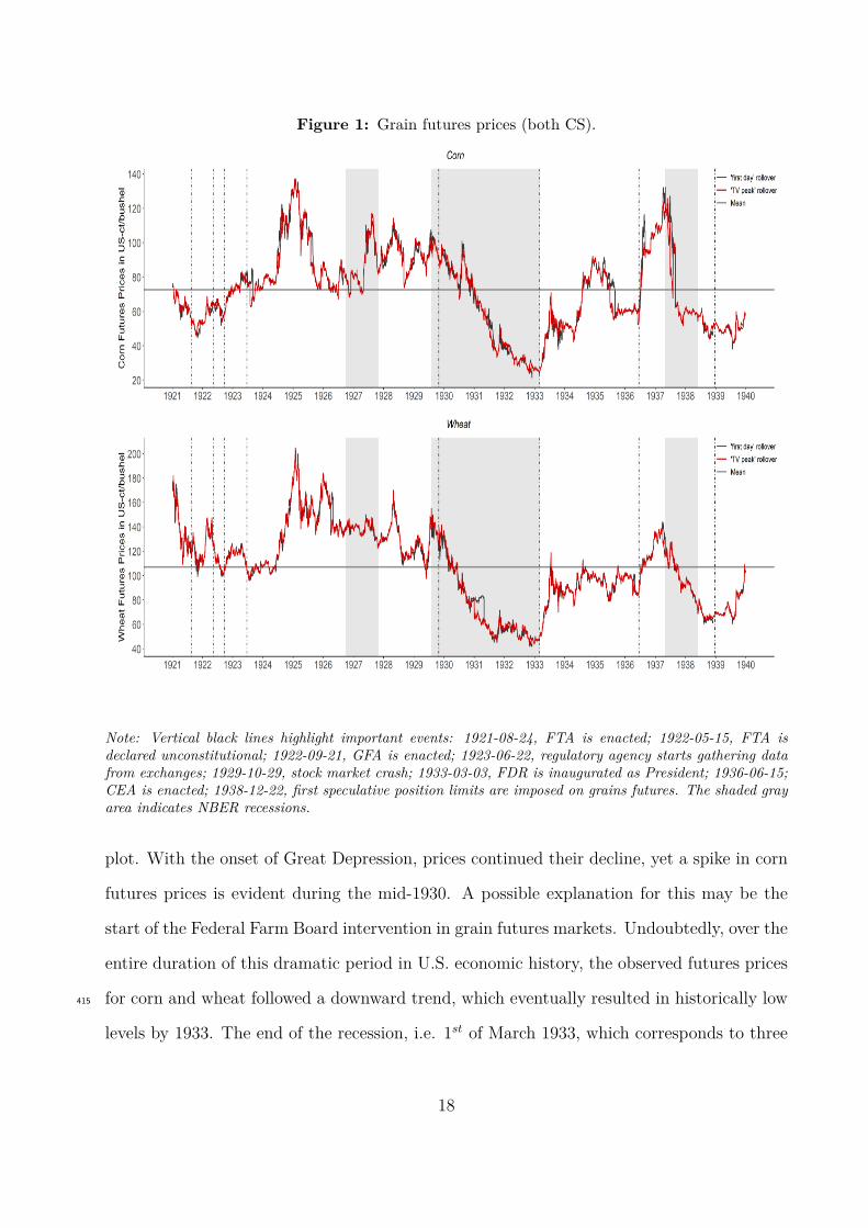
Figure 1: Grain futures prices (both CS).

Note: Vertical black lines highlight important events: 1921-08-24, FTA is enacted; 1922-05-15, FTA isdeclared unconstitutional; 1922-09-21, GFA is enacted; 1923-06-22, regulatory agency starts gathering datafrom exchanges; 1929-10-29, stock market crash; 1933-03-03, FDR is inaugurated as President; 1936-06-15;CEA is enacted; 1938-12-22, first speculative position limits are imposed on grains futures. The shaded grayarea indicates NBER recessions.

plot. With the onset of Great Depression, prices continued their decline, yet a spike in corn

futures prices is evident during the mid-1930. A possible explanation for this may be the

start of the Federal Farm Board intervention in grain futures markets. Undoubtedly, over the

entire duration of this dramatic period in U.S. economic history, the observed futures prices

for corn and wheat followed a downward trend, which eventually resulted in historically low415

levels by 1933. The end of the recession, i.e. 1st of March 1933, which corresponds to three

18

days before the inauguration of Franklin D. Roosevelt as President, marks the reversal of the

decreasing trend in grain futures prices. More specifically, prices started to increase rapidly

reaching levels close to their interwar averages, but then fell again by the end of 1933. While

wheat futures prices fluctuated moderately below their mean over the next two and a half420

years, prices for corn futures have spiked again between mid-1934 and mid-1935.

Subsequently, grain futures prices at the CBoT were nothing but stable. Traded prices for

wheat and corn futures began to increase precipitously immediately after the Commodity

Exchange Act was passed by Congress in June 1936 (see penultimate vertical dashed black

line on the plot), and the Chicago exchange has increased the limitation on price fluctu-425

ations.24 However, by the summer of 1937, grain futures prices dramatically plunged and

remained at depressed levels during the last recessionary phase of the interwar years, as

shown by the third shaded area on the plot.

Interestingly, there was no sizeable reaction of grain futures prices in response to the

adoption of the first Federal position limits imposed on speculative activities which occurred430

on December 22nd, 1938 (see last vertical line on the plot). Indeed, the traded prices at

the Chicago exchange remained at relatively low levels as before. Finally, toward the end

of 1939, a sharp rise in corn as well as wheat futures prices is visible, and, as the federal

reports suggest (see, U.S. CEAD, 1941, p.9), it can be attributed to Germany’s invasion of

Poland, an event that marked the beginning of the second World War.435

Finally, given the price data, we construct a further variable, namely futures returns,

defined as the logarithmic price differences, i.e. Rt = ln(Pt) − ln(Pt−1), where Pt and Pt−1

represent the prices at day t and t − 1, respectively. Note that, even though the continuous

price series rolls over and tracks prices of different principal futures, the returns are always

constructed using prices from futures contracts with same maturity only. This ensures an440

accurate empirical analysis of the underlying data.

24Note that, in addition to grain futures prices, these regulatory and institutional changes directly affectedthe volumes of trading at the CBoT. See Appendix A.1.

19

3.2 Grain Futures Traders

In addition to the data on volume of trading, open commitments and daily traded prices,

the CEAD (and GFAD) also furnished data of all daily sales and purchases of grain futures

at the Chicago exchange, as well as open contracts for all traders coming within the report-445

ing requirements, i.e. for all traders holding commitments equalling or exceeding 500,000

bushels (starting 1923), or 200,000 bushels (beginning with the end of 1933). The federal

regulatory agencies reported in various statistical bulletins the amount of daily long and

short commitments, by classes of traders. We collected data for corn futures covering nine

interwar years (divided into two interwar sub-periods), namely October 1924 – September450

1928, and January 1935 – December 1939, while for wheat futures, trading data have been

found only for a period of five interwar years, spanning from January 1935 to December

1939.25

The publicly available reports detail the aggregate short and long positions of corn and

wheat futures market participants by trader type, for each trading day as follows: reporting455

speculators and hedgers, and nonreporting traders.26 The long and short positions for the

latter class are obtained by subtracting the amount of daily long and short positions of

reporting traders from the total open interest. Accordingly, the class of nonreportable traders

is simply divided into long or short, but unfortunately, the classification into any of the two

trading categories, i.e. speculators or hedgers, is unknown (Hoffman, 1930; U.S. CEAD,460

1937a,b, 1940, 1941).

A detailed view of position size as a percentage of total open commitments for each

trader category is provided in Table 1. As indicated, the relative size of each trader’s class

varies through time. One explanation for this could stem from the changes in reporting

25For more details on the collection of these data, see section A.2 from Appendix.26For each sub-period, the reports provide daily information about a further class of traders, namely

clearing firms (1924-1928), and spreaders between round lots and job lots (1935-1939). However, since thesetrader types represent “small speculators”, as outlined by the Hoffman (1930) and U.S. CEAD (1937a,b,1940, 1941), long and short positions of each class are aggregated to the reporting long and short speculativepositions, respectively. See the Appendix for more details.

20

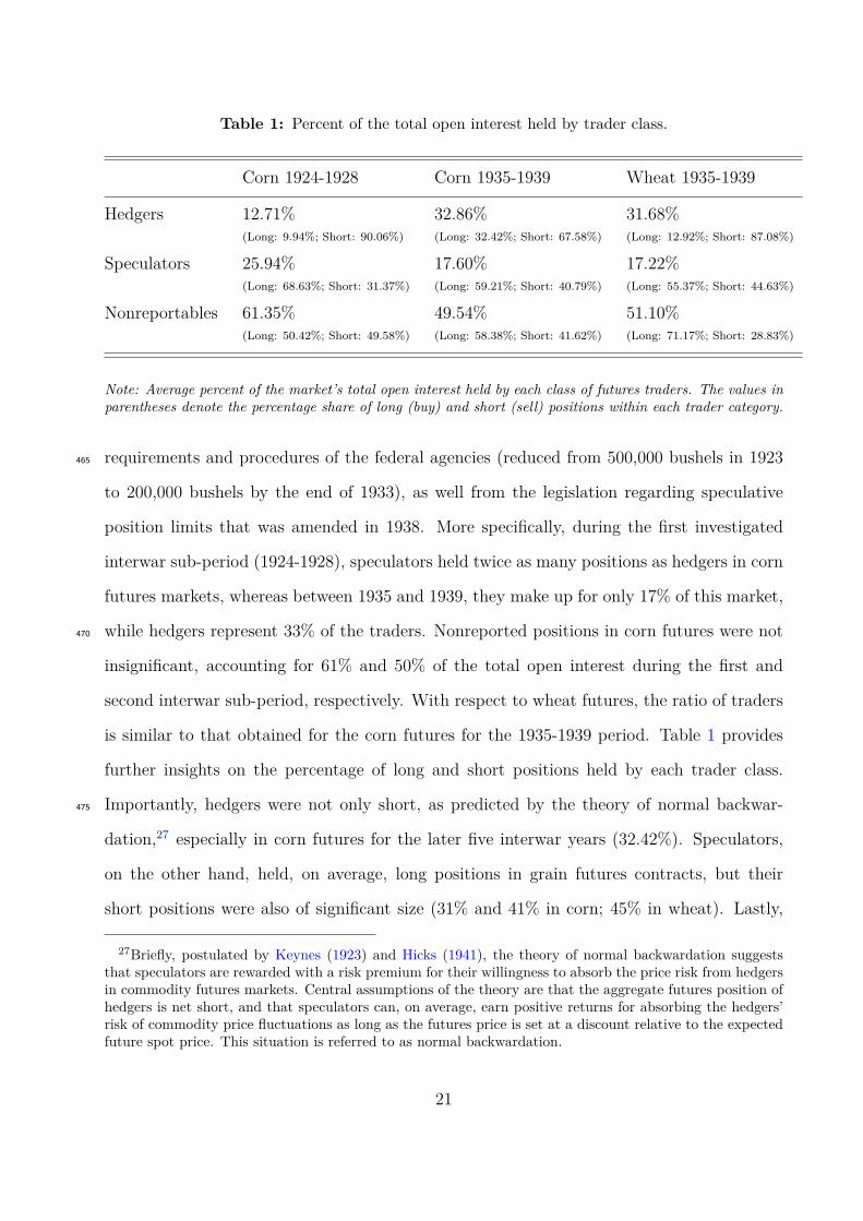
Table 1: Percent of the total open interest held by trader class.

Corn 1924-1928 Corn 1935-1939 Wheat 1935-1939

Hedgers 12.71% 32.86% 31.68%(Long: 9.94%; Short: 90.06%) (Long: 32.42%; Short: 67.58%) (Long: 12.92%; Short: 87.08%)

Speculators 25.94% 17.60% 17.22%(Long: 68.63%; Short: 31.37%) (Long: 59.21%; Short: 40.79%) (Long: 55.37%; Short: 44.63%)

Nonreportables 61.35% 49.54% 51.10%(Long: 50.42%; Short: 49.58%) (Long: 58.38%; Short: 41.62%) (Long: 71.17%; Short: 28.83%)

Note: Average percent of the market’s total open interest held by each class of futures traders. The values inparentheses denote the percentage share of long (buy) and short (sell) positions within each trader category.

requirements and procedures of the federal agencies (reduced from 500,000 bushels in 1923465

to 200,000 bushels by the end of 1933), as well from the legislation regarding speculative

position limits that was amended in 1938. More specifically, during the first investigated

interwar sub-period (1924-1928), speculators held twice as many positions as hedgers in corn

futures markets, whereas between 1935 and 1939, they make up for only 17% of this market,

while hedgers represent 33% of the traders. Nonreported positions in corn futures were not470

insignificant, accounting for 61% and 50% of the total open interest during the first and

second interwar sub-period, respectively. With respect to wheat futures, the ratio of traders

is similar to that obtained for the corn futures for the 1935-1939 period. Table 1 provides

further insights on the percentage of long and short positions held by each trader class.

Importantly, hedgers were not only short, as predicted by the theory of normal backwar-475

dation,27 especially in corn futures for the later five interwar years (32.42%). Speculators,

on the other hand, held, on average, long positions in grain futures contracts, but their

short positions were also of significant size (31% and 41% in corn; 45% in wheat). Lastly,

27Briefly, postulated by Keynes (1923) and Hicks (1941), the theory of normal backwardation suggeststhat speculators are rewarded with a risk premium for their willingness to absorb the price risk from hedgersin commodity futures markets. Central assumptions of the theory are that the aggregate futures position ofhedgers is net short, and that speculators can, on average, earn positive returns for absorbing the hedgers’risk of commodity price fluctuations as long as the futures price is set at a discount relative to the expectedfuture spot price. This situation is referred to as normal backwardation.

21

the nonreportable traders engaged in equally distributed buying and selling activities in the

wheat and corn futures markets.480

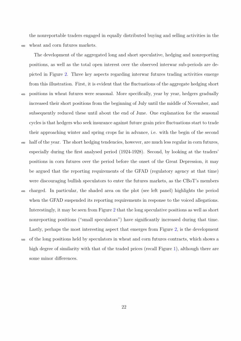
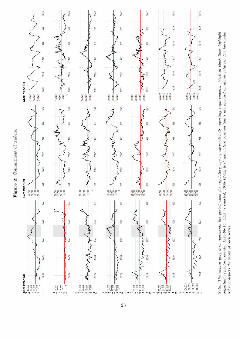
The development of the aggregated long and short speculative, hedging and nonreporting

positions, as well as the total open interest over the observed interwar sub-periods are de-

picted in Figure 2. Three key aspects regarding interwar futures trading activities emerge

from this illustration. First, it is evident that the fluctuations of the aggregate hedging short

positions in wheat futures were seasonal. More specifically, year by year, hedgers gradually485

increased their short positions from the beginning of July until the middle of November, and

subsequently reduced these until about the end of June. One explanation for the seasonal

cycles is that hedgers who seek insurance against future grain price fluctuations start to trade

their approaching winter and spring crops far in advance, i.e. with the begin of the second

half of the year. The short hedging tendencies, however, are much less regular in corn futures,490

especially during the first analysed period (1924-1928). Second, by looking at the traders’

positions in corn futures over the period before the onset of the Great Depression, it may

be argued that the reporting requirements of the GFAD (regulatory agency at that time)

were discouraging bullish speculators to enter the futures markets, as the CBoT’s members

charged. In particular, the shaded area on the plot (see left panel) highlights the period495

when the GFAD suspended its reporting requirements in response to the voiced allegations.

Interestingly, it may be seen from Figure 2 that the long speculative positions as well as short

nonreporting positions (“small speculators”) have significantly increased during that time.

Lastly, perhaps the most interesting aspect that emerges from Figure 2, is the development

of the long positions held by speculators in wheat and corn futures contracts, which shows a500

high degree of similarity with that of the traded prices (recall Figure 1), although there are

some minor differences.

22

Fig

ure

2:C

omm

itmen

tof

trad

ers.

Not

e:T

hesh

aded

gray

area

repr

esen

tsth

epe

riod

when

the

regu

lato

ryag

ency

susp

ende

dits

repo

rtin

gre

quire

men

ts.

Vert

ical

blac

klin

eshi

ghlig

htim

port

ant

regu

lato

ryev

ents

:19

36-0

6-15

;C

EAis

enac

ted;

1938

-12-

22,

first

spec

ulat

ive

posi

tion

limits

are

impo

sed

ongr

ains

futu

res.

The

hori

zont

alre

dlin

ede

pict

sth

em

ean

ofea

chse

ries

.

23

4 Do Speculators Drive Volatility in Futures Prices?

Based on the hand-collected data, we aim to further offer a comprehensive answer to an

open question in futures trading history: Are speculative activities the main drivers of grain505

futures price volatility in the early period? To answer this, we utilize a more recent empirical

method, and model the newly constructed futures returns data and their conditional volatil-

ity according to a GARCH(1,1) specification. We first discuss the determinants of interwar

speculative trading decisions in grain futures markets prior to reporting volatility estimation

results.510

4.1 Drivers of Interwar Speculative Behaviour

Traditionally, there are two views of speculators’ behaviour in futures markets. According

to Keynes (1923), speculators “irrationally” anticipate market prices and engage in futures

trading activities - they buy when prices are high and sell when prices are low - which

destabilizes commodity markets and prices and contributes to increasing price volatility.515

In contrast, Friedman (1953) argues that speculators are “rational” traders who stabilize

futures markets - they buy when prices are low and sell when prices are high thus limiting

price volatility. Stated somewhat differently, traders who purchase futures (i.e., take the

“long” side of the contract) following price increases or sell futures (i.e., are on the “short”

side of the contract) following price declines may be momentum traders, trend followers or520

feedback traders. In contrast, traders who buy (sell) following price decreases (increases)

may be contrarians.

To account for changes in speculators’ positions, we follow Kang et al. (2020) and compute

the net trading speculative variable for each futures market under scrutiny as follows:

QSi,t =Netlong positions speculatorsi,t − Netlong position speculatorsi,t−1

OIi,t−1(1)

More specifically, i = corn (1924-1928); corn (1935-1939); wheat (1935-1938), OIi,t−1525

denotes the total open interest on day t-1, and the numerator from the equation above

24

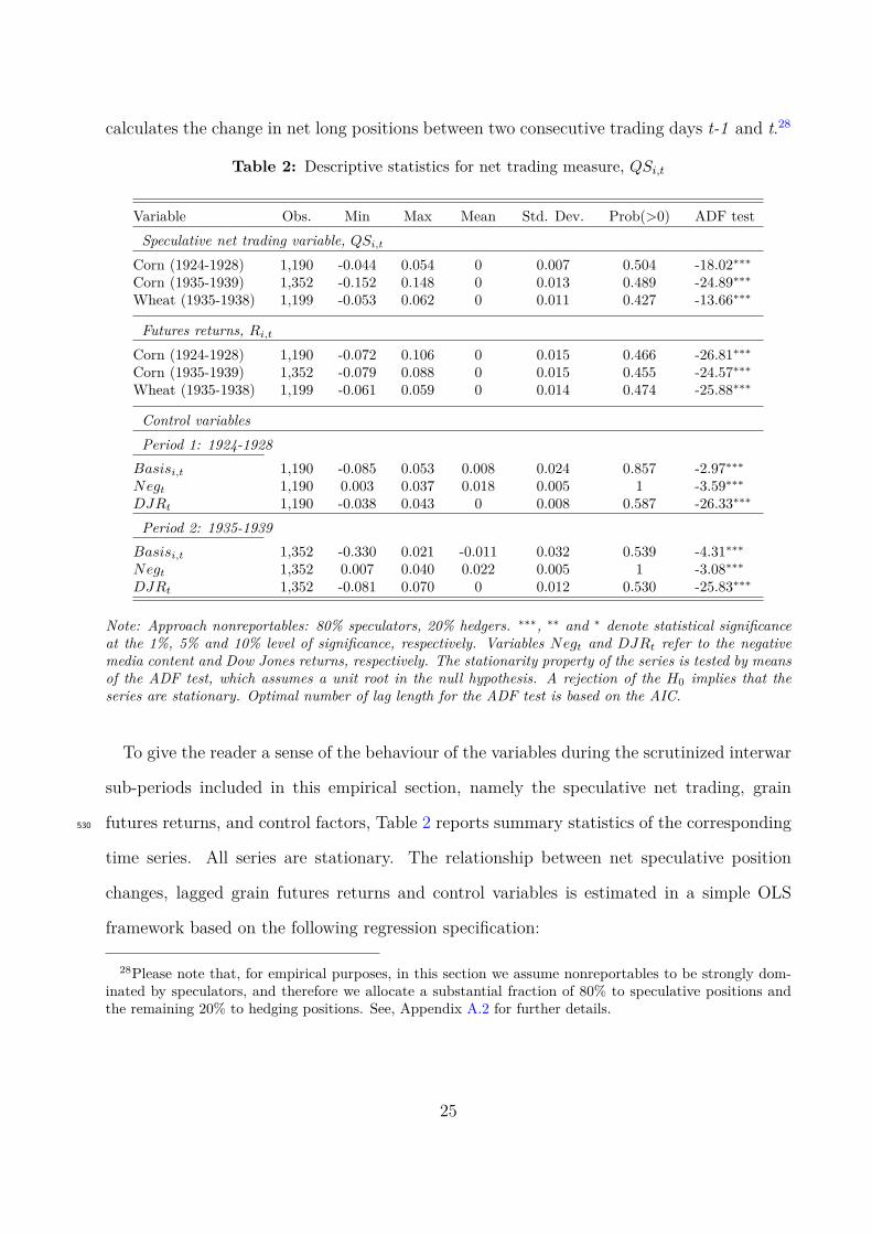
calculates the change in net long positions between two consecutive trading days t-1 and t.28

Table 2: Descriptive statistics for net trading measure, QSi,t

Variable Obs. Min Max Mean Std. Dev. Prob(>0) ADF testSpeculative net trading variable, QSi,t

Corn (1924-1928) 1,190 -0.044 0.054 0 0.007 0.504 -18.02∗∗∗

Corn (1935-1939) 1,352 -0.152 0.148 0 0.013 0.489 -24.89∗∗∗

Wheat (1935-1938) 1,199 -0.053 0.062 0 0.011 0.427 -13.66∗∗∗

Futures returns, Ri,t

Corn (1924-1928) 1,190 -0.072 0.106 0 0.015 0.466 -26.81∗∗∗

Corn (1935-1939) 1,352 -0.079 0.088 0 0.015 0.455 -24.57∗∗∗

Wheat (1935-1938) 1,199 -0.061 0.059 0 0.014 0.474 -25.88∗∗∗

Control variablesPeriod 1: 1924-1928

Basisi,t 1,190 -0.085 0.053 0.008 0.024 0.857 -2.97∗∗∗

Negt 1,190 0.003 0.037 0.018 0.005 1 -3.59∗∗∗

DJRt 1,190 -0.038 0.043 0 0.008 0.587 -26.33∗∗∗

Period 2: 1935-1939Basisi,t 1,352 -0.330 0.021 -0.011 0.032 0.539 -4.31∗∗∗

Negt 1,352 0.007 0.040 0.022 0.005 1 -3.08∗∗∗

DJRt 1,352 -0.081 0.070 0 0.012 0.530 -25.83∗∗∗

Note: Approach nonreportables: 80% speculators, 20% hedgers. ∗∗∗, ∗∗ and ∗ denote statistical significanceat the 1%, 5% and 10% level of significance, respectively. Variables Negt and DJRt refer to the negativemedia content and Dow Jones returns, respectively. The stationarity property of the series is tested by meansof the ADF test, which assumes a unit root in the null hypothesis. A rejection of the H0 implies that theseries are stationary. Optimal number of lag length for the ADF test is based on the AIC.

To give the reader a sense of the behaviour of the variables during the scrutinized interwar

sub-periods included in this empirical section, namely the speculative net trading, grain

futures returns, and control factors, Table 2 reports summary statistics of the corresponding530

time series. All series are stationary. The relationship between net speculative position

changes, lagged grain futures returns and control variables is estimated in a simple OLS

framework based on the following regression specification:

28Please note that, for empirical purposes, in this section we assume nonreportables to be strongly dom-inated by speculators, and therefore we allocate a substantial fraction of 80% to speculative positions andthe remaining 20% to hedging positions. See, Appendix A.2 for further details.

25

QSi,t = β0 + β1Ri,t−1 + β2Basisi,t−1 + β3Negt + β4DJRt−1︸ ︷︷ ︸Controls

+β5QSi,t−1 + υi,t (2)

where QSi,t represents the change of net long speculative positions between trading days t535

and t−1, and Ri,t−1 is the previous day futures return in futures market i. The set of control

variables consists of three external factors: First, we include the log basis to account for the

commodity futures risk premium.29 Second, we control how market sentiment, especially the

daily negative media content Negt, influences interwar speculative trading decisions.30 Note

that this variable represents the media content from the news market participants read on540

day t, but it is assumed to be conditional on market information from previous day t − 1.

Lastly, to control for the idiosyncratic priced risk in commodity futures, we include the Dow

Jones returns, which capture the effects of the overall economic growth.31 Finally, the υi,t

term denotes the error term.

The slope coefficients and their robust standard errors from estimating Equation (2) are545

shown in Table 3. With respect to the control variables, the parameter estimates of the

log basis are positive and highly significant, indicating that, if speculators are rewarded

with positive profits in form of a risk premium, they are more willing to buy grain futures

contracts.32 Moreover, stock market returns do not seem to have an impact on speculative

position changes in any of the scrutinized markets and periods. It is worth noting that550

the negative media content significantly impacts speculators decisions to reduce their long

29Numerous examples can be found in the empirical literature that link the basis to the commodity futuresrisk premium - as a compensation for speculators who take the price risk from hedgers (see, among others,Fama and French, 1987; Gorton and Rouwenhorst, 2006; Erb and Harvey, 2006). We follow Kang et al.(2020) and compute the log basis variable as follows: Basisi,t = ln(F (t,T2))−ln(F (t,T1))

T2−T1.

30To this end, we use the dataset provided by Garcia (2013) and calculate the percentage of daily negativewords as: Negi,t = No. of negative wordst/No. of total wordst.

31Data on this variable are retrieved from the Global Financial Database. Returns are computed aslogarithmic price differences of two consecutive days, i.e. DJRt = ln(DJt) – ln(DJt−1).

32This could be interpreted as a somewhat weak evidence in favour of Keynes’ theory of normal backwar-dation.

26

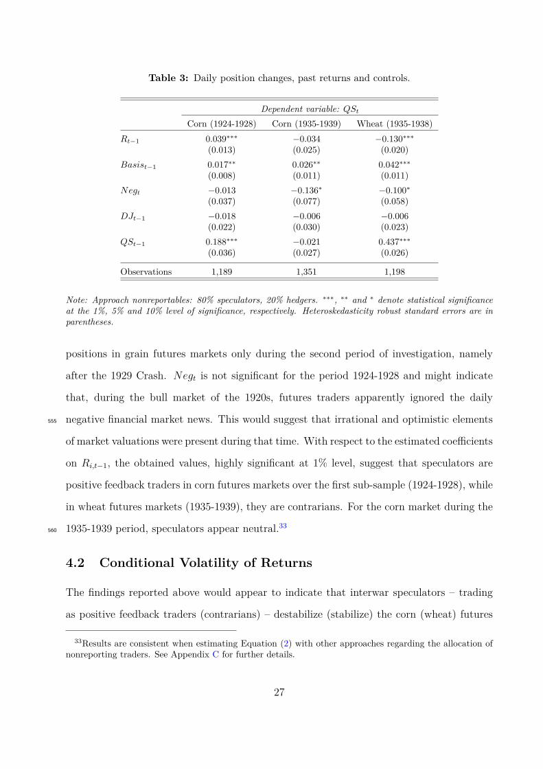
Table 3: Daily position changes, past returns and controls.

Dependent variable: QSt

Corn (1924-1928) Corn (1935-1939) Wheat (1935-1938)Rt−1 0.039∗∗∗ −0.034 −0.130∗∗∗

(0.013) (0.025) (0.020)Basist−1 0.017∗∗ 0.026∗∗ 0.042∗∗∗

(0.008) (0.011) (0.011)Negt −0.013 −0.136∗ −0.100∗

(0.037) (0.077) (0.058)DJt−1 −0.018 −0.006 −0.006

(0.022) (0.030) (0.023)QSt−1 0.188∗∗∗ −0.021 0.437∗∗∗

(0.036) (0.027) (0.026)

Observations 1,189 1,351 1,198

Note: Approach nonreportables: 80% speculators, 20% hedgers. ∗∗∗, ∗∗ and ∗ denote statistical significanceat the 1%, 5% and 10% level of significance, respectively. Heteroskedasticity robust standard errors are inparentheses.

positions in grain futures markets only during the second period of investigation, namely

after the 1929 Crash. Negt is not significant for the period 1924-1928 and might indicate

that, during the bull market of the 1920s, futures traders apparently ignored the daily

negative financial market news. This would suggest that irrational and optimistic elements555

of market valuations were present during that time. With respect to the estimated coefficients

on Ri,t−1, the obtained values, highly significant at 1% level, suggest that speculators are

positive feedback traders in corn futures markets over the first sub-sample (1924-1928), while

in wheat futures markets (1935-1939), they are contrarians. For the corn market during the

1935-1939 period, speculators appear neutral.33560

4.2 Conditional Volatility of Returns

The findings reported above would appear to indicate that interwar speculators – trading

as positive feedback traders (contrarians) – destabilize (stabilize) the corn (wheat) futures

33Results are consistent when estimating Equation (2) with other approaches regarding the allocation ofnonreporting traders. See Appendix C for further details.

27

market, by increasing (decreasing) the volatility of prices. To test this hypothesis more

formally, and in common with the relevant literature, we estimate a univariate GARCH(1,1)565

model to examine to which extent does this speculative behaviour affect the volatility of

interwar grain futures returns. The conditional mean equation is defined as:

Ri,t = β0 + β1Ri,t−1 +4∑

n=2βnControlsn,t−1 + β5QSi,t−1 + εi,t (3)

Here, the wheat and corn futures returns Ri,t are explained by an AR(1) term, i.e. past

period return, the set of control variables from Equation (2), and the lagged speculative

factor, QSi,t−1. Note that, we include lagged regressors in the specification to avoid the en-570

dogeneity problem due to simultaneity. Lastly, the serially uncorrelated errors (innovations)

εi,t are assumed to be normally distributed with mean zero and conditional variance σ2i,t, i.e.

εi,t ∼ N(0, σ2i,t). The volatility of corn returns is measured by the conditional variance of εi,t,

which reads the following formula:

σ2i,t = γ0 + γ1ε

2i,t−1 + γ2σ

2i,t−1 + γ3QSi,t−1 (4)

where ε2i,t−1 is the previous value of the squared regression disturbances, and σ2

i,t−1 represents575

the one period lagged forecast error variance. Parameter γ1 describes the ARCH effect, that

is, how strongly the conditional variance responds to new information arriving in the futures

market, whereas γ2 denotes the GARCH effect, measuring the volatility shock persistence.

Moreover, it is assumed that γ0, γ1, and γ2 are positive, and that the sum of GARCH and

ARCH effects is smaller than one (γ1 + γ2 < 1), thereby ensuring covariance stationarity580

and non-negative conditional variance. Next, the speculative variable – net trading QSi,t−1

- is additionally considered as exogenous regressor in the variance equation of the GARCH

model. Finally, the interpretation of the coefficient of interest, γ3, is straightforward. A

stabilizing impact of speculative activity on grain price volatility is indicated by a negative

significant estimate of γ3. Instead, if a positive parameter estimate is obtained for γ3,585

speculation has a destabilizing influence on grains prices, by increasing returns and their

28

volatility, such that changes in prices become more severe.

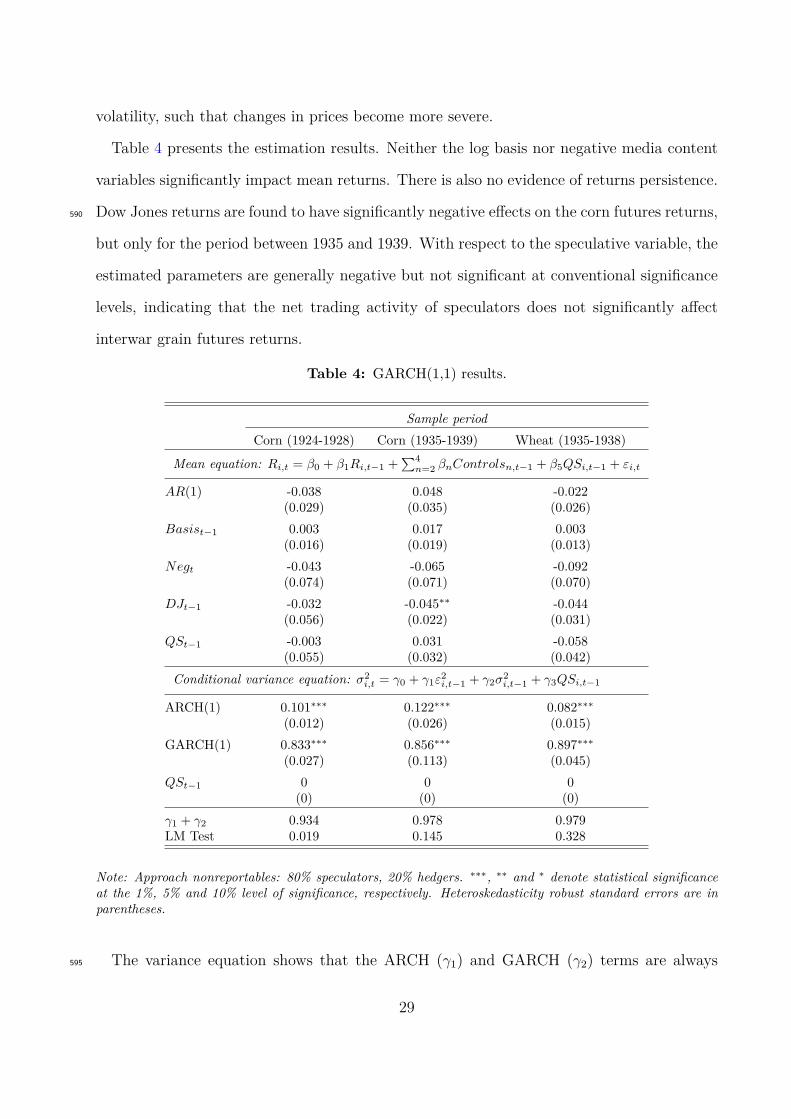
Table 4 presents the estimation results. Neither the log basis nor negative media content

variables significantly impact mean returns. There is also no evidence of returns persistence.

Dow Jones returns are found to have significantly negative effects on the corn futures returns,590

but only for the period between 1935 and 1939. With respect to the speculative variable, the

estimated parameters are generally negative but not significant at conventional significance

levels, indicating that the net trading activity of speculators does not significantly affect

interwar grain futures returns.

Table 4: GARCH(1,1) results.

Sample periodCorn (1924-1928) Corn (1935-1939) Wheat (1935-1938)

Mean equation: Ri,t = β0 + β1Ri,t−1 +∑4

n=2 βnControlsn,t−1 + β5QSi,t−1 + εi,t

AR(1) -0.038 0.048 -0.022(0.029) (0.035) (0.026)

Basist−1 0.003 0.017 0.003(0.016) (0.019) (0.013)

Negt -0.043 -0.065 -0.092(0.074) (0.071) (0.070)

DJt−1 -0.032 -0.045∗∗ -0.044(0.056) (0.022) (0.031)

QSt−1 -0.003 0.031 -0.058(0.055) (0.032) (0.042)

Conditional variance equation: σ2i,t = γ0 + γ1ε2

i,t−1 + γ2σ2i,t−1 + γ3QSi,t−1

ARCH(1) 0.101∗∗∗ 0.122∗∗∗ 0.082∗∗∗

(0.012) (0.026) (0.015)GARCH(1) 0.833∗∗∗ 0.856∗∗∗ 0.897∗∗∗

(0.027) (0.113) (0.045)QSt−1 0 0 0

(0) (0) (0)γ1 + γ2 0.934 0.978 0.979LM Test 0.019 0.145 0.328

Note: Approach nonreportables: 80% speculators, 20% hedgers. ∗∗∗, ∗∗ and ∗ denote statistical significanceat the 1%, 5% and 10% level of significance, respectively. Heteroskedasticity robust standard errors are inparentheses.

The variance equation shows that the ARCH (γ1) and GARCH (γ2) terms are always595

29

positive and highly statistically significant. While estimates for the former are close to

zero, the GARCH estimates are rather high and close to unity, indicating strong volatility

clusters in corn futures daily returns. Looking at the last row of Table 4, the very small

ARCH-LM test statistics provide an indication that there is no conditional heteroskedasticity

in the error terms, hence the AR(1)-GARCH(1,1) model specification is indeed a good fit600

for the investigated data. Moreover, the covariance stationarity and non-negative variance

constraints are met in all three specifications (γ0, γ1, γ2 ⩾ 0, and γ1+γ2 < 1). Importantly,

the estimates obtained for the speculative factor in the variance equation are all equal to

zero, suggesting that speculative position changes do not contribute to greater uncertainty

with respect to short-term futures return dynamics in the form of volatility clusters. The605

results imply therefore that speculators are not are not the main drivers of daily volatility

of the interwar grain futures markets, and hence, the “grain gamblers” did not destabilize

these markets.34

5 Conclusion

The interwar period was undeniably an era of great economic and political change in the610

United States. With respect to futures markets, the regulatory and institutional changes that

occurred during the years between the two World Wars offer important lessons for the modern

governance, regulation and institutions for futures trading. In particular, the interwar period

serves as a unique example of a shifting regulatory regime from one of self-regulation to

federal regulation of the futures exchanges. Indeed, a comprehensive understanding of the615

early development and regimes of futures trading is of great relevance, as it continues to

shape futures trading to the present.

This paper fills a gap in the literature by introducing a new hand collected dataset com-

prised of daily trading observations on grain futures contracts traded at the Chicago Board

34Similar results have been obtained for other treatments of nonreportable traders considered. See Ap-pendix C for further estimation results.

30

of Trade covering a 19 interwar years period. The daily sampling frequency represents an620

important contribution to the study of commodity futures markets. We focus on the fu-

tures trading of two of the most traded agricultural commodities during the interwar period,

namely wheat and corn, and provide key insights about how these early grain futures mar-

kets functioned at that time. Based on the collected data on commitments of traders, we

can also describe the traditional composition of futures traders and its evolution during the625

interwar era. We construct futures continuation series for prices and returns, and a net trad-

ing speculative variable, which facilitate several empirical investigations. More specifically,

we first analyse what drives speculators’ trading decisions to buy or sell futures contracts.

The main finding is that speculators are momentum traders and contrarians in corn and

wheat futures markets, respectively, and they significantly reduce their net long positions in630

response to the negative media content, especially after the onset of Great Depression. We

then go on to investigate the impact of speculative activities on the conditional volatility of

interwar futures prices and report that the net long position changes of speculators have a

zero effect on price movements.

Even though the newly collected data are limited to only a specific historical episode of635

futures trading, a thorough analysis of this early period with modern empirical and statistical

techniques provides some interesting implications for today’s institutions and governance

regimes. Further work could, for example, focus on the efficiency of the imposed regulation

and its consequent impact on the futures prices and trading decisions of market participants.

Such analysis could point to interesting parallels with the more recent financial history.640

The dataset could also serve to explore empirically market microstructure related questions

including price discovery and the behaviour of quotes and spreads. There may even be scope

to utilize data to explore the implications of futures prices on broader prices.

31

References

Baer, J. B. and Saxon, O. G. (1949). Commodity Exchanges and Futures Trading: Principles645

and Operating Methods. New York, Harper and Brothers.

Bhardwaj, G., Janardanan, R., and Rouwenhorst, K. G. (2019). The Commodity Futures

Risk Premium: 1871–2018. Available at SSRN 3452255.

Bollerslev, T. (1986). Generalized Autoregressive Conditional Heteroskedasticity. Journal

of Econometrics, 31(3):307–327.650

Brunetti, C., Büyükşahin, B., and Harris, J. H. (2016). Speculators, Prices, and Market

Volatility. Journal of Financial and Quantitative Analysis, pages 1545–1574.

Burns, J. M. (1956). Roosevelt: The Lion and the Fox (1882–1940). New York, Open Road

Media.

Campbell, D. A. (1957). Trading in Futures Under the Commodity Exchange Act. George655

Washington Law Review, 26:215–254.

CFTC (2021a). Commodity Futures Trading Commision - Glossary of the CFTC.

Technical report. Available online at https://www.cftc.gov/LearnAndProtect/

EducationCenter/CFTCGlossary/glossary_s.html. Last accessed in September 2021.

CFTC (2021b). Commodity Futures Trading Commision - History of the CFTC. Technical660

report. Available online at https://www.cftc.gov/About/HistoryoftheCFTC/history_

precftc.html. Last accessed in September 2021.

Cowing, C. B. (1965). Populists, Plungers, and Progressives: A Social History of Stock and

Commodity Speculation, 1868-1932. Princeton, New Jersey, Princeton University Press.

Duvel, J. W. T. and Hoffman, G. W. (1927). Speculative Transactions in the 1926 May665

Wheat Future. Washington, DC: U.S. Department of Agriculture, No. 1479.

32

Duvel, J. W. T. and Hoffman, G. W. (1928). Major Transactions in the 1926 December

Wheat Future. Washington, DC: U.S. Department of Agriculture, No. 79.

Erb, C. B. and Harvey, C. R. (2006). The Strategic and Tactical Value of Commodity

Futures. Financial Analysts Journal, 62(2):69–97.670

Fama, E. F. and French, K. R. (1987). Commodity Futures Prices: Some Evidence on

Forecast Power, Premiums, and the Theory of Storage. Journal of Business, 60:55–73.

Friedman, M. (1953). Essays in Positive Economics. Chicago: University of Chicago Press.

Garcia, D. (2013). Sentiment During Recessions. The Journal of Finance, 68(3):1267–1300.

Gorton, G. and Rouwenhorst, K. G. (2006). Facts and Fantasies about Commodity Futures.675

Financial Analysts Journal, 62(2):47–68.

Grant, J. (2014). The Forgotten Depression: 1921: The Crash that Cured Itself. New York,

Simon and Schuster.

Guither, H. D. (1974). Commodities Exchanges, Agrarian “Political Power,” and the An-

tioption Battle: Comment. Agricultural History, 48(1):126–129.680

Hicks, J. R. (1941). Value and Capital: An Inquiry into Some Fundamental Principles of

Economic Theory. Oxford, UK: Clarendon Press.

Hieronymus, T. A. (1977). Economics of Futures Trading for Commercial and Personal

Profit. New York: Commodity Research Bureau.

Hoffman, G. W. (1930). Trading in Corn Futures. (Technical Bulletin No. 199). Washington,685

D.C.: U.S. Department of Agriculture.

Hoffman, G. W. (1932). Future Trading Upon Organized Commodity Markets in the United

States. University of Pennsylvania Press.

33

Irwin, H. S. (1932). A Guide to Grain-Trade Statistics. Washington, D.C.: U.S. Department

of Agriculture, No. 141.690

Irwin, S. H. and Sanders, D. R. (2012). Testing the Masters Hypothesis in Commodity

Futures Markets. Energy Economics, 34(1):256–269.

Jacks, D. S. (2007). Populists versus Theorists: Futures Markets and the Volatility of Prices.

Explorations in Economic History, 44(2):342–362.

Kang, W., Rouwenhorst, K. G., and Tang, K. (2020). A Tale of Two Premiums: The Role695

of Hedgers and Speculators in Commodity Futures Markets. The Journal of Finance,

75(1):377–417.

Keaveny, J. (2004). In Defense of Market Self-Regulation - An Analysis of the History

of Futures Regulation and the Trend Toward Demutualization. Brooklyn Law Review,

70:1419–1452.700

Keynes, J. M. (1923). Some Aspects of Commodity Markets. Manchaster Guardian Com-

mercial, 13:784–786.

Kim, A. (2015). Does Futures Speculation Destabilize Commodity Markets? Journal of

Futures Markets, 35(8):696–714.

Leuchtenburg, W. E. (1963). Franklin D. Roosevelt and the New Deal, 1932-1940. New York,705

Harper & Row.

Levine, A., Ooi, Y. H., Richardson, M., and Sasseville, C. (2018). Commodities for the Long

Run. Financial Analysts Journal, 74(2):55–68.

Manera, M., Nicolini, M., and Vignati, I. (2016). Modelling Futures Price Volatility in Energy

Markets: Is There a Role for Financial Speculation? Energy Economics, 53:220–229.710

Markham, J. W. (1987). The History of Commodity Futures Trading and Its Regulation.

New York, Praeger Publishers.

34

Markham, J. W. (2002). A Financial History of the United States: From JP Morgan to the

Institutional Investor (1900-1970), volume 2. New York, M.E. Sharpe.

Morgan, D. (1979). Merchants of Grain: The Power and Profits of the Five Giant Companies715

at the Center of the world’s food supply. New York, The Viking Press.

Peck, A. E. (1985). The Economic Role of Traditional Commodity Futures Markets. Futures

markets: Their Economic Role, pages 1–81.

Petzel, T. E. (1981). A New Look at Some Old Evidence: The Wheat Market Scandal of

1925. Food Research Institute Studies, 18:117–128.720

Saleuddin, R. (2018). The Government of Markets: How Interwar Collaborations Between

the CBOT and the State Created Modern Futures Trading. Switzerland, Springer Nature

Switzerland AG.

Sanders, D. R., Irwin, S. H., and Merrin, R. P. (2010). The Adequacy of Speculation in

Agricultural Futures Markets: Too Much of a Good Thing? Applied Economic Perspectives725

and Policy, 32(1):77–94.

Santos, J. (2002). Did Futures Markets Stabilise US Grain Prices? Journal of Agricultural

Economics, 53(1):25–36.

Santos, J. M. (2013). Trading Grain Now and Then: The Relative Performance of Early

Grain Futures Markets. Applied Economics, 45(3):287–298.730

Schaede, U. (1989). Forwards and Futures in Tokugawa-Period Japan: A New Perspective

on The Dojima Rice Market. Journal of Banking & Finance, 13(4-5):487–513.

Schlesinger, A. M. (1957). The Age of Roosevelt. Boston, Houghton Mifflin.

Soule, G. (1947). Prosperity Decade. London, Pilot Press.

35

Stassen, J. H. (1982). Propaganda as Positive Law: Section 3 of the Commodity Exchange735

Act (A Case Study of How Economic Facts Can Be Changed by Act of Congress). Chicago-

Kent Law Review, 58:635–656.

Stewart, B. (1949). An Analysis of Speculative Trading in Grain Futures. (Technical Bulletin

No. 1001). Washington, D.C.: U.S. Department of Agriculture.

Taylor, C. H. (1917). History of the Board of Trade of the City of Chicago. Chicago, Robert740

O. Law.

U.S. CEAD (1937a). Corn Futures: Volume of Trading, Open Commitments, and Prices

from January 3, 1933, to December 31, 1935. (Statistical Bulletin No. 55). Washington,

D.C.: U.S. Department of Agriculture.

U.S. CEAD (1937b). Wheat Futures: Volume of Trading, Open Commitments, and Prices745

from January 3, 1933, to December 31, 1935. (Statistical Bulletin No. 54). Washington,

D.C.: U.S. Department of Agriculture.

U.S. CEAD (1940). Wheat Futures: Volume of Trading, Open Commitments, and Prices

from January 2, 1936, to December 31, 1938. (Statistical Bulletin No. 72). Washington,

D.C.: U.S. Department of Agriculture.750

U.S. CEAD (1941). Corn Futures: Volume of Trading, Open Commitments, and Prices from

January 2, 1936, to December 30, 1939. (Statistical Bulletin No. 74). Washington, D.C.:

U.S. Department of Agriculture.

U.S. CEAD (1942). Wheat Futures Statistics: January 1939 - June 1941. Washington, D.C.:

U.S. Department of Agriculture.755

U.S. Congress, House (1934). Amend Grain Futures Act, 73d Congress, 2d Session, H. R.

Rept. 1637.

36

U.S. Congress, House (1935). Commodity Exchange Act, 74th Congress, 1st Session, H. R.

Rept. 421.

U.S. Congress, Senate (1921). Congressional Record, 67th Congress, 1st Session, Aug. 9,760

1921.

U.S. Department of Agriculture (1938). Report of the Chief of the Commodity Exchange

Administration. Washington, D.C., Government Printing Office.

U.S. GFAD (1930). Wheat Futures: Volume of Trading, Open Commitments, and Prices

from January 3, 1921, to December 31, 1929. (Statistical Bulletin No. 31). Washington,765

D.C.: U.S. Department of Agriculture.

U.S. GFAD (1931). Corn Futures: Volume of Trading, Open Commitments, and Prices from

January 3, 1921, to December 31, 1929. (Statistical Bulletin No. 34). Washington, D.C.:

U.S. Department of Agriculture.

U.S. GFAD (1933a). Corn Futures: Volume of Trading, Open Commitments, and Prices770

from January 2, 1930, to December 31, 1932. (Statistical Bulletin No. 43). Washington,

D.C.: U.S. Department of Agriculture.

U.S. GFAD (1933b). Wheat Futures: Volume of Trading, Open Commitments, and Prices

from January 2, 1930, to December 31, 1932. (Statistical Bulletin No. 41). Washington,

D.C.: U.S. Department of Agriculture.775

U.S. Secretary of Agriculture (1926). Fluctuations in Wheat Futures. Letter from the Sec-

retary of Agriculture Transmitting, in Response to Senate Resolution no. 222, of June 9,

1926, a Report of the Grain Futures Administration Relative to the Extreme Fluctuation

in the Price of Wheat Futures Furing the Early Part of 1925. Washington, DC: U.S.

Government Printing Office.780

van Tielhof, M. (2002). The ’Mother of All Trades’: the Baltic Grain Trade in Amsterdam

from the Late 16th to the Early 19th Century, volume 3. Leiden, Netherlands, Brill.

37

Wakita, S. (2001). Efficiency of the Dojima Rice Futures Market in Tokugawa-Period Japan.

Journal of Banking & Finance, 25(3):535–554.

Zhang, Q. (2021). One Hundred Years of Rare Disaster Concerns and Commodity Prices.785

Journal of Futures Markets.

38

A Appendix Dataset

The data on grain futures trading comes from several sources. We hand-collected data from

different reports published by the Commodity Exchange Administration (formerly Grain

Futures Administration), all available online as scanned documents. The online collections790

can be found at: https://www.hathitrust.org/ and https://archive.org/. Below you

can find an overview of the reports used:

1. Corn futures trading (1921-1939):

• Statistical Bulletin No. 34 (1921-1929) (U.S. GFAD, 1931)

• Statistical Bulletin No. 43 (1930-1932) (U.S. GFAD, 1933a)795

• Statistical Bulletin No. 55 (1933-1935) (U.S. CEAD, 1937a)

• Statistical Bulletin No. 74 (1936-1939) (U.S. CEAD, 1941)

• Technical Bulletin No. 199 (commitment of traders, 1924-1928) (Hoffman, 1930)

2. Wheat futures trading (1921-1939):

• Statistical Bulletin No. 31 (1921-1929) (U.S. GFAD, 1930)800

• Statistical Bulletin No. 41 (1930-1932) (U.S. GFAD, 1933b)

• Statistical Bulletin No. 54 (1933-1935) (U.S. CEAD, 1937b)

• Statistical Bulletin No. 72 (1936-1938) (U.S. CEAD, 1940)

• Wheat Futures Statistics (commitment of traders, 1939) (U.S. CEAD, 1942)

1

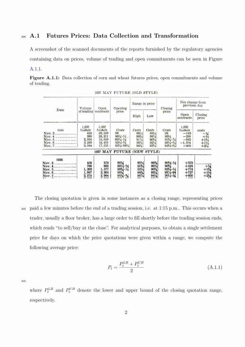
A.1 Futures Prices: Data Collection and Transformation805

A screenshot of the scanned documents of the reports furnished by the regulatory agencies

containing data on prices, volume of trading and open commitments can be seen in Figure

A.1.1.

Figure A.1.1: Data collection of corn and wheat futures prices, open commitments and volumeof trading.

The closing quotation is given in some instances as a closing range, representing prices

paid a few minutes before the end of a trading session, i.e. at 1:15 p.m.. This occurs when a810

trader, usually a floor broker, has a large order to fill shortly before the trading session ends,

which reads “to sell/buy at the close”. For analytical purposes, to obtain a single settlement

price for days on which the price quotations were given within a range, we compute the

following average price:

Pt = P LBt + P UB

t

2 (A.1.1)

815

where P LBt and P UB

t denote the lower and upper bound of the closing quotation range,

respectively.

2

Note that, over the entirety of the interwar period, there was trading in both “old style”

and “new style” for corn and wheat futures with delivery in March, May, July, September and

December for some limited number of active trading months. The need for these designations820

was occasioned by the change in grain grades deliverable on futures contracts, as suggested

by the GFAD and CEAD in the published reports. To account for the period in which

both “new style” and “old style” trading of futures contracts with the same maturity dates

occurred, we calculate the settlement price (as a weighted average) by means of the following

formula:825

Pt = TVO,t

TVT,t

· PO,t + TVN,t

TVT,t

· PN,t (A.1.2)

where TVO,t, TVN,t, and TVT,t represent the number of “old style”, “new style”, and total

trading volume on any trading day t, respectively, the latter being the sum of the first two.

Regarding the construction of the continuous series: we use data on the individual futures

contracts to create two types of futures continuation series. The first type is based on the830

“first day” rolling mechanism, i.e. we take trading data of a contract that expires in a given

month M and switch to the next nearest to expiry contract on the first day of the delivery

month M. Te second type is based on a “trading volume peak” criterion, i.e. we take trading

data of the most liquid contract L of any maturity month and switch to contract S on the

first day of the month when the trading volume of S exceeds the traded volume of L.835

Figures A.1.2 and A.1.3 depict the monthly trade volumes for corn and wheat, respectively,

and for each of the five different futures contracts of finite life span traded during the interwar

period. It is clear that rolling over on the first day of the maturity month to the next-to-

expire contract does not necessarily imply constant switching to the most liquid contract

(see, for example, volume of trading in corn during October and November 1924, when the840

May contract was more dominant than the December contract, even though the latter was

the contract nearest expiry; for wheat, see, for example volume of trading during August 1936

3

and 1937, months during which the December futures was more traded than the September

futures, although the latter was the contract nearest to maturity). In any case, for robustness

reasons and completeness, we construct the continuous series for each grain commodity under845

scrutiny using both rollover criteria described above. It is also interesting to contrast the

levels of trading volumes from Figures A.1.2 and A.1.3. In the case of corn, the peak is

around 600,000,000 bushels (=120,000 futures contracts). For wheat, there were three times

as many futures contracts monthly traded at the CBoT at the peak (i.e., 1,750,000,000

bushels, corresponding to 350,000 futures contracts). Moreover, the trading volumes of850

both commodities during the 1930s reveal significantly depressed levels compared to those

reached during the first half of the interwar period. These developments clearly suggest that

the agricultural futures market underwent dramatic changes over the course of the period

considered in our study.35

Table A.1.1 shows the descriptive statistics of the created continuous series for wheat and855

corn futures prices and returns over the interwar period.

35Recall the high number of regulatory and institutional changes, as well as the dramatic interwar eventssuch as the stock market crash and the onset of Great Depression, which have undoubtedly affected thepractice of grain futures trading.

4

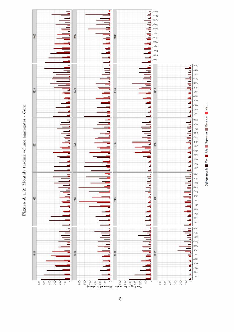
Fig

ure

A.1

.2:

Mon

thly

trad

ing

volu

me

aggr

egat

es-C

orn.

5

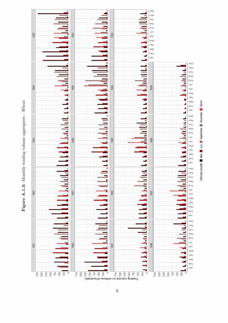
Fig

ure

A.1

.3:

Mon

thly

trad

ing

volu

me

aggr

egat

es-W

heat

.

6

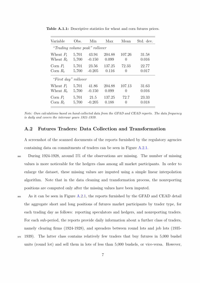
Table A.1.1: Descriptive statistics for wheat and corn futures prices.

Variable Obs. Min Max Mean Std. dev.“Trading volume peak” rollover

Wheat Pt 5,701 43.94 204.88 107.26 31.58Wheat Rt 5,700 -0.150 0.099 0 0.016Corn Pt 5,701 23.56 137.25 72.33 22.77Corn Rt 5,700 -0.205 0.116 0 0.017

“First day” rolloverWheat Pt 5,701 41.86 204.88 107.13 31.63Wheat Rt 5,700 -0.150 0.099 0 0.016Corn Pt 5,701 21.5 137.25 72.7 23.33Corn Rt 5,700 -0.205 0.188 0 0.018

Note: Own calculations based on hand-collected data from the GFAD and CEAD reports. The data frequencyis daily and covers the interwar years 1921-1939.

A.2 Futures Traders: Data Collection and Transformation

A screenshot of the scanned documents of the reports furnished by the regulatory agencies

containing data on commitments of traders can be seen in Figure A.2.1.

During 1924-1928, around 5% of the observations are missing. The number of missing860

values is more noticeable for the hedgers class among all market participants. In order to

enlarge the dataset, these missing values are imputed using a simple linear interpolation

algorithm. Note that in the data cleaning and transformation process, the nonreporting

positions are computed only after the missing values have been imputed.

As it can be seen in Figure A.2.1, the reports furnished by the GFAD and CEAD detail865

the aggregate short and long positions of futures market participants by trader type, for

each trading day as follows: reporting speculators and hedgers, and nonreporting traders.

For each sub-period, the reports provide daily information about a further class of traders,

namely clearing firms (1924-1928), and spreaders between round lots and job lots (1935-

1939). The latter class contains relatively few traders that buy futures in 5,000 bushel870

units (round lot) and sell them in lots of less than 5,000 bushels, or vice-versa. However,

7

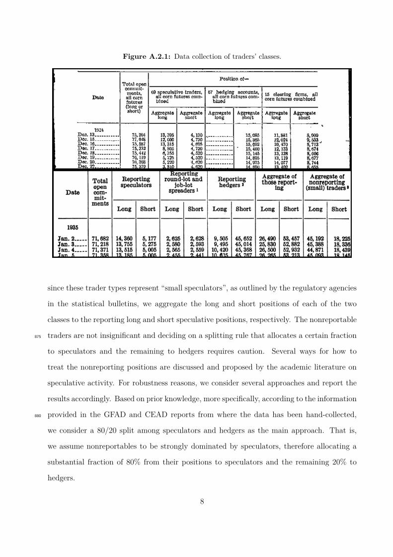
Figure A.2.1: Data collection of traders’ classes.

since these trader types represent “small speculators”, as outlined by the regulatory agencies

in the statistical bulletins, we aggregate the long and short positions of each of the two

classes to the reporting long and short speculative positions, respectively. The nonreportable

traders are not insignificant and deciding on a splitting rule that allocates a certain fraction875

to speculators and the remaining to hedgers requires caution. Several ways for how to

treat the nonreporting positions are discussed and proposed by the academic literature on

speculative activity. For robustness reasons, we consider several approaches and report the

results accordingly. Based on prior knowledge, more specifically, according to the information

provided in the GFAD and CEAD reports from where the data has been hand-collected,880

we consider a 80/20 split among speculators and hedgers as the main approach. That is,

we assume nonreportables to be strongly dominated by speculators, therefore allocating a

substantial fraction of 80% from their positions to speculators and the remaining 20% to

hedgers.

8

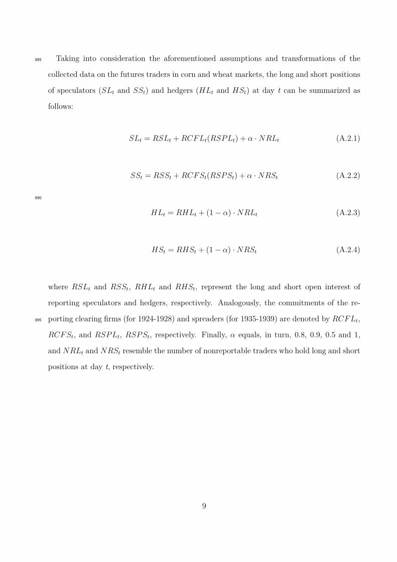
Taking into consideration the aforementioned assumptions and transformations of the885

collected data on the futures traders in corn and wheat markets, the long and short positions

of speculators (SLt and SSt) and hedgers (HLt and HSt) at day t can be summarized as

follows:

SLt = RSLt + RCFLt(RSPLt) + α · NRLt (A.2.1)

SSt = RSSt + RCFSt(RSPSt) + α · NRSt (A.2.2)

890

HLt = RHLt + (1 − α) · NRLt (A.2.3)

HSt = RHSt + (1 − α) · NRSt (A.2.4)

where RSLt and RSSt, RHLt and RHSt, represent the long and short open interest of

reporting speculators and hedgers, respectively. Analogously, the commitments of the re-

porting clearing firms (for 1924-1928) and spreaders (for 1935-1939) are denoted by RCFLt,895

RCFSt, and RSPLt, RSPSt, respectively. Finally, α equals, in turn, 0.8, 0.9, 0.5 and 1,

and NRLt and NRSt resemble the number of nonreportable traders who hold long and short

positions at day t, respectively.

9

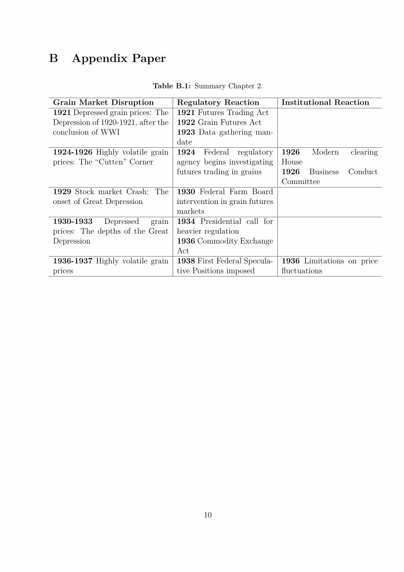
B Appendix Paper

Table B.1: Summary Chapter 2.

Grain Market Disruption Regulatory Reaction Institutional Reaction1921 Depressed grain prices: TheDepression of 1920-1921, after theconclusion of WWI

1921 Futures Trading Act1922 Grain Futures Act1923 Data gathering man-date

1924-1926 Highly volatile grainprices: The “Cutten” Corner

1924 Federal regulatoryagency begins investigatingfutures trading in grains

1926 Modern clearingHouse1926 Business ConductCommittee

1929 Stock market Crash: Theonset of Great Depression

1930 Federal Farm Boardintervention in grain futuresmarkets

1930-1933 Depressed grainprices: The depths of the GreatDepression

1934 Presidential call forheavier regulation1936 Commodity ExchangeAct

1936-1937 Highly volatile grainprices

1938 First Federal Specula-tive Positions imposed

1936 Limitations on pricefluctuations

10

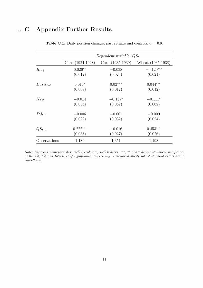
C Appendix Further Results900

Table C.1: Daily position changes, past returns and controls, α = 0.9.

Dependent variable: QSt

Corn (1924-1928) Corn (1935-1939) Wheat (1935-1938)Rt−1 0.026∗∗ −0.038 −0.129∗∗∗

(0.012) (0.026) (0.021)

Basist−1 0.015∗ 0.027∗∗ 0.044∗∗∗

(0.008) (0.012) (0.012)

Negt −0.014 −0.137∗ −0.111∗

(0.036) (0.082) (0.062)

DJt−1 −0.006 −0.001 −0.009(0.022) (0.032) (0.024)

QSt−1 0.222∗∗∗ −0.016 0.453∗∗∗

(0.038) (0.027) (0.026)Observations 1,189 1,351 1,198

Note: Approach nonreportables: 90% speculators, 10% hedgers. ∗∗∗, ∗∗ and ∗ denote statistical significanceat the 1%, 5% and 10% level of significance, respectively. Heteroskedasticity robust standard errors are inparentheses.

11

Table C.2: GARCH(1,1) results, α = 0.9.

Sample periodCorn (1924-1928) Corn (1935-1939) Wheat (1935-1938)

Mean equation: Ri,t = β0 + β1Ri,t−1 + ∑4n=2 βnControlsn,t−1 + β5QSi,t−1 + εi,t

AR(1) -0.038 0.049 -0.023(0.029) (0.035) (0.026)

Basist−1 0.002 0.017 0.003(0.016) (0.019) (0.013)

Negt -0.043 -0.065 -0.093(0.074) (0.072) (0.068)

DJt−1 -0.031 -0.046∗∗ -0.044(0.056) (0.022) (0.031)

QSt−1 0.013 0.031 -0.062(0.055) (0.031) (0.040)

Conditional variance equation: σ2i,t = γ0 + γ1ε

2i,t−1 + γ2σ

2i,t−1 + γ3QSi,t−1

ARCH(1) 0.101∗∗∗ 0.122∗∗∗ 0.082∗∗∗

(0.012) (0.026) (0.015)

GARCH(1) 0.833∗∗∗ 0.856∗∗∗ 0.897∗∗

(0.026) (0.124) (0.044)

QSt−1 0 0 0(0) (0) (0)

γ1 + γ2 0.934 0.978 0.979LM Test 0.022 0.153 0.294

Note: Approach nonreportables: 90% speculators, 10% hedgers. ∗∗∗, ∗∗ and ∗ denote statistical significanceat the 1%, 5% and 10% level of significance, respectively. Heteroskedasticity robust standard errors are inparentheses.

12

Table C.3: Daily position changes, past returns and controls, α = 0.5.

Dependent variable: QSt

Corn (1924-1928) Corn (1935-1939) Wheat (1935-1938)Rt−1 0.079∗∗∗ −0.022 −0.117∗∗∗

(0.019) (0.021) (0.018)

Basist−1 0.027∗∗ 0.024∗∗ 0.041∗∗∗

(0.011) (0.010) (0.010)

Negt −0.024 −0.130∗∗ −0.075(0.050) (0.066) (0.053)

DJt−1 −0.053∗ −0.021 0.002(0.031) (0.026) (0.021)

QSt−1 0.041 −0.032 0.318∗∗∗

(0.041) (0.027) (0.029)Observations 1,189 1,351 1,198

Note: Approach nonreportables: 50% speculators, 50% hedgers. ∗∗∗, ∗∗ and ∗ denote statistical significanceat the 1%, 5% and 10% level of significance, respectively. Heteroskedasticity robust standard errors are inparentheses.

13

Table C.4: GARCH(1,1) results, α = 0.5.

Sample periodCorn (1924-1928) Corn (1935-1939) Wheat (1935-1938)

Mean equation: Ri,t = β0 + β1Ri,t−1 + ∑4n=2 βnControlsn,t−1 + β5QSi,t−1 + εi,t

AR(1) -0.037 0.048 -0.023(0.029) (0.034) (0.028)

Basist−1 0.004 0.017 0(0.016) (0.0179) (0.019)

Negt -0.044 -0.066 -0.088(0.074) (0.068) (0.066)

DJt−1 -0.033 -0.045∗∗ -0.045(0.057) (0.022) (0.031)

QSt−1 -0.033 0.024 -0.020(0.042) (0.034) (0.048)

Conditional variance equation: σ2i,t = γ0 + γ1ε

2i,t−1 + γ2σ

2i,t−1 + γ3QSi,t−1

ARCH(1) 0.101∗∗∗ 0.121∗∗∗ 0.082∗∗∗

(0.013) (0.026) (0.021)

GARCH(1) 0.832∗∗∗ 0.857∗∗∗ 0.897∗∗∗

(0.028) (0.089) (0.084)

QSt−1 0 0 0(0) (0) (0)

γ1 + γ2 0.933 0.978 0.979LM Test 0.016 0.116 0.442

Note: Approach nonreportables: 50% speculators, 50% hedgers. ∗∗∗, ∗∗ and ∗ denote statistical significanceat the 1%, 5% and 10% level of significance, respectively. Heteroskedasticity robust standard errors are inparentheses.

14

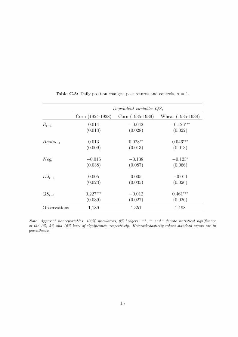
Table C.5: Daily position changes, past returns and controls, α = 1.

Dependent variable: QSt

Corn (1924-1928) Corn (1935-1939) Wheat (1935-1938)Rt−1 0.014 −0.042 −0.126∗∗∗

(0.013) (0.028) (0.022)

Basist−1 0.013 0.028∗∗ 0.046∗∗∗

(0.009) (0.013) (0.013)

Negt −0.016 −0.138 −0.123∗

(0.038) (0.087) (0.066)

DJt−1 0.005 0.005 −0.011(0.023) (0.035) (0.026)

QSt−1 0.227∗∗∗ −0.012 0.461∗∗∗

(0.039) (0.027) (0.026)Observations 1,189 1,351 1,198

Note: Approach nonreportables: 100% speculators, 0% hedgers. ∗∗∗, ∗∗ and ∗ denote statistical significanceat the 1%, 5% and 10% level of significance, respectively. Heteroskedasticity robust standard errors are inparentheses.

15

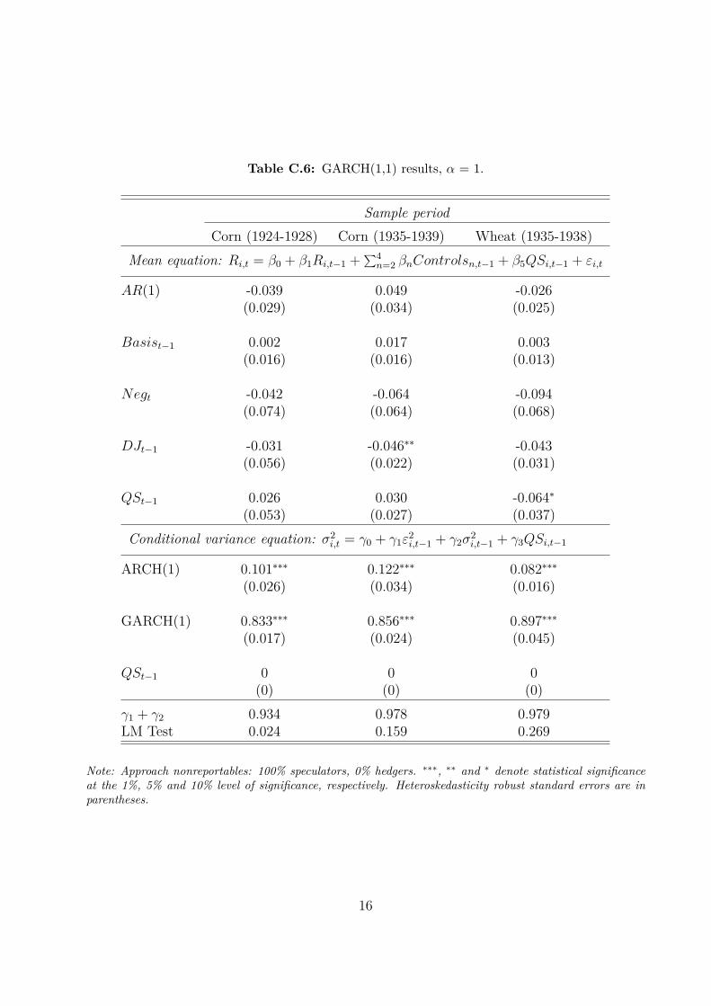
Table C.6: GARCH(1,1) results, α = 1.

Sample periodCorn (1924-1928) Corn (1935-1939) Wheat (1935-1938)

Mean equation: Ri,t = β0 + β1Ri,t−1 + ∑4n=2 βnControlsn,t−1 + β5QSi,t−1 + εi,t

AR(1) -0.039 0.049 -0.026(0.029) (0.034) (0.025)

Basist−1 0.002 0.017 0.003(0.016) (0.016) (0.013)

Negt -0.042 -0.064 -0.094(0.074) (0.064) (0.068)

DJt−1 -0.031 -0.046∗∗ -0.043(0.056) (0.022) (0.031)

QSt−1 0.026 0.030 -0.064∗

(0.053) (0.027) (0.037)Conditional variance equation: σ2

i,t = γ0 + γ1ε2i,t−1 + γ2σ

2i,t−1 + γ3QSi,t−1

ARCH(1) 0.101∗∗∗ 0.122∗∗∗ 0.082∗∗∗

(0.026) (0.034) (0.016)

GARCH(1) 0.833∗∗∗ 0.856∗∗∗ 0.897∗∗∗

(0.017) (0.024) (0.045)

QSt−1 0 0 0(0) (0) (0)

γ1 + γ2 0.934 0.978 0.979LM Test 0.024 0.159 0.269

Note: Approach nonreportables: 100% speculators, 0% hedgers. ∗∗∗, ∗∗ and ∗ denote statistical significanceat the 1%, 5% and 10% level of significance, respectively. Heteroskedasticity robust standard errors are inparentheses.

16