Glass transition temperatures in binary polymer blends

Glass Transition Temperatures In Binary Polymer Blends

IOANNIS M. KALOGERAS,1 WITOLD BROSTOW2

1Solid State Physics Section, Department of Physics, University of Athens, Panepistimiopolis, Zografos 157 84, Greece

2Laboratory of Advanced Polymers and Optimized Materials (LAPOM), Department of Materials Science and Engineeringand Department of Physics, University of North Texas, Denton, Texas 76203-5310

Received 22 July 2008; revised 1 October 2008; accepted 3 October 2008DOI: 10.1002/polb.21616Published online in Wiley InterScience (www.interscience.wiley.com).

ABSTRACT: Knowledge of the glass transition temperatures (Tgs) as function of com-position reflects miscibility (or lack of it) and is decisive for virtually all properties ofpolymer-based materials. In this article, we analyze single blend-average and effec-tive Tgs of miscible polymer blends in full concentration ranges. Shortcomings of theextant equations are discussed to support the need for an alternative. Focusing onthe deviation from a linear relationship, defined as DTg ¼ Tg � u1Tg,1 � u2Tg,2

(where ui and Tg,i are, respectively, the weight fraction and the Tg of the i-th compo-nent), a recently proposed equation for the blend Tg as a function of composition istested extensively. This equation is simple; a quadratic polynomial centered around2u1 � 1 ¼ 0 is defined to represent deviations from linearity, and up to three param-eters are used. The number of parameters needed to describe the experimental data,along with their magnitude and sign, provide a measure of the system complexity.For most binary polymer systems tested, the results obtained with the new equationare better than those attained from existing Tg equations. The key parameter of theequation a0 is related to parameters commonly used to represent intersegmentalinteractions and miscibility in binary polymer blends. VVC 2008 Wiley Periodicals, Inc. J

Polym Sci Part B: Polym Phys 47: 80–95, 2008

Keywords: blends; differential scanning calorimetry (DSC); glass transition; glasstransition temperature; intermolecular interactions; polymer blends; polymermiscibility

SCOPE

The glass transition is an important phenomenonthat characterizes a range of amorphous systems,including homopolymers, polymer blends, copoly-mers, and polymer networks. The related experi-mental signals and the underlying process on amolecular scale involve both kinetic and thermo-

dynamic features.1,2 For example, the influence ofthe direction of the change (freezing a liquid,melting a solid) and of variations in the changerate (heating or cooling) on the location of theglass transition region are illustrative of its ki-netic character, whereas the experimental obser-vation of features attributed to a second ordertransition is in line with the thermodynamic char-acter.2

Although the change from the glassy state intoeither a liquid or a rubbery state is a gradual one,and thus the glass transition phenomenon spansa wide temperature window, experimentalists

Journal of Polymer Science: Part B: Polymer Physics, Vol. 47, 80–95 (2009)VVC 2008 Wiley Periodicals, Inc.

Correspondence to: I. M. Kalogeras (E-mail: [email protected])

80

tend to report and tabulate unique values of theso-called glass transition temperature (Tg), byanalogy with the melting temperature Tm values,so as to represent a glass transition region by asingle number. This permits determination of theuse and processing temperature for many materi-als, and easier comparisons between systems ofdifferent composition and/or architecture. Differ-ent techniques lead to different Tg values.3 Tg

evaluations based on common thermal analysistechniques, such as differential scanning calorim-etry (DSC), dynamic mechanical analysis (DMA),dielectric analysis (DEA), and thermomechanicalanalysis, are in general not identical. This isrelated to different natures and time responses ofthe experimental probes (motions of side- ormain-chain polar groups, or of small or large partsof the chain; electrical, mechanical or thermalstimulation of the motion, etc). There are also dif-ferences of compatibility in the effective volumesize averaged by each technique.2 Even when oneuses DEA only, the results are not necessarily thesame when one obtains a Tg value from dielectricrelaxation spectroscopy [e.g., from isochronal per-mittivity e0(T) plots or the peak of the segmentalmode observed in dielectric loss e00(T), electric lossmodulusM00(T) or tan d ¼ e00/e0 plots] or using ther-mally stimulated current spectroscopy (e.g., fromthe temperature at which the a-relaxation bandreaches a maximum in current density versus Tplots).4

Although these complications exist, Tg valuesare useful indeed for a variety of purposes. Partic-ularly needed are Tg values as a function of com-position u for binary polymer blends; they tell uswhether the blends are miscible, semimiscible(called compatible) or not miscible at all. As a ruleof thumb, observation of a single (usually broad)glass transition region (i.e., a single Tg, the‘‘blend-average’’ Tg) for all the blends is used forestablishing full miscibility (one-phase mixture).Nevertheless, this statement is an oversimplifica-tion of the actual picture. A number of misciblepolymer mixtures—particularly blends whosecomponents show a strong difference in their Tg’sand weak intermolecular interactions—presentstrong asymmetry. Motions of the different chainsare decoupled and the relaxation dynamics ofeach component are clearly discernible. Alongthese lines, two glass transition regions haverecently been distinguished in some systems,5 ei-ther by means of carefully performed DSC experi-ments6–9 or by using techniques of increasedresolving power (DEA,6,10,11 temperature-modu-

lated DSC (TMDSC),12 DMA,6 nuclear magneticresonance,13 electron spin resonance,14 quasi-elastic neutron scattering,15 etc). The aforemen-tioned findings should not be confused with thecase of compatibility, in which any experimentaltechnique detects two Tg values that alsodepend on composition. Immiscible polymers(not an infrequent case) clearly demonstrate twoTg values for the respective pure componentsthat are independent of composition. In each ofthe aforementioned cases components’ miscibil-ity (or lack of it) is decisive for all properties ofthe blends.

Apart from miscibility, the Tgs reflect alsomany features and properties of polymeric sys-tems: helical twisting power in chiral nematicphases; changes of Tg with residual stress; effectsof fillers, polymer intercalation or clay exfoliationon thermal properties; perturbations of the seg-mental dynamics resulting from polymer’s con-finement in ultrathin films or nanopore environ-ments; consequences of aging, adsorption of sol-vents or hydration processes, and so forth. Whenwe wish to achieve compatibility, then changes inTg represent a measure of success of that opera-tion and thus allow optimization of curing condi-tions or of the compatibilizing agent concentra-tion.

The aforementioned arguments corroborate theongoing efforts to predict the compositional de-pendence of various thermophysical properties, ofTg in particular, of polymer-based materials. Inthe following section we discuss shortcomings ofthe existing approaches. We thus demonstrate theneed for an analytical equation for Tg as a func-tion of concentration that will not be subjected tomodel-specific limitations and also could serve forblends as well as for copolymers with varying con-centrations of the constituents.

EARLIER Tg VERSUS COMPOSITIONEQUATIONS

Several approaches based on kinetic or thermody-namic features of the glass transition phenom-enon have been proposed to provide a theoreticfoundation for the equations currently used topredict -and subsequently explain- the composi-tional dependence of the Tg of blends of misciblepolymers as well as those of random copoly-mers.16–24 In the case of binary polymer blends,most of the derived equations are based on theassumption of additivity for the respective basic

Tg IN MISCIBLE BINARY POLYMER BLENDS 81

Journal of Polymer Science: Part B: Polymer PhysicsDOI 10.1002/polb

properties of the blend components, that is, eitherof the specific volumes as Gordon and Taylor haveproposed,23 which is practically equivalent to theadditivity of the relevant free volumes, as Kovacshas shown,17 or of the flexible bonds contributingto the conformational changes, as DiMarzio hassuggested.25 These additivity models lead to theGordon-Taylor (GT) equation23

Tg ¼ u1Tg;1 þ kGT 1� u1ð ÞTg;2

u1 þ kGT 1� u1ð Þ (1)

for the compositional dependence of the Tg in a bi-nary (1 þ 2) polymer blend. Here, ui are the mass(weight) fractions (u2 ¼ 1 � u1) and Tg,i are theTgs of the blend components, with the subscripttwo referring to the component with the higherTg. The above equation is apparently based on theconcept that one of the components has a lessereffect on the Tg of the blend than the other. Themodel specific parameter kGT, which has to beevaluated from the experimental data, representsthe unequal contributions. In the case of the com-mon volume-additivity approach (a free volumemodel) kGT equals (q1/q2)(Da2/Da1), where qi arethe densities and Dai ¼ (amelt � aglass)i are incre-ments at Tg of the isobaric expansivities of theblend components. Assuming the validity of theempirical Simha-Boyer rule,26 DaTg ¼ 0.133 (con-stant), and neglecting in a first approximation theinfluence of the densities of the blend components(i.e., assuming that q1 � q2), the specific kGT pa-rameter for volume additivity can also be substi-tuted by the respective reversed ratio of the Tgs ofthe blend components, that is, kGT � Tg,1/Tg,2.This transforms eq 1 to the well-known Fox equa-tion22

1

Tg¼ u1

Tg;1þ 1� u1

Tg;2(2)

The Fox equation assumes random mixingbetween the two components, equal values of theheat capacity jump in the glass transition regionbetween the two components (i.e., DCp,1 ¼ DCp,2),and volume of mixing VE ¼ 0 in the entire concen-tration range. Equation 2 allows prediction ofblend properties from properties of pure compo-nents only and for that reason is one of the mostfrequently used relations. However, eq 2 fallsshort in describing the experimentally observedpositive or negative deviations of the blend Tg

from the predicted additivity values and clearlyfails to describe experimental data showing com-plex (nonmonotonic, e.g., s-shaped) compositional

dependences. Similarly, the GT expressionexplains only monotonous deviations from addi-tivity, either negative (0 \ kGT \ 1) or positive(kGT[ 1) ones.

To account for the effect on Tg of intercompo-nent interactions in the liquid and glassy state ofpolymer mixtures, empirical concentration sec-ond-order power equations have been proposed inthe literature. Jenckel and Heusch,21 for instance,suggested for plasticized polymer blends theexpression

Tg ¼ u1Tg;1 þ 1� u1ð ÞTg;2

þ b Tg;2 � Tg;1

� �u1 1� u1ð Þ ð3Þ

with b a parameter that characterizes the solventquality of the plasticizer. To account for specificinteraction, which may perturb the free volumeadditivity in the polymer mixture, Kwei24

extended the GT equation to a concentration sec-ond-order power equation of the form

Tg ¼ u1Tg;1 þ kKw 1� u1ð ÞTg;2

u1 þ kKw 1� u1ð Þ þ qu1 1� u1ð Þ (4)

by introducing in eq 1 a quadratic term, qu1(1 �u1), with q in the role of an interaction-dependentparameter. The kKw parameter is also treated as areal fitting parameter to be evaluated from the ex-perimental data. When kKw ¼ 1, the Kwei equa-tion reduces to the Jenckel-Heusch equation withb ¼ q/(Tg,2 � Tg,1). S-shaped curves can then beexplained, but only with positive deviations fromadditivity in the low-Tg range and negative devia-tions in the high-Tg range. To reproduce negativedeviations in the low-Tg range and positive devia-tions in the high-Tg range, additional correctionterms have to be used.

Several other concentration second-orderpower equations for the compositional dependenceof the blend transition temperature can be found.For example, DiMarzio25 presented an equationconsidering the concept of flexible bond additivityalong with effects of volume changes due to thedifferent specific volumes of the blend componentsat Tg. Kanig27 related changes in interaction ener-gies to the respective Gibbs functions of generat-ing one mole of holes in the equilibrium polymermelt. Nevertheless, each of the above equationscan only describe the behavior of a narrow rangeof systems and thus the quest for alternativesremains open. Brekner and coworkers28 put for-ward a virial-like concentration third-order equa-tion to account for the dependence of blend Tg

from the free volume distribution and the related

82 KALOGERAS AND BROSTOW


conformational mobility, which is controlled bythe probability of hetero-molecular contact forma-tion in the mixture due to specific interactions ofthe components including the energetic effectsinduced by conformational changes. This leads tothe Brekner-Schneider-Cantow relation

Tg ¼Tg;1þ Tg;2�Tg;1

� �1þK1ð Þ 1�u1ð Þ½

� K1þK2ð Þ 1�u1ð Þ2þK2 1�u1ð Þ3� ð5Þwhere both K1 and K2 are obtained by fitting toexperimental Tg versus concentration data.

DEVELOPMENT OF A NEW EQUATION

Typically, the description of the Tg of miscibleblends involves the use of functions that are lin-ear in concentration [e.g., eq 1] and correspond tothe first factor of a series expansion, as well asfunctions with higher terms that involve quad-ratic [e.g., eqs 3 and 4] and cubic terms of theblend composition.16,28 Let us consider hereanother approach: In the simplest possible case,the glass transition of a miscible binary polymerblend will be a linear function of composition: Tg

¼ u1Tg,1 þ (1 � u1)Tg,2. Such an equation wouldhave the advantage of the Fox equation (eq 2),namely predictability in terms of properties ofpure components only. However, the literaturedata for polymer systems, involving either amor-phous þ amorphous polymer or amorphous þsemicrystalline polymer blends, or even mixturesbetween two semicrystalline polymers that aremiscible in the amorphous state, usually demon-strate considerable deviations from linearity. Wequantify this situation by DTg

DTg ¼ Tg � Tling ¼ Tg � u1Tg;1 þ 1� u1ð ÞTg;2

� �:

(6a)

The shape of the resultant deviation versus com-position plot should depend on characteristics ofthe specific pair of polymers (e.g., molecularweight, tacticity, chemical groups, and specificinteractions), with possible contributions from anumber of factors, which include special materialpreparation procedures (use of solvents, irradia-tion, etc). Let us consider another relatively sim-ple (but not rare) case: DTg = 0 but can be repre-sented by a parabola, that is, DTg ¼ u1(1 � u1)a0,where a0 is a semiquantitative measure of thedeviation observed in a given system. DTg willnow have the highest value at u1 ¼ u2 ¼ 0.5. At

that point we have u1 � u2 ¼ 2u1 � 1 ¼ 0. Bear-ing in mind the fact that real systems usuallydemonstrate more complicated behavior, theDTg(u1) graph is likely to show a more or lessasymmetric shape. To account for such cases,let us define a quadratic polynomial centeredaround 2u1 � 1 ¼ 0 to represent deviations fromlinearity:

DTg ¼ u1 1� u1ð Þ a0 þ a1 2u1 � 1ð Þ þ a2 2u1 � 1ð Þ2h i

(6b)

Combining eq 6a,b we obtain:

Tg ¼u1Tg;1þ 1�u1ð ÞTg;2

þu1 1�u1ð Þ a0þa1 2u1�1ð Þþa2 2u1�1ð Þ2h i

:

(7)

The last term in eq 7 encompasses contribu-tions from several factors that influence the ther-mal characteristics of miscible binary polymerblends, including variations in the strength of theintermolecular interactions, irregular free-volumemodifications, and different types of segregationof the amorphous fractions with respect to thecrystalline phase.

The proposed equation contains three adjusta-ble parameters;29 their significance is exploredbelow using a large number of examples (see ‘‘Cal-culations and Confrontation with Experiment’’section). The experimental data analyzed herehave been obtained using conventional DSC.However, our approach is clearly applicable alsoto Tg(u) diagrams obtained by other techniques.4

SYSTEMS INVESTIGATED

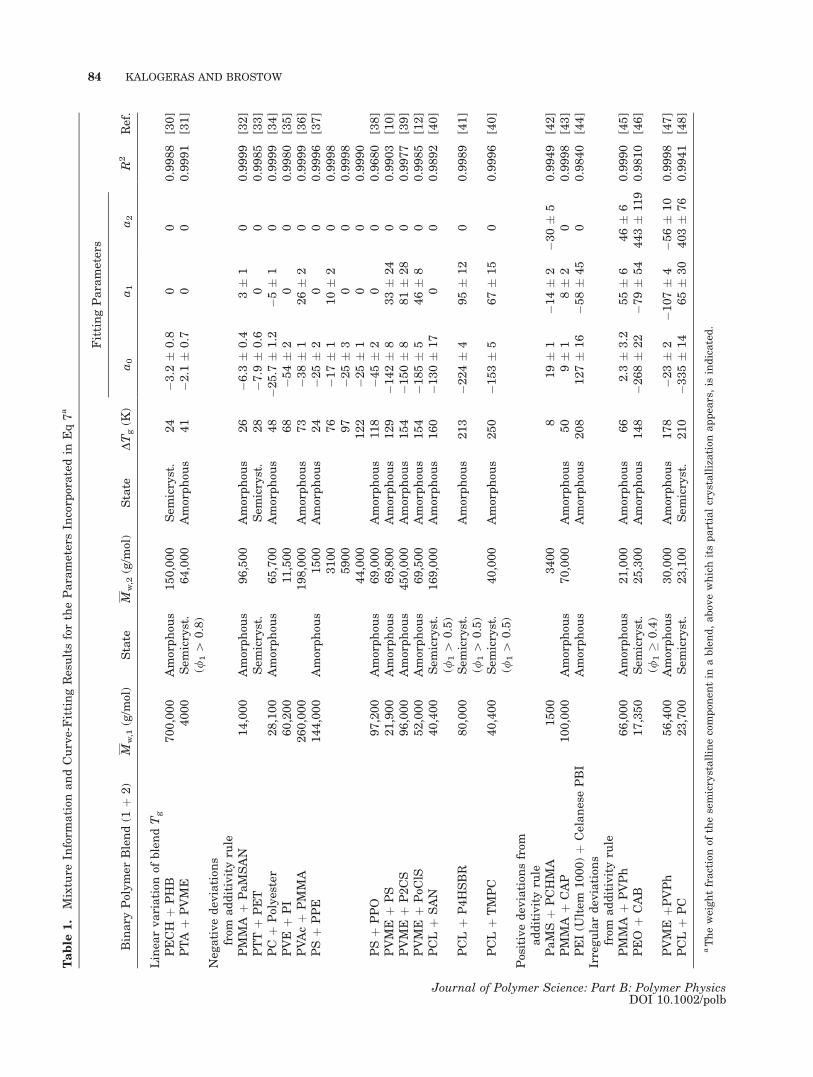
Published DSC data for a large number of misci-ble binary polymer blends were examined here(Table 1), covering a wide range of weight-averagemolecular weights (Mw), blends of different state(with completely amorphous components, one oreven two semicrystalline components), and blendswith a wide range of differences in the Tgs of theircomponents (Tg,2 � Tg,1 between 8 and 248 K).Unless otherwise stated, the single Tg values pre-sented in Table 1 and those used in the followingcalculations (see ‘‘Calculations and Confrontationwith Experiment’’ section), correspond to the so-called ‘‘blend-average’’ Tg, that is, the single Tg

value obtained from the midpoint of the heatcapacity change in second-heating DSC scans. Fora number of polymer blends considered here



Table

1.

Mixture

Inform

ation

andCurve-FittingResultsfortheParametersIn

corp

oratedin

Eq7a

Binary

Polymer

Blend(1

þ2)

Mw,1(g/m

ol)

State

Mw,2(g/m

ol)

State

DTg(K

)

FittingParameters

R2

Ref.

a0

a1

a2

Linea

rvariation

ofblendTg

PECH

þPHB

700,000

Amorphou

s150,000

Sem

icryst.

24

�3.2

�0.8

00

0.9988

[30]

PTA

þPVME

4000

Sem

icryst.

(/1[

0.8)

64,000

Amorphou

s41

�2.1

�0.7

00

0.9991

[31]

Neg

ativedev

iation

sfrom

additivityru

lePMMA

þPaMSAN

14,000

Amorphou

s96,500

Amorphou

s26

�6.3

�0.4

3�

10

0.9999

[32]

PTTþ

PET

Sem

icryst.

Sem

icryst.

28

�7.9

�0.6

00

0.9985

[33]

PC

þPolyester

28,100

Amorphou

s65,700

Amorphou

s48

�25.7

�1.2

�5�

10

0.9999

[34]

PVE

þPI

60,200

11,500

68

�54�

20

00.9980

[35]

PVAcþ

PMMA

260,000

198,000

Amorphou

s73

�38�

126�

20

0.9999

[36]

PSþ

PPE

144,000

Amorphou

s1500

Amorphou

s24

�25�

20

00.9996

[37]

3100

76

�17�

110�

20

0.9998

5900

97

�25�

30

00.9998

44,000

122

�25�

10

00.9990

PSþ

PPO

97,200

Amorphou

s69,000

Amorphou

s11

8�4

5�

20

00.9680

[38]

PVME

þPS

21,900

Amorphou

s69,800

Amorphou

s129

�142�

833�

24

00.9903

[10]

PVME

þP2CS

96,000

Amorphou

s450,000

Amorphou

s154

�150�

881�

28

00.9977

[39]

PVME

þPoC

lS52,000

Amorphou

s69,500

Amorphou

s154

�185�

546�

80

0.9985

[12]

PCL

þSAN

40,400

Sem

icryst.

(/1[

0.5)

169,000

Amorphou

s160

�130�

17

00

0.9892

[40]

PCL

þP4HSBR

80,000

Sem

icryst.

(/1[

0.5)

Amorphou

s213

�224�

495�

12

00.9989

[41]

PCL

þTMPC

40,400

Sem

icryst.

(/1[

0.5)

40,000

Amorphou

s250

�153�

567�

15

00.9996

[40]

Positivedev

iation

sfrom

additivityru

lePaMSþ

PCHMA

1500

3400

819�

1�1

4�

2�3

0�

50.9949

[42]

PMMA

þCAP

100,000

Amorphou

s70,000

Amorphou

s50

9�

18�

20

0.9998

[43]

PEI(U

ltem

1000)þ

CelanesePBI

Amorphou

sAmorphou

s208

127�

16

�58�

45

00.9840

[44]

Irregulardev

iation

sfrom

additivityru

lePMMA

þPVPh

66,000

Amorphou

s21,000

Amorphou

s66

2.3

�3.2

55�

646�

60.9990

[45]

PEO

þCAB

17,350

Sem

icryst.

(/1�

0.4)

25,300

Amorphou

s148

�268�

22

�79�

54

443�

119

0.9810

[46]

PVME

þPVPh

56,400

Amorphou

s30,000

Amorphou

s178

�23�

2�1

07�

4�5

6�

10

0.9998

[47]

PCL

þPC

23,700

Sem

icryst.

23,100

Sem

icryst.

210

�335�

14

65�

30

403�

76

0.9941

[48]

aTheweightfractionof

thesemicrystallinecompon

entin

ablend,abov

ewhichitspartialcrystallization

appea

rs,is

indicated.



bimodal glass transition regions have been alsoreported; for example, in poly(vinyl methyl ether)(PVME) þ polystyrene (PS),10–12 poly(n-butyl ac-rylate) þ PS,12 PVME þ poly(o-chloro styrene)(PoClS),12 polyethylene oxide (PEO) þ poly(methyl methacrylate) (PMMA),7,9 PEO þ poly(vinyl acetate) (PVAc),9 poly(vinyl ethylene) (PVE)þ polyisoprene (PI)8 and poly(e-caprolactone)(PCL) þ PC.6 For such blends, when available,analysis of DSC blend-average Tgs has been per-formed. We also report in ‘‘Analysis of MiscibleBlends with Two Tgs’’ section the use of eq 7 in thecase of two Tgs and discuss there the Lodge-McLe-ish (LM) model.5 Information on the experimentaldetails and any special procedures used for prepa-ration of the mixtures (temperature of mixing, type

of solvent, drying processes, etc) can be found inthe original references. The values reported wereobtained by applying a Levenberg-Marquardtleast-square minimization routine to DSC data.

CALCULATIONS AND CONFRONTATIONWITH EXPERIMENT

Mixtures with Nearly Linear CompositionalVariation of Blend Tg

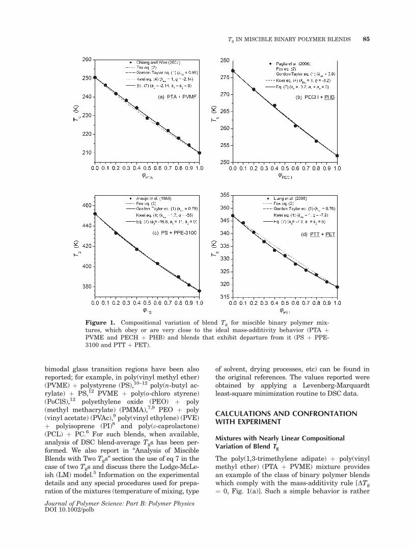
The poly(1,3-trimethylene adipate) þ poly(vinylmethyl ether) (PTA þ PVME) mixture providesan example of the class of binary polymer blendswhich comply with the mass-additivity rule [DTg

¼ 0, Fig. 1(a)]. Such a simple behavior is rather

Figure 1. Compositional variation of blend Tg for miscible binary polymer mix-tures, which obey or are very close to the ideal mass-additivity behavior (PTA þPVME and PECH þ PHB) and blends that exhibit departure from it (PS þ PPE-3100 and PTT þ PET).



rare, most likely to appear in amorphous þ amor-phous polymer mixtures with a low Tg differenceof their pure components (Tg,2 � Tg,1\ 50 K) andinsignificant differences in the strength and levelof intersegment interactions before and after mix-ing. One could expect large departures from thisbehavior to appear in blends of polymers withlarge contrast in their segmental mobilities andin the presence of at least one semicrystallinecomponent. Nevertheless, the DSC data for PTAþ PVME clearly demonstrate that the presence ofa crystalline polyester fraction in blends withvery high PTA content (for uPTA [ 0.8) is insuffi-cient to create even the slightest departure fromlinearity. Apparently, the organization of a smallweight fraction of PTA in crystalline microphaseshas little, if any, influence on the relaxational dy-namics of the chains located in the mixed amor-phous phase. A similar behavior is observed inthe poly(epichlorohydrin) þ poly(D(�)3-hydroxy-butyrate) (PECH þ PHB) blend, in which opticaldata reveal that after crystallization the PECHchains are rejected in the interlamellar or interfi-brillar regions of PHB spherulites, where theyform a homogeneous mixture with uncrystallizedPHB molecules.30 The completely weight-aver-aged behavior of the blend Tgs is described by akGT parameter nearly equal to one, kKw ¼ 1 andq ¼ 0 as far as the Kwei equation is concerned,and zero values for all the parameters appearingin our equation. A small departure from the afore-mentioned predictions is reasonable, consideringthe typical experimental errors of the Tg valuesimposed by the resolving ability of each meas-uring technique (DSC, DEA, DMA, p-V-T data,etc). By comparing the behavior (Fig. 1) exhibitedby the miscible, in the amorphous state, mixturesof PTA þ PVME,31 PECH þ PHB,30 PS þpoly(2,6-dimethylphenylene ether) (PS þ PPE)37,and poly(trimethylene terephthalate) þ poly(eth-ylene terephthalate) (PTT þ PET),33 we expectthat in the case of mass-additivity the parametersof eq 7 should obey the relations: |a0|\ �5, anda1, a2 � 0. In view of that, only the first two of thesystems included in Figure 1 are considered toabide by the mass-additivity rule.

Mixtures with DTg < 0

A behavior of moderate complexity may be consid-ered that of the miscible polymer systems that ex-hibit monotonic negative deviations from the pre-dictions of the mass- and volume-additivity (Fox)rules. This behavior is quite common and appears

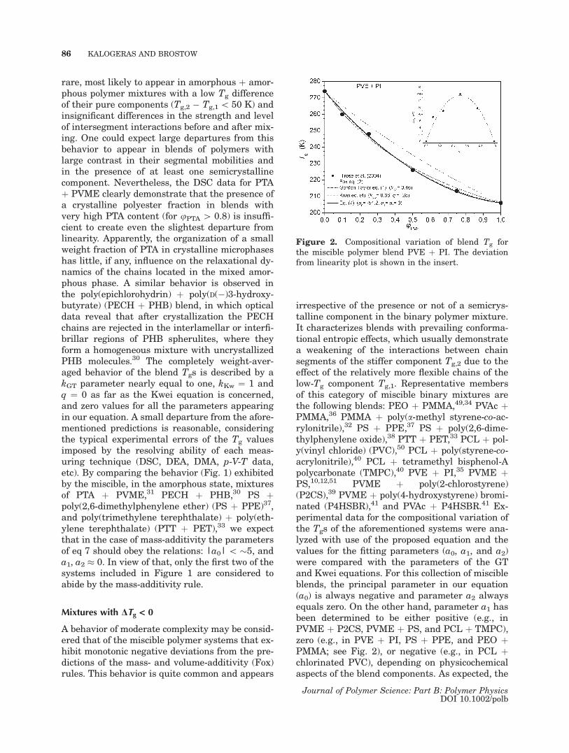
irrespective of the presence or not of a semicrys-talline component in the binary polymer mixture.It characterizes blends with prevailing conforma-tional entropic effects, which usually demonstratea weakening of the interactions between chainsegments of the stiffer component Tg,2 due to theeffect of the relatively more flexible chains of thelow-Tg component Tg,1. Representative membersof this category of miscible binary mixtures arethe following blends: PEO þ PMMA,49,34 PVAc þPMMA,36 PMMA þ poly(a-methyl styrene-co-ac-rylonitrile),32 PS þ PPE,37 PS þ poly(2,6-dime-thylphenylene oxide),38 PTT þ PET,33 PCL þ pol-y(vinyl chloride) (PVC),50 PCL þ poly(styrene-co-acrylonitrile),40 PCL þ tetramethyl bisphenol-Apolycarbonate (TMPC),40 PVE þ PI,35 PVME þPS,10,12,51 PVME þ poly(2-chlorostyrene)(P2CS),39 PVME þ poly(4-hydroxystyrene) bromi-nated (P4HSBR),41 and PVAc þ P4HSBR.41 Ex-perimental data for the compositional variation ofthe Tgs of the aforementioned systems were ana-lyzed with use of the proposed equation and thevalues for the fitting parameters (a0, a1, and a2)were compared with the parameters of the GTand Kwei equations. For this collection of miscibleblends, the principal parameter in our equation(a0) is always negative and parameter a2 alwaysequals zero. On the other hand, parameter a1 hasbeen determined to be either positive (e.g., inPVME þ P2CS, PVME þ PS, and PCL þ TMPC),zero (e.g., in PVE þ PI, PS þ PPE, and PEO þPMMA; see Fig. 2), or negative (e.g., in PCL þchlorinated PVC), depending on physicochemicalaspects of the blend components. As expected, the

Figure 2. Compositional variation of blend Tg forthe miscible polymer blend PVE þ PI. The deviationfrom linearity plot is shown in the insert.



lower the value of a0 the higher the negative devi-ation from linearity is.

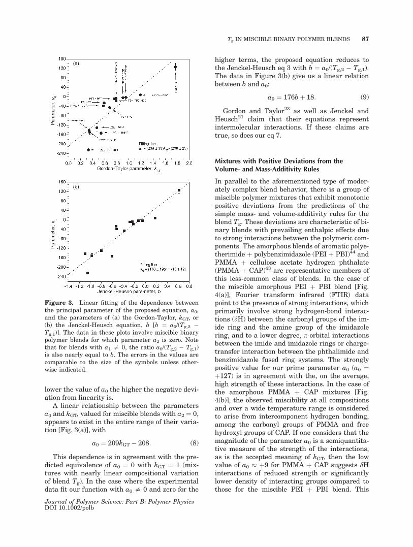
A linear relationship between the parametersa0 and kGT, valued for miscible blends with a2 ¼ 0,appears to exist in the entire range of their varia-tion [Fig. 3(a)], with

a0 ¼ 209kGT � 208: (8)

This dependence is in agreement with the pre-dicted equivalence of a0 ¼ 0 with kGT ¼ 1 (mix-tures with nearly linear compositional variationof blend Tg). In the case where the experimentaldata fit our function with a0 = 0 and zero for the

higher terms, the proposed equation reduces tothe Jenckel-Heusch eq 3 with b ¼ a0/(Tg,2 � Tg,1).The data in Figure 3(b) give us a linear relationbetween b and a0:

a0 ¼ 176bþ 18: (9)

Gordon and Taylor23 as well as Jenckel andHeusch21 claim that their equations representintermolecular interactions. If these claims aretrue, so does our eq 7.

Mixtures with Positive Deviations from theVolume- and Mass-Additivity Rules

In parallel to the aforementioned type of moder-ately complex blend behavior, there is a group ofmiscible polymer mixtures that exhibit monotonicpositive deviations from the predictions of thesimple mass- and volume-additivity rules for theblend Tg. These deviations are characteristic of bi-nary blends with prevailing enthalpic effects dueto strong interactions between the polymeric com-ponents. The amorphous blends of aromatic polye-therimide þ polybenzimidazole (PEI þ PBI)44 andPMMA þ cellulose acetate hydrogen phthalate(PMMA þ CAP)43 are representative members ofthis less-common class of blends. In the case ofthe miscible amorphous PEI þ PBI blend [Fig.4(a)], Fourier transform infrared (FTIR) datapoint to the presence of strong interactions, whichprimarily involve strong hydrogen-bond interac-tions (dH) between the carbonyl groups of the im-ide ring and the amine group of the imidazolering, and to a lower degree, p-orbital interactionsbetween the imide and imidazole rings or charge-transfer interaction between the phthalimide andbenzimidazole fused ring systems. The stronglypositive value for our prime parameter a0 (a0 ¼þ127) is in agreement with the, on the average,high strength of these interactions. In the case ofthe amorphous PMMA þ CAP mixtures [Fig.4(b)], the observed miscibility at all compositionsand over a wide temperature range is consideredto arise from intercomponent hydrogen bonding,among the carbonyl groups of PMMA and freehydroxyl groups of CAP. If one considers that themagnitude of the parameter a0 is a semiquantita-tive measure of the strength of the interactions,as is the accepted meaning of kGT, then the lowvalue of a0 � þ9 for PMMA þ CAP suggests dHinteractions of reduced strength or significantlylower density of interacting groups compared tothose for the miscible PEI þ PBI blend. This

Figure 3. Linear fitting of the dependence betweenthe principal parameter of the proposed equation, a0,and the parameters of (a) the Gordon-Taylor, kGT, or(b) the Jenckel-Heusch equation, b [b ¼ a0/(Tg,2 �Tg,1)]. The data in these plots involve miscible binarypolymer blends for which parameter a2 is zero. Notethat for blends with a1 = 0, the ratio a0/(Tg,2 � Tg,1)is also nearly equal to b. The errors in the values arecomparable to the size of the symbols unless other-wise indicated.



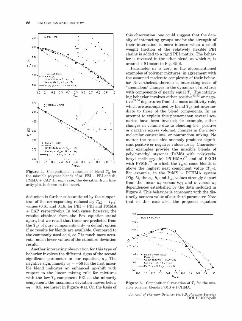
deduction is further substantiated by the compar-ison of the corresponding reduced a0/(Tg,2 � Tg,1)values (0.61 and 0.18, for PEI þ PBI and PMMAþ CAP, respectively). In both cases, however, theresults obtained from the Fox equation standapart, but we recall that these are predicted fromthe Tgs of pure components only -a default optionif no results for blends are available. Compared tothe commonly used eq 4, eq 7 is much more accu-rate; much lower values of the standard deviationresult.

Another interesting observation for this type ofbehavior involves the different signs of the secondsignificant parameter in our equation, a1. Thenegative sign, namely a1 ¼ �58 for the first misci-ble blend indicates an enhanced up-shift withrespect to the linear mixing rule for mixtureswith the low-Tg component PEI as the minoritycomponent; the maximum deviation moves belowu1 ¼ 0.5, see insert in Figure 4(a). On the basis of

this observation, one could suggest that the den-sity of interacting groups and/or the strength oftheir interaction is more intense when a smallweight fraction of the relatively flexible PEIchains is added to a rigid PBI matrix. The behav-ior is reversed in the other blend, at which a1 isaround þ 8 [insert in Fig. 4(b)].

Parameter a2 is zero in the aforementionedexamples of polymer mixtures, in agreement withthe assumed moderate complexity of their behav-ior. Nevertheless, there exist interesting cases of‘‘anomalous’’ changes in the dynamics of mixtureswith components of nearly equal Tg. The intrigu-ing behavior involves either positive42,52 or nega-tive53,54 departures from the mass-additivity rule,which are accompanied by blend Tgs not interme-diate to those of the blend components. In anattempt to explain this phenomenon several sce-narios have been invoked; for example, eitherchanges in volume due to blending (i.e., positiveor negative excess volume), changes in the inter-molecular constraints, or nonrandom mixing. Nomatter the cause, this anomaly produces signifi-cant positive or negative values for a2. Character-istic examples provide the miscible blends ofpoly(a-methyl styrene) (PaMS) with poly(cyclo-hexyl methacrylate) (PCHMA)42 and of PECHwith PVME,52 in which the Tg of some blends isabove the highest neat component value (Tg,2).For example, in the PaMS þ PCHMA system(Fig. 5), the a0, b, and kGT values strongly departfrom the linear a0 versus kGT and b versus a0dependences established by the data included inFigure 3. This behavior is consonant with the dis-tinctly nonzero value of our third parameter. Notethat in this case also, the proposed equation

Figure 4. Compositional variation of blend Tg forthe miscible polymer blends of (a) PEI þ PBI and (b)PMMA þ CAP. In each case, the deviation from line-arity plot is shown in the insert.

Figure 5. Compositional variation of Tg for the mis-cible polymer blends PaMS þ PCHMA.



provides a better fit to the experimental data -andin a wider compositional range- for the systemsconsidered here, in comparison to the two-param-eter Kwei equation or other more complex func-tions (e.g., see in ref. 42 the use of eq 5).

Mixtures with Irregular CompositionalDependence of Tg

Binary Amorphous Blends

As already stated in ‘‘Earlier Tg Versus Composi-tion Equations’’ section, the problem regardingthe need to describe peculiar compositionaldependences of the Tg in miscible binary blends,such as the alternating convex-concave (i.e., S-

shaped) parts in the plot, has been treated withmoderate success by, among others, eq 4 ofKwei,24 eq 5 of Brekner, Schneider, and Cantow,28

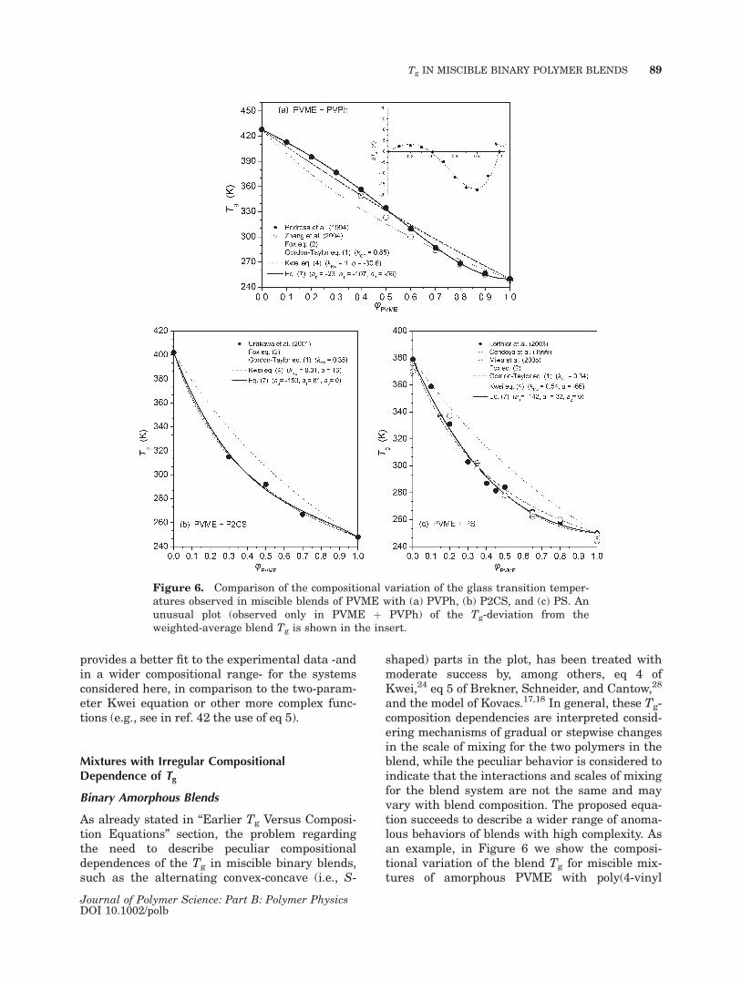
and the model of Kovacs.17,18 In general, these Tg-composition dependencies are interpreted consid-ering mechanisms of gradual or stepwise changesin the scale of mixing for the two polymers in theblend, while the peculiar behavior is considered toindicate that the interactions and scales of mixingfor the blend system are not the same and mayvary with blend composition. The proposed equa-tion succeeds to describe a wider range of anoma-lous behaviors of blends with high complexity. Asan example, in Figure 6 we show the composi-tional variation of the blend Tg for miscible mix-tures of amorphous PVME with poly(4-vinyl

Figure 6. Comparison of the compositional variation of the glass transition temper-atures observed in miscible blends of PVME with (a) PVPh, (b) P2CS, and (c) PS. Anunusual plot (observed only in PVME þ PVPh) of the Tg-deviation from theweighted-average blend Tg is shown in the insert.



phenol) [PVME þ PVPh; Fig. 6(a), P2CS (PVMEþ P2CS; Fig. 6b) and PS (PVME þ PS; Fig. 6(c)].The behavior of the first system is unique for sev-eral reasons. For this system FTIR studiesrevealed the presence of strong intermolecularhydrogen bonds between the phenolic AOHgroups in PVPh and the ether oxygen in PVME,with strength that surpasses the intrachain inter-actions between PVPh repeat units.55 Contrary tothe expected clear upshift of the blend Tg’s fromthe mass-mixing rule (see systems in the previousSection), the deviation of the blend Tg from linear-ity [insert in Fig. 6(a)] demonstrates a remarkableinversion of its sign at uPVME � 0.4. Based on theFourier-transform infrared data of Zhang et al.55

at this ‘‘critical’’ compositional threshold there is achange in the intercomponent coupling due to adifferent balancing between intermolecular andintramolecular hydrogen bonding. This modifica-tion in enthalpic characteristics of the blends islikely to induce also entropic effects that mayaccount for the observed behavior. In anotherstudy of this polymer mixture, Pedrosa et al.47

explained the peculiar shape of the Tg versus vol-ume fraction dependence using the theory ofKovacs. The theory is based on free-volume con-siderations of the glass transition phenomenon,namely free-volume additivity modified for theexcess volume of mixing VE. Two different equa-tions were used to fit the experimental data,which exhibited two well-defined regions sepa-rated by a singular point or cusp (at a critical tem-perature or, equivalently, a volume fraction). Alinear function was used for the Tg data below thecritical volume fraction of uc � 0.5 (i.e., in PVPh-rich blends). Redrawing the Tg data of Pedrosaet al.47 as function of the mass fraction of PVME[see Fig. 6(a)], the linear region transforms into acurved line with no loss of the information aboutthe existence of a ‘‘critical’’ concentration.

The behavior of the two other blends standsapart; clear negative departure from the predic-tions of the mass- and volume-additivity rules (a0� 0) and nonparabolic shape of the deviationfrom additivity plot (clearly a1 [ 0) is observed.The former advocates for very weak intercompo-nent interactions and the latter indicate dissimi-larity between the behaviors of blends with lowand high PVME contents. We should note thatthe absence of strong intermolecular interactionsbetween PVME and P2CS (or PS) and intrinsicmobility differences between the componentswere used by Urakawa et al.39 to explain theresults of their dielectric relaxation studies in

PVME þ P2CS (both components dielectricallyactive), which revealed that the components relaxindividually in their blends (i.e., two segmentalrelaxation dielectric modes are observed, despitethe miscible state of the blends).

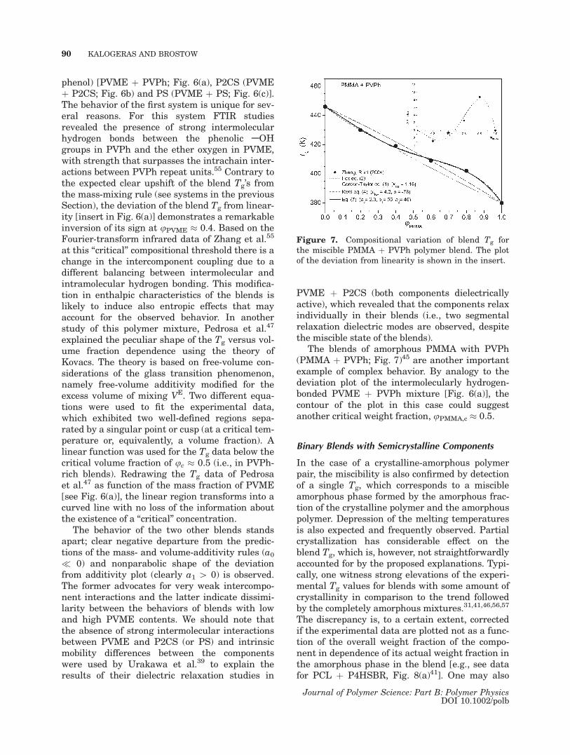
The blends of amorphous PMMA with PVPh(PMMA þ PVPh; Fig. 7)45 are another importantexample of complex behavior. By analogy to thedeviation plot of the intermolecularly hydrogen-bonded PVME þ PVPh mixture [Fig. 6(a)], thecontour of the plot in this case could suggestanother critical weight fraction, uPMMA,c � 0.5.

Binary Blends with Semicrystalline Components

In the case of a crystalline-amorphous polymerpair, the miscibility is also confirmed by detectionof a single Tg, which corresponds to a miscibleamorphous phase formed by the amorphous frac-tion of the crystalline polymer and the amorphouspolymer. Depression of the melting temperaturesis also expected and frequently observed. Partialcrystallization has considerable effect on theblend Tg, which is, however, not straightforwardlyaccounted for by the proposed explanations. Typi-cally, one witness strong elevations of the experi-mental Tg values for blends with some amount ofcrystallinity in comparison to the trend followedby the completely amorphous mixtures.31,41,46,56,57

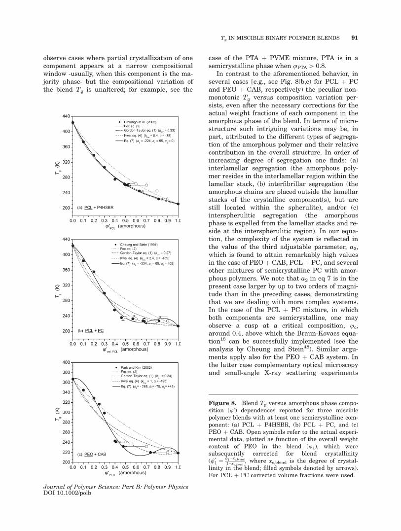
The discrepancy is, to a certain extent, correctedif the experimental data are plotted not as a func-tion of the overall weight fraction of the compo-nent in dependence of its actual weight fraction inthe amorphous phase in the blend [e.g., see datafor PCL þ P4HSBR, Fig. 8(a)41]. One may also

Figure 7. Compositional variation of blend Tg forthe miscible PMMA þ PVPh polymer blend. The plotof the deviation from linearity is shown in the insert.



observe cases where partial crystallization of onecomponent appears at a narrow compositionalwindow -usually, when this component is the ma-jority phase- but the compositional variation ofthe blend Tg is unaltered; for example, see the

case of the PTA þ PVME mixture, PTA is in asemicrystalline phase when uPTA[ 0.8.

In contrast to the aforementioned behavior, inseveral cases [e.g., see Fig. 8(b,c) for PCL þ PCand PEO þ CAB, respectively) the peculiar non-monotonic Tg versus composition variation per-sists, even after the necessary corrections for theactual weight fractions of each component in theamorphous phase of the blend. In terms of micro-structure such intriguing variations may be, inpart, attributed to the different types of segrega-tion of the amorphous polymer and their relativecontribution in the overall structure. In order ofincreasing degree of segregation one finds: (a)interlamellar segregation (the amorphous poly-mer resides in the interlamellar region within thelamellar stack, (b) interfibrillar segregation (theamorphous chains are placed outside the lamellarstacks of the crystalline component(s), but arestill located within the spherulite), and/or (c)interspherulitic segregation (the amorphousphase is expelled from the lamellar stacks and re-side at the interspherulitic region). In our equa-tion, the complexity of the system is reflected inthe value of the third adjustable parameter, a2,which is found to attain remarkably high valuesin the case of PEO þ CAB, PCL þ PC, and severalother mixtures of semicrystalline PC with amor-phous polymers. We note that a2 in eq 7 is in thepresent case larger by up to two orders of magni-tude than in the preceding cases, demonstratingthat we are dealing with more complex systems.In the case of the PCL þ PC mixture, in whichboth components are semicrystalline, one mayobserve a cusp at a critical composition, uc,around 0.4, above which the Braun-Kovacs equa-tion18 can be successfully implemented (see theanalysis by Cheung and Stein48). Similar argu-ments apply also for the PEO þ CAB system. Inthe latter case complementary optical microscopyand small-angle X-ray scattering experiments

Figure 8. Blend Tg versus amorphous phase compo-sition (u0) dependences reported for three misciblepolymer blends with at least one semicrystalline com-ponent: (a) PCL þ P4HSBR, (b) PCL þ PC, and (c)PEO þ CAB. Open symbols refer to the actual experi-mental data, plotted as function of the overall weightcontent of PEO in the blend (u1), which weresubsequently corrected for blend crystallinity(/0

1 ¼ /1�xc;blend1�xc;blend

, where xc,blend is the degree of crystal-linity in the blend; filled symbols denoted by arrows).For PCL þ PC corrected volume fractions were used.



verified the complexity of the blend revealing thatat low CAB contents the chains of the amorphouscomponent are incorporated into interlamellarregions and commence to segregate to the interfi-brillar region with increase of its weight fraction.46

Analysis of Miscible Blends with Two Tgs

There are binary polymer blends presenting twoconcentration dependent glass transitions evenwhen structural analysis points to a single-phasematerial. In such cases, thermodynamicallydriven concentration fluctuations, componentintrinsic mobility differences, or self-concentra-tion effects induced by chain connectivity, havebeen considered mainly.5,58 A model developed byLM5 considers self-concentration effect; becauseof chain connectedness the average number ofnearest neighbors of a given segment whichbelong to the same component is larger than thenumber of neighboring segments of the other com-ponent. The effective local concentration ueff,i

sensed by each polymer segment is therefore rep-resented by

ueff ;1 ¼ us;1 þ 1� us;1

� �u1 (10a)

ueff ;2 ¼ us;2 þ 1� us;2

� �1� u1ð Þ (10b)

Here, us,i is the ‘‘self-concentration’’ of the con-sidered polymer segment (i ¼ 1, 2). In the LMmodel, the length-scale related to the monomericfriction factor is regarded of the same order as theKuhn length lk defined as C!l, where C! is thecharacteristic ratio, and l is the length of the aver-age backbone bond. One assumes that relaxationof the Kuhn segment is influenced by the concen-tration of segments within a volume V ¼ gl3k (g isa geometric factor). Parameter us for each blendcomponent is calculated as the volume fractionoccupied by the Kuhn length inside V:

us ¼C1M0

kqNAVV(11)

where M0 is the molar mass of the repeat unit,NAV is the Avogadro number, k is the number ofbackbone bonds per repeat unit, and q is the massdensity.

Typically, the theoretic self-concentration ofeach component (between 0.1 and 0.6, based oncalculations using eq 11) is initially used for esti-mating effective local concentrations (eq 10). Theeffective Tg of each component in the blend is

then evaluated using the Fox equation, with theassumption that Teff

g (u) ¼ Tg(u)|u¼ueff, and com-

pared with the experiment (e.g.,5,6,9). Alternatively,us can be incorporated as an adjustable parameterin eq 2; experimental Teff

g (u) data are now fitted toobtain us estimates, compared then with predic-tions from eq 11. When the Fox equation seemsunsuitable for describing the experimental Tg,av(u)or Teff

g (u) dependencies, alternative fitting equa-tions have been used such as eq 112,14 or eq 5.59

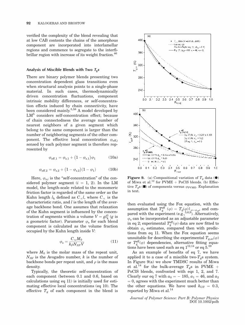
As an example of benefits of eq 7, we haveapplied it to a case of a miscible two-Tgs system.In Figure 9(a) we show TMDSC results of Miwaet al.14 for the bulk-average Tgs in PVME þPoClS blends, confronted with eqs 1, 2, and 7.Clearly our eq 7 with a0 ¼ � 185, a1 ¼ 46, and a2¼ 0, agrees with the experiment much better thanthe other equations. We have used kGT ¼ 0.3,reported by Miwa et al.14

Figure 9. (a) Compositional variation of Tg data (l)of Miwa et al.12 for PVME þ PoClS blends. (b) Effec-tive Tgs (n) of components versus uPVME. Explanationin text.



Using the aforementioned ai values in eq 7,and substituting ui by ueff,i, we have calculatedthe blend effective Tgs of each component[Teff

g;PVME(u) and Teffg;PoClS(u)] and the corresponding

self-concentrations. In Figure 9(b) we show assolid curves the results of using eq 7 with thesame a0 and a1 values as in Figure 9(a) and us asfitting parameters. We include in Figure 9(b) pre-dictions from eq 7 using the us estimates of Miwaet al.12 (dashed curves) and also GT (eq 1) fitsreported by these authors (dotted lines). Figure9(b) illustrates the success of our equation also insuch a case.

In the LM model, the lower Tg component typi-cally has a smaller persistence length, whichleads to a larger self-concentration.5 This condi-tion was assumed to be obeyed in PVME þ PoClSblends; hence Miwa et al.14 used values of us,1 ¼0.25 taken from Lodge and Mc Leish5 and us,2 ¼0.22 taken from Leroy et al.59 for PVME andPoClS, respectively, assuming g ¼ 1. Our eq 7reveals a reverse trend; us,1 ¼ 0.153 � 0.005, us,2

¼ 0.203 � 0.005, with us,1/us,2 ¼ 0.75. Ample ex-perimental evidence suggests that us is matrix-dependent and corrections for the geometric factorare required.9,60,61 In our analysis the geometricfactor for PVME is g1 ¼ 1.634 and g2 ¼ 0.957 for

PoClS; the correction for the low-Tg blend compo-nent is too high to be ignored. Even within theassumptions of the LM model, a length scale is ofthe order of Kuhn length but not necessarilyequal to that length. Further support for the va-lidity of the observed inequality (us,1/us,2 \ 1) isprovided by recent results for PCL þ PC (Herreraet al.6 us,1/us,2 ¼ 0.41) and PEO þ PMMA (Lodgeet al.7 us,1/us,2 ¼ 0.92). In particular, Herreraet al.6 analyzed their dielectric Tg results using asimilar procedure and eq 5. This resulted in a bet-ter fit than given by eq 2, yielding us,1 ¼ 0.20 forPCL and us,2 ¼ 0.49 for PC. In the frame of theLM model us,2 ¼ 0.05, while us,2 ¼ 0.49 is neededto achieve a reasonable agreement with the exper-imental data, a nearly 10-fold adjustment. Similardiscrepancies have been reported by Urakawaet al.61 for PEO þ PVAc blends. Apparently in theLM model strong intermolecular interactions areunderestimated.59,61

CONCLUDING REMARKS

One can think of a hierarchy of complexity of pol-ymeric systems. In ‘‘well behaving’’ misciblebinary systems the simple mass-additivity or

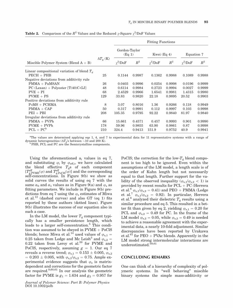
Table 2. Comparison of the R2 Values and the Reduced v-Square v2/DoF Values

Miscible Polymer System (Blend A þ B)DTg (K)

Fitting Functions

Gordon-Taylor(Eq 1) Kwei (Eq 4) Equation 7

v2/DoF R2 v2/DoF R2 v2/DoF R2

Linear compositional variation of blend Tg

PECH þ PHB 25 0.1144 0.9987 0.1362 0.9988 0.1089 0.9988Negative deviations from additivity rule

PMMA þ PaMSAN 26 0.0403 0.9996 0.0254 0.9998 0.0196 0.9999PC (Lexan) þ Polyester [T(40)C-GJ] 48 0.6114 0.9984 0.2723 0.9994 0.0027 0.9999PVE þ PI 68 2.4529 0.9966 1.6541 0.9981 1.4315 0.9980PVME þ PS 129 33.83 0.9820 22.18 0.9895 20.52 0.9903

Positive deviations from additivity rulePaMS þ PCHMA 8 3.07 0.8016 1.36 0.9266 0.118 0.9949PMMA þ CAP 50 0.317 0.9991 0.112 0.9997 0.103 0.9998PEI þ PBI 208 105.35 0.9795 92.22 0.9840 81.97 0.9840

Irregular deviations from additivity rulePMMA þ PVPh 66 15.661 0.4571 0.457 0.9993 0.901 0.9990PVME þ PVPh 178 59.96 0.9855 63.90 0.9861 0.87 0.9998PCL þ PCb 210 324.4 0.9413 151.9 0.9752 40.9 0.9941

aThe values are determined applying eqs 1, 4, and 7 to experimental data for 11 representative systems with a range ofdynamic heterogeneities (DTg’s between �10 and 200 K).

b PHB, PCL and PC are the Semicrystalline components.



volume-additivity rules such as the Fox equation(eq 2) might be sufficient. With increasing systemcomplexity, GT equation (eq 1), or Jenckel-Heuschequation (eq 3), or Kwei equation (eq 4), the free-volume approach of Kovacs, and finally our Tg(u)formula (7) can be used. The last equation hasbeen confronted with experimental data for sev-eral systems and has been found to describe welleven very complicated dependences of the Tg oncomposition. Better fit to the experimental data isseen in Table 2 in terms of the coefficient of deter-mination (R-square) values and the reduced v-square values (v2/DoF, DoF ¼ number of thedegrees of freedom) obtained using eqs 1, 4, and 7.The only possible exception can be cusp-contain-ing systems when the Braun-Kovacs equation18

serves better. Otherwise our eq 7 describes alltypes of behavior in miscible polymer blendsregardless of their complexity. Actually, the newequation alone can provide a measure of the sys-tem complexity. The number of the ai parametersneeded to reproduce well the experimental dataand the relative magnitude of each parameterserve for this purpose. In very simple systems inwhich Tg,dev can be well represented by a parab-ola, only one parameter a0 is sufficient.

Comparisons with eqs 3 and 4 show how our a0provides a measure of the strength of the inter-component interactions in miscible binary poly-mer blends. Equations 8 and 9 should not be sur-prising. As demonstrated by Flory in a long seriesof papers, those interactions determine the behav-ior of binary and other multicomponent sys-tems.62 Thus, connections between different pa-rameters that are measures of that strength areexpected. With increasing system complexity thesecond parameter a1 acquires higher absolute val-ues, with sign and magnitude that may be used topredict variations in the degree of ‘‘connectivity’’or the attraction between the components withchanges in the blend composition. The highestcomplexity is reflected in high values of the thirdparameter a2, which reflects the presence of inter-esting structural phenomena. Note that mereinspection of the chemical composition and struc-ture of each component in the mixture does notrender possible to predict which class this blendwill fall to. Blending-induced changes in the mac-roconformation and spatial organization of thepolymer chains, different, at various composi-tions, degrees of shielding of hydrogen-bondingactive chemical groups by other chain segments,and crystallization processes that become activeat narrow compositional windows and show

strongly composition-dependent kinetics, aresome of the factors that preclude a straightfor-ward categorization of the blends.

Witold Brostow acknowledges discussions with the latePaul J. Flory at Stanford on structures and thermody-namic properties of polymeric systems. A partial finan-cial support has been provided by the Robert A. WelchFoundation, Houston (Grant B-1203).

REFERENCES AND NOTES

1. Saiter, J.-M.; Negahban, M.; dos Santos Claro, P.;Delabare, P.; Garda, M.-R. J Mater Ed 2008, 30,51–95; (b) Mano, J. F. J Mater Ed 2003, 25, 151–164; (c) Bilyeu, B.; Brostow, W.; Menard, K. P. JMater Ed 2000, 22, 107–130; (d) Privalko, V. P. JMater Ed 1998, 20, 57, 373–394.

2. Menczel, J. D.; Prime, R. B., Eds.; Thermal Anal-ysis of Polymers, Fundamentals and Applications;Wiley: New York, 2009.

3. McKenna, G. B.; Simon, S. L. In Handbook ofThermal Analysis and Calorimetry, Applicationsto Polymers and Plastics; Cheng, S. Z. D., Ed.;Elsevier: Amsterdam, 2002; Vol. 3, Chapter 2, pp49–110.

4. Vassilikou-Dova, A.; Kalogeras, I. M. Dielectric Anal-ysis (DEA) In Thermal Analysis of Polymers, Funda-mentals and Applications; Menczel, J. D.; Prime, R.B., Eds.; Wiley: New York, 2009; Chapter 6.

5. Lodge, T. P.; McLeish, T. C. B. Macromolecules2000, 33, 5278–5284.

6. Herrera, D.; Zamora, J.-C.; Bello, A.; Grimau, M.;Laredo, E.; Muller, A. J.; Lodge, T. P. Macromole-cules 2005, 38, 5109–5117.

7. Lodge, T. P.; Wood, E. R.; Haley, J. C. J Polym SciPart B: Polym Phys 2006, 44, 756–763.

8. Sakaguchi, T.; Taniguchi, N.; Urakawa, O.; Ada-chi, K. Macromolecules 2005, 38, 422–428.

9. Gaikwad, A. N.; Wood, E. R.; Ngai, T.; Lodge, T.P. Macromolecules 2008, 41, 2502–2508.

10. Lorthioir, C.; Alegrıa, A.; Colmenero, J. Phys RevE 2003, 68, 031805.

11. Leroy, E.; Alegrıa, A.; Colmenero, J. Macromole-cules 2002, 35, 5587–5590.

12. Miwa, Y.; Usami, K.; Yamamoto, K.; Sakaguchi,M.; Sakai, M.; Shimada, S. Macromolecules 2005,38, 2355–2361.

13. Haley, C. J.; Lodge, T. P.; He, Y.; Ediger, M. D.;von Meerwall, E. D.; Mijovic, J. Macromolecules2003, 36, 6142–6151.

14. Miwa, Y.; Sugino, Y.; Yamamoto, K.; Tanabe, T.;Sakaguchi, M.; Sakai, M.; Shimada, S. Macromo-lecules 2004, 37, 6061–6068.

15. Hoffmann, S.;Willner, L.; Richter, D.; Arbe, A.; Colme-nero, J.; Farago, B. PhysRevLett 2000, 85, 772–775.



16. Schneider, H. A. J Res Natl Inst Stand Technol1997, 102, 229–248.

17. Kovacs, A. J. Adv Polym Sci 1963, 3, 394.18. Braun, G.; Kovacs, A. J. In Physics of Non-Crys-

talline Solids; Prim, J. A., Ed.; North-Holland:Amsterdam, 1965.

19. Utracki, L. A. Adv Polym Technol 1985, 5, 33–39.20. Couchman, P. R.; Karasz, F. E. Macromolecules

1978, 11, 117–119.21. Jenckel, E.; Heusch, R. Kolloid Z 1953, 130, 89.22. Fox, T. G. Bull Am Phys Soc 1956, 1, 123.23. Gordon,M.; Taylor, J. S. J Appl Chem 1952, 2, 493.24. Kwei, T. K. J Polym Sci Lett 1984, 22, 307.25. DiMarzio, E. A. Polymer 1990, 31, 2294–2298.26. Simha, R.; Boyer, R. F. J Chem Phys 1962, 37,

1003–1007.27. Kanig, G. Kolloid Z Z Polym 1963, 190, 1.28. Brekner, M.-J.; Schneider, A.; Cantow, H.-J. Macromol

Chem 1988, 189, 2085; (b) Brekner, M.-J.; Schneider,A.; Cantow,H.-J. Polymer 1988, 78, 78–85.

29. Brostow, W.; Chiu, R.; Kalogeras, I. M.; Vassili-kou-Dova, A. Mater Lett 2008, 62, 3152–3155.

30. Dubini Paglia, E.; Beltrame, P. L.; Canetti, M.;Seves, A.; Marcadalli, B.; Martuscelli, E. Polymer1993, 34, 996–1001.

31. Chiang, W.-J.; Woo, E. M. J Polym Sci Part B:Polym Phys 2007, 45, 2899–2911.

32. Madbouly, S. A. Polym J 2002, 34, 515–522.33. Liang, H.; Xie, F.; Chen, B.; Guo, F.; Jin, Z.; Luo,

F. J Appl Polym Sci 2008, 107, 431–437.34. Yang, H.; Yetter, W. Polymer 1994, 35, 2417–2421.35. Hirose, Y.; Urakawa, O.; Adachi, K. J Polym Sci

Part B Polym Phys 2004, 42, 4084–4094.36. Song,M.; Long, F. EurPolymMater 1991, 27, 983–986.37. de Araujo, M. A.; Stadler, R.; Cantow, H. J. Poly-

mer 1988, 29, 2235–2243.38. Prest, W. N., Jr.; Porter, R. S. J Polym Sci Part A-

2: Polym Phys 1972, 10, 1639–1655.39. Urakawa, O.; Fuse, Y.; Hori, H.; Tran-Cong, Q.;

Yano, O. Polymer 2001, 42, 765–773.40. Madbouly, S. A.; Abdou, N. Y.; Mansour, A. A.

Macromol Chem Phys 2006, 207, 978–986.41. Prolongo, M. G.; Salom, C.; Masegosa, R. M. Poly-

mer 2002, 43, 93–102.42. Roland, C. M.; Casalini, R. Macromolecules 2007,

40, 3631–3639.

43. Rao, V.; Ashokan, P. V.; Shridhar, M. H. Polymer1999, 40, 7167–7171.

44. Leung, L.; Williams, D. J.; Karasz, F. E.; Mac-Knight, W. J Polym Bull 1986, 16, 457–464.

45. Zhang, S.; Runt, J. J Polym Sci Part B: PolymPhys 2004, 42, 3405–3415.

46. Park, M. S.; Kim, J. K. J Polym Sci Part B: PolymPhys 2002, 40, 1673–1681.

47. Pedrosa, P.; Pomposo, J. A.; Calahorra, E.; Corta-zar, M. Macromolecules 1994, 27, 102–109.

48. Cheung, Y. W.; Stein, R. S. Macromolecules 1994,27, 2512–2519.

49. (a) Zawada, J. A.; Ylitalo, C. M.; Fuller, G. G.;Colby, R. H.; Long, T. E. Macromolecules 1992,25, 2896–2902; (b) Li, X.; Hsu, S. L. J Polym SciPart B: Polym Phys 1984, 22, 1331–1342.

50. Chiu, F.-C.; Min, K. Polym Int 2000, 49, 223–234.

51. Cendoya, I.; Alegria, A.; Alberti, J. M.; Colmenero,J.; Grimm, H.; Richter, D.; Frick, B. Macromole-cules 1999, 32, 4065–4078.

52. Alegria, A.; Telleria, I.; Colmenero, J. J Non-CrystSolids 1994, 172–174, 961–965.

53. Roland, C. M. Macromolecules 1995, 28, 3463–3467.

54. Casalini, R.; Santangelo, P. G.; Roland, C. M. JPhys Chem B 2002, 106, 11492–11494.

55. Zhang, S. H.; Jin, X.; Painter, P. C.; Runt, J. Poly-mer 2004, 45, 3933–3942.

56. Kalogeras, I. M.; Vassilikou-Dova, A.; Christakis,I.; Pietkiewicz, D.; Brostow, W. Macromol ChemPhys 2006, 207, 879–892.

57. Kalogeras, I. M.; Stathopoulos, A.; Vassilikou-Dova, A.; Brostow, W. J Phys Chem B 2007, 111,2774–2782.

58. Kumar, S. K.; Shenogin, S.; Colby, R. H. Macro-molecules 2007, 40, 5759–5766.

59. Leroy, E.; Alegrıa, A.; Colmenero, J. Macromole-cules 2003, 36, 7280–7288.

60. Lutz, T. R.; He, Y.; Ediger, M. D.; Pitsikalis, M.;Hadjichristidis, N. Macromolecules 2004, 37,6440–6448.

61. Urakawa, O.; Ujii, T.; Adachi, K. J Non-Cryst Sol-ids 2006, 352, 5042–5049.

62. Flory, P. J. Selected Works; Stanford UniversityPress: Stanford, 1985; Vol. 3.



Documents

Glass transition temperatures in binary polymer blends