Embed Size (px)
Citation preview

This article was downloaded by:[Dhashi][Dhashi]
On: 30 April 2007Access Details: [subscription number 772812412]Publisher: Taylor & FrancisInforma Ltd Registered in England and Wales Registered Number: 1072954Registered office: Mortimer House, 37-41 Mortimer Street, London W1T 3JH, UK
Crystallography ReviewsPublication details, including instructions for authors and subscription information:http://www.informaworld.com/smpp/title~content=t713456298
General concepts underlying ACORN, a computerprogram for the solution of protein structuresJ. Foadi
To cite this Article: J. Foadi , 'General concepts underlying ACORN, a computerprogram for the solution of protein structures', Crystallography Reviews, 9:1, 43 - 65To link to this article: DOI: 10.1080/0889311031000069777URL: http://dx.doi.org/10.1080/0889311031000069777
PLEASE SCROLL DOWN FOR ARTICLE
Full terms and conditions of use: http://www.informaworld.com/terms-and-conditions-of-access.pdf
This article maybe used for research, teaching and private study purposes. Any substantial or systematic reproduction,re-distribution, re-selling, loan or sub-licensing, systematic supply or distribution in any form to anyone is expresslyforbidden.
The publisher does not give any warranty express or implied or make any representation that the contents will becomplete or accurate or up to date. The accuracy of any instructions, formulae and drug doses should beindependently verified with primary sources. The publisher shall not be liable for any loss, actions, claims, proceedings,demand or costs or damages whatsoever or howsoever caused arising directly or indirectly in connection with orarising out of the use of this material.
© Taylor and Francis 2007
Dow
nloa
ded
By: [
Dha
shi]
At: 1
0:02
30
April
200
7
Crystallography Reviews, 2003, Vol. 9, No. 1, pp. 43–65
GENERAL CONCEPTS UNDERLYING ACORN,
A COMPUTER PROGRAM FOR THE SOLUTION OF
PROTEIN STRUCTURES
J. FOADI
(Received 10 September 2002)
ACORN has been shown to be a successful program for the solution of small and medium-size protein struc-tures, when data at atomic resolution or better are available.
At the heart of ACORN lies a density modification method called DDM (Dynamic Density Modification).DDM operates on any density map containing a minimum of information. Its action is to progressivelyenhance positive features of the map and to reduce, at the same time, undesired noise and bias towardsvery small values. This is indeed a feature claimed by other density modification procedures. The effectivenessof the procedure arises from the fact that the shape of DDM’s modification curve is one of a restricted classof functions, whose properties will be described. The importance of a proper weighting scheme will also beconsidered.
Tests on a few structures will help to clarify the theoretical concepts involved as well as to make clear thepotential applications and limits of the program.
Keywords: Solution methods; High resolution; Phase correction; Density modification; Protein crystallo-graphy; High-throughput structure determination
CONTENTS
1. INTRODUCTION 44
2. THE STRUCTURE OF ACORN 44
3. APPLICATIONS WITH TEST STRUCTURES 49
4. THE EVOLUTION OF THE ELECTRON DENSITYDURING PHASE REFINEMENT 51
5. PHASE CORRECTION AND DENSITY MODIFICATION 56
6. DDM AS A NEW KIND OF PHASE CORRECTION 59
7. CONCLUSIONS 62
References 64
Email: [email protected]
ISSN 0889-311X print: ISSN 1476-3508 online � 2003 Taylor & Francis Ltd
DOI: 10.1080/0889311031000069777
Dow
nloa
ded
By: [
Dha
shi]
At: 1
0:02
30
April
200
7
1. INTRODUCTION
The solution of protein structures has been traditionally carried out by dividing theproblem into three logically separate parts. The first consists of the production of aninitial set of imperfect phases. They can be generated using any suitable physicalmethod, such as MIR or MAD techniques, or a non-physical method, as in molecularreplacement or direct methods. A density map calculated using observed amplitudesand these phases often shows very little of the whole structure. In the second part,the original phases are improved by what are generally known as density modificationprocedures. They constrain the electron density to obey known general or specificcharacteristics of a protein structure. These constraints force phases to move towardvalues which are statistically closer to the correct ones. Once the density modificationhas converged the corresponding density map should exhibit most of the structure.The third part deals with the refinement of all the model parameters, i.e. the atomiccoordinates and thermal factors.
The computer program ACORN (Foadi et al., 2000; Jia-xing, 2001), which is part ofthe CCP4 suite of programs (Collaborative Computational Project, 1994), can performparts one and two. It is in fact a program for the solution and phase refinement of pro-tein structures.
The approach which has led to the present form of ACORN was semi-empirical.General ideas inherited from experience in direct methods and in real-space methods(Refaat et al., 1996) have been systematically adapted by trials carried out on a fewtest structures. The feedback obtained from these was in turn used to modify part ofthe theory. Various parameters and weighting schemes have been adjusted to attainthe most accurate and fastest phase refinement. The program has proved to berobust and effective, but several points of its theoretical framework are not very wellunderstood. Why is ACORN so effective? Is there anything special in the specificform of its adopted density modification? Can ACORN be improved in order towork at resolutions below 1.2 A?
In this paper we will try to give an answer to the above questions. First, a short out-line of the program will be presented. Then some applications on test structures willintroduce the reader to its limits and potentialities. Next, we will focus on DynamicDensity Modification (DDM), the density modification procedure which constitutesthe heart of ACORN. It will be shown that this procedure could be seen as a naturalevolution of a line of research initiated in the late sixties (Hoppe and Gassmann,1968). We will appreciate accordingly that the shape of DDM’s modification curveis one of a restricted class of functions, whose properties will be described. Thiswill enable us to explain why DDM is so effective in the refinement of phases. Itspower to refine, though, is gradually lost as the resolution gets lower. The likelyreason behind this limit can be seen as the result of a loss of atomicity in the electrondensity.
2. THE STRUCTURE OF ACORN
In its present version ACORN is made up of two modules, ACORN-MR and ACORN-PHASE. ACORN-MR is essentially a molecular replacement procedure which usescorrelation coefficients between observed and calculated normalized structure factor
44 J. FOADI
Dow
nloa
ded
By: [
Dha
shi]
At: 1
0:02
30
April
200
7
magnitudes as objective functions (Kissinger et al., 1999). The main task for ACORN-MR is to provide initial phases for use in either ACORN-PHASE or for any other pro-gram dealing with the extension and/or refinement of phases. ACORN-MR isexplained in detail in the original ACORN paper (Foadi et al., 2000) and in Dodson(2002), and will not be dealt with here any further.
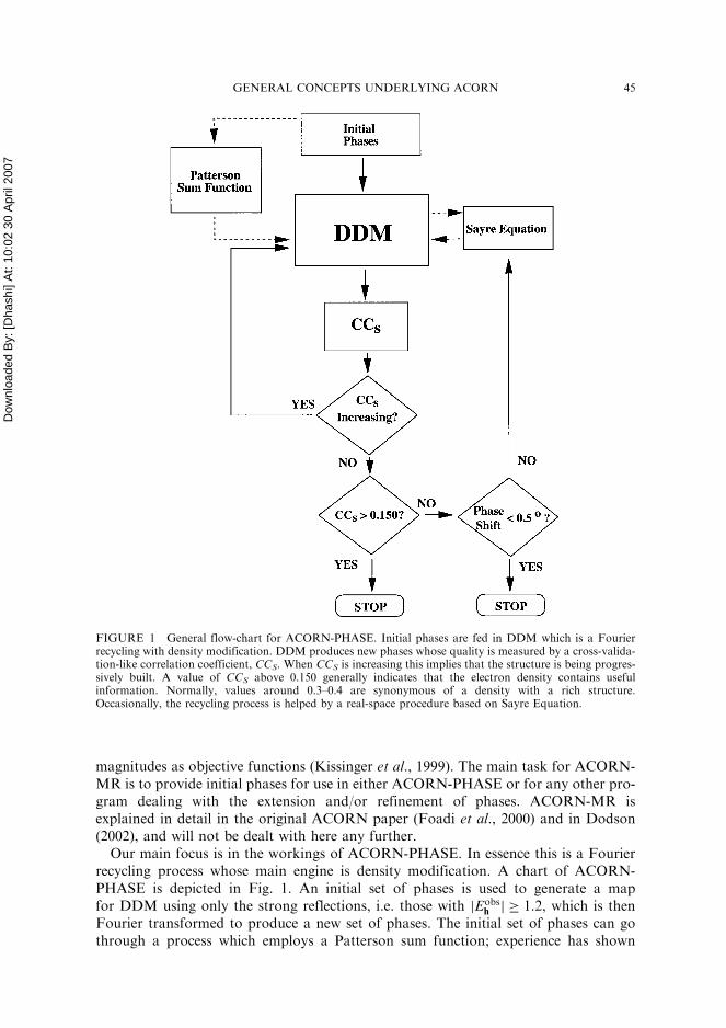
Our main focus is in the workings of ACORN-PHASE. In essence this is a Fourierrecycling process whose main engine is density modification. A chart of ACORN-PHASE is depicted in Fig. 1. An initial set of phases is used to generate a mapfor DDM using only the strong reflections, i.e. those with jEobs
h j � 1:2, which is thenFourier transformed to produce a new set of phases. The initial set of phases can gothrough a process which employs a Patterson sum function; experience has shown
FIGURE 1 General flow-chart for ACORN-PHASE. Initial phases are fed in DDM which is a Fourierrecycling with density modification. DDM produces new phases whose quality is measured by a cross-valida-tion-like correlation coefficient, CCS. When CCS is increasing this implies that the structure is being progres-sively built. A value of CCS above 0.150 generally indicates that the electron density contains usefulinformation. Normally, values around 0.3–0.4 are synonymous of a density with a rich structure.Occasionally, the recycling process is helped by a real-space procedure based on Sayre Equation.
GENERAL CONCEPTS UNDERLYING ACORN 45
Dow
nloa
ded
By: [
Dha
shi]
At: 1
0:02
30
April
200
7
that this can bring in some benefit. The quality of the new set of phases derived byDDM is judged by a correlation coefficient, CCS, defined as:
CCS �hjEobs
h jjEcalh ji � hjEobs
h jihjEcalh jiffiffiffiffiffiffiffiffiffiffiffiffiffiffiffiffiffiffiffiffiffiffiffiffiffiffiffiffiffiffiffiffiffiffiffiffiffiffiffiffi
hjEobsh j2i � hjEobs
h ji2q ffiffiffiffiffiffiffiffiffiffiffiffiffiffiffiffiffiffiffiffiffiffiffiffiffiffiffiffiffiffiffiffiffiffiffiffiffiffi
hjEcalh j2i � hjEcal
h ji2q ð1Þ
where jEobsh j is the observed amplitude, jEcal
h j is the amplitude derived from the inverse-Fourier transform of a modified density map, and all averages are taken over themedium reflections, i.e. those having 0:1 jEobs
h j 1:2. If CCS is increasing, a newcycle of DDM, to further refine the new set of phases, can be performed. The cyclingprocess will end when CCS stops increasing or the magnitude of the average phasechange between two consecutive cycles is less than 0.5 degrees. CCS greater than0.150 usually indicates a successful refinement. Sometimes the process gets trapped inloops where CCS does not increase and the average phase shift is still large. In suchcases the whole set of phases is shaken up by going through one cycle of a real-spaceversion of the Sayre equation. While this specific algorithm does not itself correct thephases significantly, it allows the successive cycles to travel along a new route in thephase space.
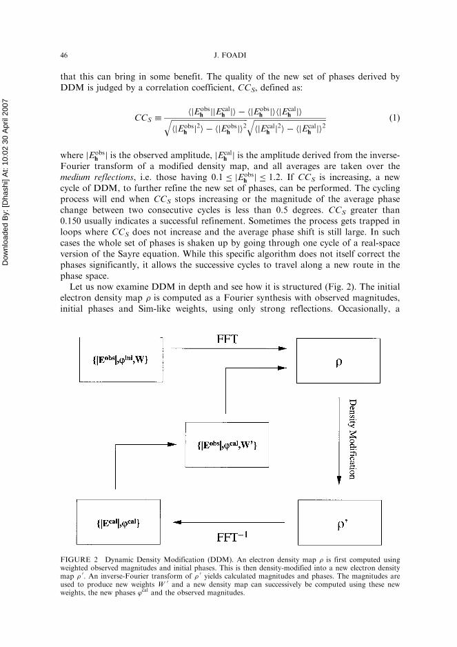
Let us now examine DDM in depth and see how it is structured (Fig. 2). The initialelectron density map � is computed as a Fourier synthesis with observed magnitudes,initial phases and Sim-like weights, using only strong reflections. Occasionally, a
FIGURE 2 Dynamic Density Modification (DDM). An electron density map � is first computed usingweighted observed magnitudes and initial phases. This is then density-modified into a new electron densitymap � 0. An inverse-Fourier transform of � 0 yields calculated magnitudes and phases. The magnitudes areused to produce new weights W 0 and a new density map can successively be computed using these newweights, the new phases ’cal and the observed magnitudes.
46 J. FOADI
Dow
nloa
ded
By: [
Dha
shi]
At: 1
0:02
30
April
200
7
small number of weak reflections, with jEobsh j < 0:1, is included in the recycling through
the Sayre-equation process. The medium reflections play no active role in the refine-ment and are thence used as a cross-validation tool, the parameter CCS, to monitorthe refinement.
Weights are based on Sim’s theory (Sim, 1959, 1960). In the original Sim weightingscheme, a weight is computed as:
Wh ¼I1ð�hÞ
I0ð�hÞ; �h �
2jFobsh jjF cal
h jP0
h
ð2Þ
where I0 and I1 are the modified Bessel functions of zeroth and first order, F calh is the
structure factor of the model atoms, andP0
h is the sum of scattering factors for all theatoms in the unit cell which are not part of the initial model. Sim’s weights are theor-etically only valid when the position of the fragment is known with infinite accuracy.When errors in the positions of the atoms arise, Eq. (2) has to be corrected with alter-native expressions which take the probabilities associated with these errors into account(Read, 1986; Srinivasan and Ramachandran, 1965; Srinivasan, 1966). In ACORN,weights are given by:
Wh ¼ tanhjEobs
h jjEcal0
h j
2
ffiffiffiffiffiffiffiP0
h
q0B@
1CA ð3Þ
where, this time,P0
h is the mean square of the values of jEcal0
h j, jEcalh j derives from the
back transform of each modified density map, and jEcal0
h j is jEcalh j scaled to jEobs
h j inshells of reciprocal space (shells of resolution). In this way, the problem of estimatingthe number of known atoms in each cycle is avoided. The choice of tanh rather thanI1=I0 is just a matter of taste; for most of the � range these two functions have thesame behaviour, provided that a proper scale factor is used.
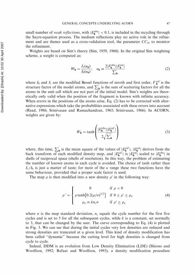
The map � is then modified into a new density �0 in the following way:
� 0 ¼
0 if � < 0
� tanh 0:2 �=�ð Þ3=2
�if 0 �0 �u
�u � knc� if �0 � �u
8>><>>: ð4Þ
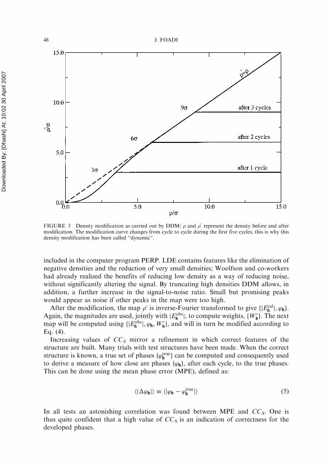
where � is the map standard deviation, nc equals the cycle number for the first fivecycles and is set to 5 for all the subsequent cycles, while k is a constant, set normallyto 3, that can be changed by the user. The curve corresponding to Eq. (4) is plottedin Fig. 3. We can see that during the initial cycles very low densities are reduced andstrong densities are truncated at a given level. This kind of density modification hasbeen called ‘‘dynamic’’ because the cutting level for high densities is changed fromcycle to cycle.
Indeed, DDM is an evolution from Low Density Elimination (LDE) (Shiono andWoolfson, 1992; Refaat and Woolfson, 1993), a density modification procedure
GENERAL CONCEPTS UNDERLYING ACORN 47
Dow
nloa
ded
By: [
Dha
shi]
At: 1
0:02
30
April
200
7
included in the computer program PERP. LDE contains features like the elimination ofnegative densities and the reduction of very small densities; Woolfson and co-workershad already realized the benefits of reducing low density as a way of reducing noise,without significantly altering the signal. By truncating high densities DDM allows, inaddition, a further increase in the signal-to-noise ratio. Small but promising peakswould appear as noise if other peaks in the map were too high.
After the modification, the map �0 is inverse-Fourier transformed to give fjEcalh j,’hg.
Again, the magnitudes are used, jointly with jEobsh j, to compute weights, fW 0
hg. The nextmap will be computed using fjEobs
h j, ’h,W0hg, and will in turn be modified according to
Eq. (4).Increasing values of CCS mirror a refinement in which correct features of the
structure are built. Many trials with test structures have been made. When the correctstructure is known, a true set of phases f’true
h g can be computed and consequently usedto derive a measure of how close are phases f’hg, after each cycle, to the true phases.This can be done using the mean phase error (MPE), defined as:
hj�’hji � hj’h � ’trueh ji ð5Þ
In all tests an astonishing correlation was found between MPE and CCS. One isthus quite confident that a high value of CCS is an indication of correctness for thedeveloped phases.
FIGURE 3 Density modification as carried out by DDM; � and �0 represent the density before and aftermodification. The modification curve changes from cycle to cycle during the first five cycles; this is why thisdensity modification has been called ‘‘dynamic’’.
48 J. FOADI
Dow
nloa
ded
By: [
Dha
shi]
At: 1
0:02
30
April
200
7
3. APPLICATIONS WITH TEST STRUCTURES
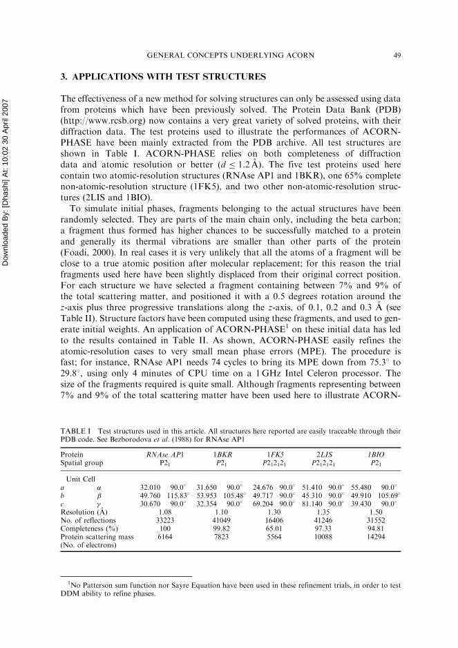
The effectiveness of a new method for solving structures can only be assessed using datafrom proteins which have been previously solved. The Protein Data Bank (PDB)(http://www.rcsb.org) now contains a very great variety of solved proteins, with theirdiffraction data. The test proteins used to illustrate the performances of ACORN-PHASE have been mainly extracted from the PDB archive. All test structures areshown in Table I. ACORN-PHASE relies on both completeness of diffractiondata and atomic resolution or better (d 1:2 A). The five test proteins used herecontain two atomic-resolution structures (RNAse AP1 and 1BKR), one 65% completenon-atomic-resolution structure (1FK5), and two other non-atomic-resolution struc-tures (2LIS and 1BIO).
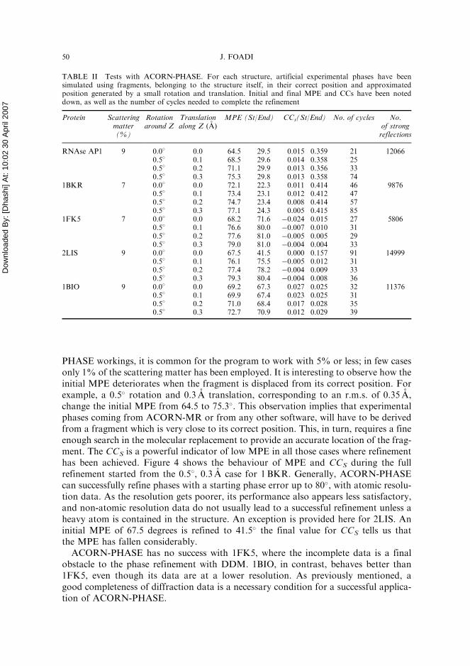
To simulate initial phases, fragments belonging to the actual structures have beenrandomly selected. They are parts of the main chain only, including the beta carbon;a fragment thus formed has higher chances to be successfully matched to a proteinand generally its thermal vibrations are smaller than other parts of the protein(Foadi, 2000). In real cases it is very unlikely that all the atoms of a fragment will beclose to a true atomic position after molecular replacement; for this reason the trialfragments used here have been slightly displaced from their original correct position.For each structure we have selected a fragment containing between 7% and 9% ofthe total scattering matter, and positioned it with a 0.5 degrees rotation around thez-axis plus three progressive translations along the z-axis, of 0.1, 0.2 and 0.3 A (seeTable II). Structure factors have been computed using these fragments, and used to gen-erate initial weights. An application of ACORN-PHASE1 on these initial data has ledto the results contained in Table II. As shown, ACORN-PHASE easily refines theatomic-resolution cases to very small mean phase errors (MPE). The procedure isfast; for instance, RNAse AP1 needs 74 cycles to bring its MPE down from 75:38 to29:88, using only 4 minutes of CPU time on a 1GHz Intel Celeron processor. Thesize of the fragments required is quite small. Although fragments representing between7% and 9% of the total scattering matter have been used here to illustrate ACORN-
1No Patterson sum function nor Sayre Equation have been used in these refinement trials, in order to testDDM ability to refine phases.
TABLE I Test structures used in this article. All structures here reported are easily traceable through theirPDB code. See Bezborodova et al. (1988) for RNAse AP1
ProteinSpatial group
RNAse AP1P21
1BKRP21
1FK5P212121
2LISP212121
1BIOP21
Unit Cella � 32.010 90.0� 31.650 90.0� 24.676 90.0� 51.410 90.0� 55.480 90.0�
b 49.760 115.83� 53.953 105.48� 49.717 90.0� 45.310 90.0� 49.910 105.69�
c 30.670 90.0� 32.354 90.0� 69.204 90.0� 81.140 90.0� 39.430 90.0�
Resolution (A) 1.08 1.10 1.30 1.35 1.50No. of reflections 33223 41049 16406 41246 31552Completeness (%) 100 99.82 65.01 97.33 94.81Protein scattering mass(No. of electrons)
6164 7823 5564 10088 14294
GENERAL CONCEPTS UNDERLYING ACORN 49
Dow
nloa
ded
By: [
Dha
shi]
At: 1
0:02
30
April
200
7
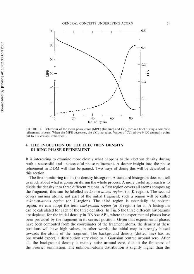
PHASE workings, it is common for the program to work with 5% or less; in few casesonly 1% of the scattering matter has been employed. It is interesting to observe how theinitial MPE deteriorates when the fragment is displaced from its correct position. Forexample, a 0.5� rotation and 0.3 A translation, corresponding to an r.m.s. of 0.35 A,change the initial MPE from 64.5 to 75.3�. This observation implies that experimentalphases coming from ACORN-MR or from any other software, will have to be derivedfrom a fragment which is very close to its correct position. This, in turn, requires a fineenough search in the molecular replacement to provide an accurate location of the frag-ment. The CCS is a powerful indicator of low MPE in all those cases where refinementhas been achieved. Figure 4 shows the behaviour of MPE and CCS during the fullrefinement started from the 0:58, 0.3 A case for 1BKR. Generally, ACORN-PHASEcan successfully refine phases with a starting phase error up to 80�, with atomic resolu-tion data. As the resolution gets poorer, its performance also appears less satisfactory,and non-atomic resolution data do not usually lead to a successful refinement unless aheavy atom is contained in the structure. An exception is provided here for 2LIS. Aninitial MPE of 67.5 degrees is refined to 41.5� the final value for CCS tells us thatthe MPE has fallen considerably.
ACORN-PHASE has no success with 1FK5, where the incomplete data is a finalobstacle to the phase refinement with DDM. 1BIO, in contrast, behaves better than1FK5, even though its data are at a lower resolution. As previously mentioned, agood completeness of diffraction data is a necessary condition for a successful applica-tion of ACORN-PHASE.
TABLE II Tests with ACORN-PHASE. For each structure, artificial experimental phases have beensimulated using fragments, belonging to the structure itself, in their correct position and approximatedposition generated by a small rotation and translation. Initial and final MPE and CCs have been noteddown, as well as the number of cycles needed to complete the refinement
Protein Scatteringmatter(%)
Rotationaround Z
Translationalong Z (A)
MPE (St/End) CCs(St/End) No. of cycles No.of strongreflections
RNAse AP1 9 0.0� 0.0 64.5 29.5 0.015 0.359 21 120660.5� 0.1 68.5 29.6 0.014 0.358 250.5� 0.2 71.1 29.9 0.013 0.356 330.5� 0.3 75.3 29.8 0.013 0.358 74
1BKR 7 0.0� 0.0 72.1 22.3 0.011 0.414 46 98760.5� 0.1 73.4 23.1 0.012 0.412 470.5� 0.2 74.7 23.4 0.008 0.414 570.5� 0.3 77.1 24.3 0.005 0.415 85
1FK5 7 0.0� 0.0 68.2 71.6 �0.024 0.015 27 58060.5� 0.1 76.6 80.0 �0.007 0.010 310.5� 0.2 77.6 81.0 �0.005 0.005 290.5� 0.3 79.0 81.0 �0.004 0.004 33
2LIS 9 0.0� 0.0 67.5 41.5 0.000 0.157 91 149990.5� 0.1 76.1 75.5 �0.005 0.012 310.5� 0.2 77.4 78.2 �0.004 0.009 330.5� 0.3 79.3 80.4 �0.004 0.008 36
1BIO 9 0.0� 0.0 69.2 67.3 0.027 0.025 32 113760.5� 0.1 69.9 67.4 0.023 0.025 310.5� 0.2 71.0 68.4 0.017 0.028 350.5� 0.3 72.7 70.9 0.012 0.029 39
50 J. FOADI
Dow
nloa
ded
By: [
Dha
shi]
At: 1
0:02
30
April
200
7
4. THE EVOLUTION OF THE ELECTRON DENSITY
DURING PHASE REFINEMENT
It is interesting to examine more closely what happens to the electron density duringboth a successful and unsuccessful phase refinement. A deeper insight into the phaserefinement in DDM will thus be gained. Two ways of doing this will be described inthis section.
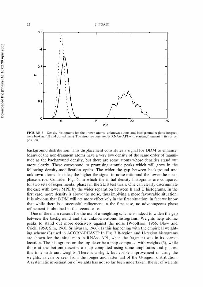
The first monitoring tool is the density histogram. A standard histogram does not tellus much about what is going on during the whole process. A more useful approach is todivide the density into three different regions. A first region covers all atoms composingthe fragment; this can be labelled as known-atoms region, (or K-region). The secondcovers missing atoms, not part of the initial fragment; such a region will be calledunknown-atoms region (or U-region). The third region is essentially the solventregion; we can adopt the term background region (or B-region) for it. A histogramcan be calculated for each of the three densities. In Fig. 5 the three different histogramsare depicted for the initial density in RNAse AP1, where the experimental phases havebeen provided by the fragment in its correct position. Given that experimental phaseshave been computed from the coordinates of the fragment atoms, the density at thesepositions will have high values, in other words, the initial map is strongly biasedtowards the atoms of the fragment. The background density (dotted line) has, asone would expect, a distribution very close to a Gaussian centred around zero. Afterall, the background density is mainly noise around zero, due to the finiteness ofthe Fourier summation. The unknown-atoms distribution is slightly higher than the
FIGURE 4 Behaviour of the mean phase error (MPE) (full line) and CCS (broken line) during a completerefinement process. When the MPE decreases, the CCS increases. Values of CCS above 0.150 generally pointout to a successful refinement.
GENERAL CONCEPTS UNDERLYING ACORN 51
Dow
nloa
ded
By: [
Dha
shi]
At: 1
0:02
30
April
200
7
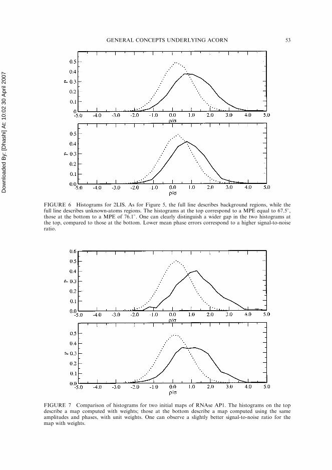
background distribution. This displacement constitutes a signal for DDM to enhance.Many of the non-fragment atoms have a very low density of the same order of magni-tude as the background density, but there are some atoms whose densities stand outmore clearly. These correspond to promising atomic peaks which will grow in thefollowing density-modification cycles. The wider the gap between background andunknown-atoms densities, the higher the signal-to-noise ratio and the lower the meanphase error. Consider Fig. 6, in which the initial density histograms are comparedfor two sets of experimental phases in the 2LIS test trials. One can clearly discriminatethe case with lower MPE by the wider separation between B and U histograms. In thefirst case, more density is above the noise, thus implying a more favourable situation.It is obvious that DDM will act more effectively in the first situation; in fact we knowthat while there is a successful refinement in the first case, no advantageous phaserefinement is obtained in the second case.
One of the main reasons for the use of a weighting scheme is indeed to widen the gapbetween the background and the unknown-atoms histograms. Weights help atomicpeaks to stand out more decisively against the noise (Woolfson, 1956; Blow andCrick, 1959; Sim, 1960; Srinivasan, 1966). Is this happening with the empirical weight-ing scheme (3) used in ACORN-PHASE? In Fig. 7 B-region and U-region histogramsare shown for the initial map in RNAse AP1, when the fragment was in its correctlocation. The histograms on the top describe a map computed with weights (3), whilethose at the bottom describe a map computed using same amplitudes and phases,this time with unit weights. There is a slight, but visible improvement in using theweights, as can be seen from the longer and fatter tail of the U-region distribution.A systematic investigation of weights has not so far been undertaken; the set of weights
FIGURE 5 Density histograms for the known-atoms, unknown-atoms and background regions (respect-ively broken, full and dotted lines). The structure here used is RNAse AP1 with starting fragment in its correctposition.
52 J. FOADI
Dow
nloa
ded
By: [
Dha
shi]
At: 1
0:02
30
April
200
7
FIGURE 6 Histograms for 2LIS. As for Figure 5, the full line describes background regions, while thefull line describes unknown-atoms regions. The histograms at the top correspond to a MPE equal to 67.5�,those at the bottom to a MPE of 76.1�. One can clearly distinguish a wider gap in the two histograms atthe top, compared to those at the bottom. Lower mean phase errors correspond to a higher signal-to-noiseratio.
FIGURE 7 Comparison of histograms for two initial maps of RNAse AP1. The histograms on the topdescribe a map computed with weights; those at the bottom describe a map computed using the sameamplitudes and phases, with unit weights. One can observe a slightly better signal-to-noise ratio for themap with weights.
GENERAL CONCEPTS UNDERLYING ACORN 53
Dow
nloa
ded
By: [
Dha
shi]
At: 1
0:02
30
April
200
7
defined in (3) was derived empirically mostly monitoring the MPE behaviour. Thewhole matter is open to original contributions.
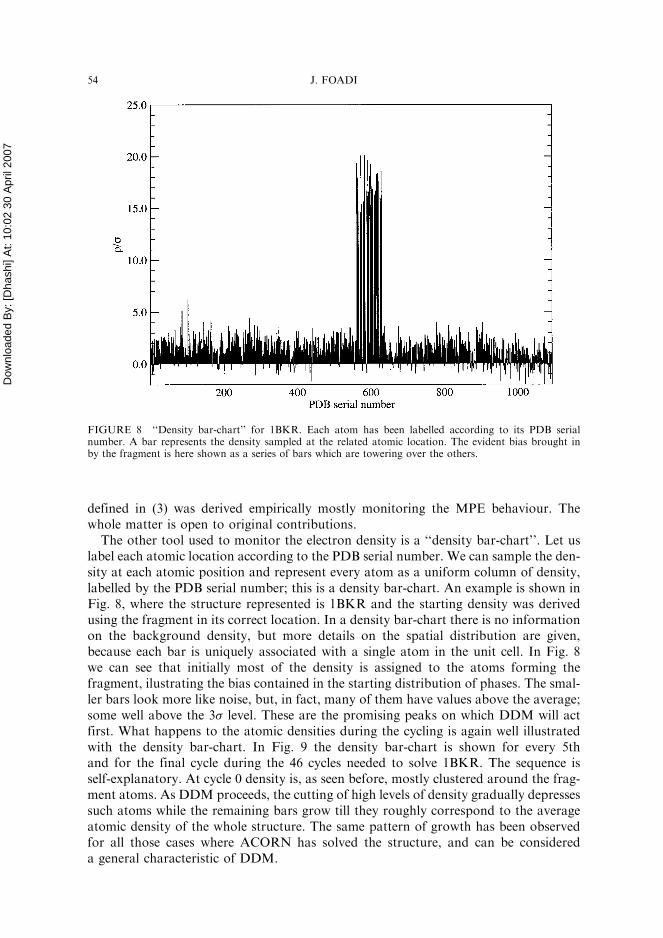
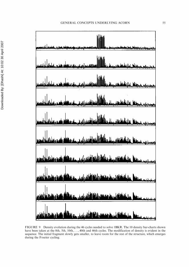
The other tool used to monitor the electron density is a ‘‘density bar-chart’’. Let uslabel each atomic location according to the PDB serial number. We can sample the den-sity at each atomic position and represent every atom as a uniform column of density,labelled by the PDB serial number; this is a density bar-chart. An example is shown inFig. 8, where the structure represented is 1BKR and the starting density was derivedusing the fragment in its correct location. In a density bar-chart there is no informationon the background density, but more details on the spatial distribution are given,because each bar is uniquely associated with a single atom in the unit cell. In Fig. 8we can see that initially most of the density is assigned to the atoms forming thefragment, ilustrating the bias contained in the starting distribution of phases. The smal-ler bars look more like noise, but, in fact, many of them have values above the average;some well above the 3� level. These are the promising peaks on which DDM will actfirst. What happens to the atomic densities during the cycling is again well illustratedwith the density bar-chart. In Fig. 9 the density bar-chart is shown for every 5thand for the final cycle during the 46 cycles needed to solve 1BKR. The sequence isself-explanatory. At cycle 0 density is, as seen before, mostly clustered around the frag-ment atoms. As DDM proceeds, the cutting of high levels of density gradually depressessuch atoms while the remaining bars grow till they roughly correspond to the averageatomic density of the whole structure. The same pattern of growth has been observedfor all those cases where ACORN has solved the structure, and can be considereda general characteristic of DDM.
FIGURE 8 ‘‘Density bar-chart’’ for 1BKR. Each atom has been labelled according to its PDB serialnumber. A bar represents the density sampled at the related atomic location. The evident bias brought inby the fragment is here shown as a series of bars which are towering over the others.
54 J. FOADI
Dow
nloa
ded
By: [
Dha
shi]
At: 1
0:02
30
April
200
7
FIGURE 9 Density evolution during the 46 cycles needed to solve 1BKR. The 10 density bar-charts shownhave been taken at the 0th, 5th, 10th, . . . , 40th and 46th cycles. The modification of density is evident in thesequence. The initial fragment slowly gets smaller, to leave room for the rest of the structure, which emergesduring the Fourier cycling.
GENERAL CONCEPTS UNDERLYING ACORN 55
Dow
nloa
ded
By: [
Dha
shi]
At: 1
0:02
30
April
200
7
5. PHASE CORRECTION AND DENSITY MODIFICATION
Fourier recycling has been associated with the solution of crystal structures throughoutthe history of structural crystallography, initially with the heavy atom method. The mainidea behind this type of recycling is that a partial structure can be completed withsuccessive Fourier syntheses, where progressive amounts of new information areincluded in the synthesis of consecutive maps. Generally, such information is measuredas percentage of the total known structure. As a rule of thumb the quantity of initialscattering matter needs to be of the same order as the remaining one (Sim, 1961;Giacovazzo et al., 1995). This requirement can be made weaker if statistical weightsare used jointly with the observed amplitudes to compute the Fourier synthesis. Withthe advent of density modification techniques the initial amount of informationrequired for a successful Fourier recycling has been further reduced.
One of the first density modifications to be introduced in crystallography is the phasecorrection method (Hoppe and Gassmann, 1968). This method is used when the initialphases are computed from a partial structure. It is well known from the work of Luzzati(1953) and Ramachandran and Srinivasan (1970), that a Fourier synthesis computedwith such phases and observed magnitudes will show, as compared to the completestructure:
(a) enhanced peaks at the sites of known atoms;(b) reduced peaks at the sites of unknown atoms;(c) reduced peaks at the sites of wrongly placed atoms;(d) background peaks.
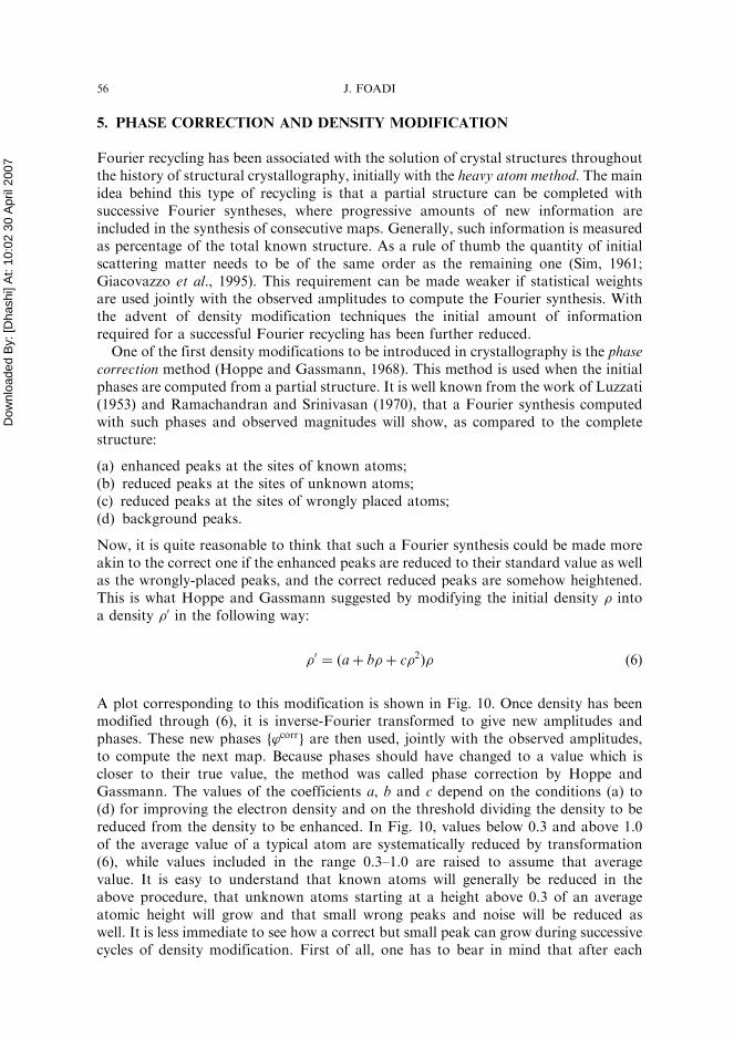
Now, it is quite reasonable to think that such a Fourier synthesis could be made moreakin to the correct one if the enhanced peaks are reduced to their standard value as wellas the wrongly-placed peaks, and the correct reduced peaks are somehow heightened.This is what Hoppe and Gassmann suggested by modifying the initial density � intoa density �0 in the following way:
�0 ¼ ðaþ b�þ c�2Þ� ð6Þ
A plot corresponding to this modification is shown in Fig. 10. Once density has beenmodified through (6), it is inverse-Fourier transformed to give new amplitudes andphases. These new phases f’corrg are then used, jointly with the observed amplitudes,to compute the next map. Because phases should have changed to a value which iscloser to their true value, the method was called phase correction by Hoppe andGassmann. The values of the coefficients a, b and c depend on the conditions (a) to(d) for improving the electron density and on the threshold dividing the density to bereduced from the density to be enhanced. In Fig. 10, values below 0.3 and above 1.0of the average value of a typical atom are systematically reduced by transformation(6), while values included in the range 0.3–1.0 are raised to assume that averagevalue. It is easy to understand that known atoms will generally be reduced in theabove procedure, that unknown atoms starting at a height above 0.3 of an averageatomic height will grow and that small wrong peaks and noise will be reduced aswell. It is less immediate to see how a correct but small peak can grow during successivecycles of density modification. First of all, one has to bear in mind that after each
56 J. FOADI
Dow
nloa
ded
By: [
Dha
shi]
At: 1
0:02
30
April
200
7
Fourier cycle only new improved phases are used, while observed magnitudes are neverchanged. What happens when observed amplitudes and ‘‘corrected’’ phases are used tocompute a Fourier synthesis is explained by Ramachandran and Srinivasan (1970) interms of convolutions. More specifically, a Fourier synthesis with coefficientsjFobsj expði’corrÞ is essentially a convolution between the Patterson of the correct struc-ture and peaks of the modified density which stand well above the noise. Such a con-volution will tend to suppress wrong peaks (not belonging to the final structure) andenhance the correct ones. During the first cycles only the most promising peaks willbe allowed to grow; at a certain point their number will be so increased that the overallpercentage of scattering matter is qualitatively higher than it was at the beginning. Inthis condition, correct peaks which were below the threshold during the initial cycles,have completed the transition above it and will successively continue to grow. At theend, most of the structure should be revealed by this process.
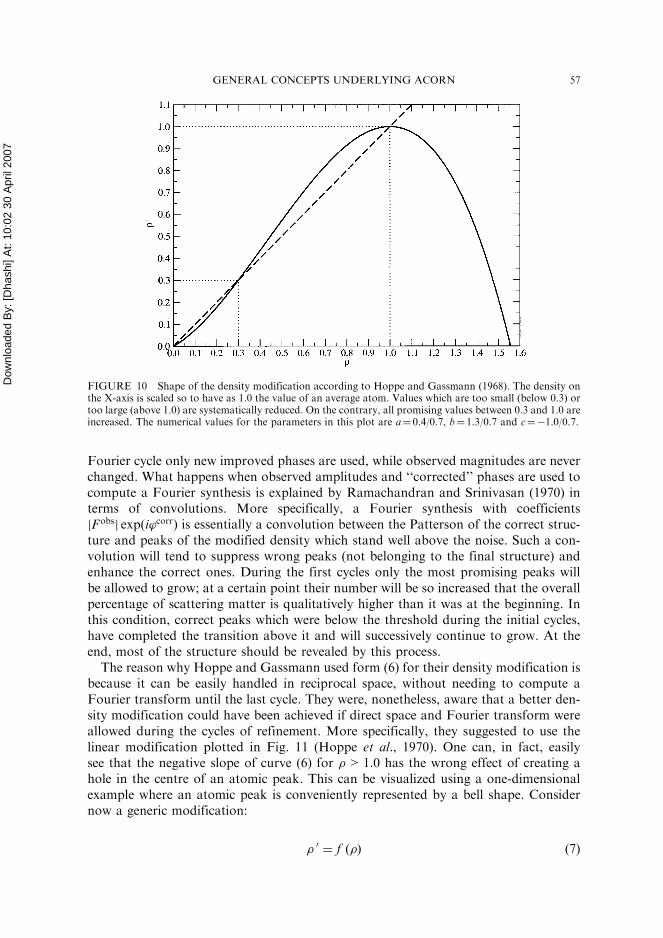
The reason why Hoppe and Gassmann used form (6) for their density modification isbecause it can be easily handled in reciprocal space, without needing to compute aFourier transform until the last cycle. They were, nonetheless, aware that a better den-sity modification could have been achieved if direct space and Fourier transform wereallowed during the cycles of refinement. More specifically, they suggested to use thelinear modification plotted in Fig. 11 (Hoppe et al., 1970). One can, in fact, easilysee that the negative slope of curve (6) for �> 1.0 has the wrong effect of creating ahole in the centre of an atomic peak. This can be visualized using a one-dimensionalexample where an atomic peak is conveniently represented by a bell shape. Considernow a generic modification:
� 0 ¼ f ð�Þ ð7Þ
FIGURE 10 Shape of the density modification according to Hoppe and Gassmann (1968). The density onthe X-axis is scaled so to have as 1.0 the value of an average atom. Values which are too small (below 0.3) ortoo large (above 1.0) are systematically reduced. On the contrary, all promising values between 0.3 and 1.0 areincreased. The numerical values for the parameters in this plot are a¼ 0.4/0.7, b¼ 1.3/0.7 and c¼�1.0/0.7.
GENERAL CONCEPTS UNDERLYING ACORN 57
Dow
nloa
ded
By: [
Dha
shi]
At: 1
0:02
30
April
200
7
For small increments of � we can approximate �� 0 as:
��0 ¼df
d��� ð8Þ
If the first derivative df =d� is positive and smaller than 1, ��0 will be smaller than ��,if it is positive and greater than 1, �� 0 will be larger than ��. In terms of bell-shapedatomic peaks this means that they will be broadened or sharpened if the first derivativeof the modification is positive and smaller than 1 or greater than 1, respectively. If thefirst derivative is negative, �� 0 will have sign opposite to the sign of ��; consequently,a negative slope will distort peaks in a bizarre way. What generally happens to abell-shaped peak under a modification which has positive slope for low values of �and negative slope for high values of �, is that at a certain height the peak starts tosplit in two separate peaks. This is what, for instance, happens to a modification like(6) for peaks with density higher than 1. If the above argument is translated intothree dimensions the peak splitting will be replaced by a depression of the density inthe centre of the peak, which is like having a hole in the atom. This does not obviouslycorrespond to a correct feature of any structure density. It is always better to avoidnegative slopes in the modification curve. The curve in Fig. 11 does a better job thanthe curve in Fig. 10.
The phase correction method was introduced more than thirty years ago and, sincethen, has been used, modified, re-discovered and inspired-by in various guises(Barrett and Zwick, 1971; Gassmann and Zechmeister, 1972; Collins, 1975; Zhangand Main, 1990). In the following section we will see how DDM originates from thesame arguments which form the basis for phase correction. We will also show that
FIGURE 11 Alternative density modification (full line) to the one represented in Fig. 10 (dotted line). Thismodification curve cuts high densities in a better way, but can only be implemented in direct-space.
58 J. FOADI
Dow
nloa
ded
By: [
Dha
shi]
At: 1
0:02
30
April
200
7
the limitations contained in the original phase correction formulation have beenhere eliminated. One could consider DDM as the best at present available form ofphase correction for solving proteins.
6. DDM AS A NEW KIND OF PHASE CORRECTION
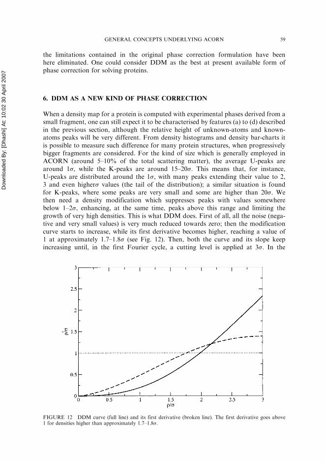
When a density map for a protein is computed with experimental phases derived from asmall fragment, one can still expect it to be characterised by features (a) to (d) describedin the previous section, although the relative height of unknown-atoms and known-atoms peaks will be very different. From density histograms and density bar-charts itis possible to measure such difference for many protein structures, when progressivelybigger fragments are considered. For the kind of size which is generally employed inACORN (around 5–10% of the total scattering matter), the average U-peaks arearound 1�, while the K-peaks are around 15–20�. This means that, for instance,U-peaks are distributed around the 1�, with many peaks extending their value to 2,3 and even higher� values (the tail of the distribution); a similar situation is foundfor K-peaks, where some peaks are very small and some are higher than 20�. Wethen need a density modification which suppresses peaks with values somewherebelow 1–2�, enhancing, at the same time, peaks above this range and limiting thegrowth of very high densities. This is what DDM does. First of all, all the noise (nega-tive and very small values) is very much reduced towards zero; then the modificationcurve starts to increase, while its first derivative becomes higher, reaching a value of1 at approximately 1.7–1.8� (see Fig. 12). Then, both the curve and its slope keepincreasing until, in the first Fourier cycle, a cutting level is applied at 3�. In the
FIGURE 12 DDM curve (full line) and its first derivative (broken line). The first derivative goes above1 for densities higher than approximately 1.7–1.8�.
GENERAL CONCEPTS UNDERLYING ACORN 59
Dow
nloa
ded
By: [
Dha
shi]
At: 1
0:02
30
April
200
7
second cycle the � value will be slightly bigger and consequently the shape of the curvewill be slightly modified. Things will, nevertheless, proceed in very much the same wayas before. The only difference is the cutting level, which is now set to 6�. The reason fordoing this is that many more peaks have grown to a higher level of density and by keep-ing the cutting level at 3� one could limit the genuine growth of correct peaks.
To summarize how an initial map, produced with phases coming from a smallfragment, has to be density modified to reproduce better features of the correct, finaldensity, we can assert that the density modification curve will need to:
1. equal zero for negative densities and be very small for small densities;2. have a first derivative greater than 1 in the region were densities need to be enhanced
and sharpened;3. tend to some sensible finite limit for large densities;4. nowhere have negative slope.
We can think of the 4 points as guidelines to produce a phase correction which ismost suitable for protein structures and which does not suffer from the problems con-nected with its original version.
Modification curves following some of the above guidelines had already been tried byWoolfson and co-workers as phase refinement and extension methods in the computerprogram PERP (Refaat et al., 1996), in what was called Low Density Elimination(Shiono and Woolfson, 1992; Refaat and Woolfson, 1993). The specific analyticalform chosen there was an algebraic one:
� 0 ¼
0 if � < 0
�ð�=0:2�cÞ
5
1 þ ð�=0:2�cÞ5
if � � 0
8><>: ð9Þ
where �c is the average peak height of a light atom (typically this height is around 4–5�,so 0:2�c is roughly equal to �). Matsugaki and Shiono (2001) have later tried aGaussian form in LDE:
� 0 ¼
0 if � < 0
� 1 � exp �1
2
�
0:2�c
� �2" #( )
if � � 0
8><>: ð10Þ
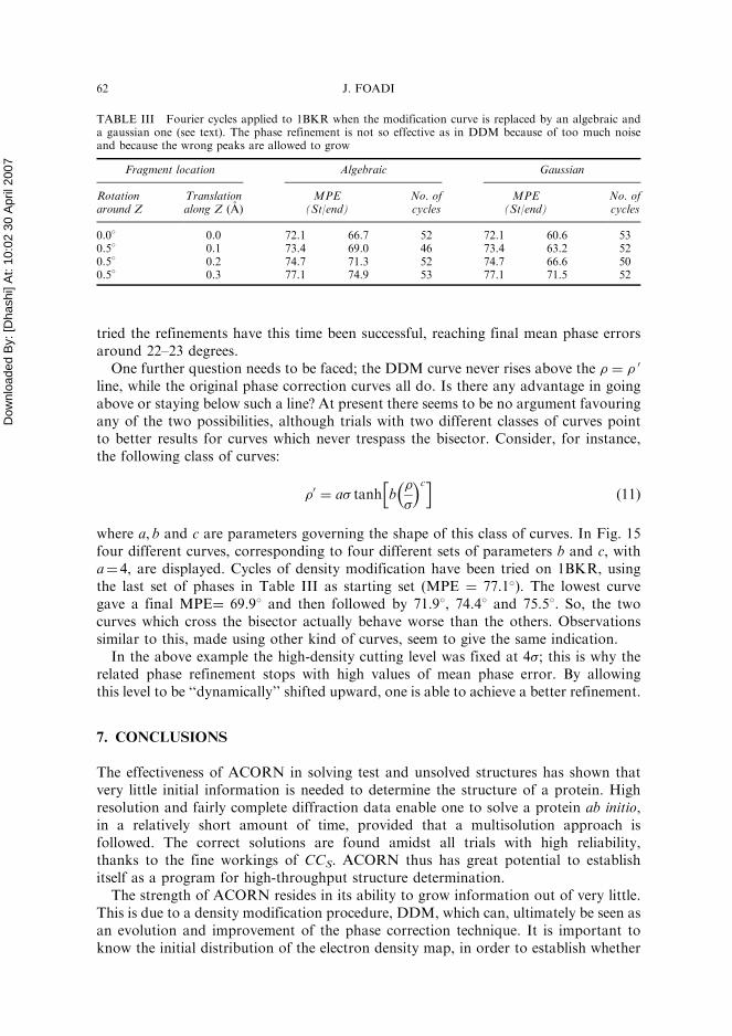
Both curves are depicted in Fig. 13. It is easy to show that these curves have their firstderivatives reaching 1 too early at just before 1�. They would enhance, consequently,peaks which are either noise or which correspond to wrong atoms. Both modificationcurves have been applied on 1BKR; results are collected in Table III. A phase refine-ment can be observed in both cases, but it is not as effective as in DDM. A cuttinglevel for high values and a correct slope for small values of density are evidently decisivefor a successful performance. Indeed, phase refinements have been tried again on 1BKRusing both algebraic and Gaussian analytical forms, this time changing �=� into�ð�=�Þ. For the algebraic form the chosen parameters are � ¼ 0:65 and ¼ 0:7,while for the Gaussian form � ¼ 0:7746 and ¼ 0:725. With this choice both the alge-braic and the Gaussian curve behave similarly to DDM curve (see Fig. 14). In all cases
60 J. FOADI
Dow
nloa
ded
By: [
Dha
shi]
At: 1
0:02
30
April
200
7
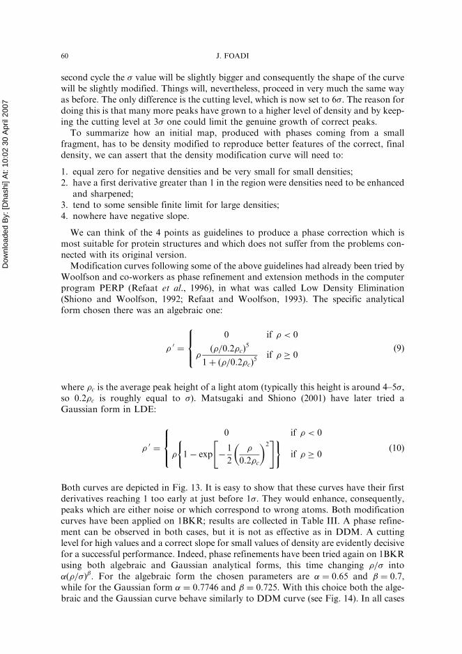
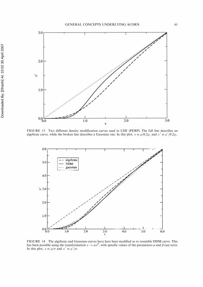
FIGURE 14 The algebraic and Gaussian curves have here been modified so to resemble DDM curve. Thishas been possible using the transformation x! �x, with specific values of the parameters � and (see text).In this plot, x � �=� and x 0
� � 0=�.
FIGURE 13 Two different density modification curves used in LDE (PERP). The full line describes analgebraic curve, while the broken line describes a Gaussian one. In this plot, x � �=0:2�c and x 0
� � 0=0:2�c.
GENERAL CONCEPTS UNDERLYING ACORN 61
Dow
nloa
ded
By: [
Dha
shi]
At: 1
0:02
30
April
200
7
tried the refinements have this time been successful, reaching final mean phase errorsaround 22–23 degrees.
One further question needs to be faced; the DDM curve never rises above the � ¼ � 0
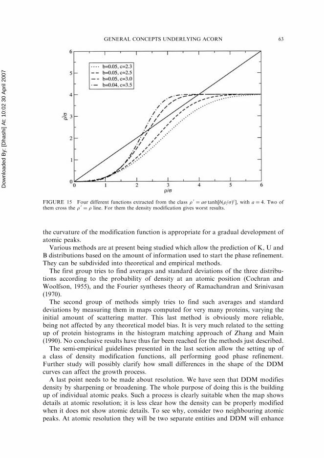
line, while the original phase correction curves all do. Is there any advantage in goingabove or staying below such a line? At present there seems to be no argument favouringany of the two possibilities, although trials with two different classes of curves pointto better results for curves which never trespass the bisector. Consider, for instance,the following class of curves:
�0 ¼ a� tanh b�
�
� �ch ið11Þ
where a, b and c are parameters governing the shape of this class of curves. In Fig. 15four different curves, corresponding to four different sets of parameters b and c, witha¼ 4, are displayed. Cycles of density modification have been tried on 1BKR, usingthe last set of phases in Table III as starting set (MPE ¼ 77.1�). The lowest curvegave a final MPE¼ 69:98 and then followed by 71:98, 74:48 and 75:58. So, the twocurves which cross the bisector actually behave worse than the others. Observationssimilar to this, made using other kind of curves, seem to give the same indication.
In the above example the high-density cutting level was fixed at 4�; this is why therelated phase refinement stops with high values of mean phase error. By allowingthis level to be ‘‘dynamically’’ shifted upward, one is able to achieve a better refinement.
7. CONCLUSIONS
The effectiveness of ACORN in solving test and unsolved structures has shown thatvery little initial information is needed to determine the structure of a protein. Highresolution and fairly complete diffraction data enable one to solve a protein ab initio,in a relatively short amount of time, provided that a multisolution approach isfollowed. The correct solutions are found amidst all trials with high reliability,thanks to the fine workings of CCS. ACORN thus has great potential to establishitself as a program for high-throughput structure determination.
The strength of ACORN resides in its ability to grow information out of very little.This is due to a density modification procedure, DDM, which can, ultimately be seen asan evolution and improvement of the phase correction technique. It is important toknow the initial distribution of the electron density map, in order to establish whether
TABLE III Fourier cycles applied to 1BKR when the modification curve is replaced by an algebraic anda gaussian one (see text). The phase refinement is not so effective as in DDM because of too much noiseand because the wrong peaks are allowed to grow
Fragment location Algebraic Gaussian
Rotationaround Z
Translationalong Z (A)
MPE(St/end)
No. ofcycles
MPE(St/end)
No. ofcycles
0.0� 0.0 72.1 66.7 52 72.1 60.6 530.5� 0.1 73.4 69.0 46 73.4 63.2 520.5� 0.2 74.7 71.3 52 74.7 66.6 500.5� 0.3 77.1 74.9 53 77.1 71.5 52
62 J. FOADI
Dow
nloa
ded
By: [
Dha
shi]
At: 1
0:02
30
April
200
7
the curvature of the modification function is appropriate for a gradual development ofatomic peaks.
Various methods are at present being studied which allow the prediction of K, U andB distributions based on the amount of information used to start the phase refinement.They can be subdivided into theoretical and empirical methods.
The first group tries to find averages and standard deviations of the three distribu-tions according to the probability of density at an atomic position (Cochran andWoolfson, 1955), and the Fourier syntheses theory of Ramachandran and Srinivasan(1970).
The second group of methods simply tries to find such averages and standarddeviations by measuring them in maps computed for very many proteins, varying theinitial amount of scattering matter. This last method is obviously more reliable,being not affected by any theoretical model bias. It is very much related to the settingup of protein histograms in the histogram matching approach of Zhang and Main(1990). No conclusive results have thus far been reached for the methods just described.
The semi-empirical guidelines presented in the last section allow the setting up ofa class of density modification functions, all performing good phase refinement.Further study will possibly clarify how small differences in the shape of the DDMcurves can affect the growth process.
A last point needs to be made about resolution. We have seen that DDM modifiesdensity by sharpening or broadening. The whole purpose of doing this is the buildingup of individual atomic peaks. Such a process is clearly suitable when the map showsdetails at atomic resolution; it is less clear how the density can be properly modifiedwhen it does not show atomic details. To see why, consider two neighbouring atomicpeaks. At atomic resolution they will be two separate entities and DDM will enhance
FIGURE 15 Four different functions extracted from the class � 0¼ a� tanh½bð�=�Þc�, with a ¼ 4. Two of
them cross the � 0¼ � line. For them the density modification gives worst results.
GENERAL CONCEPTS UNDERLYING ACORN 63
Dow
nloa
ded
By: [
Dha
shi]
At: 1
0:02
30
April
200
7
both of them. As the resolution gets lower the two peaks will gradually merge intoa single peak. When DDM acts on this peak it will enhance it, thus transforming thedensity into one produced by one single and heavier atom. No positive phaserefinement can be expected in this situation. Furthermore, the height of the variousinitial density peaks will be different at different resolutions. This means that theshape of the modification curve will have to be properly modified in order tokeep this feature into account. A modification like that carried out by DDM islikely to be difficult at resolutions which do not show density ‘‘peakiness’’.
Acknowledgement
The author would like to thank Chris Gilmore for continuous advice on many of thetopics covered in this paper. Also, Michael Woolfson is acknowledged as a primarysource of inspiration for all work concerning ACORN. Finally, many thanks toEleanor Dodson for proof-reading and invaluable suggestions that have helped shapingthis paper into its final form.
The work was supported by a BBSRC grant.
References
Barrett, A.N. and Zwick, M. (1971) A method for the extension and refinement of crystallographic proteinphases utilizing the fast fourier transform. Acta Cryst., A27, 6–11.
Bezborodova, S.I., Ermekbaeva, I.A., Shlyapnikov, S.V., Polyakov, K.M. and Bezborodov, A.M. (1988)Biokhimiya, 53, 965–973.
Blow, D.M. and Crick, F.H.C. (1959) The treatment of errors in the isomorphous replacement method. ActaCryst., 12, 794–802.
Cochran, W. and Woolfson, M.M. (1955) The theory of sign relations between structure factors. Acta Cryst.,8, 1–12.
Collaborative Computational Project (1994) The CCP4 suite: programs for protein crystallography. ActaCryst., D50, 760–763.
Collins, D.M. (1975) Efficiency in Fourier phase refinement for protein crystal structures. Acta Cryst., A31,388–389.
Dodson, E.J. (2003) The use of ACORN to determine sub-structures. Cryst. Rev., 9(1), 67–72.Foadi, J. (2000) Real-space methods to solve protein structures Ph.D. thesis, University of York, Department
of Physics, York (U.K.).Foadi, J., Woolfson, M.M., Dodson, E.J., Wilson, K.S., Jia-xing, Y. and Chao-de, Z. (2000) A flexible
and efficient procedure for the solution and phase refinement of protein structures. Acta Cryst., D56,1137–1147.
Gassman, J. and Zechmeister, K. (1972) Limits of phase expansion in direct methods. Acta Cryst., A28, 270–280.
Giacovazzo, C., Monaco, H.L., Viterbo, D., Scordari, F., Gilli, G., Zanotti, G., Catti, M. (1995)Fundamentals of crystallography. New York: IUCr Book Series Oxford University Press.
Hoppe W. and Gassmann, J. (1968) Phase correction, a new method to solve partially known structures. ActaCryst., B24, 97–107.
Hoppe, W., Gassmann, J. and Zechmeister, K. (1970) Some automatic procedures for the solution of crystalstructures with direct methods and phase correction. In: Crystallographic Computing. Copenhagen:Munksgaard.
Jia-xing, Y. (2001) CCP4 acorn. CCP4 Newsletter, 56, 17–27.Kissinger, C.R., Gehlhaar, D.K. and Fogel, D.B. (1999) Rapid automated molecular replacement by
evolutionary search. Acta Cryst., D55, 484–491.Luzzati, V. (1953) Resolution d’une Structure Cristalline Lorsque les Positions d’une Partie des Atomes
sont Connues: Traitment Statistique. Acta Cryst., 6, 142–152.Matsugaki, N. and Shiono, M. (2001) Ab initio structure determination by direct-space methods: tests of
low-density elimination. Acta Cryst., D57, 95–100.Ramachandran, G.N. and Srinivasan, R. (1970). Fourier methods in crystallography. New York: Wiley
Interscience.
64 J. FOADI
Dow
nloa
ded
By: [
Dha
shi]
At: 1
0:02
30
April
200
7
Read, R.J. (1986) Improved Fourier coefficients for maps using phases from partial structures with errors.Acta Cryst., A42, 140–149.
Refaat, L.R. and Woolfson, M.M. (1993) Direct-space methods in phase extension and phase determination.II. Developments of low-density elimination. Acta Cryst., D49, 367–371.
Refaat, L.R., Tate, C. and Woolfson, M.M. (1996) Direct-space methods in phase extension and phase refine-ment. VI. PERP (Phase Extension and Refinement Program). Acta Cryst., D52, 1119–1124.
Shiono, M. and Woolfson, M.M. (1992) Direct-space methods in phase extension and phase determination. I.low-density elimination. Acta Cryst., A48, 451–456.
Sim, G.A. (1959) The distribution of phase angles for structures containing heavy atoms. II. A Modificationof the normal heavy-atom method for non-centrosymmetrical structures. Acta Cryst., 12, 813–815.
Sim, G.A. (1960) A note on the heavy-atom method. Acta Cryst., 13, 511–512.Sim, G.A. (1961) Computing Methods and the Phase Problem in X-ray Crystal Analysis. Oxford: Pergamon
Press.Srinivasan, R. (1966) Weighting functions for use in the early stages of structure analysis when a part of the
structure is known. Acta Cryst., 20, 143–144.Srinivasan, R. and Ramachandran, G.N. (1965) Probability distribution connected with structure amplitudes
of two related crystals. V. The effect of errors in the atomic coordinates on the distribution of observedand calculated structure factors. Acta Cryst., 19, 1008–1014.
Woolfson, M.M. (1956) An improvement of the ‘heavy-atom’ method of solving crystal structures. ActaCryst., 9, 804–810.
Zhang, K.Y.J. and Main, P. (1990) Histogram matching as a new density modification technique for phaserefinement and extension of protein molecules. Acta Cryst., A46, 41–46.
GENERAL CONCEPTS UNDERLYING ACORN 65