Embed Size (px)
Citation preview
Game Theory Evolving, Second Edition

This page intentionally left blank
Game Theory Evolving, Second Edition
A Problem-Centered Introductionto Modeling Strategic Interaction
Herbert Gintis
Princeton University Press
Princeton and Oxford
Copyright c� 2009 by Princeton University Press
Published by Princeton University Press, 41 William Street, Princeton, New Jersey 08540
In the United Kingdom: Princeton University Press, 6 Oxford Street, Woodstock, Oxfordshire
OX20 1TW
All Rights Reserved
Library of Congress Cataloging-in-Publication Data
Gintis, Herbert.
Game theory evolving : a problem-centered introduction to modeling strategic interaction /
Herbert Gintis.-2nd ed.
p. cm.
Includes bibliographical references and index.
ISBN 978-0-691-14050-6 (hardcover : alk. paper)-ISBN 978-0-691-14051-3 (pbk. : alk.
paper) 1. Game theory. 2. Economics, Mathematical. I . Title.
HB144.G56 2008
330.01’5193-dc22 2008036523
British Library Cataloging-in-Publication Data is available
The publisher would like to acknowledge the author of this volume for providing the
camera-ready copy from which this book was printed
This book was composed in Times and Mathtime by the author
Printed on acid-free paper.
press.princeton.edu
Printed in the United States of America
10 9 8 7 6 5 4 3 2 1
To Marci and Dan
Riverrun, past Eve and Adam’s, from swerve of shore to
bend of bay, brings us by a Commodius vicus of recircu-
lation backJames Joyce

This page intentionally left blank
Contents
Preface xv
1 Probability Theory 1
1.1 Basic Set Theory and Mathematical Notation 1
1.2 Probability Spaces 2
1.3 De Morgan’s Laws 3
1.4 Interocitors 3
1.5 The Direct Evaluation of Probabilities 3
1.6 Probability as Frequency 4
1.7 Craps 5
1.8 A Marksman Contest 5
1.9 Sampling 5
1.10 Aces Up 6
1.11 Permutations 6
1.12 Combinations and Sampling 7
1.13 Mechanical Defects 7
1.14 Mass Defection 7
1.15 House Rules 7
1.16 The Addition Rule for Probabilities 8
1.17 A Guessing Game 8
1.18 North Island, South Island 8
1.19 Conditional Probability 9
1.20 Bayes’ Rule 9
1.21 Extrasensory Perception 10
1.22 Les Cinq Tiroirs 10
1.23 Drug Testing 10
1.24 Color Blindness 11
1.25 Urns 11
1.26 The Monty Hall Game 11
1.27 The Logic of Murder and Abuse 11
1.28 The Principle of Insufficient Reason 12
1.29 The Greens and the Blacks 12
1.30 The Brain and Kidney Problem 12
1.31 The Value of Eyewitness Testimony 13
viii Contents
1.32 When Weakness Is Strength 13
1.33 The Uniform Distribution 16
1.34 Laplace’s Law of Succession 17
1.35 From Uniform to Exponential 17
2 Bayesian Decision Theory 18
2.1 The Rational Actor Model 18
2.2 Time Consistency and Exponential Discounting 20
2.3 The Expected Utility Principle 22
2.4 Risk and the Shape of the Utility Function 26
2.5 The Scientific Status of the Rational Actor Model 30
3 Game Theory: Basic Concepts 32
3.1 Big John and Little John 32
3.2 The Extensive Form 38
3.3 The Normal Form 41
3.4 Mixed Strategies 42
3.5 Nash Equilibrium 43
3.6 The Fundamental Theorem of Game Theory 44
3.7 Solving for Mixed-Strategy Nash Equilibria 45
3.8 Throwing Fingers 46
3.9 Battle of the Sexes 46
3.10 The Hawk-Dove Game 48
3.11 The Prisoner’s Dilemma 50
4 Eliminating Dominated Strategies 52
4.1 Dominated Strategies 52
4.2 Backward Induction 54
4.3 Exercises in Eliminating Dominated Strategies 55
4.4 Subgame Perfection 57
4.5 Stackelberg Leadership 59
4.6 The Second-Price Auction 59
4.7 The Mystery of Kidnapping 60
4.8 The Eviction Notice 62
4.9 Hagar’s Battles 62
4.10 Military Strategy 63
4.11 The Dr. Strangelove Game 64
Contents ix
4.12 Strategic Voting 64
4.13 Nuisance Suits 65
4.14 An Armaments Game 67
4.15 Football Strategy 67
4.16 Poker with Bluffing 68
4.17 The Little Miss Muffet Game 69
4.18 Cooperation with Overlapping Generations 70
4.19 Dominance-Solvable Games 71
4.20 Agent-based Modeling 72
4.21 Why Play a Nash Equilibrium? 75
4.22 Modeling the Finitely-Repeated Prisoner’s Dilemma 77
4.23 Review of Basic Concepts 79
5 Pure-Strategy Nash Equilibria 80
5.1 Price Matching as Tacit Collusion 80
5.2 Competition on Main Street 81
5.3 Markets as Disciplining Devices: Allied Widgets 81
5.4 The Tobacco Market 87
5.5 The Klingons and the Snarks 87
5.6 Chess: The Trivial Pastime 88
5.7 No-Draw, High-Low Poker 89
5.8 An Agent-based Model of No-Draw, High-Low Poker 91
5.9 The Truth Game 92
5.10 The Rubinstein Bargaining Model 94
5.11 Bargaining with Heterogeneous Impatience 96
5.12 Bargaining with One Outside Option 97
5.13 Bargaining with Dual Outside Options 98
5.14 Huey, Dewey, and Louie Split a Dollar 102
5.15 Twin Sisters 104
5.16 The Samaritan’s Dilemma 104
5.17 The Rotten Kid Theorem 106
5.18 The Shopper and the Fish Merchant 107
5.19 Pure Coordination Games 109
5.20 Pick Any Number 109
5.21 Pure Coordination Games: Experimental Evidence 110
5.22 Introductory Offers 111
5.23 Web Sites (for Spiders) 112
x Contents
6 Mixed-Strategy Nash Equilibria 116
6.1 The Algebra of Mixed Strategies 116
6.2 Lions and Antelope 117
6.3 A Patent Race 118
6.4 Tennis Strategy 119
6.5 Preservation of Ecology Game 119
6.6 Hard Love 120
6.7 Advertising Game 120
6.8 Robin Hood and Little John 122
6.9 The Motorist’s Dilemma 122
6.10 Family Politics 123
6.11 Frankie and Johnny 123
6.12 A Card Game 124
6.13 Cheater-Inspector 126
6.14 The Vindication of the Hawk 126
6.15 Characterizing 2 � 2 Normal Form Games I 127
6.16 Big John and Little John Revisited 128
6.17 Dominance Revisited 128
6.18 Competition on Main Street Revisited 128
6.19 Twin Sisters Revisited 129
6.20 Twin Sisters: An Agent-Based Model 129
6.21 One-Card, Two-Round Poker with Bluffing 131
6.22 An Agent-Based Model of Poker with Bluffing 132
6.23 Trust in Networks 133
6.24 El Farol 134
6.25 Decorated Lizards 135
6.26 Sex Ratios as Nash Equilibria 137
6.27 A Mating Game 140
6.28 Coordination Failure 141
6.29 Colonel Blotto Game 141
6.30 Number Guessing Game 142
6.31 Target Selection 142
6.32 A Reconnaissance Game 142
6.33 Attack on Hidden Object 143
6.34 Two-Person, Zero-Sum Games 143
6.35 Mutual Monitoring in a Partnership 145
6.36 Mutual Monitoring in Teams 145
Contents xi
6.37 Altruism(?) in Bird Flocks 146
6.38 The Groucho Marx Game 147
6.39 Games of Perfect Information 151
6.40 Correlated Equilibria 151
6.41 Territoriality as a Correlated Equilibrium 153
6.42 Haggling at the Bazaar 154
6.43 Poker with Bluffing Revisited 156
6.44 Algorithms for Finding Nash Equilibria 157
6.45 Why Play Mixed Strategies? 160
6.46 Reviewing of Basic Concepts 161
7 Principal-Agent Models 162
7.1 Gift Exchange 162
7.2 Contract Monitoring 163
7.3 Profit Signaling 164
7.4 Properties of the Employment Relationship 168
7.5 Peasant and Landlord 169
7.6 Bob’s Car Insurance 173
7.7 A Generic Principal-Agent Model 174
8 Signaling Games 179
8.1 Signaling as a Coevolutionary Process 179
8.2 A Generic Signaling Game 180
8.3 Sex and Piety: The Darwin-Fisher Model 182
8.4 Biological Signals as Handicaps 187
8.5 The Shepherds Who Never Cry Wolf 189
8.6 My Brother’s Keeper 190
8.7 Honest Signaling among Partial Altruists 193
8.8 Educational Signaling 195
8.9 Education as a Screening Device 197
8.10 Capital as a Signaling Device 199
9 Repeated Games 201
9.1 Death and Discount Rates in Repeated Games 202
9.2 Big Fish and Little Fish 202
9.3 Alice and Bob Cooperate 204
9.4 The Strategy of an Oil Cartel 205
xii Contents
9.5 Reputational Equilibrium 205
9.6 Tacit Collusion 206
9.7 The One-Stage Deviation Principle 208
9.8 Tit for Tat 209
9.9 I’d Rather Switch Than Fight 210
9.10 The Folk Theorem 213
9.11 The Folk Theorem and the Nature of Signaling 216
9.12 The Folk Theorem Fails in Large Groups 217
9.13 Contingent Renewal Markets Do Not Clear 219
9.14 Short-Side Power in Contingent Renewal Markets 222
9.15 Money Confers Power in Contingent Renewal Markets 223
9.16 The Economy Is Controlled by the Wealthy 223
9.17 Contingent Renewal Labor Markets 224
10 Evolutionarily Stable Strategies 229
10.1 Evolutionarily Stable Strategies: Definition 230
10.2 Properties of Evolutionarily Stable Strategies 232
10.3 Characterizing Evolutionarily Stable Strategies 233
10.4 A Symmetric Coordination Game 236
10.5 A Dynamic Battle of the Sexes 236
10.6 Symmetrical Throwing Fingers 237
10.7 Hawks, Doves, and Bourgeois 238
10.8 Trust in Networks II 238
10.9 Cooperative Fishing 238
10.10 Evolutionarily Stable Strategies Are Not Unbeatable 240
10.11 A Nash Equilibrium That Is Not an EES 240
10.12 Rock, Paper, and Scissors Has No ESS 241
10.13 Invasion of the Pure-Strategy Mutants 241
10.14 Multiple Evolutionarily Stable Strategies 242
10.15 Evolutionarily Stable Strategies in Finite Populations 242
10.16 Evolutionarily Stable Strategies in Asymmetric Games 244
11 Dynamical Systems 247
11.1 Dynamical Systems: Definition 247
11.2 Population Growth 248
11.3 Population Growth with Limited Carrying Capacity 249
11.4 The Lotka-Volterra Predator-Prey Model 251
Contents xiii
11.5 Dynamical Systems Theory 255
11.6 Existence and Uniqueness 256
11.7 The Linearization Theorem 257
11.8 Dynamical Systems in One Dimension 258
11.9 Dynamical Systems in Two Dimensions 260
11.10 Exercises in Two-Dimensional Linear Systems 264
11.11 Lotka-Volterra with Limited Carrying Capacity 266
11.12 Take No Prisoners 266
11.13 The Hartman-Grobman Theorem 267
11.14 Features of Two-Dimensional Dynamical Systems 268
12 Evolutionary Dynamics 270
12.1 The Origins of Evolutionary Dynamics 271
12.2 Strategies as Replicators 272
12.3 A Dynamic Hawk-Dove Game 274
12.4 Sexual Reproduction and the Replicator Dynamic 276
12.5 Properties of the Replicator System 278
12.6 The Replicator Dynamic in Two Dimensions 279
12.7 Dominated Strategies and the Replicator Dynamic 280
12.8 Equilibrium and Stability with a Replicator Dynamic 282
12.9 Evolutionary Stability and Asymptotically Stability 284
12.10 Trust in Networks III 284
12.11 Characterizing 2 � 2 Normal Form Games II 285
12.12 Invasion of the Pure-Strategy Nash Mutants II 286
12.13 A Generalization of Rock, Paper, and Scissors 287
12.14 Uta stansburiana in Motion 287
12.15 The Dynamics of Rock, Paper, and Scissors 288
12.16 The Lotka-Volterra Model and Biodiversity 288
12.17 Asymmetric Evolutionary Games 290
12.18 Asymmetric Evolutionary Games II 295
12.19 The Evolution of Trust and Honesty 295
13 Markov Economies and Stochastic Dynamical Systems 297
13.1 Markov Chains 297
13.2 The Ergodic Theorem for Markov Chains 305
13.3 The Infinite Random Walk 307
13.4 The Sisyphean Markov Chain 308
xiv Contents
13.5 Andrei Andreyevich’s Two-Urn Problem 309
13.6 Solving Linear Recursion Equations 310
13.7 Good Vibrations 311
13.8 Adaptive Learning 312
13.9 The Steady State of a Markov Chain 314
13.10 Adaptive Learning II 315
13.11 Adaptive Learning with Errors 316
13.12 Stochastic Stability 317
14 Table of Symbols 319
15 Answers 321
Sources for Problems 373
References 375
Index 385
Preface
Was sich sagen laßt, laßt sich klar sagen, und wovon man nichtsprechen kann, daruber muß man schweigen.
Ludwig Wittgenstein
This book is a problem-centered introduction to classical and evolution-
ary game theory. For most topics, I provide just enough in the way of
definitions, concepts, theorems, and examples to begin solving problems.
Learning and insight come from grappling with and solving problems. I
provide extensive answers to some problems, sketchy and suggestive an-
swers to most others. Students should consult the answers in the back of
the book only to check their work. If a problem seems too difficult to solve,
the student should come back to it a day, a week, or a month later, rather
than peeking at the solution.
Game theory is logically demanding, but on a practical level, it requires
surprisingly few mathematical techniques. Algebra, calculus, and basic
probability theory suffice. However, game theory frequently requires con-
siderable notation to express ideas clearly. The reader should commit to
memory the precise definition of every term, and the precise statement of
most theorems.
Clarity and precision do not imply rigor. I take my inspiration from
physics, where sophisticated mathematics is common, but mathematical
rigor is considered an impediment to creative theorizing. I stand by the
truth and mathematical cogency of the arguments presented in this book,
but not by their rigor. Indeed, the stress placed on game-theoretic rigor in
recent years is misplaced. Theorists could worry more about the empirical
relevance of their models and take less solace in mathematical elegance.
For instance, if a proposition is proved for a model with a finite num-
ber of agents, it is completely irrelevant whether it is true for an infinite
number of agents. There are, after all, only a finite number of people, or
even bacteria. Similarly, if something is true in games in which payoffs are
finitely divisible (e.g., there is a minimum monetary unit), it does not matter
whether it is true when payoffs are infinitely divisible. There are no payoffs
in the universe, as far as we know, that are infinitely divisible. Even time,
xvi Preface
which is continuous in principle, can be measured only by devices with a
finite number of quantum states. Of course, models based on the real and
complex numbers can be hugely useful, but they are just approximations,
because there are only a finite number of particles in the universe, and we
can construct only a finite set of numbers, even in principle. There is thus
no intrinsic value of a theorem that is true for a continuum of agents on
a Banach space, if it is also true for a finite number of agents on a finite
choice space.
Evolutionary game theory is about the emergence, transformation, diffu-
sion, and stabilization of forms of behavior. Traditionally, game theory has
been seen as a theory of how rational actors behave. Ironically, game the-
ory, which for so long was predicated upon high-level rationality, has shown
us, by example, the limited capacity of the concept of rationality alone to
predict human behavior. I explore this issue in depth in Bounds of Reason
(Princeton, 2009), which develops themes from epistemic game theory to
fill in where classical game theory leaves off. Evolutionary game theory de-
ploys the Darwinian notion that good strategies diffuse across populations
of players rather than being learned by rational agents.
The treatment of rationality as preference consistency, a theme that we
develop in chapter 2, allows us to assume that agents choose best responses,
and otherwise behave as good citizens of game theory society. But they may
be pigs, dung beetles, birds, spiders, or even wild things like Trogs and
Klingons. How do they accomplish these feats with their small minds and
alien mentalities? The answer is that the agent is displaced by the strategy
as the dynamic game-theoretic unit.
This displacement is supported in three ways. First, we show that many
static optimization models are stable equilibria of dynamic systems in which
agents do not optimize, and we reject models that do not have attractive
stability properties. To this end, after a short treatment of evolutionary
stability, we develop dynamical systems theory (chapter 11) in sufficient
depth to allow students to solve dynamic games with replicator dynamics
(chapter 12). Second we provide animal as well as human models. Third,
we provide agent-based computer simulations of games, showing that really
stupid critters can evolve toward the solution of games previously thought
to require “rationality” and high-level information processing capacity.
The Wittgenstein quote at the head of the preface means “What can be
said, can be said clearly, and what you cannot say, you should shut up
Preface xvii
about.” This adage is beautifully reflected in the methodology of game
theory, especially epistemic game theory, which I develop in The Bounds
of Reason (2009),and which gives us a language and a set of analytical tools
for modeling an aspect of social reality with perfect clarity. Before game
theory, we had no means of speaking clearly about social reality, so the
great men and women who created the behavioral sciences from the dawn
of the Enlightenment to the mid-twentieth century must be excused for the
raging ideological battles that inevitably accompanied their attempt to talk
about what could not be said clearly. If we take Wittgenstein seriously, it
may be that those days are behind us.
Game Theory Evolving, Second Edition does not say much about how
game theory applies to fields outside economics and biology. Nor does this
volume evaluate the empirical validity of game theory, or suggest why ra-
tional agents might play Nash equilibria in the absence of an evolutionary
dynamic with an asymptotically stable critical point. The student interested
in these issues should turn to the companion volume, The Bounds of Rea-
son.
Game Theory Evolving, Second Edition was composed on a word proces-
sor that I wrote in Borland Pascal, and the figures and tables were produced
by a program that I wrote in Borland Delphi. The simulations are in Bor-
land Delphi and C++Builder, and the results are displayed using SigmaPlot.
I used NormalSolver, which I wrote in Delphi, to check solutions to many
of the normal and extensive form games analyze herein. Game Theory
Evolving, Second Edition was produced by LATEX.
The generous support of the European Science Foundation, as well as
the intellectual atmospheres of the Santa Fe Institute and the Central Eu-
ropean University (Budapest) afforded me the time and resources to com-
plete this book. I would like to thank Robert Axtell, Ken Binmore, Samuel
Bowles, Robert Boyd, Songlin Cai, Colin Camerer, Graciela Chichilnisky,
Catherine Eckel, Yehuda Elkana, Armin Falk, Ernst Fehr, Alex Field, Urs
Fischbacher, Daniel Gintis, Jack Hirshleifer, David Laibson, Michael Man-
dler, Larry Samuelson, Rajiv Sethi, E. Somanathan, and Lones Smith for
helping me with particular points. Special thanks go to Yusuke Narita and
Sean Brocklebank, who read and corrected the whole book. I am grateful
to Tim Sullivan, Seth Ditchik, and Peter Dougherty, my editors at Princeton
University Press, who had the vision and faith to make this volume possible.

This page intentionally left blank
1
Probability Theory
Doubt is disagreeable, but certainty is ridiculous.
Voltaire
1.1 Basic Set Theory and Mathematical Notation
A set is a collection of objects. We can represent a set by enumerating its
objects. Thus,
A D f1; 3; 5; 7; 9; 34gis the set of single digit odd numbers plus the number 34. We can also
represent the same set by a formula. For instance,
A D fxjx 2 N ^ .x < 10 ^ x is odd/ _ .x D 34/g:In interpreting this formula, N is the set of natural numbers (positive inte-
gers), “j” means “such that,” “2” means “is a element of,” ^ is the logical
symbol for “and,” and _ is the logical symbol for “or.” See the table of
symbols in chapter 14 if you forget the meaning of a mathematical symbol.
The subset of objects in set X that satisfy property p can be written as
fx 2 X jp.x/g:The union of two sets A; B � X is the subset of X consisting of elements
of X that are in either A or B :
A [ B D fxjx 2 A _ x 2 Bg:The intersection of two sets A; B � X is the subset of X consisting of
elements of X that are in both A or B :
A \ B D fxjx 2 A ^ x 2 Bg:If a 2 A and b 2 B , the ordered pair .a; b/ is an entity such that if
.a; b/ D .c; d/, then a D c and b D d . The set f.a; b/ja 2 A ^ b 2 Bg
1
2 Chapter 1
is called the product of A and B and is written A � B . For instance, if
A D B D R, where R is the set of real numbers, then A � B is the real
plane, or the real two-dimensional vector space. We also write
nY
iD1
Ai D A1 � : : : � An:
A function f can be thought of as a set of ordered pairs .x; f .x//. For
instance, the function f .x/ D x2 is the set
f.x; y/j.x; y 2 R/ ^ .y D x2/gThe set of arguments for which f is defined is called the domain of f and is
written dom.f /. The set of values that f takes is called the range of f and
is written range.f /. The function f is thus a subset of dom.f /�range.f /.
If f is a function defined on set A with values in set B , we write f WA!B .
1.2 Probability Spaces
We assume a finite universe or sample space � and a set X of subsets
A; B; C; : : : of �, called events. We assume X is closed under finite
unions (if A1; A2; : : : An are events, so is [niD1Ai ), finite intersections (if
A1; : : : ; An are events, so is \niD1Ai ), and complementation (if A is an event
so is the set of elements of � that are not in A, which we write Ac). If A
and B are events, we interpret A \ B D AB as the event “A and B both
occur,” A [ B as the event “A or B occurs,” and Ac as the event “A does
not occur.”
For instance, suppose we flip a coin twice, the outcome being HH
(heads on both), HT (heads on first and tails on second), TH (tails on
first and heads on second), and T T (tails on both). The sample space is
then � D fHH; TH; HT; T T g. Some events are fHH; HT g (the coin
comes up heads on the first toss), fT T g (the coin comes up tails twice), and
fHH; HT; THg (the coin comes up heads at least once).
The probability of an event A 2 X is a real number PŒA� such that 0 �PŒA� � 1. We assume that PŒ�� D 1, which says that with probability
1 some outcome occurs, and we also assume that if A D [niD1Ai , where
Ai 2 X and the fAig are disjoint (that is, Ai \ Aj D ; for all i ¤ j ), then
PŒA� D PniD1 P ŒAi �, which says that probabilities are additive over finite
disjoint unions.

Probability and Decision Theory 3
1.3 De Morgan’s Laws
Show that for any two events A and B , we have
.A [ B/c D Ac \ Bc
and
.A \ B/c D Ac [ Bc :
These are called De Morgan’s laws. Express the meaning of these formulas
in words.
Show that if we write p for proposition “event A occurs” and q for “event
B occurs,” then
not .p or q/ , . not p and not q/;
not .p and q/ , . not p or not q/:
The formulas are also De Morgan’s laws. Give examples of both rules.
1.4 Interocitors
An interocitor consists of two kramels and three trums. Let Ak be the event
“the kth kramel is in working condition,” and Bj is the event “the j th trum
is in working condition.” An interocitor is in working condition if at least
one of its kramels and two of its trums are in working condition. Let C be
the event “the interocitor is in working condition.” Write C in terms of the
Ak and the Bj :
1.5 The Direct Evaluation of Probabilities
THEOREM 1.1 Given a1; : : : ; an and b1; : : : ; bm, all distinct, there are n �m distinct ways of choosing one of the ai and one of the bj : If we also
have c1; : : : ; cr , distinct from each other, the ai and the bj , then there are
n � m � r distinct ways of choosing one of the ai , one of the bj , and one of
the ck .
Apply this theorem to determine how many different elements there are
in the sample space of
a. the double coin flip
4 Chapter 1
b. the triple coin flipc. rolling a pair of dice
Generalize the theorem.
1.6 Probability as Frequency
Suppose the sample space � consists of a finite number n of equally prob-
able elements. Suppose the event A contains m of these elements. Then the
probability of the event A is m=n.
A second definition: Suppose an experiment has n distinct outcomes, all
of which are equally likely. Let A be a subset of the outcomes, and n.A/ the
number of elements of A. We define the probability of A as PŒA� D n.A/=n.
For example, in throwing a pair of dice, there are 6 � 6 D 36 mutually
exclusive, equally likely events, each represented by an ordered pair .a; b/,
where a is the number of spots showing on the first die and b the number
on the second. Let A be the event that both dice show the same number of
spots. Then n.A/ D 6 and PŒA� D 6=36 D 1=6:
A third definition: Suppose an experiment can be repeated any number
of times, each outcome being independent of the ones before and after it.
Let A be an event that either does or does not occur for each outcome. Let
nt .A/ be the number of times A occurred on all the tries up to and including
the t th try. We define the relative frequency of A as nt.A/=t , and we define
the probability of A as
PŒA� D limt!1
nt .A/
t:
We say two events A and B are independent if PŒA� does not depend on
whether B occurs or not and, conversely, PŒB� does not depend on whether
A occurs or not. If events A and B are independent, the probability that
both occur is the product of the probabilities that either occurs: that is,
PŒA and B� D PŒA� � PŒB�:
For example, in flipping coins, let A be the event “the first ten flips are
heads.” Let B be the event “the eleventh flip is heads.” Then the two events
are independent.
For another example, suppose there are two urns, one containing 100
white balls and 1 red ball, and the other containing 100 red balls and 1
Probability and Decision Theory 5
white ball. You do not know which is which. You choose 2 balls from the
first urn. Let A be the event “The first ball is white,” and let B be the event
“The second ball is white.” These events are not independent, because if
you draw a white ball the first time, you are more likely to be drawing from
the urn with 100 white balls than the urn with 1 white ball.
Determine the following probabilities. Assume all coins and dice are
“fair” in the sense that H and T are equiprobable for a coin, and 1; : : : ; 6 are
equiprobable for a die.
a. At least one head occurs in a double coin toss.
b. Exactly two tails occur in a triple coin toss.
c. The sum of the two dice equals 7 or 11 in rolling a pair of dice.
d. All six dice show the same number when six dice are thrown.
e. A coin is tossed seven times. The string of outcomes is HHHHHHH.
f. A coin is tossed seven times. The string of outcomes is HTHHTTH.
1.7 Craps
A roller plays against the casino. The roller throws the dice and wins if the
sum is 7 or 11, but loses if the sum is 2, 3, or 12. If the sum is any other
number (4, 5, 6, 8, 9, or 10), the roller throws the dice repeatedly until either
winning by matching the first number rolled or losing if the sum is 2, 7, or
12 (“crapping out”). What is the probability of winning?
1.8 A Marksman Contest
In a head-to-head contest Alice can beat Bonnie with probability p and can
beat Carole with probability q. Carole is a better marksman than Bonnie,
so p > q. To win the contest Alice must win at least two in a row out
of three head-to-heads with Bonnie and Carole and cannot play the same
person twice in a row (that is, she can play Bonnie-Carole-Bonnie or Carole-
Bonnie-Carole). Show that Alice maximizes her probability of winning the
contest playing the better marksman, Carole, twice.
1.9 Sampling
The mutually exclusive outcomes of a random action are called sample
points. The set of sample points is called the sample space. An event A
is a subset of a sample space �: The event A is certain if A D � and
6 Chapter 1
impossible if A D ; (that is, A has no elements). The probability of an
event A is PŒA� D n.A/=n.�/, if we assume � is finite and all ! 2 � are
equally likely.
a. Suppose six dice are thrown. What is the probability all six die show
the same number?
b. Suppose we choose r object in succession from a set of n distinct ob-
jects a1; : : : ; an, each time recording the choice and returning the object
to the set before making the next choice. This gives an ordered sample
of the form (b1; : : : ; br/, where each bj is some ai . We call this sam-
pling with replacement. Show that, in sampling r times with replace-
ment from a set of n objects, there are nr distinct ordered samples.
c. Suppose we choose r objects in succession from a set of n distinct
objects a1; : : : ; an, without returning the object to the set. This gives an
ordered sample of the form (b1; : : : ; br/, where each bj is some unique
ai . We call this sampling without replacement . Show that in sampling
r times without replacement from a set of n objects, there are
n.n � 1/ : : : .n � r C 1/ D nŠ
.n � r/Š
distinct ordered samples, where nŠ D n � .n � 1/ � : : : � 2 � 1.
1.10 Aces Up
A deck of 52 cards has 4 aces. A player draws 2 cards randomly from the
deck. What is the probability that both are aces?
1.11 Permutations
A linear ordering of a set of n distinct objects is called a permutation of the
objects. It is easy to see that the number of distinct permutations of n > 0
distinct objects is nŠ D n � .n � 1/ � : : : � 2 � 1. Suppose we have a deck
of cards numbered from 1 to n > 1. Shuffle the cards so their new order
is a random permutation of the cards. What is the average number of cards
that appear in the “correct” order (that is, the kth card is in the kth position)
in the shuffled deck?
Probability and Decision Theory 7
1.12 Combinations and Sampling
The number of combinations of n distinct objects taken r at a time is the
number of subsets of size r , taken from the n things without replacement.
We write this as�
n
r
�. In this case, we do not care about the order of the
choices. For instance, consider the set of numbers f1,2,3,4g. The number of
samples of size two without replacement = 4!/2! = 12. These are precisely
f12,13,14,21,23,24,31,32,34,41,42,43g. The combinations of the four num-
bers of size two (that is, taken two at a time) are f12,13,14,23,24,34g, or
six in number. Note that 6 D �4
2
� D 4Š=2Š2Š. A set of n elements has
nŠ=rŠ.n � r/Š distinct subsets of size r . Thus, we have
n
r
!D nŠ
rŠ.n � r/Š:
1.13 Mechanical Defects
A shipment of seven machines has two defective machines. An inspector
checks two machines randomly drawn from the shipment, and accepts the
shipment if neither is defective. What is the probability the shipment is
accepted?
1.14 Mass Defection
A batch of 100 manufactured items is checked by an inspector, who exam-
ines 10 items at random. If none is defective, she accepts the whole batch.
What is the probability that a batch containing 10 defective items will be
accepted?
1.15 House Rules
Suppose you are playing the following game against the house in Las Vegas.
You pick a number between one and six. The house rolls three dice, and
pays you $1,000 if your number comes up on one die, $2,000 if your number
comes up on two dice, and $3,000 if your number comes up on all three dice.
If your number does not show up at all, you pay the house $1,000. At first
glance, this looks like a fair game (that is, a game in which the expected
payoff is zero), but in fact it is not. How much can you expect to win (or
lose)?
8 Chapter 1
1.16 The Addition Rule for Probabilities
Let A and B be two events. Then 0 � PŒA� � 1 and
PŒA [ B� D PŒA� C PŒB� � PŒAB�:
If A and B are disjoint (that is, the events are mutually exclusive), then
PŒA [ B� D PŒA� C PŒB�:
Moreover, if A1; : : : ; An are mutually disjoint, then
PŒ[iAi � DnX
iD1
PŒAi �:
We call events A1; : : : ; An a partition of the sample space � if they are
mutually disjoint and exhaustive (that is, their union is �). In this case for
any event B , we have
PŒB� DX
i
PŒBAi �:
1.17 A Guessing Game
Each day the call-in program on a local radio station conducts the follow-
ing game. A number is drawn at random from f1; 2; : : : ; ng. Callers choose
a number randomly and win a prize if correct. Otherwise, the station an-
nounces whether the guess was high or low and moves on to the next caller,
who chooses randomly from the numbers that can logically be correct, given
the previous announcements. What is the expected number f .n/ of callers
before one guesses the number?
1.18 North Island, South Island
Bob is trying to find a secret treasure buried in the ground somewhere in
North Island. According to local custom, if Bob digs and finds the treasure,
he can keep it. If the treasure is not at the digging point, though, and Bob
happens to hit rock, Bob must go to South Island. On the other hand, if Bob
hits clay on North Island, he can stay there and try again. Once on South
Island, to get back to North Island, Bob must dig and hit clay. If Bob hits
rock on South Island, he forfeits the possibility of obtaining the treasure.
Probability and Decision Theory 9
On the other hand, if Bob hits earth on South Island, he can stay on South
Island and try again. Suppose qn is the probability of finding the treasure
when digging at a random spot on North Island, rn is the probability of
hitting rock on North Island, rs is the probability of hitting rock on South
Island, and es is the probability of hitting earth on South Island. What is the
probability, Pn, that Bob will eventually find the treasure before he forfeits,
if we assume that he starts on North Island?
1.19 Conditional Probability
If A and B are events, and if the probability PŒB� that B occurs is strictly
positive, we define the conditional probability of A given B , denoted
PŒAjB�, by
PŒAjB� D PŒAB�
PŒB�:
We say B1; : : : ; Bn are a partition of event B if [iBi D B and BiBj D ;for i ¤ j . We have:
a. If A and B are events, PŒB� > 0, and B implies A (that is, B � A),
then PŒAjB� D 1.b. If A and B are contradictory (that is, AB D ;), then PŒAjB� D 0.c. If A1; : : : ; An are a partition of event A, then
PŒAjB� DnX
iD1
PŒAi jB�:
d. If B1; : : : ; Bn are a partition of the sample space �, then
PŒA� DnX
iD1
PŒAjBi � PŒBi �:
1.20 Bayes’ Rule
Suppose A and B are events with PŒA�; PŒB�; PŒBc� > 0. Then we have
PŒB jA� D PŒAjB� PŒB�
PŒAjB� PŒB� C PŒAjBc� PŒBc�:
This follows from the fact that the denominator is just PŒA�, and is called
Bayes’ rule.
10 Chapter 1
More generally, if B1; : : : ; Bn is a partition of the sample space and if
PŒA�; PŒBk� > 0, then
PŒBkjA� D PŒAjBk� PŒBk�PniD1 PŒAjBi � PŒBi �
:
To see this, note that the denominator on the right-hand side is just PŒA�,
and the numerator is just PŒABk� by definition.
1.21 Extrasensory Perception
Alice claims to have ESP. She says to Bob, “Match me against a series of
opponents in picking the high card from a deck with cards numbered 1 to
100. I will do better than chance in either choosing a higher card than my
opponent or choosing a higher card on my second try than on my first.” Bob
reasons that Alice will win on her first try with probability 1/2, and beat her
own card with probability 1/2 if she loses on the first round. Thus, Alice
should win with probability .1=2/ C .1=2/.1=2/ D 3=4. He finds, to his
surprise, that Alice wins about 5/6 of the time. Does Alice have ESP?
1.22 Les Cinq Tiroirs
You are looking for an object in one of five drawers. There is a 20% chance
that it is not in any of the drawers, but if it is in a drawer, it is equally likely
to be in each one. Show that as you look in the drawers one by one, the
probability of finding the object in the next drawer rises if not found so far,
but the probability of not finding it at all also rises.
1.23 Drug Testing
Bayes’ rule is useful because often we know PŒAjB�, PŒAjBc� and PŒB�,
and we want to find PŒB jA�. For example, suppose 5% of the population
uses drugs, and there is a drug test that is 95% accurate: it tests positive on
a drug user 95% of the time, and it tests negative on a drug nonuser 95%
of the time. Show that if an individual tests positive, the probability of his
being a drug user is 50%. Hint: Let A be the event “is a drug user,” let
“Pos” be the event “tests positive,” let “Neg” be the event “tests negative,”
and apply Bayes’ rule.
Probability and Decision Theory 11
1.24 Color Blindness
Suppose 5% of men are color-blind and 0.25% of women are color-blind.
A person is chosen at random and found to be color-blind. What is the
probability the person is male (assume the population is 50% female)?
1.25 Urns
A collection of n C 1 urns, numbered from 0 to n, each contains n balls.
Urn k contains k red and n � k white balls. An urn is chosen at random
and n balls are randomly chosen from it, the ball being replaced each time
before another is chosen. Suppose all n balls are found to be red. What
is the probability the next ball chosen from the urn will be red? Show that
when n is large, this probability is approximately n=.n C 2/. Hint: For the
last step, approximate the sum by an integral.
1.26 The Monty Hall Game
You are a contestant in a game show. The host says, “Behind one of those
three doors is a new automobile, which is your prize should you choose the
right door. Nothing is behind the other two doors. You may choose any
door.” You choose door A. The game host then opens door B and shows
you that there is nothing behind it. He then asks, “Now would you like to
change your guess to door C, at a cost of $1?” Show that the answer is no if
the game show host randomly opened one of the two other doors, but yes if
he simply opened a door he knew did not have a car behind it. Generalize
to the case where there are n doors with a prize behind one door.
1.27 The Logic of Murder and Abuse
For a given woman, let A be the event “was habitually beaten by her hus-
band” (“abused” for short), let B be the event “was murdered,” and let C
be the event “was murdered by her husband.” Suppose we know the fol-
lowing facts: (a) 5% of women are abused by their husbands; (b) 0.5% of
women are murdered; (c) 0.025% of women are murdered by their hus-
bands; (d) 90% of women who are murdered by their husbands had been
abused by their husbands; (e) a woman who is murdered but not by her
husband is neither more nor less likely to have been abused by her husband
than a randomly selected woman.
12 Chapter 1
Nicole is found murdered, and it is ascertained that she was abused by her
husband. The defense attorneys for her husband show that the probability
that a man who abuses his wife actually kills her is only 4.50%, so there is a
strong presumption of innocence for him. The attorneys for the prosecution
show that there is in fact a 94.74% chance the husband murdered his wife,
independent from any evidence other than that he abused her. Please supply
the arguments of the two teams of attorneys. You may assume that the jury
was well versed in probability theory, so they had no problem understanding
the reasoning.
1.28 The Principle of Insufficient Reason
The principle of insufficient reason says that if you are “completely igno-
rant” as to which among the states A1; : : : ; An will occur, then you should
assign probability 1=n to each of the states. The argument in favor of the
principle is strong (see Savage 1954 and Sinn 1980 for discussions), but
there are some interesting arguments against it. For instance, suppose A1 it-
self consists of m mutually exclusive events A11; : : : ; A1m. If you are “com-
pletely ignorant” concerning which of these occurs, then if PŒA1� D 1=n,
we should set PŒA1i � D 1=mn. But are we not “completely ignorant” con-
cerning which of A11; : : : ; A1m; A2; : : : ; An occurs? If so, we should set
each of these probabilities to 1=.n C m � 1/. If not, in what sense were we
“completely ignorant” concerning the original states A1; : : : ; An?
1.29 The Greens and the Blacks
The game of bridge is played with a normal 52-card deck, each of four
players being dealt 13 cards at the start of the game. The Greens and the
Blacks are playing bridge. After a deal, Mr. Brown, an onlooker, asks Mrs.
Black: “Do you have an ace in your hand?” She nods yes. After the next
deal, he asks her: “Do you have the ace of spades?” She nods yes again. In
which of the two situations is Mrs. Black more likely to have at least one
other ace in her hand? Calculate the exact probabilities in the two cases.
1.30 The Brain and Kidney Problem
A mad scientist is showing you around his foul-smelling laboratory. He
motions to an opaque, formalin-filled jar. “This jar contains either a brain
Probability and Decision Theory 13
or a kidney, each with probability 1/2,” he exclaims. Searching around
his workbench, he finds a brain and adds it to the jar. He then picks one
blob randomly from the jar, and it is a brain. What is the probability the
remaining blob is a brain?
1.31 The Value of Eyewitness Testimony
A town has 100 taxis, 85 green taxis owned by the Green Cab Company and
15 blue taxies owned by the Blue Cab Company. On March 1, 1990, Alice
was struck by a speeding cab, and the only witness testified that the cab
was blue rather than green. Alice sued the Blue Cab Company. The judge
instructed the jury and the lawyers at the start of the case that the reliability
of a witness must be assumed to be 80% in a case of this sort, and that
liability requires that the “preponderance of the evidence,” meaning at least
a 50% probability, be on the side of the plaintiff.
The lawyer for Alice argued that the Blue Cab Company should pay,
because the witness’s testimonial gives a probability of 80% that she was
struck by a blue taxi. The lawyer for the Blue Cab Company argued as
follows. A witness who was shown all the cabs in town would incorrectly
identify 20% of the 85 green taxis (that is, 17 of them) as blue, and correctly
identify 80% of the 15 blue taxis (that is, 12 of them) as blue. Thus, of the 29
identifications of a taxi as blue, only twelve would be correct and seventeen
would be incorrect. Thus, the preponderance of the evidence is in favor of
the defendant. Most likely, Alice was hit by a green taxi.
Formulate the second lawyer’s argument rigorously in terms of Bayes’
rule. Which argument do you think is correct, and if neither is correct, what
is a good argument in this case?
1.32 When Weakness Is Strength
Many people have criticized the Darwinian notion of “survival of the fittest”
by declaring that the whole thing is a simple tautology: whatever survives
is “fit” by definition! Defenders of the notion reply by noting that we can
measure fitness (e.g., speed, strength, resistance to disease, aerodynamic
stability) independent of survivability, so it becomes an empirical proposi-
tion that the fit survive. Indeed, under some conditions it may be simply
false, as game theorist Martin Shubik (1954) showed in the following inge-
nious problem.
14 Chapter 1
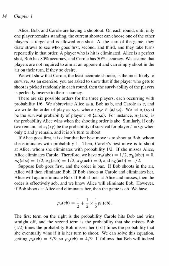
Alice, Bob, and Carole are having a shootout. On each round, until only
one player remains standing, the current shooter can choose one of the other
players as target and is allowed one shot. At the start of the game, they
draw straws to see who goes first, second, and third, and they take turns
repeatedly in that order. A player who is hit is eliminated. Alice is a perfect
shot, Bob has 80% accuracy, and Carole has 50% accuracy. We assume that
players are not required to aim at an opponent and can simply shoot in the
air on their turn, if they so desire.
We will show that Carole, the least accurate shooter, is the most likely to
survive. As an exercise, you are asked to show that if the player who gets to
shoot is picked randomly in each round, then the survivability of the players
is perfectly inverse to their accuracy.
There are six possible orders for the three players, each occurring with
probability 1/6. We abbreviate Alice as a, Bob as b, and Carole as c, and
we write the order of play as xyz, where x,y,z 2 fa,b,cg. We let �i.xyz/
be the survival probability of player i 2 fa,b,cg. For instance, �a.abc/ is
the probability Alice wins when the shooting order is abc. Similarly, if only
two remain, let �i.xy/ be the probability of survival for player i Dx,y when
only x and y remain, and it is x’s turn to shoot.
If Alice goes first, it is clear that her best move is to shoot at Bob, whom
she eliminates with probability 1. Then, Carole’s best move is to shoot
at Alice, whom she eliminates with probability 1/2. If she misses Alice,
Alice eliminates Carole. Therefore, we have �a.abc/ D 1=2, �b.abc/ D 0,
�c.abc/ D 1=2, �a.acb/ D 1=2, �b.acb/ D 0, and �c.acb/ D 1=2.
Suppose Bob goes first, and the order is bac. If Bob shoots in the air,
Alice will then eliminate Bob. If Bob shoots at Carole and eliminates her,
Alice will again eliminate Bob. If Bob shoots at Alice and misses, then the
order is effectively acb, and we know Alice will eliminate Bob. However,
if Bob shoots at Alice and eliminates her, then the game is cb. We have
pc.cb/ D 1
2C 1
2� 1
5pc.cb/:
The first term on the right is the probability Carole hits Bob and wins
straight off, and the second term is the probability that she misses Bob
(1/2) times the probability Bob misses her (1/5) times the probability that
she eventually wins if it is her turn to shoot. We can solve this equation,
getting pc.cb/ D 5=9, so pb.cb/ D 4=9. It follows that Bob will indeed

Probability and Decision Theory 15
shoot at Alice, so
pb.bac/ D 4
5� 4
9D 16
45:
Similarly, we have pb.bca/ D 16=45. Also,
pa.bac/ D 1
5pa.ca/ D 1
5� 1
2D 1
10;
because we clearly have pa.ca/ D 1=2. Similarly, pa.bca/ D 1=10. Fi-
nally,
pc.bac/ D 1
5pc.ca/ C 4
5� pc.cb/ D 1
5� 1
2C 4
5� 5
9D 49
90;
because pc.ca/ D 1=2. Similarly, pc.bca/ D 49=90. As a check on our
work, note that pa.bac/ C pb.bac/ C pc.bac/ D 1.
Suppose Carole gets to shoot first. If Carole shoots in the air, her payoff
from cab is pc.abc/ D 1=2, and from cba is pc.bac/ D 49=90. These
are also her payoffs if she misses her target. However, if she shoots Alice,
her payoff is pc.bc/, and if she shoots Bob, her payoff is pc.ac/ D 0. We
calculate pc.bc/ as follows.
pb.bc/ D 4
5C 1
5� 1
2pb.bc/;
where the first term is the probability he shoots Carole (4/5) plus the prob-
ability he misses Carole (1/5) times the probability he gets to shoot again
(1/2, because Carole misses) times pb.bc/. We solve, getting pb.bc/ D8=9. Thus, pc.bc/ D 1=9. Clearly, Carole’s best payoff is to shoot in
the air. Then pc.cab/ D 1=2, pb.cab/ D pb.abc/ D 0, and pa.cab/ Dpa.abc/ D 1=2. Also, pc.cba/ D 49=50, pb.cba/ D pb.bac/ D 16=45,
and pa.cba/ D pa.bac/ D 1=10.
The probability that Alice survives is given by
pa D 1
6.pa.abc/ C pa.acb/ C pa.bac/ C pa.bca/ C pa.cab/ C pa.cba//
D 1
6
�1
2C 1
2C 1
10C 1
10C 1
2C 1
10
�D 3
10:
The probability that Bob survives is given by
pb D 1
6.pb.abc/ C pb.acb/ C pb.bac/ C pb.bca/ C pb.cab/ C pb.cba//
D 1
6
�0 C 0 C 16
45C 16
45C 0 C 16
45
�D 8
45:
16 Chapter 1
The probability that Carole survives is given by
pc D 1
6.pc.abc/ C pc.acb/ C pc.bac/ C pc.bca/ C pc.cab/ C pc.cba//
D 1
6
�1
2C 1
2C 49
90C 49
90C 1
2C 49
90
�D 47
90:
You can check that these three probabilities add up to unity, as they should.
Note that Carole has a 52.2% chance of surviving, whereas Alice has only
a 30% chance, and Bob has a 17.8% chance.
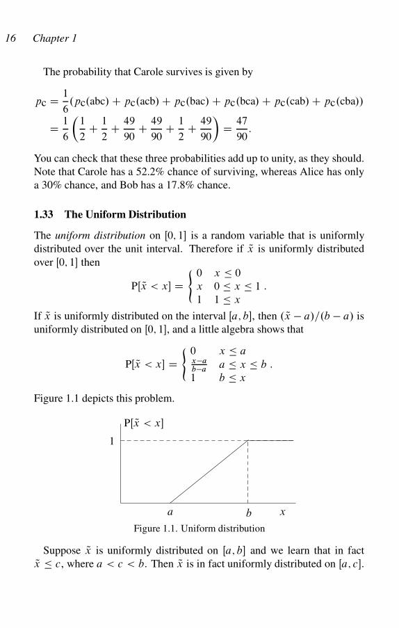
1.33 The Uniform Distribution
The uniform distribution on Œ0; 1� is a random variable that is uniformly
distributed over the unit interval. Therefore if Qx is uniformly distributed
over Œ0; 1� then
PŒ Qx < x� D(
0 x � 0
x 0 � x � 1
1 1 � x
:
If Qx is uniformly distributed on the interval Œa; b�, then . Qx � a/=.b � a/ is
uniformly distributed on Œ0; 1�, and a little algebra shows that
PŒ Qx < x� D(
0 x � ax�ab�a
a � x � b
1 b � x
:
Figure 1.1 depicts this problem.
PŒ Qx < x�
1
a b x
Figure 1.1. Uniform distribution
Suppose Qx is uniformly distributed on Œa; b� and we learn that in fact
Qx � c, where a < c < b. Then Qx is in fact uniformly distributed on Œa; c�.
Probability and Decision Theory 17
To see this, we write
PŒ Qx < xj Qx � c� D PŒ Qx < x and Qx � c�
PŒ Qx � c�
D PŒ Qx < x and Qx � c�
.c � a/=.b � a/:
We evaluate the numerator as follows:
PŒ Qx < x and Qx � c� D(
0 x � a
PŒ Qx < x� a � x � c
PŒ Qx � c� c � x
D8<
:
0 x � ax�ab�a
a � x � cc�ab�a
c � x:
Therefore,
PŒ Qx < xj Qx � c� D(
0 x � 0x�ac�a
a � x � c
1 c � x
:
This is just the uniform distribution on Œa; c�.
1.34 Laplace’s Law of Succession
An urn contains a large number n of white and black balls, where the num-
ber of white balls is uniformly distributed between 0 and n. Suppose you
pick out m balls with replacement, and r are white. Show that the probabil-
ity of picking a white ball on the next draw is approximately (rC1/=.mC2/:
1.35 From Uniform to Exponential
Bob tells Alice to draw repeatedly from the uniform distribution on Œ0; 1�
until her current draw is less than some previous draw, and he will pay her
$n, where n is the number of draws. What is the average value of this game
for Alice?
2
Bayesian Decision Theory
In a formal model the conclusions are derived from definitionsand assumptions. . . But with informal, verbal reasoning . . . onecan argue until one is blue in the face . . . because there is nocriterion for deciding the soundness of an informal argument.
Robert Aumann
2.1 The Rational Actor Model
In this section we develop a set of behavioral properties, among which con-
sistency is the most prominent, that together ensure that we can model the
individual as maximizing a preference function over outcomes, subject to
constraints.
A binary relation ˇA on a set A is a subset of A � A. We usually write
the proposition .x; y/ 2 ˇA as x ˇA y. For instance, the arithmetical
operator “less than” (<) is a binary relation, where .x; y/ 2< is normally
written x < y.1 A preference ordering �A on A is a binary relation with
the following three properties, which must hold for all x; y; z 2 A and any
set B :
1. Complete: x �A y or y �A x,
2. Transitive: x �A y and y �A z imply x �A z,
3. Independence from Irrelevant Alternatives: For x; y 2 B , x �B y
if and only if x �A y.
Because of the third property, we need not specify the choice set and can
simply write x � y. We also make the behavioral assumption that given
any choice set A, the individual chooses an element x 2 A such that for all
y 2 A, x � y. When x � y, we say “x is weakly preferred to y.”
1Additional binary relations over the set R of real numbers include
“>,”“<,”“�,” “D,” “�,” and “¤,” but “C” is not a binary relation, because x C y
is not a proposition.
18
Bayesian Decision Theory 19
Completeness implies that any member of A is weakly preferred to itself
(for any x in A, x � x). In general, we say a binary relation ˇ is reflexive
if, for all x, x ˇ x. Thus, completeness implies reflexivity. We refer to �as “weak preference” in contrast to � as “strong preference.” We define as
x � y to mean “it is false that y � x.” We say x and y are equivalent
if x � y and y � x, and we write x ' y. As an exercise, you may use
elementary logic to prove that if � satisfies the completeness condition,
then � satisfies the following exclusion condition: if x � y, then it is false
that y � x.
The second condition is transitivity, which says that x � y and y � z
imply x � z. It is hard to see how this condition could fail for anything we
might like to call a “preference ordering.”2 As an exercise, you may show
that x � y and y � z imply x � z, and x � y and y � z imply x � z.
Similarly, you may use elementary logic to prove that if � satisfies the
completeness condition, then ' is transitive (that is, satisfies the transitivity
condition).
When these three conditions are satisfied, we say the preference relation
� is consistent. If � is a consistent preference relation, then there always
exists a preference function such that the individual behaves as if maximiz-
ing this preference function over the set A from which he or she is con-
strained to choose. Formally, we say that a preference function u WA!R
represents a binary relation � if, for all x; y 2 A, u.x/ u.y/ if and only
if x � y. We have:
THEOREM 2.1 A binary relation � on the finite set A of payoffs can be
represented by a preference function uWA!R if and only if � is consistent.
It is clear that u./ is not unique, and indeed, we have the following.
THEOREM 2.2 If u./ represents the preference relation � and f ./ is a
strictly increasing function, then v./ D f .u.// also represents �. Con-
versely, if both u./ and v./ represent �, then there is an increasing func-
tion f ./ such that v./ D f .u.//.The first half of the theorem is true because if f is strictly increasing, then
u.x/ > u.y/ implies v.x/ D f .u.x// > f .u.y// D v.y/, and conversely.
2The only plausible model of intransitivity with some empirical support is re-
gret theory (Loomes 1988; Sugden 1993). This analysis applies, however, to only
a narrow range of choice situations.
20 Chapter 2
For the second half, suppose u./ and v./ both represent �, and for any
y 2 R such that v.x/ D y for some x 2 X , let f .y/ D u.v�1.y//, which
is possible because v is an increasing function. Then f ./ is increasing
(because it is the composition of two increasing functions) and f .v.x// Du.v�1.v.x/// D u.x/, which proves the theorem.
2.2 Time Consistency and Exponential Discounting
The central theorem on choice over time is that time consistency results
from assuming that utility be additive across time periods and the instan-
taneous utility function be the same in all time periods, with future utilities
discounted to the present at a fixed rate (Strotz 1955). This is called ex-
ponential discounting and is widely assumed in economic models. For in-
stance, suppose an individual can choose between two consumption streams
x D x0; x1; : : : or y D y0; y1; : : : According to exponential discounting,
he has a utility function u.x/ and a constant ı 2 .0; 1/ such that the total
utility of stream x is given by3
U.x0; x1; : : :/ D1X
kD0
ıku.xk/: (2.1)
We call ı the individual’s discount factor. Often we write ı D e�r where
we interpret r > 0 as the individual’s one-period, continuous-compounding
interest rate, in which case (2.1) becomes
U.x0; x1; : : :/ D1X
kD0
e�rku.xk/: (2.2)
This form clarifies why we call this “exponential” discounting. The indi-
vidual strictly prefers consumption stream x over stream y if and only if
U.x/ > U.y/. In the simple compounding case, where the interest accrues
at the end of the period, we write ı D 1=.1 C r/, and (2.2) becomes
U.x0; x1; : : :/ D1X
kD0
u.xk/
.1 C r/k: (2.3)
3Throughout this text, we write x 2 .a; b/ for a < x < b, x 2 Œa; b/ for
a � x < b, x 2 .a; b� for a < x � b, and x 2 Œa; b� for a � x � b.
Bayesian Decision Theory 21
The derivation of (2.2) is a bit tedious, and except for the exponential
discounting part, is intuitively obvious. So let us assume utility u.x/ is
additive and has the same shape across time, and show that exponential
discounting must hold. I will construct a very simple case that is easily
generalized. Suppose the individual has an amount of money M that he can
either invest or consume in periods t D 0; 1; 2. Suppose the interest rate
is r , and interest accrues continually, so $1 put in the bank at time k D 0
yields erk at time k. Thus, by putting an amount xke�rk in the bank today,
the individual will be able to consume xk in period k. By the additivity
and constancy across periods of utility, the individual will maximize some
objective function
V.x0; x1; x2/ D u.x0/ C au.x1/ C bu.x2/; (2.4)
subject to the income constraint
x0 C e�rx1 C e�2rx2 D M:
where r is the interest rate. We must show that b D a2 if and only if the
individual is time consistent. We form the Lagrangian
L D V.x0; x1; x2/ C �.x0 C e�rx1 C e�2rx2 � M/;
where � is the Lagrangian multiplier. The first-order conditions for a maxi-
mum are then given by @L=@xi D 0 for i D 0; 1; 2: Solving these equations,
we findu0.x1/
u0.x2/D ber
a: (2.5)
Now, time consistency means that after consuming x0 in the first period, the
individuals will still want to consume x1 in the second period and x2 in the
third. But now his objective function is
V.x1; x2/ D u.x1/ C au.x2/; (2.6)
subject to the (same) income constraint
x1 C e�rx2 D .M � x0/e�r ;
We form the Lagrangian
L1 D V.x1; x2/ C �.x1 C e�rx2 � .M � x0/e�r/;
22 Chapter 2
where � is the Lagrangian multiplier. The first-order conditions for a maxi-
mum are then given by @L1=@xi D 0 for i D 1; 2: Solving these equations,
we findu0.x1/
u0.x2/D aer : (2.7)
Now, time consistency means that (2.5) and (2.7) are equal, which means
a2 D b, as required.
2.3 The Expected Utility Principle
What about decisions in which a stochastic event determines the payoffs to
the players? Let X be a set of “prizes.” A lottery with payoffs in X is a
function pWX !Œ0; 1� such thatP
x2X p.x/ D 1. We interpret p.x/ as the
probability that the payoff is x 2 X . If X D fx1; : : : ; xng for some finite
number n, we write p.xi/ D pi .
The expected value of a lottery is the sum of the payoffs, where each pay-
off is weighted by the probability that the payoff will occur. If the lottery l
has payoffs x1 : : : xn with probabilities p1; : : : ; pn, then the expected value
EŒl� of the lottery l is given by
EŒl� DnX
iD1
pixi :
The expected value is important because of the law of large numbers (Feller
1950), which states that as the number of times a lottery is played goes to
infinity, the average payoff converges to the expected value of the lottery
with probability 1.
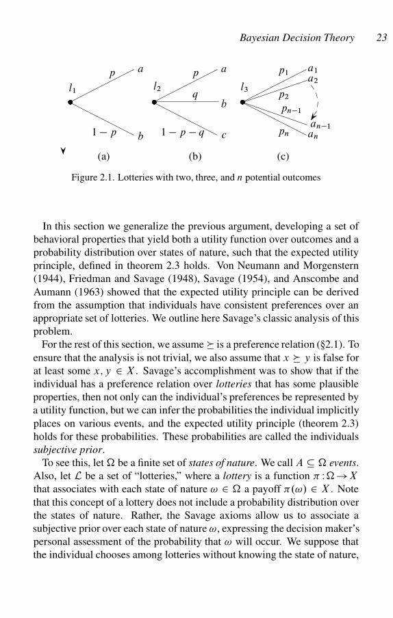
Consider the lottery l1 in pane (a) of figure 2.1, where p is the probability
of winning amount a and 1�p is the probability of winning amount b. The
expected value of the lottery is then EŒl1� D pa C .1 � p/b. Note that we
model a lottery a lot like an extensive form game, except there is only one
player.
Consider the lottery l2 with the three payoffs shown in pane (b) of fig-
ure 2.1. Here p is the probability of winning amount a, q is the probability
of winning amount b, and 1 � p � q is the probability of winning amount
c. The expected value of the lottery is EŒl2� D pa C qb C .1 � p � q/c.
A lottery with n payoffs is given in pane (c) of figure 2.1. The prizes are
now a1; : : : ; an with probabilities p1; : : : ; pn, respectively. The expected
value of the lottery is now EŒl3� D p1a1 C p2a2 C : : : C pnan.
Bayesian Decision Theory 23
a1
a2
an�1
an
�
p1
p2
pn�1
pn
a
b
c
�
p
q
1 � p � q
a
b
�
l1
p
1 � p
(a) (b) (c)
l2 l3
Figure 2.1. Lotteries with two, three, and n potential outcomes
In this section we generalize the previous argument, developing a set of
behavioral properties that yield both a utility function over outcomes and a
probability distribution over states of nature, such that the expected utility
principle, defined in theorem 2.3 holds. Von Neumann and Morgenstern
(1944), Friedman and Savage (1948), Savage (1954), and Anscombe and
Aumann (1963) showed that the expected utility principle can be derived
from the assumption that individuals have consistent preferences over an
appropriate set of lotteries. We outline here Savage’s classic analysis of this
problem.
For the rest of this section, we assume � is a preference relation (�2.1). To
ensure that the analysis is not trivial, we also assume that x � y is false for
at least some x; y 2 X . Savage’s accomplishment was to show that if the
individual has a preference relation over lotteries that has some plausible
properties, then not only can the individual’s preferences be represented by
a utility function, but we can infer the probabilities the individual implicitly
places on various events, and the expected utility principle (theorem 2.3)
holds for these probabilities. These probabilities are called the individuals
subjective prior.
To see this, let � be a finite set of states of nature. We call A � � events.
Also, let L be a set of “lotteries,” where a lottery is a function � W�!X
that associates with each state of nature ! 2 � a payoff �.!/ 2 X . Note
that this concept of a lottery does not include a probability distribution over
the states of nature. Rather, the Savage axioms allow us to associate a
subjective prior over each state of nature !, expressing the decision maker’s
personal assessment of the probability that ! will occur. We suppose that
the individual chooses among lotteries without knowing the state of nature,
24 Chapter 2
after which “Nature” chooses the state ! 2 � that obtains, so that if the
individual chose lottery � 2 L, his payoff is �.!/.
Now suppose the individual has a preference relation � over L (we use
the same symbol � for preferences over both outcomes and lotteries). We
seek a set of plausible properties of � over lotteries that together allow us
to deduce (a) a utility function u WX !R corresponding to the preference
relation � over outcomes in X ; (b) a probability distribution p W � ! R
such that the expected utility principle holds with respect to the preference
relation � over lotteries and the utility function u./; that is, if we define
E� ŒuI p� DX
!2�
p.!/u.�.!//; (2.8)
then for any �; � 2 L,
� � � ” E� ŒuI p� > E�ŒuI p�:
Our first condition is that � � � depends only on states of nature where �
and � have different outcomes. We state this more formally as
A1. For any �; �; � 0; �0 2 L, let A D f! 2 �j�.!/ ¤ �.!/g.
Suppose we also have A D f! 2 �j� 0.!/ ¤ �0.!/g. Suppose
also that �.!/ D � 0.!/ and �.!/ D �0.!/ for ! 2 A. Then
� � � , � 0 � �0.
This axiom allows us to define a conditional preference � �A �, where
A � �, which we interpret as “� is strictly preferred to �, conditional on
event A,” as follows. We say � �A � if, for some � 0; �0 2 L, �.!/ D � 0.!/
and �.!/ D �0.!/ for ! 2 A, � 0.!/ D �0.!/ for ! … A, and � 0 � �0.
Because of A1, this is well defined (that is, � �A � does not depend on
the particular � 0; �0 2 L). This allows us to define �A and �A in a similar
manner. We then define an event A � � to be null if � �A � for all
�; � 2 L.
Our second condition is then the following, where we write � D xjA to
mean �.!/ D x for all ! 2 A (that is, � D xjA means � is a lottery that
pays x when A occurs).
A2. If A � � is not null, then for all x; y 2 X , � D xjA �A � DyjA , x � y.
Bayesian Decision Theory 25
This axiom says that a natural relationship between outcomes and lotteries
holds: if � pays x given event A and � pays y given event A, and if x � y,
then � �A �, and conversely.
Our third condition asserts that the probability that a state of nature occurs
is independent from the outcome one receives when the state occurs. The
difficulty in stating this axiom is that the individual cannot choose probabili-
ties, but only lotteries. But, if the individual prefers x to y, and if A; B � �
are events, then the individual treats A as “more probable” than B if and
only if a lottery that pays x when A occurs and y when A does not occur
will be preferred to a lottery that pays x when B occurs and y when B does
not. However, this must be true for any x; y 2 X such that x � y, or the
individual’s notion of probability is incoherent (that is, it depends on what
particular payoffs we are talking about. For instance, some people engage
in “wishful thinking,” where if the prize associated with an event increases,
the individual thinks it is more likely to occur). More formally, we have the
following, where we write � D x; yjA to mean “�.!/ D x for ! 2 A and
�.!/ D y for ! … A.”
A3. Suppose x � y, x0 � y 0, �; �; � 0; �0 2 L, and A; B � �.
Suppose that � D x; yjA, � D x0; y 0jA, � 0 D x; yjB , �0 Dx0; y 0jB . Then � � � 0 , � � �0.
The fourth condition is a weak version of first-order stochastic domi-
nance, which says that if one lottery has a higher payoff than another for
any event, then the first is preferred to the second.
A4. For any event A, if x � �.!/ for all ! 2 A, then � D xjA �A
�. Also, for any event A, if �.!/ � x for all ! 2 A, then
� �A � D xjA.
In other words, if for any event A, � D x on A pays more than the best �
can pay on A, the � �A �, and conversely.
Finally, we need a technical property to show that a preference relation
can be represented by a utility function. It says that for any �; � 2 L, and
any x 2 X , we can partition � into a number of disjoint subsets A1; : : : An
such that [iAi D �, and for each Ai , if we change � so that its payoff is x
on Ai , then � is still preferred to �. Similarly, for each Ai , if we change �
so that its payoff is x on Ai , then � is still preferred to �. This means that
no payoff is “supergood,” so that no matter how unlikely an event A is, a
lottery with that payoff when A occurs is always preferred to a lottery with
26 Chapter 2
a different payoff when A occurs. Similarly, no payoff can be “superbad.”
The condition is formally as follows:
A5. For all �; � 0; �; �0 2 L with � � �, and for all x 2 X , there
are disjoint subsets A1; : : : ; An of � such that [iAi D � and
for any Ai (a) if � 0.!/ D x for ! 2 Ai and � 0.!/ D �.!/ for
! … Ai , then � 0 � �, and (b) if �0.!/ D x for ! 2 Ai and
�0.!/ D �.!/ for ! … Ai , then � � �0.
We then have Savage’s theorem.
THEOREM 2.3 Suppose A1–A5 hold. Then there is a probability function
p on � and a utility function uWX !R such that for any �; � 2 L, � � �
if and only if E� ŒuI p� > E�ŒuI p�.
The proof of this theorem is somewhat tedious (it is sketched in Kreps
1988).
We call the probability p the individual’s Bayesian prior, or subjective
prior, and say that A1–A5 imply Bayesian rationality, because they to-
gether imply Bayesian probability updating.
2.4 Risk and the Shape of the Utility Function
If � is defined over X , we can say nothing about the shape of a utility func-
tion u./ representing �, because by theorem 2.2, any increasing function
of u./ also represents �. However, if � is represented by a utility function
u.x/ satisfying the expected utility principle, then u./ is determined up to
an arbitrary constant and unit of measure.4
THEOREM 2.4 Suppose the utility function u./ represents the preference
relation � and satisfies the expected utility principle. If v./ is another
utility function representing �, then there are constants a; b 2 R with a > 0
such that v.x/ D au.x/ C b for all x 2 X .
4Because of this theorem, the difference between two utilities means nothing.
We thus say utilities over outcomes are ordinal, meaning we can say that one
bundle is preferred to another, but we cannot say by how much. By contrast, the
next theorem shows that utilities over lotteries are cardinal, in the sense that, up to
an arbitrary constant and an arbitrary positive choice of units, utility is numerically
uniquely defined.

Bayesian Decision Theory 27
G
HIF
DC
E.u.x//
u.x/
�
y
�
x
u.Ex/u.y/
�
u.x/�
Ex
A
B
E
Figure 2.2. A concave utility function
see Mas-Colell, Whinston and Green (1995):173 prove this theorem.
If X D R, so the payoffs can be considered to be “money,” and utility
satisfies the expected utility principle, what shape do such utility functions
have? It would be nice if they were linear in money, in which case expected
utility and expected value would be the same thing (why?). But generally
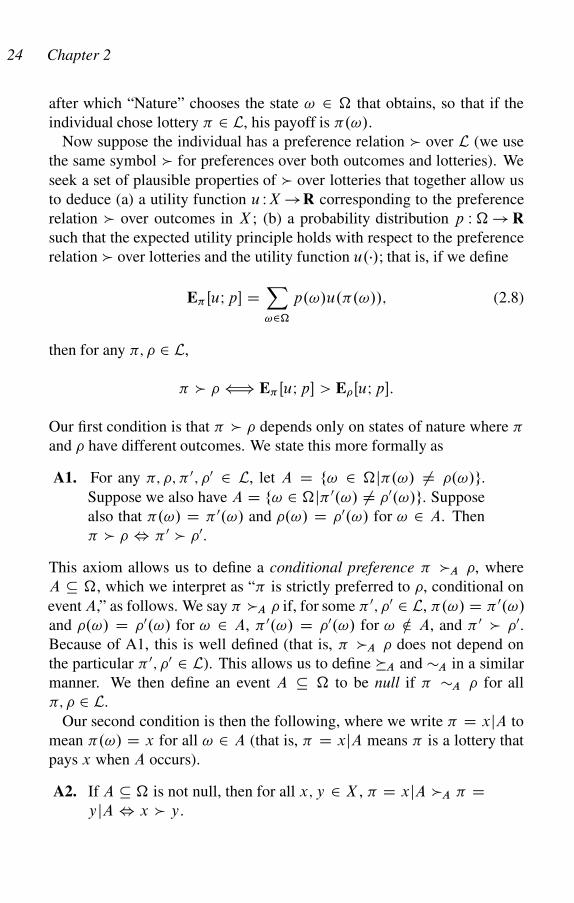
utility will be strictly concave, as illustrated in figure 2.2. We say a function
u WX !R is strictly concave, if for any x; y 2 X , and any p 2 .0; 1/, we
have pu.x/ C .1 � p/u.y/ < u.px C .1 � p/y/. We say u.x/ is weakly
concave, or simply concave if, for any x; y 2 X , pu.x/ C .1 � p/u.y/ �u.px C .1 � p/y/.
If we define the lottery � as paying x with probability p and y with
probability 1 � p, then the condition for strict concavity says that the ex-
pected utility of the lottery is less than the utility of the expected value of
the lottery, as depicted in figure 2.2. To see this, note that the expected
value of the lottery is E D px C .1 � p/y, which divides the line seg-
ment between x and y into two segments, the segment xE having length
.px C .1 � p/y/ � x D .1 � p/.y � x/, and the segment Ey having length
y � .px C .1�p/y/ D p.y �x/. Thus, E divides Œx; y� into two segments
whose lengths have ratio .1 � p/=p. From elementary geometry, it follows
that B divides segment ŒA; C � into two segments whose lengths have the
same ratio. By the same reasoning, point H divides segments ŒF; G� into
segments with the same ratio of lengths. This means the point H has the
coordinate value pu.x/ C .1 � p/u.y/, which is the expected utility of the
lottery. But by definition, the utility of the expected value of the lottery is
at D, which lies above H . This proves that the utility of the expected value
is greater than the expected value of the lottery for a strictly concave utility
function. This is know as Jensen’s inequality.
28 Chapter 2
What are good candidates for u.x/? It is easy to see that strict concavity
means u00.x/ < 0, providing u.x/ is twice differentiable (which we as-
sume). But there are lots of functions with this property. According to the
famous Weber-Fechner law of psychophysics, for a wide range of sensory
stimuli, and over a wide range of levels of stimulation, a just-noticeable
change in a stimulus is a constant fraction of the original stimulus. If this
holds for money, then the utility function is logarithmic.
We say an individual is risk averse if the individual prefers the expected
value of a lottery to the lottery itself (provided, of course, the lottery does
not offer a single payoff with probability 1, which we call a “sure thing”).
We know, then, that an individual with utility function u./ is risk averse if
and only if u./ is concave.5 Similarly, we say an individual is risk loving if
he prefers any lottery to the expected value of the lottery, and risk neutral if
he considers a lottery and its expected value to be equally desirable. Clearly,
an individual is risk neutral if and only if he has linear utility.
Does there exist a measure of risk aversion that allows us to say when
one individual is more risk averse than another, or how an individual’s risk
aversion changes with changing wealth? We may define individual A to be
more risk averse than individual B if whenever A prefers a lottery to an
amount of money x, B will also prefer the lottery to x. We say A is strictly
more risk averse than B if he is more risk averse, and there is some lottery
that B prefers to an amount of money x, but such that A prefers x to the
lottery.
Clearly, the degree of risk aversion depends on the curvature of the utility
function (by definition the curvature of u.x/ at x is u00.x/), but because
u.x/ and v.x/ D au.x/ C b (a > 0) describe the same behavior, but v.x/
has curvature a times that of u.x/, we need something more sophisticated.
The obvious candidate is �u.x/ D �u00.x/=u0.x/, which does not depend
on scaling factors. This is called the Arrow-Pratt coefficient of absolute risk
5One may ask why people play government-sponsored lotteries, or spend
money at gambling casinos, if they are generally risk averse. The most plausi-
ble explanation is that people enjoy the act of gambling. The same woman who
will have insurance on her home and car, both of which presume risk aversion, will
gamble small amounts of money for recreation. An excessive love for gambling,
of course, leads an individual either to personal destruction or to wealth and fame
(usually the former).
Bayesian Decision Theory 29
aversion, and it is exactly the measure that we need. We have the following
theorem.
THEOREM 2.5 An individual with utility function u.x/ is strictly more risk
averse than an individual with utility function v.x/ if and only if �u.x/ >
�v.x/ for all x.
For example, the logarithmic utility function u.x/ D ln.x/ has Arrow-
Pratt measure �u.x/ D 1=x, which decreases with x; that is, as the indi-
vidual becomes wealthier, he becomes less risk averse. Studies show that
this property, called decreasing absolute risk aversion, holds rather widely
(Rosenzweig and Wolpin 1993; Saha, Shumway and Talpaz 1994; Nerlove
and Soedjiana 1996). Another increasing concave function is u.x/ D xa
for a 2 .0; 1/, for which �u.x/ D .1�a/=x, which also exhibits decreasing
absolute risk aversion. Similarly, u.x/ D 1 � x�a (a > 0) is increasing
and concave, with �u.x/ D �.a C 1/=x, which again exhibits decreasing
absolute risk aversion. If utility is unbounded, it is easy to show that there
is a lottery that you would be willing to give all your wealth to play, no
matter how rich you are. This is not plausible behavior. However, this util-
ity has the additional attractive property that utility is bounded: no matter
how rich you are, u.x/ < 1. Yet another candidate for a utility function is
u.x/ D 1 � e�ax, for some a > 0. In this case �u.x/ D a, which we call
constant absolute risk aversion.
Another commonly used term is the coefficient of relative risk aversion,
�u.x/ D �u.x/=x. Note that for any of the utility functions u.x/ D ln.x/,
u.x/ D xa for a 2 .0; 1/, and u.x/ D 1 � x�a (a > 0), �u.x/ is constant,
which we call constant relative risk aversion. For u.x/ D 1�e�ax (a > 0),
we have �u.x/ D a=x, so we have decreasing relative risk aversion.
As an exercise, consider the utility function
u.x/ D 1 � e�axb
;
where b < 1 and ab 0.
a. Show that u.x/ is increasing and concave.b. Find the Arrow-Pratt measures of absolute and relative risk aversion for
this utility function.c. Show that u.x/ exhibits decreasing absolute risk aversion for a < 0,
constant relative risk aversion for a D 0, and increasing relative risk
aversion for a > 0.
30 Chapter 2
2.5 The Scientific Status of the Rational Actor Model
The extent to which the rational actor model is supported by the facts is
dealt with extensively in Gintis (2009), so I give only a brief overview of
the issues here.
The three principles of preference consistency developed in section 2.1
are sufficient to support a model of individual choice as maximizing a
preference function subject to constraints. Studies of market behavior by
economists generally support preference consistency, finding that individ-
ual choices are broadly consistent (Mattei 1994; Sippel 1997; Harbaugh,
Krause and Berry 2001; Andreoni and Miller 2002). For instance, Mat-
tei (1994) found that 50% of consumers conform perfectly to preference
consistency, and almost all deviations were very small (due to the diffi-
culty of maximizing perfectly) or involved consumers making infrequent
purchases. Moreover, as suggested by Becker (1962), aggregate demand
may exhibit consistency even when individuals are inconsistent. This ob-
servation has been tested and validated by Forsythe, Nelson, Neumann and
Wright (1992), Gode and Sunder (1993), and List and Millimet (2007).
The rational actor model is, of course, basically a psychological model,
and it has been widely tested by psychologists, most notably Amos Tver-
sky, Daniel Kahneman, and their co-workers (Kahneman, Slovic and Tver-
sky 1982). Psychologists have been generally critical of the rational actor
model, and it is not widely used in psychological research. The reason
for this discrepancy between economic and psychological data has a fairly
straightforward explanation.
Psychologists study delibertive decision making, including the formation
of long-term personal goals and the evaluation of inherently unknowable
uncertainties. Complex human decisions tend to involve problems that arise
infrequently, such as choice of career, whether to marry and to whom, how
many children to have, how to deal with a health threat, and how to evaluate
and choose when there are novel products.
By contrast, the rational actor model applies to routine choice situations,
where such ambiguities and complications are absent. In the economic
model, the choice set is clearly delineated, and the payoffs, or at least their
probabilities, are known. Most psychologists working on decision making
in fact do accept the rational actor model as the appropriate model of choice
behavior in the realm of routine choice, amended often by making an indi-
vidual’s current state an argument of the preference function. However, they
Bayesian Decision Theory 31
have not found a way to extend the model to the more complex situations
involved in deliberative decision making.
The expected utility aspect of the rational actor model (�2.3) is, of course,
a far more powerful tool than simple preference consistency, especially be-
cause it requires that the individual evaluate complex lotteries appropriately.
This is a feat that even advanced students of probability theory have diffi-
culty in accomplishing. This should be clear to you if you had problems
with the material in chapter 1! Indeed, there are systematic ways individu-
als deviate from expected utility theory, revealed in the famous Allais and
Ellsberg paradoxes, among others. However, it is reasonable to accept the
expected utility theorem and treat the experimentally derived exceptions as
equivalent to optical illusions: misjudgment does occur and can be very
dramatic, but the existence of optical illusions does not undermine our un-
derstanding of vision as generally veridical.
Even when applied to routine decision making, the archetypal rational
actor model is a considerable abstraction from individual choice behavior.
For one thing, preferences are ineluctably a function of the current state of
the actor, including physiological state, income and wealth, and everchang-
ing developmental history. Moreover, the subjective prior derived from
observed choices over lotteries is a function of beliefs, which are socially
constructed and deeply dependent upon cultural experience and social inter-
action. Finally, most humans are inextricably social creatures whose pref-
erences are affected by moral considerations that are situationally specific.
In particular, people tend to conform to social norms that are reflected in
the priorities represented in their preference orderings. Recognizing these
dimensions of rational action dramatically complicates the analytical rep-
resentation of rational action, but there is no alternative, if one’s aim is the
explanation of human behavior.
3
Game Theory: Basic Concepts
Each discipline of the social sciences rules comfortably withinits own chosen domain . . . so long as it stays largely obliviousof the others.
Edward O. Wilson
3.1 Big John and Little John
Big John and Little John eat coconuts, which dangle from a lofty branch of
a palm tree. Their favorite coconut palm produces only one fruit per tree.
To get the coconut, at least one of them must climb the tree and knock the
coconut loose so that it falls to the ground. Careful energy measurements
show that a coconut is worth 10 Kc (kilocalories) of energy, the cost of
running up the tree, shaking the coconut loose, and running back down to
the ground costs 2 Kc for Big John, but is negligible for Little John, who
is much smaller. Moreover, if both individuals climb the tree, shake the
coconut loose, then climb down the tree and eat the coconut, Big John gets
7 Kc and Little John gets only 3 Kc, because Big John hogs most of it; if
only Big John climbs the tree, while Little John waits on the ground for the
coconut to fall, Big John gets 6 Kc and Little John gets 4 Kc (Little John
eats some before Big John gets back down from the tree); if only Little John
climbs the tree, Big John gets 9 Kc and Little John gets 1 Kc (most of the
food is gone by the time Little John gets there).
What will Big John and Little John do if each wants to maximize net
energy gain? There is one crucial issue that must be resolved: who decides
first what to do, Big John or Little John? There are three possibilities:
(a) Big John decides first; (b) Little John decides first; (c) both individuals
decide simultaneously. We will go through the three cases in turn.
Assuming Big John decides first, we get the situation depicted in fig-
ure 3.1. We call a figure like this a game tree, and we call the game it
defines an extensive form game. At the top of the game tree is the root node
(the little dot labeled “Big John”) with two branches, labeled w (wait) and
32
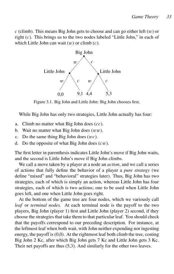
Game Theory 33
c (climb). This means Big John gets to choose and can go either left (w) or
right (c). This brings us to the two nodes labeled “Little John,” in each of
which Little John can wait (w) or climb (c).
Little John Little John
Big John
5,34,49,10,0
cwcw
cw
��
�
Figure 3.1. Big John and Little John: Big John chooses first.
While Big John has only two strategies, Little John actually has four:
a. Climb no matter what Big John does (cc).
b. Wait no matter what Big John does (ww).
c. Do the same thing Big John does (wc).
d. Do the opposite of what Big John does (cw).
The first letter in parenthesis indicates Little John’s move if Big John waits,
and the second is Little John’s move if Big John climbs.
We call a move taken by a player at a node an action, and we call a series
of actions that fully define the behavior of a player a pure strategy (we
define “mixed” and “behavioral” strategies later). Thus, Big John has two
strategies, each of which is simply an action, whereas Little John has four
strategies, each of which is two actions; one to be used when Little John
goes left, and one when Little John goes right.
At the bottom of the game tree are four nodes, which we variously call
leaf or terminal nodes. At each terminal node is the payoff to the two
players, Big John (player 1) first and Little John (player 2) second, if they
choose the strategies that take them to that particular leaf. You should check
that the payoffs correspond to our preceding description. For instance, at
the leftmost leaf when both wait, with John neither expending nor ingesting
energy, the payoff is (0,0). At the rightmost leaf both climb the tree, costing
Big John 2 Kc, after which Big John gets 7 Kc and Little John gets 3 Kc.
Their net payoffs are thus (5,3). And similarly for the other two leaves.
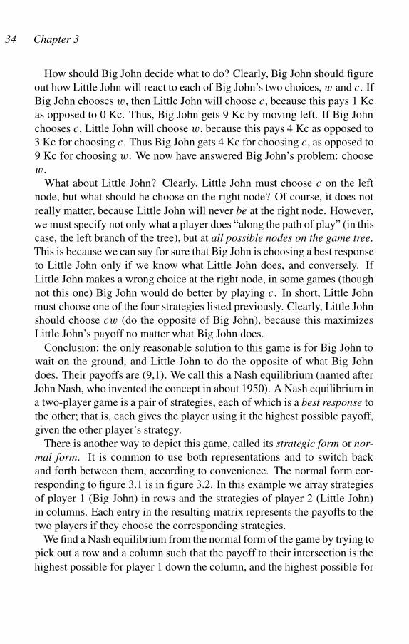
34 Chapter 3
How should Big John decide what to do? Clearly, Big John should figure
out how Little John will react to each of Big John’s two choices, w and c. If
Big John chooses w, then Little John will choose c, because this pays 1 Kc
as opposed to 0 Kc. Thus, Big John gets 9 Kc by moving left. If Big John
chooses c, Little John will choose w, because this pays 4 Kc as opposed to
3 Kc for choosing c. Thus Big John gets 4 Kc for choosing c, as opposed to
9 Kc for choosing w. We now have answered Big John’s problem: choose
w.
What about Little John? Clearly, Little John must choose c on the left
node, but what should he choose on the right node? Of course, it does not
really matter, because Little John will never be at the right node. However,
we must specify not only what a player does “along the path of play” (in this
case, the left branch of the tree), but at all possible nodes on the game tree.
This is because we can say for sure that Big John is choosing a best response
to Little John only if we know what Little John does, and conversely. If
Little John makes a wrong choice at the right node, in some games (though
not this one) Big John would do better by playing c. In short, Little John
must choose one of the four strategies listed previously. Clearly, Little John
should choose cw (do the opposite of Big John), because this maximizes
Little John’s payoff no matter what Big John does.
Conclusion: the only reasonable solution to this game is for Big John to
wait on the ground, and Little John to do the opposite of what Big John
does. Their payoffs are (9,1). We call this a Nash equilibrium (named after
John Nash, who invented the concept in about 1950). A Nash equilibrium in
a two-player game is a pair of strategies, each of which is a best response to
the other; that is, each gives the player using it the highest possible payoff,
given the other player’s strategy.
There is another way to depict this game, called its strategic form or nor-
mal form. It is common to use both representations and to switch back
and forth between them, according to convenience. The normal form cor-
responding to figure 3.1 is in figure 3.2. In this example we array strategies
of player 1 (Big John) in rows and the strategies of player 2 (Little John)
in columns. Each entry in the resulting matrix represents the payoffs to the
two players if they choose the corresponding strategies.
We find a Nash equilibrium from the normal form of the game by trying to
pick out a row and a column such that the payoff to their intersection is the
highest possible for player 1 down the column, and the highest possible for
Game Theory 35
Big
Little Johnww
0,0
4,4
wc
9,1
4,4
w
c
cw
0,0
5,3
cc
9,1
5,3John
Figure 3.2. Normal form of Big John and Little John when Big John moves first
player 2 across the row (there may be more than one such pair). Note that
.w; cw/ is indeed a Nash equilibrium of the normal form game, because 9
is better than 4 for Big John down the cw column, and 1 is the best Little
John can do across the w row.
Can we find any other Nash equilibria to this game? Clearly .w; cc/ is
also a Nash equilibrium, because w is a best reply to cc and conversely. But
the .w; cc/ equilibrium has the drawback that if Big John should happen to
make a mistake and play c, Little John gets only 3, whereas with cw Little
John gets 4. We say cc is weakly dominated by cw, meaning that cw pays
off at least as well for Little John no matter what Big John does, but for at
least one move of Big John, cw has a higher payoff than cc for Little John
(�4.1).
But what if Little John plays ww? Then Big John should play c, and it is
clear that ww is a best response to c. So this gives us another Nash equilib-
rium, .c; ww/, in which Little John does much better, getting 4 instead of
1, and Big John does much worse, getting 4 instead of 9. Why did we not
see this Nash equilibrium in our analysis of the extensive form game? The
reason is that .c; ww/ involves Little John making an incredible threat (see
section 4.2 for a further analysis of Little John’s incredible threat).
“I do not care what you do,” says Little John; “I’m waiting here on the
ground no matter what.” The threat is “incredible” because Big John knows
that if he plays w, then when it is Little John’s turn to carry out the threat to
play w, Little John will not in fact do so, simply because 1 is better than 0.1
We say a Nash equilibrium of an extensive form game is subgame perfect
if, at any point in the game tree, the play dictated by the Nash equilibrium
remains a Nash equilibrium of the subgame. The strategy .c; ww/ is not
1This argument fails if the individuals can condition their behavior in one day
on their behavior in previous days (see chapter 9). We assume the players cannot
do this.

36 Chapter 3
subgame perfect because in the subgame beginning with Little John’s choice
of w on the left of figure 3.1 is not a best response. Nice try, anyway, Little
John!
But what if Little John gets to choose first? Perhaps now Little John can
force a better split than getting 1 compared to Big John’s 9. This is the
extensive form game (figure 3.3). We now call Little John player 1 and
Big John player 2. Now Big John has four strategies (the strategies that
belonged to Little John in the previous version of the game) and Little John
has only two (the ones that belonged to Big John before). Little John notices
that Big John’s best response to w is c, and Big John’s best response to c
is w. Because Little John gets 4 in the first case and only 1 in the second,
Little John chooses w. Big John’s best choice is then cw, and the payoffs
are (4,4). Note that by going first, Little John is able to precommit to a
strategy that is an incredible threat when going second.
�
� �
w c
w c w c
0,0 4,4 1,9 3,5
Little John
Big JohnBig John
Figure 3.3. Big John and Little John: Little John chooses first
The normal form for the case when Little John goes first is illustrated in
figure 3.4. Again we find the two Nash equilibria (w; cc) and (w; cw), and
again we find another Nash equilibrium not evident at first glance from the
game tree: now it is Big John who has an incredible threat, by playing ww,
to which Little John’s best response is c.
The final possibility is that the players choose simultaneously, or, equiv-
alently, each player chooses an action without seeing what the other player
chooses. In this case, each player has two options: climb the tree (c), or
wait on the ground (w). We then get the situation in figure 3.5. Note the new
element in the game tree: the dotted line connecting the two places where
Little John chooses. This is called an information set. Roughly speaking,
an information set is a set of nodes at which (a) the same player chooses,
and (b) the player choosing does not know which particular node represents
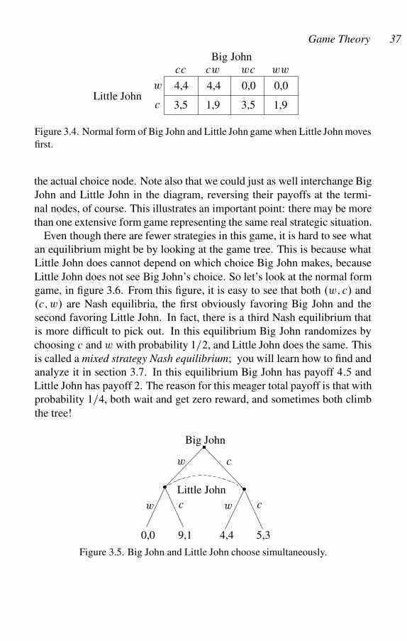
Game Theory 37
3,5
4,4
cc
1,9
4,4
cw
c
w
3,5
0,0
wc
1,9
0,0
ww
Little John
Big John
Figure 3.4. Normal form of Big John and Little John game when Little John moves
first.
the actual choice node. Note also that we could just as well interchange Big
John and Little John in the diagram, reversing their payoffs at the termi-
nal nodes, of course. This illustrates an important point: there may be more
than one extensive form game representing the same real strategic situation.
Even though there are fewer strategies in this game, it is hard to see what
an equilibrium might be by looking at the game tree. This is because what
Little John does cannot depend on which choice Big John makes, because
Little John does not see Big John’s choice. So let’s look at the normal form
game, in figure 3.6. From this figure, it is easy to see that both .w; c/ and
.c; w/ are Nash equilibria, the first obviously favoring Big John and the
second favoring Little John. In fact, there is a third Nash equilibrium that
is more difficult to pick out. In this equilibrium Big John randomizes by
choosing c and w with probability 1=2, and Little John does the same. This
is called a mixed strategy Nash equilibrium; you will learn how to find and
analyze it in section 3.7. In this equilibrium Big John has payoff 4:5 and
Little John has payoff 2. The reason for this meager total payoff is that with
probability 1=4, both wait and get zero reward, and sometimes both climb
the tree!
Little John
Big John
5,34,49,10,0
cwcw
cw
��
�
Figure 3.5. Big John and Little John choose simultaneously.
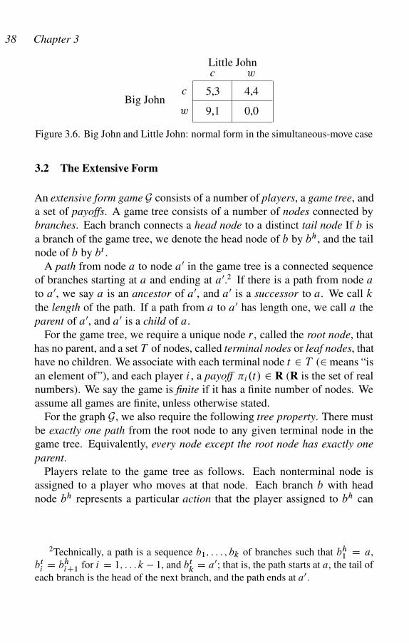
38 Chapter 3
5,3
9,1
c
4,4
0,0
w
c
w
Little John
Big John
Figure 3.6. Big John and Little John: normal form in the simultaneous-move case
3.2 The Extensive Form
An extensive form game G consists of a number of players, a game tree, and
a set of payoffs. A game tree consists of a number of nodes connected by
branches. Each branch connects a head node to a distinct tail node If b is
a branch of the game tree, we denote the head node of b by bh, and the tail
node of b by bt .
A path from node a to node a0 in the game tree is a connected sequence
of branches starting at a and ending at a0.2 If there is a path from node a
to a0, we say a is an ancestor of a0, and a0 is a successor to a. We call k
the length of the path. If a path from a to a0 has length one, we call a the
parent of a0, and a0 is a child of a.
For the game tree, we require a unique node r , called the root node, that
has no parent, and a set T of nodes, called terminal nodes or leaf nodes, that
have no children. We associate with each terminal node t 2 T (2 means “is
an element of”), and each player i , a payoff �i.t/ 2 R (R is the set of real
numbers). We say the game is finite if it has a finite number of nodes. We
assume all games are finite, unless otherwise stated.
For the graph G, we also require the following tree property. There must
be exactly one path from the root node to any given terminal node in the
game tree. Equivalently, every node except the root node has exactly one
parent.
Players relate to the game tree as follows. Each nonterminal node is
assigned to a player who moves at that node. Each branch b with head
node bh represents a particular action that the player assigned to bh can
2Technically, a path is a sequence b1; : : : ; bk of branches such that bh1 D a,
bti D bh
iC1 for i D 1; : : : k � 1, and btk
D a0; that is, the path starts at a, the tail of
each branch is the head of the next branch, and the path ends at a0.
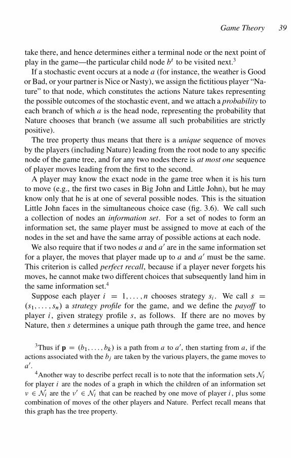
Game Theory 39
take there, and hence determines either a terminal node or the next point of
play in the game—the particular child node bt to be visited next.3
If a stochastic event occurs at a node a (for instance, the weather is Good
or Bad, or your partner is Nice or Nasty), we assign the fictitious player “Na-
ture” to that node, which constitutes the actions Nature takes representing
the possible outcomes of the stochastic event, and we attach a probability to
each branch of which a is the head node, representing the probability that
Nature chooses that branch (we assume all such probabilities are strictly
positive).
The tree property thus means that there is a unique sequence of moves
by the players (including Nature) leading from the root node to any specific
node of the game tree, and for any two nodes there is at most one sequence
of player moves leading from the first to the second.
A player may know the exact node in the game tree when it is his turn
to move (e.g., the first two cases in Big John and Little John), but he may
know only that he is at one of several possible nodes. This is the situation
Little John faces in the simultaneous choice case (fig. 3.6). We call such
a collection of nodes an information set. For a set of nodes to form an
information set, the same player must be assigned to move at each of the
nodes in the set and have the same array of possible actions at each node.
We also require that if two nodes a and a0 are in the same information set
for a player, the moves that player made up to a and a0 must be the same.
This criterion is called perfect recall, because if a player never forgets his
moves, he cannot make two different choices that subsequently land him in
the same information set.4
Suppose each player i D 1; : : : ; n chooses strategy si . We call s D.s1; : : : ; sn/ a strategy profile for the game, and we define the payoff to
player i , given strategy profile s, as follows. If there are no moves by
Nature, then s determines a unique path through the game tree, and hence
3Thus if p D .b1; : : : ; bk/ is a path from a to a0, then starting from a, if the
actions associated with the bj are taken by the various players, the game moves to
a0.4Another way to describe perfect recall is to note that the information sets Ni
for player i are the nodes of a graph in which the children of an information set
� 2 Ni are the �0 2 Ni that can be reached by one move of player i , plus some
combination of moves of the other players and Nature. Perfect recall means that
this graph has the tree property.
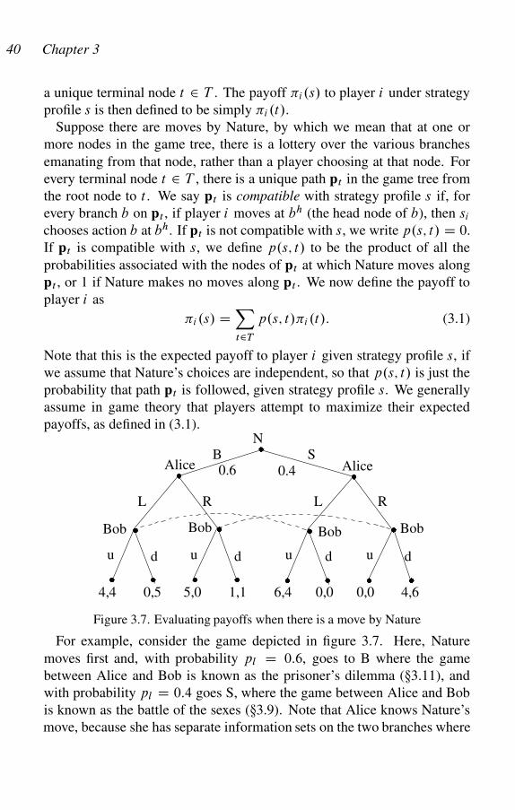
40 Chapter 3
a unique terminal node t 2 T . The payoff �i.s/ to player i under strategy
profile s is then defined to be simply �i .t/.
Suppose there are moves by Nature, by which we mean that at one or
more nodes in the game tree, there is a lottery over the various branches
emanating from that node, rather than a player choosing at that node. For
every terminal node t 2 T , there is a unique path pt in the game tree from
the root node to t . We say pt is compatible with strategy profile s if, for
every branch b on pt , if player i moves at bh (the head node of b), then si
chooses action b at bh. If pt is not compatible with s, we write p.s; t/ D 0.
If pt is compatible with s, we define p.s; t/ to be the product of all the
probabilities associated with the nodes of pt at which Nature moves along
pt , or 1 if Nature makes no moves along pt . We now define the payoff to
player i as
�i .s/ DX
t2T
p.s; t/�i .t/: (3.1)
Note that this is the expected payoff to player i given strategy profile s, if
we assume that Nature’s choices are independent, so that p.s; t/ is just the
probability that path pt is followed, given strategy profile s. We generally
assume in game theory that players attempt to maximize their expected
payoffs, as defined in (3.1).
0,00,0 4,66,45,00,5 1,14,4
R
Bob BobBob
Alice
N
��
�
� � � ���
�
� �Bob
0.40.6
L R
u u u ud dd d
L
B SAlice
Figure 3.7. Evaluating payoffs when there is a move by Nature
For example, consider the game depicted in figure 3.7. Here, Nature
moves first and, with probability pl D 0:6, goes to B where the game
between Alice and Bob is known as the prisoner’s dilemma (�3.11), and
with probability pl D 0:4 goes S, where the game between Alice and Bob
is known as the battle of the sexes (�3.9). Note that Alice knows Nature’s
move, because she has separate information sets on the two branches where
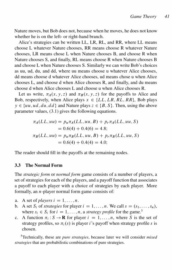
Game Theory 41
Nature moves, but Bob does not, because when he moves, he does not know
whether he is on the left- or right-hand branch.
Alice’s strategies can be written LL, LR, RL, and RR, where LL means
choose L whatever Nature chooses, RR means choose R whatever Nature
chooses, LR means chose L when Nature chooses B, and choose R when
Nature chooses S, and finally, RL means choose R when Nature chooses B
and choose L when Nature chooses S. Similarly we can write Bob’s choices
as uu, ud, du, and dd, where uu means choose u whatever Alice chooses,
dd means choose d whatever Alice chooses, ud means chose u when Alice
chooses L, and choose d when Alice chooses R, and finally, and du means
choose d when Alice chooses L and choose u when Alice chooses R.
Let us write, �A.x; y; z/ and �B.x; y; z/ for the payoffs to Alice and
Bob, respectively, when Alice plays x 2 fLL; LR; RL; RRg, Bob plays
y 2 fuu; ud; du; dd g and Nature plays z 2 fB; Sg. Then, using the above
parameter values, (3.1) gives the following equations.
�A.LL; uu/ D pu�A.LL; uu; B/ C pr�A.LL; uu; S/
D 0:6.4/ C 0:4.6/ D 4:8I�B.LL; uu/ D pu�B.LL; uu; B/ C pr�B.LL; uu; S/
D 0:6.4/ C 0:4.4/ D 4:0I
The reader should fill in the payoffs at the remaining nodes.
3.3 The Normal Form
The strategic form or normal form game consists of a number of players, a
set of strategies for each of the players, and a payoff function that associates
a payoff to each player with a choice of strategies by each player. More
formally, an n-player normal form game consists of:
a. A set of players i D 1; : : : ; n.
b. A set Si of strategies for player i D 1; : : : ; n. We call s D .s1; : : : ; sn/,
where si 2 Si for i D 1; : : : ; n, a strategy profile for the game.5
c. A function �i W S ! R for player i D 1; : : : ; n, where S is the set of
strategy profiles, so �i.s/ is player i’s payoff when strategy profile s is
chosen.
5Technically, these are pure strategies, because later we will consider mixed
strategies that are probabilistic combinations of pure strategies.

42 Chapter 3
Two extensive form games are said to be equivalent if they correspond to
the same normal form game, except perhaps for the labeling of the actions
and the naming of the players. But given an extensive form game, how
exactly do we form the corresponding normal form game? First, the play-
ers in the normal form are the same as the players in the extensive form.
Second, for each player i , let Si be the set of strategies of that player, each
strategy consisting of a choice of an action at each information set where i
moves. Finally, the payoff functions are given by equation (3.1). If there are
only two players and a finite number of strategies, we can write the payoff
function in the form of a matrix, as in figure 3.2.
As an exercise, you should work out the normal form matrix for the game
depicted in figure 3.7.
3.4 Mixed Strategies
Suppose a player has pure strategies s1; : : : ; sk in a normal form game. A
mixed strategy for the player is a probability distribution over s1; : : : ; sk;
that is, a mixed strategy has the form
� D p1s1 C : : : C pksk;
where p1; : : : pk are all nonnegative andPn
1 pj D 1. By this we mean that
the player chooses sj with probability pj , for j D 1; : : : ; k. We call pj the
weight of sj in � . If all the pj ’s are zero except one, say pl D 1, we say �
is a pure strategy, and we write � D sl . We say that pure strategy sj is used
in mixed strategy � if pj >0. We say a strategy is strictly mixed if it is not
pure, and we say that it is completely mixed if it uses all pure strategies. We
call the set of pure strategies used in a mixed strategy �i the support of �i .
In an n-player normal form game where, for i D 1; : : : ; n, player i has
pure-strategy set Si , a mixed-strategy profile � D .�1; : : : ; �n/ is the choice
of a mixed strategy �i by each player. We define the payoffs to � as follows.
Let �i .s1; : : : ; sn/ be the payoff to player i when players use the pure-
strategy profile .s1; : : : ; sn/, and if s is a pure strategy for player i , let ps be
the weight of s in �i . Then we define
�i .�/ DX
s12S1
: : :X
sn2Sn
ps1ps2
: : : psn�i .s1; : : : ; sn/:
This is a formidable expression, but the idea behind it is simple. We assume
the players’ choices are made independently, so the probability that the
Game Theory 43
particular pure strategies s1 2 S1,. . . ,sn 2 Sn will be used is simply the
product ps1: : : psn
of their weights, and the payoff to player i in this case is
just �i.s1; : : : ; sn/. We get the expected payoff by multiplying and adding
up over all n-tuples of mixed strategies.
3.5 Nash Equilibrium
The concept of a Nash equilibrium of a game is formulated most easily in
terms of the normal form. Suppose the game has n players, with strategy
sets Si and payoff functions �i WS!R, for i D 1; : : : ; n, where S is the set
of strategy profiles. We use the following very useful notation. Let Si be
the set of mixed strategies for player i , and let �S D S1 � : : : � Sn.
If � 2 �S , we write �i for the i th component of � (that is, �i is player i
mixed strategy in � ). If � 2 �S , and i 2 Si , we write
.��i ; i/ D .i ; ��i / D8<
:
.1; �2; : : : ; �n/ if i D 1
.�1; : : : ; �i�1; i ; �iC1; : : : ; �n/ if 1 < i < n
.�1; : : : ; �n�1; n/ if i D n
:
Thus, .��i ; i/ is the strategy profile obtained by replacing �i with i .
We say a strategy profile �� D .��1 ; : : : ; ��
n / 2 �S is a Nash equilibrium
if, for every player i D 1; : : : ; n, and every �i 2 Si , we have �i .��/
�i.���i ; �i/; that is, choosing ��
i is at least as good for player i as choosing
any other �i given that the other players choose ���i . Note that in a Nash
equilibrium, the strategy of each player is a best response to the strategies
chosen by all the other players. Finally, notice that a player could have
responses that are equally good as the one chosen in the Nash equilibrium;
there just cannot be a strategy that is strictly better.
The Nash equilibrium concept is important because in many cases we can
accurately (or reasonably accurately) predict how people will play a game
by assuming they will choose strategies that implement a Nash equilibrium.
It will also turn out that, in dynamic games that model an evolutionary
process whereby successful strategies drive out unsuccessful ones over time,
stable stationary states are always Nash equilibria. Conversely, we will see
that Nash equilibria that seem implausible are actually unstable equilibria
of an evolutionary process, so we would not expect to see them in the real
world. Where people appear to deviate systematically from implementing
Nash equilibria, we will sometimes find that they do not understand the
game, or that we have misspecified the game they are playing or the payoffs
44 Chapter 3
we attribute to them. But, in important cases, as we shall see, people simply
do not play Nash equilibria at all, and they are the better for it. In no sense is
the failure to play a Nash equilibrium and indication if irrationality, bounded
rationality, or any other cognitive deficit on the part of the players.
3.6 The Fundamental Theorem of Game Theory
John Nash (1950) showed that every finite game has a Nash equilibrium in
mixed strategies. More concretely, we have
THEOREM 3.1 Nash Existence Theorem. If each player in an n-player
game has a finite number of pure strategies, then the game has a (not nec-
essarily unique) Nash equilibrium in (possibly) mixed strategies.
The following fundamental theorem of mixed-strategy equilibrium devel-
ops the principles for finding Nash equilibria. Let � D .�1; : : : ; �n/ be a
mixed-strategy profile for an n-player game. For any player i D 1; : : : ; n,
let ��i represent the mixed strategies used by all the players other than
player i . The fundamental theorem of mixed-strategy Nash equilibrium
says that � is a Nash equilibrium if and only if, for any player i D 1; : : : ; n
with pure-strategy set Si ,
a. If s; s0 2 Si occur with positive probability in �i , then the payoffs to s
and s0, when played against ��i , are equal.
b. If s occurs with positive probability in �i and s0 occurs with zero prob-
ability in �i , then the payoff to s0 is less than or equal to the payoff to
s, when played against ��i .
The proof of the fundamental theorem is straightforward. Suppose � is
the player’s mixed strategy in a Nash equilibrium that uses s with proba-
bility p > 0 and s0 with probability p0 > 0. If s has a higher payoff than
s0 when played against ��i , then i’s mixed strategy that uses s with prob-
ability (p C p0), does not use s0, and assigns the same probabilities to the
other pure strategies as does � has a higher payoff than � , so � is not a best
response to ��i . This is a contradiction, which proves the assertion. The
rest of the proof is similar.
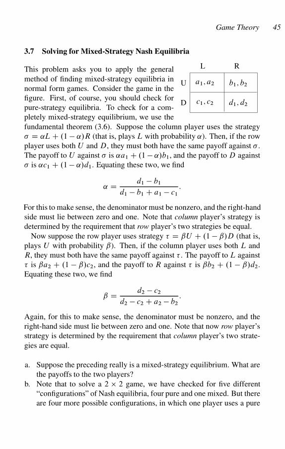
Game Theory 45
3.7 Solving for Mixed-Strategy Nash Equilibria
a1; a2 b1; b2
d1; d2c1; c2D
U
L RThis problem asks you to apply the general
method of finding mixed-strategy equilibria in
normal form games. Consider the game in the
figure. First, of course, you should check for
pure-strategy equilibria. To check for a com-
pletely mixed-strategy equilibrium, we use the
fundamental theorem (3.6). Suppose the column player uses the strategy
� D ˛L C .1 � ˛/R (that is, plays L with probability ˛). Then, if the row
player uses both U and D, they must both have the same payoff against � .
The payoff to U against � is ˛a1 C .1 � ˛/b1, and the payoff to D against
� is ˛c1 C .1 � ˛/d1. Equating these two, we find
˛ D d1 � b1
d1 � b1 C a1 � c1
:
For this to make sense, the denominator must be nonzero, and the right-hand
side must lie between zero and one. Note that column player’s strategy is
determined by the requirement that row player’s two strategies be equal.
Now suppose the row player uses strategy D ˇU C .1 � ˇ/D (that is,
plays U with probability ˇ). Then, if the column player uses both L and
R, they must both have the same payoff against . The payoff to L against
is ˇa2 C .1 � ˇ/c2, and the payoff to R against is ˇb2 C .1 � ˇ/d2.
Equating these two, we find
ˇ D d2 � c2
d2 � c2 C a2 � b2
:
Again, for this to make sense, the denominator must be nonzero, and the
right-hand side must lie between zero and one. Note that now row player’s
strategy is determined by the requirement that column player’s two strate-
gies are equal.
a. Suppose the preceding really is a mixed-strategy equilibrium. What are
the payoffs to the two players?
b. Note that to solve a 2 � 2 game, we have checked for five different
“configurations” of Nash equilibria, four pure and one mixed. But there
are four more possible configurations, in which one player uses a pure
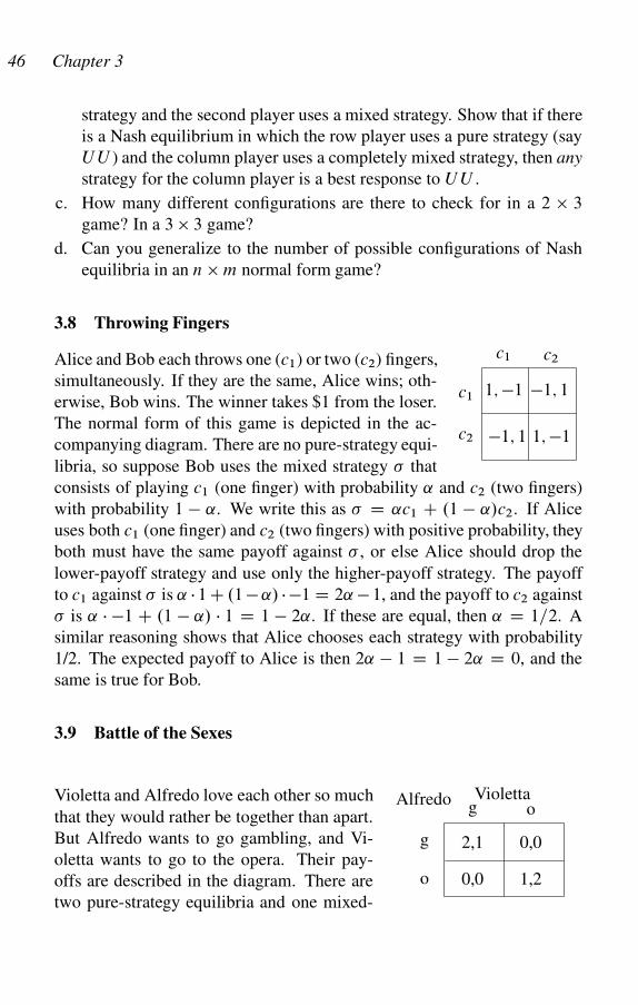
46 Chapter 3
strategy and the second player uses a mixed strategy. Show that if there
is a Nash equilibrium in which the row player uses a pure strategy (say
U U ) and the column player uses a completely mixed strategy, then any
strategy for the column player is a best response to U U .
c. How many different configurations are there to check for in a 2 � 3
game? In a 3 � 3 game?
d. Can you generalize to the number of possible configurations of Nash
equilibria in an n � m normal form game?
3.8 Throwing Fingers
�1; 1 1; �1
c2
c2
c1
c1
1; �1 �1; 1
Alice and Bob each throws one (c1) or two (c2) fingers,
simultaneously. If they are the same, Alice wins; oth-
erwise, Bob wins. The winner takes $1 from the loser.
The normal form of this game is depicted in the ac-
companying diagram. There are no pure-strategy equi-
libria, so suppose Bob uses the mixed strategy � that
consists of playing c1 (one finger) with probability ˛ and c2 (two fingers)
with probability 1 � ˛. We write this as � D ˛c1 C .1 � ˛/c2. If Alice
uses both c1 (one finger) and c2 (two fingers) with positive probability, they
both must have the same payoff against � , or else Alice should drop the
lower-payoff strategy and use only the higher-payoff strategy. The payoff
to c1 against � is ˛ 1 C .1 � ˛/ �1 D 2˛ � 1, and the payoff to c2 against
� is ˛ �1 C .1 � ˛/ 1 D 1 � 2˛. If these are equal, then ˛ D 1=2. A
similar reasoning shows that Alice chooses each strategy with probability
1/2. The expected payoff to Alice is then 2˛ � 1 D 1 � 2˛ D 0, and the
same is true for Bob.
3.9 Battle of the Sexes
2,1
0,0
g o
0,0
1,2
g
o
Alfredo ViolettaVioletta and Alfredo love each other so much
that they would rather be together than apart.
But Alfredo wants to go gambling, and Vi-
oletta wants to go to the opera. Their pay-
offs are described in the diagram. There are
two pure-strategy equilibria and one mixed-
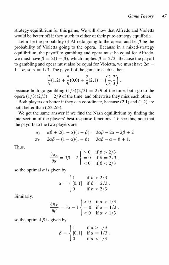
Game Theory 47
strategy equilibrium for this game. We will show that Alfredo and Violetta
would be better off if they stuck to either of their pure-strategy equilibria.
Let ˛ be the probability of Alfredo going to the opera, and let ˇ be the
probability of Violetta going to the opera. Because in a mixed-strategy
equilibrium, the payoff to gambling and opera must be equal for Alfredo,
we must have ˇ D 2.1 � ˇ/, which implies ˇ D 2=3. Because the payoff
to gambling and opera must also be equal for Violetta, we must have 2˛ D1 � ˛, so ˛ D 1=3. The payoff of the game to each is then
2
9.1;2/ C 5
9.0;0/ C 2
9.2;1/ D
�2
3;2
3
�;
because both go gambling .1=3/.2=3/ D 2=9 of the time, both go to the
opera .1=3/.2=3/ D 2=9 of the time, and otherwise they miss each other.
Both players do better if they can coordinate, because (2,1) and (1,2) are
both better than (2/3,2/3).
We get the same answer if we find the Nash equilibrium by finding the
intersection of the players’ best-response functions. To see this, note that
the payoffs to the two players are
�A D ˛ˇ C 2.1 � ˛/.1 � ˇ/ D 3˛ˇ � 2˛ � 2ˇ C 2
�V D 2˛ˇ C .1 � ˛/.1 � ˇ/ D 3˛ˇ � ˛ � ˇ C 1:
Thus,
@�A
@˛D 3ˇ � 2
8<
:
> 0 if ˇ > 2=3
D 0 if ˇ D 2=3
< 0 if ˇ < 2=3
;
so the optimal ˛ is given by
˛ D8<
:
1 if ˇ > 2=3
Œ0; 1� if ˇ D 2=3
0 if ˇ < 2=3
:
Similarly,
@�V
@ˇD 3˛ � 1
8<
:
> 0 if ˛ > 1=3
D 0 if ˛ D 1=3
< 0 if ˛ < 1=3
;
so the optimal ˇ is given by
ˇ D8<
:
1 if ˛ > 1=3
Œ0; 1� if ˛ D 1=3
0 if ˛ < 1=3
:
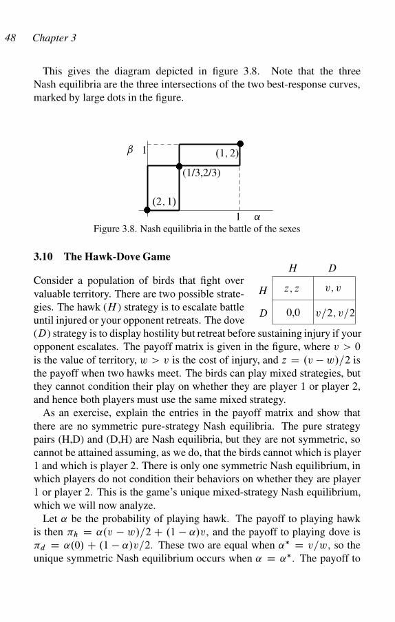
48 Chapter 3
This gives the diagram depicted in figure 3.8. Note that the three
Nash equilibria are the three intersections of the two best-response curves,
marked by large dots in the figure.
�
(1/3,2/3)
ˇ 1
1 ˛
�
�
.1; 2/
.2; 1/
Figure 3.8. Nash equilibria in the battle of the sexes
3.10 The Hawk-Dove GameH D
H
D
z; z v; v
0,0 v=2; v=2
Consider a population of birds that fight over
valuable territory. There are two possible strate-
gies. The hawk (H ) strategy is to escalate battle
until injured or your opponent retreats. The dove
(D) strategy is to display hostility but retreat before sustaining injury if your
opponent escalates. The payoff matrix is given in the figure, where v > 0
is the value of territory, w > v is the cost of injury, and z D .v � w/=2 is
the payoff when two hawks meet. The birds can play mixed strategies, but
they cannot condition their play on whether they are player 1 or player 2,
and hence both players must use the same mixed strategy.
As an exercise, explain the entries in the payoff matrix and show that
there are no symmetric pure-strategy Nash equilibria. The pure strategy
pairs (H,D) and (D,H) are Nash equilibria, but they are not symmetric, so
cannot be attained assuming, as we do, that the birds cannot which is player
1 and which is player 2. There is only one symmetric Nash equilibrium, in
which players do not condition their behaviors on whether they are player
1 or player 2. This is the game’s unique mixed-strategy Nash equilibrium,
which we will now analyze.
Let ˛ be the probability of playing hawk. The payoff to playing hawk
is then �h D ˛.v � w/=2 C .1 � ˛/v, and the payoff to playing dove is
�d D ˛.0/ C .1 � ˛/v=2. These two are equal when ˛� D v=w, so the
unique symmetric Nash equilibrium occurs when ˛ D ˛�. The payoff to
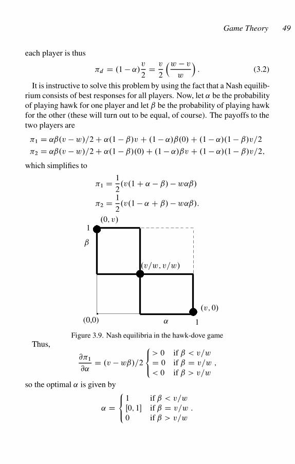
Game Theory 49
each player is thus
�d D .1 � ˛/v
2D v
2
�w � v
w
�: (3.2)
It is instructive to solve this problem by using the fact that a Nash equilib-
rium consists of best responses for all players. Now, let ˛ be the probability
of playing hawk for one player and let ˇ be the probability of playing hawk
for the other (these will turn out to be equal, of course). The payoffs to the
two players are
�1 D ˛ˇ.v � w/=2 C ˛.1 � ˇ/v C .1 � ˛/ˇ.0/ C .1 � ˛/.1 � ˇ/v=2
�2 D ˛ˇ.v � w/=2 C ˛.1 � ˇ/.0/ C .1 � ˛/ˇv C .1 � ˛/.1 � ˇ/v=2;
which simplifies to
�1 D 1
2.v.1 C ˛ � ˇ/ � w˛ˇ/
�2 D 1
2.v.1 � ˛ C ˇ/ � w˛ˇ/:
� .v=w; v=w/
ˇ
1
1
�
�
.0; v/
.v; 0/
˛(0,0)�
Figure 3.9. Nash equilibria in the hawk-dove game
Thus,
@�1
@˛D .v � wˇ/=2
8<
:
> 0 if ˇ < v=w
D 0 if ˇ D v=w
< 0 if ˇ > v=w
;
so the optimal ˛ is given by
˛ D8<
:
1 if ˇ < v=w
Œ0; 1� if ˇ D v=w
0 if ˇ > v=w
:

50 Chapter 3
Similarly,
@�2
@ˇD .v � w˛/=2
8<
:
> 0 if ˛ < v=w
D 0 if ˛ D v=w
< 1 if ˛ > v=w
;
so the optimal ˇ is given by
ˇ D8<
:
0 if ˛ > v=w
Œ0; 1� if ˛ D v=w
1 if ˛ < v=w
:
This gives the diagram depicted in figure 3.9. The best-response functions
intersect in three places, each of which is a Nash equilibrium. However, the
only symmetric Nash equilibrium, in which the players cannot condition
their move on whether they are player 1 or player 2, is the mixed strategy
Nash equilibrium .v=w; v=w/.
Note that (3.2) implies that when w is close to v, almost all the value
of the territory is dissipated in fighting, while for very high w, very little
value is lost. This is known as “mutually assured destruction” in military
parlance. Of course, if there is some possibility of error, where each player
plays hawk by mistake with positive probability, then you can easily show
that mutually assured destruction may have a very poor payoff.
3.11 The Prisoner’s Dilemma
R,R
P,P
S,T
T,S
C
C D
D
Alice and Bob can each earn a profit R if they both
work hard (pure strategy C). However, either can shirk
by working secretly on private jobs (pure strategy D),
earning T > R, but the other player will earn only
S < R. If both shirk, however, they will each earn P , where S < P < R.
Each must decide independently of the other whether to choose C or D. The
game tree is depicted in the figure. The payoff T stands for the ‘temptation’
to defect on a partner, S stands for “sucker” (for cooperating when your
partner defected), P stands for “punishment” (for both shirking), and R
stands for “reward” (for both cooperating). We usually assume also that
S C T < 2R, so there is no gain from “taking turns” playing C (cooperate)
and D (defect).
Let ˛ be the probability of playing C if you are Alice, and let ˇ be the
probability of playing C if you are Bob. To simplify the algebra, we assume
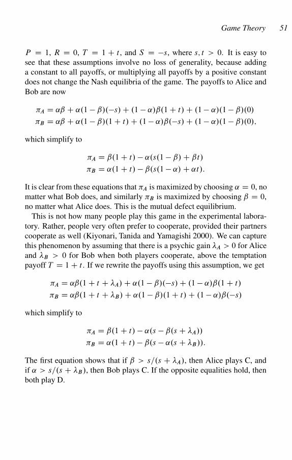
Game Theory 51
P D 1, R D 0, T D 1 C t , and S D �s, where s; t > 0. It is easy to
see that these assumptions involve no loss of generality, because adding
a constant to all payoffs, or multiplying all payoffs by a positive constant
does not change the Nash equilibria of the game. The payoffs to Alice and
Bob are now
�A D ˛ˇ C ˛.1 � ˇ/.�s/ C .1 � ˛/ˇ.1 C t/ C .1 � ˛/.1 � ˇ/.0/
�B D ˛ˇ C ˛.1 � ˇ/.1 C t/ C .1 � ˛/ˇ.�s/ C .1 � ˛/.1 � ˇ/.0/;
which simplify to
�A D ˇ.1 C t/ � ˛.s.1 � ˇ/ C ˇt/
�B D ˛.1 C t/ � ˇ.s.1 � ˛/ C ˛t/:
It is clear from these equations that �A is maximized by choosing ˛ D 0, no
matter what Bob does, and similarly �B is maximized by choosing ˇ D 0,
no matter what Alice does. This is the mutual defect equilibrium.
This is not how many people play this game in the experimental labora-
tory. Rather, people very often prefer to cooperate, provided their partners
cooperate as well (Kiyonari, Tanida and Yamagishi 2000). We can capture
this phenomenon by assuming that there is a psychic gain �A > 0 for Alice
and �B > 0 for Bob when both players cooperate, above the temptation
payoff T D 1 C t . If we rewrite the payoffs using this assumption, we get
�A D ˛ˇ.1 C t C �A/ C ˛.1 � ˇ/.�s/ C .1 � ˛/ˇ.1 C t/
�B D ˛ˇ.1 C t C �B/ C ˛.1 � ˇ/.1 C t/ C .1 � ˛/ˇ.�s/
which simplify to
�A D ˇ.1 C t/ � ˛.s � ˇ.s C �A//
�B D ˛.1 C t/ � ˇ.s � ˛.s C �B//:
The first equation shows that if ˇ > s=.s C �A/, then Alice plays C, and
if ˛ > s=.s C �B/, then Bob plays C. If the opposite equalities hold, then
both play D.
4
Eliminating Dominated Strategies
Um so schlimmer fur die Tatsache(So much the worse for the facts)
Georg Wilhelm Friedrich Hegel
4.1 Dominated Strategies
Suppose Si is a finite set of pure strategies for players i D 1; : : : ; n in
normal form game G, so that S D S1 � : : : � Sn is the set of pure-strategy
profiles for G, and �i.s/ is the payoff to player i when strategy profile s 2 S
is chosen by the players. We denote the set of mixed strategies with support
in S as �S D S1�: : :�Sn, where Si is the set of mixed strategies for
player i with support in Si , or equivalently, the set of convex combinations
of members of Si . We denote the set of vectors of mixed strategies of all
players but i by �S�i . We say s0i 2 Si is strongly dominated by si 2 Si
if, for every ��i 2 �S�i , �i .si ; ��i / > �i.s0i ; ��i /. We say s0
i is weakly
dominated by si if for every ��i 2 �S�i , �i .si ; ��i / �i .s0i ; ��i /, and
for at least one choice of ��i the inequality is strict. Note that a strategy
may fail to be strongly dominated by any pure strategy but may nevertheless
be strongly dominated by a mixed strategy.
Suppose si is a pure strategy for player i such that every � 0i ¤ si for
player i is weakly (respectively strongly) dominated by si . We call si a
weakly (respectively strongly) dominant strategy for i . If there is a Nash
equilibrium in which all players use a dominant strategy, we call this a
dominant-strategy equilibrium.
Once we have eliminated dominated strategies for each player, it often
turns out that a pure strategy that was not dominated at the outset is now
dominated. Thus, we can undertake a second round of eliminating domi-
nated strategies. Indeed, this can be repeated until pure strategies are no
longer eliminated in this manner. In a finite game, this will occur after a
finite number of rounds and will always leave at least one pure strategy re-
maining for each player. If strongly (resp. weakly) dominated strategies are
eliminated, we call this the iterated elimination of strongly (resp. weakly)
52
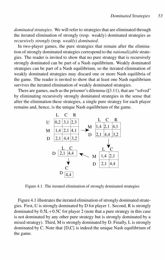
Dominated Strategies 53
dominated strategies. We will refer to strategies that are eliminated through
the iterated elimination of strongly (resp. weakly) dominated strategies as
recursively strongly (resp. weakly) dominated.
In two-player games, the pure strategies that remain after the elimina-
tion of strongly dominated strategies correspond to the rationalizable strate-
gies. The reader is invited to show that no pure strategy that is recursively
strongly dominated can be part of a Nash equilibrium. Weakly dominated
strategies can be part of a Nash equilibrium, so the iterated elimination of
weakly dominated strategies may discard one or more Nash equilibria of
the game. The reader is invited to show that at least one Nash equilibrium
survives the iterated elimination of weakly dominated strategies.
There are games, such as the prisoner’s dilemma (�3.11), that are “solved”
by eliminating recursively strongly dominated strategies in the sense that
after the elimination these strategies, a single pure strategy for each player
remains and, hence, is the unique Nash equilibrium of the game.
C
4,4D
M
L C
2,11,4
2,1 4,4D
C RL
M
U
4,12,1
3,10,2
1,4
2,3
2,1 4,4 3,2DD 3,24,42,1
1,4 2,1 4,1M
RCL
D 4,42,1CL
Figure 4.1. The iterated elimination of strongly dominated strategies
Figure 4.1 illustrates the iterated elimination of strongly dominated strate-
gies. First, U is strongly dominated by D for player 1. Second, R is strongly
dominated by 0.5LC0.5C for player 2 (note that a pure strategy in this case
is not dominated by any other pure strategy but is strongly dominated by a
mixed strategy). Third, M is strongly dominated by D. Finally, L is strongly
dominated by C. Note that fD,Cg is indeed the unique Nash equilibrium of
the game.
54 Chapter 4
4.2 Backward Induction
We can eliminate weakly dominated strategies in extensive form games
with perfect information (that is, where each information set is a single
node) as follows. Choose any terminal node t 2 T and find the parent
node of this terminal node, say node a. Suppose player i chooses at a, and
suppose i’s highest payoff at a is attained at node t 0 2 T . Erase all the
branches from a so a becomes a terminal node, and attach the payoffs from
t 0 to the new terminal node a. Also record i’s move at a, so you can specify
i’s equilibrium strategy when you have finished the analysis. Note that if
the player involved moves at one or more other nodes, you have eliminated
a weakly dominated strategy. Repeat this procedure for all terminal nodes
of the original game. When you are done, you will have an extensive form
game that is one level less deep than the original game. Now repeat the
process as many times as is possible. If the resulting game tree has just one
possible move at each node, then when you reassemble the moves you have
recorded for each player, you will have a Nash equilibrium.
We call this backward induction, because we start at the end of the game
and move backward. Note that backward induction can eliminate Nash
equilibria that use weakly dominated strategies. Moreover, backward in-
duction is not an implication of player Bayesian rationality, as we shall
show below.
For an example of backward induction, consider figure 4.2, the Big John
(BJ) and Little John (LJ) game where BJ goes first. We start with the termi-
nal node labeled (0,0) and follow it back to the LJ node on the left. At this
node, w is dominated by c because 1 > 0, so we erase the branch where LJ
plays w and its associated payoff. We locate the next terminal node in the
original game tree, (4,4) and follow back to the LJ node on the right. At this
node, c is dominated by w, so we erase the dominated node and its payoff.
Now we apply backward induction to this smaller game tree; this time, of
course, it is trivial. We find the first terminal node, (9,1), which leads back
to BJ. Here c is dominated, so we erase that branch and its payoff. We now
have our solution: BJ chooses w, LJ chooses cw, and the payoffs are (9,1).
You also can see from this example that by using backward induction
and hence eliminating weakly dominated strategies, we have eliminated the
Nash equilibrium c; ww (see figure 3.2). This is because when we assume
LJ plays c in response to BJ’s w, we have eliminated the weakly dominated
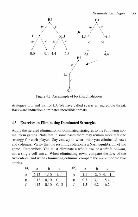
Dominated Strategies 55
�
LJ
BJ
9,1
c
w
�
�
����
LJ
BJ
5,34,49,10,0
cwcw
cw
�
LJ LJ
�
�
w c
c w
9,1 4,4
BJ
LJ
� �
Figure 4.2. An example of backward induction
strategies ww and wc for LJ. We have called c; ww an incredible threat.
Backward induction eliminates incredible threats.
4.3 Exercises in Eliminating Dominated Strategies
Apply the iterated elimination of dominated strategies to the following nor-
mal form games. Note that in some cases there may remain more that one
strategy for each player. Say exactly in what order you eliminated rows
and columns. Verify that the resulting solution is a Nash equilibrium of the
game. Remember: You must eliminate a whole row or a whole column,
not a single cell entry. When eliminating rows, compare the first of the
two entries, and when eliminating columns, compare the second of the two
entries.
a b c
5,4
4; �1
6,24,2
�2; 0
3,10,3
C
A
B
1,1
1,50,12
2,12
B
A
C
0,12 0,10
1,10
0,10 0,13
1,11
0,11
cba(a) (b)
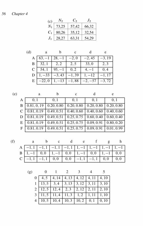
56 Chapter 4
80,26 35,12 32,54
28,27 63,31 54,29
N2 C2 J2
N1
(c)
C1
J1
73,25 57,42 66,32
(d) a b c d e
A 63; �1 28; �1 �2; 0 �2; 45 �3; 19
B 32; 1 2; 2 2; 5 33; 0 2; 3
C 54; 1 95; �1 0; 2 4; �1 0; 4
D 1; �33 �3; 43 �1; 39 1; �12 �1; 17
E �22; 0 1; �13 �1; 88 �2; �57 �3; 72
(e) a b c d e
A 0; 1 0; 1 0; 1 0; 1 0; 1
B 0:81; 0; 19 0:20; 0:80 0:20; 0:80 0:20; 0:80 0:20; 0:80
C 0:81; 0:19 0:49; 0:51 0:40; 0:60 0:40; 0:60 0:40; 0:60
D 0:81; 0:19 0:49; 0:51 0:25; 0:75 0:60; 0:40 0:60; 0:40
E 0:81; 0:19 0:49; 0:51 0:25; 0:75 0:09; 0:91 0:80; 0:20
F 0:81; 0:19 0:49; 0:51 0:25; 0:75 0:09; 0:91 0:01; 0:99
(f) a b c d e f g h
A �1; 1 �1; 1 �1; 1 �1; 1 1; �1 1; �1 1; �1 1; �1
B 1; �1 0; 0 1; �1 0; 0 1; �1 0; 0 1; �1 0; 0
C �1; 1 �1; 1 0; 0 0; 0 �1; 1 �1; 1 0; 0 0; 0
(g) 0 1 2 3 4 5
0 4; 5 4; 14 4; 13 4; 12 4; 11 4; 10
1 13; 5 3; 4 3; 13 3; 12 3; 11 3; 10
2 12; 5 12; 4 2; 3 2; 12 2; 11 2; 10
3 11; 5 11; 4 11; 3 1; 2 1; 11 1; 10
4 10; 5 10; 4 10; 3 10; 2 0; 1 0; 10
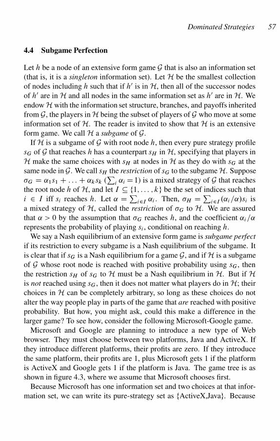
Dominated Strategies 57
4.4 Subgame Perfection
Let h be a node of an extensive form game G that is also an information set
(that is, it is a singleton information set). Let H be the smallest collection
of nodes including h such that if h0 is in H, then all of the successor nodes
of h0 are in H and all nodes in the same information set as h0 are in H. We
endow H with the information set structure, branches, and payoffs inherited
from G, the players in H being the subset of players of G who move at some
information set of H. The reader is invited to show that H is an extensive
form game. We call H a subgame of G.
If H is a subgame of G with root node h, then every pure strategy profile
sG of G that reaches h has a counterpart sH in H, specifying that players in
H make the same choices with sH at nodes in H as they do with sG at the
same node in G. We call sH the restriction of sG to the subgame H. Suppose
�G D ˛1s1 C : : : C ˛ksk (P
i ˛i D1) is a mixed strategy of G that reaches
the root node h of H, and let I � f1; : : : ; kg be the set of indices such that
i 2 I iff si reaches h. Let ˛ D Pi2I ˛i . Then, �H D P
i2I .˛i=˛/si is
a mixed strategy of H, called the restriction of �G to H. We are assured
that ˛ > 0 by the assumption that �G reaches h, and the coefficient ˛i=˛
represents the probability of playing si , conditional on reaching h.
We say a Nash equilibrium of an extensive form game is subgame perfect
if its restriction to every subgame is a Nash equilibrium of the subgame. It
is clear that if sG is a Nash equilibrium for a game G, and if H is a subgame
of G whose root node is reached with positive probability using sG , then
the restriction sH of sG to H must be a Nash equilibrium in H. But if H
is not reached using sG , then it does not matter what players do in H; their
choices in H can be completely arbitrary, so long as these choices do not
alter the way people play in parts of the game that are reached with positive
probability. But how, you might ask, could this make a difference in the
larger game? To see how, consider the following Microsoft-Google game.
Microsoft and Google are planning to introduce a new type of Web
browser. They must choose between two platforms, Java and ActiveX. If
they introduce different platforms, their profits are zero. If they introduce
the same platform, their profits are 1, plus Microsoft gets 1 if the platform
is ActiveX and Google gets 1 if the platform is Java. The game tree is as
shown in figure 4.3, where we assume that Microsoft chooses first.
Because Microsoft has one information set and two choices at that infor-
mation set, we can write its pure-strategy set as fActiveX,Javag. Because
58 Chapter 4
�
1,2
ActiveX Java
�
�
2,1
ActiveX Java
Microsoft
ActiveX Java
0,0 0,0
A J
Figure 4.3. The Microsoft-Google game
Google has two information sets and two choices at each, its pure-strategy
set has four elements fJJ; JA; AJ; AAg. Here, the first letter says what
Google does if Microsoft plays ActiveX, and the second says what Google
does if Microsoft plays Java. Thus, “AJ ” means “play ActiveX if Microsoft
plays ActiveX, and play Java if Microsoft plays Java.”
It is easy to see that fA; AAg, fA; AJ g, and fJ; JJ g are all Nash equilib-
ria (prove this formally!), but only the second is subgame perfect, because
the first is not a Nash equilibrium when restricted to the subgame starting
at J, and the third is not a Nash equilibrium when restricted to the subgame
at A. The outcomes from fA; AAg and fA; AJ g are the same, because
ActiveX is chosen by both players in either equilibrium. But the outcome
from fJ; JJ g is that Java is chosen by both players. This is obviously to the
benefit of Google, but it involves an incredible threat: Google threatens to
choose Java no matter what Microsoft does, but Microsoft knows that when
it actually comes time to choose at A, Google will in fact choose ActiveX,
not Java.
It is easy to see that a simultaneous-move game has no proper subgames
(a game is always a subgame of itself; we call the whole game an improper
subgame), because all the nodes are in the same information set for at least
one player. Similarly, a game in which Nature makes the first move and
the outcome is not known by at least one other player also has no proper
subgames.
At the other extreme, in a game of perfect information (that is, for which
all information sets are singletons), every nonterminal node is the root node
of a subgame. This allows us to find the subgame perfect Nash equilibria of
such games by backward induction, as described in section 4.2. This line of
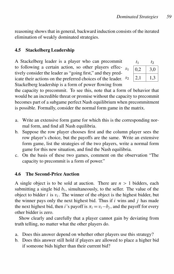
Dominated Strategies 59
reasoning shows that in general, backward induction consists of the iterated
elimination of weakly dominated strategies.
4.5 Stackelberg Leadership
2,1 1,3
3,00,2
s2
s1
t2t1A Stackelberg leader is a player who can precommit
to following a certain action, so other players effec-
tively consider the leader as “going first,” and they pred-
icate their actions on the preferred choices of the leader.
Stackelberg leadership is a form of power flowing from
the capacity to precommit. To see this, note that a form of behavior that
would be an incredible threat or promise without the capacity to precommit
becomes part of a subgame perfect Nash equilibrium when precommitment
is possible. Formally, consider the normal form game in the matrix.
a. Write an extensive form game for which this is the corresponding nor-
mal form, and find all Nash equilibria.
b. Suppose the row player chooses first and the column player sees the
row player’s choice, but the payoffs are the same. Write an extensive
form game, list the strategies of the two players, write a normal form
game for this new situation, and find the Nash equilibria.
c. On the basis of these two games, comment on the observation “The
capacity to precommit is a form of power.”
4.6 The Second-Price Auction
A single object is to be sold at auction. There are n > 1 bidders, each
submitting a single bid bi , simultaneously, to the seller. The value of the
object to bidder i is vi . The winner of the object is the highest bidder, but
the winner pays only the next highest bid. Thus if i wins and j has made
the next highest bid, then i’s payoff is �i Dvi�bj , and the payoff for every
other bidder is zero.
Show clearly and carefully that a player cannot gain by deviating from
truth telling, no matter what the other players do.
a. Does this answer depend on whether other players use this strategy?
b. Does this answer still hold if players are allowed to place a higher bid
if someone bids higher than their current bid?
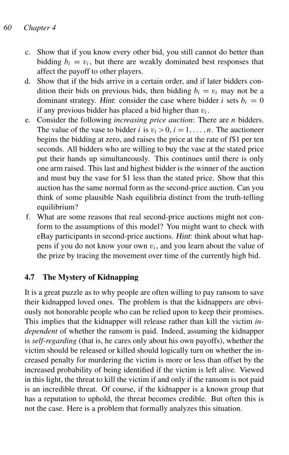
60 Chapter 4
c. Show that if you know every other bid, you still cannot do better than
bidding bi D vi , but there are weakly dominated best responses that
affect the payoff to other players.
d. Show that if the bids arrive in a certain order, and if later bidders con-
dition their bids on previous bids, then bidding bi D vi may not be a
dominant strategy. Hint: consider the case where bidder i sets bi D 0
if any previous bidder has placed a bid higher than vi .
e. Consider the following increasing price auction: There are n bidders.
The value of the vase to bidder i is vi >0, i D1; : : : ; n. The auctioneer
begins the bidding at zero, and raises the price at the rate of f$1 per ten
seconds. All bidders who are willing to buy the vase at the stated price
put their hands up simultaneously. This continues until there is only
one arm raised. This last and highest bidder is the winner of the auction
and must buy the vase for $1 less than the stated price. Show that this
auction has the same normal form as the second-price auction. Can you
think of some plausible Nash equilibria distinct from the truth-telling
equilibrium?
f. What are some reasons that real second-price auctions might not con-
form to the assumptions of this model? You might want to check with
eBay participants in second-price auctions. Hint: think about what hap-
pens if you do not know your own vi , and you learn about the value of
the prize by tracing the movement over time of the currently high bid.
4.7 The Mystery of Kidnapping
It is a great puzzle as to why people are often willing to pay ransom to save
their kidnapped loved ones. The problem is that the kidnappers are obvi-
ously not honorable people who can be relied upon to keep their promises.
This implies that the kidnapper will release rather than kill the victim in-
dependent of whether the ransom is paid. Indeed, assuming the kidnapper
is self-regarding (that is, he cares only about his own payoffs), whether the
victim should be released or killed should logically turn on whether the in-
creased penalty for murdering the victim is more or less than offset by the
increased probability of being identified if the victim is left alive. Viewed
in this light, the threat to kill the victim if and only if the ransom is not paid
is an incredible threat. Of course, if the kidnapper is a known group that
has a reputation to uphold, the threat becomes credible. But often this is
not the case. Here is a problem that formally analyzes this situation.
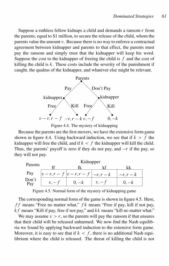
Dominated Strategies 61
Suppose a ruthless fellow kidnaps a child and demands a ransom r from
the parents, equal to $1 million, to secure the release of the child, whom the
parents value the amount v. Because there is no way to enforce a contractual
agreement between kidnapper and parents to that effect, the parents must
pay the ransom and simply trust that the kidnapper will keep his word.
Suppose the cost to the kidnapper of freeing the child is f and the cost of
killing the child is k. These costs include the severity of the punishment if
caught, the qualms of the kidnapper, and whatever else might be relevant.
v; �fv � r; r � f
Pay
Kill
�
�
�
kidnapper
Free Kill
kidnapper
�
��
�
Parents
Free
Don’t Pay
�r; r � k 0; �k
Figure 4.4. The mystery of kidnapping
Because the parents are the first movers, we have the extensive form game
shown in figure 4.4. Using backward induction, we see that if k > f the
kidnapper will free the child, and if k < f the kidnapper will kill the child.
Thus, the parents’ payoff is zero if they do not pay, and �r if the pay, so
they will not pay.
ParentsKidnapper
v; �f
�r; r � k�r; r � k
kfff fk kk
Pay
Don’t
v � r; r � f v � r; r � f
v; �f 0; �k 0; �kPay
Figure 4.5. Normal form of the mystery of kidnapping game
The corresponding normal form of the game is shown in figure 4.5. Here,
ff means “Free no matter what,” f k means “Free if pay, kill if not pay,
kf means “Kill if pay, free if not pay,” and kk means “kill no matter what.”
We may assume v > r , so the parents will pay the ransom if that ensures
that their child will be released unharmed. We now find the Nash equilib-
ria we found by applying backward induction to the extensive form game.
Moreover, it is easy to see that if k < f , there is no additional Nash equi-
librium where the child is released. The threat of killing the child is not

62 Chapter 4
credible if f < k, and the promise of freeing the child is not credible if
k > f .
Clearly, our model is inaccurate, because people often pay the ransom.
What might be incorrectly modeled? One possibility is that the kidnapper
is vindictive. We could model that by saying that the costs of freeing ver-
sus killing the child if the ransom is paid are fr and kr where fr < kr
whereas the costs of freeing versus killing the child if the ransom is not
paid are fn and kn where fn > kn. If you plug these assumptions back into
the extensive and/or normal forms you will find that there is a unique Nash
equilibrium in which the parents pay and the kidnapper frees. In a similar
vein, we may follow Harsanyi (1967) in positing that there are two “types”
of kidnappers, vindictive and self-regarding. If pv is the probability a kid-
napper is vindictive, we can again solve the problem and find that for some
range of values of pv , the ransom should be paid.
Another possibility is that the parents incur an additional cost (psychic or
reputational) if they do not pay the ransom and the child is killed. Specifi-
cally, suppose this cost is vk > r . You can now show that, once again, the
parents will pay the ransom. In this case, however, the kidnapper will free
the child only if f < k.
4.8 The Eviction Notice
A landlord has three tenants, Mr. A, Ms. B, and Msgr. C, in a rent-controlled
apartment building in New York City. A new law says that the landlord
has the right to evict one tenant per building. The landlord calculates that
the value of a vacant apartment is $15,000, both to the tenant and to her.
She sends the following letter to each of the tenants: “Tomorrow I will be
visiting your building. I will offer Mr. A $1,000 if he agrees to vacate his
apartment voluntarily; otherwise, I will evict him. If Mr. A agrees to vacate
voluntarily, I will then offer Ms. B $1,000, and if she refuses, I will evict
her. If she accepts, I will evict Msgr. C.” Show that the landlord’s plan is
consistent with the elimination of strongly dominated strategies.
4.9 Hagar’s Battles
There are ten battlefields with military values a1 <: : :<a10. Each player is
endowed with ni <10 soldiers (i D1,2). A player’s strategy is a decision to
send his soldiers to these various battlefields. A player can send at most one

Dominated Strategies 63
soldier to a given battlefield. When the fighting begins, each player wins aj
for each battlefield where he has a soldier but his opponent does not. If both
or neither combatants occupy a battlefield, the payoffs at that battlefield are
zero for both players. The winner of the war is the army whose occupied
territory has the highest total military value.
Show that this game has a unique equilibrium in which each side plays a
weakly dominant strategy, in which troups are deployed to the most valu-
able battlefields.
4.10 Military Strategy
Ihg
fed
cbA
Figure 4.6. Navigational routes between A and I
Country A and country I are at war. The two countries are separated by a
series of rivers, illustrated in figure 4.6. Country I’s fleet must stop for the
night at intersections (e.g., if the fleet takes the path IhebA, it must stop the
first night at h, the second at e, and the third at b). Country I sends a naval
fleet with just enough supplies to reach A (that is, it has enough supplies
to last three nights). If unhindered, on the fourth day the fleet will reach A
and destroy Country A. Country A can send a single fleet to prevent this.
Country A’s fleet also has enough supplies to last three nights (e.g., Abcf).
If A intercepts I’s fleet (that is, if both countries stop for the night at the
same intersection), A destroys I’s fleet and wins the war. But, if I’s fleet
reaches A without being intercepted, I wins the war. List the strategies of
the two countries and make a payoff matrix for these strategies, assuming
the winner gets 1 and the loser �1.
Show that after the elimination of weakly dominated strategies that never
arrive at the other country, there remain six pure strategies for each country.
Write out the normal form matrix for the remaining pure strategies, so that
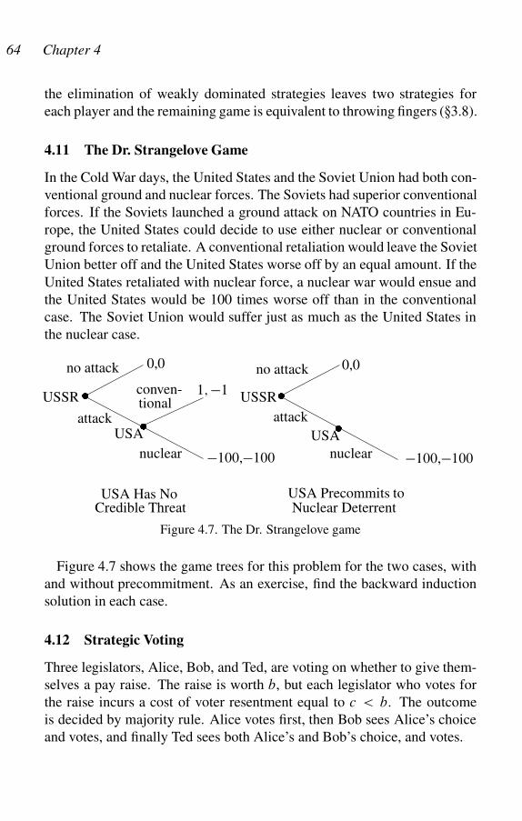
64 Chapter 4
the elimination of weakly dominated strategies leaves two strategies for
each player and the remaining game is equivalent to throwing fingers (�3.8).
4.11 The Dr. Strangelove Game
In the Cold War days, the United States and the Soviet Union had both con-
ventional ground and nuclear forces. The Soviets had superior conventional
forces. If the Soviets launched a ground attack on NATO countries in Eu-
rope, the United States could decide to use either nuclear or conventional
ground forces to retaliate. A conventional retaliation would leave the Soviet
Union better off and the United States worse off by an equal amount. If the
United States retaliated with nuclear force, a nuclear war would ensue and
the United States would be 100 times worse off than in the conventional
case. The Soviet Union would suffer just as much as the United States in
the nuclear case.
�
�
no attack
attack
conven-
nuclear
0,0
�100,�100
USSR
USA
USA Has No USA Precommits to
1; �1tional
no attack
attack
nuclear
0,0
USA�
�
USSR
Credible Threat Nuclear Deterrent
�100,�100
Figure 4.7. The Dr. Strangelove game
Figure 4.7 shows the game trees for this problem for the two cases, with
and without precommitment. As an exercise, find the backward induction
solution in each case.
4.12 Strategic Voting
Three legislators, Alice, Bob, and Ted, are voting on whether to give them-
selves a pay raise. The raise is worth b, but each legislator who votes for
the raise incurs a cost of voter resentment equal to c < b. The outcome
is decided by majority rule. Alice votes first, then Bob sees Alice’s choice
and votes, and finally Ted sees both Alice’s and Bob’s choice, and votes.

Dominated Strategies 65
Find a Nash equilibrium for this game by backward induction. Show
that there is another Nash equilibrium in which Ted votes no, whatever
Alice and Bob do, and this equilibrium favors Ted. Why is this equilibrium
eliminated by backward induction?
4.13 Nuisance Suits
Suppose Alice contemplates suing Bob over some purported ill Bob per-
petrated upon her. Suppose Alice’s court cost for initiating a suit is c, her
legal costs for going to trial are p, and Bob’s cost of defending himself is
d . Suppose both sides know these costs and also share the knowledge that
the probability that Alice will win the suit is � and the expected amount of
the settlement is x. We assume �x < p, so the suit is a frivolous “nuisance
suit” that Alice would not pursue if her goal were win the case. Finally,
suppose that before the case goes to trial (but after the suit is initiated), the
parties can settle out of court for an amount s. We assume s is given, though
clearly we could derive this value as well with the appropriate assumptions.
�
�
�
(0,0)
.�x � c � p; ��x � d/ .�c; 0/
.s � c; �s/
Do Nothing Initiate Suit
Reject Accept
Pursue Drop
Alice
Bob
Alice
�
�
.�x � c � p; ��x � d/ .�c; 0/
Pursue Suit Drop Suit
Alice
Alice
No Offer Offer Settlement�
� �
�
Figure 4.8. Nuisance suits
A consideration of the game tree for the problem, which is depicted in
figure 4.8, shows that the only subgame perfect equilibrium is for the plain-
tiff to do nothing, because the threat of carrying through with the trial is not
credible. For rolling back the game tree, we see that Drop Suit dominates
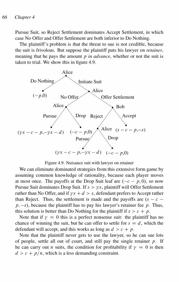
66 Chapter 4
Pursue Suit, so Reject Settlement dominates Accept Settlement, in which
case No Offer and Offer Settlement are both inferior to Do Nothing.
The plaintiff’s problem is that the threat to sue is not credible, because
the suit is frivolous. But suppose the plaintiff puts his lawyer on retainer,
meaning that he pays the amount p in advance, whether or not the suit is
taken to trial. We show this in figure 4.9.
�
�
�
(�p,0)
(�x � c � p,��x � d ) (�c � p,0)
(s � c � p,�s)
Do Nothing Initiate Suit
Reject Accept
Pursue Drop
Alice
Bob
Alice
�
�
(�x � c � p,��x � d ) (�c � p,0)
Pursue Drop
Alice
Alice
No Offer Offer Settlement
�
�
�
�
Figure 4.9. Nuisance suit with lawyer on retainer
We can eliminate dominated strategies from this extensive form game by
assuming common knowledge of rationality, because each player moves
at most once. The payoffs at the Drop Suit leaf are .�c � p; 0/, so now
Pursue Suit dominates Drop Suit. If s > �x, plaintiff will Offer Settlement
rather than No Offer, and if �x C d > s, defendant prefers to Accept rather
than Reject. Thus, the settlement is made and the payoffs are .s � c �p; �s/, because the plaintiff has to pay his lawyer’s retainer fee p. Thus,
this solution is better than Do Nothing for the plaintiff if s > c C p.
Note that if � D 0 this is a perfect nonsense suit: the plaintiff has no
chance of winning the suit, but he can offer to settle for s D d , which the
defendant will accept, and this works as long as d > c C p.
Note that the plaintiff never gets to use the lawyer, so he can sue lots
of people, settle all out of court, and still pay the single retainer p. If
he can carry out n suits, the condition for profitability if � D 0 is then
d > c C p=n, which is a less demanding constraint.
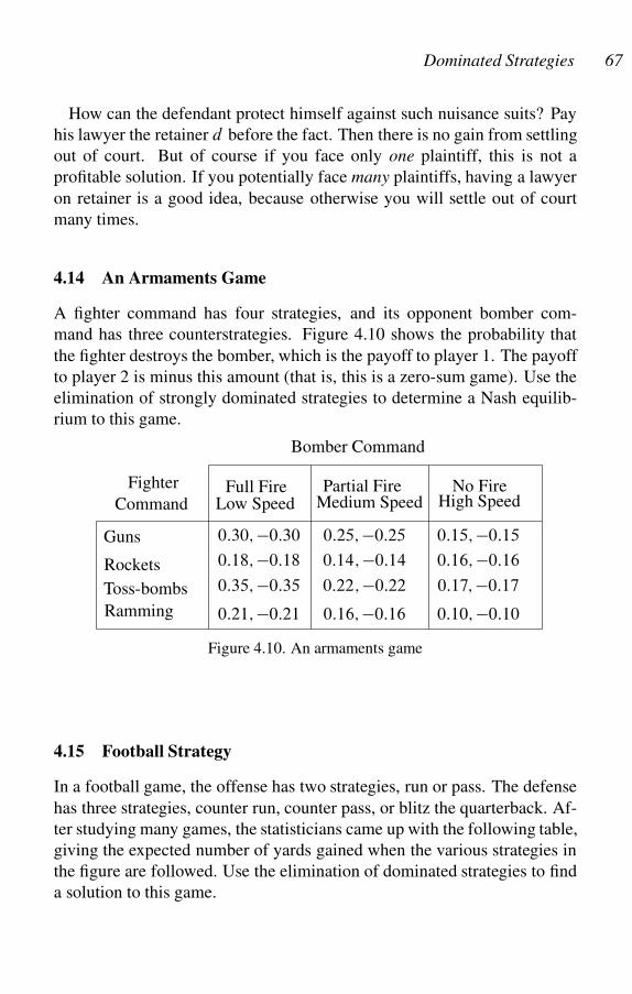
Dominated Strategies 67
How can the defendant protect himself against such nuisance suits? Pay
his lawyer the retainer d before the fact. Then there is no gain from settling
out of court. But of course if you face only one plaintiff, this is not a
profitable solution. If you potentially face many plaintiffs, having a lawyer
on retainer is a good idea, because otherwise you will settle out of court
many times.
4.14 An Armaments Game
A fighter command has four strategies, and its opponent bomber com-
mand has three counterstrategies. Figure 4.10 shows the probability that
the fighter destroys the bomber, which is the payoff to player 1. The payoff
to player 2 is minus this amount (that is, this is a zero-sum game). Use the
elimination of strongly dominated strategies to determine a Nash equilib-
rium to this game.
0:30; �0:30 0:25; �0:25 0:15; �0:15
0:18; �0:18 0:14; �0:14 0:16; �0:16
0:35; �0:35 0:22; �0:22 0:17; �0:17
0:21; �0:21 0:16; �0:16 0:10; �0:10
Full Fire Partial Fire No Fire
Bomber Command
Fighter
Guns
Rockets
Toss-bombs
Ramming
Command Low Speed Medium Speed High Speed
Figure 4.10. An armaments game
4.15 Football Strategy
In a football game, the offense has two strategies, run or pass. The defense
has three strategies, counter run, counter pass, or blitz the quarterback. Af-
ter studying many games, the statisticians came up with the following table,
giving the expected number of yards gained when the various strategies in
the figure are followed. Use the elimination of dominated strategies to find
a solution to this game.
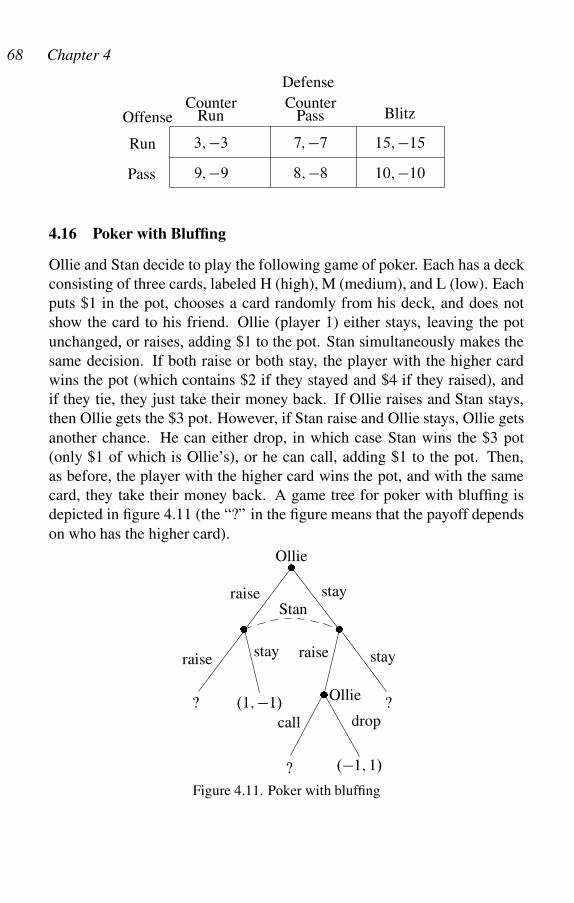
68 Chapter 4
Defense
Counter CounterBlitzRun Pass
3; �3 7; �7 15; �15
9; �9 8; �8 10; �10
Offense
Run
Pass
4.16 Poker with Bluffing
Ollie and Stan decide to play the following game of poker. Each has a deck
consisting of three cards, labeled H (high), M (medium), and L (low). Each
puts $1 in the pot, chooses a card randomly from his deck, and does not
show the card to his friend. Ollie (player 1) either stays, leaving the pot
unchanged, or raises, adding $1 to the pot. Stan simultaneously makes the
same decision. If both raise or both stay, the player with the higher card
wins the pot (which contains $2 if they stayed and $4 if they raised), and
if they tie, they just take their money back. If Ollie raises and Stan stays,
then Ollie gets the $3 pot. However, if Stan raise and Ollie stays, Ollie gets
another chance. He can either drop, in which case Stan wins the $3 pot
(only $1 of which is Ollie’s), or he can call, adding $1 to the pot. Then,
as before, the player with the higher card wins the pot, and with the same
card, they take their money back. A game tree for poker with bluffing is
depicted in figure 4.11 (the “?” in the figure means that the payoff depends
on who has the higher card).
� �
�
�
Ollie
Ollie
Stanraise stay
raisestay raise stay
call drop.1; �1/ ?
? .�1; 1/
?
Figure 4.11. Poker with bluffing
Dominated Strategies 69
a. Show that Ollie has 64 pure strategies and Stan has 8 pure strategies.
b. � Find the normal form game. Note that although poker with bluffing is
a lot simpler than real poker, the normal form is nevertheless a 64 �8 matrix! If you know computer programming, solving this is not a
hard task, however. (Recall that starred questions are more challenging
and/or more time-consuming than others).
c. � Show that the iterated elimination of one round of weakly dominated
strategies for each player leaves one Nash equilibrium. Ollie raises
with either H or M, and stays with L. If Stan raises when Ollie stays,
Ollie drops on the second round.
d. � Show that the payoff to the game for Ollie is zero.
e. � Suppose Stan sees Ollie’s first move before deciding to stay or raise
(that is, the two nodes where Stan moves are separate information sets).
Now find the normal form game. Note that this matrix is 64 � 64, so
calculating this by hand is quite prohibitive.
f. � Show that the game can still be solved by the iterated elimination of
dominated strategies. Show that both players now raise for all cards.
g. � Show that the payoff to Ollie is zero.
4.17 The Little Miss Muffet Game
While eating her curds and whey, Miss Muffet confronted a spider sitting
on her tuffet. Unfazed, she informed the spider that they would engage in a
bargaining game in which she would offer the spider a certain share x of the
curds and whey. If the spider accepts, they will divide the food accordingly,
and proceed on their merry ways. If the spider rejects, neither gets any of
the food. Miss Muffet knows that spiders are both rational and benevolent:
they reject offers only if they can gain something by doing so. Show that
Muffet gets all of the curds and whey.
Now suppose the spider has enough of a scary countenance to force an-
other game: if he rejects the first offer, he gets to make a counteroffer to
Miss Muffet, under the same conditions. He knows Miss Muffet is rational
and benevolent as well, and hence will accept any offer unless she can do
better by rejecting it. But the sun is hot, and bargaining takes time. By
the time the second offer is accepted or rejected, the curds and whey have
melted to half their original size. Show that Miss Muffet offers a 50-50
split, and the spider accepts immediately.
70 Chapter 4
Now suppose there are a maximum of three rounds of bids and the food
shrinks by one-third for each rejected offer. Show that Miss Muffet will
offer the spider 1/3 of the food, and the spider will accept.
Now suppose there are an even number n of rounds, and the curds and
whey shrink by 1=n per rejected offer. Show that Miss Muffet still offers
the spider 1/2 of the food, and the spider will accept. But if there is an odd
number n of rounds, and the curds and whey shrink by 1=n per rejected
offer, then Miss Muffet offers the spider a share 1=2�1=2n of the food, the
spider accepts, and Miss Muffet keeps the rest. As the number of periods
increases, they converge to the just solution, sharing equally.
4.18 Cooperation with Overlapping Generations
Consider a society in which there is a public good to which each member
can contribute either zero or one unit of effort each period. The value of the
public good to each member is the total amount of effort contributed to it.
Suppose the cost of contributing a unit of effort is ˛. It is clear that if
0 < ˛ < 1, a dominant strategy for each member is to contribute a unit
of effort, but if ˛ > 1, then a dominant strategy is to contribute no effort.
Suppose there are N members of this society. Then, if 1 < ˛ < N , the
unique Nash equilibrium is inefficient, but that if ˛ > N the equilibrium is
efficient. Suppose for the rest of this problem that 1 < ˛ < N , so members
would benefit from erecting incentives that induced people to contribute to
the public good.
At a town meeting, one member observed: “By the end of a period, we
know which members contributed to the public good that period. Why do
we not exclude a member from sharing in the public good in the next period
if he failed to contribute in the current period?” Another said: “That seems
like a good idea, but as we all know, we each live exactly T years, and
with your plan, the eldest generation will certainly not contribute.” A third
person responded: “Well, we revere our elders anyway, so why not tolerate
some indolence on their part? Indeed, let us agree to an ‘age of veneration’
T � such that any member who fails to contribute in the first T � periods of
life is banished from ever enjoying the public good, but members who are
older than T � need not contribute.” The first speaker queried: “How shall
we determine the proper age of veneration?” The proposer responded: “We
should choose T � to maximize our net lifetime gain from the public good.”
They all agree.

Dominated Strategies 71
Suppose there are n members of each generation, so N D nT , and they
do not discount the future. Suppose also that n.T � 1/ ˛. We can then
show that
T 2 4.˛ � 1/
n(4.1)
is necessary and sufficient for there to be a T � such that the strategy in
which each agent contributes up to age T � and shirks thereafter is a Nash
subgame perfect equilibrium.
To see this, let T � be the age of veneration. Assume all members but
one cooperate, and test whether the final player will cooperate. If this final
player is of age t � T �, the gains from cooperating are .T � t C 1/nT � �.T � � t C 1/˛, and the gains from defecting are nT � � 1. Thus, the net
gains from cooperating are
f .t; T �/ D .T � t/nT � � .T � � t C 1/˛ C 1:
Then T � supports a Nash subgame perfect equilibrium of the desired form
if and only if f .t; T �/ 0 for all t D 1; : : : ; T �. In particular, we must
have f .T �; T �/ 0. But f .t; t/ D .T � t/nt � .˛ � 1/ is a parabola with
a maximum at t D T=2, and f .T=2; T=2/ D nT 2=4 � .˛ � 1/: Because
this must be nonnegative, we see that
T 2 4.˛ � 1/
n(4.2)
is necessary.
Now suppose (4.2) holds, and choose T � such that f .T �; T �/ 0. Be-
cause f1.t; T �/ D �nT � C ˛, if ˛ � nT � then f is decreasing in t , so
f .t; T �/ 0 for all t D 1; : : : ; T �. If ˛ > nT �, f .t; T �/ is increasing in t ,
so we must ensure that f .1; T �/ 0. But f .1; T �/ D T �.n.T �1/�˛/C1,
which is strictly positive by assumption. Thus, (4.2) is sufficient.
Note that now the optimal T � is T � D T , because the total utility from
the public good for a member is T �.nT �˛/, which is an increasing function
of T �.
4.19 Dominance-Solvable Games
Let S D S1 � : : : � Sn be the set of strategy profiles in a finite game with
payoffs �i W S ! R, i D 1; : : : ; n. Let S� D S�1 � : : : � S�
n be the set
72 Chapter 4
of strategy profiles remaining in a game after the iterated elimination of
weakly dominated strategies. We say the game is dominance solvable if
each �i./ is constant on S�. Suppose the game is of perfect information
(�4.2) and satisfies the following “one-to-one” assumption (Moulin 1979):
for all s; t 2 S , and all i; j D 1; : : : ; n, if �i.s/ D �i .t/, then �j .s/ D�j .t/. Show that the game is dominance solvable. Give examples of games
that are and are not dominance solvable. Hint: Chess, checkers, and Go
are dominance solvable. For a counterexample, look at two-player games
where the first player has two moves, the second player has two moves at
each node where he chooses, his payoffs are the same for all four moves,
but the first player’s payoff depends on what the second player does.
4.20 Agent-based Modeling
In evolutionary game theory, as developed later in the book, we will see
that a simple evolutionary process in which agents who do well in a game
are imitated by others who have had less success. This evolutionary pro-
cess often converges to a Nash equilibrium. Thus, very little intelligence is
required of the agents who play the game (�12.2). This dynamical process
can be modeled on the computer in what is known as agent-based modeling.
Agent-based models are computer programs that use game theory to cre-
ate artificial strategic actors, set up the structure of their interactions and
their payoffs, and display and/or record the dynamics of the ensuing social
order. An evolutionary agent-based model has, in addition, a reproduction
phase, in which agents reproduce in proportion to their average success,
old agents die off, and the new agents inherit the behavior of their par-
ents, perhaps with some mutation. Thus, in an evolutionary agent-based
model, there is a tendency for the more successful strategies to increase in
frequency at the expense of the less successful.
Agent-based modeling is important because many games are too com-
plicated to admit closed-form analytical solutions. Moreover, sometimes
the assumptions we make to get explicit algebraic solutions to games are
sufficiently unrealistic (e.g., continuous time, infinite numbers of potential
agents) that the agent-based model performs differently from the analyti-
cal solutions, and perhaps more like the real-life situations we are trying to
model.
Virtually any computer language can be used for agent-based modeling.
My favorite is Pascal, as implemented in Borland Delphi, but C++ is almost
Dominated Strategies 73
as good, especially Borland’s C++Builder. Both are very fast, whereas most
other languages (e.g. Visual Basic and Mathematica) are painfully slow.
C++ is more difficult to learn, and compilation times are slow compared to
Delphi. Some modelers prefer Java (especially Borland’s JBuilder), but I
have not used this language extensively.
When I do serious agent-based modeling (for a journal article, for in-
stance), I try to program in two very different languages (e.g., Delphi and
Mathematica) and ensure that the output of the two are the same, although
this is infeasible for very complex models. It is even better to have some-
one else write the model in the second language, as this way one discovers
the many implicit design choices in one’s program to which one never even
gave a passing thought. Some researchers have their agent-based models
written by professional programmers. I do not advise this, unless the pro-
grammer has an excellent understanding of the theory behind the model.
So, if one wants to use agent-based models, one must either learn program-
ming or have a coauthor adequately trained in one’s behavioral discipline
who does the programming.
Figure 4.12 shows the programming structure of a typical evolutionary
agent-based model. In the figure, the “Number of Generations” specifies
how many rounds of reproduction you want to take place. This may be as
small as 10 or as large as 10 million. The “Number of Rounds/Generation”
refers to the speed of play as compared to the speed of reproduction. By
the law of large numbers, the more rounds per generation, the more ac-
curately the actual success of agents reflects the expected payoff of the
strategies they represent. “Randomly Pair All Agents” captures the evolu-
tionary nature of the model, as well as the notion that a strategy in a game
reflects a social practice occurring in the population, rather than the care-
fully thought-out optimizing strategy of the brainy actor of classical game
theory. Note that in some situations, we will want some structure to this
stage of the model. For instance, “neighbors” may meet more frequently
than “strangers,” or agents who play similar strategies may meet more fre-
quently than agents with different strategies. It’s all up to the modeler. The
“Agents Reproduce” box is expanded in figure 4.13.
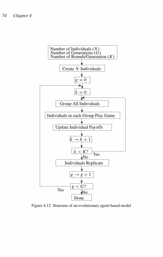
74 Chapter 4
Number of Individuals (N )Number of Generations (G)Number of Rounds/Generation (K)
Create N Individuals
g D 0
k D 0
Group All Individuals
Individuals in each Group Play Game
Update Individual Payoffs
k ! k C 1
k < K?
Individuals Replicate
NoYes
g ! g C 1
g < G?
Done
NoYes
Figure 4.12. Structure of an evolutionary agent-based model
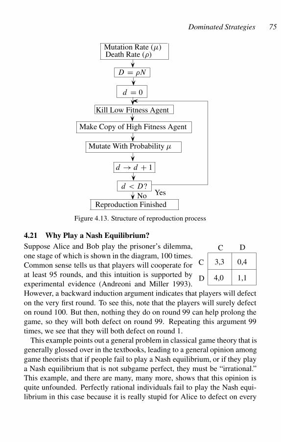
Dominated Strategies 75
Mutate With Probability �
YesNoReproduction Finished
d < D?
d ! d C 1
Make Copy of High Fitness Agent
Kill Low Fitness Agent
d D 0
D D �N
Death Rate (�)Mutation Rate (�)
Figure 4.13. Structure of reproduction process
4.21 Why Play a Nash Equilibrium?
3,3
1,1
0,4
4,0
C
C D
D
Suppose Alice and Bob play the prisoner’s dilemma,
one stage of which is shown in the diagram, 100 times.
Common sense tells us that players will cooperate for
at least 95 rounds, and this intuition is supported by
experimental evidence (Andreoni and Miller 1993).
However, a backward induction argument indicates that players will defect
on the very first round. To see this, note that the players will surely defect
on round 100. But then, nothing they do on round 99 can help prolong the
game, so they will both defect on round 99. Repeating this argument 99
times, we see that they will both defect on round 1.
This example points out a general problem in classical game theory that is
generally glossed over in the textbooks, leading to a general opinion among
game theorists that if people fail to play a Nash equilibrium, or if they play
a Nash equilibrium that is not subgame perfect, they must be “irrational.”
This example, and there are many, many more, shows that this opinion is
quite unfounded. Perfectly rational individuals fail to play the Nash equi-
librium in this case because it is really stupid for Alice to defect on every
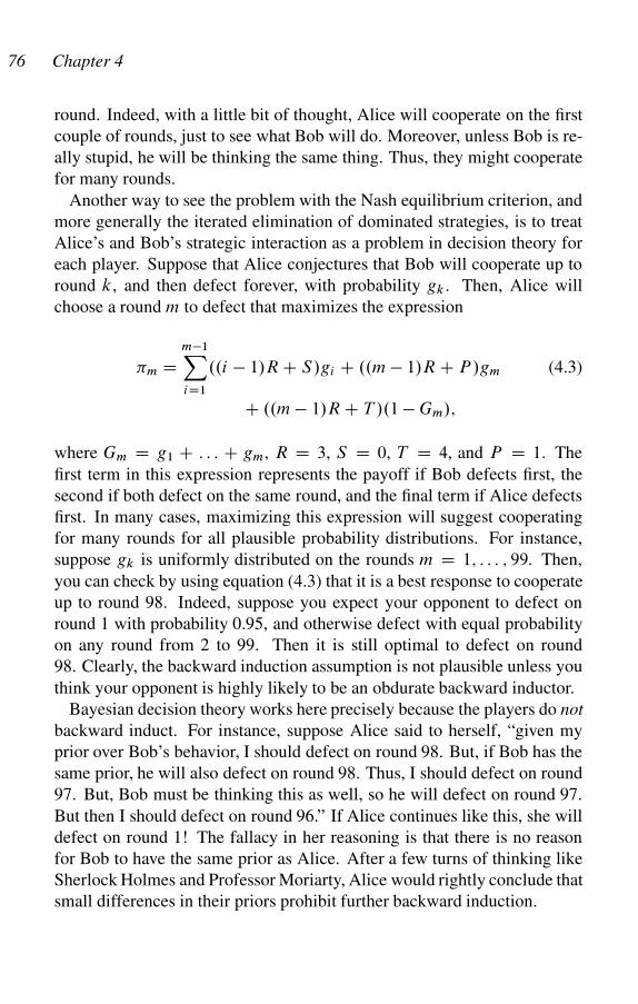
76 Chapter 4
round. Indeed, with a little bit of thought, Alice will cooperate on the first
couple of rounds, just to see what Bob will do. Moreover, unless Bob is re-
ally stupid, he will be thinking the same thing. Thus, they might cooperate
for many rounds.
Another way to see the problem with the Nash equilibrium criterion, and
more generally the iterated elimination of dominated strategies, is to treat
Alice’s and Bob’s strategic interaction as a problem in decision theory for
each player. Suppose that Alice conjectures that Bob will cooperate up to
round k, and then defect forever, with probability gk . Then, Alice will
choose a round m to defect that maximizes the expression
�m Dm�1X
iD1
..i � 1/R C S/gi C ..m � 1/R C P /gm (4.3)
C ..m � 1/R C T /.1 � Gm/;
where Gm D g1 C : : : C gm, R D 3, S D 0, T D 4, and P D 1. The
first term in this expression represents the payoff if Bob defects first, the
second if both defect on the same round, and the final term if Alice defects
first. In many cases, maximizing this expression will suggest cooperating
for many rounds for all plausible probability distributions. For instance,
suppose gk is uniformly distributed on the rounds m D 1; : : : ; 99. Then,
you can check by using equation (4.3) that it is a best response to cooperate
up to round 98. Indeed, suppose you expect your opponent to defect on
round 1 with probability 0.95, and otherwise defect with equal probability
on any round from 2 to 99. Then it is still optimal to defect on round
98. Clearly, the backward induction assumption is not plausible unless you
think your opponent is highly likely to be an obdurate backward inductor.
Bayesian decision theory works here precisely because the players do not
backward induct. For instance, suppose Alice said to herself, “given my
prior over Bob’s behavior, I should defect on round 98. But, if Bob has the
same prior, he will also defect on round 98. Thus, I should defect on round
97. But, Bob must be thinking this as well, so he will defect on round 97.
But then I should defect on round 96.” If Alice continues like this, she will
defect on round 1! The fallacy in her reasoning is that there is no reason
for Bob to have the same prior as Alice. After a few turns of thinking like
Sherlock Holmes and Professor Moriarty, Alice would rightly conclude that
small differences in their priors prohibit further backward induction.
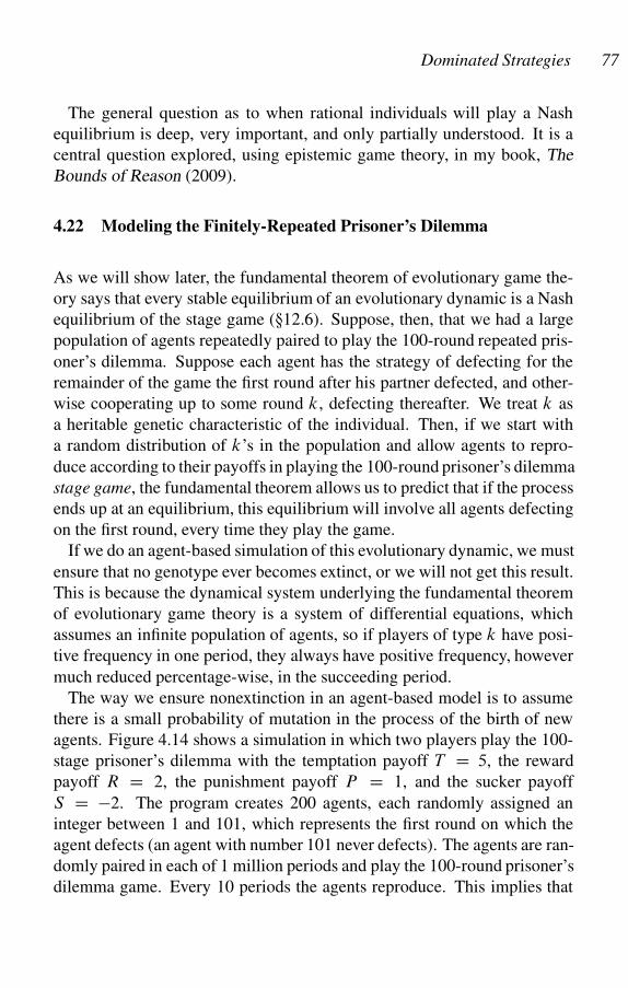
Dominated Strategies 77
The general question as to when rational individuals will play a Nash
equilibrium is deep, very important, and only partially understood. It is a
central question explored, using epistemic game theory, in my book, The
Bounds of Reason (2009).
4.22 Modeling the Finitely-Repeated Prisoner’s Dilemma
As we will show later, the fundamental theorem of evolutionary game the-
ory says that every stable equilibrium of an evolutionary dynamic is a Nash
equilibrium of the stage game (�12.6). Suppose, then, that we had a large
population of agents repeatedly paired to play the 100-round repeated pris-
oner’s dilemma. Suppose each agent has the strategy of defecting for the
remainder of the game the first round after his partner defected, and other-
wise cooperating up to some round k, defecting thereafter. We treat k as
a heritable genetic characteristic of the individual. Then, if we start with
a random distribution of k’s in the population and allow agents to repro-
duce according to their payoffs in playing the 100-round prisoner’s dilemma
stage game, the fundamental theorem allows us to predict that if the process
ends up at an equilibrium, this equilibrium will involve all agents defecting
on the first round, every time they play the game.
If we do an agent-based simulation of this evolutionary dynamic, we must
ensure that no genotype ever becomes extinct, or we will not get this result.
This is because the dynamical system underlying the fundamental theorem
of evolutionary game theory is a system of differential equations, which
assumes an infinite population of agents, so if players of type k have posi-
tive frequency in one period, they always have positive frequency, however
much reduced percentage-wise, in the succeeding period.
The way we ensure nonextinction in an agent-based model is to assume
there is a small probability of mutation in the process of the birth of new
agents. Figure 4.14 shows a simulation in which two players play the 100-
stage prisoner’s dilemma with the temptation payoff T D 5, the reward
payoff R D 2, the punishment payoff P D 1, and the sucker payoff
S D �2. The program creates 200 agents, each randomly assigned an
integer between 1 and 101, which represents the first round on which the
agent defects (an agent with number 101 never defects). The agents are ran-
domly paired in each of 1 million periods and play the 100-round prisoner’s
dilemma game. Every 10 periods the agents reproduce. This implies that
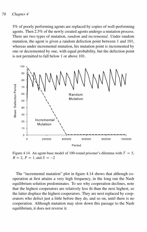
78 Chapter 4
5% of poorly performing agents are replaced by copies of well-performing
agents. Then 2.5% of the newly created agents undergo a mutation process.
There are two types of mutation, random and incremental. Under random
mutation, the agent is given a random defection point between 1 and 101,
whereas under incremental mutation, his mutation point is incremented by
one or decremented by one, with equal probability, but the defection point
is not permitted to fall below 1 or above 101.
Figure 4.14. An agent-base model of 100-round prisoner’s dilemma with T D 5,
R D 2, P D 1, and S D �2
The “incremental mutation” plot in figure 4.14 shows that although co-
operation at first attains a very high frequency, in the long run the Nash
equilibrium solution predominates. To see why cooperation declines, note
that the highest cooperators are relatively less fit than the next highest, so
the latter displace the highest cooperators. They are next replaced by coop-
erators who defect just a little before they do, and so on, until there is no
cooperation. Although mutation may slow down this passage to the Nash
equilibrium, it does not reverse it.

Dominated Strategies 79
With random mutation, we have a completely different dynamic. Here,
minimum cooperation is about 63%, maximum cooperation is about 96%,
and average cooperation is about 81%. In this case, the intuition behind
the dynamic is as follows. As in the previous case, evolution drives the
highest level of cooperators downward. When this maximum is about 80%,
approximately 20% of mutants are higher cooperators than the current max-
imum, by an average of 10 points; that is, the average mutant with a higher
defect point than 80 has a defect point 90. When two of these mutant co-
operators meet, they do better than the current majority, so they reproduce
at a fast rate, leading to a rapid increase in cooperation. This cycle repeats
indefinitely. This dynamic does not contradict the fundamental theorem of
evolutionary game theory, because this theorem does not say what happens
if an evolutionary dynamic does not converge to an equilibrium.
We conclude that our intuition concerning the absurdity of the backward
induction solution is thus likely due to the fact that we do not face the
relentless process of “weeding out” cooperators in daily life that is depicted
in the model, and/or we do not face incremental mutation. If we did face
both of these forces, we would not find the backward induction solution
strange, and we would experience life in our world, to paraphrase Thomas
Hobbes, as solitary, poor, brutish, nasty, and short.
4.23 Review of Basic Concepts
Carefully answer the following questions.
a. Describe backward induction in an extensive form game.
b. Define the notion of a strategy being strongly dominated in a normal
or extensive form game. Explain in words why a strongly dominated
strategy can never be used by a player in a Nash equilibrium.
c. Describe the iterated elimination of strongly dominated strategies and
explain why a strategy eliminated in this manner cannot be used by a
player in a Nash equilibrium.
d. Explain why, if the iterated elimination of weakly dominated strategies
leaves exactly one strategy for each player, the resulting strategy profile
is a Nash equilibrium.
5
Pure-Strategy Nash Equilibria
Competition among agents . . . has merit solely as a device toextract information optimally. Competition per se is worthless.
Bengt Holmstrom
A pure strategy Nash equilibrium of a game is a Nash equilibrium in
which each player uses a pure strategy, but not necessarily one determined
by the iterated elimination of dominated strategies (�4.1). Not every game
has a pure-strategy Nash equilibrium. Indeed, there are even very simple 2�2 normal form games with no pure-strategy Nash equilibria—for instance
throwing fingers (�3.8), where the Nash equilibrium consists in each player
throwing one or two fingers, each with probability 1/2.
This chapter explores some of the more interesting applications of games
with pure-strategy equilibria. As you will see, we obtain extremely
deep results in various branches of economic theory, including altruism
(�5.16,�5.17), the tragedy of the commons (�5.5), the existence of pure-
strategy equilibria in games of perfect information (�5.6), the real meaning
of competition (it is probably not what you think) (�5.3), honest signal-
ing equilibria (�5.9) and (�5.18). Another feature of this chapter is its use
of agent-based modeling, in no-draw, high-low poker (�5.7), to give you a
feel for the dynamic properties of games for which the Nash equilibrium
concept is a plausible description of reality.
5.1 Price Matching as Tacit Collusion
Bernie and Manny both sell DVD players and both have unit costs of 250.
They compete on price: the low-price seller gets all the market and they split
the market if they have equal prices. Explain why the only Nash equilibrium
has both firms charging 250, splitting the market and making zero profit.
Suppose that the monopoly price for DVD players (the price that max-
imizes the sum of the profits of both firms) is 300. Now suppose Bernie
80
Pure-Strategy Nash Equilibria 81
advertises that if a customer buys a DVD player from him for 300 and dis-
covers he or she can buy it cheaper at Manny’s, Bernie will refund the full
purchase price. Suppose Manny does the same thing. Show that it is now
Nash for both stores to charge 300. Conclusion: pricing strategies that seem
to be supercompetitive can in fact be anticompetitive!
5.2 Competition on Main Street
The residents of Pleasantville live on Main Street, which is the only road in
town. Two residents decide to set up general stores. Each can locate at any
point between the beginning of Main Street, which we will label 0, and the
end, which we will label 1. The two decide independently where to locate
and they must remain there forever (both can occupy the same location).
Each store will attract the customers who are closest to it and the stores
will share equally customers who are equidistant between the two. Thus,
for instance, if one store locates at point x and the second at point y > x,
then the first will get a share x C .y � x/=2 and the second will get a share
.1 � y/ C .y � x/=2 of the customers each day (draw a picture to help
you see why). Each customer contributes $1.00 in profits each day to the
general store it visits.
a. Define the actions, strategies, and daily payoffs to this game. Show that
the unique pure-strategy Nash equilibrium where both players locate at
the midpoint of Main Street;b. Suppose there are three General Stores, each independently choosing a
location point along the road (if they all choose the same point, two of
them share a building). Show that there is no pure-strategy Nash equi-
librium. Hint: First show that there is no pure-strategy Nash equilib-
rium where all three stores locate on one half of Main Street. Suppose
two stores locate on the left half of Main Street. Then, the third store
should locate a little bit to the right of the rightmost of the other two
stores. But, then the other two stores are not best responses. Therefore,
the assumption is false. Now finish the proof.
5.3 Markets as Disciplining Devices: Allied Widgets
In The Communist Manifesto of 1848, Karl Marx offered a critique of the
nascent capitalist order that was to resound around the world and fire the
imagination of socialists for nearly a century and a half.

82 Chapter 5
The bourgeoisie, wherever it has got the upper hand, has put an
end to all feudal, patriarchal, idyllic relations. It has pitilessly
torn asunder the motley feudal ties that bound man to his “nat-
ural superiors,” and has left no other nexus between man and
man than naked self-interest, than callous “cash payment” . . . It
has resolved personal worth into exchange value, and in place
of the numberless indefeasible chartered freedoms, has set up
that single, unconscionable freedom: Free Trade. (Marx 1948)
Marx’s indictment covered the two major institutions of capitalism: mar-
ket competition and private ownership of businesses. Traditional economic
theory held that the role of competition was to set prices, so supply equals
demand. If this were correct, a socialist society that took over ownership of
the businesses could replace competition by a central-planning board that
sets prices using statistical techniques to assess supply and demand curves.
The problem with this defense of socialism is that traditional economic
theory is wrong. The function of competition is to reveal private infor-
mation concerning the shape of production functions and the effort of the
firm’s managers and use that information to reward hard work and the effi-
cient use of resources by the firm. Friedrich von Hayek (1945) recognized
this error and placed informational issues at the heart of his theory of capi-
talist competition. By contrast, Joseph Schumpeter (1942), always the bit-
ter opponent of socialism, stuck to the traditional theory and predicted the
inevitable victory of the system he so hated (Gintis 1991).
This problem pins down analytically the notion that competition is valu-
able because it reveals otherwise private information. In effect, under the
proper circumstances, market competition subjects firms to a prisoner’s
dilemma in which it is in the interest of each producer to supply high effort,
even in cases where consumers and the planner cannot observe or contract
for effort itself. This is the meaning of Bengt Holmstrom’s quotation at the
head of this chapter.
If Holmstrom is right, and both game-theoretic modeling and practical
experience indicate that he is, the defense of competitive markets in neo-
classical economics is a great intellectual irony. Because of Adam Smith,
supporters of the market system have defended markets on the grounds that
they allocate goods and services efficiently. However, empirical estimates
of the losses from monopoly, tariffs, quotas, and the like indicate that misal-
location has little effect on per capita income or the rate of economic growth
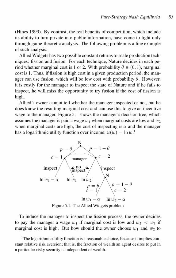
Pure-Strategy Nash Equilibria 83
(Hines 1999). By contrast, the real benefits of competition, which include
its ability to turn private into public information, have come to light only
through game-theoretic analysis. The following problem is a fine example
of such analysis.
Allied Widgets has two possible constant returns to scale production tech-
niques: fission and fusion. For each technique, Nature decides in each pe-
riod whether marginal cost is 1 or 2. With probability � 2 .0; 1/, marginal
cost is 1. Thus, if fission is high cost in a given production period, the man-
ager can use fusion, which will be low cost with probability � . However,
it is costly for the manager to inspect the state of Nature and if he fails to
inspect, he will miss the opportunity to try fusion if the cost of fission is
high.
Allied’s owner cannot tell whether the manager inspected or not, but he
does know the resulting marginal cost and can use this to give an incentive
wage to the manager. Figure 5.1 shows the manager’s decision tree, which
assumes the manager is paid a wage w1 when marginal costs are low and w2
when marginal costs are high, the cost of inspecting is ˛ and the manager
has a logarithmic utility function over income: u.w/ D ln w.1
�
� �
�
N
c D 1 c D 2
p D � p D 1 � �
noinspect
manager
inspect inspect
ln w1 � ˛ ln w1 ln w2
ln w1 � ˛ ln w2 � ˛
p D � p D 1 � �
c D 1 c D 2
N
Figure 5.1. The Allied Widgets problem
To induce the manager to inspect the fission process, the owner decides
to pay the manager a wage w1 if marginal cost is low and w2 < w1 if
marginal cost is high. But how should the owner choose w1 and w2 to
1The logarithmic utility function is a reasonable choice, because it implies con-
stant relative risk aversion; that is, the fraction of wealth an agent desires to put in
a particular risky security is independent of wealth.
84 Chapter 5
maximize profits? Suppose the manager’s payoff is ln w if he does not
inspect, ln w �˛ if he inspects and ln wo if he does not take the job at all. In
this case, wo is called the manager’s reservation wage or fallback position.
The expression that must be satisfied for a wage pair .w1; w2/ to induce
the manager to inspect the fission process is called the incentive compati-
bility constraint. To find this expression, note that the probability of using
a low-cost technique if the manager does not inspect is � , so the payoff to
the manager from not inspecting (by the expected utility principle) is
� ln w1 C .1 � �/ ln w2:
If the manager inspects, both techniques will turn out to be high cost with
probability .1 � �/2, so the probability that at least one of the techniques is
low cost is 1 � .1 � �/2. Thus, the payoff to the manager from inspecting
(again by the expected utility principle) is
Œ1 � .1 � �/2� ln w1 C .1 � �/2 ln w2 � ˛:
The incentive compatibility constraint is then
� ln w1 C .1 � �/ ln w2 � Œ1 � .1 � �/2� ln w1 C .1 � �/2 ln w2 � ˛:
Because there is no reason to pay the manager more than absolutely neces-
sary to get him to inspect, we can assume this is an equality,2 in which case
the constraint reduces to �.1 � �/ lnŒw1=w2� D ˛, or
w1 D w2e˛
�.1��/ :
For instance, suppose ˛ = 0.4 and � = 0.8. Then w1 D 12:18w2; that is, the
manager must be paid more than twelve times as much in the good state as
in the bad!
But the owner must also pay the manager enough so that taking the job,
compared to taking the fallback wo, is worthwhile. The expression that
must be satisfied for a wage pair .w1; w2/ to induce the manager to take
the job is called the participation constraint. In our case, the participation
constraint is
Œ1 � .1 � �/2� ln w1 C .1 � �/2 ln w2 � ˛ ln wo:
2Actually, this point may not be obvious and is false in the case of repeated
principal-agent models. This remark applies also to our assumption that the par-
ticipation constraint, defined in the text, is satisfied as an equality.
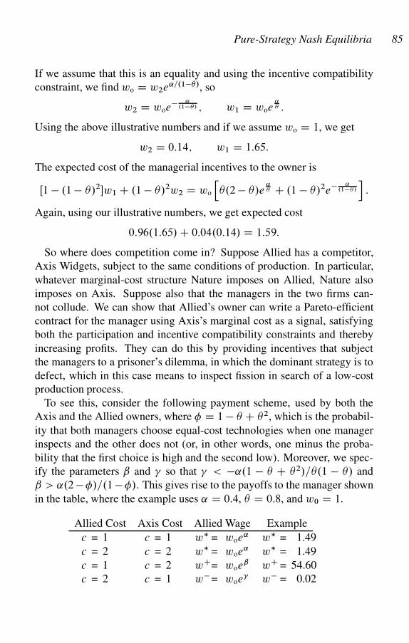
Pure-Strategy Nash Equilibria 85
If we assume that this is an equality and using the incentive compatibility
constraint, we find wo D w2e˛=.1��/, so
w2 D woe� ˛
.1��/ ; w1 D woe˛� :
Using the above illustrative numbers and if we assume wo D 1, we get
w2 D 0:14; w1 D 1:65:
The expected cost of the managerial incentives to the owner is
Œ1 � .1 � �/2�w1 C .1 � �/2w2 D wo
h�.2 � �/e
˛� C .1 � �/2e� ˛
.1��/
i:
Again, using our illustrative numbers, we get expected cost
0:96.1:65/ C 0:04.0:14/ D 1:59:
So where does competition come in? Suppose Allied has a competitor,
Axis Widgets, subject to the same conditions of production. In particular,
whatever marginal-cost structure Nature imposes on Allied, Nature also
imposes on Axis. Suppose also that the managers in the two firms can-
not collude. We can show that Allied’s owner can write a Pareto-efficient
contract for the manager using Axis’s marginal cost as a signal, satisfying
both the participation and incentive compatibility constraints and thereby
increasing profits. They can do this by providing incentives that subject
the managers to a prisoner’s dilemma, in which the dominant strategy is to
defect, which in this case means to inspect fission in search of a low-cost
production process.
To see this, consider the following payment scheme, used by both the
Axis and the Allied owners, where D 1 � � C �2, which is the probabil-
ity that both managers choose equal-cost technologies when one manager
inspects and the other does not (or, in other words, one minus the proba-
bility that the first choice is high and the second low). Moreover, we spec-
ify the parameters ˇ and � so that � < �˛.1 � � C �2/=�.1 � �/ and
ˇ > ˛.2 � /=.1 � /. This gives rise to the payoffs to the manager shown
in the table, where the example uses ˛ D 0:4, � D 0:8, and w0 D 1.
Allied Cost Axis Cost Allied Wage Example
c = 1 c = 1 w� = woe˛ w� = 1.49
c = 2 c = 2 w� = woe˛ w� = 1.49
c = 1 c = 2 wC= woeˇ wC = 54.60
c = 2 c = 1 w� = woe� w� = 0.02
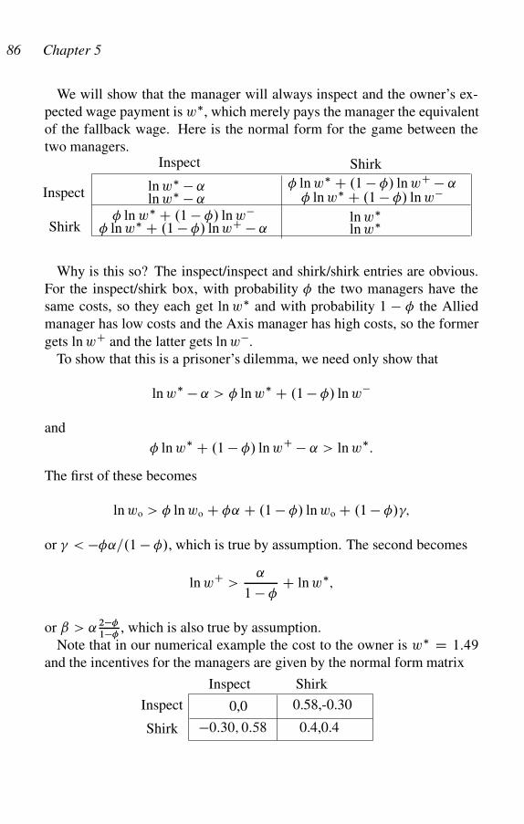
86 Chapter 5
We will show that the manager will always inspect and the owner’s ex-
pected wage payment is w�, which merely pays the manager the equivalent
of the fallback wage. Here is the normal form for the game between the
two managers.
ln w� C .1 � / ln wC � ˛
ln w�
ln w� C .1 � / ln w�
ln w�
ln w� C .1 � / ln wC � ˛ ln w� C .1 � / ln w�
ln w� � ˛ln w� � ˛
ShirkInspect
Inspect
Shirk
Why is this so? The inspect/inspect and shirk/shirk entries are obvious.
For the inspect/shirk box, with probability the two managers have the
same costs, so they each get ln w� and with probability 1 � the Allied
manager has low costs and the Axis manager has high costs, so the former
gets ln wC and the latter gets ln w�.
To show that this is a prisoner’s dilemma, we need only show that
ln w� � ˛ > ln w� C .1 � / ln w�
and
ln w� C .1 � / ln wC � ˛ > ln w�:
The first of these becomes
ln wo > ln wo C ˛ C .1 � / ln wo C .1 � /�;
or � < � ˛=.1 � /, which is true by assumption. The second becomes
ln wC >˛
1 � C ln w�;
or ˇ > ˛ 2��
1��, which is also true by assumption.
Note that in our numerical example the cost to the owner is w� D 1:49
and the incentives for the managers are given by the normal form matrix
Inspect Shirk
Inspect
Shirk
0,0 0.58,-0.30
�0:30; 0:58 0.4,0.4
Pure-Strategy Nash Equilibria 87
This example shows that markets may be disciplining devices in the sense
that they reduce the cost involved in providing the incentives for agents to
act in the interests of their employers or clients, even where enforceable
contracts cannot be written. In this case, there can be no enforceable con-
tract for managerial inspecting. Note that in this example, even though
managers are risk averse, imposing a structure of competition between the
managers means each inspects and the cost of incentives is no greater than
if a fully specified and enforceable contract for inspecting could be written.
Of course, if we weaken some of the assumptions, Pareto-optimality will
no longer be attainable. For instance, suppose when a technique is low cost
for one firm, it is not necessarily low cost for the other, but rather is low
cost with probability q > 1=2. Then competition between managers has an
element of uncertainty and optimal contracts will expose the managers to
a positive level of risk, so their expected payoff must be greater than their
fallback.
5.4 The Tobacco Market
The demand for tobacco is given by
q D 100000.10 � p/;
where p is the price per pound. However, there is a government price sup-
port program for tobacco that ensures that the price cannot go under $0.25
per pound. Three tobacco farmers have each harvested 600,000 pounds of
tobacco. Each must make an independent decision on how much to ship to
the market and how much to discard.
a. Show that there are two Nash equilibria, one in which each farmer ships
the whole crop and a second in which each farmer ships 250,000 pounds
and discards 350,000 pounds.
b. Are there any other Nash equilibria?
5.5 The Klingons and the Snarks
Two Klingons are eating from a communal cauldron of snarks. There are
1,000 snarks in the cauldron and the Klingons decide individually the rate
ri , .i D 1; 2/ at which they eat per eon. The net utility from eating snarks,
which depends on both the amount eaten and the rate of consumption
88 Chapter 5
(too slow depletes the Klingon Reservoir, too fast overloads the Klingon
Kishkes) is given by
ui D 4qi C 50ri � r2i ;
where qi is the total number of snarks Klingon i eats. Since the two Klin-
gons eventually eat all the snarks, qi D 1000ri=.r1 C r2/.
a. If they could agree on an optimal (and equal) rate of consumption, what
would that rate be?
b. When they choose independently, what rate will they choose?
c. This problem illustrates the tragedy of the commons (Hardin 1968), in
which a community (in this case the two Klingons, though it usually
involves a larger number of individuals) overexploits a resource (in this
case the bowl of snarks) because its members cannot control access to
the resource. Some economists believe the answer is simple: the prob-
lem arises because no one owns the resource. So give an individual
the right to control access to the resource and let that individual sell the
right to extract resources at a rate r to the users. To see this, suppose the
cauldron of snarks is given to a third Master Klingon and suppose the
Master Klingon charges a diner a fixed number of drecks (the Klingon
monetary unit), chosen to maximize his profits, for the right to con-
sume half the cauldron. Show that this will lead to an optimal rate of
consumption.
This “create property rights in the resource” solution is not always sat-
isfactory, however. First, it makes the new owner rich and everyone else
poor. This could possibly be solved by obliging the new owner to pay the
community for the right to control the resource. Second, it may not be pos-
sible to write a contract for the rate of resource use; the community as a
whole may be better at controlling resource use than a single owner (Os-
trom, Walker and Gardner 1992). Third, if there is unequal ability to pay
among community members, the private property solution may lead to an
unequal distribution of resources among community members.
5.6 Chess: The Trivial Pastime
A finite game is a game with a finite number of nodes in its game tree.
A game of perfect information is a game where every information set is a
single node and Nature has no moves. In 1913 the famous mathematician
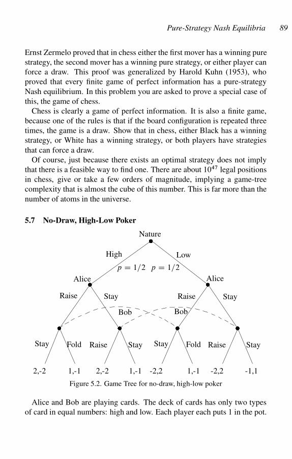
Pure-Strategy Nash Equilibria 89
Ernst Zermelo proved that in chess either the first mover has a winning pure
strategy, the second mover has a winning pure strategy, or either player can
force a draw. This proof was generalized by Harold Kuhn (1953), who
proved that every finite game of perfect information has a pure-strategy
Nash equilibrium. In this problem you are asked to prove a special case of
this, the game of chess.
Chess is clearly a game of perfect information. It is also a finite game,
because one of the rules is that if the board configuration is repeated three
times, the game is a draw. Show that in chess, either Black has a winning
strategy, or White has a winning strategy, or both players have strategies
that can force a draw.
Of course, just because there exists an optimal strategy does not imply
that there is a feasible way to find one. There are about 1047 legal positions
in chess, give or take a few orders of magnitude, implying a game-tree
complexity that is almost the cube of this number. This is far more than the
number of atoms in the universe.
5.7 No-Draw, High-Low Poker
�
�
� �
�
� �
Nature
High Low
Alice Alice
Bob Bob
Raise Stay Raise Stay
Stay Fold Stay Fold Raise Stay
2,-2 1,-1
Raise Stay
2,-2 1,-1 -2,2 1,-1 -2,2 -1,1
p D 1=2 p D 1=2
Figure 5.2. Game Tree for no-draw, high-low poker
Alice and Bob are playing cards. The deck of cards has only two types
of card in equal numbers: high and low. Each player each puts 1 in the pot.
90 Chapter 5
Alice is dealt a card (by Nature). After viewing the card, which Bob cannot
see, she either raises or stays. Bob can stay or fold if Alice raises and can
raise or stay if Alice stays. If Alice raises, she puts an additional 1 in the
pot. If Bob responds by folding, he looses and if he responds by staying,
he must put an additional 1 in the pot. If Alice stays and Bob raises, both
must put an additional 1 in the pot. If the game ends without Bob folding,
Alice wins the pot if she has a high card and loses the pot if she has a low
card. Each player’s objective is to maximize the expected value of his or
her winnings. The game tree is in figure 5.2
We now define strategies for each of the players. Alice has two infor-
mation sets (each one a node) and two choices at each. This gives four
strategies, which we label RR, RS , SR, and SS . These mean “raise no
matter what,” “raise with high, stay with low,” “stay with high, raise with
low,” and “stay no matter what.” Bob also has two information sets, one
where Alice raises and one where Alice stays. We denote his four strate-
gies SR, SS , FR, and FS . These mean “stay if Alice raises, raise if Alice
stays,” “stay no matter what,” “fold if Alice raises, raise if Alice stays,” and
“fold if Alice raises, stay if Alice stays.” To find the normal form game, we
first assume Nature gives Alice a high card and compute the normal form
matrix. We then do the same assuming Nature plays low. This give the
following payoffs:
Nature Plays High
SR SS FR FS
RR 2,-2 2,-2 1,-1 1,-1
RS 2,-2 2,-2 1,-1 1,-1
SR 2,-2 1,-1 2,-2 1,-1
SS 2,-2 1,-1 2,-2 1,-1
Nature Plays Low
SR SS FR FS
RR -2,2 -2,2 1,-1 1,-1
RS -2,2 -1,1 -2,2 -1,1
SR -2,2 -2,2 1,-1 1,-1
SS -2,2 -1,1 -2,2 -1,1
The expected values of the payoffs for the two players are simply the
averages of these two matrices of payoffs, because Nature chooses high or
Low each with probability 1/2. We have:
Pure-Strategy Nash Equilibria 91
Expected Value Payoffs
SR SS FR FS
RR 0,0 0,0 1,-1 1,-1
RS 0,0 0.5,-0.5 -0.5,0.5 0,0
SR 0,0 -0.5,0.5 1.5,-1.5 1,-1
SS 0,0 0,0 0,0 0,0
Some strategies in this game can be dropped because they are recursively
dominated. For Alice, RR weakly dominates SS and for Bob, SR weakly
dominates FS . It is quite straightforward to check that fRR,SRg is a Nash
equilibrium. Note that the game is fair: Alice raises no matter what and
Bob stays if Alice raises and raises if Alice stays. A box-by-box check
shows that there is another pure-strategy equilibrium, fSS ,SRg, in which
Alice uses a weakly dominated strategy. There are also some mixed strategy
equilibria for which you are invited to search.
5.8 An Agent-based Model of No-Draw, High-Low Poker
The heavy emphasis on finding Nash equilibria in evolutionary game the-
ory flows from two assertions. First, the equilibria of dynamic evolutionary
games are always Nash equilibria (�12.8). Second, the evolutionary pro-
cess does not require high-level rationality from the agents who populate
dynamic evolutionary games. We can illustrate both points by modeling
the dynamics of no-draw, high-low poker on the computer. In this agent-
based model, I created 100 player 1 types and 100 player 2 types, each
programmed to play exactly one pure strategy, assigned randomly to them.
In each round of play, player 1s and player 2s are randomly paired and they
play no-draw high-low poker once. Every 100 rounds we allow reproduc-
tion to take place. Reproduction consisted in killing off 5% of the players
of each type with the lowest scores and allowing the top 5% of players
with the highest score to reproduce and take the place of the defunct low
scorers. However with a 1% probability, a newly-born player ‘mutates’ by
using some randomly-chosen other strategy. The simulation ran for 50,000
rounds. The results of a typical run of the simulations for the distribution of
player 2 types in the economy are shown in figure 5.3. Note that the Nash
strategy for player 2 slowly but surely wins out and the other strategies re-
main at very low levels, though they cannot disappear altogether because
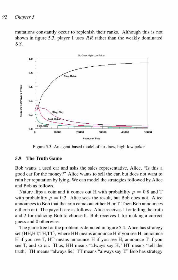
92 Chapter 5
mutations constantly occur to replenish their ranks. Although this is not
shown in figure 5.3, player 1 uses RR rather than the weakly dominated
SS .
Stay, Raise
Stay, Stay
Fold, Stay
Fold, Raise
Rounds of Play
0 10000 20000 30000 40000 500000.0
0.2
0.4
0.6
0.8
1.0
Fre
qu
en
cy o
f P
layer
2 T
yp
es
No-Draw High-Low Poker
Figure 5.3. An agent-based model of no-draw, high-low poker
5.9 The Truth Game
Bob wants a used car and asks the sales representative, Alice, “Is this a
good car for the money?” Alice wants to sell the car, but does not want to
ruin her reputation by lying. We can model the strategies followed by Alice
and Bob as follows.
Nature flips a coin and it comes out H with probability p D 0:8 and T
with probability p D 0:2. Alice sees the result, but Bob does not. Alice
announces to Bob that the coin came out either H or T. Then Bob announces
either h or t. The payoffs are as follows: Alice receives 1 for telling the truth
and 2 for inducing Bob to choose h. Bob receives 1 for making a correct
guess and 0 otherwise.
The game tree for the problem is depicted in figure 5.4. Alice has strategy
set fHH,HT,TH,TTg, where HH means announce H if you see H, announce
H if you see T, HT means announce H if you see H, announce T if you
see T, and so on. Thus, HH means “always say H,” HT means “tell the
truth,” TH means “always lie,” TT means “always say T.” Bob has strategy
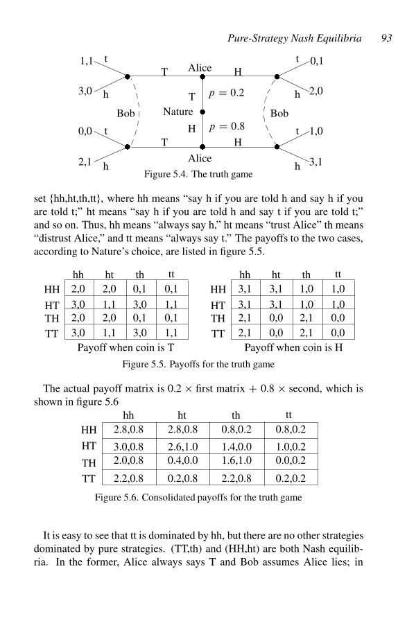
Pure-Strategy Nash Equilibria 93
�
�
�
�
�
�
��
T H
T H
T
H
p D 0:2
p D 0:8
Nature
Alice
Alice
t
h
t
h
0,1
1,0
2,0
3,1
1,1
0,0
3,0
2,1
Bob Bob
t
h
t
hFigure 5.4. The truth game
set fhh,ht,th,ttg, where hh means “say h if you are told h and say h if you
are told t;” ht means “say h if you are told h and say t if you are told t;”
and so on. Thus, hh means “always say h,” ht means “trust Alice” th means
“distrust Alice,” and tt means “always say t.” The payoffs to the two cases,
according to Nature’s choice, are listed in figure 5.5.
HH
HTTH
TT
HH
HTTH
TT
hh ht th tt hh ht th tt
2,0 2,0 0,1 0,1
3,0 1,1 3,0 1,1
2,0 2,0 0,1 0,1
3,1 3,1 1,0 1,0
2,1 0,0 2,1 0,0
3,0 1,1 3,0 1,1
3,1 3,1 1,0 1,0
2,1 0,0 2,1 0,0
Payoff when coin is T Payoff when coin is H
Figure 5.5. Payoffs for the truth game
The actual payoff matrix is 0.2 � first matrix C 0.8 � second, which is
shown in figure 5.6
hh ht th tt
HH
HT
TH
TT
2.8,0.8 2.8,0.8 0.8,0.2 0.8,0.2
3.0,0.8 2.6,1.0 1.4,0.0 1.0,0.2
2.0,0.8 0.4,0.0 1.6,1.0 0.0,0.2
2.2,0.8 0.2,0.8 2.2,0.8 0.2,0.2
Figure 5.6. Consolidated payoffs for the truth game
It is easy to see that tt is dominated by hh, but there are no other strategies
dominated by pure strategies. (TT,th) and (HH,ht) are both Nash equilib-
ria. In the former, Alice always says T and Bob assumes Alice lies; in
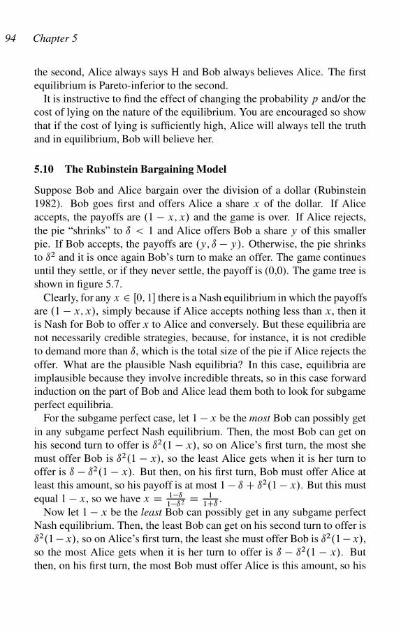
94 Chapter 5
the second, Alice always says H and Bob always believes Alice. The first
equilibrium is Pareto-inferior to the second.
It is instructive to find the effect of changing the probability p and/or the
cost of lying on the nature of the equilibrium. You are encouraged so show
that if the cost of lying is sufficiently high, Alice will always tell the truth
and in equilibrium, Bob will believe her.
5.10 The Rubinstein Bargaining Model
Suppose Bob and Alice bargain over the division of a dollar (Rubinstein
1982). Bob goes first and offers Alice a share x of the dollar. If Alice
accepts, the payoffs are .1 � x; x/ and the game is over. If Alice rejects,
the pie “shrinks” to ı < 1 and Alice offers Bob a share y of this smaller
pie. If Bob accepts, the payoffs are .y; ı � y/. Otherwise, the pie shrinks
to ı2 and it is once again Bob’s turn to make an offer. The game continues
until they settle, or if they never settle, the payoff is (0,0). The game tree is
shown in figure 5.7.
Clearly, for any x 2 Œ0; 1� there is a Nash equilibrium in which the payoffs
are .1 � x; x/, simply because if Alice accepts nothing less than x, then it
is Nash for Bob to offer x to Alice and conversely. But these equilibria are
not necessarily credible strategies, because, for instance, it is not credible
to demand more than ı, which is the total size of the pie if Alice rejects the
offer. What are the plausible Nash equilibria? In this case, equilibria are
implausible because they involve incredible threats, so in this case forward
induction on the part of Bob and Alice lead them both to look for subgame
perfect equilibria.
For the subgame perfect case, let 1 � x be the most Bob can possibly get
in any subgame perfect Nash equilibrium. Then, the most Bob can get on
his second turn to offer is ı2.1 � x/, so on Alice’s first turn, the most she
must offer Bob is ı2.1 � x/, so the least Alice gets when it is her turn to
offer is ı � ı2.1 � x/. But then, on his first turn, Bob must offer Alice at
least this amount, so his payoff is at most 1 � ı C ı2.1 � x/. But this must
equal 1 � x, so we have x D 1�ı1�ı2 D 1
1Cı.
Now let 1 � x be the least Bob can possibly get in any subgame perfect
Nash equilibrium. Then, the least Bob can get on his second turn to offer is
ı2.1 � x/, so on Alice’s first turn, the least she must offer Bob is ı2.1 � x/,
so the most Alice gets when it is her turn to offer is ı � ı2.1 � x/. But
then, on his first turn, the most Bob must offer Alice is this amount, so his
Pure-Strategy Nash Equilibria 95
Accepts
�
Alice
�
�
Bob offers x
Alice offers y
Bob offers ı2x
.1 � x; x/
.y; ı � y/
.ı2.1 � x/; ı2x/
�
�
�
RejectsAlice
AcceptsBob
RejectsBob
AcceptsAlice
RejectsAlice
Figure 5.7. Payoffs for the Rubinstein bargaining model
payoff is at least 1 � ı C ı2.1 � x/. But this must equal 1 � x, so we have
x D 1�ı1�ı2 D 1
1Cı.
Because the least Bob can earn and the most Bob can earn in a subgame
perfect Nash equilibrium are equal, there is a unique subgame perfect Nash
equilibrium, in which the payoffs are�
1
1 C ı;
ı
1 C ı
�:
Note that there is a small first-mover advantage, which disappears as ı ! 1.
Do people actually find this subgame perfect equilibrium? Because it
requires only two levels of backward induction, we might expect people
to do so, despite that fact that it involves the iterated elimination of weakly
dominated strategies (note that if the players are Bayesian rational, we never
get to Bob’s second move). But in fact, the game tree is infinite and our
trick to reducing backward induction to two steps is purely formal. Thus,
we might not expect people to settle on the Rubinstein solution. Indeed,
experimental evidence indicates that they do not (Neelin, Sonnenschein and
Spiegel 1988; Babcock, Loewenstein and Wang 1995). Part of the reason
is that fairness issues enter into many bargaining situations. These issues
are usually not important in the context of the current game, because unless
96 Chapter 5
the discount factor is very low, the outcome is almost a fifty-fifty split. But
if we complicated the model a bit—for instance, by giving players unequal
“outside options” that occur with positive probability after each rejected
offer—very unequal outcomes become possible. Also, the basic Rubinstein
model predicts that all bargaining will be efficient, because the first offer
is in fact never refused. In real-world bargaining, however, breakdowns
often occur (strike, war, divorce). Generally, we need models of bargaining
with asymmetric information or outside options to have breakdowns with
positive probability (see section 5.13 and section 6.42).
5.11 Bargaining with Heterogeneous Impatience
Suppose in the Rubinstein bargaining model we assume Bob has discount
factor ıB and Alice has discount factor ıA, so ıB and ıA represent the level
of impatience of the two players. For instance, if ıB > ıA, then Bob does
not get hurt as much by delaying agreement until the next rounds. We would
expect that a more impatient player would get a small share of the pie in a
subgame perfect Nash equilibrium and that is what we are about to see.
We must revise the extensive form game so that the payoffs are relative
to the point at which the game ends, not relative to the beginning of the
game. When it is Bob’s second time to offer, he will again offer x and if
this is accepted, he will receive 1 � x. If Alice is to induce Bob to accept
her y offer on the previous round, we must have y ıB.1 � x/, so to
maximize her payoff, Alice offers Bob y D ıB.1 � x/. This means Alice
gets 1 � y D 1 � ıB.1 � x/. But then for Bob to induce Alice to accept on
the first round, Bob must offer x ıA.1 � y/ and to maximize his payoff,
he then sets x D ıA.1 � y/. We then have
x D ıA.1 � y/ D ıA.1 � ıB.1 � x//;
which gives
x D ıA.1 � ıB/
1 � ıBıA
1 � x D 1 � ıA
1 � ıBıA
:
To see what this means, let’s set ıA D 0:9 and vary ıB from 0 (Bob is
infinitely impatient) to 1 (Bob is infinitely patient). We get figure 5.8
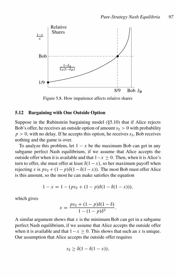
Pure-Strategy Nash Equilibria 97
ıB
Shares1�x
x
1�ıA
ıA.1�ıB /
Bob
1/9
Bob8/9
�
�
Relative
Figure 5.8. How impatience affects relative shares
5.12 Bargaining with One Outside Option
Suppose in the Rubinstein bargaining model (�5.10) that if Alice rejects
Bob’s offer, he receives an outside option of amount s2 > 0 with probability
p > 0, with no delay. If he accepts this option, he receives s2, Bob receives
nothing and the game is over.
To analyze this problem, let 1 � x be the maximum Bob can get in any
subgame perfect Nash equilibrium, if we assume that Alice accepts the
outside offer when it is available and that 1�x 0. Then, when it is Alice’s
turn to offer, she must offer at least ı.1 � x/, so her maximum payoff when
rejecting x is ps2 C .1 �p/ı.1 � ı.1 �x//. The most Bob must offer Alice
is this amount, so the most he can make satisfies the equation
1 � x D 1 � .ps2 C .1 � p/ı.1 � ı.1 � x///;
which gives
x D ps2 C .1 � p/ı.1 � ı/
1 � .1 � p/ı2:
A similar argument shows that x is the minimum Bob can get in a subgame
perfect Nash equilibrium, if we assume that Alice accepts the outside offer
when it is available and that 1�x 0. This shows that such an x is unique.
Our assumption that Alice accepts the outside offer requires
s2 ı.1 � ı.1 � x//;
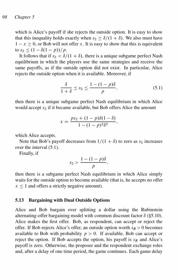
98 Chapter 5
which is Alice’s payoff if she rejects the outside option. It is easy to show
that this inequality holds exactly when s2 ı=.1 C ı/. We also must have
1 � x 0, or Bob will not offer x. It is easy to show that this is equivalent
to s2 � .1 � ı.1 � p//=p.
It follows that if s2 < ı=.1 C ı/, there is a unique subgame perfect Nash
equilibrium in which the players use the same strategies and receive the
same payoffs, as if the outside option did not exist. In particular, Alice
rejects the outside option when it is available. Moreover, if
ı
1 C ı� s2 � 1 � .1 � p/ı
p; (5.1)
then there is a unique subgame perfect Nash equilibrium in which Alice
would accept s2 if it became available, but Bob offers Alice the amount
x D ps2 C .1 � p/ı.1 � ı/
1 � .1 � p/2ı2;
which Alice accepts.
Note that Bob’s payoff decreases from 1=.1 C ı/ to zero as s2 increases
over the interval (5.1).
Finally, if
s2 >1 � .1 � p/ı
p;
then there is a subgame perfect Nash equilibrium in which Alice simply
waits for the outside option to become available (that is, he accepts no offer
x � 1 and offers a strictly negative amount).
5.13 Bargaining with Dual Outside Options
Alice and Bob bargain over splitting a dollar using the Rubinstein
alternating-offer bargaining model with common discount factor ı (�5.10).
Alice makes the first offer. Bob, as respondent, can accept or reject the
offer. If Bob rejects Alice’s offer, an outside option worth sB > 0 becomes
available to Bob with probability p > 0. If available, Bob can accept or
reject the option. If Bob accepts the option, his payoff is sB and Alice’s
payoff is zero. Otherwise, the proposer and the respondent exchange roles
and, after a delay of one time period, the game continues. Each game delay
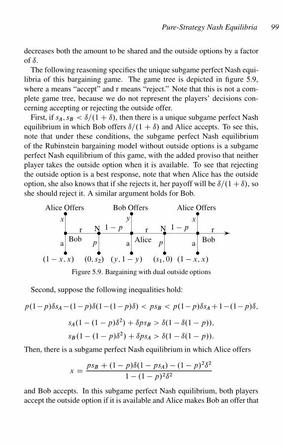
Pure-Strategy Nash Equilibria 99
decreases both the amount to be shared and the outside options by a factor
of ı.
The following reasoning specifies the unique subgame perfect Nash equi-
libria of this bargaining game. The game tree is depicted in figure 5.9,
where a means “accept” and r means “reject.” Note that this is not a com-
plete game tree, because we do not represent the players’ decisions con-
cerning accepting or rejecting the outside offer.
First, if sA; sB < ı=.1 C ı/, then there is a unique subgame perfect Nash
equilibrium in which Bob offers ı=.1 C ı/ and Alice accepts. To see this,
note that under these conditions, the subgame perfect Nash equilibrium
of the Rubinstein bargaining model without outside options is a subgame
perfect Nash equilibrium of this game, with the added proviso that neither
player takes the outside option when it is available. To see that rejecting
the outside option is a best response, note that when Alice has the outside
option, she also knows that if she rejects it, her payoff will be ı=.1 C ı/, so
she should reject it. A similar argument holds for Bob.
�Alice Offers
x
�
�
aBob
r N �
�
�
p
1 � p
.1 � x; x/ .0; s2/
�Bob Offers
y
�
a Alice
r N
�
p
1 � p
.y; 1 � y/ .s1; 0/
�Alice Offers
x
�
a Bob
r
.1 � x; x/
Figure 5.9. Bargaining with dual outside options
Second, suppose the following inequalities hold:
p.1�p/ısA �.1�p/ı.1�.1�p/ı/ < psB < p.1�p/ısA C1�.1�p/ı;
sA.1 � .1 � p/ı2/ C ıpsB > ı.1 � ı.1 � p//;
sB.1 � .1 � p/ı2/ C ıpsA > ı.1 � ı.1 � p//:
Then, there is a subgame perfect Nash equilibrium in which Alice offers
x D psB C .1 � p/ı.1 � psA/ � .1 � p/2ı2
1 � .1 � p/2ı2
and Bob accepts. In this subgame perfect Nash equilibrium, both players
accept the outside option if it is available and Alice makes Bob an offer that
100 Chapter 5
Bob accepts (note that the subgames at which these actions are carried out
do not lie on the game path). Show also that in this case, sA and sB exist
satisfying the preceding inequalities and all satisfy sA; sB > ı=.1 C ı/. To
see this if we assume that both agents take the outside option when it is
available, we have the recursive equation
x D psB C ı.1 � p/.1 � .psA C .1 � p/ı.1 � x///;
and the preceding inequalities ensure that x 2 Œ0; 1�, that sA > ı.1 � x/, so
Alice takes the outside option when available and sB > ı.1 � psA � .1 �p/ı.1 � x//, so Bob takes the outside option when available. This justifies
our assumption.
Third, suppose the following inequalities hold:
p.1 � p/ısA � psB > .1 � p/ı.1 � .1 � p/ı/;
psA C psB.1 � .1 � p/ı/ < 1 � ı2.1 � p/2:
Then, there is a subgame perfect Nash equilibrium in which Bob rejects
Alice’s offer, Bob takes the outside option if it is available and if not, Bob
offers AlicepsA
1 � .1 � p/2ı2
and Alice accepts. In this subgame perfect Nash equilibrium, Alice also
accepts the outside option if it is available. What are the payoffs to the
two players? Show also that there are sA and sB that satisfy the preceding
inequalities and we always have sB > ı=.1 C ı/. To see this, first show that
if Alice could make an acceptable offer to Bob, then the previous recursion
for x would hold, but now x < 0, which is a contradiction. Then, either
Alice accepts an offer from Bob, or Alice waits for the outside option to
become available. The payoff to waiting is
�A D .1 � p/psAı
1 � .1 � p/2ı2;
but Alice will accept ı.psAC.1�p/ı�A/, leaving Bob with 1�ı.psAC.1�p/ı�A/. This must be better for Bob than just waiting for the outside option
to become available, which has value, at the time Bob is the proposer,
.1 � p/psBı
1 � .1 � p/2ı2:
Pure-Strategy Nash Equilibria 101
Show that the preceding inequalities imply Bob will make an offer to Alice.
Then, use the inequalities to show that Alice will accept. The remainder of
the problem is now straightforward.
Show that this case applies to the parameters ı D 0:9, p D 0:6, sA D1:39, and sB D 0:08. Find Bob’s offer to Alice, calculate the payoffs to the
players and show that Alice will not make an offer that Bob would accept.
Fourth, suppose
psA > 1 � .1 � p/2ı > p.1 � p/ısA C psB :
Then, there is a subgame perfect Nash equilibrium where Alice offers Bob
psB
1 � .1 � p/2ı2
and Bob accepts. In this equilibrium, Alice accepts no offer and both play-
ers accept the outside option when it is available. It is easy to show also
that there are sA and sB that satisfy the preceding inequalities and we always
have sA > ı=.1 C ı/. Note that in this case Alice must offer Bob
�2 D psB
1 � .1 � p/2ı2;
which is what Bob can get by waiting for the outside option. Alice minus
this quantity must be greater than �A, or Alice will not offer it. Show that
this holds when the preceding inequalities hold. Now, Alice will accept
psA C .1 � p/ı�A, but you can show that this is greater than 1, so Bob
will not offer this. This justifies our assumption that Alice will not accept
anything that Bob is willing to offer.
This case applies to the parameters ı D 0:9, p D 0:6, sA D 1:55, and
sB D 0:88. Find Alice’s offer to Bob, calculate the payoffs to the players
and show that Bob will not make an offer that Alice would accept.
Finally, suppose the following inequalities hold:
1 � ı2.1 � p/2 < psB C psAı.1 � p/;
1 � ı2.1 � p/2 < psB C psAı.1 � p/:
Then, the only subgame perfect Nash equilibrium has neither agent making
an offer acceptable to the other, so both agents wait for the outside option
to become available. Note that by refusing all offers and waiting for the
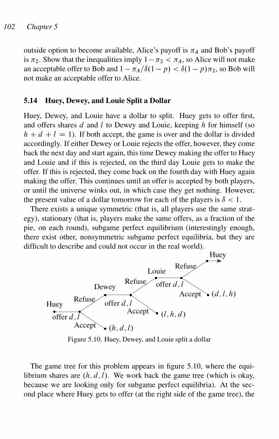
102 Chapter 5
outside option to become available, Alice’s payoff is �A and Bob’s payoff
is �2. Show that the inequalities imply 1��2 < �A, so Alice will not make
an acceptable offer to Bob and 1 � �A=ı.1 � p/ < ı.1 � p/�2, so Bob will
not make an acceptable offer to Alice.
5.14 Huey, Dewey, and Louie Split a Dollar
Huey, Dewey, and Louie have a dollar to split. Huey gets to offer first,
and offers shares d and l to Dewey and Louie, keeping h for himself (so
h C d C l D 1). If both accept, the game is over and the dollar is divided
accordingly. If either Dewey or Louie rejects the offer, however, they come
back the next day and start again, this time Dewey making the offer to Huey
and Louie and if this is rejected, on the third day Louie gets to make the
offer. If this is rejected, they come back on the fourth day with Huey again
making the offer. This continues until an offer is accepted by both players,
or until the universe winks out, in which case they get nothing. However,
the present value of a dollar tomorrow for each of the players is ı < 1.
There exists a unique symmetric (that is, all players use the same strat-
egy), stationary (that is, players make the same offers, as a fraction of the
pie, on each round), subgame perfect equilibrium (interestingly enough,
there exist other, nonsymmetric subgame perfect equilibria, but they are
difficult to describe and could not occur in the real world).
��
��
��
�
Huey
offer d; l
Refuse
Accept �
.h; d; l/
Dewey
offer d; l
Refuse
Accept .l; h; d/
Louie
offer d; l
Refuse
Accept
Huey
.d; l; h/
Figure 5.10. Huey, Dewey, and Louie split a dollar
The game tree for this problem appears in figure 5.10, where the equi-
librium shares are .h; d; l/. We work back the game tree (which is okay,
because we are looking only for subgame perfect equilibria). At the sec-
ond place where Huey gets to offer (at the right side of the game tree), the
Pure-Strategy Nash Equilibria 103
value of the game to Huey is h, because we assume a stationary equilibrium.
Thus, Louie must offer Huey at least ıh where Louie gets to offer, to get
Huey to accept. Similarly, Louie must offer Dewey at least ıd at this node.
Thus, the value of the game where Louie gets to offer is .1 � ıh � ıd/.
When Dewey gets to offer, he must offer Louie at least ı times what Louie
gets when it is Louie’s turn to offer, to get Louie to accept. This amount is
just ı.1 � ıh � ıd/. Similarly, he must offer Huey ı2h to accept, because
Huey gets ıh when it is Louie’s turn to offer. Thus, Dewey gets
1 � ı.1 � ıh � ıd/ � ı2h D 1 � ı.1 � ıd/
when it is his turn to offer.
Now Huey, on his first turn to offer, must offer Dewey ı times what
Dewey can get when it is Dewey’s turn to offer, or ı.1 � ı.1 � ıd//. But
then we must have
d D ı.1 � ı.1 � ıd//:
Solving this equation for d , we find
d D ı
1 C ı C ı2:
Moreover, Huey must offer Louie ı times what Dewey would offer Louie
in the next period or ı2.1 � ıh � ıd/. Thus, Huey offers Dewey and Louie
together
ı.1 � ı.1 � ıd// C ı2.1 � ıh � ıd/ D ı � ı3h;
so Huey gets 1 � ı C ı3h and this must equal h. Solving, we get
h D 1
1 C ı C ı2;
so we must have
l D 1 � d � h D ı2
1 C ı C ı2;
which is the solution to the problem.
Note that there is a simpler way to solve the problem, just using the fact
that the solution is symmetric: we must have d D ıh and l D ıd , from
which the result follows. This does not make clear, however, where sub-
game perfection comes in.
104 Chapter 5
5.15 Twin Sisters
A mother has twin daughters who live in different towns. She tells each to
ask for a certain whole number of dollars, at least 1 and at most 100, as a
birthday present. If the total of the two amounts does not exceed 101, each
will have her request granted. Otherwise each gets nothing.
a. Find all the pure-strategy Nash equilibria of this game.
b. Is there a symmetric equilibrium among these? A symmetric Nash equi-
librium is one in which both players use the same strategy.
c. What do you think the twins will most likely do, if we assume that they
cannot communicate? Why? Is this a Nash equilibrium?
5.16 The Samaritan’s Dilemma
Many conservatives dislike Social Security and other forms of forced sav-
ing by means of which the government prevents people from ending up in
poverty in their old age. Some liberals respond by claiming that people
are too short-sighted to manage their own retirement savings successfully.
James Buchanan (1975) has made the insightful point that even if people
are perfectly capable of managing their retirement savings, if we are altru-
istic toward others, we will force people to save more than they otherwise
would.3 Here is a simple model exhibiting his point.
A father and a daughter have current income y > 0 and z > 0, re-
spectively. The daughter saves an amount s for her schooling next year
and receives an interest rate r > 0 on her savings. She also receives
a transfer t from her father in the second period. Her utility function is
v.s; t/ D vA.z�s/Cıv2.s.1Cr/C t/, where ı > 0 is a discount factor, vA
is her first-period utility and v2 is her second-period utility. Her father has
personal utility function u.y/, but he has degree ˛ > 0 of altruistic feeling
for his daughter, so he acts to maximize U D u.y � t/ C ˛v.s; t/. Suppose
all utility functions are increasing and concave, the daughter chooses s to
maximize her utility, the father observes the daughter’s choice of s and then
chooses t . Let .s�; t�/ be the resulting equilibrium. Show that the daughter
will save too little, in the sense that if the father can precommit to t�, both
she and her father would be better off. Show by example that, if we assume
3In this case, by an altruist we mean an agent who takes actions that improve
the material well-being of other agents at a material cost to himself.
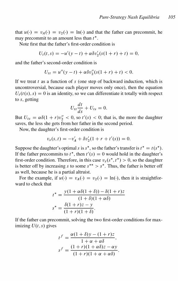
Pure-Strategy Nash Equilibria 105
that u./ D vA./ D v2./ D ln./ and that the father can precommit, he
may precommit to an amount less than t�.
Note first that the father’s first-order condition is
Ut.t; s/ D �u0.y � t/ C ˛ıv02.s.1 C r/ C t/ D 0;
and the father’s second-order condition is
Ut t D u00.y � t/ C ˛ıv002.s.1 C r/ C t/ < 0:
If we treat t as a function of s (one step of backward induction, which is
uncontroversial, because each player moves only once), then the equation
Ut.t.s/; s/ D 0 is an identity, so we can differentiate it totally with respect
to s, getting
Ut t
dt
dsC Uts D 0:
But Uts D ˛ı.1 C r/v002 < 0, so t 0.s/ < 0; that is, the more the daughter
saves, the less she gets from her father in the second period.
Now, the daughter’s first-order condition is
vs.s; t/ D �v0A C ıv0
2.1 C r C t 0.s// D 0:
Suppose the daughter’s optimal s is s�, so the father’s transfer is t� D t.s�/.
If the father precommits to t�, then t 0.s/ D 0 would hold in the daughter’s
first-order condition. Therefore, in this case vs.s�; t�/ > 0, so the daughter
is better off by increasing s to some s�� > s�. Thus, the father is better off
as well, because he is a partial altruist.
For the example, if u./ D vA./ D v2./ D ln./, then it is straightfor-
ward to check that
t� D y.1 C ˛ı.1 C ı// � ı.1 C r/z
.1 C ı/.1 C ˛ı/
s� D ı.1 C r/z � y
.1 C r/.1 C ı/:
If the father can precommit, solving the two first-order conditions for max-
imizing U.t; s/ gives
tf D ˛.1 C ı/y � .1 C r/z
1 C ˛ C ˛ı;
sf D .1 C r/.1 C ˛ı/z � ˛y
.1 C r/.1 C ˛ C ˛ı/:
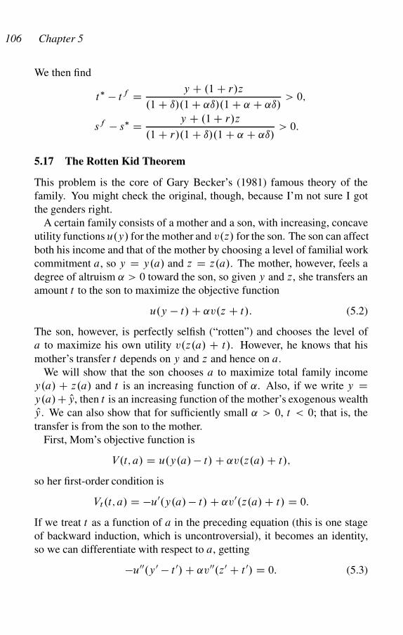
106 Chapter 5
We then find
t� � tf D y C .1 C r/z
.1 C ı/.1 C ˛ı/.1 C ˛ C ˛ı/> 0;
sf � s� D y C .1 C r/z
.1 C r/.1 C ı/.1 C ˛ C ˛ı/> 0:
5.17 The Rotten Kid Theorem
This problem is the core of Gary Becker’s (1981) famous theory of the
family. You might check the original, though, because I’m not sure I got
the genders right.
A certain family consists of a mother and a son, with increasing, concave
utility functions u.y/ for the mother and v.z/ for the son. The son can affect
both his income and that of the mother by choosing a level of familial work
commitment a, so y D y.a/ and z D z.a/. The mother, however, feels a
degree of altruism ˛ > 0 toward the son, so given y and z, she transfers an
amount t to the son to maximize the objective function
u.y � t/ C ˛v.z C t/: (5.2)
The son, however, is perfectly selfish (“rotten”) and chooses the level of
a to maximize his own utility v.z.a/ C t/. However, he knows that his
mother’s transfer t depends on y and z and hence on a.
We will show that the son chooses a to maximize total family income
y.a/ C z.a/ and t is an increasing function of ˛. Also, if we write y Dy.a/C Oy, then t is an increasing function of the mother’s exogenous wealth
Oy. We can also show that for sufficiently small ˛ > 0, t < 0; that is, the
transfer is from the son to the mother.
First, Mom’s objective function is
V.t; a/ D u.y.a/ � t/ C ˛v.z.a/ C t/;
so her first-order condition is
Vt .t; a/ D �u0.y.a/ � t/ C ˛v0.z.a/ C t/ D 0:
If we treat t as a function of a in the preceding equation (this is one stage
of backward induction, which is uncontroversial), it becomes an identity,
so we can differentiate with respect to a, getting
�u00.y 0 � t 0/ C ˛v00.z0 C t 0/ D 0: (5.3)
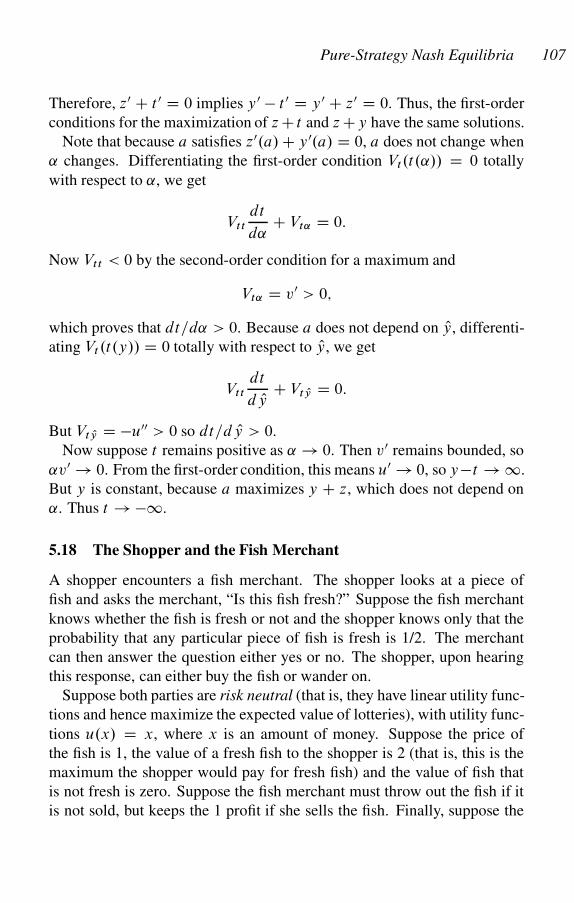
Pure-Strategy Nash Equilibria 107
Therefore, z0 C t 0 D 0 implies y 0 � t 0 D y 0 C z0 D 0. Thus, the first-order
conditions for the maximization of z C t and z Cy have the same solutions.
Note that because a satisfies z0.a/ C y 0.a/ D 0, a does not change when
˛ changes. Differentiating the first-order condition Vt.t.˛// D 0 totally
with respect to ˛, we get
Vt t
dt
d˛C Vt˛ D 0:
Now Vt t < 0 by the second-order condition for a maximum and
Vt˛ D v0 > 0;
which proves that dt=d˛ > 0. Because a does not depend on Oy, differenti-
ating Vt .t.y// D 0 totally with respect to Oy, we get
Vt t
dt
d Oy C Vt Oy D 0:
But Vt Oy D �u00 > 0 so dt=d Oy > 0.
Now suppose t remains positive as ˛ ! 0. Then v0 remains bounded, so
˛v0 ! 0. From the first-order condition, this means u0 ! 0, so y�t ! 1.
But y is constant, because a maximizes y C z, which does not depend on
˛. Thus t ! �1.
5.18 The Shopper and the Fish Merchant
A shopper encounters a fish merchant. The shopper looks at a piece of
fish and asks the merchant, “Is this fish fresh?” Suppose the fish merchant
knows whether the fish is fresh or not and the shopper knows only that the
probability that any particular piece of fish is fresh is 1/2. The merchant
can then answer the question either yes or no. The shopper, upon hearing
this response, can either buy the fish or wander on.
Suppose both parties are risk neutral (that is, they have linear utility func-
tions and hence maximize the expected value of lotteries), with utility func-
tions u.x/ D x, where x is an amount of money. Suppose the price of
the fish is 1, the value of a fresh fish to the shopper is 2 (that is, this is the
maximum the shopper would pay for fresh fish) and the value of fish that
is not fresh is zero. Suppose the fish merchant must throw out the fish if it
is not sold, but keeps the 1 profit if she sells the fish. Finally, suppose the
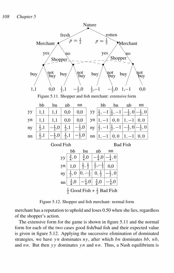
108 Chapter 5
�
�
� �
�
� �
Nature
fresh rotten
Merchant
yes no
p D 12 p D 1
2
Shopper
1,1 0,0 12
,1 �12,0 1
2,�1 �1
2,0 1,�1 0,0
Merchant
yes noShopper
buy notbuy buy not
buybuy notbuy buy not
buy
Figure 5.11. Shopper and fish merchant: extensive form
1,1 1,1 0,0 0,0
1,1 1,1 0,0 0,012,1 �1
2,0 1
2,1 �1
2,0
12,1 �1
2,0 1
2,1 �1
2,0
yy
yn
ny
nn
bb bn nb nn
Good Fish
12; �1 1
2; �1 �1
2; 0 �1
2; 0
1; �1 0; 0 1; �1 0; 012; �1 1
2; �1 �1
2; 0 �1
2; 0
1; �1 0; 0 1; �1 0; 0
yy
yn
ny
nn
bb bn nb nn
Bad Fish
34; 0 �1
4; 0
1,012; 1
2 0,012; 0 0; �1
20; 1
2�1
2; 0
yy
yn
ny
nn
bb bn nb nn
12
Good Fish + 12
Bad Fish
�14
,0
�14,0�1
4,0
34,0
34
,0 34
,0
12,�1
2
Figure 5.12. Shopper and fish merchant: normal form
merchant has a reputation to uphold and loses 0.50 when she lies, regardless
of the shopper’s action.
The extensive form for the game is shown in figure 5.11 and the normal
form for each of the two cases good fish/bad fish and their expected value
is given in figure 5.12. Applying the successive elimination of dominated
strategies, we have yn dominates ny, after which bn dominates bb, nb,
and nn. But then yy dominates yn and nn. Thus, a Nash equilibrium is
Pure-Strategy Nash Equilibria 109
yy=bn: the merchant says the fish is good no matter what and the buyer
believes him. Because some of the eliminated strategies were only weakly
dominated, there could be other Nash equilibria and we should check for
this. We find that another is for the seller to use pure strategy nn and the
buyer to use pure strategy nb. Note that this equilibrium works only if
the buyer is a “nice guy” in the sense of choosing among equally good
responses that maximizes the payoff to the seller. The equilibrium yy=bn
does not have this drawback.
5.19 Pure Coordination Games
We say one allocation of payoffs Pareto-dominates another, or is Pareto-
superior to another, if all players are at least as well off in the first as in
the second and at least one is better off. We say one allocation of payoffs
strictly Pareto-dominates another if all players are strictly better off in the
first than in the second. We say an allocation is Pareto-efficient or Pareto-
optimal if it is not Pareto-dominated by any other allocation. An allocation
is Pareto-inefficient if it is not Pareto-efficient. A pure coordination game
is a game in which there is one pure-strategy Nash equilibrium that strictly
Pareto-dominates all other Nash equilibria.
a. Consider the game where you and your partner independently guess
an integer between 1 and 5. If you guess the same number, you each
win the amount of your guess. Otherwise you lose the amount of your
guess. Show that this is a pure coordination game. Hint: Write down
the normal form of this game and find the pure-strategy Nash equilibria.
b. Consider a two-player game in which each player has two strategies.
Suppose the payoff matrices for the two players are faij g for player 1
and fbij g for player 2, where i ,j D 1,2. Find the conditions on these
payoff matrices for the game to be pure coordination game. Hint: First
solve this for a 2 � 2 game, then a 3 � 3, then generalize.
5.20 Pick Any Number
Three people independently choose an integer between zero and nine. If
the three choices are the same, each person receives the amount chosen.
Otherwise each person loses the amount the person chose.
a. What are the pure-strategy Nash equilibria of this game?
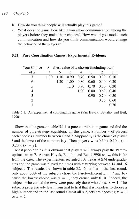
110 Chapter 5
b. How do you think people will actually play this game?
c. What does the game look like if you allow communication among the
players before they make their choices? How would you model such
communication and how do you think communication would change
the behavior of the players?
5.21 Pure Coordination Games: Experimental Evidence
Your Choice Smallest value of x chosen (including own)
of x 7 6 5 4 3 2 1
7 1.30 1.10 0.90 0.70 0.50 0.30 0.10
6 1.20 1.00 0.80 0.60 0.40 0.20
5 1.10 0.90 0.70 0.50 0.30
4 1.00 0.80 0.60 0.40
3 0.90 0.70 0.50
2 0.80 0.60
1 0.70
Table 5.1. An experimental coordination game (Van Huyck, Battalio, and Beil,
1990)
Show that the game in table 5.1 is a pure coordination game and find the
number of pure-strategy equilibria. In this game, a number n of players
each chooses a number between 1 and 7. Suppose xi is the choice of player
i and the lowest of the numbers is y. Then player i wins 0:60 C 0:10 �xi �0:20 � .xi � y/.
Most people think it is obvious that players will always play the Pareto-
optimal xi D 7. As van Huyck, Battalio and Beil (1990) show, this is far
from the case. The experimenters recruited 107 Texas A&M undergradu-
ates and the game was played ten times with n varying between 14 and 16
subjects. The results are shown in table 5.2. Note that in the first round,
only about 30% of the subjects chose the Pareto-efficient x D 7 and be-
cause the lowest choice was y D 1, they earned only 0.10. Indeed, the
subjects who earned the most were precisely those who chose x D 1. The
subjects progressively learn from trial to trial that it is hopeless to choose a
high number and in the last round almost all subjects are choosing x D 1
or x D 2.
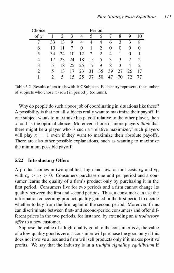
Pure-Strategy Nash Equilibria 111
Choice Period
of x 1 2 3 4 5 6 7 8 9 10
7 33 13 9 4 4 4 6 3 3 8
6 10 11 7 0 1 2 0 0 0 0
5 34 24 10 12 2 2 4 1 0 1
4 17 23 24 18 15 5 3 3 2 2
3 5 18 25 25 17 9 8 3 4 2
2 5 13 17 23 31 35 39 27 26 17
1 2 5 15 25 37 50 47 70 72 77
Table 5.2. Results of ten trials with 107 Subjects. Each entry represents the number
of subjects who chose x (row) in period y (column).
Why do people do such a poor job of coordinating in situations like these?
A possibility is that not all subjects really want to maximize their payoff. If
one subject wants to maximize his payoff relative to the other player, then
x D 1 is the optimal choice. Moreover, if one or more players think that
there might be a player who is such a “relative maximizer,” such players
will play x D 1 even if they want to maximize their absolute payoffs.
There are also other possible explanations, such as wanting to maximize
the minimum possible payoff.
5.22 Introductory Offers
A product comes in two qualities, high and low, at unit costs ch and cl ,
with ch > cl > 0. Consumers purchase one unit per period and a con-
sumer learns the quality of a firm’s product only by purchasing it in the
first period. Consumers live for two periods and a firm cannot change its
quality between the first and second periods. Thus, a consumer can use the
information concerning product quality gained in the first period to decide
whether to buy from the firm again in the second period. Moreover, firms
can discriminate between first- and second-period consumers and offer dif-
ferent prices in the two periods, for instance, by extending an introductory
offer to a new customer.
Suppose the value of a high-quality good to the consumer is h, the value
of a low-quality good is zero, a consumer will purchase the good only if this
does not involve a loss and a firm will sell products only if it makes positive
profits. We say that the industry is in a truthful signaling equilibrium if
112 Chapter 5
the firms’ choice of sale prices accurately distinguishes high-quality from
low-quality firms. If the firms’ choices do not distinguish high from low
quality, we have a pooling equilibrium. In the current situation, this means
that only the high-quality firms will sell.
Let ı be the consumer’s discount factor on second-period utility. We show
that if h > ch C .ch � cl/=ı, there is a truthful signaling equilibrium and
not otherwise. If a high-quality firm sells to a consumer in the first period
at some price p1, then in the second period the consumer will be willing to
pay p2 D h, because he knows the product is of high quality. Knowing that
it can make a profit h � ch from a customer in the second period, a high-
quality firm might want to make a consumer an “introductory offer” at a
price p1 in the first period that would not be mimicked by the low-quality
firm, in order to reap the second-period profit.
If p1 > cl , the low-quality firm could mimic the high-quality firm, so
the best the high-quality firm can do is to charge p1 D cl , which the low-
quality firm will not mimic, because the low-quality firm cannot profit by
doing so (it cannot profit in the first period and the consumer will not buy
the low-quality product in the second period). In this case, the high-quality
firm’s profits are .cl � ch/ C ı.h � ch/. As long as these profits are positive,
which reduces to h > ch C ı.ch � cl/, the high-quality firm will stay in
business.
Note that each consumer gains h�cl in the truthful signaling equilibrium
and firms gain cl � ch C ı.h � ch/ per customer.
5.23 Web Sites (for Spiders)
In the spider Agelenopsis aperta, individuals search for desirable locations
for spinning webs. The value of a web is 2v to its owner. When two spiders
come upon the same desirable location, the two invariably compete for it.
Spiders can be either strong or weak, but it is impossible to tell which type
a spider is by observation. A spider may rear onto two legs to indicate that
it is strong, or fail to do so, indicating that it is weak. However, spiders
do not have to be truthful. Under what conditions will they in fact signal
truthfully whether they are weak or strong? Note that if it is in the interest
of both the weak and the strong spider to represent itself as strong, we have
a “pooling equilibrium,” in which the value of the signal is zero and it will
be totally ignored; hence, it will probably not be issued. If only the strong
spider signals, we have a truthful signaling equilibrium.
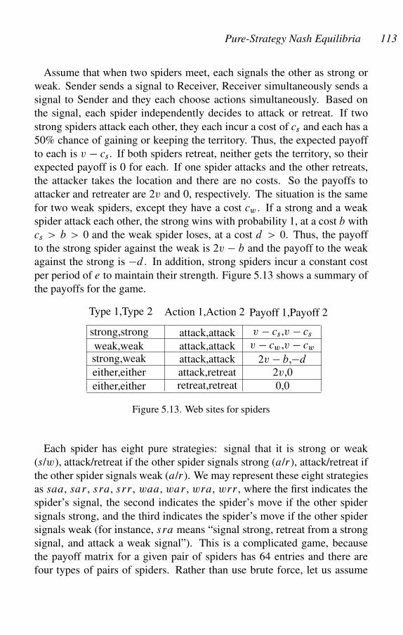
Pure-Strategy Nash Equilibria 113
Assume that when two spiders meet, each signals the other as strong or
weak. Sender sends a signal to Receiver, Receiver simultaneously sends a
signal to Sender and they each choose actions simultaneously. Based on
the signal, each spider independently decides to attack or retreat. If two
strong spiders attack each other, they each incur a cost of cs and each has a
50% chance of gaining or keeping the territory. Thus, the expected payoff
to each is v � cs. If both spiders retreat, neither gets the territory, so their
expected payoff is 0 for each. If one spider attacks and the other retreats,
the attacker takes the location and there are no costs. So the payoffs to
attacker and retreater are 2v and 0, respectively. The situation is the same
for two weak spiders, except they have a cost cw . If a strong and a weak
spider attack each other, the strong wins with probability 1, at a cost b with
cs > b > 0 and the weak spider loses, at a cost d > 0. Thus, the payoff
to the strong spider against the weak is 2v � b and the payoff to the weak
against the strong is �d . In addition, strong spiders incur a constant cost
per period of e to maintain their strength. Figure 5.13 shows a summary of
the payoffs for the game.
Type 1,Type 2 Action 1,Action 2 Payoff 1,Payoff 2
strong,strong attack,attack v � cs,v � cs
weak,weak attack,attack v � cw ,v � cw
strong,weak attack,attack 2v � b,�d
either,either attack,retreat 2v,0
either,either retreat,retreat 0,0
Figure 5.13. Web sites for spiders
Each spider has eight pure strategies: signal that it is strong or weak
(s/w), attack/retreat if the other spider signals strong (a/r), attack/retreat if
the other spider signals weak (a/r). We may represent these eight strategies
as saa, sar , sra, srr , waa, war , wra, wrr , where the first indicates the
spider’s signal, the second indicates the spider’s move if the other spider
signals strong, and the third indicates the spider’s move if the other spider
signals weak (for instance, sra means “signal strong, retreat from a strong
signal, and attack a weak signal”). This is a complicated game, because
the payoff matrix for a given pair of spiders has 64 entries and there are
four types of pairs of spiders. Rather than use brute force, let us assume
114 Chapter 5
there is a truthful signaling equilibrium and see what that tells us about the
relationships among v; b; cw ; cs; d; e and the fraction p of strong spiders in
the population.
Suppose v > cs; cw and the proportion p of strong spiders is determined
by the condition that the payoffs to the two conditions of being strong and
being weak are equal. In a truthful signaling equilibrium, strong spiders
use saa and weak spiders use wra. To see this, note that strong spiders say
they’re strong and weak spiders say they’re weak, by definition of a truthful
signaling equilibrium. Weak spiders retreat against strong spiders because
d > 0 and attack other weak spiders because v � cw > 0. Strong spiders
attack weak spiders if they do not withdraw, because 2v �b > 2v �cs > v.
If p is the fraction of strong spiders, then the expected payoff to a strong
spider is p.v�cs/C2.1�p/v�e and the expected payoff to a weak spider
is .1 � p/.v � cw/. If these two are equal, then
p D v C cw � e
cw C cs
; (5.4)
which is strictly between 0 and 1 if and only if e � cw < v < e C cs.
In a truthful signaling equilibrium, each spider has expected payoff
� D .v � cw/.cs C e � v/
cw C cs
: (5.5)
Suppose a weak spider signals that it is strong and all other spiders play the
truthful signaling equilibrium strategy. If the other spider is strong, it will
attack and the weak spider will receive �d . If the other spider is weak, it
will withdraw and the spider will gain 2v. Thus, the payoff to the spider for
a misleading communication is �pd C 2.1 � p/v, which cannot be greater
than (5.5) if truth telling is Nash. Solving for d , we get
d .cs C e � v/.v C cw/
cw � e C v:
Can a strong spider benefit from signaling that it is weak? To see that it
cannot, suppose first that it faces a strong spider. If it attacks the strong
spider after signaling that it is weak, it gets the same payoff as if it signaled
strong (because its opponent always attacks). If it withdraws against its
opponent, it gets 0, which is less than the v � cs it gets by attacking. Thus,
signaling weak against a strong opponent cannot lead to a gain. Suppose
Pure-Strategy Nash Equilibria 115
the opponent is weak. Then signaling weak means that the opponent will
attack. Responding by withdrawing, it gets 0; responding by attacking, it
gets 2v � b, because it always defeats its weak opponent. But if it had
signaled strong, it would have earned 2v > 2v � b. Thus, it never pays a
strong spider to signal that it is weak.
Note that as long as both strong and weak spiders exist in equilibrium,
an increase in the cost e of being strong leads to an increase in payoff
to all spiders, weak and strong alike. This result follows directly from
equation (5.5) and is due to the fact that higher e entails a lower fraction
of strong spiders, from (5.4). But weak spiders earn .1 � p/.v � cw/,
which is decreasing in p and strong spiders earn the same as weak spiders
in equilibrium.
6
Mixed-Strategy Nash Equilibria
Leges sine moribus vanae
Horace
This chapter presents a variety of games with mixed-strategy Nash equi-
libria, many in the form of problems to be solved by the reader. Some
mixed-strategy equilibria, such as throwing fingers (�3.8), are intuitively
obvious. Others, such as the hawk-dove equilibrium (�3.10) are not intu-
itive, but the equilibrium depends in plausible ways on the parameters of the
problem. For instance, as the cost of injury w increases in the hawk-dove
game, the probability of playing hawk declines, and as the value of the ter-
ritory v increases, the probability of playing hawk also increases. However,
the mixed-strategy equilibrium in battle of the sexes (�3.9), is implausible
because it suggest that a player’s Nash strategy does not depend on the rela-
tive strength of preferences for the two pure-strategy equilibrium outcomes.
Indeed, you will ascertain later that this mixed-strategy equilibrium is not
stable in an evolutionary dynamic (�12.17).
6.1 The Algebra of Mixed Strategies
There is a simple way to do the algebra of mixed strategies. Examples in
this case are worth more than formalities, so I will give one. The reader
will find it easy to generalize.
Suppose Alice has strategy set fL; Rg and uses mixed strategy � D ˛LC.1 � ˛/R, whereas Bob has strategy set fU; Dg and uses mixed strategy
D ˇU C .1 � ˇ/D. We can then think of the payoff to Alice, �1.�; /,
as the value to Alice of the compound lottery in figure 6.1.
We can reduce this compound lottery to a simple lottery with four payoffs,
.L; U /, .L; D/, .R; U /, and .R; D/, with probabilities ˛ˇ, ˛.1 � ˇ/, .1 �˛/ˇ, and .1 � ˛/.1 � ˇ/, respectively. The payoff to this lottery for player
i is then
�i.�; / D ˛ˇ�i.L; U / C ˛.1 � ˇ/�i .L; D/
116

Mixed-Strategy Nash Equilibria 117
�
�
�
�
L
R
˛
1 � ˛
ˇ
1 � ˇ
ˇ
1 � ˇ
U
D
U
D
�
��
�
�1.L; U /; �2.L; U /
�1.L; D/; �2.L; D/�1.R; U /; �2.R; U /
�1.R; D/; �2.R; D/
Alice
Bob
Bob
Figure 6.1. Mixed strategies as compound lotteries
C .1 � ˛/ˇ�i.R; U / C .1 � ˛/.1 � ˇ/�i.R; D/:
Another way to think of this is to define the product of mixed strategies by
� D .˛L C .1 � ˛/R/.ˇU C .1 � ˇ/D/
D ˛ˇLU C ˛.1 � ˇ/LD C .1 � ˛/ˇRU C .1 � ˛/.1 � ˇ/RD;
and then the payoff to Alice from the strategy pair .�; / is
�1.�; / D �1.˛ˇLU C ˛.1 � ˇ/LD C .1 � ˛/ˇRU C .1 � ˛/.1 � ˇ/RD/
D ˛ˇ�1.L; U / C ˛.1 � ˇ/�1.L; D/
C .1 � ˛/ˇ�1.R; U / C .1 � ˛/.1 � ˇ/�1.R; D/:
6.2 Lions and Antelope
cb=2,cb=2
cl ,cb
BA
cb ,cl
cl=2,cl =2
LA
BA
LA
Two lions out hunting see Big Antelope
and Little Antelope in the distance. They
will surely catch whatever prey they chase,
whether alone or together. However, if they
pick different antelopes to chase, there is no need to share, whereas if they
go after the same antelope, each will get only half of the kill and the other
antelope will escape. Suppose their decisions are independent, the caloric
value of Big Antelope is cb, the caloric value of Little Antelope is cl and
0 < cl < cb . Let BA be the strategy “hunt Big Antelope,” and let LA be
the strategy “hunt Little Antelope.” The normal form game is shown in the
diagram. The lions cannot distinguish between player 1 and player 2, so
only symmetric Nash equilibria are acceptable.
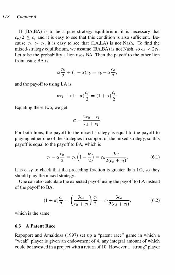
118 Chapter 6
If (BA,BA) is to be a pure-strategy equilibrium, it is necessary that
cb=2 cl and it is easy to see that this condition is also sufficient. Be-
cause cb > cl , it is easy to see that (LA,LA) is not Nash. To find the
mixed-strategy equilibrium, we assume (BA,BA) is not Nash, so cb < 2cl .
Let ˛ be the probability a lion uses BA. Then the payoff to the other lion
from using BA is
˛cb
2C .1 � ˛/cb D cb � ˛
cb
2;
and the payoff to using LA is
˛cl C .1 � ˛/cl
2D .1 C ˛/
cl
2:
Equating these two, we get
˛ D 2cb � cl
cb C cl
:
For both lions, the payoff to the mixed strategy is equal to the payoff to
playing either one of the strategies in support of the mixed strategy, so this
payoff is equal to the payoff to BA, which is
cb � ˛cb
2D cb
�1 � ˛
2
�D cb
3cl
2.cb C cl /: (6.1)
It is easy to check that the preceding fraction is greater than 1/2, so they
should play the mixed strategy.
One can also calculate the expected payoff using the payoff to LA instead
of the payoff to BA:
.1 C ˛/cl
2D�
3cb
cb C cl
�cl
2D cl
3cb
2.cb C cl/; (6.2)
which is the same.
6.3 A Patent Race
Rapoport and Amaldoss (1997) set up a “patent race” game in which a
“weak” player is given an endowment of 4, any integral amount of which
could be invested in a project with a return of 10. However a “strong” player
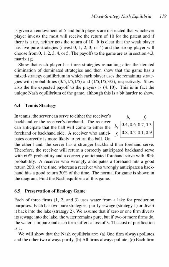
Mixed-Strategy Nash Equilibria 119
is given an endowment of 5 and both players are instructed that whichever
player invests the most will receive the return of 10 for the patent and if
there is a tie, neither gets the return of 10. It is clear that the weak player
has five pure strategies (invest 0, 1, 2, 3, or 4) and the strong player will
choose from 0, 1, 2, 3, 4, or 5. The payoffs to the game are as in section 4.3,
matrix (g).
Show that each player has three strategies remaining after the iterated
elimination of dominated strategies and then show that the game has a
mixed-strategy equilibrium in which each player uses the remaining strate-
gies with probabilities (3/5,1/5,1/5) and (1/5,1/5,3/5), respectively. Show
also the the expected payoff to the players is .4; 10/. This is in fact the
unique Nash equilibrium of the game, although this is a bit harder to show.
6.4 Tennis Strategy
0:4; 0:6
0:8; 0:2
br
0:7; 0:3
0:1; 0:9
fr
bs
fs
In tennis, the server can serve to either the receiver’s
backhand or the receiver’s forehand. The receiver
can anticipate that the ball will come to either the
forehand or backhand side. A receiver who antici-
pates correctly is more likely to return the ball. On
the other hand, the server has a stronger backhand than forehand serve.
Therefore, the receiver will return a correctly anticipated backhand serve
with 60% probability and a correctly anticipated forehand serve with 90%
probability. A receiver who wrongly anticipates a forehand hits a good
return 20% of the time, whereas a receiver who wrongly anticipates a back-
hand hits a good return 30% of the time. The normal for game is shown in
the diagram. Find the Nash equilibria of this game.
6.5 Preservation of Ecology Game
Each of three firms (1, 2, and 3) uses water from a lake for production
purposes. Each has two pure strategies: purify sewage (strategy 1) or divert
it back into the lake (strategy 2). We assume that if zero or one firm diverts
its sewage into the lake, the water remains pure, but if two or more firms do,
the water is impure and each firm suffers a loss of 3. The cost of purification
is 1.
We will show that the Nash equilibria are: (a) One firm always pollutes
and the other two always purify, (b) All firms always pollute, (c) Each firm
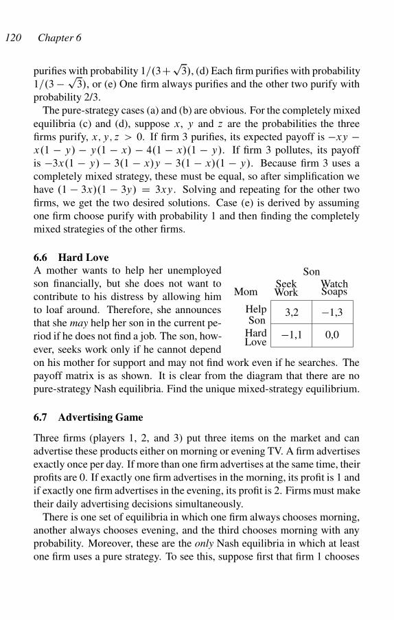
120 Chapter 6
purifies with probability 1=.3Cp3/, (d) Each firm purifies with probability
1=.3 � p3/, or (e) One firm always purifies and the other two purify with
probability 2/3.
The pure-strategy cases (a) and (b) are obvious. For the completely mixed
equilibria (c) and (d), suppose x, y and z are the probabilities the three
firms purify, x; y; z > 0. If firm 3 purifies, its expected payoff is �xy �x.1 � y/ � y.1 � x/ � 4.1 � x/.1 � y/. If firm 3 pollutes, its payoff
is �3x.1 � y/ � 3.1 � x/y � 3.1 � x/.1 � y/. Because firm 3 uses a
completely mixed strategy, these must be equal, so after simplification we
have .1 � 3x/.1 � 3y/ D 3xy. Solving and repeating for the other two
firms, we get the two desired solutions. Case (e) is derived by assuming
one firm choose purify with probability 1 and then finding the completely
mixed strategies of the other firms.
6.6 Hard Love
Work Soaps
Son
MomSeek Watch
3,2
�1,1 0,0
�1,3Help
HardSon
Love
A mother wants to help her unemployed
son financially, but she does not want to
contribute to his distress by allowing him
to loaf around. Therefore, she announces
that she may help her son in the current pe-
riod if he does not find a job. The son, how-
ever, seeks work only if he cannot depend
on his mother for support and may not find work even if he searches. The
payoff matrix is as shown. It is clear from the diagram that there are no
pure-strategy Nash equilibria. Find the unique mixed-strategy equilibrium.
6.7 Advertising Game
Three firms (players 1, 2, and 3) put three items on the market and can
advertise these products either on morning or evening TV. A firm advertises
exactly once per day. If more than one firm advertises at the same time, their
profits are 0. If exactly one firm advertises in the morning, its profit is 1 and
if exactly one firm advertises in the evening, its profit is 2. Firms must make
their daily advertising decisions simultaneously.
There is one set of equilibria in which one firm always chooses morning,
another always chooses evening, and the third chooses morning with any
probability. Moreover, these are the only Nash equilibria in which at least
one firm uses a pure strategy. To see this, suppose first that firm 1 chooses
Mixed-Strategy Nash Equilibria 121
the pure strategy M (morning). If both firms 2 and 3 choose mixed strate-
gies, then one of them could gain by shifting to pure strategy E (evening).
To see this, let the two mixed strategies be ˛M C .1 � ˛/E for firm 2 and
ˇM C .1 � ˇ/E for firm 3. Let �i .s1s2s3/ be the payoff to player i when
the three firms use pure strategies s1s2s3. Then, the payoff to M for firm 2
is
�2 D ˛ˇ�2.MMM/ C ˛.1 � ˇ/�2.MME/ C .1 � ˛/ˇ�2.MEM/
C .1 � ˛/.1 � ˇ/�2.MEE/
D ˛ˇ.0/ C ˛.1 � ˇ/.0/ C .1 � ˛/ˇ.2/ C .1 � ˛/.1 � ˇ/.0/
D 2.1 � ˛/ˇ:
Because 0 < ˇ by definition, this is maximized by choosing ˛ D 0, so firm
2 should use pure strategy E. This contradicts our assumption that both
firms 1 and 2 use mixed strategies.
A similar argument holds if firm 1 uses pure strategy E. We conclude that
if firm 1 uses a pure strategy, at least one of the other two firms will use
a pure strategy. The firm that does will not use the same pure strategy as
firm 1, because this would not be a best response. Therefore, two firms
use opposite pure strategies and it does not matter what the third firm does.
Now we repeat the whole analysis assuming firm 2 uses a pure strategy,
with clearly the same outcome. Then, we do it again for firm 3. This proves
that if one firm uses a pure strategy, at least two firms use a pure strategy,
which concludes this part of the problem.
To find the mixed-strategy equilibria, let x; y, and z be the probabilities
of advertising in the morning for firms 1, 2, and 3. The expected return to 1
of advertising in the morning is .1 � y/.1 � z/ and in the evening it is 2yz.
If these are equal, any choice of x for firm 1 is Nash. But equality means
1 � y � z � yz D 0, or y D .1 � z/=.1 C z/. Now repeat for firms 2 and 3,
giving the equalities y D .1�z/=.1Cz/ and z D .1�x/=.1Cx/. Solving
simultaneously, we get x D y D z D p2 � 1. To see this, substitute
y D .1 � z/=.1 C z/ in x D .1 � y/=.1 C y/, getting
x D 1 � y
1 C yD 1 � 1�z
1Cz
1 C 1�z1Cz
D z:
Thus, x D .1 � x/=.1 C x/, which is a simple quadratic equation, the only
root of which between 0 and 1 isp
2 � 1. Thus, this is Nash.
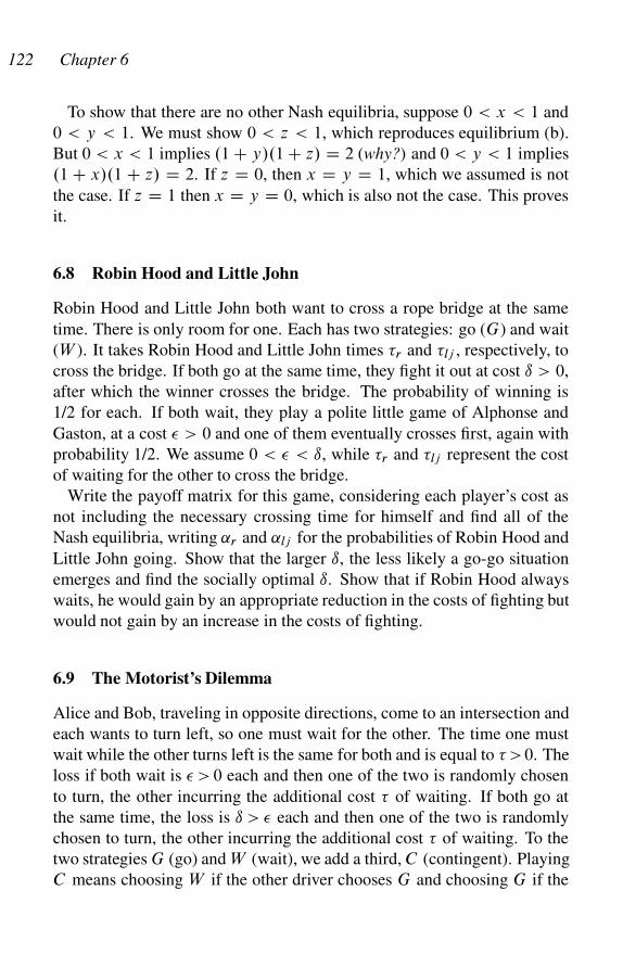
122 Chapter 6
To show that there are no other Nash equilibria, suppose 0 < x < 1 and
0 < y < 1. We must show 0 < z < 1, which reproduces equilibrium (b).
But 0 < x < 1 implies .1 C y/.1 C z/ D 2 (why?) and 0 < y < 1 implies
.1 C x/.1 C z/ D 2. If z D 0, then x D y D 1, which we assumed is not
the case. If z D 1 then x D y D 0, which is also not the case. This proves
it.
6.8 Robin Hood and Little John
Robin Hood and Little John both want to cross a rope bridge at the same
time. There is only room for one. Each has two strategies: go (G) and wait
(W ). It takes Robin Hood and Little John times r and lj , respectively, to
cross the bridge. If both go at the same time, they fight it out at cost ı > 0,
after which the winner crosses the bridge. The probability of winning is
1/2 for each. If both wait, they play a polite little game of Alphonse and
Gaston, at a cost � > 0 and one of them eventually crosses first, again with
probability 1/2. We assume 0 < � < ı, while r and lj represent the cost
of waiting for the other to cross the bridge.
Write the payoff matrix for this game, considering each player’s cost as
not including the necessary crossing time for himself and find all of the
Nash equilibria, writing ˛r and ˛lj for the probabilities of Robin Hood and
Little John going. Show that the larger ı, the less likely a go-go situation
emerges and find the socially optimal ı. Show that if Robin Hood always
waits, he would gain by an appropriate reduction in the costs of fighting but
would not gain by an increase in the costs of fighting.
6.9 The Motorist’s Dilemma
Alice and Bob, traveling in opposite directions, come to an intersection and
each wants to turn left, so one must wait for the other. The time one must
wait while the other turns left is the same for both and is equal to >0. The
loss if both wait is � > 0 each and then one of the two is randomly chosen
to turn, the other incurring the additional cost of waiting. If both go at
the same time, the loss is ı > � each and then one of the two is randomly
chosen to turn, the other incurring the additional cost of waiting. To the
two strategies G (go) and W (wait), we add a third, C (contingent). Playing
C means choosing W if the other driver chooses G and choosing G if the
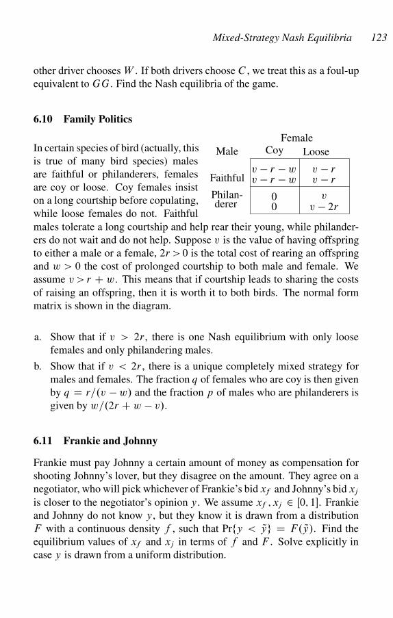
Mixed-Strategy Nash Equilibria 123
other driver chooses W . If both drivers choose C , we treat this as a foul-up
equivalent to GG. Find the Nash equilibria of the game.
6.10 Family Politics
derer
Male
Female
v � 2r0
v � rv � r � w
v0
v � rv � r � w
Philan-
Faithful
LooseCoyIn certain species of bird (actually, this
is true of many bird species) males
are faithful or philanderers, females
are coy or loose. Coy females insist
on a long courtship before copulating,
while loose females do not. Faithful
males tolerate a long courtship and help rear their young, while philander-
ers do not wait and do not help. Suppose v is the value of having offspring
to either a male or a female, 2r > 0 is the total cost of rearing an offspring
and w > 0 the cost of prolonged courtship to both male and female. We
assume v > r C w. This means that if courtship leads to sharing the costs
of raising an offspring, then it is worth it to both birds. The normal form
matrix is shown in the diagram.
a. Show that if v > 2r , there is one Nash equilibrium with only loose
females and only philandering males.
b. Show that if v < 2r , there is a unique completely mixed strategy for
males and females. The fraction q of females who are coy is then given
by q D r=.v � w/ and the fraction p of males who are philanderers is
given by w=.2r C w � v/.
6.11 Frankie and Johnny
Frankie must pay Johnny a certain amount of money as compensation for
shooting Johnny’s lover, but they disagree on the amount. They agree on a
negotiator, who will pick whichever of Frankie’s bid xf and Johnny’s bid xj
is closer to the negotiator’s opinion y. We assume xf ; xj 2 Œ0; 1�. Frankie
and Johnny do not know y, but they know it is drawn from a distribution
F with a continuous density f , such that Prfy < Qyg D F. Qy/. Find the
equilibrium values of xf and xj in terms of f and F . Solve explicitly in
case y is drawn from a uniform distribution.
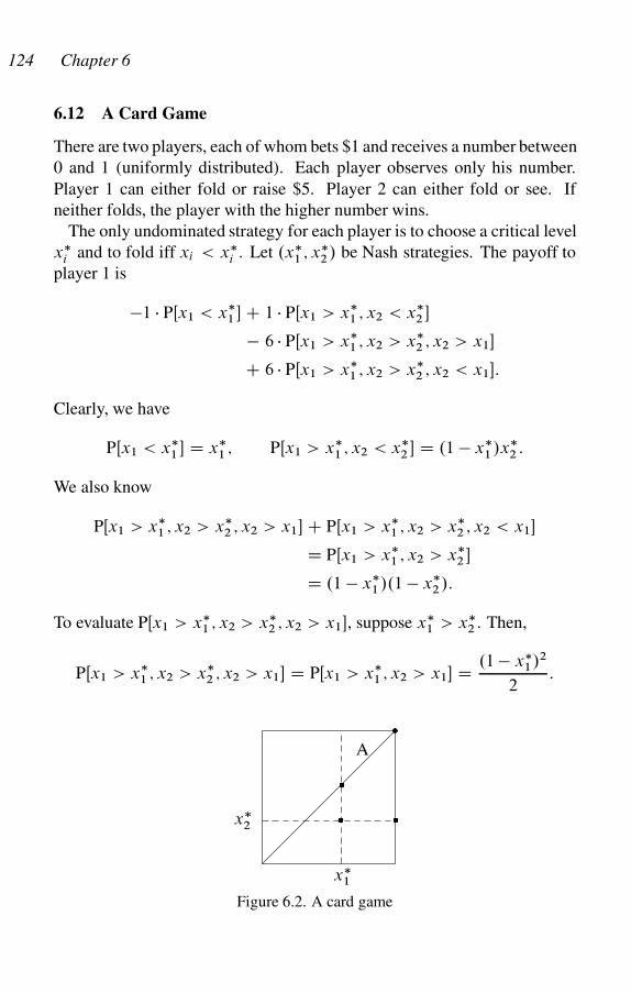
124 Chapter 6
6.12 A Card Game
There are two players, each of whom bets $1 and receives a number between
0 and 1 (uniformly distributed). Each player observes only his number.
Player 1 can either fold or raise $5. Player 2 can either fold or see. If
neither folds, the player with the higher number wins.
The only undominated strategy for each player is to choose a critical level
x�i and to fold iff xi < x�
i . Let .x�1 ; x�
2 / be Nash strategies. The payoff to
player 1 is
�1 PŒx1 < x�1 � C 1 PŒx1 > x�
1 ; x2 < x�2 �
� 6 PŒx1 > x�1 ; x2 > x�
2 ; x2 > x1�
C 6 PŒx1 > x�1 ; x2 > x�
2 ; x2 < x1�:
Clearly, we have
PŒx1 < x�1 � D x�
1 ; PŒx1 > x�1 ; x2 < x�
2 � D .1 � x�1 /x�
2 :
We also know
PŒx1 > x�1 ; x2 > x�
2 ; x2 > x1� C PŒx1 > x�1 ; x2 > x�
2 ; x2 < x1�
D PŒx1 > x�1 ; x2 > x�
2 �
D .1 � x�1 /.1 � x�
2 /:
To evaluate PŒx1 > x�1 ; x2 > x�
2 ; x2 > x1�, suppose x�1 > x�
2 . Then,
PŒx1 > x�1 ; x2 > x�
2 ; x2 > x1� D PŒx1 > x�1 ; x2 > x1� D .1 � x�
1/2
2:
x�1
x�2 �
�
�
A
�
Figure 6.2. A card game
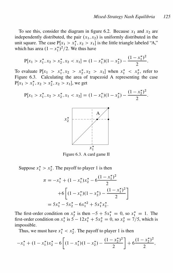
Mixed-Strategy Nash Equilibria 125
To see this, consider the diagram in figure 6.2. Because x1 and x2 are
independently distributed, the pair .x1; x2/ is uniformly distributed in the
unit square. The case PŒx1 > x�1 ; x2 > x1� is the little triangle labeled “A,”
which has area .1 � x�1 /2=2. We thus have
PŒx1 > x�1 ; x2 > x�
2 ; x2 < x1� D .1 � x�1 /.1 � x�
2 / � .1 � x�1 /2
2:
To evaluate PŒx1 > x�1 ; x2 > x�
2 ; x2 > x1� when x�1 < x�
2 , refer to
Figure 6.3. Calculating the area of trapezoid A representing the case
PŒx1 > x�1 ; x2 > x�
2 ; x2 > x1�, we get
PŒx1 > x�1 ; x2 > x�
2 ; x1 < x2� D .1 � x�1 /.1 � x�
2 / � .1 � x�2 /2
2:
x�1
x�2 �
�
�A
Figure 6.3. A card game II
Suppose x�1 > x�
2 . The payoff to player 1 is then
� D �x�1 C .1 � x�
1 /x�2 � 6
.1 � x�1 /2
2
C6
�.1 � x�
1 /.1 � x�2 / � .1 � x�
1 /2
2
�
D 5x�1 � 5x�
2 � 6x�21 C 5x�
1 x�2 :
The first-order condition on x�2 is then �5 C 5x�
1 D 0, so x�1 D 1. The
first-order condition on x�1 is 5 � 12x�
1 C 5x�2 D 0, so x�
2 D 7=5, which is
impossible.
Thus, we must have x�1 < x�
2 . The payoff to player 1 is then
�x�1 C .1 � x�
1 /x�2 � 6
�.1 � x�
1 /.1 � x�2 / � .1 � x�
2 /2
2
�C 6
.1 � x�2 /2
2;
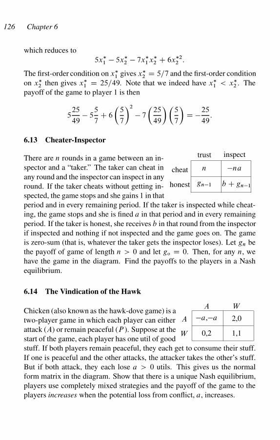
126 Chapter 6
which reduces to
5x�1 � 5x�
2 � 7x�1 x�
2 C 6x�22 :
The first-order condition on x�1 gives x�
2 D 5=7 and the first-order condition
on x�2 then gives x�
1 D 25=49. Note that we indeed have x�1 < x�
2 . The
payoff of the game to player 1 is then
525
49� 5
5
7C 6
�5
7
�2
� 7
�25
49
��5
7
�D �25
49:
6.13 Cheater-Inspector
trust inspect
cheat
honest
n �na
gn�1 b C gn�1
There are n rounds in a game between an in-
spector and a “taker.” The taker can cheat in
any round and the inspector can inspect in any
round. If the taker cheats without getting in-
spected, the game stops and she gains 1 in that
period and in every remaining period. If the taker is inspected while cheat-
ing, the game stops and she is fined a in that period and in every remaining
period. If the taker is honest, she receives b in that round from the inspector
if inspected and nothing if not inspected and the game goes on. The game
is zero-sum (that is, whatever the taker gets the inspector loses). Let gn be
the payoff of game of length n > 0 and let go D 0. Then, for any n, we
have the game in the diagram. Find the payoffs to the players in a Nash
equilibrium.
6.14 The Vindication of the Hawk
�a,�a
0,2
A
2,0
1,1
W
A
W
Chicken (also known as the hawk-dove game) is a
two-player game in which each player can either
attack (A) or remain peaceful (P ). Suppose at the
start of the game, each player has one util of good
stuff. If both players remain peaceful, they each get to consume their stuff.
If one is peaceful and the other attacks, the attacker takes the other’s stuff.
But if both attack, they each lose a > 0 utils. This gives us the normal
form matrix in the diagram. Show that there is a unique Nash equilibrium,
players use completely mixed strategies and the payoff of the game to the
players increases when the potential loss from conflict, a, increases.
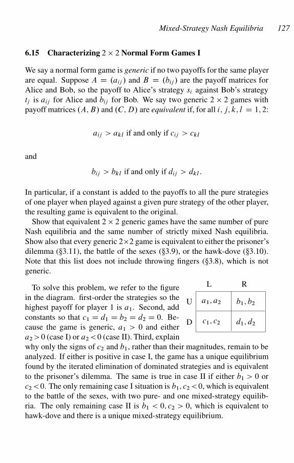
Mixed-Strategy Nash Equilibria 127
6.15 Characterizing 2 � 2 Normal Form Games I
We say a normal form game is generic if no two payoffs for the same player
are equal. Suppose A D .aij / and B D .bij / are the payoff matrices for
Alice and Bob, so the payoff to Alice’s strategy si against Bob’s strategy
tj is aij for Alice and bij for Bob. We say two generic 2 � 2 games with
payoff matrices .A; B/ and .C; D/ are equivalent if, for all i; j; k; l D 1; 2:
aij > akl if and only if cij > ckl
and
bij > bkl if and only if dij > dkl :
In particular, if a constant is added to the payoffs to all the pure strategies
of one player when played against a given pure strategy of the other player,
the resulting game is equivalent to the original.
Show that equivalent 2 � 2 generic games have the same number of pure
Nash equilibria and the same number of strictly mixed Nash equilibria.
Show also that every generic 2�2 game is equivalent to either the prisoner’s
dilemma (�3.11), the battle of the sexes (�3.9), or the hawk-dove (�3.10).
Note that this list does not include throwing fingers (�3.8), which is not
generic.
a1; a2 b1; b2
d1; d2c1; c2D
U
L RTo solve this problem, we refer to the figure
in the diagram. first-order the strategies so the
highest payoff for player 1 is a1. Second, add
constants so that c1 D d1 D b2 D d2 D 0. Be-
cause the game is generic, a1 > 0 and either
a2 >0 (case I) or a2 <0 (case II). Third, explain
why only the signs of c2 and b1, rather than their magnitudes, remain to be
analyzed. If either is positive in case I, the game has a unique equilibrium
found by the iterated elimination of dominated strategies and is equivalent
to the prisoner’s dilemma. The same is true in case II if either b1 > 0 or
c2 <0. The only remaining case I situation is b1; c2 <0, which is equivalent
to the battle of the sexes, with two pure- and one mixed-strategy equilib-
ria. The only remaining case II is b1 < 0; c2 > 0, which is equivalent to
hawk-dove and there is a unique mixed-strategy equilibrium.
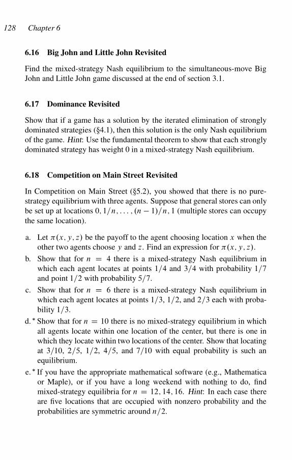
128 Chapter 6
6.16 Big John and Little John Revisited
Find the mixed-strategy Nash equilibrium to the simultaneous-move Big
John and Little John game discussed at the end of section 3.1.
6.17 Dominance Revisited
Show that if a game has a solution by the iterated elimination of strongly
dominated strategies (�4.1), then this solution is the only Nash equilibrium
of the game. Hint: Use the fundamental theorem to show that each strongly
dominated strategy has weight 0 in a mixed-strategy Nash equilibrium.
6.18 Competition on Main Street Revisited
In Competition on Main Street (�5.2), you showed that there is no pure-
strategy equilibrium with three agents. Suppose that general stores can only
be set up at locations 0; 1=n; : : : ; .n � 1/=n; 1 (multiple stores can occupy
the same location).
a. Let �.x; y; z/ be the payoff to the agent choosing location x when the
other two agents choose y and z. Find an expression for �.x; y; z/.
b. Show that for n D 4 there is a mixed-strategy Nash equilibrium in
which each agent locates at points 1=4 and 3=4 with probability 1=7
and point 1=2 with probability 5=7.
c. Show that for n D 6 there is a mixed-strategy Nash equilibrium in
which each agent locates at points 1=3, 1=2, and 2=3 each with proba-
bility 1=3.
d. � Show that for n D 10 there is no mixed-strategy equilibrium in which
all agents locate within one location of the center, but there is one in
which they locate within two locations of the center. Show that locating
at 3=10, 2=5, 1=2, 4=5, and 7=10 with equal probability is such an
equilibrium.
e. � If you have the appropriate mathematical software (e.g., Mathematica
or Maple), or if you have a long weekend with nothing to do, find
mixed-strategy equilibria for n D 12; 14; 16. Hint: In each case there
are five locations that are occupied with nonzero probability and the
probabilities are symmetric around n=2.
Mixed-Strategy Nash Equilibria 129
6.19 Twin Sisters Revisited
In section 5.15, a mother tells each of her twin daughters to ask for a cer-
tain whole number of dollars, at least 1 and at most 100. If the total of
the two amounts does not exceed 101, each will have her request granted.
Otherwise each gets nothing. What will the sisters do?
You probably answered that both sisters would ask for $50, even though
this is not a Nash equilibrium. However, if one sister is pretty sure the other
will bid $50, she herself might be tempted to bid $51. With mixed strategies
available, we can find a Nash equilibrium that captures our intuition that
bidding $50 will almost always be the observed behavior.
Let us write sx for the pure strategy “bid x.” Suppose both sisters use
the mixed strategy � D psx C .1 � p/sy , where p 2 .0; 1/ and .�; �/ is
a Nash equilibrium. In any Nash equilibrium we must have x C y D 101,
so we can assume that x < y D 101 � x. Check that because the payoffs
to sx and sy must be equal, we have x D py. Show that any � satisfying
the previous two conditions is indeed a Nash equilibrium; that is, show that
no pure strategy sz has higher payoff against � that � has against � (Hint:
consider separately the cases z < x, x < z < 51, 51 < z < y, and y < z).
It is easy to see that the payoff to the Nash equilibrium with x < y D101 � x and x D py is simply x per sister. Thus, though there are many
Nash equilibria, the highest payoff is the one in which x D 50, y D 51,
and p D 50=51, which is practically unity. So both sisters will ask for $50
most of the time, as our intuition suggested to us.
But why should the highest-payoff Nash equilibrium actually be the one
that the sisters choose? Could they not get “locked into” an inferior Nash
equilibrium, say where x D 10? The answer is: to this point, we have
no way of answering this question. But suppose the way that sisters play
this game is a sort of “social convention” that people learn and suppose fur-
ther that there is some sort of social process whereby superior conventions
grow in frequency and inferior ones contract. Then, perhaps, the x D $50
solution might come to be established in society.
6.20 Twin Sisters: An Agent-Based Model
We can use the procedures described in section 4.20 to create an agent-
based model of Twin Sisters (�5.15). I wrote a program (in the Pascal
programming language) with 200 agents, each of whom is given a random
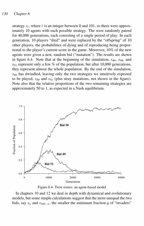
130 Chapter 6
strategy si , where i is an integer between 0 and 101, so there were approx-
imately 10 agents with each possible strategy. The were randomly paired
for 40,000 generations, each consisting of a single period of play. In each
generation, 10 players “died” and were replaced by the “offspring” of 10
other players, the probabilities of dying and of reproducing being propor-
tional to the player’s current score in the game. Moreover, 10% of the new
agents were given a new, random bid (“mutation”). The results are shown
in figure 6.4. Note that at the beginning of the simulation, s49, s50, and
s51 represent only a few % of the population, but after 10,000 generations,
they represent almost the whole population. By the end of the simulation,
s49 has dwindled, leaving only the two strategies we intuitively expected
to be played, s50 and s51 (plus stray mutations, not shown in the figure).
Note also that the relative proportions of the two remaining strategies are
approximately 50 to 1, as expected in a Nash equilibrium.
Generation
0 10000 20000 30000 40000
Fra
ctio
n o
f P
op
ula
tio
n
0.0
0.2
0.4
0.6
0.8
1.0
Bid 50
Bid 49
Bid 51
Figure 6.4. Twin sisters: an agent-based model
In chapters 10 and 12 we deal in depth with dynamical and evolutionary
models, but some simple calculations suggest that the more unequal the two
bids, say sx and s101�x , the smaller the minimum fraction q of “invaders”
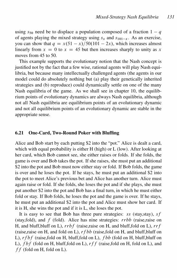
Mixed-Strategy Nash Equilibria 131
using s50 need be to displace a population composed of a fraction 1 � q
of agents playing the mixed strategy using sx and s101�x . As an exercise,
you can show that q D x.51 � x/=50.101 � 2x/, which increases almost
linearly from x D 0 to x D 45 but then increases sharply to unity as x
moves from 45 to 50.
This example supports the evolutionary notion that the Nash concept is
justified not by the fact that a few wise, rational agents will play Nash equi-
libria, but because many intellectually challenged agents (the agents in our
model could do absolutely nothing but (a) play their genetically inherited
strategies and (b) reproduce) could dynamically settle on one of the many
Nash equilibria of the game. As we shall see in chapter 10, the equilib-
rium points of evolutionary dynamics are always Nash equilibria, although
not all Nash equilibria are equilibrium points of an evolutionary dynamic
and not all equilibrium points of an evolutionary dynamic are stable in the
appropriate sense.
6.21 One-Card, Two-Round Poker with Bluffing
Alice and Bob start by each putting $2 into the “pot.” Alice is dealt a card,
which with equal probability is either H (high) or L (low). After looking at
her card, which Bob cannot see, she either raises or folds. If she folds, the
game is over and Bob takes the pot. If she raises, she must put an additional
$2 into the pot and Bob must now either stay or fold. If Bob folds, the game
is over and he loses the pot. If he stays, he must put an additional $2 into
the pot to meet Alice’s previous bet and Alice has another turn. Alice must
again raise or fold. If she folds, she loses the pot and if she plays, she must
put another $2 into the pot and Bob has a final turn, in which he must either
fold or stay. If Bob folds, he loses the pot and the game is over. If he stays,
he must put an additional $2 into the pot and Alice must show her card. If
it is H, she wins the pot and if it is L, she loses the pot.
It is easy to see that Bob has three pure strategies: ss (stay,stay), sf
(stay,fold), and f (fold). Alice has nine strategies: rrbb (raise,raise on
H, and bluff,bluff on L), rrbf (raise,raise on H, and bluff,fold on L), rrf
(raise,raise on H, and fold on L), rf bb (raise,fold on H, and bluff,bluff on
L), rf bf (raise,fold on H, bluff,fold on L), f bb (fold on H, bluff,bluff on
L), f bf (fold on H, bluff,fold on L), rff (raise,fold on H, fold on L), and
ff (fold on H, fold on L).
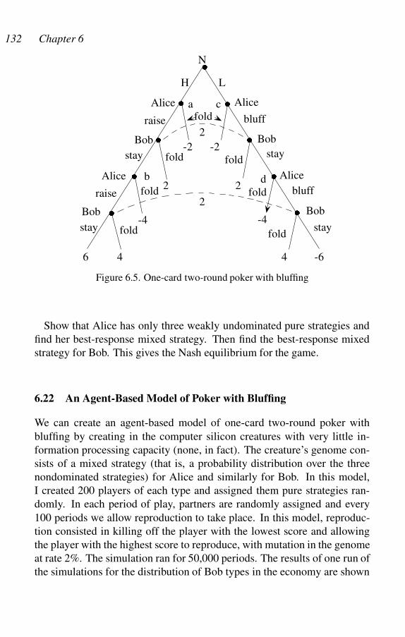
132 Chapter 6
�
�
�
�
�
�
�
�
N
H L
Alice
Bob2
2
6 4 4 -6
-4
2
-2-2
2
-4
raise bluff
staystay
raise bluff
staystay fold
fold
fold
fold
fold
fold
fold
a
b
c
d
Alice
AliceAlice
Bob
BobBob
Figure 6.5. One-card two-round poker with bluffing
Show that Alice has only three weakly undominated pure strategies and
find her best-response mixed strategy. Then find the best-response mixed
strategy for Bob. This gives the Nash equilibrium for the game.
6.22 An Agent-Based Model of Poker with Bluffing
We can create an agent-based model of one-card two-round poker with
bluffing by creating in the computer silicon creatures with very little in-
formation processing capacity (none, in fact). The creature’s genome con-
sists of a mixed strategy (that is, a probability distribution over the three
nondominated strategies) for Alice and similarly for Bob. In this model,
I created 200 players of each type and assigned them pure strategies ran-
domly. In each period of play, partners are randomly assigned and every
100 periods we allow reproduction to take place. In this model, reproduc-
tion consisted in killing off the player with the lowest score and allowing
the player with the highest score to reproduce, with mutation in the genome
at rate 2%. The simulation ran for 50,000 periods. The results of one run of
the simulations for the distribution of Bob types in the economy are shown
Mixed-Strategy Nash Equilibria 133
Stay-Stay
Fold
Stay-Fold
Nash Equilibrium Probabilities:
Stay-Stay = 0.53
Stay-Fold = 0.13
Fold = 0.33
0 10000 20000 30000 40000 50000
Rounds
0.0
0.1
0.2
0.3
0.4
0.5
0.6
Pro
ba
bili
ty
Figure 6.6. An Agent-based model of one-card two-round poker with bluffing
in figure 6.6. Note that after 25,000 periods, the frequency of each strategy
has settled down to the theoretically predicted equilibrium value.
6.23 Trust in Networks
Consider a network of many traders who are randomly paired to play a one-
shot (that is, played only once) prisoner’s dilemma in which each receives
�1 if they both defect, each receives 1 if they both cooperate and a defec-
tor receives 2 when playing against a cooperator, who receives �2. There
are three types of agents: defectors defect unconditionally against all part-
ners; trusters cooperate unconditionally with all partners; and inspectors
monitor an imperfect signal indicating whether or not one’s current partner
defects against cooperators. The signal correctly identifies a defector with
probability p > 1=2 and correctly identifies a non-defector with the same
probability p. The inspector then refuses to trade with a partner who is sig-
nalled as a defector and otherwise plays the cooperate strategy. An agent
who does not trade has payoff 0. The payoff matrix for a pair of agents has
the normal form shown in figure 6.7.
Think of a “strategy” in this network as a fraction ˛ of inspectors, a frac-
tion ˇ of trusters and a fraction 1 � ˛ � ˇ of defectors. A Nash equilibrium
is a population composition .˛; ˇ/ that is a best response to itself.

134 Chapter 6
p2 p �2.1 � p/
p 1 �2
2.1 � p/ 2 �1
Inspect Trust Defect
Inspect
Trust
Defect
p2 p 2.1 � p/
p
�2.1 � p/ �2 �1
1 2
Figure 6.7. The inspect-trust-defect game
It is easy to show that there are no pure-strategy Nash equilibria and for
p p3 � 1 � 3=4, there are no Nash equilibria involving only two types
of players. Use section 3.6 to prove that there exists a unique completely
mixed Nash equilibrium for p > 5=7 and show that it is unique.
6.24 El Farol
In Santa Fe there is nothing to do at night but look at the stars or go to the
local bar, El Farol. Let us define the utility of looking at the stars as 0 and
let the cost of walking over to the bar be 1. Suppose the utility from being
at the bar is 2 if there are fewer than three people at the bar and 1/2 if there
are three or more people at the bar. For a given Nash equilibrium, we define
the social surplus provided by the bar to be the sum of the payoffs to all the
residents.
Suppose there are three people in Santa Fe, so there are three pure-
strategy Nash equilibria, in each of which two people go to the bar and
one watches the stars. The average payoff per player in each of these is 2/3.
There is also a unique symmetric mixed-strategy Nash equilibrium (that is,
each player uses the same mixed strategy) in which each resident goes to
the bar with probabilityp
.2=3/ � 81:65%. To see this, let p be the prob-
ability of going to the bar for each resident. The payoff to not going to the
bar and the payoff to going to the bar must be equal. To find p, note that
the probability that the other two people go to the bar is p2, so the expected
payoff to going to the bar is
2.1 � p2/ C 1
2p2 � 1 D 0;
Mixed-Strategy Nash Equilibria 135
the solution to which is p Dp
.2=3/.
Note that in this equilibrium the average payoff is 0: the bar might as well
not exist!
To generalize the problem, suppose for each player i D 1; 2; 3 the cost of
walking to the bar is ci , the payoff when there are fewer than three people
in the bar is ai and the payoff otherwise is bi , where 0 < bi < ci < ai .
Now, if there is any mixed-strategy equilibrium, it is unique and once again
bar might as well not exist. To see this, let pi be the probability of player
i going to the bar, for i D 1; : : : ; 3: In a mixed strategy-equilibrium, the
payoff for each player to going to the bar and staying home must be the
same. It is easy to show that this is equivalent to
pipj D ak � ck
ak � bk
i ¤ j ¤ k ¤ i:
Let ˛k be the right-hand side of this equation. We can solve the resulting
three equations, getting pi D pj ˛k=˛i . The conditions for a mixed-
strategy equilibrium are thus ˛i j < ˛k for i ¤ j ¤ k ¤ i . We con-
clude that, if the costs and benefits of the bar are not too dissimilar for
the three players, the mixed-strategy equilibrium exists. Otherwise, one
resident must always stay home. The only equilibrium in which there is
a positive payoff from the bar’s existence is if at least one resident stays
home.
We can generalize the problem to n people, in which case the bar still
might as well not exist, provided the equilibrium is completely mixed.
However, you can show that if El Farol charges an appropriate entry fee,
the payoff to both the bar and its clients can be strictly positive.
6.25 Decorated Lizards
The side-blotched lizard Uta stansburiana has three distinct male types:
orange-throats, blue-throats, and yellow-striped. The orange-throats are
violently aggressive, keep large harems of females (up to seven) and defend
large territories. The blue-throats are less aggressive, keep small harems
(usually three females) and defend small territories. The yellow-stripes
are very docile but they look like females, so they can infiltrate another
male’s territory and secretly copulate with the females. Field researchers
note that there is regular succession from generation to generation, in which
orange-throated males are a majority in one period, followed by a majority
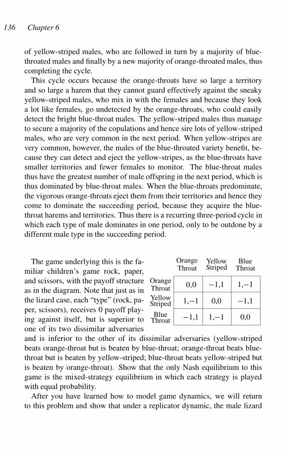
136 Chapter 6
of yellow-striped males, who are followed in turn by a majority of blue-
throated males and finally by a new majority of orange-throated males, thus
completing the cycle.
This cycle occurs because the orange-throats have so large a territory
and so large a harem that they cannot guard effectively against the sneaky
yellow-striped males, who mix in with the females and because they look
a lot like females, go undetected by the orange-throats, who could easily
detect the bright blue-throat males. The yellow-striped males thus manage
to secure a majority of the copulations and hence sire lots of yellow-striped
males, who are very common in the next period. When yellow-stripes are
very common, however, the males of the blue-throated variety benefit, be-
cause they can detect and eject the yellow-stripes, as the blue-throats have
smaller territories and fewer females to monitor. The blue-throat males
thus have the greatest number of male offspring in the next period, which is
thus dominated by blue-throat males. When the blue-throats predominate,
the vigorous orange-throats eject them from their territories and hence they
come to dominate the succeeding period, because they acquire the blue-
throat harems and territories. Thus there is a recurring three-period cycle in
which each type of male dominates in one period, only to be outdone by a
different male type in the succeeding period.
0;0 �1,1 1,�1
1,�1 0,0 �1,1
�1,1 1,�1 0,0
Throat Striped ThroatOrange Yellow Blue
Orange
Yellow
Blue
Throat
Throat
Striped
The game underlying this is the fa-
miliar children’s game rock, paper,
and scissors, with the payoff structure
as in the diagram. Note that just as in
the lizard case, each “type” (rock, pa-
per, scissors), receives 0 payoff play-
ing against itself, but is superior to
one of its two dissimilar adversaries
and is inferior to the other of its dissimilar adversaries (yellow-striped
beats orange-throat but is beaten by blue-throat; orange-throat beats blue-
throat but is beaten by yellow-striped; blue-throat beats yellow-striped but
is beaten by orange-throat). Show that the only Nash equilibrium to this
game is the mixed-strategy equilibrium in which each strategy is played
with equal probability.
After you have learned how to model game dynamics, we will return
to this problem and show that under a replicator dynamic, the male lizard
Mixed-Strategy Nash Equilibria 137
population does indeed cycle among the three forms in successive breeding
periods (�12.14).
6.26 Sex Ratios as Nash Equilibria
Most organisms that employ sexual reproduction have two sexes: male and
female. The fraction of a female’s offspring that are female is determined
by genetic factors and hence is heritable. In many species (e.g., most ani-
mals), the fraction is almost exactly 1/2, even if the viabilities of males (�m)
and females (�f ), the probability that they mature to the point of sexual re-
production, are very different. Why is this the case?
To streamline the process of solving this problem, suppose all females
breed simultaneously and their offspring constitute the next generation of
birds (that is, birds live for only one breeding period). Unless otherwise
stated, you should assume (a) females “choose” a ratio u of sons to daugh-
ters born that maximizes the expected number of their genes among their
grandchildren; (b) each female produces c offspring; (c) males and females
contribute an equal number of genes to their offspring; (d) all males are
equally likely to sire an offspring; (e) there is random mating in the next
generation; and (f) the next generation is so large that no single female can
affect the ratio v of males to females in the next generation.
First we show that u D 1=2 in equilibrium; that is, a female produces
half sons and half daughters. Call the birds surviving to maturity in the
next generation the “breeding pool.” Let s and d be the number of sons and
daughters in the breeding pool. Then ˛ D d=s is the expected fraction of
a female’s offspring sired by any given male in the breeding pool. We then
have
˛ D d
sD �f .1 � v/
�mv: (6.3)
We now write an expression for f .u; v/, the number of grandchildren of a
female, in terms of ˛ and the other parameters of the problem (u, v, �f , �m,
and c). We have
f .u; v/ D �f .1 � u/c2 C �muc2˛: (6.4)
To understand this expression, note that �f .1�u/c is the number of daugh-
ters who survive to maturity and so �f .1 � u/c2 is the number of grand-
children born to daughters. Similarly, �muc is the number of sons and
�muc.c˛/ is the number of grandchildren sired by sons.
138 Chapter 6
Substituting equation (6.3) into equation (6.4) and simplifying, we get
f .u; v/ D c2�f
1 C u
�1 � 2v
v
�:
If we now choose u to maximize f .u; v/, we see that the only Nash equi-
librium occurs when u D v. Thus, if v ¤ 1=2, there cannot be a mixed-
strategy equilibrium: if the fraction of males in the population is less than
50%, each female should produce all males (that is, set u D 1) and if the
fraction of males in the population is greater than 50%, each female should
produce all females (that is, set u D 0). The only possible Nash strategy
is therefore u D v D 1=2, because such a strategy must be symmetric (the
same for all agents) and mixed (because all pure strategies are clearly not
Nash).
Suppose now that there are n females and n is sufficiently small that
a single female’s choice does affect the ratio of daughters to sons. We
can still show that an equal number of daughters and sons remains a Nash
equilibrium. It is easy to check that (6.3) becomes
˛ D d
sD �f Œn � u � .n � 1/v�
�mŒ.n � 1/v C u�:
The number of grandchildren as expressed in (6.4) then becomes
f .u; v/ D �f .1 � u/c2 C �muc2 �f Œn � u � .n � 1/v�
�mŒ.n � 1/v C u�
D c2�f
.n � 1/v C uf�2u2 � uŒ2.n � 1/v � .n C 1/� C .n � 1/vg:
The first-order condition on u for maximizing f .u; v/ then gives
2.n � 1/v D n C 1 � 4u:
In a symmetric equilibrium, we must have u D v, which implies u D v D1=2.
Now suppose that instead of only breeding once, a fraction ım of breeding
males and ıf of breeding females die in each period and the rest remain
in the mating pool. The expression for the equilibrium ratio of males to
females is derived as follows. Let m be the number of males and let n be
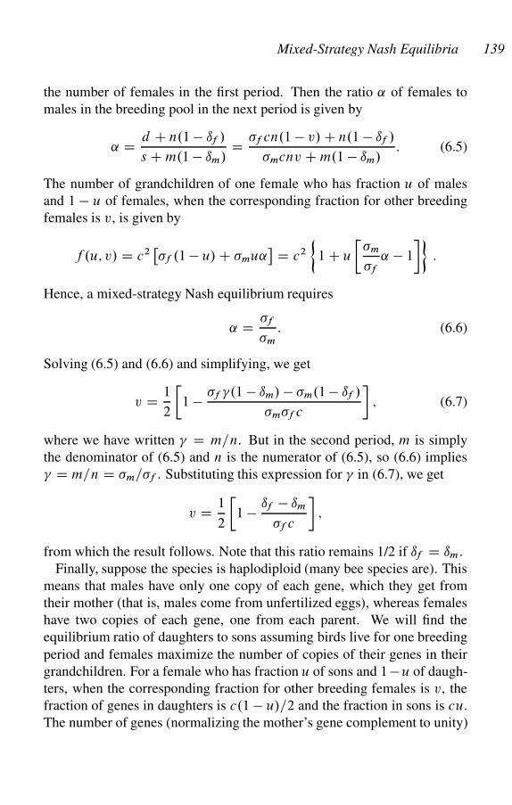
Mixed-Strategy Nash Equilibria 139
the number of females in the first period. Then the ratio ˛ of females to
males in the breeding pool in the next period is given by
˛ D d C n.1 � ıf /
s C m.1 � ım/D �f cn.1 � v/ C n.1 � ıf /
�mcnv C m.1 � ım/: (6.5)
The number of grandchildren of one female who has fraction u of males
and 1 � u of females, when the corresponding fraction for other breeding
females is v, is given by
f .u; v/ D c2��f .1 � u/ C �mu˛
� D c2
1 C u
��m
�f
˛ � 1
�:
Hence, a mixed-strategy Nash equilibrium requires
˛ D �f
�m
: (6.6)
Solving (6.5) and (6.6) and simplifying, we get
v D 1
2
�1 � �f �.1 � ım/ � �m.1 � ıf /
�m�f c
�; (6.7)
where we have written � D m=n. But in the second period, m is simply
the denominator of (6.5) and n is the numerator of (6.5), so (6.6) implies
� D m=n D �m=�f . Substituting this expression for � in (6.7), we get
v D 1
2
�1 � ıf � ım
�f c
�;
from which the result follows. Note that this ratio remains 1/2 if ıf D ım.
Finally, suppose the species is haplodiploid (many bee species are). This
means that males have only one copy of each gene, which they get from
their mother (that is, males come from unfertilized eggs), whereas females
have two copies of each gene, one from each parent. We will find the
equilibrium ratio of daughters to sons assuming birds live for one breeding
period and females maximize the number of copies of their genes in their
grandchildren. For a female who has fraction u of sons and 1 �u of daugh-
ters, when the corresponding fraction for other breeding females is v, the
fraction of genes in daughters is c.1 � u/=2 and the fraction in sons is cu.
The number of genes (normalizing the mother’s gene complement to unity)
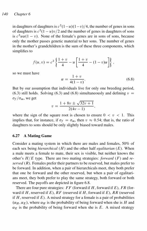
140 Chapter 6
in daughters of daughters is c2.1�u/.1�v/=4, the number of genes in sons
of daughters is c2.1 � u/v=2 and the number of genes in daughters of sons
is c2u˛.1 � v/. None of the female’s genes are in sons of sons, because
only the mother passes genetic material to her sons. The number of genes
in the mother’s grandchildren is the sum of these three components, which
simplifies to
f .u; v/ D c2
1 C v
4� u
�1 C v
4� .1 � v/˛
�;
so we must have
˛ D 1 C v
4.1 � v/: (6.8)
But by our assumption that individuals live for only one breeding period,
(6.3) still holds. Solving (6.3) and (6.8) simultaneously and defining � D�f =�m, we get
v D 1 C 8� ˙ p32� C 1
2.4� � 1/;
where the sign of the square root is chosen to ensure 0 < v < 1. This
implies that, for instance, if �f D �m, then v � 0:54; that is, the ratio of
daughters to sons should be only slightly biased toward males.
6.27 A Mating Game
Consider a mating system in which there are males and females, 50% of
each sex being hierarchical (H ) and the other half egalitarian (E). When
a male meets a female to mate, their sex is visible, but neither knows the
other’s H=E type. There are two mating strategies: forward (F ) and re-
served (R). Females prefer their partners to be reserved, but males prefer to
be forward. In addition, when a pair of hierarchicals meet, they both prefer
that one be forward and the other reserved, but when a pair of egalitari-
ans meet, they both prefer to play the same strategy, both forward or both
reserved. The payoffs are depicted in figure 6.8.
There are four pure strategies: FF (forward if H , forward if E), FR (for-
ward if H , reserved if E), RF (reserved if H , forward if E), RR (reserved
if H , reserved if E). A mixed strategy for a female is a pair of probabilities
.˛H ; ˛E /, where ˛H is the probability of being forward when she is H and
˛E is the probability of being forward when she is E. A mixed strategy
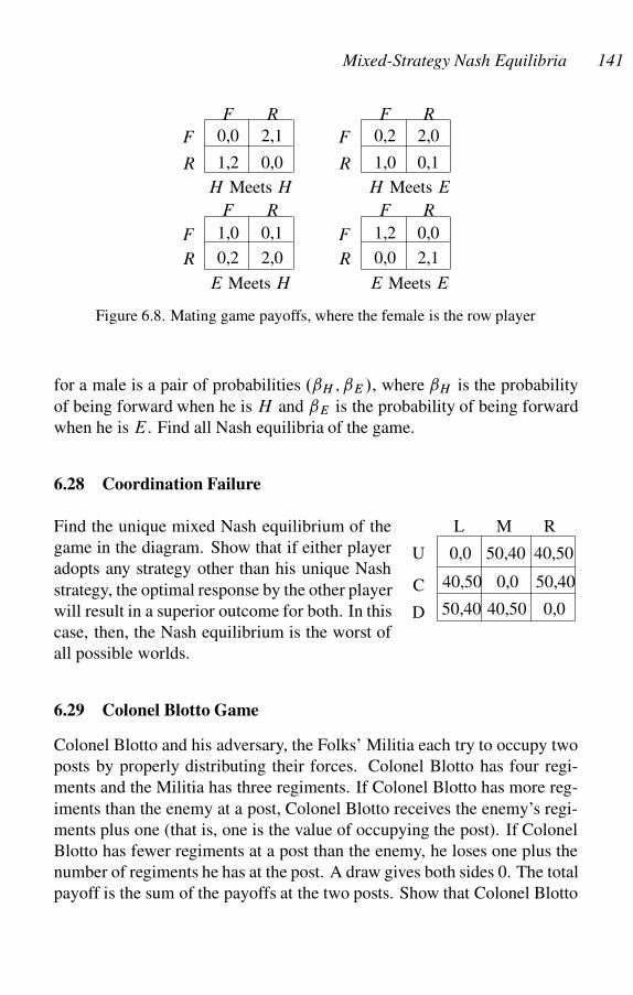
Mixed-Strategy Nash Equilibria 141
E Meets E
R
F
R
2,1
0,0
F
0,0
1,2
E Meets H
R
F
R
2,0
0,1
F
0,2
1,0
H Meets E
R
F
R
0,1
2,0
F
1,0
0,2
H Meets H
R
F
R
0,0
2,1
F
1,2
0,0
Figure 6.8. Mating game payoffs, where the female is the row player
for a male is a pair of probabilities .ˇH ; ˇE /, where ˇH is the probability
of being forward when he is H and ˇE is the probability of being forward
when he is E. Find all Nash equilibria of the game.
6.28 Coordination Failure
0,0 50,40 40,50
40,50 0,0 50,40
50,40 40,50 0,0
L RM
U
D
C
Find the unique mixed Nash equilibrium of the
game in the diagram. Show that if either player
adopts any strategy other than his unique Nash
strategy, the optimal response by the other player
will result in a superior outcome for both. In this
case, then, the Nash equilibrium is the worst of
all possible worlds.
6.29 Colonel Blotto Game
Colonel Blotto and his adversary, the Folks’ Militia each try to occupy two
posts by properly distributing their forces. Colonel Blotto has four regi-
ments and the Militia has three regiments. If Colonel Blotto has more reg-
iments than the enemy at a post, Colonel Blotto receives the enemy’s regi-
ments plus one (that is, one is the value of occupying the post). If Colonel
Blotto has fewer regiments at a post than the enemy, he loses one plus the
number of regiments he has at the post. A draw gives both sides 0. The total
payoff is the sum of the payoffs at the two posts. Show that Colonel Blotto
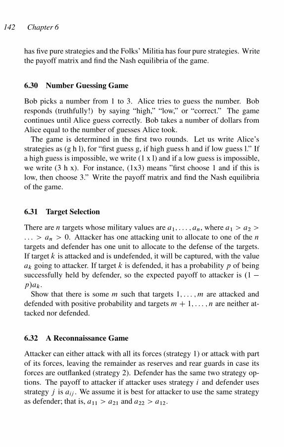
142 Chapter 6
has five pure strategies and the Folks’ Militia has four pure strategies. Write
the payoff matrix and find the Nash equilibria of the game.
6.30 Number Guessing Game
Bob picks a number from 1 to 3. Alice tries to guess the number. Bob
responds (truthfully!) by saying “high,” “low,” or “correct.” The game
continues until Alice guess correctly. Bob takes a number of dollars from
Alice equal to the number of guesses Alice took.
The game is determined in the first two rounds. Let us write Alice’s
strategies as (g h l), for “first guess g, if high guess h and if low guess l.” If
a high guess is impossible, we write (1 x l) and if a low guess is impossible,
we write (3 h x). For instance, (1x3) means ”first choose 1 and if this is
low, then choose 3.” Write the payoff matrix and find the Nash equilibria
of the game.
6.31 Target Selection
There are n targets whose military values are a1; : : : ; an, where a1 > a2 >
: : : > an > 0. Attacker has one attacking unit to allocate to one of the n
targets and defender has one unit to allocate to the defense of the targets.
If target k is attacked and is undefended, it will be captured, with the value
ak going to attacker. If target k is defended, it has a probability p of being
successfully held by defender, so the expected payoff to attacker is .1 �p/ak.
Show that there is some m such that targets 1; : : : ; m are attacked and
defended with positive probability and targets m C 1; : : : ; n are neither at-
tacked nor defended.
6.32 A Reconnaissance Game
Attacker can either attack with all its forces (strategy 1) or attack with part
of its forces, leaving the remainder as reserves and rear guards in case its
forces are outflanked (strategy 2). Defender has the same two strategy op-
tions. The payoff to attacker if attacker uses strategy i and defender uses
strategy j is aij . We assume it is best for attacker to use the same strategy
as defender; that is, a11 > a21 and a22 > a12.
Mixed-Strategy Nash Equilibria 143
Attacker can also send out a reconnaissance force, at cost c, to find out
defender’s strategy. This will surely work, unless defender takes counter-
measures at cost d (these countermeasures must be taken without knowing
whether Attacker will actually reconnoiter), in which case reconnaissance
will fail. Suppose the game is zero-sum, with attacker payoff given by
A D Œaij � D�
48 24
12 36
�with c D 9 and d D 7:
Find the Nash equilibria.
6.33 Attack on Hidden Object
Alice has a bomb that she wants to drop on Bob’s country. She can carry
the bomb in one of two identical bombers P (protected) and F (flank). Bob
can prevent the damage by destroying the bomber containing the bomb.
The two bombers fly in formation, so to attack P , Bob must fly past F ,
in which case he runs the risk ˛, with 0<˛ <1, of being shot down before
engaging P . Once Bob has engaged his target (whether F or P ), he can
destroy it with probability ˇ, with 0<ˇ1. Thus, in any attack on P , if F is
intact, the probability of destroying P is � D .1 � ˛/ˇ.
Suppose Bob has enough fuel to attack the bombers twice and hence,
two chances to hit a target and destroy the valued object. Alice has two
strategies: load the bomb in F and load the bomb in P . Bob has four
strategies: attack F both times, attack P both times, attack F the first time
and P the second time and vice versa. The understanding is that if the first
attack was successful, the second attack is directed against the remaining
target, whatever the strategy used. Write normal form and find the Nash
equilibria.
6.34 Two-Person, Zero-Sum Games
A zero-sum game is, appropriately enough, a game in which the sum of
the payoffs to all the players is 0. Von Neumann and Morgenstern (1944),
who launched modern game theory, lay great stress on zero-sum games and,
indeed, defined equilibrium in a way that works only for two-person zero-
sum games. Nash had not yet invented the equilibrium concept that bears
his name; that came in 1950.

144 Chapter 6
Suppose the payoff to player 1 is �.�; / when player 1 uses � and player
2 uses , so the payoff to player 2 is ��.�; /. Von Neumann and Morgen-
stern defined .��; �/ to be an equilibrium of the two-person, zero-sum
game if �� maximizes min� �.�; / and � minimizes max� �.�; /. They
showed that this maximin solution satisfies
�.��; �/ D max�
min�
�.�; / D min�
max�
�.�; /: (6.9)
It is easy to show that a strategy profile in a two-person, zero-sum game is
a Nash equilibrium if and only if it is a maximin solution. This implies, in
particular, that all Nash equilibria of a two-person, zero-sum game have the
same payoffs.
To prove a Nash equilibrium is a maximin solution, suppose .��; �/ is a
Nash equilibrium. Then, for all �; , we have
max�
�.�; �/ min�
max�
�.�; / �.��; �/
max�
min�
�.�; / min�
�.��; /:
The first inequality is obvious, the second follows from
min�
max�
�.�; / min�
�.��; / D �.��; �/;
the third follows from
max�
min�
�.�; / � max�
�.�; �/ D �.��; �/;
and the fourth inequality is obvious. But the first and third terms must then
be equal, because .��; �/ is Nash and similarly for the third and fifth terms.
Thus, they are all equal, so .��; �/ is maximin.
To show that a maximin solution is a Nash equilibrium, suppose .��; �/
is maximin. We know that the second equation in (6.9) holds because there
exists a Nash equilibrium and we have already shown that a Nash equilib-
rium is maximin satisfying (6.9). But then we have
�.��; �/ � max�
�.�; �/ D min�
�.��; / � �.��; �/:
This proves all three terms are equal, so .��; �/ is Nash.
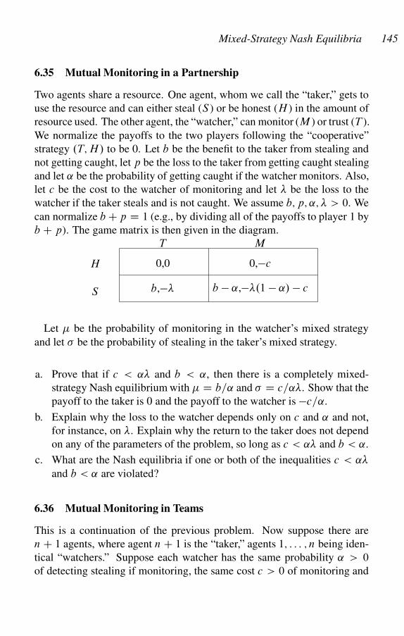
Mixed-Strategy Nash Equilibria 145
6.35 Mutual Monitoring in a Partnership
Two agents share a resource. One agent, whom we call the “taker,” gets to
use the resource and can either steal (S ) or be honest (H ) in the amount of
resource used. The other agent, the “watcher,” can monitor (M ) or trust (T ).
We normalize the payoffs to the two players following the “cooperative”
strategy .T; H/ to be 0. Let b be the benefit to the taker from stealing and
not getting caught, let p be the loss to the taker from getting caught stealing
and let ˛ be the probability of getting caught if the watcher monitors. Also,
let c be the cost to the watcher of monitoring and let � be the loss to the
watcher if the taker steals and is not caught. We assume b; p; ˛; � > 0. We
can normalize b C p D 1 (e.g., by dividing all of the payoffs to player 1 by
b C p). The game matrix is then given in the diagram.
0,0 0,�c
b,�� b � ˛,��.1 � ˛/ � c
T M
H
S
Let � be the probability of monitoring in the watcher’s mixed strategy
and let � be the probability of stealing in the taker’s mixed strategy.
a. Prove that if c < ˛� and b < ˛, then there is a completely mixed-
strategy Nash equilibrium with � D b=˛ and � D c=˛�. Show that the
payoff to the taker is 0 and the payoff to the watcher is �c=˛.
b. Explain why the loss to the watcher depends only on c and ˛ and not,
for instance, on �. Explain why the return to the taker does not depend
on any of the parameters of the problem, so long as c < ˛� and b < ˛.
c. What are the Nash equilibria if one or both of the inequalities c < ˛�
and b < ˛ are violated?
6.36 Mutual Monitoring in Teams
This is a continuation of the previous problem. Now suppose there are
n C 1 agents, where agent n C 1 is the “taker,” agents 1; : : : ; n being iden-
tical “watchers.” Suppose each watcher has the same probability ˛ > 0
of detecting stealing if monitoring, the same cost c > 0 of monitoring and
146 Chapter 6
the same loss � > 0 from an undetected theft. We care only about sym-
metric equilibria, in which all watchers choose the same probability � of
monitoring the taker.
Let b < 1 be the gain to the taker from stealing and define
� D ˛�.1 � b/n�1
n :
Answer the following questions, assuming b < ˛� and c < �.
a. Show that there is a mixed-strategy Nash equilibrium with the proba-
bility � of stealing and the probability � of monitoring given by
� D c
�� D 1 � .1 � b/
1n
˛:
b. Show that the payoff to a watcher is now �c=˛.1 � b/n�1
n . Why does
this not depend on �?
c. How does this solution change as the group size n increases? Why does
the tragedy of the commons (that is, the free rider) result not hold in this
case?
d. What would happen as n increases if, for some fixed ��, we wrote
� D ��=n? This formulation would be reasonable if a dishonest taker
imposed a fixed cost on the group no matter what its size, the cost being
shared equally by the watchers.
6.37 Altruism(?) in Bird Flocks
This is an application of the results of the previous problem. Consider a
flock of n birds eating in a group. A cat can catch a bird if it can sneak up
behind a nearby rock without being seen. Each bird has an incentive to let
the other birds look out for the cat whereas it conserves all its resources for
eating (studies show that birds dissipate a considerable amount of energy
and lose a considerable amount of time looking out for enemies). Why then
do birds actually look out for predators when they eat in flocks? Are they
“altruistic”? Perhaps not.1
1A similar problem arises in modeling the foraging behavior of flocks of birds
in patchy environments, because if one bird finds a patch of food, all get to eat
their fill (Motro 1991; Benkman 1988).
Mixed-Strategy Nash Equilibria 147
Suppose it takes the cat one second out in the open to reach the rock. If
seen during that one second by even one bird, the birds will all fly off and
the cat will lose p 2 .0; 1/ in wasted time. If the cat reaches the rock, it
catches one of the birds for a gain of b D 1 � p.
If each bird looks up from eating every k 1 seconds, it will see the
cat with probability 1=k. Thus, we can take ˛ D 1 and � D 1=k in the
previous problem (T corresponds to k D 1). The cost to the bird of being
caught is � D 1 and the cost of looking up once is c. Prove the following,
where we define � D 1 � c1=.n�1/ and � D 1 � cn=.n�1/.
THEOREM: There are three types of symmetric equilibria.
a. If c > 1, then no bird looks up and the cat stalks the birds with proba-
bility 1.
b. If c < 1 and b > �, there is a symmetric Nash equilibrium in which the
cat stalks with certainty, and birds look up every 1=� seconds.
c. If b < �, then there is a symmetric Nash equilibrium where the cat
stalks with probability � D c.1 �b/�.n�1/=n and the birds look up with
probability 1=�.
6.38 The Groucho Marx Game
Alice and Bob ante an amount a 0 and cards numbered from 1 to n are
placed in a hat. The players draw one card each, each observing his own
but not the other’s. They simultaneously and independently decide to stay
(s) or raise (r) by betting an additional b 0. The high card wins a C b, or
if one player raises and the other stays, the one raising wins a.
When n D 3, if a b a Nash equilibrium involves staying if you pick
a 1 and raising otherwise. If a < b, a Nash equilibrium is to stay unless
you pick the 3. To see this, note that staying if you get the 3 is strongly
dominated by raising, so there are four strategies left: rr, rs, sr, and ss,
where rr means “raise if you pick a 1, raise if you pick a 2”; rs means “raise
if you pick a 1, stay if you pick a 2”; etc. The payoffs, where down the first
column, 12 means Alice draws 1, Bob draws 2 etc. are shown in figure 6.9
The conclusion follows directly from the resulting payoff matrix, shown
in figure 6.10.
When n D 4, we can show that (i) if b > a D 0 it is Nash to stay unless
you pick the 4; (ii) if 2b > a > 0, it is Nash to stay unless you get a 3 or a
4; (iii) if a > 2b > 0, it is Nash to stay if you get a 1 and raise otherwise.

148 Chapter 6
rr/rr rr/rs rr/sr rr/ss rs/rs rs/sr rs/ss sr/sr sr/ss ss/ss
12 �a � b a �a � b a a �a � b a �a 0 0
13 �a � b�a � b�a � b �a � b �a � b�a � b�a � b �a �a �a
21 a C b a C b a a �a 0 0 a a 0
23 �a � b�a � b�a � b �a � b �a �a �a �a � b�a � b �a
31 a C b a C b a a a C b a a a a a
32 a C b a a C b a a a C b a a C b a a
0 2a �2b 2.a � b/ 0 �a � b a � b 0 a � b 0
Figure 6.9. The Groucho Marx game
rr rs sr ss
rr
rs
sr
ss
0 a=3 �b=3 .a � b/=3
�a=3 �.a C b/=3 .a � b/=3
b=3 .a C b/=3 0 .a � b/=3
�.a � b/=3 �.a � b/=3 �.a � b/=3 0
0
Figure 6.10. Payoff matrix for Groucho Marx game
To see this, note that staying when you pick the 4 is strongly dominated
by raising. This leaves us with eight strategies for each player. Staying
with 2 and raising with 1 is weakly dominated by staying with 1 or 2. This
generalizes to the conclusion that you can eliminate dominated strategies
by staying unless the card you pick is greater than some number between
0 and 3. Thus, four strategies remain: frrr, srr, ssr, sssg. The payoff of any
strategy against itself is clearly 0. Thus, it remains to calculate the table in
figure 6.11
Figure 6.12 shows 12 times the payoff matrix for Alice, from which the
conclusion follows.
It is possible now to generalize that for any n > 0, the only undom-
inated pure strategies take the form of choosing a particular number and
raising only if your card is greater than that number. To see this, we
represent the strategy of raising if and only if the card chosen is greater
than k by sk . Thus, each player has n pure strategies (eliminating weakly
dominated strategies). We must find the payoff to each pure-strategy pair
f.sk; sl/jk; l D 1; : : : ; ng. Suppose the pure strategies used are .sk; sl/ and
the cards picked from the hat by Alice and Bob are Qk and Ql , respectively.
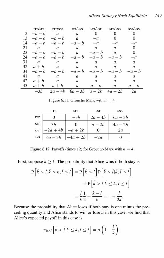
Mixed-Strategy Nash Equilibria 149
rrr/srr rrr/ssr rrr/sss srr/ssr srr/sss ssr/sss12 �a � b a a 0 0 013 �a � b �a � b a �a 0 014 �a � b �a � b �a � b �a �a �a21 a a a a a 023 �a � b �a � b a �a � b a 024 �a � b �a � b �a � b �a � b �a � b �a31 a a a a a a32 a C b a a a a a34 �a � b �a � b �a � b �a � b �a � b �a � b41 a a a a a a42 a C b a a a a a43 a C b a C b a a C b a a C b
�3b 2a � 4b 6a � 3b a � 2b 4a � 2b 2a
Figure 6.11. Groucho Marx with n D 4
rrr srr ssr sss
rrr
srr
ssr
sss
0 �3b 2a � 4b 6a � 3b
3b 0 a � 2b 4a � 2b
�2a C 4b �a C 2b 0 2a
6a � 3b �4a C 2b �2a 0
Figure 6.12. Payoffs (times 12) for Groucho Marx with n D 4
First, suppose k l. The probability that Alice wins if both stay is
Ph Qk > Ql j Qk � k; Ql � l
iD P
h Qk � li
Ph Qk > Ql j Qk; Ql � l
i
CPh Qk > lj Qk � k; Ql � l
i
D l
k
1
2C k � l
kD 1 � l
2k:
Because the probability that Alice loses if both stay is one minus the pre-
ceding quantity and Alice stands to win or lose a in this case, we find that
Alice’s expected payoff in this case is
�k�l
hQk > Ql j Qk � k; Ql � l
iD a
�1 � l
k
�:
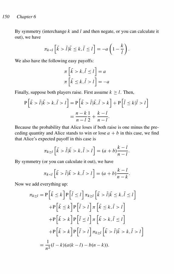
150 Chapter 6
By symmetry (interchange k and l and then negate, or you can calculate it
out), we have
�k<l
h Qk > Ql j Qk � k; Ql � li
D �a
�1 � k
l
�:
We also have the following easy payoffs:
�h Qk > k; Ql � l
iD a
�h Qk � k; Ql > l
iD �a
Finally, suppose both players raise. First assume k l. Then,
Ph Qk > Ql j Qk > k; Ql > l
iD P
h Qk > Ql j Qk; Ql > ki
C PhQl � kj Ql > l
i
D n � k
n � l
1
2C k � l
n � l:
Because the probability that Alice loses if both raise is one minus the pre-
ceding quantity and Alice stands to win or lose a C b in this case, we find
that Alice’s expected payoff in this case is
�k�l
h Qk > Ql j Qk > k; Ql > li
D .a C b/k � l
n � l:
By symmetry (or you can calculate it out), we have
�k<l
hQk > Ql j Qk > k; Ql > l
iD .a C b/
k � l
n � k:
Now we add everything up:
�k�l D Ph Qk � k
iPh Ql � l
i�k�l
h Qk > Ql j Qk � k; Ql � li
CPh Qk � k
iPh Ql > l
i�h Qk � k; Ql > l
i
CPh Qk > k
iPh Ql � l
i�h Qk > k; Ql � l
i
CPh Qk > k
iPh Ql > l
i�k�l
h Qk > Ql j Qk > k; Ql > li
D 1
n2.l � k/.a.k � l/ � b.n � k//:

Mixed-Strategy Nash Equilibria 151
By symmetry (or calculation if you do not trust your answer. I did it by
calculation and checked it by symmetry), we have
�k<l D 1
n2.k � l/.a.k � l/ C b.n � l//:
The reader is invited to write the matrix for the normal form game for
n D 5, and show that when a D 1 and b D 2, there is exactly one Nash
equilibrium, given by 0:125s1 C 0:375s3 C 0:5s4. Moreover, for n D 6,
when a D 1 and b D 2, there is exactly one Nash equilibrium, given by
0:083s1 C 0:667s4 C 0:25s5. For n D 7, when a D 1 and b D 2, there is
exactly one Nash equilibrium, given by 0:063s1 C 0:937s5.
6.39 Games of Perfect Information
Let � D f�1; : : : ; �ng be the payoffs in a Nash equilibrium of a finite
extensive form game G with perfect information (�5.6). Show that there is
a pure-strategy, subgame perfect, Nash equilibrium with payoffs � . Hint:
Use mathematical induction on the number of nonterminal nodes in the
game.
A Nash equilibrium s is strict if there is a neighborhood of s (considered
as a point in n-space) that contains no other Nash equilibrium of the game.
Strict Nash equilibria of finite games are extremely well behaved dynami-
cally, as we shall see in later chapters. They are especially well behaved if
they are unique. A strict Nash equilibrium is always a pure-strategy equilib-
rium. Give an example of a pure-strategy equilibrium in a game of perfect
information that is not strict.
6.40 Correlated Equilibria
l r
u
d
5,1 0,0
1,54,4
Consider the up-down/left-right game played by Al-
ice and Bob, with normal form matrix shown in the
diagram. There are two Pareto-efficient (�5.3) pure-
strategy equilibria: (1,5) and (5,1). There is also a
mixed-strategy equilibrium with payoffs (2.5,2.5), in
which Alice plays u with probability 0.5, and Bob plays l with probability
0.5.
If the players can jointly observe an event with probability 1/2, they can
achieve the payoff (3,3) by playing .u,l/ when the event occurs, and .d ,r/
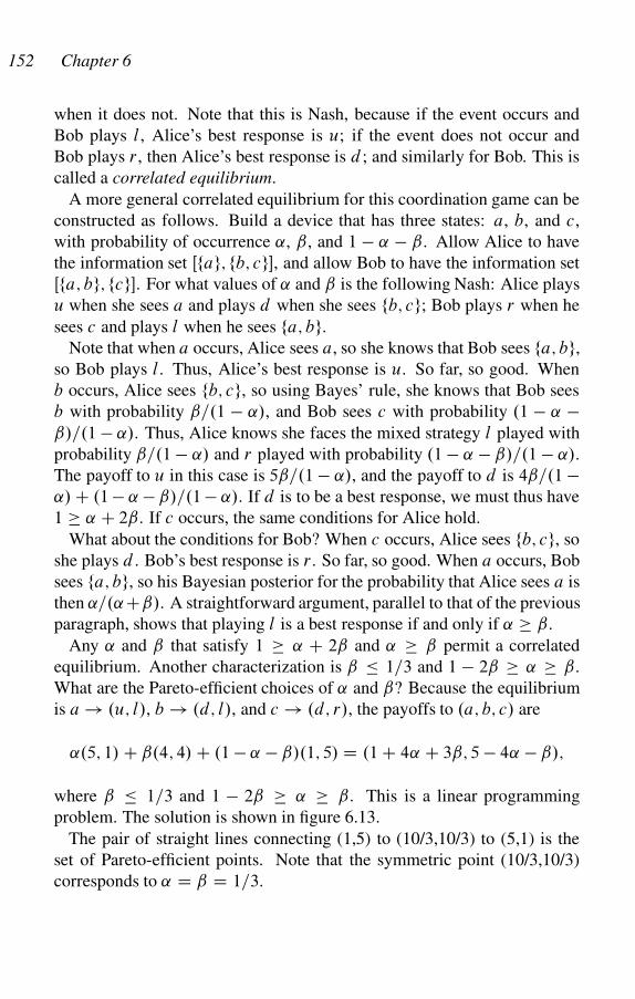
152 Chapter 6
when it does not. Note that this is Nash, because if the event occurs and
Bob plays l, Alice’s best response is u; if the event does not occur and
Bob plays r , then Alice’s best response is d ; and similarly for Bob. This is
called a correlated equilibrium.
A more general correlated equilibrium for this coordination game can be
constructed as follows. Build a device that has three states: a, b, and c,
with probability of occurrence ˛, ˇ, and 1 � ˛ � ˇ. Allow Alice to have
the information set Œfag; fb; cg�, and allow Bob to have the information set
Œfa; bg; fcg�. For what values of ˛ and ˇ is the following Nash: Alice plays
u when she sees a and plays d when she sees fb; cg; Bob plays r when he
sees c and plays l when he sees fa; bg.
Note that when a occurs, Alice sees a, so she knows that Bob sees fa; bg,
so Bob plays l. Thus, Alice’s best response is u. So far, so good. When
b occurs, Alice sees fb; cg, so using Bayes’ rule, she knows that Bob sees
b with probability ˇ=.1 � ˛/, and Bob sees c with probability .1 � ˛ �ˇ/=.1 � ˛/. Thus, Alice knows she faces the mixed strategy l played with
probability ˇ=.1 � ˛/ and r played with probability .1 � ˛ � ˇ/=.1 � ˛/.
The payoff to u in this case is 5ˇ=.1 � ˛/, and the payoff to d is 4ˇ=.1 �˛/ C .1 � ˛ � ˇ/=.1 � ˛/. If d is to be a best response, we must thus have
1 ˛ C 2ˇ. If c occurs, the same conditions for Alice hold.
What about the conditions for Bob? When c occurs, Alice sees fb; cg, so
she plays d . Bob’s best response is r . So far, so good. When a occurs, Bob
sees fa; bg, so his Bayesian posterior for the probability that Alice sees a is
then ˛=.˛Cˇ/. A straightforward argument, parallel to that of the previous
paragraph, shows that playing l is a best response if and only if ˛ ˇ.
Any ˛ and ˇ that satisfy 1 ˛ C 2ˇ and ˛ ˇ permit a correlated
equilibrium. Another characterization is ˇ � 1=3 and 1 � 2ˇ ˛ ˇ.
What are the Pareto-efficient choices of ˛ and ˇ? Because the equilibrium
is a ! .u; l/, b ! .d; l/, and c ! .d; r/, the payoffs to .a; b; c/ are
˛.5; 1/ C ˇ.4; 4/ C .1 � ˛ � ˇ/.1; 5/ D .1 C 4˛ C 3ˇ; 5 � 4˛ � ˇ/;
where ˇ � 1=3 and 1 � 2ˇ ˛ ˇ. This is a linear programming
problem. The solution is shown in figure 6.13.
The pair of straight lines connecting (1,5) to (10/3,10/3) to (5,1) is the
set of Pareto-efficient points. Note that the symmetric point (10/3,10/3)
corresponds to ˛ D ˇ D 1=3.
Mixed-Strategy Nash Equilibria 153
Bob
Alice
5
4
3
2
1
543210
(5,1)
�103
; 103
�
(1,5)
�
�
�
Figure 6.13. Alice and Bob correlate their behavior.
6.41 Territoriality as a Correlated Equilibrium
The hawk-dove game (�3.10) is an inefficient way to allocate property
rights, especially if the cost of injury w is not much larger than the value v
of the property. To see this, note that players choose hawk with probability
v=w, and you can check that the ratio of the payoff to the efficient payoff
v=2 is
1 � v
w:
When w is near v, this is close to zero.
Suppose some members of the population decide to play a new strategy
based on the fact that whenever two players have a property dispute, one
of them must have gotten there first, and the other must have come later.
We may call the former the “incumbent” and the latter the “contester.” The
new strategy, B , called the “bourgeois” strategy, always plays hawk when
incumbent and dove when contester. When we add B to the normal form
matrix of the game, we get the hawk, dove, bourgeois game depicted in fig-
ure 6.14. Note that the payoff to bourgeois against bourgeois, v=2 is greater
than 3v=4�w=4, which is the payoff to hawk against bourgeois, and is also
greater than v=4, which is the payoff to dove against bourgeois. Therefore,
bourgeois is a strict Nash equilibrium. It is also efficient, because there is
never a hawk-hawk confrontation in the bourgeois equilibrium, so there is
never any injury.
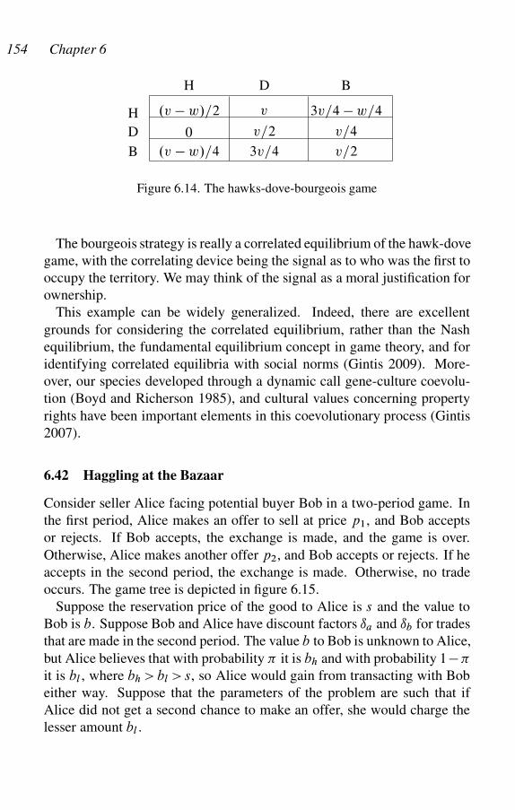
154 Chapter 6
H D
H
D
.v � w/=2 v
0 v=2
B
3v=4 � w=4
v=4
B .v � w/=4 3v=4 v=2
Figure 6.14. The hawks-dove-bourgeois game
The bourgeois strategy is really a correlated equilibrium of the hawk-dove
game, with the correlating device being the signal as to who was the first to
occupy the territory. We may think of the signal as a moral justification for
ownership.
This example can be widely generalized. Indeed, there are excellent
grounds for considering the correlated equilibrium, rather than the Nash
equilibrium, the fundamental equilibrium concept in game theory, and for
identifying correlated equilibria with social norms (Gintis 2009). More-
over, our species developed through a dynamic call gene-culture coevolu-
tion (Boyd and Richerson 1985), and cultural values concerning property
rights have been important elements in this coevolutionary process (Gintis
2007).
6.42 Haggling at the Bazaar
Consider seller Alice facing potential buyer Bob in a two-period game. In
the first period, Alice makes an offer to sell at price p1, and Bob accepts
or rejects. If Bob accepts, the exchange is made, and the game is over.
Otherwise, Alice makes another offer p2, and Bob accepts or rejects. If he
accepts in the second period, the exchange is made. Otherwise, no trade
occurs. The game tree is depicted in figure 6.15.
Suppose the reservation price of the good to Alice is s and the value to
Bob is b. Suppose Bob and Alice have discount factors ıa and ıb for trades
that are made in the second period. The value b to Bob is unknown to Alice,
but Alice believes that with probability � it is bh and with probability 1��
it is bl , where bh > bl > s, so Alice would gain from transacting with Bob
either way. Suppose that the parameters of the problem are such that if
Alice did not get a second chance to make an offer, she would charge the
lesser amount bl .
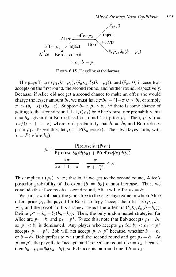
Mixed-Strategy Nash Equilibria 155
offer p1
accept
reject
p1; b � p1
offer p2
accept
reject
ısp2; ıb.b � p2/
ıss; 0
�Alice �Bob
� �Alice
Bob
Figure 6.15. Haggling at the bazaar
The payoffs are .p1; b�p1/, .ıap2; ıb.b�p2//, and .ıas; 0/ in case Bob
accepts on the first round, the second round, and neither round, respectively.
Because, if Alice did not get a second chance to make an offer, she would
charge the lesser amount bl , we must have �bh C .1��/s � bl , or simply
� � .bl �s/=.bh �s/. Suppose bh p1 > bl , so there is some chance of
getting to the second round. Let �.p1/ be Alice’s posterior probability that
b D bh, given that Bob refused on round 1 at price p1. Then, �.p1/ Dx�=.x� C 1 � �/ where x is probability that b D bh and Bob refuses
price p1. To see this, let � D P.bhjrefuse/. Then by Bayes’ rule, with
x D P.refusejbh/,
� D P.refusejbh/P.bh/
P.refusejbh/P.bh/ C P.refusejbl /P.bl/
D x�
x� C 1 � �D �
� C 1��x
� �:
This implies �.p1/ � �; that is, if we get to the second round, Alice’s
posterior probability of the event fb D bhg cannot increase. Thus, we
conclude that if we reach a second round, Alice will offer p2 D bl :
We can now roll back the game tree to the one-stage game in which Alice
offers price p1, the payoff for Bob’s strategy “accept the offer” is (p1; b�p1/, and the payoff to his strategy “reject the offer” is (ıabl ; ıb.b �bl //.
Define p� D bh �ıb.bh �bl /. Then, the only undominated strategies for
Alice are p1 D bl and p1 D p�. To see this, note that Bob accepts p1 D bl ,
so p1 < bl is dominated. Any player who accepts p1 for bl < p1 < p�
accepts p1 D p�. Bob will not accept p1 > p� because, whether b D bh
or b D bl , Bob prefers to wait until the second round and get p2 D bl . At
p1 D p�, the payoffs to “accept” and “reject” are equal if b D bh, because
then bh�p1 Dıb.bh�bl/, so Bob accepts on round one if b D bh.
156 Chapter 6
It follows that Alice chooses p1 D bl if bl is greater than �p� C .1��/ıabl , chooses p1 D p� if the opposite inequality holds, and otherwise is
indifferent between the two choices. The first case reduces to the inequality
bh >
�1 � ıa
�� .ıb � ıa/
�bl
1 � ıb
: (6.10)
We conclude that there is a unique Nash equilibrium.
Now, suppose the parameters of the problem are such that if Alice did
not get a second chance to make an offer, she would charge the greater
amount bh. Then, there is no Nash equilibrium in pure strategies. To see
this, suppose Alice chooses p2 D bl . Because Alice’s posterior probability
for fb D blg cannot be less than � (for the same reason as in the preceding
problem) and because she would charge bh in the one-shot game, she must
charge p2 D bh. So, suppose Alice chooses p2 D bh. Then, the only
undominated strategies on the first round are p1 Dıbbh and p1 Dbl . But if
Bob rejects p1 D ıbbh, we must have b D bl , so it is not subgame perfect
to charge p2 D bh: The reader is invited to find the mixed-strategy Nash
equilibrium of this game.
6.43 Poker with Bluffing Revisited
If you have access to computer software to solve for Nash equilibria of
normal form games, you can easily do the following. Doing the problem
by hand is not feasible.
a. � Show that there are two Nash equilibria to Poker with Bluffing (�4.16).
Ollie uses the same strategy in both, bluffing on the first round with
40% probability (that is, he raises with H or L on the first round, and
drops with M). Stan has two mixed-strategy best responses to Ollie,
one of which uses two pure strategies and the other uses three. The
latter involves bluffing with 40% probability. The expected payoff to
the game for Ollie is $1.20. (It’s the same for both equilibria, because
it’s a zero-sum game; see section 6.34).
b. � Now suppose Stan sees Ollie’s first move before raising or staying.
Show that there are twenty one Nash equilibria, but that Stan uses only
two different mixed strategies, and both involve raising with high and
raising with medium or low with 25% probability on the first round, and
calling with high or medium and calling with 25% probability on the
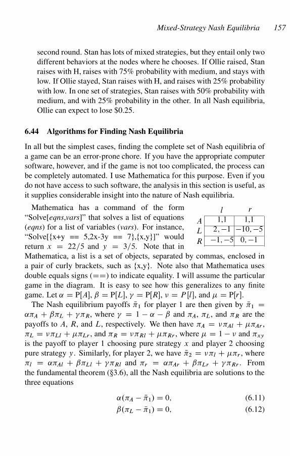
Mixed-Strategy Nash Equilibria 157
second round. Stan has lots of mixed strategies, but they entail only two
different behaviors at the nodes where he chooses. If Ollie raised, Stan
raises with H, raises with 75% probability with medium, and stays with
low. If Ollie stayed, Stan raises with H, and raises with 25% probability
with low. In one set of strategies, Stan raises with 50% probability with
medium, and with 25% probability in the other. In all Nash equilibria,
Ollie can expect to lose $0.25.
6.44 Algorithms for Finding Nash Equilibria
In all but the simplest cases, finding the complete set of Nash equilibria of
a game can be an error-prone chore. If you have the appropriate computer
software, however, and if the game is not too complicated, the process can
be completely automated. I use Mathematica for this purpose. Even if you
do not have access to such software, the analysis in this section is useful, as
it supplies considerable insight into the nature of Nash equilibria.
0; �1
�10; �5
1,11,1
2; �1
�1; �5
l r
A
L
R
Mathematica has a command of the form
“Solve[eqns,vars]” that solves a list of equations
(eqns) for a list of variables (vars). For instance,
“Solve[fx+y == 5,2x-3y == 7g,fx,yg]” would
return x D 22=5 and y D 3=5. Note that in
Mathematica, a list is a set of objects, separated by commas, enclosed in
a pair of curly brackets, such as fx,yg. Note also that Mathematica uses
double equals signs (DD) to indicate equality. I will assume the particular
game in the diagram. It is easy to see how this generalizes to any finite
game. Let ˛ D PŒA�, ˇ D PŒL�, � D PŒR�, � D P Œl�, and � D PŒr�.
The Nash equilibrium payoffs N�1 for player 1 are then given by N�1 D˛�A C ˇ�L C ��R, where � D 1 � ˛ � ˇ and �A, �L, and �R are the
payoffs to A, R, and L, respectively. We then have �A D ��Al C ��Ar ,
�L D ��Ll C ��Lr , and �R D ��Rl C ��Rr , where � D 1 � � and �xy
is the payoff to player 1 choosing pure strategy x and player 2 choosing
pure strategy y. Similarly, for player 2, we have N�2 D ��l C ��r , where
�l D ˛�Al C ˇ�Ll C ��Rl and �r D ˛�Ar C ˇ�Lr C ��Rr . From
the fundamental theorem (�3.6), all the Nash equilibria are solutions to the
three equations
˛.�A � N�1/ D 0; (6.11)
ˇ.�L � N�1/ D 0; (6.12)
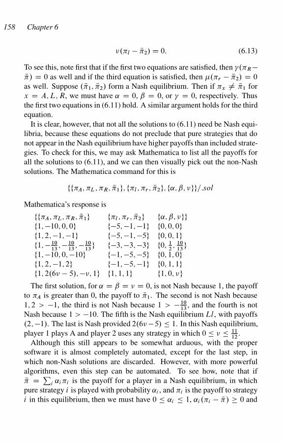
158 Chapter 6
�.�l � N�2/ D 0: (6.13)
To see this, note first that if the first two equations are satisfied, then �.�R �N�/ D 0 as well and if the third equation is satisfied, then �.�r � N�2/ D 0
as well. Suppose . N�1; N�2/ form a Nash equilibrium. Then if �x ¤ N�1 for
x D A; L; R, we must have ˛ D 0, ˇ D 0, or � D 0, respectively. Thus
the first two equations in (6.11) hold. A similar argument holds for the third
equation.
It is clear, however, that not all the solutions to (6.11) need be Nash equi-
libria, because these equations do not preclude that pure strategies that do
not appear in the Nash equilibrium have higher payoffs than included strate-
gies. To check for this, we may ask Mathematica to list all the payoffs for
all the solutions to (6.11), and we can then visually pick out the non-Nash
solutions. The Mathematica command for this is
ff�A; �L; �R; N�1g; f�l ; �r ; N�2g; f˛; ˇ; �gg=:sol
Mathematica’s response is
ff�A; �L; �R; N�1g f�l ; �r ; N�2g f˛; ˇ; �ggf1; �10; 0; 0g f�5; �1; �1g f0; 0; 0gf1; 2; �1; �1g f�5; �1; �5g f0; 0; 1gf1; �10
13; �10
13; �10
13g f�3; �3; �3g f0; 1
2; 10
13g
f1; �10; 0; �10g f�1; �5; �5g f0; 1; 0gf1; 2; �1; 2g f�1; �5; �1g f0; 1; 1gf1; 2.6� � 5/; ��; 1g f1; 1; 1g f1; 0; �g
The first solution, for ˛ D ˇ D � D 0, is not Nash because 1, the payoff
to �A is greater than 0, the payoff to N�1. The second is not Nash because
1; 2 > �1, the third is not Nash because 1 > �1013
, and the fourth is not
Nash because 1 > �10. The fifth is the Nash equilibrium Ll, with payoffs
.2; �1/. The last is Nash provided 2.6� �5/ � 1. In this Nash equilibrium,
player 1 plays A and player 2 uses any strategy in which 0 � � � 1112
.
Although this still appears to be somewhat arduous, with the proper
software it is almost completely automated, except for the last step, in
which non-Nash solutions are discarded. However, with more powerful
algorithms, even this step can be automated. To see how, note that if
N� D Pi ˛i�i is the payoff for a player in a Nash equilibrium, in which
pure strategy i is played with probability ˛i , and �i is the payoff to strategy
i in this equilibrium, then we must have 0 � ˛i � 1, ˛i .�i � N�/ 0 and
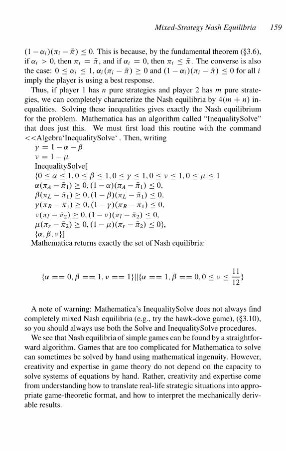
Mixed-Strategy Nash Equilibria 159
.1 � ˛i /.�i � N�/ � 0. This is because, by the fundamental theorem (�3.6),
if ˛i > 0, then �i D N� , and if ˛i D 0, then �i � N� . The converse is also
the case: 0 � ˛i � 1, ˛i .�i � N�/ 0 and .1 � ˛i /.�i � N�/ � 0 for all i
imply the player is using a best response.
Thus, if player 1 has n pure strategies and player 2 has m pure strate-
gies, we can completely characterize the Nash equilibria by 4.m C n/ in-
equalities. Solving these inequalities gives exactly the Nash equilibrium
for the problem. Mathematica has an algorithm called “InequalitySolve”
that does just this. We must first load this routine with the command
<<Algebra‘InequalitySolve‘ . Then, writing� D 1 � ˛ � ˇ
� D 1 � �
InequalitySolve[
f0 � ˛ � 1; 0 � ˇ � 1; 0 � � � 1; 0 � � � 1; 0 � � � 1
˛.�A � N�1/ 0; .1 � ˛/.�A � N�1/ � 0;
ˇ.�L � N�1/ 0; .1 � ˇ/.�L � N�1/ � 0;
�.�R � N�1/ 0; .1 � �/.�R � N�1/ � 0;
�.�l � N�2/ 0; .1 � �/.�l � N�2/ � 0,
�.�r � N�2/ 0; .1 � �/.�r � N�2/ � 0g,
f˛; ˇ; �g]Mathematica returns exactly the set of Nash equilibria:
f˛ DD 0; ˇ DD 1; � DD 1gjjf˛ DD 1; ˇ DD 0; 0 � � � 11
12g
A note of warning: Mathematica’s InequalitySolve does not always find
completely mixed Nash equilibria (e.g., try the hawk-dove game), (�3.10),
so you should always use both the Solve and InequalitySolve procedures.
We see that Nash equilibria of simple games can be found by a straightfor-
ward algorithm. Games that are too complicated for Mathematica to solve
can sometimes be solved by hand using mathematical ingenuity. However,
creativity and expertise in game theory do not depend on the capacity to
solve systems of equations by hand. Rather, creativity and expertise come
from understanding how to translate real-life strategic situations into appro-
priate game-theoretic format, and how to interpret the mechanically deriv-
able results.
160 Chapter 6
6.45 Why Play Mixed Strategies?
In twin sisters (�6.19), we found that there are no pure-strategy Nash equi-
libria, but there are many mixed-strategy Nash equilibria. In the Nash equi-
librium with the highest payoff, each sister asks for $50 with probability
50/51 and $51 with probability 1/51. However, if both pure strategies have
equal payoffs against the mixed strategy of the other player, why should
either sister bother randomizing? Indeed, if one sister conjectures that the
other will play her Nash strategy, all mixed strategies have equal payoff,
so why prefer the (50/51,1/51) strategy over any other? Moreover, if each
sister believes the other is thinking the same way, it is irrational for each to
conjecture that the other will choose the (50/51,1/51) strategy or any other
particular strategy. Therefore, the whole mixed-strategy Nash equilibrium
collapses.
Of course, this problem is not limited to twin sisters; it applies to any
strictly mixed Nash equilibrium. By the fundamental theorem (�3.6), any
mixed-strategy best response consists of equal-payoff pure strategies, so
why should a player bother randomizing? The answer is that there is no
reason at all. Therefore, no player should expect any other player to ran-
domize or to do anything else in particular.
You may think that this is some sort of trick argument, or a verbal para-
dox that can be left to the philosophers to sort out. It is not. The argument
completely destroys the classical game-theoretic analysis of mixed-strategy
Nash equilibria. In The Bounds of Reason (2009), I present some ingenious
arguments defending the mixed-strategy equilibrium by Nobel Prize win-
ners John Harsanyi (1973) and Robert Aumann (1987), but their construc-
tions do not work for games that model complex social interaction, such as
principal-agent models or repeated games.
Of course, evolutionary game theory has a solution to the problem, pro-
vided it is socially meaningful to consider the game itself as the stage game
in an evolutionary dynamic in which agents repeatedly meet to play the
game and higher-payoff strategies expand as a fraction of the population at
the expense of lower-payoff agents. In this setting, each agent plays a pure
strategy, but in an evolutionary equilibrium the fraction of each strategy
represented in the population equals its weight in the Nash equilibrium. In-
deed, this is exactly what we saw when we developed an agent-based model
of twin sisters (�6.20).
Mixed-Strategy Nash Equilibria 161
6.46 Reviewing of Basic Concepts
a. Define a mixed strategy, and write the expression for the payoff to using
a mixed strategy as a function of the payoffs to the underlying pure
strategies.
b. Write the condition for a set of mixed strategies to form a Nash equi-
librium.
c. We say a Nash equilibrium is strict if the strategy used by each player
in this equilibrium is the only best response to the strategies used by
the other player. Define a strictly mixed strategy, and show that if any
player in a Nash equilibrium uses a strictly mixed strategy, then the
equilibrium is not strict.
7
Principal-Agent Models
Things are gettin’ betterIt’s people that are gettin’ worse
Mose Allison
In the principal-agent model, the payoff to the principal depends on an
action taken by the agent. The principal cannot contract for the action, but
can compensate the agent based on some observable signal that is corre-
lated with the action. The principal is first mover, and chooses an incen-
tive scheme for paying the agent that depends on the observed signal. The
agent then determines the optimal action to take, given the incentives, then
decides whether to accept the principal’s offer, based on the expected pay-
ment and the subjective cost of performing the action. Upon accepting, the
agent chooses an action that maximizes his payoff, and the principal ob-
serves the signal correlated with the action, pays the agent according to the
incentive scheme, and receives a payoff dependent upon the signal. The
incentive scheme is a precommitment by the principal, even though the
agent’s action is not.
7.1 Gift Exchange
In a famous paper, “Labor Contracts as Partial Gift Exchange,” George Ak-
erlof (1982) suggested that sometimes employers pay employees more than
they must to attract the labor they need, and employees often reciprocate
by working harder or more carefully than they otherwise would. He called
this gift exchange. This section analyzes a simple model of gift exchange in
labor markets. A firm hires N identical employees, each of whom supplies
effort level e.w � z/, where e./ is increasing and concave, w is the wage,
and z is a benchmark wage such that w > z indicates that the employer is
being generous, and conversely w < z indicates that the boss is ungener-
ous. The firm’s revenue is an increasing and concave function f .eN/ of
total amount of effort supplied by the N employees, so the firm’s net profit
is given by
�.w; N/ D f .e.w � z/N/ � wN:
162
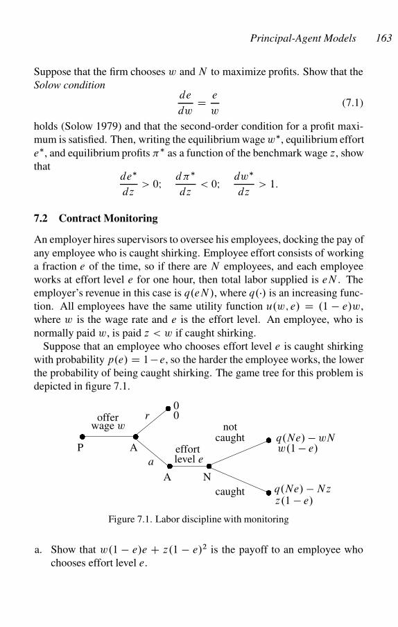
Principal-Agent Models 163
Suppose that the firm chooses w and N to maximize profits. Show that the
Solow conditionde
dwD e
w(7.1)
holds (Solow 1979) and that the second-order condition for a profit maxi-
mum is satisfied. Then, writing the equilibrium wage w�, equilibrium effort
e�, and equilibrium profits �� as a function of the benchmark wage z, show
thatde�
dz> 0I d��
dz< 0I dw�
dz> 1:
7.2 Contract Monitoring
An employer hires supervisors to oversee his employees, docking the pay of
any employee who is caught shirking. Employee effort consists of working
a fraction e of the time, so if there are N employees, and each employee
works at effort level e for one hour, then total labor supplied is eN . The
employer’s revenue in this case is q.eN/, where q./ is an increasing func-
tion. All employees have the same utility function u.w; e/ D .1 � e/w,
where w is the wage rate and e is the effort level. An employee, who is
normally paid w, is paid z < w if caught shirking.
Suppose that an employee who chooses effort level e is caught shirking
with probability p.e/ D 1 � e, so the harder the employee works, the lower
the probability of being caught shirking. The game tree for this problem is
depicted in figure 7.1.
� �
�
�
�
P A
offer r
a
caught
� �
A N
effort
00
q.Ne/ � wNw.1 � e/
q.Ne/ � Nzz.1 � e/
notwage w
level e
caught
Figure 7.1. Labor discipline with monitoring
a. Show that w.1 � e/e C z.1 � e/2 is the payoff to an employee who
chooses effort level e.
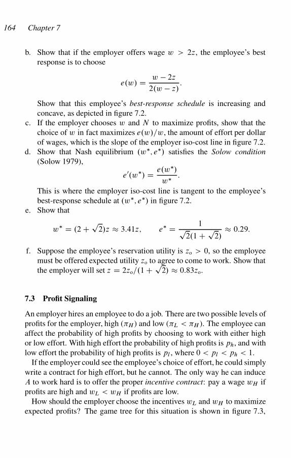
164 Chapter 7
b. Show that if the employer offers wage w > 2z, the employee’s best
response is to choose
e.w/ D w � 2z
2.w � z/:
Show that this employee’s best-response schedule is increasing and
concave, as depicted in figure 7.2.
c. If the employer chooses w and N to maximize profits, show that the
choice of w in fact maximizes e.w/=w, the amount of effort per dollar
of wages, which is the slope of the employer iso-cost line in figure 7.2.
d. Show that Nash equilibrium .w�; e�/ satisfies the Solow condition
(Solow 1979),
e0.w�/ D e.w�/
w�:
This is where the employer iso-cost line is tangent to the employee’s
best-response schedule at .w�; e�/ in figure 7.2.
e. Show that
w� D .2 Cp
2/z � 3:41z; e� D 1p2.1 C p
2/� 0:29:
f. Suppose the employee’s reservation utility is zo > 0, so the employee
must be offered expected utility zo to agree to come to work. Show that
the employer will set z D 2zo=.1 C p2/ � 0:83zo.
7.3 Profit Signaling
An employer hires an employee to do a job. There are two possible levels of
profits for the employer, high (�H ) and low (�L < �H ). The employee can
affect the probability of high profits by choosing to work with either high
or low effort. With high effort the probability of high profits is ph, and with
low effort the probability of high profits is pl , where 0 < pl < ph < 1.
If the employer could see the employee’s choice of effort, he could simply
write a contract for high effort, but he cannot. The only way he can induce
A to work hard is to offer the proper incentive contract: pay a wage wH if
profits are high and wL < wH if profits are low.
How should the employer choose the incentives wL and wH to maximize
expected profits? The game tree for this situation is shown in figure 7.3,
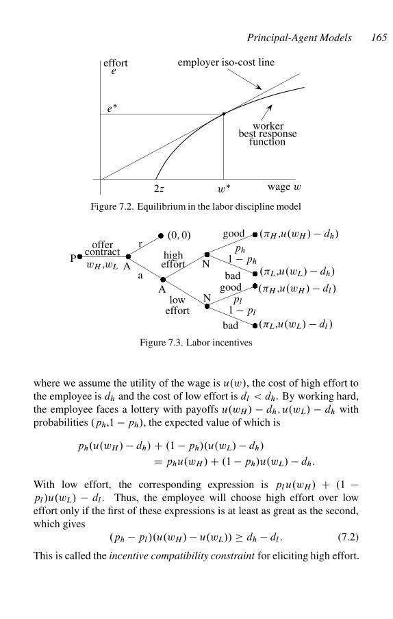
Principal-Agent Models 165
wage ww�2z
e�
efforte
employer iso-cost line
workerbest response
function
�
Figure 7.2. Equilibrium in the labor discipline model
� �
�
�
�
�
�
�
PA
A
N
N
offercontractwH ,wL
r
a
higheffort
loweffort
badgood
bad
ph
1 � ph
pl
1 � pl
.0; 0/ .�H ,u.wH / � dh/
.�L,u.wL/ � dh/
.�H ,u.wH / � dl /
.�L,u.wL/ � dl /
good
Figure 7.3. Labor incentives
where we assume the utility of the wage is u.w/, the cost of high effort to
the employee is dh and the cost of low effort is dl < dh. By working hard,
the employee faces a lottery with payoffs u.wH/ � dh; u.wL/ � dh with
probabilities .ph,1 � ph/, the expected value of which is
ph.u.wH/ � dh/ C .1 � ph/.u.wL/ � dh/
D phu.wH / C .1 � ph/u.wL/ � dh:
With low effort, the corresponding expression is pl u.wH/ C .1 �pl/u.wL/ � dl . Thus, the employee will choose high effort over low
effort only if the first of these expressions is at least as great as the second,
which gives
.ph � pl/.u.wH/ � u.wL// dh � dl : (7.2)
This is called the incentive compatibility constraint for eliciting high effort.
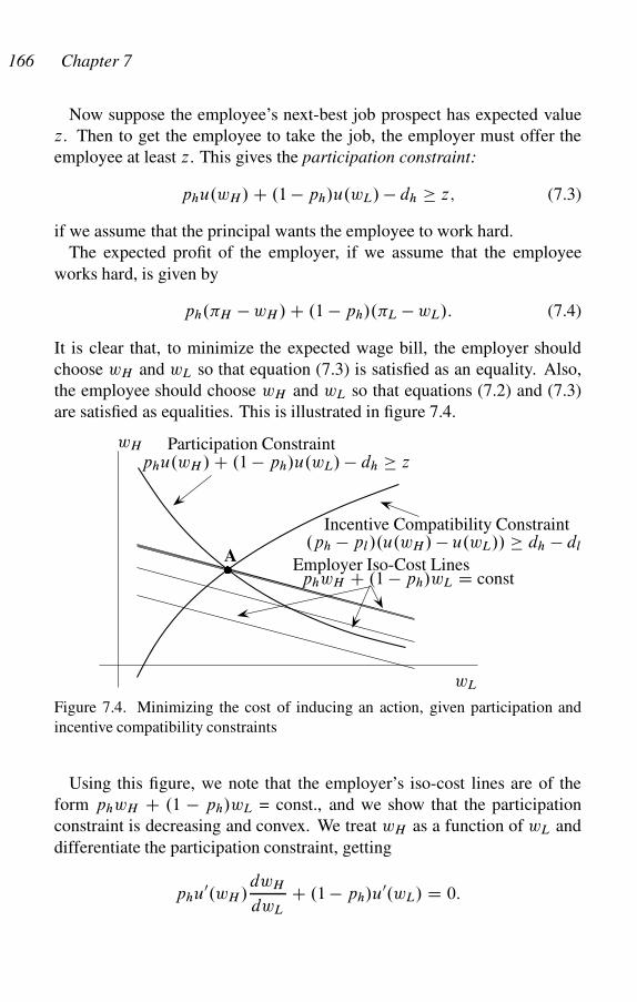
166 Chapter 7
Now suppose the employee’s next-best job prospect has expected value
z. Then to get the employee to take the job, the employer must offer the
employee at least z. This gives the participation constraint:
phu.wH/ C .1 � ph/u.wL/ � dh z; (7.3)
if we assume that the principal wants the employee to work hard.
The expected profit of the employer, if we assume that the employee
works hard, is given by
ph.�H � wH / C .1 � ph/.�L � wL/: (7.4)
It is clear that, to minimize the expected wage bill, the employer should
choose wH and wL so that equation (7.3) is satisfied as an equality. Also,
the employee should choose wH and wL so that equations (7.2) and (7.3)
are satisfied as equalities. This is illustrated in figure 7.4.
wL
wH
.ph � pl/.u.wH/ � u.wL// dh � dl
phu.wH / C .1 � ph/u.wL/ � dh z
Incentive Compatibility Constraint
Participation Constraint
� Employer Iso-Cost LinesphwH C .1 � ph/wL D const
A
Figure 7.4. Minimizing the cost of inducing an action, given participation and
incentive compatibility constraints
Using this figure, we note that the employer’s iso-cost lines are of the
form phwH C .1 � ph/wL = const., and we show that the participation
constraint is decreasing and convex. We treat wH as a function of wL and
differentiate the participation constraint, getting
phu0.wH /dwH
dwL
C .1 � ph/u0.wL/ D 0:
Principal-Agent Models 167
Thus,dwH
dwL
D �1 � ph
ph
u0.wL/
u0.wH /< �1 � ph
ph
< 0: (7.5)
The second inequality (which we use later) holds because wL < wH , so if
the agent is strictly risk averse, u0 is decreasing. The participation constraint
is thus decreasing. Now take the derivative of equation (7.5), getting
d2wH
dw2L
D �1 � ph
ph
�u00.wH /
u0.wH /� u0.wL/u00.wH /
u0.wH /2
dwH
dwL
�> 0:
Thus, the participation constraint is convex.
The incentive compatibility constraint is increasing and cuts the wL-axis
for some wL > 0. If the agent is weakly decreasingly risk averse (that is, if
u000 > 0/, then the incentive compatibility constraint is concave. To see this,
we differentiate the incentive compatibility constraint u.wH/ D u.wL/ +
constant, getting
u0.wH/dwH
dwL
D u0.wL/;
so dwH =dwL > 1 > 0, and the incentive compatibility constraint is in-
creasing. Differentiate again, getting
u00.wH/dwH
dwL
C u0.wH /d2wH
dw2L
D u00.wL/:
Thus
u0.wH/d2wH
dw2L
D u00.wL/ � u00.wH /dwH
dwL
< u00.wL/ � u00.wH / < 0;
and the constraint is concave.
If the agent is strictly risk averse (�2.4), the slope of the iso-cost lines is
less than the slope of the participation constraint at its intersection A with
the incentive compatibility constraint. To see this, note that the slope of the
iso-cost line is jdwH =dwLj D .1 � ph/=ph, which is less than the slope of
the participation constraint, which is
j.1 � ph/u0.wL/=phu0.wH /j;by equation (7.5).
It follows that the solution is at A in figure 7.4.
168 Chapter 7
7.4 Properties of the Employment Relationship
The unique Nash equilibrium in the labor discipline model of the previous
section is the solution to the two equations phu.wH/ C .1 � ph/u.wL/ �dh D z and .ph �pl /.u.wH/�u.wL// D dh �dl . Solving simultaneously,
we get
u.wL/ D z C phdl � pldh
ph � pl
; u.wH / D u.wL/ C dh � dl
ph � pl
: (7.6)
Note that the employee exactly achieves his reservation position. As we
might expect, if z rises, so do the two wage rates wL and wH . If dh rises,
you can check that wH rises and wL falls. Similar results hold when ph and
pl vary.
Now that we know the cost to the principal of inducing the agent to take
each of the two actions, we can determine which action the principal should
ask the agent to choose. If H and L are the expected profits in the good
and bad states, respectively, then the return �.a/ for inducing the agent to
take action a D h; l is given by
�.h/ D HphCL.1�ph/�Ehw; �.l/ D Hpl CL.1�pl/�Elw; (7.7)
where Ehw and Elw are the expected wage payments if the agent takes
actions h and l, respectively; that is, Ehw D phwH C .1 � ph/wL and
Elw D plwH C .1 � pl/wL.
Is it worth inducing the employee to choose high effort? For low effort,
only the participation constraint u.wl/ D dl C z must hold, where wl is
the wage paid independent of whether profits are H or L; with expected
profit plH C .1 � pl/L � wl . Choose the incentive wage if and only if
ph.H � wH / C .1 � ph/.L � wL/ plH C .1 � pl/L � wl . This can be
written
.ph � pl/.H � L/ phwH C .1 � ph/wL � wl : (7.8)
We will see that, in general, if the employee is risk neutral and it is worth
exerting high effort, then the optimum is to make the principal the fixed
claimant and the agent the residual claimant (�7.7). To see this for the
current example, we can let u.w/ D w. The participation constraint is then
phu.wH / C .1 � ph/u.wL/ D phwH C .1 � ph/wL D z C dh, and the
employer’s profit is then A D phH C.1�ph/L�.zCdh/. Suppose we give

Principal-Agent Models 169
A to the employer as a fixed payment and let wH D H � A, wL D L � A.
Then the participation constraint holds, because
phwH C .1 � ph/wL D phH C .1 � ph/L � A D z C dh:
Because high effort is superior to low effort for the employer, 7.8) must
hold, giving
.ph � pl/.H � L/ phwH C .1 � ph/wL � .z C dl /
D z C dh � .z C dl / D dh � dl :
But then,
wH � wL D H � L dh � dl
ph � pl
;
which says that the incentive compatibility constraint is satisfied.
Figure 7.5 is a graphical representation of the principal’s problem. Note
that in this case there are many profit-maximizing contracts. Indeed, any
point on the heavy solid line in the figure maximizes profits.
wL
wH
.ph � pl /.wH � wL/ � dh � dl
phwH C .1 � ph/wL � dh � z
�
dhCz
1�ph
dhCzph
dh�dl
ph�pl
contractsProfit-maximizing
Incentive Compatibility Constraint
Participation Constraint
Figure 7.5. The principal’s problem when the agent is risk neutral
7.5 Peasant and Landlord
A landlord hires a peasant to tend a cornfield. The landlord’s profit is H if
the crop is good and L < H if the crop is poor. The peasant can work at
either high effort h or low effort l, and the probability ph of a good crop

170 Chapter 7
when he exerts high effort is greater than the probability pl of a good crop
when he expends low effort, with 0 < pl < ph < 1. The landowner cannot
observe the peasant’s effort.
Suppose the peasant’s utility function when the wage is w is given by
u.w/ � dh with high effort, and u.w/ � dl with low effort. We assume
dh > dl , so unless given some inducement, the peasant will not work hard
and u0 > 0; u00 < 0, so the peasant has diminishing marginal utility of the
wage. The peasant’s fallback utility is z.
To induce the peasant to work hard, the landlord chooses a pair of wages
wH and wL, and pays the peasant wH if profit is H , and wL if profit is L.
This is called an incentive wage.
What should the landlord pay the peasant if he wants to minimize the
expected wage Ew D phwH C .1�ph/wL, subject to eliciting high effort?
First, wH and wL must satisfy a participation constraint; wH and wL must
be sufficiently large that the peasant is willing to work at all. Suppose the
peasant’s next-best alternative gives utility z. Then the landowner must
choose wH and wL so that the peasant’s expected utility is at least z:
phu.wH / C .1 � ph/u.wL/ � dh z: (PC)
Second, wH and wL must satisfy an incentive compatibility constraint: the
payoff (that is, the expected return) to the peasant for working hard must be
at least as great as the payoff to not working hard. Thus, we must have
phu.wH/ C .1 � ph/u.wL/ � dh plu.wH / C .1 � pl/u.wL/ � dl :
We can rewrite this second condition as
Œu.wH/ � u.wL/�.ph � pl/ dh � dl : (ICC)
We now prove that both the PC and the ICC must hold as equalities.
The problem is to minimize phwH C .1 � ph/wL subject to PC and ICC.
This is the same as maximizing �phwH � .1 � ph/wL subject to the same
constraints, so we form the Lagrangian
L.wH ; wL; �; �/ D �phwH � .1 � ph/wL
C �Œphu.wH/ C .1 � ph/u.wL/ � dh � z�
C �Œ.u.wH / � u.wL//.ph � pl/ � .dh � dl /�:
Principal-Agent Models 171
The first-order conditions can be written:
LH D 0;LL D 0; �; � 0Iif � > 0; then the PC holds with equalityI
if � > 0; then the ICC holds with equality:
But we have
LH D �ph C �phu0.wH / C �u0.wH/.ph � pl/ D 0;
LL D �1 C ph C �.1 � ph/u0.wL/ � �u0.wL/.ph � pl / D 0:
Suppose � D 0. Then, by adding the two first-order conditions, we get
�.u0.wH/ � u0.wL//.ph � pl/ D 1;
which implies u0.wH / > u0.wL/, so wH < wL (by declining marginal
utility of income). This, of course, is not incentive compatible, because
ICC implies u.wH/ > u.wL/, so wH > wL. It follows that our assumption
that � D 0 is contradictory and hence � > 0, from which it follows that the
participation constraint holds as an equality.
Now suppose � D 0. Then the first-order conditions LH D 0 andLL D 0
imply u0.wH / D 1=� and u0.wL/ D 1=�: Because u0.wH/ D u0.wL/ D1=�, wH D wL (because u0 is strictly decreasing). This also is impossible
by the ICC. Hence � > 0, and the ICC holds as an equality.
The optimal incentive wage for the landlord is then given by
u.wL/ D dh � ph.dh � dl/=.ph � pl/ C z
u.wH / D dh C .1 � ph/.dh � dl/=.ph � pl / C z:
To see this, suppose the landlord has concave utility function v, with v0 > 0
and v00 < 0. The peasant is risk neutral, so we can assume her utility
function is u.w; d/ D w � d , where w is income and d is effort. The
assumption that high effort produces a surplus means that the following
social optimality (SO) condition holds:
phH C .1 � ph/L � dh > plH C .1 � pl/L � dl ;
or
.ph � pl/.H � L/ > dh � dl : (SO)
172 Chapter 7
The landlord wants to maximize
phv.H � wH / C .1 � ph/v.L � wL/
subject to the participation constraint
phwH C .1 � ph/wL � dh z (PC)
and the incentive compatibility constraint, which as before reduces to
.ph � pl/.wh � wL/ dh � dl : (ICC)
We form the Lagrangian
L D phv.H � wH / C .1 � ph/v.L � wL/
C �.phwH C .1 � ph/wL � dh � z/
C �..ph � pl/.wh � wL/ � .dh � dl//;
so the first-order conditions are @L=@wH D @L=@wL D 0, �; � 0, � > 0
or the PC holds as an equality and � > 0 or the ICC holds as an equality.
The conditions @L=@wH D @L=@wL D 0 can be written as
@L
@wH
D �phv0.H � wH / C �ph C �.ph � pl/ D 0 (FOC1)
�.ph � pl/ D 0: (FOC2)
We first show that the PC holds as an equality by showing that � D 0 is
impossible. Suppose � = 0. Then (FOC) gives
�phv0.H � wH / C �.ph � pl/ D 0
�.1 � ph/v0.L � wL/ � �.ph � pl/ D 0:
If � > 0, this says that v0.L � wL/ < 0, which is impossible. If � D 0;
this says that v0.L � wL/ D 0, which is also impossible. Thus, � D 0 is
impossible and the PC holds as an equality.
Finally, if the peasant is risk neutral but the landlord is risk averse then
if high effort produces a surplus over low effort, the landlord’s profit-
maximizing solution involves getting a fixed rent from the peasant, who
Principal-Agent Models 173
becomes the residual claimant, bearing all the risk and taking all the profits
and losses. First, we can rewrite FOC1 and FOC2 as
v0.H � wH / � � D �.ph � pl/=ph (7.9)
v0.L � wL/ � � D ��.ph � pl/=.1 � ph/: (7.10)
If � > 0, then v0.H � wH / > v0.L � wL/, so H � wH < L � wL, or
H �L < wH �wL: But � > 0 implies that the ICC holds as an equality, so
.ph �pl/.wH �wL/ D dh �dl and dh �dl < .ph �pl/.H �L/ from SO,
implying H � L > wH � wL: This is a contradiction, and hence � D 0;
that is, there is no optimum in which the ICC holds as an equality.
What, then, is an optimum? If � D 0, equations (7.9) and (7.10) imply
that H � wh D L � wL, because v0 is strictly increasing (because the land-
lord is risk averse). This means the landlord gets a fixed rent, as asserted.
7.6 Bob’s Car Insurance
Bob wants to buy theft insurance for his car, which is worth $1,200. If Bob
is careful, the probability of theft is 5% and if he is careless, the probability
of theft is 7.5%. Bob is risk averse (�2.4) with utility function u.x/ Dln.x C 1/, where x is in dollars and the disutility of being careful is � > 0,
measured in utils. Suppose the car lasts one period and is either stolen or
not stolen at the beginning of the period.
We first find the value of � below which Bob will be careful. If he is
careful, the value is 0:95 ln.1201/ � �, and if he is careless the value is
0:925 ln.1201/. Being careful is worthwhile as long as 0:95 ln.1201/ � � 0:925 ln.1201/, or � � ln.1201/=40 D 0:177:
Suppose the insurance industry is competitive, so an insurer must offer
Bob a “fair” policy, the expected payout of which equals the premium x.
We can show that if Bob buys a policy with full coverage (that is, payout
in case of theft equals $1,200), his premium is x D $90. To see this, note
that Bob’s his utility is ln.1201 � x/ if he is careless, and ln.1201 � x/ � �
if he is careful, because he is fully compensated in case of theft. Thus, he
will not be careful. The probability of theft is then 7.5%, and because the
insurance company must give a fair lottery to Bob, x D .0:075/1200 D 90.
We can now show that Bob should buy insurance, whether or not he is
careful without insurance. To see this, note that the expected value of the car
plus insurance is ln.1201�90/ �D 7:013. This is greater that the payoff to
174 Chapter 7
being careless without insurance, which has value 0:925 ln.1201/ � 6:559.
If Bob is careful without insurance, his payoff is 0:95ln.1201/ � �, which
is also less that the payoff with insurance.
This analysis assumes that Bob is fully insured. Suppose the company
offered a fair policy at price xwith deductible z, so that if the car is stolen,
Bob receives 1200�x�z. Show that, whether or not Bob is careful without
insurance, the optimal value of z is zero; that is, Bob should fully insure.
However, with no deductible, Bob will not be careful, and the insurance
company will either assume the higher theft rate or require a positive de-
ductible. Moreover, it is possible that even if Bob would be careful without
insurance, there is no deductible with insurance that would lead Bob to be
careful.
7.7 A Generic Principal-Agent Model
Principal-agent games are variations of the following scenario. The agent
has a set A D fa1; : : : ; ang of available actions. The principal receives one
of a set S D fs1; : : : ; smg of signals that depend on the action chosen by the
agent. Let pij D PŒsj jai � be the conditional probability of signal sj when
the agent takes action ai . Note that we must have
mX
j D1
pij D 1 for i D 1; : : : ; n:
The agent has utility function u.w; a/, where w is money, a 2 A is the
action the agent performs, and the agent’s reservation utility is uo, which is
the minimum expected utility that would induce the agent to work for the
principal. The principal has payoff �.a/ � w for a 2 A.1
To maximize his payoff, the principal must determine the payoff associ-
ated with getting the agent to perform each action ai 2 A, and then choose
the largest of the n payoffs. Thus, for each i D 1; : : : ; n the principal
must find incentives wij ; j D 1; : : : ; m such that the principal agrees to
pay the agent wij if he observes the signal sj , and the incentive scheme
wi D fwi1; : : : ; wimg induces the agent to choose ai . The principal must
1We assume �.a/ has a stochastic component, so the principal cannot infer a
from �.a/.

Principal-Agent Models 175
then choose the index i that maximizes his return
�.ai/ � Eiwi D �.ai/ �mX
j D1
pij wij ;
where Ei is expectation with respect to the probabilities that obtain when
the agent chooses ai :
Suppose the principal wants to induce the agent to choose action ak .
There are two constraints to the problem.
Participation Constraint. The expected utility to the agent must be enough
to induce the agent to participate: Eku.wk; ak/ uo, or
mX
j D1
pkj u.wkj ; ak/ uo:
Incentive Compatibility Constraint. The chosen action ak must maximize
the payoff to the agent, among all actions ai 2 A, so Eku.wk; ak/ Eiu.wk; ai / for i D 1; : : : ; n, or
mX
j D1
pkj u.wkj ; ak/ mX
j D1
pij u.wkj ; ai/ for i D 1; : : : ; n:
Having determined the minimum expected cost Ekwk of inducing the
agent to choose action ak , the principal chooses the index k to maximize
�.ak/ � Ekwk:
Prove the following.
THEOREM 7.1 Fundamental Theorem of the Principal-Agent Model. So-
lutions to the principal-agent problem have the following characteristics:
1. The agent is indifferent between participating and taking the reserva-
tion utility uo.
2. If the agent is strictly risk averse and the principal’s optimal action ak
is not the agent’s most preferred action, then
a. At least one of the incentive compatibility constraints holds as an
equality.
b. The principal’s payoff is strictly lower than it would be if he could
write an enforceable contract for the delivery of action ak .
176 Chapter 7
3. If the agent is risk neutral and if the return �.a/ is transferable (that
is, it can be assigned to the agent), the contract that maximizes the
principal’s payoff is that which gives the principal a fixed payment and
makes the agent the residual claimant on �.a/.
The last finding says that individual agents (e.g., farmers, workers, man-
agers) should always be residual claimants on their projects, as long as
they are risk neutral and the return �.a/ to their actions is transferable. In
practice, however, such agents are normally not residual claimants on their
projects; managers may have salaries plus stock options, and farmers may
have sharecropping contracts, but these contractual forms do not render the
principals fixed claimants. The reason is that agents are risk averse, so that
they would not want to be residual claimants and they are credit constrained,
so they cannot credibly promise to make good on the project’s losses in bad
times. Moreover, �.a/ is often not transferable (e.g., in a large work team,
it is difficult to isolate the contribution of a single employee).
To prove this theorem, we argue as follows. Suppose the principal wants
to induce the agent to choose action ak . If the participation constraint is not
binding, we can reduce all the payments fwkj g by a small amount without
violating either the participation or the incentive compatibility constraints.
Moreover, if all of the incentive compatibility constraints are nonbinding,
then the payoff system fwkj g is excessively risky, in the sense that the var-
ious fwkj g can be “compressed” around their expected value without vio-
lating the incentive compatibility constraint.
Formally, we form the Lagrangian
L D �.ak/ � Ekwk C �ŒEku.wk/ � d.ak/ � uo�
CnX
iD1i¤k
�ifŒEku.wk/ � d.ak/� � ŒEiu.wk/ � d.ai/�g;
where Ei means take the expectation with respect to probabilities
fpi1; : : : ; pimg, � is the Lagrangian multiplier for the participation con-
straint, and �i is the Lagrangian multiplier for the ith incentive compatibil-
ity constraint. Writing the expectations out in full (in “real life” you would
not do this, but it’s valuable for pedagogical purposes), we get
L D �.ak/ �mX
j D1
pkj wkj C �
2
4mX
j D1
pkj u.wkj ; ak/ � uo
3
5

Principal-Agent Models 177
CnX
iD1
�i
2
4mX
j D1
pkj u.wkj ; ak/ �mX
j D1
pij u.wkj ; ai/
3
5 :
The first-order conditions for the problem assert that at a maximum,
@L=@wkj D 0 for j D 1; : : : ; m, and �; �1; : : : ; �n 0. Moreover, if
� > 0, then the participation constraint is binding (that is, holds as an
equality), and if �i > 0 for some i D 1; : : : ; n, then the incentive compati-
bility constraint holds for action ai : In our case, we have
@L
wkj
D �pkj C �pkj u0.wkj ; ak/
CnX
iD1
�i .pkj � pij /u0.wkj ; ak/ D 0 j D 1; : : : ; m:
Collecting terms, we have, for j D 1; : : : ; m;
�pkj CnX
iD1
�i .pkj � pij / D pkj
u0.wkj ; ak/: (7.11)
Now we sum this equation from j D 1 to m, noting thatP
j pij D 1 for
all i , getting
� DmX
j D1
pkj
u0.wkj ; ak/> 0;
which proves that the participation constraint is binding.
To see that at least one incentive compatibility constraint is binding, sup-
pose all the �i are zero. Then equation (7.11) gives � D 1=u0.wkj ; ak/
for all j . If the agent is risk averse, this implies all the wkj are equal
(because risk aversion implies strictly concave preference, which implies
strictly monotonic marginal utility), which means ak must be the agent’s
most preferred action.
To show that the principal’s payoff would be higher if he could write
an enforceable contract, note that with an enforceable contract, only the
participation constraint would be relevant. To induce the agent to perform
ai , the principal would pay w�i , where u.w�
i ; ai / D uo. The principal will
then choose action al such that �.al/ � w�l
is a maximum.
Suppose the optimal action when no contract can be written is ak and
the wage structure is wk.s/. The participation constraint is binding, so
178 Chapter 7
Eku.wk/ D d.ak/ C uo. Because ak is not the agent’s unconstrained pre-
ferred action (by assumption), wk.s/ is not constant, and because the agent
is strictly risk averse, we have
u.w�k ; ak/ D uo D Eu.wk; ak/ < u.Ekwk; ak/;
so w�k
< Ekwk. Because �.al/ � w�l
�.ak/ � w�k
> �.ak/ � Ekwk , we
are done.
To prive the third assertion, suppose again that al is the principal’s op-
timal choice when an enforceable contract can be written. Then al max-
imizes �.ai/ � w�i where u.w�
i ; ai / D uo. If the agent is risk neutral,
suppose the agent receives �.a/ and pays the principal the fixed amount
�.al/ � w�l
. We can assume u.w; a/ D w C d.a/ (why?). The agent then
maximizes
�.ai/ � d.ai / D u.�.ai// � u.w�i / � uo
D �.ai/ � w�i � uo;
which of course occurs when i D l. This proves the theorem.
8
Signaling Games
This above all: to thine own self be true, And it must follow,as the night the day, Thou canst not then be false to any man.
Shakespeare
8.1 Signaling as a Coevolutionary Process
A Thompson’s gazelle who spots a cheetah, instead of fleeing, will often
“stott,” which involves an 18-inch vertical jump, with legs stiff and white
rump patch fully displayed to the predator. The only plausible explanation
for this behavior (Alcock 1993) is that the gazelle is signaling the cheetah
that it would be a waste of both their times and energies for the cheetah to
chase the gazelle, because the gazelle is obviously very fit. Of course, if
the cheetah could not understand this signal, it would be a waste of time
and energy for the gazelle to emit it. Also, if the signal could be easily
falsified, and the ability to stott had nothing to do with the probability of
being caught, cheetahs would never have evolved to heed the signal in the
first place.1
A signal is a special sort of physical interaction between two agents. Like
other physical interactions, a signal changes the physical constitution of
the agents involved. But unlike interactions among nonliving objects, or
between a nonliving object and a living agent, a signal is the product of a
strategic dynamic between sender and receiver, each of whom is pursuing
distinct but interrelated objectives. Moreover, a signal is a specific type of
strategic physical interaction, one in which the content of the interaction is
determined by the sender, and it changes the receiver’s behavior by altering
the way the receiver evaluates alternative actions.
1For a review of evidence for costly signaling in birds and fish in the form of
colorful displays that indicate health and vigor, see Olson and Owens 1998. On the
more general topic of costly signaling, see Zahavi and Zahavi 1997 and section 8.4.
179
180 Chapter 8
The most important fact about a signal is that it is generally the result of a
coevolutionary process between senders and receivers in which both benefit
from its use. For if a signal is costly to emit (and if its use has been stable
over time), then the signal is most likely both beneficial to the sender and
worthy of belief for the receiver; a sender is better off sending that signal
rather than none, or some other, and a receiver is better off acting on it the
way receivers traditionally have, rather than ignoring it or acting otherwise.
The reason is obvious: if the receiver were not better off acting this way,
a mutant who ignored (or acted otherwise on) the signal would be more fit
than the current population of receivers, and would therefore increase its
frequency in the population. Ultimately, so many receivers would ignore
(or act otherwise on) the signal that, being costly to the sender, it would not
be worth sending unless, of course, the “otherwise” were also beneficial to
the sender.
Signaling systems are not always in equilibrium, and potentially benefi-
cial mutations need not occur. Moreover, human beings are especially adept
both at dissimulating (emitting “false” signals) and detecting such dissimu-
lation (Cosmides and Tooby 1992). However, human beings are disposed to
taking the signals around them at face value unless there are good reasons
for doing otherwise (Gilbert 1991). The treatment of signals as emerging
from a coevolutionary process and persisting as a Nash equilibrium of the
appropriate game, is the starting point for a theory of signaling.
8.2 A Generic Signaling Game
In signaling games, player 1 has a “type” that is revealed to player 2 via a
special “signal,” to which player 2 responds by choosing an “action,” the
payoffs to the two players being a function of player 1’s type and signal
and player 2’s action. Thus, the stage game that played so prominent a role
in the general Bayesian game framework collapses, in the case of signaling
games, to a pair of payoff functions.
Specifically, there are three players Sender, Receiver, and Nature. Na-
ture begins by choosing from a set T of possible types or states of affairs,
choosing t 2 T with probability �.t/. Sender observes t but Receiver does
not. Sender then transmits a signal s 2 S to Receiver, who uses this signal
to choose an action a 2 A. The payoffs to the two players are u.t; s; a/
and v.t; s; a/, respectively. A pure strategy for Sender is thus a function
f WT ! S , where s D f .t/ is the signal sent when Nature reveals type t ,
Signaling Games 181
and a pure strategy for Receiver is a function g W S ! A, where a D g.s/
is the action taken when Receiver receives signal s. A mixed strategy for
Sender is a probability distribution PS.sI t/ over S for each t 2 T , and a
mixed strategy for Receiver is a probability distribution pR.aI s/ over A for
each signal s received. A Nash equilibrium for the game is thus a pair of
probability distributions .PS.I t/; pR.; s// for each pair f.t; s/jt 2T; s 2Sgsuch that each agent uses a best response to the other, given the probability
distribution �.t/ used by Nature to choose the type of Sender.
We say a signal s 2S is along the path of play, given the strategy profile
.PS.I t/; pR.I s//, if there is a strictly positive probability that Sender will
transmit s, that is, ifX
t2T
�.t/PS.sI t/ > 0:
If a signal is not along the path of play, we say it is off the path of play.
If s is along the path of play, then a best response for Receiver maximizes
Receiver’s expected return, with a probability distribution over T given by
PŒt js� D PS.sI t/�.t/Pt 02T PS.sI t 0/�.t 0/
:
We thus require of PS and pR that
a. For every state t 2 T , and all signals s0 2 S such that PS.s0I t/ > 0, s0
maximizes X
a2A
u.t; s0; a/pR.aI s/
over all s 2 S ; that is, Sender chooses a best response to Receiver’s
pattern of reacting to S’s signals;b. For every signal s 2S along the path of play, and all actions a0 2A such
that pR.a0I s/ > 0, a0 maximizesX
t2T
v.t; s; a/PŒt js�
over all a 2 A; that is, Receiver chooses a best response to Sender’s
signal.c. If a signal s 2S is not along the path of play, we may choose PŒt js� ar-
bitrarily such that (b) still holds. In other words, Receiver may respond
arbitrarily to a signal that is never sent, provided this does not induce
Sender to send the signal.
182 Chapter 8
8.3 Sex and Piety: The Darwin-Fisher Model
In most species, females invest considerably more in raising their offspring
than do males; for instance, they produce a few large eggs as opposed to
the male’s millions of small sperm. So, female fitness depends more on the
quality of inseminations, whereas male fitness depends more on the quantity
of inseminations (�6.26). Hence, in most species there is an excess demand
for copulations on the part of males, for whom procreation is very cheap,
and therefore there is a nonclearing market for copulations, with the males
on the long side of the market (�9.13). In some species this imbalance
leads to violent fights among males (dissipating the rent associated with
achieving a copulation), with the winners securing the scarce copulations.
But in many species, female choice plays a central role, and males succeed
by being attractive rather than ferocious.
What criteria might females use to choose mates? We would expect fe-
males to seek mates whose appearance indicates they have genes that will
enhance the survival value of their offspring. This is indeed broadly correct.
But in many cases, with prominent examples among insects, fish, birds, and
mammals, females appear to have arbitrary prejudices for dramatic, orna-
mental, and colorful displays even when such accoutrements clearly reduce
male survival chances; for instance, the plumage of the bird of paradise, the
elaborate structures and displays of the male bowerbird, and the stunning
coloration of the male guppy. Darwin speculated that such characteristics
improve the mating chances of males at the expense of the average fitness of
the species. The great biologist R. A. Fisher (1915) offered the first genetic
analysis of the process, suggesting that an arbitrary female preference for a
trait would enhance the fitness of males with that trait, and hence the fitness
of females who pass that trait to their male offspring, so the genetic predis-
position for males to exhibit such a trait could become common in a species.
Other analytical models of sexual selection, called Fisher’s runaway pro-
cess include Lande (1981), Kirkpatrick (1982), Pomiankowski (1987), and
Bulmer (1989). We will follow Pomiankowski (1987), who showed that as
long as females incur no cost for being choosy, the Darwin-Fisher sexual
selection process works, but even with a slight cost of being choosy, costly
ornamentation cannot persist in equilibrium.
We shall model runaway selection in a way that is not dependent on the
genetics of the process, so it applies to cultural as well as genetic evolution.
Consider a community in which there are an equal number of males and
Signaling Games 183
females, and there is a cultural trait that we will call pious fasting. Although
both men and women can have this trait, only men act on it, leading to
their death prior to mating with probability u > 0. However, both men and
women pass the trait to their children through family socialization. Suppose
a fraction t of the population have the pious-fasting trait.
Suppose there is another cultural trait, a religious preference for pious
fasting, which we call being “choosy” for short. Again, both men and
women can carry the choosy trait and pass it on to their children, but only
women can act on it, by choosing mates who are pious fasters at rate a > 1
times that of otherwise equally desirable males. However, there may be a
cost of exercising this preference, because with probability k 0 a choosy
woman may fail to mate. Suppose a fraction p of community members
bears the religious preference for pious fasters.
We assume parents transmit their values to their offspring in proportion
to their own values; for instance, if one parent has the pious-fasting trait and
the other does not, then half their children will have the trait. Males who
are pious fasters then exercise their beliefs, after which females choose their
mates, and a new generation of young adults is raised (the older generation
moves to Florida to retire).
Suppose there are n young adult males and an equal number of young
adult females. Let xtp be the fraction of young adults who are “choosy
fasters,” x�p the fraction of “choosy nonfasters,” xt� the fraction of “non-
choosy fasters,” and x�� the fraction of “nonchoosy nonfasters.” Note that
t D xtp C xt� and p D xtp C x�p . If there is no correlation between the
two traits, we would have xtp D tp, xt� D t.1 � p/, and so on. But we
cannot assume this, so we write xtp D tp C d , where d (which biologists
call linkage disequilibrium) can be either positive or negative. It is easy to
check that we then have
xtp D tp C d
xt� D t.1 � p/ � d
x�p D .1 � t/p � d
x�� D .1 � t/.1 � p/ C d:
Although male and female young adults have equal fractions of each trait
because their parents pass on traits equally to both pious fasting and mate
choosing can lead to unequal frequencies in the “breeding pool” of parents
in the next generation. By assumption, a fraction k of choosy females do
184 Chapter 8
not make it to the breeding pool, so if tf is the fraction of pious-faster
females in the breeding pool, then
tf D t � kxtp
1 � kp;
where the denominator is the fraction of females in the breeding pool, and
the numerator is the fraction of pious-faster females in the breeding pool.
Similarly, if pf is the fraction of choosy females in the breeding pool, then
pf D p.1 � k/
1 � kp;
where the numerator is the fraction of choosy females in the breeding pool.
We now do the corresponding calculations for males. Let tm be the frac-
tion of pious-faster males, and pm the fraction of choosy males in the breed-
ing pool, after the losses associated with pious fasting are taken into ac-
count. We have
tm D t.1 � u/
1 � ut;
where the denominator is the fraction of males, and the numerator is the
fraction of pious-faster males in the breeding pool. Similarly,
pm D p � uxtp
1 � ut;
where the numerator is the fraction of choosy males in the breeding pool.
By assumption, all nf D n.1 � kp/ females in the breeding pool are
equally fit. We normalize this fitness to 1. The fitnesses of pious and non-
pious males in the breeding pool are, however, unequal. Suppose each
female in the breeding pool mates once. There are then nf .1 � pf /
nonchoosy females, so they mate with nf .1 � pf /.1 � tm/ nonpious
males and nf .1 � pf /tm pious males. There are also nf pf choosy fe-
males, who mate with nf pf .1 � tm/=.1 � tm C atm/ nonpious males and
nf pf atm=.1�tmCatm/ pious males (the numerators account for the a W 1
preference for pious males, and the denominator is chosen so that the two
terms add to nf pf ). If we write
r� D .1 � pf / C pf
1 � tm C atm
rt D .1 � pf / C apf
1 � tm C atm;
Signaling Games 185
then the total number of matings of nonpious males is nf .1 � tm/r�, and
the total number of matings of pious males is nf tmrt . The probability
that a mated male is pious is therefore tmrt . Because the probability that
a mated female is pious is tf , and both parents contribute equally to the
traits of their offspring, the fraction of pious traits in the next generation is
.tmrt C tf /=2. If we write ˇt D tmrt � t and p D pf � p, then the
change t in the frequency of the pious trait can be written as
t D tmrt C tf
2� t D 1
2
�ˇt C d p
p.1 � p/
�: (8.1)
What about the change in p across generations? The fraction of mated,
choosy females is simply pf , because all females in the breeding pool
mate. The number nm of males in the breeding pool is nm D n.1 � ut/, of
which nx�p are nonpious and choosy, whereas n.1 � u/xtp are pious and
choosy. Each nonpious male has nf r�=nm offspring, and each pious male
has nf rt=nm offspring, so the total number of choosy male offspring per
breeding female is just
pm0 D nx�pr�=nm C n.1 � u/xtprt=nm:
A little algebraic manipulation shows that this can be written more simply
as
pm0 D p C dˇt
t.1 � t/:
Then the change p in the frequency of the choosy trait can be written as
p D pm0 C pf
2� p D 1
2
�p C dˇt
t.1 � t/
�: (8.2)
Let us first investigate (8.1) and (8.2) when choosy females are not less
fit, so k D 0. In this case, pf D p, so p D 0. Therefore, t D p D 0
exactly when ˇt D 0. Solving this equation for t , we get
t D .a � 1/p.1 � u/ � u
u.a.1 � u/ � 1/: (8.3)
This shows that there is a range of values of p for which an equilibrium
frequency of t exists. Checking the Jacobian of the right-hand sides of
(8.1) and (8.2) (see section 11.7 if you do not know what this means) we
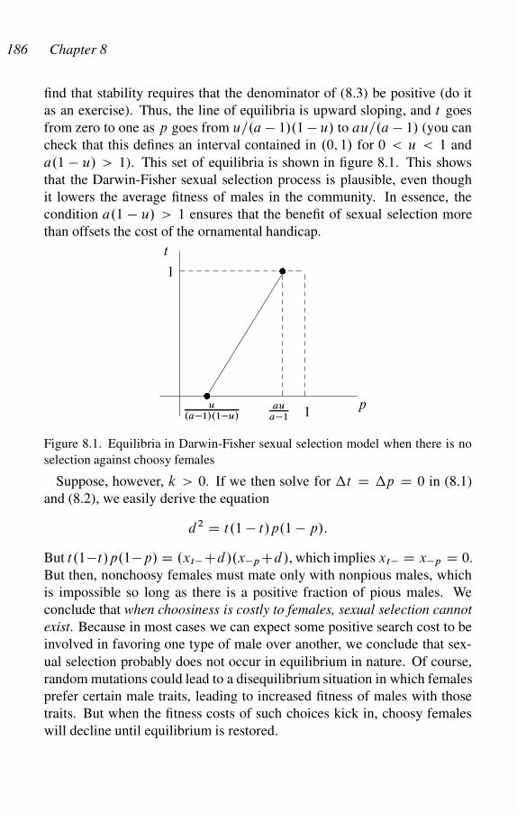
186 Chapter 8
find that stability requires that the denominator of (8.3) be positive (do it
as an exercise). Thus, the line of equilibria is upward sloping, and t goes
from zero to one as p goes from u=.a � 1/.1 � u/ to au=.a � 1/ (you can
check that this defines an interval contained in .0; 1/ for 0 < u < 1 and
a.1 � u/ > 1). This set of equilibria is shown in figure 8.1. This shows
that the Darwin-Fisher sexual selection process is plausible, even though
it lowers the average fitness of males in the community. In essence, the
condition a.1 � u/ > 1 ensures that the benefit of sexual selection more
than offsets the cost of the ornamental handicap.
p
t
1
1
�
�
u.a�1/.1�u/
aua�1
Figure 8.1. Equilibria in Darwin-Fisher sexual selection model when there is no
selection against choosy females
Suppose, however, k > 0. If we then solve for t D p D 0 in (8.1)
and (8.2), we easily derive the equation
d2 D t.1 � t/p.1 � p/:
But t.1�t/p.1�p/ D .xt�Cd/.x�pCd/, which implies xt� D x�p D 0.
But then, nonchoosy females must mate only with nonpious males, which
is impossible so long as there is a positive fraction of pious males. We
conclude that when choosiness is costly to females, sexual selection cannot
exist. Because in most cases we can expect some positive search cost to be
involved in favoring one type of male over another, we conclude that sex-
ual selection probably does not occur in equilibrium in nature. Of course,
random mutations could lead to a disequilibrium situation in which females
prefer certain male traits, leading to increased fitness of males with those
traits. But when the fitness costs of such choices kick in, choosy females
will decline until equilibrium is restored.
Signaling Games 187
8.4 Biological Signals as Handicaps
Zahavi (1975), after close observation of avian behavior, proposed an alter-
native to the Darwin-Fisher sexual selection mechanism, a notion of costly
signaling that he called the handicap principle. According to the handicap
principle, a male who mounts an elaborate display is in fact signaling his
good health and/or good genes, because an unhealthy or genetically unfit
male lacks the resources to mount such a display. The idea was treated with
skepticism for many years, because it proved difficult to model or empir-
ically validate the process. This situation changed when Grafen (1990b)
developed a simple analytical model of the handicap principle. Moreover,
empirical evidence has grown in favor of the costly signaling approach to
sexual selection, leading many to favor it over the Darwin-Fisher sexual
selection model, especially in cases where female mate selection is costly.
Grafen’s model is a special case of the generic signaling model presented
in section 8.2. Suppose a male’s type t 2 Œtmin; 1/ is a measure of male
vigor (e.g., resistance to parasites). Females do best by accurately deter-
mining t , because an overestimate of t might lead a female to mate when
she should not, and an underestimate might lead her to pass up a suitable
mate. If a male of type t signals his type as s D f .t/, and a female uses
this signal to estimate the male’s fitness as a D g.s/, then in an equilibrium
with truthful signaling we will have a D t . We suppose that the male’s
fitness is u.t; s; a/, with ut > 0 (a male with higher t is more fit), us < 0
(it is costly to signal a higher level of fitness), and ua > 0 (a male does bet-
ter if a female thinks he’s more fit). We assume the male’s fitness function
u.t; s; g.s// is such that a more vigorous male will signal a higher fitness;
that is, ds=dt > 0. Given g.s/, a male of type t will then choose s to
maximize U.s/ D u.t; s; g.s//, which has first-order condition
Us.s/ D us.t; s; g.s// C ua.t; s; g.s//dg
dsD 0: (8.4)
If there is indeed truthful signaling, then this equation must hold for t Dg.s/, giving us the differential equation
dg
dsD �us.g.s/; s; g.s//
ua.g.s/; s; g.s//; (8.5)
which, together with g.smin/ D tmin, uniquely determines g.s/. Because
us < 0 and ua > 0, we have dg=ds > 0, as expected.
188 Chapter 8
Differentiating the first-order condition (8.4) totally with respect to t , we
find
Uss
ds
dtC Ust D 0:
Because Uss < 0 by the second-order condition for a maximum, and be-
cause ds=dt > 0, we must have Ust > 0. But we can write
Ust D ust C uat g0.s/
D ust ua.g.s/; s; g.s// � uatus.g.s/; s; g.s//
ua
> 0:
Therefore,
d
dt
�us.t; s; g.s//
ua.t; s; g.s//
�D Ust
ua
> 0: (8.6)
We can now rewrite (8.4) as
ua.t; s; g.s//
�us.t; s; g.s//
ua.t; s; g.s//C g0.s/
�D 0: (8.7)
Because the fraction in this expression is increasing in t , and the expression
is zero when t D g.s/, this shows s D g�1.t/ is a local maximum, so the
male maximizes fitness by truthfully reporting s D g�1.t/, at least locally.
For an example of the handicap principle, suppose u.t; s; a/ D ar ts ,
0 < t < 1, so (8.5) becomes g0=g D �.1=r/ ln g, which has solution
ln g D ce�s=r . If we use g.smin/ D tmin this gives
g.s/ D te�s�smin
r
min
and
f .t/ D smin � r lnln t
ln tmin
:
The reader will note an important element of unrealism in this model:
it assumes that the cost of female signal processing and detection is zero,
and hence signaling is perfectly truthful and reliable. If we allow for costly
female choice, we would expect that signal detection would be imperfect,
and there would be a positive level of dishonest signaling in equilibrium,
Signaling Games 189
and the physical process of signal development should involve an evolu-
tionary dynamic intimately related to receiver neurophysiology (Dawkins
and Guilford 1991; Guilford and Dawkins 1991, 1993). In contrast with
the Darwin-Fisher model of sexual selection, we would not expect a small
amount of costly female choice to undermine a signaling equilibrium, be-
cause there are direct fitness benefits to females in locating vigorous males.
8.5 The Shepherds Who Never Cry Wolf
Because we value truthfulness, one might have the impression that when
both a truthful signaling and a nonsignaling equilibrium exist, the truthful
signaling equilibrium should entail higher payoffs for at least some of the
players. But that need not be the case. Here is a counterexample.
Two shepherds take their flocks each morning to adjoining pastures.
Sometimes a wolf will attack one of the flocks, causing pandemonium
among the threatened sheep. A wolf attack can be clearly heard by both
shepherds, allowing a shepherd to come to the aid of his companion. But
unless the wolf is hungry, the cost of giving aid exceeds the benefits, and
only the shepherd guarding the threatened flock can see if the wolf is hun-
gry.
There are three pure strategies for a threatened shepherd: never signal
(N ), signal if the wolf is hungry (H ), and always signal (A). Similarly,
there are three pure strategies for the shepherd who hears a wolf in the
other pasture: never help (N ), help if signaled (H ), and always help (A).
We make the following assumptions. The payoff to each shepherd to a
day’s work when no wolf appears is 1. The cost of being attacked by a
hungry wolf and a nonhungry wolf is a and b < a, respectively. The cost
of coming to the aid of a threatened shepherd is d , and doing so prevents
the loss to the threatened shepherd, so his payoff is still 1. Finally, it is
common knowledge that the probability that a wolf is hungry is p > 0.
We assume the shepherds’ discount rates are too high, or wolf visits too
infrequent, to support a repeated-game cooperative equilibrium using trig-
ger strategies, so the game is a one-shot. If the shepherds are self-regarding
(that is, they care only about their own payoffs), of course neither will help
the other, so we assume that they are brothers, and the total payoff to shep-
herd 1 (the threatened shepherd) is his payoff �1 plus k�2, where �2 is
the payoff of shepherd 2, and similarly, the total payoff to shepherd 2 (the
190 Chapter 8
potential helper) is �2 C k�1. If ka > d > kb, a shepherd prefers to aid
his threatened brother when wolf is hungry (why?). So we assume this is
the case. We also assume that a � dk > c > b � dk, which means that a
threatened shepherd would want his brother to come to help only if the wolf
is hungry (why?). So there ought to be a signaling equilibrium in this case.
Note, however, that this signaling equilibrium will exist whether p is small
or large, so for very large p, it might be worthwhile for a brother always to
help, thus saving the cost c of signaling to his brother, and saving the cost
kc to himself. This, in fact, is the case. Although this can be proved in
general, you are asked in this problem to prove a special case.
Assume k D 5=12 (note that k D 1=2 for full brothers, but the probability
that two brothers that ostensibly have the same father in fact have the same
father is probably about 80% in human populations). Also assume a D 3=4,
b D 1=4, c D 19=48, and d D 1=4. Finally, assume p D 3=4. After
verifying that these inequalities hold, do the following:
a. Show that there is a signaling equilibrium and find the payoffs to the
shepherds.
b. Show that there is pooling equilibrium in which a threatened shepherd
never signals, and a shepherd always helps his threatened brother. Show
that this equilibrium is Pareto-superior to the signaling equilibrium.
c. There is also a mixed-strategy Nash equilibrium (truthful signaling oc-
curs, but not with certainty) in which the threatened shepherd some-
times signals, and the other shepherd sometimes helps without being
asked. Find this equilibrium and its payoffs, and show that the payoffs
are slightly better than the signaling equilibrium but not as high as the
pooling equilibrium.
8.6 My Brother’s Keeper
Consider the following elaboration on the theme of section 8.5. Suppose
the threatened shepherd, whom we will call Sender, is either healthy, needy,
or desperate, each of which is true with probability 1/3. His brother, whom
we will call Donor, is either healthy or needy, each with probability 1/2.
Suppose there are two signals that the threatened shepherd can give: a low-
cost signal costing 0.1 and a high-cost signal costing 0.2. If he uses either
one, we say he is “asking for help.” We assume that the payoff for each
brother is his own fitness plus 3/4 of his brother’s fitness. Sender’s fitness
Signaling Games 191
is 0.9 if healthy, 0.6 if needy and 0.3 if desperate, minus whatever he pays
for signaling. Donor’s fitness is 0.9 if healthy and 0.7 if needy. However,
the has a resource that ensures his fitness is 1 if he uses it and the fitness of
Sender is 1 (minus the signaling cost) if he transfers it to the Sender. The
resource is perishable, so either he or his brother must use it in the current
period.
a. Show that after eliminating “unreasonable” strategies (define carefully
what you mean by “unreasonable”), there are six pure strategies for
Sender, in each of which a healthy sender never signals: Never Ask
(NN); Signal Low Only If Desperate (NL); Signal High Only If Des-
perate (NH); Signal Low If Desperate or Needy (LL); Signal Low If
Needy, High If Desperate (LH); and Signal High If Needy or Desperate
(HH). Similarly, there are ten strategies for Donor: Never Help (Never);
Help If Healthy and Signal Is High (Healthy, High); Help If Healthy and
Asked (Healthy, Asked); Help If Healthy (Healthy); Help If Signal Is
High (High); Help If Healthy and Asked, or Needy and Signal Is High
(Healthy,Asked/Needy,High); Help If Healthy or Signal Is High; Help
If Asked (Asked); Help If Healthy or Asked (Healthy or Asked); and
Help Unconditionally (Help).b. � If you have a lot of time on your hands, or if you know a computer
programming language, derive the 6 � 10 normal form matrix for the
game.c. � Show that there are seven pure-strategy equilibria. Among these there
is one completely pooling equilibrium: (NN—Help). This, of course,
affords the Sender the maximum possible payoff. However, the pooling
equilibrium maximizes the sum of the payoffs to both players, so it will
be preferred by both if they are equally likely to be Sender and Donor.
This is asocial optimum even among the mixed strategy equilibria, but
that is even harder to determine.d. Show that the truthful signaling strategies (LH—Healty,Asked/Needy,High)
form a Nash equilibrium, but that this equilibrium is strictly Pareto-
inferior to the pooling (nonsignaling) equilibrium.
This model shows that there can be many signaling equilibria, but all may
be inferior to complete altruism (NN—Help). This is doubtless because
the coefficient of relatedness is so high (3/4 is the coefficient of relatedness
between sisters in many bee species, where the queen mates with a single
haploid male).
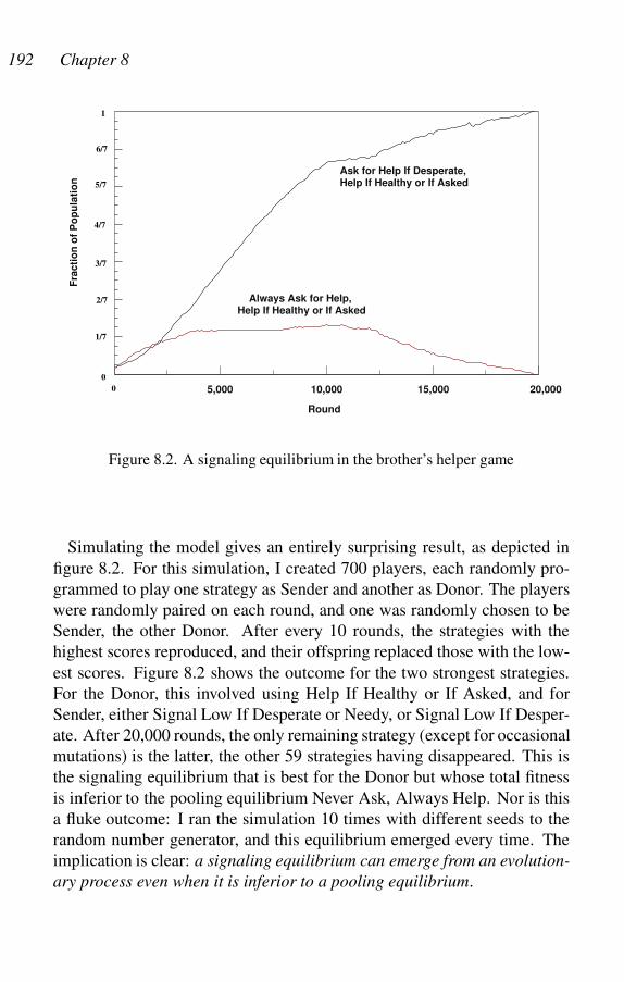
192 Chapter 8
2/7
3/7
1/7
4/7
5/7
6/7
1
Ask for Help If Desperate,Help If Healthy or If Asked
Always Ask for Help,Help If Healthy or If Asked
5,000 10,000 15,000 20,000
0
Fra
cti
on
of
Po
pu
lati
on
0
Round
Figure 8.2. A signaling equilibrium in the brother’s helper game
Simulating the model gives an entirely surprising result, as depicted in
figure 8.2. For this simulation, I created 700 players, each randomly pro-
grammed to play one strategy as Sender and another as Donor. The players
were randomly paired on each round, and one was randomly chosen to be
Sender, the other Donor. After every 10 rounds, the strategies with the
highest scores reproduced, and their offspring replaced those with the low-
est scores. Figure 8.2 shows the outcome for the two strongest strategies.
For the Donor, this involved using Help If Healthy or If Asked, and for
Sender, either Signal Low If Desperate or Needy, or Signal Low If Desper-
ate. After 20,000 rounds, the only remaining strategy (except for occasional
mutations) is the latter, the other 59 strategies having disappeared. This is
the signaling equilibrium that is best for the Donor but whose total fitness
is inferior to the pooling equilibrium Never Ask, Always Help. Nor is this
a fluke outcome: I ran the simulation 10 times with different seeds to the
random number generator, and this equilibrium emerged every time. The
implication is clear: a signaling equilibrium can emerge from an evolution-
ary process even when it is inferior to a pooling equilibrium.
Signaling Games 193
8.7 Honest Signaling among Partial Altruists
In a certain fishing community, each fisher works alone on the open sea,
earning a payoff that we will normalize to 1. A fisher occasionally en-
counters threatening weather. If the fisher does not escape the weather, his
payoff is zero. If a threatened fisher has sufficient energy reserves, he can
escape the bad weather, and his expected payoff is u, where 0 < u < 1: We
call such a fisher secure. However, with a certain probability p (0 < p < 1)
a threatened fisher does not have sufficient energy reserves. We say he is in
distress.
If a threatened fisher sees another fisher on the horizon, he can send a
signal to ask for help, at cost t , with 0 < t < 1. If the fisher is in distress
and a potential helper comes to his aid (we assume the potential helper is
not threatened), the payoff to the distressed fisher is 1, but the cost to the
helper is c > 0. Without the help, however, the distressed fisher succumbs
to the bad weather and has payoff 0.
To complicate matters, a threatened fisher who is helped by another fisher
but who is not distressed has payoff v, where 1 > v > u. Thus, threat-
ened fishers have an incentive to signal that they are in distress even when
they are not. Moreover, fishers can tell when other fishers are threatened,
but only the threatened fisher himself knows his own reserves, and hence
whether he is in distress.
We assume that encounters of this type among fishers are one-shot affairs,
because the probability of meeting the same distressed fisher again is very
small. Clearly, unless there is an element of altruism, no fisher will help a
threatened fisher. So let us suppose that in an encounter between fishers, the
nonthreatened fisher receives a fraction r > 0 of the total payoff, including
signaling costs, received by the threatened fisher (presumably because r is
the degree of genetic or cultural relatedness between fishers). However, the
helper bears the total cost c himself.
For example, if a fisher is in distress, signals for help, and receives help,
the distressed fisher’s payoff is 1 � t , and the helper’s payoff is r.1 � t/ � c.
The nonthreatened fisher (fisher 1) who sees a threatened fisher (fisher
2) has three pure strategies: Never Help, Help If Asked and Always Help.
fisher 2 also has three strategies: Never Ask, Ask When Distressed, Always
Ask. We call the strategy pair fHelp If Asked, Ask If Distressedg the hon-
est signaling strategy pair. If this pair is Nash, we have an honest signaling
equilibrium. This is called a separating equilibrium because agents truth-
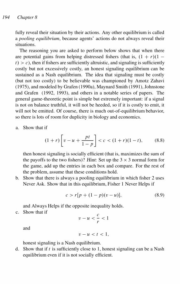
194 Chapter 8
fully reveal their situation by their actions. Any other equilibrium is called
a pooling equilibrium, because agents’ actions do not always reveal their
situations.
The reasoning you are asked to perform below shows that when there
are potential gains from helping distressed fishers (that is, .1 C r/.1 �t/ > c), then if fishers are sufficiently altruistic, and signaling is sufficiently
costly but not excessively costly, an honest signaling equilibrium can be
sustained as a Nash equilibrium. The idea that signaling must be costly
(but not too costly) to be believable was championed by Amotz Zahavi
(1975), and modeled by Grafen (1990a), Maynard Smith (1991), Johnstone
and Grafen (1992, 1993), and others in a notable series of papers. The
general game-theoretic point is simple but extremely important: if a signal
is not on balance truthful, it will not be heeded, so if it is costly to emit, it
will not be emitted. Of course, there is much out-of-equilibrium behavior,
so there is lots of room for duplicity in biology and economics.
a. Show that if
.1 C r/
�v � u C pt
1 � p
�< c < .1 C r/.1 � t/; (8.8)
then honest signaling is socially efficient (that is, maximizes the sum of
the payoffs to the two fishers)? Hint: Set up the 3 � 3 normal form for
the game, add up the entries in each box and compare. For the rest of
the problem, assume that these conditions hold.
b. Show that there is always a pooling equilibrium in which fisher 2 uses
Never Ask. Show that in this equilibrium, Fisher 1 Never Helps if
c > rŒp C .1 � p/.v � u/�; (8.9)
and Always Helps if the opposite inequality holds.
c. Show that if
v � u <c
r< 1
and
v � u < t < 1;
honest signaling is a Nash equilibrium.
d. Show that if t is sufficiently close to 1, honest signaling can be a Nash
equilibrium even if it is not socially efficient.
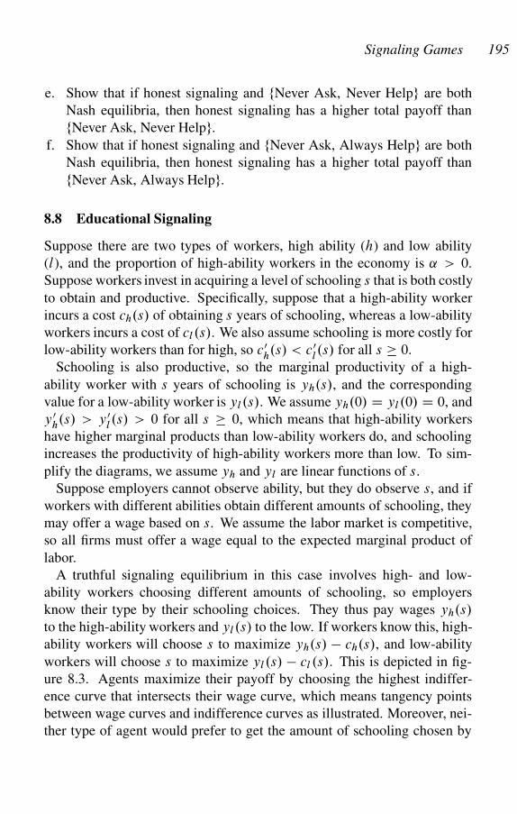
Signaling Games 195
e. Show that if honest signaling and fNever Ask, Never Helpg are both
Nash equilibria, then honest signaling has a higher total payoff than
fNever Ask, Never Helpg.
f. Show that if honest signaling and fNever Ask, Always Helpg are both
Nash equilibria, then honest signaling has a higher total payoff than
fNever Ask, Always Helpg.
8.8 Educational Signaling
Suppose there are two types of workers, high ability (h) and low ability
(l), and the proportion of high-ability workers in the economy is ˛ > 0.
Suppose workers invest in acquiring a level of schooling s that is both costly
to obtain and productive. Specifically, suppose that a high-ability worker
incurs a cost ch.s/ of obtaining s years of schooling, whereas a low-ability
workers incurs a cost of cl.s/. We also assume schooling is more costly for
low-ability workers than for high, so c0h.s/ < c0
l.s/ for all s 0.
Schooling is also productive, so the marginal productivity of a high-
ability worker with s years of schooling is yh.s/, and the corresponding
value for a low-ability worker is yl.s/. We assume yh.0/ D yl.0/ D 0, and
y 0h.s/ > y 0
l.s/ > 0 for all s 0, which means that high-ability workers
have higher marginal products than low-ability workers do, and schooling
increases the productivity of high-ability workers more than low. To sim-
plify the diagrams, we assume yh and yl are linear functions of s.
Suppose employers cannot observe ability, but they do observe s, and if
workers with different abilities obtain different amounts of schooling, they
may offer a wage based on s. We assume the labor market is competitive,
so all firms must offer a wage equal to the expected marginal product of
labor.
A truthful signaling equilibrium in this case involves high- and low-
ability workers choosing different amounts of schooling, so employers
know their type by their schooling choices. They thus pay wages yh.s/
to the high-ability workers and yl.s/ to the low. If workers know this, high-
ability workers will choose s to maximize yh.s/ � ch.s/, and low-ability
workers will choose s to maximize yl.s/ � cl .s/. This is depicted in fig-
ure 8.3. Agents maximize their payoff by choosing the highest indiffer-
ence curve that intersects their wage curve, which means tangency points
between wage curves and indifference curves as illustrated. Moreover, nei-
ther type of agent would prefer to get the amount of schooling chosen by
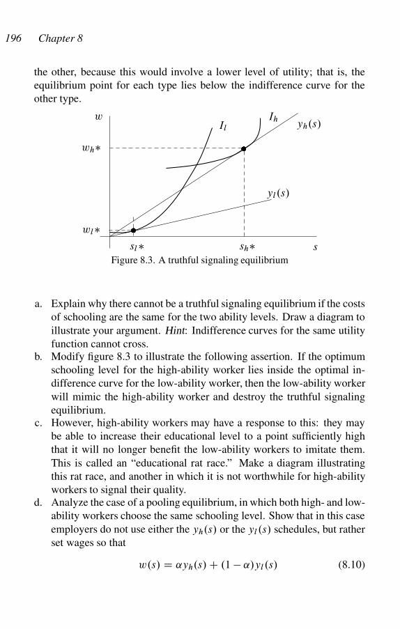
196 Chapter 8
the other, because this would involve a lower level of utility; that is, the
equilibrium point for each type lies below the indifference curve for the
other type.
w
s
�wh
wl �
sh sl
yh.s/
yl.s/
Il
Ih
Figure 8.3. A truthful signaling equilibrium
a. Explain why there cannot be a truthful signaling equilibrium if the costs
of schooling are the same for the two ability levels. Draw a diagram to
illustrate your argument. Hint: Indifference curves for the same utility
function cannot cross.b. Modify figure 8.3 to illustrate the following assertion. If the optimum
schooling level for the high-ability worker lies inside the optimal in-
difference curve for the low-ability worker, then the low-ability worker
will mimic the high-ability worker and destroy the truthful signaling
equilibrium.c. However, high-ability workers may have a response to this: they may
be able to increase their educational level to a point sufficiently high
that it will no longer benefit the low-ability workers to imitate them.
This is called an “educational rat race.” Make a diagram illustrating
this rat race, and another in which it is not worthwhile for high-ability
workers to signal their quality.d. Analyze the case of a pooling equilibrium, in which both high- and low-
ability workers choose the same schooling level. Show that in this case
employers do not use either the yh.s/ or the yl.s/ schedules, but rather
set wages so that
w.s/ D ˛yh.s/ C .1 � ˛/yl.s/ (8.10)
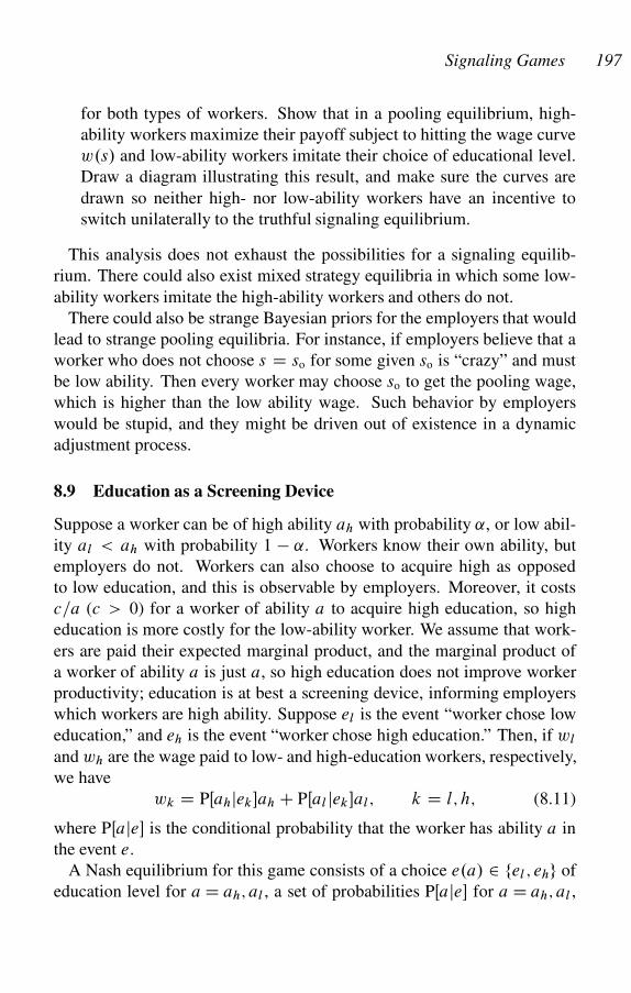
Signaling Games 197
for both types of workers. Show that in a pooling equilibrium, high-
ability workers maximize their payoff subject to hitting the wage curve
w.s/ and low-ability workers imitate their choice of educational level.
Draw a diagram illustrating this result, and make sure the curves are
drawn so neither high- nor low-ability workers have an incentive to
switch unilaterally to the truthful signaling equilibrium.
This analysis does not exhaust the possibilities for a signaling equilib-
rium. There could also exist mixed strategy equilibria in which some low-
ability workers imitate the high-ability workers and others do not.
There could also be strange Bayesian priors for the employers that would
lead to strange pooling equilibria. For instance, if employers believe that a
worker who does not choose s D so for some given so is “crazy” and must
be low ability. Then every worker may choose so to get the pooling wage,
which is higher than the low ability wage. Such behavior by employers
would be stupid, and they might be driven out of existence in a dynamic
adjustment process.
8.9 Education as a Screening Device
Suppose a worker can be of high ability ah with probability ˛, or low abil-
ity al < ah with probability 1 � ˛. Workers know their own ability, but
employers do not. Workers can also choose to acquire high as opposed
to low education, and this is observable by employers. Moreover, it costs
c=a (c > 0) for a worker of ability a to acquire high education, so high
education is more costly for the low-ability worker. We assume that work-
ers are paid their expected marginal product, and the marginal product of
a worker of ability a is just a, so high education does not improve worker
productivity; education is at best a screening device, informing employers
which workers are high ability. Suppose el is the event “worker chose low
education,” and eh is the event “worker chose high education.” Then, if wl
and wh are the wage paid to low- and high-education workers, respectively,
we have
wk D PŒahjek�ah C PŒal jek�al; k D l; h; (8.11)
where PŒaje� is the conditional probability that the worker has ability a in
the event e.
A Nash equilibrium for this game consists of a choice e.a/ 2 fel ; ehg of
education level for a D ah; al , a set of probabilities PŒaje� for a D ah; al ,
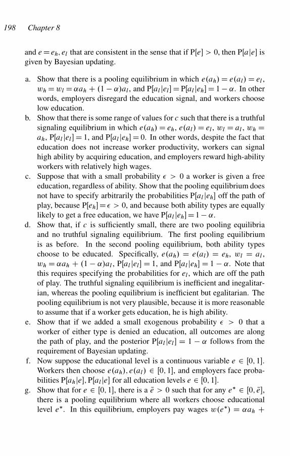
198 Chapter 8
and e Deh; el that are consistent in the sense that if PŒe� > 0, then PŒaje� is
given by Bayesian updating.
a. Show that there is a pooling equilibrium in which e.ah/ D e.al/ D el ,
wh D wl D ˛ah C .1 � ˛/al , and PŒal jel� D PŒal jeh� D 1 � ˛. In other
words, employers disregard the education signal, and workers choose
low education.
b. Show that there is some range of values for c such that there is a truthful
signaling equilibrium in which e.ah/ D eh, e.al/ D el , wl D al , wh Dah, PŒal jel � D 1, and PŒal jeh� D 0. In other words, despite the fact that
education does not increase worker productivity, workers can signal
high ability by acquiring education, and employers reward high-ability
workers with relatively high wages.
c. Suppose that with a small probability � > 0 a worker is given a free
education, regardless of ability. Show that the pooling equilibrium does
not have to specify arbitrarily the probabilities PŒal jeh� off the path of
play, because PŒeh�D� > 0, and because both ability types are equally
likely to get a free education, we have PŒal jeh�D1 � ˛.
d. Show that, if c is sufficiently small, there are two pooling equilibria
and no truthful signaling equilibrium. The first pooling equilibrium
is as before. In the second pooling equilibrium, both ability types
choose to be educated. Specifically, e.ah/ D e.al/ D eh, wl D al ,
wh D ˛ah C .1 � ˛/al , PŒal jel� D 1, and PŒal jeh� D 1 � ˛. Note that
this requires specifying the probabilities for el , which are off the path
of play. The truthful signaling equilibrium is inefficient and inegalitar-
ian, whereas the pooling equilibrium is inefficient but egalitarian. The
pooling equilibrium is not very plausible, because it is more reasonable
to assume that if a worker gets education, he is high ability.
e. Show that if we added a small exogenous probability � > 0 that a
worker of either type is denied an education, all outcomes are along
the path of play, and the posterior PŒal jel � D 1 � ˛ follows from the
requirement of Bayesian updating.
f. Now suppose the educational level is a continuous variable e 2 Œ0; 1�.
Workers then choose e.ah/; e.al/ 2 Œ0; 1�, and employers face proba-
bilities PŒahje�; PŒalje� for all education levels e 2 Œ0; 1�.
g. Show that for e 2 Œ0; 1�, there is a Ne > 0 such that for any e� 2 Œ0; Ne�,
there is a pooling equilibrium where all workers choose educational
level e�. In this equilibrium, employers pay wages w.e�/ D ˛ah C
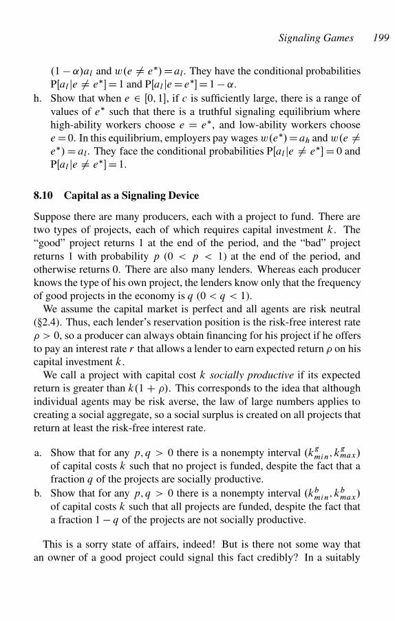
Signaling Games 199
.1 � ˛/al and w.e ¤ e�/Dal. They have the conditional probabilities
PŒal je ¤ e��D1 and PŒal je De��D1 � ˛.
h. Show that when e 2 Œ0; 1�, if c is sufficiently large, there is a range of
values of e� such that there is a truthful signaling equilibrium where
high-ability workers choose e D e�, and low-ability workers choose
e D0. In this equilibrium, employers pay wages w.e�/Dah and w.e ¤e�/ D al. They face the conditional probabilities PŒal je ¤ e�� D 0 and
PŒal je ¤ e��D1.
8.10 Capital as a Signaling Device
Suppose there are many producers, each with a project to fund. There are
two types of projects, each of which requires capital investment k. The
“good” project returns 1 at the end of the period, and the “bad” project
returns 1 with probability p (0 < p < 1) at the end of the period, and
otherwise returns 0. There are also many lenders. Whereas each producer
knows the type of his own project, the lenders know only that the frequency
of good projects in the economy is q (0 < q < 1).
We assume the capital market is perfect and all agents are risk neutral
(�2.4). Thus, each lender’s reservation position is the risk-free interest rate
� > 0, so a producer can always obtain financing for his project if he offers
to pay an interest rate r that allows a lender to earn expected return � on his
capital investment k.
We call a project with capital cost k socially productive if its expected
return is greater than k.1 C �/. This corresponds to the idea that although
individual agents may be risk averse, the law of large numbers applies to
creating a social aggregate, so a social surplus is created on all projects that
return at least the risk-free interest rate.
a. Show that for any p; q > 0 there is a nonempty interval .kgmin; k
gmax/
of capital costs k such that no project is funded, despite the fact that a
fraction q of the projects are socially productive.
b. Show that for any p; q > 0 there is a nonempty interval .kbmin; kb
max/
of capital costs k such that all projects are funded, despite the fact that
a fraction 1 � q of the projects are not socially productive.
This is a sorry state of affairs, indeed! But is there not some way that
an owner of a good project could signal this fact credibly? In a suitably
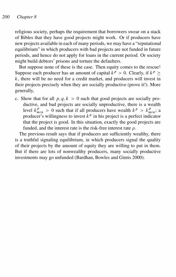
200 Chapter 8
religious society, perhaps the requirement that borrowers swear on a stack
of Bibles that they have good projects might work. Or if producers have
new projects available in each of many periods, we may have a “reputational
equilibrium” in which producers with bad projects are not funded in future
periods, and hence do not apply for loans in the current period. Or society
might build debtors’ prisons and torture the defaulters.
But suppose none of these is the case. Then equity comes to the rescue!
Suppose each producer has an amount of capital kp > 0. Clearly, if kp k, there will be no need for a credit market, and producers will invest in
their projects precisely when they are socially productive (prove it!). More
generally,
c. Show that for all p; q; k > 0 such that good projects are socially pro-
ductive, and bad projects are socially unproductive, there is a wealth
level kpmin > 0 such that if all producers have wealth kp > k
pmin; a
producer’s willingness to invest kp in his project is a perfect indicator
that the project is good. In this situation, exactly the good projects are
funded, and the interest rate is the risk-free interest rate �.
The previous result says that if producers are sufficiently wealthy, there
is a truthful signaling equilibrium, in which producers signal the quality
of their projects by the amount of equity they are willing to put in them.
But if there are lots of nonwealthy producers, many socially productive
investments may go unfunded (Bardhan, Bowles and Gintis 2000).
9
Repeated Games
Tomorrow, and tomorrow, and tomorrow,Creeps in this petty pace from day to dayTo the last syllable of recorded time
Shakespeare
When a game G is repeated an indefinite number of times by the same
players, many of the anomalies associated with finitely repeated games
(�4.2) disappear. Nash equilibria of the repeated game arise that are not
Nash equilibria of G. The exact nature of these equilibria is the subject of
the folk theorem (�9.10). We have encountered many games G in which
most, or all Nash equilibria are Pareto-inefficient. Indeed, all the generic
two-player games with two strategies, the prisoner’s dilemma (�3.11), the
battle of the sexes (�3.9), and the hawk-dove game (�3.10) are of this type.1
The folk theorem asserts that if the signals of defection (that is, the signals
that a player deviated from the behavior specified by the Nash equilibrium)
are of sufficiently high quality, and if players have sufficiently long time
horizons, the repeated game based on G can attain Pareto-efficiency, or at
least approximate Pareto-efficiency as closely as desired.
The folk theorem requires that a defection on the part of a player carry
a signal that is conveyed to other players. We say a signal is public if all
players receive the same signal. We say the signal is perfect if it accurately
reports whether or not the player in question defected. The first general folk
theorem that does not rely on incredible threats was proved by Fudenberg
and Maskin (1986) for the case of perfect public signals (�9.10).
Repeated game models provide elegant and compelling explanations of
many on-going strategic interactions. The folk theorem, however, is highly
overrated. The folk theorem achieves its magic through the unrealistic as-
sumption that the defection signal can be made arbitrarily close to public
1We say a finite normal form game is generic if all the entries in the game
matrix are distinct. More generically, we say that a property of a set of equations is
generic if, when it holds for a particular set of parameters, it holds in a sufficiently
small neighborhood of these parameters.
201
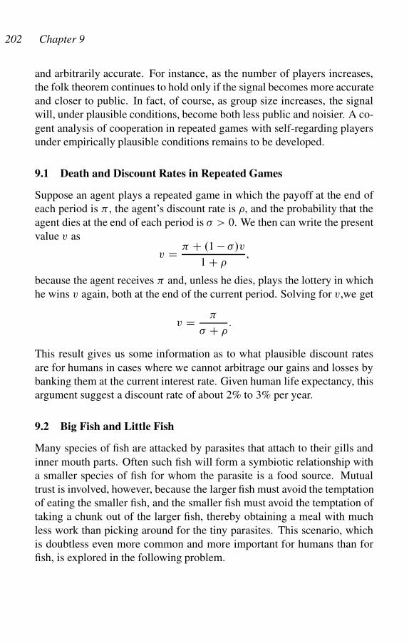
202 Chapter 9
and arbitrarily accurate. For instance, as the number of players increases,
the folk theorem continues to hold only if the signal becomes more accurate
and closer to public. In fact, of course, as group size increases, the signal
will, under plausible conditions, become both less public and noisier. A co-
gent analysis of cooperation in repeated games with self-regarding players
under empirically plausible conditions remains to be developed.
9.1 Death and Discount Rates in Repeated Games
Suppose an agent plays a repeated game in which the payoff at the end of
each period is � , the agent’s discount rate is �, and the probability that the
agent dies at the end of each period is � > 0. We then can write the present
value v as
v D � C .1 � �/v
1 C �;
because the agent receives � and, unless he dies, plays the lottery in which
he wins v again, both at the end of the current period. Solving for v,we get
v D �
� C �:
This result gives us some information as to what plausible discount rates
are for humans in cases where we cannot arbitrage our gains and losses by
banking them at the current interest rate. Given human life expectancy, this
argument suggest a discount rate of about 2% to 3% per year.
9.2 Big Fish and Little Fish
Many species of fish are attacked by parasites that attach to their gills and
inner mouth parts. Often such fish will form a symbiotic relationship with
a smaller species of fish for whom the parasite is a food source. Mutual
trust is involved, however, because the larger fish must avoid the temptation
of eating the smaller fish, and the smaller fish must avoid the temptation of
taking a chunk out of the larger fish, thereby obtaining a meal with much
less work than picking around for the tiny parasites. This scenario, which
is doubtless even more common and more important for humans than for
fish, is explored in the following problem.
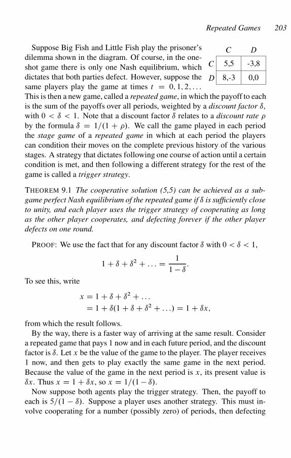
Repeated Games 203
5,5
8,-3
C
-3,8
0,0
D
C
D
Suppose Big Fish and Little Fish play the prisoner’s
dilemma shown in the diagram. Of course, in the one-
shot game there is only one Nash equilibrium, which
dictates that both parties defect. However, suppose the
same players play the game at times t D 0; 1; 2; : : :
This is then a new game, called a repeated game, in which the payoff to each
is the sum of the payoffs over all periods, weighted by a discount factor ı,
with 0 < ı < 1. Note that a discount factor ı relates to a discount rate �
by the formula ı D 1=.1 C �/. We call the game played in each period
the stage game of a repeated game in which at each period the players
can condition their moves on the complete previous history of the various
stages. A strategy that dictates following one course of action until a certain
condition is met, and then following a different strategy for the rest of the
game is called a trigger strategy.
THEOREM 9.1 The cooperative solution (5,5) can be achieved as a sub-
game perfect Nash equilibrium of the repeated game if ı is sufficiently close
to unity, and each player uses the trigger strategy of cooperating as long
as the other player cooperates, and defecting forever if the other player
defects on one round.
PROOF: We use the fact that for any discount factor ı with 0 < ı < 1,
1 C ı C ı2 C : : : D 1
1 � ı:
To see this, write
x D 1 C ı C ı2 C : : :
D 1 C ı.1 C ı C ı2 C : : :/ D 1 C ıx;
from which the result follows.
By the way, there is a faster way of arriving at the same result. Consider
a repeated game that pays 1 now and in each future period, and the discount
factor is ı. Let x be the value of the game to the player. The player receives
1 now, and then gets to play exactly the same game in the next period.
Because the value of the game in the next period is x, its present value is
ıx. Thus x D 1 C ıx, so x D 1=.1 � ı/.
Now suppose both agents play the trigger strategy. Then, the payoff to
each is 5=.1 � ı/. Suppose a player uses another strategy. This must in-
volve cooperating for a number (possibly zero) of periods, then defecting
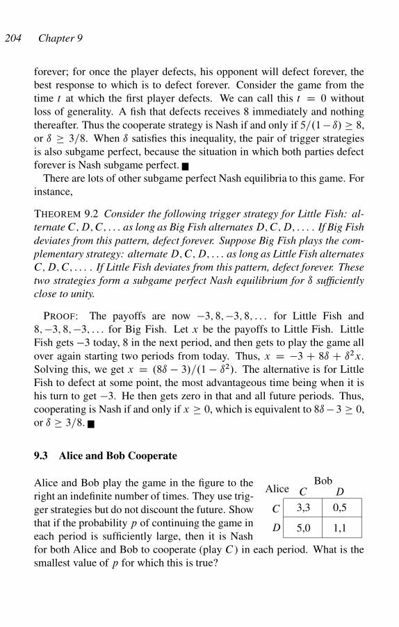
204 Chapter 9
forever; for once the player defects, his opponent will defect forever, the
best response to which is to defect forever. Consider the game from the
time t at which the first player defects. We can call this t D 0 without
loss of generality. A fish that defects receives 8 immediately and nothing
thereafter. Thus the cooperate strategy is Nash if and only if 5=.1 � ı/ 8,
or ı 3=8. When ı satisfies this inequality, the pair of trigger strategies
is also subgame perfect, because the situation in which both parties defect
forever is Nash subgame perfect.
There are lots of other subgame perfect Nash equilibria to this game. For
instance,
THEOREM 9.2 Consider the following trigger strategy for Little Fish: al-
ternate C; D; C; : : : as long as Big Fish alternates D; C; D; : : : . If Big Fish
deviates from this pattern, defect forever. Suppose Big Fish plays the com-
plementary strategy: alternate D; C; D; : : : as long as Little Fish alternates
C; D; C; : : : . If Little Fish deviates from this pattern, defect forever. These
two strategies form a subgame perfect Nash equilibrium for ı sufficiently
close to unity.
PROOF: The payoffs are now �3; 8; �3; 8; : : : for Little Fish and
8; �3; 8; �3; : : : for Big Fish. Let x be the payoffs to Little Fish. Little
Fish gets �3 today, 8 in the next period, and then gets to play the game all
over again starting two periods from today. Thus, x D �3 C 8ı C ı2x.
Solving this, we get x D .8ı � 3/=.1 � ı2/. The alternative is for Little
Fish to defect at some point, the most advantageous time being when it is
his turn to get �3. He then gets zero in that and all future periods. Thus,
cooperating is Nash if and only if x 0, which is equivalent to 8ı � 3 0,
or ı 3=8.
9.3 Alice and Bob Cooperate
C D
C
D
3,3 0,5
5,0 1,1
BobAlice
Alice and Bob play the game in the figure to the
right an indefinite number of times. They use trig-
ger strategies but do not discount the future. Show
that if the probability p of continuing the game in
each period is sufficiently large, then it is Nash
for both Alice and Bob to cooperate (play C ) in each period. What is the
smallest value of p for which this is true?
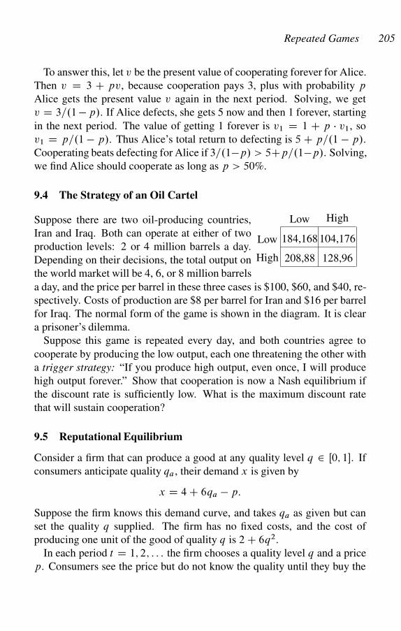
Repeated Games 205
To answer this, let v be the present value of cooperating forever for Alice.
Then v D 3 C pv, because cooperation pays 3, plus with probability p
Alice gets the present value v again in the next period. Solving, we get
v D 3=.1 � p/. If Alice defects, she gets 5 now and then 1 forever, starting
in the next period. The value of getting 1 forever is v1 D 1 C p v1, so
v1 D p=.1 � p/. Thus Alice’s total return to defecting is 5 C p=.1 � p/.
Cooperating beats defecting for Alice if 3=.1�p/ > 5Cp=.1�p/. Solving,
we find Alice should cooperate as long as p > 50%.
9.4 The Strategy of an Oil Cartel
184,168
208,88
Low
104,176
128,96
High
Low
High
Suppose there are two oil-producing countries,
Iran and Iraq. Both can operate at either of two
production levels: 2 or 4 million barrels a day.
Depending on their decisions, the total output on
the world market will be 4, 6, or 8 million barrels
a day, and the price per barrel in these three cases is $100, $60, and $40, re-
spectively. Costs of production are $8 per barrel for Iran and $16 per barrel
for Iraq. The normal form of the game is shown in the diagram. It is clear
a prisoner’s dilemma.
Suppose this game is repeated every day, and both countries agree to
cooperate by producing the low output, each one threatening the other with
a trigger strategy: “If you produce high output, even once, I will produce
high output forever.” Show that cooperation is now a Nash equilibrium if
the discount rate is sufficiently low. What is the maximum discount rate
that will sustain cooperation?
9.5 Reputational Equilibrium
Consider a firm that can produce a good at any quality level q 2 Œ0; 1�. If
consumers anticipate quality qa , their demand x is given by
x D 4 C 6qa � p:
Suppose the firm knows this demand curve, and takes qa as given but can
set the quality q supplied. The firm has no fixed costs, and the cost of
producing one unit of the good of quality q is 2 C 6q2.
In each period t D 1; 2; : : : the firm chooses a quality level q and a price
p. Consumers see the price but do not know the quality until they buy the
206 Chapter 9
good. Consumers follow a trigger strategy, in which they buy the good in
each period in which q qa, but if q < qa in some period, they never buy
from the firm again.
Suppose the firm uses discount factor ı D 0:9. Define a reputational
equilibrium as one in which quality qa is supplied in each period. What are
the conditions for a reputational equilibrium?
9.6 Tacit Collusion
Consider a duopoly operating over an infinite number of periods t D1; 2; : : : . Suppose the duopolists are price setters, so each pure strategy
for firms 1 and 2 in period t takes the form of setting prices pt1; pt
2 0,
respectively, conditioned on the history of prices in previous time periods,
and a pure strategy for the whole game is a sequence of strategies, one for
each period t . Suppose the profits in period t are given by �1.pt1; pt
2/ for
firm 1 and �2.pt1; pt
2/ for firm 2. The payoffs to the firms for the whole
game are then
�1 D1X
tD1
ıt�1.pt1; pt
2/; �2 D1X
tD1
ıt�2.pt1; pt
2/;
where ı is the common discount factor for the firms.
To specify the function �i.pt1; pt
2/, suppose the two firms have no fixed
cost and constant marginal cost c, the firms face a downward-sloping de-
mand curve, and the lowest price producer gets the whole market. Also, if
the two producers have the same price, they share the market equally.
THEOREM 9.3 There is a subgame perfect Nash equilibrium of this game
in which pt1 D pt
2 D c for t D 1; 2; : : : .
Note that this is the “competitive” equilibrium in which profits are zero
and price equals marginal cost. The existence of this Nash equilibrium
is called Bertrand’s paradox because it seems implausible (though hardly
paradoxical!) that two firms in a duopoly actually behave in this manner.
THEOREM 9.4 Suppose ı > 50%, pm is the monopoly price (that is, the
price that maximizes the profits of a monopolist) and c � p � pm. Let
s be a strategy profile which firm 1 sets pt1 D p, firm 2 sets pt
2 D p,
t D 1; 2; : : :, and each firm responds to a deviation from this behavior on
Repeated Games 207
the part of the other firm by setting price equal to c forever. Then s is a
subgame perfect Nash equilibrium.
We call a Nash equilibrium of this type tacit collusion.
PROOF: Choose p satisfying the conditions of the theorem. Let �.p/
be total industry profits if price p is charged by both firms, so �.p/ 0.
Suppose firm 2 follows the specified strategy. The payoff to firm 1 for
following this strategy is
�1.p/ D �.p/
2
�1 C ı C ı2 C : : :
� D �.p/
2.1 � ı/: (9.1)
The payoff to firm 1 for defecting on the first round by charging an amount
� > 0 less than p is �1.p � �/. Thus, 2.1 � ı/ < 1 is sufficient for Nash.
Clearly, the strategy is subgame perfect, because the Bertrand solution in
which each firm charges marginal cost is Nash.
Intuition tells us that tacit collusion is more difficult to sustain when there
are many firms. The following theorem, the proof of which we leave to the
reader (just replace the “2” in the denominators of equation (9.1) by “n”)
shows that this is correct.
THEOREM 9.5 Suppose there are n > 1 firms in the industry, but the con-
ditions of supply and demand remain as before, the set of firms with the
lowest price in a given time period sharing the market equally. Then, if
ı > 1�1=n and c � p � pm, the trigger strategies in which each firm sets
a price equal to p in each period, and each firm responds to a deviation
from this strategy on the part of another firm by setting price equal to c
forever, form a subgame perfect Nash equilibrium.
Another market condition that reduces the likelihood that tacit collusion
can be sustained is incomplete knowledge on the part of the colluding firms.
For instance, we have the following.
THEOREM 9.6 Suppose there is an n-firm oligopoly, as described previ-
ously, but a firm that has been defected upon cannot implement the trigger
strategy until k > 1 periods have passed. Then, tacit collusion can hold
only if ıkC1 > 1 � 1=n.
This theorem shows that tacit collusion is less likely to hold the more easily
a firm can “hide” its defection. This leads to the counterintuitive, but quite
208 Chapter 9
correct, conclusion that making contractual conditions public knowledge
(“putting all your cards on the table”) may reduce rather than increase the
degree of competition in an industry.
PROOF: If it takes k periods after a defection to retaliate, the gain from
defection is
�.p/.1 C ı C ı2 C : : : C ık/ D �.p/
1 � ı
�1 � ıkC1
�;
from which the result immediately follows, because the present value of
cooperating forever is �.p/=n.1 � ı/.
9.7 The One-Stage Deviation Principle
Suppose s is a strategy profile for players in a repeated game, so s specifies
what move each player makes at each stage of the game, depending on
the prior history of moves in the game. We say s satisfies the one-stage
deviation principle if no player can gain by deviating from s, either on
or off the equilibrium path of the game tree, in a single stage, otherwise
conforming to s. The following theorem is often very useful in analyzing
repeated games, because it says that a strategy profile is subgame perfect if
it satisfies the one stage deviation principle.
THEOREM 9.7 The One-Stage Deviation Principle. A strategy profile s for
a repeated game with positive discount rates, based on a finite stage game,
is a subgame perfect Nash equilibrium if and only if it satisfies the one-stage
deviation principle.
For a formal proof of this theorem (it’s not difficult) and some extensions
see Fudenberg and Tirole (1991). Here is an informal proof. Obviously,
subgame perfection implies the one-stage deviation principle. Suppose s
is not subgame perfect. Then for some player i , there is an alternative
strategy profile Qsi that offers i a higher payoff against s�i , starting at one of
i’s information sets �i . If Qsi differs from si in only a finite number of places,
we can assume Qsi has the fewest deviations from si among such alternatives
for i . If Qsi has only one deviation, we are done. If there are more than one,
then the final deviation must make i better off and again we are done. If Qsi
has an infinite number of deviations, because the payoffs are bounded, and
the discount rate is strictly positive, we can cut the game off at some period
Repeated Games 209
t such that any possible gain to i after time t are as small as we want. This
shows that there is also a finite deviation (cutting off Qsi after time t) that
improves i’s payoff starting at �i .
9.8 Tit for Tat
Consider a repeated prisoner’s dilemma with two players. The payoffs
are .r; r/ for mutual cooperation, .p; p/ for mutual defection, .t; s/ when
player 1 defects, and player 2 cooperates, and .s; t/ when player 1 cooper-
ates, and player 2 defects, where t > r > p > s and 2r > s C t . A tit for tat
player cooperates on the first round of a repeated prisoner’s dilemma, and
thereafter does what the other player did on the previous round.
It is clear that tit for tat is not Nash when played against itself if and
only if player 1 gains by defecting on the first move. Moreover, defecting
on the first round, and going back to tit for tat when you partner plays tit
for tat increases your payoff by t C ıs � r.1 C ı/, which is negative for
ı1 > .t � r/=.r � s/. Note that 0 < ı1 < 1.
After the first defect, the gain from defecting for k more rounds before
returning to cooperate is ıkC1.p � s.1 � ı/ � ır/. If this is negative, then
ı1 is the minimum discount factor for which tit for tat is Nash against itself.
If this is positive, however, then defecting forever increases payoff by t �r � .r � p/ı=.1 � ı/, which is negative for a discount factor greater than
ı2 D .t � r/=.t � p/. Because 0 < ı2 < 1, we find that there is always a
discount factor less than unity, above which tit for tat is a Nash equilibrium.
However, tit for tat is not subgame perfect, because if a player defects
on a particular round, tit for tat specifies that the two players will exchange
cooperate and defect forever, which has a lower payoff than cooperating
forever. Fortunately, we can revise tit for tat to make it subgame perfect. We
define contrite tit for tat (Boyd 1989) as follows. A player is in either good
standing or bad standing. In period 1 both players are in good standing.
A player is in good standing in period t > 1 only if in period t � 1 (i) he
cooperated and his partner was in good standing; (ii) he cooperated and he
was in bad standing; or (iii) he defects and he was in good standing, while
his partner was in bad standing. Otherwise the player is in bad standing in
period t > 1. Contrite tit for tat says to cooperate unless you are in good
standing and your partner is in bad standing. Using the one-stage deviation
principle (�9.7), it is then easy to show that contrite tit for tat is subgame
perfect.

210 Chapter 9
9.9 I’d Rather Switch Than Fight
Consider a firm that produces a quality good, which is a good whose quality
is costly to produce, can be verified only through consumer use, and cannot
be specified contractually. In a single-period model, the firm would have
no incentive to produce high quality. We develop a repeated game between
firm and consumer, in which the consumer pays a price greater than the
firm’s marginal cost, using the threat of switching to another supplier (a
trigger strategy) to induce a high level of quality on the part of the firm.
The result is a nonclearing product market, with firms enjoying price greater
than marginal cost. Thus, they are quantity constrained in equilibrium.
This model solves a major problem in our understanding of market
economies: markets in quality goods do not clear, and the success of a
firm hinges critically on its ability to sell a sufficient quantity of it product,
something that is assured in a clearing market. Thus, the problem of com-
petition in quality-goods markets is quite different from Walrasian general
equilibrium models, in which the only problem is to produce at minimum
cost.
Every Monday, families in Pleasant Valley wash their clothes. To en-
sure brightness, they all use bleach. Low-quality bleach can, with low but
positive probability, ruin clothes, destroy the washing machine’s bleach de-
livery gizmo, and irritate the skin. High-quality bleach is therefore deeply
pleasing to Pleasant Valley families. However, high-quality bleach is also
costly to produce. Why should firms supply high quality?
Because people have different clothes, washing machines, and suscepti-
bility to skin irritation, buyers cannot depend on a supplier’s reputation to
ascertain quality. Moreover, a firm could fiendishly build up its reputation
for delivering high-quality bleach and then, when it has a large customer
base, supply low-quality bleach for one period, and then close up shop (this
is called “milking your reputation”). Aggrieved families could of course
sue the company if they have been hurt by low-quality bleach but such suits
are hard to win and very costly to pursue. So no one does this.
If the quality q of bleach supplied by any particular company can be
ascertained only after having purchased the product, and if there is no way
to be compensated for being harmed by low-quality bleach, how can high
quality be assured?
Suppose the cost to a firm of producing a gallon of the bleach of quality
q is b.q/, where b.0/ > 0 and b0.q/ > 0 for q 0. Each consumer
Repeated Games 211
is a customer of a particular supplier, and purchases exactly one gallon of
bleach each Friday at price p from this supplier. If dissatisfied, the customer
switches to another supplier at zero cost. Suppose the probability of being
dissatisfied, and hence of switching, is given by the decreasing function
f .q/. We assume an infinite time horizon with a fixed discount rate �.
a. Considering both costs b.q/ and revenue q as accruing at the end of the
period, show that the value v.q/ to a firm from having a customer is
v.q/ D p � b.q/
f .q/ C �:
b. Suppose the price p is set by market competition, so it is exogenous to
the firm. Show that the firm chooses quality q so that
p D b.q/ C b0.q/g.q/;
where g.q/ D �Œf .q/ C ��=f 0.q/, provided q > 0.c. Show that quality is an increasing function of price.
Note that in this case firms are quantity constrained, because price is greater
than marginal cost in a market (Nash) equilibrium, and that consumers are
on the long side of the market.
This model raises an interesting question. What determines firm size?
In the standard perfect competition model, firm size is determined by the
condition that average costs be at a minimum. This is of course just silly,
because a firm can always produce at any multiple of the “optimal firm
size” simply by working the production process, whatever it might be,
in parallel.2 The monopolistic competition model, in which a firm has a
downward-sloping demand curve, is better, but it does not apply to a case
like ours, where firms are price takers, as in the perfect competition model,
and firm size is determined by the dynamic process of movement of cus-
tomers among firms. Here is one plausible model of such a process.
Suppose there are n firms in the bleach industry, all selling at the same
price p. Suppose firm j has market share mtj in period t . Suppose for
2The standard treatment in microeconomic theory models plant size, not firm
size. The important questions of vertical and horizontal integration, the real deter-
minants of firm size, are virtually orthogonal to the question of plant size. Indus-
trial economists have known this for a very long time. For a contemporary review
of the literature on the subject, see Sutton (1997).
212 Chapter 9
j D 1; : : : ; n, a fraction fj of firm j ’s customers leave the firm in each
period, and a fraction aj of customers who have left firms are attracted to
firm j . We say the bleach industry is in equilibrium if the market share of
each firm is constant over time. We have the following.
THEOREM 9.8 There is a unique asymptotically stable equilibrium in the
bleach industry.
PROOF: We normalize the number of customers in Pleasant Valley to one.
Then, the number of customers leaving firm j is mtj fj , so the total number
of customers looking for new suppliers isP
j mtj fj . A particular firm j
attracts a fraction aj of these. This assumes a firm can woo back a fraction
aj of its recently departed customers; the argument is the same if we assume
the opposite. Thus, the net customer loss of firm j in period t is
fj mtj � aj
nX
kD1
fkmtk: (9.2)
In equilibrium this quantity must be zero, and mtk
D mk for all t and for
k D 1; : : : ; n. This gives the equilibrium condition
mj D �j
nX
kD1
fkmk; (9.3)
where we have defined �k D ak=fk . Note also that if we add up the n
equations in (9.2), we get zero, soP
k mtk
D 1 for all t , implyingP
k mk D1. Summing (9.3), we arrive at the equilibrium conditions
mj D �jPk �k
:
Thus, there exists a unique industry equilibrium. To prove asymptotic sta-
bility, we define the n � n matrix B D .bij /, where bij D aifj for i ¤ j ,
and bi i D aifi C .1 � fi/, i; j D 1; : : : ; n. Then, writing the column
vector mt D .mt1; : : : ; mt
n/, we have mtC1 D Bmt and hence mt D B tm0,
where B t is the t th power of B . The matrix B is a positive matrix, and it is
easy to check that it has eigenvalue 1 with corresponding positive eigenvec-
tor m D .m1; : : : ; mn/. By Perron’s theorem (see, for instance, Horn and
Johnson, 1985, section 8.2), 1 is the unique maximal eigenvalue of B . Also
.1; 1; : : : ; 1/ is a right eigenvector of B corresponding to the eigenvalue 1.
It follows that B t tends to the matrix whose columns are each m (see Horn
and Johnson, 1985, theorem 8.2.8), which proves the theorem.
Repeated Games 213
9.10 The Folk Theorem
The folk theorem for repeated games is so called because no one can dis-
cover who first thought of it; it is just part of the “folklore” of game theory.
We shall first present a stripped-down analysis of the folk theorem with an
example, and provide a somewhat more complete discussion in the next
section.
5,5
8,-3
C
-3,8
0,0
D
C
D
Consider the stage game in section 9.2, reproduced
in the diagram. There is of course one subgame perfect
Nash equilibrium in which each player gets zero. More-
over, neither player can be forced to receive a negative
payoff in the repeated game based on this stage game,
because zero can be assured simply by playing D. Also, any point in the re-
gion OEABCF in figure 9.1 could be attained in the stage game, if the play-
ers could agree on a mixed strategy for each. To see this, note that if Big
Fish uses C with probability ˛, and Little Fish uses C with probability ˇ,
then the expected payoff to the pair is .8ˇ � 3˛; 8˛ � 3ˇ/, which traces out
every point in the quadrilateral OEABCF for ˛; ˇ 2 Œ0; 1� (check it out!).
Only the points in OABC are superior to the universal defect equilibrium
(0,0), however.
Consider the repeated game R based on the stage game G of section 9.2.
The folk theorem says that under the appropriate conditions concerning
the cooperate or defect signal available to players, any point in the region
OABC can be sustained as the average per-period payoff of a subgame
perfect Nash equilibrium of R, provided the discount factors of the players
are sufficiently near unity; that is, the players do not discount the future at
a high rate.
More formally, consider any n-player game with finite strategy sets Si
for i D 1; : : : ; n, so the set of strategy profiles for the game is S Df.s1; : : : ; sn/jsi 2 Si ; i D 1; : : : ; ng. The payoff for player i is �i.s/, where
s 2 S . For any s 2 S , we write s�i for the vector obtained by dropping
the i th component of s, and for any i D 1; : : : ; n we write .si ; s�i / D s.
For a given player j , suppose the other players choose strategies mj�j such
that j ’s best response mjj gives j the lowest possible payoff in the game.
We call the resulting strategy profile mj the maximum punishment payoff
for j . Then, ��j D �j .mj / is j ’s payoff when everyone else “gangs up on
him.” We call
�� D .��1 ; : : : ; ��
n /; (9.4)
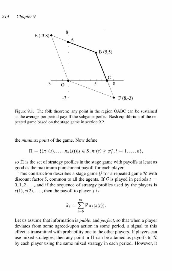
214 Chapter 9
-3 O 5
�
�
8
8
�
�
A
B (5,5)
C
-3
E (-3,8)
F (8,-3)
�
�
Figure 9.1. The folk theorem: any point in the region OABC can be sustained
as the average per-period payoff the subgame perfect Nash equilibrium of the re-
peated game based on the stage game in section 9.2.
the minimax point of the game. Now define
… D f.�1.s/; : : : ; �n.s//js 2 S; �i.s/ ��i ; i D 1; : : : ; ng;
so … is the set of strategy profiles in the stage game with payoffs at least as
good as the maximum punishment payoff for each player.
This construction describes a stage game G for a repeated game R with
discount factor ı, common to all the agents. If G is played in periods t D0; 1; 2; : : :, and if the sequence of strategy profiles used by the players is
s.1/; s.2/; : : : , then the payoff to player j is
Q�j D1X
tD0
ıt�j .s.t//:
Let us assume that information is public and perfect, so that when a player
deviates from some agreed-upon action in some period, a signal to this
effect is transmitted with probability one to the other players. If players can
use mixed strategies, then any point in … can be attained as payoffs to R
by each player using the same mixed strategy in each period. However, it
Repeated Games 215
is not clear how a signal indicating deviation from a strictly mixed strategy
should be interpreted. The simplest assumption guaranteeing the existence
of such a signal is that there is a public randomizing device that can be seen
by all players, and that players use to decide which pure strategy to use,
given that they have agreed to use a particular mixed strategy. Suppose, for
instance, the randomizing device is a circular disc with a pointer that can
be spun by a flick of the finger. Then, a player could mark off a number of
regions around the perimeter of the disc, the area of each being proportional
to the probability of using each pure strategy in a given mixed strategy to
be used by that player. In each period, each player flicks his pointer and
chooses the appropriate pure strategy, this behavior is recorded accurately
by the signaling device, and the result is transmitted to all players.
With these definitions behind us, we have the following, where for � 2…, �i.�/ 2 Si is a mixed strategy for player i such that �i .�1; : : : ; �n/ D�i :
THEOREM 9.9 Folk Theorem. Suppose players have a public randomizing
device, and the signal indicating cooperation or defection of each player
is public and perfect. Then, for any � D .�1; : : : ; �n/ 2 …, if the dis-
count factor is sufficiently close to unity, there is a Nash equilibrium of
the repeated game such that �j is j ’s payoff for j D 1; : : : ; n in each pe-
riod. The equilibrium is effected by each player i using �i.�/ as long as
no player has been signaled as having defected, and playing the minimax
strategy mji in all future periods after player j is first detected defecting.
The idea behind this theorem is straightforward. For any such � 2 …,
each player j uses the strategy �j .�/ that gives payoffs � in each period,
provided the other players do likewise. If one player deviates, however,
all other players play the strategies that impose the maximum punishment
payoff on j forever. Because �j ��j , player j cannot gain from deviating
from �j .�/, so the profile of strategies is a Nash equilibrium.
Of course, unless the strategy profile .mj1; : : : ; m
jn/ is a Nash equilibrium
for each j D 1; : : : ; n, the threat to minimax even once, let alone forever,
is not a credible threat. However, we do have the following:
THEOREM 9.10 The folk theorem with Subgame Perfection. Suppose y D.y1; : : : ; yn/ is the vector of payoffs in a Nash equilibrium of the underlying
one-shot game, and � 2 … with �i yi for i D 1; : : : ; n. Then, if ı is
216 Chapter 9
sufficiently close to unity, there is a subgame perfect Nash equilibrium of
the repeated game such that �j is j ’s payoff for j D 1; : : : ; n in each
period.
To see this, note that for any such � 2 …, each player j uses the strategy sj
that gives payoffs � in each period, provided the other players do likewise.
If one player deviates, however, all players play the strategies that give
payoff vector y forever. Fudenberg and Maskin (1986) show that subgame
perfection is possible even for the more general case where � 2 ….
9.11 The Folk Theorem and the Nature of Signaling
Repeated game theory is a key analytical tool in modeling the coordination
of behavior in teams and other groups. Indeed, economists often claim that
the folk theorem and its many variants have solved the problem of achieving
social efficiency with self-regarding agents (that is, agents who care only
about their personal payoffs). Unfortunately, such claims are exaggerated.
Folk theorems generally only assert what occurs when the discount factor
is near unity, so individuals are arbitrarily far-sighted, when the signals
indicating cooperation and defection are arbitrarily close to zero and when
the signals are sufficiently “public” in nature. In the real world, none of
these assumptions is realistic, and their realism decreases with group size.
Consider, for instance, the issue of the quality of signals of player behavior.
We say a signal is imperfect if it sometimes misreports whether or not
the player in question defected. A public imperfect signal reports the same
information to all players but it may be incorrect. The folk theorem was
extended to imperfect public signals by Fudenberg, Levine and Maskin
(1994), as was analyzed in section 9.10.
If different players receive different signals, or some receive no signal at
all, we say the signal is private. The case of private signals has proved much
more daunting than that of public signals. However, folk theorems for pri-
vate but near-public signals (that is, where there is an arbitrarily small devi-
ation � from public signals) have been developed by several game theorists,
including Sekiguchi (1997), Piccione (2002), Ely and Valimaki (2002),
Bhaskar and Obara (2002), Horner and Olszewski (2006), and Mailath and
Morris (2006).
The problem is that in the real world, private signals are generally not
near-public. For instance, in a large work team, each member will gener-
Repeated Games 217
ally work directly with only a few other workers, so the signal indicating
cooperation or defection of a worker will be sent only to a small subset
of team members. Of course, if all individuals were obligate truth-tellers,
their information could be pooled, and the public information assumption
would be plausible. But, there is no reason for self-regarding individu-
als to be truthful, so we would need a mechanism to render truth-telling
incentive compatible for self-regarding agents. Although this is possible
in some case, in general such mechanisms are not known. In fact, in hu-
man societies, gossip is probably the major mechanism for turning private
into public information, and the veracity of communication in gossip de-
pends on individuals having an ethic of truth-telling and a strong regard
for personal reputation that would be tarnished were lying detected. Ethics
and self-esteem are, however, prime examples of other-regarding, not self-
regarding, behavior (Gintis 2009).
It is also the case that, given the plethora of equilibria available in the re-
peated game case, there is no reason to believe a set of individuals would or
could spontaneously play, or learn to play, a folk theorem equilibrium. One
could argue that specific cultural institutions can arise that direct individu-
als to play their part in a particular equilibrium (Binmore 2005; Bicchieri
2006) but it can be shown that implementing the Nash equilibrium is infea-
sible unless individuals have an other-regarding predisposition to conform
to social norms even when it is costly to do so (Gintis 2009).
9.12 The Folk Theorem Fails in Large Groups
Suppose the acts involved in cooperating in section 9.2 are in fact complex
and demanding, so there is some probability � > 0 that a player will make a
mistake, playing D instead of C . Trigger strategies are devastating in such
a situation, because with probability 1 eventually one player will make a
mistake, and both will defect forever after. If it were possible to distin-
guish mistakes from intentional defection, there would be no difficulty in
sustaining cooperation. Suppose, however, that there is not. There may
nevertheless be a trembling hand cooperative equilibrium of the following
form: if either player defects, both defect for k rounds, and then both return
to cooperation (no matter what happened in the defection rounds). Given �,
of course k should be chosen to be the smallest integer such that it pays to
cooperate rather than defect.
218 Chapter 9
Does such a k exist? Let v be the value of the game when both players
use the following “trembling hand” strategy. There are two “phases” to the
game. In the “cooperate” phase, (try to) play C , and in the “punishment”
phase, play D. If the game is in the cooperate phase and either agent plays
D (on purpose or by mistake), the game moves to the punishment phase.
If the punishment phase has lasted for k rounds, the game moves to the
cooperate phase. The game starts in the cooperate phase.
It is clear that there is no gain from playing C in the punishment phase.
Can there be a gain from playing D in the cooperate phase?
Here is where the one-stage deviation principle becomes useful. If the
above strategies do not form a subgame perfect Nash equilibrium, then
playing D in the cooperate phase and then returning to the trembling hand
strategy has a higher payoff than cooperating. The payoff to playing D in
the cooperate phase and then returning to the trembling hand strategy is just
8.1 � �/ C ıkC1v, because your partner also plays D with probability �, in
which case you get nothing but still must wait k periods to resume coop-
erating. Thus, cooperating is Nash when 8.1 � �/ C ıkC1v is less than v,
or
v.1 � ıkC1/ > 8.1 � �/: (9.5)
But what is v? Well, v must satisfy the equation
v D .1��/�.�3CıkC1v/C.1��/2.5Cıv/C�Œ.1��/8CıkC1v�: (9.6)
To see this, note that if you both cooperate at the start of the game, with
probability .1 � �/�, you play C and your partner plays D, in which case
you get �3 now and after k C 1 periods, you’re back into the cooperate
phase, the present value of which is ıkC1v. This is the first term in (9.6).
With probability .1 � �/2 you both play C , so you get 5 and v again in the
next period. This is the second term. With probability � you play D, in
which case you get 8 if your partner plays C , zero if your partner plays D,
and in either case, you get v after k C 1 periods. This is the final term in
(9.6).
Solving (9.6) for v, we get
v D 5.1 � �/
1 � ı.1 � �/2 � ık�.2 � �/:
Suppose, for instance, � D 15% and ı D 95%. It is easy to check by
hand calculation that v D 85 if there is no punishment phase .k D 0/
Repeated Games 219
but the payoff to defecting is 87:55 > v. For one round of punishment
(k D 1), v D 67:27, but the value of defecting is 8.1 � �/ C ı2v D 67:51,
so punishment is still not sufficiently severe. For two rounds of punishment
.k D 2/, v D 56:14, and 8.1 � �/ C ı3v D 54:93, so two rounds of
punishment are needed to sustain cooperation.
Suppose, now, that the group is of size n > 2, so the probability at least
one member accidentally errs is now 1 � .1 � �/n. We can show that as
� ! 1=n, cooperation becomes impossible. I will not be rigorous but it is
easy to see that the argument can be made as rigorous as desired. We make
the conservative assumption that the group is sufficiently large that we can
ignore the cost to each player of another player defecting. Moreover, let us
assume that n is so large, and �n sufficiently close to one that we can use
the approximation .1 C 1=n/n � 1=e, where e � 2:718 is the base of the
natural logarithms (in fact, n 4 is usually good enough). Finally, suppose
it takes k rounds of no cooperation to make cooperating a best response.
We have the recursion equation
v D .5 C ıv/.1 � �/n C .8 C ıkv/ C .1 � � � .1 � �/n/.5 C ıkv/:
The first term on the right-hand side is the payoff when there are no errors.
The second term is the payoff when the agent errs. The third term is the
payoff in all other cases. With our approximations, this reduces to
v D e.5 C 3�/
e.1 � ık/ � ı.1 � ı/;
Now, the payoff to defecting once and returning to cooperation is vd D8Cıkv, so cooperating is a best response if and only if 8Cıkv < v, which
reduces to
8ı � 3e.1 � �/ C .3e.1 � �/ � 8/ık > 0;
which is false for small �, for all integers k 1, because 3e � 8:15 > 8 >
8ı.
9.13 Contingent Renewal Markets Do Not Clear
In many exchanges, including those between (a) employer and employee,
(b) lender and borrower, and (c) firm and customer, the agent on one side
of the exchange gives money (employer, lender, customer), whereas the

220 Chapter 9
agent on the other side of the exchange gives a promise (employee, bor-
rower, firm). The employee promises to work hard, the borrower promises
to repay the loan, and the firm promises to provide high-quality products.
Rarely, however, is this promise subject to a contract that can be enforced
at reasonably low cost.
Let us call the player who gives money the principal, and the player who
gives promises the agent. In the absence of an enforceable contract, why do
agents keep their promises? Of course, some agents are just honest but there
are doubtless enough dishonest people that exchange would break down if
enforcement were based purely on the integrity of the agents.
Perhaps the threat of suing is sufficient to secure agent compliance. But
generally such threats are not credible. Taking an employee to court for not
working hard enough is rare. A lender can sue a borrower for nonpayment,
but if the borrower has no wealth, there is not much to collect. A customer
can sue a firm for faulty goods but this is done only in cases where a product
has caused extensive personal injury. So why, then, do agents generally
keep their promises?
The answer is that if agents do not keep their promises, principals dump
them: employers fire workers who shirk, lenders refuse future loans to bor-
rowers who have defaulted, and customers switch to new suppliers when
dissatisfied. All three actions represent trigger strategies: the exchange
between principal and agent is renewed indefinitely (perhaps with some
exogenous probability of dissolution), the principal using the threat of non-
renewal to secure compliance. We call this contingent renewal exchange.
A contingent renewal market is a market in which exchanges between
buyers and sellers are regulated by contingent renewal relationships. Be-
cause the principal (employer, lender, consumer) in such markets uses a
trigger strategy (the threat of nonrenewal) to elicit performance from the
agent (worker, borrower, firm), the loss of the relationship must be costly
to the agent. But if the price is set in such markets to equate supply and de-
mand, the cost to an agent of being cut off by the principal is zero, because
the agent will secure another position in the next period at the prevailing
price. Hence, if the principal uses a trigger strategy, there must be a posi-
tive probability that there is an excess supply of agents. It follows that in a
Nash equilibrium of a contingent renewal market, there is an excess supply
of agents.

Repeated Games 221
This conclusion nicely explains some of the most pervasive facts about
market economies. Consider, for instance, labor markets. In the neoclas-
sical model, the wage rate adjusts to equate the supply of and the demand
for labor. The general condition of labor markets, however, is excess sup-
ply. Often this takes the form of explicit unemployment, which neoclassical
economists explain using complex models involving search costs, friction,
adaptive expectations, exotic intertemporal elasticities and the like. Us-
ing Occam’s razor (always opt for the simplest explanation first), a contin-
gent renewal labor market does the job. There simply cannot be full em-
ployment in such models (Gintis 1976; Shapiro and Stiglitz 1984; Bowles
1985; Bowles and Gintis 1993). Excess supply in labor markets takes the
form not only of unemployment but of “underemployment”: workers hold
one position but are capable and willing to fill a “better” position, even at
the going wage or a bit below, but they cannot secure such a position.
Another example is credit markets. In the neoclassical model, the interest
rate adjusts to equate the supply of and the demand for loans. The general
condition of credit markets, however, is excess demand. Why does the inter-
est rate not rise to cut off this excess demand? There are two basic reasons
(Stiglitz and Weiss 1981; Stiglitz 1987). First, an increase in the interest
rate will drive borrowers who have low-risk, low-expected-return projects
out of the market, and increase the expected riskiness of the remaining pool
of borrowers. Second, an interest rate increase will induce borrowers to in-
crease the riskiness of their investment projects, thus lowering the lender’s
expected return.
Because risksharing, requiring the borrower to put up a fraction of the
equity in a project, is the most widely used and effective means of endoge-
nous contract enforcement in credit markets, it follows that lending is di-
rected predominantly toward wealthy agents. This basic fact of life, which
seems so perverse from the neoclassical standpoint (loans should be from
the wealthy to the nonwealthy), is perfectly comprehensible from the stand-
point of models in which contract enforcement is endogenous, even with-
out contingent renewal. Contingent renewal (making available a line of
credit, contingent on performance) adds the dimension that a certain subset
of nonwealthy borrowers with good projects can get loans, facing the threat
of falling into the pool of unemployed “credit seekers” should their credit
line be terminated.
222 Chapter 9
A third example is consumer goods markets. In the neoclassical model,
price adjusts until supply and demand are equal. This implies that firms
can sell as much as they want, subject to the market price, and choose how
much to produce according to cost considerations. Everyday observation
tells a different story: firms try to create sales, and generally they can pro-
duce with ease whatever is needed to satisfy the demand they have gen-
erated. Of course, there are models of monopolistic competition in which
firms have differentiated products and downward-sloping demand curves,
but these notions do not capture the critical point that there is a strategic
interaction between buyer and seller, and the price is determined in part by
this interaction.
In our game-theoretic model, equilibrium price in markets with quality
goods must exceed marginal cost, not because of the price elasticity of
demand, as in monopolistic competition, but because a high price ensures
that it is costly to lose a client, thus reassuring the buyer that the seller has
an incentive to produce a high-quality good, under the threat of the buyer
finding another supplier (Klein and Leffler 1981; Gintis 1989).
9.14 Short-Side Power in Contingent Renewal Markets
We say a principal P has power over an agent A if P can impose, or credi-
bly threaten to impose, sanctions on A but A has no such capacity vis-a-vis
P (Bowles and Gintis 1992). This definition is doubtless incomplete and
unnuanced but conforms to standard notions in analytical political theory
(Simon 1953; Dahl 1957; Harsanyi 1962). In the neoclassical model there
is no power, because all markets clear and contracts are costlessly enforced.
In contingent renewal markets, however, principals have power over agents
because they can impose costs on agents by terminating them. Because
agents are in excess supply, without collusion agents can exercise no paral-
lel threat over their principals. It follows that employers have power over
employees, lenders have power over borrowers, and consumers have power
over the firms from which they buy. We may call this short-side power be-
cause it always lies with the transactor on the short side of the market; that
is, the side for which the quantity of desired transactions is the lesser.
Contingent renewal markets do not clear, and in equilibrium they allocate
power to agents located on the short side of the market.

Repeated Games 223
9.15 Money Confers Power in Contingent Renewal Markets
If we review the cast of characters in our various contingent renewal mar-
kets, we find a strong regularity: the principal gives money to the agent, and
the principal is on the short side of the market. For instance, the employer,
the lender, and the consumer hand over money to the worker, the borrower,
and the supplying firm, and the latter are all short-siders. The reason for
this is that the money side of contracts is relatively easy to enforce. This
important regularity is implicit in most repeated game principal-agent mod-
els, where it is assumed that the principal can make credible promises (to
wit, the incentive scheme), whereas agent cannot.
The application of the notion that “money talks” is particularly dramatic
in the case of consumer goods markets. In neoclassical theory, consumer
sovereignty means that free markets (under the appropriate conditions) lead
to efficient allocations. What the term really means in people’s lives is that
because firms are on the long side of the market (they are quantity con-
strained), consumers can tell producers how to behave. People are then
truly sovereign. Probably nowhere in the daily lives of ordinary people
do they feel more power and gain more respect, than when acting as con-
sumers, constantly pandered to by obsequious suppliers interested in stay-
ing in their good graces, and benefiting from the difference between price
and marginal cost.
9.16 The Economy Is Controlled by the Wealthy
It is neither a criticism nor profound to observe that the wealthy control the
market economy. This cannot be explained in neoclassical economics, in
which the wealthy have great purchasing power but this does not trans-
late into any sort of economic power over others. As Paul Samuelson
(1957:894) has noted, “in a perfectly competitive market it really does
not matter who hires whom; so let labor hire capital.” The result, expressed
long ago by Joseph Schumpeter (1934), is a decentralization of power to
consumers: “The people who direct business firms only execute what is
prescribed for them by wants.” These views taken together imply the com-
petitive economy as an arena of “solved political problems” (Lerner 1972).
However, it is not correct in the case of labor, capital and quality goods, as
we illustrate below.
224 Chapter 9
9.17 Contingent Renewal Labor Markets
In this section we develop a repeated game between employer and employee
in which the employer pays the employee a wage higher than the expected
value of his next best alternative, using the threat of termination (a trigger
strategy) to induce a high level of effort, in a situation where it is infeasible
to write and enforce a contract for labor effort. When all employers behave
in this manner, we have a nonclearing market in equilibrium.
Suppose an employer’s income per period is q.e/, an increasing, concave
function of the effort e of an employee. The employee’s payoff per pe-
riod u D u.w; e/ is an increasing function of the wage w and a decreasing
function of effort e. Effort is known to the employee but is only imper-
fectly observable by the employer. In each period, the employer pays the
employee w, the employee chooses effort e, and the employer observes
a signal that registers the employee as “shirking” with probability f .e/,
where f 0.e/ < 0. If the employee is caught shirking, he is dismissed and
receives a fallback with present value z. Presumably z depends on the value
of leisure, the extent of unemployment insurance, the cost of job search, the
startup costs in another job, and the present value of the new job. The em-
ployer chooses w to maximize profits. The tradeoff the employer faces is
that a higher wage costs more but it increases the cost of dismissal to the
employee. The profit-maximizing wage equates the marginal cost to the
marginal benefit.
The employee chooses e D e.w/ to maximize the discounted present
value v of having the job, where the flow of utility per period is u.w; e/.
Given discount rate � and fallback z, the employee’s payoff from the re-
peated game is
v D u.w; e/ C Œ1 � f .e/�v C f .e/z
1 C �;
where the first term in the numerator is the current period utility, which we
assume for convenience to accrue at the end of the period, and the others
measure the expected present value obtainable at the end of the period, the
weights being the probability of retaining or losing the position. Simplify-
ing, we get
v D u.w; e/ � �z
� C f .e/C z:
Repeated Games 225
The term �z in the numerator is the forgone flow of utility from the fallback,
so the numerator is the net flow of utility from the relationship, whereas
f .e/ in the denominator is added to the discount rate �, reflecting the fact
that future returns must be discounted by the probability of their accrual as
well as by the rate of time preference.
The employee varies e to maximize v, giving the first-order condition
@u
@e� @f
@e.v � z/ D 0; (9.7)
which says that the employee increases effort to the point where the
marginal disutility of effort is equal to the marginal reduction in the ex-
pected loss occasioned by dismissal. Solving (9.7) for e gives us the em-
ployee’s best response e.w/ to the employer’s wage offer w.
We assume that the employer can hire any real number n of workers, all
of whom have the effort function e.w/, so the employer solves
maxw;n
� D q.ne.w// � wn:
The first-order conditions on n and w give q0e D w and q0ne0 D n, which
together imply@e
@wD e
w: (9.8)
This is the famous Solow condition (Solow 1979).
The best-response function and part of the employer’s choice of an opti-
mal enforcement strategy .w�/ are shown in figure 9.2, which plots effort
against salary. The iso-v function v� is one of a family of loci of effort levels
and salaries that yield identical present values to the employee. Their slope,
�.@v=@w/=.@v=@e/, is the marginal rate of substitution between wage and
effort in the employee’s objective function. Preferred iso-v loci lie to the
right.
By the employee’s first-order conditions (9.7), the iso-v loci are vertical
where they intersect the best-response function (because @v=@e D 0/. The
negative slope of the iso-v functions below e.w/ results from the fact that
in this region the contribution of an increase in effort, via .@f =@e/.v � z/,
to the probability of keeping the job outweigh the effort-disutility effects.
Above e.w/, the effort-disutility effects predominate. Because v rises along
e.w/, the employee is unambiguously better off at a higher wage. One of

226 Chapter 9
�
w�
wage
e�
effort
x
e.w/
e D m�w
v�
Employee IndifferenceCurve
Employee Best-Response FunctionEmployer Iso-
Cost Line
Figure 9.2. The employee’s best-response function
the employer’s iso-cost loci is labeled e D m�w, where m� is the profit-
maximizing effort per dollar. The employer’s first-order condition identifies
the equilibrium wage w� as the tangency between the employer’s iso-cost
function, e D m�w and the employee’s effort function, with slope e0, or
point x in the figure.
It should be clear that the contingent renewal equilibrium at x is not first-
best, because if the parties could write a contract for effort, any point in the
lens-shaped region below the employee’s indifference curve v� and above
the employer’s iso-cost line e D m�w makes both parties strictly better off
than at x. Note that if we populated the whole economy with firms like this,
we would in general have v > z in market equilibrium, because if v D z,
(9.7) shows that @u=@e D 0, which is impossible so long as effort is a disu-
tility. This is one instance of the general principle enunciated previously,
that contingent renewal markets do not clear in (Nash) equilibrium, and the
agent whose promise is contractible (usually the agent paying money) is on
the long side of the market.
Perhaps an example would help visualize this situation. Suppose the util-
ity function is given by
u.w; e/ D w � 1
1 � e
and the shirking signal is given by
f .e/ D 1 � e:
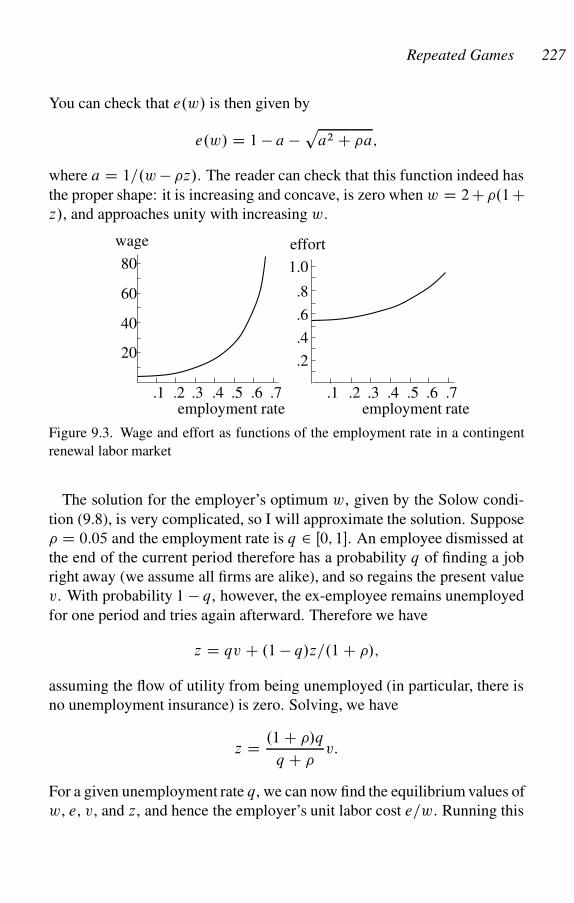
Repeated Games 227
You can check that e.w/ is then given by
e.w/ D 1 � a �p
a2 C �a;
where a D 1=.w � �z/. The reader can check that this function indeed has
the proper shape: it is increasing and concave, is zero when w D 2 C �.1 Cz/, and approaches unity with increasing w.
20
40
60
80
.1 .2 .3 .4 .5 .6 .7
.2
.4
.6
.8
.1 .2 .3 .4 .5 .6 .7
1.0
wage effort
employment rate employment rate
Figure 9.3. Wage and effort as functions of the employment rate in a contingent
renewal labor market
The solution for the employer’s optimum w, given by the Solow condi-
tion (9.8), is very complicated, so I will approximate the solution. Suppose
� D 0:05 and the employment rate is q 2 Œ0; 1�. An employee dismissed at
the end of the current period therefore has a probability q of finding a job
right away (we assume all firms are alike), and so regains the present value
v. With probability 1 � q, however, the ex-employee remains unemployed
for one period and tries again afterward. Therefore we have
z D qv C .1 � q/z=.1 C �/;
assuming the flow of utility from being unemployed (in particular, there is
no unemployment insurance) is zero. Solving, we have
z D .1 C �/q
q C �v:
For a given unemployment rate q, we can now find the equilibrium values of
w, e, v, and z, and hence the employer’s unit labor cost e=w. Running this
228 Chapter 9
through Mathematica, the equilibrium values of w and e as the employment
rate q goes from zero to 0.67 are depicted in figure 9.3.
Note that although effort increases only moderately as the unemployment
rate drops from 100% to 33%, the wage rate increases exponentially as
the unemployment rate approaches 33%. I could not find a solution for
q > 0:67. The actual unemployment rate can be fixed by specifying the
firm’s production function and imposing a zero profit condition. However
this is accomplished, there will be positive unemployment in equilibrium.
10
Evolutionarily Stable Strategies
There is but a step between the sublime and the ridiculous.
Leo Tolstoy
In 1973 the biologist John Maynard Smith and the mathematician
G. R. Price wrote an article in Nature showing how game theory applies to
the behavior of animals (Maynard Smith and Price 1973). Maynard Smith
went on to write a book on the subject (Maynard Smith 1982), which has
become a classic. The idea of applying game theory to animals, and not
just the higher primates, but fish, dung beetles, fireflies, and pond scum as
well, seemed strange at the time, because game theory had always been the
preserve of hyperrationality. Animals hardly fit the bill. Maynard Smith
made three critical shifts from traditional game theory. The first is in the
concept of a strategy, the second in the concept of equilibrium, and a third
in the nature of agent interactions.
Strategy. In classical game theory, players have strategy sets from which
they choose particular strategies. In biology, species have strategy sets
(genotypic variants), of which individuals inherit one or another variant,
perhaps mutated, that they then play in their strategic interactions. This
extends nicely to the treatment of culture in human society, in which case
we say that society has the strategy set (the set of alternative cultural forms)
and individuals inherit or choose among them.
Equilibrium. In place of the Nash equilibrium, Maynard Smith and Price
used the evolutionarily stable strategy (ESS) concept. A strategy is an ESS
if a whole population using that strategy cannot be invaded by a small group
with a mutant genotype. Similarly, a cultural form is an ESS if, upon
being adopted by all members of a society (firm, family, etc.), no small
group of individuals using an alternative cultural form can invade. We thus
move from explaining the actions of individuals to modeling the diffusion
of forms of behavior (“strategies”) in society.
229
230 Chapter 10
Player interactions. In place of the one-shot and repeated games of clas-
sical game theory, Maynard Smith introduced the notion of the repeated,
random pairing of agents who play strategies based on their genome but
not on the previous history of play.
The ESS concept is particularly useful because it says something about
the dynamic properties of a system without being committed to any particu-
lar dynamic model. As we shall see, however, an evolutionary system with
a symmetrical two-player stage game can be dynamically stable without
being an ESS (�12.9).
10.1 Evolutionarily Stable Strategies: Definition
Consider a two-player normal form game in which both players have the
set S D fs1; : : : ; sng of pure strategies, and the payoffs to an agent playing
si 2 S and another agent playing sj 2 S are �1ij for the first and �2
ij D �1ji
for the second. We call such a game symmetric in payoffs. In addition, we
assume the agents cannot condition their play on whether they are “player
1” or “player 2.” We call such a game symmetric in strategies. If a game
is symmetric in both payoffs and strategies, we simply call the game sym-
metric. We call A D .�1ij / the matrix of the symmetric game. Note that A
represents only the payoffs for the row player, because the payoffs to the
column player are just the transpose of A.
Let G be a symmetric game with matrix A (we’ll call it the stage game)
and large population of agents. In each period t D 1; 2; : : :, agents are
randomly paired and they play the stage game G once. Each agent is of
type i for some si 2 S , meaning that the agent uses strategy si in the stage
game. If the proportion of agents of type j is pj at a particular time, we say
the state of the population is � D p1s1 C : : : C pnsn. Note that we must
have p1; : : : ; pn 0 andP
i pi D 1. The payoff at that time to a player of
type i when the state of the population is � is defined by
�i� DnX
j D1
�ij pj ; (10.1)
which is the player’s expected payoff before being assigned a particular
partner. These conditions define a new game, called the evolutionary game
corresponding to the stage game G.
Evolutionarily Stable Strategies 231
Suppose the state of the population is � , and some small subpopulation
plays a “mutant” strategy D q1s1 C : : : C qnsn, in the sense that qi is the
frequency of pure strategy si in this subpopulation. We say the mutant is of
“type ,” and has payoff
��� DnX
i;j D1
qi�ij pj ;
when a random member of its population meets a random member of the
population � .
Suppose the state of the population is � D p1s1 C : : : C pnsn. The
expected payoff to a randomly chosen member of the population is thus
just ��� . If we replace a fraction � > 0 of the population with a “mutant”
of type , the new state of the population is
� D .1 � �/� C �;
so the payoff to a randomly chosen nonmutant is
�� D .1 � �/��� C ���� ;
and the expected payoff to a mutant is
�� D .1 � �/��� C ���� :
We say the mutant type can invade the population if � ¤ � and for all
sufficiently small � > 0,
�� ��;
which says that, on average, a mutant does at least as well against the new
population as does a nonmutant. We say � is an evolutionarily stable strat-
egy (ESS) if it cannot be invaded by any mutant type, in a sense defined
precisely below.
We assume that mutants can employ mixed strategies in applying the
ESS criterion, because as we shall see later (�12.7), with this assumption
evolutionarily stable strategies have powerful dynamic properties. A Nash
equilibrium in an evolutionary game can consist of a monomorphic popu-
lation of agents, each playing the same mixed strategy, or a polymorphic
population, a fraction of the population playing each of the underlying pure
232 Chapter 10
strategies in proportion to its contribution to the mixed Nash strategy. The
two interpretations are interchangeable under many conditions, and we shall
not commit ourselves exclusively to either interpretation. Because the stage
game is a one-shot, it is rarely plausible to hold that an individual will play
a strictly mixed strategy. Thus, in general, the heterogeneous population
interpretation is superior. The heterogeneous mutant must then possess
some internal mechanism for maintaining the constant frequency distribu-
tion q1; : : : ; qn from period to period. We relax this assumption when we
treat evolutionary games as dynamical systems in chapter 12.
10.2 Properties of Evolutionarily Stable Strategies
Prove the following properties of evolutionarily stable strategies:
a. Strategy � 2 S is an ESS if, for every mutant type 2 S , there is
an �� > 0 such that for all � 2 .0; ��/ and defining � D .1 � �/� C � ,
we have
�� > ��: (10.2)
b. We say that � 2 S has a uniform invasion barrier if there is some
�o 2 .0; 1/ such that (10.2) holds for all ¤ � and all � 2 .0; �o/.
Strategy � is an ESS if and only if it has a uniform invasion barrier.
c. Strategy � 2 S is an ESS if and only if, for any mutant type 2 S ,
we have
��� ��� ;
and if ��� D ��� , then
��� > ��� :
This says that � 2 S is an ESS if and only if a mutant cannot do
better against an incumbent than an incumbent can do against another
incumbent, and if a mutant does as well as an incumbent against another
incumbent, then an incumbent must do better against a mutant than a
mutant does against another mutant. Note here that we are assuming
mutants can use mixed strategies.
d. An evolutionarily stable strategy is a Nash equilibrium that is isolated
in the set of symmetric Nash equilibria (that is, it is a strictly positive
distance from any other symmetric Nash equilibrium).
e. Every strict Nash equilibrium in an evolutionary game is an ESS.
Evolutionarily Stable Strategies 233
10.3 Characterizing Evolutionarily Stable Strategies
THEOREM 10.1 Suppose symmetric two-player game G has two pure
strategies. Then, if �11 ¤ �21 and �12 ¤ �22, G has an evolutionarily
stable strategy.
PROOF: Suppose �11 > �21. Then, pure strategy 1 is a strict Nash equilib-
rium, so it is an evolutionarily stable strategy. The same is true if �22 > �12.
So suppose �11 < �21 and �22 < �12. Then, we can show that the
game has a unique completely mixed symmetric equilibrium p, where each
player uses strategy 1 with probability p 2 .0; 1/. The payoff to strategy
1 against the mixed strategy . p; 1 � p/ is then p�11 C .1 � p/�12, and
the payoff to strategy 2 against this mixed strategy is p�21 C .1 � p/�22.
Because these must be equal, we find that p D .�22 � �12/=, where
D �11 � �21 C �22 � �12 < 0. Note that under our assumptions,
0 < p < 1, so there is a unique completely mixed Nash equilibrium
. p; 1 � p/.
Now let ˛q be the probability a mutant player uses pure strategy 1. Be-
cause each pure strategy is a best response to p, ˛q must also be a best
response to p, so clearly, �qp D �pp . To show that p is an ESS, we must
show that �pq > �qq . We have
�pq D p Œ�11˛q C �12.1 � ˛q/� C .1 � p/Œ�21˛q C �22.1 � ˛q/�
and
�qq D ˛qŒ�11˛q C �12.1 � ˛q/� C .1 � ˛q/Œ�21˛q C �22.1 � ˛q/�:
Subtracting and simplifying, we get
�pq � �qq D �. p � ˛q/2 > 0;
which proves we have an ESS.
THEOREM 10.2 Using the same notation, the stage game has a strictly
mixed Nash equilibrium if and only if �11 > �21 and �22 > �12, or
�11 < �21 and �22 < �12. The equilibrium is an ESS only if the second set
of inequalities holds.
234 Chapter 10
PROOF: It is easy to check that if there is a mixed strategy equilibrium, the
frequency ˛ of pure strategy 1 must satisfy
˛ D �22 � �12
; where D �11 � �21 C �22 � �12:
Suppose > 0. Then 0 < ˛ < 1 if and only if 0 < �22 � �12 <
�11��21C�22��12, which is true if and only if �11 > �21 and �22 > �12.
If < 0, a similar argument shows that 0 < ˛ < 1 if and only if the other
pair of inequalities holds.
Suppose there is a “mutant” that uses pure strategy 1 with probability ˇ.
Thus, in general,
��ı D �ı�11 C �.1 � ı/�12 C .1 � �/ı�21 C .1 � �/.1 � ı/�22
D �ı C ı.�21 � �22/ C �.�12 � �22/ C �22:
It follows that
�˛˛ � �ˇ ˛ D .˛ � ˇ/Œ˛ � .�22 � a12/� D 0;
so the equilibrium is an ESS if and only if �˛ˇ > �ˇˇ . But
�˛ˇ � �ˇˇ D ˛ˇ C ˇ.a21 � a22/ C ˛.a12 � a22/ C a22
� ˇ2 � ˇ.a21 � a22/ � ˇ.a12 � a22/ � a22
D ˇ.˛ � ˇ/ C .˛ � ˇ/.a12 � a22/
D .˛ � ˇ/.ˇ C a12 � a22/
D .˛ � ˇ/.ˇ � ˛/
D �.˛ � ˇ/2:
Thus, the equilibrium is an ESS if and only if < 0, which is equivalent
to a11 < a21 and a22 < a12. This proves the assertion.
THEOREM 10.3 Suppose � D ˛1s1 C : : : C ˛nsn 2 S is an ESS, where
si is a pure strategy and ˛i > 0 for i D 1; : : : ; n. Suppose D ˇ1s1 C: : : C ˇnsn 2 S is also an ESS. Then, ˇi D ˛i for i D 1; : : : n. In other
words, the support of an ESS cannot strictly contain the support of another
ESS.
THEOREM 10.4 If � 2 S is weakly dominated, then � is not an ESS.
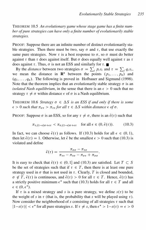
Evolutionarily Stable Strategies 235
THEOREM 10.5 An evolutionary game whose stage game has a finite num-
ber of pure strategies can have only a finite number of evolutionarily stable
strategies.
PROOF: Suppose there are an infinite number of distinct evolutionarily sta-
ble strategies. Then there must be two, say � and , that use exactly the
same pure strategies. Now is a best response to � , so � must do better
against than does against itself. But � does equally well against as
does against . Thus, � is not an ESS and similarly for .
By the distance between two strategies � D Pi pisi and D P
i qisi ,
we mean the distance in Rn between the points .p1; : : : ; pn/ and
.q1; : : : ; qn/. The following is proved in Hofbauer and Sigmund (1998).
Note that the theorem implies that an evolutionarily stable strategy � is an
isolated Nash equilibrium, in the sense that there is an � > 0 such that no
strategy ¤ � within distance � of � is a Nash equilibrium.
THEOREM 10.6 Strategy � 2 S is an ESS if and only if there is some
� > 0 such that ��� > ��� for all 2 S within distance � of � .
PROOF: Suppose � is an ESS, so for any ¤ � , there is an Q�./ such that
��;.1�/�C� < ��;.1�/�C� for all � 2 .0; Q�.//: (10.3)
In fact, we can choose Q�./ as follows. If (10.3) holds for all � 2 .0; 1/,
then let Q�./ D 1. Otherwise, let Q� be the smallest � > 0 such that (10.3) is
violated and define
Q�./ D ��� � ���
��� � ��� � ��� C ���
:
It is easy to check that Q�./ 2 .0; 1� and (10.3) are satisfied. Let T � S
be the set of strategies such that if 2 T , then there is at least one pure
strategy used in � that is not used in . Clearly, T is closed and bounded,
� 62 T , Q�./ is continuous, and Q�./ > 0 for all 2 T . Hence, Q�./ has
a strictly positive minimum �� such that (10.3) holds for all 2 T and all
� 2 .0; ��/.
If is a mixed strategy and s is a pure strategy, we define s./ to be
the weight of s in (that is, the probability that s will be played using ).
Now consider the neighborhood of s consisting of all strategies such that
j1�s./j < �� for all pure strategies s. If ¤ s, then �� > 1�s./ D � > 0
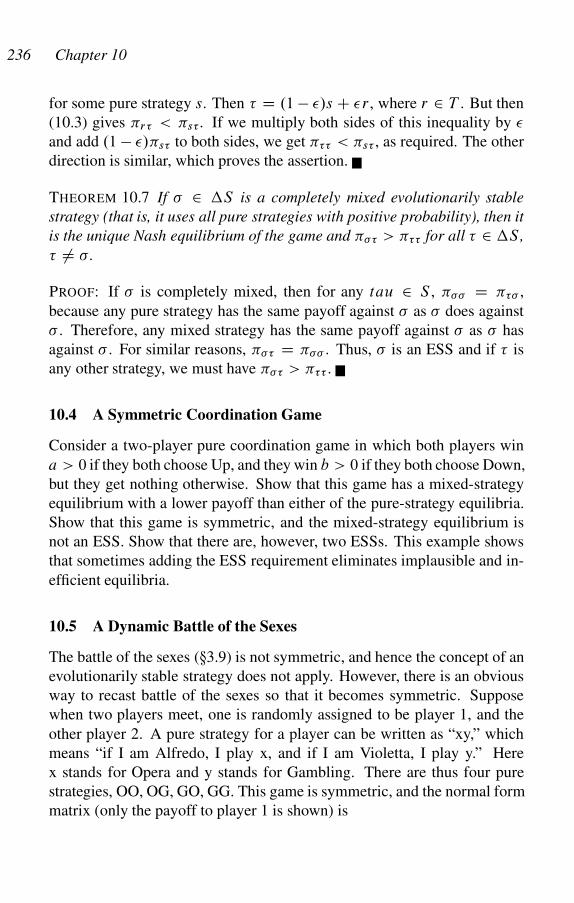
236 Chapter 10
for some pure strategy s. Then D .1 � �/s C �r , where r 2 T . But then
(10.3) gives �r� < �s� . If we multiply both sides of this inequality by �
and add .1 � �/�s� to both sides, we get ��� < �s� , as required. The other
direction is similar, which proves the assertion.
THEOREM 10.7 If � 2 S is a completely mixed evolutionarily stable
strategy (that is, it uses all pure strategies with positive probability), then it
is the unique Nash equilibrium of the game and ��� > ��� for all 2 S ,
¤ � .
PROOF: If � is completely mixed, then for any tau 2 S , ��� D ��� ,
because any pure strategy has the same payoff against � as � does against
� . Therefore, any mixed strategy has the same payoff against � as � has
against � . For similar reasons, ��� D ��� . Thus, � is an ESS and if is
any other strategy, we must have ��� > ��� .
10.4 A Symmetric Coordination Game
Consider a two-player pure coordination game in which both players win
a > 0 if they both choose Up, and they win b > 0 if they both choose Down,
but they get nothing otherwise. Show that this game has a mixed-strategy
equilibrium with a lower payoff than either of the pure-strategy equilibria.
Show that this game is symmetric, and the mixed-strategy equilibrium is
not an ESS. Show that there are, however, two ESSs. This example shows
that sometimes adding the ESS requirement eliminates implausible and in-
efficient equilibria.
10.5 A Dynamic Battle of the Sexes
The battle of the sexes (�3.9) is not symmetric, and hence the concept of an
evolutionarily stable strategy does not apply. However, there is an obvious
way to recast battle of the sexes so that it becomes symmetric. Suppose
when two players meet, one is randomly assigned to be player 1, and the
other player 2. A pure strategy for a player can be written as “xy,” which
means “if I am Alfredo, I play x, and if I am Violetta, I play y.” Here
x stands for Opera and y stands for Gambling. There are thus four pure
strategies, OO, OG, GO, GG. This game is symmetric, and the normal form
matrix (only the payoff to player 1 is shown) is
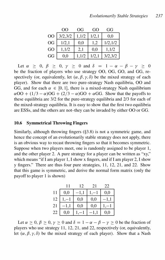
Evolutionarily Stable Strategies 237
OO OG GO GG
OO 3/2,3/2 1,1/2 1/2,1 0,0
OG 1/2,1 0,0 1,2 1/2,1/2
GO 1,1/2 2,1 0,0 1,1/2
GG 0,0 1,1/2 1/2,1 3/2,3/2
Let ˛ 0, ˇ 0, � 0 and ı D 1 � ˛ � ˇ � � 0
be the fraction of players who use strategy OO, OG, GO, and GG, re-
spectively (or, equivalently, let .˛; ˇ; �; ı/ be the mixed strategy of each
player). Show that there are two pure-strategy Nash equilibria, OO and
GG, and for each ˛ 2 Œ0; 1�, there is a mixed-strategy Nash equilibrium
˛OO C .1=3 � ˛/OG C .2=3 � ˛/GO C ˛GG. Show that the payoffs to
these equilibria are 3/2 for the pure-strategy equilibria and 2/3 for each of
the mixed-strategy equilibria. It is easy to show that the first two equilibria
are ESSs, and the others are not–they can be invaded by either OO or GG.
10.6 Symmetrical Throwing Fingers
Similarly, although throwing fingers (�3.8) is not a symmetric game, and
hence the concept of an evolutionarily stable strategy does not apply, there
is an obvious way to recast throwing fingers so that it becomes symmetric.
Suppose when two players meet, one is randomly assigned to be player 1,
and the other player 2. A pure strategy for a player can be written as “xy,”
which means “if I am player 1, I show x fingers, and if I am player 2, I show
y fingers.” There are thus four pure strategies, 11, 12, 21, and 22. Show
that this game is symmetric, and derive the normal form matrix (only the
payoff to player 1 is shown)
11 12 21 22
11 0,0 �1,1 1,�1 0,0
12 1,�1 0,0 0,0 �1,1
21 �1,1 0,0 0,0 1,�1
22 0,0 1,�1 �1,1 0,0
Let ˛ 0, ˇ 0, � 0 and ı D 1 � ˛ � ˇ � � 0 be the fraction of
players who use strategy 11, 12, 21, and 22, respectively (or, equivalently,
let .˛; ˇ; �; ı/ be the mixed strategy of each player). Show that a Nash

238 Chapter 10
equilibrium is characterized by ˛ D 1=2�� , ˇ D � (which implies ı D ˛/.
It is easy to show that any such Nash equilibrium can be invaded by any
distinct strategy .˛0; ˇ0; � 0; ı0/ with ˛0 D 1=2 � � 0, ˇ0 D � 0, so there is no
evolutionarily stable strategy for throwing fingers.
10.7 Hawks, Doves, and Bourgeois
THEOREM 10.8 The mixed-strategy equilibrium in the hawk-dove game
(�3.10) is an ESS.
PROOF: The payoff to H is ˛.v � w/=2 C .1 � ˛/v = v � ˛.v C w/=2,
and the payoff to D is .1 � ˛/.v=2/ D v=2 � ˛.v=2/. These are equated
when ˛ D v=w, which is < 1 if w > v. To show that this mixed-strategy
equilibrium is an ESS, note that �11 D .v�w/=2, �21 D 0, �22 D v=2, and
�12 D v. Thus �11 D .v � w/=2 < 0 D �21 and �22 D v=2 < v D �12,
so the equilibrium is an ESS.
Note that in the hawk-dove-bourgeois game (�6.41), the bourgeois strat-
egy is a strict Nash equilibrium, and hence is an ESS.
10.8 Trust in Networks II
We now show that the completely mixed Nash equilibrium found in trust in
networks (�6.23) is not an ESS and can be invaded by trusters. In case you
think this means this equilibrium is dynamically unstable, think again! See
Trust in Networks III (�12.10).
For specificity, we take p D 0:8. You can check that the equilibrium has
inspect share ˛� � 0:71 trust share ˇ� � 0:19, and defect share �� � 0:10.
The payoff to the equilibrium strategy s is �ss � 0:57. The payoff to trust
against the equilibrium strategy is of course �ts D �ss � 0:57, but the
payoff to trust against itself is �t t D 1, so trust can invade.
10.9 Cooperative Fishing
In a certain fishing village, two fisherman gain from having the nets put out
in the evening. However, the fishermen benefit equally whether or not they
share the costs of putting out the nets. Suppose the expected catch is �, the
cost of putting out the nets to each is c1 if each fisherman does it alone, and
the cost to each is c2 < c1 if they do it together. We assume �=2 > c1, so it
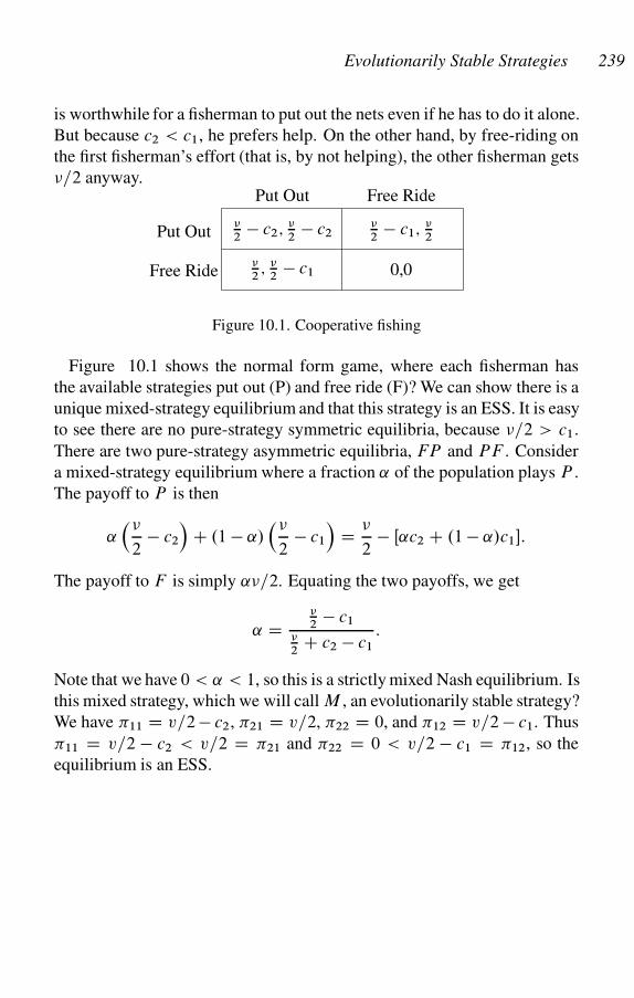
Evolutionarily Stable Strategies 239
is worthwhile for a fisherman to put out the nets even if he has to do it alone.
But because c2 < c1, he prefers help. On the other hand, by free-riding on
the first fisherman’s effort (that is, by not helping), the other fisherman gets
�=2 anyway.
�2
� c2; �2
� c2
�2; �
2� c1
Put Out
�2
� c1; �2
0,0
Free Ride
Put Out
Free Ride
Figure 10.1. Cooperative fishing
Figure 10.1 shows the normal form game, where each fisherman has
the available strategies put out (P) and free ride (F)? We can show there is a
unique mixed-strategy equilibrium and that this strategy is an ESS. It is easy
to see there are no pure-strategy symmetric equilibria, because �=2 > c1.
There are two pure-strategy asymmetric equilibria, FP and PF . Consider
a mixed-strategy equilibrium where a fraction ˛ of the population plays P .
The payoff to P is then
˛��
2� c2
�C .1 � ˛/
��
2� c1
�D �
2� Œ˛c2 C .1 � ˛/c1�:
The payoff to F is simply ˛�=2. Equating the two payoffs, we get
˛ D�2
� c1
�2
C c2 � c1
:
Note that we have 0 < ˛ < 1, so this is a strictly mixed Nash equilibrium. Is
this mixed strategy, which we will call M , an evolutionarily stable strategy?
We have �11 D v=2 � c2, �21 D v=2, �22 D 0, and �12 D v=2 � c1. Thus
�11 D v=2 � c2 < v=2 D �21 and �22 D 0 < v=2 � c1 D �12, so the
equilibrium is an ESS.
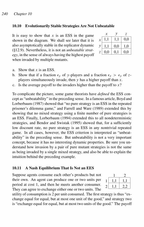
240 Chapter 10
10.10 Evolutionarily Stable Strategies Are Not Unbeatable
1,1 1,1 0,0
1,1 0,0 1,0
0,0 0,1 0,0
x y z
x
y
z
It is easy to show that x is an ESS in the game
shown in the diagram. We shall see later that it is
also asymptotically stable in the replicator dynamic
(�12.9). Nevertheless, it is not an unbeatable strat-
egy, in the sense of always having the highest payoff
when invaded by multiple mutants.
a. Show that x is an ESS.
b. Show that if a fraction �y of y-players and a fraction �z > �y of z-
players simultaneously invade, then y has a higher payoff than x.
c. Is the average payoff to the invaders higher than the payoff to x?
To complicate the picture, some game theorists have defined the ESS con-
cept as “unbeatability” in the preceding sense. In a famous article, Boyd and
Lorberbaum (1987) showed that “no pure strategy is an ESS in the repeated
prisoner’s dilemma game,” and Farrell and Ware (1989) extended this by
showing that no mixed strategy using a finite number of pure strategies is
an ESS. Finally, Lorberbaum (1994) extended this to all nondeterministic
strategies, and Bendor and Swistak (1995) showed that, for a sufficiently
low discount rate, no pure strategy is an ESS in any nontrivial repeated
game. In all cases, however, the ESS criterion is interpreted as “unbeat-
ability” in the preceding sense. But unbeatability is not a very important
concept, because it has no interesting dynamic properties. Be sure you un-
derstand how invasion by a pair of pure mutant strategies is not the same
as being invaded by a single mixed strategy, and also be able to explain the
intuition behind the preceding example.
10.11 A Nash Equilibrium That Is Not an EES
1,1
1,1
1,1
2,2
1 2
1
2
Suppose agents consume each other’s products but not
their own. An agent can produce one or two units per
period at cost 1, and then he meets another consumer.
They can agree to exchange either one or two units. The
utility of consumption is 2 per unit consumed. The first strategy is thus “ex-
change equal for equal, but at most one unit of the good,” and strategy two
is “exchange equal for equal, but at most two units of the good.” The payoff
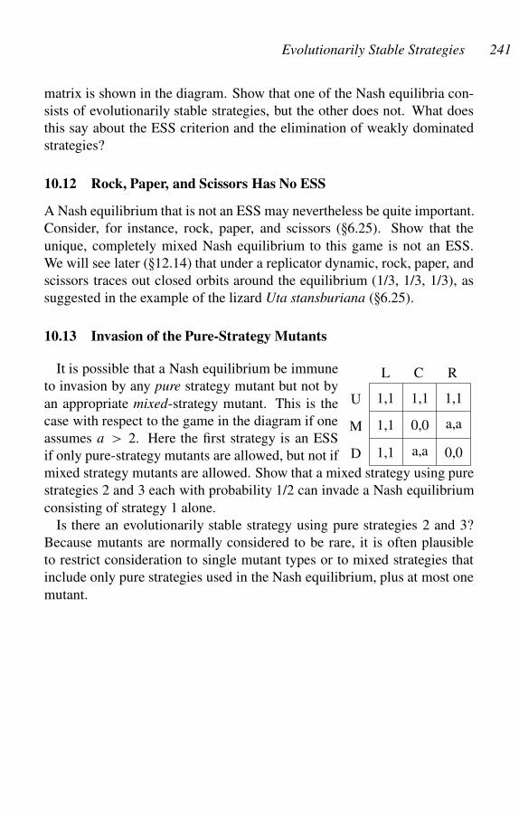
Evolutionarily Stable Strategies 241
matrix is shown in the diagram. Show that one of the Nash equilibria con-
sists of evolutionarily stable strategies, but the other does not. What does
this say about the ESS criterion and the elimination of weakly dominated
strategies?
10.12 Rock, Paper, and Scissors Has No ESS
A Nash equilibrium that is not an ESS may nevertheless be quite important.
Consider, for instance, rock, paper, and scissors (�6.25). Show that the
unique, completely mixed Nash equilibrium to this game is not an ESS.
We will see later (�12.14) that under a replicator dynamic, rock, paper, and
scissors traces out closed orbits around the equilibrium (1/3, 1/3, 1/3), as
suggested in the example of the lizard Uta stansburiana (�6.25).
10.13 Invasion of the Pure-Strategy Mutants
1,1 1,1 1,1
1,1 0,0 a,a
1,1 a,a 0,0
U
M
D
L C RIt is possible that a Nash equilibrium be immune
to invasion by any pure strategy mutant but not by
an appropriate mixed-strategy mutant. This is the
case with respect to the game in the diagram if one
assumes a > 2. Here the first strategy is an ESS
if only pure-strategy mutants are allowed, but not if
mixed strategy mutants are allowed. Show that a mixed strategy using pure
strategies 2 and 3 each with probability 1/2 can invade a Nash equilibrium
consisting of strategy 1 alone.
Is there an evolutionarily stable strategy using pure strategies 2 and 3?
Because mutants are normally considered to be rare, it is often plausible
to restrict consideration to single mutant types or to mixed strategies that
include only pure strategies used in the Nash equilibrium, plus at most one
mutant.
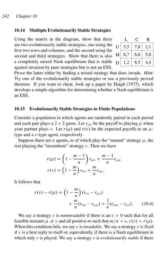
242 Chapter 10
10.14 Multiple Evolutionarily Stable Strategies
4,48,51,2
5,86,68,7
2,17,85,5
RCL
D
M
U
Using the matrix in the diagram, show that there
are two evolutionarily stable strategies, one using the
first two rows and columns, and the second using the
second and third strategies. Show that there is also
a completely mixed Nash equilibrium that is stable
against invasion by pure strategies but is not an ESS.
Prove the latter either by finding a mixed strategy that does invade. Hint:
Try one of the evolutionarily stable strategies or use a previously proved
theorem. If you want to cheat, look up a paper by Haigh (1975), which
develops a simple algorithm for determining whether a Nash equilibrium is
an ESS.
10.15 Evolutionarily Stable Strategies in Finite Populations
Consider a population in which agents are randomly paired in each period
and each pair plays a 2 � 2 game. Let r� be the payoff to playing � when
your partner plays �. Let r.�/ and r.�/ be the expected payoffs to an �-
type and a �-type agent, respectively.
Suppose there are n agents, m of which play the “mutant” strategy �, the
rest playing the “incumbent” strategy �. Then we have
r.�/ D�
1 � m � 1
n
�r� C m � 1
nr
r.�/ D�
1 � m
n
�r�� C m
nr�:
It follows that
r.�/ � r.�/ D�1 � m
n
�.r�� � r�/
C m
n.r� � r/ C 1
n.r � r�/: (10.4)
We say a strategy � is noninvadable if there is an � > 0 such that for all
feasible mutants � ¤ � and all positive m such that m=n < �, r.�/ > r.�/.
When this condition fails, we say � is invadable. We say a strategy � is Nash
if � is a best reply to itself or, equivalently, if there is a Nash equilibrium in
which only � is played. We say a strategy � is evolutionarily stable if there
Evolutionarily Stable Strategies 243
is a population size n such that � is noninvadable for all populations of size
n or greater.
While it is obviously possible for a Nash strategy to be invadable, it is
also possible for a non-Nash strategy to be noninvadable, even by a Nash
strategy. To see this, let r� D 0, r� D n, r D n C 1, and r�� D �1.
Then � is not Nash, because r� > r�� , � is Nash because r > r� and
r > r�. But, r.�/ � r.�/ D 1=n > 0 for any m.
THEOREM 10.9 Strategy � is evolutionarily stable if and only if � is a Nash
strategy, and for any � that is a best reply to �, � is a better reply to � than
� is to itself, or if � is as good a reply to itself as � is to �, then � is a
better reply to itself than � is to �.
PROOF: Suppose � is evolutionarily stable but is not Nash. Then there is
some � such that r�� < r� . Let m D 1. Then for sufficiently large n we
have r.�/ < r.�/ in
r.�/ � r.�/ D�1 � m
n
�.r�� � r�/
C m
n.r� � r/ C 1
n.r � r�/: (10.5)
Hence, � must be Nash. Now suppose � is evolutionarily stable and r�� Dr� but r� < r. Equation (10.5) becomes
r.�/ � r.�/ D 1
n
˚mŒr� � r� C Œr � r��
:
Given � > 0, choose m so that the term in brackets is negative, and then
choose n so that m=n < �. Then r.�/ < r.�/ for all positive m � m, which
is a contradiction. So suppose in addition to r�� D r� and r� D r, we
have r < r�. Then clearly r.�/ � r.�/ D Œr � r��=n < 0, again a
contradiction. This proves that the stated conditions are necessary. We can
reverse the argument to prove the conditions are sufficient as well.
The forgoing conditions are not those of Maynard Smith, which state that
� is evolutionarily stable if and only if � is Nash and for any � that is a best
reply to n, � is a better reply to � than � is to itself or, equivalently, for any
mutant �, either r�� > r� , or r�� D r� and r� > r. However, we can
derive Maynard Smith’s conditions by letting m; n ! 1 in (10.4) in such
a manner that m=n D �, but the limit argument cannot be used to conclude
that r.�/ > r.�/ in the “large finite” case.
244 Chapter 10
To see this, note that in the limit we have
r.�/ � r.�/ D .1 � �/Œr�� � r�� C �Œr� � r�:
The conclusion follows immediately from this equation. The limit argu-
ment cannot be used to conclude that r.�/ > r.�/ in the “large finite” case
if r�� D r� and r� D r.
Let p D m=n, a D r���r� , b D r��r�r��Cr� , and c D r�r� .
Then (10.4) becomes
r.�/ � r.�/ D 1
n.na C mb C c/: (10.6)
Suppose � can be invaded by mutant strategy �, and the system follows any
dynamic in which a strategy with a higher payoff increases in frequency.
Then, if n.a C b/ > c, � will invade until � is the largest integer less than
�.na C c/=b. Otherwise � will invade until � is extinct.
In the case of partial invasion in the preceding example, we say � is
quasi-evolutionarily stable. Note that � is quasi-evolutionarily stable with
respect to � for very large n if and only if � and � are part of a completely
mixed Nash equilibrium (assuming there are no other feasible pure strate-
gies).
10.16 Evolutionarily Stable Strategies in Asymmetric Games
Many situations can be modeled as evolutionary games, except for the fact
that the two players are not interchangeable. For instance, in one-card two-
round poker with bluffing (�6.21), the player going first has a different set of
strategies from the player going second. Yet, despite the lack of symmetry,
we simulated the game quite nicely as an evolutionary game. Analogous
situations include interactions between predator and prey, boss and worker,
male and female, incumbent and intruder, among a host of others.
This is not simply a technicality; it makes no sense to say that a “mutant
meets its own type” when the game is asymmetric, so the ESS criterion has
no meaning. The obvious way around this problem is to define a homo-
geneous set of players who in each period are paired randomly, one of the
pair being randomly assigned to be player 1, and the other to be player 2.
We may call this the “symmetric version” of the asymmetric evolutionary
game. However, an evolutionarily stable strategy in the symmetric version
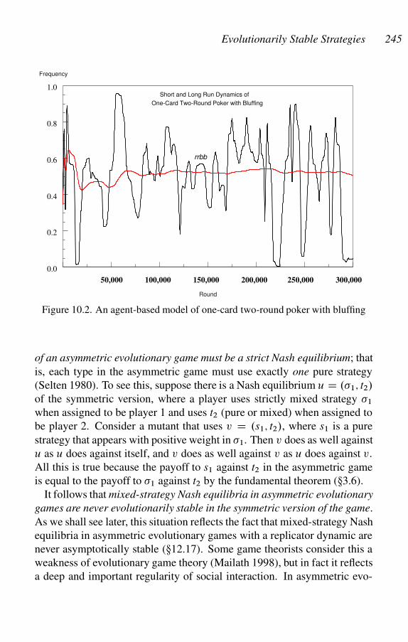
Evolutionarily Stable Strategies 245
rrbb
50,000 100,000 150,000 200,000 250,000 300,000
0.0
0.2
0.4
0.6
0.8
1.0
Frequency
Short and Long Run Dynamics of
One-Card Two-Round Poker with Bluffing
Round
Figure 10.2. An agent-based model of one-card two-round poker with bluffing
of an asymmetric evolutionary game must be a strict Nash equilibrium; that
is, each type in the asymmetric game must use exactly one pure strategy
(Selten 1980). To see this, suppose there is a Nash equilibrium u D .�1; t2/
of the symmetric version, where a player uses strictly mixed strategy �1
when assigned to be player 1 and uses t2 (pure or mixed) when assigned to
be player 2. Consider a mutant that uses v D .s1; t2/, where s1 is a pure
strategy that appears with positive weight in �1. Then v does as well against
u as u does against itself, and v does as well against v as u does against v.
All this is true because the payoff to s1 against t2 in the asymmetric game
is equal to the payoff to �1 against t2 by the fundamental theorem (�3.6).
It follows that mixed-strategy Nash equilibria in asymmetric evolutionary
games are never evolutionarily stable in the symmetric version of the game.
As we shall see later, this situation reflects the fact that mixed-strategy Nash
equilibria in asymmetric evolutionary games with a replicator dynamic are
never asymptotically stable (�12.17). Some game theorists consider this a
weakness of evolutionary game theory (Mailath 1998), but in fact it reflects
a deep and important regularity of social interaction. In asymmetric evo-
246 Chapter 10
lutionary games, the frequency of different types of behavior goes through
periodic cycles through time.
For a dramatic example of this important insight, we return to our model
of one-card two-round poker with bluffing (figure 6.6). In this agent-based
model, I lowered the mutation rate to 1% and ran the model for 300,000
periods. The results are shown in figure 10.2 for one of the player 1 types,
rrbb (bluff all the way). Note that the average frequency of each strategy
settles down to the theoretically predicted equilibrium value, but the period-
to-period frequencies fluctuate wildly in the medium run. Strategy rrbb,
which has the equilibrium frequency of about 50%, sometimes goes for
thousands of periods with frequency under 5% or over 90%.
11
Dynamical Systems
History is Spirit at war with itself.
Georg Wilhelm Freidrich Hegel
We have studied Nash equilibria of games, but do games reach Nash equi-
librium and, if so, by what process? If there are several Nash equilibria, to
which one does the game go? Indeed, what are Nash equilibria equilibria
of? To answer these questions we will study the behavior of dynamical
systems that are generally not in equilibrium but which, under appropriate
conditions, approach a state of equilibrium over time, or orbit equilibria the
way planets orbit the sun, or have some other love-hate relationship with
equilibria (e.g., strange attractors).
We can apply several analytical tools in treating strategic interactions
as dynamical systems, including difference equations, stochastic processes
(such as Markov chains and diffusion processes), statistical mechanics, and
differential equations. The differential equation approach is the most basic
and has the quickest payoff, so that is what we will develop in this chapter.
11.1 Dynamical Systems: Definition
Suppose x D .x1; : : : ; xn/ is a point in n-dimensional space Rn that traces
out a curve through time. We can describe this as
x D x.t/ D .x1.t/; : : : ; xn.t// for � 1 < t < 1:
Often we do not know x.t/ directly, but we do know the forces determining
its rate and direction of change in some region of Rn. We thus have
Px D f .x/ x 2 Rn; (11.1)
where the “dot” indicates the derivative with respect to t , so Px D dx=dt .
We always assume f has continuous partial derivatives. If we write these
vector equations out in full, we get
247
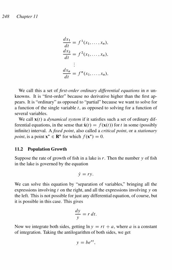
248 Chapter 11
dx1
dtD f 1.x1; : : : ; xn/;
dx2
dtD f 2.x1; : : : ; xn/;
:::dxn
dtD f n.x1; : : : ; xn/;
We call this a set of first-order ordinary differential equations in n un-
knowns. It is “first-order” because no derivative higher than the first ap-
pears. It is “ordinary” as opposed to “partial” because we want to solve for
a function of the single variable t , as opposed to solving for a function of
several variables.
We call x.t/ a dynamical system if it satisfies such a set of ordinary dif-
ferential equations, in the sense that Px.t/ D f .x.t// for t in some (possibly
infinite) interval. A fixed point, also called a critical point, or a stationary
point, is a point x� 2 Rn for which f .x�/ D 0.
11.2 Population Growth
Suppose the rate of growth of fish in a lake is r . Then the number y of fish
in the lake is governed by the equation
Py D ry:
We can solve this equation by “separation of variables,” bringing all the
expressions involving t on the right, and all the expressions involving y on
the left. This is not possible for just any differential equation, of course, but
it is possible in this case. This gives
dy
yD r dt:
Now we integrate both sides, getting ln y D rt C a, where a is a constant
of integration. Taking the antilogarithm of both sides, we get
y D bert ;
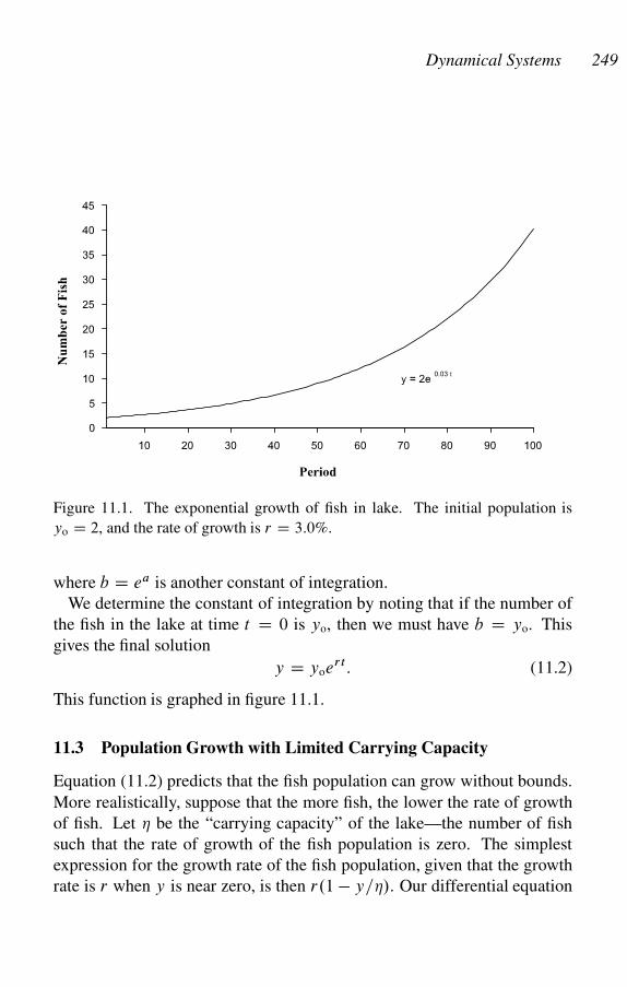
Dynamical Systems 249
Figure 11.1. The exponential growth of fish in lake. The initial population is
yo D 2, and the rate of growth is r D 3:0%.
where b D ea is another constant of integration.
We determine the constant of integration by noting that if the number of
the fish in the lake at time t D 0 is yo, then we must have b D yo. This
gives the final solution
y D yoert: (11.2)
This function is graphed in figure 11.1.
11.3 Population Growth with Limited Carrying Capacity
Equation (11.2) predicts that the fish population can grow without bounds.
More realistically, suppose that the more fish, the lower the rate of growth
of fish. Let � be the “carrying capacity” of the lake—the number of fish
such that the rate of growth of the fish population is zero. The simplest
expression for the growth rate of the fish population, given that the growth
rate is r when y is near zero, is then r.1 � y=�/. Our differential equation
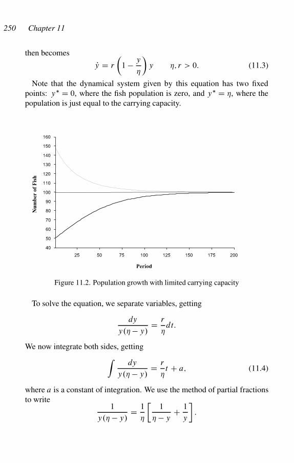
250 Chapter 11
then becomes
Py D r
�1 � y
�
�y �; r > 0: (11.3)
Note that the dynamical system given by this equation has two fixed
points: y� D 0, where the fish population is zero, and y� D �, where the
population is just equal to the carrying capacity.
Figure 11.2. Population growth with limited carrying capacity
To solve the equation, we separate variables, getting
dy
y.� � y/D r
�dt:
We now integrate both sides, getting
Zdy
y.� � y/D r
�t C a; (11.4)
where a is a constant of integration. We use the method of partial fractions
to write1
y.� � y/D 1
�
�1
� � yC 1
y
�:
Dynamical Systems 251
Thus, we have
Zdy
y.� � y/D 1
�
�Zdy
� � yCZ
dy
y
�
D 1
�ln
y
� � y:
Substituting into (11.4), we get
lny
� � yD rt C a�:
Taking antilogarithms of both sides, this becomes
y
� � yD bert ;
where b D ea� is another constant of integration. If the number of fish in
the lake at time t D 0 is yo, then we must have b D yo=.� � yo/, which
can be either positive or negative, depending on whether the initial fish
population is larger or smaller than the stationary population size �.
Now we can solve this equation for y, getting
y D �
Ae�rt C 1;
where A D .� � yo/=yo. Note that this equation predicts a smooth move-
ment from disequilibrium to stationarity as t ! 1. A picture of the process
is given in figure 11.2.
11.4 The Lotka-Volterra Predator-Prey Model
Foxes eat rabbits. Suppose we normalize the rabbit population at a point
in time to a fraction x of its maximum, given the carrying capacity of its
habitat when foxes are absent, and suppose the fox population at a point in
time is a fraction y of its maximum, given the carrying capacity of its habitat
when there is an unlimited supply of rabbits. Suppose foxes are born at the
rate ı1x but die at the rate �1.1�x/. We then have Py=y D ı1x ��1.1�x/,
which we can write as
Py D ıy.x � �/; ı > 0; 1 > � > 0; (11.5)
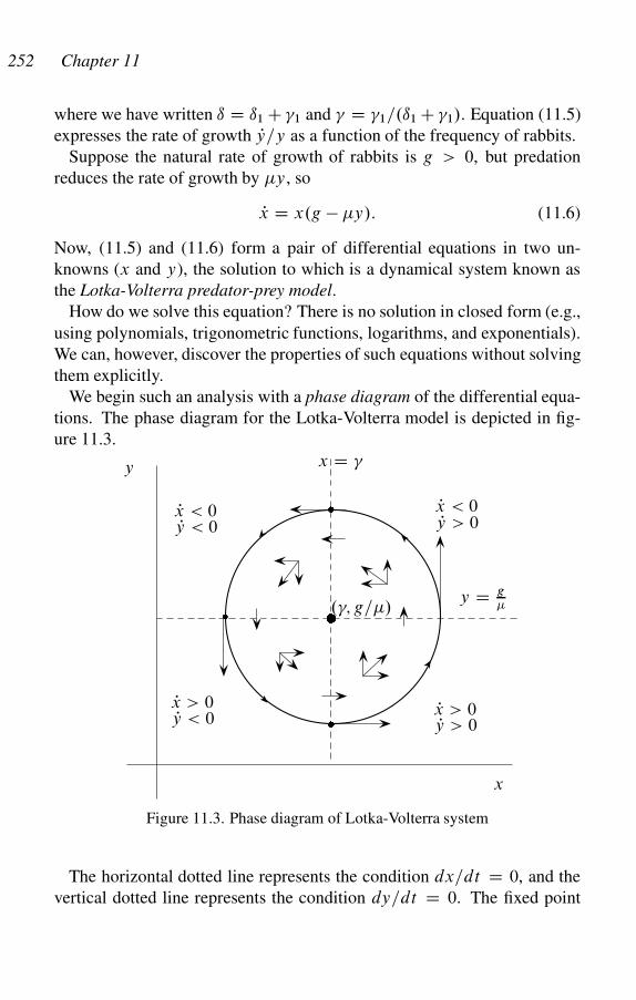
252 Chapter 11
where we have written ı D ı1 C �1 and � D �1=.ı1 C �1/. Equation (11.5)
expresses the rate of growth Py=y as a function of the frequency of rabbits.
Suppose the natural rate of growth of rabbits is g > 0, but predation
reduces the rate of growth by �y, so
Px D x.g � �y/: (11.6)
Now, (11.5) and (11.6) form a pair of differential equations in two un-
knowns (x and y), the solution to which is a dynamical system known as
the Lotka-Volterra predator-prey model.
How do we solve this equation? There is no solution in closed form (e.g.,
using polynomials, trigonometric functions, logarithms, and exponentials).
We can, however, discover the properties of such equations without solving
them explicitly.
We begin such an analysis with a phase diagram of the differential equa-
tions. The phase diagram for the Lotka-Volterra model is depicted in fig-
ure 11.3.
Px < 0
x
y x D �
y D g
� .�; g=�/�
�
�
Py < 0
Px < 0Py > 0
Px > 0Py > 0
Px > 0Py < 0
Figure 11.3. Phase diagram of Lotka-Volterra system
The horizontal dotted line represents the condition dx=dt D 0, and the
vertical dotted line represents the condition dy=dt D 0. The fixed point
Dynamical Systems 253
is at .�; g=�/, where the two intersect. The little arrows show in which
direction the flow of the dynamical system moves for that particular point
.x; y/. The arrows point northward when dy=dt > 0 and southward when
dy=dt < 0, and they point eastward when dx=dt > 0 and westward when
dx=dt < 0. The arrows are vertical where dx=dt D 0 because motion is
purely north-south instantaneously at such a point, and are horizontal where
dy=dt D 0, because motion is purely east-west at such a point. In each of
the four quadrants marked off by the dotted lines, the direction of the flow
is qualitatively similar. Thus to the northeast of the fixed point, the flow
is northwest; to the northwest, the flow is southwest; to the southwest, the
flow is southeast; and to the southeast of the fixed point, the flow is to the
northeast. So it is clear that the flow circles counterclockwise about the
fixed point. However, we cannot tell a priori whether the flow circles into
the fixed point, circles outward to infinity, or forms closed circuits about
the fixed point.
To show that the Lotka-Volterra has closed orbits (�11.5), we find a func-
tion that is constant on any trajectory of the dynamical system and show
that this function is monotonic (strictly increasing or decreasing) along a
ray starting from the fixed point and pointing northeast.1
Suppose we have such a function f and consider a path starting at a
point x on the ray, making one complete revolution around the fixed point
and hitting the ray again, say at y. Because f is constant on the path,
f .x/ D f .y/. But because f is monotonic on the ray, we must have
x D y, so the path is a closed orbit (�11.5). First, we eliminate t from the
equations for Px and Py by dividing the first by the second, getting
dy
dxD ıy.x � �/
x.g � �y/:
Now we separate variables, pulling all the x’s to the right, and all the y’s to
the left:
g � �y
ydy D ı.x � �/
xdx:
1We say a function f .x/ is (1) increasing if x > y implies f .x/ � f .y/; (2)
strictly increasing if x > y implies f .x/ > f .y/; (3) decreasing if x > y implies
f .x/ � f .y/; and (4) strictly decreasing if x > y implies f .x/ < f .y/.
254 Chapter 11
Now we integrate both sides, getting
g ln y � �y D ıx � ı� ln x C C;
where C is an arbitrary constant of integration. Bringing all the variables
over to the left and taking the antilogarithm, we get
ygxı� e�.yCıx/ D eC : (11.7)
So now we have an expression that is constant along any trajectory of the
Lotka-Volterra dynamical system.
Now, consider a ray .x; y/ that starts at the fixed point .�; g=�/ and
moves to the northeast in a direction heading away from the origin. We
can write this as x D �s, y D .g=�/s, where s is a parameter measuring
the distance from the fixed point. Note that when s D 1, .x; y/ is at the
fixed point. Substituting in (11.7), we get
�g
�
�g
� ı�sgCı�e�.gCı�/s D eC :
This looks forbidding, but it’s really not. We pull the first two terms on the
left over to the right, and then take the .g C ı� )-th root of both sides. The
right-hand side is a complicated constant, which we can abbreviate by D,
and the left is just se�s, so we have
se�s D D: (11.8)
If we can show that the left-hand side is strictly decreasing for s > 1, we
are done, because then any s > 1 that satisfies (11.8) must be unique. We
take the derivative of the left-hand side, getting
e�s � se�s D .1 � s/e�s;
which is negative for s > 1. This shows that the dynamical system moves
in closed orbits (�11.5) around the fixed point.
It follows from this analysis that if the system begins out of equilibrium,
both the fraction of rabbits and foxes will go through constant-amplitude
oscillations around their equilibrium values forever. We shall later char-
acterize this as an asymmetric evolutionary game (�12.17) for which this
oscillatory behavior is quite typical.
Dynamical Systems 255
11.5 Dynamical Systems Theory
With these examples under our belt, we can address the basic theory of
dynamical systems (a.k.a. differential equations).2
Suppose a dynamical system is at a point xo at time to. We call the locus of
points through which the system passes as t ! 1 the forward trajectory
of the system through xo, or the trajectory of the system starting at xo.
The backward trajectory of the system through xo is the locus of points
through which the system passes as t ! �1. The forward and backward
trajectories are together called the trajectory through xo.
Clearly if a dynamical system is at a fixed point x�, it will stay there
forever, so the trajectory starting at x� is simply x� itself. However, if we
perturb the system a little from x� by choosing a new initial point xo at time
t D 0, there are several things that can happen. We begin with a couple of
definitions. If x 2 Rn, and r > 0, we define a ball of radius r around x,
which we write Br.x/, as the set of points y 2 Rn whose distance from x
is less than r . We define a neighborhood of x to be any subset of Rn that
contains some ball around x. Finally, we say a set in Rn is an open set if it
is a neighborhood of each of its points. Note that a set is open if and only
if it contains a ball of some positive radius around each of its points.
We define an �-perturbation of the dynamical system at a fixed point x�
to be a trajectory of the system starting at some xo 2 B.x�/, where � > 0
and xo ¤ x�. We say a trajectory x.t/ approaches x� if x.t/ ! x� as
t ! 1. We say a trajectory x.t/ �-escapes x� if there is some to such that
x.t/ 62 B.x�/ for t > to; that is, after some point in time, the trajectory
never gets closer than � to x�.
If there is some � > 0 such that for any xo 2 B.x�/, the trajectory
through xo approaches x�, we say the fixed point at x� is asymptotically
stable. The set of points xo 2 Rn such that a trajectory through xo ap-
proaches x� is called the basin of attraction of the fixed point x�. If every
point where the differential equation is defined is in the basin of attraction
of x�, we say the fixed point is globally stable.
If x� is not asymptotically stable, but for any ball B.x�/ there is another
ball Bı.x�/ such that for any point xo 2 Bı.x�/, the trajectory starting at xo
2There are many excellent texts on differential equations. Some of my favorites
are Perko 1991, Hirsch and Smale 1974, Epstein 1997, and Hofbauer and Sigmund
1998. The last of these is a beautiful summary of evolutionary dynamics.
256 Chapter 11
never leaves B.x�/, we say the fixed point at x� is neutrally stable. Neutral
stability means that a sufficiently small perturbation about the fixed point
never leads the system too far away from the fixed point. A special case
is when any trajectory through xo 2 B.x�/ is a closed orbit; that is, the
trajectory starting at xo eventually returns to xo.
If x� is neither asymptotically stable nor neutrally stable, we say x� is
unstable. Thus, x� is unstable if there is an � > 0 such that for any ball
Bı.x�/, there is a point xo 2 Bı.x�/ such that the trajectory starting at xo
�-escapes x�.
11.6 Existence and Uniqueness
THEOREM 11.1 Existence, Uniqueness, and Continuous Dependence on
Initial Conditions. Suppose that f in equation (11.1) has continuous
derivatives on an open set D containing a point xo. Then there is some
interval I D Œ�to; to� and a unique trajectory x.t/ satisfying (11.1) defined
on I with x.0/ D xo. Moreover, x.t/ depends smoothly upon xo in the
following sense: there is some ı > 0, and a unique function x.t; y/ that
satisfies (11.1) on an interval Œ�t1; t1� with x.0; y/ D y, for all y 2 Bı.xo/.
Moreover, x.t; y/ has continuous partial derivatives, and continuous sec-
ond partial derivatives with respect to t .
This theorem says that if f .x/ is suitably well behaved, the dynamical sys-
tem (11.1) has a unique, twice-differentiable trajectory through each point
xo, and the trajectory varies differentiably as we vary xo. In particular, two
trajectories can never cross.
THEOREM 11.2 Continuous Dependence on Parameters. Let � 2 Rk be a
set of k parameters, and suppose f .x; �/ has continuous partial derivatives
in a neighborhood of .xo; �o/ 2 RnCk . Then there is a t1 > 0, a ı > 0, an
� > 0, and a unique function x.t; y; �/ that satisfies
Px D f .x.t; y; �/; �/ (11.9)
with x.0; y; �/ D y, for t 2 Œ�t1; t1�, y 2 Bı.xo/, and � 2 B.�o/. More-
over, x.t; y; �/ has continuous partial derivatives.
This theorem says that if f .x; �/ is suitably well behaved, the trajectories
of the dynamical system (11.9) vary differentiably as we vary the parame-
ters �.
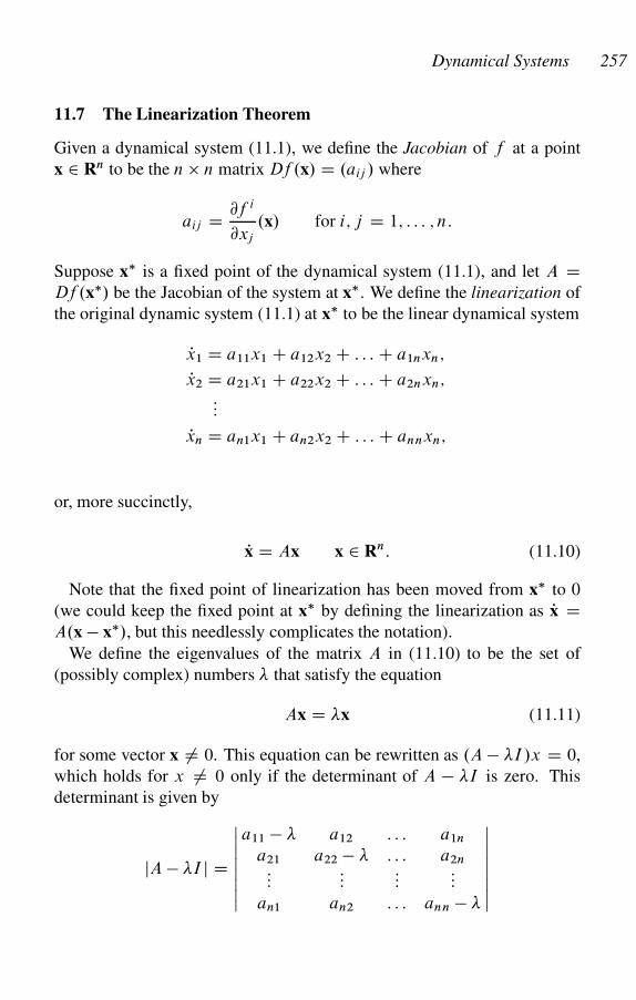
Dynamical Systems 257
11.7 The Linearization Theorem
Given a dynamical system (11.1), we define the Jacobian of f at a point
x 2 Rn to be the n � n matrix Df .x/ D .aij / where
aij D @f i
@xj
.x/ for i; j D 1; : : : ; n:
Suppose x� is a fixed point of the dynamical system (11.1), and let A DDf .x�/ be the Jacobian of the system at x�. We define the linearization of
the original dynamic system (11.1) at x� to be the linear dynamical system
Px1 D a11x1 C a12x2 C : : : C a1nxn;
Px2 D a21x1 C a22x2 C : : : C a2nxn;:::
Pxn D an1x1 C an2x2 C : : : C annxn;
or, more succinctly,
Px D Ax x 2 Rn: (11.10)
Note that the fixed point of linearization has been moved from x� to 0
(we could keep the fixed point at x� by defining the linearization as Px DA.x � x�/, but this needlessly complicates the notation).
We define the eigenvalues of the matrix A in (11.10) to be the set of
(possibly complex) numbers � that satisfy the equation
Ax D �x (11.11)
for some vector x ¤ 0. This equation can be rewritten as .A � �I/x D 0,
which holds for x ¤ 0 only if the determinant of A � �I is zero. This
determinant is given by
jA � �I j D
ˇˇˇˇ
a11 � � a12 : : : a1n
a21 a22 � � : : : a2n:::
::::::
:::
an1 an2 : : : ann � �
ˇˇˇˇ
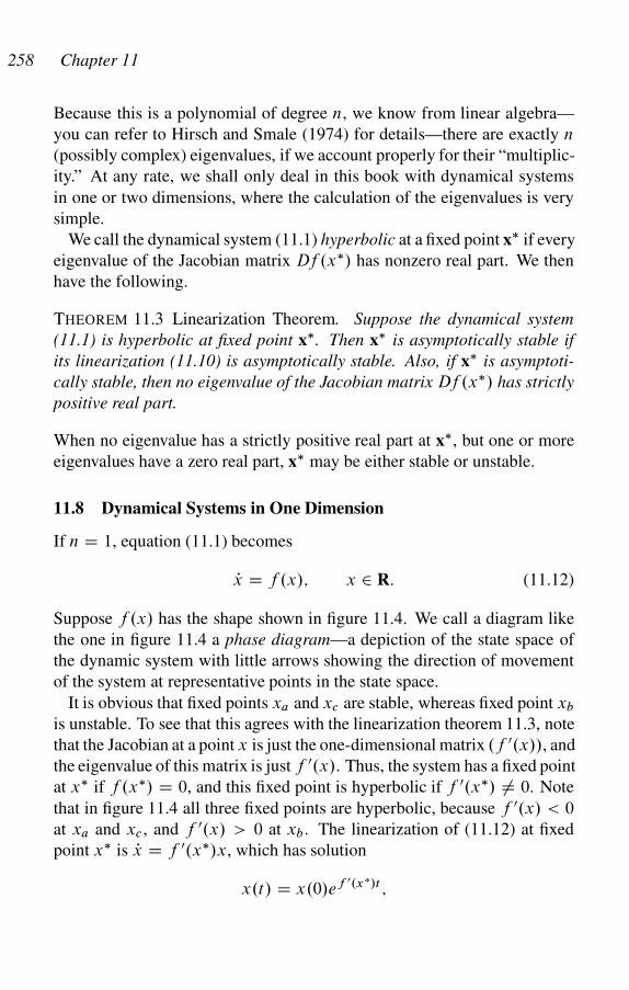
258 Chapter 11
Because this is a polynomial of degree n, we know from linear algebra—
you can refer to Hirsch and Smale (1974) for details—there are exactly n
(possibly complex) eigenvalues, if we account properly for their “multiplic-
ity.” At any rate, we shall only deal in this book with dynamical systems
in one or two dimensions, where the calculation of the eigenvalues is very
simple.
We call the dynamical system (11.1) hyperbolic at a fixed point x� if every
eigenvalue of the Jacobian matrix Df .x�/ has nonzero real part. We then
have the following.
THEOREM 11.3 Linearization Theorem. Suppose the dynamical system
(11.1) is hyperbolic at fixed point x�. Then x� is asymptotically stable if
its linearization (11.10) is asymptotically stable. Also, if x� is asymptoti-
cally stable, then no eigenvalue of the Jacobian matrix Df .x�/ has strictly
positive real part.
When no eigenvalue has a strictly positive real part at x�, but one or more
eigenvalues have a zero real part, x� may be either stable or unstable.
11.8 Dynamical Systems in One Dimension
If n D 1, equation (11.1) becomes
Px D f .x/; x 2 R: (11.12)
Suppose f .x/ has the shape shown in figure 11.4. We call a diagram like
the one in figure 11.4 a phase diagram—a depiction of the state space of
the dynamic system with little arrows showing the direction of movement
of the system at representative points in the state space.
It is obvious that fixed points xa and xc are stable, whereas fixed point xb
is unstable. To see that this agrees with the linearization theorem 11.3, note
that the Jacobian at a point x is just the one-dimensional matrix .f 0.x//, and
the eigenvalue of this matrix is just f 0.x/. Thus, the system has a fixed point
at x� if f .x�/ D 0, and this fixed point is hyperbolic if f 0.x�/ ¤ 0. Note
that in figure 11.4 all three fixed points are hyperbolic, because f 0.x/ < 0
at xa and xc , and f 0.x/ > 0 at xb . The linearization of (11.12) at fixed
point x� is Px D f 0.x�/x, which has solution
x.t/ D x.0/ef 0.x�/t ;
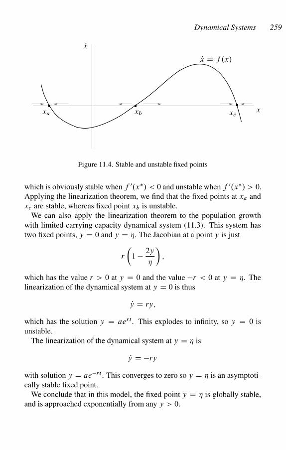
Dynamical Systems 259
x
Px
xa xb xc
Px D f .x/
���
Figure 11.4. Stable and unstable fixed points
which is obviously stable when f 0.x�/ < 0 and unstable when f 0.x�/ > 0.
Applying the linearization theorem, we find that the fixed points at xa and
xc are stable, whereas fixed point xb is unstable.
We can also apply the linearization theorem to the population growth
with limited carrying capacity dynamical system (11.3). This system has
two fixed points, y D 0 and y D �. The Jacobian at a point y is just
r
�1 � 2y
�
�;
which has the value r > 0 at y D 0 and the value �r < 0 at y D �. The
linearization of the dynamical system at y D 0 is thus
Py D ry;
which has the solution y D aert . This explodes to infinity, so y D 0 is
unstable.
The linearization of the dynamical system at y D � is
Py D �ry
with solution y D ae�rt . This converges to zero so y D � is an asymptoti-
cally stable fixed point.
We conclude that in this model, the fixed point y D � is globally stable,
and is approached exponentially from any y > 0.
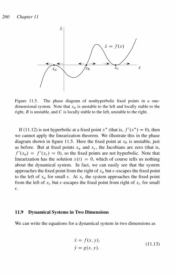
260 Chapter 11
x
Px
xa xb xc
Px D f .x/
���
Figure 11.5. The phase diagram of nonhyperbolic fixed points in a one-
dimensional system. Note that xa is unstable to the left and locally stable to the
right, B is unstable, and C is locally stable to the left, unstable to the right.
If (11.12) is not hyperbolic at a fixed point x� (that is, f 0.x�/ D 0), then
we cannot apply the linearization theorem. We illustrate this in the phase
diagram shown in figure 11.5. Here the fixed point at xb is unstable, just
as before. But at fixed points xa and xc , the Jacobians are zero (that is,
f 0.xa/ D f 0.xc/ D 0), so the fixed points are not hyperbolic. Note that
linearization has the solution x.t/ D 0, which of course tells us nothing
about the dynamical system. In fact, we can easily see that the system
approaches the fixed point from the right of xa but �-escapes the fixed point
to the left of xa for small �. At xc the system approaches the fixed point
from the left of xc but �-escapes the fixed point from right of xc for small
�.
11.9 Dynamical Systems in Two Dimensions
We can write the equations for a dynamical system in two dimensions as
Px D f .x; y/;(11.13)Py D g.x; y/:
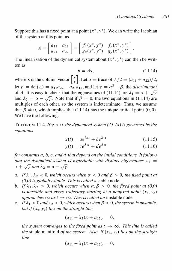
Dynamical Systems 261
Suppose this has a fixed point at a point .x�; y�/. We can write the Jacobian
of the system at this point as
A D�
a11 a12
a21 a22
�D�
fx.x�; y�/ fy.x�; y�/
gx.x�; y�/ gy.x�; y�/
�:
The linearization of the dynamical system about .x�; y�/ can then be writ-
ten as
Px D Ax; (11.14)
where x is the column vectorh
x
y
i. Let ˛ D trace of A=2 D .a11 C a22/=2,
let ˇ D det.A/ D a11a22 � a21a12, and let � D ˛2 � ˇ, the discriminant
of A. It is easy to check that the eigenvalues of (11.14) are �1 D ˛ C p�
and �2 D ˛ � p� . Note that if ˇ D 0, the two equations in (11.14) are
multiples of each other, so the system is indeterminate. Thus, we assume
that ˇ ¤ 0, which implies that (11.14) has the unique critical point .0; 0/.
We have the following.
THEOREM 11.4 If � > 0, the dynamical system (11.14) is governed by the
equations
x.t/ D ae 1t C be 2t (11.15)
y.t/ D ce 1t C de 2t (11.16)
for constants a, b, c, and d that depend on the initial conditions. It follows
that the dynamical system is hyperbolic with distinct eigenvalues �1 D˛ C p
� and �2 D ˛ � p� .
a. If �1; �2 < 0, which occurs when ˛ < 0 and ˇ > 0, the fixed point at
(0,0) is globally stable. This is called a stable node.b. If �1; �2 > 0, which occurs when ˛; ˇ > 0, the fixed point at (0,0)
is unstable and every trajectory starting at a nonfixed point .xo; yo/
approaches 1 as t ! 1. This is called an unstable node .c. If �1 > 0 and �2 < 0, which occurs when ˇ < 0, the system is unstable,
but if .xo; yo/ lies on the straight line
.a11 � �2/x C a12y D 0;
the system converges to the fixed point as t ! 1. This line is called
the stable manifold of the system. Also, if .xo; yo/ lies on the straight
line
.a11 � �1/x C a12y D 0;
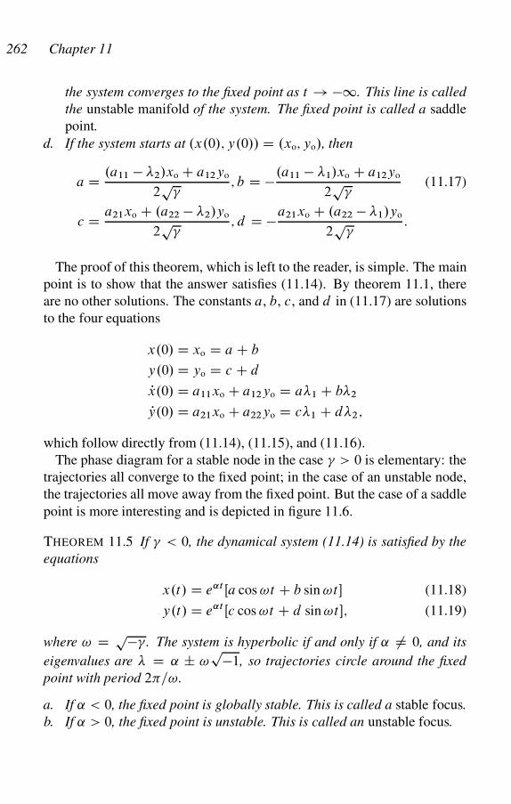
262 Chapter 11
the system converges to the fixed point as t ! �1. This line is called
the unstable manifold of the system. The fixed point is called a saddle
point.
d. If the system starts at .x.0/; y.0// D .xo; yo/, then
a D .a11 � �2/xo C a12yo
2p
�; b D �.a11 � �1/xo C a12yo
2p
�(11.17)
c D a21xo C .a22 � �2/yo
2p
�; d D �a21xo C .a22 � �1/yo
2p
�:
The proof of this theorem, which is left to the reader, is simple. The main
point is to show that the answer satisfies (11.14). By theorem 11.1, there
are no other solutions. The constants a, b, c, and d in (11.17) are solutions
to the four equations
x.0/ D xo D a C b
y.0/ D yo D c C d
Px.0/ D a11xo C a12yo D a�1 C b�2
Py.0/ D a21xo C a22yo D c�1 C d�2;
which follow directly from (11.14), (11.15), and (11.16).
The phase diagram for a stable node in the case � > 0 is elementary: the
trajectories all converge to the fixed point; in the case of an unstable node,
the trajectories all move away from the fixed point. But the case of a saddle
point is more interesting and is depicted in figure 11.6.
THEOREM 11.5 If � < 0, the dynamical system (11.14) is satisfied by the
equations
x.t/ D e˛t Œa cos !t C b sin !t� (11.18)
y.t/ D e˛t Œc cos !t C d sin !t�; (11.19)
where ! D p�� . The system is hyperbolic if and only if ˛ ¤ 0, and its
eigenvalues are � D ˛ ˙ !p�1, so trajectories circle around the fixed
point with period 2�=!.
a. If ˛ < 0, the fixed point is globally stable. This is called a stable focus.
b. If ˛ > 0, the fixed point is unstable. This is called an unstable focus.
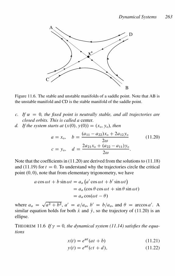
Dynamical Systems 263
D
C
x��
B
A
Figure 11.6. The stable and unstable manifolds of a saddle point. Note that AB is
the unstable manifold and CD is the stable manifold of the saddle point.
c. If ˛ D 0, the fixed point is neutrally stable, and all trajectories are
closed orbits. This is called a center.d. If the system starts at .x.0/; y.0// D .xo; yo/, then
a D xo; b D .a11 � a22/xo C 2a12yo
2!(11.20)
c D yo; d D 2a21xo C .a22 � a11/yo
2!:
Note that the coefficients in (11.20) are derived from the solutions to (11.18)
and (11.19) for t D 0. To understand why the trajectories circle the critical
point .0; 0/, note that from elementary trigonometry, we have
a cos !t C b sin !t D ao
�a0 cos !t C b0 sin !t
�
D ao .cos � cos !t C sin � sin !t/
D ao cos.!t � �/
where ao D pa2 C b2, a0 D a=ao, b0 D b=ao, and � D arccos a0. A
similar equation holds for both Px and Py, so the trajectory of (11.20) is an
ellipse.
THEOREM 11.6 If � D 0, the dynamical system (11.14) satisfies the equa-
tions
x.t/ D e˛t.at C b/ (11.21)
y.t/ D e˛t.ct C d/; (11.22)
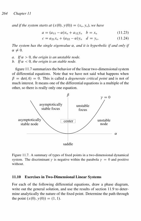
264 Chapter 11
and if the system starts at .x.0/; y.0// D .xo; yo/, we have
a D .a11 � ˛/xo C a12yo b D xo (11.23)
c D a21xo C .a22 � ˛/yo d D yo: (11.24)
The system has the single eigenvalue ˛, and it is hyperbolic if and only if
˛ ¤ 0.
a. If ˛ > 0, the origin is an unstable node.b. If ˛ < 0, the origin is an stable node.
figure 11.7 summarizes the behavior of the linear two-dimensional system
of differential equations. Note that we have not said what happens when
ˇ D det.A/ D 0. This is called a degenerate critical point and is not of
much interest. It means one of the differential equations is a multiple of the
other, so there is really only one equation.
ˇ
˛
saddle
unstable
unstableasymptotically
� D 0
centernodestable node
asymptoticallystable focus focus
Figure 11.7. A summary of types of fixed points in a two-dimensional dynamical
system. The discriminant � is negative within the parabola � D 0 and positive
without.
11.10 Exercises in Two-Dimensional Linear Systems
For each of the following differential equations, draw a phase diagram,
write out the general solution, and use the results of section 11.9 to deter-
mine analytically the nature of the fixed point. Determine the path through
the point .x.0/; y.0// D .1; 1/.
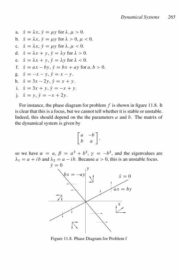
Dynamical Systems 265
a. Px D �x, Py D �y for �; � > 0.
b. Px D �x, Py D �y for � > 0, � < 0.
c. Px D �x, Py D �y for �; � < 0.
d. Px D �x C y, Py D �y for � > 0.
e. Px D �x C y, Py D �y for � < 0.
f. Px D ax � by, Py D bx C ay for a; b > 0.
g. Px D �x � y, Py D x � y.
h. Px D 3x � 2y, Py D x C y.
i. Px D 3x C y, Py D �x C y.
j. Px D y, Py D �x C 2y.
For instance, the phase diagram for problem f is shown in figure 11.8. It
is clear that this is a focus, but we cannot tell whether it is stable or unstable.
Indeed, this should depend on the the parameters a and b. The matrix of
the dynamical system is given by
�a �b
b a
�;
so we have ˛ D a, ˇ D a2 C b2, � D �b2, and the eigenvalues are
�1 D a C ib and �2 D a � ib. Because a > 0, this is an unstable focus.
Px D 0
Py D 0
ax D by
bx D �ay
x
y
Figure 11.8. Phase Diagram for Problem f
266 Chapter 11
11.11 Lotka-Volterra with Limited Carrying Capacity
The general Lotka-Volterra model (�11.4) has the form
Px D x.a � by/;(11.25)Py D y.�c C dx/:
This model has the absurd property that if the predator is absent, the prey
grows at the constant rate a forever. Suppose we add a limited carrying
capacity term (�11.3), so the first equation in (11.25) becomes
Px D x.a � by � �x/;
where � > 0, corresponding to capacity a=�. We will show that the fixed
point of this system is a stable focus for small � and a stable node for large
� (but still satisfying � < ad=c).
To see this, note that interior equilibrium satisfies x� D c=d and y� D.ad � c�/=bd . The Jacobian, evaluated at .x�; y�/ is
J D��c�=d �bc=d
y� 0
�:
The eigenvalues of the Jacobian at the equilibrium are
�c� ˙ pcp
c�2 C 4cd� � 4ad2
2d:
When � is small, the term under the square root sign is negative, so both
eigenvalues have negative real parts. The equilibrium in this case is a stable
focus. If � is large, but � > ad=c, it is easy to show that both eigenvalues
are negative, so the equilibrium is a stable node.
11.12 Take No Prisoners
Two firms share a nonmarketable, nonexcludable resource R that lowers
production costs but is subject to overcrowding and depletion. Suppose
that when firm 1 has size x and firm 2 has size y, the profits of the two
firms are given by
�x.x; y/ D �x.R � x � y/ � ˛x;
�y.x; y/ D �y.R � x � y/ � ˛y ;
Dynamical Systems 267
where �x; gy > 0. Suppose also that the firms’ growth rates are equal to
their profit rates, so
Px D x.�x.R � x � y/ � ˛x/;
Py D y.�y.R � x � y/ � ˛y/:
We assume that �xR > ˛x, �yR > ˛y , and �x=˛x > �y=˛y .
a. Show that if y D 0 the model has an unstable fixed point at x D 0 and
an asymptotically stable fixed point at x D x� D R � ax=gx.
b. Show that if x D 0 the model has an unstable equilibrium at y D 0 and
an asymptotically stable fixed point at y D y� D R � ay=gy .
c. Show that the complete model has three fixed points, (0,0), .x�; 0/, and
.0; y�/, of which only the second is asymptotically stable.
We conclude that both firms cannot coexist in equilibrium.
11.13 The Hartman-Grobman Theorem
The linearization theorem 11.3 tells us that we can determine whether a
hyperbolic fixed point of a dynamical system is asymptotically stable or
unstable by looking at its linearization. This is a fairly weak statement, be-
cause we have discovered a lot more about the nature of equilibria than just
stability. We have, for instance, distinguished nodes, foci, and saddles, and
in the latter case, we have found that there are always stable and unstable
manifolds. It turns out that in the hyperbolic case, each of these properties
of the linearization of a dynamical system is also possessed by the system
itself. This is the famous Hartman-Grobman theorem. To state the theorem,
however, we need a new definition.
Suppose the dynamical system defined by Px D f .x/ has a fixed point
at x�, and the dynamical system defined by Py D f .y/ has a fixed point at
y�. We say that the two systems are topologically equivalent at these fixed
points if there are balls B.x�/ and Bı.y�/ around the two fixed points and
a continuous one-to-one mapping W B.x�/ ! Bı.y�/ with a continu-
ous inverse that takes trajectories of the dynamical system lying in B.x�/
into trajectories of the dynamical system lying in Bı.y�/ and preserves the
direction of time.
Intuitively, two dynamical systems are topologically equivalent at x� and
y� if we can perform the following operation. Draw the phase diagram

268 Chapter 11
in the neighborhood of x� on a rubber sheet, including trajectories and ar-
rows indicating the direction of time. Now stretch the rubber sheet without
tearing or folding until it looks just like the phase diagram for the second
dynamical system in a neighborhood of y�. If this is possible, then the
systems are topologically equivalent.
THEOREM 11.7 Hartman-Grobman. If x� is a hyperbolic fixed point of the
dynamical system given by Px D f .x/, then this fixed point is topologically
equivalent to the fixed point at the origin of the linearization of the system
Px D Ax, where A D Df .x�/ is the Jacobian matrix of the system evaluated
at x�.
This means that we can determine the qualitative behavior of a dynami-
cal system in a neighborhood of a hyperbolic fixed point by looking at its
linearization, which is of course much easier to analyze. Indeed, we have
fully characterized such equilibria for one- and two-dimensional systems.
Higher-dimensional linear systems are harder to analyze, but they too can
be completely characterized and are essentially combinations of one- and
two-dimensional systems, placed at angles to each other in higher dimen-
sions.
11.14 Features of Two-Dimensional Dynamical Systems
Two-dimensional dynamical systems have lots of nice properties not shared
by higher-dimensional systems. This appears to be due to the famous Jor-
dan curve theorem, which says that any continuous, non-self-intersecting,
closed curve in the plane divides the plane into two connected pieces—an
“inside” and an “outside.” Trajectories of a dynamical system are of course
continuous and non-self-intersecting, though not generally closed.
Let x.t/ be a trajectory of the dynamical system (11.1). We say a point
y 2 Rn is an !-limit point of the trajectory if there is a sequence tn ! 1such that
limn!1
x.tn/ D y:
For instance, if x� is an asymptotically stable fixed point, then x� is the
!-limit of every trajectory starting at a point in the basin of attraction of
x�. In some cases, a trajectory can actually have lots of !-limit points.
For instance, suppose the fixed point x� is an unstable spiral, but there is a
closed orbit at some distance from x�. Then a trajectory starting at a point
Dynamical Systems 269
near x� can spiral out, getting closer and closer to the closed orbit. Each
point on the closed orbit is thus an !-limit of the trajectory. If a trajectory
is bounded (that is, is contained in some ball), then it must have at least one
!-limit point.
THEOREM 11.8 Poincare-Bendixson. Suppose x.t/ is a bounded trajec-
tory of (11.13), and � is the set of !-limit points of the trajectory. Then if
� contains no fixed points of (11.13), � is a periodic orbit of (11.13).
The following theorem is also often useful.
THEOREM 11.9 Suppose equation (11.13) has a closed orbit � and let U
be the interior region bounded by �. Then U contains a fixed point of
(11.13).
12
Evolutionary Dynamics
Through the animal and vegetable kingdoms, nature has scat-tered the seeds of life abroad with the most profuse and lib-eral hand; but has been comparatively sparing in the room andnourishment necessary to rear them.
T. R. Malthus
Fifteen months after I had begun my systematic enquiry, I hap-pened to read for amusement “Malthus on Population” . . . itat once struck me that . . . favorable variations would tendto be preserved, and unfavorable ones to be destroyed. Here,then, I had at last got a theory by which to work.
Charles Darwin
Our study of evolutionary dynamics is built around the replicator equa-
tions. We begin by defining the replicator dynamic, deriving it in several
distinct ways, and exploring its major characteristics (�12.1–�12.6). The
next several sections make good on our promise to justify Nash equilib-
rium in terms of dynamical systems, as we exhibit the relationship between
dynamic stability of evolutionary models, on the one hand, and dominated
strategies (�12.7), Nash equilibria (�12.8), evolutionarily stable strategies
(�12.9), and connected sets of Nash equilibria, on the other. Many of the
results we obtain remain valid in more general settings (e.g., when the dy-
namic has an aggregate tendency toward favoring more fit strategies, but
not necessarily as strongly as the replicator dynamic).
We next turn to asymmetric evolutionary games (�12.17), which have the
surprising property, a property that is extremely important from the point
of view of understanding real-world evolutionary dynamics, that strictly
mixed Nash equilibria are never asymptotically stable but are often neu-
trally stable, leading to generically stable orbits (the Lotka-Volterra model
has orbits, but it is not generic, as small changes in the coefficients lead to
the equilibrium being either a stable or an unstable focus). In asymmetric
games, the limit points of dynamic processes are generally Nash equilib-
270
Evolutionary Dynamics 271
ria, but virtually nothing stronger than this can be asserted, including the
elimination of weakly dominated strategies (Samuelson and Zhang 1992).
12.1 The Origins of Evolutionary Dynamics
The central actor in an evolutionary system is the replicator, which is an en-
tity having some means of making approximately accurate copies of itself.
The replicator can be a gene, an organism (defining “accurate copy” appro-
priately in the case of sexual reproduction), a strategy in a game, a belief,
a technique, a convention, or a more general institutional or cultural form.
A replicator system is a set of replicators in a particular environmental set-
ting with a structured pattern of interaction among agents. An evolutionary
dynamic of a replicator system is a process of change over time in the fre-
quency distribution of the replicators (and in the nature of the environment
and the structure of interaction, though we will not discuss these here), in
which strategies with higher payoffs reproduce faster in some appropriate
sense.
In addition to having an evolutionary dynamic, evolutionary systems may
generate novelty if random errors (“mutations” or “perturbations”) occur in
the replication process, allowing new replicators to emerge and diffuse into
the population if they are relatively well adapted to the replicator system.
The stunning variety of life forms that surround us, as well as the beliefs,
practices, techniques, and behavioral forms that constitute human culture,
are the product of evolutionary dynamics.
Evolutionary dynamics can be applied to a variety of systems, but we
consider here only two-player evolutionary games, which consist of a stage
game played by pairs of agents in a large population, each “wired” to play
some pure strategy. We assume the game is symmetric (�10.1), so the play-
ers cannot condition their actions on whether they are player 1 or player
2. In each time period, agents are paired, they play the stage game, and
the results determine their rate of replication. We generally assume there
is random pairing, in which case the payoff to an agent of type i playing
against the population is given by equation (10.1); note that this assumes
that the population is very large, so we treat the probability of an agent
meeting his own type as equal to fraction pi of the population that uses
the i th pure strategy. More generally, we could assume spatial, kinship, or
other patterns of assortation, in which case the probability of type i meeting

272 Chapter 12
type j depends on factors other than the relative frequency pj of type j in
the population.
There are various plausible ways to specify an evolutionary dynamic. See
Friedman (1991) and Hofbauer and Sigmund (1998) for details. Here we
discuss only replicator dynamics, which are quite representative of evolu-
tionary dynamics in general. Our first task is to present a few of the ways a
replicator dynamic can arise.
12.2 Strategies as Replicators
Consider an evolutionary game where each player follows one of n pure
strategies si for i D 1; : : : ; n. The play is repeated in periods t D 1; 2; : : :.
Let pti be the fraction of players playing si in period t , and suppose the
payoff to si is � ti D �i.p
t /, where pt D .pt1; : : : ; pt
n/. We look at a given
time t , and number the strategies so that � t1 � � t
2 � : : : � � tn.
Suppose in every time period dt , each agent with probability ˛dt > 0
learns the payoff to another randomly chosen other agent and changes to the
other’s strategy if he perceives that the other’s payoff is higher. However,
information concerning the difference in the expected payoffs of the two
strategies is imperfect, so the larger the difference in the payoffs, the more
likely the agent is to perceive it, and change. Specifically, we assume the
probability ptij that an agent using si will shift to sj is given by
ptij D
ˇ.� t
j � � ti / for � t
j > � ti
0 for � tj � � t
i
where ˇ is sufficiently small that pij � 1 holds for all i; j . The expected
fraction EptCdti of the population using si in period t C dt is then given by
EptCdti D pt
i � ˛dt pti
nX
j DiC1
ptj ˇ.� t
j � � ti / C
iX
j D1
˛dt ptj pt
i ˇ.� ti � � t
j /
D pti C ˛dt pt
i
nX
j D1
ptj ˇ.� t
i � � tj /
D pti C ˛dt pt
i ˇ.� ti � N� t /;
where N� t D � t1pt
1 C : : : C � tnpt
n is the average return for the whole popula-
tion. If the population is large, we can replace EptCdti by ptCdt
i . Subtract-
ing pti from both sides, dividing by dt , and taking the limit as dt ! 0, we
Evolutionary Dynamics 273
get
Ppti D ˛ˇpt
i .�ti � N� t /; for i D 1; : : : ; n; (12.1)
which is called the replicator dynamic. Because the constant factor ˛ˇ
merely changes the rate of adjustment to stationarity but leaves the stability
properties and trajectories of the dynamical system unchanged, we often
simply assume ˛ˇ D 1 (�12.5).
Several points are worth making concerning the replicator dynamic. First,
under the replicator dynamic, the frequency of a strategy increases exactly
when it has above-average payoff. In particular, this means that the repli-
cator dynamic is not a best-reply dynamic; that is, agents do not adopt a
best reply to the overall frequency distribution of strategies in the previous
period. Rather, the agents in a replicator system have limited and localized
knowledge concerning the system as a whole. Some game theorists call
such agents “boundedly rational,” but this term is very misleading, because
the real issue is the distribution of information, not the degree of rationality.
Second, if we add up all the equations, we getP
i Ppti D 0, so ifP
i pti D 1 at one point in time, this remains true forever. Moreover, al-
though a particular replicator can become extinct at t ! 1, a replicator
that is not represented in the population at one point in time will never be
represented in the population at any later point in time. So, replicator dy-
namics deal poorly with innovation. A more general system adds a term to
the replicator equation expressing the spontaneous emergence of replicators
through mutation.
Third, our derivation assumes that there are no “mistakes;” that is, players
never switch from a better to a worse strategy. We might suspect that small
probabilities of small errors would make little difference, but I do not know
under what conditions this intuition is valid.
Note that taking expected values allows us to average over the possible
behaviors of an agent, so that even if there is a positive probability that
a player will switch from better to worse, on average the player will not.
The replicator dynamic compels a dynamical system always to increase
the frequency of a strategy with above average payoff. If we do not take
expected values, this property fails. For instance, if there is a probability
p > 0, no matter how small, that a player will go from better to worse, and
if there are n players, then there is a probability pn > 0 that all players
will switch from better to worse. We would have a “stochastic dynamic”
in which movement over time probably, but not necessarily, increases the
274 Chapter 12
frequency of successful strategies. If there is a single stable equilibrium,
this might not cause much of a problem, but if there are several, such rare
accumulations of error will inevitably displace the dynamical system from
the basin of attraction of one equilibrium to that of another (see chapter 13).
It follows that the replicator dynamic, by abstracting from stochastic in-
fluences on the change in frequency of strategies, is an idealized version of
how systems of strategic interaction develop over time, and is accurate only
if the number of players is very large in some appropriate sense, compared
to the time interval of interest. To model the stochastic dynamic, we use
stochastic processes, which are Markov chains and their continuous lim-
its, diffusion processes. We provide an introduction to such dynamics in
chapter 13.
It is satisfying that as the rate of error becomes small, the deviation of the
stochastic dynamic from the replicator dynamic becomes arbitrarily small
with arbitrarily high probability (Freidlin and Wentzell 1984). But the
devil is in the details. For instance, as long as the probability of error is
positive, under quite plausible conditions a stochastic system with a repli-
cator dynamic will make regular transitions from one asymptotically stable
equilibrium to another, and superior mutant strategies may be driven to ex-
tinction with high probability; see chapter 13, as well as Foster and Young
(1990) and Samuelson (1997) for examples and references.
12.3 A Dynamic Hawk-Dove Game
There is a desert that can support n raptors. Raptors are born in the evening
and are mature by morning. There are always at least n raptors alive each
morning. They hunt all day for food, and at the end of the day, the n raptors
that remain search for nesting sites (all raptors are female and reproduce
by cloning). There are two types of nesting sites: good and bad. On a bad
nesting site, a raptor produces an average of u offspring per night, and on
a good nesting site, she produces an average of u C 2 offspring per night.
However, there are only n=2 good nesting sites, so the raptors pair off and
vie for the good sites.
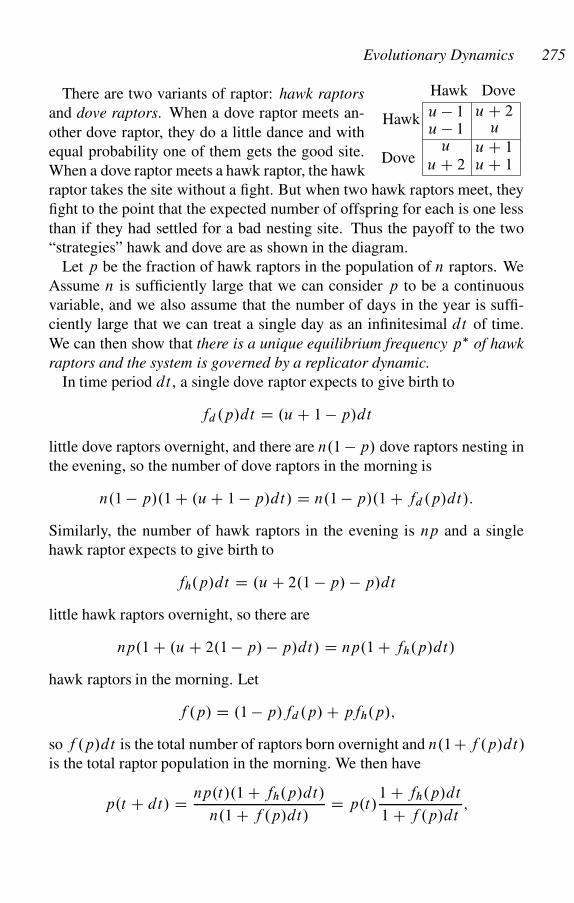
Evolutionary Dynamics 275
u � 1
Dove
Hawk
Hawk Dove
u � 1u C 2
uu
u C 2u C 1u C 1
There are two variants of raptor: hawk raptors
and dove raptors. When a dove raptor meets an-
other dove raptor, they do a little dance and with
equal probability one of them gets the good site.
When a dove raptor meets a hawk raptor, the hawk
raptor takes the site without a fight. But when two hawk raptors meet, they
fight to the point that the expected number of offspring for each is one less
than if they had settled for a bad nesting site. Thus the payoff to the two
“strategies” hawk and dove are as shown in the diagram.
Let p be the fraction of hawk raptors in the population of n raptors. We
Assume n is sufficiently large that we can consider p to be a continuous
variable, and we also assume that the number of days in the year is suffi-
ciently large that we can treat a single day as an infinitesimal dt of time.
We can then show that there is a unique equilibrium frequency p� of hawk
raptors and the system is governed by a replicator dynamic.
In time period dt , a single dove raptor expects to give birth to
fd .p/dt D .u C 1 � p/dt
little dove raptors overnight, and there are n.1 � p/ dove raptors nesting in
the evening, so the number of dove raptors in the morning is
n.1 � p/.1 C .u C 1 � p/dt/ D n.1 � p/.1 C fd .p/dt/:
Similarly, the number of hawk raptors in the evening is np and a single
hawk raptor expects to give birth to
fh.p/dt D .u C 2.1 � p/ � p/dt
little hawk raptors overnight, so there are
np.1 C .u C 2.1 � p/ � p/dt/ D np.1 C fh.p/dt/
hawk raptors in the morning. Let
f .p/ D .1 � p/fd .p/ C pfh.p/;
so f .p/dt is the total number of raptors born overnight and n.1Cf .p/dt/
is the total raptor population in the morning. We then have
p.t C dt/ D np.t/.1 C fh.p/dt/
n.1 C f .p/dt/D p.t/
1 C fh.p/dt
1 C f .p/dt;

276 Chapter 12
which implies
p.t C dt/ � p.t/
dtD p.t/
fh.p/ � f .p/
1 C f .p/dt
:
If we now let dt ! 0, we get
dp
dtD p.t/Œfh.p/ � f .p/�: (12.2)
This is of course a replicator dynamic, this time derived by assuming that
agents reproduce genetically but are selected by their success in playing a
game. Note that p.t/ is constant (that is, the population is in equilibrium)
when fh.p/ D f .p/, which means fh.p/ D fd.p/ D f .p/.
If we substitute values in equation (12.2), we get
dp
dtD p.1 � p/.1 � 2p/: (12.3)
This equation has three fixed points: p D 0; 1; 1=2. From our discussion of
one-dimensional dynamics (�11.8), we know that a fixed point is asymptot-
ically stable if the derivative of the right-hand side is negative, and is unsta-
ble if the derivative of the right-hand side is positive. It is easy to check that
the derivative of p.1 � p/.1 � 2p/ is positive for p D 0; 1 and negative for
p D 1=2. Thus, a population of all dove raptors or all hawk raptors is sta-
tionary, but the introduction of even one raptor of the other type will drive
the population toward the heterogeneous asymptotically stable equilibrium.
12.4 Sexual Reproduction and the Replicator Dynamic
Suppose the fitness (that is, the expected number of offspring) of members
of a certain population depends on a single genetic locus, at which there
are two genes (such creatures, which includes most of the “higher” plants
and animals, are called diploid). Suppose there are n alternative types of
genes (called alleles) at this genetic locus, which we label g1; : : : ; gn. An
individual whose gene pair is .gi ; gj /, whom we term an “ij -type,” then has
fitness wij , which we interpret as being the expected number of offspring
surviving to sexual maturity. We assume wij D wj i for all i ,j .
Suppose sexually mature individuals are randomly paired off once in each
time period, and for each pair .gi ; gj / of genes, gi taken from the first and
gj taken from the second member of the pair, a number of offspring of type
ij are born, of which wij reach sexual maturity. The parents then die.
Evolutionary Dynamics 277
THEOREM 12.1 For each i D 1; : : : ; n let pi.t/ be the frequency of
gi in the population. Then, fitness of a gi allele is given by wi .t/ DPnj D1 wij pj .t/, the average fitness in the population is given by w.t/ DPniD1 piwi.t/, and the following replicator equations hold:
Ppi D pi Œwi .t/ � w.t/� for i D 1; : : : ; n: (12.4)
PROOF: For any i D 1; : : : ; n, let yi be the number of alleles of type
gi , and let y be the total number of alleles, so y D Pnj D1 yj and pi D
yi=y. Because pj is the probability that a gi allele will meet a gj allele, the
expected number of gi genes in the offspring of a gi gene is justP
j wij pj ,
and so the total number of gi alleles in the next generation is yi
Pj wij pj .
This gives the differential equation
Pyi D yi
nX
j D1
wij pj :
Differentiating the identity ln pi D ln yi � ln y with respect to time t , we
get
Ppi
pi
D Pyi
yi
�nX
j D1
Pyj
yD
nX
j D1
wij pj �nX
j D1
Pyj
yj
pj DnX
j D1
wij pj �nX
j;kD1
wjkpj pk;
which is the replicator dynamic.
The following important theorem was discovered by the famous biologist
R. A. Fisher.
THEOREM 12.2 Fundamental Theorem of Natural Selection. The average
fitness w.t/ of a population increases along any trajectory of the replicator
dynamic (12.4), and satisfies the equation
Pw D 2
nX
iD1
pi .wi � w/2:
Note that the right-hand side of this equation is twice the fitness variance.
PROOF: Let W be the n � n matrix .wij / and let p.t/ D.p1.t/; : : : ; pn.t// be the column vector of allele frequencies. The fit-
ness of allele i is then
wi DnX
j D1
wij pj ;
278 Chapter 12
and the average fitness is
w DnX
iD1
piwi DnX
i;j D1
piwij pj :
Then,
Pw D 2
nX
i;j D1
pj wj i Ppi D 2
nX
i;j D1
pj wj ipi.wi � w/
D 2
nX
iD1
pi.wi � w/wi D 2
nX
iD1
pi .wi � w/2;
where the last equation follows fromPn
iD1 pi.wi � w/w D 0.
The above model can be extended in a straightforward manner to a situa-
tion in which the parents live more than one generation, and the fundamen-
tal theorem can be extended to include many genetic loci, provided they do
not interact. However, it is a bad mistake to think that the fundamental theo-
rem actually holds in the real world (this is often referred to as the Panglos-
sian fallacy, named after Voltaire’s Dr. Pangloss, who in Candide declared
that “all is for the best in this, the best of all possible worlds”). Genes do
interact, so that the fitness of an allele depends not just on the allele, but on
the other alleles in the individual’s genetic endowment. Such genes, called
epistatic genes, are actually quite common. Moreover, the fitness of pop-
ulations may be interdependent in ways that reduce fitness over time (see,
for instance, section 11.4, which describes the Lotka-Volterra predator-prey
model). Finally, stochastic effects ignored in replicator dynamics can lead
to the elimination of very fit genes and even populations.
12.5 Properties of the Replicator System
Given the replicator equation (12.1), show the following:
a. For 1 � i < j � n, show that
d
dt
�pi
pj
�D�
pi
pj
�.�i � �j /:
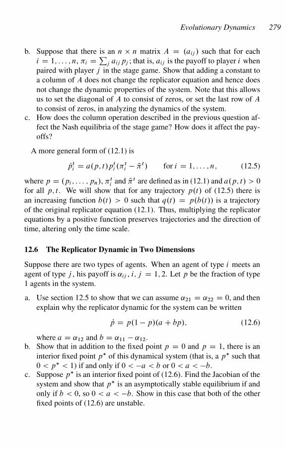
Evolutionary Dynamics 279
b. Suppose that there is an n � n matrix A D .aij / such that for each
i D 1; : : : ; n, �i D Pj aij pj ; that is, aij is the payoff to player i when
paired with player j in the stage game. Show that adding a constant to
a column of A does not change the replicator equation and hence does
not change the dynamic properties of the system. Note that this allows
us to set the diagonal of A to consist of zeros, or set the last row of A
to consist of zeros, in analyzing the dynamics of the system.c. How does the column operation described in the previous question af-
fect the Nash equilibria of the stage game? How does it affect the pay-
offs?
A more general form of (12.1) is
Ppti D a.p; t/pt
i .�ti � N� t / for i D 1; : : : ; n; (12.5)
where p D .pi ; : : : ; pn/, � ti and N� t are defined as in (12.1) and a.p; t/ > 0
for all p; t . We will show that for any trajectory p.t/ of (12.5) there is
an increasing function b.t/ > 0 such that q.t/ D p.b.t// is a trajectory
of the original replicator equation (12.1). Thus, multiplying the replicator
equations by a positive function preserves trajectories and the direction of
time, altering only the time scale.
12.6 The Replicator Dynamic in Two Dimensions
Suppose there are two types of agents. When an agent of type i meets an
agent of type j , his payoff is ˛ij , i; j D 1; 2. Let p be the fraction of type
1 agents in the system.
a. Use section 12.5 to show that we can assume ˛21 D ˛22 D 0, and then
explain why the replicator dynamic for the system can be written
Pp D p.1 � p/.a C bp/; (12.6)
where a D ˛12 and b D ˛11 � ˛12.b. Show that in addition to the fixed point p D 0 and p D 1, there is an
interior fixed point p� of this dynamical system (that is, a p� such that
0 < p� < 1) if and only if 0 < �a < b or 0 < a < �b.c. Suppose p� is an interior fixed point of (12.6). Find the Jacobian of the
system and show that p� is an asymptotically stable equilibrium if and
only if b < 0, so 0 < a < �b. Show in this case that both of the other
fixed points of (12.6) are unstable.
280 Chapter 12
d. If p� is an unstable interior fixed point of (12.6), show that the fixed
points p D 0 and p D 1 are both asymptotically stable equilibria.e. Show that if z D p=.1 � p/, then the replicator equation becomes
Pz D .1 � p/z.˛11z C ˛12/; (12.7)
and this has an interior asymptotically stable equilibrium z� D�˛12=˛11 if and only if ˛11 < 0 < ˛12.
f. Now use section 12.5 to show that this has the same trajectories as the
simpler differential equation
Pz D z.˛11z C ˛12/: (12.8)
Show that the general solution to (12.8) is given by z.t/ D˛12=.ce�˛12t � ˛11/, where c D ˛12=z.0/ C ˛11. In this case
we can verify directly that there is an interior asymptotically stable
equilibrium if and only if ˛11 < 0 < ˛12.
12.7 Dominated Strategies and the Replicator Dynamic
All Nash equilibria of a game survive the iterated elimination of strongly
dominated strategies, but not of weakly dominated strategies (see chap-
ter 3). Not surprisingly, strongly dominated strategies do not survive in a
replicator dynamic. Suppose there are n pure strategies in the stage game
of an evolutionary game in which pi .t/ is the fraction of the population
playing strategy i at time t . Recall that a strategy is completely mixed if
pi .t/ > 0 for all i . We have the following theorem.
THEOREM 12.3 Let p.t/ D .p1.t/; : : : ; pn.t// be a completely mixed tra-
jectory of the replicator dynamic (12.1) and suppose strategy i is recur-
sively strongly dominated (�4.1). Then, strategy i does not survive the
replicator dynamic; that is, limt!1 pi .t/ D 0.
To see this, first suppose i is strongly dominated by po. We write �.p; q/
for the payoff to strategy p against strategy q. Then, �.po; p/ > �i.p/ for
all mixed strategies p. Because the set of mixed strategies is closed and
bounded, � D minp.�.po; p/ � �i.p// is strictly positive. Let
f .p/ D ln.pi/ �nX
j D1
poj ln.pj /:
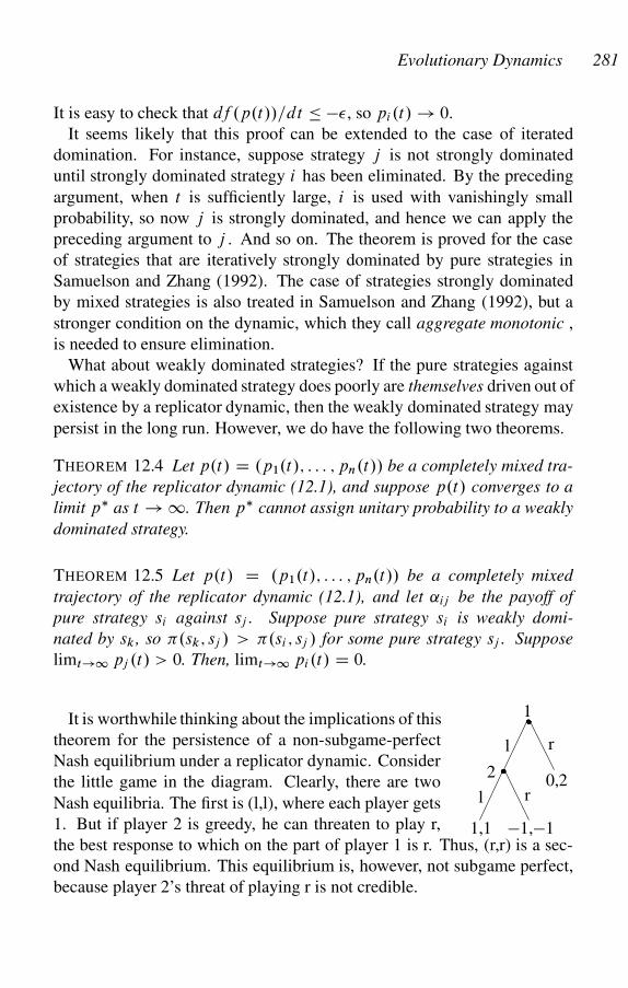
Evolutionary Dynamics 281
It is easy to check that df .p.t//=dt � ��, so pi.t/ ! 0.
It seems likely that this proof can be extended to the case of iterated
domination. For instance, suppose strategy j is not strongly dominated
until strongly dominated strategy i has been eliminated. By the preceding
argument, when t is sufficiently large, i is used with vanishingly small
probability, so now j is strongly dominated, and hence we can apply the
preceding argument to j . And so on. The theorem is proved for the case
of strategies that are iteratively strongly dominated by pure strategies in
Samuelson and Zhang (1992). The case of strategies strongly dominated
by mixed strategies is also treated in Samuelson and Zhang (1992), but a
stronger condition on the dynamic, which they call aggregate monotonic ,
is needed to ensure elimination.
What about weakly dominated strategies? If the pure strategies against
which a weakly dominated strategy does poorly are themselves driven out of
existence by a replicator dynamic, then the weakly dominated strategy may
persist in the long run. However, we do have the following two theorems.
THEOREM 12.4 Let p.t/ D .p1.t/; : : : ; pn.t// be a completely mixed tra-
jectory of the replicator dynamic (12.1), and suppose p.t/ converges to a
limit p� as t ! 1. Then p� cannot assign unitary probability to a weakly
dominated strategy.
THEOREM 12.5 Let p.t/ D .p1.t/; : : : ; pn.t// be a completely mixed
trajectory of the replicator dynamic (12.1), and let ˛ij be the payoff of
pure strategy si against sj . Suppose pure strategy si is weakly domi-
nated by sk , so �.sk; sj / > �.si ; sj / for some pure strategy sj . Suppose
limt!1 pj .t/ > 0. Then, limt!1 pi.t/ D 0.
�
�
1,1 �1,�1
0,2
l
l
r
r
1
2
It is worthwhile thinking about the implications of this
theorem for the persistence of a non-subgame-perfect
Nash equilibrium under a replicator dynamic. Consider
the little game in the diagram. Clearly, there are two
Nash equilibria. The first is (l,l), where each player gets
1. But if player 2 is greedy, he can threaten to play r,
the best response to which on the part of player 1 is r. Thus, (r,r) is a sec-
ond Nash equilibrium. This equilibrium is, however, not subgame perfect,
because player 2’s threat of playing r is not credible.
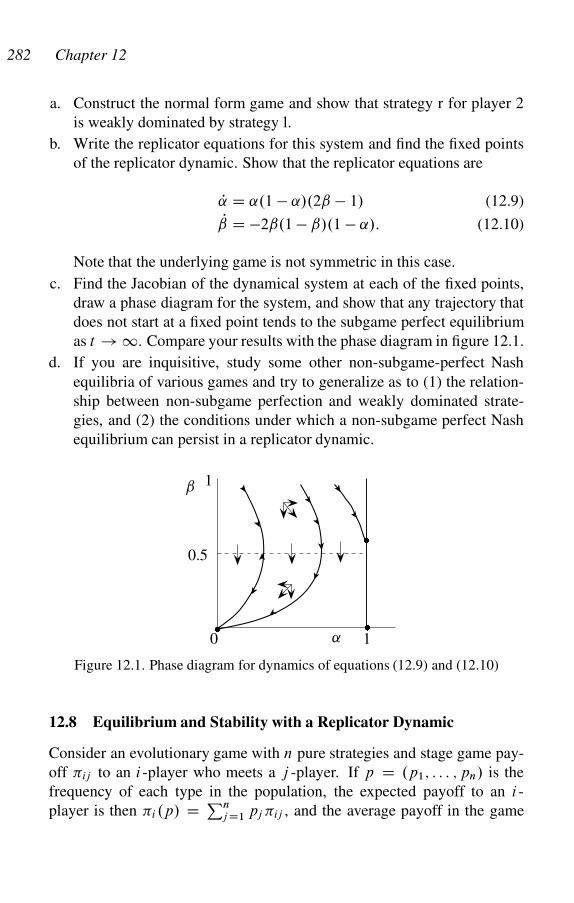
282 Chapter 12
a. Construct the normal form game and show that strategy r for player 2
is weakly dominated by strategy l.
b. Write the replicator equations for this system and find the fixed points
of the replicator dynamic. Show that the replicator equations are
P D ˛.1 � ˛/.2ˇ � 1/ (12.9)
P D �2ˇ.1 � ˇ/.1 � ˛/: (12.10)
Note that the underlying game is not symmetric in this case.
c. Find the Jacobian of the dynamical system at each of the fixed points,
draw a phase diagram for the system, and show that any trajectory that
does not start at a fixed point tends to the subgame perfect equilibrium
as t ! 1. Compare your results with the phase diagram in figure 12.1.
d. If you are inquisitive, study some other non-subgame-perfect Nash
equilibria of various games and try to generalize as to (1) the relation-
ship between non-subgame perfection and weakly dominated strate-
gies, and (2) the conditions under which a non-subgame perfect Nash
equilibrium can persist in a replicator dynamic.
�
�
�
˛0
0.5
1
1ˇ
Figure 12.1. Phase diagram for dynamics of equations (12.9) and (12.10)
12.8 Equilibrium and Stability with a Replicator Dynamic
Consider an evolutionary game with n pure strategies and stage game pay-
off �ij to an i-player who meets a j -player. If p D .p1; : : : ; pn/ is the
frequency of each type in the population, the expected payoff to an i-
player is then �i .p/ D Pnj D1 pj �ij , and the average payoff in the game
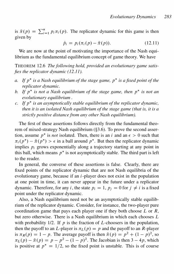
Evolutionary Dynamics 283
is N�.p/ D PniD1 pi�i .p/. The replicator dynamic for this game is then
given by
Ppi D pi.�i .p/ � N�.p//: (12.11)
We are now at the point of motivating the importance of the Nash equi-
librium as the fundamental equilibrium concept of game theory. We have
THEOREM 12.6 The following hold, provided an evolutionary game satis-
fies the replicator dynamic (12.11).
a. If p� is a Nash equilibrium of the stage game, p� is a fixed point of the
replicator dynamic.
b. If p� is not a Nash equilibrium of the stage game, then p� is not an
evolutionary equilibrium .
c. If p� is an asymptotically stable equilibrium of the replicator dynamic,
then it is an isolated Nash equilibrium of the stage game (that is, it is a
strictly positive distance from any other Nash equilibrium).
The first of these assertions follows directly from the fundamental theo-
rem of mixed-strategy Nash equilibrium (�3.6). To prove the second asser-
tion, assume p� is not isolated. Then, there is an i and an � > 0 such that
�i.p�/ � N�.p�/ > � in a ball around p�. But then the replicator dynamic
implies pi grows exponentially along a trajectory starting at any point in
this ball, which means p� is not asymptotically stable. The third part is left
to the reader.
In general, the converse of these assertions is false. Clearly, there are
fixed points of the replicator dynamic that are not Nash equilibria of the
evolutionary game, because if an i-player does not exist in the population
at one point in time, it can never appear in the future under a replicator
dynamic. Therefore, for any i , the state pi D 1, pj D 0 for j ¤ i is a fixed
point under the replicator dynamic.
Also, a Nash equilibrium need not be an asymptotically stable equilib-
rium of the replicator dynamic. Consider, for instance, the two-player pure
coordination game that pays each player one if they both choose L or R,
but zero otherwise. There is a Nash equilibrium in which each chooses L
with probability 1/2. If p is the fraction of L-choosers in the population,
then the payoff to an L-player is �L.p/ D p and the payoff to an R-player
is �R.p/ D 1 � p. The average payoff is then N�.p/ D p2 C .1 � p/2, so
�L.p/ � N�.p/ D p � p2 � .1 � p/2. The Jacobian is then 3 � 4p, which
is positive at p� D 1=2, so the fixed point is unstable. This is of course
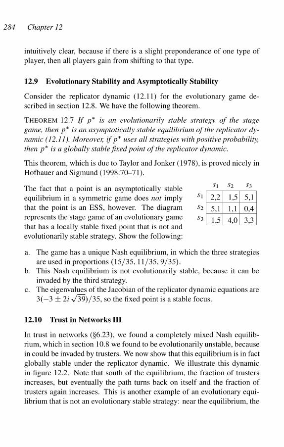
284 Chapter 12
intuitively clear, because if there is a slight preponderance of one type of
player, then all players gain from shifting to that type.
12.9 Evolutionary Stability and Asymptotically Stability
Consider the replicator dynamic (12.11) for the evolutionary game de-
scribed in section 12.8. We have the following theorem.
THEOREM 12.7 If p� is an evolutionarily stable strategy of the stage
game, then p� is an asymptotically stable equilibrium of the replicator dy-
namic (12.11). Moreover, if p� uses all strategies with positive probability,
then p� is a globally stable fixed point of the replicator dynamic.
This theorem, which is due to Taylor and Jonker (1978), is proved nicely in
Hofbauer and Sigmund (1998:70–71).
s1 2,2 1,5 5,1
5,1 1,1 0,4
1,5 4,0 3,3
s2
s3
s1 s3s2The fact that a point is an asymptotically stable
equilibrium in a symmetric game does not imply
that the point is an ESS, however. The diagram
represents the stage game of an evolutionary game
that has a locally stable fixed point that is not and
evolutionarily stable strategy. Show the following:
a. The game has a unique Nash equilibrium, in which the three strategies
are used in proportions .15=35; 11=35; 9=35/.b. This Nash equilibrium is not evolutionarily stable, because it can be
invaded by the third strategy.c. The eigenvalues of the Jacobian of the replicator dynamic equations are
3.�3 ˙ 2ip
39/=35, so the fixed point is a stable focus.
12.10 Trust in Networks III
In trust in networks (�6.23), we found a completely mixed Nash equilib-
rium, which in section 10.8 we found to be evolutionarily unstable, because
in could be invaded by trusters. We now show that this equilibrium is in fact
globally stable under the replicator dynamic. We illustrate this dynamic
in figure 12.2. Note that south of the equilibrium, the fraction of trusters
increases, but eventually the path turns back on itself and the fraction of
trusters again increases. This is another example of an evolutionary equi-
librium that is not an evolutionary stable strategy: near the equilibrium, the

Evolutionary Dynamics 285
dynamic path moves away from the equilibrium before veering back toward
it.
0.2 0.4 0.6 0.8 1
0.1
0.2
0.3
0.4
0.5
0.6
0.7
Fraction inspectors
Fraction trusters
Figure 12.2. A typical path of the trust in networks dynamical system
12.11 Characterizing 2 � 2 Normal Form Games II
Suppose a normal form game is generic in the sense that no two payoffs for
the same player are equal. Suppose A D .aij / and B D .bij / are the payoff
matrices for Alice and Bob, so the payoff to Alice’s strategy si against Bob’s
strategy tj is aij for Alice and bij for Bob. We say two generic 2 � 2 games
with payoff matrices .A; B/ and .C; D/ are equivalent if, for all i; j D 1; 2
aij > akl � cij > ckl
and
bij > bkl � dij > dkl :
In particular, if a constant is added to the payoffs to all the pure strategies
of one player when played against a given pure strategy of the other player,
the resulting game is equivalent to the original.
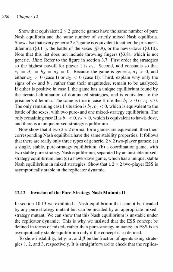
286 Chapter 12
Show that equivalent 2 � 2 generic games have the same number of pure
Nash equilibria and the same number of strictly mixed Nash equilibria.
Show also that every generic 2�2 game is equivalent to either the prisoner’s
dilemma (�3.11), the battle of the sexes (�3.9), or the hawk-dove (�3.10).
Note that this list does not include throwing fingers (�3.8), which is not
generic. Hint: Refer to the figure in section 3.7. First order the strategies
so the highest payoff for player 1 is a1. Second, add constants so that
c1 D d1 D b2 D d2 D 0. Because the game is generic, a1 > 0, and
either a2 > 0 (case I) or a2 < 0 (case II). Third, explain why only the
signs of c2 and b1, rather than their magnitudes, remain to be analyzed.
If either is positive in case I, the game has a unique equilibrium found by
the iterated elimination of dominated strategies, and is equivalent to the
prisoner’s dilemma. The same is true in case II if either b1 > 0 or c2 < 0.
The only remaining case I situation is b1; c1 < 0, which is equivalent to the
battle of the sexes, with two pure- and one mixed-strategy equilibrium. The
only remaining case II is b1 < 0; c2 > 0, which is equivalent to hawk-dove,
and there is a unique mixed-strategy equilibrium.
Now show that if two 2 � 2 normal form games are equivalent, then their
corresponding Nash equilibria have the same stability properties. It follows
that there are really only three types of generic, 2 �2 two-player games: (a)
a single, stable, pure-strategy equilibrium; (b) a coordination game, with
two stable pure-strategy Nash equilibrium, separated by an unstable mixed-
strategy equilibrium; and (c) a hawk-dove game, which has a unique, stable
Nash equilibrium in mixed strategies. Show that a 2 � 2 two-player ESS is
asymptotically stable in the replicator dynamic.
12.12 Invasion of the Pure-Strategy Nash Mutants II
In section 10.13 we exhibited a Nash equilibrium that cannot be invaded
by any pure strategy mutant but can be invaded by an appropriate mixed-
strategy mutant. We can show that this Nash equilibrium is unstable under
the replicator dynamic. This is why we insisted that the ESS concept be
defined in terms of mixed- rather than pure-strategy mutants; an ESS is an
asymptotically stable equilibrium only if the concept is so defined.
To show instability, let � , ˛, and ˇ be the fraction of agents using strate-
gies 1, 2, and 3, respectively. It is straightforward to check that the replica-
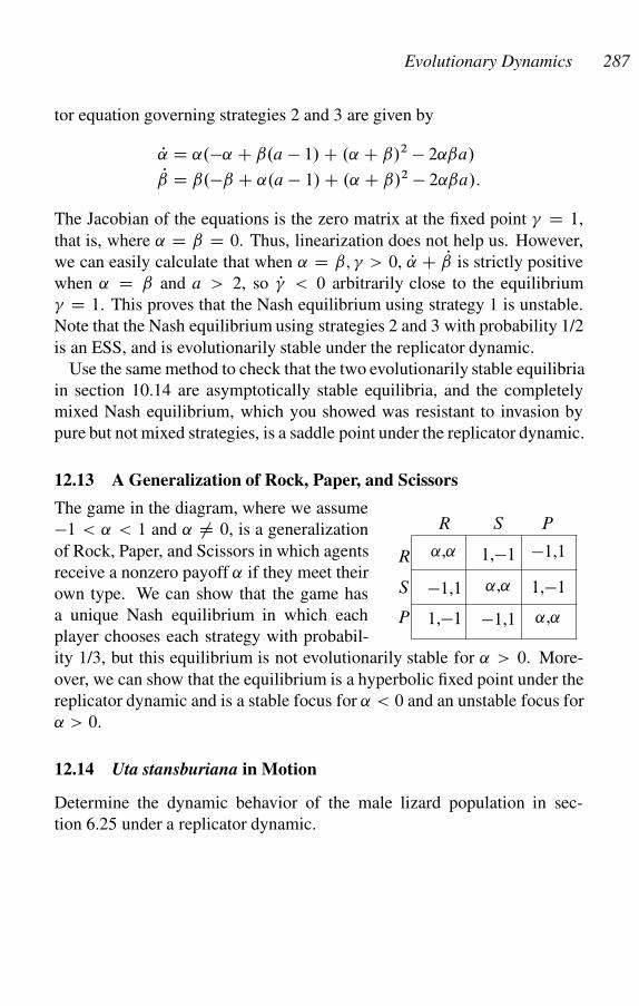
Evolutionary Dynamics 287
tor equation governing strategies 2 and 3 are given by
P D ˛.�˛ C ˇ.a � 1/ C .˛ C ˇ/2 � 2˛ˇa/
P D ˇ.�ˇ C ˛.a � 1/ C .˛ C ˇ/2 � 2˛ˇa/:
The Jacobian of the equations is the zero matrix at the fixed point � D 1,
that is, where ˛ D ˇ D 0. Thus, linearization does not help us. However,
we can easily calculate that when ˛ D ˇ; � > 0, P C P is strictly positive
when ˛ D ˇ and a > 2, so P� < 0 arbitrarily close to the equilibrium
� D 1. This proves that the Nash equilibrium using strategy 1 is unstable.
Note that the Nash equilibrium using strategies 2 and 3 with probability 1/2
is an ESS, and is evolutionarily stable under the replicator dynamic.
Use the same method to check that the two evolutionarily stable equilibria
in section 10.14 are asymptotically stable equilibria, and the completely
mixed Nash equilibrium, which you showed was resistant to invasion by
pure but not mixed strategies, is a saddle point under the replicator dynamic.
12.13 A Generalization of Rock, Paper, and Scissors
R S P
R
S
P
˛,˛
˛,˛
˛,˛
1,�1
1,�1
1,�1
�1,1
�1,1
�1,1
The game in the diagram, where we assume
�1 < ˛ < 1 and ˛ ¤ 0, is a generalization
of Rock, Paper, and Scissors in which agents
receive a nonzero payoff ˛ if they meet their
own type. We can show that the game has
a unique Nash equilibrium in which each
player chooses each strategy with probabil-
ity 1/3, but this equilibrium is not evolutionarily stable for ˛ > 0. More-
over, we can show that the equilibrium is a hyperbolic fixed point under the
replicator dynamic and is a stable focus for ˛ < 0 and an unstable focus for
˛ > 0.
12.14 Uta stansburiana in Motion
Determine the dynamic behavior of the male lizard population in sec-
tion 6.25 under a replicator dynamic.
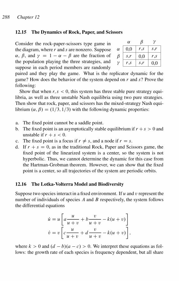
288 Chapter 12
12.15 The Dynamics of Rock, Paper, and Scissors
0,0 r ,s s,r
s,r 0,0 r ,s
r ,s s,r 0,0
˛ ˇ �
˛
ˇ
�
Consider the rock-paper-scissors type game in
the diagram, where r and s are nonzero. Suppose
˛, ˇ, and � D 1 � ˛ � ˇ are the fraction of
the population playing the three strategies, and
suppose in each period members are randomly
paired and they play the game. What is the replicator dynamic for the
game? How does the behavior of the system depend on r and s? Prove the
following:
Show that when r; s < 0, this system has three stable pure strategy equi-
libria, as well as three unstable Nash equilibria using two pure strategies.
Then show that rock, paper, and scissors has the mixed-strategy Nash equi-
librium .˛; ˇ/ D .1=3; 1=3/ with the following dynamic properties:
a. The fixed point cannot be a saddle point.
b. The fixed point is an asymptotically stable equilibrium if r C s > 0 and
unstable if r C s < 0.
c. The fixed point is a focus if r ¤ s, and a node if r D s.
d. If r C s D 0, as in the traditional Rock, Paper and Scissors game, the
fixed point of the linearized system is a center, so the system is not
hyperbolic. Thus, we cannot determine the dynamic for this case from
the Hartman-Grobman theorem. However, we can show that the fixed
point is a center, so all trajectories of the system are periodic orbits.
12.16 The Lotka-Volterra Model and Biodiversity
Suppose two species interact in a fixed environment. If u and v represent the
number of individuals of species A and B respectively, the system follows
the differential equations
Pu D u
�a
u
u C vC b
v
u C v� k.u C v/
�
Pv D v
�c
u
u C vC d
v
u C v� k.u C v/
�;
where k > 0 and .d � b/.a � c/ > 0. We interpret these equations as fol-
lows: the growth rate of each species is frequency dependent, but all share
Evolutionary Dynamics 289
an ecological niche and hence are subject to overcrowding, the intensity of
which is measured by k. For instance, suppose individuals meet at random.
Then, an A meets another A with probability u=.u C v/, and they may re-
produce at rate a, although an A meets a B with probability v=.u C v/,
in which case the A eats the B .b > 0/ or vice versa .b < 0/. Show the
following.
a. Let w D u C v, the size of the total population, and p D u=w, the
fraction of species A in the population. The stationary fraction p� of
species A is given by
p� D d � b
a � c C d � b;
which is strictly positive and independent of the crowding factor k.b. If we think of w as the whole population, then the payoff �A to species
A, the payoff �B to species B , and the mean payoff N� to a member of
the population, abstracting from the overcrowding factor k, are given
by
�A D ap C b.1 � p/;
�B D cp C d.1 � p/;
N� D p�A C .1 � p/�B :
Show that p satisfies the replicator dynamic
Pp D p.�A � N�/;
even taking into account the overcrowding factor. This equation indi-
cates that the frequency of species A in the population is independent of
the crowding factor in the dynamic interaction between the two species.
Moreover, the stability conditions for p are also independent of k, so
we conclude: If neither species can become extinct when the crowding
factor k is low, the same is true no matter how large the crowding factor
k.c. We can generalize this result as follows. Suppose there are n species,
and let ui be the number of individuals in species i , for i D 1; : : : ; n.
Define w D Pj uj and for i D 1; : : : ; n let pi D ui=w, the relative
frequency of species i . Suppose the system satisfies the equations
Pui D ui Œai1p1 C : : : C ainpn � ku�
290 Chapter 12
for k > 0. We assume the faij g are such that there is a positive sta-
tionary frequency for each species. Show that the system satisfies the
differential equations
Ppi
pi
DnX
j D1
aij pj �nX
j;kD1
ajkpj pk
for i D 1; : : : ; n. Show that this represents a replicator dynamic if the
payoffs to the various species abstract from the crowding factor k. Once
again we find that the frequency of each species is independent of the
crowding factor, and if the ecology is sustainable with low crowding
factor (that is, no species goes extinct), then it remains so with high
crowding factor.
This result is surprising, perhaps. How do we account for it? It is easy to
see that the absolute number of individuals in each species in equilibrium
is proportional to 1=k. Thus, when k is large, the justification for using
a replicator dynamic is no longer valid: with considerable probability, the
stochastic elements abstracted from in the replicator dynamic act to reduce
some pi to zero, after which it cannot ever recover unless the ecological
system is repopulated from the outside. For an example of dynamics of this
type, see Durrett and Levin (1994).
12.17 Asymmetric Evolutionary Games
Consider two populations of interacting agents. In each time period, agents
from one population (row players) are randomly paired with agents from
the other population (column players). The paired agents then play a game
in which row players have pure strategies S D fs1; : : : ; sng and column
players have pure strategies T D ft1; : : : ; tmg. Agents are “wired” to play
one of the pure strategies available to them, and the payoffs to an i-type
(that is, a row player wired to play si ) playing a j -type (that is, a column
player wired to play tj ) are ˛ij for the i-type and ˇij for the j -type. We
call the resulting game an asymmetric evolutionary game.
Suppose the frequency composition of strategies among column players
is q D .q1; : : : ; qm/, where qj is the fraction of j -types among column
Evolutionary Dynamics 291
players. Then, the payoff to an i-type row player is
˛i .q/ DmX
j D1
qj ˛ij :
Similarly if the frequency composition of strategies among row players is
p D .p1; : : : ; pn/, where pi is the fraction of i-types among row players,
then the payoff to a j -type column player is
j .p/ DnX
iD1
piˇij :
We say si 2 S is a best response to q 2 Q if ˛i .q/ ˛k.q/ for all sk 2 S ,
and we say tj 2 T is a best response to p 2 P if j .p/ ˇk.p/ for
all tk 2 T . A Nash equilibrium in an asymmetric evolutionary game is
a frequency composition p� 2 P of row players and q� 2 Q of column
players such that for all si 2 S , if p�i > 0, then si is a best response to q�,
and for all sj 2 T , if q�j > 0, then tj is a best response to p�.
Note that there is a natural correspondence between the mixed-strategy
Nash equilibria of a two-player normal form game as defined in section 3.4
and the Nash equilibria of an asymmetric evolutionary game. Thus, if we
take an arbitrary two-player game in which row players and column players
are distinguished and place the game in an evolutionary setting, we get an
asymmetric evolutionary game. Hence, the dynamics of asymmetric evolu-
tionary games more or less represent the dynamics of two-player games in
general.1
A replicator dynamic for an asymmetric evolutionary game is given by
the n C m � 2 equations
Ppi D pi.˛i .q/ � ˛.p; q//(12.12)Pqj D qj . j .p/ � ˇ.p; q//;
1I say more or less because in fact the assumption of random pairings of agents
is not at all characteristic of how agents are paired in most strategic interaction set-
tings. More common is some form of assortative interaction, in which agents with
particular characteristics have a higher than chance probability of interacting. As-
sortative interactions, for instance, are a more favorable setting for the emergence
of altruism than panmictic interactions.
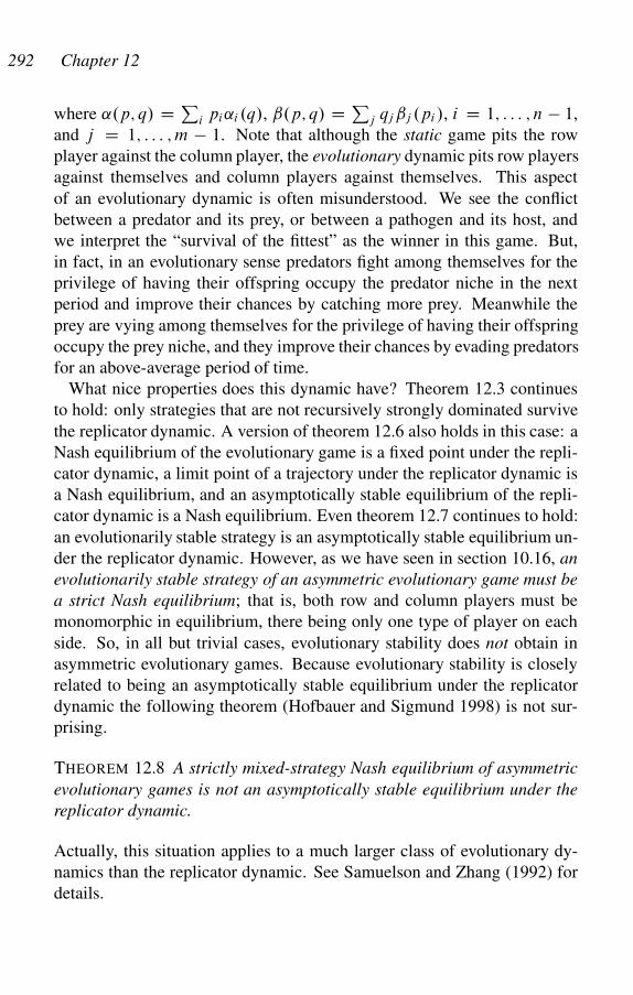
292 Chapter 12
where ˛.p; q/ D Pi pi˛i .q/, ˇ.p; q/ D P
j qj j .pi /, i D 1; : : : ; n � 1,
and j D 1; : : : ; m � 1. Note that although the static game pits the row
player against the column player, the evolutionary dynamic pits row players
against themselves and column players against themselves. This aspect
of an evolutionary dynamic is often misunderstood. We see the conflict
between a predator and its prey, or between a pathogen and its host, and
we interpret the “survival of the fittest” as the winner in this game. But,
in fact, in an evolutionary sense predators fight among themselves for the
privilege of having their offspring occupy the predator niche in the next
period and improve their chances by catching more prey. Meanwhile the
prey are vying among themselves for the privilege of having their offspring
occupy the prey niche, and they improve their chances by evading predators
for an above-average period of time.
What nice properties does this dynamic have? Theorem 12.3 continues
to hold: only strategies that are not recursively strongly dominated survive
the replicator dynamic. A version of theorem 12.6 also holds in this case: a
Nash equilibrium of the evolutionary game is a fixed point under the repli-
cator dynamic, a limit point of a trajectory under the replicator dynamic is
a Nash equilibrium, and an asymptotically stable equilibrium of the repli-
cator dynamic is a Nash equilibrium. Even theorem 12.7 continues to hold:
an evolutionarily stable strategy is an asymptotically stable equilibrium un-
der the replicator dynamic. However, as we have seen in section 10.16, an
evolutionarily stable strategy of an asymmetric evolutionary game must be
a strict Nash equilibrium; that is, both row and column players must be
monomorphic in equilibrium, there being only one type of player on each
side. So, in all but trivial cases, evolutionary stability does not obtain in
asymmetric evolutionary games. Because evolutionary stability is closely
related to being an asymptotically stable equilibrium under the replicator
dynamic the following theorem (Hofbauer and Sigmund 1998) is not sur-
prising.
THEOREM 12.8 A strictly mixed-strategy Nash equilibrium of asymmetric
evolutionary games is not an asymptotically stable equilibrium under the
replicator dynamic.
Actually, this situation applies to a much larger class of evolutionary dy-
namics than the replicator dynamic. See Samuelson and Zhang (1992) for
details.
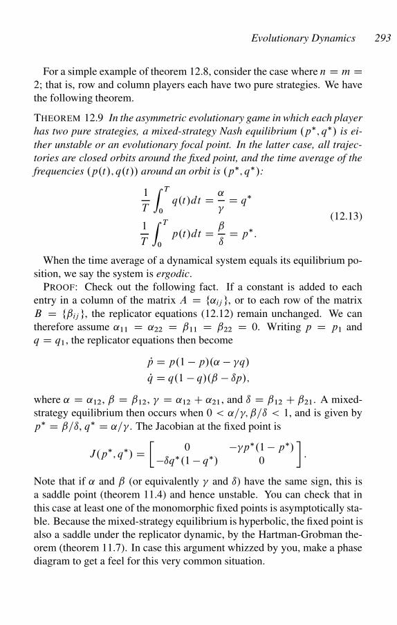
Evolutionary Dynamics 293
For a simple example of theorem 12.8, consider the case where n D m D2; that is, row and column players each have two pure strategies. We have
the following theorem.
THEOREM 12.9 In the asymmetric evolutionary game in which each player
has two pure strategies, a mixed-strategy Nash equilibrium .p�; q�/ is ei-
ther unstable or an evolutionary focal point. In the latter case, all trajec-
tories are closed orbits around the fixed point, and the time average of the
frequencies .p.t/; q.t// around an orbit is .p�; q�/:
1
T
Z T
0
q.t/dt D ˛
�D q�
(12.13)1
T
Z T
0
p.t/dt D ˇ
ıD p�:
When the time average of a dynamical system equals its equilibrium po-
sition, we say the system is ergodic.
PROOF: Check out the following fact. If a constant is added to each
entry in a column of the matrix A D f˛ij g, or to each row of the matrix
B D fˇij g, the replicator equations (12.12) remain unchanged. We can
therefore assume ˛11 D ˛22 D ˇ11 D ˇ22 D 0. Writing p D p1 and
q D q1, the replicator equations then become
Pp D p.1 � p/.˛ � �q/
Pq D q.1 � q/.ˇ � ıp/;
where ˛ D ˛12, ˇ D ˇ12, � D ˛12 C ˛21, and ı D ˇ12 C ˇ21. A mixed-
strategy equilibrium then occurs when 0 < ˛=�; ˇ=ı < 1, and is given by
p� D ˇ=ı, q� D ˛=� . The Jacobian at the fixed point is
J.p�; q�/ D�
0 ��p�.1 � p�/
�ıq�.1 � q�/ 0
�:
Note that if ˛ and ˇ (or equivalently � and ı) have the same sign, this is
a saddle point (theorem 11.4) and hence unstable. You can check that in
this case at least one of the monomorphic fixed points is asymptotically sta-
ble. Because the mixed-strategy equilibrium is hyperbolic, the fixed point is
also a saddle under the replicator dynamic, by the Hartman-Grobman the-
orem (theorem 11.7). In case this argument whizzed by you, make a phase
diagram to get a feel for this very common situation.
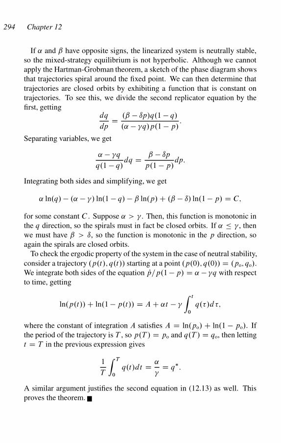
294 Chapter 12
If ˛ and ˇ have opposite signs, the linearized system is neutrally stable,
so the mixed-strategy equilibrium is not hyperbolic. Although we cannot
apply the Hartman-Grobman theorem, a sketch of the phase diagram shows
that trajectories spiral around the fixed point. We can then determine that
trajectories are closed orbits by exhibiting a function that is constant on
trajectories. To see this, we divide the second replicator equation by the
first, gettingdq
dpD .ˇ � ıp/q.1 � q/
.˛ � �q/p.1 � p/:
Separating variables, we get
˛ � �q
q.1 � q/dq D ˇ � ıp
p.1 � p/dp:
Integrating both sides and simplifying, we get
˛ ln.q/ � .˛ � �/ ln.1 � q/ � ˇ ln.p/ C .ˇ � ı/ ln.1 � p/ D C;
for some constant C . Suppose ˛ > � . Then, this function is monotonic in
the q direction, so the spirals must in fact be closed orbits. If ˛ � � , then
we must have ˇ > ı, so the function is monotonic in the p direction, so
again the spirals are closed orbits.
To check the ergodic property of the system in the case of neutral stability,
consider a trajectory .p.t/; q.t// starting at a point .p.0/; q.0// D .po; qo/.
We integrate both sides of the equation Pp=p.1 � p/ D ˛ � �q with respect
to time, getting
ln.p.t// C ln.1 � p.t// D A C ˛t � �
Z t
0
q./d;
where the constant of integration A satisfies A D ln.po/ C ln.1 � po/. If
the period of the trajectory is T , so p.T / D po and q.T / D qo, then letting
t D T in the previous expression gives
1
T
Z T
0
q.t/dt D ˛
�D q�:
A similar argument justifies the second equation in (12.13) as well. This
proves the theorem.
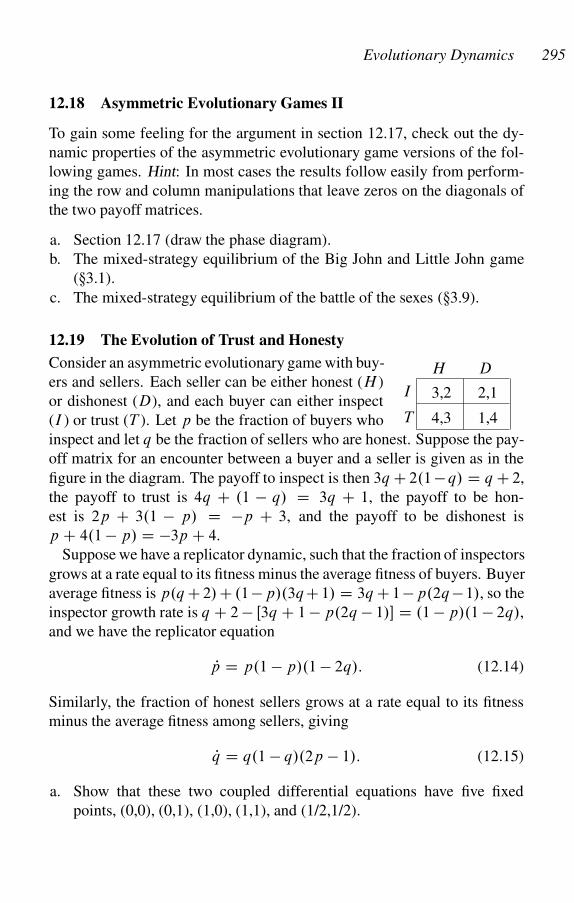
Evolutionary Dynamics 295
12.18 Asymmetric Evolutionary Games II
To gain some feeling for the argument in section 12.17, check out the dy-
namic properties of the asymmetric evolutionary game versions of the fol-
lowing games. Hint: In most cases the results follow easily from perform-
ing the row and column manipulations that leave zeros on the diagonals of
the two payoff matrices.
a. Section 12.17 (draw the phase diagram).
b. The mixed-strategy equilibrium of the Big John and Little John game
(�3.1).
c. The mixed-strategy equilibrium of the battle of the sexes (�3.9).
12.19 The Evolution of Trust and Honesty
3,2
4,3
H
2,1
1,4
D
I
T
Consider an asymmetric evolutionary game with buy-
ers and sellers. Each seller can be either honest (H )
or dishonest (D), and each buyer can either inspect
(I ) or trust (T ). Let p be the fraction of buyers who
inspect and let q be the fraction of sellers who are honest. Suppose the pay-
off matrix for an encounter between a buyer and a seller is given as in the
figure in the diagram. The payoff to inspect is then 3q C 2.1 � q/ D q C 2,
the payoff to trust is 4q C .1 � q/ D 3q C 1, the payoff to be hon-
est is 2p C 3.1 � p/ D �p C 3, and the payoff to be dishonest is
p C 4.1 � p/ D �3p C 4.
Suppose we have a replicator dynamic, such that the fraction of inspectors
grows at a rate equal to its fitness minus the average fitness of buyers. Buyer
average fitness is p.q C 2/ C .1 �p/.3qC 1/ D 3q C 1 �p.2q �1/, so the
inspector growth rate is q C 2 � Œ3q C 1 � p.2q � 1/� D .1 � p/.1 � 2q/,
and we have the replicator equation
Pp D p.1 � p/.1 � 2q/: (12.14)
Similarly, the fraction of honest sellers grows at a rate equal to its fitness
minus the average fitness among sellers, giving
Pq D q.1 � q/.2p � 1/: (12.15)
a. Show that these two coupled differential equations have five fixed
points, (0,0), (0,1), (1,0), (1,1), and (1/2,1/2).
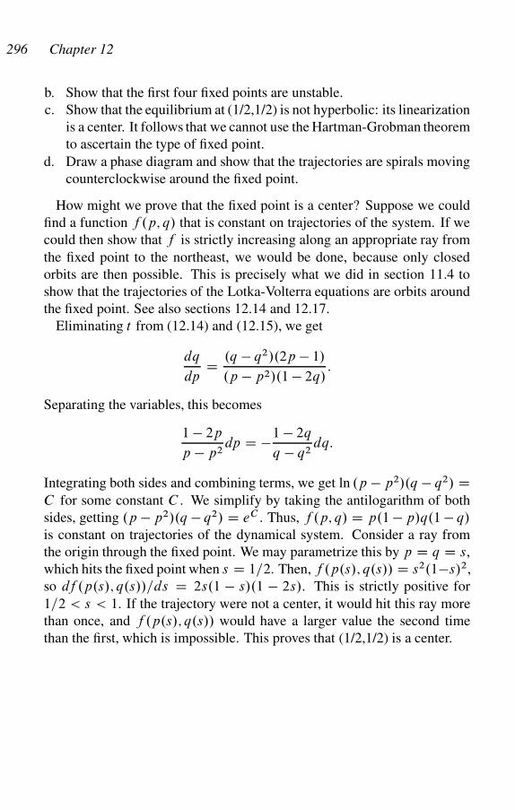
296 Chapter 12
b. Show that the first four fixed points are unstable.
c. Show that the equilibrium at (1/2,1/2) is not hyperbolic: its linearization
is a center. It follows that we cannot use the Hartman-Grobman theorem
to ascertain the type of fixed point.
d. Draw a phase diagram and show that the trajectories are spirals moving
counterclockwise around the fixed point.
How might we prove that the fixed point is a center? Suppose we could
find a function f .p; q/ that is constant on trajectories of the system. If we
could then show that f is strictly increasing along an appropriate ray from
the fixed point to the northeast, we would be done, because only closed
orbits are then possible. This is precisely what we did in section 11.4 to
show that the trajectories of the Lotka-Volterra equations are orbits around
the fixed point. See also sections 12.14 and 12.17.
Eliminating t from (12.14) and (12.15), we get
dq
dpD .q � q2/.2p � 1/
.p � p2/.1 � 2q/:
Separating the variables, this becomes
1 � 2p
p � p2dp D �1 � 2q
q � q2dq:
Integrating both sides and combining terms, we get ln .p � p2/.q � q2/ DC for some constant C . We simplify by taking the antilogarithm of both
sides, getting .p � p2/.q � q2/ D eC . Thus, f .p; q/ D p.1 � p/q.1 � q/
is constant on trajectories of the dynamical system. Consider a ray from
the origin through the fixed point. We may parametrize this by p D q D s,
which hits the fixed point when s D 1=2. Then, f .p.s/; q.s// D s2.1�s/2,
so df .p.s/; q.s//=ds D 2s.1 � s/.1 � 2s/. This is strictly positive for
1=2 < s < 1. If the trajectory were not a center, it would hit this ray more
than once, and f .p.s/; q.s// would have a larger value the second time
than the first, which is impossible. This proves that (1/2,1/2) is a center.
13
Markov Economies and Stochastic Dynamical
Systems
God does not play dicewith the Universe.
Albert Einstein
Time-discrete stochastic processes are powerful tools for characterizing
some dynamical systems. The prerequisites include an understanding of
Markov chains (�13.1). Time-discrete systems behave quite differently
from dynamical systems based on systems of ordinary differential equa-
tions. This chapter presents a Markov model of adaptive learning that il-
lustrates the concept of stochastic stability, as developed in Young (1998).
After developing some of the theoretical results, we provide an agent-based
model.
13.1 Markov Chains
A finite Markov chain is a dynamical system that in each time period t D0; 1; : : : can be any one of n states, such that if the system is in state i in one
time period, there is a probability pij that the system will be in state j in
the next time period. Thus, for each i , we must haveP
j pij D 1, because
the system must go somewhere in each period. We call the n � n matrix
P D fpij g the transition probability matrix of the Markov chain, and each
pij is called a transition probability. A denumerable Markov chain has an
infinite number of states t D 1; 2; : : :, and is otherwise the same. If we do
not care whether the finite or denumerable case obtains, we speak simply
of a Markov chain.
Many games can be viewed as Markov chains. Here are some examples:
a. Suppose two gamblers have wealth k1 and k2 dollars, respectively, and
in each period they play a game in which each has an equal chance
of winning one dollar. The game continues until one player has no
more wealth. Here the state of the system is the wealth w of player 1,
297
298 Chapter 13
pw;wC1 D pw;w�1 D 1=2 for 0 < w < k1 Ck2, and all other transition
probabilities are zero.
b. Suppose n agents play a game in which they are randomly paired in
each period, and the stage game is a prisoner’s dilemma. Players can
remember the last k moves of their various partners. Players are also
given one of r strategies, which determine their next move, depending
on their current histories. When a player dies, which occurs with a
certain probability, it is replaced by a new player who is a clone of a
successful player. We can consider this a Markov chain in which the
state of the system is the history, strategy, and score of each player, and
the transition probabilities are just the probabilities of moving from one
such state to another, given the players’ strategies (�13.8).
c. Suppose n agents play a game in which they are randomly paired in
each period to trade. Each agent has an inventory of goods to trade and
a strategy indicating which goods the agent is willing to trade for which
other goods. After trading, agents consume some of their inventory and
produce more goods for their inventory, according to some consump-
tion and production strategy. When an agent dies, it is replaced by a
new agent with the same strategy and an empty inventory. If there is
a maximum-size inventory and all goods are indivisible, we can con-
sider this a finite Markov chain in which the state of the system is the
strategy and inventory of each player and the transition probabilities are
determined accordingly.
d. In a population of beetles, females have k offspring in each period with
probability fk , and beetles live for n periods. The state of the system
is the fraction of males and females of each age. This is a denumerable
Markov chain, where the transition probabilities are calculated from the
birth and death rates of the beetles.
We are interested in the long-run behavior of Markov chains. In particu-
lar, we are interested in the behavior of systems that we expect will attain a
long-run equilibrium of some type independent from its initial conditions.
If such an equilibrium exists, we say the Markov chain is ergodic. In an
ergodic system, history does not matter: every initial condition leads to the
same long-run behavior. Nonergodic systems are history dependent. It is
intuitively reasonable that the repeated prisoner’s dilemma and the trading
model described previously are ergotic. The gambler model is not ergodic,
Stochastic Dynamical Systems 299
because the system could end up with either player bankrupt.1 What is your
intuition concerning the beetle population, if there is a positive probability
that a female has no offspring in a breeding season?
It turns out that there is a very simple and powerful theorem that tells us
exactly when a Markov chain is ergodic and provides a simple character-
ization of the long-run behavior of the system. To develop the machinery
needed to express and understand this theorem, we will define a few terms.
Let p.m/ij be the probability of being in state j in m periods if the chain is
currently in state i . Thus, if we start in state i at period 1, the probability of
being in state j at period 2 is just p.1/ij D pij . To be in state j in period 3
starting from state i in period 1, the system must move from state i to some
state k in period 2, and then from k to j in period 3. This happens with
probability pikpkj . Adding up over all k, the probability of being in state
j in period 3 is
p.2/ij D
X
k
pikpkj :
Using matrix notation, this means the matrix of two-period transitions is
given by
P .2/ D fp.2/ij ji; j D 1; 2; : : :g D P 2:
Generalizing, we see that the k-period transition matrix is simply P k . What
we are looking for, then, is the limit of P k as k ! 1. Let us call this limit
(supposing it exists) P � D fp�ij g. Now P � must have two properties. First,
because the long-run behavior of the system cannot depend on where it
started, p�ij D p�
i 0j for any two states i and i 0. This means that all the rows
of P � must be the same. Let us denote the (common value of the) rows by
u D fu1; : : : ; ung, so uj is the probability that the Markov chain will be in
state j in the long run. The second fact is that
PP � D P limk!1
P k D limk!1
P kC1 D P �:
This means u must satisfy
uj D limm!1
p.m/ij for i D 1; : : : ; n (13.1)
1Specifically, you can show that the probability that player 1 wins is k1=.k1 C
k2/, and if player 1 has wealth w at some point in the game, the probability he will
win is w=.k1 C k2/.

300 Chapter 13
uj DX
i
uipij (13.2)
X
k
uk D 1; (13.3)
for j D 1; : : : ; n. Note that (13.2) can be written in matrix notation as
u D uP , so u is a left eigenvector of P . The first equation says that uj is
the limit probability of being in state j starting from any state, the second
says that the probability of being in state j is the probability of moving
from some state i to state j , which is uipij , summed over all states i , and
the final equation says u is a probability distribution over the states of the
Markov chain. The recursion equations (13.2) and (13.3) are often suffi-
cient to determine u, which we call the invariant distribution or stationary
distribution of the Markov chain.
In the case where the Markov chain is finite, the preceding description
of the stationary distribution is a result of the Frobenius-Perron theorem
(Horn and Johnson 1985), which says that P has a maximum eigenvalue
of unity, and the associated left eigenvector, which is the stationary distri-
bution .u1; : : : ; un/ for P , exists and has nonnegative entries. Moreover, if
P k is strictly positive for some k (in which case we say P is irreducible),
then the stationary distribution has strictly positive entries.
In case a Markov chain is not ergodic, it is informative to know the whole
matrix P � D .p�ij /, because pij tell you the probability of being absorbed
by state j , starting from state i . The Frobenius-Perron theorem is useful
here also, because it tells us that all the eigenvalues of P are either unity
or strictly less than unity in absolute value. Thus, if D D .dij / is the
n � n diagonal matrix with the eigenvalues of P along the diagonal, then
D� D limk!1 Dk is the diagonal matrix with zeros everywhere except
unity where di i D 1. But, if M is the matrix of left eigenvectors of P ,
then MPM �1 D D, which follows from the definitions, implies P � DM �1D�M . This equation allows us to calculate P � rather easily.
A few examples are useful to get a feel for the recursion equations. Con-
sider first the n-state Markov chain called the random walk on a circle, in
which there are n states, and from any state t D 2; : : : ; n � 1 the system
moves with equal probability to the previous or the next state, from state n
it moves with equal probability to state 1 or state n � 1, and from state 1
it moves with equal probability to state 2 and to state n. In the long run, it
is intuitively clear that the system will be all states with equal probability
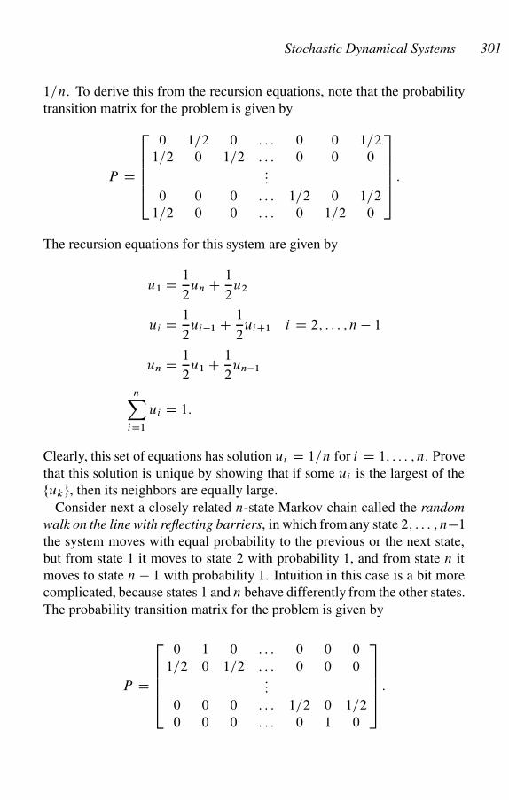
Stochastic Dynamical Systems 301
1=n. To derive this from the recursion equations, note that the probability
transition matrix for the problem is given by
P D
266664
0 1=2 0 : : : 0 0 1=2
1=2 0 1=2 : : : 0 0 0:::
0 0 0 : : : 1=2 0 1=2
1=2 0 0 : : : 0 1=2 0
377775
:
The recursion equations for this system are given by
u1 D 1
2un C 1
2u2
ui D 1
2ui�1 C 1
2uiC1 i D 2; : : : ; n � 1
un D 1
2u1 C 1
2un�1
nX
iD1
ui D 1:
Clearly, this set of equations has solution ui D 1=n for i D 1; : : : ; n. Prove
that this solution is unique by showing that if some ui is the largest of the
fukg, then its neighbors are equally large.
Consider next a closely related n-state Markov chain called the random
walk on the line with reflecting barriers, in which from any state 2; : : : ; n�1
the system moves with equal probability to the previous or the next state,
but from state 1 it moves to state 2 with probability 1, and from state n it
moves to state n � 1 with probability 1. Intuition in this case is a bit more
complicated, because states 1 and n behave differently from the other states.
The probability transition matrix for the problem is given by
P D
266664
0 1 0 : : : 0 0 0
1=2 0 1=2 : : : 0 0 0:::
0 0 0 : : : 1=2 0 1=2
0 0 0 : : : 0 1 0
377775
:
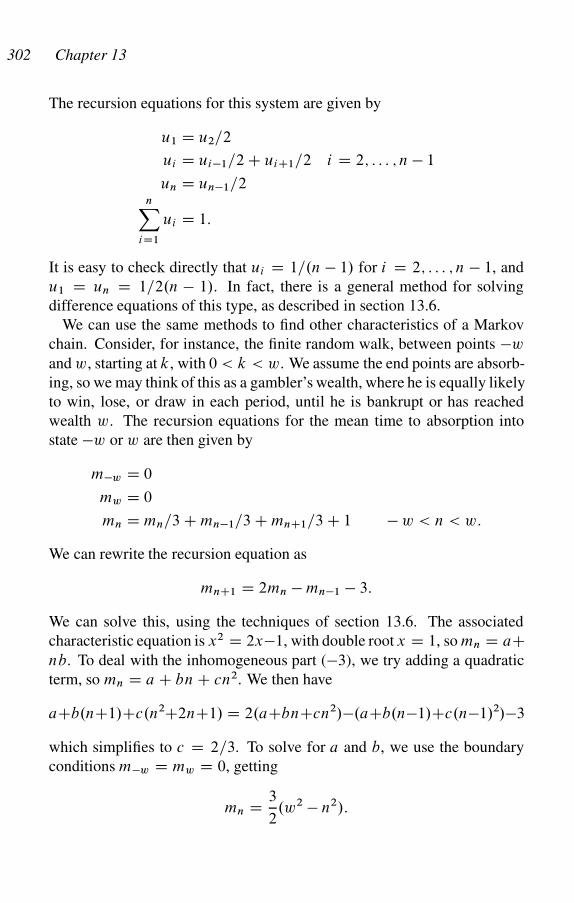
302 Chapter 13
The recursion equations for this system are given by
u1 D u2=2
ui D ui�1=2 C uiC1=2 i D 2; : : : ; n � 1
un D un�1=2nX
iD1
ui D 1:
It is easy to check directly that ui D 1=.n � 1/ for i D 2; : : : ; n � 1, and
u1 D un D 1=2.n � 1/. In fact, there is a general method for solving
difference equations of this type, as described in section 13.6.
We can use the same methods to find other characteristics of a Markov
chain. Consider, for instance, the finite random walk, between points �w
and w, starting at k, with 0 < k < w. We assume the end points are absorb-
ing, so we may think of this as a gambler’s wealth, where he is equally likely
to win, lose, or draw in each period, until he is bankrupt or has reached
wealth w. The recursion equations for the mean time to absorption into
state �w or w are then given by
m�w D 0
mw D 0
mn D mn=3 C mn�1=3 C mnC1=3 C 1 � w < n < w:
We can rewrite the recursion equation as
mnC1 D 2mn � mn�1 � 3:
We can solve this, using the techniques of section 13.6. The associated
characteristic equation is x2 D 2x�1, with double root x D 1, so mn D aCnb. To deal with the inhomogeneous part (�3), we try adding a quadratic
term, so mn D a C bn C cn2. We then have
aCb.nC1/Cc.n2C2nC1/ D 2.aCbnCcn2/�.aCb.n�1/Cc.n�1/2/�3
which simplifies to c D 2=3. To solve for a and b, we use the boundary
conditions m�w D mw D 0, getting
mn D 3
2.w2 � n2/:
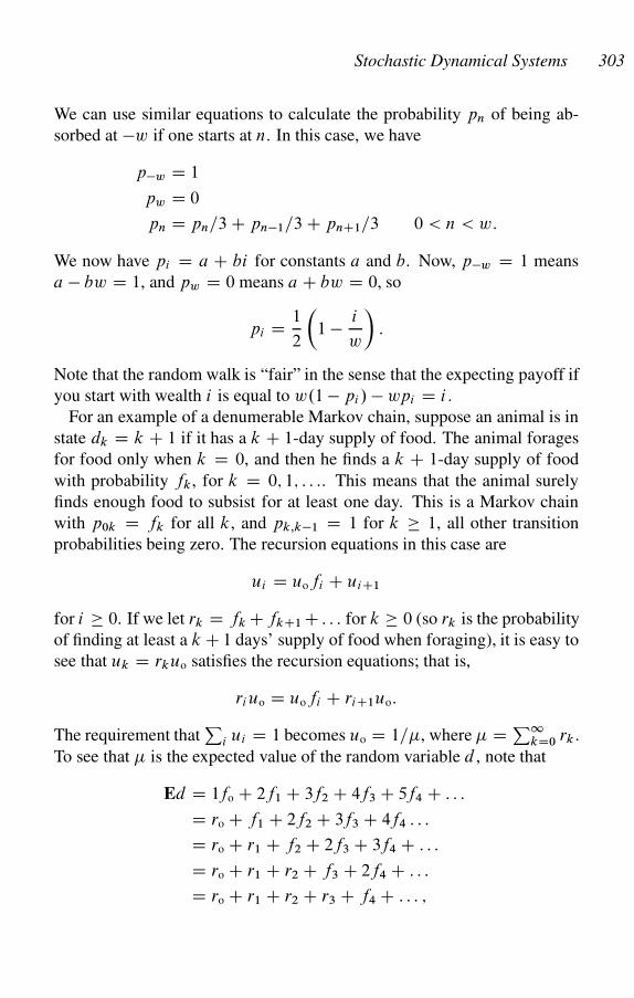
Stochastic Dynamical Systems 303
We can use similar equations to calculate the probability pn of being ab-
sorbed at �w if one starts at n. In this case, we have
p�w D 1
pw D 0
pn D pn=3 C pn�1=3 C pnC1=3 0 < n < w:
We now have pi D a C bi for constants a and b. Now, p�w D 1 means
a � bw D 1, and pw D 0 means a C bw D 0, so
pi D 1
2
�1 � i
w
�:
Note that the random walk is “fair” in the sense that the expecting payoff if
you start with wealth i is equal to w.1 � pi / � wpi D i .
For an example of a denumerable Markov chain, suppose an animal is in
state dk D k C 1 if it has a k C 1-day supply of food. The animal forages
for food only when k D 0, and then he finds a k C 1-day supply of food
with probability fk, for k D 0; 1; : : :. This means that the animal surely
finds enough food to subsist for at least one day. This is a Markov chain
with p0k D fk for all k, and pk;k�1 D 1 for k 1, all other transition
probabilities being zero. The recursion equations in this case are
ui D uofi C uiC1
for i 0. If we let rk D fk C fkC1 C : : : for k 0 (so rk is the probability
of finding at least a k C 1 days’ supply of food when foraging), it is easy to
see that uk D rkuo satisfies the recursion equations; that is,
riuo D uofi C riC1uo:
The requirement thatP
i ui D 1 becomes uo D 1=�, where � D P1kD0 rk .
To see that � is the expected value of the random variable d , note that
Ed D 1fo C 2f1 C 3f2 C 4f3 C 5f4 C : : :
D ro C f1 C 2f2 C 3f3 C 4f4 : : :
D ro C r1 C f2 C 2f3 C 3f4 C : : :
D ro C r1 C r2 C f3 C 2f4 C : : :
D ro C r1 C r2 C r3 C f4 C : : : ;
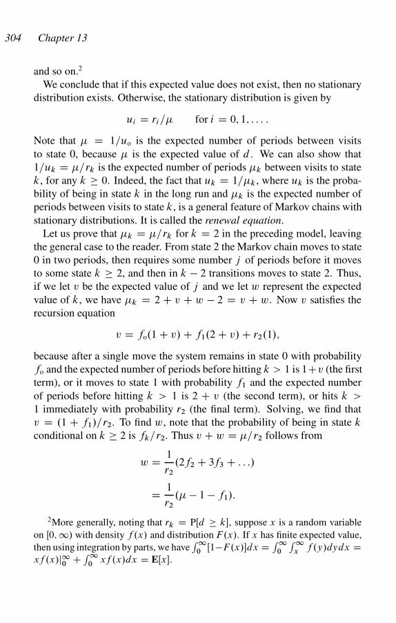
304 Chapter 13
and so on.2
We conclude that if this expected value does not exist, then no stationary
distribution exists. Otherwise, the stationary distribution is given by
ui D ri=� for i D 0; 1; : : : :
Note that � D 1=uo is the expected number of periods between visits
to state 0, because � is the expected value of d . We can also show that
1=uk D �=rk is the expected number of periods �k between visits to state
k, for any k 0. Indeed, the fact that uk D 1=�k , where uk is the proba-
bility of being in state k in the long run and �k is the expected number of
periods between visits to state k, is a general feature of Markov chains with
stationary distributions. It is called the renewal equation.
Let us prove that �k D �=rk for k D 2 in the preceding model, leaving
the general case to the reader. From state 2 the Markov chain moves to state
0 in two periods, then requires some number j of periods before it moves
to some state k 2, and then in k � 2 transitions moves to state 2. Thus,
if we let v be the expected value of j and we let w represent the expected
value of k, we have �k D 2 C v C w � 2 D v C w. Now v satisfies the
recursion equation
v D fo.1 C v/ C f1.2 C v/ C r2.1/;
because after a single move the system remains in state 0 with probability
fo and the expected number of periods before hitting k > 1 is 1Cv (the first
term), or it moves to state 1 with probability f1 and the expected number
of periods before hitting k > 1 is 2 C v (the second term), or hits k >
1 immediately with probability r2 (the final term). Solving, we find that
v D .1 C f1/=r2. To find w, note that the probability of being in state k
conditional on k 2 is fk=r2. Thus v C w D �=r2 follows from
w D 1
r2
.2f2 C 3f3 C : : :/
D 1
r2
.� � 1 � f1/:
2More generally, noting that rk D PŒd � k�, suppose x is a random variable
on Œ0; 1/ with density f .x/ and distribution F.x/. If x has finite expected value,
then using integration by parts, we haveR1
0 Œ1�F.x/�dx DR1
0
R1
x f .y/dydx D
xf .x/j10 CR1
0xf .x/dx D EŒx�:
Stochastic Dynamical Systems 305
13.2 The Ergodic Theorem for Markov Chains
When are equations (13.1)-(13.3) true, and what exactly do they say? To
answer this, we will need a few more concepts. Throughout, we let M be a
finite or denumerable Markov chain with transition probabilities fpij g. We
say a state j can be reached from a state i if p.m/ij > 0 for some positive
integer m. We say a pair of states i and j communicates if each is reached
from the other. We say a Markov chain is irreducible if every pair of states
communicates.
If M is irreducible, and if a stationary distribution u exists, then all the
ui in (13.1) are strictly positive. To see this, suppose some uj D 0. Then
by (13.2), if pij > 0, then pi D 0. Thus, any state that reaches j in one
period must also have weight zero in u. But a state i 0 that reaches j in
two periods must pass through a state i that reaches j in one period, and
because ui D 0, we also must have ui 0 D 0. Extending this argument, we
say that any state i that reaches j must have ui D 0, and because M is
irreducible, all the ui D 0, which violates (13.3).
Let qi be the probability that, starting from state i , the system returns to
state i in some future period. If qi < 1, then it is clear that with probability
one, state i can occur only a finite number of times. Thus, in the long run
we must have ui D 0, which is impossible for a stationary distribution.
Thus in order for a stationary distribution to exist, we must have qi D 1.
We say a state i is persistent or recurrent if qi D 1. Otherwise, we say
state i is transient. If all the states of M are recurrent, we say that M is
recurrent.
Let �i the be the expected number of states before the Markov chain
returns to state i . Clearly, if i is transient, then �i D 1, but even if i
is persistent, there is no guarantee that �i < 1. We call �i the mean
recurrence time of state i . If the mean recurrence time of state i is �i ,
M is in state i on average one period out of every �i , so we should have
ui D 1=�i . In fact, this can be shown to be true whenever the Markov chain
has a stationary distribution. This is called the renewal theorem for Markov
chains. We treat the renewal theorem as part of the ergodic theorem. Thus,
if M is irreducible, it can have a stationary distribution only if �i is finite,
so ui D 1=�i > 0. We say a recurrent state i in a Markov chain is null if
�i D 1, and otherwise we call the state non-null. An irreducible Markov
chain cannot have a stationary distribution unless all its recurrent states are
non-null.
306 Chapter 13
We say state i in a Markov chain is periodic if there is some integer k > 1
such that p.k/i i > 0 and p
.m/ii > 0 implies m is a multiple of k. Otherwise, we
say M is aperiodic. It is clear that if M has a non-null, recurrent, periodic
state i , then M cannot have a stationary distribution, because we must have
ui D limk!1 p.k/i i > 0, which is impossible unless p
.k/i i is bounded away
from zero for sufficiently large k.
An irreducible, non-null recurrent, aperiodic Markov chain is called er-
godic. We have shown that if an irreducible Markov chain is not ergodic,
it cannot have a stationary distribution. Conversely, we have the following
ergodic theorem for Markov chains, the proof of which can be found in
Feller (1950).
THEOREM 13.1 An ergodic Markov chain M has a unique stationary dis-
tribution, and the recursion equations (13.1)-(13.3) hold with all ui > 0.
Moreover uj D 1=�j for each state j , where �j is the mean recurrence
time for state j .
We say a subset M 0 of states of M is isolated if no state in M 0 reaches
a state not in M 0. Clearly an isolated set of states is a Markov chain. We
say M 0 is an irreducible set if M 0 is isolated and all pairs of states in M 0
communicate. Clearly, an irreducible set is an irreducible Markov chain.
Suppose a Markov chain M consists of an irreducible set M 0 plus a set A
of states, each of which reaches M 0. Then, if u0 is a stationary distribution
of M 0, there is a stationary distribution u for M such that ui D u0i for
i 2 M 0 and ui D 0 for i 2 A. We can summarize this by saying that
a Markov chain that consists of an irreducible set of states plus a set of
transient states has a unique stationary distribution in which the frequency
of the transient states is zero and the frequency of recurrent states is strictly
positive. We call such a Markov chain nearly irreducible, with transient
states A and an absorbing set of states M 0.
More generally, the states of a Markov chain M can be uniquely parti-
tioned into subsets A; M1; M2 : : : such that for each i , Mi is nearly irre-
ducible and each state in A reaches Mi for some i . The states in A are thus
transient, and if each Mi is non-null and aperiodic, it has a unique station-
ary distribution. However, M does not have a stationary distribution unless
it is nearly irreducible.
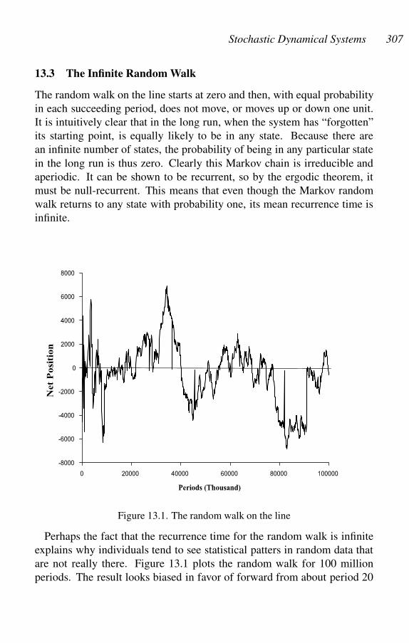
Stochastic Dynamical Systems 307
13.3 The Infinite Random Walk
The random walk on the line starts at zero and then, with equal probability
in each succeeding period, does not move, or moves up or down one unit.
It is intuitively clear that in the long run, when the system has “forgotten”
its starting point, is equally likely to be in any state. Because there are
an infinite number of states, the probability of being in any particular state
in the long run is thus zero. Clearly this Markov chain is irreducible and
aperiodic. It can be shown to be recurrent, so by the ergodic theorem, it
must be null-recurrent. This means that even though the Markov random
walk returns to any state with probability one, its mean recurrence time is
infinite.
Figure 13.1. The random walk on the line
Perhaps the fact that the recurrence time for the random walk is infinite
explains why individuals tend to see statistical patters in random data that
are not really there. Figure 13.1 plots the random walk for 100 million
periods. The result looks biased in favor of forward from about period 20
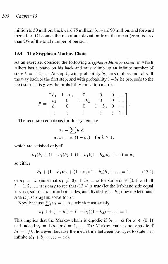
308 Chapter 13
million to 50 million, backward 75 million, forward 90 million, and forward
thereafter. Of course the maximum deviation from the mean (zero) is less
than 2% of the total number of periods.
13.4 The Sisyphean Markov Chain
As an exercise, consider the following Sisyphean Markov chain, in which
Albert has a piano on his back and must climb up an infinite number of
steps k D 1; 2; : : :. At step k, with probability bk , he stumbles and falls all
the way back to the first step, and with probability 1�bk he proceeds to the
next step. This gives the probability transition matrix
P D
2664
b1 1 � b1 0 0 0 : : :
b2 0 1 � b2 0 0 : : :
b3 0 0 1 � b3 0 : : ::::
::::::
::::::
: : :
3775 :
The recursion equations for this system are
u1 DX
uibi
ukC1 D uk.1 � bk/ for k 1;
which are satisfied only if
u1.b1 C .1 � b1/b2 C .1 � b1/.1 � b2/b3 C : : :/ D u1;
so either
b1 C .1 � b1/b2 C .1 � b1/.1 � b2/b3 C : : : D 1; (13.4)
or u1 D 1 (note that u1 ¤ 0). If bi D ˛ for some ˛ 2 Œ0; 1� and all
i D 1; 2; : : :, it is easy to see that (13.4) is true (let the left-hand side equal
x < 1, subtract b1 from both sides, and divide by 1�b1; now the left-hand
side is just x again; solve for x).
Now, becauseP
i ui D 1, u1, which must satisfy
u1Œ1 C .1 � b1/ C .1 � b1/.1 � b2/ C : : :� D 1:
This implies that the Markov chain is ergodic if bk D ˛ for ˛ 2 .0; 1/
and indeed ui D 1=˛ for i D 1; : : :. The Markov chain is not ergodic if
bk D 1=k, however, because the mean time between passages to state 1 is
infinite (b1 C b2 C : : : D 1/.
Stochastic Dynamical Systems 309
13.5 Andrei Andreyevich’s Two-Urn Problem
After Andrei Andreyevich Markov discovered the chains that bear his name,
he proved the ergodic theorem for finite chains. Then he looked around
for an interesting problem to solve. Here is what he came up with—this
problem had been solved before, but not rigorously.
Suppose there are two urns, one black and one white, each containing
m balls. Of the 2m balls, r are red and the others are blue. At each time
period t D 1; : : : two balls are drawn randomly, one from each urn, and
each ball is placed in the other urn. Let state i represent the event that there
are i 2 Œ0; : : : ; r� red balls in the black urn. What is the probability ui of
state i in the long run?
Let P D fpij g be the .r C 1/ � .r C 1/ probability transition matrix.
To move from i to i � 1, a red ball must be drawn from the black urn,
and a blue ball must be drawn from the white urn. This means pi;i�1 Di.m � r C i/=m2. To remain in state i , either both balls drawn are red or
both are blue, pi;i D .i.r � i/ C .m � i/.m � r C i//=m2. To move from i
to i C 1, a blue ball must be drawn from the black urn, and a red ball must
be drawn from the white urn. This means pi;iC1 D .m � i/.r � i/=m2. All
other transition probabilities are zero.
The recursion equations in this case are given by
ui D ui�1pi�1;i C uipi i C uiC1piC1;i (13.5)
for i D 0; : : : ; r C 1, where we set u�1 D urC2 D 0. I do not know
how Andrei solved these equations, but I suspect he guessed at the answer
and then showed that it works. At any rate, that is what I shall do. Our
intuition concerning the ergodic theorem suggests that in the long run the
probability distribution of red balls in the black urn are the same as if m
balls were randomly picked from a pile of 2m balls (of which r are red)
and put in the black urn. If we write the number of combinations of n
things taken r at a time as�
n
r
� D nŠ=rŠ.n � r/Š, then u should satisfy
ui D
m
i
! m
r � i
!, 2m
r
!:
The denominator in this expression is the number of ways the r red balls can
be allocated to the 2m possible positions in the two urns, and the numerator
is the number of ways this can be done when i red balls are in the black
urn. You can check that u now satisfies the recursion equations.
310 Chapter 13
13.6 Solving Linear Recursion Equations
In analyzing the stationary distribution of a Markov chain, we commonly
encounter an equation of the form
un D a1un�1 C a2un�2 C : : : C akun�k; (13.6)
along with some boundary conditions, including ui 0 for all i andPi ui D 1. Note that this recursion equation is linear in the sense that
if un D gi .n/ for i D 1; : : : m are m solutions, then so are all the weighted
sums of the form un D Pmj D1 bj g.j / for arbitrary weights b1; : : : ; bm.
A general approach to solving such equations is presented by Elaydi
(1999) in the general context of difference equations. We here present a
short introduction to the subject, especially suited to analyzing Markov
chains. First, form the associated k-degree characteristic equation
xn D a1xn�1 C a2xn�2 C : : : C an; (13.7)
The general solution to (13.6) is the weighted sum, with arbitrary coeffi-
cients, of solutions g.n/ of the following form. First, suppose r is a non-
repeated root of (13.7). Then g.n/ D rn is a solution to (13.6). If the root r
of (13.7) is repeated m times, then g.n/ D nj rn are independent solutions
for j D 1; : : : ; m. Now, choose the weights of the various terms to satisfy
the system’s boundary conditions.
For instance, the stationary distribution for the reflecting boundaries
model with n states, given by (13.4), satisfies
uk D 2uk�1 � uk�2;
for k D 2; : : : n �1, with boundary conditions u1 D u2=2 D un�1=2 D un
and u1 C : : : C un D 1. The characteristic equation is x2 D 2x � 1,
which has the double root x D 1. Thus the general form of the solution is
uk D a 1k C bk 1k D a C bk. The symmetry condition then implies that
b D 0, and the conditionP
i ui D 1 implies a D 1=.n � 1/.
Sometimes the recursion equations have an inhomogeneous part, as the
g.i/ in
ui D ui�1pi�1;i C uipi i C uiC1piC1;i C g.i/ (13.8)
There is no general rule for finding the solution to the inhomogeneous part,
but generally trying low-degree polynomials works.

Stochastic Dynamical Systems 311
13.7 Good Vibrations
5,5
0,0
l
0,0
3,3
r
l
r
Consider the pure coordination game in the diagram.
We can check using the techniques of chapter 6 that
there are two pure-strategy equilibria, l l and rr , as
well as a mixed strategy equilibrium. If we represent
the out-of-equilibrium dynamics of the game using
a replicator process (see chapter 12), the pure strategy equilibria will be
stable and the mixed strategy equilibrium unstable. But the concept of sta-
bility that is used, although at first glance compelling and intuitive, may be
unrealistic in some cases. The idea is that if we start at the equilibrium l l,
and we subject the system to a small disequilibrium shock, the system will
move back into equilibrium. But in the real world, dynamical systems may
be constantly subject to shocks, and if the shocks come frequently enough,
the system will not have time to move back close to equilibrium before the
next shock comes.
The evolutionary models considered in chapters 10 and 12 are certainly
subject to continual random “shocks,” because agents are paired randomly,
play mixed strategies with stochastic outcomes, and update their strategies
by sampling the population. We avoided considering the stochastic na-
ture of these processes by implicitly assuming that random variables can be
replaced by their expected values, and mutations occur infrequently com-
pared with the time to restore equilibrium. But these assumptions need not
be appropriate.
We may move to stochastic differentical equations, where we add a ran-
dom error term to the right-hand side of an equation such as (11.1). This ap-
proach is very powerful, but uses sophisticated mathematical techniques, in-
cluding stochastic processes and partial differential equations.3 Moreover,
applications have been confined mainly to financial economics. Applying
the approach to game theory is very difficult, because stochastic differential
equations with more than one independent variable virtually never have a
closed-form solution. Consider the following alternative approach, based
on the work of H. Peyton Young (1998) and others. We start by modeling
adaptive learning with and without errors.
3For relatively accessible expositions, see Dixit 1993 and Karlin and Taylor
1981.
312 Chapter 13
13.8 Adaptive Learning
How does an agent decide what strategy to follow in a game? We have
described three distinct methods so far in our study of game theory. The first
is to determine the expected behavior of the other players and choose a best
response (“rational expectations”). The second is to inherit a strategy (e.g.,
from one’s parents) and blindly play it. The third is to mimic another player
by switching to the other player’s strategy, if it seems to be doing better
than one’s own. But there is a fourth, and very commonly followed, modus
operandi: follow the history of how other players have played against you
in the past, and choose a strategy for the future that is a best response to the
past play of others. We call this adaptive learning, or adaptive expectations.
To formalize this, consider an evolutionary game in which each player
has limited memory, remembering only h D fh1; h2; : : : ; hmg, the last m
moves of the players with whom he has been paired. If the player chooses
the next move as a best response to h, we say the player follows adaptive
learning.
Suppose, for instance, two agents play the coordination game in sec-
tion 13.7, but the payoffs to l l and rr are both 5; 5. Let m D 2, so the
players look at the last two actions chosen by their opponents. The best
response to l l is thus l, the best response to rr is r , and the best response
to rl or lr is any combination of l and r . We take this combination to be:
play l with probability 1/2 and r with probability 1/2. There are 16 distinct
“states” of the game, which we label abcd , where each of the letters can
be l or r , b is the previous move by player 1, a is player 1’s move previous
to this, d is the previous move by player 2, and c is player 2’s move previ-
ous to this. For instance, l lrl means player 1 moved l on the previous two
rounds, whereas player 2 moved first r and then l.
We can reduce the number of states to 10 by recognizing that because
we do not care about the order in which the players are counted, a state
abcd and a state cdab are equivalent. Eliminating redundant states, and
ordering the remaining states alphabetically, the states become l l l l , l l lr ,
l lrl, l lrr , lrlr , lrrl, lrrr , rlrl, rlrr , and rrrr . Given any state, we can
now compute the probability of a transition to any other state on the next
play of the game. For instance, l l l l (and similarly rrrr) is an absorbing
state in the sense that, once it is entered, it stays there forever. The state
l l lr goes to states l lrl and lrrl , each with probability 1/2. The state l lrl
goes either to l l l l where it stays forever, or to l l lr , each with probability
Stochastic Dynamical Systems 313
1/2. The state lrlr goes to rlrl and rrrr each with probability 1/4, and to
rlrr with probability 1/2. And so on.
We can summarize the transitions from state to state in a 10 � 10 matrix
M D .mij /, where mabcd;efg i is the probability of moving from state abcd
to state efgi . We call M a probability transition matrix, and the dynamic
process of moving from state to state is a Markov chain (�13.1). Because
matrices are easier to describe and manipulate if their rows and columns
are numbered, we will assign numbers to the various states, as follows:
l l l l D 1, l l lr D 2, . . . rrrr D 10. This gives us the following probability
transition matrix:
M D
0BBBBBBBBBBBB@
1 0 0 0 0 0 0 0 0 0
0 0 0:5 0 0 0:5 0 0 0 0
0:5 0:5 0 0 0 0 0 0 0 0
0 0 0 0 0 1 0 0 0 0
0 0 0 0 0 0 0 0:25 0:5 0:25
0 0 0:25 0:25 0 0:25 0:25 0 0 0
0 0 0 0 0 0 0 0 0:5 0:5
0:25 0:5 0 0 0:25 0 0 0 0 0
0 0 0 0 0 0:5 0:5 0 0 0
0 0 0 0 0 0 0 0 0 1
1CCCCCCCCCCCCA
Also, if we represent the 10 states by the 10 10-dimensional row vectors
fv1; : : : ; v10g, where v1 D .1,0; : : : ; 0/, v2 D .0,1; 0; : : : ; 0/, and so on,
then it is easy to see that, if we are in state vi in one period, the probability
distribution of states in the next period is just viM , meaning the product
of vi , which is a 1 � 10 row vector, and M , which is a 10 � 10 matrix, so
the product is another 1 � 10 row vector. It is also easy to see that the sum
of the entries in viM is unity and that each entry represents the probability
that the corresponding state will be entered in the next period.
If the system starts in state i at t D 0, viM is the probability distribution
of the state it is in at t D 1. The probability distribution of the state the
system at t D 2 can be written as
viM D p1v1 C : : : C p10v10:
Then, with probability pj the system has probability distribution vj M in
the second period, so the probability distribution of states in the second
period is
p1v1M C : : : C p10v10M D viM2:
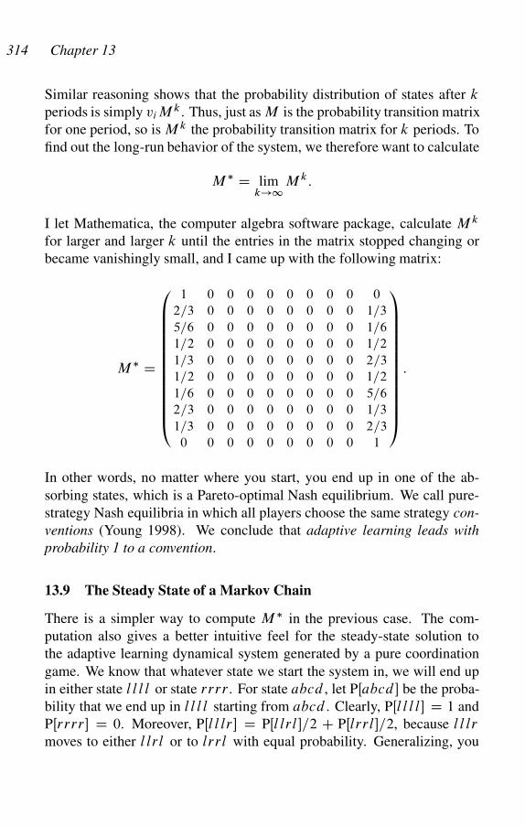
314 Chapter 13
Similar reasoning shows that the probability distribution of states after k
periods is simply viMk . Thus, just as M is the probability transition matrix
for one period, so is M k the probability transition matrix for k periods. To
find out the long-run behavior of the system, we therefore want to calculate
M � D limk!1
M k:
I let Mathematica, the computer algebra software package, calculate M k
for larger and larger k until the entries in the matrix stopped changing or
became vanishingly small, and I came up with the following matrix:
M � D
0BBBBBBBBBBBB@
1 0 0 0 0 0 0 0 0 0
2=3 0 0 0 0 0 0 0 0 1=3
5=6 0 0 0 0 0 0 0 0 1=6
1=2 0 0 0 0 0 0 0 0 1=2
1=3 0 0 0 0 0 0 0 0 2=3
1=2 0 0 0 0 0 0 0 0 1=2
1=6 0 0 0 0 0 0 0 0 5=6
2=3 0 0 0 0 0 0 0 0 1=3
1=3 0 0 0 0 0 0 0 0 2=3
0 0 0 0 0 0 0 0 0 1
1CCCCCCCCCCCCA
:
In other words, no matter where you start, you end up in one of the ab-
sorbing states, which is a Pareto-optimal Nash equilibrium. We call pure-
strategy Nash equilibria in which all players choose the same strategy con-
ventions (Young 1998). We conclude that adaptive learning leads with
probability 1 to a convention.
13.9 The Steady State of a Markov Chain
There is a simpler way to compute M � in the previous case. The com-
putation also gives a better intuitive feel for the steady-state solution to
the adaptive learning dynamical system generated by a pure coordination
game. We know that whatever state we start the system in, we will end up
in either state l l l l or state rrrr . For state abcd , let PŒabcd� be the proba-
bility that we end up in l l l l starting from abcd . Clearly, PŒl l l l� D 1 and
PŒrrrr� D 0. Moreover, PŒl l lr � D PŒl lrl�=2 C PŒlrrl�=2, because l l lr
moves to either l lrl or to lrrl with equal probability. Generalizing, you
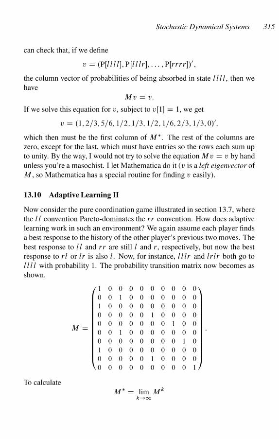
Stochastic Dynamical Systems 315
can check that, if we define
v D .PŒl l l l�; PŒl l lr �; : : : ; PŒrrrr�/0 ;
the column vector of probabilities of being absorbed in state l l l l, then we
have
Mv D v:
If we solve this equation for v, subject to vŒ1� D 1, we get
v D .1; 2=3; 5=6; 1=2; 1=3; 1=2; 1=6; 2=3; 1=3; 0/0;
which then must be the first column of M �. The rest of the columns are
zero, except for the last, which must have entries so the rows each sum up
to unity. By the way, I would not try to solve the equation Mv D v by hand
unless you’re a masochist. I let Mathematica do it (v is a left eigenvector of
M , so Mathematica has a special routine for finding v easily).
13.10 Adaptive Learning II
Now consider the pure coordination game illustrated in section 13.7, where
the l l convention Pareto-dominates the rr convention. How does adaptive
learning work in such an environment? We again assume each player finds
a best response to the history of the other player’s previous two moves. The
best response to l l and rr are still l and r , respectively, but now the best
response to rl or lr is also l. Now, for instance, l l lr and lrlr both go to
l l l l with probability 1. The probability transition matrix now becomes as
shown.
M D
0
BBBBBBBBBBBB@
1 0 0 0 0 0 0 0 0 0
0 0 1 0 0 0 0 0 0 0
1 0 0 0 0 0 0 0 0 0
0 0 0 0 0 1 0 0 0 0
0 0 0 0 0 0 0 1 0 0
0 0 1 0 0 0 0 0 0 0
0 0 0 0 0 0 0 0 1 0
1 0 0 0 0 0 0 0 0 0
0 0 0 0 0 1 0 0 0 0
0 0 0 0 0 0 0 0 0 1
1
CCCCCCCCCCCCA
:
To calculate
M � D limk!1
M k
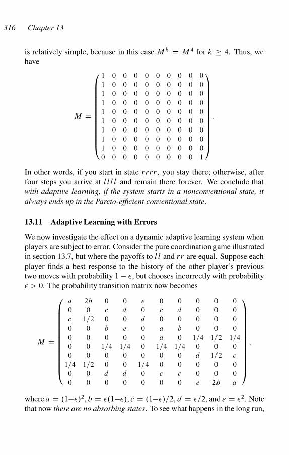
316 Chapter 13
is relatively simple, because in this case M k D M 4 for k 4. Thus, we
have
M D
0
BBBBBBBBBBBB@
1 0 0 0 0 0 0 0 0 0
1 0 0 0 0 0 0 0 0 0
1 0 0 0 0 0 0 0 0 0
1 0 0 0 0 0 0 0 0 0
1 0 0 0 0 0 0 0 0 0
1 0 0 0 0 0 0 0 0 0
1 0 0 0 0 0 0 0 0 0
1 0 0 0 0 0 0 0 0 0
1 0 0 0 0 0 0 0 0 0
0 0 0 0 0 0 0 0 0 1
1
CCCCCCCCCCCCA
:
In other words, if you start in state rrrr , you stay there; otherwise, after
four steps you arrive at l l l l and remain there forever. We conclude that
with adaptive learning, if the system starts in a nonconventional state, it
always ends up in the Pareto-efficient conventional state.
13.11 Adaptive Learning with Errors
We now investigate the effect on a dynamic adaptive learning system when
players are subject to error. Consider the pure coordination game illustrated
in section 13.7, but where the payoffs to l l and rr are equal. Suppose each
player finds a best response to the history of the other player’s previous
two moves with probability 1 � �, but chooses incorrectly with probability
� > 0. The probability transition matrix now becomes
M D
0BBBBBBBBBBBB@
a 2b 0 0 e 0 0 0 0 0
0 0 c d 0 c d 0 0 0
c 1=2 0 0 d 0 0 0 0 0
0 0 b e 0 a b 0 0 0
0 0 0 0 0 a 0 1=4 1=2 1=4
0 0 1=4 1=4 0 1=4 1=4 0 0 0
0 0 0 0 0 0 0 d 1=2 c
1=4 1=2 0 0 1=4 0 0 0 0 0
0 0 d d 0 c c 0 0 0
0 0 0 0 0 0 0 e 2b a
1CCCCCCCCCCCCA
;
where a D .1��/2, b D �.1��/, c D .1��/=2, d D �=2, and e D �2. Note
that now there are no absorbing states. To see what happens in the long run,
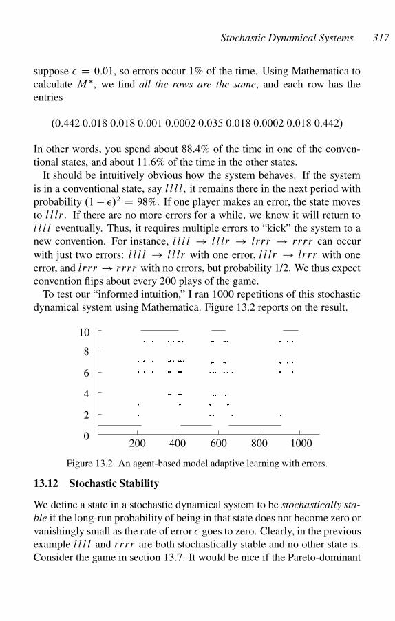
Stochastic Dynamical Systems 317
suppose � D 0:01, so errors occur 1% of the time. Using Mathematica to
calculate M �, we find all the rows are the same, and each row has the
entries
.0:442 0:018 0:018 0:001 0:0002 0:035 0:018 0:0002 0:018 0:442/
In other words, you spend about 88.4% of the time in one of the conven-
tional states, and about 11:6% of the time in the other states.
It should be intuitively obvious how the system behaves. If the system
is in a conventional state, say l l l l, it remains there in the next period with
probability .1 � �/2 D 98%. If one player makes an error, the state moves
to l l lr . If there are no more errors for a while, we know it will return to
l l l l eventually. Thus, it requires multiple errors to “kick” the system to a
new convention. For instance, l l l l ! l l lr ! lrrr ! rrrr can occur
with just two errors: l l l l ! l l lr with one error, l l lr ! lrrr with one
error, and lrrr ! rrrr with no errors, but probability 1/2. We thus expect
convention flips about every 200 plays of the game.
To test our “informed intuition,” I ran 1000 repetitions of this stochastic
dynamical system using Mathematica. Figure 13.2 reports on the result.
2
4
6
8
10
0200 400 600 800 1000
��
��
�
��
�
�
�
�
�
��
�
�
�
��
�
�
��
�
�
�
� �
� �
� � �
�
�
� �
� �
� � �
�
�
�
�
� � � �
� � �
!
Figure 13.2. An agent-based model adaptive learning with errors.
13.12 Stochastic Stability
We define a state in a stochastic dynamical system to be stochastically sta-
ble if the long-run probability of being in that state does not become zero or
vanishingly small as the rate of error � goes to zero. Clearly, in the previous
example l l l l and rrrr are both stochastically stable and no other state is.
Consider the game in section 13.7. It would be nice if the Pareto-dominant
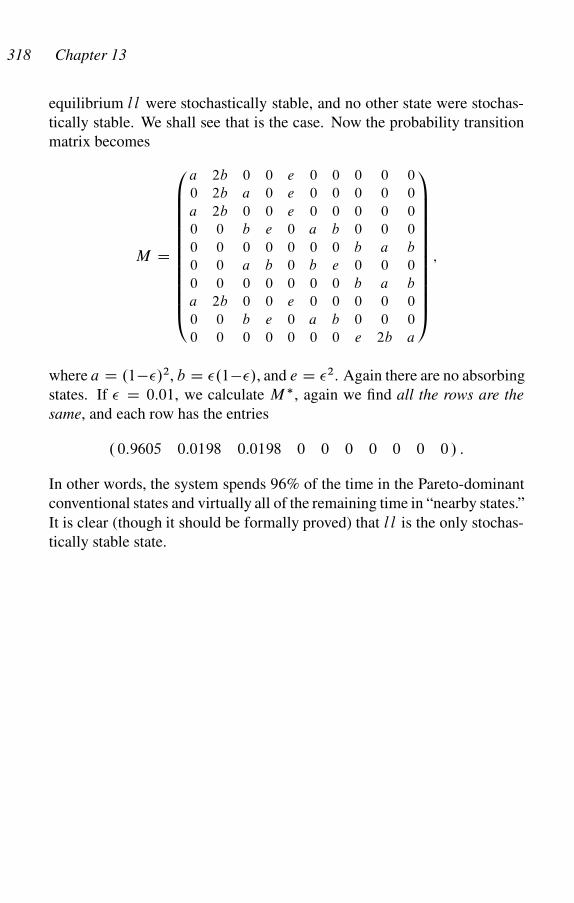
318 Chapter 13
equilibrium l l were stochastically stable, and no other state were stochas-
tically stable. We shall see that is the case. Now the probability transition
matrix becomes
M D
0BBBBBBBBBBBB@
a 2b 0 0 e 0 0 0 0 0
0 2b a 0 e 0 0 0 0 0
a 2b 0 0 e 0 0 0 0 0
0 0 b e 0 a b 0 0 0
0 0 0 0 0 0 0 b a b
0 0 a b 0 b e 0 0 0
0 0 0 0 0 0 0 b a b
a 2b 0 0 e 0 0 0 0 0
0 0 b e 0 a b 0 0 0
0 0 0 0 0 0 0 e 2b a
1CCCCCCCCCCCCA
;
where a D .1��/2, b D �.1��/, and e D �2. Again there are no absorbing
states. If � D 0:01, we calculate M �, again we find all the rows are the
same, and each row has the entries
. 0:9605 0:0198 0:0198 0 0 0 0 0 0 0 / :
In other words, the system spends 96% of the time in the Pareto-dominant
conventional states and virtually all of the remaining time in “nearby states.”
It is clear (though it should be formally proved) that l l is the only stochas-
tically stable state.
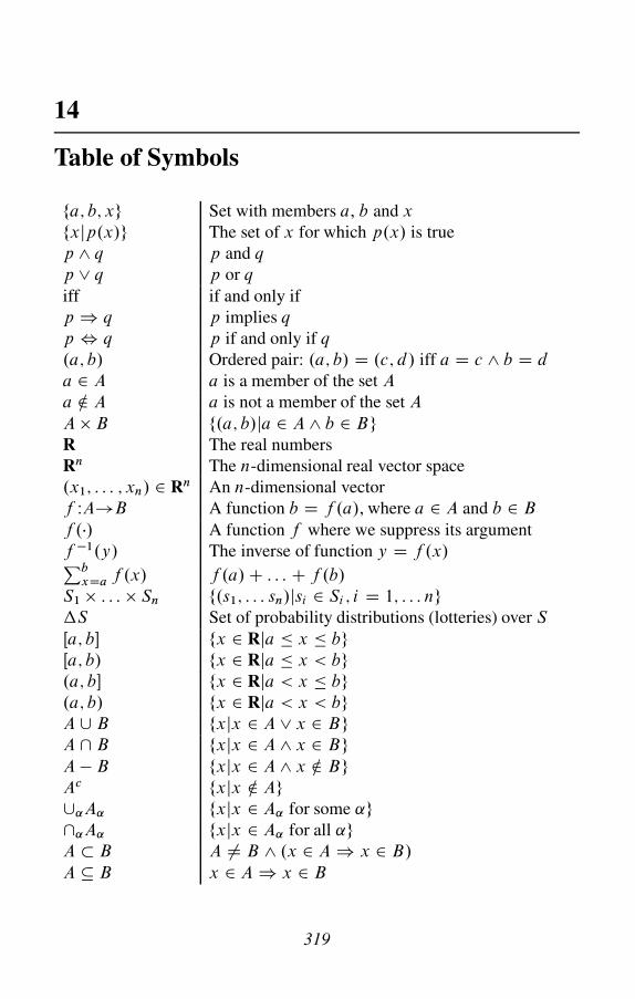
14
Table of Symbols
fa; b; xg Set with members a, b and x
fxjp.x/g The set of x for which p.x/ is true
p ^ q p and q
p _ q p or q
iff if and only if
p ) q p implies q
p , q p if and only if q
.a; b/ Ordered pair: .a; b/ D .c; d/ iff a D c ^ b D d
a 2 A a is a member of the set A
a … A a is not a member of the set A
A � B f.a; b/ja 2 A ^ b 2 BgR The real numbers
Rn The n-dimensional real vector space
.x1; : : : ; xn/ 2 Rn An n-dimensional vector
f WA!B A function b D f .a/, where a 2 A and b 2 B
f ./ A function f where we suppress its argument
f �1.y/ The inverse of function y D f .x/PbxDa f .x/ f .a/ C : : : C f .b/
S1 � : : : � Sn f.s1; : : : sn/jsi 2 Si ; i D 1; : : : ngS Set of probability distributions (lotteries) over S
Œa; b� fx 2 Rja � x � bgŒa; b/ fx 2 Rja � x < bg.a; b� fx 2 Rja < x � bg.a; b/ fx 2 Rja < x < bgA [ B fxjx 2 A _ x 2 BgA \ B fxjx 2 A ^ x 2 BgA � B fxjx 2 A ^ x … BgAc fxjx … Ag[˛A˛ fxjx 2 A˛ for some ˛g\˛A˛ fxjx 2 A˛ for all ˛gA � B A ¤ B ^ .x 2 A ) x 2 B/
A � B x 2 A ) x 2 B
319

This page intentionally left blank
15
Answers
321
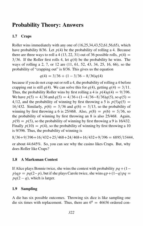
Probability Theory: Answers
1.7 Craps
Roller wins immediately with any one of (16,25,34,43,52,61,56,65), which
have probability 8/36. Let p.4/ be the probability of rolling a 4. Because
there are three ways to roll a 4 (13, 22, 31) out of 36 possible rolls, p.4/ D3=36. If the Roller first rolls 4, let q.4/ be the probability he wins. The
ways of rolling a 2, 7, or 12 are (11, 61, 52, 43, 34, 25, 16, 66), so the
probability of “crapping out” is 8/36. This gives us the equation
q.4/ D 3=36 C .1 � 3=36 � 8=36/q.4/
because if you do not crap out or roll a 4, the probability of rolling a 4 before
crapping out is still q.4/. We can solve this for q.4/, getting q.4/ D 3=11.
Thus, the probability Roller wins by first rolling a 4 is p.4/q.4/ D 9=396.
We have p.5/ D 4=36 and q.5/ D 4=36C.1�4=36�8=36/q.5/, so q.5/ D4=12, and the probability of winning by first throwing a 5 is p.5/q.5/ D16=432. Similarly, p.6/ D 5=36 and q.6/ D 5=13, so the probability of
winning by first throwing a 6 is 25/468. Also, p.8/ D p.6/ D 5=36, so
the probability of winning by first throwing an 8 is also 25/468. Again,
p.9/ D p.5/, so the probability of winning by first throwing a 9 is 16/432.
Finally p.10/ D p.4/, so the probability of winning by first throwing a 10
is 9/396. Thus, the probability of winning is
8=36C9=396C16=432C25=468C24=468C16=432C9=396 D 6895=15444;
or about 44.645%. So, you can see why the casino likes Craps. But, why
does Roller like Craps?
1.8 A Marksman Contest
If Alice plays Bonnie twice, she wins the contest with probability pqC.1�p/qp D pq.2�p/, but if she plays Carole twice, she wins qpC.1�q/pq Dpq.2 � q/, which is larger.
1.9 Sampling
A die has six possible outcomes. Throwing six dice is like sampling one
die six times with replacement. Thus, there are 66 D 46656 ordered con-
322

Probability Theory: Answers 323
figurations of the 6 dice. There are 6 outcomes in which all the faces are
the same. Thus, the probability is 6=46656 D 0:0001286. A more straight-
forward solution is to note that the second through sixth die must match the
first, which happens with probability .1=6/5.
1.10 Aces Up
There are 52 ways to choose the first card, and 51 ways to choose the second
card, so there are 52 �51 different ways to choose two cards from the deck.
There are 4 ways to choose the first ace, and 3 ways to choose the second,
so there are 4 � 3 ways to choose a pair of aces. Thus, the probability
of choosing a pair of aces is 12=.52 � 51/ D 1=221 � 0:0045248 �0:45248%.
1.11 Permutations
Let’s first solve the problem for a particular n, say n D 3. We can write the
nŠ D 6 permutations as follows:
1 1 2 2 3 3
2 3 1 3 1 2
3 2 3 1 2 1
Each row has exactly 2 D .n � 1/Š matches and there are 3 D n rows, so
the total number of matches is 6 D n � .n � 1/Š D nŠ. Thus the average
number of matches is 6=6 D nŠ=nŠ D 1. You can generalize this to show
that the average number of matches for any n is 1.
1.13 Mechanical Defects
This is sampling 2 times without replacement from a set of 7 objects. There
are 7Š=.7 � 2/Š D 7 � 6 D 42 such samples. How many of these are
two nondefective machines? How many samples of two are there from a
population of 5 (the number of nondefectives)? The answer is 5Š=.5�2/Š D5 � 4 D 20. Thus, the probability is 20=42 D 0:4762.
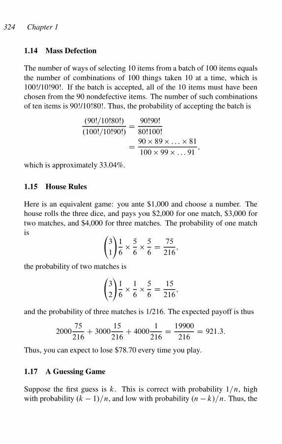
324 Chapter 1
1.14 Mass Defection
The number of ways of selecting 10 items from a batch of 100 items equals
the number of combinations of 100 things taken 10 at a time, which is
100!/10!90!. If the batch is accepted, all of the 10 items must have been
chosen from the 90 nondefective items. The number of such combinations
of ten items is 90!/10!80!. Thus, the probability of accepting the batch is
.90Š=10Š80Š/
.100Š=10Š90Š/D 90Š90Š
80Š100Š
D 90 � 89 � : : : � 81
100 � 99 � : : : 91;
which is approximately 33.04%.
1.15 House Rules
Here is an equivalent game: you ante $1,000 and choose a number. The
house rolls the three dice, and pays you $2,000 for one match, $3,000 for
two matches, and $4,000 for three matches. The probability of one match
is 3
1
!1
6� 5
6� 5
6D 75
216;
the probability of two matches is
3
2
!1
6� 1
6� 5
6D 15
216;
and the probability of three matches is 1/216. The expected payoff is thus
200075
216C 3000
15
216C 4000
1
216D 19900
216D 921:3:
Thus, you can expect to lose $78.70 every time you play.
1.17 A Guessing Game
Suppose the first guess is k. This is correct with probability 1=n, high
with probability .k � 1/=n, and low with probability .n � k/=n. Thus, the
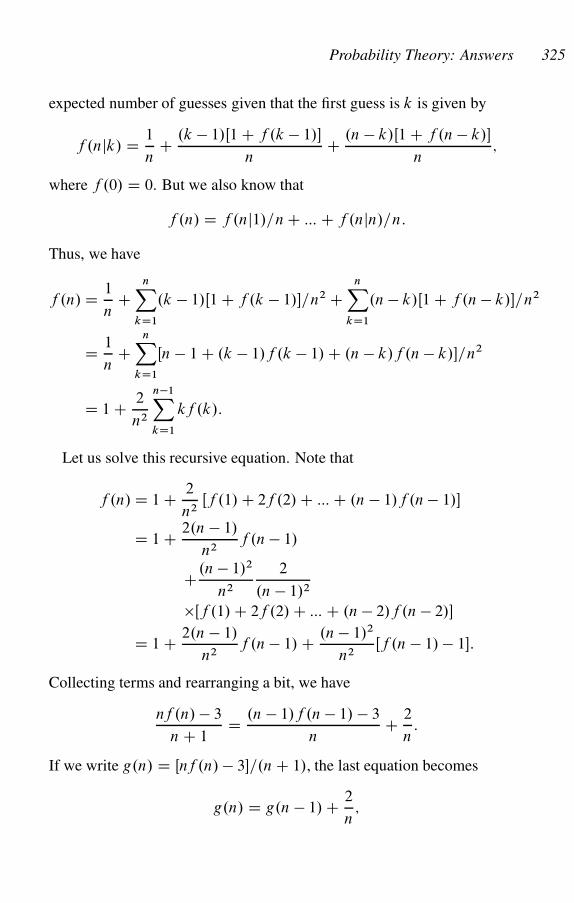
Probability Theory: Answers 325
expected number of guesses given that the first guess is k is given by
f .njk/ D 1
nC .k � 1/Œ1 C f .k � 1/�
nC .n � k/Œ1 C f .n � k/�
n;
where f .0/ D 0. But we also know that
f .n/ D f .nj1/=n C ::: C f .njn/=n:
Thus, we have
f .n/ D 1
nC
nX
kD1
.k � 1/Œ1 C f .k � 1/�=n2 CnX
kD1
.n � k/Œ1 C f .n � k/�=n2
D 1
nC
nX
kD1
Œn � 1 C .k � 1/f .k � 1/ C .n � k/f .n � k/�=n2
D 1 C 2
n2
n�1X
kD1
kf .k/:
Let us solve this recursive equation. Note that
f .n/ D 1 C 2
n2Œf .1/ C 2f .2/ C ::: C .n � 1/f .n � 1/�
D 1 C 2.n � 1/
n2f .n � 1/
C.n � 1/2
n2
2
.n � 1/2
�Œf .1/ C 2f .2/ C ::: C .n � 2/f .n � 2/�
D 1 C 2.n � 1/
n2f .n � 1/ C .n � 1/2
n2Œf .n � 1/ � 1�:
Collecting terms and rearranging a bit, we have
nf .n/ � 3
n C 1D .n � 1/f .n � 1/ � 3
nC 2
n:
If we write g.n/ D Œnf .n/ � 3�=.n C 1/, the last equation becomes
g.n/ D g.n � 1/ C 2
n;
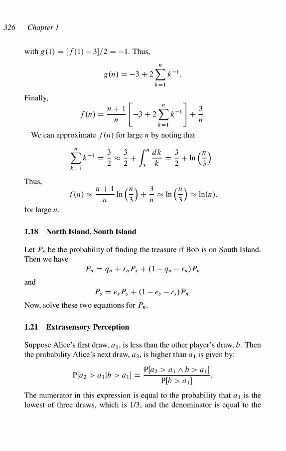
326 Chapter 1
with g.1/ D Œf .1/ � 3�=2 D �1. Thus,
g.n/ D �3 C 2
nX
kD1
k�1:
Finally,
f .n/ D n C 1
n
"�3 C 2
nX
kD1
k�1
#C 3
n:
We can approximate f .n/ for large n by noting that
nX
kD1
k�1 D 3
2� 3
2CZ n
3
dk
kD 3
2C ln
�n
3
�:
Thus,
f .n/ � n C 1
nln�n
3
�C 3
n� ln
�n
3
�� ln.n/:
for large n.
1.18 North Island, South Island
Let Ps be the probability of finding the treasure if Bob is on South Island.
Then we have
Pn D qn C rnPs C .1 � qn � rn/Pn
and
Ps D esPs C .1 � es � rs/Pn:
Now, solve these two equations for Pn.
1.21 Extrasensory Perception
Suppose Alice’s first draw, a1, is less than the other player’s draw, b. Then
the probability Alice’s next draw, a2, is higher than a1 is given by:
PŒa2 > a1jb > a1� D PŒa2 > a1 ^ b > a1�
PŒb > a1�:
The numerator in this expression is equal to the probability that a1 is the
lowest of three draws, which is 1/3, and the denominator is equal to the

Probability Theory: Answers 327
probability that a1 is the lowest of two draws, which is 1/2. Thus, Alice
beats herself on the second draw with probability 2/3, and the overall prob-
ability she wins is .1=2/ C .1=2/.2=3/ D 5=6.
1.22 Les Cinq Tiroirs
We depict the whole event space as a rectangle with six pieces. Piece A,
which consists of 20% of the space, represents the event “the object is not
in any drawer.”
16%
16%
16%16%
20%
AD1D2
D3
D4
D5 16%
The other five events, D1, D2, D3, D4, and D5, represent the event where
the object is in one of the drawers. Because these are equally likely, each
such event represents (1-0.2)/5 = 16% of the space.
The probability of D1, which we may write PŒD1� is, of course 16%. The
probability of D2 given not D1 is PŒD2jD1c �. We can evaluate this by
PŒD2jD1c� D PŒD2 ^ D1c�
PŒD1c�D PŒD2�
1 � 0:16D 0:16=0:84 � 19%:
The probability of D3 given not D1 or D2 is PŒD3jD1c ^ D2c�. We can
evaluate this by
PŒD3jD1c ^ D2c� D PŒD3 ^ D1c ^ D2c�
PŒD1c ^ D2c�D PŒD3�
1 � 0:16 � 0:16
D 0:16=0:68 � 23:5%:
You can check that the probability of finding the object in the fourth
drawer, given that it was not in any previous drawer, is 0:16=0:52 D30:77%, and the probability that it is in the fifth drawer given that it is nei-
ther of the first four is 0:16=0:36 D 44:44%. So the probability of finding
the object rises from drawer 1 to drawer 5.
What about the probability of not finding the object? Let N be the event
“the object is in none of the drawers.” the PŒN � D 0:2. What is PŒN jD1c �,
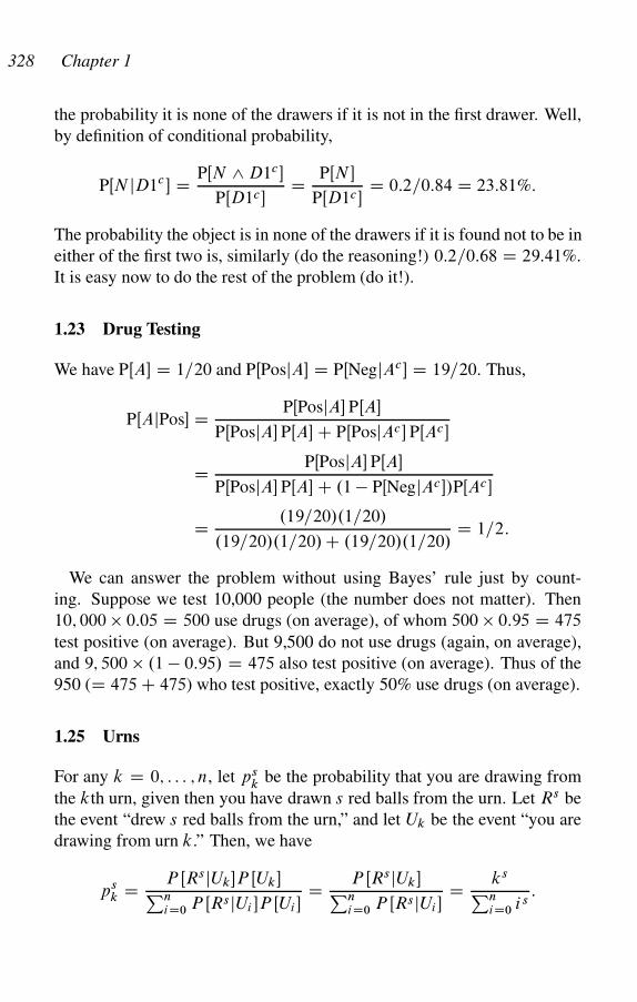
328 Chapter 1
the probability it is none of the drawers if it is not in the first drawer. Well,
by definition of conditional probability,
PŒN jD1c � D PŒN ^ D1c�
PŒD1c�D PŒN �
PŒD1c�D 0:2=0:84 D 23:81%:
The probability the object is in none of the drawers if it is found not to be in
either of the first two is, similarly (do the reasoning!) 0:2=0:68 D 29:41%.
It is easy now to do the rest of the problem (do it!).
1.23 Drug Testing
We have PŒA� D 1=20 and PŒPosjA� D PŒNegjAc� D 19=20. Thus,
PŒAjPos� D PŒPosjA� PŒA�
PŒPosjA� PŒA� C PŒPosjAc� PŒAc�
D PŒPosjA� PŒA�
PŒPosjA� PŒA� C .1 � PŒNegjAc�/PŒAc�
D .19=20/.1=20/
.19=20/.1=20/ C .19=20/.1=20/D 1=2:
We can answer the problem without using Bayes’ rule just by count-
ing. Suppose we test 10,000 people (the number does not matter). Then
10; 000 � 0:05 D 500 use drugs (on average), of whom 500 � 0:95 D 475
test positive (on average). But 9,500 do not use drugs (again, on average),
and 9; 500 � .1 � 0:95/ D 475 also test positive (on average). Thus of the
950 (D 475 C 475) who test positive, exactly 50% use drugs (on average).
1.25 Urns
For any k D 0; : : : ; n, let psk
be the probability that you are drawing from
the kth urn, given then you have drawn s red balls from the urn. Let Rs be
the event “drew s red balls from the urn,” and let Uk be the event “you are
drawing from urn k.” Then, we have
psk D P ŒRsjUk�P ŒUk�Pn
iD0 P ŒRsjUi �P ŒUi �D P ŒRsjUk�Pn
iD0 P ŒRsjUi �D ks
PniD0 i s
:
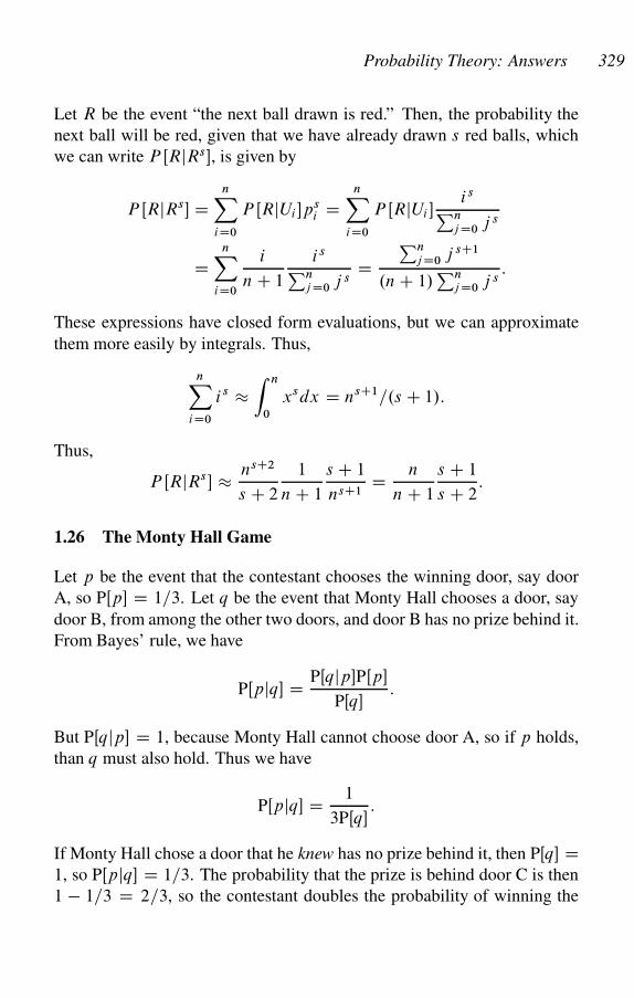
Probability Theory: Answers 329
Let R be the event “the next ball drawn is red.” Then, the probability the
next ball will be red, given that we have already drawn s red balls, which
we can write P ŒRjRs�, is given by
P ŒRjRs� DnX
iD0
P ŒRjUi �psi D
nX
iD0
P ŒRjUi �i s
Pnj D0 j s
DnX
iD0
i
n C 1
i s
Pnj D0 j s
DPn
j D0 j sC1
.n C 1/Pn
j D0 j s:
These expressions have closed form evaluations, but we can approximate
them more easily by integrals. Thus,
nX
iD0
i s �Z n
0
xsdx D nsC1=.s C 1/:
Thus,
P ŒRjRs � � nsC2
s C 2
1
n C 1
s C 1
nsC1D n
n C 1
s C 1
s C 2:
1.26 The Monty Hall Game
Let p be the event that the contestant chooses the winning door, say door
A, so PŒp� D 1=3. Let q be the event that Monty Hall chooses a door, say
door B, from among the other two doors, and door B has no prize behind it.
From Bayes’ rule, we have
PŒpjq� D PŒqjp�PŒp�
PŒq�:
But PŒqjp� D 1, because Monty Hall cannot choose door A, so if p holds,
than q must also hold. Thus we have
PŒpjq� D 1
3PŒq�:
If Monty Hall chose a door that he knew has no prize behind it, then PŒq� D1, so PŒpjq� D 1=3. The probability that the prize is behind door C is then
1 � 1=3 D 2=3, so the contestant doubles the probability of winning the
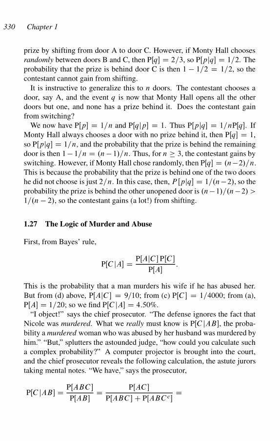
330 Chapter 1
prize by shifting from door A to door C. However, if Monty Hall chooses
randomly between doors B and C, then PŒq� D 2=3, so PŒpjq� D 1=2. The
probability that the prize is behind door C is then 1 � 1=2 D 1=2, so the
contestant cannot gain from shifting.
It is instructive to generalize this to n doors. The contestant chooses a
door, say A, and the event q is now that Monty Hall opens all the other
doors but one, and none has a prize behind it. Does the contestant gain
from switching?
We now have PŒp� D 1=n and PŒqjp� D 1. Thus PŒpjq� D 1=nPŒq�. If
Monty Hall always chooses a door with no prize behind it, then PŒq� D 1,
so PŒpjq� D 1=n, and the probability that the prize is behind the remaining
door is then 1 � 1=n D .n � 1/=n. Thus, for n 3, the contestant gains by
switching. However, if Monty Hall chose randomly, then PŒq� D .n�2/=n.
This is because the probability that the prize is behind one of the two doors
he did not choose is just 2=n. In this case, then, P Œpjq� D 1=.n�2/, so the
probability the prize is behind the other unopened door is .n�1/=.n�2/ >
1=.n � 2/, so the contestant gains (a lot!) from shifting.
1.27 The Logic of Murder and Abuse
First, from Bayes’ rule,
PŒC jA� D PŒAjC � PŒC �
PŒA�:
This is the probability that a man murders his wife if he has abused her.
But from (d) above, PŒAjC � D 9=10; from (c) PŒC � D 1=4000; from (a),
PŒA� D 1=20; so we find PŒC jA� D 4:50%.
“I object!” says the chief prosecutor. “The defense ignores the fact that
Nicole was murdered. What we really must know is PŒC jAB�, the proba-
bility a murdered woman who was abused by her husband was murdered by
him.” “But,” splutters the astounded judge, “how could you calculate such
a complex probability?” A computer projector is brought into the court,
and the chief prosecutor reveals the following calculation, the astute jurors
taking mental notes. “We have,” says the prosecutor,
PŒC jAB� D PŒABC �
PŒAB�D PŒAC �
PŒABC � C PŒABC c�D
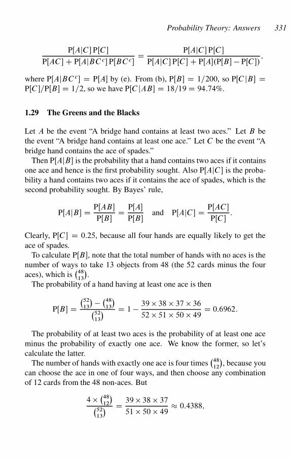
Probability Theory: Answers 331
PŒAjC � PŒC �
PŒAC � C PŒAjBC c� PŒBC c�D PŒAjC � PŒC �
PŒAjC � PŒC � C PŒA�.PŒB� � PŒC �/;
where PŒAjBC c� D PŒA� by (e). From (b), PŒB� D 1=200, so PŒC jB� DPŒC �=PŒB� D 1=2, so we have PŒC jAB� D 18=19 D 94:74%.
1.29 The Greens and the Blacks
Let A be the event “A bridge hand contains at least two aces.” Let B be
the event “A bridge hand contains at least one ace.” Let C be the event “A
bridge hand contains the ace of spades.”
Then PŒAjB� is the probability that a hand contains two aces if it contains
one ace and hence is the first probability sought. Also PŒAjC � is the proba-
bility a hand contains two aces if it contains the ace of spades, which is the
second probability sought. By Bayes’ rule,
PŒAjB� D PŒAB�
PŒB�D PŒA�
PŒB�and PŒAjC � D PŒAC �
PŒC �:
Clearly, PŒC � D 0:25, because all four hands are equally likely to get the
ace of spades.
To calculate PŒB�, note that the total number of hands with no aces is the
number of ways to take 13 objects from 48 (the 52 cards minus the four
aces), which is�
48
13
�.
The probability of a hand having at least one ace is then
PŒB� D�
52
13
� � �48
13
��
52
13
� D 1 � 39 � 38 � 37 � 36
52 � 51 � 50 � 49D 0:6962:
The probability of at least two aces is the probability of at least one ace
minus the probability of exactly one ace. We know the former, so let’s
calculate the latter.
The number of hands with exactly one ace is four times�
48
12
�, because you
can choose the ace in one of four ways, and then choose any combination
of 12 cards from the 48 non-aces. But
4 � �48
12
��
52
13
� D 39 � 38 � 37
51 � 50 � 49� 0:4388;
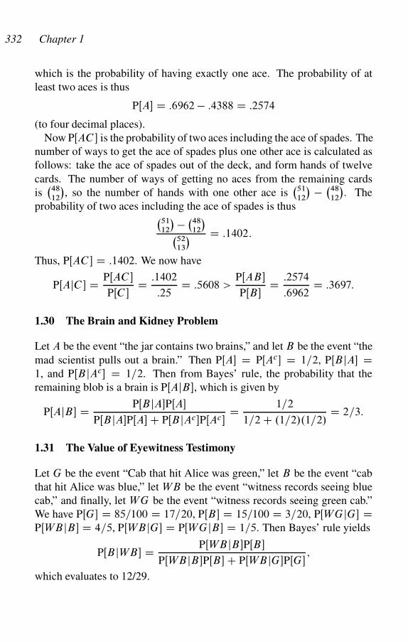
332 Chapter 1
which is the probability of having exactly one ace. The probability of at
least two aces is thus
PŒA� D :6962 � :4388 D :2574
(to four decimal places).
Now PŒAC � is the probability of two aces including the ace of spades. The
number of ways to get the ace of spades plus one other ace is calculated as
follows: take the ace of spades out of the deck, and form hands of twelve
cards. The number of ways of getting no aces from the remaining cards
is�
48
12
�, so the number of hands with one other ace is
�51
12
� � �48
12
�. The
probability of two aces including the ace of spades is thus�
51
12
� � �48
12
��
52
13
� D :1402:
Thus, PŒAC � D :1402. We now have
PŒAjC � D PŒAC �
PŒC �D :1402
:25D :5608 >
PŒAB�
PŒB�D :2574
:6962D :3697:
1.30 The Brain and Kidney Problem
Let A be the event “the jar contains two brains,” and let B be the event “the
mad scientist pulls out a brain.” Then PŒA� D PŒAc� D 1=2, PŒB jA� D1, and PŒB jAc� D 1=2. Then from Bayes’ rule, the probability that the
remaining blob is a brain is PŒAjB�, which is given by
PŒAjB� D PŒB jA�PŒA�
PŒB jA�PŒA� C PŒB jAc�PŒAc�D 1=2
1=2 C .1=2/.1=2/D 2=3:
1.31 The Value of Eyewitness Testimony
Let G be the event “Cab that hit Alice was green,” let B be the event “cab
that hit Alice was blue,” let WB be the event “witness records seeing blue
cab,” and finally, let W G be the event “witness records seeing green cab.”
We have PŒG� D 85=100 D 17=20, PŒB� D 15=100 D 3=20, PŒW GjG� DPŒWB jB� D 4=5, PŒWB jG� D PŒW GjB� D 1=5. Then Bayes’ rule yields
PŒB jWB� D PŒWB jB�PŒB�
PŒWB jB�PŒB� C PŒWB jG�PŒG�;
which evaluates to 12/29.
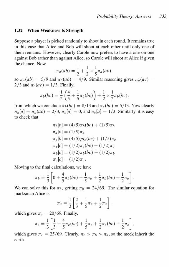
Probability Theory: Answers 333
1.32 When Weakness Is Strength
Suppose a player is picked randomly to shoot in each round. It remains true
in this case that Alice and Bob will shoot at each other until only one of
them remains. However, clearly Carole now prefers to have a one-on-one
against Bob rather than against Alice, so Carole will shoot at Alice if given
the chance. Now
�a.ab/ D 1
2C 1
2� 1
5�a.ab/;
so �a.ab/ D 5=9 and �b.ab/ D 4=9. Similar reasoning gives �a.ac/ D2=3 and �c.ac/ D 1=3. Finally,
�b.bc/ D 1
2
�4
5C 1
5�b.bc/
�C 1
2� 1
2�b.bc/;
from which we conclude �b.bc/ D 8=13 and �c.bc/ D 5=13. Now clearly
�aŒa� D �a.ac/ D 2=3, �bŒa� D 0, and �cŒa� D 1=3. Similarly, it is easy
to check that
�bŒb� D .4=5/�b.bc/ C .1=5/�b
�aŒb� D .1=5/�a
�cŒb� D .4=5/pic.bc/ C .1=5/�c
�cŒc� D .1=2/�c.bc/ C .1=2/�c
�bŒc� D .1=2/�b.bc/ C .1=2/�b
�aŒc� D .1=2/�a:
Moving to the final calculations, we have
�b D 1
3
�0 C 4
5�b.bc/ C 1
5�b C 1
2�b.bc/ C 1
2�b
�:
We can solve this for �b , getting �b D 24=69. The similar equation for
marksman Alice is
�a D 1
3
�2
3C 1
5�a C 1
2�a
�;
which gives �a D 20=69. Finally,
�c D 1
3
�1
3C 4
5�c.bc/ C 1
5�c C 1
2�c.bc/ C 1
2�c
�;
which gives �c D 25=69. Clearly, �c > �b > �a, so the meek inherit the
earth.
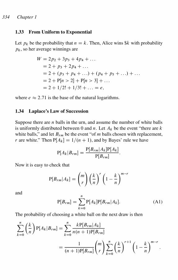
334 Chapter 1
1.33 From Uniform to Exponential
Let pk be the probability that n D k. Then, Alice wins $k with probability
pk , so her average winnings are
W D 2p2 C 3p3 C 4p4 C : : :
D 2 C p3 C 2p4 C : : :
D 2 C .p3 C p4 C : : :/ C .p4 C p5 C : : :/ C : : :
D 2 C PŒn > 2� C PŒn > 3� C : : :
D 2 C 1=2Š C 1=3Š C : : : D e;
where e � 2:71 is the base of the natural logarithms.
1.34 Laplace’s Law of Succession
Suppose there are n balls in the urn, and assume the number of white balls
is uniformly distributed between 0 and n. Let Ak be the event “there are k
white balls,” and let Brm be the event “of m balls chosen with replacement,
r are white.” Then PŒAk� D 1=.n C 1/, and by Bayes’ rule we have
PŒAkjBrm� D PŒBrmjAk�PŒAk�
PŒBrm�:
Now it is easy to check that
PŒBrmjAk� D
m
r
!�k
n
�r �1 � k
n
�m�r
and
PŒBrm� DnX
kD0
PŒAk�PŒBrmjAk�: (A1)
The probability of choosing a white ball on the next draw is then
nX
kD0
�k
n
�PŒAkjBrm� D
nX
kD0
kPŒBrmjAk�
n.n C 1/PŒBrm�
D 1
.n C 1/PŒBrm�
m
r
!nX
kD0
�k
n
�rC1�1 � k
n
�m�r
:
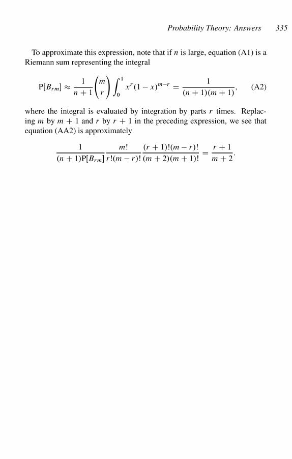
Probability Theory: Answers 335
To approximate this expression, note that if n is large, equation (A1) is a
Riemann sum representing the integral
PŒBrm� � 1
n C 1
m
r
!Z 1
0
xr.1 � x/m�r D 1
.n C 1/.m C 1/; (A2)
where the integral is evaluated by integration by parts r times. Replac-
ing m by m C 1 and r by r C 1 in the preceding expression, we see that
equation (AA2) is approximately
1
.n C 1/PŒBrm�
mŠ
rŠ.m � r/Š
.r C 1/Š.m � r/Š
.m C 2/.m C 1/ŠD r C 1
m C 2:
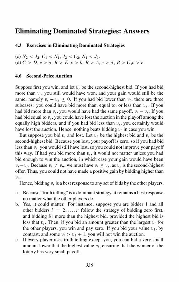
Eliminating Dominated Strategies: Answers
4.3 Exercises in Eliminating Dominated Strategies
(c) N2 < J2, C1 < N1, J2 < C2, N1 < J1.
(d) C > D, e > a, B > E, c > b, B > A, c > d , B > C ,c > e.
4.6 Second-Price Auction
Suppose first you win, and let vs be the second-highest bid. If you had bid
more than vi , you still would have won, and your gain would still be the
same, namely vi � vs 0. If you had bid lower than vi , there are three
subcases: you could have bid more than, equal to, or less than vs. If you
had bid more than vs, you would have had the same payoff, vi � vs. If you
had bid equal to vs, you could have lost the auction in the playoff among the
equally high bidders, and if you had bid less than vs, you certainly would
have lost the auction. Hence, nothing beats bidding vi in case you win.
But suppose you bid vi and lost. Let vh be the highest bid and vs be the
second-highest bid. Because you lost, your payoff is zero, so if you had bid
less than vi , you would still have lost, so you could not improve your payoff
this way. If had you bid more than vi , it would not matter unless you had
bid enough to win the auction, in which case your gain would have been
vs �vi . Because vi ¤ vh, we must have vi � vs, as vs is the second-highest
offer. Thus, you could not have made a positive gain by bidding higher than
vi .
Hence, bidding vi is a best response to any set of bids by the other players.
a. Because “truth telling” is a dominant strategy, it remains a best response
no matter what the other players do.b. Yes, it could matter. For instance, suppose you are bidder 1 and all
other bidders i D 2; : : : ; n follow the strategy of bidding zero first,
and bidding $1 more than the highest bid, provided the highest bid is
less that vi . Then, if you bid an amount greater than the largest vi for
the other players, you win and pay zero. If you bid your value v1, by
contrast, and some vi > v1 C 1, you will not win the auction.c. If every player uses truth telling except you, you can bid a very small
amount lower that the highest value vi , ensuring that the winner of the
lottery has very small payoff.
336
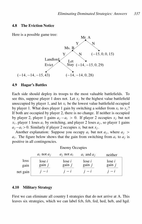
Eliminating Dominated Strategies: Answers 337
4.8 The Eviction Notice
Here is a possible game tree:�
Mr. A
NY
�
.�15; 0; 0; 15/
�Ms. B
NY
�
.�14; �15; 0; 29/
��Landlord LetEvict
�
.�14; �14; 0; 28/.�14; �14; �15; 43/
�
Stay
4.9 Hagar’s Battles
Each side should deploy its troops to the most valuable battlefields. To
see this, suppose player 1 does not. Let xj be the highest value battlefield
unoccupied by player 1, and let xi be the lowest value battlefield occupied
by player 1. What does player 1 gain by switching a soldier from xi to xj ‹
If both are occupied by player 2, there is no change. If neither is occupied
by player 2, player 1 gains aj �ai > 0. If player 2 occupies xj but not
xi ; player 1 loses ai by switching, and player 2 loses aj , so player 1 gains
aj �ai >0. Similarly if player 2 occupies xi but not xj :
Another explanation: Suppose you occupy ai but not aj , where aj >
ai . The figure below shows that the gain from switching from ai to aj is
positive in all contingencies.
Enemy Occupies
ai not aj aj not ai ai and aj neither
lose igain j
j � i
lose igain j
j � i
lose igain j
j � i
lose igain j
j � i
loss
gain
net gain
4.10 Military Strategy
First we can eliminate all country I strategies that do not arrive at A. This
leaves six strategies, which we can label fcb, feb, fed, hed, heb, and hgd.
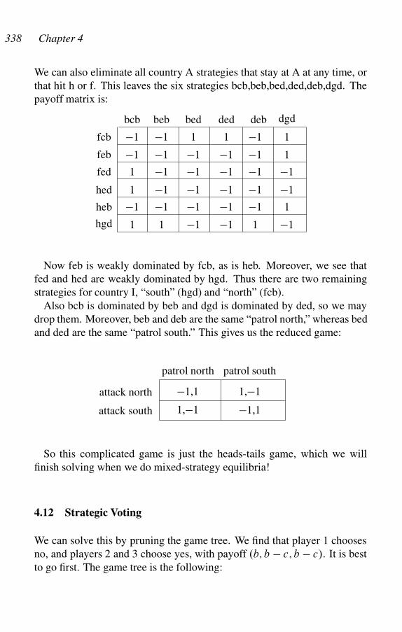
338 Chapter 4
We can also eliminate all country A strategies that stay at A at any time, or
that hit h or f. This leaves the six strategies bcb,beb,bed,ded,deb,dgd. The
payoff matrix is:
�1 �1 1 1 �1 1
�1 �1 �1 �1 �1 1
1 �1 �1 �1 �1 �1
1 �1 �1 �1 �1 �1
�1 �1 �1 �1 �1 1
1 1 �1 �1 1 �1
bcb beb bed ded deb dgd
fcb
feb
fed
hed
heb
hgd
Now feb is weakly dominated by fcb, as is heb. Moreover, we see that
fed and hed are weakly dominated by hgd. Thus there are two remaining
strategies for country I, “south” (hgd) and “north” (fcb).
Also bcb is dominated by beb and dgd is dominated by ded, so we may
drop them. Moreover, beb and deb are the same “patrol north,” whereas bed
and ded are the same “patrol south.” This gives us the reduced game:
patrol north patrol south
attack north
attack south
�1,1
1,�1
1,�1
�1,1
So this complicated game is just the heads-tails game, which we will
finish solving when we do mixed-strategy equilibria!
4.12 Strategic Voting
We can solve this by pruning the game tree. We find that player 1 chooses
no, and players 2 and 3 choose yes, with payoff .b; b � c; b � c/. It is best
to go first. The game tree is the following:
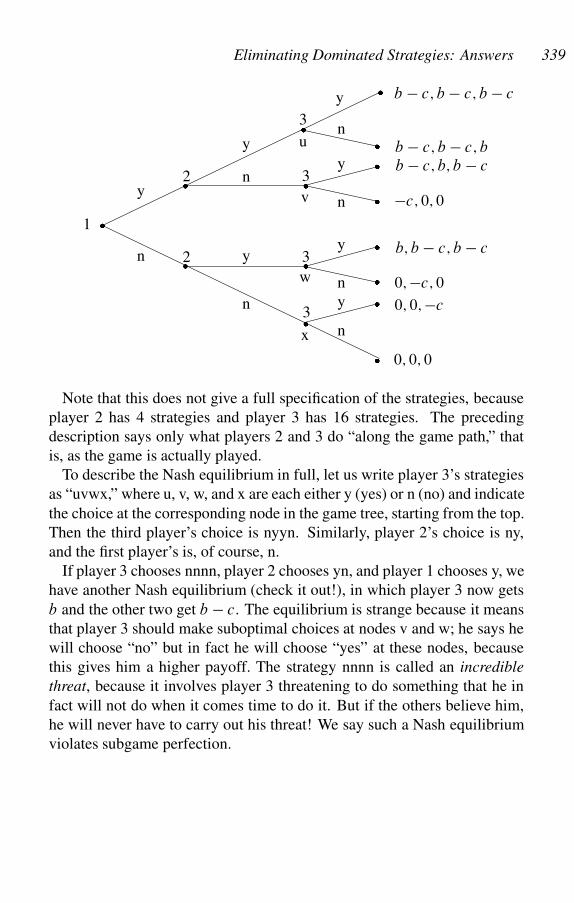
Eliminating Dominated Strategies: Answers 339
�
�
�
�
�
�
�
�
1
y2
y
3
y
n
ny
n
n
n
3
y
n
b � c; b � c; b � c
b � c; b � c; b
b � c; b; b � c
�c; 0; 0
b; b � c; b � c
0; �c; 0
0; 0; �c
0; 0; 0
3
u
v
x
��
�
2y
n
3
w
�y
Note that this does not give a full specification of the strategies, because
player 2 has 4 strategies and player 3 has 16 strategies. The preceding
description says only what players 2 and 3 do “along the game path,” that
is, as the game is actually played.
To describe the Nash equilibrium in full, let us write player 3’s strategies
as “uvwx,” where u, v, w, and x are each either y (yes) or n (no) and indicate
the choice at the corresponding node in the game tree, starting from the top.
Then the third player’s choice is nyyn. Similarly, player 2’s choice is ny,
and the first player’s is, of course, n.
If player 3 chooses nnnn, player 2 chooses yn, and player 1 chooses y, we
have another Nash equilibrium (check it out!), in which player 3 now gets
b and the other two get b � c. The equilibrium is strange because it means
that player 3 should make suboptimal choices at nodes v and w; he says he
will choose “no” but in fact he will choose “yes” at these nodes, because
this gives him a higher payoff. The strategy nnnn is called an incredible
threat, because it involves player 3 threatening to do something that he in
fact will not do when it comes time to do it. But if the others believe him,
he will never have to carry out his threat! We say such a Nash equilibrium
violates subgame perfection.
Pure-Strategy Nash Equilibria: Answers
5.4 The Tobacco Market
a. Let’s not use numbers until we need to. We can write p D a � bq,
where q D q1 C q2 C q3, and qi is the amount sent to market by farmer
i . Farmer 1 maximizes pq1 D .a � bq/q1. If there is an interior
solution, the first-order condition on q1 must satisfy
a � b.q2 C q3/ � 2bq1 D 0:
If all farmers ship the same amount of tobacco, then q2 D q3 D q1,
so this equation becomes 4bq1 D a, which gives q1 D q2 D q3 Da=4b, and q D 3a=4b, so p D a=4. The revenue of each farmer is
pq D a2=16b. In our case a D 10 and b D 1=100000, so the price is
$2.50 per pound, and each farmer ships 250,000 pounds and discards
the rest. The price support does not matter, because p > $0:25. Each
farmer has profit $625,000.
If the second and third farmers send their whole crop to market, then
q2 C q3 D 1; 200; 000. In this case even if farmer 1 shipped nothing,
the market price would be 10 � 1; 200; 000=100; 000 D �2 < 0:25, so
the price support would kick in. Farmer 1 should then also ship all his
tobacco at $0.25 per pound, and each farmer has profit $150,000.
b. You can check that there are no other Nash equilibria. If one farmer
sends all his crop to market, the other two would each send 400,000/3
pounds to market. But then the first farmer would gain by sending less
to market.
5.5 The Klingons and the Snarks
Suppose the Klingons choose a common rate r of consumption. Then each
eats 500 snarks, and each has payoff
u D 2000 C 50r � r2:
Setting the derivative u0 to zero, we get r D 25, so each has utility u D2000 C 50.25/ � 252 D 2625.
340
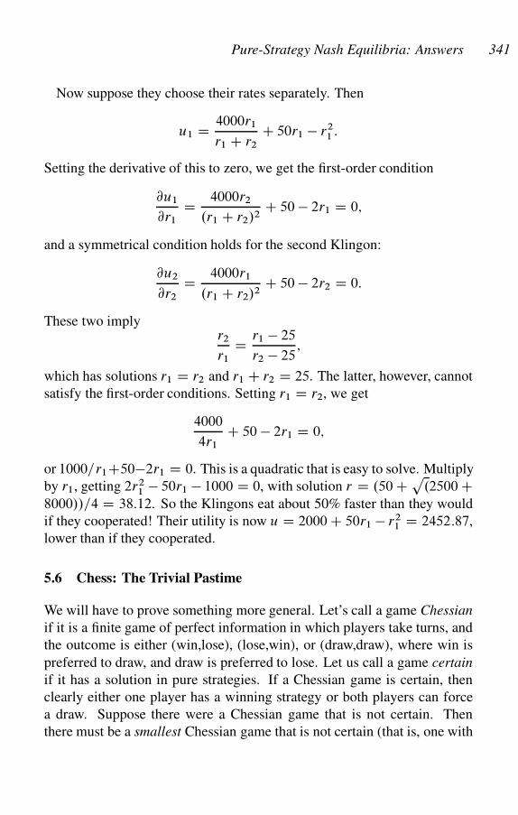
Pure-Strategy Nash Equilibria: Answers 341
Now suppose they choose their rates separately. Then
u1 D 4000r1
r1 C r2
C 50r1 � r21 :
Setting the derivative of this to zero, we get the first-order condition
@u1
@r1
D 4000r2
.r1 C r2/2C 50 � 2r1 D 0;
and a symmetrical condition holds for the second Klingon:
@u2
@r2
D 4000r1
.r1 C r2/2C 50 � 2r2 D 0:
These two implyr2
r1
D r1 � 25
r2 � 25;
which has solutions r1 D r2 and r1 C r2 D 25. The latter, however, cannot
satisfy the first-order conditions. Setting r1 D r2, we get
4000
4r1
C 50 � 2r1 D 0;
or 1000=r1C50�2r1 D 0. This is a quadratic that is easy to solve. Multiply
by r1, getting 2r21 � 50r1 � 1000 D 0, with solution r D .50 Cp
.2500 C8000//=4 D 38:12. So the Klingons eat about 50% faster than they would
if they cooperated! Their utility is now u D 2000 C 50r1 � r21 D 2452:87,
lower than if they cooperated.
5.6 Chess: The Trivial Pastime
We will have to prove something more general. Let’s call a game Chessian
if it is a finite game of perfect information in which players take turns, and
the outcome is either (win,lose), (lose,win), or (draw,draw), where win is
preferred to draw, and draw is preferred to lose. Let us call a game certain
if it has a solution in pure strategies. If a Chessian game is certain, then
clearly either one player has a winning strategy or both players can force
a draw. Suppose there were a Chessian game that is not certain. Then
there must be a smallest Chessian game that is not certain (that is, one with
342 Chapter 5
fewest nodes). Suppose this has k nodes. Clearly, k > 1, because it is
obvious that a Chessian game with one node is certain. Take any node all
of whose child nodes are terminal nodes (why must this exist?). Call this
node A. Suppose Red (player 1) chooses at A (the argument is similar if
Black chooses). If one of the terminal nodes from A is (win,lose), label
A (lose,win); if all of the terminal nodes from A are (lose,win), label A
(win,lose); otherwise label A (draw,draw). Now erase the branches from
A, along with their terminal nodes. Now we have a new, smaller, Chessian
game, which is certain, by our induction assumption. It is easy to see that
if Red has a winning strategy in the smaller game, it can be extended to
a winning strategy in the larger game. Similarly, if Black has a winning
strategy in the smaller game, it can be extended to a winning strategy in the
larger game. Finally, if both players can force a draw in the smaller game,
their respective strategies must force a draw in the larger game.
5.7 No-Draw, High-Low Poker
You can check that 0:75RR C 0:25SR; SR and 0:33RR C 0:67RS; SR are
additional Nash equilibria.
Mixed-Strategy Nash Equilibria: Answers
6.4 Tennis Strategy
� D ˛br C .1 � ˛/fr ; D ˇbs C .1 � ˇ/fs
�bsD ˛�1.bs; br/ C .1 � ˛/�1.bs; fr/
where �1.bs; br/ D the server’s payoff to bs; br
D :4˛ C :7.1 � ˛/ D :7 � :3˛
�fsD ˛�1.fs; br/ C .1 � ˛/�1.fs; fr/
D :8˛ C :1.1 � ˛/ D :1 C :7˛
:7 � :3˛ D :1 C :7˛ ) ˛ D 3=5
�brD ˇ�2.bs; br/ C .1 � ˇ/�2.fs; br/
D :6ˇ C :2.1 � ˇ/ D :2 C :4ˇ
�frD ˇ�2.bs; fr/ C .1 � ˇ/�2.fs; fr/
D :3ˇ C :9.1 � ˇ/ D :9 � :6ˇ
:2 C :4ˇ D :9 � :6ˇ ) ˇ D 7=10
Payoffs to Players:
�1 D :4 3
5C :7 2
5D :52; �2 D :6 7
10C :2 3
10D :48:
6.8 Robin Hood and Little John
The payoff matrix is:
G�ı � lj =2 0
W
�ı � r=2 �r
�lj �� � lj =2
0 �� � r=2
G W
The pure Nash equilibria are:
GG: r ; lj 2ı
W G: 2ı lj
GW : 2ı r .
343
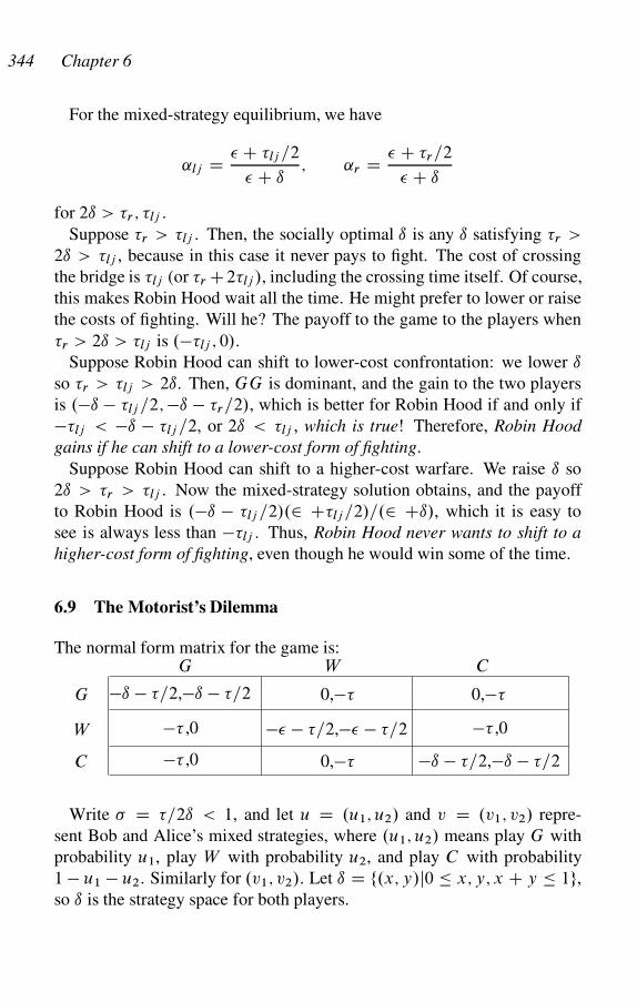
344 Chapter 6
For the mixed-strategy equilibrium, we have
˛lj D � C lj =2
� C ı; ˛r D � C r=2
� C ı
for 2ı > r ; lj :
Suppose r > lj . Then, the socially optimal ı is any ı satisfying r >
2ı > lj , because in this case it never pays to fight. The cost of crossing
the bridge is lj (or r C2lj /, including the crossing time itself. Of course,
this makes Robin Hood wait all the time. He might prefer to lower or raise
the costs of fighting. Will he? The payoff to the game to the players when
r > 2ı > lj is .�lj ; 0/:
Suppose Robin Hood can shift to lower-cost confrontation: we lower ı
so r > lj > 2ı. Then, GG is dominant, and the gain to the two players
is .�ı � lj =2; �ı � r=2/, which is better for Robin Hood if and only if
�lj < �ı � lj =2, or 2ı < lj , which is true! Therefore, Robin Hood
gains if he can shift to a lower-cost form of fighting.
Suppose Robin Hood can shift to a higher-cost warfare. We raise ı so
2ı > r > lj . Now the mixed-strategy solution obtains, and the payoff
to Robin Hood is .�ı � lj =2/.2 Clj =2/=.2 Cı/, which it is easy to
see is always less than �lj . Thus, Robin Hood never wants to shift to a
higher-cost form of fighting, even though he would win some of the time.
6.9 The Motorist’s Dilemma
The normal form matrix for the game is:G W C
G
W
C
�ı � =2,�ı � =2 0,�
� ,0 �� � =2,�� � =2
�ı � =2,�ı � =2
0,�
0,�� ,0
� ,0
Write � D =2ı < 1, and let u D .u1; u2/ and v D .v1; v2/ repre-
sent Bob and Alice’s mixed strategies, where .u1; u2/ means play G with
probability u1, play W with probability u2, and play C with probability
1 � u1 � u2. Similarly for .v1; v2/. Let ı D f.x; y/j0 � x; y; x C y � 1g,
so ı is the strategy space for both players.
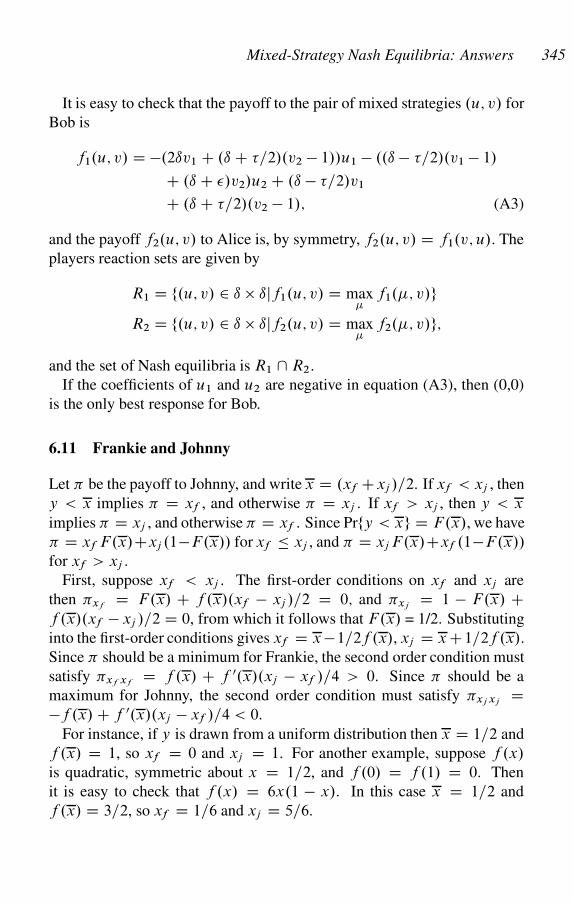
Mixed-Strategy Nash Equilibria: Answers 345
It is easy to check that the payoff to the pair of mixed strategies .u; v/ for
Bob is
f1.u; v/ D �.2ıv1 C .ı C =2/.v2 � 1//u1 � ..ı � =2/.v1 � 1/
C .ı C �/v2/u2 C .ı � =2/v1
C .ı C =2/.v2 � 1/; (A3)
and the payoff f2.u; v/ to Alice is, by symmetry, f2.u; v/ D f1.v; u/: The
players reaction sets are given by
R1 D f.u; v/ 2 ı � ıjf1.u; v/ D max
f1.�; v/gR2 D f.u; v/ 2 ı � ıjf2.u; v/ D max
f2.�; v/g;
and the set of Nash equilibria is R1 \ R2:
If the coefficients of u1 and u2 are negative in equation (A3), then (0,0)
is the only best response for Bob.
6.11 Frankie and Johnny
Let � be the payoff to Johnny, and write x D .xf Cxj /=2. If xf < xj , then
y < x implies � D xf , and otherwise � D xj . If xf > xj , then y < x
implies � D xj , and otherwise � D xf . Since Prfy < xg D F.x/, we have
� D xf F.x/Cxj .1�F.x// for xf � xj , and � D xj F.x/Cxf .1�F.x//
for xf > xj .
First, suppose xf < xj . The first-order conditions on xf and xj are
then �xfD F.x/ C f .x/.xf � xj /=2 D 0; and �xj
D 1 � F.x/ Cf .x/.xf � xj /=2 D 0, from which it follows that F.x/ = 1/2. Substituting
into the first-order conditions gives xf D x �1=2f .x/, xj D x C1=2f .x/.
Since � should be a minimum for Frankie, the second order condition must
satisfy �xf xfD f .x/ C f 0.x/.xj � xf /=4 > 0. Since � should be a
maximum for Johnny, the second order condition must satisfy �xj xjD
�f .x/ C f 0.x/.xj � xf /=4 < 0.
For instance, if y is drawn from a uniform distribution then x D 1=2 and
f .x/ D 1, so xf D 0 and xj D 1. For another example, suppose f .x/
is quadratic, symmetric about x D 1=2, and f .0/ D f .1/ D 0. Then
it is easy to check that f .x/ D 6x.1 � x/. In this case x D 1=2 and
f .x/ D 3=2, so xf D 1=6 and xj D 5=6.
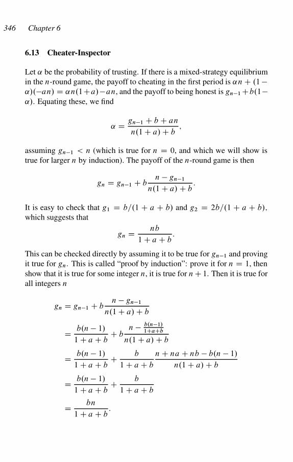
346 Chapter 6
6.13 Cheater-Inspector
Let ˛ be the probability of trusting. If there is a mixed-strategy equilibrium
in the n-round game, the payoff to cheating in the first period is ˛n C .1 �˛/.�an/ D ˛n.1Ca/�an, and the payoff to being honest is gn�1 Cb.1�˛/. Equating these, we find
˛ D gn�1 C b C an
n.1 C a/ C b;
assuming gn�1 < n (which is true for n D 0, and which we will show is
true for larger n by induction). The payoff of the n-round game is then
gn D gn�1 C bn � gn�1
n.1 C a/ C b:
It is easy to check that g1 D b=.1 C a C b/ and g2 D 2b=.1 C a C b/;
which suggests that
gn D nb
1 C a C b:
This can be checked directly by assuming it to be true for gn�1 and proving
it true for gn. This is called “proof by induction”: prove it for n D 1, then
show that it is true for some integer n, it is true for n C 1. Then it is true for
all integers n
gn D gn�1 C bn � gn�1
n.1 C a/ C b
D b.n � 1/
1 C a C bC b
n � b.n�1/
1CaCb
n.1 C a/ C b
D b.n � 1/
1 C a C bC b
1 C a C b
n C na C nb � b.n � 1/
n.1 C a/ C b
D b.n � 1/
1 C a C bC b
1 C a C b
D bn
1 C a C b:
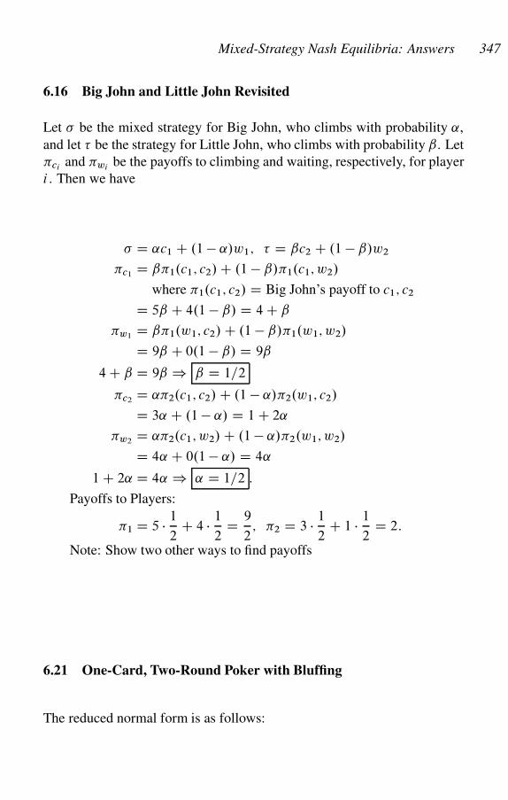
Mixed-Strategy Nash Equilibria: Answers 347
6.16 Big John and Little John Revisited
Let � be the mixed strategy for Big John, who climbs with probability ˛,
and let be the strategy for Little John, who climbs with probability ˇ. Let
�ciand �wi
be the payoffs to climbing and waiting, respectively, for player
i . Then we have
� D ˛c1 C .1 � ˛/w1; D ˇc2 C .1 � ˇ/w2
�c1D ˇ�1.c1; c2/ C .1 � ˇ/�1.c1; w2/
where �1.c1; c2/ D Big John’s payoff to c1; c2
D 5ˇ C 4.1 � ˇ/ D 4 C ˇ
�w1D ˇ�1.w1; c2/ C .1 � ˇ/�1.w1; w2/
D 9ˇ C 0.1 � ˇ/ D 9ˇ
4 C ˇ D 9ˇ ) ˇ D 1=2
�c2D ˛�2.c1; c2/ C .1 � ˛/�2.w1; c2/
D 3˛ C .1 � ˛/ D 1 C 2˛
�w2D ˛�2.c1; w2/ C .1 � ˛/�2.w1; w2/
D 4˛ C 0.1 � ˛/ D 4˛
1 C 2˛ D 4˛ ) ˛ D 1=2 :
Payoffs to Players:
�1 D 5 1
2C 4 1
2D 9
2; �2 D 3 1
2C 1 1
2D 2:
Note: Show two other ways to find payoffs
6.21 One-Card, Two-Round Poker with Bluffing
The reduced normal form is as follows:
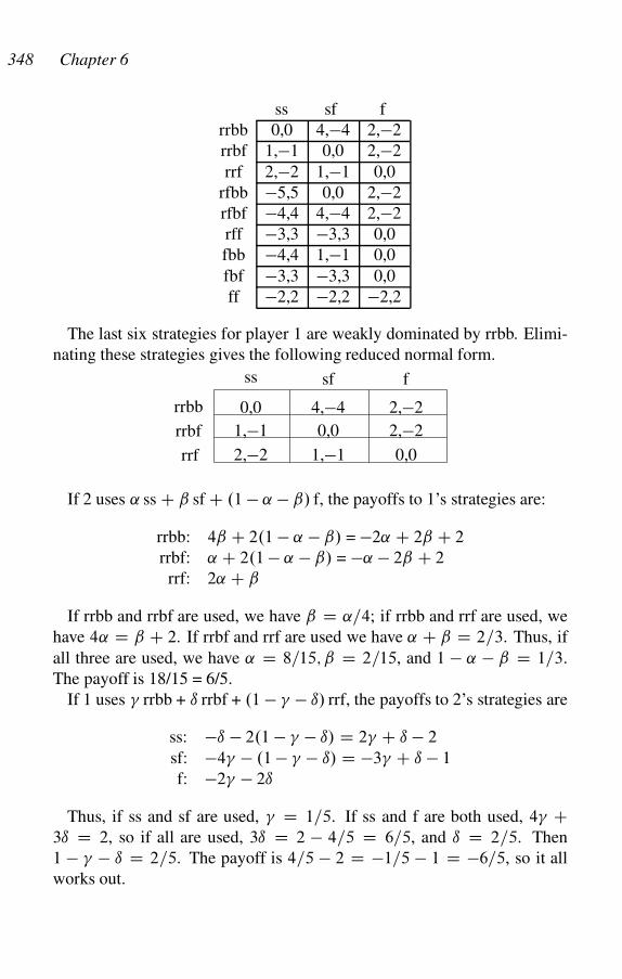
348 Chapter 6
ss sf f
rrbb 0,0 4,�4 2,�2
rrbf 1,�1 0,0 2,�2
rrf 2,�2 1,�1 0,0
rfbb �5,5 0,0 2,�2
rfbf �4,4 4,�4 2,�2
rff �3,3 �3,3 0,0
fbb �4,4 1,�1 0,0
fbf �3,3 �3,3 0,0
ff �2,2 �2,2 �2,2
The last six strategies for player 1 are weakly dominated by rrbb. Elimi-
nating these strategies gives the following reduced normal form.
0,0
1,�1
2,�2
4,�4
0,0
1,�1
2,�2
2,�2
0,0
ss sf f
rrbb
rrbf
rrf
If 2 uses ˛ ss C ˇ sf C .1 � ˛ � ˇ/ f, the payoffs to 1’s strategies are:
rrbb: 4ˇ C 2.1 � ˛ � ˇ/ = �2˛ C 2ˇ C 2
rrbf: ˛ C 2.1 � ˛ � ˇ/ = �˛ � 2ˇ C 2
rrf: 2˛ C ˇ
If rrbb and rrbf are used, we have ˇ D ˛=4; if rrbb and rrf are used, we
have 4˛ D ˇ C 2. If rrbf and rrf are used we have ˛ C ˇ D 2=3. Thus, if
all three are used, we have ˛ D 8=15; ˇ D 2=15, and 1 � ˛ � ˇ D 1=3:
The payoff is 18/15 = 6/5.
If 1 uses � rrbb + ı rrbf + .1 � � � ı/ rrf, the payoffs to 2’s strategies are
ss: �ı � 2.1 � � � ı/ D 2� C ı � 2
sf: �4� � .1 � � � ı/ D �3� C ı � 1
f: �2� � 2ı
Thus, if ss and sf are used, � D 1=5. If ss and f are both used, 4� C3ı D 2, so if all are used, 3ı D 2 � 4=5 D 6=5, and ı D 2=5. Then
1 � � � ı D 2=5. The payoff is 4=5 � 2 D �1=5 � 1 D �6=5, so it all
works out.
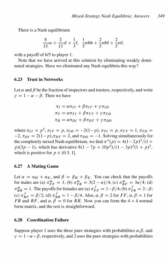
Mixed-Strategy Nash Equilibria: Answers 349
There is a Nash equilibrium
8
15ss C 2
15sf C 1
3f;
1
5rrbb C 2
5rrbf C 2
5rrf;
with a payoff of 6/5 to player 1.
Note that we have arrived at this solution by eliminating weakly domi-
nated strategies. Have we eliminated any Nash equilibria this way?
6.23 Trust in Networks
Let ˛ and ˇ be the fraction of inspectors and trusters, respectively, and write
� D 1 � ˛ � ˇ. Then we have
�I D ˛�II C ˇ�IT C ��ID
�T D ˛�TI C ˇ�T T C ��TD
�D D ˛�DI C ˇ�DT C ��DD
where �II D p2, �IT D p, �ID D �2.1�p/, �TI D p, �T T D 1, �TD D�2, �DI D 2.1�p/,�DT D 2, and �DD D �1. Solving simultaneously for
the completely mixed Nash equilibrium, we find ��.p/ D 4.1�2p/2=.1Cp/.3p � 1/, which has derivative 8.1 � 7p C 10p2/=.1 � 3p/2.1 C p/2,
which is positive for p 2 .0:5; 1�.
6.27 A Mating Game
Let ˛ D ˛H C ˛E , and ˇ D ˇH C ˇE . You can check that the payoffs
for males are (a) �mFF D 1; (b) �m
FR D 3.2 � ˛/=4; (c) �mRF D 3˛=4; (d)
�mRR D 1. The payoffs for females are (a) �
fFF D 1�ˇ=4; (b) �
fFR D 2�ˇ;
(c) �fRF D ˇ=2; (d) �
fRR D 1 � ˇ=4. Also, ˛; ˇ D 2 for FF , ˛; ˇ D 1 for
FR and RF , and ˛; ˇ D 0 for RR. Now you can form the 4 � 4 normal
form matrix, and the rest is straightforward.
6.28 Coordination Failure
Suppose player 1 uses the three pure strategies with probabilities ˛,ˇ, and
� D 1�˛�ˇ, respectively, and 2 uses the pure strategies with probabilities
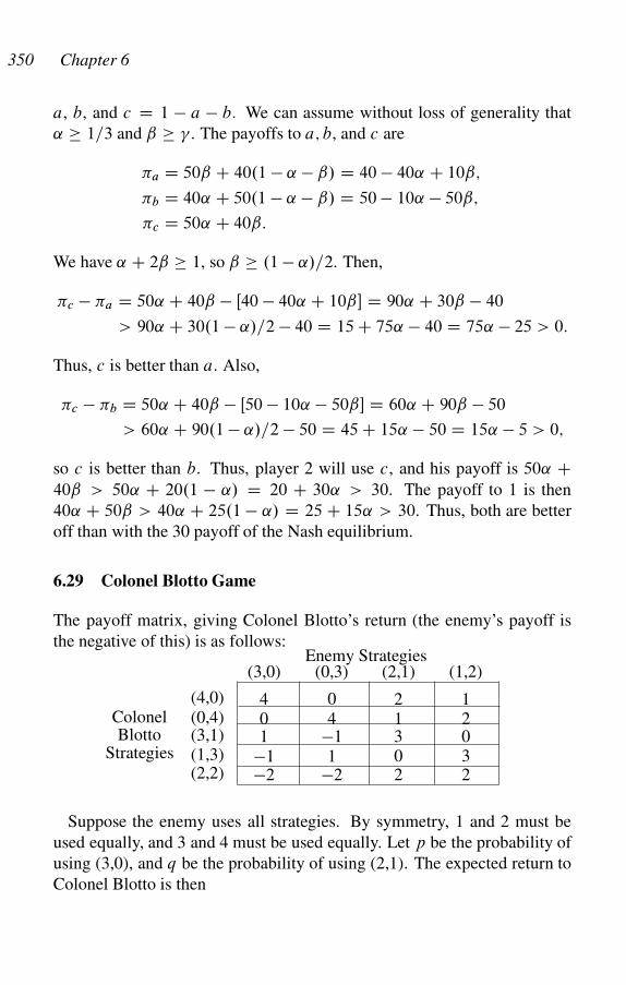
350 Chapter 6
a, b, and c D 1 � a � b. We can assume without loss of generality that
˛ 1=3 and ˇ � . The payoffs to a; b, and c are
�a D 50ˇ C 40.1 � ˛ � ˇ/ D 40 � 40˛ C 10ˇ;
�b D 40˛ C 50.1 � ˛ � ˇ/ D 50 � 10˛ � 50ˇ;
�c D 50˛ C 40ˇ:
We have ˛ C 2ˇ 1, so ˇ .1 � ˛/=2. Then,
�c � �a D 50˛ C 40ˇ � Œ40 � 40˛ C 10ˇ� D 90˛ C 30ˇ � 40
> 90˛ C 30.1 � ˛/=2 � 40 D 15 C 75˛ � 40 D 75˛ � 25 > 0:
Thus, c is better than a. Also,
�c � �b D 50˛ C 40ˇ � Œ50 � 10˛ � 50ˇ� D 60˛ C 90ˇ � 50
> 60˛ C 90.1 � ˛/=2 � 50 D 45 C 15˛ � 50 D 15˛ � 5 > 0;
so c is better than b. Thus, player 2 will use c, and his payoff is 50˛ C40ˇ > 50˛ C 20.1 � ˛/ D 20 C 30˛ > 30. The payoff to 1 is then
40˛ C 50ˇ > 40˛ C 25.1 � ˛/ D 25 C 15˛ > 30. Thus, both are better
off than with the 30 payoff of the Nash equilibrium.
6.29 Colonel Blotto Game
The payoff matrix, giving Colonel Blotto’s return (the enemy’s payoff is
the negative of this) is as follows:
(4,0) 4 0 2 1Colonel (0,4) 0 4 1 2Blotto (3,1) 1 �1 3 0
Strategies (1,3) �1 1 0 3
(3,0) (0,3) (2,1) (1,2)
(2,2) �2 �2 2 2
Enemy Strategies
Suppose the enemy uses all strategies. By symmetry, 1 and 2 must be
used equally, and 3 and 4 must be used equally. Let p be the probability of
using (3,0), and q be the probability of using (2,1). The expected return to
Colonel Blotto is then
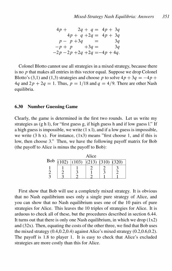
Mixed-Strategy Nash Equilibria: Answers 351
4p C 2q C q D 4p C 3q
4p C q C2q D 4p C 3q
p � p C3q D 3q
�p C p C3q D 3q
�2p �2p C2q C2q D�4p C 4q:
Colonel Blotto cannot use all strategies in a mixed strategy, because there
is no p that makes all entries in this vector equal. Suppose we drop Colonel
Blotto’s (3,1) and (1,3) strategies and choose p to solve 4p C 3q D �4p C4q and 2p C 2q D 1. Thus, p D 1=18 and q D 4=9. There are other Nash
equilibria.
6.30 Number Guessing Game
Clearly, the game is determined in the first two rounds. Let us write my
strategies as (g h l), for “first guess g, if high guess h and if low guess l.” If
a high guess is impossible, we write (1 x l), and if a low guess is impossible,
we write (3 h x). For instance, (1x3) means ”first choose 1, and if this is
low, then choose 3.” Then, we have the following payoff matrix for Bob
(the payoff to Alice is minus the payoff to Bob):
(102) (103) (213) (310) (320)
1 1 2 2 32 3 1 3 23 2 2 1 1
123
BobAlice
First show that Bob will use a completely mixed strategy. It is obvious
that no Nash equilibrium uses only a single pure strategy of Alice, and
you can show that no Nash equilibrium uses one of the 10 pairs of pure
strategies for Alice. This leaves the 10 triples of strategies for Alice. It is
arduous to check all of these, but the procedures described in section 6.44.
It turns out that there is only one Nash equilibrium, in which we drop (1x2)
and (32x). Then, equating the costs of the other three, we find that Bob uses
the mixed strategy (0.4,0.2,0.4) against Alice’s mixed strategy (0.2,0.6,0.2).
The payoff is 1.8 to player 1. It is easy to check that Alice’s excluded
strategies are more costly than this for Alice.
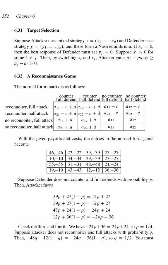
352 Chapter 6
6.31 Target Selection
Suppose Attacker uses mixed strategy x D .x1; : : : ; xn/ and Defender uses
strategy y D .y1; : : : ; yn/, and these form a Nash equilibrium. If xj D 0,
then the best response of Defender must set yj D 0. Suppose xi > 0 for
some i > j . Then, by switching xi and xj , Attacker gains aj � paiyi aj � ai > 0.
6.32 A Reconnaissance Game
The normal form matrix is as follows:
counterfull defend
counterhalf defend
no counterfull defend
no counterhalf defend
reconnoiter, full attack
reconnoiter, half attack
no reconnoiter, full attack
no reconnoiter, half attack
a11 � c C d a12 � c C d a11 � c a12 � c
a21 � c C d a22 � c C d a21 � c a22 � c
a11 C d a12 C d a11 a12
a21 C d a22 C d a21 a22
With the given payoffs and costs, the entries in the normal form game
become
46,�46 22,�22 39,�39 27,�27
10,�10 34,�34 39,�39 27,�27
55,�55 31,�31 48,�48 24,�24
19,�19 43,�43 12,�12 36,�36
Suppose Defender does not counter and full defends with probability p.
Then, Attacker faces
39p C 27.1 � p/ D 12p C 27
39p C 27.1 � p/ D 12p C 27
48p C 24.1 � p/ D 24p C 24
12p C 36.1 � p/ D �24p C 36:
Check the third and fourth. We have �24pC36 D 24pC24, so p D 1=4:
Suppose attacker does not reconnoiter and full attacks with probability q.
Then, �48q � 12.1 � q/ D �24q � 36.1 � q/, so q D 1=2. You must
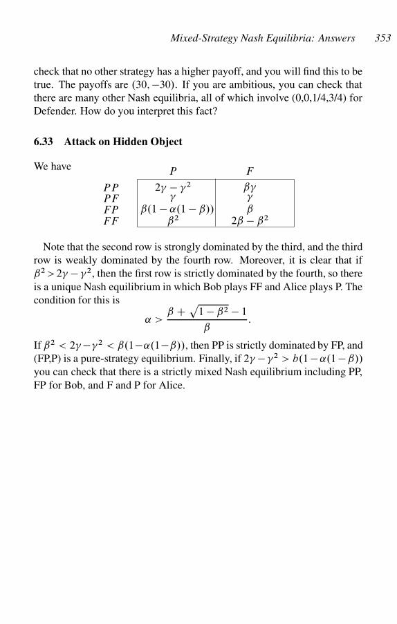
Mixed-Strategy Nash Equilibria: Answers 353
check that no other strategy has a higher payoff, and you will find this to be
true. The payoffs are .30; �30/. If you are ambitious, you can check that
there are many other Nash equilibria, all of which involve (0,0,1/4,3/4) for
Defender. How do you interpret this fact?
6.33 Attack on Hidden Object
We have
PP 2� � �2 ˇ�PF � �
FP ˇ.1 � ˛.1 � ˇ// ˇFF ˇ2 2ˇ � ˇ2
P F
Note that the second row is strongly dominated by the third, and the third
row is weakly dominated by the fourth row. Moreover, it is clear that if
ˇ2 >2� � �2, then the first row is strictly dominated by the fourth, so there
is a unique Nash equilibrium in which Bob plays FF and Alice plays P. The
condition for this is
˛ >ˇ C
p1 � ˇ2 � 1
ˇ:
If ˇ2 < 2� ��2 < ˇ.1�˛.1�ˇ//, then PP is strictly dominated by FP, and
(FP,P) is a pure-strategy equilibrium. Finally, if 2� � �2 > b.1 � ˛.1 � ˇ//
you can check that there is a strictly mixed Nash equilibrium including PP,
FP for Bob, and F and P for Alice.
Principal-Agent Models: Answers
7.1 Gift Exchange
Choosing w and N to maximize profits gives the first-order conditions
�w.w; N/ D Œf 0.eN/e0 � 1�N D 0 (A4)
�N .w; N/ D f 0.eN/e � w D 0: (A5)
Solving these equations gives the Solow condition.
The second partials are
�ww D Œf 00Ne02 C f 0e00�N < 0; �NN D f 00e2 < 0;
�wN D f 00Nee0 C f 0e0 � 1 D f 00Nee0 < 0:
It is easy to check that the second-order conditions are satisfied: �ww < 0,
�NN < 0, and �ww�NN � �2wN > 0.
To show that dw=dz > 1, differentiate the first-order conditions (AA5)
totally with respect to w and N :
�ww
dw
dzC �wN
dN
dzC �wz D 0
(A6)
�Nw
dw
dzC �NN
dN
dzC �Nz D 0:
Solving these two equations in the two unknowns dw=dz and dN=dz, we
finddw
dzD ��NN �wz � �Nw�Nz
�NN �wz � �2Nw
: (A7)
But we also calculate directly that
�wz D �Œf 00Ne02 C f 0e00�N D ��ww ;
�Nz D �f 0e0 � f 00Nee0 D �f 0e0 � �Nw:
Substituting these values in (A7), we get
dw
dzD 1 � �Nwf 0e0
�NN �wz � �2Nw
;
354
Principal-Agent Models: Answers 355
and the fraction in this expression is negative (the denominator is positive
by the second-order conditions, while �Nw < 0 and f 0; e0 > 0).
Because dw=dz > 1, it follows from the chain rule that
de
dzD e0
�dw
dz� 1
�> 0;
dN
dzD ��wz � �ww
dwdz
�wN
D �ww
�wN
�1 � dw
dz
�< 0 [by (AA6), (AA7)],
d�
dzD @�
@w
dw
dzC @�
@N
dN
dzC @�
@zD @�
@zD �f 0e0N < 0:
7.6 Bob’s Car Insurance
Suppose Bob is careful without insurance, so we know � � 0:177. Because
the insurance company’s lottery is fair, we have x D 0:95.1200�z/ if Bob
is careful with insurance, and x D 0:925.1200�z/ if Bob is careless with
insurance. We cannot assume he will be careless in this case, because the
deductible might induce Bob to be careful.
If Bob is careless with insurance, the value of car plus insurance is v D0:925 ln.1201�x/ C 0:075 ln.1201�z�x/, and because the insurance is
fair, we have x D0:075.1200�z/. Subsituting the second expression for x
in the first, and taking the derivative with respect to z, we find
dv
dz� z
z2 C 13612Z � 17792000;
which is negative for z 2 .0; 1200/. Thus, zero deductible is optimal.
Now suppose Bob is careful. Then, the value of car plus insurance is
v D 0:95 ln.1201�x/ C 0:05 ln.1201�z �x/, and fair insurance implies
x D0:05.1200�z/. The derivative of this with respect to z is
dv
dz� z
z2 C 21618:9Z � 27408000;
which is also negative, so the optimal deductible for Bob is zero. However,
in this case, z must be sufficiently large that Bob wants to be careful, or the
356 Chapter 7
insurance company will not be willing to issue the insurance at the low rate
x D0:05.1200�z/. To make taking care worthwhile, we must have
0:95 ln.1201 � z/ C 0:05 ln.1201 � z � x/ � � 0:925 ln.1201 � z/ C 0:075 ln.1201 � z � x/:
The minimum z satisfying this is when the equality holds. This equation
cannot be solved analytically, but calculations show that there is no solution
for � > 0:0012, and when � D 0:001, the deductible must be at least z D$625.
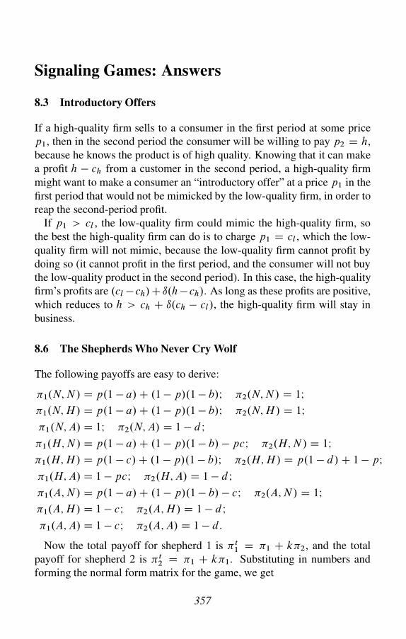
Signaling Games: Answers
8.3 Introductory Offers
If a high-quality firm sells to a consumer in the first period at some price
p1, then in the second period the consumer will be willing to pay p2 D h,
because he knows the product is of high quality. Knowing that it can make
a profit h � ch from a customer in the second period, a high-quality firm
might want to make a consumer an “introductory offer” at a price p1 in the
first period that would not be mimicked by the low-quality firm, in order to
reap the second-period profit.
If p1 > cl , the low-quality firm could mimic the high-quality firm, so
the best the high-quality firm can do is to charge p1 D cl , which the low-
quality firm will not mimic, because the low-quality firm cannot profit by
doing so (it cannot profit in the first period, and the consumer will not buy
the low-quality product in the second period). In this case, the high-quality
firm’s profits are .cl � ch/ C ı.h � ch/. As long as these profits are positive,
which reduces to h > ch C ı.ch � cl/, the high-quality firm will stay in
business.
8.6 The Shepherds Who Never Cry Wolf
The following payoffs are easy to derive:
�1.N; N/ D p.1 � a/ C .1 � p/.1 � b/I �2.N; N/ D 1I�1.N; H/ D p.1 � a/ C .1 � p/.1 � b/I �2.N; H/ D 1I�1.N; A/ D 1I �2.N; A/ D 1 � d I
�1.H; N/ D p.1 � a/ C .1 � p/.1 � b/ � pcI �2.H; N/ D 1I�1.H; H/ D p.1 � c/ C .1 � p/.1 � b/I �2.H; H/ D p.1 � d/ C 1 � pI�1.H; A/ D 1 � pcI �2.H; A/ D 1 � d I�1.A; N/ D p.1 � a/ C .1 � p/.1 � b/ � cI �2.A; N/ D 1I�1.A; H/ D 1 � cI �2.A; H/ D 1 � d I�1.A; A/ D 1 � cI �2.A; A/ D 1 � d:
Now the total payoff for shepherd 1 is � t1 D �1 C k�2, and the total
payoff for shepherd 2 is � t2 D �1 C k�1. Substituting in numbers and
forming the normal form matrix for the game, we get
357
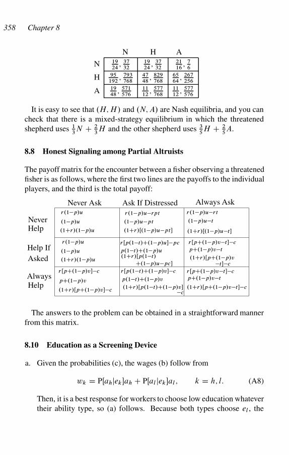
358 Chapter 8
N H A
N 1924
; 3732
1924
; 3732
2116
; 76
H 95192
; 793768
4748
; 829768
6564
; 267256
A 1948
; 571576
1112
; 577768
1112
; 577576
It is easy to see that .H; H/ and .N; A/ are Nash equilibria, and you can
check that there is a mixed-strategy equilibrium in which the threatened
shepherd uses 13N C 2
3H and the other shepherd uses 3
5H C 2
5A.
8.8 Honest Signaling among Partial Altruists
The payoff matrix for the encounter between a fisher observing a threatened
fisher is as follows, where the first two lines are the payoffs to the individual
players, and the third is the total payoff:
r.1�p/u
.1�p/u�pt
r.1�p/u�rt
rŒp.1�t/C.1�p/u��pc
Never Ask Ask If Distressed Always Ask
Never
Help If
Always
.1Cr/.1�p/u .1Cr/Œ.1�p/u�pt� .1Cr/Œ.1�p/u�t�
C.1�p/u�pc�
.1�p/u
r.1�p/u�rpt
.1�p/u�t
r.1�p/u
.1Cr/.1�p/u
.1�p/u p.1�t/C.1�p/u.1Cr/Œp.1�t/
Help
Asked
Help
pC.1�p/v�t
�t��c
rŒpC.1�p/v�t��c
.1Cr/ŒpC.1�p/v
rŒpC.1�p/v��c
pC.1�p/v
.1Cr/ŒpC.1�p/v��c
rŒp.1�t/C.1�p/v��c
p.1�t/C.1�p/v
.1Cr/Œp.1�t/C.1�p/v�
rŒpC.1�p/v�t��c
pC.1�p/v�t
.1Cr/ŒpC.1�p/v�t��c�c
The answers to the problem can be obtained in a straightforward manner
from this matrix.
8.10 Education as a Screening Device
a. Given the probabilities (c), the wages (b) follow from
wk D PŒahjek�ah C PŒal jek�al ; k D h; l: (A8)
Then, it is a best response for workers to choose low education whatever
their ability type, so (a) follows. Because both types choose el , the
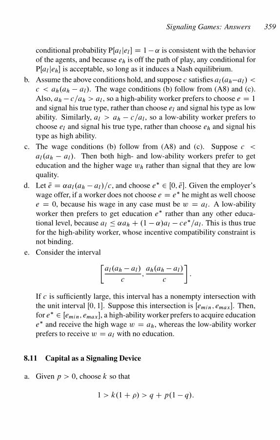
Signaling Games: Answers 359
conditional probability PŒal jel � D 1 � ˛ is consistent with the behavior
of the agents, and because eh is off the path of play, any conditional for
PŒal jeh� is acceptable, so long as it induces a Nash equilibrium.
b. Assume the above conditions hold, and suppose c satisfies al.ah�al/ <
c < ah.ah � al/. The wage conditions (b) follow from (A8) and (c).
Also, ah � c=ah > al , so a high-ability worker prefers to choose e D 1
and signal his true type, rather than choose el and signal his type as low
ability. Similarly, al > ah � c=al , so a low-ability worker prefers to
choose el and signal his true type, rather than choose eh and signal his
type as high ability.
c. The wage conditions (b) follow from (A8) and (c). Suppose c <
al.ah � al/. Then both high- and low-ability workers prefer to get
education and the higher wage wh rather than signal that they are low
quality.
d. Let Ne D ˛al.ah � al/=c, and choose e� 2 Œ0; Ne�. Given the employer’s
wage offer, if a worker does not choose e D e� he might as well choose
e D 0, because his wage in any case must be w D al . A low-ability
worker then prefers to get education e� rather than any other educa-
tional level, because al � ˛ah C .1 � ˛/al � ce�=al . This is thus true
for the high-ability worker, whose incentive compatibility constraint is
not binding.
e. Consider the interval
�al.ah � al/
c;ah.ah � al/
c
�:
If c is sufficiently large, this interval has a nonempty intersection with
the unit interval Œ0; 1�. Suppose this intersection is Œemin; emax�. Then,
for e� 2 Œemin; emax�, a high-ability worker prefers to acquire education
e� and receive the high wage w D ah, whereas the low-ability worker
prefers to receive w D al with no education.
8.11 Capital as a Signaling Device
a. Given p > 0, choose k so that
1 > k.1 C �/ > q C p.1 � q/:
360 Chapter 8
This is possible because q C p.1 � q/ < 1. Then it is clear that the
fraction q of good projects is socially productive. The interest rate r
that a producer must offer then must satisfy
k.1 C �/ D qk.1 C r/ C .1 � q/kp.1 C r/ D k.1 C r/Œq C p.1 � q/�;
so
r D 1 C �
q C p.1 � q/� 1: (A9)
The net profit of a producer with a good project is then
1 � k.1 C r/ D q C p.1 � q/ � k.1 C �/
q C p.1 � q/< 0;
so such producers will be unwilling to offer lenders an interest rate they
are willing to accept. The same is clearly true of bad projects, so no
projects get funded. Note that bad projects are not socially productive
in this case, because p�k.1C�/ < p�.qCp.1�q// D �q.1�p/ < 0.b. Choose k so that p < k.1 C �/ < q C p.1 � q/, which is clearly
always possible. Then the fraction 1 � q of bad projects are socially
unproductive. The interest rate r must still satisfy equation (A9), so the
payoff to a successful project (good or bad) is
1 � k.1 C r/ D q C p.1 � q/ � k.1 C �/
q C p.1 � q/> 0;
so producers of both good and bad projects are willing to offer interest
rate r , and lenders are willing to lend at this rate to all producers.c. Let
kpmin D pŒ1 � k.1 C �/�
.1 � p/.1 C �/:
Note that because good projects are socially productive, kpmin > 0.
Suppose all producers have wealth kp > kpmin, and lenders believe that
only a producer with a good project will invest kp in his project. Then
lenders will be willing to lend at interest rate �. If a producer invests
kp in his project and borrows k � kp, his return is 1 and his costs are
forgone earnings kp.1 C �/ and capital costs .k � kp/.1 C �/. Thus,
his profit is
1 � kp.1 C �/ � .k � kp/.1 C �/ D 1 � k.1 C �/ > 0;
Signaling Games: Answers 361
so such a producer is willing to undertake this transaction. If the pro-
ducer with a bad project invests his capital kp, his return is
pŒ1 � k.1 C �/� � .1 � p/kp.1 C �/ < 0;
so he will not put up the equity. This proves the theorem.
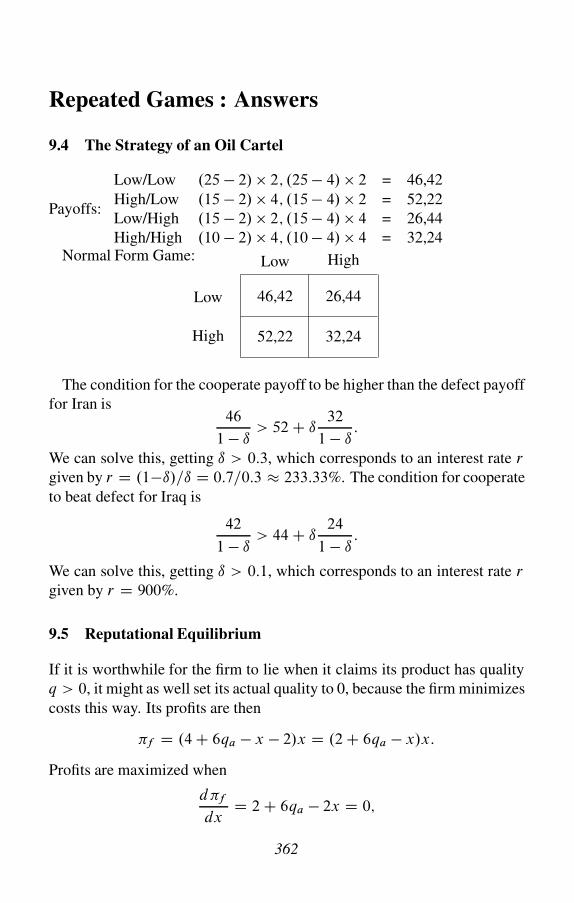
Repeated Games : Answers
9.4 The Strategy of an Oil Cartel
Payoffs:
Low/Low .25 � 2/ � 2; .25 � 4/ � 2 = 46,42
High/Low .15 � 2/ � 4; .15 � 4/ � 2 = 52,22
Low/High .15 � 2/ � 2; .15 � 4/ � 4 = 26,44
High/High .10 � 2/ � 4; .10 � 4/ � 4 = 32,24Normal Form Game:
46,42
52,22
Low
26,44
32,24
High
Low
High
The condition for the cooperate payoff to be higher than the defect payoff
for Iran is46
1 � ı> 52 C ı
32
1 � ı:
We can solve this, getting ı > 0:3, which corresponds to an interest rate r
given by r D .1�ı/=ı D 0:7=0:3 � 233:33%. The condition for cooperate
to beat defect for Iraq is
42
1 � ı> 44 C ı
24
1 � ı:
We can solve this, getting ı > 0:1, which corresponds to an interest rate r
given by r D 900%.
9.5 Reputational Equilibrium
If it is worthwhile for the firm to lie when it claims its product has quality
q > 0, it might as well set its actual quality to 0, because the firm minimizes
costs this way. Its profits are then
�f D .4 C 6qa � x � 2/x D .2 C 6qa � x/x:
Profits are maximized when
d�f
dxD 2 C 6qa � 2x D 0;
362
Repeated Games: Answers 363
so x D 1 C 3qa , and �f D .1 C 3qa/2:
Now suppose the firm tells the truth. Then, if �t is per-period profits, we
have
�t D .2 C 6qa � 6q2a � x/x;
d�t
dxD 2 C 6qa � 6q2
a � 2x D 0;
so x D 1 C 3qa � 3q2a , and �t D .1 C 3qa � 3q2
a/2. But total profits …
from truth telling are �t forever, discounted at rate ı D 0:9, or
… D �t
1 � ıD 10.1 C 3qa � 3q2
a/2:
Truth-telling is profitable then when … �f , or when
10.1 C 3qa � 3q2a/2 > .1 C 3qa/2: (A10)
Note that equation (A10) is true for very small qa (that is, qa near 0) and
false for very large qa (that is, qa near 1).

Evolutionary Stable Strategies: Answers
10.4 A Symmetric Coordination Game
a. Let sa and sb be the two strategies, and write � D ˛sa C .1 � ˛/sb
for the mixed strategy where sa is played with probability ˛. If Dˇsa C .1 � ˇ/sb, we have �Œ�; � D ˛ˇa C .1 � ˛/.1 � ˇ/b: Suppose
.�; �/ is a Nash equilibrium. Then by the fundamental theorem (�3.6),
�Œsa; � � D �Œsb; � �, which implies ˛ D b=.aCb/: Note that �Œ�; �� Dab=.a C b/, which is smaller than either a or b. We shall show that b
can invade a population that plays � . By the fundamental theorem,
�Œsb; � � D �Œ�; ��, because ˛ < 1. Thus � is impervious to invasion
by sb only if �Œ�; sb� > �Œsb; sb�, which reduces to ab=.a C b/ > b,
which is false.
364
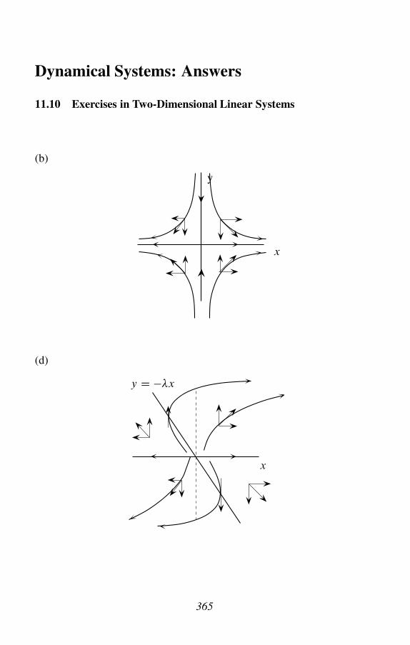
Dynamical Systems: Answers
11.10 Exercises in Two-Dimensional Linear Systems
(b)
x
y
(d)
y D ��x
x
365
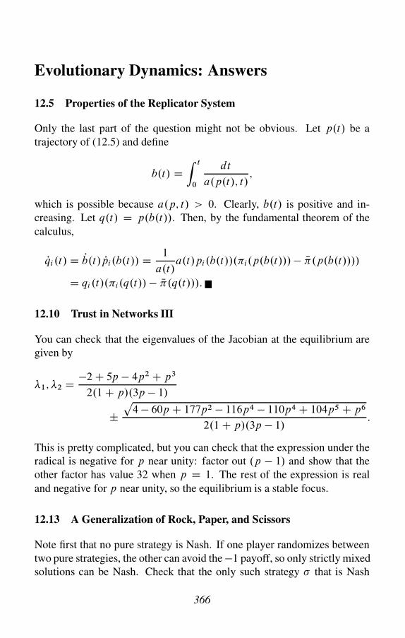
Evolutionary Dynamics: Answers
12.5 Properties of the Replicator System
Only the last part of the question might not be obvious. Let p.t/ be a
trajectory of (12.5) and define
b.t/ DZ t
0
dt
a.p.t/; t/;
which is possible because a.p; t/ > 0. Clearly, b.t/ is positive and in-
creasing. Let q.t/ D p.b.t//. Then, by the fundamental theorem of the
calculus,
Pqi .t/ D Pb.t/ Ppi.b.t// D 1
a.t/a.t/pi.b.t//.�i.p.b.t/// � N�.p.b.t////
D qi .t/.�i.q.t// � N�.q.t///:
12.10 Trust in Networks III
You can check that the eigenvalues of the Jacobian at the equilibrium are
given by
�1; �2 D �2 C 5p � 4p2 C p3
2.1 C p/.3p � 1/
˙p
4 � 60p C 177p2 � 116p4 � 110p4 C 104p5 C p6
2.1 C p/.3p � 1/:
This is pretty complicated, but you can check that the expression under the
radical is negative for p near unity: factor out .p � 1/ and show that the
other factor has value 32 when p D 1. The rest of the expression is real
and negative for p near unity, so the equilibrium is a stable focus.
12.13 A Generalization of Rock, Paper, and Scissors
Note first that no pure strategy is Nash. If one player randomizes between
two pure strategies, the other can avoid the �1 payoff, so only strictly mixed
solutions can be Nash. Check that the only such strategy � that is Nash
366
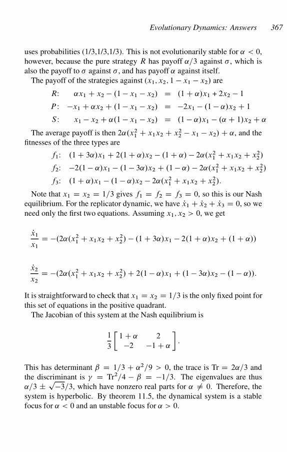
Evolutionary Dynamics: Answers 367
uses probabilities (1/3,1/3,1/3). This is not evolutionarily stable for ˛ < 0,
however, because the pure strategy R has payoff ˛=3 against � , which is
also the payoff to � against � , and has payoff ˛ against itself.
The payoff of the strategies against (x1; x2; 1 � x1 � x2/ are
R: ˛x1 C x2 � .1 � x1 � x2/ D .1 C ˛/x1 + 2x2 � 1
P : �x1 C ˛x2 C .1 � x1 � x2/ D �2x1 � .1 � ˛/x2 C 1
S : x1 � x2 C ˛.1 � x1 � x2/ D .1 � ˛/x1 � .˛ C 1/x2 C ˛
The average payoff is then 2˛.x21 C x1x2 C x2
2 � x1 � x2/ C ˛, and the
fitnesses of the three types are
f1: .1 C 3˛/x1 C 2.1 C ˛/x2 � .1 C ˛/ � 2˛.x21 C x1x2 C x2
2/
f2: �2.1 � ˛/x1 � .1 � 3˛/x2 C .1 � ˛/ � 2˛.x21 C x1x2 C x2
2/
f3: .1 C ˛/x1 � .1 � ˛/x2 � 2˛.x21 C x1x2 C x2
2/.
Note that x1 D x2 D 1=3 gives f1 D f2 D f3 D 0, so this is our Nash
equilibrium. For the replicator dynamic, we have Px1 C Px2 C Px3 D 0, so we
need only the first two equations. Assuming x1; x2 > 0, we get
Px1
x1
D �.2˛.x21 C x1x2 C x2
2/ � .1 C 3˛/x1 � 2.1 C ˛/x2 C .1 C ˛//
Px2
x2
D �.2˛.x21 C x1x2 C x2
2/ C 2.1 � ˛/x1 C .1 � 3˛/x2 � .1 � ˛//:
It is straightforward to check that x1 D x2 D 1=3 is the only fixed point for
this set of equations in the positive quadrant.
The Jacobian of this system at the Nash equilibrium is
1
3
�1 C ˛ 2
�2 �1 C ˛
�:
This has determinant ˇ D 1=3 C ˛2=9 > 0, the trace is Tr D 2˛=3 and
the discriminant is � D Tr2=4 � ˇ D �1=3. The eigenvalues are thus
˛=3 ˙ p�3=3, which have nonzero real parts for ˛ ¤ 0. Therefore, the
system is hyperbolic. By theorem 11.5, the dynamical system is a stable
focus for ˛ < 0 and an unstable focus for ˛ > 0.

368 Chapter 12
12.14 Uta stansburiana in Motion
It is easy to check that if the frequencies of orange-throats (rock), blue-
throats (paper), and yellow-striped (scissors) are ˛; ˇ, and 1 � ˛ � ˇ, re-
spectively, the payoffs to the three strategies are 1 � ˛ � 2ˇ; 2˛ C ˇ � 1,
and ˇ � ˛, respectively. The average payoff is zero (check this!), so the
replicator dynamic equations are
d˛
dtD ˛.1 � ˛ � 2ˇ/
(A11)dˇ
dtD ˇ.2˛ C ˇ � 1/:
The Jacobian matrix at the fixed point ˛ D ˇ D 1=3 is given by
��1=3 �2=3
2=3 1=3
�:
The trace of the Jacobian is thus zero, the determinant is 1=3 > 0, and the
discriminant is �1=3 < 0. By theorem 11.5 the eigenvalues are imaginary
so the system is not hyperbolic. It is easy to solve for the trajectories of
this system because, by theorem 11.5, they are closed orbits, and the fixed
point is a center. But this tells us nothing about the original, nonlinear
system (A11), because the fixed point is not hyperbolic (see theorem 11.3).
So, back to the drawing board.
Let V.˛; ˇ; �/ D ln.˛/ C ln.ˇ/ C ln.�/. Along a trajectory of the dy-
namical system, we have
PV D P˛
CPˇ
C P��
D .1 � ˛ � 2ˇ/ C .2˛ C ˇ � 1/ C .ˇ � ˛/ D 0:
Thus, V is constant on trajectories. This implies that trajectories are
bounded and bounded away from .0; 0/ so the set � of !-limit points of
a trajectory contains no fixed points, and hence by the Poincare-Bendixson
theorem (theorem 11.8), � is a periodic orbit. But then by theorem 11.9, �
must contain .0; 0/. Hence, trajectories also must spiral around .0; 0/, and
because V is increasing along a ray going northeast from the fixed point,
trajectories must be closed orbits.
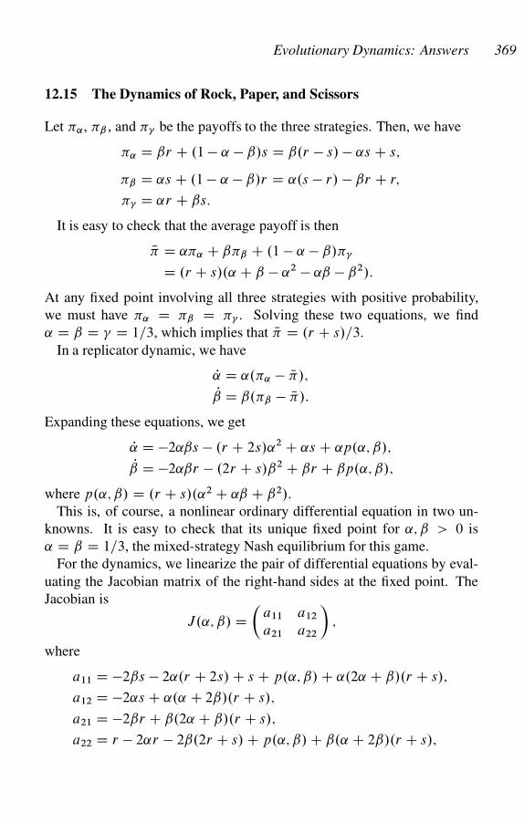
Evolutionary Dynamics: Answers 369
12.15 The Dynamics of Rock, Paper, and Scissors
Let �˛, �ˇ , and �� be the payoffs to the three strategies. Then, we have
�˛ D ˇr C .1 � ˛ � ˇ/s D ˇ.r � s/ � ˛s C s;
�ˇ D ˛s C .1 � ˛ � ˇ/r D ˛.s � r/ � ˇr C r;
�� D ˛r C ˇs:
It is easy to check that the average payoff is then
N� D ˛�˛ C ˇ�ˇ C .1 � ˛ � ˇ/��
D .r C s/.˛ C ˇ � ˛2 � ˛ˇ � ˇ2/:
At any fixed point involving all three strategies with positive probability,
we must have �˛ D �ˇ D �� . Solving these two equations, we find
˛ D ˇ D � D 1=3, which implies that N� D .r C s/=3.
In a replicator dynamic, we have
P D ˛.�˛ � N�/;
P D ˇ.�ˇ � N�/:
Expanding these equations, we get
P D �2˛ˇs � .r C 2s/˛2 C ˛s C ˛p.˛; ˇ/;
P D �2˛ˇr � .2r C s/ˇ2 C ˇr C ˇp.˛; ˇ/;
where p.˛; ˇ/ D .r C s/.˛2 C ˛ˇ C ˇ2/.
This is, of course, a nonlinear ordinary differential equation in two un-
knowns. It is easy to check that its unique fixed point for ˛; ˇ > 0 is
˛ D ˇ D 1=3, the mixed-strategy Nash equilibrium for this game.
For the dynamics, we linearize the pair of differential equations by eval-
uating the Jacobian matrix of the right-hand sides at the fixed point. The
Jacobian is
J.˛; ˇ/ D�
a11 a12
a21 a22
�;
where
a11 D �2ˇs � 2˛.r C 2s/ C s C p.˛; ˇ/ C ˛.2˛ C ˇ/.r C s/;
a12 D �2˛s C ˛.˛ C 2ˇ/.r C s/;
a21 D �2ˇr C ˇ.2˛ C ˇ/.r C s/;
a22 D r � 2˛r � 2ˇ.2r C s/ C p.˛; ˇ/ C ˇ.˛ C 2ˇ/.r C s/;
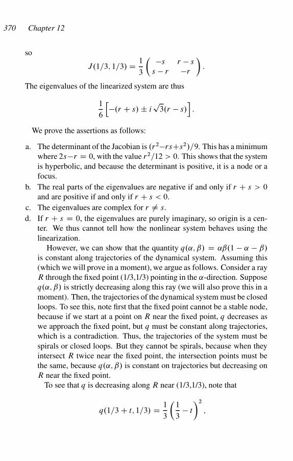
370 Chapter 12
so
J.1=3; 1=3/ D 1
3
� �s r � s
s � r �r
�:
The eigenvalues of the linearized system are thus
1
6
h�.r C s/ ˙ i
p3.r � s/
i:
We prove the assertions as follows:
a. The determinant of the Jacobian is .r2�rsCs2/=9. This has a minimum
where 2s�r D 0, with the value r2=12 > 0. This shows that the system
is hyperbolic, and because the determinant is positive, it is a node or a
focus.
b. The real parts of the eigenvalues are negative if and only if r C s > 0
and are positive if and only if r C s < 0.
c. The eigenvalues are complex for r ¤ s.
d. If r C s D 0, the eigenvalues are purely imaginary, so origin is a cen-
ter. We thus cannot tell how the nonlinear system behaves using the
linearization.
However, we can show that the quantity q.˛; ˇ/ D ˛ˇ.1 � ˛ � ˇ/
is constant along trajectories of the dynamical system. Assuming this
(which we will prove in a moment), we argue as follows. Consider a ray
R through the fixed point (1/3,1/3) pointing in the ˛-direction. Suppose
q.˛; ˇ/ is strictly decreasing along this ray (we will also prove this in a
moment). Then, the trajectories of the dynamical system must be closed
loops. To see this, note first that the fixed point cannot be a stable node,
because if we start at a point on R near the fixed point, q decreases as
we approach the fixed point, but q must be constant along trajectories,
which is a contradiction. Thus, the trajectories of the system must be
spirals or closed loops. But they cannot be spirals, because when they
intersect R twice near the fixed point, the intersection points must be
the same, because q.˛; ˇ/ is constant on trajectories but decreasing on
R near the fixed point.
To see that q is decreasing along R near (1/3,1/3), note that
q.1=3 C t; 1=3/ D 1
3
�1
3� t
�2
;

Evolutionary Dynamics: Answers 371
which has a derivative with respect to t that evaluates to �2=9 < 0 at
t D 0.
To see that q.˛; ˇ/ is constant along trajectories, note that the differen-
tial equations for the dynamical system, assuming r D 1, s D �1, can
be written as
P D 2˛ˇ C ˛2 � ˛ (A12)
P D �2˛ˇ � ˇ2 C ˇ: (A13)
Then,
d
dtq.˛; ˇ/ D d
dtŒ˛ˇ.1 � ˛ � ˇ/�
D ˇ.1 � ˛ � ˇ/ P C ˛.1 � ˛ � ˇ/ P C ˛ˇ.� P � P/D 0;
where we get the last step by substituting the expressions for P and Pfrom (AA12) and (AA13).
12.16 The Lotka-Volterra Model and Biodiversity
a. This is simple algebra, though you should check that the restrictions on
the signs of a, b, c,and d ensure that p� > 0.
b. We have
Ppp
D Puu
�� Pu
wC Pv
w
�
D Puu
��p
Puu
C .1 � p/Pvv
�
D ap C b.1 � p/ � kw
� ŒpŒap C b.1 � p/ � kw� C .1 � p/Œcp C d.1 � p/ � kw��
D ap C b.1 � p/ � ŒpŒap C b.1 � p/� C .1 � p/Œcp C d.1 � p/��
D �A � N�:
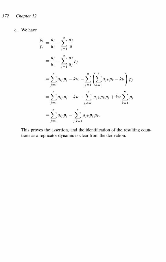
372 Chapter 12
c. We have
Ppi
pi
D Pui
ui
�nX
j D1
Puj
u
D Pui
ui
�nX
j D1
Puj
uj
pj
DnX
j D1
aij pj � kw �nX
j D1
nX
kD1
ajkpk � ku
!pj
DnX
j D1
aij pj � ku �nX
j;kD1
ajkpkpj C ku
nX
kD1
pj
DnX
j D1
aij pj �nX
j;kD1
ajkpj pk:
This proves the assertion, and the identification of the resulting equa-
tions as a replicator dynamic is clear from the derivation.
Sources for Problems
Bar-Hillel (1980): 1.31;
Bendor and Swistak (1995): 10.10
Binmore (1993): 12.3;
Bishop and Cannings (1978): 10.14;
Casscells, Schoenberger and Grayboys (1978): 1.23;
Gintis (1989): 9.9;
Hofbauer and Sigmund (1998): 10.1, 11.11, 11.12, 12.5, 12.6, 12.8, 12.9;
Kreps (1990): 9.5;
Morrow (1994): 4.2;
Moulin (1986): 3.9, 6.21;
Rasmusen (1989): 3.1;
Riley (1979): 10.15;
Rotemberg and Saloner (1991): 9.6;
Shubik (1954): 1.32;
Sinervo and Lively (1996): 6.25;
Tirole (1988): 6.42;
van Damme (1987): 10.1;
vos Savant (1991): 1.29;
vos Savant (December 27, 1998): 1.15;
Weibull (1995): 12.7;
Many individuals were kind enough to point out errors and misprints in the
text, including Songlin Cai, Jeffery Carpenter, Kevin Fenwich, Jack Hir-
shleifer, Arjun Jayadev, Nona Karalashvili, Michael Mesterton-Gibbons,
Smiljana Petrovich, Rohit Parikh, Daniel Sadoc Menasche, and Martin
Schmidt.

This page intentionally left blank
References
Akerlof, George A., “Labor Contracts as Partial Gift Exchange,” Quarterly Journal
of Economics 97,4 (November 1982):543–569.
Alcock, John, Animal Behavior: An Evolutionary Approach (Sunderland, MA:
Sinauer, 1993).
Andreoni, James and John H. Miller, “Rational Cooperation in the Finitely Re-
peated Prisoner’s Dilemma: Experimental Evidence,” Economic Journal 103
(May 1993):570–585.
and , “Giving According to GARP: An Experimental Test of the Consistency
of Preferences for Altruism,” Econometrica 70,2 (2002):737–753.
Anscombe, F. and Robert J. Aumann, “A Definition of Subjective Probability,”
Annals of Mathematical Statistics 34 (1963):199–205.
Aumann, Robert J., “Correlated Equilibrium and an Expression of Bayesian Ra-
tionality,” Econometrica 55 (1987):1–18.
Babcock, Linda, George F. Loewenstein, and Xianghong Wang, “The Relation-
ship between Uncertainty, the Contract Zone, and Efficiency in a Bargaining
Experiment,” Journal of Economic Behavior and Organization 27,3 (August
1995):475–485.
Bar-Hillel, M., “The Base-rate Fallacy in Probability Judgments,” Acta Psycho-
logica 44 (1980):211–233.
Bardhan, Pranab, Samuel Bowles, and Herbert Gintis, “Wealth Inequality, Credit
Constraints, and Economic Performance,” in Anthony Atkinson and Francois
Bourguignon (eds.), Handbook of Income Distribution (Dortrecht: North-
Holland, 2000) pp. 541–603.
Becker, Gary S., “Irrational Behavior and Economic Theory,” Journal of Political
Economy 70,1 (February 1962):1–13.
, A Treatise on the Family (Cambridge, MA: Harvard University Press, 1981).
Bendor, Jonathan and Piotr Swistak, “Types of Evolutionary Stability and the
Problem of Cooperation,” Proc. Natl. Acad. Sci. USA 92 (April 1995):3596–
3600.
Benkman, C. W., “Flock Size, Food Dispersion, and the Feeding Behavior of
Crossbills,” Behavioral Ecology and Sociobiology 23 (1988):167–175.
375
376 References
Bhaskar, V. and Ichiro Obara, “Belief-Based Equilibria: The Repeated Pris-
oner’s Dilemma with Private Monitoring,” Journal of Economic Theory 102
(2002):40–69.
Bicchieri, Cristina, The Grammar of Society: The Nature and Dynamics of Social
Norms (Cambridge: Cambridge University Press, 2006).
Binmore, Kenneth G., Game Theory and the Social Contract: Playing Fair (Cam-
bridge, MA: MIT Press, 1993).
, Natural Justice (Oxford: Oxford University Press, 2005).
Bishop, D. T. and C. Cannings, “The Generalised War of Attrition,” Advances in
Applied Probability 10,1 (March 1978):6–7.
Bowles, Samuel, “The Production Process in a Competitive Economy: Wal-
rasian, Neo- Hobbesian, and Marxian Models,” American Economic Review
75,1 (March 1985):16–36.
and Herbert Gintis, “Power and Wealth in a Competitive Capitalist Economy,”
Philosophy and Public Affairs 21,4 (Fall 1992):324–353.
and , “The Revenge of Homo economicus: Contested Exchange and the
Revival of Political Economy,” Journal of Economic Perspectives 7,1 (Winter
1993):83–102.
Boyd, Robert, “Mistakes Allow Evolutionary Stability in the Repeated Prisoner’s
Dilemma Game,” Journal of Theoretical Biology 136 (1989):47–56.
and J. Lorberbaum, “No Pure Strategy Is Evolutionarily Stable in the Repeated
Prisoner’s Dilemma Game,” Nature 327 (1987):58–59.
and Peter J. Richerson, Culture and the Evolutionary Process (Chicago: Uni-
versity of Chicago Press, 1985).
Buchanan, James, “The Samaritan’s Dilemma,” in Edmund S. Phelps (ed.), Altru-
ism, Morality, and Economic Theory (New York: Russell Sage, 1975) pp. 71–
85.
Bulmer, Michael G., “Structural Stability in Models of Sexual Selection,” Theo-
retical Population Biology 35 (1989):195–206.
Casscells, W., A. Schoenberger, and T. Grayboys, “Interpretation by Physi-
cians of Clinical Laboratory Results,” New England Journal of Medicine 298
(1978):999–1001.
Cosmides, Leda and John Tooby, “Cognitive Adaptations for Social Exchange,” in
Jerome H. Barkow, Leda Cosmides, and John Tooby (eds.), The Adapted Mind:
Evolutionary Psychology and the Generation of Culture (New York: Oxford
University Press, 1992) pp. 163–228.
Dahl, Robert A., “The Concept of Power,” Behavioral Science 2 (1957):201–215.
Dawkins, Marian Stamp and Tim Guilford, “The Corruption of Honest Signalling,”
Animal Behaviour 41 (1991):865–873.
References 377
Dixit, Avenash, The Art of Smooth Pasting (Chur, Switzerland: Harwood, 1993).
Durrett, Richard and Simon Levin, “The Importance of Being Discrete (and Spa-
tial),” Theoretical Population Biology 46 (1994):363–394.
Elaydi, Saber N., An Introduction to Difference Equations (New York: Springer,
1999).
Ely, Jeffrey C. and Juuso Valimaki, “A Robust Folk Theorem for the Prisoner’s
Dilemma,” Journal of Economic Theory 102 (2002):84–105.
Epstein, Joshua M., Nonlinear Dynamics, Mathematical Biology, and Social Sci-
ence (Reading, MA: Addison-Wesley, 1997).
Farrell, Joseph and Roger Ware, “Evolutionary Stability in the Repeated Prisoner’s
Dilemma Game,” Theoretical Population Biology 36,2 (October 1989):161–
166.
Feller, William, An Introduction to Probability Theory and Its Applications Vol. 1
(New York: John Wiley & Sons, 1950).
Fisher, Ronald A., “The Evolution of Sexual Preference,” Eugenics Review 7
(1915):184–192.
Forsythe, Robert, Forrest Nelson, George R. Neumann, and Jack Wright,
“Anatomy of an Experimental Political Stock Market,” American Economic Re-
view 82,5 (1992):1142–1161.
Foster, Dean and H. Peyton Young, “Stochastic Evolutionary Game Dynamics,”
Theoretical Population Biology 38 (1990):219–232.
Freidlin, Mark I. and Alexander D. Wentzell, Random Perturbations of Dynamical
Systems (New York: Springer, 1984).
Friedman, Daniel, “Evolutionary Games in Economics,” Econometrica 59,3 (May
1991):637–666.
Friedman, Milton and Leonard J. Savage, “The Utility Analysis of Choices Involv-
ing Risk,” Journal of Political Economy 56 (1948):279–304.
Fudenberg, Drew and Eric Maskin, “The Folk Theorem in Repeated Games
with Discounting or with Incomplete Information,” Econometrica 54,3 (May
1986):533–554.
and Jean Tirole, Game Theory (Cambridge, MA: MIT Press, 1991).
, David K. Levine, and Eric Maskin, “The Folk Theorem with Imperfect Public
Information,” Econometrica 62 (1994):997–1039.
Gilbert, Daniel T., “How Mental Systems Believe,” American Psychologist 46,2
(February 1991):107–119.
Gintis, Herbert, “The Nature of the Labor Exchange and the Theory of Capitalist
Production,” Review of Radical Political Economics 8,2 (Summer 1976):36–54.
378 References
, “The Power to Switch: On the Political Economy of Consumer Sovereignty,”
in Samuel Bowles, Richard C. Edwards, and William G. Shepherd (eds.), Un-
conventional Wisdom: Essays in Honor of John Kenneth Galbraith (New York:
Houghton-Mifflin, 1989) pp. 65–80.
, “Where Did Schumpeter Go Wrong?: Understanding Capitalism, Socialism,
and Democracy,” Challenge 34,1 (January–February 1991):27–33.
, “The Evolution of Private Property,” Journal of Economic Behavior and Orga-
nization 64,1 (September 2007):1–16.
, The Bounds of Reason: Game Theory and the Unification of the Behavioral
Sciences (Princeton, NJ: Princeton University Press, 2009).
Gode, Dhananjay K. and Shyam Sunder, “Allocative Efficiency of Markets with
Zero-Intelligence Traders: Markets as a Partial Substitute for Individual Ratio-
nality,” Journal of Political Economy 101,1 (1993):119–1137.
Grafen, Alan, “Biological Signals as Handicaps,” Journal of Theoretical Biology
144 (1990):517–546.
, “Sexual Selection Unhandicapped by the Fisher Process,” Journal of Theoret-
ical Biology 144 (1990):473–516.
Guilford, Tim and Marian Stamp Dawkins, “Receiver Psychology and the Evolu-
tion of Animal Signals,” Animal Behaviour 42 (1991):1–14.
and , “Receiver Psychology and the Design of Animal Signals,” Trends in
Neuroscience 16,11 (1993):420–436.
Haigh, J., “Game Theory and Evolution,” Advances in Applied Probability 7,1
(1975):8–11.
Harbaugh, W. T., K. Krause, and T. R. Berry, “GARP for Kids: On the De-
velopment of Rational Choice Behavior,” American Economic Review 91
(2001):1539–1945.
Hardin, Garrett, “The Tragedy of the Commons,” Science 162 (1968):1243–1248.
Harsanyi, John C., “Measurement of Social Power, Opportunity Costs, and the
Theory of Two-Person Bargaining Games,” Behavioral Science 7 (1962):67–
81.
, “Games with Incomplete Information Played by Bayesian Players, Parts I, II,
and III,” Behavioral Science 14 (1967):159–182, 320–334, 486–502.
, “Games with Randomly Disturbed Payoffs: A New Rationale for Mixed-
Strategy Equilibrium Points,” International Journal of Game Theory 2 (1973):1–
23.
Hayek, F. A., “The Use of Knowledge in Society,” American Economic Review
35,4 (September 1945):519–530.
Hines, James R., “Three Sides of Harberger Triangles,” Journal of Economic Per-
spectives 13,2 (Spring 1999):167–188.
References 379
Hirsch, Morris W. and Stephen Smale, Differential Equations, Dynamical Sys-
tems, and Linear Systems (San Diego: Academic Press, 1974).
Hofbauer, Josef and Karl Sigmund, Evolutionary Games and Population Dynamics
(Cambridge, UK: Cambridge University Press, 1998).
Holmstrom, Bengt, “Moral Hazard in Teams,” Bell Journal of Economics 7
(1982):324–340.
Horn, Roger A. and Charles R. Johnson, Matrix Analysis (Cambridge, UK: Cam-
bridge University Press, 1985).
Horner, Johannes and Wojciech Olszewski, “The Folk Theorem for Games with
Private Almost-Perfect Monitoring,” Econometrica 74,6 (2006):1499–1545.
Johnstone, Rufus A. and Alan Grafen, “The Continuous Sir Philip Sidney Game:
A Simple Model of Biological Signalling,” Journal of Theoretical Biology 156
(1992):215–234.
and , “Dishonesty and the Handicap Principle,” Animal Behavior 46
(1993):759–764.
Kahneman, Daniel, Paul Slovic, and Amos Tversky, Judgment under Uncertainty:
Heuristics and Biases (Cambridge, UK: Cambridge University Press, 1982).
Karlin, Samuel and Howard M. Taylor, A Second Course in Stochastic Processes
(Boston: Academic Press, 1981).
Kirkpatrick, M., “Sexual Selection and the Evolution of Female Choice,” Evolu-
tion 36 (1982):1–12.
Kiyonari, Toko, Shigehito Tanida, and Toshio Yamagishi, “Social Exchange and
Reciprocity: Confusion or a Heuristic?,” Evolution and Human Behavior 21
(2000):411–427.
Klein, Benjamin and Keith Leffler, “The Role of Market Forces in Assuring Con-
tractual Performance,” Journal of Political Economy 89 (August 1981):615–
641.
Kreps, David M., Notes on the Theory of Choice (London: Westview, 1988).
, A Course in Microeconomic Theory (Princeton, NJ: Princeton University
Press, 1990).
Kuhn, H. W., “Extensive Games and the Problem of Information,” in H. W. Kuhn
and A. W. Tucker (eds.), Contributions to the Theory of Games Vol. 2 of An-
nals of Mathematics Studies (Princeton, NJ: Princeton University Press, 1953)
pp. 193–216.
Lande, R., “Models of Speciation by Sexual Selection of Polygenic Traits,” Pro-
ceedings of the National Academy of Sciences USA 78 (1981):3721–3725.
Lerner, Abba, “The Economics and Politics of Consumer Sovereignty,” American
Economic Review 62,2 (May 1972):258–266.
380 References
List, John A. and Daniel L. Millimet, “The Market: Catalyst for Rationality and
Filter of Irrationality,” 2007. NBER, University of Chicago.
Loomes, Graham, “When Actions Speak Louder than Prospects,” American Eco-
nomic Review 78,3 (June 1988):463–470.
Lorberbaum, Jeffrey, “No Strategy is Evolutionarily Stable in the Repeated Pris-
oner’s Dilemma,” Journal of Theoretical Biology 168,2 (May 1994):117–130.
Mailath, George J., “Do People Play Nash Equilibrium? Lessons from Evolution-
ary Game Theory,” Journal of Economic Literature 36 (September 1998):1347–
1374.
and Stephen Morris, “Coordination Failure in Repeated Games with Almost-
public Monitoring,” Theoretical Economics 1 (2006):311–340.
Marx, Karl, The Communist Manifesto (New York: Signet Classics, 1948).
Reprint edition 1998.
Mas-Colell, Andreu, Michael D. Whinston, and Jerry R. Green, Microeconomic
Theory (New York: Oxford University Press, 1995).
Mattei, Aurelio, “A Non-parametric Test of Consumer Behavior Using Panel
Data,” Revue Suisse d’Economie Politique et de Statistique 130,1 (1994):3–20.
Maynard Smith, John, Evolution and the Theory of Games (Cambridge, UK: Cam-
bridge University Press, 1982).
, “Honest Signalling: The Philip Sidney Game,” Animal Behavior 42
(1991):1034–1035.
and G. R. Price, “The Logic of Animal Conflict,” Nature 246 (2 November
1973):15–18.
Morrow, James D., Game Theory for Political Scientists (Princeton, NJ: Princeton
University Press, 1994).
Motro, Uzi, “Co-operation and Defection: Playing the Field and the ESS,” Journal
of Theoretical Biology 151,2 (July 1991):145–154.
Moulin, Herve, “Dominance Solvable Voting Schemes,” Econometrica 47,6
(1979):1337–1351.
, Game Theory for the Social Sciences (New York: New York University Press,
1986).
Nash, John F., “Equilibrium Points in n-Person Games,” Proceedings of the Na-
tional Academy of Sciences 36 (1950):48–49.
Neelin, J., H. Sonnenschein, and M. Spiegel, “A Further Test of Non-Cooperative
Bargaining Theory,” American Economic Review 78 (1988):824–836.
Nerlove, Marc and Tjeppy D. Soedjiana, “Slamerans and Sheep: Savings and
Small Ruminants in Semi-Subsistence Agriculture in Indonesia,” 1996. De-
partment of Agriculture and Resource Economics, University of Maryland.
References 381
Olson, Valerie A. and I. P. F. Owens, “Costly Sexual Signals: Are Carotenoids
Rare, Risky or Required?,” Trends in Evolution and Ecology 13,12 (December
1998):510–514.
Ostrom, Elinor, James Walker, and Roy Gardner, “Covenants with and without a
Sword: Self-Governance Is Possible,” American Political Science Review 86,2
(June 1992):404–417.
Perko, Lawrence, Differential Equations and Dynamical Systems (New York:
Springer, 1991).
Piccione, Michele, “The Repeated Prisoner’s Dilemma with Imperfect Private
Monitoring,” Journal of Economic Theory 102 (2002):70–83.
Pomiankowski, A. N., “The Costs of Choice in Sexual Selection,” Journal of The-
oretical Biology 128 (1987):195–218.
Rapoport, Amnon and Wilfred Amaldoss, “Competition for the Development of a
New Product,” 1997. Hong Kong University of Science and Technology.
Rasmusen, Eric, Games and Information: An Introduction to Game Theory (Cam-
bridge, UK: Blackwell Scientific, 1989).
Riley, John G., “Evolutionary Equilibrium Strategies,” Journal of Theoretical Bi-
ology 76 (1979):109–123.
Rosenzweig, Mark R. and Kenneth I. Wolpin, “Credit Market Constraints, Con-
sumption Smoothing, and the Accumulation of Durable Production Assets in
Low-Income Countries: Investment in Bullocks in India,” Journal of Political
Economy 101,2 (1993):223–244.
Rotemberg, Julio and Garth Saloner, “A Supergame-Theoretic Model of Price
Wars during Booms,” in Gregory N. Mankiw and David Romer (eds.), New
Keynesian Economics, vol. 2 (Cambridge, MA: MIT Press, 1991) pp. 387–415.
Rubinstein, Ariel, “Perfect Equilibrium in a Bargaining Model,” Econometrica 50
(1982):97–109.
Saha, Atanu, Richard C. Shumway, and Hovav Talpaz, “Joint Estimation of Risk
Preference Structure and Technology Using Expo-Power Utility,” American
Journal of Agricultural Economics 76,2 (May 1994):173–184.
Samuelson, Larry, Evolutionary Games and Equilibrium Selection (Cambridge,
MA: MIT Press, 1997).
and Jianbo Zhang, “Evolutionary Stability in Asymmetric Games,” Journal of
Economic Theory 57,2 (1992):363–391.
Samuelson, Paul, “Wages and Interests: A Modern Dissection of Marxian Eco-
nomics,” American Economic Review 47 (1957):884–921.
Savage, Leonard J., The Foundations of Statistics (New York: John Wiley & Sons,
1954).
382 References
Schumpeter, Joseph, The Theory of Economic Development: An Inquiry into Prof-
its, Capital, Credit, Interest and the Business Cycle (Oxford: Oxford University
Press, 1934).
, Capitalism, Socialism, and Democracy (New York: Harper & Row, 1942).
Sekiguchi, Tadashi, “Efficiency in Repeated Prisoner’s Dilemma with Private
Monitoring,” Journal of Economic Theory 76 (1997):345–361.
Selten, Reinhard, “A Note on Evolutionarily Stable Strategies in Asymmetric An-
imal Conflicts,” Journal of Theoretical Biology 84 (1980):93–101.
Shapiro, Carl and Joseph Stiglitz, “Unemployment as a Worker Discipline De-
vice,” American Economic Review 74,3 (June 1984):433–444.
Shubik, Martin, “Does the Fittest Necessarily Survive?,” in Martin Shubik (ed.),
Readings in Game Theory and Political Behavior (New York: Doubleday, 1954)
pp. 43–46.
Simon, Herbert, “Notes on the Observation and Measurement of Political Power,”
Journal of Politics 4 (November 1953):500– 516.
Sinervo, Barry and Curtis M. Lively, “The Rock-Paper-Scissors Game and the
Evolution of Alternative Male Strategies,” Nature 380,6571 (May 1996):240–
243.
Sinn, Hans-Werner, “A Rehabilitation of the Principle of Insufficient Reason,”
Quarterly Journal of Economics 94,3 (May 1980):493–506.
Sippel, R., “An Experiment on the Pure Theory of Consumers’ Behavior,” Eco-
nomic Journal 107 (1997):1431–1434.
Solow, Robert, “Another Possible Source of Wage Stickiness,” Journal of Macroe-
conomics 1 (1979):79–82.
Stiglitz, Joseph, “The Causes and Consequences of the Dependence of Quality on
Price,” Journal of Economic Literature 25 (March 1987):1–48.
and Andrew Weiss, “Credit Rationing in Markets with Imperfect Information,”
American Economic Review 71 (June 1981):393– 411.
Strotz, Robert H., “Myopia and Inconsistency in Dynamic Utility Maximization,”
Review of Economic Studies 23,3 (1955):165–180.
Sugden, Robert, “An Axiomatic Foundation for Regret Theory,” Journal of Eco-
nomic Theory 60,1 (June 1993):159–180.
Sutton, John, “Gibrat’s Legacy,” Journal of Economic Literature 35,1 (March
1997):40–59.
Taylor, Peter and Leo Jonker, “Evolutionarily Stable Strategies and Game Dynam-
ics,” Mathematical Biosciences 40 (1978):145–156.
Tirole, Jean, The Theory of Industrial Organization (Cambridge, MA: MIT Press,
1988).
References 383
van Damme, Eric, Stability and Perfection of Nash Equilibria (Berlin: Springer-
Verlag, 1987).
van Huyck, John, Raymond C. Battalio, and Richard O. Beil, “Tacit Coordination
Games, Strategic Uncertainty, and Coordination Failure,” American Economic
Review 80 (1990):234–248.
Von Neumann, John and Oskar Morgenstern, Theory of Games and Economic
Behavior (Princeton, NJ: Princeton University Press, 1944).
vos Savant, Marilyn, “Ask Marilyn,” Parade Magazine (1991).
, “Ask Marilyn,” Parade Magazine (December 27, 1998).
Weibull, Jorgen W., Evolutionary Game Theory (Cambridge, MA: MIT Press,
1995).
Wilson, Edward O., Consilience: The Unity of Knowledge (New York: Knopf,
1998).
Young, H. Peyton, Individual Strategy and Social Structure: An Evolutionary The-
ory of Institutions (Princeton, NJ: Princeton University Press, 1998).
Zahavi, Amotz, “Mate Selection—A Selection for Handicap,” Journal of Theoret-
ical Biology 53 (1975):205–214.
and Avishay Zahavi, The Handicap Principle: A Missing Piece of Darwin’s
Puzzle (New York: Oxford University Press, 1997).
Zermelo, Ernst, “Uber eine Anwendung der Mengenlehrer auf der Theorie des
Schachspiels,” in E. Hobson and A. Love (eds.), Proceedings of the Fifth Inter-
national Congress of Mathematicians, vol II (Cambridge: Cambridge University
Press, 1913) pp. 501–504.

This page intentionally left blank
Index
action, 33, 38
adaptive expectations, 310
adaptive learning, 309–315
Agelenopsis aperta, 112
agent-based model, 72
evolutionary, 72
no-draw high-low poker, 91
repeated prisoner’s dilemma, 78
Akerlof, George, 162
along the path of play, 181
altruism, 104
in bird flocks, 147
ancestor node, 38
assortative interaction, 289
asymptotically stable fixed point, 254
Aumann, Robert, 23
backward induction, 54, 58
bargaining
heterogeneous impatience, 96
outside options, 97, 98
basin of attraction, 254
Bayesian prior, 26
Bayesian rationality, 26
Becker, Gary, 106
beliefs, 31
Bertrand’s paradox, 206
best response, 34, 43
best-response
schedule, 164
Big John and Little John
Revisited, 128
binary relation, 18
Binmore, Ken, 371
Bowles, Samuel, 221, 222
Boyd, Robert, 209, 240
branches (of game tree), 32
Buchanan, James, 104
Bulmer, Michael, 182
cardinal utility, 26
center (property of a fixed point), 262
characteristic equation, 308
child node (in a game tree), 38
closed orbit (of a dynamical system),
254
combinations, 7
Competition on Main Street, 81, 129
completely mixed, 42
completely mixed Nash equilibrium,
278
concave utility function, 27
conditional preference, 24
consistent, 19
constant relative risk aversion, 29
contingent renewal market, 220
385
386 Index
conventions, 312
Cosmides, Leda, 180
critical point, see fixed point
degenerate, 262
curvature (of a utility function), 28
Dahl, Robert, 222
Dawkins, Marian Stamp, 189
De Morgan’s laws, 3
death and discount rates, 202
decreasing function, 252
degenerate critical point, 262
delibertive decision making, 30
denumerable Markov chain, 295
discount factor, 20, 203
discriminant, 259
Dixit, Avenash, 309
dominance solvable, 72
dominated
recursively strongly, 53
recursively weakly, 53
dominated strategies, 52
dynamic
aggregate monotonic, 279
dynamical systems, 246
in one dimension, 257
theory, 253
in two dimensions, 259
Education as Screening Device, 356
eigenvalue, 256
eigenvector
left, 298
epistatic genes, 276
equilibrium
dominant-strategy, 52
ergodic, 291, 296
theorem for finite Markov
chains, 303
events (in a probability space), 2
evolution
of trust and honesty, 293
evolutionarily stable strategies
in asymmetric games, 244
in asymmetric games, 244
in finite populations, 242
multiple, 241
evolutionarily stable strategy, 229,
231
quasi, 244
evolutionary
dynamic, 269
game, 230
Evolutionary Dynamics
Origins, 269
excess demand for copulations, 182
expected value, 22
exponential discounting, 20
extensive form game, 32, 38
definition of, 38
equivalent, 42
Nature, as player in, 39
subgame, 57
fair (of coin or die), 5
fair game, 7
fallback position, 84
female choice, 182
finite game, 38, 88
first-order ordinary differential equa-
tions, 247
first-order stochastic dominance, 25
Fisher, R. A., 182, 275
Fisher’s runaway process, 182
fitness, 274
fixed point, 247
asymptotically stable, 254
center, 262
degenerate, 262
globally stable, 254
Index 387
stable focus, 261
unstable, 254
unstable focus, 262
unstable node, 260
folk theorem for repeated games, 213
Foster, Dean, 272
Freidlin, Mark I., 272
Friedman, Daniel, 270
Friedman, Milton, 23
Frobenius-Perron, 298
Fudenberg, Drew, 208, 216
fundamental theorem of
game theory, 44
natural selection, 275
principal-agent model, 175
game, generic, 127
game tree, 32, 38
generic, 201
genetic locus, 274
gift exchange, 162
globally stable fixed point, 254
Grafen, Alan, 179, 187, 194
Greens and Blacks, 12
Guilford, Tim, 189
handicap principle, 187
Hardin, Garrett, 88
Harsanyi, John, 222
hawk, dove, bourgeois game, 154
hawk-dove game, 48
hawk-dove-bourgeois, 154
head node (of a game tree), 38
Hofbauer, Josef, 235, 371
Holmstrom, Bengt, 80
hyperbolic fixed point, 256
improper, 58
incentive compatibility constraint,
84, 165, 170, 175
incentive contract, 164
increasing function, 252
incredible
threat, 35, 58
incredible threat, 55
information set, 36, 39
invadable, 242
invariant distribution, 298
Jacobian, 255
Jensen’s inequality, 27
Johnstone, Rufus A., 194
Jordan curve theorem, 267
Kirkpatrick, M., 182
Kreps, David, 371
Kuhn, Harold, 89
Lande, R., 182
leaf node (of a game tree), 33
leaf nodes, 38
left eigenvector, 313
linearization, 256
Logic of Murder and Abuse, 11
Loomes, Graham, 19
Lotka-Volterra
limited carrying capacity, 264
Predator-Prey Model, 250
lottery, 22, 23
Mailath, George J., 245
markets as disciplining devices, 81
Markov chain, 295
aperiodic, 304
denumerable, 295
ergodic, 304
ergodic theorem, 304
irreducible, 303
non-null recurrent, 303
recurrent, 303
Sisyphean, 306
steady state, 312
388 Index
Maskin, Eric, 216
maximin solution, 144
Maynard Smith, John, 229
mean recurrence time, 303
Microsoft-Google game, 57
minimax point, 214
mixed strategy, 42
Nash equilibrium, 37
profile, 42
support of, 42
Morgenstern, Oskar, 23, 144
Morrow, James D., 371
Moulin, Herve, 371
Myerson, Roger, 371
Nash, John, 44
Nash equilibrium, 34
of an asymmetric evolutionary
game, 289
completely mixed, 278
of evolutionary game, 231
existence, 44
mixed strategy, 37
pure strategy, 80
subgame perfect, 35
neighborhood, 254
neutrally stable fixed point, 254
nonclearing market for copulations,
182
noninvadable, 242
normal form, 34, 41
off the path of play, 181
one-shot, 134
one-stage deviation principle, 208
open set, 254
ordinal utility, 26
Panglossian fallacy, 276
parent node (in a game tree), 38
Pareto-dominates, 109
Pareto-efficient, 109
Pareto-inefficient, 109
Pareto-optimal, 109
Pareto-superior, 109
participation constraint, 84, 166, 170,
175
partition, 9, 25
path in a game tree, 38
perfect information, 54, 88
perfect recall, 39
permutation, 6
phase diagram, 251, 257
poker with bluffing, 68
revisited, 157
Pomiankowski, A. N., 182
pooling equilibrium, 112, 194, 196
population
monomorphic, 231
polymorphic, 231
preference ordering, 18
Price, G. R., 229
principal, 162
principal-agent model, 162
agent, 220
principal, 220
principle of insufficient reason, 12
prisoner’s dilemma
game, 50
probability, 4
probability spaces, 2
probability transition matrix, 311
pure coordination games, 109
experimental evidence, 110
pure strategy, 33, 42
quality good, 210
quasi-evolutionarily stable, 244
Rabin, Matthew, 371
random walk
Index 389
on a circle, 298
with reflecting barriers, 299
Rasmusen, Eric, 371
rationalizable, 53
recursion equations, 298
reflexive, 19
regret theory, 19
relative frequency, 4
renewal equation, 302
renewal theorem, 303
repeated game, 203
replicator, 269
replicator dynamics, 270, 271, 289
replicator system, 269
properties of, 276
reservation wage, 84
risk aversion, 28
Arrow-Pratt coefficient, 29
coefficient of relative, 29
constant absolute, 29
constant relative, 83
decreasing absolute, 29
decreasing relative, 29
more risk averse than, 28
strictly, 167
weakly decreasing, 167
risk loving, 28
risk neutral, 28, 107
root node, 38
root node (of a game tree), 32
routine choice, 30
Rubinstein bargaining, 94
Rubinstein, Ariel, 94
saddle point, 260
sample space, 2
sampling
with replacement, 6
without replacement, 6
Samuelson, Larry, 269, 272
Samuelson, Paul, 223
Savage, Leonard J., 23
Schumpeter, Joseph, 223
self-regarding, 60, 189, 216
Selten, Reinhard, 245
separating equilibrium, 193
set theory, 1
sex ratios as Nash equilibria, 137
Shapiro, Carl, 221
short-side power, 222
Shubik, Martin, 13
Sigmund, Karl, 235, 371
signal, 179
imperfect, 216
perfect, 201
private, 216
public, 201
signaling
handicap principle, 187
signaling game, 180
generic, 180
Simon, Herbert, 222
social creatures, 31
social norms, 31
Solow, Robert, 163, 225
Solow condition, 163, 164
Solow, Robert, 164
stable focus, 261
stable manifold, 260
stable node, 260
stage game, 77, 203
state
null, 303
persistent, 303
recurrent, 303
transient, 303
state of nature, 23, 25
stationary distribution, 298
stationary point, see fixed point
Stiglitz, Joseph, 221
390 Index
strategic form, 34, 41
strategy
completely mixed, 42
dominant, 52
strategy profile, 39, 41
strict, 152
strict Nash equilibrium, 161
strictly concave, 27
strictly decreasing function, 252
strictly increasing function, 252
strictly mixed, 42
strongly dominated, 52
subgame perfection, 57
subjective prior, 23, 26
successor node, 38
Sugden, Robert, 19
support (of a mixed strategy), 42
symmetric equilibria, 146
symmetric equilibrium, 104
symmetric in payoffs, 230
symmetric in strategies, 230
tacit collusion, 207
tail node (of a game tree), 38
terminal node (of a game tree), 33
terminal nodes, 38
Tirole, Jean, 208, 371
tit for tat, 209
contrite, 209
Tooby, John, 180
topologically equivalent, 266
trajectory, 254
transition probability, 295
transition probability matrix, 295
tree property, 38
trembling hand, 217
trigger strategies, 220
trigger strategy
in repeated game, 203
trigger strategy:, 205
truthful signaling equilibrium, 111,
195
twin sisters
modeled, 130
revisited, 129
unbeatable strategy, 240
uniform invasion barrier, 232
universe, 2
unstable
fixed point, 254
focus, 262
manifold, 260
node, 260
Uta stansburiana in Motion, 285
van Damme, Eric, 371
von Neumann, John, 23, 144
weakly concave utility function, 27
weakly dominated strategy, 35
Weber-Fechner law, 28
Weibull, Jorgen, 371
Wentzell, Alexander D., 272
Young, H. Peyton, 272, 295
Zahavi, Amotz, 179, 194
Zermelo, Ernst, 89
zero-sum game, 144


