Embed Size (px)
Citation preview

Game playing
Chapter 5, Sections 1–5
Chapter 5, Sections 1–5 1

Outline
♦ Perfect play
♦ Resource limits
♦ α–β pruning
♦ Games of chance
Chapter 5, Sections 1–5 2

Games
One of the oldest areas of AI
Chess programs were especially chosen because success would be a proof ofa machine doing something intelligent.
Chapter 5, Sections 1–5 3

Games vs. Search problems: Uncertainty
The presence of an opponent that introduces uncertainty makes the decisionproblem more complicated than search problems.
Chapter 5, Sections 1–5 4

Games vs. search problems
“Unpredictable” opponent ⇒ solution is a strategyspecifying a move for every possible opponent reply
Chapter 5, Sections 1–5 5
Games vs. Search problems: Time constraints
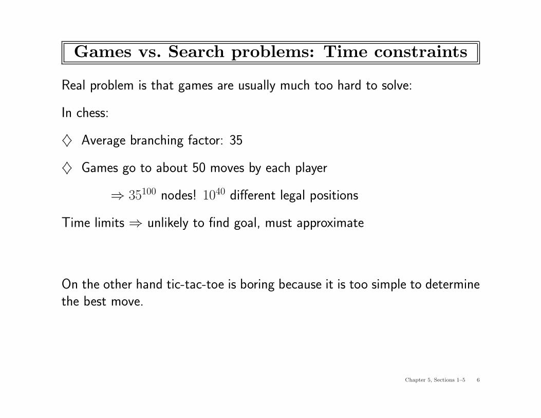
Real problem is that games are usually much too hard to solve:
In chess:
♦ Average branching factor: 35
♦ Games go to about 50 moves by each player
⇒ 35100 nodes! 1040 different legal positions
Time limits ⇒ unlikely to find goal, must approximate
On the other hand tic-tac-toe is boring because it is too simple to determinethe best move.
Chapter 5, Sections 1–5 6

Games vs. Search problems
The complexity of games introduces a new kind of uncertainty:
not due to lack of information but because one does not have time to cal-culate the exact consequences of any move.
Chapter 5, Sections 1–5 7

Types of games
deterministic chance
perfect information
imperfect information
chess, checkers,go, othello
backgammonmonopoly
bridge, poker, scrabblenuclear war
Chapter 5, Sections 1–5 8

Perfect Decisions in Two-Person Games
A game can be formally defined as a kind of search problem with:
♦ initial state (of the board and whose turn it is)
♦ set of operators (which define the legal moves)
♦ terminal test (goal test )
♦ utility function: (numeric value for the outcome of a game)
Ex. backgammon (+1, -1, +2); Chess (win, lose, draw)... which is a zero-sum game.
Chapter 5, Sections 1–5 9

Perfect Decisions in Two-Person Games
Players: MAX and MIN taking turns until game is over
Chapter 5, Sections 1–5 10

Search Tree for the Game Tic-Tac-Toe
XXXX
XX
X
XX
MAX (X)
MIN (O)
X X
O
OOX O
OO O
O OO
MAX (X)
X OX OX O XX X
XX
X X
MIN (O)
X O X X O X X O X
. . . . . . . . . . . .
. . .
. . .
. . .
TERMINALXX
−1 0 +1Utility
Chapter 5, Sections 1–5 11

Minimax
Minimax algorithm is designed to determine the optimal strategy for MAX:Perfect play for deterministic, perfect-information games
Idea: choose move to position with highest minimax value= best achievable payoff against best play
Chapter 5, Sections 1–5 12

Minimax
E.g., 2-ply game:MAX
3 12 8 642 14 5 2
MIN
3
A1
A3
A2
A13A
12A
11A
21 A23
A22
A33A
32A
31
3 2 2
Chapter 5, Sections 1–5 13

Minimax algorithm
function Minimax-Decision(game) returns an operator
for each op in Operators[game] do
Value[op]←Minimax-Value(Apply(op, game), game)
end
return the op with the highest Value[op]
function Minimax-Value(state, game) returns a utility value
if Terminal-Test[game](state) then
return Utility[game](state)
else if max is to move in state then
return the highest Minimax-Value of Successors(state)
else
return the lowest Minimax-Value of Successors(state)
Chapter 5, Sections 1–5 14
Minimax algorithm
The optimal strategy can be determined by examining the minimax value ofeach node.
Max maximizes its worst-case outcome!
Recursive search.
Chapter 5, Sections 1–5 15

Properties of minimax
Minimax: Maximizes the utility under the assumption that the opponentwill play perfectly to minimize it.
Complete??
Optimal??
Time complexity??
Space complexity??
Chapter 5, Sections 1–5 16
Properties of minimax
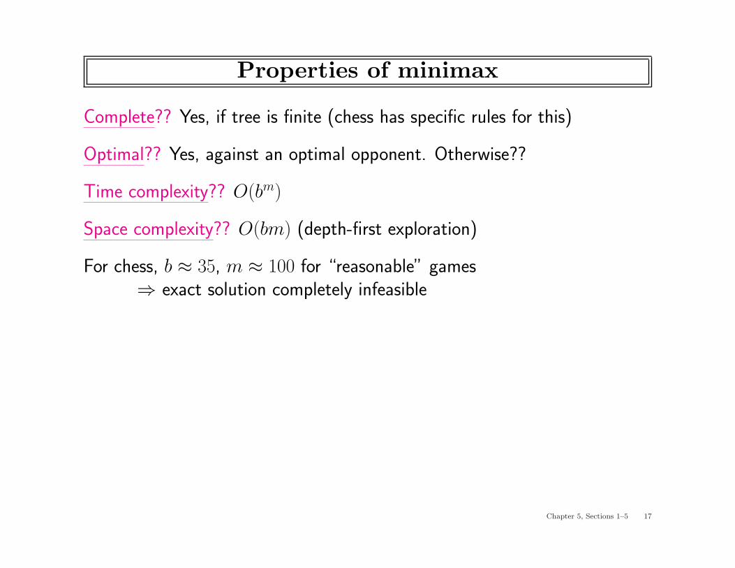
Complete?? Yes, if tree is finite (chess has specific rules for this)
Optimal?? Yes, against an optimal opponent. Otherwise??
Time complexity?? O(bm)
Space complexity?? O(bm) (depth-first exploration)
For chess, b ≈ 35, m ≈ 100 for “reasonable” games⇒ exact solution completely infeasible
Chapter 5, Sections 1–5 17

Imperfect decisions
The minimax algorithm assumes that the program has time to search all theway down to terminal states, which is usually not practical.
Shannon proposed that instead of going all the way down to terminal statesand using the utility function, the program should cut-off the search ear-lier, and apply a heuristic evaluation function to the leaves of the tree.
Chapter 5, Sections 1–5 18

Resource limits
Suppose we have 100 seconds, explore 104 nodes/second⇒ 106 nodes per move
Standard approach:
• cutoff teste.g., depth limit
• evaluation function= estimated desirability of position
Chapter 5, Sections 1–5 19

Resource limits
• cutoff teste.g., depth limitReplace terminal test by CUTOFF-TEST in MINIMAX-VALUE
• evaluation function= estimated desirability of positionReplace Utility by EVAL in MINIMAX-VALUE
Chapter 5, Sections 1–5 20

function Minimax-Decision(game) returns an operator
for each op in Operators[game] do
Value[op]←Minimax-Value(Apply(op, game), game)
end
return the op with the highest Value[op]
function Minimax-Value(state, game) returns a utility value
if Terminal-Test[game](state) then
return Utility[game](state)
else if max is to move in state then
return the highest Minimax-Value of Successors(state)
else
return the lowest Minimax-Value of Successors(state)
Chapter 5, Sections 1–5 21

Evaluation functions
Estimate of the expected utility of the game from a given position.
E.g. material value for each piece: 1 for pawn, 3 for knight or bishop,...
Performance of a game-playing program is extremely depen-dent on the quality of its evaluation function.
Chapter 5, Sections 1–5 22

Evaluation functions
Black to move
White slightly better
White to move
Black winning
For chess, typically linear weighted sum of features
Eval(s) = w1f1(s) + w2f2(s) + . . . + wnfn(s)
e.g., w1 = 9 withf1(s) = (number of white queens) – (number of black queens)
Chapter 5, Sections 1–5 23

Where do the weights come from?
Chapter 5, Sections 1–5 24

Evaluation functions
Evaluation functions:
♦ should agree with the utility function on terminal states.
♦ must not take too long to calculate!
♦ should accurately reflect the chances of winning (if we have to cut-off,we do not know what will happen in subsequent moves)
Chapter 5, Sections 1–5 25

Cutting off search
MinimaxCutoff is identical to MinimaxValue except1. Terminal? is replaced by Cutoff?2. Utility is replaced by Eval
Does it work in practice?
Chapter 5, Sections 1–5 26

Cutting off search
Suppose we have 100 seconds to decide on a move and we can explore 104
nodes/second⇒ 106 nodes per move
bm = 106, b = 35 ⇒ m = 4
4-ply lookahead is a hopeless chess player!
4-ply ≈ human novice8-ply ≈ typical PC, human master12-ply ≈ Deep Blue, Kasparov
Chapter 5, Sections 1–5 27

Exact values don’t matter
MIN
MAX
21
1
42
2
20
1
1 40020
20
Behaviour is preserved under any monotonic transformation of Eval
Only the order matters:payoff in deterministic games acts as an ordinal utility function
Chapter 5, Sections 1–5 28

Cutting off search
Should look further:
♦ in positions where favorable captures can be made (non-quiescent posi-tions)
♦ in positions where unavoidable (but beyond the horizon moves) will affectthe situation drastically
e.g. pawn turning into queen
Chapter 5, Sections 1–5 29

α–β pruning
With minimax 4-ply possible, but even average human players can makeplans 6-8 ply ahead!
How can we improve minimax search?
Chapter 5, Sections 1–5 30

α–β pruning example
MAX
3 12 8
MIN 3
3
Chapter 5, Sections 1–5 31
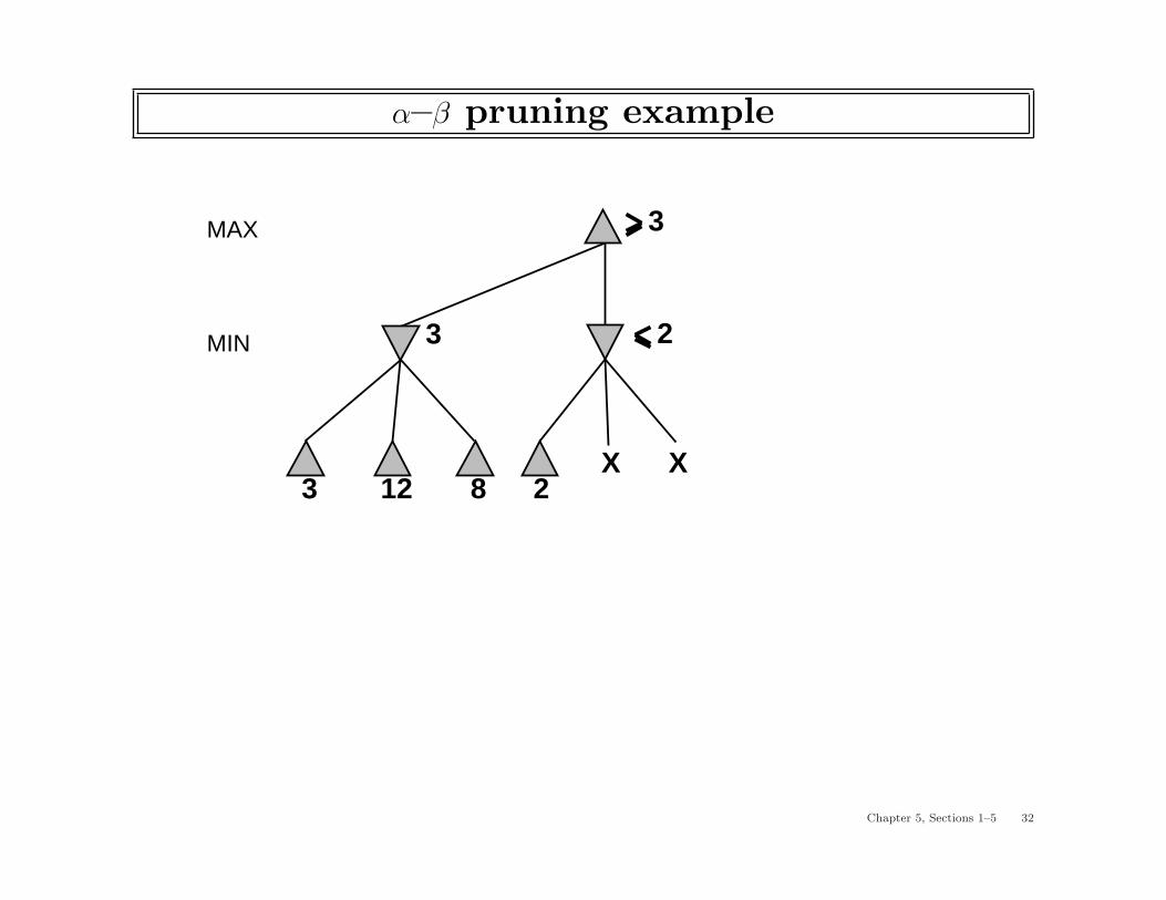
α–β pruning example
MAX
3 12 8
MIN 3
2
2
X X
3
Chapter 5, Sections 1–5 32

α–β pruning example
MAX
3 12 8
MIN 3
2
2
X X14
14
3
Chapter 5, Sections 1–5 33

α–β pruning example
MAX
3 12 8
MIN 3
2
2
X X14
14
5
5
3
Chapter 5, Sections 1–5 34

α–β pruning example
MAX
3 12 8
MIN
3
3
2
2
X X14
14
5
5
2
2
3
Chapter 5, Sections 1–5 35

Properties of α–β
Pruning does not affect final result
Good move ordering improves effectiveness of pruning (e.g. pick move withb=2 rather than b=14)
With “perfect ordering,” time complexity = O(bm/2)⇒ doubles depth of search⇒ can easily reach depth 8 and play good chess
Chapter 5, Sections 1–5 36

Why is it called α–β?
..
..
..
MAX
MIN
MAX
MIN V
α is the best value (to max) found so far off the current path
If V is worse than α, max will avoid it ⇒ prune that branch
Define β similarly for min
Chapter 5, Sections 1–5 37

The α–β algorithm
Basically Minimax + keep track of α, β + prune
Chapter 5, Sections 1–5 38

function Max-Value(state, game,α,β) returns the minimax value of state
inputs: state, current state in game
game, game description
α, the best score for max along the path to state
β, the best score for min along the path to state
if Cutoff-Test(state) then return Eval(state)
for each s in Successors(state) do
α←Max(α,Min-Value(s, game,α,β))
if α ≥ β then return β
end
return α
function Min-Value(state, game,α,β) returns the minimax value of state
if Cutoff-Test(state) then return Eval(state)
for each s in Successors(state) do
β←Min(β,Max-Value(s, game,α,β))
if β ≤ α then return α
end
return β
Chapter 5, Sections 1–5 39

Minimax algorithm
MAX
MIN
99 1000 1000 1000 100 101 102 100
10099
Minimax is an optimal method for selecting a move from a given search treeprovided that the leaf node evaluations are exactly correct.
It is quite likely that the value of the left brach is higher.
Chapter 5, Sections 1–5 40
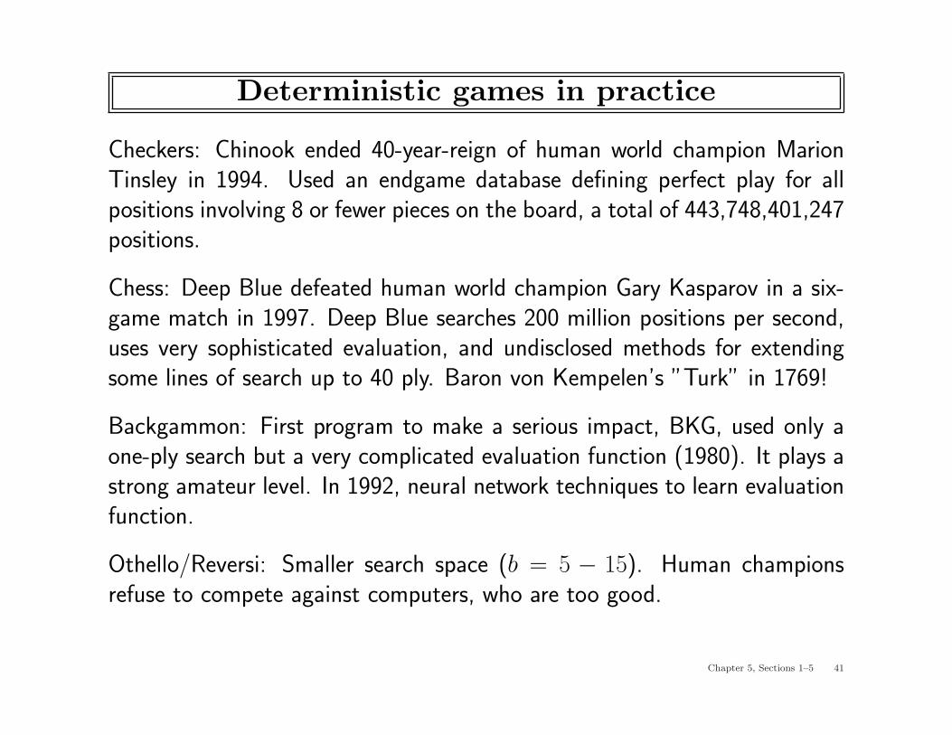
Deterministic games in practice
Checkers: Chinook ended 40-year-reign of human world champion MarionTinsley in 1994. Used an endgame database defining perfect play for allpositions involving 8 or fewer pieces on the board, a total of 443,748,401,247positions.
Chess: Deep Blue defeated human world champion Gary Kasparov in a six-game match in 1997. Deep Blue searches 200 million positions per second,uses very sophisticated evaluation, and undisclosed methods for extendingsome lines of search up to 40 ply. Baron von Kempelen’s ”Turk” in 1769!
Backgammon: First program to make a serious impact, BKG, used only aone-ply search but a very complicated evaluation function (1980). It plays astrong amateur level. In 1992, neural network techniques to learn evaluationfunction.
Othello/Reversi: Smaller search space (b = 5 − 15). Human championsrefuse to compete against computers, who are too good.
Chapter 5, Sections 1–5 41

Go: human champions refuse to compete against computers, who are toobad. In go, b > 300, so most programs use pattern knowledge bases tosuggest plausible moves.
Chapter 5, Sections 1–5 42

Nondeterministic games in practice
1000
2000
3000
0
1970 1980 1990
Mac
Hac
k (1
400)
Che
ss 3
.0 (
1500
)
Che
ss 4
.6 (
1900
)
Bel
le (
2200
)
Hite
ch (
2400
)
Dee
p T
houg
ht (
2551
)
1965 1975 1985
Fisc
her
(278
5)
Kar
pov
(270
5)
Spas
sky
(248
0)
Petr
osia
n (2
363)
Kas
paro
v (2
740)
1960
Bot
vinn
ik (
2616
)
Kor
chno
i (26
45)
Kas
paro
v (2
805)
Dee
p T
houg
ht 2
(ap
prox
. 260
0)
Extrapolate?
Chapter 5, Sections 1–5 43

Nondeterministic games
E..g, in backgammon, the dice rolls determine the legal moves
Simplified example with coin-flipping instead of dice-rolling:
MIN
MAX
2
CHANCE
4 7 4 6 0 5 −2
2 4 0 −2
0.5 0.5 0.5 0.5
3 −1
Chapter 5, Sections 1–5 44

Algorithm for nondeterministic games
Expectiminimax gives perfect play
Just like Minimax, except we must also handle chance nodes:
. . .if state is a chance node then
return average of ExpectiMinimax-Value of Successors(state)
Chapter 5, Sections 1–5 45

Nondeterministic games
DICE
MIN
MAX
DICE
MAX
. . .
. . .
. . .
B
2 1 −1 1−1
. . .6,66,51,1
1/361,21/18
TERMINAL
6,66,51,11/36
1,21/18
......
.........
.........
...... ......
...C
Rest?
Chapter 5, Sections 1–5 46

Nondeterministic games in practice
Dice rolls increase b: 21 possible rolls with 2 dice
Backgammon ≈ 20 legal moves
depth 4 = 20× (21× 20)3 ≈ 1.2× 10⁹
As depth increases, probability of reaching a given node shrinks⇒ value of lookahead is diminished
TDGammon uses depth-2 search + very good Eval≈ world-champion level
Chapter 5, Sections 1–5 47

Nondeterministic games in practice
α–β pruning is much less effective:
The advantage of α–β pruning is that it ignores future developments thatjust are not going to happen, given best play.
Thus in concentrates on likely moves.
In games with dice, there are no likely sequences of moves, because for thosmoves to take place, the dice would have to come out the right way to makethem legal.
Chapter 5, Sections 1–5 48

Digression: Exact values DO matter
DICE
MIN
MAX
2 2 3 3 1 1 4 4
2 3 1 4
.9 .1 .9 .1
2.1 1.3
20 20 30 30 1 1 400 400
20 30 1 400
.9 .1 .9 .1
21 40.9
Behaviour is preserved only by positive linear transformation of Eval
Hence Eval should be proportional to the expected payoff
Chapter 5, Sections 1–5 49

Summary
Games are fun to work on! (and dangerous)
They illustrate several important points about AI
♦ perfection is unattainable ⇒ must approximate
♦ good idea to think about what to think about
♦ uncertainty constrains the assignment of values to states
Games are to AI as grand prix racing is to automobile design
Chapter 5, Sections 1–5 50


