arX

iv:a

stro

-ph/

0501

144v

1 9

Jan

200

5Astronomy & Astrophysics manuscript no. pipeline February 2, 2008(DOI: will be inserted by hand later)

GaBoDS: The Garching-Bonn Deep Survey

IV. Methods for the Image reduction of multi-chip Cameras⋆

T. Erben1, M. Schirmer1,2, J. P. Dietrich1, O. Cordes1, L. Haberzettl1,3, M. Hetterscheidt1, H.Hildebrandt1, O. Schmithuesen1,3, P. Schneider1, P. Simon1, J. C. Cuillandre4, E. Deul5, R. N. Hook6, N.

Kaiser7, M. Radovich8, C. Benoist9, M. Nonino10, L. F. Olsen11,9, I. Prandoni12, R. Wichmann13, S.Zaggia10, D. Bomans3, R. J. Dettmar3, and J. M. Miralles14,1

1Institut fur Astrophysik und Extraterrestrische Forschung (IAEF), Universitat Bonn, Auf dem Hugel 71,D-53121 Bonn, Germany2Isaac Newton Group of Telescopes, Apartado de correos 321, 38700 Santa Cruz de La Palma, Tenerife, Spain3Astronomisches Institut der Ruhr-Universitat-Bochum, Universitatsstr. 150, D-44780 Bochum, Germany4Canada-France-Hawaii Telescope Corporation, 65-1238 Mamalahoa Highway, Kamuela, HI 967435Leiden Observatory, Postbus 9513, NL-2300 RA Leiden, The Netherlands6Space Telescope European Coordinating Facility, European Southern Observatory, Karl-Schwarzschild-Strasse2, D-85748 Garching bei Munchen, Germany7Institute for Astronomy, University of Hawaii, 2680 Woodlawn Drive, Honolulu, HI 968228INAF, Osservatorio Astronomico di Capodimonte, via Moiariello 16, 80131 Napoli, Italy9Laboratoire Cassiopee, CNRS, Observatoire de la Cote d’Azur, BP4229, 06304 Nice Cedex 4, France10INAF, Osservatorio Astronomico di Trieste, Via G. Tiepolo 11, 34131 Trieste, Italy11Copenhagen University Observatory, Copenhagen University, Juliane Maries Vej 30, 2100 Copenhagen,Denmark12Instituto di Radioastronomia, CNR, Via Gobetti 101, 40129, Bologna, Italy13Hamburger Sternwarte, University of Hamburg, Gojenbergsweg 112, 21029 Hamburg, Germany14European Southern Observatory, Karl-Schwarzschild-Strasse 2, D-85748 Garching bei Munchen, Germany

Received June 15, 2004; accepted June 16, 2004

Abstract. We present our image processing system for the reduction of optical imaging data from multi-chipcameras. In the framework of the Garching Bonn Deep Survey (GaBoDS; Schirmer et al. 2003) consisting ofabout 20 square degrees of high-quality data from WFI@MPG/ESO 2.2m, our group developed an imagingpipeline for the homogeneous and efficient processing of this large data set. Having weak gravitational lensing asthe main science driver, our algorithms are optimised to produce deep co-added mosaics from individual exposuresobtained from empty field observations. However, the modular design of our pipeline allows an easy adaption todifferent scientific applications. Our system has already been ported to a large variety of optical instruments andits products have been used in various scientific contexts. In this paper we give a thorough description of thealgorithms used and a careful evaluation of the accuracies reached. This concerns the removal of the instrumentalsignature, the astrometric alignment, photometric calibration and the characterisation of final co-added mosaics.In addition we give a more general overview on the image reduction process and comment on observing strategieswhere they have significant influence on the data quality.

Key words. Methods: data analysis – Techniques: image processing

1. Introduction

During the last decades, optical Wide-Field Imaging hasbecome one of the most important tools in observational

Send offprint requests to: T. Erben: terben@astro.uni-bonn.de⋆ Based on observations made with ESO Telescopes at the

La Silla Observatory

astronomy. The advances in this field are closely linkedto the development of highly sensitive detectors basedon charge coupled devices (CCDs). These detectors havegrown in size from a few hundred pixels on a side to thecurrently largest arrays of about 4000 × 4000 pixels. Theneed for ever larger fields-of-view and deeper images, andthe technical constraints in the manufacturing processes

2 T. Erben et al.: Methods for WFI data reduction

2046 pix

E

4098

pix

1 2 3 4

8 7 6 5

N

23"

1 pix = 0.238"

Gui

ding

CC

D

7"

127 mm = 34’

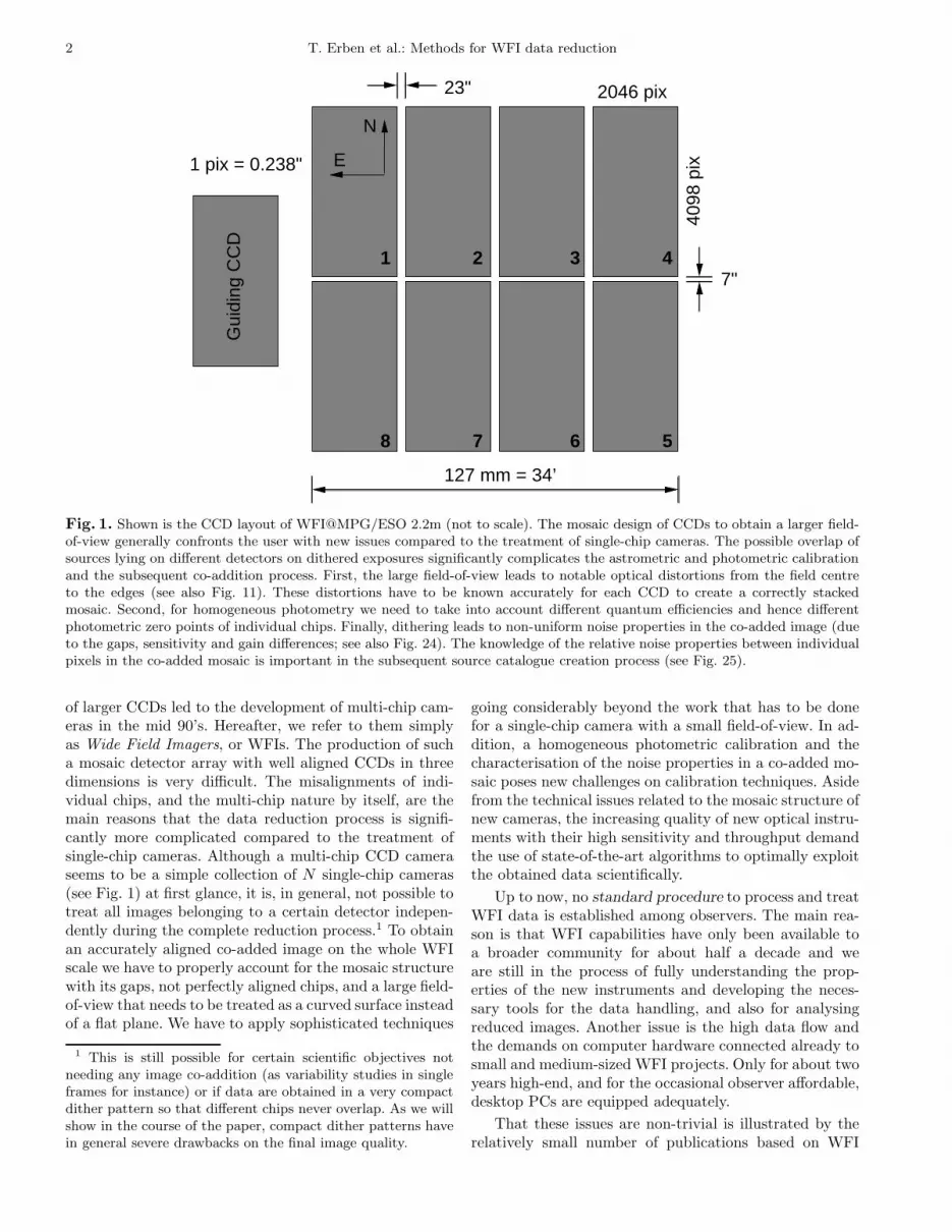
Fig. 1. Shown is the CCD layout of WFI@MPG/ESO 2.2m (not to scale). The mosaic design of CCDs to obtain a larger field-of-view generally confronts the user with new issues compared to the treatment of single-chip cameras. The possible overlap ofsources lying on different detectors on dithered exposures significantly complicates the astrometric and photometric calibrationand the subsequent co-addition process. First, the large field-of-view leads to notable optical distortions from the field centreto the edges (see also Fig. 11). These distortions have to be known accurately for each CCD to create a correctly stackedmosaic. Second, for homogeneous photometry we need to take into account different quantum efficiencies and hence differentphotometric zero points of individual chips. Finally, dithering leads to non-uniform noise properties in the co-added image (dueto the gaps, sensitivity and gain differences; see also Fig. 24). The knowledge of the relative noise properties between individualpixels in the co-added mosaic is important in the subsequent source catalogue creation process (see Fig. 25).

of larger CCDs led to the development of multi-chip cam-eras in the mid 90’s. Hereafter, we refer to them simplyas Wide Field Imagers, or WFIs. The production of sucha mosaic detector array with well aligned CCDs in threedimensions is very difficult. The misalignments of indi-vidual chips, and the multi-chip nature by itself, are themain reasons that the data reduction process is signifi-cantly more complicated compared to the treatment ofsingle-chip cameras. Although a multi-chip CCD cameraseems to be a simple collection of N single-chip cameras(see Fig. 1) at first glance, it is, in general, not possible totreat all images belonging to a certain detector indepen-dently during the complete reduction process.1 To obtainan accurately aligned co-added image on the whole WFIscale we have to properly account for the mosaic structurewith its gaps, not perfectly aligned chips, and a large field-of-view that needs to be treated as a curved surface insteadof a flat plane. We have to apply sophisticated techniques

1 This is still possible for certain scientific objectives notneeding any image co-addition (as variability studies in singleframes for instance) or if data are obtained in a very compactdither pattern so that different chips never overlap. As we willshow in the course of the paper, compact dither patterns havein general severe drawbacks on the final image quality.

going considerably beyond the work that has to be donefor a single-chip camera with a small field-of-view. In ad-dition, a homogeneous photometric calibration and thecharacterisation of the noise properties in a co-added mo-saic poses new challenges on calibration techniques. Asidefrom the technical issues related to the mosaic structure ofnew cameras, the increasing quality of new optical instru-ments with their high sensitivity and throughput demandthe use of state-of-the-art algorithms to optimally exploitthe obtained data scientifically.

Up to now, no standard procedure to process and treatWFI data is established among observers. The main rea-son is that WFI capabilities have only been available toa broader community for about half a decade and weare still in the process of fully understanding the prop-erties of the new instruments and developing the neces-sary tools for the data handling, and also for analysingreduced images. Another issue is the high data flow andthe demands on computer hardware connected already tosmall and medium-sized WFI projects. Only for about twoyears high-end, and for the occasional observer affordable,desktop PCs are equipped adequately.

That these issues are non-trivial is illustrated by therelatively small number of publications based on WFI

T. Erben et al.: Methods for WFI data reduction 3

projects compared to the amount of data acquired. Forexample, after the WFI at the 2.2m MPG/ESO telescope(hereafter WFI@2.2m) became operational in January1999, only 35 refereed papers based on its data appeareduntil the end of 2002. Meanwhile, the rate has risen2,but is still significantly behind those of other ESO instru-ments which are under similar pressure by proposers asWFI@2.2m.

In this paper we present the methods and algorithmswe use to process WFI data. The presentation is organisedas follows: In Sect. 2 we introduce the basic concepts of theGaBoDS pipeline and the philosophy behind the choiceswe made. We discuss the advantages and the disadvan-tages that arise thereof. The pre-reduction process (i.e.the removal of the instrumental signature from the data),which is in principle identical for single- and multi-chipcameras, is described in Sect. 3. Details of the astrometricand photometric calibration of the data are presented inSect. 4. An explanation of our adopted scheme to deal withthe inhomogeneous noise properties in co-added mosaicdata is given in Sect. 5, followed by the image co-additionmethods in Sect. 6. We perform quality control checks onco-added data in Sect. 7 and draw our conclusions in Sect.8.

No astronomical pipeline will produce the best possi-ble result with data obtained in arbitrary conditions andstrategies. Hence, besides a pure description of algorithms,our presentation also contains guidelines how WFI datashould be obtained to achieve good results.

We assume familiarity with data processing of opti-cal imaging data. In this publication we focus on describ-ing the algorithms used for all necessary processing steps.Where the reduction differs significantly from well estab-lished algorithms for single-chip cameras (this mostly con-cerns the astrometric alignment and the photometric cal-ibration) we give a scientific evaluation and a thoroughestimation of the accuracies reached.

We note that we mainly work on data from WFI@2.2mand most of the examples and figures in this paper referto data from this instrument. The reader has to be awarethat the quoted results, the accuracies and the overall us-ability of our algorithms can vary significantly when beingapplied to data sets from other cameras. At critical pointswe come back to this issue in the text.

2. Pipeline characteristics

2.1. Scientific motivation

While all optical data need the same treatment to removethe instrumental signature (bias correction, flat-fielding,fringe correction etc; see Sect. 3), the subsequent treat-ment of the images strongly depends on the scientific ob-jectives and on the kind of data at hand. Our primaryscientific interests are weak gravitational lensing studies(see e.g. Bartelmann & Schneider 2001 for an extended

2 The ESO Telescope Bibliography turns up a total of 107refereed papers until December 2004.

review) in deep blank-field surveys. These studies mainlydepend on shape measurements of faint galaxies. To en-sure that the light distribution is deformed as little aspossible by the Earth’s atmosphere and the optics of thetelescope, weak lensing data are typically obtained undersuperb seeing conditions at telescopes with state-of-the-art optical equipment. For a proper treatment of thosedata, the main requirements on a data processing pipelineare the following:

– We need to align very accurately galaxy images ofsubsequent exposures that are finally stacked. This in-volves an accurate mapping of possible distortions (seeFig. 11).

– We need the highest possible resolution, and hence aco-addition on a sub-pixel basis (see Sect. 6). Togetherwith the previous step, this is crucial for an accuratemeasurement of object shapes in the subsequent lens-ing analysis.

– We need to accurately map the noise properties in ourfinally co-added images (see Fig. 25). This knowledgeenables us to use as many faint galaxies as possible andto push the object detection limit. This also requiresthat the sky-background in the co-added image is asflat as possible.

The algorithms we use are chosen to go from raw im-ages to a final co-added mosaic with the objectives de-scribed above. The responsibility of the pipeline ends withthe co-addition step. We are fully aware that the cho-sen procedures and algorithms may not be optimal forprojects having different scientific objectives such as ac-curate photometry, the investigation of crowded fields orthe study of large scale, low surface brightness objectsfor instance. However, the modular design of our pipeline(see below) allows an easy exchange of algorithms or theintegration of new methods necessary for different appli-cations. The main characteristics of our current pipelineare summarised in the following:

– Ability to process exposures from a multi-chip camerawith N CCDs. To date we have successfully pro-cessed data from: WFI@2.2m, CFH12K@CFHT,FORS1/2@VLT, WFI@AAO, MOSAIC-I/II@CTIO/KPNO, SUPRIMECAM@Subaru,WFC@INT, WFC@WHT, and several single-chipcameras (e.g. BUSCA@2.2m Calar Alto).

– Ability to handle mosaic data taken with arbitrarydither patterns.

– Precise image alignments without prior knowledgeabout distortions. The astrometric calibration is per-formed with the data itself.

– Absolute astrometric calibration of the final images tosky coordinates.

– An appropriate co-addition of data obtained under dif-ferent photometric conditions.

– Image defects on all exposures are identified andmarked before the co-addition process.

4 T. Erben et al.: Methods for WFI data reduction

– Creation of weight maps taking into account differ-ent noise/gain properties and image defects for the co-addition.

– Accurate co-addition on sub-pixel level/ability torescale data to an “arbitrary” scale (ability to easilycombine data from different cameras/telescopes).

We are currently extending our algorithms to near-IRcameras which will be described in a forthcoming pub-lication (Schirmer et al. in prep.).

2.2. Implementation details

As mentioned above, many tools for WFI data process-ing are currently under active development and differentgroups have already released excellent software packagesfor specific tasks. Hence, we built our own efforts on al-ready publicly available software modules wherever possi-ble. Many of the algorithms used are very similar to thosedeveloped for the EIS (ESO Imaging Survey) Wide surveyin 1997-1999 (see Nonino et al. 1999). The main pillars ofour pipeline are the following software modules:

– The LDAC software3: The LDAC (Leiden DataAnalysis Centre) software was the backbone of the firstEIS pipeline. It provides a binary catalogue format (inthe form of system-independent binary FITS tables)including a large amount of tools for their handling.Moreover, this module contains software for the astro-metric and photometric calibration of mosaic data.

– The EIS Drizzle4: A specific version of the IRAFpackage drizzle (Fruchter & Hook 2002) was devel-oped for EIS. It directly uses the astrometric calibra-tion provided by the LDAC astrom part and performsa weighted linear co-addition of the imaging data.

– TERAPIX software5: (Bertin et al. 2002)SExtractor is used to obtain object cataloguesfor the astrometric calibration. Moreover it producesa cosmic ray mask in connection with EYE6 in additionto smoothed and sky-subtracted images at differentparts of the pipeline. SWarp, the TERAPIX softwaremodule for resampling and co-adding FITS images, isused alternatively to EIS Drizzle for the final imageco-addition.

– FLIPS7: (Magnier & Cuillandre 2004) FLIPS is one ofthe modules for data pre-reduction. It is optimised toperform operations on large format CCDs with min-imal memory requirements at the cost of I/O perfor-mance.

3 available at ftp://ftp.strw.leidenuniv.nl/pub/ldac/software/4 available via ESO’s SCISOFT CD (see

http://www.eso.org/scisoft/)5 available at http://terapix.iap.fr/soft/6EYE (Enhance Your Extraction) allows the user to generate

image filters for the detection of small-scale features in astro-nomical images by machine learning (neural networks). Thesefilters are loaded into SExtractor that performs the actual de-tection. We use such filters to detect cosmic rays in our images.

7 see http://www.cfht.hawaii.edu/∼jcc/Flips/flips.html

– Eclipse and qfits tools8: (Devillard 2001) Weuse several stand-alone FITS header tools from theEclipse package to update/query our image header.Moreover, tools based on the qfits library offer analternative to FLIPS for image pre-reduction.

– Astrometrix9: Astrometrix (developed atTERAPIX) is another module for obtaining as-trometric calibration.

– IMCAT utilities10: From the IMCAT tools we exten-sively use the image calculator ic.

These tools have been adapted for our purposes if neces-sary and wrapped by UNIX/bash shell scripts to formour pipeline. Our main effort is to provide the neces-sary interfaces for the communication between the indi-vidual modules and to add instrument and science spe-cific modules for our purposes (as a thorough quantifica-tion of PSF properties for instance). With our implemen-tation approach we can make use of already well-testedand maintained software packages. The description abovealso shows that we can easily exchange modules as soonas new algorithms or better implementations for a cer-tain task become available. To further enhance the mod-ularity of the pipeline, we split up the whole reductionprocess into small tasks (a complete reduction process forWFI@2.2m data typically involves the call to 20-30 dif-ferent scripts but superscripts collecting several tasks caneasily be written). This ensures a very high flexibility ofthe system and that potential users can easily adapt it totheir needs or to specific instruments.

Nearly the whole system is implemented in ANSI Cand UNIX bash shell scripts (EIS Drizzle is written inFORTRAN77 and embedded into IRAF, Astrometrix isdeveloped under Perl+PDL and parts of our photomet-ric calibration module are implemented in Python). Thuswe have full control over the source codes and can portthe pipeline to different UNIX flavours. Table 1 lists thesystems on which we successfully used it so far.

The main disadvantage of building up a pipeline frommany different software modules instead of developinga homogeneous system from scratch is that it becomesvery difficult to automatically control the data flow orto construct a sophisticated error handling and data in-tegrity checking system. Furthermore, our pipeline so faroffers only very limited possibilities to store the historyof the reduction process or to administrate raw and pro-cessed image products. Also, formal speed estimates forthe throughput of our processing system are low comparedto homogeneous systems (see Table 2). Thus, the usabil-ity for large, long-term projects of the system is limitedat this stage.

With the compactness, the flexibility and the usabil-ity of our system for the occasional user11 we regard

8 available at http://www.eso.org/projects/aot/eclipse/9 available at http://www.na.astro.it/∼radovich/wifix.htm

10 available at http://www.ifa.hawaii.edu/∼kaiser/imcat/11 The usage of our pipeline can easily be learned within afew days by users having good experience in the reduction of

T. Erben et al.: Methods for WFI data reduction 5

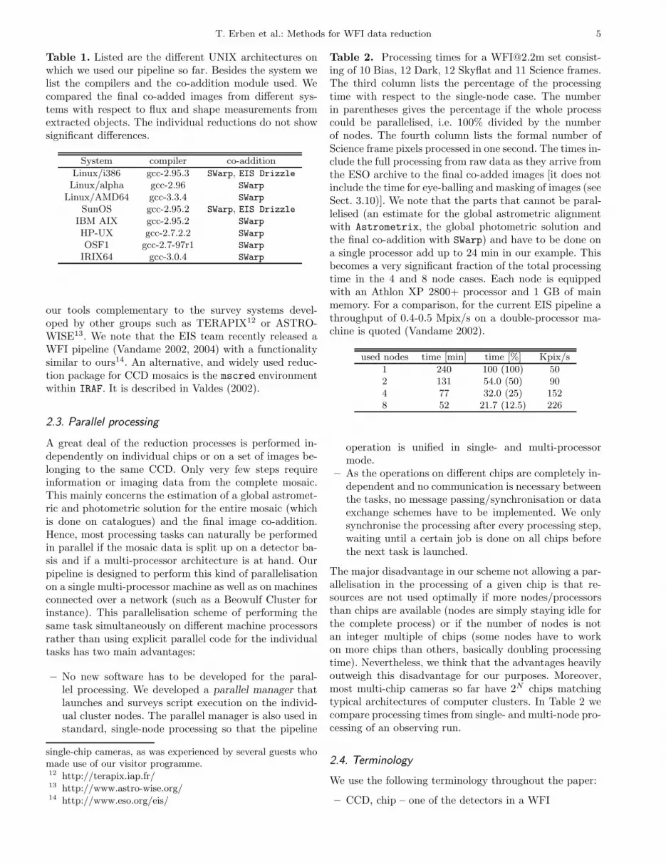
Table 1. Listed are the different UNIX architectures onwhich we used our pipeline so far. Besides the system welist the compilers and the co-addition module used. Wecompared the final co-added images from different sys-tems with respect to flux and shape measurements fromextracted objects. The individual reductions do not showsignificant differences.

System compiler co-addition

Linux/i386 gcc-2.95.3 SWarp, EIS Drizzle

Linux/alpha gcc-2.96 SWarp

Linux/AMD64 gcc-3.3.4 SWarp

SunOS gcc-2.95.2 SWarp, EIS Drizzle

IBM AIX gcc-2.95.2 SWarp

HP-UX gcc-2.7.2.2 SWarp

OSF1 gcc-2.7-97r1 SWarp

IRIX64 gcc-3.0.4 SWarp

our tools complementary to the survey systems devel-oped by other groups such as TERAPIX12 or ASTRO-WISE13. We note that the EIS team recently released aWFI pipeline (Vandame 2002, 2004) with a functionalitysimilar to ours14. An alternative, and widely used reduc-tion package for CCD mosaics is the mscred environmentwithin IRAF. It is described in Valdes (2002).

2.3. Parallel processing

A great deal of the reduction processes is performed in-dependently on individual chips or on a set of images be-longing to the same CCD. Only very few steps requireinformation or imaging data from the complete mosaic.This mainly concerns the estimation of a global astromet-ric and photometric solution for the entire mosaic (whichis done on catalogues) and the final image co-addition.Hence, most processing tasks can naturally be performedin parallel if the mosaic data is split up on a detector ba-sis and if a multi-processor architecture is at hand. Ourpipeline is designed to perform this kind of parallelisationon a single multi-processor machine as well as on machinesconnected over a network (such as a Beowulf Cluster forinstance). This parallelisation scheme of performing thesame task simultaneously on different machine processorsrather than using explicit parallel code for the individualtasks has two main advantages:

– No new software has to be developed for the paral-lel processing. We developed a parallel manager thatlaunches and surveys script execution on the individ-ual cluster nodes. The parallel manager is also used instandard, single-node processing so that the pipeline

single-chip cameras, as was experienced by several guests whomade use of our visitor programme.12 http://terapix.iap.fr/13 http://www.astro-wise.org/14 http://www.eso.org/eis/

Table 2. Processing times for a WFI@2.2m set consist-ing of 10 Bias, 12 Dark, 12 Skyflat and 11 Science frames.The third column lists the percentage of the processingtime with respect to the single-node case. The numberin parentheses gives the percentage if the whole processcould be parallelised, i.e. 100% divided by the numberof nodes. The fourth column lists the formal number ofScience frame pixels processed in one second. The times in-clude the full processing from raw data as they arrive fromthe ESO archive to the final co-added images [it does notinclude the time for eye-balling and masking of images (seeSect. 3.10)]. We note that the parts that cannot be paral-lelised (an estimate for the global astrometric alignmentwith Astrometrix, the global photometric solution andthe final co-addition with SWarp) and have to be done ona single processor add up to 24 min in our example. Thisbecomes a very significant fraction of the total processingtime in the 4 and 8 node cases. Each node is equippedwith an Athlon XP 2800+ processor and 1 GB of mainmemory. For a comparison, for the current EIS pipeline athroughput of 0.4-0.5 Mpix/s on a double-processor ma-chine is quoted (Vandame 2002).

used nodes time [min] time [%] Kpix/s

1 240 100 (100) 502 131 54.0 (50) 904 77 32.0 (25) 1528 52 21.7 (12.5) 226

operation is unified in single- and multi-processormode.

– As the operations on different chips are completely in-dependent and no communication is necessary betweenthe tasks, no message passing/synchronisation or dataexchange schemes have to be implemented. We onlysynchronise the processing after every processing step,waiting until a certain job is done on all chips beforethe next task is launched.

The major disadvantage in our scheme not allowing a par-allelisation in the processing of a given chip is that re-sources are not used optimally if more nodes/processorsthan chips are available (nodes are simply staying idle forthe complete process) or if the number of nodes is notan integer multiple of chips (some nodes have to workon more chips than others, basically doubling processingtime). Nevertheless, we think that the advantages heavilyoutweigh this disadvantage for our purposes. Moreover,most multi-chip cameras so far have 2N chips matchingtypical architectures of computer clusters. In Table 2 wecompare processing times from single- and multi-node pro-cessing of an observing run.

2.4. Terminology

We use the following terminology throughout the paper:

– CCD, chip – one of the detectors in a WFI

6 T. Erben et al.: Methods for WFI data reduction

– exposure – a single WFI shot through the telescope– image – the part of the exposure that belongs to a

particular CCD– frame – this term is used as a synonym for an image.– BIAS – an exposure/image with zero seconds exposure

time– DARK – an exposure/image with non-zero exposure

time, keeping the shutter closed– FLAT – an exposure/image of a uniformly illumi-

nated area; this can be the telescope dome giv-ing DOMEFLATs or sky observations during eveningand/or morning twilight providing SKYFLATs

– SCIENCE – an exposure/image of the actual target,not a calibration image

– SUPERFLAT – properly stacked SCIENCE data toextract large scale illuminations or fringe patterns.

– STANDARD – an exposure/image of photometricstandard stars

– other terms written in CAPITAL letters denote addi-tional images or calibration frames. Their meaning willbe clear within the context.

– mosaic – this term is used as a synonym for exposureor for the final co-added image.

– dithering – offsetting the telescope between the expo-sures

– overlap – images from different CCDs and exposuresoverlap if the dithering between the exposures waslarge enough

– stack – a set of n images belonging to the same chipthat have been combined pixel by pixel.

– Names of software packages are written in theTypeWriter font.

3. Pre-reduction (Run processing)

In the following we describe our algorithms for the pre-reduction of optical data, i.e. the removal of the instru-mental signature. The first issue is the compilation of datafor this step. For most of the effects to be corrected for(instrument bias, bad CCD pixels, flat-field properties)we can safely assume stability of the instrument and theCCD characteristics over several days or even a few weeks.Hence, in many cases we can collect data from a completeobserving run and benefit from having many images forthe necessary corrections from which most are of statisti-cal nature. As described below, the matter can becomemore complex when dealing with strong fringes in redpassbands. Here, the time scales from which SCIENCEdata can safely be combined in the process is much shorter,sometimes only a couple of hours. The issue is further dis-cussed in Sect. 3.9. In any case we say that we performthe pre-reduction process on a Run basis regardless of howlong this period actually is. The pre-reduction is done in-dependently on each CCD of a mosaic camera. Only in onestep, the sky-background equalisation (see Sect. 3.6), theaction to be performed on a CCD depends on propertiesfrom the rest of the mosaic. Hence, unless stated other-wise, each step described below has to be performed on a

detector basis. For this part of the pipeline we can use twodifferent software packages, one based on FLIPS, the otheron Eclipse. FLIPS is very I/O intensive but has very lowmemory requirements, while Eclipse reduces the neces-sary I/O to a minimum and operates very efficiently onimaging data by keeping it in virtual memory. Dependingon the size of the data set and the computer equipment athand, one or the other is preferable. In the following wefocus on the description of the Eclipse package and wemention FLIPS where its functionality differs significantlyfrom Eclipse.

3.1. Handling the data and the FITS headers

The variety of ways in which header information and rawdata from WFIs are stored in FITS files are as large as thenumber of instruments, i.e. so far there is no establishedstandard on the FITS format of CCD mosaics. In order tocope with the different formats and to unify the treatment,we perform the following tasks on raw data:

1. If the data are stored in Multiple Extension Fits(MEF) files, we extract all the images from them. Allsubsequent pipeline processing is done on individualimages and also our pipeline parallelisation is basedon the simultaneous execution of the same task on dif-ferent images.

2. We substitute the original image headers from thechips by a new one containing only a minimum set ofkeywords necessary for a successful pipeline processing(see App. A). Especially the astrometric calibrationdepends on correct header entries.

3. If necessary we flip and/or rotate individual CCDs tobring all images of the mosaic to the same orientationwith respect to the sky. Only rotations by 90 degrees,that do not require pixel resampling, are performed.

All these tasks are performed by a qfits-based utility.

3.2. Modes, medians, and the stacking of images

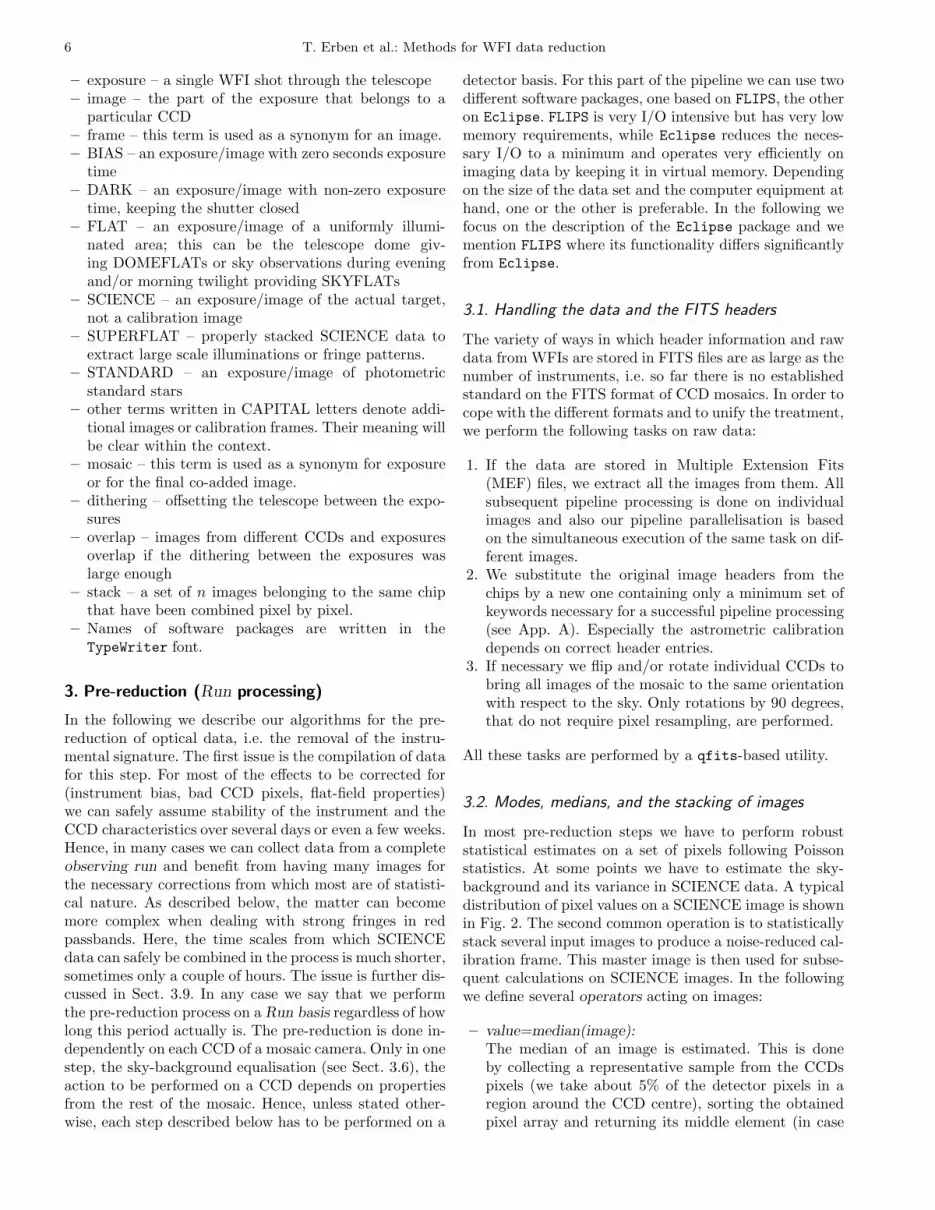
In most pre-reduction steps we have to perform robuststatistical estimates on a set of pixels following Poissonstatistics. At some points we have to estimate the sky-background and its variance in SCIENCE data. A typicaldistribution of pixel values on a SCIENCE image is shownin Fig. 2. The second common operation is to statisticallystack several input images to produce a noise-reduced cal-ibration frame. This master image is then used for subse-quent calculations on SCIENCE images. In the followingwe define several operators acting on images:

– value=median(image):The median of an image is estimated. This is doneby collecting a representative sample from the CCDspixels (we take about 5% of the detector pixels in aregion around the CCD centre), sorting the obtainedpixel array and returning its middle element (in case

T. Erben et al.: Methods for WFI data reduction 7

Fig. 2. Shown is a typical pixel value distribution in an astro-nomical image. The clear peak denotes the brightness of thenight sky. Due to the presence of objects the distribution isstrongly skewed towards high values. The most accurate es-timate for the sky comes from analysing the histogram anddetermining the peak (the mode of the distribution) directly.The median (for a set of N points the median element is de-fined so that there are as many greater as smaller values thanthe median in the set) also gives a very robust (and for ourpurposes sufficient though biased) estimate for it. Due to thelong tail of the distribution, a straight mean is completely use-less as an estimate for the sky value. As the values to the leftof the mode form half of a Gaussian distribution, an estimatefor the sky variance can be obtained from that part.

the array has an even number of elements we returnthe mean of the two middle elements).

– value=mode(image):The mode of an image is estimated. We consider thesame representative pixel sub-sample as for the medianestimation, build a smoothed histogram and return thepeak value.

– image=rescale(images):This operator rescales a set of images so that they havethe same median after the process. The resulting me-dian is chosen to be the mean of the medians (we writemeanmed for it) from the input images. Hence on eachinput image we perform the operation image → image* meanmed / median(image). The operator is usuallyapplied to a set of images before they are stacked (asSKYFLATs or SCIENCE images). The median of thestacked image is then by construction equal to mean-med.

– image=stack(images):A set of input images is stacked to produce a noise-reduced master image. The following procedure is per-formed independently on each pixel position. We col-

lect all pixel values from the input images into an array,sort it and reject several low and high values (typicallywe reject the three lowest and three highest values ifwe have 15 input images or more). From the rest weestimate the median that goes into the master image.Here FLIPS uses a more sophisticated algorithm. Onthe remaining array it first performs an iterative sigmaclipping. It estimates mean and sigma, rejects low andhigh values (typically pixels lying more than 3.5 sigmabelow and above the mean) and repeats the procedureuntil no more pixels are rejected. From the rest it re-turns the median for the master image.

We will use additional pseudo operators in the followingwhose meaning and behaviour will be clear within the con-text. All calculations with these operators are written inslanted notation.

3.3. A first quality check, Overscan correction, masterBIASes and DARKs

Before any exposure enters the reduction process, we es-timate its mode. If this estimate lies outside predefinedboundaries, the exposure will not be processed. This re-jects most of the completely faulty images (such as satu-rated SKYFLATs) at the very beginning. After this ini-tial quality check, the first step in the reduction processof each image is the correction of an overall estimate forthe BIAS value by considering pixels in not illuminatedparts of each CCD (the overscan region). This first-orderBIAS correction is done by collecting for each line all pix-els in the overscan region, rejecting the lowest and high-est values (usually the overscan regions contains about 40columns and we reject the 5 lowest and 5 highest values)and estimating a straight mean from the rest. This mean issubtracted from the corresponding line. After this correc-tion, the overscan regions are trimmed off the images. Forcorrecting spatially varying BIAS patterns in the FLATor SCIENCE images, a master BIAS is created for eachCCD from several individual BIAS exposures:

1. Each BIAS exposure is overscan corrected andtrimmed.

2. The master BIAS is formed by masBIAS=stack(BIASframes)

In the same way, a master DARK (masDARK) frameis created. So far, we do not correct FLAT or SCIENCEframes for a possible dark current but we use the mas-DARK for the identification of bad pixels, rows andcolumns (see Sect. 5).

3.4. Methods for flat-fielding

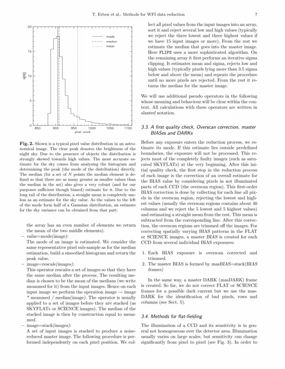
The illumination of a CCD and its sensitivity is in gen-eral not homogeneous over the detector area. Illuminationusually varies on large scales, but sensitivity can changesignificantly from pixel to pixel (see Fig. 3). In order to

8 T. Erben et al.: Methods for WFI data reduction

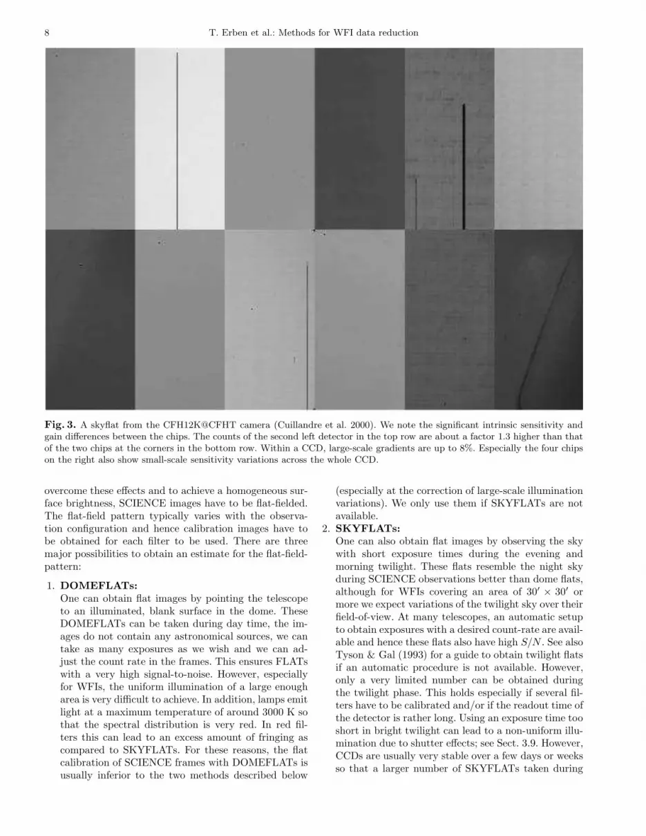
Fig. 3. A skyflat from the CFH12K@CFHT camera (Cuillandre et al. 2000). We note the significant intrinsic sensitivity andgain differences between the chips. The counts of the second left detector in the top row are about a factor 1.3 higher than thatof the two chips at the corners in the bottom row. Within a CCD, large-scale gradients are up to 8%. Especially the four chipson the right also show small-scale sensitivity variations across the whole CCD.

overcome these effects and to achieve a homogeneous sur-face brightness, SCIENCE images have to be flat-fielded.The flat-field pattern typically varies with the observa-tion configuration and hence calibration images have tobe obtained for each filter to be used. There are threemajor possibilities to obtain an estimate for the flat-field-pattern:

1. DOMEFLATs:

One can obtain flat images by pointing the telescopeto an illuminated, blank surface in the dome. TheseDOMEFLATs can be taken during day time, the im-ages do not contain any astronomical sources, we cantake as many exposures as we wish and we can ad-just the count rate in the frames. This ensures FLATswith a very high signal-to-noise. However, especiallyfor WFIs, the uniform illumination of a large enougharea is very difficult to achieve. In addition, lamps emitlight at a maximum temperature of around 3000 K sothat the spectral distribution is very red. In red fil-ters this can lead to an excess amount of fringing ascompared to SKYFLATs. For these reasons, the flatcalibration of SCIENCE frames with DOMEFLATs isusually inferior to the two methods described below

(especially at the correction of large-scale illuminationvariations). We only use them if SKYFLATs are notavailable.

2. SKYFLATs:

One can also obtain flat images by observing the skywith short exposure times during the evening andmorning twilight. These flats resemble the night skyduring SCIENCE observations better than dome flats,although for WFIs covering an area of 30′ × 30′ ormore we expect variations of the twilight sky over theirfield-of-view. At many telescopes, an automatic setupto obtain exposures with a desired count-rate are avail-able and hence these flats also have high S/N . See alsoTyson & Gal (1993) for a guide to obtain twilight flatsif an automatic procedure is not available. However,only a very limited number can be obtained duringthe twilight phase. This holds especially if several fil-ters have to be calibrated and/or if the readout time ofthe detector is rather long. Using an exposure time tooshort in bright twilight can lead to a non-uniform illu-mination due to shutter effects; see Sect. 3.9. However,CCDs are usually very stable over a few days or weeksso that a larger number of SKYFLATs taken during

T. Erben et al.: Methods for WFI data reduction 9

several nights can be combined into good master flatimages.

3. SUPERFLATs:

In addition, one can try to extract the flat-field pat-tern from the SCIENCE observations itself. If a suffi-cient number of SCIENCE exposures is at hand (usu-ally more than a dozen), and if the dither pattern wassignificantly larger than the largest object in the field,each pixel of the camera will see the sky-backgroundseveral times. Hence, a proper combination of these ex-posures yields a master FLAT that closely representsthe night sky during observations. We refer to such aFLAT as a SUPERFLAT. A straightforward applica-tion of this method is often hampered by several fac-tors: During phases of grey and bright time, the nightsky shows large gradients and variable reflections in thedome and telescope can occur. Thus, a careful selec-tion of images that go into the SUPERFLAT has to bedone. In medium/narrow band filters and in the ultraviolet, the counts and hence the S/N of SUPERFLATsin these bands are typically low. Furthermore, the tech-nique is very difficult to apply in programmes wherethe imaged target has a size comparable to the field-of-view. In this case also large dither patterns cannotassure sufficient sky coverage on the complete mosaic.

As the superflat technique cannot be applied in generalwe use the following two-stage flat-fielding process:

1. In a first step, the SCIENCE observations are flat-fielded with SKYFLATs (if those are not at hand weuse DOMEFLATs instead). This typically corrects thesmall-scale sensitivity variations and leaves large-scalegradients around the 3% level on the scale of a chip(see Fig. 5).

2. If the data permit it, a SUPERFLAT is created out ofthe flat-fielded SCIENCE observations, smoothed witha large kernel to extract remaining large-scale varia-tions and is applied to the individual images. For ourempty field observations at the WFI@2.2m this leavestypical large-scale variations around the 1% level inU, B, V, R broad band observations (in I the presenceof strong fringing often leads to significantly higherresiduals).

This two-stage flat-fielding process is very similar to themethod adopted by Alcala et al. (2002).

3.5. The creation of master DOME-/SKYFLATs

The master FLAT (SKYFLAT or DOMEFLAT) for eachCCD is created as follows:

1. All individual FLAT exposures are overscan-correctedand trimmed.

2. The masBIAS is subtracted from all images.3. The FLATs are rescaled to a common median:

rescFLAT=rescale(FLAT).4. We form the master FLAT by mas-

FLAT=stack(rescFLAT frames)

3.6. Sky-background equalisation

Within a mosaic, CCDs have different quantum efficien-cies, varying intrinsic gains and hence different photomet-ric zero points (see Fig. 3). For the later photometric cal-ibration it is desirable to equalise the photometric zeropoints in all detectors, which is achieved by scaling allCCDs to the same sky-background.We rescale all chips tothe median of the CCD with the highest count-rate dur-ing flat-fielding. If possible we perform this step withinthe SUPERFLAT correction as its median estimation ismore robust than with the SKYFLATs. This is becauseSKYFLATs show larger variations in brightness than theSUPERFLATs which are calculated from already flat-fielded data. We estimate that photometric zero pointsof the mosaic agree with an rms scatter of about 0.01-0.03mag after sky-background equalisation (see Sect. 4.6).

3.7. SCIENCE image processing, the creation andapplication of the SUPERFLAT

The individual steps in the SCIENCE frame processingare:

1. The images are overscan-corrected and trimmed.Afterwards the masBIAS is subtracted and theframes are divided by masFLAT. We writeflatSCIENCE=(SCIENCE−masBIAS)/masFLAT.In the case where no SUPERFLAT correction isapplied to the data, masFLAT is rescaled at this stepto equalise the sky-background between individualdetectors (see Sect. 3.6).

2. For the creation of the SUPERFLAT we first removeastronomical sources from the flatSCIENCE images.To this end we run SExtractor (Bertin & Arnouts1996) on them and create a new set of im-ages where pixels belonging to objects (i.e.above certain detection thresholds) are flagged(objSCIENCE=flatSCIENCE−OBJECTS). See alsoFig. 4. The flagged pixels are not taken into accountin the subsequent processing.

3. The objSCIENCE images are rescaled to a commonmedian rescobjSCIENCE=rescale(objSCIENCE).

4. We calculate the SUPERFLAT[SUPERFLAT=stack(rescobjSCIENCE frames)].If all input pixels of a given position are flagged (i.e.all the images had an object at that position) weassign the meanmed value from the objSCIENCEframes to the SUPERFLAT.

5. The SUPERFLAT is heavily smoothed by creatinga SExtractor BACKGROUND check-image with abackground mesh of 512 pixels (see Bertin 2003 onthe SExtractor sky-background estimation). This im-age, the illumination correction image, forms thebasis for removing large-scale flat-field variations(ILLUMINATION=smooth(SUPERFLAT)).

6. The flatSCIENCE images are divided by theILLUMINATION image which has been rescaledto equalise the sky-background of the differ-

10 T. Erben et al.: Methods for WFI data reduction

ent detectors (see Sect. 3.6). We write illum-SCIENCE=flatSCIENCE/rescaled(ILLUMINATION).

For blue passbands not showing any fringing, the pre-reduction ends here and the illumSCIENCE images areused in the subsequent processing. See Fig. 5 for an ex-ample of a pre-reduced V -band exposure.

3.8. Fringing correction in red passbands

Fringing is observed as an additional, additive instrumen-tal signature in red passbands. It is most prominent oncameras that use thinned CCDs and hence are optimisedfor observations in blue passbands. Fringes show up as spa-tially quickly varying, wave-like structures on the CCDs(see Fig. 6). The geometry of these patterns usually doesnot change with time since this interference effect is cre-ated in the substrate of the CCD itself. WFI@2.2m showsfringes with an amplitude of about 1% as compared tothe sky-background in broad-band R. In the I- and Z-bands, fringing becomes much stronger and reaches up toabout 10% of the night sky. Unfortunately, contrary tothe geometry of the fringing, its amplitude is not stablein consecutive SCIENCE exposures since it strongly de-pends on the night sky conditions (as brightness, cloudcoverage), the position on the sky and the airmass. If areasonably good SUPERFLAT can be constructed froma sufficient number of SCIENCE frames obtained understable sky conditions, a possible way to correct for fringesis the following:

1. Besides the large-scale sky variations not corrected forby SKYFLATs, the SUPERFLAT contains the fringepattern as an additive component. Hence, the fringepattern can be isolated from the SUPERFLAT byFRINGE=SUPERFLAT−ILLUMINATION.

2. Individual SCIENCE frames are corrected forfringing by fringeSCIENCE=illumSCIENCE−f ×FRINGE. We assume that the fringe amplitude di-rectly scales with sky brightness and f is calculated byf=median(illumSCIENCE)/median(ILLUMINATION).

In the case of WFI@2.2m, this method removes very ef-ficiently the low-level fringes in the R-band. Fringing isusually no longer visible and we estimate possible residu-als well below 0.1%. In the case of I- and Z-bands, fringescan be suppressed to a level of about 0.1% of the sky am-plitude if a very good SUPERFLAT can be constructed(see Fig. 6). If this is not the case, our approach may per-form very poorly in reducing the fringe amplitude and wecannot propose a pipeline solution to the problem at thisstage.

3.9. Guidelines for constructing calibration images

The success of the image pre-reduction heavily dependson the quality of calibration data at hand. In the creationof flatSCIENCE, we propagate the noise in masBIAS andmasFLAT to our SCIENCE frames. As the noise in these

calibration frames is of statistical nature we can dimin-ish it by using as many images in the stacking process aspossible. For the successful creation of a SUPERFLAT,and hence for the later quality of large-scale illuminationand fringing correction, not only the number of images isimportant but it is essential that each pixel in the mosaicsees blank sky several times during SCIENCE observa-tions. This suggests that the best observing strategy toachieve this goal is a large dither pattern between con-secutive exposures (ideally it should be wider than thelargest object in the field). In the case that the targetoccupies a significant fraction of the mosaic (as big galax-ies or globular clusters for instance) the best strategy isto observe a neighbouring blank field for a short while ifa SUPERFLAT and/or fringe correction is important. Inthe following we give some additional guidelines leadingto good results in most of our own reductions:

– For the stacking process for masBIAS (masDARK) andmasFLAT, about 15-20 individual images of each typeshould be acquired. As the noise in the final images isinversely proportional to the square root of the numberof input images this is a good compromise betweenthe number of exposures that can be taken during atypical observing run (in the case of SKYFLATs) andthe noise reduction.

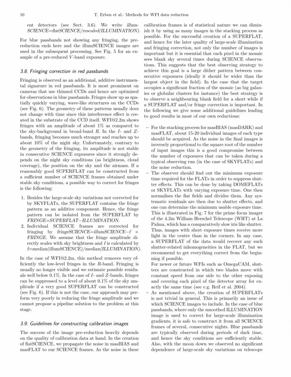
– The observer should find out the minimum exposuretime required for the FLATs in order to suppress shut-ter effects. This can be done by taking DOMEFLATsor SKYFLATs with varying exposure time. One thennormalises the flat fields and divides them. Any sys-tematic residuals are then due to shutter effects, andone can determine the minimum usable exposure time.This is illustrated in Fig. 7 for the prime focus imagerof the 4.2m William Herschel Telescope (WHT) at LaPalma, which has a comparatively slow iris like shutter.Thus, images with short exposure times receive morelight in the centre than in the corners. In any case,a SUPERFLAT of the data would recover any suchshutter-related inhomogeneities in the FLAT, but werecommend to get everything correct from the begin-ning if possible.For newer or future WFIs such as OmegaCAM, shut-ters are constructed in which two blades move withconstant speed from one side to the other exposingand covering each pixel of the detector array for ex-actly the same time (see e.g. Reif et al. 2004).

– As mentioned above, the creation of SUPERFLATsis not trivial in general. This is primarily an issue ofwhich SCIENCE images to include. In the case of bluepassbands, where only the smoothed ILLUMINATIONimage is used to correct for large-scale illuminationgradients, it is safe to construct it from all SCIENCEframes of several, consecutive nights. Blue passbandsare typically observed during periods of dark time,and hence the sky conditions are sufficiently stable.Also, with the moon down we observed no significantdependence of large-scale sky variations on telescope

T. Erben et al.: Methods for WFI data reduction 11

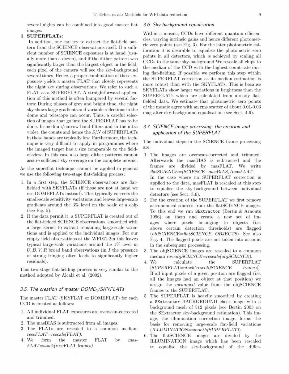
Fig. 4. For the creation of SUPERFLATs we mask pixels belonging to astronomical sources in the SCIENCE frames. The leftpanel shows a SCIENCE image before and the right panel after objects have been detected by SExtractor and flagged. Wemask all structures having 50 contiguous pixels with 1.0 sigma above the sky-background. This helps to pick up also pixels ofextended halos around bright stars. For images containing strong fringing we change the parameters to 7 pixels above 5 sigmaas otherwise fringes would be detected and masked.

Fig. 7. Ratio of two normalised sky flats taken with theprime focus imager of the WHT (2 CCDs). The imageswere exposed for 0.3 and 1.0 seconds, respectively. Onecan see the way the iris shutter exposed and covered thedetector again. The illumination difference between thebrightest and faintest part in this representation is 20%.For the WHT prime focus imager it is recommended toexpose for at least 2.0 seconds.

pointing. Hence, a robust SUPERFLAT can be ob-tained with a sufficient number of images during anobserving run. This is no longer the case if we needto correct for strong fringing. We observe that our as-

sumption of a sole dependence of the fringe amplitudeon sky brightness typically fails when constructing theSUPERFLAT from SCIENCE frames of different skypositions. As the appearance of the overall pattern isvery stable, this means either that the fringe ampli-tude is no longer a linear function of sky brightness orthat the sky-background varies on scales significantlysmaller than a CCD so that the scaling factor becomesdependent on CCD position. In addition, a similar be-haviour is observed as a function of time, dependingon the excitation of the OH− night-sky emission lines.For our blank-field observations we obtain good resultsin the fringing correction if we observe the same targetbetween 10 and 15 times with a large dither patternwithin an hour (at WFI@2.2m with an overhead ofabout 2 minutes per image this can be achieved with300 s exposures).

– If a very good SUPERFLAT could be constructed, flat-fielding results from our proposed method and from apure SUPERFLAT application (i. e. using flat-fieldingmethod 3 in Sect. 3.4) should be compared if flatness inSCIENCE images is crucial. Especially if only a smallnumber of individual frames went into the constructionof masFLAT, the direct SUPERFLAT approach oftengives better results.

– Offsetting the telescope between the exposures is fun-damental for high-quality, high-S/N mosaics. Thedither box, i.e. the box that encloses all dither off-sets, should be clearly larger than the gaps betweenthe CCDs and the objects in the field. This has sev-eral advantages as compared to the staring mode (nooffsets at all) or to the application of only small offsets.First, the CCDs in a multi-chip camera are fully in-dependent from each other. They see the sky through

12 T. Erben et al.: Methods for WFI data reduction

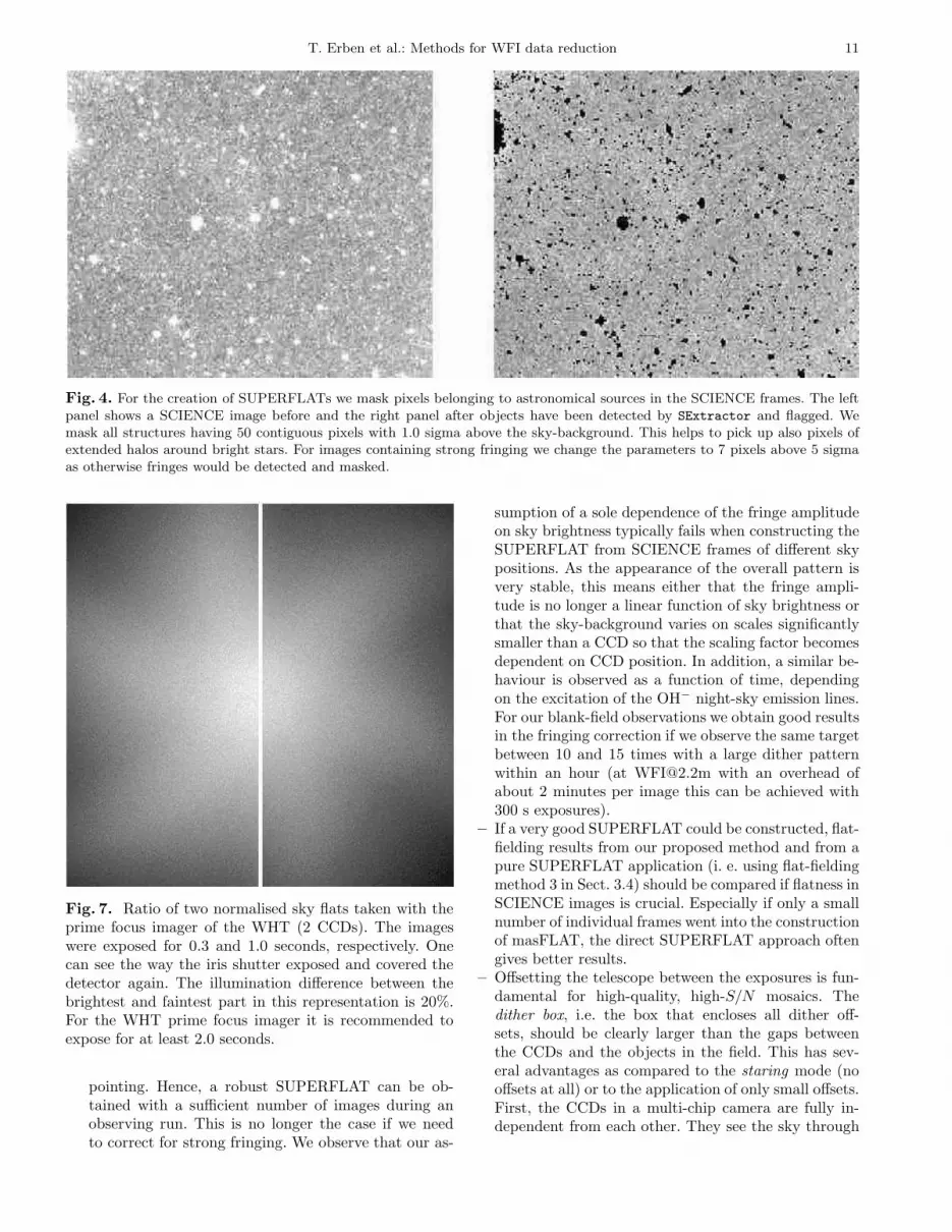
Fig. 5. The pre-reduction steps on a V -band exposure from WFI@2.2m: Panel (A) shows the raw image, panel (B) the resultfrom applying masBIAS, trimming the CCDs and flat-fielding with the masFLAT. The high S/N masFLAT takes out small-scalevariations but leaves large-scale residuals of up to 3% on the scale of the CCD [panel (D)]. These and the differences in the skycount-rate are removed after the application of ILLUMINATION giving a flatness of 1% over the entire mosaic in most of thecases as seen in panels (C) and (E).

different sections of the filter, and they have their in-dividual flat-fields, gains and read-out noise. Choosinga wide dither pattern is the easiest way to establish anaccurate global photometric and astrometric solutionfor the entire mosaic, based on enough overlap objects.Second, the wide dither pattern allows for a signif-icantly better superflattening of the data, since theobjects do not fall on top of themselves in the stacks

and thus for every pixel a good estimate of the back-ground can be obtained. Besides, remaining very low-amplitude patterns in the sky background caused byimproper flat-fields etc. do not add in the mosaic, butare averaged out. Thus, a wide dither pattern will leadto an improved sky background from which the S/Nwill benefit; see also Fig. 8.

T. Erben et al.: Methods for WFI data reduction 13

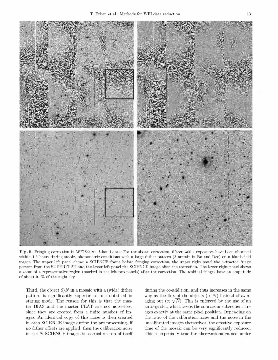
Fig. 6. Fringing correction in WFI@2.2m I-band data: For the shown correction, fifteen 300 s exposures have been obtainedwithin 1.5 hours during stable, photometric conditions with a large dither pattern (3 arcmin in Ra and Dec) on a blank-fieldtarget. The upper left panel shows a SCIENCE frame before fringing correction, the upper right panel the extracted fringepattern from the SUPERFLAT and the lower left panel the SCIENCE image after the correction. The lower right panel showsa zoom of a representative region (marked in the left two panels) after the correction. The residual fringes have an amplitudeof about 0.1% of the night sky.

Third, the object S/N in a mosaic with a (wide) ditherpattern is significantly superior to one obtained instaring mode. The reason for this is that the mas-ter BIAS and the master FLAT are not noise-free,since they are created from a finite number of im-ages. An identical copy of this noise is then createdin each SCIENCE image during the pre-processing. Ifno dither offsets are applied, then the calibration noisein the N SCIENCE images is stacked on top of itself

during the co-addition, and thus increases in the sameway as the flux of the objects (∝ N) instead of aver-aging out (∝

√N). This is enforced by the use of an

auto-guider, which keeps the sources in subsequent im-ages exactly at the same pixel position. Depending onthe ratio of the calibration noise and the noise in theuncalibrated images themselves, the effective exposuretime of the mosaic can be very significantly reduced.This is especially true for observations gained under

14 T. Erben et al.: Methods for WFI data reduction

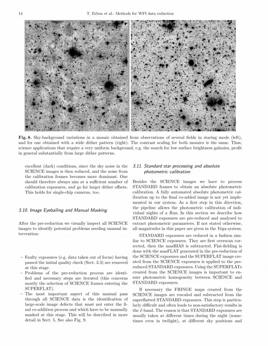
Fig. 8. Sky-background variations in a mosaic obtained from observations of several fields in staring mode (left),and for one obtained with a wide dither pattern (right). The contrast scaling for both mosaics is the same. Thus,science applications that require a very uniform background, e.g. the search for low surface brightness galaxies, profitin general substantially from large dither patterns.

excellent (dark) conditions, since the sky noise in theSCIENCE images is then reduced, and the noise fromthe calibration frames becomes more dominant. Oneshould therefore always aim at a sufficient number ofcalibration exposures, and go for larger dither offsets.This holds for single-chip cameras, too.

3.10. Image Eyeballing and Manual Masking

After the pre-reduction we visually inspect all SCIENCEimages to identify potential problems needing manual in-tervention:

– Faulty exposures (e.g. data taken out of focus) havingpassed the initial quality check (Sect. 3.3) are removedat this stage.

– Problems of the pre-reduction process are identi-fied and necessary steps are iterated (this concernsmostly the selection of SCIENCE frames entering theSUPERFLAT).

– The most important aspect of this manual passthrough all SCIENCE data is the identification oflarge-scale image defects that must not enter the fi-nal co-addition process and which have to be manuallymasked at this stage. This will be described in moredetail in Sect. 5. See also Fig. 9.

3.11. Standard star processing and absolutephotometric calibration

Besides the SCIENCE images we have to processSTANDARD frames to obtain an absolute photometriccalibration. A fully automated absolute photometric cal-ibration up to the final co-added image is not yet imple-mented in our system. As a first step in this direction,the pipeline allows the photometric calibration of indi-vidual nights of a Run. In this section we describe howSTANDARD exposures are pre-reduced and analysed toextract photometric parameters. If not stated otherwise,all magnitudes in this paper are given in the Vega system.

STANDARD exposures are reduced in a fashion sim-ilar to SCIENCE exposures. They are first overscan cor-rected, then the masBIAS is subtracted. Flat-fielding isdone with the masFLAT generated in the pre-reduction ofthe SCIENCE exposures and the SUPERFLAT image cre-ated from the SCIENCE exposures is applied to the pre-reduced STANDARD exposures. Using the SUPERFLATscreated from the SCIENCE images is important to en-sure photometric homogeneity between SCIENCE andSTANDARD exposures.

If necessary the FRINGE maps created from theSCIENCE images are rescaled and subtracted from thesuperflatted STANDARD exposures. This step is particu-larly difficult and often leads to non-satisfactory results inthe I-band. The reason is that STANDARD exposures areusually taken at different times during the night (some-times even in twilight), at different sky positions and

T. Erben et al.: Methods for WFI data reduction 15

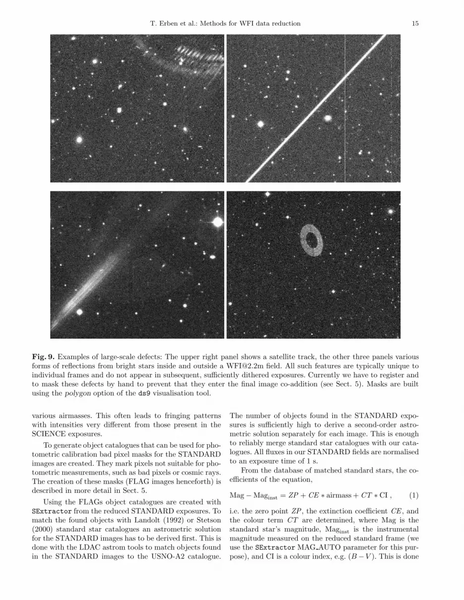
Fig. 9. Examples of large-scale defects: The upper right panel shows a satellite track, the other three panels variousforms of reflections from bright stars inside and outside a WFI@2.2m field. All such features are typically unique toindividual frames and do not appear in subsequent, sufficiently dithered exposures. Currently we have to register andto mask these defects by hand to prevent that they enter the final image co-addition (see Sect. 5). Masks are builtusing the polygon option of the ds9 visualisation tool.

various airmasses. This often leads to fringing patternswith intensities very different from those present in theSCIENCE exposures.

To generate object catalogues that can be used for pho-tometric calibration bad pixel masks for the STANDARDimages are created. They mark pixels not suitable for pho-tometric measurements, such as bad pixels or cosmic rays.The creation of these masks (FLAG images henceforth) isdescribed in more detail in Sect. 5.

Using the FLAGs object catalogues are created withSExtractor from the reduced STANDARD exposures. Tomatch the found objects with Landolt (1992) or Stetson(2000) standard star catalogues an astrometric solutionfor the STANDARD images has to be derived first. This isdone with the LDAC astrom tools to match objects foundin the STANDARD images to the USNO-A2 catalogue.

The number of objects found in the STANDARD expo-sures is sufficiently high to derive a second-order astro-metric solution separately for each image. This is enoughto reliably merge standard star catalogues with our cata-logues. All fluxes in our STANDARD fields are normalisedto an exposure time of 1 s.

From the database of matched standard stars, the co-efficients of the equation,

Mag − Maginst = ZP + CE ∗ airmass + CT ∗ CI , (1)

i.e. the zero point ZP , the extinction coefficient CE , andthe colour term CT are determined, where Mag is thestandard star’s magnitude, Maginst is the instrumentalmagnitude measured on the reduced standard frame (weuse the SExtractor MAG AUTO parameter for this pur-pose), and CI is a colour index, e.g. (B −V ). This is done

16 T. Erben et al.: Methods for WFI data reduction

using a non-linear least-squares Marquardt-Levenberg al-gorithm with an iterative 3σ rejection, which allows re-jected points to be used again if they are compatible withlater solutions. As this algorithm is not guaranteed to con-verge, the iteration is aborted as soon as one of the fol-lowing three criteria is true:

1. The iteration converged and no new points are re-jected.

2. The maximum number of iterations (set to 20) isreached.

3. More than a fixed percentage (set to 50%) of all pointsare rejected.

In a first step all three coefficients are fit simultaneously.However, in order to reliably estimate the extinction co-efficient standard star observations must be spread overa range of airmasses. This is sometimes neglected by ob-servers. To find an acceptable photometric solution in thiscase, the user can supply a default value for the extinctioncoefficient. The fit is then repeated with the extinction co-efficient fixed at the user supplied value and the zero pointand colour term as free parameters.

Although wide-field observations of Landolt/Stetsonfields typically cover a wide range of stellar colours, theuser can also supply a default value for the colour term.This is then used for a 1-parameter fit in which the zeropoint is the only free parameter.

In an interactive step the user can then choose betweenthe 1-, 2-, and 3-parameter solution, or reject the night asnon-photometric. The FITS headers of the frames belong-ing to the same night are then updated with the selectedzero point and extinction coefficient or left at the defaultvalue −1.0, indicating that no photometric calibration forthat frame is available.

We note that we perform the fit simultaneously forall mosaic chips. As discussed in Sect. 4.6 zero pointsof individual chips agree within 0.01-0.03 mag after sky-background equalisation. We do not take into accountpossible colour term variations between individual imagesthat are expected due to slightly different CCD transmis-sion curves. Notable differences can occur in the U and Zfilters that are cut off by the CCD transmission.

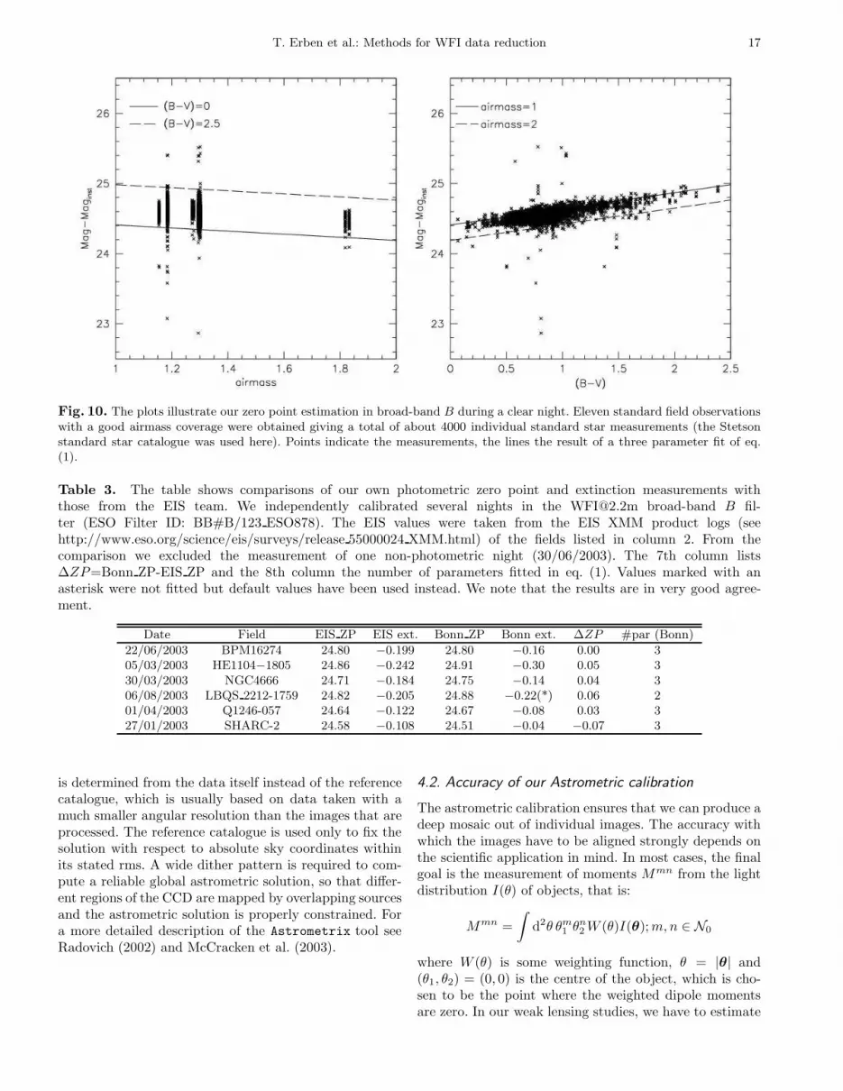
Fig. 10 illustrates our photometric calibration which isimplemented in Python. We compared our own zero pointand extinction measurements for several nights with thoserecently obtained by the EIS team. Table 3 shows that themeasurements are in very good agreement.

3.12. Runs and Sets

As discussed in the beginning of Sect. 3 the pre-reductionis done on a Run basis usually containing observationsfrom different patches of the sky. Before proceeding weneed to split up the SCIENCE exposures of a Run into theSets that have to be co-added later. By Set we mean theseries of all exposures of the same target in a particularfilter. This means that all the following reduction stepsup to the final co-addition have to be done on each Set

independently. We note that a Set can have been observedin multiple Runs so that all Runs containing images of acertain Set have to be processed at this stage.

4. Astrometric and photometric Set calibration

4.1. Astrometry

After the pre-processing, a global astrometric solution anda global relative photometric solution is calculated for allSCIENCE images. This is where the reduction of WFIdata becomes much more complicated than the one forsingle-chip cameras.

In a first step, high S/N objects in each image are de-tected by SExtractor, and a catalogue of non-saturatedstars is generated. Typically, we use all objects hav-ing at least 5 contiguous pixels with 5σ above the sky-background in the following analysis (these numbers mayvary according to filter and exposure time; in the U -bandfor instance, we need to lower these thresholds in order tohave enough sources to compare with a standard star cat-alogue). This usually gives us between 3 and 6 objects persquare arcmin in high-galactic latitude empty field obser-vations. Based on a comparison with the USNO-A2 (seeMonet et al. 1998) astrometric reference catalogue (or anyother reference catalogue), a zero-order, single shift astro-metric solution is calculated for each image. For a single-chip camera with a small field-of-view such an approach isoften sufficient, but it no longer holds for multi-chip cam-eras with their large field-of-view. In this case, the CCDscan be rotated with respect to each other, tilted againstthe focal plane, and in general cover areas at a distancefrom the optical axis where field distortions become large.Fig. 11 shows the difference between a zero order (sin-gle shift with respect to a reference catalogue) and a fullastrometric second-order astrometric solution per image.From this figure it is obvious that the simple shift-and-addapproach will not work for the entire mosaic. The issue isfurther complicated by the gaps between the CCDs andlarge dither patterns that are used to cover them. Thus,images with very different distortions overlap. In addition,due to the large field-of-view, one must take into accountthat the spherically curved sky is mapped into the flattangential detector plane.

In the second step, Mario Radovich’s Astrometrix15

package is used to determine third-order polynomials forthe astrometric solution of each image. This corrects forthe aforementioned effects, and thus allows for the propermosaicing in the later co-addition process. For this pur-pose all high S/N objects (stars and galaxies) detected inthe first step are matched, including those from the over-lap regions. The latter ones are most important in estab-lishing a global astrometric (and photometric) solution,since the accuracy of available reference catalogues suchas the USNO-A2 with an rms of about 0.′′3 is insufficientfor sub-pixel registration. Thus the astrometric solution

15 http://www.na.astro.it/∼radovich/WIFIX/astrom.ps

T. Erben et al.: Methods for WFI data reduction 17

Fig. 10. The plots illustrate our zero point estimation in broad-band B during a clear night. Eleven standard field observationswith a good airmass coverage were obtained giving a total of about 4000 individual standard star measurements (the Stetsonstandard star catalogue was used here). Points indicate the measurements, the lines the result of a three parameter fit of eq.(1).

Table 3. The table shows comparisons of our own photometric zero point and extinction measurements withthose from the EIS team. We independently calibrated several nights in the WFI@2.2m broad-band B fil-ter (ESO Filter ID: BB#B/123 ESO878). The EIS values were taken from the EIS XMM product logs (seehttp://www.eso.org/science/eis/surveys/release 55000024 XMM.html) of the fields listed in column 2. From thecomparison we excluded the measurement of one non-photometric night (30/06/2003). The 7th column lists∆ZP=Bonn ZP-EIS ZP and the 8th column the number of parameters fitted in eq. (1). Values marked with anasterisk were not fitted but default values have been used instead. We note that the results are in very good agree-ment.

Date Field EIS ZP EIS ext. Bonn ZP Bonn ext. ∆ZP #par (Bonn)

22/06/2003 BPM16274 24.80 −0.199 24.80 −0.16 0.00 305/03/2003 HE1104−1805 24.86 −0.242 24.91 −0.30 0.05 330/03/2003 NGC4666 24.71 −0.184 24.75 −0.14 0.04 306/08/2003 LBQS 2212-1759 24.82 −0.205 24.88 −0.22(*) 0.06 201/04/2003 Q1246-057 24.64 −0.122 24.67 −0.08 0.03 327/01/2003 SHARC-2 24.58 −0.108 24.51 −0.04 −0.07 3

is determined from the data itself instead of the referencecatalogue, which is usually based on data taken with amuch smaller angular resolution than the images that areprocessed. The reference catalogue is used only to fix thesolution with respect to absolute sky coordinates withinits stated rms. A wide dither pattern is required to com-pute a reliable global astrometric solution, so that differ-ent regions of the CCD are mapped by overlapping sourcesand the astrometric solution is properly constrained. Fora more detailed description of the Astrometrix tool seeRadovich (2002) and McCracken et al. (2003).

4.2. Accuracy of our Astrometric calibration

The astrometric calibration ensures that we can produce adeep mosaic out of individual images. The accuracy withwhich the images have to be aligned strongly depends onthe scientific application in mind. In most cases, the finalgoal is the measurement of moments Mmn from the lightdistribution I(θ) of objects, that is:

Mmn =

∫

d2θ θm1 θn

2 W (θ)I(θ); m, n ∈ N0

where W (θ) is some weighting function, θ = |θ| and(θ1, θ2) = (0, 0) is the centre of the object, which is cho-sen to be the point where the weighted dipole momentsare zero. In our weak lensing studies, we have to estimate

18 T. Erben et al.: Methods for WFI data reduction

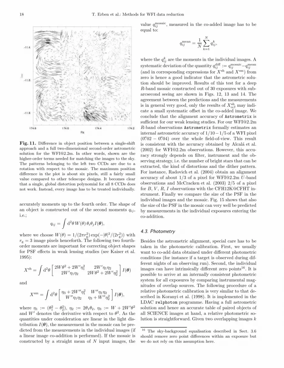
Fig. 11. Difference in object position between a single-shiftapproach and a full two-dimensional second-order astrometricsolution for the WFI@2.2m. In other words, shown are thehigher-order terms needed for matching the images to the sky.The patterns belonging to the left two CCDs are due to arotation with respect to the mosaic. The maximum positiondifference in the plot is about six pixels, still a fairly smallvalue compared to other telescope designs. It becomes clearthat a single, global distortion polynomial for all 8 CCDs doesnot work. Instead, every image has to be treated individually.

accurately moments up to the fourth order. The shape ofan object is constructed out of the second moments qij ,i.e.;

qij =

∫

d2θ W (θ) θiθjI(θ),

where we choose W (θ) = 1/(2πr2g) exp(−|θ|2/(2r2

g)) withrg = 3 image pixels henceforth. The following two fourth-order moments are important for correcting object shapesfor PSF effects in weak lensing studies (see Kaiser et al.1995):

Xsh =

∫

d2θ

[

2Wθ2 + 2W ′η21 2W ′η1η2

2W ′η1η2 2Wθ2 + 2W ′η22

]

I(θ)

and

Xsm =

∫

d2θ

[

η3 + 2W ′′η21 W ′′η1η2

W ′′η1η2 η3 + W ′′η22

]

I(θ),

where η1 := (θ21 − θ2

2), η2 := 2θ1θ2, η3 := W + 2W ′θ2

and W ′ denotes the derivative with respect to θ2. As thequantities under consideration are linear in the light dis-tribution I(θ), the measurement in the mosaic can be pre-dicted from the measurements in the individual images (ifa linear image co-addition is performed). If the mosaic isconstructed by a straight mean of N input images, the

value qmosaicij , measured in the co-added image has to be

equal to:

qmeanij =

1

N

N∑

k=1

qkij ,

where the qkij are the moments in the individual images. A

systematic deviation of the quantity qdiffij := qmosaic

ij −qmeanij

(and in corresponding expressions for Xsh and Xsm) fromzero is hence a good indicator that the astrometric solu-tion should be improved. Results of this test for a deepR-band mosaic constructed out of 30 exposures with sub-arcsecond seeing are shown in Figs. 12, 13 and 14. Theagreement between the predictions and the measurementsis in general very good, only the results of Xsh

αβ may indi-cate a small systematic offset in the co-added image. Weconclude that the alignment accuracy of Astrometrix issufficient for our weak lensing studies. For our WFI@2.2mR-band observations Astrometrix formally estimates aninternal astrometric accuracy of 1/10−1/5 of a WFI pixel(0.′′02 − 0.′′04) over the whole field-of-view. This resultis consistent with the accuracy obtained by Alcala et al.(2002) for WFI@2.2m observations. However, this accu-racy strongly depends on filter, instrument and the ob-serving strategy, i.e. the number of bright stars that can beextracted, the kind of distortions and the dither pattern.For instance, Radovich et al. (2004) obtain an alignmentaccuracy of about 1/3 of a pixel for WFI@2.2m U -bandobservations and McCracken et al. (2003) 2/5 of a pixelfor B, V , R, I observations with the CFH12K@CFHT in-strument. Finally we compare the size of the PSF in theindividual images and the mosaic. Fig. 15 shows that alsothe size of the PSF in the mosaic can very well be predictedby measurements in the individual exposures entering theco-addition.

4.3. Photometry

Besides the astrometric alignment, special care has to betaken in the photometric calibration. First, we usuallywant to co-add data obtained under different photometricconditions (for instance if a target is observed during dif-ferent nights of an observing run). Second, the individualimages can have intrinsically different zero points16. It ispossible to arrive at an internally consistent photometricsystem for all exposures by comparing instrumental mag-nitudes of overlap sources. The following procedure of arelative photometric calibration is very similar to that de-scribed in Koranyi et al. (1998). It is implemented in theLDAC relphotom programme. Having a full astrometricsolution and hence an accurate table of paired objects ofall SCIENCE images at hand, a relative photometric so-lution is straightforward. Given two overlapping images k

16 The sky-background equalisation described in Sect. 3.6should remove zero point differences within an exposure butwe do not rely on this assumption here.

T. Erben et al.: Methods for WFI data reduction 19

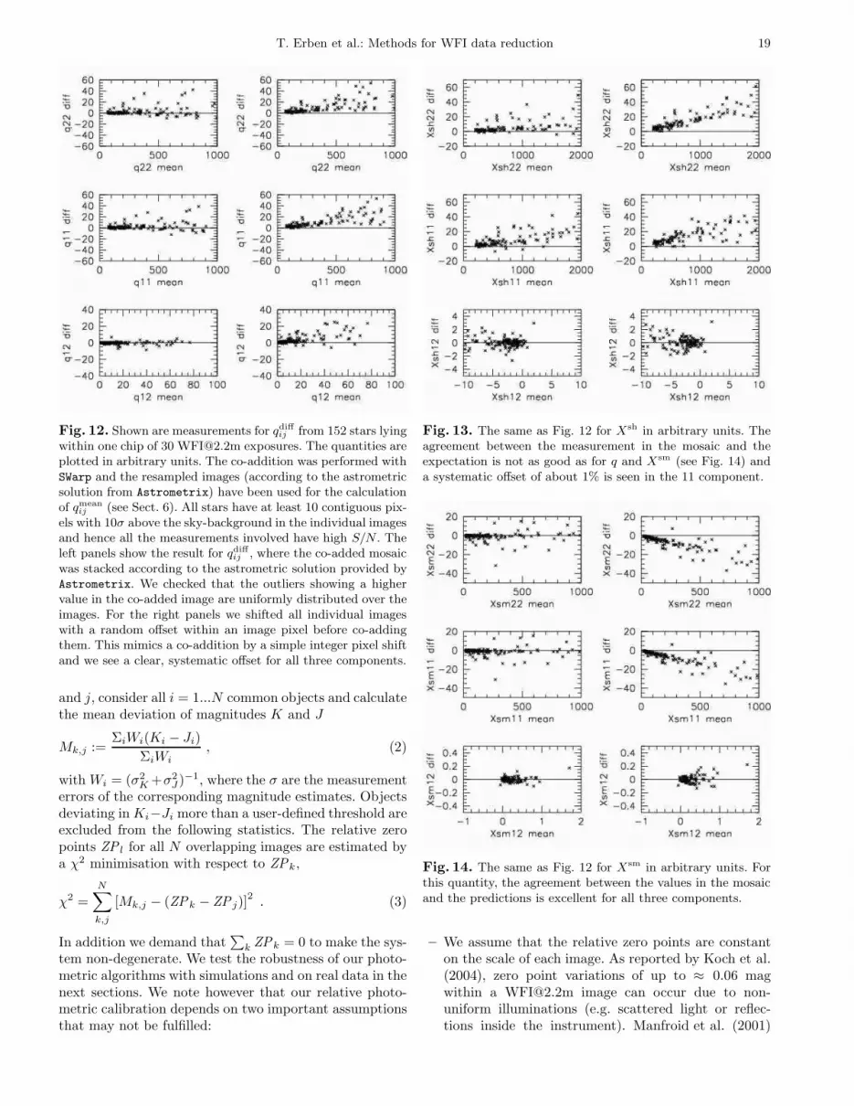
Fig. 12. Shown are measurements for qdiff

ij from 152 stars lyingwithin one chip of 30 WFI@2.2m exposures. The quantities areplotted in arbitrary units. The co-addition was performed withSWarp and the resampled images (according to the astrometricsolution from Astrometrix) have been used for the calculationof qmean

ij (see Sect. 6). All stars have at least 10 contiguous pix-els with 10σ above the sky-background in the individual imagesand hence all the measurements involved have high S/N . Theleft panels show the result for qdiff

ij , where the co-added mosaicwas stacked according to the astrometric solution provided byAstrometrix. We checked that the outliers showing a highervalue in the co-added image are uniformly distributed over theimages. For the right panels we shifted all individual imageswith a random offset within an image pixel before co-addingthem. This mimics a co-addition by a simple integer pixel shiftand we see a clear, systematic offset for all three components.

and j, consider all i = 1...N common objects and calculatethe mean deviation of magnitudes K and J

Mk,j :=ΣiWi(Ki − Ji)

ΣiWi

, (2)

with Wi = (σ2K +σ2

J)−1, where the σ are the measurementerrors of the corresponding magnitude estimates. Objectsdeviating in Ki−Ji more than a user-defined threshold areexcluded from the following statistics. The relative zeropoints ZP l for all N overlapping images are estimated bya χ2 minimisation with respect to ZPk,

χ2 =N

∑

k,j

[Mk,j − (ZPk − ZP j)]2 . (3)

In addition we demand that∑

k ZPk = 0 to make the sys-tem non-degenerate. We test the robustness of our photo-metric algorithms with simulations and on real data in thenext sections. We note however that our relative photo-metric calibration depends on two important assumptionsthat may not be fulfilled:

Fig. 13. The same as Fig. 12 for Xsh in arbitrary units. Theagreement between the measurement in the mosaic and theexpectation is not as good as for q and Xsm (see Fig. 14) anda systematic offset of about 1% is seen in the 11 component.

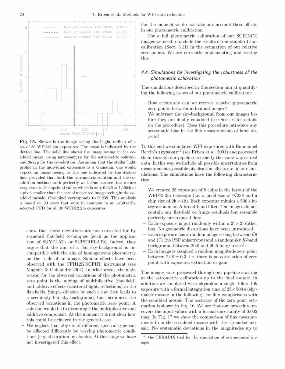
Fig. 14. The same as Fig. 12 for Xsm in arbitrary units. Forthis quantity, the agreement between the values in the mosaicand the predictions is excellent for all three components.

– We assume that the relative zero points are constanton the scale of each image. As reported by Koch et al.(2004), zero point variations of up to ≈ 0.06 magwithin a WFI@2.2m image can occur due to non-uniform illuminations (e.g. scattered light or reflec-tions inside the instrument). Manfroid et al. (2001)

20 T. Erben et al.: Methods for WFI data reduction

Fig. 15. Shown is the image seeing (half-light radius) of aset of 30 WFI@2.2m exposures. The mean is indicated by thedotted line. The solid line shows the image seeing in the co-added image, using Astrometrix for the astrometric solutionand SWarp for the co-addition. Assuming that the stellar lightprofile in the individual exposures is a Gaussian, one wouldexpect an image seeing as the one indicated by the dashedline, provided that both the astrometric solution and the co-addition method work perfectly well. One can see that we arevery close to the optimal value, which is only 0.026 ≈ 1/40th ofa pixel smaller than the actual measured image seeing in the co-added mosaic. One pixel corresponds to 0.′′238. This analysisis based on 29 stars that were in common in an arbitrarilyselected CCD for all 30 WFI@2.2m exposures.

show that these deviations are not corrected for bystandard flat-field techniques (such as the applica-tion of SKYFLATs or SUPERFLATs). Indeed, theyargue that the aim of a flat sky-background is in-compatible with the aim of homogeneous photometryon the scale of an image. Similar effects have beenobserved with the CFH12K@CFHT instrument (seeMagnier & Cuillandre 2004). In other words, the mainreason for the observed variations of the photometriczero point is the mixing of multiplicative (flat-field)and additive effects (scattered light, reflections) in theflat-fields. Simple division by such a flat then leads toa seemingly flat sky-background, but introduces theobserved variations in the photometric zero point. Asolution would be to disentangle the multiplicative andadditive component. At the moment it is not clear howthis could be achieved in the general case.

– We neglect that objects of different spectral type canbe affected differently by varying photometric condi-tions (e.g. absorption by clouds). At this stage we havenot investigated this effect.

For the moment we do not take into account these effectsin our photometric calibration.

For a full photometric calibration of our SCIENCEimages we need to include the results of our standard starcalibration (Sect. 3.11) in the estimation of our relativezero points. We are currently implementing and testingthis.

4.4. Simulations for investigating the robustness of thephotometric calibration

The simulations described in this section aim at quantify-ing the following issues of our photometric calibration:

– How accurately can we recover relative photometriczero points between individual images?

– We subtract the sky-background from our images be-fore they are finally co-added (see Sect. 6 for detailson the procedure). Does this procedure introduce anysystematic bias in the flux measurements of faint ob-jects?

To this end we simulated WFI exposures with EmmanuelBertin’s skymaker17 (see Erben et al. 2001) and processedthem through our pipeline in exactly the same way as realdata. In this way we include all possible uncertainties frommeasurements, possible pixelisation effects etc. in our sim-ulations. The simulations have the following characteris-tics:

– We created 25 exposures of 8 chips in the layout of theWFI@2.2m telescope (i.e. a pixel size of 0.′′238 and achip size of 2k×4k). Each exposure mimics a 500 s in-tegration in an R broad-band filter. The images do notcontain any flat-field or fringe residuals but resembleperfectly pre-reduced data.

– Each exposure is put randomly within a 2′ × 2′ ditherbox. No geometric distortions have been introduced.

– Each exposure has a random image seeing between 0.′′9and 1.′′1 (no PSF anisotropy) and a random sky R-bandbackground between 20.0 and 20.5 mag/arcsec2.

– Each image is assigned a random magnitude zero pointbetween 24.9 ± 0.3, i.e. there is no correlation of zeropoint with exposure, extinction or gain.

The images were processed through our pipeline startingat the astrometric calibration up to the final mosaic. Inaddition we simulated with skymaker a single 10k × 10kexposure with a formal integration time of 25×500 s (sky-maker mosaic in the following) for flux comparisons withthe co-added mosaic. The accuracy of the zero point esti-mation is shown in Fig. 16. We see that our procedure re-covers the input values with a formal uncertainty of 0.002mag. In Fig. 17 we show the comparison of flux measure-ments from the co-added mosaic with the skymaker mo-saic. No systematic deviations in the magnitudes up to

17 the TERAPIX tool for the simulation of astronomical im-ages

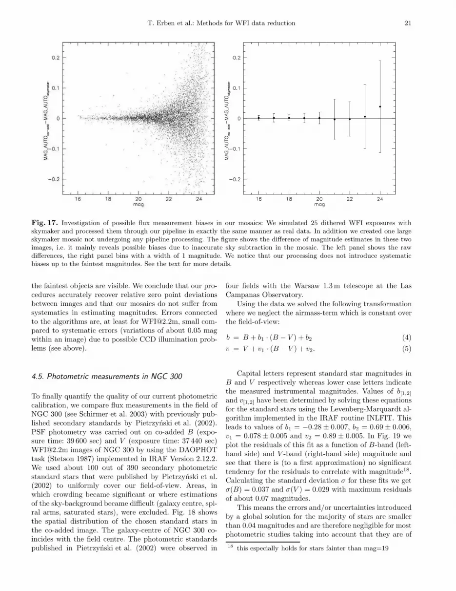
T. Erben et al.: Methods for WFI data reduction 21

Fig. 17. Investigation of possible flux measurement biases in our mosaics: We simulated 25 dithered WFI exposures withskymaker and processed them through our pipeline in exactly the same manner as real data. In addition we created one largeskymaker mosaic not undergoing any pipeline processing. The figure shows the difference of magnitude estimates in these twoimages, i.e. it mainly reveals possible biases due to inaccurate sky subtraction in the mosaic. The left panel shows the rawdifferences, the right panel bins with a width of 1 magnitude. We notice that our processing does not introduce systematicbiases up to the faintest magnitudes. See the text for more details.

the faintest objects are visible. We conclude that our pro-cedures accurately recover relative zero point deviationsbetween images and that our mosaics do not suffer fromsystematics in estimating magnitudes. Errors connectedto the algorithms are, at least for WFI@2.2m, small com-pared to systematic errors (variations of about 0.05 magwithin an image) due to possible CCD illumination prob-lems (see above).

4.5. Photometric measurements in NGC 300

To finally quantify the quality of our current photometriccalibration, we compare flux measurements in the field ofNGC 300 (see Schirmer et al. 2003) with previously pub-lished secondary standards by Pietrzynski et al. (2002).PSF photometry was carried out on co-added B (expo-sure time: 39 600 sec) and V (exposure time: 37 440 sec)WFI@2.2m images of NGC 300 by using the DAOPHOTtask (Stetson 1987) implemented in IRAF Version 2.12.2.We used about 100 out of 390 secondary photometricstandard stars that were published by Pietrzynski et al.(2002) to uniformly cover our field-of-view. Areas, inwhich crowding became significant or where estimationsof the sky-background became difficult (galaxy centre, spi-ral arms, saturated stars), were excluded. Fig. 18 showsthe spatial distribution of the chosen standard stars inthe co-added image. The galaxy-centre of NGC 300 co-incides with the field centre. The photometric standardspublished in Pietrzynski et al. (2002) were observed in

four fields with the Warsaw 1.3m telescope at the LasCampanas Observatory.

Using the data we solved the following transformationwhere we neglect the airmass-term which is constant overthe field-of-view:

b = B + b1 · (B − V ) + b2 (4)

v = V + v1 · (B − V ) + v2. (5)

Capital letters represent standard star magnitudes inB and V respectively whereas lower case letters indicatethe measured instrumental magnitudes. Values of b[1,2]

and v[1,2] have been determined by solving these equationsfor the standard stars using the Levenberg-Marquardt al-gorithm implemented in the IRAF routine INLFIT. Thisleads to values of b1 = −0.28 ± 0.007, b2 = 0.69 ± 0.006,v1 = 0.078 ± 0.005 and v2 = 0.89 ± 0.005. In Fig. 19 weplot the residuals of this fit as a function of B-band (left-hand side) and V -band (right-hand side) magnitude andsee that there is (to a first approximation) no significanttendency for the residuals to correlate with magnitude18.Calculating the standard deviation σ for these fits we getσ(B) = 0.037 and σ(V ) = 0.029 with maximum residualsof about 0.07 magnitudes.

This means the errors and/or uncertainties introducedby a global solution for the majority of stars are smallerthan 0.04 magnitudes and are therefore negligible for mostphotometric studies taking into account that they are of

18 this especially holds for stars fainter than mag=19

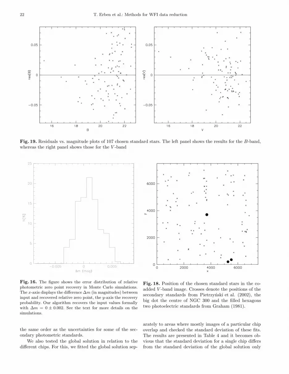
22 T. Erben et al.: Methods for WFI data reduction

Fig. 19. Residuals vs. magnitude plots of 107 chosen standard stars. The left panel shows the results for the B-band,whereas the right panel shows those for the V -band

Fig. 16. The figure shows the error distribution of relativephotometric zero point recovery in Monte Carlo simulations.The x-axis displays the difference ∆m (in magnitudes) betweeninput and recovered relative zero point, the y-axis the recoveryprobability. Our algorithm recovers the input values formallywith ∆m = 0 ± 0.002. See the text for more details on thesimulations.

the same order as the uncertainties for some of the sec-ondary photometric standards.

We also tested the global solution in relation to thedifferent chips. For this, we fitted the global solution sep-

Fig. 18. Position of the chosen standard stars in the co-added V -band image. Crosses denote the positions of thesecondary standards from Pietrzynski et al. (2002), thebig dot the centre of NGC 300 and the filled hexagonstwo photoelectric standards from Graham (1981).

arately to areas where mostly images of a particular chipoverlap and checked the standard deviation of these fits.The results are presented in Table 4 and it becomes ob-vious that the standard deviation for a single chip differsfrom the standard deviation of the global solution only

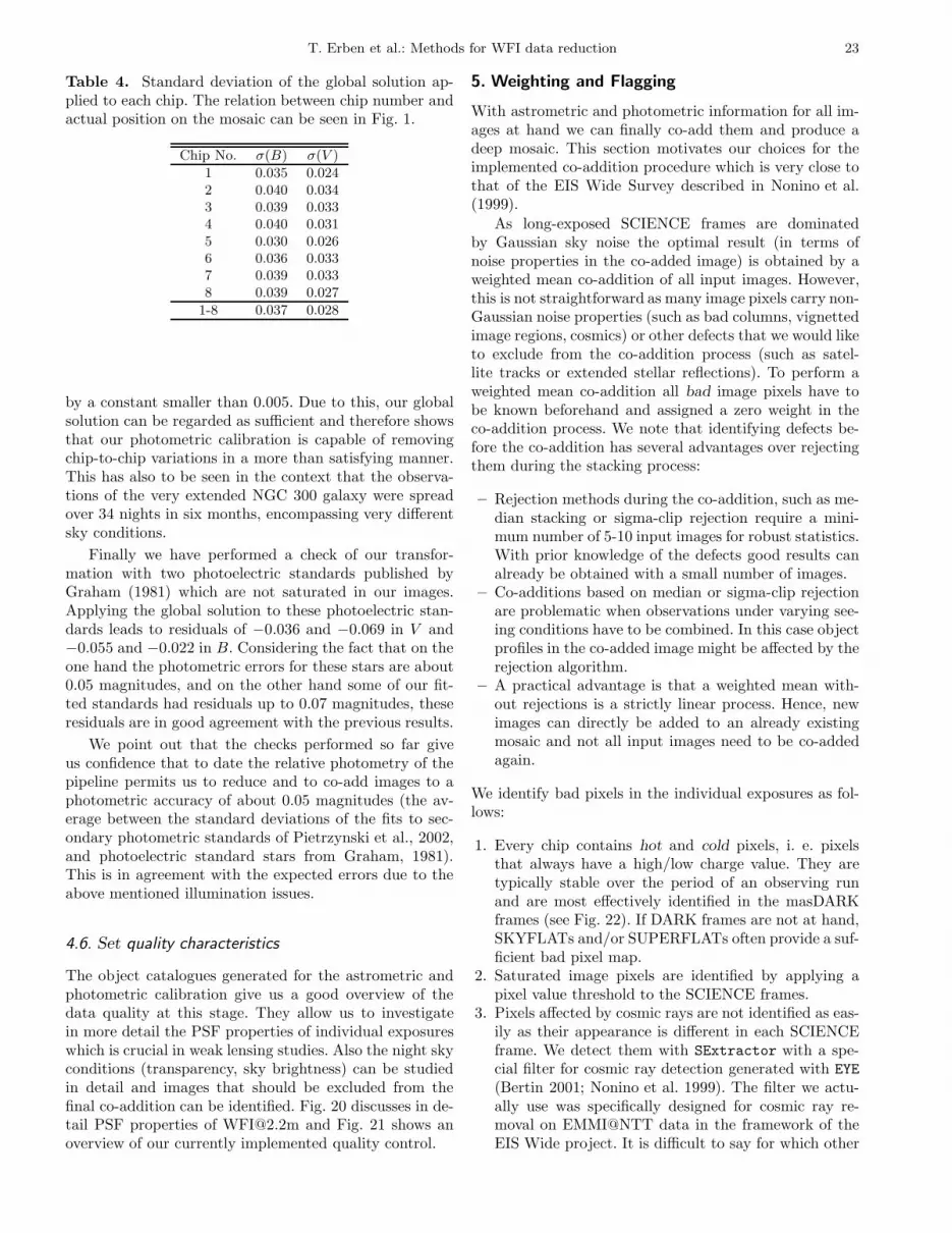
T. Erben et al.: Methods for WFI data reduction 23

Table 4. Standard deviation of the global solution ap-plied to each chip. The relation between chip number andactual position on the mosaic can be seen in Fig. 1.

Chip No. σ(B) σ(V )

1 0.035 0.0242 0.040 0.0343 0.039 0.0334 0.040 0.0315 0.030 0.0266 0.036 0.0337 0.039 0.0338 0.039 0.027

1-8 0.037 0.028

by a constant smaller than 0.005. Due to this, our globalsolution can be regarded as sufficient and therefore showsthat our photometric calibration is capable of removingchip-to-chip variations in a more than satisfying manner.This has also to be seen in the context that the observa-tions of the very extended NGC 300 galaxy were spreadover 34 nights in six months, encompassing very differentsky conditions.

Finally we have performed a check of our transfor-mation with two photoelectric standards published byGraham (1981) which are not saturated in our images.Applying the global solution to these photoelectric stan-dards leads to residuals of −0.036 and −0.069 in V and−0.055 and −0.022 in B. Considering the fact that on theone hand the photometric errors for these stars are about0.05 magnitudes, and on the other hand some of our fit-ted standards had residuals up to 0.07 magnitudes, theseresiduals are in good agreement with the previous results.

We point out that the checks performed so far giveus confidence that to date the relative photometry of thepipeline permits us to reduce and to co-add images to aphotometric accuracy of about 0.05 magnitudes (the av-erage between the standard deviations of the fits to sec-ondary photometric standards of Pietrzynski et al., 2002,and photoelectric standard stars from Graham, 1981).This is in agreement with the expected errors due to theabove mentioned illumination issues.

4.6. Set quality characteristics

The object catalogues generated for the astrometric andphotometric calibration give us a good overview of thedata quality at this stage. They allow us to investigatein more detail the PSF properties of individual exposureswhich is crucial in weak lensing studies. Also the night skyconditions (transparency, sky brightness) can be studiedin detail and images that should be excluded from thefinal co-addition can be identified. Fig. 20 discusses in de-tail PSF properties of WFI@2.2m and Fig. 21 shows anoverview of our currently implemented quality control.

5. Weighting and Flagging

With astrometric and photometric information for all im-ages at hand we can finally co-add them and produce adeep mosaic. This section motivates our choices for theimplemented co-addition procedure which is very close tothat of the EIS Wide Survey described in Nonino et al.(1999).

As long-exposed SCIENCE frames are dominatedby Gaussian sky noise the optimal result (in terms ofnoise properties in the co-added image) is obtained by aweighted mean co-addition of all input images. However,this is not straightforward as many image pixels carry non-Gaussian noise properties (such as bad columns, vignettedimage regions, cosmics) or other defects that we would liketo exclude from the co-addition process (such as satel-lite tracks or extended stellar reflections). To perform aweighted mean co-addition all bad image pixels have tobe known beforehand and assigned a zero weight in theco-addition process. We note that identifying defects be-fore the co-addition has several advantages over rejectingthem during the stacking process:

– Rejection methods during the co-addition, such as me-dian stacking or sigma-clip rejection require a mini-mum number of 5-10 input images for robust statistics.With prior knowledge of the defects good results canalready be obtained with a small number of images.

– Co-additions based on median or sigma-clip rejectionare problematic when observations under varying see-ing conditions have to be combined. In this case objectprofiles in the co-added image might be affected by therejection algorithm.

– A practical advantage is that a weighted mean with-out rejections is a strictly linear process. Hence, newimages can directly be added to an already existingmosaic and not all input images need to be co-addedagain.

We identify bad pixels in the individual exposures as fol-lows:

1. Every chip contains hot and cold pixels, i. e. pixelsthat always have a high/low charge value. They aretypically stable over the period of an observing runand are most effectively identified in the masDARKframes (see Fig. 22). If DARK frames are not at hand,SKYFLATs and/or SUPERFLATs often provide a suf-ficient bad pixel map.

2. Saturated image pixels are identified by applying apixel value threshold to the SCIENCE frames.

3. Pixels affected by cosmic rays are not identified as eas-ily as their appearance is different in each SCIENCEframe. We detect them with SExtractor with a spe-cial filter for cosmic ray detection generated with EYE

(Bertin 2001; Nonino et al. 1999). The filter we actu-ally use was specifically designed for cosmic ray re-moval on EMMI@NTT data in the framework of theEIS Wide project. It is difficult to say for which other

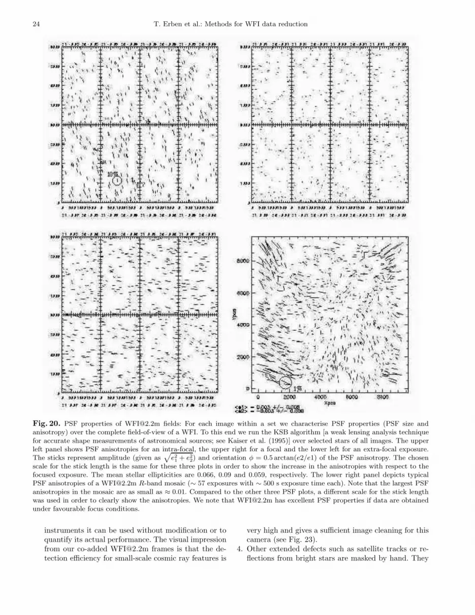
24 T. Erben et al.: Methods for WFI data reduction

Fig. 20. PSF properties of WFI@2.2m fields: For each image within a set we characterise PSF properties (PSF size andanisotropy) over the complete field-of-view of a WFI. To this end we run the KSB algorithm [a weak lensing analysis techniquefor accurate shape measurements of astronomical sources; see Kaiser et al. (1995)] over selected stars of all images. The upperleft panel shows PSF anisotropies for an intra-focal, the upper right for a focal and the lower left for an extra-focal exposure.The sticks represent amplitude (given as

√

e21+ e2

2) and orientation φ = 0.5 arctan(e2/e1) of the PSF anisotropy. The chosen

scale for the stick length is the same for these three plots in order to show the increase in the anisotropies with respect to thefocused exposure. The mean stellar ellipticities are 0.066, 0.09 and 0.059, respectively. The lower right panel depicts typicalPSF anisotropies of a WFI@2.2m R-band mosaic (∼ 57 exposures with ∼ 500 s exposure time each). Note that the largest PSFanisotropies in the mosaic are as small as ≈ 0.01. Compared to the other three PSF plots, a different scale for the stick lengthwas used in order to clearly show the anisotropies. We note that WFI@2.2m has excellent PSF properties if data are obtainedunder favourable focus conditions.

instruments it can be used without modification or toquantify its actual performance. The visual impressionfrom our co-added WFI@2.2m frames is that the de-tection efficiency for small-scale cosmic ray features is

very high and gives a sufficient image cleaning for thiscamera (see Fig. 23).

4. Other extended defects such as satellite tracks or re-flections from bright stars are masked by hand. They

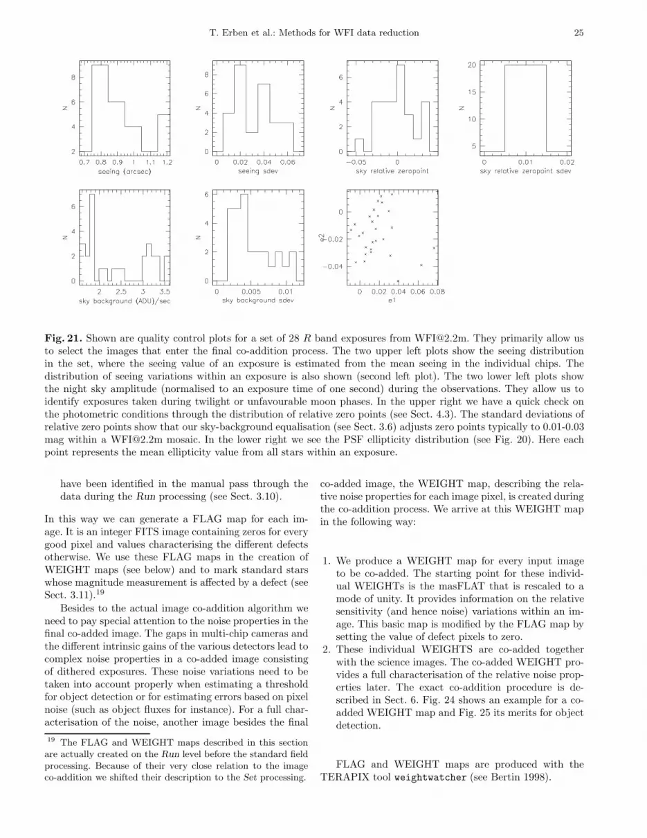
T. Erben et al.: Methods for WFI data reduction 25

Fig. 21. Shown are quality control plots for a set of 28 R band exposures from WFI@2.2m. They primarily allow usto select the images that enter the final co-addition process. The two upper left plots show the seeing distributionin the set, where the seeing value of an exposure is estimated from the mean seeing in the individual chips. Thedistribution of seeing variations within an exposure is also shown (second left plot). The two lower left plots showthe night sky amplitude (normalised to an exposure time of one second) during the observations. They allow us toidentify exposures taken during twilight or unfavourable moon phases. In the upper right we have a quick check onthe photometric conditions through the distribution of relative zero points (see Sect. 4.3). The standard deviations ofrelative zero points show that our sky-background equalisation (see Sect. 3.6) adjusts zero points typically to 0.01-0.03mag within a WFI@2.2m mosaic. In the lower right we see the PSF ellipticity distribution (see Fig. 20). Here eachpoint represents the mean ellipticity value from all stars within an exposure.

have been identified in the manual pass through thedata during the Run processing (see Sect. 3.10).

In this way we can generate a FLAG map for each im-age. It is an integer FITS image containing zeros for everygood pixel and values characterising the different defectsotherwise. We use these FLAG maps in the creation ofWEIGHT maps (see below) and to mark standard starswhose magnitude measurement is affected by a defect (seeSect. 3.11).19

Besides to the actual image co-addition algorithm weneed to pay special attention to the noise properties in thefinal co-added image. The gaps in multi-chip cameras andthe different intrinsic gains of the various detectors lead tocomplex noise properties in a co-added image consistingof dithered exposures. These noise variations need to betaken into account properly when estimating a thresholdfor object detection or for estimating errors based on pixelnoise (such as object fluxes for instance). For a full char-acterisation of the noise, another image besides the final

19 The FLAG and WEIGHT maps described in this sectionare actually created on the Run level before the standard fieldprocessing. Because of their very close relation to the imageco-addition we shifted their description to the Set processing.

co-added image, the WEIGHT map, describing the rela-tive noise properties for each image pixel, is created duringthe co-addition process. We arrive at this WEIGHT mapin the following way:

1. We produce a WEIGHT map for every input imageto be co-added. The starting point for these individ-ual WEIGHTs is the masFLAT that is rescaled to amode of unity. It provides information on the relativesensitivity (and hence noise) variations within an im-age. This basic map is modified by the FLAG map bysetting the value of defect pixels to zero.

2. These individual WEIGHTS are co-added togetherwith the science images. The co-added WEIGHT pro-vides a full characterisation of the relative noise prop-erties later. The exact co-addition procedure is de-scribed in Sect. 6. Fig. 24 shows an example for a co-added WEIGHT map and Fig. 25 its merits for objectdetection.

FLAG and WEIGHT maps are produced with theTERAPIX tool weightwatcher (see Bertin 1998).

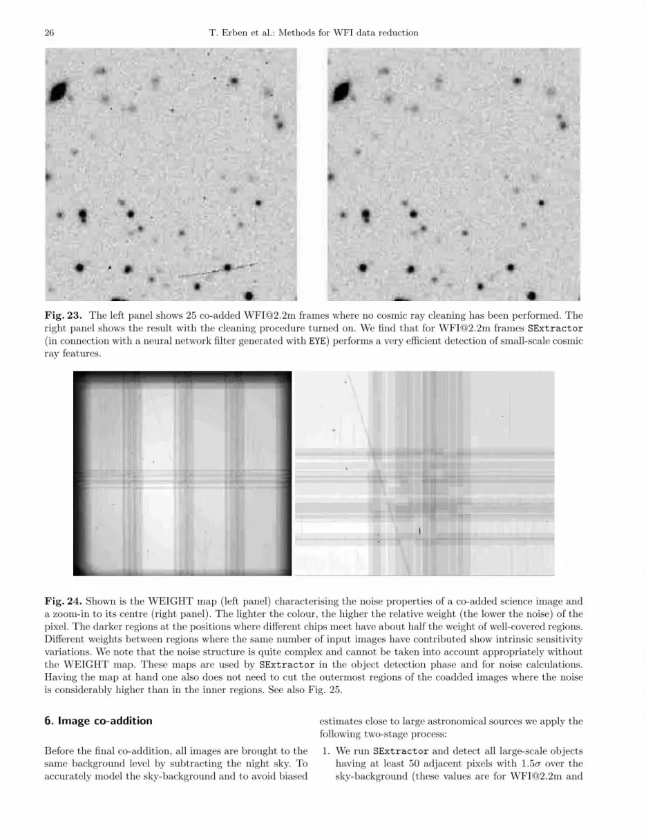
26 T. Erben et al.: Methods for WFI data reduction

Fig. 23. The left panel shows 25 co-added WFI@2.2m frames where no cosmic ray cleaning has been performed. Theright panel shows the result with the cleaning procedure turned on. We find that for WFI@2.2m frames SExtractor(in connection with a neural network filter generated with EYE) performs a very efficient detection of small-scale cosmicray features.

Fig. 24. Shown is the WEIGHT map (left panel) characterising the noise properties of a co-added science image anda zoom-in to its centre (right panel). The lighter the colour, the higher the relative weight (the lower the noise) of thepixel. The darker regions at the positions where different chips meet have about half the weight of well-covered regions.Different weights between regions where the same number of input images have contributed show intrinsic sensitivityvariations. We note that the noise structure is quite complex and cannot be taken into account appropriately withoutthe WEIGHT map. These maps are used by SExtractor in the object detection phase and for noise calculations.Having the map at hand one also does not need to cut the outermost regions of the coadded images where the noiseis considerably higher than in the inner regions. See also Fig. 25.

6. Image co-addition

Before the final co-addition, all images are brought to thesame background level by subtracting the night sky. Toaccurately model the sky-background and to avoid biased

estimates close to large astronomical sources we apply thefollowing two-stage process:

1. We run SExtractor and detect all large-scale objectshaving at least 50 adjacent pixels with 1.5σ over thesky-background (these values are for WFI@2.2m and

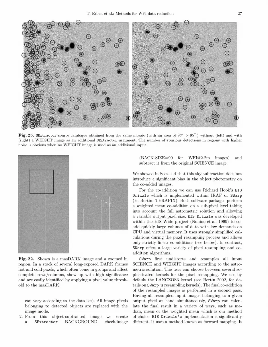
T. Erben et al.: Methods for WFI data reduction 27

Fig. 25. SExtractor source catalogue obtained from the same mosaic (with an area of 95′′ × 95′′ ) without (left) and with(right) a WEIGHT image as an additional SExtractor argument. The number of spurious detections in regions with highernoise is obvious when no WEIGHT image is used as an additional input.

Fig. 22. Shown is a masDARK image and a zoomed inregion. In a stack of several long-exposed DARK frameshot and cold pixels, which often come in groups and affectcomplete rows/columns, show up with high significanceand are easily identified by applying a pixel value thresh-old to the masDARK.

can vary according to the data set). All image pixelsbelonging to detected objects are replaced with theimage mode.

2. From this object-subtracted image we createa SExtractor BACKGROUND check-image

(BACK SIZE=90 for WFI@2.2m images) andsubtract it from the original SCIENCE image.

We showed in Sect. 4.4 that this sky subtraction does notintroduce a significant bias in the object photometry onthe co-added images.

For the co-addition we can use Richard Hook’s EIS

Drizzle which is implemented within IRAF or SWarp

(E. Bertin, TERAPIX). Both software packages performa weighted mean co-addition on a sub-pixel level takinginto account the full astrometric solution and allowinga variable output pixel size. EIS Drizzle was developedwithin the EIS Wide project (Nonino et al. 1999) to co-add quickly large volumes of data with low demands onCPU and virtual memory. It uses strongly simplified cal-culations during the pixel resampling process and allowsonly strictly linear co-additions (see below). In contrast,SWarp offers a large variety of pixel resampling and co-addition algorithms.

SWarp first undistorts and resamples all inputSCIENCE and WEIGHT images according to the astro-metric solution. The user can choose between several so-phisticated kernels for the pixel remapping. We use bydefault the LANCZOS3 kernel (see Bertin 2002, for de-tails on SWarp’s resampling kernels). The final co-additionof the resampled images is performed in a second pass.Having all resampled input images belonging to a givenoutput pixel at hand simultaneously, SWarp can calcu-late the final result in a variety of ways, such as me-dian, mean or the weighted mean which is our methodof choice. EIS Drizzle’s implementation is significantlydifferent. It uses a method known as forward mapping. It

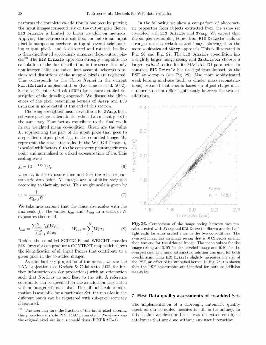
28 T. Erben et al.: Methods for WFI data reduction

performs the complete co-addition in one pass by puttingthe input images consecutively on the output grid. Hence,EIS Drizzle is limited to linear co-addition methods.Applying the astrometric solution, an individual inputpixel is mapped somewhere on top of several neighbour-ing output pixels, and is distorted and rotated. Its fluxis then distributed accordingly amongst these output pix-els.20 The EIS Drizzle approach strongly simplifies thecalculation of the flux distribution, in the sense that onlynon-integer shifts are taken into account, whereas rota-tions and distortions of the mapped pixels are neglected.This corresponds to the Turbo Kernel in the currentMultiDrizzle implementation (Koekemoer et al. 2002).See also Fruchter & Hook (2002) for a more detailed de-scription of the drizzling approach. We discuss the differ-ences of the pixel resampling kernels of SWarp and EIS

Drizzle in more detail at the end of this section.Choosing a weighted mean co-addition for SWarp, both

software packages calculate the value of an output pixel inthe same way. Four factors contribute to the final resultin our weighted mean co-addition. Given are the valueIi, representing the part of an input pixel that goes toa specified output pixel Iout in the co-added image. Wi

represents the associated value in the WEIGHT map. Ii

is scaled with factors fi to the consistent photometric zeropoint and normalised to a fixed exposure time of 1 s. Thisscaling reads

fi = 10−0.4ZPi/ti, (6)

where ti is the exposure time and ZPi the relative pho-tometric zero point. All images are in addition weightedaccording to their sky noise. This weight scale is given by

wi =1

σ2sky,if

2i

. (7)

We take into account that the noise also scales with theflux scale fi. The values Iout and Wout in a stack of Nexposures then read

Iout =

∑Ni=1 IifiWiwi∑N

i=1 Wiwi

, Wout =

N∑

i=1

Wiwi . (8)

Besides the co-added SCIENCE and WEIGHT mosaicsEIS Drizzle can produce a CONTEXT map which allowsthe identification of all input frames that contribute to agiven pixel in the co-added images.

As standard sky projection of the mosaic we use theTAN projection (see Greisen & Calabretta 2002, for fur-ther information on sky projections) with an orientationsuch that North is up and East to the left. A referencecoordinate can be specified for the co-addition, associatedwith an integer reference pixel. Thus, if multi-colour infor-mation is available for a particular Set, the mosaics in thedifferent bands can be registered with sub-pixel accuracyif required.

20 The user can vary the fraction of the input pixel enteringthis procedure (drizzle PIXFRAC parameter). We always usethe original pixel size in our co-additions (PIXFRAC=1).

In the following we show a comparison of photomet-ric properties from objects extracted from the same setco-added with EIS Drizzle and SWarp. We expect thatthe simpler resampling kernel from EIS Drizzle leads tostronger noise correlations and image blurring than themore sophisticated SWarp approach. This is illustrated inFig. 26 and Fig. 27. The EIS Drizzle co-addition hasa slightly larger image seeing and SExtractor chooses alarger optimal radius for its MAG AUTO parameter. Incontrast, EIS Drizzle has no significant impact on thePSF anisotropies (see Fig. 28). Also more sophisticatedweak lensing analyses (such as cluster mass reconstruc-tions) revealed that results based on object shape mea-surements do not differ significantly between the two co-additions.

Fig. 26. Comparison of the image seeing between two mo-saics created with SWarp and EIS Drizzle. Shown are the half-light radii for unsaturated stars in the two co-additions. Theswarped image has an image seeing that is 0.09 pixels smallerthan the one for the drizzled image. The mean values for theimage seeing are 0.′′95 for the drizzled image and 0.′′91 for theswarped one. The same astrometric solution was used for bothco-additions. Thus EIS Drizzle slightly increases the size ofthe PSF, an effect of its simplified kernel. In Fig. 28 it is shownthat the PSF anisotropies are identical for both co-additionstrategies.

7. First Data quality assessments of co-added Sets

The implementation of a thorough, automatic qualitycheck on our co-added mosaics is still in its infancy. Inthis section we describe basic tests on extracted objectcatalogues that are done without any user interaction.

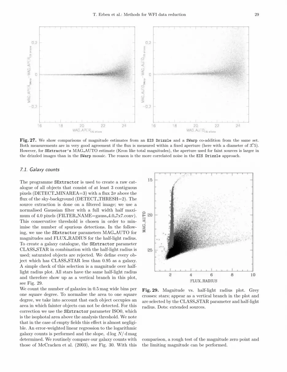
T. Erben et al.: Methods for WFI data reduction 29

Fig. 27. We show comparisons of magnitude estimates from an EIS Drizzle and a SWarp co-addition from the same set.Both measurements are in very good agreement if the flux is measured within a fixed aperture (here with a diameter of 3.′′5).However, for SExtractor’s MAG AUTO estimate (Kron like total magnitudes), the aperture used for faint sources is larger inthe drizzled images than in the SWarp mosaic. The reason is the more correlated noise in the EIS Drizzle approach.

7.1. Galaxy counts

The programme SExtractor is used to create a raw cat-alogue of all objects that consist of at least 3 contiguouspixels (DETECT MINAREA=3) with a flux 2σ above theflux of the sky-background (DETECT THRESH=2). Thesource extraction is done on a filtered image; we use anormalised Gaussian filter with a full width half maxi-mum of 4.0 pixels (FILTER NAME=gauss 4.0 7x7.conv).This conservative threshold is chosen in order to min-imise the number of spurious detections. In the follow-ing, we use the SExtractor parameters MAG AUTO formagnitudes and FLUX RADIUS for the half-light radius.To create a galaxy catalogue, the SExtractor parameterCLASS STAR in combination with the half-light radius isused; saturated objects are rejected. We define every ob-ject which has CLASS STAR less than 0.95 as a galaxy.A simple check of this selection is a magnitude over half-light radius plot. All stars have the same half-light radiusand therefore show up as a vertical branch in this plot,see Fig. 29.We count the number of galaxies in 0.5 mag wide bins perone square degree. To normalise the area to one squaredegree, we take into account that each object occupies anarea in which fainter objects can not be detected. For thiscorrection we use the SExtractor parameter ISO0, whichis the isophotal area above the analysis threshold. We notethat in the case of empty fields this effect is almost negligi-ble. An error-weighted linear regression to the logarithmicgalaxy counts is performed and the slope, d log N/ dmagdetermined. We routinely compare our galaxy counts withthose of McCracken et al. (2003), see Fig. 30. With this

Fig. 29. Magnitude vs. half-light radius plot. Greycrosses: stars; appear as a vertical branch in the plot andare selected by the CLASS STAR parameter and half-lightradius. Dots: extended sources.

comparison, a rough test of the magnitude zero point andthe limiting magnitude can be performed.

30 T. Erben et al.: Methods for WFI data reduction

Fig. 28. PSF anisotropies in a drizzled (left column) and a swarped (right column) mosaic of the same data set. The patternsare virtually identical. Yet EIS Drizzle marginally increases the size of the PSF, as was shown in the left panel of Fig. 26. Themean PSF anisotropy for this particular mosaic amounts to mere 0.022 ± 0.015.

7.2. Clustering of extended sources

A further test for the quality of the co-added image is theclustering of sources. For that purpose we use the two-point angular correlation function, ω(θ), where ω(θ)δθ isthe excess probability of finding a pair separated by anangle between θ and θ + δθ. We estimate this quantity bycreating a large number of random catalogues (by default40 mock catalogues are created) and count the pairs withinthe data catalogue, DD, within the random catalogue, RR

and between the data and random catalogues, DR. Theestimator for ω(θ), proposed by Landy & Szalay (1993),is

ω(θ) =DD − 2DR + RR

RR. (9)

The random fields must have the same geometry as thedata field. Therefore we calculate an obscuration mask outof the number density of extracted sources as follows. Amesh with 512× 512 mesh cells is placed on top of a datafield and the number of objects in each cell is counted.

T. Erben et al.: Methods for WFI data reduction 31

Fig. 30. The figure displays the logarithmic galaxy countsin 0.5 mag bins per one square degree from our re-duction of the Chandra Deep Field South (CDFS; seeGiavalisco et al. 2004). The error bars are due to Poissonnoise; the line fit is an error-weighted linear regression in amagnitude range between the saturation and the limitingmagnitude (here: R ∈ [16.3; 23.8]). For the normalisationof the area we take into account that each detected objectoccupies an area in which fainter objects cannot be de-tected. As a comparison to our galaxy counts we also plotthe galaxy number counts from the CFH12K-VIRMOSdeep field (McCracken et al. 2003). For the CDFS we alsoplot the number counts from Arnouts et al. (2001).

Then the cell count matrix is smoothed with a Gaussiankernel of about 512/60 cells FWHM, and all matrix ele-ments lower than a given fraction (we use 75% as defaultbut varying this parameter between 50% and 80% doesnot change the results significantly) of the mean numberof galaxies inside a cell are defined as a masked region.The borders of a field, bright stars, and part of their halosare masked automatically by this method (see Fig. 31).

To maximise computational speed, we perform our cal-culations by creating an index tree for galaxy position asexplained in Zhang & Pen (2004). The error bars in ourcheck-plots for each angular bin are simply estimated byPoisson noise and are therefore a lower limit to the uncer-tainty in ω(θ).

As an example we present the two-point angular cor-relation function of galaxies in our R-band reductions for11 WFI-fields in the EIS Deep Public Survey (EIS DPS).For three different magnitude bins we fitted a power law,ω(θ) = Aθδ − C, to the data. The variable C is the so-called integral constraint (see for instance Roche et al.1993), which only becomes important for large fields atlarger scales (θ > 2′). We therefore neglect the integral

Fig. 32. The two-point angular correlation function ofgalaxies for different magnitude bins, for 11 WFI-fieldsin the DPS. We show the logarithm of the amplitude,log ω(θ), as a function of the angular separation θ in ar-cmin. Here the error bar in each bin is due to the field-to-field variance. We perform a simple error-weighted linearregression in the angular interval θ ∈ [0.′′06; 2′ ] (where theintegral constraint is negligible) to determine the slope δand the amplitude A1 = ω(θ = 1′).

constraint and perform the fit for small scales (θ < 2′).The results are shown in Fig. 32.

The results from our clustering analysis can be cross-checked by considering the aperture number count disper-sion 〈N2〉(θ). It is directly related to the angular correla-tion function ω(θ) by

〈N2〉(θ) =

∫

dϑϑ

θ2ω(ϑ)T+

(

ϑ

θ2

)

, (10)

where the function T+ is defined as eq. (35) inSchneider et al. (2002) and it has the nice property of be-ing independent of the integral constraint. As an exam-ple we use the measured ω(θ) for the magnitude intervalR ∈ [19.5; 21] from the 11 WFI-fields of the last sectionto calculate 〈N2

obs〉(θ), see Fig. 33. To compare the slopeδ and amplitude A1 of the fitted power law to the mea-sured ω(θ) of the previous section (Fig. 32), 〈N2

fit〉(θ) iscalculated for the power law, ω(θ) = A1 θδ. The resultsshow that the slope δ obtained from the power law fitof the angular correlation function is correct. The ampli-tude A1, however, seems, with A1 = 0.133, to be a bitlarger; this small discrepancy can easily arise due to thefact that 〈N2

obs〉(θ) is calculated using ω(θ) over the en-tire θ-range and that the ω-fit is slightly influenced bythe integral constraint. As a comparison, Fig. 33 displays

32 T. Erben et al.: Methods for WFI data reduction

Fig. 31. Obscuration mask for the CDFS. Left panel: Distribution of detected sources. Right panel: FITS image ofthe CDFS. White contours indicate masked region. In deep fields, our automatic obscuration mask based on objectdensity variations reliably marks large-scale astronomical sources and noisy borders which would significantly influencethe area of our correlation function analysis. This approach turned out to be sufficient for quality check purposes.

the function 〈N2〉(θ) for the fit parameters determined byHoekstra et al. (2002) for RC-band data of the same mag-nitude range. Note that this can only be a rough compari-son, because of different source extraction algorithms andslightly different R-band filter.

8. Conclusions and Outlook

We have presented our image processing methods formulti-chip cameras that we developed in the course of theGaBoDS project. A significant fraction of GaBoDS is avirtual survey in which observational data were collectedfrom the ESO Science archive within an ASTROVIRTELprogram21 primarily for weak gravitational lensing stud-ies. This allowed us to test and to apply our procedureson data sets which were acquired for a large variety ofscientific programmes (e.g. deep field observations, searchfor moving objects, Cepheid studies in nearby galaxies)and obtained in many different ways (very compact tovery wide dither patterns, Sets observed within a singlenight or over several years). Our experiences regardingthe processing of these data sets from WFI@2.2m are thefollowing:

– The techniques described perform very well on emptyfield observations with WFI@2.2m. The excellent op-tics of this instrument allow an accurate astrometricalignment of images which is crucial for weak lens-ing studies (Schirmer et al. 2003, 2004). Also very

21 ASTROVIRTEL Cycle 2: Gravitational lensing studies inrandomly distributed, high galactic latitude fields; P.I. Erben

Fig. 33. The aperture number count dispersion 〈N2obs〉(θ)

as a function of angular scale θ in arcmin for 11 WFI-fieldsin the magnitude interval R ∈ [19.5; 21]. The error bars onthe function 〈N2〉(θ) are due to the field-to-field varianceof the 11 fields. Note that the points are correlated. Thelines display the function 〈N2

fit〉(θ) assuming a power lawfor the angular two-point correlation function of the formω(θ) = A1 θδ for different parameters A1 = ω(θ = 1′)and δ. Solid line: 〈N2

fit〉(θ) calculated for the fit parameterobtained from the angular correlation function (see Fig.32); dotted line: comparison with 〈N2〉(θ) calculated forthe fit parameters determined by Hoekstra et al. (2002);dashed line: best fit to 〈N2〉(θ).

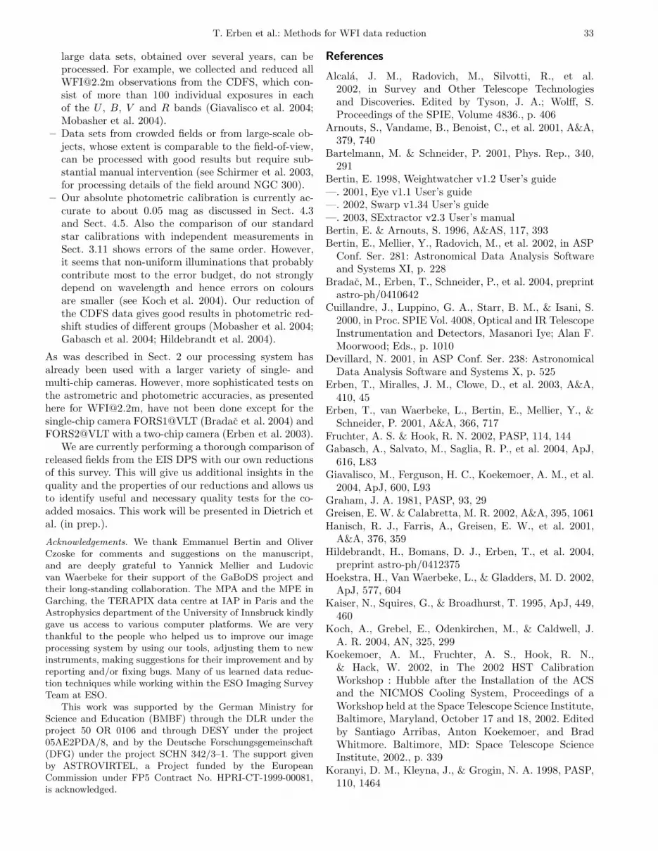
T. Erben et al.: Methods for WFI data reduction 33

large data sets, obtained over several years, can beprocessed. For example, we collected and reduced allWFI@2.2m observations from the CDFS, which con-sist of more than 100 individual exposures in eachof the U , B, V and R bands (Giavalisco et al. 2004;Mobasher et al. 2004).

– Data sets from crowded fields or from large-scale ob-jects, whose extent is comparable to the field-of-view,can be processed with good results but require sub-stantial manual intervention (see Schirmer et al. 2003,for processing details of the field around NGC 300).

– Our absolute photometric calibration is currently ac-curate to about 0.05 mag as discussed in Sect. 4.3and Sect. 4.5. Also the comparison of our standardstar calibrations with independent measurements inSect. 3.11 shows errors of the same order. However,it seems that non-uniform illuminations that probablycontribute most to the error budget, do not stronglydepend on wavelength and hence errors on coloursare smaller (see Koch et al. 2004). Our reduction ofthe CDFS data gives good results in photometric red-shift studies of different groups (Mobasher et al. 2004;Gabasch et al. 2004; Hildebrandt et al. 2004).

As was described in Sect. 2 our processing system hasalready been used with a larger variety of single- andmulti-chip cameras. However, more sophisticated tests onthe astrometric and photometric accuracies, as presentedhere for WFI@2.2m, have not been done except for thesingle-chip camera FORS1@VLT (Bradac et al. 2004) andFORS2@VLT with a two-chip camera (Erben et al. 2003).

We are currently performing a thorough comparison ofreleased fields from the EIS DPS with our own reductionsof this survey. This will give us additional insights in thequality and the properties of our reductions and allows usto identify useful and necessary quality tests for the co-added mosaics. This work will be presented in Dietrich etal. (in prep.).

Acknowledgements. We thank Emmanuel Bertin and OliverCzoske for comments and suggestions on the manuscript,and are deeply grateful to Yannick Mellier and Ludovicvan Waerbeke for their support of the GaBoDS project andtheir long-standing collaboration. The MPA and the MPE inGarching, the TERAPIX data centre at IAP in Paris and theAstrophysics department of the University of Innsbruck kindlygave us access to various computer platforms. We are verythankful to the people who helped us to improve our imageprocessing system by using our tools, adjusting them to newinstruments, making suggestions for their improvement and byreporting and/or fixing bugs. Many of us learned data reduc-tion techniques while working within the ESO Imaging SurveyTeam at ESO.

This work was supported by the German Ministry forScience and Education (BMBF) through the DLR under theproject 50 OR 0106 and through DESY under the project05AE2PDA/8, and by the Deutsche Forschungsgemeinschaft(DFG) under the project SCHN 342/3–1. The support givenby ASTROVIRTEL, a Project funded by the EuropeanCommission under FP5 Contract No. HPRI-CT-1999-00081,is acknowledged.

References

Alcala, J. M., Radovich, M., Silvotti, R., et al.2002, in Survey and Other Telescope Technologiesand Discoveries. Edited by Tyson, J. A.; Wolff, S.Proceedings of the SPIE, Volume 4836., p. 406

Arnouts, S., Vandame, B., Benoist, C., et al. 2001, A&A,379, 740

Bartelmann, M. & Schneider, P. 2001, Phys. Rep., 340,291

Bertin, E. 1998, Weightwatcher v1.2 User’s guide—. 2001, Eye v1.1 User’s guide—. 2002, Swarp v1.34 User’s guide—. 2003, SExtractor v2.3 User’s manualBertin, E. & Arnouts, S. 1996, A&AS, 117, 393Bertin, E., Mellier, Y., Radovich, M., et al. 2002, in ASP

Conf. Ser. 281: Astronomical Data Analysis Softwareand Systems XI, p. 228

Bradac, M., Erben, T., Schneider, P., et al. 2004, preprintastro-ph/0410642

Cuillandre, J., Luppino, G. A., Starr, B. M., & Isani, S.2000, in Proc. SPIE Vol. 4008, Optical and IR TelescopeInstrumentation and Detectors, Masanori Iye; Alan F.Moorwood; Eds., p. 1010

Devillard, N. 2001, in ASP Conf. Ser. 238: AstronomicalData Analysis Software and Systems X, p. 525

Erben, T., Miralles, J. M., Clowe, D., et al. 2003, A&A,410, 45

Erben, T., van Waerbeke, L., Bertin, E., Mellier, Y., &Schneider, P. 2001, A&A, 366, 717

Fruchter, A. S. & Hook, R. N. 2002, PASP, 114, 144Gabasch, A., Salvato, M., Saglia, R. P., et al. 2004, ApJ,

616, L83Giavalisco, M., Ferguson, H. C., Koekemoer, A. M., et al.

2004, ApJ, 600, L93Graham, J. A. 1981, PASP, 93, 29Greisen, E. W. & Calabretta, M. R. 2002, A&A, 395, 1061Hanisch, R. J., Farris, A., Greisen, E. W., et al. 2001,

A&A, 376, 359Hildebrandt, H., Bomans, D. J., Erben, T., et al. 2004,

preprint astro-ph/0412375Hoekstra, H., Van Waerbeke, L., & Gladders, M. D. 2002,

ApJ, 577, 604Kaiser, N., Squires, G., & Broadhurst, T. 1995, ApJ, 449,

460Koch, A., Grebel, E., Odenkirchen, M., & Caldwell, J.

A. R. 2004, AN, 325, 299Koekemoer, A. M., Fruchter, A. S., Hook, R. N.,

& Hack, W. 2002, in The 2002 HST CalibrationWorkshop : Hubble after the Installation of the ACSand the NICMOS Cooling System, Proceedings of aWorkshop held at the Space Telescope Science Institute,Baltimore, Maryland, October 17 and 18, 2002. Editedby Santiago Arribas, Anton Koekemoer, and BradWhitmore. Baltimore, MD: Space Telescope ScienceInstitute, 2002., p. 339

Koranyi, D. M., Kleyna, J., & Grogin, N. A. 1998, PASP,110, 1464

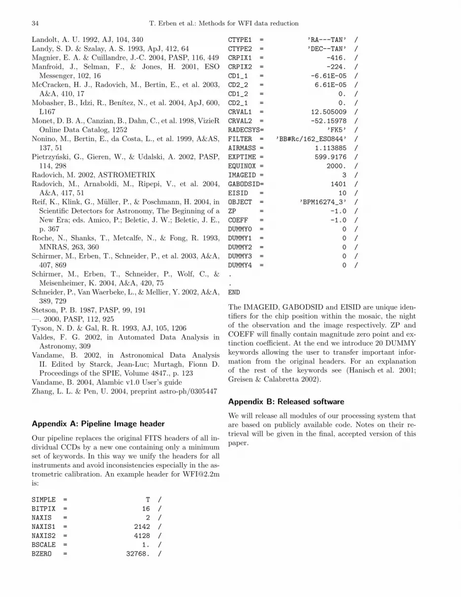
34 T. Erben et al.: Methods for WFI data reduction

Landolt, A. U. 1992, AJ, 104, 340Landy, S. D. & Szalay, A. S. 1993, ApJ, 412, 64Magnier, E. A. & Cuillandre, J.-C. 2004, PASP, 116, 449Manfroid, J., Selman, F., & Jones, H. 2001, ESO

Messenger, 102, 16McCracken, H. J., Radovich, M., Bertin, E., et al. 2003,

A&A, 410, 17Mobasher, B., Idzi, R., Benıtez, N., et al. 2004, ApJ, 600,

L167Monet, D. B. A., Canzian, B., Dahn, C., et al. 1998, VizieR

Online Data Catalog, 1252Nonino, M., Bertin, E., da Costa, L., et al. 1999, A&AS,

137, 51Pietrzynski, G., Gieren, W., & Udalski, A. 2002, PASP,

114, 298Radovich, M. 2002, ASTROMETRIXRadovich, M., Arnaboldi, M., Ripepi, V., et al. 2004,

A&A, 417, 51Reif, K., Klink, G., Muller, P., & Poschmann, H. 2004, in

Scientific Detectors for Astronomy, The Beginning of aNew Era; eds. Amico, P.; Beletic, J. W.; Beletic, J. E.,p. 367

Roche, N., Shanks, T., Metcalfe, N., & Fong, R. 1993,MNRAS, 263, 360

Schirmer, M., Erben, T., Schneider, P., et al. 2003, A&A,407, 869

Schirmer, M., Erben, T., Schneider, P., Wolf, C., &Meisenheimer, K. 2004, A&A, 420, 75

Schneider, P., Van Waerbeke, L., & Mellier, Y. 2002, A&A,389, 729

Stetson, P. B. 1987, PASP, 99, 191—. 2000, PASP, 112, 925Tyson, N. D. & Gal, R. R. 1993, AJ, 105, 1206Valdes, F. G. 2002, in Automated Data Analysis in

Astronomy, 309Vandame, B. 2002, in Astronomical Data Analysis

II. Edited by Starck, Jean-Luc; Murtagh, Fionn D.Proceedings of the SPIE, Volume 4847., p. 123

Vandame, B. 2004, Alambic v1.0 User’s guideZhang, L. L. & Pen, U. 2004, preprint astro-ph/0305447

Appendix A: Pipeline Image header

Our pipeline replaces the original FITS headers of all in-dividual CCDs by a new one containing only a minimumset of keywords. In this way we unify the headers for allinstruments and avoid inconsistencies especially in the as-trometric calibration. An example header for WFI@2.2mis:

SIMPLE = T /

BITPIX = 16 /

NAXIS = 2 /

NAXIS1 = 2142 /

NAXIS2 = 4128 /

BSCALE = 1. /

BZERO = 32768. /

CTYPE1 = ’RA---TAN’ /

CTYPE2 = ’DEC--TAN’ /

CRPIX1 = -416. /

CRPIX2 = -224. /

CD1_1 = -6.61E-05 /

CD2_2 = 6.61E-05 /

CD1_2 = 0. /

CD2_1 = 0. /

CRVAL1 = 12.505009 /

CRVAL2 = -52.15978 /

RADECSYS= ’FK5’ /

FILTER = ’BB#Rc/162_ESO844’ /

AIRMASS = 1.113885 /

EXPTIME = 599.9176 /

EQUINOX = 2000. /

IMAGEID = 3 /

GABODSID= 1401 /

EISID = 10 /

OBJECT = ’BPM16274_3’ /

ZP = -1.0 /

COEFF = -1.0 /

DUMMY0 = 0 /

DUMMY1 = 0 /

DUMMY2 = 0 /

DUMMY3 = 0 /

DUMMY4 = 0 /

.

.

END

The IMAGEID, GABODSID and EISID are unique iden-tifiers for the chip position within the mosaic, the nightof the observation and the image respectively. ZP andCOEFF will finally contain magnitude zero point and ex-tinction coefficient. At the end we introduce 20 DUMMYkeywords allowing the user to transfer important infor-mation from the original headers. For an explanationof the rest of the keywords see (Hanisch et al. 2001;Greisen & Calabretta 2002).

Appendix B: Released software

We will release all modules of our processing system thatare based on publicly available code. Notes on their re-trieval will be given in the final, accepted version of thispaper.