arX

iv:a

stro

-ph/

0210

118v

2 9

Oct

200

2

The Deep Lens Survey

D. Wittmana, J. A. Tysona, I. P. Dell’Antoniob, A. C. Beckera, V. E. Margoninera,J. Cohenc, D. Normand, D. Loombae, G. Squiresf, G. Wilsonb,f, C. Stubbsg, J. Hennawih,

D. Spergelh, P. Boeshaari, A. Clocchiattij, M. Hamuyk, G. Bernsteinl,A. Gonzalezm, P. Guhathakurtan, W. Huo, U. Seljakh, D. Zaritskyp

aBell Labs, Lucent Technologies; bBrown University; cCaltech; dCTIOeUniversity of New Mexico; fIPAC/Caltech; gUniversity of Washington

hPrinceton University; iDrew University; jPUCC; kCarnegie ObservatorylUniversity of Pennsylvania; mUniversity of Florida; nUCO/Lick

oUniversity of Chicago; pSteward Observatory, University of Arizona

ABSTRACT

The Deep Lens Survey (DLS) is a deep BV Rz′ imaging survey of seven 2×2 degree fields, with all data to bemade public. The primary scientific driver is weak gravitational lensing, but the survey is also designed to enablea wide array of other astrophysical investigations. A unique feature of this survey is the search for transientphenomena. We subtract multiple exposures of a field, detect differences, classify, and release transients on theWeb within about an hour of observation. Here we summarize the scientific goals of the DLS, field and filterselection, observing techniques and current status, data reduction, data products and release, and transientdetections. Finally, we discuss some lessons which might apply to future large surveys such as LSST.

Keywords: surveys, gravitational lensing, astrophysical transients

1. SCIENCE DRIVERS

The primary purpose of the DLS is to study the evolution of mass clustering over cosmic time using weakgravitational lensing. Secondary goals include studying the relationship between mass and light through galaxy-galaxy lensing, galaxy and galaxy-quasar correlation functions, and optical searches for galaxy clusters; time-domain astrophysics stemming from the transient search and followup; and enabling a broad array of astrophysicsby publicly releasing a large, uniform dataset of images and catalogs.

The evolution of mass clustering over cosmic time is our primary goal because to date, most of what we knowabout the large-scale structure of the universe comes from the observed anisotropies in the cosmic microwavebackground (CMB) at a redshift z ∼ 1100, and from the distribution of galaxies at z ∼ 0. The concordancemodel of cosmology adequately explains both, but to really test the paradigm, we must examine the evolutionbetween these two extremes.

Weak gravitational lensing is our tool of choice because unlike many other tools, it is sensitive to all typesof matter, luminous or dark, baryonic or not. Furthermore, it provides constraints on cosmological parameterswhich are complementary to the CMB and to the expansion history of the universe as probed by Type Iasupernovae. For example, certain weak lensing statistics constrain Ωm very well while constraining ΩΛ onlyweakly. The CMB and supernovae results each constrain different combinations of Ωm and ΩΛ. The DLS willtest the validity of the foundation of the theoretical model by providing a third, precision measurement relyingon different physics–weak gravitational lensing.

The term “weak lensing” actually includes several independent measurements, all of which take advantageof the fact that shapes of distant galaxies are distorted when their light rays pass through intervening massdistributions on their way to us. The most straightforward measurement is that of counting mass concentrationsabove a certain mass threshold. (Henceforth, we will call these “clusters” for simplicity, but it should beunderstood that weak lensing is sensitive to all mass concentrations, whether or not they contain light-emitting

galaxies.) The number of such clusters as a function of redshift between z = 0 and z = 1 is a sensitive functionof Ωm and w, the dark energy equation of state.

In a complementary measurement, the power spectrum of mass fluctuations is derived from the statisticsof the source shapes without the need to identify any particular mass concentration. This power spectrum isexpected to grow with cosmic time in a certain way, so by measuring it at a series of different redshifts, theDLS will provide sharp constraints on the models.

For visualization, the DLS will produce maps of the mass distribution at a series of redshifts. Assembledinto a time series, these maps will show the growth of structure from z ∼ 1, when the universe was about halfits present age, to the present.

These weak lensing projects imposed the following qualitative requirements on the data:

• imaging in 4-5 different filters with a wavelength baseline sufficient to derive photometric redshifts

• deep enough to derive photometric redshifts for ∼ 50–100 galaxies arcmin−2

• subarcsecond resolution, so that shape information about distant galaxies is retained even after dilutionby seeing

• at least 5 independent, well-separated fields, selected without regard to already-known structures, to geta handle on cosmic variance

• in each field, coverage of an area of sky sufficient to include the largest structures expected

Of course deep imaging is useful for a huge variety of other investigations, so we resolved to retain as muchgeneral utilty as possible while optimizing the survey for lensing. For example, we chose widely used filters(described below) rather than adopting a custom set.

At the same time, we realized that the data would be useful for a completely different application. Inaddition to coadding multiple exposures of the same field, we could subtract one epoch from another and findtransient phenomena including moving objects in the solar system, bursting objects such as supernovae andpossibly optical counterparts to gamma-ray bursts, and variable stars and AGN.

Image subtraction, or difference image analysis (DIA), has been used quite successfully by supernova searchgroups. For that application, however, all other types of transients are nuisances, and their elimination fromthe sample is part of the art of the supernova search. Ironically, there are other groups using the same 4-meter telescopes and wide-field imagers, often during the same dark run, to look for asteroids while discardingsupernovae! We decided to try a new approach, in which we would do the difference image analysis whileobserving and release information about all types of transients on the Web the same night, so that others couldfollow up any subsample of their choosing. This attempt to do parallel astrophysics is in many ways a precursorof the much larger survey projects now in the planning stage which seek to further open the time domain fordeep imaging, and we will discuss some of the lessons learned.

2. BASIC PARAMETERS

We chose the Kitt Peak National Observatory (KPNO) and Cerro Tololo Inter-American Observatory (CTIO)4-m telescopes for their good combination of aperture and field of view. Each telescope is equipped with an 8k× 8k Mosaic imager (Muller et al. 1998), providing a 35′ field of view with 0.25′′ pxels and very small gapsbetween three-edge-buttable devices. A further strength is that with some observing with each of two similarsetups, we can provide a check on systematic errors due to optical distortions, seeing, and the like, withoutsacrificing homegeneity of the dataset in terms of depth, sampling, and so on.

We set our goal for photometric redshift accuracy at 20% in 1 + z. This is quite modest in comparisonto the state of the art, but we do not need better accuracy. A bigger contribution to the error on a lensingmeasurement from any one galaxy is shape noise, the noise stemming from the random unlensed orientations

of galaxies. Thus we do not need great redshift accuracy on each galaxy, but we do need the redshifts to beunbiased in the mean.

To keep the total amount of telescope time reasonable, we wanted to use the absolute minimum numberof filters necessary for estimating photometric redshifts to this accuracy. Simulations showed that four wasthe minimum. We chose a wavelength baseline from Harris B to Sloan z′, which is the maximum possiblewithout taking a large efficiency efficiency hit from the prime focus correctors in U or from a switch to infrareddetectors on the other end. Between these extremes, we chose Harris V and R, where throughput is maximized;simulations showed that photometric redshift performance did not depend critically on these choices.

Our depth goal is a 1-σ sky noise of 29 mag arcsec−2 in BV R and 28 in z′, which required total exposuretimes of 12 ksec in BV z

′ and 18 ksec in R according to exposure time calculators, for a total of 54 ksec exposureon each patch of sky (see below for discussion). We divided this total time into 20 exposures of 600 (900)seconds each in BV z′ (R). Twenty exposures was a compromise between efficiency (given a read time of ∼ 140seconds) and the need to take many dithered exposures to obtain good dark-sky flats.

The metric size of expected mass structures, and the redshift at which they most effectively lens faintbackground galaxies, sets the angular scale for a field. In order to study the mass clustering on linear scales(out to 15h−1 Mpc at z=0.3), we must image 2 × 2 regions of the sky. With Mosaic providing a 40′ fieldof view after dithering, we assemble each 2 field from a 3×3 array of Mosaic-size subfields. Thus each fieldrequires a total exposure time of 9×54 ksec, or 486 ksec.

The number of such fields should be as large as possible to get a handle on cosmic variance. To fit theentire program into a reasonable amount of telescope time, we decided on five fields observed from scratch plustwo others in which we can build on a previous survey, the NOAO Deep Wide-Field Survey (NDWFS). TheNDWFS is a BW RI survey of two 9 deg2 fields with partial JHK coverage as well. We decided to locate a DLSfield within the infrared-covered area of each of these fields, and simply add additional R imaging (10 exposuresof 900 seconds on each patch of sky) to bring it to the same R depth as the remainder of the DLS. Thus thetotal exposure time for piggybacking on the NDWFS fields is 9ksec times 18 subfields, or 162 ksec. The totalexposure time for the entire survey is then 2592 ksec.

The number of nights is then determined by the observing efficiency. The read time of the Mosaic was ∼

140 seconds at the start of the survey, implying about 82% efficiency if the observers are able to focus and takestandard star images during twilight. The read time was slated to decrease significantly after an upgrade from8 to 16-amplifier readout, and so we felt 82% efficiency was a reasonable goal for the entire survey (see belowfor discussion). Thus we needed 3 Msec of time, which is 86 10-hour nights. We split this between KPNO andCTIO by assigning two new and one NDWFS field to KPNO and three new and one NDWFS field to CTIO.

3. FIELD SELECTION

The first consideration in field selection was availability of deep spectroscopy for calibrating photometric redshiftsin at least one field. After choosing that one field, the gross location of the other fields fell into place throughtraditional considerations such as avoiding the plane of the Galaxy and spacing the fields to share nightssmoothly. The precise location was then chosen to avoid bright stars as much as possible. Fields were notchosen with regard to known structures such as clusters.

We chose the Caltech Faint Galaxy Redshift Survey (Cohen et al. 1999) for our deep spectroscopy, so wecentered our first field (F1) in the north at 00:53:25.3 +12:33:55 (all coordinates are J2000). The second field(F2) must then be ∼5 hours earlier or later to be able to share nights with this field. Earlier is impracticalbecause it would require summer observing during the monsoon season at Kitt Peak. A later field would haveto be further north to avoid the plane of the Galaxy. We chose 09:18:00 +30:00:00 because it had few brightstars and low extinction.

In the south, we wanted our fields complementary in RA to those in the north, so that we would not havesimultaneous observing runs in the same month. It was difficult to find three southern fields for the 5–15 hrange evenly spaced in RA, while avoiding the galaxy. The middle of the three (F4) was fixed at 10:52 -05:00because redshifts would be available from the 2dF Galaxy Redshift Survey (2dFGRS, Colless et al. 2001). The

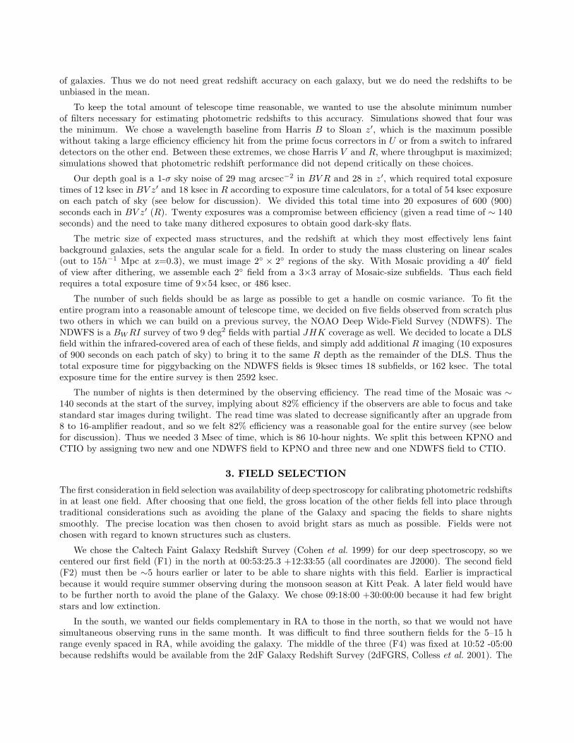
Field RA DEC l,b E(B-V)F1 00:53:25.3 +12:33:55 125,-50 0.06F2 09:18:00 +30:00:00 197, 44 0.02F3 05:20:00 -49:00:00 255,-35 0.02F4 10:52:00 -05:00:00 257,47 0.025F5 13:55:00 -10:00:00 328,49 0.05F6 02:10:00 -04:30:00 166,-61 0.04F7 14:32:06 +34:16:48 57,63 0.015

Figure 1. Field information. Coordinates are J2000, at the field center. F6 and F7 are subsections of the NOAO DeepWide- Field Survey, and their exact positions within the larger NDWFS fields will not be set exactly unto; the imagequality and wavelength coverage variations of the NDWFS are known. Extinctions are from the maps of Schlegel et aland represent rough averages over large areas which vary somewhat.

2dFGRS covers vastly more area, but this happens to be a region of low extinction. (The 2dFGRS goes toz ∼ 0.3, and thus is of much less importance than the CFGRS in calibrating our photometric redshifts, whichwe want to push to z ∼ 2. However, we felt that any additional spectroscopy would help.) The late field (F5)was chosen to be very near the ecliptic to help the hunt for Kuiper belt objects (KBOs); 13:55 -10:00 was chosenfor low extinction, and partial overlap with the Las Campanas Distant Cluster Survey (LCDCS; Gonzalez et

al. 2001). The early field (F3) was the most difficult to place because it was up against the Galaxy. We chose05:20 -49:00, which at a Galactic latitude of -35 is the closest field to the plane.

Note that proximity to the plane is really shorthand for two different things: Galactic extinction, which weextracted from the maps of Schlegel et al, and bright stars, for which we consulted star atlases. Stars in generalare actually helpful for lensing, because they reveal the point-spread function (PSF), but they become uselesswhen saturated (at around 18.5m in most of the R exposures), and in fact become destructive when they arebright enough to prohibit detection and evaluation of galaxies projected nearby (a tenth magnitude star causesa significant amount of lost area). These two aspects are not perfectly correlated, so while F3 is closest to theplane and has the most bright stars, it does not have the greatest extinction.

The NDWFS (F6 and F7) is still completing their observations, so we decided to postpone exact location ofour fields within theirs until late in our survey, when we should know where the imaging quality and wavelengthcoverage are best.

4. OBSERVING STRATEGY

Subarcsecond resolution is common for individual exposures on these telescopes, but achieving this resolutionin the final product of a large survey is another matter, as a large range of seeing conditions is to be expected.We address this problem by observing in R when the seeing conditions are 0.9′′ or better, and switching toB, V , or z′ when the seeing becomes worse than 0.9′′ . Thus the final R images are guaranteed to be 0.9′′ orbetter. We will then make the weak lensing shape measurements in R and use the other filters only for colorinformation.

This seeing dependence is the main element in deciding what to observe when at the telescope. The nextmost important consideration is moon—when there is significant moon illumination, we observe in z′, whichis the least sensitive to such illumination. Next, there is observing efficiency. We can offset, but do notwish to slew while reading out, so the most efficient tactic is to take as many consecutive dithered exposuresas possible on a given subfield. Dithers are up to ±200′′ , or half the width of a 2k×4k device, to insuregood superflats. Although we could change filters rapidly while reading out, the filter is mostly dictated byatmospheric conditions as described above. Thus we settled on a pattern of five dithered exposures in anygiven subfield/filter combination before slewing to another subfield (and possible changing filters if conditionsdictate). This still leaves several degrees of freedom, which we grant to the transient search.

We wish to sample a range of timescales, from minutes to years. As described above, we spend of order onehour on a given subfield/filter combination. This timescale is perfect for discovering inner solar system objects

(in fact it is used by the supernova searches to eliminate asteroids). It is also largely unexplored for more exoticbursting objects; supernova searches do take exposures on a given field one hour apart, but with only two datapoints, anything that does not behave as expected is simply thrown out.

The next priority is to capture the one-month timescale, which has a known population of interestingtransients: supernovae. We schedule runs a month apart for sensitivity to supernovae, and make every attemptto observe subfields and filters which were observed the previous month. At KPNO, we have two runs each yearseparated by a month, and at CTIO, three runs each separated by a month, barring scheduling difficulties.

Finally, we also have day (suitable for searches for rans-neptunian objects and possible optical afterglows ofgamma-ray bursts) and year (suitable for supernovae and AGN) timescales. We have runs of 4–6 nights each,so in the latter half of a run the priority is to revisit a subfield/filter combination done in the first half of therun. And one-year timescales are involved because we typically do not finish all twenty exposures in a givensubfield/filter combination in a single observing season.

5. DATA REDUCTION

The following steps are performed at the end of a run using IRAF’s mscred package:

• Astrometric solution: each image comes is matched to the USNO-A2 star catalog using the msccmatch

task). After this step, the uncertainty in the global RA,DEC coordinate system relative to the USNO-A2is less than 0.01′′ . The rms error in each object’s position is ∼0.3′′ , which is mostly limited by the A-2catalog’s internal accuracy.

• Crosstalk correction: We use the NOAO-determined corrections to mitigate the crosstalk which occurs asmultiple amplifiers are read in parallel. This step and the overscan, zero, and flattening are done with theccdproc task.

• Overscan subtraction

• Zero subtraction

• Flatfield pupil removal: in the KPNO z′ data, a ghost image of the pupil appears as an additive effect inthe dome flats. We use the rmpupil task to remove it.

• Dome-flat correction

• Sky-flat correction: the sky flat is made from a stack of all the deep dome-flattened images in a givenfilter from the entire run.

• Pupil removal (KPNO z′ data only)

• Defringing (z′ data only; rmfringe task)

These are performed in the traditional way, by manually running the tasks and inspecting the results. We feelthat our mission is sufficiently small that every exposure should be inspected. At the same time, the tools tomake an effective pipeline from existing IRAF tasks were not in place when we started the survey. With theemergence of tools like PyRAF, we leave open the possibility that a final re-reduction of all the inspected datamay be done with an automated pipeline.

Conceptually, the next step is the lensing-specific step of making the PSF round. Because this is specificto lensing, this is where our custom software takes over; we view the flatfielded data as “raw” data for ourlensing pipeline. Figure 2 illustrates the problem: an anisotropic PSF mimics a gravitational lensing effect inmany ways, with shapes of objects correlated at least locally. PSFs on real telescopes tend to be ∼ 1 − 10%elliptical, which is much larger than the lensing signal we are looking for, and thus must be eradicated as muchas possible. This is done by convolving the image with a kernel with ellipticity components opposite to that ofthe PSF (Fischer & Tyson 1997). Because the PSF is position-dependent, the kernel must be also.

1000 2000

1000

2000

3000

4000

x (pix)

1000 2000

x (pix)

Figure 2. Point-spread function correction in one 2k×4k CCD. Shapes of stars, which as point sources should be perfectlyround, are represented as sticks encoding ellipticity and position angle. Left panel: raw data with spatially varying PSFellipticities up to 10%. Right panel: after convolution with a spatially varying asymmetric kernel, ellipticities are vastlyreduced (stars with ǫ < 0.5% are shown as dots), and the residuals are not spatially correlated as a lensing signal wouldbe.

However, this correction cannot be applied immediately, as each image must be remapped onto a commoncoordinate system (optical distortions reach 30′′ at the corners of the Mosaic), and this remapping itself changesthe PSF shape. Therefore the software must catalog each image; set up a coordinate system for the final image;match catalogs and use the matches to determine the transformations to the final coordinate system, rejectingoutliers; select stars; compute what the PSF shape will be after remapping (to avoid the computational expenseof writing out intermediate images); fit for the spatial variation of the stellar shapes, rejecting outliers; determinethe photometric scaling between images from the matched catalogs; and combine the images using all thesetransformations. Most of these tasks are implemented as standalone programs written in C, and they areexecuted in the proper order by a Perl script, dlsmake, which also checks the return values, and often theoutput data, of the tasks for potential errors. Human intervention is required only for inspection of the starselection, which sometimes goes awry. There is a graphical user interface which displays the magnitude-sizeplane and allows the user to adjust the stellar locus by dragging a box over it.

Precise registration is crucial, as a small registration error can mimic a shear. The rms departure of objectcentroids from the coordinate fit prediction is ∼ 0.1 pixel, or 0.025′′ . To nullify any PSF shape systematicswhich might have been introduced by this, we select a new sample of stars from the coadded image, and convolveit with the appropriate spatially varying kernel.

We make extensive use of existing tools. For example, we use Sextractor (Bertin & Arnouts 1996) to makequick catalogs of each input image for the pipeline, even though we have not settled on it for the science-gradecataloging of the final images. At the same time, we ask Sextractor to produce a sky-subtracted version of eachinput image. We use these sky-subtracted versions in the combine, so that chip-to-chip sky variations do notproduce artifacts in the final image. These are the only intermediate images written to disk; the resampled andconvolved versions reside only temporarily in buffers in the combine program, dlscombine.

Throughout, attention is paid to masking. In addition to straightforward bad-pixel masking, we must dealwith plumes of scattered light from very bright stars off the edge of the field in some individual exposures. Weuse ds9 to draw regions around these and save a link to the region file in the image header. dlsmake thenmakes a custom bad-pixel mask on the fly, but applies it only where relevant. For example, the region is still

Figure 3. Input and output of the difference imaging technique. The left-most panel shows the template, or comparisonimage, at a previous epoch. The supernova contained in the second epoch image, central panel, is not evident. However,the difference of the two image, right-most panel, subtracts the entire galaxy off, revealing this transient event.

Figure 4. Transient event with no apparent host. The temporal baseline between the template and comparison imagewas approximately 10 months. Photometric follow-up indicated the object was very blue (V − R ∼ 0.08). Spectroscopyfrom the Las Campanas Observatory 6.5-m Baade telescope was inconclusive, but showed a blue featureless continuum.This information combined with a lack of temporal variability over several days suggests this object was possibly a TypeII SN.

examined for sources which will help determine the coordinate transformation or the spatial variation of thePSF; otherwise an image could not be processed at all if a substantial part of it must be masked.

6. TRANSIENTS

In a separate pipeline, we use difference image analysis to subtract off the temporally constant parts of ourimages and reveal the variability. This pipeline is now managed using the Opus data processing environment(Miller & Rose 2001 and references therein), and runs while observing. Thus it must use afternoon dome flatsinstead of sky flats. The difference in image quality is not great, but it is the main reason that these reductionsare carried out separately from the deep imaging reductions.

We use a modified version of the Alard (2000) algorithm to register both the height and shape of theindividual point-spread functions. We difference the individual dithers for short timescale events down to∼ 23rd magnitude, and co-add the images for comparison to a previous co-add for sensitivity down to ∼

24.5th mag. Detection and some winnowing of spurious events (cosmic rays, bleeds from bright stars) isdone automatically, but the observer is required to do the final classification. The main motivation here isthat events are posted to the web as soon as they are approved, so human-caliber quality assurance is moreimportant than maintaining strict objectivity, even if that makes efficiency calculations difficult. The website(http://dls/bell-labs.com/transients.html) lists positions, dates, magnitudes, classifications, and hastime series images similar to the figures shown here. We find several hundred transients per run, so entries arecolor-coded according to classification. For each moving object, the angular velocity is listed, and an ephemerisis available. For stationary objects, a finding chart is available.

Figure 3 shows how well the image subtraction works, revealing a supernova otherwise enmeshed in theisophotes of an extended host galaxy. Over the couse of the survey, we have detected nearly 100 supernovacandidates, and a similar number of transients close enough to the nuclei of galaxies to potentially be AGNs.Over the last year we have made a concerted effort to reacquire supernova candidates on subsequent nights(possibly in other filters) to meet the requirements of the International Astronomical Union for designatingofficial supernova. Thus, 12 out of 14 of our designated supernova have come in the past year. We hope tocoordinate and distribute upcoming supernovae to next-generation supernova projects.

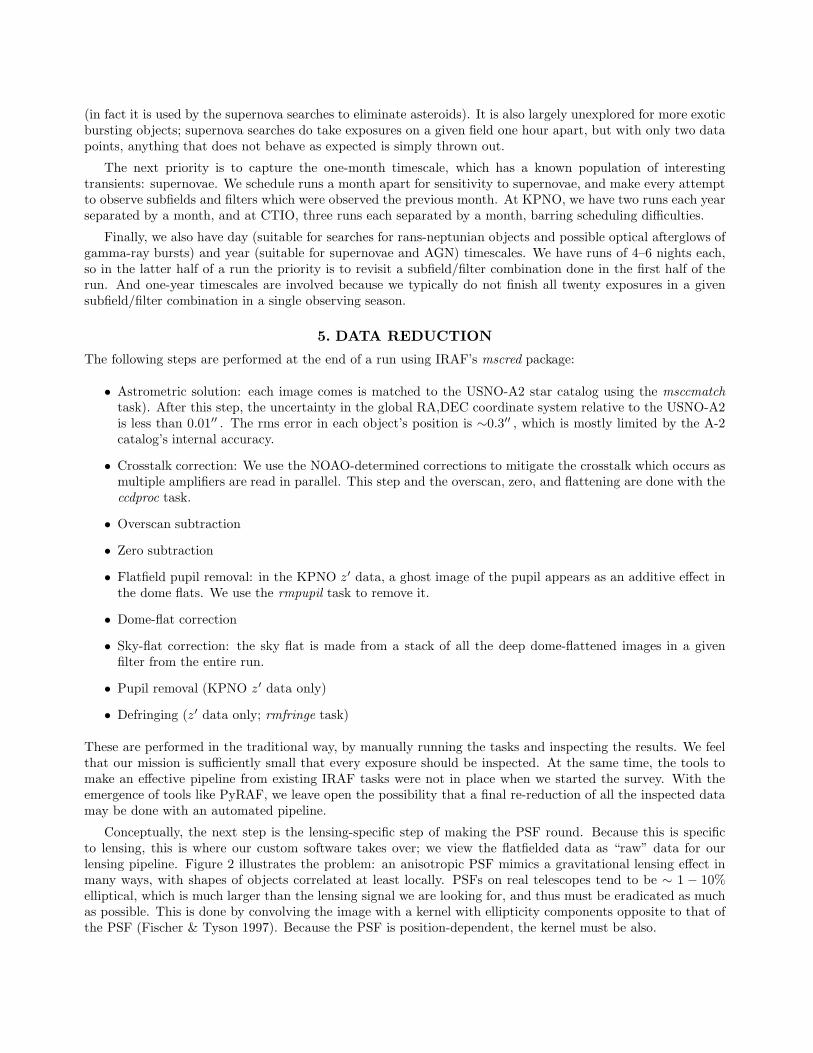
Figure 5. A bright bursting event apparently in a faint host galaxy. Images are separated by 600 seconds. Subsequentspectroscopy showed that the line of sight to the unsuspecting galaxy contained a flare star.

We have had suceess obtaining follow-up observations for the interesting cases where there is no apparenthost for the transient. In the case of the transient in Figure 4, from Jan 2002, we were able to obtain bothphotometric and spectroscopic follow-up observations after disseminating information on this event over theVariable Star NETwork ∗, and expect to further our response by using the Astronomer’s Telegram †.

In the most interesting of the classes of transients, rapidly varying phenomena, we have a very small cropof candidates, none of which have proved to be extragalactic. Figure 5 shows an exaple, in which a burst wasdetected over what appears to be a background galaxy. This burst appeared in the third of five consecutive 600-second exposures, then faded rapidly. We immediately obtained follow-up spectroscopy on the Las CampanasObservatory 6.5-m Baade telescope, showing the spectral signatures of an M4 dwarf with H-α in emission—aforeground Galactic flare star—on top of a faint blue background galaxy. Exotic-looking events with low eventrates are not necessarily astrophysically interesting!

We also have several thousand temporal sequences of solar system objects down to 23rd magnitude. Pre-liminary analysis of this sample confirms the finding by Izevic et al. (2001) of a break in the power-law slope ofthe size distribution. The Minor Planet Center has awarded preliminary designations to approximately 200 ofthese objects.

7. CURRENT STATUS

Observing started in the fall of 1999. After three observing seasons, we have completed 7 of the 63 sub-fields. The remaining coverage is fairly random due to the twin constraints of switching to R in good see-ing and maximizing the transient productivity. Thus most subfields are not yet useful scientifically, becausethe coverage is too shallow and/or limited to a few filters. In the NDWFS fields, the R data upon whichwe intended to piggyback is unsuitable due to poor seeing (lensing is not one of the drivers of that sur-vey), so those fields are very far behind. The full status of each subfield and filter is best visualized athttp://dls.bell-labs.com/progress.html, which is updated after each run. We released deep images andcatalogs of the first two completed subfields in August 2001, and will release five more in August/September2002. Refer to the DLS website http://dls.bell-labs.com for the latest details.

∗http://vsnet.kusastro.kyoto-u.ac.jp/vsnet/†http://atel.caltech.edu/

0 0.5 1 1.5

0

0.5

1

1.5

0 0.5 1 1.5

-0.4

-0.2

0

0.2

0.4

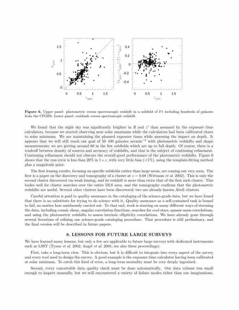
Figure 6. Upper panel: photometric versus spectroscopic redshift in a subfield of F1 including hundreds of galaxiesfrom the CFGRS. Lower panel: residuals versus spectroscopic redshift.

We found that the night sky was significantly brighter in R and z′ than assumed by the exposure time

calculators, because we started observing near solar maximum while the calculators had been calibrated closerto solar minimum. We are maintaining the planned exposure times while assessing the impact on depth. Itappears that we will still reach our goal of 50–100 galaxies arcmin−2 with photometric redshifts and shapemeasurements; we are getting around 60 in the few subfields which are up to full depth. Of course, there is atradeoff between density of sources and accuracy of redshifts, and that is the subject of continuing refinement.Continuing refinement should not obscure the overall good performance of the photometric redshifts. Figure 6shows that the rms error is less than 20% in 1+z, with very little bias (<1%), using the template-fitting methodplus a magnitude prior.

The first lensing results, focusing on specific subfields rather than large areas, are coming out very soon. Thefirst is a paper on the discovery and tomography of a cluster at z = 0.68 (Wittman et al. 2002). This is only thesecond cluster discovered via weak lensing, and its redshift is more than twice that of the first such cluster. Thisbodes well for cluster searches over the entire DLS area, and the tomography confirms that the photometricredshifts are useful. Several other clusters have been discovered; two are already-known Abell clusters.

Careful attention is paid to quality assurance in the cataloging of the science-grade data, but we have foundthat there is no substitute for trying to do science with it. Quality assurance as a self-contained task is boundto fail, no matter how assiduously carried out. To that end, work is starting on many different ways of stressingthe data, including cosmic shear, angular correlation functions, searches for cool stars, quasar-mass correlations,and using the photometric redshifts to assess intrinsic ellipticity correlations. We have already gone throughseveral iterations of refining our science-grade cataloging procedure. That procedure is still preliminary, andthe final version will be described in future papers.

8. LESSONS FOR FUTURE LARGE SURVEYS

We have learned many lessons, but only a few are applicable to future large surveys with dedicated instrumentssuch as LSST (Tyson et al. 2002; Angel et al. 2001; see also these proceedings).

First, take a long-term view. This is obvious, but it is difficult to integrate into every aspect of the surveyand every tool used to design the survey. A good example is the exposure time calculator having been calibratedat solar minimum. To catch this kind of error, a long-term mentality must be very deeply ingrained.

Second, every conceivable data quality check must be done automatically. Our data volume was smallenough to inspect manually, but we still encountered a variety of failure modes richer than our imaginations.

Each instrument has its own peculiarities, so it is vital to have some early data from the instrument to helprefine the software. Simulated data will not do.

Another aspect which simply will not scale is our manual classification of transients. Automatic classificationis a problem which has not been tackled because it hasn’t been necessary, and therefore we really don’t knowhow difficult it will be. Thus, work should be started now, well in advance of any flood of data, and we areplanning to do so in the next year. The example of the flare star in front of a faint galaxy shows that exploringlow-event-rate physics is complicated by all kinds of other low-event-rate processes.

Finally, we have been very successful at finding transients, but followup has been extremely difficult tocoordinate. The problem scales roughly as the factorial of the number of different observatories involved.Furthermore, it is easy to detect transients which are too faint to reach with spectroscopy. Therefore, time-domain experiments like LSST must design in as much self-followup as possible by revisiting fields at a usefulcadence. One thing that would help greatly is obtaining colors right away, which unfortunately wasn’t possiblegiven the design of the DLS. Simply finding transients turned out to be the easy part; the challenge is in followupand in quickly measuring features which enable effective followup.

9. ACKNOWLEDGEMENTS

We thank the KPNO and CTIO staffs for their invaluable assistance. NOAO is operated by the Association ofUniversities for Research in Astronomy (AURA), Inc. under cooperative agreement with the National ScienceFoundation.

REFERENCES

1. Alard, C. A&A 144, 363, 2000.

2. Angel, J. R. P., Claver, C. F., Sarlot, R., Martin, H. M., Burge, J. H., Tyson, J. A., Wittman, D., & Cook,K. American Astronomical Society Meeting, 199, 2001

3. Bertin, E. & Arnouts, S. 1996, A&A Supp., 117, 393

4. Cohen, J. G., Hogg, D. W., Pahre, M. A., Blandford, R., Shopbell, P. L., & Richberg, K. ApJS, 120, 171,1999

5. Colless, M. et al., MNRAS, 328, 1039, 2001

6. Fischer, P. & Tyson, J. A., AJ, 114, 14, 1997

7. Gonzalez, A. H., Zaritsky, D., Dalcanton, J. J., & Nelson, A., ApJS, 137, 117, 2001

8. Ivezic, Z. et al., AJ, 122, 2749, 2001

9. Miller, W. W. & Rose, J. F., ASP Conf. Ser. 238: Astronomical Data Analysis Software and Systems X,10, 325, 2001

10. Muller, G. P., Reed, R., Armandroff, T., Boroson, T. A., & Jacoby, G. H., Proc. SPIE, 3355, 577, 1998

11. Schlegel, D. J., Finkbeiner, D. P., & Davis, M., ApJ, 500, 525, 1998

12. Tyson, T., Wittman, D., Hennawi, J., & Spergel, D. 2002, American Physical Society, April Meeting,Jointly Sponsored with the High Energy Astrophysics Division (HEAD) of the American AstronomicalSociety April 20 - 23, 2002 Albuquerque Convention Center Albuquerque, New Mexico Meeting ID: APR02,abstract #Y6.004, 6004, 2002

13. Wittman, D., Margoniner, V. E., Tyson, J. A., Cohen, J. G. & Dell’Antonio, I., ApJL, submitted, 2002