Kybernetika

Enrique Barbieri; Sergey Drakunov; J. Fernando FigueroaFurther results on sliding manifold design and observation for a heat equation

Kybernetika, Vol. 36 (2000), No. 1, [133]--147

Persistent URL: http://dml.cz/dmlcz/135339

Terms of use:© Institute of Information Theory and Automation AS CR, 2000

Institute of Mathematics of the Academy of Sciences of the Czech Republic provides access to digitizeddocuments strictly for personal use. Each copy of any part of this document must contain theseTerms of use.

This paper has been digitized, optimized for electronic delivery and stamped withdigital signature within the project DML-CZ: The Czech Digital Mathematics Libraryhttp://project.dml.cz

K Y B E R N E T I K A — VOLUME 36 ( 2 0 0 0 ) , NUMBER 1, P A G E S 1 3 3 - 1 4 7

FURTHER RESULTS ON SLIDING MANIFOLD DESIGN AND OBSERVATION FOR A HEAT EQUATION

E N R I Q U E B A R B I E R I , S E R G E Y D R A K U N O V AND J . F E R N A N D O F I G U E R O A

This article presents new extensions regarding a nonlinear control design framework that is suitable for a class of distributed parameter systems with uncertainties (DPS). The control objective is first formulated as a function of the distributed system state. Then, a control is sought such that the set in the state space where this relation is true forms an integral manifold reachable in finite time. The manifold is called a Sliding Manifold. The Sliding Mode controller implements a theoretically infinite gain but with finite control amplitudes serving as an effective tool to suppress the influence of matched disturbances and uncertainties in the system behavior. The theory is developed generically for a finite dimensional Jordan Canonical representation of the DPS. The controller manifold design is described in detail and the observer manifold design can be described in a dual man­ner. Finally, the control law is expressed in terms of the distributed state. However, in a temperature field control problem motivated by a robotic arc-welding application, the simulations presented are done in the standard manner: a reduced-order finite-dimensional model is used to design the controller which is then implemented on a higher-order, still finite-dimensional (truth) model of the system. An analysis of the potential spillover prob­lem shows the effectiveness of our approach. The article concludes with a brief description of the development of an experimental setup that is underway in our Control Systems Lab.

1. INTRODUCTION

We are developing an implementable theory of stable integral manifold synthesis for control and observation problems for a general type of distributed parameter systems (DPS). The first step is to design a manifold which defines control goals and specifications as a function of the system states. Therefore, when the s tate is confined to the manifold by a suitably chosen control, the required goals are achieved. This general problem sta tement is seen to consist of three parts :

1. Manifold Design: the requirements are written as a function of the system states.

2. Control Design: a controller is specified which forces the states to the manifold and maintains them there. At this stage, one assumes the availability of the state vector.

134 E. BARBIERI, S. DRAKUNOV AND J .F . FIGUEROA

3. State Estimator Design: an observer is specified to implement the controller.

Typical examples of DPS include nonlinear diffusion equations modeling the evo­lution of the temperature field in arc welding, and Euler-Bernoulli or Timoshenko equations modeling the vibrations of a flexible manipulator. The main difficulties to control these systems are complexity and strong uncertainty. Although one can assume for simulation purposes that the geometry and properties of the heated ma­terial are known, or that the manipulator payload is negligible, in practice they may vary in a wide range. For these reasons, the control engineer selects a simpli­fied DPS model together with a suitable set of boundary conditions that describe a closely-related problem. For example, a flexible maiiipulator with a payload may be modeled by an Euler-Bernoulli beam equation with clamped-free boundary con­ditions. In arc-welding applications, one may select 2D or 3D heat equations on a plate with Dirichlet-Neumann boundary conditions. After the simplified DPS model is selected, one solves the associated eigenvalue/eigenfunction problem and invokes the assumed-mode method [9, 3] to derive a model for the original system. The resulting model comprises a theoretically infinite number of uncoupled differential equations for the so called system modes. In practice one truncates the model for controller design and simulates on a higher dimensional model so that the effect of unmodelled dynamics or spillover effects can be examined. This familiar technique of truncated modal expansions is therefore seen to lead very naturally to a finite dimensional model in the Jordan Canonical Form. In our work we allow the state vector of the finite dimensional model to evolve in the complex vector space Cn for convenience. The spectrum of the system matrix may consist of real and complex, simple and repeated eigenvalues, with complex eigenvalues appearing in complex conjugate pairs.

The sliding mode control methodology is well developed for finite dimensional systems (see, for example [4] and references therein) but relatively very little has appeared in the literature for infinite dimensional systems [5, 8]. The appeal of the sliding mode controller is its natural insensitivity to matched disturbances and pa­rameter variations thereby providing robustness to the controller. We are interested in employing this design methodology for DPS as applied to the specific engineering problem of robotic arc-welding [2, 6, 7]. The design idea is based on the following procedure: in order to solve a control problem such as the stabilization of the weld width or heat penetration, we reformulate these objectives as a certain function of the system states which defines a desired manifold [7]. A control is found such that the set in the state space where this relation is true forms a sliding manifold, that is, an integral manifold reachable in finite time. The sliding mode algorithm implements a high (theoretically infinite) gain needed to keep the state on the man­ifold and as a result, the influence of disturbances and uncertainties in the system behavior is suppressed.

The remainder of the article is organized as follows: Section 2 describes the general model of DPS that is being considered and its finite dimensional model in the Jordan form; Section 3 introduces two transformations that convert the model to the phase-canonic form where the design of the sliding surface becomes very natural and transparent; Section 4 details the design of the controller sliding manifold; Section 5

Further Results on Sliding Manifold Design and Observation for a Heat Equation 135

provides the control law synthesis and stability analysis via a standard Lyapunov argument; Section 6 illustrates the results by simulation, describes the development of an experimental setup, and takes a glimpse at the spillover problem; and Section 7 draws several conclusions and lists topics for further research.

2. DISTRIBUTED PARAMETER SYSTEM MODEL

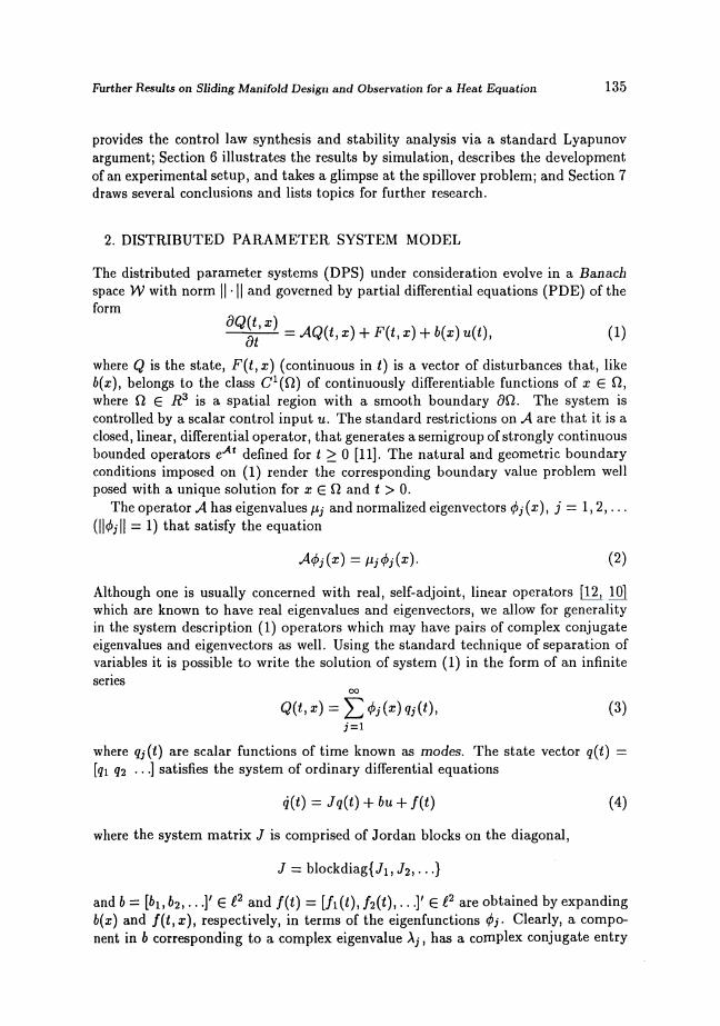
The distributed parameter systems (DPS) under consideration evolve in a Banach space W with norm || • || and governed by partial differential equations (PDE) of the form

^ | ^ = AQ(t, x) + F(t, x) + b(x) u(t), (1)

where Q is the state, F(t,x) (continuous in t) is a vector of disturbances that, like b(x), belongs to the class Cl(Q.) of continuously differentiable functions of x e fi, where Q e R3 is a spatial region with a smooth boundary <9f2. The system is controlled by a scalar control input u. The standard restrictions on A are that it is a closed, linear, differential operator, that generates a semigroup of strongly continuous bounded operators eAt defined for t > 0 [11]. The natural and geometric boundary conditions imposed on (1) render the corresponding boundary value problem well posed with a unique solution for x e fi and t > 0.

The operator A has eigenvalues fij and normalized eigenvectors <j>j(x), j = 1,2,... (||0j|| = 1) that satisfy the equation

A(j>j(x) = ^(j)j(x). (2)

Although one is usually concerned with real, self-adjoint, linear operators [12, 10] which are known to have real eigenvalues and eigenvectors, we allow for generality in the system description (1) operators which may have pairs of complex conjugate eigenvalues and eigenvectors as well. Using the standard technique of separation of variables it is possible to write the solution of system (1) in the form of an infinite series

oo

Q(tyx) = Y,<i>j(x)<l&), (3) i= i

where qj(t) are scalar functions of time known as modes. The state vector q(t) = [qi </2 • • •] satisfies the system of ordinary differential equations

q(t) = Jq(t) + bu + f(t) (4)

where the system matrix J is comprised of Jordan blocks on the diagonal,

J = blockdiag{Ji, J2,...}

and 6 = [&i, 6 2 , . . . ] ' e I2 and f(t) = [fi(t)y f2(t),...]' e I2 are obtained by expanding b(x) and /(tf,x), respectively, in terms of the eigenfunctions </>j> Clearly, a compo­nent in 6 corresponding to a complex eigenvalue Aj, has a complex conjugate entry

136 E. BARBIERI, S. DRAKUNOV AND J .F . FIGUEROA

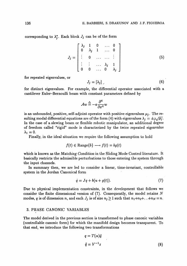
corresponding to A!-. Each block Jj can be of the form

гл;- 1 0 0 ' 0 X, 1 . . . 0

Jj = 0

. 0 0 . . . *i

0

1

(5)

for repeated eigenvalues, or

(6) Jj = [Ay]..

for distinct eigenvalues. For example, the differential operator associated with a cantilever Euler-Bernoulli beam with constant parameters defined by

AW=-aWW

is an unbounded, positive, self-adjoint operator with positive eigenvalues fij. The re­sulting modal differential equations are of the form (4) with eigenvalues Xj = ±Jy/PJ. In the case of a slewing beam or flexible robotic manipulator, an additional degree of freedom called "rigid" mode is characterized by the twice repeated eigenvalue Ai = 0 .

Finally, in the ideal situation we require the following assumption to hold

/(*) G Range{6} — f(t) = bg(t)

which is known as the Matching Condition in the Sliding Mode Control literature. It basically restricts the admissible perturbations to those entering the system through the input channels.

In summary then, we are led to consider a linear, time-invariant, controllable system in the Jordan Canonical form

q = Jq + b(u + д(t)). (7)

Due to physical implementation constraints, in the development that follows we consider the finite dimensional version of (7). Consequently, the model retains IV modes, q is of dimension n, and each Jj is of size nj > 1 such that rai+ri2+- • .+njy = n.

3. PHASE CANONIC VARIABLES

The model derived in the previous section is transformed to phase canonic variables (controllable canonic form) for which the manifold design becomes transparent. To that end, we introduce the following two transformations

q = T(а)q

= V-Xz (8)

Further Results on Sliding Manifold Design and Observation for a Heat Equation 137

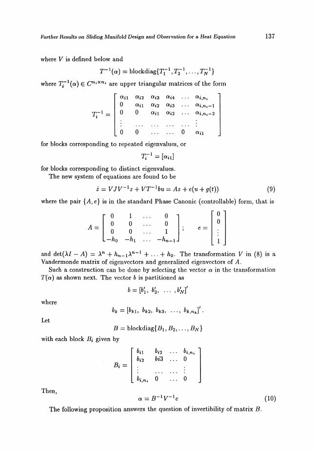
where V is defined below and

T~l(a) = blockdiag{T1-1, I?1,..., T^1}

where TV"1 (a) £ cniXni are upper triangular matrices of the form

т - i =

OÍÌI OLІ2 a i з a i 4

0 aц ai2 aiз

0 0 aц ai2

<*i,nt

ai,nt-l

<xi}ni-2

0 0 0 an

for blocks corresponding to repeated eigenvalues, or

T-1 = [aa]

for blocks corresponding to distinct eigenvalues. The new system of equations are found to be

z = VJV~lz + VT~xbu = Az + e{u + g(t)) (9)

where the pair {A, e) is in the standard Phase Canonic (controllable) form, that is

A-

and det(AI - A) = Xn + hn-i\n"1 + ... + h0. The transformation V in (8) is a Vandermonde matrix of eigenvectors and generalized eigenvectors of A.

Such a construction can be done by selecting the vector a in the transformation T(a) as shown next. The vector 6 is partitioned as

b= [b[, b'2) ... , 6 ^ ]

0 1 o - " 0

0 0 0 0

0 0 1 ; e =

-Лo -hx . • —Һn-\- ì

where

Let

bk = [ЬJЫ, bk2) bk3ì . . . , ЬkìПk] .

B = blockdiag{5i, H2,..., BN}

with each block Bi given by

BІ =

bц Ьi2

Ьi2

6ѓЗ

bi,Пi o

bi,m 0

0

Then, a = B--V-le

The following proposition answers the question of invertibility of matrix B.

(10)

138 E. BARBIERI, S. DRAKUNOV AND J.F. FIGUEROA

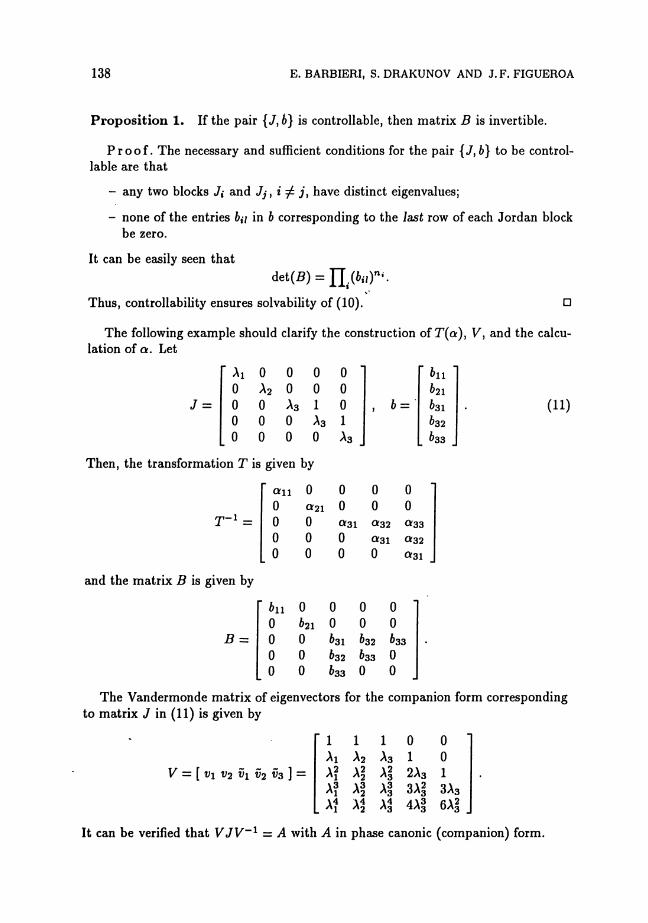
Proposition 1. If the pair {J, b] is controllable, then matrix B is invertible.

P r o o f . The necessary and sufficient conditions for the pair {J,6} to be control­lable are that

- any two blocks J,- a n d J / , i ^ j , have dist inct eigenvalues;

- n o n e of t h e entr ies 6,7 in b corresponding t o t h e last row of each J o r d a n block be zero.

It can be easily seen t h a t

det(5) = rj,.(Mn<-

Thus, controllability ensures solvability of (10). D

The following example should clarify the construction of T(a), V, and the calcu­lation of a. Let

j =

Лi 0 0 A2

0 0 0

0 0

Aз 0 0

0 0 1

Aз 0

Then, the transformation T is given by

т - i =

and the matrix B is given by

в =

oц 0

0 0 0 1

Aз

0

bu 62i 631 Ьз2 bзз

bu 0 0 0 0

«21 0 0 0 0

0

621 0 0 0

<*31 <*32 £*зз 0 «31 <*32 0 0 £*зi

0 0 0 0 0 0

bзi 632 bзз bз2 bзз 0 633 0 0

(П)

The Vandermonde matrix of eigenvectors for the companion form corresponding to matrix J in (11) is given by

V = [ Vг V2 Щ V2 vз ] =

1 1 1 0 0 Ax A2 A 3 1 0 \\ \\ \\ 2A 3 1 Ai A2 A 3 3A3 0A3 \\ \i \i 4Ai 6A1

It can be verified that VJV"1 = A with A in phase canonic (companion) form.

Further Results on Sliding Manifold Design and Observation for a Heat Equation 139

4. CONTROL MANIFOLD SYNTHESIS

The first step in the control design is to consider a linear, time-varying manifold in the state space of system (9) defined by

S = 7i*i + . . • + 7n-l*n-l + Zn - w(t) = 0. (12)

We now prove the main result of this article:

Theorem 1. Denote by P(A) a desired, Hurwitz, closed-loop characteristic poly­nomial written as follows:

P(A) = A n- 1 + 7„- iA n - 2 + . . . + 7 2A + 71- (13)

Consider A;- an eigenvalue of J and compute the polynomials Pk, k = 2, 3 , . . . , n;-

A(A) = P « . If the control u in system (7) is such that the state q belongs to the time-varying manifold

S={qeCn : Kq(t) - w(t) = 0} (14)

for t > t\j then the coefficient vector K is given by

к = Ei(Ai)P2(A1)...P1(A2)P2(A2)

П 2

. • V.

П l

т-\ (15)

P r o o f . Since the control u is such that S = 0 for t > t\, then, from (12) we have

Zn = -7iZi - . . . - 7n-l*n-l + W(t), (16)

and the dynamics of the closed loop system restricted to S are described by

i i = z2

\ \ (17)

i„_i = - 7 i * i - . . . - 7„_i*„-i + w(t).

which indicates that 7 i , . . . , 7 n _ i are the coefficients of the characteristic polyno­mial (13) for the free motion of the system constrained within the manifold.

Now, let us return to the original state variable q. The function S can be writ­ten as

r *i

*2

S= [ т i , - . , T n - i . l ] — w(t) = y'z — w(t). (18)

140 E. BARBIERI, S. DRAKUNOV AND J.F. FIGUEROA

or equivalently, S = YVT-1q-w(t) (19)

from which the result follows as we observe that the product y'V can be written as shown in (15). •

R e m a r k . We show next that (15) is equivalent to Ackermann's Pole Placement formula. For brevity we show this for a second order Jordan system. Ackermann's formula [1] for a gain vector K in the full-state feedback law u = Kq for system (7) can be written as follows

K = e'C-l(J,b)Pdes(J) (20)

where C(J, 6) is the Controllability matrix of the pair (J, 6), and Pdes denotes the desired closed-loop characteristic polynomial. Using the notation in this paper, it is straightforward to verify that

K = e'(V')-1(B')-1Pdes(J) = a'Pdes(J)

Pi(Ai) P2(Ai) 0 Pi(Xi)

= [«i a2] = [A(Ai) Л(Ai)]Г - ì

5. CONTROL DESIGN

Let us assume that the control u in (1) is such that it steers and keeps the state Q on the manifold

S(t, Q) = J a(x)Q(t) x) dx - w(t) Jd

= (a(x),Q(t,x))Li-w(t) = Q. (21)

Then N

S = £>(<) M*)' h ^ v - (0- (22)

Comparing (22), (14), and (15) we obtain that, to guarantee the desired dynamics,

N

a(x)cj>j(x)dx = Kj => a(x) ^^Krf^x) (23) i = i

/ Jft

that is, the function c(x) is easily resolved by invoking the orthogonality property of the eigenfunctions <f>j(x).

The general expression for the control law can be written as

u = -(<r(z), b(x))ll2 (A<r(x), Q(t, x))L2 - g(t) + v(S), (24)

where v(S) is any function continuous or discontinuous such that Sv(S) < 0. In this case, differentiating (21) and using (1) and (24) we obtain

S = -v (S) (25)

Further Results on Sliding Manifold Design and Observation for a Heat Equation 141

which guarantees convergence S —> 0. If g(t) cannot be measured as it usually happens in practice, then let v(S) = —Msign(S). In this case the control law

u = -(<T(X),b(x))ll(Aff(x)tQ(t, x))L* - Msign(S), (26)

results in S = —M sign(S) + g(t) and convergence is guaranteed if \g\ < M, that is, if the control magnitude M dominates the bound on the disturbance vector g.

5.1. Observer design

The problem of designing an observer can be treated as the dual of the controller design. Due to space limitations however, the details are not included in this paper.

6. A TEMPERATURE FIELD CONTROL PROBLEM

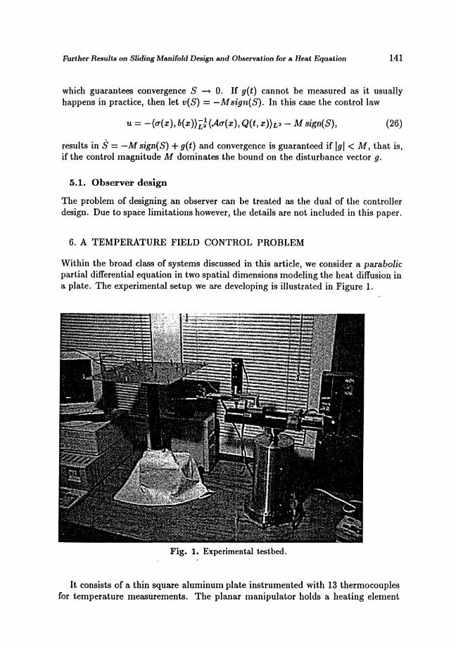
Within the broad class of systems discussed in this article, we consider a parabolic partial differential equation in two spatial dimensions modeling the heat diffusion in a plate. The experimental setup we are developing is illustrated in Figure 1.

Fig. 1. Experimental testbed.

It consists of a thin square aluminum plate instrumented with 13 thermocouples for temperature measurements. The planar manipulator holds a heating element

142 E. BARBIERI, S. DRAKUNOV AND J .F . FIGUEROA

with its end-effector that is used as the heat input. The motivation is a robotic arc-welding application. The controller is synthesized using the SIMULINK environment and implemented in a DSP board by dSPACE. In this article we only report on simulation results.

The operator A is the Laplacian defined in L2(Q) which, together with Dirichlet-Neumann boundary conditions, is known to be a positive self-adjoint operator with positive (real) eigenvalues Aj, j = 1,2,... and normalized eigenfunctions <f>j(x), j = 1,2,... forming an orthonormal basis for the Hilbert space L2(Q).

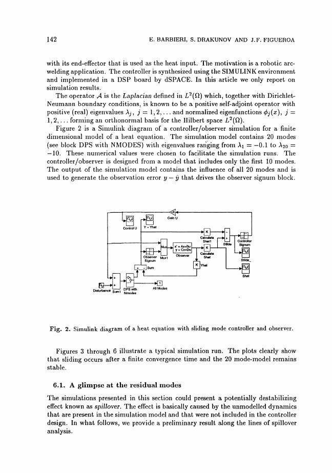
Figure 2 is a Simulink diagram of a controller/observer simulation for a finite dimensional model of a heat equation. The simulation model contains 20 modes (see block DPS with NMODES) wTith eigenvalues ranging from Ai = —0.1 to A20 = — 10. These numerical values were chosen to facilitate the simulation runs. The controller/observer is designed from a model that includes only the first 10 modes. The output of the simulation model contains the influence of all 20 modes and is used to generate the observation error y — y that drives the observer signum block.

Fig. 2. Simulink diagram of a heat equation with sliding mode controller and observer.

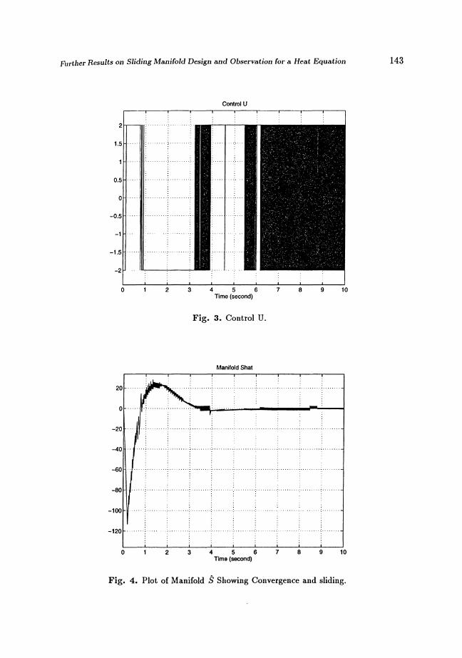
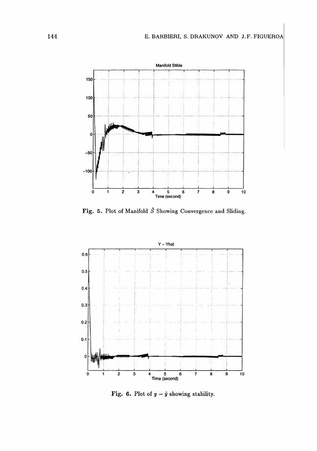
Figures 3 through 6 illustrate a typical simulation run. The plots clearly show that sliding occurs after a finite convergence time and the 20 mode-model remains stable.

6.1. A glimpse at the residual modes

The simulations presented in this section could present a potentially destabilizing effect known as spillover. The effect is basically caused by the unmodelled dynamics that are present in the simulation model and that were not included in the controller design. In what follows, we provide a preliminary result along the lines of spillover analysis.

Further Results on Sliding Manifold Design and Observation for a Heat Equation 143

20-

0-

-20

-40

-60

-80-

- 1 0 0 -

-120-

Control U

2

i i i i i i i i i 1

2 Hl PMШШfli И__И_H

1.5 ннннн 1 нËlHtHEH

0.5 HHHHH 0 HHEІІHH

0.5 иPЯИИІ -1 HHHHHI 1.5 . HlHiiHH -2 H l HИ---ДД--І--M -2

_ L . . . 1 L . . 1 L _ _ . . _ J . 1 , . , 1 _ J

0 1 2 3 4 5 6 7 8 9 10 Time (second)

Fig. 3. Control U.

Manifold Shat

1 1 1 1 1 1 1

' • " / " ' • " / "

1 І І 1 І І. ._ . _ І . . J 0 1 2 3 4 5 6 7 8 9 10

Time (second)

Fig. 4. Plot of Manifold S Showing Convergence and sliding.

144 E. BARBIERI, S. DRAKUNOV AND J . F . FIGUEROA

Manifold Stilde

150

100

-100

- i 1 i 1 Г"

J i i i i i i_ 0 1 2 3 4 5 6 7 8 9 10

Time (second)

Fig . 5. Plot of Manifold S Showing Convergence and Sliding.

Y - Yhat

0.6 -i i i i i i i i i

0.5 : • • : \ -

0.4 : ; ; ; ; -

0.3 : : : ; -

0.2 • • • ; .; • • • • - ; ; -

0.1

0

; ; ; ; -0.1

0

i i i i i i i i

4 5 6 Time (second)

9 10

Fig. 6. Plot of y — y showing stability.

Further Results on Sliding Manifold Design and Observation for a Heat Equation 145

Consider the following infinite dimensional model

X =

Y

л m 0 0 л r

= [CmCr]X

Xm

Xr +

Ьm

W («(*)+*(*)) (27)

where the subscript m denotes modeled and the subscript r denotes residual. There­fore, Xm £ Rm and in practice, one would consider Xr £ Rr where r >• ra.

The design of a sliding mode controller/observer pair discussed in the simulations section leads to the following sliding surface dynamics

l'bm + (ІL)(CmL)-lCrbr 0 O f Ø r —O771L/ +

El E2

(28)

where S is the controller sliding function, a is the observer sliding function, the respective control/observer inputs are u and v, the observer gain matrix is L, and Fi and F2 are disturbance functions.

In order to design a sliding mode controller of the form u~ M sign(S) in the first equation of (28), it is necessary that the sign of the coefficient of u be known. Upon examining (28), we establish the following fairly conservative bound that makes the coefficient of u positive. The bound also provides a guideline in the selection of L and of the relative sizes of ra and r, that is, the modeled and residual subsystem sizes:

Proposit ion 2, If \\Crbr\\ < \\(ÍL)(CmL)-'\\

then the coefficient of u in (28) is positive. Moreover, the observer gain L may be selected in accordance with the following mini-max problem:

minmaxA[ L(CmL)-l(CmL)-'L1 ]

where A() is an eigenvalue of the indicated matrix.

We observe that the above proposition also gives an indication of how to tackle the sensor placement problem. This direction is currently being investigated.

7. CONCLUSIONS

We have investigated the problems of control and observation designs for a class of distributed parameter systems. In particular, we write the system in the Jordan canonical form and develop a formula for the sliding manifolds. The main result states that the manifolds can be synthesized in terms of the desired closed-loop characteristic polynomial evaluated at the known open-loop eigenvalues. This result was initially reported at the 1997 American Control Conference by Drakunov et al [6] for the special case of a diagonal system matrix. The recent work in 1998 by

146 E. BARBIERI, S. DRAKUNOV AND J. F. FIGUEROA

Ackermann and Utkin [1] makes a connection between the manifold design problem and Ackermann's formula for eigenvalue placement. The connection between our result and Ackermann's formula is also shown. Simulations are included for a heat equation and a brief analysis of the spillover problem is presented. Further research efforts are underway to (1) obtain experimental results on a square plate temperature control problem; (2) to tackle the sensor placement problem using Proposition 2; and (3) to apply the results of this paper to an arc-welding problem for weld-quality control.

ACKNOWLEDGEMENTS

The authors gratefully acknowledge the support of NSF Grant ECS-9631321,BOR Grant 96-98-RD-B-09, and NSF Grant CMS-9813284. The article was prepared while the first author was on sabbatical in the Departamento de Automatica y Sistemas, Escuela de Ingenieria Electrica, Universidad de Carabobo, Venezuela. Their support and that of Programa Perez Bonalde, Funda,ya,cucho, Caracas, Venezuela, are also recognized.

(Received December 11, 1998.)

R E F E R E N C E S

[1] J. Ackermann and V. Utkin: Sliding mode control based on Ackermann's formula. IEEE Trans. Automat. Control 43 (1998), 2, 234-237.

[2] E. Barbieri and S. Drakunov: Manifold control and observation of Jordan forms with application to distributed parameter systems. In: Proceedings of the 1998 Conference on Decision and Control (CDC), Tampa, Fl.

[3] E. Barbieri and U. Ozgiiner: Unconstrained and constrained mode expansions for a flexible slewing link. ASME J. Dynamic Systems, Measurement and Control 110 (1988), 4, 416-421.

[4] R. DeCarlo, S. Zak and S. Drakunov: Variable structure and sliding mode control. In: The Control Handbook (W.S. Levine, ed.), CRC Press, Boca Raton, Fl. 1996, pp. 941-950.

[5] S. Drakunov and U. Ozguner: Generalized sliding modes for manifold control of dis­tributed parameter systems. In: Variable Structure and Lyapunov Control (Lecture Notes in Control and Information Sciences Series 193, A.S.I . Zinober, ed.), Springer-Verlag, Berlin 1994, pp. 109-132.

[6] S. Drakunov S. and E. Barbieri: Sliding surfaces design for distributed parameter sys­tems. In: Proceedings of the 1997 American Control Conference (ACC), Albuquerque 1997, pp. 3023-3027.

[7] S. Drakunov, E. Barbieri and D. Silver: Sliding mode control of a heat equation with application to arc welding. In: Proceedings of the 1996 IEEE International Conference on Control Applications, Dearborn 1996, pp. 668-672.

[8] S. Drakunov and V. Utkin: Sliding mode control in dynamic systems. Internat. J. Control 55(1992), 4, 1029-1037.

[9] L. Meirovitch: Analytical Methods in Vibrations. MacMillan, New York 1967. [10] J .T . Oden: Applied Functional Analysis. Prentice-Hall, Englewood Cliffs, N.J. 1979. [11] D. Russell: Observability of linear distributed-parameter systems. In: The Control

Handbook (W.S. Levine, ed.), CRC Press, Boca Raton, Fl. 1996, pp. 1169-1175.

Further Results on Sliding Manifold Design and Observation for a Heat Equation 147

[12] L.A. Segel: Mathematics Applied to Continuum Mechanics. MacMillan, New York 1977.

Dr. Enrique Barbieri, Dr. Sergey Drakunov, Department of Electrical Engineering and Computer Science, Tulane University, New Orleans, LA 70118. U.S.A. e-mails: barbieri,drakunov@eecs.tulane.edu

Dr. J. Fernando Figueroa, Department of Mechanical Engineering, Tulane University, New Orleans, LA 70118. U.S.A. e-mail: fernando@mailhost.tcs.tulane.edu