Embed Size (px)
Citation preview
arX
iv:0
910.
1559
v3 [
mat
h.G
T]
24
Oct
201
0
Contemporary Mathematics
Fundamental groups, Alexander invariants, and
cohomology jumping loci
Alexander I. Suciu
Dedicated to Anatoly Libgober on the occasion of his sixtieth birthday
Abstract. We survey the cohomology jumping loci and the Alexander-typeinvariants associated to a space, or to its fundamental group. Though most ofthe material is expository, we provide new examples and applications, whichin turn raise several questions and conjectures.
The jump loci of a space X come in two basic flavors: the characteristicvarieties, or, the support loci for homology with coefficients in rank 1 localsystems, and the resonance varieties, or, the support loci for the homology ofthe cochain complexes arising from multiplication by degree 1 classes in thecohomology ring of X. The geometry of these varieties is intimately relatedto the formality, (quasi-) projectivity, and homological finiteness properties ofπ1(X).
We illustrate this approach with various applications to the study of hy-perplane arrangements, Milnor fibrations, 3-manifolds, and right-angled Artingroups.
Contents
1. Introduction 22. Characteristic varieties 53. Homology of abelian covers 84. Alexander invariants 105. Resonance varieties 156. Bieri–Neumann–Strebel–Renz invariants 177. Formality properties 198. Kahler and quasi-Kahler manifolds 219. Hyperplane arrangements 26
2000 Mathematics Subject Classification. Primary 14F35; Secondary 20J05, 32S22, 55N25.Key words and phrases. Fundamental group, Alexander polynomial, characteristic variety,
resonance variety, abelian cover, formality, Bieri–Neumann–Strebel–Renz invariant, right-angledArtin group, Kahler manifold, quasi-Kahler manifold, hyperplane arrangement, Milnor fibration,boundary manifold.
Partially supported by NSA grant H98230-09-1-0012 and an ENHANCE grant from North-eastern University.
c©0000 (copyright holder)
1
2 ALEXANDER I. SUCIU
10. Milnor fibrations 3311. Three-dimensional manifolds 37References 41
1. Introduction
1.1. Fundamental groups. The fundamental group of a topological spacewas introduced in 1904 by H. Poincare, with the express purpose of distinguishingbetween certain manifolds, such as the dodecahedral space and the three-sphere,which otherwise share a lot in common. Subsequently, it was realized that thegeometric nature of a manifold M influences the group-theoretic properties of itsfundamental group, π1(M); and conversely, the nature of a group G can say a lotabout those manifolds with fundamental group G, at least in low dimensions.
As is well-known, every finitely presented group G occurs as the fundamentalgroup of a smooth, compact connected, orientable manifold M of dimension n = 4.The manifold can even be chosen to be symplectic (Gompf); and, if one is willingto go to dimension n = 6, it can be chosen to be complex (Taubes). On the otherhand, requiring M to be 3-dimensional, or to carry a Kahler structure puts severerestrictions on its fundamental group.
A finitely presented group G is said to be a Kahler group if it can be realizedas G = π1(M), where M is a compact, connected Kahler manifold. The notions ofquasi-Kahler group and (quasi-) projective group are defined similarly. A classicalproblem, formulated by J.-P. Serre in the late 1950s (cf. [80]), is to determine whichgroups can be so realized.
A basic theme of this survey is that certain topological invariants, such as theAlexander polynomial, or the cohomology jumping loci, are very good tools forstudying questions about fundamental groups in algebraic geometry. In particular,they can be brought to bear to settle Serre’s realization problem for several notableclasses of groups.
1.2. Alexander-type invariants. In his foundational paper [1], J. W. Alexan-der assigned to every knot K in S3 a polynomial with integer coefficients, asfollows. Let π : X ′ → X be the infinite cyclic cover of the knot complement.Then A = H1(X
′, π−1(x0),Z) is a finitely presented module over the group ringZZ ∼= Z[t±1]. The Alexander polynomial, ∆K(t), equals—up to normalization—the greatest common divisor of the codimension 1 minors of a presentation matrixfor the Alexander module A. Clearly, ∆K(t) depends only on the knot group,G = π1(X, x0). More generally, if K is an n-component link in S3, there is a multi-variable Alexander polynomial ∆K(t1, . . . , tn), depending only on the link group,and a choice of meridians.
These definitions extend with only slight modifications to arbitrary finitely pre-sented groups (see §4). In [54], A. Libgober considered the single-variable Alexanderpolynomial ∆C(t) associated to the complement of an algebraic curve C ⊂ C2, andits total linking cover. He then proved in [56] that all the roots of ∆C(t) are roots ofunity, a result which constrains the class of groups realizable as fundamental groupsof plane curve complements.
FUNDAMENTAL GROUPS AND COHOMOLOGY JUMPING LOCI 3
As shown in [29, 30], the multi-variable Alexander polynomial and the relatedAlexander varieties provide further constraints on the kind of fundamental groupsthat can appear in this algebraic context. For example, if G is a quasi-projectivegroup with b1(G) 6= 2, then the Newton polytope of ∆G is a line segment; and, ifG is a projective group, then ∆G must be constant (see Theorem 8.10).
1.3. Cohomology jumping loci. An essential tool for us are the cohomologyjumping loci associated to a connected, finite-type CW-complex X . The charac-teristic varieties V id(X, k) are algebraic subvarieties of Hom(π1(X), k×), while theresonance varieties Ri
d(X, k) are homogeneous subvarieties ofH1(X, k). The formerare the jump loci for the homology of X with rank 1 twisted complex coefficients(see §2), while the latter are the jump loci for the homology of the cochain com-plexes arising from multiplication by degree 1 classes in H∗(X, k) (see §5). Thejump loci of a group are defined in terms of the jump loci of the correspondingclassifying space.
It has been known since the work of Hironaka [51] that the degree 1 characteris-tic varieties of a finitely generated group G coincide with the determinantal varietiesof its Alexander matrix, at least away from the origin. A more general statement,valid in arbitrary degrees, was recently proved in [74] (see Theorem 4.6).
Foundational results on the structure of the characteristic varieties of Kahlerand quasi-Kahler manifolds and smooth projective and quasi-projective varietieswere obtained by Beauville [6], Green–Lazarsfeld [49], Simpson [82], Campana [11],and ultimately, Arapura [3]. In particular, if X = X \D, with X compact Kahler,b1(X) = 0, and D a normal-crossings divisor, then each variety V id(X,C) is a unionof subtori of Hom(π1(X),C×), possibly translated by unitary characters (see §8).In [57], Libgober—who coined the name “characteristic varieties”—showed how tofind irreducible components of V1
d(X,C) from the faces of a certain “polytope ofquasiadjunction,” in the case when X is a plane curve complement. Recently, heproved in [59] a local version of Arapura’s theorem, in which all the translationsare done by characters of finite order.
The resonance varieties were first defined by Falk in [39], in the case when X =X(A) is the complement of a complex hyperplane arrangement A. Best understoodare the degree 1 resonance varieties Rd(A) = R1
d(X(A),C); these varieties admita very precise combinatorial description, owing to work of Falk [39], Cohen–Suciu[18], Libgober [57], Libgober–Yuzvinsky [60], and others, with the state of the artbeing the work of Falk, Pereira, and Yuzvinsky [41, 75, 91].
The cohomology jump loci provide a unifying framework for the study of ahost of questions, both quantitative and qualitative, concerning a space X and itsfundamental group, G = π1(X). A lot of the recent developments described in thissurvey come from our joint work with A. Dimca and S. Papadima [29, 30, 31, 32,72, 74].
1.4. Abelian covers. As shown by Libgober in [55], with further refinementsby Hironaka [50], Sarnak–Adams [79], Sakuma [78], and Matei–Suciu [65], countingtorsion points on the character group, according to their depth with respect to thestratification by the characteristic varieties, yields very precise information aboutthe homology of finite abelian covers of X (see §3).
An old observation in knot theory is that the Alexander polynomial ∆K(t)of a fibered knot K is monic. More generally, Dwyer and Fried [34] showed that
4 ALEXANDER I. SUCIU
the support varieties of the Alexander invariants of a finite CW-complex completelydetermine the homological finiteness properties of its free abelian covers. This resultwas recast in [74] in terms of the characteristic varieties and their (exponential)tangent cones (see Theorem 3.2).
In [8], Bieri, Neumann, and Strebel associated to every finitely generated groupG an open, conical subset Σ1(G) of the real vector space Hom(G,R). The BNSinvariant and its higher-order generalizations, the invariants Σq(G,Z) of Bieri andRenz [9], hold subtle information about the homological finiteness properties ofnormal subgroups of G with abelian quotients (see §6). The actual computation ofthe Σ-invariants is enormously complicated. Yet, as shown in [74], the cohomologyjumping loci of a classifying space K(G, 1) provide computable upper bounds forthe Σ-invariants of G (see Theorems 6.1 and 6.2).
1.5. Formality and the tangent cone formula. A central point in thetheory of cohomology jumping loci is the relationship between the characteristic andresonance varieties. As proved by Libgober in [58], the tangent cone to V id(X,C)at the origin is contained in Ri
d(X,C), for any finite-type CW-complex X . But, asfirst noted in [65], the inclusion can be strict; in fact, as shown in [30], equalitymay even fail for quasi-projective groups.
The crucial property that bridges the gap between the tangent cone to a char-acteristic variety and the corresponding resonance variety is formality (see §7). Aspace X as above is formal if its Sullivan minimal model is quasi-isomorphic to(H∗(X,Q), 0), while a finitely generated group G is 1-formal if its Malcev Lie alge-bra has a quadratic presentation. For a recent survey of these notions, we refer to[73].
One of the main results from [30] establishes an isomorphism between theanalytic germ of V1
d(G,C) at 1 and the analytic germ of R1d(G,C) at 0, in the case
when G is a 1-formal group (see Theorem 7.1). This isomorphism provides a new,and very effective 1-formality criterion.
As also shown in [30], the tangent cone theorem, when used in conjunction withArapura’s theorem, imposes very strong restrictions on the nature of the resonancevarieties of Kahler groups, and, more generally, 1-formal, quasi-Kahler groups (seeTheorem 8.5). These restrictions lead to both quasi-projectivity obstructions (inthe formal setting), and enhanced formality obstructions (in the quasi-projectivesetting).
1.6. Applications. The techniques described above have a large range of ap-plicability. We illustrate their usefulness with a variety of examples, arising inalgebraic geometry, low-dimensional topology, combinatorics, and group theory.
As a running example, we use an especially well-suited class of combinatoriallydefined spaces. A simplicial complex L on n vertices determines a subcomplex TL ofthe n-torus, with fundamental group the right-angled Artin groupGΓ correspondingto the graph Γ = L(1). The cohomology jumping loci of these “toric complexes”were computed in [72]. Using the computation of R1
1(GΓ,C), it was shown in [30]that a groupGΓ is quasi-projective if and only if Γ is a complete multi-partite graph.We show here that the Alexander polynomial of GΓ is non-constant if and only ifΓ has connectivity 1 (see Proposition 4.13).
In §9, we treat in detailed fashion an important class of quasi-projective va-rieties: those arising as complements of complex hyperplane arrangements. The
FUNDAMENTAL GROUPS AND COHOMOLOGY JUMPING LOCI 5
cohomology jumping loci of such a complement, X = X(A), are rather well under-stood, especially in degree 1, with a major open problem being the determination ofthe translated components in V1
1 (X(A),C). Much effort has been put over the yearsinto comprehending fundamental groups of arrangements (see [83] for more on thissubject). We identify here precisely the class of line arrangements A in C2 for whichthe group G(A) = π1(X(A)) is a Kahler group (see Theorem 9.11), respectively, aright-angled Artin group (see Theorem 9.12). Along the way, we reprove a recentresult of Fan [43], identifying those line arrangements A for which G(A) is a freegroup (see Theorem 9.10).
In §10, we discuss Milnor fibrations, with special emphasis on those arisingfrom hyperplane arrangements. A well-known construction, due to J. Milnor [68],associates to a weighted homogeneous polynomial f ∈ C[z0, . . . , zd] of degree n asmooth fibration, f : X → C×, where X is the complement in Cd+1 of the hypersur-face f = 0. The Milnor fiber, F = f−1(1), is an n-fold cyclic cover of U = X/C×.We review this construction, and the method of computing the homology groupsH1(F, k) from the characteristic varieties V1
d(U, k), provided (chark, n) = 1. Wealso review recent progress on the formality question for the Milnor fiber, firstraised in [73], and recently answered—with different examples—by Zuber [92] andFernandez de Bobadilla [46].
We conclude in §11 with a look at the world of 3-dimensional manifolds. Amajor application of the techniques discussed in this survey is the solution givenin [32] to the following question asked by S. Donaldson and W. Goldman in 1989,and independently by A. Reznikov in 1993: Which 3-manifold groups are Kahlergroups? The proof uses in an essential way the contrasting nature of the resonancevarieties for these two classes of groups. Another application, given in [31], is tothe classification (up to Malcev completion) of 3-manifold groups which are also1-formal, quasi-Kahler groups. This classification can be made very precise in thecase of boundary manifolds of line arrangements in CP2: as shown in [20] and [29],the only way the fundamental group of a boundary manifold M(A) can be either1-formal, or quasi-Kahler (or both), is for A to be a pencil, or a near-pencil.
2. Characteristic varieties
We start with the jumping loci for homology in rank 1 local systems, and twotypes of tangent cones associated to a subvariety of the character variety of a group.
2.1. Rank 1 local systems. Let X be a connected CW-complex, with finitek-skeleton, for some k ≥ 1. Without loss of generality, we may assumeX has a single0-cell, call it x0. Moreover, we may assume all attaching maps (Si, ∗) → (X i, x0)are basepoint-preserving.
Fix a field k, and denote by (Ci(X, k), ∂i)i≥0 the cellular chain complex of
X . Let p : X → X be the universal cover. The cell structure on X lifts in a
natural fashion to a cell structure on X . Fixing a lift x0 ∈ p−1(x0) identifiesthe fundamental group, G = π1(X, x0), with the group of deck transformations of
X, which permute the cells. Therefore, we may view (Ci(X, k), ∂i)i≥0 as a chaincomplex of left-modules over the group ring kG.
Let k× be the group of units in k. The group of k-valued characters, Hom(G, k×),is an algebraic group, with pointwise multiplication inherited from k×, and identitythe character taking constant value 1 ∈ k× for all g ∈ G. This character group
6 ALEXANDER I. SUCIU
parametrizes rank 1 local systems on X : given a character ρ : G → k×, denoteby kρ the 1-dimensional k-vector space, viewed as a right module over the groupring kG via a · g = ρ(g)a, for g ∈ G and a ∈ k. The homology groups of X withcoefficients in kρ are defined as
(1) Hi(X, kρ) := Hi(C•(X, k)⊗kG kρ).
In this setup, the identity 1 ∈ Hom(G, k×) corresponds to the trivial coefficientsystem, k1 := k, and H∗(X, k) is the usual homology of X with k-coefficients.
2.2. Homology jump loci. Computing homology groups with coefficients inrank 1 local systems leads to a natural filtration of the character group.
Definition 2.1. The characteristic varieties of X (over k) are the Zariski closedsets
V id(X, k) = ρ ∈ Hom(G, k×) | dimkHi(X, kρ) ≥ d,
defined for all integers 0 ≤ i ≤ k and d > 0.
When computing the characteristic varieties in degrees up to k, we may assume,without loss of generality, that X is a finite CW-complex of dimension k+1; see [74,Lemma 2.1] for an explanation. In each fixed degree i, the characteristic varietiesdefine a descending filtration on the character group,
(2) Hom(G, k×) ⊇ V i1(X, k×) ⊇ V i2(X, k
×) ⊇ · · · .
Clearly, 1 ∈ V i1(X, k) if and only if Hi(X, k) 6= 0. In degree 0, we haveV01 (X, k) = 1 and V0
d(X, k) = ∅, for d > 1. In degree 1, the characteristic varietiesV1d(X, k) depend only on the fundamental group G = π1(X)—in fact, only on its
maximal metabelian quotient, G/G′′—so we sometimes denote them as Vd(G, k).Define the depth of a character ρ : π1(X, x0) → k× relative to the stratification
(2) by
(3) depthik(ρ) = maxd | ρ ∈ V id(X, k).
As above, we abbreviate depthk(ρ) = depth1k(ρ).In general, the characteristic varieties depend on the field of definition k. Nev-
ertheless, if k ⊆ K is a field extension, then
(4) V id(X, k) = V id(X,K) ∩ Hom(G, k×).
Thus, for practical purposes it is usually assumed that k is algebraically closed.We will often suppress the coefficient field in the default situation when k = C; forinstance, we will write V id(X) = V id(X,C).
The depth-1 characteristic varieties satisfy a simple product formula:
(5) V i1(X1 ×X2, k) =⋃
p+q=i
Vp1 (X1, k)× Vq1 (X2, k),
provided both X1 and X2 have finitely many i-cells, see [74, Proposition 13.1].
FUNDAMENTAL GROUPS AND COHOMOLOGY JUMPING LOCI 7
2.3. Toric complexes. Before developing the theory further, let us pause forsome examples, showing how the characteristic varieties can be computed explicitlyin favorable situations.
Example 2.2. Let S1 be the unit circle in R2, with basepoint ∗ = (1, 0). Iden-tify the fundamental group π1(S
1, x0) with Z, and its character group, Hom(Z, k),with k×. It is readily seen that V0
1 (S1, k) = V1
1 (S1, k) = 1, and V id(S
1, k) = ∅,otherwise.
More generally, let T n = S1 × · · · × S1 be the n-torus. Upon identifyingπ1(T
n) = Zn and Hom(Zn, k) = (k×)n, we find that V id(Tn, k) = 1, if d ≤
(ni
),
and V id(Tn, k) = ∅, otherwise.
Example 2.3. Now let (T n)(1) =∨n
S1 be the 1-skeleton of the n-torus, identifiedwith the wedge of n copies of S1 at the basepoint. Clearly, π1(
∨nS1) = Fn, the free
group of rank n, and Hom(Fn, k) = (k×)n. It is readily seen that V1d(∨n S1, k) =
(k×)n for d ≤ n− 1, while V1n(∨n
S1, k) = 1 and V1d(∨n
S1, k) = ∅ for d > n.
The above computations can be put in an unified context, as follows. Givena simplicial complex L on n vertices, define the associated toric complex, TL, asthe subcomplex of the n-torus, obtained by deleting the cells corresponding to themissing simplices of L, i.e.,
(6) TL =⋃
σ∈L
T σ, where T σ = x ∈ T n | xi = ∗ if i /∈ σ.
This construction behaves well with respect to simplicial joins: TL∗L′ = TL × TL′ .Let Γ = (V,E) be the graph with vertex set V the 0-cells of L, and edge set E
the 1-cells of L. The fundamental group of the toric complex TL is the right-angledArtin group
(7) GΓ = 〈v ∈ V | vw = wv if v, w ∈ E〉.
Groups of this sort interpolate between GΓ = Zn in case Γ is the complete graphKn, and GΓ = Fn in case Γ is the discrete graph Kn. Evidently, this class of groupsis closed under direct products: GΓ ×GΓ′ = GΓ∗Γ′ .
Given a right-angled Artin groupGΓ, identify the character group Hom(GΓ, k×)with the algebraic torus (k×)V := (k×)n. For each subsetW ⊆ V, let (k×)W ⊆ (k×)V
be the corresponding subtorus; in particular, (k×)∅ = 1.
Theorem 2.4 ([72]). With notation as above,
(8) V id(TL, k) =⋃
W⊆V∑σ∈L
V\Wdimk Hi−1−|σ|(lkL
W(σ),k)≥d
(k×)W,
where LW is the subcomplex induced by L on W, and lkK(σ) is the link of a simplexσ in a subcomplex K ⊆ L.
A classifying space for the group GΓ is the toric complex T∆Γ, where ∆Γ is the
flag complex of Γ, i.e., the maximal simplicial complex with 1-skeleton equal to thegraph Γ. Thus, for i = d = 1, formula (8) yields:
(9) V1(GΓ, k) =⋃
W⊆V
ΓW disconnected
(k×)W.
8 ALEXANDER I. SUCIU
2.4. Tangent cones. We now return to the general situation from §2.2. In thesequel, we will be interested in approximating the characteristic varieties V id(X,C)by their tangent cones (or exponential versions thereof) at the origin, that is, 1 ∈Hom(π1(X, x0),C×). We conclude this section with a review of these constructions.
Let G be a finitely generated group. Its character group, Hom(G,C×), may beidentified with the cohomology group H1(G,C×), while the group Hom(G,C) maybe identified with H1(G,C). The exponential map C → C×, z 7→ ez is a grouphomomorphism. As such, it defines a coefficient homomorphism, exp: H1(G,C) →H1(G,C×).
Now let W be a Zariski closed subset of Hom(G,C×). The tangent cone of Wat 1 is the subset of H1(G,C) = Cn, where n = b1(G), defined as follows. Let Jbe the ideal in the ring of analytic functions Cz1, . . . , zn defining the germ of Wat 1, and let in(J) be the ideal in the polynomial ring C[z1, . . . , zn] spanned by theinitial forms of non-zero elements of J . Then
(10) TC1(W ) = V (in(J)).
On the other hand, the exponential tangent cone of W at 1 is the set
(11) τ1(W ) = z ∈ H1(G,C) | exp(tz) ∈W, for all t ∈ C.
It is readily seen that both TC1(W ) and τ1(W ) are homogeneous subvarieties ofH1(G,C), depending only on the analytic germ of W at the identity. In particular,TC1(W ) and τ1(W ) are non-empty if and only if 1 belongs to W .
Lemma 2.5 ([30]). For any subvariety W ⊆ H1(G,C×), the exponential tangentcone τ1(W ) is a finite union of rationally defined linear subspaces of H1(G,C).
Let us describe these subspaces explicitly. Clearly, τ1 commutes with intersec-tions, so it is enough to consider the case W = V (f), where f =
∑u∈S cut
u1
1 · · · tun
n
is a non-zero Laurent polynomial, with support S ⊆ Zn. We may assume f(1) = 0,for otherwise, τ1(W ) = ∅. Let P be the set of partitions p = S1
∐· · ·
∐Sr of S,
having the property that∑u∈Si
cu = 0, for all 1 ≤ i ≤ r. For each such partition,let L(p) be the (rational) linear subspace consisting of all points z ∈ Cn for whichthe dot product 〈u − v, z〉 vanishes, for all u, v ∈ Si and all 1 ≤ i ≤ r. Then, asshown in [30, Lemma 4.3],
(12) τ1(W ) =⋃
p∈P
L(p).
By [74, Proposition 4.4], the following inclusion holds for any subvariety W ⊆H1(G,C×):
(13) τ1(W ) ⊆ TC1(W ).
If all irreducible components of W containing 1 are subtori, then clearly τ1(W ) =TC1(W ), but in general the two types of tangent cones differ.
3. Homology of abelian covers
Much on the initial motivation for studying the characteristic varieties of a spacecomes from the precise information they give about the homology of its regularabelian covers. We now describe some of the ways in which this is achieved.
FUNDAMENTAL GROUPS AND COHOMOLOGY JUMPING LOCI 9
3.1. Finite abelian covers. Work of Libgober [55], Hironaka [50, 51], Sar-nak and Adams [79], and Sakuma [78] revealed the varied and fruitful connectionsbetween the characteristic varieties, the Alexander invariants (see §4 below), andthe Betti numbers of finite abelian covers. Let us summarize two of those results,in a somewhat stronger form, following the treatment from [65] and [83].
As before, let X be a connected CW-complex with finite 1-skeleton, and denoteby G its fundamental group. Let p : Y → X be a regular, n-fold cyclic cover,with classifying map λ : G ։ Zn. Fix an algebraically closed field k, and assumechark ∤ n. Then, the homomorphism ι : Zn → k× which sends a generator of Zn toa primitive n-th root of unity in k is an injection. For each integer j > 0, define acharacter (ι λ)j : G→ k× by (ι λ)j(g) = ι(λ(g))j . Proceeding as in the proof ofTheorem 6.1 from [65], we obtain the following slightly more general result.
Theorem 3.1 ([65]). Let λ : G ։ Zn be an epimorphism, and let Y → X be thecorresponding regular cover. If k = k and chark ∤ n, then
(14) dimkH1(Y, k) = dimkH1(X, k) +∑
16=k|n
ϕ(k) depthk
((ι λ)n/k
),
where ϕ is the Euler totient function.
In the same vein, for each n > 1, let Xn be the n-th congruence cover of X , i.e.,the regular cover determined by the canonical projection π1(X, x0) ։ H1(X,Zn).Then, a mild generalization of Theorem 5.2 from [83] yields the following formulafor the first Betti number of such a cover:
(15) b1(Xn) = b1(X) +∑
ρ
depthC(ρ),
where the sum is taken over all characters ρ ∈ Hom(G,C×) of order exactly equalto n.
3.2. Free abelian covers. It turns out that the characteristic varieties alsocontrol the homological finiteness properties of (regular) free abelian covers.
Let ν : G։ Zr (r > 0) be an epimorphism, and let Xν → X be the correspond-ing cover. Denote by ν∗ : Hom(Zr , k×) → Hom(G, k×) the induced homomorphismbetween character groups. When r = 1, denote by νk ∈ H1(X, k) the correspondingcohomology class.
Theorem 3.2 ([34], [74]). Suppose X has finite k-skeleton.
(i)∑ki=0 dimkHi(X
ν , k) <∞ ⇐⇒ im(ν∗) ∩(⋃k
i=0 Vi1(X, k)
)is finite.
(ii) If r = 1, then∑k
i=0 dimCHi(Xν,C) <∞ ⇐⇒ νC 6∈
⋃ki=0 τ1
(V i1(X,C)
).
Part (i) was proved by Dwyer and Fried in [34], and reinterpreted in this contextin [74, Corollary 6.2], while part (ii) was proved in [74, Theorem 6.5].
An epimorphism ν : G ։ Zr as above gives rise to a map ν : H1(X,Q) ։ Qr,which may be viewed as an element in the Grassmanian Grr(H
1(X,Q)) of r planesin the vector space H1(X,Q). Following [34], consider the set
(16) Ωkr (X) =ν ∈ Grr(H
1(X,Q)) |k∑
i=0
dimCHi(Xν ,C) <∞
.
10 ALEXANDER I. SUCIU
By Theorem 3.2(ii) and Lemma 2.5, Ωk1(X) is the complement of a finite union ofprojective subspaces; in particular, it is an open set. For r > 1, though, Ωkr(X) isnot necessarily open, as the following example of Dwyer and Fried shows.
Example 3.3 ([34]). Let Y = T 3 ∨ S2. Then π1(Y ) = H , a free abelian group ongenerators x1, x2, x3, and π2(Y ) = ZH , a free module generated by the inclusion ofS2 in Y . Let f : S2 → Y represent the element x1 − x2 + 1 of π2(Y ), and attach a3-cell to Y along f to obtain a CW-complex X = Y ∪f D3, with π1(X) = H andπ2(X) = ZH/(x1 − x2+1). Identifying Hom(H,C) = (C×)3, we have V1
1 (X) = 1and V2
1 (X) = z ∈ (C×)3 | z1 − z2 + 1 = 0.Consider an algebraic 2-torus T in (C×)3, given by an equation of the form
za11 za22 za33 = 1, for some ai ∈ Z. It is readily checked that the subvariety T∩V21 (X)
is either the empty set (this happens precisely when T = z1z−12 = 1 or T =
z2 = 1), or is 1-dimensional. Thus, the locus in the Grassmannian of 2-planes inH1(X,Q) = Q3 giving rise to algebraic 2-tori in (C×)3 having finite intersection withV21 (X) consists of two points. It follows that exactly two Z2-covers of X have finite
Betti numbers. In particular, the set Ω22(X) is not open in Gr2(H
1(X,Q)) = QP2,even for the usual topology on this projective plane.
For an in-depth discussion of the interplay between the geometry of the coho-mology jumping loci and the homological finiteness properties of free abelian covers,we refer to [85] and [86].
4. Alexander invariants
In this section, we discuss the various Alexander-type invariants associated toa space, with special emphasis on the Alexander polynomial and the Alexandervarieties, and how these objects relate to the characteristic varieties.
4.1. Alexander modules. As before, let X be a connected CW-complex,with a unique 0-cell, x0, which we take as the basepoint, and with finitely many1-cells. Let G = π1(X, x0) be the fundamental group, and let
(17) H = H1(G,Z)/torsion ∼= Zb1(G)
be its maximal torsion-free abelian quotient. The canonical projection, ab: G։ H ,determines a regular cover, π : X ′ → X . Set F = π−1(x0). The exact sequence ofthe pair (X ′, F ) yields an exact sequence of ZH-modules,
(18) 0 // H1(X′,Z) // H1(X
′, F,Z) // H0(F,Z) // H0(X′,Z) // 0 .
The module H1(X′,Z) is called the (first) Alexander invariant of X , while
H1(X′, F,Z) is called the Alexander module of X . Clearly, these two ZH-modules
depend only on the fundamental group G = π1(X, x0), so we denote them by BGand AG, respectively. Identifying the kernel of the map H0(F,Z) → H0(X
′,Z) withthe augmentation ideal, IH = ker
(ǫ : ZH → Z
), one extracts from (18) the exact
sequence 0 → BG → AG → IH → 0.
4.2. Fox derivatives and the Alexander matrix. The free differential cal-culus of R. Fox [47, 48] yields an efficient algorithm for computing the Alexandermodule of a finitely generated group G. For all practical purposes, we may assumeG is finitely presented; as explained in [29, §2.6], there is no real loss of generalityin doing that.
FUNDAMENTAL GROUPS AND COHOMOLOGY JUMPING LOCI 11
Let Fq be the free group with generators x1, . . . , xq. For each 1 ≤ j ≤ q, thereis a linear operator ∂j = ∂/∂xj : ZFq → ZFq, known as the j-th Fox derivative,uniquely determined by the following rules: ∂j(1) = 0, ∂j(xi) = δij , and ∂j(uv) =∂j(u)ǫ(v) + u∂j(v).
Next, let G = 〈x1, . . . , xq | r1, . . . , rm〉 be a finite presentation for our group,and let φ : Fq → G be the presenting homomorphism. Define the Jacobian matrixof (the given presentation of) G as
(19) JG =(∂jri
)φ: ZGm → ZGq.
As noted by Fox (see [65, Theorem 4.1] for a short proof), the matrix JG determinesthe first homology group of any finite-index subgroup of G.
Proposition 4.1 ([48]). Let K < G be a subgroup of index k < ∞, let σ : G →Sym(G/K) ∼= Sk be the coset representation, and let π : Sk → GL(k,Z) be thepermutation representation. Then JπσG is a presentation matrix for the abeliangroup H1(K)⊕ Zk−1.
Define now the Alexander matrix of the group G as the (torsion-free) abelian-ization of the Fox Jacobian matrix of G,
(20) ΦG = JabG : ZHm → ZHq.
Proposition 4.2 ([47]). The Alexander matrix ΦG is a presentation matrix for theAlexander module AG.
4.3. Elementary ideals. Before proceeding, we need to recall some basicnotions from commutative algebra. Let R be a commutative ring with unit. AssumeR is Noetherian and a unique factorization domain. Let M be a finitely generatedR-module. Then M admits a finite presentation, of the form
(21) RmΦ
// Rq // M // 0 .
The i-th elementary ideal of M , denoted Ei(M), is the ideal generated by theminors of size q − i of the q ×m matrix Φ, with the convention that Ei(M) = R ifi ≥ q, and Ei(M) = 0 if q − i > m. It is a standard exercise to show that Ei(M)does not depend on the choice of presentation (21). Clearly, Ei(M) ⊂ Ei+1(M),for all i ≥ 0. The annihilator ideal, ann(M), contains the ideal of maximal minors,E0(M), and they both have the same radical.
Let ∆i(M) be a generator of the smallest principal ideal in R containing Ei(M),i.e., the greatest common divisor of all elements of Ei(M). As such, ∆i(M) is well-defined only up to units in R. (If two elements ∆, ∆′ in R generate the sameprincipal ideal, that is, ∆ = u∆′, for some unit u ∈ R∗, we shall write ∆
.= ∆′.)
Note that ∆i+1(M) divides ∆i(M), for all i ≥ 0.
4.4. Alexander polynomial. As before, let G be a finitely generated group,and let H = ab(G) be its maximal torsion-free abelian quotient. It is readilyseen that the group ring ZH is a (commutative) Noetherian ring, and a uniquefactorization domain.
Definition 4.3. The Alexander polynomial of the group G is the greatest commondivisor of all elements in the first elementary ideal of the Alexander module of G,
(22) ∆G = ∆1(AG) = gcd(E1(AG)) ∈ ZH.
12 ALEXANDER I. SUCIU
From the discussion in §4.3, it follows that ∆G depends only on G, modulounits in ZH .
Now suppose G admits a finite presentation, with q generators and m relators.Fix a basis α = α1, . . . , αn for the free abelian group H = ab(G). This identifiesthe group ring ZH with the Laurent polynomial ring Λ = Z[t±1
1 , . . . , t±1n ]. In this
fashion, the Alexander polynomial of G may be viewed as a Laurent polynomial in nvariables, well-defined up to monomials of the form u = ±tν11 · · · tνnn . By Proposition4.2, ∆G is the greatest common divisor of the minors of size q− 1 of the Alexandermatrix, ΦG : Λm → Λq.
Remark 4.4. Note that the Alexander polynomial, when viewed as an element ofΛ, depends on the choice of basis α for H = Zn, even though we suppress that de-pendence from the notation. If α′ is another choice of basis, then the correspondingpolynomial, ∆′
G, is obtained from ∆G by applying the automorphism of the ringΛ = ZZn induced by the linear automorphism of Zn taking α to α′. Nevertheless,various features of the Alexander polynomial, such as the constancy of ∆G, or thedimension of its Newton polytope, are unaffected by the choice of basis for H .
4.5. Alexander varieties. Let X be CW-complex as in §4.1, with fundamen-tal group G = π1(X, x0), and let X ′ → X be the maximal abelian cover, definedby the projection ab: G ։ H . Fix a field k, and let Hom(G, k×)0 be the identitycomponent of the algebraic group Hom(G, k×). Clearly, the map ab induces an
isomorphism ab∗ : Hom(H, k×)≃−→ Hom(G, k×)0.
Now consider the i-th Alexander invariant of X , defined as the homology groupHi(X
′, k), viewed as a module over the group ring kH . The support loci of theelementary ideals of this finitely generated kH-module define a filtration of thecharacter group Spec kH = Hom(H, k×).
Definition 4.5. The Alexander varieties of X (over k) are the subvarieties ofHom(G, k×)0 given by
W id(X, k) = ab∗(V (Ed−1(Hi(X
′, k)))).
In particular, W i1(X, k) = ab∗(V (annHi(X
′, k))).
In degree i = 1, these varieties depend only on the group G = π1(X, x0).Suppose G admits a finite presentation, with, say, q generators, and identify thegroup Hom(G, k×)0 with the algebraic torus (k×)b1(G). The varieties Wd(G, k) =W1d(X, k) can then be described as the subvarieties of this torus, defined by the
vanishing of all minors of size q − d of the Alexander matrix ΦG.
4.6. Alexander varieties and characteristic varieties. It has been knownsince the work of Hironaka [51] that the characteristic and Alexander varieties of aspace are closely related. As shown in [74, Theorem 3.6], there is an exact matchbetween the filtrations defined on the identity component of the character varietyby these subvarieties, at least for depth d = 1.
Theorem 4.6 ([74]). For all q ≥ 0,
(23) Hom(G, k×)0 ∩( q⋃
i=0
V i1(X, k))=
q⋃
i=0
W i1(X, k).
FUNDAMENTAL GROUPS AND COHOMOLOGY JUMPING LOCI 13
In homological degree 1, there is a more precise comparison, valid for arbitrarydepths. The following result was proved in [51], and further extended in [65] and[29].
Proposition 4.7. Let ρ : H → k× be a non-trivial character. Then, for all d ≥ 1,
ab∗(ρ) ∈ Vd(G, k) ⇐⇒ ρ ∈ V (Ed(AG ⊗ k)) ⇐⇒ ρ ∈ V (Ed−1(BG ⊗ k)).
We now isolate a class of groups G for which all characteristic varieties Vd(G, k)are determined by the Alexander matrix ΦG, even at the trivial character.
Definition 4.8. A group G is said to be a commutator-relators group if it admits apresentation of the formG = 〈x1, . . . , xn | r1, . . . , rm〉, with each relator ri belongingto the commutator subgroup of Fn = 〈x1, . . . , xn〉.
For a commutator-relators group G as above, the group H = H1(G,Z) is freeabelian of rank n, and comes endowed with a preferred basis, ab(x1), . . . , ab(xn).This allows us to identify in a standard way Hom(G, k×) with (k×)n. Let ΦG : Λm →Λn be the Alexander matrix of G, and let ΦG(t) : km → kn be its evaluation at apoint t = (t1, . . . , tn) in (k×)n. A routine computation with Fox derivatives showsthat ΦG(1) is the zero matrix. The next result then follows from Propositions 4.2and 4.7.
Proposition 4.9. Let G be a commutator-relators group, with b1(G) = n. ThenVd(G, k) = t ∈ (k×)n | rankΦG(t) < n− d.
4.7. Alexander polynomial and characteristic varieties. Let V1(G) =V1(G,C) be the depth 1 characteristic variety of G, with coefficients in C. De-note by V1(G) the union of all codimension-one irreducible components of V1(G) ∩Hom(G,C×)0. The Alexander polynomial ∆G defines a hypersurface, V (∆G), in thecomplex algebraic torus Hom(G,C×)0. The next theorem details the relationshipbetween V1(G) and V (∆G).
Theorem 4.10 ([29]). For a finitely generated group G, the following hold:
(i) ∆G = 0 if and only if Hom(G,C×)0 ⊆ V1(G). In this case, V1(G) = ∅.(ii) If b1(G) ≥ 1 and ∆G 6= 0, then
V1(G) =
V (∆G) if b1(G) > 1
V (∆G)∐1 if b1(G) = 1.
(iii) If b1(G) ≥ 2, then V1(G) = ∅ if and only if ∆G.= const.
In particular, if ∆G does not vanish identically, then V1(G)\1 = V (∆G)\1.Moreover, under all circumstances,
(24) V1(G) \ 1 ⊇ V (∆G) \ 1.
In general, we cannot expect a perfect match between V1(G) and V (∆G), asthe following example from knot theory illustrates.
Example 4.11. Let K be a non-trivial knot in the 3-sphere, with complementX = S3\K. The knot group, G = π1(X), has abelianization Z, and thus 1 ∈ V1(G).On the other hand, the Alexander polynomial of the knot, ∆G ∈ Z[t±1], satisfies∆G(1) = ±1; thus, 1 /∈ V (∆G). Nevertheless, by Theorem 4.10(ii), V1(G) \ 1equals V (∆G), the set of roots of the Alexander polynomial.
14 ALEXANDER I. SUCIU
As a further application of Theorem 4.10, we consider the Alexander polynomial∆GΓ
associated to a right-angled Artin group, and ask: for which graphs Γ is ∆GΓ
constant? It is easy to see that ∆Fn= 0, for n ≥ 1, while ∆Zn
.= 1, for n > 1. To
handle the general case, we need to recall a definition from graph theory.
Definition 4.12. The connectivity of a graph Γ = (V,E), denoted κ(Γ), is themaximum integer r so that, for any subset W ⊂ V with |W| < r, the inducedsubgraph on V \W is connected.
Proposition 4.13. A right-angled Artin group GΓ has non-constant Alexanderpolynomial if and only if the graph Γ has connectivity 1:
∆GΓ6.= const ⇐⇒ κ(Γ) = 1.
Proof. Recall from formula (9) that V1(GΓ) consists of coordinate subspaces(C×)W, indexed by (maximal) subsets W ⊂ V such that ΓW is disconnected. Thus,V1(GΓ) is non-empty if and only if Γ is connected and has a cut point, i.e., κ(Γ) = 1.
If Γ has just 1 vertex, then κ(Γ) = 0; on the other hand, GΓ = Z, and so∆GΓ
= 0. For all other graphs, b1(GΓ) ≥ 2, and Theorem 4.10(iii) yields thedesired conclusion.
4.8. Almost principal Alexander ideals. We conclude this section with aclass of groups G for which the Alexander polynomial ∆G may be used to informin a more precise fashion on the characteristic varieties Vd(G). We start with adefinition from [29], inspired by work of Eisenbud–Neumann [35] and McMullen[66].
Definition 4.14. Let G be a finitely generated group, and set H = ab(G). We saythat the Alexander ideal E1(AG) ⊂ ZH is almost principal if there exists an integerq ≥ 0 such that the following inclusion holds in CH :
(25) IqH · (∆G) ⊆ E1(AG)⊗ C.
For this class of groups, the Alexander polynomial determines to a large extentthe depth 1 characteristic variety.
Proposition 4.15. Suppose the Alexander ideal E1(AG) is almost principal. Then:
(i)(V1(G) ∩ Hom(G,C×)0
)\ 1 = V (∆G) \ 1.
(ii) If, moreover, H1(G,Z) is torsion-free, then V1(G) \ 1 = V (∆G) \ 1.
Proof. Part (i) follows from (24) and (25). Part (ii) is now obvious.
lFinally, let us remark on the connection between the multiplicities of the factors
of ∆G and the higher-depth characteristic varieties of G. Identify Hom(G,C×)0 =(C×)n, where n = b1(G). For a character ρ ∈ (C×)n, and a Laurent polynomialf ∈ Z[t±1
1 , . . . , t±1n ], denote by νρ(f) the order of vanishing of the germ of f at ρ.
Theorem 4.16 ([29]). Suppose the Alexander ideal of G is almost principal, andlet ∆G
.= cfµ1
1 · · · fµs
s be the decomposition into irreducible factors of the Alexanderpolynomial. Then, dimCH1(G;Cρ) ≤
∑sj=1 µj · νρ(fj), for all ρ ∈ Hom(G,C×)0 \
1.
If the upper bound from Theorem 4.16 is attained for every nontrivial characterρ : G → C×, then clearly the Alexander polynomial ∆G determines the character-istic varieties Vd(G), for all d ≥ 1, at least away from 1.
FUNDAMENTAL GROUPS AND COHOMOLOGY JUMPING LOCI 15
5. Resonance varieties
We now look at the jumping loci associated to the cohomology ring of a space,and how they relate to the Alexander matrix and to the characteristic varieties.
5.1. Jump loci for the Aomoto complex. As before, let X be a connectedCW-complex with finite k-skeleton, for some k ≥ 1. Also, let k be a field; ifchark = 2, assume additionally that H1(X,Z) has no 2-torsion.
Consider the cohomology algebra A = H∗(X, k), with graded ranks the k-Betti numbers, bi = dimkA
i. For each a ∈ A1, we have a2 = 0, by graded-commutativity of the cup product (and our assumption on the 2-torsion). Thus,right-multiplication by a defines a cochain complex
(26) (A, ·a) : A0 a// A1 a
// A2 // · · · ,
known as the Aomoto complex. Let βi(A, a) = dimkHi(A, ·a) be the Betti numbers
of this complex. The jump loci for the Aomoto-Betti numbers define a naturalfiltration of the affine space A1 = H1(X, k).
Definition 5.1. The resonance varieties of X (over k) are the algebraic sets
Rid(X, k) = a ∈ A1 | βi(A, a) ≥ d,
defined for all integers 0 ≤ i ≤ k and d > 0.
It is readily seen that each of these sets is a homogeneous algebraic subvarietyof A1 = kb1 . Indeed, βi(A, xa) = βi(A, a), for all x ∈ k×, and homogeneity follows.In each degree i ≥ 0, the resonance varieties provide a descending filtration,
(27) H1(X, k) ⊇ Ri1(X, k) ⊇ · · · ⊇ Ri
bi(X, k) ⊇ Ribi+1(X, k) = ∅.
Note that, if Ai = 0, then Rid(X, k) = ∅, for all d > 0. In degree 0, we have
R01(X, k) = 0, and R0
d(X, k) = ∅, for d > 1. In degree 1, the varieties R1d(X, k)
depend only on the group G = π1(X)—in fact, only on the cup-product map∪ : H1(G, k) ∧H1(G, k) → H2(G, k)—so we sometimes denote them by Rd(G, k).
The resonance varieties depend only on the characteristic of the ground field:if k ⊆ K is an extension, then Ri
d(X, k) = Rid(X,K) ∩H1(X, k). Moreover,
(28) Ri1(X1 ×X2, k) =
⋃
p+q=i
Rp1(X1, k)×Rq
1(X2, k),
provided both X1 and X2 have finitely many i-cells, see [74, Proposition 13.1].
5.2. Matrix interpretation. An alternate way to compute the degree 1 reso-nance varieties of the algebra A = H∗(X, k) is to realize them as the determinantalvarieties of a certain matrix of linear forms. Let us describe this method, followingthe approach taken in [64].
By definition, an element a ∈ A1 belongs to Rd(X, k) if and only if there existsa subspace W ⊂ A1 of dimension d + 1 such that a ∪ b = 0, for all b ∈ W . Fixordered bases, α1, . . . , αb1 for A1 and β1, . . . , βb2 for A2. The multiplicationmap, µ : A1 ⊗A1 → A2, is then given by
(29) µ(αi, αj) =
b2∑
k=1
µijk βk,
16 ALEXANDER I. SUCIU
with coefficients µijk ∈ k satisfying µjik = −µijk. Denote by A1 the dual k-vectorspace to A1, and identify the symmetric algebra S = Sym(A1) with the polynomialring C[x1, . . . , xb1 ], where xi is the dual of αi. With this notation, define thelinearized Alexander matrix of A as
(30) ΘA =(Θkj
): Sb2 → Sb1 , where Θkj =
b1∑
i=1
µijkxi.
Adapting the proof of [64, Theorem 3.9] to this slightly more general context,we obtain the following result.
Proposition 5.2 ([64]). With notation as above,
(31) Rd(X, k) = V (Ed(ΘA)).
Now let G be a finitely presented group. Set H = ab(G), and identify Λ = kHwith k[t±1
1 , . . . , t±1n ], where n = rankH . Let I = IH be the augmentation ideal. The
I-adic completion, Λ, may be identified with the power series ring k[[t1, . . . , tn]],while the associated graded ring, gr(Λ), may be identified with the polynomial ringS = k[x1, . . . , xn], where xi = t1 − 1.
The next result (adapted from [64, §3.5]) describes the relationship between theAlexander matrix from (20) and the linearized Alexander matrix from (30), therebyjustifying a posteriori the terminology.
Proposition 5.3 ([64]). Let G = 〈x1, . . . , xq | r1, . . . , rm〉 be a finitely presented
group. Let ΦG : Λm → Λq be the Alexander matrix, and gr(ΦG) : Sm → Sq its
image under the gr functor. Finally, let A = H∗(X, k) be the cohomology ring ofthe presentation 2-complex. Then:
(32) gr(ΦG) = ΘA.
5.3. Tangent cone inclusion. The above discussion hints at a relationshipbetween the characteristic varieties Vd(X, k)—the determinantal varieties of theAlexander matrix, at least away from 1—and the resonance varieties Rd(X, k)—the determinantal varieties of the linearized Alexander matrix. This relationship,explored in the context of hyperplane arrangements in [18], was established in fullgenerality by Libgober in [58], at least for k = C.
Theorem 5.4 ([58]). Let X be a connected CW-complex with finite k-skeleton.Then, for all i < k and all d > 0,
(33) TC1(Vid(X,C)) ⊆ Ri
d(X,C).
For many spaces X , equality holds in (33). We illustrate this phenomenon withthe class of spaces discussed in §2.3.
Example 5.5. Let L be a simplicial complex on finite vertex set V, and let X = TLbe the associated toric complex. As shown in [72, Theorem 3.8], the resonancevarieties Ri
d(TL, k) are given by the exact same expression as in (8), with thesubtorus (k×)W replaced by the coordinate subspace kW. It follows that the ex-ponential map exp: CV → (C×)V restricts to an isomorphism of analytic germs,
exp: (Rid(TL), 0)
≃−→ (V id(TL), 1), for all i ≥ 0. In particular,
(34) TC1(Vid(TL)) = Ri
d(TL).
FUNDAMENTAL GROUPS AND COHOMOLOGY JUMPING LOCI 17
On the other hand, as first noted in [65, Remark 10.3], the inclusion fromTheorem 5.4 can be strict. We illustrate this point with a much simpler examplethan the original one.
Example 5.6. Let M = GR/GZ be the 3-dimensional Heisenberg nilmanifold,where GR is the group of real, unipotent 3 × 3 matrices, and GZ = π1(M) is thesubgroup of integral matrices in GR. A straightforward computation shows thatV1(M) = 1, and thus TC1(V1(M)) = 0. On the other hand, R1(M) = C2,since the cup product vanishes on H1(M,C). Thus,
(35) TC1(V1(M)) & R1(M).
For more information on the characteristic and resonance varieties of finitelygenerated nilpotent groups, we refer to Macinic and Papadima [63] and Macinic[62].
6. Bieri–Neumann–Strebel–Renz invariants
In this section, we review the definition of the Σ-invariants of a group G (and,more generally, of a space X), and discuss the relation of these invariants to thehomology jumping loci.
6.1. Σ-invariants. We start with a definition given by Bieri, Neumann, andStrebel in [8]. Let G be a finitely generated group. Choose a finite set of generatorsfor G, and let C(G) be the corresponding Cayley graph. Given a homomorphismχ : G→ R, let Cχ(G) be the induced subgraph on vertex set Gχ = g ∈ G | χ(g) ≥0. The BNS invariant of G is the set
(36) Σ1(G) = χ ∈ Hom(G,R) \ 0 | Cχ(G) is connected.
As shown in [8], Σ1(G) is an open, conical subset of the vector space Hom(G,R) =H1(G,R); moreover, this set is independent of the choice of generators for G.
In [9], Bieri and Renz extended this definition, as follows. Recall that a group G(or, more generally, a monoid G) is of type FPk if there is a projective ZG-resolutionP• → Z, with Pi finitely generated, for all i ≤ k. In particular, G is of type FP1 ifand only if G is finitely generated. The BNSR invariants of G are the sets
(37) Σq(G,Z) = χ ∈ Hom(G,R) \ 0 | the monoid Gχ is of type FPq.
These sets form a descending chain of open subsets of Hom(G,R), starting atΣ1(G,Z) = Σ1(G). Moreover, Σq(G,Z) is non-empty only if G is of type FPq.
To a large extent, the importance of the Σ-invariants lies in the fact that theycontrol the finiteness properties of kernels of projections to abelian quotients. Moreprecisely, let N be a normal subgroup of G, with G/N abelian. Then, as shown in[8, 9], the group N is of type FPq if and only if χ ∈ Hom(G,R) \ 0 | χ(N) =0 ⊆ Σq(G,Z). In particular, the kernel of an epimorphism χ : G ։ Z is finitelygenerated if and only if both χ and −χ belong to Σ1(G).
6.2. Novikov homology. In [81], Sikorav reinterpreted the BNS invariant ofa finitely generated group G in terms of Novikov homology. This interpretation wasextended to all BNSR invariants by Bieri [7], leading to a very general definition ofthe BNSR invariants of a space [45, 74].
The Novikov–Sikorav completion of the group ring ZG with respect to a ho-momorphism χ : G → R consists of all formal sums λ =
∑i nigi, with ni ∈ Z and
18 ALEXANDER I. SUCIU
gi ∈ G, having the property that, for each c ∈ R, the set of indices i for whichni 6= 0 and χ(gi) ≥ c is finite. With the obvious addition and multiplication, the
Novikov–Sikorav completion, ZGχ, is a ring, containing ZG as a subring; in partic-
ular, ZGχ carries a natural G-module structure. For details, we refer to Farber’sbook [44].
Now let X be a connected CW-complex with finite 1-skeleton, and let G =π1(X, x0) be its fundamental group. The BNSR invariants of X are the sets
(38) Σq(X,Z) = χ ∈ Hom(G,R) \ 0 | Hi(X, ZG−χ) = 0, ∀ i ≤ q.
Identifying Hom(G,R) = H1(G,R) = H1(X,R), we may view the Σ-invariants ofX as subsets of the vector space H1(X,R). As shown in [7], definitions (37) and(38) agree: If G is a group of type FPk, then Σq(G,Z) = Σq(K(G, 1),Z), for allq ≤ k.
6.3. Σ-invariants and characteristic varieties. In practice, the BNSR in-variants are extremely hard to compute: a complete description of the sets Σq(G,Z)is known only for some very special classes of groups G, such as one-relator groupsand right-angled Artin groups. The following result from [74] gives a computable“upper bound” for the Σ-invariants of a space X or a group G, in terms of the realpoints on the exponential tangent cones to the respective characteristic varieties(discussed in §2.4).
Theorem 6.1 ([74]). Let X be a connected CW-complex with finite k-skeleton, forsome k ≥ 1. Then, for each q ≤ k, the following holds:
(39) Σq(X,Z) ⊆(H1(X,R) ∩
⋃
i≤q
τ1(V i1(X,C)
))∁
.
In particular, for every finitely generated group G,
(40) Σ1(G) ⊆(H1(G,R) ∩ τ1(V1(G,C))
)∁
.
Qualitatively, the above theorem says that each Σ-invariant is contained in thecomplement of a union of rationally defined subspaces. As noted in [74], bound (39)is sharp. For example, if G is a finitely generated nilpotent group, then Σq(G,Z) =Hom(G,R) \ 0, while Vq1 (G,C) = 1, for all q ≥ 1. Thus, (39) holds as anequality for X = K(G, 1).
6.4. Σ-invariants and valuations. In [24], Delzant discovered a surprisingconnection between the BNS invariant Σ1(G), discrete valuations on a field k, andthe first characteristic variety V1
1 (G, k). Delzant’s result was extended in [74], asfollows.
Theorem 6.2 ([74]). With notation as above, let ρ : G→ k× be a homomorphismsuch that ρ ∈
⋃i≤q V
i1(X, k), for some q ≤ k, and let v : k× → R be a valuation
such that v ρ 6= 0. Then v ρ 6∈ Σq(X,Z).Conversely, let χ : G → R be a homomorphism such that −χ ∈ Σq(X,Z), for
some q ≤ k, and let ξ : G։ Γ be the corestriction of χ to its image. Suppose there isa character ρ : Γ → k× which is not an algebraic integer. Then ρξ 6∈
⋃i≤q V
i1(X, k).
Here, ρ is an algebraic integer if there is an element ∆ =∑nγγ ∈ ZΓ with
∆(ρ) = 0 and nγ0 = 1, where γ0 is the greatest element of supp(∆).
FUNDAMENTAL GROUPS AND COHOMOLOGY JUMPING LOCI 19
7. Formality properties
In this section, all spaces X will be connected, and homotopy equivalent to aCW-complex with finite 1-skeleton. Likewise, all groups G will be assumed to befinitely generated.
7.1. CDGAs and formality. Fix a ground field k, of characteristic 0. Acommutative differential graded algebra (for short, a CDGA), is a graded, graded-commutative k-algebra A, endowed with a differential dA : A → A of degree 1. ACDGA morphism is a quasi-isomorphism if it induces an isomorphism in cohomol-ogy. Two CDGAs, A and B, are said to be weakly equivalent if there is a zig-zagof quasi-isomorphisms (going both ways), connecting A to B.
A CDGA is formal if it is weakly equivalent to its cohomology algebra, endowedwith the zero differential. A CDGA (A, dA) is q-formal, for some q ≥ 1, if thereis a zig-zag of morphisms connecting (A, dA) to (H∗(A, dA), d = 0), with eachone of these maps inducing an isomorphism in cohomology up to degree q, and amonomorphism in degree q + 1.
The best-known formality test is provided by the (higher-order) Massey prod-ucts. Let us briefly recall the definition of these cohomology operations in thesimplest case. Suppose α1, α2, α3 are homogeneous elements in H∗(A) such thatα1α2 = α2α3 = 0. Pick representative cocycles ai for αi, and elements x, y ∈ Asuch that dx = a1a2 and dy = a2a3. It is readily checked that xa3 − (−1)|a1|a1yis a cocyle. The Massey triple product 〈α1, α2, α3〉 is the set of cohomology classesof all such cocycles. The image of this set in the quotient ring H∗(A)/(α1, α3) is awell-defined element of degree |α1|+ |α2|+ |α3| − 1. The triple product 〈α1, α2, α3〉is non-vanishing if this element does not equal 0. If (A, d) is formal, then all Masseyproducts of order 3 (or higher) in H∗(A) vanish. We refer to [23, 87] for proofsand further details.
7.2. Formality of spaces. Given a spaceX as above, Sullivan [87] constructsan algebra APL(X) of polynomial differential forms on X with coefficients in k, andprovides it with a natural CDGA structure. The space X is said to be formal (overk) if Sullivan’s algebra APL(X) is formal; likewise, X is q-formal if this CDGA isq-formal. When X is a smooth manifold, and k = R or C, one may replace inthe definition the algebra of polynomial forms by de Rham’s algebra of differentialforms.
Examples of formal spaces include rational cohomology tori, surfaces, toriccomplexes, compact connected Lie groups, as well as their classifying spaces. On theother hand, the only nilmanifolds which are formal are tori. Formality is preservedunder wedges and products of spaces, and connected sums of manifolds.
Whether a space X is 1-formal or not depends only on its fundamental group,G = π1(X, x0). Indeed, if f : X → K(G, 1) is a classifying map, then the inducedhomomorphism, f∗ : Hi(G, k) → Hi(X, k), is an isomorphism for i = 1 and amonomorphism for i = 2.
7.3. 1-formality of groups. In [76], Quillen associates to any group G apronilpotent, filtered Lie algebra, called the Malcev completion of G. Concretely,the group ring kG has a Hopf algebra structure, with comultiplication given by g 7→g⊗g, and with counit the augmentation map. This Hopf algebra structure naturallyextends to the completion of kG with respect to powers of the augmentation ideal.
20 ALEXANDER I. SUCIU
The Malcev completion of G, denoted m(G), is the Lie algebra of primitive elements
in kG, equipped with the inverse limit filtration.For a finitely generated group G, the 1-formality property is equivalent to the
quadraticity ofm(G). More precisely, G is 1-formal if and only if m(G) is isomorphic,as a filtered Lie algebra, to the completion with respect to degree of a quadratic Liealgebra.
Examples of 1-formal groups include finitely generated free groups and freeabelian groups (more generally, right-angled Artin groups), surface groups, andgroups with first Betti number equal to 0 or 1. The 1-formality property is preservedunder free products and direct products.
7.4. The tangent cone theorem. The main bridge between the 1-formalityproperty of a group and the nature of its cohomology jumping loci is provided bythe following result, which summarizes Theorems A and B from [30] in the presentsetting.
Theorem 7.1 ([30]). Let G be a 1-formal group. For each d > 0,
(i) The exponential map exp: H1(G,C) → H1(G,C×) restricts to an isomor-
phism of analytic germs, exp: (Rd(G), 0)≃−→ (Vd(G), 1).
(ii) The following “tangent cone formula” holds: τ1(Vd(G)) = TC1(Vd(G)) =Rd(G).
(iii) The irreducible components of Rd(G) are all linear subspaces, defined overQ.
(iv) The components of Vd(G) passing through the origin are all rational subtoriof the form exp(L), with L running through the irreducible components ofRd(G).
The tangent cone formula from part (ii) of the theorem can be employed asa non-formality test. We illustrate how this works with a well-known example ofa manifold, whose lack of formality is usually detected by means of triple Masseyproducts.
Example 7.2. Let M = GR/GZ be the Heisenberg nilmanifold. As we saw inExample 5.6, TC1(V1(GZ)) 6= R1(GZ). Thus, GZ is not 1-formal, and hence M isnot formal.
Next, we illustrate how the rationality property from part (iii) can also be usedto detect non-formality.
Example 7.3 ([30]). Consider the group G = 〈x1, x2, x3, x4 | r1, r2, r3〉, withrelators r1 = [x1, x2], r2 = [x1, x4][x
−22 , x3], and r3 = [x−1
1 , x3][x2, x4]. ThenR1(G) = z ∈ C4 | z21 − 2z22 = 0 splits into linear subspaces defined over R,but not over Q. Thus, G is not 1-formal.
7.5. Resonance upper bound. We return now to the BNSR invariants. Asbefore, let X be a connected CW-complex with finite k-skeleton, for some k ≥1. Suppose there is an integer q ≤ k such that the exponential map induces an
isomorphism of analytic germs, exp: (Rid(G), 0)
≃−→ (V id(G), 1), for all i ≤ q. We
then get from Theorem 6.1 the following “resonance upper bound” for the q-thΣ-invariant of X :
(41) Σq(X,Z) ⊆( ⋃
i≤q
Ri1(X,R)
)∁
.
FUNDAMENTAL GROUPS AND COHOMOLOGY JUMPING LOCI 21
Example 7.4. For a toric complex TL associated to a finite simplicial complex
L, the discussion from Example 5.5, yields Σq(TL,Z) ⊆(⋃
i≤qRi1(TL,R)
)∁
, for allq ≥ 1, where
(42) Rid(TL,R) =
⋃
W⊆V∑σ∈L
V\Wdimk Hi−1−|σ|(lkL
W(σ),k)≥d
RW.
For a right-angled group GΓ associated to a graph Γ, the BNSR invariants werecomputed by Meier, Meinert, and Van-Vyck in [67]. Comparing these invariantswith the resonance varieties of GΓ as in [74, §14.3] reveals that the equality
(43) Σq(GΓ,Z) =( ⋃
i≤q
Ri1(GΓ,R)
)∁
holds, provided the following condition is satisfied: for every simplex σ of ∆ =∆Γ, and for every subset W ⊆ V such that σ ∩ W = ∅, the homology groups
Hj(lk∆W(σ),Z) are torsion-free, for all j ≤ q−dim(σ)−2. This condition is satisfied,
for instance, when Γ is a tree, or q = 1.
As an immediate application of Theorem 7.1, we have the following corollary.
Corollary 7.5 ([74]). Let G be a 1-formal group. Then
(44) Σ1(G) ⊆ H1(G,R) \ R1(G,R).
Recall that R1(G,R) is a homogeneous subvariety of H1(G,R). Thus, forequality to hold in (44), the set Σ1(G) must be symmetric about the origin, i.e.,Σ1(G) = −Σ1(G). This does not happen, in general.
Example 7.6. Let G = 〈x1, x2 | x1x2x−11 = x22〉. Then H1(G,R) = R; thus, G is
1-formal, and R1(G,R) = 0. On the other hand, it follows from [9, Theorem 7.3]that Σ1(G) = (−∞, 0); in particular, Σ1(G) 6= −Σ1(G) and Σ1(G) 6= R1(G,R)∁.
In Example 11.7, we will exhibit a 1-formal groupG for which Σ1(G) = −Σ1(G),and yet Σ1(G) 6= R1(G,R)∁.
Finally, let us note that inclusion (44) may fail to hold when G is not 1-formal:If M = GR/GZ is the Heisenberg nilmanifold, then Σ1(G) = H1(G,R) \ 0, yetR1(G,R)∁ = ∅.
8. Kahler and quasi-Kahler manifolds
In this section, we discuss the Alexander polynomial, cohomology jumping loci,and BNSR invariants of Kahler and quasi-Kahler manifolds and their fundamentalgroups.
8.1. Kahler manifolds and formality. A compact, connected, complex man-ifold M is called a Kahler manifold ifM admits a Hermitian metric h for which theimaginary part ω = ℑ(h) is a closed 2-form. The best known examples are smooth,complex projective varieties.
A finitely presented group G is said to be a Kahler group if it can be realizedas G = π1(M), where M is a compact Kahler manifold. If M can be chosen to bea smooth, irreducible, complex projective variety, then G is said to be a projectivegroup. Both classes of groups are closed under finite direct products. Clearly, every
22 ALEXANDER I. SUCIU
projective group is a Kahler group, but whether the converse holds is an openproblem.
For example, G = Z2r is the fundamental group of the complex torus (S1×S1)r,and thus a projective group. Furthermore, all finite groups are projective, by aclassical result of J.-P. Serre. For background information on Kahler groups, werefer to the monograph [2].
If M is a compact Kahler manifold, then each cohomology group Hm(M,Z)admits a pure Hodge structure of weightm. That is, the vector spaceHm(M,Z)⊗Cdecomposes as a direct sum
⊕p+q=mH
p,q, withHq,p the complex conjugate ofHp,q.Hodge theory has strong implications on the topology of compact Kahler manifolds.For example, their odd Betti numbers must be even. Consequently, if G is a Kahlergroup, then b1(G) must be even.
A deeper constraint was established by Deligne, Griffiths, Morgan, and Sullivanin [23]. For a compact Kahler manifold M , let d be the exterior derivative, J thecomplex structure, and dc = J−1dJ . Then the following holds: If α is a form whichis closed for both d and dc, and exact for either d or dc, then α is exact for ddc.As a consequence of this “ddc Lemma,” all compact Kahler manifolds are formal;in particular, all Kahler groups are 1-formal.
8.2. Quasi-Kahler manifolds. A manifold X is said to be a quasi-Kahlermanifold if there is a compact Kahler manifold X and a normal-crossings divisor Dsuch that X = X \D. Smooth, irreducible, quasi-projective complex varieties areexamples of quasi-Kahler manifolds.
The notions of quasi-Kahler group and quasi-projective group are defined asabove. Both classes of groups are closed under finite direct products. Clearly, everyquasi-projective group is a quasi-Kahler group, but again, whether the converseholds is an open problem. Furthermore, every Kahler group is a quasi-Kahler group,but the converse does not hold; for instance, Z = π1(C×) is a quasi-projective, non-Kahler group.
By a well-known result of Deligne [21, 22], each cohomology group H =Hk(X,Z) of a quasi-projective variety X admits a mixed Hodge structure, thatis, an increasing filtration W• on HQ = H ⊗ Q, called the weight filtration, anda decreasing filtration F • on HC = H ⊗ C, called the Hodge filtration, such that,for each m ≥ 0, the associated graded piece grWm (HQ), together with the filtrationinduced by F • on HC, is a pure Hodge structure of weight m. Similarly, a quasi-Kahler manifold X inherits a mixed Hodge structure from each compactification Xas above; if X is a smooth, quasi-projective variety, this structure is unique.
For a quasi-Kahler manifold X , the existence of mixed Hodge structures on itscohomology groups puts definite constraints on the topology of X . Not surprisingly,these constraints are weaker than in the Kahler case. For instance, quasi-Kahlergroups need not be 1-formal. As an illustration, let X be complex Heisenbergmanifold, i.e., the total space of the C×-bundle over C× × C×, with Euler number1; then X is a smooth, quasi-projective variety which fails to be 1-formal.
In this framework, Morgan [69] proved the following result: If X is a smooth,quasi-projective variety with W1(H
1(X,C)) = 0, then X is 1-formal. As noted byDeligne [21, 22], W1 vanishes whenever X admits a non-singular compactificationX with b1(X) = 0. This happens, for instance, when X is the complement of a hy-persurface in CPn. It follows that fundamental groups of complements of projectivehypersurfaces are 1-formal.
FUNDAMENTAL GROUPS AND COHOMOLOGY JUMPING LOCI 23
Remark 8.1. Let C be an algebraic curve in CP2, with complement X = CP2 \C.By the above, the group π1(X) is 1-formal. In fact, as shown by Macinic [62] andCogolludo–Matei [13] (using different methods), a stronger conclusion holds in thiscase: the space X is formal.
8.3. Characteristic varieties. Foundational results on the structure of thecohomology support loci for local systems on smooth projective varieties, and moregenerally, on compact Kahler manifolds were obtained by Beauville [6], Green–Lazarsfeld [49], Simpson [82], and Campana [11]. A more general result, valid inthe quasi-Kahler case, was obtained by Arapura [3].
Theorem 8.2 ([3]). Let X = X \D be a quasi-Kahler manifold. Then:
(i) Each component of V11 (X) is either an isolated unitary character, or of the
form ρ ·f∗(H1(C,C×)), for some torsion character ρ and some admissiblemap f : X → C.
(ii) If either X = X or b1(X) = 0, then, for all i ≥ 0 and d ≥ 1, eachcomponent of V id(X) is of the form ρ · f∗(H1(T,C×)), for some unitarycharacter ρ and some holomorphic map f : X → T to a complex torus.
Here, a map f : X → C is said to be admissible if f is a holomorphic, surjectivemap to a connected, smooth complex curve C, and f has a holomorphic, surjectiveextension with connected fibers to smooth compactifications, f : X → C, obtainedby adding divisors with normal crossings; in particular, the generic fiber of f isconnected, and the induced homomorphism, f♯ : π1(X) → π1(C), is onto. A complextorus is a complex Lie group T which decomposes as a product of factors of theform C× or S1 × S1.
For smooth, quasi-projective varieties X , the isolated points in V11 (X) are ac-
tually torsion characters, see [10], [5].As noted in [74], Arapura’s theorem has the following immediate corollary.
Corollary 8.3. For a quasi-Kahler manifold X, all the components of V id(X) pass-ing through the origin of Hom(π1(X),C×) are subtori, provided one of the followingconditions holds.
(i) i = d = 1.(ii) X is Kahler.(iii) W1(H
1(X,C)) = 0.
In particular, τ1(V id(X)) = TC1(V id(X)), whenever one of the above conditionsis satisfied.
In [59, Theorem 1.1], Libgober proves a “local” version of Arapura’s theorem,in which all the translations are done by characters of finite order.
Theorem 8.4 ([59]). Let X be a germ of a complex space with an isolated, normalsingularity whose link is simply-connected, and let D be a divisor on X with nirreducible components. Then:
(i) The character group Hom(π1(X \ D),C×) is the complex algebraic torus(C×)n.
(ii) Each characteristic variety V id(X \D) is a finite union of complex algebraicsubtori, possibly translated by roots of unity.
24 ALEXANDER I. SUCIU
8.4. Resonance varieties. As shown in Theorem C and Corollary 7.4 of [30],the presence of a Kahler metric on a compact, connected, complex manifold M im-poses very stringent conditions on the degree 1 resonance varieties of M . Likewise,the existence of a quasi-Kahler structure on an open manifold X puts subtle geo-metric constraints on Rd(X), provided X is 1-formal. These results—which usein an essential way Theorems 7.1 and 8.2, as well as theorems from [23] and [69]mentioned in §8.1 and §8.2—may be summarized as follows.
Theorem 8.5 ([30]). Let X be a quasi-Kahler manifold, with fundamental groupG = π1(X), and let Lαα be the collection of positive-dimensional, irreduciblecomponents of R1(G). If G is 1-formal, then
(i) Each Lα is a p-isotropic linear subspace of H1(G,C), of dimension at least2p+ 2, for some p = p(α) ∈ 0, 1.
(ii) If α 6= β, then Lα ∩ Lβ = 0.(iii) Rd(G) = 0 ∪
⋃α Lα, where the union is over all α for which dimLα >
d+ p(α).
Furthermore,
(iv) If X is a compact Kahler manifold, then G is 1-formal, and each Lα iseven-dimensional and 1-isotropic.
(v) If X is a smooth, quasi-projective variety, and W1(H1(X,C)) = 0, then
G is 1-formal, and each Lα is 0-isotropic.
Here, we say that a non-zero subspace U ⊆ H1(G,C) is p-isotropic with respectto the cup-product map ∪G : H1(G,C) ∧ H1(G,C) → H2(G,C) if the restrictionof ∪G to U ∧ U has rank p. For example, if C is a smooth complex curve withχ(C) < 0, then R1(π1(C),C) = H1(C,C), and H1(C,C) is either 1- or 0-isotropic,according to whether C is compact or not.
8.5. Examples and applications. Theorem 8.5 can be used in a variety ofways to derive information on the fundamental groups of quasi-projective varieties—or rule out certain groups from being quasi-projective. As a first application, weobtain the following corollary, by comparing the conclusions of parts (iv) and (v).
Corollary 8.6. Let X be a smooth, quasi-projective variety with W1(H1(X,C)) =
0. Let G = π1(X), and suppose R1(G) 6= 0. Then G is not a Kahler group(though G is 1-formal).
Using now Deligne’s result mentioned in §8.2, we obtain a further corollary.
Corollary 8.7. Let X be the complement of a hypersurface in CPn, and let G =π1(X). If R1(G) 6= 0, then G is not a Kahler group.
The assumption R1(G) 6= 0 is really necessary. For example, take X =C2 \ z1z2 = 0. Then G = Z2 is clearly a Kahler group, but R1(G) = 0.
The linearity property from Theorem 8.5(i) only uses the 1-formality assump-tion on the group G, and follows at once from Theorem 7.1(iii). This property canbe used to show that certain quasi-projective groups are not 1-formal.
Example 8.8 ([30]). Let X = F (Σg, n) be the configuration space of n labeledpoints on a Riemann surface of genus g. Clearly, X is a connected, smooth, quasi-projective variety. Its fundamental group, π1(X) = Pg,n, is the pure braid group on
FUNDAMENTAL GROUPS AND COHOMOLOGY JUMPING LOCI 25
n strings on Σg. The cohomology ring H∗(F (Σg, n),C) was computed by Totaro in[89]. Using this computation, we get
R1(P1,n) =
(x, y) ∈ Cn × Cn
∣∣∣∣∑n
i=1 xi =∑n
i=1 yi = 0,
xiyj − xjyi = 0, for 1 ≤ i < j < n
.
For n ≥ 3, this is an irreducible, non-linear variety (a rational normal scroll). Hence,the group P1,n is not 1-formal.
The more refined isotropicity properties from Theorem 8.5, parts (i), (iv), and(v) use both the 1-formality and the (quasi-) Kahlerianity assumptions on the groupG. These isotropicity properties of the components of R1(G) are utilized in [30,Theorem 11.7] to achieve a complete classification of (quasi-) Kahler groups withinthe class of right-angled Artin groups (which, recall, are always 1-formal).
Theorem 8.9 ([30]). Let Γ be a finite simple graph, and GΓ the correspondingright-angled Artin group. Then:
(1) GΓ is a quasi-Kahler group if and only if Γ is a complete multipartite graphKn1,...,nr
= Kn1∗ · · · ∗Knr
, in which case GΓ = Fn1× · · · × Fnr
.(2) GΓ is a quasi-Kahler group if and only if Γ is a complete graph K2m, in
which case GΓ = Z2m.
8.6. Alexander polynomial. The approach we have been using so far in thissection also informs on the Alexander polynomial of a (quasi-) Kahler group G. Thefollowing theorem was proved in [29], assuming G is (quasi-) projective; the sameproof works in the stated generality.
Theorem 8.10 ([29]). Let G be a quasi-Kahler group. Set n = b1(G), and let ∆G
be the Alexander polynomial of G.
(i) If n 6= 2, then the Newton polytope of ∆G is a line segment.(ii) If G is actually a Kahler group, then ∆G
.= const.
If n ≥ 3, we may write ∆G(t1, . . . , tn).= cP (te11 · · · tenn ), for some c ∈ Z, some
polynomial P ∈ Z[t] equal to a product of cyclotomic polynomials, and some expo-nents ei ≥ 1 with gcd(e1, . . . , en) = 1.
8.7. Bieri–Neumann–Strebel invariants. Recently, Delzant [25] found avery precise connection between the BNS invariant of a compact Kahler manifoldM and admissible maps f : M → C. (Recall that such maps, also known as pencils,are holomorphic, surjective maps to smooth complex curves, and have connectedgeneric fiber.)
Theorem 8.11 (Delzant [25]). Let M be a compact Kahler manifold, with G =π1(M). Then Σ1(G)∁ =
⋃f∗α
(H1(Cα,R)
), where the union is taken over those
pencils fα : M → Cα with the property that either χ(Cα) < 0, or χ(Cα) = 0 and fαhas some multiple fiber.
Recall from Corollary 7.5 that the BNS invariant of a 1-formal group G iscontained in the complement in H1(G,R) of the resonance variety R1(G,R). Ingeneral, this inclusion is strict. Nevertheless the class of Kahler groups for whichthe aforementioned inclusion is an equality can be identified precisely. This is donein [74, Theorem 16.4], using the above result of Delzant, together with work ofArapura [3] and Theorem 8.5.
26 ALEXANDER I. SUCIU
Theorem 8.12 ([74]). Let M be a compact Kahler manifold with b1(M) > 0,and let G = π1(M). Then Σ1(G) = R1(G,R)∁ if and only if there is no pencilf : M → E onto an elliptic curve E such that f has multiple fibers.
The equality Σ1(G) = R1(G,R)∁ does not hold for arbitrary Kahler groupsG. The following example, based on a well-known construction of Beauville [6],illustrates this point.
Example 8.13. Let Y be a compact Kahler manifold on which a finite group πacts freely. Let E be an elliptic curve, and let p : C → E be a ramified, regularπ-cover, with at least one ramification point. Clearly, the diagonal action of π onC × Y is free; let M = (C × Y )/π be the orbit space. It is readily seen that M is acompact Kahler manifold, with b1(M) > 0.
Consider the commuting diagram
(45) C × Yq
//
pr1
M
f
Cp
// E
where q is the orbit map and f is the map induced by the first-coordinate projection.As noted in [6, Example 1.8], the fibers of f over the ramification points of p aremultiple fibers, while the other (generic) fibers of f are isomorphic to Y . In otherwords, f : M → E is an elliptic pencil with multiple fibers. Let G = π1(M). ByTheorem 8.12, then, the BNS invariant Σ1(G) is strictly contained in R1(G,R)∁.
9. Hyperplane arrangements
9.1. The complement of an arrangement. A hyperplane arrangement is afinite collection of hyperplanes in some complex affine space Cℓ. The main topologi-cal object associated to an arrangementA is its complement, X(A) = Cℓ\
⋃H∈AH .
This is a smooth, quasi-projective variety, whose topological invariants are inti-mately connected to the combinatorics of the arrangement, as encoded in the inter-section lattice, L(A), which is the poset of all non-empty intersections of A, orderedby reverse inclusion.
Example 9.1. The best-known example is the braid arrangement Aℓ, consisting ofthe diagonal hyperplanes in Cℓ. The complement is the configuration space F (C, ℓ)of ℓ ordered points in C, while the intersection lattice is the lattice of partitionsof [ℓ] = 1, . . . , ℓ, ordered by refinement. In the early 1960s, Fox and Neuwirthshowed that π1(X(Aℓ)) = Pℓ, the pure braid group on ℓ strings, while Neuwirthand Fadell showed that X(Aℓ) is aspherical.
For a general arrangement with complement X = X(A), the cohomology ringH∗(X,Z) was computed by Brieskorn in the early 1970s, building on pioneeringwork of Arnol’d on the cohomology ring of the braid arrangement. It follows fromBrieskorn’s work that the space X is formal. In 1980, Orlik and Solomon gave asimple combinatorial description of the ring H∗(X,Z): it is the quotient A = E/Iof the exterior algebra E on classes dual to the meridians, modulo a certain ideal Idetermined by the intersection poset. We refer to the book by Orlik and Terao [71]for detailed explanations and further references.
FUNDAMENTAL GROUPS AND COHOMOLOGY JUMPING LOCI 27
The fundamental group of the complement, G(A) = π1(X(A)), can be com-puted algorithmically, using the braid monodromy associated to a generic projectionof a generic slice B in C2; see [17] and references therein. The end result is a finitepresentation with generators x1, . . . , xn corresponding to the meridians (orientedcompatibly with the complex orientations of C2 and the lines in B), and commuta-tor relators of the form xiαj(xi)
−1, where αj ∈ Pn are the (pure) braid monodromygenerators, acting on the meridians via the Artin representation. In particular,H1(G(A),Z) = Zn, with preferred basis the images of the meridional generators.
It should be noted that arrangement groups are not always combinatoriallydetermined. Indeed, G. Rybnikov has produced a pair arrangements, A and A′,with L(A) ∼= L(A′), but G(A) 6∼= G(A′). For a detailed account of Rybnikov’scelebrated example, we refer to [4].
9.2. Resonance varieties of arrangements. Let A be a central arrange-ment in Cℓ (i.e., all hyperplanes of A pass through the origin). The resonancevarieties Ri
1(X(A),C) were first defined and studied by Falk in [39]. The resonancevarieties over an arbitrary field, Ri
d(X(A), k), were considered by Matei and Suciuin [64], and investigated in detail by Falk in [40]. The varieties Ri
d(X(A), k) lie inthe affine space kn, where n = |A|; they depend solely on the intersection lattice,L(A), and on the characteristic of the field k. A basic problem in the subject is tofind concrete formulas making this dependence explicit.
Best understood are the degree 1 resonance varieties over the complex num-bers, Rd(A) = R1
d(X(A),C). These varieties admit a very precise combinatorialdescription, owing to work of Falk [39], Cohen–Suciu [18], Libgober [57], Libgober–Yuzvinsky [60], and others, with the state of the art being the recent work ofFalk–Yuzvinsky [41], Pereira–Yuzvinsky [75], and Yuzvinsky [91]. Let us brieflydescribe these varieties, based on the original approach from [39], with updates aswarranted; for the latest approach, using “multinets,” we refer to [41].
By the Lefschetz-type theorem of Hamm and Le, taking a generic two-dimen-sional section does not change the fundamental group of the complement. Thus, inorder to describe R1(A) = R1(G(A)), we may assume A = ℓ1, . . . , ℓn is an affineline arrangement in C2, for which no two lines are parallel. The following facts areknown:
(1) The variety R1(A) ⊂ Cn lies in the hyperplane ∆n = x ∈ Cn |∑n
i=1 xi =0.
(2) Each component is a linear subspace of dimension at least 2.(3) Two distinct components ofR1(A) meet only at 0, and Rd(A) is the union
of those subspaces of dimension greater than d.
Example 9.2. Let A be a pencil of n lines through the origin of C2, definedby the equation zn1 − zn2 = 0. The fundamental group of the complement isG = 〈x1, . . . , xn | x1 · · ·xn central〉. If n = 1 or 2, then R1(A) = 0; otherwise,R1(A) = · · · = Rn−2(A) = ∆n, and Rn−1(A) = 0.
Returning to the general case, the simplest components of R1(A) are the localcomponents: to an intersection point vJ =
⋂j∈J ℓj of multiplicity |J | ≥ 3, there
corresponds a subspace LJ of dimension |J | − 1, given by equations of the form∑j∈J xj = 0, and xi = 0 if i /∈ J .The remaining components correspond to certain “neighborly partitions” of
sub-arrangements of A: to each such partition Π, there corresponds a subspace LΠ,
28 ALEXANDER I. SUCIU
given by equations of the form∑j∈π xj = 0, with π running through the blocks of
Π. Moreover, dimLΠ > 0 if and only if a certain bilinear form associated to Π isdegenerate.
If |A| ≤ 5, then all components of R1(A) are local. For |A| ≥ 6, though, theresonance variety R1(A) may have interesting components.
Example 9.3. Let A be a generic 3-slice of the braid arrangementA4, with definingpolynomial Q(A) = z0z1z2(z0 − z1)(z0 − z2)(z1 − z2). Take a generic plane section,and label the corresponding lines as 6, 2, 4, 3, 5, 1. The variety R1(A) ⊂ C6 has4 local components, corresponding to the triple points 124, 135, 236, 456, and onenon-local component, corresponding to the neighborly partition Π = (16|25|34):
L124 = x1 + x2 + x4 = x3 = x5 = x6 = 0, L135 = x1 + x3 + x5 = x2 = x4 = x6 = 0,
L236 = x2 + x3 + x6 = x1 = x4 = x5 = 0, L456 = x4 + x5 + x6 = x1 = x2 = x3 = 0,
LΠ = x1 + x2 + x3 = x1 − x6 = x2 − x5 = x3 − x4 = 0.
Since all these components are 2-dimensional, R2(A) = 0.
For an arbitrary arrangement A, it follows from the work of Falk, Pereira,and Yuzvinsky [41, 75, 91] that any non-local component in R1(A) has dimensioneither 2 or 3. The only known example for which non-local components of dimension3 occur is the Hessian arrangement of 12 planes in C3, defined by the polynomial
Q(A) = z0z1z2∏2j=0
∏2k=0(z0 + ωjz1 + ωkz2), where ω = exp(2πi/3).
9.3. Characteristic varieties of arrangements. Let A = H1, . . . , Hn bea central arrangement in Cℓ, and let G(A) = π1(X(A)) be the fundamental groupof its complement. From the discussion in §9.1, we know that G(A) is a quasi-projective, 1-formal group. Let Vd(A) = Vd(G(A),C) be its (degree 1) characteristicvarieties.
From Arapura’s Theorem 8.2, we know that Vd(A) consists of subtori in (C×)n,possibly translated by roots of unity (necessarily of finite order, if d = 1), togetherwith a finite number of isolated unitary characters. By Theorem 7.1, we have
(46) TC1(Vd(A)) = Rd(A), for all d ≥ 1.
The tangent cone formula (46) for complements of hyperplane arrangements wasfirst proved (by different methods) by Cohen and Suciu [18], Libgober [58], andLibgober and Yuzvinsky [60], and was generalized to the higher-degree jump lociby Cohen and Orlik [15].
As an upshot of (46), the components of V1(A) passing through the origin arecompletely determined by R1(A), and thus, by the intersection lattice, L(A): toeach (linear) component L ⊂ Cn of R1(A) there corresponds a (torus) componentT = exp(L) ⊂ (C×)n of V1(A). The only novelty here is that some of these subtorimay intersect away from the origin, sometimes in a character belonging to V2(A)—aphenomenon first noted in [18, Example 4.4].
Example 9.4. For the arrangement A from Example 9.3, the variety V1(A) hasfour local components—V124, V135, V236, and V456—and one non-local component,VΠ. Any two of these components intersect only at 1; moreover, V2(A) = 1.Computing the Alexander matrix of G(A) and applying Proposition 4.9 revealsthat there are no translated components in V1(A).
FUNDAMENTAL GROUPS AND COHOMOLOGY JUMPING LOCI 29
Not too much is known about the components of V1(A) not passing through 1.A major open problem in the subject is to decide whether such “translated” com-ponents are combinatorially determined. That this is not a moot point is illustratedby the following example from [84].
Example 9.5. Let A be the deleted B3 arrangement, with defining polynomialQ(A) = z0z1(z
20 − z21)(z
20 − z22)(z
21 − z22). The variety V1(A) contains 7 local com-
ponents, corresponding to 6 triple points and one quadruple point, and 5 non-localcomponents passing through 1, corresponding to braid sub-arrangements. Addi-tionally, V1(A) contains a component of the form ρ · T , where
T = (t2, t−2, 1, 1, t−1, t−1, t, t) | t ∈ C×
is a 1-dimensional subtorus of (C×)8, and ρ = (1, 1,−1,−1,−1,−1, 1, 1) is a rootof unity of order 2.
In [28], Dimca provides an effective algorithm for detecting translated tori inthe characteristic varieties of arrangements, such as the component ρ · T arising inthe above example. In [70], Nazir and Raza prove the following result: If A has 2lines (or less) that contain all intersection points of multiplicity 3 and higher, thenV1(A) has no translated components. For the deleted B3 arrangement, there existprecisely 3 lines containing all high-multiplicity points, and so Nazir and Raza’sresult is best possible from this point of view.
9.4. Arrangements with parallel lines. The theory developed so far workswith only minimal modifications for arbitrary affine line arrangements in C2, i.e, forarrangements A = ℓ1, . . . , ℓn which may contain parallel lines. Homogenizing, weget an arrangement A = L0, L1, . . . , Ln, with L0 = CP2 \ C2 the line at infinity.
Viewing A as the projectivization of a central arrangement A in C3, and taking ageneric 2-section B of A, we are back to the situation studied previously.
Remark 9.6. Note that the complement of A in C2 is the same as the complementof A in CP2. Thus, the arrangement group, G(A) = π1(X(A)), can be viewed asthe fundamental group of the complement of a projective hypersurface.
It is now an easy matter to relate the jump loci of A to those of B. For instance,the resonance variety R1(A) ⊂ Cn may be obtained from R1(B) ⊂ Cn+1 by slicingwith a suitable hyperplane.
Example 9.7. Let A be an arrangement of n parallel lines in C2. Clearly, X(A) =(C \ n points) × C, and thus G(A) = Fn. It is readily seen that B is a pencil ofn+1 lines in C2, and thus, G(B) ∼= Z×Fn. This isomorphism identifies R1(B) = ∆n
with R1(A) = Cn.
In general, to a family of k ≥ 2 parallel lines in A there corresponds a pencil ofk+1 lines in B. The corresponding k-dimensional local component of R1(B) yieldsa k-dimensional component of R1(A). Similar considerations apply to non-localcomponents.
Example 9.8. Let A be the line arrangement defined by the polynomial Q(A) =
z1z2(z1 − 1)(z2 − 1)(z1 − z2). The corresponding central arrangement, A, is thearrangement from Example 9.3. Thus, R1(A) has a (unique) non-local component,L = x1 + x2 + x3 = x2 − x5 = x3 − x4 = 0.
30 ALEXANDER I. SUCIU
9.5. Zariski-type theorems. A well-known theorem of Zariski asserts thatan arrangement of lines in CP2 has only double points if and only if the fundamen-tal group of its complement is free abelian; see [12, Theorem 1.1] for details andreferences. One may wonder whether there are other classes of line arrangementswhich may be similarly characterized in terms of their groups.
In [12, Corollary 1.7], Choudary, Dimca, and Papadima prove an analogueof Zariski’s theorem, in the setting of affine arrangements. Given an r-tuple ofintegers m = (m1, . . . ,mr), a line arrangement A in C2 is said to be of type A(m)if A consists of lines in r parallel directions, each direction containing mi lines.Clearly, such arrangements have only double points, and any nodal arrangement inC2 is of type A(m), for some r-tuple m.
Theorem 9.9 ([12]). Let A be a line arrangement in C2, with group G = G(A).The following are equivalent:
(i) A is of type A(m), for some r-tuple m = (m1, . . . ,mr).(ii) G is isomorphic to Fm1
× · · · × Fmr, via an isomorphism preserving the
standard generators in H1.
In particular, if a line arrangement A has only double points, then the funda-mental group of its complement is isomorphic to a finite direct product of finitelygenerated free groups.
The next result was inspired by recent work of Fan [43]. The implication(i) ⇒ (iv) below recovers the main result (Theorem 1) from [43]. It also improves onTheorem 9.9 in the particular case when r = 1, by allowing arbitrary isomorphismsbetween G and a free group. We offer a completely different—and much shorter—proof of this implication, based on the techniques described so far.
Theorem 9.10. Let A = ℓ1, . . . , ℓn be an arrangement of lines in C2, with groupG = G(A). The following are equivalent:
(i) The group G is a free group.(ii) The characteristic variety V1(A) coincides with (C×)n.(iii) The resonance variety R1(A) coincides with Cn.(iv) The lines ℓ1, . . . , ℓn are all parallel.
Proof. (i) ⇒ (ii). If G is a free group (necessarily, of rank n), then, as notedin Example 2.3, V1(G) = (C×)n.
(ii) ⇒ (iii). If V1(G) = (C×)n, then obviously TC1(V1(G)) = Cn. Hence, byformula (33) (or, alternatively, formula (46)), R1(G) = Cn.
(iii) ⇒ (iv). Suppose A has a point of multiplicity k ≥ 3. Then R1(A) has a(local) component of dimension k− 1. But k ≤ n, and so this contradicts R1(A) =Cn. Thus, all multiple points of A must be double points, i.e, A must be of typeA(m), for some r-tuple m = (m1, . . . ,mr). To each family of mi ≥ 2 parallel lines,there corresponds a component of R1(A) of dimension mi. But mi < n, unlessr = 1 and m1 = n, i.e., A consists of n parallel lines.
(iv) ⇒ (i). If the lines are parallel, then, as noted in Example 9.7, G = Fn.
9.6. Comparison with Kahler groups. Recall that arrangement groups are1-formal, quasi-projective groups. But are they Kahler groups? Of course, a nec-essary condition for G = G(A) to be a Kahler group is that b1(G) = |A| must beeven. In [2, Example 3.48], it is noted that the group of a pencil of n ≥ 3 linescannot be realized as a “non-fibered” Kahler group, i.e., the fundamental group of
FUNDAMENTAL GROUPS AND COHOMOLOGY JUMPING LOCI 31
a compact Kahler manifold which does not fiber over a Riemann surface of genusg ≥ 2.
In the next theorem, we go much further, and identify precisely which arrange-ment groups are Kahler groups.
Theorem 9.11. Let A be an arrangement of lines in C2, with group G = G(A).The following are equivalent:
(i) G is a Kahler group.(ii) G is a free abelian group of even rank.(iii) A is an arrangement of an even number of lines in general position.
Proof. Implication (iii) ⇒ (ii) follows from Zariski’s theorem, while (ii) ⇒ (i)follows from the discussion in §8.1.
To prove (i) ⇒ (iii), assume G = G(A) is a Kahler group. If A is not in generalposition, i.e, A is not of type A(1, . . . , 1), then either A has an intersection pointof multiplicity k + 1 ≥ 3, or A contains a family of k ≥ 2 parallel lines. In eithercase, R1(A) has a k-dimensional component; in particular, R1(A) 6= 0. In viewof Remark 9.6, the conclusion follows from Corollary 8.7.
9.7. Comparison with right-angled Artin groups. Arrangement groupsalso share many common features with right-angled Artin groups. For instance, ifG is a group in either class, then G is a commutator-relators group; G is 1-formal;and each resonance variety Rd(G) is a union of linear subspaces. Moreover, the freegroups Fn and the free abelian groups Zn belong to both classes. So what exactlyis the intersection of these two classes of naturally defined groups?
To answer this question, we need one more definition, due to Fan [42]. Givena line arrangement A, its multiplicity graph, Γ(A), is the graph with vertices theintersection points with multiplicity at least 3, and edges the segments betweenmultiple points on lines which pass through more than one multiple point.
Theorem 9.12. Let A be an arrangement of lines in C2, with group G = G(A).The following are equivalent:
(i) G is a right-angled Artin group.(ii) G is a finite direct product of finitely generated free groups.(iii) The multiplicity graph Γ(A) is a forest.
Proof. Recalling that every arrangement group is a quasi-Kahler group, equiv-alence (i) ⇔ (ii) follows at once from Theorem 8.9(1).
Implication (iii) ⇒ (ii) is proved in [42, Theorem 1], while (ii) ⇒ (iii) is provedin [37, Theorem 6.1], if we keep in mind Remark 2.8 from that paper.
9.8. Alexander polynomials of arrangements. As we saw in Theorem4.10, there is a strong relationship between the Alexander polynomial of a group Gand the codimension-1 strata of its degree-1 jump loci. This relationship was usedin [29, Proposition 3.4] to compute the Alexander polynomial of G = π1(X(A)),in the case when A is a generic plane section of a central hyperplane arrangement.A similar proof works for arbitrary affine line arrangements. For the sake of com-pleteness, we go over the argument, with the required modifications.
Let A be an arrangement of n lines in C2, with group G = G(A). RecallH = ab(G) is isomorphic to Zn, and comes equipped with a preferred basis, corre-sponding to the oriented meridians around the lines; this yields an identification of
32 ALEXANDER I. SUCIU
ZH with Λ = Z[t±11 , . . . , t±1
n ]. Define the Alexander polynomial of the arrangementto be ∆A := ∆G, viewed as a Laurent polynomial in Λ. This polynomial depends(up to normalization) only on the group G and its peripheral structure; thus, onlyon the homeomorphism type of the complement X(A).
Example 9.13. Let A a pencil of n lines. Recall we have G = 〈x1, . . . , xn |x1 · · ·xn central〉. It is readily checked that ∆A = 0 if n = 1; ∆A = 1 if n = 2; and∆A = (t1 · · · tn − 1)n−2, otherwise.
Example 9.14. Let A be an arrangement of n − 1 parallel lines, together with atransverse line, i.e., an arrangement of type A(n − 1, 1). Then G = 〈x1, . . . , xn |xn central〉 = Fn−1 × Z. It is readily checked that ∆A = 0 if n = 1; ∆A = 1 ifn = 2; and ∆A = (tn − 1)n−2, otherwise.
Note that, for n ≥ 3, the corresponding pair of arrangements have isomorphicgroups, but non-homeomorphic complements: the difference is picked up by theAlexander polynomial.
Theorem 9.15. Let A be an arrangement of n lines in C2, with Alexander poly-nomial ∆A.
(i) If A is a pencil and n ≥ 3, then ∆A = (t1 · · · tn − 1)n−2.(ii) If A is of type A(n− 1, 1) and n ≥ 3, then ∆A = (tn − 1)n−2.(iii) For all other arrangements, ∆A
.= const.
Proof. Cases (i) and (ii) have been treated already in the previous two ex-amples. Thus, we may assume A does not belong to either class; in particular,n ≥ 3.
From §§9.3–9.4, we know that intersection points of multiplicity k+1 ≥ 3, andfamilies of k ≥ 2 parallel lines give rise to local components of V1(A), of dimensionk. In both situations, we must have k ≤ n− 2, since we are in case (iii).
If n ≤ 5, then all components of V1(A) are local, except if A is the arrangementof 5 lines from Example 9.8, in which case V1(A) has a 2-dimensional global com-ponent. If n ≥ 6, the variety V1(A) may very well have non-local components; yet,as shown in [75, Theorem 7.2], the dimension of any such component is at most 4.
Putting things together, we see that all components of V1(A) must have codi-mension at least 2; in other words, the codimension-1 stratum of this variety, V1(A),is empty. Since n ≥ 2, Theorem 4.10(iii) implies that ∆A
.= const.
9.9. Σ-invariants of arrangements. Let A be a central arrangement in Cℓ,with complement X = X(A). It follows from the work of Esnault, Schechtman,and Viehweg [38] that the exponential map, exp: H1(X,C) → H1(X,C×), induces
an isomorphism of analytic germs, exp: (Rid(X,C), 0)
≃−→ (V id(X,C), 1), for all
i ≥ 0 and all d > 0. In particular, the resonance varieties Rid(X,C) are all finite
unions of rationally defined linear subspaces. Formula (41) now yields the followingcombinatorial upper bound for the BNSR invariants of an arrangement.
Proposition 9.16 ([74]). Let A be a hyperplane arrangement in Cℓ, with comple-
ment X. Then Σq(X,Z) ⊆(⋃
i≤qRi1(X,R)
)∁
, for all q ≥ 0.
On the other hand, it is known from the work of Eisenbud, Popescu, and Yuzvin-sky [36] that resonance “propagates” for the Orlik-Solomon algebra of an arrange-
ment. More precisely, if i < j ≤ ℓ, then Ri1(X,C) ⊆ Rj
1(X,C). Using this fact, weget the following immediate corollary.
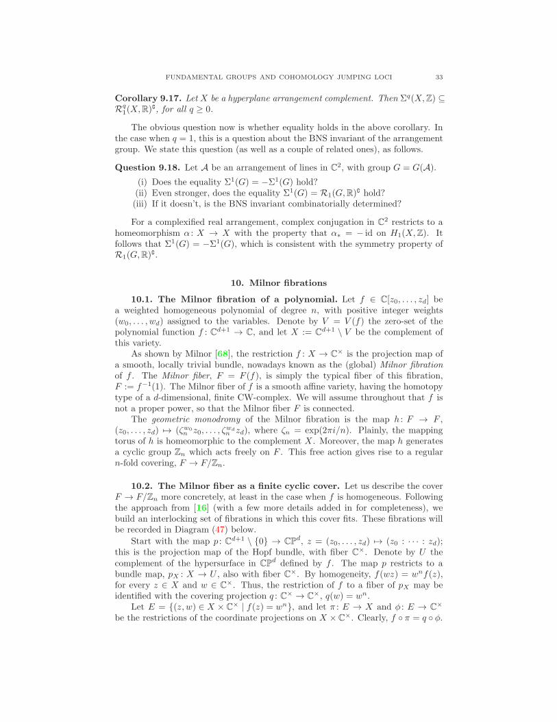
FUNDAMENTAL GROUPS AND COHOMOLOGY JUMPING LOCI 33
Corollary 9.17. Let X be a hyperplane arrangement complement. Then Σq(X,Z) ⊆Rq
1(X,R)∁, for all q ≥ 0.
The obvious question now is whether equality holds in the above corollary. Inthe case when q = 1, this is a question about the BNS invariant of the arrangementgroup. We state this question (as well as a couple of related ones), as follows.
Question 9.18. Let A be an arrangement of lines in C2, with group G = G(A).
(i) Does the equality Σ1(G) = −Σ1(G) hold?(ii) Even stronger, does the equality Σ1(G) = R1(G,R)∁ hold?(iii) If it doesn’t, is the BNS invariant combinatorially determined?
For a complexified real arrangement, complex conjugation in C2 restricts to ahomeomorphism α : X → X with the property that α∗ = − id on H1(X,Z). Itfollows that Σ1(G) = −Σ1(G), which is consistent with the symmetry property ofR1(G,R)∁.
10. Milnor fibrations
10.1. The Milnor fibration of a polynomial. Let f ∈ C[z0, . . . , zd] bea weighted homogeneous polynomial of degree n, with positive integer weights(w0, . . . , wd) assigned to the variables. Denote by V = V (f) the zero-set of thepolynomial function f : Cd+1 → C, and let X := Cd+1 \ V be the complement ofthis variety.
As shown by Milnor [68], the restriction f : X → C× is the projection map ofa smooth, locally trivial bundle, nowadays known as the (global) Milnor fibrationof f . The Milnor fiber, F = F (f), is simply the typical fiber of this fibration,F := f−1(1). The Milnor fiber of f is a smooth affine variety, having the homotopytype of a d-dimensional, finite CW-complex. We will assume throughout that f isnot a proper power, so that the Milnor fiber F is connected.
The geometric monodromy of the Milnor fibration is the map h : F → F ,(z0, . . . , zd) 7→ (ζw0
n z0, . . . , ζwd
n zd), where ζn = exp(2πi/n). Plainly, the mappingtorus of h is homeomorphic to the complement X . Moreover, the map h generatesa cyclic group Zn which acts freely on F . This free action gives rise to a regularn-fold covering, F → F/Zn.
10.2. The Milnor fiber as a finite cyclic cover. Let us describe the coverF → F/Zn more concretely, at least in the case when f is homogeneous. Followingthe approach from [16] (with a few more details added in for completeness), webuild an interlocking set of fibrations in which this cover fits. These fibrations willbe recorded in Diagram (47) below.
Start with the map p : Cd+1 \ 0 → CPd, z = (z0, . . . , zd) 7→ (z0 : · · · : zd);this is the projection map of the Hopf bundle, with fiber C×. Denote by U thecomplement of the hypersurface in CPd defined by f . The map p restricts to abundle map, pX : X → U , also with fiber C×. By homogeneity, f(wz) = wnf(z),for every z ∈ X and w ∈ C×. Thus, the restriction of f to a fiber of pX may beidentified with the covering projection q : C× → C×, q(w) = wn.
Let E = (z, w) ∈ X × C× | f(z) = wn, and let π : E → X and φ : E → C×
be the restrictions of the coordinate projections on X ×C×. Clearly, f π = q φ.
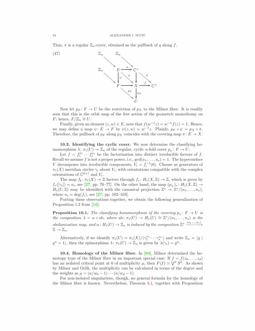
34 ALEXANDER I. SUCIU
Thus, π is a regular Zn-cover, obtained as the pullback of q along f .
(47) Zn
BB
B
B
B
B
B
B
Zn
!!BB
B
B
B
B
B
B
Zn
!!BB
B
B
B
B
B
B
Eφ
//
ψ
π
!!CC
C
C
C
C
C
C
C×
q
!!CC
C
C
C
C
C
C
F //
pF
!!CC
C
C
C
C
C
C
Xf
//
pX
C×
U
Now let pF : F → U be the restriction of pX to the Milnor fiber. It is readilyseen that this is the orbit map of the free action of the geometric monodromy onF ; hence, F/Zn ∼= U .
Finally, given an element (z, w) ∈ E, note that f(w−1z) = w−nf(z) = 1. Hence,we may define a map ψ : E → F by ψ(z, w) = w−1z. Plainly, pF ψ = pX π.Therefore, the pullback of pF along pX coincides with the covering map π : E → X .
10.3. Identifying the cyclic cover. We now determine the classifying ho-momorphism λ : π1(U) ։ Zn of the regular, cyclic n-fold cover p
F: F → U .
Let f = fa11 · · · fass be the factorization into distinct irreducible factors of f .Recall we assume f is not a proper power, i.e., gcd(a1, . . . , as) = 1. The hypersurfaceV decomposes into irreducible components, Vi = f−1
i (0). Choose as generators ofπ1(X) meridian circles γi about Vi, with orientations compatible with the complexorientations of Cd+1 and Vi.
The map f♯ : π1(X) → Z factors through f∗ : H1(X,Z) → Z, which is given byf∗([γi]) = ai, see [27, pp. 76–77]. On the other hand, the map (p
X)∗ : H1(X,Z) →
H1(U,Z) may be identified with the canonical projection Zs ։ Zs/(n1, . . . , ns),where ni = deg(fi), see [27, pp. 102–103].
Putting these observations together, we obtain the following generalization ofProposition 1.2 from [16].
Proposition 10.1. The classifying homomorphism of the covering pF: F → U is
the composition λ = α ab, where ab: π1(U) → H1(U) ∼= Zs/(n1, . . . , ns) is the
abelianization map, and α : H1(U) → Zn is induced by the composition Zs(a1,...,as)−−−−−−→
Z ։ Zn.
Alternatively, if we identify π1(U) = π1(X)/〈γn1
1 · · · γns
s 〉 and write Zn = 〈g |gn = 1〉, then the epimorphism λ : π1(U) ։ Zn is given by λ(γi) = gai .
10.4. Homology of the Milnor fiber. In [68], Milnor determined the ho-motopy type of the Milnor fiber in an important special case: If f = f(z0, . . . , zd)has an isolated critical point at 0 of multiplicity µ, then F (f) ≃
∨µSd. As shown
by Milnor and Orlik, the multiplicity can be calculated in terms of the degree andthe weights as µ = (n/w0 − 1) · · · (n/wd − 1).
For non-isolated singularities, though, no general formula for the homology ofthe Milnor fiber is known. Nevertheless, Theorem 3.1, together with Proposition
FUNDAMENTAL GROUPS AND COHOMOLOGY JUMPING LOCI 35
10.1, yields a formula for the homology groups H1(F, k), in terms of the character-istic varieties Vd(U, k) of the projectivized complement, under suitable assumptionson the field k.
Theorem 10.2. Let f = fa11 · · · fass be a homogeneous polynomial of degree n, withirreducible factors fi, and with gcd(a1, . . . , as) = 1. Let k be an algebraically closedfield of characteristic not dividing n, and fix a primitive n-th root of unity ζ ∈ k.Then,
(48) dimkH1(F, k) = s− 1 +∑
16=k|n
ϕ(k) depthk
(ρn/k
),
where ρ : π1(U) → k× is the character defined on meridians by ρ(γi) = ζai .
In the case where deg(fi) = 1 for 1 ≤ i ≤ s, this result reduces to Theorem 4.4from [14].
10.5. Milnor fibers of arrangements. Much effort has been put over thepast two decades in computing the homology groups of the Milnor fiber of a hyper-plane arrangement. For our purposes here, we shall restrict to central arrangementsin C3, defined by polynomials of the form f = f1 · · · fn, with fi = fi(z0, z1, z2) linearforms.
Let A be such an arrangement, with complement X , projectivized complementU , and meridians γ1, . . . , γn. Since CPd \ fi = 0 ∼= Cd, the bundle pX : X → U istrivial. This gives a diffeomorphism X ∼= U × C×, under which the group π1(C×)corresponds to Z = 〈γ1 · · · γn〉. Thus, the characteristic varieties of π1(U) are givenby
(49) Vd(U, k) = t ∈ (k×)n | t ∈ Vd(X, k) and t1 · · · tn = 1.
In particular, Vd(U,C) ⊂ (C×)n is the intersection of Vd(A) = Vd(X,C) with thesubtorus (C×)n−1 = t1 · · · tn = 1.
Some well-known questions arise.
Question 10.3. Let F = f = 1 be the Milnor fiber of a central arrangement Ain C3.
(i) Is H1(F,Z) torsion-free?(ii) Is H1(F,Z) determined by the intersection lattice L(A)?(iii) Is b1(F ) determined by L(A)?
Of course, an affirmative answer to (ii) implies one for (iii), while an affirmativeanswer to both (i) and (iii) implies one for (ii). In view of Theorem 10.2, if one couldshow that all translated components of Vd(U,C) are combinatorially determined,one would obtain an affirmative answer to (iii).
Example 10.4. Let A be a generic 3-slice of the braid arrangement, with definingpolynomial f = z0z1z2(z0 − z1)(z0 − z2)(z1 − z2). Let U be the projectivizedcomplement of A, and let ρ : π1(U) → C, γi 7→ ζ6 be the character corresponding tothe Milnor fiber F . Recalling from Example 9.4 the decomposition into irreduciblecomponents of V1(U), we see that λ2 belongs to VΠ, yet λ /∈ V1(U). Since V2(U) =1, we find
b1(F ) = 5 + ϕ(3) · depthC(λ2) = 5 + 2 · 1 = 7.
Direct computation with the Jacobian matrix of π1(U), based on the method out-lined in Proposition 4.1 shows that, in fact, H1(F,Z) = Z7.
36 ALEXANDER I. SUCIU
If one is willing to go to multi-arrangements, then the answer to Question 10.3(i)is negative, as the following example from [14, §7.3] illustrates.
Example 10.5. Let A be the be the deleted B3 arrangement discussed in Example9.5. Assigning weights (2, 1, 3, 3, 2, 2, 1, 1) to the factors of Q(A), we obtain a newhomogeneous polynomial (of degree 15),
f = z20z1(z20 − z21)
3(z20 − z22)2(z21 − z22).
Note that A and V (f) share the same (projectivized) complement, yet theMilnor fibers ofQ(A) and f are different. Applying Theorem 10.2 to the Milnor fiberF = F (f), we find that dimkH1(F, k) = 7 if chark 6= 2, 3, or 5, yet dimkH1(F, k) =9 if chark = 2.
Direct computation with the Jacobian matrix of π1(U) yields the precise formulafor the homology with integer coefficients:
H1(F,Z) = Z7 ⊕ Z2 ⊕ Z2.
10.6. Formality of the Milnor fiber. The following question was raised in[73]: Is the Milnor fiber of a reduced polynomial, F (f), always 1-formal? Thisquestion has led to a certain amount of recent activity, out of which two completelydifferent examples came out, showing that, in general, the Milnor fiber is not formal.
Example 10.6 (Zuber [92]). Let A = A(3, 3, 3) be the monomial arrangement inC3 defined by the polynomial
f(z0, z1, z2) = (z30 − z31)(z30 − z32)(z
31 − z32),
and let F be the Milnor fiber of f . It is shown in [92] that TC1(V1(F,C)) 6=R1(F,C); hence, by Theorem 7.1, F is not 1-formal.
Example 10.7 (Fernandez de Bobadilla [46]). Consider the polynomial
f(z0, . . . , z10) = z0z2z3z5z6 + z0z2z4z7 + z1z2z4z8 + z1z3z5z9 + z1z3z4z10.
Then f is weighted homogeneous of degree 5, with weights (1, 1, 1, 1, 1, 1, 1, 2, 2, 2, 2).As shown in [46], the Milnor fiber F is homotopy equivalent to the complement ofthe coordinate subspace arrangement A = AK from [26, §9.3]. This arrangementconsists of subspaces H1, . . . , H5 in C6, given by Hi = xi = xi+1 = 0.
It is easy to see that F is 2-connected. Computations from [26, §6.2] showthat there are classes α, β, γ ∈ H3(F,Z) = Z5 such that the triple Massey product〈α, β, γ〉 ∈ H8(F,Z) = Z is defined, with 0 indeterminacy, and does not vanish.Hence, F is not formal.
In view of these examples, Question 5.5 from [73] needs to be reformulated, asfollows.
Question 10.8. For which (weighted) homogeneous polynomials f is the Milnorfiber F (f) a 1-formal (or even formal) space?
For hyperplane arrangements, we can ask an even more precise question.
Question 10.9. Let A be a central arrangement in C3, with Milnor fiber F .
(i) Is the Milnor fiber 1-formal?(ii) If not, can this be detected by means of (triple) Massey products in
H2(F,Q)?(iii) Is the formality property of the Milnor fiber combinatorially determined?
FUNDAMENTAL GROUPS AND COHOMOLOGY JUMPING LOCI 37
11. Three-dimensional manifolds
11.1. Alexander polynomial and characteristic varieties. Throughoutthis section, M will be a compact, connected 3-manifold, possibly with boundary∂M . Let G = π1(M) be the fundamental group of M , and H = ab(G) its maximaltorsion-free abelian quotient. Let E1(AG) ⊂ ZH be the Alexander ideal, and ∆G =gcd(E1(AG)) the Alexander polynomial of G.
We start with a lemma from [29], based on the work of Eisenbud–Neumann[35] and McMullen [66].
Lemma 11.1. If either (1) ∂M 6= ∅ and χ(∂M) = 0, or (2) ∂M = ∅ and M isorientable, then E1(AG) is almost principal (in the sense of Definition 4.14).
In the first case, E1(AG) = IH · (∆G), by [35], while in the second case,I2H · (∆G) ⊆ E1(AG), by [66]. Proposition 4.15 now yields the following corol-lary, relating the first characteristic variety of M to the zero set of the Alexanderpolynomial of G = π1(M).
Corollary 11.2. Under the above assumptions,
(i)(V1(G) ∩ Hom(G,C×)0
)\ 1 = V (∆G) \ 1.
(ii) If, moreover, H1(G,Z) is torsion-free, then V1(G) \ 1 = V (∆G) \ 1.
Example 11.3. Let L = (L1, . . . , Ln) be a link in S3, and letM = S3\⋃ni=1N(Li)
be its exterior (i.e., the complement of an open tubular neighborhood of the link).Then M is a compact, connected, orientable 3-manifold, with ∂M consisting of ndisjoint tori, so that χ(∂M) = 0.
Let G = π1(M) be the link group. By Lemma 11.1, the Alexander ideal of Gis almost principal. Since H1(G,Z) = Zn, Corollary 11.2(ii) insures that V1(G) =V (∆G), at least away from 1.
11.2. Resonance varieties. Assume now M is closed (i.e., ∂M = ∅) andorientable, and fix an orientation [M ] ∈ H3(M,Z) ∼= Z. With this choice, thecup product on M and Kronecker pairing determine an alternating 3-form η onH1(M,Z), given by η(x, y, z) = 〈x ∪ y ∪ z, [M ]〉. In turn, the cup-product mapµ : H1(M,Z)∧H1(M,Z) → H2(M,Z) is determined by the form η, via 〈x∪ y, γ〉 =µ(x, y, z), where z = PD(γ) is the Poincare dual of γ ∈ H2(M,Z).
Fix a basis e1, . . . , en for H1(M,C), and choose e∨1 , . . . , e∨n as basis for
H2(M,C), where e∨i denotes the Kronecker dual of PD(ei). Writing µ(ei, ej) =∑nk=1 µijke
∨k as in (29), we find that η(ei, ej, ek) = µijk.
By Proposition 5.2, the resonance variety R1(M) is the vanishing locus of thecodimension 1 minors of the n×n matrix Θ with entries Θkj =
∑ni=1 µijkxi. Since η
is an alternating form, Θ is a skew-symmetric matrix. Using this fact, the followingstructure theorem is proved in [32].
Theorem 11.4 ([32]). Let M be a closed, orientable 3-manifold. Then:
(i) H1(M,C) is not 1-isotropic.(ii) If b1(M) is even, then R1(M) = H1(M,C).(iii) If R1(M) contains a 0-isotropic hyperplane, then R1(M) = H1(M,C).
11.3. Thurston norm. For each compact, orientable 3-manifoldM , Thurstondefined in [88] a (semi-)norm on H1(M,R), as follows. For a cohomology classφ ∈ H1(M,Z), set ‖φ‖ = infSχ−
(S), with the infimum taken over all properly
38 ALEXANDER I. SUCIU
embedded, compact surfaces S representing the dual of φ, and where χ−(S) =∑
imax−χ(Si), 0, after decomposing S as a disjoint union of connected surfacesSi.
It turns out that the assignment φ 7→ ‖φ‖ is a seminorm on H1(M,Z), whichcan be extended to the whole of H1(M,R). Even though ‖ · ‖ vanishes on sphericaland toroidal classes, it is simply called the Thurston norm of M . The unit ball inthis norm, BT = φ | ‖φ‖ ≤ 1, is a rational convex polyhedron, i.e., the intersectionof finitely many rationally defined hyperplanes.
A non-zero cohomology class φ ∈ H1(M,Z) is said to be fibered if there is asmooth fibration f : M → S1 such that φ corresponds to f∗ : H1(M,Z) → Z underthe isomorphism H1(M,Z) ∼= Hom(H1(M,Z),Z). In this case, ‖φ‖ = χ
−(S), where
S = f−1(1) is the fiber of the fibration. Given a fibered class φ, there exists a (top-dimensional) face F of BT so that φ belongs to the open cone R+ ·F . Such a faceF is called a fibered face, the reason being that each integral cohomology class inR+ · F is fibered.
11.4. Alexander norm and Thurston norm. In [66], McMullen used theAlexander polynomial of G = π1(M) to define a (semi-)norm on H1(M,R), calledthe Alexander norm. If we write ∆G =
∑nigi, with ni ∈ Z \ 0 and gi ∈ ab(G),
then the norm of a class φ ∈ H1(M,R) is defined by ‖φ‖A = supφ(gi−gj). The unitball BA of the Alexander norm is, up to scaling, the polytope dual to the Newtonpolytope of ∆G.
Theorem 11.5 ([66]). Let M be a compact, orientable 3-manifold whose boundary,if any, is a union of tori. Then:
(i) If b1(M) ≥ 2, then ‖φ‖A ≤ ‖φ‖T , for all φ ∈ H1(M,R).(ii) If b1(M) = 1, then ‖φ‖A ≤ ‖φ‖T + b3(M) + 1, for all primitive classes
φ ∈ H1(M,Z).
Moreover, equality holds when φ ∈ H1(M,Z) is a fibered class, represented by afibration f : M → S1 with χ(f−1(1)) ≤ 0.
McMullen’s inequalities generalize the classical relation deg∆K(t) ≤ 2 genus(K)for knots. In many cases, the Alexander and Thurston norms agree on all ofH1(M,R). Yet even when M fibers over the circle and b1(M) ≥ 2, the two normsmay disagree, as examples of Dunfield [33] show. Nevertheless, as shown by Long[61], the two norms coincide for irreducible graph links in homology 3-spheres.
11.5. BNS invariant. In [8], Bieri, Neumann, and Strebel found a remarkableconnection between the Thurston norm ofM and the BNS invariant of G = π1(M).We summarize their result, as follows.
Theorem 11.6 ([8]). Let M be a compact, connected 3-manifold, with fundamentalgroup G = π1(M). Then, Σ1(G) is the union of open cones R+ ·F , with F runningthrough the fibered faces of the Thurston unit ball BT . Consequently:
(i) Σ1(G) = −Σ1(G).(ii) M fibers over the circle if and only if Σ1(G) 6= ∅.
We exploit this theorem to give the example promised in §7.5, showing thatthe inclusion Σ1(G) ⊆ R1(G,R)∁ may be strict, even when G is 1-formal andΣ1(G) = −Σ1(G).
FUNDAMENTAL GROUPS AND COHOMOLOGY JUMPING LOCI 39
Example 11.7. Let L = (L1, L2) be a non-fibered, two-component link in S3 withnon-zero linking number. Let X be the complement of L, and G = π1(X). Sincelk(L1, L2) 6= 0, we have a ring isomorphism H∗(X,Q) ∼= H∗(T 2,Q). Consequently,X is a formal space, and R1(G,R) = 0. On the other hand, since G is a linkgroup, Σ1(G) = −Σ1(G), by Theorem 11.6(i). Furthermore, since L is not a fibered
link, Σ1(G) 6= 0∁, by Theorem 11.6(ii).
Here is a another application.
Corollary 11.8 ([74]). Let M be a closed, orientable 3-manifold. If b1(M) is even,and G = π1(M) is 1-formal, then M does not fiber over the circle.
Indeed, by Theorem 11.4(ii), we must have R1(G,R) = H1(G,R). Hence, byCorollary 7.5, Σ1(G) = ∅, and the conclusion follows from Theorem 11.6(ii).
11.6. Kahler 3-manifold groups. The following question was raised byS. Donaldson and W. Goldman and in 1989, and independently by A. Reznikovin 1993: Which 3-manifold groups are Kahler groups? In [77], Reznikov obtaineda deep restriction on certain groups lying at the intersection of these two classes offundamental groups. In [32], the question was answered in full generality.
Theorem 11.9 ([32]). Let G be the fundamental group of a closed 3-manifold.Then G is a Kahler group if and only if G is a finite subgroup of O(4), acting freelyon S3.
The backward implication follows from classical work of J.-P. Serre. In thecase when b1(G) > 0, the forward implication can be readily explained, using thetechniques outlined in §8.4 and §11.2. By passing to orientation double covers ifnecessary, we may assume G = π1(M), with M a closed, orientable 3-manifold.Then G is still a Kahler group, and so b1(G) must be even (and positive). FromTheorem 11.4, we know that R1(G,C) = H1(G,C), and H1(G,C) is not 1-isotropic.But, since G is a Kahler group, this contradicts Theorem 8.5(iv).
To deal with the remaining case, b1(G) = 0, one needs some deep facts from3-manifold theory, together with theorems of Reznikov and Fujiwara, relating theKahler, respectively the 3-manifold condition on a group to Kazhdan’s property(T ).
A similar classification of quasi-Kahler, 3-manifold groups seems to be beyondreach at the present time. Nevertheless, such groups are classified in [31, Theorem1.1], but only at the level of Malcev completions, and under a formality assumption.
Theorem 11.10 ([31]). Let G be the fundamental group of a closed, orientable3-manifold. Assume G is 1-formal. Then the following are equivalent.
(i) m(G) ∼= m(π1(X)), for some quasi-Kahler manifold X.(ii) m(G) ∼= m(π1(M)), where M is either S3, #nS1 × S2, or S1 × Σg.
In particular, if G is a quasi-Kahler, 1-formal, orientable 3-manifold group, thenits Malcev completion is isomorphic to that of either 1, Fn, or Z× π1(Σg).
11.7. Boundary manifolds of line arrangements. We conclude with amore detailed description of a special class of closed, orientable 3-manifolds, arisingin the context of hyperplane arrangements. Let A = ℓ0, . . . , ℓn be an arrange-ment of lines in CP2. The boundary manifold M = M(A) is obtained by taking
the boundary of a regular neighborhood of⋃ni=0 ℓi in CP2. Such manifolds were
40 ALEXANDER I. SUCIU
investigated by Jiang and Yau [53], Westlund [90], and Hironaka [52], and morerecently, in [19, 20].
Example 11.11 ([19]). Suppose A is a pencil of n+1 lines; then M = ♯nS1 ×S2.On the other hand, if A is a near-pencil (i.e., a pencil of n lines, together withanother line in general position), then M = S1 × Σn−1.
Suppose now A has r non-transverse intersection points, i.e., points FJ =⋂j∈J ℓj of multiplicity |J | ≥ 3. Blowing up CP2 at each of these points, we obtain
an arrangement A = L0, . . . , Ln+r in CP2 ∼= CP2#rCP
2, consisting of the proper
transforms of the lines of A, together with the exceptional lines arising from theblow-ups.
This construction realizes the boundary manifold of A as a graph manifold, inthe sense of Waldhausen. The underlying graph Γ has vertex set V(Γ), with vertices
in one-to-one correspondence with the lines of A: the vertex corresponding to ℓi islabeled vi, while the vertex corresponding to FJ is labeled vJ . The graph Γ has anedge ei,j from vi to vj , i < j, if the corresponding lines ℓi and ℓj are transverse,and an edge eJ,i from vJ to vi if ℓi ⊃ FJ .
Since M is a graph manifold, the group G = π1(M) may be realized as thefundamental group of a graph of groups. As shown in [20, Proposition 3.7], the re-sulting presentation for G may be simplified to a commutator-relators presentation.
Theorem 11.12 ([20]). Let A be an essential line arrangement in CP2, let Γ bethe associated graph, and let G be the fundamental group of the boundary manifoldM(A). Then the Alexander polynomial of G is
∆G =∏
v∈V(Γ)
(tv − 1)mv−2,
where mv denotes the degree of the vertex v, and tv =∏i∈v ti.
11.8. Jumping loci of boundary manifolds. The first characteristic vari-ety of the group G = π1(M(A)) can be easily computed from Theorem 11.12. Firstnote that ∆G(1) = 0. Hence, by Corollary 11.2(ii),
(50) V1(G) =⋃
v∈V(Γ) :mv≥3
tv − 1 = 0.
The resonance varieties of boundary manifolds were studied in detail in [19,
20]. As before, let A = ℓ0, . . . , ℓn be an arrangement of lines in CP2. The firstresonance variety of G = π1(M(A)) admits a particularly simple description:
(51) R1(G) =
Cn if A is a pencil,
C2(n−1) if A is a near-pencil,
H1(G,C) otherwise.
The higher-depth resonance varieties, though, can be much more complicated,as the following example extracted from [19, §6.9] illustrates.
Example 11.13. Let A be an arrangement of 5 lines in CP2 in general position,and set G = π1(M(A)). Then H1(G,C) = C10, and R7(G) = Q× 0, where
Q = z ∈ C6 | z1z6 − z2z5 + z3z4 = 0,
FUNDAMENTAL GROUPS AND COHOMOLOGY JUMPING LOCI 41
which is an irreducible quadric, with an isolated singular point at 0. On theother hand, formula (50) implies that Vd(G) ⊆ 1, for all d ≥ 1. Consequently,TC1(V7(G)) 6= R7(G). The tangent cone theorem now shows that G is not 1-formal.
The above computation indicates that, for arrangements different from thosein Example 11.11, the boundary manifold may well be non-formal. As a matter offact, we have the following result, which summarizes Theorem 9.7 from [20] andProposition 4.7 from [29], and makes Theorem 11.10 much more precise for thisparticular class of 3-manifolds.
Theorem 11.14 ([20, 29]). Let A = ℓ0, . . . , ℓn be an arrangement of lines inCP2, and let M be the corresponding boundary manifold. The following are equiva-lent:
(i) The manifold M is formal.(ii) The group G = π1(M) is 1-formal.(iii) The group G is quasi-projective.(iv) The group G is quasi-Kahler.(v) A is either a pencil or a near-pencil.(vi) M is either ♯nS1 × S2 or S1 × Σn−1.
The crucial implications here are (ii) ⇒ (v), which follows from Theorem 7.1,together with formulas (50) and (51), and (iv) ⇒ (v), which makes use of Theorem8.10 and Theorem 11.12.
References
[1] J. W. Alexander, Topological invariants of knots and links, Trans. Amer. Math. Soc. 30
(1928), no. 2, 275–306. MR1501429 1.2[2] J. Amoros, M. Burger, K. Corlette, D. Kotschick, D. Toledo, Fundamental groups of compact
Kahler manifolds, Math. Surveys Monogr., vol. 44, Amer. Math. Soc., Providence, RI, 1996.MR1379330 (97d:32037) 8.1, 9.6
[3] D. Arapura, Geometry of cohomology support loci for local systems I, J. Alg. Geometry 6
(1997), no. 3, 563–597. MR1487227 (98m:32043) 1.3, 8.3, 8.2, 8.7[4] E. Artal Bartolo, J. Carmona Ruber, J. I. Cogolludo-Agustın, M. Marco-Buzunariz, Invari-
ants of combinatorial line arrangements and Rybnikov’s example, in: Singularity Theoryand its Applications, Adv. Studies in Pure Math., vol. 43, Math. Soc. Japan, Tokyo, 2007,pp. 1–34. MR2313406 (2008g:32042) 9.1
[5] E. Artal Bartolo, J. I. Cogolludo-Agustın, D. Matei, Characteristic varieties of quasi-projective manifolds and orbifolds, preprint arXiv:1005.4761v1. 8.3
[6] A. Beauville, Annulation du H1 pour les fibres en droites plats, in: Complex algebraic va-rieties (Bayreuth, 1990), 1–15, Lecture Notes in Math., vol. 1507, Springer, Berlin, 1992.MR1178716 (94a:14048) 1.3, 8.3, 8.7, 8.13
[7] R. Bieri, Deficiency and the geometric invariants of a group, J. Pure Appl. Alg. 208 (2007),no. 3, 951–959. MR2283437 (2008a:20081) 6.2, 6.2
[8] R. Bieri, W. Neumann, R. Strebel, A geometric invariant of discrete groups, Invent. Math.90 (1987), no. 3, 451–477. MR0914846 (89b:20108) 1.4, 6.1, 6.1, 6.1, 11.5, 11.6
[9] R. Bieri, B. Renz, Valuations on free resolutions and higher geometric invariants of groups,Comment. Math. Helvetici 63 (1988), no. 3, 464–497. MR0960770 (90a:20106) 1.4, 6.1, 6.1,7.6
[10] N. Budur, Unitary local systems, multiplier ideals, and polynomial periodicity of Hodge num-bers, Adv. Math. 221 (2009), no. 1, 217–250. MR2509325 (2010j:32046) 8.3
[11] F. Campana, Ensembles de Green-Lazarsfeld et quotients resolubles des groupes de Kahler,J. Alg. Geometry 10 (2001), no. 4, 599–622. MR1838973 (2002k:32037) 1.3, 8.3
42 ALEXANDER I. SUCIU
[12] A. D. R. Choudary, A. Dimca, S. Papadima, Some analogs of Zariski’s Theorem on nodalline arrangements, Algebr. Geom. Topol. 5 (2005), 691–711. MR2153112 (2006f:32038) 9.5,9.9
[13] J. I. Cogolludo-Agustın, D. Matei, Cohomology algebra of plane curves, weak combinatorialtype, and formality, to appear in Trans. Amer. Math. Soc.; available at arXiv:0711.1951v1.8.1
[14] D. C. Cohen, G. Denham, A. I. Suciu, Torsion in Milnor fiber homology, Alg. Geom. Topology3 (2003), 511–535. MR1997327 (2004d:32043) 10.4, 10.5
[15] D. C. Cohen, P. Orlik, Arrangements and local systems, Math. Res. Lett. 7 (2000), no. 2-3,299–316. MR1764324 (2001i:57040) 9.3
[16] D. C. Cohen, A. I. Suciu, On Milnor fibrations of arrangements, J. London Math. Soc. (2)51 (1995), no. 1, 105–119. MR1310725 (96e:32034) 10.2, 10.3
[17] D. C. Cohen, A. I. Suciu, The braid monodromy of plane algebraic curves and hyperplanearrangements, Comment. Math. Helvetici 72 (1997), no. 2, 285–315. MR1470093 (98f:52012)9.1
[18] D. C. Cohen, A. I. Suciu, Characteristic varieties of arrangements, Math. Proc. CambridgePhil. Soc. 127 (1999), no. 1, 33–53. MR1692519 (2000m:32036) 1.3, 5.3, 9.2, 9.3
[19] D. C. Cohen, A. I. Suciu, Boundary manifolds of projective hypersurfaces, Advances in Math.206 (2006), no. 2, 538–566. MR2263714 (2007j:14064) 11.7, 11.11, 11.8, 11.8
[20] D. C. Cohen, A. I. Suciu, The boundary manifold of a complex line arrangement, Geometry &Topology Monographs 13 (2008), 105–146. MR2508203 (2010c:32051) 1.6, 11.7, 11.7, 11.12,11.8, 11.8, 11.14
[21] P. Deligne, Theorie de Hodge. II, Inst. Hautes Etudes Sci. Publ. Math. 40 (1972), 5–57.MR0498551 (58 #16653a) 8.2
[22] P. Deligne, Theorie de Hodge. III, Inst. Hautes Etudes Sci. Publ. Math. 44 (1974), 5–77.MR0498552 (58 #16653b) 8.2
[23] P. Deligne, P. Griffiths, J. Morgan, D. Sullivan, Real homotopy theory of Kahler manifolds,Invent. Math. 29 (1975), no. 3, 245–274. MR0382702 (52 #3584) 7.1, 8.1, 8.4
[24] T. Delzant, Trees, valuations, and the Green-Lazarsfeld sets, Geom. Funct. Anal. 18 (2008),no. 4, 1236–1250. MR2465689 (2009j:20035) 6.4
[25] T. Delzant, L’invariant de Bieri Neumann Strebel des groupes fondamentaux des varieteskahleriennes, Math. Annalen 348 (2010), no. 1, 119–125. 8.7, 8.11
[26] G. Denham, A. I. Suciu, Moment-angle complexes, monomial ideals, and Massey products,Pure and Applied Math. Quarterly 3 (2007), no. 1, 25–60. MR2330154 (2008g:55028) 10.7
[27] A. Dimca, Singularities and topology of hypersurfaces, Universitext, Springer-Verlag, NewYork, 1992. MR1194180 (94b:32058) 10.3
[28] A. Dimca, Characteristic varieties and constructible sheaves, Rend. Lincei Mat. Appl. 18
(2007), no. 4, 365–389. MR2349994 (2009a:14006) 9.3[29] A. Dimca, S. Papadima, A. I. Suciu, Alexander polynomials: Essential variables and multiplic-
ities, Int. Math. Res. Notices 2008, no. 3, Art. ID rnm119, 36 pp. MR2416998 (2009i:32036)1.2, 1.3, 1.6, 4.2, 4.6, 4.10, 4.8, 4.16, 8.6, 8.10, 9.8, 11.1, 11.8, 11.14
[30] A. Dimca, S. Papadima, A. I. Suciu, Topology and geometry of cohomology jump loci, Duke
Math. Journal 148 (2009), no. 3, 405–457. MR2527322 1.2, 1.3, 1.5, 1.6, 2.5, 2.4, 7.4, 7.1, 7.3,8.4, 8.5, 8.8, 8.5, 8.9
[31] A. Dimca, S. Papadima, A. I. Suciu, Quasi-Kahler groups, 3-manifold groups, and formality,Math. Zeit., published online on Jan. 28, 2010 at doi:10.1007/s00209-010-0664-y. 1.3, 1.6,11.6, 11.10
[32] A. Dimca, A. I. Suciu, Which 3-manifold groups are Kahler groups?, J. Eur. Math. Soc. 11(2009), no. 3, 521–528. MR2505439 1.3, 1.6, 11.2, 11.4, 11.6, 11.9
[33] N. Dunfield, Alexander and Thurston norms of fibered 3-manifolds, Pacific J. Math. 200
(2001), no. 1, 43–58. MR1863406 (2003f:57041) 11.4[34] W. G. Dwyer, D. Fried, Homology of free abelian covers. I, Bull. London Math. Soc. 19
(1987), no. 4, 350–352. MR0887774 (88g:55011) 1.4, 3.2, 3.2, 3.3[35] D. Eisenbud, W. Neumann, Three-dimensional link theory and invariants of plane curve
singularities, Annals of Math. Studies, vol. 110, Princeton University Press, Princeton, NJ,1985. MR0817982 (87g:57007) 4.8, 11.1, 11.1
FUNDAMENTAL GROUPS AND COHOMOLOGY JUMPING LOCI 43
[36] D. Eisenbud, S. Popescu, S. Yuzvinsky, Hyperplane arrangement cohomology and mono-mials in the exterior algebra, Trans. Amer. Math. Soc. 55 (2003), no. 11, 4365–4383.MR1986506 (2004g:52036) 9.9
[37] M. Eliyahu, E. Liberman, M. Schaps, M. Teicher, Characterization of line arrangement forwhich the fundamental group of the complement is a direct product of free groups, Algebr.Geom. Topol. 10 (2010), 1285–1304. 9.7
[38] H. Esnault, V. Schechtman, E. Viehweg, Cohomology of local systems of the complement ofhyperplanes, Invent. Math. 109 (1992), no. 3, 557–561. MR1176205 (93g:32051) 9.9
[39] M. Falk, Arrangements and cohomology, Ann. Combin. 1 (1997), no. 2, 135–157.MR1629681 (99g:52017) 1.3, 9.2
[40] M. Falk, Resonance varieties over fields of positive characteristic, Int. Math. Research Notices2007 (2007), no. 3, article ID rnm009, 25 pages. MR2337033 (2008m:14107) 9.2
[41] M. Falk, S. Yuzvinsky, Multinets, resonance varieties, and pencils of plane curves, CompositioMath. 143 (2007), no. 4, 1069–1088. MR2339840 (2009e:52043) 1.3, 9.2, 9.2
[42] K.-M. Fan, Direct product of free groups as the fundamental group of the complement of aunion of lines, Michigan Math. J. 44 (1997), no. 2, 283–291. MR1460414 (98j:14039) 9.7, 9.7
[43] K.-M. Fan, On parallel lines and free group, preprint arXiv:0905.1178v1. 1.6, 9.5[44] M. Farber, Topology of closed one-forms, Math. Surveys Monogr., vol. 108, Amer. Math. Soc.,
Providence, RI, 2004. MR2034601 (2005c:58023) 6.2[45] M. Farber, R. Geoghegan, D. Schutz, Closed 1-forms in topology and geometric group theory,
Russian Math. Surveys 65 (2010), no. 1, 143–172. MR2655245 6.2[46] J. Fernandez de Bobadilla, On homotopy types of complements of analytic sets and Milnor
fibres, to appear in Contemp. Math., Amer. Math. Soc., Providence, RI, 2011; available atarXiv:0907.2176v2. 1.6, 10.7
[47] R. Fox, Free differential calculus. II. The isomorphism problem of groups, Ann. of Math. 59(1954), 196–210. MR0062125 (15,931e) 4.2, 4.2
[48] R. Fox, Free differential calculus. III. Subgroups, Ann. of Math. 64 (1956), 407–419.MR0095876 (20 #2374) 4.2, 4.1
[49] M. Green, R. Lazarsfeld, Higher obstructions to deforming cohomology groups of line bundles,J. Amer. Math. Soc. 4 (1991), no. 1, 87–103. MR1076513 (92i:32021) 1.3, 8.3
[50] E. Hironaka, Abelian coverings of the complex projective plane branched along configura-tions of real lines, Memoirs A.M.S., vol. 502, Amer. Math. Soc., Providence, RI, 1993.MR1164128 (94b:14020) 1.4, 3.1
[51] E. Hironaka, Alexander stratifications of character varieties, Annales de l’Institut Fourier(Grenoble) 47 (1997), no. 2, 555–583. MR1450425 (98e:14020) 1.3, 3.1, 4.6, 4.6
[52] E. Hironaka, Boundary manifolds of line arrangements, Math. Annalen 319 (2001), no. 1,17–32. MR1812817 (2001m:32061) 11.7
[53] T. Jiang, S. S.-T. Yau, Topological invariance of intersection lattices of arrangements in CP2,
Bull. Amer. Math. Soc. 29 (1993), no. 1, 88–93. MR1197426 (94b:52022) 11.7[54] A. Libgober, Alexander polynomial of plane algebraic curves and cyclic multiple planes, Duke
Math. J. 49 (1982), no. 4, 833–851. MR0683005 (84g:14030) 1.2[55] A. Libgober, On the homology of finite abelian coverings, Topology Appl. 43 (1992), no. 2,
157–166. MR1152316 (93e:57003) 1.4, 3.1[56] A. Libgober, Groups which cannot be realized as fundamental groups of the complements to
hypersurfaces in CN , in: Algebraic geometry and its applications (West Lafayette, IN, 1990),203–207, Springer, New York, 1994. MR1272031 (95b:14013) 1.2
[57] A. Libgober, Characteristic varieties of algebraic curves, in: Applications of algebraic geom-etry to coding theory, physics and computation (Eilat, 2001), pp. 215–254, NATO Sci. Ser. IIMath. Phys. Chem., vol. 36, Kluwer Acad. Publ., Dordrecht, 2001. MR1866902 (2003e:14008)1.3, 9.2
[58] A. Libgober, First order deformations for rank one local systems with a non-vanishing co-homology, Topology Appl. 118 (2002), no. 1-2, 159–168. MR1877722 (2002m:52025) 1.5, 5.3,5.4, 9.3
[59] A. Libgober, Non vanishing loci of Hodge numbers of local systems, Manuscripta Math. 128(2009), no. 1, 1–31. MR2470184 (2010g:32026) 1.3, 8.3, 8.4
[60] A. Libgober, S. Yuzvinsky, Cohomology of Orlik–Solomon algebras and local systems, Com-positio Math. 21 (2000), no. 3, 337–361. MR1761630 (2001j:52032) 1.3, 9.2, 9.3
[61] D. Long, Alexander and Thurston norms of graph links, preprint arXiv:0808.1066v1. 11.4
44 ALEXANDER I. SUCIU
[62] A. Macinic, Cohomology rings and formality properties of nilpotent groups, J. Pure Appl.Algebra 214 (2010), no. 10, 1818–1826. MR2608110 5.3, 8.1
[63] A. Macinic, S. Papadima, Characteristic varieties of nilpotent groups and applications, in:Proceedings of the Sixth Congress of Romanian Mathematicians (Bucharest, 2007), pp. 57–64,vol. 1, Romanian Academy, Bucharest, 2009. MR2641547 5.3
[64] D. Matei, A. I. Suciu, Cohomology rings and nilpotent quotients of real and complex arrange-ments, in: Arrangements–Tokyo 1998, pp. 185–215, Adv. Stud. Pure Math., vol. 27, Math.Soc. Japan, Tokyo, 2000. MR1796900 (2002b:32045) 5.2, 5.2, 5.2, 5.2, 5.3, 9.2
[65] D. Matei, A. I. Suciu, Hall invariants, homology of subgroups, and characteristic varieties,Internat. Math. Res. Notices 2002 (2002), no. 9, 465–503. MR1884468 (2003d:20055) 1.4, 1.5,3.1, 3.1, 4.2, 4.6, 5.3
[66] C. T. McMullen, The Alexander polynomial of a 3-manifold and the Thurston norm on
cohomology, Ann. Sci. Ecole Norm. Sup. 35 (2002), no. 2, 153–171. MR1914929 (2003d:57044)4.8, 11.1, 11.1, 11.4, 11.5
[67] J. Meier, H. Meinert, L. VanWyk, Higher generation subgroup sets and the Σ-invariants ofgraph groups, Comment. Math. Helv. 73 (1998), no. 1, 22–44. MR1610579 (99f:57002) 7.4
[68] J. Milnor, Singular points of complex hypersurfaces, Annals of Math. Studies, vol. 61, Prince-ton Univ. Press, Princeton, NJ, 1968. MR0239612 (39 #969) 1.6, 10.1, 10.4
[69] J. W. Morgan, The algebraic topology of smooth algebraic varieties, Inst. Hautes Etudes Sci.Publ. Math. 48 (1978), 137–204. MR0516917 (80e:55020) 8.2, 8.4
[70] S. Nazir, Z. Raza, Admissible local systems for a class of line arrangements, Proc. Amer.Math. Soc. 137 (2009), no. 4, 1307–1313. MR2465653 (2009k:32030) 9.3
[71] P. Orlik, H. Terao, Arrangements of hyperplanes, Grundlehren Math. Wiss., vol. 300,Springer-Verlag, Berlin, 1992. MR1217488 (94e:52014) 9.1
[72] S. Papadima, A. I. Suciu, Toric complexes and Artin kernels, Advances in Math. 220 (2009),no. 2, 441–477. MR2466422 (2010h:57007) 1.3, 1.6, 2.4, 5.5
[73] S. Papadima, A. Suciu, Geometric and algebraic aspects of 1-formality, Bull. Math. Soc. Sci.Math. Roumanie 52 (2009), no. 3, 355–375. MR2554494 (2010k:55018) 1.5, 1.6, 10.6, 10.6
[74] S. Papadima, A. I. Suciu, Bieri–Neumann–Strebel–Renz invariants and homology jumpingloci, Proc. London Math. Soc. 100 (2010), no. 3, 795–834. MR2640291 1.3, 1.4, 2.2, 2.2, 2.4,3.2, 3.2, 4.6, 4.6, 5.1, 6.2, 6.3, 6.1, 6.3, 6.4, 6.2, 7.4, 7.5, 8.3, 8.7, 8.12, 9.16, 11.8
[75] J. Pereira, S. Yuzvinsky, Completely reducible hypersurfaces in a pencil, Adv. Math. 219
(2008), no. 2, 672–688. MR2435653 (2009g:14010) 1.3, 9.2, 9.2, 9.8[76] D. Quillen, Rational homotopy theory, Ann. of Math. 90 (1969), no. 2, 205–295.
MR0258031 (41 #2678) 7.3[77] A. Reznikov, The structure of Kahler groups. I. Second cohomology, in: Motives, polyloga-
rithms and Hodge theory, Part II (Irvine, CA, 1998), pp. 717–730, Int. Press Lect. Ser., vol. 3,II, Int. Press, Somerville, MA, 2002. MR1978716 (2004c:32042) 11.6
[78] M. Sakuma, Homology of abelian coverings of links and spatial graphs, Canad. J. Math. 47(1995), no. 1, 201–224. MR1319696 (96d:57008) 1.4, 3.1
[79] P. Sarnak, S. Adams, with an appendix by Z. Rudnick, Betti numbers of congruence groups,Israel J. Math. 88 (1994), no. 1-3, 31–72. MR1303490 (96k:11064) 1.4, 3.1
[80] J.-P. Serre, Revetements ramifies du plan projectif (d’apres S. Abhyankar), Seminaire Bour-baki, Vol. 5 (1958–1960), Exp. No. 204, 483–489, Soc. Math. France, Paris, 1960. MR16034891.1
[81] J.-Cl. Sikorav, Homologie de Novikov associee a une classe de cohomologie reele de degre un,These Orsay, 1987. 6.2
[82] C. Simpson, Higgs bundles and local systems, Inst. Hautes Etudes Sci. Publ. Math. 75 (1992),5–95. MR1179076 (94d:32027) 1.3, 8.3
[83] A. I. Suciu, Fundamental groups of line arrangements: Enumerative aspects, in: Advancesin algebraic geometry motivated by physics (Lowell, MA, 2000), pp. 43–79, Contemp. Math.,vol. 276, Amer. Math. Soc., Providence, RI, 2001. MR1837109 (2002k:14029) 1.6, 3.1, 3.1
[84] A. I. Suciu, Translated tori in the characteristic varieties of complex hyperplane arrange-ments, Topology Appl. 118 (2002), no. 1-2, 209–223. MR1877726 (2002j:32027) 9.3
[85] A. I. Suciu, Characteristic varieties and Betti numbers of free abelian covers, preprint, 2010.3.2
[86] A. I. Suciu, Resonance varieties and Dwyer–Fried invariants, preprint, 2010. 3.2
FUNDAMENTAL GROUPS AND COHOMOLOGY JUMPING LOCI 45
[87] D. Sullivan, Infinitesimal computations in topology, Inst. Hautes Etudes Sci. Publ. Math. 47(1977), 269–331. MR0646078 (58 #31119) 7.1, 7.2
[88] W. P. Thurston, A norm for the homology of 3-manifolds, Mem. Amer. Math. Soc., 59 (1986),no. 339. MR0823443 (88h:57014) 11.3
[89] B. Totaro, Configuration spaces of algebraic varieties, Topology 35 (1996), no. 6, 1057–1067.MR1404924 (97g:57033) 8.8
[90] E. Westlund, The boundary manifold of an arrangement, Ph.D. thesis, University of Wiscon-sin, Madison, WI, 1997 MR2697010 11.7
[91] S. Yuzvinsky, A new bound on the number of special fibers in a pencil of curves, Proc. Amer.Math. Soc. 137 (2009), no. 5, 1641–1648. MR2470822 (2009k:14015) 1.3, 9.2, 9.2
[92] H. Zuber, Non-formality of Milnor fibres of line arrangements, Bull. London Math. Soc. 42(2010), no. 5, 905–911. 1.6, 10.6
Department of Mathematics, Northeastern University, Boston, MA 02115, USA
E-mail address: [email protected]
URL: http://www.math.neu.edu/~suciu


