Embed Size (px)
Citation preview
arX
iv:0
705.
3231
v1 [
mat
h.Q
A]
22 M
ay 2
007
Cohomology of the Adjoint of Hopf Algebras
J. Scott Carter∗
University of South Alabama
Alissa S. Crans
Loyola Marymount University
Mohamed Elhamdadi
University of South Florida
Masahico Saito†
University of South Florida
June 13, 2013
Abstract
A cohomology theory of the adjoint of Hopf algebras, via deformations, is presented by means
of diagrammatic techniques. Explicit calculations are provided in the cases of group algebras,
function algebras on groups, and the bosonization of the super line. As applications, solutions
to the YBE are given and quandle cocycles are constructed from groupoid cocycles.
1 Introduction
Algebraic deformation theory [10] can be used to define 2-dimensional cohomology in a wide variety
of contexts. This theory has also been understood diagrammatically [7, 16, 17] via PROPs, for
example. In this paper, we use diagrammatic techniques to define a cohomological deformation of
the adjoint map ad(x⊗y) =∑S(y(1))xy(2) in an arbitrary Hopf algebra. We have concentrated on
the diagrammatic versions here because diagrammatics have led to topological invariants [6, 13, 19],
diagrammatic methodology is prevalent in understanding particle interactions and scattering in
the physics literature, and most importantly kinesthetic intuition can be used to prove algebraic
identities.
The starting point for this calculation is a pair of identities that the adjoint map satisfies and
that are sufficient to construct Woronowicz’s solution [22] R = (1⊗ ad)(τ ⊗ 1)(1⊗∆) to the Yang-
Baxter equation (YBE): (R⊗1)(1⊗R)(R⊗1) = (1⊗R)(R⊗1)(1⊗R). We use deformation theory to
define an extension 2-cocycle. Then we show that the resulting 2-coboundary map, when composed
with the Hochschild 1-coboundary map is trivial. A 3-coboundary is defined via the “movie move”
technology. Applications of this cohomology theory include constructing new solutions to the YBE
by deformations and constructing quandle cocycles from groupoid cocycles that arise from this
theory.
The paper is organized as follows. Section 2 reviews the definition of Hopf algebras, defines the
adjoint map, and illustrates Woronowicz’s solution to the YBE. Section 3 contains the deforma-
tion theory. Section 4 defines the chain groups and differentials in general. Example calculations
∗Supported in part by NSF Grant DMS #0301095, #0603926.†Supported in part by NSF Grant DMS #0301089, #0603876.
1
in the case of a group algebra, the function algebra on a group, and a calculation of the 1- and
2-dimensional cohomology of the bosonization of the superline are presented in Section 5. In-
terestingly, the group algebra and the function algebra on a group are cohomologically different.
Moreover, the conditions that result when a function on the group algebra satisfies the cocycle con-
dition coincide with the definition of groupoid cohomology. This relationship is given in Section 6,
along with a construction of quandle 3-cocycles from groupoid 3-cocycles. In Section 7, we use the
deformation cocycles to construct solutions to the Yang-Baxter equation.
1.1 Acknowledgements
JSC and MS gratefully acknowledge the support of the NSF without which substantial portions of
the work would not have been possible. JSC, ME, and MS have benefited from several detailed
presentations on deformation theory that have been given by Jorg Feldvoss. AC acknowledges
useful and on-going conversations with John Baez.
2 Preliminaries
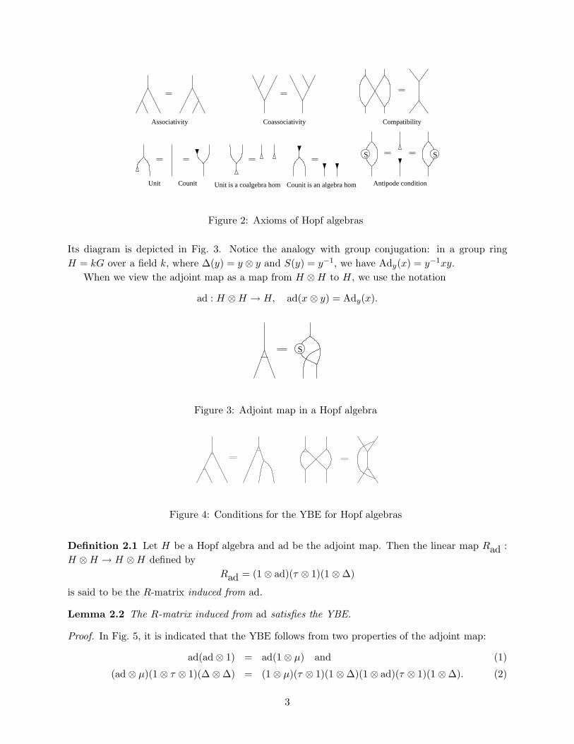
We begin by recalling the operations and axioms in Hopf algebras, and their diagrammatic conven-
tions depicted in Figures 1 and 2.
A coalgebra is a vector space C over a field k together with a comultiplication ∆ : C → C ⊗ C
that is bilinear and coassociative: (∆ ⊗ 1)∆ = (1 ⊗ ∆)∆. A coalgebra is cocommutative if the
comultiplication satisfies τ∆ = ∆, where τ : C ⊗C → C ⊗C is the transposition τ(x⊗ y) = y⊗ x.
A coalgebra with counit is a coalgebra with a linear map called the counit ǫ : C → k such that
(ǫ ⊗ 1)∆ = 1 = (1 ⊗ ǫ)∆ via k ⊗ C ∼= C. A bialgebra is an algebra A over a field k together with
a linear map called the unit η : k → A, satisfying η(a) = a1 where 1 ∈ A is the multiplicative
identity and with an associative multiplication µ : A⊗A → A that is also a coalgebra such that the
comultiplication ∆ is an algebra homomorphism. A Hopf algebra is a bialgebra C together with a
map called the antipode S : C → C such that µ(S ⊗ 1)∆ = ηǫ = µ(1 ⊗ S)∆, where ǫ is the counit.
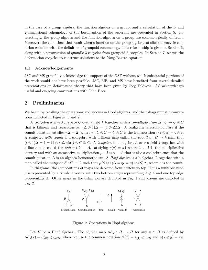
In diagrams, the compositions of maps are depicted from bottom to top. Thus a multiplication
µ is represented by a trivalent vertex with two bottom edges representing A⊗A and one top edge
representing A. Other maps in the definition are depicted in Fig. 1 and axioms are depicted in
Fig. 2.
x
∆
x x(1) (2)
ε
η
xS( )
x x y
τ
xy
TranspositionComultiplicationMultiplication Unit Counit Antipode
x y
µ
xy
S
Figure 1: Operations in Hopf algebras
Let H be a Hopf algebra. The adjoint map Ady : H → H for any y ∈ H is defined by
Ady(x) = S(y(1))xy(2), where we use the common notation ∆(x) = x(1) ⊗ x(2) and µ(x⊗ y) = xy.
2
Associativity
Unit Counit Counit is an algebra hom
CompatibilityCoassociativity
Antipode conditionUnit is a coalgebra hom
S S
Figure 2: Axioms of Hopf algebras
Its diagram is depicted in Fig. 3. Notice the analogy with group conjugation: in a group ring
H = kG over a field k, where ∆(y) = y ⊗ y and S(y) = y−1, we have Ady(x) = y−1xy.
When we view the adjoint map as a map from H ⊗H to H, we use the notation
ad : H ⊗H → H, ad(x⊗ y) = Ady(x).
S
Figure 3: Adjoint map in a Hopf algebra
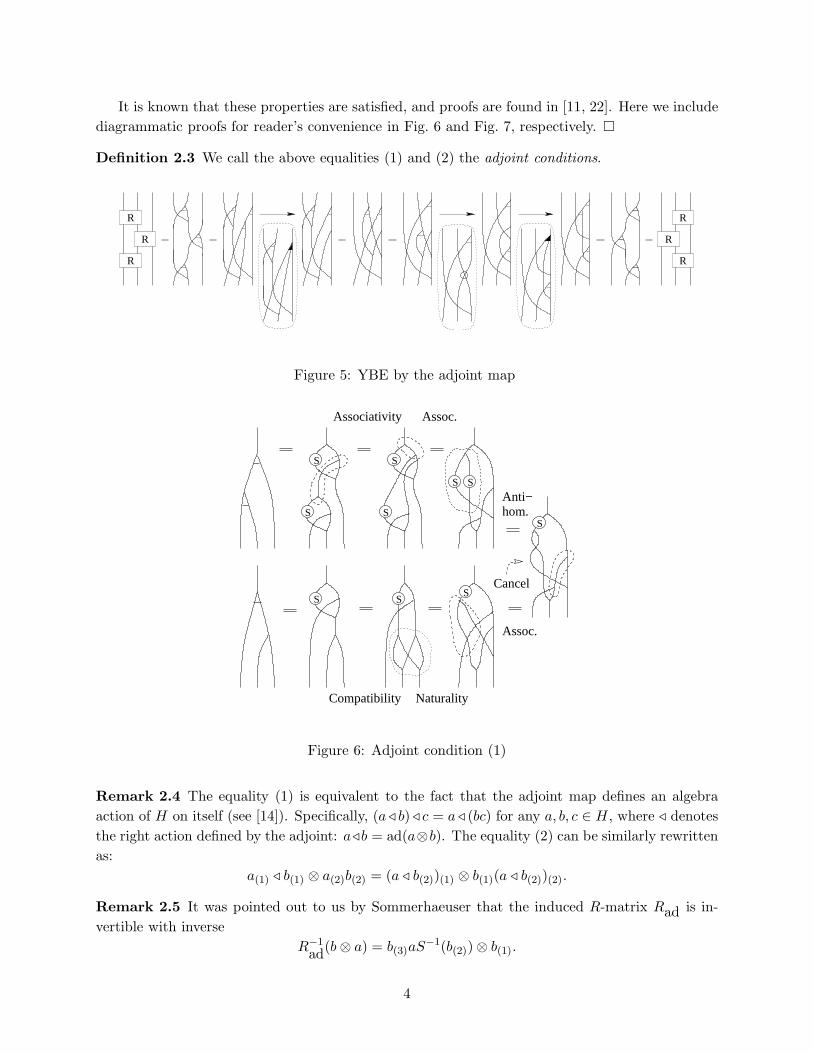
Figure 4: Conditions for the YBE for Hopf algebras
Definition 2.1 Let H be a Hopf algebra and ad be the adjoint map. Then the linear map Rad :
H ⊗H → H ⊗H defined by
Rad = (1 ⊗ ad)(τ ⊗ 1)(1 ⊗ ∆)
is said to be the R-matrix induced from ad.
Lemma 2.2 The R-matrix induced from ad satisfies the YBE.
Proof. In Fig. 5, it is indicated that the YBE follows from two properties of the adjoint map:
ad(ad ⊗ 1) = ad(1 ⊗ µ) and (1)
(ad ⊗ µ)(1 ⊗ τ ⊗ 1)(∆ ⊗ ∆) = (1 ⊗ µ)(τ ⊗ 1)(1 ⊗ ∆)(1 ⊗ ad)(τ ⊗ 1)(1 ⊗ ∆). (2)
3
It is known that these properties are satisfied, and proofs are found in [11, 22]. Here we include
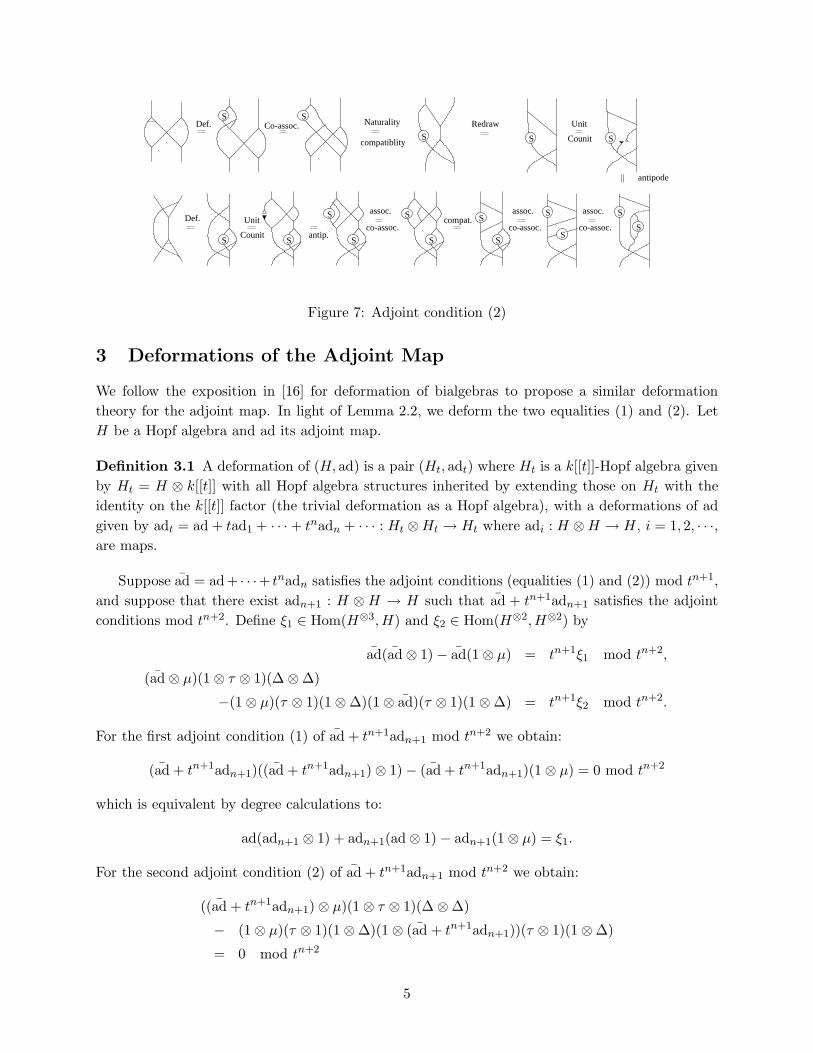
diagrammatic proofs for reader’s convenience in Fig. 6 and Fig. 7, respectively. �
Definition 2.3 We call the above equalities (1) and (2) the adjoint conditions.
R
R
R
R
R
R
Figure 5: YBE by the adjoint map
Assoc.
Anti−hom.
Associativity Assoc.
NaturalityCompatibility
Cancel
S
S S
S
S
S
S
S
S
S
Figure 6: Adjoint condition (1)
Remark 2.4 The equality (1) is equivalent to the fact that the adjoint map defines an algebra
action of H on itself (see [14]). Specifically, (a ⊳ b) ⊳ c = a ⊳ (bc) for any a, b, c ∈ H, where ⊳ denotes
the right action defined by the adjoint: a⊳b = ad(a⊗b). The equality (2) can be similarly rewritten
as:
a(1) ⊳ b(1) ⊗ a(2)b(2) = (a ⊳ b(2))(1) ⊗ b(1)(a ⊳ b(2))(2).
Remark 2.5 It was pointed out to us by Sommerhaeuser that the induced R-matrix Rad is in-
vertible with inverse
R−1
ad(b⊗ a) = b(3)aS
−1(b(2)) ⊗ b(1).
4
Def.
Counit
UnitDef.
antip.
compat.
Redraw
Counit
Unit
co-assoc.
assoc.assoc.
co-assoc.co-assoc.
antipode
compatiblity
assoc.
NaturalityCo-assoc.
S
S
S
S
S
S
SS
S
S S
S
S
S
S
S
S
Figure 7: Adjoint condition (2)
3 Deformations of the Adjoint Map
We follow the exposition in [16] for deformation of bialgebras to propose a similar deformation
theory for the adjoint map. In light of Lemma 2.2, we deform the two equalities (1) and (2). Let
H be a Hopf algebra and ad its adjoint map.
Definition 3.1 A deformation of (H, ad) is a pair (Ht, adt) where Ht is a k[[t]]-Hopf algebra given
by Ht = H ⊗ k[[t]] with all Hopf algebra structures inherited by extending those on Ht with the
identity on the k[[t]] factor (the trivial deformation as a Hopf algebra), with a deformations of ad
given by adt = ad + tad1 + · · · + tnadn + · · · : Ht ⊗Ht → Ht where adi : H ⊗H → H, i = 1, 2, · · ·,
are maps.
Suppose ad = ad+ · · ·+ tnadn satisfies the adjoint conditions (equalities (1) and (2)) mod tn+1,
and suppose that there exist adn+1 : H ⊗H → H such that ad + tn+1adn+1 satisfies the adjoint
conditions mod tn+2. Define ξ1 ∈ Hom(H⊗3,H) and ξ2 ∈ Hom(H⊗2,H⊗2) by
ad(ad ⊗ 1) − ad(1 ⊗ µ) = tn+1ξ1 mod tn+2,
(ad ⊗ µ)(1 ⊗ τ ⊗ 1)(∆ ⊗ ∆)
−(1 ⊗ µ)(τ ⊗ 1)(1 ⊗ ∆)(1 ⊗ ad)(τ ⊗ 1)(1 ⊗ ∆) = tn+1ξ2 mod tn+2.
For the first adjoint condition (1) of ad + tn+1adn+1 mod tn+2 we obtain:
(ad + tn+1adn+1)((ad + tn+1adn+1) ⊗ 1) − (ad + tn+1adn+1)(1 ⊗ µ) = 0 mod tn+2
which is equivalent by degree calculations to:
ad(adn+1 ⊗ 1) + adn+1(ad ⊗ 1) − adn+1(1 ⊗ µ) = ξ1.
For the second adjoint condition (2) of ad + tn+1adn+1 mod tn+2 we obtain:
((ad + tn+1adn+1) ⊗ µ)(1 ⊗ τ ⊗ 1)(∆ ⊗ ∆)
− (1 ⊗ µ)(τ ⊗ 1)(1 ⊗ ∆)(1 ⊗ (ad + tn+1adn+1))(τ ⊗ 1)(1 ⊗ ∆)
= 0 mod tn+2
5
which is equivalent by degree calculations to:
(adn+1 ⊗ µ)(1 ⊗ τ ⊗ 1)(∆ ⊗ ∆)
− (1 ⊗ µ)(τ ⊗ 1)(1 ⊗ ∆)(1 ⊗ adn+1)(τ ⊗ 1)(1 ⊗ ∆) = ξ2.
In summary we proved the following:
Lemma 3.2 The map ad + tn+1adn+1 satisfies the adjoint conditions mod tn+2 if and only if
ad(adn+1 ⊗ 1) + adn+1(ad ⊗ 1) − adn+1(1 ⊗ µ) = ξ1,
and (adn+1 ⊗ µ)(1 ⊗ τ ⊗ 1)(∆ ⊗ ∆)
−(1 ⊗ µ)(τ ⊗ 1)(1 ⊗ ∆)(1 ⊗ adn+1)(τ ⊗ 1)(1 ⊗ ∆) = ξ2.
4 Differentials and Cohomology
4.1 Chain Groups
We define chain groups, for positive integers n, n > 1, and i = 1, . . . , n by:
Cn,iad (H;H) = Hom(H⊗(n+1−i),H⊗i),
Cnad(H;H) = ⊕i>0, i≤n+1−i C
n,iad (H;H).
Specifically, chain groups in low dimensions of our concern are:
C2ad(H;H) = Hom(H⊗2,H),
C3ad(H;H) = Hom(H⊗3,H) ⊕ Hom(H⊗2,H⊗2).
For n = 1, define
C1ad(H;H) = {f ∈ Homk(H,H) | fµ = µ(f ⊗ 1) + µ(1 ⊗ f), ∆f = (f ⊗ 1)∆ + (1 ⊗ f)∆ }.
In the remaining sections we will define differentials that are homomorphisms between the chain
groups:
dn,i : Cnad(H;H) → Cn+1,i
ad (H;H)(= Hom(H⊗(n+2−i),H⊗i))
that will be defined individually for n = 1, 2, 3 and for i with 2i ≤ n+ 1, and
D1 = d1,1 : C1ad(H;H) → C2
ad(H;H),
D2 = d2,1 + d2,2 : C2ad(H;H) → C3
ad(H;H),
D3 = d3,1 + d3,2 + d3,3 : C3ad(H;H) → C3
ad(H;H).
4.2 First Differentials
By analogy with the differential for multiplication, we make the following definition:
Definition 4.1 The first differential
d1,1 : C1ad(H;H) → C2,1
ad (H;H)
is defined by
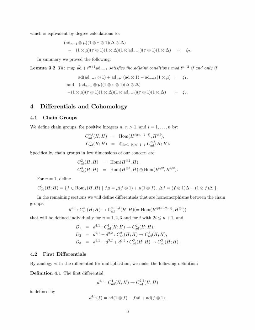
d1,1(f) = ad(1 ⊗ f) − fad + ad(f ⊗ 1).
6
( d1,1 )
Figure 8: The 1-differential
Diagrammatically, we represent d1,1 as depicted in Fig. 8, where a 1-cochain is represented by a
circle on a string.
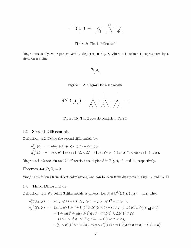
η1
Figure 9: A diagram for a 2-cochain
0( )d2,1
Figure 10: The 2-cocycle condition, Part I
4.3 Second Differentials
Definition 4.2 Define the second differentials by:
d2,1
ad(φ) = ad(φ⊗ 1) + φ(ad ⊗ 1) − φ(1 ⊗ µ),
d2,2
ad(φ) = (φ⊗ µ)(1 ⊗ τ ⊗ 1)(∆ ⊗ ∆) − (1 ⊗ µ)(τ ⊗ 1)(1 ⊗ ∆)(1 ⊗ φ)(τ ⊗ 1)(1 ⊗ ∆).
Diagrams for 2-cochain and 2-differentials are depicted in Fig. 9, 10, and 11, respectively.
Theorem 4.3 D2D1 = 0.
Proof. This follows from direct calculations, and can be seen from diagrams in Figs. 12 and 13. �
4.4 Third Differentials
Definition 4.4 We define 3-differentials as follows. Let ξi ∈ C3,i(H;H) for i = 1, 2. Then
d3,1
ad(ξ1, ξ2) = ad(ξ1 ⊗ 1) + ξ1(1 ⊗ µ⊗ 1) − ξ1(ad ⊗ 12 + 12 ⊗ µ),
d3,2
ad(ξ1, ξ2) = (ad ⊗ µ)(1 ⊗ τ ⊗ 1)(12 ⊗ ∆)(ξ2 ⊗ 1) + (1 ⊗ µ)(τ ⊗ 1)(1 ⊗ ξ2)(Rad ⊗ 1)
+(1 ⊗ µ)(12 ⊗ µ)(τ ⊗ 12)(1 ⊗ τ ⊗ 1)(12 ⊗ ∆)((12 ⊗ ξ1)
·(1 ⊗ τ ⊗ 12)(τ ⊗ 13)(12 ⊗ τ ⊗ 1)(1 ⊗ ∆ ⊗ ∆))
−(ξ1 ⊗ µ)(12 ⊗ τ ⊗ 1)(12 ⊗ µ⊗ 12)(1 ⊗ τ ⊗ 13)(∆ ⊗ ∆ ⊗ ∆) − ξ2(1 ⊗ µ),
7
d2,2 ( ) 0
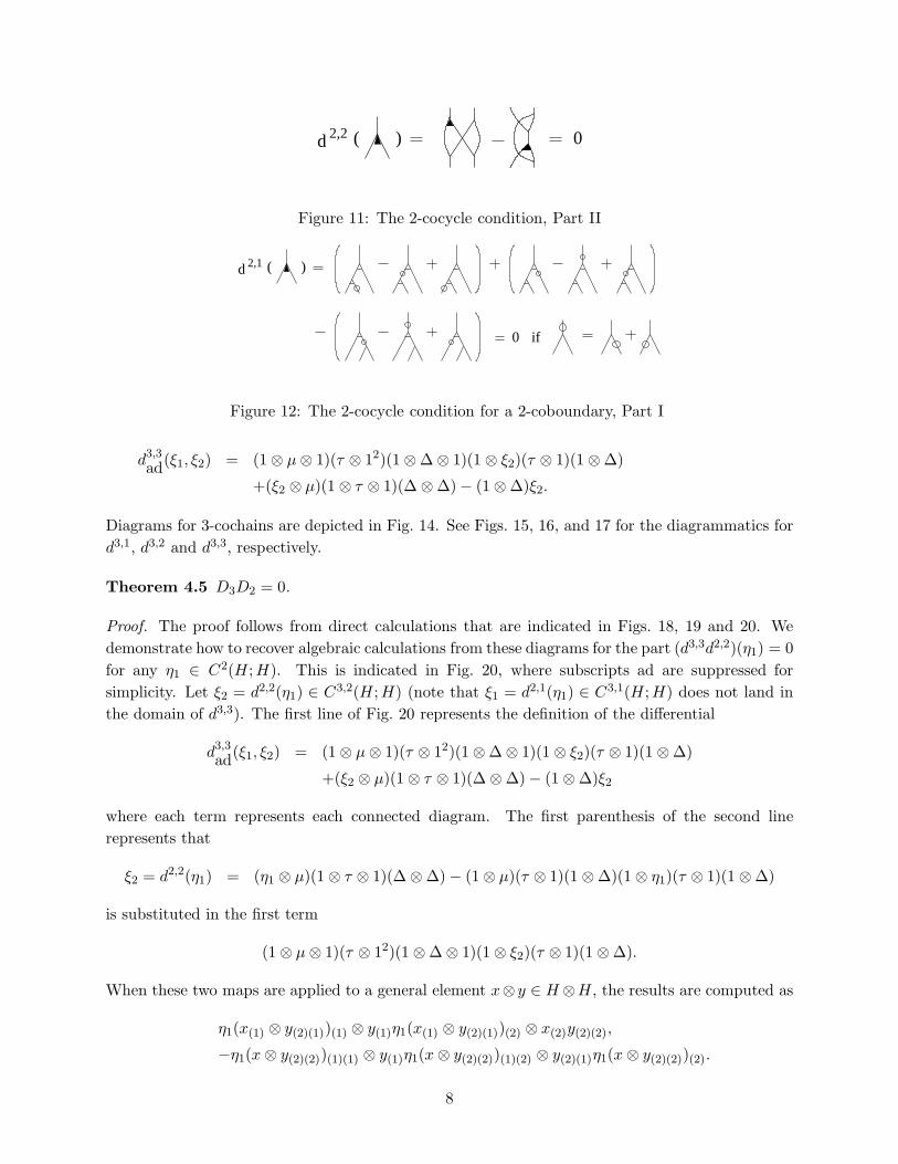
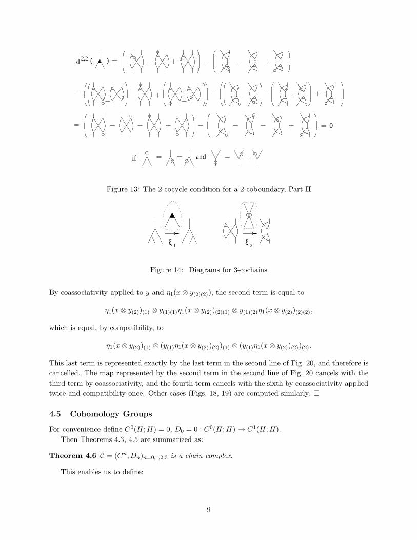
Figure 11: The 2-cocycle condition, Part II
2,1
0 if
( )d
Figure 12: The 2-cocycle condition for a 2-coboundary, Part I
d3,3
ad(ξ1, ξ2) = (1 ⊗ µ⊗ 1)(τ ⊗ 12)(1 ⊗ ∆ ⊗ 1)(1 ⊗ ξ2)(τ ⊗ 1)(1 ⊗ ∆)
+(ξ2 ⊗ µ)(1 ⊗ τ ⊗ 1)(∆ ⊗ ∆) − (1 ⊗ ∆)ξ2.
Diagrams for 3-cochains are depicted in Fig. 14. See Figs. 15, 16, and 17 for the diagrammatics for
d3,1, d3,2 and d3,3, respectively.
Theorem 4.5 D3D2 = 0.
Proof. The proof follows from direct calculations that are indicated in Figs. 18, 19 and 20. We
demonstrate how to recover algebraic calculations from these diagrams for the part (d3,3d2,2)(η1) = 0
for any η1 ∈ C2(H;H). This is indicated in Fig. 20, where subscripts ad are suppressed for
simplicity. Let ξ2 = d2,2(η1) ∈ C3,2(H;H) (note that ξ1 = d2,1(η1) ∈ C3,1(H;H) does not land in
the domain of d3,3). The first line of Fig. 20 represents the definition of the differential
d3,3
ad(ξ1, ξ2) = (1 ⊗ µ⊗ 1)(τ ⊗ 12)(1 ⊗ ∆ ⊗ 1)(1 ⊗ ξ2)(τ ⊗ 1)(1 ⊗ ∆)
+(ξ2 ⊗ µ)(1 ⊗ τ ⊗ 1)(∆ ⊗ ∆) − (1 ⊗ ∆)ξ2
where each term represents each connected diagram. The first parenthesis of the second line
represents that
ξ2 = d2,2(η1) = (η1 ⊗ µ)(1 ⊗ τ ⊗ 1)(∆ ⊗ ∆) − (1 ⊗ µ)(τ ⊗ 1)(1 ⊗ ∆)(1 ⊗ η1)(τ ⊗ 1)(1 ⊗ ∆)
is substituted in the first term
(1 ⊗ µ⊗ 1)(τ ⊗ 12)(1 ⊗ ∆ ⊗ 1)(1 ⊗ ξ2)(τ ⊗ 1)(1 ⊗ ∆).
When these two maps are applied to a general element x⊗ y ∈ H ⊗H, the results are computed as
η1(x(1) ⊗ y(2)(1))(1) ⊗ y(1)η1(x(1) ⊗ y(2)(1))(2) ⊗ x(2)y(2)(2),
−η1(x⊗ y(2)(2))(1)(1) ⊗ y(1)η1(x⊗ y(2)(2))(1)(2) ⊗ y(2)(1)η1(x⊗ y(2)(2))(2).
8
and
d2,2 ( )
0
if
Figure 13: The 2-cocycle condition for a 2-coboundary, Part II
1ξ ξ 2
Figure 14: Diagrams for 3-cochains
By coassociativity applied to y and η1(x⊗ y(2)(2)), the second term is equal to
η1(x⊗ y(2))(1) ⊗ y(1)(1)η1(x⊗ y(2))(2)(1) ⊗ y(1)(2)η1(x⊗ y(2))(2)(2),
which is equal, by compatibility, to
η1(x⊗ y(2))(1) ⊗ (y(1)η1(x⊗ y(2))(2))(1) ⊗ (y(1)η1(x⊗ y(2))(2))(2).
This last term is represented exactly by the last term in the second line of Fig. 20, and therefore is
cancelled. The map represented by the second term in the second line of Fig. 20 cancels with the
third term by coassociativity, and the fourth term cancels with the sixth by coassociativity applied
twice and compatibility once. Other cases (Figs. 18, 19) are computed similarly. �
4.5 Cohomology Groups
For convenience define C0(H;H) = 0, D0 = 0 : C0(H;H) → C1(H;H).
Then Theorems 4.3, 4.5 are summarized as:
Theorem 4.6 C = (Cn,Dn)n=0,1,2,3 is a chain complex.
This enables us to define:
9
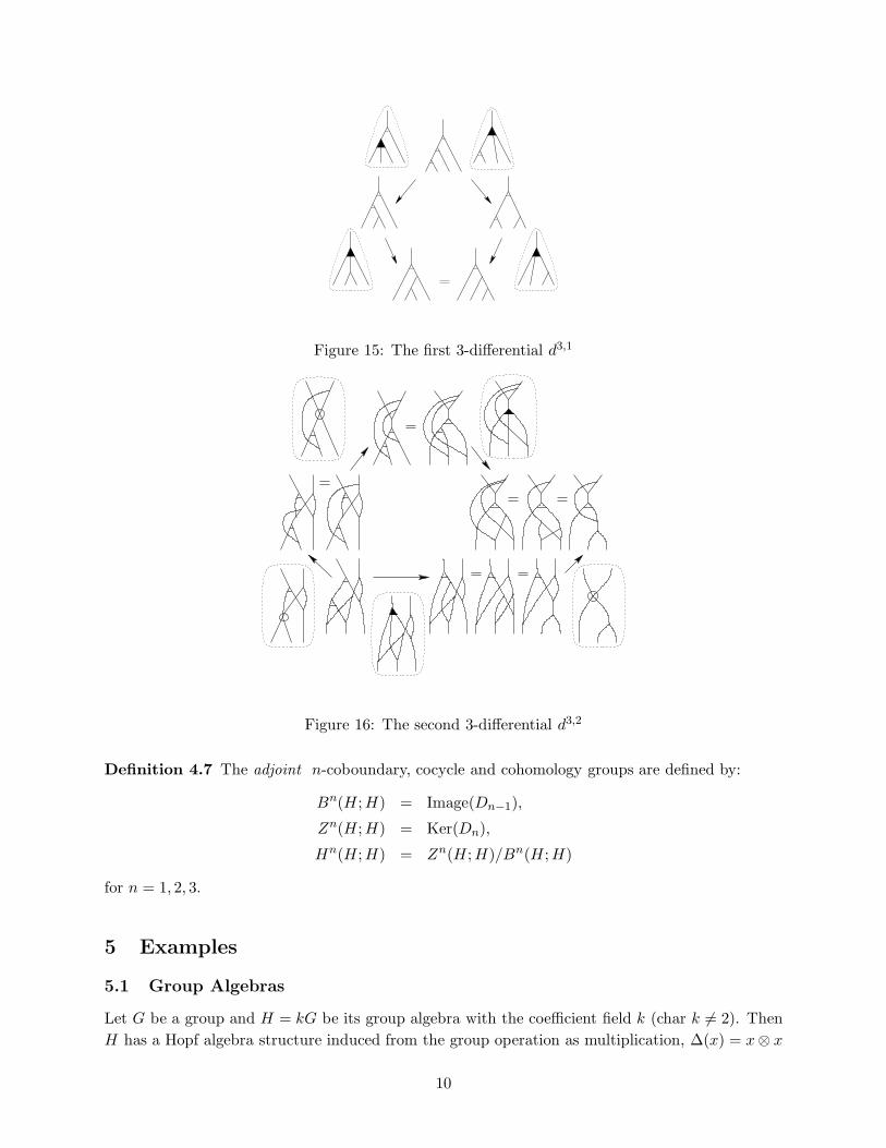
Figure 15: The first 3-differential d3,1
Figure 16: The second 3-differential d3,2
Definition 4.7 The adjoint n-coboundary, cocycle and cohomology groups are defined by:
Bn(H;H) = Image(Dn−1),
Zn(H;H) = Ker(Dn),
Hn(H;H) = Zn(H;H)/Bn(H;H)
for n = 1, 2, 3.
5 Examples
5.1 Group Algebras
Let G be a group and H = kG be its group algebra with the coefficient field k (char k 6= 2). Then
H has a Hopf algebra structure induced from the group operation as multiplication, ∆(x) = x⊗ x
10
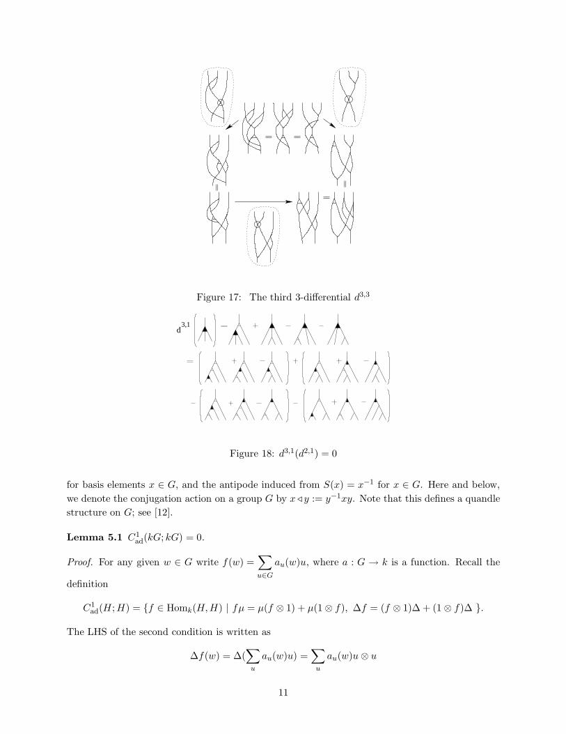
Figure 17: The third 3-differential d3,3
d3,1
Figure 18: d3,1(d2,1) = 0
for basis elements x ∈ G, and the antipode induced from S(x) = x−1 for x ∈ G. Here and below,
we denote the conjugation action on a group G by x ⊳ y := y−1xy. Note that this defines a quandle
structure on G; see [12].
Lemma 5.1 C1ad(kG; kG) = 0.
Proof. For any given w ∈ G write f(w) =∑
u∈G
au(w)u, where a : G → k is a function. Recall the
definition
C1ad(H;H) = {f ∈ Homk(H,H) | fµ = µ(f ⊗ 1) + µ(1 ⊗ f), ∆f = (f ⊗ 1)∆ + (1 ⊗ f)∆ }.
The LHS of the second condition is written as
∆f(w) = ∆(∑
u
au(w)u) =∑
u
au(w)u⊗ u
11
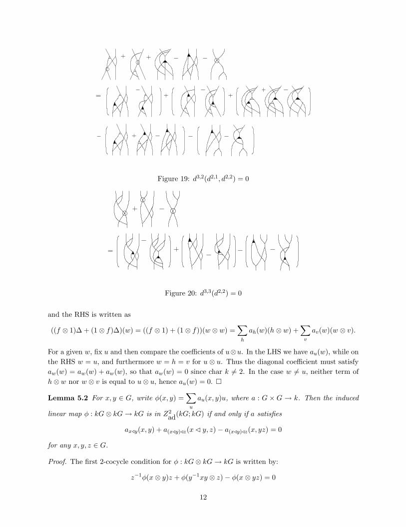
Figure 19: d3,2(d2,1, d2,2) = 0
Figure 20: d3,3(d2,2) = 0
and the RHS is written as
((f ⊗ 1)∆ + (1 ⊗ f)∆)(w) = ((f ⊗ 1) + (1 ⊗ f))(w ⊗ w) =∑
h
ah(w)(h ⊗ w) +∑
v
av(w)(w ⊗ v).
For a given w, fix u and then compare the coefficients of u⊗u. In the LHS we have au(w), while on
the RHS w = u, and furthermore w = h = v for u ⊗ u. Thus the diagonal coefficient must satisfy
aw(w) = aw(w) + aw(w), so that aw(w) = 0 since char k 6= 2. In the case w 6= u, neither term of
h⊗w nor w ⊗ v is equal to u⊗ u, hence au(w) = 0. �
Lemma 5.2 For x, y ∈ G, write φ(x, y) =∑
u
au(x, y)u, where a : G ×G → k. Then the induced
linear map φ : kG⊗ kG→ kG is in Z2ad(kG; kG) if and only if a satisfies
ax⊳y(x, y) + a(x⊳y)⊳z(x⊳ y, z) − a(x⊳y)⊳z(x, yz) = 0
for any x, y, z ∈ G.
Proof. The first 2-cocycle condition for φ : kG⊗ kG→ kG is written by:
z−1φ(x⊗ y)z + φ(y−1xy ⊗ z) − φ(x⊗ yz) = 0
12
for basis elements x, y, z ∈ G. The second is formulated by
LHS = φ(x⊗ y) ⊗ xy =∑
u
au(x, y)(u⊗ xy), RHS =∑
w
aw(x, y)(w ⊗ yw).
They have the common term u ⊗ xy for w = y−1xy = u, and otherwise they are different terms.
Thus we obtain aw(x, y) = 0 unless w = y−1xy. For these terms, the first condition becomes
z−1(ay−1xy(x, y)y−1xy)z + az−1y−1xyz(y
−1xy, z)z−1y−1xyz − az−1y−1xyz(x, yz)z−1y−1xyz = 0
and the result follows. �
Remark 5.3 In the preceding proof, since the term aw(x, y) = 0 unless w = x ⊳ y, let ax⊳y(x, y) =
a(x, y). Then the condition stated becomes
a(x, y) + a(x ⊳ y, z) − a(x, yz) = 0.
Proposition 5.4 Let G be a group. Let (ξ1, ξ2) ∈ C3ad(kG; kG), where ξ1 is the map that is defined
by linearly extending ξ1(x ⊗ y ⊗ z) =∑
u∈G
cu(x, y, z)u. Then (ξ1, ξ2) ∈ Z3ad(kG; kG) if and only if
ξ2 = 0 and the coefficients satisfy the following properties:
(a) cu(x, y, z) = 0 if u 6= z−1y−1xyz and
(b) c(x, y, z) = cz−1y−1xyz(x, y, z) satisfies
c(x, y, z) + c(x, yz,w) = c(y−1xy, z, w) + c(x, y, zw).
Proof. Suppose (ξ1, ξ2) ∈ Z3ad(kG; kG). Let ξ2 be the map that is defined by linearly extending
ξ2(x⊗ y) =∑
u,v∈G
au,v(x, y)u⊗ v. Then the third 3-cocycle condition from Definition 4.4 gives:
(abbreviating au,v(x, y) = au,v)
d3,3(ξ1, ξ2)(x⊗ y)
=∑
u1,v1
au1,v1(u1 ⊗ yu1 ⊗ v1) +
∑
u2,v2
au2,v2(u2 ⊗ v2 ⊗ xy) −
∑
u3,v3
au3,v3(u3 ⊗ v3 ⊗ v3) = 0.
We first consider terms in which the third tensorand is xy. From the third summand, this forces
the second tensorand to be xy, so we collect the terms of the form (u⊗ xy ⊗ xy). This gives:
∑
u
(au,xy + au,xy − au,xy)(u⊗ xy ⊗ xy) = 0,
which implies au,xy = 0 for all u ∈ G. The remaining terms are
∑
u1,v1 6=xy
au1,v1(u1 ⊗ yu1 ⊗ v1) +
∑
u2,v2 6=xy
au2,v2(u2 ⊗ v2 ⊗ xy) −
∑
u3,v3 6=xy
au3,v3(u3 ⊗ v3 ⊗ v3) = 0.
From the second sum we obtain au,v(x, y) = 0 for v 6= xy. In conclusion, if d3,3(ξ1, ξ2) = 0 for kG
then ξ2 = 0.
13
We now consider d3,2(ξ1, ξ2), with ξ2 = 0. Let ξ1 be the map that is defined by linearly extending
ξ1(x⊗ y ⊗ z) =∑
u∈G
cu(x, y, z)u for x, y, z ∈ G. The second 3-cocycle condition from Definition 4.4,
with ξ2 = 0, is∑
u
cuu⊗ yzu =∑
v
cvv ⊗ xyz. In order to combine like terms, we need yzu = xyz,
meaning u = z−1y−1xyz. Thus, cu(x, y, z) = 0 except in the case when u = z−1y−1xyz. In this
case, we obtain ξ1(x⊗ y ⊗ z) = c(x, y, z)z−1y−1xyz ⊗ xyz where c(x, y, z) = cz−1y−1xyz(x, y, z).
Finally we consider the first 3-cocycle condition from Definition 4.4, which is formulated for
basis elements by
w−1 ξ1(x⊗ y ⊗ z) w + ξ1(x⊗ yz ⊗ w) = ξ1(x ⊳ y ⊗ z ⊗ w) + ξ1(x⊗ y ⊗ zw).
Substituting in the formula for c(x, y, z) which we found above, we obtain
c(x, y, z) + c(x, yz,w) = c(y−1xy, z, w) + c(x, y, zw).
This is a group 3-cocycle condition with the first term x · c(y, z, w) omitted. This is expected from
Fig. 15. Constant functions, for example, satisfy this condition. �
Next we look at a coboundary condition. A 3-coboundary is written as
ξ1(x⊗ y ⊗ z) =∑
u
cu(x, y, z)u = d2,1(φ)(x⊗ y ⊗ z) = z−1φ(x⊗ y)z + φ(y−1xy ⊗ z) − φ(x⊗ yz).
If we write φ(x, y) =∑
u
hu(x, y)u, then
(d2,1(φ))(x ⊗ y ⊗ z)
= z−1
(∑
u
hu(x, y)u
)z +
(∑
v
hv(y−1xy, z)v
)−
(∑
w
hw(x, yz)w
)
=∑
g
( hzgz−1(x, y) + hg(y−1xy, z) − hg(x, yz) ) g.
Hence
cu(x, y, z) = hzuz−1(x, y) + hu(y−1xy, z) − hu(x, yz)
and in particular for the coefficients cu(x, y, z) from Proposition 5.4,
c(x, y, z) = cz−1y−1xyz(x, y, z) = hy−1xy(x, y) + hz−1y−1xyz(y−1xy, z) − hz−1y−1xyz(x, yz).
By setting hy−1xy(x, y) = a(x, y), we obtain:
Lemma 5.5 A 3-cocycle c(x, y, z) is a coboundary if for some a(x, y),
c(x, y, z) = a(x, y) + a(y−1xy, z) − a(x, yz).
Remark 5.6 From Remark 5.3, Proposition 5.4, and Lemma 5.5, we have the following situation.
The 2-cocycle condition, the 3-cocycle condition, and the 3-coboundary condition, respectively,
gives rise to the equations
a(x, y) + a(y−1xy, z) − a(x, yz) = 0,
c(x, y, z) + c(x, yz,w) − c(y−1xy, z, w) − c(x, y, zw) = 0,
c(x, y, z) = a(x, y) + a(y−1xy, z) − a(x, yz).
This suggests a cohomology theory, which we investigate in Section 6.
14
Proposition 5.7 For the symmetric group G = S3 on three letters, we have H1ad(kG; kG) = 0 and
H2ad(kG; kG) ∼=
⊕
3
(kG) for k = C and F3.
Proof. By Lemma 5.1, we have H1ad(kG; kG) = 0 and B2
ad(kG, kG) = 0. Hence H2(kG; kG) ∼=
Z2ad(kG; kG), which is computed by solving the system of equations stated in Lemma 5.2 and
Remark 5.3. Computations by Maple and Mathematica shows that the solution set is of dimension
3 and generated by (a((1 2 3), (1 2)), a((2 3), (1 3 2)), and a((1 3), (1 2)) for the above mentioned
coefficient fields. �
5.2 Function Algebras on Groups
Let G be a finite group and k a field with char(k) 6= 2. The set kG of functions from G to k
with pointwise addition and multiplication is a unital associative algebra. It has a Hopf algebra
structure using kG×G ∼= kG ⊗ kG with comultiplication defined through ∆ : kG → kG×G by
∆(f)(u⊗ v) = f(uv) and the antipode by S(f)(x) = f(x−1).
Now kG has basis (the characteristic function) δg : G → k defined by δg(x) = 1 if x = g and
zero otherwise. Since S(δg) = δg−1 and ∆(δh) =∑
uv=h
δu ⊗ δv, the adjoint map becomes
ad(δg ⊗ δh) =∑
uv=h
δu−1δgδv =
{δg if h = 1,
0 otherwise.
Lemma 5.8 C1ad(kG; kG) = 0.
Proof. Recall that
C1ad(H;H) = {f ∈ Homk(H,H) | fµ = µ(f ⊗ 1) + µ(1 ⊗ f), ∆f = (f ⊗ 1)∆ + (1 ⊗ f)∆ }.
Let G = {g1, . . . , gn} be a given finite group and abbreviate δgi= δi for i = 1, . . . , n. Describe
f : kG → kG by f(δi) =n∑
j=1
sjiδj . Then fµ = µ(f ⊗ 1) + µ(1 ⊗ f) is written for basis elements by
LHS = f(δiδj) and
RHS = f(δi)δj + δif(δj)
= (n∑
ℓ=1
sℓiδℓ)δj + δi(
n∑
h=1
shj δh)
= sjiδj + si
jδi.
For i = j we obtain LHS=
n∑
w=1
swi δw and RHS = 2si
iδi so that sji = 0 for all i, j as desired. �
Lemma 5.9 Z2ad(kG; kG) = 0.
Proof. Recall that d2,1(η1) = ad(η1 ⊗ 1) + η1(ad ⊗ 1) − η1(1 ⊗ µ) for η1 ∈ C2ad(kG, kG). Describe
15
a general element η1 ∈ C2ad(kG, kG) by η1(δi ⊗ δj) =
∑
ℓ
sℓi jδℓ. Consider d2,1(η1)(δa ⊗ δb ⊗ δc). If
c 6= 1, then the first term is zero by the definition of ad. If c 6= 1 and b = 1, then the third term
is also zero, and we obtain that the second term η1(δa ⊗ δc) is zero. Hence η1(δa ⊗ δc) = 0 unless
c = 1. Next, set b = c = 1 in the general form. Then all three terms equal η1(δa ⊗ δ1) and we
obtain η1(δa ⊗ δ1) = 0, and the result follows. �
By combining the above lemmas, we obtain the following:
Theorem 5.10 For any finite group G and a field k, we have Hn
ad(kG; kG) = 0 for n = 1, 2.
Observe that k(G) and kG are cohomologically distinct.
5.3 Bosonization of the Superline
Let H be generated by 1, g, x with relations x2 = 0, g2 = 1, xg = −gx and Hopf algebra structure
∆(x) = x⊗ 1 + g ⊗ x, ∆(g) = g ⊗ g, ǫ(x) = 0, ǫ(g) = 1, S(x) = −gx, S(g) = g (this Hopf algebra
is called the bosonization of the superline [15], page 39, Example 2.1.7).
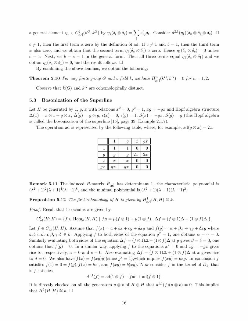
The operation ad is represented by the following table, where, for example, ad(g ⊗ x) = 2x.
1 g x gx
1 1 1 0 0
g g g 2x 2x
x x −x 0 0
gx gx −gx 0 0
Remark 5.11 The induced R-matrix Rad has determinant 1, the characteristic polynomial is
(λ2 + 1)2(λ+ 1)4(λ− 1)8, and the minimal polynomial is (λ2 + 1)(λ + 1)(λ − 1)2.
Proposition 5.12 The first cohomology of H is given by H1ad(H,H) ∼= k.
Proof. Recall that 1-cochains are given by
C1ad(H;H) = {f ∈ Homk(H,H) | fµ = µ(f ⊗ 1) + µ(1 ⊗ f), ∆f = (f ⊗ 1)∆ + (1 ⊗ f)∆ }.
Let f ∈ C1ad(H;H). Assume that f(x) = a+ bx + cg + dxg and f(g) = α+ βx + γg + δxg where
a, b, c, d, α, β, γ, δ ∈ k. Applying f to both sides of the equation g2 = 1, one obtains α = γ = 0.
Similarly evaluating both sides of the equation ∆f = (f ⊗1)∆+(1⊗f)∆ at g gives β = δ = 0, one
obtains that f(g) = 0. In a similar way, applying f to the equations x2 = 0 and xg = −gx gives
rise to, respectively, a = 0 and c = 0. Also evaluating ∆f = (f ⊗ 1)∆ + (1 ⊗ f)∆ at x gives rise
to d = 0. We also have f(x) = f(xg)g (since g2 = 1),which implies f(xg) = bxg. In conclusion f
satisfies f(1) = 0 = f(g), f(x) = bx , and f(xg) = b(xg). Now consider f in the kernel of D1, that
is f satisfies
d1,1(f) = ad(1 ⊗ f) − fad + ad(f ⊗ 1).
It is directly checked on all the generators u ⊗ v of H ⊗H that d1,1(f)(u ⊗ v) = 0. This implies
that H1(H,H) ∼= k. �
16
Proposition 5.13 For any field k of characteristic not 2, H2ad(H,H) ∼= k3.
Proof. With d1,1 = 0 from the preceding Proposition, we have H2ad(H,H) ∼= Z2
ad(H,H).
For the convenience of the reader we compute, ∆(gx) = gx⊗ g+ 1⊗ gx. A number of key facts
will be repeatedly recalled; these are inclosed in boxes.
The first 2-differential is written as
ad(φ(a⊗ b) ⊗ c) + φ(ad(a⊗ b) ⊗ c) − φ(a⊗ bc) = 0.
Take b = c = 1, then since ad(a⊗ 1) = a for any a ∈ H, all three terms are the same and gives
that φ(a⊗ 1) = 0 for any a.
Take a = g and b = c = x, then the third term vanishes and we obtain ad(φ(g ⊗ x) ⊗ x) +
φ(2x ⊗ x) = 0. For any possible value of φ(g ⊗ x), the value of the first term is written as hx for
some h ∈ k from the table of ad above. Since φ is bilinear, constants can be renamed to obtain
φ(x⊗ x) = hx . A similar argument gives φ(x⊗ gx) = h′x from a = g, b = x and c = gx, for
another constant h′ ∈ k.
The second differential is written as
φ(a(1) ⊗ b(1)) ⊗ a(2)b(2) = φ(a⊗ b(2))(1) ⊗ b(1)φ(a⊗ b(2))(2).
Taking a = b = x, we obtain the LHS φ(x ⊗ x) ⊗ 1 + (φ(x ⊗ g) + φ(g ⊗ x)) ⊗ x. The RHS is
φ(x⊗ x)(1) ⊗ gφ(x⊗ x)(2), and using that φ(x⊗ x) = hx, we obtain h(x⊗ g+ g⊗ gx) for the RHS.
Since there is no ⊗1 term in the RHS, we obtain φ(x ⊗ x) = 0, and in particular, h = 0, which
makes RHS = 0, and we also obtain φ(x⊗ g) = −φ(g ⊗ x) .
Let a = b = g in the second differential. Then LHS = φ(g ⊗ g) ⊗ 1 and RHS = φ(g ⊗ g)(1) ⊗
gφ(g⊗ g)(2). This implies that φ(g⊗ g) is written as hgg for some hg ∈ k, and RHS = hg(g⊗ g2) =
hg(g ⊗ 1) = LHS. With a = b = c = g in the first differential, we obtain ad(hgg⊗ g) + hgg− 0 = 0,
hence, in fact, hg = 0 if 2 is invertible, giving rise to φ(g ⊗ g) = 0 .
Let a = g and b = x in the second differential. Then the LHS = φ(g ⊗ x) ⊗ g, and the
RHS = φ(g⊗x)(1) ⊗ gφ(g⊗x)(2). For the RHS to have terms ending in ⊗g only, φ(g⊗x) can have
neither g nor gx terms since they would result in a ( ⊗1) term, so let φ(g ⊗ x) = hg,x1 + h′g,xx.
Then one computes RHS = (hg,x1 + h′g,xx) ⊗ g + h′g,x(g ⊗ gx). Equating this with LHS, we obtain
h′g,x = 0. Thus we obtained φ(g ⊗ x) = hg,x1 = −φ(x⊗ g) . In the first differential, take a = b = g
and c = x to obtain φ(g ⊗ gx) = φ(g ⊗ x) = hg,x1 .
Let a = 1 and b = x in the second differential. Then the LHS = φ(1 ⊗ x) ⊗ 1 + φ(1 ⊗ g) ⊗ x,
and the RHS = φ(1 ⊗ x)(1) ⊗ gφ(1 ⊗ x)(2). For the RHS to have terms ending in ⊗1 or ⊗x
only, φ(1 ⊗ x) can have neither 1 nor x terms since they would result in a ( ⊗g) term, so let
φ(1 ⊗ x) = h1,xg + h1,ggx . Then one computes RHS = h1,xg⊗1+h1,g(gx⊗1+1⊗x). Comparing
with the LHS, we obtain φ(1 ⊗ g) = h1,g1 . With a = 1, b = x and c = g in the first differential,
we also obtain φ(1 ⊗ gx) = −h1,xg + h1,ggx .
Recall that φ(x⊗ gx) = h′x. For a = x and b = gx in the second differential gives
LHS = φ(x⊗ gx) ⊗ g − φ(g ⊗ gx) ⊗ gx = h′(x⊗ g) − hg,x(1 ⊗ gx)
RHS = −hg,x(1 ⊗ gx) + h′(x⊗ 1 + g ⊗ x)
17
which implies φ(x⊗ gx) = 0 .
In the second differential, take a = gx and b = x. Then we obtain
LHS = φ(gx⊗ x) ⊗ g + (φ(gx ⊗ g) + φ(1 ⊗ x)) ⊗ gx
= φ(gx⊗ x) ⊗ g + (φ(gx ⊗ g) + h1,xg + h1,ggx) ⊗ gx
RHS = φ(gx⊗ x)(1) ⊗ gφ(gx ⊗ x)(2).
The LHS has only ⊗g and ⊗gx terms, so that φ(gx⊗x) does not have g or gx terms, and we can write
φ(gx⊗x) = hgx,x1+h′gx,xx and compute RHS = hgx,x(1⊗g)+h′gx,x(x⊗g+g⊗gx). Comparing with
the LHS we obtain h′gx,xg = φ(gx⊗g)+h1,xg+h1,ggx, so that φ(gx⊗ g) = (h′gx,x − h1,x)g − h1,ggx .
By the first differential with (a, b, c) = (gx, g, x), we obtain
φ(gx⊗ gx) = 2(h′gx,x − h1,x)x− (hgx,x1 + h′gx,xx) = −hgx,x1 + (h′gx,x − 2h1,x)x.
By the first differential with (a, b, c) = (gx, gx, g), we obtain
(−hgx,x1 − (h′gx,x − 2h1,x)x) + 0 + (hgx,x1 + h′gx,xx) = 0
which implies h1,x = 0. In particular, we obtain φ(gx⊗ g) = h′gx,xg − h1,ggx and
φ(gx ⊗ gx) = −hgx,x1 + h′gx,xx . By the second differential with a = b = gx, we obtain
LHS = φ(gx⊗ gx) ⊗ 1 + φ(1 ⊗ gx) ⊗ (gx)g
= (−hgx,x1 + h′gx,xx) ⊗ 1 − h1,g(gx⊗ x)
RHS = φ(gx⊗ g)(1) ⊗ (gx)φ(gx ⊗ g)(2) + φ(gx⊗ gx)(1) ⊗ φ(gx⊗ gx)(2)
= (h′gx,x(g ⊗ gxg) + h1,g(gx⊗ x)) + (−hgx,x(1 ⊗ 1) + h′gx,x(x⊗ 1 + g ⊗ x))
and comparing the terms we obtain 2h1,g = 0. In summary, resetting free variables by hg,x = α,
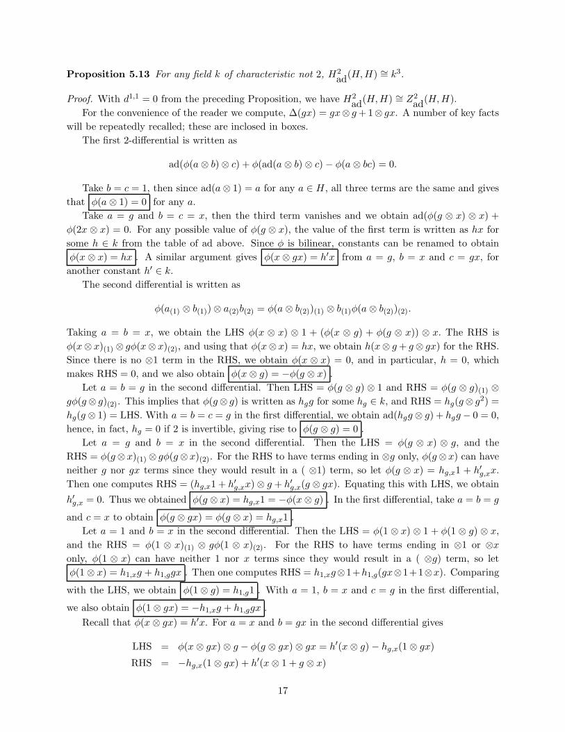
hgx,x = β and h′gx,x = γ, we obtained a general solution represented by the following table.
1 g x gx
1 0 0 0 0
g 0 0 α1 α1
x 0 −α1 0 0
gx 0 γg β1 + γx −β1 + γx
It is checked, either by hand, or computer guided calculations, that these are indeed solutions. �
6 Adjoint, Groupoid, and Quandle Cohomology Theories
From Remark 5.6, the adjoint cohomology leads us to cohomology, especially for conjugate groupoids
of groups as defined below. Through the relation between Reidemeister moves for knots and the
adjoint, groupoid cohomology, we obtain a new construction of quandle cocycles. In this section we
investigate these relations. First we formulate a general definition. Many formulations of groupoid
18
cohomology can be found in literature, and relations of the following formulation to previously
known theories are not clear. See [20], for example.
Let G be a groupoid with objects Ob(G) and morphisms G(x, y) for x, y ∈ Ob(G). Let fi ∈
G(xi, xi+1), 0 ≤ i < n, for non-negative integers i and n. Let Cn(G) be the free abelian group
generated by
{(x0, f0, . . . , fn) | x0 ∈ Ob(G), fi ∈ G(xi, xi+1), 0 ≤ i < n}.
The boundary map ∂ : Cn+1(G) → Cn(G) is defined by by linearly extending
∂(x0, f0, . . . , fn) = (x1, f1, . . . , fn)
+
n−1∑
i=0
(−1)i+1(x0, f0, . . . , fi−1, fifi+1, fi+2, . . . , fn)
+ (−1)n+1(x0, f0, . . . , fn−1).
Then it is easily seen that this differential defines a chain complex.
The corresponding groupoid 1- and 2-cocycle conditions are written as:
a(x1, f1) − a(x0, f0f1) + a(x0, f0) = 0
c(x1, f1, f2) − c(x0, f0f1, f2) + c(x0, f0, f1f2) − c(x0, f0, f1) = 0
The general cohomological theory of homomorphisms and extensions applies, such as:
Remark 6.1 Let G be a groupoid and A be an abelian group regarded as a one-object groupoid.
Then α : hom(x0, x1) → A gives a groupoid homomorphism from G to A, which sends Ob(G) to
the single object of A, if and only if a : C1(G) → A, defined by a(x0, f0) = α(f0), is a groupoid
1-cocycle.
Next we consider extensions of groupoids. Define ◦ : (hom(x0, x1)×A) × (hom(x1, x2) ×A) →
hom(x0, x2) ×A by
(f0, a) ◦ (f1, b) = (f0f1, a+ b+ c(x0, f0, f1))
where c(x0, f0, f1) ∈ hom(C2(G), A). If G×A is a groupoid, the function c with the value c(x0, f0, f1)
is a groupoid 2-cocycle.
Example 6.2 Let G be a group. Define the conjugate groupoid of G, denoted G, by:
Ob(G) = G
Mor(G) = G×G
where the source of the morphism (x, y) ∈ hom(x, y−1xy) is x and its target is y−1xy, for x, y ∈ G.
Composition is defined by (x, y) ◦ (y−1xy, z) = (x, yz). For this example, the groupoid 1- and
2-cocycle conditions are:
a(x, y) + a(y−1xy, z) − a(x, yz) = 0,
c(x, y, z) + c(x, yz,w) − c(y−1xy, z, w) − c(x, y, zw) = 0.
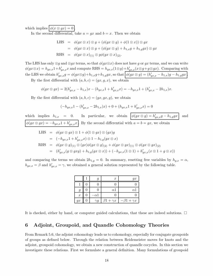
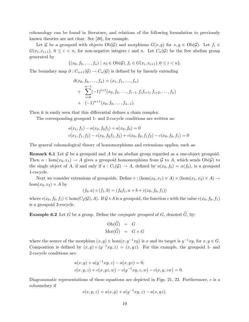
Diagrammatic representations of these equations are depicted in Figs. 21, 22. Furthermore, c is a
coboundary if
c(x, y, z) = a(x, y) + a(y−1xy, z) − a(x, yz).
19
Compare with Remark 5.6.
For G = S3, the symmetric group on 3 letters, with coefficient group C, Z2, Z3, Z5 and Z7,
respectively, the dimensions of the conjugation groupoid 2-cocycles are 3, 5, 4, 3 and 3.
1y xy
yz
1y xy
yzx
y
z
1y xya( , z)
x
y
z x
a(x, y) a(x, yz)
Figure 21: Diagrams for a groupoid 1-cocycle
1y xy
yzx
yz
wzw
yz1y xy
1y xyc( , z, w)
x
yz
w
x
yz
zw
c(x, y, zw)w
c(x, y, z) c(x, yz, w)
Figure 22: Diagrams for a groupoid 2-cocycle
For the rest of the section, we present new constructions of quandle cocycles from groupoid
cocycles of conjugate groupoids of groups. Let G be a finite group, and a : G2 → k be adjoint
2-cocycle coefficients that were defined in Remark 5.3. These satisfy
a(x, y) + a(x ⊳ y, z) − a(x, yz) = 0.
Proposition 6.3 Let ψ(x, y) = a(x, y). Then ψ satisfies the rack 2-cocycle condition
ψ(x, y) + ψ(x ⊳ y, z) = ψ(x, z) + ψ(x ⊳ z, y ⊳ z).
Proof. By definition ψ(x, y) + ψ(x ⊳ y, z) = a(x, yz), and ψ(x, z) + ψ(x ⊳ z, y ⊳ z) = a(x, z) +
a(z−1xz, z−1yz) = a(x, z(y ⊳ z)). �
Let G be a finite group, and c : G3 → k be a coefficient of the adjoint 3-cocycle defined in
Proposition 5.4. This satisfies
c(x, y, z) + c(x, yz,w) = c(x ⊳ y, z, w) + c(x, y, zw).
20
Proposition 6.4 Let G be a group that is considered as a quandle under conjugation. Then θ :
G3 → k defined by θ(x, y, z) = c(x, y, z) − c(x, z, z−1yz) is a rack 3-cocycle.
Proof. We must show that θ satsifies
θ(x, y, z) + θ(x ⊳ z, y ⊳ z,w) + θ(x, z, w)
= θ(x ⊳ y, z, w) + θ(x, y,w) + θ(x ⊳ w, y ⊳ w, z ⊳ w).
We compute
LHS − RHS = [ c(x, y, z) − c(x, z, z−1yz) ]
+[ c(z−1xz, z−1yz,w) − c(z−1xz,w,w−1z−1yzw) ]
+[ c(x, z, w) − c(x,w,w−1zw) ]
−[ c(y−1xy, z, w) − c(y−1xy,w,w−1zw) ]
−[ c(x, y,w) − c(x,w,w−1yw) ]
−[ c(w−1xw,w−1yw,w−1zw) − c(w−1xw,w−1zw,w−1z−1yzw) ]
= [ c(x, y, z) − c(y−1xy, z, w) ]
−[ c(x, z, z−1yz) − c(z−1xz, z−1yz,w) ]
+[ c(x, z, w) − c(z−1xz,w,w−1z−1yzw) ]
−[ c(x,w,w−1zw) − c(w−1xw,w−1zw,w−1z−1yzw) ]
−[ c(x, y,w) − c(y−1xy,w,w−1zw) ]
+[ c(x,w,w−1yw) − c(w−1xw,w−1yw,w−1zw) ]
= [ −c(x, yz,w) + c(x, y, zw) ]
−[ −c(x, zz−1yz,w) + c(x, z, z−1yzw) ]
+[ −c(x, zw,w−1z−1yzw) + c(x, z, ww−1z−1yzw) ]
−[ −c(x,ww−1zw,w−1z−1yzw) + c(x,w,w−1zww−1yw) ]
−[ −c(x, yw,w−1zw) + c(x, y,ww−1zw) ]
+[ −c(x,ww−1yw,w−1zw) + c(x,w,w−1yww−1zw) ]
= 0
as desired. �
7 Deformations of R-matrices by adjoint 2-cocycles
In this section we give, in an explicit form, deformations of R-matrices by 2-cocycles of the adjoint
cohomology theory we developed in this paper. Let H be a Hopf algebra and ad its adjoint map.
In Section 3 a deformation of (H, ad) was defined to be a pair (Ht, adt) where Ht is a k[[t]]-Hopf
algebra given by Ht = H ⊗ k[[t]] with all Hopf algebra structures inherited by extending those on
Ht. Let A = (H ⊗ k[[t]])/(t2)) and the Hopf algebra structure maps µ,∆, ǫ, η, S be inherited on A.
As a vector space A can be regarded as H ⊕ tH
Recall that a solution to the YBE, R-matrix Rad is induced from the adjoint map. Then from
the constructions of the adjoint cohomology from the point of view of the deformation theory, we
obtain the following deformation of this R-matrix induced from the adjoint map.
21
Theorem 7.1 Let φ ∈ Z2ad(H;H) be an adjoint 2-cocycle. Then the map R : A ⊗ A → A ⊗ A
defined by R = Rad+tφsatisfies the YBE.
Proof. The equalities of Lemma 3.2 hold in the quotient A = (H ⊗ k[[t]])/(t2), where n = 1 and
the modulus t2 is considered. These cocycle conditions, on the other hand, were formulated from
the motivation from Lemma 2.2 for the induced R-matrix Rad to satisfy the YBE. Hence these
two lemmas imply the theorem. �
Example 7.2 In Subsection 5.3, the adjoint map ad was computed for the bosonization H of the
superline, with basis {1, g, x, gx}, as well as a general 2-cocycle φ with three free variables α, β, γ
written by φ(g ⊗ x) = φ(g ⊗ gx) = α1, φ(x ⊗ g) = −α1, φ(gx ⊗ g) = γg, φ(gx ⊗ x) = β1 + γx,
φ(gx ⊗ gx) = −β1 + γx, and zero otherwise. Thus we obtain the deformed solution to the YBE
R = Rad+tφon A with three variables tα, tβ, tγ of degree one.
8 Concluding Remarks
In [7] we concluded with A Compendium of Questions regarding our discoveries. Here we attempt
to address some of these questions by providing relationships between this paper and [7], and offer
further questions for our future consideration.
It was pointed out in [7] that there was a clear distinction between the Hopf algebra case and
the cocommutative coalgebra case as to why self-adjoint maps satisfy the YBE. In [7] a cohomology
theory was constructed for the coalgebra case. In this paper, many of the same ideas and techniques,
in particular deformations and diagrams, were used to construct a cohomology theory in the Hopf
algebra case, with applications to the YBE and quandle cohomology.
The aspects that unify these two theories are deformations and a systematic process we call
“diagrammatic infiltration.” So far, these techniques have only been successful in defining cobound-
aries up through dimension 3. This is a deficit of the diagrammatic approach, but diagrams give
direct applications to other algebraic problems such as the YBE and quandle cohomology, and
suggest further applications to knot theory. By taking the trace as in Turaev’s [21], for example, a
new deformed version of a given invariant is expected to be obtained.
Many questions remain: Can 3-cocycles be used for solving the tetrahedral equation? Can they
be used for knotted surface invariants? Can the coboundary maps be expressed skein theoretically?
How are the deformations of R-matrices related to deformations of underlying Hopf algebras?
When a Hopf algebra contains a coalgebra, such as the universal enveloping algebra and its Lie
algebra together with the ground field of degree-zero part, what is the relation between the two
theories developed in this paper and in [7]? How these theories, other than the same diagrammatic
techniques, can be uniformly formulated, and to higher dimensions?
References
[1] Andruskiewitsch, N.; Grana, M., From racks to pointed Hopf algebras, Adv. in Math. 178
(2003), 177–243.
[2] Baez, J.C.; Crans, A.S., Higher-Dimensional Algebra VI: Lie 2-Algebras, Theory and Appli-
cations of Categories 12 (2004), 492–538.
22
[3] Baez, J.C.; Langford, L., 2-tangles, Lett. Math. Phys. 43 (1998), 187–197.
[4] Brieskorn, E., Automorphic sets and singularities, Contemporary math., 78 (1988), 45–115.
[5] J. S. Carter; M. Elhamdadi; M. Saito Twisted Quandle homology theory and cocycle knot
invariants Algebraic and Geometric Topology 2 (2002), 95–135.
[6] Carter, J.S.; Jelsovsky, D.; Kamada, S.; Langford, L.; Saito, M., Quandle cohomology and
state-sum invariants of knotted curves and surfaces, Trans. Amer. Math. Soc. 355 (2003),
3947–3989.
[7] Carter, J.S.; Crans, A.; Elhamdadi, M.; Saito, S., Cohomology of Categorical Self-
Distributivity, Preprint, available at arXiv:math.GT/0607417.
[8] Crans, A.S., Lie 2-algebras, Ph.D. Dissertation, 2004, UC Riverside, available at
arXiv:math.QA/0409602.
[9] Fenn, R.; Rourke, C., Racks and links in codimension two, Journal of Knot Theory and Its
Ramifications 1 (1992), 343–406.
[10] Gerstenharber, M; Schack, S.D., Bialgebra cohomology, deformations, and quantum groups,
Proc. Nat. Acad. Sci. U.S.A., 87 (1990), 478–481.
[11] Hennings, M.A., On solutions to the braid equation identified by Woronowicz, Lett. Math.
Phys. 27 (1993), 13–17.
[12] Joyce, D., A classifying invariant of knots, the knot quandle, J. Pure Appl. Alg. 23 (1982)
37–65.
[13] Kuperberg, G., Involutory Hopf algebras and 3-manifold invariants, Internat. J. Math. 2
(1991), 41–66.
[14] Majid, S. “A quantum groups primer.” London Mathematical Society Lecture Note Series,
292. Cambridge University Press, Cambridge, 2002.
[15] Majid, S. “Foundations of quantum group theory.” Cambridge University Press, Cambridge,
1995.
[16] Markl, M.; Stasheff, J.D., Deformation theory via deviations, J. Algebra 170 (1994), 122–155.
[17] Markl, M.; Voronov, A.; PROPped up graph cohomology, to appear in Maninfest, preprint at
http://arxiv.org/pdf/math/0307081.
[18] Matveev, S., Distributive groupoids in knot theory, (Russian) Mat. Sb. (N.S.) 119(161) (1982),
78–88 (160).
[19] Reshetikhin, N.; Turaev, V. G., Invariants of 3-manifolds via link polynomials and quantum
groups, Invent. Math. 103 (1991), 547–597.
[20] Tu, J.-L., Groupoid cohomology and extensions, Trans. Amer. Math. Soc. 358 (2006), 4721–
4747.
[21] Turaev, V. G. The Yang-Baxter equation and invariants of links, Invent. Math. 92 (1988), no.
3, 527–553.
[22] Woronowicz, S.L., Solutions of the braid equation related to a Hopf algebra, Lett. Math. Phys.
23 (1991), 143–145.
23