Embed Size (px)
Citation preview
IJMMS 29:12 (2002) 701–718PII. S0161171202020197
http://ijmms.hindawi.com© Hindawi Publishing Corp.
A GENERALISED HOPF ALGEBRA FOR SOLITONS
FALLEH R. AL-SOLAMY and EDWIN J. BEGGS
Received 17 April 2001 and in revised form 22 October 2001
This paper considers a generalisation of the idea of a Hopf algebra in which a commutativering replaces the field in the unit and counit. It is motivated by an example from the inversescattering formalism for solitons. We begin with the corresponding idea for groups, wherethe concept of the identity is altered.
2000 Mathematics Subject Classification: 16W30, 37K30.
1. Introduction. Group factorisation plays a vital role in the inverse scattering pro-
cedure [1, 8]. For example, the Riemann-Hilbert problem is a (not quite exact) factori-
sation of group-valued functions on the real line into functions analytic on the lower
half-plane times functions analytic on the upper half-plane. However, there is a prob-
lem, a group-valued function which is analytic on the lower half-plane need not have
an inverse which is analytic there. On the Lie algebra level all is well since any smooth
loop which is uniformly sufficiently close to the identity and is analytic on the lower
half-plane has an inverse which is also analytic on the lower half-plane. To avoid the
problem, we consider the Lie algebras or a neighbourhood of a group near the identity.
This corresponds in inverse scattering to considering solutions not too far from the
vacuum. However, the soliton solutions for many integrable systems are character-
ized by meromorphic loops, and there the factors are very definitely not closed under
inverse. For example, if we take the meromorphic function given by (for P ∈Mn(C) a
Hermitian projection matrix and P⊥ = 1−P )
φ(λ)= P⊥+ λ−αλ−αP, (1.1)
which has a pole at α in the upper half-plane, its inverse is given by
φ−1(λ)= P⊥+ λ−αλ−αP, (1.2)
which has a pole at α in the lower half-plane.
The meromorphic loops which specify the solitons in a classical integrable system
are not uniquely defined, there are vacuum loops which can be added without generat-
ing any extra solitons. However, these can be thought of as allowing soliton-antisoliton
pair creation in the integrable system. When the system is quantised a vacuum loop
could be perturbed into a soliton-antisoliton pair by a slight movement of the pole
positions. Effectively the vacuum loops get round the problem which would occur
702 F. R. AL-SOLAMY AND E. J. BEGGS
if we could count solitons by the number of poles. The number of poles cannot be
changed by a small perturbation, so without the vacuum loops soliton-antisoliton pair
production might seem impossible. To calculate the total quantum energy and mo-
mentum for a soliton, the contributions for these vacuum loops would have to be
added. This quantum correction is observed in the Sine-Gordon model, calculated by
other methods [11].
The existence of the vacuum loops and the fact that the upper and lower factors
for the meromorphic loop group are not groups are related, and are both taken into
account in the ideas described in this paper of an almost group and matched pairs of
almost groups. This naturally leads to the idea of an almost Hopf algebra, in which
the unit and counit map are modified to use a commutative algebra instead of the
ground field. From the discussion above, the commutative algebra would arise from
the vacuum loops. A group factorisation into a subgroup (a group doublecross prod-
uct) is well known to lead to a Hopf algebra bicrossproduct [2, 5, 10]. Here, we also
carry out the corresponding procedure for almost groups and almost Hopf algebras.
This is not the only generalisation of the idea of a Hopf algebra. In [3], there are
axioms for weak C∗-Hopf algebras, but in this case the unit and counit are not algebra
maps, which they are in our axioms.
Note that although we use some infinite examples of almost groups as motivation,
in the detailed proofs of the results about the algebras we always assume that almost
groups are finite.
2. Almost groups
Definition 2.1. An almost group is a set G with an associative binary operation ·,a 1-1 correspondence i :G→G (written g� gi), and a set J ⊂G which is closed under
the binary operation · and i. Also the following properties are satisfied:
(i) (gh)i = higi, for all g,h∈G;
(ii) for all g ∈G, and for all j ∈ J, jg = gj;(iii) for all g ∈G, ggi = gig ∈ J;
(iv) (gi)i = g, for all g ∈G.
Example 2.2. In the case where J = {e}, where ge = g for all g ∈ G, we just get a
group.
Example 2.3. Take G to be the set of meromorphic functions from C∞ to GLn(C)which are unitary on the real axis, normalized to the identity at infinity, and have all
poles in the upper half-plane. All such loops can be factored as a product of functions
of the form (1.1). We define the i operation on (1.1) by
φi(λ)= λ−αλ−αP
⊥+P. (2.1)
Here G is an almost group when J consists of all meromorphic complex-valued func-
tions times the identity matrix (the vacuum loops), and the binary operation is the
usual matrix multiplication.
A GENERALISED HOPF ALGEBRA FOR SOLITONS 703
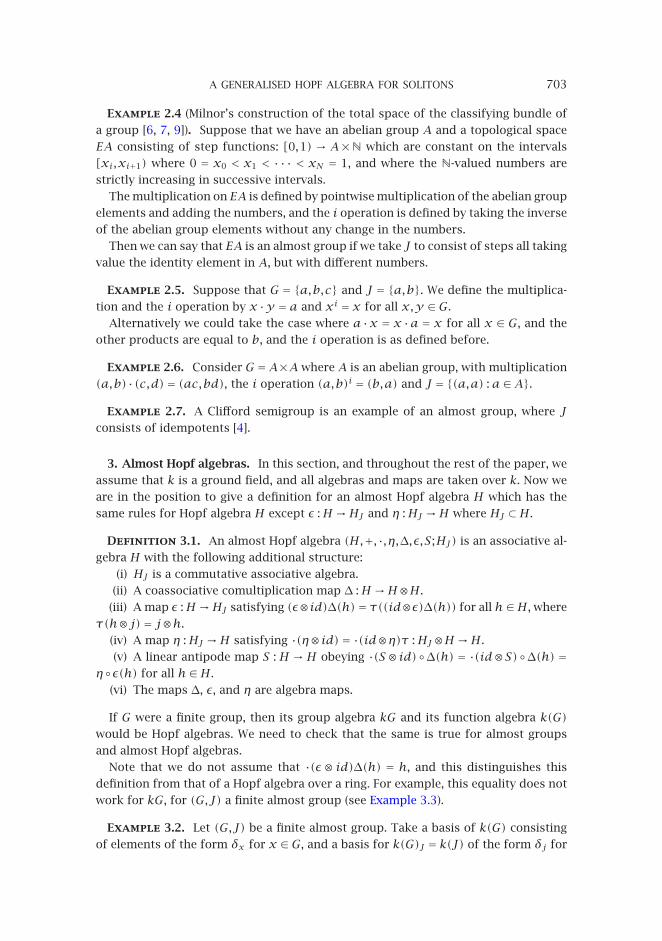
Example 2.4 (Milnor’s construction of the total space of the classifying bundle of
a group [6, 7, 9]). Suppose that we have an abelian group A and a topological space
EA consisting of step functions: [0,1) → A×N which are constant on the intervals
[xi,xi+1) where 0 = x0 < x1 < ··· < xN = 1, and where the N-valued numbers are
strictly increasing in successive intervals.
The multiplication on EA is defined by pointwise multiplication of the abelian group
elements and adding the numbers, and the i operation is defined by taking the inverse
of the abelian group elements without any change in the numbers.
Then we can say that EA is an almost group if we take J to consist of steps all taking
value the identity element in A, but with different numbers.
Example 2.5. Suppose that G = {a,b,c} and J = {a,b}. We define the multiplica-
tion and the i operation by x ·y = a and xi = x for all x,y ∈G.
Alternatively we could take the case where a ·x = x ·a = x for all x ∈ G, and the
other products are equal to b, and the i operation is as defined before.
Example 2.6. Consider G =A×A where A is an abelian group, with multiplication
(a,b)·(c,d)= (ac,bd), the i operation (a,b)i = (b,a) and J = {(a,a) : a∈A}.
Example 2.7. A Clifford semigroup is an example of an almost group, where Jconsists of idempotents [4].
3. Almost Hopf algebras. In this section, and throughout the rest of the paper, we
assume that k is a ground field, and all algebras and maps are taken over k. Now we
are in the position to give a definition for an almost Hopf algebra H which has the
same rules for Hopf algebra H except ε :H →HJ and η :HJ →H where HJ ⊂H.
Definition 3.1. An almost Hopf algebra (H,+,·,η,∆,ε,S;HJ) is an associative al-
gebra H with the following additional structure:
(i) HJ is a commutative associative algebra.
(ii) A coassociative comultiplication map ∆ :H →H⊗H.
(iii) A map ε :H →HJ satisfying (ε⊗id)∆(h)= τ((id⊗ε)∆(h)) for all h∈H, where
τ(h⊗j)= j⊗h.
(iv) A map η :HJ →H satisfying ·(η⊗id)= ·(id⊗η)τ :HJ⊗H →H.
(v) A linear antipode map S : H → H obeying ·(S⊗ id)◦∆(h) = ·(id⊗S)◦∆(h) =η◦ε(h) for all h∈H.
(vi) The maps ∆, ε, and η are algebra maps.
If G were a finite group, then its group algebra kG and its function algebra k(G)would be Hopf algebras. We need to check that the same is true for almost groups
and almost Hopf algebras.
Note that we do not assume that ·(ε⊗ id)∆(h) = h, and this distinguishes this
definition from that of a Hopf algebra over a ring. For example, this equality does not
work for kG, for (G,J) a finite almost group (see Example 3.3).
Example 3.2. Let (G,J) be a finite almost group. Take a basis of k(G) consisting
of elements of the form δx for x ∈G, and a basis for k(G)J = k(J) of the form δj for
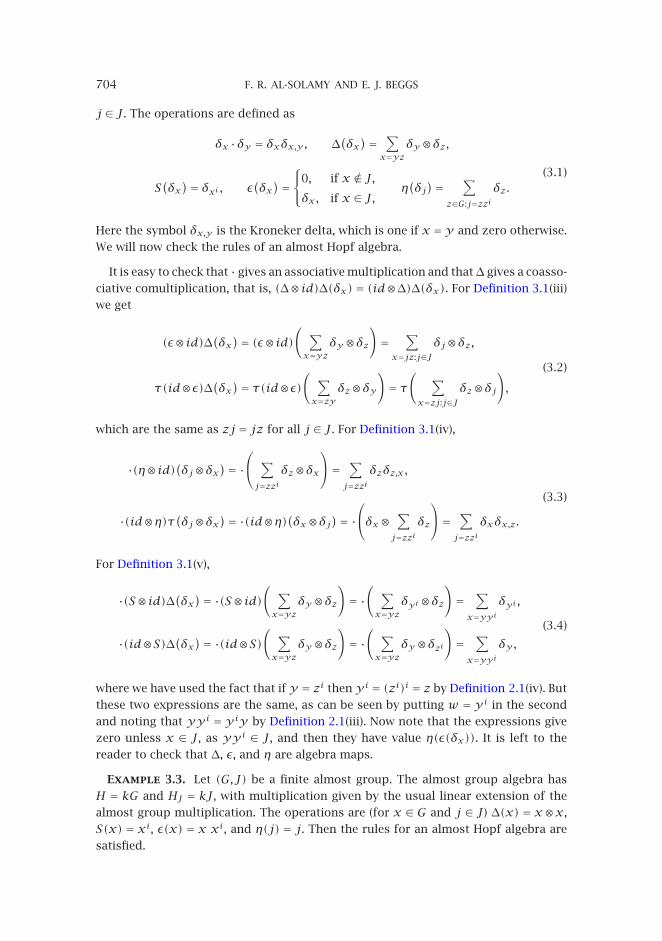
704 F. R. AL-SOLAMY AND E. J. BEGGS
j ∈ J. The operations are defined as
δx ·δy = δxδx,y , ∆(δx)= ∑
x=yzδy⊗δz,
S(δx)= δxi , ε
(δx)=
0, if x ∈ J,δx, if x ∈ J, η
(δj)= ∑
z∈G:j=zziδz.
(3.1)
Here the symbol δx,y is the Kroneker delta, which is one if x =y and zero otherwise.
We will now check the rules of an almost Hopf algebra.
It is easy to check that · gives an associative multiplication and that∆ gives a coasso-
ciative comultiplication, that is, (∆⊗id)∆(δx)= (id⊗∆)∆(δx). For Definition 3.1(iii)
we get
(ε⊗id)∆(δx)= (ε⊗id)( ∑x=yz
δy⊗δz)=
∑x=jz:j∈J
δj⊗δz,
τ(id⊗ε)∆(δx)= τ(id⊗ε)( ∑x=zy
δz⊗δy)= τ
( ∑x=zj:j∈J
δz⊗δj),
(3.2)
which are the same as zj = jz for all j ∈ J. For Definition 3.1(iv),
·(η⊗id)(δj⊗δx)= · ∑j=zzi
δz⊗δx= ∑
j=zziδzδz,x,
·(id⊗η)τ(δj⊗δx)= ·(id⊗η)(δx⊗δj)= ·δx⊗ ∑
j=zziδz
= ∑
j=zziδxδx,z.
(3.3)
For Definition 3.1(v),
·(S⊗id)∆(δx)= ·(S⊗id)( ∑x=yz
δy⊗δz)= ·
( ∑x=yz
δyi⊗δz)=
∑x=yyi
δyi ,
·(id⊗S)∆(δx)= ·(id⊗S)( ∑x=yz
δy⊗δz)= ·
( ∑x=yz
δy⊗δzi)=
∑x=yyi
δy,(3.4)
where we have used the fact that if y = zi then yi = (zi)i = z by Definition 2.1(iv). But
these two expressions are the same, as can be seen by putting w = yi in the second
and noting that yyi = yiy by Definition 2.1(iii). Now note that the expressions give
zero unless x ∈ J, as yyi ∈ J, and then they have value η(ε(δx)). It is left to the
reader to check that ∆, ε, and η are algebra maps.
Example 3.3. Let (G,J) be a finite almost group. The almost group algebra has
H = kG and HJ = kJ, with multiplication given by the usual linear extension of the
almost group multiplication. The operations are (for x ∈ G and j ∈ J) ∆(x) = x⊗x,
S(x) = xi, ε(x) = x xi, and η(j) = j. Then the rules for an almost Hopf algebra are
satisfied.
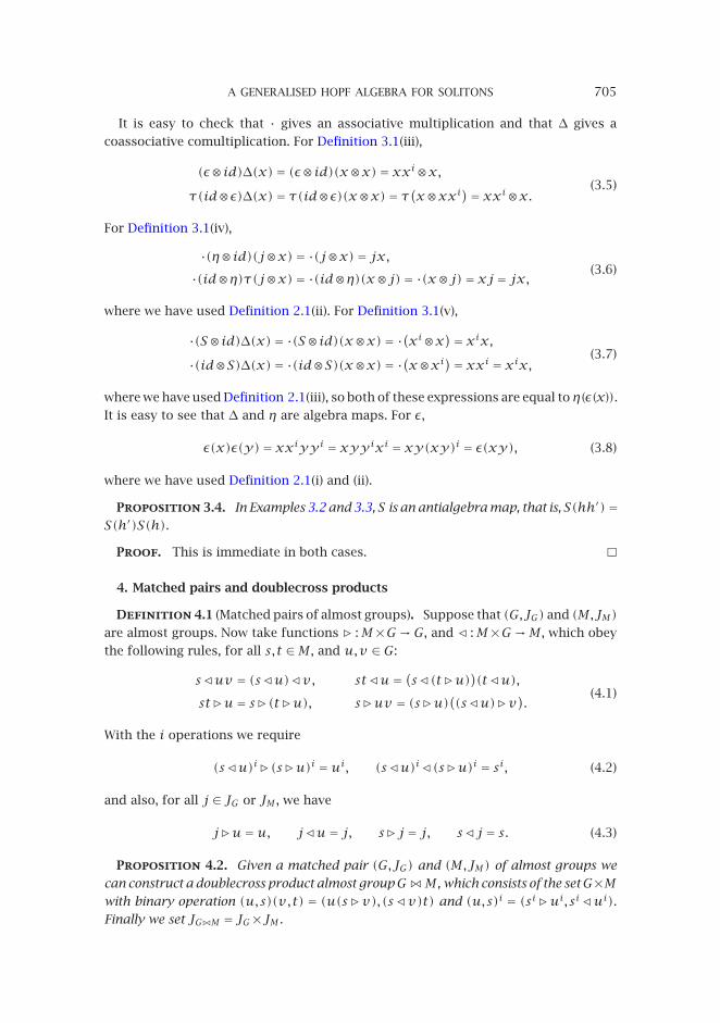
A GENERALISED HOPF ALGEBRA FOR SOLITONS 705
It is easy to check that · gives an associative multiplication and that ∆ gives a
coassociative comultiplication. For Definition 3.1(iii),
(ε⊗id)∆(x)= (ε⊗id)(x⊗x)= xxi⊗x,τ(id⊗ε)∆(x)= τ(id⊗ε)(x⊗x)= τ(x⊗xxi)= xxi⊗x. (3.5)
For Definition 3.1(iv),
·(η⊗id)(j⊗x)= ·(j⊗x)= jx,·(id⊗η)τ(j⊗x)= ·(id⊗η)(x⊗j)= ·(x⊗j)= xj = jx, (3.6)
where we have used Definition 2.1(ii). For Definition 3.1(v),
·(S⊗id)∆(x)= ·(S⊗id)(x⊗x)= ·(xi⊗x)= xix,·(id⊗S)∆(x)= ·(id⊗S)(x⊗x)= ·(x⊗xi)= xxi = xix, (3.7)
where we have used Definition 2.1(iii), so both of these expressions are equal toη(ε(x)).It is easy to see that ∆ and η are algebra maps. For ε,
ε(x)ε(y)= xxiyyi = xyyixi = xy(xy)i = ε(xy), (3.8)
where we have used Definition 2.1(i) and (ii).
Proposition 3.4. In Examples 3.2 and 3.3, S is an antialgebra map, that is, S(hh′)=S(h′)S(h).
Proof. This is immediate in both cases.
4. Matched pairs and doublecross products
Definition 4.1 (Matched pairs of almost groups). Suppose that (G,JG) and (M,JM)are almost groups. Now take functions � :M×G→G, and :M×G→M , which obey
the following rules, for all s,t ∈M , and u,v ∈G:
suv = (su)v, stu= (s(t�u))(tu),st�u= s�(t�u), s�uv = (s�u)((su)�v). (4.1)
With the i operations we require
(su)i�(s�u)i =ui, (su)i(s�u)i = si, (4.2)
and also, for all j ∈ JG or JM , we have
j�u=u, ju= j, s�j = j, sj = s. (4.3)
Proposition 4.2. Given a matched pair (G,JG) and (M,JM) of almost groups we
can construct a doublecross product almost groupGM , which consists of the setG×Mwith binary operation (u,s)(v,t) = (u(s �v),(s v)t) and (u,s)i = (si �ui,si ui).Finally we set JGM = JG×JM .
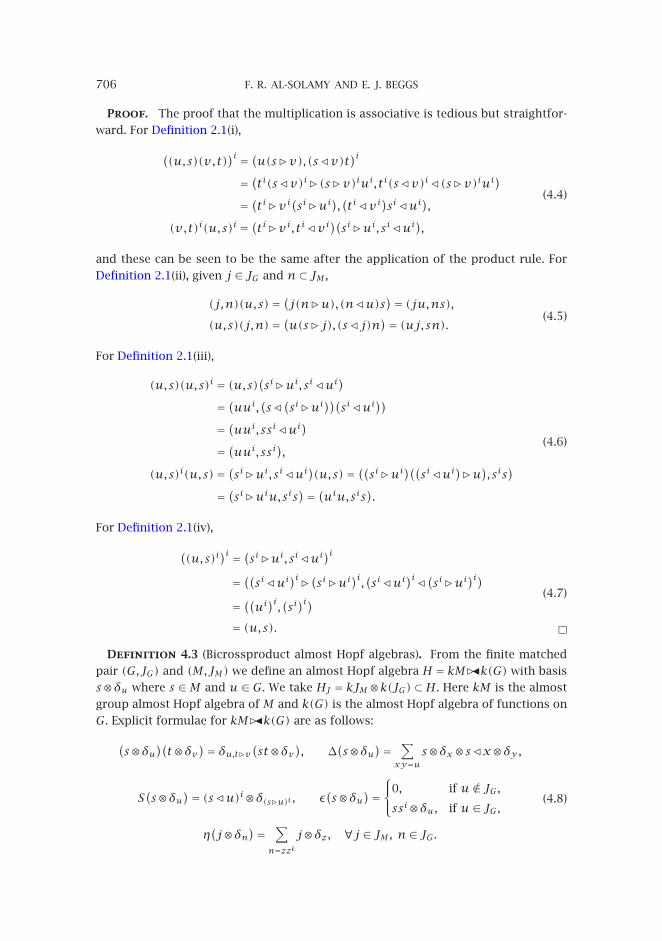
706 F. R. AL-SOLAMY AND E. J. BEGGS
Proof. The proof that the multiplication is associative is tedious but straightfor-
ward. For Definition 2.1(i),
((u,s)(v,t)
)i = (u(s�v),(sv)t)i= (ti(sv)i�(s�v)iui,ti(sv)i(s�v)iui)= (ti�vi(si�ui),(tivi)siui),
(v,t)i(u,s)i = (ti�vi,tivi)(si�ui,siui),(4.4)
and these can be seen to be the same after the application of the product rule. For
Definition 2.1(ii), given j ∈ JG and n⊂ JM ,
(j,n)(u,s)= (j(n�u),(nu)s)= (ju,ns),(u,s)(j,n)= (u(s�j),(sj)n)= (uj,sn). (4.5)
For Definition 2.1(iii),
(u,s)(u,s)i = (u,s)(si�ui,siui)= (uui,(s(si�ui))(siui))= (uui,ssiui)= (uui,ssi),
(u,s)i(u,s)= (si�ui,siui)(u,s)= ((si�ui)((siui)�u),sis)= (si�uiu,sis)= (uiu,sis).
(4.6)
For Definition 2.1(iv),
((u,s)i
)i = (si�ui,siui)i= ((siui)i �(si�ui)i,(siui)i (si�ui)i)= ((ui)i,(si)i)= (u,s).
(4.7)
Definition 4.3 (Bicrossproduct almost Hopf algebras). From the finite matched
pair (G,JG) and (M,JM) we define an almost Hopf algebra H = kM��k(G) with basis
s⊗δu where s ∈M and u∈G. We take HJ = kJM ⊗k(JG)⊂H. Here kM is the almost
group almost Hopf algebra of M and k(G) is the almost Hopf algebra of functions on
G. Explicit formulae for kM��k(G) are as follows:
(s⊗δu
)(t⊗δv
)= δu,t�v(st⊗δv), ∆(s⊗δu
)= ∑xy=u
s⊗δx⊗sx⊗δy,
S(s⊗δu
)= (su)i⊗δ(s�u)i , ε(s⊗δu
)=0, if u ∈ JG,ssi⊗δu, if u∈ JG,
η(j⊗δn
)= ∑n=zzi
j⊗δz, ∀j ∈ JM, n∈ JG.
(4.8)
A GENERALISED HOPF ALGEBRA FOR SOLITONS 707
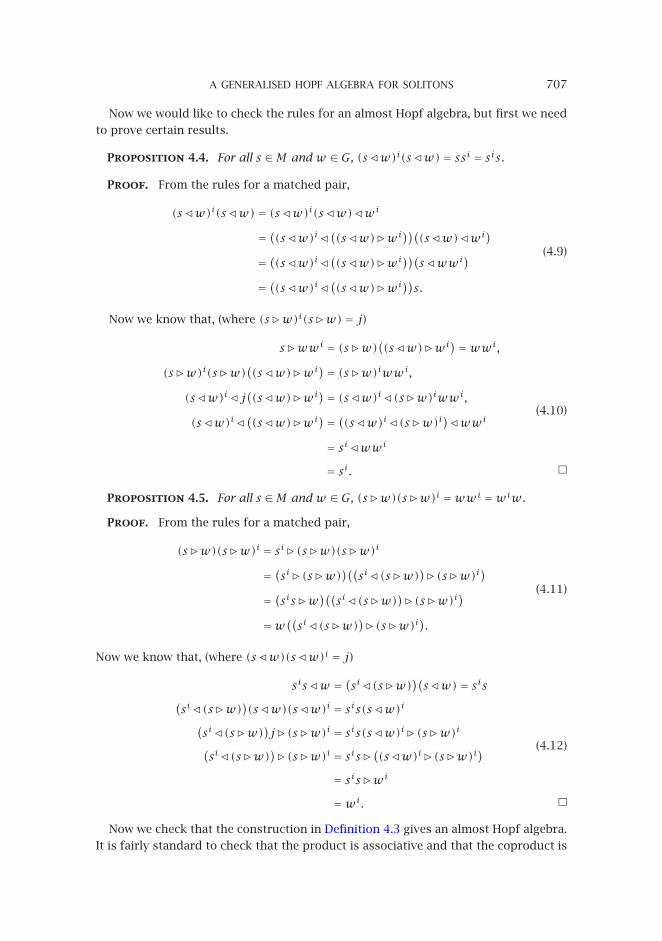
Now we would like to check the rules for an almost Hopf algebra, but first we need
to prove certain results.
Proposition 4.4. For all s ∈M and w ∈G, (sw)i(sw)= ssi = sis.
Proof. From the rules for a matched pair,
(sw)i(sw)= (sw)i(sw)wi
= ((sw)i((sw)�wi))((sw)wi)= ((sw)i((sw)�wi))(swwi)= ((sw)i((sw)�wi))s.
(4.9)
Now we know that, (where (s�w)i(s�w)= j)
s�wwi = (s�w)((sw)�wi)=wwi,
(s�w)i(s�w)((sw)�wi)= (s�w)iwwi,
(sw)ij((sw)�wi)= (sw)i(s�w)iwwi,
(sw)i((sw)�wi)= ((sw)i(s�w)i)wwi
= siwwi
= si.
(4.10)
Proposition 4.5. For all s ∈M and w ∈G, (s�w)(s�w)i =wwi =wiw.
Proof. From the rules for a matched pair,
(s�w)(s�w)i = si�(s�w)(s�w)i
= (si�(s�w))((si(s�w))�(s�w)i)= (sis�w)((si(s�w))�(s�w)i)=w((si(s�w))�(s�w)i).
(4.11)
Now we know that, (where (sw)(sw)i = j)
sisw = (si(s�w))(sw)= sis(si(s�w)
)(sw)(sw)i = sis(sw)i(
si(s�w))j�(s�w)i = sis(sw)i�(s�w)i(
si(s�w))�(s�w)i = sis�((sw)i�(s�w)i)
= sis�wi
=wi.
(4.12)
Now we check that the construction in Definition 4.3 gives an almost Hopf algebra.
It is fairly standard to check that the product is associative and that the coproduct is
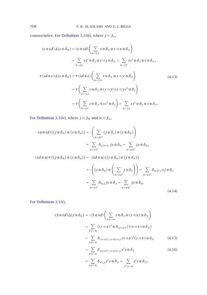
708 F. R. AL-SOLAMY AND E. J. BEGGS
coassociative. For Definition 3.1(iii), where j ∈ JG,
(ε⊗id)∆(s⊗δu)= (ε⊗id)( ∑u=xy
s⊗δx⊗sx⊗δy)
=∑u=jy
ssi⊗δj⊗sj⊗δy =∑u=jy
ssi⊗δj⊗s⊗δy,
τ(id⊗ε)∆(s⊗δu)= τ(id⊗ε)( ∑u=yx
s⊗δy⊗sy⊗δx)
= τ( ∑u=yj
s⊗δy⊗(sy)(sy)i⊗δj)
= τ( ∑u=jy
s⊗δy⊗ssi⊗δj)=
∑u=jy
ssi⊗δj⊗s⊗δy.
(4.13)
For Definition 3.1(iv), where j ∈ JM and n∈ JG,
·(η⊗id)((j⊗δn)⊗(s⊗δu))= · ∑n=zzi
(j⊗δz
)⊗(s⊗δu)
=∑
n=zziδz,s�u js⊗δu =
∑n=uui
js⊗δu,
·(id⊗η)τ((j⊗δn)⊗(s⊗δu))= ·(id⊗η)((s⊗δu)⊗(j⊗δn))
= ·(s⊗δu)⊗
∑n=zzi
j⊗δz= ∑
n=zziδu,j�zsj⊗δz
=∑
n=zziδu,zjs⊗δz =
∑n=uui
js⊗δu.
(4.14)
For Definition 3.1(v),
·(S⊗id)∆(s⊗δu)= ·(S⊗id)( ∑xy=u
s⊗δx⊗(sx)⊗δy)
=∑xy=u
((sx)i⊗δ(s�x)i
)((sx)⊗δy
)
=∑xy=u
δ(s�x)i,(sx)�y(sx)i(sx)⊗δy (4.15)
=∑xy=u
δ(s�x)i,(sx)�ysis⊗δy (4.16)
=∑xy=u
δxi,ysis⊗δy =
∑yiy=u
sis⊗δy,
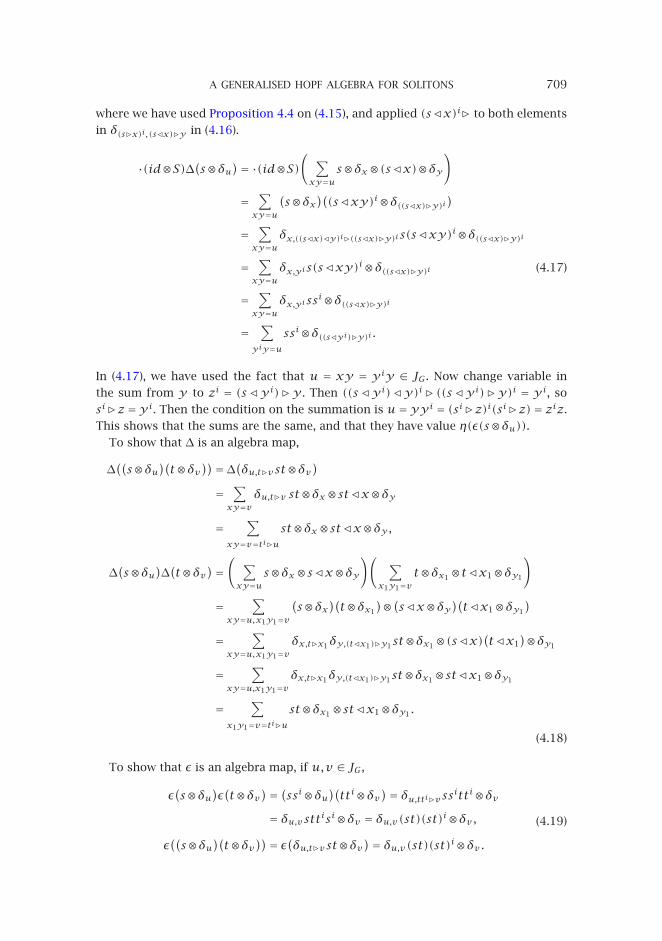
A GENERALISED HOPF ALGEBRA FOR SOLITONS 709
where we have used Proposition 4.4 on (4.15), and applied (sx)i� to both elements
in δ(s�x)i,(sx)�y in (4.16).
·(id⊗S)∆(s⊗δu)= ·(id⊗S)( ∑xy=u
s⊗δx⊗(sx)⊗δy)
=∑xy=u
(s⊗δx
)((sxy)i⊗δ((sx)�y)i
)
=∑xy=u
δx,((sx)y)i�((sx)�y)is(sxy)i⊗δ((sx)�y)i
=∑xy=u
δx,yis(sxy)i⊗δ((sx)�y)i (4.17)
=∑xy=u
δx,yissi⊗δ((sx)�y)i
=∑
yiy=ussi⊗δ((syi)�y)i .
In (4.17), we have used the fact that u = xy = yiy ∈ JG. Now change variable in
the sum from y to zi = (s yi)�y . Then ((s yi)y)i � ((s yi)�y)i = yi, so
si�z =yi. Then the condition on the summation is u=yyi = (si�z)i(si�z)= ziz.
This shows that the sums are the same, and that they have value η(ε(s⊗δu)).To show that ∆ is an algebra map,
∆((s⊗δu
)(t⊗δv
))=∆(δu,t�vst⊗δv)=
∑xy=v
δu,t�v st⊗δx⊗stx⊗δy
=∑
xy=v=ti�ust⊗δx⊗stx⊗δy,
∆(s⊗δu
)∆(t⊗δv
)=( ∑xy=u
s⊗δx⊗sx⊗δy)( ∑
x1y1=vt⊗δx1⊗tx1⊗δy1
)
=∑
xy=u,x1y1=v
(s⊗δx
)(t⊗δx1
)⊗(sx⊗δy)(tx1⊗δy1
)
=∑
xy=u,x1y1=vδx,t�x1δy,(tx1)�y1st⊗δx1⊗(sx)
(tx1
)⊗δy1
=∑
xy=u,x1y1=vδx,t�x1δy,(tx1)�y1st⊗δx1⊗stx1⊗δy1
=∑
x1y1=v=ti�ust⊗δx1⊗stx1⊗δy1 .
(4.18)
To show that ε is an algebra map, if u,v ∈ JG,
ε(s⊗δu
)ε(t⊗δv
)= (ssi⊗δu)(tti⊗δv)= δu,tti�vssitti⊗δv= δu,vsttisi⊗δv = δu,v(st)(st)i⊗δv,
ε((s⊗δu
)(t⊗δv
))= ε(δu,t�vst⊗δv)= δu,v(st)(st)i⊗δv.(4.19)
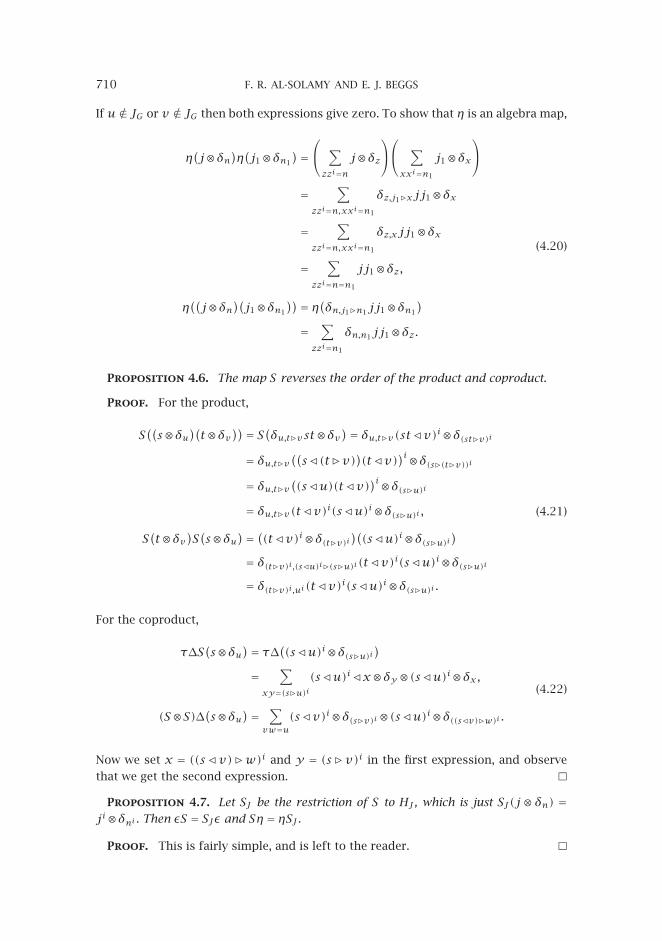
710 F. R. AL-SOLAMY AND E. J. BEGGS
If u ∈ JG or v ∈ JG then both expressions give zero. To show that η is an algebra map,
η(j⊗δn
)η(j1⊗δn1
)= ∑zzi=n
j⊗δz ∑xxi=n1
j1⊗δx
=∑
zzi=n,xxi=n1
δz,j1�xjj1⊗δx
=∑
zzi=n,xxi=n1
δz,xjj1⊗δx
=∑
zzi=n=n1
jj1⊗δz,
η((j⊗δn
)(j1⊗δn1
))= η(δn,j1�n1jj1⊗δn1
)=
∑zzi=n1
δn,n1jj1⊗δz.
(4.20)
Proposition 4.6. The map S reverses the order of the product and coproduct.
Proof. For the product,
S((s⊗δu
)(t⊗δv
))= S(δu,t�vst⊗δv)= δu,t�v(stv)i⊗δ(st�v)i= δu,t�v
((s(t�v)
)(tv)
)i⊗δ(s�(t�v))i= δu,t�v
((su)(tv)
)i⊗δ(s�u)i= δu,t�v(tv)i(su)i⊗δ(s�u)i ,
S(t⊗δv
)S(s⊗δu
)= ((tv)i⊗δ(t�v)i)((su)i⊗δ(s�u)i)= δ(t�v)i,(su)i�(s�u)i(tv)i(su)i⊗δ(s�u)i= δ(t�v)i,ui(tv)i(su)i⊗δ(s�u)i .
(4.21)
For the coproduct,
τ∆S(s⊗δu
)= τ∆((su)i⊗δ(s�u)i)=
∑xy=(s�u)i
(su)ix⊗δy⊗(su)i⊗δx,
(S⊗S)∆(s⊗δu)= ∑vw=u
(sv)i⊗δ(s�v)i⊗(su)i⊗δ((sv)�w)i .
(4.22)
Now we set x = ((s v)�w)i and y = (s �v)i in the first expression, and observe
that we get the second expression.
Proposition 4.7. Let SJ be the restriction of S to HJ , which is just SJ(j ⊗δn) =ji⊗δni . Then εS = SJε and Sη= ηSJ .
Proof. This is fairly simple, and is left to the reader.
A GENERALISED HOPF ALGEBRA FOR SOLITONS 711
5. The meromorphic loop group. In this section, we continue with the meromor-
phic loops introduced in Example 2.3. Any invertible meromorphic function φ : C∞ →Mn(C) which is unitary on the real axis can be written as a constant matrix times a
product of factors of the form
Φα,P (λ)= P⊥+ λ−αλ−αP, (5.1)
where α∈ C\R and P is a self-adjoint projection in Mn(C). Define the sets
G = {φ : φ(∞)= 1, φ(λ) has no singularities for im(λ) > 0},
JG ={φ : φ(∞)= 1, φ(λ) has no singularities for im(λ) > 0,
φ is a scalar function times the identity matrix},
M = {φ : φ(∞)= 1, φ(λ) has no singularities for im(λ) < 0},
JM ={φ : φ(∞)= 1, φ(λ) has no singularities for im(λ) < 0,
φ is a scalar function times the identity matrix}.
(5.2)
The normalization φ(∞)= 1 just means that we can forget about the constant factor.
Define the i operation by
Φiα,P (λ)=λ−αλ−αP
⊥+P, (5.3)
and extend this to products of basic loops by reversing order, that is, (ΦΨ)i = Ψ iΦi. It
is not too difficult to show that (G,JG) and (M,JM) are almost groups, with the usual
matrix multiplication.
Definition 5.1. We define the actions � and by reversal of order of multi-
plication, that is, for s ∈ M and u ∈ G choose s � u ∈ G and s u ∈ M so that
su= (s�u)(su).
Here we must issue a warning; there is no uniqueness of factorisation. To factor a
meromorphic loop φ we can use the procedure in [1] to write φ as a product of basic
loops, choosing the lower half-plane poles first, φ = su. There are other possible
factorisations of the form φ = s′u′, where s′ = st ∈ M and u′ = t−1u ∈ G, all we
have to do is to take t with all poles in the upper half-plane, so t−1 has all poles
in the lower half-plane. This occurs because G and M are not groups, as they are not
closed under the inverse operation. To get round this, we always choose a factorisation
with the minimum number of basic factors. It is also possible to have ambiguities
in the factorisation where poles coincide or are at complex conjugate positions (as
noted in the proof of the following proposition). Strictly we should restrict our results
on actions to the dense open set of loops which have no multiple poles or poles at
complex conjugate positions. We will assume this for the rest of the section (with the
exception of the next proposition).
We can calculate the actions on the basic factors by the next result. The actions on
products of basic factors are calculated by successive reversals of factors, a procedure
which does not increase the number of factors. In fact, s�u has exactly the same pole
positions as u, and su has exactly the same pole positions as s.
712 F. R. AL-SOLAMY AND E. J. BEGGS
Proposition 5.2. Suppose thatθα(λ)= (λ−α)/(λ−α) and θβ(λ)= (λ−β)/(λ−β),where α and β are in different half-planes (in particular α≠ β). Then
(P⊥1 +θαP1
)(P⊥2 +θβP2
)= (P⊥3 +θβP3)(P⊥4 +θαP4
), (5.4)
where (if we put Vi to be the image of the projection Pi)
V3 =(P⊥1 +θα(β)P1
)V2, V4 =
(P⊥3 +θ−1
β (α)P3)V1, (5.5)
if β≠ α, and if β= α we get P3 = 1−P1 and P4 = 1−P2.
Proof. We know P1 and P2, and we want to get P3 and P4. If α≠ β, we have (P⊥1 +θα(β)P1)V2 = V3 and (P⊥3 +θβ(α)P3)V4 = V1, which implies V4 = (P⊥3 +θ−1
β (α)P3)V1.
But if β= α there is a problem, because θβ(α) is not invertible. If β= α, we know that
θα(λ)= 1/θβ(λ). Then setting z = θα(λ), we can write the factorisation as
(P⊥1 +zP1
)(P⊥2 +
1zP2
)=(P⊥3 +
1zP3
)(P⊥4 +zP4
), (5.6)
which can be rearranged to give
(P⊥2 +
1zP2
)(P⊥4 +
1zP4
)=(P⊥1 +
1zP1
)(P⊥3 +
1zP3
). (5.7)
By separating powers of z we get P4 = P3 + P1 − P2 and (P1 − P2)P3 = P2(P1 − P2).In the case where P1 − P2 is invertible, we can define P3 as the unique solution to
(P1−P2)P3 = P2(P1−P2), and this will then give a unique value of P4. From substitut-
ing in the equation we see that these unique solutions are P3 = 1−P1 and P4 = 1−P2.
To preserve continuity, we define these to be the actions even if P1−P2 is not invertible.
Proposition 5.3. The meromorphic loop almost groups (G,JG) and (M,JM), with
the actions and i operation specified, form a matched pair.
Proof. Consider the associativity of the multiplication stu where s,t ∈ M and
u∈G. Then,
s(tu)= (st)u= (st�u)(stu)= s(t�u)(tu)= (s�(t�u))(s(t�u))(tu). (5.8)
By the uniqueness of the factorisation (on the open dense subset referred to earlier),
we see that s�(t�u)= st�u and (s(t�u))(tu)= stu. Similarly, for all s ∈Mand u,v ∈G, we have
(su)v = s(uv)= (s�uv)(suv)= (s�u)(su)v= (s�u)((su)�v)((su)v) (5.9)
which gives (s�u)((su)�v)= s�uv and (su)v = suv . Also, for all j ∈ JMand u ∈ G, we have ju = uj = (j �u)(j u), which gives j �u = u and j u = j.
A GENERALISED HOPF ALGEBRA FOR SOLITONS 713
Similarly, for all j ∈ JG and s ∈ M , we have sj = js = (s � j)(s j), which gives
s�j = j and sj = s. Finally, for all s ∈M and u∈G, we have
(su)i =uisi = ((s�u)(su))i = (su)i(s�u)i= ((su)i�(s�u)i)((su)i(s�u)i). (5.10)
By the uniqueness of the factorisation, we see that
(su)i�(s�u)i =ui, (su)i(s�u)i = si. (5.11)
6. Duality. We take (G,JG) and (M,JM) to be a matched pair of finite almost groups.
There is a dual almost Hopf algebra H′ = k(M)�kG to H = kM��k(G) with basis
δs⊗u where s ∈M and u∈G, with JH′ = k(JM)�kJG. The explicit formulae for this
almost Hopf algebra are as follows:
(δs⊗u
)(δt⊗v
)= δsu,t(δs⊗uv), ∆(δs⊗u
)= ∑a,b∈M :ab=s
δa⊗b�u⊗δb⊗u,
S(δs⊗u
)= δ(su)i⊗(s�u)i, ε(δs⊗u
)=0, if s ∈ JM,δs⊗uui, if s ∈ JM,
η(δj⊗n
)= ∑a∈M :j=aai
δa⊗n.
(6.1)
The dual pairing between H′ and H is given by
⟨δs⊗u,t⊗δv
⟩= δs,tδu,v . (6.2)
Proposition 6.1. The almost Hopf algebras H = kM��k(G) and H′ = k(M)�kGare dual to each other.
Proof. First we check that the counits and the units are dual to each other:
⟨ε(δs⊗u
),j⊗δn
⟩= δs,jδuui,n⟨δs⊗u,η
(j⊗δn
)⟩=⟨δs⊗u,
∑n=zzi
j⊗δz⟩= δs,jδuui,n,
⟨δj⊗n,ε
(s⊗δu
)⟩= δj,ssiδn,u⟨η(δj⊗n
),s⊗δu
⟩=⟨ ∑j=zzi
δz⊗n,s⊗δu⟩= δj,ssiδn,u.
(6.3)
Now we check the antipodes
⟨S(δs⊗u
), t⊗δv
⟩= ⟨δ(su)i⊗(s�u)i,t⊗δv⟩= δ(su)i,tδ(s�u)i,v ,⟨δs⊗u,S
(t⊗δv
)⟩= ⟨δs⊗u,(tv)i⊗δ(t�v)i⟩= δs,(tv)iδu,(t�v)i , (6.4)
and these are the same by the original definition of the actions. It is left to the reader
714 F. R. AL-SOLAMY AND E. J. BEGGS
to check the product and coproduct, that is,
⟨(δs⊗u
)(δt⊗v
),r ⊗δw
⟩= ⟨(δs⊗u)⊗(δt⊗v),∆(r ⊗δw)⟩,⟨δs⊗u,
(t⊗δv
)(r ⊗δw
)⟩= ⟨∆(δs⊗u),(t⊗δv)⊗(r ⊗δw)⟩. (6.5)
7. The ∗ operation. We take (G,JG) and (M,JM) to be a matched pair of finite al-
most groups, and continue with the notation of the last section. We define a ∗ opera-
tion onH by (s⊗δu)∗ = si⊗δs�u on the basis elements, extended to a conjugate-linear
map from H to H.
Proposition 7.1. The ∗ operation reverses the order of multiplication.
Proof. Applying the ∗ map to a product,
((s⊗δu
)(t⊗δv
))∗ = (δu,t�vst⊗δv)∗= δu,t�v(st)i⊗δst�v ,(
t⊗δv)∗(s⊗δu)∗ = (ti⊗δt�v)(si⊗δs�u)
= δt�v,si�(s�u)tisi⊗δs�u= δt�v,sis�u(st)i⊗δs�u= δt�v,u(st)i⊗δs�(t�v).
(7.1)
Proposition 7.2. The ∗ operation preserves the comultiplication.
Proof. Applying the ∗ map to a coproduct,
∆((s⊗δu
)∗)=∆(si⊗δs�u)=
∑xy=s�u
si⊗δx⊗six⊗δy,
(∆(s⊗δu
))∗ =( ∑x1y1=u
s⊗δx1⊗sx1⊗δy1
)∗
=∑
x1y1=usi⊗δs�x1⊗
(sx1
)i⊗δ(sx1)�y1 .
(7.2)
Since s�u= s�x1y1 = (s�x1)((sx1)�y1), if we considerx = s�x1 (i.e.,x1 = si�x)
and y = (sx1)�y1 (i.e., y1 = (sx1)i �y) we see that the two sums are the same.
Proposition 7.3. The ∗ operation preserves the unit, counit, and antipode.
Proof. For the unit,
(η(j⊗δn
))∗ = ∑zzi=n
j⊗δz∗
=∑
zzi=nji⊗δj�z =
∑zzi=n
ji⊗δz,
η((j⊗δn
)∗)= η(ji⊗δj�n)= ∑zzi=j�n
ji⊗δz =∑
zzi=nji⊗δz.
(7.3)
A GENERALISED HOPF ALGEBRA FOR SOLITONS 715
For the counit,
ε((s⊗δu
)∗)= ε(si⊗δs�u)
=0, if s�u ∈ JGsis⊗δs�u, if s�u∈ JG
=0, if u ∈ JGsis⊗δu, if u∈ JG
= (ε(s⊗δu))∗.
(7.4)
For the antipode,
(S(s⊗δu
))∗ = ((su)i⊗δ(s�u)i)∗= ((su)i)i⊗δ(su)i�(s�u)i= (su)⊗δui ,
S((s⊗δu
)∗)= S(si⊗δs�u)= (si(s�u))i⊗δ(si�(s�u))i= (si(s�u))i⊗δ(sis�u)i= (su)⊗δui ,
(7.5)
as si(s�u)= (su)i (just apply (s�u)i to both sides).
8. Mutually inverse matched pairs. Here we discuss a property motivated by the
meromorphic loop example discussed earlier.
Definition 8.1. The matched pair (G,JG) and (M,JM) is said to be mutually in-
verse if the following conditions hold:
(i) the doublecross product GM is a group, with identity e= (eG,eM)∈ JG×JMand inverse operation x� x−1;
(ii) for all s ∈M , s−1 ∈G and also for all u∈G, u−1 ∈M ;
(iii) the map inverse: JG → JM is a 1-1 correspondence;
(iv) for all x ∈GM , (x−1)i = (xi)−1;
(v) for all s ∈M and u∈G, u−1�s−1 = (su)−1 and u−1s−1 = (s�u)−1.
Note that from Definition 8.1(i) it can easily be seen that eG is an identity for G,
and that eM is an identity for M . We can then imbed G ⊂ G M by u� (u,eM) and
M ⊂ G M by s � (eG,s). Then Definition 8.1(ii) can more properly be written as
(u,eM)−1 = (eG,u−1) and (eG,s)−1 = (s−1,eM).
Example 8.2. The meromorphic loop almost groups defined in Definition 5.1 form
a mutually inverse matched pair (with the usual caveat about densely defined actions).
The doublecross product just consists of meromorphic loops which are unitary on
the real axis, with the usual pointwise multiplication. On the single pole factors the
716 F. R. AL-SOLAMY AND E. J. BEGGS
inverse is
(P⊥+ λ−α
λ−αP)−1
= P⊥+ λ−αλ−αP, (8.1)
so that a factor with a pole in the upper half-plane has an inverse with a pole in the
lower half-plane, and vice versa. It is fairly easy to check that (x−1)i = (xi)−1 from
this formula.
If we take a factorisation su= (s�u)(su) (where s ∈M and u∈G), and take the
inverses of both sides we get u−1s−1 = (s u)−1(s �u)−1. But u−1 ∈M and s−1 ∈ G,
so u−1s−1 = (u−1�s−1)(u−1s−1). As both u−1�s−1 and (s u)−1 have the same
pole positions we see that u−1�s−1 = (su)−1, and similarly, u−1s−1 = (s�u)−1.
Definition 8.3. In the case where we have a mutually inverse matched pair of
finite almost groups, we define the map T : H = kM��k(G) → H′ = k(M)�kG by
T(s⊗δu)= δu−1⊗s−1, and TJ : JH → JH′ by TJ(j⊗δn)= δn−1⊗j−1.
Proposition 8.4. The map T reverses the order of both multiplication and comul-
tiplication.
Proof. For multiplication,
T((s⊗δu
)(t⊗δv
))= T(δu,t�vst⊗δv)= δu,t�vδv−1⊗(st)−1,
T(t⊗δv
)T(s⊗δu
)= (δv−1⊗t−1)(δu−1⊗s−1)= δv−1t−1,u−1δv−1⊗t−1s−1
= δ(t�v)−1,u−1δv−1⊗(st)−1.
(8.2)
For comultiplication,
(T ⊗T)(∆(s⊗δu))= (T ⊗T)( ∑xy=u
s⊗δx⊗sx⊗δy)
=∑xy=u
δx−1⊗s−1⊗δy−1⊗(sx)−1,
τ∆(T(s⊗δu
))= τ∆(δu−1⊗s−1)= τ( ∑ab=u−1
δa⊗b�s−1⊗δb⊗s−1
)
=∑
ab=u−1
δb⊗s−1⊗δa⊗b�s−1,
(8.3)
which can be seen to be the same on substituting a=y−1 and b = x−1.
Proposition 8.5. The map T preserves the antipode and ∗-operation, where ∗ on
H′ is defined by (δs⊗u)∗ = δsu⊗ui.Proof. For the antipode,
ST(s⊗δu
)= S(δu−1⊗s−1)= δ(u−1s−1)i⊗(u−1�s−1)i
= δ((s�u)−1)i⊗((su)−1)i,
TS(s⊗δu
)= T((su)i⊗δ(s�u)i)= δ((s�u)i)−1⊗((su)i)−1.
(8.4)
A GENERALISED HOPF ALGEBRA FOR SOLITONS 717
For the ∗-operation,
(∗◦T)(s⊗δu)=∗(δu−1⊗s−1)= δu−1s−1⊗(s−1)i = δ(s�u)−1⊗(s−1)i,(T ◦∗)(s⊗δu)= T(si⊗δs�u)= δ(s�u)−1⊗(si)−1 = δ(s�u)−1⊗(s−1)i. (8.5)
Proposition 8.6. The maps T and TJ preserve the unit and counit.
Proof. For the unit,
Tη(j⊗δn
)= T ∑z∈G:zzi=n
j⊗δz= ∑
z∈G:zzi=nδz−1⊗j−1,
ηTJ(j⊗δn
)= η(δn−1⊗j−1)= ∑a∈M :aai=n−1
δa⊗j−1,(8.6)
and these are the same by putting a= z−1.
For the counit, if u∈ JG,
εT(s⊗δu
)= ε(δu−1⊗s−1)= δu−1⊗s−1(s−1)i = δu−1⊗(sis)−1,
TJε(s⊗δu
)= TJ(ssi⊗δu)= δu−1⊗(ssi)−1 = δu−1⊗(sis)−1.(8.7)
If u ∈ JG then both expressions will give zero.
Theorem 8.7. The almost Hopf algebra H = kM��k(G) is self dual by the map
H S�����→H T
���������→H′.
Proof. We have seen that both S and T reverse the order of the product and co-
product, and preserve the unit, counit, and antipode. Further, both S and T are invert-
ible.
Acknowledgments. The authors would like to thank T. Brzezinski (Swansea),
M. V. Lawson (Bangor), and S. Majid (QMW London) for their assistance, and the refer-
ees for several useful suggestions.
References
[1] E. J. Beggs, Solitons in the chiral equation, Comm. Math. Phys. 128 (1990), no. 1, 131–139.[2] E. J. Beggs, J. D. Gould, and S. Majid, Finite group factorizations and braiding, J. Algebra
181 (1996), no. 1, 112–151.[3] G. Bòhm and K. Szlachónyi, A coassociative C∗-quantum group with nonintegral dimen-
sions, Lett. Math. Phys. 38 (1996), no. 4, 437–456.[4] M. V. Lawson, Inverse Semigroups, World Scientific Publishing, New Jersey, 1998.[5] S. Majid, Foundations of Quantum Group Theory, Cambridge University Press, Cambridge,
1995.[6] J. W. Milnor, Construction of universal bundles. I, Ann. of Math. (2) 63 (1956), 272–284.[7] J. W. Milnor and J. D. Stasheff, Characteristic Classes, Princeton University Press, New
Jersey, 1974.[8] S. Novikov, S. V. Manakov, L. P. Pitaevskiı, and V. E. Zakharov, Theory of Solitons, Consul-
tants Bureau [Plenum], New York, 1984.[9] G. Segal, Classifying spaces and spectral sequences, Inst. Hautes Études Sci. Publ. Math.
(1968), no. 34, 105–112.
718 F. R. AL-SOLAMY AND E. J. BEGGS
[10] M. Takeuchi, Matched pairs of groups and bismash products of Hopf algebras, Comm.Algebra 9 (1981), no. 8, 841–882.
[11] A. B. Zamolodchikov and A. B. Zamolodchikov, Factorized S-matrices in two dimensions asthe exact solutions of certain relativistic quantum field theory models, Ann. Physics120 (1979), no. 2, 253–291.
Falleh R. Al-Solamy: Department of Mathematics, Faculty of Science, King AbdulAziz University, P.O. Box 80015, Jeddah 21589, Saudi Arabia
Edwin J. Beggs: Department of Mathematics, University of Wales Swansea, Swansea,SA2 8PP, Wales, UK
Mathematical Problems in Engineering
Special Issue on
Time-Dependent Billiards
Call for PapersThis subject has been extensively studied in the past yearsfor one-, two-, and three-dimensional space. Additionally,such dynamical systems can exhibit a very important and stillunexplained phenomenon, called as the Fermi accelerationphenomenon. Basically, the phenomenon of Fermi accelera-tion (FA) is a process in which a classical particle can acquireunbounded energy from collisions with a heavy moving wall.This phenomenon was originally proposed by Enrico Fermiin 1949 as a possible explanation of the origin of the largeenergies of the cosmic particles. His original model wasthen modified and considered under different approachesand using many versions. Moreover, applications of FAhave been of a large broad interest in many different fieldsof science including plasma physics, astrophysics, atomicphysics, optics, and time-dependent billiard problems andthey are useful for controlling chaos in Engineering anddynamical systems exhibiting chaos (both conservative anddissipative chaos).
We intend to publish in this special issue papers reportingresearch on time-dependent billiards. The topic includesboth conservative and dissipative dynamics. Papers dis-cussing dynamical properties, statistical and mathematicalresults, stability investigation of the phase space structure,the phenomenon of Fermi acceleration, conditions forhaving suppression of Fermi acceleration, and computationaland numerical methods for exploring these structures andapplications are welcome.
To be acceptable for publication in the special issue ofMathematical Problems in Engineering, papers must makesignificant, original, and correct contributions to one ormore of the topics above mentioned. Mathematical papersregarding the topics above are also welcome.
Authors should follow the Mathematical Problems inEngineering manuscript format described at http://www.hindawi.com/journals/mpe/. Prospective authors shouldsubmit an electronic copy of their complete manuscriptthrough the journal Manuscript Tracking System at http://mts.hindawi.com/ according to the following timetable:
Manuscript Due December 1, 2008
First Round of Reviews March 1, 2009
Publication Date June 1, 2009
Guest Editors
Edson Denis Leonel, Departamento de Estatística,Matemática Aplicada e Computação, Instituto deGeociências e Ciências Exatas, Universidade EstadualPaulista, Avenida 24A, 1515 Bela Vista, 13506-700 Rio Claro,SP, Brazil ; [email protected]
Alexander Loskutov, Physics Faculty, Moscow StateUniversity, Vorob’evy Gory, Moscow 119992, Russia;[email protected]
Hindawi Publishing Corporationhttp://www.hindawi.com