Hindawi Publishing CorporationAbstract and Applied AnalysisVolume 2013 Article ID 495072 13 pageshttpdxdoiorg1011552013495072

Research ArticleHopf Bifurcation Analysis for a Semiratio-DependentPredator-Prey System with Two Delays

Ming Zhao

Software College Pingdingshan University Pingdingshan 467000 China

Correspondence should be addressed to Ming Zhao zhaomingxh2013163com

Received 12 August 2013 Accepted 25 August 2013

Academic Editor Massimiliano Ferrara

Copyright copy 2013 Ming Zhao This is an open access article distributed under the Creative Commons Attribution License whichpermits unrestricted use distribution and reproduction in any medium provided the original work is properly cited

This paper is concerned with a semiratio-dependent predator-prey systemwith nonmonotonic functional response and two delaysIt is shown that the positive equilibriumof the system is locally asymptotically stable when the time delay is small enough Change ofstability of the positive equilibrium will cause bifurcating periodic solutions as the time delay passes through a sequence of criticalvalues The properties of Hopf bifurcation such as direction and stability are determined by using the normal form method andcenter manifold theorem Numerical simulations confirm our theoretical findings

1 Introduction

It is well known that there are many factors which canaffect dynamical properties of predator-prey systems Oneof the important factors is the functional response describ-ing the number of prey consumed per predator per unittime for given quantities of prey and predators Numerouslaboratory experiment and observations have shown that amore suitable general predator-prey system should be basedon the ldquoratio-dependentrdquo theory especially when predatorshave to search share or compete for food [1ndash3] And ratio-dependent predator-prey systems have been investigated bymany scholars [4ndash11] In [4] Zhang and Lu considered thefollowing semi-ratio-dependent predator-prey system withthe nonmonotonic functional response

1198891199091(119905)

119889119905= 1199091(119905)

times [1199031(119905) minus 119887

1(119905) 1199091(119905) minus

1198861(119905) 1199092(119905)

1198982 + 1198991199091(119905) + 1199092

1(119905)

]

1198891199092(119905)

119889119905= 1199092(119905) [1199032(119905) minus

1198862(119905) 1199092(119905)

1199091(119905)

]

(1)

where 1199091(119905) and 119909

2(119905) denote the densities of the prey and

the predator respectively 1199031(119905) and 119903

2(119905) denote the intrinsic

growth rates of the prey and the predator respectively 1198871(119905)

is the intraspecific competition rate of the prey 1198861(119905) is the

capturing rate of the predator 1198862(119905) is a measure of the food

quality that the prey provided for conversion into predatorbirth The predator grows logistically with the carryingcapacity 119909

1(119905)1198862(119905) proportional to the population size of the

prey119898 = 0 119899 ge 0 and 119886

119894(119905) 119903119894(119905) 1198871(119905) (119894 = 1 2) are assumed

to be continuously positive periodic functions with period120596 Zhang and Lu [4] established the existence of positiveperiodic solutions of system (1) and sufficient conditions forthe uniqueness and global stability of the positive solutionsof system (1) were also obtained by constructing a Lyapunovfunction

Time delays of one type or another have been incorpo-rated into predator-prey systems by many researchers sincea time delay could cause a stable equilibrium to becomeunstable and cause the population to fluctuate [5 6 12ndash15]In [5] Ding et al incorporated the time delay 120591(119905) ge 0

due to negative feedback of the prey into system (1) andgot the special case (119899 = 0) of system (1) with timedelay

2 Abstract and Applied Analysis

1198891199091(119905)

119889119905= 1199091(119905) [1199031(119905) minus 119887

1(119905) 1199091(119905 minus 120591 (119905)) minus

1198861(119905) 1199092(119905)

1198982 + 11990921(119905)

]

1198891199092(119905)

119889119905= 1199092(119905) [1199032(119905) minus

1198862(119905) 1199092(119905)

1199091(119905)

]

(2)

Ding et al [5] established the existence of a positive periodicsolution for system (2) by using the continuation theoremof coincidence degree theory Sufficient conditions for thepermanence of system (2) were obtained by Li and Yang in[6] But studies on predator-prey systems not only involve thepersistence and the periodic phenomenon but also involvemany patterns of other behavior such as global attractivity[16 17] and bifurcation phenomenon [18ndash21] Starting fromthis point we will study the bifurcation phenomenon andthe properties of periodic solutions of the following predator-prey system with two delays

1198891199091(119905)

119889119905= 1199091(119905) [1199031minus 11988711199091(119905 minus 1205911) minus

11988611199092(119905)

1198982 + 1198991199091(119905) + 1199092

1(119905)

]

1198891199092(119905)

119889119905= 1199092(119905) [1199032minus

11988621199092(119905 minus 1205912)

1199091(119905 minus 1205912)

]

(3)

Unlike the assumptions in [4ndash6] we assume that all theparameters of system (3) are positive constants 120591

1ge 0 and

1205912ge 0 are the feedback delays of the prey and the predator

respectivelyThe rest of this paper is organized as follows In Section 2

sufficient conditions are obtained for the local stability of thepositive equilibrium and the existence of Hopf bifurcationfor possible combinations of the two delays in system (3)In Section 3 we give the formula determining the directionof Hopf bifurcation and the stability of the bifurcatingperiodic solutions Finally numerical simulations supportingthe theoretical analysis are also included

2 Stability of the Positive Equilibrium andLocal Hopf Bifurcations

It is not difficult to verify that system (2) has at least onepositive equilibrium 119864

lowast(119909lowast

1 119909lowast

2) where 119909

lowast

2= 1199032119909lowast

11198862and 119909

lowast

1

is the root of (4)

11988711199093

1+ (1198991198871minus 1199031) 1199092

1+ (

11988611199032

1198862

minus 1198991199031+ 11989821198871)1199091minus 11989821199031= 0

(4)

Let 1199091(119905) = 119909

1(119905) minus 119909

lowast

1 1199092(119905) = 119909

2(119905) minus 119909

lowast

2 Dropping the

bars for the sake of simplicity system (2) can be rewritten inthe following system

1198891199091(119905)

119889119905= 119886111199091(119905) + 119886

121199092(119905) + 119887

111199091(119905 minus 1205911) + 1198911

1198891199092(119905)

119889119905= 119888211199091(119905 minus 1205912) + 119888221199092(119905 minus 1205912) + 1198912

(5)

where

11988611

=1198861119909lowast

1119909lowast

2(119899 + 2119909

lowast

1)

(1198982 + 119899119909lowast1+ (119909lowast1)2

)2

11988612

= minus1198861119909lowast

1

1198982 + 119899119909lowast1+ (119909lowast1)2

11988711

= minus1198871119909lowast

1 119888

21=

1198862(119909lowast

2)2

(119909lowast1)2

11988822

= minus1198862119909lowast

2

119909lowast1

1198911= 119886131199092

1(119905) + 119886

141199091(119905) 1199092(119905) + 119886

151199091(119905) 1199091(119905 minus 1205911)

+ 119886161199092

1(119905) 1199092(119905) + 119886

171199093

1(119905) + sdot sdot sdot

1198912= 119888231199092

1(119905 minus 1205912) + 119888241199091(119905 minus 1205912) 1199092(119905)

+ 119888251199092(119905 minus 1205912) 1199092(119905) + 119888

261199091(119905 minus 1205912) 1199092(119905 minus 1205912)

+ 119888271199093

1(119905 minus 1205912) + 119888281199092

1(119905 minus 1205912) 1199092(119905)

+ 119888291199092

1(119905 minus 1205912) 1199092(119905 minus 1205912) + 119888210

1199091(119905 minus 1205912)

times 1199092(119905 minus 1205912) 1199092(119905) + sdot sdot sdot

11988613

=1198861119909lowast

1119909lowast

2(1198982minus 1198992minus 3119899119909

lowast

1minus 3(119909lowast

1)2

)

(1198982 + 119899119909lowast1+ (119909lowast1)2

)3

11988614

=1198861((119909lowast

1)2

minus 1198982)

(1198982 + 119899119909lowast1+ (119909lowast1)2

)2 119886

15= minus1198871

11988616

=1198861119909lowast

1(1198982minus 1198992minus 3119899119909

lowast

1minus 3(119909lowast

1)2

)

(1198982 + 119899119909lowast1+ (119909lowast1)2

)3

11988617

=1198861119909lowast

2(1198982minus 1198992minus 6119899119909

lowast

1minus 9(119909lowast

1)2

)

3(1198982 + 119899119909lowast1+ (119909lowast1)2

)3

minus1198861119909lowast

1119909lowast

2(1198982minus 1198992minus 3119899119909

lowast

1minus 3(119909lowast

1)2

) (119899 + 2119909lowast

1)

(1198982 + 119899119909lowast1+ (119909lowast1)2

)4

11988823

= minus1198862(119909lowast

2)2

(119909lowast1)3

11988824

=1198862119909lowast

2

(119909lowast1)2

11988825

= minus1198862

119909lowast1

11988826

=1198862119909lowast

2

(119909lowast1)2

11988827

=1198862(119909lowast

2)2

(119909lowast1)4

11988828

= minus1198862119909lowast

2

(119909lowast1)3

11988829

= minus1198862119909lowast

2

(119909lowast1)3 119888

210=

1198862

(119909lowast1)2

(6)

Abstract and Applied Analysis 3

The linearized system of (5) is

1198891199091(119905)

119889119905= 119886111199091(119905) + 119886

121199092(119905) + 119887

111199091(119905 minus 1205911)

1198891199092(119905)

119889119905= 119888211199091(119905 minus 1205912) + 119888221199092(119905 minus 1205912)

(7)

The associated characteristic equation of system (7) is

1205822+ 119860120582 + 119861120582119890

minus1205821205911 + (119862120582 + 119863) 119890

minus1205821205912 + 119864119890

minus120582(1205911+1205912)= 0 (8)

where

119860 = minus11988611 119861 = minus119887

11 119862 = minus119888

22

119863 = 1198861111988822

minus 1198861211988821 119864 = 119887

1111988822

(9)

Case 1 (1205911= 1205912= 0) Equation (8) becomes

1205822+ (119860 + 119861 + 119862) 120582 + 119863 + 119864 = 0 (10)

All the roots of (10) have negative real parts if and only if

(1198671) 119860 + 119861 + 119862 gt 0 and119863 + 119864 gt 0

Thus the positive equilibrium 119864lowast(119909lowast

1 119909lowast

2) is locally stable

when the condition (1198671) holds

Case 2 (1205911gt 0 1205912= 0) Equation (8) becomes

1205822+ (119860 + 119862) 120582 + 119863 + (119861120582 + 119864) 119890

minus1205821205911 = 0 (11)

Let 120582 = 1198941205961(1205961gt 0) be the root of (11) and we have

1198611205961sin 12059111205961+ 119864 cos 120591

11205961= 1205962

1minus 119863

119861120596 cos 12059111205961minus 119864 sin 120591

11205961= minus (119860 + 119862)120596

1

(12)

It follows that

1205964

1+ ((119860 + 119862)

2minus 1198612minus 2119863)120596

2

1+ 1198632minus 1198642= 0 (13)

If condition (1198672)119863 minus 119864 lt 0 holds then (13) has only one

positive root

12059610

= (( minus ((119860 + 119862)2minus 1198612minus 2119863)

+radic((119860 + 119862)2minus 1198612 minus 2119863)

2

minus 4 (1198632 minus 1198642) )

times2minus1)

12

(14)

Now we can get the critical value of 1205911by substituting120596

10into

(12) After computing we obtain

1205911119896

=1

12059610

arccos(119864 minus 119860119861 minus 119861119862)120596

2

10minus 119863119864

1198612120596210

+ 1198642+

2119896120587

12059610

119896 = 0 1 2

(15)

Then when 120591 = 1205911119896 the characteristic equation (11) has a pair

of purely imaginary roots plusmn1198941205960

Next we will verify the transversality condition Differ-entiating (11) with respect to 120591

1 we get

[119889120582

1198891205911

]

minus1

= minus2120582 + 119860 + 119862

120582 [1205822 + (119860 + 119862) 120582 + 119863]+

119861

120582 (119861120582 + 119864)minus

1205911

120582

(16)

Thus

Re [ 119889120582

1198891205911

]

minus1

1205911=12059110

=21205962

10+ (119860 + 119862)

2minus 1198612minus 2119863

1198612120596210

+ 1198642

=

radic((119860 + 119862)2minus 1198612 minus 2119863)

2

minus 4 (1198632 minus 1198642)

1198612120596210

+ 1198642

(17)

Obviously if condition (1198672) holds then Re [119889120582119889120591

1]minus1

1205911=1205910

gt 0Note that sgnRe [119889120582119889120591

1]minus1

1205911=12059110

= sgn[119889Re(120582)1198891205911]minus1

1205911=12059110

Therefore if condition (119867

2) holds the transversality

condition is satisfied From the analysis above we have thefollowing results

Theorem 1 If conditions (1198671) and (119867

2) hold then the positive

equilibrium119864lowast(119909lowast

1 119909lowast

2) of system (3) is asymptotically stable for

1205911isin [0 120591

10) and unstable when 120591

1gt 12059110 System (3) undergoes

a Hopf bifurcation at the positive equilibrium 119864lowast(119909lowast

1 119909lowast

2)when

1205911= 12059110

Case 3 (1205911= 0 1205912gt 0) Equation (8) becomes

1205822+ (119860 + 119861) 120582 + (119862120582 + 119863 + 119864) 119890

minus1205821205912 = 0 (18)

Let 120582 = 1198941205962(1205962gt 0) be the root of (18) and then we have

1198621205962sin 12059121205962+ (119863 + 119864) cos 120591

21205962= 1205962

2

1198621205962cos 12059121205962minus (119863 + 119864) sin 120591

21205962= minus (119860 + 119861) 120596

2

(19)

which leads to

1205964

2+ ((119860 + 119861)

2minus 1198622) 1205962

2minus (119863 + 119864)

2= 0 (20)

Obviously if the condition (1198671) holds and then (20) has only

one positive root

12059620

=radic minus ((119860 + 119861)

2minus 1198622) + radic((119860 + 119861)

2minus 1198622)

2

+ 4(119863 + 119864)2

2

(21)

The corresponding critical value of 1205912is

1205912119896

=1

12059620

arccos(119863 + 119864 minus 119860119862 minus 119861119862)120596

2

10

1198622120596220

+ (119863 + 119864)2

+2119896120587

12059620

119896 = 0 1 2

(22)

4 Abstract and Applied Analysis

Similar to Case 2 differentiating (18) with respect to 1205912 we

get

[119889120582

1198891205912

]

minus1

= minus2120582 + 119860 + 119861

120582 [1205822 + (119860 + 119861) 120582]+

119862

120582 (119862120582 + 119863 + 119864)minus

1205912

120582

(23)

Then we can get

Re [ 119889120582

1198891205912

]

minus1

1205912=12059120

=21205962

20+ (119860 + 119861)

2minus 1198622

1198622120596220

+ (119863 + 119864)2

=

radic((119860 + 119861)2minus 1198622)

2

minus 4(119863 + 119864)2

1198622120596220

+ (119863 + 119864)2

(24)

Obviously if condition (1198671) holds then Re[119889120582

1198891205912]minus1

1205912=12059120

gt 0 Namely if condition (1198671) holds then the

transversality condition is satisfied Thus we have thefollowing results

Theorem 2 If condition (1198671) holds then the positive equi-

librium 119864lowast(119909lowast

1 119909lowast

2) of system (3) is asymptotically stable for

1205912isin [0 120591

20) and unstable when 120591

2gt 12059120 System (3) undergoes

a Hopf bifurcation at the positive equilibrium 119864lowast(119909lowast

1 119909lowast

2)when

1205912= 12059120

Case 4 (1205911= 1205912= 120591 gt 0) Equation (8) can be transformed

into the following form

1205822+ 119860120582 + ((119861 + 119862) 120582 + 119863) 119890

minus120582120591+ 119864119890minus2120582120591

= 0 (25)

Multiplying 119890120582120591 on both sides of (25) we get

(119861 + 119862) 120582 + 119863 + (1205822+ 119860120582) 119890

120582120591+ 119864119890minus120582120591

= 0 (26)

Let 120582 = 119894120596 (120596 gt 0) be the root of (26) then we obtain

119860120596 sin 120591120596 + (1205962minus 119864) cos 120591120596 = 119863

119860120596 cos 120591120596 minus (1205962+ 119864) sin 120591120596 = minus (119861 + 119862)120596

(27)

which follows that

sin 120591120596 =(119861 + 119862)120596

3+ (119860119863 minus 119861119864 minus 119862119864)120596

1205964 + 11986021205962 minus 1198642

cos 120591120596 =(119863 minus 119860119861 minus 119860119862)120596

2+ 119863119864

1205964 + 11986021205962 minus 1198642

(28)

Then we have

1205968+ 11988831205966+ 11988821205964+ 11988811205962+ 1198880= 0 (29)

where1198880= 1198644 119888

3= 21198602minus (119861 + 119862)

2

1198881= 2119863119864 (119860119861 + 119860119862 minus 119863) minus 2119860

21198642

minus (119860119863 minus 119861119864 minus 119862119864)2

1198882= 1198604minus 21198642minus 2 (119861 + 119862) (119860119863 minus 119861119864 minus 119862119864)

minus (119863 minus 119860119861 minus 119860119862)2

(30)

Denote 1205962= V and then (29) becomes

V4 + 1198883V3 + 1198882V2 + 1198881V + 1198880= 0 (31)

Next we give the following assumption

(1198673) Equation (31) has at least one positive real root

Suppose that (1198673) holds Without loss of generality we

assume that (31) has four real positive roots which aredenoted by V

1 V2 V3 and V

4Then (29) has four positive roots

120596119896= radicV119896 119896 = 1 2 3 4

For every fixed 120596119896 the corresponding critical value of

time delay is

120591(119895)

119896=

1

120596119896

arccos(119863 minus 119860119861 minus 119860119862)120596

2

119896+ 119863119864

1205964119896+ 11986021205962

119896minus 1198642

+2119895120587

120596119896

119896 = 1 2 3 4 119895 = 0 1 2

(32)

Let

1205910= min 120591

(0)

119896 119896 = 1 2 3 4 120596

0= 1205961198960

(33)

Taking the derivative of 120582 with respect to 120591 in (26) we obtain

[119889120582

119889120591]

minus1

=(2120582 + 119860) 119890

120582120591+ 119861 + 119862

120582 [119864119890minus120582120591 minus (1205822 + 119860120582) 119890120582120591]minus

120591

120582 (34)

Thus

Re [119889120582

119889120591]

minus1

120591=1205910

=119875119877119876119877+ 119875119868119876119868

1198762119877+ 1198762119868

(35)

with

119875119877= 119860 cos 120591

01205960minus 21205960sin 12059101205960+ 119861 + 119862

119875119868= 119860 sin 120591

01205960+ 21205960cos 12059101205960

119876119877= 1198601205962

0cos 12059101205960+ (119864120596

0minus 1205963

0) sin 120591

01205960

119876119868= 1198601205962

0sin 12059101205960+ (119864120596

0+ 1205963

0) cos 120591

01205960

(36)

It is easy to see that if condition (1198674)119875119877119876119877+119875119868119876119868

= 0 thenRe [119889120582119889120591]minus1

120591=1205910

= 0 Therefore we have the following results

Theorem 3 If conditions (1198671) and (119867

4) holds then the pos-

itive equilibrium 119864lowast(119909lowast

1 119909lowast

2) of system (3) is asymptotically

stable for 120591 isin [0 1205910) and unstable when 120591 gt 120591

0 System

(3) undergoes a Hopf bifurcation at the positive equilibrium119864lowast(119909lowast

1 119909lowast

2) when 120591 = 120591

0

Case 5 (1205911

= 1205912 1205911gt 0 and 120591

2gt 0) Considered the following

1205822+ 119860120582 + 119861120582119890

minus1205821205911 + (119862120582 + 119863) 119890

minus1205821205912

+ 119864119890minus120582(1205911+1205912)= 0

(37)

We consider (8) with 1205912in its stable interval and regard 120591

1

as a parameter

Abstract and Applied Analysis 5

Let 120582 = 119894120596lowast

1(120596lowast1

gt 0) be the root of (8) and then we canobtain

(119861120596lowast

1minus 119864 sin 120591

2120596lowast

1) sin 120591

1120596lowast

1+ 119864 cos 120591

2120596lowast

1cos 1205911120596lowast

1

= (120596lowast

1)2

minus 119863 cos 1205912120596lowast

1minus 119862120596lowast

1sin 1205912120596lowast

1

(119861120596lowast

1minus 119864 sin 120591

2120596lowast

1) cos 120591

1120596lowast

1minus 119864 cos 120591

2120596lowast

1cos 1205911120596lowast

1

= minus119860120596lowast

1+ 119863 sin 120591

2120596lowast

1minus 119862120596lowast

1cos 1205912120596lowast

1

(38)

Then we get

(120596lowast

1)4

+ (1198602minus 1198612+ 1198622) (120596lowast

1)2

+ 1198632minus 1198642

+ 2 (119860119862 minus 1198632) (120596lowast

1)2 cos 120591

2120596lowast

1

minus 2 (119862(120596lowast

1)3

+ 119860119863120596lowast

1) sin 120591

2120596lowast

1= 0

(39)

Define

119865 (120596lowast

1) = (120596

lowast

1)4

+ (1198602minus 1198612+ 1198622) (120596lowast

1)2

+ 1198632minus 1198642

+ 2 (119860119862 minus 1198632) (120596lowast

1)2 cos 120591

2120596lowast

1

minus 2 (119862 (120596lowast

1)3

+ 119860119863120596lowast

1) sin 120591

2120596lowast

1

(40)

If condition (1198671) 119863 + 119864 gt 0 and (119867

2) 119863 minus 119864 lt 0 hold

then 119865(0) = 1198632minus 1198642

lt 0 In addition 119865(+infin) = +infinTherefore (39) has at least one positive root We suppose thatthe positive roots of (39) are denoted as 120596lowast

11 120596lowast

12 120596lowast

1119896 For

every fixed 120596lowast

1119894 the corresponding critical value of time delay

120591lowast(119895)

1119894=

1

120596lowast1119894

timesarccos1198901(120596lowast

1119894)+1198902(120596lowast

1119894) cos 120591

2120596lowast

1119894+1198903(120596lowast

1119894) sin 120591

2120596lowast

1119894

1198904(120596lowast1119894)+1198905(120596lowast1119894) sin 120591

2120596lowast1119894

+2119895120587

120596lowast1119894

119894 = 1 2 3 119896 119895 = 0 1 2

(41)

with

1198901(120596lowast

1119894) = minus119860119861(120596

lowast

1119894)2

minus 119863119864 1198902(120596lowast

1119894) = (119864 minus 119861119862) (120596

lowast

1119894)2

1198903(120596lowast

1119894) = (119860119864 + 119861119863)120596

lowast

1119894 119890

4(120596lowast

1119894) = 1198612(120596lowast

1119894)2

+ 1198642

1198905(120596lowast

1119894) = minus2119861119864120596

lowast

1119894

(42)

Let 1205911lowast

= min120591lowast(0)1119894

119894 = 1 2 3 119896 When 1205911= 1205911lowast (8) has

a pair of purely imaginary roots plusmn1198941205961lowast

for 1205912isin (0 120591

20)

Next in order to give the main results we give thefollowing assumption

(1198675) 119889Re 120582(120591lowast

10)1198891205911

= 0

Therefore we have the following results on the stability andbifurcation in system (3)

Theorem 4 If the conditions (1198671) and (119867

5) hold and 120591

2isin

(0 12059120) then the positive equilibrium 119864

lowast(119909lowast

1 119909lowast

2) of system (3)

is asymptotically stable for 1205911

isin [0 1205911lowast) and unstable when

1205911

gt 1205911lowast System (3) undergoes a Hopf bifurcation at the

positive equilibrium 119864lowast(119909lowast

1 119909lowast

2) when 120591

1= 1205911lowast

3 Direction and Stability ofthe Hopf Bifurcation

In this section we will investigate the direction of Hopfbifurcation and stability of the bifurcating periodic solutionsof system (3) with respect to 120591

1for 1205912isin (0 120591

20) We assume

that 1205912lowast

lt 1205911lowast

where 1205912lowast

isin (0 12059120)

Let 1205911= 1205911lowast

+120583 120583 isin 119877 so that120583 = 0 is theHopf bifurcationvalue of system (3) Rescale the time delay by 119905 rarr (119905120591

1) Let

1199061(119905) = 119909

1(119905)minus119909

lowast

1 1199062(119905) = 119909

2(119905)minus119909

lowast

2 and then system (3) can

be rewritten as an PDE in 119862 = 119862([minus1 0] 1198772) as

(119905) = 119871120583119906119905+ 119865 (120583 119906

119905) (43)

where

119906 (119905) = (1199061(119905) 1199062(119905))119879

isin 1198772

119871120583 119862 997888rarr 119877

2 119865 119877 times 119862 997888rarr 119877

2

(44)

are given respectively by

119871120583120601 = (120591

1lowast+ 120583) (119860

1015840120601 (0) + 119862

1015840120601(minus

1205912lowast

1205911lowast

) + 1198611015840120601 (minus1))

119865 (120583 119906119905) = (120591

1lowast+ 120583) (119865

1 1198652)119879

(45)

with

120601 (120579) = (1206011(120579) 120601

2(120579))119879

isin 119862 ([minus1 0] 1198772)

1198601015840= (

11988611

11988612

0 0) 119861

1015840= (

11988711

0

0 0)

1198621015840= (

0 0

11988821

11988822

)

1198651= 119886131206012

1(0) + 119886

141206011(0) 1206012(0) + 119886

151206011(0) 1206011(minus1)

+ 119886161206012

1(0) 1206012(0) + 119886

171206013

1(0) + sdot sdot sdot

1198652= 119888231206012

1(minus

1205912lowast

1205911lowast

) + 119888241206011(minus

1205912lowast

1205911lowast

)1206012(0)

+ 119888251206012(minus

1205912lowast

1205911lowast

)1206012(0) + 119888

261206011(minus

1205912lowast

1205911lowast

)1206012(minus

1205912lowast

1205911lowast

)

+ 119888271206013

1(minus

1205912lowast

1205911lowast

) + 119888281206012

1(minus

1205912lowast

1205911lowast

)1206012(0)

+ 119888291206012

1(minus

1205912lowast

1205911lowast

)1206012(minus

1205912lowast

1205911lowast

)

+ 119888210

1206011(minus

1205912lowast

1205911lowast

)1206012(minus

1205912lowast

1205911lowast

)1206012(0) + sdot sdot sdot

(46)

6 Abstract and Applied Analysis

By the Riesz representation theorem there is a 2 times 2 matrixfunction with bounded variation components 120578(120579 120583) 120579 isin

[minus1 0] such that

119871120583120601 = int

0

minus1

119889120578 (120579 120583) 120601 (120579) 120601 isin 119862 (47)

In fact we have chosen

120578 (120579 120583) =

(1205911lowast

+ 120583) (1198601015840+ 1198611015840+ 1198621015840) 120579 = 0

(1205911lowast

+ 120583) (1198611015840+ 1198621015840) 120579 isin [minus

1205912lowast

1205911lowast

0)

(1205911lowast

+ 120583) 1198611015840 120579 isin (minus1 minus

1205912lowast

1205911lowast

)

0 120579 = minus1

(48)

For 120601 isin 119862([minus1 0]) 1198772 we define

119860 (120583) 120601 =

119889120601 (120579)

119889120579 minus1 le 120579 lt 0

int

0

minus1

119889120578 (120579 120583) 120601 (120579) 120579 = 0

119877 (120583) 120601 = 0 minus1 le 120579 lt 0

119865 (120583 120601) 120579 = 0

(49)

Then system (43) is equivalent to the following operator equa-tion

(119905) = 119860 (120583) 119906119905+ 119877 (120583) 119906

119905 (50)

where 119906119905= 119906(119905 + 120579) for 120579 isin [minus1 0]

For 120593 isin 119862([minus1 0]) (1198772)lowast we define the adjoint operator

119860lowast of 119860 as

119860lowast(120583) 119904 =

minus119889120593 (119904)

119889119904 0 lt 119904 le 1

int

0

minus1

119889120578119879(119904 120583) 120593 (minus119904) 119904 = 0

(51)

and a bilinear inner product

⟨120593 120601⟩ = 120593 (0) 120601 (0) minus int

0

120579=minus1

int

120579

120585=0

120593 (120585 minus 120579) 119889120578 (120579) 120601 (120585) 119889120585

(52)

where 120578(120579) = 120578(120579 0)Then119860(0) and119860

lowast(0) are adjoint operators From the dis-

cussion above we can know that plusmn1198941205961lowast1205911lowast

are the eigenvaluesof 119860(0) and they are also eigenvalues of 119860lowast(0)

Let 119902(120579) = (1 1199022)1198791198901198941205961lowast1205911lowast120579 be the eigenvector of 119860(0)

corresponding to 1198941205961lowast1205911lowast and 119902

lowast(120579) =119863(1 119902

lowast

2)1198901198941205961lowast1205911lowast119904 be the

eigenvector of 119860lowast(0) corresponding to minus119894120596

1lowast1205911lowast Then we

have

119860 (0) 119902 (120579) = 1198941205961lowast1205911lowast119902 (120579)

119860lowast(0) 119902lowast(120579) = minus119894120596

1lowast1205911lowast119902lowast(120579)

(53)

By a simple computation we can get

1199022=

1198941205961lowast

minus 11988611

minus 11988711119890minus1198941205961lowast1205911lowast

11988612

119902lowast

2=

1198941205961lowast

minus 11988611

minus 119887111198901198941205961lowast1205911lowast

119888211198901198941205961lowast1205912lowast

119863 = [1 + 1199022119902lowast

2+ 119887111205911lowast119890minus1198941205961lowast1205911lowast

+119902lowast

2(11988821

+ 119888221199022) 1205912lowast119890minus1198941205961lowast1205912lowast]minus1

(54)

Then

⟨119902lowast 119902⟩ = 1 ⟨119902

lowast 119902⟩ = 0 (55)

Following the algorithms explained in the work of Has-sard et al [22] and using a computation process similar tothat in [18] we can get the following coefficients which candetermine the properties of Hopf bifurcation

11989220

= 21205911lowast119863[11988613

+ 11988614119902(2)

(0) + 11988615119902(1)

(minus1)

+ 119902lowast

2(11988823(119902(1)

(minus1205912lowast

1205911lowast

))

2

+ 11988824119902(1)

(minus1205912lowast

1205911lowast

)

times 119902(2)

(0) + 11988825119902(2)

(minus1205912lowast

1205911lowast

) 119902(2)

(0)

+ 11988826119902(1)

(minus1205912lowast

1205911lowast

) 119902(2)

(minus1205912lowast

1205911lowast

))]

11989211

= 1205911lowast119863[2119886

13+ 11988614

(119902(2)

(0) + 119902(2)

(0))

+ 11988615

(119902(1)

(minus1) + 119902(1)

(minus1))

+ 119902lowast

2(211988823119902(1)

(minus1205912lowast

1205911lowast

) 119902(1)

(minus1205912lowast

1205911lowast

)

+ 11988824

(119902(1)

(minus1205912lowast

1205911lowast

) 119902(2)

(0)

+ 119902(1)

(minus1205912lowast

1205911lowast

) 119902(2)

(0))

+ 11988825

(119902(2)

(minus1205912lowast

1205911lowast

) 119902(2)

(0)

+ 119902(2)

(minus1205912lowast

1205911lowast

) 119902(2)

(0))

+ 11988826

(119902(1)

(minus1205912lowast

1205911lowast

) 119902(2)

(minus1205912lowast

1205911lowast

)

+ 119902(1)

(minus1205912lowast

1205911lowast

) 119902(2)

(minus1205912lowast

1205911lowast

)))]

Abstract and Applied Analysis 7

0 50 10025

3

35

4

45

5

55x1(t)

Time t

(a)

0 50 1006

65

7

75

8

85

9

x2(t)

Time t

(b)

3 4 56

65

7

75

8

85

9

x1(t)

x2(t)

(c)

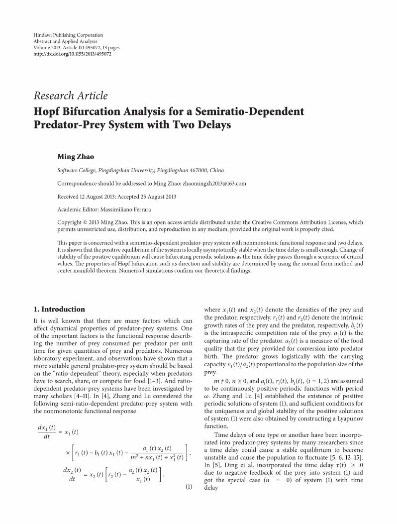
Figure 1 119864lowast is asymptotically stable for 1205911= 0350 lt 120591

10= 03788

0 50 10025

3

35

4

45

5

55

x1(t)

Time t

(a)

0 50 10055

6

65

7

75

8

85

9

95

x2(t)

Time t

(b)

2 4 655

6

65

7

75

8

85

9

95

x2(t)

x1(t)

(c)

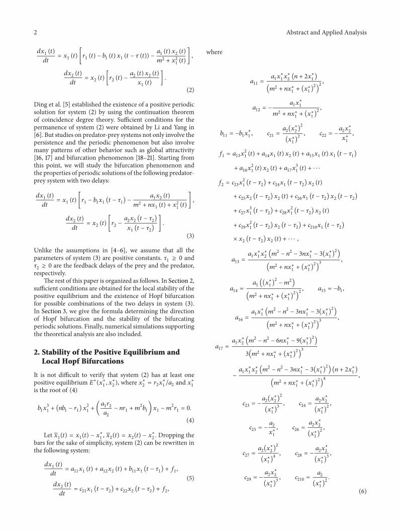
Figure 2 119864lowast is unstable for 1205911= 0395 gt 120591

10= 03788

8 Abstract and Applied Analysis

0 50 1003

31

32

33

34

35

36

37

38

39x1(t)

Time t

(a)

0 50 1004

5

6

7

8

9

10

x2(t)

Time t

(b)

3 35 44

5

6

7

8

9

10

x2(t)

x1(t)

(c)

Figure 3 119864lowast is asymptotically stable for 1205912= 0450 lt 120591

20= 04912

0 50 1003

31

32

33

34

35

36

37

38

39

x1(t)

Time t

(a)

0 50 1004

5

6

7

8

9

10

11

x2(t)

Time t

(b)

3 35 44

5

6

7

8

9

10

11

x2(t)

x1(t)

(c)

Figure 4 119864lowast is unstable for 1205912= 0505 gt 120591

20= 04912

Abstract and Applied Analysis 9

0 50 1003

35

4

45x1(t)

Time t

(a)

0 50 1005

55

6

65

7

75

8

85

9

95

10

x2(t)

Time t

(b)

3 35 4 455

55

6

65

7

75

8

85

9

95

10

x2(t)

x1(t)

(c)

Figure 5 119864lowast is asymptotically stable for 120591 = 0320 lt 1205910= 03361

0 50 1003

32

34

36

38

4

42

44

46

48

x1(t)

Time t

(a)

0 50 1004

5

6

7

8

9

10

11

x2(t)

Time t

(b)

3 4 54

5

6

7

8

9

10

11

x2(t)

x1(t)

(c)

Figure 6 119864lowast is unstable for 120591 = 0355 gt 1205910= 03361

10 Abstract and Applied Analysis

0 50 1003

35

4

45x1(t)

Time t

(a)

0 50 10055

6

65

7

75

8

85

9

95

x2(t)

Time t

(b)

3 35 4 4555

6

65

7

75

8

85

9

95

x2(t)

x1(t)

(c)

Figure 7 119864lowast is asymptotically stable for 1205911= 0325 lt 120591

1lowast= 03490 at 120591

2= 03

0 50 1003

32

34

36

38

4

42

44

46

x1(t)

Time t

(a)

0 50 1005

55

6

65

7

75

8

85

9

95

10

x2(t)

Time t

(b)

3 4 55

55

6

65

7

75

8

85

9

95

10

x2(t)

x1(t)

(c)

Figure 8 119864lowast is unstable for 1205911= 0360 gt 120591

1lowast= 03490 at 120591

2= 03

Abstract and Applied Analysis 11

11989202

= 21205911lowast119863[11988613

+ 11988614119902(2)

(0) + 11988615119902(1)

(minus1)

+ 119902lowast

2(11988823(119902(1)

(minus1205912lowast

1205911lowast

))

2

+ 11988824119902(1)

(minus1205912lowast

1205911lowast

)119902(2)

(0)

+ 11988825119902(2)

(minus1205912lowast

1205911lowast

)119902(2)

(0)

+11988826119902(1)

(minus1205912lowast

1205911lowast

) 119902(2)

(minus1205912lowast

1205911lowast

))]

11989221

= 21205911lowast119863[11988613

(119882(1)

11(0) + 119882

(1)

20(0))

+ 11988614

(119882(1)

11(0) 119902(2)

(0) +1

2119882(1)

20(0) 119902(2)

(0)

+ 119882(2)

11(0) +

1

2119882(2)

20(0))

+ 11988615

(119882(1)

11(0) 119902(1)

(minus1) +1

2119882(1)

20(0) 119902(1)

(minus1)

+ 119882(1)

11(minus1) +

1

2119882(1)

20(minus1))

+ 11988616

(119902(2)

(0) + 2119902(2)

(0)) + 311988617119902(1)

(0)

+ 119902lowast

2(11988823

(2119882(1)

11(minus

1205912lowast

1205911lowast

) 119902(1)

(minus1205912lowast

1205911lowast

)

+119882(1)

20(minus

1205912lowast

1205911lowast

) 119902(1)

(minus1205912lowast

1205911lowast

))

+ 11988824

(119882(1)

11(minus

1205912lowast

1205911lowast

) 119902(2)

(0)

+1

2119882(1)

20(minus

1205912lowast

1205911lowast

) 119902(2)

(0)

+ 119882(2)

11(0) 119902(1)

(minus1205912lowast

1205911lowast

)

+1

2119882(2)

20(0) 119902(1)

(minus1205912lowast

1205911lowast

))

+ 11988825

(119882(2)

11(minus

1205912lowast

1205911lowast

) 119902(2)

(0)

+1

2119882(2)

20(minus

1205912lowast

1205911lowast

) 119902(2)

(0)

+ 119882(2)

11(0) 119902(2)

(minus1205912lowast

1205911lowast

)

+1

2119882(2)

20(0) 119902(2)

(minus1205912lowast

1205911lowast

))

+ 11988826

(119882(1)

11(minus

1205912lowast

1205911lowast

) 119902(2)

(minus1205912lowast

1205911lowast

)

+1

2119882(1)

20(minus

1205912lowast

1205911lowast

) 119902(2)

(minus1205912lowast

1205911lowast

)

+ 119882(2)

11(minus

1205912lowast

1205911lowast

) 119902(1)

(minus1205912lowast

1205911lowast

)

+1

2119882(2)

20(minus

1205912lowast

1205911lowast

) 119902(1)

(minus1205912lowast

1205911lowast

))

+ 311988827(119902(1)

(minus1205912lowast

1205911lowast

))

2

119902(1)

(minus1205912lowast

1205911lowast

)

+ 11988828

((119902(1)

(minus1205912lowast

1205911lowast

))

2

119902(2)

(0)

+2119902(1)

(minus1205912lowast

1205911lowast

) 119902(2)

(0) 119902(1)

(minus1205912lowast

1205911lowast

))

+ 11988829

((119902(1)

(minus1205912lowast

1205911lowast

))

2

119902(2)

(minus1205912lowast

1205911lowast

)+ 2119902(1)

times(minus1205912lowast

1205911lowast

) 119902(2)

(minus1205912lowast

1205911lowast

) 119902(1)

(minus1205912lowast

1205911lowast

))

+119888210

(119902(1)

(minus1205912lowast

1205911lowast

) 119902(2)

(minus1205912lowast

1205911lowast

) 119902(2)

(0)

+ 119902(1)

(minus1205912lowast

1205911lowast

) 119902(2)

(minus1205912lowast

1205911lowast

)

times 119902(2)

(0) + 119902(1)

(minus1205912lowast

1205911lowast

)

times 119902(2)

(minus1205912lowast

1205911lowast

)119902(2)

(0)))]

(56)

with

11988220

(120579) =11989411989220119902 (0)

1205961lowast1205911lowast

1198901198941205961lowast1205911lowast120579+

11989411989202119902 (0)

31205961lowast1205911lowast

119890minus1198941205961lowast1205911lowast120579

+ 119864111989021198941205961lowast1205911lowast120579

11988211

(120579) = minus11989411989211119902 (0)

1205961lowast1205911lowast

1198901198941205961lowast1205911lowast120579+

11989411989211119902 (0)

1205961lowast1205911lowast

119890minus1198941205961lowast1205911lowast120579+ 1198642

(57)

where 1198641and 119864

2can be determined by the following equa-

tions respectively

(21198941205961lowast

minus 11988611

minus 11988711119890minus21198941205961lowast1205911lowast minus119886

12

minus11988821119890minus21198941205961lowast1205912lowast 2119894120596

1lowastminus 11988833119890minus21198941205961lowast1205912lowast

)1198641

= 2(

119864(1)

1

119864(2)

1

)

(11988611

+ 11988711

11988612

11988821

11988822

)1198642= minus(

119864(1)

2

119864(2)

2

)

(58)

12 Abstract and Applied Analysis

with

119864(1)

1= 11988613

+ 11988614119902(2)

(0) + 11988615119902(1)

(minus1)

119864(1)

1= 11988823(119902(1)

(minus1205912lowast

1205911lowast

))

2

+ 11988824119902(1)

(minus1205912lowast

1205911lowast

) 119902(2)

(0)

+ 11988825119902(2)

(minus1205912lowast

1205911lowast

) 119902(2)

(0)

+ 11988826119902(1)

(minus1205912lowast

1205911lowast

) 119902(2)

(minus1205912lowast

1205911lowast

)

119864(1)

2= 211988613

+ 11988614

(119902(2)

(0) + 119902(2)

(0))

+ 11988615

(119902(1)

(minus1) + 119902(1)

(minus1))

119864(2)

2= 211988823119902(1)

(minus1205912lowast

1205911lowast

) 119902(1)

(minus1205912lowast

1205911lowast

)

+ 11988824

(119902(1)

(minus1205912lowast

1205911lowast

) 119902(2)

(0) + 119902(1)

(minus1205912lowast

1205911lowast

) 119902(2)

(0))

+ 11988825

(119902(2)

(minus1205912lowast

1205911lowast

) 119902(2)

(0) + 119902(2)

(minus1205912lowast

1205911lowast

) 119902(2)

(0))

+ 11988826

(119902(1)

(minus1205912lowast

1205911lowast

) 119902(2)

(minus1205912lowast

1205911lowast

)

+119902(1)

(minus1205912lowast

1205911lowast

) 119902(2)

(minus1205912lowast

1205911lowast

))

(59)

Then we can get the following coefficients

1198621(0) =

119894

21205961lowast1205911lowast

(1198921111989220

minus 2100381610038161003816100381611989211

10038161003816100381610038162

minus

10038161003816100381610038161198920210038161003816100381610038162

3) +

11989221

2

1205832= minus

Re 1198621(0)

Re 1205821015840 (1205911lowast)

1205732= 2Re 119862

1(0)

1198792= minus

Im 1198621(0) + 120583

2Im 120582

1015840(1205911lowast)

1205961lowast1205911lowast

(60)

In conclusion we have the following results

Theorem 5 If 1205832

gt 0 (1205832

lt 0) then the Hopf bifurcationis supercritical (subcritical) if 120573

2lt 0 (120573

2gt 0) then the

bifurcating periodic solutions are stable (unstable) if 1198792

gt 0

(1198792lt 0) then the period of the bifurcating periodic solutions

increases (decreases)

4 Numerical Simulation and Discussions

To demonstrate the algorithm for determining the existenceof Hopf bifurcation in Section 2 and the properties of Hopf

bifurcation in Section 3 we give an example of system (3) inthe following form

1198891199091(119905)

119889119905= 1199091(119905) [4 minus 119909

1(119905 minus 1205911) minus

051199092(119905)

4 + 1199091(119905) + 1199092

1(119905)

]

1198891199092(119905)

119889119905= 1199092(119905) [3 minus

151199092(119905 minus 1205912)

1199091(119905 minus 1205912)

]

(61)

which has a positive equilibrium 119864lowast(38298 76596) By

calculation we have119860+119861+119862 = 65788119863+119864 = 112470 and119863 minus 119864 = minus117318 Namely conditions (119867

1) and (119867

2) hold

For 1205911

gt 0 1205912

= 0 We can get 12059610

= 3907412059110

= 03788 By Theorem 1 we know that when 1205911

isin

[0 12059110) the positive equilibrium 119864

lowast(38298 76596) is locally

asymptotically stable and is unstable if 1205911

gt 12059110 As

can be seen from Figure 1 when we let 1205911

= 035 isin

[0 12059110) the positive equilibrium 119864

lowast(38298 76596) is locally

asymptotically stable However when 1205911

= 0395 gt 12059110

the positive equilibrium 119864lowast(38298 76596) is unstable and

a Hopf bifurcation occurs and a family of periodic solutionsbifurcate from the positive equilibrium 119864

lowast(38298 76596)

which can be illustrated by Figure 2 Similarly we can get12059620

= 30827 12059120

= 04912 The corresponding waveformand the phase plots are shown in Figures 3 and 4

For 1205911

= 1205912

= 120591 gt 0 We can obtain 1205960

=

34601 1205910

= 03361 By Theorem 3 we know that whenthe time delay 120591 increases from zero to the critical value1205910

= 03361 the positive equilibrium 119864lowast(38298 76596) is

locally asymptotically stable It will lose its stability and aHopf bifurcation occurs once 120591 gt 120591

0= 03361 This property

can be illustrated by Figures 5 and 6Finally consider 120591

1as a parameter and let 120591

2= 03 isin

(0 12059120) We can get 120596

1lowast= 23761 120591

1lowast= 03490 1205821015840(120591

1lowast) =

82230 + 26054119894 From Theorem 4 the positive equilibrium119864lowast(38298 76596) is locally asymptotically stable for 120591

1isin

[0 03490) and unstable when 1205911gt 1205911lowast

= 03490 which canbe seen from Figures 7 and 8

In addition from (60) we can get 1198621(0) = minus415020 minus

178366119894 Furthermore we have 1205832

= 50471 gt 0 1205732

=

minus830040 lt 0 1198792= 56519 gt 0 Therefore from Theorem 5

we know that the Hopf bifurcation is supercritical Thebifurcating periodic solutions are stable and increase If thebifurcating periodic solutions are stable then the prey and thepredator may coexist in an oscillatory mode Therefore thetwo species in system (3) may coexist in an oscillatory modeunder certain conditions

Conflict of Interests

The author declares that there is no conflict of interestsregarding the publication of this paper

References

[1] R Arditi and L R Ginzburg ldquoCoupling in predator-preydynamics ratio-dependencerdquo Journal ofTheoretical Biology vol139 no 3 pp 311ndash326 1989

Abstract and Applied Analysis 13

[2] R Arditi N Perrin and H Saiah ldquoFunctional responses andheterogeneities an experimental test with cladoceransrdquo Oikosvol 60 no 1 pp 69ndash75 1991

[3] I Hanski ldquoThe functional response of predators worries aboutscalerdquo Trends in Ecology and Evolution vol 6 no 5 pp 141ndash1421991

[4] L Zhang and C Lu ldquoPeriodic solutions for a semi-ratio-dependent predator-prey system with Holling IV functionalresponserdquo Journal of Applied Mathematics and Computing vol32 no 2 pp 465ndash477 2010

[5] X Ding C Lu andM Liu ldquoPeriodic solutions for a semi-ratio-dependent predator-prey system with nonmonotonic func-tional response and time delayrdquo Nonlinear Analysis Real WorldApplications vol 9 no 3 pp 762ndash775 2008

[6] X Li and W Yang ldquoPermanence of a semi-ratio-dependentpredator-prey system with nonmonotonic functional responseand time delayrdquoAbstract and Applied Analysis vol 2009 ArticleID 960823 6 pages 2009

[7] M Sen M Banerjee and A Morozov ldquoBifurcation analysis ofa ratio-dependent prey-predator model with the Allee effectrdquoEcological Complexity vol 11 pp 12ndash27 2012

[8] X Ding and G Zhao ldquoPeriodic solutions for a semi-ratio-dependent predator-prey system with delays on time scalesrdquoDiscrete Dynamics in Nature and Society vol 2012 Article ID928704 15 pages 2012

[9] B Yang ldquoPattern formation in a diffusive ratio-dependentHolling-Tanner predator-prey model with Smith growthrdquo Dis-crete Dynamics in Nature and Society vol 2013 Article ID454209 8 pages 2013

[10] Z Yue and W Wang ldquoQualitative analysis of a diffusive ratio-dependent Holling-Tanner predator-prey model with Smithgrowthrdquo Discrete Dynamics in Nature and Society vol 2013Article ID 267173 9 pages 2013

[11] M Haque ldquoRatio-dependent predator-prey models of interact-ing populationsrdquo Bulletin of Mathematical Biology vol 71 no 2pp 430ndash452 2009

[12] M Ferrara and L Guerrini ldquoCenter manifold analysis fora delayed model with classical savingrdquo Far East Journal ofMathematical Sciences vol 70 no 2 pp 261ndash269 2012

[13] S Guo and W Jiang ldquoHopf bifurcation analysis on generalGause-type predator-prey models with delayrdquo Abstract andApplied Analysis vol 2012 Article ID 363051 17 pages 2012

[14] C YWang SWang F P Yang and L R Li ldquoGlobal asymptoticstability of positive equilibrium of three-species Lotka-Volterramutualism models with diffusion and delay effectsrdquo AppliedMathematical Modelling vol 34 no 12 pp 4278ndash4288 2010

[15] M Ferrara L Guerrini and R Mavilia ldquoModified neoclassicalgrowth models with delay a critical survey and perspectivesrdquoApplied Mathematical Sciences vol 7 pp 4249ndash4257 2013

[16] J J Jiao L S Chen and J J Nieto ldquoPermanence and globalattractivity of stage-structured predator-prey model with con-tinuous harvesting on predator and impulsive stocking on preyrdquoApplied Mathematics andMechanics vol 29 no 5 pp 653ndash6632008

[17] Y Zhu and K Wang ldquoExistence and global attractivity ofpositive periodic solutions for a predator-prey model withmodified Leslie-Gower Holling-type II schemesrdquo Journal ofMathematical Analysis andApplications vol 384 no 2 pp 400ndash408 2011

[18] M Ferrara L Guerrini and C Bianca ldquoThe Cai model withtime delay existence of periodic solutions and asymptotic

analysisrdquoAppliedMathematicsamp Information Sciences vol 7 no1 pp 21ndash27 2013

[19] R M Etoua and C Rousseau ldquoBifurcation analysis of a gen-eralized Gause model with prey harvesting and a generalizedHolling response function of type IIIrdquo Journal of DifferentialEquations vol 249 no 9 pp 2316ndash2356 2010

[20] Y Yang ldquoHopf bifurcation in a two-competitor one-preysystemwith time delayrdquoAppliedMathematics and Computationvol 214 no 1 pp 228ndash235 2009

[21] Y Qu and JWei ldquoBifurcation analysis in a time-delaymodel forprey-predator growth with stage-structurerdquo Nonlinear Dynam-ics vol 49 no 1-2 pp 285ndash294 2007

[22] B D Hassard N D Kazarinoff and Y H Wan Theory andApplications of Hopf Bifurcation Cambridge University PressCambridge UK 1981

2 Abstract and Applied Analysis

1198891199091(119905)

119889119905= 1199091(119905) [1199031(119905) minus 119887

1(119905) 1199091(119905 minus 120591 (119905)) minus

1198861(119905) 1199092(119905)

1198982 + 11990921(119905)

]

1198891199092(119905)

119889119905= 1199092(119905) [1199032(119905) minus

1198862(119905) 1199092(119905)

1199091(119905)

]

(2)

Ding et al [5] established the existence of a positive periodicsolution for system (2) by using the continuation theoremof coincidence degree theory Sufficient conditions for thepermanence of system (2) were obtained by Li and Yang in[6] But studies on predator-prey systems not only involve thepersistence and the periodic phenomenon but also involvemany patterns of other behavior such as global attractivity[16 17] and bifurcation phenomenon [18ndash21] Starting fromthis point we will study the bifurcation phenomenon andthe properties of periodic solutions of the following predator-prey system with two delays

1198891199091(119905)

119889119905= 1199091(119905) [1199031minus 11988711199091(119905 minus 1205911) minus

11988611199092(119905)

1198982 + 1198991199091(119905) + 1199092

1(119905)

]

1198891199092(119905)

119889119905= 1199092(119905) [1199032minus

11988621199092(119905 minus 1205912)

1199091(119905 minus 1205912)

]

(3)

Unlike the assumptions in [4ndash6] we assume that all theparameters of system (3) are positive constants 120591

1ge 0 and

1205912ge 0 are the feedback delays of the prey and the predator

respectivelyThe rest of this paper is organized as follows In Section 2

sufficient conditions are obtained for the local stability of thepositive equilibrium and the existence of Hopf bifurcationfor possible combinations of the two delays in system (3)In Section 3 we give the formula determining the directionof Hopf bifurcation and the stability of the bifurcatingperiodic solutions Finally numerical simulations supportingthe theoretical analysis are also included

2 Stability of the Positive Equilibrium andLocal Hopf Bifurcations

It is not difficult to verify that system (2) has at least onepositive equilibrium 119864

lowast(119909lowast

1 119909lowast

2) where 119909

lowast

2= 1199032119909lowast

11198862and 119909

lowast

1

is the root of (4)

11988711199093

1+ (1198991198871minus 1199031) 1199092

1+ (

11988611199032

1198862

minus 1198991199031+ 11989821198871)1199091minus 11989821199031= 0

(4)

Let 1199091(119905) = 119909

1(119905) minus 119909

lowast

1 1199092(119905) = 119909

2(119905) minus 119909

lowast

2 Dropping the

bars for the sake of simplicity system (2) can be rewritten inthe following system

1198891199091(119905)

119889119905= 119886111199091(119905) + 119886

121199092(119905) + 119887

111199091(119905 minus 1205911) + 1198911

1198891199092(119905)

119889119905= 119888211199091(119905 minus 1205912) + 119888221199092(119905 minus 1205912) + 1198912

(5)

where

11988611

=1198861119909lowast

1119909lowast

2(119899 + 2119909

lowast

1)

(1198982 + 119899119909lowast1+ (119909lowast1)2

)2

11988612

= minus1198861119909lowast

1

1198982 + 119899119909lowast1+ (119909lowast1)2

11988711

= minus1198871119909lowast

1 119888

21=

1198862(119909lowast

2)2

(119909lowast1)2

11988822

= minus1198862119909lowast

2

119909lowast1

1198911= 119886131199092

1(119905) + 119886

141199091(119905) 1199092(119905) + 119886

151199091(119905) 1199091(119905 minus 1205911)

+ 119886161199092

1(119905) 1199092(119905) + 119886

171199093

1(119905) + sdot sdot sdot

1198912= 119888231199092

1(119905 minus 1205912) + 119888241199091(119905 minus 1205912) 1199092(119905)

+ 119888251199092(119905 minus 1205912) 1199092(119905) + 119888

261199091(119905 minus 1205912) 1199092(119905 minus 1205912)

+ 119888271199093

1(119905 minus 1205912) + 119888281199092

1(119905 minus 1205912) 1199092(119905)

+ 119888291199092

1(119905 minus 1205912) 1199092(119905 minus 1205912) + 119888210

1199091(119905 minus 1205912)

times 1199092(119905 minus 1205912) 1199092(119905) + sdot sdot sdot

11988613

=1198861119909lowast

1119909lowast

2(1198982minus 1198992minus 3119899119909

lowast

1minus 3(119909lowast

1)2

)

(1198982 + 119899119909lowast1+ (119909lowast1)2

)3

11988614

=1198861((119909lowast

1)2

minus 1198982)

(1198982 + 119899119909lowast1+ (119909lowast1)2

)2 119886

15= minus1198871

11988616

=1198861119909lowast

1(1198982minus 1198992minus 3119899119909

lowast

1minus 3(119909lowast

1)2

)

(1198982 + 119899119909lowast1+ (119909lowast1)2

)3

11988617

=1198861119909lowast

2(1198982minus 1198992minus 6119899119909

lowast

1minus 9(119909lowast

1)2

)

3(1198982 + 119899119909lowast1+ (119909lowast1)2

)3

minus1198861119909lowast

1119909lowast

2(1198982minus 1198992minus 3119899119909

lowast

1minus 3(119909lowast

1)2

) (119899 + 2119909lowast

1)

(1198982 + 119899119909lowast1+ (119909lowast1)2

)4

11988823

= minus1198862(119909lowast

2)2

(119909lowast1)3

11988824

=1198862119909lowast

2

(119909lowast1)2

11988825

= minus1198862

119909lowast1

11988826

=1198862119909lowast

2

(119909lowast1)2

11988827

=1198862(119909lowast

2)2

(119909lowast1)4

11988828

= minus1198862119909lowast

2

(119909lowast1)3

11988829

= minus1198862119909lowast

2

(119909lowast1)3 119888

210=

1198862

(119909lowast1)2

(6)

Abstract and Applied Analysis 3

The linearized system of (5) is

1198891199091(119905)

119889119905= 119886111199091(119905) + 119886

121199092(119905) + 119887

111199091(119905 minus 1205911)

1198891199092(119905)

119889119905= 119888211199091(119905 minus 1205912) + 119888221199092(119905 minus 1205912)

(7)

The associated characteristic equation of system (7) is

1205822+ 119860120582 + 119861120582119890

minus1205821205911 + (119862120582 + 119863) 119890

minus1205821205912 + 119864119890

minus120582(1205911+1205912)= 0 (8)

where

119860 = minus11988611 119861 = minus119887

11 119862 = minus119888

22

119863 = 1198861111988822

minus 1198861211988821 119864 = 119887

1111988822

(9)

Case 1 (1205911= 1205912= 0) Equation (8) becomes

1205822+ (119860 + 119861 + 119862) 120582 + 119863 + 119864 = 0 (10)

All the roots of (10) have negative real parts if and only if

(1198671) 119860 + 119861 + 119862 gt 0 and119863 + 119864 gt 0

Thus the positive equilibrium 119864lowast(119909lowast

1 119909lowast

2) is locally stable

when the condition (1198671) holds

Case 2 (1205911gt 0 1205912= 0) Equation (8) becomes

1205822+ (119860 + 119862) 120582 + 119863 + (119861120582 + 119864) 119890

minus1205821205911 = 0 (11)

Let 120582 = 1198941205961(1205961gt 0) be the root of (11) and we have

1198611205961sin 12059111205961+ 119864 cos 120591

11205961= 1205962

1minus 119863

119861120596 cos 12059111205961minus 119864 sin 120591

11205961= minus (119860 + 119862)120596

1

(12)

It follows that

1205964

1+ ((119860 + 119862)

2minus 1198612minus 2119863)120596

2

1+ 1198632minus 1198642= 0 (13)

If condition (1198672)119863 minus 119864 lt 0 holds then (13) has only one

positive root

12059610

= (( minus ((119860 + 119862)2minus 1198612minus 2119863)

+radic((119860 + 119862)2minus 1198612 minus 2119863)

2

minus 4 (1198632 minus 1198642) )

times2minus1)

12

(14)

Now we can get the critical value of 1205911by substituting120596

10into

(12) After computing we obtain

1205911119896

=1

12059610

arccos(119864 minus 119860119861 minus 119861119862)120596

2

10minus 119863119864

1198612120596210

+ 1198642+

2119896120587

12059610

119896 = 0 1 2

(15)

Then when 120591 = 1205911119896 the characteristic equation (11) has a pair

of purely imaginary roots plusmn1198941205960

Next we will verify the transversality condition Differ-entiating (11) with respect to 120591

1 we get

[119889120582

1198891205911

]

minus1

= minus2120582 + 119860 + 119862

120582 [1205822 + (119860 + 119862) 120582 + 119863]+

119861

120582 (119861120582 + 119864)minus

1205911

120582

(16)

Thus

Re [ 119889120582

1198891205911

]

minus1

1205911=12059110

=21205962

10+ (119860 + 119862)

2minus 1198612minus 2119863

1198612120596210

+ 1198642

=

radic((119860 + 119862)2minus 1198612 minus 2119863)

2

minus 4 (1198632 minus 1198642)

1198612120596210

+ 1198642

(17)

Obviously if condition (1198672) holds then Re [119889120582119889120591

1]minus1

1205911=1205910

gt 0Note that sgnRe [119889120582119889120591

1]minus1

1205911=12059110

= sgn[119889Re(120582)1198891205911]minus1

1205911=12059110

Therefore if condition (119867

2) holds the transversality

condition is satisfied From the analysis above we have thefollowing results

Theorem 1 If conditions (1198671) and (119867

2) hold then the positive

equilibrium119864lowast(119909lowast

1 119909lowast

2) of system (3) is asymptotically stable for

1205911isin [0 120591

10) and unstable when 120591

1gt 12059110 System (3) undergoes

a Hopf bifurcation at the positive equilibrium 119864lowast(119909lowast

1 119909lowast

2)when

1205911= 12059110

Case 3 (1205911= 0 1205912gt 0) Equation (8) becomes

1205822+ (119860 + 119861) 120582 + (119862120582 + 119863 + 119864) 119890

minus1205821205912 = 0 (18)

Let 120582 = 1198941205962(1205962gt 0) be the root of (18) and then we have

1198621205962sin 12059121205962+ (119863 + 119864) cos 120591

21205962= 1205962

2

1198621205962cos 12059121205962minus (119863 + 119864) sin 120591

21205962= minus (119860 + 119861) 120596

2

(19)

which leads to

1205964

2+ ((119860 + 119861)

2minus 1198622) 1205962

2minus (119863 + 119864)

2= 0 (20)

Obviously if the condition (1198671) holds and then (20) has only

one positive root

12059620

=radic minus ((119860 + 119861)

2minus 1198622) + radic((119860 + 119861)

2minus 1198622)

2

+ 4(119863 + 119864)2

2

(21)

The corresponding critical value of 1205912is

1205912119896

=1

12059620

arccos(119863 + 119864 minus 119860119862 minus 119861119862)120596

2

10

1198622120596220

+ (119863 + 119864)2

+2119896120587

12059620

119896 = 0 1 2

(22)

4 Abstract and Applied Analysis

Similar to Case 2 differentiating (18) with respect to 1205912 we

get

[119889120582

1198891205912

]

minus1

= minus2120582 + 119860 + 119861

120582 [1205822 + (119860 + 119861) 120582]+

119862

120582 (119862120582 + 119863 + 119864)minus

1205912

120582

(23)

Then we can get

Re [ 119889120582

1198891205912

]

minus1

1205912=12059120

=21205962

20+ (119860 + 119861)

2minus 1198622

1198622120596220

+ (119863 + 119864)2

=

radic((119860 + 119861)2minus 1198622)

2

minus 4(119863 + 119864)2

1198622120596220

+ (119863 + 119864)2

(24)

Obviously if condition (1198671) holds then Re[119889120582

1198891205912]minus1

1205912=12059120

gt 0 Namely if condition (1198671) holds then the

transversality condition is satisfied Thus we have thefollowing results

Theorem 2 If condition (1198671) holds then the positive equi-

librium 119864lowast(119909lowast

1 119909lowast

2) of system (3) is asymptotically stable for

1205912isin [0 120591

20) and unstable when 120591

2gt 12059120 System (3) undergoes

a Hopf bifurcation at the positive equilibrium 119864lowast(119909lowast

1 119909lowast

2)when

1205912= 12059120

Case 4 (1205911= 1205912= 120591 gt 0) Equation (8) can be transformed

into the following form

1205822+ 119860120582 + ((119861 + 119862) 120582 + 119863) 119890

minus120582120591+ 119864119890minus2120582120591

= 0 (25)

Multiplying 119890120582120591 on both sides of (25) we get

(119861 + 119862) 120582 + 119863 + (1205822+ 119860120582) 119890

120582120591+ 119864119890minus120582120591

= 0 (26)

Let 120582 = 119894120596 (120596 gt 0) be the root of (26) then we obtain

119860120596 sin 120591120596 + (1205962minus 119864) cos 120591120596 = 119863

119860120596 cos 120591120596 minus (1205962+ 119864) sin 120591120596 = minus (119861 + 119862)120596

(27)

which follows that

sin 120591120596 =(119861 + 119862)120596

3+ (119860119863 minus 119861119864 minus 119862119864)120596

1205964 + 11986021205962 minus 1198642

cos 120591120596 =(119863 minus 119860119861 minus 119860119862)120596

2+ 119863119864

1205964 + 11986021205962 minus 1198642

(28)

Then we have

1205968+ 11988831205966+ 11988821205964+ 11988811205962+ 1198880= 0 (29)

where1198880= 1198644 119888

3= 21198602minus (119861 + 119862)

2

1198881= 2119863119864 (119860119861 + 119860119862 minus 119863) minus 2119860

21198642

minus (119860119863 minus 119861119864 minus 119862119864)2

1198882= 1198604minus 21198642minus 2 (119861 + 119862) (119860119863 minus 119861119864 minus 119862119864)

minus (119863 minus 119860119861 minus 119860119862)2

(30)

Denote 1205962= V and then (29) becomes

V4 + 1198883V3 + 1198882V2 + 1198881V + 1198880= 0 (31)

Next we give the following assumption

(1198673) Equation (31) has at least one positive real root

Suppose that (1198673) holds Without loss of generality we

assume that (31) has four real positive roots which aredenoted by V

1 V2 V3 and V

4Then (29) has four positive roots

120596119896= radicV119896 119896 = 1 2 3 4

For every fixed 120596119896 the corresponding critical value of

time delay is

120591(119895)

119896=

1

120596119896

arccos(119863 minus 119860119861 minus 119860119862)120596

2

119896+ 119863119864

1205964119896+ 11986021205962

119896minus 1198642

+2119895120587

120596119896

119896 = 1 2 3 4 119895 = 0 1 2

(32)

Let

1205910= min 120591

(0)

119896 119896 = 1 2 3 4 120596

0= 1205961198960

(33)

Taking the derivative of 120582 with respect to 120591 in (26) we obtain

[119889120582

119889120591]

minus1

=(2120582 + 119860) 119890

120582120591+ 119861 + 119862

120582 [119864119890minus120582120591 minus (1205822 + 119860120582) 119890120582120591]minus

120591

120582 (34)

Thus

Re [119889120582

119889120591]

minus1

120591=1205910

=119875119877119876119877+ 119875119868119876119868

1198762119877+ 1198762119868

(35)

with

119875119877= 119860 cos 120591

01205960minus 21205960sin 12059101205960+ 119861 + 119862

119875119868= 119860 sin 120591

01205960+ 21205960cos 12059101205960

119876119877= 1198601205962

0cos 12059101205960+ (119864120596

0minus 1205963

0) sin 120591

01205960

119876119868= 1198601205962

0sin 12059101205960+ (119864120596

0+ 1205963

0) cos 120591

01205960

(36)

It is easy to see that if condition (1198674)119875119877119876119877+119875119868119876119868

= 0 thenRe [119889120582119889120591]minus1

120591=1205910

= 0 Therefore we have the following results

Theorem 3 If conditions (1198671) and (119867

4) holds then the pos-

itive equilibrium 119864lowast(119909lowast

1 119909lowast

2) of system (3) is asymptotically

stable for 120591 isin [0 1205910) and unstable when 120591 gt 120591

0 System

(3) undergoes a Hopf bifurcation at the positive equilibrium119864lowast(119909lowast

1 119909lowast

2) when 120591 = 120591

0

Case 5 (1205911

= 1205912 1205911gt 0 and 120591

2gt 0) Considered the following

1205822+ 119860120582 + 119861120582119890

minus1205821205911 + (119862120582 + 119863) 119890

minus1205821205912

+ 119864119890minus120582(1205911+1205912)= 0

(37)

We consider (8) with 1205912in its stable interval and regard 120591

1

as a parameter

Abstract and Applied Analysis 5

Let 120582 = 119894120596lowast

1(120596lowast1

gt 0) be the root of (8) and then we canobtain

(119861120596lowast

1minus 119864 sin 120591

2120596lowast

1) sin 120591

1120596lowast

1+ 119864 cos 120591

2120596lowast

1cos 1205911120596lowast

1

= (120596lowast

1)2

minus 119863 cos 1205912120596lowast

1minus 119862120596lowast

1sin 1205912120596lowast

1

(119861120596lowast

1minus 119864 sin 120591

2120596lowast

1) cos 120591

1120596lowast

1minus 119864 cos 120591

2120596lowast

1cos 1205911120596lowast

1

= minus119860120596lowast

1+ 119863 sin 120591

2120596lowast

1minus 119862120596lowast

1cos 1205912120596lowast

1

(38)

Then we get

(120596lowast

1)4

+ (1198602minus 1198612+ 1198622) (120596lowast

1)2

+ 1198632minus 1198642

+ 2 (119860119862 minus 1198632) (120596lowast

1)2 cos 120591

2120596lowast

1

minus 2 (119862(120596lowast

1)3

+ 119860119863120596lowast

1) sin 120591

2120596lowast

1= 0

(39)

Define

119865 (120596lowast

1) = (120596

lowast

1)4

+ (1198602minus 1198612+ 1198622) (120596lowast

1)2

+ 1198632minus 1198642

+ 2 (119860119862 minus 1198632) (120596lowast

1)2 cos 120591

2120596lowast

1

minus 2 (119862 (120596lowast

1)3

+ 119860119863120596lowast

1) sin 120591

2120596lowast

1

(40)

If condition (1198671) 119863 + 119864 gt 0 and (119867

2) 119863 minus 119864 lt 0 hold

then 119865(0) = 1198632minus 1198642

lt 0 In addition 119865(+infin) = +infinTherefore (39) has at least one positive root We suppose thatthe positive roots of (39) are denoted as 120596lowast

11 120596lowast

12 120596lowast

1119896 For

every fixed 120596lowast

1119894 the corresponding critical value of time delay

120591lowast(119895)

1119894=

1

120596lowast1119894

timesarccos1198901(120596lowast

1119894)+1198902(120596lowast

1119894) cos 120591

2120596lowast

1119894+1198903(120596lowast

1119894) sin 120591

2120596lowast

1119894

1198904(120596lowast1119894)+1198905(120596lowast1119894) sin 120591

2120596lowast1119894

+2119895120587

120596lowast1119894

119894 = 1 2 3 119896 119895 = 0 1 2

(41)

with

1198901(120596lowast

1119894) = minus119860119861(120596

lowast

1119894)2

minus 119863119864 1198902(120596lowast

1119894) = (119864 minus 119861119862) (120596

lowast

1119894)2

1198903(120596lowast

1119894) = (119860119864 + 119861119863)120596

lowast

1119894 119890

4(120596lowast

1119894) = 1198612(120596lowast

1119894)2

+ 1198642

1198905(120596lowast

1119894) = minus2119861119864120596

lowast

1119894

(42)

Let 1205911lowast

= min120591lowast(0)1119894

119894 = 1 2 3 119896 When 1205911= 1205911lowast (8) has

a pair of purely imaginary roots plusmn1198941205961lowast

for 1205912isin (0 120591

20)

Next in order to give the main results we give thefollowing assumption

(1198675) 119889Re 120582(120591lowast

10)1198891205911

= 0

Therefore we have the following results on the stability andbifurcation in system (3)

Theorem 4 If the conditions (1198671) and (119867

5) hold and 120591

2isin

(0 12059120) then the positive equilibrium 119864

lowast(119909lowast

1 119909lowast

2) of system (3)

is asymptotically stable for 1205911

isin [0 1205911lowast) and unstable when

1205911

gt 1205911lowast System (3) undergoes a Hopf bifurcation at the

positive equilibrium 119864lowast(119909lowast

1 119909lowast

2) when 120591

1= 1205911lowast

3 Direction and Stability ofthe Hopf Bifurcation

In this section we will investigate the direction of Hopfbifurcation and stability of the bifurcating periodic solutionsof system (3) with respect to 120591

1for 1205912isin (0 120591

20) We assume

that 1205912lowast

lt 1205911lowast

where 1205912lowast

isin (0 12059120)

Let 1205911= 1205911lowast

+120583 120583 isin 119877 so that120583 = 0 is theHopf bifurcationvalue of system (3) Rescale the time delay by 119905 rarr (119905120591

1) Let

1199061(119905) = 119909

1(119905)minus119909

lowast

1 1199062(119905) = 119909

2(119905)minus119909

lowast

2 and then system (3) can

be rewritten as an PDE in 119862 = 119862([minus1 0] 1198772) as

(119905) = 119871120583119906119905+ 119865 (120583 119906

119905) (43)

where

119906 (119905) = (1199061(119905) 1199062(119905))119879

isin 1198772

119871120583 119862 997888rarr 119877

2 119865 119877 times 119862 997888rarr 119877

2

(44)

are given respectively by

119871120583120601 = (120591

1lowast+ 120583) (119860

1015840120601 (0) + 119862

1015840120601(minus

1205912lowast

1205911lowast

) + 1198611015840120601 (minus1))

119865 (120583 119906119905) = (120591

1lowast+ 120583) (119865

1 1198652)119879

(45)

with

120601 (120579) = (1206011(120579) 120601

2(120579))119879

isin 119862 ([minus1 0] 1198772)

1198601015840= (

11988611

11988612

0 0) 119861

1015840= (

11988711

0

0 0)

1198621015840= (

0 0

11988821

11988822

)

1198651= 119886131206012

1(0) + 119886

141206011(0) 1206012(0) + 119886

151206011(0) 1206011(minus1)

+ 119886161206012

1(0) 1206012(0) + 119886

171206013

1(0) + sdot sdot sdot

1198652= 119888231206012

1(minus

1205912lowast

1205911lowast

) + 119888241206011(minus

1205912lowast

1205911lowast

)1206012(0)

+ 119888251206012(minus

1205912lowast

1205911lowast

)1206012(0) + 119888

261206011(minus

1205912lowast

1205911lowast

)1206012(minus

1205912lowast

1205911lowast

)

+ 119888271206013

1(minus

1205912lowast

1205911lowast

) + 119888281206012

1(minus

1205912lowast

1205911lowast

)1206012(0)

+ 119888291206012

1(minus

1205912lowast

1205911lowast

)1206012(minus

1205912lowast

1205911lowast

)

+ 119888210

1206011(minus

1205912lowast

1205911lowast

)1206012(minus

1205912lowast

1205911lowast

)1206012(0) + sdot sdot sdot

(46)

6 Abstract and Applied Analysis

By the Riesz representation theorem there is a 2 times 2 matrixfunction with bounded variation components 120578(120579 120583) 120579 isin

[minus1 0] such that

119871120583120601 = int

0

minus1

119889120578 (120579 120583) 120601 (120579) 120601 isin 119862 (47)

In fact we have chosen

120578 (120579 120583) =

(1205911lowast

+ 120583) (1198601015840+ 1198611015840+ 1198621015840) 120579 = 0

(1205911lowast

+ 120583) (1198611015840+ 1198621015840) 120579 isin [minus

1205912lowast

1205911lowast

0)

(1205911lowast

+ 120583) 1198611015840 120579 isin (minus1 minus

1205912lowast

1205911lowast

)

0 120579 = minus1

(48)

For 120601 isin 119862([minus1 0]) 1198772 we define

119860 (120583) 120601 =

119889120601 (120579)

119889120579 minus1 le 120579 lt 0

int

0

minus1

119889120578 (120579 120583) 120601 (120579) 120579 = 0

119877 (120583) 120601 = 0 minus1 le 120579 lt 0

119865 (120583 120601) 120579 = 0

(49)

Then system (43) is equivalent to the following operator equa-tion

(119905) = 119860 (120583) 119906119905+ 119877 (120583) 119906

119905 (50)

where 119906119905= 119906(119905 + 120579) for 120579 isin [minus1 0]

For 120593 isin 119862([minus1 0]) (1198772)lowast we define the adjoint operator

119860lowast of 119860 as

119860lowast(120583) 119904 =

minus119889120593 (119904)

119889119904 0 lt 119904 le 1

int

0

minus1

119889120578119879(119904 120583) 120593 (minus119904) 119904 = 0

(51)

and a bilinear inner product

⟨120593 120601⟩ = 120593 (0) 120601 (0) minus int

0

120579=minus1

int

120579

120585=0

120593 (120585 minus 120579) 119889120578 (120579) 120601 (120585) 119889120585

(52)

where 120578(120579) = 120578(120579 0)Then119860(0) and119860

lowast(0) are adjoint operators From the dis-

cussion above we can know that plusmn1198941205961lowast1205911lowast

are the eigenvaluesof 119860(0) and they are also eigenvalues of 119860lowast(0)

Let 119902(120579) = (1 1199022)1198791198901198941205961lowast1205911lowast120579 be the eigenvector of 119860(0)

corresponding to 1198941205961lowast1205911lowast and 119902

lowast(120579) =119863(1 119902

lowast

2)1198901198941205961lowast1205911lowast119904 be the

eigenvector of 119860lowast(0) corresponding to minus119894120596

1lowast1205911lowast Then we

have

119860 (0) 119902 (120579) = 1198941205961lowast1205911lowast119902 (120579)

119860lowast(0) 119902lowast(120579) = minus119894120596

1lowast1205911lowast119902lowast(120579)

(53)

By a simple computation we can get

1199022=

1198941205961lowast

minus 11988611

minus 11988711119890minus1198941205961lowast1205911lowast

11988612

119902lowast

2=

1198941205961lowast

minus 11988611

minus 119887111198901198941205961lowast1205911lowast

119888211198901198941205961lowast1205912lowast

119863 = [1 + 1199022119902lowast

2+ 119887111205911lowast119890minus1198941205961lowast1205911lowast

+119902lowast

2(11988821

+ 119888221199022) 1205912lowast119890minus1198941205961lowast1205912lowast]minus1

(54)

Then

⟨119902lowast 119902⟩ = 1 ⟨119902

lowast 119902⟩ = 0 (55)

Following the algorithms explained in the work of Has-sard et al [22] and using a computation process similar tothat in [18] we can get the following coefficients which candetermine the properties of Hopf bifurcation

11989220

= 21205911lowast119863[11988613

+ 11988614119902(2)

(0) + 11988615119902(1)

(minus1)

+ 119902lowast

2(11988823(119902(1)

(minus1205912lowast

1205911lowast

))

2

+ 11988824119902(1)

(minus1205912lowast

1205911lowast

)

times 119902(2)

(0) + 11988825119902(2)

(minus1205912lowast

1205911lowast

) 119902(2)

(0)

+ 11988826119902(1)

(minus1205912lowast

1205911lowast

) 119902(2)

(minus1205912lowast

1205911lowast

))]

11989211

= 1205911lowast119863[2119886

13+ 11988614

(119902(2)

(0) + 119902(2)

(0))

+ 11988615

(119902(1)

(minus1) + 119902(1)

(minus1))

+ 119902lowast

2(211988823119902(1)

(minus1205912lowast

1205911lowast

) 119902(1)

(minus1205912lowast

1205911lowast

)

+ 11988824

(119902(1)

(minus1205912lowast

1205911lowast

) 119902(2)

(0)

+ 119902(1)

(minus1205912lowast

1205911lowast

) 119902(2)

(0))

+ 11988825

(119902(2)

(minus1205912lowast

1205911lowast

) 119902(2)

(0)

+ 119902(2)

(minus1205912lowast

1205911lowast

) 119902(2)

(0))

+ 11988826

(119902(1)

(minus1205912lowast

1205911lowast

) 119902(2)

(minus1205912lowast

1205911lowast

)

+ 119902(1)

(minus1205912lowast

1205911lowast

) 119902(2)

(minus1205912lowast

1205911lowast

)))]

Abstract and Applied Analysis 7

0 50 10025

3

35

4

45

5

55x1(t)

Time t

(a)

0 50 1006

65

7

75

8

85

9

x2(t)

Time t

(b)

3 4 56

65

7

75

8

85

9

x1(t)

x2(t)

(c)

Figure 1 119864lowast is asymptotically stable for 1205911= 0350 lt 120591

10= 03788

0 50 10025

3

35

4

45

5

55

x1(t)

Time t

(a)

0 50 10055

6

65

7

75

8

85

9

95

x2(t)

Time t

(b)

2 4 655

6

65

7

75

8

85

9

95

x2(t)

x1(t)

(c)

Figure 2 119864lowast is unstable for 1205911= 0395 gt 120591

10= 03788

8 Abstract and Applied Analysis

0 50 1003

31

32

33

34

35

36

37

38

39x1(t)

Time t

(a)

0 50 1004

5

6

7

8

9

10

x2(t)

Time t

(b)

3 35 44

5

6

7

8

9

10

x2(t)

x1(t)

(c)

Figure 3 119864lowast is asymptotically stable for 1205912= 0450 lt 120591

20= 04912

0 50 1003

31

32

33

34

35

36

37

38

39

x1(t)

Time t

(a)

0 50 1004

5

6

7

8

9

10

11

x2(t)

Time t

(b)

3 35 44

5

6

7

8

9

10

11

x2(t)

x1(t)

(c)

Figure 4 119864lowast is unstable for 1205912= 0505 gt 120591

20= 04912

Abstract and Applied Analysis 9

0 50 1003

35

4

45x1(t)

Time t

(a)

0 50 1005

55

6

65

7

75

8

85

9

95

10

x2(t)

Time t

(b)

3 35 4 455

55

6

65

7

75

8

85

9

95

10

x2(t)

x1(t)

(c)

Figure 5 119864lowast is asymptotically stable for 120591 = 0320 lt 1205910= 03361

0 50 1003

32

34

36

38

4

42

44

46

48

x1(t)

Time t

(a)

0 50 1004

5

6

7

8

9

10

11

x2(t)

Time t

(b)

3 4 54

5

6

7

8

9

10

11

x2(t)

x1(t)

(c)

Figure 6 119864lowast is unstable for 120591 = 0355 gt 1205910= 03361

10 Abstract and Applied Analysis

0 50 1003

35

4

45x1(t)

Time t

(a)

0 50 10055

6

65

7

75

8

85

9

95

x2(t)

Time t

(b)

3 35 4 4555

6

65

7

75

8

85

9

95

x2(t)

x1(t)

(c)

Figure 7 119864lowast is asymptotically stable for 1205911= 0325 lt 120591

1lowast= 03490 at 120591

2= 03

0 50 1003

32

34

36

38

4

42

44

46

x1(t)

Time t

(a)

0 50 1005

55

6

65

7

75

8

85

9

95

10

x2(t)

Time t

(b)

3 4 55

55

6

65

7

75

8

85

9

95

10

x2(t)

x1(t)

(c)

Figure 8 119864lowast is unstable for 1205911= 0360 gt 120591

1lowast= 03490 at 120591

2= 03

Abstract and Applied Analysis 11

11989202

= 21205911lowast119863[11988613

+ 11988614119902(2)

(0) + 11988615119902(1)

(minus1)

+ 119902lowast

2(11988823(119902(1)

(minus1205912lowast

1205911lowast

))

2

+ 11988824119902(1)

(minus1205912lowast

1205911lowast

)119902(2)

(0)

+ 11988825119902(2)

(minus1205912lowast

1205911lowast

)119902(2)

(0)

+11988826119902(1)

(minus1205912lowast

1205911lowast

) 119902(2)

(minus1205912lowast

1205911lowast

))]

11989221

= 21205911lowast119863[11988613

(119882(1)

11(0) + 119882

(1)

20(0))

+ 11988614

(119882(1)

11(0) 119902(2)

(0) +1

2119882(1)

20(0) 119902(2)

(0)

+ 119882(2)

11(0) +

1

2119882(2)

20(0))

+ 11988615

(119882(1)

11(0) 119902(1)

(minus1) +1

2119882(1)

20(0) 119902(1)

(minus1)

+ 119882(1)

11(minus1) +

1

2119882(1)

20(minus1))

+ 11988616

(119902(2)

(0) + 2119902(2)

(0)) + 311988617119902(1)

(0)

+ 119902lowast

2(11988823

(2119882(1)

11(minus

1205912lowast

1205911lowast

) 119902(1)

(minus1205912lowast

1205911lowast

)

+119882(1)

20(minus

1205912lowast

1205911lowast

) 119902(1)

(minus1205912lowast

1205911lowast

))

+ 11988824

(119882(1)

11(minus

1205912lowast

1205911lowast

) 119902(2)

(0)

+1

2119882(1)

20(minus

1205912lowast

1205911lowast

) 119902(2)

(0)

+ 119882(2)

11(0) 119902(1)

(minus1205912lowast

1205911lowast

)

+1

2119882(2)

20(0) 119902(1)

(minus1205912lowast

1205911lowast

))

+ 11988825

(119882(2)

11(minus

1205912lowast

1205911lowast

) 119902(2)

(0)

+1

2119882(2)

20(minus

1205912lowast

1205911lowast

) 119902(2)

(0)

+ 119882(2)

11(0) 119902(2)

(minus1205912lowast

1205911lowast

)

+1

2119882(2)

20(0) 119902(2)

(minus1205912lowast

1205911lowast

))

+ 11988826

(119882(1)

11(minus

1205912lowast

1205911lowast

) 119902(2)

(minus1205912lowast

1205911lowast

)

+1

2119882(1)

20(minus

1205912lowast

1205911lowast

) 119902(2)

(minus1205912lowast

1205911lowast

)

+ 119882(2)

11(minus

1205912lowast

1205911lowast

) 119902(1)

(minus1205912lowast

1205911lowast

)

+1

2119882(2)

20(minus

1205912lowast

1205911lowast

) 119902(1)

(minus1205912lowast

1205911lowast

))

+ 311988827(119902(1)

(minus1205912lowast

1205911lowast

))

2

119902(1)

(minus1205912lowast

1205911lowast

)

+ 11988828

((119902(1)

(minus1205912lowast

1205911lowast

))

2

119902(2)

(0)

+2119902(1)

(minus1205912lowast

1205911lowast

) 119902(2)

(0) 119902(1)

(minus1205912lowast

1205911lowast

))

+ 11988829

((119902(1)

(minus1205912lowast

1205911lowast

))

2

119902(2)

(minus1205912lowast

1205911lowast

)+ 2119902(1)

times(minus1205912lowast

1205911lowast

) 119902(2)

(minus1205912lowast

1205911lowast

) 119902(1)

(minus1205912lowast

1205911lowast

))

+119888210

(119902(1)

(minus1205912lowast

1205911lowast

) 119902(2)

(minus1205912lowast

1205911lowast

) 119902(2)

(0)

+ 119902(1)

(minus1205912lowast

1205911lowast

) 119902(2)

(minus1205912lowast

1205911lowast

)

times 119902(2)

(0) + 119902(1)

(minus1205912lowast

1205911lowast

)

times 119902(2)

(minus1205912lowast

1205911lowast

)119902(2)

(0)))]

(56)

with

11988220

(120579) =11989411989220119902 (0)

1205961lowast1205911lowast

1198901198941205961lowast1205911lowast120579+

11989411989202119902 (0)

31205961lowast1205911lowast

119890minus1198941205961lowast1205911lowast120579

+ 119864111989021198941205961lowast1205911lowast120579

11988211

(120579) = minus11989411989211119902 (0)

1205961lowast1205911lowast

1198901198941205961lowast1205911lowast120579+

11989411989211119902 (0)

1205961lowast1205911lowast

119890minus1198941205961lowast1205911lowast120579+ 1198642

(57)

where 1198641and 119864

2can be determined by the following equa-

tions respectively

(21198941205961lowast

minus 11988611

minus 11988711119890minus21198941205961lowast1205911lowast minus119886

12

minus11988821119890minus21198941205961lowast1205912lowast 2119894120596

1lowastminus 11988833119890minus21198941205961lowast1205912lowast

)1198641

= 2(

119864(1)

1

119864(2)

1

)

(11988611

+ 11988711

11988612

11988821

11988822

)1198642= minus(

119864(1)

2

119864(2)

2

)

(58)

12 Abstract and Applied Analysis

with

119864(1)

1= 11988613

+ 11988614119902(2)

(0) + 11988615119902(1)

(minus1)

119864(1)

1= 11988823(119902(1)

(minus1205912lowast

1205911lowast

))

2

+ 11988824119902(1)

(minus1205912lowast

1205911lowast

) 119902(2)

(0)

+ 11988825119902(2)

(minus1205912lowast

1205911lowast

) 119902(2)

(0)

+ 11988826119902(1)

(minus1205912lowast

1205911lowast

) 119902(2)

(minus1205912lowast

1205911lowast

)

119864(1)

2= 211988613

+ 11988614

(119902(2)

(0) + 119902(2)

(0))

+ 11988615

(119902(1)

(minus1) + 119902(1)

(minus1))

119864(2)

2= 211988823119902(1)

(minus1205912lowast

1205911lowast

) 119902(1)

(minus1205912lowast

1205911lowast

)

+ 11988824

(119902(1)

(minus1205912lowast

1205911lowast

) 119902(2)

(0) + 119902(1)

(minus1205912lowast

1205911lowast

) 119902(2)

(0))

+ 11988825

(119902(2)

(minus1205912lowast

1205911lowast

) 119902(2)

(0) + 119902(2)

(minus1205912lowast

1205911lowast

) 119902(2)

(0))

+ 11988826

(119902(1)

(minus1205912lowast

1205911lowast

) 119902(2)

(minus1205912lowast

1205911lowast

)

+119902(1)

(minus1205912lowast

1205911lowast

) 119902(2)

(minus1205912lowast

1205911lowast

))

(59)

Then we can get the following coefficients

1198621(0) =

119894

21205961lowast1205911lowast

(1198921111989220

minus 2100381610038161003816100381611989211

10038161003816100381610038162

minus

10038161003816100381610038161198920210038161003816100381610038162

3) +

11989221

2

1205832= minus

Re 1198621(0)

Re 1205821015840 (1205911lowast)

1205732= 2Re 119862

1(0)

1198792= minus

Im 1198621(0) + 120583

2Im 120582

1015840(1205911lowast)

1205961lowast1205911lowast

(60)

In conclusion we have the following results

Theorem 5 If 1205832

gt 0 (1205832

lt 0) then the Hopf bifurcationis supercritical (subcritical) if 120573

2lt 0 (120573

2gt 0) then the

bifurcating periodic solutions are stable (unstable) if 1198792

gt 0

(1198792lt 0) then the period of the bifurcating periodic solutions

increases (decreases)

4 Numerical Simulation and Discussions

To demonstrate the algorithm for determining the existenceof Hopf bifurcation in Section 2 and the properties of Hopf

bifurcation in Section 3 we give an example of system (3) inthe following form

1198891199091(119905)

119889119905= 1199091(119905) [4 minus 119909

1(119905 minus 1205911) minus

051199092(119905)

4 + 1199091(119905) + 1199092

1(119905)

]

1198891199092(119905)

119889119905= 1199092(119905) [3 minus

151199092(119905 minus 1205912)

1199091(119905 minus 1205912)

]

(61)

which has a positive equilibrium 119864lowast(38298 76596) By

calculation we have119860+119861+119862 = 65788119863+119864 = 112470 and119863 minus 119864 = minus117318 Namely conditions (119867

1) and (119867

2) hold

For 1205911

gt 0 1205912

= 0 We can get 12059610

= 3907412059110

= 03788 By Theorem 1 we know that when 1205911

isin

[0 12059110) the positive equilibrium 119864

lowast(38298 76596) is locally

asymptotically stable and is unstable if 1205911

gt 12059110 As

can be seen from Figure 1 when we let 1205911

= 035 isin

[0 12059110) the positive equilibrium 119864

lowast(38298 76596) is locally

asymptotically stable However when 1205911

= 0395 gt 12059110

the positive equilibrium 119864lowast(38298 76596) is unstable and

a Hopf bifurcation occurs and a family of periodic solutionsbifurcate from the positive equilibrium 119864

lowast(38298 76596)

which can be illustrated by Figure 2 Similarly we can get12059620

= 30827 12059120

= 04912 The corresponding waveformand the phase plots are shown in Figures 3 and 4

For 1205911

= 1205912

= 120591 gt 0 We can obtain 1205960

=

34601 1205910

= 03361 By Theorem 3 we know that whenthe time delay 120591 increases from zero to the critical value1205910

= 03361 the positive equilibrium 119864lowast(38298 76596) is

locally asymptotically stable It will lose its stability and aHopf bifurcation occurs once 120591 gt 120591

0= 03361 This property

can be illustrated by Figures 5 and 6Finally consider 120591

1as a parameter and let 120591

2= 03 isin

(0 12059120) We can get 120596

1lowast= 23761 120591

1lowast= 03490 1205821015840(120591

1lowast) =

82230 + 26054119894 From Theorem 4 the positive equilibrium119864lowast(38298 76596) is locally asymptotically stable for 120591

1isin

[0 03490) and unstable when 1205911gt 1205911lowast

= 03490 which canbe seen from Figures 7 and 8

In addition from (60) we can get 1198621(0) = minus415020 minus

178366119894 Furthermore we have 1205832

= 50471 gt 0 1205732

=

minus830040 lt 0 1198792= 56519 gt 0 Therefore from Theorem 5

we know that the Hopf bifurcation is supercritical Thebifurcating periodic solutions are stable and increase If thebifurcating periodic solutions are stable then the prey and thepredator may coexist in an oscillatory mode Therefore thetwo species in system (3) may coexist in an oscillatory modeunder certain conditions

Conflict of Interests

The author declares that there is no conflict of interestsregarding the publication of this paper

References

[1] R Arditi and L R Ginzburg ldquoCoupling in predator-preydynamics ratio-dependencerdquo Journal ofTheoretical Biology vol139 no 3 pp 311ndash326 1989

Abstract and Applied Analysis 13

[2] R Arditi N Perrin and H Saiah ldquoFunctional responses andheterogeneities an experimental test with cladoceransrdquo Oikosvol 60 no 1 pp 69ndash75 1991

[3] I Hanski ldquoThe functional response of predators worries aboutscalerdquo Trends in Ecology and Evolution vol 6 no 5 pp 141ndash1421991

[4] L Zhang and C Lu ldquoPeriodic solutions for a semi-ratio-dependent predator-prey system with Holling IV functionalresponserdquo Journal of Applied Mathematics and Computing vol32 no 2 pp 465ndash477 2010

[5] X Ding C Lu andM Liu ldquoPeriodic solutions for a semi-ratio-dependent predator-prey system with nonmonotonic func-tional response and time delayrdquo Nonlinear Analysis Real WorldApplications vol 9 no 3 pp 762ndash775 2008

[6] X Li and W Yang ldquoPermanence of a semi-ratio-dependentpredator-prey system with nonmonotonic functional responseand time delayrdquoAbstract and Applied Analysis vol 2009 ArticleID 960823 6 pages 2009

[7] M Sen M Banerjee and A Morozov ldquoBifurcation analysis ofa ratio-dependent prey-predator model with the Allee effectrdquoEcological Complexity vol 11 pp 12ndash27 2012

[8] X Ding and G Zhao ldquoPeriodic solutions for a semi-ratio-dependent predator-prey system with delays on time scalesrdquoDiscrete Dynamics in Nature and Society vol 2012 Article ID928704 15 pages 2012

[9] B Yang ldquoPattern formation in a diffusive ratio-dependentHolling-Tanner predator-prey model with Smith growthrdquo Dis-crete Dynamics in Nature and Society vol 2013 Article ID454209 8 pages 2013

[10] Z Yue and W Wang ldquoQualitative analysis of a diffusive ratio-dependent Holling-Tanner predator-prey model with Smithgrowthrdquo Discrete Dynamics in Nature and Society vol 2013Article ID 267173 9 pages 2013

[11] M Haque ldquoRatio-dependent predator-prey models of interact-ing populationsrdquo Bulletin of Mathematical Biology vol 71 no 2pp 430ndash452 2009

[12] M Ferrara and L Guerrini ldquoCenter manifold analysis fora delayed model with classical savingrdquo Far East Journal ofMathematical Sciences vol 70 no 2 pp 261ndash269 2012

[13] S Guo and W Jiang ldquoHopf bifurcation analysis on generalGause-type predator-prey models with delayrdquo Abstract andApplied Analysis vol 2012 Article ID 363051 17 pages 2012

[14] C YWang SWang F P Yang and L R Li ldquoGlobal asymptoticstability of positive equilibrium of three-species Lotka-Volterramutualism models with diffusion and delay effectsrdquo AppliedMathematical Modelling vol 34 no 12 pp 4278ndash4288 2010

[15] M Ferrara L Guerrini and R Mavilia ldquoModified neoclassicalgrowth models with delay a critical survey and perspectivesrdquoApplied Mathematical Sciences vol 7 pp 4249ndash4257 2013

[16] J J Jiao L S Chen and J J Nieto ldquoPermanence and globalattractivity of stage-structured predator-prey model with con-tinuous harvesting on predator and impulsive stocking on preyrdquoApplied Mathematics andMechanics vol 29 no 5 pp 653ndash6632008

[17] Y Zhu and K Wang ldquoExistence and global attractivity ofpositive periodic solutions for a predator-prey model withmodified Leslie-Gower Holling-type II schemesrdquo Journal ofMathematical Analysis andApplications vol 384 no 2 pp 400ndash408 2011

[18] M Ferrara L Guerrini and C Bianca ldquoThe Cai model withtime delay existence of periodic solutions and asymptotic

analysisrdquoAppliedMathematicsamp Information Sciences vol 7 no1 pp 21ndash27 2013

[19] R M Etoua and C Rousseau ldquoBifurcation analysis of a gen-eralized Gause model with prey harvesting and a generalizedHolling response function of type IIIrdquo Journal of DifferentialEquations vol 249 no 9 pp 2316ndash2356 2010

[20] Y Yang ldquoHopf bifurcation in a two-competitor one-preysystemwith time delayrdquoAppliedMathematics and Computationvol 214 no 1 pp 228ndash235 2009

[21] Y Qu and JWei ldquoBifurcation analysis in a time-delaymodel forprey-predator growth with stage-structurerdquo Nonlinear Dynam-ics vol 49 no 1-2 pp 285ndash294 2007

[22] B D Hassard N D Kazarinoff and Y H Wan Theory andApplications of Hopf Bifurcation Cambridge University PressCambridge UK 1981

Abstract and Applied Analysis 3

The linearized system of (5) is

1198891199091(119905)

119889119905= 119886111199091(119905) + 119886

121199092(119905) + 119887

111199091(119905 minus 1205911)

1198891199092(119905)

119889119905= 119888211199091(119905 minus 1205912) + 119888221199092(119905 minus 1205912)

(7)

The associated characteristic equation of system (7) is

1205822+ 119860120582 + 119861120582119890

minus1205821205911 + (119862120582 + 119863) 119890

minus1205821205912 + 119864119890

minus120582(1205911+1205912)= 0 (8)

where

119860 = minus11988611 119861 = minus119887

11 119862 = minus119888

22

119863 = 1198861111988822

minus 1198861211988821 119864 = 119887

1111988822

(9)

Case 1 (1205911= 1205912= 0) Equation (8) becomes

1205822+ (119860 + 119861 + 119862) 120582 + 119863 + 119864 = 0 (10)

All the roots of (10) have negative real parts if and only if

(1198671) 119860 + 119861 + 119862 gt 0 and119863 + 119864 gt 0

Thus the positive equilibrium 119864lowast(119909lowast

1 119909lowast

2) is locally stable

when the condition (1198671) holds

Case 2 (1205911gt 0 1205912= 0) Equation (8) becomes

1205822+ (119860 + 119862) 120582 + 119863 + (119861120582 + 119864) 119890

minus1205821205911 = 0 (11)

Let 120582 = 1198941205961(1205961gt 0) be the root of (11) and we have

1198611205961sin 12059111205961+ 119864 cos 120591

11205961= 1205962

1minus 119863

119861120596 cos 12059111205961minus 119864 sin 120591

11205961= minus (119860 + 119862)120596

1

(12)

It follows that

1205964

1+ ((119860 + 119862)

2minus 1198612minus 2119863)120596

2

1+ 1198632minus 1198642= 0 (13)

If condition (1198672)119863 minus 119864 lt 0 holds then (13) has only one

positive root

12059610

= (( minus ((119860 + 119862)2minus 1198612minus 2119863)

+radic((119860 + 119862)2minus 1198612 minus 2119863)

2

minus 4 (1198632 minus 1198642) )

times2minus1)

12

(14)

Now we can get the critical value of 1205911by substituting120596

10into

(12) After computing we obtain

1205911119896

=1

12059610

arccos(119864 minus 119860119861 minus 119861119862)120596

2

10minus 119863119864

1198612120596210

+ 1198642+

2119896120587

12059610

119896 = 0 1 2

(15)

Then when 120591 = 1205911119896 the characteristic equation (11) has a pair

of purely imaginary roots plusmn1198941205960

Next we will verify the transversality condition Differ-entiating (11) with respect to 120591

1 we get

[119889120582

1198891205911

]

minus1

= minus2120582 + 119860 + 119862

120582 [1205822 + (119860 + 119862) 120582 + 119863]+

119861

120582 (119861120582 + 119864)minus

1205911

120582

(16)

Thus

Re [ 119889120582

1198891205911

]

minus1

1205911=12059110

=21205962

10+ (119860 + 119862)

2minus 1198612minus 2119863

1198612120596210

+ 1198642

=

radic((119860 + 119862)2minus 1198612 minus 2119863)

2

minus 4 (1198632 minus 1198642)

1198612120596210

+ 1198642

(17)

Obviously if condition (1198672) holds then Re [119889120582119889120591

1]minus1

1205911=1205910

gt 0Note that sgnRe [119889120582119889120591

1]minus1

1205911=12059110

= sgn[119889Re(120582)1198891205911]minus1

1205911=12059110

Therefore if condition (119867

2) holds the transversality

condition is satisfied From the analysis above we have thefollowing results

Theorem 1 If conditions (1198671) and (119867

2) hold then the positive

equilibrium119864lowast(119909lowast

1 119909lowast

2) of system (3) is asymptotically stable for

1205911isin [0 120591

10) and unstable when 120591

1gt 12059110 System (3) undergoes

a Hopf bifurcation at the positive equilibrium 119864lowast(119909lowast

1 119909lowast

2)when

1205911= 12059110

Case 3 (1205911= 0 1205912gt 0) Equation (8) becomes

1205822+ (119860 + 119861) 120582 + (119862120582 + 119863 + 119864) 119890

minus1205821205912 = 0 (18)

Let 120582 = 1198941205962(1205962gt 0) be the root of (18) and then we have

1198621205962sin 12059121205962+ (119863 + 119864) cos 120591

21205962= 1205962

2

1198621205962cos 12059121205962minus (119863 + 119864) sin 120591

21205962= minus (119860 + 119861) 120596

2

(19)

which leads to

1205964

2+ ((119860 + 119861)

2minus 1198622) 1205962

2minus (119863 + 119864)

2= 0 (20)

Obviously if the condition (1198671) holds and then (20) has only

one positive root

12059620

=radic minus ((119860 + 119861)

2minus 1198622) + radic((119860 + 119861)

2minus 1198622)

2

+ 4(119863 + 119864)2

2

(21)

The corresponding critical value of 1205912is

1205912119896

=1

12059620

arccos(119863 + 119864 minus 119860119862 minus 119861119862)120596

2

10

1198622120596220

+ (119863 + 119864)2

+2119896120587

12059620

119896 = 0 1 2

(22)

4 Abstract and Applied Analysis

Similar to Case 2 differentiating (18) with respect to 1205912 we

get

[119889120582

1198891205912

]

minus1

= minus2120582 + 119860 + 119861

120582 [1205822 + (119860 + 119861) 120582]+

119862

120582 (119862120582 + 119863 + 119864)minus

1205912

120582

(23)

Then we can get

Re [ 119889120582

1198891205912

]

minus1

1205912=12059120

=21205962

20+ (119860 + 119861)

2minus 1198622

1198622120596220

+ (119863 + 119864)2

=

radic((119860 + 119861)2minus 1198622)

2

minus 4(119863 + 119864)2

1198622120596220

+ (119863 + 119864)2

(24)

Obviously if condition (1198671) holds then Re[119889120582

1198891205912]minus1

1205912=12059120

gt 0 Namely if condition (1198671) holds then the

transversality condition is satisfied Thus we have thefollowing results

Theorem 2 If condition (1198671) holds then the positive equi-

librium 119864lowast(119909lowast

1 119909lowast

2) of system (3) is asymptotically stable for

1205912isin [0 120591

20) and unstable when 120591

2gt 12059120 System (3) undergoes

a Hopf bifurcation at the positive equilibrium 119864lowast(119909lowast

1 119909lowast

2)when

1205912= 12059120

Case 4 (1205911= 1205912= 120591 gt 0) Equation (8) can be transformed

into the following form

1205822+ 119860120582 + ((119861 + 119862) 120582 + 119863) 119890

minus120582120591+ 119864119890minus2120582120591

= 0 (25)

Multiplying 119890120582120591 on both sides of (25) we get

(119861 + 119862) 120582 + 119863 + (1205822+ 119860120582) 119890

120582120591+ 119864119890minus120582120591

= 0 (26)

Let 120582 = 119894120596 (120596 gt 0) be the root of (26) then we obtain

119860120596 sin 120591120596 + (1205962minus 119864) cos 120591120596 = 119863

119860120596 cos 120591120596 minus (1205962+ 119864) sin 120591120596 = minus (119861 + 119862)120596

(27)

which follows that

sin 120591120596 =(119861 + 119862)120596

3+ (119860119863 minus 119861119864 minus 119862119864)120596

1205964 + 11986021205962 minus 1198642

cos 120591120596 =(119863 minus 119860119861 minus 119860119862)120596

2+ 119863119864

1205964 + 11986021205962 minus 1198642

(28)

Then we have

1205968+ 11988831205966+ 11988821205964+ 11988811205962+ 1198880= 0 (29)

where1198880= 1198644 119888

3= 21198602minus (119861 + 119862)

2

1198881= 2119863119864 (119860119861 + 119860119862 minus 119863) minus 2119860

21198642

minus (119860119863 minus 119861119864 minus 119862119864)2

1198882= 1198604minus 21198642minus 2 (119861 + 119862) (119860119863 minus 119861119864 minus 119862119864)

minus (119863 minus 119860119861 minus 119860119862)2

(30)

Denote 1205962= V and then (29) becomes

V4 + 1198883V3 + 1198882V2 + 1198881V + 1198880= 0 (31)

Next we give the following assumption

(1198673) Equation (31) has at least one positive real root

Suppose that (1198673) holds Without loss of generality we

assume that (31) has four real positive roots which aredenoted by V

1 V2 V3 and V

4Then (29) has four positive roots

120596119896= radicV119896 119896 = 1 2 3 4

For every fixed 120596119896 the corresponding critical value of

time delay is

120591(119895)

119896=

1

120596119896

arccos(119863 minus 119860119861 minus 119860119862)120596

2

119896+ 119863119864

1205964119896+ 11986021205962

119896minus 1198642

+2119895120587

120596119896

119896 = 1 2 3 4 119895 = 0 1 2

(32)

Let

1205910= min 120591

(0)

119896 119896 = 1 2 3 4 120596

0= 1205961198960

(33)

Taking the derivative of 120582 with respect to 120591 in (26) we obtain

[119889120582

119889120591]

minus1

=(2120582 + 119860) 119890

120582120591+ 119861 + 119862

120582 [119864119890minus120582120591 minus (1205822 + 119860120582) 119890120582120591]minus

120591

120582 (34)

Thus

Re [119889120582

119889120591]

minus1

120591=1205910

=119875119877119876119877+ 119875119868119876119868

1198762119877+ 1198762119868

(35)

with

119875119877= 119860 cos 120591

01205960minus 21205960sin 12059101205960+ 119861 + 119862

119875119868= 119860 sin 120591

01205960+ 21205960cos 12059101205960

119876119877= 1198601205962

0cos 12059101205960+ (119864120596

0minus 1205963

0) sin 120591

01205960

119876119868= 1198601205962

0sin 12059101205960+ (119864120596

0+ 1205963

0) cos 120591

01205960

(36)

It is easy to see that if condition (1198674)119875119877119876119877+119875119868119876119868

= 0 thenRe [119889120582119889120591]minus1

120591=1205910

= 0 Therefore we have the following results

Theorem 3 If conditions (1198671) and (119867

4) holds then the pos-

itive equilibrium 119864lowast(119909lowast

1 119909lowast

2) of system (3) is asymptotically

stable for 120591 isin [0 1205910) and unstable when 120591 gt 120591

0 System

(3) undergoes a Hopf bifurcation at the positive equilibrium119864lowast(119909lowast

1 119909lowast

2) when 120591 = 120591

0

Case 5 (1205911

= 1205912 1205911gt 0 and 120591

2gt 0) Considered the following

1205822+ 119860120582 + 119861120582119890

minus1205821205911 + (119862120582 + 119863) 119890

minus1205821205912

+ 119864119890minus120582(1205911+1205912)= 0

(37)

We consider (8) with 1205912in its stable interval and regard 120591

1

as a parameter

Abstract and Applied Analysis 5

Let 120582 = 119894120596lowast

1(120596lowast1

gt 0) be the root of (8) and then we canobtain

(119861120596lowast

1minus 119864 sin 120591

2120596lowast

1) sin 120591

1120596lowast

1+ 119864 cos 120591

2120596lowast

1cos 1205911120596lowast

1

= (120596lowast

1)2

minus 119863 cos 1205912120596lowast

1minus 119862120596lowast

1sin 1205912120596lowast

1

(119861120596lowast

1minus 119864 sin 120591

2120596lowast

1) cos 120591

1120596lowast

1minus 119864 cos 120591

2120596lowast

1cos 1205911120596lowast

1

= minus119860120596lowast

1+ 119863 sin 120591

2120596lowast

1minus 119862120596lowast

1cos 1205912120596lowast

1

(38)

Then we get

(120596lowast

1)4

+ (1198602minus 1198612+ 1198622) (120596lowast

1)2

+ 1198632minus 1198642

+ 2 (119860119862 minus 1198632) (120596lowast

1)2 cos 120591

2120596lowast

1

minus 2 (119862(120596lowast

1)3

+ 119860119863120596lowast

1) sin 120591

2120596lowast

1= 0

(39)

Define

119865 (120596lowast

1) = (120596

lowast

1)4

+ (1198602minus 1198612+ 1198622) (120596lowast

1)2

+ 1198632minus 1198642

+ 2 (119860119862 minus 1198632) (120596lowast

1)2 cos 120591

2120596lowast

1

minus 2 (119862 (120596lowast

1)3

+ 119860119863120596lowast

1) sin 120591

2120596lowast

1

(40)

If condition (1198671) 119863 + 119864 gt 0 and (119867

2) 119863 minus 119864 lt 0 hold

then 119865(0) = 1198632minus 1198642

lt 0 In addition 119865(+infin) = +infinTherefore (39) has at least one positive root We suppose thatthe positive roots of (39) are denoted as 120596lowast

11 120596lowast

12 120596lowast

1119896 For

every fixed 120596lowast

1119894 the corresponding critical value of time delay

120591lowast(119895)

1119894=

1

120596lowast1119894

timesarccos1198901(120596lowast

1119894)+1198902(120596lowast

1119894) cos 120591

2120596lowast

1119894+1198903(120596lowast

1119894) sin 120591

2120596lowast

1119894

1198904(120596lowast1119894)+1198905(120596lowast1119894) sin 120591

2120596lowast1119894

+2119895120587

120596lowast1119894

119894 = 1 2 3 119896 119895 = 0 1 2

(41)

with

1198901(120596lowast

1119894) = minus119860119861(120596

lowast

1119894)2

minus 119863119864 1198902(120596lowast

1119894) = (119864 minus 119861119862) (120596

lowast

1119894)2

1198903(120596lowast

1119894) = (119860119864 + 119861119863)120596

lowast

1119894 119890

4(120596lowast

1119894) = 1198612(120596lowast

1119894)2

+ 1198642

1198905(120596lowast

1119894) = minus2119861119864120596

lowast

1119894

(42)

Let 1205911lowast

= min120591lowast(0)1119894

119894 = 1 2 3 119896 When 1205911= 1205911lowast (8) has

a pair of purely imaginary roots plusmn1198941205961lowast

for 1205912isin (0 120591

20)

Next in order to give the main results we give thefollowing assumption

(1198675) 119889Re 120582(120591lowast

10)1198891205911

= 0

Therefore we have the following results on the stability andbifurcation in system (3)

Theorem 4 If the conditions (1198671) and (119867

5) hold and 120591

2isin

(0 12059120) then the positive equilibrium 119864

lowast(119909lowast

1 119909lowast

2) of system (3)

is asymptotically stable for 1205911

isin [0 1205911lowast) and unstable when

1205911

gt 1205911lowast System (3) undergoes a Hopf bifurcation at the

positive equilibrium 119864lowast(119909lowast

1 119909lowast

2) when 120591

1= 1205911lowast

3 Direction and Stability ofthe Hopf Bifurcation

In this section we will investigate the direction of Hopfbifurcation and stability of the bifurcating periodic solutionsof system (3) with respect to 120591

1for 1205912isin (0 120591

20) We assume

that 1205912lowast

lt 1205911lowast

where 1205912lowast

isin (0 12059120)

Let 1205911= 1205911lowast

+120583 120583 isin 119877 so that120583 = 0 is theHopf bifurcationvalue of system (3) Rescale the time delay by 119905 rarr (119905120591

1) Let

1199061(119905) = 119909

1(119905)minus119909

lowast

1 1199062(119905) = 119909

2(119905)minus119909

lowast

2 and then system (3) can

be rewritten as an PDE in 119862 = 119862([minus1 0] 1198772) as

(119905) = 119871120583119906119905+ 119865 (120583 119906

119905) (43)

where

119906 (119905) = (1199061(119905) 1199062(119905))119879

isin 1198772

119871120583 119862 997888rarr 119877

2 119865 119877 times 119862 997888rarr 119877

2

(44)

are given respectively by

119871120583120601 = (120591

1lowast+ 120583) (119860

1015840120601 (0) + 119862

1015840120601(minus

1205912lowast

1205911lowast

) + 1198611015840120601 (minus1))

119865 (120583 119906119905) = (120591

1lowast+ 120583) (119865

1 1198652)119879

(45)

with

120601 (120579) = (1206011(120579) 120601

2(120579))119879

isin 119862 ([minus1 0] 1198772)

1198601015840= (

11988611

11988612

0 0) 119861

1015840= (

11988711

0

0 0)

1198621015840= (

0 0

11988821

11988822

)

1198651= 119886131206012

1(0) + 119886

141206011(0) 1206012(0) + 119886

151206011(0) 1206011(minus1)

+ 119886161206012

1(0) 1206012(0) + 119886

171206013

1(0) + sdot sdot sdot

1198652= 119888231206012

1(minus

1205912lowast

1205911lowast

) + 119888241206011(minus

1205912lowast

1205911lowast

)1206012(0)

+ 119888251206012(minus

1205912lowast

1205911lowast

)1206012(0) + 119888

261206011(minus

1205912lowast

1205911lowast

)1206012(minus

1205912lowast

1205911lowast

)

+ 119888271206013

1(minus

1205912lowast

1205911lowast

) + 119888281206012

1(minus

1205912lowast

1205911lowast

)1206012(0)

+ 119888291206012

1(minus

1205912lowast

1205911lowast

)1206012(minus

1205912lowast

1205911lowast

)

+ 119888210

1206011(minus

1205912lowast

1205911lowast

)1206012(minus

1205912lowast

1205911lowast

)1206012(0) + sdot sdot sdot

(46)

6 Abstract and Applied Analysis

By the Riesz representation theorem there is a 2 times 2 matrixfunction with bounded variation components 120578(120579 120583) 120579 isin

[minus1 0] such that

119871120583120601 = int

0

minus1

119889120578 (120579 120583) 120601 (120579) 120601 isin 119862 (47)

In fact we have chosen

120578 (120579 120583) =

(1205911lowast

+ 120583) (1198601015840+ 1198611015840+ 1198621015840) 120579 = 0

(1205911lowast

+ 120583) (1198611015840+ 1198621015840) 120579 isin [minus

1205912lowast

1205911lowast

0)

(1205911lowast

+ 120583) 1198611015840 120579 isin (minus1 minus

1205912lowast

1205911lowast

)

0 120579 = minus1

(48)

For 120601 isin 119862([minus1 0]) 1198772 we define

119860 (120583) 120601 =

119889120601 (120579)

119889120579 minus1 le 120579 lt 0

int

0

minus1

119889120578 (120579 120583) 120601 (120579) 120579 = 0

119877 (120583) 120601 = 0 minus1 le 120579 lt 0

119865 (120583 120601) 120579 = 0

(49)

Then system (43) is equivalent to the following operator equa-tion

(119905) = 119860 (120583) 119906119905+ 119877 (120583) 119906

119905 (50)

where 119906119905= 119906(119905 + 120579) for 120579 isin [minus1 0]

For 120593 isin 119862([minus1 0]) (1198772)lowast we define the adjoint operator

119860lowast of 119860 as

119860lowast(120583) 119904 =

minus119889120593 (119904)

119889119904 0 lt 119904 le 1

int

0

minus1

119889120578119879(119904 120583) 120593 (minus119904) 119904 = 0

(51)

and a bilinear inner product

⟨120593 120601⟩ = 120593 (0) 120601 (0) minus int

0

120579=minus1

int

120579

120585=0

120593 (120585 minus 120579) 119889120578 (120579) 120601 (120585) 119889120585

(52)

where 120578(120579) = 120578(120579 0)Then119860(0) and119860

lowast(0) are adjoint operators From the dis-

cussion above we can know that plusmn1198941205961lowast1205911lowast

are the eigenvaluesof 119860(0) and they are also eigenvalues of 119860lowast(0)

Let 119902(120579) = (1 1199022)1198791198901198941205961lowast1205911lowast120579 be the eigenvector of 119860(0)

corresponding to 1198941205961lowast1205911lowast and 119902

lowast(120579) =119863(1 119902

lowast

2)1198901198941205961lowast1205911lowast119904 be the

eigenvector of 119860lowast(0) corresponding to minus119894120596

1lowast1205911lowast Then we

have

119860 (0) 119902 (120579) = 1198941205961lowast1205911lowast119902 (120579)

119860lowast(0) 119902lowast(120579) = minus119894120596

1lowast1205911lowast119902lowast(120579)

(53)

By a simple computation we can get

1199022=

1198941205961lowast

minus 11988611

minus 11988711119890minus1198941205961lowast1205911lowast

11988612

119902lowast

2=

1198941205961lowast

minus 11988611

minus 119887111198901198941205961lowast1205911lowast

119888211198901198941205961lowast1205912lowast

119863 = [1 + 1199022119902lowast

2+ 119887111205911lowast119890minus1198941205961lowast1205911lowast

+119902lowast

2(11988821

+ 119888221199022) 1205912lowast119890minus1198941205961lowast1205912lowast]minus1

(54)

Then

⟨119902lowast 119902⟩ = 1 ⟨119902

lowast 119902⟩ = 0 (55)

Following the algorithms explained in the work of Has-sard et al [22] and using a computation process similar tothat in [18] we can get the following coefficients which candetermine the properties of Hopf bifurcation

11989220

= 21205911lowast119863[11988613

+ 11988614119902(2)

(0) + 11988615119902(1)

(minus1)

+ 119902lowast

2(11988823(119902(1)

(minus1205912lowast

1205911lowast

))

2

+ 11988824119902(1)

(minus1205912lowast

1205911lowast

)

times 119902(2)

(0) + 11988825119902(2)

(minus1205912lowast

1205911lowast

) 119902(2)

(0)

+ 11988826119902(1)

(minus1205912lowast

1205911lowast

) 119902(2)

(minus1205912lowast

1205911lowast

))]

11989211

= 1205911lowast119863[2119886

13+ 11988614

(119902(2)

(0) + 119902(2)

(0))

+ 11988615

(119902(1)

(minus1) + 119902(1)

(minus1))

+ 119902lowast

2(211988823119902(1)

(minus1205912lowast

1205911lowast

) 119902(1)

(minus1205912lowast

1205911lowast

)

+ 11988824

(119902(1)

(minus1205912lowast

1205911lowast

) 119902(2)

(0)

+ 119902(1)

(minus1205912lowast

1205911lowast

) 119902(2)

(0))

+ 11988825

(119902(2)

(minus1205912lowast

1205911lowast

) 119902(2)

(0)

+ 119902(2)

(minus1205912lowast

1205911lowast

) 119902(2)

(0))

+ 11988826

(119902(1)

(minus1205912lowast

1205911lowast

) 119902(2)

(minus1205912lowast

1205911lowast

)

+ 119902(1)

(minus1205912lowast

1205911lowast

) 119902(2)

(minus1205912lowast

1205911lowast

)))]

Abstract and Applied Analysis 7

0 50 10025

3

35

4

45

5

55x1(t)

Time t

(a)

0 50 1006

65

7

75

8

85

9

x2(t)

Time t

(b)

3 4 56

65

7

75

8

85

9

x1(t)

x2(t)

(c)

Figure 1 119864lowast is asymptotically stable for 1205911= 0350 lt 120591

10= 03788

0 50 10025

3

35

4

45

5

55

x1(t)

Time t

(a)

0 50 10055

6

65

7

75

8

85

9

95

x2(t)

Time t

(b)

2 4 655

6

65

7

75

8

85

9

95

x2(t)

x1(t)

(c)

Figure 2 119864lowast is unstable for 1205911= 0395 gt 120591

10= 03788

8 Abstract and Applied Analysis

0 50 1003

31

32

33

34

35

36

37

38

39x1(t)

Time t

(a)

0 50 1004

5

6

7

8

9

10

x2(t)

Time t

(b)

3 35 44

5

6

7

8

9

10

x2(t)

x1(t)

(c)

Figure 3 119864lowast is asymptotically stable for 1205912= 0450 lt 120591

20= 04912

0 50 1003

31

32

33

34

35

36

37

38

39

x1(t)

Time t

(a)

0 50 1004

5

6

7

8

9

10

11

x2(t)

Time t

(b)

3 35 44

5

6

7

8

9

10

11

x2(t)

x1(t)

(c)

Figure 4 119864lowast is unstable for 1205912= 0505 gt 120591

20= 04912

Abstract and Applied Analysis 9

0 50 1003

35

4

45x1(t)

Time t

(a)

0 50 1005

55

6

65

7

75

8

85

9

95

10

x2(t)

Time t

(b)

3 35 4 455

55

6

65

7

75

8

85

9

95

10

x2(t)

x1(t)

(c)

Figure 5 119864lowast is asymptotically stable for 120591 = 0320 lt 1205910= 03361

0 50 1003

32

34

36

38

4

42

44

46

48

x1(t)

Time t

(a)

0 50 1004

5

6

7

8

9

10

11

x2(t)

Time t

(b)

3 4 54

5

6

7

8

9

10

11

x2(t)

x1(t)

(c)

Figure 6 119864lowast is unstable for 120591 = 0355 gt 1205910= 03361

10 Abstract and Applied Analysis

0 50 1003

35

4

45x1(t)

Time t

(a)

0 50 10055

6

65

7

75

8

85

9

95

x2(t)

Time t

(b)

3 35 4 4555

6

65

7

75

8

85

9

95

x2(t)

x1(t)

(c)

Figure 7 119864lowast is asymptotically stable for 1205911= 0325 lt 120591

1lowast= 03490 at 120591

2= 03

0 50 1003

32

34

36

38

4

42

44

46

x1(t)

Time t

(a)

0 50 1005

55

6

65

7

75

8

85

9

95

10

x2(t)

Time t

(b)

3 4 55

55

6

65

7

75

8

85

9

95

10

x2(t)

x1(t)

(c)

Figure 8 119864lowast is unstable for 1205911= 0360 gt 120591

1lowast= 03490 at 120591

2= 03

Abstract and Applied Analysis 11

11989202

= 21205911lowast119863[11988613

+ 11988614119902(2)

(0) + 11988615119902(1)

(minus1)

+ 119902lowast

2(11988823(119902(1)

(minus1205912lowast

1205911lowast

))

2

+ 11988824119902(1)

(minus1205912lowast

1205911lowast

)119902(2)

(0)

+ 11988825119902(2)

(minus1205912lowast

1205911lowast

)119902(2)

(0)

+11988826119902(1)

(minus1205912lowast

1205911lowast

) 119902(2)

(minus1205912lowast

1205911lowast

))]

11989221

= 21205911lowast119863[11988613

(119882(1)

11(0) + 119882

(1)

20(0))

+ 11988614

(119882(1)

11(0) 119902(2)

(0) +1

2119882(1)

20(0) 119902(2)

(0)

+ 119882(2)

11(0) +

1

2119882(2)

20(0))

+ 11988615

(119882(1)

11(0) 119902(1)

(minus1) +1

2119882(1)

20(0) 119902(1)

(minus1)

+ 119882(1)

11(minus1) +

1

2119882(1)

20(minus1))

+ 11988616

(119902(2)

(0) + 2119902(2)

(0)) + 311988617119902(1)

(0)

+ 119902lowast

2(11988823

(2119882(1)

11(minus

1205912lowast

1205911lowast

) 119902(1)

(minus1205912lowast

1205911lowast

)

+119882(1)

20(minus

1205912lowast

1205911lowast

) 119902(1)

(minus1205912lowast

1205911lowast

))

+ 11988824

(119882(1)

11(minus

1205912lowast

1205911lowast

) 119902(2)

(0)

+1

2119882(1)

20(minus

1205912lowast

1205911lowast

) 119902(2)

(0)

+ 119882(2)

11(0) 119902(1)

(minus1205912lowast

1205911lowast

)

+1

2119882(2)

20(0) 119902(1)

(minus1205912lowast

1205911lowast

))

+ 11988825

(119882(2)

11(minus

1205912lowast

1205911lowast

) 119902(2)

(0)

+1

2119882(2)

20(minus

1205912lowast

1205911lowast

) 119902(2)

(0)

+ 119882(2)

11(0) 119902(2)

(minus1205912lowast

1205911lowast

)

+1

2119882(2)

20(0) 119902(2)

(minus1205912lowast

1205911lowast

))

+ 11988826

(119882(1)

11(minus

1205912lowast

1205911lowast

) 119902(2)

(minus1205912lowast

1205911lowast

)

+1

2119882(1)

20(minus

1205912lowast

1205911lowast

) 119902(2)

(minus1205912lowast

1205911lowast

)

+ 119882(2)

11(minus

1205912lowast

1205911lowast

) 119902(1)

(minus1205912lowast

1205911lowast

)

+1

2119882(2)

20(minus

1205912lowast

1205911lowast

) 119902(1)

(minus1205912lowast

1205911lowast

))

+ 311988827(119902(1)

(minus1205912lowast

1205911lowast

))

2

119902(1)

(minus1205912lowast

1205911lowast

)

+ 11988828

((119902(1)

(minus1205912lowast

1205911lowast

))

2

119902(2)

(0)

+2119902(1)

(minus1205912lowast

1205911lowast

) 119902(2)

(0) 119902(1)

(minus1205912lowast

1205911lowast

))

+ 11988829

((119902(1)

(minus1205912lowast

1205911lowast

))

2

119902(2)

(minus1205912lowast

1205911lowast

)+ 2119902(1)

times(minus1205912lowast

1205911lowast

) 119902(2)

(minus1205912lowast

1205911lowast

) 119902(1)

(minus1205912lowast

1205911lowast

))

+119888210

(119902(1)

(minus1205912lowast

1205911lowast

) 119902(2)

(minus1205912lowast

1205911lowast

) 119902(2)

(0)

+ 119902(1)

(minus1205912lowast

1205911lowast

) 119902(2)

(minus1205912lowast

1205911lowast

)

times 119902(2)

(0) + 119902(1)

(minus1205912lowast

1205911lowast

)

times 119902(2)

(minus1205912lowast

1205911lowast

)119902(2)

(0)))]

(56)

with

11988220

(120579) =11989411989220119902 (0)

1205961lowast1205911lowast

1198901198941205961lowast1205911lowast120579+

11989411989202119902 (0)

31205961lowast1205911lowast

119890minus1198941205961lowast1205911lowast120579

+ 119864111989021198941205961lowast1205911lowast120579

11988211

(120579) = minus11989411989211119902 (0)

1205961lowast1205911lowast

1198901198941205961lowast1205911lowast120579+

11989411989211119902 (0)

1205961lowast1205911lowast

119890minus1198941205961lowast1205911lowast120579+ 1198642

(57)

where 1198641and 119864

2can be determined by the following equa-

tions respectively

(21198941205961lowast

minus 11988611

minus 11988711119890minus21198941205961lowast1205911lowast minus119886

12

minus11988821119890minus21198941205961lowast1205912lowast 2119894120596

1lowastminus 11988833119890minus21198941205961lowast1205912lowast

)1198641

= 2(

119864(1)

1

119864(2)

1

)

(11988611

+ 11988711

11988612

11988821

11988822

)1198642= minus(

119864(1)

2

119864(2)

2

)

(58)

12 Abstract and Applied Analysis

with

119864(1)

1= 11988613

+ 11988614119902(2)

(0) + 11988615119902(1)

(minus1)

119864(1)

1= 11988823(119902(1)

(minus1205912lowast

1205911lowast

))

2

+ 11988824119902(1)

(minus1205912lowast

1205911lowast

) 119902(2)

(0)

+ 11988825119902(2)

(minus1205912lowast

1205911lowast

) 119902(2)

(0)

+ 11988826119902(1)

(minus1205912lowast

1205911lowast

) 119902(2)

(minus1205912lowast

1205911lowast

)

119864(1)

2= 211988613

+ 11988614

(119902(2)

(0) + 119902(2)

(0))

+ 11988615

(119902(1)

(minus1) + 119902(1)

(minus1))

119864(2)

2= 211988823119902(1)

(minus1205912lowast

1205911lowast

) 119902(1)

(minus1205912lowast

1205911lowast

)

+ 11988824

(119902(1)

(minus1205912lowast

1205911lowast

) 119902(2)

(0) + 119902(1)

(minus1205912lowast

1205911lowast

) 119902(2)

(0))

+ 11988825

(119902(2)

(minus1205912lowast

1205911lowast

) 119902(2)

(0) + 119902(2)

(minus1205912lowast

1205911lowast

) 119902(2)

(0))

+ 11988826

(119902(1)

(minus1205912lowast

1205911lowast

) 119902(2)

(minus1205912lowast

1205911lowast

)

+119902(1)

(minus1205912lowast

1205911lowast

) 119902(2)

(minus1205912lowast

1205911lowast

))

(59)

Then we can get the following coefficients

1198621(0) =

119894

21205961lowast1205911lowast

(1198921111989220

minus 2100381610038161003816100381611989211

10038161003816100381610038162

minus

10038161003816100381610038161198920210038161003816100381610038162

3) +

11989221

2

1205832= minus

Re 1198621(0)

Re 1205821015840 (1205911lowast)

1205732= 2Re 119862

1(0)

1198792= minus

Im 1198621(0) + 120583

2Im 120582

1015840(1205911lowast)

1205961lowast1205911lowast

(60)

In conclusion we have the following results

Theorem 5 If 1205832

gt 0 (1205832

lt 0) then the Hopf bifurcationis supercritical (subcritical) if 120573

2lt 0 (120573

2gt 0) then the

bifurcating periodic solutions are stable (unstable) if 1198792

gt 0

(1198792lt 0) then the period of the bifurcating periodic solutions

increases (decreases)

4 Numerical Simulation and Discussions

To demonstrate the algorithm for determining the existenceof Hopf bifurcation in Section 2 and the properties of Hopf

bifurcation in Section 3 we give an example of system (3) inthe following form

1198891199091(119905)

119889119905= 1199091(119905) [4 minus 119909

1(119905 minus 1205911) minus

051199092(119905)

4 + 1199091(119905) + 1199092

1(119905)

]

1198891199092(119905)

119889119905= 1199092(119905) [3 minus

151199092(119905 minus 1205912)

1199091(119905 minus 1205912)

]

(61)

which has a positive equilibrium 119864lowast(38298 76596) By

calculation we have119860+119861+119862 = 65788119863+119864 = 112470 and119863 minus 119864 = minus117318 Namely conditions (119867

1) and (119867

2) hold

For 1205911

gt 0 1205912

= 0 We can get 12059610

= 3907412059110

= 03788 By Theorem 1 we know that when 1205911

isin

[0 12059110) the positive equilibrium 119864

lowast(38298 76596) is locally

asymptotically stable and is unstable if 1205911

gt 12059110 As

can be seen from Figure 1 when we let 1205911

= 035 isin

[0 12059110) the positive equilibrium 119864

lowast(38298 76596) is locally

asymptotically stable However when 1205911

= 0395 gt 12059110

the positive equilibrium 119864lowast(38298 76596) is unstable and

a Hopf bifurcation occurs and a family of periodic solutionsbifurcate from the positive equilibrium 119864

lowast(38298 76596)

which can be illustrated by Figure 2 Similarly we can get12059620

= 30827 12059120

= 04912 The corresponding waveformand the phase plots are shown in Figures 3 and 4

For 1205911

= 1205912

= 120591 gt 0 We can obtain 1205960

=

34601 1205910

= 03361 By Theorem 3 we know that whenthe time delay 120591 increases from zero to the critical value1205910

= 03361 the positive equilibrium 119864lowast(38298 76596) is

locally asymptotically stable It will lose its stability and aHopf bifurcation occurs once 120591 gt 120591

0= 03361 This property

can be illustrated by Figures 5 and 6Finally consider 120591

1as a parameter and let 120591

2= 03 isin

(0 12059120) We can get 120596

1lowast= 23761 120591

1lowast= 03490 1205821015840(120591

1lowast) =

82230 + 26054119894 From Theorem 4 the positive equilibrium119864lowast(38298 76596) is locally asymptotically stable for 120591

1isin

[0 03490) and unstable when 1205911gt 1205911lowast

= 03490 which canbe seen from Figures 7 and 8

In addition from (60) we can get 1198621(0) = minus415020 minus

178366119894 Furthermore we have 1205832

= 50471 gt 0 1205732

=

minus830040 lt 0 1198792= 56519 gt 0 Therefore from Theorem 5

we know that the Hopf bifurcation is supercritical Thebifurcating periodic solutions are stable and increase If thebifurcating periodic solutions are stable then the prey and thepredator may coexist in an oscillatory mode Therefore thetwo species in system (3) may coexist in an oscillatory modeunder certain conditions

Conflict of Interests

The author declares that there is no conflict of interestsregarding the publication of this paper

References

[1] R Arditi and L R Ginzburg ldquoCoupling in predator-preydynamics ratio-dependencerdquo Journal ofTheoretical Biology vol139 no 3 pp 311ndash326 1989

Abstract and Applied Analysis 13

[2] R Arditi N Perrin and H Saiah ldquoFunctional responses andheterogeneities an experimental test with cladoceransrdquo Oikosvol 60 no 1 pp 69ndash75 1991

[3] I Hanski ldquoThe functional response of predators worries aboutscalerdquo Trends in Ecology and Evolution vol 6 no 5 pp 141ndash1421991

[4] L Zhang and C Lu ldquoPeriodic solutions for a semi-ratio-dependent predator-prey system with Holling IV functionalresponserdquo Journal of Applied Mathematics and Computing vol32 no 2 pp 465ndash477 2010

[5] X Ding C Lu andM Liu ldquoPeriodic solutions for a semi-ratio-dependent predator-prey system with nonmonotonic func-tional response and time delayrdquo Nonlinear Analysis Real WorldApplications vol 9 no 3 pp 762ndash775 2008

[6] X Li and W Yang ldquoPermanence of a semi-ratio-dependentpredator-prey system with nonmonotonic functional responseand time delayrdquoAbstract and Applied Analysis vol 2009 ArticleID 960823 6 pages 2009

[7] M Sen M Banerjee and A Morozov ldquoBifurcation analysis ofa ratio-dependent prey-predator model with the Allee effectrdquoEcological Complexity vol 11 pp 12ndash27 2012

[8] X Ding and G Zhao ldquoPeriodic solutions for a semi-ratio-dependent predator-prey system with delays on time scalesrdquoDiscrete Dynamics in Nature and Society vol 2012 Article ID928704 15 pages 2012

[9] B Yang ldquoPattern formation in a diffusive ratio-dependentHolling-Tanner predator-prey model with Smith growthrdquo Dis-crete Dynamics in Nature and Society vol 2013 Article ID454209 8 pages 2013

[10] Z Yue and W Wang ldquoQualitative analysis of a diffusive ratio-dependent Holling-Tanner predator-prey model with Smithgrowthrdquo Discrete Dynamics in Nature and Society vol 2013Article ID 267173 9 pages 2013

[11] M Haque ldquoRatio-dependent predator-prey models of interact-ing populationsrdquo Bulletin of Mathematical Biology vol 71 no 2pp 430ndash452 2009

[12] M Ferrara and L Guerrini ldquoCenter manifold analysis fora delayed model with classical savingrdquo Far East Journal ofMathematical Sciences vol 70 no 2 pp 261ndash269 2012

[13] S Guo and W Jiang ldquoHopf bifurcation analysis on generalGause-type predator-prey models with delayrdquo Abstract andApplied Analysis vol 2012 Article ID 363051 17 pages 2012

[14] C YWang SWang F P Yang and L R Li ldquoGlobal asymptoticstability of positive equilibrium of three-species Lotka-Volterramutualism models with diffusion and delay effectsrdquo AppliedMathematical Modelling vol 34 no 12 pp 4278ndash4288 2010

[15] M Ferrara L Guerrini and R Mavilia ldquoModified neoclassicalgrowth models with delay a critical survey and perspectivesrdquoApplied Mathematical Sciences vol 7 pp 4249ndash4257 2013

[16] J J Jiao L S Chen and J J Nieto ldquoPermanence and globalattractivity of stage-structured predator-prey model with con-tinuous harvesting on predator and impulsive stocking on preyrdquoApplied Mathematics andMechanics vol 29 no 5 pp 653ndash6632008

[17] Y Zhu and K Wang ldquoExistence and global attractivity ofpositive periodic solutions for a predator-prey model withmodified Leslie-Gower Holling-type II schemesrdquo Journal ofMathematical Analysis andApplications vol 384 no 2 pp 400ndash408 2011

[18] M Ferrara L Guerrini and C Bianca ldquoThe Cai model withtime delay existence of periodic solutions and asymptotic

analysisrdquoAppliedMathematicsamp Information Sciences vol 7 no1 pp 21ndash27 2013

[19] R M Etoua and C Rousseau ldquoBifurcation analysis of a gen-eralized Gause model with prey harvesting and a generalizedHolling response function of type IIIrdquo Journal of DifferentialEquations vol 249 no 9 pp 2316ndash2356 2010

[20] Y Yang ldquoHopf bifurcation in a two-competitor one-preysystemwith time delayrdquoAppliedMathematics and Computationvol 214 no 1 pp 228ndash235 2009

[21] Y Qu and JWei ldquoBifurcation analysis in a time-delaymodel forprey-predator growth with stage-structurerdquo Nonlinear Dynam-ics vol 49 no 1-2 pp 285ndash294 2007

[22] B D Hassard N D Kazarinoff and Y H Wan Theory andApplications of Hopf Bifurcation Cambridge University PressCambridge UK 1981

4 Abstract and Applied Analysis

Similar to Case 2 differentiating (18) with respect to 1205912 we

get

[119889120582

1198891205912

]

minus1

= minus2120582 + 119860 + 119861

120582 [1205822 + (119860 + 119861) 120582]+

119862

120582 (119862120582 + 119863 + 119864)minus

1205912

120582

(23)

Then we can get

Re [ 119889120582

1198891205912

]

minus1

1205912=12059120

=21205962

20+ (119860 + 119861)

2minus 1198622

1198622120596220

+ (119863 + 119864)2

=

radic((119860 + 119861)2minus 1198622)

2

minus 4(119863 + 119864)2

1198622120596220

+ (119863 + 119864)2

(24)

Obviously if condition (1198671) holds then Re[119889120582

1198891205912]minus1

1205912=12059120

gt 0 Namely if condition (1198671) holds then the

transversality condition is satisfied Thus we have thefollowing results

Theorem 2 If condition (1198671) holds then the positive equi-

librium 119864lowast(119909lowast

1 119909lowast

2) of system (3) is asymptotically stable for

1205912isin [0 120591

20) and unstable when 120591

2gt 12059120 System (3) undergoes

a Hopf bifurcation at the positive equilibrium 119864lowast(119909lowast

1 119909lowast

2)when

1205912= 12059120

Case 4 (1205911= 1205912= 120591 gt 0) Equation (8) can be transformed

into the following form

1205822+ 119860120582 + ((119861 + 119862) 120582 + 119863) 119890

minus120582120591+ 119864119890minus2120582120591

= 0 (25)

Multiplying 119890120582120591 on both sides of (25) we get

(119861 + 119862) 120582 + 119863 + (1205822+ 119860120582) 119890

120582120591+ 119864119890minus120582120591

= 0 (26)

Let 120582 = 119894120596 (120596 gt 0) be the root of (26) then we obtain

119860120596 sin 120591120596 + (1205962minus 119864) cos 120591120596 = 119863

119860120596 cos 120591120596 minus (1205962+ 119864) sin 120591120596 = minus (119861 + 119862)120596

(27)

which follows that

sin 120591120596 =(119861 + 119862)120596

3+ (119860119863 minus 119861119864 minus 119862119864)120596

1205964 + 11986021205962 minus 1198642

cos 120591120596 =(119863 minus 119860119861 minus 119860119862)120596

2+ 119863119864

1205964 + 11986021205962 minus 1198642

(28)

Then we have

1205968+ 11988831205966+ 11988821205964+ 11988811205962+ 1198880= 0 (29)

where1198880= 1198644 119888

3= 21198602minus (119861 + 119862)

2

1198881= 2119863119864 (119860119861 + 119860119862 minus 119863) minus 2119860

21198642

minus (119860119863 minus 119861119864 minus 119862119864)2

1198882= 1198604minus 21198642minus 2 (119861 + 119862) (119860119863 minus 119861119864 minus 119862119864)

minus (119863 minus 119860119861 minus 119860119862)2

(30)

Denote 1205962= V and then (29) becomes

V4 + 1198883V3 + 1198882V2 + 1198881V + 1198880= 0 (31)

Next we give the following assumption

(1198673) Equation (31) has at least one positive real root

Suppose that (1198673) holds Without loss of generality we

assume that (31) has four real positive roots which aredenoted by V

1 V2 V3 and V

4Then (29) has four positive roots

120596119896= radicV119896 119896 = 1 2 3 4

For every fixed 120596119896 the corresponding critical value of

time delay is

120591(119895)

119896=

1

120596119896

arccos(119863 minus 119860119861 minus 119860119862)120596

2

119896+ 119863119864

1205964119896+ 11986021205962

119896minus 1198642

+2119895120587

120596119896

119896 = 1 2 3 4 119895 = 0 1 2

(32)

Let

1205910= min 120591

(0)

119896 119896 = 1 2 3 4 120596

0= 1205961198960

(33)

Taking the derivative of 120582 with respect to 120591 in (26) we obtain

[119889120582

119889120591]

minus1

=(2120582 + 119860) 119890

120582120591+ 119861 + 119862

120582 [119864119890minus120582120591 minus (1205822 + 119860120582) 119890120582120591]minus

120591

120582 (34)

Thus

Re [119889120582

119889120591]

minus1

120591=1205910

=119875119877119876119877+ 119875119868119876119868

1198762119877+ 1198762119868

(35)

with

119875119877= 119860 cos 120591

01205960minus 21205960sin 12059101205960+ 119861 + 119862

119875119868= 119860 sin 120591

01205960+ 21205960cos 12059101205960

119876119877= 1198601205962

0cos 12059101205960+ (119864120596

0minus 1205963

0) sin 120591

01205960

119876119868= 1198601205962

0sin 12059101205960+ (119864120596

0+ 1205963

0) cos 120591

01205960

(36)

It is easy to see that if condition (1198674)119875119877119876119877+119875119868119876119868

= 0 thenRe [119889120582119889120591]minus1

120591=1205910

= 0 Therefore we have the following results

Theorem 3 If conditions (1198671) and (119867

4) holds then the pos-

itive equilibrium 119864lowast(119909lowast

1 119909lowast

2) of system (3) is asymptotically

stable for 120591 isin [0 1205910) and unstable when 120591 gt 120591

0 System

(3) undergoes a Hopf bifurcation at the positive equilibrium119864lowast(119909lowast

1 119909lowast

2) when 120591 = 120591

0

Case 5 (1205911

= 1205912 1205911gt 0 and 120591

2gt 0) Considered the following

1205822+ 119860120582 + 119861120582119890

minus1205821205911 + (119862120582 + 119863) 119890

minus1205821205912

+ 119864119890minus120582(1205911+1205912)= 0

(37)

We consider (8) with 1205912in its stable interval and regard 120591

1

as a parameter

Abstract and Applied Analysis 5

Let 120582 = 119894120596lowast

1(120596lowast1

gt 0) be the root of (8) and then we canobtain

(119861120596lowast

1minus 119864 sin 120591

2120596lowast

1) sin 120591

1120596lowast

1+ 119864 cos 120591

2120596lowast

1cos 1205911120596lowast

1

= (120596lowast

1)2

minus 119863 cos 1205912120596lowast

1minus 119862120596lowast

1sin 1205912120596lowast

1

(119861120596lowast

1minus 119864 sin 120591

2120596lowast

1) cos 120591

1120596lowast

1minus 119864 cos 120591

2120596lowast

1cos 1205911120596lowast

1

= minus119860120596lowast

1+ 119863 sin 120591

2120596lowast

1minus 119862120596lowast

1cos 1205912120596lowast

1

(38)

Then we get

(120596lowast

1)4

+ (1198602minus 1198612+ 1198622) (120596lowast

1)2

+ 1198632minus 1198642

+ 2 (119860119862 minus 1198632) (120596lowast

1)2 cos 120591

2120596lowast

1

minus 2 (119862(120596lowast

1)3

+ 119860119863120596lowast

1) sin 120591

2120596lowast

1= 0

(39)

Define

119865 (120596lowast

1) = (120596

lowast

1)4

+ (1198602minus 1198612+ 1198622) (120596lowast

1)2

+ 1198632minus 1198642

+ 2 (119860119862 minus 1198632) (120596lowast

1)2 cos 120591

2120596lowast

1

minus 2 (119862 (120596lowast

1)3

+ 119860119863120596lowast

1) sin 120591

2120596lowast

1

(40)

If condition (1198671) 119863 + 119864 gt 0 and (119867

2) 119863 minus 119864 lt 0 hold

then 119865(0) = 1198632minus 1198642

lt 0 In addition 119865(+infin) = +infinTherefore (39) has at least one positive root We suppose thatthe positive roots of (39) are denoted as 120596lowast

11 120596lowast

12 120596lowast

1119896 For

every fixed 120596lowast

1119894 the corresponding critical value of time delay

120591lowast(119895)

1119894=

1

120596lowast1119894

timesarccos1198901(120596lowast

1119894)+1198902(120596lowast

1119894) cos 120591

2120596lowast

1119894+1198903(120596lowast

1119894) sin 120591

2120596lowast

1119894

1198904(120596lowast1119894)+1198905(120596lowast1119894) sin 120591

2120596lowast1119894

+2119895120587

120596lowast1119894

119894 = 1 2 3 119896 119895 = 0 1 2

(41)

with

1198901(120596lowast

1119894) = minus119860119861(120596

lowast

1119894)2

minus 119863119864 1198902(120596lowast

1119894) = (119864 minus 119861119862) (120596

lowast

1119894)2

1198903(120596lowast

1119894) = (119860119864 + 119861119863)120596

lowast

1119894 119890

4(120596lowast

1119894) = 1198612(120596lowast

1119894)2

+ 1198642

1198905(120596lowast

1119894) = minus2119861119864120596

lowast

1119894

(42)

Let 1205911lowast

= min120591lowast(0)1119894

119894 = 1 2 3 119896 When 1205911= 1205911lowast (8) has

a pair of purely imaginary roots plusmn1198941205961lowast

for 1205912isin (0 120591

20)

Next in order to give the main results we give thefollowing assumption

(1198675) 119889Re 120582(120591lowast

10)1198891205911

= 0

Therefore we have the following results on the stability andbifurcation in system (3)

Theorem 4 If the conditions (1198671) and (119867

5) hold and 120591

2isin

(0 12059120) then the positive equilibrium 119864

lowast(119909lowast

1 119909lowast

2) of system (3)

is asymptotically stable for 1205911

isin [0 1205911lowast) and unstable when

1205911

gt 1205911lowast System (3) undergoes a Hopf bifurcation at the

positive equilibrium 119864lowast(119909lowast

1 119909lowast

2) when 120591

1= 1205911lowast

3 Direction and Stability ofthe Hopf Bifurcation

In this section we will investigate the direction of Hopfbifurcation and stability of the bifurcating periodic solutionsof system (3) with respect to 120591

1for 1205912isin (0 120591

20) We assume

that 1205912lowast

lt 1205911lowast

where 1205912lowast

isin (0 12059120)

Let 1205911= 1205911lowast

+120583 120583 isin 119877 so that120583 = 0 is theHopf bifurcationvalue of system (3) Rescale the time delay by 119905 rarr (119905120591

1) Let

1199061(119905) = 119909

1(119905)minus119909

lowast

1 1199062(119905) = 119909

2(119905)minus119909

lowast

2 and then system (3) can

be rewritten as an PDE in 119862 = 119862([minus1 0] 1198772) as

(119905) = 119871120583119906119905+ 119865 (120583 119906

119905) (43)

where

119906 (119905) = (1199061(119905) 1199062(119905))119879

isin 1198772

119871120583 119862 997888rarr 119877

2 119865 119877 times 119862 997888rarr 119877

2

(44)

are given respectively by

119871120583120601 = (120591

1lowast+ 120583) (119860

1015840120601 (0) + 119862

1015840120601(minus

1205912lowast

1205911lowast

) + 1198611015840120601 (minus1))

119865 (120583 119906119905) = (120591

1lowast+ 120583) (119865

1 1198652)119879

(45)

with

120601 (120579) = (1206011(120579) 120601

2(120579))119879

isin 119862 ([minus1 0] 1198772)

1198601015840= (

11988611

11988612

0 0) 119861

1015840= (

11988711

0

0 0)

1198621015840= (

0 0

11988821

11988822

)

1198651= 119886131206012

1(0) + 119886

141206011(0) 1206012(0) + 119886

151206011(0) 1206011(minus1)

+ 119886161206012

1(0) 1206012(0) + 119886

171206013

1(0) + sdot sdot sdot

1198652= 119888231206012

1(minus

1205912lowast

1205911lowast

) + 119888241206011(minus

1205912lowast

1205911lowast

)1206012(0)

+ 119888251206012(minus

1205912lowast

1205911lowast

)1206012(0) + 119888

261206011(minus

1205912lowast

1205911lowast

)1206012(minus

1205912lowast

1205911lowast

)

+ 119888271206013

1(minus

1205912lowast

1205911lowast

) + 119888281206012

1(minus

1205912lowast

1205911lowast

)1206012(0)

+ 119888291206012

1(minus

1205912lowast

1205911lowast

)1206012(minus

1205912lowast

1205911lowast

)

+ 119888210

1206011(minus

1205912lowast

1205911lowast

)1206012(minus

1205912lowast

1205911lowast

)1206012(0) + sdot sdot sdot

(46)

6 Abstract and Applied Analysis

By the Riesz representation theorem there is a 2 times 2 matrixfunction with bounded variation components 120578(120579 120583) 120579 isin

[minus1 0] such that

119871120583120601 = int

0

minus1

119889120578 (120579 120583) 120601 (120579) 120601 isin 119862 (47)

In fact we have chosen

120578 (120579 120583) =

(1205911lowast

+ 120583) (1198601015840+ 1198611015840+ 1198621015840) 120579 = 0

(1205911lowast

+ 120583) (1198611015840+ 1198621015840) 120579 isin [minus

1205912lowast

1205911lowast

0)

(1205911lowast

+ 120583) 1198611015840 120579 isin (minus1 minus

1205912lowast

1205911lowast

)

0 120579 = minus1

(48)

For 120601 isin 119862([minus1 0]) 1198772 we define

119860 (120583) 120601 =

119889120601 (120579)

119889120579 minus1 le 120579 lt 0

int

0

minus1

119889120578 (120579 120583) 120601 (120579) 120579 = 0

119877 (120583) 120601 = 0 minus1 le 120579 lt 0

119865 (120583 120601) 120579 = 0

(49)

Then system (43) is equivalent to the following operator equa-tion

(119905) = 119860 (120583) 119906119905+ 119877 (120583) 119906

119905 (50)

where 119906119905= 119906(119905 + 120579) for 120579 isin [minus1 0]

For 120593 isin 119862([minus1 0]) (1198772)lowast we define the adjoint operator

119860lowast of 119860 as

119860lowast(120583) 119904 =

minus119889120593 (119904)

119889119904 0 lt 119904 le 1

int

0

minus1

119889120578119879(119904 120583) 120593 (minus119904) 119904 = 0

(51)

and a bilinear inner product

⟨120593 120601⟩ = 120593 (0) 120601 (0) minus int

0

120579=minus1

int

120579

120585=0

120593 (120585 minus 120579) 119889120578 (120579) 120601 (120585) 119889120585

(52)

where 120578(120579) = 120578(120579 0)Then119860(0) and119860

lowast(0) are adjoint operators From the dis-

cussion above we can know that plusmn1198941205961lowast1205911lowast

are the eigenvaluesof 119860(0) and they are also eigenvalues of 119860lowast(0)

Let 119902(120579) = (1 1199022)1198791198901198941205961lowast1205911lowast120579 be the eigenvector of 119860(0)

corresponding to 1198941205961lowast1205911lowast and 119902

lowast(120579) =119863(1 119902

lowast

2)1198901198941205961lowast1205911lowast119904 be the

eigenvector of 119860lowast(0) corresponding to minus119894120596

1lowast1205911lowast Then we

have

119860 (0) 119902 (120579) = 1198941205961lowast1205911lowast119902 (120579)

119860lowast(0) 119902lowast(120579) = minus119894120596

1lowast1205911lowast119902lowast(120579)

(53)

By a simple computation we can get

1199022=

1198941205961lowast

minus 11988611

minus 11988711119890minus1198941205961lowast1205911lowast

11988612

119902lowast

2=

1198941205961lowast

minus 11988611

minus 119887111198901198941205961lowast1205911lowast

119888211198901198941205961lowast1205912lowast

119863 = [1 + 1199022119902lowast

2+ 119887111205911lowast119890minus1198941205961lowast1205911lowast

+119902lowast

2(11988821

+ 119888221199022) 1205912lowast119890minus1198941205961lowast1205912lowast]minus1

(54)

Then

⟨119902lowast 119902⟩ = 1 ⟨119902

lowast 119902⟩ = 0 (55)

Following the algorithms explained in the work of Has-sard et al [22] and using a computation process similar tothat in [18] we can get the following coefficients which candetermine the properties of Hopf bifurcation

11989220

= 21205911lowast119863[11988613

+ 11988614119902(2)

(0) + 11988615119902(1)

(minus1)

+ 119902lowast

2(11988823(119902(1)

(minus1205912lowast

1205911lowast

))

2

+ 11988824119902(1)

(minus1205912lowast

1205911lowast

)

times 119902(2)

(0) + 11988825119902(2)

(minus1205912lowast

1205911lowast

) 119902(2)

(0)

+ 11988826119902(1)

(minus1205912lowast

1205911lowast

) 119902(2)

(minus1205912lowast

1205911lowast

))]

11989211

= 1205911lowast119863[2119886

13+ 11988614

(119902(2)

(0) + 119902(2)

(0))

+ 11988615

(119902(1)

(minus1) + 119902(1)

(minus1))

+ 119902lowast

2(211988823119902(1)

(minus1205912lowast

1205911lowast

) 119902(1)

(minus1205912lowast

1205911lowast

)

+ 11988824

(119902(1)

(minus1205912lowast

1205911lowast

) 119902(2)

(0)

+ 119902(1)

(minus1205912lowast

1205911lowast

) 119902(2)

(0))

+ 11988825

(119902(2)

(minus1205912lowast

1205911lowast

) 119902(2)

(0)

+ 119902(2)

(minus1205912lowast

1205911lowast

) 119902(2)

(0))

+ 11988826

(119902(1)

(minus1205912lowast

1205911lowast

) 119902(2)

(minus1205912lowast

1205911lowast

)

+ 119902(1)

(minus1205912lowast

1205911lowast

) 119902(2)

(minus1205912lowast

1205911lowast

)))]

Abstract and Applied Analysis 7

0 50 10025

3

35

4

45

5

55x1(t)

Time t

(a)

0 50 1006

65

7

75

8

85

9

x2(t)

Time t

(b)

3 4 56

65

7

75

8

85

9

x1(t)

x2(t)

(c)

Figure 1 119864lowast is asymptotically stable for 1205911= 0350 lt 120591

10= 03788

0 50 10025

3

35

4

45

5

55

x1(t)

Time t

(a)

0 50 10055

6

65

7

75

8

85

9

95

x2(t)

Time t

(b)

2 4 655

6

65

7

75

8

85

9

95

x2(t)

x1(t)

(c)

Figure 2 119864lowast is unstable for 1205911= 0395 gt 120591

10= 03788

8 Abstract and Applied Analysis

0 50 1003

31

32

33

34

35

36

37

38

39x1(t)

Time t

(a)

0 50 1004

5

6

7

8

9

10

x2(t)

Time t

(b)

3 35 44

5

6

7

8

9

10

x2(t)

x1(t)

(c)

Figure 3 119864lowast is asymptotically stable for 1205912= 0450 lt 120591

20= 04912

0 50 1003

31

32

33

34

35

36

37

38

39

x1(t)

Time t

(a)

0 50 1004

5

6

7

8

9

10

11

x2(t)

Time t

(b)

3 35 44

5

6

7

8

9

10

11

x2(t)

x1(t)

(c)

Figure 4 119864lowast is unstable for 1205912= 0505 gt 120591

20= 04912

Abstract and Applied Analysis 9

0 50 1003

35

4

45x1(t)

Time t

(a)

0 50 1005

55

6

65

7

75

8

85

9

95

10

x2(t)

Time t

(b)

3 35 4 455

55

6

65

7

75

8

85

9

95

10

x2(t)

x1(t)

(c)

Figure 5 119864lowast is asymptotically stable for 120591 = 0320 lt 1205910= 03361

0 50 1003

32

34

36

38

4

42

44

46

48

x1(t)

Time t

(a)

0 50 1004

5

6

7

8

9

10

11

x2(t)

Time t

(b)

3 4 54

5

6

7

8

9

10

11

x2(t)

x1(t)

(c)

Figure 6 119864lowast is unstable for 120591 = 0355 gt 1205910= 03361

10 Abstract and Applied Analysis

0 50 1003

35

4

45x1(t)

Time t

(a)

0 50 10055

6

65

7

75

8

85

9

95

x2(t)

Time t

(b)

3 35 4 4555

6

65

7

75

8

85

9

95

x2(t)

x1(t)

(c)

Figure 7 119864lowast is asymptotically stable for 1205911= 0325 lt 120591

1lowast= 03490 at 120591

2= 03

0 50 1003

32

34

36

38

4

42

44

46

x1(t)

Time t

(a)

0 50 1005

55

6

65

7

75

8

85

9

95

10

x2(t)

Time t

(b)

3 4 55

55

6

65

7

75

8

85

9

95

10

x2(t)

x1(t)

(c)

Figure 8 119864lowast is unstable for 1205911= 0360 gt 120591

1lowast= 03490 at 120591

2= 03

Abstract and Applied Analysis 11

11989202

= 21205911lowast119863[11988613

+ 11988614119902(2)

(0) + 11988615119902(1)

(minus1)

+ 119902lowast

2(11988823(119902(1)

(minus1205912lowast

1205911lowast

))

2

+ 11988824119902(1)

(minus1205912lowast

1205911lowast

)119902(2)

(0)

+ 11988825119902(2)

(minus1205912lowast

1205911lowast

)119902(2)

(0)

+11988826119902(1)

(minus1205912lowast

1205911lowast

) 119902(2)

(minus1205912lowast

1205911lowast

))]

11989221

= 21205911lowast119863[11988613

(119882(1)

11(0) + 119882

(1)

20(0))

+ 11988614

(119882(1)

11(0) 119902(2)

(0) +1

2119882(1)

20(0) 119902(2)

(0)

+ 119882(2)

11(0) +

1

2119882(2)

20(0))

+ 11988615

(119882(1)

11(0) 119902(1)

(minus1) +1

2119882(1)

20(0) 119902(1)

(minus1)

+ 119882(1)

11(minus1) +

1

2119882(1)

20(minus1))

+ 11988616

(119902(2)

(0) + 2119902(2)

(0)) + 311988617119902(1)

(0)

+ 119902lowast

2(11988823

(2119882(1)

11(minus

1205912lowast

1205911lowast

) 119902(1)

(minus1205912lowast

1205911lowast

)

+119882(1)

20(minus

1205912lowast

1205911lowast

) 119902(1)

(minus1205912lowast

1205911lowast

))

+ 11988824

(119882(1)

11(minus

1205912lowast

1205911lowast

) 119902(2)

(0)

+1

2119882(1)

20(minus

1205912lowast

1205911lowast

) 119902(2)

(0)

+ 119882(2)

11(0) 119902(1)

(minus1205912lowast

1205911lowast

)

+1

2119882(2)

20(0) 119902(1)

(minus1205912lowast

1205911lowast

))

+ 11988825

(119882(2)

11(minus

1205912lowast

1205911lowast

) 119902(2)

(0)

+1

2119882(2)

20(minus

1205912lowast

1205911lowast

) 119902(2)

(0)

+ 119882(2)

11(0) 119902(2)

(minus1205912lowast

1205911lowast

)

+1

2119882(2)

20(0) 119902(2)

(minus1205912lowast

1205911lowast

))

+ 11988826

(119882(1)

11(minus

1205912lowast

1205911lowast

) 119902(2)

(minus1205912lowast

1205911lowast

)

+1

2119882(1)

20(minus

1205912lowast

1205911lowast

) 119902(2)

(minus1205912lowast

1205911lowast

)

+ 119882(2)

11(minus

1205912lowast

1205911lowast

) 119902(1)

(minus1205912lowast

1205911lowast

)

+1

2119882(2)

20(minus

1205912lowast

1205911lowast

) 119902(1)

(minus1205912lowast

1205911lowast

))

+ 311988827(119902(1)

(minus1205912lowast

1205911lowast

))

2

119902(1)

(minus1205912lowast

1205911lowast

)

+ 11988828

((119902(1)

(minus1205912lowast

1205911lowast

))

2

119902(2)

(0)

+2119902(1)

(minus1205912lowast

1205911lowast

) 119902(2)

(0) 119902(1)

(minus1205912lowast

1205911lowast

))

+ 11988829

((119902(1)

(minus1205912lowast

1205911lowast

))

2

119902(2)

(minus1205912lowast

1205911lowast

)+ 2119902(1)

times(minus1205912lowast

1205911lowast

) 119902(2)

(minus1205912lowast

1205911lowast

) 119902(1)

(minus1205912lowast

1205911lowast

))

+119888210

(119902(1)

(minus1205912lowast

1205911lowast

) 119902(2)

(minus1205912lowast

1205911lowast

) 119902(2)

(0)

+ 119902(1)

(minus1205912lowast

1205911lowast

) 119902(2)

(minus1205912lowast

1205911lowast

)

times 119902(2)

(0) + 119902(1)

(minus1205912lowast

1205911lowast

)

times 119902(2)

(minus1205912lowast

1205911lowast

)119902(2)

(0)))]

(56)

with

11988220

(120579) =11989411989220119902 (0)

1205961lowast1205911lowast

1198901198941205961lowast1205911lowast120579+

11989411989202119902 (0)

31205961lowast1205911lowast

119890minus1198941205961lowast1205911lowast120579

+ 119864111989021198941205961lowast1205911lowast120579

11988211

(120579) = minus11989411989211119902 (0)

1205961lowast1205911lowast

1198901198941205961lowast1205911lowast120579+

11989411989211119902 (0)

1205961lowast1205911lowast

119890minus1198941205961lowast1205911lowast120579+ 1198642

(57)

where 1198641and 119864

2can be determined by the following equa-

tions respectively

(21198941205961lowast

minus 11988611

minus 11988711119890minus21198941205961lowast1205911lowast minus119886

12

minus11988821119890minus21198941205961lowast1205912lowast 2119894120596

1lowastminus 11988833119890minus21198941205961lowast1205912lowast

)1198641

= 2(

119864(1)

1

119864(2)

1

)

(11988611

+ 11988711

11988612

11988821

11988822

)1198642= minus(

119864(1)

2

119864(2)

2

)

(58)

12 Abstract and Applied Analysis

with

119864(1)

1= 11988613

+ 11988614119902(2)

(0) + 11988615119902(1)

(minus1)

119864(1)

1= 11988823(119902(1)

(minus1205912lowast

1205911lowast

))

2

+ 11988824119902(1)

(minus1205912lowast

1205911lowast

) 119902(2)

(0)

+ 11988825119902(2)

(minus1205912lowast

1205911lowast

) 119902(2)

(0)

+ 11988826119902(1)

(minus1205912lowast

1205911lowast

) 119902(2)

(minus1205912lowast

1205911lowast

)

119864(1)

2= 211988613

+ 11988614

(119902(2)

(0) + 119902(2)

(0))

+ 11988615

(119902(1)

(minus1) + 119902(1)

(minus1))

119864(2)

2= 211988823119902(1)

(minus1205912lowast

1205911lowast

) 119902(1)

(minus1205912lowast

1205911lowast

)

+ 11988824

(119902(1)

(minus1205912lowast

1205911lowast

) 119902(2)

(0) + 119902(1)

(minus1205912lowast

1205911lowast

) 119902(2)

(0))

+ 11988825

(119902(2)

(minus1205912lowast

1205911lowast

) 119902(2)

(0) + 119902(2)

(minus1205912lowast

1205911lowast

) 119902(2)

(0))

+ 11988826

(119902(1)

(minus1205912lowast

1205911lowast

) 119902(2)

(minus1205912lowast

1205911lowast

)

+119902(1)

(minus1205912lowast

1205911lowast

) 119902(2)

(minus1205912lowast

1205911lowast

))

(59)

Then we can get the following coefficients

1198621(0) =

119894

21205961lowast1205911lowast

(1198921111989220

minus 2100381610038161003816100381611989211

10038161003816100381610038162

minus

10038161003816100381610038161198920210038161003816100381610038162

3) +

11989221

2

1205832= minus

Re 1198621(0)

Re 1205821015840 (1205911lowast)

1205732= 2Re 119862

1(0)

1198792= minus

Im 1198621(0) + 120583

2Im 120582

1015840(1205911lowast)

1205961lowast1205911lowast

(60)

In conclusion we have the following results

Theorem 5 If 1205832

gt 0 (1205832

lt 0) then the Hopf bifurcationis supercritical (subcritical) if 120573

2lt 0 (120573

2gt 0) then the

bifurcating periodic solutions are stable (unstable) if 1198792

gt 0

(1198792lt 0) then the period of the bifurcating periodic solutions

increases (decreases)

4 Numerical Simulation and Discussions

To demonstrate the algorithm for determining the existenceof Hopf bifurcation in Section 2 and the properties of Hopf

bifurcation in Section 3 we give an example of system (3) inthe following form

1198891199091(119905)

119889119905= 1199091(119905) [4 minus 119909

1(119905 minus 1205911) minus

051199092(119905)

4 + 1199091(119905) + 1199092

1(119905)

]

1198891199092(119905)

119889119905= 1199092(119905) [3 minus

151199092(119905 minus 1205912)

1199091(119905 minus 1205912)

]

(61)

which has a positive equilibrium 119864lowast(38298 76596) By

calculation we have119860+119861+119862 = 65788119863+119864 = 112470 and119863 minus 119864 = minus117318 Namely conditions (119867

1) and (119867

2) hold

For 1205911

gt 0 1205912

= 0 We can get 12059610

= 3907412059110

= 03788 By Theorem 1 we know that when 1205911

isin

[0 12059110) the positive equilibrium 119864

lowast(38298 76596) is locally

asymptotically stable and is unstable if 1205911

gt 12059110 As

can be seen from Figure 1 when we let 1205911

= 035 isin

[0 12059110) the positive equilibrium 119864

lowast(38298 76596) is locally

asymptotically stable However when 1205911

= 0395 gt 12059110

the positive equilibrium 119864lowast(38298 76596) is unstable and

a Hopf bifurcation occurs and a family of periodic solutionsbifurcate from the positive equilibrium 119864

lowast(38298 76596)

which can be illustrated by Figure 2 Similarly we can get12059620

= 30827 12059120

= 04912 The corresponding waveformand the phase plots are shown in Figures 3 and 4

For 1205911

= 1205912

= 120591 gt 0 We can obtain 1205960

=

34601 1205910

= 03361 By Theorem 3 we know that whenthe time delay 120591 increases from zero to the critical value1205910

= 03361 the positive equilibrium 119864lowast(38298 76596) is

locally asymptotically stable It will lose its stability and aHopf bifurcation occurs once 120591 gt 120591

0= 03361 This property

can be illustrated by Figures 5 and 6Finally consider 120591

1as a parameter and let 120591

2= 03 isin

(0 12059120) We can get 120596

1lowast= 23761 120591

1lowast= 03490 1205821015840(120591

1lowast) =

82230 + 26054119894 From Theorem 4 the positive equilibrium119864lowast(38298 76596) is locally asymptotically stable for 120591

1isin

[0 03490) and unstable when 1205911gt 1205911lowast

= 03490 which canbe seen from Figures 7 and 8

In addition from (60) we can get 1198621(0) = minus415020 minus

178366119894 Furthermore we have 1205832

= 50471 gt 0 1205732

=

minus830040 lt 0 1198792= 56519 gt 0 Therefore from Theorem 5

we know that the Hopf bifurcation is supercritical Thebifurcating periodic solutions are stable and increase If thebifurcating periodic solutions are stable then the prey and thepredator may coexist in an oscillatory mode Therefore thetwo species in system (3) may coexist in an oscillatory modeunder certain conditions

Conflict of Interests

The author declares that there is no conflict of interestsregarding the publication of this paper

References

[1] R Arditi and L R Ginzburg ldquoCoupling in predator-preydynamics ratio-dependencerdquo Journal ofTheoretical Biology vol139 no 3 pp 311ndash326 1989

Abstract and Applied Analysis 13

[2] R Arditi N Perrin and H Saiah ldquoFunctional responses andheterogeneities an experimental test with cladoceransrdquo Oikosvol 60 no 1 pp 69ndash75 1991

[3] I Hanski ldquoThe functional response of predators worries aboutscalerdquo Trends in Ecology and Evolution vol 6 no 5 pp 141ndash1421991

[4] L Zhang and C Lu ldquoPeriodic solutions for a semi-ratio-dependent predator-prey system with Holling IV functionalresponserdquo Journal of Applied Mathematics and Computing vol32 no 2 pp 465ndash477 2010

[5] X Ding C Lu andM Liu ldquoPeriodic solutions for a semi-ratio-dependent predator-prey system with nonmonotonic func-tional response and time delayrdquo Nonlinear Analysis Real WorldApplications vol 9 no 3 pp 762ndash775 2008

[6] X Li and W Yang ldquoPermanence of a semi-ratio-dependentpredator-prey system with nonmonotonic functional responseand time delayrdquoAbstract and Applied Analysis vol 2009 ArticleID 960823 6 pages 2009

[7] M Sen M Banerjee and A Morozov ldquoBifurcation analysis ofa ratio-dependent prey-predator model with the Allee effectrdquoEcological Complexity vol 11 pp 12ndash27 2012

[8] X Ding and G Zhao ldquoPeriodic solutions for a semi-ratio-dependent predator-prey system with delays on time scalesrdquoDiscrete Dynamics in Nature and Society vol 2012 Article ID928704 15 pages 2012

[9] B Yang ldquoPattern formation in a diffusive ratio-dependentHolling-Tanner predator-prey model with Smith growthrdquo Dis-crete Dynamics in Nature and Society vol 2013 Article ID454209 8 pages 2013

[10] Z Yue and W Wang ldquoQualitative analysis of a diffusive ratio-dependent Holling-Tanner predator-prey model with Smithgrowthrdquo Discrete Dynamics in Nature and Society vol 2013Article ID 267173 9 pages 2013

[11] M Haque ldquoRatio-dependent predator-prey models of interact-ing populationsrdquo Bulletin of Mathematical Biology vol 71 no 2pp 430ndash452 2009

[12] M Ferrara and L Guerrini ldquoCenter manifold analysis fora delayed model with classical savingrdquo Far East Journal ofMathematical Sciences vol 70 no 2 pp 261ndash269 2012

[13] S Guo and W Jiang ldquoHopf bifurcation analysis on generalGause-type predator-prey models with delayrdquo Abstract andApplied Analysis vol 2012 Article ID 363051 17 pages 2012

[14] C YWang SWang F P Yang and L R Li ldquoGlobal asymptoticstability of positive equilibrium of three-species Lotka-Volterramutualism models with diffusion and delay effectsrdquo AppliedMathematical Modelling vol 34 no 12 pp 4278ndash4288 2010

[15] M Ferrara L Guerrini and R Mavilia ldquoModified neoclassicalgrowth models with delay a critical survey and perspectivesrdquoApplied Mathematical Sciences vol 7 pp 4249ndash4257 2013

[16] J J Jiao L S Chen and J J Nieto ldquoPermanence and globalattractivity of stage-structured predator-prey model with con-tinuous harvesting on predator and impulsive stocking on preyrdquoApplied Mathematics andMechanics vol 29 no 5 pp 653ndash6632008

[17] Y Zhu and K Wang ldquoExistence and global attractivity ofpositive periodic solutions for a predator-prey model withmodified Leslie-Gower Holling-type II schemesrdquo Journal ofMathematical Analysis andApplications vol 384 no 2 pp 400ndash408 2011

[18] M Ferrara L Guerrini and C Bianca ldquoThe Cai model withtime delay existence of periodic solutions and asymptotic

analysisrdquoAppliedMathematicsamp Information Sciences vol 7 no1 pp 21ndash27 2013

[19] R M Etoua and C Rousseau ldquoBifurcation analysis of a gen-eralized Gause model with prey harvesting and a generalizedHolling response function of type IIIrdquo Journal of DifferentialEquations vol 249 no 9 pp 2316ndash2356 2010

[20] Y Yang ldquoHopf bifurcation in a two-competitor one-preysystemwith time delayrdquoAppliedMathematics and Computationvol 214 no 1 pp 228ndash235 2009

[21] Y Qu and JWei ldquoBifurcation analysis in a time-delaymodel forprey-predator growth with stage-structurerdquo Nonlinear Dynam-ics vol 49 no 1-2 pp 285ndash294 2007

[22] B D Hassard N D Kazarinoff and Y H Wan Theory andApplications of Hopf Bifurcation Cambridge University PressCambridge UK 1981

Abstract and Applied Analysis 5

Let 120582 = 119894120596lowast

1(120596lowast1

gt 0) be the root of (8) and then we canobtain

(119861120596lowast

1minus 119864 sin 120591

2120596lowast

1) sin 120591

1120596lowast

1+ 119864 cos 120591

2120596lowast

1cos 1205911120596lowast

1

= (120596lowast

1)2

minus 119863 cos 1205912120596lowast

1minus 119862120596lowast

1sin 1205912120596lowast

1

(119861120596lowast

1minus 119864 sin 120591

2120596lowast

1) cos 120591

1120596lowast

1minus 119864 cos 120591

2120596lowast

1cos 1205911120596lowast

1

= minus119860120596lowast

1+ 119863 sin 120591

2120596lowast

1minus 119862120596lowast

1cos 1205912120596lowast

1

(38)

Then we get

(120596lowast

1)4

+ (1198602minus 1198612+ 1198622) (120596lowast

1)2

+ 1198632minus 1198642

+ 2 (119860119862 minus 1198632) (120596lowast

1)2 cos 120591

2120596lowast

1

minus 2 (119862(120596lowast

1)3

+ 119860119863120596lowast

1) sin 120591

2120596lowast

1= 0

(39)

Define

119865 (120596lowast

1) = (120596

lowast

1)4

+ (1198602minus 1198612+ 1198622) (120596lowast

1)2

+ 1198632minus 1198642

+ 2 (119860119862 minus 1198632) (120596lowast

1)2 cos 120591

2120596lowast

1

minus 2 (119862 (120596lowast

1)3

+ 119860119863120596lowast

1) sin 120591

2120596lowast

1

(40)

If condition (1198671) 119863 + 119864 gt 0 and (119867

2) 119863 minus 119864 lt 0 hold

then 119865(0) = 1198632minus 1198642

lt 0 In addition 119865(+infin) = +infinTherefore (39) has at least one positive root We suppose thatthe positive roots of (39) are denoted as 120596lowast

11 120596lowast

12 120596lowast

1119896 For

every fixed 120596lowast

1119894 the corresponding critical value of time delay

120591lowast(119895)

1119894=

1

120596lowast1119894

timesarccos1198901(120596lowast

1119894)+1198902(120596lowast

1119894) cos 120591

2120596lowast

1119894+1198903(120596lowast

1119894) sin 120591

2120596lowast

1119894

1198904(120596lowast1119894)+1198905(120596lowast1119894) sin 120591

2120596lowast1119894

+2119895120587

120596lowast1119894

119894 = 1 2 3 119896 119895 = 0 1 2

(41)

with

1198901(120596lowast

1119894) = minus119860119861(120596

lowast

1119894)2

minus 119863119864 1198902(120596lowast

1119894) = (119864 minus 119861119862) (120596

lowast

1119894)2

1198903(120596lowast

1119894) = (119860119864 + 119861119863)120596

lowast

1119894 119890

4(120596lowast

1119894) = 1198612(120596lowast

1119894)2

+ 1198642

1198905(120596lowast

1119894) = minus2119861119864120596

lowast

1119894

(42)

Let 1205911lowast

= min120591lowast(0)1119894

119894 = 1 2 3 119896 When 1205911= 1205911lowast (8) has

a pair of purely imaginary roots plusmn1198941205961lowast

for 1205912isin (0 120591

20)

Next in order to give the main results we give thefollowing assumption

(1198675) 119889Re 120582(120591lowast

10)1198891205911

= 0

Therefore we have the following results on the stability andbifurcation in system (3)

Theorem 4 If the conditions (1198671) and (119867

5) hold and 120591

2isin

(0 12059120) then the positive equilibrium 119864

lowast(119909lowast

1 119909lowast

2) of system (3)

is asymptotically stable for 1205911

isin [0 1205911lowast) and unstable when

1205911

gt 1205911lowast System (3) undergoes a Hopf bifurcation at the

positive equilibrium 119864lowast(119909lowast

1 119909lowast

2) when 120591

1= 1205911lowast

3 Direction and Stability ofthe Hopf Bifurcation

In this section we will investigate the direction of Hopfbifurcation and stability of the bifurcating periodic solutionsof system (3) with respect to 120591

1for 1205912isin (0 120591

20) We assume

that 1205912lowast

lt 1205911lowast

where 1205912lowast

isin (0 12059120)

Let 1205911= 1205911lowast

+120583 120583 isin 119877 so that120583 = 0 is theHopf bifurcationvalue of system (3) Rescale the time delay by 119905 rarr (119905120591

1) Let

1199061(119905) = 119909

1(119905)minus119909

lowast

1 1199062(119905) = 119909

2(119905)minus119909

lowast

2 and then system (3) can

be rewritten as an PDE in 119862 = 119862([minus1 0] 1198772) as

(119905) = 119871120583119906119905+ 119865 (120583 119906

119905) (43)

where

119906 (119905) = (1199061(119905) 1199062(119905))119879

isin 1198772

119871120583 119862 997888rarr 119877

2 119865 119877 times 119862 997888rarr 119877

2

(44)

are given respectively by

119871120583120601 = (120591

1lowast+ 120583) (119860

1015840120601 (0) + 119862

1015840120601(minus

1205912lowast

1205911lowast

) + 1198611015840120601 (minus1))

119865 (120583 119906119905) = (120591

1lowast+ 120583) (119865

1 1198652)119879

(45)

with

120601 (120579) = (1206011(120579) 120601

2(120579))119879

isin 119862 ([minus1 0] 1198772)

1198601015840= (

11988611

11988612

0 0) 119861

1015840= (

11988711

0

0 0)

1198621015840= (

0 0

11988821

11988822

)

1198651= 119886131206012

1(0) + 119886

141206011(0) 1206012(0) + 119886

151206011(0) 1206011(minus1)

+ 119886161206012

1(0) 1206012(0) + 119886

171206013

1(0) + sdot sdot sdot

1198652= 119888231206012

1(minus

1205912lowast

1205911lowast

) + 119888241206011(minus

1205912lowast

1205911lowast

)1206012(0)

+ 119888251206012(minus

1205912lowast

1205911lowast

)1206012(0) + 119888

261206011(minus

1205912lowast

1205911lowast

)1206012(minus

1205912lowast

1205911lowast

)

+ 119888271206013

1(minus

1205912lowast

1205911lowast

) + 119888281206012

1(minus

1205912lowast

1205911lowast

)1206012(0)

+ 119888291206012

1(minus

1205912lowast

1205911lowast

)1206012(minus

1205912lowast

1205911lowast

)

+ 119888210

1206011(minus

1205912lowast

1205911lowast

)1206012(minus

1205912lowast

1205911lowast

)1206012(0) + sdot sdot sdot

(46)

6 Abstract and Applied Analysis

By the Riesz representation theorem there is a 2 times 2 matrixfunction with bounded variation components 120578(120579 120583) 120579 isin

[minus1 0] such that

119871120583120601 = int

0

minus1

119889120578 (120579 120583) 120601 (120579) 120601 isin 119862 (47)

In fact we have chosen

120578 (120579 120583) =

(1205911lowast

+ 120583) (1198601015840+ 1198611015840+ 1198621015840) 120579 = 0

(1205911lowast

+ 120583) (1198611015840+ 1198621015840) 120579 isin [minus

1205912lowast

1205911lowast

0)

(1205911lowast

+ 120583) 1198611015840 120579 isin (minus1 minus

1205912lowast

1205911lowast

)

0 120579 = minus1

(48)

For 120601 isin 119862([minus1 0]) 1198772 we define

119860 (120583) 120601 =

119889120601 (120579)

119889120579 minus1 le 120579 lt 0

int

0

minus1

119889120578 (120579 120583) 120601 (120579) 120579 = 0

119877 (120583) 120601 = 0 minus1 le 120579 lt 0

119865 (120583 120601) 120579 = 0

(49)

Then system (43) is equivalent to the following operator equa-tion

(119905) = 119860 (120583) 119906119905+ 119877 (120583) 119906

119905 (50)

where 119906119905= 119906(119905 + 120579) for 120579 isin [minus1 0]

For 120593 isin 119862([minus1 0]) (1198772)lowast we define the adjoint operator

119860lowast of 119860 as

119860lowast(120583) 119904 =

minus119889120593 (119904)

119889119904 0 lt 119904 le 1

int

0

minus1

119889120578119879(119904 120583) 120593 (minus119904) 119904 = 0

(51)

and a bilinear inner product

⟨120593 120601⟩ = 120593 (0) 120601 (0) minus int

0

120579=minus1

int

120579

120585=0

120593 (120585 minus 120579) 119889120578 (120579) 120601 (120585) 119889120585

(52)

where 120578(120579) = 120578(120579 0)Then119860(0) and119860

lowast(0) are adjoint operators From the dis-

cussion above we can know that plusmn1198941205961lowast1205911lowast

are the eigenvaluesof 119860(0) and they are also eigenvalues of 119860lowast(0)

Let 119902(120579) = (1 1199022)1198791198901198941205961lowast1205911lowast120579 be the eigenvector of 119860(0)

corresponding to 1198941205961lowast1205911lowast and 119902

lowast(120579) =119863(1 119902

lowast

2)1198901198941205961lowast1205911lowast119904 be the

eigenvector of 119860lowast(0) corresponding to minus119894120596

1lowast1205911lowast Then we

have

119860 (0) 119902 (120579) = 1198941205961lowast1205911lowast119902 (120579)

119860lowast(0) 119902lowast(120579) = minus119894120596

1lowast1205911lowast119902lowast(120579)

(53)

By a simple computation we can get

1199022=

1198941205961lowast

minus 11988611

minus 11988711119890minus1198941205961lowast1205911lowast

11988612

119902lowast

2=

1198941205961lowast

minus 11988611

minus 119887111198901198941205961lowast1205911lowast

119888211198901198941205961lowast1205912lowast

119863 = [1 + 1199022119902lowast

2+ 119887111205911lowast119890minus1198941205961lowast1205911lowast

+119902lowast

2(11988821

+ 119888221199022) 1205912lowast119890minus1198941205961lowast1205912lowast]minus1

(54)

Then

⟨119902lowast 119902⟩ = 1 ⟨119902

lowast 119902⟩ = 0 (55)

Following the algorithms explained in the work of Has-sard et al [22] and using a computation process similar tothat in [18] we can get the following coefficients which candetermine the properties of Hopf bifurcation

11989220

= 21205911lowast119863[11988613

+ 11988614119902(2)

(0) + 11988615119902(1)

(minus1)

+ 119902lowast

2(11988823(119902(1)

(minus1205912lowast

1205911lowast

))

2

+ 11988824119902(1)

(minus1205912lowast

1205911lowast

)

times 119902(2)

(0) + 11988825119902(2)

(minus1205912lowast

1205911lowast

) 119902(2)

(0)

+ 11988826119902(1)

(minus1205912lowast

1205911lowast

) 119902(2)

(minus1205912lowast

1205911lowast

))]

11989211

= 1205911lowast119863[2119886

13+ 11988614

(119902(2)

(0) + 119902(2)

(0))

+ 11988615

(119902(1)

(minus1) + 119902(1)

(minus1))

+ 119902lowast

2(211988823119902(1)

(minus1205912lowast

1205911lowast

) 119902(1)

(minus1205912lowast

1205911lowast

)

+ 11988824

(119902(1)

(minus1205912lowast

1205911lowast

) 119902(2)

(0)

+ 119902(1)

(minus1205912lowast

1205911lowast

) 119902(2)

(0))

+ 11988825

(119902(2)

(minus1205912lowast

1205911lowast

) 119902(2)

(0)

+ 119902(2)

(minus1205912lowast

1205911lowast

) 119902(2)

(0))

+ 11988826

(119902(1)

(minus1205912lowast

1205911lowast

) 119902(2)

(minus1205912lowast

1205911lowast

)

+ 119902(1)

(minus1205912lowast

1205911lowast

) 119902(2)

(minus1205912lowast

1205911lowast

)))]

Abstract and Applied Analysis 7

0 50 10025

3

35

4

45

5

55x1(t)

Time t

(a)

0 50 1006

65

7

75

8

85

9

x2(t)

Time t

(b)

3 4 56

65

7

75

8

85

9

x1(t)

x2(t)

(c)

Figure 1 119864lowast is asymptotically stable for 1205911= 0350 lt 120591

10= 03788

0 50 10025

3

35

4

45

5

55

x1(t)

Time t

(a)

0 50 10055

6

65

7

75

8

85

9

95

x2(t)

Time t

(b)

2 4 655

6

65

7

75

8

85

9

95

x2(t)

x1(t)

(c)

Figure 2 119864lowast is unstable for 1205911= 0395 gt 120591

10= 03788

8 Abstract and Applied Analysis

0 50 1003

31

32

33

34

35

36

37

38

39x1(t)

Time t

(a)

0 50 1004

5

6

7

8

9

10

x2(t)

Time t

(b)

3 35 44

5

6

7

8

9

10

x2(t)

x1(t)

(c)

Figure 3 119864lowast is asymptotically stable for 1205912= 0450 lt 120591

20= 04912

0 50 1003

31

32

33

34

35

36

37

38

39

x1(t)

Time t

(a)

0 50 1004

5

6

7

8

9

10

11

x2(t)

Time t

(b)

3 35 44

5

6

7

8

9

10

11

x2(t)

x1(t)

(c)

Figure 4 119864lowast is unstable for 1205912= 0505 gt 120591

20= 04912

Abstract and Applied Analysis 9

0 50 1003

35

4

45x1(t)

Time t

(a)

0 50 1005

55

6

65

7

75

8

85

9

95

10

x2(t)

Time t

(b)

3 35 4 455

55

6

65

7

75

8

85

9

95

10

x2(t)

x1(t)

(c)

Figure 5 119864lowast is asymptotically stable for 120591 = 0320 lt 1205910= 03361

0 50 1003

32

34

36

38

4

42

44

46

48

x1(t)

Time t

(a)

0 50 1004

5

6

7

8

9

10

11

x2(t)

Time t

(b)

3 4 54

5

6

7

8

9

10

11

x2(t)

x1(t)

(c)

Figure 6 119864lowast is unstable for 120591 = 0355 gt 1205910= 03361

10 Abstract and Applied Analysis

0 50 1003

35

4

45x1(t)

Time t

(a)

0 50 10055

6

65

7

75

8

85

9

95

x2(t)

Time t

(b)

3 35 4 4555

6

65

7

75

8

85

9

95

x2(t)

x1(t)

(c)

Figure 7 119864lowast is asymptotically stable for 1205911= 0325 lt 120591

1lowast= 03490 at 120591

2= 03

0 50 1003

32

34

36

38

4

42

44

46

x1(t)

Time t

(a)

0 50 1005

55

6

65

7

75

8

85

9

95

10

x2(t)

Time t

(b)

3 4 55

55

6

65

7

75

8

85

9

95

10

x2(t)

x1(t)

(c)

Figure 8 119864lowast is unstable for 1205911= 0360 gt 120591

1lowast= 03490 at 120591

2= 03

Abstract and Applied Analysis 11

11989202

= 21205911lowast119863[11988613

+ 11988614119902(2)

(0) + 11988615119902(1)

(minus1)

+ 119902lowast

2(11988823(119902(1)

(minus1205912lowast

1205911lowast

))

2

+ 11988824119902(1)

(minus1205912lowast

1205911lowast

)119902(2)

(0)

+ 11988825119902(2)

(minus1205912lowast

1205911lowast

)119902(2)

(0)

+11988826119902(1)

(minus1205912lowast

1205911lowast

) 119902(2)

(minus1205912lowast

1205911lowast

))]

11989221

= 21205911lowast119863[11988613

(119882(1)

11(0) + 119882

(1)

20(0))

+ 11988614

(119882(1)

11(0) 119902(2)

(0) +1

2119882(1)

20(0) 119902(2)

(0)

+ 119882(2)

11(0) +

1

2119882(2)

20(0))

+ 11988615

(119882(1)

11(0) 119902(1)

(minus1) +1

2119882(1)

20(0) 119902(1)

(minus1)

+ 119882(1)

11(minus1) +

1

2119882(1)

20(minus1))

+ 11988616

(119902(2)

(0) + 2119902(2)

(0)) + 311988617119902(1)

(0)

+ 119902lowast

2(11988823

(2119882(1)

11(minus

1205912lowast

1205911lowast

) 119902(1)

(minus1205912lowast

1205911lowast

)

+119882(1)

20(minus

1205912lowast

1205911lowast

) 119902(1)

(minus1205912lowast

1205911lowast

))

+ 11988824

(119882(1)

11(minus

1205912lowast

1205911lowast

) 119902(2)

(0)

+1

2119882(1)

20(minus

1205912lowast

1205911lowast

) 119902(2)

(0)

+ 119882(2)

11(0) 119902(1)

(minus1205912lowast

1205911lowast

)

+1

2119882(2)

20(0) 119902(1)

(minus1205912lowast

1205911lowast

))

+ 11988825

(119882(2)

11(minus

1205912lowast

1205911lowast

) 119902(2)

(0)

+1

2119882(2)

20(minus

1205912lowast

1205911lowast

) 119902(2)

(0)

+ 119882(2)

11(0) 119902(2)

(minus1205912lowast

1205911lowast

)

+1

2119882(2)

20(0) 119902(2)

(minus1205912lowast

1205911lowast

))

+ 11988826

(119882(1)

11(minus

1205912lowast

1205911lowast

) 119902(2)

(minus1205912lowast

1205911lowast

)

+1

2119882(1)

20(minus

1205912lowast

1205911lowast

) 119902(2)

(minus1205912lowast

1205911lowast

)

+ 119882(2)

11(minus

1205912lowast

1205911lowast

) 119902(1)

(minus1205912lowast

1205911lowast

)

+1

2119882(2)

20(minus

1205912lowast

1205911lowast

) 119902(1)

(minus1205912lowast

1205911lowast

))

+ 311988827(119902(1)

(minus1205912lowast

1205911lowast

))

2

119902(1)

(minus1205912lowast

1205911lowast

)

+ 11988828

((119902(1)

(minus1205912lowast

1205911lowast

))

2

119902(2)

(0)

+2119902(1)

(minus1205912lowast

1205911lowast

) 119902(2)

(0) 119902(1)

(minus1205912lowast

1205911lowast

))

+ 11988829

((119902(1)

(minus1205912lowast

1205911lowast

))

2

119902(2)

(minus1205912lowast

1205911lowast

)+ 2119902(1)

times(minus1205912lowast

1205911lowast

) 119902(2)

(minus1205912lowast

1205911lowast

) 119902(1)

(minus1205912lowast

1205911lowast

))

+119888210

(119902(1)

(minus1205912lowast

1205911lowast

) 119902(2)

(minus1205912lowast

1205911lowast

) 119902(2)

(0)

+ 119902(1)

(minus1205912lowast

1205911lowast

) 119902(2)

(minus1205912lowast

1205911lowast

)

times 119902(2)

(0) + 119902(1)

(minus1205912lowast

1205911lowast

)

times 119902(2)

(minus1205912lowast

1205911lowast

)119902(2)

(0)))]

(56)

with

11988220

(120579) =11989411989220119902 (0)

1205961lowast1205911lowast

1198901198941205961lowast1205911lowast120579+

11989411989202119902 (0)

31205961lowast1205911lowast

119890minus1198941205961lowast1205911lowast120579

+ 119864111989021198941205961lowast1205911lowast120579

11988211

(120579) = minus11989411989211119902 (0)

1205961lowast1205911lowast

1198901198941205961lowast1205911lowast120579+

11989411989211119902 (0)

1205961lowast1205911lowast

119890minus1198941205961lowast1205911lowast120579+ 1198642

(57)

where 1198641and 119864

2can be determined by the following equa-

tions respectively

(21198941205961lowast

minus 11988611

minus 11988711119890minus21198941205961lowast1205911lowast minus119886

12

minus11988821119890minus21198941205961lowast1205912lowast 2119894120596

1lowastminus 11988833119890minus21198941205961lowast1205912lowast

)1198641

= 2(

119864(1)

1

119864(2)

1

)

(11988611

+ 11988711

11988612

11988821

11988822

)1198642= minus(

119864(1)

2

119864(2)

2

)

(58)

12 Abstract and Applied Analysis

with

119864(1)

1= 11988613

+ 11988614119902(2)

(0) + 11988615119902(1)

(minus1)

119864(1)

1= 11988823(119902(1)

(minus1205912lowast

1205911lowast

))

2

+ 11988824119902(1)

(minus1205912lowast

1205911lowast

) 119902(2)

(0)

+ 11988825119902(2)

(minus1205912lowast

1205911lowast

) 119902(2)

(0)

+ 11988826119902(1)

(minus1205912lowast

1205911lowast

) 119902(2)

(minus1205912lowast

1205911lowast

)

119864(1)

2= 211988613

+ 11988614

(119902(2)

(0) + 119902(2)

(0))

+ 11988615

(119902(1)

(minus1) + 119902(1)

(minus1))

119864(2)

2= 211988823119902(1)

(minus1205912lowast

1205911lowast

) 119902(1)

(minus1205912lowast

1205911lowast

)

+ 11988824

(119902(1)

(minus1205912lowast

1205911lowast

) 119902(2)

(0) + 119902(1)

(minus1205912lowast

1205911lowast

) 119902(2)

(0))

+ 11988825

(119902(2)

(minus1205912lowast

1205911lowast

) 119902(2)

(0) + 119902(2)

(minus1205912lowast

1205911lowast

) 119902(2)

(0))

+ 11988826

(119902(1)

(minus1205912lowast

1205911lowast

) 119902(2)

(minus1205912lowast

1205911lowast

)

+119902(1)

(minus1205912lowast

1205911lowast

) 119902(2)

(minus1205912lowast

1205911lowast

))

(59)

Then we can get the following coefficients

1198621(0) =

119894

21205961lowast1205911lowast

(1198921111989220

minus 2100381610038161003816100381611989211

10038161003816100381610038162

minus

10038161003816100381610038161198920210038161003816100381610038162

3) +

11989221

2

1205832= minus

Re 1198621(0)

Re 1205821015840 (1205911lowast)

1205732= 2Re 119862

1(0)

1198792= minus

Im 1198621(0) + 120583

2Im 120582

1015840(1205911lowast)

1205961lowast1205911lowast

(60)

In conclusion we have the following results

Theorem 5 If 1205832

gt 0 (1205832

lt 0) then the Hopf bifurcationis supercritical (subcritical) if 120573

2lt 0 (120573

2gt 0) then the

bifurcating periodic solutions are stable (unstable) if 1198792

gt 0

(1198792lt 0) then the period of the bifurcating periodic solutions

increases (decreases)

4 Numerical Simulation and Discussions

To demonstrate the algorithm for determining the existenceof Hopf bifurcation in Section 2 and the properties of Hopf

bifurcation in Section 3 we give an example of system (3) inthe following form

1198891199091(119905)

119889119905= 1199091(119905) [4 minus 119909

1(119905 minus 1205911) minus

051199092(119905)

4 + 1199091(119905) + 1199092

1(119905)

]

1198891199092(119905)

119889119905= 1199092(119905) [3 minus

151199092(119905 minus 1205912)

1199091(119905 minus 1205912)

]

(61)

which has a positive equilibrium 119864lowast(38298 76596) By

calculation we have119860+119861+119862 = 65788119863+119864 = 112470 and119863 minus 119864 = minus117318 Namely conditions (119867

1) and (119867

2) hold

For 1205911

gt 0 1205912

= 0 We can get 12059610

= 3907412059110

= 03788 By Theorem 1 we know that when 1205911

isin

[0 12059110) the positive equilibrium 119864

lowast(38298 76596) is locally

asymptotically stable and is unstable if 1205911

gt 12059110 As

can be seen from Figure 1 when we let 1205911

= 035 isin

[0 12059110) the positive equilibrium 119864

lowast(38298 76596) is locally

asymptotically stable However when 1205911

= 0395 gt 12059110

the positive equilibrium 119864lowast(38298 76596) is unstable and

a Hopf bifurcation occurs and a family of periodic solutionsbifurcate from the positive equilibrium 119864

lowast(38298 76596)

which can be illustrated by Figure 2 Similarly we can get12059620

= 30827 12059120

= 04912 The corresponding waveformand the phase plots are shown in Figures 3 and 4

For 1205911

= 1205912

= 120591 gt 0 We can obtain 1205960

=

34601 1205910

= 03361 By Theorem 3 we know that whenthe time delay 120591 increases from zero to the critical value1205910

= 03361 the positive equilibrium 119864lowast(38298 76596) is

locally asymptotically stable It will lose its stability and aHopf bifurcation occurs once 120591 gt 120591

0= 03361 This property

can be illustrated by Figures 5 and 6Finally consider 120591

1as a parameter and let 120591

2= 03 isin

(0 12059120) We can get 120596

1lowast= 23761 120591

1lowast= 03490 1205821015840(120591

1lowast) =

82230 + 26054119894 From Theorem 4 the positive equilibrium119864lowast(38298 76596) is locally asymptotically stable for 120591

1isin

[0 03490) and unstable when 1205911gt 1205911lowast

= 03490 which canbe seen from Figures 7 and 8

In addition from (60) we can get 1198621(0) = minus415020 minus

178366119894 Furthermore we have 1205832

= 50471 gt 0 1205732

=

minus830040 lt 0 1198792= 56519 gt 0 Therefore from Theorem 5

we know that the Hopf bifurcation is supercritical Thebifurcating periodic solutions are stable and increase If thebifurcating periodic solutions are stable then the prey and thepredator may coexist in an oscillatory mode Therefore thetwo species in system (3) may coexist in an oscillatory modeunder certain conditions

Conflict of Interests

The author declares that there is no conflict of interestsregarding the publication of this paper

References

[1] R Arditi and L R Ginzburg ldquoCoupling in predator-preydynamics ratio-dependencerdquo Journal ofTheoretical Biology vol139 no 3 pp 311ndash326 1989

Abstract and Applied Analysis 13

[2] R Arditi N Perrin and H Saiah ldquoFunctional responses andheterogeneities an experimental test with cladoceransrdquo Oikosvol 60 no 1 pp 69ndash75 1991

[3] I Hanski ldquoThe functional response of predators worries aboutscalerdquo Trends in Ecology and Evolution vol 6 no 5 pp 141ndash1421991

[4] L Zhang and C Lu ldquoPeriodic solutions for a semi-ratio-dependent predator-prey system with Holling IV functionalresponserdquo Journal of Applied Mathematics and Computing vol32 no 2 pp 465ndash477 2010

[5] X Ding C Lu andM Liu ldquoPeriodic solutions for a semi-ratio-dependent predator-prey system with nonmonotonic func-tional response and time delayrdquo Nonlinear Analysis Real WorldApplications vol 9 no 3 pp 762ndash775 2008

[6] X Li and W Yang ldquoPermanence of a semi-ratio-dependentpredator-prey system with nonmonotonic functional responseand time delayrdquoAbstract and Applied Analysis vol 2009 ArticleID 960823 6 pages 2009

[7] M Sen M Banerjee and A Morozov ldquoBifurcation analysis ofa ratio-dependent prey-predator model with the Allee effectrdquoEcological Complexity vol 11 pp 12ndash27 2012

[8] X Ding and G Zhao ldquoPeriodic solutions for a semi-ratio-dependent predator-prey system with delays on time scalesrdquoDiscrete Dynamics in Nature and Society vol 2012 Article ID928704 15 pages 2012

[9] B Yang ldquoPattern formation in a diffusive ratio-dependentHolling-Tanner predator-prey model with Smith growthrdquo Dis-crete Dynamics in Nature and Society vol 2013 Article ID454209 8 pages 2013

[10] Z Yue and W Wang ldquoQualitative analysis of a diffusive ratio-dependent Holling-Tanner predator-prey model with Smithgrowthrdquo Discrete Dynamics in Nature and Society vol 2013Article ID 267173 9 pages 2013

[11] M Haque ldquoRatio-dependent predator-prey models of interact-ing populationsrdquo Bulletin of Mathematical Biology vol 71 no 2pp 430ndash452 2009

[12] M Ferrara and L Guerrini ldquoCenter manifold analysis fora delayed model with classical savingrdquo Far East Journal ofMathematical Sciences vol 70 no 2 pp 261ndash269 2012

[13] S Guo and W Jiang ldquoHopf bifurcation analysis on generalGause-type predator-prey models with delayrdquo Abstract andApplied Analysis vol 2012 Article ID 363051 17 pages 2012

[14] C YWang SWang F P Yang and L R Li ldquoGlobal asymptoticstability of positive equilibrium of three-species Lotka-Volterramutualism models with diffusion and delay effectsrdquo AppliedMathematical Modelling vol 34 no 12 pp 4278ndash4288 2010

[15] M Ferrara L Guerrini and R Mavilia ldquoModified neoclassicalgrowth models with delay a critical survey and perspectivesrdquoApplied Mathematical Sciences vol 7 pp 4249ndash4257 2013

[16] J J Jiao L S Chen and J J Nieto ldquoPermanence and globalattractivity of stage-structured predator-prey model with con-tinuous harvesting on predator and impulsive stocking on preyrdquoApplied Mathematics andMechanics vol 29 no 5 pp 653ndash6632008

[17] Y Zhu and K Wang ldquoExistence and global attractivity ofpositive periodic solutions for a predator-prey model withmodified Leslie-Gower Holling-type II schemesrdquo Journal ofMathematical Analysis andApplications vol 384 no 2 pp 400ndash408 2011

[18] M Ferrara L Guerrini and C Bianca ldquoThe Cai model withtime delay existence of periodic solutions and asymptotic

analysisrdquoAppliedMathematicsamp Information Sciences vol 7 no1 pp 21ndash27 2013

[19] R M Etoua and C Rousseau ldquoBifurcation analysis of a gen-eralized Gause model with prey harvesting and a generalizedHolling response function of type IIIrdquo Journal of DifferentialEquations vol 249 no 9 pp 2316ndash2356 2010

[20] Y Yang ldquoHopf bifurcation in a two-competitor one-preysystemwith time delayrdquoAppliedMathematics and Computationvol 214 no 1 pp 228ndash235 2009

[21] Y Qu and JWei ldquoBifurcation analysis in a time-delaymodel forprey-predator growth with stage-structurerdquo Nonlinear Dynam-ics vol 49 no 1-2 pp 285ndash294 2007

[22] B D Hassard N D Kazarinoff and Y H Wan Theory andApplications of Hopf Bifurcation Cambridge University PressCambridge UK 1981

6 Abstract and Applied Analysis

By the Riesz representation theorem there is a 2 times 2 matrixfunction with bounded variation components 120578(120579 120583) 120579 isin

[minus1 0] such that

119871120583120601 = int

0

minus1

119889120578 (120579 120583) 120601 (120579) 120601 isin 119862 (47)

In fact we have chosen

120578 (120579 120583) =

(1205911lowast

+ 120583) (1198601015840+ 1198611015840+ 1198621015840) 120579 = 0

(1205911lowast

+ 120583) (1198611015840+ 1198621015840) 120579 isin [minus

1205912lowast

1205911lowast

0)

(1205911lowast

+ 120583) 1198611015840 120579 isin (minus1 minus

1205912lowast

1205911lowast

)

0 120579 = minus1

(48)

For 120601 isin 119862([minus1 0]) 1198772 we define

119860 (120583) 120601 =

119889120601 (120579)

119889120579 minus1 le 120579 lt 0

int

0

minus1

119889120578 (120579 120583) 120601 (120579) 120579 = 0

119877 (120583) 120601 = 0 minus1 le 120579 lt 0

119865 (120583 120601) 120579 = 0

(49)

Then system (43) is equivalent to the following operator equa-tion

(119905) = 119860 (120583) 119906119905+ 119877 (120583) 119906

119905 (50)

where 119906119905= 119906(119905 + 120579) for 120579 isin [minus1 0]

For 120593 isin 119862([minus1 0]) (1198772)lowast we define the adjoint operator

119860lowast of 119860 as

119860lowast(120583) 119904 =

minus119889120593 (119904)

119889119904 0 lt 119904 le 1

int

0

minus1

119889120578119879(119904 120583) 120593 (minus119904) 119904 = 0

(51)

and a bilinear inner product

⟨120593 120601⟩ = 120593 (0) 120601 (0) minus int

0

120579=minus1

int

120579

120585=0

120593 (120585 minus 120579) 119889120578 (120579) 120601 (120585) 119889120585

(52)

where 120578(120579) = 120578(120579 0)Then119860(0) and119860

lowast(0) are adjoint operators From the dis-

cussion above we can know that plusmn1198941205961lowast1205911lowast

are the eigenvaluesof 119860(0) and they are also eigenvalues of 119860lowast(0)

Let 119902(120579) = (1 1199022)1198791198901198941205961lowast1205911lowast120579 be the eigenvector of 119860(0)

corresponding to 1198941205961lowast1205911lowast and 119902

lowast(120579) =119863(1 119902

lowast

2)1198901198941205961lowast1205911lowast119904 be the

eigenvector of 119860lowast(0) corresponding to minus119894120596

1lowast1205911lowast Then we

have

119860 (0) 119902 (120579) = 1198941205961lowast1205911lowast119902 (120579)

119860lowast(0) 119902lowast(120579) = minus119894120596

1lowast1205911lowast119902lowast(120579)

(53)

By a simple computation we can get

1199022=

1198941205961lowast

minus 11988611

minus 11988711119890minus1198941205961lowast1205911lowast

11988612

119902lowast

2=

1198941205961lowast

minus 11988611

minus 119887111198901198941205961lowast1205911lowast

119888211198901198941205961lowast1205912lowast

119863 = [1 + 1199022119902lowast

2+ 119887111205911lowast119890minus1198941205961lowast1205911lowast

+119902lowast

2(11988821

+ 119888221199022) 1205912lowast119890minus1198941205961lowast1205912lowast]minus1

(54)

Then

⟨119902lowast 119902⟩ = 1 ⟨119902

lowast 119902⟩ = 0 (55)

Following the algorithms explained in the work of Has-sard et al [22] and using a computation process similar tothat in [18] we can get the following coefficients which candetermine the properties of Hopf bifurcation

11989220

= 21205911lowast119863[11988613

+ 11988614119902(2)

(0) + 11988615119902(1)

(minus1)

+ 119902lowast

2(11988823(119902(1)

(minus1205912lowast

1205911lowast

))

2

+ 11988824119902(1)

(minus1205912lowast

1205911lowast

)

times 119902(2)

(0) + 11988825119902(2)

(minus1205912lowast

1205911lowast

) 119902(2)

(0)

+ 11988826119902(1)

(minus1205912lowast

1205911lowast

) 119902(2)

(minus1205912lowast

1205911lowast

))]

11989211

= 1205911lowast119863[2119886

13+ 11988614

(119902(2)

(0) + 119902(2)

(0))

+ 11988615

(119902(1)

(minus1) + 119902(1)

(minus1))

+ 119902lowast

2(211988823119902(1)

(minus1205912lowast

1205911lowast

) 119902(1)

(minus1205912lowast

1205911lowast

)

+ 11988824

(119902(1)

(minus1205912lowast

1205911lowast

) 119902(2)

(0)

+ 119902(1)

(minus1205912lowast

1205911lowast

) 119902(2)

(0))

+ 11988825

(119902(2)

(minus1205912lowast

1205911lowast

) 119902(2)

(0)

+ 119902(2)

(minus1205912lowast

1205911lowast

) 119902(2)

(0))

+ 11988826

(119902(1)

(minus1205912lowast

1205911lowast

) 119902(2)

(minus1205912lowast

1205911lowast

)

+ 119902(1)

(minus1205912lowast

1205911lowast

) 119902(2)

(minus1205912lowast

1205911lowast

)))]

Abstract and Applied Analysis 7

0 50 10025

3

35

4

45

5

55x1(t)

Time t

(a)

0 50 1006

65

7

75

8

85

9

x2(t)

Time t

(b)

3 4 56

65

7

75

8

85

9

x1(t)

x2(t)

(c)

Figure 1 119864lowast is asymptotically stable for 1205911= 0350 lt 120591

10= 03788

0 50 10025

3

35

4

45

5

55

x1(t)

Time t

(a)

0 50 10055

6

65

7

75

8

85

9

95

x2(t)

Time t

(b)

2 4 655

6

65

7

75

8

85

9

95

x2(t)

x1(t)

(c)

Figure 2 119864lowast is unstable for 1205911= 0395 gt 120591

10= 03788

8 Abstract and Applied Analysis

0 50 1003

31

32

33

34

35

36

37

38

39x1(t)

Time t

(a)

0 50 1004

5

6

7

8

9

10

x2(t)

Time t

(b)

3 35 44

5

6

7

8

9

10

x2(t)

x1(t)

(c)

Figure 3 119864lowast is asymptotically stable for 1205912= 0450 lt 120591

20= 04912

0 50 1003

31

32

33

34

35

36

37

38

39

x1(t)

Time t

(a)

0 50 1004

5

6

7

8

9

10

11

x2(t)

Time t

(b)

3 35 44

5

6

7

8

9

10

11

x2(t)

x1(t)

(c)

Figure 4 119864lowast is unstable for 1205912= 0505 gt 120591

20= 04912

Abstract and Applied Analysis 9

0 50 1003

35

4

45x1(t)

Time t

(a)

0 50 1005

55

6

65

7

75

8

85

9

95

10

x2(t)

Time t

(b)

3 35 4 455

55

6

65

7

75

8

85

9

95

10

x2(t)

x1(t)

(c)

Figure 5 119864lowast is asymptotically stable for 120591 = 0320 lt 1205910= 03361

0 50 1003

32

34

36

38

4

42

44

46

48

x1(t)

Time t

(a)

0 50 1004

5

6

7

8

9

10

11

x2(t)

Time t

(b)

3 4 54

5

6

7

8

9

10

11

x2(t)

x1(t)

(c)

Figure 6 119864lowast is unstable for 120591 = 0355 gt 1205910= 03361

10 Abstract and Applied Analysis

0 50 1003

35

4

45x1(t)

Time t

(a)

0 50 10055

6

65

7

75

8

85

9

95

x2(t)

Time t

(b)

3 35 4 4555

6

65

7

75

8

85

9

95

x2(t)

x1(t)

(c)

Figure 7 119864lowast is asymptotically stable for 1205911= 0325 lt 120591

1lowast= 03490 at 120591

2= 03

0 50 1003

32

34

36

38

4

42

44

46

x1(t)

Time t

(a)

0 50 1005

55

6

65

7

75

8

85

9

95

10

x2(t)

Time t

(b)

3 4 55

55

6

65

7

75

8

85

9

95

10

x2(t)

x1(t)

(c)

Figure 8 119864lowast is unstable for 1205911= 0360 gt 120591

1lowast= 03490 at 120591

2= 03

Abstract and Applied Analysis 11

11989202

= 21205911lowast119863[11988613

+ 11988614119902(2)

(0) + 11988615119902(1)

(minus1)

+ 119902lowast

2(11988823(119902(1)

(minus1205912lowast

1205911lowast

))

2

+ 11988824119902(1)

(minus1205912lowast

1205911lowast

)119902(2)

(0)

+ 11988825119902(2)

(minus1205912lowast

1205911lowast

)119902(2)

(0)

+11988826119902(1)

(minus1205912lowast

1205911lowast

) 119902(2)

(minus1205912lowast

1205911lowast

))]

11989221

= 21205911lowast119863[11988613

(119882(1)

11(0) + 119882

(1)

20(0))

+ 11988614

(119882(1)

11(0) 119902(2)

(0) +1

2119882(1)

20(0) 119902(2)

(0)

+ 119882(2)

11(0) +

1

2119882(2)

20(0))

+ 11988615

(119882(1)

11(0) 119902(1)

(minus1) +1

2119882(1)

20(0) 119902(1)

(minus1)

+ 119882(1)

11(minus1) +

1

2119882(1)

20(minus1))

+ 11988616

(119902(2)

(0) + 2119902(2)

(0)) + 311988617119902(1)

(0)

+ 119902lowast

2(11988823

(2119882(1)

11(minus

1205912lowast

1205911lowast

) 119902(1)

(minus1205912lowast

1205911lowast

)

+119882(1)

20(minus

1205912lowast

1205911lowast

) 119902(1)

(minus1205912lowast

1205911lowast

))

+ 11988824

(119882(1)

11(minus

1205912lowast

1205911lowast

) 119902(2)

(0)

+1

2119882(1)

20(minus

1205912lowast

1205911lowast

) 119902(2)

(0)

+ 119882(2)

11(0) 119902(1)

(minus1205912lowast

1205911lowast

)

+1

2119882(2)

20(0) 119902(1)

(minus1205912lowast

1205911lowast

))

+ 11988825

(119882(2)

11(minus

1205912lowast

1205911lowast

) 119902(2)

(0)

+1

2119882(2)

20(minus

1205912lowast

1205911lowast

) 119902(2)

(0)

+ 119882(2)

11(0) 119902(2)

(minus1205912lowast

1205911lowast

)

+1

2119882(2)

20(0) 119902(2)

(minus1205912lowast

1205911lowast

))

+ 11988826

(119882(1)

11(minus

1205912lowast

1205911lowast

) 119902(2)

(minus1205912lowast

1205911lowast

)

+1

2119882(1)

20(minus

1205912lowast

1205911lowast

) 119902(2)

(minus1205912lowast

1205911lowast

)

+ 119882(2)

11(minus

1205912lowast

1205911lowast

) 119902(1)

(minus1205912lowast

1205911lowast

)

+1

2119882(2)

20(minus

1205912lowast

1205911lowast

) 119902(1)

(minus1205912lowast

1205911lowast

))

+ 311988827(119902(1)

(minus1205912lowast

1205911lowast

))

2

119902(1)

(minus1205912lowast

1205911lowast

)

+ 11988828

((119902(1)

(minus1205912lowast

1205911lowast

))

2

119902(2)

(0)

+2119902(1)

(minus1205912lowast

1205911lowast

) 119902(2)

(0) 119902(1)

(minus1205912lowast

1205911lowast

))

+ 11988829

((119902(1)

(minus1205912lowast

1205911lowast

))

2

119902(2)

(minus1205912lowast

1205911lowast

)+ 2119902(1)

times(minus1205912lowast

1205911lowast

) 119902(2)

(minus1205912lowast

1205911lowast

) 119902(1)

(minus1205912lowast

1205911lowast

))

+119888210

(119902(1)

(minus1205912lowast

1205911lowast

) 119902(2)

(minus1205912lowast

1205911lowast

) 119902(2)

(0)

+ 119902(1)

(minus1205912lowast

1205911lowast

) 119902(2)

(minus1205912lowast

1205911lowast

)

times 119902(2)

(0) + 119902(1)

(minus1205912lowast

1205911lowast

)

times 119902(2)

(minus1205912lowast

1205911lowast

)119902(2)

(0)))]

(56)

with

11988220

(120579) =11989411989220119902 (0)

1205961lowast1205911lowast

1198901198941205961lowast1205911lowast120579+

11989411989202119902 (0)

31205961lowast1205911lowast

119890minus1198941205961lowast1205911lowast120579

+ 119864111989021198941205961lowast1205911lowast120579

11988211

(120579) = minus11989411989211119902 (0)

1205961lowast1205911lowast

1198901198941205961lowast1205911lowast120579+

11989411989211119902 (0)

1205961lowast1205911lowast

119890minus1198941205961lowast1205911lowast120579+ 1198642

(57)

where 1198641and 119864

2can be determined by the following equa-

tions respectively

(21198941205961lowast

minus 11988611

minus 11988711119890minus21198941205961lowast1205911lowast minus119886

12

minus11988821119890minus21198941205961lowast1205912lowast 2119894120596

1lowastminus 11988833119890minus21198941205961lowast1205912lowast

)1198641

= 2(

119864(1)

1

119864(2)

1

)

(11988611

+ 11988711

11988612

11988821

11988822

)1198642= minus(

119864(1)

2

119864(2)

2

)

(58)

12 Abstract and Applied Analysis

with

119864(1)

1= 11988613

+ 11988614119902(2)

(0) + 11988615119902(1)

(minus1)

119864(1)

1= 11988823(119902(1)

(minus1205912lowast

1205911lowast

))

2

+ 11988824119902(1)

(minus1205912lowast

1205911lowast

) 119902(2)

(0)

+ 11988825119902(2)

(minus1205912lowast

1205911lowast

) 119902(2)

(0)

+ 11988826119902(1)

(minus1205912lowast

1205911lowast

) 119902(2)

(minus1205912lowast

1205911lowast

)

119864(1)

2= 211988613

+ 11988614

(119902(2)

(0) + 119902(2)

(0))

+ 11988615

(119902(1)

(minus1) + 119902(1)

(minus1))

119864(2)

2= 211988823119902(1)

(minus1205912lowast

1205911lowast

) 119902(1)

(minus1205912lowast

1205911lowast

)

+ 11988824

(119902(1)

(minus1205912lowast

1205911lowast

) 119902(2)

(0) + 119902(1)

(minus1205912lowast

1205911lowast

) 119902(2)

(0))

+ 11988825

(119902(2)

(minus1205912lowast

1205911lowast

) 119902(2)

(0) + 119902(2)

(minus1205912lowast

1205911lowast

) 119902(2)

(0))

+ 11988826

(119902(1)

(minus1205912lowast

1205911lowast

) 119902(2)

(minus1205912lowast

1205911lowast

)

+119902(1)

(minus1205912lowast

1205911lowast

) 119902(2)

(minus1205912lowast

1205911lowast

))

(59)

Then we can get the following coefficients

1198621(0) =

119894

21205961lowast1205911lowast

(1198921111989220

minus 2100381610038161003816100381611989211

10038161003816100381610038162

minus

10038161003816100381610038161198920210038161003816100381610038162

3) +

11989221

2

1205832= minus

Re 1198621(0)

Re 1205821015840 (1205911lowast)

1205732= 2Re 119862

1(0)

1198792= minus

Im 1198621(0) + 120583

2Im 120582

1015840(1205911lowast)

1205961lowast1205911lowast

(60)

In conclusion we have the following results

Theorem 5 If 1205832

gt 0 (1205832

lt 0) then the Hopf bifurcationis supercritical (subcritical) if 120573

2lt 0 (120573

2gt 0) then the

bifurcating periodic solutions are stable (unstable) if 1198792

gt 0

(1198792lt 0) then the period of the bifurcating periodic solutions

increases (decreases)

4 Numerical Simulation and Discussions

To demonstrate the algorithm for determining the existenceof Hopf bifurcation in Section 2 and the properties of Hopf

bifurcation in Section 3 we give an example of system (3) inthe following form

1198891199091(119905)

119889119905= 1199091(119905) [4 minus 119909

1(119905 minus 1205911) minus

051199092(119905)

4 + 1199091(119905) + 1199092

1(119905)

]

1198891199092(119905)

119889119905= 1199092(119905) [3 minus

151199092(119905 minus 1205912)

1199091(119905 minus 1205912)

]

(61)

which has a positive equilibrium 119864lowast(38298 76596) By

calculation we have119860+119861+119862 = 65788119863+119864 = 112470 and119863 minus 119864 = minus117318 Namely conditions (119867

1) and (119867

2) hold

For 1205911

gt 0 1205912

= 0 We can get 12059610

= 3907412059110

= 03788 By Theorem 1 we know that when 1205911

isin

[0 12059110) the positive equilibrium 119864

lowast(38298 76596) is locally

asymptotically stable and is unstable if 1205911

gt 12059110 As

can be seen from Figure 1 when we let 1205911

= 035 isin

[0 12059110) the positive equilibrium 119864

lowast(38298 76596) is locally

asymptotically stable However when 1205911

= 0395 gt 12059110

the positive equilibrium 119864lowast(38298 76596) is unstable and

a Hopf bifurcation occurs and a family of periodic solutionsbifurcate from the positive equilibrium 119864

lowast(38298 76596)

which can be illustrated by Figure 2 Similarly we can get12059620

= 30827 12059120

= 04912 The corresponding waveformand the phase plots are shown in Figures 3 and 4

For 1205911

= 1205912

= 120591 gt 0 We can obtain 1205960

=

34601 1205910

= 03361 By Theorem 3 we know that whenthe time delay 120591 increases from zero to the critical value1205910

= 03361 the positive equilibrium 119864lowast(38298 76596) is

locally asymptotically stable It will lose its stability and aHopf bifurcation occurs once 120591 gt 120591

0= 03361 This property

can be illustrated by Figures 5 and 6Finally consider 120591

1as a parameter and let 120591

2= 03 isin

(0 12059120) We can get 120596

1lowast= 23761 120591

1lowast= 03490 1205821015840(120591

1lowast) =

82230 + 26054119894 From Theorem 4 the positive equilibrium119864lowast(38298 76596) is locally asymptotically stable for 120591

1isin

[0 03490) and unstable when 1205911gt 1205911lowast

= 03490 which canbe seen from Figures 7 and 8

In addition from (60) we can get 1198621(0) = minus415020 minus

178366119894 Furthermore we have 1205832

= 50471 gt 0 1205732

=

minus830040 lt 0 1198792= 56519 gt 0 Therefore from Theorem 5

we know that the Hopf bifurcation is supercritical Thebifurcating periodic solutions are stable and increase If thebifurcating periodic solutions are stable then the prey and thepredator may coexist in an oscillatory mode Therefore thetwo species in system (3) may coexist in an oscillatory modeunder certain conditions

Conflict of Interests

The author declares that there is no conflict of interestsregarding the publication of this paper

References

[1] R Arditi and L R Ginzburg ldquoCoupling in predator-preydynamics ratio-dependencerdquo Journal ofTheoretical Biology vol139 no 3 pp 311ndash326 1989

Abstract and Applied Analysis 13

[2] R Arditi N Perrin and H Saiah ldquoFunctional responses andheterogeneities an experimental test with cladoceransrdquo Oikosvol 60 no 1 pp 69ndash75 1991

[3] I Hanski ldquoThe functional response of predators worries aboutscalerdquo Trends in Ecology and Evolution vol 6 no 5 pp 141ndash1421991

[4] L Zhang and C Lu ldquoPeriodic solutions for a semi-ratio-dependent predator-prey system with Holling IV functionalresponserdquo Journal of Applied Mathematics and Computing vol32 no 2 pp 465ndash477 2010

[5] X Ding C Lu andM Liu ldquoPeriodic solutions for a semi-ratio-dependent predator-prey system with nonmonotonic func-tional response and time delayrdquo Nonlinear Analysis Real WorldApplications vol 9 no 3 pp 762ndash775 2008

[6] X Li and W Yang ldquoPermanence of a semi-ratio-dependentpredator-prey system with nonmonotonic functional responseand time delayrdquoAbstract and Applied Analysis vol 2009 ArticleID 960823 6 pages 2009

[7] M Sen M Banerjee and A Morozov ldquoBifurcation analysis ofa ratio-dependent prey-predator model with the Allee effectrdquoEcological Complexity vol 11 pp 12ndash27 2012

[8] X Ding and G Zhao ldquoPeriodic solutions for a semi-ratio-dependent predator-prey system with delays on time scalesrdquoDiscrete Dynamics in Nature and Society vol 2012 Article ID928704 15 pages 2012

[9] B Yang ldquoPattern formation in a diffusive ratio-dependentHolling-Tanner predator-prey model with Smith growthrdquo Dis-crete Dynamics in Nature and Society vol 2013 Article ID454209 8 pages 2013

[10] Z Yue and W Wang ldquoQualitative analysis of a diffusive ratio-dependent Holling-Tanner predator-prey model with Smithgrowthrdquo Discrete Dynamics in Nature and Society vol 2013Article ID 267173 9 pages 2013

[11] M Haque ldquoRatio-dependent predator-prey models of interact-ing populationsrdquo Bulletin of Mathematical Biology vol 71 no 2pp 430ndash452 2009

[12] M Ferrara and L Guerrini ldquoCenter manifold analysis fora delayed model with classical savingrdquo Far East Journal ofMathematical Sciences vol 70 no 2 pp 261ndash269 2012

[13] S Guo and W Jiang ldquoHopf bifurcation analysis on generalGause-type predator-prey models with delayrdquo Abstract andApplied Analysis vol 2012 Article ID 363051 17 pages 2012

[14] C YWang SWang F P Yang and L R Li ldquoGlobal asymptoticstability of positive equilibrium of three-species Lotka-Volterramutualism models with diffusion and delay effectsrdquo AppliedMathematical Modelling vol 34 no 12 pp 4278ndash4288 2010

[15] M Ferrara L Guerrini and R Mavilia ldquoModified neoclassicalgrowth models with delay a critical survey and perspectivesrdquoApplied Mathematical Sciences vol 7 pp 4249ndash4257 2013

[16] J J Jiao L S Chen and J J Nieto ldquoPermanence and globalattractivity of stage-structured predator-prey model with con-tinuous harvesting on predator and impulsive stocking on preyrdquoApplied Mathematics andMechanics vol 29 no 5 pp 653ndash6632008

[17] Y Zhu and K Wang ldquoExistence and global attractivity ofpositive periodic solutions for a predator-prey model withmodified Leslie-Gower Holling-type II schemesrdquo Journal ofMathematical Analysis andApplications vol 384 no 2 pp 400ndash408 2011

[18] M Ferrara L Guerrini and C Bianca ldquoThe Cai model withtime delay existence of periodic solutions and asymptotic

analysisrdquoAppliedMathematicsamp Information Sciences vol 7 no1 pp 21ndash27 2013

[19] R M Etoua and C Rousseau ldquoBifurcation analysis of a gen-eralized Gause model with prey harvesting and a generalizedHolling response function of type IIIrdquo Journal of DifferentialEquations vol 249 no 9 pp 2316ndash2356 2010

[20] Y Yang ldquoHopf bifurcation in a two-competitor one-preysystemwith time delayrdquoAppliedMathematics and Computationvol 214 no 1 pp 228ndash235 2009

[21] Y Qu and JWei ldquoBifurcation analysis in a time-delaymodel forprey-predator growth with stage-structurerdquo Nonlinear Dynam-ics vol 49 no 1-2 pp 285ndash294 2007

[22] B D Hassard N D Kazarinoff and Y H Wan Theory andApplications of Hopf Bifurcation Cambridge University PressCambridge UK 1981

Abstract and Applied Analysis 7

0 50 10025

3

35

4

45

5

55x1(t)

Time t

(a)

0 50 1006

65

7

75

8

85

9

x2(t)

Time t

(b)

3 4 56

65

7

75

8

85

9

x1(t)

x2(t)

(c)

Figure 1 119864lowast is asymptotically stable for 1205911= 0350 lt 120591

10= 03788

0 50 10025

3

35

4

45

5

55

x1(t)

Time t

(a)

0 50 10055

6

65

7

75

8

85

9

95

x2(t)

Time t

(b)

2 4 655

6

65

7

75

8

85

9

95

x2(t)

x1(t)

(c)

Figure 2 119864lowast is unstable for 1205911= 0395 gt 120591

10= 03788

8 Abstract and Applied Analysis

0 50 1003

31

32

33

34

35

36

37

38

39x1(t)

Time t

(a)

0 50 1004

5

6

7

8

9

10

x2(t)

Time t

(b)

3 35 44

5

6

7

8

9

10

x2(t)

x1(t)

(c)

Figure 3 119864lowast is asymptotically stable for 1205912= 0450 lt 120591

20= 04912

0 50 1003

31

32

33

34

35

36

37

38

39

x1(t)

Time t

(a)

0 50 1004

5

6

7

8

9

10

11

x2(t)

Time t

(b)

3 35 44

5

6

7

8

9

10

11

x2(t)

x1(t)

(c)

Figure 4 119864lowast is unstable for 1205912= 0505 gt 120591

20= 04912

Abstract and Applied Analysis 9

0 50 1003

35

4

45x1(t)

Time t

(a)

0 50 1005

55

6

65

7

75

8

85

9

95

10

x2(t)

Time t

(b)

3 35 4 455

55

6

65

7

75

8

85

9

95

10

x2(t)

x1(t)

(c)

Figure 5 119864lowast is asymptotically stable for 120591 = 0320 lt 1205910= 03361

0 50 1003

32

34

36

38

4

42

44

46

48

x1(t)

Time t

(a)

0 50 1004

5

6

7

8

9

10

11

x2(t)

Time t

(b)

3 4 54

5

6

7

8

9

10

11

x2(t)

x1(t)

(c)

Figure 6 119864lowast is unstable for 120591 = 0355 gt 1205910= 03361

10 Abstract and Applied Analysis

0 50 1003

35

4

45x1(t)

Time t

(a)

0 50 10055

6

65

7

75

8

85

9

95

x2(t)

Time t

(b)

3 35 4 4555

6

65

7

75

8

85

9

95

x2(t)

x1(t)

(c)

Figure 7 119864lowast is asymptotically stable for 1205911= 0325 lt 120591

1lowast= 03490 at 120591

2= 03

0 50 1003

32

34

36

38

4

42

44

46

x1(t)

Time t

(a)

0 50 1005

55

6

65

7

75

8

85

9

95

10

x2(t)

Time t

(b)

3 4 55

55

6

65

7

75

8

85

9

95

10

x2(t)

x1(t)

(c)

Figure 8 119864lowast is unstable for 1205911= 0360 gt 120591

1lowast= 03490 at 120591

2= 03

Abstract and Applied Analysis 11

11989202

= 21205911lowast119863[11988613

+ 11988614119902(2)

(0) + 11988615119902(1)

(minus1)

+ 119902lowast

2(11988823(119902(1)

(minus1205912lowast

1205911lowast

))

2

+ 11988824119902(1)

(minus1205912lowast

1205911lowast

)119902(2)

(0)

+ 11988825119902(2)

(minus1205912lowast

1205911lowast

)119902(2)

(0)

+11988826119902(1)

(minus1205912lowast

1205911lowast

) 119902(2)

(minus1205912lowast

1205911lowast

))]

11989221

= 21205911lowast119863[11988613

(119882(1)

11(0) + 119882

(1)

20(0))

+ 11988614

(119882(1)

11(0) 119902(2)

(0) +1

2119882(1)

20(0) 119902(2)

(0)

+ 119882(2)

11(0) +

1

2119882(2)

20(0))

+ 11988615

(119882(1)

11(0) 119902(1)

(minus1) +1

2119882(1)

20(0) 119902(1)

(minus1)

+ 119882(1)

11(minus1) +

1

2119882(1)

20(minus1))

+ 11988616

(119902(2)

(0) + 2119902(2)

(0)) + 311988617119902(1)

(0)

+ 119902lowast

2(11988823

(2119882(1)

11(minus

1205912lowast

1205911lowast

) 119902(1)

(minus1205912lowast

1205911lowast

)

+119882(1)

20(minus

1205912lowast

1205911lowast

) 119902(1)

(minus1205912lowast

1205911lowast

))

+ 11988824

(119882(1)

11(minus

1205912lowast

1205911lowast

) 119902(2)

(0)

+1

2119882(1)

20(minus

1205912lowast

1205911lowast

) 119902(2)

(0)

+ 119882(2)

11(0) 119902(1)

(minus1205912lowast

1205911lowast

)

+1

2119882(2)

20(0) 119902(1)

(minus1205912lowast

1205911lowast

))

+ 11988825

(119882(2)

11(minus

1205912lowast

1205911lowast

) 119902(2)

(0)

+1

2119882(2)

20(minus

1205912lowast

1205911lowast

) 119902(2)

(0)

+ 119882(2)

11(0) 119902(2)

(minus1205912lowast

1205911lowast

)

+1

2119882(2)

20(0) 119902(2)

(minus1205912lowast

1205911lowast

))

+ 11988826

(119882(1)

11(minus

1205912lowast

1205911lowast

) 119902(2)

(minus1205912lowast

1205911lowast

)

+1

2119882(1)

20(minus

1205912lowast

1205911lowast

) 119902(2)

(minus1205912lowast

1205911lowast

)

+ 119882(2)

11(minus

1205912lowast

1205911lowast

) 119902(1)

(minus1205912lowast

1205911lowast

)

+1

2119882(2)

20(minus

1205912lowast

1205911lowast

) 119902(1)

(minus1205912lowast

1205911lowast

))

+ 311988827(119902(1)

(minus1205912lowast

1205911lowast

))

2

119902(1)

(minus1205912lowast

1205911lowast

)

+ 11988828

((119902(1)

(minus1205912lowast

1205911lowast

))

2

119902(2)

(0)

+2119902(1)

(minus1205912lowast

1205911lowast

) 119902(2)

(0) 119902(1)

(minus1205912lowast

1205911lowast

))

+ 11988829

((119902(1)

(minus1205912lowast

1205911lowast

))

2

119902(2)

(minus1205912lowast

1205911lowast

)+ 2119902(1)

times(minus1205912lowast

1205911lowast

) 119902(2)

(minus1205912lowast

1205911lowast

) 119902(1)

(minus1205912lowast

1205911lowast

))

+119888210

(119902(1)

(minus1205912lowast

1205911lowast

) 119902(2)

(minus1205912lowast

1205911lowast

) 119902(2)

(0)

+ 119902(1)

(minus1205912lowast

1205911lowast

) 119902(2)

(minus1205912lowast

1205911lowast

)

times 119902(2)

(0) + 119902(1)

(minus1205912lowast

1205911lowast

)

times 119902(2)

(minus1205912lowast

1205911lowast

)119902(2)

(0)))]

(56)

with

11988220

(120579) =11989411989220119902 (0)

1205961lowast1205911lowast

1198901198941205961lowast1205911lowast120579+

11989411989202119902 (0)

31205961lowast1205911lowast

119890minus1198941205961lowast1205911lowast120579

+ 119864111989021198941205961lowast1205911lowast120579

11988211

(120579) = minus11989411989211119902 (0)

1205961lowast1205911lowast

1198901198941205961lowast1205911lowast120579+

11989411989211119902 (0)

1205961lowast1205911lowast

119890minus1198941205961lowast1205911lowast120579+ 1198642

(57)

where 1198641and 119864

2can be determined by the following equa-

tions respectively

(21198941205961lowast

minus 11988611

minus 11988711119890minus21198941205961lowast1205911lowast minus119886

12

minus11988821119890minus21198941205961lowast1205912lowast 2119894120596

1lowastminus 11988833119890minus21198941205961lowast1205912lowast

)1198641

= 2(

119864(1)

1

119864(2)

1

)

(11988611

+ 11988711

11988612

11988821

11988822

)1198642= minus(

119864(1)

2

119864(2)

2

)

(58)

12 Abstract and Applied Analysis

with

119864(1)

1= 11988613

+ 11988614119902(2)

(0) + 11988615119902(1)

(minus1)

119864(1)

1= 11988823(119902(1)

(minus1205912lowast

1205911lowast

))

2

+ 11988824119902(1)

(minus1205912lowast

1205911lowast

) 119902(2)

(0)

+ 11988825119902(2)

(minus1205912lowast

1205911lowast

) 119902(2)

(0)

+ 11988826119902(1)

(minus1205912lowast

1205911lowast

) 119902(2)

(minus1205912lowast

1205911lowast

)

119864(1)

2= 211988613

+ 11988614

(119902(2)

(0) + 119902(2)

(0))

+ 11988615

(119902(1)

(minus1) + 119902(1)

(minus1))

119864(2)

2= 211988823119902(1)

(minus1205912lowast

1205911lowast

) 119902(1)

(minus1205912lowast

1205911lowast

)

+ 11988824

(119902(1)

(minus1205912lowast

1205911lowast

) 119902(2)

(0) + 119902(1)

(minus1205912lowast

1205911lowast

) 119902(2)

(0))

+ 11988825

(119902(2)

(minus1205912lowast

1205911lowast

) 119902(2)

(0) + 119902(2)

(minus1205912lowast

1205911lowast

) 119902(2)

(0))

+ 11988826

(119902(1)

(minus1205912lowast

1205911lowast

) 119902(2)

(minus1205912lowast

1205911lowast

)

+119902(1)

(minus1205912lowast

1205911lowast

) 119902(2)

(minus1205912lowast

1205911lowast

))

(59)

Then we can get the following coefficients

1198621(0) =

119894

21205961lowast1205911lowast

(1198921111989220

minus 2100381610038161003816100381611989211

10038161003816100381610038162

minus

10038161003816100381610038161198920210038161003816100381610038162

3) +

11989221

2

1205832= minus

Re 1198621(0)

Re 1205821015840 (1205911lowast)

1205732= 2Re 119862

1(0)

1198792= minus

Im 1198621(0) + 120583

2Im 120582

1015840(1205911lowast)

1205961lowast1205911lowast

(60)

In conclusion we have the following results

Theorem 5 If 1205832

gt 0 (1205832

lt 0) then the Hopf bifurcationis supercritical (subcritical) if 120573

2lt 0 (120573

2gt 0) then the

bifurcating periodic solutions are stable (unstable) if 1198792

gt 0

(1198792lt 0) then the period of the bifurcating periodic solutions

increases (decreases)

4 Numerical Simulation and Discussions

To demonstrate the algorithm for determining the existenceof Hopf bifurcation in Section 2 and the properties of Hopf

bifurcation in Section 3 we give an example of system (3) inthe following form

1198891199091(119905)

119889119905= 1199091(119905) [4 minus 119909

1(119905 minus 1205911) minus

051199092(119905)

4 + 1199091(119905) + 1199092

1(119905)

]

1198891199092(119905)

119889119905= 1199092(119905) [3 minus

151199092(119905 minus 1205912)

1199091(119905 minus 1205912)

]

(61)

which has a positive equilibrium 119864lowast(38298 76596) By

calculation we have119860+119861+119862 = 65788119863+119864 = 112470 and119863 minus 119864 = minus117318 Namely conditions (119867

1) and (119867

2) hold

For 1205911

gt 0 1205912

= 0 We can get 12059610

= 3907412059110

= 03788 By Theorem 1 we know that when 1205911

isin

[0 12059110) the positive equilibrium 119864

lowast(38298 76596) is locally

asymptotically stable and is unstable if 1205911

gt 12059110 As

can be seen from Figure 1 when we let 1205911

= 035 isin

[0 12059110) the positive equilibrium 119864

lowast(38298 76596) is locally

asymptotically stable However when 1205911

= 0395 gt 12059110

the positive equilibrium 119864lowast(38298 76596) is unstable and

a Hopf bifurcation occurs and a family of periodic solutionsbifurcate from the positive equilibrium 119864

lowast(38298 76596)

which can be illustrated by Figure 2 Similarly we can get12059620

= 30827 12059120

= 04912 The corresponding waveformand the phase plots are shown in Figures 3 and 4

For 1205911

= 1205912

= 120591 gt 0 We can obtain 1205960

=

34601 1205910

= 03361 By Theorem 3 we know that whenthe time delay 120591 increases from zero to the critical value1205910

= 03361 the positive equilibrium 119864lowast(38298 76596) is

locally asymptotically stable It will lose its stability and aHopf bifurcation occurs once 120591 gt 120591

0= 03361 This property

can be illustrated by Figures 5 and 6Finally consider 120591

1as a parameter and let 120591

2= 03 isin

(0 12059120) We can get 120596

1lowast= 23761 120591

1lowast= 03490 1205821015840(120591

1lowast) =

82230 + 26054119894 From Theorem 4 the positive equilibrium119864lowast(38298 76596) is locally asymptotically stable for 120591

1isin

[0 03490) and unstable when 1205911gt 1205911lowast

= 03490 which canbe seen from Figures 7 and 8

In addition from (60) we can get 1198621(0) = minus415020 minus

178366119894 Furthermore we have 1205832

= 50471 gt 0 1205732

=

minus830040 lt 0 1198792= 56519 gt 0 Therefore from Theorem 5

we know that the Hopf bifurcation is supercritical Thebifurcating periodic solutions are stable and increase If thebifurcating periodic solutions are stable then the prey and thepredator may coexist in an oscillatory mode Therefore thetwo species in system (3) may coexist in an oscillatory modeunder certain conditions

Conflict of Interests

The author declares that there is no conflict of interestsregarding the publication of this paper

References

[1] R Arditi and L R Ginzburg ldquoCoupling in predator-preydynamics ratio-dependencerdquo Journal ofTheoretical Biology vol139 no 3 pp 311ndash326 1989

Abstract and Applied Analysis 13

[2] R Arditi N Perrin and H Saiah ldquoFunctional responses andheterogeneities an experimental test with cladoceransrdquo Oikosvol 60 no 1 pp 69ndash75 1991

[3] I Hanski ldquoThe functional response of predators worries aboutscalerdquo Trends in Ecology and Evolution vol 6 no 5 pp 141ndash1421991

[4] L Zhang and C Lu ldquoPeriodic solutions for a semi-ratio-dependent predator-prey system with Holling IV functionalresponserdquo Journal of Applied Mathematics and Computing vol32 no 2 pp 465ndash477 2010

[5] X Ding C Lu andM Liu ldquoPeriodic solutions for a semi-ratio-dependent predator-prey system with nonmonotonic func-tional response and time delayrdquo Nonlinear Analysis Real WorldApplications vol 9 no 3 pp 762ndash775 2008

[6] X Li and W Yang ldquoPermanence of a semi-ratio-dependentpredator-prey system with nonmonotonic functional responseand time delayrdquoAbstract and Applied Analysis vol 2009 ArticleID 960823 6 pages 2009

[7] M Sen M Banerjee and A Morozov ldquoBifurcation analysis ofa ratio-dependent prey-predator model with the Allee effectrdquoEcological Complexity vol 11 pp 12ndash27 2012

[8] X Ding and G Zhao ldquoPeriodic solutions for a semi-ratio-dependent predator-prey system with delays on time scalesrdquoDiscrete Dynamics in Nature and Society vol 2012 Article ID928704 15 pages 2012

[9] B Yang ldquoPattern formation in a diffusive ratio-dependentHolling-Tanner predator-prey model with Smith growthrdquo Dis-crete Dynamics in Nature and Society vol 2013 Article ID454209 8 pages 2013

[10] Z Yue and W Wang ldquoQualitative analysis of a diffusive ratio-dependent Holling-Tanner predator-prey model with Smithgrowthrdquo Discrete Dynamics in Nature and Society vol 2013Article ID 267173 9 pages 2013

[11] M Haque ldquoRatio-dependent predator-prey models of interact-ing populationsrdquo Bulletin of Mathematical Biology vol 71 no 2pp 430ndash452 2009

[12] M Ferrara and L Guerrini ldquoCenter manifold analysis fora delayed model with classical savingrdquo Far East Journal ofMathematical Sciences vol 70 no 2 pp 261ndash269 2012

[13] S Guo and W Jiang ldquoHopf bifurcation analysis on generalGause-type predator-prey models with delayrdquo Abstract andApplied Analysis vol 2012 Article ID 363051 17 pages 2012

[14] C YWang SWang F P Yang and L R Li ldquoGlobal asymptoticstability of positive equilibrium of three-species Lotka-Volterramutualism models with diffusion and delay effectsrdquo AppliedMathematical Modelling vol 34 no 12 pp 4278ndash4288 2010

[15] M Ferrara L Guerrini and R Mavilia ldquoModified neoclassicalgrowth models with delay a critical survey and perspectivesrdquoApplied Mathematical Sciences vol 7 pp 4249ndash4257 2013

[16] J J Jiao L S Chen and J J Nieto ldquoPermanence and globalattractivity of stage-structured predator-prey model with con-tinuous harvesting on predator and impulsive stocking on preyrdquoApplied Mathematics andMechanics vol 29 no 5 pp 653ndash6632008

[17] Y Zhu and K Wang ldquoExistence and global attractivity ofpositive periodic solutions for a predator-prey model withmodified Leslie-Gower Holling-type II schemesrdquo Journal ofMathematical Analysis andApplications vol 384 no 2 pp 400ndash408 2011

[18] M Ferrara L Guerrini and C Bianca ldquoThe Cai model withtime delay existence of periodic solutions and asymptotic

analysisrdquoAppliedMathematicsamp Information Sciences vol 7 no1 pp 21ndash27 2013

[19] R M Etoua and C Rousseau ldquoBifurcation analysis of a gen-eralized Gause model with prey harvesting and a generalizedHolling response function of type IIIrdquo Journal of DifferentialEquations vol 249 no 9 pp 2316ndash2356 2010

[20] Y Yang ldquoHopf bifurcation in a two-competitor one-preysystemwith time delayrdquoAppliedMathematics and Computationvol 214 no 1 pp 228ndash235 2009

[21] Y Qu and JWei ldquoBifurcation analysis in a time-delaymodel forprey-predator growth with stage-structurerdquo Nonlinear Dynam-ics vol 49 no 1-2 pp 285ndash294 2007

[22] B D Hassard N D Kazarinoff and Y H Wan Theory andApplications of Hopf Bifurcation Cambridge University PressCambridge UK 1981

8 Abstract and Applied Analysis

0 50 1003

31

32

33

34

35

36

37

38

39x1(t)

Time t

(a)

0 50 1004

5

6

7

8

9

10

x2(t)

Time t

(b)

3 35 44

5

6

7

8

9

10

x2(t)

x1(t)

(c)

Figure 3 119864lowast is asymptotically stable for 1205912= 0450 lt 120591

20= 04912

0 50 1003

31

32

33

34

35

36

37

38

39

x1(t)

Time t

(a)

0 50 1004

5

6

7

8

9

10

11

x2(t)

Time t

(b)

3 35 44

5

6

7

8

9

10

11

x2(t)

x1(t)

(c)

Figure 4 119864lowast is unstable for 1205912= 0505 gt 120591

20= 04912

Abstract and Applied Analysis 9

0 50 1003

35

4

45x1(t)

Time t

(a)

0 50 1005

55

6

65

7

75

8

85

9

95

10

x2(t)

Time t

(b)

3 35 4 455

55

6

65

7

75

8

85

9

95

10

x2(t)

x1(t)

(c)

Figure 5 119864lowast is asymptotically stable for 120591 = 0320 lt 1205910= 03361

0 50 1003

32

34

36

38

4

42

44

46

48

x1(t)

Time t

(a)

0 50 1004

5

6

7

8

9

10

11

x2(t)

Time t

(b)

3 4 54

5

6

7

8

9

10

11

x2(t)

x1(t)

(c)

Figure 6 119864lowast is unstable for 120591 = 0355 gt 1205910= 03361

10 Abstract and Applied Analysis

0 50 1003

35

4

45x1(t)

Time t

(a)

0 50 10055

6

65

7

75

8

85

9

95

x2(t)

Time t

(b)

3 35 4 4555

6

65

7

75

8

85

9

95

x2(t)

x1(t)

(c)

Figure 7 119864lowast is asymptotically stable for 1205911= 0325 lt 120591

1lowast= 03490 at 120591

2= 03

0 50 1003

32

34

36

38

4

42

44

46

x1(t)

Time t

(a)

0 50 1005

55

6

65

7

75

8

85

9

95

10

x2(t)

Time t

(b)

3 4 55

55

6

65

7

75

8

85

9

95

10

x2(t)

x1(t)

(c)

Figure 8 119864lowast is unstable for 1205911= 0360 gt 120591

1lowast= 03490 at 120591

2= 03

Abstract and Applied Analysis 11

11989202

= 21205911lowast119863[11988613

+ 11988614119902(2)

(0) + 11988615119902(1)

(minus1)

+ 119902lowast

2(11988823(119902(1)

(minus1205912lowast

1205911lowast

))

2

+ 11988824119902(1)

(minus1205912lowast

1205911lowast

)119902(2)

(0)

+ 11988825119902(2)

(minus1205912lowast

1205911lowast

)119902(2)

(0)

+11988826119902(1)

(minus1205912lowast

1205911lowast

) 119902(2)

(minus1205912lowast

1205911lowast

))]

11989221

= 21205911lowast119863[11988613

(119882(1)

11(0) + 119882

(1)

20(0))

+ 11988614

(119882(1)

11(0) 119902(2)

(0) +1

2119882(1)

20(0) 119902(2)

(0)

+ 119882(2)

11(0) +

1

2119882(2)

20(0))

+ 11988615

(119882(1)

11(0) 119902(1)

(minus1) +1

2119882(1)

20(0) 119902(1)

(minus1)

+ 119882(1)

11(minus1) +

1

2119882(1)

20(minus1))

+ 11988616

(119902(2)

(0) + 2119902(2)

(0)) + 311988617119902(1)

(0)

+ 119902lowast

2(11988823

(2119882(1)

11(minus

1205912lowast

1205911lowast

) 119902(1)

(minus1205912lowast

1205911lowast

)

+119882(1)

20(minus

1205912lowast

1205911lowast

) 119902(1)

(minus1205912lowast

1205911lowast

))

+ 11988824

(119882(1)

11(minus

1205912lowast

1205911lowast

) 119902(2)

(0)

+1

2119882(1)

20(minus

1205912lowast

1205911lowast

) 119902(2)

(0)

+ 119882(2)

11(0) 119902(1)

(minus1205912lowast

1205911lowast

)

+1

2119882(2)

20(0) 119902(1)

(minus1205912lowast

1205911lowast

))

+ 11988825

(119882(2)

11(minus

1205912lowast

1205911lowast

) 119902(2)

(0)

+1

2119882(2)

20(minus

1205912lowast

1205911lowast

) 119902(2)

(0)

+ 119882(2)

11(0) 119902(2)

(minus1205912lowast

1205911lowast

)

+1

2119882(2)

20(0) 119902(2)

(minus1205912lowast

1205911lowast

))

+ 11988826

(119882(1)

11(minus

1205912lowast

1205911lowast

) 119902(2)

(minus1205912lowast

1205911lowast

)

+1

2119882(1)

20(minus

1205912lowast

1205911lowast

) 119902(2)

(minus1205912lowast

1205911lowast

)

+ 119882(2)

11(minus

1205912lowast

1205911lowast

) 119902(1)

(minus1205912lowast

1205911lowast

)

+1

2119882(2)

20(minus

1205912lowast

1205911lowast

) 119902(1)

(minus1205912lowast

1205911lowast

))

+ 311988827(119902(1)

(minus1205912lowast

1205911lowast

))

2

119902(1)

(minus1205912lowast

1205911lowast

)

+ 11988828

((119902(1)

(minus1205912lowast

1205911lowast

))

2

119902(2)

(0)

+2119902(1)

(minus1205912lowast

1205911lowast

) 119902(2)

(0) 119902(1)

(minus1205912lowast

1205911lowast

))

+ 11988829

((119902(1)

(minus1205912lowast

1205911lowast

))

2

119902(2)

(minus1205912lowast

1205911lowast

)+ 2119902(1)

times(minus1205912lowast

1205911lowast

) 119902(2)

(minus1205912lowast

1205911lowast

) 119902(1)

(minus1205912lowast

1205911lowast

))

+119888210

(119902(1)

(minus1205912lowast

1205911lowast

) 119902(2)

(minus1205912lowast

1205911lowast

) 119902(2)

(0)

+ 119902(1)

(minus1205912lowast

1205911lowast

) 119902(2)

(minus1205912lowast

1205911lowast

)

times 119902(2)

(0) + 119902(1)

(minus1205912lowast

1205911lowast

)

times 119902(2)

(minus1205912lowast

1205911lowast

)119902(2)

(0)))]

(56)

with

11988220

(120579) =11989411989220119902 (0)

1205961lowast1205911lowast

1198901198941205961lowast1205911lowast120579+

11989411989202119902 (0)

31205961lowast1205911lowast

119890minus1198941205961lowast1205911lowast120579

+ 119864111989021198941205961lowast1205911lowast120579

11988211

(120579) = minus11989411989211119902 (0)

1205961lowast1205911lowast

1198901198941205961lowast1205911lowast120579+

11989411989211119902 (0)

1205961lowast1205911lowast

119890minus1198941205961lowast1205911lowast120579+ 1198642

(57)

where 1198641and 119864

2can be determined by the following equa-

tions respectively

(21198941205961lowast

minus 11988611

minus 11988711119890minus21198941205961lowast1205911lowast minus119886

12

minus11988821119890minus21198941205961lowast1205912lowast 2119894120596

1lowastminus 11988833119890minus21198941205961lowast1205912lowast

)1198641

= 2(

119864(1)

1

119864(2)

1

)

(11988611

+ 11988711

11988612

11988821

11988822

)1198642= minus(

119864(1)

2

119864(2)

2

)

(58)

12 Abstract and Applied Analysis

with

119864(1)

1= 11988613

+ 11988614119902(2)

(0) + 11988615119902(1)

(minus1)

119864(1)

1= 11988823(119902(1)

(minus1205912lowast

1205911lowast

))

2

+ 11988824119902(1)

(minus1205912lowast

1205911lowast

) 119902(2)

(0)

+ 11988825119902(2)

(minus1205912lowast

1205911lowast

) 119902(2)

(0)

+ 11988826119902(1)

(minus1205912lowast

1205911lowast

) 119902(2)

(minus1205912lowast

1205911lowast

)

119864(1)

2= 211988613

+ 11988614

(119902(2)

(0) + 119902(2)

(0))

+ 11988615

(119902(1)

(minus1) + 119902(1)

(minus1))

119864(2)

2= 211988823119902(1)

(minus1205912lowast

1205911lowast

) 119902(1)

(minus1205912lowast

1205911lowast

)

+ 11988824

(119902(1)

(minus1205912lowast

1205911lowast

) 119902(2)

(0) + 119902(1)

(minus1205912lowast

1205911lowast

) 119902(2)

(0))

+ 11988825

(119902(2)

(minus1205912lowast

1205911lowast

) 119902(2)

(0) + 119902(2)

(minus1205912lowast

1205911lowast

) 119902(2)

(0))

+ 11988826

(119902(1)

(minus1205912lowast

1205911lowast

) 119902(2)

(minus1205912lowast

1205911lowast

)

+119902(1)

(minus1205912lowast

1205911lowast

) 119902(2)

(minus1205912lowast

1205911lowast

))

(59)

Then we can get the following coefficients

1198621(0) =

119894

21205961lowast1205911lowast

(1198921111989220

minus 2100381610038161003816100381611989211

10038161003816100381610038162

minus

10038161003816100381610038161198920210038161003816100381610038162

3) +

11989221

2

1205832= minus

Re 1198621(0)

Re 1205821015840 (1205911lowast)

1205732= 2Re 119862

1(0)

1198792= minus

Im 1198621(0) + 120583

2Im 120582

1015840(1205911lowast)

1205961lowast1205911lowast

(60)

In conclusion we have the following results

Theorem 5 If 1205832

gt 0 (1205832

lt 0) then the Hopf bifurcationis supercritical (subcritical) if 120573

2lt 0 (120573

2gt 0) then the

bifurcating periodic solutions are stable (unstable) if 1198792

gt 0

(1198792lt 0) then the period of the bifurcating periodic solutions

increases (decreases)

4 Numerical Simulation and Discussions

To demonstrate the algorithm for determining the existenceof Hopf bifurcation in Section 2 and the properties of Hopf

bifurcation in Section 3 we give an example of system (3) inthe following form

1198891199091(119905)

119889119905= 1199091(119905) [4 minus 119909

1(119905 minus 1205911) minus

051199092(119905)

4 + 1199091(119905) + 1199092

1(119905)

]

1198891199092(119905)

119889119905= 1199092(119905) [3 minus

151199092(119905 minus 1205912)

1199091(119905 minus 1205912)

]

(61)

which has a positive equilibrium 119864lowast(38298 76596) By

calculation we have119860+119861+119862 = 65788119863+119864 = 112470 and119863 minus 119864 = minus117318 Namely conditions (119867

1) and (119867

2) hold

For 1205911

gt 0 1205912

= 0 We can get 12059610

= 3907412059110

= 03788 By Theorem 1 we know that when 1205911

isin

[0 12059110) the positive equilibrium 119864

lowast(38298 76596) is locally

asymptotically stable and is unstable if 1205911

gt 12059110 As

can be seen from Figure 1 when we let 1205911

= 035 isin

[0 12059110) the positive equilibrium 119864

lowast(38298 76596) is locally

asymptotically stable However when 1205911

= 0395 gt 12059110

the positive equilibrium 119864lowast(38298 76596) is unstable and

a Hopf bifurcation occurs and a family of periodic solutionsbifurcate from the positive equilibrium 119864

lowast(38298 76596)

which can be illustrated by Figure 2 Similarly we can get12059620

= 30827 12059120

= 04912 The corresponding waveformand the phase plots are shown in Figures 3 and 4

For 1205911

= 1205912

= 120591 gt 0 We can obtain 1205960

=

34601 1205910

= 03361 By Theorem 3 we know that whenthe time delay 120591 increases from zero to the critical value1205910

= 03361 the positive equilibrium 119864lowast(38298 76596) is

locally asymptotically stable It will lose its stability and aHopf bifurcation occurs once 120591 gt 120591

0= 03361 This property

can be illustrated by Figures 5 and 6Finally consider 120591

1as a parameter and let 120591

2= 03 isin

(0 12059120) We can get 120596

1lowast= 23761 120591

1lowast= 03490 1205821015840(120591

1lowast) =

82230 + 26054119894 From Theorem 4 the positive equilibrium119864lowast(38298 76596) is locally asymptotically stable for 120591

1isin

[0 03490) and unstable when 1205911gt 1205911lowast

= 03490 which canbe seen from Figures 7 and 8

In addition from (60) we can get 1198621(0) = minus415020 minus

178366119894 Furthermore we have 1205832

= 50471 gt 0 1205732

=

minus830040 lt 0 1198792= 56519 gt 0 Therefore from Theorem 5

we know that the Hopf bifurcation is supercritical Thebifurcating periodic solutions are stable and increase If thebifurcating periodic solutions are stable then the prey and thepredator may coexist in an oscillatory mode Therefore thetwo species in system (3) may coexist in an oscillatory modeunder certain conditions

Conflict of Interests

The author declares that there is no conflict of interestsregarding the publication of this paper

References

[1] R Arditi and L R Ginzburg ldquoCoupling in predator-preydynamics ratio-dependencerdquo Journal ofTheoretical Biology vol139 no 3 pp 311ndash326 1989

Abstract and Applied Analysis 13

[2] R Arditi N Perrin and H Saiah ldquoFunctional responses andheterogeneities an experimental test with cladoceransrdquo Oikosvol 60 no 1 pp 69ndash75 1991

[3] I Hanski ldquoThe functional response of predators worries aboutscalerdquo Trends in Ecology and Evolution vol 6 no 5 pp 141ndash1421991

[4] L Zhang and C Lu ldquoPeriodic solutions for a semi-ratio-dependent predator-prey system with Holling IV functionalresponserdquo Journal of Applied Mathematics and Computing vol32 no 2 pp 465ndash477 2010

[5] X Ding C Lu andM Liu ldquoPeriodic solutions for a semi-ratio-dependent predator-prey system with nonmonotonic func-tional response and time delayrdquo Nonlinear Analysis Real WorldApplications vol 9 no 3 pp 762ndash775 2008

[6] X Li and W Yang ldquoPermanence of a semi-ratio-dependentpredator-prey system with nonmonotonic functional responseand time delayrdquoAbstract and Applied Analysis vol 2009 ArticleID 960823 6 pages 2009

[7] M Sen M Banerjee and A Morozov ldquoBifurcation analysis ofa ratio-dependent prey-predator model with the Allee effectrdquoEcological Complexity vol 11 pp 12ndash27 2012

[8] X Ding and G Zhao ldquoPeriodic solutions for a semi-ratio-dependent predator-prey system with delays on time scalesrdquoDiscrete Dynamics in Nature and Society vol 2012 Article ID928704 15 pages 2012

[9] B Yang ldquoPattern formation in a diffusive ratio-dependentHolling-Tanner predator-prey model with Smith growthrdquo Dis-crete Dynamics in Nature and Society vol 2013 Article ID454209 8 pages 2013

[10] Z Yue and W Wang ldquoQualitative analysis of a diffusive ratio-dependent Holling-Tanner predator-prey model with Smithgrowthrdquo Discrete Dynamics in Nature and Society vol 2013Article ID 267173 9 pages 2013

[11] M Haque ldquoRatio-dependent predator-prey models of interact-ing populationsrdquo Bulletin of Mathematical Biology vol 71 no 2pp 430ndash452 2009

[12] M Ferrara and L Guerrini ldquoCenter manifold analysis fora delayed model with classical savingrdquo Far East Journal ofMathematical Sciences vol 70 no 2 pp 261ndash269 2012

[13] S Guo and W Jiang ldquoHopf bifurcation analysis on generalGause-type predator-prey models with delayrdquo Abstract andApplied Analysis vol 2012 Article ID 363051 17 pages 2012

[14] C YWang SWang F P Yang and L R Li ldquoGlobal asymptoticstability of positive equilibrium of three-species Lotka-Volterramutualism models with diffusion and delay effectsrdquo AppliedMathematical Modelling vol 34 no 12 pp 4278ndash4288 2010

[15] M Ferrara L Guerrini and R Mavilia ldquoModified neoclassicalgrowth models with delay a critical survey and perspectivesrdquoApplied Mathematical Sciences vol 7 pp 4249ndash4257 2013

[16] J J Jiao L S Chen and J J Nieto ldquoPermanence and globalattractivity of stage-structured predator-prey model with con-tinuous harvesting on predator and impulsive stocking on preyrdquoApplied Mathematics andMechanics vol 29 no 5 pp 653ndash6632008

[17] Y Zhu and K Wang ldquoExistence and global attractivity ofpositive periodic solutions for a predator-prey model withmodified Leslie-Gower Holling-type II schemesrdquo Journal ofMathematical Analysis andApplications vol 384 no 2 pp 400ndash408 2011

[18] M Ferrara L Guerrini and C Bianca ldquoThe Cai model withtime delay existence of periodic solutions and asymptotic

analysisrdquoAppliedMathematicsamp Information Sciences vol 7 no1 pp 21ndash27 2013

[19] R M Etoua and C Rousseau ldquoBifurcation analysis of a gen-eralized Gause model with prey harvesting and a generalizedHolling response function of type IIIrdquo Journal of DifferentialEquations vol 249 no 9 pp 2316ndash2356 2010

[20] Y Yang ldquoHopf bifurcation in a two-competitor one-preysystemwith time delayrdquoAppliedMathematics and Computationvol 214 no 1 pp 228ndash235 2009

[21] Y Qu and JWei ldquoBifurcation analysis in a time-delaymodel forprey-predator growth with stage-structurerdquo Nonlinear Dynam-ics vol 49 no 1-2 pp 285ndash294 2007

[22] B D Hassard N D Kazarinoff and Y H Wan Theory andApplications of Hopf Bifurcation Cambridge University PressCambridge UK 1981

Abstract and Applied Analysis 9

0 50 1003

35

4

45x1(t)

Time t

(a)

0 50 1005

55

6

65

7

75

8

85

9

95

10

x2(t)

Time t

(b)

3 35 4 455

55

6

65

7

75

8

85

9

95

10

x2(t)

x1(t)

(c)

Figure 5 119864lowast is asymptotically stable for 120591 = 0320 lt 1205910= 03361

0 50 1003

32

34

36

38

4

42

44

46

48

x1(t)

Time t

(a)

0 50 1004

5

6

7

8

9

10

11

x2(t)

Time t

(b)

3 4 54

5

6

7

8

9

10

11

x2(t)

x1(t)

(c)

Figure 6 119864lowast is unstable for 120591 = 0355 gt 1205910= 03361

10 Abstract and Applied Analysis

0 50 1003

35

4

45x1(t)

Time t

(a)

0 50 10055

6

65

7

75

8

85

9

95

x2(t)

Time t

(b)

3 35 4 4555

6

65

7

75

8

85

9

95

x2(t)

x1(t)

(c)

Figure 7 119864lowast is asymptotically stable for 1205911= 0325 lt 120591

1lowast= 03490 at 120591

2= 03

0 50 1003

32

34

36

38

4

42

44

46

x1(t)

Time t

(a)

0 50 1005

55

6

65

7

75

8

85

9

95

10

x2(t)

Time t

(b)

3 4 55

55

6

65

7

75

8

85

9

95

10

x2(t)

x1(t)

(c)

Figure 8 119864lowast is unstable for 1205911= 0360 gt 120591

1lowast= 03490 at 120591

2= 03

Abstract and Applied Analysis 11

11989202

= 21205911lowast119863[11988613

+ 11988614119902(2)

(0) + 11988615119902(1)

(minus1)

+ 119902lowast

2(11988823(119902(1)

(minus1205912lowast

1205911lowast

))

2

+ 11988824119902(1)

(minus1205912lowast

1205911lowast

)119902(2)

(0)

+ 11988825119902(2)

(minus1205912lowast

1205911lowast

)119902(2)

(0)

+11988826119902(1)

(minus1205912lowast

1205911lowast

) 119902(2)

(minus1205912lowast

1205911lowast

))]

11989221

= 21205911lowast119863[11988613

(119882(1)

11(0) + 119882

(1)

20(0))

+ 11988614

(119882(1)

11(0) 119902(2)

(0) +1

2119882(1)

20(0) 119902(2)

(0)

+ 119882(2)

11(0) +

1

2119882(2)

20(0))

+ 11988615

(119882(1)

11(0) 119902(1)

(minus1) +1

2119882(1)

20(0) 119902(1)

(minus1)

+ 119882(1)

11(minus1) +

1

2119882(1)

20(minus1))

+ 11988616

(119902(2)

(0) + 2119902(2)

(0)) + 311988617119902(1)

(0)

+ 119902lowast

2(11988823

(2119882(1)

11(minus

1205912lowast

1205911lowast

) 119902(1)

(minus1205912lowast

1205911lowast

)

+119882(1)

20(minus

1205912lowast

1205911lowast

) 119902(1)

(minus1205912lowast

1205911lowast

))

+ 11988824

(119882(1)

11(minus

1205912lowast

1205911lowast

) 119902(2)

(0)

+1

2119882(1)

20(minus

1205912lowast

1205911lowast

) 119902(2)

(0)

+ 119882(2)

11(0) 119902(1)

(minus1205912lowast

1205911lowast

)

+1

2119882(2)

20(0) 119902(1)

(minus1205912lowast

1205911lowast

))

+ 11988825

(119882(2)

11(minus

1205912lowast

1205911lowast

) 119902(2)

(0)

+1

2119882(2)

20(minus

1205912lowast

1205911lowast

) 119902(2)

(0)

+ 119882(2)

11(0) 119902(2)

(minus1205912lowast

1205911lowast

)

+1

2119882(2)

20(0) 119902(2)

(minus1205912lowast

1205911lowast

))

+ 11988826

(119882(1)

11(minus

1205912lowast

1205911lowast

) 119902(2)

(minus1205912lowast

1205911lowast

)

+1

2119882(1)

20(minus

1205912lowast

1205911lowast

) 119902(2)

(minus1205912lowast

1205911lowast

)

+ 119882(2)

11(minus

1205912lowast

1205911lowast

) 119902(1)

(minus1205912lowast

1205911lowast

)

+1

2119882(2)

20(minus

1205912lowast

1205911lowast

) 119902(1)

(minus1205912lowast

1205911lowast

))

+ 311988827(119902(1)

(minus1205912lowast

1205911lowast

))

2

119902(1)

(minus1205912lowast

1205911lowast

)

+ 11988828

((119902(1)

(minus1205912lowast

1205911lowast

))

2

119902(2)

(0)

+2119902(1)

(minus1205912lowast

1205911lowast

) 119902(2)

(0) 119902(1)

(minus1205912lowast

1205911lowast

))

+ 11988829

((119902(1)

(minus1205912lowast

1205911lowast

))

2

119902(2)

(minus1205912lowast

1205911lowast

)+ 2119902(1)

times(minus1205912lowast

1205911lowast

) 119902(2)

(minus1205912lowast

1205911lowast

) 119902(1)

(minus1205912lowast

1205911lowast

))

+119888210

(119902(1)

(minus1205912lowast

1205911lowast

) 119902(2)

(minus1205912lowast

1205911lowast

) 119902(2)

(0)

+ 119902(1)

(minus1205912lowast

1205911lowast

) 119902(2)

(minus1205912lowast

1205911lowast

)

times 119902(2)

(0) + 119902(1)

(minus1205912lowast

1205911lowast

)

times 119902(2)

(minus1205912lowast

1205911lowast

)119902(2)

(0)))]

(56)

with

11988220

(120579) =11989411989220119902 (0)

1205961lowast1205911lowast

1198901198941205961lowast1205911lowast120579+

11989411989202119902 (0)

31205961lowast1205911lowast

119890minus1198941205961lowast1205911lowast120579

+ 119864111989021198941205961lowast1205911lowast120579

11988211

(120579) = minus11989411989211119902 (0)

1205961lowast1205911lowast

1198901198941205961lowast1205911lowast120579+

11989411989211119902 (0)

1205961lowast1205911lowast

119890minus1198941205961lowast1205911lowast120579+ 1198642

(57)

where 1198641and 119864

2can be determined by the following equa-

tions respectively

(21198941205961lowast

minus 11988611

minus 11988711119890minus21198941205961lowast1205911lowast minus119886

12

minus11988821119890minus21198941205961lowast1205912lowast 2119894120596

1lowastminus 11988833119890minus21198941205961lowast1205912lowast

)1198641

= 2(

119864(1)

1

119864(2)

1

)

(11988611

+ 11988711

11988612

11988821

11988822

)1198642= minus(

119864(1)

2

119864(2)

2

)

(58)

12 Abstract and Applied Analysis

with

119864(1)

1= 11988613

+ 11988614119902(2)

(0) + 11988615119902(1)

(minus1)

119864(1)

1= 11988823(119902(1)

(minus1205912lowast

1205911lowast

))

2

+ 11988824119902(1)

(minus1205912lowast

1205911lowast

) 119902(2)

(0)

+ 11988825119902(2)

(minus1205912lowast

1205911lowast

) 119902(2)

(0)

+ 11988826119902(1)

(minus1205912lowast

1205911lowast

) 119902(2)

(minus1205912lowast

1205911lowast

)

119864(1)

2= 211988613

+ 11988614

(119902(2)

(0) + 119902(2)

(0))

+ 11988615

(119902(1)

(minus1) + 119902(1)

(minus1))

119864(2)

2= 211988823119902(1)

(minus1205912lowast

1205911lowast

) 119902(1)

(minus1205912lowast

1205911lowast

)

+ 11988824

(119902(1)

(minus1205912lowast

1205911lowast

) 119902(2)

(0) + 119902(1)

(minus1205912lowast

1205911lowast

) 119902(2)

(0))

+ 11988825

(119902(2)

(minus1205912lowast

1205911lowast

) 119902(2)

(0) + 119902(2)

(minus1205912lowast

1205911lowast

) 119902(2)

(0))

+ 11988826

(119902(1)

(minus1205912lowast

1205911lowast

) 119902(2)

(minus1205912lowast

1205911lowast

)

+119902(1)

(minus1205912lowast

1205911lowast

) 119902(2)

(minus1205912lowast

1205911lowast

))

(59)

Then we can get the following coefficients

1198621(0) =

119894

21205961lowast1205911lowast

(1198921111989220

minus 2100381610038161003816100381611989211

10038161003816100381610038162

minus

10038161003816100381610038161198920210038161003816100381610038162

3) +

11989221

2

1205832= minus

Re 1198621(0)

Re 1205821015840 (1205911lowast)

1205732= 2Re 119862

1(0)

1198792= minus

Im 1198621(0) + 120583

2Im 120582

1015840(1205911lowast)

1205961lowast1205911lowast

(60)

In conclusion we have the following results

Theorem 5 If 1205832

gt 0 (1205832

lt 0) then the Hopf bifurcationis supercritical (subcritical) if 120573

2lt 0 (120573

2gt 0) then the

bifurcating periodic solutions are stable (unstable) if 1198792

gt 0

(1198792lt 0) then the period of the bifurcating periodic solutions

increases (decreases)

4 Numerical Simulation and Discussions

To demonstrate the algorithm for determining the existenceof Hopf bifurcation in Section 2 and the properties of Hopf

bifurcation in Section 3 we give an example of system (3) inthe following form

1198891199091(119905)

119889119905= 1199091(119905) [4 minus 119909

1(119905 minus 1205911) minus

051199092(119905)

4 + 1199091(119905) + 1199092

1(119905)

]

1198891199092(119905)

119889119905= 1199092(119905) [3 minus

151199092(119905 minus 1205912)

1199091(119905 minus 1205912)

]

(61)

which has a positive equilibrium 119864lowast(38298 76596) By

calculation we have119860+119861+119862 = 65788119863+119864 = 112470 and119863 minus 119864 = minus117318 Namely conditions (119867

1) and (119867

2) hold

For 1205911

gt 0 1205912

= 0 We can get 12059610

= 3907412059110

= 03788 By Theorem 1 we know that when 1205911

isin

[0 12059110) the positive equilibrium 119864

lowast(38298 76596) is locally

asymptotically stable and is unstable if 1205911

gt 12059110 As

can be seen from Figure 1 when we let 1205911

= 035 isin

[0 12059110) the positive equilibrium 119864

lowast(38298 76596) is locally

asymptotically stable However when 1205911

= 0395 gt 12059110

the positive equilibrium 119864lowast(38298 76596) is unstable and

a Hopf bifurcation occurs and a family of periodic solutionsbifurcate from the positive equilibrium 119864

lowast(38298 76596)

which can be illustrated by Figure 2 Similarly we can get12059620

= 30827 12059120

= 04912 The corresponding waveformand the phase plots are shown in Figures 3 and 4

For 1205911

= 1205912

= 120591 gt 0 We can obtain 1205960

=

34601 1205910

= 03361 By Theorem 3 we know that whenthe time delay 120591 increases from zero to the critical value1205910

= 03361 the positive equilibrium 119864lowast(38298 76596) is

locally asymptotically stable It will lose its stability and aHopf bifurcation occurs once 120591 gt 120591

0= 03361 This property

can be illustrated by Figures 5 and 6Finally consider 120591

1as a parameter and let 120591

2= 03 isin

(0 12059120) We can get 120596

1lowast= 23761 120591

1lowast= 03490 1205821015840(120591

1lowast) =

82230 + 26054119894 From Theorem 4 the positive equilibrium119864lowast(38298 76596) is locally asymptotically stable for 120591

1isin

[0 03490) and unstable when 1205911gt 1205911lowast

= 03490 which canbe seen from Figures 7 and 8

In addition from (60) we can get 1198621(0) = minus415020 minus

178366119894 Furthermore we have 1205832

= 50471 gt 0 1205732

=

minus830040 lt 0 1198792= 56519 gt 0 Therefore from Theorem 5

we know that the Hopf bifurcation is supercritical Thebifurcating periodic solutions are stable and increase If thebifurcating periodic solutions are stable then the prey and thepredator may coexist in an oscillatory mode Therefore thetwo species in system (3) may coexist in an oscillatory modeunder certain conditions

Conflict of Interests

The author declares that there is no conflict of interestsregarding the publication of this paper

References

[1] R Arditi and L R Ginzburg ldquoCoupling in predator-preydynamics ratio-dependencerdquo Journal ofTheoretical Biology vol139 no 3 pp 311ndash326 1989

Abstract and Applied Analysis 13

[2] R Arditi N Perrin and H Saiah ldquoFunctional responses andheterogeneities an experimental test with cladoceransrdquo Oikosvol 60 no 1 pp 69ndash75 1991

[3] I Hanski ldquoThe functional response of predators worries aboutscalerdquo Trends in Ecology and Evolution vol 6 no 5 pp 141ndash1421991

[4] L Zhang and C Lu ldquoPeriodic solutions for a semi-ratio-dependent predator-prey system with Holling IV functionalresponserdquo Journal of Applied Mathematics and Computing vol32 no 2 pp 465ndash477 2010

[5] X Ding C Lu andM Liu ldquoPeriodic solutions for a semi-ratio-dependent predator-prey system with nonmonotonic func-tional response and time delayrdquo Nonlinear Analysis Real WorldApplications vol 9 no 3 pp 762ndash775 2008

[6] X Li and W Yang ldquoPermanence of a semi-ratio-dependentpredator-prey system with nonmonotonic functional responseand time delayrdquoAbstract and Applied Analysis vol 2009 ArticleID 960823 6 pages 2009

[7] M Sen M Banerjee and A Morozov ldquoBifurcation analysis ofa ratio-dependent prey-predator model with the Allee effectrdquoEcological Complexity vol 11 pp 12ndash27 2012

[8] X Ding and G Zhao ldquoPeriodic solutions for a semi-ratio-dependent predator-prey system with delays on time scalesrdquoDiscrete Dynamics in Nature and Society vol 2012 Article ID928704 15 pages 2012

[9] B Yang ldquoPattern formation in a diffusive ratio-dependentHolling-Tanner predator-prey model with Smith growthrdquo Dis-crete Dynamics in Nature and Society vol 2013 Article ID454209 8 pages 2013

[10] Z Yue and W Wang ldquoQualitative analysis of a diffusive ratio-dependent Holling-Tanner predator-prey model with Smithgrowthrdquo Discrete Dynamics in Nature and Society vol 2013Article ID 267173 9 pages 2013

[11] M Haque ldquoRatio-dependent predator-prey models of interact-ing populationsrdquo Bulletin of Mathematical Biology vol 71 no 2pp 430ndash452 2009

[12] M Ferrara and L Guerrini ldquoCenter manifold analysis fora delayed model with classical savingrdquo Far East Journal ofMathematical Sciences vol 70 no 2 pp 261ndash269 2012

[13] S Guo and W Jiang ldquoHopf bifurcation analysis on generalGause-type predator-prey models with delayrdquo Abstract andApplied Analysis vol 2012 Article ID 363051 17 pages 2012

[14] C YWang SWang F P Yang and L R Li ldquoGlobal asymptoticstability of positive equilibrium of three-species Lotka-Volterramutualism models with diffusion and delay effectsrdquo AppliedMathematical Modelling vol 34 no 12 pp 4278ndash4288 2010

[15] M Ferrara L Guerrini and R Mavilia ldquoModified neoclassicalgrowth models with delay a critical survey and perspectivesrdquoApplied Mathematical Sciences vol 7 pp 4249ndash4257 2013

[16] J J Jiao L S Chen and J J Nieto ldquoPermanence and globalattractivity of stage-structured predator-prey model with con-tinuous harvesting on predator and impulsive stocking on preyrdquoApplied Mathematics andMechanics vol 29 no 5 pp 653ndash6632008

[17] Y Zhu and K Wang ldquoExistence and global attractivity ofpositive periodic solutions for a predator-prey model withmodified Leslie-Gower Holling-type II schemesrdquo Journal ofMathematical Analysis andApplications vol 384 no 2 pp 400ndash408 2011

[18] M Ferrara L Guerrini and C Bianca ldquoThe Cai model withtime delay existence of periodic solutions and asymptotic

analysisrdquoAppliedMathematicsamp Information Sciences vol 7 no1 pp 21ndash27 2013

[19] R M Etoua and C Rousseau ldquoBifurcation analysis of a gen-eralized Gause model with prey harvesting and a generalizedHolling response function of type IIIrdquo Journal of DifferentialEquations vol 249 no 9 pp 2316ndash2356 2010

[20] Y Yang ldquoHopf bifurcation in a two-competitor one-preysystemwith time delayrdquoAppliedMathematics and Computationvol 214 no 1 pp 228ndash235 2009

[21] Y Qu and JWei ldquoBifurcation analysis in a time-delaymodel forprey-predator growth with stage-structurerdquo Nonlinear Dynam-ics vol 49 no 1-2 pp 285ndash294 2007

[22] B D Hassard N D Kazarinoff and Y H Wan Theory andApplications of Hopf Bifurcation Cambridge University PressCambridge UK 1981

10 Abstract and Applied Analysis

0 50 1003

35

4

45x1(t)

Time t

(a)

0 50 10055

6

65

7

75

8

85

9

95

x2(t)

Time t

(b)

3 35 4 4555

6

65

7

75

8

85

9

95

x2(t)

x1(t)

(c)

Figure 7 119864lowast is asymptotically stable for 1205911= 0325 lt 120591

1lowast= 03490 at 120591

2= 03

0 50 1003

32

34

36

38

4

42

44

46

x1(t)

Time t

(a)

0 50 1005

55

6

65

7

75

8

85

9

95

10

x2(t)

Time t

(b)

3 4 55

55

6

65

7

75

8

85

9

95

10

x2(t)

x1(t)

(c)

Figure 8 119864lowast is unstable for 1205911= 0360 gt 120591

1lowast= 03490 at 120591

2= 03

Abstract and Applied Analysis 11

11989202

= 21205911lowast119863[11988613

+ 11988614119902(2)

(0) + 11988615119902(1)

(minus1)

+ 119902lowast

2(11988823(119902(1)

(minus1205912lowast

1205911lowast

))

2

+ 11988824119902(1)

(minus1205912lowast

1205911lowast

)119902(2)

(0)

+ 11988825119902(2)

(minus1205912lowast

1205911lowast

)119902(2)

(0)

+11988826119902(1)

(minus1205912lowast

1205911lowast

) 119902(2)

(minus1205912lowast

1205911lowast

))]

11989221

= 21205911lowast119863[11988613

(119882(1)

11(0) + 119882

(1)

20(0))

+ 11988614

(119882(1)

11(0) 119902(2)

(0) +1

2119882(1)

20(0) 119902(2)

(0)

+ 119882(2)

11(0) +

1

2119882(2)

20(0))

+ 11988615

(119882(1)

11(0) 119902(1)

(minus1) +1

2119882(1)

20(0) 119902(1)

(minus1)

+ 119882(1)

11(minus1) +

1

2119882(1)

20(minus1))

+ 11988616

(119902(2)

(0) + 2119902(2)

(0)) + 311988617119902(1)

(0)

+ 119902lowast

2(11988823

(2119882(1)

11(minus

1205912lowast

1205911lowast

) 119902(1)

(minus1205912lowast

1205911lowast

)

+119882(1)

20(minus

1205912lowast

1205911lowast

) 119902(1)

(minus1205912lowast

1205911lowast

))

+ 11988824

(119882(1)

11(minus

1205912lowast

1205911lowast

) 119902(2)

(0)

+1

2119882(1)

20(minus

1205912lowast

1205911lowast

) 119902(2)

(0)

+ 119882(2)

11(0) 119902(1)

(minus1205912lowast

1205911lowast

)

+1

2119882(2)

20(0) 119902(1)

(minus1205912lowast

1205911lowast

))

+ 11988825

(119882(2)

11(minus

1205912lowast

1205911lowast

) 119902(2)

(0)

+1

2119882(2)

20(minus

1205912lowast

1205911lowast

) 119902(2)

(0)

+ 119882(2)

11(0) 119902(2)

(minus1205912lowast

1205911lowast

)

+1

2119882(2)

20(0) 119902(2)

(minus1205912lowast

1205911lowast

))

+ 11988826

(119882(1)

11(minus

1205912lowast

1205911lowast

) 119902(2)

(minus1205912lowast

1205911lowast

)

+1

2119882(1)

20(minus

1205912lowast

1205911lowast

) 119902(2)

(minus1205912lowast

1205911lowast

)

+ 119882(2)

11(minus

1205912lowast

1205911lowast

) 119902(1)

(minus1205912lowast

1205911lowast

)

+1

2119882(2)

20(minus

1205912lowast

1205911lowast

) 119902(1)

(minus1205912lowast

1205911lowast

))

+ 311988827(119902(1)

(minus1205912lowast

1205911lowast

))

2

119902(1)

(minus1205912lowast

1205911lowast

)

+ 11988828

((119902(1)

(minus1205912lowast

1205911lowast

))

2

119902(2)

(0)

+2119902(1)

(minus1205912lowast

1205911lowast

) 119902(2)

(0) 119902(1)

(minus1205912lowast

1205911lowast

))

+ 11988829

((119902(1)

(minus1205912lowast

1205911lowast

))

2

119902(2)

(minus1205912lowast

1205911lowast

)+ 2119902(1)

times(minus1205912lowast

1205911lowast

) 119902(2)

(minus1205912lowast

1205911lowast

) 119902(1)

(minus1205912lowast

1205911lowast

))

+119888210

(119902(1)

(minus1205912lowast

1205911lowast

) 119902(2)

(minus1205912lowast

1205911lowast

) 119902(2)

(0)

+ 119902(1)

(minus1205912lowast

1205911lowast

) 119902(2)

(minus1205912lowast

1205911lowast

)

times 119902(2)

(0) + 119902(1)

(minus1205912lowast

1205911lowast

)

times 119902(2)

(minus1205912lowast

1205911lowast

)119902(2)

(0)))]

(56)

with

11988220

(120579) =11989411989220119902 (0)

1205961lowast1205911lowast

1198901198941205961lowast1205911lowast120579+

11989411989202119902 (0)

31205961lowast1205911lowast

119890minus1198941205961lowast1205911lowast120579

+ 119864111989021198941205961lowast1205911lowast120579

11988211

(120579) = minus11989411989211119902 (0)

1205961lowast1205911lowast

1198901198941205961lowast1205911lowast120579+

11989411989211119902 (0)

1205961lowast1205911lowast

119890minus1198941205961lowast1205911lowast120579+ 1198642

(57)

where 1198641and 119864

2can be determined by the following equa-

tions respectively

(21198941205961lowast

minus 11988611

minus 11988711119890minus21198941205961lowast1205911lowast minus119886

12

minus11988821119890minus21198941205961lowast1205912lowast 2119894120596

1lowastminus 11988833119890minus21198941205961lowast1205912lowast

)1198641

= 2(

119864(1)

1

119864(2)

1

)

(11988611

+ 11988711

11988612

11988821

11988822

)1198642= minus(

119864(1)

2

119864(2)

2

)

(58)

12 Abstract and Applied Analysis

with

119864(1)

1= 11988613

+ 11988614119902(2)

(0) + 11988615119902(1)

(minus1)

119864(1)

1= 11988823(119902(1)

(minus1205912lowast

1205911lowast

))

2

+ 11988824119902(1)

(minus1205912lowast

1205911lowast

) 119902(2)

(0)

+ 11988825119902(2)

(minus1205912lowast

1205911lowast

) 119902(2)

(0)

+ 11988826119902(1)

(minus1205912lowast

1205911lowast

) 119902(2)

(minus1205912lowast

1205911lowast

)

119864(1)

2= 211988613

+ 11988614

(119902(2)

(0) + 119902(2)

(0))

+ 11988615

(119902(1)

(minus1) + 119902(1)

(minus1))

119864(2)

2= 211988823119902(1)

(minus1205912lowast

1205911lowast

) 119902(1)

(minus1205912lowast

1205911lowast

)

+ 11988824

(119902(1)

(minus1205912lowast

1205911lowast

) 119902(2)

(0) + 119902(1)

(minus1205912lowast

1205911lowast

) 119902(2)

(0))

+ 11988825

(119902(2)

(minus1205912lowast

1205911lowast

) 119902(2)

(0) + 119902(2)

(minus1205912lowast

1205911lowast

) 119902(2)

(0))

+ 11988826

(119902(1)

(minus1205912lowast

1205911lowast

) 119902(2)

(minus1205912lowast

1205911lowast

)

+119902(1)

(minus1205912lowast

1205911lowast

) 119902(2)

(minus1205912lowast

1205911lowast

))

(59)

Then we can get the following coefficients

1198621(0) =

119894

21205961lowast1205911lowast

(1198921111989220

minus 2100381610038161003816100381611989211

10038161003816100381610038162

minus

10038161003816100381610038161198920210038161003816100381610038162

3) +

11989221

2

1205832= minus

Re 1198621(0)

Re 1205821015840 (1205911lowast)

1205732= 2Re 119862

1(0)

1198792= minus

Im 1198621(0) + 120583

2Im 120582

1015840(1205911lowast)

1205961lowast1205911lowast

(60)

In conclusion we have the following results

Theorem 5 If 1205832

gt 0 (1205832

lt 0) then the Hopf bifurcationis supercritical (subcritical) if 120573

2lt 0 (120573

2gt 0) then the

bifurcating periodic solutions are stable (unstable) if 1198792

gt 0

(1198792lt 0) then the period of the bifurcating periodic solutions

increases (decreases)

4 Numerical Simulation and Discussions

To demonstrate the algorithm for determining the existenceof Hopf bifurcation in Section 2 and the properties of Hopf

bifurcation in Section 3 we give an example of system (3) inthe following form

1198891199091(119905)

119889119905= 1199091(119905) [4 minus 119909

1(119905 minus 1205911) minus

051199092(119905)

4 + 1199091(119905) + 1199092

1(119905)

]

1198891199092(119905)

119889119905= 1199092(119905) [3 minus

151199092(119905 minus 1205912)

1199091(119905 minus 1205912)

]

(61)

which has a positive equilibrium 119864lowast(38298 76596) By

calculation we have119860+119861+119862 = 65788119863+119864 = 112470 and119863 minus 119864 = minus117318 Namely conditions (119867

1) and (119867

2) hold

For 1205911

gt 0 1205912

= 0 We can get 12059610

= 3907412059110

= 03788 By Theorem 1 we know that when 1205911

isin

[0 12059110) the positive equilibrium 119864

lowast(38298 76596) is locally

asymptotically stable and is unstable if 1205911

gt 12059110 As

can be seen from Figure 1 when we let 1205911

= 035 isin

[0 12059110) the positive equilibrium 119864

lowast(38298 76596) is locally

asymptotically stable However when 1205911

= 0395 gt 12059110

the positive equilibrium 119864lowast(38298 76596) is unstable and

a Hopf bifurcation occurs and a family of periodic solutionsbifurcate from the positive equilibrium 119864

lowast(38298 76596)

which can be illustrated by Figure 2 Similarly we can get12059620

= 30827 12059120

= 04912 The corresponding waveformand the phase plots are shown in Figures 3 and 4

For 1205911

= 1205912

= 120591 gt 0 We can obtain 1205960

=

34601 1205910

= 03361 By Theorem 3 we know that whenthe time delay 120591 increases from zero to the critical value1205910

= 03361 the positive equilibrium 119864lowast(38298 76596) is

locally asymptotically stable It will lose its stability and aHopf bifurcation occurs once 120591 gt 120591

0= 03361 This property

can be illustrated by Figures 5 and 6Finally consider 120591

1as a parameter and let 120591

2= 03 isin

(0 12059120) We can get 120596

1lowast= 23761 120591

1lowast= 03490 1205821015840(120591

1lowast) =

82230 + 26054119894 From Theorem 4 the positive equilibrium119864lowast(38298 76596) is locally asymptotically stable for 120591

1isin

[0 03490) and unstable when 1205911gt 1205911lowast

= 03490 which canbe seen from Figures 7 and 8

In addition from (60) we can get 1198621(0) = minus415020 minus

178366119894 Furthermore we have 1205832

= 50471 gt 0 1205732

=

minus830040 lt 0 1198792= 56519 gt 0 Therefore from Theorem 5

we know that the Hopf bifurcation is supercritical Thebifurcating periodic solutions are stable and increase If thebifurcating periodic solutions are stable then the prey and thepredator may coexist in an oscillatory mode Therefore thetwo species in system (3) may coexist in an oscillatory modeunder certain conditions

Conflict of Interests

The author declares that there is no conflict of interestsregarding the publication of this paper

References

[1] R Arditi and L R Ginzburg ldquoCoupling in predator-preydynamics ratio-dependencerdquo Journal ofTheoretical Biology vol139 no 3 pp 311ndash326 1989

Abstract and Applied Analysis 13

[2] R Arditi N Perrin and H Saiah ldquoFunctional responses andheterogeneities an experimental test with cladoceransrdquo Oikosvol 60 no 1 pp 69ndash75 1991

[3] I Hanski ldquoThe functional response of predators worries aboutscalerdquo Trends in Ecology and Evolution vol 6 no 5 pp 141ndash1421991

[4] L Zhang and C Lu ldquoPeriodic solutions for a semi-ratio-dependent predator-prey system with Holling IV functionalresponserdquo Journal of Applied Mathematics and Computing vol32 no 2 pp 465ndash477 2010

[5] X Ding C Lu andM Liu ldquoPeriodic solutions for a semi-ratio-dependent predator-prey system with nonmonotonic func-tional response and time delayrdquo Nonlinear Analysis Real WorldApplications vol 9 no 3 pp 762ndash775 2008

[6] X Li and W Yang ldquoPermanence of a semi-ratio-dependentpredator-prey system with nonmonotonic functional responseand time delayrdquoAbstract and Applied Analysis vol 2009 ArticleID 960823 6 pages 2009

[7] M Sen M Banerjee and A Morozov ldquoBifurcation analysis ofa ratio-dependent prey-predator model with the Allee effectrdquoEcological Complexity vol 11 pp 12ndash27 2012

[8] X Ding and G Zhao ldquoPeriodic solutions for a semi-ratio-dependent predator-prey system with delays on time scalesrdquoDiscrete Dynamics in Nature and Society vol 2012 Article ID928704 15 pages 2012

[9] B Yang ldquoPattern formation in a diffusive ratio-dependentHolling-Tanner predator-prey model with Smith growthrdquo Dis-crete Dynamics in Nature and Society vol 2013 Article ID454209 8 pages 2013

[10] Z Yue and W Wang ldquoQualitative analysis of a diffusive ratio-dependent Holling-Tanner predator-prey model with Smithgrowthrdquo Discrete Dynamics in Nature and Society vol 2013Article ID 267173 9 pages 2013

[11] M Haque ldquoRatio-dependent predator-prey models of interact-ing populationsrdquo Bulletin of Mathematical Biology vol 71 no 2pp 430ndash452 2009

[12] M Ferrara and L Guerrini ldquoCenter manifold analysis fora delayed model with classical savingrdquo Far East Journal ofMathematical Sciences vol 70 no 2 pp 261ndash269 2012

[13] S Guo and W Jiang ldquoHopf bifurcation analysis on generalGause-type predator-prey models with delayrdquo Abstract andApplied Analysis vol 2012 Article ID 363051 17 pages 2012

[14] C YWang SWang F P Yang and L R Li ldquoGlobal asymptoticstability of positive equilibrium of three-species Lotka-Volterramutualism models with diffusion and delay effectsrdquo AppliedMathematical Modelling vol 34 no 12 pp 4278ndash4288 2010

[15] M Ferrara L Guerrini and R Mavilia ldquoModified neoclassicalgrowth models with delay a critical survey and perspectivesrdquoApplied Mathematical Sciences vol 7 pp 4249ndash4257 2013

[16] J J Jiao L S Chen and J J Nieto ldquoPermanence and globalattractivity of stage-structured predator-prey model with con-tinuous harvesting on predator and impulsive stocking on preyrdquoApplied Mathematics andMechanics vol 29 no 5 pp 653ndash6632008

[17] Y Zhu and K Wang ldquoExistence and global attractivity ofpositive periodic solutions for a predator-prey model withmodified Leslie-Gower Holling-type II schemesrdquo Journal ofMathematical Analysis andApplications vol 384 no 2 pp 400ndash408 2011

[18] M Ferrara L Guerrini and C Bianca ldquoThe Cai model withtime delay existence of periodic solutions and asymptotic

analysisrdquoAppliedMathematicsamp Information Sciences vol 7 no1 pp 21ndash27 2013

[19] R M Etoua and C Rousseau ldquoBifurcation analysis of a gen-eralized Gause model with prey harvesting and a generalizedHolling response function of type IIIrdquo Journal of DifferentialEquations vol 249 no 9 pp 2316ndash2356 2010

[20] Y Yang ldquoHopf bifurcation in a two-competitor one-preysystemwith time delayrdquoAppliedMathematics and Computationvol 214 no 1 pp 228ndash235 2009

[21] Y Qu and JWei ldquoBifurcation analysis in a time-delaymodel forprey-predator growth with stage-structurerdquo Nonlinear Dynam-ics vol 49 no 1-2 pp 285ndash294 2007

[22] B D Hassard N D Kazarinoff and Y H Wan Theory andApplications of Hopf Bifurcation Cambridge University PressCambridge UK 1981

Abstract and Applied Analysis 11

11989202

= 21205911lowast119863[11988613

+ 11988614119902(2)

(0) + 11988615119902(1)

(minus1)

+ 119902lowast

2(11988823(119902(1)

(minus1205912lowast

1205911lowast

))

2

+ 11988824119902(1)

(minus1205912lowast

1205911lowast

)119902(2)

(0)

+ 11988825119902(2)

(minus1205912lowast

1205911lowast

)119902(2)

(0)

+11988826119902(1)

(minus1205912lowast

1205911lowast

) 119902(2)

(minus1205912lowast

1205911lowast

))]

11989221

= 21205911lowast119863[11988613

(119882(1)

11(0) + 119882

(1)

20(0))

+ 11988614

(119882(1)

11(0) 119902(2)

(0) +1

2119882(1)

20(0) 119902(2)

(0)

+ 119882(2)

11(0) +

1

2119882(2)

20(0))

+ 11988615

(119882(1)

11(0) 119902(1)

(minus1) +1

2119882(1)

20(0) 119902(1)

(minus1)

+ 119882(1)

11(minus1) +

1

2119882(1)

20(minus1))

+ 11988616

(119902(2)

(0) + 2119902(2)

(0)) + 311988617119902(1)

(0)

+ 119902lowast

2(11988823

(2119882(1)

11(minus

1205912lowast

1205911lowast

) 119902(1)

(minus1205912lowast

1205911lowast

)

+119882(1)

20(minus

1205912lowast

1205911lowast

) 119902(1)

(minus1205912lowast

1205911lowast

))

+ 11988824

(119882(1)

11(minus

1205912lowast

1205911lowast

) 119902(2)

(0)

+1

2119882(1)

20(minus

1205912lowast

1205911lowast

) 119902(2)

(0)

+ 119882(2)

11(0) 119902(1)

(minus1205912lowast

1205911lowast

)

+1

2119882(2)

20(0) 119902(1)

(minus1205912lowast

1205911lowast

))

+ 11988825

(119882(2)

11(minus

1205912lowast

1205911lowast

) 119902(2)

(0)

+1

2119882(2)

20(minus

1205912lowast

1205911lowast

) 119902(2)

(0)

+ 119882(2)

11(0) 119902(2)

(minus1205912lowast

1205911lowast

)

+1

2119882(2)

20(0) 119902(2)

(minus1205912lowast

1205911lowast

))

+ 11988826

(119882(1)

11(minus

1205912lowast

1205911lowast

) 119902(2)

(minus1205912lowast

1205911lowast

)

+1

2119882(1)

20(minus

1205912lowast

1205911lowast

) 119902(2)

(minus1205912lowast

1205911lowast

)

+ 119882(2)

11(minus

1205912lowast

1205911lowast

) 119902(1)

(minus1205912lowast

1205911lowast

)

+1

2119882(2)

20(minus

1205912lowast

1205911lowast

) 119902(1)

(minus1205912lowast

1205911lowast

))

+ 311988827(119902(1)

(minus1205912lowast

1205911lowast

))

2

119902(1)

(minus1205912lowast

1205911lowast

)

+ 11988828

((119902(1)

(minus1205912lowast

1205911lowast

))

2

119902(2)

(0)

+2119902(1)

(minus1205912lowast

1205911lowast

) 119902(2)

(0) 119902(1)

(minus1205912lowast

1205911lowast

))

+ 11988829

((119902(1)

(minus1205912lowast

1205911lowast

))

2

119902(2)

(minus1205912lowast

1205911lowast

)+ 2119902(1)

times(minus1205912lowast

1205911lowast

) 119902(2)

(minus1205912lowast

1205911lowast

) 119902(1)

(minus1205912lowast

1205911lowast

))

+119888210

(119902(1)

(minus1205912lowast

1205911lowast

) 119902(2)

(minus1205912lowast

1205911lowast

) 119902(2)

(0)

+ 119902(1)

(minus1205912lowast

1205911lowast

) 119902(2)

(minus1205912lowast

1205911lowast

)

times 119902(2)

(0) + 119902(1)

(minus1205912lowast

1205911lowast

)

times 119902(2)

(minus1205912lowast

1205911lowast

)119902(2)

(0)))]

(56)

with

11988220

(120579) =11989411989220119902 (0)

1205961lowast1205911lowast

1198901198941205961lowast1205911lowast120579+

11989411989202119902 (0)

31205961lowast1205911lowast

119890minus1198941205961lowast1205911lowast120579

+ 119864111989021198941205961lowast1205911lowast120579

11988211

(120579) = minus11989411989211119902 (0)

1205961lowast1205911lowast

1198901198941205961lowast1205911lowast120579+

11989411989211119902 (0)

1205961lowast1205911lowast

119890minus1198941205961lowast1205911lowast120579+ 1198642

(57)

where 1198641and 119864

2can be determined by the following equa-

tions respectively

(21198941205961lowast

minus 11988611

minus 11988711119890minus21198941205961lowast1205911lowast minus119886

12

minus11988821119890minus21198941205961lowast1205912lowast 2119894120596

1lowastminus 11988833119890minus21198941205961lowast1205912lowast

)1198641

= 2(

119864(1)

1

119864(2)

1

)

(11988611

+ 11988711

11988612

11988821

11988822

)1198642= minus(

119864(1)

2

119864(2)

2

)

(58)

12 Abstract and Applied Analysis

with

119864(1)

1= 11988613

+ 11988614119902(2)

(0) + 11988615119902(1)

(minus1)

119864(1)

1= 11988823(119902(1)

(minus1205912lowast

1205911lowast

))

2

+ 11988824119902(1)

(minus1205912lowast

1205911lowast

) 119902(2)

(0)

+ 11988825119902(2)

(minus1205912lowast

1205911lowast

) 119902(2)

(0)

+ 11988826119902(1)

(minus1205912lowast

1205911lowast

) 119902(2)

(minus1205912lowast

1205911lowast

)

119864(1)

2= 211988613

+ 11988614

(119902(2)

(0) + 119902(2)

(0))

+ 11988615

(119902(1)

(minus1) + 119902(1)

(minus1))

119864(2)

2= 211988823119902(1)

(minus1205912lowast

1205911lowast

) 119902(1)

(minus1205912lowast

1205911lowast

)

+ 11988824

(119902(1)

(minus1205912lowast

1205911lowast

) 119902(2)

(0) + 119902(1)

(minus1205912lowast

1205911lowast

) 119902(2)

(0))

+ 11988825

(119902(2)

(minus1205912lowast

1205911lowast

) 119902(2)

(0) + 119902(2)

(minus1205912lowast

1205911lowast

) 119902(2)

(0))

+ 11988826

(119902(1)

(minus1205912lowast

1205911lowast

) 119902(2)

(minus1205912lowast

1205911lowast

)

+119902(1)

(minus1205912lowast

1205911lowast

) 119902(2)

(minus1205912lowast

1205911lowast

))

(59)

Then we can get the following coefficients

1198621(0) =

119894

21205961lowast1205911lowast

(1198921111989220

minus 2100381610038161003816100381611989211

10038161003816100381610038162

minus

10038161003816100381610038161198920210038161003816100381610038162

3) +

11989221

2

1205832= minus

Re 1198621(0)

Re 1205821015840 (1205911lowast)

1205732= 2Re 119862

1(0)

1198792= minus

Im 1198621(0) + 120583

2Im 120582

1015840(1205911lowast)

1205961lowast1205911lowast

(60)

In conclusion we have the following results

Theorem 5 If 1205832

gt 0 (1205832

lt 0) then the Hopf bifurcationis supercritical (subcritical) if 120573

2lt 0 (120573

2gt 0) then the

bifurcating periodic solutions are stable (unstable) if 1198792

gt 0

(1198792lt 0) then the period of the bifurcating periodic solutions

increases (decreases)

4 Numerical Simulation and Discussions

To demonstrate the algorithm for determining the existenceof Hopf bifurcation in Section 2 and the properties of Hopf

bifurcation in Section 3 we give an example of system (3) inthe following form

1198891199091(119905)

119889119905= 1199091(119905) [4 minus 119909

1(119905 minus 1205911) minus

051199092(119905)

4 + 1199091(119905) + 1199092

1(119905)

]

1198891199092(119905)

119889119905= 1199092(119905) [3 minus

151199092(119905 minus 1205912)

1199091(119905 minus 1205912)

]

(61)

which has a positive equilibrium 119864lowast(38298 76596) By

calculation we have119860+119861+119862 = 65788119863+119864 = 112470 and119863 minus 119864 = minus117318 Namely conditions (119867

1) and (119867

2) hold

For 1205911

gt 0 1205912

= 0 We can get 12059610

= 3907412059110

= 03788 By Theorem 1 we know that when 1205911

isin

[0 12059110) the positive equilibrium 119864

lowast(38298 76596) is locally

asymptotically stable and is unstable if 1205911

gt 12059110 As

can be seen from Figure 1 when we let 1205911

= 035 isin

[0 12059110) the positive equilibrium 119864

lowast(38298 76596) is locally

asymptotically stable However when 1205911

= 0395 gt 12059110

the positive equilibrium 119864lowast(38298 76596) is unstable and

a Hopf bifurcation occurs and a family of periodic solutionsbifurcate from the positive equilibrium 119864

lowast(38298 76596)

which can be illustrated by Figure 2 Similarly we can get12059620

= 30827 12059120

= 04912 The corresponding waveformand the phase plots are shown in Figures 3 and 4

For 1205911

= 1205912

= 120591 gt 0 We can obtain 1205960

=

34601 1205910

= 03361 By Theorem 3 we know that whenthe time delay 120591 increases from zero to the critical value1205910

= 03361 the positive equilibrium 119864lowast(38298 76596) is

locally asymptotically stable It will lose its stability and aHopf bifurcation occurs once 120591 gt 120591

0= 03361 This property

can be illustrated by Figures 5 and 6Finally consider 120591

1as a parameter and let 120591

2= 03 isin

(0 12059120) We can get 120596

1lowast= 23761 120591

1lowast= 03490 1205821015840(120591

1lowast) =

82230 + 26054119894 From Theorem 4 the positive equilibrium119864lowast(38298 76596) is locally asymptotically stable for 120591

1isin

[0 03490) and unstable when 1205911gt 1205911lowast

= 03490 which canbe seen from Figures 7 and 8

In addition from (60) we can get 1198621(0) = minus415020 minus

178366119894 Furthermore we have 1205832

= 50471 gt 0 1205732

=

minus830040 lt 0 1198792= 56519 gt 0 Therefore from Theorem 5

we know that the Hopf bifurcation is supercritical Thebifurcating periodic solutions are stable and increase If thebifurcating periodic solutions are stable then the prey and thepredator may coexist in an oscillatory mode Therefore thetwo species in system (3) may coexist in an oscillatory modeunder certain conditions

Conflict of Interests

The author declares that there is no conflict of interestsregarding the publication of this paper

References

[1] R Arditi and L R Ginzburg ldquoCoupling in predator-preydynamics ratio-dependencerdquo Journal ofTheoretical Biology vol139 no 3 pp 311ndash326 1989

Abstract and Applied Analysis 13

[2] R Arditi N Perrin and H Saiah ldquoFunctional responses andheterogeneities an experimental test with cladoceransrdquo Oikosvol 60 no 1 pp 69ndash75 1991

[3] I Hanski ldquoThe functional response of predators worries aboutscalerdquo Trends in Ecology and Evolution vol 6 no 5 pp 141ndash1421991

[4] L Zhang and C Lu ldquoPeriodic solutions for a semi-ratio-dependent predator-prey system with Holling IV functionalresponserdquo Journal of Applied Mathematics and Computing vol32 no 2 pp 465ndash477 2010

[5] X Ding C Lu andM Liu ldquoPeriodic solutions for a semi-ratio-dependent predator-prey system with nonmonotonic func-tional response and time delayrdquo Nonlinear Analysis Real WorldApplications vol 9 no 3 pp 762ndash775 2008

[6] X Li and W Yang ldquoPermanence of a semi-ratio-dependentpredator-prey system with nonmonotonic functional responseand time delayrdquoAbstract and Applied Analysis vol 2009 ArticleID 960823 6 pages 2009

[7] M Sen M Banerjee and A Morozov ldquoBifurcation analysis ofa ratio-dependent prey-predator model with the Allee effectrdquoEcological Complexity vol 11 pp 12ndash27 2012

[8] X Ding and G Zhao ldquoPeriodic solutions for a semi-ratio-dependent predator-prey system with delays on time scalesrdquoDiscrete Dynamics in Nature and Society vol 2012 Article ID928704 15 pages 2012

[9] B Yang ldquoPattern formation in a diffusive ratio-dependentHolling-Tanner predator-prey model with Smith growthrdquo Dis-crete Dynamics in Nature and Society vol 2013 Article ID454209 8 pages 2013

[10] Z Yue and W Wang ldquoQualitative analysis of a diffusive ratio-dependent Holling-Tanner predator-prey model with Smithgrowthrdquo Discrete Dynamics in Nature and Society vol 2013Article ID 267173 9 pages 2013

[11] M Haque ldquoRatio-dependent predator-prey models of interact-ing populationsrdquo Bulletin of Mathematical Biology vol 71 no 2pp 430ndash452 2009

[12] M Ferrara and L Guerrini ldquoCenter manifold analysis fora delayed model with classical savingrdquo Far East Journal ofMathematical Sciences vol 70 no 2 pp 261ndash269 2012

[13] S Guo and W Jiang ldquoHopf bifurcation analysis on generalGause-type predator-prey models with delayrdquo Abstract andApplied Analysis vol 2012 Article ID 363051 17 pages 2012

[14] C YWang SWang F P Yang and L R Li ldquoGlobal asymptoticstability of positive equilibrium of three-species Lotka-Volterramutualism models with diffusion and delay effectsrdquo AppliedMathematical Modelling vol 34 no 12 pp 4278ndash4288 2010

[15] M Ferrara L Guerrini and R Mavilia ldquoModified neoclassicalgrowth models with delay a critical survey and perspectivesrdquoApplied Mathematical Sciences vol 7 pp 4249ndash4257 2013

[16] J J Jiao L S Chen and J J Nieto ldquoPermanence and globalattractivity of stage-structured predator-prey model with con-tinuous harvesting on predator and impulsive stocking on preyrdquoApplied Mathematics andMechanics vol 29 no 5 pp 653ndash6632008

[17] Y Zhu and K Wang ldquoExistence and global attractivity ofpositive periodic solutions for a predator-prey model withmodified Leslie-Gower Holling-type II schemesrdquo Journal ofMathematical Analysis andApplications vol 384 no 2 pp 400ndash408 2011

[18] M Ferrara L Guerrini and C Bianca ldquoThe Cai model withtime delay existence of periodic solutions and asymptotic

analysisrdquoAppliedMathematicsamp Information Sciences vol 7 no1 pp 21ndash27 2013

[19] R M Etoua and C Rousseau ldquoBifurcation analysis of a gen-eralized Gause model with prey harvesting and a generalizedHolling response function of type IIIrdquo Journal of DifferentialEquations vol 249 no 9 pp 2316ndash2356 2010

[20] Y Yang ldquoHopf bifurcation in a two-competitor one-preysystemwith time delayrdquoAppliedMathematics and Computationvol 214 no 1 pp 228ndash235 2009

[21] Y Qu and JWei ldquoBifurcation analysis in a time-delaymodel forprey-predator growth with stage-structurerdquo Nonlinear Dynam-ics vol 49 no 1-2 pp 285ndash294 2007

[22] B D Hassard N D Kazarinoff and Y H Wan Theory andApplications of Hopf Bifurcation Cambridge University PressCambridge UK 1981

12 Abstract and Applied Analysis

with

119864(1)

1= 11988613

+ 11988614119902(2)

(0) + 11988615119902(1)

(minus1)

119864(1)

1= 11988823(119902(1)

(minus1205912lowast

1205911lowast

))

2

+ 11988824119902(1)

(minus1205912lowast

1205911lowast

) 119902(2)

(0)

+ 11988825119902(2)

(minus1205912lowast

1205911lowast

) 119902(2)

(0)

+ 11988826119902(1)

(minus1205912lowast

1205911lowast

) 119902(2)

(minus1205912lowast

1205911lowast

)

119864(1)

2= 211988613

+ 11988614

(119902(2)

(0) + 119902(2)

(0))

+ 11988615

(119902(1)

(minus1) + 119902(1)

(minus1))

119864(2)

2= 211988823119902(1)

(minus1205912lowast

1205911lowast

) 119902(1)

(minus1205912lowast

1205911lowast

)

+ 11988824

(119902(1)

(minus1205912lowast

1205911lowast

) 119902(2)

(0) + 119902(1)

(minus1205912lowast

1205911lowast

) 119902(2)

(0))

+ 11988825

(119902(2)

(minus1205912lowast

1205911lowast

) 119902(2)

(0) + 119902(2)

(minus1205912lowast

1205911lowast

) 119902(2)

(0))

+ 11988826

(119902(1)

(minus1205912lowast

1205911lowast

) 119902(2)

(minus1205912lowast

1205911lowast

)

+119902(1)

(minus1205912lowast

1205911lowast

) 119902(2)

(minus1205912lowast

1205911lowast

))

(59)

Then we can get the following coefficients

1198621(0) =

119894

21205961lowast1205911lowast

(1198921111989220

minus 2100381610038161003816100381611989211

10038161003816100381610038162

minus

10038161003816100381610038161198920210038161003816100381610038162

3) +

11989221

2

1205832= minus

Re 1198621(0)

Re 1205821015840 (1205911lowast)

1205732= 2Re 119862

1(0)

1198792= minus

Im 1198621(0) + 120583

2Im 120582

1015840(1205911lowast)

1205961lowast1205911lowast

(60)

In conclusion we have the following results

Theorem 5 If 1205832

gt 0 (1205832

lt 0) then the Hopf bifurcationis supercritical (subcritical) if 120573

2lt 0 (120573

2gt 0) then the

bifurcating periodic solutions are stable (unstable) if 1198792

gt 0

(1198792lt 0) then the period of the bifurcating periodic solutions

increases (decreases)

4 Numerical Simulation and Discussions

To demonstrate the algorithm for determining the existenceof Hopf bifurcation in Section 2 and the properties of Hopf

bifurcation in Section 3 we give an example of system (3) inthe following form

1198891199091(119905)

119889119905= 1199091(119905) [4 minus 119909

1(119905 minus 1205911) minus

051199092(119905)

4 + 1199091(119905) + 1199092

1(119905)

]

1198891199092(119905)

119889119905= 1199092(119905) [3 minus

151199092(119905 minus 1205912)

1199091(119905 minus 1205912)

]

(61)

which has a positive equilibrium 119864lowast(38298 76596) By

calculation we have119860+119861+119862 = 65788119863+119864 = 112470 and119863 minus 119864 = minus117318 Namely conditions (119867

1) and (119867

2) hold

For 1205911

gt 0 1205912

= 0 We can get 12059610

= 3907412059110

= 03788 By Theorem 1 we know that when 1205911

isin

[0 12059110) the positive equilibrium 119864

lowast(38298 76596) is locally

asymptotically stable and is unstable if 1205911

gt 12059110 As

can be seen from Figure 1 when we let 1205911

= 035 isin

[0 12059110) the positive equilibrium 119864

lowast(38298 76596) is locally

asymptotically stable However when 1205911

= 0395 gt 12059110

the positive equilibrium 119864lowast(38298 76596) is unstable and

a Hopf bifurcation occurs and a family of periodic solutionsbifurcate from the positive equilibrium 119864

lowast(38298 76596)

which can be illustrated by Figure 2 Similarly we can get12059620

= 30827 12059120

= 04912 The corresponding waveformand the phase plots are shown in Figures 3 and 4

For 1205911

= 1205912

= 120591 gt 0 We can obtain 1205960

=

34601 1205910

= 03361 By Theorem 3 we know that whenthe time delay 120591 increases from zero to the critical value1205910

= 03361 the positive equilibrium 119864lowast(38298 76596) is

locally asymptotically stable It will lose its stability and aHopf bifurcation occurs once 120591 gt 120591

0= 03361 This property

can be illustrated by Figures 5 and 6Finally consider 120591

1as a parameter and let 120591

2= 03 isin

(0 12059120) We can get 120596

1lowast= 23761 120591

1lowast= 03490 1205821015840(120591

1lowast) =

82230 + 26054119894 From Theorem 4 the positive equilibrium119864lowast(38298 76596) is locally asymptotically stable for 120591

1isin

[0 03490) and unstable when 1205911gt 1205911lowast

= 03490 which canbe seen from Figures 7 and 8

In addition from (60) we can get 1198621(0) = minus415020 minus

178366119894 Furthermore we have 1205832

= 50471 gt 0 1205732

=

minus830040 lt 0 1198792= 56519 gt 0 Therefore from Theorem 5

we know that the Hopf bifurcation is supercritical Thebifurcating periodic solutions are stable and increase If thebifurcating periodic solutions are stable then the prey and thepredator may coexist in an oscillatory mode Therefore thetwo species in system (3) may coexist in an oscillatory modeunder certain conditions

Conflict of Interests

The author declares that there is no conflict of interestsregarding the publication of this paper

References

[1] R Arditi and L R Ginzburg ldquoCoupling in predator-preydynamics ratio-dependencerdquo Journal ofTheoretical Biology vol139 no 3 pp 311ndash326 1989

Abstract and Applied Analysis 13

[2] R Arditi N Perrin and H Saiah ldquoFunctional responses andheterogeneities an experimental test with cladoceransrdquo Oikosvol 60 no 1 pp 69ndash75 1991

[3] I Hanski ldquoThe functional response of predators worries aboutscalerdquo Trends in Ecology and Evolution vol 6 no 5 pp 141ndash1421991

[4] L Zhang and C Lu ldquoPeriodic solutions for a semi-ratio-dependent predator-prey system with Holling IV functionalresponserdquo Journal of Applied Mathematics and Computing vol32 no 2 pp 465ndash477 2010

[5] X Ding C Lu andM Liu ldquoPeriodic solutions for a semi-ratio-dependent predator-prey system with nonmonotonic func-tional response and time delayrdquo Nonlinear Analysis Real WorldApplications vol 9 no 3 pp 762ndash775 2008

[6] X Li and W Yang ldquoPermanence of a semi-ratio-dependentpredator-prey system with nonmonotonic functional responseand time delayrdquoAbstract and Applied Analysis vol 2009 ArticleID 960823 6 pages 2009

[7] M Sen M Banerjee and A Morozov ldquoBifurcation analysis ofa ratio-dependent prey-predator model with the Allee effectrdquoEcological Complexity vol 11 pp 12ndash27 2012

[8] X Ding and G Zhao ldquoPeriodic solutions for a semi-ratio-dependent predator-prey system with delays on time scalesrdquoDiscrete Dynamics in Nature and Society vol 2012 Article ID928704 15 pages 2012

[9] B Yang ldquoPattern formation in a diffusive ratio-dependentHolling-Tanner predator-prey model with Smith growthrdquo Dis-crete Dynamics in Nature and Society vol 2013 Article ID454209 8 pages 2013

[10] Z Yue and W Wang ldquoQualitative analysis of a diffusive ratio-dependent Holling-Tanner predator-prey model with Smithgrowthrdquo Discrete Dynamics in Nature and Society vol 2013Article ID 267173 9 pages 2013

[11] M Haque ldquoRatio-dependent predator-prey models of interact-ing populationsrdquo Bulletin of Mathematical Biology vol 71 no 2pp 430ndash452 2009

[12] M Ferrara and L Guerrini ldquoCenter manifold analysis fora delayed model with classical savingrdquo Far East Journal ofMathematical Sciences vol 70 no 2 pp 261ndash269 2012

[13] S Guo and W Jiang ldquoHopf bifurcation analysis on generalGause-type predator-prey models with delayrdquo Abstract andApplied Analysis vol 2012 Article ID 363051 17 pages 2012

[14] C YWang SWang F P Yang and L R Li ldquoGlobal asymptoticstability of positive equilibrium of three-species Lotka-Volterramutualism models with diffusion and delay effectsrdquo AppliedMathematical Modelling vol 34 no 12 pp 4278ndash4288 2010

[15] M Ferrara L Guerrini and R Mavilia ldquoModified neoclassicalgrowth models with delay a critical survey and perspectivesrdquoApplied Mathematical Sciences vol 7 pp 4249ndash4257 2013

[16] J J Jiao L S Chen and J J Nieto ldquoPermanence and globalattractivity of stage-structured predator-prey model with con-tinuous harvesting on predator and impulsive stocking on preyrdquoApplied Mathematics andMechanics vol 29 no 5 pp 653ndash6632008

[17] Y Zhu and K Wang ldquoExistence and global attractivity ofpositive periodic solutions for a predator-prey model withmodified Leslie-Gower Holling-type II schemesrdquo Journal ofMathematical Analysis andApplications vol 384 no 2 pp 400ndash408 2011

[18] M Ferrara L Guerrini and C Bianca ldquoThe Cai model withtime delay existence of periodic solutions and asymptotic

analysisrdquoAppliedMathematicsamp Information Sciences vol 7 no1 pp 21ndash27 2013

[19] R M Etoua and C Rousseau ldquoBifurcation analysis of a gen-eralized Gause model with prey harvesting and a generalizedHolling response function of type IIIrdquo Journal of DifferentialEquations vol 249 no 9 pp 2316ndash2356 2010

[20] Y Yang ldquoHopf bifurcation in a two-competitor one-preysystemwith time delayrdquoAppliedMathematics and Computationvol 214 no 1 pp 228ndash235 2009

[21] Y Qu and JWei ldquoBifurcation analysis in a time-delaymodel forprey-predator growth with stage-structurerdquo Nonlinear Dynam-ics vol 49 no 1-2 pp 285ndash294 2007

[22] B D Hassard N D Kazarinoff and Y H Wan Theory andApplications of Hopf Bifurcation Cambridge University PressCambridge UK 1981

Abstract and Applied Analysis 13

[2] R Arditi N Perrin and H Saiah ldquoFunctional responses andheterogeneities an experimental test with cladoceransrdquo Oikosvol 60 no 1 pp 69ndash75 1991

[3] I Hanski ldquoThe functional response of predators worries aboutscalerdquo Trends in Ecology and Evolution vol 6 no 5 pp 141ndash1421991

[4] L Zhang and C Lu ldquoPeriodic solutions for a semi-ratio-dependent predator-prey system with Holling IV functionalresponserdquo Journal of Applied Mathematics and Computing vol32 no 2 pp 465ndash477 2010

[5] X Ding C Lu andM Liu ldquoPeriodic solutions for a semi-ratio-dependent predator-prey system with nonmonotonic func-tional response and time delayrdquo Nonlinear Analysis Real WorldApplications vol 9 no 3 pp 762ndash775 2008

[6] X Li and W Yang ldquoPermanence of a semi-ratio-dependentpredator-prey system with nonmonotonic functional responseand time delayrdquoAbstract and Applied Analysis vol 2009 ArticleID 960823 6 pages 2009

[7] M Sen M Banerjee and A Morozov ldquoBifurcation analysis ofa ratio-dependent prey-predator model with the Allee effectrdquoEcological Complexity vol 11 pp 12ndash27 2012

[8] X Ding and G Zhao ldquoPeriodic solutions for a semi-ratio-dependent predator-prey system with delays on time scalesrdquoDiscrete Dynamics in Nature and Society vol 2012 Article ID928704 15 pages 2012

[9] B Yang ldquoPattern formation in a diffusive ratio-dependentHolling-Tanner predator-prey model with Smith growthrdquo Dis-crete Dynamics in Nature and Society vol 2013 Article ID454209 8 pages 2013

[10] Z Yue and W Wang ldquoQualitative analysis of a diffusive ratio-dependent Holling-Tanner predator-prey model with Smithgrowthrdquo Discrete Dynamics in Nature and Society vol 2013Article ID 267173 9 pages 2013

[11] M Haque ldquoRatio-dependent predator-prey models of interact-ing populationsrdquo Bulletin of Mathematical Biology vol 71 no 2pp 430ndash452 2009

[12] M Ferrara and L Guerrini ldquoCenter manifold analysis fora delayed model with classical savingrdquo Far East Journal ofMathematical Sciences vol 70 no 2 pp 261ndash269 2012

[13] S Guo and W Jiang ldquoHopf bifurcation analysis on generalGause-type predator-prey models with delayrdquo Abstract andApplied Analysis vol 2012 Article ID 363051 17 pages 2012

[14] C YWang SWang F P Yang and L R Li ldquoGlobal asymptoticstability of positive equilibrium of three-species Lotka-Volterramutualism models with diffusion and delay effectsrdquo AppliedMathematical Modelling vol 34 no 12 pp 4278ndash4288 2010

[15] M Ferrara L Guerrini and R Mavilia ldquoModified neoclassicalgrowth models with delay a critical survey and perspectivesrdquoApplied Mathematical Sciences vol 7 pp 4249ndash4257 2013

[16] J J Jiao L S Chen and J J Nieto ldquoPermanence and globalattractivity of stage-structured predator-prey model with con-tinuous harvesting on predator and impulsive stocking on preyrdquoApplied Mathematics andMechanics vol 29 no 5 pp 653ndash6632008

[17] Y Zhu and K Wang ldquoExistence and global attractivity ofpositive periodic solutions for a predator-prey model withmodified Leslie-Gower Holling-type II schemesrdquo Journal ofMathematical Analysis andApplications vol 384 no 2 pp 400ndash408 2011

[18] M Ferrara L Guerrini and C Bianca ldquoThe Cai model withtime delay existence of periodic solutions and asymptotic

analysisrdquoAppliedMathematicsamp Information Sciences vol 7 no1 pp 21ndash27 2013

[19] R M Etoua and C Rousseau ldquoBifurcation analysis of a gen-eralized Gause model with prey harvesting and a generalizedHolling response function of type IIIrdquo Journal of DifferentialEquations vol 249 no 9 pp 2316ndash2356 2010

[20] Y Yang ldquoHopf bifurcation in a two-competitor one-preysystemwith time delayrdquoAppliedMathematics and Computationvol 214 no 1 pp 228ndash235 2009

[21] Y Qu and JWei ldquoBifurcation analysis in a time-delaymodel forprey-predator growth with stage-structurerdquo Nonlinear Dynam-ics vol 49 no 1-2 pp 285ndash294 2007

[22] B D Hassard N D Kazarinoff and Y H Wan Theory andApplications of Hopf Bifurcation Cambridge University PressCambridge UK 1981
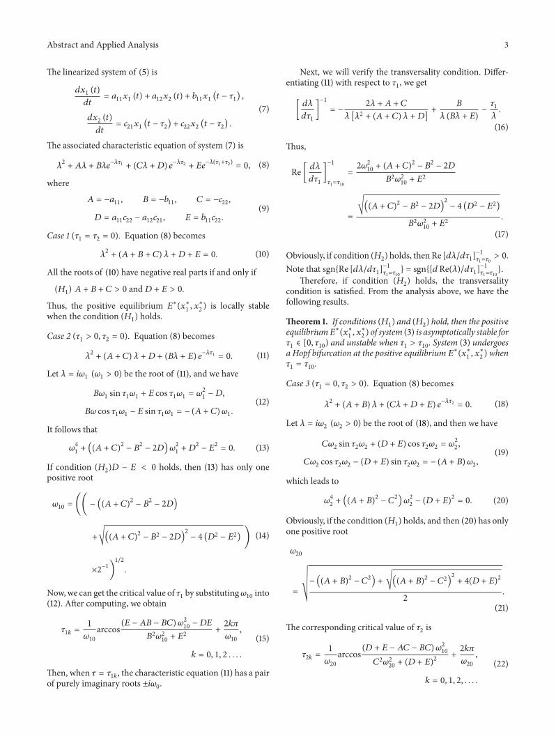
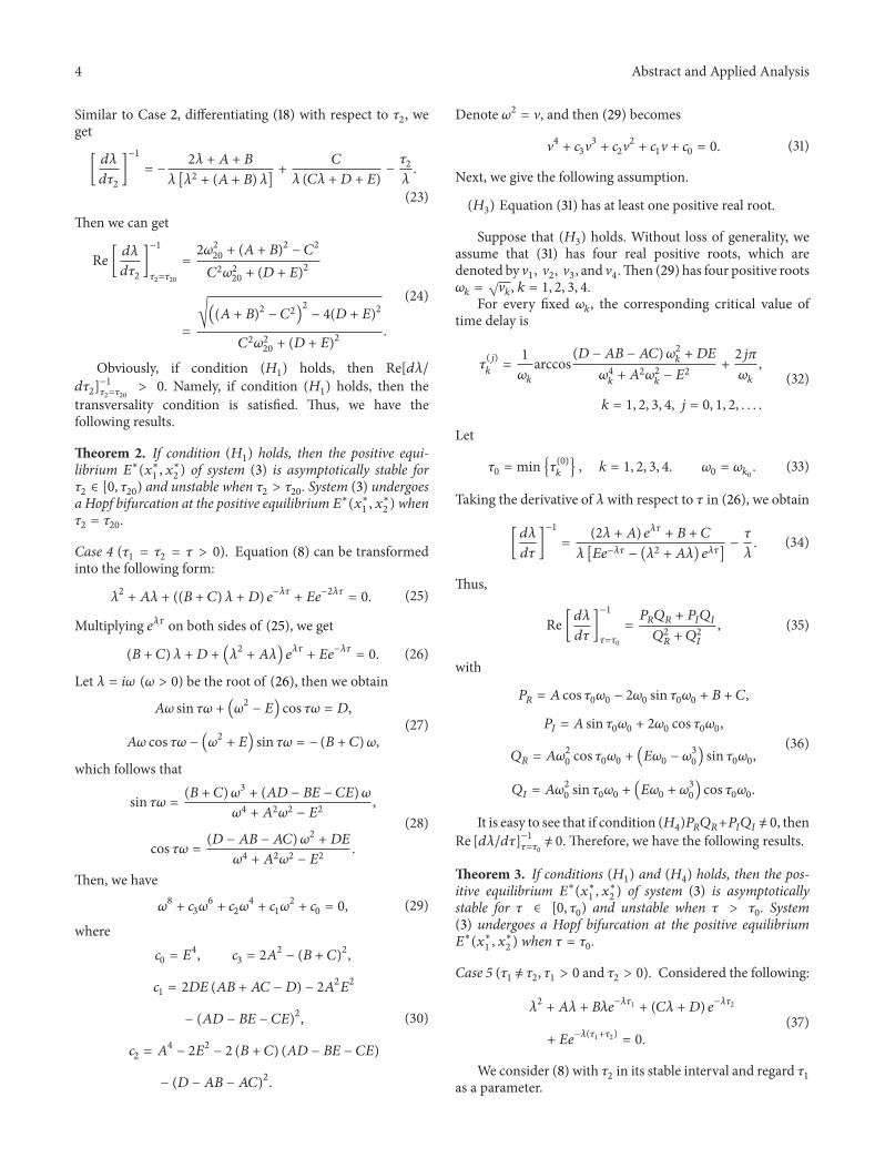
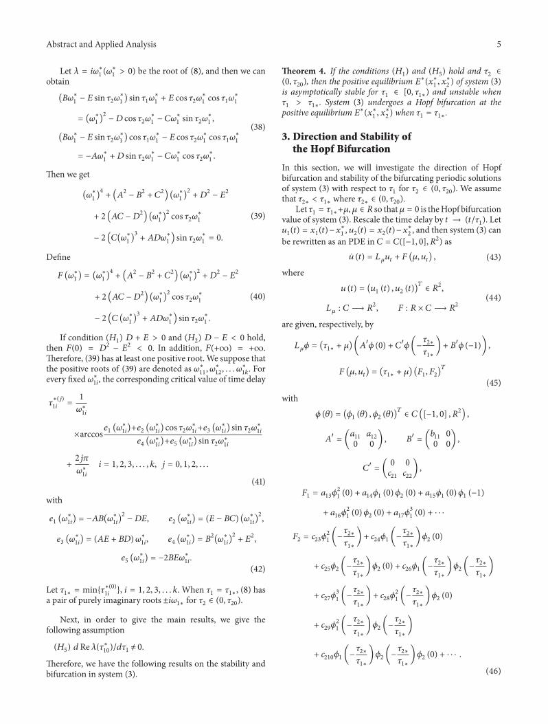
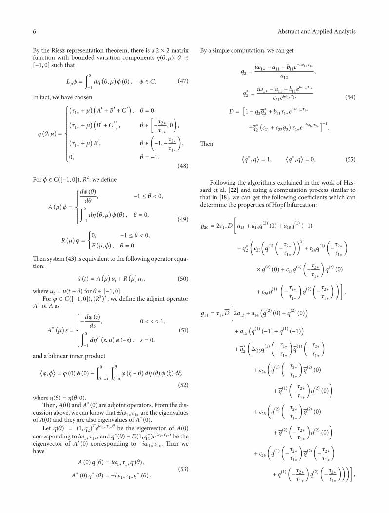
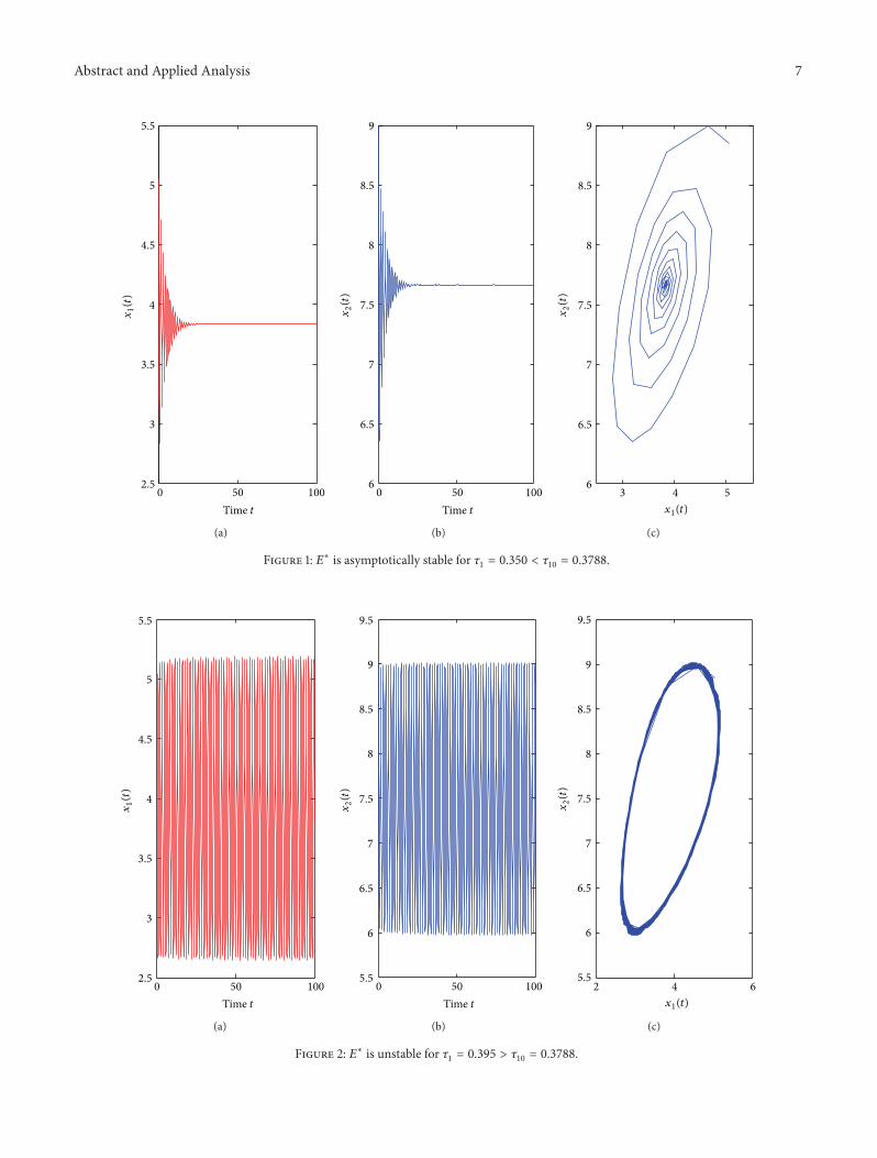
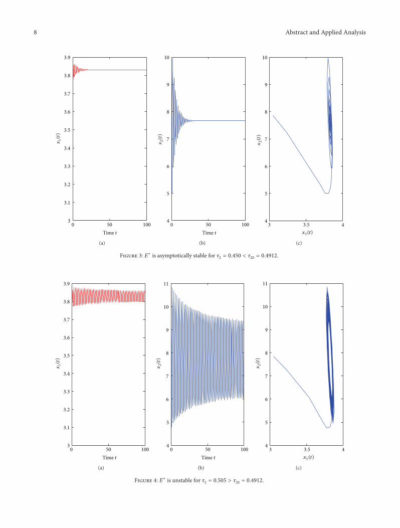
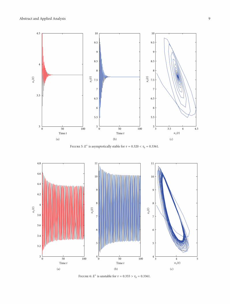
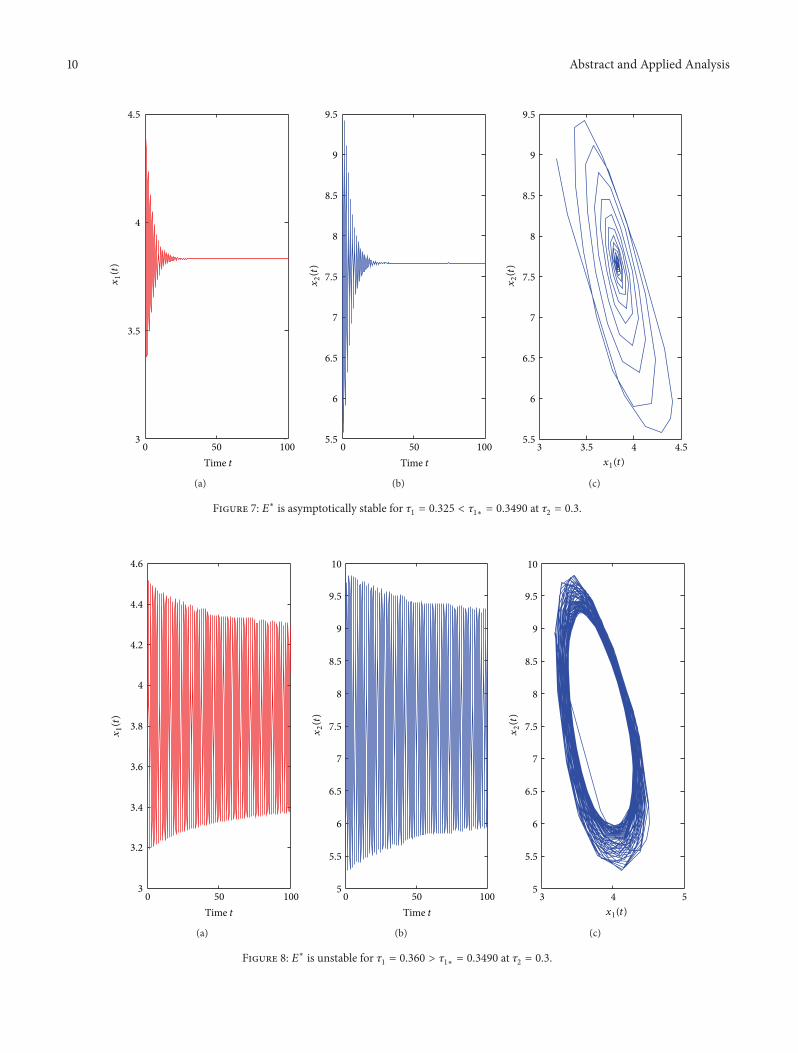
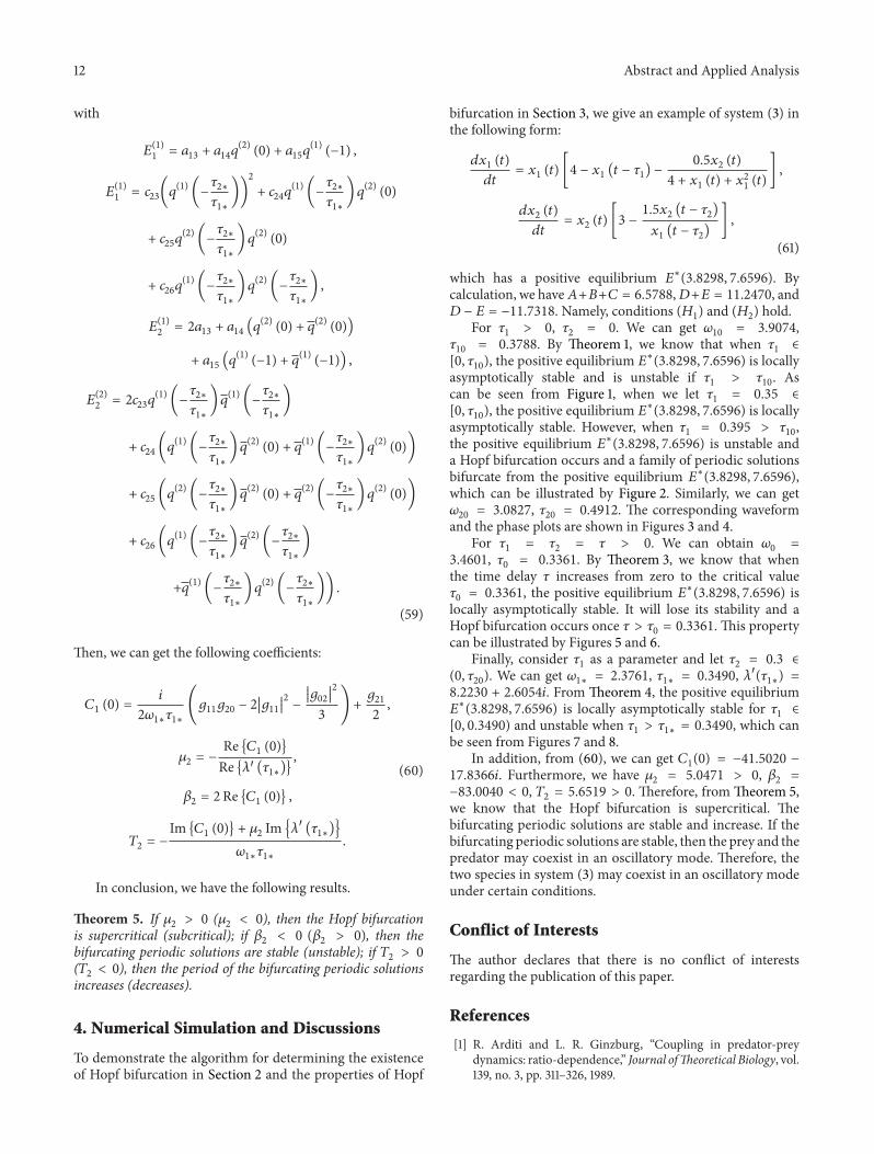