Embed Size (px)
Citation preview
This draft was prepared using the LaTeX style file belonging to the Journal of Fluid Mechanics 1
Theories of Binary Fluid Mixtures:From Phase-Separation Kinetics to Active
Emulsions
Michael E. Cates1† and Elsen Tjhung1‡1DAMTP, University of Cambridge, Centre for Mathematical Sciences, Wilberforce Road,
Cambridge CB3 0WA, UK
(Received xx; revised xx; accepted xx)
Binary fluid mixtures are examples of complex fluids whose microstructure and flow arestrongly coupled. For pairs of simple fluids, the microstructure consists of droplets orbicontinuous demixed domains and the physics is controlled by the interfaces betweenthese domains. At continuum level, the structure is defined by a composition field whosegradients – which are steep near interfaces – drive its diffusive current. These gradientsalso cause thermodynamic stresses which can drive fluid flow. Fluid flow in turn advectsthe composition field, while thermal noise creates additional random fluxes that allow thesystem to explore its configuration space and move towards the Boltzmann distribution.This article introduces continuum models of binary fluids, first covering some well-studied areas such as the thermodynamics and kinetics of phase separation, and emulsionstability. We then address cases where one of the fluid components has anisotropicstructure at mesoscopic scales creating nematic (or polar) liquid-crystalline order; this canbe described through an additional tensor (or vector) order parameter field. We concludeby outlining a thriving area of current research, namely active emulsions, in which oneof the binary components consists of living or synthetic material that is continuouslyconverting chemical energy into mechanical work. Such activity can be modelled withjudicious additional terms in the equations of motion for simple or liquid-crystallinebinary fluids. Throughout, the emphasis of the article is on presenting the theoreticaltools needed to address a wide range of physical phenomena. Examples include thekinetics of fluid-fluid demixing from an initially uniform state; the result of imposinga steady macroscopic shear flow on this demixing process; and the diffusive coarsening,Brownian motion and coalescence of emulsion droplets. We discuss strategies to createlong-lived emulsions by adding trapped species, solid particles, or surfactants; to addressthe latter we outline the theory of bending energy for interfacial films. In emulsions whereone of the components is liquid crystalline, ‘anchoring’ terms can create preferentialorientation tangential or normal to the fluid-fluid interface. These allow droplets of anisotropic fluid in a liquid crystal (or vice versa) to support a variety of topologicaldefects, which we describe, altering their interactions and stability. Addition of activeterms to the equations of motion for binary simple fluids creates a model of ‘motility-induced’ phase separation, where demixing stems from self-propulsion of particles ratherthan their interaction forces, altering the relation between interfacial structure and fluidstress. Coupling activity to binary liquid crystal dynamics creates models of active liquid-crystalline emulsion droplets. Such droplets show various modes of locomotion, some ofwhich strikingly resemble the swimming or crawling motions of biological cells.
† Email address for correspondence: [email protected]‡ Email address for correspondence: [email protected]
2 M. E. Cates and E. Tjhung
1. Introduction
A binary fluid mixture contains two types of molecule, A and B (oil and water, forinstance). In many cases these molecules have an energetic preference to be surroundedby others of the same type. At high temperatures, this is overcome by entropy and thefluid remains well mixed at a molecular scale. At low temperatures, it undergoes phaseseparation into A-rich and B-rich domains. (In a few systems, particularly those withhydrogen bonding, this temperature dependence is inverted so the system demixes uponraising temperature instead.) A sudden change in temperature, known as a ‘quench’,initiates phase separation (Chaikin & Lubensky 1995).
Usually the resulting fluid domains grow indefinitely in time so that phase separationgoes to completion (Bray 1994; Onuki 2002). But in many cases one wants to avoidor arrest this process. One strategy is to steadily stir the fluid, in the hope of remixingthe domains so that they can never become large. Another is to introduce additional(molecular or colloidal) species that inhibit the growth of domains. The resulting finelydivided mixtures, called emulsions, are generally not thermodynamically stable, but canbe long-lived. They have many applications ranging from foods via agrochemicals andpharmaceuticals, to display device materials (Bibette et al. 2002). Partly because ofthese applications, there is increasing interest in emulsions where at least one of thecomponents is not a simple fluid but has its own microstructure: for instance, a liquidcrystal in which rod-like molecules align along a common axis. In the confined geometryof an emulsion droplet, liquid crystals can show complex behaviour caused by an interplaybetween boundary conditions and bulk energy minimization (Poulin 1999).
Another growth area for binary fluids research concerns cases where one (or both) ofthe two fluids escapes the laws of conventional thermodynamics by continually consumingfuel. This allows continuous fluxes of energy, momentum and particles through thesystem, whereas in thermal equilibrium steady-state fluxes are prohibited by the time-reversal symmetry of the microscopic laws of motion (Marchetti et al. 2013). In theseso-called ‘active fluids’ thermal equilibrium is only reached when the fuel has run out;prior to that, the system can show steady-state behaviour without microscopic timereversal symmetry, leading to new effects. Many models of active fluids also addressliquid crystallinity of the active component; such models were first developed to describea system of active fibres such as those present in the cytoskeleton of eukaryotic cells.The cytoskeleton, which is responsible for shape changes and locomotion of these cells,contains locally aligned rod-like structures that are tugged lengthwise towards one an-other by active molecular motors; the rods can also actively move along their own lengthby adding protein subunits at one end and dropping them from the other (Marchettiet al. 2013). (Both of these processes are fuelled by adenosine triphosphate, ATP.)An interesting question in then whether the emergent dynamics of such cells can beunderstood in terms of simple physical models: can a cell be viewed as an active liquidcrystal emulsion droplet?
This Perspectives article explains some of the theoretical tools and approaches thatcan be used to investigate quantitatively all the above issues. The focus is on theoreticalconcepts rather than quantitative prediction, particularly in the later sections. Althoughin many cases the ideas presented have been amply confirmed by experiments, thecorroborating evidence will not be much discussed. In addition, we will often considersimplified or asymptotic regimes for which the main testing ground of theoretical ideasis provided by computer simulations, in which an appropriate numerical methodology(such as the Lattice Boltzmann method (Kendon et al. 2001; Cates et al. 2009)) is usedto solve the equations of simplified models of the type presented below. Such simulations
Binary Fluid Mixtures 3
are vital in checking our theoretical beliefs about how such a model should behave. Theycan also tell us whether the resulting behaviour is close to that seen experimentally. If itis, we have evidence that the simplified model captures the dominant mechanisms in theexperimental system, allowing us to better identify what those mechanisms are.
2. Order parameters for complex fluids
We first consider an isothermal, incompressible, simple fluid with Newtonian viscosityη and density ρ. This obeys the Navier Stokes equation (NSE)
ρ(v + v·∇v) = η∇2v −∇P, (2.1)
where the pressure field P must be chosen to enforce the incompressibility condition
∇·v = 0. (2.2)
One generic approach to complex fluids is to consider a simple fluid obeying the NSE,coupled to a set of coarse-grained internal variables ψ(r, t), each a function of positionand time. These variables are generally called order parameter fields or simply ‘orderparameters’. Obviously they are not parameters of the model but its dynamical variables,and indeed v(r, t) is itself an order parameter since it describes a local average of randommolecular velocities. Other order parameters encountered below include the following:
(i) A scalar field φ that describes the local molecular composition of a binary fluidmixture. We define it at each instant as
φ(r) =〈nA − nB〉meso
〈nA + nB〉meso. (2.3)
Here nA,B denotes the number of A,B molecules per unit volume locally; the mesoscopicaverage 〈·〉meso is taken over a large enough (but still small) local volume so that φ(r)is smooth. For notational simplicity we have assumed that A and B molecules havethe same (constant) molecular volume. Given the incompressibility condition (2.2), thedenominator in (2.3) is a constant, and our composition variable obeys −1 6 φ 6 1 withφ = 1 in a fluid of pure A.
(ii) A vector field p, describing the mean orientation of rodlike molecules:
p(r) = 〈ν〉meso, (2.4)
with ν a unit vector along the axis of a single molecule. A material of nonzero p iscalled a polar liquid crystal. This order parameter makes sense only for molecules thathave one end different from the other. Even in that case p vanishes when molecules areoriented but not aligned, in the sense that they point preferentially along some axis butare equally likely to point up that axis as down it.
(iii) To describe cases with orientation but not alignment (in the sense just defined),we need a second rank tensor
Q(r) = 〈νν〉meso − I/d, (2.5)
where νν is a dyadic product (and independent of which way the unit vector points alongthe molecule); I is the unit tensor, and d is the dimension of space. The resulting tensor istraceless by construction and therefore vanishes if the rods are isotropically distributed.A fluid in which Q is finite but p is zero is called a nematic liquid crystal.
In general the density and viscosity in (2.1) should depend directly on our chosenset of order parameters ψ(r, t). For example, in a binary fluid A and B moleculesmay have the same volume but different masses, and pure A and pure B fluids might
4 M. E. Cates and E. Tjhung
have different viscosities. However a big simplification, which does not affect much theconceptual physics discussed below, is to assume these dependences are negligible. Theremaining effect of the structural order parameters ψ(r, t) is then to create an additionalthermodynamic stress σ that enters the NSE as
ρ(v + v·∇v) = η∇2v −∇P +∇·σ[ψ]. (2.6)
(This is more properly now called a Cauchy equation; but we call it the NSE in thisarticle.) The stress term, which is a functional of the order parameters can alternativelybe viewed as a force density s =∇·σ exerted by the order parameter fields on the fluidcontinuum. Note that any isotropic contribution to σ can be absorbed into P .
To fully specify the dynamics of our system, we need two further things. The firstis a set of equations of motion for the order parameters themselves. In general thesemust allow for their advection by the fluid flow v; this enters alongside whatever physicswould describe the system at rest. More precisely, for a composition variable φ, withv = 0 one has φ =∇·J where J is a diffusive current; this form reflects the fact that φis a conserved quantity that cannot be created or destroyed locally. In contrast, p andQ are not conserved and can relax directly towards their thermodynamic equilibriumstate. In all three cases, the equations of motion involve derivatives of a functional F [ψ]which gives the (Helmholtz) free energy in terms of the order parameter fields. Thesecond thing we need is a recipe for calculating the stress σ[ψ] from the (instantaneous)order parameter configuration ψ(r). This calculation is nontrivial, particularly for liquidcrystals (Beris & Edwards 1994), but is unambiguous so long as the system is not toofar from thermodynamic equilibrium locally. In active systems, this does not apply andadditional terms arise in both the equations of motion and the stress, whose form is lessrigorously known but can be selected empirically. In what follows we consider both theorder parameter evolution equations and the stress expression on a case by case basis.
3. The symmetric binary fluid
In the simplest model of a binary fluid, the AA and BB interactions are the same butthere is an additional repulsive energy, say EAB , between adjacent molecules of A andB. Combined with our previous assumptions, the system is now completely symmetricat a molecular level. At high temperatures, T > TC ' EAB/kB (with kB Boltzmann’sconstant) the repulsive interactions are overcome by mixing entropy and the two fluidsremain completely miscible. At lower T however, the A-B repulsion causes demixing intotwo co-existing phases, one rich in A, one rich in B. Entropy ensures that there is alwaysa small amount of the other type of molecule present in each phase; close to the criticaltemperature TC the two phases differ only slightly in φ, merging at φ = φC = 0.
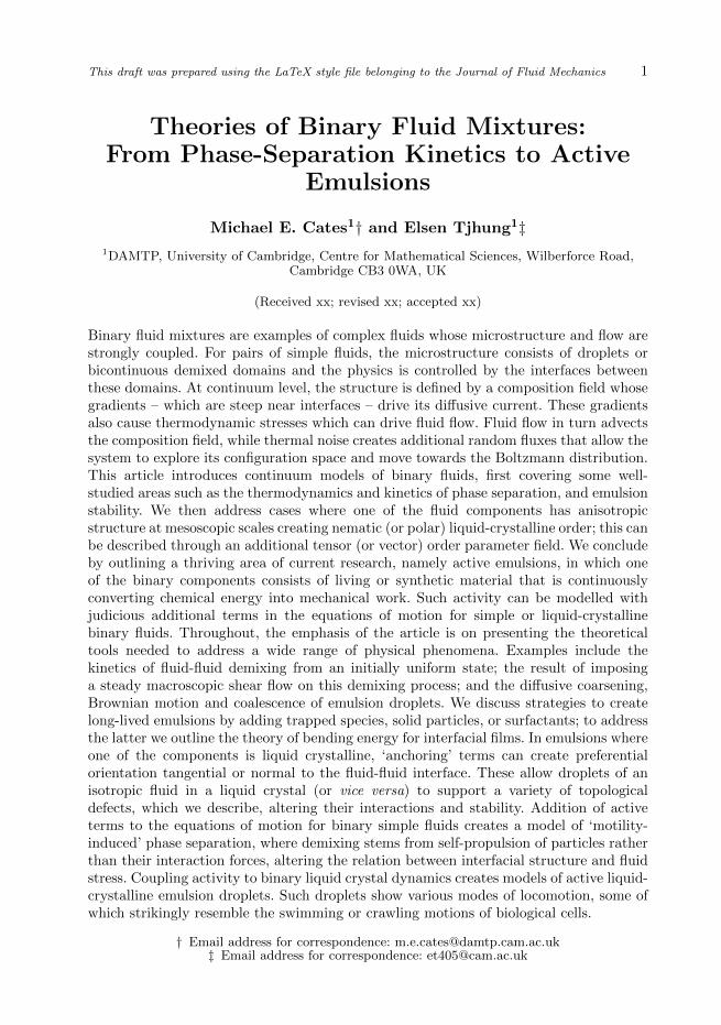
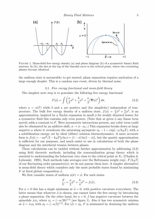
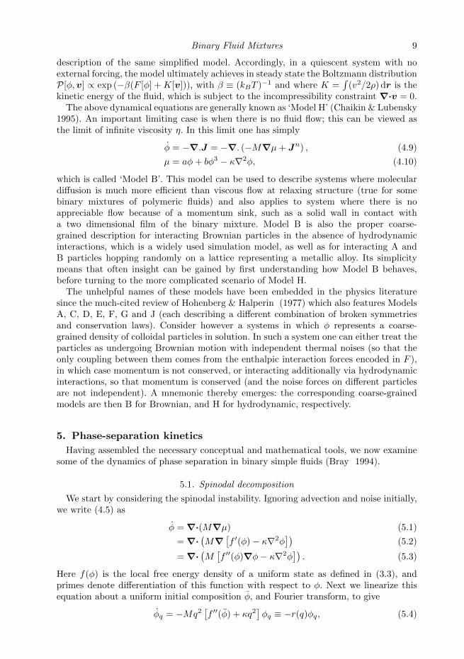
A schematic phase diagram for the symmetric binary fluid is shown in figure 1. Thelocus of coexisting compositions φ = ±φb(T ) is called the binodal curve; for globalcompositions φ =
∫φ(r)dr within the binodal, the equilibrium state comprises two
phases of composition ±φb. The volumes occupied by the A-rich and B-rich phases,VA,B , obey VA + VB = V where V is the overall volume of the system and
(VA − VB)φb = φ. (3.1)
Thus the ‘phase volume’ of the A-rich phase, ΦA ≡ VA/V , evolves from zero to one as theoverall composition φ is swept across the miscibility gap from −φb to φb. The dotted lineon the phase diagram is the spinodal, φ = ±φs(T ), within which the globally uniformstate φ(r) = φ is locally unstable. Between the spinodal and the binodal (φs 6 |φ| 6 φb)
Binary Fluid Mixtures 5
Figure 1. Mean-field free energy density (a) and phase diagram (b) of a symmetric binary fluidmixture. In (b), the dot at the top of the binodal curve is the critical point, where two coexistingphases become identical.
the uniform state is metastable; to get started, phase separation requires nucleation of alarge enough droplet. This is a random rare event, driven by thermal noise.
3.1. Free energy functional and mean-field theory
The simplest next step is to postulate the following free energy functional
F [φ] =
∫ (a
2φ2 +
b
4φ4 +
κ
2(∇φ)2
)dr, (3.2)
where a = a(T ) while b and κ are positive and (for simplicity) independent of tem-perature. The bulk free energy density of a uniform state, f(φ) = a
2φ2 + b
4φ4, is an
approximation, inspired by a Taylor expansion in small φ for weakly demixed states; fora symmetric fluid this contains only even powers. (Note that at given φ any linear termmerely adds a constant to F . Were asymmetric interactions present, any cubic term couldalso be eliminated by an additive shift, φ→ φ−φC .) This expansion breaks down at largenegative a where it overshoots the saturating asymptote φb − 1 ∼ exp[−u/kBT ], with ua solubilization energy, set by ideal (dilute) solution thermodynamics. A more accurateform is f(φ) = −uφ2/2− kBT [φ lnφ+ (1− φ) ln(1− φ)], but the quartic approximationis sufficient for our purposes, and much easier to use in calculations of both the phasediagram and the interfacial tension between phases.
These calculations can be tackled without further approximation by addressing (3.2)using field theoretic methods, including the renormalization group theory which isessential to understanding the behaviour very close to the critical point at TC (Chaikin &Lubensky 1995). Such methods take averages over the Boltzmann weight exp[−F/kBT ]of our fluctuating order parameter(s); we do not pursue them here. A simpler alternativeis mean-field theory which considers only the most probable states found by minimizingF at fixed global composition φ.
We first consider states of uniform φ(r) = φ. For such states
F
V=a
2φ2 +
b
4φ4 = f(φ). (3.3)
For a > 0 this has a single minimum at φ = 0, with positive curvature everywhere. Thelatter means that whatever φ is chosen, one cannot lower the free energy by introducinga phase separation. On the other hand, for a < 0, f has negative curvature between thespinodals ±φs where φs = (−a/3b)1/2 (see figure 1). Also it has two symmetric minimaat φ = ±φb with φb = (−a/b)1/2. For |φ| < φb, F is minimized by demixing the uniform
6 M. E. Cates and E. Tjhung
state at φ into two coexisting states at φ = ±φb. A price must be paid to create aninterface between these, but the interfacial area scales as V 1−1/d V so that for a largeenough system, this price is always worth paying.
Although so far restricted to symmetric fluid pairs, this calculation is more generalthan it first appears. For an asymmetric fluid, one expects (to quartic order) additionallinear and cubic terms in f(φ). However, any linear term in F is of the form
∫φdr = φV
which is simply a constant set by the global composition. Such an additive constant toF has no physical effects. In contrast, a cubic term
∫(cφ3/3)dr creates an asymmetric
phase diagram, which is useful in fitting the model to real fluid pairs for which someasymmetry is always present. However, it is a simple exercise then to show this cubiccontribution can be absorbed by shifts a→ a−aC and φ→ φ−φC with aC = c2/3b andφC = −c/3b. In other words, at our chosen level of treating f(φ) as a quartic polynomial,the cubic term merely shifts the mean-field critical point to a new position on the phasediagram; measuring φ and a relative to this new position, nothing has changed.
3.2. Interfacial profile and tension
In equilibrium, our two bulk phases will minimize their mutual surface area; in mostgeometries, this requires the interface to be flat. To calculate its interfacial tension,we take the surface normal along the x direction so that φ(r) = φ(x). The boundaryconditions are that φ(x) approaches ±φb at x = ±∞. To find the profile, we minimizeF [φ] − λ
∫φdr with these boundary conditions. (Here λ is a Lagrange multiplier that
holds the global composition fixed during the minimization.) The resulting condition,
δ
δφ
[F − λ
∫φdr
]= 0, (3.4)
involves the functional derivative of F which we denote by
µ(x) ≡ δF
δφ= aφ+ bφ3 − κ∇2φ. (3.5)
This is called the chemical potential (or more properly the exchange chemical potential)because, up to a factor of molecular volume, it gives the free energy change on replacingan A molecule with a B molecule locally such that if φ is incremented by δφ(r), then thefree energy change is δF =
∫µ δφdr.
Equation (3.4) requires that µ = λ which is constant in space. For our symmetricchoice of F [φ] we have µ = df/dφ = 0 in the two bulk phases at density ±φb, so it followsthat λ = 0. It is then a good exercise (Chaikin & Lubensky 1995) to show that, withthe boundary conditions already given, the solution for φ(x) of the ODE µ(x) = 0 is
φ(x) = ±φ0(x) ≡ ±φb tanh
(x− x0
ξ0
). (3.6)
Here ξ0 = (−κ/2a)1/2 is an interfacial width parameter, x0 marks the midpoint of theinterface, and the overall sign choice depends on whether the A-rich or B-rich phaseoccupies the region at large positive x. The interfacial profile is fixed by a trade-offbetween the penalty for sharp gradients (set by κ) and the purely local free energy termswhich, on their own, would be minimized by a profile φ(x) that jumps discontinuouslyfrom one binodal value to the other. A further exercise is to show that the equilibriuminterfacial tension γ0, defined as the excess free energy per unit area of a flat interface,
Binary Fluid Mixtures 7
obeys (Chaikin & Lubensky 1995)
γ0 =
∫κ(∂xφ0(x))2dx =
(−8κa3
9b2
)1/2
. (3.7)
3.3. Stress tensor
If the interfacial profile departs from the equilibrium one, a thermodynamic stress σwill act on the fluid. An important example is when the interface is not flat but curved;under these conditions µ cannot be zero everywhere. For use in the NSE we require notthe stress tensor directly but the thermodynamic force density s ≡∇·σ. Consider now asmall incompressible displacement field u: that is r → r+u(r) with∇·u = 0. Advectionof the φ field by this displacement induces the change φ(r)→ φ(r − u). To linear orderthis gives the increment δφ = −u·∇φ from which we find the free energy increment as
δF =
∫δF
δφδφdr = −
∫µu·∇φ dr =
∫(φ∇µ)·udr, (3.8)
where the final form follows by partial integration and incompressibility. (We considerperiodic boundary conditions without loss of generality; this eliminates the boundaryterm.) This result can be compared with the free energy increment caused by a straintensor ε =∇u
δF =
∫σ:(∇u) dr = −
∫s·udr, (3.9)
where the second form again follows by partial integration. Comparison of (3.8,3.9) showsthat ∇·σ ≡ s = −φ∇µ. This form, which is all we need to know about the stress tensorfor the purposes of solving the NSE, could also have been derived from the followingexpression for the stress tensor itself:
σij = −Πδij − κ(∂iφ)(∂jφ). (3.10)
Here Π = φµ−F is the order parameter contribution to the (local) pressure, better knownas the osmotic pressure; we have defined F = f(φ) + κ(∇φ)2/2 which is the local freeenergy density, i.e.,
∫F dr = F . The non-gradient part of Π is in turn Πbulk = φµbulk−f
with µbulk ≡ df/dφ; this is the usual thermodynamic relation between pressure and freeenergy density (Chaikin & Lubensky 1995). In some cases it is possible to think of the flowresulting from the force density s as loosely arising from “a gradient of osmotic pressure”.This can be useful for estimating the size of terms in the NSE, but cannot be interpretedtoo literally, since a term −∇P already appears there to enforce incompressibility. Theirrotational term in the order parameter force density s = −∇Π can be absorbed intothis and so has, strictly speaking, no role in the dynamics.
4. Model H and Model B
Above we have determined the force density s = −φ∇µ that appears in the NSE for abinary fluid mixture, as a result of spatial variations in composition φ(r). Next we needan equation of motion for φ itself. This takes the form
φ+ v·∇φ = −∇·J, (4.1)
where the left-hand side is the co-moving derivative of φ. This derivative must be thedivergence of a current, because A and B particles are not created or destroyed and thusφ is a conserved field. The form for the compositional current is
J = −M∇µ, (4.2)
8 M. E. Cates and E. Tjhung
where M could in principle depend locally (or indeed nonlocally) on composition, but ishere chosen constant for simplicity. The collective mobility M describes, under conditionsof fixed total particle density, how fast A and B molecules can move down their (equal andopposite) chemical potential gradients to relax the composition field. The linear relationbetween flux and chemical potential gradient assumes that gradient is small enough forthe system to remain locally close to thermal equilibrium everywhere.
Combining (4.1,4.2) with our earlier results for the chemical potential and the NSE,we arrive at a closed set of equations for an isothermal, binary fluid mixture:
ρ(v + v·∇v) = η∇2v −∇P − φ∇µ+∇·σn, (4.3)
∇·v = 0, (4.4)
φ+ v·∇φ = −∇·(−M∇µ+ Jn), (4.5)
µ(r) = aφ+ bφ3 − κ∇2φ. (4.6)
Here the quantities σn and Jn represent noise terms, discussed below. As derived so far,however, these equations are at the level of a deterministic hydrodynamic description forwhich both such terms are zero.
The noise terms are important in several situations. One is near the critical point (notaddressed in this article) where thermal fluctuations play a dominant role in the statisticsof φ: the mean-field theory implicit in the noise-free treatment then breaks down. Anothercase where noise matters is when there are well-separated fluid droplets suspended in acontinuous fluid phase. These objects will move by Brownian motion, but without noiseterms (specifically σn) droplets of one fluid in another cannot diffuse and, in a quiescentsystem, would never meet and coalesce. The lifetime of such a droplet emulsion is thusnoise-controlled. Also, if a uniform system is prepared with φs < φ < φb (between thespinodal and the binodal on the phase diagram), a noise-free treatment would predict thisto remain uniform indefinitely, whereas in practice the system phase separates after anaccumulation of noise (entering via Jn) has driven it across a nucleation barrier involvingformation of a droplet of the phase on the opposite binodal.
The noise terms can be determined using the fluctuation dissipation theorem whichstems from the requirement for Boltzmann equilibrium in steady state (Chaikin &Lubensky 1995). The order parameter current Jni (Cartesian component i; superscriptn for noise) is a zero-mean Gaussian variable of the following statistics:
〈Jni (r, t)Jnj (r′, t′)〉 = 2kBTMδijδ(r − r′)δ(t− t′), (4.7)
where 〈·〉 denotes an average over the unresolved microscopic dynamics responsible forthe noise. Meanwhile the random stress in the NSE is likewise a zero-mean Gaussianthermal stress whose statistics obey (Landau & Lifshitz 1959)
〈σnij(r, t)σnkl(r′, t′)〉 = 2kBTη[δikδjl + δilδjk]δ(r − r′)δ(t− t′). (4.8)
Note that due to incompressibility the isotropic (pressure-like) part of this noise stressis optional, and often explicitly removed in the literature. The resulting noisy NSE isfundamental to the fluid mechanics of thermal systems, although in some cases – notablysuspensions of Brownian spheres – it can be impersonated by adding a set of correlatednoise forces direct to the equations of motion of individual suspended objects (Brady &Bossis 1988). That approach does not generalize to fluid domains of variable shape andis therefore not helpful in the binary fluid context.
With these noise terms duly added, equations (4.3–4.6) are lifted from a mean-field dynamics of the simplest binary fluid, whose free energy functional is the chosenF [φ] and whose mobility and viscosity are φ-independent, to a complete dynamical
Binary Fluid Mixtures 9
description of the same simplified model. Accordingly, in a quiescent system with noexternal forcing, the model ultimately achieves in steady state the Boltzmann distributionP[φ,v] ∝ exp (−β(F [φ] +K[v])), with β ≡ (kBT )−1 and where K =
∫(v2/2ρ) dr is the
kinetic energy of the fluid, which is subject to the incompressibility constraint ∇·v = 0.The above dynamical equations are generally known as ‘Model H’ (Chaikin & Lubensky
1995). An important limiting case is when there is no fluid flow; this can be viewed asthe limit of infinite viscosity η. In this limit one has simply
φ = −∇.J = −∇. (−M∇µ+ Jn) , (4.9)
µ = aφ+ bφ3 − κ∇2φ, (4.10)
which is called ‘Model B’. This model can be used to describe systems where moleculardiffusion is much more efficient than viscous flow at relaxing structure (true for somebinary mixtures of polymeric fluids) and also applies to system where there is noappreciable flow because of a momentum sink, such as a solid wall in contact witha two dimensional film of the binary mixture. Model B is also the proper coarse-grained description for interacting Brownian particles in the absence of hydrodynamicinteractions, which is a widely used simulation model, as well as for interacting A andB particles hopping randomly on a lattice representing a metallic alloy. Its simplicitymeans that often insight can be gained by first understanding how Model B behaves,before turning to the more complicated scenario of Model H.
The unhelpful names of these models have been embedded in the physics literaturesince the much-cited review of Hohenberg & Halperin (1977) which also features ModelsA, C, D, E, F, G and J (each describing a different combination of broken symmetriesand conservation laws). Consider however a systems in which φ represents a coarse-grained density of colloidal particles in solution. In such a system one can either treat theparticles as undergoing Brownian motion with independent thermal noises (so that theonly coupling between them comes from the enthalpic interaction forces encoded in F ),in which case momentum is not conserved, or interacting additionally via hydrodynamicinteractions, so that momentum is conserved (and the noise forces on different particlesare not independent). A mnemonic thereby emerges: the corresponding coarse-grainedmodels are then B for Brownian, and H for hydrodynamic, respectively.
5. Phase-separation kinetics
Having assembled the necessary conceptual and mathematical tools, we now examinesome of the dynamics of phase separation in binary simple fluids (Bray 1994).
5.1. Spinodal decomposition
We start by considering the spinodal instability. Ignoring advection and noise initially,we write (4.5) as
φ =∇·(M∇µ) (5.1)
=∇·(M∇
[f ′(φ)− κ∇2φ
])(5.2)
=∇·(M[f ′′(φ)∇φ− κ∇2φ
]). (5.3)
Here f(φ) is the local free energy density of a uniform state as defined in (3.3), andprimes denote differentiation of this function with respect to φ. Next we linearize thisequation about a uniform initial composition φ, and Fourier transform, to give
φq = −Mq2[f ′′(φ) + κq2
]φq ≡ −r(q)φq, (5.4)
10 M. E. Cates and E. Tjhung
where we have defined a wave-vector dependent decay rate r(q). For f ′′(φ) > 0 thisis positive for all q: all Fourier modes decay and the initial state is stable. In contrastfor f ′′(φ) < 0, the system is unstable, with r(q) negative at small and intermediatewavevectors. (Stability is restored at high enough q by the κ term.) Solving dr/dq = 0for q identifies the fastest growing instability to be at q∗ = −f ′′(φ)/2κ. Because couplingto fluid flow was neglected this is technically a Model B result, but in fact such coupling(Model H) does not change the result of this linear stability analysis.
Even neglecting the thermal noise in the dynamics (4.7,4.8), the initial condition canbe assumed to have some fluctuations. Those whose wavenumbers lie near q∗ growexponentially faster than the rest, so that the time-dependent composition correlatorSq(t) ≡ 〈φq(t)φ−q(t)〉 soon develops a peak of height growing as exp[−r(q∗)t] aroundq∗. Hence during this ‘early stage’ of spinodal decomposition a local domain morphologyis created by compositional interdiffusion with a well defined length-scale set by π/q∗.The amplitude of these compositional fluctuations grows until local values approach thebinodals ±φb. From this emerges a domain pattern, still initially with the same lengthscale, consisting of phases in local coexistence, separated by relatively sharp interfaces ofwidth ξ0 and interfacial tension γ0 as found from the equilibrium interfacial profile (3.6).
The next stage of the phase separation depends crucially on the topology of the newlyformed fluid domains. This is controlled mainly by the phase volumes ΦA,B of the A-richand B-rich phases. Roughly speaking, if 0.3 6 ΦA 6 0.7 the domains remain bicontinuous:one can trace a path through the A-rich phase from one side of the sample to the other,and likewise for the B-rich phase. Outside this window, the structure instead has dropletsof A in B (ΦA < 0.3) or B in A (ΦA > 0.7). The values 0.3 and 0.7 are rule-of-thumbfigures only, with details depending on many other factors (including any asymmetryin viscosity or mobility) that we do not consider here. Note also that the window ofbicontinuity shrinks to zero width in two dimensions, where the slightest asymmetry inphase volume and/or material properties will generally result in a droplet geometry inwhich only one phase is continuous. We next assemble the tools needed to understandthe late stages of phase separation before discussing their dynamics.
5.2. Laplace pressure of curved interfaces
Once the interfaces are sharp, their geometry becomes a dominant factor in the timeevolution. Unless they are perfectly flat, interfaces exert forces on the fluid via the s =−φ∇µ term in (4.3), in response to which the fluid may or may not be set in motion.(No motion is implied if s remains irrotational, as discussed previously.) The physicsof this term, for interfaces that are locally equilibrated but not flat, is that of Laplacepressure. Consider for example a spherical droplet of one fluid in another with radiusR and interfacial tension γ. Suppose that that the pressure inside the droplet is greaterthan that outside by an amount ∆P . The total force on the upper half of the dropletexerted by the bottom half is then (in three dimensions)
πR2∆P − 2πγR = 0, (5.5)
which must vanish if the droplet is not moving. The first term comes from the verticalcomponent of the extra pressure acting across the equatorial disc, and the second is thetension acting across its perimeter. The resulting pressure excess, known as ‘Laplacepressure’, is ∆P = 2γ/R. More generally in three dimensions one has ∆P = γH =γ(R1−1 +R2
−1)
where H is the mean curvature and R1 and R2 are the principal radiiof curvature. Note also that for a (hyper-)sphere in d dimensions, ∆P = (d− 1)γ/R. Inall these expressions we can set γ = γ0 as calculated in section 3.2, so long as curvatureis weak (Hξ0 1) and there is local thermodynamic equilibrium across the interface.
Binary Fluid Mixtures 11
A closely related result concerns the chemical potential µ at a representative point on aweakly curved interface. Local equlibrium fixes the interfacial profile as φ(r) ' φ0(w) ≡φb tanh(w/ξ0) where w is a Cartesian coordinate normal to the interface that vanishesat the midpoint of the profile. Then ∇φ = ∂wφ(w)w with w the unit normal (pointingfrom low to high φ). It follows that ∇2φ = ∂2
wφ+ ∂wφ∇·w. From the definition of µ asδF/δφ = f ′(φ)− κ∇2φ we have
µ = f ′(φ)− κ∂2wφ− κ∂wφ∇·w. (5.6)
For the local equilibrium profile φ(r) = φ0(w) = φb tanh(w/ξ0) the first two terms onthe right cancel. Moreover, local equilibrium requires that µ is almost constant on thescale of the interfacial thickness ξ0. Denoting this locally constant value interfacial by µI ,multiplying by ∂wφ and integrating through the interface gives 2φbµI = Hκ
∫(∂wφ)2 dw
where H = −∇·w is the mean curvature, defined as above to be positive when theinterface curves towards the high φ phase. Using the previously quoted result γ0 =∫κ(∂xφ0(x))2dx we find that µI = γ0H/2φB (Bray 1994).
Thus for a large spherical droplet of the high φ phase in the low φ phase (so that H =2/R) the chemical potential µI at the interface has a small positive value proportionalto the Laplace pressure. If the chemical potential in the surrounding phase takes itsequilibrium value far away (µ = 0 at coexistence) we requires a gradient of µ and thusa constant outward flux of φ from the droplet surface. Stable equilibrium of a finitedroplet surrounded by the opposite phase is possible, but only in a finite system thathas µ(r) = µI everywhere so that J = −M∇µ = 0. This arises when the phase volumesΦA,B are sufficiently asymmetric that the interfacial area of a droplet configuration isless than that of a slab geometry, which depends on the shape of the container and itsboundary conditions; even if so, R→∞ and µI → 0 in the large system limit. In all othersituations (nonspherical domains, spherical droplets of unequal sizes, or a droplet in aninfinite bath) there is a flux onto or off the interface proportional to the local curvature.
To quantify this, consider the state of stable equilibrium for a droplet of A-rich phase(φ ' +φb) in a finite domain of the B-rich phase (φ ' −φb). After expanding f(φ) =aφ2/2 + bφ4/4 for small deviations about ±φb, equating the Laplace pressure ∆P to thedifference in osmotic pressure φµ(φ)−f(φ) of the A-rich and B-rich bulk phases gives theresult that φA,B = ±φb + δ, with both phases equally shifted upwards in composition φrelative to the equivalent state of bulk coexistence with a flat interface. The upward shiftobeys δ = γ0/(αφbR) where α ≡ f ′′(±φb) = −2a and R is the droplet radius. (This δwould reverse in sign for a B-rich droplet in an A-rich phase.) The result can alternativelybe derived by setting µI = αδ in the equation µI = γ0H/2φB quoted above.
We next assume that these local equilibrium conditions apply across the curved dropletinterface in an infinite B-rich reservoir whose composition far away is −φb+ε where ε < δ.Here the far-field parameter ε is known as the ambient supersaturation. We then seek aspherically symmetric quasi-static (φ = −∇·J = 0) exterior solution φ(r) = −φb + φ(r)where φ(R) = δ and φ(∞) = ε. With J = −M∇µ this solution obeys µ = αφ where∇2φ = 0; note that the square gradient contribution to µ vanishes in this geometry. Withthe given boundary conditions, the result is φ = ε+ (δ − ε)R/r. If we now calculate theradial current J = |J | exterior to the droplet, we have J = −αM∂φ/∂r = αM(δ−ε)R/r2;just outside the droplet itself this becomes −αM(δ − ε)R. By mass conservation (giventhe compositional jump ∆φ = 2φb across the interface) we then find R = −J(R)/2φb or
R =1
2φb
[αM
R(ε− δ(R))
]=
1
2φb
[αM
R
(ε− γ0
αφbR
)]. (5.7)
12 M. E. Cates and E. Tjhung
This result will be used in section 5.4 below to discuss the process of competitive growthand shrinkage of droplets known as Ostwald ripening.
5.3. Coalescence of droplet states
If the post-spinodal structure is that of droplets, each relaxes rapidly to minimizeits area at fixed volume, resulting in a spherical shape. For well separated droplets thethermodynamic force s in the neighbourhood of each droplet has radial symmetry andhence is the gradient of a scalar (pressure) contribution. This has no consequences for fluidflow since all such terms are subsumed into an overall pressure set by the incompressibilityconstraint. Accordingly there is no net fluid motion in the absence of noise. Thermal noiseallows droplets to move around by Brownian motion, resulting in collisions that cause themean droplet radius R to increase by coalescence. To estimate the time dependence of R
we observe that for A droplets in B, the mean inter-droplet distance L is of order RΦ−1/3A
at small ΦA; more generally, L/R is a function of ΦA only. Each droplet will collide withanother in a time ∆t of order L2/D where D ' kBT/ηR is the droplet diffusivity. Uponcollision, two droplets of radius R make a new one of radius approximately 21/3R causingan increment ∆ lnR ' (ln 2)/3. This gives
∆ lnR
∆t∝ kBT
ηR3, (5.8)
where the precise factor of 21/3 has ceased to matter, and the left hand side can beapproximated as d lnR/dt = R/R. By integration we then obtain the scaling law
R(t) ∼(kBTt
η
)1/3
. (5.9)
This argument assumes that coalescence is diffusion-limited, and shows that in this caseBrownian motion will cause indefinite growth of the mean droplet size, culminating intotal phase separation.
The assumption of independently diffusing spherical droplets should be reliable at lowenough phase volumes ΦA of the dispersed phase, where it is the dominant coarseningmechanism so long as the Ostwald process (described next) is suppressed. But at largerΦA more complicated routes to coalescence, some involving droplet-scale or macroscopicfluid flow, are possible. One of these is so-called ‘coalescence-induced coalescence’ wherethe shape relaxation post-collision of a pair of droplets creates enough flow to causeanother coalescence nearby (Wagner & Cates 2001). This gives a new scaling (R ∼ γ0t/η)which coincides with one of the regimes described later for the coarsening of bicontinuousstructures (section 5.16 below). Indeed it stems from the same balance of forces as willbe discussed for that case. Quite recently a new picture has emerged of hydrodynamiccoarsening in moderately concentrated droplet suspensions (ΦA > 0.2), which supersedesa longstanding view that equation (5.9) still holds in this regime. This picture involvesmechanical (Marangoni) forces resulting from departures of the interfacial tension fromits equilibrium value (γ 6= γ0). These departures arise because the presence of neighboursbreaks rotational symmetry around any given droplet so that the thermodynamic forcedensity is no longer a pure pressure gradient (Shimuzu & Tanaka 2015).
In many droplet emulsions it is possible to inhibit the coalescence step, so that thisentire route to phase separation is effectively blocked. For instance, adding chargedsurfactants can stabilize oil droplets in water against coalescence by creating a Coulombicbarrier opposing the close approach of droplet surfaces. (Surfactants are amphiphilicmolecules that have a polar or charged head-group and an oily tail; they are widely used
Binary Fluid Mixtures 13
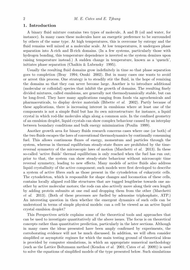
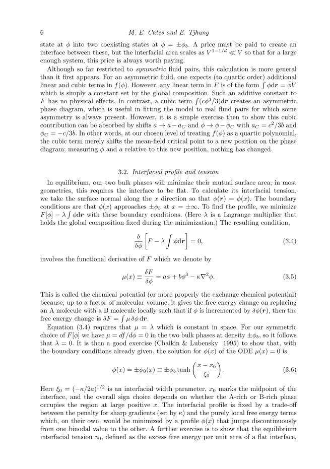
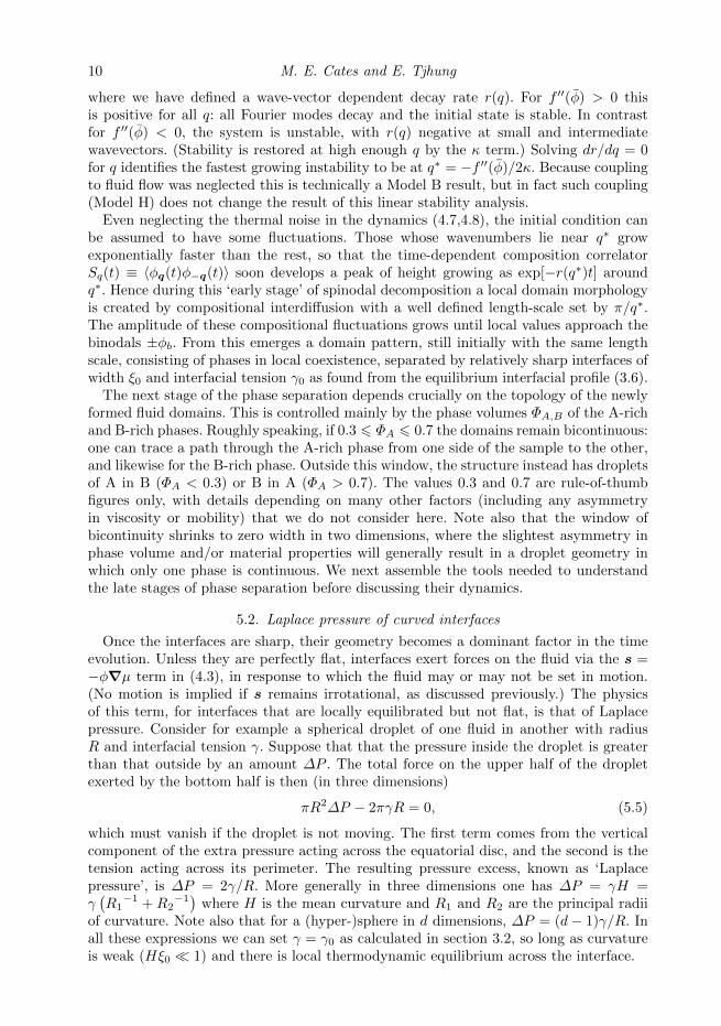
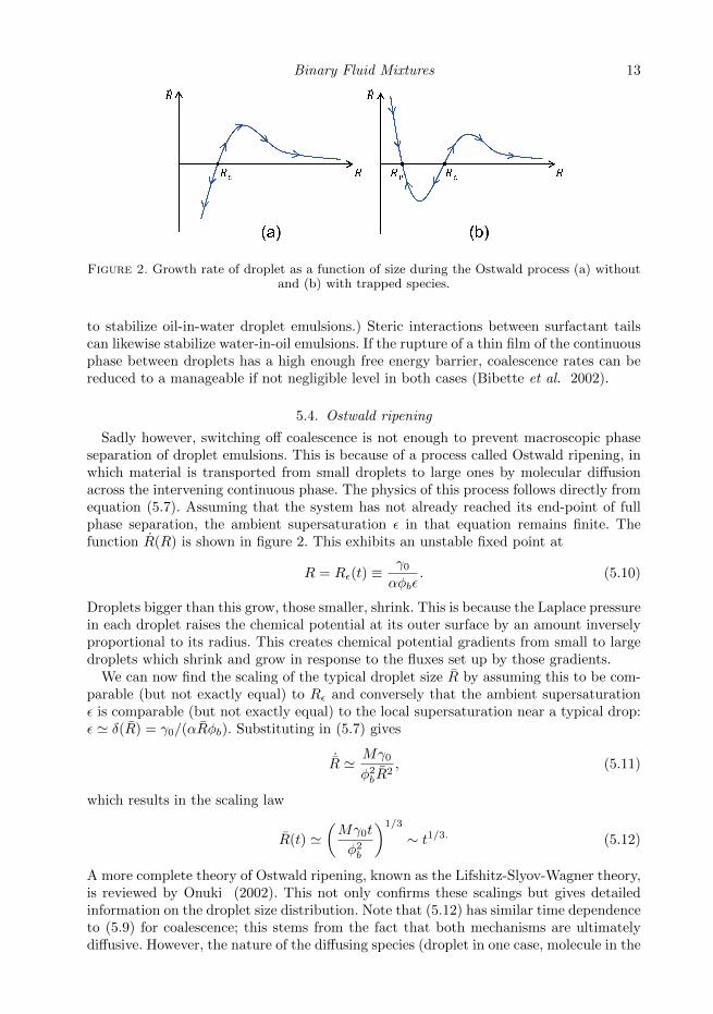
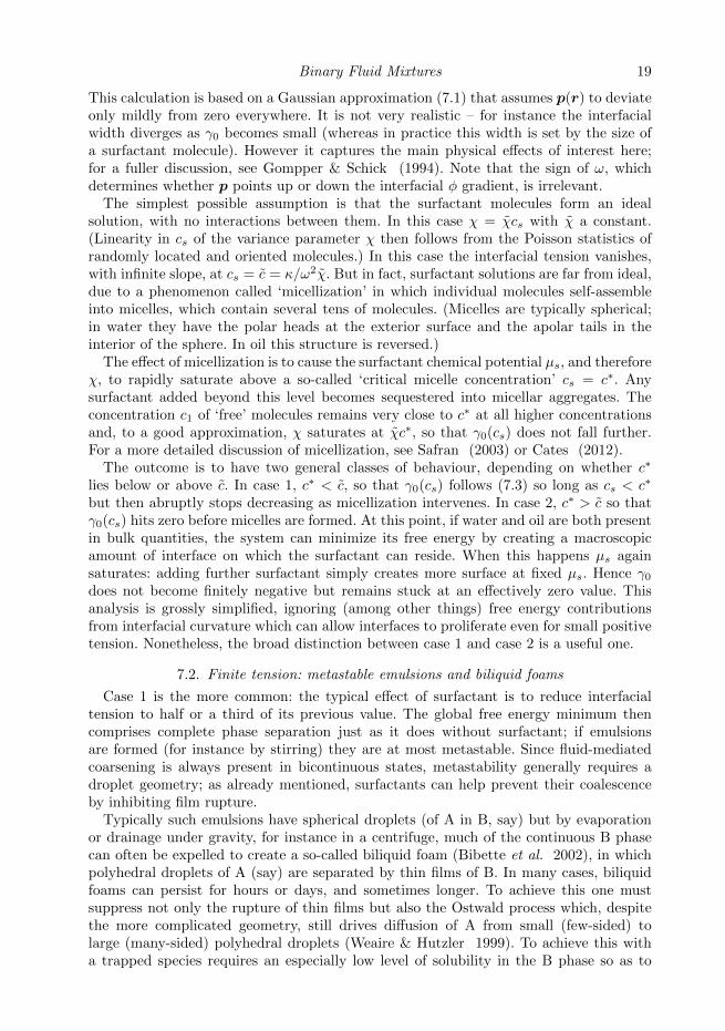
Figure 2. Growth rate of droplet as a function of size during the Ostwald process (a) withoutand (b) with trapped species.
to stabilize oil-in-water droplet emulsions.) Steric interactions between surfactant tailscan likewise stabilize water-in-oil emulsions. If the rupture of a thin film of the continuousphase between droplets has a high enough free energy barrier, coalescence rates can bereduced to a manageable if not negligible level in both cases (Bibette et al. 2002).
5.4. Ostwald ripening
Sadly however, switching off coalescence is not enough to prevent macroscopic phaseseparation of droplet emulsions. This is because of a process called Ostwald ripening, inwhich material is transported from small droplets to large ones by molecular diffusionacross the intervening continuous phase. The physics of this process follows directly fromequation (5.7). Assuming that the system has not already reached its end-point of fullphase separation, the ambient supersaturation ε in that equation remains finite. Thefunction R(R) is shown in figure 2. This exhibits an unstable fixed point at
R = Rε(t) ≡γ0
αφbε. (5.10)
Droplets bigger than this grow, those smaller, shrink. This is because the Laplace pressurein each droplet raises the chemical potential at its outer surface by an amount inverselyproportional to its radius. This creates chemical potential gradients from small to largedroplets which shrink and grow in response to the fluxes set up by those gradients.
We can now find the scaling of the typical droplet size R by assuming this to be com-parable (but not exactly equal) to Rε and conversely that the ambient supersaturationε is comparable (but not exactly equal) to the local supersaturation near a typical drop:ε ' δ(R) = γ0/(αRφb). Substituting in (5.7) gives
˙R ' Mγ0
φ2bR
2, (5.11)
which results in the scaling law
R(t) '(Mγ0t
φ2b
)1/3
∼ t1/3. (5.12)
A more complete theory of Ostwald ripening, known as the Lifshitz-Slyov-Wagner theory,is reviewed by Onuki (2002). This not only confirms these scalings but gives detailedinformation on the droplet size distribution. Note that (5.12) has similar time dependenceto (5.9) for coalescence; this stems from the fact that both mechanisms are ultimatelydiffusive. However, the nature of the diffusing species (droplet in one case, molecule in the
14 M. E. Cates and E. Tjhung
other) is quite different, resulting in prefactors that involve unrelated material propertiesfor the two mechanisms.
5.5. Preventing Ostwald ripening
It follow from (5.12) that the Ostwald process can be slowed by reducing the interfacialtension γ0, but so long as this remains positive it cannot be stopped entirely. A moreeffective approach is to include within the A phase a modest concentration of a somespecies that is effectively insoluble in B. This might be a polymer or, if A is water andB oil, a simple salt. The idea is that the trapped species in the A droplets creates anosmotic pressure which rises as R falls, hence opposing the Laplace pressure. Treating thetrapped species as an ideal solution in A, (5.7) is replaced by (Webster & Cates 1998)
R =1
2φb
[αM
R
(ε− γ0
αφbR+ην
R3
)], (5.13)
where η (unrelated to the fluid viscosity η) is a combination of molecular parameters andphysical constants, and ν is the number of trapped molecules in the droplet. The finalterm reflects the extra osmotic pressure of the trapped material. There is now a stablefixed point, even for zero ambient supersaturation, at finite droplet size
Rν =
(ηναφbγ0
)1/2
. (5.14)
If we start from a uniform set of droplets of size R0, then ν = c4πR30/3 with c the initial
concentration of the added species in the A-rich phase. Droplets that have shrunk toa size Rν can coexist with a bulk A-rich phase without shrinking further: the Laplacepressure is balance by the trapped species’ osmotic pressure. Moreover, if the initialsize obeys R0 < Rν the Ostwald process is reversed: if an emulsion of such dropletsplaced in contact with a bulk A-rich phase, they will expand up to size Rν . By addingtrapped species one can thus make robust ‘mini-emulsions’ (Landfester 2003) or ‘nano-emulsions’ (Fryd & Mason 2012) which permanently resist coarsening by the Ostwaldprocess. However these are still metastable: so long as the tension γ0 is positive, the freeenergy can always be reduced by coalescing droplets to reduce the interfacial area.
5.6. Coarsening of bicontinuous states
For roughly equal volumes of the two coexisting phases, say 0.3 6 ΦA 6 0.7 thedomains of A-rich and B-rich coexisting fluids remain bicontinuous. (This applies inthree dimensions; the two-dimensional case is special and considered later.) This allowscoarsening by a process in which the interfacial stresses – or loosely speaking, Laplacepressure gradients – pump fluid from one place to another. In all but the most viscousfluids, this process is ultimately faster than either coalescence or Ostwald ripening: wewill see below that it allows L(t) to grow with a larger power of the time. Here L(t) isnow defined as the characteristic length scale of the bicontinuous structure, for exampleas the inverse of its interfacial area per unit volume. The flow-mediated coarsening iscaptured by Model H, but absent in Model B. In the latter, domain growth is controlledby a version of the Ostwald process in which diffusive fluxes in both phases act to flattenout interfaces (reducing their curvature) and move material from thinner to fatter regionsof the bicontinuous structure. This leads again to (5.12) for the characteristic domainsize, which is now unaffected by adding insoluble species which can move diffusivelythroughout the relevant phase. In both cases the driving force is interfacial tension.
To describe flow-mediated coarsening, we assume that L(t) is much larger than the
Binary Fluid Mixtures 15
interfacial width, and is the only relevant length in the problem, so that in estimatingterms in the NSE (4.3) we may write ∇ ∼ 1/L. The forcing term φ∇µ is then of orderγ0/L
2 where we have used the result found above, µI = γ0H/2φB , for the chemicalpotential on an interface of curvature H ∼ 1/L. The fluid velocity is of order L so theviscous term scales as ηL/L2. The inertial terms are ρv ∼ ρL and ρv.∇v ∼ ρ(L)2/L.The ∇P term, enforcing incompressibility, is slave to the other terms.
Importantly, once sharp interfaces are present so that φ∇µ ∼ γ0/L2, the NSE (4.3)
involves only three parameters, ρ, γ0 and η. From these three quantities one can makeonly one length, L0 = η2/ργ0, and one time t0 = η3/ργ2
0 . This means that the domainscale L(t) must obey (Siggia 1979; Furukawa 1985)
L(t)
L0= f
(t
t0
). (5.15)
where, for given phase volumes, f(x) is a function common to all fully symmetric binaryfluid pairs. This scaling applies only to bicontinuous states; as previously described, instates comprising spherical droplets the forcing term in the NSE is instead subsumed bythe pressure term at leading order.
In systems showing fluid-mediated coarsening via (5.15), we expect different behaviouraccording to whether L/L0 is large or small. For L/L0 small it is simple to confirm thatthe inertial terms in (4.3) are negligible. (Note also that, in any regime where f(x) is apower law, the two inertial terms have the same scaling.) The primary balance in theNSE is then ηL/L2 ∼ γ0/L
2 resulting in the scaling law L(t) ∼ γ0t/η so that
f(x) ∝ x ; x x∗. (5.16)
This is called the viscous hydrodynamic (VH) regime and holds below some crossovervalue x = x∗. In contrast, for x x∗ the primary balance in the NSE is between theinterfacial and inertial terms. It is a simple exercise then to show that L(t) ∼ (γ0/ρ)1/3t2/3
so that
f(x) ∝ x2/3 ; x x∗. (5.17)
This is called the inertial hydrodynamic (IH) regime. In practice this crossover from VHto IH is several decades wide, and the crossover value rather high: x∗ ' 104 (Kendonet al. 2001). The high crossover point is less surprising if one calculates a domain-scaleReynolds number
Re =ρLL
η= f(x)
df
dx. (5.18)
The crossover value of Re then turns out to be of order 10 (Kendon et al. 2001), andthe largeness of x∗ is found to stem from a modest constant of proportionality in (5.16).It means that in practice a clean observation of the inertial hydrodynamic regime hasonly been achieved in computer simulation: in terrestrial laboratory experiments thedomains are by then so large (millimetres to centimetres for typical fluid pairs) that theslightest density difference between A and B causes gravitational terms to dominate.These terms give a body force pulling the two fluids apart along the gravitational axis,greatly speeding phase separation.
Note finally that in two dimensions, bicontinuity is exceptional. For fully symmetricfluid pairs it arises only when the phase volumes ΦA,B are also symmetric, allowingpercolating paths through both fluids to cross the container (but only just). Moregenerally, it arises at only one special phase volume whose value is set by the asymmetryof the two fluids; even if one could create this state, it would typically not be sustainedduring coarsening (since the meticulous dynamical balance required varies with the
16 M. E. Cates and E. Tjhung
scale parameter x). Alongside Ostwald and coalescence regimes, one can find, at leastin simulations, various complex structures involving cascades of nested droplets whosedetails may be noise-dependent (Gonnella et al. 1999).
6. Emulsification by shearing
Suppose we wish to stop the coarsening of a bicontinuous fluid mixture by theflow-mediated mechanism just described. In a processing context, it is often enoughto temporarily maintain a well-mixed, emulsified state merely by stirring the system.Industrial stirring is complicated, with nonuniform flows that often combine very differentlocal flow geometries (extension or shear) within a single device. Here we restrict attentionto the effects of a simple shear flow, focusing on scaling issues and the question of whetheror not such a flow can actually stop the coarsening process.
We consider uniform shearing with macroscopic fluid velocity along x, and its gradientalong y; z is then the neutral (or vorticity) direction. In simulations one can use boundaryconditions with one static wall at y = 0, another sliding one at y = Λ and periodic BCsin x, z. In practice there are ways to introduce periodic BCs also in y; nonetheless, thesystem size in that direction, Λ, is important in what follows. The top plate moves withspeed Λ/ts where 1/ts is the shear rate: vmacro = yx/ts.
For the coarsening to be fully arrested by shear, the system must reach a nonequilib-rium steady state time-reversal symmetryin which the fluid domains have finite lengthscales Lx,y,z in all three directions. (These can be defined as the inverse of the length ofinterface per unit area on a plane perpendicular to each axis.) The simplest hypothesisis that these steady-state lengths, if they exist, all have similar scaling: Lx,y,z ∼ L (Doi& Ohta 1991). Moreover, given the preceding discussion of terms in the NSE, we expectin steady state that L/L0 is now a function, not of t/t0, but of ts/t0. That is, in steadystate the previous dependence on time is replaced by a dependence on the inverse shearrate. The functional form of this dependence could in principle be anything at all, butthe simplest scaling ansatz is that the system coarsens as usual until t ∼ ts, whereuponthe shearing takes over and L stops increasing. If so,
L
L0' f
(tst0
), (6.1)
where f(x) is approximately the same function as introduced previously, for which(5.16,5.17) hold. If so, for ts/t0 x∗ we have L/L0 ∼ ts/t0 and for ts/t0 x∗ wehave L/L0 ∼ (ts/t0)2/3. In the first of these regimes, the force balance in NSE betweenviscous and interfacial stresses corresponds to setting a suitably defined capillary number(on the scale of L) to an order-unity value. (This is a criterion for the maximum sizeof droplets in dilute emulsions also.) Note however that the Reynolds number obeysRe ∼ f(x)df/dx as in (5.18). In contrast to what happens for any problem involvingshear flow around objects of fixed geometry, Re is now small when the shear rate is largeand vice versa. This is because at small shear rates, very large domains are formed.
There are several possible complications to this picture. First, in principle Lx,y,z couldall have different scalings. The resulting anisotropies could spoil any clear separationof the viscous hydrodynamic and inertial hydrodynamic regimes; with three-way forcebalance in the NSE, there is no reason to expect clean power laws for any of thesequantities. Secondly, at high shear rates the system-size Reynolds number ReΛ ∼ ρΛ2/ηtsbecomes large. The presence of a complex microstructure could promote or suppressthe transition to conventional fluid turbulence expected in this regime. In practice,experimental studies on sheared symmetric binary fluids are sparse (Onuki 2002).
Binary Fluid Mixtures 17
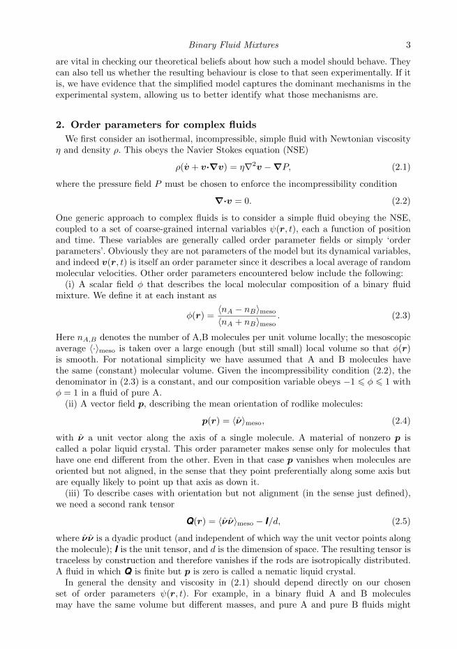
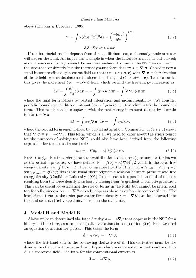
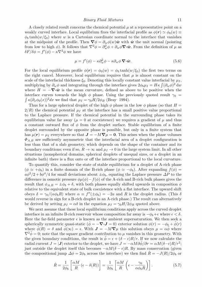
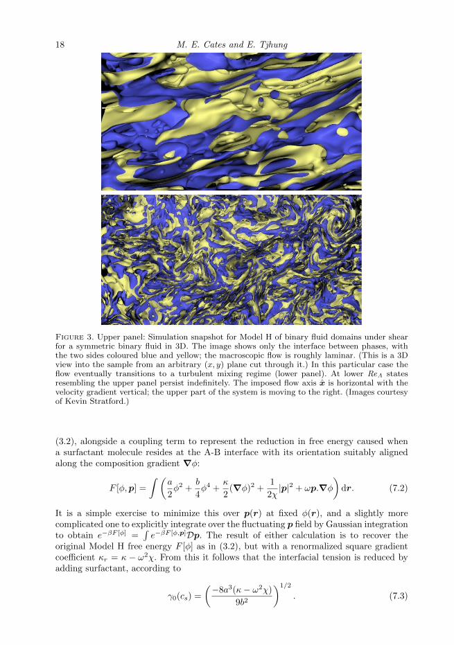
Gravity complicates matters, as does viscosity asymmetry (unavoidable in practice)between phases. However, relatively clean tests are possible via computer simulation(Stansell et al. 2006; Stratford et al. 2007). In 2D one finds data fitted by Lx/L0 ∼(ts/t0)2/3 and Ly/L0 ∼ (ts/t0)3/4 over a fairly wide range of length and timescales,most of which are however in the crossover region around x∗ (Stansell et al. 2006). Thefitted exponents change slightly if instead of the flow and gradient direction one usesthe principal axes of the distorted density patterns, but they remain unequal. Thereis no theory for these exponents as yet, but it is credible that the length-scales alongand across the stretched domains have different scalings with shear rate. (Indeed if thedynamics resembled stretching of droplets of fixed volume, the two exponents wouldadd to zero in 2D.) In 3D, where the simulations require very large computations, theinertial hydrodynamic (2/3 power) scaling has been observed within numerical error forall three length scales within the range of accessible domain-scale Reynolds numbers,defined as ReL ∼ ρL2/ηts, which lies between 200 and 2000 (Stratford et al. 2007).These measurements are however limited by the onset of a macroscopic instability toturbulent mixing at ReΛ ' 20, 000. Snapshots of the highly distorted domain structuresseen in computer simulations of sheared binary fluids are shown in figure 3.
The above simple arguments suggest that in both 2D and 3D, a nonequilibriumsteady state can be achieved in which the force balance in (4.3) is entirely betweenviscous and interfacial stresses, with the inertial terms negligible, as holds in the viscoushydrodynamic regime for the coarsening process. If so, this should be the situation atlow enough ReL, that is, large enough shear rate. Evidence that things are yet morecomplicated has been presented by Fielding (2008), who showed that if inertial termsare omitted altogether from (4.3), coarsening in two dimensions appears to proceedindefinitely. This suggests that a three-way balance of viscous, inertial and interfacialterms ultimately controls the formation of the nonequilibrium steady state.
7. Thermodynamic emulsification
Surfactant molecules, comprising small amphiphilic models with a polar or chargedhead group and an apolar tail, are well known to reduce the interfacial tension betweencoexisting phases of oil and water (as well as other pairs of apolar and polar fluids). Theygenerally have fast exchange kinetics between the interface and at least one bulk phase inwhich they are soluble; this means that the interface remains locally in equilibrium. Useof surfactants can thus be viewed as a thermodynamic route to the partial or completestabilization of interfacial structures. This is a separate effect from their role in creatinga kinetic barrier to coalescence discussed previously.
7.1. Interfacial tension in the presence of surfactant
Consider first a solution of surfactant molecules each carrying a unit vector νi denotingits head/tail orientation; local coarse graining creates a smooth field p(r) = 〈ν〉meso. Inthe absence of interfaces, this fluctuating mesoscopic field is zero on average, and itssmall (hence Gaussian) fluctuations are governed by a free energy contribution
Fs =
∫ (|p(r)|2
2χ
)dr. (7.1)
This is defined such that the variance of p is set by the ‘osmotic compressibility’ χ(µs)which is an increasing function of the surfactant chemical potential µs(cs), which is itselfa function of surfactant concentration cs. We can add this to the binary fluid free energy
18 M. E. Cates and E. Tjhung
Figure 3. Upper panel: Simulation snapshot for Model H of binary fluid domains under shearfor a symmetric binary fluid in 3D. The image shows only the interface between phases, withthe two sides coloured blue and yellow; the macroscopic flow is roughly laminar. (This is a 3Dview into the sample from an arbitrary (x, y) plane cut through it.) In this particular case theflow eventually transitions to a turbulent mixing regime (lower panel). At lower ReΛ statesresembling the upper panel persist indefinitely. The imposed flow axis x is horizontal with thevelocity gradient vertical; the upper part of the system is moving to the right. (Images courtesyof Kevin Stratford.)
(3.2), alongside a coupling term to represent the reduction in free energy caused whena surfactant molecule resides at the A-B interface with its orientation suitably alignedalong the composition gradient ∇φ:
F [φ,p] =
∫ (a
2φ2 +
b
4φ4 +
κ
2(∇φ)2 +
1
2χ|p|2 + ωp.∇φ
)dr. (7.2)
It is a simple exercise to minimize this over p(r) at fixed φ(r), and a slightly morecomplicated one to explicitly integrate over the fluctuating p field by Gaussian integrationto obtain e−βF [φ] =
∫e−βF [φ,p]Dp. The result of either calculation is to recover the
original Model H free energy F [φ] as in (3.2), but with a renormalized square gradientcoefficient κr = κ − ω2χ. From this it follows that the interfacial tension is reduced byadding surfactant, according to
γ0(cs) =
(−8a3(κ− ω2χ)
9b2
)1/2
. (7.3)
Binary Fluid Mixtures 19
This calculation is based on a Gaussian approximation (7.1) that assumes p(r) to deviateonly mildly from zero everywhere. It is not very realistic – for instance the interfacialwidth diverges as γ0 becomes small (whereas in practice this width is set by the size ofa surfactant molecule). However it captures the main physical effects of interest here;for a fuller discussion, see Gompper & Schick (1994). Note that the sign of ω, whichdetermines whether p points up or down the interfacial φ gradient, is irrelevant.
The simplest possible assumption is that the surfactant molecules form an idealsolution, with no interactions between them. In this case χ = χcs with χ a constant.(Linearity in cs of the variance parameter χ then follows from the Poisson statistics ofrandomly located and oriented molecules.) In this case the interfacial tension vanishes,with infinite slope, at cs = c = κ/ω2χ. But in fact, surfactant solutions are far from ideal,due to a phenomenon called ‘micellization’ in which individual molecules self-assembleinto micelles, which contain several tens of molecules. (Micelles are typically spherical;in water they have the polar heads at the exterior surface and the apolar tails in theinterior of the sphere. In oil this structure is reversed.)
The effect of micellization is to cause the surfactant chemical potential µs, and thereforeχ, to rapidly saturate above a so-called ‘critical micelle concentration’ cs = c∗. Anysurfactant added beyond this level becomes sequestered into micellar aggregates. Theconcentration c1 of ‘free’ molecules remains very close to c∗ at all higher concentrationsand, to a good approximation, χ saturates at χc∗, so that γ0(cs) does not fall further.For a more detailed discussion of micellization, see Safran (2003) or Cates (2012).
The outcome is to have two general classes of behaviour, depending on whether c∗
lies below or above c. In case 1, c∗ < c, so that γ0(cs) follows (7.3) so long as cs < c∗
but then abruptly stops decreasing as micellization intervenes. In case 2, c∗ > c so thatγ0(cs) hits zero before micelles are formed. At this point, if water and oil are both presentin bulk quantities, the system can minimize its free energy by creating a macroscopicamount of interface on which the surfactant can reside. When this happens µs againsaturates: adding further surfactant simply creates more surface at fixed µs. Hence γ0
does not become finitely negative but remains stuck at an effectively zero value. Thisanalysis is grossly simplified, ignoring (among other things) free energy contributionsfrom interfacial curvature which can allow interfaces to proliferate even for small positivetension. Nonetheless, the broad distinction between case 1 and case 2 is a useful one.
7.2. Finite tension: metastable emulsions and biliquid foams
Case 1 is the more common: the typical effect of surfactant is to reduce interfacialtension to half or a third of its previous value. The global free energy minimum thencomprises complete phase separation just as it does without surfactant; if emulsionsare formed (for instance by stirring) they are at most metastable. Since fluid-mediatedcoarsening is always present in bicontinuous states, metastability generally requires adroplet geometry; as already mentioned, surfactants can help prevent their coalescenceby inhibiting film rupture.
Typically such emulsions have spherical droplets (of A in B, say) but by evaporationor drainage under gravity, for instance in a centrifuge, much of the continuous B phasecan often be expelled to create a so-called biliquid foam (Bibette et al. 2002), in whichpolyhedral droplets of A (say) are separated by thin films of B. In many cases, biliquidfoams can persist for hours or days, and sometimes longer. To achieve this one mustsuppress not only the rupture of thin films but also the Ostwald process which, despitethe more complicated geometry, still drives diffusion of A from small (few-sided) tolarge (many-sided) polyhedral droplets (Weaire & Hutzler 1999). To achieve this witha trapped species requires an especially low level of solubility in the B phase so as to
20 M. E. Cates and E. Tjhung
ensure negligible diffusion even across the thin B films present in the foam structure.So long as they remain metastable against rupture and coarsening, biliquid foams, likesoap froths, are solid materials (generally amorphous, though ordered examples can bemade). As such they have an elastic modulus, and also a yield stress, both of which scaleas G ∼ γ0/R with R the mean droplet size. This is an interesting example of a solidbehaviour emerging solely from the spatial organization of locally fluid components – foreven the surfactant on the interface is (normally) a 2D fluid film.
7.3. Near-zero tension: stable microemulsions
In case 2, added surfactant can reduce γ0 to negligible levels for cs > c. This canlead to thermodynamically stable emulsions, generally called “microemulsions”, in whichenough A-B interface is created to accommodate all surplus surfactant, of which theconcentration is cs − c. There are two broad approaches to describing the resultingstructures. One avenue is to base a description on the φ,p order parameters alreadyintroduced, addressing (7.2) in the case where κr = κ− ω2χ so that the thermodynamicinterfacial tension is negative. Unsurprisingly, this model is unstable unless further termsare added to prevent interfacial proliferation; the most natural addition to F is a termin∫
(∇φ)4dr. The competition of this term with the effectively negative square gradientcoefficient κr sets a characteristic length scale for stable domains of A-rich and B-rich fluids. This approach leads to many insights (Gompper & Schick 1994) but ismainly appropriate for systems in which ‘weak’ surfactants (whose adsorption energyat an interface is not much larger than the thermal energy kBT ) are present at highconcentration so that the domain size L and interfacial width ξ are comparable. Thestructure of the microemulsion can then be viewed as a smooth spatial modulation ofcomposition φ(r) rather than a system of well separated, surfactant-coated interfaces.
For strong surfactants, which have small c, one can instead treat almost all thesurfactant as interfacial. The interfacial area S of the fluid film then obeys
SV
= (cs − c)Σ ' csΣ =φsvsΣ. (7.4)
Here Σ is a preferred area per molecule; φs is the volume fraction of surfactant and vsits molecular volume. For the soluble surfactants normally used for emulsification, thearea per molecule is maintained very close to Σ by rapid adsorption and desorption atthe interface; the specific interfacial area S/V is then fixed directly by φs via (7.4).
With interfacial tension negligible, the energetics of a given structure in case 2 isdetermined by the cost of bending the interfacial surfactant film at fixed area. We treatthis by a leading order harmonic expansion about a state of preferred curvature set bymolecular geometry. By a theorem of differential geometry (David 2004), at each pointon the A-B interface one can uniquely define two principal radii of curvature, R1, R2
which we take positive for curvature towards A. (For a spherical droplet of A of radiusR, we have R1 = R2 = R whereas for a cylinder of radius R, we have R1 = R andR2 =∞. A saddle shape has R1and R2 of opposite signs.) The harmonic bending energyfor a fluid film then reads
Fbend =
∫ [K
2
(1
R1+
1
R2− 2
R0
)2
+K
R1R2
]dS. (7.5)
There are 3 material parameters: the elastic constants K and K (both with dimensions ofenergy), and R0, a length defining the preferred radius of mean curvature, whose relationto the molecular geometry of surfactants is discussed by Safran (2003). The integral in
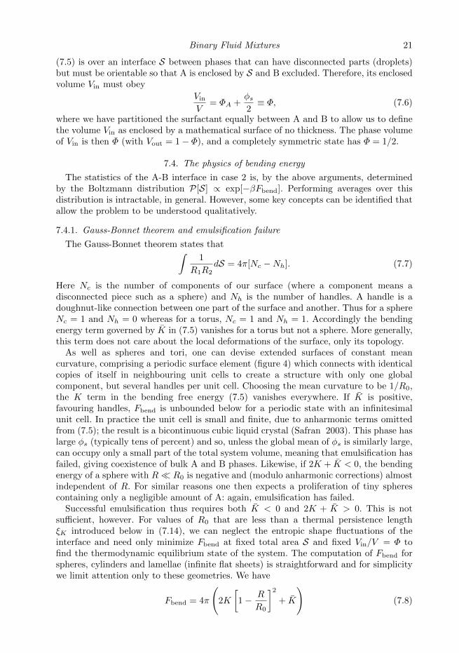
Binary Fluid Mixtures 21
(7.5) is over an interface S between phases that can have disconnected parts (droplets)but must be orientable so that A is enclosed by S and B excluded. Therefore, its enclosedvolume Vin must obey
Vin
V= ΦA +
φs2≡ Φ, (7.6)
where we have partitioned the surfactant equally between A and B to allow us to definethe volume Vin as enclosed by a mathematical surface of no thickness. The phase volumeof Vin is then Φ (with Vout = 1− Φ), and a completely symmetric state has Φ = 1/2.
7.4. The physics of bending energy
The statistics of the A-B interface in case 2 is, by the above arguments, determinedby the Boltzmann distribution P[S] ∝ exp[−βFbend]. Performing averages over thisdistribution is intractable, in general. However, some key concepts can be identified thatallow the problem to be understood qualitatively.
7.4.1. Gauss-Bonnet theorem and emulsification failure
The Gauss-Bonnet theorem states that∫1
R1R2dS = 4π[Nc −Nh]. (7.7)
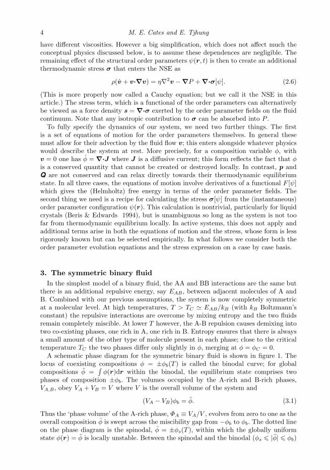
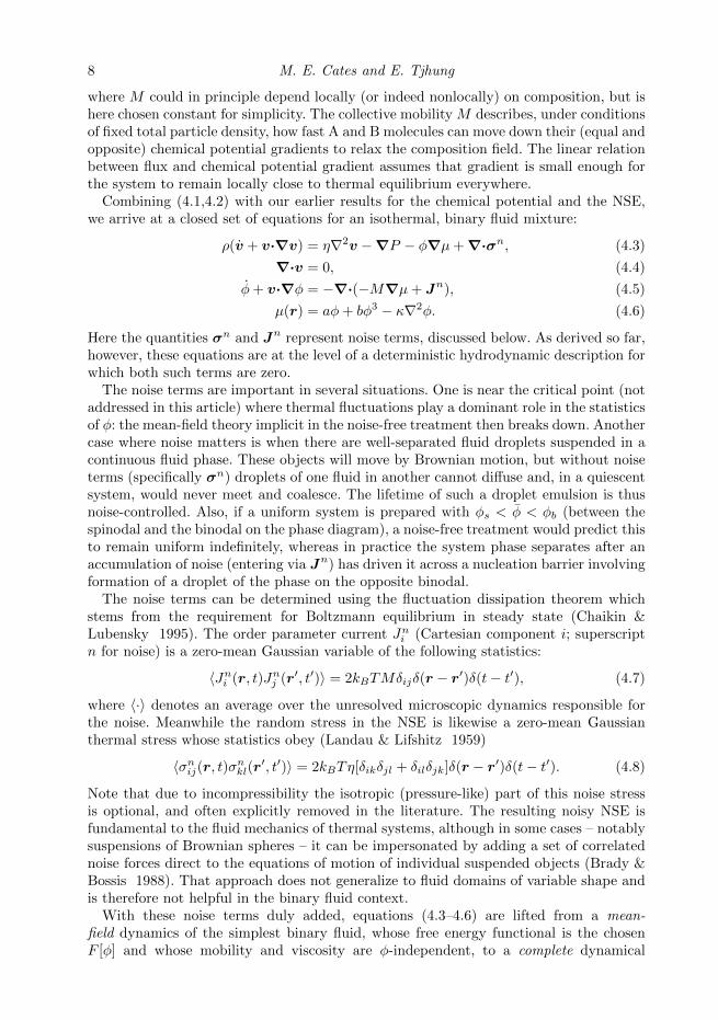
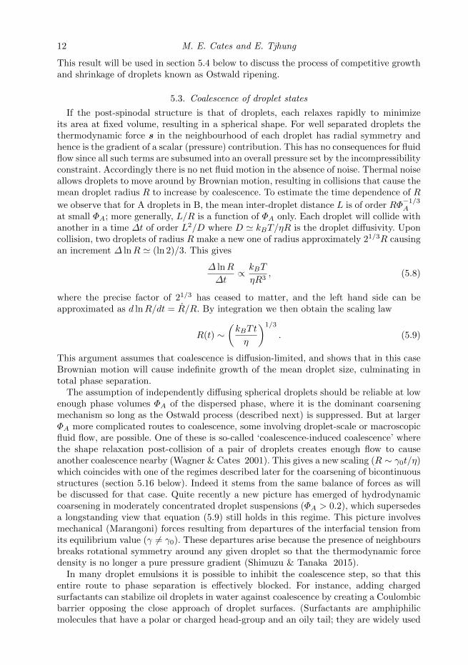
Here Nc is the number of components of our surface (where a component means adisconnected piece such as a sphere) and Nh is the number of handles. A handle is adoughnut-like connection between one part of the surface and another. Thus for a sphereNc = 1 and Nh = 0 whereas for a torus, Nc = 1 and Nh = 1. Accordingly the bendingenergy term governed by K in (7.5) vanishes for a torus but not a sphere. More generally,this term does not care about the local deformations of the surface, only its topology.
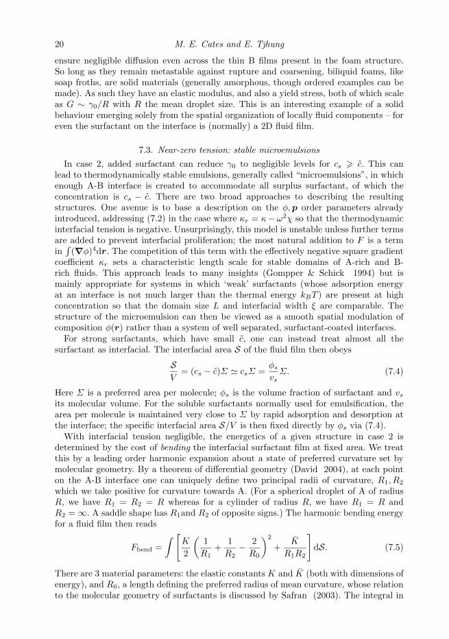
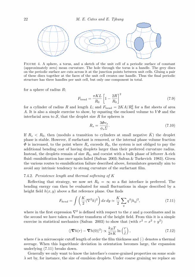
As well as spheres and tori, one can devise extended surfaces of constant meancurvature, comprising a periodic surface element (figure 4) which connects with identicalcopies of itself in neighbouring unit cells to create a structure with only one globalcomponent, but several handles per unit cell. Choosing the mean curvature to be 1/R0,the K term in the bending free energy (7.5) vanishes everywhere. If K is positive,favouring handles, Fbend is unbounded below for a periodic state with an infinitesimalunit cell. In practice the unit cell is small and finite, due to anharmonic terms omittedfrom (7.5); the result is a bicontinuous cubic liquid crystal (Safran 2003). This phase haslarge φs (typically tens of percent) and so, unless the global mean of φs is similarly large,can occupy only a small part of the total system volume, meaning that emulsification hasfailed, giving coexistence of bulk A and B phases. Likewise, if 2K + K < 0, the bendingenergy of a sphere with R R0 is negative and (modulo anharmonic corrections) almostindependent of R. For similar reasons one then expects a proliferation of tiny spherescontaining only a negligible amount of A: again, emulsification has failed.
Successful emulsification thus requires both K < 0 and 2K + K > 0. This is notsufficient, however. For values of R0 that are less than a thermal persistence lengthξK introduced below in (7.14), we can neglect the entropic shape fluctuations of theinterface and need only minimize Fbend at fixed total area S and fixed Vin/V = Φ tofind the thermodynamic equilibrium state of the system. The computation of Fbend forspheres, cylinders and lamellae (infinite flat sheets) is straightforward and for simplicitywe limit attention only to these geometries. We have
Fbend = 4π
(2K
[1− R
R0
]2
+ K
)(7.8)
22 M. E. Cates and E. Tjhung
Figure 4. A sphere, a torus, and a sketch of the unit cell of a periodic surface of constant(approximately zero) mean curvature. The hole through the torus is a handle. The grey discson the periodic surface are cuts across it at the junction points between unit cells. Gluing a pairof these discs together at the faces of the unit cell creates one handle. Thus the final periodicstructure has three handles per unit cell, but only one component in total.
for a sphere of radius R;
Fbend =πKL
R0
[1− 2R
R0
]2
(7.9)
for a cylinder of radius R and length L; and Fbend = 2KA/R20 for a flat sheets of area
A. It is also a simple exercise to show, by equating the enclosed volume to V Φ and theinterfacial area to S, that the droplet size R for spheres is
Rs =3ΦvsφsΣ
. (7.10)
If Rs < R0, then (modulo a transition to cylinders at small negative K) the dropletphase is stable. However, if surfactant is removed, or the internal phase volume fractionΦ is increased, to the point where Rs exceeds R0, the system is not obliged to pay theadditional bending cost of having droplets larger than their preferred curvature radius.Instead, the droplets remain of size R0, and coexist with a bulk phase of leftover A-richfluid: emulsification has once again failed (Safran 2003; Safran & Turkevich 1983). Giventhe various routes to emulsification failure described above, formulators generally aim toavoid any intrinsic tendency to strong curvature of the surfactant film.
7.4.2. Persistence length and thermal softening of K
Reflecting that strategy, we now set R0 = ∞ so a flat interface is preferred. Thebending energy can then be evaluated for small fluctuations in shape described by aheight field h(x, y) above a flat reference plane. One finds
Fbend =
∫ (K
2(∇2h)2
)dx dy ' K
2
∑q
q4|hq|2, (7.11)
where in the first expression ∇2 is defined with respect to the x and y coordinates and inthe second we have taken a Fourier transform of the height field. From this it is a simpleexercise in statistical mechanics (Safran 2003) to show that (with r2 = x2 + y2)
〈|∇h(r)−∇h(0)|2〉 ∝ kBT
2πKln(r`
), (7.12)
where ` is a microscopic cutoff length of order the film thickness and 〈·〉 denotes a thermalaverage. When this logarithmic deviation in orientation becomes large, the expansionunderlying (7.11) breaks down.
Generally we only want to know the interface’s coarse-grained properties on some scaleλ set by, for instance, the size of emulsion droplets. Under coarse graining we replace an
Binary Fluid Mixtures 23
entropically wiggly interface by a smooth one on the scale λ. By carefully integrating outthe thermal undulations, one can show (David 2004) that their perturbative effect is tosoften the elastic constant:
Keff(λ) = K − 3kBT
4πln
(λ
`
). (7.13)
Thus there is very little resistance to bending at scales beyond a ‘persistence length’
ξK ' ` exp
[4πK
3kBT
]. (7.14)
Note that ξK is exponentially dependent on K: for ` = 1 nm, ξK ' 1µm when K =1.65kBT . For K = 3kBT , we already have ξk > 300µm; and ξK is irrelevantly large, forour purposes, once K is much larger than this.
7.5. Bicontinuous microemulsions
In so-called ‘balanced’ microemulsions, the spontaneous curvature is tuned to be small,so that R0 ξK . For simplicity we set R0 → ∞ as above. We also assume ` ξK 100µm, so that the entropy of the interface (including the renormalization of K) cannotbe ignored. Assuming Φ of order 0.5 (roughly symmetric amounts of A- and B-rich fluid)we can introduce a structural length scale λ which is then set by φs. Specifically for alamellar phase, comprising a 1D stack of alternating layers of A and B with relativelyflat interfaces between these, one has a layer spacing λ between adjacent surfactant filmsset by φs ' `
λ+` . When λ ' ` the system has no option but to fill space with flat parallellayers. As φs is reduced (λ raised) the layer spacing λ becomes comparable to ξK . Forλ/ξK 6 1/3 (or so), the lamellar phase fluctuates but remains stable.
On the other hand, if φs is then decreased further so that λ ' ξK , these layers meltinto an isotropic phase comprising (for Φ ' 0.5) bicontinuous domains of A and Bfluids separated by a fluctuating surfactant film. This is the bicontinuous microemulsionand effectively represents a thermodynamic route to prevent coarsening of the transientbicontinuous structures encountered in section 5 above. If Φ now deviates strongly from0.5, then (just as found there) the structure depercolates, forming a droplet phase. Thisdiffers from the one discussed above for R0 ξK , since this one is stabilized by entropyand fluctuations, not by a preferred curvature of the droplets. Theories of the bicontinousmicroemulsion were initiated by de Gennes & Taupin (1982). Some of these theories usecoarse grained lattice models in which fluid domains are placed at random on a lattice ofsome scale ξ; the bending energy and area of the resulting interface can be estimated andused to calculate a phase diagram (Andelman et al. 1987). One specific feature is theappearance of three-phase coexistence in which a ‘middle phase’ microemulsion coexistswith excess phases of both oil and water: this roughly corresponds to a ‘double-sided’emulsification failure in which both oil and water are expelled.
7.6. The sponge phase and vesicles
Closely related to the bicontinuous microemulsion is the ‘sponge phase’. This ariseswhen there is a huge phase volume aysmmetry between A-rich and B-rich fluids, butonly in case-2 systems where the surfactant has a molecular preference to form a flatfilm rather than highly curved structures such as micelles. The interfacial structure thatforms spontaneously at cs = c is, in the almost complete absence of B, necessarily nowa bilayer with A (usually water) on both sides and a thin B layer in the middle. Thelamellar state now consists of flattish bilayers alternating with A domains; for smallvolume fractions of bilayer such that their separation exceeds their persistence length,
24 M. E. Cates and E. Tjhung
this structure melts, just as described above for the microemulsion. The result is subtlydifferent though: we now have a bilayer film that separates two randomly interpenetratingdomains containing the same solvent A. This is called the ‘sponge phase’. It is not directlyuseful for A/B emulsification, since the minority B phase has negligible phase volume.However, the sponge phase does have remarkable phase transitions associated with the‘in-out’ symmetry between the two A domains, which can be broken spontaneously (Huse& Leibler 1988; Roux et al. 1992). When the symmetry is strongly broken, one hasdiscrete droplets of A separated from a continuous A phase by a bilayer. This can beviewed as a thermodynamically stabilized A-in-A emulsion (typically water-in-water),which can be useful for encapsulation. Such structures, called vesicles, can also exist inthe complete absence of B, so that the bilayer contains only surfactant.
Similar vesicles can also be formed from lipids, which are biological molecules closelyrelated to surfactants. The main difference is that for lipids c is extremely small comparedto typical values for surfactants. This renders them effectively insoluble in water, sinceany attempt to increase cs above this small value leads instead to the creation ofmore interface on which the lipid resides (typically organized as a lamellar phase). Thisinsolubility means that although in local equilibrium γ0 is effectively zero, there is norapid equilibration of the surface area per molecule Σ by molecular exchange betweeninterface and bulk. As a result, if a lipid vesicle is mechanically stretched a tensionsoon develops. Such tension can also arise by swelling the vesicle to an inflated sphericalshape rather than a relaxed, floppy shape of lesser volume. Only in the absence of suchstretching can a lipid bilayer can be described by the bending free energy (7.5) in whichtypically R0 =∞ because there is no preferred curvature by symmetry; in this case thereare large shape fluctuations so long as K/kBT is not large. The spontaneous curvatureradius R0 can however be finite if the composition of the lipid bilayer is different onits two faces. This is common in biology where a bilayer of mixed lipids separates theinterior and exterior of a cell. Note that, because of their insoluble character, the globaldistribution of lipids to form vesicles is almost never in equilibrium: the size of eachvesicle is set by the amount of lipid present at its surface, not by thermodynamics.
8. Particle-stabilized emulsions
A typical soluble surfactant has an energy of attachment to the A-B (oil-water)interface of between 5kBT and 15kBT . This is high enough to alter interfacial propertiesbut low enough to maintain local equilibrium by exchange of molecules with one orboth bulk phases. Larger amphiphilic species range from lipids as just discussed, viadiblock copolymers (in which two polymer chains of different chemistry are covalentlybonded together) and globular proteins, to colloidal ‘Janus beads’. The latter are colloidalspheres, up to a micron in size, with surface chemistry that favours water on onehemisphere and oil on the other. For typical solid-fluid interfacial tensions (' 0.01Nm−2) Janus beads have attachment energies of order 107kBT or larger. Such speciesare adsorbed irreversibly at the A-B interface, in the sense that Brownian motion alonewill almost never lead to detachment.
8.1. Colloidal particles at fluid-fluid interfaces
Although Janus beads are often studied (Lattuada & Hatton 2011), they are rarelyused for emulsion stabilization, because it is much cheaper to use ordinary colloidalspheres of homogeneous surface chemistry. Perhaps surprisingly, so long as the colloidhas roughly equal affinity to the two fluids A and B, interfacial attachment energiesremain vastly larger than kBT . The simplest case is when the two solid–fluid interfacial
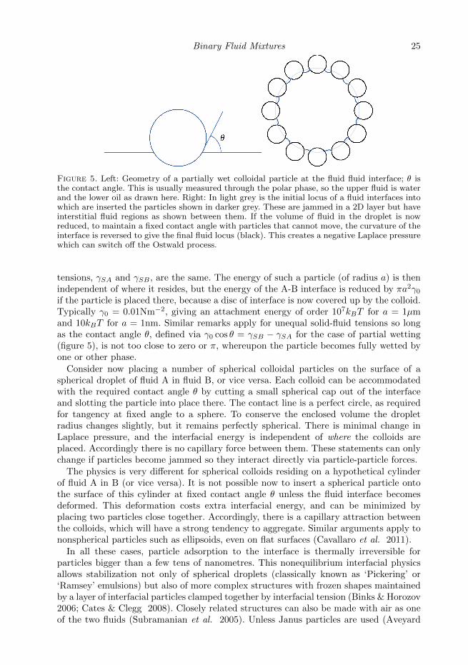
Binary Fluid Mixtures 25
Figure 5. Left: Geometry of a partially wet colloidal particle at the fluid fluid interface; θ isthe contact angle. This is usually measured through the polar phase, so the upper fluid is waterand the lower oil as drawn here. Right: In light grey is the initial locus of a fluid interfaces intowhich are inserted the particles shown in darker grey. These are jammed in a 2D layer but haveinterstitial fluid regions as shown between them. If the volume of fluid in the droplet is nowreduced, to maintain a fixed contact angle with particles that cannot move, the curvature of theinterface is reversed to give the final fluid locus (black). This creates a negative Laplace pressurewhich can switch off the Ostwald process.
tensions, γSA and γSB , are the same. The energy of such a particle (of radius a) is thenindependent of where it resides, but the energy of the A-B interface is reduced by πa2γ0
if the particle is placed there, because a disc of interface is now covered up by the colloid.Typically γ0 = 0.01Nm−2, giving an attachment energy of order 107kBT for a = 1µmand 10kBT for a = 1nm. Similar remarks apply for unequal solid-fluid tensions so longas the contact angle θ, defined via γ0 cos θ = γSB − γSA for the case of partial wetting(figure 5), is not too close to zero or π, whereupon the particle becomes fully wetted byone or other phase.
Consider now placing a number of spherical colloidal particles on the surface of aspherical droplet of fluid A in fluid B, or vice versa. Each colloid can be accommodatedwith the required contact angle θ by cutting a small spherical cap out of the interfaceand slotting the particle into place there. The contact line is a perfect circle, as requiredfor tangency at fixed angle to a sphere. To conserve the enclosed volume the dropletradius changes slightly, but it remains perfectly spherical. There is minimal change inLaplace pressure, and the interfacial energy is independent of where the colloids areplaced. Accordingly there is no capillary force between them. These statements can onlychange if particles become jammed so they interact directly via particle-particle forces.
The physics is very different for spherical colloids residing on a hypothetical cylinderof fluid A in B (or vice versa). It is not possible now to insert a spherical particle ontothe surface of this cylinder at fixed contact angle θ unless the fluid interface becomesdeformed. This deformation costs extra interfacial energy, and can be minimized byplacing two particles close together. Accordingly, there is a capillary attraction betweenthe colloids, which will have a strong tendency to aggregate. Similar arguments apply tononspherical particles such as ellipsoids, even on flat surfaces (Cavallaro et al. 2011).
In all these cases, particle adsorption to the interface is thermally irreversible forparticles bigger than a few tens of nanometres. This nonequilibrium interfacial physicsallows stabilization not only of spherical droplets (classically known as ‘Pickering’ or‘Ramsey’ emulsions) but also of more complex structures with frozen shapes maintainedby a layer of interfacial particles clamped together by interfacial tension (Binks & Horozov2006; Cates & Clegg 2008). Closely related structures can also be made with air as oneof the two fluids (Subramanian et al. 2005). Unless Janus particles are used (Aveyard
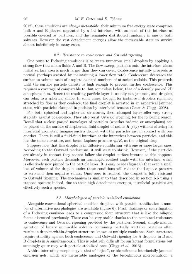
26 M. E. Cates and E. Tjhung
2012), these emulsions are always metastable: their minimum free energy state comprisesbulk A and B phases, separated by a flat interface, with as much of this interface aspossible covered by particles, and the remainder distributed randomly in one or bothsolvents. However the vast detachment energies allow the metastable state to survivealmost indefinitely in many cases.
8.2. Resistance to coalescence and Ostwald ripening
One route to Pickering emulsions is to create numerous small droplets by applying astrong flow that mixes fluids A and B. The flow sweeps particles onto the interface whoseinitial surface area is much larger than they can cover. Coalescence initially proceeds asnormal (perhaps assisted by maintaining a lower flow rate). Coalescence decreases thesurface-to-volume ratio of droplets at fixed numbers of attached colloids. This proceedsuntil the surface particle density is high enough to prevent further coalescence. Thisrequires a coverage of comparable to, but somewhat below, that of a densely packed 2Damorphous film. Hence the resulting particle layer is usually not jammed, and dropletscan relax to a spherical shape. In some cases, though, for instance if droplets remainedstretched by flow as they coalesce, the final droplet is arrested in an aspherical jammedstate, with particles clamped in position by interfacial tension (Cates & Clegg 2008).
For both spherical and aspherical structures, these clamped layers offer very strongstability against coalescence. They also resist Ostwald ripening, for the following reason.Recall that a close packed monolayer of particles (whether ordered or amorphous) canbe placed on the surface of a spherical fluid droplet of radius R (say) without altering itsinterfacial geometry. Imagine such a droplet with the particles just in contact with oneanother. There is still a fluid-fluid interface at the interstices between particles, and thishas the same curvature, and hence Laplace pressure γ0/R, as the original drop.
Suppose now that this droplet is in diffusive equilibrium with one or more larger ones.According to the Ostwald mechanism, it will start to shrink. However, if the particlesare already in contact they cannot follow the droplet surface inwards as this happens.Moreover, each particle demands an unchanged contact angle with the interface, whichis effectively now pinned to the particle layer. It is easy to see (figure 5) that even a smallloss of volume of the droplet under these conditions will reduce the Laplace pressureto zero and then negative values. Once zero is reached, the droplet is fully resistantto Ostwald ripening. The mechanism is similar to that described in section 5.5 using atrapped species; indeed, due to their high detachment energies, interfacial particles areeffectively such a species.
8.3. Morphologies of particle-stabilized emulsions
Alongside conventional spherical emulsion droplets, with particle stabilization a num-ber of alternative morphologies are available (figure 6). First, drainage or centrifugationof a Pickering emulsion leads to a compressed foam structure that is like the biliquidfoams discussed previously. These can be very stable thanks to the combined resistanceto coalescence and Ostwald ripening provided by the particles. Second, simple manualagitation of binary immiscible solvents containing partially wettable particles oftenresults in droplet-within-droplet structures known as multiple emulsions. Such structuresrequire stability against both coalescence and Ostwald ripening for A droplets in B andB droplets in A simultaneously. This is relatively difficult for surfactant formulations butseemingly quite easy with particle-stabilized ones (Clegg et al. 2016).
A third interesting morphology is that of “bijels”, or bicontinuous interfacially jammedemulsion gels, which are metastable analogues of the bicontinuous microemulsion: a
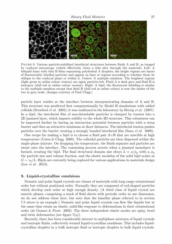
Binary Fluid Mixtures 27
Figure 6. Various particle-stabilized interfacial structures between fluids A and B, as imagedby confocal microscopy (which effectively views a thin slice through the material). Left: Abiliquid foam with thin B films separating polyhedral A droplets; the bright regions are layersof fluorescently labelled particles and appear as lines or regions according to whether these lieoblique to the confocal plane or within it. Centre: A multiple emulsion. The brightest regions(light green in online colour version) are again particle-rich. Fluid A is dark grey and fluid B ismid-grey (dull red in online colour version). Right: A bijel; the fluorescent labelling is similarto the multiple emulsion except that fluid B (dull red in online colour) is now the darker of thetwo in grey scale. (Images courtesy of Paul Clegg.)
particle layer resides at the interface between interpenetrating domains of A and B.This structure was predicted first computationally by Model H simulations with addedcolloids (Stratford et al. 2005); it was confirmed in the laboratory by Herzig et al. (2007).In a bijel, the interfacial film of non-detachable particles is clamped by tension into a2D jammed layer, which imparts solidity to the whole 3D structure. This robustness canbe improved further by having an interaction potential between particles with a steepbarrier and then an attractive minimum at short distances. The interfacial tension pushesparticles over the barrier creating a strongly bonded interfacial film (Sanz et al. 2009).
One recipe for making a bijel is to choose a fluid pair A+B that are miscible at hightemperature (Cates & Clegg 2008). The colloidal particles are then dispersed within thesingle-phase mixture. On dropping the temperature, the fluids separate and particles areswept onto the interface. The coarsening process arrests when a jammed monolayer isformed, creating the bijel. The final structural domain size obeys L ' a/φp with a, φpthe particle size and volume fraction, and the elastic modulus of the solid bijel scales asG ∼ γ0/L. Bijels are currently being explored for various applications in materials design(Lee et al. 2013).
9. Liquid-crystalline emulsions
Nematic and polar liquid crystals are classes of materials with long range orientationalorder but without positional order. Normally they are composed of rod-shaped particleswhich develop such order at high enough density. (A third class of liquid crystal aresmectic phases, comprising a stack of fluid sheets with periodic order in one dimension;we do not address these here, but note that the lamellar phase referred to in section7.5 above is an example.) Nematic and polar liquid crystals can flow like liquids but atthe same time retain an elastic, solid-like response to deformations in their orientationalorder (de Gennes & Prost 2002). The three independent elastic modes are splay, bendand twist deformation (see figure 7(a)).
Recently, there has been considerable interest in multiphase mixtures of liquid crystalsand isotropic fluids, collectively termed liquid-crystalline emulsions. This includes liquid-crystalline droplets in a bulk isotropic fluid or isotropic droplets in bulk liquid crystals.
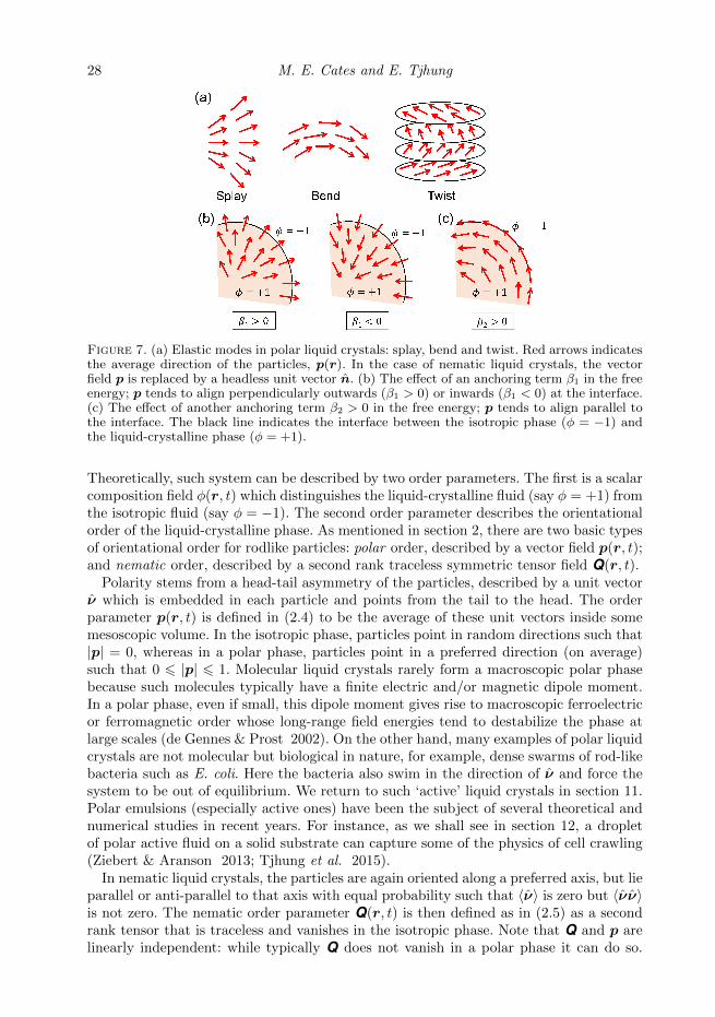
28 M. E. Cates and E. Tjhung
Figure 7. (a) Elastic modes in polar liquid crystals: splay, bend and twist. Red arrows indicatesthe average direction of the particles, p(r). In the case of nematic liquid crystals, the vectorfield p is replaced by a headless unit vector n. (b) The effect of an anchoring term β1 in the freeenergy; p tends to align perpendicularly outwards (β1 > 0) or inwards (β1 < 0) at the interface.(c) The effect of another anchoring term β2 > 0 in the free energy; p tends to align parallel tothe interface. The black line indicates the interface between the isotropic phase (φ = −1) andthe liquid-crystalline phase (φ = +1).
Theoretically, such system can be described by two order parameters. The first is a scalarcomposition field φ(r, t) which distinguishes the liquid-crystalline fluid (say φ = +1) fromthe isotropic fluid (say φ = −1). The second order parameter describes the orientationalorder of the liquid-crystalline phase. As mentioned in section 2, there are two basic typesof orientational order for rodlike particles: polar order, described by a vector field p(r, t);and nematic order, described by a second rank traceless symmetric tensor field Q(r, t).
Polarity stems from a head-tail asymmetry of the particles, described by a unit vectorν which is embedded in each particle and points from the tail to the head. The orderparameter p(r, t) is defined in (2.4) to be the average of these unit vectors inside somemesoscopic volume. In the isotropic phase, particles point in random directions such that|p| = 0, whereas in a polar phase, particles point in a preferred direction (on average)such that 0 6 |p| 6 1. Molecular liquid crystals rarely form a macroscopic polar phasebecause such molecules typically have a finite electric and/or magnetic dipole moment.In a polar phase, even if small, this dipole moment gives rise to macroscopic ferroelectricor ferromagnetic order whose long-range field energies tend to destabilize the phase atlarge scales (de Gennes & Prost 2002). On the other hand, many examples of polar liquidcrystals are not molecular but biological in nature, for example, dense swarms of rod-likebacteria such as E. coli. Here the bacteria also swim in the direction of ν and force thesystem to be out of equilibrium. We return to such ‘active’ liquid crystals in section 11.Polar emulsions (especially active ones) have been the subject of several theoretical andnumerical studies in recent years. For instance, as we shall see in section 12, a dropletof polar active fluid on a solid substrate can capture some of the physics of cell crawling(Ziebert & Aranson 2013; Tjhung et al. 2015).
In nematic liquid crystals, the particles are again oriented along a preferred axis, but lieparallel or anti-parallel to that axis with equal probability such that 〈ν〉 is zero but 〈νν〉is not zero. The nematic order parameter Q(r, t) is then defined as in (2.5) as a secondrank tensor that is traceless and vanishes in the isotropic phase. Note that Q and p arelinearly independent: while typically Q does not vanish in a polar phase it can do so.
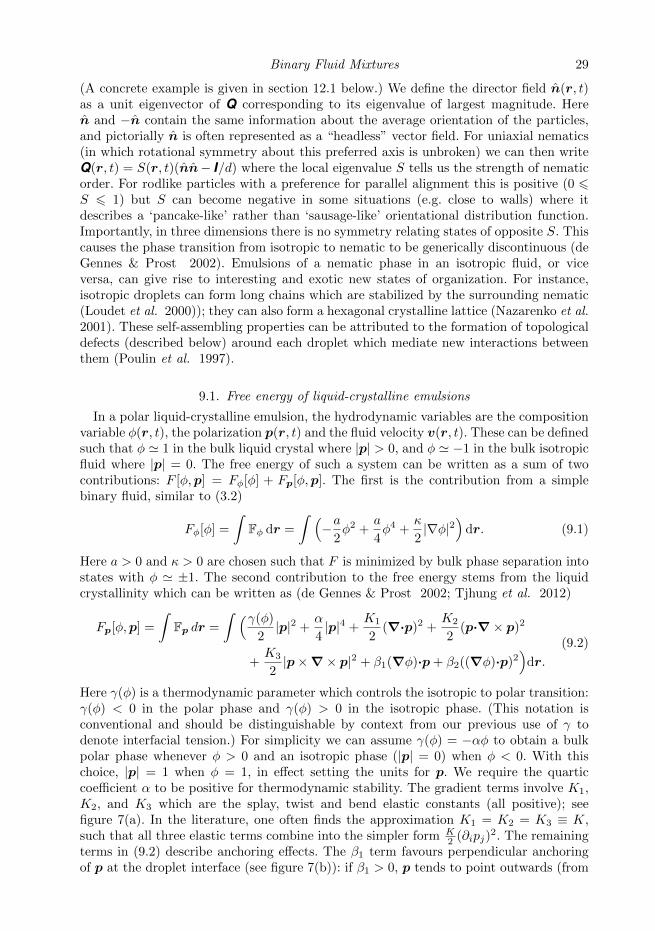
Binary Fluid Mixtures 29
(A concrete example is given in section 12.1 below.) We define the director field n(r, t)as a unit eigenvector of Q corresponding to its eigenvalue of largest magnitude. Heren and −n contain the same information about the average orientation of the particles,and pictorially n is often represented as a “headless” vector field. For uniaxial nematics(in which rotational symmetry about this preferred axis is unbroken) we can then writeQ(r, t) = S(r, t)(nn− I/d) where the local eigenvalue S tells us the strength of nematicorder. For rodlike particles with a preference for parallel alignment this is positive (0 6S 6 1) but S can become negative in some situations (e.g. close to walls) where itdescribes a ‘pancake-like’ rather than ‘sausage-like’ orientational distribution function.Importantly, in three dimensions there is no symmetry relating states of opposite S. Thiscauses the phase transition from isotropic to nematic to be generically discontinuous (deGennes & Prost 2002). Emulsions of a nematic phase in an isotropic fluid, or viceversa, can give rise to interesting and exotic new states of organization. For instance,isotropic droplets can form long chains which are stabilized by the surrounding nematic(Loudet et al. 2000)); they can also form a hexagonal crystalline lattice (Nazarenko et al.2001). These self-assembling properties can be attributed to the formation of topologicaldefects (described below) around each droplet which mediate new interactions betweenthem (Poulin et al. 1997).
9.1. Free energy of liquid-crystalline emulsions
In a polar liquid-crystalline emulsion, the hydrodynamic variables are the compositionvariable φ(r, t), the polarization p(r, t) and the fluid velocity v(r, t). These can be definedsuch that φ ' 1 in the bulk liquid crystal where |p| > 0, and φ ' −1 in the bulk isotropicfluid where |p| = 0. The free energy of such a system can be written as a sum of twocontributions: F [φ,p] = Fφ[φ] + Fp[φ,p]. The first is the contribution from a simplebinary fluid, similar to (3.2)
Fφ[φ] =
∫Fφ dr =
∫ (−a
2φ2 +
a
4φ4 +
κ
2|∇φ|2
)dr. (9.1)
Here a > 0 and κ > 0 are chosen such that F is minimized by bulk phase separation intostates with φ ' ±1. The second contribution to the free energy stems from the liquidcrystallinity which can be written as (de Gennes & Prost 2002; Tjhung et al. 2012)
Fp[φ,p] =
∫Fp dr =
∫ (γ(φ)
2|p|2 +
α
4|p|4 +
K1
2(∇·p)2 +
K2
2(p·∇× p)2
+K3
2|p×∇× p|2 + β1(∇φ)·p+ β2((∇φ)·p)2
)dr.
(9.2)
Here γ(φ) is a thermodynamic parameter which controls the isotropic to polar transition:γ(φ) < 0 in the polar phase and γ(φ) > 0 in the isotropic phase. (This notation isconventional and should be distinguishable by context from our previous use of γ todenote interfacial tension.) For simplicity we can assume γ(φ) = −αφ to obtain a bulkpolar phase whenever φ > 0 and an isotropic phase (|p| = 0) when φ < 0. With thischoice, |p| = 1 when φ = 1, in effect setting the units for p. We require the quarticcoefficient α to be positive for thermodynamic stability. The gradient terms involve K1,K2, and K3 which are the splay, twist and bend elastic constants (all positive); seefigure 7(a). In the literature, one often finds the approximation K1 = K2 = K3 ≡ K,such that all three elastic terms combine into the simpler form K
2 (∂ipj)2. The remaining
terms in (9.2) describe anchoring effects. The β1 term favours perpendicular anchoringof p at the droplet interface (see figure 7(b)): if β1 > 0, p tends to point outwards (from
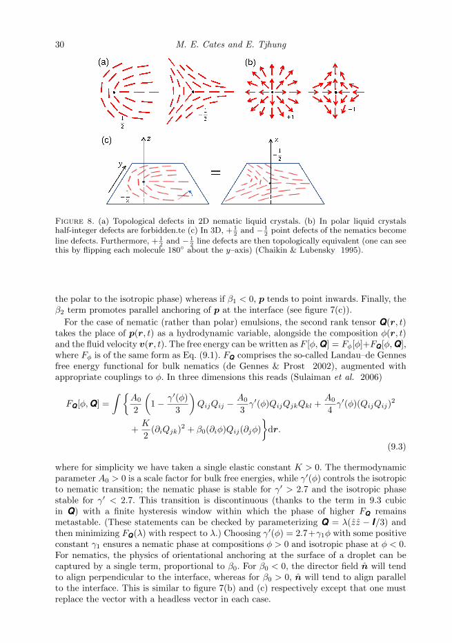
30 M. E. Cates and E. Tjhung
Figure 8. (a) Topological defects in 2D nematic liquid crystals. (b) In polar liquid crystalshalf-integer defects are forbidden.te (c) In 3D, + 1
2and − 1
2point defects of the nematics become
line defects. Furthermore, + 12
and − 12
line defects are then topologically equivalent (one can seethis by flipping each molecule 180 about the y–axis) (Chaikin & Lubensky 1995).
the polar to the isotropic phase) whereas if β1 < 0, p tends to point inwards. Finally, theβ2 term promotes parallel anchoring of p at the interface (see figure 7(c)).
For the case of nematic (rather than polar) emulsions, the second rank tensor Q(r, t)takes the place of p(r, t) as a hydrodynamic variable, alongside the composition φ(r, t)and the fluid velocity v(r, t). The free energy can be written as F [φ,Q] = Fφ[φ]+FQ[φ,Q],where Fφ is of the same form as Eq. (9.1). FQ comprises the so-called Landau–de Gennesfree energy functional for bulk nematics (de Gennes & Prost 2002), augmented withappropriate couplings to φ. In three dimensions this reads (Sulaiman et al. 2006)
FQ[φ,Q] =
∫ A0
2
(1− γ′(φ)
3
)QijQij −
A0
3γ′(φ)QijQjkQkl +
A0
4γ′(φ)(QijQij)
2
+K
2(∂iQjk)2 + β0(∂iφ)Qij(∂jφ)
dr.
(9.3)
where for simplicity we have taken a single elastic constant K > 0. The thermodynamicparameter A0 > 0 is a scale factor for bulk free energies, while γ′(φ) controls the isotropicto nematic transition; the nematic phase is stable for γ′ > 2.7 and the isotropic phasestable for γ′ < 2.7. This transition is discontinuous (thanks to the term in 9.3 cubicin Q) with a finite hysteresis window within which the phase of higher FQ remainsmetastable. (These statements can be checked by parameterizing Q = λ(zz − I/3) andthen minimizing FQ(λ) with respect to λ.) Choosing γ′(φ) = 2.7+γ1φ with some positiveconstant γ1 ensures a nematic phase at compositions φ > 0 and isotropic phase at φ < 0.For nematics, the physics of orientational anchoring at the surface of a droplet can becaptured by a single term, proportional to β0. For β0 < 0, the director field n will tendto align perpendicular to the interface, whereas for β0 > 0, n will tend to align parallelto the interface. This is similar to figure 7(b) and (c) respectively except that one mustreplace the vector with a headless vector in each case.
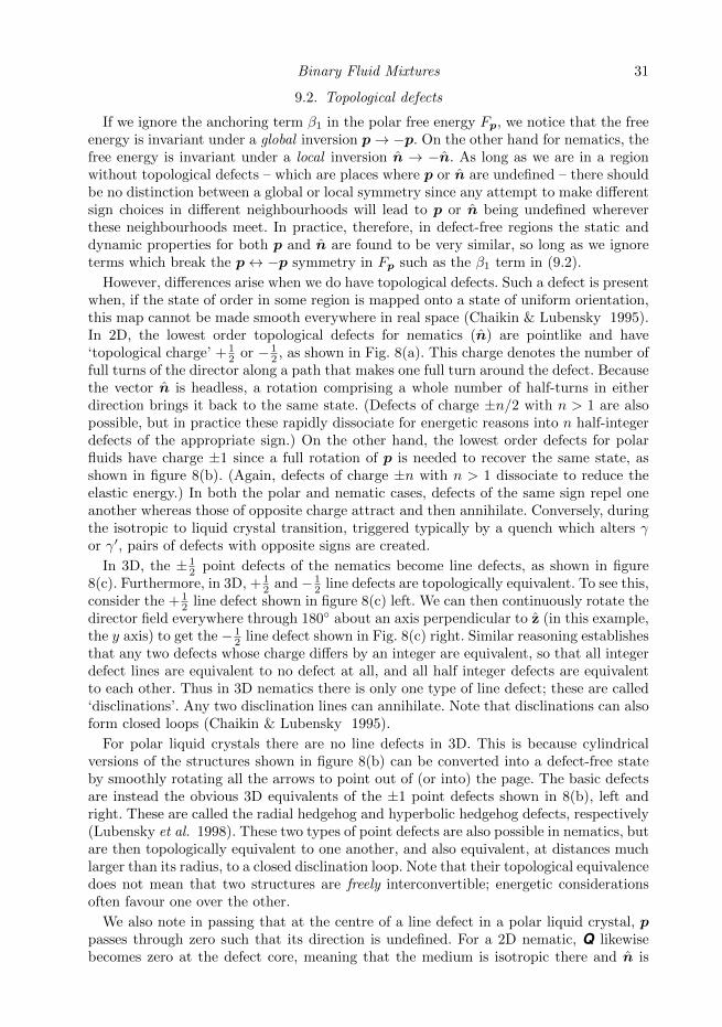
Binary Fluid Mixtures 31
9.2. Topological defects
If we ignore the anchoring term β1 in the polar free energy Fp, we notice that the freeenergy is invariant under a global inversion p→ −p. On the other hand for nematics, thefree energy is invariant under a local inversion n → −n. As long as we are in a regionwithout topological defects – which are places where p or n are undefined – there shouldbe no distinction between a global or local symmetry since any attempt to make differentsign choices in different neighbourhoods will lead to p or n being undefined whereverthese neighbourhoods meet. In practice, therefore, in defect-free regions the static anddynamic properties for both p and n are found to be very similar, so long as we ignoreterms which break the p↔ −p symmetry in Fp such as the β1 term in (9.2).
However, differences arise when we do have topological defects. Such a defect is presentwhen, if the state of order in some region is mapped onto a state of uniform orientation,this map cannot be made smooth everywhere in real space (Chaikin & Lubensky 1995).In 2D, the lowest order topological defects for nematics (n) are pointlike and have‘topological charge’ + 1
2 or − 12 , as shown in Fig. 8(a). This charge denotes the number of
full turns of the director along a path that makes one full turn around the defect. Becausethe vector n is headless, a rotation comprising a whole number of half-turns in eitherdirection brings it back to the same state. (Defects of charge ±n/2 with n > 1 are alsopossible, but in practice these rapidly dissociate for energetic reasons into n half-integerdefects of the appropriate sign.) On the other hand, the lowest order defects for polarfluids have charge ±1 since a full rotation of p is needed to recover the same state, asshown in figure 8(b). (Again, defects of charge ±n with n > 1 dissociate to reduce theelastic energy.) In both the polar and nematic cases, defects of the same sign repel oneanother whereas those of opposite charge attract and then annihilate. Conversely, duringthe isotropic to liquid crystal transition, triggered typically by a quench which alters γor γ′, pairs of defects with opposite signs are created.
In 3D, the ± 12 point defects of the nematics become line defects, as shown in figure
8(c). Furthermore, in 3D, + 12 and − 1
2 line defects are topologically equivalent. To see this,consider the + 1
2 line defect shown in figure 8(c) left. We can then continuously rotate thedirector field everywhere through 180 about an axis perpendicular to z (in this example,the y axis) to get the − 1
2 line defect shown in Fig. 8(c) right. Similar reasoning establishesthat any two defects whose charge differs by an integer are equivalent, so that all integerdefect lines are equivalent to no defect at all, and all half integer defects are equivalentto each other. Thus in 3D nematics there is only one type of line defect; these are called‘disclinations’. Any two disclination lines can annihilate. Note that disclinations can alsoform closed loops (Chaikin & Lubensky 1995).
For polar liquid crystals there are no line defects in 3D. This is because cylindricalversions of the structures shown in figure 8(b) can be converted into a defect-free stateby smoothly rotating all the arrows to point out of (or into) the page. The basic defectsare instead the obvious 3D equivalents of the ±1 point defects shown in 8(b), left andright. These are called the radial hedgehog and hyperbolic hedgehog defects, respectively(Lubensky et al. 1998). These two types of point defects are also possible in nematics, butare then topologically equivalent to one another, and also equivalent, at distances muchlarger than its radius, to a closed disclination loop. Note that their topological equivalencedoes not mean that two structures are freely interconvertible; energetic considerationsoften favour one over the other.
We also note in passing that at the centre of a line defect in a polar liquid crystal, ppasses through zero such that its direction is undefined. For a 2D nematic, Q likewisebecomes zero at the defect core, meaning that the medium is isotropic there and n is
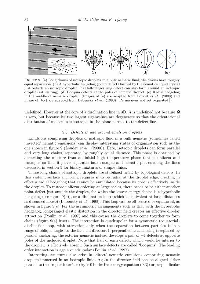
32 M. E. Cates and E. Tjhung
Figure 9. (a) Long chains of isotropic droplets in a bulk nematic fluid; the chains have roughlyequal separation. (b) A hyperbolic hedgehog (point defect) formed by the nematics liquid crystaljust outside an isotropic droplet. (c) Half-integer ring defect can also form around an isotropicdroplet (saturn ring). (d) Boojum defects at the poles of nematic droplet. (e) Radial hedgehogin the middle of nematic droplet. (Images of (a) are adapted from Loudet et al. (2000) andimage of (b,c) are adapted from Lubensky et al. (1998). [Permissions not yet requested.])
undefined. However at the core of a disclination line in 3D, n is undefined not because Qis zero, but because its two largest eigenvalues are degenerate so that the orientationaldistribution of molecules is isotropic in the plane normal to the defect line.
9.3. Defects in and around emulsion droplets
Emulsions comprising droplets of isotropic fluid in a bulk nematic (sometimes called‘inverted’ nematic emulsions) can display interesting states of organization such as theone shown in figure 9 (Loudet et al. (2000)). Here, isotropic droplets can form paralleland very long chains, separated by roughly equal distance. This phase is obtained byquenching the mixture from an initial high temperature phase that is uniform andisotropic, so that it phase separates into isotropic and nematic phases along the linesdiscussed in section 5 for binary mixtures of simple fluids.
These long chains of isotropic droplets are stabilized in 3D by topological defects. Inthis system, surface anchoring requires n to be radial at the droplet edge, creating ineffect a radial hedgehog that cannot be annihilated because its core is effectively insidethe droplet. To restore uniform ordering at large scales, there needs to be either anotherpoint defect just outside the droplet, for which the lowest energy choice is a hyperbolichedgehog (see figure 9(b)), or a disclination loop (which is equivalent at large distancesas discussed above) (Lubensky et al. 1998). This loop can be off-centred or equatorial, asshown in figure 9(c). For the asymmetric arrangements such as that with the hyperbolichedgehog, long-ranged elastic distortion in the director field creates an effective dipolarattraction (Poulin et al. 1997) and this causes the droplets to come together to formchains (figure 9(a) inset). The interaction is quadrupolar for a symmetric (equatorial)disclination loop, with attraction only when the separation between particles is in arange of oblique angles to the far-field director. If perpendicular anchoring is replaced byparallel anchoring, the exterior nematic instead develops a pair of +1 defects at oppositepoles of the included droplet. Note that half of each defect, which would lie interior tothe droplet, is effectively absent. Such surface defects are called ‘boojums’. The leadingorder interaction is again quadrupolar (Poulin et al. 1997).
Interesting structures also arise in ‘direct’ nematic emulsions comprising nematicdroplets immersed in an isotropic fluid. Again the director field can be aligned eitherparallel to the droplet interface (β0 > 0 in the free energy equation (9.3)) or perpendicular
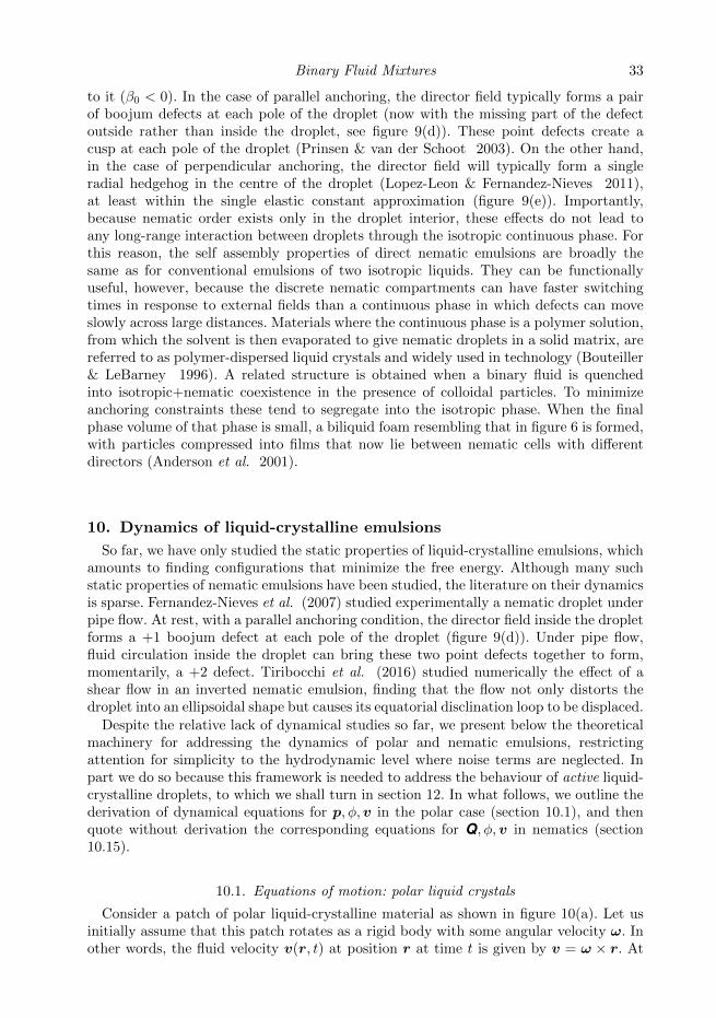
Binary Fluid Mixtures 33
to it (β0 < 0). In the case of parallel anchoring, the director field typically forms a pairof boojum defects at each pole of the droplet (now with the missing part of the defectoutside rather than inside the droplet, see figure 9(d)). These point defects create acusp at each pole of the droplet (Prinsen & van der Schoot 2003). On the other hand,in the case of perpendicular anchoring, the director field will typically form a singleradial hedgehog in the centre of the droplet (Lopez-Leon & Fernandez-Nieves 2011),at least within the single elastic constant approximation (figure 9(e)). Importantly,because nematic order exists only in the droplet interior, these effects do not lead toany long-range interaction between droplets through the isotropic continuous phase. Forthis reason, the self assembly properties of direct nematic emulsions are broadly thesame as for conventional emulsions of two isotropic liquids. They can be functionallyuseful, however, because the discrete nematic compartments can have faster switchingtimes in response to external fields than a continuous phase in which defects can moveslowly across large distances. Materials where the continuous phase is a polymer solution,from which the solvent is then evaporated to give nematic droplets in a solid matrix, arereferred to as polymer-dispersed liquid crystals and widely used in technology (Bouteiller& LeBarney 1996). A related structure is obtained when a binary fluid is quenchedinto isotropic+nematic coexistence in the presence of colloidal particles. To minimizeanchoring constraints these tend to segregate into the isotropic phase. When the finalphase volume of that phase is small, a biliquid foam resembling that in figure 6 is formed,with particles compressed into films that now lie between nematic cells with differentdirectors (Anderson et al. 2001).
10. Dynamics of liquid-crystalline emulsions
So far, we have only studied the static properties of liquid-crystalline emulsions, whichamounts to finding configurations that minimize the free energy. Although many suchstatic properties of nematic emulsions have been studied, the literature on their dynamicsis sparse. Fernandez-Nieves et al. (2007) studied experimentally a nematic droplet underpipe flow. At rest, with a parallel anchoring condition, the director field inside the dropletforms a +1 boojum defect at each pole of the droplet (figure 9(d)). Under pipe flow,fluid circulation inside the droplet can bring these two point defects together to form,momentarily, a +2 defect. Tiribocchi et al. (2016) studied numerically the effect of ashear flow in an inverted nematic emulsion, finding that the flow not only distorts thedroplet into an ellipsoidal shape but causes its equatorial disclination loop to be displaced.
Despite the relative lack of dynamical studies so far, we present below the theoreticalmachinery for addressing the dynamics of polar and nematic emulsions, restrictingattention for simplicity to the hydrodynamic level where noise terms are neglected. Inpart we do so because this framework is needed to address the behaviour of active liquid-crystalline droplets, to which we shall turn in section 12. In what follows, we outline thederivation of dynamical equations for p, φ,v in the polar case (section 10.1), and thenquote without derivation the corresponding equations for Q, φ,v in nematics (section10.15).
10.1. Equations of motion: polar liquid crystals
Consider a patch of polar liquid-crystalline material as shown in figure 10(a). Let usinitially assume that this patch rotates as a rigid body with some angular velocity ω. Inother words, the fluid velocity v(r, t) at position r at time t is given by v = ω × r. At
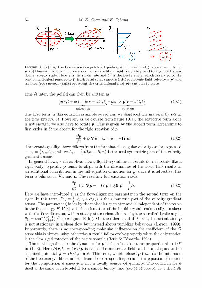
34 M. E. Cates and E. Tjhung
Figure 10. (a) Rigid body rotation in a patch of liquid-crystalline material; (red) arrows indicatep. (b) However most liquid crystals do not rotate like a rigid body, they tend to align with shearflow at steady state. Here γ is the strain rate and θL is the Leslie angle, which is related to thephenomenological parameter ξ. Horizontal (blue) arrows (left) represents fluid velocity v(r) andinclined (red) arrows (right) represent the orientational field p(r) at steady state.
time δt later, the p-field can then be written as:
p(r, t+ δt) = p(r − vδt, t)︸ ︷︷ ︸advection
+ωδt× p(r − vδt, t)︸ ︷︷ ︸rotation
. (10.1)
The first term in this equation is simple advection; we displaced the material by vδt inthe time interval δt. However, as we can see from figure 10(a), the advective term aloneis not enough; we also have to rotate p. This is given by the second term. Expanding tofirst order in δt we obtain for the rigid rotation of p:
∂p
∂t+ v·∇p = ω × p = −Ω·p. (10.2)
The second equality above follows from the fact that the angular velocity can be expressedas ωi = 1
2εijkΩjk, where Ωij ≡ 12 (∂ivj − ∂jvi) is the anti-symmetric part of the velocity
gradient tensor.In general flows, such as shear flows, liquid-crystalline materials do not rotate like a
rigid body; typically p tends to align with the streamlines of the flow. This results inan additional contribution in the full equation of motion for p; since it is advective, thisterm is bilinear in ∇v and p. The resulting full equation reads:
∂p
∂t+ v·∇p = −Ω·p+ ξD·p− 1
Γh. (10.3)
Here we have introduced ξ as the flow-alignment parameter in the second term on theright. In this term, Dij ≡ 1
2 (∂ivj + ∂jvi) is the symmetric part of the velocity gradienttensor. The parameter ξ is set by the molecular geometry and is independent of the termsin the free energy F . If |ξ| > 1, the orientation of the liquid crystal tends to align in shearwith the flow direction, with a steady-state orientation set by the so-called Leslie angle,θL = tan−1( ξ−1
ξ+1 )1/2 (see figure 10(b)). On the other hand if |ξ| < 1, the orientation p
is not stationary in a shear flow but instead shows tumbling behaviour (Larson 1999).Importantly, there is no corresponding molecular influence on the coefficient of the Ωterm: this is always unity, otherwise p would fail to evolve properly when the only motionis the slow rigid rotation of the entire sample (Beris & Edwards 1994).
The final ingredient in the dynamics for p is the relaxation term proportional to 1/Γin (10.3). Here h(r, t) = δF/δp is called the molecular field, and is analogous to thechemical potential µ = δF/δφ for φ. This term, which relaxes p towards the minimumof the free energy, differs in form from the corresponding term in the equation of motionfor the composition φ since p is not a locally conserved quantity. The equation for φitself is the same as in Model H for a simple binary fluid (see (4.5) above), as is the NSE
Binary Fluid Mixtures 35
(see (4.3)) for v except that a different expression, detailed below, is now needed for thethermodynamic stress σ.
To summarise, for polar liquid crystals, at hydrodynamic (deterministic) level, thedynamics is governed by the following set of equations (Kung et al. 2006):
ρ(v + v·∇v) = η∇2v −∇P +∇·σ[φ,p], (10.4)
∇·v = 0, (10.5)
φ+∇ · (φv) =∇·(M∇µ), (10.6)
p+ v·∇p = −Ω·p+ ξD·p− h/Γ. (10.7)
Here M is the mobility and µ[φ,p] = δF/δφ is the chemical potential. By constructionthese reduce to the noise-free version of Model H in the limit where p = 0 everywhere.
It only remains to derive the total elastic stress σ[φ,p] which enters the NSE (10.4).We know already from section 3.3 that even in the absence of p there an interfacial stresscontribution. This takes the form (compare (3.10))
σφij = (Fφ − φµ)δij −∂F
∂(∂jφ)∂iφ, (10.8)
where Fφ = f(φ) + κ(∇φ)2/2 is the local free energy density as defined in (9.1). In thefinal term we have generalized (3.10) to allow for the addition of anchoring terms, whichalso can contribute to the chemical potential and the interfacial stress; hence the full freeenergy density F = Fφ + Fp appears here. This can be confirmed by a straightforwardanalogue of the following argument, in which for simplicity we calculate the elastic stresscontribution from p only (Beris & Edwards 1994).
To find this stress contribution, we consider the rate of change in Fp:
dFp
dt=
∫δFp
δpi
∂pi∂t
dr =
∫hipi dr. (10.9)
Substituting (10.7) for pi, we obtain
dFp
dt=
∫ ((pj∂ihj)vi −Ωijhipj + ξDijhipj −
|h|2
Γ
)dr, (10.10)
where the underlined term has been integrated by parts. The resulting surface contri-bution vanishes for periodic boundary conditions which we choose here without loss ofgenerality (just as we did in section 3.3 when discussing Model H). The underlined termin (10.10) is reminiscent of (3.8) for δF (φ) in the case where only a composition variableis present. Thus −pj∂ihj is effectively a force density, playing a similar role to −φ∇iµthere. Allowing for the fact that the small displacement u is now vdt, this term gives acontribution δF ′p =
∫(pj∂ihj)uidr (where the prime on F ′p reminds us that this is not
the only contribution). Following the same procedure using (3.9) as in section 3.3, thistranslates into an elastic stress contribution that is the direct analogue of (10.8):
σ′ij = (Fp − p·h)δij −∂F
∂(∂jpk)∂ipk. (10.11)
It is simple to check from this that ∂jσ′ij = −pj∂ihj .
The remaining contribution σ′′ij to the elastic stress has no counterpart in Model H; it
36 M. E. Cates and E. Tjhung
stems from the rotation and alignment terms (10.10) which may be written
dF ′′pdt
=
∫(−Ωijhipj+ξDijhipj) dr =
∫ (Ωij
1
2(pihj − pjhi) + ξDij
1
2(pihj + pjhi)
)dr.
(10.12)In the second equality, we have decomposed hipj into symmetric and anti-symmetricparts, and used the fact that XijYij = 0 for any symmetric tensor Xij and anti-symmetrictensor Yij . Once again using (3.9) with u = vdt we obtain
dF ′′pdt
=
∫σ′′ij∂jvi dr =
∫ (σ′′ij
SDij − σ′′ij
AΩij
)dr, (10.13)
where the second form decomposes the rate of strain tensor ∂jvi into its symmetric
and antisymmetric parts. Comparing Eq. (10.12) and Eq. (10.13) we identify σ′′ijS
=ξ2 (pihj+pjhi) and σ′′ij
A= − 1
2 (pihj−pjhi). The presence of an antisymmetric contributionis generic in liquid crystals in which rotational symmetry is spontaneously broken.
Note finally that the last term, proportional to 1/Γ , in (10.10) causes a purelydissipative loss of free energy and hence does not contribute to the elastic stress, whichinstead describes how the stored free energy changes with sample shape. This term isnegative definite, ensuring that in the absence of a driving force the free energy steadilydecreases towards its minimum value.
Adding the contributions σφ and σp = σ′+σ′′S +σ′′A found above, we can assemblethe total elastic stress tensor σ[φ,p] in the NSE (10.4). This reads
σij = (F− φµ− p·h)δij −∂F
∂(∂jφ)∂iφ−
∂F∂(∂jpk)
∂ipk +ξ
2(pihj + pjhi)−
1
2(pihj − pjhi).
(10.14)It is important to note that, alongside the rigid-rotation term (the final term on theright), the flow alignment parameter ξ, as defined via the equation of motion (10.7) forp, also enters the elastic stress in a non-negotiable fashion (Beris & Edwards 1994). Thisis because it controls the response of p to an incremental strain and hence affects theresulting free energy increment which determines the stress.
10.2. Equations of motion: nematic liquid crystals
In principle, one can repeat the same calculation as above for nematic liquid crystals.Here we shall just quote the results (Beris & Edwards 1994) which are included forcompleteness. The dynamical equation for the order parameter Q is
∂Q∂t
+ (v·∇)Q = +S(∇v,Q)− 1
ΓH, (10.15)
where the first term on the right describes the combined effect of rigid body rotation andshear aligning. This takes the following form
S(∇v,Q) = (ξD +Ω)(Q + I/d) + (Q + I/d)(ξD−Ω)− 2ξ(Q + I/d) Tr(Q:∇v), (10.16)
where ξ is a flow-aligning parameter analogous to that introduced previously for p. Thisequation describes similar physics to the corresponding terms for p. The quantity Q+ I/denters (rather than just the traceless Q) because the entire orientational distributionfunction, including its isotropic part, is stretched and rotated by the flow. The finalterm in (10.15) is a local relaxation term similar to that used in (10.7) for p, with Γ an
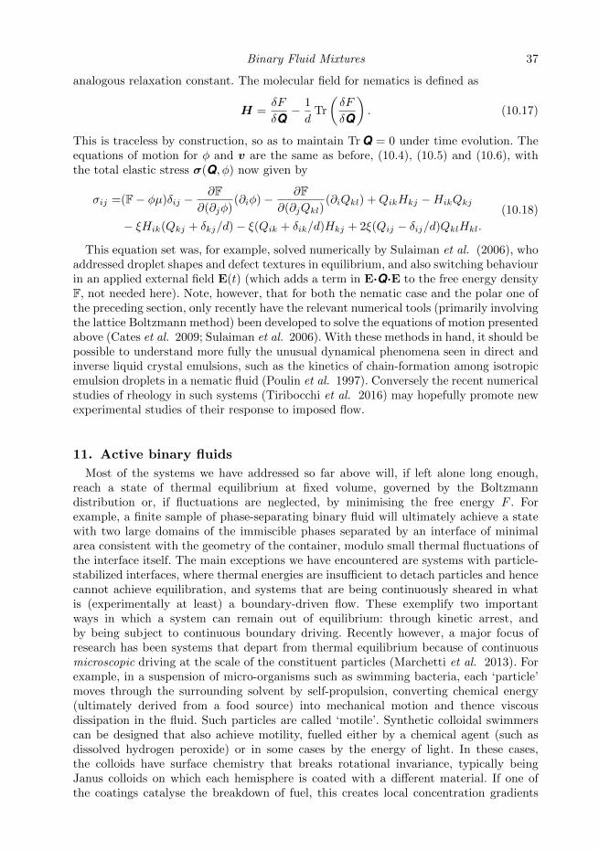
Binary Fluid Mixtures 37
analogous relaxation constant. The molecular field for nematics is defined as
H =δF
δQ− 1
dTr
(δF
δQ
). (10.17)
This is traceless by construction, so as to maintain Tr Q = 0 under time evolution. Theequations of motion for φ and v are the same as before, (10.4), (10.5) and (10.6), withthe total elastic stress σ(Q, φ) now given by
σij =(F− φµ)δij −∂F
∂(∂jφ)(∂iφ)− ∂F
∂(∂jQkl)(∂iQkl) +QikHkj −HikQkj
− ξHik(Qkj + δkj/d)− ξ(Qik + δik/d)Hkj + 2ξ(Qij − δij/d)QklHkl.
(10.18)
This equation set was, for example, solved numerically by Sulaiman et al. (2006), whoaddressed droplet shapes and defect textures in equilibrium, and also switching behaviourin an applied external field E(t) (which adds a term in E·Q·E to the free energy densityF, not needed here). Note, however, that for both the nematic case and the polar one ofthe preceding section, only recently have the relevant numerical tools (primarily involvingthe lattice Boltzmann method) been developed to solve the equations of motion presentedabove (Cates et al. 2009; Sulaiman et al. 2006). With these methods in hand, it should bepossible to understand more fully the unusual dynamical phenomena seen in direct andinverse liquid crystal emulsions, such as the kinetics of chain-formation among isotropicemulsion droplets in a nematic fluid (Poulin et al. 1997). Conversely the recent numericalstudies of rheology in such systems (Tiribocchi et al. 2016) may hopefully promote newexperimental studies of their response to imposed flow.
11. Active binary fluids
Most of the systems we have addressed so far above will, if left alone long enough,reach a state of thermal equilibrium at fixed volume, governed by the Boltzmanndistribution or, if fluctuations are neglected, by minimising the free energy F . Forexample, a finite sample of phase-separating binary fluid will ultimately achieve a statewith two large domains of the immiscible phases separated by an interface of minimalarea consistent with the geometry of the container, modulo small thermal fluctuations ofthe interface itself. The main exceptions we have encountered are systems with particle-stabilized interfaces, where thermal energies are insufficient to detach particles and hencecannot achieve equilibration, and systems that are being continuously sheared in whatis (experimentally at least) a boundary-driven flow. These exemplify two importantways in which a system can remain out of equilibrium: through kinetic arrest, andby being subject to continuous boundary driving. Recently however, a major focus ofresearch has been systems that depart from thermal equilibrium because of continuousmicroscopic driving at the scale of the constituent particles (Marchetti et al. 2013). Forexample, in a suspension of micro-organisms such as swimming bacteria, each ‘particle’moves through the surrounding solvent by self-propulsion, converting chemical energy(ultimately derived from a food source) into mechanical motion and thence viscousdissipation in the fluid. Such particles are called ‘motile’. Synthetic colloidal swimmerscan be designed that also achieve motility, fuelled either by a chemical agent (such asdissolved hydrogen peroxide) or in some cases by the energy of light. In these cases,the colloids have surface chemistry that breaks rotational invariance, typically beingJanus colloids on which each hemisphere is coated with a different material. If one ofthe coatings catalyse the breakdown of fuel, this creates local concentration gradients
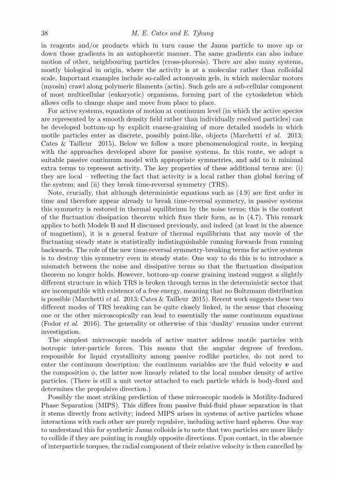
38 M. E. Cates and E. Tjhung
in reagents and/or products which in turn cause the Janus particle to move up ordown those gradients in an autophoretic manner. The same gradients can also inducemotion of other, neighbouring particles (cross-phoresis). There are also many systems,mostly biological in origin, where the activity is at a molecular rather than colloidalscale. Important examples include so-called actomyosin gels, in which molecular motors(myosin) crawl along polymeric filaments (actin). Such gels are a sub-cellular componentof most multicellular (eukaryotic) organisms, forming part of the cytoskeleton whichallows cells to change shape and move from place to place.
For active systems, equations of motion at continuum level (in which the active speciesare represented by a smooth density field rather than individually resolved particles) canbe developed bottom-up by explicit coarse-graining of more detailed models in whichmotile particles enter as discrete, possibly point-like, objects (Marchetti et al. 2013;Cates & Tailleur 2015). Below we follow a more phenomenological route, in keepingwith the approaches developed above for passive systems. In this route, we adopt asuitable passive continuum model with appropriate symmetries, and add to it minimalextra terms to represent activity. The key properties of these additional terms are: (i)they are local – reflecting the fact that activity is a local rather than global forcing ofthe system; and (ii) they break time-reversal symmetry (TRS).
Note, crucially, that although deterministic equations such as (4.9) are first order intime and therefore appear already to break time-reversal symmetry, in passive systemsthis symmetry is restored in thermal equilibrium by the noise terms; this is the contentof the fluctuation dissipation theorem which fixes their form, as in (4.7). This remarkapplies to both Models B and H discussed previously, and indeed (at least in the absenceof magnetism), it is a general feature of thermal equilibrium that any movie of thefluctuating steady state is statistically indistinguishable running forwards from runningbackwards. The role of the new time-reversal symmetry-breaking terms for active systemsis to destroy this symmetry even in steady state. One way to do this is to introduce amismatch between the noise and dissipative terms so that the fluctuation dissipationtheorem no longer holds. However, bottom-up coarse graining instead suggest a slightlydifferent structure in which TRS is broken through terms in the deterministic sector thatare incompatible with existence of a free energy, meaning that no Boltzmann distributionis possible (Marchetti et al. 2013; Cates & Tailleur 2015). Recent work suggests these twodifferent modes of TRS breaking can be quite closely linked, in the sense that choosingone or the other microscopically can lead to essentially the same continuum equations(Fodor et al. 2016). The generality or otherwise of this ‘duality’ remains under currentinvestigation.
The simplest microscopic models of active matter address motile particles withisotropic inter-particle forces. This means that the angular degrees of freedom,responsible for liquid crystallinity among passive rodlike particles, do not need toenter the continuum description: the continuum variables are the fluid velocity v andthe composition φ, the latter now linearly related to the local number density of activeparticles. (There is still a unit vector attached to each particle which is body-fixed anddetermines the propulsive direction.)
Possibly the most striking prediction of these microscopic models is Motility-InducedPhase Separation (MIPS). This differs from passive fluid-fluid phase separation in thatit stems directly from activity; indeed MIPS arises in systems of active particles whoseinteractions with each other are purely repulsive, including active hard spheres. One wayto understand this for synthetic Janus colloids is to note that two particles are more likelyto collide if they are pointing in roughly opposite directions. Upon contact, in the absenceof interparticle torques, the radial component of their relative velocity is then cancelled by
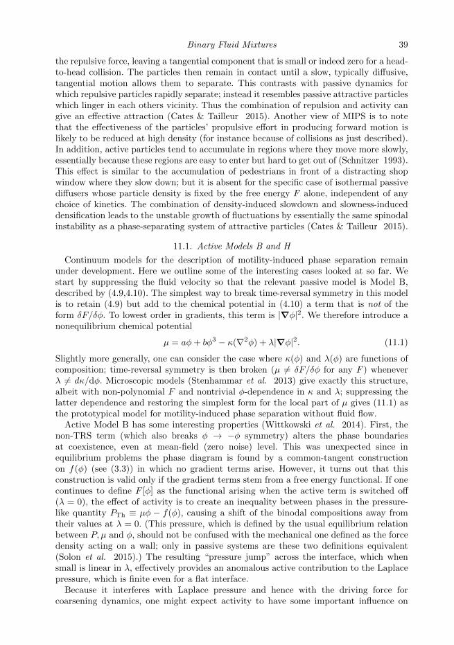
Binary Fluid Mixtures 39
the repulsive force, leaving a tangential component that is small or indeed zero for a head-to-head collision. The particles then remain in contact until a slow, typically diffusive,tangential motion allows them to separate. This contrasts with passive dynamics forwhich repulsive particles rapidly separate; instead it resembles passive attractive particleswhich linger in each others vicinity. Thus the combination of repulsion and activity cangive an effective attraction (Cates & Tailleur 2015). Another view of MIPS is to notethat the effectiveness of the particles’ propulsive effort in producing forward motion islikely to be reduced at high density (for instance because of collisions as just described).In addition, active particles tend to accumulate in regions where they move more slowly,essentially because these regions are easy to enter but hard to get out of (Schnitzer 1993).This effect is similar to the accumulation of pedestrians in front of a distracting shopwindow where they slow down; but it is absent for the specific case of isothermal passivediffusers whose particle density is fixed by the free energy F alone, independent of anychoice of kinetics. The combination of density-induced slowdown and slowness-induceddensification leads to the unstable growth of fluctuations by essentially the same spinodalinstability as a phase-separating system of attractive particles (Cates & Tailleur 2015).
11.1. Active Models B and H
Continuum models for the description of motility-induced phase separation remainunder development. Here we outline some of the interesting cases looked at so far. Westart by suppressing the fluid velocity so that the relevant passive model is Model B,described by (4.9,4.10). The simplest way to break time-reversal symmetry in this modelis to retain (4.9) but add to the chemical potential in (4.10) a term that is not of theform δF/δφ. To lowest order in gradients, this term is |∇φ|2. We therefore introduce anonequilibrium chemical potential
µ = aφ+ bφ3 − κ(∇2φ) + λ|∇φ|2. (11.1)
Slightly more generally, one can consider the case where κ(φ) and λ(φ) are functions ofcomposition; time-reversal symmetry is then broken (µ 6= δF/δφ for any F ) wheneverλ 6= dκ/dφ. Microscopic models (Stenhammar et al. 2013) give exactly this structure,albeit with non-polynomial F and nontrivial φ-dependence in κ and λ; suppressing thelatter dependence and restoring the simplest form for the local part of µ gives (11.1) asthe prototypical model for motility-induced phase separation without fluid flow.
Active Model B has some interesting properties (Wittkowski et al. 2014). First, thenon-TRS term (which also breaks φ → −φ symmetry) alters the phase boundariesat coexistence, even at mean-field (zero noise) level. This was unexpected since inequilibrium problems the phase diagram is found by a common-tangent constructionon f(φ) (see (3.3)) in which no gradient terms arise. However, it turns out that thisconstruction is valid only if the gradient terms stem from a free energy functional. If onecontinues to define F [φ] as the functional arising when the active term is switched off(λ = 0), the effect of activity is to create an inequality between phases in the pressure-like quantity PTh ≡ µφ − f(φ), causing a shift of the binodal compositions away fromtheir values at λ = 0. (This pressure, which is defined by the usual equilibrium relationbetween P, µ and φ, should not be confused with the mechanical one defined as the forcedensity acting on a wall; only in passive systems are these two definitions equivalent(Solon et al. 2015).) The resulting “pressure jump” across the interface, which whensmall is linear in λ, effectively provides an anomalous active contribution to the Laplacepressure, which is finite even for a flat interface.
Because it interferes with Laplace pressure and hence with the driving force forcoarsening dynamics, one might expect activity to have some important influence on
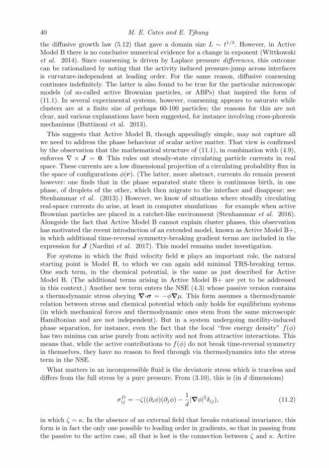
40 M. E. Cates and E. Tjhung
the diffusive growth law (5.12) that gave a domain size L ∼ t1/3. However, in ActiveModel B there is no conclusive numerical evidence for a change in exponent (Wittkowskiet al. 2014). Since coarsening is driven by Laplace pressure differences, this outcomecan be rationalized by noting that the activity induced pressure-jump across interfacesis curvature-independent at leading order. For the same reason, diffusive coarseningcontinues indefinitely. The latter is also found to be true for the particular microscopicmodels (of so-called active Brownian particles, or ABPs) that inspired the form of(11.1). In several experimental systems, however, coarsening appears to saturate whileclusters are at a finite size of perhaps 60-100 particles; the reasons for this are notclear, and various explanations have been suggested, for instance involving cross-phoresismechanisms (Buttinoni et al. 2013).
This suggests that Active Model B, though appealingly simple, may not capture allwe need to address the phase behaviour of scalar active matter. That view is confirmedby the observation that the mathematical structure of (11.1), in combination with (4.9),enforces ∇ × J = 0. This rules out steady-state circulating particle currents in realspace. These currents are a low dimensional projection of a circulating probability flux inthe space of configurations φ(r). (The latter, more abstract, currents do remain presenthowever: one finds that in the phase separated state there is continuous birth, in onephase, of droplets of the other, which then migrate to the interface and disappear; seeStenhammar et al. (2013).) However, we know of situations where steadily circulatingreal-space currents do arise, at least in computer simulations – for example when activeBrownian particles are placed in a ratchet-like environment (Stenhammar et al. 2016).Alongside the fact that Active Model B cannot explain cluster phases, this observationhas motivated the recent introduction of an extended model, known as Active Model B+,in which additional time-reversal symmetry-breaking gradient terms are included in theexpression for J (Nardini et al. 2017). This model remains under investigation.
For systems in which the fluid velocity field v plays an important role, the naturalstarting point is Model H, to which we can again add minimal TRS-breaking terms.One such term, in the chemical potential, is the same as just described for ActiveModel B. (The additional terms arising in Active Model B+ are yet to be addressedin this context.) Another new term enters the NSE (4.3) whose passive version containsa thermodynamic stress obeying ∇·σ = −φ∇µ. This form assumes a thermodynamicrelation between stress and chemical potential which only holds for equilibrium systems(in which mechanical forces and thermodynamic ones stem from the same microscopicHamiltonian and are not independent). But in a system undergoing motility-inducedphase separation, for instance, even the fact that the local “free energy density” f(φ)has two minima can arise purely from activity and not from attractive interactions. Thismeans that, while the active contributions to f(φ) do not break time-reversal symmetryin themselves, they have no reason to feed through via thermodynamics into the stressterm in the NSE.
What matters in an incompressible fluid is the deviatoric stress which is traceless anddiffers from the full stress by a pure pressure. From (3.10), this is (in d dimensions)
σDij = −ζ((∂iφ)(∂jφ)− 1
d|∇φ|2δij), (11.2)
in which ζ = κ. In the absence of an external field that breaks rotational invariance, thisform is in fact the only one possible to leading order in gradients, so that in passing fromthe passive to the active case, all that is lost is the connection between ζ and κ. Active
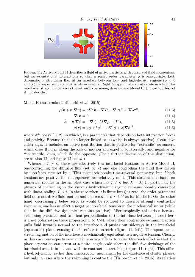
Binary Fluid Mixtures 41
Figure 11. Active Model H describes a fluid of active particles with conserved fluid momentum,but no orientational interactions so that a scalar order parameter φ is appropriate. Left:Schematic of stretching flow at an interface between low- and high-density regions (φ < 0and φ > 0 respectively) of contractile swimmers. Right: Snapshot of a steady state in which thisinterfacial stretching balances the intrinsic coarsening dynamics of Model H. (Image courtesy ofA. Tiribocchi.)
Model H thus reads (Tiribocchi et al. 2015)
ρ(v + v·∇v) = η∇2v −∇P −∇·σD +∇·σn, (11.3)
∇·v = 0, (11.4)
φ+ v·∇φ = −∇·(−M∇µ+ Jn), (11.5)
µ(r) = aφ+ bφ3 − κ∇2φ+ λ|∇φ|2. (11.6)
where σD obeys (11.2), in which ζ is a parameter that depends on both interaction forcesand activity. Because this is no longer linked to κ (which is always postive), ζ can haveeither sign. It includes an active contribution that is positive for “extensile” swimmers,which draw fluid in along the axis of motion and expel it equatorially, and negative for“contractile” ones, which do the opposite. (For a further discussion of this distinction,see section 12 and figure 12 below.)
Whenever ζ 6= κ, there are effectively two interfacial tensions in Active Model H,one controlling the diffusive flux (set by κ) and one controlling the fluid flow drivenby interfaces, now set by ζ. This mismatch breaks time-reversal symmetry, but if bothtensions are positive the consequences are relatively mild. (This statement is based onnumerical studies in the simplest case which has ζ 6= κ but λ = 0.) In particular, thephysics of coarsening in the viscous hydrodynamic regime remains broadly consistentwith linear scaling, L ∼ t. In the case when κ is finite but ζ is zero, the order parameterfield does not drive fluid motion and one recovers L ∼ t1/3 as for Model B. On the otherhand, decreasing ζ below zero, as would be required to describe strongly contractileswimmers, one has in effect a negative interfacial tension in the mechanical sector (whilethat in the diffusive dynamics remains positive). Microscopically this arises becauseswimming particles tend to orient perpendicular to the interface between phases (thereis a net polarization there proportional to ∇φ), where their contractile swimming actionpulls fluid inwards normal to the interface and pushes out sideways in the interfacial(equatorial) plane causing the interface to stretch (figure 11, left). The spontaneousstretching motion of the interface is mechanically equivalent to a negative tension. Clearly,in this case one expects new and interesting effects to arise. One such effect is that thephase separation can arrest at a finite length scale where the diffusive shrinkage of theinterfacial area is in balance with its contractile stretching (figure 11, right). This offersa hydrodynamic, rather than microscopic, mechanism for the existence of cluster phases,but only in cases where the swimming is contractile (Tiribocchi et al. 2015); its relation
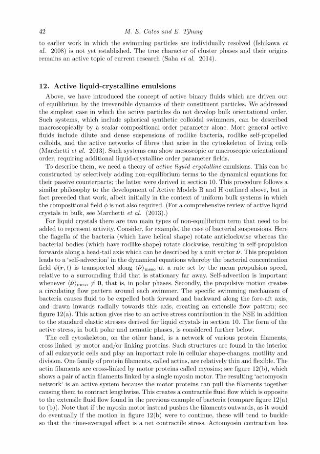
42 M. E. Cates and E. Tjhung
to earlier work in which the swimming particles are individually resolved (Ishikawa etal. 2008) is not yet established. The true character of cluster phases and their originsremains an active topic of current research (Saha et al. 2014).
12. Active liquid-crystalline emulsions
Above, we have introduced the concept of active binary fluids which are driven outof equilibrium by the irreversible dynamics of their constituent particles. We addressedthe simplest case in which the active particles do not develop bulk orientational order.Such systems, which include spherical synthetic colloidal swimmers, can be describedmacroscopically by a scalar compositional order parameter alone. More general activefluids include dilute and dense suspensions of rodlike bacteria, rodlike self-propelledcolloids, and the active networks of fibres that arise in the cytoskeleton of living cells(Marchetti et al. 2013). Such systems can show mesoscopic or macroscopic orientationalorder, requiring additional liquid-crystalline order parameter fields.
To describe them, we need a theory of active liquid-crystalline emulsions. This can beconstructed by selectively adding non-equilibrium terms to the dynamical equations fortheir passive counterparts; the latter were derived in section 10. This procedure follows asimilar philosophy to the development of Active Models B and H outlined above, but infact preceded that work, albeit initially in the context of uniform bulk systems in whichthe compositional field φ is not also required. (For a comprehensive review of active liquidcrystals in bulk, see Marchetti et al. (2013).)
For liquid crystals there are two main types of non-equilibrium term that need to beadded to represent activity. Consider, for example, the case of bacterial suspensions. Herethe flagella of the bacteria (which have helical shape) rotate anticlockwise whereas thebacterial bodies (which have rodlike shape) rotate clockwise, resulting in self-propulsionforwards along a head-tail axis which can be described by a unit vector ν. This propulsionleads to a ‘self-advection’ in the dynamical equations whereby the bacterial concentrationfield φ(r, t) is transported along 〈ν〉meso at a rate set by the mean propulsion speed,relative to a surrounding fluid that is stationary far away. Self-advection is importantwhenever 〈ν〉meso 6= 0, that is, in polar phases. Secondly, the propulsive motion createsa circulating flow pattern around each swimmer. The specific swimming mechanism ofbacteria causes fluid to be expelled both forward and backward along the fore-aft axis,and drawn inwards radially towards this axis, creating an extensile flow pattern; seefigure 12(a). This action gives rise to an active stress contribution in the NSE in additionto the standard elastic stresses derived for liquid crystals in section 10. The form of theactive stress, in both polar and nematic phases, is considered further below.
The cell cytoskeleton, on the other hand, is a network of various protein filaments,cross-linked by motor and/or linking proteins. Such structures are found in the interiorof all eukaryotic cells and play an important role in cellular shape-changes, motility anddivision. One family of protein filaments, called actins, are relatively thin and flexible. Theactin filaments are cross-linked by motor proteins called myosins; see figure 12(b), whichshows a pair of actin filaments linked by a single myosin motor. The resulting ‘actomyosinnetwork’ is an active system because the motor proteins can pull the filaments togethercausing them to contract lengthwise. This creates a contractile fluid flow which is oppositeto the extensile fluid flow found in the previous example of bacteria (compare figure 12(a)to (b)). Note that if the myosin motor instead pushes the filaments outwards, as it woulddo eventually if the motion in figure 12(b) were to continue, these will tend to buckleso that the time-averaged effect is a net contractile stress. Actomyosin contraction has
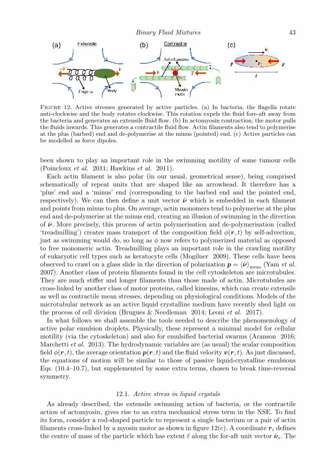
Binary Fluid Mixtures 43
Figure 12. Active stresses generated by active particles. (a) In bacteria, the flagella rotateanti-clockwise and the body rotates clockwise. This rotation expels the fluid fore-aft away fromthe bacteria and generates an extensile fluid flow. (b) In actomyosin contraction, the motor pullsthe fluids inwards. This generates a contractile fluid flow. Actin filaments also tend to polymeriseat the plus (barbed) end and de-polymerise at the minus (pointed) end. (c) Active particles canbe modelled as force dipoles.
been shown to play an important role in the swimming motility of some tumour cells(Poincloux et al. 2011; Hawkins et al. 2011).
Each actin filament is also polar (in our usual, geometrical sense), being comprisedschematically of repeat units that are shaped like an arrowhead. It therefore has a‘plus’ end and a ‘minus’ end (corresponding to the barbed end and the pointed end,respectively). We can then define a unit vector ν which is embedded in each filamentand points from minus to plus. On average, actin monomers tend to polymerise at the plusend and de-polymerise at the minus end, creating an illusion of swimming in the directionof ν. More precisely, this process of actin polymerisation and de-polymerisation (called‘treadmilling’) creates mass transport of the composition field φ(r, t) by self-advection,just as swimming would do, so long as φ now refers to polymerized material as opposedto free monomeric actin. Treadmilling plays an important role in the crawling motilityof eukaryotic cell types such as keratocyte cells (Mogilner 2009). These cells have beenobserved to crawl on a glass slide in the direction of polarization p = 〈ν〉meso (Yam et al.2007). Another class of protein filaments found in the cell cytoskeleton are microtubules.They are much stiffer and longer filaments than those made of actin. Microtubules arecross-linked by another class of motor proteins, called kinesins, which can create extensileas well as contractile mean stresses, depending on physiological conditions. Models of themicrotubular network as an active liquid crystalline medium have recently shed light onthe process of cell division (Brugues & Needleman 2014; Leoni et al. 2017).
In what follows we shall assemble the tools needed to describe the phenomenology ofactive polar emulsion droplets. Physically, these represent a minimal model for cellularmotility (via the cytoskeleton) and also for emulsified bacterial swarms (Aranson 2016;Marchetti et al. 2013). The hydrodynamic variables are (as usual) the scalar compositionfield φ(r, t), the average orientation p(r, t) and the fluid velocity v(r, t). As just discussed,the equations of motion will be similar to those of passive liquid-crystalline emulsionsEqs. (10.4–10.7), but supplemented by some extra terms, chosen to break time-reversalsymmetry.
12.1. Active stress in liquid crystals
As already described, the extensile swimming action of bacteria, or the contractileaction of actomyosin, gives rise to an extra mechanical stress term in the NSE. To findits form, consider a rod-shaped particle to represent a single bacterium or a pair of actinfilaments cross-linked by a myosin motor as shown in figure 12(c). A coordinate ri definesthe centre of mass of the particle which has extent ` along the for-aft unit vector νi. The
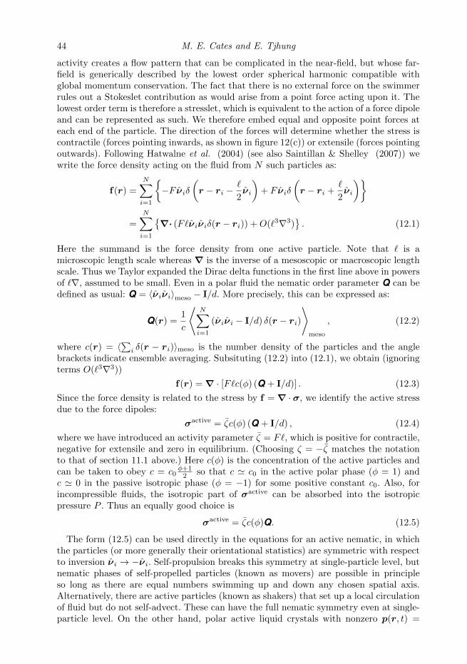
44 M. E. Cates and E. Tjhung
activity creates a flow pattern that can be complicated in the near-field, but whose far-field is generically described by the lowest order spherical harmonic compatible withglobal momentum conservation. The fact that there is no external force on the swimmerrules out a Stokeslet contribution as would arise from a point force acting upon it. Thelowest order term is therefore a stresslet, which is equivalent to the action of a force dipoleand can be represented as such. We therefore embed equal and opposite point forces ateach end of the particle. The direction of the forces will determine whether the stress iscontractile (forces pointing inwards, as shown in figure 12(c)) or extensile (forces pointingoutwards). Following Hatwalne et al. (2004) (see also Saintillan & Shelley (2007)) wewrite the force density acting on the fluid from N such particles as:
f(r) =
N∑i=1
−F νiδ
(r − ri −
`
2νi
)+ F νiδ
(r − ri +
`
2νi
)
=
N∑i=1
∇· (F`νiνiδ(r − ri)) +O(`3∇3)
. (12.1)
Here the summand is the force density from one active particle. Note that ` is amicroscopic length scale whereas ∇ is the inverse of a mesoscopic or macroscopic lengthscale. Thus we Taylor expanded the Dirac delta functions in the first line above in powersof `∇, assumed to be small. Even in a polar fluid the nematic order parameter Q can bedefined as usual: Q = 〈νiνi〉meso − I/d. More precisely, this can be expressed as:
Q(r) =1
c
⟨N∑i=1
(νiνi − I/d) δ(r − ri)
⟩meso
, (12.2)
where c(r) = 〈∑i δ(r − ri)〉meso is the number density of the particles and the angle
brackets indicate ensemble averaging. Subsituting (12.2) into (12.1), we obtain (ignoringterms O(`3∇3))
f(r) =∇ · [F`c(φ) (Q + I/d)] . (12.3)
Since the force density is related to the stress by f =∇ ·σ, we identify the active stressdue to the force dipoles:
σactive = ζc(φ) (Q + I/d) , (12.4)
where we have introduced an activity parameter ζ = F`, which is positive for contractile,negative for extensile and zero in equilibrium. (Choosing ζ = −ζ matches the notationto that of section 11.1 above.) Here c(φ) is the concentration of the active particles andcan be taken to obey c = c0
φ+12 so that c ' c0 in the active polar phase (φ = 1) and
c ' 0 in the passive isotropic phase (φ = −1) for some positive constant c0. Also, forincompressible fluids, the isotropic part of σactive can be absorbed into the isotropicpressure P . Thus an equally good choice is
σactive = ζc(φ)Q. (12.5)
The form (12.5) can be used directly in the equations for an active nematic, in whichthe particles (or more generally their orientational statistics) are symmetric with respectto inversion νi → −νi. Self-propulsion breaks this symmetry at single-particle level, butnematic phases of self-propelled particles (known as movers) are possible in principleso long as there are equal numbers swimming up and down any chosen spatial axis.Alternatively, there are active particles (known as shakers) that set up a local circulationof fluid but do not self-advect. These can have the full nematic symmetry even at single-particle level. On the other hand, polar active liquid crystals with nonzero p(r, t) =
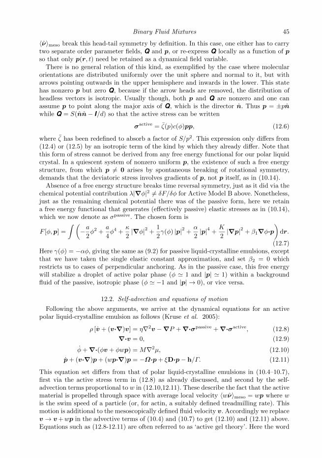
Binary Fluid Mixtures 45
〈ν〉meso break this head-tail symmetry by definition. In this case, one either has to carrytwo separate order parameter fields, Q and p, or re-express Q locally as a function of pso that only p(r, t) need be retained as a dynamical field variable.
There is no general relation of this kind, as exemplified by the case where molecularorientations are distributed uniformly over the unit sphere and normal to it, but witharrows pointing outwards in the upper hemisphere and inwards in the lower. This statehas nonzero p but zero Q, because if the arrow heads are removed, the distribution ofheadless vectors is isotropic. Usually though, both p and Q are nonzero and one canassume p to point along the major axis of Q, which is the director n. Thus p = ±pnwhile Q = S(nn− I/d) so that the active stress can be written
σactive = ζ(p)c(φ)pp, (12.6)
where ζ has been redefined to absorb a factor of S/p2. This expression only differs from(12.4) or (12.5) by an isotropic term of the kind by which they already differ. Note thatthis form of stress cannot be derived from any free energy functional for our polar liquidcrystal. In a quiescent system of nonzero uniform p, the existence of such a free energystructure, from which p 6= 0 arises by spontaneous breaking of rotational symmetry,demands that the deviatoric stress involves gradients of p, not p itself, as in (10.14).
Absence of a free energy structure breaks time reversal symmetry, just as it did via thechemical potential contribution λ|∇φ|2 6= δF/δφ for Active Model B above. Nonetheless,just as the remaining chemical potential there was of the passive form, here we retaina free energy functional that generates (effectively passive) elastic stresses as in (10.14),which we now denote as σpassive. The chosen form is
F [φ,p] =
∫ (−a
2φ2 +
a
4φ4 +
κ
2|∇φ|2 +
1
2γ(φ) |p|2 +
α
2|p|4 +
K
2|∇p|2 + β1∇φ·p
)dr.
(12.7)Here γ(φ) = −αφ, giving the same as (9.2) for passive liquid-crystalline emulsions, exceptthat we have taken the single elastic constant approximation, and set β2 = 0 whichrestricts us to cases of perpendicular anchoring. As in the passive case, this free energywill stabilize a droplet of active polar phase (φ ' 1 and |p| ' 1) within a backgroundfluid of the passive, isotropic phase (φ ' −1 and |p| → 0), or vice versa.
12.2. Self-advection and equations of motion
Following the above arguments, we arrive at the dynamical equations for an activepolar liquid-crystalline emulsion as follows (Kruse et al. 2005):
ρ [v + (v·∇)v] = η∇2v −∇P +∇·σpassive +∇·σactive, (12.8)
∇·v = 0, (12.9)
φ+∇·(φv + φwp) = M∇2µ, (12.10)
p+ (v·∇)p+ (wp·∇)p = −Ω·p+ ξD·p− h/Γ. (12.11)
This equation set differs from that of polar liquid-crystalline emulsions in (10.4–10.7),first via the active stress term in (12.8) as already discussed, and second by the self-advection terms proportional to w in (12.10,12.11). These describe the fact that the activematerial is propelled through space with average local velocity 〈wν〉meso = wp where wis the swim speed of a particle (or, for actin, a suitably defined treadmilling rate). Thismotion is additional to the mesoscopically defined fluid velocity v. Accordingly we replacev → v+wp in the advective terms of (10.4) and (10.7) to get (12.10) and (12.11) above.Equations such as (12.8-12.11) are often referred to as ‘active gel theory’. Here the word
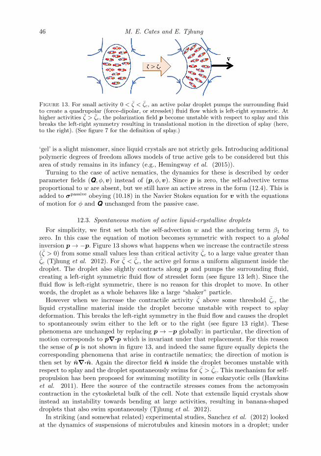
46 M. E. Cates and E. Tjhung
Figure 13. For small activity 0 < ζ < ζc, an active polar droplet pumps the surrounding fluidto create a quadrupolar (force-dipolar, or stresslet) fluid flow which is left-right symmetric. Athigher activities ζ > ζc, the polarization field p become unstable with respect to splay and thisbreaks the left-right symmetry resulting in translational motion in the direction of splay (here,to the right). (See figure 7 for the definition of splay.)
‘gel’ is a slight misnomer, since liquid crystals are not strictly gels. Introducing additionalpolymeric degrees of freedom allows models of true active gels to be considered but thisarea of study remains in its infancy (e.g., Hemingway et al. (2015)).
Turning to the case of active nematics, the dynamics for these is described by orderparameter fields (Q, φ,v) instead of (p, φ,v). Since p is zero, the self-advective termsproportional to w are absent, but we still have an active stress in the form (12.4). This isadded to σpassive obeying (10.18) in the Navier Stokes equation for v with the equationsof motion for φ and Q unchanged from the passive case.
12.3. Spontaneous motion of active liquid-crystalline droplets
For simplicity, we first set both the self-advection w and the anchoring term β1 tozero. In this case the equation of motion becomes symmetric with respect to a globalinversion p→ −p. Figure 13 shows what happens when we increase the contractile stress(ζ > 0) from some small values less than critical activity ζc to a large value greater thanζc (Tjhung et al. 2012). For ζ < ζc, the active gel forms a uniform alignment inside thedroplet. The droplet also slightly contracts along p and pumps the surrounding fluid,creating a left-right symmetric fluid flow of stresslet form (see figure 13 left). Since thefluid flow is left-right symmetric, there is no reason for this droplet to move. In otherwords, the droplet as a whole behaves like a large “shaker” particle.
However when we increase the contractile activity ζ above some threshold ζc, theliquid crystalline material inside the droplet become unstable with respect to splaydeformation. This breaks the left-right symmetry in the fluid flow and causes the dropletto spontaneously swim either to the left or to the right (see figure 13 right). Thesephenomena are unchanged by replacing p→ −p globally: in particular, the direction ofmotion corresponds to p∇·p which is invariant under that replacement. For this reasonthe sense of p is not shown in figure 13, and indeed the same figure equally depicts thecorresponding phenomena that arise in contractile nematics; the direction of motion isthen set by n∇·n. Again the director field n inside the droplet becomes unstable withrespect to splay and the droplet spontaneously swims for ζ > ζc. This mechanism for self-propulsion has been proposed for swimming motility in some eukaryotic cells (Hawkinset al. 2011). Here the source of the contractile stresses comes from the actomyosincontraction in the cytoskeletal bulk of the cell. Note that extensile liquid crystals showinstead an instability towards bending at large activities, resulting in banana-shapeddroplets that also swim spontaneously (Tjhung et al. 2012).
In striking (and somewhat related) experimental studies, Sanchez et al. (2012) lookedat the dynamics of suspensions of microtubules and kinesin motors in a droplet; under
Binary Fluid Mixtures 47
the conditions used, these form an extensile nematic phase. They observed spontaneousmotion of the droplet driven by the activity of the kinesin motors, albeit with complexdynamics resulting in non-Brownian diffusion at the droplet scale. A further complicationin this system is that the active gel phase separates into a thin layer near the dropletsurface; indeed these experiments have fuelled theoretical and numerical studies of activenematics in quasi-2D geometries. Both experiments and simulations show complex flowpatterns within the 2D film, driven primarily by defect motion. Intriguingly, defects oftopological charge −1/2 are advected by the flow field v in a quasi-passive manner,whereas those of charge +1/2 have additionally an active ballistic motion, somewhatresembling the self-propulsion of contractile emulsion droplets described in the previousparagraph (Giomi et al. 2013). This stems from the fact that the +1/2 defect structurebreaks spatial symmetry because it looks like an arrow, unlike the −1/2 case which is3-fold symmetrical (see figure 8(a)). The ballistic separation of defect pairs, which arecreated by active flow, counters the normal passive evolution in which ±1/2 defects areattracted to one another and gradually annihilate to give an increasingly ordered state;this competition allows the active system to attain a stationary chaotic flow.
Active polar and nematic emulsions models have also been used to address the bi-ological process of cell division, known as mitosis. During mitosis, the filaments of thecytoskeleton self-organize themselves to create a structure called the ‘mitotic spindle’ thatin liquid-crystalline language can be viewed as a pair of +1 aster defects. Experimentalmeasurements of the fluctuations in the mitotic spindle shows very good agreement withthose predicted from the active gel theory outlined above (Brugues & Needleman 2014).Once the two asters are created, subsequent division of the droplet can be explainedmainly by equilibrium free energy minimization. Specifically, if the anchoring term β1
is much larger than the elastic constant K, division into two equally-sized dropletsis energetically favourable. However, if the elastic constant K is much larger thanβ1, the droplet only elongates, without dividing (Leoni et al. 2017). This is one ofseveral examples where a complex and highly regulated biophysical process can beimpersonated by models involving minimal physical ingredients, prompting speculationthat the biochemical machinery of the cell is sometimes used to control and exploitthe autonomous function of generic active-matter building blocks, rather than to createcellular functionality from scratch. We next address another example of this type.
12.4. Active emulsion droplets and the physics of cell crawling
Some eukaryotic cell types, such as keratocytes, are able to crawl on a solid substratesuch as glass slide (Verkhovsky et al. 1999). The crawling motility is driven mainly by theactin treadmilling process. The actin filaments are found mostly at the leading edge of thecrawling cell where they have polarization p = 〈ν〉meso. The filaments polymerise at theirfront (plus) ends and therefore self-advect in the direction of p, creating forward motionof the entire cell. An important feature is that the actin filaments communicate chemo-mechanically with the supporting wall through structures called ‘focal adhesions’. Theseprovide anchorpoints for the filaments so that their treadmilling is converted into a tank-treading motion of the cellular perimeter, driving the cell forward. This communicationtakes place across the plasma membrane, a lipid bilayer that encloses the cell.
To model this situation within active gel theory, we consider an active polar droplet ona solid substrate as shown in figure 14(a). For simplicity the confining plasma membraneis not modelled directly; instead there is, as usual, an interfacial tension between theinterior of the droplet (or now cell) and the exterior. Focal adhesions are accounted forvia a no-slip or partial-slip boundary condition on the fluid flow at the wall. We introducea free energy functional similar to (12.7), but assume either (a) that the polarization field
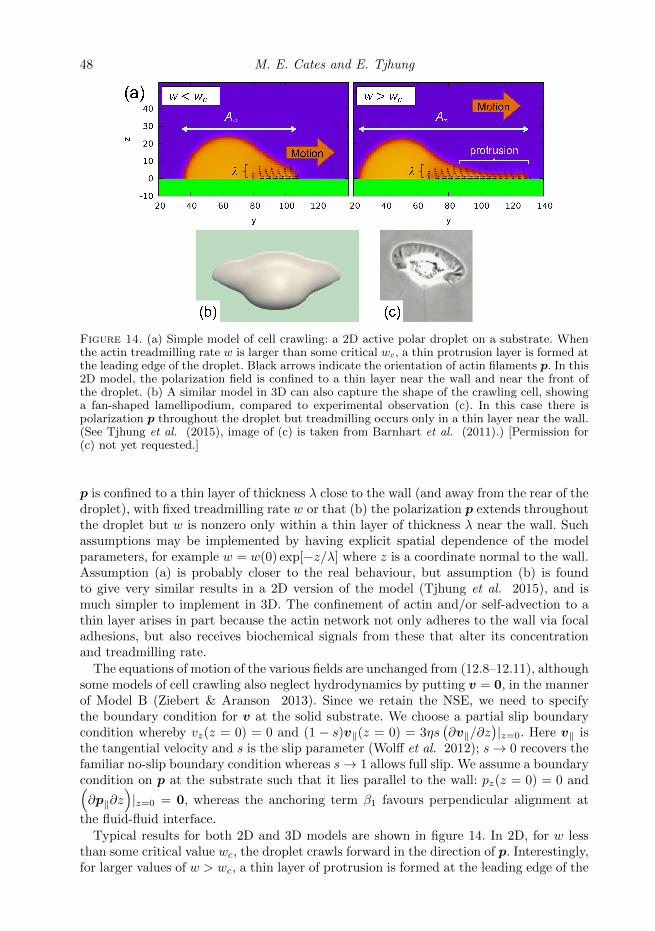
48 M. E. Cates and E. Tjhung
Figure 14. (a) Simple model of cell crawling: a 2D active polar droplet on a substrate. Whenthe actin treadmilling rate w is larger than some critical wc, a thin protrusion layer is formed atthe leading edge of the droplet. Black arrows indicate the orientation of actin filaments p. In this2D model, the polarization field is confined to a thin layer near the wall and near the front ofthe droplet. (b) A similar model in 3D can also capture the shape of the crawling cell, showinga fan-shaped lamellipodium, compared to experimental observation (c). In this case there ispolarization p throughout the droplet but treadmilling occurs only in a thin layer near the wall.(See Tjhung et al. (2015), image of (c) is taken from Barnhart et al. (2011).) [Permission for(c) not yet requested.]
p is confined to a thin layer of thickness λ close to the wall (and away from the rear of thedroplet), with fixed treadmilling rate w or that (b) the polarization p extends throughoutthe droplet but w is nonzero only within a thin layer of thickness λ near the wall. Suchassumptions may be implemented by having explicit spatial dependence of the modelparameters, for example w = w(0) exp[−z/λ] where z is a coordinate normal to the wall.Assumption (a) is probably closer to the real behaviour, but assumption (b) is foundto give very similar results in a 2D version of the model (Tjhung et al. 2015), and ismuch simpler to implement in 3D. The confinement of actin and/or self-advection to athin layer arises in part because the actin network not only adheres to the wall via focaladhesions, but also receives biochemical signals from these that alter its concentrationand treadmilling rate.
The equations of motion of the various fields are unchanged from (12.8–12.11), althoughsome models of cell crawling also neglect hydrodynamics by putting v = 0, in the mannerof Model B (Ziebert & Aranson 2013). Since we retain the NSE, we need to specifythe boundary condition for v at the solid substrate. We choose a partial slip boundarycondition whereby vz(z = 0) = 0 and (1 − s)v‖(z = 0) = 3ηs
(∂v‖/∂z
)|z=0. Here v‖ is
the tangential velocity and s is the slip parameter (Wolff et al. 2012); s→ 0 recovers thefamiliar no-slip boundary condition whereas s→ 1 allows full slip. We assume a boundarycondition on p at the substrate such that it lies parallel to the wall: pz(z = 0) = 0 and(∂p‖∂z
)|z=0 = 0, whereas the anchoring term β1 favours perpendicular alignment at
the fluid-fluid interface.
Typical results for both 2D and 3D models are shown in figure 14. In 2D, for w lessthan some critical value wc, the droplet crawls forward in the direction of p. Interestingly,for larger values of w > wc, a thin layer of protrusion is formed at the leading edge of the
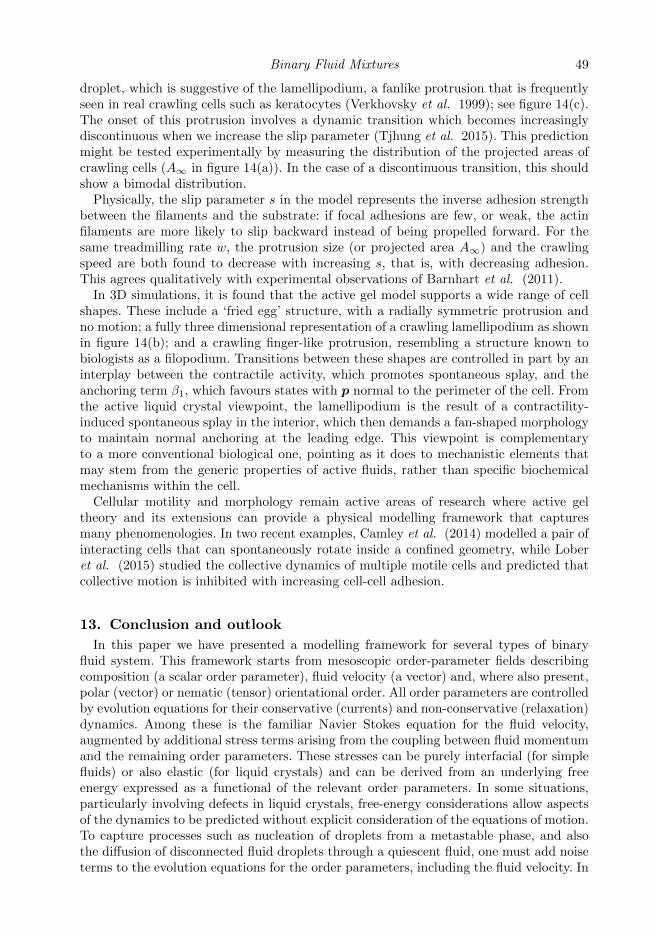
Binary Fluid Mixtures 49
droplet, which is suggestive of the lamellipodium, a fanlike protrusion that is frequentlyseen in real crawling cells such as keratocytes (Verkhovsky et al. 1999); see figure 14(c).The onset of this protrusion involves a dynamic transition which becomes increasinglydiscontinuous when we increase the slip parameter (Tjhung et al. 2015). This predictionmight be tested experimentally by measuring the distribution of the projected areas ofcrawling cells (A∞ in figure 14(a)). In the case of a discontinuous transition, this shouldshow a bimodal distribution.
Physically, the slip parameter s in the model represents the inverse adhesion strengthbetween the filaments and the substrate: if focal adhesions are few, or weak, the actinfilaments are more likely to slip backward instead of being propelled forward. For thesame treadmilling rate w, the protrusion size (or projected area A∞) and the crawlingspeed are both found to decrease with increasing s, that is, with decreasing adhesion.This agrees qualitatively with experimental observations of Barnhart et al. (2011).
In 3D simulations, it is found that the active gel model supports a wide range of cellshapes. These include a ‘fried egg’ structure, with a radially symmetric protrusion andno motion; a fully three dimensional representation of a crawling lamellipodium as shownin figure 14(b); and a crawling finger-like protrusion, resembling a structure known tobiologists as a filopodium. Transitions between these shapes are controlled in part by aninterplay between the contractile activity, which promotes spontaneous splay, and theanchoring term β1, which favours states with p normal to the perimeter of the cell. Fromthe active liquid crystal viewpoint, the lamellipodium is the result of a contractility-induced spontaneous splay in the interior, which then demands a fan-shaped morphologyto maintain normal anchoring at the leading edge. This viewpoint is complementaryto a more conventional biological one, pointing as it does to mechanistic elements thatmay stem from the generic properties of active fluids, rather than specific biochemicalmechanisms within the cell.
Cellular motility and morphology remain active areas of research where active geltheory and its extensions can provide a physical modelling framework that capturesmany phenomenologies. In two recent examples, Camley et al. (2014) modelled a pair ofinteracting cells that can spontaneously rotate inside a confined geometry, while Loberet al. (2015) studied the collective dynamics of multiple motile cells and predicted thatcollective motion is inhibited with increasing cell-cell adhesion.
13. Conclusion and outlook
In this paper we have presented a modelling framework for several types of binaryfluid system. This framework starts from mesoscopic order-parameter fields describingcomposition (a scalar order parameter), fluid velocity (a vector) and, where also present,polar (vector) or nematic (tensor) orientational order. All order parameters are controlledby evolution equations for their conservative (currents) and non-conservative (relaxation)dynamics. Among these is the familiar Navier Stokes equation for the fluid velocity,augmented by additional stress terms arising from the coupling between fluid momentumand the remaining order parameters. These stresses can be purely interfacial (for simplefluids) or also elastic (for liquid crystals) and can be derived from an underlying freeenergy expressed as a functional of the relevant order parameters. In some situations,particularly involving defects in liquid crystals, free-energy considerations allow aspectsof the dynamics to be predicted without explicit consideration of the equations of motion.To capture processes such as nucleation of droplets from a metastable phase, and alsothe diffusion of disconnected fluid droplets through a quiescent fluid, one must add noiseterms to the evolution equations for the order parameters, including the fluid velocity. In
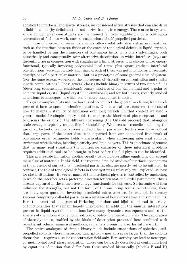
50 M. E. Cates and E. Tjhung
addition to interfacial and elastic stresses, we considered active stresses that can also drivea fluid flow but (by definition) do not derive from a free energy. These arise in systemswhose fundamental constituents are maintained far from equilibrium by a continuousconversion of fuel into work, such as suspensions of self-propelled particles.
Our use of mesoscopic order parameters allows relatively sharp structural features,such as the interface between fluids or the cores of topological defects in liquid crystals,to be handled within the framework of continuous fields. This offers advantages, bothnumerically and conceptually, over alternative descriptions in which interfaces (say) arediscontinuities in composition with singular interfacial stresses. Our choices of free energyfunctional, typically involving polynomial local terms plus square-gradient interfacialcontributions, were deliberately kept simple: each of these was not intended as an accuratedescriptions of a particular material, but as a prototype of some general class of system.(For the same reason, we ignored the dependence of viscosity on concentration and similarkinetic complications.) Those general classes include binary mixtures of two simple fluids(describing conventional emulsions); binary mixtures of one simple fluid and a polar ornematic liquid crystal (liquid crystalline emulsions); and for both cases, recently studiedextensions to analogues in which one or more component is active.
To give examples of its use, we have tried to connect the general modelling frameworkpresented here to specific scientific questions. One classical area concerns the issue ofhow to maintain stability of emulsions over long periods. In that context we used ageneric model for simple binary fluids to explore the kinetics of phase separation andto discuss the origins of the diffusive coarsening (the Ostwald process) that, alongsidecoalescence, is typically responsible for instability. We discussed remedies including theuse of surfactants, trapped species and interfacial particles. Readers may have noticedthat large parts of the latter discussion departed from our announced framework ofcontinuous order parameter fields – particularly when addressing interfacial colloids,surfactant micellization, bending elasticity and lipid bilayers. This is an acknowledgementthat in many real situations the multi-scale character of these interfacial problemsrequires additional tools to be brought to bear before the full physics can be identified.
This multi-scale limitation applies equally to liquid-crystalline emulsions, our secondmain class of materials. In this field, the required detailed studies of interfacial phenomenain the presence of surfactants, interfacial particles, etc., are mostly yet to be initiated. Incontrast, the role of topological defects in these systems is relatively well explored, at leastfor static situations. However, much of the interfacial physics is controlled by anchoring,in which the interface sets a preferred direction for orientational order parameters; this isalready captured in the chosen free energy functionals for this case. Surfactants will theninfluence the strengths, but not the form, of the anchoring terms. Nonetheless, thereare many open questions involving interfacial microstructure, for example in ternarysystems comprising colloidal particles in a mixture of liquid-crystalline and simple fluids.Here the structural analogues of Pickering emulsions and bijels could lead to a rangeof functionalities that remain largely unexplored. In addition, the unusual interactionspresent in liquid-crystalline emulsions have many dynamical consequences such as thekinetics of chain formation among isotropic droplets in a nematic matrix. The explorationof these dynamics, enabled by the kinds of description presented here combined withrecently introduced numerical methods, remains a promising area for future work.
The active analogues of simple binary fluids include suspensions of spherical, self-propelled colloids whose mesoscopic description – now at a scale larger than the colloidsthemselves – requires a scalar concentration field only. Here activity can lead to new typesof ‘motility-induced’ phase separation. These can be partly described at continuum levelby equations of motion that differ from those studied historically (Models B and H)
Binary Fluid Mixtures 51
by active contributions to the compositional current and the stress. One experimentalmystery is the observation that such active phase separation is often incomplete, cul-minating in a state of dynamical clusters whose average size no longer increases withtime. Various system-specific microscopic interpretations of this behaviour have beenoffered; continuing work on active continuum models aims to clarify whether fully genericmechanisms also exist.
For rodlike swimmers and filamentary cytoskeletal materials the corresponding theoryis that of active liquid crystals, which are commonly, but not always, polar ratherthan nematic. (The opposite is true for the passive case.) Within our general modellingframework, theories for binary systems involving these materials are again obtained byselectively adding active terms, that break time-reversal symmetry and do not thereforestem from any free energy, to the equations of motion of an otherwise passive system.For active polar media the main terms are an active stress and self-advection of thepolarization and concentration fields. The latter encodes the mean effect of either self-propulsion along the polarization vector of individual molecules, or, in the case of actinfilaments, polymerization at one end and depolymerization at the other. These self-advection contributions are absent in active nematics, whose mean polarization is zeroby definition.
When such active terms are included in theories of polar liquid-crystal emulsions,some surprising phenomena emerge which appear similar to observations of contractility-induced swimming and cell-division in biological cells. Allowing also for spatial variationsof the active terms within an emulsion droplet next to a solid wall, these similaritiesextend to cell-crawling, where the occurrence of a fan-shaped protrusion at the front ofthe crawling cell emerges from an interplay of a splay instability caused by activity andthe anchoring of polarity at the droplet surface. These are among the first findings of anew and developing field in which continuum theories of active fluids form a platform forphysics-inspired models of biological function. The aim of these models is not to replacethe biologists’ understanding of cellular motility and related functionality, which is largelybased on a relatively detailed analysis of underlying biochemical process. Rather, the aimis to determine the extent to which these processes are necessary to sustain even basicmodes of functionality, and the extent to which they instead exert close control over aset of pre-existing autonomous behaviours that are generically present in active fluids,whether closely controlled or not.
Acknowledgements
Sections 1–8 of this article are based in part on previous lecture notes by one ofus (Cates 2012). We acknowledge the contributions of numerous colleagues, studentsand collaborators with whom we have discussed the topics covered in this article. MECacknowledges funding from the Royal Society in the form of a Research Professorship.We thank Kevin Stratford, Paul Clegg and Adriano Tiribocchi for the images in figures3, 6 and 11 (right) respectively.
REFERENCES
Andelman D., Cates, M. E., Roux D. & Safran S. A. 1987 Structure and phase equilibriaof microemulsions, J. Chem. Phys. 87, 7229–7241.
Anderson V. J., Terentjev E. M., Meeker S. P., Crain J. & Poon W. C. K. 2001Cellular solid behaviour of liquid crystal colloids -1. Phase separation and morphology,Eur. Phys. J. E 4 11–20.
Aranson I. S. 2016 Physical Models of Cell Motility, Springer.
52 M. E. Cates and E. Tjhung
Aveyard R. 2012 Can Janus particles give thermodynamically stable Pickering emulsions? SoftMatt. 8, 5233–5240.
Barnhart E. L., Lee K.-C., Keren K., Mogilner A. & Theriot J. A. 2011 An adhesion-dependent switch between mechanisms that determine motile cell shape, PLoS Biol. 9,e1001059.
Beris A. N. & Edwards B. J. 1994 Thermodynamics of Flowing Systems with InternalMicrostructure, Oxford University Press.
Bibette, J., Leal-Calderon, F., Schmitt ,V. & Poulin P. 2002 Emulsion Science, Springer.Binks B. P. & Horozov, T. S., Eds. 2006 Colloidal Particles at Liquid Interfaces, Cambridge.Bouteiller, L & LeBarny, P. 1996 Polymer-dispersed liquid crystals: Preparation, operation
and application, Liquid Crystals bf 21, 157–174.Brady, J. F. & Bossis, G. 1988 Stokesian dynamics, Ann. Rev. Fluid Mech. 20, 111–157.Bray A. J. 1994 Theory of phase-ordering kinetics, Advances in Physics, 43, 357–459.Brugues J. & Needleman D. 2014 Physical basis of spindle self-organization, Proc. Natl.
Acad. Sci. USA, 111, 18496–18500.Buttinoni I., Bialke J., Kummel F., Lowen H., Bechinger C. & Speck T. Dynamic
clustering and phase separation in suspensions of self-propelled colloidal particles, Phys.Rev. Lett. 110 238301.
Camley B. A., Zhang Y., Zhao Y., Li B., Ben-Jacob E., Levine H. & Rappel W.-J. 2014 Polarity mechanism such as contact inhibition of locomotion regulate persistentrotational motion of mammalian cells on micropatterns, Proc. Natl. Acad. Sci. USA 111,14770–14775.
Cates, M. E., Henrich, O., Marenduzzo, D. & Stratford, K., 2009 Lattice Boltzmannsimulations of liquid crystalline fluids: Active gels and Blue Phases, Soft Matter 5, 3791–3800.
Cates, M. E. 2012 Complex fluids: The physics of emulsions, arXiv preprint, 1209.2290; Ch.10 in Soft Interfaces (proceedings of les Houches 2012 Summer School, Session XCVIII),Bocquet L., Quere D., Witten T. A. & Cugliandolo L. F., et al, Eds., Oxford UniversityPress 2017.
Cates M. E. & Clegg P. S. 2008 Bijels: a new class of soft materials, Soft Matter 4 2132–2138.Cates, M. E. & Tailleur, J. 2015 Motility-induced phase separation, Ann. Rev. Cond. Mat.
Phys. 6, 219–244.Cavallaro M., Botto L., Lewandowski E. P.,1, Wang M. & Stebe K. J. 2011 Curvature-
driven capillary migration and assembly of rod-like particles, Proc. Nat. Acad. Sci. USA,108, 20923–20928.
Chaikin, P. M. & Lubensky, T. C. 1995 Principles of Condensed Matter Physics CambridgeUniversity Press.
Clegg P. S., Tavacoli J. W. & Wilde P. J. 2016 One-step production of multiple emulsions:microfluidic, polymer-stabilized and particle-stabilized approaches, Soft Matter 12, 998–1008.
David, F. 2004 Geometry and field theory of random surfaces and membranes, in Nelson D. R.,Piran T. and Weinberg S., Eds., Statistical Mechanics of Membranes and Surfaces, WorldScientific.
de Gennes P.-G. & Taupin C. 1982 Microemulsions and the flexibility of oil-water interfaces,J. Phys. Chem. 86, 2294–2304.
de Gennes P. G. & Prost J. 2002 The Physics of Liquid Crystals, 2nd Edition, Oxford SciencePublication, Oxford.
Doi M. & Ohta T. 1991 Dynamics and rheology of complex interfaces, J. Chem. Phys. 95,1242–1248.
Fernandez-Nieves A., Link D. R., Marquez M. & Weitz D. A. 2007 Topological changesin bipolar nematic droplets under flow, Phys. Rev. Lett. 98, 087801.
Fielding S. M. 2008 Role of inertia in nonequilibrium steady states of sheared binary fluids,Phys. Rev. E 77, 021504.
Fodor E., Nardini C., Cates M. E., Tailleur J., Visco P., van Wijland F. 2016 Howfar from equilibrium is active matter? Phys. Rev. Lett. 117, 038103.
Fryd M. M., Mason T. G. 2012 Advanced nanoemulsions, Ann. Rev. Phys. Chem. 63, 493–518.
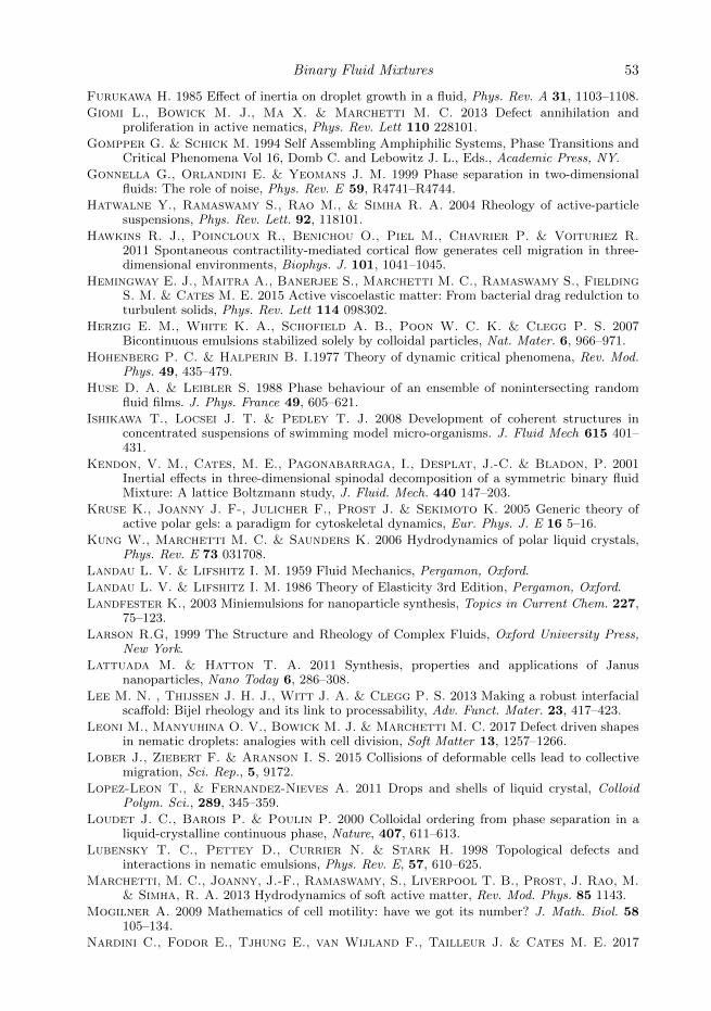
Binary Fluid Mixtures 53
Furukawa H. 1985 Effect of inertia on droplet growth in a fluid, Phys. Rev. A 31, 1103–1108.
Giomi L., Bowick M. J., Ma X. & Marchetti M. C. 2013 Defect annihilation andproliferation in active nematics, Phys. Rev. Lett 110 228101.
Gompper G. & Schick M. 1994 Self Assembling Amphiphilic Systems, Phase Transitions andCritical Phenomena Vol 16, Domb C. and Lebowitz J. L., Eds., Academic Press, NY.
Gonnella G., Orlandini E. & Yeomans J. M. 1999 Phase separation in two-dimensionalfluids: The role of noise, Phys. Rev. E 59, R4741–R4744.
Hatwalne Y., Ramaswamy S., Rao M., & Simha R. A. 2004 Rheology of active-particlesuspensions, Phys. Rev. Lett. 92, 118101.
Hawkins R. J., Poincloux R., Benichou O., Piel M., Chavrier P. & Voituriez R.2011 Spontaneous contractility-mediated cortical flow generates cell migration in three-dimensional environments, Biophys. J. 101, 1041–1045.
Hemingway E. J., Maitra A., Banerjee S., Marchetti M. C., Ramaswamy S., FieldingS. M. & Cates M. E. 2015 Active viscoelastic matter: From bacterial drag redulction toturbulent solids, Phys. Rev. Lett 114 098302.
Herzig E. M., White K. A., Schofield A. B., Poon W. C. K. & Clegg P. S. 2007Bicontinuous emulsions stabilized solely by colloidal particles, Nat. Mater. 6, 966–971.
Hohenberg P. C. & Halperin B. I.1977 Theory of dynamic critical phenomena, Rev. Mod.Phys. 49, 435–479.
Huse D. A. & Leibler S. 1988 Phase behaviour of an ensemble of nonintersecting randomfluid films. J. Phys. France 49, 605–621.
Ishikawa T., Locsei J. T. & Pedley T. J. 2008 Development of coherent structures inconcentrated suspensions of swimming model micro-organisms. J. Fluid Mech 615 401–431.
Kendon, V. M., Cates, M. E., Pagonabarraga, I., Desplat, J.-C. & Bladon, P. 2001Inertial effects in three-dimensional spinodal decomposition of a symmetric binary fluidMixture: A lattice Boltzmann study, J. Fluid. Mech. 440 147–203.
Kruse K., Joanny J. F-, Julicher F., Prost J. & Sekimoto K. 2005 Generic theory ofactive polar gels: a paradigm for cytoskeletal dynamics, Eur. Phys. J. E 16 5–16.
Kung W., Marchetti M. C. & Saunders K. 2006 Hydrodynamics of polar liquid crystals,Phys. Rev. E 73 031708.
Landau L. V. & Lifshitz I. M. 1959 Fluid Mechanics, Pergamon, Oxford.
Landau L. V. & Lifshitz I. M. 1986 Theory of Elasticity 3rd Edition, Pergamon, Oxford.
Landfester K., 2003 Miniemulsions for nanoparticle synthesis, Topics in Current Chem. 227,75–123.
Larson R.G, 1999 The Structure and Rheology of Complex Fluids, Oxford University Press,New York.
Lattuada M. & Hatton T. A. 2011 Synthesis, properties and applications of Janusnanoparticles, Nano Today 6, 286–308.
Lee M. N. , Thijssen J. H. J., Witt J. A. & Clegg P. S. 2013 Making a robust interfacialscaffold: Bijel rheology and its link to processability, Adv. Funct. Mater. 23, 417–423.
Leoni M., Manyuhina O. V., Bowick M. J. & Marchetti M. C. 2017 Defect driven shapesin nematic droplets: analogies with cell division, Soft Matter 13, 1257–1266.
Lober J., Ziebert F. & Aranson I. S. 2015 Collisions of deformable cells lead to collectivemigration, Sci. Rep., 5, 9172.
Lopez-Leon T., & Fernandez-Nieves A. 2011 Drops and shells of liquid crystal, ColloidPolym. Sci., 289, 345–359.
Loudet J. C., Barois P. & Poulin P. 2000 Colloidal ordering from phase separation in aliquid-crystalline continuous phase, Nature, 407, 611–613.
Lubensky T. C., Pettey D., Currier N. & Stark H. 1998 Topological defects andinteractions in nematic emulsions, Phys. Rev. E, 57, 610–625.
Marchetti, M. C., Joanny, J.-F., Ramaswamy, S., Liverpool T. B., Prost, J. Rao, M.& Simha, R. A. 2013 Hydrodynamics of soft active matter, Rev. Mod. Phys. 85 1143.
Mogilner A. 2009 Mathematics of cell motility: have we got its number? J. Math. Biol. 58105–134.
Nardini C., Fodor E., Tjhung E., van Wijland F., Tailleur J. & Cates M. E. 2017
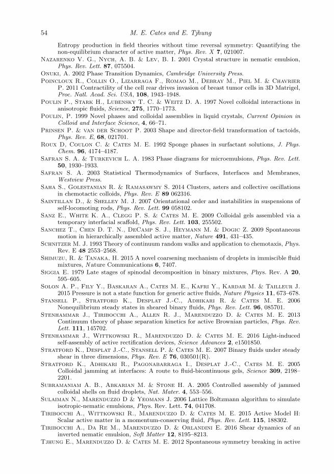
54 M. E. Cates and E. Tjhung
Entropy production in field theories without time reversal symmetry: Quantifying thenon-equilibrium character of active matter, Phys. Rev. X 7, 021007.
Nazarenko V. G., Nych, A. B. & Lev, B. I. 2001 Crystal structure in nematic emulsion,Phys. Rev. Lett. 87, 075504.
Onuki, A. 2002 Phase Transition Dynamics, Cambridge University Press.Poincloux R., Collin O., Lizarraga F., Romao M., Debray M., Piel M. & Chavrier
P. 2011 Contractility of the cell rear drives invasion of breast tumor cells in 3D Matrigel,Proc. Natl. Acad. Sci. USA, 108, 1943–1948.
Poulin P., Stark H., Lubensky T. C. & Weitz D. A. 1997 Novel colloidal interactions inanisotropic fluids, Science, 275, 1770–1773.
Poulin, P. 1999 Novel phases and colloidal assemblies in liquid crystals, Current Opinion inColloid and Interface Science, 4, 66–71.
Prinsen P. & van der Schoot P. 2003 Shape and director-field transformation of tactoids,Phys. Rev. E, 68, 021701.
Roux D, Coulon C. & Cates M. E. 1992 Sponge phases in surfactant solutions, J. Phys.Chem. 96, 4174–4187.
Safran S. A. & Turkevich L. A. 1983 Phase diagrams for microemulsions, Phys. Rev. Lett.50, 1930–1933.
Safran S. A. 2003 Statistical Thermodynamics of Surfaces, Interfaces and Membranes,Westview Press.
Saha S., Golestanian R. & Ramasawmy S. 2014 Clusters, asters and collective oscillationsin chemotactic colloids, Phys. Rev. E 89 062316.
Saintillan D., & Shelley M. J. 2007 Orientational order and instabilities in suspensions ofself-locomoting rods, Phys. Rev. Lett. 99 058102.
Sanz E., White K. A., Clegg P. S. & Cates M. E. 2009 Colloidal gels assembled via atemporary interfacial scaffold, Phys. Rev. Lett. 103, 255502.
Sanchez T., Chen D. T. N., DeCamp S. J., Heymann M. & Dogic Z. 2009 Spontaneousmotion in hierarchically assembled active matter, Nature 491, 431–435.
Schnitzer M. J. 1993 Theory of continuum random walks and application to chemotaxis, Phys.Rev. E 48 2553–2568.
Shimuzu, R. & Tanaka, H. 2015 A novel coarsening mechanism of droplets in immiscible fluidmixtures, N ature Communications 6, 7407.
Siggia E. 1979 Late stages of spinodal decomposition in binary mixtures, Phys. Rev. A 20,595–605.
Solon A. P., Fily Y., Baskaran A., Cates M. E., Kafri Y., Kardar M. & Tailleur J.2015 Pressure is not a state function for generic active fluids, Nature Physics 11, 673–678.
Stansell P., Stratford K., Desplat J.-C., Adhikari R. & Cates M. E. 2006Nonequilibrium steady states in sheared binary fluids, Phys. Rev. Lett. 96, 085701.
Stenhammar J., Tiribocchi A., Allen R. J., Marenduzzo D. & Cates M. E. 2013Continuum theory of phase separation kinetics for active Brownian particles, Phys. Rev.Lett. 111, 145702.
Stenhammar J., Wittkowski R., Marenduzzo D. & Cates M. E. 2016 Light-inducedself-assembly of active rectification devices, Science Advances 2, e1501850.
Stratford K., Desplat J.-C., Stansell P. & Cates M. E. 2007 Binary fluids under steadyshear in three dimensions, Phys. Rev. E 76, 030501(R).
Stratford K., Adhikari R., Pagonabarraga I., Desplat J.-C., Cates M. E. 2005Colloidal jamming at interfaces: A route to fluid-bicontinuous gels, Science 309, 2198–2201.
Subramaniam A. B., Abkarian M. & Stone H. A. 2005 Controlled assembly of jammedcolloidal shells on fluid droplets, Nat. Mater. 4, 553–556.
Sulaiman N., Marenduzzo D & Yeomans J. 2006 Lattice Boltzmann algorithm to simulateisotropic-nematic emulsions, Phys. Rev. Lett. 74, 041708.
Tiribocchi A., Wittkowski R., Marenduzzo D. & Cates M. E. 2015 Active Model H:Scalar active matter in a momentum-conserving fluid, Phys. Rev. Lett. 115, 188302.
Tiribocchi A., Da Re M., Marenduzzo D. & Orlandini E. 2016 Shear dynamics of aninverted nematic emulsion, Soft Matter 12, 8195–8213.
Tjhung E., Marenduzzo D. & Cates M. E. 2012 Spontaneous symmetry breaking in active
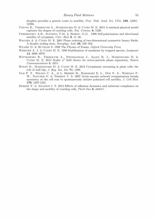
Binary Fluid Mixtures 55
droplets provides a generic route to motility, Proc. Natl. Acad. Sci. USA. 109, 12381–12386.
Tjhung E., Tiribocchi A., Marenduzzo D. & Cates M. E. 2015 A minimal physical modelcaptures the shapes of crawling cells, Nat. Comms. 6, 5420.
Verkhovsky A.B., Svitkina T.M. & Borisy. G.G. 1999 Self-polarization and directionalmotility of cytoplasm, Curr. Biol. 9, 11–20.
Wagner A. & Cates M. E. 2001 Phase ordering of two-dimensional symmetric binary fluids:A droplet scaling state, Europhys. Lett. 56, 556–562.
Weaire D. & Hutzler S. 1999 The Physics of Foams, Oxford University Press.Webster A. J. & Cates M. E. 1998 Stabilization of emulsions by trapped species, Langmuir
14, 2068–2079 .Wittkowski R., Tiribocchi A., Stenhammar J., Allen R. J., Marenduzzo D. &
Cates M. E. 2014 Scalar φ4 field theory for active-particle phase separation, NatureCommunications 5, 4351.
Wolff K., Marenduzzo D. & Cates M. E. 2012 Cytoplasmic streaming in plant cells: therole of wall slip, J. Roy. Soc. Int. 71, 1398.
Yam P. T., Wilson C. A., Ji L. Hebert B., Barnhart E. L., Dye N. A., Wiseman P.W., Danuser G. & Theriot J. A. 2007 Actin–myosin network reorganization breakssymmetry at the cell rear to spontaneously initiate polarized cell motility, J. Cell Biol.178, 1207-1221.
Ziebert F. & Aranson I. S. 2013 Effects of adhesion dynamics and substrate compliance onthe shape and motility of crawling cells, PLoS One 8, e64511.


