Fractal analysis of ostracod shell variability:A comparison with geometric and classic morphometrics

GIUSEPPE AIELLO, FILIPPO BARATTOLO, DIANA BARRA, GRAZIANO FIORITO,

ADRIANO MAZZARELLA, PASQUALE RAIA, and RAFFAELE VIOLA

Aiello, G., Barattolo, F., Barra, D., Fiorito, G., Mazzarella, A., Raia, P., and Viola, R. 2007. Fractal analysis of ostracodshell variability: A comparison with geometric and classic morphometrics. Acta Palaeontologica Polonica 52 (3):563–573.

Two statistical methods, fractal geometry and geometric morphometrics, are tested for their applicability to ostracod sys−tematics. For this comparison, two morphologically similar ostracod species (Krithe compressa and Krithe iniqua) whosegenus−level systematics is still incompletely resolved, are selected. Twenty−nine right valves of each species were col−lected from the upper Pliocene samples at the Monte San Nicola section in southern Italy. Statistical analyses (MANOVAon morphometric shape variables, and D values) were utilized to test if geometric morphometrics and fractal analysis areappropriate into discriminating between the two species. Both methods succeeded in distinguishing the species statisti−cally. The fractal analysis of the two ostracod species shows D values centered on 1.31±0.02 for Krithe iniqua and on1.40±0.02 for Krithe compressa. Geometric morphometric analysis indicates significant differences between the two spe−cies and allows studying intra−populational variability as well as. The most variable traits indicated by geometric morpho−metrics are vestibular area and posterior outline of the shell, indicating that these traits are the most relevant for the sys−tematics of the species analyzed. Both fractal geometry and geometric morphometrics provide a measure of populationvariability. Fractal analysis has the advantage of being free from any subjectivity in the selection of characters and couldbe most appropriate to use for analysis of complex ornamentation for systematic purposes. However, a possible advantageof geometric morphometrics over fractal analysis is its ability to indicate where statistically significant variations in shapeoccur on the shell.

Key words: Ostracoda, Krithe, fractal geometry, geometric morphometrics, morphological variability, systematics.

Giuseppe Aiello [aie64llo@hotmail.com], Filippo Barattolo [lippolo@unina.it], and Diana Barra [dibarra@unina.it],Dipartimento di Scienze della Terra, Università di Napoli “Federico II”, Largo S. Marcellino, 10, 80138, Napoli, Italy;Graziano Fiorito [gfiorito@szn.it], Stazione Zoologica “Anton Dohrn”, Villa Comunale, 1−80121 Napoli, Italy;Adriano Mazzarella [adriano.mazzarella@unina.it] and Raffaele Viola [rafviola@unina.it], Dipartimento di Geofisicae Vulcanologia, Università di Napoli “Federico II”, Largo S. Marcellino, 10, 80138 Napoli, Italy;Pasquale Raia [pasquale.raia@libero.it], Dipartimento S.T.A.T. Università del Molise, Isernia, Via Mazzini 8, 86170,Isernia, Italy.

Introduction

Analysis of morphological variability is one of the funda−mental steps for the resolution of taxonomic problems. As−sessment of the amount and nature of morphological vari−ability among organisms, both living and fossil, is currentlybenefiting from mathematical studies that allow statisticalanalysis of morphological disparity in a given group for agiven time−interval.

Several techniques are currently being used to describeand measure morphological variability. However there is nogeneral agreement among researchers on the appropriatenessof one method over the others.

The aim of this paper is to compare the relative power andappropriateness of fractal geometry and geometric morpho−metrics for taxonomy. By attributing a numerical value to acurved line, fractal geometry provides a method of standardi−

sation when trying to distinguish between different species.On the other hand, geometric morphometrics has the advan−tage of topologically investigating shape variation throughthin plate spline visualization, thereby providing a potentialconnection with the naked−eye approaches of classical sys−tematics.

In requiring a certain number of specimens for statisticalanalysis, both methods are technically well−suited to the studyof fossil species taxonomy, especially of invertebrates andmicrofossils for which large populations are often available.

This study does not address questions concerning speciesconcepts: natural scientists have discussed the “species prob−lem” extensively, introducing numerous species definitionsbut without reaching full agreement (Mayden 1997). The useof the morphological (or typological) species concept hasbeen severely criticized by the upholders of the biologicalspecies concept (e.g., Mayr 1996) who tend to treat it as an

http://app.pan.pl/acta52/app52−563.pdfActa Palaeontol. Pol. 52 (3): 563–573, 2007

obsolete notion. Despite this criticism, most paleontologistsand many neontologists accept “morphospecies” as a matterof fact in their daily research. For the purpose of this study,some of the modern definitions of morphological species areequally satisfactory. For example, Claridge et al. (1997) de−fined species as “a community, or a number of related com−munities, whose distinctive morphological characters are, inthe opinion of a competent systematist, sufficiently definiteto entitle it, or them, to a specific name”. Cronquist (1988)considered species as “the smallest groups that are consis−tently and persistently distinct and distinguishable by ordi−nary means.”

In the last two decades, the increased use of fractals in thelife sciences has led to many applications in different areas ofresearch in biology, palaeontology and related disciplines.Fractal geometry may contribute to the description and betterunderstanding of a large number of phenomena, rangingfrom the architecture of chromosomes to the structure ofbronchial tubes, and from insects movement to populationgrowth rate, that is, virtually everywhere life expresses itscomplexity (references in Stanley 1992; Nonnenmacher etal. 1994; Kenkel and Walker 1996). The study of the mor−phology of living and fossil organisms by fractals is still notgreatly developed, although some authors have laid thegroundwork with the publication of papers on the fractal di−mension of, for instance, leaf outlines (Vlcek and Cheung1986), root systems (Tatsumi et al. 1989), perimeters of algalspecies (Corbit and Garbary 1995; Davenport et al. 1996)and ammonoid suture lines (Boyajian and Lutz 1992). Vlcekand Cheung (1986) were possibly the first, measuring thefractal dimension of the leaf margins in some tree species andshowing the potential of fractal geometry in taxonomy.

Geometric morphometrics can be traced back to D’ArcyThompson seminal book On Growth and Form (1917). Be−cause of the implicit difficulties in the mathematics involved,full−fledged application to systematics is relatively recent(e.g., Reyment 1993, 1995; Reyment and Abe 1995; Elewa2003, 2004). Since Bookstein’s (1989, 1991) thin plate splinemethod and Rohlf and Slice’s (1990) paper on generalisedleast squares, countless published studies have been added tothe bibliography on geometric morphometrics (Adams et al.2004). Geometric morphometrics has been traditionally usedin taxonomic studies (for ostracods, see Reyment 1993, 1995;Reyment and Abe 1995; Elewa 2003). Yet, the recent litera−ture also provides examples of morphofunctional studies (e.g.,Bruner and Manzi 2004; Raia 2004; to name just a few of thelatest in the field of paleontology).

To achieve the aims of the current paper, two ostracodspecies belonging to Krithe Brady, Crosskey, and Robertson,1874 have been chosen due to the nature of the shell featuresof this genus. Species of Krithe are characterized by havingsmooth valves; consequently, the taxonomic features used todifferentiate species are essentially internal, mainly locatedon the inner lamella. Krithe compressa (Seguenza, 1880) andKrithe iniqua Abate, Barra, Aiello, and Bonaduce, 1993 are

similar but distinct species, previously discussed by Abate etal. (1993).

The shape, width and size of the anterior vestibulum, andthe pattern of marginal pore canals are generally consideredas the most important specific characters. All of these fea−tures are best observed in transmitted light. In contrast to thecarapace ornament of many ostracod taxa, these features arenot well expressed in Krithe.

There is general agreement on the degree of variability ofthese characters; however, different evaluations have beengiven of their range of variation within a single species. Vanden Bold (1968) and Zhou and Ikeya (1992) showed two ex−amples of extremely different approaches: the former figuredspecimens with rather dissimilar vestibula as Krithe dolicho−deira Bold, 1946; the latter split two species, K. antisawa−nensis Ishizaki, 1966 and K. surugensis Zhou and Ikeya,1992, on the basis of very minute morphological details.

Despite disagreement about the importance of some fea−tures, recent studies attempting to clarify the systematics ofvarious species of Krithe (e.g., Abate et al. 1993; Coles etal. 1994; Ayress et al. 1999) have produced encouraging re−sults. The diagnostic criteria accepted in the present paperare the ones used by Abate et al. (1993). It is worth notingthat Krithe species are usually very diffult to demarkate.This is mostly due to ecophenotypic variation of the diag−nostic characters due to environmental factors such as dis−solved oxygen, food supply and water depth (Peypouquet1975, 1977, 1979; Van Harten 1995), although the very na−ture of these effects is still controversial (McKenzie et al.1989; Zhou and Ikeya 1992; Whatley and Zhao 1993; VanHarten 1996; Corbari 2004).

In this first attempt, three−dimensional morphological ana−lysis has been found unsuitable due to the complexity of dataacquisition. Instead, we have used two−dimensional projec−tions, which are common in studies of the morphology andsystematics of Krithe. This type of graphical representation—commonly utilized in modern studies in the natural sciences—provides detailed, clear and relatively simple images whichprove to be adequate for the aims of the current study.

Institutional abbreviation.—B.O.C., Bonaduce OstracodsCollections, Museo di Paleontologia dell’Università “Fede−rico II” Napoli.

Other abbreviations.—D, fractal dimension; H, maximumheight of the shell; K−S, Kolmogorov−Smirnov statistic; L,maximum length of the shell; p, pobability of significance oftest statistics; RW, relative warp; SV, single value of relativewarp vectors; U, Mann−Whitney statistics.

Fractal areal clusteringThe topological (DT) and Euclidean (DE) dimensions of geo−metrical sets assume only the integer values zero, one, two,three (for some sets they can be equal), differently from thefractal dimension D which can assume all the decimal values

564 ACTA PALAEONTOLOGICA POLONICA 52 (3), 2007

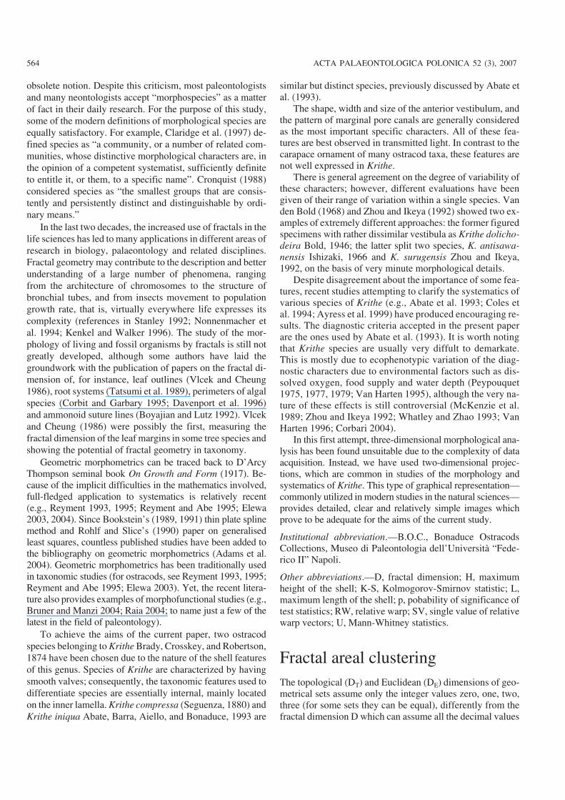
between zero and three (Mandelbrot 1983; Fig. 1). The clus−tering index of a coordinate set can be obtained in a very ef−fective way using the fractal dimension that may be com−puted through the correlation integral C(R) (Grassberger andProcaccia 1983; Luongo and Mazzarella 1997), whichcounts the number of pairs with distance |Xi−Xj| smaller thanR. This is done by taking each point in turn as a centre andanalysing the distribution of the remaining points relative toit. The correlation integral is defined as:

C RN N

R X Xij

N

i

N

j( )( )

( )�

�

� �

��

��

2

1 11

� , i � j

where � is the Heaviside function, N is the number of avail−able points and Xi is the co−ordinate set of the ith point. Thenormalisation factor 2/(N(N–1)) represents the reciprocal ofthe number of pairs so that C(R) tends to one for R tending toinfinite. If the distribution of N points has a fractal structurethen:

C(R) ~ RD

or, equivalently, on a log−log scaled plane

log(C) ~ Dlog(R) (1)

C(R) can be considered as the cumulative frequency dis−tribution of all inter−point distances. D indicates the correla−tion dimension that is a lower bound for the true fractal di−mension, although it is generally assumed that the two di−mensions are similar (Korvin et al. 1990). Theoretically,fractal sets display a straight line in the log−log plot for virtu−ally any interval of R. However, for experimental data thereis a limited scaling region with lower and upper limits, duerespectively to the minimum and maximum distance amongpairs of co−ordinates: for the minimum distance, values mustnot be lower than the precision of the data, while for the max−imum distance the most important constraint is the size andshape of the region investigated. These considerations lead toan estimation of D from the regression coefficient of the rela−tionship (1), within a specific range of distances, only whenthe correlation coefficient r among the available n pairs oflog(C) and log(R) has a confidence level not lower than 99%.The confidence level is here based on the null hypothesis ofzero correlation that is rejected at 99% confidence levelwhen the following relationship

� �� �r n r� �

�

2 1 21

gives a value larger than that provided by the Student t distri−bution with the number of degrees of freedom equal to 2� andthe confidence level 99% (Mazzarella 1998).

To understand fully the problem of a fractal characterisa−tion of a data set, let us compute the correlation integral of anideal distribution of 225 points uniformly distributed, for ex−ample, at a distance of 2 µm over an area of 30 × 30 µm2

(Fig. 1). For the computation of C(R), the smallest distancehas been chosen to be 2 µm gradually increased by a factor oftwo. The fractal relationship is found to hold for R between4 and 16 µm with a D = 2.0. For R greater than 16 µm, that is

equal to about one third of the largest distance, the log−logplot of C(R) is curved. Therefore, a correct interpretation ofD requires that values of C(R) for R larger than one third ofthe entire image size have to be discarded (Dongsheng et al.1994), in concordance with the rules of spectral analysis ap−plied to time series (Bath 1974). Moreover, the lower limit ofthe scaling region, here equal to 4 µm, represents the mini−mum detectable wavelength whose identification requiresonly three points; it corresponds to two times the griddingarea of the investigated data set.

http://app.pan.pl/acta52/app52−563.pdf

AIELLO ET AL.—FRACTAL ANALYSIS OF OSTRACOD SHELLS 565

0

0

10

10

20

20

30

30

40

40

0.0

0.0

-0.5

0.5

-1.0

1.0

-1.5

1.5

-2.0

2.0

-2.5

2.5

-3.0

3.0

log

(C)

Fig. 1. A. Ideal uniform network of 225 points spaced 2 mm apart over anarea of 30 × 30 mm2. B. The log of number of pairs C of the stations, withmutual distance smaller than R, as a function of log(R) (mm); the verticaldashed lines represent the lower (4 mm) and upper (16 mm) limits of R, in−side which the linear slope provides the best fitting to the investigatedco−ordinates.

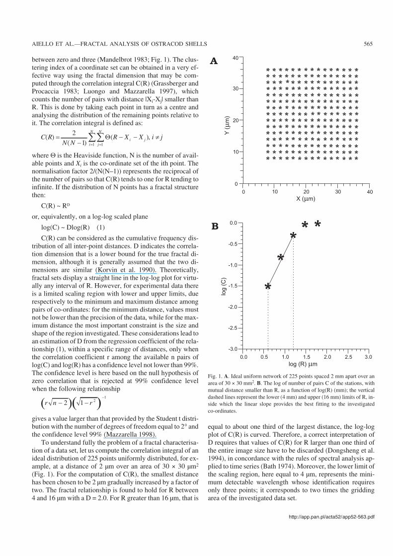
Materials and data collectionAdult specimens of the ostracod species Krithe compressa(Seguenza, 1880) and Krithe iniqua Abate, Barra, Aiello,and Bonaduce, 1993, were collected from the upper Pliocenesamples of the Monte San Nicola section (Abate et al. 1993;Aiello et al. 2000). The material consists of 29 right valves ofK. iniqua from sample 59 (KI−01 to KI−29), and 29 rightvalves of K. compressa from samples 50 (7 valves: KC−01 toKC−07), 51 (11 valves: KC−08 to KC−18) and 58 (11 valves:KC−19 to KC−29).

All specimens were observed under transmitted light anddrawn by means of a visopan Reichert at a magnification of×201(successively reduced in Figs. 2, 3). Basically, thesedrawings depict the lateral outline of the valves and the ante−rior third of the inner lamella (Fig. 4). The pictures were drawnwith a technical pen (line thickness 0.30 mm) on tracing paper.

For each specimen we also measured length (L) andheight (H) in mm.

Each drawing was imported using a flatbed scanner andthen visualized on a PC monitor in bitmap format. Since theresulting raster image is made of pixels, it was necessary to

566 ACTA PALAEONTOLOGICA POLONICA 52 (3), 2007

Fig. 2. Krithe iniqua Abate, Barra, Aiello, and Bonaduce, 1993, right valves; transparence drawings from external view; sample 59; upper Pliocene.A. KI−01, B.O.C. 2490. B. KI−02, B.O.C. 2491. C. KI−03, B.O.C. 2492. D. KI−04, B.O.C. 2493. E. KI−05, B.O.C. 2494. F. KI−06, B.O.C. 2495. G. KI−07,B.O.C. 2496. H. KI−08, B.O.C. 2497. I. KI−09, B.O.C. 2498. J. KI−10, B.O.C. 2499. K. KI−11, B.O.C. 2500. I. KI−12, B.O.C. 2501. L. KI−13, B.O.C. 2502.M. KI−14, B.O.C. 2503. N. KI−15, B.O.C. 2504. O. KI−16, B.O.C. 2505. P. KI−17, B.O.C. 2506. Q. KI−18, B.O.C. 2507. R. KI−19, B.O.C. 2508. S. KI−20,B.O.C. 2509. T. KI−21, B.O.C. 2510. U. KI−22, B.O.C. 2511. V. KI−23, B.O.C. 2512. W. KI−24, B.O.C. 2513. Y. KI−25, B.O.C. 2514. Z. KI−26, B.O.C.2515. AA. KI−27, B.O.C. 2516. BB. KI−28, B.O.C. 2517.

utilise a vector form with a larger amount of details, which isin turn dependent on the size and resolution of the image.

In fact, a vector image is stored as geometric objects, suchas lines and arcs drawn between specific coordinates. Vectordrawings are largely used in CAD (Computer Aided Design)and GIS (Geographical Informations Systems) and in otherapplications that require a high standard of accuracy. Aftermany trials, we concluded that a resolution of 300 dpi was suf−ficiently high to reduce the noise inherent in the digitizationprocess and was appropriate for the spatial resolution of thedigitized drawings of the ostracods. A resolution lower than

300 dpi does not provide a sufficient number of data points toobtain reliable fractal dimensions. Moreover, the values offractal dimensions have been found to be independent of reso−lution at values higher than 300 dpi.

The vectorization process takes into account the magnifi−cation (201×) and the digitization resolution (300 dpi) andtransforms the bidimensional projections of ostracod shellsinto x,y co−ordinates measured in microns.

To quantify the degree of areal clustering of morphologicalvariability of the two ostracod species and to identify the spe−cific range of distances inside which the co−ordinates follow

http://app.pan.pl/acta52/app52−563.pdf

AIELLO ET AL.—FRACTAL ANALYSIS OF OSTRACOD SHELLS 567

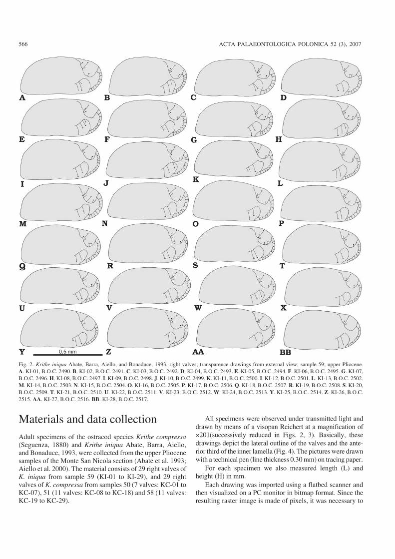
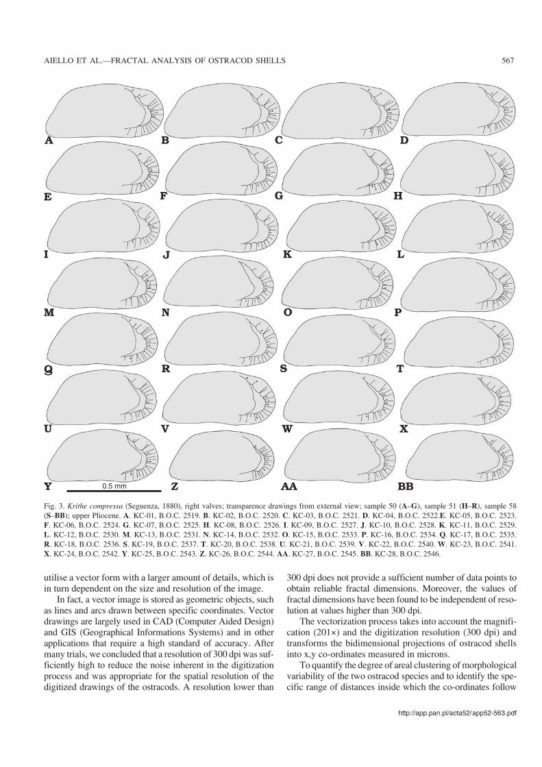
Fig. 3. Krithe compressa (Seguenza, 1880), right valves; transparence drawings from external view; sample 50 (A–G), sample 51 (H–R), sample 58(S–BB); upper Pliocene. A. KC−01, B.O.C. 2519. B. KC−02, B.O.C. 2520. C. KC−03, B.O.C. 2521. D. KC−04, B.O.C. 2522.E. KC−05, B.O.C. 2523.F. KC−06, B.O.C. 2524. G. KC−07, B.O.C. 2525. H. KC−08, B.O.C. 2526. I. KC−09, B.O.C. 2527. J. KC−10, B.O.C. 2528. K. KC−11, B.O.C. 2529.L. KC−12, B.O.C. 2530. M. KC−13, B.O.C. 2531. N. KC−14, B.O.C. 2532. O. KC−15, B.O.C. 2533. P. KC−16, B.O.C. 2534. Q. KC−17, B.O.C. 2535.R. KC−18, B.O.C. 2536. S. KC−19, B.O.C. 2537. T. KC−20, B.O.C. 2538. U. KC−21, B.O.C. 2539. V. KC−22, B.O.C. 2540. W. KC−23, B.O.C. 2541.X. KC−24, B.O.C. 2542. Y. KC−25, B.O.C. 2543. Z. KC−26, B.O.C. 2544. AA. KC−27, B.O.C. 2545. BB. KC−28, B.O.C. 2546.

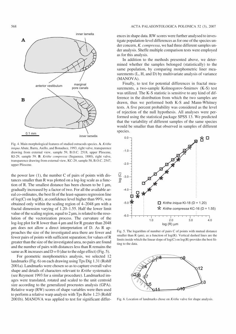
the power law (1), the number C of pairs of points with dis−tances smaller than R was plotted on a log−log scale as a func−tion of R. The smallest distance has been chosen to be 1 µm,gradually increased by a factor of two. For all the available ar−eal co−ordinates, the best fit of the least−squares regression lineof log(C) on log(R), at confidence level higher than 99%, wasobtained only within the scaling region of 4–2048 µm with afractal dimension varying of 1.20–1.55. Half the lower limitvalue of the scaling region, equal to 2 µm, is related to the reso−lution of the vectorization process. The curvature of thelog−log plot for R lower than 4 µm and for R greater than 2048µm does not allow a direct interpretation of D. As R ap−proaches the size of the investigated area there are fewer andfewer pairs of points with sufficient separation; for values of Rgreater than the size of the investigated area, no pairs are foundand the number of pairs with distances less than R remains thesame as R increases and D = 0 (due to the edge effect) (Fig. 5).

For geometric morphometrics analysis, we selected 12landmarks (Fig. 6) on each drawing using Tps Dig 1.31 (Rohlf2001a). Landmarks were chosen so as to capture overall valveshape and details of characters relevant to Krithe systematics(see Reyment 1993 for a similar procedure). Landmarked im−ages were translated, rotated and scaled to the unit centroidsize according to the generalized procrustes analysis (GPA).Relative warp (RW) scores of shape variables were then usedto perform a relative warp analysis with Tps Relw 1.23 (Rohlf2001b). MANOVA was applied to test for significant differ−

ences in shape data. RW scores were further analysed to inves−tigate population−level differences as for one of the species un−der concern, K. compressa, we had three different samples un−der analysis. Sheffe multiple comparison tests were employedas for this analysis.

In addition to the methods presented above, we deter−mined whether the samples belonged (statistically) to thesame population, by comparing morphometric liner mea−surements (L, H, and D) by multivariate analysis of variance(MANOVA).

Finally, to test for potential differences in fractal mea−surements, a two−sample Kolmogorov−Smirnov (K−S) testwas utilized. The K−S statistic is sensitive to any kind of dif−ference in the distribution from which the two samples aredrawn, thus we performed both K−S and Mann−Whitneytests. A five percent probability was considered as the levelof rejection of the null hypothesis. All analyses were per−formed using the statistical package SPSS 13. We predictedthat the variability of different samples of the same specieswould be smaller than that observed in samples of differentspecies.

568 ACTA PALAEONTOLOGICA POLONICA 52 (3), 2007

inner lamella

anterior vestibulummarginal

pore canals

inner lamella0.1 mm

Fig. 4. Main morphological features of studied ostracods species. A. Kritheiniqua Abate, Barra, Aiello, and Bonaduce, 1993, right valve, transparencedrawing from external view, sample 59, B.O.C. 2518, upper Pliocene,KI−29, sample 59. B. Krithe compressa (Seguenza, 1880), right valve,transparence drawing from external view, KC−29, sample 58, B.O.C. 2547,upper Pliocene.

-6.0

-5.0

-4.0

-3.0

-2.0

-1.0

1.0 2.0 3.0 4.0

0.0

log

(C)

Krithe compressa KC-16 (D = 1.55)

Krithe iniqua KI-18 (D = 1.20)

Fig. 5. The logarithm of number of pairs C of points with mutual distancesmaller than R (µm), as a function of log(R). Vertical dashed lines are thelimits inside which the linear slope of log(C) on log(R) provides the best fit−ting to the data.

Fig. 6. Location of landmarks chose on Krithe valve for shape analysis.

Results and discussionResults of the fractal analysis are summarized in Table 1. Inorder to evaluate morphological variations in Krithe com−pressa and K. iniqua we measured their lengths (L), heights

(H) and fractal dimensions (D). We compared L and H of dif−ferent samples of K. compressa (samples 50, 51, 58) betweenthemselves and with K. iniqua. These comparisons indicatethat when the four samples of the two species are considered,MANOVA shows highly significant differences (Wilk’s

http://app.pan.pl/acta52/app52−563.pdf

AIELLO ET AL.—FRACTAL ANALYSIS OF OSTRACOD SHELLS 569

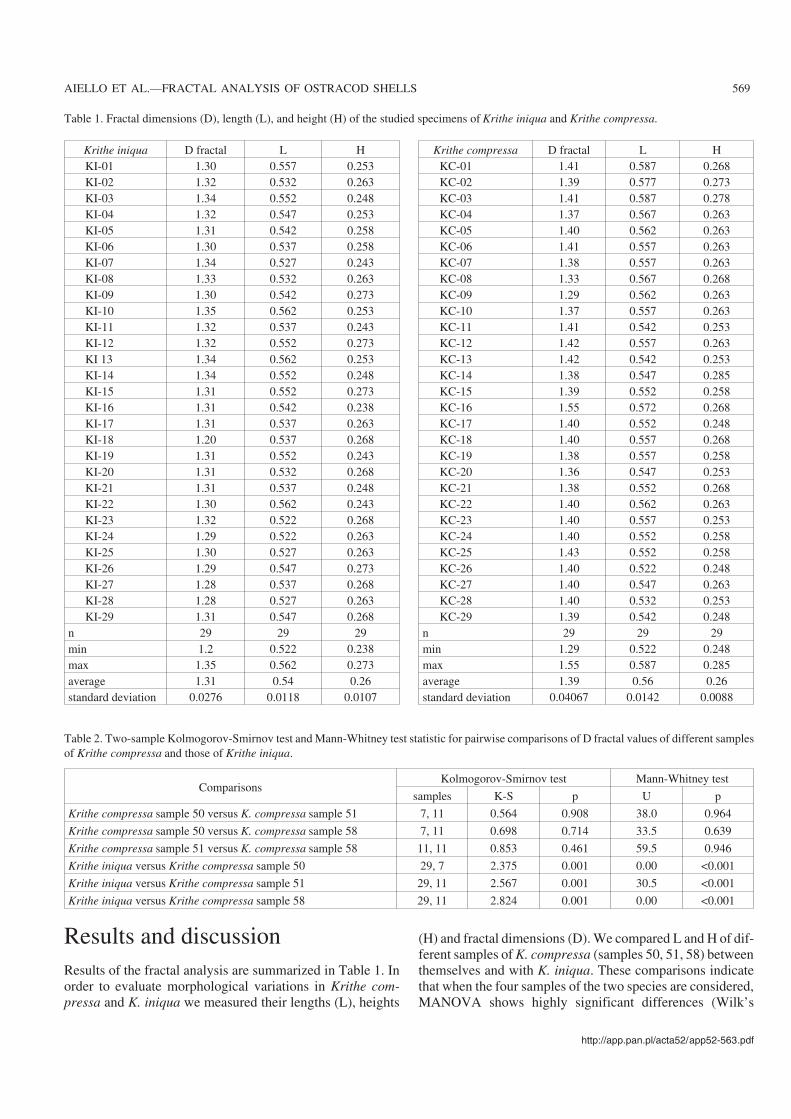
Table 1. Fractal dimensions (D), length (L), and height (H) of the studied specimens of Krithe iniqua and Krithe compressa.

Krithe iniqua D fractal L HKI−01 1.30 0.557 0.253KI−02 1.32 0.532 0.263KI−03 1.34 0.552 0.248KI−04 1.32 0.547 0.253KI−05 1.31 0.542 0.258KI−06 1.30 0.537 0.258KI−07 1.34 0.527 0.243KI−08 1.33 0.532 0.263KI−09 1.30 0.542 0.273KI−10 1.35 0.562 0.253KI−11 1.32 0.537 0.243KI−12 1.32 0.552 0.273KI 13 1.34 0.562 0.253KI−14 1.34 0.552 0.248KI−15 1.31 0.552 0.273KI−16 1.31 0.542 0.238KI−17 1.31 0.537 0.263KI−18 1.20 0.537 0.268KI−19 1.31 0.552 0.243KI−20 1.31 0.532 0.268KI−21 1.31 0.537 0.248KI−22 1.30 0.562 0.243KI−23 1.32 0.522 0.268KI−24 1.29 0.522 0.263KI−25 1.30 0.527 0.263KI−26 1.29 0.547 0.273KI−27 1.28 0.537 0.268KI−28 1.28 0.527 0.263KI−29 1.31 0.547 0.268

n 29 29 29min 1.2 0.522 0.238max 1.35 0.562 0.273average 1.31 0.54 0.26standard deviation 0.0276 0.0118 0.0107

Krithe compressa D fractal L HKC−01 1.41 0.587 0.268KC−02 1.39 0.577 0.273KC−03 1.41 0.587 0.278KC−04 1.37 0.567 0.263KC−05 1.40 0.562 0.263KC−06 1.41 0.557 0.263KC−07 1.38 0.557 0.263KC−08 1.33 0.567 0.268KC−09 1.29 0.562 0.263KC−10 1.37 0.557 0.263KC−11 1.41 0.542 0.253KC−12 1.42 0.557 0.263KC−13 1.42 0.542 0.253KC−14 1.38 0.547 0.285KC−15 1.39 0.552 0.258KC−16 1.55 0.572 0.268KC−17 1.40 0.552 0.248KC−18 1.40 0.557 0.268KC−19 1.38 0.557 0.258KC−20 1.36 0.547 0.253KC−21 1.38 0.552 0.268KC−22 1.40 0.562 0.263KC−23 1.40 0.557 0.253KC−24 1.40 0.552 0.258KC−25 1.43 0.552 0.258KC−26 1.40 0.522 0.248KC−27 1.40 0.547 0.263KC−28 1.40 0.532 0.253KC−29 1.39 0.542 0.248

n 29 29 29min 1.29 0.522 0.248max 1.55 0.587 0.285average 1.39 0.56 0.26standard deviation 0.04067 0.0142 0.0088

Table 2. Two−sample Kolmogorov−Smirnov test and Mann−Whitney test statistic for pairwise comparisons of D fractal values of different samplesof Krithe compressa and those of Krithe iniqua.

ComparisonsKolmogorov−Smirnov test Mann−Whitney test

samples K−S p U p

Krithe compressa sample 50 versus K. compressa sample 51 7, 11 0.564 0.908 38.0 0.964

Krithe compressa sample 50 versus K. compressa sample 58 7, 11 0.698 0.714 33.5 0.639

Krithe compressa sample 51 versus K. compressa sample 58 11, 11 0.853 0.461 59.5 0.946

Krithe iniqua versus Krithe compressa sample 50 29, 7 2.375 0.001 0.00 <0.001

Krithe iniqua versus Krithe compressa sample 51 29, 11 2.567 0.001 30.5 <0.001

Krithe iniqua versus Krithe compressa sample 58 29, 11 2.824 0.001 0.00 <0.001

Lambda 0.249, F = 10.857, df = 9, P = 2.15×10–12) among thesamples. A test of between samples effects shows that onlylength and D are, however, significantly different among thefour samples [L: F(3,54) = 8.558, p = 0.001; H: F(3,54) =2.827, p = 0.068, NS; D: F(3,54) = 8.942, p <0.001]. Resultsof post−hoc pair−wise comparisons for L of different samples(and species) indicate that individuals of K. compressa insample 58 are not distinguishable from those of K. iniqua andthat individuals in sample 51 are not different from those ofsample 58 of K. compressa.

On the other hand, fractal analysis of the two ostracodspecies shows values of D centered on 1.31±0.02 for Kritheiniqua and on 1.40±0.04 for K. compressa (Table 1). Also inthis case we compared D values of K. compressa from differ−ent samples among themselves. No significant differenceswere found (Table 2). However, D values are significantlydifferent when individuals of K. iniqua are compared withthose of K. compressa (Table 2).

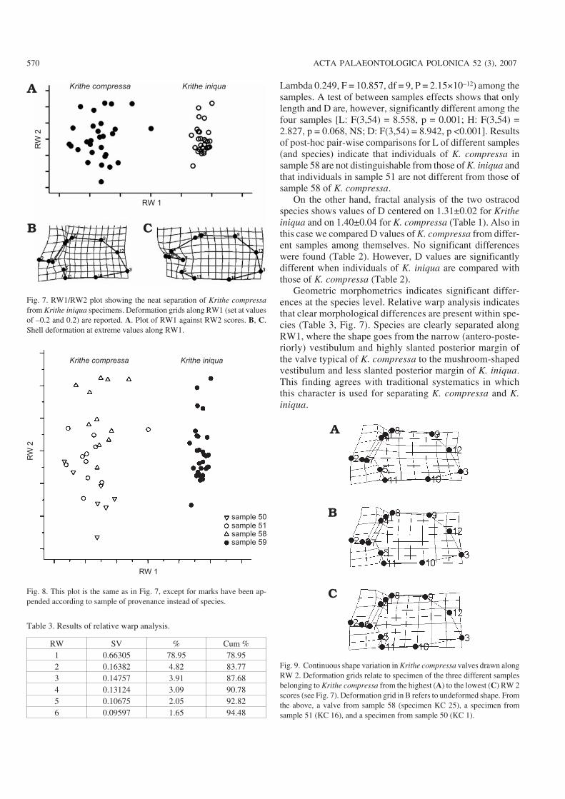
Geometric morphometrics indicates significant differ−ences at the species level. Relative warp analysis indicatesthat clear morphological differences are present within spe−cies (Table 3, Fig. 7). Species are clearly separated alongRW1, where the shape goes from the narrow (antero−poste−riorly) vestibulum and highly slanted posterior margin ofthe valve typical of K. compressa to the mushroom−shapedvestibulum and less slanted posterior margin of K. iniqua.This finding agrees with traditional systematics in whichthis character is used for separating K. compressa and K.iniqua.

570 ACTA PALAEONTOLOGICA POLONICA 52 (3), 2007

Krithe compressa

RW

2

RW 1

Krithe iniqua

Fig. 7. RW1/RW2 plot showing the neat separation of Krithe compressafrom Krithe iniqua specimens. Deformation grids along RW1 (set at valuesof –0.2 and 0.2) are reported. A. Plot of RW1 against RW2 scores. B, C.Shell deformation at extreme values along RW1.

sample 50

sample 51

sample 58

sample 59

Krithe compressa

RW

2

RW 1

Krithe iniqua

Fig. 8. This plot is the same as in Fig. 7, except for marks have been ap−pended according to sample of provenance instead of species.

Fig. 9. Continuous shape variation in Krithe compressa valves drawn alongRW 2. Deformation grids relate to specimen of the three different samplesbelonging to Krithe compressa from the highest (A) to the lowest (C) RW 2scores (see Fig. 7). Deformation grid in B refers to undeformed shape. Fromthe above, a valve from sample 58 (specimen KC 25), a specimen fromsample 51 (KC 16), and a specimen from sample 50 (KC 1).

Table 3. Results of relative warp analysis.

RW SV % Cum %1 0.66305 78.95 78.952 0.16382 4.82 83.773 0.14757 3.91 87.684 0.13124 3.09 90.785 0.10675 2.05 92.826 0.09597 1.65 94.48

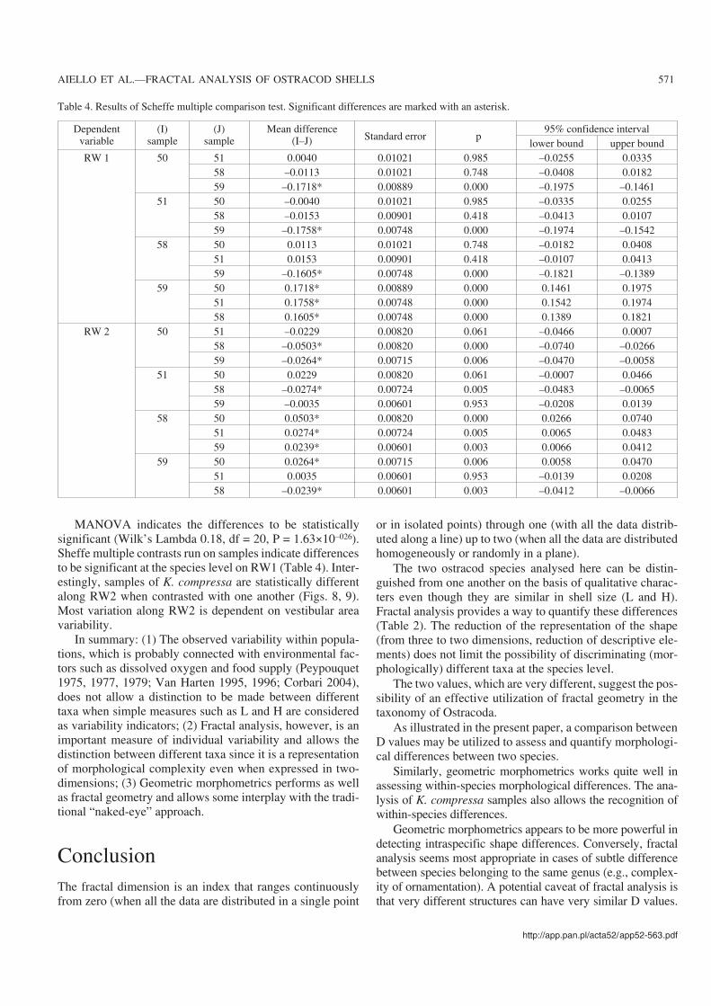
MANOVA indicates the differences to be statisticallysignificant (Wilk’s Lambda 0.18, df = 20, P = 1.63×10–026).Sheffe multiple contrasts run on samples indicate differencesto be significant at the species level on RW1 (Table 4). Inter−estingly, samples of K. compressa are statistically differentalong RW2 when contrasted with one another (Figs. 8, 9).Most variation along RW2 is dependent on vestibular areavariability.

In summary: (1) The observed variability within popula−tions, which is probably connected with environmental fac−tors such as dissolved oxygen and food supply (Peypouquet1975, 1977, 1979; Van Harten 1995, 1996; Corbari 2004),does not allow a distinction to be made between differenttaxa when simple measures such as L and H are consideredas variability indicators; (2) Fractal analysis, however, is animportant measure of individual variability and allows thedistinction between different taxa since it is a representationof morphological complexity even when expressed in two−dimensions; (3) Geometric morphometrics performs as wellas fractal geometry and allows some interplay with the tradi−tional “naked−eye” approach.

ConclusionThe fractal dimension is an index that ranges continuouslyfrom zero (when all the data are distributed in a single point

or in isolated points) through one (with all the data distrib−uted along a line) up to two (when all the data are distributedhomogeneously or randomly in a plane).

The two ostracod species analysed here can be distin−guished from one another on the basis of qualitative charac−ters even though they are similar in shell size (L and H).Fractal analysis provides a way to quantify these differences(Table 2). The reduction of the representation of the shape(from three to two dimensions, reduction of descriptive ele−ments) does not limit the possibility of discriminating (mor−phologically) different taxa at the species level.

The two values, which are very different, suggest the pos−sibility of an effective utilization of fractal geometry in thetaxonomy of Ostracoda.

As illustrated in the present paper, a comparison betweenD values may be utilized to assess and quantify morphologi−cal differences between two species.

Similarly, geometric morphometrics works quite well inassessing within−species morphological differences. The ana−lysis of K. compressa samples also allows the recognition ofwithin−species differences.

Geometric morphometrics appears to be more powerful indetecting intraspecific shape differences. Conversely, fractalanalysis seems most appropriate in cases of subtle differencebetween species belonging to the same genus (e.g., complex−ity of ornamentation). A potential caveat of fractal analysis isthat very different structures can have very similar D values.

http://app.pan.pl/acta52/app52−563.pdf

AIELLO ET AL.—FRACTAL ANALYSIS OF OSTRACOD SHELLS 571

Table 4. Results of Scheffe multiple comparison test. Significant differences are marked with an asterisk.

Dependentvariable

(I)sample

(J)sample

Mean difference(I–J) Standard error p

95% confidence intervallower bound upper bound

RW 1 50 51 0.0040 0.01021 0.985 –0.0255 0.033558 –0.0113 0.01021 0.748 –0.0408 0.018259 –0.1718* 0.00889 0.000 –0.1975 –0.1461

51 50 –0.0040 0.01021 0.985 –0.0335 0.025558 –0.0153 0.00901 0.418 –0.0413 0.010759 –0.1758* 0.00748 0.000 –0.1974 –0.1542

58 50 0.0113 0.01021 0.748 –0.0182 0.040851 0.0153 0.00901 0.418 –0.0107 0.041359 –0.1605* 0.00748 0.000 –0.1821 –0.1389

59 50 0.1718* 0.00889 0.000 0.1461 0.197551 0.1758* 0.00748 0.000 0.1542 0.197458 0.1605* 0.00748 0.000 0.1389 0.1821

RW 2 50 51 –0.0229 0.00820 0.061 –0.0466 0.000758 –0.0503* 0.00820 0.000 –0.0740 –0.026659 –0.0264* 0.00715 0.006 –0.0470 –0.0058

51 50 0.0229 0.00820 0.061 –0.0007 0.046658 –0.0274* 0.00724 0.005 –0.0483 –0.006559 –0.0035 0.00601 0.953 –0.0208 0.0139

58 50 0.0503* 0.00820 0.000 0.0266 0.074051 0.0274* 0.00724 0.005 0.0065 0.048359 0.0239* 0.00601 0.003 0.0066 0.0412

59 50 0.0264* 0.00715 0.006 0.0058 0.047051 0.0035 0.00601 0.953 –0.0139 0.020858 –0.0239* 0.00601 0.003 –0.0412 –0.0066

This supports the idea that fractal analysis is most appropriatein analyses of congeneric species. Special attention should bepaid to homology. Geometric morphometrics operationallyincludes the use of both homologous (true landmarks) andoperationally analogous (pseudolandmarks) shape indicators(i.a., Reyment 1993). Fractal analysis is free from the use ofhomologous structures. Although potentially misleading ifcomparing distantly−related organisms, this latter characteris−tic is welcome in cases of uncertain homology in closely−re−lated species.

Our results encourage future developments and the inte−gration of mathematically based approaches such as fractalgeometry and geometric morphometrics to studies of taxa ofhigher hierarchical level.

AcknowledgementWe are grateful to Paul Taylor (Natural History Museum, London, UK)for linguistic adjustment. Gene Hunt (Department of Paleobiology,Smithsonian Institution, Washington, USA) gave us important advicethat let us improve the manuscript. We are grateful to Mike Foote (De−partment of the Geophysical Sciences, University of Chicago, USA),Øyvind Hammer (Paleontological Museum, Oslo, Norway) for theirhelpful comments and precious advice. We are grateful to LoredanaPellecchia who helped us with the preparation of some figures.

ReferencesAbate, S., Barra, D., Aiello, G., and Bonaduce, G. 1993. The genus Krithe

Brady, Crosskey and Robertson, 1874 (Crustacea: Ostracoda) in thePliocene–Early Pleistocene of the M. San Nicola Section (Gela, Sicily).Bollettino della Società Paleontologica Italiana 32: 349–366.

Adams, D.C., Rohlf, F.J., and Slice, D.E. 2004. Geometric morphometrics:ten years of progress following the “revolution”. Italian Journal of Zo−ology 71: 5–16.

Aiello, G., Barra, D., and Bonaduce, G. 2000. Systematics and biostratigraphyof the Ostracoda of the Plio−Pleistocene Monte S. Nicola section (Gela,Sicily). Bollettino della Società Paleontologica Italiana 39: 83–112.

Ayress, M.A., Barrows, T., Passlow, V., and Whatley, R. 1999. Neogene toRecent species of Krithe (Crustacea: Ostracoda) from the Tasman Seaand off Southern Australia with description of five new species. Re−cords of the Australian Museum 51: 1–22.

Bath, A. 1974. Spectral Analysis in Geophysics. 563 pp. Elsevier, Amsterdam.Bold, W.A. van den 1946. Contribution to the Study of Ostracoda with Special

Reference to the Tertiary and Cretaceous Microfauna of the CaribbeanRegion. 167 pp. Proefschrift Rijks Universiteit Utrecht, Amsterdam.

Bold, W.A. van den 1968. Ostracoda of the Yague Group (Neogene) of theNorthern Dominican Republic. Bulletins of American Paleontology 54(239): 1–106.

Bookstein, F.L. 1989. Principal warps: thin plate spline and the decomposi−tion of deformations. I.E.E.E. Transactions on Pattern Analysis andMachine Intelligence 11: 567–585.

Bookstein, F.L. 1991. Morphometric Tools for Landmark Data: Geometryand Biology. 435 pp. Cambridge University Press, New York.

Boyajian, G. and Lutz, T. 1992. Evolution of biological complexity and itsrelation to taxonomic longevity in the Ammonoidea. Geology 20:983–986

Brady, G.S., Crosskey, H.W., and Robertson, D. 1874. A monograph of thePost−Tertiary Entomostraca of Scotland including species from Eng−

land and Ireland. Annual Volumes (Monographs) of the Palaeontogra−phical Society 28: 1–232.

Bruner E. and Manzi, G. 2004. Variability in facial size and shape amongNorth and East African human populations. Italian Journal of Zoology71: 51–56.

Claridge, M.F., Dawah, H.A., and Wilson, M.R. 1997. Practical approaches tospecies concepts for living organisms In: M.F. Claridge, H.A. Dawah, andM.R. Wilson (eds.), Species: the Units of Biodiversity, 1–15. Chapmanand Hall, London.

Coles, G.P., Whatley, R.W., and Moguilevsky, A. 1994. The ostracod genusKrithe from the Tertiary and Quaternary of the North Atlantic. Paleon−tology 37: 71–120.

Corbari, L. 2004. Physiologie respiratoire, comportementale et morphofon−ctionnelle des ostracodes Podocopes et Myodocopes et d’un amphipodecaprellidé profond. Stratégies adaptatives et implications évolutives.300 pp. M.Sc. thesis 2885, Université Bordeaux 1, Bordeaux.

Corbit, J.D. and Garbary, D.J. 1995. Fractal dimension as a quantitativemeasure of complexity in plant development. Proceedings of the RoyalSociety of London B 262: 1–6.

Cronquist, A. 1988. The Evolution and Classification of Flowering Plants.555 pp. The New York Botanical Garden, New York.

Davenport, J., Pugh, P.J.A., and McKechnie, J. 1996. Mixed fractals andanisotropy in subantarctic marine macroalgae from South Georgia: im−plications for epifaunal biomass and abundance. Marine Ecology Prog−ress Series 136: 245–255.

Dongsheng, L., Zhaobi, Z., and Binghong, W. 1994. Research into multifractalanalysis of earthquake spatial distribution. Tectonophysics 233: 91–97.

Elewa, A. 2003. Morphometric studies on three ostracod species of the ge−nus Digmocythere Mandelstam from the Middle Eocene of Egypt.Palaeontologia Electronica 6 (2): 1–11.

Elewa, A. 2004. Morphometrics: Applications in Biology and Paleontol−ogy. 263 pp. Springer Verlag, Heidelberg.

Grassberger, P. and Procaccia, I. 1983. Measuring the strangeness of strangeattractors. Physica D 9: 189–208.

Ishizaki, K. 1966. Miocene and Pliocene ostracodes from the Sendai area,Japan. Science Reports of the Tohoku University, series 2 (Geology) 37:131–163.

Kenkel, N.C. and Walker, D.J. 1996. Fractals in the biological sciences.Coenoses 11: 77–100.

Korvin, G., Boyd, D.M., and O’Dowd, R. 1990. Fractal characterization ofthe South Australian gravity station network. Geophysical Journal In−ternational 100: 535–539.

Luongo, G. and Mazzarella, A. 1997. On the clustering of seismicity in theSouthern Tyrrhenian sea. Annali di Geofisica 40: 1–7.

Mandelbrot, B.B. 1983. The Fractal Geometry of Nature. 460 pp. Freeman,New York.

Mayden, R.L. 1997. A hierarchy of species concepts: the denouement in thesaga of the species problem In: M.F. Claridge, H.A. Dawah, and M.R.Wilson (eds.), Species: the Units of Biodiversity, 381–424. Chapmanand Hall, London.

Mayr, E. 1996. What is a species, and what is not? Philosophy of Science 63:262–277.

Mazzarella, A. 1998. The time clustering of floodings in Venice and the Cantordust method. Theoretical and Applied Climatology 59: 147–150.

McKenzie, K.G., Majoran, S., Emami, V., and Reyment, R.A. 1989. TheKrithe problem—First test of Peypouquet’s hypothesis, with a rede−scription of Krithe praetexta praetexta (Crustacea, Ostracoda). Palaeo−geography, Palaeoclimatology, Palaeoecology 74: 343–354.

Nonnenmacher, T.F., Losa, G.A., and Weibel, E.R. 1994. Fractals in Biol−ogy and Medicine. 416 pp. Birkhauser, Boston.

Peypouquet, J.P. 1975. Les variations des caractères morphologiques interneschez les ostracodes des genres Krithe et Parakrithe: relation possible avecle teneur en O2 dissous dans l’eau. Bulletin de l’Institut de Géologie duBassin Aquitaine 17: 81–88.

Peypouquet, J.P. 1977. Les ostracodes et la connaissance des paleomilieuxprofonds. Application au Cenozoïque de l’Atlantique nord−oriental.443 pp. Ph.D. thesis. Université de Bordeaux, Bordeaux.

572 ACTA PALAEONTOLOGICA POLONICA 52 (3), 2007

Peypouquet, J.P. 1979. Ostracodes et paléoenvironnements. Méthodologieet application aux domaines profonds du Cénozoïque. Bulletin du Bu−reau de Recherches Géologiques et Minieres 4: 3–79.

Raia, P. 2004. Morphological correlates of tough food consumption in largeland carnivores. Italian Journal of Zoology 71: 45–50.

Reyment, R.A. 1993. Ornamental and shape variation in Hemicytherurafulva McKenzie, Reyment and Reyment (Ostracoda, Eocene, Austra−lia). Revista Española de Paleontologia 8: 125–131.

Reyment, R.A. 1995. On multivariate morphometrics applied to OstracodaIn: J. Ríha (ed.), Ostracoda and Biostratigraphy, 203–213. Balkema,Rotterdam.

Reyment, R.A. and Abe, K. 1995. Morphometrics of Vargula hilgendorfii(Müller). Mitteilungen aus dem hamburgischen zoologischen Museumund Institut 92: 325–336.

Rohlf, F.J. 2001a. TpsDig: Thin Plate Spline Digitise. (Version 1.31). StateUniversity of New York, Stony Brook.

Rohlf, F.J. 2001b. TpsRelw: Thin Plate Spline Relative Warp Analysis.(Version 1.22). State University of New York, Stony Brook.

Rohlf, F.J. and Slice, D. 1990. Extension of the procrustes method for theoptimal superimposition of landmarks. Systematic Zoology 39: 40–59.

Seguenza, G. 1880. Le formazioni terziarie della provincia di Reggio(Calabria). Atti della Reale Accademia dei Lincei, serie 3 (Memoriedella classe di Scienze Fisiche, Matemetiche e Naturali) 6: 3–446.

Stanley, H.E. 1992. Fractal landscapes in physics and biology. Physica A186: 1–32.

Tatsumi, J., Yamauchi, A., and Kono, Y. 1989. Fractal analysis of plant rootsystems. Annals of Botany 64: 499–503.

Thompson, D’A.W. 1917. On Growth and Form. 793 pp. Cambridge Uni−versity Press, Cambridge.

Van Harten, D. 1995. Differential food−detection: a speculative reinterpreta−tion of vestibule variability in Krithe (Crustacea: Ostracoda) In: J. Ríha(ed.), Ostracoda and Biostratigraphy, 33–36. Balkema, Rotterdam.

Van Harten, D. 1996. The case against Krithe as a tool to estimate the depthand the oxygenation of ancient oceans In: A. Moguilewsky and R.Whatley (eds.), Microfossils and Oceanic Environments, 297–303.University of Wales, Aberystwyth.

Vlcek, J. and Cheung, E. 1986. Fractal analysis of leaf shapes. CanadianJournal of Forest Research 16: 124–127.

Whatley, R. and Zhao, Q. 1993. The Krithe problem: A case history of thedistribution of Krithe and Pararakrithe (Crustacea, Ostracoda) in theSouth China Sea. Palaeogeography, Palaeoclimatology, Palaeoecol−ogy 103: 281–297.

Zhou, B. and Ikeya, N. 1992. Three species of Krithe (Crustacea : Ostra−coda) from Suruga Bay, Central Japan. Transactions and Proceedingsof the Palaeontological Society of Japan, new series 166: 1097–1115.

http://app.pan.pl/acta52/app52−563.pdf

AIELLO ET AL.—FRACTAL ANALYSIS OF OSTRACOD SHELLS 573