The Fractal Nature of Bitcoin

The Fractal Nature of Bitcoin

1

FUNDACION UNIVERSIDAD DE LAS AMERICAS PUEBLA

Escuela de Negocios y Economía

Departamento de Economía

THE FRACTAL NATURE OF BITCOIN: EVIDENCE FROM

WAVELET POWER SPECTRA

TESIS PROFESIONAL PRESENTADA POR

RAFAEL DELFIN VIDAL

COMO REQUISITO PARCIAL

PARA OBTENER EL TÍTULO DE LICENCIADO EN ECONOMÍA

Asesor

Dr. Guillermo Romero Meléndez

Santa Catarina Mártir, Puebla Otoño 2014


2

Summary. In this study a continuous wavelet transform is performed on bitcoin’s

historical returns. Despite the asset’s novelty and high volatility, evidence from the

wavelet power spectra shows clear dominance of specific investment horizons during

periods of high volatility. Thanks to wavelet analysis it is also possible to observe the

presence of fractal dynamics in the asset’s behavior. Wavelet analysis is a method to

decompose a time series into several layers of time scales, making it possible to analyze

how the local variance, or wavelet power, changes both in the frequency and time domain.

Although relatively new to finance and economic, wavelet analysis represents a powerful

tool that can be used to study how economic phenomena operates at simultaneous time

horizons, as well as aggregated processes that are the result of several agents or

variables with different term objectives.

Keywords: Fractal Market Hypothesis, Bitcoin, Wavelet Power Spectrum, Wolfram

Mathematica, Economics and Finance, Cryptocurrencies, Wavelet Analysis


3

Chapter I Introduction

Bitcoin is a digital currency that relies on cryptographic technology to control its creation

and distribution. Just like banknotes or coins, transactions in bitcoin can be performed

directly between two individuals without the need of an intermediary. However, bitcoins

are not issued by any government or other legal entity, they are produced by a large

number of people running computers around the world, using software that solves

mathematical problems. It’s the first example of a growing category of money known as

cryptocurrency.

Unlike fiat currencies, whose value is derived through regulation or law and

underwritten by the state, bitcoin’s technology has currency, platform, and equity

properties that make it extremely difficult to assess its intrinsic value (Weisenthal 2013).

As a consequence, most of bitcoin’s value is based on a highly volatile demand—what

people are willing to pay and receive for them at any given time. In April 2011, less than

one year after the first transactions using bitcoins took place, a single bitcoin (currency

ticker BTC) was worth about $0.80 USD. Three years later, as of October 29, 2014 one

bitcoin is now worth $348, having reached a historical maximum value of $1,132 in

December 2013.

It is widely known the bitcoin economy has experienced a recurring volatility

cycle over its short existence. As media coverage on the cryptocurrency increased, this

attracted new waves of investors pushing bitcoin’s price to unprecedented highs, leading

to an eventual crash of the BTC/USD exchange rate. Before reaching its $1,120 historical

maximum in December 2013, bitcoin’s price rose 40-fold from around $0.80 in April


4

2011 to more than $30 by June 2011 to then fall below $2 by November 2011 before

stabilizing at around $5 in early 2012. After the initial boom and bust, bitcoin’s price

gradually stabilized between $4.30 and $5.48 during the first half of 2012. In the second

half of 2012, BTC prices climbed from $5.15 in June to $13.59 by December 2012. This

pattern repeated itself twice during 2013. From $13.50 at the start of the year, bitcoin’s

value soared to $237 in May and then crashed to $68 later that same month. After the first

volatility cycle in 2013, BTC prices ranged between $68 and $130 until October 2013,

then by the end of November bitcoin prices reached $1,120. Finally, during the first half

of 2014 the USD/BTC exchange rate has steadily decreased to around $400-500.

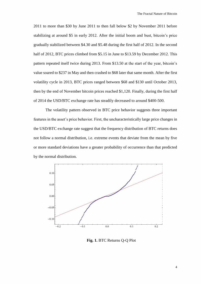
The volatility pattern observed in BTC price behavior suggests three important

features in the asset’s price behavior. First, the uncharacteristically large price changes in

the USD/BTC exchange rate suggest that the frequency distribution of BTC returns does

not follow a normal distribution, i.e. extreme events that deviate from the mean by five

or more standard deviations have a greater probability of occurrence than that predicted

by the normal distribution.

Fig. 1. BTC Returns Q-Q Plot


5

Figure 1 shows the Quantile-Quantile Plot for BTC historical returns and

illustrates the evidence of long tails and over dispersion in the series, represented by the

blue thick line.

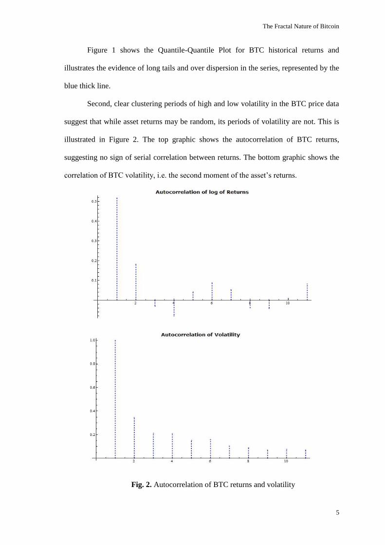
Second, clear clustering periods of high and low volatility in the BTC price data

suggest that while asset returns may be random, its periods of volatility are not. This is

illustrated in Figure 2. The top graphic shows the autocorrelation of BTC returns,

suggesting no sign of serial correlation between returns. The bottom graphic shows the

correlation of BTC volatility, i.e. the second moment of the asset’s returns.

Fig. 2. Autocorrelation of BTC returns and volatility


6

The second graphic in Figure 2 shows a clear positive trend in the autocorrelation

of the asset’s volatility, a clear sign of long memory, or persistent behavior. Finally,

bitcoin price data exhibits evidence of scale invariance, or self-similar statistical

structures, at different price levels. For example, BTC returns follow the same frequency

distribution regardless of time scale; while bitcoin’s price volatility cycles show the same

behavior, independent of price level.

These features directly violate the fundamental assumptions of Gaussian

distribution required by the established Efficient Markets Hypothesis (EMH), rendering

most financial modelling approaches unsuitable to study bitcoin price behavior. Moreover,

after decades of statistical analysis of price fluctuations across different markets, asset

types, and time periods, there is a large number of studies documenting the failure of

EMH to mirror or model the empirical evidence of financial time series (Mandelbrot 1963,

1997; Blackledge 2010). Despite the widespread use of the Brownian motion and

Gaussian distribution paradigms in financial economics, a number of systematic

statistical departures from the EMF have been identified and are now widely

acknowledged as “stylized facts” of financial time series (Rama 2001, 2005; Borland et

al. 2005; Ehrentreich 2008; Dermietzel 2008).

Notably, the main stylized facts standing out in the literature include the three

prominent features of bitcoin’s volatility cycle previously mentioned: heavy tails or non-

normal distribution of returns, long memory effect in squared returns also known as

volatility clustering, and presence of fractal dynamics. Therefore, given the strong

deviations from the EMH framework readily observable in the BTC price data, an

alternative analytical framework is used to study financial data with likely presence of

non-normality, self-similarity, and persistent volatility.


7

The Fractal Market Hypothesis (FMH) is a theoretical framework developed by

Peters (1991a, 1991b, 1994) where he proposes a more realistic market structure that

places no statistical requirements on the process; explain why self-similar statistical

structures exist; and how risk is shared and distributed among investors (1994, 39). Under

the FMH approach market stability is maintained only when many investors participate

and they can cover a large number of investment horizons, thus ensuring ample liquidity

for trading (44). Peters argues that after adjusting for scale of investment horizon, all

investors must share same risk levels, which explains why the frequency of distribution

of BTC returns exhibits self-similar behavior at different scales (46). According to the

FMH, a market becomes unstable when its self-similar structure breaks down, i.e. when

investors with long term horizons either stop participating in the market or become short-

term investors themselves. When long-term fundamental information is no longer

important or unreliable, markets become unstable and are characterized by extreme high

levels of short-term volatility. This approach explains the presence of periods of

clustering volatility in the BTC time series and the occurrence of extreme events that

violate the normality of the frequency distribution of bitcoin returns.

The FMH suggests that stable markets are characterized by equally representation

of all investment horizons in the market so that supply and demand are efficiently cleared.

When investors at one horizon (or group of horizons) become dominant, the selling or

buying signals of the investors at these horizons will not be met with a corresponding

order of the remaining horizons and periods of high volatility might occur. Thanks to

time-frequency analysis it is possible to investigate whether BTC returns follow the

market dynamics established by the fractal markets hypothesis and its focus on liquidity

and investment horizons. According to Kristoufek (2013), after performing a continuous


8

wavelet transform to a time series and obtaining its wavelet power spectra it is possible

detect the dominance of specific investment horizons during periods of high volatility.

Wavelet analysis is a method to decompose a time series into time-frequency

space, it uses mathematical expansions that transform data from the time domain into

different layers of frequency levels. This makes possible to observe and analyze data at

different scales. Although this approach is relatively new to economics, wavelets have

been used in a wide range of fields. For example, for the analysis of oceanic and

atmospheric flow phenomena in geophysics (Torrence and Compo 1998), image

processing for computer and image compression (Grapps 1995), as well as in medicine

for heart rate monitoring (Thurner, Feurstein, and Teich 1998), and for molecular

dynamics simulation and energy transfer in physics (McCowan 2007) just to name a few.

Among the most well-known applications of wavelet analysis are the FBI algorithm for

fingerprint data compression and the JPEG algorithm for image compression (Grapps

1995, Li 2003).

Scope of this thesis

The main goal of this study is to provide empirical evidence supporting the Fractal

Market Hypothesis. To do so, the BTC returns time series is analyzed to determine the

existence of dominance of short investment horizons during periods of high market

turbulence. This objective is accomplished using a continuous wavelet transform analysis

to obtain information about bitcoin’s price volatility across time and different scales of

investment horizons.

There are several reasons for the importance of this study. First, to date this is the

only study using wavelet analysis to detect dominance of investment horizons in BTC

price returns. Second, the results of the continuous wavelet transform of the time series

show supporting evidence in favor of the Fractal Market Hypothesis. Third, the wavelet


9

analysis performed suggests that while bitcoin’s price has been characterized by high

volatility, it follow the same market dynamics as other currencies and equity markets (e.g.,

government bonds, stocks, and commodities). Finally, the use of wavelet to analyze

economic phenomena is relatively recent, this work will show original contributions to

the applications of wavelet analysis in economics, finance and cryptocurrencies.1

Organization of the manuscript

The remainder of this work is organized as follows. The Theoretical Framework section

presents an overview of the Bitcoin payment system and an introduction Wavelet

Analysis and its relation to FMH. The following section presents the continuous wavelet

transform methodology, results and discussion. Then, the final section concludes with a

general discussion, future research subjects, and benefits of wavelet analysis to the study

of economic phenomena.

1 This manuscript is based on the undergraduate thesis project of the first author (Delfin 2014)

and supervised by the second author.


10

Chapter II Theoretical Framework

This background section should provide an introductory understanding to the topics

presented in the following sections, although it is far from a complete examination of the

concepts covered in this study. Although the intersection of these subjects has yet to gain

wider recognition, studies on Bitcoin’s public ledger technology along with Wavelet

Analysis span several fields within economics and finance in general. It is highly

recommended to consult the sources referenced in this section should the reader be

interested in a more comprehensive understanding of the topics covered in this work.

2.1 The Bitcoin Protocol

Bitcoin is a peer-to-peer payment system introduced as open source software in

January 2009 by a computer programmer using the pseudonym Satoshi Nakamoto

(Nakamoto 2009). It is referred a cryptocurrency because it relies on cryptographic

principles to validate transaction in the system and ultimately, control the production of

the currency itself. Each transaction in the system is recorded in a public ledger, also

known as the Bitcoin block chain, using the network’s own unit of account, also called

bitcoin. 2 The block chain ledger is a database where transactions are sequentially stored

and the file containing it is visible to all members on the network.

2 According to the Bitcoin wiki website

(https://en.bitcoin.it/wiki/Introduction#Capitalization_.2F_Nomenclature), capitalization and

nomenclature can be confusing since Bitcoin is both a currency and a protocol. Bitcoin, singular

with an upper case letter B, will be used to label the protocol, software, and community, and

bitcoins, with a lower case b, will be used to label units of the currency.


11

Bitcoin’s block chain is a unique technology since it solves several problems at

once: it avoids forgery or counterfeiting, it also avoids the need for a trusted intermediary,

and regulates the creation of new bitcoins in a controlled way (Congressional Research

Service 2013; Velde 2013). Since validation for each transaction is a computationally

intensive task, the Bitcoin protocol solves these problems by rewarding those who devote

computing power to validate transactions with the privilege to create new bitcoins in a

controlled way.

According to Barber et al. (2012), there are several reasons why Bitcoin, despite

more than three decades of previous attempts at digital money by cryptography

researchers (see for example Chaum 1983; Chaum, Fiat, and Naor 1990; Szabo 2008),

has witnessed enormous success since its invention. Among the number of reasons are:

no central point of trust, economic incentives to participate, predictable money supply,

divisibility and fungibility, transaction irreversibility, low transaction costs, and readily

available implementation.

Contrary to earlier implementations of e-cash, Bitcoin is a decentralized network

that lacks a central trusted entity. The network assumes that the majority of its nodes are

honest, and as mentioned earlier, the task of validating transactions for dispute resolution

and to avoid double spending are carried out by members on the network dedicating

computing power for those purposes. The absence of a central point of trust guarantees

that the currency cannot be subverted by any single entity—government, bank or

authority—for its own benefit, and while this feature can be used for illegal purposes

there are also numerous legitimate reasons for using this technology.

Regarding the economic incentives for participation in the Bitcoin network, Kroll,

Davey, and Felten (2013) argue if all parties act according to their incentives the Bitcoin

protocol can be stable, meaning the system will continue to operate. Since the generation


12

of new bitcoins is rewarded only to those individuals who devote computing power to

validate transactions, also known as bitcoin mining, this reward ensures that users have

clear economic incentives to invest unused computing power in the network. In addition

to rewards from dedicating computational cycles to verify transactions, miners can charge

small transaction fees for performing said validation. Finally, Barber et al. (2012, 3) argue

the open-source nature of the project also gives incentives for new applications within the

protocol and the creation of a large ecosystem of new businesses. For example, new

applications that add better anonymity measures or payment processing services that

allow merchants to receive payments in bitcoin, send money internationally at significant

low cost.

In addition to a predictable money supply, Barber et al. (2012) argue that the

divisibility, fungibility, and transaction irreversibility of Bitcoin gives it an advantage

over other e-cash systems since the coins can be easily divided, up to eight decimal places,

and recombined allows to create a large number of denominations; while the

irreversibility of transactions means that merchants concerned with credit-card fraud and

chargebacks can conduct business with customers in countries with high prevalence of

credit card fraud. Moreover, thanks to its high divisibility Bitcoin has great potential as a

platform for enabling micropayments, payments much smaller than what the traditional

financial system can handle.

After Nakamoto’s publication of the Bitcoin protocol in January 2009, the

homonymous currency remained a modest project undertaken by a small community of

cryptographers during its first year. However, Nakamoto’s creation soon spreaded

beyond the initial community and took a life of his own. In October 2009 the first

USD/BTC exchange rates were published by New Liberty Standard (2009), $1 was

valued at 1,309.03 BTC. In May 2010, Laszlo Hanyecz, a Florida programmer, conducted


13

what is thought to be the first real-world bitcoin transaction, agreeing to pay 10,000

bitcoins for two pizzas from Papa John’s worth around $25 at the time (Mack 2013). Two

months later in July 2010, bitcoin’s exchange value began a 10x increase over a 5 day

period, from about $0.008/BTC to $0.08/BTC. By November of that year bitcoin had

reached a market capitalization of $1 million while the exchange rate was $0.50 for 1

bitcoin (Bitcoin 2014). The next important milestone for the currency occurred in

February 2011 when bitcoin reached parity with the US dollar at the now defunct

Japanese exchange MtGox.

During the spring of 2011 after several stories on the new cryptocurrency by high

profile media outlets, one from Time (Brito 2011) another one by Forbes reporter

Timothy Lee (2011), and also from popular design and technology blog Gizmodo (Biddle

2011), the price of bitcoin skyrocketed from around 86 cents in early April to $9 at the

end of May. Additionally, in June 1st media outlet Gawker published a story about the

use of bitcoin in the online black market Silk Road to buy drugs, weapons, and stolen

personal information thanks to the currency’s pseudoanonymous features (Chen 2011a,

2011b). One week later bitcoin’s exchange rate increased three-fold from $9/BTC to

$31/BTC.

As the price of bitcoin rose and stories of return on investment in the order of

thousands, mining became more popular. Now real money stakes and the dramatic price

rise had attracted people who saw bitcoin as a commodity in which to speculate. However,

given the novelty of this asset and how its uncharacteristic behavior clearly violates the

fundamental assumptions of most financial modelling approaches, an alternative

analytical framework is used to study bitcoin price behavior.


14

2.2 Wavelet Analysis and the Fractal Market Hypothesis

As mentioned in the introductory section, the FMH suggests that stable markets

are characterized by equally representation of all investment horizons while market

volatility occurs when the selling or buying signals of a dominant investment horizon are

no met with a corresponding order from the remaining horizons. However, simultaneous

operation at different time horizons it’s not only restricted to currency and equity markets.

Aguiar-Conraria and Soares (2011, 1) argue that many economic processes are the result

of actions of several agents who have different time objectives and therefore, many

economic time series are an aggregation of components operating on different frequencies

(spanning milliseconds in High Frequency Trading to several decades for institutional

investors). Moreover, Ramsey and Lampart (1997a) argue that economists have long

acknowledged the importance of time scale but only until recently it had been difficult to

decompose economic time series into time scale components. Central banks for example

have different objectives in the short and long run, and therefore operate at different time

scales.

The main advantage of using the continuous wavelet transform (referred as CWT

from now on) in economic time series is its ability to analyze how the wavelet power of

the underlying process changes in both the time and frequency domain. In terms of

financial economics, the wavelet power spectrum (WPS) is defined by Rua (2012) as the

contribution to the variance around each time and scale. Formally the WPS is defined as

the squared absolute value of the wavelet coefficients resulting from the transform.

According to FMH a high power spectrum is associated with dominant investment

horizons, i.e. the selling or buying signals of investors at the dominant horizons are not

being met with a corresponding order from the remaining horizons and periods of short-


15

term volatility might occur. Therefore, high power spectrum values should be observed

at low time scales (high frequencies) during periods of high volatility.

2.3 Origins of Wavelet Analysis

In order to talk about wavelet analysis it is necessary to talk about Fourier analysis

first since the former has various points of similarity and contrast with the later. The

Fourier transform is based on using a sum of sine and cosine functions of different

wavelengths to represent any other function. The Fourier transform of a time series 𝑓(𝑡)

is a function ℱ(𝜔) in the frequency domain ℱ(𝜔) = ∫ 𝑥(𝑡)𝑒−𝑖𝜔𝑡𝑑𝑡∞

−∞, where 𝜔 is the

angular frequency and 𝑒−𝑖𝜔𝑡 = 𝐶𝑜𝑠(𝜔𝑡) − 𝑖 𝑆𝑖𝑛(𝜔𝑡) according to Euler’s formula.

However, the Fourier transform does not allow the frequency content of the signal to

change over time, making it unsuitable for analyzing processes that have time-varying

features. This means that if a single frequency is present in a process but it varies over

time the Fourier transform does not allow to identify when in time the frequency

component changes (Rua 2012).

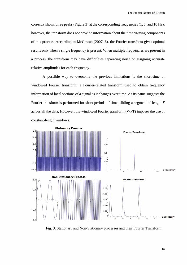
To illustrate the shortcomings of the Fourier transform when reproducing signals

that have time-varying features, the following example is based on Wolfram’s

presentation on wavelet concepts (see Wolfram 2014a). Considering the stationary

process 𝑠(𝑡) = 𝐶𝑜𝑠([2𝜋]20𝑡) + 𝐶𝑜𝑠([2𝜋]40𝑡). This process is composed of two signals,

one at 20 Hz and another at 40 Hz. When the Fourier transform of this data is performed

two frequencies are correctly identified, at two times the frequency in the x-axis, i.e. 40

and 80 Hz respectively (see Figure 3). While the Fourier transform provides frequency

information it lacks time information about these frequencies, i.e., at what time did these

frequencies occur and for how long? Considering now a non-stationary process with three

frequency components defined by 𝑠′(𝑡) = {

𝑆𝑖𝑛([2𝜋]𝑡) 0 ≤ 𝑡 ≤ 2

𝑆𝑖𝑛([2𝜋]5𝑡) 2 ≤ 𝑡 ≤ 4

𝑆𝑖𝑛([2𝜋]10𝑡) 4 ≤ 𝑡 ≤ 8, the Fourier transform


16

correctly shows three peaks (Figure 3) at the corresponding frequencies (1, 5, and 10 Hz),

however, the transform does not provide information about the time varying components

of this process. According to McCowan (2007, 6), the Fourier transform gives optimal

results only when a single frequency is present. When multiple frequencies are present in

a process, the transform may have difficulties separating noise or assigning accurate

relative amplitudes for each frequency.

A possible way to overcome the previous limitations is the short-time or

windowed Fourier transform, a Fourier-related transform used to obtain frequency

information of local sections of a signal as it changes over time. As its name suggests the

Fourier transform is performed for short periods of time, sliding a segment of length 𝑇

across all the data. However, the windowed Fourier transform (WFT) imposes the use of

constant-length windows.

Fig. 3. Stationary and Non-Stationary processes and their Fourier Transform


17

This restriction makes the WFT an inaccurate method for time-frequency analysis

since many high and low-frequency components of the process or signal will not fall

within the frequency range of the window. Relatively small windows will fail to detect

frequencies whose wavelengths are larger than the size of the window while relatively

large windows will decrease the temporal resolution because larger intervals of signal are

analyzed at once.

Torrence and Compo (1998, 63) argue that for analyses where a predetermined

scaling may not be appropriate because of a wide range of dominant frequencies are

present in the process, a method of time–frequency localization that is scale independent,

such as wavelet analysis, should be employed.

2.4 The Continuous Wavelet Transform

Just as the windowed Fourier transform, the aim of the continuous wavelet

transform (CWT) is to detect the frequency, or spectral, content of a signal and describe

how it changes over time. The CWT however uses a base function that can be stretched

and translated with a flexible resolution in both frequency and time, making it possible to

analyze non-stationary time series that contain many different frequencies. Moreover, the

CWT intrinsically adjusts the time resolution to the frequency content. This means the

analyzing window width with will narrow when focusing on high frequencies (short time

periods) and widen when assessing low frequencies (long time scales).

The CWT of a discrete sequence 𝑥𝑛 can be formally defined as𝑊𝑥(𝜏, 𝑠) =

∫ 𝑥(𝑡) 𝜓∗𝜏,𝑠(𝑡) 𝑑𝑡

+∞

−∞, where * denotes the complex conjugate. Starting with a mother

wavelet 𝜓(𝑡), the CWT decomposes the time series 𝑥(𝑡) in terms of analyzing wavelets

𝜓𝜏,𝑠(𝑡). The analyzing wavelets are obtained by scaling and translating 𝜓(𝑡), which is

defined as 𝜓∗𝜏,𝑠(𝑡) =

1

√|𝑠|𝜓(

𝑡−𝜏

𝑠), where s is the scale and 𝜏 the translation parameters.


18

Real Part

Imaginary Part

The wavelets can be stretched (if |𝑠| > 1) or compressed (if |𝑠| < 1), while translating

the wavelet means shifting their position in time. Thanks to the CWT flexible resolution

in both frequency and time, rapidly changing feature can be capture at low scales, or

wavelengths, whereas slow changing, or higher time scales, components can be detected

with dilated analyzing wavelets (Torrence and Compo 1998; Aguiar-Conraria and Soares

2011).

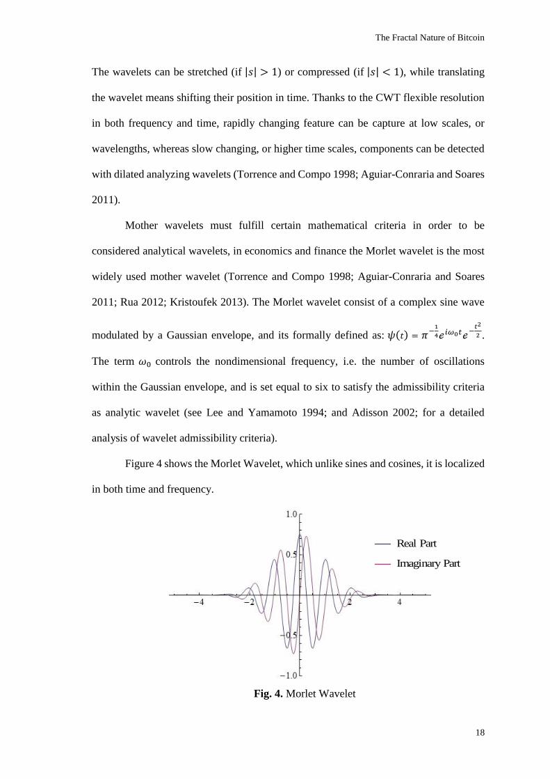
Mother wavelets must fulfill certain mathematical criteria in order to be

considered analytical wavelets, in economics and finance the Morlet wavelet is the most

widely used mother wavelet (Torrence and Compo 1998; Aguiar-Conraria and Soares

2011; Rua 2012; Kristoufek 2013). The Morlet wavelet consist of a complex sine wave

modulated by a Gaussian envelope, and its formally defined as: 𝜓(𝑡) = 𝜋−1

4ℯ𝑖𝜔0𝑡ℯ−𝑡2

2 .

The term 𝜔0 controls the nondimensional frequency, i.e. the number of oscillations

within the Gaussian envelope, and is set equal to six to satisfy the admissibility criteria

as analytic wavelet (see Lee and Yamamoto 1994; and Adisson 2002; for a detailed

analysis of wavelet admissibility criteria).

Figure 4 shows the Morlet Wavelet, which unlike sines and cosines, it is localized

in both time and frequency.

Fig. 4. Morlet Wavelet


19

2.5 Wavelet Power Spectrum and other Definitions in the Wavelet Domain

Once the CWT has been defined, we offer two definitions from the wavelet

domain to analyze an asset’s volatility as well as its local covariance with other assets

(see Ranta 2010 for additional definitions regarding correlation and contagion in the time-

frequency domain). First, the wavelet power spectrum (WPS) can be defined as

|𝑊𝑥(𝜏, 𝑠)|2, i.e. the square of the absolute value of each coefficient at each time and scale,

and measures the local contribution to the variance of the series. Second, the cross-

wavelet transform (XWT) of two time series 𝑥(𝑡) and 𝑦(𝑡), with continuous wavelet

transforms 𝑊𝑥(𝜏, 𝑠) and 𝑊𝑦(𝜏, 𝑠) , is defined as 𝑊𝑥𝑦(𝜏, 𝑠) = 𝑊𝑥(𝜏, 𝑠)𝑊𝑦∗(𝜏, 𝑠) . The

corresponding cross-wavelet spectrum is defined as 𝑋𝑊𝑃𝑥𝑦 = |𝑊𝑥𝑦| . According to

Aguiar-Conraria and Soares (2011, 16), the cross-wavelet power of two time series can

be defined as the local covariance between them in the time-frequency domain, giving

the researcher a quantified indication of the similarity of volatility between the time series.


20

Chapter III Methods and Results

In this section the CWT will be implemented on the BTC historical returns time series to

provide evidence for the dominance of short investment horizons during periods of high

volatility. Additionally, since all the analysis in this study was performed using the

computational software Mathematica, the code used to perform the computations will be

used to provide the reader new tools for wavelet analysis. The findings of this analysis

will be discussed afterward.

3.1 Data

A time series for the price of bitcoin against the U.S. Dollar will be analyzed to

find their respective wavelet power spectrum. The oldest available date for bitcoin prices

is July 17, 2010. The time series cover the oldest available BTC price until October 29,

2014.

Additionally BTC prices are compared against Litecoin (LTC) prices, both in

USD. Just as Bitcoin, Litecoin is a peer-to-peer cryptocurrency inspired by Bitcoin and

introduced as an improvement on it. As of November, 2014 Litecoin has the third largest

cryptocurrency market capitalization with approximately $128,786,179. Bitcoin is the

leading cryptocurrency in terms of market capitalization ($5,090,366,912), followed by

the Ripple protocol ($157,341,776) and Litecoin. Cross-wavelet transformation will be

used to study the local covariance in the time-frequency domain between the BTC and

LTC returns time series. Data was not sufficiently available to perform wavelet analysis

on the Ripple (XRP) currency.


21

The data used for this study was obtained from the data platform Qandl’s website,

a search engine for numerical data with access to a large collection of financial, economic,

and social datasets.

3.2 Method: Basic Wavelet Concepts

Performing a CWT in Mathematica can be done with very few commands. Before

the main analysis of this study, three examples will be presented to overview basic

wavelet transform concepts and their advantage over time or frequency analysis.

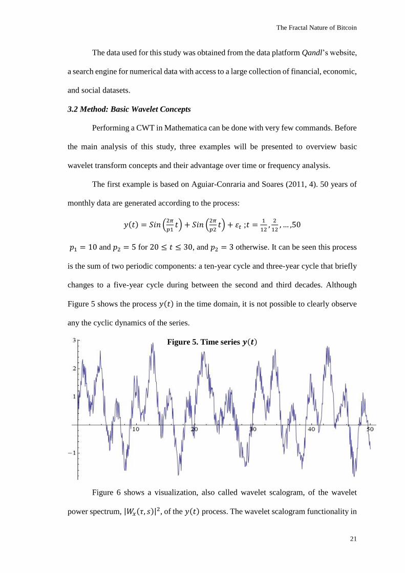
The first example is based on Aguiar-Conraria and Soares (2011, 4). 50 years of

monthly data are generated according to the process:

𝑦(𝑡) = 𝑆𝑖𝑛 (2𝜋

𝑝1𝑡) + 𝑆𝑖𝑛 (

2𝜋

𝑝2𝑡) + 𝜀𝑡 ; 𝑡 =

1

12,2

12, … ,50

𝑝1 = 10 and 𝑝2 = 5 for 20 ≤ 𝑡 ≤ 30, and 𝑝2 = 3 otherwise. It can be seen this process

is the sum of two periodic components: a ten-year cycle and three-year cycle that briefly

changes to a five-year cycle during between the second and third decades. Although

Figure 5 shows the process 𝑦(𝑡) in the time domain, it is not possible to clearly observe

any the cyclic dynamics of the series.

Figure 5. Time series 𝒚(𝒕)

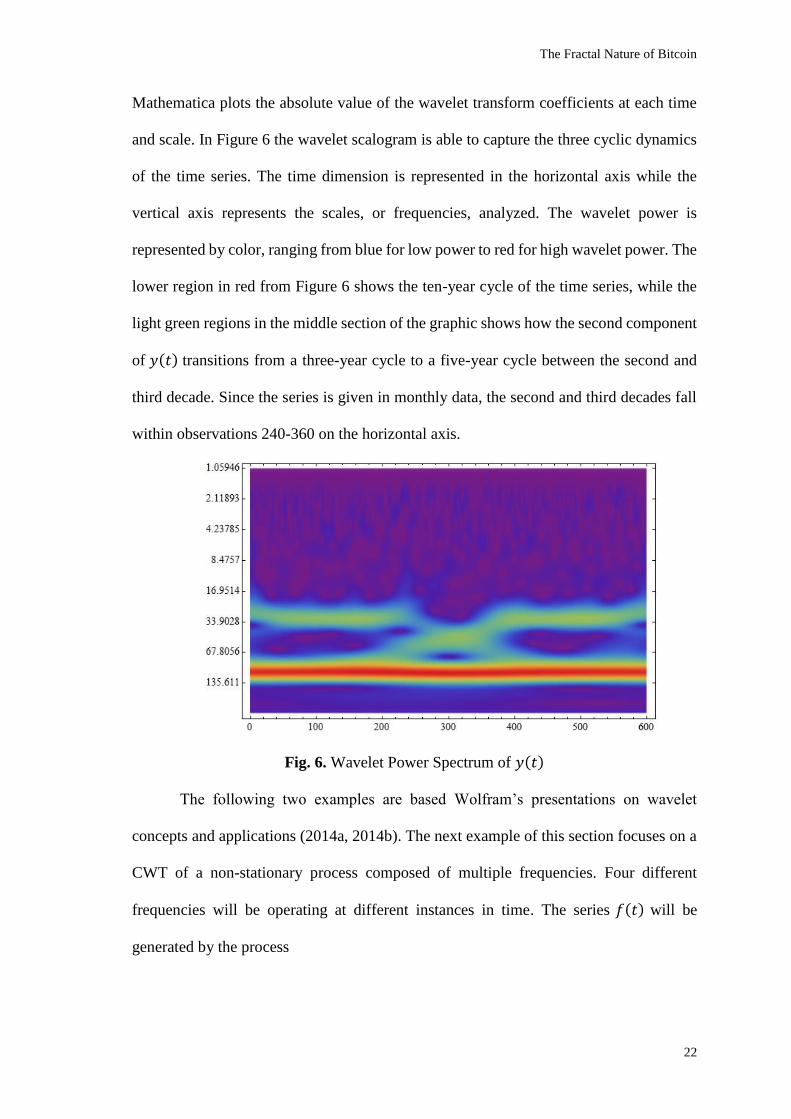
Figure 6 shows a visualization, also called wavelet scalogram, of the wavelet

power spectrum, |𝑊𝑥(𝜏, 𝑠)|2, of the 𝑦(𝑡) process. The wavelet scalogram functionality in


22

Mathematica plots the absolute value of the wavelet transform coefficients at each time

and scale. In Figure 6 the wavelet scalogram is able to capture the three cyclic dynamics

of the time series. The time dimension is represented in the horizontal axis while the

vertical axis represents the scales, or frequencies, analyzed. The wavelet power is

represented by color, ranging from blue for low power to red for high wavelet power. The

lower region in red from Figure 6 shows the ten-year cycle of the time series, while the

light green regions in the middle section of the graphic shows how the second component

of 𝑦(𝑡) transitions from a three-year cycle to a five-year cycle between the second and

third decade. Since the series is given in monthly data, the second and third decades fall

within observations 240-360 on the horizontal axis.

Fig. 6. Wavelet Power Spectrum of 𝑦(𝑡)

The following two examples are based Wolfram’s presentations on wavelet

concepts and applications (2014a, 2014b). The next example of this section focuses on a

CWT of a non-stationary process composed of multiple frequencies. Four different

frequencies will be operating at different instances in time. The series 𝑓(𝑡) will be

generated by the process


23

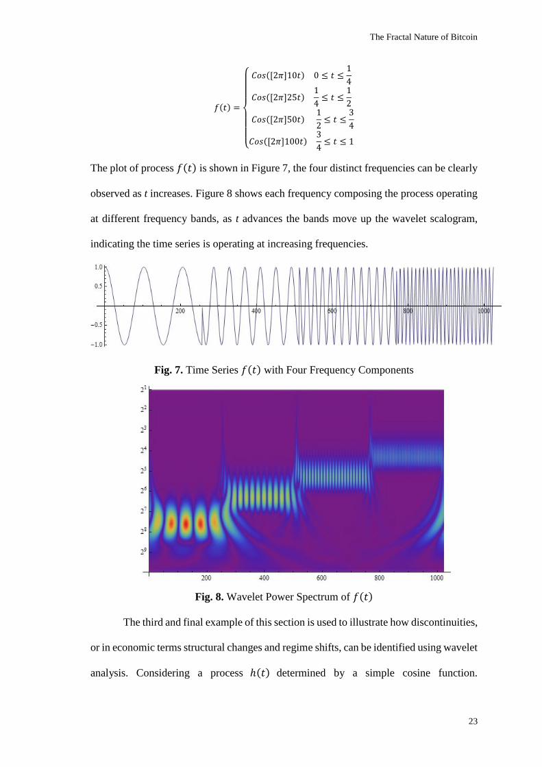
𝑓(𝑡) =

{

𝐶𝑜𝑠([2𝜋]10𝑡) 0 ≤ 𝑡 ≤

1

4

𝐶𝑜𝑠([2𝜋]25𝑡)1

4≤ 𝑡 ≤

1

2

𝐶𝑜𝑠([2𝜋]50𝑡)1

2≤ 𝑡 ≤

3

4

𝐶𝑜𝑠([2𝜋]100𝑡)3

4≤ 𝑡 ≤ 1

The plot of process 𝑓(𝑡) is shown in Figure 7, the four distinct frequencies can be clearly

observed as t increases. Figure 8 shows each frequency composing the process operating

at different frequency bands, as t advances the bands move up the wavelet scalogram,

indicating the time series is operating at increasing frequencies.

Fig. 7. Time Series 𝑓(𝑡) with Four Frequency Components

Fig. 8. Wavelet Power Spectrum of 𝑓(𝑡)

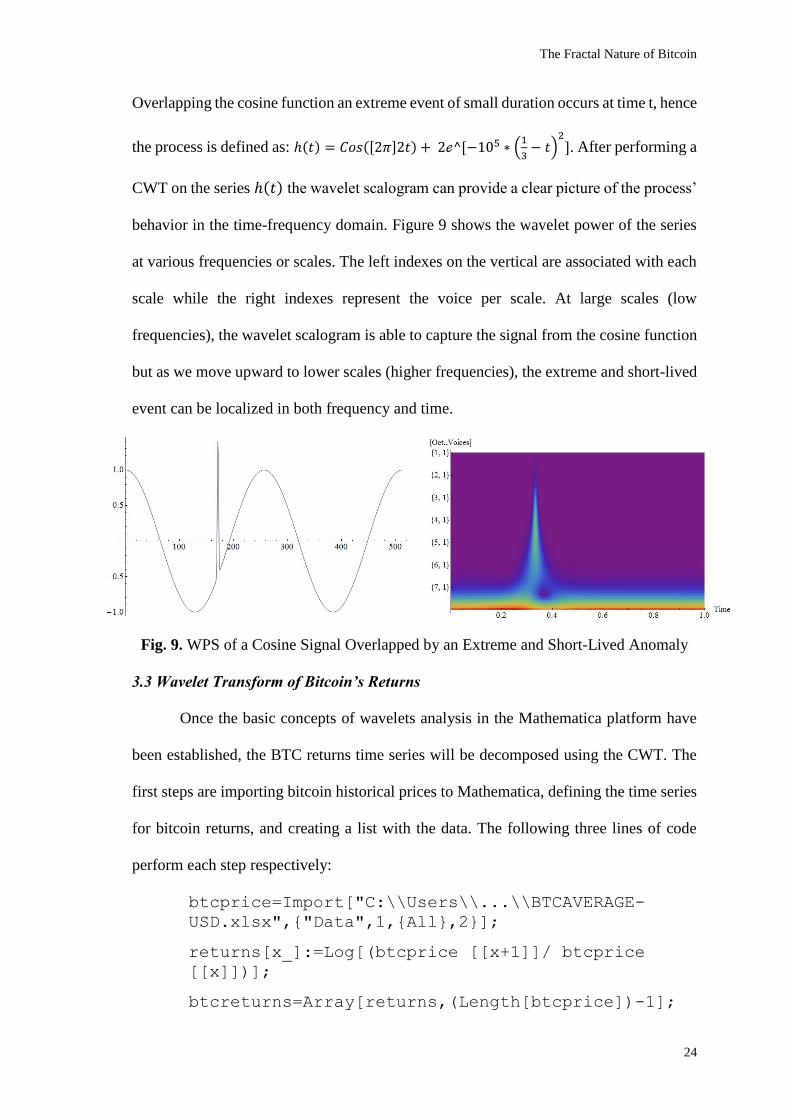
The third and final example of this section is used to illustrate how discontinuities,

or in economic terms structural changes and regime shifts, can be identified using wavelet

analysis. Considering a process ℎ(𝑡) determined by a simple cosine function.


24

Overlapping the cosine function an extreme event of small duration occurs at time t, hence

the process is defined as: ℎ(𝑡) = 𝐶𝑜𝑠([2𝜋]2𝑡) + 2ℯ^[−105 ∗ (1

3− 𝑡)

2]. After performing a

CWT on the series ℎ(𝑡) the wavelet scalogram can provide a clear picture of the process’

behavior in the time-frequency domain. Figure 9 shows the wavelet power of the series

at various frequencies or scales. The left indexes on the vertical are associated with each

scale while the right indexes represent the voice per scale. At large scales (low

frequencies), the wavelet scalogram is able to capture the signal from the cosine function

but as we move upward to lower scales (higher frequencies), the extreme and short-lived

event can be localized in both frequency and time.

Fig. 9. WPS of a Cosine Signal Overlapped by an Extreme and Short-Lived Anomaly

3.3 Wavelet Transform of Bitcoin’s Returns

Once the basic concepts of wavelets analysis in the Mathematica platform have

been established, the BTC returns time series will be decomposed using the CWT. The

first steps are importing bitcoin historical prices to Mathematica, defining the time series

for bitcoin returns, and creating a list with the data. The following three lines of code

perform each step respectively:

btcprice=Import["C:\\Users\\...\\BTCAVERAGE-

USD.xlsx",{"Data",1,{All},2}];

returns[x_]:=Log[(btcprice [[x+1]]/ btcprice

[[x]])];

btcreturns=Array[returns,(Length[btcprice])-1];


25

After the BTC returns data is defined, a CWT can be applied with the following

command:

cwt=ContinuousWaveletTransform[btcreturns,MorletWavelet[],

{9,10}]. The CWT command gives the wavelet transform of btcreturns, using the

complex MorletWavelet[], and decomposes the data into nine octaves, or scales,

and ten subsequent voices, or samples for each scale. The scales chosen for the wavelet

transform are defined as fractional powers of two: 𝑠𝑗 = 𝑠02𝑗/𝑣𝑜𝑐; 𝑗 = 0, 1, … , 𝐽; and 𝐽 =

𝑜𝑐𝑡 ∗ 𝑣𝑜𝑐, where 𝑠0 is the smallest resolvable scale and 𝐽 determines the total number of

layers in which the signal will be decomposed, i.e. 𝐽 = #𝑜𝑐𝑎𝑡𝑣𝑒𝑠 ∗ #𝑣𝑜𝑖𝑐𝑒𝑠 .

Additionally, the smallest resolvable scale 𝑠0 is computed automatically as the inverse of

Fourier wavelet length of the wavelet (Wolfram 2014c). For the CWT of the

btcreturns time series the smallest resolvable scale computed is .86 days or about 20

hours, therefore the scales and samples per scale will be computed as 𝑠𝑗 = .86 ∗ 2𝑗/90,

𝑗 = 0, 1, … , 90.

By default Mathematica computes the number of scales used in each transform as

𝑙𝑜𝑔2 (𝑁

2), where N is the length of the time series, while the default value for the number

of voices per octave is four. Computing the 𝑙𝑜𝑔2 (𝑁

2), where 𝑁 = 1547 for the BTC

returns time series results in 9.59. Mathematica correctly computes the number of scales

to be used in the wavelet transform, however the number of scales was explicitly indicated

in the CWT command in order to specify the number of voices per scale as well. The

more voices per scale are used in the CWT the better the time-frequency resolution, hence

it was increased to ten from the default value of four.

Mathematica evaluates the CWT command and the output Continuous Wavelet

Data object (CWDo) in the form {{𝑜𝑐𝑡1, 𝑣𝑜𝑐1} → 𝑐𝑜𝑒𝑓1, … , 𝑐𝑜𝑒𝑓𝑁} , with N wavelet


26

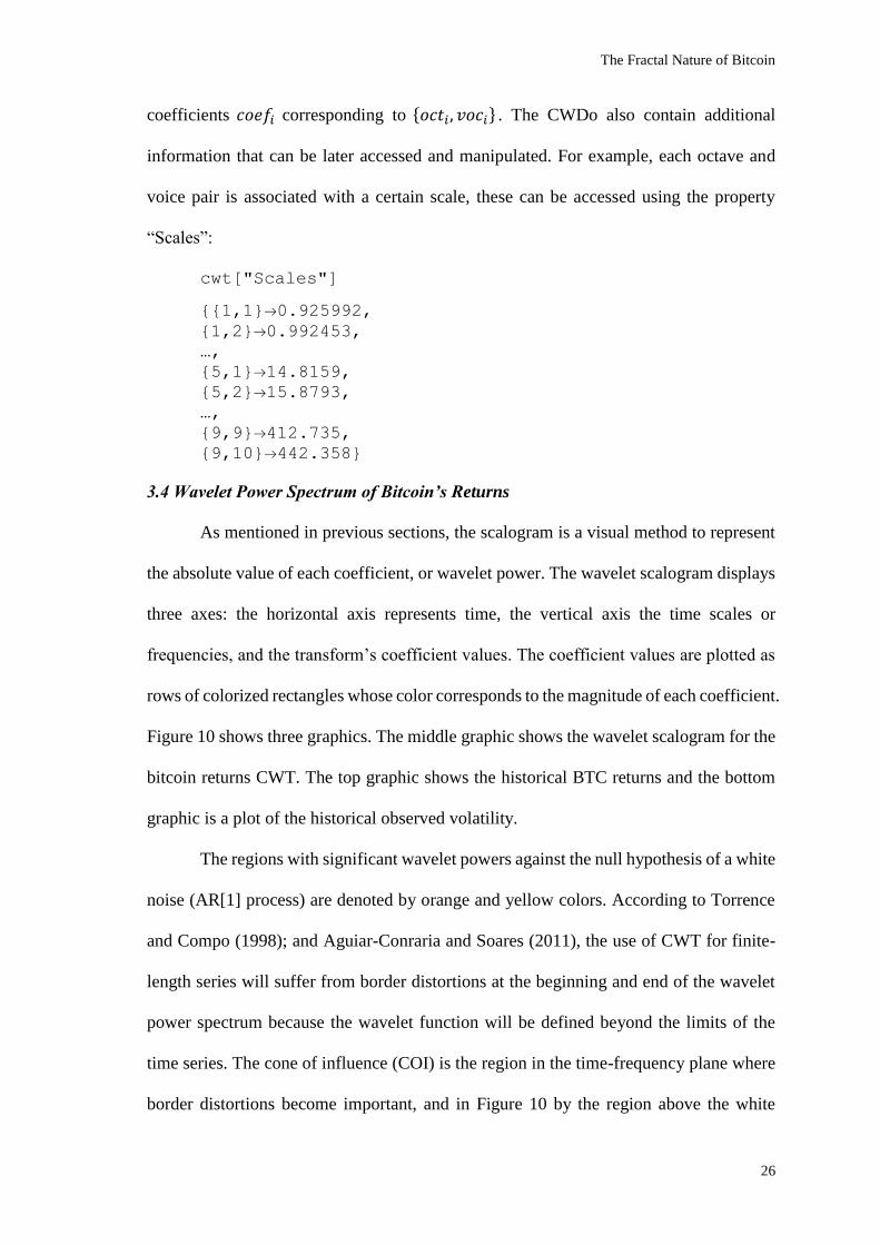
coefficients 𝑐𝑜𝑒𝑓𝑖 corresponding to {𝑜𝑐𝑡𝑖, 𝑣𝑜𝑐𝑖} . The CWDo also contain additional

information that can be later accessed and manipulated. For example, each octave and

voice pair is associated with a certain scale, these can be accessed using the property

“Scales”:

cwt["Scales"]

{{1,1}0.925992, {1,2}0.992453, …,

{5,1}14.8159, {5,2}15.8793, …,

{9,9}412.735, {9,10}442.358}

3.4 Wavelet Power Spectrum of Bitcoin’s Returns

As mentioned in previous sections, the scalogram is a visual method to represent

the absolute value of each coefficient, or wavelet power. The wavelet scalogram displays

three axes: the horizontal axis represents time, the vertical axis the time scales or

frequencies, and the transform’s coefficient values. The coefficient values are plotted as

rows of colorized rectangles whose color corresponds to the magnitude of each coefficient.

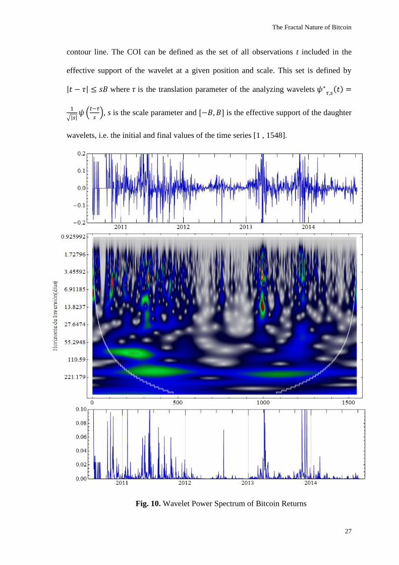
Figure 10 shows three graphics. The middle graphic shows the wavelet scalogram for the

bitcoin returns CWT. The top graphic shows the historical BTC returns and the bottom

graphic is a plot of the historical observed volatility.

The regions with significant wavelet powers against the null hypothesis of a white

noise (AR[1] process) are denoted by orange and yellow colors. According to Torrence

and Compo (1998); and Aguiar-Conraria and Soares (2011), the use of CWT for finite-

length series will suffer from border distortions at the beginning and end of the wavelet

power spectrum because the wavelet function will be defined beyond the limits of the

time series. The cone of influence (COI) is the region in the time-frequency plane where

border distortions become important, and in Figure 10 by the region above the white


27

contour line. The COI can be defined as the set of all observations t included in the

effective support of the wavelet at a given position and scale. This set is defined by

|𝑡 − 𝜏| ≤ 𝑠𝐵 where 𝜏 is the translation parameter of the analyzing wavelets 𝜓∗𝜏,𝑠(𝑡) =

1

√|𝑠|𝜓(

𝑡−𝜏

𝑠), s is the scale parameter and [−𝐵, 𝐵] is the effective support of the daughter

wavelets, i.e. the initial and final values of the time series [1 , 1548].

Fig. 10. Wavelet Power Spectrum of Bitcoin Returns


28

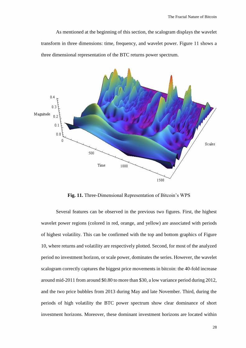
As mentioned at the beginning of this section, the scalogram displays the wavelet

transform in three dimensions: time, frequency, and wavelet power. Figure 11 shows a

three dimensional representation of the BTC returns power spectrum.

Fig. 11. Three-Dimensional Representation of Bitcoin’s WPS

Several features can be observed in the previous two figures. First, the highest

wavelet power regions (colored in red, orange, and yellow) are associated with periods

of highest volatility. This can be confirmed with the top and bottom graphics of Figure

10, where returns and volatility are respectively plotted. Second, for most of the analyzed

period no investment horizon, or scale power, dominates the series. However, the wavelet

scalogram correctly captures the biggest price movements in bitcoin: the 40-fold increase

around mid-2011 from around $0.80 to more than $30, a low variance period during 2012,

and the two price bubbles from 2013 during May and late November. Third, during the

periods of high volatility the BTC power spectrum show clear dominance of short

investment horizons. Moreover, these dominant investment horizons are located within


29

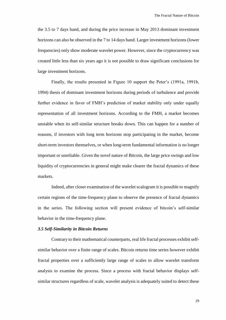
the 3.5 to 7 days band, and during the price increase in May 2013 dominant investment

horizons can also be observed in the 7 to 14 days band. Larger investment horizons (lower

frequencies) only show moderate wavelet power. However, since the cryptocurrency was

created little less than six years ago it is not possible to draw significant conclusions for

large investment horizons.

Finally, the results presented in Figure 10 support the Peter’s (1991a, 1991b,

1994) thesis of dominant investment horizons during periods of turbulence and provide

further evidence in favor of FMH’s prediction of market stability only under equally

representation of all investment horizons. According to the FMH, a market becomes

unstable when its self-similar structure breaks down. This can happen for a number of

reasons, if investors with long term horizons stop participating in the market, become

short-term investors themselves, or when long-term fundamental information is no longer

important or unreliable. Given the novel nature of Bitcoin, the large price swings and low

liquidity of cryptocurrencies in general might make clearer the fractal dynamics of these

markets.

Indeed, after closer examination of the wavelet scalogram it is possible to magnify

certain regions of the time-frequency plane to observe the presence of fractal dynamics

in the series. The following section will present evidence of bitcoin’s self-similar

behavior in the time-frequency plane.

3.5 Self-Similarity in Bitcoin Returns

Contrary to their mathematical counterparts, real life fractal processes exhibit self-

similar behavior over a finite range of scales. Bitcoin returns time series however exhibit

fractal properties over a sufficiently large range of scales to allow wavelet transform

analysis to examine the process. Since a process with fractal behavior displays self-

similar structures regardless of scale, wavelet analysis is adequately suited to detect these


30

properties. The basic principle for studying fractal processes with wavelet transform is

that since the signal is self-similar at any scale, the wavelet coefficients of the transform

too will be self-similar and this can be observed plotting the power spectrum of the signal

or series.

In order to show the self-similarity of BTC returns in the time frequency domain,

first only the real values of each wavelet coefficient are taken:

Rcwt= ReplacePart[cwt,1Re[cwt[[1]]]];

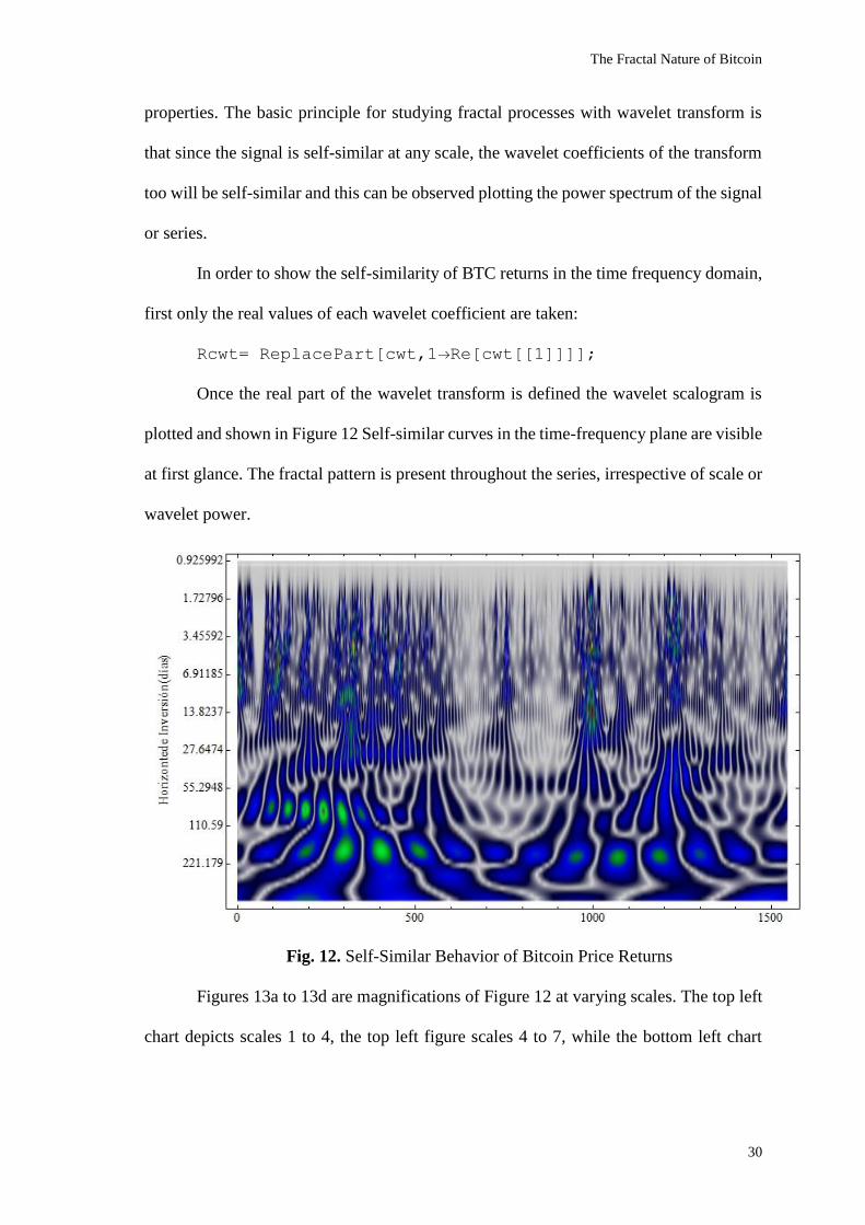
Once the real part of the wavelet transform is defined the wavelet scalogram is

plotted and shown in Figure 12 Self-similar curves in the time-frequency plane are visible

at first glance. The fractal pattern is present throughout the series, irrespective of scale or

wavelet power.

Fig. 12. Self-Similar Behavior of Bitcoin Price Returns

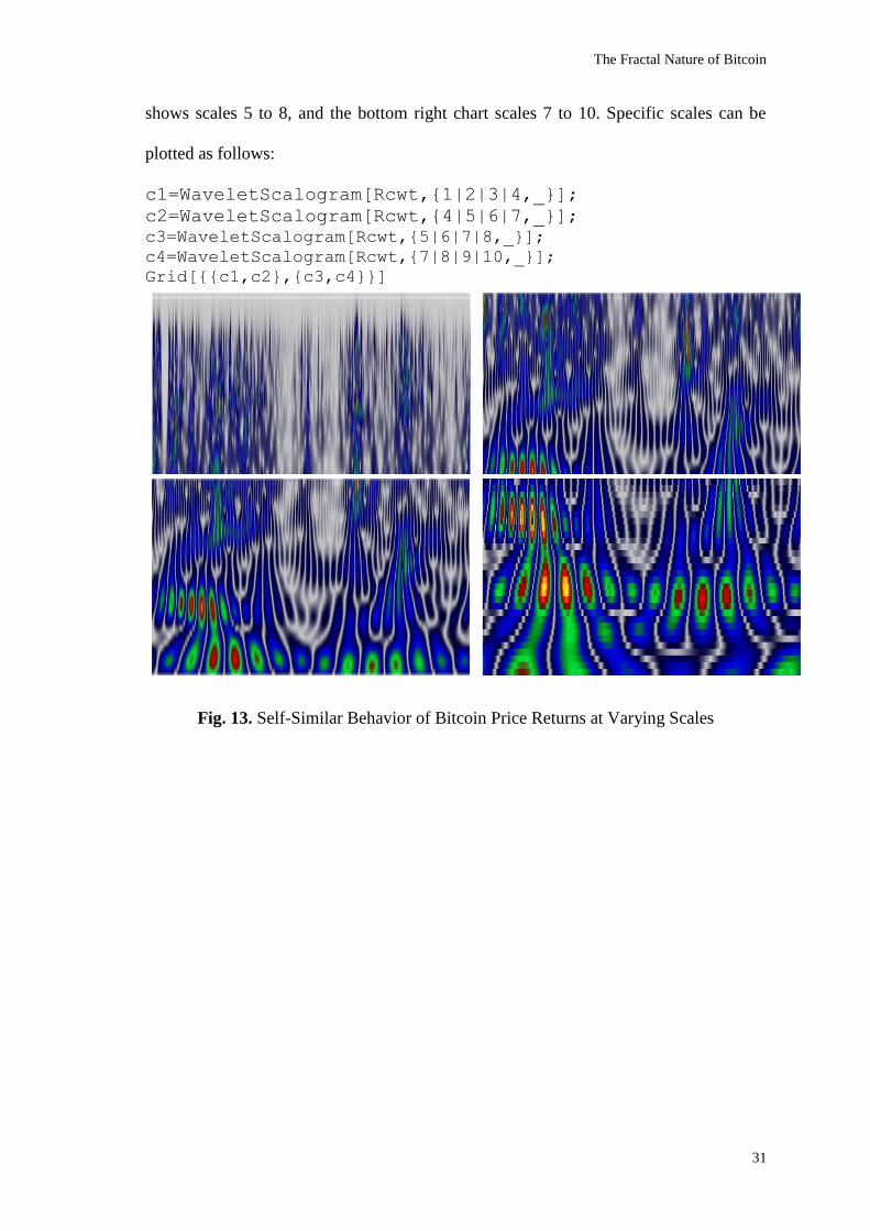
Figures 13a to 13d are magnifications of Figure 12 at varying scales. The top left

chart depicts scales 1 to 4, the top left figure scales 4 to 7, while the bottom left chart


31

shows scales 5 to 8, and the bottom right chart scales 7 to 10. Specific scales can be

plotted as follows:

c1=WaveletScalogram[Rcwt,{1|2|3|4,_}];




Grid[{{c1,c2},{c3,c4}}]

Fig. 13. Self-Similar Behavior of Bitcoin Price Returns at Varying Scales


32

Chapter IV Conclusion

Concluding remarks are presented in this section. The contribution of wavelets analysis

to the Fractal Market Hypothesis and the economic sciences in general are discussed, as

well as the future possible areas of research using time-frequency analysis.

4.1 Fractal Market Hypothesis: Evidence from Wavelet Power Spectrum

In spite of the novelty of the Bitcoin protocol and the uncharacteristically high

volatility of the homonymous currency, the predictions made by the Fractal Market

Hypothesis correctly capture the asset’s behavior. Thanks to the ability of wavelet

analysis to decompose a time series into different scales it is possible to observe the

dominance of short investment horizons during periods of price volatility. The theoretical

framework developed by Peters (1991a, 1991b, 1994) takes into account heterogeneous

agents who operate at simultaneous time horizons and react to market information with

respect to their investment horizon, therefore it is possible to account for the statistical

departures to the Efficient Market Hypothesis observed in the cryptocurrency’s returns.

Additionally, the use wavelet analysis allowed to observe the presence of self-

similar dynamics in the time series through the wavelet power spectrum. This

methodology has also been used to detect fractal properties in a wide range natural

phenomena, from fluid turbulence, to DNA sequences, and breathing rate variability

(Addison 2002).

4.2 Wavelet Analysis in Economics and Finance

Many authors argue the importance of multiscale relationships in economics and

finance (In and Kim 2012; Aguiar-Conraria and Soares 2011; and Ramsey and Lampart


33

1997). In financial terms, market dynamics are affected by investment horizons that range

from high frequency trading to individual stock brokers, hedge funds, multinational

corporations, pension funds, and government debt. However, despite the wide range of

investment horizons operating in the market, most economic analysis has relied on only

two scales, short and long run. The use of time-frequency analysis is being rapidly

adopted in economics to study how a process operates across a wide range of time scales.

Wavelet analysis has been used to investigate the multiscale relationship between the

stock and futures markets over various time horizons, the interest rate swap market in the

time-frequency domain, long memory in rates and volatility of LIBOR, and the

relationship between stock returns and risk factors at various time scales (In and Kim

2012)

Ramsey (2002) lists many benefits of incorporating wavelet analysis to the

discipline, for example estimators for novel situations, greater estimation efficiency,

robustness of modelling error, reduction of biased estimations, and most importantly,

discovering new insights into the properties of economic phenomena. For example,

Ramsey (2002) mentions previous studies using wavelet analysis, or time-scale

decomposition, to study the term structure of interest rates (Ramsey and Lampart 1997b),

the distinction between permanent and transitory shocks, or the relationship by time-scale

of money and income, and expenditure and income (Ramsey and Lampart 1998a, 1998b).

In their studies of money, income, and expenditure in the time-frequency domain

Ramsey and Lampart (1998a, 1998b) found evidence of complex behavior in the

relationships between these variables. The authors found that the delays observed

between variables are a function of time and scale, contrary to the accepted assumption

that delays between variables are fixed. This provides opportunities for future research

examining the underlying mechanisms of the time-varying delays. Ramsey (2002, 16)


34

speculates the “timing” of actions by economics agents can explain time-varying delays

and provides as an example a 2001 push by auto-manufacturers to lower the purchase

price on cars. The author argues the automakers’ decision had two effects. First,

undoubtedly increased quantity demanded in reaction to an implicit price decline, but it

also shortened the delay between income and expenditure.

Wavelet analysis can also be used to study structural change and regime shifts,

for example, to model the impact of minimum wage and tax legislation, and innovation.

Aggregate time series can be decomposed into long term structural components, medium

term seasonal components, and short term random components. This approach can allow

to characterize a robust system at high scales that also permits fluctuations that are not

entirely random and shorter time scales. As it was shown in Figure 6, wavelet analysis

allows for the study of transitional changes that were previously impossible to observe

thanks to wavelet’s ability to capture hidden dynamics.

Ramsey (2002, 22) also points to the analysis of term structure of interest rates as

a field where wavelet applications should provide extensive and deep insights since the

role of the horizon of the decision maker on market outcomes is so clearly indicated.

Kiermeier (2014) for example, analyses the risk factors of the European term structure of

interest rates and find good forecasting results, with up to one month of significant

forecasts even during times of financial market distress.

Time-frequency analysis also allows for new developments on forecasting. By

decomposing a time series into its global and local aspects, specific forecasting

techniques can be applied to each scale of the time series.

4.3 Future Research

The results presented in this study indicate new areas for both empirical and

theoretical research. For example how agents operate at several scales simultaneously,


35

both at the individual and aggregate level; or what are the long and short term structural

components underlying cryptocurrencies and their relationship to other economic

variables in the time-frequency domain. The application of wavelet analysis to economics

and finance is still in its infancy when compared with other fields. However, the wavelet

literature in economics is rapidly growing and expanding to other areas in the fields.

While most of wavelet analysis has fallen into three broad categories (macroeconomics,

volatility and asset pricing; and forecasting and spectral analysis), this new approach can

provide not only novel techniques but also new insights in many fields of economics.


36

References

Adisson, Paul S. 2002. The Illustrated Wavelet Transform Handbook: Introductory Theory and

Applications in Science, Engineering, Medicine and Finance. Boca Raton, FL: CRC

Press

Aguiar-Conraria, Luis, and Maria Joana Soares. 2011. “The Continuous Wavelet Transform: A

Primer.” Núcleo de Investigação em Políticas Económicas [Research Unit in Economic

Policy]. Accessed on May 10, 2014. Available online at http://www.nipe.eeg.uminho.pt/Uploads/WP_2011/NIPE_WP_16_2011.pdf

Barber, Simon, Xavier Boyen, Elaine Shi, and Ersin Uzun. 2012. “Bitter to Better—How to Make

Bitcoin a Better Currency.” Financial Cryptography and Data Security 7379: 399-414.

Accessed on May 10, 2014. Available online at

http://crypto.stanford.edu/~xb/fc12/bitcoin.pdf

Biddle, Sam. 2011. “What is Bitcoin?” Gizmodo. Accessed on May 10, 2014. Available online at

http://gizmodo.com/5803124/what-is-bitcoin

Bitcoin. 2014. “Important Milestones of the Bitcoin Project.” Bitcoin. Accessed on May 10, 2014.

Available online at https://en.bitcoin.it/wiki/History

Blackledge, Jonathan M. 2010. “The Fractal Market Hypothesis: Applications to Financial

Forecasting.” Dublin Institute of Technology. Accessed on May 10, 2014. Available

online at http://eleceng.dit.ie/papers/182.pdf

Borland, Lisa, Jean-Philippe Bouchaud, Jean-Francois Muzy, and Gilles Zumbach. 2005. “The

Dynamics of Financial Markets: Mandelbrot's Multifractal Cascades, and Beyond.”

Wilmott Magazine. Accessed on May 10, 2014. Available online at

http://arxiv.org/pdf/cond-mat/0501292.pdf

Brito, Jerry. 2011. “Online Cash Bitcoin Could Challenge Governments, Banks.” Time. Accessed

on May 10, 2014. Available online at http://techland.time.com/2011/04/16/online-cash-

bitcoin-could-challenge-governments/

Capgemini. 2013. “World Payments Report 2013.” Capgemini. Accessed on May 10, 2014.

Available online at http://www.capgemini.com/wpr13

Chaum, David. 1983. “Blind signatures for untraceable payments.” Advances in Cryptology 82

(3): 199-203. Accessed on May 10, 2014. Available online at

http://blog.koehntopp.de/uploads/Chaum.BlindSigForPayment.1982.PDF

Chaum, David, Amos Fiat, and Moni Naor. 1990. “Untraceable Electronic Cash.” Lecture Notes

in Computer Science 403: 319-327. Accessed on May 10, 2014. Available online at

http://blog.koehntopp.de/uploads/chaum_fiat_naor_ecash.pdf

Chen, Adrian. 2011a. “The Underground Website Where You Can Buy Any Drug Imaginable.”

Gawker. Accessed on May 10, 2014. Available online at http://gawker.com/the-

underground-website-where-you-can-buy-any-drug-imag-30818160

_____. 2011b. “Everyone Wants Bitcoins After Learning They Can Buy Drugs With Them.”

Gawker. Accessed on May 10, 2014. Available online at http://gawker.com/5808314/everyone-wants-bitcoins-after-learning-they-can-buy-drugs-

with-them

Congresional Research Service. 2013. “Bitcoin: Questions, Answers, and Analysis of Legal

Issues.” Federation of American Scientists. Accessed on May 10, 2014. Available online

at https://www.fas.org/sgp/crs/misc/R43339.pdf

Delfin, Rafael. 2014. “The Fractal Nature of Bitcoin: Evidence from Wavelet Power Spectra.”

Universidad de las Américas Puebla. Accessed on May 10, 2014. Available online at http://goo.gl/qCGmfn


37

Dermietzel, Jörn. 2008. “The Heterogeneous Agents Approach to Financial Markets -

Development and Milestones.” In Handbook on Information Technology in Finance

International Handbooks Information System, edited by Detlef Seese, Christof Weinhardt,

Frank Schlottmann, Berlin, Alemania: Springer Berlin Heidelberg. 443-464. Accessed on

May 10, 2014. Available online at http://link.springer.com/chapter/10.1007%2F978-3-

540-49487-4_19

Descôteaux, David. 2014. “Bitcoin: More Than a Currency, a Potential for Innovation.” Montreal

Economic Institute. Accessed on May 10, 2014. Available online at

http://www.iedm.org/46955-bitcoin-more-than-a-currency-a-potential-for-innovation

Dougherty, Carter. 2014. “Bitcoin Targets Payments Business of Giants Visa to JPMorgan.”

Bloomberg. Accessed on May 10, 2014. Available online at

http://www.bloomberg.com/news/2014-01-22/bitcoin-targets-giants-visa-to-jpmorgan-

with-lower-cost-payments.html

Ehrentreich, Norman. 2008. “Replicating the Stylized Facts of Financial Markets.” In Agent-

Based Modeling The Santa Fe Institute Artificial Stock Market Model Revisited, edited

by Norman Ehrentreich, Berlin, Germany: Springer Berlin Heidelberg. 51-88. Accessed

on May 10, 2014. Available online at http://link.springer.com/chapter/10.1007/978-3-

540-73879-4_5

Grapps, Amara. 1995. “Introduction to Wavelets.” IEEE Computational Science and Engineering

2 (2): 50-61. Accessed on November 10, 2014. Available online at

http://cs.haifa.ac.il/~nimrod/Compression/Wavelets/Wavelets_Graps.pdf

In, Francis, and Sangbae Kim. 2012. An Introduction to Wavelet Theory in Finance: A Wavelet

Multiscale Approach. Singapore, Singapore: World Scientific Publishing Company

Kiermeier, Michaela M. 2014. “Essay on Wavelet Analysis and the European Term Structure of

Interest Rates.” Business and Economic Horizons 9 (4): 18-26. https://ideas.repec.org/a/pdc/jrnbeh/v9y2014i4p18-26.html

Kristoufek, Ladislav. 2012. “Fractal Market Hypothesis and the Global Financial Crisis: Scaling,

Investment Horizons, and Liquidity.” Advances in Complex Systems 15 (6): 1-11.

Accessed on May 10, 2014. Available online at http://arxiv.org/abs/1203.4979

_____. 2013. “Fractal Market Hypothesis and the Global Financial Crisis: Wavelet Power

Evidence.” Scientific Reports. Accessed on May 10, 2014. Available online at

http://www.nature.com/srep/2013/131004/srep02857/full/srep02857.html

Kroll, Joshua A., Ian C. Davey, and Edward W. Felten. 2013. “The Economics of Bitcoin Mining,

or Bitcoin in the Presence of Adversaries.” Workshop on the Economics of Information

Security. Accessed on May 10, 2014. Available online at

http://weis2013.econinfosec.org/papers/KrollDaveyFeltenWEIS2013.pdf

Lee, Timothy B. 2011. “The Bitcoin Bubble.” Bottom-up. Accessed on May 10, 2014. Available

online at http://timothyblee.com/2011/04/18/the-bitcoin-bubble/

Lee, Daniel T. L., and Akio Yamamoto. 1994. “Wavelet Analysis: Theory and Applications.”

Hewlett-Packard Journal. Accessed on May 10, 2014. Available online at http://www.hpl.hp.com/hpjournal/94dec/dec94a6.pdf

Li, Jin. 2003. “Image Compression: The Mathematics of JPEG 2000.” Modern Signal Processing

46: 185-221. Accessed on May 10, 2014. Available online at

http://library.msri.org/books/Book46/files/08li.pdf

Mack, Erick. 2013. “The Bitcoin Pizza Purchase That's Worth $7 Million Today.” Forbes.


http://www.forbes.com/sites/ericmack/2013/12/23/the-bitcoin-pizza-purchase-thats-

worth-7-million-today/


38

Mandelbrot, Benoit. 1963. “The Variation of Certain Speculative Prices.” The Journal of Business

36 (4): 394-419. Accessed on May 10, 2014. Available online at

http://ideas.repec.org/p/cwl/cwldpp/1164.html

_____. 1997. Fractals and Scaling in Finance: Discontinuity, Concentration, Risk. Berlin,

Germany: Springer

McCowan, David. 2007. “Spectral Estimation with Wavelets.” The University of Chicago.

Accessed on November 10, 2014. Available online at http://home.uchicago.edu/~mccowan/research/wavelets/mccowan_htc_thesis.pdf

Nakamoto, Satoshi. 2009. “Bitcoin: A Peer-to-Peer Electronic Cash System.” Bitcoin. Accessed

on May 10, 2014. Available online at https://bitcoin.org/bitcoin.pdf

Peters, Edgar E. 1991a. Chaos and Order in the Capital Markets: A New View of Cycles, Prices,

and Market Volatility. New York, NY: John Wiley and Sons

_____. 1991b. “A Chaotic Attractor for the S&P 500.” Financial Analysis Journal 47 (2): 55-62.


http://harpgroup.org/muthuswamy/talks/cs498Spring2013/AChaoticAttractorForTheSA

ndP500.pdf

_____. 1994. Fractal Market Analysis: Applying Chaos Theory to Investment and Economics.

New York, NY: John Wiley and Sons.

Rama, Cont. 2001. “Empirical Properties of Asset Returns: Stylized Facts and Statistical Issues.”

Quantitative Finance 1 (2): 223-236. Accessed on May 10, 2014. Available online at

http://www-

stat.wharton.upenn.edu/~steele/Resources/FTSResources/StylizedFacts/Cont2001.pdf

_____. 2005. “Volatility Clustering in Financial Markets: Empirical Facts and Agent-Based

Models.” Social Science Research Network. Accessed on May 10, 2014. Available online

at https://www.newton.ac.uk/preprints/NI05015.pdf

Ramsey, James B. 2002. “Wavelets in Economics and Finance: Past and Future.” Studies in

Nonlinear Dynamics & Econometrics 6 (1): 1-27. Accessed on November 10, 2014.

Available online at http://plaza.ufl.edu/yiz21cn/refer/wavelet%20in%20economics%20and%20finance.pdf

Ramsey, James B., and Camille Lampart. 1997a. “The Decomposition of Economic Relationships

by Time Scale Using Wavelets.” New York University. Accessed on May 10, 2014.

Available online at http://econ.as.nyu.edu/docs/IO/9382/RR97-08.PDF

_____. 1997b. “The Analysis of Foreign Exchange Rates Using Waveform Dictionaries.” The

Journal of Empirical Finance. Accessed on May 10, 2014. Available online at http://citeseerx.ist.psu.edu/viewdoc/summary?doi=10.1.1.52.9744

_____. 1998a. “The Decomposition of Economic Relationships by Time Scale Using Wavelets:

Money and Income.” Macroeconomic Dynamics 2: 49-71. Accessed on May 10, 2014.

Available online at http://journals.cambridge.org/article_S1365100598006038

_____. 1998b. “The Decomposition of Economic Relationships by Time Scale Using Wavelets:

Expenditure and Income.” Studies in Nonlinear Dynamics and Econometrics 3 (4): 49-

71. Accessed on May 10, 2014. Available online at https://ideas.repec.org/a/bpj/sndecm/v3y1998i1n2.html

Ranta, Mikko. 2010. “Wavelet Multiresolution Analysis of Financial Time Series.” University of

Vaasa. Accessed on May 10, 2014. Available online at http://www.uva.fi/materiaali/pdf/isbn_978-952-476-303-5.pdf

Rua, António. 2012. “Wavelets in Economics.” Banco de Portugal. Accessed on May 10, 2014.

Available online at https://www.bportugal.pt/en-

US/BdP%20Publications%20Research/AB201208_e.pdf


39

Szabo, Nick. 2008. “Bit Gold.” Unenumerated. Accessed on May 10, 2014. Available online at

http://unenumerated.blogspot.mx/2005/12/bit-gold.html

Thurner, Stefan, Markus C. Feurstein, and Malvin C. Teich. 1998. “Multiresolution Wavelet

Analysis of Heartbeat Intervals Discriminates Healthy Patiens from those with Cardia

Pathology.” Physical Review Letters 80 (7): 1544-1547. Accessed on May 10, 2014.

Available online at http://sws.bu.edu/teich/pdfs/PRL-80-1544-1998.pdf

Torrence, Christoper, and Gilbert P. Compo. 1998. “A Practical Guide to Wavelet Analysis.”

Program in Atmospheric and Oceanic Sciences. Accessed on November 10, 2014.

Available online at http://paos.colorado.edu/research/wavelets/bams_79_01_0061.pdf

Velde, Francois R. 2013. “Chicago Fed Letter - Bitcoin: A Primer.” The Federal Reserve Bank of

Chicago. Accessed on May 10, 2014. Available online at

http://www.chicagofed.org/webpages/publications/chicago_fed_letter/2013/december_3

17.cfm

Weisenthal, Joe. 2013. “Here's The Answer To Paul Krugman's Difficult Question About Bitcoin.”

Business Insider. Accessed on May 10, 2014. Available online at

http://www.businessinsider.com/why-bitcoin-has-value-2013-12

Wolfram. 2014a. “Wavelet Analysis: Concepts.” Wolfram. Accessed on May 10, 2014. Available

online at http://www.wolfram.com/training/videos/ENG811/

Wolfram. 2014b. “Wavelet Analysis: Applications.” Wolfram. Accessed on May 10, 2014.

Available online at http://www.wolfram.com/training/videos/ENG812/

Wolfram. 2014c. “WaveletScale.” Wolfram. Accessed on May 10, 2014. Available online at http://reference.wolfram.com/language/ref/WaveletScale.html

World Bank. 2013. “Developing Countries to Receive Over $410 Billion in Remittances in 2013,

Says World Bank.” World Bank. Accessed on May 10, 2014. Available online at

http://www.worldbank.org/en/news/press-release/2013/10/02/developing-countries-

remittances-2013-world-bank

Documents

The Fractal Nature of Bitcoin