1

FoCUS: Fourier-based Coded UltrasoundAlmog Lahav, Tanya Chernyakova, Student Member, IEEE, Yonina C. Eldar, Fellow, IEEE

Abstract—Modern imaging systems typically use single-carriershort pulses for transducer excitation. Coded signals togetherwith pulse compression are successfully used in radar andcommunication to increase the amount of transmitted energy.Previous research verified significant improvement in SNR andimaging depth for ultrasound imaging with coded signals. Sincepulse compression needs to be applied at each transducerelement, the implementation of coded excitation (CE) in arrayimaging is computationally complex. Applying pulse compressionon the beamformer output reduces the computational load butalso degrades both the axial and lateral point spread function(PSF) compromising image quality. In this work we present anapproach for efficient implementation of pulse compression byintegrating it into frequency domain beamforming. This methodleads to significant reduction in the amount of computationswithout affecting axial resolution. The lateral resolution is dic-tated by the factor of savings in computational load. We verifythe performance of our method on a Verasonics imaging systemand compare the resulting images to time-domain processing. Weshow that up to 77 fold reduction in computational complexitycan be achieved in a typical imaging setups. The efficientimplementation makes CE a feasible approach in array imagingpaving the way to enhanced SNR as well as improved imagingdepth and frame-rate.

Index Terms—Array processing, beamforming, ultrasound,coded excitation.

I. INTRODUCTION

Ultrasound is a radiation free imaging modality with nu-merous applications. In standard ultrasound systems an arrayof transducer elements transmits a short single-carrier Gaus-sian pulse. During its propagation echoes are scattered byacoustic impedance perturbations in the tissue, and receivedby the array elements. These echoes are essentially a streamof replicas of the transmitted pulse implying that the axialresolution is defined by the pulse duration. The data, collectedby the transducers, is sampled and digitally integrated in away referred to as beamforming, yielding a signal steered ina predefined direction and optimally focused at each depth.Such a beamformed signal, referred to as beam, forms a linein the image.

While the resolution is defined by the pulse duration, theresulting signal-to-noise ratio (SNR) and imaging depth areproportional to the amount of transmitted energy. One wayto increase the energy is to transmit a longer pulse at a costof resolution. Increasing the energy while retaining the samepulse duration, requires higher peak intensity levels, whichcan potentially damage the tissue and thus are limited bythe Food and Drug Administration (FDA) regulations. Moreelaborate coded signals are used in radar and communicationto overcome the above trade-off between the transmittedenergy and resolution.

When coded signals are used for excitation, pulse com-pression is performed on the detected signal by applying a

matched filter (MF) defined by the transmitted pulse-shape. Asa result a stream of pulse’s replicas is converted to a stream ofits autocorrelations. The width of the pulse’s autocorrelationis on the order of the inverse bandwidth [1], implying thatthe resolution is now defined only by the available system’sbandwidth and is independent of pulse duration. Therefore,a longer pulse can be used to transmit more energy withoutdegrading axial resolution. In coded ultrasound imaging phase-modulated signals are of interest since amplitude modulationis suboptimal in terms of energy.

Extensive studies show that, despite the frequency de-pendent attenuation characterizing biological tissues and thedifferences between detection and imaging nature of radarand ultrasound, coded signals can be successfully used inmedical imaging [2], [3]. Experimental results reported in [4]show improvement of 15-20 dB in SNR as well as 30-40mm improvement in penetration depth. Due to these superiorproperties coded excitation (CE) was successfully applied innumerous ultrasound modalities including B-mode, flow andstrain imaging [5], [6] as well as contrast imaging [7], [8].

Increased penetration and SNR are even more crucial forapplications where the amount of transmitted energy is inher-ently reduced, e.g. synthetic aperture and plane wave imaging[9]–[11]. The feasibility of CE in plane-wave based shear wavemotion detection was recently studied, showing substantialperformance improvement [11]. Beyond the improvement inimaging depth, high SNR allows the utilization of higherfrequencies and consequently better image resolution [12]. Inaddition, Misaridis and Jensen have shown a way to increasethe frame rate by an orthogonal coding approach [3], [13],[14].

A. Challenges and Existing SolutionsDespite the proven advantages of coded imaging its applica-

tion in commercial medical systems is still very limited. Oneof the main challenges of CE in medical ultrasound is its appli-cation to imaging with an array of transducer elements due tocomputational complexity of the required processing [2], [15]–[17]. Regardless of the type of transmitted signal, samplingrates required to perform high resolution digital beamformingare typically significantly higher than the Nyquist rate of thesignal. Rates up to 4-10 times the central frequency of thetransmitted pulse are used in order to eliminate artifacts causedby digital implementation of beamforming in time [18]. Takinginto account the number of transducer elements the amount ofsampled data that needs to be transferred to the processing unitand digitally processed in real time is very large. The pulsecompression step, required in coded imaging, further increasesthe computational load.

Implementation of CE in array imaging requires a MFfor every transducer element increasing the computational

arX

iv:1

612.

0174

9v1

[cs

.IT

] 6

Dec

201

6

2

complexity. Most reported experimental studies use either asingle transducer element [3], [6], [7] or an array of elementswith one MF applied on the beamformed output [2], [4].Even though the advantage of a single application of a MFon the beamformed data is obvious from the computationalperspective, this approach degrades the performance of pulsecompression [2]. The process of beamforming is comprisedof averaging the received signals after their alignment withappropriate delays. To obtain dynamic focusing the applieddelays are non-linear and time dependent and, thus, distort thephases of the coded signals. Due to this distortion the sidelobelevel and the main lobe width of the MF output are degraded,leading to decreased contrast and resolution, which are highlyprominent at low imaging depth.

One way to minimize this effect is to limit the durationof the transmitted pulse [4]. However, this obviously reducesthe amount of transmitted energy and, thus, goes against themain motivation behind the usage of coded signals. Anotherapproach is based on the results reported in [15]. There it isshown that the degradation of the compression performancedue to dynamic beamforming depends on the depth of thetransmit focus. A possible solution is, therefore, to dividean image to several depth zones and adjust the code lengthaccording to the depth in order to reduce the compressionerror. In this case, however, the number of transmission eventsis increased in accordance to the number of focal zones, whichin turn increases the acquisition time.

B. Contributions

Here we propose an approach that achieves perfect pulsecompression, while keeping the computational complexity low.Our method is based on incorporating pulse compression intofrequency domain beamforming (FDBF) developed recentlyfor medical ultrasound [19]–[21]. This allows to use a MF ineach transducer element at a low cost.

The concept of beamforming in frequency was first ad-dressed back in the sixties for sonar arrays operating in the farfield. However, translating these ideas to ultrasound imagingis much more involved due to near field operation, requiringnon-linear beamforming. To the best of our knowledge, it wasfirst addressed in [19], [20], where it was shown that in thefrequency domain the Fourier components of the beamformedsignal can be computed as a weighted average of those of theindividual detected signals. Since the beam is obtained directlyin frequency, its Fourier components are computed only withinits effective bandwidth. This is done using generalized low-rate samples of the received signals, implying sampling andprocessing at the effective Nyquist rate which is defined withrespect to the signals effective bandpass bandwidth [22].

We note that according to the convolution theorem, pulsecompression applied at each transducer element through MFis equivalent to multiplication in the frequency domain. In thiswork we show that it can be applied by appropriate modifi-cation of weights required for FDBF. As a result, not only isbeamforming performed in frequency at a low rate, but it alsoincludes MF of each individual channel without any additionalcomputational load to the FDFB technique. The proposed

method, performing both beamforming and pulse compressionin frequency, is referred to as FoCUS, Fourier-based codedultrasound. The performance of our method is verified on aVerasonics ultrasound system and is compared to time-domainprocessing in terms of lateral and axial resolution. We evaluatethe computational load for typical imaging setup and show thatit can be reduced by 4 to 77 fold compared to time-domainimplementation, depending on the oversampling factor andthe required lateral resolution. This efficient implementationallows CE to become a practical approach in array imaging.

The rest of the paper is organized as follows: Section IIreviews basics of CE applied to medical imaging. In SectionIII we discuss the requirements and challenges of CE inthe context of array imaging. We next propose a solutionbased on frequency domain beamforming in Section IV. Theexperimental results and the performance of FoCUS in termsof image quality and computational complexity are presentedin Section V.

II. CODED EXCITATION IN MEDICAL ULTRASOUND

In CE a modulated signal is used for transducer excitation

s(t) = a(t) cos(2πf0t+ ψ(t)), 0 ≤ t ≤ Tp. (1)

where ψ(t) and a(t) are phase and amplitude modulation func-tions respectively, f0 is the central frequency of a transducerand Tp is the duration of the signal. Assuming L scatterersalong the transmitted signal propagation path, the reflectedsignal, ϕ(t), detected by an individual transducer element isgiven by

ϕ(t) =

L∑

l=1

αls(t− tl), (2)

where {αl}Ll=1 and {tl}Ll=1 are amplitudes and delays definedrespectively by the scatterer’s reflectivity and location.

Next, pulse compression is performed on the detectedsignal, ϕ(t), by applying a MF, h(t) = s∗(−t). The outputis then a combination of autocorrelations of the transmittedpulse [13]

ϕCE(t) = ϕ(t) ∗ s∗(−t) =

L∑

l=1

αlRss(t− tl). (3)

The autocorrelation is given by

Rss(t) =

∫ ∞

−∞s(τ)s∗(τ − t)dτ. (4)

The half-power width of the main lobe of the autocorrelation,which determines the range resolution, is approximately equalto the inverse bandwidth B−1 [1] of the transmitted pulse. As aresult, in contrast to the conventional approach, the pulse timeduration, Tp , can be increased and more energy transmittedwithout degrading range resolution. The resulting gain insignal-to-noise ratio of the MF processing is approximatelyequal to the time-bandwidth product D = TpB [23].

The above result holds when the detected signal is com-prised of the exact replicas of the transmitted pulse. In practice,when acoustic wave propagates in biological tissues, highfrequencies undergo stronger attenuation due to the medium’s

3

properties. A common way to model this effect is to assumethat it does not distort the complex envelope of the reflectedsignal and only downshifts its central frequency [24]. Thepulse reflected from the lth scatterer is then given by

s(t−tl, fl) = a(t−tl) cos(2π(f0−fl)(t−tl)+ψ(t−tl)). (5)

As a result, the MF output depends on the central frequencyshift, fl, and is given by

A(t− tl, fl) =

∫ ∞

−∞s(τ − tl, fl)s∗(τ − t)dτ. (6)

The function A(t, f) is referred to as the ambiguity function.Similar to (3), for L scatterers the output of the MF is a streamof cross-sections of ambiguity function

ϕCE(t) = ϕ(t) ∗ s∗(−t) =

L∑

l=1

αlA(t− tl, fl). (7)

In ultrasound imaging the frequency shifts do not carry valu-able information and thus do not need to be found explicitly.However, the width of the main lobe of the ambiguity functionneeds to be small for all values of fl to ensure good axialresolution for all frequency shifts. This makes the ambiguityfunction of linear frequency modulation (FM) a good choicefor ultrasound imaging.

The expression for a linear FM signal is

s(t) = a(t) cos

(2π

((f0 −B/2)t+

B

2Tpt2))

, 0 ≤ t ≤ Tp.

(8)

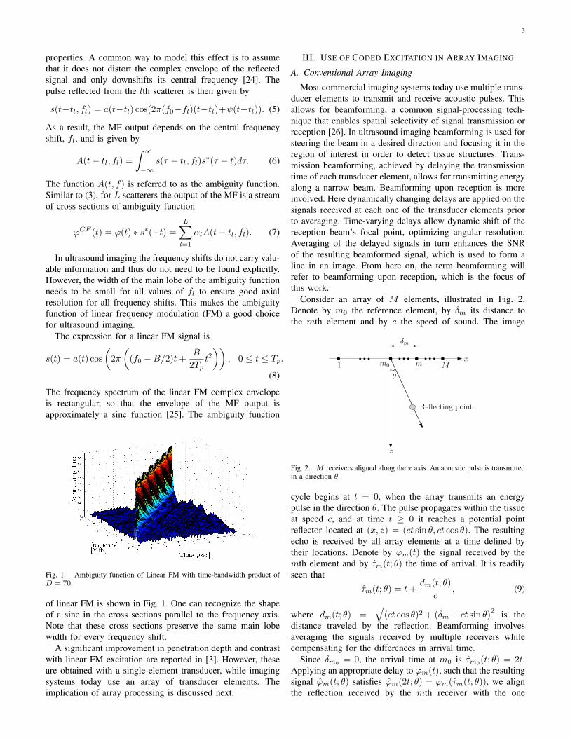
The frequency spectrum of the linear FM complex envelopeis rectangular, so that the envelope of the MF output isapproximately a sinc function [25]. The ambiguity function

Fig. 1. Ambiguity function of Linear FM with time-bandwidth product ofD = 70.

of linear FM is shown in Fig. 1. One can recognize the shapeof a sinc in the cross sections parallel to the frequency axis.Note that these cross sections preserve the same main lobewidth for every frequency shift.

A significant improvement in penetration depth and contrastwith linear FM excitation are reported in [3]. However, theseare obtained with a single-element transducer, while imagingsystems today use an array of transducer elements. Theimplication of array processing is discussed next.

III. USE OF CODED EXCITATION IN ARRAY IMAGING

A. Conventional Array Imaging

Most commercial imaging systems today use multiple trans-ducer elements to transmit and receive acoustic pulses. Thisallows for beamforming, a common signal-processing tech-nique that enables spatial selectivity of signal transmission orreception [26]. In ultrasound imaging beamforming is used forsteering the beam in a desired direction and focusing it in theregion of interest in order to detect tissue structures. Trans-mission beamforming, achieved by delaying the transmissiontime of each transducer element, allows for transmitting energyalong a narrow beam. Beamforming upon reception is moreinvolved. Here dynamically changing delays are applied on thesignals received at each one of the transducer elements priorto averaging. Time-varying delays allow dynamic shift of thereception beam’s focal point, optimizing angular resolution.Averaging of the delayed signals in turn enhances the SNRof the resulting beamformed signal, which is used to form aline in an image. From here on, the term beamforming willrefer to beamforming upon reception, which is the focus ofthis work.

Consider an array of M elements, illustrated in Fig. 2.Denote by m0 the reference element, by δm its distance tothe mth element and by c the speed of sound. The image

1 m0 m Mx

δm

Reflecting point

θ

z

Fig. 2. M receivers aligned along the x axis. An acoustic pulse is transmittedin a direction θ.

cycle begins at t = 0, when the array transmits an energypulse in the direction θ. The pulse propagates within the tissueat speed c, and at time t ≥ 0 it reaches a potential pointreflector located at (x, z) = (ct sin θ, ct cos θ). The resultingecho is received by all array elements at a time defined bytheir locations. Denote by ϕm(t) the signal received by themth element and by τm(t; θ) the time of arrival. It is readilyseen that

τm(t; θ) = t+dm(t; θ)

c, (9)

where dm(t; θ) =

√(ct cos θ)2 + (δm − ct sin θ)

2 is thedistance traveled by the reflection. Beamforming involvesaveraging the signals received by multiple receivers whilecompensating for the differences in arrival time.

Since δm0 = 0, the arrival time at m0 is τm0(t; θ) = 2t.Applying an appropriate delay to ϕm(t), such that the resultingsignal ϕm(t; θ) satisfies ϕm(2t; θ) = ϕm(τm(t; θ)), we alignthe reflection received by the mth receiver with the one

4

received at m0. Denoting τm(t; θ) = τm(t/2; θ) and using(9), the following aligned signal is obtained

ϕm(t; θ) = ϕm(τm(t; θ)), (10)

τm(t; θ) =1

2

(t+√t2 − 4(δm/c)t sin θ + 4(δm/c)2

).

The beamformed signal may now be derived by averaging thealigned signals

Φ(t; θ) =1

M

M∑

m=1

ϕm(t; θ) =1

M

M∑

m=1

ϕm(τm(t; θ)). (11)

Such a beam is optimally focused at each depth and henceexhibits improved angular localization and enhanced SNR.

In practice, the processing defined in (11) is performeddigitally, where the values of the detected signal ϕm(t) atτm(t; θ) are obtained by linear interpolation.

B. Matched Filtering and Beamforming

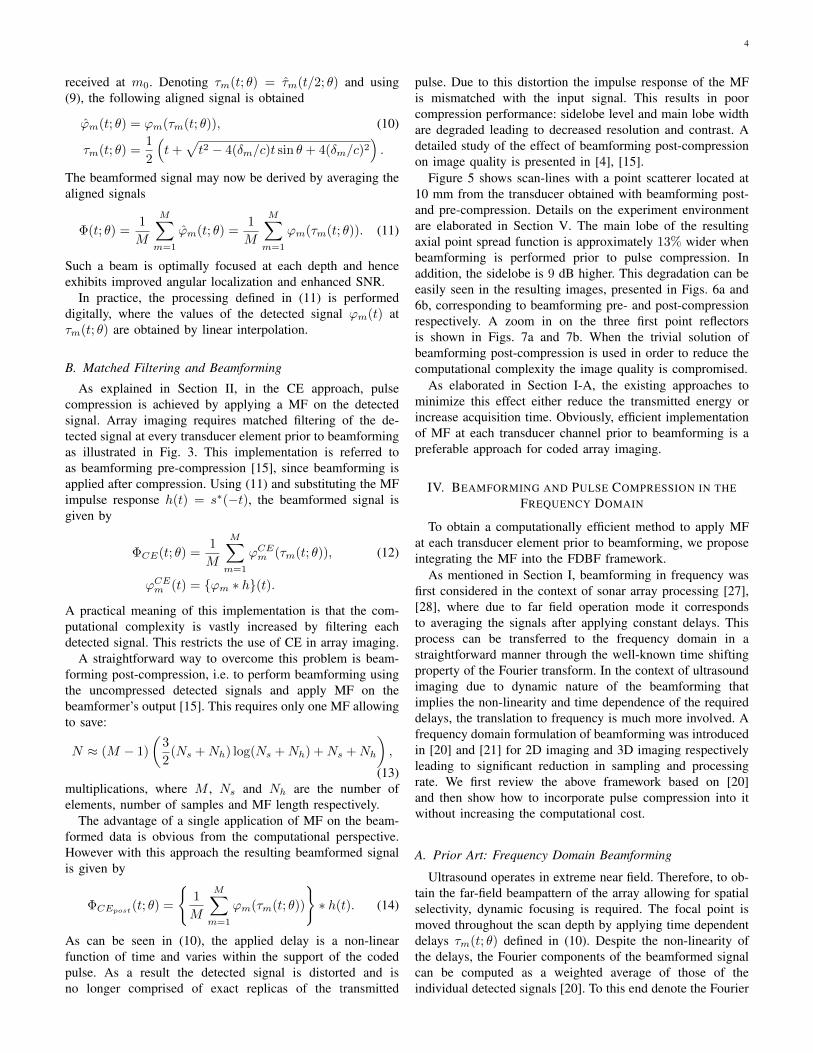
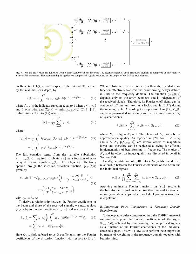
As explained in Section II, in the CE approach, pulsecompression is achieved by applying a MF on the detectedsignal. Array imaging requires matched filtering of the de-tected signal at every transducer element prior to beamformingas illustrated in Fig. 3. This implementation is referred toas beamforming pre-compression [15], since beamforming isapplied after compression. Using (11) and substituting the MFimpulse response h(t) = s∗(−t), the beamformed signal isgiven by

ΦCE(t; θ) =1

M

M∑

m=1

ϕCEm (τm(t; θ)), (12)

ϕCEm (t) = {ϕm ∗ h}(t).

A practical meaning of this implementation is that the com-putational complexity is vastly increased by filtering eachdetected signal. This restricts the use of CE in array imaging.

A straightforward way to overcome this problem is beam-forming post-compression, i.e. to perform beamforming usingthe uncompressed detected signals and apply MF on thebeamformer’s output [15]. This requires only one MF allowingto save:

N ≈ (M − 1)

(3

2(Ns +Nh) log(Ns +Nh) +Ns +Nh

),

(13)multiplications, where M , Ns and Nh are the number ofelements, number of samples and MF length respectively.

The advantage of a single application of MF on the beam-formed data is obvious from the computational perspective.However with this approach the resulting beamformed signalis given by

ΦCEpost(t; θ) =

{1

M

M∑

m=1

ϕm(τm(t; θ))

}∗ h(t). (14)

As can be seen in (10), the applied delay is a non-linearfunction of time and varies within the support of the codedpulse. As a result the detected signal is distorted and isno longer comprised of exact replicas of the transmitted

pulse. Due to this distortion the impulse response of the MFis mismatched with the input signal. This results in poorcompression performance: sidelobe level and main lobe widthare degraded leading to decreased resolution and contrast. Adetailed study of the effect of beamforming post-compressionon image quality is presented in [4], [15].

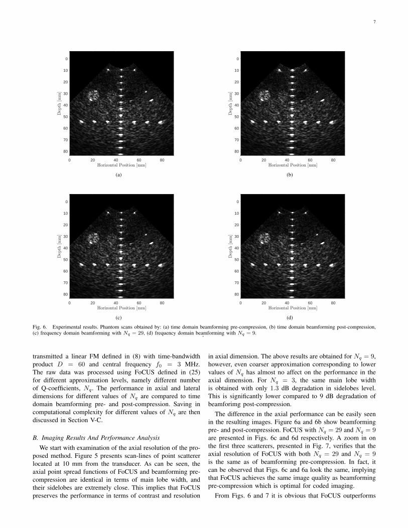
Figure 5 shows scan-lines with a point scatterer located at10 mm from the transducer obtained with beamforming post-and pre-compression. Details on the experiment environmentare elaborated in Section V. The main lobe of the resultingaxial point spread function is approximately 13% wider whenbeamforming is performed prior to pulse compression. Inaddition, the sidelobe is 9 dB higher. This degradation can beeasily seen in the resulting images, presented in Figs. 6a and6b, corresponding to beamforming pre- and post-compressionrespectively. A zoom in on the three first point reflectorsis shown in Figs. 7a and 7b. When the trivial solution ofbeamforming post-compression is used in order to reduce thecomputational complexity the image quality is compromised.

As elaborated in Section I-A, the existing approaches tominimize this effect either reduce the transmitted energy orincrease acquisition time. Obviously, efficient implementationof MF at each transducer channel prior to beamforming is apreferable approach for coded array imaging.

IV. BEAMFORMING AND PULSE COMPRESSION IN THEFREQUENCY DOMAIN

To obtain a computationally efficient method to apply MFat each transducer element prior to beamforming, we proposeintegrating the MF into the FDBF framework.

As mentioned in Section I, beamforming in frequency wasfirst considered in the context of sonar array processing [27],[28], where due to far field operation mode it correspondsto averaging the signals after applying constant delays. Thisprocess can be transferred to the frequency domain in astraightforward manner through the well-known time shiftingproperty of the Fourier transform. In the context of ultrasoundimaging due to dynamic nature of the beamforming thatimplies the non-linearity and time dependence of the requireddelays, the translation to frequency is much more involved. Afrequency domain formulation of beamforming was introducedin [20] and [21] for 2D imaging and 3D imaging respectivelyleading to significant reduction in sampling and processingrate. We first review the above framework based on [20]and then show how to incorporate pulse compression into itwithout increasing the computational cost.

A. Prior Art: Frequency Domain Beamforming

Ultrasound operates in extreme near field. Therefore, to ob-tain the far-field beampattern of the array allowing for spatialselectivity, dynamic focusing is required. The focal point ismoved throughout the scan depth by applying time dependentdelays τm(t; θ) defined in (10). Despite the non-linearity ofthe delays, the Fourier components of the beamformed signalcan be computed as a weighted average of those of theindividual detected signals [20]. To this end denote the Fourier

5

Beamforming

1M

∑{ϕm ∗ h}(τm(t; θ))

ϕ1(t)

ϕ2(t)

ϕM (t)

Matched

h(t) = s(−t)Filter

Matched

h(t) = s(−t)Filter

Matched

h(t) = s(−t)Filter

1

2

m

m0

M

δm

Fig. 3. On the left echoes are reflected from 3 point scatterers in the medium. The received signal at each transducer element is composed of reflections ofa linear FM waveform. The beamforming is applied on compressed signals, obtained at the output of the MF at each element.

coefficients of Φ(t; θ) with respect to the interval T , definedby the maximal scan depth, by

c[k] =1

T

∫ T

0

I[0,TB(θ))(t)Φ(t; θ)e−i2πT ktdt, (15)

where I[a,b) is the indicator function equal to 1 when a ≤ t < band 0 otherwise and TB(θ) = min1≤m≤M τ−1m (T ; θ) [19].Substituting (11) into (15) results in

c[k] =1

M

M∑

m=1

cm[k], (16)

where

cm[k] =1

T

∫ T

0

I[0,TB(θ))(t)ϕm(τm(t; θ))e−i2πT ktdt (17)

=1

T

∫ T

0

ϕm(t)qk,m(t; θ)e−i2πT ktdt.

The last equation stems from the variable substitutionx = τm(t; θ), required to obtain c[k] as a function of non-delayed receive signals ϕm(t). The delays are effectivelyapplied through the so-called distortion function, qk,m(t; θ)given by

qk,m(t; θ) =I[|γm|,τm(T ;θ))(t)

(1 +

γ2m cos2 θ

(t− γm sin θ)2

)×

(18)

exp

{i2π

Tkγm − t sin θ

t− γm sin θγm

},

with γm = δm/c.To derive a relationship between the Fourier coefficients of

the beam and those of the received signals, we next replaceϕm(t) by its Fourier coefficients cm[n] and rewrite (17) as

cm[k] =∑

n

cm[n]1

T

∫ T

0

qk,m(t; θ)e−i2πT (k−n)tdt (19)

=∑

n

cm[k − n]Qk,m;θ[n].

Here Qk,m;θ[n], referred to as Q-coefficients, are the Fouriercoefficients of the distortion function with respect to [0, T ).

When substituted by its Fourier coefficients, the distortionfunction effectively transfers the beamforming delays definedin (10) to the frequency domain. The function qk,m(t; θ)depends only on the array geometry and is independent ofthe received signals. Therefore, its Fourier coefficients can becomputed off-line and used as a look-up-table (LUT) duringthe imaging cycle. According to Proposition 1 in [19], cm[k]can be approximated sufficiently well with a finite number Nqof Q-coefficients

cm[k] 'N2∑

n=−N1

cm[k − n]Qk,m;θ[n], (20)

where Nq = N2 − N1 + 1. The choice of Nq controls theapproximation quality. As reported in [20] for n < −N1

and n > N2 {Qk,m;θ[n]} are several orders of magnitudelower and therefore can be neglected allowing for efficientimplementation of beamforming in frequency. The choice ofNq and its effect on image quality are discussed in detail inSection V-B.

Finally, substitution of (20) into (16) yields the desiredrelationship between the Fourier coefficients of the beam andthe individual signals

c[k] ' 1

M

M∑

m=1

N2∑

n=−N1

cm[k − n]Qk,m;θ[n]. (21)

Applying an inverse Fourier transform on {c[k]} results inthe beamformed signal in time. We then proceed to standardimage generation steps which include log-compression andinterpolation.

B. Integrating Pulse Compression in Frequency DomainBeamforming

To incorporate pulse compression into the FDBF frameworkwe aim to express the Fourier coefficients of the signalΦCE(t; θ), obtained by beamforming the compressed signals,as a function of the Fourier coefficients of the individualdetected signals. This will allow us to perform the compressionby means of weighting in the frequency domain together withbeamforming.

6

-100 -80 -60 -40 -20 0 20 40 60 80 100n, Fourier coefficient index

-80

-70

-60

-50

-40

-30

-20

-10

0

Magnitude[dB]

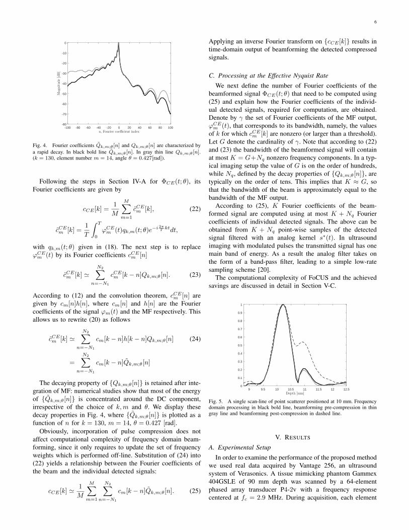
Fig. 4. Fourier coefficients Qk,m;θ[n] and Qk,m;θ[n] are characterized bya rapid decay. In black bold line Qk,m;θ[n]. In gray thin line Qk,m;θ[n].(k = 130, element number m = 14, angle θ = 0.427[rad]).

Following the steps in Section IV-A for ΦCE(t; θ), itsFourier coefficients are given by

cCE [k] =1

M

M∑

m=1

cCEm [k], (22)

cCEm [k] =1

T

∫ T

0

ϕCEm (t)qk,m(t; θ)e−i2πT ktdt,

with qk,m(t; θ) given in (18). The next step is to replaceϕCEm (t) by its Fourier coefficients cCEm [n]

cCEm [k] 'N2∑

n=−N1

cCEm [k − n]Qk,m;θ[n]. (23)

According to (12) and the convolution theorem, cCEm [n] aregiven by cm[n]h[n], where cm[n] and h[n] are the Fouriercoefficients of the signal ϕm(t) and the MF respectively. Thisallows us to rewrite (20) as follows

cCEm [k] 'N2∑

n=−N1

cm[k − n]h[k − n]Qk,m;θ[n] (24)

=

N2∑

n=−N1

cm[k − n]Qk,m;θ[n]

The decaying property of {Qk,m;θ[n]} is retained after inte-gration of MF: numerical studies show that most of the energyof {Qk,m;θ[n]} is concentrated around the DC component,irrespective of the choice of k,m and θ. We display thesedecay properties in Fig. 4, where {Qk,m;θ[n]} is plotted as afunction of n for k = 130, m = 14, θ = 0.427 [rad].

Obviously, incorporation of pulse compression does notaffect computational complexity of frequency domain beam-forming, since it only requires to update the set of frequencyweights which is performed off-line. Substitution of (24) into(22) yields a relationship between the Fourier coefficients ofthe beam and the individual detected signals:

cCE [k] ' 1

M

M∑

m=1

N2∑

n=−N1

cm[k − n]Qk,m;θ[n]. (25)

Applying an inverse Fourier transform on {cCE [k]} results intime-domain output of beamforming the detected compressedsignals.

C. Processing at the Effective Nyquist Rate

We next define the number of Fourier coefficients of thebeamformed signal ΦCE(t; θ) that need to be computed using(25) and explain how the Fourier coefficients of the individ-ual detected signals, required for computation, are obtained.Denote by γ the set of Fourier coefficients of the MF output,ϕCEm (t), that corresponds to its bandwidth, namely, the valuesof k for which cCEm [k] are nonzero (or larger than a threshold).Let G denote the cardinality of γ. Note that according to (22)and (23) the bandwidth of the beamformed signal will containat most K = G+Nq nonzero frequency components. In a typ-ical imaging setup the value of G is on the order of hundreds,while Nq , defined by the decay properties of {Qk,m;θ[n]}, aretypically on the order of tens. This implies that K ≈ G, sothat the bandwidth of the beam is approximately equal to thebandwidth of the MF output.

According to (25), K Fourier coefficients of the beam-formed signal are computed using at most K + Nq Fouriercoefficients of individual detected signals. The above can beobtained from K + Nq point-wise samples of the detectedsignal filtered with an analog kernel s∗(t). In ultrasoundimaging with modulated pulses the transmitted signal has onemain band of energy. As a result the analog filter takes onthe form of a band-pass filter, leading to a simple low-ratesampling scheme [20].

The computational complexity of FoCUS and the achievedsavings are discussed in detail in Section V-C.

9 9.5 10 10.5 11 11.5 12 12.5Depth [mm]

0

0.1

0.2

0.3

0.4

0.5

0.6

0.7

0.8

0.9

1

Fig. 5. A single scan-line of point scatterer positioned at 10 mm. Frequencydomain processing in black bold line, beamforming pre-compression in thingray line and beamforming post-compression in dashed line.

V. RESULTS

A. Experimental Setup

In order to examine the performance of the proposed methodwe used real data acquired by Vantage 256, an ultrasoundsystem of Verasonics. A tissue mimicking phantom Gammex404GSLE of 90 mm depth was scanned by a 64-elementphased array transducer P4-2v with a frequency responsecentered at fc = 2.9 MHz. During acquisition, each element

7

0 20 40 60 80Horizontal Position [mm]

0

10

20

30

40

50

60

70

80

Depth

[mm]

(a)

0 20 40 60 80Horizontal Position [mm]

0

10

20

30

40

50

60

70

80

Depth

[mm]

(b)

0 20 40 60 80Horizontal Position [mm]

0

10

20

30

40

50

60

70

80

Depth

[mm]

(c)

0 20 40 60 80Horizontal Position [mm]

0

10

20

30

40

50

60

70

80

Depth

[mm]

(d)

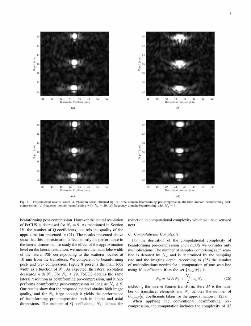
Fig. 6. Experimental results. Phantom scans obtained by: (a) time domain beamforming pre-compression, (b) time domain beamforming post-compression,(c) frequency domain beamforming with Nq = 29, (d) frequency domain beamforming with Nq = 9..

transmitted a linear FM defined in (8) with time-bandwidthproduct D = 60 and central frequency f0 = 3 MHz.The raw data was processed using FoCUS defined in (25)for different approximation levels, namely different numberof Q-coefficients, Nq . The performance in axial and lateraldimensions for different values of Nq are compared to timedomain beamforming pre- and post-compression. Saving incomputational complexity for different values of Nq are thendiscussed in Section V-C.

B. Imaging Results And Performance Analysis

We start with examination of the axial resolution of the pro-posed method. Figure 5 presents scan-lines of point scattererlocated at 10 mm from the transducer. As can be seen, theaxial point spread functions of FoCUS and beamforming pre-compression are identical in terms of main lobe width, andtheir sidelobes are extremely close. This implies that FoCUSpreserves the performance in terms of contrast and resolution

in axial dimension. The above results are obtained for Nq = 9,however, even coarser approximation corresponding to lowervalues of Nq has almost no affect on the performance in theaxial dimension. For Nq = 3, the same main lobe widthis obtained with only 1.3 dB degradation in sidelobes level.This is significantly lower compared to 9 dB degradation ofbeamforimg post-compression.

The difference in the axial performance can be easily seenin the resulting images. Figure 6a and 6b show beamformingpre- and post-compression. FoCUS with Nq = 29 and Nq = 9are presented in Figs. 6c and 6d respectively. A zoom in onthe first three scatterers, presented in Fig. 7, verifies that theaxial resolution of FoCUS with both Nq = 29 and Nq = 9is the same as of beamforming pre-compression. In fact, itcan be observed that Figs. 6c and 6a look the same, implyingthat FoCUS achieves the same image quality as beamformingpre-compression which is optimal for coded imaging.

From Figs. 6 and 7 it is obvious that FoCUS outperforms

8

38 40 42 44 46 48 50 52Horizontal Position [mm]

10

12

14

16

18

20

22

Depth

[mm]

(a)

38 40 42 44 46 48 50 52Horizontal Position [mm]

10

12

14

16

18

20

22

Depth

[mm]

(b)

38 40 42 44 46 48 50 52Horizontal Position [mm]

10

12

14

16

18

20

22

Depth

[mm]

(c)

38 40 42 44 46 48 50 52Horizontal Position [mm]

10

12

14

16

18

20

22

Depth

[mm]

(d)

Fig. 7. Experimental results, zoom in. Phantom scans obtained by: (a) time domain beamforming pre-compression, (b) time domain beamforming post-compression, (c) frequency domain beamforming with Nq = 29, (d) frequency domain beamforming with Nq = 9..

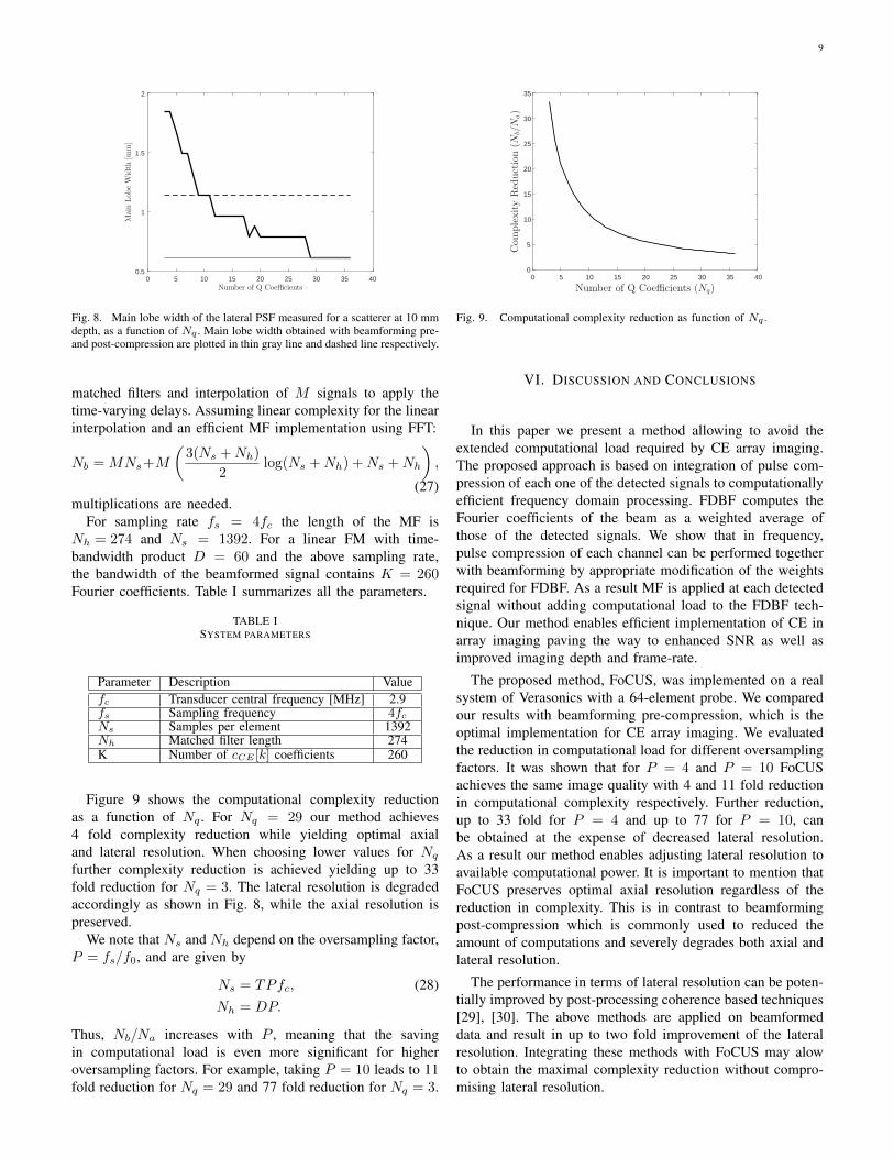
beamforming post-compression. However the lateral resolutionof FoCUS is decreased for Nq = 9. As mentioned in SectionIV, the number of Q-coefficients, controls the quality of theapproximation presented in (21). The results presented aboveshow that this approximation affects mostly the performance inthe lateral dimension. To study the effect of the approximationlevel on the lateral resolution, we measure the main lobe widthof the lateral PSF corresponding to the scatterer located at10 mm from the transducer. We compare it to beamformingpost- and pre- compression. Figure 8 presents the main lobewidth as a function of Nq . As expected, the lateral resolutiondecreases with Nq . For Nq ≥ 29, FoCUS obtains the samelateral resolution as beamforming pre-compression, and it out-performs beamforming post-compression as long as Nq ≥ 9.Our results show that the proposed method obtains high imagequality, and for Nq large enough it yields the performanceof beamforming pre-compression both in lateral and axialdimensions. The number of Q-coefficients, Nq , defines the

reduction in computational complexity which will be discussednext.

C. Computational ComplexityFor the derivation of the computational complexity of

beamforming pre-compression and FoCUS we consider onlymultiplications. The number of samples comprising each scan-line is denoted by Ns, and is determined by the samplingrate and the imaging depth. According to (25) the numberof multiplications needed for a computation of one scan-lineusing K coefficients from the set {cCE [k]} is:

Na = MKNq +Ns2

logNs, (26)

including the inverse Fourier transform. Here M is the num-ber of transducer elements and Nq denotes the number ofQk,m;θ[n] coefficients taken for the approximation in (25).

When applying the conventional beamforming pre-compression, the computation includes the complexity of M

9

0 5 10 15 20 25 30 35 40Number of Q Coefficients

0.5

1

1.5

2

MainLob

eW

idth

[mm]

Fig. 8. Main lobe width of the lateral PSF measured for a scatterer at 10 mmdepth, as a function of Nq . Main lobe width obtained with beamforming pre-and post-compression are plotted in thin gray line and dashed line respectively.

matched filters and interpolation of M signals to apply thetime-varying delays. Assuming linear complexity for the linearinterpolation and an efficient MF implementation using FFT:

Nb = MNs+M

(3(Ns +Nh)

2log(Ns +Nh) +Ns +Nh

),

(27)multiplications are needed.

For sampling rate fs = 4fc the length of the MF isNh = 274 and Ns = 1392. For a linear FM with time-bandwidth product D = 60 and the above sampling rate,the bandwidth of the beamformed signal contains K = 260Fourier coefficients. Table I summarizes all the parameters.

TABLE ISYSTEM PARAMETERS

Parameter Description Valuefc Transducer central frequency [MHz] 2.9fs Sampling frequency 4fcNs Samples per element 1392Nh Matched filter length 274K Number of cCE [k] coefficients 260

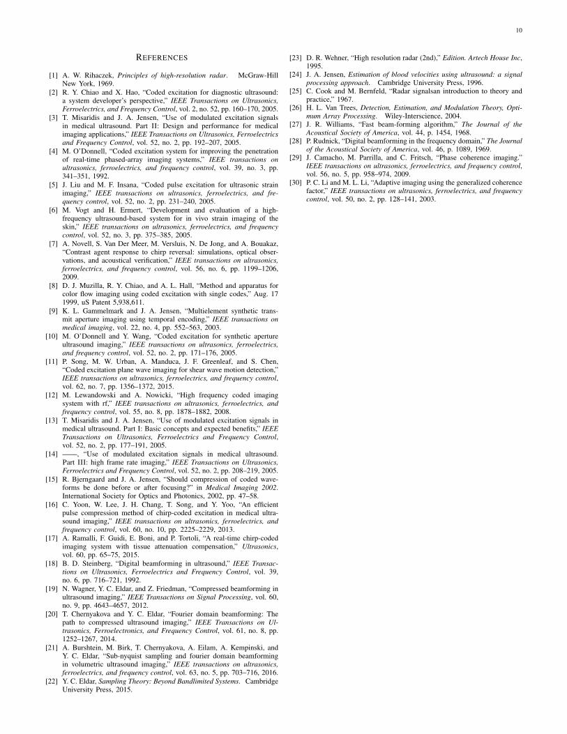
Figure 9 shows the computational complexity reductionas a function of Nq . For Nq = 29 our method achieves4 fold complexity reduction while yielding optimal axialand lateral resolution. When choosing lower values for Nqfurther complexity reduction is achieved yielding up to 33fold reduction for Nq = 3. The lateral resolution is degradedaccordingly as shown in Fig. 8, while the axial resolution ispreserved.

We note that Ns and Nh depend on the oversampling factor,P = fs/f0, and are given by

Ns = TPfc, (28)Nh = DP.

Thus, Nb/Na increases with P , meaning that the savingin computational load is even more significant for higheroversampling factors. For example, taking P = 10 leads to 11fold reduction for Nq = 29 and 77 fold reduction for Nq = 3.

0 5 10 15 20 25 30 35 40

Number of Q Coefficients (Nq)

0

5

10

15

20

25

30

35

Com

plexityReduction(N

b/N

a)

Fig. 9. Computational complexity reduction as function of Nq .

VI. DISCUSSION AND CONCLUSIONS

In this paper we present a method allowing to avoid theextended computational load required by CE array imaging.The proposed approach is based on integration of pulse com-pression of each one of the detected signals to computationallyefficient frequency domain processing. FDBF computes theFourier coefficients of the beam as a weighted average ofthose of the detected signals. We show that in frequency,pulse compression of each channel can be performed togetherwith beamforming by appropriate modification of the weightsrequired for FDBF. As a result MF is applied at each detectedsignal without adding computational load to the FDBF tech-nique. Our method enables efficient implementation of CE inarray imaging paving the way to enhanced SNR as well asimproved imaging depth and frame-rate.

The proposed method, FoCUS, was implemented on a realsystem of Verasonics with a 64-element probe. We comparedour results with beamforming pre-compression, which is theoptimal implementation for CE array imaging. We evaluatedthe reduction in computational load for different oversamplingfactors. It was shown that for P = 4 and P = 10 FoCUSachieves the same image quality with 4 and 11 fold reductionin computational complexity respectively. Further reduction,up to 33 fold for P = 4 and up to 77 for P = 10, canbe obtained at the expense of decreased lateral resolution.As a result our method enables adjusting lateral resolution toavailable computational power. It is important to mention thatFoCUS preserves optimal axial resolution regardless of thereduction in complexity. This is in contrast to beamformingpost-compression which is commonly used to reduced theamount of computations and severely degrades both axial andlateral resolution.

The performance in terms of lateral resolution can be poten-tially improved by post-processing coherence based techniques[29], [30]. The above methods are applied on beamformeddata and result in up to two fold improvement of the lateralresolution. Integrating these methods with FoCUS may alowto obtain the maximal complexity reduction without compro-mising lateral resolution.

10

REFERENCES

[1] A. W. Rihaczek, Principles of high-resolution radar. McGraw-HillNew York, 1969.

[2] R. Y. Chiao and X. Hao, “Coded excitation for diagnostic ultrasound:a system developer’s perspective,” IEEE Transactions on Ultrasonics,Ferroelectrics, and Frequency Control, vol. 2, no. 52, pp. 160–170, 2005.

[3] T. Misaridis and J. A. Jensen, “Use of modulated excitation signalsin medical ultrasound. Part II: Design and performance for medicalimaging applications,” IEEE Transactions on Ultrasonics, Ferroelectricsand Frequency Control, vol. 52, no. 2, pp. 192–207, 2005.

[4] M. O’Donnell, “Coded excitation system for improving the penetrationof real-time phased-array imaging systems,” IEEE transactions onultrasonics, ferroelectrics, and frequency control, vol. 39, no. 3, pp.341–351, 1992.

[5] J. Liu and M. F. Insana, “Coded pulse excitation for ultrasonic strainimaging,” IEEE transactions on ultrasonics, ferroelectrics, and fre-quency control, vol. 52, no. 2, pp. 231–240, 2005.

[6] M. Vogt and H. Ermert, “Development and evaluation of a high-frequency ultrasound-based system for in vivo strain imaging of theskin,” IEEE transactions on ultrasonics, ferroelectrics, and frequencycontrol, vol. 52, no. 3, pp. 375–385, 2005.

[7] A. Novell, S. Van Der Meer, M. Versluis, N. De Jong, and A. Bouakaz,“Contrast agent response to chirp reversal: simulations, optical obser-vations, and acoustical verification,” IEEE transactions on ultrasonics,ferroelectrics, and frequency control, vol. 56, no. 6, pp. 1199–1206,2009.

[8] D. J. Muzilla, R. Y. Chiao, and A. L. Hall, “Method and apparatus forcolor flow imaging using coded excitation with single codes,” Aug. 171999, uS Patent 5,938,611.

[9] K. L. Gammelmark and J. A. Jensen, “Multielement synthetic trans-mit aperture imaging using temporal encoding,” IEEE transactions onmedical imaging, vol. 22, no. 4, pp. 552–563, 2003.

[10] M. O’Donnell and Y. Wang, “Coded excitation for synthetic apertureultrasound imaging,” IEEE transactions on ultrasonics, ferroelectrics,and frequency control, vol. 52, no. 2, pp. 171–176, 2005.

[11] P. Song, M. W. Urban, A. Manduca, J. F. Greenleaf, and S. Chen,“Coded excitation plane wave imaging for shear wave motion detection,”IEEE transactions on ultrasonics, ferroelectrics, and frequency control,vol. 62, no. 7, pp. 1356–1372, 2015.

[12] M. Lewandowski and A. Nowicki, “High frequency coded imagingsystem with rf,” IEEE transactions on ultrasonics, ferroelectrics, andfrequency control, vol. 55, no. 8, pp. 1878–1882, 2008.

[13] T. Misaridis and J. A. Jensen, “Use of modulated excitation signals inmedical ultrasound. Part I: Basic concepts and expected benefits,” IEEETransactions on Ultrasonics, Ferroelectrics and Frequency Control,vol. 52, no. 2, pp. 177–191, 2005.

[14] ——, “Use of modulated excitation signals in medical ultrasound.Part III: high frame rate imaging,” IEEE Transactions on Ultrasonics,Ferroelectrics and Frequency Control, vol. 52, no. 2, pp. 208–219, 2005.

[15] R. Bjerngaard and J. A. Jensen, “Should compression of coded wave-forms be done before or after focusing?” in Medical Imaging 2002.International Society for Optics and Photonics, 2002, pp. 47–58.

[16] C. Yoon, W. Lee, J. H. Chang, T. Song, and Y. Yoo, “An efficientpulse compression method of chirp-coded excitation in medical ultra-sound imaging,” IEEE transactions on ultrasonics, ferroelectrics, andfrequency control, vol. 60, no. 10, pp. 2225–2229, 2013.

[17] A. Ramalli, F. Guidi, E. Boni, and P. Tortoli, “A real-time chirp-codedimaging system with tissue attenuation compensation,” Ultrasonics,vol. 60, pp. 65–75, 2015.

[18] B. D. Steinberg, “Digital beamforming in ultrasound,” IEEE Transac-tions on Ultrasonics, Ferroelectrics and Frequency Control, vol. 39,no. 6, pp. 716–721, 1992.

[19] N. Wagner, Y. C. Eldar, and Z. Friedman, “Compressed beamforming inultrasound imaging,” IEEE Transactions on Signal Processing, vol. 60,no. 9, pp. 4643–4657, 2012.

[20] T. Chernyakova and Y. C. Eldar, “Fourier domain beamforming: Thepath to compressed ultrasound imaging,” IEEE Transactions on Ul-trasonics, Ferroelectronics, and Frequency Control, vol. 61, no. 8, pp.1252–1267, 2014.

[21] A. Burshtein, M. Birk, T. Chernyakova, A. Eilam, A. Kempinski, andY. C. Eldar, “Sub-nyquist sampling and fourier domain beamformingin volumetric ultrasound imaging,” IEEE transactions on ultrasonics,ferroelectrics, and frequency control, vol. 63, no. 5, pp. 703–716, 2016.

[22] Y. C. Eldar, Sampling Theory: Beyond Bandlimited Systems. CambridgeUniversity Press, 2015.

[23] D. R. Wehner, “High resolution radar (2nd),” Edition. Artech House Inc,1995.

[24] J. A. Jensen, Estimation of blood velocities using ultrasound: a signalprocessing approach. Cambridge University Press, 1996.

[25] C. Cook and M. Bernfeld, “Radar signalsan introduction to theory andpractice,” 1967.

[26] H. L. Van Trees, Detection, Estimation, and Modulation Theory, Opti-mum Array Processing. Wiley-Interscience, 2004.

[27] J. R. Williams, “Fast beam-forming algorithm,” The Journal of theAcoustical Society of America, vol. 44, p. 1454, 1968.

[28] P. Rudnick, “Digital beamforming in the frequency domain,” The Journalof the Acoustical Society of America, vol. 46, p. 1089, 1969.

[29] J. Camacho, M. Parrilla, and C. Fritsch, “Phase coherence imaging.”IEEE transactions on ultrasonics, ferroelectrics, and frequency control,vol. 56, no. 5, pp. 958–974, 2009.

[30] P. C. Li and M. L. Li, “Adaptive imaging using the generalized coherencefactor,” IEEE transactions on ultrasonics, ferroelectrics, and frequencycontrol, vol. 50, no. 2, pp. 128–141, 2003.