1

Blind Updates in Coded Caching

Suman Ghosh, Prasad Krishnan and Lakshmi Prasad Natarajan

Abstract

We consider the centralized coded caching system where a library of files is available at the server

and their subfiles are cached at the clients as prescribed by a placement delivery array (PDA). We are

interested in the problem where a specific file in the library is replaced with a new file at the server, the

contents of which are correlated with the file being replaced, and this change needs to be communicated

to the caches. Upon replacement, the server has access only to the updated file and is unaware of its

differences with the original, while each cache has access to specific subfiles of the original file as

dictated by the PDA. We model the correlation between the two files by assuming that they differ in at

the most ε subfiles, and aim to reduce the number of bits broadcast by the server to update the caches.

We design a new elegant coded transmission strategy for the server to update the caches blindly, and

also identify a simple scheme that is based on MDS codes. We then derive converse bounds on the

minimum communication cost `∗ among all linear strategies. For two well-known families of PDAs –

Maddah-Ali & Niesen’s caching scheme and a PDA by Tang & Ramamoorthy and Yan et al. – our new

scheme has cost `∗(1 + o(1)) when the updates are sufficiently sparse, while the scheme using MDS

codes has order-optimal cost when the updates are dense.

Index Terms

blind update, broadcast channel, coded caching, communication cost, placement delivery array.

I. INTRODUCTION

Coded caching is a powerful technique that utilizes memory as a resource to offset commu-

nication costs [1]. A systematic placement of files in the client caches and a careful design

This paper was presented in part at the 2020 IEEE Information Theory Workshop (ITW 2020), Riva del Garda, Italy.

Suman Ghosh and Lakshmi Prasad Natarajan are with the Department of Electrical Engineering, Indian Institute of Technology

Hyderabad, Sangareddy 502 285, India (email: ee16resch11006, lakshminatarajan@iith.ac.in).

Prasad Krishnan is with the Signal Processing and Communications Research Center, International Institute of Information

Technology, Hyderabad 500032, India. (email: prasad.krishnan@iiit.ac.in)

arX

iv:2

010.

1046

4v2

[cs

.IT

] 1

5 M

ay 2

021

2

of coded transmissions can significantly reduce the number of bits being broadcast during file

delivery. Coded caching has been shown to provide benefits in a variety of scenarios, such as in

wireless networks [2], [3], decentralized caching [4], in D2D networks [5], and in the presence of

relays [6]. Caching could play a key role in overcoming bandwidth bottlenecks in next generation

communication networks.

We consider centralized coded caching schemes that are designed based on placement delivery

arrays or PDAs [7]. A PDA is a structure that provides (i) a scheme for partitioning every file

in the library into subfiles and placing these subfiles in the caches, and (ii) a method to generate

coded transmissions to meet the demand of the clients during the delivery phase. The notion

of PDAs provides a systematic framework for designing centralized coded caching schemes. A

number of works in the literature have designed coded caching schemes to achieve a graceful

trade-off between communication rate and subpacketization level, and several of them – including

Maddah-Ali & Niesen scheme of [1] – fall into the framework of PDAs, such as [7]–[13]. Apart

from coded caching, PDAs are also known to play an important role in the design of coded

distributed computing techniques [14]–[16].

In this paper, we consider the scenario where one of the files in the library is replaced with a

new file of equal size. We assume that the contents of the new file are written over the contents

of the file being replaced, and hence, the server loses the old file once the library is updated. This

is a reasonable mode of operation when the server, in order to save memory and reduce system

complexity, does not intend to maintain a detailed log of the changes in the library and the store

the previous versions of the state of the library. Once the file is replaced at the server, these

changes must be communicated to the caches in order to update their contents. We consider the

scenario where the contents of the new file and the old file (that has been removed at the server)

are correlated, and we design coded transmission strategies for updating the cache contents that

exploit this correlation. We model the correlation between the two in terms of the number of

subfiles in which the two files differ.

We assume that the files are cached using a (K,F, Z, S)-PDA, where K is the number of

caches, F is the number of subfiles that each file is split into, Z is the number of subfiles of

each file that is cached at each client, and S denotes the number of transmissions in the delivery

phase of coded caching. We further impose the conditions (which are satisfied by several PDAs

known in the literature) that every subfile must be cached in a constant number of caches, say

3

c 𝐖{1,2}′ + 𝐖{3,4}

′ 𝐖{1,3}′ + 𝐖{3,4}

′ 𝐖{1,4}′ + 𝐖{3,4}

′ 𝐖{2,4}′ + 𝐖{3,4}

′ 𝐖{2,3}′ + 𝐖{3,4}

′

𝑢1 𝑢3 𝑢2

Server

𝑢4

𝐖{1,2} 𝐖{1,3} 𝐖{1,4}

𝐖{1,2}′

𝐖{1,3}′

𝐖{1,4}′

𝐖{1,2} 𝐖{2,3} 𝐖{2,4}

𝐖{1,2}′

𝐖{2,3}′

𝐖{2,4}′

𝐖{1,3} 𝐖{2,3} 𝐖{3,4}

𝐖{1,3}′

𝐖{2,3}′

𝐖{3,4}′

𝐖{1,4} 𝐖{2,4} 𝐖{3,4}

𝐖{1,4}′

𝐖{2,4}′

𝐖{3,4}′

c

Type equation here. c

Type equation here. c

Type equation here.

c

Type equation here.

=Type equation here.

Figure 1: The coded blind cache update scheme in Example 1.

r caches out of K, and each subfile must be cached in a distinct subset of users (see (4)). If

there exist two or more users whose cache contents are identical, without loss of generality, we

replace this set of users by a single user with the same cache content. Under such scenario,

suppose that a specific file is replaced with another file, whose contents differ in at the most

ε subfiles. We assume that the server knows the value of ε, but since the server has lost the

older file, it does not know in which subfiles the two files differ. The objective is to design a

strategy that can be used by the server to communicate this update to the users. Since the server

is ignorant of the exact difference between the old and new files, we refer to this process as

blind cache update or simply cache update. We use the number of bits transmitted by the server

as the performance metric of an update scheme.

In a naive strategy the server broadcasts the entirety of the new file, which can be directly

used by the clients to update their respective caches. However this strategy does not exploit the

side information available at the clients, which are the subfiles of the older file available in their

cache. In this paper, we show that the communication cost can be reduced by using carefully

designed coded transmissions that exploit this side information. Each user will use the coded

transmissions from the server and the subfiles of the older file that are available in its cache to

decode the newer version of these subfiles.

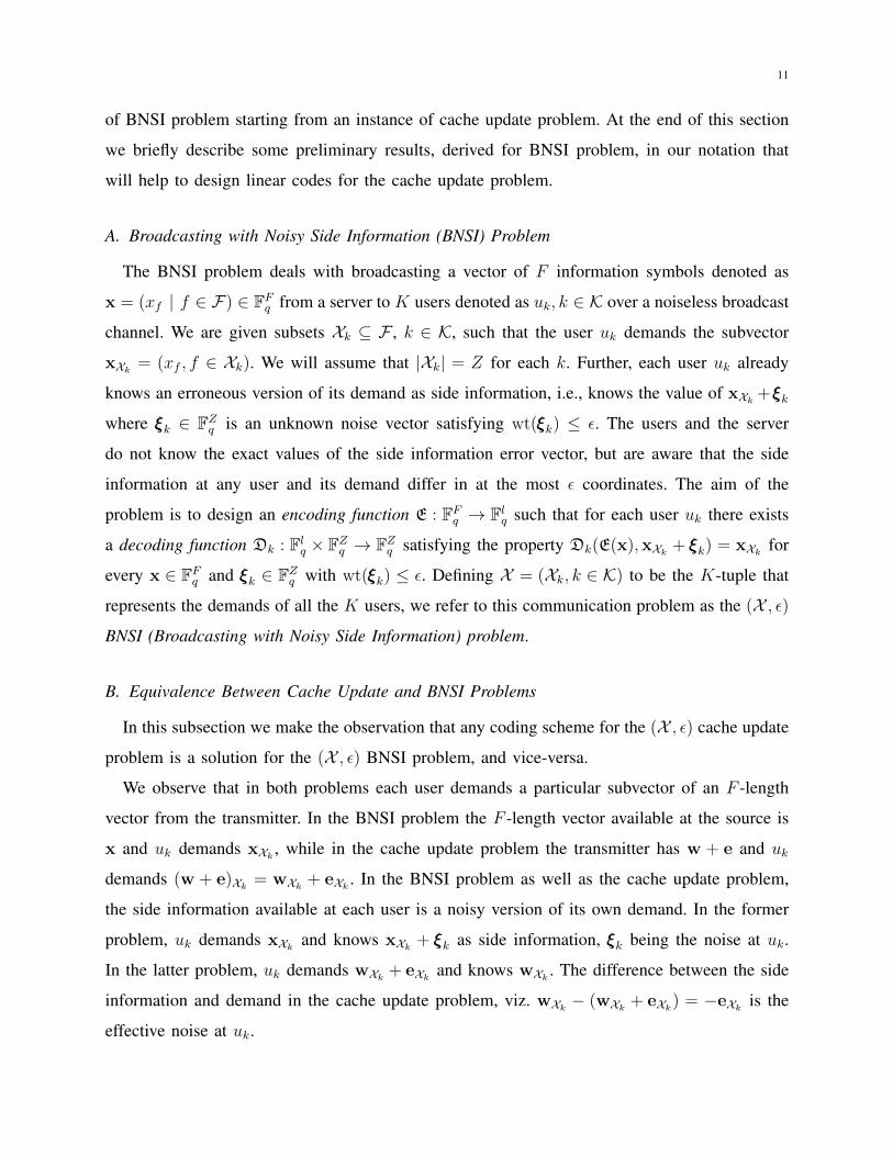
Example 1. In this toy example, we illustrate how the older subfiles available in user caches can

be used to reduce the communication cost. Consider the Maddah-Ali & Niesen’s caching scheme

4

across K = 4 users u1, . . . , u4 with caching ratio Z/F = 1/2. A file w is split into 6 subfiles

w = (wT , T ∈([4]2

)), where

([4]2

)is the collection of all 2-sized subsets of [4] = {1, . . . , 4}. For

simplicity, assume that each subfile is a single bit, i.e., wT ∈ F2 for all T ∈([4]2

). User uk caches

subfile wT if and only if k ∈ T . Suppose w is updated to a newer version w′ = (w′T , T ∈([4]2

)),

such that w and w′ differ in at the most one subfile. That is, the Hamming weight of the update

vector e = (eT , T ∈([4]2

)) , w′ −w is at the most ε = 1. If a naive update scheme is used, the

server will broadcast the entire updated file w′ consisting of 6 bits. Each user uk can obtain its

new cache content (w′T | T ∈([4]2

), k ∈ T ) from the corresponding sub-vectors of w′. However, if

we use the coded transmission shown in Fig. 1, cache updates can be effected using 5 transmitted

bits. We illustrate the decoding procedure at u1. The procedure at other caches are similar.

User u1 intends to recover (w′{1,2}, w′{1,3}, w

′{1,4}) = (w{1,2}, w{1,3}, w{1,4})+(e{1,2}, e{1,3}, e{1,4}),

or equivalently, recover (e{1,2}, e{1,3}, e{1,4}) since he already knows (w{1,2}, w{1,3}, w{1,4}). In

order to decode (e{1,2}, e{1,3}, e{1,4}), u1 computes a syndrome (s1, s2) using the components of

the broadcast codeword and its present cache contents as follows

s1 , (w′{1,2} + w′{3,4}) + (w′{1,3} + w′{3,4}) + w{1,2} + w{1,3} = e{1,2} + e{1,3},

s2 , (w′{1,3} + w′{3,4}) + (w′{1,4} + w′{3,4}) + w{1,3} + w{1,4} = e{1,3} + e{1,4}.

Note that (s1, s2) is the syndrome of (e{1,2}, e{1,3}, e{1,4}) for the length-3 binary repetition code.

Since the Hamming weight of (e{1,2}, e{1,3}, e{1,4}) is at the most 1 and since the length-3

repetition code is a 1-error correcting code we conclude that (s1, s2) is sufficient to identify

(e{1,2}, e{1,3}, e{1,4}).

The coding schemes designed in this paper for blind cache updates are also useful in the fol-

lowing communication scenario known as broadcasting with noisy side information (BNSI) [17].

In the placement phase of a coded caching system, the server broadcasts each file in the library

to the users, and each user stores a specific subset of the subfiles of each file in its cache. Now

suppose that the channel between the server and the users faces a temporary outage during the

transmission of a particular file. Because of the outage, the users receive erroneous versions of

the subfiles of this file and request the server for a retransmission. In the retransmission phase,

each user demands a specific collection of subfiles from the server, and each user has side

information in the form of a noisy version of the set of subfiles that it demands from the server.

5

SECTION SUMMARY OF CONTENTS CACHING SCHEME MAIN RESULTS

Sec II System model. Review of PDAs Any PDA

Sec III-B Cache update and BNSI problems are equivalent Any PDA Theorem 1

Sec III-C Design criterion for linear cache update schemes Any PDA Theorem 2

Sec III-C A cache update scheme based on MDS codes Any PDA Lemma 1

Sec IV A new cache update scheme PDAs satisfying (4) Theorem 4

Sec V-A Condition for `∗ = F (for naive update scheme to be optimal) Any PDA Lemma 5

Sec V-A Proving that `∗ ≥ 2ε. Conditions for `∗ = 2ε, 2ε+ 1, 2ε+ 2 Any PDA Lemmas 7, 8

Sec V-A A generic lower bound for any linear update scheme Any PDA Theorem 5

Sec V-B Lower bound on `∗. Exact `∗ for a special case Construction I of [9]

Sec V-C Performance analysis for ε = O(F ); log2 ε = O(log2 F ), o(log2 F ) Maddah-Ali & Niesen [1] Lemmas 9, 10

Sec V-D Performance analysis for ε = O(F ); log2 ε = O(log2 F ), o(log2 F ) A scheme from [7], [10] Lemmas 13, 14

Table I: Summary of the contents of this paper.

The task of designing a communication scheme for this retransmission phase is a BNSI problem

(we describe this problem formally in Section III-A). Our cache update coding strategies serve

as solutions to this BNSI problem (details are in Section III-B).

A. Contributions

In this paper, we provide a formal framework for the design of blind schemes for updating

cache contents. Throughout this paper we study only linear coding schemes, and all the converse

bounds and results related to optimality of communication costs are with respect to the family

of linear coding strategies. The main contributions of this paper (summarized in Table I) are as

follows.

1. Design criterion and a construction based on MDS codes (Section III): We show that the

cache update problem is equivalent to a BNSI problem. Based on this equivalence, we obtain a

design criterion for constructing a linear code for the cache update problem (Theorem 2). Relying

on a construction from [17], we also identify a simple coding scheme with communication cost

of (F − (Z − 2ε)+)B bits that uses the parity-check matrix of MDS codes for encoding, where

B is the number of bits in each subfile and x+ = max{x, 0}.

6

2. A new code construction (Section IV): We propose a new coding scheme for the cache update

problem with cost (2ε(K − r) + 1)B bits. The encoder is designed by associating a subspace

with each user and by choosing each column of the encoder matrix from the intersection of a

carefully chosen collection of these subspaces. The proposed construction is random and is over

the finite field of size 2B. Using the Schwartz-Zippel lemma, we show that this construction

succeeds with high probability for all sufficiently large B.

3. Converse bounds and performance analysis (Section V): We present a lower bound on

the optimal communication cost `∗ of linear update schemes (Theorem 5). Using this bound,

we explicitly identify `∗ for a special case of the class of PDAs designed by Shangguan et

al. [9]. We then specialize our lower bound to two well known families of PDAs – the Maddah-

Ali & Niesen’s scheme [1] and a PDA designed independently by Yan et al. [7] and Tang

& Ramamoorthy [10] – and conduct performance analysis when the number of users K is

made large while the caching ratio Z/F is held constant. For these two families of PDAs, the

communication cost of our new scheme from Section IV is nearly-optimal and equals `∗(1+o(1))

when log2 ε = o(log2 F ), i.e., if the updates are sufficiently sparse. When the updates are dense,

i.e., when ε = O(F ), the MDS codes based construction is order optimal.

We introduce the system model in Section II and draw conclusions in Section VI.

B. Related Work

We are not aware of any prior coding strategies in the literature that exploit the contents of a

deleted file to push blind updates into caching nodes. However, a problem of similar flavour has

been studied in [18], [19] for coded distributed storage systems where storage nodes maintain

coded versions (i.e., specific linear combinations) of a data file to provide protection against

node failures. Communication schemes were designed to update the contents of a ‘stale’ node

in the system by either a central server [18] or the other nodes in distributed storage [19] that

have access to the updated content. Our paper differs fundamentally from the problem setting

of [18], [19] since we are interested in uncoded placement of subfiles in the caching nodes, i.e.,

the caching nodes store fragments of the original file instead of linear combinations.

Notation: Matrices and column vectors will be denoted using bold upper case and bold lower

case letters, respectively. For any matrix A, C(A) denotes the column span of A. For any vector

x = (xf | f ∈ F) whose entries are indexed by the set F and for any A ⊆ F , xA = (xf | f ∈ A)

7

W

𝑢1 𝑢2 𝑢𝐾

N files w 𝑤𝑓1

𝑤𝑓2 𝑤𝑓3

𝑤𝑓𝐹 …

Server

....

K users

F subfiles

(a) System Model.

W

𝑢1 𝑢2 𝑢𝐾

Server

....

𝐖′

(b) Update of a file W to W ′.

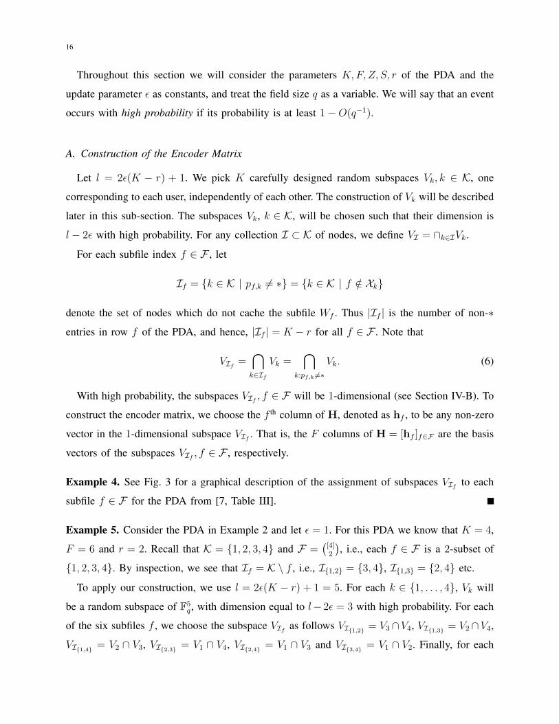
Figure 2: System model of the cache update problem. Here, the index set of subfiles is F =

{f1, . . . , fF} and the index set of users is K = {1, . . . , K}.

is the subvector of x consisting of entries indexed by A. For any subspace U , dim(U) denotes

the dimension of the subspace. If A is a set and a an integer, then(Aa

)is the collection of all

a-sized subsets of A. For any positive integer n, [n] denotes the set {1, . . . , n}. The empty set

is denoted by φ. For any real number x, x+ = max{x, 0}.

II. SYSTEM MODEL

We consider a caching system with K clients and a single server as shown in Fig 2a. The

server stores a library of N files. We view each file as a collection of subfiles, and the subfiles

of all the N files are cached in a predetermined way across the K caching nodes. We assume

that one specific file in the library, say W , is being replaced with a new file as shown in Fig 2b.

The other N − 1 files existing in the system are unaffected by this change. Hence, throughout

this paper, we focus only on W and its subfiles and ignore the existence of the other files in the

coded caching system.

The file W is a collection of F equal sized subfiles Wf , f ∈ F , where F denotes the index

set of the subfiles and |F| = F . The K caching nodes are denoted as uk, k ∈ K, where K is

the index set of the nodes and |K| = K. Throughout this paper we will assume that the subfiles

are cached across the nodes in an uncoded fashion based on a placement delivery array [7]. We

8

also assume that the server is connected to the K nodes through a noiseless broadcast link.

A. A Brief Review of Placement Delivery Arrays

A (K,F, Z, S) Placement Delivery Array (PDA) is an F ×K array P whose entries consist

of a symbol ∗ and S non-negative integers 0, 1, . . . , S − 1. The rows and columns of this array

are indexed by the sets F and K, respectively, i.e., P = [pf,k], f ∈ F and k ∈ K. The array

satisfies the following properties

1) the symbol ∗ appears Z times in each column;

2) each non-negative integer s ∈ {0, 1, . . . , S − 1} appears at least once in the array; and

3) for any two distinct entries (f1, k1) and (f2, k2) such that pf1,k1 = pf2,k2 = s, we have

f1 6= f2, k1 6= k2 and pf1,k2 = pf2,k1 = ∗.

We assume that the file W is cached across the K nodes using the strategy based on the PDA

P , which is as follows: a node uk caches a subfile Wf if and only if pf,k = ∗.

Remark 1. The locations of the ∗ symbol in a PDA dictate the placement of subfiles in caches,

while the integers {0, 1, . . . , S−1} determine the coded transmissions during the delivery phase

of the coded caching system when the clients reveal their file demands to the server. In this

paper, we are only interested in the specific placement of subfiles in caches since our primary

objective is to update the contents of the caches. Hence, we will not be interested in the integer

entries of the PDA.

In this work we consider the family of PDAs in which ∗ appears a constant number of times

in each row. This family includes several well known PDAs proposed in the literature for coded

caching [1], [7]–[10] and coded MapReduce [14]–[16]. The number of times ∗ appears in each

row of the PDA will be denoted by r. This implies that each node caches Z out of F subfiles

and each subfile is replicated at r nodes. If we count the number of times the symbol ∗ appears

in each column of the F ×K array P then the total count is KZ. Similarly counting the number

of times the symbol ∗ appears in each row of the array P the total count is rF . Now equating

these two numbers we get r = KZF

.

The index set of the subfiles cached at node uk will be denoted as Xk = {f ∈ F | pf,k = ∗}.

Note that |Xk| = Z for all k ∈ K. Observe that the tuple X = (Xk, k ∈ K) completely describes

the cache placement strategy.

9

Example 2. Suppose we are given the following (K = 4, F = 6, Z = 3, S = 4) PDA

P =

1 2 3 4

{1, 2} ∗ ∗ 0 1

{1, 3} ∗ 0 ∗ 2

{1, 4} ∗ 1 2 ∗

{2, 3} 0 ∗ ∗ 3

{2, 4} 1 ∗ 3 ∗

{3, 4} 2 3 ∗ ∗

.

For this PDA, the node index set is K = [4] = {1, 2, 3, 4} and the subfile index set is F =([4]2

)which is the collection of all 2-sized subsets of K. The caching scheme consists of 4 nodes

u1, u2, u3, u4 and 6 subfiles W{1,2},W{1,3},W{1,4},W{2,3},W{2,4},W{3,4}. The index set of the

subfiles cached at the four nodes are X1 = {{1, 2}, {1, 3}, {1, 4}}, X2 = {{1, 2}, {2, 3}, {2, 4}},

X3 = {{1, 3}, {2, 3}, {3, 4}} and X4 = {{1, 4}, {2, 4}, {3, 4}}, respectively. Note that |Xk| =

Z, ∀k ∈ {1, 2, 3, 4}, and each subfile is cached at r = 2 nodes. The update problem in Example 1

is based on this PDA.

B. The Blind Cache Update Problem

Let w = (wf , f ∈ F) ∈ FFq denote the content of the file to be updated where each subfile

content, denoted by wf , is an element over a finite field Fq. The cached content of node uk is

denoted as wXk = (wf | f ∈ Xk). We observe that wXk ∈ FZq for all k ∈ K.

Suppose the file content w is updated to w+e, where e ∈ FFq represents an update to the file

content, i.e., wt(e) ≤ ε where wt() denotes the Hamming weight of a vector and ε is a known

constant. In other words the original file undergoes an update where at the most ε subfiles have

been updated. The update is modeled as a substitution of the original collection of the subfiles.

We assume that the server is unaware of the old version of the file w and the identities of

updated subfiles. The server knows the updated file content w + e and knows that the number

of the updated subfiles is at the most ε. The parameter ε characterizes the update process. For

example, if the ratio εF

is small and tends to 0 as F → ∞ then we view such an update as a

sparse update. On the other hand if ε is proportional to F then the update is dense.

The server wants to communicate the update to the users, so that each user uk can update its

contents from wXk to (w + e)Xk . Considering ε as a design parameter, we are interested in the

10

problem of designing a coding scheme to update the cache of each user described by the cache

placement strategy X = (Xk, k ∈ K) with an update of at the most ε subfiles. We will call this

problem the (X , ε) cache update problem or the (X , ε) update problem.

Definition 1. A valid encoding function of codelength l for the (X , ε) update problem over the

field Fq is a function E : FFq → Flq such that for each node uk, k ∈ K there exists a decoding

function Dk : Flq×FZq → FZq satisfying the following property: Dk(E(w+e),wXk) = (w+e)Xk

for every w ∈ FFq and e ∈ FFq with wt(e) ≤ ε.

The communication cost of the coding scheme, in number of bits, is l × log2 q bits. The

objective of the code construction is to design the coding scheme (E,Dk, k ∈ K) such that the

codelength l is minimized.

A coding scheme (E,D1, . . . ,DK) is said to be linear if the encoding function is an Fq-linear

transformation. For a linear coding scheme, the transmitted codeword c = H(w + e), where

H ∈ Fl×Fq is the encoder matrix. The optimum communication cost among all valid linear coding

schemes (considering all possible choices of the finite field Fq) for the (X , ε) update problem

will be denoted as `∗(X , ε) or simply `∗.

We assume that the code designer has the flexibility to choose the operating finite field

when constructing the update scheme. Our code construction in Section IV is applicable for

all sufficiently large finite fields, while our lower bounds in Section V are independent of the

choice of the finite field.

The trivial coding scheme that transmits the updated file content w + e as such, i.e., c =

IF×F (w + e) is a valid coding scheme with codelength F since each node can directly update

its cache contents using c. We refer to this trivial coding scheme as the naive scheme where

H = I. Thus, we have the following trivial upper bound on the optimum linear codelength

`∗ ≤ F. (1)

III. EQUIVALENCE BETWEEN CACHE UPDATE

AND BROADCASTING WITH NOISY SIDE INFORMATION

In this section we show that every cache update problem is equivalent to a broadcasting with

noisy side information (BNSI) problem [17]. We start this section with a brief introduction of

BNSI problem. We show that by performing a simple change of variables we obtain an instance

11

of BNSI problem starting from an instance of cache update problem. At the end of this section

we briefly describe some preliminary results, derived for BNSI problem, in our notation that

will help to design linear codes for the cache update problem.

A. Broadcasting with Noisy Side Information (BNSI) Problem

The BNSI problem deals with broadcasting a vector of F information symbols denoted as

x = (xf | f ∈ F) ∈ FFq from a server to K users denoted as uk, k ∈ K over a noiseless broadcast

channel. We are given subsets Xk ⊆ F , k ∈ K, such that the user uk demands the subvector

xXk = (xf , f ∈ Xk). We will assume that |Xk| = Z for each k. Further, each user uk already

knows an erroneous version of its demand as side information, i.e., knows the value of xXk +ξξξkwhere ξξξk ∈ FZq is an unknown noise vector satisfying wt(ξξξk) ≤ ε. The users and the server

do not know the exact values of the side information error vector, but are aware that the side

information at any user and its demand differ in at the most ε coordinates. The aim of the

problem is to design an encoding function E : FFq → Flq such that for each user uk there exists

a decoding function Dk : Flq × FZq → FZq satisfying the property Dk(E(x),xXk + ξξξk) = xXk for

every x ∈ FFq and ξξξk ∈ FZq with wt(ξξξk) ≤ ε. Defining X = (Xk, k ∈ K) to be the K-tuple that

represents the demands of all the K users, we refer to this communication problem as the (X , ε)

BNSI (Broadcasting with Noisy Side Information) problem.

B. Equivalence Between Cache Update and BNSI Problems

In this subsection we make the observation that any coding scheme for the (X , ε) cache update

problem is a solution for the (X , ε) BNSI problem, and vice-versa.

We observe that in both problems each user demands a particular subvector of an F -length

vector from the transmitter. In the BNSI problem the F -length vector available at the source is

x and uk demands xXk , while in the cache update problem the transmitter has w + e and uk

demands (w + e)Xk = wXk + eXk . In the BNSI problem as well as the cache update problem,

the side information available at each user is a noisy version of its own demand. In the former

problem, uk demands xXk and knows xXk + ξξξk as side information, ξξξk being the noise at uk.

In the latter problem, uk demands wXk + eXk and knows wXk . The difference between the side

information and demand in the cache update problem, viz. wXk − (wXk + eXk) = −eXk is the

effective noise at uk.

12

The noise affecting the K users in the cache update problem, −eXk , k ∈ K, are all subvectors

of the negative of the update vector e ∈ FFq . In contrast, the noise vectors affecting the users in

the BNSI problem ξξξ1, . . . , ξξξK are arbitrary and could be independent of each other. This is the

key difference between the two problems. However, in spite of this difference, we next observe

that the coding solutions to both the problems are identical. The reason why the dependence

or correlation of the noise vectors in the cache update problem does not provide any additional

coding leverage is because the communication channel is a broadcast link and the users do not

collude or cooperate during decoding.

We first show that any coding scheme for the (X , ε) cache update problem is a valid coding

scheme for the (X , ε) BNSI problem. Let E, Dk, k ∈ K be valid encoding and decoding functions

for the cache update problem, that is

Dk(E(w + e),wXk) = wXk + eXk = (w + e)Xk (2)

for all choices of w and e with wt(e) ≤ ε and for every user uk. We know that the noise vectors

ξξξk ∈ FZq , k ∈ K, in the BNSI problem have weight at the most ε. For each k ∈ K, define the

vector e(k) ∈ FFq as follows, e(k)Xk = −ξξξk and e(k)f = 0 for all f /∈ Xk. Observe that wt(e(k)) ≤ ε

and xXk + ξξξk = xXk − e(k)Xk = (x− e(k))Xk . When the coding scheme (E,Dk, k ∈ K) is applied

to the BNSI problem, for each k ∈ K, we have

Dk(E(x),xXk + ξξξk) = Dk

(E((x− e(k)) + e(k)

), (x− e(k))Xk

)= ((x− e(k)) + e(k))Xk = xXk ,

where the second equality follows from (2) with (x− e(k)) and e(k) playing the roles of w and

e, respectively. Hence, (E,Dk, k ∈ K) is a valid coding scheme for the (X , ε) BNSI problem.

Conversely, now assume that E and Dk, k ∈ K, are valid encoding and decoding functions for

the (X , ε) BNSI problem. That is, for every uk and any choice of x, ξξξk, k ∈ K with wt(ξξξk) ≤ ε,

Dk(E(x),xXk + ξξξk) = xXk . (3)

For given values of w and e in the cache update problem, define x = w + e and ξξξk = −eXkfor all k ∈ K. We know that wt(e) ≤ ε, and hence, wt(ξξξk) = wt(−eXk) ≤ wt(−e) ≤ ε. Also,

wXk = xXk − eXk = xXk + ξξξk. From (3), and using the fact wt(ξξξk) ≤ ε, we have

Dk(E(w + e),wXk) = Dk(E(x),xXk + ξξξk) = xXk = wXk + eXk .

Hence, (E,Dk, k ∈ K) is a valid coding scheme for the cache update problem.

13

The equivalence proved above holds for all codes, including linear and non-linear codes.

Suppose linear codes are used, i.e., the codeword is generated at the transmitter by multiplying

the F -length information vector with an l×F matrix H. We say that the encoding matrix H is

valid for the given problem (either the BNSI or the cache update problem) if every receiver can

decode its demand using the codeword generated by H and its own side information. Applying

the equivalence proved in this subsection to linear codes we obtain

Theorem 1. A matrix H is a valid encoder for the (X , ε) cache update problem if and only if

it is a valid encoder for the (X , ε) BNSI problem.

C. Preliminaries

We now recall some relevant results from [17], including a necessary and sufficient condition

for a matrix H to be a valid encoder for the BNSI problem. Since the BNSI problem is equivalent

to the cache update problem, we directly state these results as applied to the cache update

problem. We then recall a construction of the encoder matrix from [17] based on Maximum

Distance Separable (MDS) codes.

The linear code design criterion of [17] is in terms of the span of the columns of specific

submatrices of H. For each node uk, k ∈ K, let Yk = F \ Xk denote the index set of subfiles

that are not cached by the node uk. Since |Xk| = Z, we have |Yk| = F − Z.

We index the F columns of H by the elements of F . For any A ⊆ F , let HA ∈ Fl×|A|q be the

submatrix of H consisting of the columns of H with indices belonging to A. Also, let C(HA)

denote the subspace of Flq spanned by the columns of HA.

Theorem 2. [17, Corollary 1] A matrix H is a valid encoder matrix for the (X , ε) cache update

problem if and only if for every k ∈ K, any non-zero linear combination of any 2ε or fewer

columns of HXk does not belong to C(HYk), i.e.,

HXkx+HYky 6= 0 for all x ∈ FZq \ {0} with wt(x) ≤ 2ε and y ∈ FF−Zq .

Since the column span C(HYk) includes 000, Theorem 2 implies that any 2ε or fewer columns

of HXk must be linearly independent.

Corollary 1. [17, Corollary 2] If H is a valid encoder matrix for the (X , ε) cache update

problem then any 2ε or fewer columns of HXk are linearly independent for every k ∈ K.

14

Example 3. Consider the (X , ε = 1) cache update problem, with K = 4 users and F = 6 subfiles

and the cache placement as given in Example 2 over any finite field Fq. Here the subfiles are

indexed by all 2-subsets of [4] = {1, . . . , 4}, i.e., F =([4]2

). Now consider

H =

{1, 2} {1, 3} {1, 4} {2, 3} {2, 4} {3, 4}

1 0 0 0 0 1

0 1 0 0 0 1

0 0 1 0 0 1

0 0 0 1 0 1

0 0 0 0 1 1

.

Note that any five columns of H are linearly independent. For user u1, X1 = {{1, 2}, {1, 3}, {1, 4}}

and Y1 = F \ X1 = {{2, 3}, {2, 4}, {3, 4}}. Observe that any two columns of HX1 are linearly

independent, and any non-zero linear combination of any two columns of HX1 does not belong

to C(HY1). Similar observations hold for users u2, u3 and u4 as well. Hence, H is a valid encoder

matrix and achieves codelength l = 5 that saves 1 channel use with respect to the naive update

scheme. This is the coding scheme used in Example 1.

The following result from [17] will be used in Section V-A to identify the scenarios where

coding can reduce the communication cost with respect to the naive transmission scheme.

Theorem 3. [17, Theorem 3] Let S = {k ∈ K | |Xk| ≤ 2ε} be the index set of all nodes that

cache 2ε or fewer subfiles. Let XS = ∪k∈SXk be the index set of all subfiles cached among the

nodes in S. Then `∗ ≥ |XS|+min{2ε, F − |XS|}.

In the cache update setting |Xk| = Z for all k. Hence, in Theorem 3, we either have S = φ

or S = K, and correspondingly, XS = φ or XS = F .

We now recall a coding scheme from [17] that relies on MDS codes. In this scheme, we

choose H to be the parity-check matrix of an MDS code of length F and dimension (Z− 2ε)+.

The number of rows l of H is F − (Z − 2ε)+, and from the properties of MDS codes we know

that any l columns of H are linearly independent. Note that the number of columns of HXk is

|Xk| = Z. To check if H satisfies the criteria of Theorem 2, consider any k ∈ K and the union

of any min{2ε, Z} columns of HXk and all the columns of HYk . The total number of columns

15

in this union is min{2ε, Z}+ |Yk| = min{2ε, Z}+ F − Z = F − (Z − 2ε)+ = l. Hence, these

columns are linearly independent and satisfy the criteria of Theorem 2. Such an MDS code

exists over Fq if q ≥ F . Hence, we have the following upper bound on `∗.

Lemma 1. The optimal codelength `∗ of a (X , ε) cache update problem satisfies `∗ ≤ F − (Z−

2ε)+.

This code design provides savings in communication cost with respect to naive transmission,

i.e., has codelength l < F if and only if Z ≥ 2ε+ 1.

IV. A SCHEME FOR BLIND UPDATES IN CODED CACHING

In this section we provide a construction of a linear coding scheme for the (X , ε) update

problem arising from a PDA. We will assume that the PDA satisfies the following condition

{k | pf1,k = ∗} 6= {k | pf2,k = ∗} for any f1 6= f2, (4)

that is, for any two distinct subfiles Wf1 and Wf2 the set of nodes storing Wf1 and the set of

nodes storing Wf2 are distinct. Several popular families of PDAs satisfy this condition, such

as [1], [8]–[10]. The communication cost of our coding scheme is l = 2ε(K− r)+1, where r is

the number of times ∗ appears in each row of the PDA. The construction is random and yields

a valid encoder matrix with probability 1−O(q−1) when designed over the finite field Fq. If we

use a sufficiently large finite field, then this probability is non-zero, and hence, this proves the

existence of a valid code. For ease of exposition, and considering the engineering significance,

we will consider only finite fields of characteristic 2. The main result of this section is

Theorem 4. Over every sufficiently large finite field of characteristic 2 there exists a valid linear

code for the (X , ε) update problem with codelength l = 2ε(K − r) + 1 if the PDA satisfies (4).

Combining this result with Lemma 1, for any PDA satisfying (4) we have

`∗ ≤ min{2ε(K − r) + 1, F − (Z − 2ε)+}. (5)

We provide an overview of the construction in Section IV-A, and in Section IV-B prove that

this construction yields a valid code with high probability for large finite fields.

16

Throughout this section we will consider the parameters K,F, Z, S, r of the PDA and the

update parameter ε as constants, and treat the field size q as a variable. We will say that an event

occurs with high probability if its probability is at least 1−O(q−1).

A. Construction of the Encoder Matrix

Let l = 2ε(K − r) + 1. We pick K carefully designed random subspaces Vk, k ∈ K, one

corresponding to each user, independently of each other. The construction of Vk will be described

later in this sub-section. The subspaces Vk, k ∈ K, will be chosen such that their dimension is

l − 2ε with high probability. For any collection I ⊂ K of nodes, we define VI = ∩k∈IVk.

For each subfile index f ∈ F , let

If = {k ∈ K | pf,k 6= ∗} = {k ∈ K | f /∈ Xk}

denote the set of nodes which do not cache the subfile Wf . Thus |If | is the number of non-∗

entries in row f of the PDA, and hence, |If | = K − r for all f ∈ F . Note that

VIf =⋂k∈If

Vk =⋂

k:pf,k 6=∗

Vk. (6)

With high probability, the subspaces VIf , f ∈ F will be 1-dimensional (see Section IV-B). To

construct the encoder matrix, we choose the f th column of H, denoted as hf , to be any non-zero

vector in the 1-dimensional subspace VIf . That is, the F columns of H = [hf ]f∈F are the basis

vectors of the subspaces VIf , f ∈ F , respectively.

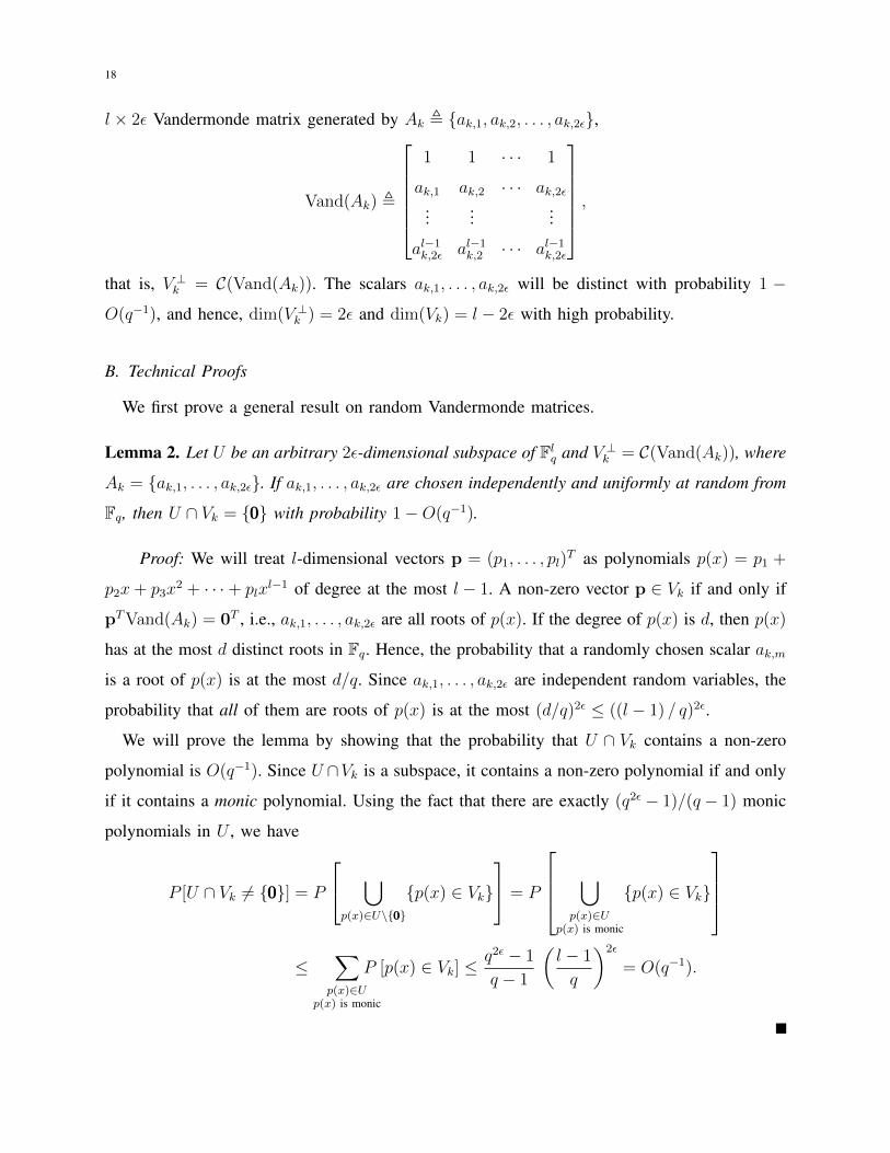
Example 4. See Fig. 3 for a graphical description of the assignment of subspaces VIf to each

subfile f ∈ F for the PDA from [7, Table III].

Example 5. Consider the PDA in Example 2 and let ε = 1. For this PDA we know that K = 4,

F = 6 and r = 2. Recall that K = {1, 2, 3, 4} and F =([4]2

), i.e., each f ∈ F is a 2-subset of

{1, 2, 3, 4}. By inspection, we see that If = K \ f , i.e., I{1,2} = {3, 4}, I{1,3} = {2, 4} etc.

To apply our construction, we use l = 2ε(K − r) + 1 = 5. For each k ∈ {1, . . . , 4}, Vk will

be a random subspace of F5q , with dimension equal to l− 2ε = 3 with high probability. For each

of the six subfiles f , we choose the subspace VIf as follows VI{1,2} = V3 ∩V4, VI{1,3} = V2 ∩V4,

VI{1,4} = V2 ∩ V3, VI{2,3} = V1 ∩ V4, VI{2,4} = V1 ∩ V3 and VI{3,4} = V1 ∩ V2. Finally, for each

17

Figure 3: The 9× 9 matrix (enclosed within square brackets) is the PDA called A(3,2) from [7].

The parameters of this PDA are K = 9, F = 9, Z = 3, S = 18, r = 3. The columns and rows

of the PDA are indexed by 2-tuples as shown, and this notation arises from the construction

technique of this PDA. The set of column indices is K which represents the caching nodes,

and the set of row indices is F which denotes the set of subfiles. The subfiles cached at node

k = (2, 0) is Xk = {(0, 0), (1, 0), (2, 0)}. The nodes that do not contain the subfile f = (0, 2) is

If = {(1, 1), (1, 2), (2, 0), (2, 1), (3, 0), (3, 1)}. Our coding scheme assigns a randomly generated

subspace Vk to each column k of the PDA. Using these K subspaces, we generate F subspaces,

one corresponding to each row of the PDA. The subspace assigned to row f is VIf = ∩k∈IfVk.

f ∈ F , we pick hf to be any non-zero vector in the subspace VIf . The encoder matrix is

H =[h{1,2} h{1,3} h{1,4} h{2,3} h{2,4} h{3,4}

].

We now describe how the subspaces Vk, k ∈ K, are chosen. We utilize a set of 2εK random

scalars ak,m, k ∈ K, m ∈ [2ε], which are independent and uniformly distributed over Fq. We

define Vk through its orthogonal complement V ⊥k as follows: V ⊥k is the column space of the

18

l × 2ε Vandermonde matrix generated by Ak , {ak,1, ak,2, . . . , ak,2ε},

Vand(Ak) ,

1 1 · · · 1

ak,1 ak,2 · · · ak,2ε...

......

al−1k,2ε al−1k,2 · · · al−1k,2ε

,

that is, V ⊥k = C(Vand(Ak)). The scalars ak,1, . . . , ak,2ε will be distinct with probability 1 −

O(q−1), and hence, dim(V ⊥k ) = 2ε and dim(Vk) = l − 2ε with high probability.

B. Technical Proofs

We first prove a general result on random Vandermonde matrices.

Lemma 2. Let U be an arbitrary 2ε-dimensional subspace of Flq and V ⊥k = C(Vand(Ak)), where

Ak = {ak,1, . . . , ak,2ε}. If ak,1, . . . , ak,2ε are chosen independently and uniformly at random from

Fq, then U ∩ Vk = {000} with probability 1−O(q−1).

Proof: We will treat l-dimensional vectors p = (p1, . . . , pl)T as polynomials p(x) = p1 +

p2x+ p3x2 + · · ·+ plx

l−1 of degree at the most l − 1. A non-zero vector p ∈ Vk if and only if

pTVand(Ak) = 0T , i.e., ak,1, . . . , ak,2ε are all roots of p(x). If the degree of p(x) is d, then p(x)

has at the most d distinct roots in Fq. Hence, the probability that a randomly chosen scalar ak,m

is a root of p(x) is at the most d/q. Since ak,1, . . . , ak,2ε are independent random variables, the

probability that all of them are roots of p(x) is at the most (d/q)2ε ≤ ((l − 1) / q)2ε.

We will prove the lemma by showing that the probability that U ∩ Vk contains a non-zero

polynomial is O(q−1). Since U ∩Vk is a subspace, it contains a non-zero polynomial if and only

if it contains a monic polynomial. Using the fact that there are exactly (q2ε − 1)/(q − 1) monic

polynomials in U , we have

P [U ∩ Vk 6= {000}] = P

⋃p(x)∈U\{000}

{p(x) ∈ Vk}

= P

⋃p(x)∈U

p(x) is monic

{p(x) ∈ Vk}

≤

∑p(x)∈U

p(x) is monic

P [p(x) ∈ Vk] ≤q2ε − 1

q − 1

(l − 1

q

)2ε

= O(q−1).

19

Towards showing that our construction succeeds we will now show that the subspaces VIf , f ∈

F are one-dimensional with high probability.

Lemma 3. The subspaces VIf , f ∈ F , are 1-dimensional with probability 1−O(q−1).

Proof: From the definition (6) of VIf , we have V ⊥If =∑

k∈If V⊥k , which is the subspace

obtained by the sum of the column spaces of Vand(Ak), k ∈ If . That is, V ⊥If is the column

space of Vand(∪k∈IfAk) which is the l × 2ε(K − r) Vandermonde matrix generated by the

scalars ∪k∈IfAk = {ak,m | k ∈ If ,m ∈ [2ε]}. This matrix has rank 2ε(K − r) = l − 1, and

hence, dim(VIf ) = 1, as long as all the scalars in ∪k∈IfAk are distinct. The probability that any

two random variables in ∪k∈IfAk take the same value is O(q−1). Thus the proof is complete.

We will denote the set of 2ε(K − r) scalars ∪k∈IfAk by AIf . We will use the notation

ak,m ∈ AIf to imply that ak,m is such that k ∈ If and m ∈ [2ε].

We will now explicitly identify a basis vector for VIf . Since V ⊥If is the column span of

Vand(AIf ), an l-dimensional vector will belong to VIf if its components are the coefficients of a

polynomial with AIf as its roots. In particular, we consider the polynomial∏

ak,m∈AIf(x−ak,m) =∏

k∈If

∏2εm=1(x− ak,m) which is of degree 2ε|If | = 2ε(K − r) = l− 1. Since the characteristic

of the underlying field Fq is 2, the coefficients of this polynomial are (starting from the smallest

degree term)∏ak,m∈AIf

ak,m,∑

S∈(AIfl−2

)∏

ak,m∈S

ak,m, . . . ,∑

S∈(AIf2)

∏ak,m∈S

ak,m,∑

ak,m∈AIf

ak,m, 1.

The f th column vector hf of the encoder matrix is the vector whose l coordinates are these

coefficients, that is, the ith component of hf is as follows

hi,f =∑

S∈(AIfl−i )

∏ak,m∈S

ak,m, (7)

with the convention that multiplication over an empty set of scalars is 1, i.e., hl,f = 1.

We use this structure of hf , along with the Schwartz-Zippel lemma, to arrive at this next

result.

Lemma 4. Any set of 2ε columns of H are linearly independent with probability 1−O(q−1).

Proof: See Appendix A.

20

Proof of Theorem 4: We are now ready to prove the main result of this section by showing

that the proposed random construction of H satisfies the criteria of Theorem 2. Consider any

k ∈ K. From Lemma 4, we know that any 2ε columns of HXk are linearly independent with

high probability.

Consider any subfile f ∈ Yk. Since pf,k 6= ∗, we have k ∈ If . Hence, VIf ⊂ Vk, and therefore,

hf , which is a basis vector of VIf , will be in Vk. Thus, we have

C(HYk) ⊂ Vk. (8)

By construction, the random subspaces Vk, k ∈ K are statistically independent. Now consider

any subfile f ∈ Xk. Since pf,k = ∗, k does not belong to If . Hence, for every f ∈ Xk, the

subspace VIf and the vector hf ∈ VIf are statistically independent of Vk. It follows that the

subspace spanned by a given set of 2ε columns of HXk is statistically independent of Vk. Let

Ak be any 2ε-sized subset of Xk. Using (8), Lemmas 2 and 4, and the fact that HAk and Vk are

statistically independent, we have

P [C(HAk) ∩ C(HYk) 6= {000}] ≤ P [C(HAk) ∩ Vk 6= {000}]

≤ P [rank(HAk) 6= 2ε] + P [C(HAk) ∩ Vk 6= {000} | rank(HAk) = 2ε]

= O(q−1) +∑U⊂Flq

dim(U)=2ε

P [C(HAk) = U ]P [U ∩ Vk 6= {000} | C(HAk) = U ]

= O(q−1) +∑U⊂Flq

dim(U)=2ε

P [C(HAk) = U ]P [U ∩ Vk 6= {000}]

= O(q−1) +∑U⊂Flq

dim(U)=2ε

P [C(HAk) = U ]O(q−1)

= O(q−1) +O(q−1)P [rank(HAk) = 2ε]

= O(q−1).

Using a union bound argument, we immediately deduce that H satisfies all the design conditions

of Theorem 2 with probability 1−O(q−1).

21

V. CONVERSE BOUNDS

We derive lower bounds on the optimal communication cost `∗ in this section. In Section V-A

we exhibit results applicable to all PDAs. We first show that 2ε ≤ `∗ ≤ F and characterize

the update problems with near-extreme values of `∗, i.e., problems with `∗ close to 2ε and F .

We then derive a generic lower bound on `∗ (Theorem 5) that will be used in the rest of this

section as a benchmark for our achievable schemes. In Section V-B we apply these results to a

PDA designed by Shangguan et al. [9]. In Sections V-C and V-D we consider the Maddah-Ali

& Niesen caching scheme [1] and a PDA independently designed by Yan et al. [7] and Tang &

Ramamoorthy [10], respectively. We show that for these latter two families of PDAs the update

schemes proposed in this paper are optimal up to a constant multiplicative factor under some

operating regimes. We also prove the following strong result for these two classes of PDAs when

the updates are sufficiently sparse: as the number of nodes in the system increases while the

caching ratio is kept constant, the cost l = 2ε(K − r) + 1 of the scheme of Theorem 4 satisfiesl`∗→ 1 if log2 ε = o(log2 F ).

A. General Results for any PDA

1) Near-Extreme Communication Costs: We know from (1) that `∗ is at the most F . We now

identify the update problem scenarios for which `∗ takes this largest possible value.

Lemma 5. For the (X , ε) cache update problem based on a (K,F, Z, S) PDA, `∗ = F if and

only if Z ≤ 2ε.

Proof: If Z ≥ 2ε+ 1, from Lemma 1, `∗ ≤ F − (Z − 2ε)+ ≤ F − 1. On the other hand, if

Z ≤ 2ε, then |Xk| = Z ≤ 2ε for all k ∈ K. Using Theorem 3 we see that S = K, XS = F and

`∗ ≥ |XS|+min{2ε, F − |XS|} = F −min{2ε, 0} = F .

In other words, if the number of subfiles to be updated ε is Z/2 or more then broadcasting

the updated file contents without coding is optimal with respect to communication cost.

Let us now assume a non-trivial coding scenario, i.e., Z ≥ 2ε + 1. Applying Theorem 3 to

such a scenario, we see that S = φ, XS = φ, and hence, `∗ ≥ min{2ε, F} = 2ε, where we have

used 2ε < Z ≤ F . Hence, 2ε is a lower bound for `∗ if Z ≥ 2ε + 1. The following result is

useful in determining when the optimal communication cost `∗ takes values close to 2ε.

22

Lemma 6. For any ε ≥ 1 and any PDA, if H ∈ Fl×Fq is a valid encoder for a cache update

problem then any two columns of H are linearly independent.

Proof: Let the columns of H be indexed by F . We first prove that every column of H

is non-zero. For any f ∈ F , there must exist a k ∈ K such that f ∈ Xk since r ≥ 1. From

Corollary 1 we conclude that the column vector indexed by f must be linearly independent by

itself, i.e., must be non-zero.

Consider two columns with indices f, f ′ ∈ F . If f, f ′ ∈ Xk for some choice of k, then by

Corollary 1 and using the fact 2ε ≥ 2, these two column vectors are linearly independent. On

the other hand, if f, f ′ are such that f ∈ Xk and f ′ /∈ Xk for some choice of k, then we observe

that f ′ ∈ Yk. The column indexed by f ′ must be non-zero, and from Theorem 2, its span must

not include the column indexed by f .

We are now ready to identify the scenarios when `∗ = 2ε.

Lemma 7. Assume Z ≥ 2ε+1. The optimal communication cost of updating the cache contents

based on a (K,F, Z, S) PDA satisfies `∗ ≥ 2ε and attains equality if and only if Z = F .

Proof: We have already shown earlier in this section that `∗ ≥ 2ε if Z ≥ 2ε+ 1.

Now suppose Z = F . Using the MDS-based coding scheme and Lemma 1, we have `∗ ≤

F − (Z − 2ε) = 2ε.

On the other hand, consider the case Z < F . For any k ∈ K, |Yk| ≥ 1. Now consider any

2ε columns whose indices lie in Xk and any one column with index in Yk. From Lemma 6, the

column with index in Yk is non-zero. Further, using Theorem 2, this column along with the 2ε

former columns form a linearly independent set. Hence, `∗ ≥ rank(H) ≥ 2ε+ 1.

The scenario when `∗ = 2ε, or equivalently Z = F , corresponds to a trivial cache placement

since every node caches all the subfiles. The next possible values of `∗ are 2ε + 1 and 2ε + 2,

which we consider next.

Lemma 8. Assume Z ≥ 2ε+ 1. The optimal communication cost `∗ is

1) `∗ = 2ε+ 1 if Z = F − 1, and

2) `∗ = 2ε+ 2 if Z = F − 2.

Proof: Using the code design based on the parity-check matrix of MDS codes, we know

23

that `∗ ≤ 2ε+ 1 and `∗ ≤ 2ε+ 2 for Z = F − 1 and Z = F − 2, respectively.

To obtain a converse for Z = F − 1, we use Lemma 7 which states that `∗ = 2ε if and only

if Z = F . Hence, Z = F − 1 necessarily implies `∗ > 2ε, i.e, `∗ ≥ 2ε+ 1.

We now prove the converse for Z = F−2. Let H be any valid encoder matrix. For any k ∈ K,

|Yk| = 2. By Lemma 6 these two columns are linearly independent, and by Theorem 2 their

column span intersects with the column span of any 2ε columns from HXk only at 000. Since these

2ε columns are linearly independent, we deduce that rank(H) ≥ 2ε+ 2. Hence, `∗ ≥ 2ε+ 2.

2) A generic lower bound: The following lower bound is applicable to any PDA. In the sequel

we will use this result to derive good lower bounds for specific well-known families of PDAs

from the literature. Consider any choice of L ∈ [K]. Our lower bound is obtained by considering

any L out of the K caching nodes in a sequence, say π1, . . . , πL ∈ K, and counting the number

of subfiles cached in each node πi which are not cached in any of the earlier nodes π1, . . . , πi−1

in the sequence.

Theorem 5. For any (X , ε) update problem and any choice of L ≤ K, let π1, . . . , πL ∈ K be

indices of distinct nodes. Then `∗ ≥∑L

i=1min{2ε,

∣∣Xπi \ (Xπ1 ∪ · · · ∪ Xπi−1

)∣∣ }.

Proof: For each i ∈ [L], let Aπi be any subset of Xπi \(Xπ1 ∪ · · · ∪ Xπi−1

)of size

min{2ε, |Xπi \ (Xπ1 ∪ · · · ∪ Xπi−1)|}. Note that Aπ1 , . . . ,AπL are disjoint subsets of F , and

that the lower bound claimed in the theorem is∑L

i=1 |Aπi | = |Aπ1 ∪ · · · ∪ AπL|. We will show

that if H is any valid encoder matrix for this update problem, then the columns of H indexed

by Aπ1 ∪ · · · ∪AπL are linearly independent. Then, the number of transmissions required, which

is equal to the number of rows of H, is lower bounded by the rank of H, which in turn is lower

bounded by the size |Aπ1 ∪ · · · ∪ AπL| of this set of linearly independent columns.

Observe that Aπi ⊂ Xπi and |Aπi | ≤ 2ε. Thus, from Corollary 1, the columns of H indexed

by Aπi are linearly independent. For any j > i, we note that Aπj ∩ Xπi = φ, i.e., Aπj ⊂

Yπi . Considering all values of j > i, we then deduce that Aπi+1∪ · · · ∪ AπL ⊂ Yπi . Now

applying Theorem 2, we see that the column span of HAπi intersects with the column span of

HAπi+1∪···∪AπL only at 000. In summary, the matrix HAπ1∪···∪AπL can be partitioned into submatrices

HAπ1 , . . . ,HAπL , and each submatrix HAπi has linearly independent columns and its column span

intersects trivially with the column span of the submatrices appearing later in the sequence, i.e.,

with the column span of HAπi+1∪···∪AπL . Hence, HAπ1∪···∪AπL has linearly independent columns.

24

B. The Construction-I PDA of Shangguan et al.

In this sub-section we consider a class of PDAs given by Construction-I of Shangguan et al. [9]

using hypergraphs and equivalently by Yan et al. [8] using strong edge coloring of bipartite

graphs. This family of PDAs includes the Maddah-Ali & Niesen placement as a special case.

We will derive a lower bound for this class of PDAs, and then specialize our bound to the

Maddah-Ali & Niesen PDA in Section V-C. This family of PDAs is characterized by three

positive integers n, a, b such that a + b ≤ n. The subfiles are indexed by a-sized subsets of

[n], i.e., F =([n]a

), and the users are indexed by b-sized subsets of [n], K =

([n]b

). A subfile

f ∈([n]a

)is cached at user k ∈

([n]b

)if and only if f ∩ k 6= φ. This PDA has F =

(na

), K =

(nb

),

Z =(na

)−(n−ba

).

We will assume that Z ≥ 2ε + 1, since otherwise we know that `∗ = F . To derive a lower

bound on the optimal communication cost of updating the cache contents, we use Theorem 5

with L = n− b+ 1 nodes indexed by

π1 = {1, . . . , b}, π2 = {2, . . . , b+1}, . . . , πi = {i, . . . , b+ i− 1}, . . . , πL = {n− b+1, . . . , n}.

Observe that |Xπ1| = Z > 2ε, and for any i = 2, . . . , L, Xπi \ (Xπ1 ∪· · ·∪Xπi−1) is the collection

of all a-sized subsets of [n] that contain b + i − 1 and do not contain any of 1, . . . , b + i − 2.

Thus, |Xπi \ (Xπ1 ∪ · · · ∪ Xπi−1)| =

(n−(b+i−1)

a−1

). From Theorem 5, we have

`∗ ≥ min{2ε, |Xπ1|}+n−b+1∑i=2

min{2ε, |Xπi \ (Xπ1 ∪ · · · ∪ Xπi−1)|}

= 2ε+n−b+1∑i=2

min

{2ε,

(n− b− i+ 1

a− 1

)}

= 2ε+n−b−1∑j=0

min

{2ε,

(j

a− 1

)}. (9)

Let a0 be the smallest integer such that(a0a−1

)≥ 2ε. Then min{2ε,

(j

a−1

)} =

(j

a−1

)if and only if

j ≤ a0 − 1. Using this in (9) we have, if a0 ≤ n− b then

`∗ ≥ 2ε+

a0−1∑j=0

(j

a− 1

)+

n−b−1∑j=a0

2ε = 2ε+

(a0a

)+ 2ε(n− b− a0) = 2ε(n− b− a0 + 1) +

(a0a

).

(10)

25

Example 6. This example shows that the bound (10) is tight. Consider n = 5, a = b = 2 and

ε = 1. Then, F = K =(52

)= 10, Z =

(52

)−(32

)= 7, which is greater than 2ε, and the value of

a0 is 2. Then the lower bound (10) on `∗ is 5. The achievability scheme using the parity-check

matrix of MDS codes has codelength F − (Z−2ε)+ = 5, which meets this lower bound. Hence,

`∗ = 5 for this update problem.

We now identify the optimal communication cost for the family of PDAs corresponding to

a = 1, i.e., F = [n], K =([n]b

)and a subfile f ∈ [n] is cached at node k ∈

([n]b

)if and only if

f ∈ k. In this case F = n and Z = b. Assuming Z = b ≥ 2ε+ 1 and applying (9), we have

`∗ ≥ 2ε+n−b−1∑j=0

min

{2ε,

(j

0

)}= 2ε+ n− b.

From Lemma 1, `∗ ≤ F − Z + 2ε = 2ε + n − b. Hence, the optimal communication cost is

`∗ = 2ε+ n− b.

C. The Maddah-Ali & Niesen PDA

The placement scheme of Maddah-Ali and Niesen, denoted as MN PDA, is the special case

of the family considered in Section V-B corresponding to b = 1. We will follow the standard

notation used in the literature, i.e., K = [K], F =([K]t

)and a subfile f ∈

([K]t

)is cached at

node k ∈ [K] if and only if k ∈ f . Hence, F =(Kt

), Z =

(K−1t−1

)and r = t. Compared to the

notation used in Section V-B, t and K replace the symbols a and n, respectively.

Note that `∗ = F when Z =(K−1t−1

)≤ 2ε. In the rest of this sub-section we will assume

Z =(K−1t−1

)≥ 2ε + 1, where ε ≥ 1. This implies t ≥ 2. Since

(K−1t−1

)> 2ε, the smallest integer

a0 such that(a0t−1

)≥ 2ε satisfies a0 ≤ K − 1 = n− b. Hence, the lower bound (10) holds.

The caching ratio of the MN PDA is Z/F = t/K, which is the fraction of the overall library

cached at each node; this is denoted as M/N in the literature, where N is the number of files

in the library and M is the cache size at each node in terms of number of files. It is common

to assume that as the number of nodes in the system varies, the cache size of individual nodes

remain the same, and hence, the caching ratio remains constant. We will assume that the caching

ratio is a constant β, 0 < β < 1, and t = βK. The number of subfiles F =(KβK

)= O(2KH2(β)),

where H2(β) = β log2(1/β) + (1− β) log2(1/(1− β)) is the binary entropy function.

We will consider three different operating regimes for updating the MN PDA based on

the sparsity level of the update, i.e., how ε varies with F . For each case we show that the

26

communication cost of the achievability schemes proposed in this paper are either optimal or

within a constant multiplicative gap from the optimal scheme.

1) Regime 1, ε ≤ t/2: In this regime the update scheme of Section IV yields the optimal

communication cost. Observe that the communication cost of this scheme is 2ε(K − t) + 1. To

show that this cost is optimal, we use the lower bound (10). Here a0 is the smallest integer such

that(a0t−1

)≥ 2ε. Since

(t−1t−1

)= 1 < 2ε and

(tt−1

)= t ≥ 2ε, we conclude that a0 = t. Hence, (10)

implies `∗ ≥ 2ε(K − t) + 1. Thus, we have `∗ = 2ε(K − t) + 1.

2) Regime 2, Sparse Update: We assume that the number of subfiles to be updated grows

exponentially with K, i.e., ε = 2γK for some constant γ. If γ < H2(β), then εF→ 0 as K →∞.

We will show that if γ is sufficiently small and K large, the communication cost of the update

scheme of Section IV is within a constant multiplicative gap from the optimal cost.

Lemma 9. Let ε = 2γK and t ≥ 2. If t = βK, the communication cost l = 2ε(K − t) + 1 of the

update scheme in Theorem 4 satisfies

l

`∗≤

1− β + 12εK[

1− 2K− 21/(βK−1)

(β − 1

K

)2γK/(βK−1)

]+ . (11)

Proof: See Appendix B.

We now apply this bound to the scenario when the sparsity parameter γ is small and the number

of users in the system K is large. If γ < β log2(1β), then Lemma 9 implies that lim supK→∞

l`∗≤

1−β1−β2γ/β .

As another corollary to Lemma 9, we observe that if ε = 2o(K) is sub-exponential in K, i.e.,

log2 ε /K → 0, or equivalently log2 ε / log2 F → 0, as K →∞, then(2ε(K − t) + 1

)/ `∗ → 1

as K →∞. We state this observation as

Lemma 10. For the MN PDA, if t/K ∈ (0, 1) is a constant and log2 ε = o(log2 F ), then the

cost l = 2ε(K − t) + 1 of the update scheme from Theorem 4 satisfies limK→∞l`∗

= 1.

3) Regime 3, Dense Update: In this case, we assume that ε is a constant fraction of the

number of subfiles F , i.e., ε = αF for some 0 < α < 1/2 (if α ≥ 1/2, then 2ε ≥ F ≥ Z, and

hence `∗ = F ). We know from Lemma 7, that `∗ ≥ 2ε = 2αF . Consider the MDS codes based

update scheme of Lemma 1, with l = F − Z + 2ε. Since, β = t/K = Z/F , we observe that

l

`∗≤ F − Z + 2ε

2ε=

1− β + 2α

2α.

27

Hence, when ε is a constant fraction of the number of subfiles, the communication cost promised

by Lemma 1 is within a constant multiplicative factor of the optimal cost.

D. The Yan et al. and Tang & Ramamoorthy PDA

We consider a family of PDAs constructed by Yan et al. [7] and Tang and Ramamoorthy [10]

that have smaller subpacketization than the MN PDA. This family of PDAs is parameterized by

two integers q,m ≥ 2. Let Zq = {0, 1, . . . , q − 1} denote the additive cyclic group of order q.

The subfiles are indexed by F = Zmq , the vectors of length m over Zq. The index set of nodes

is K = {(u, v) | 1 ≤ u ≤ m+1, v ∈ Zq}. For 1 ≤ u ≤ m and any v ∈ Zq, the set X(u,v) (which

consists of the indices of the subfiles cached at the user (u, v)) contains all vectors from Zmqwhose uth coordinate is equal to v. For u = m + 1 and any v ∈ Zq, X(m+1,v) contains a vector

from Zmq if and only if the sum of its coordinates over Zq is equal to v. Note that K = q(m+1),

F = qm, Z = qm−1, r = m+1 and the caching ratio β = Z/F = 1/q. The PDA in Fig. 3 is an

instance of this family corresponding to parameters q = 3 and m = 2.

We will assume Z ≥ 2ε+ 1. Consider the nodes (u, v) ∈ K with 1 ≤ u ≤ m and v ∈ Zq. To

apply Theorem 5, we order these qm nodes in the following sequence:

(1, 0), (2, 0), . . . , (m, 0), (1, 1), (2, 1), . . . , (m, 1), . . . , (1, q− 1), (2, q− 1), . . . , (m, q− 1). (12)

A node (u′, v′) appears earlier in the sequence than a node (u, v) if either v′ < v, or v′ = v

and u′ < u. In this case, we say that (u′, v′) precedes (u, v) and denote this by (u′, v′) ≺ (u, v).

Let x(u,v) denote the number of subfiles in the node (u, v) that are not contained in any of the

preceding nodes, i.e.,

x(u,v) =∣∣∣X(u,v) \

⋃(u′,v′):

(u′,v′)≺(u,v)

X(u′,v′)

∣∣∣.Applying Theorem 5 to this sequence of nodes, we have

`∗ ≥q−1∑v=0

m∑u=1

min{2ε, x(u,v)

}. (13)

The value of x(u,v) is the number of vectors (s1, . . . , sm) ∈ Zmq that satisfy the following

properties

1) su = v,

2) if u > 1, none of s1, . . . , su−1 belong to {0, . . . , v}, i.e., s1, . . . , su−1 ∈ {v+1, . . . , q− 1},

28

3) if u < m, none of su+1, . . . , sm belong to {0, . . . , v−1}, i.e., su+1, . . . , sm ∈ {v, . . . , q−1}.

In the second condition above, the set {v + 1, . . . , q − 1} is empty if v = q − 1, in which case

there is no suitable choice for the coordinates s1, . . . , su−1. We conclude that

x(u,v) = (q − v − 1)u−1(q − v)m−u for any u ∈ [m], v ∈ Zq, (14)

where we treat 00 to be equal to 1. Note that (q − v − 1)m−1 ≤ x(u,v) ≤ (q − v)m−1 for any

u ∈ [m] and v ∈ Zq.

Lemma 11. The sequence x(u,v) is a decreasing sequence, that is, x(u′,v′) ≥ x(u,v) if (u′, v′) ≺

(u, v).

Proof: Let (u′, v′) ≺ (u, v). If v′ = v, then necessarily u′ < u. From (14), it clear that

x(u′,v′) ≥ x(u,v). On the other hand, if v′ < v, then

x(u′,v′) ≥ (q − v′ − 1)m−1 ≥ (q − v)m−1 ≥ x(u,v).

Based on the fact that x(u,v) is a decreasing sequence, we define (u0, v0) to be the first index

in the sequence (12) such that x(u0,v0) < 2ε. A counting exercise leads us to

Lemma 12. The optimal communication cost `∗ ≥ 2ε ( v0(m− 1) + u0 + q − 2 ), and u0 > 1.

Proof: See Appendix C.

To illustrate the goodness of our achievability schemes we consider two different operating

regimes. We will assume that the caching ratio Z/F = 1/q is a constant, and the number of

nodes in the system is increased by increasing the value of m. Note that the subpacketization

F = qm is exponential in m.

1) Regime 1, Sparse Update: We assume that ε = γm for some constant γ ∈ [1, q). In this

case the fraction of subfiles being updated ε/F → 0 as m→∞. To apply Lemma 12, we will

first derive a lower bound on v0. Since u0 > 1 (from Lemma 12) and (u0 − 1, v0) immediately

precedes (u0, v0), we have

(q − v0)m−1 ≥ x(u0−1,v0) ≥ 2ε > x(u0,v0) ≥ (q − v0 − 1)m−1.

This implies q− (2ε)1

m−1 − 1 < v0 ≤ q− (2ε)1

m−1 . Using this and u0 ≥ 2 in Lemma 12, we have

`∗ ≥ 2ε((m− 1)(q − 2

1m−1γ

mm−1 − 1) + q

). (15)

29

Comparing this with the communication cost l = 2ε(K−r)+1 = 2ε(m+1)(q−1)+1 guaranteed

by Theorem 4, we arrive at

Lemma 13. Consider the Yan et al. and Tang & Ramamoorthy PDA, with Z/F = 1/q being a

constant and ε = γm for γ ∈ [1, q − 1). The communication cost of the scheme in Theorem 4

for updating this PDA satisfies lim supm→∞l`∗≤ q−1

q−1−γ .

Proof: From (15), l`∗

is upper bounded by

(m+ 1)(q − 1) + 12ε

(m− 1)(q − 21

m−1γmm−1 − 1) + q

=

m+1m−1(q − 1) + 1

2γm(m−1)

q − 21

m−1γmm−1 − 1 + q

m−1

.

The lemma follows from observing that 21

m−1 → 1 and γmm−1 → γ as m→∞.

It is clear from Lemma 13 that if ε is subexponential in m, i.e., if log2 ε = o(m) = o(log2 F ),

then limm→∞l`∗

= 1.

We now consider the case q = 2. For this case x(u,v) = 2m−u if v = 0, x(1,1) = 1, and

x(u,v) = 0 for v = 1, u > 1. Clearly, v0 = 0 and u0 satisfies 2m−u0+1 ≥ 2ε > 2m−u0 . Hence, we

have m− log2(2ε) < u0 ≤ m− log2(2ε) + 1. Applying Lemma 12,

`∗ ≥ 2εu0 ≥ 2ε(m− log2(2ε)) = 2ε (m(1− log2 γ)− 1 ) .

The ratio of l = 2ε(K−r)+1 = 2ε(m+1)+1 to this lower bound tends to 1(1−log2 γ)

as m→∞.

Hence, we have proved

Lemma 14. Consider the Yan et al. and Tang & Ramamoorthy PDA, with Z/F = 1/2 being a

constant and ε = γm for γ ∈ [1, 2). The communication cost of the scheme in Theorem 4 for

updating this PDA satisfies lim supm→∞l`∗≤ 1

1−log2 γ.

2) Regime 2, Dense Update: We now consider the case where the number of subfiles being

updated are a constant fraction of F , say ε = αF for some 0 < α < 12q

(if α > 12q

, then

2ε = 2αF ≥ Fq= Z, and hence, `∗ = F ). From Lemma 12, `∗ ≥ 2ε(u0+ q− 2) ≥ 2εq = 2αFq.

Comparing with the cost l = F − Z + 2ε = F − F/q + 2αF from the scheme of Lemma 1,

l

`∗≤

1− 1q+ 2α

2αq,

which is a constant independent of the scaling parameter m.

To conclude, we have shown that l = min{2ε(K − r) + 1, F − (Z − 2ε)+} is order optimal

in some sparse and as well as dense operating regimes.

30

VI. CONCLUSION AND DISCUSSION

We formulated the problem of pushing updates blindly into the client nodes of a coded caching

system. We designed a new coded transmission strategy for blind updates, and this scheme has

near-optimal communication cost when the updates are sufficiently sparse for two well-known

families of PDAs. On the other hand the simple scheme of using the parity-check matrices of

MDS codes is order-optimal when the updates are dense.

We are yet to device efficient decoding strategies for our achievability schemes, and explicitly

characterize the optimal cost `∗ in general. Another line of work is to consider a probabilistic

scenario where the contents of the file being replaced and that of the new file arise from

a known joint probability distribution, and characterize the information-theoretically optimal

communication load in such a case.

APPENDIX A

PROOF OF LEMMA 4

We will rely on the Schwartz-Zippel lemma for our proof.

Theorem 6 (The Schwartz-Zippel lemma). Let f(t1, . . . , tn) ∈ Fq[t1, . . . , tn] be a non-zero

polynomial of total degree d over Fq. If a1, . . . , an are chosen at random independently and

uniformly from Fq, then f(a1, . . . , an) = 0 with probability at the most d/q.

In other words, if the multivariate polynomial f is not the zero polynomial, and if a1, . . . , an

are independent and uniformly distributed over Fq, then the probability that f(a1, . . . , an) 6= 0

is 1−O(q−1).

In order to use the Schwartz-Zippel lemma, we will replace the random variables ak,m with

indeterminates tk,m, and consider the entries (7) of the encoder matrix as multivariate polynomials

in tk,m, k ∈ K,m ∈ [2ε]. Analogous to Ak and AIf , we also define Tk = {tk,m | m ∈ [2ε]} and

TIf = ∪k∈IfTk = {tk,m | k ∈ If ,m ∈ [2ε]}. Then, the ith component of the f th column of H is

hi,f =∑

S∈(TIfl−i )

∏tk,m∈S

tk,m.

Now suppose f1, . . . , f2ε are distinct columns of H. We will denote the 2ε × 2ε submatrix of

31

[hf1 · · ·hf2ε ] indexed by the rows (i− 1)(K − r) + 1, i ∈ [2ε], as B = [bi,j]. Note that

bi,j =∑

S∈(TIfj

l−((i−1)(K−r)+1))

∏tk,m∈S

tk,m =∑

S∈(TIfj

(2ε−i+1)(K−r))

∏tk,m∈S

tk,m, where i, j ∈ [2ε].

We will show that the determinant of B is a non-zero polynomial. This will imply that [hf1 · · ·hf2ε ]

has rank 2ε with probability 1 − O(q−1) when the indeterminates tk,m are replaced by random

elements from Fq.

Denoting the set of all permutations on [2ε] by P , and using the fact that the characteristic of

Fq is 2, we have

det(B) =∑σ∈P

2ε∏j=1

bσ(j),j =∑σ∈P

2ε∏j=1

∑S⊂TIfj

|S|=(2ε−σ(j)+1)(K−r)

∏tk,m∈S

tk,m

. (16)

Considering det(B) as a polynomial, each monomial in its expansion is of the form

g(σ, S1, . . . , S2ε) ,2ε∏j=1

∏tk,m∈Sj

tk,m (17)

for some choice of permutation σ and subsets S1, . . . , S2ε where Sj ⊂ TIfj and |Sj| = (2ε −

σ(j) + 1)(K − r). Note that TIfj = {tk,m | k ∈ Ifj ,m ∈ [2ε]}. One of the monomials in the

expansion (16), corresponding to σ being the identity permutation and Sj = {tk,m | k ∈ Ifj , j ≤

m ≤ 2ε} for each j ∈ [2ε], is g∗ =∏2ε

j=1

∏k∈Ifj

∏2εm=j tk,m.

We will show that det(B) is a non-zero polynomial by proving that the monomial g∗ occurs

exactly once in the expansion (16). Now suppose that a permutation σ and subsets S1, . . . , S2ε sat-

isfying Sj ⊂ TIfj and |Sj| = (2ε−σ(j)+1)(K−r) are such that the monomial g(σ, S1, . . . , S2ε)

in (17) equals g∗, i.e.,2ε∏j=1

∏tk,m∈Sj

tk,m =2ε∏j=1

∏k∈Ifj

2ε∏m=j

tk,m. (18)

We prove by induction on j that, necessarily, σ(j) = j, Sj = {tk,m | k ∈ Ifj ,m ≥ j} for all

j ∈ [2ε]. From (4) we know that If1 , . . . , If2ε are distinct. This will be used in our proof.

Consider j0 = σ−1(1). Note that |Sj0| = 2ε(K − r) and Sj0 ⊂ TIfj0, that is, Sj0 = TIfj0

.

Thus,∏

tk,m∈TIfj0tk,m =

∏k∈Ifj0

∏2εm=1 tk,m is a factor of g(σ, S1, . . . , S2ε), and hence, a factor

of g∗. In particular,∏

k∈Ifj0tk,1 is a factor of the RHS of (18). Observe that the factors in the

32

RHS of (18) of the form tk,1, for some choice of k, are {tk,1 | k ∈ If1}. Since If1 , . . . , If2ε are

distinct, we conclude that Ifj0 = If1 . Hence j0 = 1, and σ(1) = 1.

Now let i0 ≥ 2. Assume σ(j) = j and Sj = {tk,m | k ∈ Ifj ,m ≥ j} for all j ≤ i0 − 1.

From (18),

g∗i0 ,g∗∏i0−1

j=1

∏tk,m∈Sj tk,m

=2ε∏j=i0

∏tk,m∈Sj

tk,m =2ε∏j=i0

∏k∈Ifj

2ε∏m=j

tk,m. (19)

Let j0 = σ−1(i0). By the induction hypothesis, we know that j0 ≥ i0. From the RHS of (19),

we observe that each factor tk,m of g∗i0 satisfies m ≥ i0. Thus, for any j ≥ i0, we have Sj ⊂

{tk,m | k ∈ Ifj ,m ≥ i0}. Since σ(j0) = i0, we have |Sj0| = (K − r)(2ε − i0 + 1), and hence,

we deduce that Sj0 = {tk,m | k ∈ Ifj0 ,m ≥ i0}. Using this with the fact that∏

tk,m∈Sj0tk,m

is a factor of g∗i0 , we see that∏

k∈Ifj0tk,i0 is a factor of g∗i0 . We also observe from the RHS

of (19) that the only factors of g∗i0 of the form tk,i0 , for some choice of k, are {tk,i0 | k ∈ Ifi0}.

Using the fact that If1 , . . . , If2ε are distinct, we conclude that Ifj0 = Ifi0 i.e., i0 = j0. Hence,

σ(i0) = i0. This completes the proof of the induction step.

We conclude that the monomial g∗ appears exactly once in the expansion (16) of det(B), and

hence this monomial does not vanish, and therefore, det(B) is a non-zero polynomial in the

indeterminates tk,m, k ∈ K,m ∈ [2ε]. From the Schwartz-Zippel lemma, we deduce that if ak,m,

k ∈ K,m ∈ [2ε], are chosen independently and uniformly at random from Fq, then the probability

that det(B) evaluates to a non-zero value at the evaluation point (ak,m | k ∈ K,m ∈ [2ε]) is

1−O(q−1). Since B is a 2ε× 2ε submatrix of [hf1 · · · hf2ε ], we conclude that hf1 , . . . ,hf2ε are

linearly independent with probability 1−O(q−1).

33

APPENDIX B

PROOF OF LEMMA 9

From (10), we know that if a0 is the smallest integer such that(a0t−1

)≥ 2ε, then `∗ is lower

bounded by 2ε(K − a0)+(a0t

). Using this, along with the result

(a0t

)=(a0t−1

)× a0−t+1

t, we have

`∗ ≥ 2ε(K − a0) +(

a0t− 1

)a0 − t+ 1

t

≥ 2ε(K − a0) + 2ε(a0 − t+ 1)

t

= 2ε

(K − t− 1

t− a0(t− 1)

t

)≥ 2ε(K − 1− a0), since

t− 1

t≤ 1.

If a′ is any integer such that(a′

t−1

)≥ 2ε, then a′ ≥ a0, and `∗ ≥ 2ε(K−1−a0) ≥ 2ε(K−1−a′).

We now observe that a′ =⌈(t− 1)× (2ε)1/(t−1)

⌉satisfies this condition, since(

a′

t− 1

)≥(

a′

t− 1

)t−1≥ 2ε.

Hence we have the lower bound

`∗ ≥ 2ε(K − 1− a′) ≥ 2ε(K − 1−⌈(t− 1)× (2ε)1/(t−1)

⌉)

≥ 2ε(K − 2 − (t− 1)(2ε)1/(t−1)

)≥ 2ε

(K − 2− (βK − 1)21/(βK−1)2γK/(βK−1)

)Using this with the trivial bound `∗ ≥ 0, we have

`∗ ≥ 2εK

[1− 2

K− 21/(βK−1)

(β − 1

K

)2γK/(βK−1)

]+.

Finally, comparing this lower bound with l = 2ε(K − t) + 1 = 2εK(1− β + 1

2εK

), we arrive at

the statement of this lemma.

APPENDIX C

PROOF OF LEMMA 12

The sequence x(u,v) has the following properties. For any v ∈ Zq,m∑u=1

x(u,v) =m∑u=1

(q − v − 1)u−1(q − v)m−u = (q − v)m − (q − v − 1)m.

34

This implies that∑q−1

v=v0+1

∑mu=1 x(u,v) =

∑q−1v=v0+1(q − v)m − (q − v − 1)m = (q − v0 − 1)m.

Also, it is straightforward to see thatm∑

u=u0

x(u0,v0) =m∑

u=u0

(q − v0 − 1)u−1(q − v0)m−u

=(q − v0)m

(q − v0 − 1)

m∑u=u0

(q − v0 − 1

q − v0

)u

=(q − v0)m

(q − v0 − 1)×

(q−v0−1q−v0

)u0−(q−v0−1q−v0

)m+1

1− q−v0−1q−v0

= (q − v0 − 1)u0−1(q − v0)m−u0+1 − (q − v0 − 1)m.

We now argue that u0 ≥ 2. Let us assume the contrary, i.e., u0 = 1. Then v0 ≥ 1, since

otherwise 2ε > x(u0,v0) = x(1,0) = Z, which contradicts our assumption that Z ≥ 2ε + 1. Now

notice that (m, v0 − 1) ≺ (1, v0) and x(m,v0−1) = x(1,v0) since both are equal to (q − v0)m−1.

Hence, x(m,v0−1) < 2ε. This contradicts the assumption that (u0, v0) is the first element in the

sequence (12) with value strictly less than 2ε since (m, v0 − 1) ≺ (1, v0) = (u0, v0). Hence, we

conclude that u0 ≥ 2.

The element immediately preceding (u0, v0) is (u0 − 1, v0) and x(u0−1,v0) ≥ 2ε, that is,

(q − v0 − 1)u0−2(q − v0)m−u0+1 ≥ 2ε. Hence,m∑

u=u0

x(u0,v0) = (q− v0− 1)u0−1(q− v0)m−u0+1− (q− v0− 1)m ≥ 2ε(q− v0− 1)− (q− v0− 1)m.

We now apply all the results derived in this appendix together with Lemma 11 to obtain

`∗ ≥∑(u,v)

min{2ε, x(u,v)} =∑

(u,v)≺(u0,v0)

2ε +m∑

u=u0

x(u0,v0) +

q−1∑v=v0+1

m∑u=1

x(u,v)

≥ 2ε(v0m+ u0 − 1) + 2ε(q − v0 − 1)− (q − v0 − 1)m + (q − v0 − 1)m

= 2ε (v0(m− 1) + u0 + q − 2) .

REFERENCES

[1] M. A. Maddah-Ali and U. Niesen, “Fundamental Limits of Caching,” IEEE Trans. Inform. Theory, vol. 60, no. 5, pp.

2856–2867, May 2014.

[2] N. Naderializadeh, M. A. Maddah-Ali, and A. S. Avestimehr, “Fundamental limits of cache-aided interference management,”

IEEE Trans. Inform. Theory, vol. 63, no. 5, pp. 3092–3107, 2017.

35

[3] E. Lampiris and P. Elia, “Adding transmitters dramatically boosts coded-caching gains for finite file sizes,” IEEE Journal

on Selected Areas in Communications, vol. 36, no. 6, pp. 1176–1188, 2018.

[4] M. A. Maddah-Ali and U. Niesen, “Decentralized coded caching attains order-optimal memory-rate tradeoff,” IEEE/ACM

Transactions on Networking, vol. 23, no. 4, pp. 1029–1040, 2015.

[5] M. Ji, G. Caire, and A. F. Molisch, “Fundamental limits of caching in wireless d2d networks,” IEEE Transactions on

Information Theory, vol. 62, no. 2, pp. 849–869, 2016.

[6] M. Ji, M. F. Wong, A. M. Tulino, J. Llorca, G. Caire, M. Effros, and M. Langberg, “On the fundamental limits of

caching in combination networks,” in 2015 IEEE 16th International Workshop on Signal Processing Advances in Wireless

Communications (SPAWC), 2015, pp. 695–699.

[7] Q. Yan, M. Cheng, X. Tang, and Q. Chen, “On the Placement Delivery Array Design for Centralized Coded Caching

Scheme,” IEEE Transactions on Information Theory, vol. 63, no. 9, pp. 5821–5833, 2017.

[8] Q. Yan, X. Tang, Q. Chen, and M. Cheng, “Placement delivery array design through strong edge coloring of bipartite

graphs,” IEEE Communications Letters, vol. 22, no. 2, pp. 236–239, 2018.

[9] C. Shangguan, Y. Zhang, and G. Ge, “Centralized coded caching schemes: A hypergraph theoretical approach,” IEEE

Transactions on Information Theory, vol. 64, no. 8, pp. 5755–5766, 2018.

[10] L. Tang and A. Ramamoorthy, “Coded caching schemes with reduced subpacketization from linear block codes,” IEEE

Transactions on Information Theory, vol. 64, no. 4, pp. 3099–3120, 2018.

[11] M. Cheng, J. Jiang, Q. Yan, and X. Tang, “Constructions of coded caching schemes with flexible memory size,” IEEE

Transactions on Communications, vol. 67, no. 6, pp. 4166–4176, 2019.

[12] M. Cheng, Q. Yan, X. Tang, and J. Jiang, “Coded caching schemes with low rate and subpacketizations,” CoRR, vol.

arXiv:1703.01548.

[13] H. H. S. Chittoor and P. Krishnan, “Low subpacketization coded caching via projective geometry for broadcast and d2d

networks,” in 2019 IEEE Global Communications Conference (GLOBECOM), 2019, pp. 1–6.

[14] S. Li, M. A. Maddah-Ali, Q. Yu, and A. S. Avestimehr, “A fundamental tradeoff between computation and communication

in distributed computing,” IEEE Transactions on Information Theory, vol. 64, no. 1, pp. 109–128, 2018.

[15] V. Ramkumar and P. V. Kumar, “Coded MapReduce Schemes Based on Placement Delivery Array,” in 2019 IEEE

International Symposium on Information Theory (ISIT), 2019, pp. 3087–3091.

[16] K. Konstantinidis and A. Ramamoorthy, “Leveraging coding techniques for speeding up distributed computing,” in 2018

IEEE Global Communications Conference (GLOBECOM), 2018, pp. 1–6.

[17] S. Ghosh and L. Natarajan, “Linear Codes for Broadcasting With Noisy Side Information,” IEEE Transactions on

Information Theory, vol. 65, no. 7, pp. 4207–4226, 2019.

[18] N. Prakash and M. Medard, “Communication cost for updating linear functions when message updates are sparse:

Connections to maximally recoverable codes,” IEEE Trans. Inform. Theory, vol. 64, no. 12, pp. 7557–7576, 2018.

[19] P. Nakkiran, N. B. Shah, and K. V. Rashmi, “Fundamental limits on communication for oblivious updates in storage

networks,” in 2014 IEEE Global Communications Conference, 2014, pp. 2363–2368.