Embed Size (px)
Citation preview
University of Camerino
Bachelor’s degree course in Computer Science
Laboratory of Algorithms and Data Structures
Academic Year 2014/2015
PROJECT
Finding the Minimum Cycle Bases of anUndirected Graph
Author1: Michael Vasquez Otazu (081556) [email protected]
Abstract
This document is the final project of the course of Algorithms and Data Structures, it’saimed to provide an analysis and implementation of the more recent algorithm for Findingthe Minimum Cycle Basis in undirected graphs developed by Amaldi (2009), includingan overview on graph theory and a special mention of the Horton’s first polynomial-time algorithm (1987) which is considered a milestone in the study and development ofthis problem and the De Pina’s algorithm that is one of the most important performedoptimizations.
Contents
1 INTRODUCTION 2
2 BACKGROUND 32.1 Graphs . . . . . . . . . . . . . . . . . . . . . . . . . . . . . . . . . . . . . . 32.2 Types . . . . . . . . . . . . . . . . . . . . . . . . . . . . . . . . . . . . . . 42.3 Walks, paths and trails . . . . . . . . . . . . . . . . . . . . . . . . . . . . . 62.4 Cycles . . . . . . . . . . . . . . . . . . . . . . . . . . . . . . . . . . . . . . 62.5 Cycle basis . . . . . . . . . . . . . . . . . . . . . . . . . . . . . . . . . . . 7
3 MCB ALGORITHM 93.1 Horton analysis . . . . . . . . . . . . . . . . . . . . . . . . . . . . . . . . . 103.2 Horton implementation . . . . . . . . . . . . . . . . . . . . . . . . . . . . . 113.3 De Pina analysis . . . . . . . . . . . . . . . . . . . . . . . . . . . . . . . . 143.4 De Pina implementation . . . . . . . . . . . . . . . . . . . . . . . . . . . . 153.5 Amaldi analysis . . . . . . . . . . . . . . . . . . . . . . . . . . . . . . . . . 173.6 Amaldi implementation . . . . . . . . . . . . . . . . . . . . . . . . . . . . . 18
4 CONCLUSION 20
1
Chapter 1
INTRODUCTION
In Graph Theory, the computation of the cycle vector space of a graph and the mini-mum cycle bases contained on it constitutes a crucial step for the perception of its cyclicstructures, which is a key element for the development of science studies across variousfields including engineering, biology and chemistry among others.
Since the development of the first algorithm to find Minimum Cycle Bases, reducing thecomplexity of said algorithm has been a continuous challenge that has fascinated com-puter scientists and researchers aware of the importance of the real-world applications ofthis knowledge for a number of scopes including electrical schemes, engineering structures,surface reconstruction and periodic timetabling.
In an undirected and weighted graph, a cycle is a set of edges with respect to which everyvertex has even degree; the weight of a cycle is calculated as the sum of the weight of allits edges. The union of all the cycles of a graph forms its Cycle Vector Space thatyields a limited number of cycle basis, which are sets of cycles which main property isthe ability to span all cycles of the graph. The so called Minimum Cycle Basis issimply a -generally not unique- basis with the total minimum weight among all basis inthe Cycle Vector Space.
In this paper we consider the problem of computing a minimum cycle basis of an undi-rected, weighted graph G with m edges and n vertices; associating a {0, 1} incidencevector to each cycle that generates the Cycle Vector Space of G. We present the firstpolynomial-time algorithm O(m3 ∗ n) developed by J. D. Horton on 1987 to compute aminimum cycle basis, a key optimization given by De Pina on 1995, and especially thelatest improved hybrid algorithm ((m2) ∗ n/log(n)) developed by E. Amaldi on 2009.
2
Chapter 2
BACKGROUND
2.1 Graphs
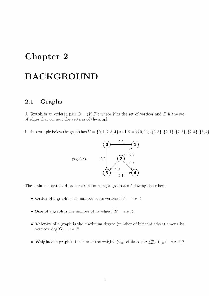
A Graph is an ordered pair G = (V,E); where V is the set of vertices and E is the setof edges that connect the vertices of the graph.
In the example below the graph has V = {0, 1, 2, 3, 4} and E = {{0, 1}, {(0, 3}, {2, 1}, {2, 3}, {2, 4}, {3, 4}}:
2
0
3
1
4
0.3
0.70.2
0.9
0.5
0.1
graph G:
The main elements and properties concerning a graph are following described:
• Order of a graph is the number of its vertices: |V | e.g. 5
• Size of a graph is the number of its edges: |E| e.g. 6
• Valency of a graph is the maximum degree (number of incident edges) among itsvertices: deg(G) e.g. 3
• Weight of a graph is the sum of the weights (wn) of its edges:∑n
i=1 (wn) e.g. 2,7
3
2.2. TYPES CHAPTER 2. BACKGROUND
2.2 Types
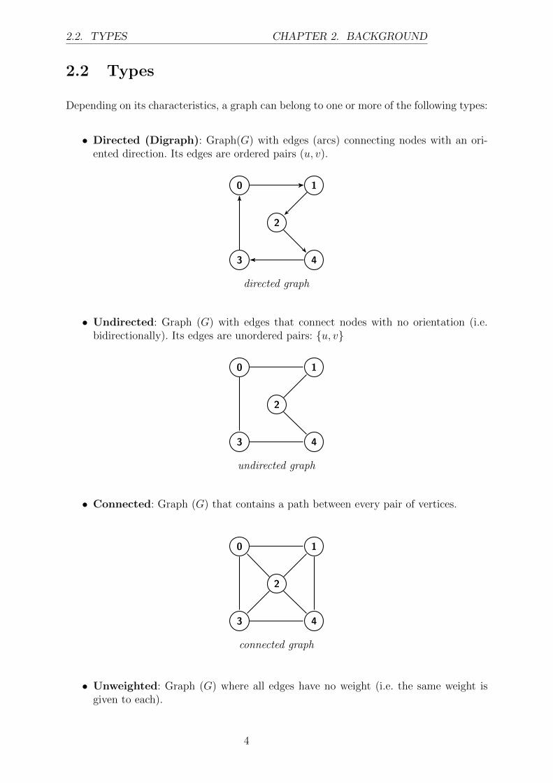
Depending on its characteristics, a graph can belong to one or more of the following types:
• Directed (Digraph): Graph(G) with edges (arcs) connecting nodes with an ori-ented direction. Its edges are ordered pairs (u, v).
2
0
3
1
4
directed graph
• Undirected: Graph (G) with edges that connect nodes with no orientation (i.e.bidirectionally). Its edges are unordered pairs: {u, v}
2
0
3
1
4
undirected graph
• Connected: Graph (G) that contains a path between every pair of vertices.
2
0
3
1
4
connected graph
• Unweighted: Graph (G) where all edges have no weight (i.e. the same weight isgiven to each).
4
2.2. TYPES CHAPTER 2. BACKGROUND
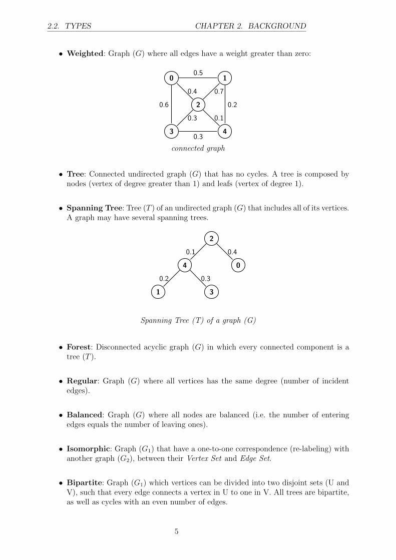
• Weighted: Graph (G) where all edges have a weight greater than zero:
2
0
3
1
4
0.4
0.3
0.7
0.1
0.6
0.5
0.3
0.2
connected graph
• Tree: Connected undirected graph (G) that has no cycles. A tree is composed bynodes (vertex of degree greater than 1) and leafs (vertex of degree 1).
• Spanning Tree: Tree (T ) of an undirected graph (G) that includes all of its vertices.A graph may have several spanning trees.
2
4 0
1 3
0.1 0.4
0.2 0.3
Spanning Tree (T) of a graph (G)
• Forest: Disconnected acyclic graph (G) in which every connected component is atree (T ).
• Regular: Graph (G) where all vertices has the same degree (number of incidentedges).
• Balanced: Graph (G) where all nodes are balanced (i.e. the number of enteringedges equals the number of leaving ones).
• Isomorphic: Graph (G1) that have a one-to-one correspondence (re-labeling) withanother graph (G2), between their Vertex Set and Edge Set.
• Bipartite: Graph (G1) which vertices can be divided into two disjoint sets (U andV), such that every edge connects a vertex in U to one in V. All trees are bipartite,as well as cycles with an even number of edges.
5
2.3. WALKS, PATHS AND TRAILS CHAPTER 2. BACKGROUND
2.3 Walks, paths and trails
A Walk is a sequence of alternating vertices and edges of a graph G = (V,E) expressedas v0e1, v1e2, v2e3, ..., vkek, where each edge ei is defined as ei = {vi−1, vi} and can berepeated. The length of this walk is k, where k ≥ 0.
A Walk is considered open if the starting vertex is different from the ending vertex (i.e.v0 6= vk). A walk is considered closed otherwise (i.e. v0 = vk).
A Trail is a walk with no repeated edges. Depending on the equality of their starting andending vertices, trails can be open or closed (circuits).
A Path is an open trail with no repeated vertices. The shortest path (called distance)between two vertices is the path that either carries less weight (on weighted graphs) ortraverse less edges (on unweighted graphs).
2.4 Cycles
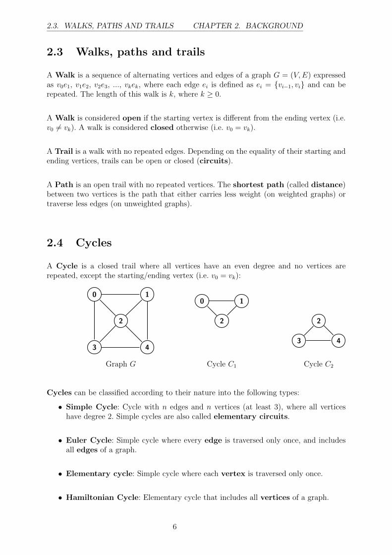
A Cycle is a closed trail where all vertices have an even degree and no vertices arerepeated, except the starting/ending vertex (i.e. v0 = vk):
2
0
3
1
4
Graph G
2
0 1
Cycle C1
2
3 4
Cycle C2
Cycles can be classified according to their nature into the following types:
• Simple Cycle: Cycle with n edges and n vertices (at least 3), where all verticeshave degree 2. Simple cycles are also called elementary circuits.
• Euler Cycle: Simple cycle where every edge is traversed only once, and includesall edges of a graph.
• Elementary cycle: Simple cycle where each vertex is traversed only once.
• Hamiltonian Cycle: Elementary cycle that includes all vertices of a graph.
6
2.5. CYCLE BASIS CHAPTER 2. BACKGROUND
• Fundamental Cycle (FC): Unique cycle obtained by adding a non-tree edge ofa graph G to its spanning tree T .
• Fundamental Cutset: Cycle created by deleting just one edge from a spanningtree.
• Horton Cycle: Fundamental cycle created from the shortest path tree of a graph G.
• Isometric Cycle: Cycle where the distance between two vertices is equal to theirdistances in the graph G. An elementary cycle is isometric if it contains the shortestpath between every pair (u,v) of its vertices.
• Cycle space (C): Vector space over GF (2) formed by the collection of all cyclesof a graph G.
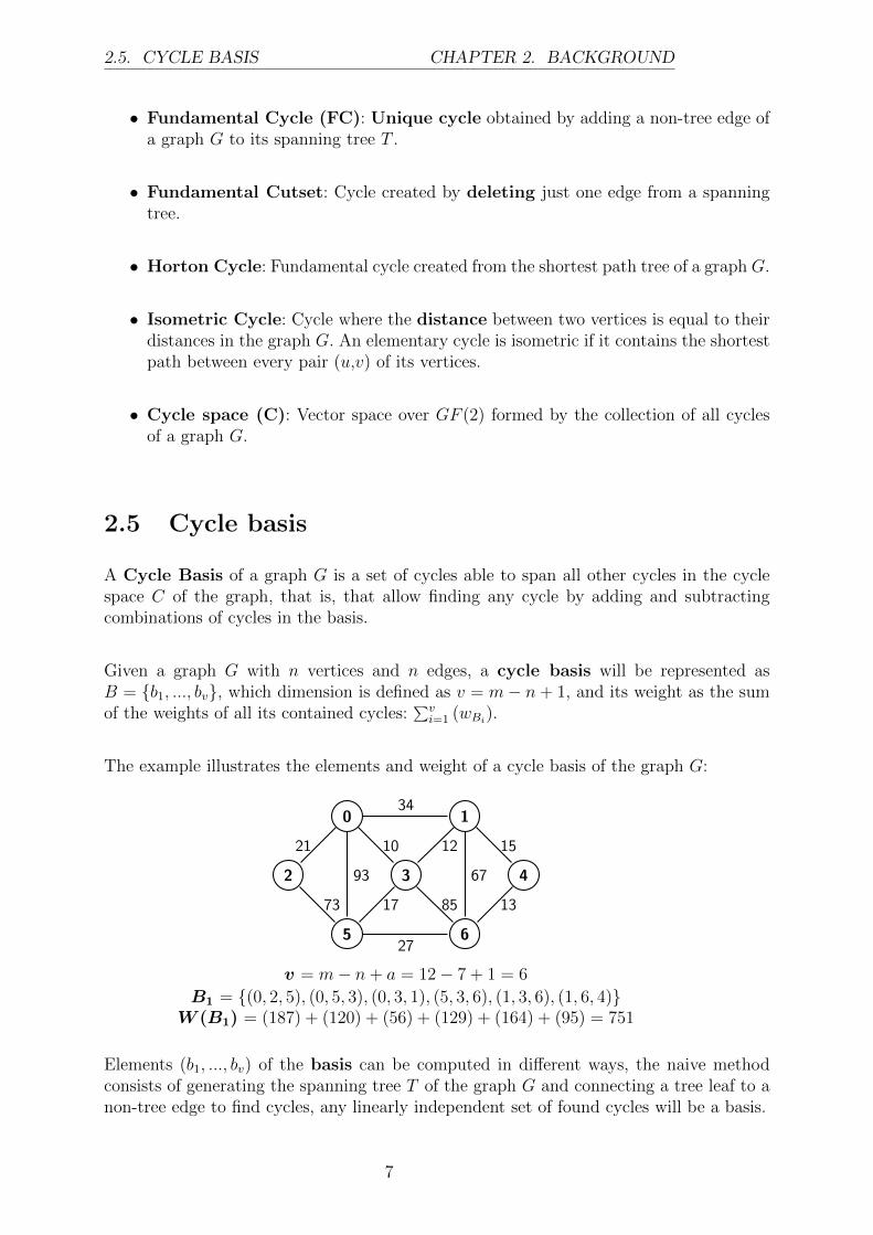
2.5 Cycle basis
A Cycle Basis of a graph G is a set of cycles able to span all other cycles in the cyclespace C of the graph, that is, that allow finding any cycle by adding and subtractingcombinations of cycles in the basis.
Given a graph G with n vertices and n edges, a cycle basis will be represented asB = {b1, ..., bv}, which dimension is defined as v = m− n + 1, and its weight as the sumof the weights of all its contained cycles:
∑vi=1 (wBi
).
The example illustrates the elements and weight of a cycle basis of the graph G:
0
2 3
1
4
5 6
34
21 10
93
12 15
67
73 17 85 13
27
v = m− n + a = 12− 7 + 1 = 6
B1 = {(0, 2, 5), (0, 5, 3), (0, 3, 1), (5, 3, 6), (1, 3, 6), (1, 6, 4)}W (B1) = (187) + (120) + (56) + (129) + (164) + (95) = 751
Elements (b1, ..., bv) of the basis can be computed in different ways, the naive methodconsists of generating the spanning tree T of the graph G and connecting a tree leaf to anon-tree edge to find cycles, any linearly independent set of found cycles will be a basis.
7
2.5. CYCLE BASIS CHAPTER 2. BACKGROUND
Depending on their specific characteristics, cycle basis can be:
• Fundamental Cycle Basis: Or ”FCB”, or ”Strongly Fundamental Cycle Basis” isa cycle basis formed by the fundamental cycles of a graph G. The FCB can becomputed from any spanning tree of a graph, by selecting the cycles formed by thecombination of a path in the three and a single path outside the tree. Each funda-mental cycle is linearly independent from the other cycles constructed from thesame tree.
• Weakly Fundamental Cycle Basis: Cycle basis formed by cycles which can beplaced into a linear ordering such that each cycle includes at least one edge thatis not included in any earlier cycle.
• Shortest Cycle Basis: The cycle basis with minimum number of vertices.
• Minimum Fundamental Cycle Basis: or ”MFCB”, is the FCB having mini-mum weight. It can be found in NP-complete polynomial time.
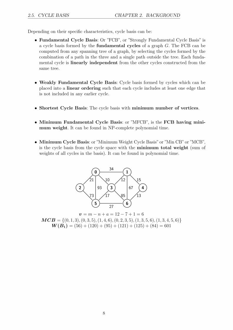
• Minimum Cycle Basis: or ”Minimum Weight Cycle Basis”or ”Min CB”or ”MCB”,is the cycle basis from the cycle space with the minimum total weight (sum ofweights of all cycles in the basis). It can be found in polynomial time.
0
2 3
1
4
5 6
34
21 10
93
12 15
67
73 17 85 13
27
v = m− n + a = 12− 7 + 1 = 6
MCB = {(0, 1, 3), (0, 3, 5), (1, 4, 6), (0, 2, 3, 5), (1, 3, 5, 6), (1, 3, 4, 5, 6)}W (B1) = (56) + (120) + (95) + (121) + (125) + (84) = 601
8
Chapter 3
FINDING THE MCB
Finding the Minimum Cycle Bases (MCB) in the Cycle Vector Space of a graphconstitutes a crucial step for the perception of its cyclic structures, a key element for thedevelopment of science studies concerning:
• Test electrical circuits
• Analyze engineering structures
• Perform surface reconstruction
• Schedule periodic timetables
• Analyze frequency of computers programs
• Plan complex syntheses in organic chemistry
Since the development of the first algorithm to find Minimum Cycle Bases, reducing thecomplexity of said algorithm has been a continuous challenge that has fascinated com-puter scientists and researchers aware of the importance of its real-world applications.
The table below provides a summary of the most important algorithms developed acrossyears to improve its worst-case complexity:
Algorithm Year Big-O Complexity
Horton 1987 O(m3 ∗ n)
De Pina 1995 O(m2 ∗ n + m ∗ (n2) ∗ log(n))
Hybrid (Amaldi) 2009 O((m2) ∗ n/log(n))
This chapter will provide a special focus on the first and last algorithms developed forfinding the minimum cycle basis (namely Horton’s and Amaldi’s ones), a detailedanalysis will be provided including their implementation in the C++ programming lan-guage.
9
3.1. HORTON ANALYSIS CHAPTER 3. MCB ALGORITHM
3.1 Horton analysis
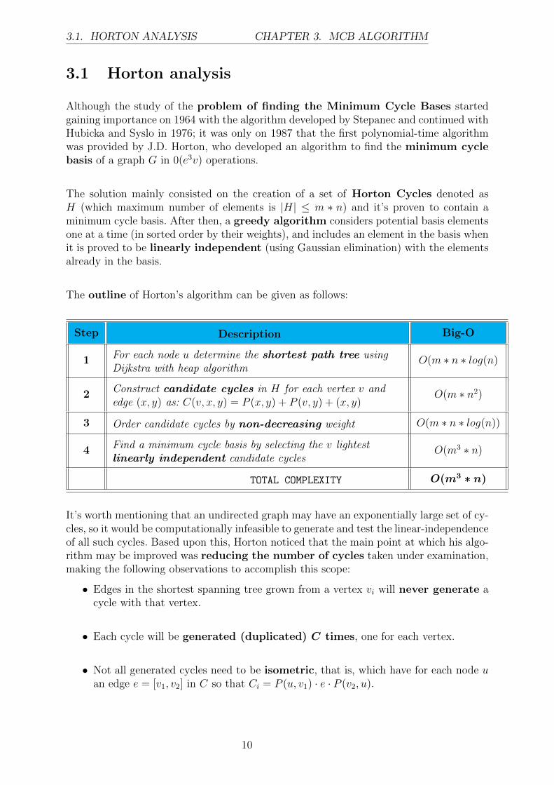
Although the study of the problem of finding the Minimum Cycle Bases startedgaining importance on 1964 with the algorithm developed by Stepanec and continued withHubicka and Syslo in 1976; it was only on 1987 that the first polynomial-time algorithmwas provided by J.D. Horton, who developed an algorithm to find the minimum cyclebasis of a graph G in 0(e3v) operations.
The solution mainly consisted on the creation of a set of Horton Cycles denoted asH (which maximum number of elements is |H| ≤ m ∗ n) and it’s proven to contain aminimum cycle basis. After then, a greedy algorithm considers potential basis elementsone at a time (in sorted order by their weights), and includes an element in the basis whenit is proved to be linearly independent (using Gaussian elimination) with the elementsalready in the basis.
The outline of Horton’s algorithm can be given as follows:
Step Description Big-O
1 For each node u determine the shortest path tree usingDijkstra with heap algorithm
O(m ∗ n ∗ log(n)
2 Construct candidate cycles in H for each vertex v andedge (x, y) as: C(v, x, y) = P (x, y) + P (v, y) + (x, y)
O(m ∗ n2)
3 Order candidate cycles by non-decreasing weight O(m ∗ n ∗ log(n))
4 Find a minimum cycle basis by selecting the v lightestlinearly independent candidate cycles
O(m3 ∗ n)
TOTAL COMPLEXITY O(m3 ∗ n)
It’s worth mentioning that an undirected graph may have an exponentially large set of cy-cles, so it would be computationally infeasible to generate and test the linear-independenceof all such cycles. Based upon this, Horton noticed that the main point at which his algo-rithm may be improved was reducing the number of cycles taken under examination,making the following observations to accomplish this scope:
• Edges in the shortest spanning tree grown from a vertex vi will never generate acycle with that vertex.
• Each cycle will be generated (duplicated) C times, one for each vertex.
• Not all generated cycles need to be isometric, that is, which have for each node uan edge e = [v1, v2] in C so that Ci = P (u, v1) · e · P (v2, u).
10
3.2. HORTON IMPLEMENTATION CHAPTER 3. MCB ALGORITHM
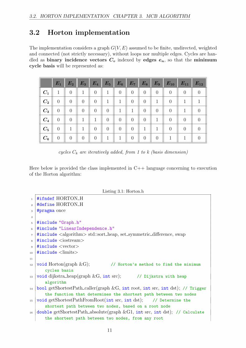
3.2 Horton implementation
The implementation considers a graph G(V,E) assumed to be finite, undirected, weightedand connected (not strictly necessary), without loops nor multiple edges. Cycles are han-dled as binary incidence vectors Cv indexed by edges en, so that the minimumcycle basis will be represented as:
E1 E2 E3 E4 E5 E6 E7 E8 E9 E10 E11 E12
C1 1 0 1 0 1 0 0 0 0 0 0 0
C2 0 0 0 0 1 1 0 0 1 0 1 1
C3 0 0 0 0 0 1 1 0 0 0 1 0
C4 0 0 1 1 0 0 0 0 1 0 0 0
C5 0 1 1 0 0 0 0 1 1 0 0 0
C6 0 0 0 0 1 1 0 0 0 1 1 0
cycles Ck are iteratively added, from 1 to k (basis dimension)
Here below is provided the class implemented in C++ language concerning to executionof the Horton algorithm:
Listing 3.1: Horton.h
1 #ifndef HORTON H2 #define HORTON H3 #pragma once4
5 #include "Graph.h"
6 #include "LinearIndependence.h"
7 #include <algorithm> std::sort heap, set symmetric difference, swap8 #include <iostream>9 #include <vector>
10 #include <limits>11
12 void Horton(graph &G); // Horton’s method to find the minimum
cycles basis
13 void dijkstra heap(graph &G, int src); // Dijkstra with heap
algorithm
14 bool getShortestPath caller(graph &G, int root, int src, int dst); // Trigger
the function that determines the shortest path between two nodes
15 void getShortestPathFromRoot(int src, int dst); // Determine the
shortest path between two nodes, based on a root node
16 double getShortestPath absolute(graph &G1, int src, int dst); // Calculate
the shortest path between two nodes, from any root
11
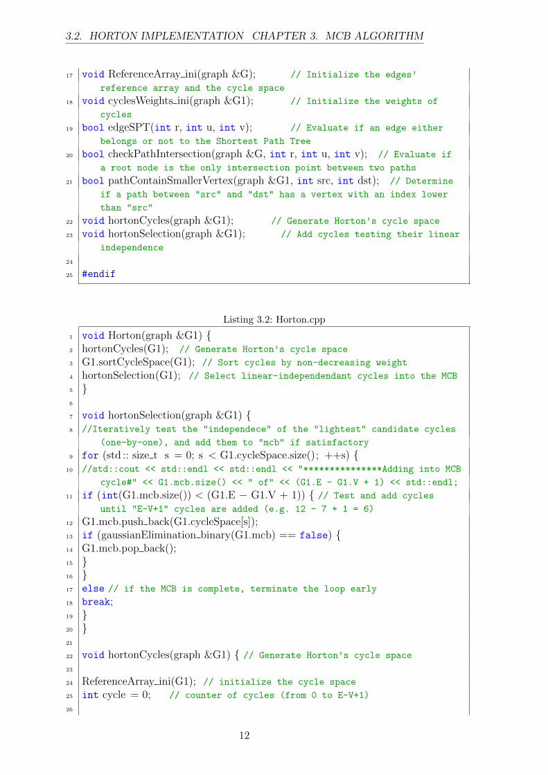
3.2. HORTON IMPLEMENTATION CHAPTER 3. MCB ALGORITHM
17 void ReferenceArray ini(graph &G); // Initialize the edges’
reference array and the cycle space
18 void cyclesWeights ini(graph &G1); // Initialize the weights of
cycles
19 bool edgeSPT(int r, int u, int v); // Evaluate if an edge either
belongs or not to the Shortest Path Tree
20 bool checkPathIntersection(graph &G, int r, int u, int v); // Evaluate if
a root node is the only intersection point between two paths
21 bool pathContainSmallerVertex(graph &G1, int src, int dst); // Determine
if a path between "src" and "dst" has a vertex with an index lower
than "src"
22 void hortonCycles(graph &G1); // Generate Horton’s cycle space
23 void hortonSelection(graph &G1); // Add cycles testing their linear
independence
24
25 #endif
Listing 3.2: Horton.cpp
1 void Horton(graph &G1) {2 hortonCycles(G1); // Generate Horton’s cycle space
3 G1.sortCycleSpace(G1); // Sort cycles by non-decreasing weight
4 hortonSelection(G1); // Select linear-independendant cycles into the MCB
5 }6
7 void hortonSelection(graph &G1) {8 //Iteratively test the "independece" of the "lightest" candidate cycles
(one-by-one), and add them to "mcb" if satisfactory
9 for (std :: size t s = 0; s < G1.cycleSpace.size(); ++s) {10 //std::cout << std::endl << std::endl << "***************Adding into MCB
cycle#" << G1.mcb.size() << " of" << (G1.E - G1.V + 1) << std::endl;
11 if (int(G1.mcb.size()) < (G1.E − G1.V + 1)) { // Test and add cycles
until "E-V+1" cycles are added (e.g. 12 - 7 + 1 = 6)
12 G1.mcb.push back(G1.cycleSpace[s]);13 if (gaussianElimination binary(G1.mcb) == false) {14 G1.mcb.pop back();15 }16 }17 else // if the MCB is complete, terminate the loop early
18 break;19 }20 }21
22 void hortonCycles(graph &G1) { // Generate Horton’s cycle space
23
24 ReferenceArray ini(G1); // initialize the cycle space
25 int cycle = 0; // counter of cycles (from 0 to E-V+1)
26
12
3.2. HORTON IMPLEMENTATION CHAPTER 3. MCB ALGORITHM
27 // 1.2 Construct candidate cycles as: Cycle(v, x, y) = (x, y) + Path(v,
x) + Path(v, y)
28 // The set has a theorical "M*N" number of elements (both, isometric and
non-isometric candidate cycles are considered)
29
30 // For every vertex in G...
31 for (int v = 0; v < G1.V; v++) {//G1.V or 1
32 spt. clear () ; // Clear the Shortest Path Tree (spt)
33 dijkstra heap(G1, v); // Generate the Shortest Path Tree (spt)
34 for (std :: size t e = 0; e < G1.edgesReference.size(); e++) {35 ...36 }37 }38 }
13
3.3. DE PINA ANALYSIS CHAPTER 3. MCB ALGORITHM
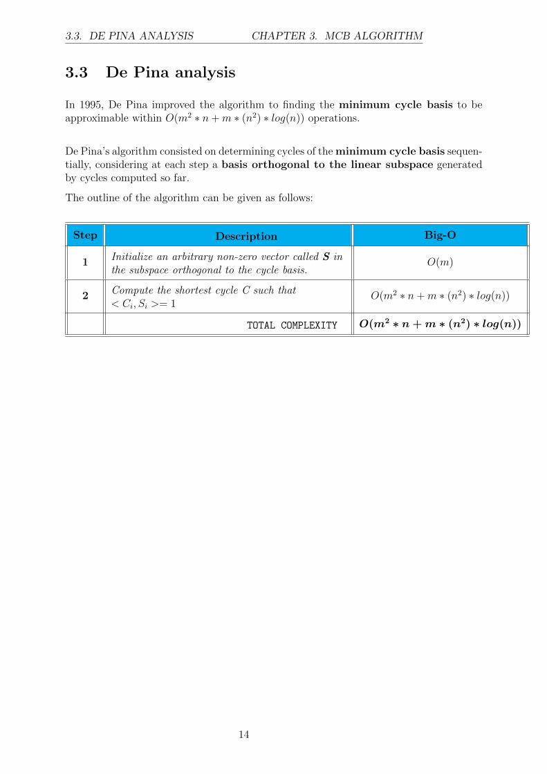
3.3 De Pina analysis
In 1995, De Pina improved the algorithm to finding the minimum cycle basis to beapproximable within O(m2 ∗ n + m ∗ (n2) ∗ log(n)) operations.
De Pina’s algorithm consisted on determining cycles of the minimum cycle basis sequen-tially, considering at each step a basis orthogonal to the linear subspace generatedby cycles computed so far.
The outline of the algorithm can be given as follows:
Step Description Big-O
1 Initialize an arbitrary non-zero vector called S inthe subspace orthogonal to the cycle basis.
O(m)
2 Compute the shortest cycle C such that< Ci, Si >= 1
O(m2 ∗ n + m ∗ (n2) ∗ log(n))
TOTAL COMPLEXITY O(m2 ∗ n + m ∗ (n2) ∗ log(n))
14
3.4. DE PINA IMPLEMENTATION CHAPTER 3. MCB ALGORITHM
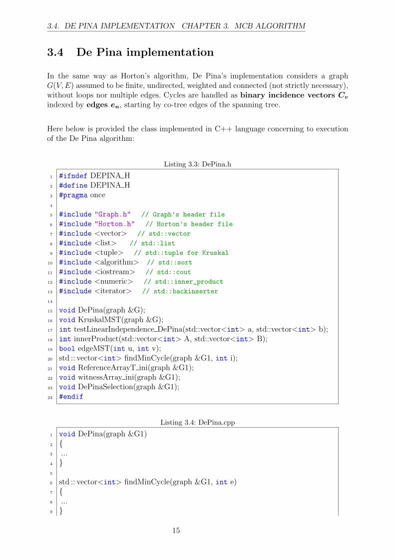
3.4 De Pina implementation
In the same way as Horton’s algorithm, De Pina’s implementation considers a graphG(V,E) assumed to be finite, undirected, weighted and connected (not strictly necessary),without loops nor multiple edges. Cycles are handled as binary incidence vectors Cv
indexed by edges en, starting by co-tree edges of the spanning tree.
Here below is provided the class implemented in C++ language concerning to executionof the De Pina algorithm:
Listing 3.3: DePina.h
1 #ifndef DEPINA H2 #define DEPINA H3 #pragma once4
5 #include "Graph.h" // Graph’s header file
6 #include "Horton.h" // Horton’s header file
7 #include <vector> // std::vector
8 #include <list> // std::list
9 #include <tuple> // std::tuple for Kruskal
10 #include <algorithm> // std::sort
11 #include <iostream> // std::cout
12 #include <numeric> // std::inner_product
13 #include <iterator> // std::backinserter
14
15 void DePina(graph &G);16 void KruskalMST(graph &G);17 int testLinearIndependence DePina(std::vector<int> a, std::vector<int> b);18 int innerProduct(std::vector<int> A, std::vector<int> B);19 bool edgeMST(int u, int v);20 std :: vector<int> findMinCycle(graph &G1, int i);21 void ReferenceArrayT ini(graph &G1);22 void witnessArray ini(graph &G1);23 void DePinaSelection(graph &G1);24 #endif
Listing 3.4: DePina.cpp
1 void DePina(graph &G1)2 {3 ...4 }5
6 std :: vector<int> findMinCycle(graph &G1, int e)7 {8 ...9 }
15
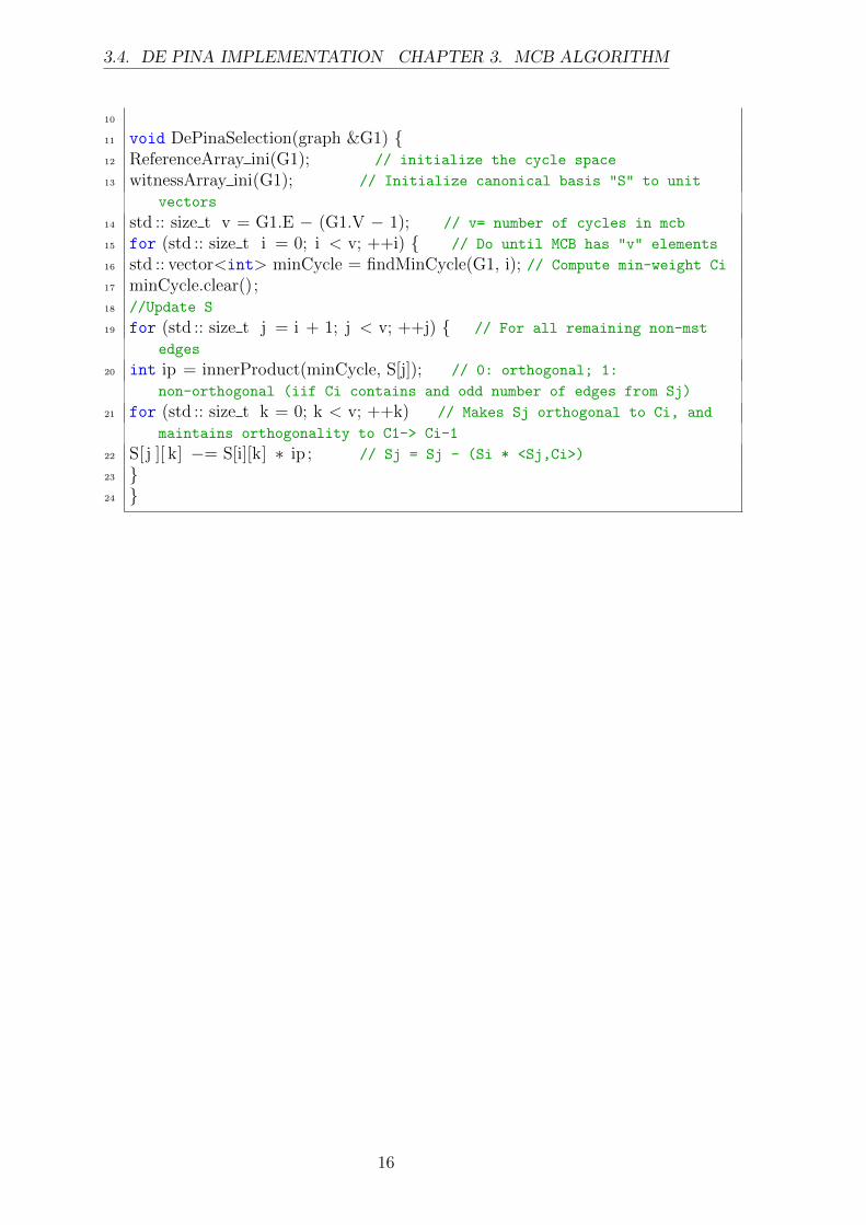
3.4. DE PINA IMPLEMENTATION CHAPTER 3. MCB ALGORITHM
10
11 void DePinaSelection(graph &G1) {12 ReferenceArray ini(G1); // initialize the cycle space
13 witnessArray ini(G1); // Initialize canonical basis "S" to unit
vectors
14 std :: size t v = G1.E − (G1.V − 1); // v= number of cycles in mcb
15 for (std :: size t i = 0; i < v; ++i) { // Do until MCB has "v" elements
16 std :: vector<int> minCycle = findMinCycle(G1, i); // Compute min-weight Ci
17 minCycle.clear();18 //Update S
19 for (std :: size t j = i + 1; j < v; ++j) { // For all remaining non-mst
edges
20 int ip = innerProduct(minCycle, S[j]); // 0: orthogonal; 1:
non-orthogonal (iif Ci contains and odd number of edges from Sj)
21 for (std :: size t k = 0; k < v; ++k) // Makes Sj orthogonal to Ci, and
maintains orthogonality to C1-> Ci-1
22 S[j ][ k] −= S[i][k] ∗ ip ; // Sj = Sj - (Si * <Sj,Ci>)
23 }24 }
16
3.5. AMALDI ANALYSIS CHAPTER 3. MCB ALGORITHM
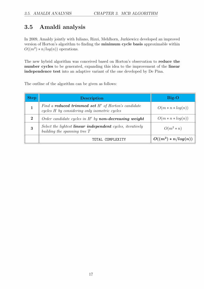
3.5 Amaldi analysis
In 2009, Amaldy jointly with Iuliano, Rizzi, Mehlhorn, Jurkiewicz developed an improvedversion of Horton’s algorithm to finding the minimum cycle basis approximable withinO((m2) ∗ n/log(n)) operations.
The new hybrid algorithm was conceived based on Horton’s observation to reduce thenumber cycles to be generated, expanding this idea to the improvement of the linearindependence test into an adaptive variant of the one developed by De Pina.
The outline of the algorithm can be given as follows:
Step Description Big-O
1 Find a reduced trimmed set H ′ of Horton’s candidatecycles H by considering only isometric cycles
O(m ∗ n ∗ log(n))
2 Order candidate cycles in H ′ by non-decreasing weight O(m ∗ n ∗ log(n))
3 Select the lightest linear independent cycles, iterativelybuilding the spanning tree T
O(m2 ∗ n)
TOTAL COMPLEXITY O((m2) ∗ n/log(n))
17
3.6. AMALDI IMPLEMENTATION CHAPTER 3. MCB ALGORITHM
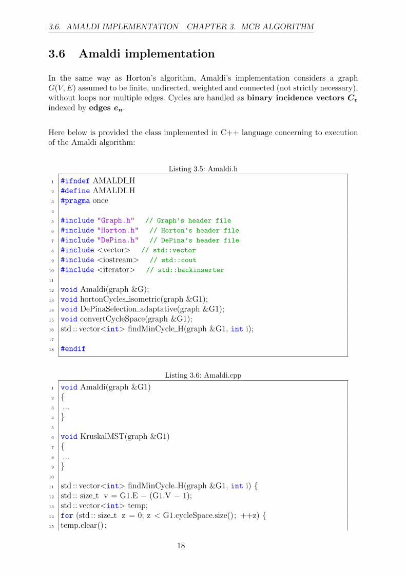
3.6 Amaldi implementation
In the same way as Horton’s algorithm, Amaldi’s implementation considers a graphG(V,E) assumed to be finite, undirected, weighted and connected (not strictly necessary),without loops nor multiple edges. Cycles are handled as binary incidence vectors Cv
indexed by edges en.
Here below is provided the class implemented in C++ language concerning to executionof the Amaldi algorithm:
Listing 3.5: Amaldi.h
1 #ifndef AMALDI H2 #define AMALDI H3 #pragma once4
5 #include "Graph.h" // Graph’s header file
6 #include "Horton.h" // Horton’s header file
7 #include "DePina.h" // DePina’s header file
8 #include <vector> // std::vector
9 #include <iostream> // std::cout
10 #include <iterator> // std::backinserter
11
12 void Amaldi(graph &G);13 void hortonCycles isometric(graph &G1);14 void DePinaSelection adaptative(graph &G1);15 void convertCycleSpace(graph &G1);16 std :: vector<int> findMinCycle H(graph &G1, int i);17
18 #endif
Listing 3.6: Amaldi.cpp
1 void Amaldi(graph &G1)2 {3 ...4 }5
6 void KruskalMST(graph &G1)7 {8 ...9 }
10
11 std :: vector<int> findMinCycle H(graph &G1, int i) {12 std :: size t v = G1.E − (G1.V − 1);13 std :: vector<int> temp;14 for (std :: size t z = 0; z < G1.cycleSpace.size(); ++z) {15 temp.clear() ;
18
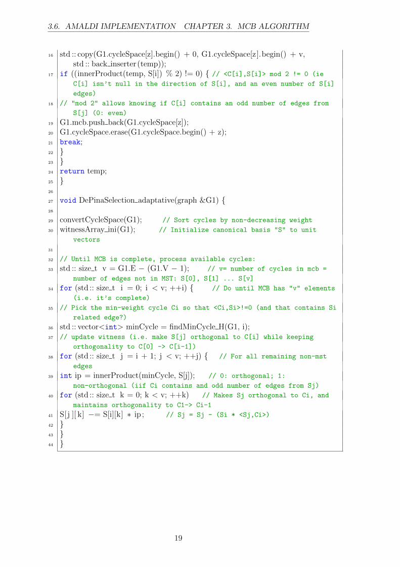
3.6. AMALDI IMPLEMENTATION CHAPTER 3. MCB ALGORITHM
16 std :: copy(G1.cycleSpace[z].begin() + 0, G1.cycleSpace[z].begin() + v,std :: back inserter(temp));
17 if ((innerProduct(temp, S[i]) % 2) != 0) { // <C[i],S[i]> mod 2 != 0 (ie
C[i] isn’t null in the direction of S[i], and an even number of S[i]
edges)
18 // "mod 2" allows knowing if C[i] contains an odd number of edges from
S[j] (0: even)
19 G1.mcb.push back(G1.cycleSpace[z]);20 G1.cycleSpace.erase(G1.cycleSpace.begin() + z);21 break;22 }23 }24 return temp;25 }26
27 void DePinaSelection adaptative(graph &G1) {28
29 convertCycleSpace(G1); // Sort cycles by non-decreasing weight
30 witnessArray ini(G1); // Initialize canonical basis "S" to unit
vectors
31
32 // Until MCB is complete, process available cycles:
33 std :: size t v = G1.E − (G1.V − 1); // v= number of cycles in mcb =
number of edges not in MST: S[0], S[1] ... S[v]
34 for (std :: size t i = 0; i < v; ++i) { // Do until MCB has "v" elements
(i.e. it’s complete)
35 // Pick the min-weight cycle Ci so that <Ci,Si>!=0 (and that contains Si
related edge?)
36 std :: vector<int> minCycle = findMinCycle H(G1, i);37 // update witness (i.e. make S[j] orthogonal to C[i] while keeping
orthogonality to C[0] -> C[i-1])
38 for (std :: size t j = i + 1; j < v; ++j) { // For all remaining non-mst
edges
39 int ip = innerProduct(minCycle, S[j]); // 0: orthogonal; 1:
non-orthogonal (iif Ci contains and odd number of edges from Sj)
40 for (std :: size t k = 0; k < v; ++k) // Makes Sj orthogonal to Ci, and
maintains orthogonality to C1-> Ci-1
41 S[j ][ k] −= S[i][k] ∗ ip ; // Sj = Sj - (Si * <Sj,Ci>)
42 }43 }44 }
19
Chapter 4
CONCLUSION
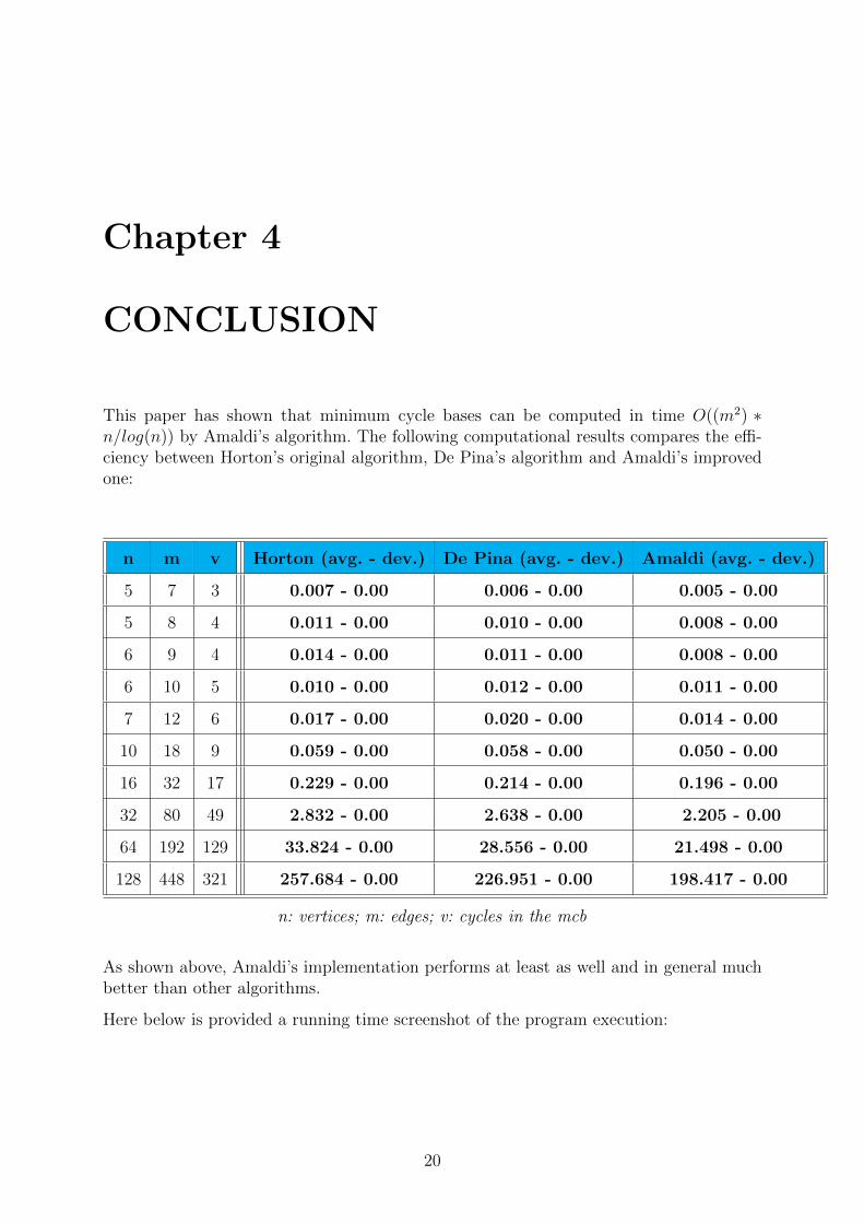
This paper has shown that minimum cycle bases can be computed in time O((m2) ∗n/log(n)) by Amaldi’s algorithm. The following computational results compares the effi-ciency between Horton’s original algorithm, De Pina’s algorithm and Amaldi’s improvedone:
n m v Horton (avg. - dev.) De Pina (avg. - dev.) Amaldi (avg. - dev.)
5 7 3 0.007 - 0.00 0.006 - 0.00 0.005 - 0.00
5 8 4 0.011 - 0.00 0.010 - 0.00 0.008 - 0.00
6 9 4 0.014 - 0.00 0.011 - 0.00 0.008 - 0.00
6 10 5 0.010 - 0.00 0.012 - 0.00 0.011 - 0.00
7 12 6 0.017 - 0.00 0.020 - 0.00 0.014 - 0.00
10 18 9 0.059 - 0.00 0.058 - 0.00 0.050 - 0.00
16 32 17 0.229 - 0.00 0.214 - 0.00 0.196 - 0.00
32 80 49 2.832 - 0.00 2.638 - 0.00 2.205 - 0.00
64 192 129 33.824 - 0.00 28.556 - 0.00 21.498 - 0.00
128 448 321 257.684 - 0.00 226.951 - 0.00 198.417 - 0.00
n: vertices; m: edges; v: cycles in the mcb
As shown above, Amaldi’s implementation performs at least as well and in general muchbetter than other algorithms.
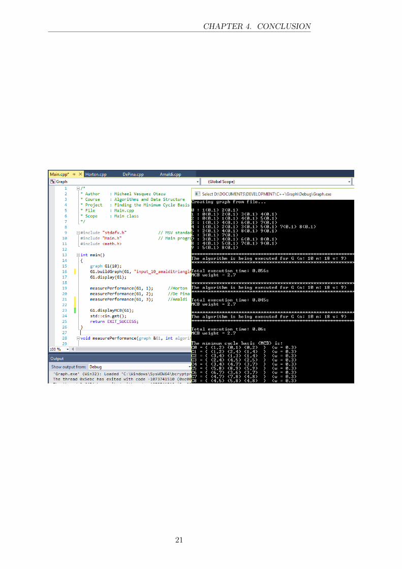
Here below is provided a running time screenshot of the program execution:
20
CHAPTER 4. CONCLUSION
21
Bibliography
[1] Edoardo Amaldi. An improved method algorithm for finding minimum cycle bases inundirected graphs, 2009
[2] E. Amaldi, C. Iuliano, R. Rizzi. IPCO2010 - Efficient Deterministic Algorithms forFinding a Minimum Cycle Basis in Undirected Graphs, 2010
[3] Edoardo Amaldi, Claudio Iuliano, Romeo Rizzi, Kurt Melhorn, Tomasz Jurkiewicz.Breaking the O(m2n) Barrier for Minimum Cycle Bases, 2009
[4] Edoardo Amaldi, Claudio Iuliano, Romeo Rizzi, Kurt Melhorn, Tomasz Jurkiewicz.Improved minimum cycle bases algorithms by restriction to isometric cycles, 2009
[5] Narshing Deo, G.M. Prabhu and M.S. Krishnamoorthy. Algorithms for generatingFundamental Cycles in a Graph, 1982.
[6] Christian Liebchen, Romo Rizzi. Classes of cycle Basis, 2005.
[7] Philippe Vismara. Union of all the Minimum Cycle Bases of a Graph, 1997.
[8] Joseph D. Horton. A polynomial-time algorithm to find the shortest cycle basis of agraph, 1987
[9] James C. Tiernan. An efficient search algorithm to find the Elementary Circuits of agraph, 1970.
[10] T. Kavitha, K. Mehlhorn, D. Michail, K. Paluch. A faster algorithm for MinimumCycle Basis of graphs, 2002.
[11] Dorothea Wagner. Algorithmentechnik - Kreisbasen, Matroide and Algorithmen 2012.
22


