Exposure to air pollutants in English homes

Exposure to air pollutants in English homes

GARY J. RAW, SARA K.D. COWARD, VERONICA M. BROWN AND DERRICK R. CRUMP

BRE, Watford, UK

BRE has conducted a national representative survey of air pollutants in 876 homes in England, designed to increase knowledge of baseline pollutant levels

and factors associated with high concentrations. Homes were monitored for carbon monoxide (CO), nitrogen dioxide (NO2), formaldehyde and volatile

organic compounds (VOCs). In the majority of the homes, concentrations of the measured pollutants were low. However, some homes have

concentrations that would suggest a need for precautionary mitigation. Those factors that are most likely to lead to exposures of concern in homes are

identified as gas cooking (for CO and NO2), the use of unflued appliances for heating (for CO and NO2), emissions from materials in new homes (for total

VOC (TVOC) and formaldehyde), and painting and decorating, with a significant increase in risk suspected to exist where there is not a place to store

materials away from the living space (for TVOC). It is noteworthy that seasonal effects on CO and NO2 were largely due to indoor sources. This would

need to be considered when interpreting time series studies of the effect of outdoor air pollution on health. It is also of some significance that the critical

factors are related much more to sources than to ventilation: source control is therefore, as would be expected, the most appropriate approach to reducing

the risk of hazardous exposure to air pollutants in homes.

Journal of Exposure Analysis and Environmental Epidemiology (2004) 14, S85–S94. doi:10.1038/sj.jea.7500363

Keywords: homes, carbon monoxide, nitrogen dioxide, volatile organic compounds, formaldehyde, measurements.

Introduction

There is an increasing general recognition that, for most

people, exposure to air pollution is determined principally by

indoor exposure. Furthermore, exposure in the home

represents a significant proportion of total exposure and,

for those who are housebound, the total of their annual

exposure. In this context, it is perhaps surprising that

relatively little has been quantified regarding exposures in

the home. Within the UK, several studies have provided

indicative data on exposure to some key air pollutants (e.g.,

Wiech and Raw, 1995, 1996; Berry et al., 1996; Venn et al.,

2001), but none could claim to be representative of the

housing stock. The largest single study (Berry et al., 1996)

included only 174 homes, all in one English county.

The UK Government therefore commissioned a larger,

more representative survey, which led to monitoring of air

pollutants and potential determinants of exposure in 876

homes in England (Coward et al., 2001). The pollutants

monitored were nitrogen dioxide (NO2), carbon monoxide

(CO), formaldehyde and other volatile organic compounds

(VOCs) (evaluated both as total VOCs (TVOC) and

individual VOCs). The study was restricted to England

because that was the remit of the commissioning

department.

The survey was designed to increase knowledge of baseline

pollutant levels and of factors associated with high concen-

trations. This paper focuses on the implications for exposure.

Method

The survey structure and methodology, including quality

control/quality assurance procedures, are described in a

published report (Coward et al., 2001) and are therefore only

summarized here to the extent necessary to understand the

findings.

The Selection of HomesThe Survey of English Housing (SEH) was used as a vehicle

for selecting homes (DETR, 1999). The SEH entails visits to

20,000 randomly selected homes per year, using a team of

interviewers located throughout England. Using the SEH as

a sampling base, the aim was to obtain indoor air pollutant

measurements in 1000 homes, the monitoring being dis-

tributed across a full year so that seasonal variation could be

investigated. The requirement was therefore to recruit 80–85

homes per month; the SEH interviewers approached

randomly selected households in order to achieve this

number. The proportion of households that agreed to take

part was less than anticipated, so that the BRE research team

received, from the SEH operators, approximately 80

1. Address all Correspondence to: Dr Crump, BRE, Bucknalls Lane,

Watford WD25 9XX, UK.

Tel.: þ 44-1923-664452; Fax: þ 44-1923-664786.

E-mail: [email protected]

Journal of Exposure Analysis and Environmental Epidemiology (2004) 14, S85–S94r 2004 Nature Publishing Group All rights reserved 1053-4245/04/$25.00

www.nature.com/jea

addresses per month on average, and only about 75% of

these completed the survey. Consequently, the survey was

extended from 12 to 17 months (October 1997 to February

1999). By the end of the study, results had been obtained

from 876 homes. The householders did not return usable

samples for every pollutant in each case; hence, the number

of measurements varies between pollutants.

During each selection visit, the SEH interviewer adminis-

tered a questionnaire on behalf of BRE, if the householder

had agreed to take part in the air quality survey. The

questions concerned the homes, the characteristics of the

occupants and their activities in the home. The interviewer

also demonstrated the use of the various types of air sampler,

and showed the householder suitable locations for exposing

the samplers. No samplers were placed at this time because

the pollutants were monitored using small, simple, passive air

samplers, which could conveniently be sent by post.

The air samplers were subsequently dispatched by post

from BRE to the householders, typically within a week of

each address being received. The sampler packs included full

instructions for the use of the samplers, self-completion

questionnaires about activities during the sampling time and

reply-paid envelopes for the return of the samplers and

questionnaires to BRE. The households closed and returned

the samplers at different times in order to optimize the known

detection range of the samplers, based on the expected range

of environmental concentrations.

Data Collection

Carbon Monoxide CO was monitored for 2 weeks in the

kitchen and a bedroom in each home, using colorimetric

diffusion tubes (Drager Ltd). A single tube was placed in

each room. No blanks were used; the tubes are sealed glass

until opened. The manufacturer’s quality control system

conforms to the requirements of DIN ISO 9001. To ensure

consistent quality, the manufacturer stores tubes from each

production batch for routine tests at regular intervals. The

manufacturer has tested the tubes for measurement of low

concentrations of CO over a period of up to 15 days

(Pannwitz, 1987) and claims an accuracy of 750% for a

single-tube reading.

During exposure, CO diffuses along the tube and reacts

with the chemicals on an inert support, producing a colored

stain. The length of the stain is compared to a nonlinear scale

on the side of the tube to indicate exposure over a range of

50–600 parts per million (p.p.m.) hours. The scale is marked

at only five intervals and thus interpolation is required to give

an approximation for exposure between these intervals. To

improve accuracy, the scale on the tube was measured and

regression analysis used to provide a second-order poly-

nomial equation that converted stain length to exposure,

allowing more accurate interpolation between the marked

intervals. The tubes were ‘analyzed’ by two researchers who

were trained and experienced in reading stain lengths on the

detector tubes. These quality procedures in the reading

process were considered to be a more cost-effective approach

than using duplicate tubes.

Nitrogen Dioxide NO2 was monitored using Palmes

diffusion tubes (Atkins et al., 1978). The samplers were

exposed for 2 weeks in each home, in the kitchen, the main

bedroom and outdoors. A single tube was placed in each

location (no duplicates). Previous work which used the same

method (Berry et al., 1996) has established that duplicate

measurements within the same room had a high precision,

and it was not felt the increased analytical cost was justified

for the present study. The error (combined accuracy and

precision) of NO2 measurement by Palmes Tube in

comparison with a chemiluminescent monitor is 710%,

for concentrations across the range found in the built

environment (Apling et al., 1979).

One tube from each batch was returned for analysis

unexposed to ensure that it was blank. Experience has shown

that the quality is consistent, and that unopened tubes do not

pick up NO2. The tubes were analyzed colorimetrically using

a Bran and Luebbe Autoanalyzer, dedicated to NO2

analysis. The instrument was calibrated for each run, using

three dilutions of a standard solution, whose concentrations

fall on a straight line. The calibration was checked using a

second independent standard.

Volatile Organic Compounds VOCs were determined by

passive diffusion using Perkin-Elmer-type sampling tubes

packed with Tenax TA adsorbent, with an exposure period of

4 consecutive weeks. A single sampling tube was placed in the

bedroom of each home. Previous studies (Berry et al., 1996;

Brown et al., 1996) have shown that VOC levels vary little

between rooms in the majority of UK homes and that a

single measurement in the bedroom is representative of levels

elsewhere in the home. The bedroom was selected for the

sampling location as that is where most people spend the

majority of their time indoors. In 10% of homes selected at

random, a duplicate sampling tube was exposed alongside the

first tube, for quality control purposes. Additionally, for

every 10 tubes despatched a blank sample was retained and

analyzed along with the field samples.

Analysis of exposed samplers was undertaken using

automated thermal desorption gas chromatography (Per-

kin-Elmer ATD 400 and Autosystem GC) with flame

ionization for measurement of TVOC and mass spectro-

metric detection for characterization and measurement of

individual VOCs. The chromatographic conditions and

procedures used have been published previously (Brown

et al., 1999). TVOC concentrations were calculated from the

sum of all peaks that have a boiling point within the range

defined by C6–C16 hydrocarbons and using the response

factor for toluene. The limit of detection of the analytical

Air pollutants in English homesRaw et al.

S86 Journal of Exposure Analysis and Environmental Epidemiology (2004) 14(S1)

method is 2 ng toluene equivalent, which represents a 4-week

mean concentration of 0.1 mg/m3 in air. The analytical

quality assurance was provided through BRE’s participation

in the Workplace Analysis Scheme for Proficiency (WASP)

quality assurance scheme for determination of VOCs. WASP

is a proficiency testing scheme for the analysis of occupa-

tional hygiene and environmental air samples set up by the

UK Health and Safety Executive.

Formaldehyde Formaldehyde levels were measured over a

period of 3 consecutive days in the bedroom of each home

using a single GMD 570 series dosimeter. The analytical

procedure used desorption with acetonitrile and high-

performance liquid chromatography (HPLC) on Zorbax

ODS C18 with UV detection at 345 nm. The procedure

accords with the draft international standard ISO/DIS

16,000-4 ‘Determination of formaldehyde in indoor air

quality by the diffusive method’. The limit of detection for

formaldehyde is 1mg/m3 and the precision of replicate

measurements is 7.2%. The analytical quality assurance

procedures were as described previously (Berry et al., 1996)

and through BRE’s participation in the WASP quality

assurance scheme for determination of aldehydes.

Questionnaires Householders completed questionnaires on

homes, occupants and activities in the home. The main

independent variables derived from the sampling records and

questionnaire were season, region, area type (degree of

urbanization), building date, type of dwelling, presence/type

of garage, household size, number of habitable rooms,

occupant density, cooking fuel, heating system/fuel, heating

with portable/unfueled heaters or a gas cooker, having an

extract fan, amount of cigarette smoking, and the presence of

condensation, damp or mold. Season was defined according

to the month when sampling commenced: spring (March,

April, May); summer (June, July, August); autumn

(September, October, November); winter (December,

January, February).

Analysis

The measurements obtained for each of the pollutants were

log-normally distributed; therefore, the data were log-

transformed before analysis and only geometric means are

presented. The analysis employed t-tests for comparisons of

two groups and ANOVA for comparisons of more than two

groups. All of the dependent variables were used in the

analysis for each pollutant; hence, if a difference is not

mentioned as being significant, it is because it was included in

the analysis and found not to have a significant effect on the

pollutant in question.

Results and discussion

A detailed analysis of determinants of pollutant concentra-

tions has been reported (Coward et al., 2001, 2002). The

second report also covers relationships among the different

pollutants. Therefore, this paper concentrates on those

findings that have important implications for exposure.

Carbon MonoxideCO levels were measured successfully in 830 homes, with 821

homes providing results for both kitchens and bedrooms.

Minimum, maximum, geometric mean and percentile values

are shown in Table 1. Concentrations were significantly

higher in kitchens than in bedrooms.

The maximum 14-day average concentration of CO did

not exceed the WHO 8-h average guideline value of 10 mg/

m3 (WHO, 2000) in any home. The monthly mean

concentration was less than 1 mg/m3 in every month of

sampling. While there may be concerns that long-term

exposure to CO at concentrations below the WHO guideline

level may have health effects, this is yet to be confirmed.

Therefore, the measurements made in this study have little

direct implication for health at population level.

Of course, it remains possible that the guideline is exceeded

in homes over shorter periods. Previous work has shown that

exposures while cooking with gas can exceed 100 mg/m3 over

a period of 1 h, which is considerably in excess of the WHO

1-h guideline of 30 mg/m3 (Ross and Wilde, 1999).

Evaluation of hazardous exposure to CO should, therefore,

focus on the time spent in the presence of known sources.

Nevertheless, it should be clear that hazardous exposures

are very unlikely to occur unless there is an indoor source of

CO, and this can be confirmed by reference to the detailed

findings from the present study. Three indoor sources were

shown to be independent significant determinants of indoor

CO concentration: gas cooking, tobacco smoking and the use

of unflued combustion appliances for heating. In addition,

two factors related to outdoor concentration (and ventila-

tion/heating) were significant determinants of indoor CO

concentration: area type and season.

The analysis of cooking fuel compared three groups: (i)

homes with natural gas cooking including a natural gas oven,

(ii) homes with some natural gas cooking (hob and/or grill)

but no gas oven and (iii) homes with no fossil fuel cooking.

The difference between the groups was highly significant

Table 1. Statistics for CO concentrations (mg/m3).

Location Minimum Maximum Geometric

mean

Percentiles

10% 50% 75% 95%

Bedrooms o0.01 3.90 0.39 0.12 0.44 0.69 1.68

Kitchens o0.01 4.45 0.47 0.14 0.50 0.90 2.07

Air pollutants in English homes Raw et al.

Journal of Exposure Analysis and Environmental Epidemiology (2004) 14(S1) S87

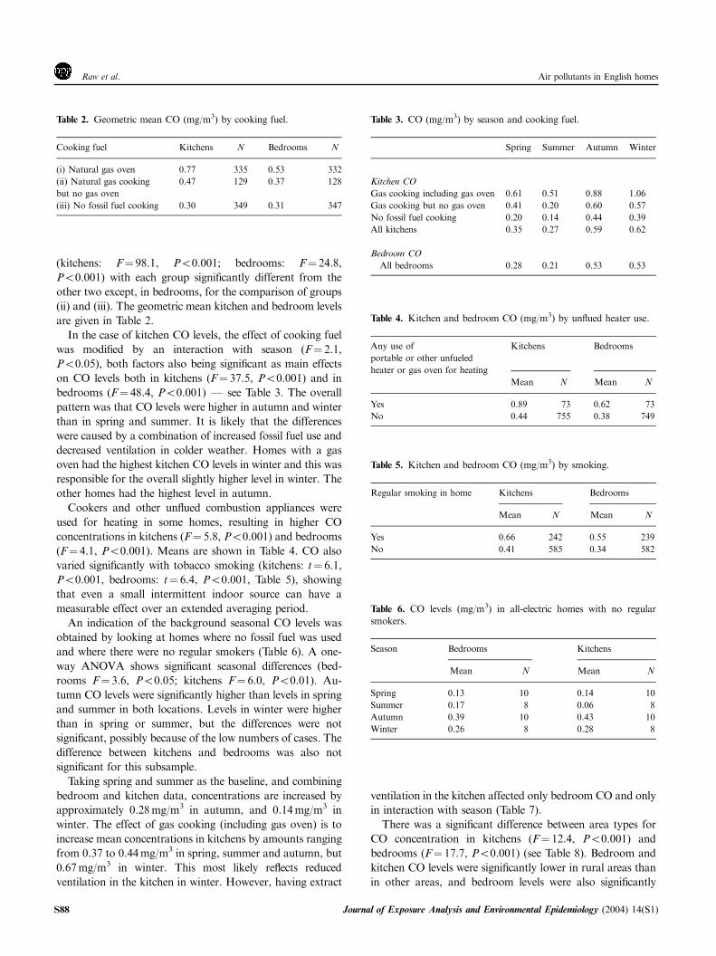
(kitchens: F¼ 98.1, Po0.001; bedrooms: F¼ 24.8,

Po0.001) with each group significantly different from the

other two except, in bedrooms, for the comparison of groups

(ii) and (iii). The geometric mean kitchen and bedroom levels

are given in Table 2.

In the case of kitchen CO levels, the effect of cooking fuel

was modified by an interaction with season (F¼ 2.1,

Po0.05), both factors also being significant as main effects

on CO levels both in kitchens (F¼ 37.5, Po0.001) and in

bedrooms (F¼ 48.4, Po0.001) F see Table 3. The overall

pattern was that CO levels were higher in autumn and winter

than in spring and summer. It is likely that the differences

were caused by a combination of increased fossil fuel use and

decreased ventilation in colder weather. Homes with a gas

oven had the highest kitchen CO levels in winter and this was

responsible for the overall slightly higher level in winter. The

other homes had the highest level in autumn.

Cookers and other unflued combustion appliances were

used for heating in some homes, resulting in higher CO

concentrations in kitchens (F¼ 5.8, Po0.001) and bedrooms

(F¼ 4.1, Po0.001). Means are shown in Table 4. CO also

varied significantly with tobacco smoking (kitchens: t¼ 6.1,

Po0.001, bedrooms: t¼ 6.4, Po0.001, Table 5), showing

that even a small intermittent indoor source can have a

measurable effect over an extended averaging period.

An indication of the background seasonal CO levels was

obtained by looking at homes where no fossil fuel was used

and where there were no regular smokers (Table 6). A one-

way ANOVA shows significant seasonal differences (bed-

rooms F¼ 3.6, Po0.05; kitchens F¼ 6.0, Po0.01). Au-

tumn CO levels were significantly higher than levels in spring

and summer in both locations. Levels in winter were higher

than in spring or summer, but the differences were not

significant, possibly because of the low numbers of cases. The

difference between kitchens and bedrooms was also not

significant for this subsample.

Taking spring and summer as the baseline, and combining

bedroom and kitchen data, concentrations are increased by

approximately 0.28 mg/m3 in autumn, and 0.14 mg/m3 in

winter. The effect of gas cooking (including gas oven) is to

increase mean concentrations in kitchens by amounts ranging

from 0.37 to 0.44 mg/m3 in spring, summer and autumn, but

0.67 mg/m3 in winter. This most likely reflects reduced

ventilation in the kitchen in winter. However, having extract

ventilation in the kitchen affected only bedroom CO and only

in interaction with season (Table 7).

There was a significant difference between area types for

CO concentration in kitchens (F¼ 12.4, Po0.001) and

bedrooms (F¼ 17.7, Po0.001) (see Table 8). Bedroom and

kitchen CO levels were significantly lower in rural areas than

in other areas, and bedroom levels were also significantly

Table 2. Geometric mean CO (mg/m3) by cooking fuel.

Cooking fuel Kitchens N Bedrooms N

(i) Natural gas oven 0.77 335 0.53 332

(ii) Natural gas cooking

but no gas oven

0.47 129 0.37 128

(iii) No fossil fuel cooking 0.30 349 0.31 347

Table 3. CO (mg/m3) by season and cooking fuel.

Spring Summer Autumn Winter

Kitchen CO

Gas cooking including gas oven 0.61 0.51 0.88 1.06

Gas cooking but no gas oven 0.41 0.20 0.60 0.57

No fossil fuel cooking 0.20 0.14 0.44 0.39

All kitchens 0.35 0.27 0.59 0.62

Bedroom CO

All bedrooms 0.28 0.21 0.53 0.53

Table 4. Kitchen and bedroom CO (mg/m3) by unflued heater use.

Any use of

portable or other unfueled

heater or gas oven for heating

Kitchens Bedrooms

Mean N Mean N

Yes 0.89 73 0.62 73

No 0.44 755 0.38 749

Table 5. Kitchen and bedroom CO (mg/m3) by smoking.

Regular smoking in home Kitchens Bedrooms

Mean N Mean N

Yes 0.66 242 0.55 239

No 0.41 585 0.34 582

Table 6. CO levels (mg/m3) in all-electric homes with no regular

smokers.

Season Bedrooms Kitchens

Mean N Mean N

Spring 0.13 10 0.14 10

Summer 0.17 8 0.06 8

Autumn 0.39 10 0.43 10

Winter 0.26 8 0.28 8



lower in suburban than in central urban areas. Taking rural

areas as a baseline, CO exposure in the home is approxi-

mately doubled by living in a central urban area, a difference

of 0.41 mg/m3 in bedrooms and 0.38 mg/m3 in kitchens.

Nitrogen DioxideNO2 levels were measured successfully in 845 homes, with

812 homes providing results for all three locations (kitchen,

bedroom and outdoors). Minimum, maximum, geometric

mean and percentile values are shown in Table 9. Seasonal

NO2 levels are shown in Table 10.

NO2 levels were significantly higher in kitchens than in

bedrooms, because many homes had cooking-related sources

in the kitchen. In each season, bedroom levels were

significantly lower than the levels outdoors, most likely due

to the removal of infiltrating NO2 by indoor sinks. Indoor

sources would generally have less impact in bedrooms than in

kitchens because they are more likely to be in the kitchen.

NO2 levels in bedrooms were closest to outdoor levels in

summer, when it would be expected that windows were more

likely to be opened.

The most important effects on outdoor NO2 concentration

were of season (F¼ 35.8, Po0.001, Table 10) and area type

(F¼ 26.6, Po0.001, Table 11). Some other significant effects

can probably be explained by the area type, that is, effects of

region, dwelling type and age of home.

Effects on indoor concentrations were dominated by

cooking fuel (see Table 12). The difference between the

groups was highly significant (kitchens: F¼ 343, Po0.001;

bedrooms: F¼ 128, Po0.001) with each group being

significantly different from the other two (all Po0.001).

Heating fuel also had some effect, but this was confounded

with cooking fuel in a way that was difficult to untangle.

Considering only homes with no fossil fuel cooking

appliances, the homes with no fossil fuel heating had a mean

NO2 concentration of 6.7 mg/m3 compared with 15.5mg/m3

for those with individual gas heaters, a difference of only

8.8 mg/m3. The use of an unflued gas heater, including the use

of a gas oven for heating, had a greater effect, especially in

kitchens (F¼ 54.5, Po0.001) and also in bedrooms

(F¼ 19.0, Po0.001) (see Table 13). However, fewer than

10% of homes used unflued heating. Smoking also had only

a small effect but bedroom NO2 was significantly higher

(t¼ 4.0, Po0.001) in smokers’ homes (14.1 mg/m3) than in

other homes (11.1 mg/m3).

The effect of season on indoor NO2 concentrations was

significant (kitchens: F¼ 4.9, Po0.01; bedrooms: F¼ 7.4,

Po0.001). In kitchens, levels were significantly lower in

spring than in other seasons. In bedrooms, levels were highest

in summer.

Table 7. Bedroom CO (mg/m3) by season and extract fan.

Extract fan in home Spring Summer Autumn Winter

Yes 0.38 0.24 0.58 0.59

No 0.32 0.29 0.61 0.65

Table 8. Mean CO levels (mg/m3) by location and area type.

Area type Bedrooms Kitchens

Mean N Mean N

Rural 0.28 234 0.34 235

Suburban 0.41 336 0.52 339

Urban 0.50 220 0.54 222

Central urban 0.69 31 0.72 31

Table 9. Statistics for NO2 concentrations (mg/m3).

Minimum Maximum Geometric

mean

Percentiles

10% 50% 75% 95%

Kitchen 0.8 620.0 21.8 7.2 21.8 40.1 90.0

Bedroom 0.4 752.6 11.9 4.4 12.1 19.8 38.1

Outdoors 1.0 151.6 20.9 9.9 22.5 32.4 48.9

Table 10. NO2 levels (mg/m3) by season.


Kitchen 17.2 23.3 23.7 22.3

Bedroom 10.1 14.6 12.7 11.0

Outdoors 15.1 17.0 26.7 22.4

Table 11. Geometric mean outdoor NO2 (mg/m3) by area type.

Rural Suburban Urban Central urban

16.1 21.9 25.0 33.1

Table 12. Geometric mean indoor NO2 (mg/m3) by cooking fuel.

Cooking fuel Kitchens Bedrooms

Mean N Mean N

Natural gas oven 42.8 338 18.2 338

Natural gas cooking but no gas oven 22.4 128 12.8 128

No fossil fuel cooking 11.5 356 7.9 354



As with CO, for kitchen NO2, there was a significant

interaction between season and cooking fuel (Table 14).

Season had a greater effect in homes with a gas oven, where

NO2 levels were lowest in spring and highest in winter. In

homes with some gas cooking but no gas oven, the effect was

much smaller, but in the same direction. In electric-cooking

homes, NO2 levels were highest in summer and autumn and,

again, the variation is small and similar to the pattern seen in

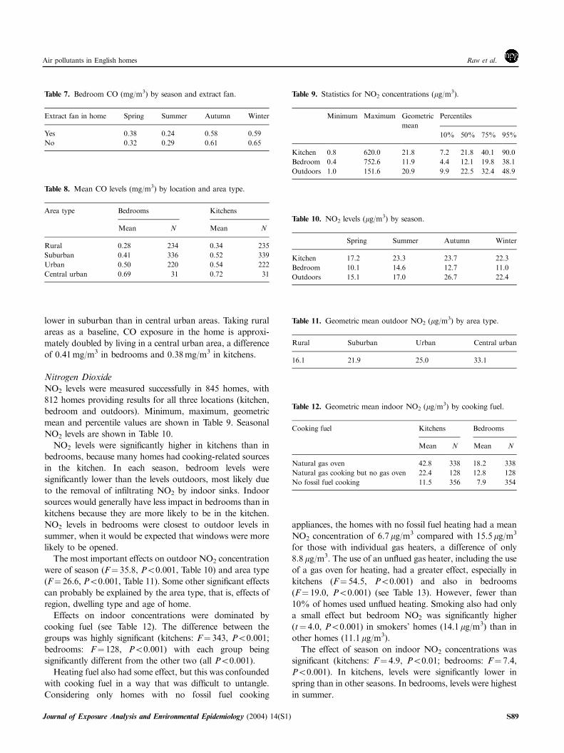
bedrooms. This is depicted in Figure 1.

It seems likely that there was a higher ventilation rate in

summer and that this allowed more NO2 from gas cooking to

escape, but allowed more to enter from outdoors, thus

increasing NO2 levels in electric cooking homes. It is also

plausible that there was more cooking in the cooler months.

Of greater importance is the implication that indoor seasonal

variation results mainly from indoor sources, rather than

variation in outdoor concentrations.

The provision of extract fans had relatively little effect

overall, but resulted in slightly higher NO2 levels where there

was no indoor source and slightly lower levels where there

was an indoor source. An example is shown in Table 15. This

particular interaction was not significant for kitchen NO2

concentrations, suggesting that the effect of fans is more to

reduce spread around the home than to decrease levels in the

source room.

NO2 in kitchens was significantly related to area type

(F¼ 19.1, Po0.001, Table 16). NO2 levels also varied

significantly with dwelling type and age of home, but these

effects are probably explained mainly by the location of the

home.

Taking season and cooking fuel as the initial determinants

of indoor concentrations, the worst case shown in the data is

kitchens with a gas cooker, in winter (50.4 mg/m3) compared

with 9.0 mg/m3 for all-electric kitchens in spring. With some

reasonable assumptions, a somewhat higher value can be

determined. Being in a central urban, rather than rural,

location would add approximately 10–15mg/m3 and using an

unflued heater would add perhaps 20–25 mg/m3. With all

these conditions satisfied, simple summation would suggest

that an average of about 85 mg/m3 might be expected, but the

database is not large enough to confirm the validity of this

summation.

The WHO annual average guideline for exposure to NO2

of 40 mg/m3 (WHO, 2000) was exceeded in kitchens in 25%

of all homes and in 53% of homes with a gas oven. It is

exceeded in bedrooms in fewer than 5% of homes.

Maximum kitchen levels exceeded the WHO 1-h guideline

of 200mg/m3 in 6 months out of 17, and in bedrooms in 2

months out of 17. It can reasonably be assumed that the

guideline was exceeded more frequently for periods of an

hour (i.e. the reference period for the guideline).

Volatile Organic CompoundsVOC results are available for 796 homes. Typically around

150–200 individual VOCs exceeded the detection limit

(0.1 mg/m3) in each home. Of these, 22 were quantified and

seven were selected for statistical analysis: benzene, toluene,

Table 13. Geometric mean kitchen and bedroom NO2 (mg/m3) by

unfueled heater use.

Any use of unfueled heating Yes No

Kitchen NO2 44.7 20.3

Bedroom NO2 17.2 11.5

0

10

20

30

40

50

60


Season

Nitr

ogen

dio

xide

con

cent

ratio

n

Gas oven Gas cooking but no oven No fossil fuel cooking Bedroom

Figure 1. Interaction effect of season and cooking fuel on NO2

concentrations (bedroom NO2 concentrations also shown for compar-ison).

Table 14. Geometric mean kitchen NO2 (mg/m3) by cooking fuel and

season.

Cooking fuel Spring Summer Autumn Winter

Gas oven 32.4 41.0 45.4 50.4

Gas cooking but no oven 19.1 21.9 23.1 23.5

No fossil fuel cooking 9.0 13.1 14.1 10.0Table 15. Geometric mean bedroom NO2 (mg/m3) by cooking fueland extract fan.

Any extract fans? Gas cooking No fossil fuel cooking

Yes 15.0 7.8

No 18.1 8.0

Table 16. Geometric mean kitchen and bedroom NO2 by area type

(mg/m3).

Rural Suburban Urban Central urban

Kitchen 14.5 25.9 24.5 31.6

Bedroom 8.4 13.4 13.8 17.6



m/p-xylene, limonene, undecane, 2,2,4-trimethyl-1,3-penta-

nediol monoisobutyrate (TPDMIB) and 2,2,4-trimethyl-1,3-

pentanediol diisobutyrate (TPDDIB). These were chosen to

represent various groups of substances and different types of

source. Table 17 shows minimum, maximum, geometric

mean and percentile values. The remainder of this section

deals only with TVOC. Results for the individual VOCs can

be found in Coward et al. (2002).

Season significantly affected TVOC (F¼ 11.6, Po0.001),

with significant differences between spring and autumn,

summer and autumn, summer and winter, and autumn and

winter (see Table 18).

Homes where painting had been undertaken during

sampling or during the previous 4 weeks had significantly

higher TVOC concentrations than other homes (F¼ 40.6,

Po0.001). Concentrations were higher where the painting

was in the same bedroom as the sampler than where it was

elsewhere in the home (means 368 vs. 319 mg/m3).

There was a significant effect on TVOC concentration

(F¼ 7.2, Po0.001) of whether the home had an integral

garage (244 mg/m3), detached garage (179 mg/m3) or no

garage (218 mg/m3). Homes with an integral garage had

significantly higher TVOC levels than homes with detached

garages. It is perhaps initially surprising that homes with no

garage had higher TVOC levels than homes with a detached

garage, since homes with no garage tend to be older, and

would therefore be expected to have lower TVOC levels. A

possible reason for this is that, in the absence of a garage,

greater amounts of volatile substances might be stored in the

home. The availability of storage space for decorating

materials, separately from the living space, may therefore

be a critical issue for reducing exposure to VOCs. This is

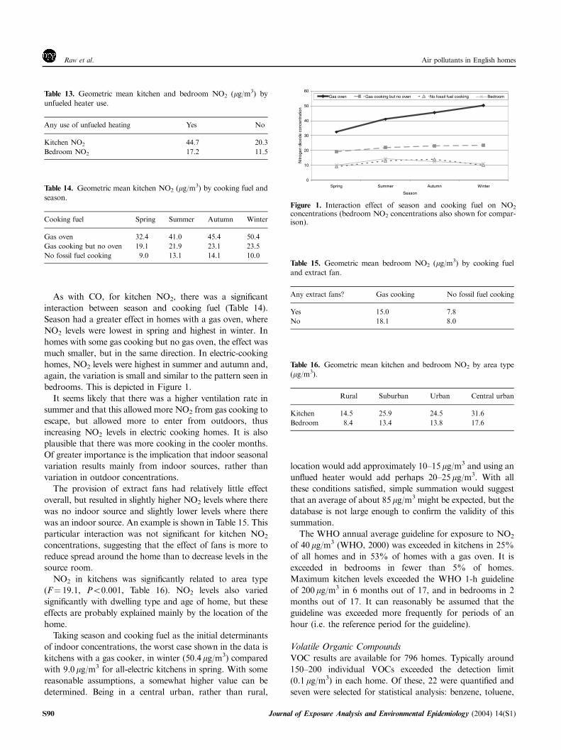
supported by an interaction between garage and painting for

TVOC (see Figure 2).

After removing data for homes where painting had been

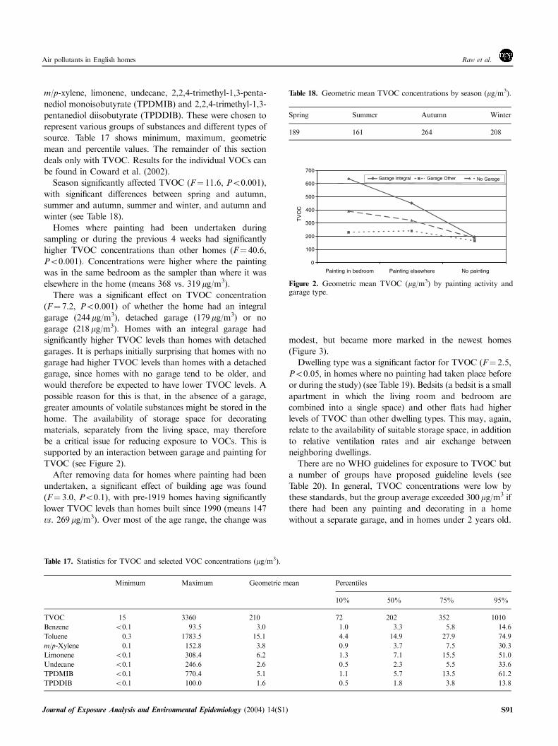
undertaken, a significant effect of building age was found

(F¼ 3.0, Po0.1), with pre-1919 homes having significantly

lower TVOC levels than homes built since 1990 (means 147

vs. 269mg/m3). Over most of the age range, the change was

modest, but became more marked in the newest homes

(Figure 3).

Dwelling type was a significant factor for TVOC (F¼ 2.5,

Po0.05, in homes where no painting had taken place before

or during the study) (see Table 19). Bedsits (a bedsit is a small

apartment in which the living room and bedroom are

combined into a single space) and other flats had higher

levels of TVOC than other dwelling types. This may, again,

relate to the availability of suitable storage space, in addition

to relative ventilation rates and air exchange between

neighboring dwellings.

There are no WHO guidelines for exposure to TVOC but

a number of groups have proposed guideline levels (see

Table 20). In general, TVOC concentrations were low by

these standards, but the group average exceeded 300mg/m3 if

there had been any painting and decorating in a home

without a separate garage, and in homes under 2 years old.

Table 17. Statistics for TVOC and selected VOC concentrations (mg/m3).

Minimum Maximum Geometric mean Percentiles

10% 50% 75% 95%

TVOC 15 3360 210 72 202 352 1010

Benzene o0.1 93.5 3.0 1.0 3.3 5.8 14.6

Toluene 0.3 1783.5 15.1 4.4 14.9 27.9 74.9

m/p-Xylene 0.1 152.8 3.8 0.9 3.7 7.5 30.3

Limonene o0.1 308.4 6.2 1.3 7.1 15.5 51.0

Undecane o0.1 246.6 2.6 0.5 2.3 5.5 33.6

TPDMIB o0.1 770.4 5.1 1.1 5.7 13.5 61.2

TPDDIB o0.1 100.0 1.6 0.5 1.8 3.8 13.8

Table 18. Geometric mean TVOC concentrations by season (mg/m3).


189 161 264 208

0

100

200

300

400

500

600

700

Painting in bedroom Painting elsewhere No painting

TV

OC

Garage Integral Garage Other No Garage

Figure 2. Geometric mean TVOC (mg/m3) by painting activity andgarage type.



The group average TVOC concentration exceeded 500 mg/m3

in homes where there had been painting and decorating in the

room where the sample was taken, and there was an integral

garage, or if the home was under a year old.

About 5% of homes exceeded 1000mg/m3. Some occu-

pants exposed to this level of TVOC may well report an odor

nuisance and may suffer some discomfort. Maximum 28-day

average TVOC levels exceeded 2000mg/m3 in 12 months out

of 17 and exceeded 3000 mg/m3 in 3 of these months. At this

higher level, occupants of the homes are likely to suffer

adverse health effects including headache, nausea and slight

narcotic effects.

FormaldehydeResults are available for concentrations of formaldehyde in

833 bedrooms. The geometric mean, minimum, maximum

and percentile values are shown in Table 21. Season had a

significant effect (F¼ 6.8, Po0.001), with a significant

difference between autumn and winter (Po0.001) (see

Table 22).

Formaldehyde concentrations varied significantly with

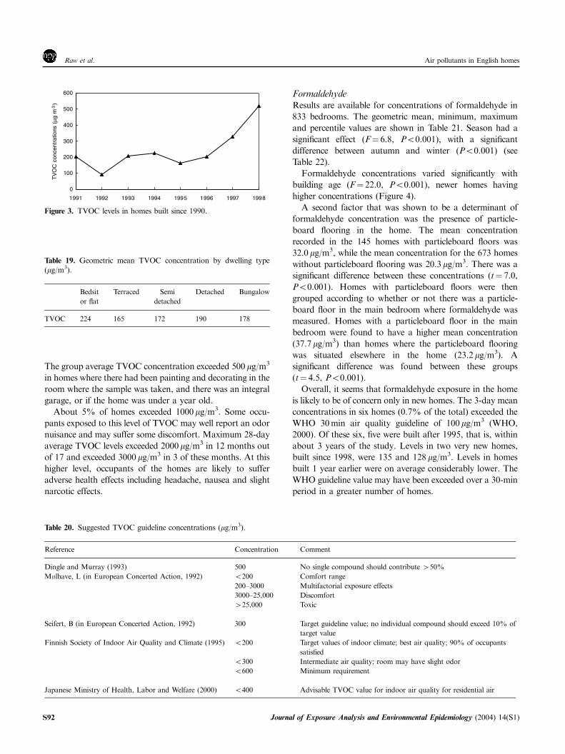
building age (F¼ 22.0, Po0.001), newer homes having

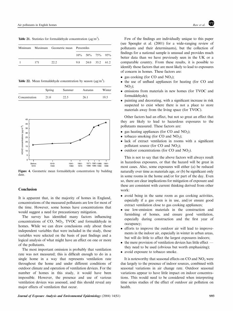
higher concentrations (Figure 4).

A second factor that was shown to be a determinant of

formaldehyde concentration was the presence of particle-

board flooring in the home. The mean concentration

recorded in the 145 homes with particleboard floors was

32.0mg/m3, while the mean concentration for the 673 homes

without particleboard flooring was 20.3mg/m3. There was a

significant difference between these concentrations (t¼ 7.0,

Po0.001). Homes with particleboard floors were then

grouped according to whether or not there was a particle-

board floor in the main bedroom where formaldehyde was

measured. Homes with a particleboard floor in the main

bedroom were found to have a higher mean concentration

(37.7 mg/m3) than homes where the particleboard flooring

was situated elsewhere in the home (23.2 mg/m3). A

significant difference was found between these groups

(t¼ 4.5, Po0.001).

Overall, it seems that formaldehyde exposure in the home

is likely to be of concern only in new homes. The 3-day mean

concentrations in six homes (0.7% of the total) exceeded the

WHO 30 min air quality guideline of 100mg/m3 (WHO,

2000). Of these six, five were built after 1995, that is, within

about 3 years of the study. Levels in two very new homes,

built since 1998, were 135 and 128 mg/m3. Levels in homes

built 1 year earlier were on average considerably lower. The

WHO guideline value may have been exceeded over a 30-min

period in a greater number of homes.

0

100

200

300

400

500

600

1991 1992 1993 1994 1995 1996 1997 1998

TV

OC

con

cent

ratio

ns (

µg m

-3)

Figure 3. TVOC levels in homes built since 1990.

Table 19. Geometric mean TVOC concentration by dwelling type

(mg/m3).

Bedsit

or flat

Terraced Semi

detached

Detached Bungalow

TVOC 224 165 172 190 178

Table 20. Suggested TVOC guideline concentrations (mg/m3).

Reference Concentration Comment

Dingle and Murray (1993) 500 No single compound should contribute 450%

M�lhave, L (in European Concerted Action, 1992) o200 Comfort range

200–3000 Multifactorial exposure effects

3000–25,000 Discomfort

425,000 Toxic

Seifert, B (in European Concerted Action, 1992) 300 Target guideline value; no individual compound should exceed 10% of

target value

Finnish Society of Indoor Air Quality and Climate (1995) o200 Target values of indoor climate; best air quality; 90% of occupants

satisfied

o300 Intermediate air quality; room may have slight odor

o600 Minimum requirement

Japanese Ministry of Health, Labor and Welfare (2000) o400 Advisable TVOC value for indoor air quality for residential air



Conclusion

It is apparent that, in the majority of homes in England,

concentrations of the measured pollutants are low for most of

the time. However, some homes have concentrations that

would suggest a need for precautionary mitigation.

The survey has identified many factors influencing

concentrations of CO, NO2, TVOC and formaldehyde in

homes. While we can draw conclusions only about those

independent variables that were included in the study, those

variables were selected on the basis of past findings and a

logical analysis of what might have an effect on one or more

of the pollutants.

The most important omission is probably that ventilation

rate was not measured; this is difficult enough to do in a

single home in a way that represents ventilation rate

throughout the home and under different conditions of

outdoor climate and operation of ventilation devices. For the

number of homes in this study, it would have been

impossible. However, the presence and use of various

ventilation devices was assessed, and this should reveal any

major effects of ventilation that occur.

Few of the findings are individually unique to this paper

(see Spengler et al. (2001) for a wide-ranging review of

pollutants and their determinants), but the collection of

findings for a national sample is unusual and provides much

better data than we have previously seen in the UK or a

comparable country. From these results, it is possible to

identify those factors that are most likely to lead to exposures

of concern in homes. These factors are:

� gas cooking (for CO and NO2);

� the use of unflued appliances for heating (for CO and

NO2);

� emissions from materials in new homes (for TVOC and

formaldehyde);

� painting and decorating, with a significant increase in risk

suspected to exist where there is not a place to store

materials away from the living space (for TVOC).

Other factors had an effect, but not so great an effect that

they are likely to lead to hazardous exposures to the

pollutants measured. These factors are:

� gas heating appliances (for CO and NO2);

� tobacco smoking (for CO and NO2);

� lack of extract ventilation in rooms with a significant

pollutant source (for CO and NO2);

� outdoor concentrations (for CO and NO2).

This is not to say that the above factors will always result

in hazardous exposures, or that the hazard will be great in

most cases. Also, some exposures will either (a) be reduced

naturally over time as materials age, or (b) be significant only

in some rooms in the home and/or for part of the day. Even

so, there are clear implications for mitigation of exposure and

these are consistent with current thinking derived from other

work:

� avoid being in the same room as gas cooking activities,

especially if a gas oven is in use, and/or ensure good

extract ventilation close to gas cooking appliances;

� use low-emission materials in the construction and

furnishing of homes, and ensure good ventilation,

especially during construction and the first year of

occupancy;

� efforts to improve the outdoor air will lead to improve-

ments in the indoor air, especially in winter in urban areas,

but will do little to affect the largest exposures indoors;

� the mere provision of ventilation devices has little effect Fthey need to be used (obvious but worth emphasizing);

� avoid exposure to tobacco smoke.

It is noteworthy that seasonal effects on CO and NO2 were

due largely to the presence of indoor sources, combined with

seasonal variations in air change rate. Outdoor seasonal

variations appear to have little impact on indoor concentra-

tions. This would need to be considered when interpreting

time series studies of the effect of outdoor air pollution on

health.

Table 21. Statistics for formaldehyde concentration (mg/m3).

Minimum Maximum Geometric mean Percentiles

10% 50% 75% 95%

1 171 22.2 9.8 24.0 35.2 61.2

Table 22. Mean formaldehyde concentration by season (mg/m3).


Concentration 21.0 22.5 26.1 19.5

0

5

10

15

20

25

30

35

40

45

HC

HO

con

cent

ratio

ns (

µg m

-3)

Before1919

1919-1940

1941-1960

1961-1970

1971-1980

1981-1985

1986-1990

1991-1998

Figure 4. Geometric mean formaldehyde concentration by buildingdate.



It is also of some significance that the critical factors are

related much more to sources than to provision for

ventilation: source control is therefore, as would be expected,

the most appropriate approach to reducing the risk of

hazardous exposure to air pollutants in homes.

Acknowledgements

The work was commissioned and funded by the Chemicals

and Biotechnology Division of the Department of the

Environment, Transport and the Regions, now the Depart-

ment of the Environment, Food and Rural Affairs

(DEFRA). Palmes Tubes were analyzed by AEA Technol-

ogy, Harwell, England. Advice on sampling methods for CO

and NO2 was provided by Dr. David Ross of BRE. Dr. Jeff

Llewellyn played a major role in managing the whole project

and the authors are grateful for his support.

References

Apling A.J., Stevenson K.J., Goldstein B.D., Melia R.J.W., and Atkins D.H.F.

Air pollution in homes 2: validation of diffusion tube measurements of

nitrogen dioxide. Warren Spring Laboratory Report LR 311 (AP), WSL,

Stevenage,, 1979.

Atkins D.H.F., Healy C., and Tarrant J.B. The use of simple diffusion tubes for

the measurement of nitrogen dioxide levels in homes using gas and electricity

for cooking. AERE Report R9184, AERE Harwell, Oxfordshire, 1978.

Berry R.W., Brown V.M., Coward S.K.D., Crump D.R., Gavin M., Grimes

C.P., Higham D.F., Hull A.V., Hunter C.A., Jeffery I.G., Lea R.G.,

Llewellyn J.W., and Raw G.J. Indoor air quality in homes. The BRE Indoor

Environment Study. BRE Reports BR299 and BR300, CRC press, London,

1996.

Brown V.M., Crump D.R., and Mann H.S. The effect of measures to alleviate the

symptoms of asthma on concentrations of VOCs and formaldehyde in UK

homes. Proceedings of Indoor Air ‘96, Vol. 4, Indoor Air ’96, Nagoya, 1996:

pp. 69–74.

Brown V.M., Mann H.S., and Crump D.R. Formaldehyde and VOC levels in

homes in England. Proceedings of Indoor Air 99, Vol. 4, CRC press, London,

1999: pp. 95–100.

Coward S.K.D., Brown V.M., Crump D.R., Raw G.J., and Llewellyn J.W.

Indoor air quality in homes in England: volatile organic compounds. BRE

Report 446, CRC press, London, 2002.

Coward S.K.D., Llewellyn J.W., Raw G.J., Brown V.M., Crump D.R., and Ross

D.I. Indoor air quality in homes in England. BRE Report 433, CRC press,

London, 2001.

DETR. Housing in England 1997/98, ISBN 0116213655, 1999: (also available on

DEFRA Statbase Website).

Dingle P., and Murray F. Control and regulation of indoor air: an Australian

perspective. Indoor Environment 1993: 2: 217.

European Concerted Action. Guidelines for ventilation requirements in buildings.

ECA Indoor air quality and its impact on man, Report No. 11. Report EUR

14449 EN, Commission of European Communities, Luxembourg, 1992.

Finnish Society of Indoor Air Quality and Climate. Classification of Indoor

Climate, Construction and Finishing Materials, Finnish Society of Indoor Air

Quality and Climate, Helsinki, 1995.

Japanese Ministry of Health, Labor and Welfare. Committee on Sick House

Syndrome: Indoor air Pollution, Progress Report No. 1 F Summary of

Discussions from the 1st to 3rd Meetings, 26 June 2000,, 2000.

Pannwitz K.-H. Monitoring of inorganic air contaminants in indoor environments

by direct reading diffusion tubes. Proceedings of Indoor Air ‘87, Vol. 1,

Institut fur Wasser- Boden- und Lufthygiene, Berlin, 1987: pp. 440–444.

Ross D.I., and Wilde D.J. Continuous monitoring of nitrogen dioxide and carbon

monoxide levels in UK homes. Proceedings of Indoor Air 99, Vol. 3, CRC

press, London, 1999: pp. 147–152.

Spengler J.D., Samet J.M., and McCarthy J.F. Indoor Air Quality Handbook.

McGraw-Hill, New York, 2001.

Venn A., Cooper M., Brown V., Crump D., Britton J., and Lewis S. Common

indoor air pollutants in the home and the risk and severity of wheezing illness

in school children. Paper submitted to the Conference of the American

Thoracic Society, May, 2001.

Wiech C.R., and Raw G.J. Asthma, dust mites, ventilation and air quality: study

design and initial carbon monoxide results. Proceedings of Healthy Buildings

‘95, Vol. 1, Healthy Buildings ’95, Milan, 1995: pp. 425–430.

Wiech C.R., and Raw G.J. The effect of mechanical ventilation on indoor nitrogen

dioxide levels. Proceedings of Indoor Air ‘96, Vol. 2, Indoor Air ’96, Nagoya,

1996: pp. 123–128.

World Health Organization. Guidelines for Air Quality. WHO, Geneva, 2000.



https://www.researchgate.net/publication/247731465_Control_and_Regulation_of_Indoor_Air_An_Australian_Perspective?el=1_x_8&enrichId=rgreq-8fd4634d-1411-4e7e-8b1d-acf1dc3b7a5e&enrichSource=Y292ZXJQYWdlOzg1ODYwNjQ7QVM6OTg5Nzg1NzQxMTA3MjhAMTQwMDYwOTczOTU1OA==

https://www.researchgate.net/publication/247731465_Control_and_Regulation_of_Indoor_Air_An_Australian_Perspective?el=1_x_8&enrichId=rgreq-8fd4634d-1411-4e7e-8b1d-acf1dc3b7a5e&enrichSource=Y292ZXJQYWdlOzg1ODYwNjQ7QVM6OTg5Nzg1NzQxMTA3MjhAMTQwMDYwOTczOTU1OA==

Documents

Exposure to air pollutants in English homes