Control Engineering Practice 8 (2000) 1167}1176

Experimental evaluation of an augmented IMC for nonlinear systems

Q. Hu, P. Saha, G. P. Rangaiah*,1

Department of Chemical and Environmental Engineering, The National University of Singapore, 119260, Singapore

Received 13 September 1999; accepted 6 March 2000

Abstract

Performance of internal model control (IMC), which is a!ected by the inevitable errors in the model used, can be improved by

augmented IMC (AuIMC) having an additional feedback of process/model mismatch through a suitable gain. This paper presents

a detailed study on real-time control of an open-loop stable single-input}single-output (SISO) nonlinear system by AuIMC. The

AuIMC structure is "rst analyzed theoretically to show its robustness and performance characteristics, followed by its experimental

evaluation on pH control of a neutralization process. The experimental results show that signi"cantly improved control is obtained by

the AuIMC compared to the standard IMC. ( 2000 Elsevier Science Ltd. All rights reserved.

Keywords: Nonlinear systems; Internal model control; Input}output linearization; Augmented internal model control; Neutralization process; pH

control

1. Introduction

Several industrially important processes such as high-

purity distillation columns, exothermic chemical reac-

tions, neutralization processes, etc., exhibit nonlinear

dynamic characteristics. Improved and robust control of

these processes is becoming necessary due to increasing

competition and environmental considerations. Also, the

availability of advanced technology and inexpensive

computing power are a boon for design and implementa-

tion of advanced control strategies. Many control tech-

niques have been proposed and analyzed for nonlinear

processes, and a good review of these is available in

Bequette (1991). Linear Internal model control (IMC) as

a general structure (Garcia & Morari, 1982) that uses a

model in parallel with the process, has become very

popular among practising engineers. The linear IMC

scheme has been extended to its nonlinear version by

employing an approximate inverse of the model through

a formulation similar to Newton's method using local

linear approximation (Economou, Morari & Palsson,

1986); Hirschorn inverse along with a nonlinear "lter

(Henson & Seborg, 1991); and quadratic perturbation

1This paper was written when the author was at Curtin University of

Technology, Western Australia as visiting Professor.

*Corresponding author. Tel.: #65-874-2187; fax: #65-779-1936.

E-mail address: chegpr@nus.edu.sg (G. P. Rangaiah).

model (Patwardhan & Madhavan, 1998). Kulkarni,

Tambe, Shukla and Deshpande (1991) proposed a di!er-

ent methodology based on the similarity between the

model and its inverse for designing a nonlinear IMC

controller, and proved its capabilities for pH control via

simulation. Brown, Lightbody and Irwin (1997) proposed

a nonlinear internal model control using local model

networks, which are represented by a set of locally valid

sub-models across the operating point.

Nevertheless a key issue in IMC application is the

mismatch between the process and the model used in the

strategy. In practical situations where modelling

errors are inevitable, the performance of the IMC system

may become poor and unacceptable. The two main ap-

proaches for reducing the e!ect of process-model mis-

match are parameter adaptation (e.g., Sastry & Isidori,

1989; Shukla, Deshpande, Ravikumar & Kulkarni 1993;

Hu & Rangaiah, 1999a) and additional feedback loop

(Zhu, Hong, Teo & Poo 1995; Wu, Hwang & Chuang

1996; Hu & Rangaiah, 1999b). Zhu et al. (1995) proposed

an enhanced IMC where the di!erence between the plant

and model outputs was fed back via an additional con-

troller and added to the manipulated variable of the

process. Wu et al. (1996) added an external loop to

modify the control action of the conventional-feedback

control system. Both these studies have mainly con-

sidered linear systems. Hu and Rangaiah (1999b) studied

two strategies* adaptive IMC (AdIMC) and augmented

IMC (AuIMC) for improving the nonlinear IMC for pH

0967-0661/00/$ - see front matter ( 2000 Elsevier Science Ltd. All rights reserved.

PII: S 0 9 6 7 - 0 6 6 1 ( 0 0 ) 0 0 0 4 1 - 1

Nomenclature

d disturbance vector

e error signal

f, g vector "elds

fa

augmented feedback

G transfer function

h output function

K tuning parameter of AuIMC

¸ifh ith-order Lie derivative of a scalar function,

h with respect to a vector function, f

M model

pH potential of hydrogen

pK log of equilibrium constant

P process

r reference input

u manipulated variable

v transformed input

< volume of tank

=a

reaction invariant a

=b

reaction invariant b

x state variables

y controlled output

Greek letters

ai

controller tuning parameter

b AuIMC tuning parameter

c relative degree

m transformed state variable

Subscripts

A AuIMC

d disturbance

control via simulation. The latter structure consists of

IMC and an additional feedback, where the di!erence

between the plant and model outputs is fed back with

a gain and added to the input of the controller. Consider-

able improvement in controller performance was ob-

tained using AuIMC rather than standard IMC in the

simulation study of Hu and Rangaiah (1999b). In this

paper, AuIMC is further studied and evaluated experi-

mentally for real-time control of a neutralization process.

Of particular interest is the signi"cant improvement in

control that can be easily achieved due to the additional

feedback, under practical conditions.

2. Development of a nonlinear internal model control

For completeness, development of a nonlinear IMC

and AuIMC is brie#y described in this section and

the next section. Consider a single-input}single-output

nonlinear system, P described by

x5 "f (x)#g(x)u,

y"h(x), (1)

where x3Rn, u3R1, y3R1, and f (x), g(x) and h(x) are

assumed to be smooth functions. If the relative degree,

c of system is well de"ned, the state feedback control law

u"v!¸c

fh

¸g¸c~1f

h(2)

yields the linear closed-loop system

y(c)"v, (3)

where v is the transformed inputs to the control system.

Imposing on this system a feedback control of the form

v"!ac¸c~1f

h(x)!ac~1

¸c~2f

h(x)!2

!a1h(x)#a

1r, (4)

where r is the reference input and a are the tuning

parameters, yields an overall closed-loop system charac-

terised by the equation of the form

mQ "C0 1 0 2 0

0 0 1 2 0

. . . 2 .

0 0 0 2 1

!a1

!a2

!a3 2 !a

c

D m#C0

0

.

0

a1

D r, (5)

y"[1 0 0 2 0]m,

where m is the transformed state variable as

m"[h(x) ¸fh(x) 2 ¸c~1

fh(x)]T. (6)

If the zero dynamics of the system are asymptotically

stable, and the tuning parameters ai, i"1, 2, c, in

Eq. (4) are chosen such that sc#acsc~1#2#a

2s#a

1(where s is the Laplace transform operator) is a Hurwitz

polynomial, the system is locally and asymptotically

stable (Kantor, 1986; Isidori, 1995). The controller in Eq.

(2) is not suitable for controlling real processes since it

requires all state variables and the absence of integral

action does not ensure o!set-free performance (Kravaris

& Kantor, 1990). Further modelling errors are unavoid-

able, which may lead to o!set or deviation from the

speci"ed closed-loop dynamics. To avoid all these

problems, an IMC structure (Fig. 1) was suggested (e.g.,

Henson & Seborg, 1991; Hu & Rangaiah, 1999a). In this

structure, the control law is given by

u"v!¸c

8

fIh3

¸g8¸c

8 ~1fI

h3, (7)

1168 Q. Hu et al. / Control Engineering Practice 8 (2000) 1167}1176

Fig. 1. Nonlinear IMC.

Fig. 2. Structure of augmented IMC.

Fig. 3. Equivalent structure of AuIMC.

where

v"!ac8 ¸c

8 ~1fI

h3 (x8 )!ac8 ~1

¸c8 ~2fI

h3 (x8 )!2

!a1h3 (x8 )#a

1r6 (8)

and &˜' represents the model. Comparing Eqs. (7) and (8)

with (2) and (4), respectively, it can be seen that the

system equations are replaced by the model equations,

and the input to the controller is r6 "r!y#y8 (Eq. (8))

and not r.

3. Augmented internal model control

If there are errors or uncertainties in the model, the

performance of the IMC (Fig. 1) may not be satisfactory.

To make IMC robust, Hu and Rangaiah (1999b) de-

veloped an augmented internal model control (AuIMC)

shown in Fig. 2, and applied to pH control via simula-

tion. The AuIMC is composed of the original IMC and

an additional loop where the information on process-

model mismatch is fed back through a compensation

controller K, and added to the input of the controller

manipulating the input to the process. That is, control

action to the model, u.

is still Eq. (7), while the control

action to the process, u1

is also Eq. (7) but with v replaced

by

vA

"!ac8 ¸c

8 ~1fI

h3 (x8 )!ac8 ~1

¸c8 ~2fI

h3 (x8 )!2!a1h3 (x8 )

#a1(r6 !f

a), (9)

where

fa"K(y!y8 ). (10)

Comparing Eq. (9) with Eq. (8), only the last term is

di!erent. By inserting the additional path, the output of

the original IMC controller to the process is augmented

by the additional control action generated from the pro-

cess-model error, y!y8 .In Fig. 1, the dynamics between r6 and y8 can be repre-

sented by a linear transfer function, GI (s) because of input-

output linearization,

GI (s)"y8 (s)r6 (s)

"a1

sc8 #ac8 sc

8 ~1#2#a2s#a

1

. (11)

The dynamics between r6 and y can also be represented by

a linear transfer function, G(s) which is dependent on the

operating point, i.e., G(s) may change with the operating

point. Thus, the AuIMC in Fig. 2 can be represented in

the equivalent form (Fig. 3) where

GA(s)"[1#KG(s)]~1G(s)[1#KGI (s)], (12)

dA(s)"[1#KG(s)]~1d(s), (13)

Assuming that G(s)"Z(s)/N(s) and GI (s)"ZI (s)/NI (s),

GA(s) and d

A(s) are given by

GA(s)"

Z(s)[N(s)#KZI (s)]

NI (s)[N(s)#KZ(s)], (14)

dA(s)"

N(s)

N(s)#KZ(s)d(s). (15)

If the original IMC is stable, i.e., the process, the model

and the IMC controller are stable, then the stability

of the AuIMC depends on the stability of GA(s) whose

characteristic equation is

NI (s)[N(s)#KZ(s)]"0. (16)

Q. Hu et al. / Control Engineering Practice 8 (2000) 1167}1176 1169

Hu and Rangaiah (1999b) studied the performance of

AuIMC, where K is a pure proportional controller, in

their simulation of a strong acid strong base pH control

system. In this study,

K"1

a1

(b1#b

2s#2#b

csc~1) (17)

is chosen.

Theorem 1. Both IMC and AuIMC provide owset-free

performance.

Proof. The dynamic behaviour between r6 and y8 for both

IMC and AuIMC (see Figs. 1 and 3) is Eq. (11), i.e.,

limt?=

y8 (t)"limt?=

r6 (t). Since r6 "r!y#y8 (Figs. 1

and 3), it follows that limt?4

y(t)"r. h

Theorem 2. The AuIMC is stable if for 1)i)c, bi)bH

i,

where bHi

is the value of bi

at the crossover point of the

root locus of equation N(s)#KZ(s)"0 with bi

as the

parameter.

Proof. The characteristic equation of GA(s) is Eq. (15),

and NI (s) is a stable polynomial since GI (s) is stable. Hence,

only that N(s)#KZ(s) is a stable polynomial for the

stability of AuIMC needs to be proved. Because G(s) is

stable, the roots of G(s) are in the left half of the s-plane,

and so root locus of equation N(s)#KZ(s)"0 starts in

the left half of the s plane. For bi)bH

i, the root locus of

equation N(s)#KZ(s)"0 must lie in the left half of

s-plane, and therefore N(s)#KZ(s) is a stable poly-

nomial. Hence the AuIMC is stable. Thus, if the original

nonlinear IMC control system is stable, there always

exists a K for which the AuIMC is stable. h

Theorem 3. The uncertainties in the process are reduced in

the AuIMC compared to the original IMC.

Proof. For the original IMC, G(s) can be represented as

(Morari & Za"riou, 1989)

G(s)"[I#l.(s)]GI (s)#l

!(s), (18)

where lm(s) and l

!(s) respectively, are the multiplicative

and additive uncertainty. For the AuIMC shown in

Fig. 3, GA(s) can be obtained after some manipulation as

GA(s)"M1#[1#KG(s)]~1l

.(s)NGI (s)

#[1#KG(s)]~1l!(s). (19)

By comparing the corresponding terms in Eq. (19) with

those in Eq. (18), it can be seen that both the multiplica-

tive and additive uncertainties existing in the process, are

reduced in the AuIMC if E[1#KG(s)]~1E=

)1. It can

be seen that if G(s) is stable and minimum phase, then

E[1#KG(s)]~1E=

)1. This reduction in the AuIMC

can be expected to improve the robustness of the control

system. h

Theorem 4. The ewect of external disturbance, d, on the

process is reduced in the AuIMC compared to the original

IMC.

Proof. The disturbance transfer function, G$(s) between

d and y for the original IMC can be derived as

G$(s)"[1!GI (s)][1#G(s)!GI (s)]~1. (20)

For the AuIMC, the corresponding disturbance transfer

function, GA$

(s) can be shown to be

GA$

(s)"[1!GI (s)][1#(1#K)G(s)!GI (s)]~1. (21)

From Eqs. (20) and (21), it can be seen that the e!ect of

external disturbance is reduced in the AuIMC compared

to the original IMC. h

It can be seen that if the model is perfect, GA(s)"G(s)

and

N(s)#KZ(s)

"sc#(ac#b

c)sc~1#2#(a

1#b

1). (22)

This means that bi, 1)i)c, can be chosen so that the

poles of Eq. (15) are far placed in the left of s plane, and

the e!ect of disturbance of the system will be reduced

quickly. The above analysis shows the bene"t of augmen-

tation in the AuIMC. Application of the AuIMC to an

experimental process follows in the next section.

4. Application to a neutralization process

4.1. Experimental set-up

The experimental set-up (Fig. 4) consists of a continu-

ous-stirred tank reactor (CSTR) of capacity 400 ml, three

supply tanks (each of 50 l capacity) with associated pip-

ing, a rotameter, two #ow sensors, two motor-operated

control valves, a manually operated valve, pumps, a pH

electrode, a pH meter, two transmitters, an analog-to-

digital and digital-to-analog conversion (AD/DA) card,

an extension board, a personal computer and a printer.

Three liquid streams * an acid #ow (q1), a bu!er #ow

(q2), and a base #ow (q

3), are pumped into the CSTR.

A #ow sensor and a control valve are installed on each of

the acid and base lines for monitoring and control.

A rotameter (20}240 cm3/min) is used to monitor the

#ow rate of the bu!er. In the present study, pH is the

process variable to be controlled by manipulating

the acid #ow rate. The base and bu!er #ow rates act as

unmeasured disturbances. An over#ow is arranged to

ensure constant volume of the CSTR, and a mechanical

stirrer operating at 500 rpm is provided for good mixing.

The pH at the outlet of the CSTR is monitored using

a pH electrode and a pH meter with automatic temper-

ature compensation. The meter converts the signal from

1170 Q. Hu et al. / Control Engineering Practice 8 (2000) 1167}1176

Fig. 4. Experimental set-up for pH control.

the electrode into a current signal of 4}20 mA, which

itself is converted to voltage signal of 0}10 V in the

extension board. Of the 16 input and 2 output channels

in the AD/DA converter, three input channels are used to

read pH, acid and base #ow rates, and one analog output

port is used to send the controller output signal from the

computer to the acid control valve through a transmitter

which converts the 0}10 V into a 4}20 mA signal suitable

for operating the motorised acid control valve. The in#u-

ent base valve is operated via keyboard through another

analog output port and a transmitter. The data acquisi-

tion and control are all carried out on-line using a per-

sonal computer (PentiumII/300) which serves to acquire

and display data, introduce a step disturbance of desired

magnitude and compute the controller output. The con-

trol objective is to maintain pH at the speci"ed set point

of 7 despite unmeasured disturbances in bu!er and/or

base #ow. At steady state in automatic mode, base #ow

disturbance is introduced by changing the output to the

base control valve through the keyboard, and bu!er #ow

disturbance via the manually operated valve.

4.2. Process model

The neutralisation process essentially involves a strong

acid, a bu!er and a strong base. Dilute acid and base

streams were employed for safety and environmental

reasons. Nominal inlet stream compositions were:

0.004 M nitric acid (HNO3) as the acid stream (q

1),

0.003 M sodium bicarbonate (NaHCO3) as the bu!er

stream (q2), and the base stream (q

3) consisted of a mix-

ture of 0.003 M sodium hydroxide (NaOH) and 0.0005 M

NaHCO3. The dynamic model of the pH neutralisation

system (CSTR) is derived using conservation equations

and equilibrium relations (Hall & Seborg, 1989). Model-

ling assumptions include perfect mixing, constant density

and complete solubility of the ions involved. The chem-

ical reactions in the neutralisation process are

H2O H OH~#H`, (23)

H2CO

3H HCO~

3#H`, (24)

HCO~3

H CO2~3

#H`. (25)

The equilibrium constants for the three reactions are,

respectively,

K8

"[H`][OH~], (26)

Ka1

"[HCO~

3][H`]

[H2CO

3]

, (27)

Ka2

"[CO2~

3][H`]

[HCO~3]

. (28)

The neutralisation process is modelled using the reaction

invariant approach (Gustafsson & Waller, 1983). For the

experiment, two invariants are de"ned for each inlet

stream (i"1}3):

=ai

"[H`]i![OH~]

i![HCO~

3]i!2[CO2~

3]i, (29)

=bi

"[H2CO

3]i#[HCO~

3]i#[CO2~

3]i. (30)

The =a

is charge related whereas =b

represents the

concentration of ions containing CO2~3

ion. Unlike pH,

these invariants are independent of the extent of the

reactions in Eqs. (23)}(25) and are conserved quantities.

Assuming the reactions are su$ciently fast so that the

system is at equilibrium, hydrogen ion concentration in

a stream can be determined from =a

and =b, and the

equilibrium relations (Eqs. (26)}(28)):

=b

(Ka1

/[H`])#(2Ka1

Ka2

/[H`]2)

1#(Ka1

/[H`])#(Ka1

Ka2

/[H`]2)#=

a

#(K8/[H`])![H`]"0 . (31)

Q. Hu et al. / Control Engineering Practice 8 (2000) 1167}1176 1171

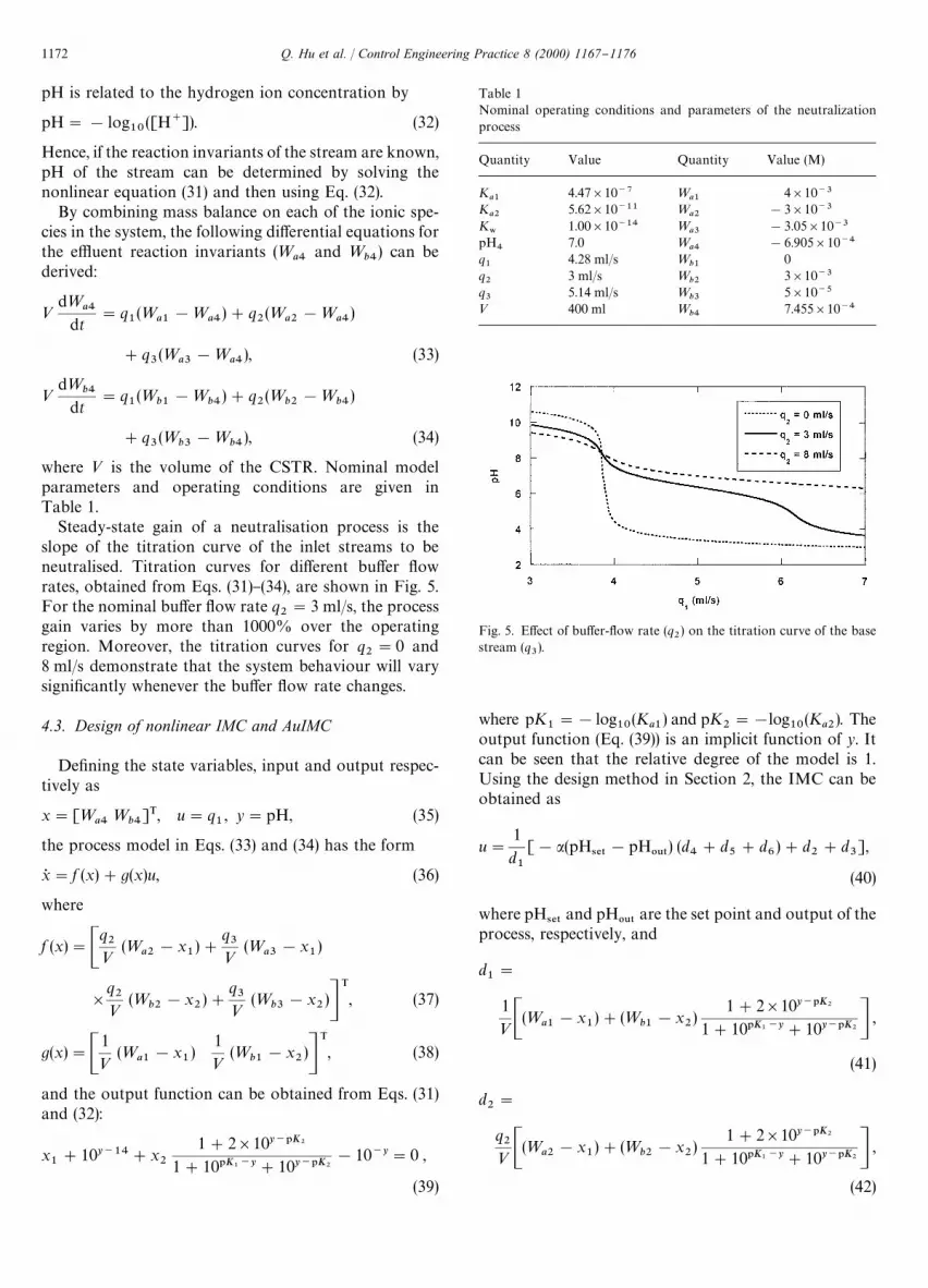
Table 1

Nominal operating conditions and parameters of the neutralization

process

Quantity Value Quantity Value (M)

Ka1

4.47]10~7 =a1

4]10~3

Ka2

5.62]10~11 =a2

!3]10~3

K8

1.00]10~14 =a3

!3.05]10~3

pH4

7.0 =a4

!6.905]10~4

q1

4.28 ml/s =b1

0

q2

3 ml/s =b2

3]10~3

q3

5.14 ml/s =b3

5]10~5

< 400 ml =b4

7.455]10~4

Fig. 5. E!ect of bu!er-#ow rate (q2) on the titration curve of the base

stream (q3).

pH is related to the hydrogen ion concentration by

pH"!log10

([H`]). (32)

Hence, if the reaction invariants of the stream are known,

pH of the stream can be determined by solving the

nonlinear equation (31) and then using Eq. (32).

By combining mass balance on each of the ionic spe-

cies in the system, the following di!erential equations for

the e%uent reaction invariants (=a4

and =b4

) can be

derived:

<d=

a4dt

"q1(=

a1!=

a4)#q

2(=

a2!=

a4)

#q3(=

a3!=

a4), (33)

<d=

b4dt

"q1(=

b1!=

b4)#q

2(=

b2!=

b4)

#q3(=

b3!=

b4), (34)

where < is the volume of the CSTR. Nominal model

parameters and operating conditions are given in

Table 1.

Steady-state gain of a neutralisation process is the

slope of the titration curve of the inlet streams to be

neutralised. Titration curves for di!erent bu!er #ow

rates, obtained from Eqs. (31)}(34), are shown in Fig. 5.

For the nominal bu!er #ow rate q2"3 ml/s, the process

gain varies by more than 1000% over the operating

region. Moreover, the titration curves for q2"0 and

8 ml/s demonstrate that the system behaviour will vary

signi"cantly whenever the bu!er #ow rate changes.

4.3. Design of nonlinear IMC and AuIMC

De"ning the state variables, input and output respec-

tively as

x"[=a4=

b4]T, u"q

1, y"pH, (35)

the process model in Eqs. (33) and (34) has the form

x5 "f (x)#g(x)u, (36)

where

f (x)"Cq2<

(=a2

!x1)#

q3<

(=a3

!x1)

]q2<

(=b2

!x2)#

q3<

(=b3

!x2)D

T, (37)

g(x)"C1

<(=

a1!x

1)

1

<(=

b1!x

2)D

T, (38)

and the output function can be obtained from Eqs. (31)

and (32):

x1#10y~14#x

2

1#2]10y~1K2

1#101K1~y#10y~1K2!10~y"0 ,

(39)

where pK1"!log

10(K

a1) and pK

2"!log

10(K

a2). The

output function (Eq. (39)) is an implicit function of y. It

can be seen that the relative degree of the model is 1.

Using the design method in Section 2, the IMC can be

obtained as

u"1

d1

[!a(pH4%5

!pH065

) (d4#d

5#d

6)#d

2#d

3],

(40)

where pH4%5

and pH065

are the set point and output of the

process, respectively, and

d1"

1

<C(=a1!x

1)#(=

b1!x

2)

1#2]10y~1K2

1#101K1~y#10y~1K2D ,

(41)

d2"

q2< C(=a2

!x1)#(=

b2!x

2)

1#2]10y~1K2

1#101K1~y#10y~1K2D ,

(42)

1172 Q. Hu et al. / Control Engineering Practice 8 (2000) 1167}1176

Fig. 6. Open-loop responses to $20% step change in the acid-#ow

rate (q1).

d3"

q3< C(=a3

!x1)#(=

b3!x

2)

1#2]10y~1K2

1#101K1~y#10y~1K2D ,

(43)

d4"[e(y~14) -/ 10#e~y -/ 10 ] ln 10, (44)

d5"

2x2e(y~1K2 ) -/ 10(1#101K1~y#10y~1K2 ) ln 10

(1#101K1~y#10y~1K2)2, (45)

d6"

x2(1#2]10y~1K2)[e(1K1~y) -/ 10!e(y~1K2 ) -/ 10] ln 10

(1#101K1~y#10y~1K2)2.

(46)

There is only one tuning parameter (a) in the controller

equation (40). Based on the derivation of Section 3, the

control action for the AuIMC is

u"1

d1

[!a(pH4%5

!pH065

!f ) (d4#d

5#d

6)

#d2#d

3], (47)

where

f"K(pH065

!y). (48)

Note that all quantities (except pH065

) in the equations in

this section refer to the model and/or the controller.

4.4. Results and discussion

The open-loop responses to$20% step changes in the

acid #ow are shown in Fig. 6. Although the step changes

are symmetrical, experimental pH responses are highly

asymmetric due to the large variation in the process gain.

The tuning parameter, a was selected as 130

, i.e, the closed-

loop time constant in the nonlinear IMC controller was

selected as 30 s, which is approximately one-half of the

open-loop time constant for the !20% change in the

acid #ow rate (Fig. 6). A smaller closed-loop time con-

stant could result in instability of the IMC system. For

the AuIMC, K"30 (i.e., b1"1) was selected after a few

preliminary trials. Sampling period for control was 1 s

in all cases. The di!erential equations of the model

(Eqs. (33) and (34)) were solved using fourth-order

Runge}Kutta method and a constant step size of 0.1 s.

All programs for data acquisition and control were writ-

ten using C## language.

To ascertain the superior control o!ered by the

AuIMC, tests with PI controller of the form K#(1#1/

¹Is) were also conducted and the corresponding experi-

mental results are presented besides those for the nonlin-

ear IMC (i.e., without augmentation). The PI controller

was tuned to provide stable response for the most severe

disturbance tried, namely, the bu!er #ow rate change

from q2"3 to 0 ml/s. The "nal values of the tuning

parameters are K#"!0.5 ml/s and ¹

I"100 s. The set

point tracking of the PI, IMC and AuIMC controllers is

shown in Fig. 7. The response of PI control to the

set-point change is extremely sluggish. Although both

IMC and AuIMC track the set point change quickly, the

tracking by AuIMC is faster, but it needs a greater

control action. IMC and AuIMC controllers should have

the same performance for set point changes in the ab-

sence of modelling errors and disturbances. In Fig. 7,

since IMC and AuIMC give di!erent performances, this

indicates the discrepancy between the model developed

in Section 4.3 and the real process.

The regulatory performance of PI, IMC and AuIMC

controllers for bu!er #ow rate change from 3 to 8 ml/s as

shown in Fig. 8. The AuIMC is able to reject the distur-

bance very e!ectively. Compared with the PI controller,

IMC gives better regulatory performance. Like the set

point tracking behaviour, the regulatory performance

of the PI controller is very sluggish. Control moves in

Fig. 8 show that AuIMC takes appropriate control ac-

tion quickly. The regulatory performance of the control-

lers for a bu!er #ow rate disturbance from 3 to 0 ml/s is

shown in Fig. 9. This is a di$cult situation to control,

since the process gain is very high. All the three control-

lers are able to control the pH at its set point. As ex-

pected, the nonlinear IMC and AuIMC outperform the

PI controller (Fig. 9), and AuIMC provides better control

than the nonlinear IMC.

Performance of the three controllers for unmeasured

disturbances in the base #ow rate are shown in Figs. 10

and 11. pH responses for a#50% base #ow rate distur-

bance (Fig. 10) demonstrate that AuIMC provides su-

perior control compared to the IMC and PI controller.

Both PI and IMC allow large pH deviations from the set

point and are sluggish. Relative performance of the three

Q. Hu et al. / Control Engineering Practice 8 (2000) 1167}1176 1173

Fig. 7. Performance for a setpoint change from pH"7}9: (a) control-

led variable and (b) manipulated variable.

Fig. 8. Performance for a bu!er #ow rate change from 3 to 8 ml/s: (a)

controlled variable and (b) manipulated variable.

Fig. 9. Performance for a bu!er #ow rate change from 3 to 0 ml/s: (a)

controlled variable and (b) manipulated variable.

Fig. 10. Performance for a #50% base-#ow rate disturbance: (a)

controlled variable and (b) manipulated variable.

1174 Q. Hu et al. / Control Engineering Practice 8 (2000) 1167}1176

Fig. 11. Performance for a !50% base-#ow rate disturbance: (a)

controlled variable and (b) manipulated variable.

Table 2

Control performance in terms of IAE for unmeasured disturbances

Unmeasured disturbance IAE for control by

PI IMC AuIMC

Bu!er #ow change from 3 to 8 ml/s 556 398 103

Bu!er #ow change from 3 to 0 ml/s 109 54 34

Base #ow change by #50% 548 245 138

Base #ow change by !50% 317 175 62

controllers to a !50% acid #ow rate disturbance

(Fig. 11) is similar to that in Fig. 10.

Table 2 shows the control performance in terms of IAE

of the three controllers for the disturbances studied; IAE

was calculated until the "nal times shown in Figs. 8}11.

Since the response by PI has not often reached the "nal

steady state, actual IAE for this controller will be more

than the value in Table 2. Without considering this,

results in Table 2 indicate that IAE for IMC is about

half of that for PI. More importantly, the introduction

of augmentation as in AuIMC reduces IAE by IMC

even further by a factor 1.5 to 3 for unmeasured distur-

bances.

5. Conclusions

An AuIMC structure consisting of a standard IMC

and an additional feedback loop, is described for control

of SISO open-loop stable nonlinear systems. The AuIMC

was experimentally evaluated for control of a neutralisa-

tion process, and its performance was compared with

that of nonlinear IMC and PI controllers. A simple

process model and only the measured pH were used for

developing and implementing the nonlinear IMC and

AuIMC controllers, and no state variables were needed.

Experimental results for several unmeasured distur-

bances show that the nonlinear IMC outperforms the PI

controller and that the performance of AuIMC is signi"-

cantly superior to that of the nonlinear IMC. Reduction

in IAE values due to augmentation in AuIMC for un-

measured disturbances can be 40% or more, and yet

AuIMC requires very few computations in addition to

those for the nonlinear IMC. Apart from equipment

problems, no major di$culties were encountered in the

development and implementation of nonlinear IMC and

AuIMC for the neutralisation process.

References

Bequette, B. W. (1991). Nonlinear control of chemical processes:

A review. Industrial and Engineering Chemistry Research, 30,

1391}1413.

Brown, M. D., Lightbody, G., & Irwin, G. W. (1997). Nonlinear internal

model control using local model networks. IEE Proceedings Control

Theory and Applications, 144, 505}514.

Economou, C. G., Morari, M., & Palsson, B. O. (1986). Internal

model control: 5. Extension to nonlinear systems. Industrial

and Engineering Chemistry Process Design and Development, 25,

403}411.

Garcia, C. E., & Morari, M. (1982). Internal model control * I.

A unifying review and some new results. Industrial and Engineering

Chemistry, Process Design and Development, 21, 308}323.

Gustafsson, T. K., & Waller, K. V. (1983). Dynamic modelling and

reaction invariant control of pH. Chemical Engineering Science, 38,

289}398.

Hall, R. C., & Seborg, D. E. (1989). Modelling and self-tuning control of

a multivariable pH neutralisation process. Part 1: Modelling and

multiloop control. Proceedings of the American control conference,

Pittsburgh (pp. 1822}1827).

Henson, M. A., & Seborg, D. E. (1991). An internal model control

strategy for nonlinear systems. A.I.Ch.E. Journal, 37, 1065}1081.

Hu, Q., & Rangaiah, G. P. (1999a). Adaptive internal model control

of nonlinear processes. Chemical Engineering Science, 54,

1205}1220.

Hu, Q., & Rangaiah, G. P. (1999b). Strategies for enhancing nonlinear

internal model control of pH processes. Journal of Chemical Engin-

eering of Japan, 32, 59}68.

Isidori, A. (1995). Nonlinear control systems (3rd ed.). New York:

Springer.

Kantor, J. C. (1986). Stability of state feedback transformations for

nonlinear systems* some practical considerations. Proceedings of

the American Control Conference, Seattle (pp. 1014}1016).

Kravaris, C., & Kantor, J. C. (1990). Geometric methods for nonlinear

process control: 1. Background, 2. Controller synthesis. Industrial

and Engineering Chemistry Research, 29, 2295}2323.

Q. Hu et al. / Control Engineering Practice 8 (2000) 1167}1176 1175

Kulkarni, B. D., Tambe, S. S., Shukla, N. V., & Deshpande, P. B. (1991).

Nonlinear pH control. Chemistry and Engineering Science, 46, 995}1003.

Morari, M., & Za"riou, E. (1989). Robust process control. Englewood

Cli!s, NJ: Prentice-Hall.

Patwardhan, S. C., & Madhavan, K. P. (1998). Nonlinear internal

model control using quadratic perturbation models. Computers in

Chemical Engineering, 22, 587}601.

Sastry, S. S., & Isidori, A. (1989). Adaptive control of linearizable

systems. IEEE Transactions on Automatic Control, 34, 1123}1131.

Shukla, N. V., Deshpande, P. B., Ravi Kumar, V., & Kulkarni, B. D.

(1993). Enhancing the robustness of internal-model-based nonlinear

pH controller. Chemical Engineering Science, 48, 913}920.

Wu, W. T., Hwang, Z. P., & Chuang, I. H. (1996). Experimental

investigation of a robust control system based on the EMC struc-

ture. Journal of Processing Control, 6, 157}160.

Zhu, H. A., Hong, G. S., Teo, C. L., & Poo, A. N. (1995). Internal model

control with enhanced robustness. International Journal of Systems

Science, 26, 277}293.

1176 Q. Hu et al. / Control Engineering Practice 8 (2000) 1167}1176