Ex-ante and Ex-post Subcontracting

in Highway Procurement Markets

Jorge Balat∗ Tatiana Komarova† Elena Krasnokutskaya‡

July 25, 2017

Preliminary and Incomplete. Do not circulate.

Abstract

This paper provides a novel evidence (based on a new dataset) on bidding and subcon-tracting behavior of primary contractors participating in California highway procurementmarket. We develop a model of procurement auction with subcontracting stage which iscapable of rationalizing the patterns documented in the data. Next, we use this frameworkto assess the implications of ex-ante subcontracting rule which is frequently imposed ingovernment procurement.

Keywords: highway procurement, subcontracting

JEL Classification: C73, C63, D44, H57, L20

∗University of Texas, Department of Economics. Email: jorge.balat@jhu.edu†London School of Economics. Email: T.Komarova@lse.ac.uk‡Johns Hopkins University, Department of Economics. Email: ekrasno1@jhu.edu

1

1 Introduction

Many infrastructure procurement markets have a two-tier structure with contractors routinely

subcontracting parts of the projects they win in the primary auctions. This feature, however,

remains relatively understudied in the literature. In this paper we present novel evidence on

bidding and subcontracting activity in a large procurement market (California highway procure-

ment market). We then construct a model consistent with the patterns documented in the data

and use this model to study implications of ex-ante subcontracting requirement maintained in

most government procurement markets in US.

The analysis in this paper is based on a new dataset which provides detailed information about

bidding and subcontracting activity of individual contractors for a large number of projects auc-

tioned in California highway procurement market. Specifically, for each project (represented as a

list of items compiled by CalTrans engineers) and for each participating contractor, we observe

the list of items this contractor subcontracts, with the names of associated subcontractors,and

the itemized list of subcontractors’ prices.

The data analysis reveals that subcontracting is very prevalent in this market. Indeed, 95%

of participating contractors subcontract at least one item on an average project. Interestingly,

for most tasks contractors tend to subcontract items associated with this task on a fraction of

projects. This indicates that subcontracting decisions do not reflect firms’ capability to perform

a given task. Instead, contractors are likely to use subcontracting in order to modify their costs

and improve their competitiveness in a given auction. Therefore, subcontracting decisions are

likely to be influenced by the contractors’ own cost of performing the task as well as competitive

conditions in the primary and subcontracting markets.

Further, we document that contractors competing for a given project frequently employ over-

lapping sets of subcontractors. In addition, while own subcontracting decision is not predictive

of the own bid level (presumably contractor may subcontract because his own cost of complet-

ing the task is high or because he has been offered a low subcontracting price), the fact that

two contractors share the same subcontractor is associated with lower bids submitted by these

contractors. This indicates that subcontractors compete for the right to be listed on contractors’

bids. On the other hand, contractors bidding on the same project frequently hire different sub-

contractors, and the prices charged by a subcontractor tend to differ across contractors within the

same project. This leads us to conclude that factors other than price must influence contractors’

choice of subcontractors and that these factors have to be contractor-subcontractor-specific.

We use the patterns documented in the descriptive analysis to guide our modeling choices.

2

Specifically, we develop a model of procurement auction with subcontracting which consists of

two stages. In accordance with the rules of government procurement, in the first stage contractors

develop a plan of how the work would be completed should they win the project. During this

stage they run a subcontracting auction for each task listed on the project and on the basis

of subcontractors’ quotes decide whether the task should be subcontracted and to whom. In

the second stage, contractors submit their bids and the winner is determined. In accordance

with the findings described in the previous paragraph, we assume that contractors rely on a

discriminatory subcontracting auctions where they may engage a preferred subcontractor even

if his price exceeds the lowest quote (but not more than by a certain margin). A contractor may

give such a preference to subcontractor because of previous interaction, or due to reputation

for quality – contractors may differ in their preference for quality which leads to contractor-

subcontractor-specific preferences. There are, of course, other mechanism that may rationalize

the patterns observed in the data. For example, subcontractor may have different costs for

working with different contractors. While this is possible, such mechanism is not very appealing

since, independent of who wins the main contract, subcontractor, if listed on the winning bid,

will be facing the same scope of work. Further, the model where subcontractor’s costs differences

associated with various contractors are private is intractable; whereas the model where these

differences are public predicts behavior which is similar to the one implied by our model.

The model we consider in this paper differs from a standard model of procurement auction

along several dimensions. First, participating contractors have an opportunity to modify their

costs and thus improve their competitiveness in a given auction. Further, an access to subcon-

tracting market gives contractors’ an opportunity to acquire valuable information about rivals’

costs. Second, subcontractors have to interact with multiple contractors. Given the differences in

contractors’ preferences and possibly costs, subcontractors use different pricing strategies with

different contractors. Nevertheless, the prices submitted by a given subcontractor to different

contractors are related since they are based on the same underlying realization of subcontrac-

tor’s costs. In this game subcontractors internalize the fact that wining an engagement with a

contractor results in them working on the project only with some probability. They also recog-

nize that their price quotes are influencing the probabilities of primary contractors winning the

project.

From the equilibrium characterization point of view, this model presents a number of chal-

lenges. First, the subcontractors’ pricing strategies have to account for simultaneity of subcon-

tracting auctions as well as to take into account the dynamic consequences of subcontractors’

3

pricing decisions on allocation in the second stage. Discriminatory feature incorporated in sub-

contracting stage complicates subcontractors’ incentives at the high cost realizations since at

high cost levels a subcontractor may prefer to target only the auctions where he has an advan-

tage (due to contractor’s preference) rather than attempting to win a higher overall number of

auctions. We believe that analysis of this feature is novel and constitutes a separate contribution

of the paper.

Finally, we use this framework to assess the impact of the ex-ante subcontracting rule. We

note that ex-ante subcontracting eliminates part of the inherent uncertainty about rivals’ costs

since just obtaining subcontractors’ quotes enables contractors to narrow down their assessment

of competitors’ costs which induces contractors to behave more aggressively. This is in contrast to

the ex-post markets where the possibility of future subcontracting activity introduces additional

common uncertainty which in turn promotes less aggressive behavior on the part of bidders.

On the other hand, under ex-ante subcontracting rule, subcontracting prices are determined at

the bidder rather than the winner level which diffuses risk of loosing from the subcontractors’

point of view and thus allows them to behave less aggressively. The balance of these two effects

determines the impact of ex-ante subcontracting rule.

Literature review. [ INCOMPLETE ] Wambach (2009), Jeziorski and Krasnokutskaya

(2014), Bajari, Houghton, and Tadelis (2014), Gil and Marion (2012), Marion (2013), Miller

(2014), Moretti and Valbonesi (2012), Branzoli and Decarolis (2014), Haile (2001).

The structure of the paper is as follows. In Section 2 we summarize the highway procure-

ment process in California. Section 3 describes construction of the data set and characterizes

subcontracting patterns reflected in the data. Section 4 describes a simple procurement auction

model with ex-ante subcontracting stage which is capable of rationalizing patterns documented

in the previous section. In Section 5 we discuss the identification and estimation of the structural

model.

2 Procurement Process

We study the market for highway procurement in the state of California which is supervised by

California Department of Transportation (CalTrans). The projects transacted in this market deal

with highway repairs, highway construction and associated work such as signing, striping and

landscaping. These projects are allocated through a first-price sealed bid auction mechanism.

Procurement process proceeds through the following stages. First, the project is announced.

4

At this point only a short description of work with the time and location details is provided.

The interested contractors may request a detailed project description compiled by government

engineers which lists all the items included in the project with the engineer’s estimate of the size

and the cost of each item. The list of tasks is fixed for the purpose of auction. Each contractor

has to summarize his bid in the form which states the price for each item on this list. Second,

contractors work on the plan for project completion, finding out their costs broken down by

item. During this time contractors are approached by subcontractors who quote their prices for

the items they are qualified to perform. CalTrans requires that all the details of project imple-

mentation including subcontracting agreements have to be settled before the bid is submitted.

The finalized plan of work (who does what and at what price) has to be reflected in the bid doc-

uments. Third, at the previously announced date submitted bid documents are opened and the

winner is determined on the basis of the total bid which is equal to the sum of the item-specific

prices.

The subcontracting of work is strictly regulated. Specifically, the government imposes an

upper bound of 40% of the project value for the amount that contractor is allowed to subcontract.

The subcontractors have to be certified to do work for the government. Further, CalTrans pays

subcontractors directly to ensure that they recieve their pay on time and possibly to enforce the

rule that the subcontractor listed on the bid documents is the one who does the work.

3 Data

3.1 Data Construction

We have assembled a novel dataset which allows us to gain insights into the subcontracting

activities in the California highway procurement market. Existing empirical research on high-

way procurement traditionally relies on the data collected from bid summaries which include

the names and the bids of all participating contractors as well as engineers estimate, contract

duration, location and the type of work.1 In contrast, our data set is constructed on the basis

of the full bid documents which for each project contain the list of items involved, the item-

specific bids for each participating contractor, and, for each participating contractor, the list of

1See, for example, Hong and Shum (2002), Porter and Zona (1993), Jofre-Bonet and Pesendorfer (2003),Krasnokutskaya (2011), etc. More recently, the researchers also used information on the identities of contractorswho purchased bid documents for a specific project and thus seriously contemplated submitting a bid in acorresponding auction (see, for example, Krasnokutskaya and Seim (2011) and Balat (2014)); as well as moredetailed information on the list of tasks involved, negotiated bid adjustments subsequent to the auction, and thedetails of the project supervision (as in Bajari, Houghton, and Tadelis (2014), Bajari and Lewis (2011)).

5

the subcontractors this firm plans to use and the items each subcontractor is hired to perform.

We assembled this information for all the projects auctioned by CalTrans between January 2002

and December 2016.

In constructing this dataset we had to overcome several challenges. First, we had to match

subcontractors to the items and thus the prices they were promised in connection with a given

project. Specifically, subcontractors’ assignments in the bid documents are occasionally described

verbally (instead of referring to the item number) and the verbal description was not always

identical to the description used in the official CalTrans list of items. In order to reconcile the

two pieces of data we designed and implemented a word recognition algorithm. The final dataset

includes only the projects for which we were able to match the subcontracting assignments

for all items and for all contractors with high degree of confidence. The matching algorithm is

applied mostly to the earlier years in our data. In the later years (after 2010) contractors mostly

provided item numbers rather than verbal descriptions to summarize the scope of subcontractors’

assignments. This feature additionally allowed us to verify performance of the matching algorithm

by checking that the subcontractors’ areas of specialization as inferred from the data do not

change over the years, and that the patterns of behavior documented on the basis of the whole

dataset are similar to those documented from the more recent data.

The next issue we had to tackle was related to the fact that the number of distinct items

recorded in our dataset is very large. This does not allow us to study patterns in subcontracting

activity with any degree of statistical confidence. We used the state-issued document summa-

rizing the state-approved cost for each item to aggregate items into larger classes (tasks). This

document effectively lists every item which appeared on the bid documents in the previous ten

years. The items are arranged by specialization and each item is assigned a six digit number.

We aggregated these items into groups (tasks) such that all items associated with the same task

share the first two digits in the number assigned to the item by CalTrans.

Focusing on the projects associated with road or bridge work, we identified 13 distinct tasks

(types of work) which appear in our data. We performed various checks to verify that such

grouping indeed makes sense. For example, we find that for any two items which appear on the

same bid document, and which belong to the same task according to our grouping, the probability

that both tasks are subcontracted (by the same contractor) if one of them is subcontracted is

89%. This number is only slightly lower from the one which obtains when the groups of tasks

are formed on the basis of the first three digits of the task numbers (93%).

We use this final dataset where the bid information is arranged by project, by contractor

6

within project, and by item for each contractor and project, and where items are further charac-

terized by the type of work defined as explained above to study patterns in the subcontracting

behavior. We summarize our finding in the next section.

3.2 Descriptive Data Analysis

In this section we provide a number of statistics summarizing the data in general and the

subcontracting activity reflected in the data specifically.

3.2.1 General Summary Statistics

Table 1 provides general summary statistics. It indicates that the projects vary in size quite sub-

stantially: from $190, 000 on a lower end to $10, 670, 000 on the upper end of the size distribution

with the median project’s value equal to $700, 000. Projects further differ in the allowed duration

which ranges from one to eight months with the median duration equal to 50 days. Engineering

description breaks the project into items with the number of items ranging from 14 to 57 and

the median number of items given by 22. Our algorithm for aggregating items into tasks which is

described above indicates that the project on average consists of four tasks (the average number

of tasks is 3.77 and the median number is 4). Also, an auction on average attracts 5 bidders (the

median number of bidders is 4 with smaller projects attracting higher number of participants).

The table further reports statistics traditionally considered in auction markets. The variable

“money-left-on-the table” is constructed as the difference between the lowest and second lowest

bid divided by the lowest bid: (rank2−rank1)rank1

. It reflects the level of uncertainty about contractors’

costs or informational asymmetries in the market. In our data, the second lowest bid is on average

9% higher than the winning bid. This is comparable to other datasets used to study highway

procurement market. Information asymmetries can also be seen from the relative difference of the

winning bid to the engineer’s estimate. The winning bid is on average 7% below the engineer’s

estimate.

3.2.2 Subcontracting Activity

Table 2 summarizes subcontracting activity recorded in our data. The table indicates that sub-

contracting is very prevalent in this market. Indeed, if we consider an indicator variable which

7

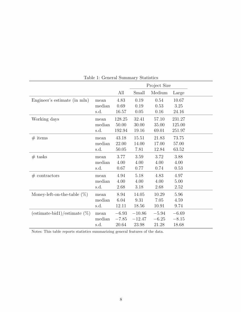
Table 1: General Summary Statistics

Project Size

All Small Medium Large

Engineer’s estimate (in mln) mean 4.83 0.19 0.54 10.67median 0.69 0.19 0.53 3.25s.d. 16.57 0.05 0.16 24.16

Working days mean 128.25 32.41 57.10 231.27median 50.00 30.00 35.00 125.00s.d. 192.94 19.16 69.01 251.97

# items mean 43.18 15.51 21.83 73.75median 22.00 14.00 17.00 57.00s.d. 50.05 7.81 12.84 63.52

# tasks mean 3.77 3.59 3.72 3.88median 4.00 4.00 4.00 4.00s.d. 0.67 0.77 0.74 0.53

# contractors mean 4.94 5.18 4.83 4.97median 4.00 4.00 4.00 5.00s.d. 2.68 3.18 2.68 2.52

Money-left-on-the-table (%) mean 8.94 14.05 10.29 5.96median 6.04 9.31 7.05 4.59s.d. 12.11 18.56 10.91 9.74

(estimate-bid1)/estimate (%) mean −6.93 −10.86 −5.94 −6.69median −7.85 −12.47 −6.25 −8.15s.d. 20.64 23.98 21.28 18.68

Notes: This table reports statistics summarizing general features of the data.

8

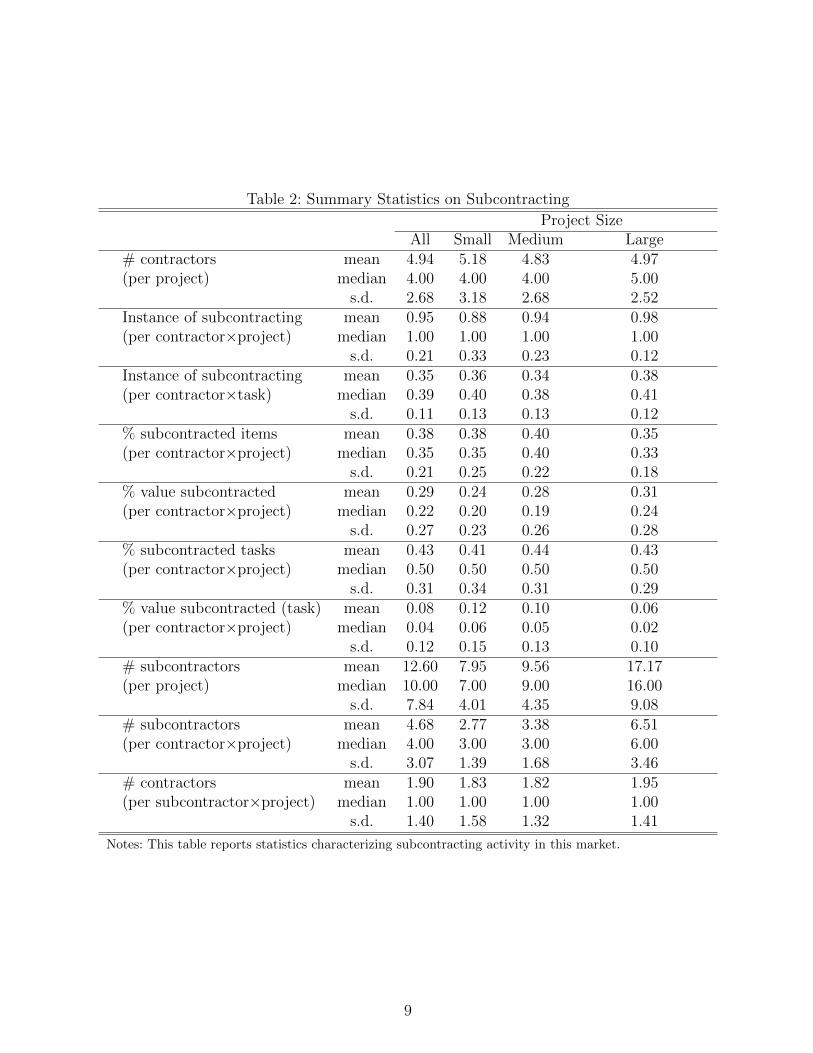
Table 2: Summary Statistics on Subcontracting

Project SizeAll Small Medium Large

# contractors mean 4.94 5.18 4.83 4.97(per project) median 4.00 4.00 4.00 5.00

s.d. 2.68 3.18 2.68 2.52Instance of subcontracting mean 0.95 0.88 0.94 0.98(per contractor×project) median 1.00 1.00 1.00 1.00

s.d. 0.21 0.33 0.23 0.12Instance of subcontracting mean 0.35 0.36 0.34 0.38(per contractor×task) median 0.39 0.40 0.38 0.41

s.d. 0.11 0.13 0.13 0.12% subcontracted items mean 0.38 0.38 0.40 0.35(per contractor×project) median 0.35 0.35 0.40 0.33

s.d. 0.21 0.25 0.22 0.18% value subcontracted mean 0.29 0.24 0.28 0.31(per contractor×project) median 0.22 0.20 0.19 0.24

s.d. 0.27 0.23 0.26 0.28% subcontracted tasks mean 0.43 0.41 0.44 0.43(per contractor×project) median 0.50 0.50 0.50 0.50

s.d. 0.31 0.34 0.31 0.29% value subcontracted (task) mean 0.08 0.12 0.10 0.06(per contractor×project) median 0.04 0.06 0.05 0.02

s.d. 0.12 0.15 0.13 0.10# subcontractors mean 12.60 7.95 9.56 17.17(per project) median 10.00 7.00 9.00 16.00

s.d. 7.84 4.01 4.35 9.08# subcontractors mean 4.68 2.77 3.38 6.51(per contractor×project) median 4.00 3.00 3.00 6.00

s.d. 3.07 1.39 1.68 3.46# contractors mean 1.90 1.83 1.82 1.95(per subcontractor×project) median 1.00 1.00 1.00 1.00

s.d. 1.40 1.58 1.32 1.41

Notes: This table reports statistics characterizing subcontracting activity in this market.

9

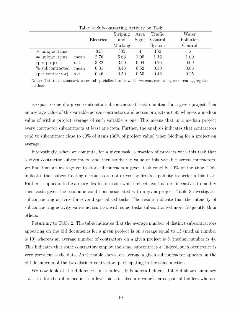
Table 3: Subcontracting Activity by Task

Striping Area Traffic WaterElectrical and Signs Control Pollution

Marking System Control# unique items 813 335 4 130 6# unique items mean 2.76 6.63 1.00 1.16 1.00(per project) s.d. 3.82 3.90 0.04 0.76 0.09% subcontracted mean 0.31 0.48 0.52 0.30 0.06(per contractor) s.d. 0.46 0.50 0.50 0.46 0.25

Notes: This table summarizes several specialized tasks which we construct using our item aggregationmethod.

is equal to one if a given contractor subcontracts at least one item for a given project then

an average value of this variable across contractors and across projects is 0.95 whereas a median

value of within project average of such variable is one. This means that in a median project

every contractor subcontracts at least one item. Further, the analysis indicates that contractors

tend to subcontract close to 40% of items (30% of project value) when bidding for a project on

average.

Interestingly, when we compute, for a given task, a fraction of projects with this task that

a given contractor subcontracts, and then study the value of this variable across contractors,

we find that an average contractor subcontracts a given task roughly 40% of the time. This

indicates that subcontracting decisions are not driven by firm’s capability to perform this task.

Rather, it appears to be a more flexible decision which reflects contractors’ incentives to modify

their costs given the economic conditions associated with a given project. Table 3 investigates

subcontracting activity for several specialized tasks. The results indicate that the intencity of

subcontracting activity varies across task with some tasks subcontracted more frequently than

others.

Returning to Table 2. The table indicates that the average number of distinct subcontractors

appearing on the bid documents for a given project is on average equal to 13 (median number

is 10) whereas an average number of contractors on a given project is 5 (median number is 4).

This indicates that some contractors employ the same subcontractor. Indeed, such occurrence is

very prevalent is the data. As the table shows, on average a given subcontractor appears on the

bid documents of the two distinct contractors participating in the same auction.

We now look at the differences in item-level bids across bidders. Table 4 shows summary

statistics for the difference in item-level bids (in absolute value) across pair of bidders who are

10

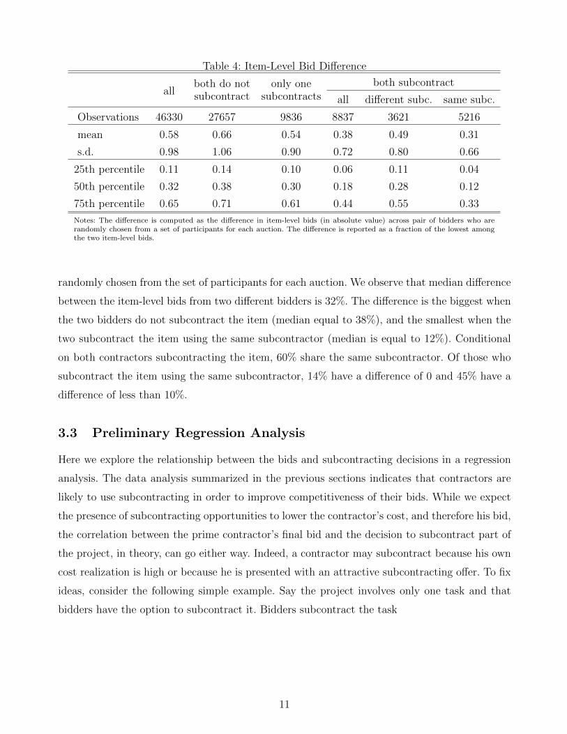
Table 4: Item-Level Bid Difference

both do not only one both subcontractall subcontract subcontracts all different subc. same subc.

Observations 46330 27657 9836 8837 3621 5216

mean 0.58 0.66 0.54 0.38 0.49 0.31

s.d. 0.98 1.06 0.90 0.72 0.80 0.66

25th percentile 0.11 0.14 0.10 0.06 0.11 0.04

50th percentile 0.32 0.38 0.30 0.18 0.28 0.12

75th percentile 0.65 0.71 0.61 0.44 0.55 0.33

Notes: The difference is computed as the difference in item-level bids (in absolute value) across pair of bidders who arerandomly chosen from a set of participants for each auction. The difference is reported as a fraction of the lowest amongthe two item-level bids.

randomly chosen from the set of participants for each auction. We observe that median difference

between the item-level bids from two different bidders is 32%. The difference is the biggest when

the two bidders do not subcontract the item (median equal to 38%), and the smallest when the

two subcontract the item using the same subcontractor (median is equal to 12%). Conditional

on both contractors subcontracting the item, 60% share the same subcontractor. Of those who

subcontract the item using the same subcontractor, 14% have a difference of 0 and 45% have a

difference of less than 10%.

3.3 Preliminary Regression Analysis

Here we explore the relationship between the bids and subcontracting decisions in a regression

analysis. The data analysis summarized in the previous sections indicates that contractors are

likely to use subcontracting in order to improve competitiveness of their bids. While we expect

the presence of subcontracting opportunities to lower the contractor’s cost, and therefore his bid,

the correlation between the prime contractor’s final bid and the decision to subcontract part of

the project, in theory, can go either way. Indeed, a contractor may subcontract because his own

cost realization is high or because he is presented with an attractive subcontracting offer. To fix

ideas, consider the following simple example. Say the project involves only one task and that

bidders have the option to subcontract it. Bidders subcontract the task

11

Tab

le5:

Bid

san

dSub

contr

acti

ng

(1)

(2)

(3)

(4)

(5)

(6)

(7)

(8)

(9)

con

stant

1.09

8***

1.11

0***

1.10

1***

1.17

5***

1.19

1***

1.18

0***

1.27

4***

1.27

7***

1.26

4***

(0.0

15)

(0.0

12)

(0.0

15)

(0.0

28)

(0.0

26)

(0.0

28)

(0.1

23)

(0.1

22)

(0.1

23)

eng.

esti

mat

e0.

189

0.16

70.

178

−0.0

11−

0.04

7−

0.0

40(0.4

73)

(0.4

72)

(0.4

72)

(0.5

01)

(0.5

00)

(0.5

00)

day

s0.

148*

**0.

141*

**0.

144*

**0.

189*

*0.

195*

**0.

196*

**(0.0

54)

(0.0

54)

(0.0

54)

(0.0

75)

(0.0

75)

(0.0

75)

nu

m.

item

s−

0.0

01**

−0.0

01*

−0.0

01*

−0.0

01−

0.00

0−

0.0

01(0.0

00)

(0.0

00)

(0.0

00)

(0.0

00)

(0.0

00)

(0.0

00)

nu

m.

bid

der

s−

0.0

15**

*−

0.01

6***−

0.0

16**

*−

0.0

12**

*−

0.01

3***−

0.01

3***

(0.0

04)

(0.0

04)

(0.0

04)

(0.0

04)

(0.0

04)

(0.0

04)

%va

lue

sub

contr

act

ed0.0

01

0.0

490.

001

0.05

10.

000

0.04

4(0.0

44)

(0.0

49)

(0.0

44)

(0.0

49)

(0.0

44)

(0.0

49)

%va

lue

sam

esu

bco

ntr

act

or

−0.1

57*−

0.19

9**

−0.1

70**

−0.

211*

*−

0.15

8*−

0.1

93**

(0.0

82)

(0.0

92)

(0.0

82)

(0.0

92)

(0.0

83)

(0.0

92)

tim

eF

En

on

on

on

on

on

oye

sye

syes

regio

nF

En

on

ono

no

no

no

yes

yes

yes

wor

kty

pe

FE

no

no

no

no

no

no

yes

yes

yes

ob

serv

atio

ns

1160

1160

1160

1160

1160

1160

1160

1160

1160

Note

s:T

he

dep

end

ent

vari

ab

leis

the

norm

alize

db

id:

bid

/es

tim

ate

.S

tan

dard

erro

rsin

pare

nth

esis

.***,

**,

*d

enote

sign

ifica

nce

at

the

1%

,5%

an

d10%

level

.

12

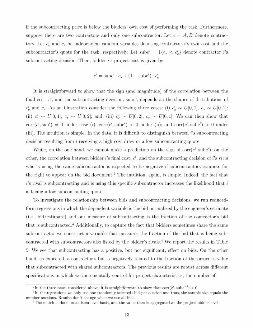
if the subcontracting price is below the bidders’ own cost of performing the task. Furthermore,

suppose there are two contractors and only one subcontractor. Let i = A,B denote contrac-

tors. Let cic and cs be independent random variables denoting contractor i’s own cost and the

subcontractor’s quote for the task, respectively. Let subci = 1{cs < cic} denote contractor i’s

subcontracting decision. Then, bidder i’s project cost is given by

ci = subci · cs + (1− subci) · cic.

It is straightforward to show that the sign (and magnitude) of the correlation between the

final cost, ci, and the subcontracting decision, subci, depends on the shapes of distributions of

cic and cs. As an illustration consider the following three cases: (i) cic ∼ U [0, 1], cs ∼ U [0, 1];

(ii) cic ∼ U [0, 1], cs ∼ U [0, 2]; and, (iii) cic ∼ U [0, 2], cs ∼ U [0, 1]. We can then show that

corr(ci, subi) = 0 under case (i); corr(ci, subci) < 0 under (ii); and corr(ci, subci) > 0 under

(iii). The intuition is simple. In the data, it is difficult to distinguish between i’s subcontracting

decision resulting from i receiving a high cost draw or a low subcontracting quote.

While, on the one hand, we cannot make a prediction on the sign of corr(ci, subci), on the

other, the correlation between bidder i’s final cost, ci, and the subcontracting decision of i’s rival

who is using the same subcontractor is expected to be negative if subcontractors compete for

the right to appear on the bid document.2 The intuition, again, is simple. Indeed, the fact that

i’s rival is subcontracting and is using this specific subcontractor increases the likelihood that i

is facing a low subcontracting quote.

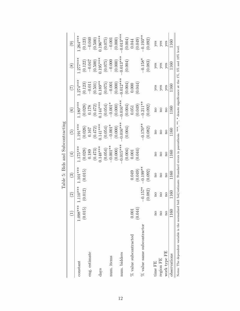
To investigate the relationship between bids and subcontracting decisions, we run reduced-

form regressions in which the dependent variable is the bid normalized by the engineer’s estimate

(i.e., bid/estimate) and our measure of subcontracting is the fraction of the contractor’s bid

that is subcontracted.3 Additionally, to capture the fact that bidders sometimes share the same

subcontractor we construct a variable that measures the fraction of the bid that is being sub-

contracted with subcontractors also listed by the bidder’s rivals.4 We report the results in Table

5. We see that subcontracting has a positive, but not significant, effect on bids. On the other

hand, as expected, a contractor’s bid is negatively related to the fraction of the project’s value

that subcontracted with shared subcontractors. The previous results are robust across different

specifications in which we incrementally control for project characteristics, the number of

2In the three cases considered above, it is straightforward to show that corr(ci, subc−i) < 0.3In the regressions we only use one (randomly selected) bid per auction and thus, the sample size equals the

number auctions. Results don’t change when we use all bids.4The match is done on an item-level basis, and the value then is aggregated at the project-bidder level.

13

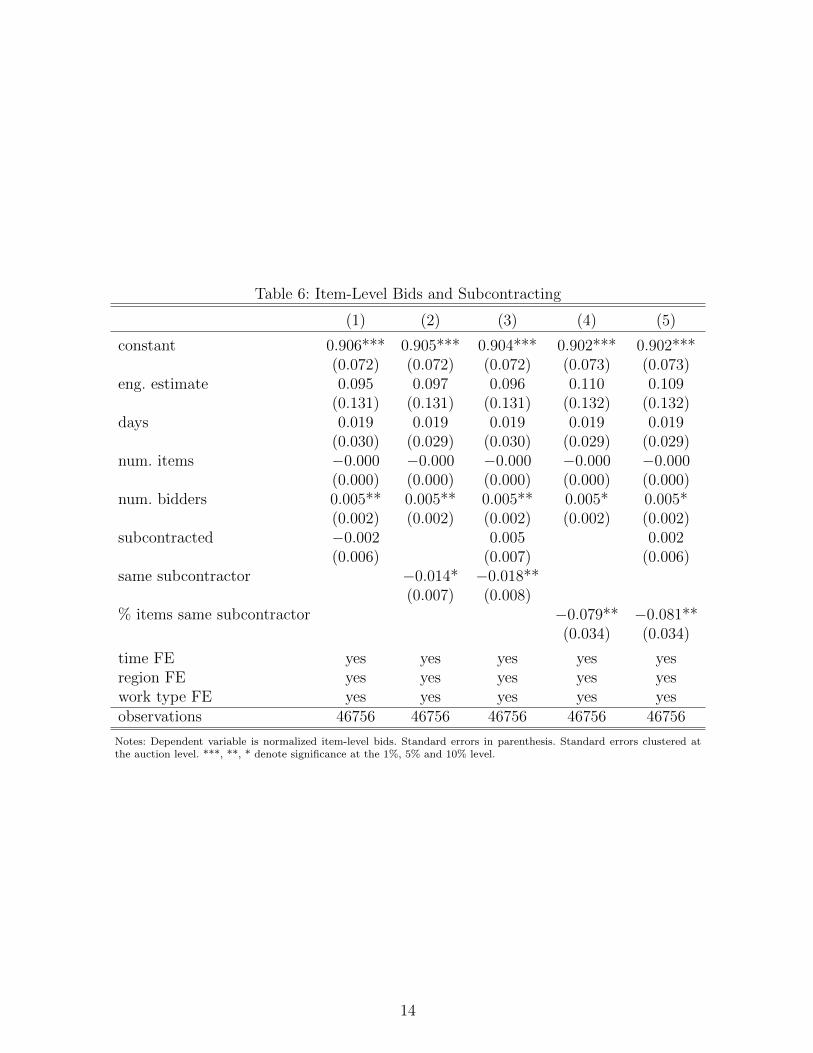
Table 6: Item-Level Bids and Subcontracting

(1) (2) (3) (4) (5)

constant 0.906*** 0.905*** 0.904*** 0.902*** 0.902***(0.072) (0.072) (0.072) (0.073) (0.073)

eng. estimate 0.095 0.097 0.096 0.110 0.109(0.131) (0.131) (0.131) (0.132) (0.132)

days 0.019 0.019 0.019 0.019 0.019(0.030) (0.029) (0.030) (0.029) (0.029)

num. items −0.000 −0.000 −0.000 −0.000 −0.000(0.000) (0.000) (0.000) (0.000) (0.000)

num. bidders 0.005** 0.005** 0.005** 0.005* 0.005*(0.002) (0.002) (0.002) (0.002) (0.002)

subcontracted −0.002 0.005 0.002(0.006) (0.007) (0.006)

same subcontractor −0.014* −0.018**(0.007) (0.008)

% items same subcontractor −0.079** −0.081**(0.034) (0.034)

time FE yes yes yes yes yesregion FE yes yes yes yes yeswork type FE yes yes yes yes yesobservations 46756 46756 46756 46756 46756

Notes: Dependent variable is normalized item-level bids. Standard errors in parenthesis. Standard errors clustered atthe auction level. ***, **, * denote significance at the 1%, 5% and 10% level.

14

bidders, and time, region, and work type fixed effects.

We also explore the relationship between bids and subcontracting decisions at a item level.

The results are shown in Table 6. The left-hand-side variable is the item-level normalized bid,

where the normalization is done on an item-by-item basis. The variable ‘subcontracted’ is a

dummy variable that equals 1 if the contractor has chosen to subcontract the item. To capture

common subcontractors across bidders we use a dummy variable that equals 1 if there is another

bidder in the auction that is listing the same subcontractor for the same item. Alternatively, we

also use the fraction of items for which the bidder lists a subcontractor also listed by his rivals.

In all the regressions we cluster the standard errors at the auction-bidder level. Similarly to what

we found in the previous regressions, there is no effect of the bidder’s choice to subcontract an

item on the submitted bid for that item; but when the subcontractor is also listed by one of

the contractor’s rivals, we find that the effect is negative and significant, as expected. We find

similar results if we instead use the fraction of items that feature a common subcontractor.

3.4 Summary and Modeling Implications

The descriptive analysis summarized above highlights several patterns which guide our modeling

of subcontracting process in this market. Specifically, on the basis of this analysis we conclude

that

1. For each task, contractors choose to subcontract or not on the project-by-project basis.

The decision most likely depends on contractor’s own cost of performing the task in house

as well as economic conditions associated with a given project and a subcontracting market

for a given task.

2. Subcontractors compete for the opportunity to work with a given contractor (this is in-

dicated by regression analysis). We therefore model subcontracting stage as a secondary

auction run by each contractor and for each task. At this stage we abstract away from

subcontractors’ participation decisions and assume that all subcontractors qualified for a

given task (available during the time of project for which project is scheduled) participate

in all subcontracting auctions for this task.

3. The subcontracting decisions are not based on straightforward comparison of price quotes

such as we would see in the first price auction. It they were, we would observe (a) the same

subcontractor being employed by all subcontracting contractors. Also, we would tend to

see (b) the same subcontractor charging the same price to different contractors (for this

15

we would also need main contractors to be symmetric in their cost distributions). The

regularities (a) and (b) do not hold in the data. Different prices could potentially be ratio-

nalized by asymmetries between primary contractors. However, even in this case the same

contractor would be engaged by all subcontracting contractors. Notice that this regularity

cannot be driven by subcontractor’s capacity constraints since only one contractor will

eventually win the project. To account for this regularity we model subcontracting auction

as an auction with preferential treatment where primary contractor may accept a bid which

is higher by a certain margin than the lowest bid in the subcontracting auction if this bid

is submitted by a preferred subcontractor (more details on this are provided in the model

section). Such a preference may be given if a subcontractor has better reputation or if con-

tractor has previous experience of working with this subcontractor. Of course, the features

we observe in the data could be rationalized in a different way. For example, it is possible

that the subcontractor’s cost for the task differs across contractors. However, if the model

where contractor-subcontractor differences in costs are private information is intractable

whereas the model where such differences are commonly known is equivalent to our setting.

We therefore believe that our approach represent a reasonable first approximation of this

environment.

4 Auction Model with Subcontracting

In this section we present a first-price (procurement) auction model in which bidders are allowed

to subcontract part of the project. We analyze both the optimal bidding strategies for contractors

in the primary market, and the optimal pricing strategies for subcontractors in the secondary

market. The auction consists of two stages. In the first stage the contractors draw their costs for

task one and simultaneously hold subcontracting auctions for task two. At the end of this stage

contractors’ costs are realized. Then in stage two contractors construct their bids, submit them

to auctioneer and the winner of the primary auction is determined. Notice that here we maintain

the rule imposed in most US government procurement auctions that the subcontracting decisions

have to finalized prior to the main auction.

The interrelationship between the primary and subcontracting markets adds several key fea-

tures that differentiate our model from a standard first-price auction model. On the one hand,

subcontractors: (i) internalize the fact that their quotes affect the contractors’ likelihood of win-

ning the project; and (ii) take into account that winning an engagement with a given contractor

16

does not necessary result in them working on the project. On the other hand, primary con-

tractors: (i) use subcontracting to modify their costs realizations, and (ii) take into account the

information about rivals’ costs contained in subcontractors’ prices.

We begin with a simplified setting (two tasks, two main contractors, two subcontractors) in

order to highlight the new issues introduced by allowing for subcontracting. The simple model

can be generalized in a straightforward way to allow for the number of tasks, the number of

primary contractors and/or the number of subcontractors to be greater than two.

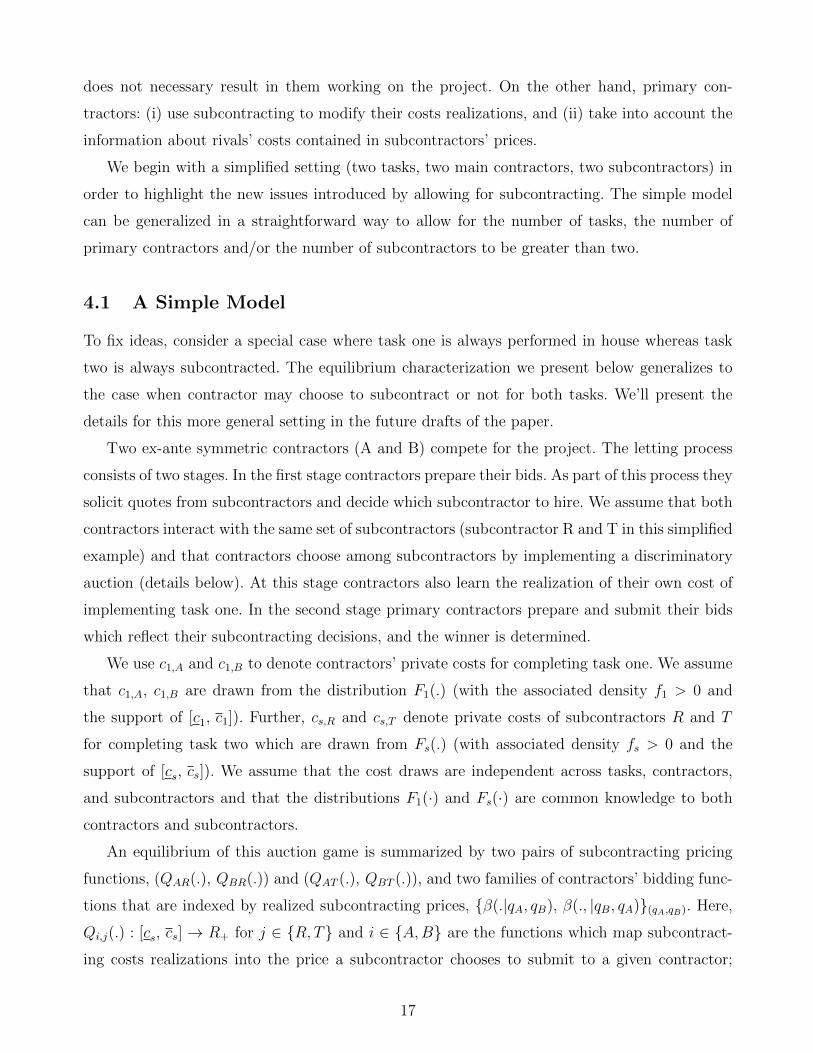
4.1 A Simple Model

To fix ideas, consider a special case where task one is always performed in house whereas task

two is always subcontracted. The equilibrium characterization we present below generalizes to

the case when contractor may choose to subcontract or not for both tasks. We’ll present the

details for this more general setting in the future drafts of the paper.

Two ex-ante symmetric contractors (A and B) compete for the project. The letting process

consists of two stages. In the first stage contractors prepare their bids. As part of this process they

solicit quotes from subcontractors and decide which subcontractor to hire. We assume that both

contractors interact with the same set of subcontractors (subcontractor R and T in this simplified

example) and that contractors choose among subcontractors by implementing a discriminatory

auction (details below). At this stage contractors also learn the realization of their own cost of

implementing task one. In the second stage primary contractors prepare and submit their bids

which reflect their subcontracting decisions, and the winner is determined.

We use c1,A and c1,B to denote contractors’ private costs for completing task one. We assume

that c1,A, c1,B are drawn from the distribution F1(.) (with the associated density f1 > 0 and

the support of [c1, c1]). Further, cs,R and cs,T denote private costs of subcontractors R and T

for completing task two which are drawn from Fs(.) (with associated density fs > 0 and the

support of [cs, cs]). We assume that the cost draws are independent across tasks, contractors,

and subcontractors and that the distributions F1(·) and Fs(·) are common knowledge to both

contractors and subcontractors.

An equilibrium of this auction game is summarized by two pairs of subcontracting pricing

functions, (QAR(.), QBR(.)) and (QAT (.), QBT (.)), and two families of contractors’ bidding func-

tions that are indexed by realized subcontracting prices, {β(.|qA, qB), β(., |qB, qA)}(qA,qB). Here,

Qi,j(.) : [cs, cs] → R+ for j ∈ {R, T} and i ∈ {A,B} are the functions which map subcontract-

ing costs realizations into the price a subcontractor chooses to submit to a given contractor;

17

βi(.) = βi(. |qi, q−i) : [c, c] → R+ for i ∈ {A,B} are the function which map the points from

the support of contractor i’s cost distribution into positive real numbers. We use qi to denote

the price quoted by the subcontractor that contractor i choses to hire. Bidding functions of

contractors are indexed by the vector of subcontracting prices since own subcontracting price is

an important determinant of contractor’s costs and since all subcontracting prices are known to

all contractors.

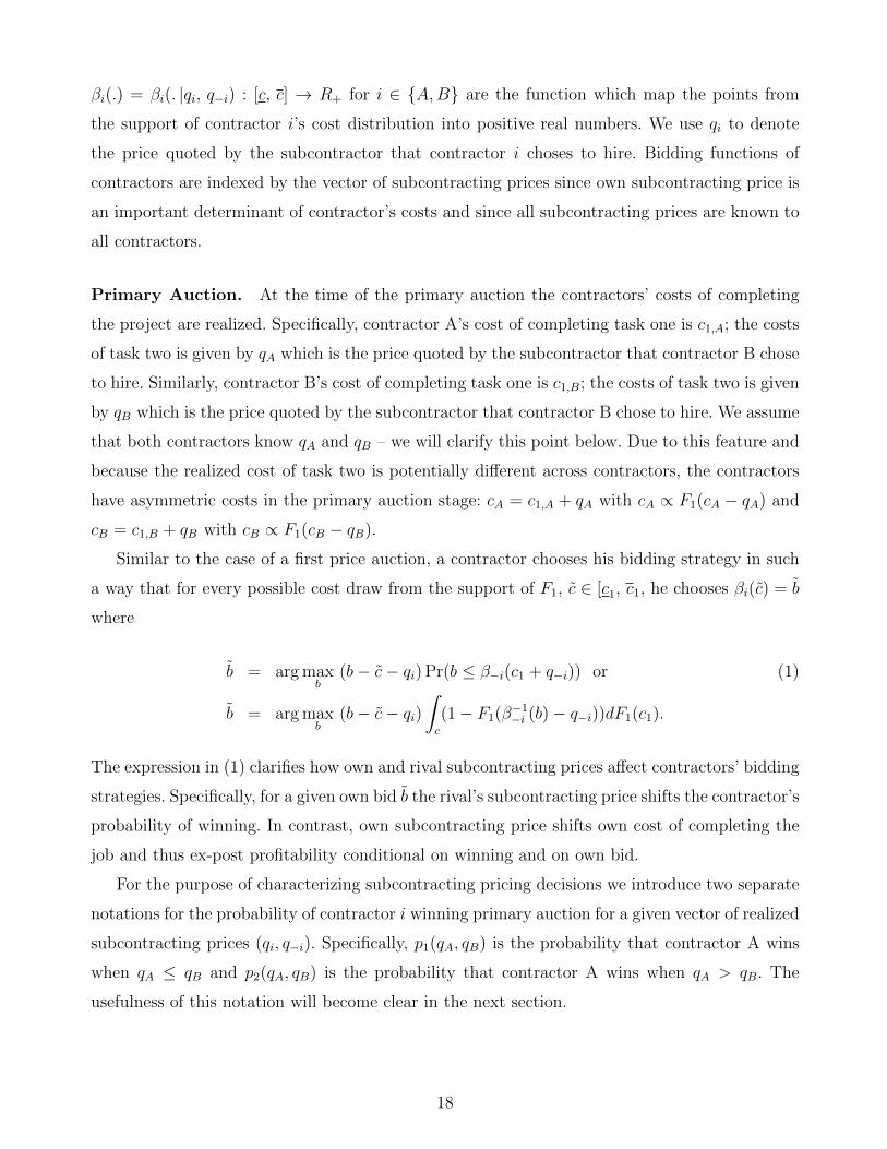
Primary Auction. At the time of the primary auction the contractors’ costs of completing

the project are realized. Specifically, contractor A’s cost of completing task one is c1,A; the costs

of task two is given by qA which is the price quoted by the subcontractor that contractor B chose

to hire. Similarly, contractor B’s cost of completing task one is c1,B; the costs of task two is given

by qB which is the price quoted by the subcontractor that contractor B chose to hire. We assume

that both contractors know qA and qB – we will clarify this point below. Due to this feature and

because the realized cost of task two is potentially different across contractors, the contractors

have asymmetric costs in the primary auction stage: cA = c1,A + qA with cA ∝ F1(cA − qA) and

cB = c1,B + qB with cB ∝ F1(cB − qB).

Similar to the case of a first price auction, a contractor chooses his bidding strategy in such

a way that for every possible cost draw from the support of F1, c̃ ∈ [c1, c1, he chooses βi(c̃) = b̃

where

b̃ = arg maxb

(b− c̃− qi) Pr(b ≤ β−i(c1 + q−i)) or (1)

b̃ = arg maxb

(b− c̃− qi)∫c

(1− F1(β−1−i (b)− q−i))dF1(c1).

The expression in (1) clarifies how own and rival subcontracting prices affect contractors’ bidding

strategies. Specifically, for a given own bid b̃ the rival’s subcontracting price shifts the contractor’s

probability of winning. In contrast, own subcontracting price shifts own cost of completing the

job and thus ex-post profitability conditional on winning and on own bid.

For the purpose of characterizing subcontracting pricing decisions we introduce two separate

notations for the probability of contractor i winning primary auction for a given vector of realized

subcontracting prices (qi, q−i). Specifically, p1(qA, qB) is the probability that contractor A wins

when qA ≤ qB and p2(qA, qB) is the probability that contractor A wins when qA > qB. The

usefulness of this notation will become clear in the next section.

18

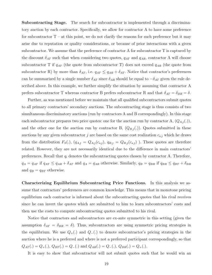
Subcontracting Stage. The search for subcontractor is implemented through a discrimina-

tory auction by each contractor. Specifically, we allow for contractor A to have some preference

for subcontractor T – at this point, we do not clarify the reasons for such preference but it may

arise due to reputation or quality considerations, or because of prior interactions with a given

subcontractor. We assume that the preference of contractor A for subcontractor T is captured by

the discount δAT such that when considering two quotes, qAT and qAR, contractor A will choose

subcontractor T if qAT (the quote from subcontractor T) does not exceed qAR (the quote from

subcontractor R) by more than δAT , i.e. qAT ≤ qAR + δAT . Notice that contractor’s preferences

can be summarized by a single number δAT since δAR should be equal to −δAT given the rule de-

scribed above. In this example, we further simplify the situation by assuming that contractor A

prefers subcontractor T whereas contractor B prefers subcontractor R and that δAT = δBR = δ.

Further, as was mentioned before we maintain that all qualified subcontractors submit quotes

to all primary contractors’ secondary auctions. The subcontracting stage is thus consists of two

simultaneous discriminatory auctions (run by contractors A and B correspondingly). In this stage

each subcontractor prepares two price quotes: one for the auction run by contractor A, (QA,j(.)),

and the other one for the auction run by contractor B, (QB,j(.)). Quotes submitted in these

auctions by any given subcontractor j are based on the same cost realization cs,j which he draws

from the distribution FS(.), (qA,j = QA,j(cs,j), qB,j = QB,j(cs,j) ). These quotes are therefore

related. However, they are not necessarily identical due to the difference in main contractors’

preferences. Recall that qi denotes the subcontracting quotes chosen by contractor A. Therefore,

qA = qAT if qAT ≤ qAR + δAT and qA = qAR otherwise. Similarly, qB = qBR if qBR ≤ qBT + δBR

and qB = qBT otherwise.

Characterizing Equilibrium Subcontracting Price Functions. In this analysis we as-

sume that contractors’ preferences are common knowledge. This means that in monotone pricing

equilibrium each contractor is informed about the subcontracting quotes that his rival receives

since he can invert the quotes which are submitted to him to learn subcontractors’ costs and

then use the costs to compute subcontracting quotes submitted to his rival.

Notice that contractors and subcontractors are ex-ante symmetric in this setting (given the

assumption δAT = δBR = δ). Thus, subcontractors are using symmetric pricing strategies in

the equilibrium. We use Q+(.) and Q−(.) to denote subcontractor’s pricing strategies in the

auction where he is a preferred and where is not a preferred participant correspondingly, so that

QAT (.) = Q+(.), QBT (.) = Q−(.) and QAR(.) = Q−(.), QBR(.) = Q+(.).

It is easy to show that subcontractor will not submit quotes such that he would win an

19

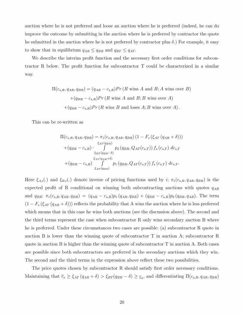
auction where he is not preferred and loose an auction where he is preferred (indeed, he can do

improve the outcome by submitting in the auction where he is preferred by contractor the quote

he submitted in the auction where he is not preferred by contractor plus δ.) For example, it easy

to show that in equilibrium qAR ≤ qBR and qBT ≤ qAT .

We describe the interim profit function and the necessary first order conditions for subcon-

tractor R below. The profit function for subcontractor T could be characterized in a similar

way.

Π(cs,R, qAR, qBR) = (qAR − cs,R)Pr (R wins A and B;A wins over B)

+(qBR − cs,R)Pr (R wins A and B;B wins over A)

+(qBR − cs,R)Pr (R wins B and loses A;B wins over A) .

This can be re-written as

Π(cs,R, qAR, qBR) = π1(cs,R, qAR, qBR) (1− Fs (ξAT (qAR + δ)))

+(qBR − cs,R) ·ξAT (qBR)∫

ξBT (qBR−δ)p2 (qBR, QAT (cs,T )) fs (cs,T ) dcs,T

+(qBR − cs,R)ξAT (qAR+δ)∫ξAT (qBR)

p1 (qBR, QAT (cs,T )) fs (cs,T ) dcs,T .

Here ξA,i(.) and ξB,i(.) denote inverse of pricing functions used by i; π1(cs,R, qAR, qBR) is the

expected profit of R conditional on winning both subcontracting auctions with quotes qAR

and qBR: π1(cs,R, qAR, qBR) = (qAR − cs,R)p1 (qAR, qBR) + (qBR − cs,R)p2 (qBR, qAR). The term

(1− Fs (ξAT (qAR + δ))) reflects the probability that A wins the auction where he is less preferred

which means that in this case he wins both auctions (see the discussion above). The second and

the third terms represent the case when subcontractor R only wins secondary auction B where

he is preferred. Under these circumstances two cases are possible: (a) subcontractor R quote in

auction B is lower than the winning quote of subcontractor T in auction A; subcontractor R

quote in auction B is higher than the winning quote of subcontractor T in auction A. Both cases

are possible since both subcontractors are preferred in the secondary auctions which they win.

The second and the third terms in the expression above reflect these two possibilities.

The price quotes chosen by subcontractor R should satisfy first order necessary conditions.

Maintaining that cs ≥ ξAT (qAR + δ) > ξBT (qBR − δ) ≥ cs, and differentiating Π(cs,R, qAR, qBR)

20

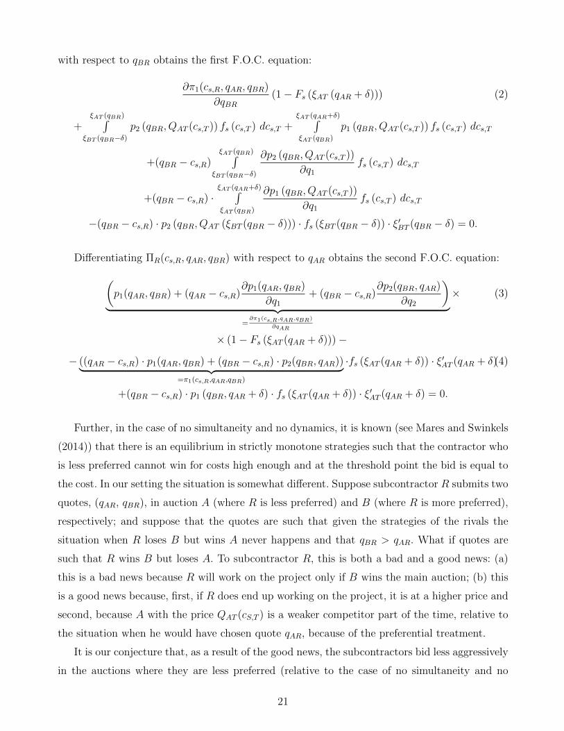
with respect to qBR obtains the first F.O.C. equation:

∂π1(cs,R, qAR, qBR)

∂qBR(1− Fs (ξAT (qAR + δ))) (2)

+ξAT (qBR)∫

ξBT (qBR−δ)p2 (qBR, QAT (cs,T )) fs (cs,T ) dcs,T +

ξAT (qAR+δ)∫ξAT (qBR)

p1 (qBR, QAT (cs,T )) fs (cs,T ) dcs,T

+(qBR − cs,R)ξAT (qBR)∫

ξBT (qBR−δ)

∂p2 (qBR, QAT (cs,T ))

∂q1

fs (cs,T ) dcs,T

+(qBR − cs,R) ·ξAT (qAR+δ)∫ξAT (qBR)

∂p1 (qBR, QAT (cs,T ))

∂q1

fs (cs,T ) dcs,T

−(qBR − cs,R) · p2 (qBR, QAT (ξBT (qBR − δ))) · fs (ξBT (qBR − δ)) · ξ′BT (qBR − δ) = 0.

Differentiating ΠR(cs,R, qAR, qBR) with respect to qAR obtains the second F.O.C. equation:(p1(qAR, qBR) + (qAR − cs,R)

∂p1(qAR, qBR)

∂q1

+ (qBR − cs,R)∂p2(qBR, qAR)

∂q2

)︸ ︷︷ ︸

=∂π1(cs,R,qAR,qBR)

∂qAR

× (3)

× (1− Fs (ξAT (qAR + δ)))−

− ((qAR − cs,R) · p1(qAR, qBR) + (qBR − cs,R) · p2(qBR, qAR))︸ ︷︷ ︸=π1(cs,R,qAR,qBR)

·fs (ξAT (qAR + δ)) · ξ′AT (qAR + δ)(4)

+(qBR − cs,R) · p1 (qBR, qAR + δ) · fs (ξAT (qAR + δ)) · ξ′AT (qAR + δ) = 0.

Further, in the case of no simultaneity and no dynamics, it is known (see Mares and Swinkels

(2014)) that there is an equilibrium in strictly monotone strategies such that the contractor who

is less preferred cannot win for costs high enough and at the threshold point the bid is equal to

the cost. In our setting the situation is somewhat different. Suppose subcontractor R submits two

quotes, (qAR, qBR), in auction A (where R is less preferred) and B (where R is more preferred),

respectively; and suppose that the quotes are such that given the strategies of the rivals the

situation when R loses B but wins A never happens and that qBR > qAR. What if quotes are

such that R wins B but loses A. To subcontractor R, this is both a bad and a good news: (a)

this is a bad news because R will work on the project only if B wins the main auction; (b) this

is a good news because, first, if R does end up working on the project, it is at a higher price and

second, because A with the price QAT (cS,T ) is a weaker competitor part of the time, relative to

the situation when he would have chosen quote qAR, because of the preferential treatment.

It is our conjecture that, as a result of the good news, the subcontractors bid less aggressively

in the auctions where they are less preferred (relative to the case of no simultaneity and no

21

dynamics) and, thus, in the equilibrium the quotes qAR and qBR are closer to each other than

in the case with no dynamics and no simultaneity. Another consequence of the good news bit is

that R’s bid at the cost value where he stops winning in auction A (threshold costs) is strictly

higher than the cost. The threshold cost level and the corresponding price are such that R is

indifferent between the bad news and the good news described above. With cost realization above

the threshold R only can win subcontracting auction B. These findings are summarized in the

Theorem presented below.

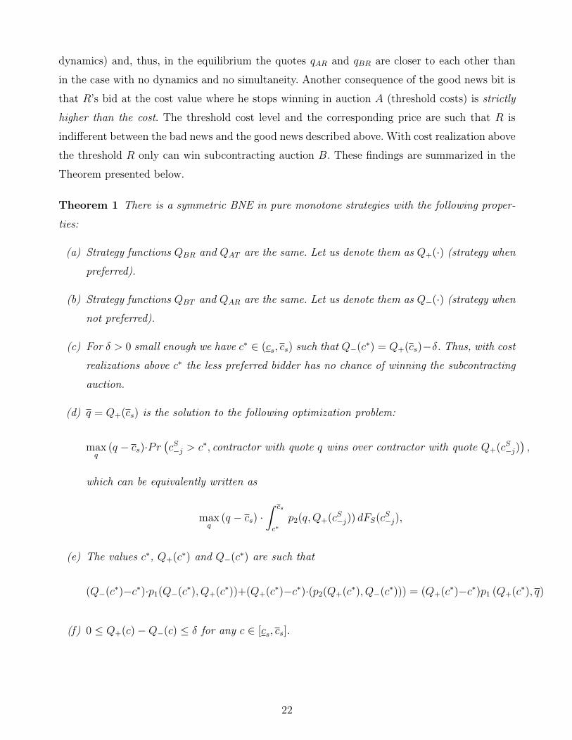
Theorem 1 There is a symmetric BNE in pure monotone strategies with the following proper-

ties:

(a) Strategy functions QBR and QAT are the same. Let us denote them as Q+(·) (strategy when

preferred).

(b) Strategy functions QBT and QAR are the same. Let us denote them as Q−(·) (strategy when

not preferred).

(c) For δ > 0 small enough we have c∗ ∈ (cs, cs) such that Q−(c∗) = Q+(cs)−δ. Thus, with cost

realizations above c∗ the less preferred bidder has no chance of winning the subcontracting

auction.

(d) q = Q+(cs) is the solution to the following optimization problem:

maxq

(q − cs)·Pr(cS−j > c∗, contractor with quote q wins over contractor with quote Q+(cS−j)

),

which can be equivalently written as

maxq

(q − cs) ·∫ cs

c∗p2(q,Q+(cS−j)) dFS(cS−j),

(e) The values c∗, Q+(c∗) and Q−(c∗) are such that

(Q−(c∗)−c∗)·p1(Q−(c∗), Q+(c∗))+(Q+(c∗)−c∗)·(p2(Q+(c∗), Q−(c∗))) = (Q+(c∗)−c∗)p1 (Q+(c∗), q)

(f) 0 ≤ Q+(c)−Q−(c) ≤ δ for any c ∈ [cs, cs].

22

5 Identification of Model Primitives

The model primitives that need to be recovered in the case of the simple model are the distri-

bution of contractors’ costs for task one, F1, the distribution of subcontractors’ costs for task

two, Fs, and the factor reflecting preferential treatment, δ. We exploit the structure on our data

which reports the bids by task, the identity of subcontractor and the price at which the task two

is subcontracted by each of the contractors.

The identification is straightforward when δi,j are observed at the level of contractor-

subcontractor pair or when many observations per pair are observed (alternatively, δ can be

parameterized). Indeed, the standard GPV argument can be used to recover the distribution of

costs for task one; similarly, the first order conditions associated with subcontractors’ pricing

problem could be used to recover the distribution of subcontractors’ costs.

The identification is somewhat more complicated when contractors may decide whether or

not to subcontract a given task or not. The identification in that case resemble identification

argument for Roy’s model.

References

Bajari, P., S. Houghton, and S. Tadelis (2014): “Bidding for Incomplete Contracts: An

Empirical Analysis of Adaptation Costs,” American Economic Review, 104(4), 1288–1319.

Bajari, P., and G. Lewis (2011): “Procurement with Time Incentives,” Quarterly Journal of

Economics, 126.

Balat, J. (2014): “Highway Procurement and the Stimulus Package: Identification and Esti-

mation of Dynamic Auctions with Unobserved Heterogeneity,” working paper.

Branzoli, N., and F. Decarolis (2014): “Entry and Subcontracting in Public Procurement

Auctions,” working paper.

Gil, R., and J. Marion (2012): “Self-Enforcing Agreements and Relational Contracting: Ev-

idence from California Highway Procurement,” The Journal of Law, Economics, & Organiza-

tion, 29(2), 239—277.

Haile, P. A. (2001): “Auctions with Resale Markets: An Application to U.S. Forest Service

Timber Sales,” American Economic Review, 91(3), 399—427.

23

Hong, H., and M. Shum (2002): “Increasing Competition and the Winner’s Curse: Evidence

from Procurement,” Review of Economic Studies, 69(4), 871–898.

Jeziorski, P., and E. Krasnokutskaya (2014): “Dynamic Auction Environment with Sub-

contracting,” working paper.

Jofre-Bonet, M., and M. Pesendorfer (2003): “Estimation of a Dynamic Auction Game,”

Econometrica, 71(5), 1443–1489.

Krasnokutskaya, E. (2011): “Identification and Estimation in Procurement Auctions under

Unobserved Auction Heterogeneity,” Review of Economic Studies, 101.

Krasnokutskaya, E., and K. Seim (2011): “Bid Preference Programs and Participation in

Highway Procurement,” American Economic Review, 101(2653-2686).

Mares, V., and J. Swinkels (2014): “Comparing First and Second Price Auctions with

Asymmetric Bidders,” International Journal of Game Theory, 43(487-514).

Marion, J. (2013): “Sourcing From the Enemy: Horizontal Subcontracting in Highway Pro-

curement,” working paper.

Miller, D. (2014): “Subcontracting and competitive bidding on incomplete procurement con-

tracts,” RAND Journal of Economics, 45(4), 705—746.

Moretti, L., and P. Valbonesi (2012): “Subcontracting in Public Procurement: An Empir-

ical Investigaion,” working paper.

Porter, R. H., and J. D. Zona (1993): “Detection of Bid Rigging in Procurement Auctions,”

Journal of Political Economy, 101(3), 518–538.

Wambach, A. (2009): “How to subcontract?,” Economics Letters, 105, 152–155.

24