Embed Size (px)
Citation preview
Evolution and Consequences of Coronal Mass
Ejections in the Heliosphere
A Thesis
submitted for the award of Ph.D. degree of
MOHANLAL SUKHADIA UNIVERSITY
in the
Faculty of Science
By
Wageesh Mishra
Under the Supervision of
Prof. Nandita Srivastava
Udaipur Solar Observatory
Physical Research Laboratory, Udaipur
Department of Physics
Faculty of Science
MOHANLAL SUKHADIA UNIVERSITY
UDAIPUR
Year of submission: 2015
arX
iv:2
204.
0987
9v1
[as
tro-
ph.S
R]
21
Apr
202
2

DECLARATION
I, Mr. Wageesh Mishra, S/o Mr. Nagesh Mishra, resident of C-2, USO
staff colony, Badi road, Udaipur-313 001, hereby declare that the research work
incorporated in the present thesis entitled, “Evolution and Consequences
of Coronal Mass Ejections in the Heliosphere” is my own work and is
original. This work (in part or in full) has not been submitted to any University
for the award of a Degree or a Diploma. I have properly acknowledged the
material collected from secondary sources wherever required. I solely own the
responsibility for the originality of the entire content.
Date:Wageesh Mishra
(Author)Udaipur Solar Observatory
Physical Research Laboratory(Dept. of Space, Govt. of India)
P.B. No. 198, Dewali, Badi RoadUdaipur-313 001
Rajasthan, India.
CERTIFICATE
I feel great pleasure in certifying that the thesis entitled “Evolution and
Consequences of Coronal Mass Ejections in the Heliosphere” embodies
a record of the results of investigations carried out by Mr. Wageesh Mishra
under my guidance. He has completed the following requirements as per Ph.D.
regulations of the University.
(a) Course work as per the university rules.
(b) Residential requirements of the university.
(c) Regularly submitted six monthly progress report.
(d) Presented his work in the departmental committee.
(e) Published/accepted minimum of one research paper in a refereed research
journal.
I recommend the submission of thesis.
Date:
Countersigned byHead of the Department
Prof. Nandita Srivastava(Thesis Supervisor)
Udaipur Solar ObservatoryPhysical Research Laboratory
(Dept. of Space, Govt. of India)P.B. No. 198, Dewali, Badi Road
Udaipur-313 001Rajasthan, India.

This thesis is dedicated to my parents,who have made sacrifices throughout to help me get where I am today.
Contents
List of Figures vi
List of Tables ix
Acknowledgments x
Abstract xiv
List of Publications xvi
1 Introduction 11.1 The Sun . . . . . . . . . . . . . . . . . . . . . . . . . . . . . . . . 11.2 Structure of the Sun . . . . . . . . . . . . . . . . . . . . . . . . . 2
1.2.1 Solar interior . . . . . . . . . . . . . . . . . . . . . . . . . 21.2.2 Solar atmosphere . . . . . . . . . . . . . . . . . . . . . . . 41.2.3 Solar wind and the heliosphere . . . . . . . . . . . . . . . 5
1.3 Coronal Mass Ejections . . . . . . . . . . . . . . . . . . . . . . . . 71.3.1 Observations of CMEs . . . . . . . . . . . . . . . . . . . . 81.3.2 Thomson scattering . . . . . . . . . . . . . . . . . . . . . . 101.3.3 Properties of CMEs . . . . . . . . . . . . . . . . . . . . . . 13
1.4 Heliospheric Evolution of CMEs . . . . . . . . . . . . . . . . . . . 141.4.1 CME studies before STEREO era . . . . . . . . . . . . . . 15
1.4.1.1 CME kinematics and their arrival time at L1 . . 161.4.1.2 In situ observations of CMEs . . . . . . . . . . . 18
1.4.2 CME studies in STEREO era . . . . . . . . . . . . . . . . 221.5 Heliospheric Consequences of CMEs . . . . . . . . . . . . . . . . . 251.6 Motivation and Organization of the Thesis . . . . . . . . . . . . . 29
2 Observational Data and Analysis Methodology 342.1 Introduction . . . . . . . . . . . . . . . . . . . . . . . . . . . . . . 34
2.1.1 Remote observations from STEREO/SECCHI . . . . . . . 352.1.2 SECCHI/COR observations . . . . . . . . . . . . . . . . . 352.1.3 SECCHI/HI observations . . . . . . . . . . . . . . . . . . . 37
2.2 Observations Near 1 AU . . . . . . . . . . . . . . . . . . . . . . . 40
i
Contents
2.2.1 In situ observations from ACE & WIND . . . . . . . . . . 402.2.2 Ground-based magnetometer observations . . . . . . . . . 41
2.3 Analysis Methodology . . . . . . . . . . . . . . . . . . . . . . . . 432.3.1 Reconstruction methods using COR2 observations . . . . . 44
2.3.1.1 Tie-point (TP) reconstruction . . . . . . . . . . . 442.3.1.2 Forward modeling method . . . . . . . . . . . . . 45
2.3.2 Reconstruction methods using COR & HI observations . . 462.3.2.1 Construction of J -maps . . . . . . . . . . . . . . 472.3.2.2 Single spacecraft reconstruction methods . . . . . 48
2.3.2.2.1 Point-P (PP) method . . . . . . . . . . 492.3.2.2.2 Fixed-phi (FP) method . . . . . . . . . 502.3.2.2.3 Harmonic mean (HM) method . . . . . . 512.3.2.2.4 Self-similar expansion (SSE) method . . 52
2.3.2.3 Single spacecraft fitting methods . . . . . . . . . 532.3.2.3.1 Fixed-phi fitting (FPF) method . . . . . 532.3.2.3.2 Harmonic mean fitting (HMF) method . 542.3.2.3.3 Self-similar expansion fitting (SSEF) method 54
2.3.2.4 Twin spacecraft methods . . . . . . . . . . . . . 562.3.2.4.1 Geometric triangulation (GT) method . 562.3.2.4.2 Tangent to a sphere (TAS) method . . . 582.3.2.4.3 Stereoscopic self-similar expansion (SSSE)
method . . . . . . . . . . . . . . . . . . 592.3.3 Estimation of the arrival time of CMEs . . . . . . . . . . . 61
2.3.3.1 Drag based model for propagation of CMEs . . . 612.4 Identification of CMEs and Their Consequences Near the Earth . 62
3 Estimation of Arrival Time of CMEs 643.1 Introduction . . . . . . . . . . . . . . . . . . . . . . . . . . . . . . 643.2 Estimating the Arrival Time of CMEs Using GT Method . . . . . 69
3.2.1 2008 December 12 . . . . . . . . . . . . . . . . . . . . . . 713.2.1.1 Application of 3D reconstruction method in COR
FOV . . . . . . . . . . . . . . . . . . . . . . . . . 733.2.1.2 Application of 3D reconstruction method in HI FOV 733.2.1.3 Estimation of arrival time and transit speed of
2008 December 12 CME at L1 . . . . . . . . . . . 763.2.2 2010 February 7 CME . . . . . . . . . . . . . . . . . . . . 783.2.3 2010 February 12 CME . . . . . . . . . . . . . . . . . . . . 803.2.4 2010 March 14 CME . . . . . . . . . . . . . . . . . . . . . 823.2.5 2010 April 3 CME . . . . . . . . . . . . . . . . . . . . . . 843.2.6 2010 April 8 CME . . . . . . . . . . . . . . . . . . . . . . 863.2.7 2010 October 10 CME . . . . . . . . . . . . . . . . . . . . 873.2.8 2010 October 26 CME . . . . . . . . . . . . . . . . . . . . 89
ii
Contents
3.3 Arrival Time Estimation of the CMEs Using GT Method: Resultsand Discussion . . . . . . . . . . . . . . . . . . . . . . . . . . . . 90
3.4 Assessing the Relative Performance of Ten Reconstruction Meth-ods for Estimating the Arrival Time of CMEs Using SECCHI/HIObservations . . . . . . . . . . . . . . . . . . . . . . . . . . . . . . 97
3.5 Reconstruction Methods and Their Application to the SelectedCMEs . . . . . . . . . . . . . . . . . . . . . . . . . . . . . . . . . 993.5.1 2010 October 6 CME . . . . . . . . . . . . . . . . . . . . . 101
3.5.1.1 Reconstruction methods using single spacecraftobservations . . . . . . . . . . . . . . . . . . . . . 102
3.5.1.1.1 Point-P (PP) method . . . . . . . . . . 1023.5.1.1.2 Fixed-phi (FP) method . . . . . . . . . 1073.5.1.1.3 Harmonic mean (HM) method . . . . . . 1083.5.1.1.4 Self-similar expansion (SSE) method . . 1093.5.1.1.5 Error analysis for FP, HM and SSE
methods . . . . . . . . . . . . . . . . . . 1093.5.1.2 Single spacecraft fitting methods for SECCHI/HI
observations . . . . . . . . . . . . . . . . . . . . . 1103.5.1.2.1 Fixed-phi fitting (FPF), Harmonic mean
fitting (HMF) and Self-similar expansionfitting (SSEF) method . . . . . . . . . . 110
3.5.1.3 Stereoscopic reconstruction methods using SEC-CHI/HI observations . . . . . . . . . . . . . . . . 112
3.5.1.3.1 Geometric triangulation (GT) method . 1123.5.1.3.2 Tangent to a sphere (TAS) method . . . 1143.5.1.3.3 Stereoscopic self-similar expansion (SSSE)
method . . . . . . . . . . . . . . . . . . 1143.5.2 2010 April 3 CME . . . . . . . . . . . . . . . . . . . . . . 1153.5.3 2010 February 12 CME . . . . . . . . . . . . . . . . . . . . 118
3.6 Identification of Tracked CME Features Using In Situ ObservationsNear the Earth . . . . . . . . . . . . . . . . . . . . . . . . . . . . 119
3.7 Results and Discussion . . . . . . . . . . . . . . . . . . . . . . . . 1223.7.1 Relative performance of single spacecraft methods . . . . . 1233.7.2 Relative performance of stereoscopic methods . . . . . . . 1263.7.3 Relative performance of single spacecraft fitting methods . 127
3.8 Conclusion . . . . . . . . . . . . . . . . . . . . . . . . . . . . . . . 129
4 Association between Remote and In Situ Observations of CMEs1314.1 Introduction . . . . . . . . . . . . . . . . . . . . . . . . . . . . . . 1314.2 In Situ Observations of CMEs . . . . . . . . . . . . . . . . . . . . 134
4.2.1 2008 December 12 CME . . . . . . . . . . . . . . . . . . . 1344.2.2 2010 February 7 CME . . . . . . . . . . . . . . . . . . . . 1354.2.3 2010 February 12 CME . . . . . . . . . . . . . . . . . . . . 136
iii
Contents
4.2.4 2010 March 14 CME . . . . . . . . . . . . . . . . . . . . . 1374.2.5 2010 April 3 CME . . . . . . . . . . . . . . . . . . . . . . 1384.2.6 2010 April 8 CME . . . . . . . . . . . . . . . . . . . . . . 1394.2.7 2010 October 6 CME . . . . . . . . . . . . . . . . . . . . . 1404.2.8 2010 October 10 CME . . . . . . . . . . . . . . . . . . . . 1424.2.9 2010 October 26 CME . . . . . . . . . . . . . . . . . . . . 143
4.3 Tracking of Different Features of 2010 October 6 CME Using Re-mote and In Situ Observations . . . . . . . . . . . . . . . . . . . . 1434.3.1 Remote sensing observations of 2010 October 6 CME . . . 1454.3.2 Reconstruction of 2010 October 6 CME . . . . . . . . . . . 1464.3.3 Comparison of kinematics of tracked features . . . . . . . . 1524.3.4 Identification of filament plasma using near-Earth in situ
observations . . . . . . . . . . . . . . . . . . . . . . . . . . 1554.4 Results and Discussion . . . . . . . . . . . . . . . . . . . . . . . . 157
5 Interplanetary Consequences of CMEs 1605.1 Interaction of CMEs . . . . . . . . . . . . . . . . . . . . . . . . . 1605.2 Interacting CMEs of 2011 February 13-15 . . . . . . . . . . . . . . 164
5.2.1 Morphological evolution of interacting CMEs in the CORFOV . . . . . . . . . . . . . . . . . . . . . . . . . . . . . . 166
5.2.2 Kinematic evolution and interaction of CMEs in the helio-sphere . . . . . . . . . . . . . . . . . . . . . . . . . . . . . 1715.2.2.1 3D reconstruction in COR FOV . . . . . . . . . . 1715.2.2.2 Comparison of angular widths of CMEs derived
from GCS model . . . . . . . . . . . . . . . . . . 1745.2.2.3 Reconstruction of CMEs in HI FOV . . . . . . . 1765.2.2.4 Comparison of kinematics derived from other
stereoscopic methods . . . . . . . . . . . . . . . . 1805.2.3 Energy, momentum exchange and nature of collision be-
tween CMEs of 2011 February 14 and 15 . . . . . . . . . . 1835.2.3.1 Estimation of true mass of CMEs . . . . . . . . . 1845.2.3.2 Estimation of coefficient of restitution . . . . . . 186
5.2.4 In situ observations, arrival time and geomagnetic responseof interacting CMEs of 2011 February 13-15 . . . . . . . . 1895.2.4.1 In situ observations . . . . . . . . . . . . . . . . . 1895.2.4.2 Estimation of arrival time of CMEs . . . . . . . . 1915.2.4.3 Geomagnetic response of interacting CMEs . . . 193
5.2.5 Results and Discussion on 2011 February 13-15 CMEs . . . 1945.2.5.1 Morphological evolution of CMEs . . . . . . . . . 1955.2.5.2 Kinematic evolution of interacting CMEs . . . . . 1965.2.5.3 Interacting CMEs near the Earth . . . . . . . . . 197
5.3 Interacting CMEs of 2012 November 9-10 . . . . . . . . . . . . . . 1985.3.1 3D reconstruction in COR2 FOV . . . . . . . . . . . . . . 198
iv
Contents
5.3.2 Tracking of CMEs in HI FOV . . . . . . . . . . . . . . . . 2015.3.3 Momentum, energy exchange, and nature of collision be-
tween CMEs of 2012 November 9 and 10 . . . . . . . . . . 2055.3.4 In situ observations, arrival time, and geomagnetic response
of interacting CMEs of 2012 November 9 and 10 . . . . . . 2085.3.4.1 In situ identification of tracked CME features . . 2085.3.4.2 Arrival time of tracked features . . . . . . . . . . 2115.3.4.3 Geomagnetic consequences of interacting CMEs . 212
5.3.5 Results and Discussion on 2012 November 9-10 CMEs . . . 2185.4 Conclusion . . . . . . . . . . . . . . . . . . . . . . . . . . . . . . . 222
6 Conclusions and Future Work 2266.1 Conclusions . . . . . . . . . . . . . . . . . . . . . . . . . . . . . . 2266.2 Future Work . . . . . . . . . . . . . . . . . . . . . . . . . . . . . . 229
6.2.1 Dynamic evolution of the CMEs . . . . . . . . . . . . . . . 2306.2.2 Consequences of interacting CMEs . . . . . . . . . . . . . 2306.2.3 Assessing the performance of reconstruction methods using
the off-ecliptic CMEs . . . . . . . . . . . . . . . . . . . . . 231
Bibliography 232
v
List of Figures
1.1 Variations of temperature and density in the solar atmosphere . . 41.2 Brightness variation of the different components of the solar corona
with radial distance (reproduced from Golub and Pasachoff, 2009,Ch. 5). . . . . . . . . . . . . . . . . . . . . . . . . . . . . . . . . . 6
1.3 A “halo” CME observed by LASCO-C2 coronagraph on SOHO . 101.4 A classical CME with 3-part structure . . . . . . . . . . . . . . . 111.5 Relevant angles in the context of the Thomson scattering geometry 121.6 Three phase kinematic profile of a CME . . . . . . . . . . . . . . 141.7 Four possible tracks of an in situ spacecraft through a CME . . . 221.8 A CME observed in STEREO/SECCHI images . . . . . . . . . . 241.9 Different phases of a typical geomagnetic storm . . . . . . . . . . 27
2.1 The location of STEREO, inner solar system planets and theParker spiral . . . . . . . . . . . . . . . . . . . . . . . . . . . . . . 36
2.2 Field of view (FOV) of CORs and HIs . . . . . . . . . . . . . . . 382.3 Inner and outer edges of HI FOV corresponding to different sepa-
ration angle of STEREO-A and B . . . . . . . . . . . . . . . . . . 392.4 GCS model representation . . . . . . . . . . . . . . . . . . . . . . 462.5 J -maps using COR2, HI1 and HI2 images . . . . . . . . . . . . . 482.6 CME feature tracking in FP, HM and SSE model geometry . . . . 512.7 Geometric triangulation for a moving CME feature . . . . . . . . 582.8 The SSE modeled circular CME . . . . . . . . . . . . . . . . . . . 60
3.1 Evolution of the 2008 December 12 CME as seen in COR and HIFOV . . . . . . . . . . . . . . . . . . . . . . . . . . . . . . . . . . 72
3.2 J -maps for the 2008 December 12 CME . . . . . . . . . . . . . . 733.3 Estimated 3D height, radial velocity, acceleration, longitude and
latitude of the 2008 December 12 CME using tie-pointing method 743.4 Estimated distance, propagation direction, and velocity of the 2008
December 12 CME using GT method . . . . . . . . . . . . . . . . 753.5 As Figure 3.4, for the 2010 February 7 CME . . . . . . . . . . . . 793.6 As Figure 3.4, for the 2010 February 12 CME . . . . . . . . . . . 813.7 As Figure 3.4, for the 2010 March 14 CME . . . . . . . . . . . . . 833.8 As Figure 3.4, for the 2010 April 3 CME . . . . . . . . . . . . . . 85
vi
List of Figures
3.9 As Figure 3.4, for the 2010 April 8 CME . . . . . . . . . . . . . . 863.10 As Figure 3.4, for the 2010 October 10 CME . . . . . . . . . . . . 883.11 As Figure 3.4, for the 2010 October 26 CME . . . . . . . . . . . . 903.12 Evolution of the 2010 October 6 CME observed in COR2, HI1 and
HI2 images . . . . . . . . . . . . . . . . . . . . . . . . . . . . . . 1033.13 J -maps for the 2010 October 6 CME . . . . . . . . . . . . . . . . 1043.14 Estimated distance and speed profiles for the tracked feature of
the 2010 October 6 CME using the PP, FP, HM, and SSE methods 1053.15 Best fit FPF and HMF results for the 2010 October 6 CME . . . 1113.16 Distance, propagation direction, and speed profiles for the tracked
feature of the 2010 October 6 CME using GT, TAS, and SSSEmethods . . . . . . . . . . . . . . . . . . . . . . . . . . . . . . . . 113
3.17 As Figure 3.14, for the 2010 April 3 CME. . . . . . . . . . . . . . 1163.18 As Figure 3.16, for the 2010 April 3 CME. . . . . . . . . . . . . . 1183.19 As Figure 3.14, for the 2010 February 12 CME. . . . . . . . . . . 1193.20 As Figure 3.16, for the 2010 February 12 CME. . . . . . . . . . . 121
4.1 In situ measurements of plasma and magnetic field parameters ofthe 2008 December 12 CME . . . . . . . . . . . . . . . . . . . . . 135
4.2 As Figure 4.1, for the 2010 February 7 CME . . . . . . . . . . . . 1364.3 As Figure 4.1, for the 2010 February 12 CME . . . . . . . . . . . 1374.4 As Figure 4.1, for the 2010 March 14 CME . . . . . . . . . . . . . 1384.5 As Figure 4.1, for the 2010 April 3 CME . . . . . . . . . . . . . . 1394.6 As Figure 4.1, for the 2010 April 8 CME . . . . . . . . . . . . . . 1404.7 As Figure 4.1, for the 2010 October 6 CME . . . . . . . . . . . . 1414.8 As Figure 4.1, for the 2010 October 10 CME . . . . . . . . . . . . 1424.9 As Figure 4.1, for the 2010 October 26 CME . . . . . . . . . . . . 1444.10 J -maps for the 2010 October 6 CME . . . . . . . . . . . . . . . . 1464.11 Estimated height, speed, acceleration, longitude and latitude of
the leading edge and core of the 2010 October 6 CME . . . . . . . 1474.12 Distance and speed profiles using PP, FP, HM, and SSE methods
for the tracked Feature 2 of the 2010 October 6 CME . . . . . . . 1494.13 Distance, propagation direction and speed using stereoscopic (GT,
TAS and SSSE) methods for the tracked Feature 2 of the 2010October 6 CME . . . . . . . . . . . . . . . . . . . . . . . . . . . . 151
4.14 Separation between tracked features of 2010 October 6 CME . . . 154
5.1 CMEs of the 2011 February 14 and 15 in COR2-A FOV . . . . . . 1685.2 Time-variation of the estimated 2D cone angular width . . . . . . 1695.3 Variations in cone and contour area of the 2011 February 14 CME 1705.4 As Figure 5.3, for the 2011 February 15 CME. . . . . . . . . . . . 1715.5 The contemporaneous image triplets for CMEs from SECCHI/COR2-
B (left), SOHO/LASCO (C2 or C3) (middle), and SECCHI/COR2-A (right) with GCS wireframe (with green) overlaid on it . . . . . 172
vii
List of Figures
5.6 Estimated radial velocity, acceleration, longitude and latitude of2011 February 13-15 CMEs using GCS model . . . . . . . . . . . 174
5.7 The base difference HI1-A and HI1-B images show the collision ofthe CMEs launched on 2011 February 14 and 15 . . . . . . . . . . 177
5.8 J -maps for the 2011 February 13-15 CMEs . . . . . . . . . . . . . 1775.9 Estimates of distance, propagation direction, and speed of the 2011
February 13-15 CMEs using SSSE method . . . . . . . . . . . . . 1795.10 Estimated direction of propagation of CMEs using GT method . . 1825.11 Coefficient of restitution values corresponding to different mass
ratios of interacting CMEs of the 2011 February 14 and 15 . . . . 1895.12 In situ measurements of the 2011 February 13-15 CMEs . . . . . . 1915.13 Estimated 3D kinematics of the 2012 November 9 and 10 CMEs
using tie-poining method . . . . . . . . . . . . . . . . . . . . . . . 1995.14 GCS model applied on the 2012 November 9 and 10 CMEs
images taken from STEREO/COR2-B, SOHO/LASCO-C3, andSTEREO/COR2-A . . . . . . . . . . . . . . . . . . . . . . . . . . 200
5.15 Evolution of the 2012 November 9 and 10 CMEs in COR2, HI1,and HI2 images . . . . . . . . . . . . . . . . . . . . . . . . . . . . 202
5.16 J -map for the 2012 November 9 and 10 CMEs . . . . . . . . . . . 2045.17 Contours of derived elongation of tracked features overplotted on
the base difference HI1-A images . . . . . . . . . . . . . . . . . . 2055.18 Estimated distance and speed of the tracked features using HM
method for the 2012 November 9 and 10 CMEs . . . . . . . . . . 2065.19 Coefficient of restitution corresponding to different mass ratios of
interacting CMEs of the 2012 November 9 and 10 . . . . . . . . . 2085.20 In situ measurements of interacting CMEs of the 2012 November
9 and 10 . . . . . . . . . . . . . . . . . . . . . . . . . . . . . . . . 2105.21 Variations in geomagnetic field and in situ parameters during the
interval of 2012 November 12-15 . . . . . . . . . . . . . . . . . . . 215
viii
List of Tables
3.1 List of selected CMEs with their arrival times at L1 . . . . . . . . 713.2 Errors in the predicted arrival time of CMEs using two different
approaches . . . . . . . . . . . . . . . . . . . . . . . . . . . . . . . 933.3 Errors in the predicted arrival time estimated using the 3D velocity
in the COR2 FOV . . . . . . . . . . . . . . . . . . . . . . . . . . 943.4 Results of different reconstruction techniques applied to the 2010
October 6 CME . . . . . . . . . . . . . . . . . . . . . . . . . . . . 1063.5 As Table 3.4, for the 2010 April 3 CME . . . . . . . . . . . . . . . 1173.6 As Table 3.4, for the 2010 February 12 CME . . . . . . . . . . . . 120
4.1 Results of different reconstruction techniques applied to trailingfeature of the 2010 October 6 CME . . . . . . . . . . . . . . . . . 150
5.1 The estimates of mass and direction for the 2011 February 14 and15 CMEs . . . . . . . . . . . . . . . . . . . . . . . . . . . . . . . . 186
5.2 The estimates of mass and direction for the 2012 November 9 and10 CMEs . . . . . . . . . . . . . . . . . . . . . . . . . . . . . . . . 207
5.3 Estimated kinematics, predicted arrival time and transit speed atL1 for the tracked features of the 2012 November 9 and 10 . . . . 213
5.4 A comparison of estimated characteristics for the interacting CMEsof the 2011 February 13-15 and 2012 November 9-10. . . . . . . . 224
ix

Acknowledgments
I feel immense pleasure on the completion of my Ph.D. thesis work. I
received help directly or indirectly from several people during various stages of this
work. First and foremost, I thank almighty God for giving me the determination,
patience and environment required to pursue my research work successfully. I
express my sincere gratitude to my Ph.D. supervisor Prof. Nandita Srivastava
for her invaluable guidance, support and encouragement throughout to mould
me as an independent researcher. I could participate in several international
and national conferences/schools/workshops due to her backing and boost. This
provided me an opportunity to interact with many scientists and students for
realizing varieties of research problems. I am indeed proud to be her student and
feel fortunate for having such an experienced and knowledgeable supervisor. I am
grateful to her for allowing me to work under her guidance. I believe whatever I
have learned working with her, I could not have learned anywhere else.
I would like to extend special thanks to Prof. P. Venkatakrishnan, Head
Udaipur Solar Observatory (USO), who always encouraged and helped me. I
enjoyed discussing with him at his house on several subjects ranging from science
to mythology. I remember the day when I gave my first USO seminar after which
Prof. Ashok Ambastha had literally told me ‘Well done’, I sincerely thank him
for his continuous encouragement. The informal discussion with Dr. Shibu K.
Mathew has been beneficial in my work and I express my thanks to him. I am
a great admirer of his supportive nature regarding genuine issues of students.
His exemplary hard work has always prompted me to do the same. I thank Dr.
Brajesh Kumar and Dr. Bhuwan Joshi for their suggestions at various stages
of my thesis. I have also been benefited from the lectures given by Dr. Ramit
Bhattacharyya at USO. His questions during my presentations often motivated
me for further reading. I am delighted to acknowledge the instant help received
from Mr. Raja Bayanna whenever required. He helped me in learning IDL
programming in the initial phase at USO. I also thank Ms. Bireddy Ramya for her
pleasant company. Her single minded dedication towards work is tremendously
inspiring.
x
I express my gratitude to Prof. J. N. Goswami, Director, Physical Research
Laboratory (PRL), and all faculty and staff of PRL, for giving me a nice oppor-
tunity to pursue my research work. I have immensely enjoyed the lectures by Dr.
Dibyendu Chakrabarty and Dr. Bhuwan Joshi during my course work in PRL. I
sincerely thank the academic committee for reviewing my progress from time to
time and encouraging me. I also thank Prof. K. S. Baliyan and Dr. S. Naik for
scientific discussions during my stay in PRL.
I would like to thank Dr. J. A. Davies (RAL, UK), Dr. T. A. Howard
(SwRI, USA), Dr. Y. D. Liu (UC Berkeley, USA), Dr. N. Lugaz (UNH, USA)
and Dr. C. Mostl (UC Berkeley, USA) for their help and discussion via emails.
Especially, I am indebted to Dr. Davies for her quick reply to my emails and
guidance regarding HI images processing and data analysis. I also thank Prof.
Yuming Wang (USTC, China), Dr. B. Vrsnak (Hvar Observatory, Croatia), Prof.
C. Farrugia (UNH, USA), and Dr. M. Temmer (University of Graz, Austria) for
the discussion, especially via emails. I thank Prof. R. Harrison (RAL, UK), Dr.
Davies and Dr. Lugaz for giving me an opportunity to participate in ‘CME-
CME Interaction Workshop’ held in Oxford, UK. I am thankful to organizers of
‘Heliophysics Summer School-2013’ for selecting me to attend the school held in
HAO, Boulder, USA. I am grateful to Dr. Mausumi Dikpati (HAO) for arranging
my talk in her institute during my visit to attend the summer school. I thank
Prof. P. K. Manoharan (NCRA, Pune) and organizers of ‘International Space
Weather Winter School-2013’ for supporting me to attend the school held in
NCU, Taiwan. I am extremely lucky to meet and discuss with several scientists
in various conferences, namely Dr. Prasad Subramanian (IISER, Pune), Prof.
Manoharan, Dr. Durgesh Tripathi (IUCAA, Pune), Prof. B. N. Dwivedi (IIT,
BHU), Dr. D. Banerjee (IIA, Bangalore), Prof. S. Ananthakrishnan (University
of Pune), Dr. R. Ramesh (IIA, Bangalore), Dr. A. K. Srivastava (IIT, BHU) and
many others.
I extend thanks to my friends at USO, Anand D. Joshi, Vemareddy Pan-
diti, Suruchi Goel, Dinesh Kumar, Upendra Kushwaha, Sanjay Kumar, Alok
Tiwari, Rahul Yadav, Hemant Saini, Ramya and Sudarshan. I have enjoyed their
xi

company whether it be playing badminton, outings, having party, taking meals or
discussing over science, society, politics, mythology and many other non-scientific
aspects of life. I am especially grateful to Anand from whom I have learnt a lot
about IDL programing. I also learnt several concepts of MHD from Sanjay. I
also thank my friends Arushi, Puneet and Tanuj who although spent a short
time at USO during their projects, are still in contact. We learn and enjoy to-
gether among the true friends, and I believe to achieve all these throughout my
academics.
I thank the administrative staff of USO, Mr. Raju Koshy, Mr. Rakesh
Jaroli, and Mr. Pinakin S. Shikari for providing me good facilities at USO.
The affection and support shown by Mr. Koshy is greatly acknowledged. I
also thank Mr. Naresh Jain, Mr. Mukesh Saradava, Mr. Laxmi Lal Suthar,
Mr. Jagdish Singh Chauhan and Mr. Dal Chand Purohit for providing me the
cordial environment at USO. My especial thanks go to late Mr. Sudhir Kumar
Gupta who was very kind, helpful and always encouraged me. We had celebrated
several festivals together and his absence is a grief to me. I sincerely acknowledge
the friendly nature of USO library staff Mr. Nurul Alam and Ms. Hemlata
Kumhar. I also thank the staff of Physics department and Ph.D. section of
Mohanlal Sukhadia University for their kind cooperation throughout my thesis.
I have enjoyed the hospitality of Mrs. Usha Venkatakrishnan, Mrs. Mahima
Kanthalia, Mrs. Saraswathi, Mrs. Bharati and Mrs. Richa, I express my grati-
tude to all of them. I thank everyone living at USO colony for their help, arranging
get-together, and homely environment provided. I am indebted to Usha madam
for her affection and encouragement. The kind and friendly nature of Mahima is
greatly acknowledged.
Although, I spent a short time at PRL but I enjoyed my stay with my
friends. I would like to thank friends of my batch, Gaurav Tomar, Gaurav
Sharma, Naveen Negi, Girish, Yashpal, Priyanka, Monojit, Anjali, Avdhesh,
Bhavya, Lekshmy, Gangi Reddy, Tanmoy and Gulab. I would like to acknowledge
the continuous help and encouragement from Sharma, Tomar and Negi which is
beyond the description. I thank my other friends at PRL, Arun Awasthi, Susanta
xii

Bisoi, Sunil Chandra, Arun Pandey, Girish, Diptiranjan, Rukmani, Kuldeep,
Navpreet and several others. I also thank my school friends Jainendra, Yogendra
and Anandita for their help and inspiring company. I convey thanks to my col-
lege and university friends Arjun Tiwari, Anuj Verma, Shishir Pandey, Himanshu
Rai, Abhishek, Rashmi, Jamwant, Siddhi, Suneeta, Narayan Datt and Jyotsana
who have been always supportive and encouraging. I also thank Sargam Mulay,
Bidya Binay, Sharad, Hitaishi, Sajal, Pandey ji, Yogita, Vasanth and Rahul for
their support and suggestions at various stages of my thesis.
My especial thanks go to my teachers of the Gorakhpur university, Prof. U.
S. Pandey, Prof. M. Mishra, Prof. S. N. Tiwari, Prof. S. Rastogi and Dr. R.
S. Singh who have had an impact on me. I always admire Prof. Pandey for his
helpfulness, simplicity and dedication that has helped me in my career. I also
thank my college teachers Dr. S. C. Verma and Dr. B. K Verma, although with
whom I am not associated now. My gratitude towards my teachers would remain
incomplete without remembering my school teachers Mr. J. P. Pathak, Mr. K.
Tiwari and Mr. O. P. Chaturvedi.
I am in dearth of words to thank my parents (Mr. Nagesh Mishra and
Mrs. Shyama Devi) for the encouragement and the support they have provided
me throughout my life. Their sacrifices and way of instilling discipline, compas-
sion, honesty and spirituality into me, for my true success, cannot be expressed
in words. Therefore, I dedicate my thesis to them. I am deeply sad that my
late mother, who used to ask me about my work and life and always gave her
blessings, could not see the completion of my thesis. I miss her but feel that she
is continuously watching and blessing me from the heaven. I also thank my dear
brothers (Rajiv, Ashutosh and Gyaneesh) and sisters (Sadhana and Kamana) for
their support, suggestions and love. I extend thanks to my grandmother, grand-
father, aunty, uncle, bhabhi and cousins for their affection and support. Last and
really not least, I thank all my friends, relatives, teachers, preachers (DJJS) and
students from whom I have learned something to be where I am today.
Wageesh Mishra
xiii
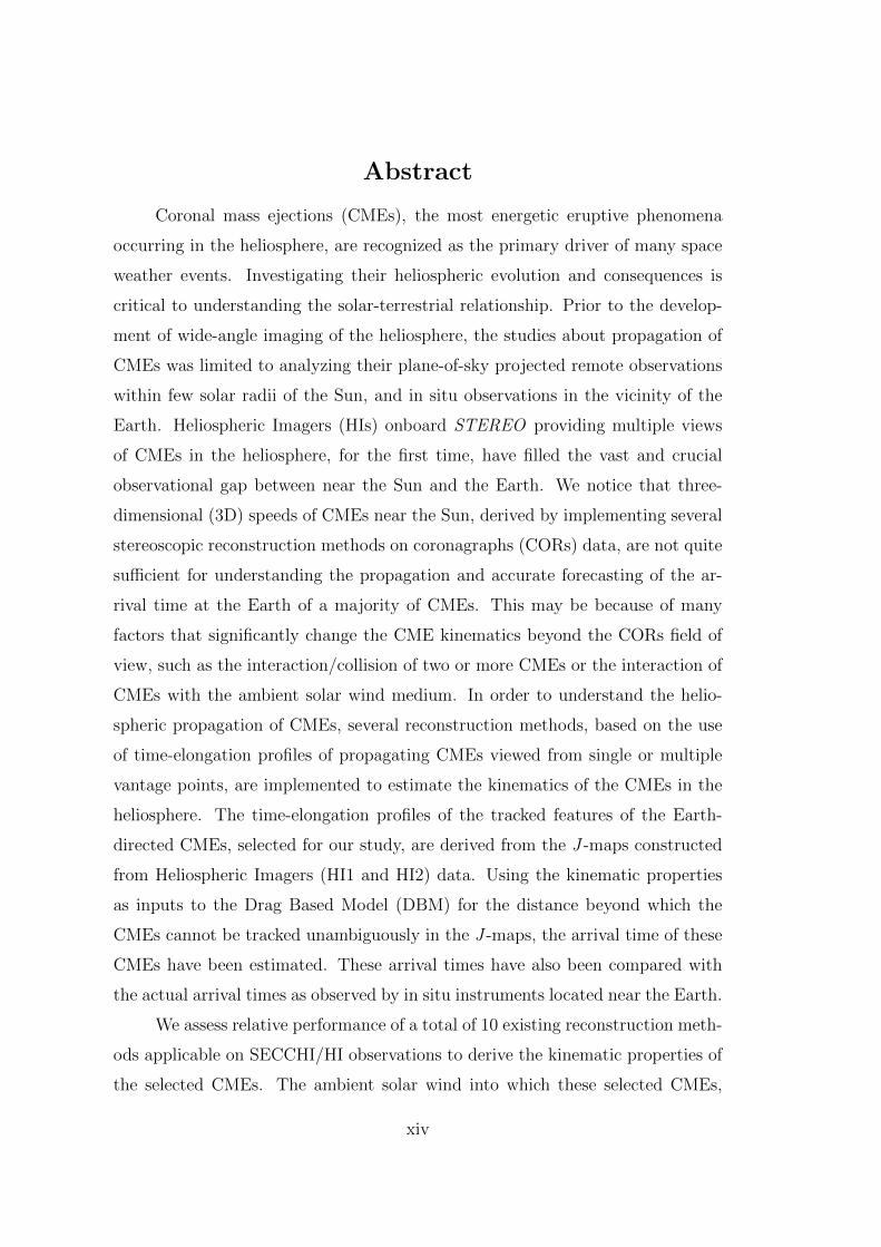
Abstract
Coronal mass ejections (CMEs), the most energetic eruptive phenomena
occurring in the heliosphere, are recognized as the primary driver of many space
weather events. Investigating their heliospheric evolution and consequences is
critical to understanding the solar-terrestrial relationship. Prior to the develop-
ment of wide-angle imaging of the heliosphere, the studies about propagation of
CMEs was limited to analyzing their plane-of-sky projected remote observations
within few solar radii of the Sun, and in situ observations in the vicinity of the
Earth. Heliospheric Imagers (HIs) onboard STEREO providing multiple views
of CMEs in the heliosphere, for the first time, have filled the vast and crucial
observational gap between near the Sun and the Earth. We notice that three-
dimensional (3D) speeds of CMEs near the Sun, derived by implementing several
stereoscopic reconstruction methods on coronagraphs (CORs) data, are not quite
sufficient for understanding the propagation and accurate forecasting of the ar-
rival time at the Earth of a majority of CMEs. This may be because of many
factors that significantly change the CME kinematics beyond the CORs field of
view, such as the interaction/collision of two or more CMEs or the interaction of
CMEs with the ambient solar wind medium. In order to understand the helio-
spheric propagation of CMEs, several reconstruction methods, based on the use
of time-elongation profiles of propagating CMEs viewed from single or multiple
vantage points, are implemented to estimate the kinematics of the CMEs in the
heliosphere. The time-elongation profiles of the tracked features of the Earth-
directed CMEs, selected for our study, are derived from the J -maps constructed
from Heliospheric Imagers (HI1 and HI2) data. Using the kinematic properties
as inputs to the Drag Based Model (DBM) for the distance beyond which the
CMEs cannot be tracked unambiguously in the J -maps, the arrival time of these
CMEs have been estimated. These arrival times have also been compared with
the actual arrival times as observed by in situ instruments located near the Earth.
We assess relative performance of a total of 10 existing reconstruction meth-
ods applicable on SECCHI/HI observations to derive the kinematic properties of
the selected CMEs. The ambient solar wind into which these selected CMEs,
xiv
traveling with different speeds, are launched, is different. Therefore, these CMEs
evolve differently during their journey from the Sun to 1 AU. Our results show
that stereoscopic reconstruction methods perform better, especially those which
take into account the global geometry of a CME and assume that the line of
sight of both observers simultaneously images different parts of a CME. For un-
derstanding the association between remote and in situ observations of CMEs,
we have continuously tracked different density enhanced features using J -maps.
Further, we compared their estimated heliospheric kinematics and arrival time,
and then associated them with features observed in situ.
We have attempted to understand the evolution and consequences of the
interacting/colliding CMEs in the heliosphere using SECCHI/HI, WIND and
ACE observations. By estimating the true mass and 3D kinematics of these
interacting CMEs in the inner heliosphere, we have studied their pre- and post-
collision dynamics, momentum and energy exchange between them during the
collision phase. We found a significant change in the dynamics of the CMEs after
their collision and interaction. Relating heliospheric imaging observations with
in situ measurements at L1, we find that the interacting CMEs move adjacent
to each other after their collision in the heliosphere and are recognized as dis-
tinct structures in in situ observations. These observations also show heating
and compression, formation of magnetic holes (MHs) and interaction region (IR)
as signatures of CME-CME interaction. We also noticed that long-lasting IR,
formed at the rear edge of preceding CME, is responsible for large geomagnetic
perturbations. Our analysis shows an improvement in arrival time prediction of
CMEs using their post-collision dynamics than using pre-collision dynamics. We
also examined the differences in geometrical evolution of slow and fast CMEs
during their propagation in the heliosphere.
Our study highlights the significance of using J -maps constructed from
STEREO/HI observations in studying heliospheric evolution of CMEs, CME-
CME collision, identifying and associating three-part structure of CMEs in their
remote and in stiu observations, and hence for the purpose of improved space
weather forecasting.
xv
List of Publications
I. Research Papers in Refereed Journals:
1. Wageesh Mishra and Nandita Srivastava, 2014, Heliospheric tracking
of enhanced density structures of the 2010 October 6 CME, J. Space
Weather Space Clim., (under revision)
2. Wageesh Mishra, Nandita Srivastava, and D. Chakrabarty, 2015, Evolu-
tion and consequences of interacting CMEs of 9-10 November 2012 using
STEREO/SECCHI and in situ observations, Solar Phys., 290, 527.
3. Wageesh Mishra and Nandita Srivastava, 2014, Morphological and kine-
matic evolution of three interacting coronal mass ejections of 2011 February
13-15, Astrophys. J., 794, 64.
4. Wageesh Mishra, Nandita Srivastava, and Jackie A. Davies, 2014, A
comparison of reconstruction methods for the estimation of coronal mass
ejections kinematics based on SECCHI/HI observations, Astrophys. J.,
784, 135.
5. Wageesh Mishra and Nandita Srivastava, 2013, Estimating the arrival
time of earth-directed coronal mass ejections at in situ spacecraft using COR
and HI observations from STEREO, Astrophys. J., 772, 70.
II. Research Papers in Proceedings:
1. Wageesh Mishra and Nandita Srivastava, 2013, Estimating arrival time
of 10 October 2010 CME using STEREO/SECCHI and in situ observations
ASI Conference Series, 10, 127.
xvi
Chapter 1
Introduction
1.1 The Sun
The early humans of several countries and civilizations had considered the
Sun as their God or Goddess and worshipped it. This is possibly because they
realized from their daily experience that without the Sun there will be no light,
warmth, life, change in seasons, and measurement of time on the Earth. Even
in modern times, the Sun is worshipped in many countries and religions. Un-
derstanding the importance of the Sun, several observatories or observing sites
were built and used by various civilizations around the globe, beginning from the
middle neolithic period (Mukerjee, 2003, Bhatnagar and Livingston, 2005, ch. 1;
Boser, 2006).
With the progress made in the field of astronomy, it is now well understood
that the Sun is the nearest star from the Earth, and therefore it can be observed
with good spatial resolution and studied in details. The Sun being in plasma state
acts as a laboratory to test and understand various theories of plasma physics.
In addition, the study of the Sun is important from the astrophysics perspective,
in general. The modern space and ground based observations have unmasked the
dynamic and active nature of the Sun in the form of sunspots, faculae, filaments,
prominences, coronal holes, flares, and coronal mass ejections (CMEs). Further,
the Sun is the driving factor for the terrestrial and space weather, therefore the
study of solar-terrestrial relations is of great importance for our space and ground
1
Chapter 1. Introduction
based technological systems as well as for human life and health.
The Sun is a main sequence star of spectral type G2V with mass M� ≈1.98 × 1030 kg, luminosity L� ≈ 3.84 × 1026 W and radius R� ≈ 6.96 × 10⁸
m (Lang, 2006, p. 24). The mass of the Sun is about 99% of the total mass of
the solar system. The solar system, to which the Sun, the 8 planets, asteroids,
meteorites, comets and other small dust particles belong, is located in our Milky
Way galaxy. Similar to other stars, the Sun was born from the gravitational
collapse of a molecular cloud approximately around 4.6 × 10⁹ years ago, and now
is currently in a state of hydrostatic equilibrium. It is predicted that the Sun will
enter in a red giant phase in another ≈ 5 billion years before ending its life as a
white dwarf (Foukal, 2004, p. 432).
1.2 Structure of the Sun
1.2.1 Solar interior
The modern picture of the internal structure of the Sun has been built up
over time. The three most important contributions to this have been the ‘standard
solar model’ (SSM; Bahcall et al. 1982), helioseismology (Leibacher et al., 1985),
and solar neutrino observations (Bahcall, 2001). As the interior of the Sun cannot
be directly observed, its structure is modeled and then compared to the observed
properties by iteratively changing the model parameters, until they match the
observations. The SSM is essentially several differential equations, constrained
by boundary conditions (mass, radius, and luminosity of the Sun), which are
derived from the principles of fundamental physics. Helioseismology allows us to
probe the solar interior by studying the propagation of waves in the Sun, mainly
the sound waves (Leighton, Noyes, and Simon, 1962; Ulrich, 1970).
The Sun’s interior includes the core, the radiation zone, and the convection
zone. The core, which extends out to about 0.25 R� from the center, is at a
temperature of about 1.5 × 10⁷ K and has a density ≈ 1.5 × 10⁵ kg m−3 (Lang,
2006, p. 24). The core of the Sun is the source of its energy via the process of
thermonuclear fusion which results in the formation of heavier elements as well
2
Chapter 1. Introduction
as the release of energy in the form of gamma ray photons.
Outside the core is the radiative zone which extends out from 0.25 R� to
0.70 R�. The gamma photons produced in the core are absorbed and re-emitted
repeatedly by nuclei in the radiative zone, with the re-emitted photons having
successively lower energies and longer wavelengths. The temperature drops from
about 7 × 10⁶ K at the bottom of the radiative zone to 2 × 10⁶ K just at the
top of the radiative zone. Due to the high density (≈ 2 × 10⁴ kg m−3) in the
radiative zone, the mean free path of the photons is very small (≈ 9.0 × 10⁻²
cm), hence the photons take approximately tens to hundreds of thousands of
years to travel through the radiative zone (Mitalas and Sills, 1992). Hence, if the
energy generation processes in the core of the Sun suddenly stopped, the sun will
continue to shine for millions of years.
Above the radiative zone is the convective zone extending from about 0.70
R� to 1 R� at the surface of the Sun. The convection zone rotates differen-
tially and temperature in this zone decreases very rapidly with increasing height
and becomes around 5700 K at its outer boundary. In this zone the energy is
transported by convection. Hot regions at the bottom of this layer become buoy-
ant and rise, cooler material from above descends, and giant convective cells are
formed which can be seen on the surface of the Sun (i.e. photosphere) as granules.
In the convection zone, the temperature gradient set up by radiative transport
is larger than adiabatic gradient and hence a convection pattern is established
(Foukal, 2004, p. 204). Convective circulation of plasma (charged particles) gen-
erates large magnetic fields that play an important role in producing solar activity
on the Sun. From the recent helioseismology results, it has been proposed that
around 0.7 R� from the center of the Sun (i.e. transition layer between radiative
and convective zone with thickness of 0.04 R�), the solar magnetic fields are gen-
erated through a dynamo mechanism. Here the sound speed and density profiles
show a distinct sudden ‘bump’ called the tachocline (Spiegel and Zahn, 1992).
3
Chapter 1. Introduction
1.2.2 Solar atmosphere
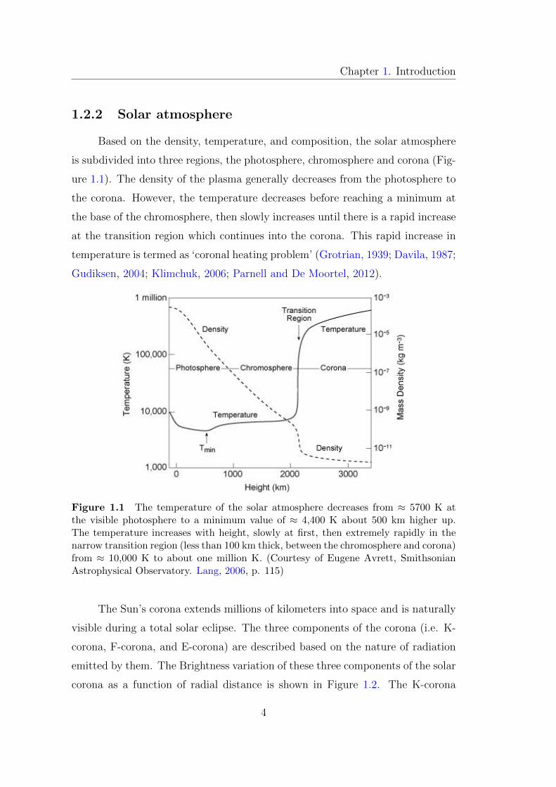
Based on the density, temperature, and composition, the solar atmosphere
is subdivided into three regions, the photosphere, chromosphere and corona (Fig-
ure 1.1). The density of the plasma generally decreases from the photosphere to
the corona. However, the temperature decreases before reaching a minimum at
the base of the chromosphere, then slowly increases until there is a rapid increase
at the transition region which continues into the corona. This rapid increase in
temperature is termed as ‘coronal heating problem’ (Grotrian, 1939; Davila, 1987;
Gudiksen, 2004; Klimchuk, 2006; Parnell and De Moortel, 2012).
Figure 1.1 The temperature of the solar atmosphere decreases from ≈ 5700 K atthe visible photosphere to a minimum value of ≈ 4,400 K about 500 km higher up.The temperature increases with height, slowly at first, then extremely rapidly in thenarrow transition region (less than 100 km thick, between the chromosphere and corona)from ≈ 10,000 K to about one million K. (Courtesy of Eugene Avrett, SmithsonianAstrophysical Observatory. Lang, 2006, p. 115)
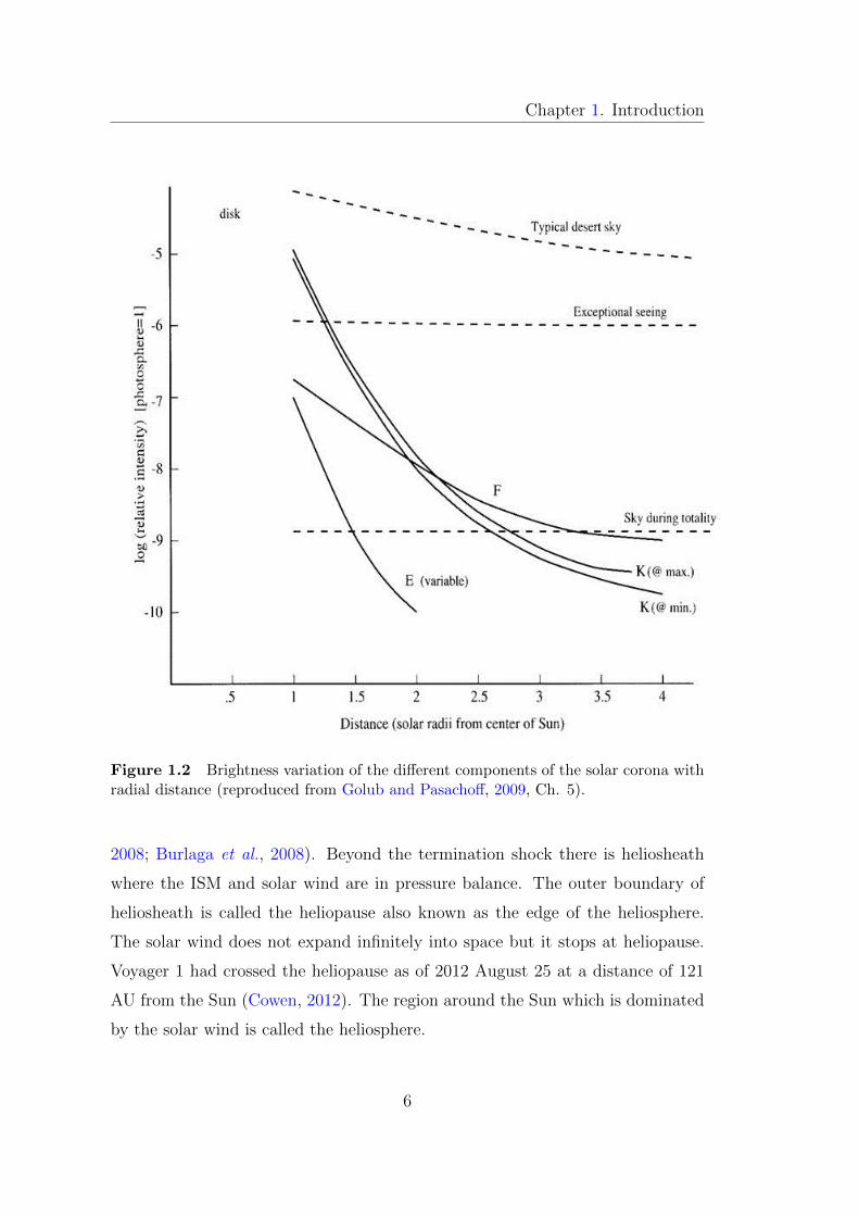
The Sun’s corona extends millions of kilometers into space and is naturally
visible during a total solar eclipse. The three components of the corona (i.e. K-
corona, F-corona, and E-corona) are described based on the nature of radiation
emitted by them. The Brightness variation of these three components of the solar
corona as a function of radial distance is shown in Figure 1.2. The K-corona
4
Chapter 1. Introduction
dominates between 1.03 R�-2.5 R�. From this region, the emitted scattered light
from the coronal plasma shows the continuous spectrum of the photosphere with
no Fraunhofer lines and is found to be strongly polarised. The F-corona dominates
beyond 2.5 R� displays the solar spectrum with Fraunhofer lines superimposed
on the continuum. The outer part of the F-corona is observed to merge into
the zodiacal light. The E-corona is due to spectral line emission from visible to
EUV by several atoms and ions in the inner part of the corona, containing many
forbidden line transitions, thus it contains many polarization states. These lines
provide information on very low density and extremely high temperature of the
corona. The density of the particles is only of the order of 106 to 108 cm−3 as
against the value of 1010 to 1012 cm−3 for chromosphere and of 1016 to 1017 cm−3
for the photosphere (Golub and Pasachoff, 2009, ch. 1).
1.2.3 Solar wind and the heliosphere
The solar wind is constant out-stream of charged particles of plasma (mix-
ture of ions and electrons) from the Sun’s atmosphere and fills the space around
the Sun (Biermann, 1951; Parker, 1958). The outer atmosphere of the Sun (i.e.
corona) is so hot that even the gravity of the Sun can not prevent it from con-
tinuously evaporating. The escaping particles carry energies of ≈ 1 keV, and is
observed in two states of fast and slow speed. The slow solar wind has speed of
≈ 400 km s−1 with a typical proton density of ≈ 10 cm−3 and the fast solar wind
has speed of ≈ 800 km s−1 with a typical proton density of ≈ 3 cm−3 (Schwenn
and Marsch, 1990). In 1973, in the Skylab era, sources of fast speed solar wind
was discovered as coronal holes (Krieger, Timothy, and Roelof, 1973). Coronal
holes are usually found where “open” magnetic field lines prevail.
As the solar wind runs into the interstellar medium (ISM) it becomes
abruptly slow from being supersonic to sub-sonic speed at a certain location from
the Sun. This location in ISM is called the termination shock. The Voyager 1
spacecraft in 2004 and Voyager 2 spacecraft in 2007 passed through the termina-
tion shock at ≈ 94 AU and 84 AU from the Sun, respectively (Richardson et al.,
5
Chapter 1. Introduction
Figure 1.2 Brightness variation of the different components of the solar corona withradial distance (reproduced from Golub and Pasachoff, 2009, Ch. 5).
2008; Burlaga et al., 2008). Beyond the termination shock there is heliosheath
where the ISM and solar wind are in pressure balance. The outer boundary of
heliosheath is called the heliopause also known as the edge of the heliosphere.
The solar wind does not expand infinitely into space but it stops at heliopause.
Voyager 1 had crossed the heliopause as of 2012 August 25 at a distance of 121
AU from the Sun (Cowen, 2012). The region around the Sun which is dominated
by the solar wind is called the heliosphere.
6
Chapter 1. Introduction
1.3 Coronal Mass Ejections
Observations of solar corona has been carried out earlier during solar
eclipses. The earliest observation of a Coronal Mass Ejection (CME) proba-
bly dates back to the eclipse of 1860 which is clear from a drawing recorded by
G. Temple. Then, in space era, a CME was imaged on 1971 December 14 by a
coronagraph on board the seventh Orbiting Solar Observatory (OSO-7) satellite
(Tousey, 1973). A coronagraph is an instrument which blocks the photospheric
light from the disk of the Sun and observes the corona by creating an artifi-
cial eclipse. After the discovery of CME from OSO-7, thousands of CMEs have
been observed from a series of space-based coronagraphs e.g. Apollo Telescope
Mount on board Skylab (Gosling et al., 1974), Solwind coronagraph on board
P78-1 satellite (Sheeley et al., 1980), Coronagraph/Polarimeter on board Solar
Maximum Mission (SMM) (MacQueen et al., 1980), Large Angle Spectrometric
COronagraph (LASCO) on board SOlar and Heliospheric Observatory (Brueck-
ner et al., 1995), and the coronagraphs (CORs) on Solar TErrestrial RElations
Observatory (STEREO) (Howard et al., 2008). These observations were comple-
mented by white light data from the ground-based Mauna Loa Solar Observatory
(MLSO) K-coronameter which had a FOV from 1.2 R�-2.9 R� (Fisher et al.,
1981) and emission line observations from the coronagraphs at Sacramento Peak,
New Mexico (Demastus, Wagner, and Robinson, 1973) and Norikura, Japan (Hi-
rayama and Nakagomi, 1974).
The name CME was initially coined for a feature which shows an observable
change in coronal structure that occurs on a time scale of few minutes to several
hours and involves the appearance (and outward motion) of a new, discrete,
bright, white-light feature in the coronagraphic field of view (FOV) (Hundhausen
et al., 1984). It is now well established that CMEs are frequent expulsions of
magnetized plasma from the Sun into the heliosphere. In white light observations,
it is noted that the frequency of occurrence of CMEs around solar maximum is
≈ 5 per day and at solar minimum is ≈ 1 per day (St. Cyr et al., 2000; Webb
and Howard, 2012).
7
Chapter 1. Introduction
It is evident from a survey of literature that consequences of CME have
been observed well before its discovery in 1971. For example, CMEs were ob-
served at larger distances from the Sun in radio via interplanetary scintillation
(IPS) observations from the 1960s. However, only around 1980s the associa-
tion between IPS and CMEs could be established (Hewish, Scott, and Wills,
1964; Houminer and Hewish, 1972; Tappin, Hewish, and Gapper, 1983). The IPS
technique is based on measurements of the fluctuating intensity level of a large
number of point-like distant meter-wavelength radio sources. Also, the zodiacal
light photometers on the twin Helios spacecraft during 1975 to 1983 (Richter,
Leinert, and Planck, 1982) have observed the regions in the inner heliosphere
from 0.3 AU to 1.0 AU but with an extremely limited FOV. In the present era
of heliospheric imagers, e.g. Solar Mass Ejection Imager (SMEI) (Eyles et al.,
2003) on board the Coriolis spacecraft launched early in 2003 and Heliospheric
Imagers (HIs) (Eyles et al., 2009) launched on the twin STEREO spacecraft in
late 2006, several CMEs have been observed far from the Sun. SOHO/LASCO
has detected well over 104 CMEs till date and still continues (Yashiro et al.
2004; http://cdaw.gsfc.nasa.gov/CME_list/). SMEI observed nearly 400
transients during its 8.5 year lifetime, it was switched off in September 2011.
The number of CME “events” reported using the HIs on board STEREO is now
more than one thousand (http://www.stereo.rl.ac.uk/HIEventList.html),
although less than 100 have been discussed so far in the scientific literature (Webb
and Howard, 2012).
1.3.1 Observations of CMEs
In white light images, CMEs are seen due to Thomson scattering of pho-
tospheric light from the free electrons of coronal and heliospheric plasma. The
intensity of Thomson scattered light has an angular dependence which must be
accounted for the measured brightness of CMEs (Billings, 1966; Vourlidas and
Howard, 2006; Howard and Tappin, 2009). They are faint relative to the back-
ground corona, but much more transient, therefore a suitable coronal background
8
Chapter 1. Introduction
subtraction is applied to identify them. The advantage of white light observations
over radio, IR or UV observations is that Thomson scattering only depends on
the observed electron density and is independent of the wavelength and tempera-
ture (Hundhausen, 1993). The coronagraphs record two-dimensional (2D) image
of a three-dimensional (3D) CME projected onto the plane of sky. Therefore,
the morphology of CME in coronagraphic observations depends on the location
of the observing instruments (e.g. coronagraphs) and launch direction of CME
from the Sun. The CMEs launched from the Sun toward or away from the Earth,
when observed from the near Earth coronagraphs (e.g. LASCO coronagraph on
board SOHO located at L1 point of Sun-Earth system), will appear as ‘halos’
surrounding the occulting disk of coronagraphs (Howard et al., 1982). Such a
CME is called a “halo” CME (Figure 1.3). A CME having 360◦ apparent angular
width is called “full halo” CME and with apparent angular width greater than
120◦ but less than 360◦ is called as “partial halo”. Thus, the nomenclature of a
CME is restricted by its viewing perspective. The observations of solar activity
on the solar disk, associated with CME, are necessary to help distinguish whether
a halo CME was launched from the front or backside of the Sun relative to the
observer. Front side halo CMEs observed by SOHO/LASCO are important as
they are the key link between solar eruptions and major space weather phenom-
ena such as geomagnetic storms and solar energetic particle events. Such CMEs
that are launched from near the disk center tend to be more geoeffective while
those closer to solar limb are less so. It is important to note that among all the
CMEs, only about 10% are partial halo type (i.e. width greater than 120◦) and
about 4% are full halo type (Webb et al., 2000).
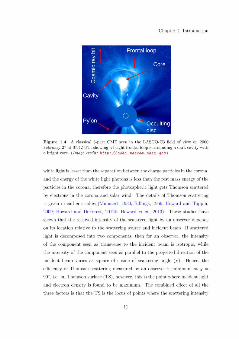
A typical CME observed near the Sun often appears as “three-part” struc-
ture comprising of an outer bright frontal loop (i.e. leading edge), and a darker
underlying cavity within which is embedded a brighter core as shown in Fig-
ure 1.4 (Illing and Hundhausen, 1985). The front may contain swept-up material
by erupting flux ropes or the presence of pre-existing material in the overlying
fields (Illing and Hundhausen, 1985; Riley et al., 2008). The cavity is a region of
lower plasma density but probably higher magnetic field strength. The core of
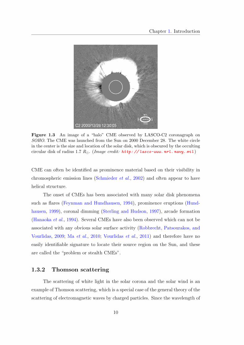
9
Chapter 1. Introduction
Figure 1.3 An image of a “halo” CME observed by LASCO-C2 coronagraph onSOHO. The CME was launched from the Sun on 2000 December 28. The white circlein the center is the size and location of the solar disk, which is obscured by the occultingcircular disk of radius 1.7 R�. (Image credit: http: // lasco-www. nrl. navy. mil )
CME can often be identified as prominence material based on their visibility in
chromospheric emission lines (Schmieder et al., 2002) and often appear to have
helical structure.
The onset of CMEs has been associated with many solar disk phenomena
such as flares (Feynman and Hundhausen, 1994), prominence eruptions (Hund-
hausen, 1999), coronal dimming (Sterling and Hudson, 1997), arcade formation
(Hanaoka et al., 1994). Several CMEs have also been observed which can not be
associated with any obvious solar surface activity (Robbrecht, Patsourakos, and
Vourlidas, 2009; Ma et al., 2010; Vourlidas et al., 2011) and therefore have no
easily identifiable signature to locate their source region on the Sun, and these
are called the “problem or stealth CMEs”.
1.3.2 Thomson scattering
The scattering of white light in the solar corona and the solar wind is an
example of Thomson scattering, which is a special case of the general theory of the
scattering of electromagnetic waves by charged particles. Since the wavelength of
10
Chapter 1. Introduction
Frontal loop
Cavity
Core
Occulting
disc
Pylon
Co
sm
ic r
ay h
it
Figure 1.4 A classical 3-part CME seen in the LASCO-C3 field of view on 2000February 27 at 07:42 UT, showing a bright frontal loop surrounding a dark cavity witha bright core. (Image credit: http: // soho. nascom. nasa. gov )
white light is lesser than the separation between the charge particles in the corona,
and the energy of the white light photons is less than the rest mass energy of the
particles in the corona, therefore the photospheric light gets Thomson scattered
by electrons in the corona and solar wind. The details of Thomson scattering
is given in earlier studies (Minnaert, 1930; Billings, 1966; Howard and Tappin,
2009; Howard and DeForest, 2012b; Howard et al., 2013). These studies have
shown that the received intensity of the scattered light by an observer depends
on its location relative to the scattering source and incident beam. If scattered
light is decomposed into two components, then for an observer, the intensity
of the component seen as transverse to the incident beam is isotropic, while
the intensity of the component seen as parallel to the projected direction of the
incident beam varies as square of cosine of scattering angle (χ). Hence, the
efficiency of Thomson scattering measured by an observer is minimum at χ =
90◦, i.e. on Thomson surface (TS), however, this is the point where incident light
and electron density is found to be maximum. The combined effect of all the
three factors is that the TS is the locus of points where the scattering intensity
11
Chapter 1. Introduction
is maximized however a spread of the observed intensity to larger distances from
the TS is noted. This spreading is called ‘Thomson plateau’ which is greater at
larger distances (elongations) from the Sun, where elongation is the Sun-observer-
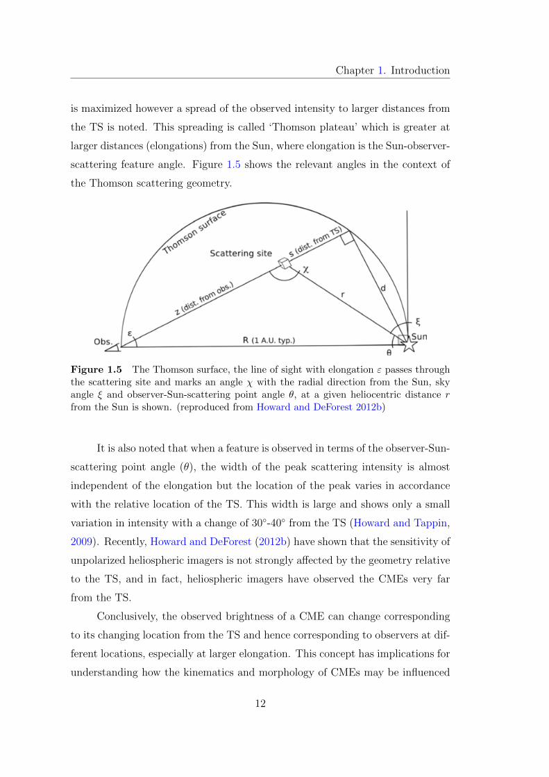
scattering feature angle. Figure 1.5 shows the relevant angles in the context of
the Thomson scattering geometry.
Figure 1.5 The Thomson surface, the line of sight with elongation ε passes throughthe scattering site and marks an angle χ with the radial direction from the Sun, skyangle ξ and observer-Sun-scattering point angle θ, at a given heliocentric distance rfrom the Sun is shown. (reproduced from Howard and DeForest 2012b)
It is also noted that when a feature is observed in terms of the observer-Sun-
scattering point angle (θ), the width of the peak scattering intensity is almost
independent of the elongation but the location of the peak varies in accordance
with the relative location of the TS. This width is large and shows only a small
variation in intensity with a change of 30◦-40◦ from the TS (Howard and Tappin,
2009). Recently, Howard and DeForest (2012b) have shown that the sensitivity of
unpolarized heliospheric imagers is not strongly affected by the geometry relative
to the TS, and in fact, heliospheric imagers have observed the CMEs very far
from the TS.
Conclusively, the observed brightness of a CME can change corresponding
to its changing location from the TS and hence corresponding to observers at dif-
ferent locations, especially at larger elongation. This concept has implications for
understanding how the kinematics and morphology of CMEs may be influenced
12
Chapter 1. Introduction
from different locations of the observers.
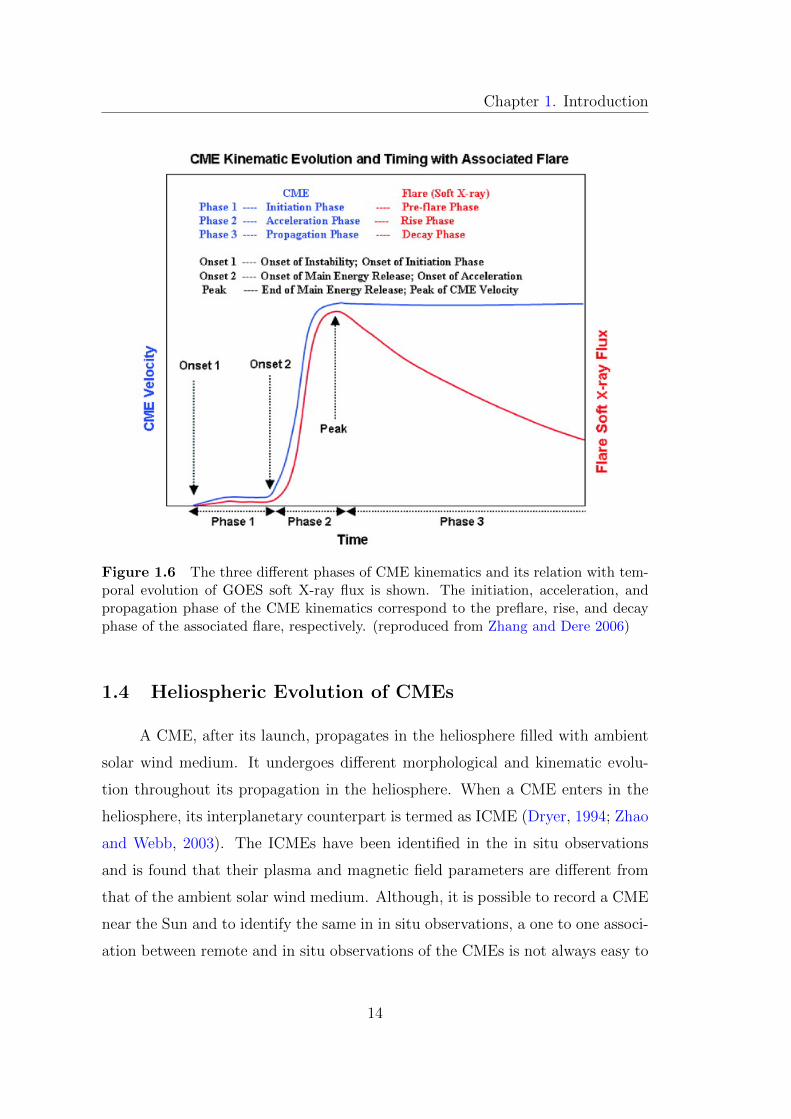
1.3.3 Properties of CMEs
CMEs are characterized by their speed, angular width, source location rel-
ative to solar disk, mass and energies. It is noted that speeds of CMEs near
the Sun range from few km s−1 to 3000 km s−1 (St. Cyr et al., 2000). After a
distance of about 2 R� from the Sun, CMEs accelerate or decelerate slowly in
the FOV of coronagraphs (St. Cyr et al., 2000; Yashiro et al., 2004). It is also
found that a typical CME shows three-phase kinematic profile, first, a slow rise
over tens of minutes, then a rapid acceleration between 1.4 R�-4.5 R� during the
main phase of a flare, and finally a propagation phase with constant or decreasing
speed (Zhang and Dere, 2006). These three distinct phases of a CME are shown
in Figure 1.6. Excluding the partial and full halo CMEs, the apparent angular
width of CMEs is found to vary from few degrees to more than 120◦, with an
average value of about ≈ 50◦ (Yashiro et al., 2004). The source locations of a
majority of CMEs are near the solar equator between 25◦ N and S, around the
solar minimum, however, few CMEs are seen at higher latitudes also (St. Cyr
et al., 2000). The estimated total mass of CMEs range from 1010 kg to 1013 kg,
and the total energy from 1020 J to 1026 J. The average mass and energy of a
CME is 1.4 × 10¹² kg and 2.6 × 10²³ J, respectively (Vourlidas et al., 2002).
It is noted that aforementioned properties of CMEs are estimated from the
2D coronagraphic images of CMEs and therefore are subject to the problem of pro-
jection and perspective. These studies are based on the plane of sky assumption,
i.e. CMEs are propagating orthogonal to observer, therefore if this assumption
is not fulfilled, the speed, mass, and energies of CMEs will be underestimated
(Vourlidas et al., 2010) while the angular width will be severely overestimated
(Burkepile et al., 2004). These properties derived from a statistical study, will
also depend on the sensitivity of the coronagraphs and the selection of sample of
CMEs.
13
Chapter 1. Introduction
Figure 1.6 The three different phases of CME kinematics and its relation with tem-poral evolution of GOES soft X-ray flux is shown. The initiation, acceleration, andpropagation phase of the CME kinematics correspond to the preflare, rise, and decayphase of the associated flare, respectively. (reproduced from Zhang and Dere 2006)
1.4 Heliospheric Evolution of CMEs
A CME, after its launch, propagates in the heliosphere filled with ambient
solar wind medium. It undergoes different morphological and kinematic evolu-
tion throughout its propagation in the heliosphere. When a CME enters in the
heliosphere, its interplanetary counterpart is termed as ICME (Dryer, 1994; Zhao
and Webb, 2003). The ICMEs have been identified in the in situ observations
and is found that their plasma and magnetic field parameters are different from
that of the ambient solar wind medium. Although, it is possible to record a CME
near the Sun and to identify the same in in situ observations, a one to one associ-
ation between remote and in situ observations of the CMEs is not always easy to
14
Chapter 1. Introduction
establish. There may be several factors responsible for this which are discussed
below.
It is understood that fast CMEs often generate large-scale density waves out
into space which finally steepen to form collisionless shock waves (Gopalswamy
et al., 1998b). This shock wave is similar to the bow shock formed in front of the
Earth’s magnetosphere. Following the shock there is a sheath structure which
has signatures of significant heating and compression of the ambient solar wind
(Manchester et al., 2005). After the shock and the sheath, the ICME structure is
found. The main problem in understanding the evolution of CMEs is our limited
knowledge about their physical properties. In addition, remote sensing observa-
tions (e.g. coronagraphs) do not provide plasma and magnetic field parameters
of CMEs. Several attempts in the recent past have been made for associating
near Earth in situ observed structures of ICME by Advanced Composition Ex-
plorer (ACE ) (Stone et al., 1998) and WIND (Ogilvie et al., 1995) spacecraft
with observed Earth-directed front-side halos CMEs in LASCO coronagraph im-
ages. Such studies have suffered severely because of difficulties in determining
3D speed of Earth-directed CMEs. Another problem is that an in situ spacecraft
takes measurements along a certain trajectory through the ICME, therefore does
not provide the global characteristics of CME plasma.
Different ICME structures may have strong, out-of the ecliptic components
and therefore a southward pointing interplanetary magnetic field (IMF). Such
southward Bz, different than usual Parker spiral, have potential to produce severe
consequences on the Earth’s geomagnetism (Dungey, 1961; Tsurutani et al., 1988;
Gonzalez et al., 1994). Keeping in mind the goal of understanding the Sun-Earth
connection, several studies have been undertaken to estimate the arrival time of
CMEs at 1 AU near the Earth.
1.4.1 CME studies before STEREO era
Before the launch of STEREO in 2006, several studies (Schwenn, 2006,
and references therein) were carried out using imaging observations from several
15
Chapter 1. Introduction
space based instruments mentioned in Section 1.3. Among all the space based in-
struments dedicated to observe the CMEs, the SOHO/LASCO launched in 1995
can be considered as the most successful mission in observing several thousand
CMEs which led to several research papers. SOHO/LASCO with three corona-
graphs C1 (no longer operating since June 1998), C2, and C3 could observe the
solar corona from 1.1 R� to 30 R�, with overlapping FOV. Using these observa-
tions, studies were carried out to estimate the source location, mass, kinematics,
morphology and arrival time of CMEs (St. Cyr et al., 2000; Xie, Ofman, and
Lawrence, 2004; Schwenn et al., 2005, and references therein). To explain the
initiation and propagation of CMEs, several theoretical models have also been
developed (Chen, 2011, and references therein). However, these models differ
from one another considerably in the involved mechanism of progenitor, trigger-
ing, and eruption of CME. Realizing the consequences of CMEs on our modern
high-tech society, several studies were dedicated to find a correlation between
intensity of magnetic disturbances on the Earth’s surface with the characteristics
of CMEs estimated near the Sun (Gosling et al., 1990; Srivastava and Venkatakr-
ishnan, 2002, 2004). Based on the angular width, CMEs were classified as halo,
symmetric halo, asymmetric halo, partial halo, limb, and narrow CMEs. Fur-
ther, based on the acceleration profile, the CMEs were classified as gradual and
impulsive CMEs (Sheeley et al., 1999; Srivastava et al., 1999). However, it is
believed that all the CMEs belong to a dynamical continuum with a single phys-
ical initiation process (Crooker, 2002). With the availability of complementary
disk observations of solar active regions and prominences, statistical studies on
association of different types of CMEs with flares and prominences were carried
out in details (Kahler, 1992; Gopalswamy et al., 2003b, and references therein).
1.4.1.1 CME kinematics and their arrival time at L1
Several studies of evolution of CMEs were carried out using SOHO/LASCO
observations, in situ observations near the Earth by ACE and WIND combined
with modeling efforts (Gopalswamy et al., 2000a, 2001a, 2005; Yashiro et al., 2004;
Wood et al., 1999; Andrews, Wang, and Wu, 1999). These studies were based
16
Chapter 1. Introduction
on understanding of the kinematics of CMEs using two point measurements, one
near the Sun up to a distance of 30 R� using coronagraph (LASCO/C2 and C3)
images, and the other near the Earth using in situ instruments. Using the LASCO
images, one could estimate the projected speeds of CMEs, although we lacked
information about the 3D speed and direction of the Earth-directed CMEs. These
studies, carried out to calculate the kinematics and the travel time of CMEs from
the Sun to the Earth, suffered from a lot of assumptions regarding the geometry
and evolution of a CME in the interplanetary medium (Howard and Tappin, 2009;
Vrsnak et al., 2010).
Various models have been developed to forecast the CME arrival time at 1
AU, based on an empirical relationship between measured projected speeds and
arrival time characteristics of various events (Gopalswamy et al., 2001b; Vrsnak
and Gopalswamy, 2002; Schwenn et al., 2005). However, the empirical models
have inherent difficulties and individual CMEs must be studied separately in
order to derive their kinematics and morphology to be compared with theoretical
models. Also few attempts have been made to fit the observed kinematics profiles
of CMEs using an appropriate mathematical function (Gallagher, Lawrence, and
Dennis, 2003). The above mentioned studies are subject to large uncertainties
due to projection effects. To overcome the projection effects, the methods such
as forward modeling, which approximates a CME as a cone (Zhao, Plunkett, and
Liu, 2002; Xie, Ofman, and Lawrence, 2004; Xue, Wang, and Dou, 2005) and
varies the model parameters to best fit the 2D observations of CME, have been
used to estimate the CME kinematics. However, this derived kinematics is also
subject to several new sources of errors due to presumed geometry of the CME.
Another method known as polarimetric technique, using the ratio of unpolarised
to polarised brightness of the Thomson-scattered K-corona, has been applied to
estimate the average line of sight distance of CME from the instrument plane of
sky (Moran and Davila, 2004). This technique is only applicable up to ≈ 5 R�
because beyond this the F-corona cannot be considered as unpolarised.
Analytical drag-based models (DBM; e.g., Vrsnak and Zic, 2007; Lara and
Borgazzi, 2009; Vrsnak et al., 2010) and numerical MHD simulation models (e.g.,
17
Chapter 1. Introduction
Odstrcil, Riley, and Zhao, 2004; Manchester et al., 2004; Smith et al., 2009) have
been developed and used to predict CME arrival times (Dryer et al., 2004; Feng
et al., 2009; Smith et al., 2009). These studies show that the predicted arrival
time is usually within an error of ± 10 hr but sometimes the errors can be larger
than 24 hr. Many studies have also shown that CMEs interact significantly with
the ambient solar wind as they propagate in the interplanetary medium, resulting
in acceleration of slow CMEs and deceleration of fast CMEs toward the ambient
solar wind speed (Lindsay et al., 1999; Gopalswamy et al., 2000a, 2001b; Yashiro
et al., 2004; Manoharan, 2006; Vrsnak and Zic, 2007). The interaction between the
solar wind and the CME is understood in terms of a ‘drag force’ (Cargill et al.,
1996; Vrsnak and Gopalswamy, 2002). However, even during the propagation
phase of a CME the role of Lorentz force is acknowledged in some earlier studies
(Kumar and Rust, 1996; Subramanian and Vourlidas, 2005, 2007; Subramanian
et al., 2014). Despite several studies on CME propagation, very little is known
about the exact nature of the forces governing the propagation of CME. However,
it is obvious from the observations that there must be some forces acting on the
CME which tend to equalize the CME velocity to that of the background solar
wind speed.
1.4.1.2 In situ observations of CMEs
As previously mentioned, a CME in the interplanetary medium is known
as ICME. Various plasma, magnetic field and compositional parameters of an
ICME are measured by in situ spacecraft at the instant when it intersects the
ICME. The identification of ICME in in situ data is not very straightforward and
is based on several signatures which are summarized below.
Magnetic field signatures in the plasma
The ICME in in situ observations is identified based on the increased magnetic
field strength and reduced variability in magnetic field (Klein and Burlaga, 1982).
A subset of ICMEs is known as Magnetic Cloud (MC) which shows additional
signatures such as enhanced magnetic field greater than ≈ 10 nT, smooth rotation
18
Chapter 1. Introduction
of magnetic field vector by greater than ≈ 30◦, and plasma β (ratio of thermal
and magnetic field energies) less than unity (Lepping, Burlaga, and Jones, 1990;
Burlaga, 1991).
Dynamics signatures in the plasma
The ICME in in situ data is identified by its characteristics of expansion in the
ambient solar wind. Due to expansion, CMEs also show depressed proton tem-
perature inside the ICME in contrast to ambient solar wind. ICME leading edge,
i.e. front has speed greater than its trailing edge and the difference of speeds at
boundaries is equal to two times the expansion speed of CME. Hence, a mono-
tonic decrease in the plasma velocity inside a ICME is noticed (Klein and Burlaga,
1982). According to Lopez (1987), for the normal solar wind there is an empirical
relation between proton temperature and solar wind speed as follow:
Texp = (0.031Vsw − 5.1)2 × 10³, when Vsw < 500 km s−1 (1.1a)
Texp = (0.51Vsw − 142)× 103, when Vsw > 500 km s−1 (1.1b)
However, Richardson and Cane (1995) found that ICMEs typically have Tp
< 0.5 Texp , where Texp is “expected” temperature determined from the equa-
tion 1.1. Also, Neugebauer and Goldstein (1997) defined a thermal index (Ith)
using the observed proton temperature and proton velocity and found that Ith
> 1 for the plasma associated with an ICME, while this may or may not be the
case when Ith < 1. The equation for thermal index is as below:
Ith = (500Vp + 1.75× 10⁵)/Tp (1.2)
It is also noted that in an ICME, the electron temperature (Te) is greater
than proton temperature (Tp). Richardson, Farrugia, and Cane (1997) proposed
the ratio of electron to proton temperature, i.e. Te/Tp > 2 is a good indicator of
an ICME.
19

Chapter 1. Introduction
Compositional signatures in the plasma
The composition of an ICME is different than the ambient solar wind medium.
In situ observations have shown that alpha to proton ratio (He+2/H) is higher
(> 6%) inside an ICME than its values in normal solar wind. This suggested
that an ICME also contains material from the solar atmosphere below the corona
(Hirshberg, Asbridge, and Robbins, 1971; Zurbuchen et al., 2003). It is observed
that relative to the solar wind, an ICME shows an enhancement in value of
3He+2/4He+2 (Ho et al., 2000), heavy ion abundances (especially iron) and its
enhanced charge states (Lepri et al., 2001; Lepri and Zurbuchen, 2004). ICME
associated plasma with enhanced charge states of iron suggest that CME source
is “hot” relative to the ambient solar wind. It is also noted that ICME shows
relative enhancement of O+7/O+6 (Richardson and Cane, 2004; Rodriguez et al.,
2004). However, few CMEs have been identified with unusual low ion charge
states such as presence of singly-charged helium abundances well above solar
wind values (Schwenn, Rosenbauer, and Muehlhaeuser, 1980; Burlaga et al., 1998;
Skoug et al., 1999). Such low charge states suggest that the plasma is associated
with possibly the cool, and dense prominence material (Gopalswamy et al., 1998a;
Lepri and Zurbuchen, 2010; Sharma and Srivastava, 2012).
Energetic particles signatures in the plasma
Since, ICMEs have loops structures rooted at the Sun, therefore the presence of
bidirectional beams of suprathermal (≥ 100 eV) electrons (BDEs) is considered
as a typical ICME signature (Gosling et al., 1987). Sometimes such BDEs are
absent when the ICME field lines in the legs of the loops reconnect with open in-
terplanetary magnetic field lines. In addition, the short-term (few days duration)
depressions in the galactic cosmic ray intensity and the onset of solar energetic
particles are well associated with ICMEs (Zurbuchen and Richardson, 2006, and
references therein).
Association with interplanetary shock and sheath
It is understood that some of the fast CMEs generate a forward shock ahead
20
Chapter 1. Introduction
of them. Such shocks are wide and span several tens of heliospheric longitude
approximately two times the value of angular width of related driver ICME
(Richardson and Cane, 1993). In in situ observations, a forward shock is iden-
tified based on a simultaneous increase in the density, temperature, speed and
magnetic field in the plasma. The shock is followed by a sheath region before
the ICME/MC. These sheaths are identified as turbulent and compressed regions
of solar wind having strong fluctuations in magnetic fields which last for several
hours (Zurbuchen and Richardson, 2006, and references therein). The magnetic
fields in the compressed sheath region may be deflected out of the ecliptic by
draping around the ICME (McComas et al., 1989). The compressed and deflected
magnetic field in the sheath result in geo-effectiveness. If the shock is perpen-
dicular, the compression of the magnetic field is especially strong and sheath can
lead to more intense geomagnetic storms in comparison to that by parallel shocks
(Jurac et al., 2002).
Several studies have shown that different ICMEs show different signatures
(Jian et al., 2006; Richardson and Cane, 2010). For example, few ICMEs show
signatures of flux ropes while others do not. However, it is still not well under-
stood why few ICMEs are not observed as flux-ropes in in situ data. Similarly,
cold filament materiel which is often observed in COR images as a ‘bright core’
following the cavity is rarely observed in in situ observations near 1 AU (Skoug
et al., 1999; Lepri and Zurbuchen, 2010).
Before the STEREO era, the biggest limitation of CME study was that most
of the in situ data analysis was restricted to a single point observations at 1 AU
while ICMEs are large 3D structures. Figure 1.7 shows how a single point in situ
instrument can measure different structures and hence show different signatures
of an ICME.
Such single point in situ spacecraft will also measure different dynamics of
an ICME based on its relative location with ICME. Hence, in the absence of
information about the part of ICME being sampled by in situ spacecraft, finding
an association between the speed derived in COR FOV and the one measured in
situ may be erroneous. Hence, multi-point in situ observations and investigation
21
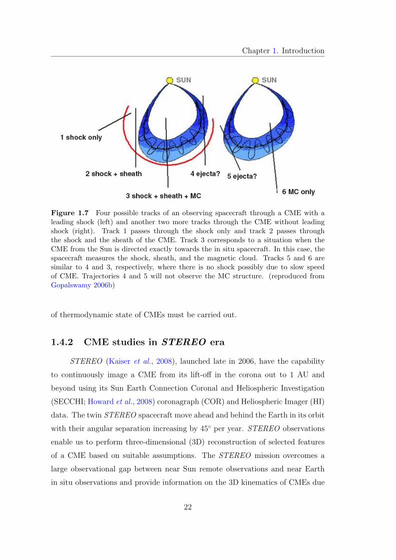
Chapter 1. Introduction
Figure 1.7 Four possible tracks of an observing spacecraft through a CME with aleading shock (left) and another two more tracks through the CME without leadingshock (right). Track 1 passes through the shock only and track 2 passes throughthe shock and the sheath of the CME. Track 3 corresponds to a situation when theCME from the Sun is directed exactly towards the in situ spacecraft. In this case, thespacecraft measures the shock, sheath, and the magnetic cloud. Tracks 5 and 6 aresimilar to 4 and 3, respectively, where there is no shock possibly due to slow speedof CME. Trajectories 4 and 5 will not observe the MC structure. (reproduced fromGopalswamy 2006b)
of thermodynamic state of CMEs must be carried out.
1.4.2 CME studies in STEREO era
STEREO (Kaiser et al., 2008), launched late in 2006, have the capability
to continuously image a CME from its lift-off in the corona out to 1 AU and
beyond using its Sun Earth Connection Coronal and Heliospheric Investigation
(SECCHI; Howard et al., 2008) coronagraph (COR) and Heliospheric Imager (HI)
data. The twin STEREO spacecraft move ahead and behind the Earth in its orbit
with their angular separation increasing by 45◦ per year. STEREO observations
enable us to perform three-dimensional (3D) reconstruction of selected features
of a CME based on suitable assumptions. The STEREO mission overcomes a
large observational gap between near Sun remote observations and near Earth
in situ observations and provide information on the 3D kinematics of CMEs due
22
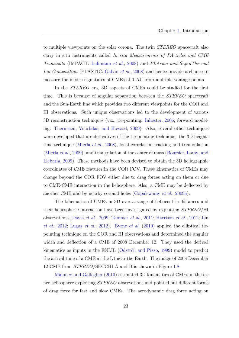
Chapter 1. Introduction
to multiple viewpoints on the solar corona. The twin STEREO spacecraft also
carry in situ instruments called In situ Measurements of PArticles and CME
Transients (IMPACT: Luhmann et al., 2008) and PLAsma and SupraThermal
Ion Composition (PLASTIC: Galvin et al., 2008) and hence provide a chance to
measure the in situ signatures of CMEs at 1 AU from multiple vantage points.
In the STEREO era, 3D aspects of CMEs could be studied for the first
time. This is because of angular separation between the STEREO spacecraft
and the Sun-Earth line which provides two different viewpoints for the COR and
HI observations. Such unique observations led to the development of various
3D reconstruction techniques (viz., tie-pointing: Inhester, 2006; forward model-
ing: Thernisien, Vourlidas, and Howard, 2009). Also, several other techniques
were developed that are derivatives of the tie-pointing technique: the 3D height-
time technique (Mierla et al., 2008), local correlation tracking and triangulation
(Mierla et al., 2009), and triangulation of the center of mass (Boursier, Lamy, and
Llebaria, 2009). These methods have been devised to obtain the 3D heliographic
coordinates of CME features in the COR FOV. These kinematics of CMEs may
change beyond the COR FOV either due to drag forces acting on them or due
to CME-CME interaction in the heliosphere. Also, a CME may be deflected by
another CME and by nearby coronal holes (Gopalswamy et al., 2009a).
The kinematics of CMEs in 3D over a range of heliocentric distances and
their heliospheric interaction have been investigated by exploiting STEREO/HI
observations (Davis et al., 2009; Temmer et al., 2011; Harrison et al., 2012; Liu
et al., 2012; Lugaz et al., 2012). Byrne et al. (2010) applied the elliptical tie-
pointing technique on the COR and HI observations and determined the angular
width and deflection of a CME of 2008 December 12. They used the derived
kinematics as inputs in the ENLIL (Odstrcil and Pizzo, 1999) model to predict
the arrival time of a CME at the L1 near the Earth. The image of 2008 December
12 CME from STEREO/SECCHI-A and B is shown in Figure 1.8.
Maloney and Gallagher (2010) estimated 3D kinematics of CMEs in the in-
ner heliosphere exploiting STEREO observations and pointed out different forms
of drag force for fast and slow CMEs. The aerodynamic drag force acting on
23
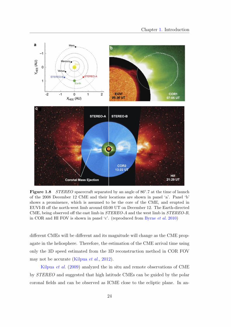
Chapter 1. Introduction
Figure 1.8 STEREO spacecraft separated by an angle of 86◦.7 at the time of launchof the 2008 December 12 CME and their locations are shown in panel ‘a’. Panel ‘b’shows a prominence, which is assumed to be the core of the CME, and erupted inEUVI-B off the north-west limb around 03:00 UT on December 12. The Earth-directedCME, being observed off the east limb in STEREO-A and the west limb in STEREO-B,in COR and HI FOV is shown in panel ‘c’. (reproduced from Byrne et al. 2010)
different CMEs will be different and its magnitude will change as the CME prop-
agate in the heliosphere. Therefore, the estimation of the CME arrival time using
only the 3D speed estimated from the 3D reconstruction method in COR FOV
may not be accurate (Kilpua et al., 2012).
Kilpua et al. (2009) analyzed the in situ and remote observations of CME
by STEREO and suggested that high latitude CMEs can be guided by the polar
coronal fields and can be observed as ICME close to the ecliptic plane. In an-
24
Chapter 1. Introduction
other study, Kilpua et al. (2011) emphasize that an ICME cannot be explained
in terms of simple flux ropes models. They also noted different in situ struc-
tures at STEREO spacecraft even when they were separated by only few degrees
in longitude. Despite the advantage of multi-point in situ observations, it is still
unclear whether all CMEs have flux ropes or in other words whether all interplan-
etary CMEs are magnetic clouds. Also, it is not well understood how a remotely
observed CME evolves into a CME observed in situ in the solar wind.
1.5 Heliospheric Consequences of CMEs
Until the early 1990s, the observed geomagnetic activity was primarily at-
tributed to solar flares, and CMEs were believed to be the result of flare-driven
shock waves. However, the paper on ‘The solar flare myth’ published by Gosling
(1993), for the first time, highlighted that geomagnetic activity is mainly related
to the CMEs and not flares. CMEs can lead to several consequences at the vari-
ous locations in the heliosphere, e.g. interplanetary shocks, radio bursts, intense
geomagnetic storms, large solar energetic particles (SEPs) events and Forbush
decrease.
CMEs drive interplanetary shock when their speeds exceed the Alfven speed
in the heliosphere (Gopalswamy et al., 2000b; Gopalswamy, 2006a). Such shocks
can cause SEPs near the Sun and in the interplanetary medium. When this shock
arrives at the Earth’s magnetosphere it causes the storm sudden commencement
(SSC) (Chao and Lepping, 1974). SSC is because of compression of the day-side
Earth’s magnetosphere by the shock and therefore the horizontal component of
Earth’s magnetic field which can be measured by ground based magnetometers, is
found to be increased (Dessler, Francis, and Parker, 1960; Tsunomura, 1998). It
is known that type II radio bursts are excellent indicators of CME-driven shocks
(Robinson, 1985; Gopalswamy et al., 2001a). Type II radio bursts are produced
via a plasma emission mechanism by the non-thermal electrons accelerated at the
shock front. Such electrons generate plasma waves which is converted to electro-
magnetic radiation at the fundamental and harmonic of the plasma frequency.
25
Chapter 1. Introduction
CMEs which give rise to type II bursts with emission wavelength from metric
(m) to decameter-hectometric (DH) to the kilometric (Km) are the most ener-
getic with a typical speed of ≈ 1500 km s−1 (Gopalswamy, 2006a). It is found
that about two-third of CME-driven shocks observed at in situ spacecraft near 1
AU are radio-loud, i.e., they generate type II radio bursts near or far from the
Sun. However, about one-third of interplanetary shocks observed at 1 AU are
related to radio-quiet CMEs. Such CMEs have slow speeds near the Sun and
accelerate away from the Sun, but their driven shocks are too weak to produce
radio bursts (Gopalswamy et al., 2010).
The magnetic nature of the planet decides the effect of CMEs on a planet.
Mars has no magnetic field, and therefore there is no magnetic storm on Mars, but
its atmosphere has been considerably eroded by the solar wind (Haff, Switkowski,
and Tombrello, 1978; Luhmann and Bauer, 1992). The Earth has a magnetic
field, and hence Earth-directed CMEs with a southward interplanetary magnetic
field component interact with the Earth’s magnetosphere at the dayside mag-
netopause. In this interaction, solar wind energy is transferred to the magne-
tosphere, primarily via magnetic reconnection that produces non-recurrent geo-
magnetic storms (Dungey, 1961). The rate of transfer of solar wind energy into
the magnetosphere depends on the magnitude of the interplanetary convective
electric field (E = V × B; Gosling et al., 1991). The main phase of a geomag-
netic storm is characterized by a depression in the horizontal component of the
Earth’s magnetic field measured on the surface of the Earth. The main phase of
a geomagnetic storm is the enhancement in the trapped magnetospheric particle
population. The gradient and curvature in the Earth’s magnetic field and gyra-
tion of trapped particles, lead to ions moving from midnight toward dusk (i.e.,
westward) and electrons from midnight toward dawn (i.e., eastward) , giving an
overall current in the westward direction around the Earth. This current can be
visualized as a toroidal shaped electric current that is centered at the equato-
rial plane, with variable density at an altitude between 2 R⊕ to 9 R⊕. During
geomagnetic storms, the main carriers of the ring current are positive ions with
energies from 1 keV to a few hundred keV having their origin from the solar wind
26

Chapter 1. Introduction
and the ionosphere (Gonzalez et al., 1994, and references therein). It is found
that during the quiescent time, ring current ions are basically of solar wind origin.
However, during the storm, the relative and absolute abundance of O+ ions are
found to be increased, which are of ionospheric origin. The abundances of O+ ions
increase rapidly during the onset of geomagnetic storms, which causes a sharp
depression in the Earth’s magnetic field. After the main phase of a geomagnetic
storm, the ring current weakens via various mechanisms, and Earth’s horizontal
component of magnetic field starts to recover to its quiescent value and is known
as the ‘recovery phase’ of a geomagnetic storm. The origin, evolution, dynam-
ics, and losses of ring current are reviewed by Daglis et al. (1999). A typical
geomagnetic storm with its different phases is shown in Figure 1.9.
Figure 1.9 Different phases of a typical geomagnetic storm are shown. The suddencommencement, initial, main and recovery phases are characterized by a sudden rise,constant, fast decrease, and slow recovery in the horizontal components of Earth’smagnetic field, respectively.
CMEs naturally have a southward component of magnetic field (negative
Bz) because of their flux ropes structures. If the CME drives a shock, then the
sheath region lying between the shock and flux ropes may also have negative
Bz. Also, it has been shown that 83% intense geomagnetic storms are due to
27
Chapter 1. Introduction
CMEs (Zhang et al., 2007). Few intense storms may occur because of corotating
interactions regions (CIRs). CIRs form when the fast speed solar wind overtakes
the slow speed solar wind ahead and leads to the formation of a interface region
with increased temperature, density, and magnetic field. The negative Bz in the
CIRs responsible for geomagnetic storms are due to enhancement in the pre-
existing negative Bz in the Alfvenic fluctuations in the stream interface region.
From a space weather perspective, it is essential to estimate the arrival time and
transit speeds of CMEs near the Earth well in advance to predict the severity
of these events. However, the prediction of negative Bz at the Earth is most
important for predicting the occurrence of geomagnetic storms (Gonzalez et al.,
1989; Srivastava and Venkatakrishnan, 2002). Determination of the negative Bz
component in the CMEs by exploiting the solar observations is far from reality.
By examining the neutral line in the source region of a CME, one can attempt
to guess the inclination of the flux rope, the expected direction of rotation, and
the portion of flux rope where negative Bz may occur (Yurchyshyn, Hu, and
Abramenko, 2005). Our understanding of the flux rope structure of a CME is
very limited, and is still debated whether such flux ropes are formed during the
eruption or exist before the eruption (Chen, 2011).
In the STEREO era, by exploiting the Sun to Earth remote observations of
CMEs from twin viewpoints, we expect to have better success in predicting the
speed and direction of CME near the 1 AU at the Earth. However, without the
knowledge about the negative Bz component of CME from remote observations,
prediction of the intensity of resulting geomagnetic storms well in advance is
difficult.
Kahler, Hildner, and Van Hollebeke (1978) found an association between
the SEPs events and the CMEs and concluded that the protons must be acceler-
ated at the front of the CME-driven shocks, which was confirmed later in several
observations (Reames, 1999, and references therein). Direct evidence of particles’
acceleration by the shock comes from observing energetic storm particle (ESP)
events. In ESP events, the locally accelerated particles by the shocks and the
shocks themselves are detected at in situ spacecraft at 1 AU. If a shock is gen-
28

Chapter 1. Introduction
erated near the Sun, it is expected to be strong enough to accelerate SEPs and
inject them back into the heliosphere. Gopalswamy et al. (2003a) have shown
that SEP events are associated with fast and wide CMEs. It is also well proven
that CMEs are responsible for the periodic 11-year variation in the intensity of
galactic cosmic rays (GCRs). Further, CMEs are found to be responsible for
Forbush decreases (FDs) (Forbush, 1937; Cane, 2000, and references therein).
Non-recurrent FDs are defined as sudden shorter-term decrease of the recorded
intensity of GCRs when the ICME passes through the Earth. In FDs, the de-
pression in the intensity of GCRs typically lasts for less than one day, while its
recovery to normal level takes place in several days. FDs are due to the exclusion
of GCRs because of their inability to diffuse “across” the relatively strong and
ordered IMF in the vicinity of interplanetary shock, in the sheath and/or a MC
region.
1.6 Motivation and Organization of the Thesis
As mentioned earlier, until recently, understanding of the nature and prop-
agation of the CMEs has been limited for many reasons. The most significant
are projection effects, the lack of continuous high spatial resolution, and high ca-
dence CME observations through the inner heliosphere. Also, many CME arrival
time prediction models utilize the projected kinematics from single viewpoint.
Very few studies have been carried out to continuously track the CMEs in the
heliosphere and predict their arrival time at 1 AU based on their 3D kinematics
estimated by exploiting multiple viewpoints observations for them. Therefore,
the success in finding an association between remote observations and in situ
observations of CME at 1 AU is still limited.
With the availability of stereoscopic observations for CMEs, several 3D
reconstruction techniques have been developed recently; however a detailed study
to understand the relative importance and validity of ideal assumptions used in
these techniques has not been carried out. Hence, a comparison of existing 3D
reconstruction techniques, which use the data from COR and HI to accurately
29
Chapter 1. Introduction
predict the arrival time of CMEs is required. Such studies are essential from
space weather prediction perspective and for understanding the bulk of plasma
motion in an ambient medium.
A majority of work done so far has been focused on the propagation of a
single CME from the Sun to Earth and its consequences on hitting the Earth’s
magnetosphere. However, the interaction or collision of successive CMEs can,
in some cases, produce an extended period of southward Bz and cause strong
geomagnetic storms. Also, during the interaction of CMEs, their kinematics is
expected to change. Hence, any scheme to estimate the arrival time of interact-
ing CMEs must take their post-interaction kinematics into account. Further, it
is essential to understand the nature of the CME-CME collision. In addition,
various plasma processes during the interaction of CMEs that can change the
initial identity and properties of CME plasma must be investigated in detail.
The specific objectives of my thesis related to the evolution and conse-
quences of CMEs are outlined below:
1. Estimating three-dimensional kinematics using STEREO observations on
the Earth-directed CMEs and compare with kinematics estimated using
data from a single coronagraph alone.
2. To continuously track the Earth-directed CMEs from the Sun to Earth and
estimate their kinematic evolution using various 3D reconstruction meth-
ods. This approach has been used to estimate the arrival time of CMEs on
the Earth. As different reconstruction techniques are based on specific as-
sumptions, we also examine the relative performance of these reconstruction
methods for various CMEs.
3. To understand the role of Drag Based Model (DBM) in the prediction of
arrival time, particularly for the CMEs that cannot be tracked up to the
Earth.
4. To associate the CME features continuously observed far from the Sun in
heliospheric imaging observations with that observed in in situ observations.
30
Chapter 1. Introduction
5. A prime objective of the thesis is to understand the heliospheric conse-
quences of interacting CMEs. In this context, one goal is to understand
the consequences of a CME on another CME kinematics if many CMEs
follow each other, especially when they collide en route from the Sun to the
Earth. We also plan to investigate the geomagnetic consequences of inter-
acting CMEs and examine if it is different than the geomagnetic response
of an isolated CME.
Based on the work carried out to accomplish the aforementioned objectives,
this thesis is organized into six chapters. A brief description of each chapter is
given below.
Chapter 1: Introduction
In this chapter, the basics of the Sun and the heliosphere is presented briefly,
followed by a discussion on CMEs and their properties. A review of work car-
ried out on CMEs propagation, arrival time estimation, and their heliospheric
consequences are presented based on pre-and post STEREO observations.
Chapter 2: Observational Data and Analysis Methodology
In this chapter remote sensing observations of CME from STEREO/SECCHI and
in situ observations from ACE and WIND spacecraft is given briefly. Then the
analysis methodology used to carry out the objectives is presented in detail. The
various 3D reconstruction techniques used for COR and HI observations of CMEs
have been described, along with their possible advantages and limitations. The
theory of drag-based model (DBM) implemented for selected CMEs in our study
to understand the role of solar wind medium on the propagation of CMEs is also
presented.
Chapter 3: Estimation of Arrival Time
In this chapter, the application of 3D reconstruction techniques on selected fea-
tures of a few Earth-directed CMEs is carried out in COR2 FOV. Further, the
CMEs are tracked by constructing the time-elongation map (J -map) using the HI
31
Chapter 1. Introduction
observations taken from twin STEREO spacecraft. Using the derived elongation-
time profiles for the tracked features of CMEs from the J -map and implementing
several reconstruction techniques, the kinematics of all the CMEs are estimated.
The kinematics is either extrapolated or used as input in the DBM to estimate
the arrival time of a CME at 1 AU. We assess the performance of using various
approaches, e.g., 3D speed near the Sun, extrapolation of heliospheric kinematics,
and DBM combined with kinematics, in arrival time prediction of CME at 1 AU.
An assessment of the relative performance of several reconstruction methods is
also presented in this chapter. This chapter is based on the work published in
Mishra and Srivastava (2013) and Mishra, Srivastava, and Davies (2014).
Chapter 4: Association Between Remote and In Situ Observations
In this chapter, we present the analysis of the in situ observations of selected
Earth-directed CMEs and attempt to identify different interplanetary structures
of CMEs, i.e., shock, sheath, and magnetic cloud. We also identified in in situ
data the remotely tracked features of CMEs. The actual arrival time of tracked
features of CMEs (described in Chapter 3) for assessing the performance of dif-
ferent reconstruction methods are explained. This chapter is based on the work
published in Mishra and Srivastava (2013) and Mishra, Srivastava, and Davies
(2014).
Chapter 5: Interplanetary Consequences of CMEs
In this chapter, the interaction of CMEs observed in HI images is demonstrated
as a heliospheric consequence of CME. We also describe the morphological and
kinematic evolution of interacting CMEs selected for our study. By measuring
the energy, and momentum exchange during collision/interaction of CMEs, we
attempt to understand the nature of collision of CMEs. Also, the arrival time and
in situ signatures of interacting CMEs at 1 AU is shown. Finally, the geomagnetic
consequences of interacting CMEs are presented. This chapter is based on the
published work in Mishra and Srivastava (2014) and Mishra, Srivastava, and
Chakrabarty (2015).
32
Chapter 1. Introduction
Chapter 6: Conclusions and Future Work
In this chapter, the main results on the propagation and consequences of CMEs,
in particular the Earth-directed ones, are highlighted. The role of interaction
between CMEs in defining the geomagnetic consequences is also emphasized. A
short discussion on the limitation of the applied approaches in the thesis is also
included in this chapter. Finally, a future research plan on this topic is mentioned
to address a few unanswered questions.
33
Chapter 2
Observational Data and Analysis
Methodology
2.1 Introduction
The objective of the present thesis is to study the propagation and con-
sequences of CMEs in the heliosphere. For this purpose, we have analyzed two
sets of observations of Earth-directed CMEs, viz. remote and in situ. In remote
observations, a CME is observed in visible photospheric light scattered by elec-
trons of plasma. In in situ observations, the plasma parameters of a CME are
measured when it passes through the instruments. The speed, direction, mass,
and morphology of a CME at a particular location in the heliosphere can be stud-
ied by exploiting its remote observations, while the temperature, speed, density,
magnetic field, composition, and charge states of CME plasma/solar wind can be
measured from in situ observations. By the time a CME reaches the in situ space-
craft, it is already evolved, and therefore the plasma parameters are different than
those measured remotely (Crooker and Horbury, 2006). However, if the physics
of evolution of CME is known, then its properties estimated remotely can be ex-
trapolated up to in situ spacecraft, and then a comparison between both sets of
observations can be made with reasonable accuracy. In the absence of a complete
understanding of the true nature of the evolution of CMEs, it is often difficult
34
Chapter 2. Observational Data and Analysis Methodology
to predict their arrival time near the Earth based on their initial characteristics
estimated from remote observations near the Sun. The CME characteristics es-
timated from remote observations suffer from the line of sight integration and
projection effects, while CME/solar wind parameters can be measured along a
specific trajectory through the CME by the in situ spacecraft. Few of these lim-
itations can be overcome to some extent if there are remote observations of a
CME from multiple viewpoints providing continuous spatial coverage from the
Sun to in situ spacecraft. Such observations are possible by the instruments on-
board twin STEREO spacecraft. This chapter describes the details of remote
observations, near-Earth in situ observations of CMEs, and the methodology to
study their kinematics and propagation. The details of remote sensing and in
situ instruments are described in Sections 2.1.1 and 2.2.1, respectively.
2.1.1 Remote observations from STEREO/SECCHI
NASA’s twin STEREO spacecraft was launched to understand the initiation
of CMEs and their propagation in the inner heliosphere. The location of STEREO
on 2010 April 3 is shown in Figure 2.1. Each STEREO spacecraft has identical
optical, radio, and in situ particles and fields instruments. These instruments are
in four different measurement packages named SECCHI, IMPACT, PLASTIC
and S/WAVES. The suite of instruments in the SECCHI package consists of two
white-light coronagraphs (COR1 and COR2), an Extreme Ultraviolet Imager
(EUVI) and two white light heliospheric imagers (HI1 and HI2), which jointly
can image a CME from its lift-off in the corona out to 1 AU.
2.1.2 SECCHI/COR observations
A coronagraph is an instrument that images the faint solar corona visible
due to scattered light from the much brighter solar photosphere. As mentioned
in the previous section SECCHI has two white-light coronagraphs, COR1 is a
Lyot internally occulting refractive coronagraph (Lyot, 1939) and its field of view
(FOV) is from 1.4 R� to 4.0 R�. The internal occultation enables better spatial
35
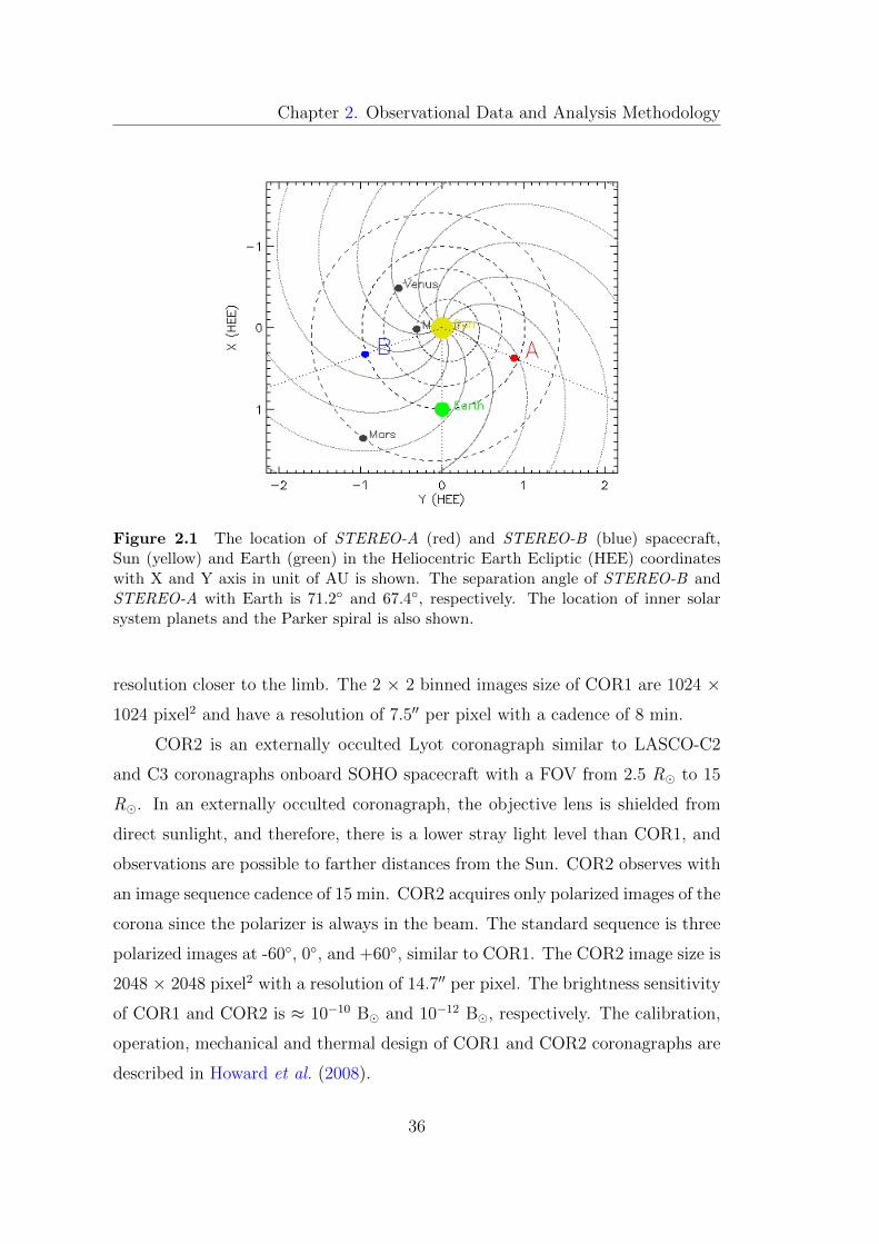
Chapter 2. Observational Data and Analysis Methodology
Figure 2.1 The location of STEREO-A (red) and STEREO-B (blue) spacecraft,Sun (yellow) and Earth (green) in the Heliocentric Earth Ecliptic (HEE) coordinateswith X and Y axis in unit of AU is shown. The separation angle of STEREO-B andSTEREO-A with Earth is 71.2◦ and 67.4◦, respectively. The location of inner solarsystem planets and the Parker spiral is also shown.
resolution closer to the limb. The 2 × 2 binned images size of COR1 are 1024 ×1024 pixel2 and have a resolution of 7.5′′ per pixel with a cadence of 8 min.
COR2 is an externally occulted Lyot coronagraph similar to LASCO-C2
and C3 coronagraphs onboard SOHO spacecraft with a FOV from 2.5 R� to 15
R�. In an externally occulted coronagraph, the objective lens is shielded from
direct sunlight, and therefore, there is a lower stray light level than COR1, and
observations are possible to farther distances from the Sun. COR2 observes with
an image sequence cadence of 15 min. COR2 acquires only polarized images of the
corona since the polarizer is always in the beam. The standard sequence is three
polarized images at -60◦, 0◦, and +60◦, similar to COR1. The COR2 image size is
2048 × 2048 pixel2 with a resolution of 14.7′′ per pixel. The brightness sensitivity
of COR1 and COR2 is ≈ 10−10 B� and 10−12 B�, respectively. The calibration,
operation, mechanical and thermal design of COR1 and COR2 coronagraphs are
described in Howard et al. (2008).
36
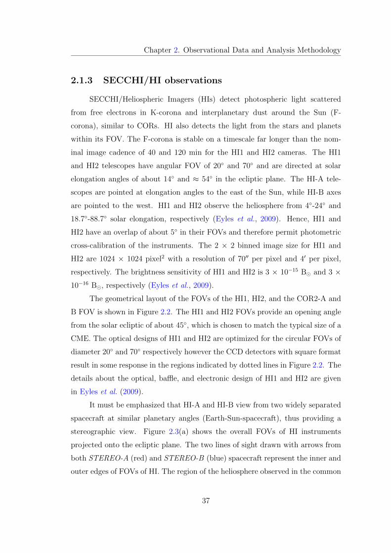
Chapter 2. Observational Data and Analysis Methodology
2.1.3 SECCHI/HI observations
SECCHI/Heliospheric Imagers (HIs) detect photospheric light scattered
from free electrons in K-corona and interplanetary dust around the Sun (F-
corona), similar to CORs. HI also detects the light from the stars and planets
within its FOV. The F-corona is stable on a timescale far longer than the nom-
inal image cadence of 40 and 120 min for the HI1 and HI2 cameras. The HI1
and HI2 telescopes have angular FOV of 20◦ and 70◦ and are directed at solar
elongation angles of about 14◦ and ≈ 54◦ in the ecliptic plane. The HI-A tele-
scopes are pointed at elongation angles to the east of the Sun, while HI-B axes
are pointed to the west. HI1 and HI2 observe the heliosphere from 4◦-24◦ and
18.7◦-88.7◦ solar elongation, respectively (Eyles et al., 2009). Hence, HI1 and
HI2 have an overlap of about 5◦ in their FOVs and therefore permit photometric
cross-calibration of the instruments. The 2 × 2 binned image size for HI1 and
HI2 are 1024 × 1024 pixel2 with a resolution of 70′′ per pixel and 4′ per pixel,
respectively. The brightness sensitivity of HI1 and HI2 is 3 × 10⁻¹⁵ B� and 3 ×10⁻¹⁶ B�, respectively (Eyles et al., 2009).
The geometrical layout of the FOVs of the HI1, HI2, and the COR2-A and
B FOV is shown in Figure 2.2. The HI1 and HI2 FOVs provide an opening angle
from the solar ecliptic of about 45◦, which is chosen to match the typical size of a
CME. The optical designs of HI1 and HI2 are optimized for the circular FOVs of
diameter 20◦ and 70◦ respectively however the CCD detectors with square format
result in some response in the regions indicated by dotted lines in Figure 2.2. The
details about the optical, baffle, and electronic design of HI1 and HI2 are given
in Eyles et al. (2009).
It must be emphasized that HI-A and HI-B view from two widely separated
spacecraft at similar planetary angles (Earth-Sun-spacecraft), thus providing a
stereographic view. Figure 2.3(a) shows the overall FOVs of HI instruments
projected onto the ecliptic plane. The two lines of sight drawn with arrows from
both STEREO-A (red) and STEREO-B (blue) spacecraft represent the inner and
outer edges of FOVs of HI. The region of the heliosphere observed in the common
37
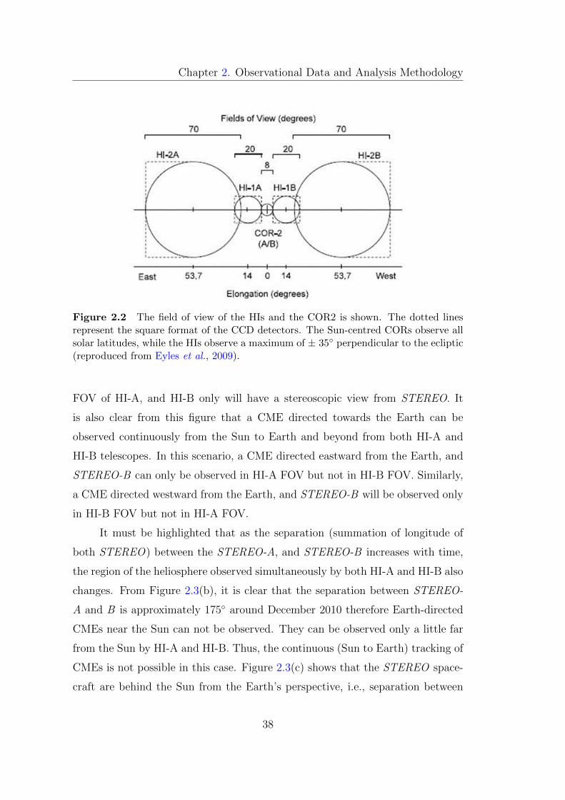
Chapter 2. Observational Data and Analysis Methodology
Figure 2.2 The field of view of the HIs and the COR2 is shown. The dotted linesrepresent the square format of the CCD detectors. The Sun-centred CORs observe allsolar latitudes, while the HIs observe a maximum of ± 35◦ perpendicular to the ecliptic(reproduced from Eyles et al., 2009).
FOV of HI-A, and HI-B only will have a stereoscopic view from STEREO. It
is also clear from this figure that a CME directed towards the Earth can be
observed continuously from the Sun to Earth and beyond from both HI-A and
HI-B telescopes. In this scenario, a CME directed eastward from the Earth, and
STEREO-B can only be observed in HI-A FOV but not in HI-B FOV. Similarly,
a CME directed westward from the Earth, and STEREO-B will be observed only
in HI-B FOV but not in HI-A FOV.
It must be highlighted that as the separation (summation of longitude of
both STEREO) between the STEREO-A, and STEREO-B increases with time,
the region of the heliosphere observed simultaneously by both HI-A and HI-B also
changes. From Figure 2.3(b), it is clear that the separation between STEREO-
A and B is approximately 175◦ around December 2010 therefore Earth-directed
CMEs near the Sun can not be observed. They can be observed only a little far
from the Sun by HI-A and HI-B. Thus, the continuous (Sun to Earth) tracking of
CMEs is not possible in this case. Figure 2.3(c) shows that the STEREO space-
craft are behind the Sun from the Earth’s perspective, i.e., separation between
38
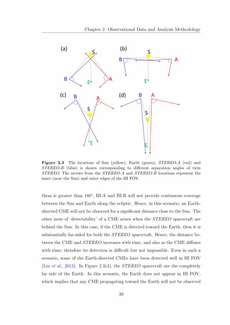
Chapter 2. Observational Data and Analysis Methodology
(a) S
A B E
S
A B
E
(b)
A B
S
E
(d) B A
S
E
(c)
Figure 2.3 The locations of Sun (yellow), Earth (green), STEREO-A (red) andSTEREO-B (blue) is shown corresponding to different separation angles of twinSTEREO. The arrows from the STEREO-A and STEREO-B locations represent theinner (near the Sun) and outer edges of the HI FOV.
them is greater than 180◦, HI-A and HI-B will not provide continuous coverage
between the Sun and Earth along the ecliptic. Hence, in this scenario, an Earth-
directed CME will not be observed for a significant distance close to the Sun. The
other issue of ‘detectability’ of a CME arises when the STEREO spacecraft are
behind the Sun. In this case, if the CME is directed toward the Earth, then it is
substantially far-sided for both the STEREO spacecraft. Hence, the distance be-
tween the CME and STEREO increases with time, and also as the CME diffuses
with time; therefore its detection is difficult but not impossible. Even in such a
scenario, some of the Earth-directed CMEs have been detected well in HI FOV
(Liu et al., 2013). In Figure 2.3(d), the STEREO spacecraft are the completely
far side of the Earth. In this scenario, the Earth does not appear in HI FOV,
which implies that any CME propagating toward the Earth will not be observed
39
Chapter 2. Observational Data and Analysis Methodology
during its journey from the Sun to the Earth.
2.2 Observations Near 1 AU
The term ‘Interplanetary Coronal Mass Ejection’ (ICME) was originally
coined for near-Earth observations of CME by an in situ spacecraft to distinguish
it from the coronagraphic observations near the Sun. In the present STEREO
era, where CMEs can be tracked from near the Sun to the Earth and beyond,
the term ICME has become redundant (Webb and Howard, 2012). Therefore,
hereafter, throughout this thesis, we will use the term CME to refer to both
CME and ICME. The details about signatures and identification of CMEs in in
situ observations have been described in Section 1.4.1.2 of Chapter 1. In the
present section, we briefly state the principles on which the in situ instruments
work. When a CME arrives at the Earth’s magnetosphere, it produces magnetic
disturbance on the surface of the Earth and inside the magnetosphere, which can
be observed by ground-based magnetometers (See, Section 2.2.2).
2.2.1 In situ observations from ACE & WIND
ACE spacecraft was launched in 1995 and is located close to the L1 La-
grangian point. It carries nine high-resolution instruments which measure the
elemental, isotopic, and ionic charge-state composition of energetic nuclei by
monitoring the state of the solar wind medium. For CME identification, we
have mainly used the observations from three instruments, namely Solar Wind
Ion Composition Spectrometer (SWICS) (Gloeckler et al., 1998), Solar Wind
Electron, Protn Alpha Monitor (SWEPAM) (McComas et al., 1998) and Magne-
tometer (MAG) (Smith et al., 1998). SWICS measures the elemental and ionic
charge-state composition of solar wind ions (H to Fe) using a combination of elec-
trostatic deflection, post-acceleration, time-of-flight, and energy measurements.
SWEPAM contains an electrostatic analyzer and provides the electron and ion
distribution functions in 3D over all the velocity space to characterize the solar
wind’s bulk flow and kinetic properties. MAG consists of twin boom-mounted,
40

Chapter 2. Observational Data and Analysis Methodology
triaxial flux-gate sensors that measure the local vector magnetic field in the in-
terplanetary medium.
WIND spacecraft was launched in 1994 and is located near the L1 point.
This spacecraft carries a total of nine instruments and continuously monitors
the solar wind plasma, energetic particles, magnetic fields, radio and plasma
waves, and cosmic gamma-ray bursts. In the present thesis, we have used the
observations from three instruments, namely Magnetic Field Instrument (MFI)
(Lepping et al., 1995), Solar Wind Experiment (SWE) (Ogilvie et al., 1995),
Three-Dimensional Plasma and Energetic Particle Investigation (3DP) (Lin et al.,
1995). MFI consists of boom-mounted double triaxial sensors and measures the
interplanetary magnetic field. SWE instrument is a suite of two Faraday cup (FC)
sensors, Vector Electron and Ion Spectrometer (VEIS), and a strahl sensor. FC
sensors measure the density, temperature, and velocity of the solar wind. VEIS
measures the foreshock (region upstream of the bow shock) ions and electrons
reflected from the bow shock. Strahl sensor can measure the electron velocity
distribution function near the direction of the magnetic field. 3DP measures the
3D distribution of suprathermal electrons and ions in the solar wind. It must
be noted that WIND spacecraft lacks an instrument like SWICS on board ACE.
Therefore chemical abundance and charge state composition of the solar wind
can only be studied using ACE data.
2.2.2 Ground-based magnetometer observations
As a CME having a southward orientation of the magnetic field passes
through the Earth, various electric current systems in Earth’s magnetosphere are
intensified, which lead to perturbations in the geomagnetic field. These perturba-
tions at the surface of the Earth can be measured by a series of ground-based mag-
netometers. Based on these measurements, various geomagnetic indices are cal-
culated, which monitor different geomagnetic responses, e.g., geomagnetic storms
and substorms (Akasofu, 1964). The perturbations measured in the geomagnetic
field can be resolved in horizontal (north-south dipole) direction and orthogo-
41
Chapter 2. Observational Data and Analysis Methodology
nal (east-west) direction and are denoted by H and D components, respectively.
The formation of the magnetospheric ring current and its effect on the horizontal
component (H) of Earth’s magnetic field is explained in Section 1.5 of Chapter 1.
A series of magnetometers around the equator (mid-latitudes) of the Earth mea-
sure the perturbations in the horizontal component of Earth’s magnetic field and
monitor the ring current intensity and hence geomagnetic storms (Dessler and
Parker, 1959; Sckopke, 1966). The hourly average of such measured perturba-
tions is known as Disturbance storm time (Dst) index (Sugiura, 1964; Mayaud,
1980). The negative values of the Dst index represent the intensification of the
ring current. Also, high resolution (1 min) measurements of symmetric (SYM)
and asymmetric (ASY) disturbance are introduced for both H and D components.
Sym-H index is very similar to the Dst index, but with high resolution and de-
rived from different sets of stations using a slightly different coordinate systems
and base values (Iyemori, 1990).
There are a series of magnetometers in the northern hemisphere auroral
zone of the Earth. During the perturbations in the magnetosphere, these mag-
netometers can measure the positive (upper bound) or negative (lower bound)
fluctuations in the H-component of the geomagnetic field. Such positive or nega-
tive fluctuations are averaged for several stations and are known as the AU or AL
index. The difference between maximum negative (AL) and positive (AU) fluctu-
ations is known as AE index (Davis and Sugiura, 1966). AL and AU index moni-
tors the westward and eastward electrojet, respectively. AE index represents the
magnetospheric substorms and has durations of tens of minutes to several hours
(Akasofu, 1969; McPherron, 1970). It must be noted that although a geomag-
netic index primarily monitors a single current system but a small contribution
to the index by several other current systems formed during magnetospheric per-
turbations cannot be neglected. Also, an index known as the PC index is derived
from a magnetic station in the northern and southern hemispheres designed to
monitor the perturbation in the geomagnetic field due to ionospheric and field-
aligned currents (Troshichev et al., 2000). To examine the geomagnetic effects of
the CMEs, we have mainly used the Dst index data; however, for a few events
42
Chapter 2. Observational Data and Analysis Methodology
the AL and PC indices are also analyzed.
2.3 Analysis Methodology
To achieve our objective of understanding the evolution and consequences
of CMEs, we followed three main steps. In the first step, we selected those CMEs
that could be continuously observed from the Sun to the Earth in remote sensing
observations. Their plasma parameters could also be measured in in situ observa-
tions. As we also aimed to understand the geomagnetic consequences of CMEs,
the selected CMEs for our study are directed approximately towards the Earth.
These selected CMEs have been broadly classified into two groups, one consists of
isolated CMEs to study their heliospheric evolution, and other comprises interact-
ing CMEs to study the nature of their collision and geomagnetic responses. In the
second step, CMEs features are tracked through the heliosphere by constructing
J -maps (Sheeley et al., 1999). Using J -maps, the variation in elongation (angle of
the feature concerning the Sun-spacecraft line) of a moving CME feature is esti-
mated. In the third step, the kinematics of tracked features of CMEs is calculated
using stereoscopic reconstruction techniques on COR2 observations. Further, to
understand the heliospheric propagation of selected CMEs, various stereoscopic
or single spacecraft methods are used on their time-elongation profiles (derived
from J -maps) observed in HI FOV. The stereoscopic methods based on certain
assumptions and used on COR2 observations are generally not suitable for HI
observations because these assumptions break down at large distances from the
Sun. In the fourth step, we extrapolate the kinematics of CME features and use
them as input to the drag-based model (DBM) of propagation of CMEs for esti-
mating their arrival time at 1 AU. In the fifth step, in situ observations of CME
at 1 AU are analyzed, and actual arrival time of a CME is marked. Finally, we
attempt to associate remotely tracked features of CME to the features observed
in in situ observations. The aforementioned methodology has been adopted for
several cases of geo-effective CMEs and interacting/colliding CMEs to address
the specific objectives.
43
Chapter 2. Observational Data and Analysis Methodology
2.3.1 Reconstruction methods using COR2 observations
Various 3D reconstruction methods have been developed which can be used
on SECCHI/COR observations, i.e., for a CME feature close to the Sun. These
have been reviewed in Mierla et al. (2010). In our study, we have used the tie-
pointing method of 3D reconstruction (Thompson, 2009) and forward modeling
method (Thernisien, Vourlidas, and Howard, 2009) on the SECCHI/COR obser-
vations of CMEs. These methods have been used to estimate the kinematics of
selected features of CMEs before they enter into the HI FOV.
2.3.1.1 Tie-point (TP) reconstruction
The tie-pointing method of stereoscopic reconstruction is based on the con-
cept of epipolar geometry. The position of two STEREO spacecraft and the point
to be triangulated defines a plane called epipolar plane (Inhester, 2006). Since
every epipolar plane is seen head-on from both spacecraft, it is reduced to a line
in the respective image projection. This line is called the epipolar line. Epipolar
lines in each image can easily be determined from the observer’s position and the
direction of the observer’s optical axes.
Any object which lies on a certain epipolar line in one image must lie on
the same epipolar line in the other image. This straightforward geometrical con-
sequence is known as epipolar constraint. Due to the epipolar constraint, finding
the correspondence of an object in the contemporaneous image of both spacecraft
reduces to finding out correspondence along the same epipolar lines in both im-
ages. Once the correspondence between the pixels is found, the 3D reconstruction
is achieved by calculating the line of sight rays corresponding to those pixels and
back tracking them in 3D space. Since the rays are constrained to lie in the same
epipolar plane, they intersect at a point on tracking backward. This procedure
is called tie-pointing (Inhester, 2006). The point of intersection of both lines of
sight gives the 3D coordinates of the identified object or feature in both sets of
images.
In our study, we have used the tie-pointing method (scc measure: Thomp-
44
Chapter 2. Observational Data and Analysis Methodology
son, 2009) of 3D reconstruction. Before implementing this method, the processing
of SECCHI/COR2 images and creation of minimum intensity images, and then
its subtraction from the sequence of processed COR2 images were carried out as
described in Mierla et al. (2008) and Srivastava et al. (2009). This method has a
graphical user interface (GUI) in the Interactive Data Language (IDL) and has
been widely used by several authors to estimate the 3D coordinates of a selected
feature of the CME.
2.3.1.2 Forward modeling method
In this method, a specific parametric shape of CME is assumed and itera-
tively fit until it matches with its actual image. This method produces a physical
solution based on the model assumptions but presumes that the solution only fits
that model. We have used the 3D reconstruction method of Thernisien, Vourli-
das, and Howard (2009) where they have applied the Graduated Cylindrical Shell
(GCS) model on CMEs observed by SECCHI/COR2-A and B. This model repre-
sents the flux rope structure of CMEs with two shapes; the conical legs and the
curved (tubular) fronts (Figure 2.4). The resulting shape is like a “hollow crois-
sant”. The model also assumes that the GCS structure moves in a self-similar
way. In principle, this technique can be applied to images from all other tele-
scopes of the SECCHI package. However we applied this technique only to COR2
images. This is because, in COR2 FOV, the flux-rope structure of CMEs is well
identified, while it is not fully developed in COR1 FOV and is too faint in the HI
FOV.
GCS model fitting tool in IDL involves simultaneous adjusting six model pa-
rameters so that the resulting GCS flux structure matches well with the observed
flux rope structure of the CME. These six parameters, including the longitude,
latitude, tilt angle of the flux ropes with a height of the legs, half-angle between
the legs, and aspect ratio of the curved front, are adjusted to match the spatial
extent of the CME. These have been discussed in detail in Thernisien (2011).
The best fit six parameters obtained for the observed CME with GCS modeled
CME used to calculate various geometrical dimensions of a CME.
45
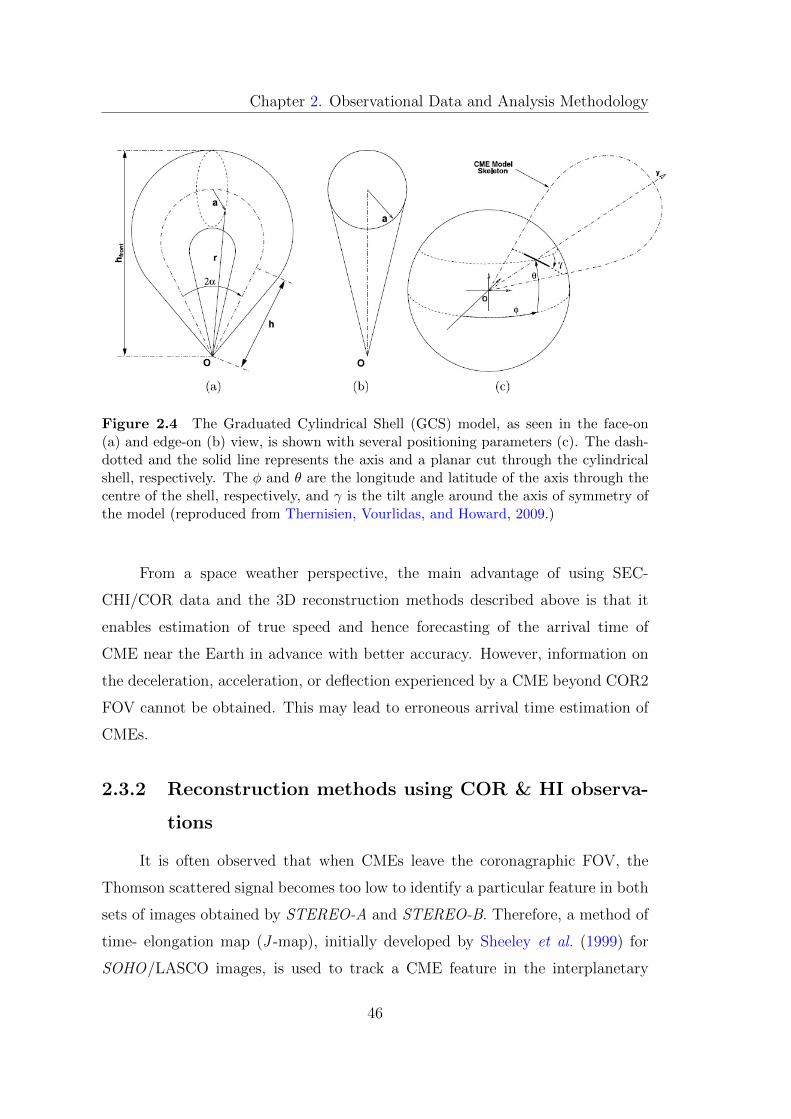
Chapter 2. Observational Data and Analysis Methodology
Figure 2.4 The Graduated Cylindrical Shell (GCS) model, as seen in the face-on(a) and edge-on (b) view, is shown with several positioning parameters (c). The dash-dotted and the solid line represents the axis and a planar cut through the cylindricalshell, respectively. The φ and θ are the longitude and latitude of the axis through thecentre of the shell, respectively, and γ is the tilt angle around the axis of symmetry ofthe model (reproduced from Thernisien, Vourlidas, and Howard, 2009.)
From a space weather perspective, the main advantage of using SEC-
CHI/COR data and the 3D reconstruction methods described above is that it
enables estimation of true speed and hence forecasting of the arrival time of
CME near the Earth in advance with better accuracy. However, information on
the deceleration, acceleration, or deflection experienced by a CME beyond COR2
FOV cannot be obtained. This may lead to erroneous arrival time estimation of
CMEs.
2.3.2 Reconstruction methods using COR & HI observa-
tions
It is often observed that when CMEs leave the coronagraphic FOV, the
Thomson scattered signal becomes too low to identify a particular feature in both
sets of images obtained by STEREO-A and STEREO-B. Therefore, a method of
time- elongation map (J -map), initially developed by Sheeley et al. (1999) for
SOHO/LASCO images, is used to track a CME feature in the interplanetary
46
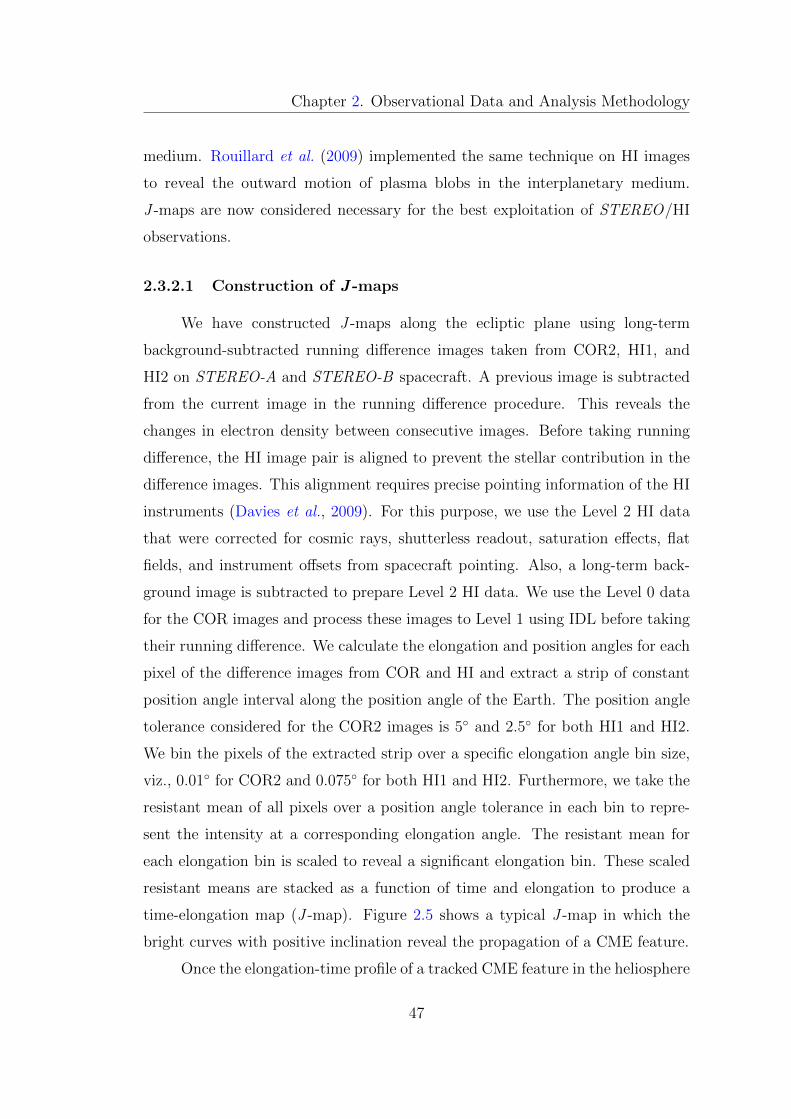
Chapter 2. Observational Data and Analysis Methodology
medium. Rouillard et al. (2009) implemented the same technique on HI images
to reveal the outward motion of plasma blobs in the interplanetary medium.
J -maps are now considered necessary for the best exploitation of STEREO/HI
observations.
2.3.2.1 Construction of J -maps
We have constructed J -maps along the ecliptic plane using long-term
background-subtracted running difference images taken from COR2, HI1, and
HI2 on STEREO-A and STEREO-B spacecraft. A previous image is subtracted
from the current image in the running difference procedure. This reveals the
changes in electron density between consecutive images. Before taking running
difference, the HI image pair is aligned to prevent the stellar contribution in the
difference images. This alignment requires precise pointing information of the HI
instruments (Davies et al., 2009). For this purpose, we use the Level 2 HI data
that were corrected for cosmic rays, shutterless readout, saturation effects, flat
fields, and instrument offsets from spacecraft pointing. Also, a long-term back-
ground image is subtracted to prepare Level 2 HI data. We use the Level 0 data
for the COR images and process these images to Level 1 using IDL before taking
their running difference. We calculate the elongation and position angles for each
pixel of the difference images from COR and HI and extract a strip of constant
position angle interval along the position angle of the Earth. The position angle
tolerance considered for the COR2 images is 5◦ and 2.5◦ for both HI1 and HI2.
We bin the pixels of the extracted strip over a specific elongation angle bin size,
viz., 0.01◦ for COR2 and 0.075◦ for both HI1 and HI2. Furthermore, we take the
resistant mean of all pixels over a position angle tolerance in each bin to repre-
sent the intensity at a corresponding elongation angle. The resistant mean for
each elongation bin is scaled to reveal a significant elongation bin. These scaled
resistant means are stacked as a function of time and elongation to produce a
time-elongation map (J -map). Figure 2.5 shows a typical J -map in which the
bright curves with positive inclination reveal the propagation of a CME feature.
Once the elongation-time profile of a tracked CME feature in the heliosphere
47
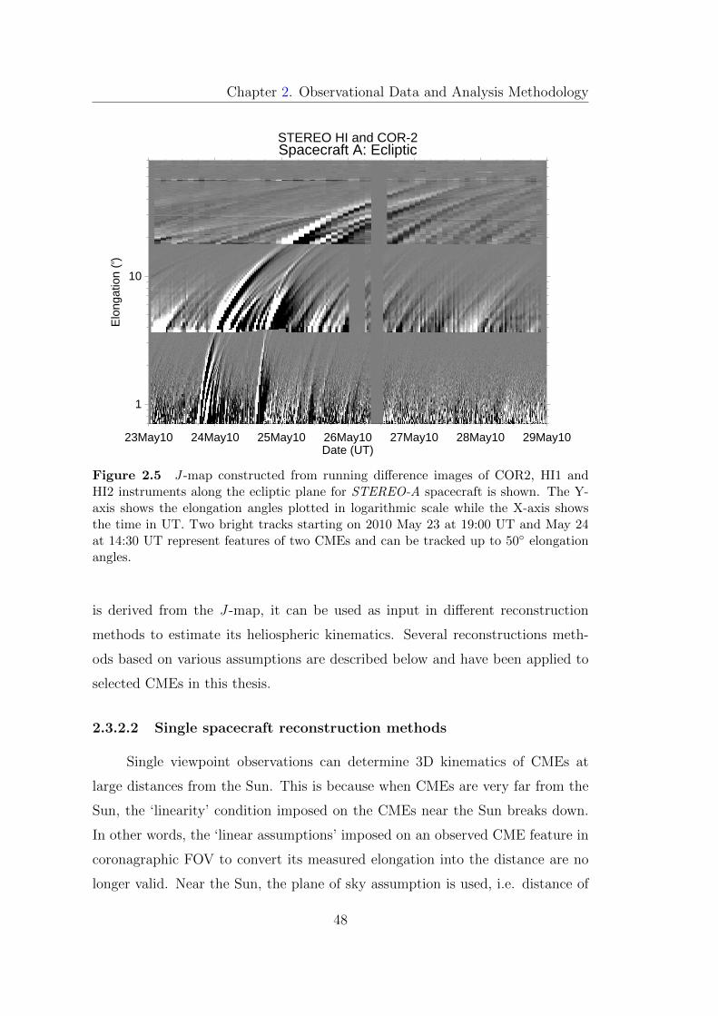
Chapter 2. Observational Data and Analysis Methodology
Spacecraft A: Ecliptic
23May10 24May10 25May10 26May10 27May10 28May10 29May10Date (UT)
1
10
Elo
ngat
ion
(o )
STEREO HI and COR-2
Figure 2.5 J -map constructed from running difference images of COR2, HI1 andHI2 instruments along the ecliptic plane for STEREO-A spacecraft is shown. The Y-axis shows the elongation angles plotted in logarithmic scale while the X-axis showsthe time in UT. Two bright tracks starting on 2010 May 23 at 19:00 UT and May 24at 14:30 UT represent features of two CMEs and can be tracked up to 50◦ elongationangles.
is derived from the J -map, it can be used as input in different reconstruction
methods to estimate its heliospheric kinematics. Several reconstructions meth-
ods based on various assumptions are described below and have been applied to
selected CMEs in this thesis.
2.3.2.2 Single spacecraft reconstruction methods
Single viewpoint observations can determine 3D kinematics of CMEs at
large distances from the Sun. This is because when CMEs are very far from the
Sun, the ‘linearity’ condition imposed on the CMEs near the Sun breaks down.
In other words, the ‘linear assumptions’ imposed on an observed CME feature in
coronagraphic FOV to convert its measured elongation into the distance are no
longer valid. Near the Sun, the plane of sky assumption is used, i.e. distance of
48

Chapter 2. Observational Data and Analysis Methodology
a feature d =tanα, and further for small α; d = α can be used. Far from the
Sun, it is difficult to assume that the same feature of a CME can be observed
from different viewpoints or even at different locations in the heliosphere. This
increases the complexity in the stereoscopic reconstruction techniques. However,
if the images of the CMEs are taken at large distances from the Sun and across
a large FOV, then, with proper treatment of Thomson scattering and simplistic
assumptions about the geometry and trajectory of CMEs, some 3D parameters
of CMEs can be estimated by exploiting the images from a single viewpoint
alone. However, such an approach cannot be applied to images obtained from
coronagraphs, as they observe across a small angular extent, and therefore the
geometric effects of the CME structure are not detectable. As HIs have large
FOV and can observe the CMEs at farther distances from the Sun, therefore,
3D parameters of the CMEs can be derived using the elongation-time profile
of a tracked feature from only STEREO-A or STEREO-B location. The single
spacecraft reconstruction methods require observations from a single viewpoint
and are described below.
2.3.2.2.1 Point-P (PP) method
The Point-P (PP) method was developed by (Howard et al., 2006) to convert
the elongation angle to distance from the Sun center. This method was devel-
oped soon after the launch of SMEI (Eyles et al., 2003), which can measure the
elongation angle of a moving feature of a CME. The accuracy of this conversion
is constrained by the effects of the Thomson scattering process and the geometry
of CMEs, which govern their projection in the images. In this method, to remove
the plane of sky approximation, especially for HIs, it is assumed that a CME is a
wide circular structure centered on the sun, and an observer looks and tracks the
point where the CME intersects the Thomson surface (Vourlidas and Howard,
2006)—under these assumptions derived radial distance (RPP ) of CME from the
Sun center is, RPP = d0 sin ε, where ε is the measured elongation of a moving
feature and d0 is the distance of the observer from the Sun. This method has
been used earlier by Howard et al. (2007); Wood et al. (2009); Wood, Howard,
49
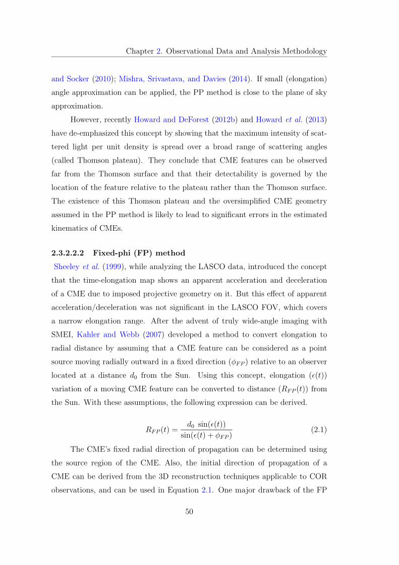
Chapter 2. Observational Data and Analysis Methodology
and Socker (2010); Mishra, Srivastava, and Davies (2014). If small (elongation)
angle approximation can be applied, the PP method is close to the plane of sky
approximation.
However, recently Howard and DeForest (2012b) and Howard et al. (2013)
have de-emphasized this concept by showing that the maximum intensity of scat-
tered light per unit density is spread over a broad range of scattering angles
(called Thomson plateau). They conclude that CME features can be observed
far from the Thomson surface and that their detectability is governed by the
location of the feature relative to the plateau rather than the Thomson surface.
The existence of this Thomson plateau and the oversimplified CME geometry
assumed in the PP method is likely to lead to significant errors in the estimated
kinematics of CMEs.
2.3.2.2.2 Fixed-phi (FP) method
Sheeley et al. (1999), while analyzing the LASCO data, introduced the concept
that the time-elongation map shows an apparent acceleration and deceleration
of a CME due to imposed projective geometry on it. But this effect of apparent
acceleration/deceleration was not significant in the LASCO FOV, which covers
a narrow elongation range. After the advent of truly wide-angle imaging with
SMEI, Kahler and Webb (2007) developed a method to convert elongation to
radial distance by assuming that a CME feature can be considered as a point
source moving radially outward in a fixed direction (φFP ) relative to an observer
located at a distance d0 from the Sun. Using this concept, elongation (ε(t))
variation of a moving CME feature can be converted to distance (RFP (t)) from
the Sun. With these assumptions, the following expression can be derived.
RFP (t) =d0 sin(ε(t))
sin(ε(t) + φFP )(2.1)
The CME’s fixed radial direction of propagation can be determined using
the source region of the CME. Also, the initial direction of propagation of a
CME can be derived from the 3D reconstruction techniques applicable to COR
observations, and can be used in Equation 2.1. One major drawback of the FP
50
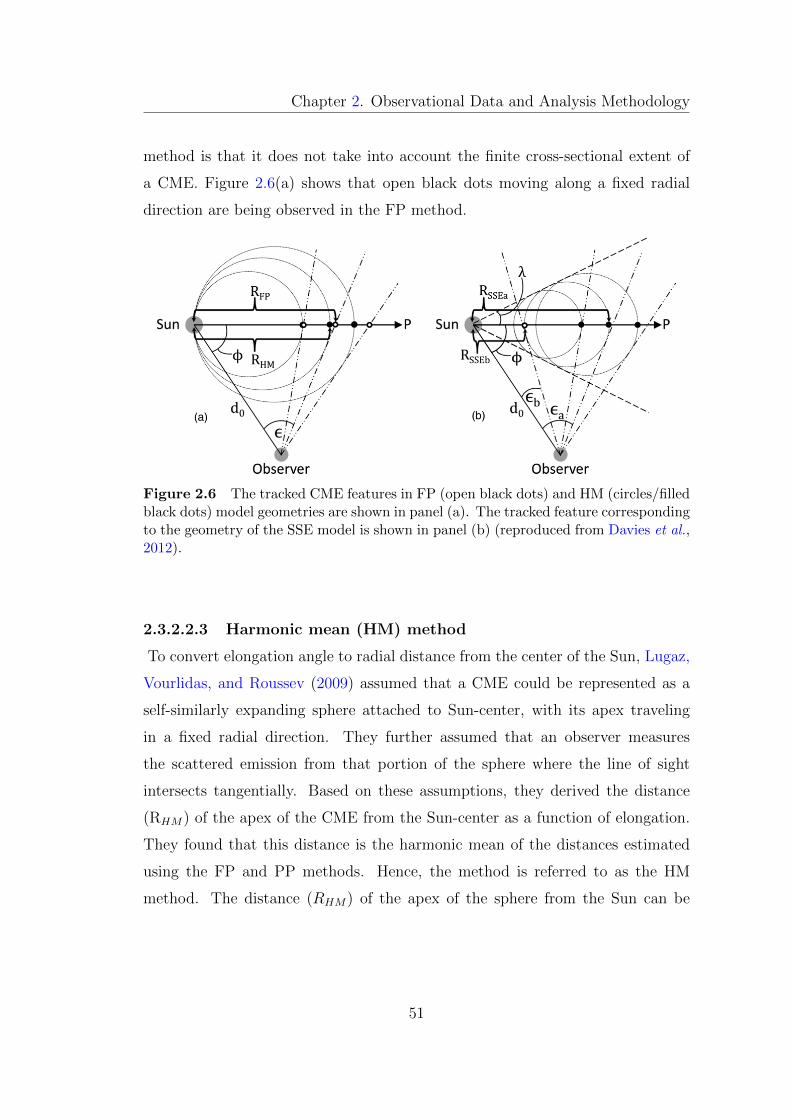
Chapter 2. Observational Data and Analysis Methodology
method is that it does not take into account the finite cross-sectional extent of
a CME. Figure 2.6(a) shows that open black dots moving along a fixed radial
direction are being observed in the FP method.
Figure 2.6 The tracked CME features in FP (open black dots) and HM (circles/filledblack dots) model geometries are shown in panel (a). The tracked feature correspondingto the geometry of the SSE model is shown in panel (b) (reproduced from Davies et al.,2012).
2.3.2.2.3 Harmonic mean (HM) method
To convert elongation angle to radial distance from the center of the Sun, Lugaz,
Vourlidas, and Roussev (2009) assumed that a CME could be represented as a
self-similarly expanding sphere attached to Sun-center, with its apex traveling
in a fixed radial direction. They further assumed that an observer measures
the scattered emission from that portion of the sphere where the line of sight
intersects tangentially. Based on these assumptions, they derived the distance
(RHM) of the apex of the CME from the Sun-center as a function of elongation.
They found that this distance is the harmonic mean of the distances estimated
using the FP and PP methods. Hence, the method is referred to as the HM
method. The distance (RHM) of the apex of the sphere from the Sun can be
51
Chapter 2. Observational Data and Analysis Methodology
estimated by,
RHM(t) =2d0 sin(ε(t))
1 + sin(ε(t) + φHM)(2.2)
where φHM is the radial direction of propagation of CME from the Sun-
observer line and ε is the elongation angle, and d is the distance of the observer
from the Sun. Although, in this method, the geometry of CMEs is taken into
account, the assumption of such geometry may not be valid due to possible flat-
tening of CME front on interaction with the solar wind. Figure 2.6(a) shows that
the filled black dots moving along a fixed radial direction will be observed for a
circular model geometry considered for the HM method.
2.3.2.2.4 Self-similar expansion (SSE) method
Davies et al. (2012) derived an expression for the elongation variation as a
function of the time of a CME viewed from a single vantage point and termed
as Self-Similar Expansion (SSE) method. In this method, a CME is considered
to have a circular cross-section, in the plane corresponding to the position angle
(PA) of interest, is not anchored to the Sun, and, during its propagation away
from the Sun, its radius increases such that it always subtends a fixed angle to
the Sun center. They also showed that the SSE geometry could be characterized
by an angular half-width (λ), and in its extreme forms, the SSE geometry is
equivalent to the FP (λ = 0◦) and HM methods (λ = 90◦). It must be noted
that λ can also be considered a parameter related to the curvature of the CME
front. Figure 2.6(b) shows the feature marked with filled black dots that will be
observed under the SSE method. The distance (RSSE) of a feature using this
method at a certain elongation measured from STEREO-A or STEREO-B can
be calculated from the Equation 2.3.
RSSE(t) =d0 sin(ε(t))(1 + sin(λ))
sin(ε(t) + φSSE) + sin(λ)(2.3)
In all the single spacecraft methods described above, i.e., FP, HM, and SSE,
it is assumed that a CME propagates along a fixed radial trajectory (in particular,
52
Chapter 2. Observational Data and Analysis Methodology
estimated in COR FOV), ignoring real or “artificial” heliospheric deflections.
This assumption is likely to introduce errors. As a CME moves away from the
Sun, not only the direction of propagation but also the geometry plays a role
(Howard, 2011). Such a geometrical effect comes to the picture because distances
are estimated, taking into account that part of the CME which makes a tangent
with the line of sight. Therefore, as the CME is far from the Sun, the observer
from a certain location cannot estimate the kinematics of the same part of the
leading edge of a CME in subsequent consecutive images. This is because of
geometrical effect, which produces a situation similar to the deflection of CME
and is called ‘artificial deflection.’ This effect leads to overestimating the distance
of the CME estimated from the FP method, which is more severe when the CME
approaches longer elongation angles.
2.3.2.3 Single spacecraft fitting methods
2.3.2.3.1 Fixed-phi fitting (FPF) method
The original concept of Sheeley et al. (1999) about deceptive acceleration or
deceleration of a CME moving with constant speed in the imager (SMEI & HI)
at large elongation angles from the Sun is used widely to assess the direction of
propagation and speed of CME (Rouillard et al., 2008; Sheeley et al., 2008a; Davis
et al., 2009; Mostl et al., 2009, 2010; Howard and Tappin, 2009; Mostl et al., 2011).
Under the assumption that a CME is traveling at a constant speed, the shape
of the observed elongation-time profile of CME will be different for observers
at different locations. Solving the Equation 2.1 for the elongation (ε(t)) with
assumption of constant velocity (vFP ) of CME along the fixed radial direction
(φFP ), we get,
ε(t) = arctan( vFP (t) sin(φFP )
d0 − vFP (t) cos(φFP )
)(2.4)
From this Equation 2.4, the launch time of CME from the sun center, i.e.
t0FP can also be calculated, and for this ε(t0FP ) = 0 will be satisfied. In practice,
we should calculate the launch time of a CME in the corona, i.e., at an elongation
53
Chapter 2. Observational Data and Analysis Methodology
corresponding to height in the corona. But to make the calculation simpler, we
consider the launch time on the Sun’s center (Mostl et al., 2011). Theoretical
elongation variation obtained from Equation 2.4 can be fitted to match most
closely with the observed elongation variation for a real CME by finding the
most suitable physically realistic combinations of vFP , φFP and t0FP values. This
approach to finding the direction of CME propagation and its speed is called the
Fixed-Phi-Fitting (FPF) method. This method has been applied to transients
like CIRs (Rouillard et al., 2008) and also on CMEs (Davis et al., 2009; Davies
et al., 2009; Rouillard et al., 2009; Mishra, Srivastava, and Davies, 2014).
2.3.2.3.2 Harmonic mean fitting (HMF) method
Based on HM approximation (Lugaz, Vourlidas, and Roussev, 2009) for CMEs,
Lugaz (2010) solved the equation of elongation angle and obtained the Harmonic
mean fitting (HMF) relation. Further, following the fitting version of the FP
method, i.e. FPF, Mostl et al. (2011) derived a new fitting version of the HM
method. They write the ε for Equation 2.2 as below, assuming a constant speed
(vHM) of CME propagating along a fixed radial direction (φHM).
ε(t) = arccos(−b+ a
√a2 + b2 − 1
a2 + b2
)(2.5)
In this equation, a and b are represented as below.
a =2d0
vHM t− cos(φHM) and b = sin(φHM)
It must be noted that in the case of a limb CME, its flank will be observed
in HI FOV because of the Thomson scattering surface. The flank of a CME is
relatively closer to the Sun than its apex. HMF method accounts for this effect
and estimates the propagation direction is always farther away from the observer
compared to the direction derived by the FPF method.
2.3.2.3.3 Self-similar expansion fitting (SSEF) method
Davies et al. (2012) derived a method to convert the measured elongation of an
54
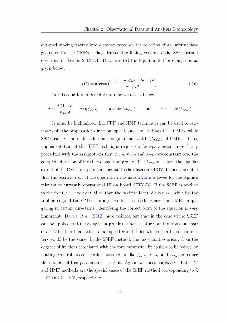
Chapter 2. Observational Data and Analysis Methodology
outward moving feature into distance based on the selection of an intermediate
geometry for the CMEs. They derived the fitting version of the SSE method
described in Section 2.3.2.2.4. They inverted the Equation 2.3 for elongation as
given below.
ε(t) = arccos(−bc+ a
√a2 + b2 − c2
a2 + b2
)(2.6)
In this equation, a, b and c are represented as below.
a =d0(1 + c)
vSSEt− cos(φSSE) ; b = sin(φSSE) and c = ± sin(λSSE)
It must be highlighted that FPF and HMF techniques can be used to esti-
mate only the propagation direction, speed, and launch time of the CMEs, while
SSEF can estimate the additional angular half-width (λSSE) of CMEs. Thus,
implementation of the SSEF technique requires a four-parameter curve fitting
procedure with the assumptions that φSSE, vSSE and λSSE are constant over the
complete duration of the time-elongation profile. The λSSE measures the angular
extent of the CME in a plane orthogonal to the observer’s FOV. It must be noted
that the positive root of the quadratic in Equation 2.6 is allowed for the regimes
relevant to currently operational HI on board STEREO. If the SSEF is applied
to the front, i.e., apex of CMEs, then the positive form of c is used, while for the
trailing edge of the CMEs, its negative form is used. Hence, for CMEs propa-
gating in certain directions, identifying the correct form of the equation is very
important. Davies et al. (2012) have pointed out that in the case where SSEF
can be applied to time-elongation profiles of both features at the front and rear
of a CME, then their fitted radial speed would differ while other fitted parame-
ters would be the same. In the SSEF method, the uncertainties arising from the
degrees of freedom associated with the four-parameter fit could also be solved by
putting constraints on the other parameters, like φSSE, λSSE, and vSSE to reduce
the number of free parameters in the fit. Again, we must emphasize that FPF
and HMF methods are the special cases of the SSEF method corresponding to λ
= 0◦ and λ = 90◦, respectively.
55
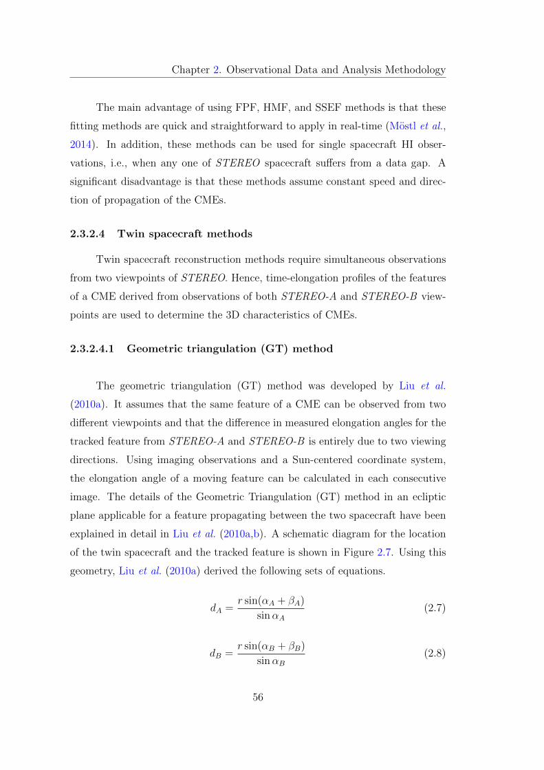
Chapter 2. Observational Data and Analysis Methodology
The main advantage of using FPF, HMF, and SSEF methods is that these
fitting methods are quick and straightforward to apply in real-time (Mostl et al.,
2014). In addition, these methods can be used for single spacecraft HI obser-
vations, i.e., when any one of STEREO spacecraft suffers from a data gap. A
significant disadvantage is that these methods assume constant speed and direc-
tion of propagation of the CMEs.
2.3.2.4 Twin spacecraft methods
Twin spacecraft reconstruction methods require simultaneous observations
from two viewpoints of STEREO. Hence, time-elongation profiles of the features
of a CME derived from observations of both STEREO-A and STEREO-B view-
points are used to determine the 3D characteristics of CMEs.
2.3.2.4.1 Geometric triangulation (GT) method
The geometric triangulation (GT) method was developed by Liu et al.
(2010a). It assumes that the same feature of a CME can be observed from two
different viewpoints and that the difference in measured elongation angles for the
tracked feature from STEREO-A and STEREO-B is entirely due to two viewing
directions. Using imaging observations and a Sun-centered coordinate system,
the elongation angle of a moving feature can be calculated in each consecutive
image. The details of the Geometric Triangulation (GT) method in an ecliptic
plane applicable for a feature propagating between the two spacecraft have been
explained in detail in Liu et al. (2010a,b). A schematic diagram for the location
of the twin spacecraft and the tracked feature is shown in Figure 2.7. Using this
geometry, Liu et al. (2010a) derived the following sets of equations.
dA =r sin(αA + βA)
sinαA(2.7)
dB =r sin(αB + βB)
sinαB(2.8)
56
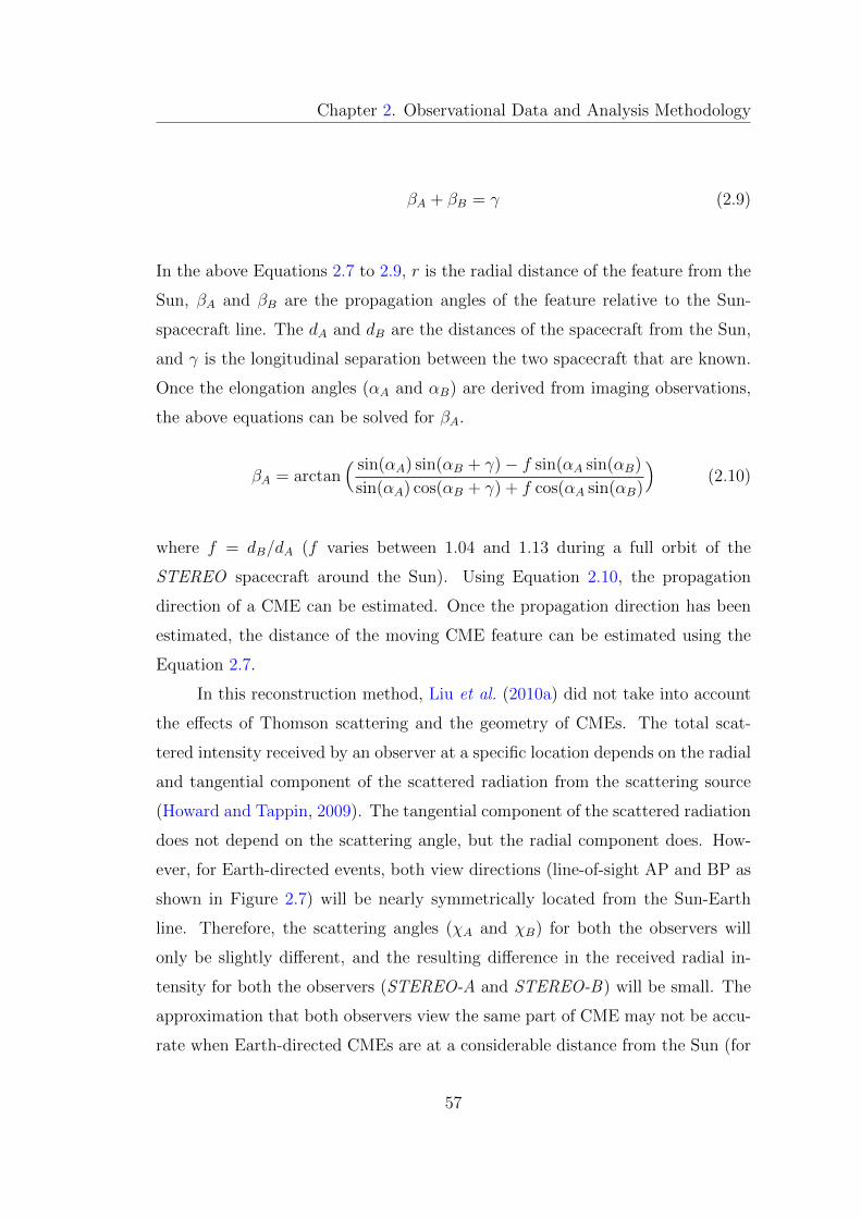
Chapter 2. Observational Data and Analysis Methodology
βA + βB = γ (2.9)
In the above Equations 2.7 to 2.9, r is the radial distance of the feature from the
Sun, βA and βB are the propagation angles of the feature relative to the Sun-
spacecraft line. The dA and dB are the distances of the spacecraft from the Sun,
and γ is the longitudinal separation between the two spacecraft that are known.
Once the elongation angles (αA and αB) are derived from imaging observations,
the above equations can be solved for βA.
βA = arctan( sin(αA) sin(αB + γ)− f sin(αA sin(αB)
sin(αA) cos(αB + γ) + f cos(αA sin(αB)
)(2.10)
where f = dB/dA (f varies between 1.04 and 1.13 during a full orbit of the
STEREO spacecraft around the Sun). Using Equation 2.10, the propagation
direction of a CME can be estimated. Once the propagation direction has been
estimated, the distance of the moving CME feature can be estimated using the
Equation 2.7.
In this reconstruction method, Liu et al. (2010a) did not take into account
the effects of Thomson scattering and the geometry of CMEs. The total scat-
tered intensity received by an observer at a specific location depends on the radial
and tangential component of the scattered radiation from the scattering source
(Howard and Tappin, 2009). The tangential component of the scattered radiation
does not depend on the scattering angle, but the radial component does. How-
ever, for Earth-directed events, both view directions (line-of-sight AP and BP as
shown in Figure 2.7) will be nearly symmetrically located from the Sun-Earth
line. Therefore, the scattering angles (χA and χB) for both the observers will
only be slightly different, and the resulting difference in the received radial in-
tensity for both the observers (STEREO-A and STEREO-B) will be small. The
approximation that both observers view the same part of CME may not be accu-
rate when Earth-directed CMEs are at a considerable distance from the Sun (for
57
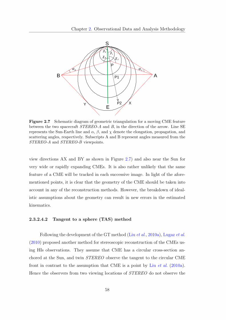
Chapter 2. Observational Data and Analysis Methodology
S
B
P2
P
Y X
P1 A
E
Aα
Bα
AβB
β
AχB
χ
Figure 2.7 Schematic diagram of geometric triangulation for a moving CME featurebetween the two spacecraft STEREO-A and B, in the direction of the arrow. Line SErepresents the Sun-Earth line and α, β, and χ denote the elongation, propagation, andscattering angles, respectively. Subscripts A and B represent angles measured from theSTEREO-A and STEREO-B viewpoints.
view directions AX and BY as shown in Figure 2.7) and also near the Sun for
very wide or rapidly expanding CMEs. It is also rather unlikely that the same
feature of a CME will be tracked in each successive image. In light of the afore-
mentioned points, it is clear that the geometry of the CME should be taken into
account in any of the reconstruction methods. However, the breakdown of ideal-
istic assumptions about the geometry can result in new errors in the estimated
kinematics.
2.3.2.4.2 Tangent to a sphere (TAS) method
Following the development of the GT method (Liu et al., 2010a), Lugaz et al.
(2010) proposed another method for stereoscopic reconstruction of the CMEs us-
ing HIs observations. They assume that CME has a circular cross-section an-
chored at the Sun, and twin STEREO observe the tangent to the circular CME
front in contrast to the assumption that CME is a point by Liu et al. (2010a).
Hence the observers from two viewing locations of STEREO do not observe the
58
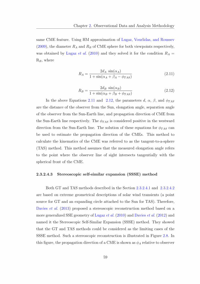
Chapter 2. Observational Data and Analysis Methodology
same CME feature. Using HM approximation of Lugaz, Vourlidas, and Roussev
(2009), the diameter RA and RB of CME sphere for both viewpoints respectively,
was obtained by Lugaz et al. (2010) and they solved it for the condition RA =
RB, where
RA =2dA sin(αA)
1 + sin(αA + βA − φTAS)(2.11)
RB =2dB sin(αB)
1 + sin(αB + βB + φTAS)(2.12)
In the above Equations 2.11 and 2.12, the parameters d, α, β, and φTAS
are the distance of the observer from the Sun, elongation angle, separation angle
of the observer from the Sun-Earth line, and propagation direction of CME from
the Sun-Earth line respectively. The φTAS is considered positive in the westward
direction from the Sun-Earth line. The solution of these equations for φTAS can
be used to estimate the propagation direction of the CMEs. This method to
calculate the kinematics of the CME was referred to as the tangent-to-a-sphere
(TAS) method. This method assumes that the measured elongation angle refers
to the point where the observer line of sight intersects tangentially with the
spherical front of the CME.
2.3.2.4.3 Stereoscopic self-similar expansion (SSSE) method
Both GT and TAS methods described in the Section 2.3.2.4.1 and 2.3.2.4.2
are based on extreme geometrical descriptions of solar wind transients (a point
source for GT and an expanding circle attached to the Sun for TAS). Therefore,
Davies et al. (2013) proposed a stereoscopic reconstruction method based on a
more generalized SSE geometry of Lugaz et al. (2010) and Davies et al. (2012) and
named it the Stereoscopic Self-Similar Expansion (SSSE) method. They showed
that the GT and TAS methods could be considered as the limiting cases of the
SSSE method. Such a stereoscopic reconstruction is illustrated in Figure 2.8. In
this figure, the propagation direction of a CME is shown as φA relative to observer
59
Chapter 2. Observational Data and Analysis Methodology
STEREO-A, φB relative to STEREO-B, and φE relative to Earth (E) and γ is
separation angle between both observer located at distances dA and dB from the
Sun. At each instance, εA and εB is the elongation measured from line of sight
from STEREO-A and STEREO-B, respectively.
Figure 2.8 The SSE modeled circular CME, with a constant λ is labeled as (i), (ii)and (iii), show three instances of propagation away from the Sun (S) in the commonFOV of two observers. The shaded region with gray color represents the common FOVof STEREO-A and STEREO-B. Geometry marked with (iv) is outside the commonFOV however both observers can observe it while geometry (v) is outside the FOVof STEREO-B and therefore can only be observed by STEREO-A (reproduced fromDavies et al., 2013).
Davies et al. (2012) used the Equation 2.3 corresponding to both viewpoints
of STEREO-A and STEREO-B and derived an expression for calculating the
propagation direction (φA or φB) of the CME. The propagation direction can be
used in Equation 2.3 to estimate the distance of tracked CME feature. This is
the same methodology utilized in the GT and TAS methods. SSSE method is
special as we can take a reasonable angular extent (λ) of CME geometry contrary
to extreme geometrical description taken in both GT and TAS methods. The
details of the SSSE method and important considerations for implementation of
this method have been discussed in Davies et al. (2013).
60

Chapter 2. Observational Data and Analysis Methodology
2.3.3 Estimation of the arrival time of CMEs
In our study, the kinematics of CMEs estimated by implementing 3D recon-
struction methods in COR2 and HI FOV is used to calculate their arrival time at
the Earth. In our study, we use the estimated kinematics either in the drag-based
model or extrapolate it to find the arrival time of CMEs near 1 AU at the Earth.
2.3.3.1 Drag based model for propagation of CMEs
When a CME is far from the Sun, the Lorentz and gravity forces decrease
such that drag can be considered to govern CME dynamics. Although it is not
proven that drag is the only force that shapes CME dynamics in the interplanetary
medium, the observed deceleration/acceleration of some CMEs have been closely
reproduced by considering only the drag force acting between the CME and the
ambient solar wind medium (Lindsay et al., 1999; Cargill, 2004; Manoharan, 2006;
Vrsnak et al., 2009; Lara and Borgazzi, 2009). In our study, we have used the
drag-based model (DBM) (Vrsnak et al., 2013) to derive the kinematic properties
for the distance range beyond which a CME cannot be tracked in the J -maps.
The DBM model assumes that, after 20 R�, the dynamics of CMEs is solely
governed by the drag force and that the drag acceleration has the form, ad = -γ
(v − w) |(v − w)|, (see e.g. Cargill et al. 1996; Cargill 2004; Vrsnak et al. 2010),
where v is the speed of the CME, w is the ambient solar wind speed and γ is the
drag parameter.
The drag parameter is given by γ = cdAρwM+Mv
, where cd is the dimensional
drag coefficient, A is the cross-sectional area of the CME perpendicular to its
propagation direction (which depends on the CME-cone angular width), ρw is
the ambient solar wind density, M is the CME mass, and Mv is the virtual CME
mass. The latter is written as, Mv = ρwV/2, where V is the CME volume. A
statistical study has shown that the drag parameter generally lies between 0.2 ×10⁻⁷ and 2.0 × 10⁻⁷ km−1 (Vrsnak et al., 2013). They assumed that the mass
and angular width of CMEs do not vary beyond 20 R� and also showed that the
solar wind speed lies between 300 and 400 km s−1 for slow solar wind conditions.
61
Chapter 2. Observational Data and Analysis Methodology
For the case where a CME propagates in high-speed solar wind or if a coronal
hole is present in the vicinity of the CME source region, the ambient solar wind
speed should be chosen to lie between 500 and 600 km s−1, along with a lower
value of the drag parameter.
2.4 Identification of CMEs and Their Consequences Near
the Earth
Once the CMEs arrive near the 1 AU at the Earth, they can cause severe
geomagnetic consequences in the Earth’s magnetosphere. Analyzing the observa-
tion of in situ spacecraft (e.g., ACE, WIND), we identify various parts of CME
structures and mark their boundaries. The identification of CME boundaries is
carried out using multiple signatures of CMEs (described in Section 1.4.1.2 of
Chapter 1). It is essential to mention here that no CMEs show all the signatures,
and therefore there is no unique scheme to identify them in in situ observations.
Also, different signatures may appear for different intervals of time, and hence,
CMEs may have different boundaries in plasma, magnetic field, and other signa-
tures. This is possible as different signatures have their origin due to different
physical processes. If we identify CMEs based on only a few signatures, then
they may be falsely identified. On the other hand, if several in situ signatures
are considered, then such an attempt may lead to the omission of a few CMEs.
Therefore, our approach is to identify as many signatures as possible. Such a
procedure helps for reliable identification of the CMEs in in situ observations;
however, marking their boundaries may still be ambiguous. Various lists of CMEs
observed near the Earth have been compiled based on different criteria, e.g. by
Richardson and Cane (1995); Cane and Richardson (2003); Richardson and Cane
(2010). Richardson and Cane (2010) have identified approximately 300 CMEs
near the Earth during the complete solar cycle 23, i.e., between year 1996 to
2009.
Identifying CMEs in in situ observations is extremely difficult when they
arrive as structures formed due to the interaction or collision of several CMEs.
62
Chapter 2. Observational Data and Analysis Methodology
The collision of CMEs is expected during their evolution between the Sun and
the Earth when they are launched in quick succession in the same direction from
the Sun. As they interact, they experience a change in their plasma, dynamic and
magnetic field parameters. Hence, the collision of CMEs may lead to a new type
of solar wind structure which is expected to show different in situ signatures than
isolated normal CMEs. In addition, such new structures might have a different
geomagnetic response than isolated CMEs. We have investigated the geomagnetic
responses of interacting CMEs as an example of the heliospheric consequences of
CMEs. The actual arrival times of remotely tracked features of the CMEs are
marked in in situ observations. We compare the estimated arrival times of tracked
features based on the kinematics and actual arrival times. In this way, we attempt
to make an association between remote and in situ observations of the CMEs and
assess the performance of several 3D reconstruction methods used to estimate
CME kinematics.
In summary, continuous tracking of CMEs in the heliosphere and implemen-
tation of suitable 3D reconstruction methods to estimate and understand their
kinematics is an important step in our study. Finding an association of remote
observations to in situ and ground-based magnetometer observations is also car-
ried out. The heliospheric consequences and geomagnetic responses of interacting
CMEs have been studied.
63
Chapter 3
Estimation of Arrival Time of
CMEs
3.1 Introduction
Due to the significant role of CMEs and interplanetary shocks in the context
of space weather, understanding their heliospheric evolution and predicting their
arrival times at the Earth is a major objective of various forecast centers. The pre-
diction of CME/shock arrival time means that forecasters utilize the observables
of solar disturbance obtained prior to arrival as inputs to predict whether/when
they will arrive. A longer lead time in prediction is yielded if the solar observables
are used. The arrival time of CMEs at 1 AU can be related to their characteristics
(velocity, acceleration) near the Sun in order to develop the prediction methods
for CME’s arrival time. Different models of CME/shock arrival time prediction
have been developed, e.g., empirical models, expansion speed models, drag-based
models, physics-based models, and MHD models.
The models that adopt relatively simple equations to fit the relations be-
tween the arrival time of the CME disturbance at the Earth and their observables
near the Sun (such as initial velocity) are called empirical prediction models. Van-
das et al. (1996) found that the transit time (in hr) to 1 AU for the CME flux rope
(cloud/driver) leading edge is Tdriver = 85-0.014Vi for a slow background solar
64
Chapter 3. Estimation of Arrival Time of CMEs
wind speed (say, 361 km s−1), and Tdriver = 42-0.0041Vi for a faster background
solar wind speed (say, 794 km s−1). Here Vi (km s−1) is the propagation speed of
the leading edge of CME at 18 R�. Then the transit time of the shock preceding
the magnetic cloud is Tshock = 74 - 0.015Vi for slow solar wind and Tshock =
43-0.006Vi for fast solar wind. Brueckner et al. (1998) found that the difference
in time between the CME launch on the Sun and the time when the associated
geomagnetic storm reaches its peak is about 80 hr. One of the most typical and
widely used empirical prediction models is empirical CME arrival (ECA) and
empirical shock arrival (ESA) models. The empirical CME arrival (ECA) model
developed by Gopalswamy et al. (2001b) considers that a CME has an average
acceleration up to a distance of 0.7 AU-0.95 AU. After the cessation of accel-
eration, a CME is assumed to move at a constant speed. They found that the
average acceleration has a linear relationship with the initial plane-of-sky speed
of the CME. The ECA model has been able to predict the arrival time of CMEs
within an error of approximately ± 35 hr with an average error of 11 hr. Later, an
empirical shock arrival (ESA) model was developed that was able to predict the
arrival time of CMEs to within an error of approximately ± 30 hr with an average
error of 12 hr (Gopalswamy et al., 2005). The ESA model is a modified version of
the ECA model in which a CME is considered to be the driver of magnetohydro-
dynamic (MHD) shocks. The other assumption is that fast mode MHD shocks
are similar to gas dynamic shocks. The gas-dynamic piston-shock relationship is
thus utilized in this model. Various efforts have been made to derive an empirical
formula for CME arrival time based on the projected speed of a large number of
CMEs (Wang et al., 2002; Zhang et al., 2003; Srivastava and Venkatakrishnan,
2004; Manoharan et al., 2004). Vrsnak and Zic (2007) found that CME transit
time depends on both the CME take-off speed and the background solar wind
speed. In the majority of these models, the initial speeds of CMEs used were
measured from the plane of sky LASCO/SOHO observations, and therefore the
measured kinematics are not representative of the true CME motion.
To overcome plane-of-sky effects, Dal Lago, Schwenn, and Gonzalez (2003)
used a sample of 57 limb CMEs to derive an empirical relationship between their
65
Chapter 3. Estimation of Arrival Time of CMEs
radial and expansion speeds as Vrad = 0.88Vexp. This result led to lateral ex-
pansion speed as a proxy for the radial speed of halo CMEs that could not be
measured. Also, Schwenn et al. (2005) analyzed 75 events to derive an empirical
formula for transit time of CMEs to Earth Ttr = 203 - 20.77 ln(Vexp). Their re-
sults show that the formula can predict ICME arrivals, with a 95% error margin
of about 24 hr.
Several observations have revealed that the dynamics of CMEs are governed
mainly by their interaction with the background solar wind beyond a certain
helio-distance. On this basis, several analytical models have been developed to
depict the propagation of CMEs and predict their arrival times. These analytical
models are based on the equation of motion of CMEs, where the drag accelera-
tion/deceleration has a quadratic dependence on the relative speed between CME
and the background solar wind. It was found that the measured deceleration rates
are proportional to the relative velocity between CME and the background solar
wind, as well as a dimensionless drag coefficient (cd) (Vrsnak, 2001; Vrsnak and
Gopalswamy, 2002; Cargill, 2004). Recently, Subramanian, Lara, and Borgazzi
(2012) have discussed the variation of the drag coefficient (cd) with heliocentric
distance for the first time. They adopt a microphysical prescription for viscosity
in the turbulent solar wind to obtain an analytical model for the drag coefficient.
Vrsnak et al. (2013) have simplified the drag-based model and presented an ex-
plicit solution for the Sun-Earth transit time of CMEs and their impact speed at
1 AU.
One physics-based prediction model is the “Shock Time of Arrival” (STOA)
model, which is based on the theory of similar blast waves from point explo-
sions. This concept was revised by introducing the piston-driven concept (Dryer,
1974; Smart and Shea, 1985). Another such model is the “Interplanetary Shock
Propagation Model” (ISPM), which is based on a 2.5D MHD parametric study
of numerically simulated shocks. The model demonstrates that the organizing
parameter for the shock is the net energy released into the solar wind (Smith
and Dryer, 1990). The “Hakamada-Akasofu-Fry version 2” (HAFv.2) model is
a “modified kinematic” solar wind model that calculates the solar wind speed,
66
Chapter 3. Estimation of Arrival Time of CMEs
density, magnetic field, and dynamic pressure as a function of time and location
(Dryer et al., 2001, 2004; Fry et al., 2001, 2007; Smith et al., 2009). This model
provides a global description of the propagation of multiple and interacting shocks
in nonuniform, stream-stream interacting solar wind flows in the ecliptic plane.
The STOA, ISPM, and HAFv.2 models use similar input solar parameters (i.e.,
the source location of the associated flare, the start time of the metric Type II
radio burst, the proxy piston driving time duration, and the background solar
wind speed).
Also, several physics-based magnetohydrodynamics (MHD) numerical mod-
els have been developed. The coupled Wang-Sheeley-Arge (WSA) + ENLIL +
Cone model (Odstrcil, Riley, and Zhao, 2004) is widely used to simulate the
propagation and evolution of CMEs in interplanetary space and provides a 1-
2 day lead time forecasting for major CMEs (Taktakishvili et al., 2009; Pizzo
et al., 2011). WSA is a quasi-steady global solar wind model that uses synoptic
magnetograms as inputs to predict ambient solar wind speed and interplanetary
magnetic field polarity at Earth (Wang and Sheeley, 1995; Arge and Pizzo, 2000).
The ENLIL model is a time-dependent, 3D ideal MHD model of the solar wind in
the heliosphere (Odstrcil et al., 2002; Odstrcil, Riley, and Zhao, 2004). The cone
model assumes a CME as a cone with constant angular width in the heliosphere
(Zhao, Plunkett, and Liu, 2002; Xie, Ofman, and Lawrence, 2004). The input of
ENLIL at its inner boundary of 21.5 R� is taken from the output of WSA to get
the background solar wind flows and interplanetary magnetic field.
Some of the aforementioned models are complicated, while others are rel-
atively simple and easy. However, no significant differences are found between
their prediction capabilities of CME arrival time. The predictions yield a root-
mean-square error of ≈ 12 hr and a mean absolute error of ≈ 10 hr for many
CMEs. There are many factors that are responsible for the limited accuracies
of these models, e.g. (1) The inputs parameters (kinematics and morphology)
of the model have their uncertainties. (2) The real-time background solar wind
condition into which CME travels is difficult to observe or simulate from MHD.
(3) The change in the kinematics of the CME due to its interaction with other
67
Chapter 3. Estimation of Arrival Time of CMEs
large or small scale solar wind structures. These factors are challenging to be
taken into account in a single model. Improvement in the accuracy of these ar-
rival time models requires a better understanding of CME’s heliospheric evolution
and the ambient solar wind medium. Using the observations of CMEs, such as
by SECCHI instruments onboard STEREO, their heliospheric evolution can be
investigated and compared with results from the models. Such observations can
help to impose several constraints on the aforementioned models.
STEREO observations have greatly enhanced our ability to track the CMEs
continuously. This is because of STEREO’s two viewpoints which allow the
3D reconstruction of CMEs. Also, the large field of view (FOV) of its imaging
telescopes (such as HI1 and HI2) enables the tracking of CMEs to a much larger
distance in the heliosphere. Using STEREO observations, several attempts have
been made to understand the 3D propagation of CMEs and estimate their arrival
time (Mierla et al., 2009; Srivastava et al., 2009; Kahler and Webb, 2007; Liu et al.,
2010a; Mostl et al., 2011; Davies et al., 2012, 2013). In a recent study, a CME
was tracked beyond the Earth’s distance, and was shown that a proper treatment
of CME geometry must be performed in estimating CME kinematics, especially
when a CME is directed away from the observer (Liu et al., 2013). Using different
reconstruction methods on HI observations, Mostl et al. (2014) show an absolute
difference between predicted and observed CME arrival times as 8.1 ± 6.3 hr.
The HI observations have also revealed imaging of a few cases of interacting
CMEs. The interaction of CMEs complicates the problem of estimating their
arrival time. Several attempts have been made to understand the propagation of
interacting CMEs using SECCHI/HI observations (Harrison et al., 2012; Temmer
et al., 2012; Mostl et al., 2012; Lugaz et al., 2012). In an attempt to combine the
CME kinematics with a model, Kilpua et al. (2012) estimated the 3D speed of
CMEs in the COR FOV (close to the Sun) from the forward modeling (Thernisien,
Vourlidas, and Howard, 2009) method and used in CME travel-time prediction
models of Gopalswamy et al. (2000a, 2001b). They compared the estimated
travel time with the actual travel time of CME from the Sun to STEREO, ACE
and WIND spacecraft. They also compared the estimated travel time with that
68
Chapter 3. Estimation of Arrival Time of CMEs
estimated using the projected CME speed in the models. Their study shows that
CME 3D speeds give slightly (≈ 4 hr) better predictions than projected CME
speeds. However, in their study, a large average error of 11 hr is noted between
the predicted and observed travel times.
For understanding the heliospheric evolution of CMEs from the Sun to
Earth, we have estimated the kinematics of various selected CMEs by imple-
menting suitable 3D reconstruction methods on the remote sensing observations
of the CMEs. This chapter consists of two major studies:
1. Estimating the arrival time of CMEs at L1 by tracking them into heliosphere
(HI FOV) and applying geometric triangulation (GT) method (Liu et al.,
2010a) of 3D reconstruction.
2. Assessment of the relative performance of several 3D reconstruction meth-
ods, applicable on HI observations, for estimating the arrival time of CMEs.
3.2 Estimating the Arrival Time of CMEs Using GT
Method
In this study, we attempt to understand the 3D propagation of CMEs by
tracking them continuously throughout the interplanetary medium. For this pur-
pose, we use the GT reconstruction method on the time-elongation maps (J -
maps) (Sheeley et al., 1999), constructed from COR2 and HI observations, to
estimate the 3D kinematics of CMEs. These estimated values of kinematics are
used as inputs in the drag-based model (Vrsnak et al., 2013) beyond the distance
where a CME could not be tracked unambiguously, and its arrival time, as well as
its transit velocity at the L1 point, are predicted. The predicted arrival time and
transit velocity of the CME at L1 is then compared with the actual arrival time
and transit velocity as observed by in situ instruments, e.g., ACE and WIND.
The predicted arrival time is also compared with the arrival time estimated using
the 3D speed obtained by the 3D reconstruction methods applicable on COR2
observation alone, e.g., tie-pointing procedure (scc measure: Thompson, 2009)
69

Chapter 3. Estimation of Arrival Time of CMEs
from SECCHI/COR2 data alone. Hence, in this study, we attempt to examine
the improvement in arrival time prediction of CMEs by using the GT method on
heliospheric observations of CMEs (HI FOV) over using only coronagraph (COR)
observations. The in situ observations of selected CMEs and their interpretation
are described separately in detail in Chapter 4.
Selection of CMEs
Keeping in mind our goal to track a CME in the heliosphere and then implement
the 3D reconstruction method, we selected only the Earth-directed CMEs in our
study. This is because the HI instruments on STEREO have been designed in such
a way that only a CME is directed towards the Earth (i.e., between STEREO-A
and STEREO-B) can be observed in both FOV of HI-A and HI-B. In addition,
the in situ observations of these CMEs can be used as a reference for their actual
arrival time to constrain the kinematics of the CMEs. Further, these CMEs are
important to study because of their consequences on the Earth. We selected eight
Earth-directed CMEs observed on different dates after the launch of the STEREO
spacecraft. These CMEs observed with STEREO at different separation angles
between them, the arrival time of CME shock/sheath, leading and trailing edge
at L1 are listed in Table 3.1. These CMEs have been observed from their birth
in the corona through the inner heliosphere by coronagraphs and HIs. It must be
noted that during the time of favorable separation between STEREO spacecraft,
for more appropriate 3D reconstruction of Earth-directed CMEs in HI FOV, very
few Earth-directed CMEs occurred during 2006 to 2010.
Remote sensing observational data of CMEs by the twin STEREO space-
craft are taken from UKSSDC (http://www.ukssdc.ac.uk/solar/stereo/data.html).
In situ observations of CMEs were obtained from the ACE and WIND space-
craft situated at the L1 point, upstream from the Earth. We used the OMNI
data with a 1 min time resolution for solar wind parameters, e.g., magnetic
field, proton velocity, proton density, proton temperature, and plasma beta. We
also used the latitude and longitude of magnetic field vector data with a time
resolution of 1 hr. Combined OMNI data were taken from NASA CDAWeb
70
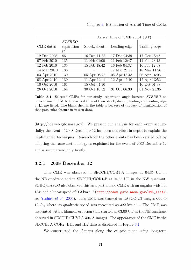
Chapter 3. Estimation of Arrival Time of CMEs
Arrival time of CME at L1 (UT)
CME datesSTEREOseparation(◦)
Shock/sheath Leading edge Trailing edge
12 Dec 2008 86 16 Dec 11:55 17 Dec 04:39 17 Dec 15:4807 Feb 2010 135 11 Feb 01:00 11 Feb 12:47 11 Feb 23:1312 Feb 2010 135 15 Feb 18:42 16 Feb 04:32 16 Feb 12:3814 Mar 2010 138 – 17 Mar 21:19 18 Mar 11:2603 Apr 2010 139 05 Apr 08:28 05 Apr 13:43 06 Apr 16:0508 Apr 2010 139 11 Apr 12:44 12 Apr 02:10 12 Apr 13:5210 Oct 2010 161 15 Oct 04:30 – 16 Oct 01:3826 Oct 2010 164 30 Oct 10:32 31 Oct 06:30 01 Nov 21:35
Table 3.1 Selected CMEs for our study, separation angle between STEREO onlaunch time of CMEs, the arrival time of their shock/sheath, leading and trailing edgeat L1 are listed. The blank shell in the table is because of the lack of identification ofthat particular feature in in situ data.
(http://cdaweb.gsfc.nasa.gov). We present our analysis for each event sequen-
tially; the event of 2008 December 12 has been described in-depth to explain the
implemented techniques. Research for the other events has been carried out by
adopting the same methodology as explained for the event of 2008 December 12
and is summarized only briefly.
3.2.1 2008 December 12
This CME was observed in SECCHI/COR1-A images at 04:35 UT in
the NE quadrant and in SECCHI/COR1-B at 04:55 UT in the NW quadrant.
SOHO/LASCO also observed this as a partial halo CME with an angular width of
184◦ and a linear speed of 203 km s−1 (http://cdaw.gsfc.nasa.gov/CME_list/;
see Yashiro et al., 2004). This CME was tracked in LASCO-C3 images out to
12 R� where its quadratic speed was measured as 322 km s−1. The CME was
associated with a filament eruption that started at 03:00 UT in the NE quadrant
observed in SECCHI/EUVI-A 304 A images. The appearance of the CME in the
SECCHI-A COR2, HI1, and HI2 data is displayed in Figure 3.1.
We constructed the J -maps along the ecliptic plane using long-term
71
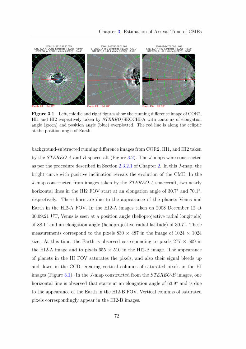
Chapter 3. Estimation of Arrival Time of CMEs
2040
60
80
100
120
140 16
0
180 200
220
240
260
280
300
320
340
2
2
4
4
4
4
2008-12-12T10:37:30.005
Earth PA: 84.92o
STEREO_A COR2 Longitude (HEEQ): 42.09o
STEREO_A COR2 Latitude (HEEQ): -5.44o
4060
60
8080
100
100
120 140
10
10
20
20
2008-12-13T00:09:01.005
Earth PA: 84.98o
STEREO_A HI1 Longitude (HEEQ): 42.11o
STEREO_A HI1 Latitude (HEEQ): -5.49o
40
60
60
8080
100
100
120 140
20
40
40
60
60
80
80
2008-12-14T02:09:21.005
Earth PA: 85.08o
STEREO_A HI2 Longitude (HEEQ): 42.14o
STEREO_A HI2 Latitude (HEEQ): -5.58o
Figure 3.1 Left, middle and right figures show the running difference image of COR2,HI1 and HI2 respectively taken by STEREO/SECCHI-A with contours of elongationangle (green) and position angle (blue) overplotted. The red line is along the eclipticat the position angle of Earth.
background-subtracted running difference images from COR2, HI1, and HI2 taken
by the STEREO-A and B spacecraft (Figure 3.2). The J -maps were constructed
as per the procedure described in Section 2.3.2.1 of Chapter 2. In this J -map, the
bright curve with positive inclination reveals the evolution of the CME. In the
J -map constructed from images taken by the STEREO-A spacecraft, two nearly
horizontal lines in the HI2 FOV start at an elongation angle of 30.7◦ and 70.1◦,
respectively. These lines are due to the appearance of the planets Venus and
Earth in the HI2-A FOV. In the HI2-A images taken on 2008 December 12 at
00:09:21 UT, Venus is seen at a position angle (helioprojective radial longitude)
of 88.1◦ and an elongation angle (helioprojective radial latitude) of 30.7◦. These
measurements correspond to the pixels 830 × 487 in the image of 1024 × 1024
size. At this time, the Earth is observed corresponding to pixels 277 × 509 in
the HI2-A image and to pixels 655 × 510 in the HI2-B image. The appearance
of planets in the HI FOV saturates the pixels, and also their signal bleeds up
and down in the CCD, creating vertical columns of saturated pixels in the HI
images (Figure 3.1). In the J -map constructed from the STEREO-B images, one
horizontal line is observed that starts at an elongation angle of 63.9◦ and is due
to the appearance of the Earth in the HI2-B FOV. Vertical columns of saturated
pixels correspondingly appear in the HI2-B images.
72
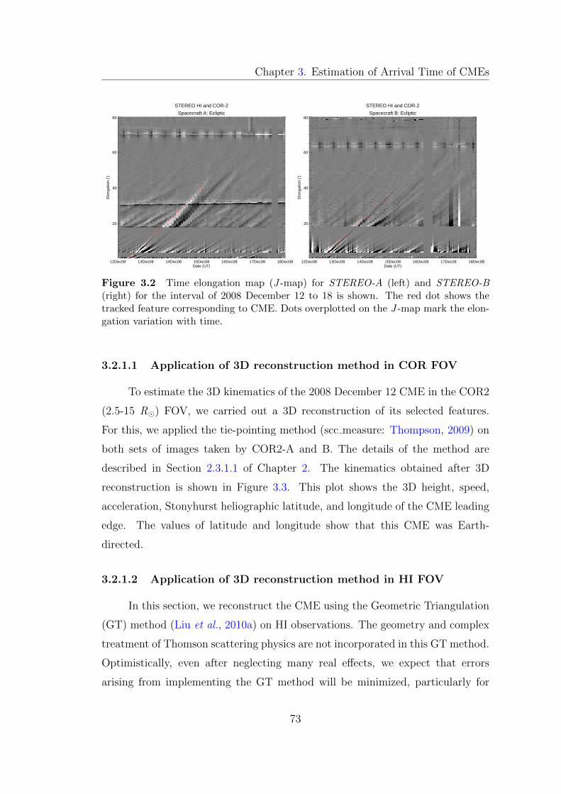
Chapter 3. Estimation of Arrival Time of CMEs
Spacecraft A: Ecliptic
12Dec08 13Dec08 14Dec08 15Dec08 16Dec08 17Dec08 18Dec08Date (UT)
20
40
60
80
Elo
ngat
ion
(o )STEREO HI and COR-2
Spacecraft B: Ecliptic
12Dec08 13Dec08 14Dec08 15Dec08 16Dec08 17Dec08 18Dec08Date (UT)
20
40
60
80
Elo
ngat
ion
(o )
STEREO HI and COR-2
Figure 3.2 Time elongation map (J -map) for STEREO-A (left) and STEREO-B(right) for the interval of 2008 December 12 to 18 is shown. The red dot shows thetracked feature corresponding to CME. Dots overplotted on the J -map mark the elon-gation variation with time.
3.2.1.1 Application of 3D reconstruction method in COR FOV
To estimate the 3D kinematics of the 2008 December 12 CME in the COR2
(2.5-15 R�) FOV, we carried out a 3D reconstruction of its selected features.
For this, we applied the tie-pointing method (scc measure: Thompson, 2009) on
both sets of images taken by COR2-A and B. The details of the method are
described in Section 2.3.1.1 of Chapter 2. The kinematics obtained after 3D
reconstruction is shown in Figure 3.3. This plot shows the 3D height, speed,
acceleration, Stonyhurst heliographic latitude, and longitude of the CME leading
edge. The values of latitude and longitude show that this CME was Earth-
directed.
3.2.1.2 Application of 3D reconstruction method in HI FOV
In this section, we reconstruct the CME using the Geometric Triangulation
(GT) method (Liu et al., 2010a) on HI observations. The geometry and complex
treatment of Thomson scattering physics are not incorporated in this GT method.
Optimistically, even after neglecting many real effects, we expect that errors
arising from implementing the GT method will be minimized, particularly for
73
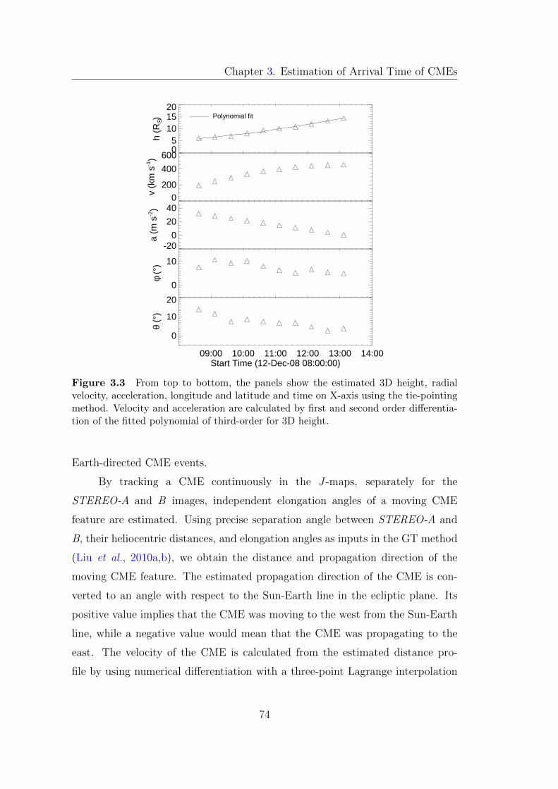
Chapter 3. Estimation of Arrival Time of CMEs
05
101520
h (R
O •) Polynomial fit
0
200
400
600v
(km
s-1)
-20
0
20
40
a (m
s-2)
0
10
φ (°
)
09:00 10:00 11:00 12:00 13:00 14:00Start Time (12-Dec-08 08:00:00)
0
10
20
θ (°
)
Figure 3.3 From top to bottom, the panels show the estimated 3D height, radialvelocity, acceleration, longitude and latitude and time on X-axis using the tie-pointingmethod. Velocity and acceleration are calculated by first and second order differentia-tion of the fitted polynomial of third-order for 3D height.
Earth-directed CME events.
By tracking a CME continuously in the J -maps, separately for the
STEREO-A and B images, independent elongation angles of a moving CME
feature are estimated. Using precise separation angle between STEREO-A and
B, their heliocentric distances, and elongation angles as inputs in the GT method
(Liu et al., 2010a,b), we obtain the distance and propagation direction of the
moving CME feature. The estimated propagation direction of the CME is con-
verted to an angle with respect to the Sun-Earth line in the ecliptic plane. Its
positive value implies that the CME was moving to the west from the Sun-Earth
line, while a negative value would mean that the CME was propagating to the
east. The velocity of the CME is calculated from the estimated distance pro-
file by using numerical differentiation with a three-point Lagrange interpolation
74
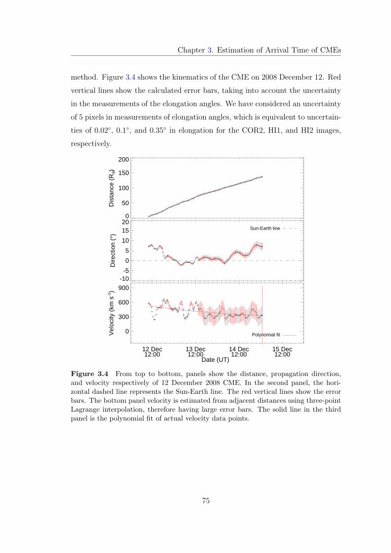
Chapter 3. Estimation of Arrival Time of CMEs
method. Figure 3.4 shows the kinematics of the CME on 2008 December 12. Red
vertical lines show the calculated error bars, taking into account the uncertainty
in the measurements of the elongation angles. We have considered an uncertainty
of 5 pixels in measurements of elongation angles, which is equivalent to uncertain-
ties of 0.02◦, 0.1◦, and 0.35◦ in elongation for the COR2, HI1, and HI2 images,
respectively.
0
50
100
150
200
Dis
tanc
e (R
O •)
-10-5
0
5
10
1520
Dire
ctio
n (°
)
Sun-Earth line
12 Dec12:00
13 Dec12:00
14 Dec12:00
15 Dec12:00
0
300
600
900
Vel
ocity
(km
s-1)
Polynomial fit
Date (UT)
Figure 3.4 From top to bottom, panels show the distance, propagation direction,and velocity respectively of 12 December 2008 CME. In the second panel, the hori-zontal dashed line represents the Sun-Earth line. The red vertical lines show the errorbars. The bottom panel velocity is estimated from adjacent distances using three-pointLagrange interpolation, therefore having large error bars. The solid line in the thirdpanel is the polynomial fit of actual velocity data points.
75
Chapter 3. Estimation of Arrival Time of CMEs
3.2.1.3 Estimation of arrival time and transit speed of 2008 December
12 CME at L1
Using the GT method on HI data, we have estimated the kinematics of
the CME of 2008 December 12 out to approximately 138 R�. We assume that
after traversing such a large distance, the speed of the CME will depend solely on
aerodynamic drag. Therefore, we use the Drag-based model (DBM) developed by
Vrsnak et al. (2013) to estimate the arrival time of the 2008 December 12 CME.
The details of the DBM are described in Section 2.3.3.1 of Chapter 2.
Although there is limited accuracy in reliable estimation of the variables
(mass, cone angle of the CME, and solar wind density) on which the drag pa-
rameter depends, we used the extreme values of the range of the drag parameter
for CMEs in our study. The limitation on the accurate and reliable estimation of
the CME mass using single coronagraph images has been discussed in Vourlidas
et al. (2000). Colaninno and Vourlidas (2009) discussed the limitations on the
reliable estimation of CME mass using multiple viewpoints COR images. Choos-
ing extreme values of the range of the drag parameter, we estimate the maximum
possible error in arrival time that can occur due to CMEs having different char-
acteristics.
We used the estimated kinematics as inputs for three different approaches in
order to predict the arrival time of CMEs at L1 (≈ 1 AU). These three approaches
are described as follows.
1. Using 3D speed estimated in the COR2 FOV
From the 3D reconstruction of the CME leading edge using the tie-pointing
(scc measure) method on SECCHI/COR2 data, the 3D velocity was found
to be 453 km s−1 at 14.4 R� at 13:07 UT on 2008 December 12. With a
simple assumption that the speed of the CME remains constant beyond the
COR2 FOV, the predicted arrival time at L1 is 01:45 UT on 2008 December
16.
2. Using a polynomial fit of distance estimated from the GT tech-
nique with COR2 and HI data
76
Chapter 3. Estimation of Arrival Time of CMEs
The radial distance of a moving feature, estimated by implementing the
GT method, is fitted to a second-order polynomial. We obtained the ar-
rival time of the CME at L1 by extrapolation for the distance beyond which
the moving feature could not be tracked. The predicted arrival time is 06:23
UT on 2008 December 17. In an earlier study by Liu et al. (2010a), the
predicted arrival time for this CME was found to be 16:00-18:00 UT on
2008 December 16. The difference in the two arrival times may arise due to
different extrapolation techniques but is most likely due to manual tracking
of different features in J -maps. Since fitting the estimated distance using
a second-order polynomial includes all the points with different velocity
phases, this technique may result in more significant uncertainties in the
extrapolated arrival times.
3. From DBM with inputs from GT on COR2 and HI
We used the DBM, combined with the inputs obtained by implementing
the GT technique on COR2 and HI observations. For the inputs in the
DBM, we used the initial radial distance and CME take-off date and time
as obtained from the last data points estimated in the GT method. The
initial take-off velocity is taken as the average of the last few velocity points
of the fitted polynomial for the estimated velocity in the ecliptic plane. In
this particular event of 2008 December 12, we used the DBM with a take-off
date and time of 2008 December 15 at 01:00 UT, a take-off distance of 138.3
R�, a take-off velocity of 330 km s−1, an ambient solar wind speed of 350
km s−1, and a drag parameter of 0.2 × 10⁻⁷ km−1. Using these values, we
obtained its arrival time as 20:25 UT on 2008 December 16, with a transit
speed of 331 km s−1 at the L1 point. Using the maximum value of the
average range of the drag parameter (2 × 10⁻⁷ km−1) and keeping other
parameters the same in the DBM, the predicted arrival time of the CME
was found to be 19:55 UT on 2008 December 16 with a transit speed of 338
km s−1.
An in-depth analysis of this CME was carried out earlier by Byrne et al.
77
Chapter 3. Estimation of Arrival Time of CMEs
(2010) using STEREO COR and HI observations. They predicted the arrival
time of this CME using 3D reconstruction of the CME front and the ENLIL
simulation. In their study, they found that the predicted arrival time of the
CME agreed well (within ± 10 hr) with the CME front plasma pileup ahead of a
magnetic cloud observed in situ by the ACE and WIND spacecraft.
In our study, we have tracked the positively inclined bright features in the
J -maps that are considered to be enhanced density regions of CMEs moving along
the ecliptic. The arrival time of these bright features is expected to match with
the arrival of the enhanced density features in in situ observations. Therefore, in
the present study, we define the actual arrival time of a CME as the time when
the first density peak is observed in in situ measurements taken at the L1 point.
The in situ observations of 2008 December 12 CME are described in Chapter 4.
The predicted arrival time and transit speed of the tracked feature of the CME
are marked in Figure 4.1.
3.2.2 2010 February 7 CME
SOHO/LASCO recorded this CME on 2010 February 7 at 03:54 UT as
a halo CME with a linear speed of 421 km s−1. The speed of the CME was
nearly constant in the LASCO FOV. It appeared in the COR1 FOV of STEREO-
A and B at east and west limbs, respectively, at 02:45 UT. We constructed
the J -map for this CME as described for the 2008 December 12 CME. At the
time of this CME, the distances of STEREO-A and B from the Sun were 0.96
and 1.01 AU, respectively. In the HI2-A and HI2-B FOVs, the planets Earth
and Mars were visible. As a result, a vertical column of saturated pixels in the
images appears, and parallel lines in the J -maps corresponding to the planet’s
elongation angles are visible. This event was tracked in the heliosphere, and an
independent elongation of a moving feature of the CME from two vantage points
was estimated using the J -maps. These estimated independent elongation angles
and the positional inputs of the twin STEREO spacecraft were used in the GT
scheme to estimate the kinematics of the CME. The obtained kinematics are
78

Chapter 3. Estimation of Arrival Time of CMEs
shown in Figure 3.5, in which the gap in the estimated parameters is due to the
existence of a singularity in the GT method. The estimated points in this range
have nonphysical variations; these have therefore been removed (Liu et al., 2011).
0
50
100
150
200D
ista
nce
(RO •)
-20-10
0
10
20
3040
Dire
ctio
n (°
)
Sun-Earth line
07 Feb12:00
08 Feb12:00
09 Feb12:00
10 Feb12:00
0
300
600
900
Vel
ocity
(km
s-1)
Polynomial fit
Figure 3.5 From top to bottom, panels show the distance, propagation direction,and velocity, respectively, of the 2010 February 7 event. The details are given in theFigure 3.4 caption.
We found that the singularity in the GT method occurs when the sum of
both independent elongation angles measured from two spacecraft and the sepa-
ration angle between two spacecraft becomes nearly 180◦. In this situation, the
line of sight from the two viewpoints of the spacecraft coincides along their entire
length. Therefore, a single value of longitude cannot be obtained in this scenario.
In Figure 2.7 of Chapter 2, we show that the line of sight from the two locations
of STEREO-A and B (AP1 and BP1) will be parallel for point P1 to be triangu-
lated. Therefore, in this case, a singularity will occur in a triangulation scheme.
If the separation angle between STEREO spacecraft is larger, the occurrence of
a singularity is an issue at smaller elongation angles.
We used the drag model with inputs from the last data point of estimated
79
Chapter 3. Estimation of Arrival Time of CMEs
kinematics to calculate the arrival time of the CME at the L1 point. Using a
take-off distance of 171 R�, a take-off time of 2010, February 10 at 03:30 UT,
a take-off velocity of 455 km s−1, a drag parameter of 0.2 × 10⁻⁷ km−1, and an
ambient solar wind speed of 350 km s−1, we obtained a predicted arrival time
of 21:40 UT on February 10 and a transit speed 442 km s−1 at the L1 point.
Keeping all the input parameters the same but changing the drag parameter to
2.0 × 10⁻⁷ km−1, the predicted arrival time is 22:50 UT on February 10, and the
transit speed is 393 km s−1. Using a second-order polynomial fit for the estimated
distance points and extrapolating it, we obtained an arrival time of 00:50 UT on
February 11 at the L1 point. We also carried out the 3D reconstruction of this
CME using SECCHI/COR2 data and estimated the 3D heliographic coordinates
of a selected feature along the leading edge. The 3D velocity was estimated as
480 km s−1 at 13.5 R� at 06:39 UT on 2010 February 7. Assuming that the 3D
velocity of the CME is constant beyond the COR2 FOV, the predicted arrival
time is 14:55 UT on 2010 February 10 at L1. The in situ observations of the
CME of 2010 February 7 are given in Figure 4.2 of Chapter 4.
3.2.3 2010 February 12 CME
This CME was observed in the NE quadrant in SECCHI/COR1-A obser-
vations and in the NW quadrant in SECCHI/COR1-B images at 11:50 UT on
February 12. It was also observed by SOHO/LASCO coronagraph at 13:42 UT
as a halo CME with a linear speed of 509 km s−1. The CME decelerated in the
LASCO FOV, and its speed at final height (≈ 25 R�) was measured to be 358
km s−1. We constructed the J -maps using COR2, HI1, and HI2 observations
for the CME. In the SECCHI/HI2-A & B FOV, planets Earth and Mars were
visible as parallel lines corresponding to their elongation angles in the J -maps.
The independent elongation angle of a moving feature from two viewpoints was
estimated by tracking the bright, positively inclined feature in the J -maps cor-
responding to this CME. Implementing the GT technique, the kinematics of the
CME were estimated and are shown in Figure 3.6. The data gap in this plot is
80
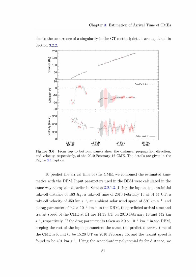
Chapter 3. Estimation of Arrival Time of CMEs
due to the occurrence of a singularity in the GT method; details are explained in
Section 3.2.2.
0
50
100
150
200D
ista
nce
(RO •)
-30
-20
-10
0
10
Dire
ctio
n (°
)
Sun-Earth line
12 Feb12:00
13 Feb12:00
14 Feb12:00
15 Feb12:00
0
300
600
900
Vel
ocity
(km
s-1)
Polynomial fit
Figure 3.6 From top to bottom, panels show the distance, propagation direction,and velocity, respectively, of the 2010 February 12 CME. The details are given in theFigure 3.4 caption.
To predict the arrival time of this CME, we combined the estimated kine-
matics with the DBM. Input parameters used in the DBM were calculated in the
same way as explained earlier in Section 3.2.1.3. Using the inputs, e.g., an initial
take-off distance of 183 R�, a take-off time of 2010 February 15 at 01:44 UT, a
take-off velocity of 450 km s−1, an ambient solar wind speed of 350 km s−1, and
a drag parameter of 0.2 × 10⁻⁷ km−1 in the DBM, the predicted arrival time and
transit speed of the CME at L1 are 14:35 UT on 2010 February 15 and 442 km
s−1, respectively. If the drag parameter is taken as 2.0 × 10⁻⁷ km−1 in the DBM,
keeping the rest of the input parameters the same, the predicted arrival time of
the CME is found to be 15:20 UT on 2010 February 15, and the transit speed is
found to be 401 km s−1. Using the second-order polynomial fit for distance, we
81
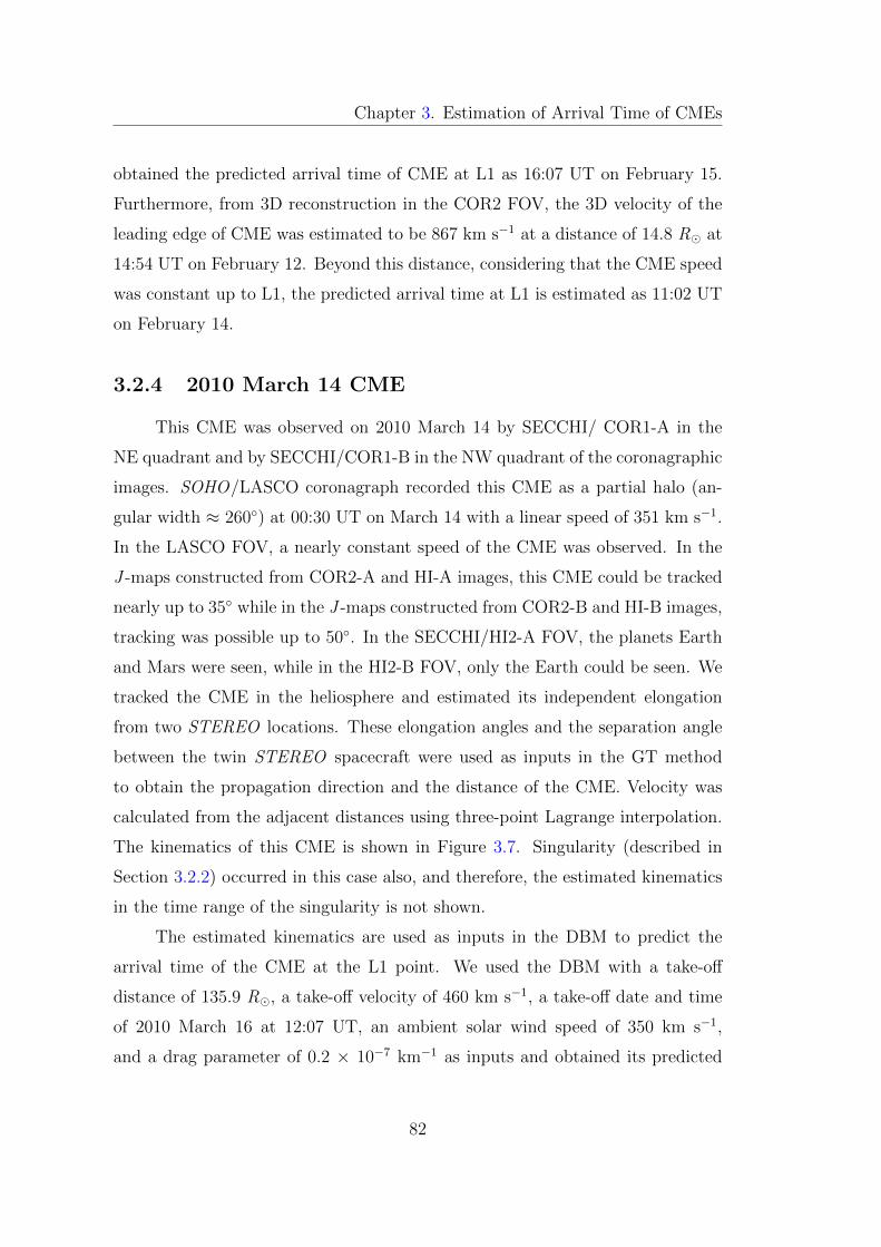
Chapter 3. Estimation of Arrival Time of CMEs
obtained the predicted arrival time of CME at L1 as 16:07 UT on February 15.
Furthermore, from 3D reconstruction in the COR2 FOV, the 3D velocity of the
leading edge of CME was estimated to be 867 km s−1 at a distance of 14.8 R� at
14:54 UT on February 12. Beyond this distance, considering that the CME speed
was constant up to L1, the predicted arrival time at L1 is estimated as 11:02 UT
on February 14.
3.2.4 2010 March 14 CME
This CME was observed on 2010 March 14 by SECCHI/ COR1-A in the
NE quadrant and by SECCHI/COR1-B in the NW quadrant of the coronagraphic
images. SOHO/LASCO coronagraph recorded this CME as a partial halo (an-
gular width ≈ 260◦) at 00:30 UT on March 14 with a linear speed of 351 km s−1.
In the LASCO FOV, a nearly constant speed of the CME was observed. In the
J -maps constructed from COR2-A and HI-A images, this CME could be tracked
nearly up to 35◦ while in the J -maps constructed from COR2-B and HI-B images,
tracking was possible up to 50◦. In the SECCHI/HI2-A FOV, the planets Earth
and Mars were seen, while in the HI2-B FOV, only the Earth could be seen. We
tracked the CME in the heliosphere and estimated its independent elongation
from two STEREO locations. These elongation angles and the separation angle
between the twin STEREO spacecraft were used as inputs in the GT method
to obtain the propagation direction and the distance of the CME. Velocity was
calculated from the adjacent distances using three-point Lagrange interpolation.
The kinematics of this CME is shown in Figure 3.7. Singularity (described in
Section 3.2.2) occurred in this case also, and therefore, the estimated kinematics
in the time range of the singularity is not shown.
The estimated kinematics are used as inputs in the DBM to predict the
arrival time of the CME at the L1 point. We used the DBM with a take-off
distance of 135.9 R�, a take-off velocity of 460 km s−1, a take-off date and time
of 2010 March 16 at 12:07 UT, an ambient solar wind speed of 350 km s−1,
and a drag parameter of 0.2 × 10⁻⁷ km−1 as inputs and obtained its predicted
82
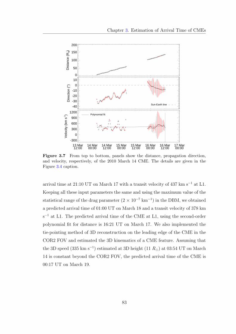
Chapter 3. Estimation of Arrival Time of CMEs
0
50
100
150
200
Dis
tanc
e (R
O •)
-40
-30
-20
-10
0
10
Dire
ctio
n (°
)
Sun-Earth line
13 Mar12:00
14 Mar00:00
14 Mar12:00
15 Mar00:00
15 Mar12:00
16 Mar00:00
16 Mar12:00
17 Mar00:00
-300
0
300
600
900
1200
Vel
ocity
(km
s-1) Polynomial fit
Figure 3.7 From top to bottom, panels show the distance, propagation direction,and velocity, respectively, of the 2010 March 14 CME. The details are given in theFigure 3.4 caption.
arrival time at 21:10 UT on March 17 with a transit velocity of 437 km s−1 at L1.
Keeping all these input parameters the same and using the maximum value of the
statistical range of the drag parameter (2 × 10⁻⁷ km−1) in the DBM, we obtained
a predicted arrival time of 01:00 UT on March 18 and a transit velocity of 378 km
s−1 at L1. The predicted arrival time of the CME at L1, using the second-order
polynomial fit for distance is 16:21 UT on March 17. We also implemented the
tie-pointing method of 3D reconstruction on the leading edge of the CME in the
COR2 FOV and estimated the 3D kinematics of a CME feature. Assuming that
the 3D speed (335 km s−1) estimated at 3D height (11 R�) at 03:54 UT on March
14 is constant beyond the COR2 FOV, the predicted arrival time of the CME is
00:17 UT on March 19.
83
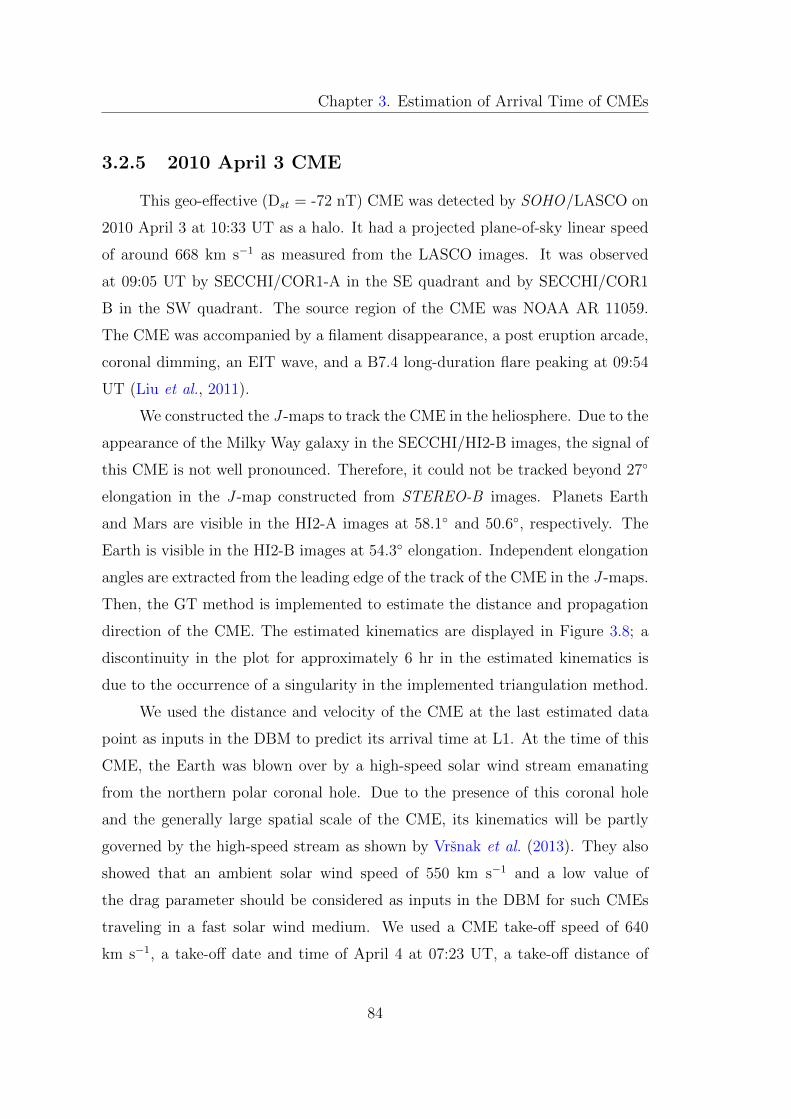
Chapter 3. Estimation of Arrival Time of CMEs
3.2.5 2010 April 3 CME
This geo-effective (Dst = -72 nT) CME was detected by SOHO/LASCO on
2010 April 3 at 10:33 UT as a halo. It had a projected plane-of-sky linear speed
of around 668 km s−1 as measured from the LASCO images. It was observed
at 09:05 UT by SECCHI/COR1-A in the SE quadrant and by SECCHI/COR1
B in the SW quadrant. The source region of the CME was NOAA AR 11059.
The CME was accompanied by a filament disappearance, a post eruption arcade,
coronal dimming, an EIT wave, and a B7.4 long-duration flare peaking at 09:54
UT (Liu et al., 2011).
We constructed the J -maps to track the CME in the heliosphere. Due to the
appearance of the Milky Way galaxy in the SECCHI/HI2-B images, the signal of
this CME is not well pronounced. Therefore, it could not be tracked beyond 27◦
elongation in the J -map constructed from STEREO-B images. Planets Earth
and Mars are visible in the HI2-A images at 58.1◦ and 50.6◦, respectively. The
Earth is visible in the HI2-B images at 54.3◦ elongation. Independent elongation
angles are extracted from the leading edge of the track of the CME in the J -maps.
Then, the GT method is implemented to estimate the distance and propagation
direction of the CME. The estimated kinematics are displayed in Figure 3.8; a
discontinuity in the plot for approximately 6 hr in the estimated kinematics is
due to the occurrence of a singularity in the implemented triangulation method.
We used the distance and velocity of the CME at the last estimated data
point as inputs in the DBM to predict its arrival time at L1. At the time of this
CME, the Earth was blown over by a high-speed solar wind stream emanating
from the northern polar coronal hole. Due to the presence of this coronal hole
and the generally large spatial scale of the CME, its kinematics will be partly
governed by the high-speed stream as shown by Vrsnak et al. (2013). They also
showed that an ambient solar wind speed of 550 km s−1 and a low value of
the drag parameter should be considered as inputs in the DBM for such CMEs
traveling in a fast solar wind medium. We used a CME take-off speed of 640
km s−1, a take-off date and time of April 4 at 07:23 UT, a take-off distance of
84
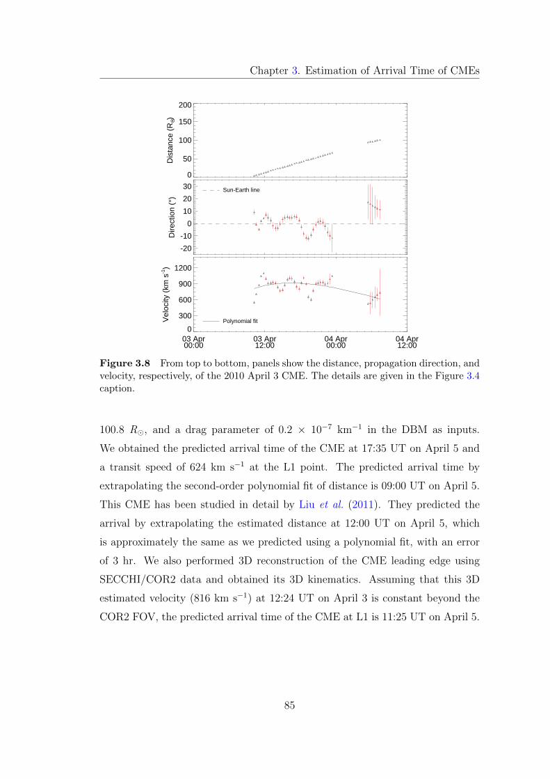
Chapter 3. Estimation of Arrival Time of CMEs
0
50
100
150
200
Dis
tanc
e (R
O •)
-20
-10
0
10
20
30
Dire
ctio
n (°
)
Sun-Earth line
03 Apr00:00
03 Apr12:00
04 Apr00:00
04 Apr12:00
0
300
600
900
1200
Vel
ocity
(km
s-1)
Polynomial fit
Figure 3.8 From top to bottom, panels show the distance, propagation direction, andvelocity, respectively, of the 2010 April 3 CME. The details are given in the Figure 3.4caption.
100.8 R�, and a drag parameter of 0.2 × 10⁻⁷ km−1 in the DBM as inputs.
We obtained the predicted arrival time of the CME at 17:35 UT on April 5 and
a transit speed of 624 km s−1 at the L1 point. The predicted arrival time by
extrapolating the second-order polynomial fit of distance is 09:00 UT on April 5.
This CME has been studied in detail by Liu et al. (2011). They predicted the
arrival by extrapolating the estimated distance at 12:00 UT on April 5, which
is approximately the same as we predicted using a polynomial fit, with an error
of 3 hr. We also performed 3D reconstruction of the CME leading edge using
SECCHI/COR2 data and obtained its 3D kinematics. Assuming that this 3D
estimated velocity (816 km s−1) at 12:24 UT on April 3 is constant beyond the
COR2 FOV, the predicted arrival time of the CME at L1 is 11:25 UT on April 5.
85
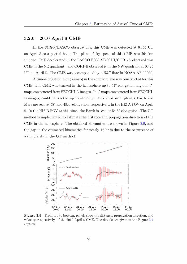
Chapter 3. Estimation of Arrival Time of CMEs
3.2.6 2010 April 8 CME
In the SOHO/LASCO observations, this CME was detected at 04:54 UT
on April 8 as a partial halo. The plane-of-sky speed of this CME was 264 km
s−1; the CME decelerated in the LASCO FOV. SECCHI/COR1-A observed this
CME in the NE quadrant , and COR1-B observed it in the NW quadrant at 03:25
UT on April 8. The CME was accompanied by a B3.7 flare in NOAA AR 11060.
A time-elongation plot (J -map) in the ecliptic plane was constructed for this
CME. The CME was tracked in the heliosphere up to 54◦ elongation angle in J -
maps constructed from SECCHI-A images. In J -maps constructed from SECCHI-
B images, could be tracked up to 44◦ only. For comparison, planets Earth and
Mars are seen at 58◦ and 48.4◦ elongation, respectively, in the HI2-A FOV on April
8. In the HI2-B FOV at this time, the Earth is seen at 54.5◦ elongation. The GT
method is implemented to estimate the distance and propagation direction of the
CME in the heliosphere. The obtained kinematics are shown in Figure 3.9, and
the gap in the estimated kinematics for nearly 12 hr is due to the occurrence of
a singularity in the GT method.
0
50
100
150
200
Dis
tanc
e (R
O •)
-20
-10
0
10
20
Dire
ctio
n (°
) Sun-Earth line
08 Apr00:00
08 Apr12:00
09 Apr00:00
09 Apr12:00
10 Apr00:00
10 Apr12:00
11 Apr00:00
0
300
600
900
1200
Vel
ocity
(km
s-1)
Polynomial fit
Figure 3.9 From top to bottom, panels show the distance, propagation direction, andvelocity, respectively, of the 2010 April 8 CME. The details are given in the Figure 3.4caption.
86
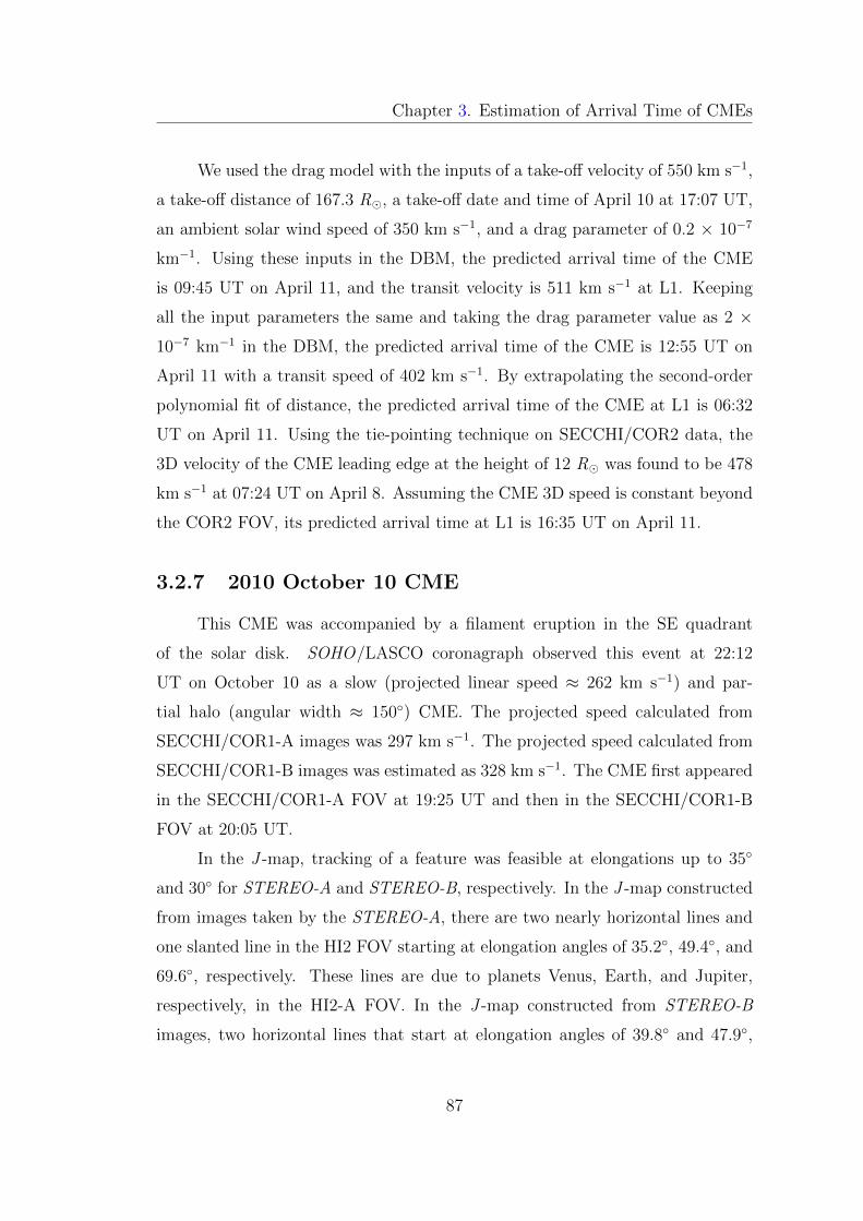
Chapter 3. Estimation of Arrival Time of CMEs
We used the drag model with the inputs of a take-off velocity of 550 km s−1,
a take-off distance of 167.3 R�, a take-off date and time of April 10 at 17:07 UT,
an ambient solar wind speed of 350 km s−1, and a drag parameter of 0.2 × 10⁻⁷
km−1. Using these inputs in the DBM, the predicted arrival time of the CME
is 09:45 UT on April 11, and the transit velocity is 511 km s−1 at L1. Keeping
all the input parameters the same and taking the drag parameter value as 2 ×10⁻⁷ km−1 in the DBM, the predicted arrival time of the CME is 12:55 UT on
April 11 with a transit speed of 402 km s−1. By extrapolating the second-order
polynomial fit of distance, the predicted arrival time of the CME at L1 is 06:32
UT on April 11. Using the tie-pointing technique on SECCHI/COR2 data, the
3D velocity of the CME leading edge at the height of 12 R� was found to be 478
km s−1 at 07:24 UT on April 8. Assuming the CME 3D speed is constant beyond
the COR2 FOV, its predicted arrival time at L1 is 16:35 UT on April 11.
3.2.7 2010 October 10 CME
This CME was accompanied by a filament eruption in the SE quadrant
of the solar disk. SOHO/LASCO coronagraph observed this event at 22:12
UT on October 10 as a slow (projected linear speed ≈ 262 km s−1) and par-
tial halo (angular width ≈ 150◦) CME. The projected speed calculated from
SECCHI/COR1-A images was 297 km s−1. The projected speed calculated from
SECCHI/COR1-B images was estimated as 328 km s−1. The CME first appeared
in the SECCHI/COR1-A FOV at 19:25 UT and then in the SECCHI/COR1-B
FOV at 20:05 UT.
In the J -map, tracking of a feature was feasible at elongations up to 35◦
and 30◦ for STEREO-A and STEREO-B, respectively. In the J -map constructed
from images taken by the STEREO-A, there are two nearly horizontal lines and
one slanted line in the HI2 FOV starting at elongation angles of 35.2◦, 49.4◦, and
69.6◦, respectively. These lines are due to planets Venus, Earth, and Jupiter,
respectively, in the HI2-A FOV. In the J -map constructed from STEREO-B
images, two horizontal lines that start at elongation angles of 39.8◦ and 47.9◦,
87
Chapter 3. Estimation of Arrival Time of CMEs
respectively, are due to the appearance of planets Venus and Earth in the HI2-
B FOV. The kinematics obtained for this CME is shown in Figure 3.10, where
the discontinuity in the plot occurs due to the existence of a singularity in the
method.
0
20406080
100120140
Dis
tanc
e (R
O •)
-40
-20
0
20
40
Dire
ctio
n (°
) Sun-Earth line
10 Oct12:00
11 Oct12:00
12 Oct12:00
13 Oct12:00
14 Oct12:00
0200
400
600
8001000
Vel
ocity
(km
s-1)
Polynomial fit
Date (UT)
Figure 3.10 From top to bottom, panels show the distance, propagation direction,and velocity, respectively, of the 2010 October 10 CME. The details are given in theFigure 3.4 caption.
We used the DBM developed by Vrsnak et al. (2013) to estimate the arrival
time of the CME. For this event, we used the DBM with a take-off distance of
120.65 R�, a take-off date and time of 2010 October 13 at 09:33 UT, a take-off
velocity of 354 km s−1, an ambient solar wind speed of 350 km s−1, and a drag
parameter of 0.2 × 10⁻⁷ km−1 to 2 × 10⁻⁷ km−1. We obtained its arrival time as
11:40-11:45 UT on October 15 and its transit velocity as 354-353 km s−1 at L1. By
extrapolating the second-order polynomial fit for distance, the predicted arrival
time of the CME at L1 is October 14 at 22:53 UT. From the 3D reconstruction
of the CME leading edge using the tie-pointing method on SECCHI/COR2 data,
the estimated 3D velocity was found to be 565.8 km s−1 at 14.5 R� at 06:50 UT
on 2010 October 11. Assuming that the speed of CME is constant beyond the
88
Chapter 3. Estimation of Arrival Time of CMEs
COR2 FOV, the predicted arrival time is 02:33 UT on 2010 October 14 at L1.
3.2.8 2010 October 26 CME
This CME was observed in SOHO/LASCO images around 01:36 UT on
October 26 with an angular width of 83◦ and had a projected linear speed of 214
km s−1 at a position angle of 210◦. It was also observed by both the STEREO
spacecraft in COR1 images on October 26.
The independent elongation angle of a tracked feature from two different
vantage points is extracted using J -maps. In both J -maps, the leading edge of the
bright feature has a positive slope, revealing that the CME propagation could be
tracked up to 28◦ without ambiguity. For comparison, on October 26 in the HI2-
A FOV, planets Venus, Earth, and Jupiter are observed at elongation angles of
38.3◦, 48.9◦, and 55.8◦, respectively. In the HI2-B FOV, planets Venus and Earth
are observed at elongation angles of 36.9◦ and 46.7◦, respectively. Figure 3.11
shows the kinematics of the CME of 2010 October 26, which were obtained by
implementing the GT technique (Liu et al., 2010a) with the independent elon-
gations estimated from two different viewpoints as inputs. There is a gap in the
estimated parameters (Figure 3.11) due to the existence of a singularity in the
triangulation scheme.
We applied the tie-pointing method for the 3D reconstruction of a feature
along with the identified bright blob behind the leading edge in both sets of
calibrated and background-subtracted images obtained by SECCHI/COR2. Our
goal was to estimate its 3D kinematics in the COR2 FOV. Estimated latitude (≈-25◦) and longitude (≈ 15◦) show that the CME is Earth-directed. The speed of
the CME using 3D reconstruction at the outer edge of the COR2 FOV is about
600 km s−1 with an acceleration of 30 m s−2. Assuming that the speed of the
CME is constant beyond this distance, the predicted arrival time of the CME at
L1 is 07:45 UT on 2010 October 29. We used the DBM with a take-off date and
time of 2010 October 28 at 13:57 UT, a take-off distance of 110.5 R� a take-off
velocity of 341 km s−1, an ambient solar wind speed of 350 km s−1, and a drag
89
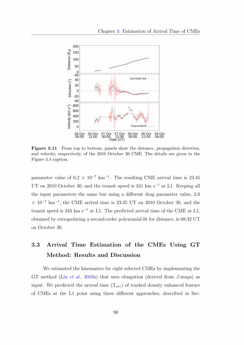
Chapter 3. Estimation of Arrival Time of CMEs
0
50
100
150
200
Dis
tanc
e (R
O •)
-40-20
0
20
4060
Dire
ctio
n (°
) Sun-Earth line
26 Oct00:00
26 Oct12:00
27 Oct00:00
27 Oct12:00
28 Oct00:00
28 Oct12:00
29 Oct00:00
0
200
400
600
800
Vel
ocity
(km
s-1)
Polynomial fit
Date (UT)
Figure 3.11 From top to bottom, panels show the distance, propagation direction,and velocity, respectively, of the 2010 October 26 CME. The details are given in theFigure 3.4 caption.
parameter value of 0.2 × 10⁻⁷ km−1. The resulting CME arrival time is 23:45
UT on 2010 October 30, and the transit speed is 341 km s−1 at L1. Keeping all
the input parameters the same but using a different drag parameter value, 2.0
× 10−7 km−1, the CME arrival time is 23:35 UT on 2010 October 30, and the
transit speed is 343 km s−1 at L1. The predicted arrival time of the CME at L1,
obtained by extrapolating a second-order polynomial fit for distance, is 08:32 UT
on October 30.
3.3 Arrival Time Estimation of the CMEs Using GT
Method: Results and Discussion
We estimated the kinematics for eight selected CMEs by implementing the
GT method (Liu et al., 2010a) that uses elongation (derived from J -maps) as
input. We predicted the arrival time (Tarr) of tracked density enhanced feature
of CMEs at the L1 point using three different approaches, described in Sec-
90
Chapter 3. Estimation of Arrival Time of CMEs
tion 3.2.1.3. The arrival time predicted using the two different approaches (DBM
and polynomial fit) that use inputs of derived parameters from GT with J -maps
were compared with the actual arrival time of the enhanced density feature at L1.
For each CME studied here, the actual arrival time and errors in the predicted
arrival time using these two approaches are shown in Table 3.2. The predicted
arrival time of a CME using DBM is shown in the third column of Table 3.2,
corresponding to the two extreme values of the range of the drag parameter.
Predicted transit speed (v1) of the CME at L1 is also compared with the actual
measured speed (fifth column) at the time of the arrival of the enhanced density
feature. Negative (positive) values of errors in arrival time indicate that the pre-
dicted arrival is earlier (later) than the actual arrival time. Negative (positive)
values of error in the transit speed of the CME at L1 indicate that the predicted
transit velocity of the CME at L1 is lesser (greater) than the transit velocity
measured in situ.
To examine the efficacy of the third approach, one must be certain that
the arrival time of the tracked feature at L1 is correctly marked. It is generally
difficult to mark the actual (reference) arrival time of a remotely observed (in
COR2) feature at L1 by analyzing the in situ data. This difficulty arises due to
uncertainty in the one-to-one identification of remotely observed structures with
in situ observed structures. For all the CMEs studied in our case, except 2010
October 26, we could estimate the 3D speed of a feature along its leading edge
in the COR2 FOV by implementing the tie-pointing method. Therefore, we take
the arrival of the leading edge of the CME in in situ data at L1 as a reference for
the CME arrival time (Table 3.1). The details of in situ observations of selected
CMEs are presented in Chapter 4. The error in the predicted arrival time of the
CME using 3D speed (estimated in the COR2 FOV) is shown in Table 3.3. This
table shows the 3D speed in the COR2 FOV and the measured speed of the CME
leading edge at L1. The CME of 2010 October 10, is not included here because
the CME boundaries could not be identified in in situ data; it seems probable
that only the CME flank was encountered by the spacecraft. It would have been
possible to confirm the above by discussing multi-point observations of this CME
91
Chapter 3. Estimation of Arrival Time of CMEs
if the STEREO spacecraft had a smaller separation angle at this time (similar to
the study carried out by Kilpua et al. (2011).
From Tables 3.2 and 3.3, it is clear that, in general, a more accurate
prediction of CME arrival time is possible using DBM combined with kinematics
estimated from the GT method. It is also evident from Table 3.3 that, for the
2010 April 3 and April 8 CMEs, the implementation of the tie-pointing technique
provides a more accurate arrival time prediction. In these cases, CME transit
speeds at L1 are approximately equal to the measured CME speeds in the COR2
FOV. This result shows that the speeds of the CMEs did not change significantly
during their propagation in the heliosphere. Therefore, in these particular cases,
the observed CME speeds in the COR2 FOV are sufficient to predict their arrival
times near 1AU with reasonably good accuracy. Our analysis of the April 3 CME
shows that CME speed is partly governed by the high-speed stream from a coronal
hole located in a geo-effective location on the Sun. The estimated speed (≈ 816
km s−1) of the April 3 CME in the COR2 FOV and its in situ speed (≈ 800 km
s−1) highlight that it experienced a weak drag force throughout its journey up
to 1 AU. These findings are in good agreement with the results of Temmer et al.
(2011).
Predicting arrival time by extrapolating the fitted second-order polynomial
for estimated distance is better than the prediction made using only the 3D speed
estimated in the COR2 FOV. The decelerating trend of the 2008 December 12
CME in the inner heliosphere is in good agreement with the results of Liu et al.
(2010a). Using extrapolation, the error in the predicted arrival time is also less
if a CME is tracked up to large distances in the heliosphere (using HI), as in the
case of the 2010 February 7 CME where the J -map allowed tracking of CME
features at elongations up to nearly 50◦ (≈ 170 R�). The high-speed (≈ 867
km s−1) CME of 2010 February 12 shows a significant, continuous deceleration
in the heliosphere. This is in agreement with the results of previous studies
that demonstrate that the drag force plays an important role in shaping CME
dynamics (Lindsay et al., 1999; Gopalswamy et al., 2001a; Manoharan, 2006;
Vrsnak and Zic, 2007).
92
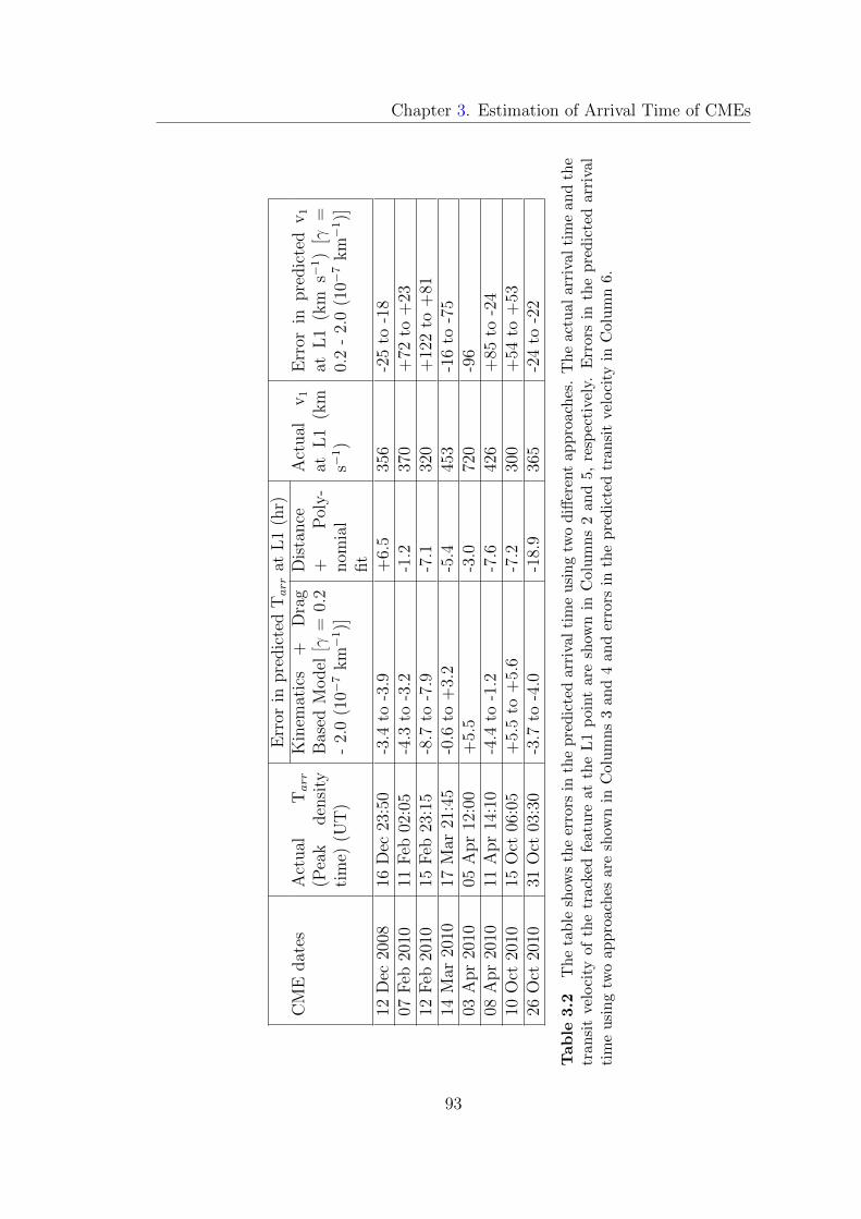
Chapter 3. Estimation of Arrival Time of CMEs
Err
orin
pre
dic
ted
Tarr
atL
1(h
r)C
ME
dat
esA
ctual
Tarr
(Pea
kden
sity
tim
e)(U
T)
Kin
emat
ics
+D
rag
Bas
edM
odel
[γ=
0.2
-2.
0(1
0−7
km−
1)]
Dis
tance
+P
oly-
nom
ial
fit
Act
ual
v1
atL
1(k
ms−
1)
Err
orin
pre
dic
ted
v1
atL
1(k
ms−
1)
[γ=
0.2
-2.
0(1
0−7
km−
1)]
12D
ec20
0816
Dec
23:5
0-3
.4to
-3.9
+6.
535
6-2
5to
-18
07F
eb20
1011
Feb
02:0
5-4
.3to
-3.2
-1.2
370
+72
to+
2312
Feb
2010
15F
eb23
:15
-8.7
to-7
.9-7
.132
0+
122
to+
8114
Mar
2010
17M
ar21
:45
-0.6
to+
3.2
-5.4
453
-16
to-7
503
Apr
2010
05A
pr
12:0
0+
5.5
-3.0
720
-96
08A
pr
2010
11A
pr
14:1
0-4
.4to
-1.2
-7.6
426
+85
to-2
410
Oct
2010
15O
ct06
:05
+5.
5to
+5.
6-7
.230
0+
54to
+53
26O
ct20
1031
Oct
03:3
0-3
.7to
-4.0
-18.
936
5-2
4to
-22
Table
3.2
Th
eta
ble
show
sth
eer
rors
inth
ep
redic
ted
arri
val
tim
eu
sin
gtw
od
iffer
ent
app
roac
hes
.T
he
actu
alar
riva
lti
me
and
the
tran
sit
velo
city
of
the
track
edfe
atu
reat
the
L1
poi
nt
are
show
nin
Col
um
ns
2an
d5,
resp
ecti
vely
.E
rror
sin
the
pre
dic
ted
arri
val
tim
eu
sin
gtw
oap
pro
ach
esare
show
nin
Col
um
ns
3an
d4
and
erro
rsin
the
pre
dic
ted
tran
sit
velo
city
inC
olu
mn
6.
93
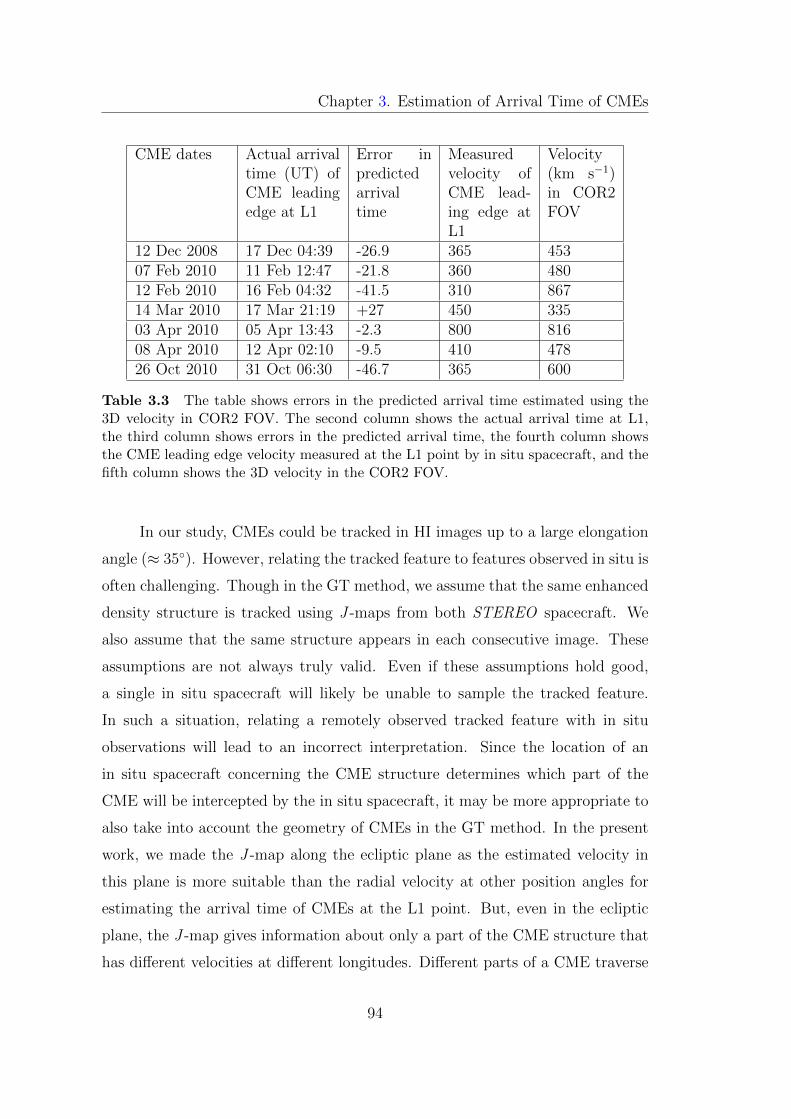
Chapter 3. Estimation of Arrival Time of CMEs
CME dates Actual arrivaltime (UT) ofCME leadingedge at L1
Error inpredictedarrivaltime
Measuredvelocity ofCME lead-ing edge atL1
Velocity(km s−1)in COR2FOV
12 Dec 2008 17 Dec 04:39 -26.9 365 45307 Feb 2010 11 Feb 12:47 -21.8 360 48012 Feb 2010 16 Feb 04:32 -41.5 310 86714 Mar 2010 17 Mar 21:19 +27 450 33503 Apr 2010 05 Apr 13:43 -2.3 800 81608 Apr 2010 12 Apr 02:10 -9.5 410 47826 Oct 2010 31 Oct 06:30 -46.7 365 600
Table 3.3 The table shows errors in the predicted arrival time estimated using the3D velocity in COR2 FOV. The second column shows the actual arrival time at L1,the third column shows errors in the predicted arrival time, the fourth column showsthe CME leading edge velocity measured at the L1 point by in situ spacecraft, and thefifth column shows the 3D velocity in the COR2 FOV.
In our study, CMEs could be tracked in HI images up to a large elongation
angle (≈ 35◦). However, relating the tracked feature to features observed in situ is
often challenging. Though in the GT method, we assume that the same enhanced
density structure is tracked using J -maps from both STEREO spacecraft. We
also assume that the same structure appears in each consecutive image. These
assumptions are not always truly valid. Even if these assumptions hold good,
a single in situ spacecraft will likely be unable to sample the tracked feature.
In such a situation, relating a remotely observed tracked feature with in situ
observations will lead to an incorrect interpretation. Since the location of an
in situ spacecraft concerning the CME structure determines which part of the
CME will be intercepted by the in situ spacecraft, it may be more appropriate to
also take into account the geometry of CMEs in the GT method. In the present
work, we made the J -map along the ecliptic plane as the estimated velocity in
this plane is more suitable than the radial velocity at other position angles for
estimating the arrival time of CMEs at the L1 point. But, even in the ecliptic
plane, the J -map gives information about only a part of the CME structure that
has different velocities at different longitudes. Different parts of a CME traverse
94
Chapter 3. Estimation of Arrival Time of CMEs
a fixed radial distance from the Sun at different times. The time is minimized for
the apex of a CME (Schwenn et al., 2005). If the tracked feature happens to be
at the apex of a CME moving in a different direction (longitude) from the Sun-L1
line, then the predicted arrival time of this CME using the estimated speed of
the tracked feature will be earlier than the actual arrival time of the CME at
the L1 point. Therefore, to obtain the actual arrival time and transit velocity
of a CME passing the in situ spacecraft, it is necessary to take into account the
propagation direction of the tracked feature. Mostl et al. (2011) showed that the
speed of a CME flank measured at a given angle θ to the CME apex is reduced
by a factor of cos(θ) for a circular geometry of the CME. Therefore, it seems
reasonable that the transit speed measured in situ and the arrival time of the
CME at L1 should be compared with the corresponding corrected speed of the
tracked feature along the Sun-L1 line and the arrival time, respectively. However,
we note that if the apex of the CME moves with a linear speed of 400 km s−1
at 10◦ to the Sun-L1 line, the correction in the actual arrival time of the CME
at L1 is only approximately 2 hr for a fixed distance of nearly 1 AU. It seems
appropriate to also take the geometry of CMEs into account in the triangulation
method. However, idealistic assumptions about geometry also are far from the
real structure. Further, CME shapes can be distorted in the heliosphere by the
solar wind, interplanetary shocks, and CME interactions. Therefore, one needs to
be cautious, as assumptions about the CME geometry may result in new sources
of errors.
Despite various assumptions made in the DBM (Vrsnak et al., 2013) and
the GT method (Liu et al., 2010a), the predicted arrival times of CMEs are found
within acceptable error. It must be mentioned here that the estimated velocity
profiles of the selected CMEs show small apparent accelerations and decelerations
for a few hr that do not seem to be real. We believe that these may be due to
errors in the manual tracking of a CME feature using J -maps and the extraction
of the elongation angles. We have shown the error bars with vertical red lines
in the kinematics plot. However, these do not denote the actual errors in the
triangulation method but are representative of the sensitivity of the technique
95
Chapter 3. Estimation of Arrival Time of CMEs
to elongation uncertainties (Liu et al., 2010a). Considering that the elongation
angles determined for each pixel in level 0 data for COR2 and level 2 data for HI1
and HI2 is quite accurate; the resolution will determine the minimum uncertainty
in the elongation in elongation that is used to construct the J -maps. However, as
mentioned above, the actual error in this GT method owes to the manual error in
tracking the bright points using J -maps. This error is assessed by repeating the
manual tracking of a feature several times and comparing the derived parameters.
One should also ensure that the same feature is tracked continuously in the J -
maps. This is often difficult due to the different sensitivities of the COR2, HI1,
and HI2 imaging instruments, which cover a wide range of elongation angles. The
actual sources of error in the GT technique are inherent in the assumption that the
CME feature is a single point and the same point is being tracked continuously
from both twin STEREO spacecraft. If the assumption fails (likely at larger
elongations) at some segment of the journey in the interplanetary medium, the
CME kinematics will not be correctly estimated.
We also note that the density distribution along the line of sight is not well
known, as we project the 3D structure of CME features onto a 2D image. Relating
remote sensing observations to in situ measurements of CMEs is often uncertain
because the bright feature observed in J -maps are due to the contribution of
intensity along with the entire depth of the line of sight, but ACE or WIND
density measurements near 1 AU are only along the Sun-Earth line. Despite
these constraints on observations and assumptions in implemented techniques,
our study shows a fair agreement in relating remotely observed features with in
situ measurements. We track the CMEs up to large distances in the heliosphere.
The efficacy of any forecasting scheme for CME arrival time must be validated
with real-time data so that the results are unbiased.
96
Chapter 3. Estimation of Arrival Time of CMEs
3.4 Assessing the Relative Performance of Ten Recon-
struction Methods for Estimating the Arrival Time
of CMEs Using SECCHI/HI Observations
Several reconstruction methods have been developed, based on a variety
of assumptions regarding their geometry, propagation direction, and speed, to
derive CME kinematics by exploiting heliospheric imagers (i.e., SMEI and HI)
observations (e.g., Howard et al. 2006; Jackson et al. 2006, 2007, 2008; Kahler and
Webb 2007; Sheeley et al. 2008a; Howard and Tappin 2009; Tappin and Howard
2009; Lugaz, Vourlidas, and Roussev 2009; Lugaz 2010; Liu et al. 2010a; Lugaz
et al. 2010; Davies et al. 2012, 2013). These methods are based on a different
set of assumptions which make them independent of each other to some degree.
Several of the methods treat CMEs as a point, while other methods consider
CMEs to have a larger-scale geometry as explained in Section 2.3.2 of Chapter 2.
In some of the methods, CMEs are assumed to propagate with a constant speed,
while other methods can estimate the time variations of the speed of a CME as
it propagates through the heliosphere.
Since some of the critical questions in CME and space weather research
relate to the propagation of CMEs, it is an obvious next step to attempt to as-
certain the relative merits of various reconstruction methods for estimating the
kinematic properties of CMEs, including their arrival time at Earth. Several
such studies, based mainly on HI observations, have been performed previously.
For example, Davis, Kennedy, and Davies (2010) applied the Fixed-Phi Fitting
method (Sheeley et al., 2008b; Rouillard et al., 2008; Davies et al., 2009) to HI
observations to estimate the propagation direction and speed of CMEs and com-
pared their results with those obtained by Thernisien, Vourlidas, and Howard
(2009) using the Forward Modeling method for the same CMEs observed in the
COR FOV. The authors found that their retrieved CME directions were in good
agreement with those from forward modeling. At the same time, the discrepancy
in speed between the two methods could be explained in terms of the accelera-
tion of slow CMEs and the deceleration of fast CMEs in the HI FOV. It is also
97

Chapter 3. Estimation of Arrival Time of CMEs
worth noting that Thernisien, Vourlidas, and Howard (2009) had compared their
estimated CME propagation directions with those obtained by Colaninno and
Vourlidas (2009) using an entirely different technique. The method of Colaninno
and Vourlidas (2009) is based on the constraint that both COR2-A and COR2-B
should record the same true mass for any given CME. Wood et al. (2009) applied
the Point-P (Howard et al., 2006) and Fixed-Phi methods to the CME of 2008
February 4; their results suggested that the Fixed-Phi method performs better,
which they argued for the studied CME having a small angular extent. Similarly,
Wood, Howard, and Socker (2010) implemented the Point-P, Fixed-Phi, and Har-
monic Mean (Lugaz, Vourlidas, and Roussev, 2009) methods on the 2008 June 1
CME and showed that different methods could give significantly different kine-
matic profiles, especially in the HI2 FOV. Recently, Lugaz (2010) has assessed the
accuracy and limitations of two fitting methods (Fixed-Phi Fitting and Harmonic
Mean Fitting) and two stereoscopic methods, Geometric Triangulation (Liu et al.,
2010a) and Tangent to A Sphere (Lugaz et al., 2010), to estimate the propaga-
tion direction of 12 CMEs launched during 2008 and 2009. Their results showed
that the Fixed-Phi Fitting approach could result in significant errors in the CME
direction when the CME is propagating outside 60◦ ± 20◦ of the Sun-spacecraft
direction, and Geometric Triangulation can yield large errors if the CME is prop-
agating outside ± 20◦ of the Sun-Earth line. More recently, Colaninno, Vourlidas,
and Wu (2013) derived the deprojected height-time profiles of CMEs by applying
the graduated cylindrical shell model (Forward Modeling: Thernisien, Vourlidas,
and Howard 2009) using SECCHI and LASCO images. They fitted the derived
height-time data with six different methods to estimate the CME arrival time
and speed at Earth.
The studies above are mainly limited to comparing CME propagation di-
rections and sometimes speeds retrieved using different methods. These studies
do not consider the characteristics of either the individual CMEs or the ambient
medium into which they are launched, nor do they (except Colaninno, Vourlidas,
and Wu 2013) use the estimated kinematics of CMEs to predict their arrival time
near 1 AU. They do not compare the derived CME arrival time with the actual
98
Chapter 3. Estimation of Arrival Time of CMEs
CME arrival time identified from in situ observations. However, to understand
the validity of these methods for space weather forecasting, we use different re-
construction methods to predict the arrival time and speed of CMEs launched at
different speeds and launched into different ambient solar wind conditions. Our
selection of three CMEs, launched with different speeds into different solar wind
conditions (on 2010 October 6, April 3, and February 12), satisfy such crite-
ria. On the other hand, previous studies have been carried out by implementing
several methods to an individual CME.
We implemented a total of 10 different reconstruction methods, ranging
from single spacecraft methods and their fitting analogues to stereoscopic meth-
ods, to ascertain the performance of specific methods under specific conditions.
Such extensive analysis undertaken in our study has not previously been reported.
Moreover, we have not only compared the estimated direction and speed of the
three selected CMEs but have also assessed the relative performance of these
techniques in estimating CME arrival time at L1. We compare the estimated
arrival time and speed of each CME to the actual arrival time and speed based
on in situ signatures at L1 (Zurbuchen and Richardson, 2006). Such a study is a
useful step toward identifying the most appropriate techniques for the practical
purpose of forecasting CME arrival time at Earth in the near future.
3.5 Reconstruction Methods and Their Application to the
Selected CMEs
We applied ten reconstruction methods to the following three CMEs ob-
served by STEREO :
– 2010 October 6 CME, slow (3D speed in COR2 FOV = 340 km s−1), tra-
versed through a slow speed ambient solar wind medium.
– 2010 April 3 CME, fast (3D speed in COR2 FOV = 867 km s−1), traversed
through a fast speed ambient solar wind medium.
99
Chapter 3. Estimation of Arrival Time of CMEs
– 2010 February 12 CME, fast, (3D speed in COR2 FOV = 816 km s−1),
traversed through a slow speed ambient solar wind medium.
The fast 2010 April 3 CME experienced only a modest deceleration during
its journey and was the fastest CME at 1 AU since the 2006 December 13 CME.
We note that, during this time, the Earth was in the throes of high-speed solar
wind, which perhaps governed the dynamics of this CME. The 2010 April 3 CME
has been investigated extensively in earlier studies (Mostl et al., 2010; Liu et al.,
2011; Wood et al., 2011; Temmer et al., 2011; Mishra and Srivastava, 2013).
The methods used to derive the heliospheric kinematics of CMEs can be
classified into two groups, one which uses single spacecraft observations and the
other which requires simultaneous observations from two viewpoints. We have
implemented seven single spacecraft methods and three stereoscopic methods.
– Single spacecraft reconstruction methods: (i) Point-P (PP: Howard
et al. 2006) (ii) Fixed-Phi (FP: Kahler and Webb 2007) (iii) Harmonic
Mean (HM: Lugaz, Vourlidas, and Roussev 2009) (iv) Self-Similar Expan-
sion (SSE: Davies et al. 2012) (v) Fixed-Phi Fitting (FPF: Rouillard et al.
2008) (vi) Harmonic Mean Fitting (HMF: Lugaz 2010) (vii) Self-Similar
Expansion Fitting (SSEF: Davies et al. 2012)
– Stereoscopic reconstruction methods: (i) Geometric Triangulation
(GT: Liu et al. 2010a) (ii) Tangent to A Sphere (TAS: Lugaz et al. 2010)
(iii) Stereoscopic Self-Similar Expansion (SSSE: Davies et al. 2013)
Using the FP, HM, and SSE methods, one can estimate the kinematics of
a CME, provided an estimate of its 3D propagation direction is known. The 3D
propagation direction of a CME close to the Sun can be estimated by applying
the scc measure.pro routine (Thompson, 2009) to COR2 observations. We derive
the kinematics of these three CMEs in the heliosphere using the methods above
and use those kinematics (averaged over the last few data points) as inputs to
the Drag Based Model (DBM: Vrsnak et al. 2013) to estimate the arrival times
of the CMEs at L1. If, for any method, the derived kinematics show implausible
100
Chapter 3. Estimation of Arrival Time of CMEs
(unphysical) variations over the last few points, then the kinematics prior to
that time are used instead. The details about the nature of the drag forces and
DBM developed by Vrsnak et al. (2013) have been described in Section 2.3.3.1
of Chapter 2. The details of these reconstruction methods implemented in our
study have been summarized in Section 2.3.2 of Chapter 2.
In the following sections, we discuss the application of various reconstruction
methods to the three selected CMEs. The analysis of the CME of 2010 October
6 is presented in Section 3.5.1 in detail. Results of similar analyses of the 2010
April 3 and February 12 CMEs are presented briefly in Sections 3.5.2 and 3.5.3,
respectively.
3.5.1 2010 October 6 CME
The CME of 2010 October 6 was first observed by SOHO/LASCO C2 at
07:12 UT as a partial halo with a linear plane of sky speed of 282 km s−1 (online
LASCO CME catalog: http://cdaw.gsfc.nasa.gov/CME list/; see Yashiro et al.
2004). This CME was associated with a filament eruption from the north-east
(NE) quadrant of the solar disc. In the LASCO C3 FOV, this CME was observed
to accelerate at 7 m s−2. COR1-A and COR1-B, with an angular separation of
approximately 161◦, first observed the CME at 04:05 UT in the NE and north-
west (NW) quadrants, respectively. The CME was subsequently observed by
COR2, and HI1 and HI2, on both STEREO-A and B (Figure 3.12). The arrival
of this CME at the Earth caused a moderate geomagnetic storm with a peak Dst
index of approximately -80 nT on 2010 October 11 at 19:00 UT.
We applied the COR2 data processing scheme as described by Mierla
et al. (2010) before implementing the tie-pointing technique of 3D reconstruc-
tion (Thompson, 2009). The 3D radial speed of the 2010 October 6 CME is
estimated to be 340 km s−1 at a 3D height of nearly ten R� from the Sun. The
central latitude of the CME feature was estimated to be ≈ 20◦ North, and its
longitude ≈ 10◦ East of the Earth. As the CME was propagating slightly north-
eastward of the Sun-Earth line, it was expected to impact the Earth. Assuming a
101
Chapter 3. Estimation of Arrival Time of CMEs
constant speed of 340 km s−1 beyond the COR2 FOV, the predicted CME arrival
time at L1 is estimated to be on 2010 October 11, at 06:10 UT.
3.5.1.1 Reconstruction methods using single spacecraft observations
Using heliospheric imagers, which image at and across large distances from
the Sun, 3D information about CMEs can be extracted without multiple view-
point observations. In this section, we apply reconstruction methods based on
single viewpoint observations of CMEs in the heliosphere, i.e., the PP, FP, HM,
and SSE methods described in Section 2.3.2.2 of Chapter 2.
3.5.1.1.1 Point-P (PP) method
It becomes very diffuse when a CME is in the FOV of a heliospheric imager (Cori-
olis/SMEI or SECCHI/HI). Therefore to track and extract the time-elongation
profile of a moving solar wind structure, a technique developed originally by
Sheeley et al. (1999), involves the generation of time-elongation maps (J -maps:
Rouillard et al. 2008; Davies et al. 2009; Mostl et al. 2010; Liu et al. 2010a; Har-
rison et al. 2012) is often applied. For the current study, we constructed J -maps
using running difference images from the HI1 and HI2 instruments, as explained
in Section 2.3.2.1 of Chapter 2 (see also, Mishra and Srivastava, 2013). Ecliptic
J -maps covering the passage of the 2010 October 6 CME, from the viewpoints of
both STEREO-A and B, are shown in Figure 3.13. In the HI2-A FOV on 2010
October 6, Venus, Earth, Jupiter, and Neptune were identified at position angles
of 86.5◦, 83.1◦, 84.4◦, and 83.8◦ with elongations of 34.3◦, 49.5◦, 73.1◦, and 50.3◦
respectively (see Figure 3.12). In the HI2-B FOV, Venus and Earth were identi-
fied at elongations of 40.4◦ and 48.2◦ respectively. In each J -map (Figure 3.13),
two horizontal lines are due to the presence of Venus and Earth in the HI2 FOV.
A slanted line that appears in the STEREO-A J -map on October 10 is due to
the entrance of Jupiter into the HI2-A FOV.
In each J -map, a set of the positively inclined bright features corresponds
to the 2010 October 6 CME. We tracked the leading edge of the first bright track,
corresponding to the initial CME front, in the STEREO-A J -map (red dashed
102
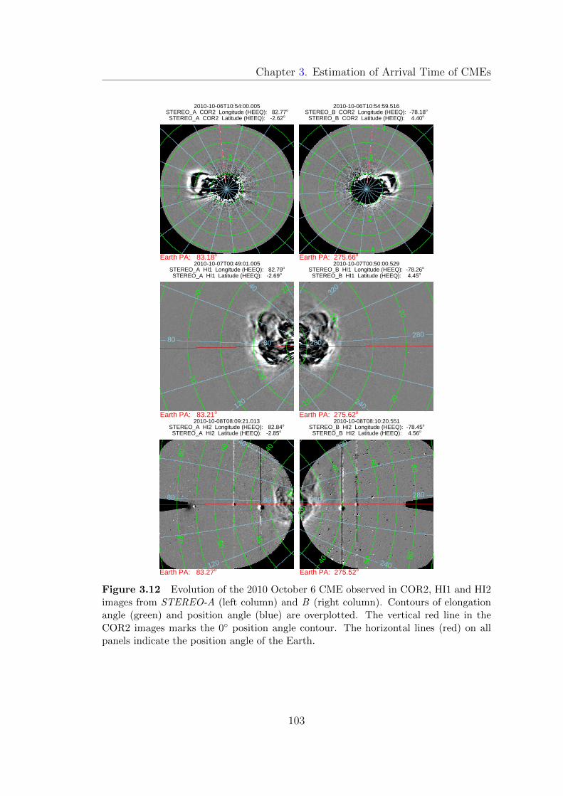
Chapter 3. Estimation of Arrival Time of CMEs
2
2
4
4
4
4
2010-10-06T10:54:00.005
Earth PA: 83.18o
STEREO_A COR2 Longitude (HEEQ): 82.77o
STEREO_A COR2 Latitude (HEEQ): -2.62o
2
2
4
4
4
4
2010-10-06T10:54:59.516
Earth PA: 275.66o
STEREO_B COR2 Longitude (HEEQ): -78.18o
STEREO_B COR2 Latitude (HEEQ): 4.40o
40
80 80
120
10
10
20
20
2010-10-07T00:49:01.005
Earth PA: 83.21o
STEREO_A HI1 Longitude (HEEQ): 82.79o
STEREO_A HI1 Latitude (HEEQ): -2.69o
240
280280
320
10
10
20
20
2010-10-07T00:50:00.529
Earth PA: 275.62o
STEREO_B HI1 Longitude (HEEQ): -78.26o
STEREO_B HI1 Latitude (HEEQ): 4.45o
40
80 80
120
20
40
40
60
60
80
80
2010-10-08T08:09:21.013
Earth PA: 83.27o
STEREO_A HI2 Longitude (HEEQ): 82.84o
STEREO_A HI2 Latitude (HEEQ): -2.85o
240
280280
320
20
40
40
60
60
80
80
2010-10-08T08:10:20.551
Earth PA: 275.52o
STEREO_B HI2 Longitude (HEEQ): -78.45o
STEREO_B HI2 Latitude (HEEQ): 4.56o
Figure 3.12 Evolution of the 2010 October 6 CME observed in COR2, HI1 and HI2images from STEREO-A (left column) and B (right column). Contours of elongationangle (green) and position angle (blue) are overplotted. The vertical red line in theCOR2 images marks the 0◦ position angle contour. The horizontal lines (red) on allpanels indicate the position angle of the Earth.
103
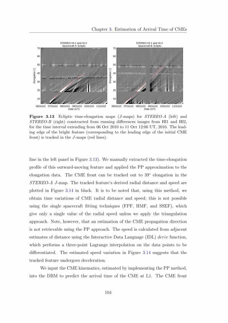
Chapter 3. Estimation of Arrival Time of CMEs
Spacecraft A: Ecliptic
06Oct10 07Oct10 08Oct10 09Oct10 10Oct10 11Oct10Date (UT)
10
20
30
40
50
60
70
Elo
ngat
ion
(o )
STEREO HI-1 and HI-2 Spacecraft B: Ecliptic
06Oct10 07Oct10 08Oct10 09Oct10 10Oct10 11Oct10Date (UT)
10
20
30
40
50
60
70
Elo
ngat
ion
(o )
STEREO HI-1 and HI-2
Figure 3.13 Ecliptic time-elongation maps (J -maps) for STEREO-A (left) andSTEREO-B (right) constructed from running differences images from HI1 and HI2,for the time interval extending from 06 Oct 2010 to 11 Oct 12:00 UT, 2010. The lead-ing edge of the bright feature (corresponding to the leading edge of the initial CMEfront) is tracked in the J -maps (red lines).
line in the left panel in Figure 3.13). We manually extracted the time-elongation
profile of this outward-moving feature and applied the PP approximation to the
elongation data. The CME front can be tracked out to 39◦ elongation in the
STEREO-A J -map. The tracked feature’s derived radial distance and speed are
plotted in Figure 3.14 in black. It is to be noted that, using this method, we
obtain time variations of CME radial distance and speed; this is not possible
using the single spacecraft fitting techniques (FPF, HMF, and SSEF), which
give only a single value of the radial speed unless we apply the triangulation
approach. Note, however, that an estimation of the CME propagation direction
is not retrievable using the PP approach. The speed is calculated from adjacent
estimates of distance using the Interactive Data Language (IDL) deriv function,
which performs a three-point Lagrange interpolation on the data points to be
differentiated. The estimated speed variation in Figure 3.14 suggests that the
tracked feature undergoes deceleration.
We input the CME kinematics, estimated by implementing the PP method,
into the DBM to predict the arrival time of the CME at L1. The CME front
104
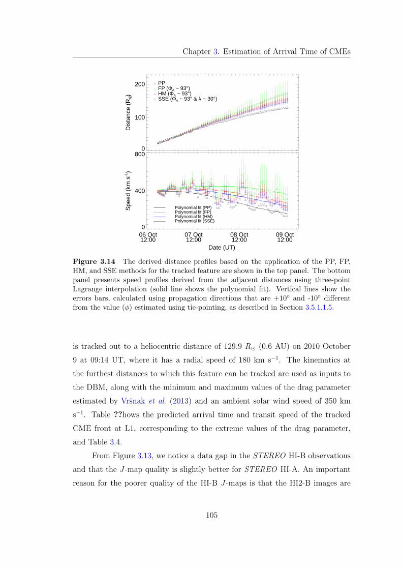
Chapter 3. Estimation of Arrival Time of CMEs
0
100
200
Dis
tanc
e (R
O •)
PPFP (ΦA ~ 93°)HM (ΦA ~ 93°)SSE (ΦA ~ 93° & λ ~ 30°)
06 Oct12:00
07 Oct12:00
08 Oct12:00
09 Oct12:00
0
400
800
Spe
ed (
km s
-1)
Polynomial fit (SSE)Polynomial fit (HM)Polynomial fit (FP)Polynomial fit (PP)
Date (UT)
Figure 3.14 The derived distance profiles based on the application of the PP, FP,HM, and SSE methods for the tracked feature are shown in the top panel. The bottompanel presents speed profiles derived from the adjacent distances using three-pointLagrange interpolation (solid line shows the polynomial fit). Vertical lines show theerrors bars, calculated using propagation directions that are +10◦ and -10◦ differentfrom the value (φ) estimated using tie-pointing, as described in Section 3.5.1.1.5.
is tracked out to a heliocentric distance of 129.9 R� (0.6 AU) on 2010 October
9 at 09:14 UT, where it has a radial speed of 180 km s−1. The kinematics at
the furthest distances to which this feature can be tracked are used as inputs to
the DBM, along with the minimum and maximum values of the drag parameter
estimated by Vrsnak et al. (2013) and an ambient solar wind speed of 350 km
s−1. Table ??hows the predicted arrival time and transit speed of the tracked
CME front at L1, corresponding to the extreme values of the drag parameter,
and Table 3.4.
From Figure 3.13, we notice a data gap in the STEREO HI-B observations
and that the J -map quality is slightly better for STEREO HI-A. An important
reason for the poorer quality of the HI-B J -maps is that the HI2-B images are
105
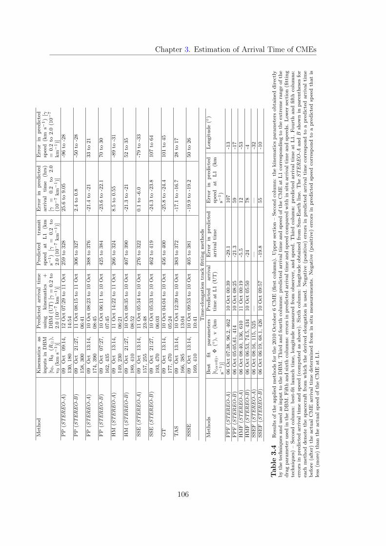
Chapter 3. Estimation of Arrival Time of CMEs
Met
hod
Kin
emati
csas
inp
uts
inD
BM
[t0,
R0
(R�
),v0
(km
s−1)]
Pre
dic
ted
arr
ival
tim
eu
sin
gkin
emati
cs+
DB
M(U
T)
[γ=
0.2
to2.0
(10−7
km
−1)]
Pre
dic
ted
tran
sit
spee
dat
L1
(km
s−1)
[γ=
0.2
to2.0
(10−7
km
−1)]
Err
or
inp
red
icte
darr
ival
tim
e(h
rs)
[γ=
0.2
to2.0
(10−7
km
−1)]
Err
or
inp
red
icte
dsp
eed
(km
s−1)
[γ=
0.2
to2.0
(10−7
km
−1)]
PP
(STEREO-A
)09
Oct
09:1
4,
130,
180
12
Oct
07:2
9to
11
Oct
14:5
4259
to328
25.6
to9.0
5-9
6to
-28
PP
(STEREO-B
)09
Oct
21:2
7,
158,
300
11
Oct
08:1
5to
11
Oct
06:4
1306
to327
2.4
to0.8
-50
to-2
8
FP
(STEREO-A
)09
Oct
13:1
4,
174,
390
10
Oct
08:2
3to
10
Oct
08:4
5388
to376
-21.4
to-2
133
to21
FP
(STEREO-B
)09
Oct
07:2
7,
162,
435
10
Oct
06:1
1to
10
Oct
07:4
5425
to384
-23.6
to-2
2.1
70
to30
HM
(STEREO-A
)09
Oct
13:1
4,
149,
230
11
Oct
14:2
2to
11
Oct
06:2
1266
to324
8.5
to0.5
5-8
9to
-31
HM
(STEREO-B
)09
Oct
21:2
7,
189,
410
10
Oct
08:3
5to
10
Oct
08:5
2407
to390
-21.3
to-2
152
to35
SS
E(S
TEREO-A
)09
Oct
13:1
4,
157,
255
11
Oct
05:3
4to
10
Oct
23:4
8276
to322
0.1
to-6
.0-7
9to
-33
SS
E(S
TEREO-B
)09
Oct
21:2
7,
193,
470
10
Oct
05:3
3to
10
Oct
06:0
3462
to419
-24.3
to-2
3.8
107
to64
GT
09
Oct
13:1
4,
177,
470
10
Oct
04:0
4to
10
Oct
05:2
4456
to400
-25.8
to-2
4.4
101
to45
TA
S09
Oct
13:1
4,
166,
385
10
Oct
12:3
9to
10
Oct
13:0
4383
to372
-17.1
to-1
6.7
28
to17
SS
SE
09
Oct
13:1
4,
169,
410
10
Oct
09:5
3to
10
Oct
10:4
1405
to381
-19.9
to-1
9.2
50
to26
Tim
e-el
on
gati
on
track
fitt
ing
met
hod
sM
eth
ods
Bes
tfi
tp
ara
met
ers
[t(α
=0),
Φ(◦
),v
(km
s−1)]
Pre
dic
ted
arr
ival
tim
eat
L1
(UT
)E
rror
inp
red
icte
darr
ival
tim
eE
rror
inp
red
icte
dsp
eed
at
L1
(km
s−1)
Lon
git
ud
e(◦
)
FP
F(S
TEREO-A
)06
Oct
07:3
8,
96.2
,462
10
Oct
00:3
9-2
9.1
107
-13
FP
F(S
TEREO-B
)06
Oct
05:0
5,6
1,
414
10
Oct
08:2
5-2
1.3
59
-17
HM
F(S
TEREO-A
)06
Oct
08:4
0,
136,
610
11
Oct
00:1
9-5
.512
-53
HM
F(S
TEREO-B
)06
Oct
06:5
3,
74.5
,434
10
Oct
05:5
0-2
478
-4S
SE
F(S
TEREO-A
)06
Oct
08:1
6,
115,
525
——
—-3
2S
SE
F(S
TEREO-B
)06
Oct
06:1
9,
68.1
,426
10
Oct
09:5
7-1
9.8
55
-10
Table
3.4
Res
ult
sof
the
ap
plied
met
hod
sfo
rth
e2010
Oct
ob
er6
CM
E(fi
rst
colu
mn
).U
pp
erse
ctio
n–
Sec
on
dco
lum
n:
the
kin
emati
csp
ara
met
ers
ob
tain
edd
irec
tly
by
the
tech
niq
ues
an
du
sed
as
inp
ut
toth
eD
BM
.T
hir
dan
dfo
urt
hco
lum
ns:
pre
dic
ted
arr
ival
tim
ean
dsp
eed
of
the
CM
Eat
L1
corr
esp
on
din
gto
the
extr
eme
ran
ge
of
the
dra
gp
ara
met
eru
sed
inth
eD
BM
.F
ifth
an
dsi
xth
colu
mn
s:er
rors
inp
red
icte
darr
ival
tim
ean
dsp
eed
com
pare
dw
ith
insi
tuarr
ival
tim
ean
dsp
eed
s.L
ow
erse
ctio
n(fi
ttin
gte
chn
iqu
es)
–S
econ
dco
lum
n:
bes
t-fi
tla
un
chti
me,
lon
git
ud
em
easu
red
from
ob
serv
er,
an
dsp
eed
.T
hir
dco
lum
n:
pre
dic
ted
arr
ival
tim
eat
L1.
Fou
rth
an
dfi
fth
colu
mn
s:er
rors
inp
red
icte
darr
ival
tim
ean
dsp
eed
(com
pu
ted
as
ab
ove)
.S
ixth
colu
mn
:lo
ngit
ud
eob
tain
edfr
om
Su
n-E
art
hlin
e.T
heSTEREO-A
an
dB
show
nin
pare
nth
eses
for
each
met
hod
den
ote
the
space
craft
from
wh
ich
the
der
ived
elon
gati
on
isu
sed
.N
egati
ve
(posi
tive)
erro
rsin
pre
dic
ted
arr
ival
tim
eco
rres
pon
dto
apre
dic
ted
arr
ival
tim
eb
efore
(aft
er)
the
act
ual
CM
Earr
ival
tim
ed
eter
min
edfr
om
insi
tum
easu
rem
ents
.N
egati
ve
(posi
tive)
erro
rsin
pre
dic
ted
spee
dco
rres
pon
dto
ap
red
icte
dsp
eed
that
isle
ss(m
ore
)th
an
the
act
ual
spee
dof
the
CM
Eat
L1.
106
Chapter 3. Estimation of Arrival Time of CMEs
out of focus compared to HI2-A images (Brown, Bewsher, and Eyles, 2009).
Another reason for the poorer quality of HI-B images is that HI on STEREO-B
suffers small pointing discontinuities due to dust impact. Since HI-B is facing
the direction of travel of the STEREO-B spacecraft, it gets impacted directly
by interplanetary dust; HI-A is on the opposite side to the direction of travel of
STEREO-A, so it does not suffer direct impact (Davis et al., 2012). Due to the
large gradient inherent in the F-coronal signal, even a small pointing offset can
result in an inaccurate F-corona subtraction, which results in degraded image
quality. Despite this, we tracked the leading edge of the October 6 CME in HI-B
J -maps even beyond the data gap (right panel in Figure 3.13). Adopting the same
procedure described for the feature tracked by STEREO-A, we also estimated the
kinematics and the arrival times at L1 of the CME based on its elongation profile
extracted from the STEREO-B J -map. Its estimated kinematics over the last
few tracked points, which are used as inputs to the DBM, and predicted arrival
time at L1 are noted in Table 3.4.
3.5.1.1.2 Fixed-phi (FP) method
The distance profile of the CME can be derived using this so-called FP ap-
proximation by assuming a propagation direction that can be determined by
identifying the CME source region. However, in our analysis of the CME of 2010
October 6, we use the propagation direction (φFP ) derived from the 3D recon-
struction of COR2 data as discussed in Section 3.5.1. We assume that, beyond
the COR2 FOV, the CME will continue to travel in the same direction. The
estimated longitude of the CME is ≈ 10◦ east of the Earth, which corresponds to
a longitude difference of ≈ 93 ◦ from the STEREO-A spacecraft; the separation
angle between STEREO-A and the Earth was ≈ 83◦ at that time. Using the
elongation variation of the tracked feature, extracted manually from the ecliptic
J -maps constructed from HI-A images as shown in Figure 3.13 (left), and φFP =
93◦, we calculated the distance profile of the leading bright front of the CME. The
obtained time variations of the radial distance and speed are shown in green in
Figure 3.14. The unphysical deceleration of the CME beyond 100 R� (suggested
107
Chapter 3. Estimation of Arrival Time of CMEs
by a speed less than ambient solar wind speed) may be due to the erroneous
fixing of the propagation angle in the case of a real deflection or, indeed, the in-
accurate characterization of the propagation angle. However, it is most likely due
to the breakdown of the simple assumption that the observer is always looking
at the same point-like feature of the CME. This can lead to large errors in the
estimated height of the CME leading edge, particularly at greater elongations
where the expanding CME geometry plays a significant role and the observer will
be unlikely to record the intensity from the same part of CME’s leading edge
(artificial deflection: Howard and Tappin, 2009; Howard, 2011). The limitations
of this and other methods will be discussed in Section 3.7.
As with the PP analysis, we apply the DBM based on the kinematics of the
tracked CME feature estimated using the FP method. Running the DBM with
the derived CME kinematics as inputs, along with an ambient solar wind speed
of 350 km s−1 and the two extreme values of the drag parameter, we obtained
the L1 arrival times and transit speeds given in Table 3.4.
We also applied the FP method to the elongation profile derived from the
STEREO-B J -map. (Figure 3.13, right). In STEREO-B, the feature can be
tracked out to 162 R� (0.75 AU) on 09 October 07:27 UT, where its speed is
approximately 435 km s−1.1 Again, these kinematics are used as inputs to the
DBM to estimate the arrival times and transit speeds at L1 (see Table 3.4).
3.5.1.1.3 Harmonic mean (HM) method
We used the CME longitude estimated from the 3D reconstruction of COR2 data
(as described earlier) and the elongation profile extracted from the STEREO-A
J -map to estimate the distance and speed profiles of the CME front using the
HM approximation (blue lines in Figure 3.14). A polynomial fit to the speed
profile (solid blue line in the bottom panel of Figure 3.14) suggests an overall
deceleration of the tracked CME feature. The non-physical deceleration of this
feature at large distances could result from the real deflection of this feature
or inaccuracy in the assumed ‘fixed’ direction, or be because the observer (in
this case STEREO-A) detects scattered light from a different part of the CME
108
Chapter 3. Estimation of Arrival Time of CMEs
than that assumed (artificial deflection). The limitations of the HM method are
discussed in Section 3.7.
Again, the estimated kinematics derived over the last segment of the tracked
time-elongation profile at around 13:14 UT on 2010 October 9 (distance: 149 R�,
i.e., 0.69 AU and speed 230 km s−1) are used as inputs into the DBM, to predict
the CME arrival time and transit speed at L1 (Table 3.4). As above, the DBM
assumes an ambient solar wind speed of 350 km s−1 and is run for the two extreme
values of the drag parameter.
The same methodology is applied to the CME track observed by STEREO-
B. At the end of its observed track, on October 9 at 21:27 UT, the CME speed
is estimated to be 410 km s−1 at a distance of 189 R� (0.87 AU). These values
are used as inputs in the DBM to derive arrival times and transit speeds at L1
(Table 3.4).
3.5.1.1.4 Self-similar expansion (SSE) method Assuming λ = 30◦, we
use the longitude estimated from 3D reconstruction in the COR2 FOV to estimate
the distance and speed profiles of the CME tracked in the STEREO-A J -map,
using the SSE method (shown in red in Figure 3.14). The DBM was run in the
same manner as described earlier, based on these kinematics inputs, to obtain
the arrival times and transit speeds (Table 3.41). The same methodology was
applied to STEREO-B observations (results are included in Table 3.4).
3.5.1.1.5 Error analysis for FP, HM and SSE methods
As described above, as input to the FP, HM, and SSE method, we used the
propagation direction (φ) of the CME estimated from the tie-pointing method
of 3D reconstruction. To examine the uncertainties arising from using the tie-
pointing method, we compared the CME kinematics derived using propagation
directions obtained from other methods. We note that, for all CMEs that form
part of this study, the propagation directions estimated using tie-pointing and for-
ward modeling (Thernisien, Vourlidas, and Howard, 2009) are within 10◦, which
is in agreement with results of Mierla et al. (2010). Propagation directions es-
109
Chapter 3. Estimation of Arrival Time of CMEs
timated from CME source locations are within 10◦ of the values obtained from
tie-pointing. We repeated FP, HM, and SSE analysis, as described above, using
propagation directions that are +10◦ and -10◦ different from the value (φ) esti-
mated using tie-pointing to estimate uncertainties in the distance (vertical error
bars in Figure 3.14). The speed’s standard deviation (uncertainty) is calculated
using the IDL derivsig function. These error bars do not denote all errors in
these single spacecraft methods but simply represent the method’s sensitivity to
uncertainties in direction.
3.5.1.2 Single spacecraft fitting methods for SECCHI/HI observa-
tions
3.5.1.2.1 Fixed-phi fitting (FPF), Harmonic mean fitting (HMF) and
Self-similar expansion fitting (SSEF) method
We used Equation 2.4 (Chapter 2) to get the most physically realistic combina-
tions of speed (vFP ), direction (φFP ), and launch time from Sun-centre (t0FP ),
where α(t0FP ) = 0, which can closely reproduce the elongation-time profiles of
CMEs derived from the J -maps.
We applied the FPF technique to the elongation variation of the 2010 Oc-
tober 6 CME derived from the STEREO-A HI J -map. We implemented the IDL
routine MPFITFUN (Markwardt, 2009) to find the set of vFP , φFP , and t0FP
parameters that best reproduced the observed elongation variation. In the up-
per panel of Figure 3.15 (red line), we show how well the observed variation is
produced by equation (1) of Rouillard et al. (2008). We estimated the fitting
residuals (bottom panels) by following the approach of Mostl et al. (2011). Ap-
plying FPF to the initial front of the October 6 CME tracked in the STEREO-A
J -map yields a propagation direction of 96.3◦ from the spacecraft (i.e., 13.3◦ East
of the Sun-Earth line), a speed of 462 km s−1, and a launch time of 07:38 UT on
2010 October 6. Assuming this speed is constant from the Sun to L1, the CME
is predicted to arrive at L1 at 00:39 UT on 2010 October 10.
Following the same basic procedure as for FPF, the best fit elongation
variation, derived using the HMF approach, is shown in Figure 3.15 (upper panel)
110
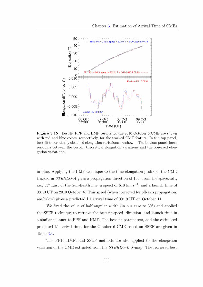
Chapter 3. Estimation of Arrival Time of CMEs
0
10
20
30
40
50
Elo
ngat
ion
(°)
HM : Phi = 136.0, speed = 610.0, T = 6-10-2010 8:40:38
FP : Phi = 96.3, speed = 462.2, T = 6-10-2010 7:38:29
06 Oct12:00
07 Oct12:00
08 Oct12:00
09 Oct12:00
-0.010
-0.005
0.000
0.005
0.010
Elo
ngat
ion
diffe
renc
e (
°)
Residue HM : 0.0034
Residue FF : 0.0031
Date (UT)
Figure 3.15 Best-fit FPF and HMF results for the 2010 October 6 CME are shownwith red and blue colors, respectively, for the tracked CME feature. In the top panel,best-fit theoretically obtained elongation variations are shown. The bottom panel showsresiduals between the best-fit theoretical elongation variations and the observed elon-gation variations.
in blue. Applying the HMF technique to the time-elongation profile of the CME
tracked in STEREO-A gives a propagation direction of 136◦ from the spacecraft,
i.e., 53◦ East of the Sun-Earth line, a speed of 610 km s−1, and a launch time of
08:40 UT on 2010 October 6. This speed (when corrected for off-axis propagation,
see below) gives a predicted L1 arrival time of 00:19 UT on October 11.
We fixed the value of half angular width (in our case to 30◦) and applied
the SSEF technique to retrieve the best-fit speed, direction, and launch time in
a similar manner to FPF and HMF. The best-fit parameters, and the estimated
predicted L1 arrival time, for the October 6 CME based on SSEF are given in
Table 3.4.
The FPF, HMF, and SSEF methods are also applied to the elongation
variation of the CME extracted from the STEREO-B J -map. The retrieved best
111
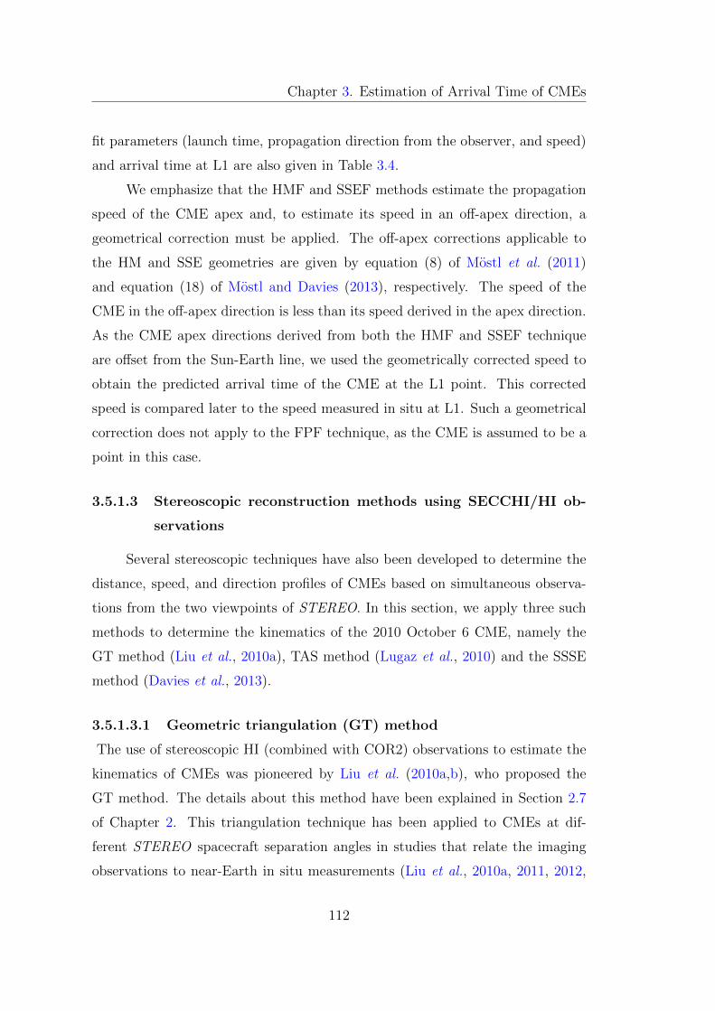
Chapter 3. Estimation of Arrival Time of CMEs
fit parameters (launch time, propagation direction from the observer, and speed)
and arrival time at L1 are also given in Table 3.4.
We emphasize that the HMF and SSEF methods estimate the propagation
speed of the CME apex and, to estimate its speed in an off-apex direction, a
geometrical correction must be applied. The off-apex corrections applicable to
the HM and SSE geometries are given by equation (8) of Mostl et al. (2011)
and equation (18) of Mostl and Davies (2013), respectively. The speed of the
CME in the off-apex direction is less than its speed derived in the apex direction.
As the CME apex directions derived from both the HMF and SSEF technique
are offset from the Sun-Earth line, we used the geometrically corrected speed to
obtain the predicted arrival time of the CME at the L1 point. This corrected
speed is compared later to the speed measured in situ at L1. Such a geometrical
correction does not apply to the FPF technique, as the CME is assumed to be a
point in this case.
3.5.1.3 Stereoscopic reconstruction methods using SECCHI/HI ob-
servations
Several stereoscopic techniques have also been developed to determine the
distance, speed, and direction profiles of CMEs based on simultaneous observa-
tions from the two viewpoints of STEREO. In this section, we apply three such
methods to determine the kinematics of the 2010 October 6 CME, namely the
GT method (Liu et al., 2010a), TAS method (Lugaz et al., 2010) and the SSSE
method (Davies et al., 2013).
3.5.1.3.1 Geometric triangulation (GT) method
The use of stereoscopic HI (combined with COR2) observations to estimate the
kinematics of CMEs was pioneered by Liu et al. (2010a,b), who proposed the
GT method. The details about this method have been explained in Section 2.7
of Chapter 2. This triangulation technique has been applied to CMEs at dif-
ferent STEREO spacecraft separation angles in studies that relate the imaging
observations to near-Earth in situ measurements (Liu et al., 2010a, 2011, 2012,
112
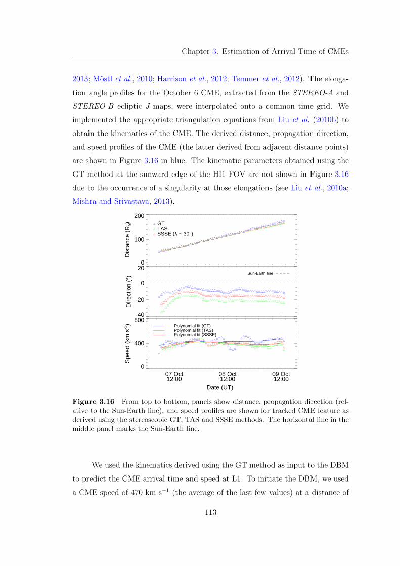
Chapter 3. Estimation of Arrival Time of CMEs
2013; Mostl et al., 2010; Harrison et al., 2012; Temmer et al., 2012). The elonga-
tion angle profiles for the October 6 CME, extracted from the STEREO-A and
STEREO-B ecliptic J -maps, were interpolated onto a common time grid. We
implemented the appropriate triangulation equations from Liu et al. (2010b) to
obtain the kinematics of the CME. The derived distance, propagation direction,
and speed profiles of the CME (the latter derived from adjacent distance points)
are shown in Figure 3.16 in blue. The kinematic parameters obtained using the
GT method at the sunward edge of the HI1 FOV are not shown in Figure 3.16
due to the occurrence of a singularity at those elongations (see Liu et al., 2010a;
Mishra and Srivastava, 2013).
0
100
200
Dis
tanc
e (R
O •) GT
TASSSSE (λ ~ 30°)
-40
-20
0
20
Dire
ctio
n (°
) Sun-Earth line
07 Oct12:00
08 Oct12:00
09 Oct12:00
0
400
800
Spe
ed (
km s
-1) Polynomial fit (GT)
Polynomial fit (TAS)Polynomial fit (SSSE)
Date (UT)
Figure 3.16 From top to bottom, panels show distance, propagation direction (rel-ative to the Sun-Earth line), and speed profiles are shown for tracked CME feature asderived using the stereoscopic GT, TAS and SSSE methods. The horizontal line in themiddle panel marks the Sun-Earth line.
We used the kinematics derived using the GT method as input to the DBM
to predict the CME arrival time and speed at L1. To initiate the DBM, we used
a CME speed of 470 km s−1 (the average of the last few values) at a distance of
113
Chapter 3. Estimation of Arrival Time of CMEs
177 R� (0.82 AU) at 13:14 UT on 2010 October 9. As before, the ambient solar
wind speed was set to 350 km s−1. The resultant L1 arrival times and speeds,
corresponding to the extreme range of the drag parameter, are given in Table 3.4.
3.5.1.3.2 Tangent to a sphere (TAS) method
The details about the TAS method have been explained in Section 2.3.2.4.2 of
Chapter 2. We apply equation (2) of Lugaz et al. (2010) to estimate the prop-
agation direction of the tracked CME using this technique. As in the previous
section, we use the derived time-direction profiles to estimate the distance, hence
the speed, profiles of the CME based on the expression for the radial distance of
the transient’s apex. The results are shown in Figure 3.16 in green.
The central panel of Figure 3.16 (green line) suggests that the CME is
propagating slightly eastward of the Sun-Earth line. At the last point of its track
(13:14 UT on October 9), the estimated CME distance and speed are 166 R�
(0.77 AU) and 385 km s−1, respectively. The kinematics at the sunward edge of
the HI1 FOV are not shown due to the occurrence of a singularity, as in the GT
method. We applied the DBM exactly as discussed earlier; the results are shown
in Table 3.4.
3.5.1.3.3 Stereoscopic self-similar expansion (SSSE) method
The details about the SSSE method have been explained in Section 2.8 of Chap-
ter 2. We used the equations. (23), (24), and (4a) of Davies et al. (2013) to
estimate the propagation direction from the observer and distance profiles for the
tracked CME. Although this SSSE method can take any value of the half angular
width (λ) of the CME between 0◦ and 90◦, we use a fixed value of 30◦. The
obtained kinematics for the tracked feature is shown in Figure 3.16 in red. The
kinematics for the points at the sun-ward edge of HI FOV are not shown due to
significant errors. For these points, the sum of the elongation from both observers
and the separation angle between the two observers is close to 180◦. As pointed
out by Davies et al. (2013), in such a situation, small errors in elongation will
result in significant errors in direction, and hence in distance and speed, around
114
Chapter 3. Estimation of Arrival Time of CMEs
the aforementioned singularity. The estimated kinematics at the end of the track
are used as inputs in the DBM to predict the arrival times and speeds at L1
(Table 3.4).
3.5.2 2010 April 3 CME
We used the tie-pointing method of 3D reconstruction (scc measure:
Thompson 2009) on a selected feature along the leading edge of this CME and ob-
tained its 3D kinematics. The 3D speed, latitude, and longitude were estimated
as 816 km s−1, 25◦ south and 5◦ east of the Earth, respectively, at the outer edge
of the COR2 FOV. The kinematics of this fast CME seems to be partly influ-
enced by the presence of high-speed solar wind, as the CME experiences slight
deceleration during its journey from the Sun to 1 AU; during this time, the Earth
was immersed in the fast solar wind. The kinematics of this CME have been
studied extensively by several authors (Mostl et al., 2010; Wood et al., 2011; Liu
et al., 2011). In contrast to the 2010 October 6 event, this allows us to assess the
accuracy of various methods for the case of a fast CME moving in a fast ambient
solar wind.
We constructed STEREO-A and B ecliptic J -maps for this interval encom-
passing this CME using COR2 and HI images and extracted, from each, the time-
elongation profile for the leading edge of the initial CME front. The Milky Way
is visible in the HI2-B images. Therefore the CME signal is slightly difficult to
track. This CME can be tracked out to 54.5◦ and 26.5◦ elongation in STEREO-A
and B J -maps, respectively. We implemented the seven single spacecraft methods
(PP, FP, FPF, HM, HMF, SSE, and SSEF) and the three stereoscopic methods
(GT, TAS, and SSSE) to derive the CME kinematics. Estimated kinematics from
the PP, FP, HM, and SSE methods, applied to the time-elongation profile of the
CME extracted from the STEREO-A J -map, is shown in Figure 3.17. Errors
bars are calculated in the same manner as for the 2010 October 6 CME discussed
in Section 3.5.1.1.5. We also estimated the kinematics of the CME based on the
STEREO-B J -map. We used the kinematics from both spacecraft as inputs to
115
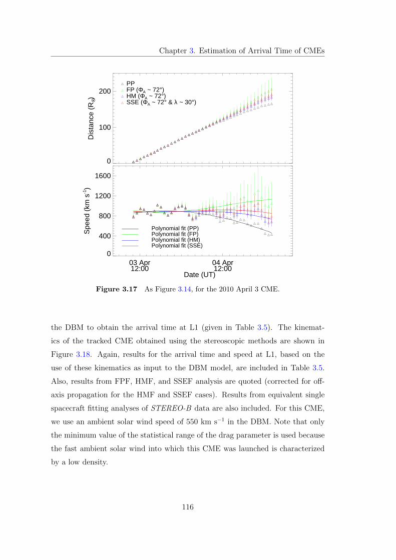
Chapter 3. Estimation of Arrival Time of CMEs
0
100
200D
ista
nce
(RO •)
PPFP (ΦA ~ 72°)HM (ΦA ~ 72°)SSE (ΦA ~ 72° & λ ~ 30°)
03 Apr12:00
04 Apr12:00
0
400
800
1200
1600
Spe
ed (
km s
-1)
Polynomial fit (SSE)Polynomial fit (HM)Polynomial fit (FP)Polynomial fit (PP)
Date (UT)
Figure 3.17 As Figure 3.14, for the 2010 April 3 CME.
the DBM to obtain the arrival time at L1 (given in Table 3.5). The kinemat-
ics of the tracked CME obtained using the stereoscopic methods are shown in
Figure 3.18. Again, results for the arrival time and speed at L1, based on the
use of these kinematics as input to the DBM model, are included in Table 3.5.
Also, results from FPF, HMF, and SSEF analysis are quoted (corrected for off-
axis propagation for the HMF and SSEF cases). Results from equivalent single
spacecraft fitting analyses of STEREO-B data are also included. For this CME,
we use an ambient solar wind speed of 550 km s−1 in the DBM. Note that only
the minimum value of the statistical range of the drag parameter is used because
the fast ambient solar wind into which this CME was launched is characterized
by a low density.
116
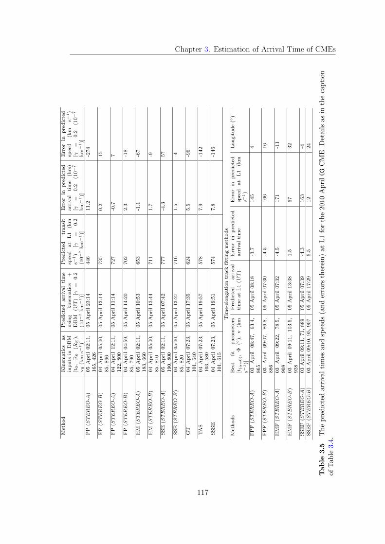
Chapter 3. Estimation of Arrival Time of CMEs
Met
hod
Kin
emati
csas
inp
uts
inD
BM
[t0,
R0
(R�
),v0
(km
s−1)]
Pre
dic
ted
arr
ival
tim
eu
sin
gkin
emati
cs+
DB
M(U
T)
[γ=
0.2
(10−7
km
−1)]
Pre
dic
ted
tran
sit
spee
dat
L1
(km
s−1)
[γ=
0.2
(10−7
km
−1)]
Err
or
inp
red
icte
darr
ival
tim
e(h
rs)
[γ=
0.2
(10−7
km
−1)]
Err
or
inp
red
icte
dsp
eed
(km
s−1)
[γ=
0.2
(10−7
km
−1)]
PP
(STEREO-A
)05
Ap
ril
02:1
1,
165,
426
05
Ap
ril
23:1
4446
11.2
-274
PP
(STEREO-B
)04
Ap
ril
05:0
0,
85,
866
05
Ap
ril
12:1
4735
0.2
15
FP
(STEREO-A
)04
Ap
ril
12:1
1,
122,
800
05
Ap
ril
11:1
4727
-0.7
7
FP
(STEREO-B
)04
Ap
ril
04:5
9,
85,
790
05
Ap
ril
14:2
0702
2.3
-18
HM
(STEREO-A
)05
Ap
ril
02:1
1,
183,
660
05
Ap
ril
10:5
3653
-1.1
-67
HM
(STEREO-B
)04
Ap
ril
05:0
0,
85,
810
05
Ap
ril
13:4
4711
1.7
-9
SS
E(S
TEREO-A
)05
Ap
ril
02:1
1,
190,
800
05
Ap
ril
07:4
2777
-4.3
57
SS
E(S
TEREO-B
)04
Ap
ril
05:0
0,
85,
820
05
Ap
ril
13:2
7716
1.5
-4
GT
04
Ap
ril
07:2
3,
101,
640
05
Ap
ril
17:3
5624
5.5
-96
TA
S04
Ap
ril
07:2
3,
103,
580
05
Ap
ril
19:5
7578
7.9
-142
SS
SE
04
Ap
ril
07:2
3,
101,
615
05
Ap
ril
19:5
1574
7.8
-146
Tim
e-el
on
gati
on
track
fitt
ing
met
hod
sM
eth
od
sB
est
fit
para
met
ers
[t(α
=0),
Φ(◦
),v
(km
s−1)]
Pre
dic
ted
arr
ival
tim
eat
L1
(UT
)E
rror
inp
red
icte
darr
ival
tim
eE
rror
inp
red
icte
dsp
eed
at
L1
(km
s−1)
Lon
git
ud
e(◦
)
FP
F(S
TEREO-A
)03
Ap
ril
08:4
7,
63.4
,865
05
Ap
ril
08:1
8-3
.7145
4
FP
F(S
TEREO-B
)03
Ap
ril
09:0
7,
86.8
,886
05
Ap
ril
07:3
0-4
.5166
16
HM
F(S
TEREO-A
)03
Ap
ril
09:2
2,
78.5
,908
05
Ap
ril
07:3
2-4
.5171
-11
HM
F(S
TEREO-B
)03
Ap
ril
09:1
1,
103.5
,928
05
Ap
ril
13:3
81.5
67
32
SS
EF
(STEREO-A
)03
Ap
ril
09:1
1,
71,
889
05
Ap
ril
07:3
9-4
.3163
-4S
SE
F(S
TEREO-B
)03
Ap
ril
09:1
0,
95,
907
05
Ap
ril
17:2
95.5
12
24
Table
3.5
Th
ep
red
icte
darr
ival
tim
esan
dsp
eed
s(a
nd
erro
rsth
erei
n)
atL
1fo
rth
e20
10A
pri
l03
CM
E.
Det
ails
asin
the
cap
tion
of
Tab
le3.4
.
117
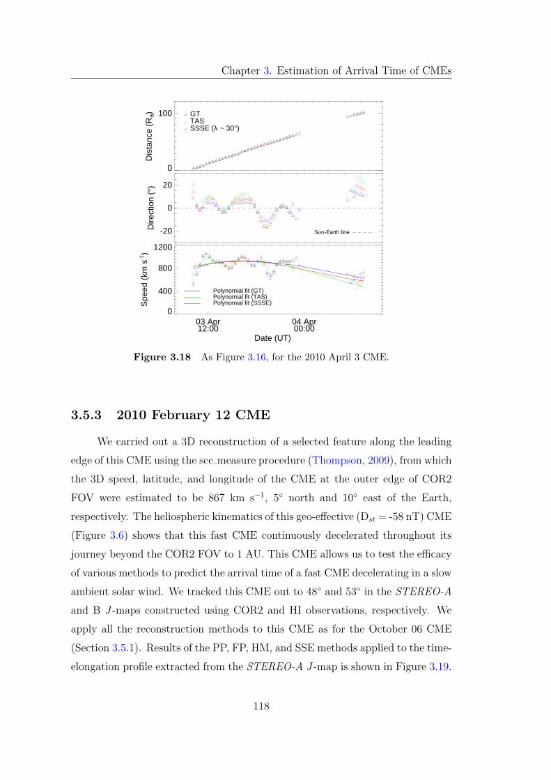
Chapter 3. Estimation of Arrival Time of CMEs
0
100
Dis
tanc
e (R
O •) GT
TASSSSE (λ ~ 30°)
-20
0
20
Dire
ctio
n (°
)
Sun-Earth line
03 Apr12:00
04 Apr00:00
0
400
800
1200
Spe
ed (
km s
-1)
Polynomial fit (SSSE)Polynomial fit (TAS)Polynomial fit (GT)
Date (UT)
Figure 3.18 As Figure 3.16, for the 2010 April 3 CME.
3.5.3 2010 February 12 CME
We carried out a 3D reconstruction of a selected feature along the leading
edge of this CME using the scc measure procedure (Thompson, 2009), from which
the 3D speed, latitude, and longitude of the CME at the outer edge of COR2
FOV were estimated to be 867 km s−1, 5◦ north and 10◦ east of the Earth,
respectively. The heliospheric kinematics of this geo-effective (Dst = -58 nT) CME
(Figure 3.6) shows that this fast CME continuously decelerated throughout its
journey beyond the COR2 FOV to 1 AU. This CME allows us to test the efficacy
of various methods to predict the arrival time of a fast CME decelerating in a slow
ambient solar wind. We tracked this CME out to 48◦ and 53◦ in the STEREO-A
and B J -maps constructed using COR2 and HI observations, respectively. We
apply all the reconstruction methods to this CME as for the October 06 CME
(Section 3.5.1). Results of the PP, FP, HM, and SSE methods applied to the time-
elongation profile extracted from the STEREO-A J -map is shown in Figure 3.19.
118
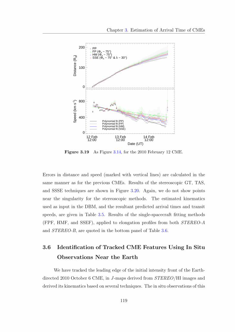
Chapter 3. Estimation of Arrival Time of CMEs
0
100
200
Dis
tanc
e (R
O •)
PPFP (ΦA ~ 75°)HM (ΦA ~ 75°)SSE (ΦA ~ 75° & λ ~ 30°)
12 Feb12:00
13 Feb12:00
14 Feb12:00
0
400
800
Spe
ed (
km s
-1)
Polynomial fit (SSE)Polynomial fit (HM)Polynomial fit (FP)Polynomial fit (PP)
Date (UT)
Figure 3.19 As Figure 3.14, for the 2010 February 12 CME.
Errors in distance and speed (marked with vertical lines) are calculated in the
same manner as for the previous CMEs. Results of the stereoscopic GT, TAS,
and SSSE techniques are shown in Figure 3.20. Again, we do not show points
near the singularity for the stereoscopic methods. The estimated kinematics
used as input in the DBM, and the resultant predicted arrival times and transit
speeds, are given in Table 3.5. Results of the single-spacecraft fitting methods
(FPF, HMF, and SSEF), applied to elongation profiles from both STEREO-A
and STEREO-B, are quoted in the bottom panel of Table 3.6.
3.6 Identification of Tracked CME Features Using In Situ
Observations Near the Earth
We have tracked the leading edge of the initial intensity front of the Earth-
directed 2010 October 6 CME, in J -maps derived from STEREO/HI images and
derived its kinematics based on several techniques. The in situ observations of this
119
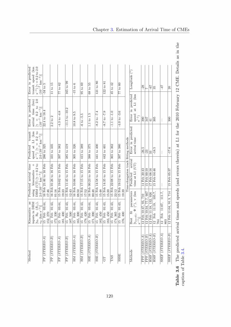
Chapter 3. Estimation of Arrival Time of CMEsM
eth
od
Kin
emati
csas
inp
uts
inD
BM
[t0,
R0
(R�
),v0
(km
s−1)]
Pre
dic
ted
arr
ival
tim
eu
sin
gkin
emati
cs+
DB
M(U
T)
[γ=
0.2
to2.0
(10−7
km
−1)]
Pre
dic
ted
tran
sit
spee
dat
L1
(km
s−1)
[γ=
0.2
to2.0
(10−7
km
−1)]
Err
or
inp
red
icte
darr
ival
tim
e(h
rs)
[γ=
0.2
to2.0
(10−7
km
−1)]
Err
or
inp
red
icte
dtr
an
sit
spee
d(k
ms−
1)
[γ=
0.2
to2.0
(10−7
km
−1)]
PP
(STEREO-A
)15
Feb
03:4
4,
152,
270
16
Feb
21:4
6to
16
Feb
17:4
6286
to325
22.4
to18.4
-34
to5
PP
(STEREO-B
)15
Feb
01:4
3,
172,
330
16
Feb
01:2
6to
16
Feb
01:1
6331
to335
2.2
to2
11
to15
FP
(STEREO-A
)15
Feb
03:4
4,
181,
400
15
Feb
19:0
2to
15
Feb
19:2
3397
to382
-4.3
to-4
.877
to62
FP
(STEREO-B
)15
Feb
01:4
3,
187,
500
15
Feb
11:4
5to
15
Feb
12:4
3485
to419
-11.5
to-1
0.2
165
to99
HM
(STEREO-A
)15
Feb
03:4
4,
165,
300
16
Feb
10:0
6to
16
Feb
08:5
0305
to326
10.8
to9.5
-15
to6
HM
(STEREO-B
)15
Feb
01:4
3,
179,
420
15
Feb
17:1
5to
15
Feb
17:5
2415
to389
-6to
-5.5
95
to69
SS
E(S
TEREO-A
)15
Feb
03:4
4,
171,
390
16
Feb
00:2
3to
16
Feb
00:4
8388
to375
1.1
to1.5
68
to55
SS
E(S
TEREO-B
)15
Feb
01:4
3,
182,
450
15
Feb
14:5
8to
15
Feb
15:4
8441
to400
-8.2
to-7
.4121
to80
GT
15
Feb
01:4
3,
183,
450
15
Feb
14:3
5to
15
Feb
15:2
0442
to401
-8.7
to-7
.9122
to81
TA
S15
Feb
01:4
3,
174,
365
15
Feb
22:0
8to
15
Feb
22:1
2365
to362
-1.1
to-1
.045
to42
SS
SE
15
Feb
01:4
3,
176,
400
15
Feb
19:1
2to
15
Feb
19:3
9397
to380
-4.0
to-3
.677
to60
Tim
e-el
on
gati
on
track
fitt
ing
met
hod
sM
eth
ods
Bes
tfi
tp
ara
met
ers
[t(α
=0),
Φ(◦
),v
(km
s−1)]
Pre
dic
ted
arr
ival
tim
eat
L1
(UT
)E
rror
inp
red
icte
darr
ival
tim
eE
rror
inp
red
icte
dsp
eed
at
L1
(km
s−1)
Lon
git
ud
e(◦
)
FP
F(S
TEREO-A
)12
Feb
10:4
7,
93,
710
14
Feb
20:4
3-2
6.5
390
-28
FP
F(S
TEREO-B
)12
Feb
10:3
4,
77.7
,667
15
Feb
00:1
0-2
3347
7H
MF
(STEREO-A
)12
Feb
11:1
8,
132,
926
17
Feb
08:1
633
41
-67
HM
F(S
TEREO-B
)12
Feb
11:1
9,
105.7
,764
15
Feb
04:4
6-1
8.5
305
35
SS
EF
(STEREO-A
)12
Feb
11:0
7,
111.7
,803
——
—-4
7
SS
EF
(STEREO-B
)12
Feb
11:0
4,
91.3
,714
15
Feb
05:3
7-1
7.6
300
20
Table
3.6
Th
ep
red
icte
darr
ival
tim
esan
dsp
eed
s(a
nd
erro
rsth
erei
n)
atL
1fo
rth
e201
0F
ebru
ary
12
CM
E.
Det
ail
sas
inth
eca
pti
onof
Tab
le3.
4.
120
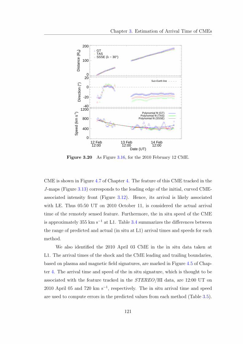
Chapter 3. Estimation of Arrival Time of CMEs
0
100
200
Dis
tanc
e (R
O •) GT
TASSSSE (λ ~ 30°)
-40
-20
0
20D
irect
ion
(°) Sun-Earth line
12 Feb12:00
13 Feb12:00
14 Feb12:00
0
400
800
1200
Spe
ed (
km s
-1) Polynomial fit (GT)
Polynomial fit (TAS)Polynomial fit (SSSE)
Date (UT)
Figure 3.20 As Figure 3.16, for the 2010 February 12 CME.
CME is shown in Figure 4.7 of Chapter 4. The feature of this CME tracked in the
J -maps (Figure 3.13) corresponds to the leading edge of the initial, curved CME-
associated intensity front (Figure 3.12). Hence, its arrival is likely associated
with LE. Thus 05:50 UT on 2010 October 11, is considered the actual arrival
time of the remotely sensed feature. Furthermore, the in situ speed of the CME
is approximately 355 km s−1 at L1. Table 3.4 summarizes the differences between
the range of predicted and actual (in situ at L1) arrival times and speeds for each
method.
We also identified the 2010 April 03 CME in the in situ data taken at
L1. The arrival times of the shock and the CME leading and trailing boundaries,
based on plasma and magnetic field signatures, are marked in Figure 4.5 of Chap-
ter 4. The arrival time and speed of the in situ signature, which is thought to be
associated with the feature tracked in the STEREO/HI data, are 12:00 UT on
2010 April 05 and 720 km s−1, respectively. The in situ arrival time and speed
are used to compute errors in the predicted values from each method (Table 3.5).
121
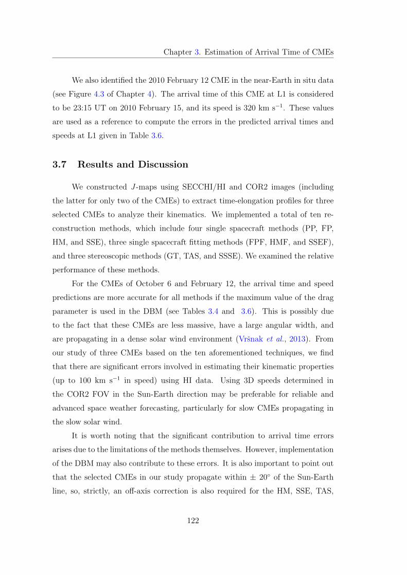
Chapter 3. Estimation of Arrival Time of CMEs
We also identified the 2010 February 12 CME in the near-Earth in situ data
(see Figure 4.3 of Chapter 4). The arrival time of this CME at L1 is considered
to be 23:15 UT on 2010 February 15, and its speed is 320 km s−1. These values
are used as a reference to compute the errors in the predicted arrival times and
speeds at L1 given in Table 3.6.
3.7 Results and Discussion
We constructed J -maps using SECCHI/HI and COR2 images (including
the latter for only two of the CMEs) to extract time-elongation profiles for three
selected CMEs to analyze their kinematics. We implemented a total of ten re-
construction methods, which include four single spacecraft methods (PP, FP,
HM, and SSE), three single spacecraft fitting methods (FPF, HMF, and SSEF),
and three stereoscopic methods (GT, TAS, and SSSE). We examined the relative
performance of these methods.
For the CMEs of October 6 and February 12, the arrival time and speed
predictions are more accurate for all methods if the maximum value of the drag
parameter is used in the DBM (see Tables 3.4 and 3.6). This is possibly due
to the fact that these CMEs are less massive, have a large angular width, and
are propagating in a dense solar wind environment (Vrsnak et al., 2013). From
our study of three CMEs based on the ten aforementioned techniques, we find
that there are significant errors involved in estimating their kinematic properties
(up to 100 km s−1 in speed) using HI data. Using 3D speeds determined in
the COR2 FOV in the Sun-Earth direction may be preferable for reliable and
advanced space weather forecasting, particularly for slow CMEs propagating in
the slow solar wind.
It is worth noting that the significant contribution to arrival time errors
arises due to the limitations of the methods themselves. However, implementation
of the DBM may also contribute to these errors. It is also important to point out
that the selected CMEs in our study propagate within ± 20◦ of the Sun-Earth
line, so, strictly, an off-axis correction is also required for the HM, SSE, TAS,
122
Chapter 3. Estimation of Arrival Time of CMEs
and SSSE methods before using the resultant speed as the input to the DBM.
However, for these CMEs, we estimate that such a correction would decrease the
speed by only a few km s−1 and hence increase the travel time by only a few
tens of minutes. We expect that if the final estimated speed of each tracked
CME were taken as constant for the rest of its journey to L1, then the errors
in predicted arrival time would be similar to that obtained from using the DBM
with the minimum drag parameter. This is because the CMEs are tracked out
to a significant fraction of 1 AU (≈ 0.5 to 0.8 AU), and beyond this distance, a
small drag force will have little effect on the CME dynamics.
Our assessment of the relative performance of various methods is based
mainly on the difference between the CME arrival time predicted at L1 by dif-
ferent reconstruction methods and the “actual” arrival time determined in situ.
We do not perform a detailed comparison of the kinematic profiles derived using
each method. Of course, different kinematics profiles can lead to the same arrival
time. Moreover, it is unlikely that the same part of a CME tracked in remote
imaging observations will pass through the spacecraft meant for in situ measure-
ments. We cannot advocate, with confidence, the superiority of one method over
others based only on the accuracy of arrival time predictions. It would be useful
to compare the speed profile of a CME derived in the inner heliosphere using 3D
MHD modeling with that obtained using HI observations. Of course, results from
MHD models also need to be considered with caution.
3.7.1 Relative performance of single spacecraft methods
In our study, we assess the performance of various reconstruction techniques
based on the obtained difference between the predicted and actual arrival times
of three CMEs. Of the four single spacecraft methods that do not rely on a
curve-fitting approach, the PP method gives the largest range of errors (up to
25 hr) in the predicted arrival time of all CMEs. This is perhaps due to its
oversimplified geometry. At large elongations (beyond ≈ 120 R�), for the CMEs
of October 6 and February 12, the speed estimated using the PP technique is
123
Chapter 3. Estimation of Arrival Time of CMEs
less than the ambient solar wind speed, which is unphysical. For the October 6
CME, the PP, FP, HM, and SSE approaches produce roughly similar errors in
predicted arrival time (up to 25 hr) and transit speed (up to 100 km s−1). For the
CME of April 3, the HM and PP methods provide the most and least accurate
predictions of arrival time at L1, respectively. For the CME of February 12, the
SSE method provides the most precise L1 arrival time, while the PP method is
the least accurate of these four methods.
The kinematics of the April 3 CME estimated using the FP method (Fig-
ure 3.17: green track) show a sudden unphysical late acceleration, possibly due
to its real deflection. We suggest that the FP, HM, and SSE methods, as imple-
mented here, can give accurate results if the estimated speeds tend to a constant
value far from the Sun. In the FP method, the tracked feature is assumed to
correspond to the same point moving in a fixed radial direction, which is unlikely
to be valid for a real CME structure (Howard, 2011). One major drawback of the
FP method is that it does not take into account the finite cross-sectional extent
of a CME. In terms of the four single viewpoint methods that enable estimation
of the kinematics properties as a function of time, the HM and SSE methods
provide a more accurate arrival time prediction for this CME. Of course, the as-
sumption of a circular front in these methods may not be valid due to possible
flattening of the CME front resulting from its interaction with the structured
coronal magnetic field and solar wind ahead of the CME (Odstrcil, Pizzo, and
Arge, 2005). Also, the assumption made here in implementing the HM and SSE
methods (and indeed the FP method) that the CME propagates along a fixed
radial trajectory (in particular one derived close to the Sun), ignoring real or
“artificial” heliospheric deflections, will induce errors, particularly for slow speed
CMEs that are more likely to undergo deflection in the interplanetary medium
(Wang et al., 2004; Gui et al., 2011). As noted previously, “artificial deflection”
means that the observer does not detect the same feature of CME in consecutive
images due to a well-known geometrical effect. We conclude that the implausible
deceleration of October 6 CME to a speed less than that of the ambient solar
wind speed (see Figure 3.14) is due to violations of the assumptions inherent in
124
Chapter 3. Estimation of Arrival Time of CMEs
the PP, HM, and SSE methods at elongations beyond 30◦.
Irrespective of the event, the PP, FP, HM, and SSE methods estimate sig-
nificantly different radial distance and speed profiles after approximately 100 R�.
This is because the assumed geometry impacts the results with increasing elon-
gation. For the PP and FP methods, implausible acceleration or deceleration
evident beyond approximately 100 R�, if assumed to be real, would lead to un-
realistically large errors in arrival time prediction. Therefore, among the single
spacecraft methods, we suggest that methods like HM and SSE should be used
to achieve reasonable arrival time predictions.
The value of the propagation direction adopted for each CME in our imple-
mentation of the FP, HM, and SSE techniques will affect the performance of each
method; this is an important issue in our study. The quoted CME arrival times
in Tables 1, 2, and 3 based on the FP, HM, and SSE techniques are based on a
direction estimated from tie-pointing. To assess the sensitivity of our results to
the exact value of the propagation direction used, we have repeated our analysis
using a range of propagation directions. As described in Section 3.5.1.1.5, we
repeated our FP, HM, and SSE analyses using propagation directions that are
+10◦ and -10◦ different from the values (φ) estimated using tie-pointing. We used
these revised kinematic profiles to estimate the arrival time and transit speed of
the selected CMEs in our study for φ ± 10◦.
For the October 6 CME analyzed using the FP method, using φ+10 (φ-10)
resulted in predicted arrival times that are 21 hr later (earlier) for STEREO-A
and 10 hr earlier (later) for STEREO-B than the arrival time predicted using φ.
For the HM method, using φ+10 (φ-10) resulted in a predicted arrival time 12
hr later (earlier) for STEREO-A and 6 hr earlier (later) for STEREO-B. For the
SSE method, using φ+10 (φ-10) results in a predicted arrival time 16 hr later
(earlier) for STEREO-A and 7 hr earlier (later) for STEREO-B. For the 2010
April 3 CME, the deviation in arrival time from that quoted in Table 2 is less
than 5 hr for STEREO-A and less than 3 hr for STEREO-B for all the three
single spacecraft methods for φ+10. Assuming a propagation direction equal to
φ-10 yields the same uncertainties as for φ+10, except for the FP method applied
125
Chapter 3. Estimation of Arrival Time of CMEs
to STEREO-A where the uncertainty increases to 8 hr. For the 2010 February
12 CME, assuming that the propagation direction is φ+10 (φ-10) in FP analysis
results in predicted arrival times 9 hr later (14 hr earlier) for STEREO-A and
4 hr earlier (6 hr later) for STEREO-B than the values quoted in Table 3 that
are based on using φ directly from tie-pointing. In the case of the HM and SSE
methods, using φ+10 (φ-10) results in predicted arrival times that are less than 9
hr later (earlier) for STEREO-A and less than 6 hr earlier (later) for STEREO-B
than the values quoted in Table 3.
The uncertainties discussed above do not reflect the total errors involved in
implementing the FP, HM and SSE methods. The uncertainties in the distance
and speed due to a change in propagation direction are not significant at smaller
elongations (Wood et al., 2009; Howard, 2011). Therefore, for a case like that
of the April 3 CME as observed by STEREO-B, in particular, where the CME
cannot be tracked out far in elongation angle, any uncertainty in propagation
direction will have a minimal effect on the derived kinematic profile and also the
predicted arrival time. At greater elongations, however, this effect, along with the
“well-known effect of CME geometry”, will severely limit the accuracy of these
methods. Given the effects of uncertainty in propagation direction in the FP,
HM, and SSE methods, we note that it may be better to combine the DBM with
CME kinematics derived in the near-Sun HI1 FOV to optimize the goal of space
weather prediction, at least for CMEs launched into a slow speed ambient solar
wind medium.
3.7.2 Relative performance of stereoscopic methods
For the October 6 CME, the stereoscopic GT method provides a large range
of arrival time errors (up to 25 hr), while the stereoscopic TAS method predicts
arrival time within 17 hr. For this CME, the errors resulting from the applica-
tion of the SSSE method are intermediate between those from the GT and TAS
methods. For the February 12 CME, among the three stereoscopic methods, the
TAS method provides the best prediction of L1 arrival time (within 2 hr of the
126
Chapter 3. Estimation of Arrival Time of CMEs
in situ arrival) and transit speed (within 45 km s−1 of the in situ speed). For
the April 3 CME, all of the stereoscopic methods give approximately the same
arrival time errors (within 8 hr).
As in the FP (and FPF) techniques, the assumption in GT that the same
point of a CME is being observed in consecutive images is likely to become increas-
ingly invalid with increasing elongation. GT also assumes that the same point is
observed simultaneously from both viewpoints. Moreover, the effect of ignoring
the Thomson scattering geometry is minimized for Earth-directed events. There-
fore deviations from such a configuration will also result in errors in the estimated
kinematics. From our analysis, which is limited to three CMEs, we conclude that
TAS technique performs most accurately, and GT performs least accurately in
estimating CME arrival times and speeds among the three stereoscopic methods.
The predicted SSSE arrival time is within a couple of hours of that predicted
by the TAS technique. As the estimated kinematics properties from the SSSE
method (here implemented with an angular half-width of 30◦) are intermediate
between the kinematics derived from the GT and TAS methods (see Figure 3.16,
3.18, 3.20), we are tempted to suggest that the SSSE method may be preferable
for space weather forecasting if a reasonable estimate of a half angular width
of a CME is available. In all the stereoscopic methods used, any effects due to
the Thomson scattering geometry are ignored, and the assumption of self-similar
expansion (Xue, Wang, and Dou, 2005) may also result in errors. However,
one needs to quantify the potential errors due to ignoring real effects for each
method, over different elongation ranges, and for different spacecraft separation
angles, before concluding the unbiased superiority of the TAS technique.
3.7.3 Relative performance of single spacecraft fitting
methods
Results from the single spacecraft fitting techniques (FPF, HMF, and SSEF)
suggest that the October 6 CME propagates eastward of the Sun-Earth line. All
three methods give roughly the same launch time for the CME. Using STEREO-A
127
Chapter 3. Estimation of Arrival Time of CMEs
observations, the error in the predicted CME arrival time at L1 is least (within 5
hr) for HMF and largest (within 30 hr) for FPF. Arrival time errors derived from
STEREO-B observations are similar for all three methods (≈ 22 hr). For the fast
CME of 2010, April 3, which did not decelerate noticeably, arrival time errors are
small (within 5 hr) for all three fitting methods. For this CME, SSEF predicts
most accurately the arrival time at L1 while FPF is least accurate. Note that the
estimated longitudes by these fitting methods are up to 40◦ from the Sun-Earth
line for both the October 6 and April 3 CMEs. We consider these CMEs to
be closely Earth-directed. For the fast, decelerating CME of 2010 February 12,
arrival time errors from these single spacecraft fitting techniques are very large
(18 to 33 hr), and the estimated CME longitudes (Table 3.6) can be more than
70◦ from the Sun-Earth line. Large errors in the results by applying these fitting
methods to slow or decelerating CMEs are most likely due to a breakdown in
their inherent assumptions of constant speed and direction. The predicted arrival
times, errors therein, and errors in transit speed resulting from the application
of the SSEF technique to the STEREO-A profiles are not shown for the October
6 and April 3 CMEs. In these cases, the CME is not predicted to hit an in situ
spacecraft at L1, based on the retrieved propagation direction. Note that all of
the fitting methods reproduce the observed elongation track well, so we must be
cautious about relying on the fitted parameters to consider one method superior.
In terms of the three fitting methods (FPF, HMF, and SSEF), we find that
HMF and SSEF (applied with λ = 30◦) predict arrival time and transit more
accurately speed at L1 than does the FPF method. For all three CMEs, the
propagation direction derived from applying these fitting techniques separately
to the STEREO-A and STEREO-B elongation variations show little consistency
(Tables 3.4, 3.5 & 3.6). However, our study suggests that CME propagation
direction is best obtained using the FPF method while it is worst from the HMF
method. Lugaz (2010) has shown that the FPF method can give significant errors
in propagation direction when a CME is propagating at an angle beyond 60◦ ±20◦ from the Sun-spacecraft line; this is not in agreement with our findings.
We also note that in the case of the fast 2010 February 12 CME, where the
128
Chapter 3. Estimation of Arrival Time of CMEs
assumption of a constant CME speed is not valid, i.e. a physical deceleration is
observed, the propagation direction estimated from all fitting methods is highly
erroneous. These elongation profile fitting approaches have the potential to give
better results if features are tracked out to large elongations (≈ 40◦) and the
manual selection of points is done with extreme care (Williams et al., 2009).
3.8 Conclusion
We have studied the kinematics of eight CMEs, by exploiting the STEREO
COR2 and HI observations (Section 3.2). 3D Speeds of the selected CMEs in
our study range from low (≈ 335 km s−1) to high (≈ 870 km s−1) at the exit of
coronagraphic (COR2) FOV. In our study, we obtained a good agreement (within
≈ 100 km s−1) between the speed calculated using the tie-pointing method of 3D
reconstruction and the speed derived by implementing the GT method using J -
maps in the COR2 FOV. The difference in the speeds using the two techniques
can occur because of the estimation of speeds of different features at different
latitudes. We conclude that the use of the GT method on HI data combined with
DBM gives a better prediction of the CME arrival time than using only the 3D
speed estimated in COR FOV. We also show that by estimating 3D speed in COR
FOV and assuming that it remains constant up to L1, the arrival time cannot
be predicted correctly for most CMEs. Therefore, longer tracking of CMEs using
HIs observations is necessary for an improved understanding of the evolution and
consequences of CMEs in the heliosphere. Combining the estimated kinematics
from the GT method with DBM, errors of predicted arrival time range from 3-9
hr and that of transit speed near 1 AU range from 25-120 km s−1.
We have applied a total of ten reconstruction methods to three Earth-
directed CMEs observed by STEREO (Section 3.5). These three CMEs hav-
ing different speeds are launched into different ambient solar wind environments.
We found that stereoscopic methods are more accurate than single spacecraft
methods to predict CME arrival times and speeds at L1. Irrespective of the char-
acteristics of the CMEs, among the three stereoscopic methods, the TAS method
129
Chapter 3. Estimation of Arrival Time of CMEs
gives the best prediction of transit speed (within a few tens of km s−1) and arrival
time (within 8 hr for fast CMEs and 17 hr for slow or fast decelerating CMEs).
We also find that the HM method (based on a propagation direction re-
trieved from the 3D reconstruction of COR2 data) performs best among the
single spacecraft techniques. For the selected fast speed CME with no apparent
deceleration, the HM method provides the best estimate of the predicted L1 ar-
rival time (within 2 hr) and speed (within 60 km s−1). However, for the fast but
decelerating CME, this method predicts arrival time to around 10 hr, and this
increases to ≈ 20 hr for the slow CME in our study.
Independent of the characteristics of the CMEs, our study shows that the
HMF and SSEF single spacecraft fitting methods perform better than FPF. All
three fitting methods provide reasonable arrival time predictions (within 5 hr of
the arrival time identified in situ) for the fast speed CME that undergoes no
discernible deceleration. For the slow CME and the fast but decelerating CME,
the fitting methods are only accurate to 10 to 30 hr in terms of their arrival
time prediction and yield relatively larger errors (up to hundreds of km s−1) in
predicted speed.
In summary, the HI imagers provide an opportunity for us to understand
the association between remotely observed CME structures and in situ observa-
tions. Our study demonstrates the difficulties inherent in reliably predicting CME
propagation direction and arrival time and speed at 1 AU based on such remote-
sensing observations. From our research, we conclude that, although HIs provide
the potential to improve the space weather forecasting for slow or decelerating
CMEs, the specific assumptions in some of the currently-used 3D reconstruc-
tion methods compromise the estimates of CMEs kinematics and hence result in
deviations from the actual arrival time at Earth.
130
Chapter 4
Association between Remote and
In Situ Observations of CMEs
4.1 Introduction
A classic CME imaged near the Sun displays the so-called three-part struc-
ture, i.e., a bright leading edge followed by a dark cavity and finally a bright
core (Illing and Hundhausen, 1985). If a CME travels faster than the character-
istic speed of the ambient medium, then it drives a shock (Gopalswamy et al.,
1998b). The identification of CMEs in in situ spacecraft observations is carried
out using various plasma properties of CMEs (Zurbuchen and Richardson, 2006).
Further, due to a lack of information regarding the evolution of a CME during its
propagation between the Sun and Earth, and the process by which it manifests
itself in the ambient solar wind, sometimes, its identification in in situ obser-
vations is difficult. It is believed that the leading edge, which appears bright
due to the sweeping up of coronal plasma by erupting flux ropes or the presence
of pre-existing material in the overlying fields (Riley et al., 2008), is identified
near the Earth in the in situ observations as the CME sheath region (the dis-
turbed region in front of the leading edge of the CME; Forsyth et al., 2006). The
darker region is assumed to correspond to a flux rope structure having a large
magnetic field and a low plasma density and is identified as a magnetic cloud
131
Chapter 4. Association between Remote and In Situ Observations of CMEs
(or MC) (Klein and Burlaga, 1982) in in situ observations (Burlaga, 1991). In
a classical sense, an MC is a plasma and magnetic field structure that shows an
enhanced magnetic field, a rotation in the magnetic field vector, a low plasma
density, and temperature, and a plasma β of less than unity (Burlaga et al., 1981;
Lepping, Burlaga, and Jones, 1990; Zurbuchen and Richardson, 2006). Gosling
et al. (1990) have shown that 30% of ICMEs during 1978-1982 were MCs. How-
ever, Bothmer and Schwenn (1996), using the in situ data of ICMEs from Helios
spacecraft and the remote data of CMEs from the coronagraph onboard P78/1
spacecraft during 1979-1981, have concluded that approximately 41% of the ejecta
are MCs. Further, analyzing the Helios data, Cane, Richardson, and Wibberenz
(1997) has shown that approximately 60% of ejecta are MCs. In addition, they
used the observations of Helios 1, Helios 2, and IMP 8 and showed that some
ejecta observed at one spacecraft show signatures of MC but not at the other.
Therefore, they concluded that MCs are a substructure of ejecta (ICME), and
the signatures of ICMEs depend on where the ejecta is intercepted by in situ
spacecraft. The inner-most bright feature (the CME core) has been observed in
H-α which indicates its cooler temperature and corresponds to a solar filament
(Schwenn, Rosenbauer, and Muehlhaeuser, 1980; Burlaga et al., 1998). However,
such cool and dense structures are rarely observed in in situ observations (Lepri
and Zurbuchen, 2010). Hence, an association of remote observations to in situ
observations of CMEs remains difficult even today. Since different structures of
a CME have different characteristics and result in a different response to Earth.
Therefore identification and prediction of their arrival time to Earth is a prime
concern for a solar-terrestrial physicist.
STEREO Heliospheric Imager (HI) (Eyles et al., 2009) era has proved to
be a boon for a solar-terrestrial physicist in improving the understanding of the
propagation of the Earth-directed CME. However, identification of different fea-
tures of CMEs in the heliosphere by continuous tracking using J -maps and the
prediction of their arrival time at 1 AU has been achieved with limited accuracy
only (Liu et al., 2010a; Howard and DeForest, 2012a; Liu et al., 2013; Mishra and
Srivastava, 2013, 2014; Mishra, Srivastava, and Chakrabarty, 2015). This is be-
132
Chapter 4. Association between Remote and In Situ Observations of CMEs
cause of the challenges in extracting the faint Thomson scattered signal from the
brighter background signals dominated by instrumental stray light, F-corona, and
background star-field (Eyles et al., 2009). The estimation of kinematics by using
derived elongations from J -maps have been carried out using various reconstruc-
tion methods in Chapter 3. These methods are based on several assumptions on
the geometry and evolution of CMEs, and therefore, even if tracked continuously
out to larger elongations, the predicted CME arrival time is not very accurate.
The errors in the predicted arrival time of CMEs which may be due to sampling
of different features in remote and in in situ observations, can lead to incorrect
interpretations.
It has often been challenging to associate CME features imaged near the
Sun with features observed in situ. This was because of the large distance gap
between the Sun and the location of in situ spacecraft and the difficulty in char-
acterizing the true evolution of the remotely-sensed features. However, using HI
observations, it is now possible to relate the near Sun remote observations and
near-Earth in situ spacecraft observations of the CMEs. In this chapter, we de-
scribe the in situ observations of several selected CMEs, whose remote sensing
observations have been described in Chapter 3. Among all the studied CMEs in
Chapter 3, interestingly, a CME of 2010 October 6 shows two bright tracks in the
J -maps. In Section 4.3, we have tracked these two bright tracks, which are prob-
ably at the front and rear edge of 2010 October 6 CME, in imaging observations.
The obtained kinematics and arrival times of both tracked features have been
associated with the density enhanced structures observed in in situ observations.
We attempt to find an association between the three-part structures of CME as
seen in the COR field of view (FOV) with features observed in HI and in in situ
observations. The tracking and estimation of different CME features’ kinematics
can also help investigate different forces possibly acting on them.
133
Chapter 4. Association between Remote and In Situ Observations of CMEs
4.2 In Situ Observations of CMEs
In this section, we describe the in situ observations of the CMEs presented in
Chapter 3. The in situ identification criteria based on several magnetic, plasma,
and compositional signatures of the CMEs are described in Section 1.4.1.2 of
Chapter 1. CME is an expanding plasma structure with enhanced magnetic field
with lesser fluctuation, lower temperature, and enhanced alpha to proton ratio
than ambient solar wind plasma.
4.2.1 2008 December 12 CME
We plotted the in situ measured parameters of solar wind in Figure 4.1
and identified 2008 December 12 CME by a combination of various signatures
(Zurbuchen and Richardson, 2006). The figure shows the predicted arrival time
and transit velocity at WIND in situ spacecraft situated at the L1 point. These
predicted values are estimated with the extreme values of the average range of
the drag parameter used in the Drag Based Model (DBM), as discussed in Sec-
tion 3.2.1.3 of Chapter 3. In Figure 4.1, the first dashed vertical line (red) marks
the arrival of the sheath at 11:55 UT on December 16, and the second dashed
vertical line (red) marks the arrival of the leading edge of a magnetic cloud (Klein
and Burlaga, 1982) at 04:39 UT on December 17. The third dashed vertical line
(red) marks the trailing edge of a magnetic cloud at 15:48 UT on 2008 December
17. The hatched region (blue) shows the predicted arrival time (with uncertain-
ties due to the range of values of the drag parameter adopted in DBM) using the
DBM. In the fourth panel, two red horizontal lines mark the predicted transit
velocities at L1 of the tracked feature corresponding to different values of the
drag parameter used in the DBM. In the third panel (from the top), the red
curve shows the expected proton temperature calculated from the observed in
situ proton speed (Lopez and Freeman, 1986; Lopez, 1987).
134
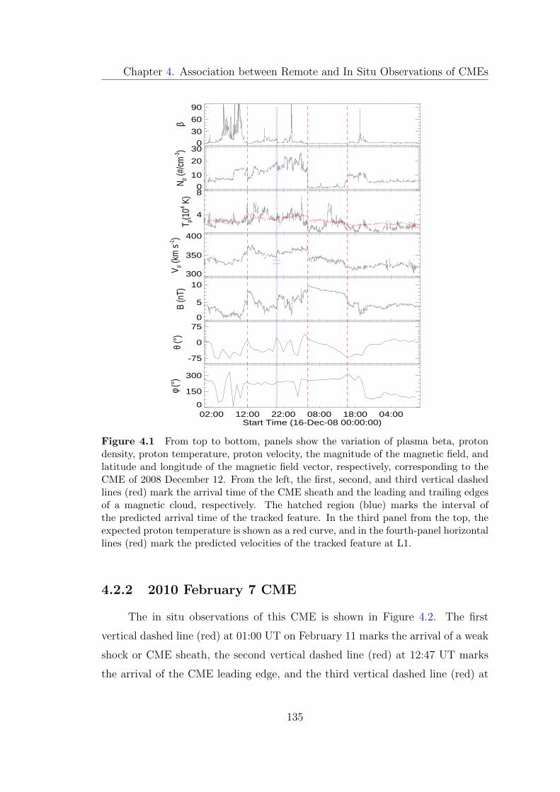
Chapter 4. Association between Remote and In Situ Observations of CMEs
0
30
60
90
β
0
10
20
30
N p (#/
cm-3)
4
8T p(1
04 K)
300
350
400
V p (km
s-1)
0
5
10
B (n
T)
-75
0
75
θ (°)
02:00 12:00 22:00 08:00 18:00 04:00Start Time (16-Dec-08 00:00:00)
0
150
300
φ (°)
Figure 4.1 From top to bottom, panels show the variation of plasma beta, protondensity, proton temperature, proton velocity, the magnitude of the magnetic field, andlatitude and longitude of the magnetic field vector, respectively, corresponding to theCME of 2008 December 12. From the left, the first, second, and third vertical dashedlines (red) mark the arrival time of the CME sheath and the leading and trailing edgesof a magnetic cloud, respectively. The hatched region (blue) marks the interval ofthe predicted arrival time of the tracked feature. In the third panel from the top, theexpected proton temperature is shown as a red curve, and in the fourth-panel horizontallines (red) mark the predicted velocities of the tracked feature at L1.
4.2.2 2010 February 7 CME
The in situ observations of this CME is shown in Figure 4.2. The first
vertical dashed line (red) at 01:00 UT on February 11 marks the arrival of a weak
shock or CME sheath, the second vertical dashed line (red) at 12:47 UT marks
the arrival of the CME leading edge, and the third vertical dashed line (red) at
135
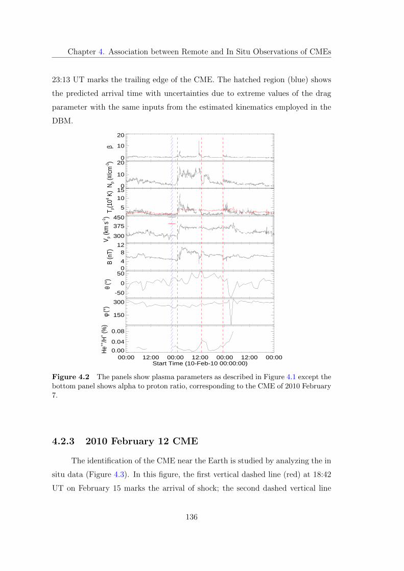
Chapter 4. Association between Remote and In Situ Observations of CMEs
23:13 UT marks the trailing edge of the CME. The hatched region (blue) shows
the predicted arrival time with uncertainties due to extreme values of the drag
parameter with the same inputs from the estimated kinematics employed in the
DBM.
0
10
20
β
0
10
20
Np (
#/cm
-3)
5
10
15
T p(104 K
)
300
375
450
V p (km
s-1)
04
812
B (n
T)
-50
0
50
θ (°)
150
300
φ (°)
00:00 12:00 00:00 12:00 00:00 12:00 00:00Start Time (10-Feb-10 00:00:00)
0.00
0.04
0.08
He++
/H+ (%
)
Figure 4.2 The panels show plasma parameters as described in Figure 4.1 except thebottom panel shows alpha to proton ratio, corresponding to the CME of 2010 February7.
4.2.3 2010 February 12 CME
The identification of the CME near the Earth is studied by analyzing the in
situ data (Figure 4.3). In this figure, the first vertical dashed line (red) at 18:42
UT on February 15 marks the arrival of shock; the second dashed vertical line
136
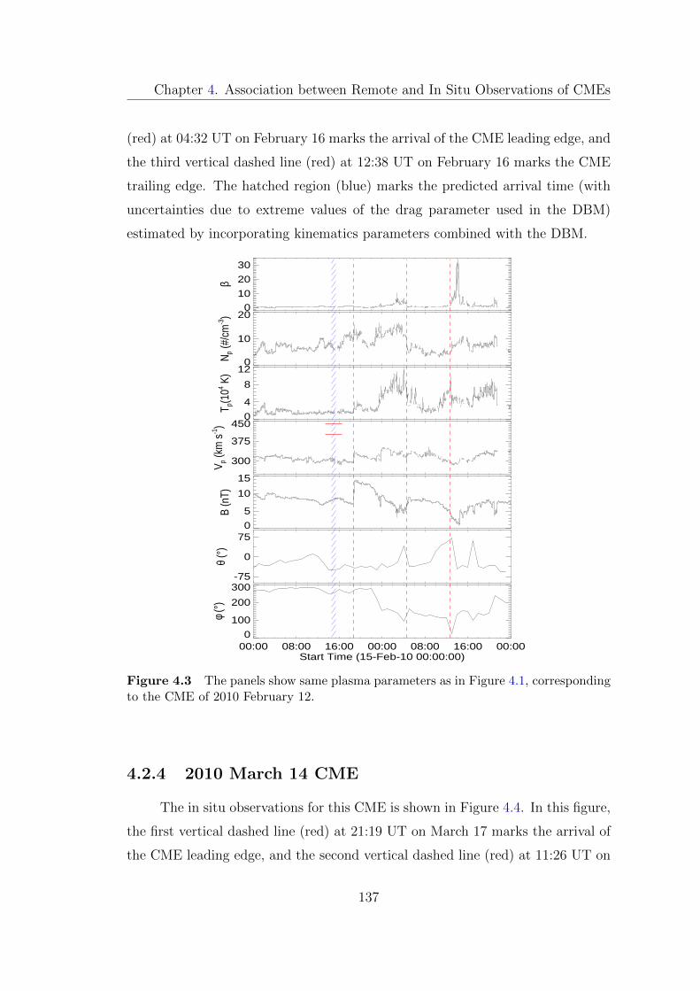
Chapter 4. Association between Remote and In Situ Observations of CMEs
(red) at 04:32 UT on February 16 marks the arrival of the CME leading edge, and
the third vertical dashed line (red) at 12:38 UT on February 16 marks the CME
trailing edge. The hatched region (blue) marks the predicted arrival time (with
uncertainties due to extreme values of the drag parameter used in the DBM)
estimated by incorporating kinematics parameters combined with the DBM.
0
10
20
30
β
0
10
20
Np (
#/cm
-3)
0
4
8
12
T p(104 K
)
300
375
450
V p (km
s-1)
0
5
10
15
B (n
T)
-75
0
75
θ (°)
00:00 08:00 16:00 00:00 08:00 16:00 00:00Start Time (15-Feb-10 00:00:00)
0
100
200
300
φ (°)
Figure 4.3 The panels show same plasma parameters as in Figure 4.1, correspondingto the CME of 2010 February 12.
4.2.4 2010 March 14 CME
The in situ observations for this CME is shown in Figure 4.4. In this figure,
the first vertical dashed line (red) at 21:19 UT on March 17 marks the arrival of
the CME leading edge, and the second vertical dashed line (red) at 11:26 UT on
137
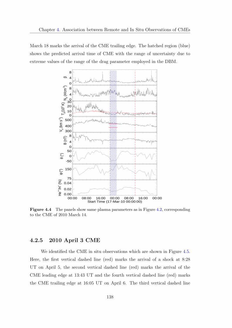
Chapter 4. Association between Remote and In Situ Observations of CMEs
March 18 marks the arrival of the CME trailing edge. The hatched region (blue)
shows the predicted arrival time of CME with the range of uncertainty due to
extreme values of the range of the drag parameter employed in the DBM.
0
4
8
β
0
4
8
Np (
#/cm
-3)
0
10
2030
T p(104 K
)
300
400
500
V p (km
s-1)
0
4
8
B (n
T)
-50
0
50
θ (°)
75
150
φ (°)
00:00 08:00 16:00 00:00 08:00 16:00 00:00Start Time (17-Mar-10 00:00:00)
0.00
0.02
0.04
He++
/H+ (%
)
Figure 4.4 The panels show same plasma parameters as in Figure 4.2, correspondingto the CME of 2010 March 14.
4.2.5 2010 April 3 CME
We identified the CME in situ observations which are shown in Figure 4.5.
Here, the first vertical dashed line (red) marks the arrival of a shock at 8:28
UT on April 5, the second vertical dashed line (red) marks the arrival of the
CME leading edge at 13:43 UT and the fourth vertical dashed line (red) marks
the CME trailing edge at 16:05 UT on April 6. The third vertical dashed line
138
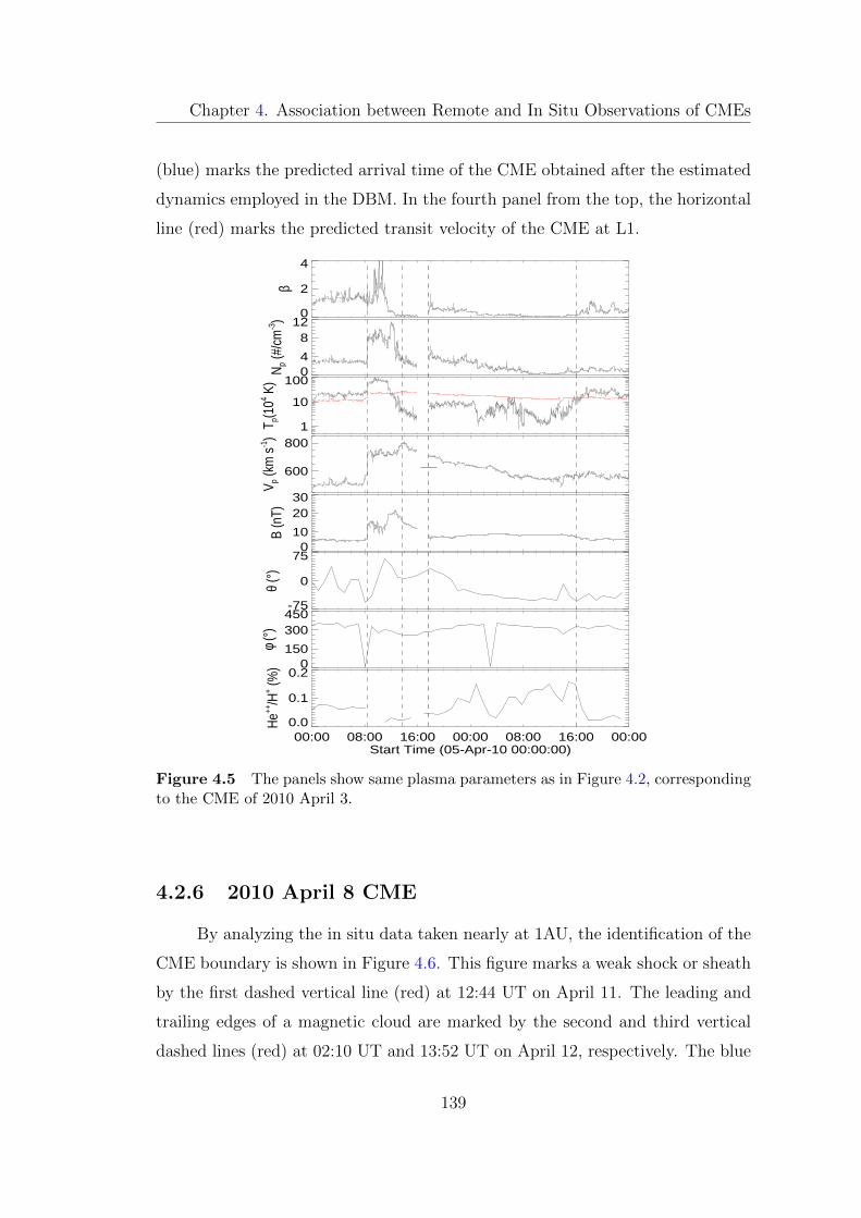
Chapter 4. Association between Remote and In Situ Observations of CMEs
(blue) marks the predicted arrival time of the CME obtained after the estimated
dynamics employed in the DBM. In the fourth panel from the top, the horizontal
line (red) marks the predicted transit velocity of the CME at L1.
0
2
4
β
04
812
Np (
#/cm
-3)
1
10
100
T p(104 K
)
600
800
V p (km
s-1)
0
10
2030
B (n
T)
-75
0
75
θ (°)
0
150
300450
φ (°)
00:00 08:00 16:00 00:00 08:00 16:00 00:00Start Time (05-Apr-10 00:00:00)
0.0
0.1
0.2
He++
/H+ (%
)
Figure 4.5 The panels show same plasma parameters as in Figure 4.2, correspondingto the CME of 2010 April 3.
4.2.6 2010 April 8 CME
By analyzing the in situ data taken nearly at 1AU, the identification of the
CME boundary is shown in Figure 4.6. This figure marks a weak shock or sheath
by the first dashed vertical line (red) at 12:44 UT on April 11. The leading and
trailing edges of a magnetic cloud are marked by the second and third vertical
dashed lines (red) at 02:10 UT and 13:52 UT on April 12, respectively. The blue
139
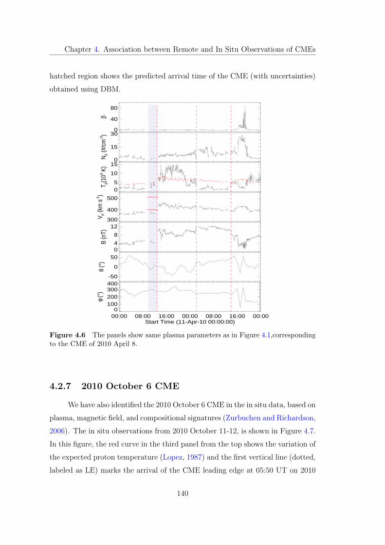
Chapter 4. Association between Remote and In Situ Observations of CMEs
hatched region shows the predicted arrival time of the CME (with uncertainties)
obtained using DBM.
0
40
80β
0
15
30
Np (
#/cm
-3)
05
10
15
T p(104 K
)
300
400
500
V p (km
s-1)
04
8
12
B (n
T)
-50
0
50
θ (°)
00:00 08:00 16:00 00:00 08:00 16:00 00:00Start Time (11-Apr-10 00:00:00)
0100200300400
φ (°)
Figure 4.6 The panels show same plasma parameters as in Figure 4.1,correspondingto the CME of 2010 April 8.
4.2.7 2010 October 6 CME
We have also identified the 2010 October 6 CME in the in situ data, based on
plasma, magnetic field, and compositional signatures (Zurbuchen and Richardson,
2006). The in situ observations from 2010 October 11-12, is shown in Figure 4.7.
In this figure, the red curve in the third panel from the top shows the variation of
the expected proton temperature (Lopez, 1987) and the first vertical line (dotted,
labeled as LE) marks the arrival of the CME leading edge at 05:50 UT on 2010
140
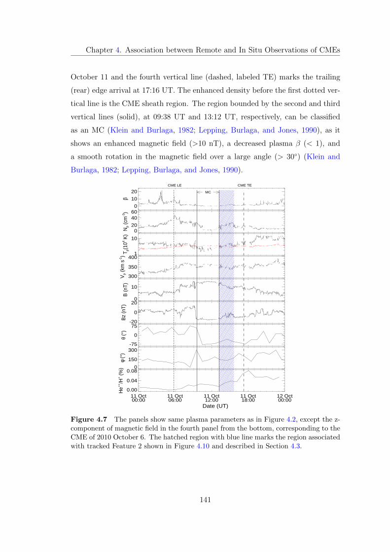
Chapter 4. Association between Remote and In Situ Observations of CMEs
October 11 and the fourth vertical line (dashed, labeled TE) marks the trailing
(rear) edge arrival at 17:16 UT. The enhanced density before the first dotted ver-
tical line is the CME sheath region. The region bounded by the second and third
vertical lines (solid), at 09:38 UT and 13:12 UT, respectively, can be classified
as an MC (Klein and Burlaga, 1982; Lepping, Burlaga, and Jones, 1990), as it
shows an enhanced magnetic field (>10 nT), a decreased plasma β (< 1), and
a smooth rotation in the magnetic field over a large angle (> 30◦) (Klein and
Burlaga, 1982; Lepping, Burlaga, and Jones, 1990).
0
10
20
β
MC
CME LE CME TE
0
20
4060
Np (
cm-3)
1
10
T p(1
04 K)
300
350
400
Vp (
km s
-1)
0
10
B (n
T)
-20
0
20
Bz
(nT)
-75
0
75
θ (°
)
0
150
300
φ (°
)
11 Oct00:00
11 Oct06:00
11 Oct12:00
11 Oct18:00
12 Oct00:00
0.00
0.04
0.08
He++
/H+ (%
)
Date (UT)
Figure 4.7 The panels show same plasma parameters as in Figure 4.2, except the z-component of magnetic field in the fourth panel from the bottom, corresponding to theCME of 2010 October 6. The hatched region with blue line marks the region associatedwith tracked Feature 2 shown in Figure 4.10 and described in Section 4.3.
141
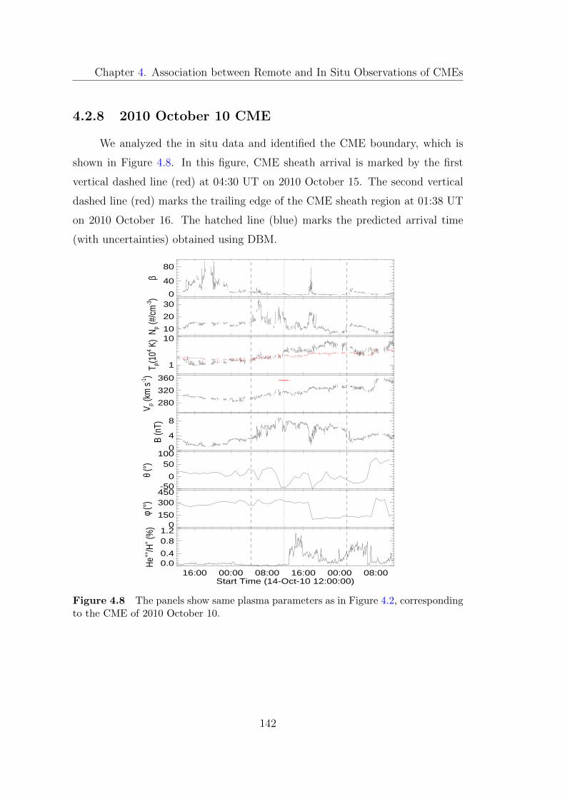
Chapter 4. Association between Remote and In Situ Observations of CMEs
4.2.8 2010 October 10 CME
We analyzed the in situ data and identified the CME boundary, which is
shown in Figure 4.8. In this figure, CME sheath arrival is marked by the first
vertical dashed line (red) at 04:30 UT on 2010 October 15. The second vertical
dashed line (red) marks the trailing edge of the CME sheath region at 01:38 UT
on 2010 October 16. The hatched line (blue) marks the predicted arrival time
(with uncertainties) obtained using DBM.
0
40
80
β
10
20
30
N p (#/
cm-3)
1
10
T p(104 K
)
280
320
360
V p (km
s-1)
0
4
8
B (n
T)
-50
0
50100
θ (°)
0
150
300450
φ (°)
16:00 00:00 08:00 16:00 00:00 08:00Start Time (14-Oct-10 12:00:00)
0.00.4
0.81.2
He++
/H+ (%
)
Figure 4.8 The panels show same plasma parameters as in Figure 4.2, correspondingto the CME of 2010 October 10.
142
Chapter 4. Association between Remote and In Situ Observations of CMEs
4.2.9 2010 October 26 CME
In situ observations of solar wind taken nearly at 1 AU and the identifica-
tion of 2010 October 26 CME is shown in Figure 4.9. This figure shows a sudden
enhancement of density, temperature, and velocity at 10:32 UT on October 30.
These changes mark the arrival of a shock, as indicated by the first dashed vertical
line (red) from the left. The hatched region (blue) marks the CME’s predicted
arrival time (with uncertainty) using DBM. From the left, the second and fourth
vertical dashed lines (red) mark the leading and trailing edges of the CME. This
CME also shows MC (Klein and Burlaga, 1982; Lepping, Burlaga, and Jones,
1990) structure which is identified as the region between the third and fourth
vertical dashed lines (red) at 01:30 and 21:35 UT on November 1, respectively.
This region has a low proton beta (Burlaga et al., 1981; Cane and Richardson,
2003), a decrease in proton density (Richardson et al., 2000), a decrease in proton
temperature (Gosling, Pizzo, and Bame, 1973), a monotonic decrease in proton
velocity (Klein and Burlaga, 1982), and an enhanced alpha to proton ratio (Bor-
rini et al., 1982).
4.3 Tracking of Different Features of 2010 October 6 CME
Using Remote and In Situ Observations
The heliospheric tracking of CME features using J -maps mainly deals with
tracking the CME bright front and associating it with CME sheath observed
before the leading edge in in situ data (Davis et al., 2009; Liu et al., 2010a, 2011;
Mostl et al., 2011; Mishra and Srivastava, 2013). In a rare attempt, Howard
and DeForest (2012a) tracked a feature like a ‘cavity’ (in coronagraph images)
of a classical CME using HI images. This cavity-like feature was associated with
an MC identified in in situ data near the Earth. DeForest, Howard, and Tappin
(2011) have also attempted to identify different CME structures in STEREO/HI2
observations and compared them with in situ features detected near 1 AU.
As a CME shows large-scale inhomogeneous structures in terms of density
143
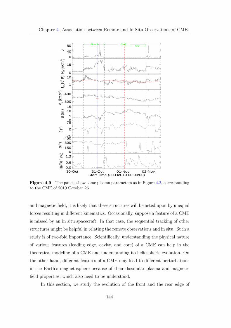
Chapter 4. Association between Remote and In Situ Observations of CMEs
0
40
80
β
Sheath CMEMC
0
15N p (
#/cm
-3)
1
10
T p(104 K
)
300
400
V p (km
s-1)
05
1015
B (n
T)
-75
0
75
θ (°)
0
150
300450
φ (°)
30-Oct 31-Oct 01-Nov 02-NovStart Time (30-Oct-10 00:00:00)
0.0
0.6
1.2
He++
/H+ (%
)
Figure 4.9 The panels show same plasma parameters as in Figure 4.2, correspondingto the CME of 2010 October 26.
and magnetic field, it is likely that these structures will be acted upon by unequal
forces resulting in different kinematics. Occasionally, suppose a feature of a CME
is missed by an in situ spacecraft. In that case, the sequential tracking of other
structures might be helpful in relating the remote observations and in situ. Such a
study is of two-fold importance. Scientifically, understanding the physical nature
of various features (leading edge, cavity, and core) of a CME can help in the
theoretical modeling of a CME and understanding its heliospheric evolution. On
the other hand, different features of a CME may lead to different perturbations
in the Earth’s magnetosphere because of their dissimilar plasma and magnetic
field properties, which also need to be understood.
In this section, we study the evolution of the front and the rear edge of
144
Chapter 4. Association between Remote and In Situ Observations of CMEs
a filament associated geoeffective CME of 2010 October 6. The filament was
located in north-east (NE) quadrant of the solar disc as seen from the Earth’s
perspective. For this study, we used the white light observations of CME from
twin STEREO and in situ plasma and magnetic field parameters of the solar
wind from the ACE and WIND spacecraft.
4.3.1 Remote sensing observations of 2010 October 6
CME
The evolution of 2010 October 6 CME in COR and HI FOV are shown in
Figure 3.12 of Chapter 3. The front/leading edge (hereafter termed as F1) and
core/associated filament material (hereafter termed as F2) of the CME could be
easily identified in COR1 and COR2 images. As the CME reached near the edge
of COR2 FOV, STEREO-A had a data gap, and when the CME appeared in HI1-
A FOV, it was diffused, and the leading edge and core could not be distinguished
as in COR FOV. In the J -maps for this CME (Figure 4.10), two bright tracks
having positive inclination are noticed where they are termed as Feature 1 and
Feature 2 as we are not certain that these features are the same as F1 and F2
noticed in COR FOV.
It must be noted that kinematics of tracked Feature 1, using ten reconstruc-
tion methods (Point-P (PP), Fixed-Phi (FP), Fixed-Phi Fitting (FPF), Harmonic
Mean (HM), Harmonic Mean Fitting (HMF), Self-Similar Expansion (SSE), Self-
Similar Expansion Fitting (SSEF), Geometric Triangulation (GT), Tangent to
A Sphere (TAS), Stereoscopic Self-Similar Expansion (SSSE)), has been esti-
mated and described in Section 3.5.1 of Chapter 3. To consider the maximum
uncertainties in our analysis, various reconstruction methods for the estimation
of kinematics are used. The obtained kinematics are used as inputs in the DBM
(Vrsnak et al., 2013) to estimate the arrival time (for details see, Figure 3.14,
3.15, 3.16 and Table 3.4 in Chapter 3). For identification of the second tracked
feature in in situ observations, we followed the same analysis of Feature 2 as
described for Feature 1.
145
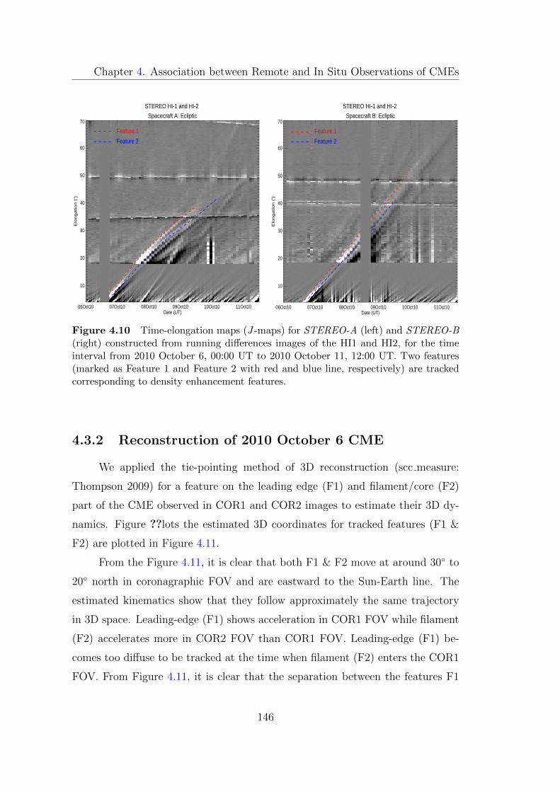
Chapter 4. Association between Remote and In Situ Observations of CMEs
Spacecraft A: Ecliptic
06Oct10 07Oct10 08Oct10 09Oct10 10Oct10 11Oct10Date (UT)
10
20
30
40
50
60
70
Elo
ng
atio
n (
o)
STEREO HI-1 and HI-2
Feature 1
Feature 2
Spacecraft B: Ecliptic
06Oct10 07Oct10 08Oct10 09Oct10 10Oct10 11Oct10Date (UT)
10
20
30
40
50
60
70
Elo
ngation (
o)
STEREO HI-1 and HI-2
Feature 1
Feature 2
Figure 4.10 Time-elongation maps (J -maps) for STEREO-A (left) and STEREO-B(right) constructed from running differences images of the HI1 and HI2, for the timeinterval from 2010 October 6, 00:00 UT to 2010 October 11, 12:00 UT. Two features(marked as Feature 1 and Feature 2 with red and blue line, respectively) are trackedcorresponding to density enhancement features.
4.3.2 Reconstruction of 2010 October 6 CME
We applied the tie-pointing method of 3D reconstruction (scc measure:
Thompson 2009) for a feature on the leading edge (F1) and filament/core (F2)
part of the CME observed in COR1 and COR2 images to estimate their 3D dy-
namics. Figure ??lots the estimated 3D coordinates for tracked features (F1 &
F2) are plotted in Figure 4.11.
From the Figure 4.11, it is clear that both F1 & F2 move at around 30◦ to
20◦ north in coronagraphic FOV and are eastward to the Sun-Earth line. The
estimated kinematics show that they follow approximately the same trajectory
in 3D space. Leading-edge (F1) shows acceleration in COR1 FOV while filament
(F2) accelerates more in COR2 FOV than COR1 FOV. Leading-edge (F1) be-
comes too diffuse to be tracked at the time when filament (F2) enters the COR1
FOV. From Figure 4.11, it is clear that the separation between the features F1
146
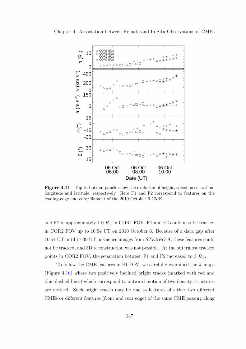
Chapter 4. Association between Remote and In Situ Observations of CMEs
0
10
h (R
O •) COR1 (F1)
COR1 (F2)COR2 (F1)COR2 (F2)
0
200
400v
(km
s-1)
0
150
a (m
s-2)
-30-15
015
φ (°
)
06 Oct06:00
06 Oct08:00
06 Oct10:00
15
30
θ (°
)
Date (UT)
Figure 4.11 Top to bottom panels show the evolution of height, speed, acceleration,longitude and latitude, respectively. Here F1 and F2 correspond to features on theleading edge and core/filament of the 2010 October 6 CME.
and F2 is approximately 1.0 R� in COR1 FOV. F1 and F2 could also be tracked
in COR2 FOV up to 10:54 UT on 2010 October 6. Because of a data gap after
10:54 UT until 17:39 UT in science images from STEREO-A, these features could
not be tracked, and 3D reconstruction was not possible. At the outermost tracked
points in COR2 FOV, the separation between F1 and F2 increased to 3 R�.
To follow the CME features in HI FOV, we carefully examined the J -maps
(Figure 4.10) where two positively inclined bright tracks (marked with red and
blue dashed lines) which correspond to outward motion of two density structures
are noticed. Such bright tracks may be due to features of either two different
CMEs or different features (front and rear edge) of the same CME passing along
147
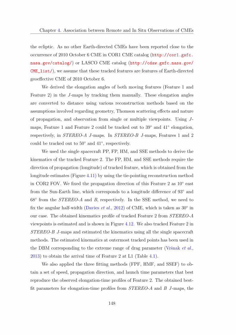
Chapter 4. Association between Remote and In Situ Observations of CMEs
the ecliptic. As no other Earth-directed CMEs have been reported close to the
occurrence of 2010 October 6 CME in COR1 CME catalog (http://cor1.gsfc.
nasa.gov/catalog/) or LASCO CME catalog (http://cdaw.gsfc.nasa.gov/
CME_list/), we assume that these tracked features are features of Earth-directed
geoeffective CME of 2010 October 6.
We derived the elongation angles of both moving features (Feature 1 and
Feature 2) in the J -maps by tracking them manually. These elongation angles
are converted to distance using various reconstruction methods based on the
assumptions involved regarding geometry, Thomson scattering effects and nature
of propagation, and observation from single or multiple viewpoints. Using J -
maps, Feature 1 and Feature 2 could be tracked out to 39◦ and 41◦ elongation,
respectively, in STEREO-A J -maps. In STEREO-B J -maps, Features 1 and 2
could be tracked out to 50◦ and 41◦, respectively.
We used the single spacecraft PP, FP, HM, and SSE methods to derive the
kinematics of the tracked Feature 2. The FP, HM, and SSE methods require the
direction of propagation (longitude) of tracked feature, which is obtained from the
longitude estimates (Figure 4.11) by using the tie-pointing reconstruction method
in COR2 FOV. We fixed the propagation direction of this Feature 2 as 10◦ east
from the Sun-Earth line, which corresponds to a longitude difference of 93◦ and
68◦ from the STEREO-A and B, respectively. In the SSE method, we need to
fix the angular half-width (Davies et al., 2012) of CME, which is taken as 30◦ in
our case. The obtained kinematics profile of tracked Feature 2 from STEREO-A
viewpoints is estimated and is shown in Figure 4.12. We also tracked Feature 2 in
STEREO-B J -maps and estimated the kinematics using all the single spacecraft
methods. The estimated kinematics at outermost tracked points has been used in
the DBM corresponding to the extreme range of drag parameter (Vrsnak et al.,
2013) to obtain the arrival time of Feature 2 at L1 (Table 4.1).
We also applied the three fitting methods (FPF, HMF, and SSEF) to ob-
tain a set of speed, propagation direction, and launch time parameters that best
reproduce the observed elongation-time profiles of Feature 2. The obtained best-
fit parameters for elongation-time profiles from STEREO-A and B J -maps, the
148
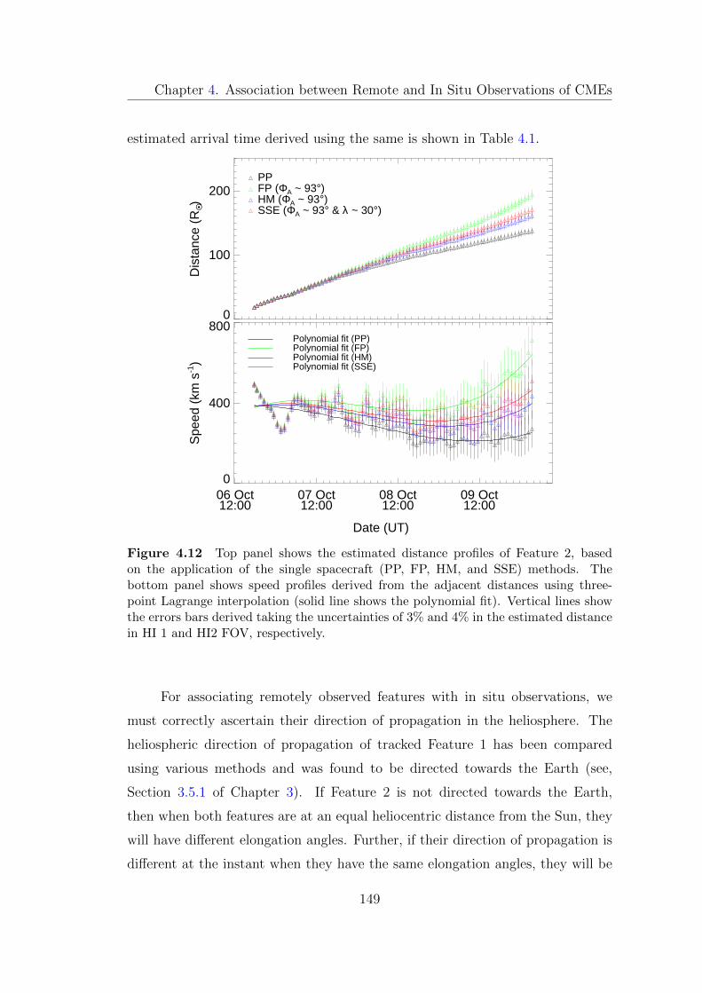
Chapter 4. Association between Remote and In Situ Observations of CMEs
estimated arrival time derived using the same is shown in Table 4.1.
0
100
200D
ista
nce
(RO •)
PPFP (ΦA ~ 93°)HM (ΦA ~ 93°)SSE (ΦA ~ 93° & λ ~ 30°)
06 Oct12:00
07 Oct12:00
08 Oct12:00
09 Oct12:00
0
400
800
Spe
ed (
km s
-1)
Polynomial fit (PP)Polynomial fit (FP)Polynomial fit (HM)Polynomial fit (SSE)
Date (UT)
Figure 4.12 Top panel shows the estimated distance profiles of Feature 2, basedon the application of the single spacecraft (PP, FP, HM, and SSE) methods. Thebottom panel shows speed profiles derived from the adjacent distances using three-point Lagrange interpolation (solid line shows the polynomial fit). Vertical lines showthe errors bars derived taking the uncertainties of 3% and 4% in the estimated distancein HI 1 and HI2 FOV, respectively.
For associating remotely observed features with in situ observations, we
must correctly ascertain their direction of propagation in the heliosphere. The
heliospheric direction of propagation of tracked Feature 1 has been compared
using various methods and was found to be directed towards the Earth (see,
Section 3.5.1 of Chapter 3). If Feature 2 is not directed towards the Earth,
then when both features are at an equal heliocentric distance from the Sun, they
will have different elongation angles. Further, if their direction of propagation is
different at the instant when they have the same elongation angles, they will be
149
Chapter 4. Association between Remote and In Situ Observations of CMEsM
eth
od
Kin
emati
csas
inp
uts
inD
BM
[t0,
R0
(R�
),v0
(km
s−1)]
Pre
dic
ted
arr
ival
tim
eu
sin
gkin
emati
cs+
DB
M(U
T)
[γ=
0.2
to2.0
(10−7
km
−1)]
Pre
dic
ted
tran
sit
spee
dat
L1
(km
s−1)
[γ=
0.2
to2.0
(10−7
km
−1)]
Err
or
inp
red
icte
darr
ival
tim
e(h
rs)
[γ=
0.2
to2.0
(10−7
km
−1)]
Err
or
inp
red
icte
dtr
an
sit
spee
d(k
ms−
1)
[γ=
0.2
to2.0
(10−7
km
−1)]
PP
(STEREO-A
)10
Oct
03:3
0,
137,
230
12
Oct
.12:5
1to
12
Oct
.03:2
2270
to327
23.7
to14.2
-85
to-2
8
PP
(STEREO-B
)09
Oct
12:4
0,
137,
360
11
Oct
05:1
4to
11
Oct
05:2
1360
to358
-8to
-7.8
5to
3
FP
(STEREO-A
)09
Oct
10:3
0,
149,
380
10
Oct
18:5
4to
10
Oct
19:2
7378
to368
-18.2
to-1
7.6
23
to13
FP
(STEREO-B
)08
Oct
23:3
9,
130,
464
10
Oct
11:0
5to
10
Oct
15:2
8438
to377
-26.3
to-2
1.7
83
to22
HM
(STEREO-A
)09
Oct
11:3
0,
132,
285
11
Oct
.16:4
8to
11
Oct
.12:4
3298
to330
3.6
to-0
.4-5
7to
-25
HM
(STEREO-B
)09
Oct
12:4
0,
158,
430
10
Oct
13:2
9to
10
Oct
15:0
7420
to382
-23.7
to-2
2.1
65
to27
GT
09
Oct
12:4
0,
159,
450
10
Oct
12:0
3to
10
Oct
14:0
6436
to385
-25.2
to-2
3.2
81
to30
TA
S09
Oct
12:4
0,
131,
280
11
Oct
19:2
1to
11
Oct
14:4
1295
to330
6.1
to1.4
-60
to-2
5
SS
SE
09
Oct
12:4
0,
154,
385
10
Oct
18:0
9to
10
Oct
18:4
5383
to370
-19.1
to-1
8.5
28
to15
Tim
e-el
on
gati
on
track
fitt
ing
met
hod
sM
eth
ods
Bes
tfi
tp
ara
met
ers
[t(α
=0),
Φ(◦
),v
(km
s−1)]
Pre
dic
ted
arr
ival
tim
eat
L1
(UT
)E
rror
inp
red
icte
darr
ival
tim
eE
rror
inp
red
icte
dsp
eed
at
L1
(km
s−1)
Lon
git
ud
e(◦
)
FP
F(S
TEREO-A
)06
Oct
07:4
4,
90,
378
10
Oct
20:2
9-1
6.9
23
-7F
PF
(STEREO-B
)06
Oct
04:1
4,
56.2
,369
10
Oct
19:2
5-1
7.7
14
-21.5
HM
F(S
TEREO-A
)06
Oct
08:5
4,
125,
467
11
Oct
07:4
8-5
.4-1
8-4
2H
MF
(STEREO-B
)06
Oct
05:5
1,
58,
378
11
Oct
01:3
5-1
1.6
-10
-19.8
SS
EF
(STEREO-A
)06
Oct
08:4
0,
114,
436
11
Oct
09:0
2-4
.2-1
3-3
1S
SE
F(S
TEREO-B
)06
Oct
05:3
7,
57.4
,377
11
Oct
05:4
3-7
.5-1
2-2
0.4
Table
4.1
Th
ees
tim
ate
dkin
emat
ics
(use
das
inp
ut
inth
eD
BM
)an
dp
red
icte
dar
riva
lti
me
an
dsp
eed
(an
der
rors
ther
ein
)of
Fea
ture
2at
L1
corr
esp
ond
ing
toth
eex
trem
era
nge
ofd
rag
par
amet
eru
sed
inth
eD
BM
issh
own.
Th
eb
ott
omp
anel
give
sb
est
fit
par
amet
ers,
pre
dic
ted
arri
val
tim
e,an
dsp
eed
(an
der
rors
ther
ein
)es
tim
ated
from
tim
e-el
onga
tion
trac
kfi
ttin
gm
ethod
s.T
he
STEREO-A
an
dB
show
nin
pare
nth
eses
for
each
met
hod
den
ote
the
spac
ecra
ftfr
omw
hic
hth
eim
ages
are
obta
ined
tod
eriv
eel
on
gati
on
.N
egati
ve(p
osit
ive)
erro
rsin
pre
dic
ted
arri
val
tim
eco
rres
pon
dto
ap
red
icte
dar
riva
lti
me
bef
ore
(aft
er)
the
actu
alC
ME
arr
ival
tim
ed
eter
min
edfr
om
insi
tum
easu
rem
ents
.N
egat
ive
(pos
itiv
e)er
rors
inp
red
icte
dsp
eed
corr
esp
on
dto
ap
red
icte
dsp
eed
that
isle
ss(m
ore
)th
anth
eact
ual
spee
dof
CM
Eat
L1.
150
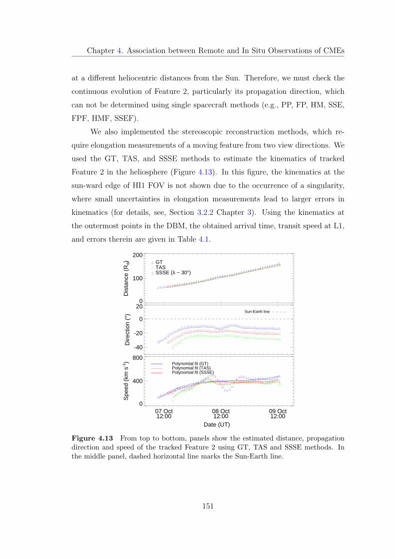
Chapter 4. Association between Remote and In Situ Observations of CMEs
at a different heliocentric distances from the Sun. Therefore, we must check the
continuous evolution of Feature 2, particularly its propagation direction, which
can not be determined using single spacecraft methods (e.g., PP, FP, HM, SSE,
FPF, HMF, SSEF).
We also implemented the stereoscopic reconstruction methods, which re-
quire elongation measurements of a moving feature from two view directions. We
used the GT, TAS, and SSSE methods to estimate the kinematics of tracked
Feature 2 in the heliosphere (Figure 4.13). In this figure, the kinematics at the
sun-ward edge of HI1 FOV is not shown due to the occurrence of a singularity,
where small uncertainties in elongation measurements lead to larger errors in
kinematics (for details, see, Section 3.2.2 Chapter 3). Using the kinematics at
the outermost points in the DBM, the obtained arrival time, transit speed at L1,
and errors therein are given in Table 4.1.
0
100
200
Dis
tanc
e (R
O •) GT
TASSSSE (λ ~ 30°)
-40
-20
0
20
Dire
ctio
n (°
) Sun-Earth line
07 Oct12:00
08 Oct12:00
09 Oct12:00
0
400
800
Spe
ed (
km s
-1) Polynomial fit (GT)
Polynomial fit (TAS)Polynomial fit (SSSE)
Date (UT)
Figure 4.13 From top to bottom, panels show the estimated distance, propagationdirection and speed of the tracked Feature 2 using GT, TAS and SSSE methods. Inthe middle panel, dashed horizontal line marks the Sun-Earth line.
151
Chapter 4. Association between Remote and In Situ Observations of CMEs
From Figure 4.12 (top panel), we see that the PP method gives the lowest
estimate of the distance while the FP method gives the highest estimate. HM,
and SSE methods give an intermediate distance estimate between PP and FP
methods. The observed unphysical late acceleration for Feature 2 (Figure 4.12,
lower panel) is attributed to possible deflection of the tracked feature far from
the Sun. Although real deflection of features far from the Sun is rarely observed,
however, it refers to the infeasibility of tracking the same feature sequentially at
larger elongation due to the overall expansion of the CME. In our analysis, we have
taken care that if the estimated kinematics becomes unreliable at any instant, the
value of speeds prior to those points are considered inputs in the DBM. Also, speed
obtained by implementing fitting methods (FPF, HMF, and SSEF) is corrected
for off-axis correction before using it for estimation of the arrival time at L1
(Mostl et al., 2011; Mostl and Davies, 2013). From Table 4.1, we also notice that
different fitting methods give different estimates of the propagation direction of
Feature 2. In light of our earlier study in Mishra, Srivastava, and Davies (2014),
we rely on the estimates of direction from stereoscopic methods such as GT, TAS,
and SSSE.
From Figure 4.13 for Feature 2 and Figure 3.16 for Feature 1 in Chapter 3,
we can see that both tracked Features are moving approximately in the same
direction in the heliosphere. Therefore, both these Earth-directed features are
likely to be detected by in situ spacecraft located at L1. Since we have no infor-
mation on the plasma and magnetic field properties associated with these tracked
features from remote sensing observations, we can only rely on their estimated
arrival time at L1 to relate features in situ data with remotely tracked Feature 1
and Feature 2.
4.3.3 Comparison of kinematics of tracked features
We tracked the front (leading) and the rear (trailing) edge of the intensity
front in the STEREO/HI J -maps and derived the kinematics of these two CME
features. Figure ??hows the separation between Feature 1 and Feature 2 based on
152
Chapter 4. Association between Remote and In Situ Observations of CMEs
their height derived from different reconstruction methods is shown in Figure 4.14.
We found that the separation of the two features increased with time (Figure 4.11
& 4.14) during their evolution from the COR to HI FOV. The estimated large
separation may be due to unequal driving forces on different features, an overall
CME expansion, or a combination of both. From Figure 4.14, it is evident that
the separation increased from 4.4 R� to 11.3 R� (as found by using the PP
method) between the first and last common tracked points, respectively. The
FP method showed a continuously increasing separation, ranging from 4.6 R� to
21.7 R�. Using the HM method, the separation was found to increase from 4.5
R� to 15.4 R�. For the GT, TAS, and SSSE techniques, the separation between
tracked features (Feature 1 and Feature 2) increased up to 16.0, 12.5, and 13.5 R�,
respectively. It is noted that the separation between the two features (estimated
from GT, TAS, and SSSE) became approximately constant at large distances of
≈ 120 R�.
Due to the occurrence of singularity at the sunward edge of HI1 FOV in GT,
TAS, and SSSE methods, the separation between both tracked features (Feature
1 and Feature 2) is estimated to be slightly lesser than the observed separation
in COR FOV. However, these initial erroneous estimates of separation can be
discarded by considering the results obtained from GT, TAS, and SSSE methods
at higher elongation and estimates from other methods. Based on the results of all
the reconstruction methods applied on SECCHI/HI observations, the estimated
separation between Feature 1 and 2 ranges between 11.2 R� to 21.7 R�.
Several authors have shown that, at a large distance from the Sun, the
kinematic evolution of CMEs is mostly attributed to the drag force between the
CMEs and the ambient solar wind (Cargill, 2004; Manoharan, 2006; Vrsnak et al.,
2010). In the present case, both features are tracked at sufficiently larger distances
beyond the HI1 FOV. They attain speed close to ambient solar wind speed, so
driving forces on Feature 1 and Feature 2 will become equal. The expansion speed
of CME at larger distances is more likely due to the high internal thermal pressure
of CME than the ambient solar wind pressure (Schwenn et al., 2005; Gopalswamy
et al., 2009b; Michalek, Gopalswamy, and Yashiro, 2009; Poomvises, Zhang, and
153
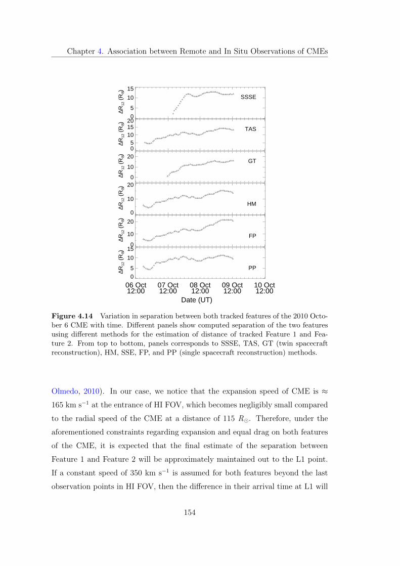
Chapter 4. Association between Remote and In Situ Observations of CMEs
0
5
10
15
∆R12
(R
O •)
SSSE
05
101520
∆R12
(R
O •)
TAS
0
10
20
∆R12
(R
O •)
GT
0
10
20
∆R12
(R
O •)
HM
0
10
20
∆R12
(R
O •)
FP
06 Oct12:00
07 Oct12:00
08 Oct12:00
09 Oct12:00
10 Oct12:00
0
5
10
15
∆R12
(R
O •)
PP
Date (UT)
Figure 4.14 Variation in separation between both tracked features of the 2010 Octo-ber 6 CME with time. Different panels show computed separation of the two featuresusing different methods for the estimation of distance of tracked Feature 1 and Fea-ture 2. From top to bottom, panels corresponds to SSSE, TAS, GT (twin spacecraftreconstruction), HM, SSE, FP, and PP (single spacecraft reconstruction) methods.
Olmedo, 2010). In our case, we notice that the expansion speed of CME is ≈165 km s−1 at the entrance of HI FOV, which becomes negligibly small compared
to the radial speed of the CME at a distance of 115 R�. Therefore, under the
aforementioned constraints regarding expansion and equal drag on both features
of the CME, it is expected that the final estimate of the separation between
Feature 1 and Feature 2 will be approximately maintained out to the L1 point.
If a constant speed of 350 km s−1 is assumed for both features beyond the last
observation points in HI FOV, then the difference in their arrival time at L1 will
154
Chapter 4. Association between Remote and In Situ Observations of CMEs
range from 6.1 to 11.9 hr.
4.3.4 Identification of filament plasma using near-Earth
in situ observations
The identification of the 2010 October 6 CME using in situ observations
is shown in Figure 4.7. The tracked Feature 1 is the leading edge of the first
bright positively inclined track in the J -maps (Figure 4.10). Hence, the arrival
of enhanced density associated with this Feature 1 can be associated with the
in situ measured density enhancement (LE) at 05:50 UT on 2010 October 11
(Mishra, Srivastava, and Davies, 2014). In Figure 4.7, we do not notice a mono-
tonic decrease in the speed of CME, i.e., there is no expansion. This is consistent
with the finding that separation between Feature 1 and Feature 2 has become
constant well before reaching the L1. As discussed in the previous Section 4.3.3,
we expect the Feature 2 to arrive at L1 approximately 6 to 12 hr after the arrival
of Feature 1. Therefore, we associate the arrival of Feature 2 with a second peak
in proton density between 13:14 and 15:40 UT on 2010 October 11, associated
with a low proton temperature (≈ 104 K). Since the Feature 2 follows the MC
and is associated with dense (maximum Np = 27 cm−3), cold material (mini-
mum Tp = 2.4 × 10⁴ K) observed in situ, it possibly corresponds to the core of
a classical three-part structure CME. We need to examine the plasma compo-
sition and charge state and the root mean square deviations of bulk velocity in
high-resolution data (Burlaga et al., 1998; Gopalswamy et al., 1998a; Lepri and
Zurbuchen, 2010; Sharma and Srivastava, 2012; Sharma et al., 2013) to confirm
the presence of filament material in the associated CME at L1.
Hourly-resolution ACE/SWICS (Gloeckler et al., 1998) data show that dur-
ing the density enhancement, the C+6/C+5 ratio reduces to 0.5; its average value
is ≈ 1.0 after that. The O+7/O+6 ratio is roughly constant (≈ 0.2) before and
after the density enhancement between 13:14 to 15:40 UT. Moreover, the aver-
age charges state of Carbon (+5), Oxygen (+6), and Iron (+10) remain roughly
constant over this period. The Fe/O ratio is enhanced up to 0.24, which is three
155
Chapter 4. Association between Remote and In Situ Observations of CMEs
times larger than its ambient solar wind value.
The alpha to proton ratio (Figure 4.7, lowest panel) is elevated over the
entire CME interval peaking at 0.07 at 18:30 UT 2010, October 11, which is seven
times the ambient solar wind value. During the time interval of second density
enhancement alpha to proton ratio is approximately three times greater than its
value in the ambient solar wind (before the leading edge of CME). Between 13:14
and 15:40 UT, the thermal speeds of He+2, C+5, O+7, Fe+10 are depressed, with
minimum value of 18, 13, 12, and 13 km s−1, respectively. These signatures are
indicative of filament material from 13:14 to 15:40 UT.
Previously, using very restrictive criteria, attempts have been made to iden-
tify filament plasma near 1 AU (Lepri and Zurbuchen, 2010), and in a few cases
filament signatures have been identified (Burlaga et al., 1998; Gopalswamy et al.,
1998a). In these studies, a selected threshold value for the thermal and composi-
tional characteristics of the plasma was used to identify cold filament. However,
these values will likely vary for CMEs associated with eruptive prominences at
different phases of the solar cycle, and hence for different solar wind conditions.
Sharma and Srivastava (2012) adopted less stringent criteria for the identification
of filaments in in situ data, based on the thermal speed signatures of various ions,
charge states of carbon, oxygen, and iron, and relative abundances of He+2/H+,
Fe/O, C+6/C+5, O+7/O+6 for the events of 2003 November 18 and 2010 August
1. Based on the criteria of Sharma and Srivastava (2012), many of the signatures
observed between 13:00 and 16:00 UT on 11 October 2010 suggest that second
density enhancement in in situ data associated with Feature 2 can be identified as
filament material. Further, Sharma and Srivastava (2012) observed a depression
in the average charge state of carbon (+4 to +5), oxygen (+ 5 to +6), and iron
(+8); however, for the present case, we do not notice such a depression. In addi-
tion, we find a drop in the C+6/C+5 ratio to 0.5 in the filament region, while the
minimum value of the C+6/C+5 ratio reported by Sharma and Srivastava (2012)
was nearly 0.15 in the cold plasma region. Therefore, although the CME of 2010
October 6 was associated with a filament eruption, all the criteria required to
definitively identify filament plasma are not fulfilled. This may be due to in
156
Chapter 4. Association between Remote and In Situ Observations of CMEs
situ observations taken at a single point or may occur due to the heating of the
cold filament material during its journey to L1 (Skoug et al., 1999; Sharma and
Srivastava, 2012).
4.4 Results and Discussion
For nine selected Earth-directed CMEs, the association between remote
and in situ observations was carried out. In this study, we tracked the first
density enhancement of CMEs in the J -maps. The density enhancement in the
shock-sheath region of the CME identified in situ observations is considered as
a reference for the actual arrival time of the remotely observed tracked feature.
Based on our analysis, we found that it is difficult to track a CME-driven shock
in the J -maps constructed from HI observations. We also realize that using
difference images for tracking cavity (observed as MC in in situ) may be extremely
difficult. It is because of the extremely low density associated with a cavity (flux
rope), which on taking the running difference becomes indistinguishable from the
brighter background. However, our analysis shows that the arrival time of the
first density peak of the CME at L1 can be predicted reasonably well using J -
maps constructed from SECCHI/HI observations. Therefore, we conclude that
an association between remote and in situ observations of CMEs can be made if
they are tracked by estimating their 3D kinematics out to larger elongation using
HI observations.
In several studies carried out previously without the construction of J -
maps, different authors have adopted different signatures of CMEs near 1 AU as
references in correlating remote sensing observations with in situ observations.
For instance, in the derivation of the ECA time prediction model, (Gopalswamy
et al., 2000a) adopted the start time of the magnetic cloud and low proton beta
(β < 1) as a reference for the actual arrival time of the CME. In another study,
(Schwenn et al., 2005), an IP shock was taken as a reliable in situ signature for
the arrival of a CME. Zhang et al. (2003) considered the minimum Dst index of
the associated geomagnetic storm as the ICME arrival time. Kilpua et al. (2012)
157
Chapter 4. Association between Remote and In Situ Observations of CMEs
considered the arrival time of the CME leading edge at in situ spacecraft as the
arrival of a CME. In our selected CMEs, the CMEs of 2010 February 7, and
2010 April 8 drive extremely weak shocks, which seem to arrival of the sheath
structure; however, CME of 2010 February 12, 2010 April 3, and 2010 October 6
drive a clear IP shock identified in in situ observations at L1. Furthermore, four
events, i.e., 2008 December 12, 2010 April 8, 2010 October 6, and 2010 October
26, could be categorized as magnetic clouds in in situ measurements. Also, for all
the CMEs, except 2010 October 10, leading and trailing boundaries of the CMEs
could be well-identified using in situ data. Hence, we can infer that specific
signatures (i.e. for shock, leading edge, and MC) in situ observations cannot
always be strictly found and used to pinpoint the actual (reference) arrival time
of a remotely tracked features of the CME. The absence of MC for a few selected
CMEs may be because either it was not intersected by the in situ spacecraft or it
was veritably absent or less structured (Gopalswamy, 2006b; Webb and Howard,
2012) in those CMEs.
For 2010 October 6 CME, two bright features were tracked, which are associ-
ated with two enhanced density structures in in situ observations at L1. Feature
1 is associated with the sheath region of CME, while Feature 2 is associated
with density enhancement at the rear edge of the magnetic cloud. The plasma
parameters in the second density structure show signatures of filament material.
Association between remotely tracked Feature 2 and second density enhancement
measured in situ relies on the kinematics of both features. Since filament follows
the cavity (flux rope) in imaging (COR) observations, therefore, based on the in
situ ( plasma and compositional) data, we expect that the second peak in den-
sity corresponding to Feature 2 at the rear edge of MC is due to the arrival of
the filament structure. Based on our approach of continuously tracking density
structures at the front and rear edge of CME and comparing them with in situ
data, we highlight that it is possible to track a filament in the heliosphere us-
ing HI images. As mentioned in Section 4.3.2, F1 and F2 have been tracked as
leading edge and filament in COR2 FOV as such, while Feature 1 and Feature
2 tracked as brightness enhancement (in HI FOV) could be associated as sheath
158
Chapter 4. Association between Remote and In Situ Observations of CMEs
and filament material, respectively, in in situ data. Therefore, one can infer that
Feature 1 and Feature 2 represent the continuous tracking of F1 and F2 further
out in the heliosphere.
Although we believe that remotely observed features have been successfully
associated with in situ structures for the CMEs studied here, it is important to
remember the fundamental difference between both sets of observations. While
the imaging observations record the density information at all depths (azimuth)
of the heliosphere along the line of sight, the in situ observations measure density
at a particular depth and azimuth in the heliosphere at a time. Moreover, due
to a fixed single point location of in situ spacecraft, it is difficult to claim that
remotely tracked features are certainly intersected by the in situ spacecraft unless
we track them up to L1, which could not be done in the present case.
159
Chapter 5
Interplanetary Consequences of
CMEs
CMEs are frequent expulsions of massive magnetized plasma from the so-
lar corona into the heliosphere. They are known to cause several interplanetary
consequences and space weather effects. Such consequences are described in Sec-
tion 1.5 of Chapter 1. If the CMEs are directed toward the Earth and have
enhanced southward magnetic field, they can result in severe geomagnetic storms
(Dungey, 1961; Gosling et al., 1990; Echer et al., 2008). This chapter focuses
on understanding the heliospheric and geomagnetic consequences of interacting
CMEs. The CMEs in the heliosphere can affect the other solar wind structures
(e.g., CIRs/CMEs) if they collide or interact with them. Here, we also investigate
the morphological and kinematic evolution of CMEs launched in quick succession
from the Sun.
5.1 Interaction of CMEs
The typical transit time of CMEs from the Sun to the Earth is between 1
to 4 days, and the number of CMEs launched from the Sun is about 5 per day
around solar maximum (St. Cyr et al., 2000; Webb and Howard, 2012). Some-
times, CMEs are observed to erupt in quick succession, which, under certain
favorable initial conditions, can interact or merge during their propagation in
160
Chapter 5. Interplanetary Consequences of CMEs
the heliosphere. Therefore, the interaction of CMEs in the heliosphere is ex-
pected to be more frequent near the solar maximum. In such a scenario, space
weather prediction schemes may not be successful without considering the post-
interaction CME characteristics. The possibility of CME-CME interaction has
been reported much earlier by analyzing in situ observations of CMEs by Pioneer
9 spacecraft (Intriligator, 1976). The compound streams (interaction of CME-
CIR or CME-CME) were first inferred by Burlaga, Behannon, and Klein (1987)
using observations from Helios and ISEE-3 spacecraft. They showed that such
compound streams formed due to interactions have amplified parameters respon-
sible for producing major geomagnetic storms. Using a wide field of view (FOV)
coronagraphic observations of LASCO (Brueckner et al., 1995) on-board SOHO
and long-wavelength radio observations, Gopalswamy et al. (2001c) first time
provided evidence for CME-CME interaction. Burlaga, Plunkett, and St. Cyr
(2002) identified a set of successive halo CMEs directed toward the Earth and
found that they appeared as complex ejecta near 1 AU (Burlaga et al., 2001).
They inferred that these CMEs launched successively, merged en route from the
Sun to the Earth, and formed complex ejecta in which the identity of individual
CMEs was lost. Thus, these interactions are of great importance from a space
weather point of view.
Farrugia and Berdichevsky (2004); Farrugia et al. (2006) showed that CME-
CME interactions are important as they can result in an extended period of
enhanced southward magnetic field, which can cause intense geomagnetic storms.
Such interactions help to understand the collisions between large-scale magnetized
plasmoids and hence various plasma processes. Also, suppose a shock from a
following CME penetrates a preceding CME. In that case, it provides a unique
opportunity to study the evolution of the shock strength and structure and its
effect on preceding CME plasma parameters (Lugaz, Manchester, and Gombosi,
2005; Mostl et al., 2012; Liu et al., 2012). Since estimating the arrival time
of CMEs at the Earth is crucial for predicting space weather effects near the
Earth, and CME-CME interactions are responsible for changing the dynamics
of interacting CMEs in the heliosphere. Therefore, such interactions need to
161
Chapter 5. Interplanetary Consequences of CMEs
be examined in detail. Further, reconnection between magnetic flux tubes of
CMEs can be explored by studying cases of CME-CME interactions (Gopalswamy
et al., 2001c; Wang, Ye, and Wang, 2003a) which are also known to lead to solar
energetic particles (SEPs) events (Gopalswamy et al., 2002).
Before the era of wide-angle imaging far from the Sun, the understanding
of involved physical mechanisms in CME-CME or CME-shock interaction was
achieved mainly from magnetohydrodynamic (MHD) numerical simulations of
the interaction of a shock wave with a magnetic cloud (MC) (Vandas et al., 1997;
Vandas and Odstrcil, 2004; Xiong et al., 2006), the interaction of two ejecta
(Gonzalez-Esparza, Santillan, and Ferrer, 2004; Lugaz, Manchester, and Gom-
bosi, 2005; Wang et al., 2005), and the interaction of two MCs (Xiong et al.,
2007; Xiong, Zheng, and Wang, 2009). Also, limited efforts regarding CME-
CME interaction studies were made by analyzing imaging observations near the
Sun and in situ observations near the Earth. Wang, Ye, and Wang (2003a) have
shown that a forward shock can cause an intense southward magnetic field of
long duration in the preceding MC. Such modifications in the preceding cloud
are important for space weather prediction. Therefore, events involving CME-
CME and CME-shock interactions are important candidates to investigate their
kinematics and arrival time near theEarth.
After the launch of twin STEREO (Kaiser et al., 2008) in 2006, it is possible
to continuously image the CMEs from its lift-off in the corona up to the Earth and
beyond. Such twin spacecraft observations also enable to determination the 3D
locations of CMEs features in the heliosphere and hence provide direct evidence
of CME-CME interaction using images from Heliospheric Imager (HI) on the
SECCHI package (Howard et al., 2008). However, immediately after the launch of
STEREO, during deep extended solar minimum, not many interacting CMEs were
observed. As the current solar cycle progressed, CME interaction appears to be a
fairly common phenomenon, particularly around solar maximum. The interacting
CMEs of 2010 August 1 have been studied extensively by using primarily the
STEREO/HI (white light imaging), near-Earth in situ and, STEREO/Waves
radio observations (Harrison et al., 2012; Liu et al., 2012; Mostl et al., 2012;
162
Chapter 5. Interplanetary Consequences of CMEs
Temmer et al., 2012; Martınez Oliveros et al., 2012; Webb et al., 2013). Also,
Lugaz et al. (2012) have reported a clear deflection of 2010 May 23-24 CMEs after
their interaction. Therefore, only a few studies on CME interaction have been
reported as mentioned above. Several key questions regarding CME interaction
need to be addressed, which are not well understood quantitatively, viz.
1. How do the dynamics of CMEs change after the interaction? What is the
regime of interaction, i.e. elastic, inelastic, or super-elastic? (Lugaz et al.,
2012; Shen et al., 2012; Mishra and Srivastava, 2014; Mishra, Srivastava,
and Chakrabarty, 2015).
2. What are the consequences of the interaction of CME-shock structure? How
does the overtaking shock change the plasma and magnetic field properties
in the preceding magnetic cloud? (Lugaz, Manchester, and Gombosi, 2005;
Lugaz et al., 2012; Liu et al., 2012).
3. What are the favorable conditions for the merging of CMEs and the role of
magnetic reconnection in it? (Gopalswamy et al., 2001c).
4. What is the possibility for the production of a reverse shock at the CME-
CME interaction site? (Lugaz, Manchester, and Gombosi, 2005).
5. Do these interacted structures produce different geomagnetic consequences
than individual CMEs, on their arrival to the magnetosphere? (Farrugia
et al., 2006).
6. What are the favorable conditions for the deflection of CMEs and enhanced
radio emission during CME-CME interaction? (Lugaz et al., 2012; Martınez
Oliveros et al., 2012).
In light of the aforementioned questions and only a few studies reported, it
is clear that the prediction of the arrival time of interacting CMEs and association
of remote observations of such CMEs with in situ observations are challenging.
Our study selected two cases of interacting CMEs of 2011 February 13-15 and
2012 November 9-10. We exploited the remote observations of these CMEs from
163
Chapter 5. Interplanetary Consequences of CMEs
SOHO/LASCO, SECCHI/COR, and SECCHI/HI as well as near-Earth observa-
tions from ACE and WIND spacecraft to achieve our goals.
5.2 Interacting CMEs of 2011 February 13-15
We had selected three Earth-directed interacting CMEs launched during
2011, February 13 - 15, from NOAA AR 11158, when the twin STEREO space-
craft were separated by approximately 180◦. The interaction of these CMEs
has been studied based on imaging and in situ observations from STEREO and
WIND spacecraft, respectively. These interacting CMEs have also been studied
by Maricic et al. (2014) and Temmer et al. (2014).
Maricic et al. (2014) used the plane of sky approximation and Harmonic
Mean (HM) method (Lugaz, Vourlidas, and Roussev, 2009) to convert the derived
elongation-time profiles from single STEREO spacecraft to distance-time profiles
of the leading edge of CMEs and then estimated their arrival time at L1. Their
approach seems to be less reliable at larger elongation, where the direction of
propagation and structure of CME plays a crucial role. Further, Maricic et al.
(2014) did not construct the J -maps and could track a CME feature only up
to small elongations (≈ 25◦). However, in our analysis, we have constructed J -
maps (Sheeley et al., 1999; Davies et al., 2009) which allow us to track the CMEs
to significantly greater elongations (≈ 45◦). Recent studies have shown that
tracking of CMEs to larger elongation using J -maps and subsequent stereoscopic
reconstruction gives more precise kinematics and estimates of the arrival time
of CMEs than using single spacecraft reconstruction methods (Williams et al.,
2009; Liu et al., 2010a; Lugaz, 2010; Mishra and Srivastava, 2013; Colaninno,
Vourlidas, and Wu, 2013; Mishra, Srivastava, and Davies, 2014). In our study,
we have applied the stereoscopic methods (Stereoscopic Self-Similar Expansion
(SSSE); Davies et al. 2013, Tangent to A Sphere (TAS); Lugaz et al. 2010 and
Geometric Triangulation (GT); Liu et al. 2010a) which apart from the dynamics
also yield the time-variations of the direction of propagation of CMEs. We have
estimated the kinematics of overall CME structure using Graduated Cylindrical
164
Chapter 5. Interplanetary Consequences of CMEs
Shell (GCS) model (Thernisien, Vourlidas, and Howard, 2009) in COR2 FOV
while Maricic et al. (2014) estimated the kinematics of a single tracked feature.
The kinematics of the overall CME structure in COR2 FOV helps determine the
probability of collision of CMEs beyond COR2 FOV. Temmer et al. (2014) studied
the interaction of February 14-15 CMEs corresponding to different position angles
measured over the entire latitudinal extent of these CMEs. In this context, the
present study is important as it also focuses on understanding the nature of
collision by calculating momentum and energy exchange during the collision phase
of the CMEs.
At the time of 2011 February interacting CMEs, the unique positioning of
twin STEREO spacecraft with ≈ 180◦ separation between them, the first time
since its launch, enticed us to do an additional study on the geometrical evolution
of these Earth-directed CMEs in COR2 FOV from identical multiple viewpoints.
The location of the active region (S20E04 to S20W12 during February 13-15)
for these CMEs allowed its SECCHI/COR coronagraph to observe these Earth-
directed CMEs at the limb (i.e., plane orthogonal to the Sun-STEREO line)
contrary to SOHO/LASCO observations, which always record such CMEs as
halos. In this scenario, the CME observations are least affected by the projection
effects in both SECCHI/COR-A and B FOV, and hence crucial parameters, i.e.,
widths, speeds, etc. that define the geoeffectiveness of CMEs can be determined
with reasonable accuracy. Morphological studies have been carried out earlier,
assuming either a cone or ice cream cone model for CMEs for estimating the true
angular width, central position angle, radial speed, and acceleration of halo CMEs
(Zhao, Plunkett, and Liu, 2002; Micha lek, Gopalswamy, and Yashiro, 2003; Xie,
Ofman, and Lawrence, 2004; Xue, Wang, and Dou, 2005). Also, Howard et al.
(1982); Fisher and Munro (1984) suggested that the geometrical properties of
CMEs can be described by a cone model, which can be used to estimate their
mass. All the cone models assume that the angular width of CMEs remains
constant beyond a few solar radii as they propagate through the solar corona.
Vrsnak et al. (2010, 2013) also assumed a constant cone angular width of a CME
for developing the drag-based model (DBM) of propagation of CMEs. Our study
165
Chapter 5. Interplanetary Consequences of CMEs
of the morphological evolution of the selected CMEs is expected to provide results
that can help to refine the cone model by incorporating the possible variation
in angular width of CMEs corresponding to their different speed, i.e., slower,
comparable, and faster than the ambient solar wind speed.
In Section 5.2.1, we present the morphological evolution of CMEs. In Sec-
tion 5.2.2, the kinematics and interaction of CMEs in the heliosphere are dis-
cussed. In Section 5.2.2.2, the angular widths of CMEs determined from 2D
images are compared with the angular widths derived from the GCS model. In
Section 5.2.3, we focus on the nature of the collision and estimate the energy and
momentum transfer during the collision of CMEs. In Section 5.2.4, in situ obser-
vations of CMEs are described. Section 5.2.4.2 & 5.2.4.3 describes the arrival of
CMEs at L1 and their geomagnetic response, respectively. The main results of
the present study are discussed in Section 5.2.5.
5.2.1 Morphological evolution of interacting CMEs in the
COR FOV
CME of February 13 (hereinafter, CME1) was observed by SOHO/LASCO-
C2 at 18:36 UT on 2011 February 13 as a faint partial halo CME with an angular
width of 276◦ and a linear speed of 370 km s−1. In SECCHI/COR1-A and B,
this CME appeared at 17:45 UT in SE and SW quadrants, respectively. The
CME of February 14 (hereinafter, CME2) was first recorded by SOHO/LASCO-
C2 at 18:24 UT on 2011 February 14 as a halo with a linear speed of ≈ 325 km
s−1. The CME2 appeared in SECCHI/COR1-A and B at 17:45 UT at the east
and west limb, respectively. In SOHO/LASCO-C2 FOV, CME of February 15
(hereinafter, CME3) was first observed at 02:24 UT on 2011 February 15 as a
halo with a linear speed of ≈ 670 km s−1. In SECCHI/COR1-A and B images,
the CME3 was first observed at 02:05 UT at the east and west limbs respectively.
At the time of observation of CMEs presented in this study, STEREO-A was ≈87◦ west, and STEREO-B was ≈ 94◦ east of the Earth. They were approximately
in an ecliptic plane with 0.96 AU and 1.0 AU distance from the Sun.
166

Chapter 5. Interplanetary Consequences of CMEs
We measured the geometrical properties (e.g., cone angle) of the selected
CMEs by analyzing the SECCHI/COR2 images to study the deviation of CMEs
from the ideal cone model. We based our analysis on the concept that slow and
fast speed CMEs interact with solar wind differently, and hence, the deviation of
each from the cone model might be different. We did not use COR1 images, as
near the Sun, magnetic forces are dominant within a few solar radii, and CMEs
are not fully developed. We excluded the CME1 for morphological study as it
was very faint in COR2 FOV. We selected CME2 and CME3, which had different
speeds in COR2 FOV for the morphological analysis.
We consider the ice-cream model of Xue, Wang, and Dou (2005) wherein
CMEs are assumed to have a symmetrical cone shape combined with a sphere.
The apex of the cone and center of the globe both are located at the center of
the Sun, and CME is assumed to move radially outward, having constant cone
angular width beyond a few solar radii from the Sun. We measured the cone
angular width of CMEs using COR2 images and estimated the cone area,
i.e., A = πr2Θ/360, where Θ is the cone angular width in degrees, and r is the
radius of the sphere ,which is equal to the distance between the front edge of CME
and the center of the Sun. Hence, the estimated area using the above equation, is
the area of the CME as it appears from sideways (perpendicular to its direction
of propagation).
To calculate the cone area, we processed the SECCHI/COR2 images of
CME2 and CME3 and then subtracted a background image from them. Further,
we enclosed the CME area by manual clicking and outlining the CME boundary.
We used a few initial points on each side of the CME flank close to the corona-
graph occulter to fit a cone model. These points are used to estimate the position
angle at both flanks (near the apex of cone) of CMEs. The difference in position
angle at both flanks is the 2D angular width of CME. In the top panel of the
Figure 5.1, the evolution of slow speed CME2 as observed in COR2-A images
is shown with overlaid contour enclosing the entire CME, and over-plotted lines
denoting limiting position angle at both the flanks of CME. We repeated this
analysis for the fast speed CME3, and its appearance in COR2-A FOV is shown
167
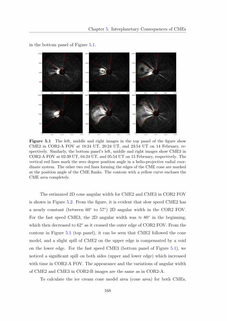
Chapter 5. Interplanetary Consequences of CMEs
in the bottom panel of Figure 5.1.
Figure 5.1 The left, middle and right images in the top panel of the figure showCME2 in COR2-A FOV at 18:24 UT, 20:24 UT, and 23:54 UT on 14 February, re-spectively. Similarly, the bottom panel’s left, middle and right images show CME3 inCOR2-A FOV at 02:39 UT, 04:24 UT, and 05:54 UT on 15 February, respectively. Thevertical red lines mark the zero degree position angle in a helio-projective radial coor-dinate system. The other two red lines forming the edges of the CME cone are markedat the position angle of the CME flanks. The contour with a yellow curve encloses theCME area completely.
The estimated 2D cone angular width for CME2 and CME3 in COR2 FOV
is shown in Figure 5.2. From the figure, it is evident that slow speed CME2 has
a nearly constant (between 60◦ to 57◦) 2D angular width in the COR2 FOV.
For the fast speed CME3, the 2D angular width was ≈ 80◦ in the beginning,
which then decreased to 62◦ as it crossed the outer edge of COR2 FOV. From the
contour in Figure 5.1 (top panel), it can be seen that CME2 followed the cone
model, and a slight spill of CME2 on the upper edge is compensated by a void
on the lower edge. For the fast speed CME3 (bottom panel of Figure 5.1), we
noticed a significant spill on both sides (upper and lower edge) which increased
with time in COR2-A FOV. The appearance and the variations of angular width
of CME2 and CME3 in COR2-B images are the same as in COR2-A.
To calculate the ice cream cone model area (cone area) for both CMEs,
168
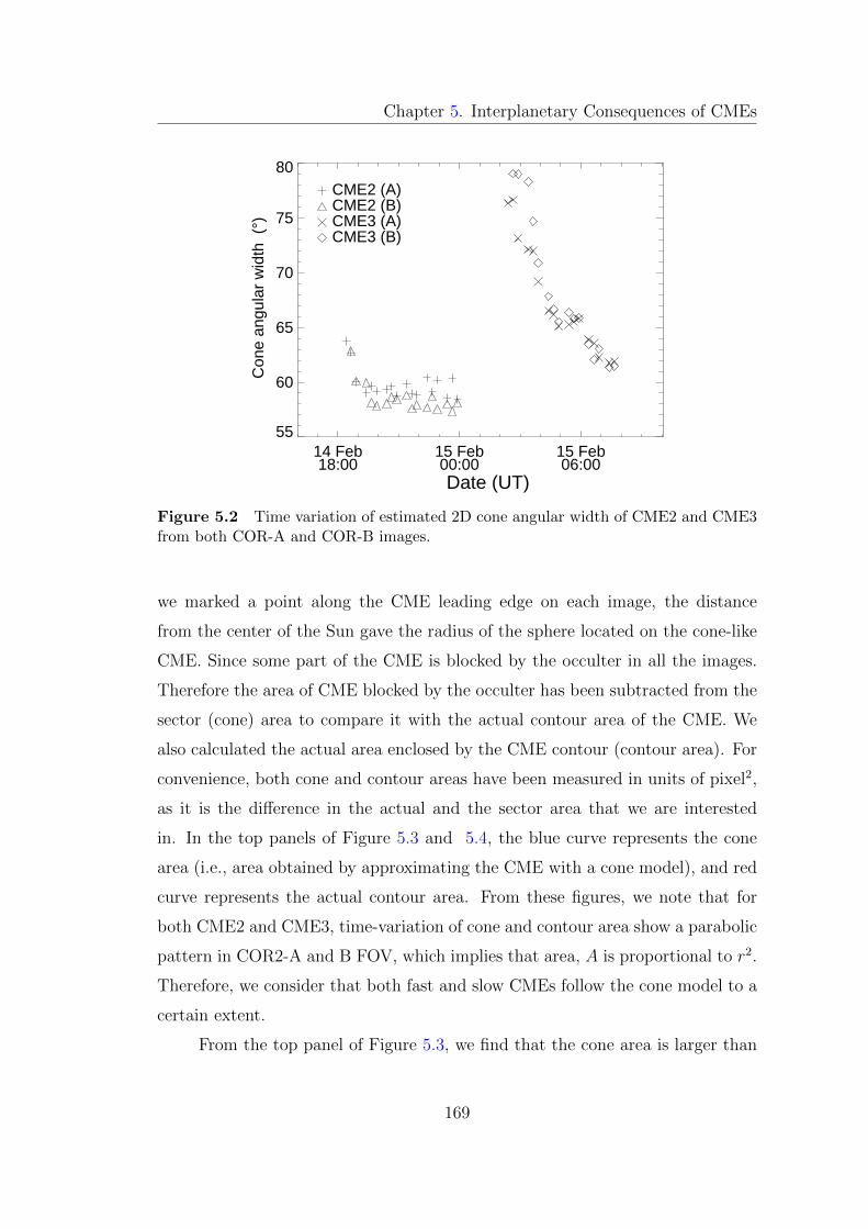
Chapter 5. Interplanetary Consequences of CMEs
14 Feb18:00
15 Feb00:00
15 Feb06:00
55
60
65
70
75
80
Con
e an
gula
r w
idth
(°)
CME2 (A)CME2 (B)CME3 (A)CME3 (B)
Date (UT)
Figure 5.2 Time variation of estimated 2D cone angular width of CME2 and CME3from both COR-A and COR-B images.
we marked a point along the CME leading edge on each image, the distance
from the center of the Sun gave the radius of the sphere located on the cone-like
CME. Since some part of the CME is blocked by the occulter in all the images.
Therefore the area of CME blocked by the occulter has been subtracted from the
sector (cone) area to compare it with the actual contour area of the CME. We
also calculated the actual area enclosed by the CME contour (contour area). For
convenience, both cone and contour areas have been measured in units of pixel2,
as it is the difference in the actual and the sector area that we are interested
in. In the top panels of Figure 5.3 and 5.4, the blue curve represents the cone
area (i.e., area obtained by approximating the CME with a cone model), and red
curve represents the actual contour area. From these figures, we note that for
both CME2 and CME3, time-variation of cone and contour area show a parabolic
pattern in COR2-A and B FOV, which implies that area, A is proportional to r2.
Therefore, we consider that both fast and slow CMEs follow the cone model to a
certain extent.
From the top panel of Figure 5.3, we find that the cone area is larger than
169
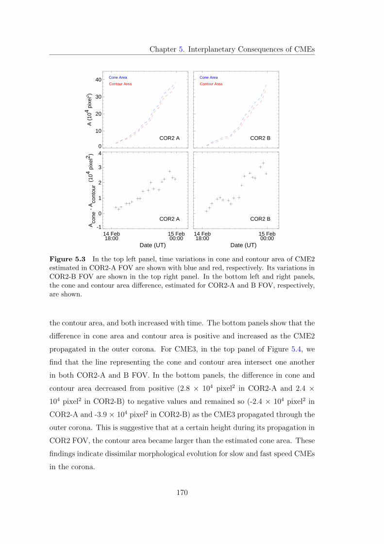
Chapter 5. Interplanetary Consequences of CMEs
0
10
20
30
40
A (
104 p
ixel
2 )
Cone Area
Contour Area
COR2 A
14 Feb18:00
15 Feb00:00
-1
0
1
2
3
4
Aco
ne -
Aco
ntou
r (10
4 pix
el2 )
COR2 A
Date (UT)
Cone Area
Contour Area
COR2 B
14 Feb18:00
15 Feb00:00
COR2 B
Date (UT)
Figure 5.3 In the top left panel, time variations in cone and contour area of CME2estimated in COR2-A FOV are shown with blue and red, respectively. Its variations inCOR2-B FOV are shown in the top right panel. In the bottom left and right panels,the cone and contour area difference, estimated for COR2-A and B FOV, respectively,are shown.
the contour area, and both increased with time. The bottom panels show that the
difference in cone area and contour area is positive and increased as the CME2
propagated in the outer corona. For CME3, in the top panel of Figure 5.4, we
find that the line representing the cone and contour area intersect one another
in both COR2-A and B FOV. In the bottom panels, the difference in cone and
contour area decreased from positive (2.8 × 104 pixel2 in COR2-A and 2.4 ×104 pixel2 in COR2-B) to negative values and remained so (-2.4 × 104 pixel2 in
COR2-A and -3.9 × 104 pixel2 in COR2-B) as the CME3 propagated through the
outer corona. This is suggestive that at a certain height during its propagation in
COR2 FOV, the contour area became larger than the estimated cone area. These
findings indicate dissimilar morphological evolution for slow and fast speed CMEs
in the corona.
170
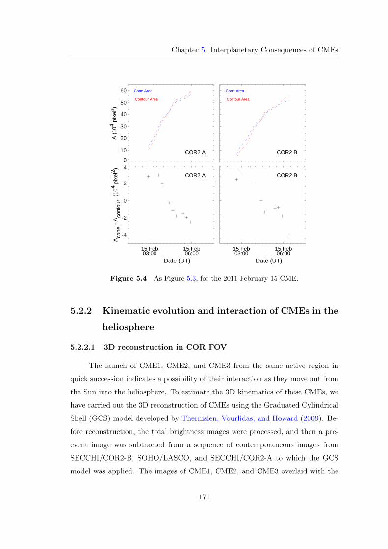
Chapter 5. Interplanetary Consequences of CMEs
0
10
20
30
40
50
60
A (
104 p
ixel
2 )
Cone Area
Contour Area
COR2 A
15 Feb03:00
15 Feb06:00
-4
-2
0
2
4
Aco
ne -
Aco
ntou
r (10
4 pix
el2 )
COR2 A
Date (UT)
Cone Area
Contour Area
COR2 B
15 Feb03:00
15 Feb06:00
COR2 B
Date (UT)
Figure 5.4 As Figure 5.3, for the 2011 February 15 CME.
5.2.2 Kinematic evolution and interaction of CMEs in the
heliosphere
5.2.2.1 3D reconstruction in COR FOV
The launch of CME1, CME2, and CME3 from the same active region in
quick succession indicates a possibility of their interaction as they move out from
the Sun into the heliosphere. To estimate the 3D kinematics of these CMEs, we
have carried out the 3D reconstruction of CMEs using the Graduated Cylindrical
Shell (GCS) model developed by Thernisien, Vourlidas, and Howard (2009). Be-
fore reconstruction, the total brightness images were processed, and then a pre-
event image was subtracted from a sequence of contemporaneous images from
SECCHI/COR2-B, SOHO/LASCO, and SECCHI/COR2-A to which the GCS
model was applied. The images of CME1, CME2, and CME3 overlaid with the
171
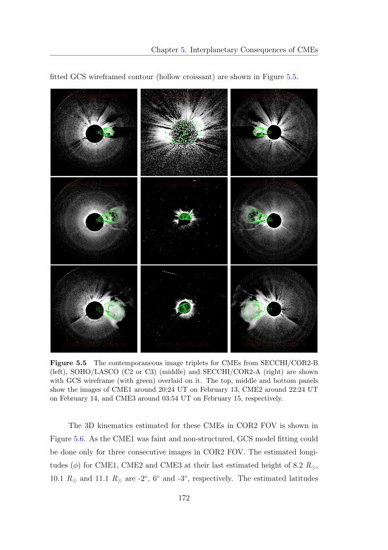
Chapter 5. Interplanetary Consequences of CMEs
fitted GCS wireframed contour (hollow croissant) are shown in Figure 5.5.
Figure 5.5 The contemporaneous image triplets for CMEs from SECCHI/COR2-B(left), SOHO/LASCO (C2 or C3) (middle) and SECCHI/COR2-A (right) are shownwith GCS wireframe (with green) overlaid on it. The top, middle and bottom panelsshow the images of CME1 around 20:24 UT on February 13, CME2 around 22:24 UTon February 14, and CME3 around 03:54 UT on February 15, respectively.
The 3D kinematics estimated for these CMEs in COR2 FOV is shown in
Figure 5.6. As the CME1 was faint and non-structured, GCS model fitting could
be done only for three consecutive images in COR2 FOV. The estimated longi-
tudes (φ) for CME1, CME2 and CME3 at their last estimated height of 8.2 R�,
10.1 R� and 11.1 R� are -2◦, 6◦ and -3◦, respectively. The estimated latitudes
172
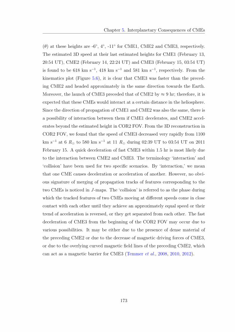
Chapter 5. Interplanetary Consequences of CMEs
(θ) at these heights are -6◦, 4◦, -11◦ for CME1, CME2 and CME3, respectively.
The estimated 3D speed at their last estimated heights for CME1 (February 13,
20:54 UT), CME2 (February 14, 22:24 UT) and CME3 (February 15, 03:54 UT)
is found to be 618 km s−1, 418 km s−1 and 581 km s−1, respectively. From the
kinematics plot (Figure 5.6), it is clear that CME3 was faster than the preced-
ing CME2 and headed approximately in the same direction towards the Earth.
Moreover, the launch of CME3 preceded that of CME2 by ≈ 9 hr; therefore, it is
expected that these CMEs would interact at a certain distance in the heliosphere.
Since the direction of propagation of CME1 and CME2 was also the same, there is
a possibility of interaction between them if CME1 decelerates, and CME2 accel-
erates beyond the estimated height in COR2 FOV. From the 3D reconstruction in
COR2 FOV, we found that the speed of CME3 decreased very rapidly from 1100
km s−1 at 6 R� to 580 km s−1 at 11 R� during 02:39 UT to 03:54 UT on 2011
February 15. A quick deceleration of fast CME3 within 1.5 hr is most likely due
to the interaction between CME2 and CME3. The terminology ‘interaction’ and
‘collision’ have been used for two specific scenarios. By ‘interaction,’ we mean
that one CME causes deceleration or acceleration of another. However, no obvi-
ous signature of merging of propagation tracks of features corresponding to the
two CMEs is noticed in J -maps. The ‘collision’ is referred to as the phase during
which the tracked features of two CMEs moving at different speeds come in close
contact with each other until they achieve an approximately equal speed or their
trend of acceleration is reversed, or they get separated from each other. The fast
deceleration of CME3 from the beginning of the COR2 FOV may occur due to
various possibilities. It may be either due to the presence of dense material of
the preceding CME2 or due to the decrease of magnetic driving forces of CME3,
or due to the overlying curved magnetic field lines of the preceding CME2, which
can act as a magnetic barrier for CME3 (Temmer et al., 2008, 2010, 2012).
173
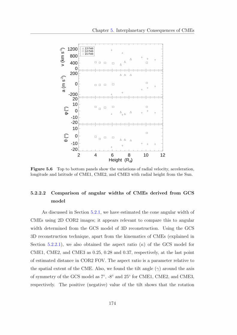
Chapter 5. Interplanetary Consequences of CMEs
0
400
800
1200
v (k
m s
-1) 13 Feb
14 Feb15 Feb
-200
0
200
a (m
s-2)
-20-10
01020
φ (°
)
2 4 6 8 10 12Height (R
O •)
-20-10
0
10
θ (°
)
Figure 5.6 Top to bottom panels show the variations of radial velocity, acceleration,longitude and latitude of CME1, CME2, and CME3 with radial height from the Sun.
5.2.2.2 Comparison of angular widths of CMEs derived from GCS
model
As discussed in Section 5.2.1, we have estimated the cone angular width of
CMEs using 2D COR2 images; it appears relevant to compare this to angular
width determined from the GCS model of 3D reconstruction. Using the GCS
3D reconstruction technique, apart from the kinematics of CMEs (explained in
Section 5.2.2.1), we also obtained the aspect ratio (κ) of the GCS model for
CME1, CME2, and CME3 as 0.25, 0.28 and 0.37, respectively, at the last point
of estimated distance in COR2 FOV. The aspect ratio is a parameter relative to
the spatial extent of the CME. Also, we found the tilt angle (γ) around the axis
of symmetry of the GCS model as 7◦, -8◦ and 25◦ for CME1, CME2, and CME3,
respectively. The positive (negative) value of the tilt shows that the rotation
174
Chapter 5. Interplanetary Consequences of CMEs
is anticlockwise (clockwise) out of the ecliptic plane. The angular width (2α)
between both legs of a CME (in a GCS representation) is 34◦, 64◦ and 36◦ for
CME1, CME2 and CME3, respectively. These values are in agreement (within ±10%) with the values obtained by Temmer et al. (2014). It is to be noted that the
measured 2D angular width of CME depends on the orientation of the GCS flux
ropes. For ecliptic orientation of the flux ropes, i.e., γ = 0◦, the angular width of
CME seen in 2D images is equal to the 3D edge-on angular width (ωEO = 2δ) of
GCS model, where δ = arcsin(κ). For γ = 90◦, the measured 2D width is equal
to 3D face-on angular width (ωFO = 2α+2δ) of the GCS modeled CME.
We converted the GCS modeled 3D width to 2D angular width for CME2
using the expression, ω2D = ωEOcos(γ)+ωFOsin(γ), and find that CME2 has
approximately constant 2D angular width in COR2 FOV. We find that the fast
speed CME3 has γ = 21◦, κ=0.40 and α = 16◦ in the beginning of the COR2 FOV
while γ = 21◦, κ=0.31 and α = 18◦ at the last measured point in COR2 FOV.
Hence, as CME3 propagates further in COR2 FOV, its 2D angular width (derived
using GCS modeled 3D width) decreases from 77◦ to 63◦. These findings are in
accordance with the observed 2D angular width of CME2 and CME3 (Figure 5.2).
The possibility of rotation of CMEs has been discussed theoretically (Lynch et al.
2009, and references therein) and reported in low corona observations (Lynch
et al., 2010). Such changes in the 2D measured angular width are also possible
due to rotation (change in CME orientation, i.e., tilt, angle) of fast speed CME
towards or away from the equator as shown by Yurchyshyn, Abramenko, and
Tripathi (2009) who suggested a higher rotation rate for a faster CME (Lynch
et al., 2010; Poomvises, Zhang, and Olmedo, 2010). However, we must emphasize
that based on the GCS modeling, we could not infer any noticeable rotation
(change in γ) or deflection (change in φ in Figure 5.6) in the COR2 FOV for the
selected CMEs. The uncertainties involved in the estimation of 3D and observed
2D angular widths are discussed in Section 5.2.5.
Vourlidas et al. (2011) reported that despite the rapid rotation of CMEs,
there are no significant projection effects (change in angular width) in single
coronagraphic observations. They showed, for a CME launched on 2010 June
175
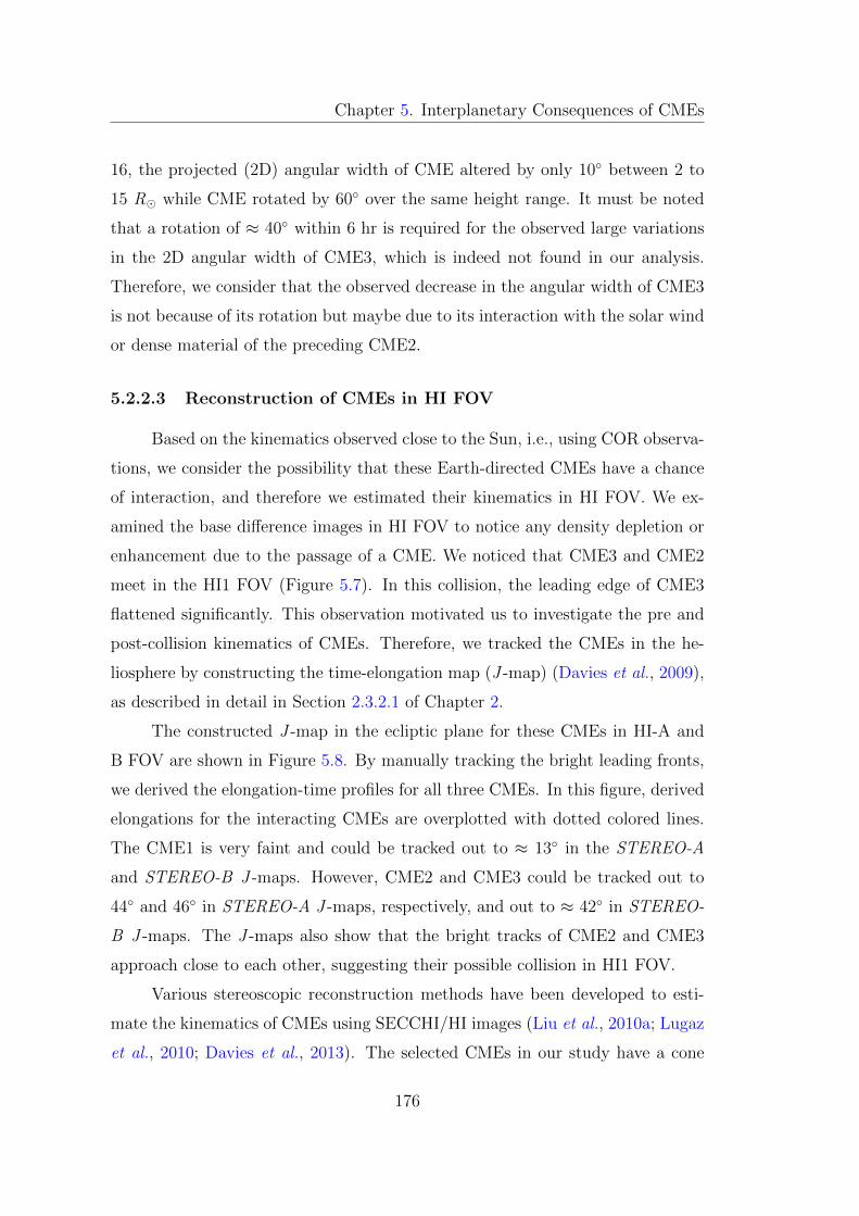
Chapter 5. Interplanetary Consequences of CMEs
16, the projected (2D) angular width of CME altered by only 10◦ between 2 to
15 R� while CME rotated by 60◦ over the same height range. It must be noted
that a rotation of ≈ 40◦ within 6 hr is required for the observed large variations
in the 2D angular width of CME3, which is indeed not found in our analysis.
Therefore, we consider that the observed decrease in the angular width of CME3
is not because of its rotation but maybe due to its interaction with the solar wind
or dense material of the preceding CME2.
5.2.2.3 Reconstruction of CMEs in HI FOV
Based on the kinematics observed close to the Sun, i.e., using COR observa-
tions, we consider the possibility that these Earth-directed CMEs have a chance
of interaction, and therefore we estimated their kinematics in HI FOV. We ex-
amined the base difference images in HI FOV to notice any density depletion or
enhancement due to the passage of a CME. We noticed that CME3 and CME2
meet in the HI1 FOV (Figure 5.7). In this collision, the leading edge of CME3
flattened significantly. This observation motivated us to investigate the pre and
post-collision kinematics of CMEs. Therefore, we tracked the CMEs in the he-
liosphere by constructing the time-elongation map (J -map) (Davies et al., 2009),
as described in detail in Section 2.3.2.1 of Chapter 2.
The constructed J -map in the ecliptic plane for these CMEs in HI-A and
B FOV are shown in Figure 5.8. By manually tracking the bright leading fronts,
we derived the elongation-time profiles for all three CMEs. In this figure, derived
elongations for the interacting CMEs are overplotted with dotted colored lines.
The CME1 is very faint and could be tracked out to ≈ 13◦ in the STEREO-A
and STEREO-B J -maps. However, CME2 and CME3 could be tracked out to
44◦ and 46◦ in STEREO-A J -maps, respectively, and out to ≈ 42◦ in STEREO-
B J -maps. The J -maps also show that the bright tracks of CME2 and CME3
approach close to each other, suggesting their possible collision in HI1 FOV.
Various stereoscopic reconstruction methods have been developed to esti-
mate the kinematics of CMEs using SECCHI/HI images (Liu et al., 2010a; Lugaz
et al., 2010; Davies et al., 2013). The selected CMEs in our study have a cone
176
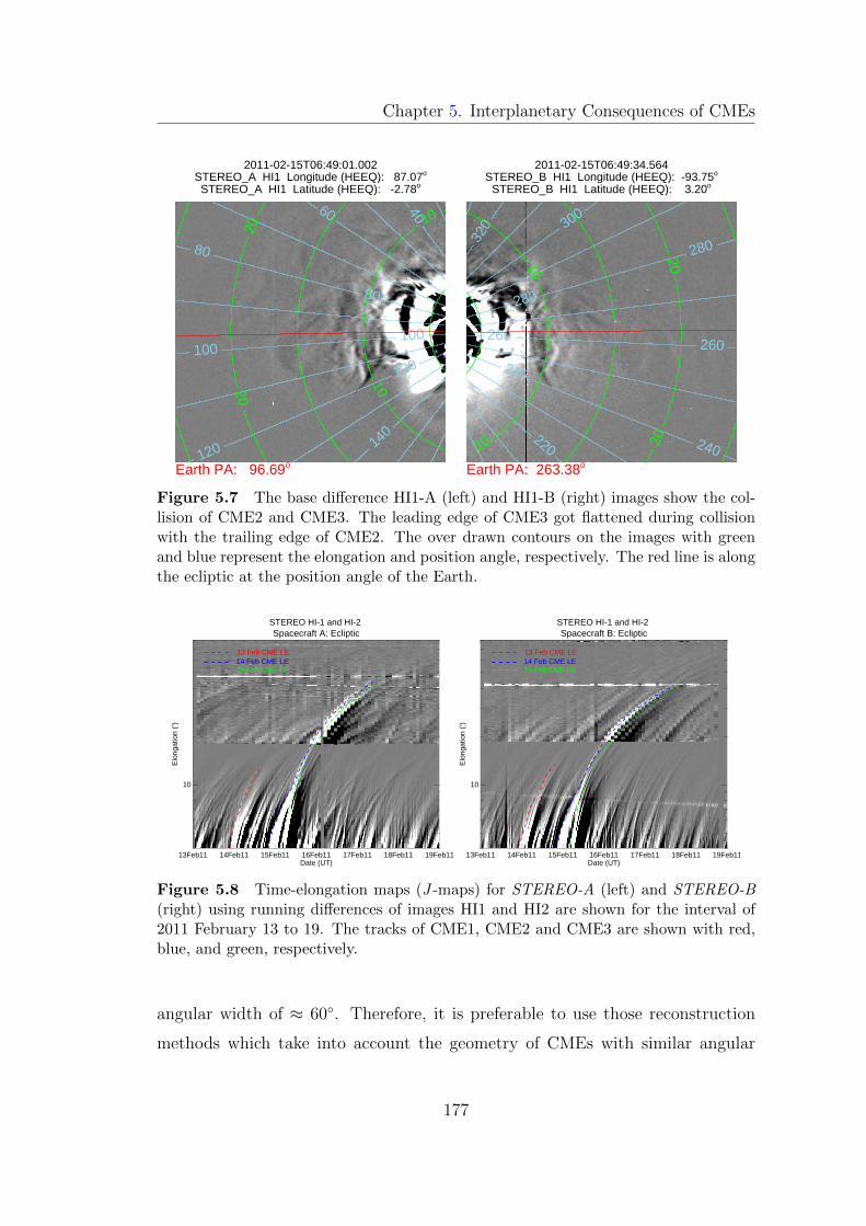
Chapter 5. Interplanetary Consequences of CMEs
4060
80
80
100100
120
120
140
10
10
20
20
2011-02-15T06:49:01.002
Earth PA: 96.69o
STEREO_A HI1 Longitude (HEEQ): 87.07o
STEREO_A HI1 Latitude (HEEQ): -2.78o
220 240
240
260260
280
280
300
320
10
10
20
20
2011-02-15T06:49:34.564
Earth PA: 263.38o
STEREO_B HI1 Longitude (HEEQ): -93.75o
STEREO_B HI1 Latitude (HEEQ): 3.20o
Figure 5.7 The base difference HI1-A (left) and HI1-B (right) images show the col-lision of CME2 and CME3. The leading edge of CME3 got flattened during collisionwith the trailing edge of CME2. The over drawn contours on the images with greenand blue represent the elongation and position angle, respectively. The red line is alongthe ecliptic at the position angle of the Earth.
Spacecraft A: Ecliptic
13Feb11 14Feb11 15Feb11 16Feb11 17Feb11 18Feb11 19Feb11Date (UT)
10
Elo
ngat
ion
(o )
STEREO HI-1 and HI-2
13 Feb CME LE14 Feb CME LE15 Feb CME LE
Spacecraft B: Ecliptic
13Feb11 14Feb11 15Feb11 16Feb11 17Feb11 18Feb11 19Feb11Date (UT)
10
Elo
ngat
ion
(o )
STEREO HI-1 and HI-2
13 Feb CME LE14 Feb CME LE15 Feb CME LE
Figure 5.8 Time-elongation maps (J -maps) for STEREO-A (left) and STEREO-B(right) using running differences of images HI1 and HI2 are shown for the interval of2011 February 13 to 19. The tracks of CME1, CME2 and CME3 are shown with red,blue, and green, respectively.
angular width of ≈ 60◦. Therefore, it is preferable to use those reconstruction
methods which take into account the geometry of CMEs with similar angular
177
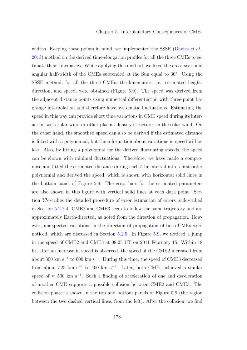
Chapter 5. Interplanetary Consequences of CMEs
widths. Keeping these points in mind, we implemented the SSSE (Davies et al.,
2013) method on the derived time-elongation profiles for all the three CMEs to es-
timate their kinematics. While applying this method, we fixed the cross-sectional
angular half-width of the CMEs subtended at the Sun equal to 30◦. Using the
SSSE method, for all the three CMEs, the kinematics, i.e., estimated height,
direction, and speed, were obtained (Figure 5.9). The speed was derived from
the adjacent distance points using numerical differentiation with three-point La-
grange interpolation and therefore have systematic fluctuations. Estimating the
speed in this way can provide short time variations in CME speed during its inter-
action with solar wind or other plasma density structures in the solar wind. On
the other hand, the smoothed speed can also be derived if the estimated distance
is fitted with a polynomial, but the information about variations in speed will be
lost. Also, by fitting a polynomial for the derived fluctuating speeds, the speed
can be shown with minimal fluctuations. Therefore, we have made a compro-
mise and fitted the estimated distance during each 5 hr interval into a first-order
polynomial and derived the speed, which is shown with horizontal solid lines in
the bottom panel of Figure 5.9. The error bars for the estimated parameters
are also shown in this figure with vertical solid lines at each data point. Sec-
tion ??escribes the detailed procedure of error estimation of errors is described
in Section 5.2.2.4. CME2 and CME3 seem to follow the same trajectory and are
approximately Earth-directed, as noted from the direction of propagation. How-
ever, unexpected variations in the direction of propagation of both CMEs were
noticed, which are discussed in Section 5.2.5. In Figure 5.9, we noticed a jump
in the speed of CME2 and CME3 at 08:25 UT on 2011 February 15. Within 18
hr, after an increase in speed is observed, the speed of the CME2 increased from
about 300 km s−1 to 600 km s−1. During this time, the speed of CME3 decreased
from about 525 km s−1 to 400 km s−1. Later, both CMEs achieved a similar
speed of ≈ 500 km s−1. Such a finding of acceleration of one and deceleration
of another CME supports a possible collision between CME2 and CME3. The
collision phase is shown in the top and bottom panels of Figure 5.9 (the region
between the two dashed vertical lines, from the left). After the collision, we find
178
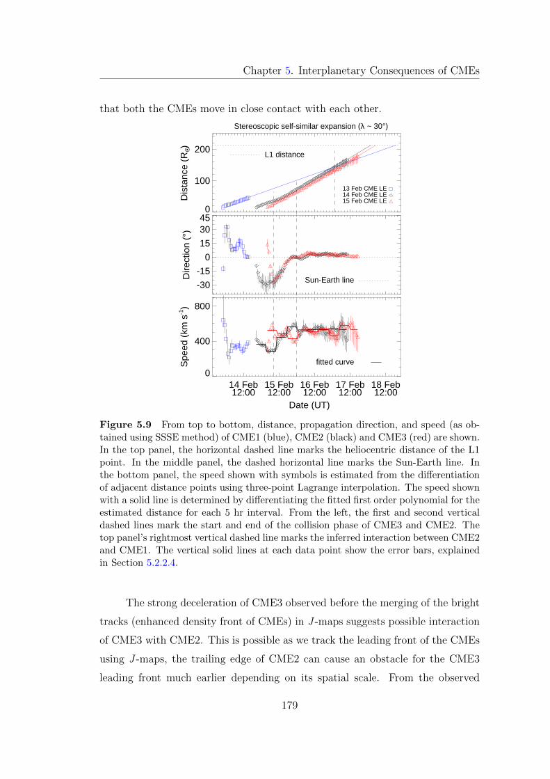
Chapter 5. Interplanetary Consequences of CMEs
that both the CMEs move in close contact with each other.
0
100
200
Dis
tanc
e (R
O •)
L1 distance
15 Feb CME LE14 Feb CME LE13 Feb CME LE
Stereoscopic self-similar expansion (λ ~ 30°)
-30
-15
0
15
3045
Dire
ctio
n (°
)
Sun-Earth line
14 Feb12:00
15 Feb12:00
16 Feb12:00
17 Feb12:00
18 Feb12:00
0
400
800
Spe
ed (
km s
-1)
fitted curve
Date (UT)
Figure 5.9 From top to bottom, distance, propagation direction, and speed (as ob-tained using SSSE method) of CME1 (blue), CME2 (black) and CME3 (red) are shown.In the top panel, the horizontal dashed line marks the heliocentric distance of the L1point. In the middle panel, the dashed horizontal line marks the Sun-Earth line. Inthe bottom panel, the speed shown with symbols is estimated from the differentiationof adjacent distance points using three-point Lagrange interpolation. The speed shownwith a solid line is determined by differentiating the fitted first order polynomial for theestimated distance for each 5 hr interval. From the left, the first and second verticaldashed lines mark the start and end of the collision phase of CME3 and CME2. Thetop panel’s rightmost vertical dashed line marks the inferred interaction between CME2and CME1. The vertical solid lines at each data point show the error bars, explainedin Section 5.2.2.4.
The strong deceleration of CME3 observed before the merging of the bright
tracks (enhanced density front of CMEs) in J -maps suggests possible interaction
of CME3 with CME2. This is possible as we track the leading front of the CMEs
using J -maps, the trailing edge of CME2 can cause an obstacle for the CME3
leading front much earlier depending on its spatial scale. From the observed
179
Chapter 5. Interplanetary Consequences of CMEs
timings, it is clear that interaction of CME3 with CME2 had started ≈ 5 hr
before their collision in HI FOV. Our analysis also shows that the leading front
of CME3 reflects the effect of interaction (i.e. strong deceleration) at 6 R� while
leading edge of CME2 shows this effect (i.e. acceleration) at 28 R�. Therefore, the
force acting on the trailing edge of CME2 takes approximately ≈ 5.7 hr to reach
the leading front of this CME. Based on these values, the propagation speed of
disturbance responsible for the acceleration of the leading front of CME2 should
be ≈ 750 km s−1. From the Radio and Plasma Wave Experiment (WAVES)
(Bougeret et al., 1995) on board WIND spacecraft, we noticed a type II burst
during 02:10-07:00 UT in the 16000-400 kHz range. Such radio bursts provide
information on CME-driven shock (Gopalswamy et al., 2000b). This shock is
associated with the fast-speed CME3. The average shock cone angle (≈ 100◦) as
seen from the Sun is significantly greater than the average angular size (≈ 45◦) of
any CME (Schwenn, 2006). This shock likely traveled across CME2. Therefore,
the acceleration of CME2, observed in HI1 FOV, may be due to the combined
effect of the shock and the leading front of CME3. As previously mentioned,
CME1 was very faint, and its kinematics could be estimated up to 46 R� only.
Based on the linear extrapolation of the height-time curves of CME1 and CME2,
we infer that they should meet each other at 144 R� at 01:40 UT on 2011 February
17.
5.2.2.4 Comparison of kinematics derived from other stereoscopic
methods
To examine the range of uncertainties in the estimated kinematics of the
CMEs of 2011 February 13-15, by implementing SSSE method, we applied other
stereoscopic methods, viz. TAS (Lugaz et al., 2010) and GT (Liu et al., 2010a)
method to all the three CMEs. Using the kinematics estimated from TAS and
GT methods, we found that the leading edge of CME3 caught the leading edge of
CME2 at the approximately same distance (within a few solar radii) as obtained
from the SSSE method. Based on linear extrapolation of the height-time profile
of CME2 and CME1 estimated from TAS and GT methods, we inferred that
180
Chapter 5. Interplanetary Consequences of CMEs
CME2 would have reached CME1 at 157 R� at 03:35 UT on 2011 February 17
and at 138 R� on 20:24 UT on February 17, respectively.
The kinematics derived from the SSSE method is shown in Figure 5.9, and
cognizance of the involved uncertainties is important. However, the actual un-
certainties in the derived kinematics owe to several factors (geometry, elonga-
tion measurements, Thomson scattering, line of sight integration effect, break-
down of assumptions in the method itself), and its quantification is challenging.
Davies et al. (2013) have shown that GT and TAS methods are special cases of
SSSE method corresponding to two extreme cross-sectional extent (geometry) of
a CME, i.e., corresponding to angular half-width of λ = 0◦ and λ = 90◦, re-
spectively. We estimated the uncertainties by considering different geometry in
the three implemented stereoscopic techniques (GT, TAS, and SSSE). Such un-
certainties are shown with error bars with vertical solid lines in Figure 5.9. We
estimated the absolute difference between kinematics values derived from SSSE
and GT method and display it as a vertical lower error (lower segment of er-
ror bars). Similarly, the absolute difference between the SSSE method and TAS
method kinematics values is displayed as a vertical upper error. From Figure 5.9,
we notice that the results from all three methods are in reasonable agreement.
Further, we attempted to examine the contribution of errors in the kinemat-
ics due to errors in tracking (i.e., elongation measurements) of a selected feature.
Following the error analysis approach of Liu et al. (2010b), we consider an uncer-
tainty of 10 pixels in elongation measurements from both STEREO viewpoints
which correspond to elongation uncertainty of 0.04◦, 0.2◦ and 0.7◦ in COR2, HI1
and HI2 FOV, respectively. This leads to an uncertainly of 0.20-0.35 R�, 0.21-0.75
R�, and 0.19-0.74 R� in the estimated distance for CME1, CME2 and CME3,
respectively. Such small uncertainties in the distance are expected to result in an
error of less than ≈ 100 km s−1 in speed. However, similar elongation uncertainty
leads to crucially larger uncertainty in the estimated direction of propagation of
CMEs when they are close to the entrance of HI1 FOV, where singularity occurs
(described in Section 3.2.2 of Chapter 3). The estimated propagation direction
of CMEs from the GT method is shown in Figure 5.10 in which vertical lines at
181
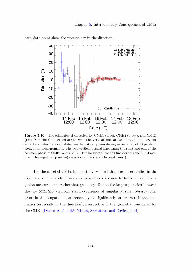
Chapter 5. Interplanetary Consequences of CMEs
each data point show the uncertainty in the direction.
14 Feb12:00
15 Feb12:00
16 Feb12:00
17 Feb12:00
18 Feb12:00
-40
-30
-20
-10
0
10
20
30
40D
irect
ion
(°)
Sun-Earth line
13 Feb CME LE14 Feb CME LE15 Feb CME LE
Date (UT)
Figure 5.10 The estimates of direction for CME1 (blue), CME2 (black), and CME3(red) from the GT method are shown. The vertical lines at each data point show theerror bars, which are calculated mathematically considering uncertainty of 10 pixels inelongation measurements. The two vertical dashed lines mark the start and end of thecollision phase of CME2 and CME3. The horizontal dashed line denotes the Sun-Earthline. The negative (positive) direction angle stands for east (west).
For the selected CMEs in our study, we find that the uncertainties in the
estimated kinematics from stereoscopic methods owe mostly due to errors in elon-
gation measurements rather than geometry. Due to the large separation between
the two STEREO viewpoints and occurrence of singularity, small observational
errors in the elongation measurements yield significantly larger errors in the kine-
matics (especially in the direction), irrespective of the geometry considered for
the CMEs (Davies et al., 2013; Mishra, Srivastava, and Davies, 2014).
182
Chapter 5. Interplanetary Consequences of CMEs
5.2.3 Energy, momentum exchange and nature of collision
between CMEs of 2011 February 14 and 15
The dynamics and structure of CMEs are likely to change when they collide
with one another. Therefore, estimation of post-collision kinematics is crucial
for predicting the space weather consequences. As the CMEs are large-scale
magnetized plasmoids that interact with each other, it is worth investigating the
nature of collision for CMEs which is expected to be different than the collision
of gaseous bubbles with no internal magnetic field. In collision dynamics, the
total momentum of colliding bodies is conserved irrespective of the nature of the
collision provided that external forces are absent.
We attempt to investigate the nature of collision for CME2 and CME3.
As the CME3 follows the trajectory of CME2 before and after the collision, we
simply use the velocity derived from the SSSE method to deal with the collision
dynamics. We did not take into account the 3D velocity components and intricate
mathematics for determining the motion of centroid of colliding CMEs, as used
in Shen et al. (2012). We studied one-dimensional collision dynamics similar to
the head-on collision case for the interacting CMEs. We note that the start of the
collision phase (marked by the dashed vertical line) occurred at the instant when
the speed of CME2 starts to increase while the speed of CME3 starts to decrease
(Figure 5.9, bottom panel). This trend of speeds is maintained up to 18 hr, where
the collision phase ends. Later, CME2 and CME3 show a trend of deceleration
and acceleration, respectively, reaching a constant speed of 500 km s−1. From
the obtained velocity profiles (Figure 5.9), we notice that velocity of CME2 and
CME3 before the collision are u1 = 300 and u2 = 525 km s−1, respectively. After
the collision and exchange of velocity, the velocity of CME2 and CME3 is found
to be v1 = 600 and v2 = 400 km s−1, respectively. If the true mass of CME2 and
CME3 be m1 and m2, respectively, then the conservation of momentum requires
m1u1 + m2u2 = m1v1 + m2v2. To examine the momentum conservation for the
case of colliding CMEs, we need to calculate the true mass of both CMEs, which
is discussed in the following section.
183
Chapter 5. Interplanetary Consequences of CMEs
5.2.3.1 Estimation of true mass of CMEs
Since the appearance of a CME is due to Thomson scattered photospheric
light from the electrons in the CME (Minnaert, 1930; Billings, 1966; Howard
and Tappin, 2009), the recorded scattered intensity can be converted into the
number of electrons, and hence the mass of a CME can be estimated, if the
composition of the CME is known. But an observer from different vantage points
receives a different amount of scattered light from the electrons; therefore, the
true location of electrons in the CME, i.e. the propagation direction of the CME
must be known to estimate the actual mass of the CME. However, historically,
the mass of a CME has been calculated using the plane of sky approximation,
which resulted in an underestimated value (Munro et al., 1979; Poland et al.,
1981; Vourlidas et al., 2000). Although the propagation direction of the CME
was calculated in our study using the forward modeling (Thernisien, Vourlidas,
and Howard, 2009) method and described in Section 5.2.2.1, to avoid any bias
in the reconstruction methods, we use a different method based on the Thomson
scattering theory to estimate 3D propagation direction and then the true mass
of CMEs in COR2 FOV (Colaninno and Vourlidas, 2009). Before applying this
approach, base difference images were obtained following the procedure described
in Vourlidas et al. (2000, 2010); Bein et al. (2013). To estimate the projected mass
of CMEs in base difference COR2-A and B images, we selected a region of interest
(ROI) that enclosed the full extent of a CME. The intensity at each pixel was
then converted to the number of electrons at each pixel and then the mass per
pixel was obtained. The total mass of CME was calculated by summing the mass
at each pixel inside this ROI. In this way, we estimated the projected mass of
CME, MA and MB from two viewpoints of STEREO-A and STEREO-B in COR2
FOV.
According to Colaninno and Vourlidas (2009), CME masses MA and MB
are expected to be equal as the same CME volume is observed from two different
angles. Any difference between these two masses, must be due to incorrect use
of the propagation angle in the Thomson scattering calculation. Based on this
184
Chapter 5. Interplanetary Consequences of CMEs
assumption, they derived an equation for true mass (MT ) as a function of pro-
jected mass and 3D direction of propagation of CME (see their equations 7 and
8). We used a slightly different approach to solve these equations, viz.
MA/MB = Be(θA)/Be(θA + ∆) (5.1)
where θA is the angle of direction of propagation of CME measured from
the plane of sky of STEREO-A, Be(θA) is the brightness of a single electron at an
angular distance of θA from the plane of sky and ∆ is the summation of longitude
of both STEREO-A and STEREO-B from the Sun-Earth line. Once we obtained
the measured values of MA and MB, we derived its ratio and calculate θA. In
this way, we obtained multiple values of θA which result in the same value of
the ratio of MA and MB. The correct and unique value of θA was confirmed by
visual inspection of CME images in COR FOV. The true mass of CME was then
estimated using the equation (4) of Colaninno and Vourlidas (2009). Here we
must emphasize that estimation of 3D propagation direction of CMEs (θA) using
aforementioned approach has large errors if ∆ approaches 180◦. This is a severe
limitation of the method of true mass estimation and arises because in such a
scenario a CME from the Sun, despite its propagation in any direction (not only
towards the Earth), will be measured at an equal propagation angle from the
plane of the sky of both spacecraft. Therefore, in principle, both the estimated
MA and MB should be exactly equal, and any deviation (which is likely) will
result in the highly erroneous value of θA, and consequently in the true mass
of CME. Such a limitation has also been reported by Colaninno and Vourlidas
(2009) for a very small spacecraft separation angles. This implies that an accurate
propagation direction cannot be derived with this method unless we adjust the
separation angle between STEREO spacecraft slightly. Hence, we use a slightly
different value of ∆ ≈ 160◦ for our case. By repeating our analysis several times
for these CMEs, we noted that a change in ∆ by 20◦ has a negligibly small effect
on the mass of a CME.
We also estimated the accurate mass using the 3D propagation direction
185

Chapter 5. Interplanetary Consequences of CMEs
Parameters February 14 CME February 15 CMEMA 5.30 × 10¹² kg at ≈ 10 R� 4.56 × 10¹² kg at ≈ 12 R�MB 4.38 × 10¹² kg at ≈ 10 R� 4.77 × 10¹² kg at ≈ 12 R�Direction 24◦ east from the Sun-Earth
line30◦ east from the Sun-Earthline
True mass m1 = 5.40 × 10¹² kg m2 = 4.78 × 10¹² kg
Table 5.1 The estimates of mass and direction for 2011 February 14 and 15 CMEs.MA and MB are the estimated mass from two viewpoints of STEREO-A and STEREO-B, respectively.
obtained from another method (GCS forward fitting model) and found that these
results are within≈ 15% of estimates from the method of Colaninno and Vourlidas
(2009), therefore can be used for further analysis.
The estimated mass and direction of propagation for CME2 and CME3 are
given in Table 5.1. We also noticed that mass of CMEs increased with distance
from the Sun. We interpret this increase in mass as an observational artifact due
to the emergence of CME material from behind the occulter of the coronagraphs.
However the possibility of a small real increase in CME mass can not be ignored
completely.
5.2.3.2 Estimation of coefficient of restitution
The coefficient of restitution measures the bounciness (efficiency to re-
bound) of a pair of objects in a collision and is defined as the ratio of their
relative velocity of separation to their relative velocity of approach. Hence, for e
< 1, e = 1, and e > 1, the collision is termed inelastic, elastic, and super-elastic,
and consequently, the kinetic energy of the system after the collision is found
to decrease, stay equal, and increase than before the collision, respectively. Our
analysis shows that the masses of CME become constant after ≈ 10 R� therefore,
we assume that they remain constant before and after their collision in HI FOV.
Combining the equation of conservation of momentum with a coefficient of resti-
tution, the velocities of CME2 and CME3 after the collision can be estimated
186
Chapter 5. Interplanetary Consequences of CMEs
theoretically (v1th, v2th).
v1th =m1u1 +m2u2 +m2e(u2 − u1)
(m1 +m2); v2th =
m1u1 +m2u2 +m1e(u1 − u2)
(m1 +m2)(5.2)
where e is the coefficient of restitution, e = v2 - v1/u1 - u2 and signifies the
nature of collision.
Using the velocity (u1,u2) = (300,525) km s−1 and true mass values (m1,m2)
= (5.40 × 10¹², 4.78 × 10¹²) kg, we calculate a set of theoretical values of final
velocity (v1th,v2th) after the collision of CMEs from equation (5.2) corresponding
to a set of different values of coefficient of restitution (e). We define a parameter
called variance, σ =√
(v1th − v1)2 + (v2th − v2)2. Considering the theoretically
estimated final velocity from the equation (5.2) and variance (σ) values, one can
obtain the most suitable value of e, corresponding to which the theoretically
estimated final velocity (v1th,v2th) is found to be the closest to the observed final
velocity (v1,v2) of CMEs. This implies that the computed variance is minimum
at this e value.
We have estimated the total kinetic energy of the system before the collision
as 9.01 × 10²³ J. The individual kinetic energy of CME2 and CME3 is 2.43 × 10²³
J and 6.58 × 10²³ J, respectively. We note that momentum of CME2 and CME3
is 1.6 × 10¹⁸ N s and 2.5 × 10¹⁸ N s, respectively, just before their observed
collision. Hence, the total momentum of the system is equal to 4.13 × 10¹⁸
N s. We consider (v1,v2) the estimated final velocity (from SSSE method) as
(600,400) km s−1 (Figure 5.9). We found that (v1th,v2th) = (495,304) km s−1
and the minimum value of σ is 142 corresponding to e = 0.85. For this value
of e, the momentum is found to be conserved, and nature of collision is in an
inelastic regime. Such a collision resulted in a decrease in total kinetic energy of
the system by 2% of its value before the collision. If the measured velocity values
are directly used, then e is estimated as 0.89, which is approximately equal to
that obtained from the aforementioned theoretical approach.
To account for uncertainties in the results, we repeated our computation by
187
Chapter 5. Interplanetary Consequences of CMEs
taking an uncertainty of ± 100 km s−1 in the estimated final velocity after the
collision of CMEs. For example, if we use (v1,v2) = (700,500), then minimum
value of σ = 288 is found corresponding to e = 0.80. The estimate for σ is found
to be minimum and is equal to 2.0 corresponding to e = 0.90, when (v1,v2) =
(500,300) km s−1 is used and in this case (v1th,v2th) = (501,298) is obtained. This
implies that keeping the conservation of momentum as a necessary condition, the
combination of (u1,u2) = (300,525) km s−1 and (v1,v2) = (500,300) km s−1 with e
= 0.90 best suits the observed case of collision of CME2 and CME3. In this case,
the total kinetic energy after the collision decreased by only 1.3%, the kinetic
energy of CME2 increased by 177%, and the kinetic energy of CME3 decreased
by 67% of its value before the collision. It implies that the observed collision is in
the inelastic regime but closer to the elastic regime. For this case, the momentum
of CME2 increased by 68%, and momentum of CME3 decreased by 35% of its
value before their collision. Our analysis, therefore, shows that there is a huge
transfer of momentum and kinetic energy during the collision phase of CMEs.
It is worth examining the effect of uncertainty in mass in the estimation
of the value of e or the nature of the collision. We have estimated the true
mass, which is also uncertain and difficult to quantify (Colaninno and Vourlidas,
2009). However, a straightforward uncertainty arises from the assumption that
CME structure lies in the plane of the 3D propagation direction of CME. Vourl-
idas et al. (2000) have shown that such a simplified assumption can cause the
underestimation of CME mass by up to 15%. Applying this uncertainty to the
estimated true mass of CME2 and CME3, their mass ratio (m1/m2 = 1.12) can
range between 0.97 to 1.28. To examine the effect of larger uncertainties in the
mass, we arbitrarily change the mass ratio between 0.5 to 3.0 in the step of 0.25
and repeat the analysis above (using Equation (5.2) and calculating σ value) to
estimate the value of e corresponding to each mass ratio. The variation of e with
mass ratio is shown in Figure 5.11 corresponding to the observed final velocity
(v1,v2) = (600,400) km s−1 after the collision of CMEs in our case. We have
shown earlier that the best suited final velocity of CMEs for our observed case of
CME collision is (v1,v2) = (500,300) km s−1. Therefore, corresponding to this ve-
188
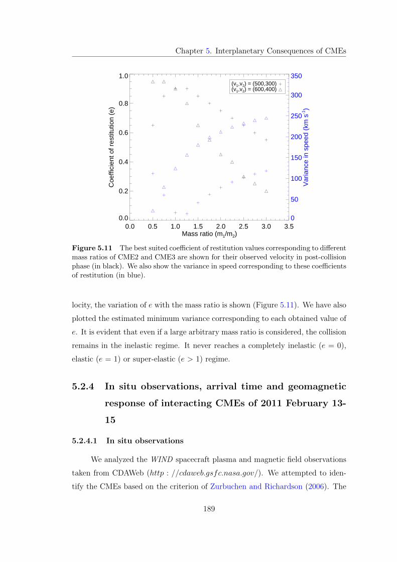
Chapter 5. Interplanetary Consequences of CMEs
0.0 0.5 1.0 1.5 2.0 2.5 3.0 3.5Mass ratio (m1/m2)
0.0
0.2
0.4
0.6
0.8
1.0
Coe
ffici
ent o
f res
titut
ion
(e)
0
50
100
150
200
250
300
350
Var
ianc
e in
spe
ed (
km s
-1)
(v1,v2) = (500,300)(v1,v2) = (600,400)
Figure 5.11 The best suited coefficient of restitution values corresponding to differentmass ratios of CME2 and CME3 are shown for their observed velocity in post-collisionphase (in black). We also show the variance in speed corresponding to these coefficientsof restitution (in blue).
locity, the variation of e with the mass ratio is shown (Figure 5.11). We have also
plotted the estimated minimum variance corresponding to each obtained value of
e. It is evident that even if a large arbitrary mass ratio is considered, the collision
remains in the inelastic regime. It never reaches a completely inelastic (e = 0),
elastic (e = 1) or super-elastic (e > 1) regime.
5.2.4 In situ observations, arrival time and geomagnetic
response of interacting CMEs of 2011 February 13-
15
5.2.4.1 In situ observations
We analyzed the WIND spacecraft plasma and magnetic field observations
taken from CDAWeb (http : //cdaweb.gsfc.nasa.gov/). We attempted to iden-
tify the CMEs based on the criterion of Zurbuchen and Richardson (2006). The
189
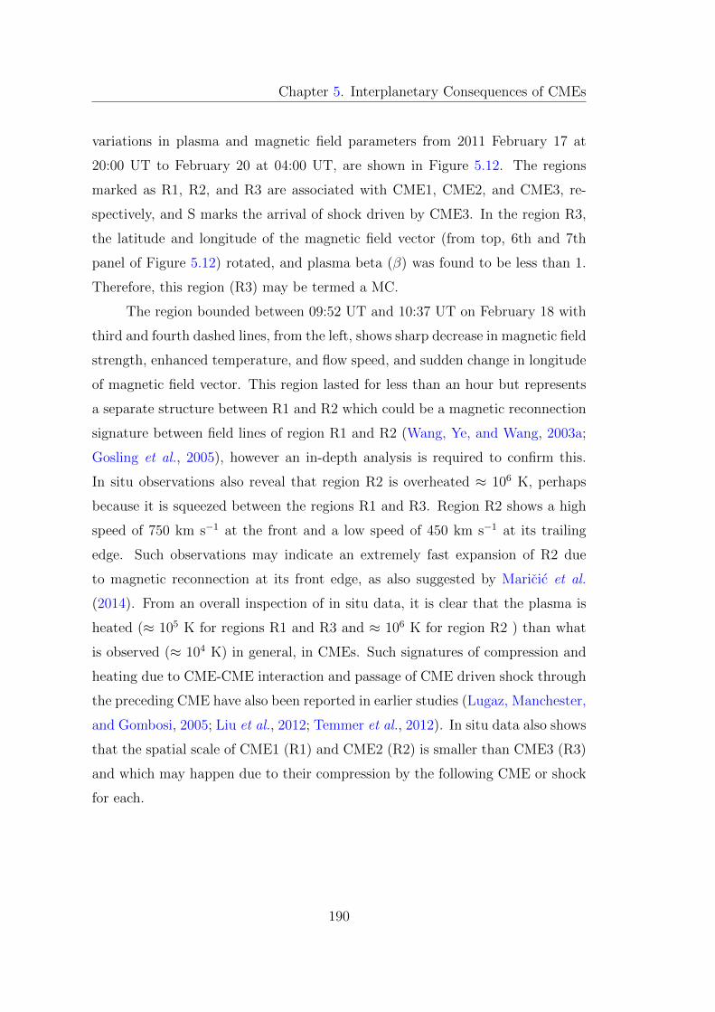
Chapter 5. Interplanetary Consequences of CMEs
variations in plasma and magnetic field parameters from 2011 February 17 at
20:00 UT to February 20 at 04:00 UT, are shown in Figure 5.12. The regions
marked as R1, R2, and R3 are associated with CME1, CME2, and CME3, re-
spectively, and S marks the arrival of shock driven by CME3. In the region R3,
the latitude and longitude of the magnetic field vector (from top, 6th and 7th
panel of Figure 5.12) rotated, and plasma beta (β) was found to be less than 1.
Therefore, this region (R3) may be termed a MC.
The region bounded between 09:52 UT and 10:37 UT on February 18 with
third and fourth dashed lines, from the left, shows sharp decrease in magnetic field
strength, enhanced temperature, and flow speed, and sudden change in longitude
of magnetic field vector. This region lasted for less than an hour but represents
a separate structure between R1 and R2 which could be a magnetic reconnection
signature between field lines of region R1 and R2 (Wang, Ye, and Wang, 2003a;
Gosling et al., 2005), however an in-depth analysis is required to confirm this.
In situ observations also reveal that region R2 is overheated ≈ 106 K, perhaps
because it is squeezed between the regions R1 and R3. Region R2 shows a high
speed of 750 km s−1 at the front and a low speed of 450 km s−1 at its trailing
edge. Such observations may indicate an extremely fast expansion of R2 due
to magnetic reconnection at its front edge, as also suggested by Maricic et al.
(2014). From an overall inspection of in situ data, it is clear that the plasma is
heated (≈ 105 K for regions R1 and R3 and ≈ 106 K for region R2 ) than what
is observed (≈ 104 K) in general, in CMEs. Such signatures of compression and
heating due to CME-CME interaction and passage of CME driven shock through
the preceding CME have also been reported in earlier studies (Lugaz, Manchester,
and Gombosi, 2005; Liu et al., 2012; Temmer et al., 2012). In situ data also shows
that the spatial scale of CME1 (R1) and CME2 (R2) is smaller than CME3 (R3)
and which may happen due to their compression by the following CME or shock
for each.
190
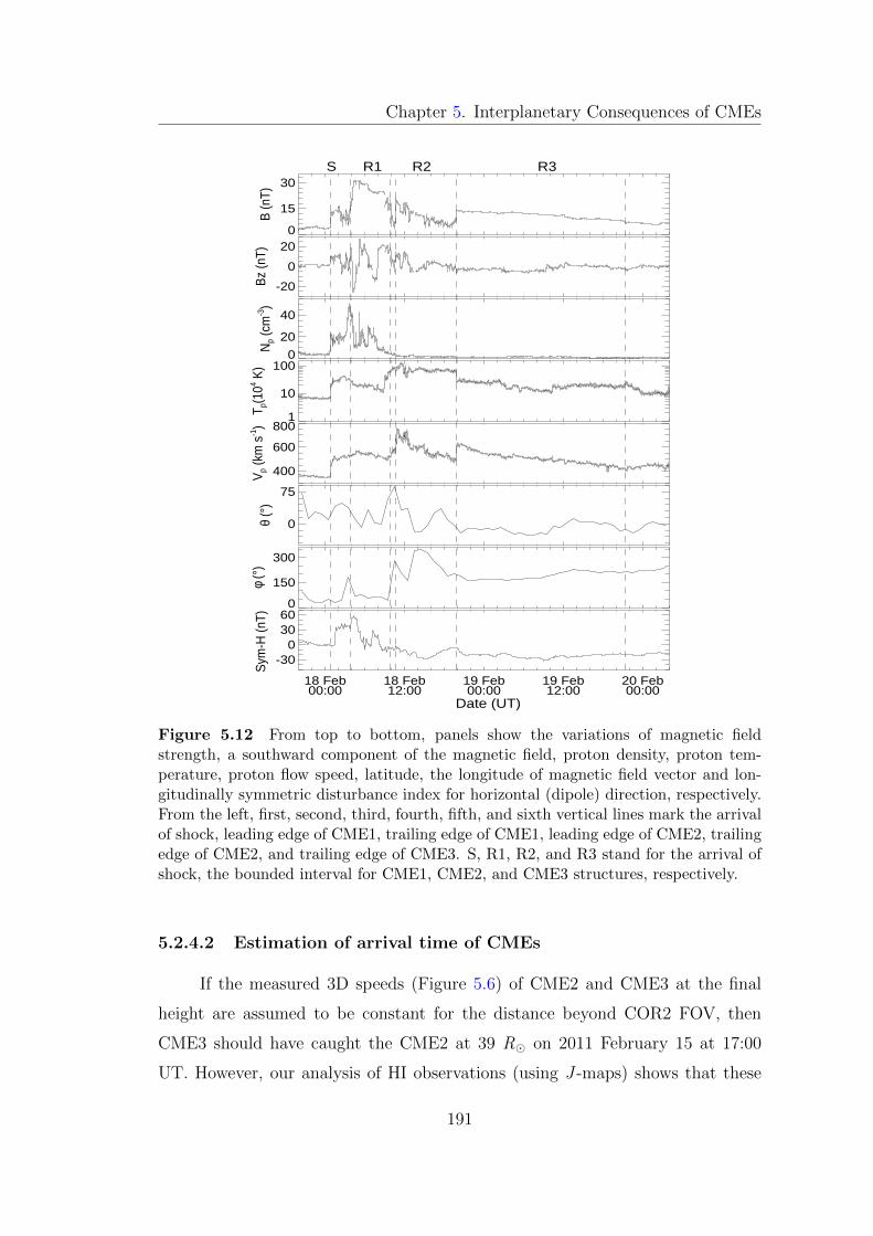
Chapter 5. Interplanetary Consequences of CMEs
0
15
30
B (n
T)
-20
0
20B
z (n
T)
0
20
40
Np (
cm-3)
1
10
100
T p(1
04 K)
400
600
800
Vp (
km s
-1)
0
75
θ (°)
0
150
300
φ (°)
18 Feb00:00
18 Feb12:00
19 Feb00:00
19 Feb12:00
20 Feb00:00
-300
3060
Sym
-H (n
T)
Date (UT)
S R1 R2 R3
Figure 5.12 From top to bottom, panels show the variations of magnetic fieldstrength, a southward component of the magnetic field, proton density, proton tem-perature, proton flow speed, latitude, the longitude of magnetic field vector and lon-gitudinally symmetric disturbance index for horizontal (dipole) direction, respectively.From the left, first, second, third, fourth, fifth, and sixth vertical lines mark the arrivalof shock, leading edge of CME1, trailing edge of CME1, leading edge of CME2, trailingedge of CME2, and trailing edge of CME3. S, R1, R2, and R3 stand for the arrival ofshock, the bounded interval for CME1, CME2, and CME3 structures, respectively.
5.2.4.2 Estimation of arrival time of CMEs
If the measured 3D speeds (Figure 5.6) of CME2 and CME3 at the final
height are assumed to be constant for the distance beyond COR2 FOV, then
CME3 should have caught the CME2 at 39 R� on 2011 February 15 at 17:00
UT. However, our analysis of HI observations (using J -maps) shows that these
191
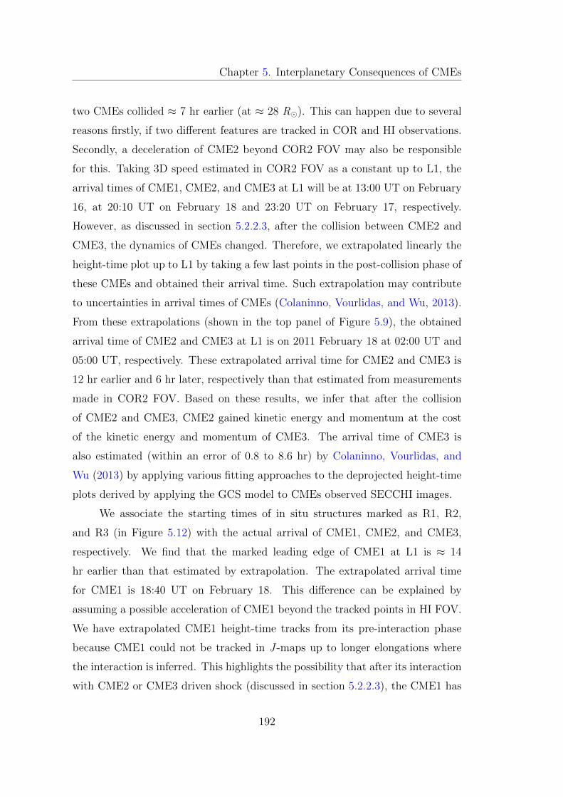
Chapter 5. Interplanetary Consequences of CMEs
two CMEs collided ≈ 7 hr earlier (at ≈ 28 R�). This can happen due to several
reasons firstly, if two different features are tracked in COR and HI observations.
Secondly, a deceleration of CME2 beyond COR2 FOV may also be responsible
for this. Taking 3D speed estimated in COR2 FOV as a constant up to L1, the
arrival times of CME1, CME2, and CME3 at L1 will be at 13:00 UT on February
16, at 20:10 UT on February 18 and 23:20 UT on February 17, respectively.
However, as discussed in section 5.2.2.3, after the collision between CME2 and
CME3, the dynamics of CMEs changed. Therefore, we extrapolated linearly the
height-time plot up to L1 by taking a few last points in the post-collision phase of
these CMEs and obtained their arrival time. Such extrapolation may contribute
to uncertainties in arrival times of CMEs (Colaninno, Vourlidas, and Wu, 2013).
From these extrapolations (shown in the top panel of Figure 5.9), the obtained
arrival time of CME2 and CME3 at L1 is on 2011 February 18 at 02:00 UT and
05:00 UT, respectively. These extrapolated arrival time for CME2 and CME3 is
12 hr earlier and 6 hr later, respectively than that estimated from measurements
made in COR2 FOV. Based on these results, we infer that after the collision
of CME2 and CME3, CME2 gained kinetic energy and momentum at the cost
of the kinetic energy and momentum of CME3. The arrival time of CME3 is
also estimated (within an error of 0.8 to 8.6 hr) by Colaninno, Vourlidas, and
Wu (2013) by applying various fitting approaches to the deprojected height-time
plots derived by applying the GCS model to CMEs observed SECCHI images.
We associate the starting times of in situ structures marked as R1, R2,
and R3 (in Figure 5.12) with the actual arrival of CME1, CME2, and CME3,
respectively. We find that the marked leading edge of CME1 at L1 is ≈ 14
hr earlier than that estimated by extrapolation. The extrapolated arrival time
for CME1 is 18:40 UT on February 18. This difference can be explained by
assuming a possible acceleration of CME1 beyond the tracked points in HI FOV.
We have extrapolated CME1 height-time tracks from its pre-interaction phase
because CME1 could not be tracked in J -maps up to longer elongations where
the interaction is inferred. This highlights the possibility that after its interaction
with CME2 or CME3 driven shock (discussed in section 5.2.2.3), the CME1 has
192
Chapter 5. Interplanetary Consequences of CMEs
accelerated.
The actual arrival times of CME2 and CME3 leading edge (shown in Fig-
ure 5.12) are ≈ 8.5 and 15 hr later, respectively, than obtained by direct linear
extrapolation of the height-time curve (Figure 5.9). From the aforementioned
arrival time estimates, we notice an improvement in arrival time estimation of
CME2 and CME3 by a few (up to 10) hr when the post-collision speeds are used
instead of using the pre-collision speeds. The average measured (actual) transit
speed of CME2 and CME3 at L1 is approximately 100 km s−1 larger than its
speed in remote observations in the post-collision phase. Such an inconsistency
of delayed arrival is possible only if it is assumed that CME2 and CME3 over-
expand before reaching L1 or in situ spacecraft is not hit by the nose of these
CMEs (Maricic et al., 2014). The short duration of CME2 in in situ data with a
lack of magnetic cloud signature favors a flank encounter of CME2 at the space-
craft. The late arrival of CME3 may also be due to its higher deceleration than
estimated in HI FOV. If the remotely tracked feature is incorrectly identified in
the in situ data, such inconsistency may also arise.
5.2.4.3 Geomagnetic response of interacting CMEs
In the bottom panel of Figure 5.12, longitudinally symmetric disturbance
(Sym-H) (Iyemori, 1990) index is plotted. This index is similar to the hourly
disturbance storm time (Dst) (Sugiura, 1964) index. Still, it uses 1 minute values
recorded from a different set of stations and slightly different coordinate systems
and method to determine base values. The effect of solar wind dynamic pressure
is more clearly seen in Sym-H index than in the hourly Dst index. We observed
a sudden increase in Sym-H index up to 30 nT around 01:30 UT on February 18
which is within an hour of the arrival of interplanetary shock. The Sym-H index
continued to rise, and around 04:15 UT reached 57 nT. The first steep rise in this
index marked by the shock is represented by the enhanced magnetic field, speed,
and density. The second peak in Sym-H is primarily due to a corresponding
peak in magnetic field strength and density. However no peak in speed was
observed at this time. During the passage of region R1, the z- component of
193
Chapter 5. Interplanetary Consequences of CMEs
the interplanetary magnetic field (Bz) began to turn negative at 04:07 UT and
remained so up to one hour. During this period, it reached -25 nT at 04:15 UT
and then turned to positive values around 05:00 UT. We noticed that Bz turned
negative a second time at 07:07 UT and remained so for 47 minutes, reaching a
value of -15 nT at 07:31 UT on February 18. From the Sym-H plot, it is clear that
the negative turning of Bz twice caused a fast decrease in elevated sym-H values.
Dungey (1961) has shown that the negative Bz values and process of magnetic
reconnection at the magnetosphere enables magnetized plasma to transfer its
energy into the magnetosphere and form a ring current.
Succinctly, we infer that the arrival of magnetized plasma can be attributed
to the strong storm’s sudden commencement (SSC) (Dst = 57 nT) and short
duration (47 minutes) negative Bz field therein resulting in a minor geomagnetic
storm (Dst = -32 nT). The intensity of SSC is independent of the peak value
of depression in the horizontal component of the magnetic field during the main
phase of a geomagnetic storm. Our analysis supports the idea of collision (or
interaction) of multiple CMEs, which can enhance the magnetic field strength,
density, and temperature within CMEs (Liu et al., 2012; Mostl et al., 2012).
Such enhanced parameters can increase the conductivity of CME plasma and
result in intense induced electric current in CME when it propagates towards the
Earth’s magnetic field. This induced electric current within CME plasma causes
its intense shielding from Earth’s field and increases the magnetic field intensity
around the Earth, which is manifested as SSC (Chapman and Ferraro, 1931).
5.2.5 Results and Discussion on 2011 February 13-15
CMEs
We summarize our results on the analysis of the interaction of three Earth-
directed CMEs launched in succession during 2011, February 13-15, on three main
aspects. These include the morphological & kinematic study of interacting CMEs
and near-Earth manifestations.
194
Chapter 5. Interplanetary Consequences of CMEs
5.2.5.1 Morphological evolution of CMEs
We have studied the morphological properties of Earth-directed CMEs
(CME2 and CME3) when the separation angle between STEREO-A and STEREO-
B was 180◦. Comparing the morphological evolution of CMEs with the cone
model, we found that slow speed CME2 maintained a constant angular width in
the corona. Still, the angular width of fast speed CME3 decreased monotonically
as it propagated further in the corona. The possible explanation for this is that
when CME3 was launched from the Sun, its leading edge suddenly experienced
the ambient solar wind pressure, and resulted in its flattening (Odstrcil, Pizzo,
and Arge, 2005), causing a large angular width. However, as the CME3 propa-
gated further in the corona, there was a decrease in interaction between the solar
wind and the part of CME (i.e., near apex of the cone), which decides the angular
width. Therefore, a decrease in angular width is noticed away from the Sun.
The difference in the cone and contour area of CME2 increases linearly with
the radial height of the CME leading edge (bottom panel of Figure 5.3). This can
be explained by the fact that the CME2 interacted with the solar wind such that
its leading edge (especially the nose) stretched out thereby increasing the value
of r (distance between Sun-center and nose of CME) and also the ice-cream cone
area. For the fast speed CME3, we find that the contour area is less than the
cone area close to the Sun, but as the CME propagated further in the corona, its
contour area became larger than the cone area (Figure 5.4). This can be possibly
explained by the concept that, contrary to the behavior of CME2, as the CME3
propagated further in the corona, its front flattened due to drag force, leading
to spilling some CME mass outside the cone, i.e., at the flanks of CME. This
flattening resulted in a lower estimated value of r and hence a decrease in the
estimated cone area. Therefore, a negative value is obtained for the difference
between cone area and contour area (bottom panel of Figure 5.4). From Figure 5.3
and 5.4 (bottom panels), we can say that slow and fast speed CMEs deviate from
the cone model differently.
Our analysis shows that the estimated 2D angular width (converted from
195

Chapter 5. Interplanetary Consequences of CMEs
3D) follows the same trend as observed in 2D images (Figure 5.2) but has slightly
different (within 5% for CME3 and 15% for CME2) value at a certain height. We
also emphasize that the GCS model parameters (γ, κ and α) are very sensitive
(Thernisien, Vourlidas, and Howard, 2009) and can only be fitted with limited
accuracy, especially for fast CME whose front gets distorted (see, Figure 5.4)
due to possible interaction with the solar wind. Also, the estimation of these
parameters depends on the visual agreement between GCS modeled CME and
the observed CME and is user dependent. It is to be noted that the minor error
in these sensitive parameters can lead to significant errors in the 3D edge-on and
face-on width of GCS modeled CME. This is the reason, despite a reasonably
good agreement between GCS model parameters derived in our study with those
derived in Temmer et al. (2014), the 3D values of angular widths for fast CME
of February 15 (CME3) do not match well with their results. Although, we
acknowledge that measurements of observed 2D width (Figure 5.2) also have
some error (within 5◦), which is relatively small than the involved uncertainties
in the 3D or 2D angular width estimated from the GCS model. In light of the
aforementioned uncertainties and results, further work needs to be carried out to
investigate the change in angular width of fast CMEs.
5.2.5.2 Kinematic evolution of interacting CMEs
The 3D speed and direction estimated for three selected CMEs in COR2
FOV suggest their possible interaction in the interplanetary medium. We have
found that CME3 is the fastest among all the three CMEs and shows strong
deceleration in the COR2 FOV because of the preceding CME2, which acts as a
barrier for it. From the analysis of the kinematics of CMEs in the heliosphere
using stereoscopic methods, we have noted that a collision between CME3 and
CME2 took place around 24 R�-28 R�. As the CME1 was faint and could not
be tracked up to HI2 FOV in J -maps, we inferred based on the extrapolation of
distances that CME2 caught up with CME1 between 138 R� to 157 R�.
It may be noted that using three stereoscopic methods in our study, the
estimates of velocity and location of collision for three selected CMEs are ap-
196
Chapter 5. Interplanetary Consequences of CMEs
proximately the same (within a reasonable error of a few tens of km s−1 and
within a few solar radii) to those obtained by Maricic et al. (2014) using single
spacecraft method.
We have identified collision signatures between CMEs in the kinematics
profiles as an exchange in their speed. We analyzed momentum and energy
exchange during the collision phase of CME2 and CME3 and found that the
nature of collision was in an inelastic regime, reaching close to elastic. Our study
found that even after considering reasonable uncertainties in derived mass and
velocity parameters, the coefficient of restitution (e) lies between 0.78 to 0.90 for
the interacting CME2 and CME3. This implies that the total kinetic energy of
the system of CMEs after the collision is less than its value before the collision.
5.2.5.3 Interacting CMEs near the Earth
We have examined the interaction and the collision signatures of CMEs
in the in situ (WIND) observations. The interacting CMEs could be identified
as a separate entity in in situ observations, therefore, could not be termed as
complex ejecta as defined by Burlaga, Plunkett, and St. Cyr (2002). The in situ
observations suggest that a shock launched by the fastest CME of February 15
(CME3) passed through the CME of February 14 (CME2) and CME of February
13 (CME1) and caused compression, heating, and acceleration, in particular for
the CME of February 14 which is sandwiched between preceding CME (CME1)
and the following CME (CME3). Our analysis shows that the interacting CMEs
resulted in a minor geomagnetic storm with a strong long, duration SSC. This
is in contrast to the results of Farrugia and Berdichevsky (2004); Farrugia et al.
(2006); Mishra and Srivastava (2014), which suggested that interaction of CMEs
leads to long-duration southward component of magnetic field and, therefore to
intense geomagnetic storms.
197
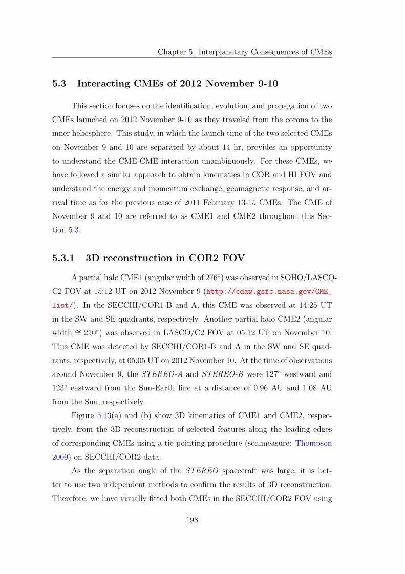
Chapter 5. Interplanetary Consequences of CMEs
5.3 Interacting CMEs of 2012 November 9-10
This section focuses on the identification, evolution, and propagation of two
CMEs launched on 2012 November 9-10 as they traveled from the corona to the
inner heliosphere. This study, in which the launch time of the two selected CMEs
on November 9 and 10 are separated by about 14 hr, provides an opportunity
to understand the CME-CME interaction unambiguously. For these CMEs, we
have followed a similar approach to obtain kinematics in COR and HI FOV and
understand the energy and momentum exchange, geomagnetic response, and ar-
rival time as for the previous case of 2011 February 13-15 CMEs. The CME of
November 9 and 10 are referred to as CME1 and CME2 throughout this Sec-
tion 5.3.
5.3.1 3D reconstruction in COR2 FOV
A partial halo CME1 (angular width of 276◦) was observed in SOHO/LASCO-
C2 FOV at 15:12 UT on 2012 November 9 (http://cdaw.gsfc.nasa.gov/CME_
list/). In the SECCHI/COR1-B and A, this CME was observed at 14:25 UT
in the SW and SE quadrants, respectively. Another partial halo CME2 (angular
width ∼= 210◦) was observed in LASCO/C2 FOV at 05:12 UT on November 10.
This CME was detected by SECCHI/COR1-B and A in the SW and SE quad-
rants, respectively, at 05:05 UT on 2012 November 10. At the time of observations
around November 9, the STEREO-A and STEREO-B were 127◦ westward and
123◦ eastward from the Sun-Earth line at a distance of 0.96 AU and 1.08 AU
from the Sun, respectively.
Figure 5.13(a) and (b) show 3D kinematics of CME1 and CME2, respec-
tively, from the 3D reconstruction of selected features along the leading edges
of corresponding CMEs using a tie-pointing procedure (scc measure: Thompson
2009) on SECCHI/COR2 data.
As the separation angle of the STEREO spacecraft was large, it is bet-
ter to use two independent methods to confirm the results of 3D reconstruction.
Therefore, we have visually fitted both CMEs in the SECCHI/COR2 FOV using
198
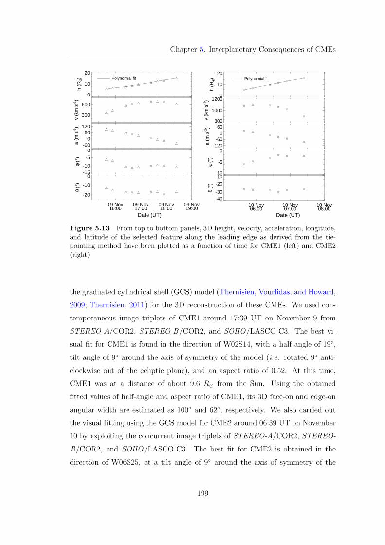
Chapter 5. Interplanetary Consequences of CMEs
0
10
20h
(RO •) Polynomial fit
300
600
v (k
m s
-1)
-600
60120
a (m
s-2)
-15-10
-50
φ (°
)
09 Nov16:00
09 Nov17:00
09 Nov18:00
09 Nov19:00
-20
-10
0
θ (°
)
Date (UT)
0
10
20
h (R
O •) Polynomial fit
800
1000
1200
v (k
m s
-1)
-120-60
060
a (m
s-2)
-10
-5
0
φ (°
)10 Nov06:00
10 Nov07:00
10 Nov08:00
-40-30
-20-10
θ (°
)Date (UT)
Figure 5.13 From top to bottom panels, 3D height, velocity, acceleration, longitude,and latitude of the selected feature along the leading edge as derived from the tie-pointing method have been plotted as a function of time for CME1 (left) and CME2(right)
the graduated cylindrical shell (GCS) model (Thernisien, Vourlidas, and Howard,
2009; Thernisien, 2011) for the 3D reconstruction of these CMEs. We used con-
temporaneous image triplets of CME1 around 17:39 UT on November 9 from
STEREO-A/COR2, STEREO-B/COR2, and SOHO/LASCO-C3. The best vi-
sual fit for CME1 is found in the direction of W02S14, with a half angle of 19◦,
tilt angle of 9◦ around the axis of symmetry of the model (i.e. rotated 9◦ anti-
clockwise out of the ecliptic plane), and an aspect ratio of 0.52. At this time,
CME1 was at a distance of about 9.6 R� from the Sun. Using the obtained
fitted values of half-angle and aspect ratio of CME1, its 3D face-on and edge-on
angular width are estimated as 100◦ and 62◦, respectively. We also carried out
the visual fitting using the GCS model for CME2 around 06:39 UT on November
10 by exploiting the concurrent image triplets of STEREO-A/COR2, STEREO-
B/COR2, and SOHO/LASCO-C3. The best fit for CME2 is obtained in the
direction of W06S25, at a tilt angle of 9◦ around the axis of symmetry of the
199
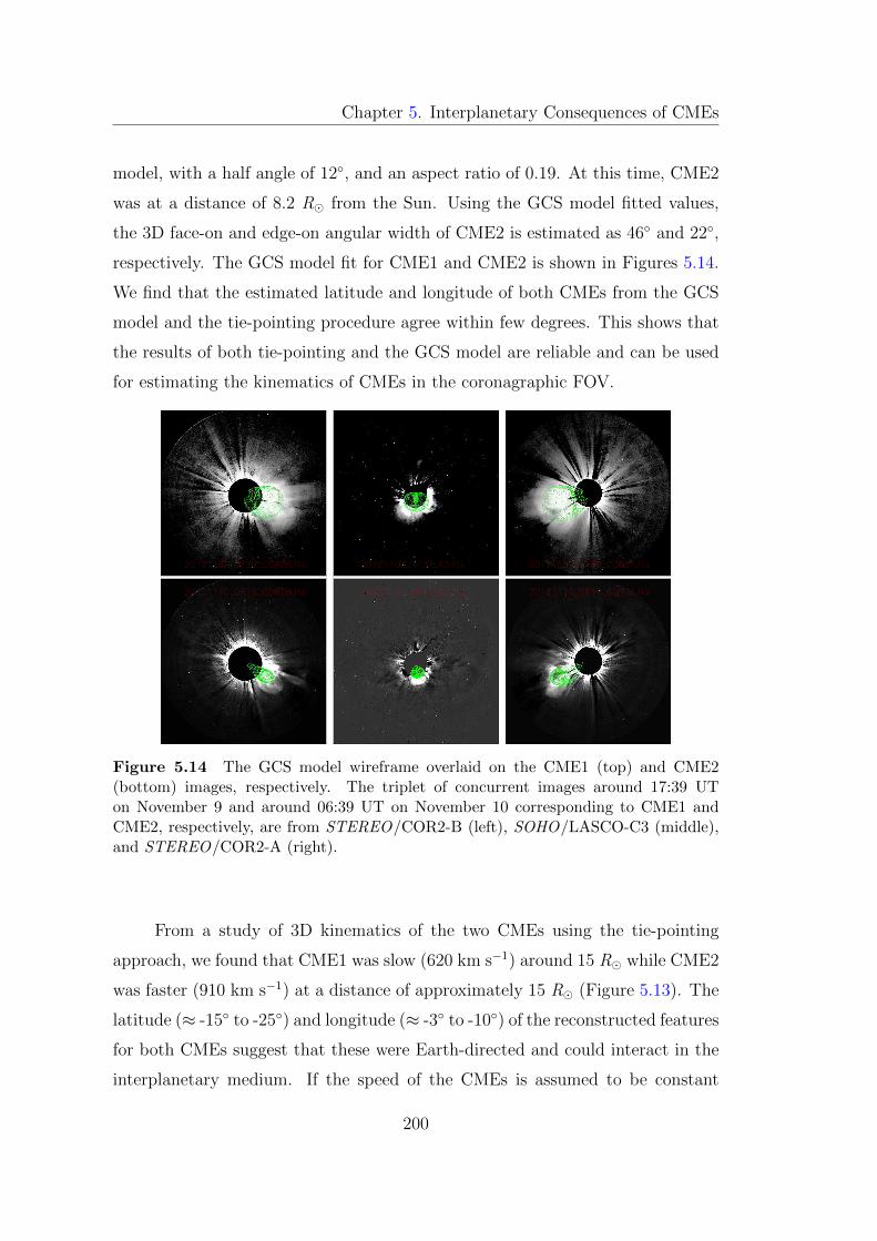
Chapter 5. Interplanetary Consequences of CMEs
model, with a half angle of 12◦, and an aspect ratio of 0.19. At this time, CME2
was at a distance of 8.2 R� from the Sun. Using the GCS model fitted values,
the 3D face-on and edge-on angular width of CME2 is estimated as 46◦ and 22◦,
respectively. The GCS model fit for CME1 and CME2 is shown in Figures 5.14.
We find that the estimated latitude and longitude of both CMEs from the GCS
model and the tie-pointing procedure agree within few degrees. This shows that
the results of both tie-pointing and the GCS model are reliable and can be used
for estimating the kinematics of CMEs in the coronagraphic FOV.
Figure 5.14 The GCS model wireframe overlaid on the CME1 (top) and CME2(bottom) images, respectively. The triplet of concurrent images around 17:39 UTon November 9 and around 06:39 UT on November 10 corresponding to CME1 andCME2, respectively, are from STEREO/COR2-B (left), SOHO/LASCO-C3 (middle),and STEREO/COR2-A (right).
From a study of 3D kinematics of the two CMEs using the tie-pointing
approach, we found that CME1 was slow (620 km s−1) around 15 R� while CME2
was faster (910 km s−1) at a distance of approximately 15 R� (Figure 5.13). The
latitude (≈ -15◦ to -25◦) and longitude (≈ -3◦ to -10◦) of the reconstructed features
for both CMEs suggest that these were Earth-directed and could interact in the
interplanetary medium. If the speed of the CMEs is assumed to be constant
200
Chapter 5. Interplanetary Consequences of CMEs
beyond the outer edge of the COR2 FOV, then these CMEs should have collided
at approximately 130 R� on November 11 around 02:30 UT. However, earlier
studies have shown that the speed of a CME can significantly change after the
coronagraphic FOV (Lindsay et al., 1999; Gopalswamy et al., 2000a; Cargill,
2004; Manoharan, 2006; Vrsnak et al., 2010). Therefore, further tracking of CME
features in the heliosphere is required to determine the exact location and time
of interaction of these CMEs.
5.3.2 Tracking of CMEs in HI FOV
The evolution of CME1 and CME2 in the running difference images of
COR2, HI1, and HI2 FOV is shown in Figure 5.15. To track and estimate the
arrival times of the CMEs in the heliosphere using HI1 and HI2 images, we
constructed the so-called J -maps. We derived the variation in the elongation
of selected features with time. The positively inclined bright features in the J -
maps (Figure 5.16) correspond to the enhanced density structure of the CMEs.
We tracked the leading and trailing edges (marked in green and red) of a bright
feature corresponding to the slow CME1 and the top edge (blue) of a bright
feature corresponding to the fast CME2. Prior to interpreting the tracked features
of CME1 in the J -map as its leading and trailing edges, respectively, the derived
elongations corresponding to all the three tracked features were overplotted on
the base difference HI1 images. On careful inspection of the sequence of these
images, we noticed that the two tracked features of CME1 correspond to the first
density enhancement at the front and the second density enhancement at the rear
edge of CME1, respectively. The base difference HI1-A images with overplotted
contours of elongation corresponding to the tracked features of CME1 and CME2
are shown in Figure 5.17. It is to be noted that the term ‘trailing edge’ of CME1
does not correspond to the rear-most portion of CME1 but refers to the part
behind the front and is not an image artifact in the J -map constructed from
running difference images.
Since the tracked features of CME2 were not observed well in the STEREO-
201
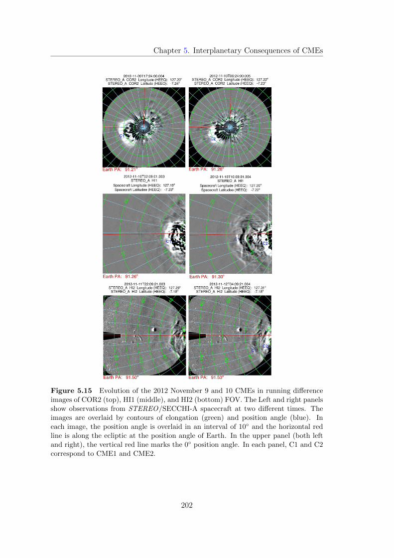
Chapter 5. Interplanetary Consequences of CMEs
Figure 5.15 Evolution of the 2012 November 9 and 10 CMEs in running differenceimages of COR2 (top), HI1 (middle), and HI2 (bottom) FOV. The Left and right panelsshow observations from STEREO/SECCHI-A spacecraft at two different times. Theimages are overlaid by contours of elongation (green) and position angle (blue). Ineach image, the position angle is overlaid in an interval of 10◦ and the horizontal redline is along the ecliptic at the position angle of Earth. In the upper panel (both leftand right), the vertical red line marks the 0◦ position angle. In each panel, C1 and C2correspond to CME1 and CME2.
202
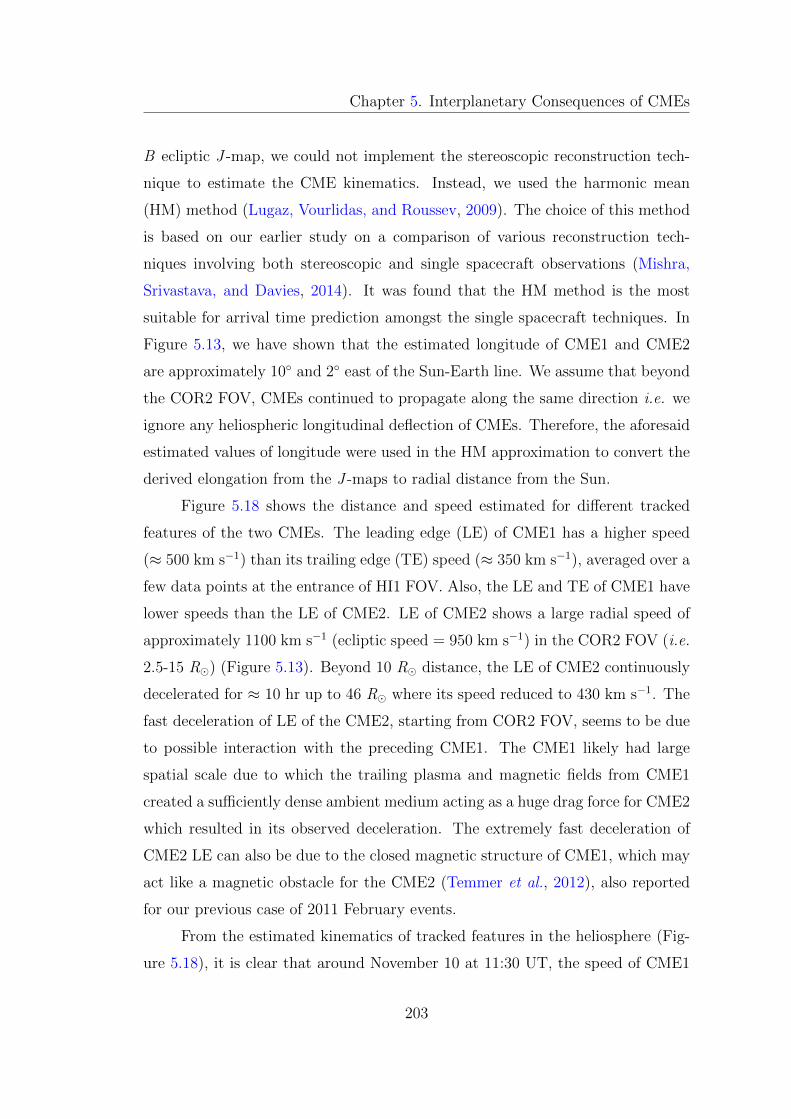
Chapter 5. Interplanetary Consequences of CMEs
B ecliptic J -map, we could not implement the stereoscopic reconstruction tech-
nique to estimate the CME kinematics. Instead, we used the harmonic mean
(HM) method (Lugaz, Vourlidas, and Roussev, 2009). The choice of this method
is based on our earlier study on a comparison of various reconstruction tech-
niques involving both stereoscopic and single spacecraft observations (Mishra,
Srivastava, and Davies, 2014). It was found that the HM method is the most
suitable for arrival time prediction amongst the single spacecraft techniques. In
Figure 5.13, we have shown that the estimated longitude of CME1 and CME2
are approximately 10◦ and 2◦ east of the Sun-Earth line. We assume that beyond
the COR2 FOV, CMEs continued to propagate along the same direction i.e. we
ignore any heliospheric longitudinal deflection of CMEs. Therefore, the aforesaid
estimated values of longitude were used in the HM approximation to convert the
derived elongation from the J -maps to radial distance from the Sun.
Figure 5.18 shows the distance and speed estimated for different tracked
features of the two CMEs. The leading edge (LE) of CME1 has a higher speed
(≈ 500 km s−1) than its trailing edge (TE) speed (≈ 350 km s−1), averaged over a
few data points at the entrance of HI1 FOV. Also, the LE and TE of CME1 have
lower speeds than the LE of CME2. LE of CME2 shows a large radial speed of
approximately 1100 km s−1 (ecliptic speed = 950 km s−1) in the COR2 FOV (i.e.
2.5-15 R�) (Figure 5.13). Beyond 10 R� distance, the LE of CME2 continuously
decelerated for ≈ 10 hr up to 46 R� where its speed reduced to 430 km s−1. The
fast deceleration of LE of the CME2, starting from COR2 FOV, seems to be due
to possible interaction with the preceding CME1. The CME1 likely had large
spatial scale due to which the trailing plasma and magnetic fields from CME1
created a sufficiently dense ambient medium acting as a huge drag force for CME2
which resulted in its observed deceleration. The extremely fast deceleration of
CME2 LE can also be due to the closed magnetic structure of CME1, which may
act like a magnetic obstacle for the CME2 (Temmer et al., 2012), also reported
for our previous case of 2011 February events.
From the estimated kinematics of tracked features in the heliosphere (Fig-
ure 5.18), it is clear that around November 10 at 11:30 UT, the speed of CME1
203

Chapter 5. Interplanetary Consequences of CMEs
Figure 5.16 Time-elongation map (J -map) using the COR2 and HI observationsof STEREO/SECCHI spacecraft during the interval of 2012 November 9-14 is shown.The features corresponding to the CME1 leading edge (LE), CME1 trailing edge (TE),and CME2 leading edge are (LE) tracked and over plotted on the J -map with green,red, and blue, respectively. The red rectangle (rightmost) is an enlarged plot of thered rectangle (on the left) which clearly shows that the red and blue tracks meet in theHI1 FOV.
TE started to increase from 365 km s−1 with a simultaneous decrease in speed
of CME2 LE from 625 km s−1. Such an observation of acceleration of CME1
and deceleration of CME2 provides evidence for the commencement of collision
(Temmer et al., 2012; Lugaz et al., 2012; Shen et al., 2012; Maricic et al., 2014;
Temmer et al., 2014; Mishra, Srivastava, and Davies, 2014).
Carefully observing the variations of speed of tracked CME1 TE and CME2
LE, the start and end boundaries of the collision phase are drawn as vertical lines
in Figure 5.18 (bottom). We noticed that at the end of the collision phase around
10 November at 17:15 UT, the speed of CME1 TE is ≈ 450 km s−1 and the speed
of CME2 LE is 430 km s−1. At the beginning of the marked collision phase,
CME1 TE was at a distance of 37 R�, and CME2 was at 30 R�. At the end
204
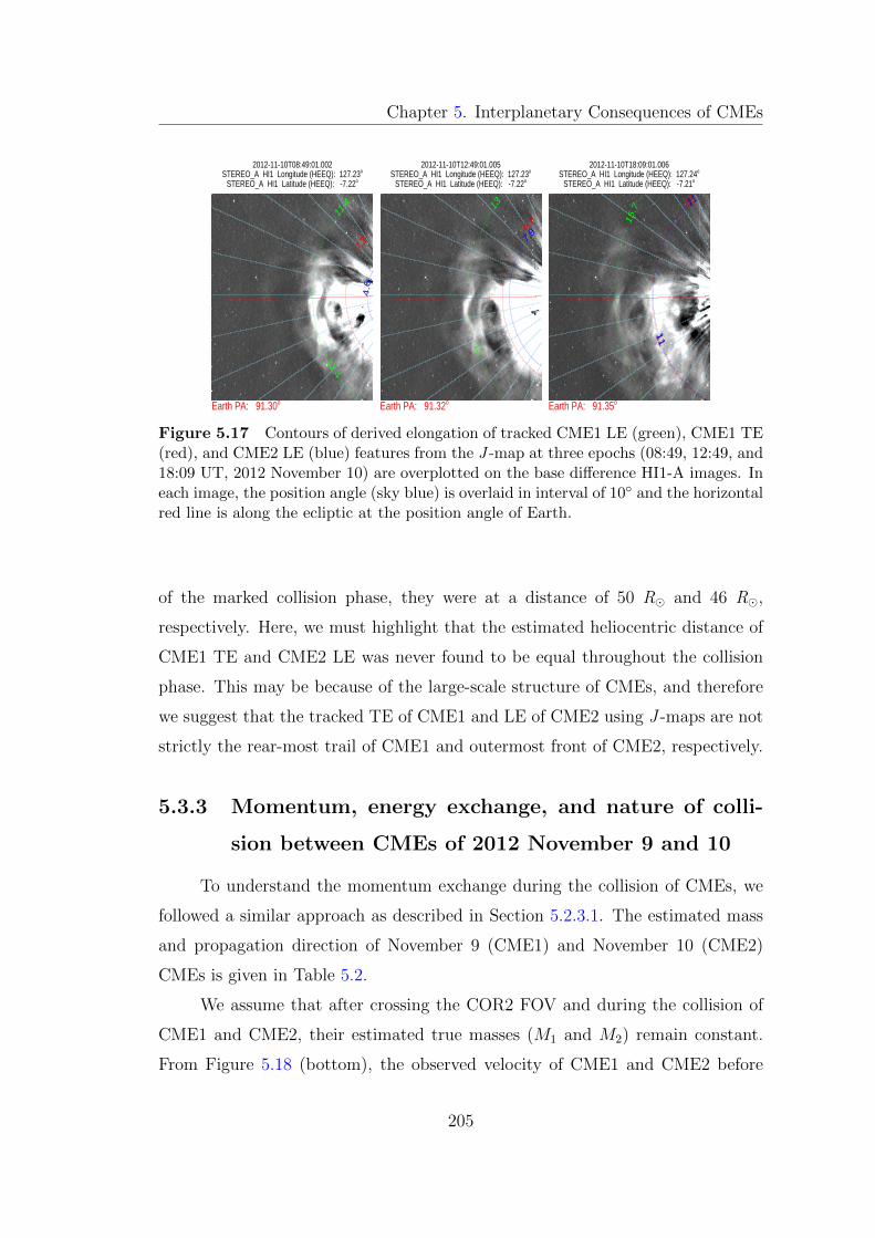
Chapter 5. Interplanetary Consequences of CMEs
11.4
11.4
7.2
4.6
2012-11-10T08:49:01.002
Earth PA: 91.30o
STEREO_A HI1 Longitude (HEEQ): 127.23o
STEREO_A HI1 Latitude (HEEQ): -7.22o
13
13
8.7
7.9
2012-11-10T12:49:01.005
Earth PA: 91.32o
STEREO_A HI1 Longitude (HEEQ): 127.23o
STEREO_A HI1 Latitude (HEEQ): -7.22o
15.7
1111
1111
2012-11-10T18:09:01.006
Earth PA: 91.35o
STEREO_A HI1 Longitude (HEEQ): 127.24o
STEREO_A HI1 Latitude (HEEQ): -7.21o
Figure 5.17 Contours of derived elongation of tracked CME1 LE (green), CME1 TE(red), and CME2 LE (blue) features from the J -map at three epochs (08:49, 12:49, and18:09 UT, 2012 November 10) are overplotted on the base difference HI1-A images. Ineach image, the position angle (sky blue) is overlaid in interval of 10◦ and the horizontalred line is along the ecliptic at the position angle of Earth.
of the marked collision phase, they were at a distance of 50 R� and 46 R�,
respectively. Here, we must highlight that the estimated heliocentric distance of
CME1 TE and CME2 LE was never found to be equal throughout the collision
phase. This may be because of the large-scale structure of CMEs, and therefore
we suggest that the tracked TE of CME1 and LE of CME2 using J -maps are not
strictly the rear-most trail of CME1 and outermost front of CME2, respectively.
5.3.3 Momentum, energy exchange, and nature of colli-
sion between CMEs of 2012 November 9 and 10
To understand the momentum exchange during the collision of CMEs, we
followed a similar approach as described in Section 5.2.3.1. The estimated mass
and propagation direction of November 9 (CME1) and November 10 (CME2)
CMEs is given in Table 5.2.
We assume that after crossing the COR2 FOV and during the collision of
CME1 and CME2, their estimated true masses (M1 and M2) remain constant.
From Figure 5.18 (bottom), the observed velocity of CME1 and CME2 before
205
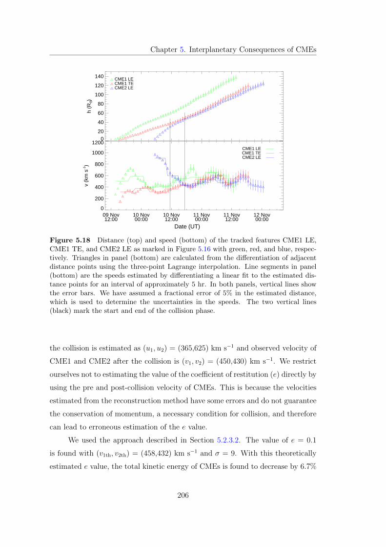
Chapter 5. Interplanetary Consequences of CMEs
0
20
40
60
80
100
120
140
h (R
O •)
CME1 LECME1 TECME2 LE
09 Nov12:00
10 Nov00:00
10 Nov12:00
11 Nov00:00
11 Nov12:00
12 Nov00:00
0
200
400
600
800
1000
1200
v (k
m s
-1)
CME1 LECME1 TECME2 LE
Date (UT)
Figure 5.18 Distance (top) and speed (bottom) of the tracked features CME1 LE,CME1 TE, and CME2 LE as marked in Figure 5.16 with green, red, and blue, respec-tively. Triangles in panel (bottom) are calculated from the differentiation of adjacentdistance points using the three-point Lagrange interpolation. Line segments in panel(bottom) are the speeds estimated by differentiating a linear fit to the estimated dis-tance points for an interval of approximately 5 hr. In both panels, vertical lines showthe error bars. We have assumed a fractional error of 5% in the estimated distance,which is used to determine the uncertainties in the speeds. The two vertical lines(black) mark the start and end of the collision phase.
the collision is estimated as (u1, u2) = (365,625) km s−1 and observed velocity of
CME1 and CME2 after the collision is (v1, v2) = (450,430) km s−1. We restrict
ourselves not to estimating the value of the coefficient of restitution (e) directly by
using the pre and post-collision velocity of CMEs. This is because the velocities
estimated from the reconstruction method have some errors and do not guarantee
the conservation of momentum, a necessary condition for collision, and therefore
can lead to erroneous estimation of the e value.
We used the approach described in Section 5.2.3.2. The value of e = 0.1
is found with (v1th, v2th) = (458,432) km s−1 and σ = 9. With this theoretically
estimated e value, the total kinetic energy of CMEs is found to decrease by 6.7%
206
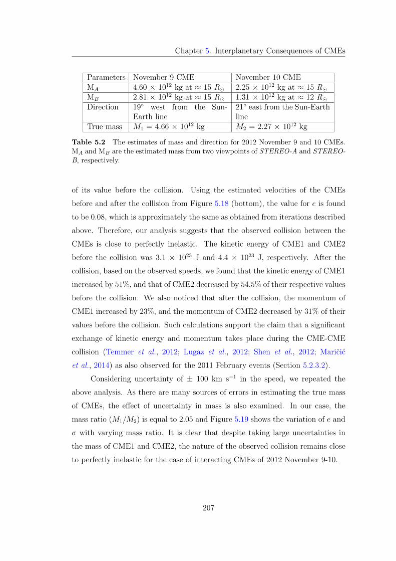
Chapter 5. Interplanetary Consequences of CMEs
Parameters November 9 CME November 10 CMEMA 4.60 × 10¹² kg at ≈ 15 R� 2.25 × 10¹² kg at ≈ 15 R�MB 2.81 × 10¹² kg at ≈ 15 R� 1.31 × 10¹² kg at ≈ 12 R�Direction 19◦ west from the Sun-
Earth line21◦ east from the Sun-Earthline
True mass M1 = 4.66 × 10¹² kg M2 = 2.27 × 10¹² kg
Table 5.2 The estimates of mass and direction for 2012 November 9 and 10 CMEs.MA and MB are the estimated mass from two viewpoints of STEREO-A and STEREO-B, respectively.
of its value before the collision. Using the estimated velocities of the CMEs
before and after the collision from Figure 5.18 (bottom), the value for e is found
to be 0.08, which is approximately the same as obtained from iterations described
above. Therefore, our analysis suggests that the observed collision between the
CMEs is close to perfectly inelastic. The kinetic energy of CME1 and CME2
before the collision was 3.1 × 10²³ J and 4.4 × 10²³ J, respectively. After the
collision, based on the observed speeds, we found that the kinetic energy of CME1
increased by 51%, and that of CME2 decreased by 54.5% of their respective values
before the collision. We also noticed that after the collision, the momentum of
CME1 increased by 23%, and the momentum of CME2 decreased by 31% of their
values before the collision. Such calculations support the claim that a significant
exchange of kinetic energy and momentum takes place during the CME-CME
collision (Temmer et al., 2012; Lugaz et al., 2012; Shen et al., 2012; Maricic
et al., 2014) as also observed for the 2011 February events (Section 5.2.3.2).
Considering uncertainty of ± 100 km s−1 in the speed, we repeated the
above analysis. As there are many sources of errors in estimating the true mass
of CMEs, the effect of uncertainty in mass is also examined. In our case, the
mass ratio (M1/M2) is equal to 2.05 and Figure 5.19 shows the variation of e and
σ with varying mass ratio. It is clear that despite taking large uncertainties in
the mass of CME1 and CME2, the nature of the observed collision remains close
to perfectly inelastic for the case of interacting CMEs of 2012 November 9-10.
207
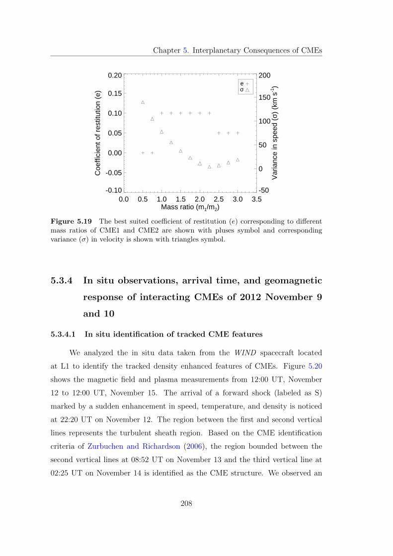
Chapter 5. Interplanetary Consequences of CMEs
0.0 0.5 1.0 1.5 2.0 2.5 3.0 3.5Mass ratio (m1/m2)
-0.10
-0.05
0.00
0.05
0.10
0.15
0.20
Coe
ffici
ent o
f res
titut
ion
(e)
-50
0
50
100
150
200
Var
ianc
e in
spe
ed (
σ) (
km s
-1)e
σ
Figure 5.19 The best suited coefficient of restitution (e) corresponding to differentmass ratios of CME1 and CME2 are shown with pluses symbol and correspondingvariance (σ) in velocity is shown with triangles symbol.
5.3.4 In situ observations, arrival time, and geomagnetic
response of interacting CMEs of 2012 November 9
and 10
5.3.4.1 In situ identification of tracked CME features
We analyzed the in situ data taken from the WIND spacecraft located
at L1 to identify the tracked density enhanced features of CMEs. Figure 5.20
shows the magnetic field and plasma measurements from 12:00 UT, November
12 to 12:00 UT, November 15. The arrival of a forward shock (labeled as S)
marked by a sudden enhancement in speed, temperature, and density is noticed
at 22:20 UT on November 12. The region between the first and second vertical
lines represents the turbulent sheath region. Based on the CME identification
criteria of Zurbuchen and Richardson (2006), the region bounded between the
second vertical lines at 08:52 UT on November 13 and the third vertical line at
02:25 UT on November 14 is identified as the CME structure. We observed an
208
Chapter 5. Interplanetary Consequences of CMEs
expansion of the CME in this region characterized by a monotonic decrease in
proton speed and temperature. Based on the predicted arrival times, which were
derived using the estimated kinematics of the remotely observed tracked features
of CME1 and CME2 as inputs in the DBM (explained in Section 5.3.4.2), this
region was associated with Earth-directed CME1 launched on November 9.
During the passage of CME1, the magnetic field was observed to be high
(≈ 20 nT), and plasma beta was less than unity (β < 1) with smooth rotation
in the magnetic field vector. Also, the latitude (θ) value of the magnetic field
vector decreased from 43◦ to -43◦ and its longitude (φ) decreased from 203◦ to
74◦. Therefore, this region can be classified as an MC and based on the observed
arrival time; it was associated with CME1. Due to the interaction of the CMEs,
the region associated with CME1 is found to be at a higher temperature than
found generally for a normal isolated CME.
The magnetic field strength (after the time marked by the third vertical
line) decreased, reaching a minimum value of 6 nT around 4:00 UT on November
14. This interval of a sudden drop in the magnetic field was associated with
a sudden rise in density, temperature, and plasma β, suggestive of a possible
magnetic hole (MH) (Tsurutani et al., 2006) which is considered as a signature of
magnetic reconnection (Burlaga and Lemaire, 1978). Another region of magnetic
field depression from 08:05 UT to 10:15 UT on November 14, reaching a minimum
value of 3 nT, is also noticed. Corresponding to this minimum magnetic field
value, the plasma β and temperature were found to increase. The region from
03:45 UT-08:05 UT on November 14, bounded between two distinct MH like
structures, has an enhanced magnetic field (≈ 15 nT) and plasma β less than
unity. This region, between two MH, seems to be a magnetic field remnant of
reconnecting CME structures.
Based on the extremely elevated interval of plasma beta, temperature, ob-
servation of MH, and probably sudden fast rotation in the magnetic field vector
in the region bounded between the third and fourth vertical lines in Figure 5.20,
this region was identified as the interaction region (labeled as IR) of CME1 TE
with CME2 LE.
209
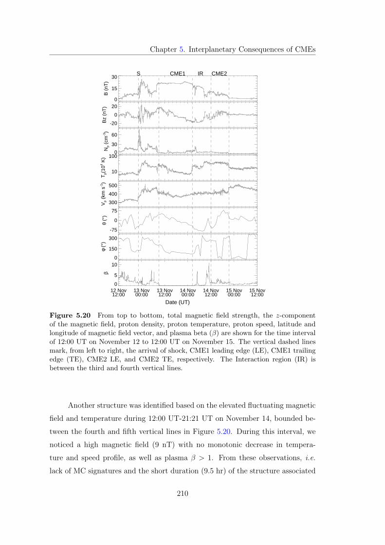
Chapter 5. Interplanetary Consequences of CMEs
0
15
30
B (
nT)
-20
0
20B
z (n
T)
0
30
60
Np
(cm
-3)
10
100
Tp(
104 K
)
300
400
500
Vp
(km
s-1)
-75
0
75
θ (°
)
0
150
300
φ (°
)
12 Nov12:00
13 Nov00:00
13 Nov12:00
14 Nov00:00
14 Nov12:00
15 Nov00:00
15 Nov12:00
0
5
10
β
Date (UT)
S CME1 IR CME2
Figure 5.20 From top to bottom, total magnetic field strength, the z-componentof the magnetic field, proton density, proton temperature, proton speed, latitude andlongitude of magnetic field vector, and plasma beta (β) are shown for the time intervalof 12:00 UT on November 12 to 12:00 UT on November 15. The vertical dashed linesmark, from left to right, the arrival of shock, CME1 leading edge (LE), CME1 trailingedge (TE), CME2 LE, and CME2 TE, respectively. The Interaction region (IR) isbetween the third and fourth vertical lines.
Another structure was identified based on the elevated fluctuating magnetic
field and temperature during 12:00 UT-21:21 UT on November 14, bounded be-
tween the fourth and fifth vertical lines in Figure 5.20. During this interval, we
noticed a high magnetic field (9 nT) with no monotonic decrease in tempera-
ture and speed profile, as well as plasma β > 1. From these observations, i.e.
lack of MC signatures and the short duration (9.5 hr) of the structure associated
210
Chapter 5. Interplanetary Consequences of CMEs
with CME2, we infer that the WIND spacecraft perhaps intersected the flank
of CME2 (Mostl et al., 2010). This is also confirmed by the estimated latitude
(-25◦) of CME2 using the GCS model (described in Section 5.3.1). On examining
the evolution of CME2 in the HI1-A movie, we noticed that CME2 was directed
towards the southern hemisphere, which was a favorable condition for its flank
to encounter with the WIND spacecraft.
We observed that the magnitude of the magnetic field in the MC region
was constant around ≈ 20 nT, which may be due to the passage of the shock
from CME1. We also noticed that the average temperature in the first half
of CME1 was higher (≈ 105 K) than found in general (≈ 104 K). The high
temperature of the CME1 may occur due to its collision with CME2, thereby
resulting in its compression. Another possibility of high temperature of CME1 is
due to the passage of the forward shock driven by CME2 as reported in earlier
studies (Lugaz, Manchester, and Gombosi, 2005; Liu et al., 2012; Maricic et al.,
2014; Mishra and Srivastava, 2014). However, in the present case, the following
CME2 was also observed with a high temperature (≈ 5 × 10⁵ K), which has not
been reported in earlier studies of interacting CMEs. We noticed significant high
density at the front of CME1, possibly due to overall compression by sweeping
the plasma of CME1 at its leading edge by CME2 driven shock.
5.3.4.2 Arrival time of tracked features
We used the estimated speed at the last point of measurement (up to where
CMEs could be tracked unambiguously in HI) and used it as input to the DBM
developed by Vrsnak et al. (2013) to estimate the arrival time of tracked features
at L1. The estimated speed, time, and distance (v0, t0, and R�) of LE of CME1
(a green track in the J -map) are used as inputs to the DBM, corresponding to an
extreme range of the drag parameter, to predict its arrival time and transit speed
at L1. In situ observations show a peak in density, ≈ 0.5 hr after the shock arrival
around 23:00 UT on November 12 with a transit speed of 375 km s−1, which is
expected to be the actual arrival of the tracked LE feature corresponding to
CME1. The predicted values of the arrival time and transit speed of the features
211

Chapter 5. Interplanetary Consequences of CMEs
and errors from the actual values are shown in Table 5.3.
For the TE feature of CME1 and LE of CME2, we assume they encountered
the dense ambient solar wind medium created by the preceding CME1 LE. There-
fore, their kinematics with the maximum value of the statistical range of the drag
parameter (2.0 × 10⁻⁷ km−1) are used as inputs to the DBM. We consider that
the TE of CME1 corresponds to the density enhancement at the trailing front of
CME1. At the rear edge of CME1, a density enhancement (12 particles cm−3)
was observed around 23:30 UT in WIND observations on November 13, which
is considered the actual arrival of TE of CME1. The predicted arrival time and
transit speed of this feature and errors therein are given in Table 5.3. We further
notice that in in situ data, an enhancement in density corresponding to LE of
CME2 around 12:00 UT on 14 November (marked as the arrival of CME2 with
the fourth vertical line in Figure 5.20) was observed, which can be considered
as the actual arrival time of LE of CME2. The predicted values of CME2 LE,
using its kinematics with DBM and errors therein, are also listed in Table 5.3.
The error for CME2 LE is large, but several factors can lead to such large errors,
which are discussed in Section 5.3.5. It must be highlighted that if the 3D speed
of CMEs estimated at the final height in COR2 FOV is assumed to be constant
up to L1, then the predicted arrival time of CME1 and CME2 will be ≈ 10-16 hr
and 44 hr earlier, respectively, than the predicted arrival times using post-collision
speeds combined with DBM. This emphasizes HI observations and post-collision
speeds of CMEs as inputs to the DBM for an improved arrival time prediction of
interacting CMEs. Similarly, using HI observations, Colaninno, Vourlidas, and
Wu (2013) have shown that a linear fit to the deprojected height-time data above
50 R� gives a 12 hr improvement over the CME arrival time estimated using
LASCO data.
5.3.4.3 Geomagnetic consequences of interacting CMEs
As mentioned in Section 5.1, very few studies have been dedicated to the
study of the geomagnetic consequences of interacting CMEs. The CMEs of 2012
November 9-10 resulted in a single strong geomagnetic storm with Dst index ≈
212
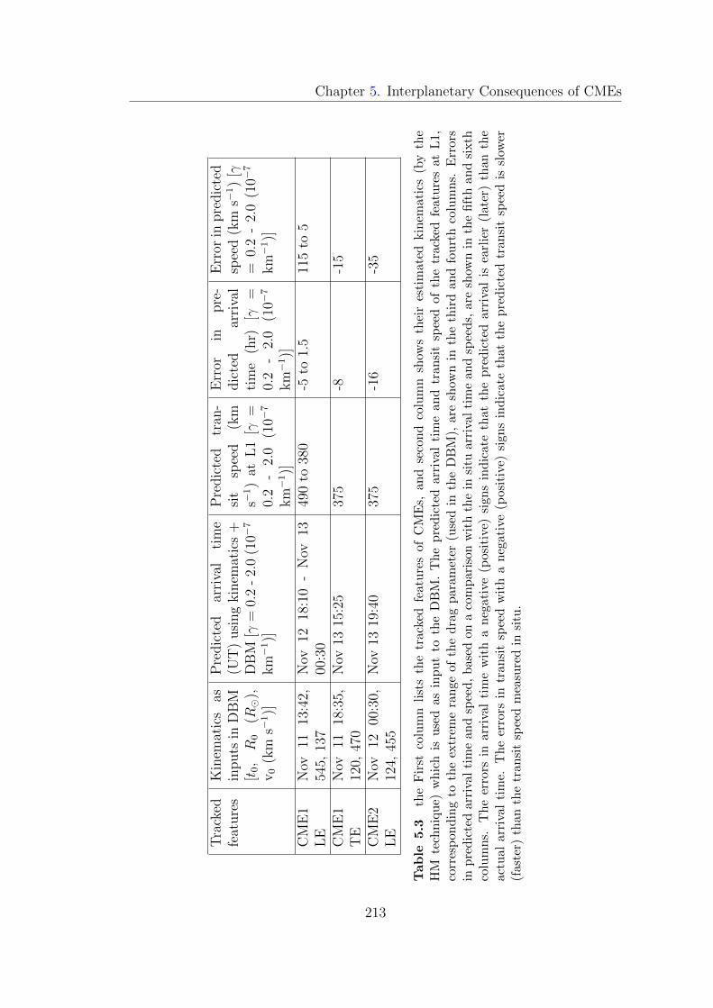
Chapter 5. Interplanetary Consequences of CMEs
Tra
cked
feat
ure
sK
inem
atic
sas
inputs
inD
BM
[t0,R
0(R�
),v
0(k
ms−
1)]
Pre
dic
ted
arri
val
tim
e(U
T)
usi
ng
kin
emat
ics
+D
BM
[γ=
0.2
-2.
0(1
0−7
km−
1)]
Pre
dic
ted
tran
-si
tsp
eed
(km
s−1)
atL
1[γ
=0.
2-
2.0
(10−
7
km−
1)]
Err
orin
pre
-dic
ted
arri
val
tim
e(h
r)[γ
=0.
2-
2.0
(10−
7
km−
1)]
Err
orin
pre
dic
ted
spee
d(k
ms−
1)
[γ=
0.2
-2.
0(1
0−7
km−
1)]
CM
E1
LE
Nov
1113
:42,
545,
137
Nov
1218
:10
-N
ov13
00:3
049
0to
380
-5to
1.5
115
to5
CM
E1
TE
Nov
1118
:35,
120,
470
Nov
1315
:25
375
-8-1
5
CM
E2
LE
Nov
1200
:30,
124,
455
Nov
1319
:40
375
-16
-35
Table
5.3
the
Fir
stco
lum
nli
sts
the
trac
ked
feat
ure
sof
CM
Es,
and
seco
nd
colu
mn
show
sth
eir
esti
mat
edkin
emat
ics
(by
the
HM
tech
niq
ue)
wh
ich
isu
sed
asin
pu
tto
the
DB
M.
Th
ep
red
icte
dar
riva
lti
me
and
tran
sit
spee
dof
the
trac
ked
feat
ure
sat
L1,
corr
esp
on
din
gto
the
extr
eme
ran
geof
the
dra
gp
aram
eter
(use
din
the
DB
M),
are
show
nin
the
thir
dan
dfo
urt
hco
lum
ns.
Err
ors
inp
red
icte
darr
ival
tim
ean
dsp
eed
,b
ased
ona
com
par
ison
wit
hth
ein
situ
arri
val
tim
ean
dsp
eed
s,ar
esh
own
inth
efi
fth
and
sixth
colu
mn
s.T
he
erro
rsin
arr
ival
tim
ew
ith
an
egat
ive
(pos
itiv
e)si
gns
ind
icat
eth
atth
epre
dic
ted
arri
val
isea
rlie
r(l
ater
)th
anth
eact
ual
arr
ival
tim
e.T
he
erro
rsin
tran
sit
spee
dw
ith
an
egat
ive
(pos
itiv
e)si
gns
ind
icat
eth
atth
epre
dic
ted
tran
sit
spee
dis
slow
er(f
ast
er)
than
the
tran
sit
spee
dm
easu
red
insi
tu.
213
Chapter 5. Interplanetary Consequences of CMEs
-108 nT at 8:00 UT on November 14, therefore it is important to investigate
the impact of the interaction of the CME1 of November 9 with the CME2 of
November 10 on the terrestrial magnetosphere-ionosphere system in details.
Figures 5.21(a-e) reveal the variations in the solar wind parameters in the
geocentric solar ecliptic (GSE) coordinate system during 2012 November 12-
15. These parameters include solar wind proton density (in cm−3), velocity
(in km s−1, negative X-direction), ram pressure (in nPa), the Z-component
of the interplanetary magnetic field (IMF Bz, in nT) and the Y -component
of the interplanetary electric field (IEFy, in mV m−1) respectively. These
data with a cadence of 1 min are taken from the NASA GSFC CDAWeb
(www.cdaweb.gsfc.nasa.gov/istp_public/). It is also important to note that
the solar wind parameters presented in Figures 5.21(a-e) are corrected for prop-
agation lag till the nose of the terrestrial bow shock. To compare the variations
of these parameters with the magnetospheric and ionospheric parameters, addi-
tional time lags that account for the magnetosheath transit time and the Alfven
transit time are calculated (Chakrabarty et al., 2005). Therefore, the solar wind
parameters presented in Figures 5.21(a-e) are corrected for the propagation lag,
point by point, till ionosphere.
Figure 5.21(f) represents the variation in the polar cap (PC) index. The
PC index is shown (Troshichev et al., 2000) to capture the variations in the
ionospheric electric field over the polar region efficiently. Figure 5.21(g) shows
the variation in the Sym-H (in nT) index which primarily represents the variation
in the magnetospheric ring current (Iyemori and Rao, 1996). Figure 5.21(h)
shows variations in the westward (midnight sector) auroral electrojet (AL) current
(in nT) which captures auroral substorm processes reasonably well. Further, in
Figure 5.21, the arrival of the shock is denoted by S; different vertical lines mark
the arrival of different features of CME1 and CME2 and are labeled in the same
manner as in Figure 5.20.
Figure 5.21(a) reveals the arrival of two distinctly enhanced density struc-
tures; first enhancement occurred at the arrival of the shock-sheath region before
CME1 LE (on November 12 at 20:00 UT to November 13 at 04:00 UT), and the
214
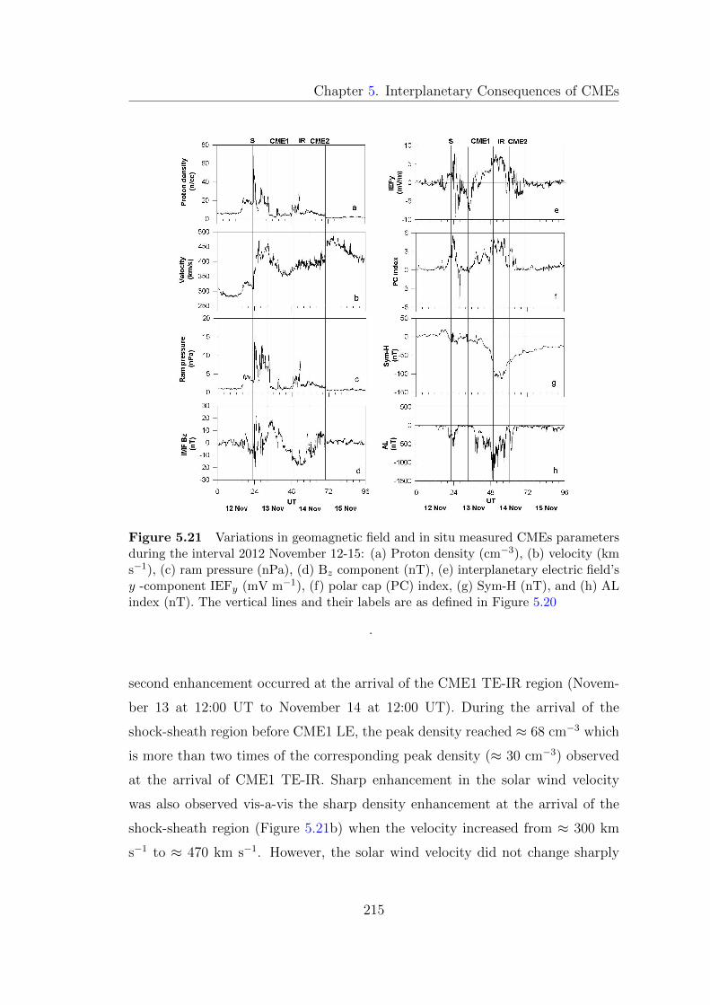
Chapter 5. Interplanetary Consequences of CMEs
Figure 5.21 Variations in geomagnetic field and in situ measured CMEs parametersduring the interval 2012 November 12-15: (a) Proton density (cm−3), (b) velocity (kms−1), (c) ram pressure (nPa), (d) Bz component (nT), (e) interplanetary electric field’sy -component IEFy (mV m−1), (f) polar cap (PC) index, (g) Sym-H (nT), and (h) ALindex (nT). The vertical lines and their labels are as defined in Figure 5.20
.
second enhancement occurred at the arrival of the CME1 TE-IR region (Novem-
ber 13 at 12:00 UT to November 14 at 12:00 UT). During the arrival of the
shock-sheath region before CME1 LE, the peak density reached ≈ 68 cm−3 which
is more than two times of the corresponding peak density (≈ 30 cm−3) observed
at the arrival of CME1 TE-IR. Sharp enhancement in the solar wind velocity
was also observed vis-a-vis the sharp density enhancement at the arrival of the
shock-sheath region (Figure 5.21b) when the velocity increased from ≈ 300 km
s−1 to ≈ 470 km s−1. However, the solar wind velocity did not change sharply
215
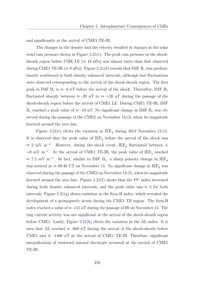
Chapter 5. Interplanetary Consequences of CMEs
and significantly at the arrival of CME1 TE-IR.
The changes in the density and the velocity resulted in changes in the solar
wind ram pressure shown in Figure 5.21(c). The peak ram pressure in the shock-
sheath region before CME LE (≈ 18 nPa) was almost twice than that observed
during CME1 TE-IR (≈ 9 nPa). Figure 5.21(d) reveals that IMF Bz was predom-
inantly southward in both density enhanced intervals, although fast fluctuations
were observed corresponding to the arrival of the shock-sheath region. The first
peak in IMF Bz is ≈ -8 nT before the arrival of the shock. Thereafter, IMF Bz
fluctuated sharply between ≈ -20 nT to ≈ +20 nT during the passage of the
shock-sheath region before the arrival of CME1 LE. During CME1 TE-IR, IMF
Bz reached a peak value of ≈ -18 nT. No significant change in IMF Bz was ob-
served during the passage of the CME2 on November 14-15, when its magnitude
hovered around the zero line.
Figure 5.21(e) elicits the variation in IEFy during 2012 November 12-15.
It is observed that the peak value of IEFy before the arrival of the shock was
≈ 2 mV m−1. However, during the shock event, IEFy fluctuated between ±∼8 mV m−1. At the arrival of CME1 TE-IR, the peak value of IEFy reached
≈ 7.5 mV m−1. In fact, similar to IMF Bz, a sharp polarity change in IEFy
was noticed at ≈ 09:40 UT on November 14. No significant change in IEFy was
observed during the passage of the CME2 on November 14-15, when its magnitude
hovered around the zero line. Figure 5.21(f) shows that the PC index increased
during both density enhanced intervals, and the peak value was ≈ 5 for both
intervals. Figure 5.21(g) shows variation in the Sym-H index, which revealed the
development of a geomagnetic storm during the CME1 TE region. The Sym-H
index reached a value of ≈ -115 nT during the passage of IR on November 14. The
ring current activity was not significant at the arrival of the shock-sheath region
before CME1. Lastly, Figure 5.21(h) elicits the variation in the AL index. It is
seen that AL reached ≈ -600 nT during the arrival of the shock-sheath before
CME1 and ≈ -1400 nT at the arrival of CME1 TE-IR. Therefore, significant
intensification of westward auroral electrojet occurred at the arrival of CME1
TE-IR.
216
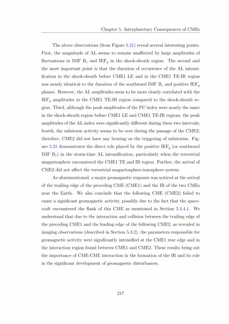
Chapter 5. Interplanetary Consequences of CMEs
The above observations (from Figure 5.21) reveal several interesting points.
First, the magnitude of AL seems to remain unaffected by large amplitudes of
fluctuations in IMF Bz and IEFy in the shock-sheath region. The second and
the most important point is that the duration of occurrence of the AL intensi-
fication in the shock-sheath before CME1 LE and in the CME1 TE-IR region
was nearly identical to the duration of the southward IMF Bz and positive IEFy
phases. However, the AL amplitudes seem to be more closely correlated with the
IEFy amplitudes in the CME1 TE-IR region compared to the shock-sheath re-
gion. Third, although the peak amplitudes of the PC index were nearly the same
in the shock-sheath region before CME1 LE and CME1 TE-IR regions, the peak
amplitudes of the AL index were significantly different during these two intervals;
fourth, the substorm activity seems to be over during the passage of the CME2;
therefore, CME2 did not have any bearing on the triggering of substorms. Fig-
ure 5.21 demonstrates the direct role played by the positive IEFy (or southward
IMF Bz) in the storm-time AL intensification, particularly when the terrestrial
magnetosphere encountered the CME1 TE and IR region. Further, the arrival of
CME2 did not affect the terrestrial magnetosphere-ionosphere system.
As aforementioned, a major geomagnetic response was noticed at the arrival
of the trailing edge of the preceding CME (CME1) and the IR of the two CMEs
near the Earth. We also conclude that the following CME (CME2) failed to
cause a significant geomagnetic activity, possibly due to the fact that the space-
craft encountered the flank of this CME as mentioned in Section 5.3.4.1. We
understand that due to the interaction and collision between the trailing edge of
the preceding CME1 and the leading edge of the following CME2, as revealed in
imaging observations (described in Section 5.3.2), the parameters responsible for
geomagnetic activity were significantly intensified at the CME1 rear edge and in
the interaction region found between CME1 and CME2. These results bring out
the importance of CME-CME interaction in the formation of the IR and its role
in the significant development of geomagnetic disturbances.
217
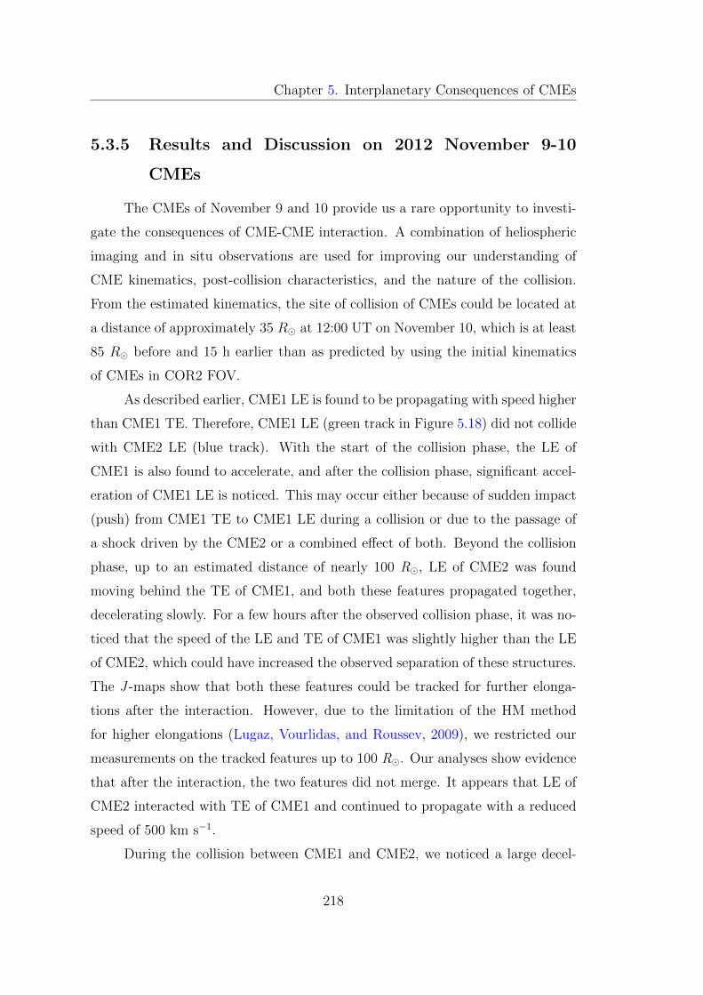
Chapter 5. Interplanetary Consequences of CMEs
5.3.5 Results and Discussion on 2012 November 9-10
CMEs
The CMEs of November 9 and 10 provide us a rare opportunity to investi-
gate the consequences of CME-CME interaction. A combination of heliospheric
imaging and in situ observations are used for improving our understanding of
CME kinematics, post-collision characteristics, and the nature of the collision.
From the estimated kinematics, the site of collision of CMEs could be located at
a distance of approximately 35 R� at 12:00 UT on November 10, which is at least
85 R� before and 15 h earlier than as predicted by using the initial kinematics
of CMEs in COR2 FOV.
As described earlier, CME1 LE is found to be propagating with speed higher
than CME1 TE. Therefore, CME1 LE (green track in Figure 5.18) did not collide
with CME2 LE (blue track). With the start of the collision phase, the LE of
CME1 is also found to accelerate, and after the collision phase, significant accel-
eration of CME1 LE is noticed. This may occur either because of sudden impact
(push) from CME1 TE to CME1 LE during a collision or due to the passage of
a shock driven by the CME2 or a combined effect of both. Beyond the collision
phase, up to an estimated distance of nearly 100 R�, LE of CME2 was found
moving behind the TE of CME1, and both these features propagated together,
decelerating slowly. For a few hours after the observed collision phase, it was no-
ticed that the speed of the LE and TE of CME1 was slightly higher than the LE
of CME2, which could have increased the observed separation of these structures.
The J -maps show that both these features could be tracked for further elonga-
tions after the interaction. However, due to the limitation of the HM method
for higher elongations (Lugaz, Vourlidas, and Roussev, 2009), we restricted our
measurements on the tracked features up to 100 R�. Our analyses show evidence
that after the interaction, the two features did not merge. It appears that LE of
CME2 interacted with TE of CME1 and continued to propagate with a reduced
speed of 500 km s−1.
During the collision between CME1 and CME2, we noticed a large decel-
218
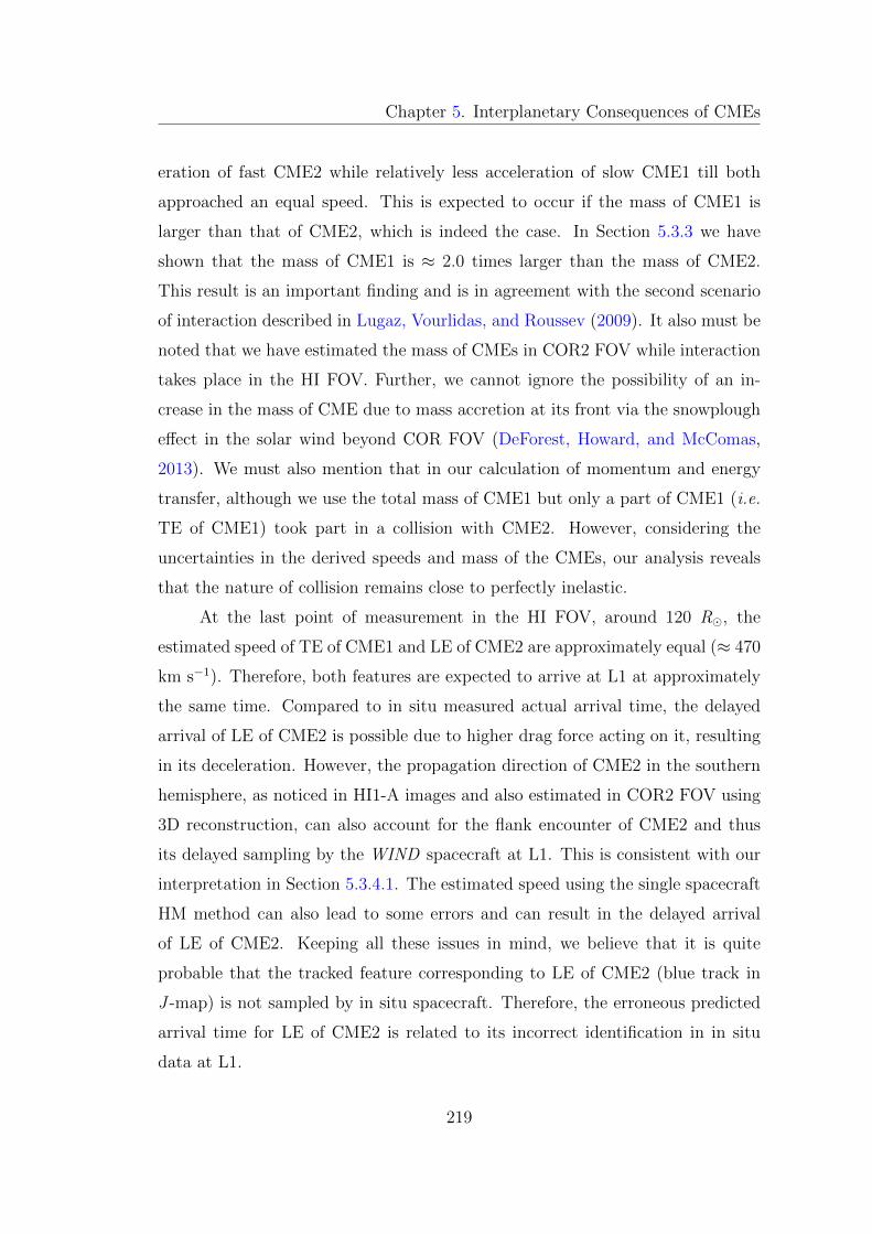
Chapter 5. Interplanetary Consequences of CMEs
eration of fast CME2 while relatively less acceleration of slow CME1 till both
approached an equal speed. This is expected to occur if the mass of CME1 is
larger than that of CME2, which is indeed the case. In Section 5.3.3 we have
shown that the mass of CME1 is ≈ 2.0 times larger than the mass of CME2.
This result is an important finding and is in agreement with the second scenario
of interaction described in Lugaz, Vourlidas, and Roussev (2009). It also must be
noted that we have estimated the mass of CMEs in COR2 FOV while interaction
takes place in the HI FOV. Further, we cannot ignore the possibility of an in-
crease in the mass of CME due to mass accretion at its front via the snowplough
effect in the solar wind beyond COR FOV (DeForest, Howard, and McComas,
2013). We must also mention that in our calculation of momentum and energy
transfer, although we use the total mass of CME1 but only a part of CME1 (i.e.
TE of CME1) took part in a collision with CME2. However, considering the
uncertainties in the derived speeds and mass of the CMEs, our analysis reveals
that the nature of collision remains close to perfectly inelastic.
At the last point of measurement in the HI FOV, around 120 R�, the
estimated speed of TE of CME1 and LE of CME2 are approximately equal (≈ 470
km s−1). Therefore, both features are expected to arrive at L1 at approximately
the same time. Compared to in situ measured actual arrival time, the delayed
arrival of LE of CME2 is possible due to higher drag force acting on it, resulting
in its deceleration. However, the propagation direction of CME2 in the southern
hemisphere, as noticed in HI1-A images and also estimated in COR2 FOV using
3D reconstruction, can also account for the flank encounter of CME2 and thus
its delayed sampling by the WIND spacecraft at L1. This is consistent with our
interpretation in Section 5.3.4.1. The estimated speed using the single spacecraft
HM method can also lead to some errors and can result in the delayed arrival
of LE of CME2. Keeping all these issues in mind, we believe that it is quite
probable that the tracked feature corresponding to LE of CME2 (blue track in
J -map) is not sampled by in situ spacecraft. Therefore, the erroneous predicted
arrival time for LE of CME2 is related to its incorrect identification in in situ
data at L1.
219
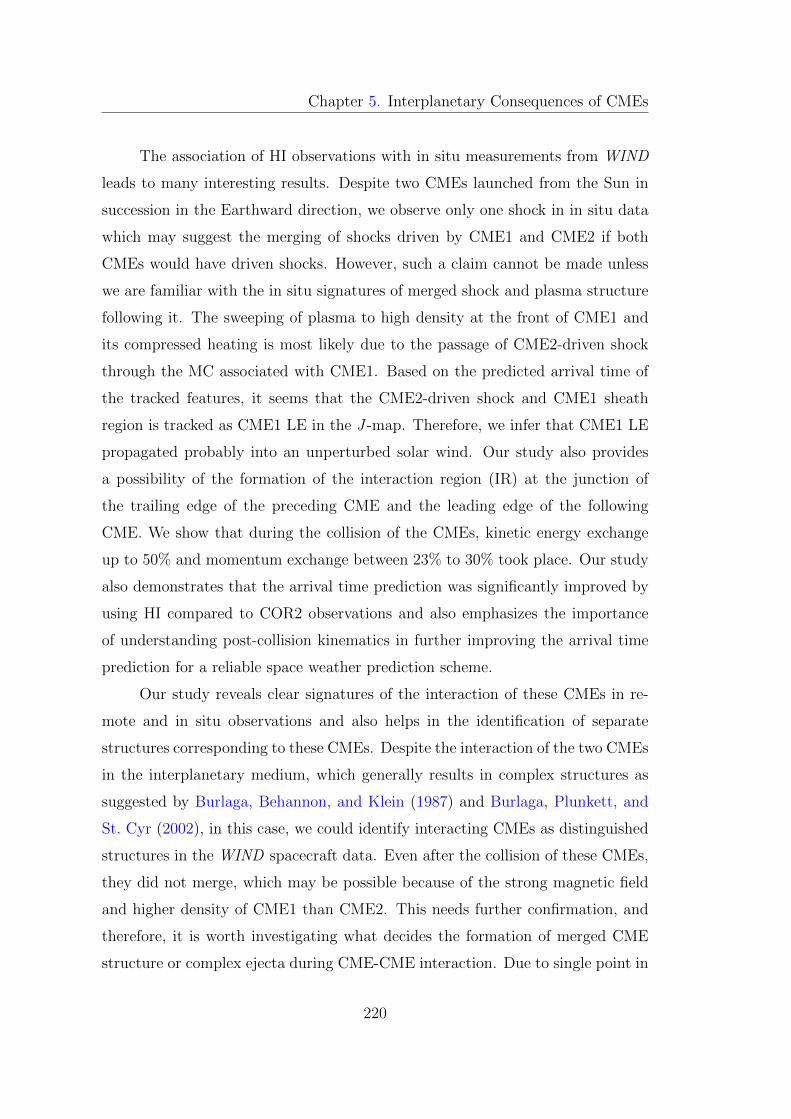
Chapter 5. Interplanetary Consequences of CMEs
The association of HI observations with in situ measurements from WIND
leads to many interesting results. Despite two CMEs launched from the Sun in
succession in the Earthward direction, we observe only one shock in in situ data
which may suggest the merging of shocks driven by CME1 and CME2 if both
CMEs would have driven shocks. However, such a claim cannot be made unless
we are familiar with the in situ signatures of merged shock and plasma structure
following it. The sweeping of plasma to high density at the front of CME1 and
its compressed heating is most likely due to the passage of CME2-driven shock
through the MC associated with CME1. Based on the predicted arrival time of
the tracked features, it seems that the CME2-driven shock and CME1 sheath
region is tracked as CME1 LE in the J -map. Therefore, we infer that CME1 LE
propagated probably into an unperturbed solar wind. Our study also provides
a possibility of the formation of the interaction region (IR) at the junction of
the trailing edge of the preceding CME and the leading edge of the following
CME. We show that during the collision of the CMEs, kinetic energy exchange
up to 50% and momentum exchange between 23% to 30% took place. Our study
also demonstrates that the arrival time prediction was significantly improved by
using HI compared to COR2 observations and also emphasizes the importance
of understanding post-collision kinematics in further improving the arrival time
prediction for a reliable space weather prediction scheme.
Our study reveals clear signatures of the interaction of these CMEs in re-
mote and in situ observations and also helps in the identification of separate
structures corresponding to these CMEs. Despite the interaction of the two CMEs
in the interplanetary medium, which generally results in complex structures as
suggested by Burlaga, Behannon, and Klein (1987) and Burlaga, Plunkett, and
St. Cyr (2002), in this case, we could identify interacting CMEs as distinguished
structures in the WIND spacecraft data. Even after the collision of these CMEs,
they did not merge, which may be possible because of the strong magnetic field
and higher density of CME1 than CME2. This needs further confirmation, and
therefore, it is worth investigating what decides the formation of merged CME
structure or complex ejecta during CME-CME interaction. Due to single point in
220
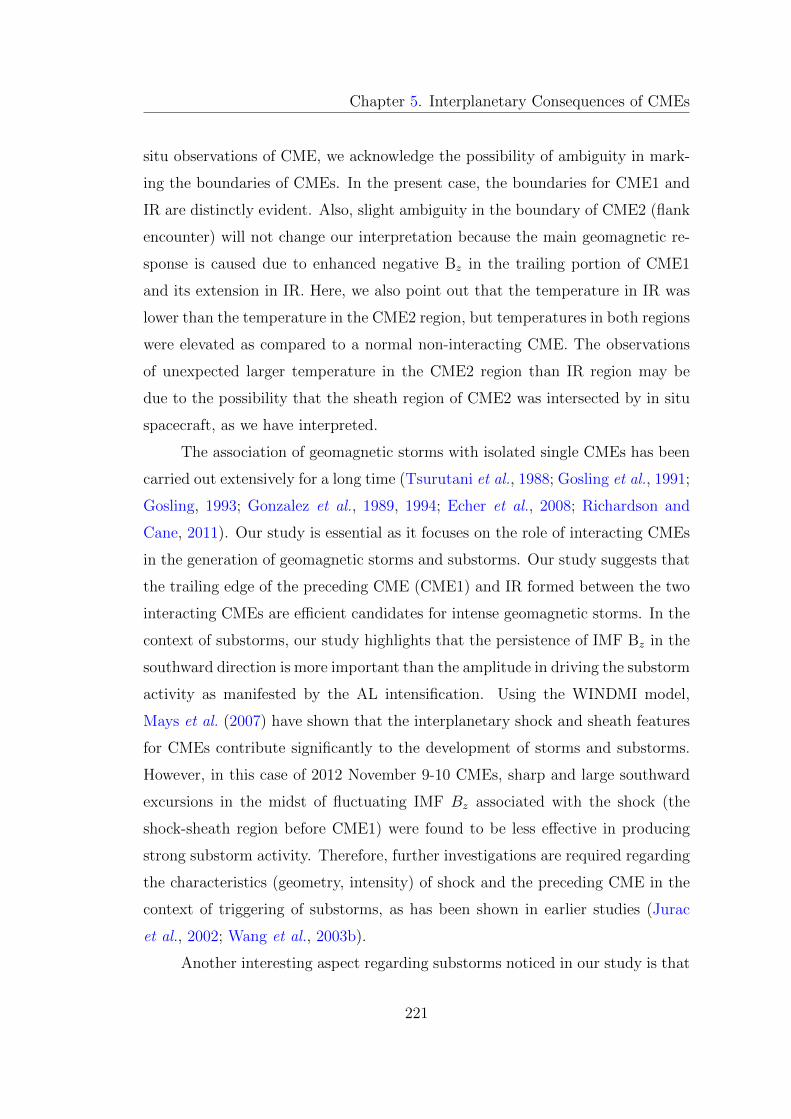
Chapter 5. Interplanetary Consequences of CMEs
situ observations of CME, we acknowledge the possibility of ambiguity in mark-
ing the boundaries of CMEs. In the present case, the boundaries for CME1 and
IR are distinctly evident. Also, slight ambiguity in the boundary of CME2 (flank
encounter) will not change our interpretation because the main geomagnetic re-
sponse is caused due to enhanced negative Bz in the trailing portion of CME1
and its extension in IR. Here, we also point out that the temperature in IR was
lower than the temperature in the CME2 region, but temperatures in both regions
were elevated as compared to a normal non-interacting CME. The observations
of unexpected larger temperature in the CME2 region than IR region may be
due to the possibility that the sheath region of CME2 was intersected by in situ
spacecraft, as we have interpreted.
The association of geomagnetic storms with isolated single CMEs has been
carried out extensively for a long time (Tsurutani et al., 1988; Gosling et al., 1991;
Gosling, 1993; Gonzalez et al., 1989, 1994; Echer et al., 2008; Richardson and
Cane, 2011). Our study is essential as it focuses on the role of interacting CMEs
in the generation of geomagnetic storms and substorms. Our study suggests that
the trailing edge of the preceding CME (CME1) and IR formed between the two
interacting CMEs are efficient candidates for intense geomagnetic storms. In the
context of substorms, our study highlights that the persistence of IMF Bz in the
southward direction is more important than the amplitude in driving the substorm
activity as manifested by the AL intensification. Using the WINDMI model,
Mays et al. (2007) have shown that the interplanetary shock and sheath features
for CMEs contribute significantly to the development of storms and substorms.
However, in this case of 2012 November 9-10 CMEs, sharp and large southward
excursions in the midst of fluctuating IMF Bz associated with the shock (the
shock-sheath region before CME1) were found to be less effective in producing
strong substorm activity. Therefore, further investigations are required regarding
the characteristics (geometry, intensity) of shock and the preceding CME in the
context of triggering of substorms, as has been shown in earlier studies (Jurac
et al., 2002; Wang et al., 2003b).
Another interesting aspect regarding substorms noticed in our study is that
221
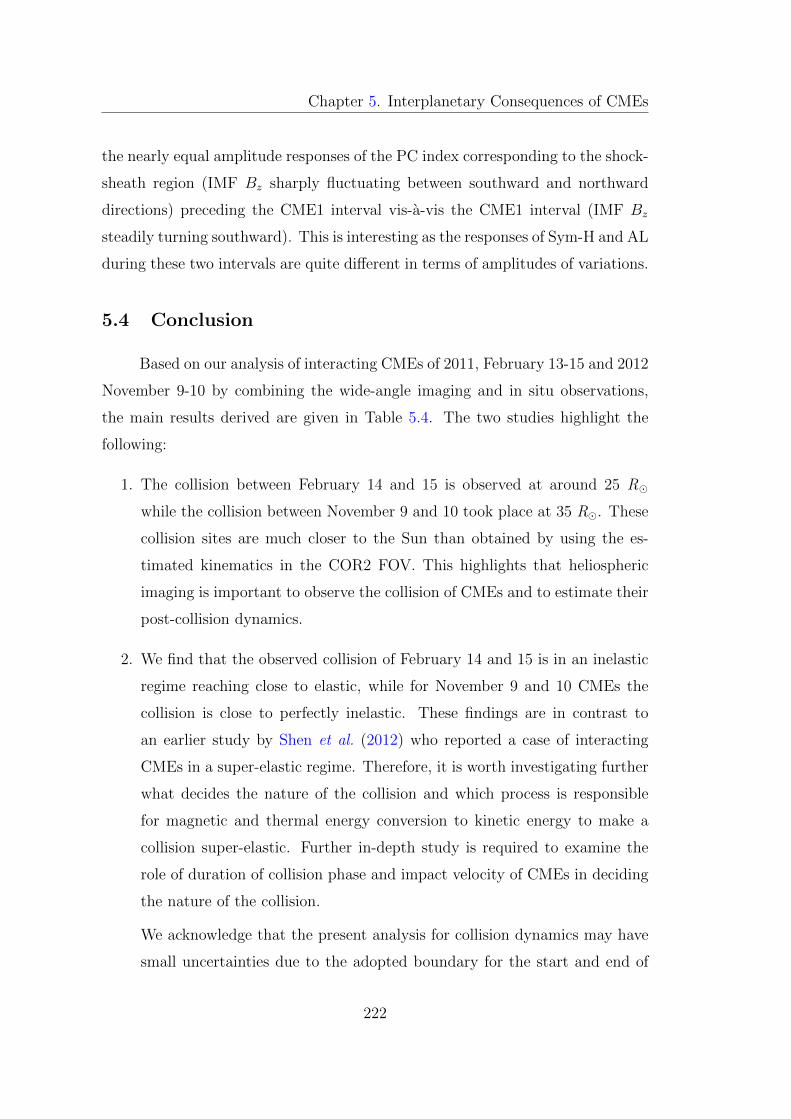
Chapter 5. Interplanetary Consequences of CMEs
the nearly equal amplitude responses of the PC index corresponding to the shock-
sheath region (IMF Bz sharply fluctuating between southward and northward
directions) preceding the CME1 interval vis-a-vis the CME1 interval (IMF Bz
steadily turning southward). This is interesting as the responses of Sym-H and AL
during these two intervals are quite different in terms of amplitudes of variations.
5.4 Conclusion
Based on our analysis of interacting CMEs of 2011, February 13-15 and 2012
November 9-10 by combining the wide-angle imaging and in situ observations,
the main results derived are given in Table 5.4. The two studies highlight the
following:
1. The collision between February 14 and 15 is observed at around 25 R�
while the collision between November 9 and 10 took place at 35 R�. These
collision sites are much closer to the Sun than obtained by using the es-
timated kinematics in the COR2 FOV. This highlights that heliospheric
imaging is important to observe the collision of CMEs and to estimate their
post-collision dynamics.
2. We find that the observed collision of February 14 and 15 is in an inelastic
regime reaching close to elastic, while for November 9 and 10 CMEs the
collision is close to perfectly inelastic. These findings are in contrast to
an earlier study by Shen et al. (2012) who reported a case of interacting
CMEs in a super-elastic regime. Therefore, it is worth investigating further
what decides the nature of the collision and which process is responsible
for magnetic and thermal energy conversion to kinetic energy to make a
collision super-elastic. Further in-depth study is required to examine the
role of duration of collision phase and impact velocity of CMEs in deciding
the nature of the collision.
We acknowledge that the present analysis for collision dynamics may have
small uncertainties due to the adopted boundary for the start and end of
222

Chapter 5. Interplanetary Consequences of CMEs
the collision phase. In this context, we emphasize that it is often difficult to
define the start of collision as the following CME starts to decelerate (due
to its interaction with the preceding CME) and the preceding CME starts
to accelerate before (most possibly due to shock driven by the following
CME) they actually merge as observed in HI FOV. Hence, different timing
and large time-interval of acceleration of one CME and deceleration of other
prevent us from pinpointing the exact start and end of the collision phase.
Further, we have not considered the expansion velocity and propagation
direction of the centroid of CMEs, which may be different before and after
the collision.
3. The total kinetic energy of February 14 and 15 CMEs after the observed
collision is reduced by 1.3%, and for November 9 and 10 CMEs, it decreased
by 6.7% to its value before the collision. We also found that speeds and
momentum of 2011 February CMEs changed from 35% to 68%, and for
2012 November CMEs, it changed from 23% to 30% compared to their
values before the collision.
Our analysis used the total mass of CMEs to study their collision dynamics,
but as the CME is not a solid body, its total mass is not expected to
participate in the collision. Keeping in mind various limitations of the
present study, we believe that more detailed work, by incorporating multiple
plasma processes, is required to understand the CME-CME interaction.
Also, the assumption that there is no mass transfer between CME2 and
CME3 during the collision may result in some uncertainties.
4. The in situ measurements of these CMEs near 1 AU show that interacting
CMEs are accelerated or decelerated, compressed, and heated. Our analysis
also highlights that the estimated heliospheric kinematics, particularly after
collisions, is important to combine with DBM for improving the estimation
of the arrival times of different features of CME that experience different
drag forces during their propagation through the heliosphere.
223
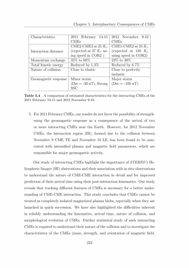
Chapter 5. Interplanetary Consequences of CMEs
Characteristics 2011 February 13-15CMEs
2012 November 9-10CMEs
Interaction distance
CME2-CME3 at 25 R�(expected at 37 R� us-ing speed in COR2 )
CME1-CME2 at 35 R�(expected at 130 R�using speed in COR2)
Momentum exchange 35% to 68% 23% to 30%Total kinetic energy Reduced by 1.3% Reduced by 6.7%Nature of collision Close to elastic Close to perfectly
inelasticGeomagnetic response Minor storm
(Dst = -30 nT), StrongSSC
Major storm(Dst = -108 nT)
Table 5.4 A comparison of estimated characteristics for the interacting CMEs of the2011 February 13-15 and 2012 November 9-10.
5. For 2011 February CMEs, our results do not favor the possibility of strength-
ening the geomagnetic response as a consequence of the arrival of two
or more interacting CMEs near the Earth. However, for 2012 November
CMEs, the interaction region (IR), formed due to the collision between
November 9 CME TE and November 10 LE, has been found to be asso-
ciated with intensified plasma and magnetic field parameters, which are
responsible for major geomagnetic activity.
Our study of interacting CMEs highlight the importance of STEREO’s He-
liospheric Imager (HI) observations and their association with in situ observations
to understand the nature of CME-CME interaction in detail and for improved
prediction of their arrival time using their post-interaction kinematics. Our study
reveals that tracking different features of CMEs is necessary for a better under-
standing of CME-CME interaction. This study concludes that CMEs cannot be
treated as completely isolated magnetized plasma blobs, especially when they are
launched in quick succession. We have also highlighted the difficulties inherent
in reliably understanding the kinematics, arrival time, nature of collision, and
morphological evolution of CMEs. Further statistical study of such interacting
CMEs is required to understand their nature of the collision and to investigate the
characteristics of the CMEs (mass, strength, and orientation of magnetic field,
224

Chapter 5. Interplanetary Consequences of CMEs
speed and direction of propagation, and duration of collision phase), which are
responsible for their interaction.
225
Chapter 6
Conclusions and Future Work
In this thesis, I have attempted to understand the evolution and conse-
quences of CMEs in the heliosphere. For this purpose, we have exploited the
remote sensing observations of CMEs mainly from the STEREO spacecraft and
in situ observation from ACE and WIND spacecraft. Our study is crucial to
achieving a better scheme for arrival time prediction of CMEs at 1AU, which
is a prime concern for any solar-terrestrial physicist. The principal conclusions
of my thesis are given in Section 6.1. Some of the limitations of the current
study undertaken for this thesis will be addressed in the future to enhance our
understanding of the heliospheric evolution and consequences of CMEs. These
are described in Section 6.2.
6.1 Conclusions
Based on our study, we conclude that by exploiting white light images from
twin vantage points of STEREO, the uncertainties in the morphology and kine-
matics of CMEs due to projection effects in the white light images from a sin-
gle viewpoint can be resolved. This can be done by implementing appropriate
3D reconstruction techniques on the CME images near and far from the Sun.
Our study highlights that by constructing the J -maps using the running differ-
ence white light images of CMEs from STEREO, a CME can be unambiguously
tracked continuously from its liftoff in the inner corona to almost the Earth. By
226
Chapter 6. Conclusions and Future Work
continuously tracking different features of a CME and implementing 3D recon-
struction techniques to estimate their kinematics, we found that characteristics
(speed, direction, and morphology) of CMEs change as they propagate in the he-
liosphere. Such findings, particularly that the CMEs accelerate or decelerate until
they obtain the speed of ambient solar wind medium, have been inferred before.
However, our analysis, using the reconstruction techniques on the SECCHI/HI
observations of several Earth-directed CMEs, helps to show directly.
We have shown that the 3D speed (estimated using 3D reconstruction tech-
niques) of CMEs near the Sun (in COR field of view (FOV)), and assuming that
it remains constant for the remaining distance, i.e., up to 1 AU, is not sufficient
to predict the arrival time accurately for a majority of CMEs at the Earth. This
is true, especially for a fast speed CME traveling in the slow solar wind environ-
ment or a slow speed CME traveling in the high-speed stream. We show that a
small error in the estimated speed of CMEs in the COR2 FOV may result in a
large variation in the predicted arrival time near 1 AU. This variation may be
due to the large distance between the COR2 FOV and L1. However, for fast
CMEs, this variation in arrival time using slightly different estimated 3D speeds
will be minimized. We also conclude that a fast-speed stream, from a coronal
hole hitting the back of a CME, can significantly change its dynamics. Our study
shows that if the estimated 3D kinematics of CMEs in the heliosphere are used
as inputs in drag-based model (DBM), the arrival time prediction of these at 1
AU is improved compared to using only 3D speed estimated close to the Sun.
Based on this, we conclude that the role of drag forces in the dynamics of CMEs,
is effective farther out (few thirties of solar radii) from the Sun. From estimating
the propagation direction of CMEs, we conclude that a CME may undergo the
non-radial motion even far from the Sun.
We assessed the relative performance of 10 reconstruction techniques by
applying them to SECCHI/HI observations for estimating the arrival time of
CMEs at the Earth. For the first time, such a detailed analysis pointing out
the limitations and advantages of each reconstruction technique was carried out.
Recently, Mostl et al. (2014) also assessed the accuracy and limitations of three
227
Chapter 6. Conclusions and Future Work
fitting methods. Based on our study, we conclude that although single spacecraft
reconstruction techniques are capable of estimating the 3D kinematics of CMEs
in the heliosphere, relative performance of such techniques is inferior than double
spacecraft reconstruction techniques. Among the double spacecraft reconstruc-
tion techniques, the TAS method performs the best for predicting the arrival
time and transit speed of CMEs at 1 AU, while GT method performs the least
accurately. This is true, irrespective of the characteristics of the CMEs taken
in our study. We also conclude that the HM method best estimates the arrival
time among the single spacecraft techniques that we applied. Among the single
spacecraft fitting methods, our study concludes that HMF and SSEF methods
are always superior to FPF. We also show that these techniques can estimate
different kinematics (speed and direction) of CMEs. Therefore, anyone needs to
be careful before using these estimates directly.
We also attempted to track two density structures at the front and the rear
edge of a CME. We found that density structure at the rear edge corresponds
most probably to cool and dense filament identified after the magnetic cloud,
while density structure at the front corresponds to the sheath before the leading
edge of CME in the in situ observations taken by ACE and WIND spacecraft.
This is also one of the first attempts to associate optical and in situ observations,
and only a few studies have been carried out so far with STEREO observations
(Howard and DeForest, 2012a). We highlight the importance of J -maps con-
structed from SECCHI/HI observations for associating the three-part structure
of CME in remote and in situ observations.
Our study shows that a CME can interact/collide with another CME under
favorable conditions. We also show that tracking different features of a CME in
the HI observations is important to witness the CME-CME interaction. In this
thesis, we have attempted to investigate the nature of the collision of two CMEs.
There has been only one case study by Shen et al. (2012) who showed that collision
was super-elastic. We conclude that there is a significant exchange of momentum
and kinetic energy during the collision of the CMEs. Hence, the consequences
of CMEs on other CMEs can be noted; therefore, post-collision kinematics of
228
Chapter 6. Conclusions and Future Work
CMEs must be used for their improved arrival time prediction at 1 AU. Our
analysis reveals that CMEs collide at much earlier than that derived from the
estimated 3D kinematics in the COR2 FOV. Our study found that the nature
of CME-CME collision can range from elastic to perfectly inelastic. This finding
raises a question as to what decides the nature of collision of magnetized plasma
blobs, which are expected to be different than gaseous blobs or solid balls. We
also conclude that such collision of CMEs has significant effects on the magnetic
and plasma parameters of both preceding and following CMEs. Our study shows
the formation of interaction region and magnetic hole (probably the signatures of
magnetic reconnection) by the collision of CMEs. These interaction regions are
seen to be responsible for significant geomagnetic activity. Our study also shows
that the morphology (angular width) of a fast CME can change significantly
during its propagation in the heliosphere, especially when it traverses in a dense
solar wind environment which may be formed due to remnants of a preceding
CME.
Our study is a dedicated attempt to understand and implement the several
reconstruction techniques applicable to COR and HI observations of CMEs for es-
timating their 3D kinematics, arrival time at 1 AU, morphological evolution, and
CME-CME interaction geomagnetic consequences of interacting CMEs. We con-
clude that tracking the CMEs out to longer elongation in the heliosphere using HI
is necessary for an improved understanding of their evolution and consequences.
6.2 Future Work
In the study undertaken for this thesis, we have analyzed only a few CMEs.
However, a large number of CMEs need to be studied in order to answer the
questions regarding the heliospheric propagation and consequences of CMEs. In
the thesis, we have focused mainly on the Earth-directed CMEs; however, CMEs
launched in different directions from the Sun need to be included to assess the
performance of reconstruction techniques. In our study of the collision of CMEs,
the actual mass of the CMEs estimated in the COR FOV is assumed to be con-
229

Chapter 6. Conclusions and Future Work
stant up to the HI FOV, which may not always be true. Therefore, the mass of
CMEs in the HI FOV must be estimated. We have not compared the obtained
kinematics of the CMEs to the kinematics profiles of the CMEs derived from the
theoretical models. Such comparison must be made for a better understanding of
the propagation of CMEs. Based on our study of interacting CMEs, we need to
examine what decides the nature of collision of CMEs and why only some interact-
ing CMEs cause significant geomagnetic activity. We plan to pursue studies that
can remove some of the uncertainties in our current approach to understanding
the evolution and consequences of different features of CMEs.
6.2.1 Dynamic evolution of the CMEs
We plan to understand how the physical parameters of CMEs vary with he-
liocentric distance, particularly the polytropic index of plasma of CMEs, Lorentz
force and thermal energy inside the CMEs, and their role in the dynamic evolu-
tion of the CMEs. The contribution of Lorentz forces in driving the CMEs in the
heliosphere will also be investigated because in several CME propagation models,
the effect of Lorentz force is considered negligible after a few solar radii from the
Sun. One also needs to incorporate the interaction of CMEs in the solar wind in
the drag-based model of propagation of CMEs. We also plan to investigate how
the magnetic energy stored in the CMEs is used in driving, expanding, and heat-
ing the CME material during their heliospheric propagation. Based on tracking
of different features of a CME in remote and in situ observations, we can attempt
to understand the forces acting on them as they travel in the heliosphere.
6.2.2 Consequences of interacting CMEs
The possibility of the formation of complex ejecta on the interaction of
CMEs and their geomagnetic response will be investigated. This will be at-
tempted to understand how differently complex ejecta affects the Earth’s magne-
tosphere than an isolated CME or magnetic cloud. The dependence of the geoef-
fectiveness of the preceding CME on the intensity of the following shock will also
230
Chapter 6. Conclusions and Future Work
be examined, which will help us improve the status of predicting major geomag-
netic storms. In a few earlier studies, the enhancement in long-wavelength radio
emission is presented as evidence for interacting CMEs (Gopalswamy et al., 2001c;
Martınez Oliveros et al., 2012). We plan to investigate the favorable conditions
or the mechanism for enhanced radio emission during CME-CME interaction.
6.2.3 Assessing the performance of reconstruction meth-
ods using the off-ecliptic CMEs
We will track different features of CMEs in the J -maps along with dif-
ferent position angles to derive their time-elongation profiles and estimate their
kinematics by implementing reconstruction techniques. Such an analysis of the
selected CMEs will better assess the relative performance of several reconstruc-
tion techniques. Further, the estimated kinematics at different PAs will help to
understand the global evolution, i.e. at the different latitudinal extent of CMEs,
especially in the case of CME-CME interaction.
The future investigation described above can improve our understanding of
the evolution and consequences of CMEs and to interact CMEs in the heliosphere.
Some of these studies will better understand and resolve the critical issues of space
weather, viz. propagation of CMEs and estimation of their arrival time.
231
Bibliography
Akasofu, S.I.: 1964, Planet. Space Sci. 12, 273.
Akasofu, S.I.: 1969, Nature 221, 1020.
Andrews, M.D., Wang, A.H., Wu, S.T.: 1999, Solar Phys. 187, 427.
Arge, C.N., Pizzo, V.J.: 2000, J. Geophys. Res. 105, 10465.
Bahcall, J.N.: 2001, Nature 412, 29.
Bahcall, J.N., Huebner, W.F., Lubow, S.H., Parker, P.D., Ulrich, R.K.: 1982,Reviews of Modern Physics 54, 767.
Bein, B.M., Temmer, M., Vourlidas, A., Veronig, A.M., Utz, D.: 2013, Astrophys.J. 768, 31.
Bhatnagar, A., Livingston, W.: 2005, Fundamentals of solar astronomy, WorldScientific.
Biermann, L.: 1951, ZA 29, 274.
Billings, D.E.: 1966, A guide to the solar corona, Academic Press, New York,150.
Borrini, G., Gosling, J.T., Bame, S.J., Feldman, W.C.: 1982, J. Geophys. Res.87, 7370.
Boser, U.: 2006, Solar Circle 59.
Bothmer, V., Schwenn, R.: 1996, Advances in Space Research 17, 319.
Bougeret, J.L., Kaiser, M.L., Kellogg, P.J., Manning, R., Goetz, K., Monson,S.J., Monge, N., Friel, L., Meetre, C.A., Perche, C., Sitruk, L., Hoang, S.:1995, Space Sci. Rev. 71, 231.
Boursier, Y., Lamy, P., Llebaria, A.: 2009, Solar Phys. 256, 131.
Brown, D.S., Bewsher, D., Eyles, C.J.: 2009, Solar Phys. 254, 185.
Brueckner, G.E., Howard, R.A., Koomen, M.J., Korendyke, C.M., Michels, D.J.,Moses, J.D., Socker, D.G., Dere, K.P., Lamy, P.L., Llebaria, A., Bout, M.V.,Schwenn, R., Simnett, G.M., Bedford, D.K., Eyles, C.J.: 1995, Solar Phys.162, 357.
Brueckner, G.E., Delaboudiniere, J.P., Howard, R.A., Paswaters, S.E., St. Cyr,O.C., Schwenn, R., Lamy, P., Simnett, G.M., Thompson, B., Wang, D.: 1998,Geophys. Res. Lett. 25, 3019.
232
Bibliography
Burkepile, J.T., Hundhausen, A.J., Stanger, A.L., St. Cyr, O.C., Seiden, J.A.:2004, Journal of Geophysical Research (Space Physics) 109, 3103.
Burlaga, L.F., Lemaire, J.F.: 1978, J. Geophys. Res. 83, 5157.
Burlaga, L.F., Behannon, K.W., Klein, L.W.: 1987, J. Geophys. Res. 92, 5725.
Burlaga, L.F., Plunkett, S.P., St. Cyr, O.C.: 2002, J. Geophys. Res. 107, 1266.
Burlaga, L.F.E.: 1991, In: Schwenn, R., Marsch, E. (eds.) Magnetic Clouds, 1.
Burlaga, L.F., Skoug, R.M., Smith, C.W., Webb, D.F., Zurbuchen, T.H., Reinard,A.: 2001, J. Geophys. Res. 106, 20957.
Burlaga, L.F., Ness, N.F., Acuna, M.H., Lepping, R.P., Connerney, J.E.P.,Richardson, J.D.: 2008, Nature 454, 75.
Burlaga, L., Sittler, E., Mariani, F., Schwenn, R.: 1981, J. Geophys. Res. 86,6673.
Burlaga, L., Fitzenreiter, R., Lepping, R., Ogilvie, K., Szabo, A., Lazarus, A.,Steinberg, J., Gloeckler, G., Howard, R., Michels, D., Farrugia, C., Lin, R.P.,Larson, D.E.: 1998, J. Geophys. Res. 103, 277.
Byrne, J.P., Maloney, S.A., McAteer, R.T.J., Refojo, J.M., Gallagher, P.T.: 2010,Nature Communications 1.
Cane, H.V.: 2000, Space Sci. Rev. 93, 55.
Cane, H.V., Richardson, I.G.: 2003, Journal of Geophysical Research (SpacePhysics) 108, 1156.
Cane, H.V., Richardson, I.G., Wibberenz, G.: 1997, J. Geophys. Res. 102, 7075.
Cargill, P.J.: 2004, Solar Phys. 221, 135.
Cargill, P.J., Chen, J., Spicer, D.S., Zalesak, S.T.: 1996, J. Geophys. Res. 101,4855.
Chakrabarty, D., Sekar, R., Narayanan, R., Devasia, C.V., Pathan, B.M.: 2005,Journal of Geophysical Research (Space Physics) 110, 11301.
Chao, J.K., Lepping, R.P.: 1974, In: Flare-Produced Shock Waves in the Coronaand in Interplanetary Space, 225.
Chapman, S., Ferraro, V.C.A.: 1931, Terrestrial Magnetism and AtmosphericElectricity (J. Geophys. Res.) 36, 171.
Chen, P.F.: 2011, Living Reviews in Solar Physics 8, 1.
Colaninno, R.C., Vourlidas, A.: 2009, Astrophys. J. 698, 852.
Colaninno, R.C., Vourlidas, A., Wu, C.C.: 2013, J. Geophys. Res. 118, 6866.
Cowen, R.: 2012, Nature 489, 20.
Crooker, N.: 2002, EOS Transactions 83, 24.
233
Bibliography
Crooker, N.U., Horbury, T.S.: 2006, Space Sci. Rev. 123, 93.
Daglis, I.A., Thorne, R.M., Baumjohann, W., Orsini, S.: 1999, Reviews of Geo-physics 37, 407.
Dal Lago, A., Schwenn, R., Gonzalez, W.D.: 2003, Advances in Space Research32, 2637.
Davies, J.A., Harrison, R.A., Rouillard, A.P., Sheeley, N.R., Perry, C.H., Bew-sher, D., Davis, C.J., Eyles, C.J., Crothers, S.R., Brown, D.S.: 2009, Geophys.Res. Lett. 36, 2102.
Davies, J.A., Harrison, R.A., Perry, C.H., Mostl, C., Lugaz, N., Rollett, T., Davis,C.J., Crothers, S.R., Temmer, M., Eyles, C.J., Savani, N.P.: 2012, Astrophys.J. 750, 23.
Davies, J.A., Perry, C.H., Trines, R.M.G.M., Harrison, R.A., Lugaz, N., Mostl,C., Liu, Y.D., Steed, K.: 2013, Astrophys. J. 776, 1.
Davila, J.M.: 1987, Astrophys. J. 317, 514.
Davis, C.J., Kennedy, J., Davies, J.A.: 2010, Solar Phys. 263, 209.
Davis, C.J., Davies, J.A., Lockwood, M., Rouillard, A.P., Eyles, C.J., Harrison,R.A.: 2009, Geophys. Res. Lett. 36, 8102.
Davis, C.J., Davies, J.A., St Cyr, O.C., Campbell-Brown, M., Skelt, A., Kaiser,M., Meyer-Vernet, N., Crothers, S., Lintott, C., Smith, A., Bamford, S.,Baeten, E.M.L.: 2012, Mon. Not. Roy. Astron. Soc. 420, 1355.
Davis, T.N., Sugiura, M.: 1966, J. Geophys. Res. 71, 785.
DeForest, C.E., Howard, T.A., McComas, D.J.: 2013, Astrophys. J. 769, 43.
DeForest, C.E., Howard, T.A., Tappin, S.J.: 2011, Astrophys. J. 738, 103.
Demastus, H.L., Wagner, W.J., Robinson, R.D.: 1973, Solar Phys. 31, 449.
Dessler, A.J., Parker, E.N.: 1959, J. Geophys. Res. 64, 2239.
Dessler, A.J., Francis, W.E., Parker, E.N.: 1960, J. Geophys. Res. 65, 2715.
Dryer, M.: 1974, Space Sci. Rev. 15, 403.
Dryer, M.: 1994, Space Sci. Rev. 67, 363.
Dryer, M., Fry, C.D., Sun, W., Deehr, C., Smith, Z., Akasofu, S.I., Andrews,M.D.: 2001, Solar Phys. 204, 265.
Dryer, M., Smith, Z., Fry, C.D., Sun, W., Deehr, C.S., Akasofu, S.I.: 2004, SpaceWeather 2, 9001.
Dungey, J.W.: 1961, Phys. Rev. Lett. 6, 47.
Echer, E., Gonzalez, W.D., Tsurutani, B.T., Gonzalez, A.L.C.: 2008, J. Geophys.Res. 113, 5221.
Eyles, C.J., Simnett, G.M., Cooke, M.P., Jackson, B.V., Buffington, A., Hick,P.P., Waltham, N.R., King, J.M., Anderson, P.A., Holladay, P.E.: 2003, SolarPhys. 217, 319.
234
Bibliography
Eyles, C.J., Harrison, R.A., Davis, C.J., Waltham, N.R., Shaughnessy, B.M.,Mapson-Menard, H.C.A., Bewsher, D., Crothers, S.R., Davies, J.A., Simnett,G.M., Howard, R.A., Moses, J.D., Newmark, J.S., Socker, D.G., Halain, J.P.,Defise, J.M., Mazy, E., Rochus, P.: 2009, Solar Phys. 254, 387.
Farrugia, C., Berdichevsky, D.: 2004, Ann. Geophys. 22, 3679.
Farrugia, C.J., Jordanova, V.K., Thomsen, M.F., Lu, G., Cowley, S.W.H.,Ogilvie, K.W.: 2006, J. Geophys. Res. 111, 11104.
Feng, X.S., Zhang, Y., Sun, W., Dryer, M., Fry, C.D., Deehr, C.S.: 2009, Journalof Geophysical Research (Space Physics) 114, 1101.
Feynman, J., Hundhausen, A.J.: 1994, J. Geophys. Res. 99, 8451.
Fisher, R.R., Munro, R.H.: 1984, Astrophys. J. 280, 428.
Fisher, R.R., Lee, R.H., MacQueen, R.M., Poland, A.I.: 1981, ApOpt 20, 1094.
Forbush, S.E.: 1937, Physical Review 51, 1108.
Forsyth, R.J., Bothmer, V., Cid, C., Crooker, N.U., Horbury, T.S., Kecskemety,K., Klecker, B., Linker, J.A., Odstrcil, D., Reiner, M.J., Richardson, I.G.,Rodriguez-Pacheco, J., Schmidt, J.M., Wimmer-Schweingruber, R.F.: 2006,Space Sci. Rev. 123, 383.
Foukal, P.V.: 2004, Solar Astrophysics, 2nd, Revised Edition, Wiley-VCH.
Fry, C.D., Sun, W., Deehr, C.S., Dryer, M., Smith, Z., Akasofu, S.I., Tokumaru,M., Kojima, M.: 2001, J. Geophys. Res. 106, 20985.
Fry, C.D., Detman, T.R., Dryer, M., Smith, Z., Sun, W., Deehr, C.S., Akasofu,S.I., Wu, C.C., McKenna-Lawlor, S.: 2007, Journal of Atmospheric and Solar-Terrestrial Physics 69, 109.
Gallagher, P.T., Lawrence, G.R., Dennis, B.R.: 2003, Astrophys. J. 588, L53.
Galvin, A.B., Kistler, L.M., Popecki, M.A., Farrugia, C.J., Simunac, K.D.C.,Ellis, L., Mobius, E., Lee, M.A., Boehm, M., Carroll, J., Crawshaw, A., Conti,M., Demaine, P., Ellis, S., Gaidos, J.A., Googins, J., Granoff, M., Gustafson,A., Heirtzler, D., King, B., Knauss, U., Levasseur, J., Longworth, S., Singer,K., Turco, S., Vachon, P., Vosbury, M., Widholm, M., Blush, L.M., Karrer, R.,Bochsler, P., Daoudi, H., Etter, A., Fischer, J., Jost, J., Opitz, A., Sigrist, M.,Wurz, P., Klecker, B., Ertl, M., Seidenschwang, E., Wimmer-Schweingruber,R.F., Koeten, M., Thompson, B., Steinfeld, D.: 2008, Space Sci. Rev. 136,437.
Gloeckler, G., Cain, J., Ipavich, F.M., Tums, E.O., Bedini, P., Fisk, L.A., Zur-buchen, T.H., Bochsler, P., Fischer, J., Wimmer-Schweingruber, R.F., Geiss,J., Kallenbach, R.: 1998, Space Sci. Rev. 86, 497.
Golub, L., Pasachoff, J.M.: 2009, The Solar Corona.
Gonzalez, W.D., Gonzalez, A.L.C., Tsurutani, B.T., Smith, E.J., Tang, F.: 1989,J. Geophys. Res. 94, 8835.
Gonzalez, W.D., Joselyn, J.A., Kamide, Y., Kroehl, H.W., Rostoker, G., Tsuru-tani, B.T., Vasyliunas, V.M.: 1994, J. Geophys. Res. 99, 5771.
235

Bibliography
Gonzalez-Esparza, A., Santillan, A., Ferrer, J.: 2004, Annales Geophysicae 22,3741.
Gopalswamy, N.: 2006, Washington DC American Geophysical Union Geophysi-cal Monograph Series 165, 207.
Gopalswamy, N.: 2006, Space Sci. Rev. 124, 145.
Gopalswamy, N., Hanaoka, Y., Kosugi, T., Lepping, R.P., Steinberg, J.T., Plun-kett, S., Howard, R.A., Thompson, B.J., Gurman, J., Ho, G., Nitta, N., Hud-son, H.S.: 1998, Geophys. Res. Lett. 25, 2485.
Gopalswamy, N., Kaiser, M.L., Lepping, R.P., Kahler, S.W., Ogilvie, K.,Berdichevsky, D., Kondo, T., Isobe, T., Akioka, M.: 1998, J. Geophys. Res.103, 307.
Gopalswamy, N., Lara, A., Lepping, R.P., Kaiser, M.L., Berdichevsky, D.,St. Cyr, O.C.: 2000, Geophys. Res. Lett. 27, 145.
Gopalswamy, N., Kaiser, M.L., Thompson, B.J., Burlaga, L.F., Szabo, A., Lara,A., Vourlidas, A., Yashiro, S., Bougeret, J.L.: 2000, Geophys. Res. Lett. 27,1427.
Gopalswamy, N., Yashiro, S., Kaiser, M.L., Howard, R.A., Bougeret, J.L.: 2001,J. Geophys. Res. 106, 29219.
Gopalswamy, N., Lara, A., Yashiro, S., Kaiser, M.L., Howard, R.A.: 2001, J.Geophys. Res. 106, 29207.
Gopalswamy, N., Yashiro, S., Kaiser, M.L., Howard, R.A., Bougeret, J.L.: 2001,Astrophys. J. 548, L91.
Gopalswamy, N., Yashiro, S., Micha lek, G., Kaiser, M.L., Howard, R.A., Reames,D.V., Leske, R., von Rosenvinge, T.: 2002, Astrophys. J. 572, L103.
Gopalswamy, N., Yashiro, S., Lara, A., Kaiser, M.L., Thompson, B.J., Gallagher,P.T., Howard, R.A.: 2003, Geophys. Res. Lett. 30, 8015.
Gopalswamy, N., Shimojo, M., Lu, W., Yashiro, S., Shibasaki, K., Howard, R.A.:2003, Astrophys. J. 586, 562.
Gopalswamy, N., Lara, A., Manoharan, P.K., Howard, R.A.: 2005, Advances inSpace Research 36, 2289.
Gopalswamy, N., Makela, P., Xie, H., Akiyama, S., Yashiro, S.: 2009, Journal ofGeophysical Research (Space Physics) 114, 0.
Gopalswamy, N., Dal Lago, A., Yashiro, S., Akiyama, S.: 2009, Central EuropeanAstrophysical Bulletin 33, 115.
Gopalswamy, N., Xie, H., Makela, P., Akiyama, S., Yashiro, S., Kaiser, M.L.,Howard, R.A., Bougeret, J.L.: 2010, Astrophys. J. 710, 1111.
Gosling, J.T.: 1993, J. Geophys. Res. 98, 18937.
Gosling, J.T., Pizzo, V., Bame, S.J.: 1973, J. Geophys. Res. 78, 2001.
Gosling, J.T., Hildner, E., MacQueen, R.M., Munro, R.H., Poland, A.I., Ross,C.L.: 1974, J. Geophys. Res. 79, 4581.
236
Bibliography
Gosling, J.T., Baker, D.N., Bame, S.J., Feldman, W.C., Zwickl, R.D., Smith,E.J.: 1987, J. Geophys. Res. 92, 8519.
Gosling, J.T., Bame, S.J., McComas, D.J., Phillips, J.L.: 1990, Geophys. Res.Lett. 17, 901.
Gosling, J.T., McComas, D.J., Phillips, J.L., Bame, S.J.: 1991, J. Geophys. Res.96, 7831.
Gosling, J.T., Skoug, R.M., McComas, D.J., Smith, C.W.: 2005, J. Geophys.Res. 110, 1107.
Grotrian, W.: 1939, Naturwissenschaften 27, 214.
Gudiksen, B.V.: 2004, The coronal heating problem. PhD thesis, University ofStockholm.
Gui, B., Shen, C., Wang, Y., Ye, P., Liu, J., Wang, S., Zhao, X.: 2011, SolarPhys. 271, 111.
Haff, P.K., Switkowski, Z.E., Tombrello, T.A.: 1978, Nature 272, 803.
Hanaoka, Y., Kurokawa, H., Enome, S., Nakajima, H., Shibasaki, K., Nishio, M.,Takano, T., Torii, C., Sekiguchi, H., Kawashima, S., Bushimata, T., Shinohara,N., Irimajiri, Y., Koshiishi, H., Shiomi, Y., Nakai, Y., Funakoshi, Y., Kitai, R.,Ishiura, K., Kimura, G.: 1994, Pub. Astron. Soc. Japan 46, 205.
Harrison, R.A., Davies, J.A., Mostl, C., Liu, Y., Temmer, M., Bisi, M.M., East-wood, J.P., de Koning, C.A., Nitta, N., Rollett, T., Farrugia, C.J., Forsyth,R.J., Jackson, B.V., Jensen, E.A., Kilpua, E.K.J., Odstrcil, D., Webb, D.F.:2012, Astrophys. J. 750, 45.
Hewish, A., Scott, P.F., Wills, D.: 1964, Nature 203, 1214.
Hirayama, T., Nakagomi, Y.: 1974, Pub. Astron. Soc. Japan 26, 53.
Hirshberg, J., Asbridge, J.R., Robbins, D.E.: 1971, Solar Phys. 18, 313.
Ho, G.C., Hamilton, D.C., Gloeckler, G., Bochsler, P.: 2000, Geophys. Res. Lett.27, 309.
Houminer, Z., Hewish, A.: 1972, Planet. Space Sci. 20, 1703.
Howard, R.A., Michels, D.J., Sheeley, N.R. Jr., Koomen, M.J.: 1982, Astrophys.J. 263, L101.
Howard, R.A., Moses, J.D., Vourlidas, A., Newmark, J.S., Socker, D.G., Plun-kett, S.P., Korendyke, C.M., Cook, J.W., Hurley, A., Davila, J.M., Thomp-son, W.T., St Cyr, O.C., Mentzell, E., Mehalick, K., Lemen, J.R., Wuelser,J.P., Duncan, D.W., Tarbell, T.D., Wolfson, C.J., Moore, A., Harrison, R.A.,Waltham, N.R., Lang, J., Davis, C.J., Eyles, C.J., Mapson-Menard, H., Sim-nett, G.M., Halain, J.P., Defise, J.M., Mazy, E., Rochus, P., Mercier, R., Ravet,M.F., Delmotte, F., Auchere, F., Delaboudiniere, J.P., Bothmer, V., Deutsch,W., Wang, D., Rich, N., Cooper, S., Stephens, V., Maahs, G., Baugh, R.,McMullin, D., Carter, T.: 2008, Space Sci. Rev. 136, 67.
Howard, T.A.: 2011, Journal of Atmospheric and Solar-Terrestrial Physics 73,1242.
237
Bibliography
Howard, T.A., DeForest, C.E.: 2012, Astrophys. J. 746, 64.
Howard, T.A., DeForest, C.E.: 2012, Astrophys. J. 752, 130.
Howard, T.A., Tappin, S.J.: 2009, Space Sci. Rev. 147, 31.
Howard, T.A., Webb, D.F., Tappin, S.J., Mizuno, D.R., Johnston, J.C.: 2006,Journal of Geophysical Research (Space Physics) 111, 4105.
Howard, T.A., Fry, C.D., Johnston, J.C., Webb, D.F.: 2007, Astrophys. J. 667,610.
Howard, T.A., Tappin, S.J., Odstrcil, D., DeForest, C.E.: 2013, Astrophys. J.765, 45.
Hundhausen, A.: 1999, In: Strong, K.T., Saba, J.L.R., Haisch, B.M., Schmelz,J.T. (eds.) The many faces of the sun: a summary of the results from NASA’sSolar Maximum Mission., 143.
Hundhausen, A.J.: 1993, J. Geophys. Res. 98, 13177.
Hundhausen, A.J., Sawyer, C.B., House, L., Illing, R.M.E., Wagner, W.J.: 1984,J. Geophys. Res. 89, 2639.
Illing, R.M.E., Hundhausen, A.J.: 1985, J. Geophys. Res. 90, 275.
Inhester, B.: 2006, ArXiv Astrophysics e-prints.
Intriligator, D.S.: 1976, Space Sci. Rev. 19, 629.
Iyemori, T.: 1990, Journal of Geomagnetism and Geoelectricity 42, 1249.
Iyemori, T., Rao, D.R.K.: 1996, Annales Geophysicae 14, 608.
Jackson, B.V., Buffington, A., Hick, P.P., Wang, X., Webb, D.: 2006, J. Geophys.Res. 111, 4.
Jackson, B.V., Bisi, M.M., Hick, P.P., Buffington, A.: 2007, In: American Astro-nomical Society Meeting Abstracts #210, Bulletin of the American Astronom-ical Society 39, 141.
Jackson, B.V., Bisi, M.M., Hick, P.P., Buffington, A., Clover, J.M., Sun, W.:2008, J. Geophys. Res. 113, 0.
Jian, L., Russell, C.T., Luhmann, J.G., Skoug, R.M.: 2006, Solar Phys. 239,393.
Jurac, S., Kasper, J.C., Richardson, J.D., Lazarus, A.J.: 2002, Geophys. Res.Lett. 29, 1463.
Kahler, S.W.: 1992, Ann. Rev. Astron. Astrophys. 30, 113.
Kahler, S.W., Webb, D.F.: 2007, Journal of Geophysical Research (Space Physics)112, 9103.
Kahler, S.W., Hildner, E., Van Hollebeke, M.A.I.: 1978, Solar Phys. 57, 429.
Kaiser, M.L., Kucera, T.A., Davila, J.M., St. Cyr, O.C., Guhathakurta, M.,Christian, E.: 2008, Space Sci. Rev. 136, 5.
238
Bibliography
Kilpua, E.K.J., Pomoell, J., Vourlidas, A., Vainio, R., Luhmann, J., Li, Y.,Schroeder, P., Galvin, A.B., Simunac, K.: 2009, Annales Geophysicae 27,4491.
Kilpua, E.K.J., Jian, L.K., Li, Y., Luhmann, J.G., Russell, C.T.: 2011, Journalof Atmospheric and Solar-Terrestrial Physics 73, 1228.
Kilpua, E.K.J., Mierla, M., Rodriguez, L., Zhukov, A.N., Srivastava, N., West,M.J.: 2012, Solar Phys. 279, 477.
Klein, L.W., Burlaga, L.F.: 1982, J. Geophys. Res. 87, 613.
Klimchuk, J.A.: 2006, Solar Phys. 234, 41.
Krieger, A.S., Timothy, A.F., Roelof, E.C.: 1973, Solar Phys. 29, 505.
Kumar, A., Rust, D.M.: 1996, J. Geophys. Res. 101, 15667.
Lang, K.R.: 2006, Sun, Earth and Sky, Springer.
Lara, A., Borgazzi, A.I.: 2009, In: Gopalswamy, N., Webb, D.F. (eds.) IAUSymposium, IAU Symposium 257, 287.
Leibacher, J.W., Noyes, R.W., Toomre, J., Ulrich, R.K.: 1985, Scientific Ameri-can 253, 48.
Leighton, R.B., Noyes, R.W., Simon, G.W.: 1962, Astrophys. J. 135, 474.
Lepping, R.P., Burlaga, L.F., Jones, J.A.: 1990, J. Geophys. Res. 95, 11957.
Lepping, R.P., Acuna, M.H., Burlaga, L.F., Farrell, W.M., Slavin, J.A., Schatten,K.H., Mariani, F., Ness, N.F., Neubauer, F.M., Whang, Y.C., Byrnes, J.B.,Kennon, R.S., Panetta, P.V., Scheifele, J., Worley, E.M.: 1995, Space Sci.Rev. 71, 207.
Lepri, S.T., Zurbuchen, T.H.: 2004, Journal of Geophysical Research (SpacePhysics) 109, 1112.
Lepri, S.T., Zurbuchen, T.H.: 2010, Astrophys. J. 723, L22.
Lepri, S.T., Zurbuchen, T.H., Fisk, L.A., Richardson, I.G., Cane, H.V., Gloeckler,G.: 2001, J. Geophys. Res. 106, 29231.
Lin, R.P., Anderson, K.A., Ashford, S., Carlson, C., Curtis, D., Ergun, R., Lar-son, D., McFadden, J., McCarthy, M., Parks, G.K., Reme, H., Bosqued, J.M.,Coutelier, J., Cotin, F., D’Uston, C., Wenzel, K.P., Sanderson, T.R., Henrion,J., Ronnet, J.C., Paschmann, G.: 1995, Space Sci. Rev. 71, 125.
Lindsay, G.M., Luhmann, J.G., Russell, C.T., Gosling, J.T.: 1999, J. Geophys.Res. 104, 12515.
Liu, Y.D., Luhmann, J.G., Mostl, C., Martinez-Oliveros, J.C., Bale, S.D., Lin,R.P., Harrison, R.A., Temmer, M., Webb, D.F., Odstrcil, D.: 2012, Astrophys.J. 746, L15.
Liu, Y.D., Luhmann, J.G., Lugaz, N., Mostl, C., Davies, J.A., Bale, S.D., Lin,R.P.: 2013, Astrophys. J. 769, 45.
239
Bibliography
Liu, Y., Davies, J.A., Luhmann, J.G., Vourlidas, A., Bale, S.D., Lin, R.P.: 2010,Astrophys. J. 710, L82.
Liu, Y., Thernisien, A., Luhmann, J.G., Vourlidas, A., Davies, J.A., Lin, R.P.,Bale, S.D.: 2010, Astrophys. J. 722, 1762.
Liu, Y., Luhmann, J.G., Bale, S.D., Lin, R.P.: 2011, Astrophys. J. 734, 84.
Lopez, R.E.: 1987, J. Geophys. Res. 92, 11189.
Lopez, R.E., Freeman, J.W.: 1986, J. Geophys. Res. 91, 1701.
Lugaz, N.: 2010, Solar Phys. 267, 411.
Lugaz, N., Manchester, W.B. IV, Gombosi, T.I.: 2005, Astrophys. J. 634, 651.
Lugaz, N., Vourlidas, A., Roussev, I.I.: 2009, Annales Geophysicae 27, 3479.
Lugaz, N., Hernandez-Charpak, J.N., Roussev, I.I., Davis, C.J., Vourlidas, A.,Davies, J.A.: 2010, Astrophys. J. 715, 493.
Lugaz, N., Farrugia, C.J., Davies, J.A., Mostl, C., Davis, C.J., Roussev, I.I.,Temmer, M.: 2012, Astrophys. J. 759, 68.
Luhmann, J.G., Bauer, S.J.: 1992, Washington DC American Geophysical UnionGeophysical Monograph Series 66, 417.
Luhmann, J.G., Curtis, D.W., Schroeder, P., McCauley, J., Lin, R.P., Larson,D.E., Bale, S.D., Sauvaud, J.A., Aoustin, C., Mewaldt, R.A., Cummings, A.C.,Stone, E.C., Davis, A.J., Cook, W.R., Kecman, B., Wiedenbeck, M.E., vonRosenvinge, T., Acuna, M.H., Reichenthal, L.S., Shuman, S., Wortman, K.A.,Reames, D.V., Mueller-Mellin, R., Kunow, H., Mason, G.M., Walpole, P.,Korth, A., Sanderson, T.R., Russell, C.T., Gosling, J.T.: 2008, Space Sci.Rev. 136, 117.
Lynch, B.J., Antiochos, S.K., Li, Y., Luhmann, J.G., DeVore, C.R.: 2009, As-trophys. J. 697, 1918.
Lynch, B.J., Li, Y., Thernisien, A.F.R., Robbrecht, E., Fisher, G.H., Luhmann,J.G., Vourlidas, A.: 2010, Journal of Geophysical Research (Space Physics)115, 7106.
Lyot, B.: 1939, Mon. Not. Roy. Astron. Soc. 99, 580.
Ma, S., Attrill, G.D.R., Golub, L., Lin, J.: 2010, Astrophys. J. 722, 289.
MacQueen, R.M., Csoeke-Poeckh, A., Hildner, E., House, L., Reynolds, R.,Stanger, A., Tepoel, H., Wagner, W.: 1980, Solar Phys. 65, 91.
Maloney, S.A., Gallagher, P.T.: 2010, Astrophys. J. 724, L127.
Manchester, W.B. IV, Gombosi, T.I., De Zeeuw, D.L., Sokolov, I.V., Roussev,I.I., Powell, K.G., Kota, J., Toth, G., Zurbuchen, T.H.: 2005, Astrophys. J.622, 1225.
Manchester, W.B., Gombosi, T.I., Roussev, I., Ridley, A., De Zeeuw, D.L.,Sokolov, I.V., Powell, K.G., Toth, G.: 2004, Journal of Geophysical Research(Space Physics) 109, 2107.
240
Bibliography
Manoharan, P.K.: 2006, Solar Phys. 235, 345.
Manoharan, P.K., Gopalswamy, N., Yashiro, S., Lara, A., Michalek, G., Howard,R.A.: 2004, Journal of Geophysical Research (Space Physics) 109, 6109.
Maricic, D., Vrsnak, B., Dumbovic, M., Zic, T., Rosa, D., Hrzina, D., Lulic, S.,Romstajn, I., Busic, I., Salamon, K., Temmer, M., Rollett, T., Veronig, A.,Bostanjyan, N., Chilingarian, A., Mailyan, B., Arakelyan, K., Hovhannisyan,A., Mujic, N.: 2014, Solar Phys. 289, 351.
Markwardt, C.B.: 2009, In: Bohlender, D.A., Durand, D., Dowler, P. (eds.)Astronomical Data Analysis Software and Systems XVIII, Astronomical Societyof the Pacific Conference Series 411, 251.
Martınez Oliveros, J.C., Raftery, C.L., Bain, H.M., Liu, Y., Krupar, V., Bale, S.,Krucker, S.: 2012, Astrophys. J. 748, 66.
Mayaud, P.N.: 1980, Washington DC American Geophysical Union GeophysicalMonograph Series 22, 607.
Mays, M.L., Horton, W., Kozyra, J., Zurbuchen, T.H., Huang, C., Spencer, E.:2007, Geophys. Res. Lett. 34, 11104.
McComas, D.J., Gosling, J.T., Bame, S.J., Smith, E.J., Cane, H.V.: 1989, J.Geophys. Res. 94, 1465.
McComas, D.J., Bame, S.J., Barker, P., Feldman, W.C., Phillips, J.L., Riley, P.,Griffee, J.W.: 1998, Space Sci. Rev. 86, 563.
McPherron, R.L.: 1970, J. Geophys. Res. 75, 5592.
Micha lek, G., Gopalswamy, N., Yashiro, S.: 2003, Astrophys. J. 584, 472.
Michalek, G., Gopalswamy, N., Yashiro, S.: 2009, Solar Phys. 260, 401.
Mierla, M., Davila, J., Thompson, W., Inhester, B., Srivastava, N., Kramar, M.,St. Cyr, O.C., Stenborg, G., Howard, R.A.: 2008, Solar Phys. 252, 385.
Mierla, M., Inhester, B., Marque, C., Rodriguez, L., Gissot, S., Zhukov, A.N.,Berghmans, D., Davila, J.: 2009, Solar Phys. 259, 123.
Mierla, M., Inhester, B., Antunes, A., Boursier, Y., Byrne, J.P., Colaninno, R.,Davila, J., de Koning, C.A., Gallagher, P.T., Gissot, S., Howard, R.A., Howard,T.A., Kramar, M., Lamy, P., Liewer, P.C., Maloney, S., Marque, C., McAteer,R.T.J., Moran, T., Rodriguez, L., Srivastava, N., St. Cyr, O.C., Stenborg, G.,Temmer, M., Thernisien, A., Vourlidas, A., West, M.J., Wood, B.E., Zhukov,A.N.: 2010, Annales Geophysicae 28, 203.
Minnaert, M.: 1930, ZA 1, 209.
Mishra, W., Srivastava, N.: 2013, Astrophys. J. 772, 70.
Mishra, W., Srivastava, N.: 2014, Astrophys. J. 794, 64.
Mishra, W., Srivastava, N., Chakrabarty, D.: 2015, Solar Phys. 290, 527.
Mishra, W., Srivastava, N., Davies, J.A.: 2014, Astrophys. J. 784, 135.
Mitalas, R., Sills, K.R.: 1992, Astrophys. J. 401, 759.
241

Bibliography
Moran, T.G., Davila, J.M.: 2004, Science 305, 66.
Mostl, C., Davies, J.A.: 2013, Solar Phys. 285, 411.
Mostl, C., Farrugia, C.J., Temmer, M., Miklenic, C., Veronig, A.M., Galvin, A.B.,Leitner, M., Biernat, H.K.: 2009, Astrophys. J. 705, L180.
Mostl, C., Temmer, M., Rollett, T., Farrugia, C.J., Liu, Y., Veronig, A.M., Leit-ner, M., Galvin, A.B., Biernat, H.K.: 2010, Geophys. Res. Lett. 37, 24103.
Mostl, C., Rollett, T., Lugaz, N., Farrugia, C.J., Davies, J.A., Temmer, M.,Veronig, A.M., Harrison, R.A., Crothers, S., Luhmann, J.G., Galvin, A.B.,Zhang, T.L., Baumjohann, W., Biernat, H.K.: 2011, Astrophys. J. 741, 34.
Mostl, C., Farrugia, C.J., Kilpua, E.K.J., Jian, L.K., Liu, Y., Eastwood, J.P.,Harrison, R.A., Webb, D.F., Temmer, M., Odstrcil, D., Davies, J.A., Rollett,T., Luhmann, J.G., Nitta, N., Mulligan, T., Jensen, E.A., Forsyth, R., Lavraud,B., de Koning, C.A., Veronig, A.M., Galvin, A.B., Zhang, T.L., Anderson, B.J.:2012, Astrophys. J. 758, 10.
Mostl, C., Amla, K., Hall, J.R., Liewer, P.C., De Jong, E.M., Colaninno, R.C.,Veronig, A.M., Rollett, T., Temmer, M., Peinhart, V., Davies, J.A., Lugaz, N.,Liu, Y.D., Farrugia, C.J., Luhmann, J.G., Vrsnak, B., Harrison, R.A., Galvin,A.B.: 2014, Astrophys. J. 787, 119.
Mukerjee, M.: 2003, Circles for Space.
Munro, R.H., Gosling, J.T., Hildner, E., MacQueen, R.M., Poland, A.I., Ross,C.L.: 1979, Solar Phys. 61, 201.
Neugebauer, M., Goldstein, R.: 1997, Washington DC American GeophysicalUnion Geophysical Monograph Series 99, 245.
Odstrcil, D., Pizzo, V.J., Arge, C.N.: 2005, Journal of Geophysical Research(Space Physics) 110, 2106.
Odstrcil, D., Riley, P., Zhao, X.P.: 2004, Journal of Geophysical Research (SpacePhysics) 109, 2116.
Odstrcil, D., Linker, J.A., Lionello, R., Mikic, Z., Riley, P., Pizzo, V.J., Luhmann,J.G.: 2002, Journal of Geophysical Research (Space Physics) 107, 1493.
Odstrcil, D., Pizzo, V.J.: 1999, J. Geophys. Res. 104, 483.
Ogilvie, K.W., Chornay, D.J., Fritzenreiter, R.J., Hunsaker, F., Keller, J., Lobell,J., Miller, G., Scudder, J.D., Sittler, E.C. Jr., Torbert, R.B., Bodet, D., Needell,G., Lazarus, A.J., Steinberg, J.T., Tappan, J.H., Mavretic, A., Gergin, E.:1995, Space Sci. Rev. 71, 55.
Parker, E.N.: 1958, Astrophys. J. 128, 664.
Parnell, C.E., De Moortel, I.: 2012, Royal Society of London Philosophical Trans-actions Series A 370, 3217.
Pizzo, V., Millward, G., Parsons, A., Biesecker, D., Hill, S., Odstrcil, D.: 2011,Space Weather 9, 3004.
Poland, A.I., Howard, R.A., Koomen, M.J., Michels, D.J., Sheeley, N.R. Jr.:1981, Solar Phys. 69, 169.
242
Bibliography
Poomvises, W., Zhang, J., Olmedo, O.: 2010, Astrophys. J. 717, L159.
Reames, D.V.: 1999, Space Sci. Rev. 90, 413.
Richardson, I.G., Cane, H.V.: 1993, J. Geophys. Res. 98, 15295.
Richardson, I.G., Cane, H.V.: 1995, J. Geophys. Res. 100, 23397.
Richardson, I.G., Cane, H.V.: 2004, Journal of Geophysical Research (SpacePhysics) 109, 9104.
Richardson, I.G., Cane, H.V.: 2010, Solar Phys. 264, 189.
Richardson, I.G., Cane, H.V.: 2011, Space Weather 9, 7005.
Richardson, I.G., Farrugia, C.J., Cane, H.V.: 1997, J. Geophys. Res. 102, 4691.
Richardson, I.G., Berdichevsky, D., Desch, M.D., Farrugia, C.J.: 2000, Geophys.Res. Lett. 27, 3761.
Richardson, J.D., Kasper, J.C., Wang, C., Belcher, J.W., Lazarus, A.J.: 2008,Nature 454, 63.
Richter, I., Leinert, C., Planck, B.: 1982, Astron. Astrophys. 110, 115.
Riley, P., Lionello, R., Mikic, Z., Linker, J.: 2008, Astrophys. J. 672, 1221.
Robbrecht, E., Patsourakos, S., Vourlidas, A.: 2009, Astrophys. J. 701, 283.
Robinson, R.D.: 1985, Solar Phys. 95, 343.
Rodriguez, L., Woch, J., Krupp, N., Franz, M., von Steiger, R., Forsyth, R.J.,Reisenfeld, D.B., Glaßmeier, K.H.: 2004, Journal of Geophysical Research(Space Physics) 109, 1108.
Rouillard, A.P., Davies, J.A., Forsyth, R.J., Rees, A., Davis, C.J., Harrison, R.A.,Lockwood, M., Bewsher, D., Crothers, S.R., Eyles, C.J., Hapgood, M., Perry,C.H.: 2008, Geophys. Res. Lett. 35, 10110.
Rouillard, A.P., Savani, N.P., Davies, J.A., Lavraud, B., Forsyth, R.J., Morley,S.K., Opitz, A., Sheeley, N.R., Burlaga, L.F., Sauvaud, J.A., Simunac, K.D.C.,Luhmann, J.G., Galvin, A.B., Crothers, S.R., Davis, C.J., Harrison, R.A.,Lockwood, M., Eyles, C.J., Bewsher, D., Brown, D.S.: 2009, Solar Phys. 256,307.
Schmieder, B., van Driel-Gesztelyi, L., Aulanier, G., Demoulin, P., Thompson,B., De Forest, C., Wiik, J.E., Saint Cyr, C., Vial, J.C.: 2002, Advances inSpace Research 29, 1451.
Schwenn, R.: 2006, Living Reviews in Solar Physics 3, 2.
Schwenn, R., Marsch, E.: 1990, Physics of the Inner Heliosphere I. Large-ScalePhenomena..
Schwenn, R., Rosenbauer, H., Muehlhaeuser, K.H.: 1980, Geophys. Res. Lett. 7,201.
Schwenn, R., dal Lago, A., Huttunen, E., Gonzalez, W.D.: 2005, Annales Geo-physicae 23, 1033.
243

Bibliography
Sckopke, N.: 1966, J. Geophys. Res. 71, 3125.
Sharma, R., Srivastava, N.: 2012, Journal of Space Weather and Space Climate2(26), A260000.
Sharma, R., Srivastava, N., Chakrabarty, D., Mostl, C., Hu, Q.: 2013, Journalof Geophysical Research (Space Physics) 118, 3954.
Sheeley, N.R. Jr., Michels, D.J., Howard, R.A., Koomen, M.J.: 1980, Astrophys.J. 237, L99.
Sheeley, N.R. Jr., Herbst, A.D., Palatchi, C.A., Wang, Y.M., Howard, R.A.,Moses, J.D., Vourlidas, A., Newmark, J.S., Socker, D.G., Plunkett, S.P., Ko-rendyke, C.M., Burlaga, L.F., Davila, J.M., Thompson, W.T., St Cyr, O.C.,Harrison, R.A., Davis, C.J., Eyles, C.J., Halain, J.P., Wang, D., Rich, N.B.,Battams, K., Esfandiari, E., Stenborg, G.: 2008, Astrophys. J. 675, 853.
Sheeley, N.R. Jr., Herbst, A.D., Palatchi, C.A., Wang, Y.M., Howard, R.A.,Moses, J.D., Vourlidas, A., Newmark, J.S., Socker, D.G., Plunkett, S.P., Ko-rendyke, C.M., Burlaga, L.F., Davila, J.M., Thompson, W.T., St Cyr, O.C.,Harrison, R.A., Davis, C.J., Eyles, C.J., Halain, J.P., Wang, D., Rich, N.B.,Battams, K., Esfandiari, E., Stenborg, G.: 2008, Astrophys. J. 674, L109.
Sheeley, N.R., Walters, J.H., Wang, Y.M., Howard, R.A.: 1999, J. Geophys.Res. 104, 24739.
Shen, C., Wang, Y., Wang, S., Liu, Y., Liu, R., Vourlidas, A., Miao, B., Ye, P.,Liu, J., Zhou, Z.: 2012, Nature 8, 923.
Skoug, R.M., Bame, S.J., Feldman, W.C., Gosling, J.T., McComas, D.J., Stein-berg, J.T., Tokar, R.L., Riley, P., Burlaga, L.F., Ness, N.F., Smith, C.W.:1999, Geophys. Res. Lett. 26, 161.
Smart, D.F., Shea, M.A.: 1985, J. Geophys. Res. 90, 183.
Smith, C.W., L’Heureux, J., Ness, N.F., Acuna, M.H., Burlaga, L.F., Scheifele,J.: 1998, Space Sci. Rev. 86, 613.
Smith, Z., Dryer, M.: 1990, Solar Phys. 129, 387.
Smith, Z.K., Dryer, M., McKenna-Lawlor, S.M.P., Fry, C.D., Deehr, C.S., Sun,W.: 2009, Journal of Geophysical Research (Space Physics) 114, 5106.
Spiegel, E.A., Zahn, J.P.: 1992, Astron. Astrophys. 265, 106.
Srivastava, N., Venkatakrishnan, P.: 2002, Geophys. Res. Lett. 29, 1287.
Srivastava, N., Venkatakrishnan, P.: 2004, Journal of Geophysical Research(Space Physics) 109, 10103.
Srivastava, N., Schwenn, R., Inhester, B., Stenborg, G., Podlipnik, B.: 1999, In:Habbal, S.R., Esser, R., Hollweg, J.V., Isenberg, P.A. (eds.) American Instituteof Physics Conference Series, American Institute of Physics Conference Series471, 115.
Srivastava, N., Inhester, B., Mierla, M., Podlipnik, B.: 2009, Solar Phys. 259,213.
244
Bibliography
St. Cyr, O.C., Plunkett, S.P., Michels, D.J., Paswaters, S.E., Koomen, M.J.,Simnett, G.M., Thompson, B.J., Gurman, J.B., Schwenn, R., Webb, D.F.,Hildner, E., Lamy, P.L.: 2000, J. Geophys. Res. 105, 18169.
Sterling, A.C., Hudson, H.S.: 1997, Astrophys. J. 491, L55.
Stone, E.C., Frandsen, A.M., Mewaldt, R.A., Christian, E.R., Margolies, D.,Ormes, J.F., Snow, F.: 1998, Space Sci. Rev. 86, 1.
Subramanian, P., Vourlidas, A.: 2005, In: Dere, K., Wang, J., Yan, Y. (eds.)Coronal and Stellar Mass Ejections, IAU Symposium 226, 314.
Subramanian, P., Vourlidas, A.: 2007, Astron. Astrophys. 467, 685.
Subramanian, P., Lara, A., Borgazzi, A.: 2012, Geophys. Res. Lett. 39, 19107.
Subramanian, P., Arunbabu, K.P., Vourlidas, A., Mauriya, A.: 2014, Astrophys.J. 790, 125.
Sugiura, M.: 1964, Ann. Int. Geophys. Year 35, 9.
Taktakishvili, A., Kuznetsova, M., MacNeice, P., Hesse, M., Rastatter, L., Pulkki-nen, A., Chulaki, A., Odstrcil, D.: 2009, Space Weather 7, 3004.
Tappin, S.J., Howard, T.A.: 2009, Space Sci. Rev. 147, 55.
Tappin, S.J., Hewish, A., Gapper, G.R.: 1983, Planet. Space Sci. 31, 1171.
Temmer, M., Veronig, A.M., Vrsnak, B., Rybak, J., Gomory, P., Stoiser, S.,Maricic, D.: 2008, Astrophys. J. 673, L95.
Temmer, M., Veronig, A.M., Kontar, E.P., Krucker, S., Vrsnak, B.: 2010, As-trophys. J. 712, 1410.
Temmer, M., Rollett, T., Mostl, C., Veronig, A.M., Vrsnak, B., Odstrcil, D.:2011, Astrophys. J. 743, 101.
Temmer, M., Vrsnak, B., Rollett, T., Bein, B., de Koning, C.A., Liu, Y., Bosman,E., Davies, J.A., Mostl, C., Zic, T., Veronig, A.M., Bothmer, V., Harrison, R.,Nitta, N., Bisi, M., Flor, O., Eastwood, J., Odstrcil, D., Forsyth, R.: 2012,Astrophys. J. 749, 57.
Temmer, M., Veronig, A.M., Peinhart, V., Vrsnak, B.: 2014, Astrophys. J. 785,85.
Thernisien, A.: 2011, Astrophys. J. Sup. Ser. 194, 33.
Thernisien, A., Vourlidas, A., Howard, R.A.: 2009, Solar Phys. 256, 111.
Thompson, W.T.: 2009, Icarus 200, 351.
Tousey, R.: 1973, In: Rycroft, M., Runcorn, S. (eds.) Space Research XIII,Akademie-Verlag, Berlin, 713.
Troshichev, O.A., Lukianova, R.Y., Papitashvili, V.O., Rich, F.J., Rasmussen,O.: 2000, Geophys. Res. Lett. 27, 3809.
Tsunomura, S.: 1998, Earth, Planets, and Space 50, 755.
245
Bibliography
Tsurutani, B.T., Smith, E.J., Gonzalez, W.D., Tang, F., Akasofu, S.I.: 1988, J.Geophys. Res. 93, 8519.
Tsurutani, B.T., Gonzalez, W.D., Gonzalez, A.L.C., Guarnieri, F.L., Gopal-swamy, N., Grande, M., Kamide, Y., Kasahara, Y., Lu, G., Mann, I., McPher-ron, R., Soraas, F., Vasyliunas, V.: 2006, Journal of Geophysical Research(Space Physics) 111, 7.
Ulrich, R.K.: 1970, Astrophys. J. 162, 993.
Vandas, M., Odstrcil, D.: 2004, Astron. Astrophys. 415, 755.
Vandas, M., Fischer, S., Dryer, M., Smith, Z., Detman, T.: 1996, J. Geophys.Res. 101, 15645.
Vandas, M., Fischer, S., Dryer, M., Smith, Z., Detman, T., Geranios, A.: 1997,J. Geophys. Res. 102, 22295.
Vourlidas, A., Howard, R.A.: 2006, Astrophys. J. 642, 1216.
Vourlidas, A., Subramanian, P., Dere, K.P., Howard, R.A.: 2000, Astrophys. J.534, 456.
Vourlidas, A., Buzasi, D., Howard, R.A., Esfandiari, E.: 2002, In: Wilson, A.(ed.) Solar Variability: From Core to Outer Frontiers, ESA Special Publication506, 91.
Vourlidas, A., Howard, R.A., Esfandiari, E., Patsourakos, S., Yashiro, S.,Michalek, G.: 2010, Astrophys. J. 722, 1522.
Vourlidas, A., Colaninno, R., Nieves-Chinchilla, T., Stenborg, G.: 2011, Astro-phys. J. 733, L23.
Vrsnak, B.: 2001, Solar Phys. 202, 173.
Vrsnak, B., Gopalswamy, N.: 2002, Journal of Geophysical Research (SpacePhysics) 107, 1019.
Vrsnak, B., Zic, T.: 2007, Astron. Astrophys. 472, 937.
Vrsnak, B., Vrbanec, D., Calogovic, J., Zic, T.: 2009, In: Gopalswamy, N., Webb,D.F. (eds.) IAU Symposium, IAU Symposium 257, 271.
Vrsnak, B., Zic, T., Falkenberg, T.V., Mostl, C., Vennerstrom, S., Vrbanec, D.:2010, Astron. Astrophys. 512, A43.
Vrsnak, B., Zic, T., Vrbanec, D., Temmer, M., Rollett, T., Mostl, C., Veronig, A.,Calogovic, J., Dumbovic, M., Lulic, S., Moon, Y.J., Shanmugaraju, A.: 2013,Solar Phys. 285, 295.
Wang, Y.M., Sheeley, N.R. Jr.: 1995, Astrophys. J. 447, L143.
Wang, Y.M., Ye, P.Z., Wang, S.: 2003, Journal of Geophysical Research (SpacePhysics) 108, 1370.
Wang, Y.M., Ye, P.Z., Wang, S., Zhou, G.P., Wang, J.X.: 2002, Journal ofGeophysical Research (Space Physics) 107, 1340.
246
Bibliography
Wang, Y.M., Ye, P.Z., Wang, S., Xue, X.H.: 2003, Geophys. Res. Lett. 30, 1700.
Wang, Y., Shen, C., Wang, S., Ye, P.: 2004, Solar Phys. 222, 329.
Wang, Y., Zheng, H., Wang, S., Ye, P.: 2005, Astron. Astrophys. 434, 309.
Webb, D.F., Howard, T.A.: 2012, Liv. Rev. Solar Phys. 9, 3.
Webb, D.F., Cliver, E.W., Crooker, N.U., Cry, O.C.S., Thompson, B.J.: 2000,J. Geophys. Res. 105, 7491.
Webb, D.F., Mostl, C., Jackson, B.V., Bisi, M.M., Howard, T.A., Mulligan, T.,Jensen, E.A., Jian, L.K., Davies, J.A., de Koning, C.A., Liu, Y., Temmer, M.,Clover, J.M., Farrugia, C.J., Harrison, R.A., Nitta, N., Odstrcil, D., Tappin,S.J., Yu, H.S.: 2013, Solar Phys. 285, 317.
Williams, A.O., Davies, J.A., Milan, S.E., Rouillard, A.P., Davis, C.J., Perry,C.H., Harrison, R.A.: 2009, Annales Geophysicae 27, 4359.
Wood, B.E., Howard, R.A., Socker, D.G.: 2010, Astrophys. J. 715, 1524.
Wood, B.E., Karovska, M., Chen, J., Brueckner, G.E., Cook, J.W., Howard,R.A.: 1999, Astrophys. J. 512, 484.
Wood, B.E., Howard, R.A., Plunkett, S.P., Socker, D.G.: 2009, Astrophys. J.694, 707.
Wood, B.E., Wu, C.C., Howard, R.A., Socker, D.G., Rouillard, A.P.: 2011, As-trophys. J. 729, 70.
Xie, H., Ofman, L., Lawrence, G.: 2004, J. Geophys. Res. 109, 3109.
Xiong, M., Zheng, H., Wang, S.: 2009, Journal of Geophysical Research (SpacePhysics) 114, 11101.
Xiong, M., Zheng, H., Wang, Y., Wang, S.: 2006, Journal of Geophysical Research(Space Physics) 111, 11102.
Xiong, M., Zheng, H., Wu, S.T., Wang, Y., Wang, S.: 2007, Journal of Geophys-ical Research (Space Physics) 112, 11103.
Xue, X.H., Wang, C.B., Dou, X.K.: 2005, J. Geophys. Res. 110, 8103.
Yashiro, S., Gopalswamy, N., Michalek, G., St. Cyr, O.C., Plunkett, S.P., Rich,N.B., Howard, R.A.: 2004, Journal of Geophysical Research (Space Physics)109, 7105.
Yurchyshyn, V., Abramenko, V., Tripathi, D.: 2009, Astrophys. J. 705, 426.
Yurchyshyn, V., Hu, Q., Abramenko, V.: 2005, Space Weather 3, 8.
Zhang, J., Dere, K.P.: 2006, Astrophys. J. 649, 1100.
Zhang, J., Dere, K.P., Howard, R.A., Bothmer, V.: 2003, Astrophys. J. 582,520.
247
Bibliography
Zhang, J., Richardson, I.G., Webb, D.F., Gopalswamy, N., Huttunen, E., Kasper,J.C., Nitta, N.V., Poomvises, W., Thompson, B.J., Wu, C.C., Yashiro, S.,Zhukov, A.N.: 2007, Journal of Geophysical Research (Space Physics) 112,10102.
Zhao, X.P., Webb, D.F.: 2003, Journal of Geophysical Research (Space Physics)108, 1234.
Zhao, X.P., Plunkett, S.P., Liu, W.: 2002, J. Geophys. Res. 107, 1223.
Zurbuchen, T.H., Richardson, I.G.: 2006, Space Sci. Rev. 123, 31.
Zurbuchen, T.H., Fisk, L.A., Lepri, S.T., von Steiger, R.: 2003, In: Velli, M.,Bruno, R., Malara, F., Bucci, B. (eds.) Solar Wind Ten, American Institute ofPhysics Conference Series 679, 604.
248


