Endogenous Choice of Capacity andProduct Innovation in aDi¤erentiated Duopoly¤

Luca Lambertini - Gianpaolo RossiniDipartimento di Scienze Economiche

Università di BolognaStrada Maggiore, 45

I-40125 Bolognafax ++39.51.6402664

lamberti@spbo.unibo.itrossini@spbo.unibo.it

November 16, 1998

AbstractWe model a symmetric duopoly where …rms choose whether to

be quantity setters or price setters by deciding the optimal capacity;undertake R&D activity to determine the degree of di¤erentiation;and …nally compete in the market. Two games are proposed, whereinvestment decisions follow di¤erent sequences. We assess price andquantity decisions, …nding a set of equilibria where the choice of themarket variable is a¤ected by both technological commitments. Asa result, the acquired wisdom that quantity setting is a dominantstrategy for …rms, while price setting is a dominant strategy from asocial standpoint, may not be con…rmed.

J.E.L. classi…cation: D43, L13, O31Keywords: R&D, product innovation, capacity

¤Acknowledgements. We thank seminar audience at Catholic University in Milanfor useful comments and discussion. The usual disclaimer applies.

1

1 Introduction

The interplay between technological choices and market behaviour in oligopolymodels has been studied along two alternative routes. The …rst has empha-sized the link between the shape of competition prevailing on the market and…rms’ incentives to invest either in process or in product innovation. The sec-ond concerns the in‡uence of capacity constraints on market equilibrium.

Most literature on R&D races in oligopoly deals with the evaluation ofincentives to undertake cost reducing investments as the number of …rmschanges. This Schumpeterian approach holds that a major factor determiningthe pace of technological progress is market structure (amongst the countlesscontributions in this vein, see Arrow, 1962; Loury; 1979; Lee and Wilde, 1980;Dasgupta and Stiglitz, 1980; Delbono and Denicolò, 1991; for an overviewsee Reinganum, 1989).

An established result on cost reducing investment in oligopolistic marketsunder perfect certainty states that there is excess expenditure in R&D underCournot competition, and conversely under Bertrand competition, due tothe opposite slopes of reaction functions at the market stage (Brander andSpencer, 1983; Dixon, 1985). An extension of these results to the case of dif-ferentiated products can be found in Bester and Petrakis (1993). They main-tain that the incentive to invest in cost reducing innovation depends uponthe degree of product substitutability. Under both Cournot and Bertrandcompetition, underinvestment, as compared to the social optimum, obtainswhen products are fairly imperfect substitutes, while the opposite may oc-cur when products are su¢ciently similar. Cournot competition provides alower (respectively, higher) incentive to innovate than Bertrand competitionif substitutability is high (respectively, low). As a result, social welfare maybe higher under Cournot than under Bertrand competition (Delbono andDenicolò, 1990; Qiu, 1997).

While the R&D literature investigates the in‡uence of market competi-tion on the optimal investment, contributions on capacity constraints follow areverse route. They analyse how plant size determines the intensity of mar-ket competition (Levitan and Shubik, 1972; Kreps and Scheinkman, 1983;Osborne and Pitchik, 1986; Davidson and Deneckere, 1986). When …rmshave enough capacity to serve the whole market a Bertrand equilibrium ob-

2

tains. If capacity is binding, the Cournot outcome emerges. Deneckere andKovenock (1996) prove that, under cost asymmetry, there is an incentive forthe more e¢cient …rm to drive the opponent out of business. This preventsthe market from reaching a Cournot equilibrium.1

The main purpose of this paper is to bridge these two streams of literaturein order to investigate the e¤ect of technological choices on the shape ofmarket competition, i.e., on …rms’ incentives to set either prices or quantities.

As far as R&D is concerned, a priori, there is no clearcut intuition asto how the shape of market competition can a¤ect product innovation, i.e.,investment aimed at reducing product substitutability. A preliminary resultcan be found in Lambertini and Rossini (1998), who show that a Prisoner’sDilemma can be responsible for product homogeneity in a binary model ofinvestment in product innovation, followed by either Bertrand or Cournotcompetition. Here we extend the analysis to the case in which both R&Dand capacity are continuous variables. The choice of capacity strategicallyanticipates the equilibrium output set according to the market variable cho-sen. As a result, in our model, capacity never binds, since it is endogenouslyset. Therefore, the optimal choice of capacity plays the role of a commit-ment of …rms as to the market variable. We propose two alternative games.The …rst describes a symmetric duopoly where …rms choose whether to bequantity setters or price setters, i.e., they …x capacity, then determine thereciprocal degree of di¤erentiation through R&D, and …nally compete in themarket. In the second game, the …rst two stages follow a reverse order.

We are then able to reassess the choice between price and quantity. Sofar, the established wisdom in this respect (Singh and Vives, 1984) maintainsthat …rms prefer to play a Cournot game because quantity setting is a dom-inant strategy for any given degree of substitutability. By introducing twoadditional stages, where …rms undertake irreversible commitments, we …nda richer set of equilibria, where the choice of the market variable is a¤ectedby technology. In neither of the two games Singh and Vives’s result neces-sarily holds. When the R&D decision is taken at the second stage, goodsare characterised by di¤erent degrees of substitutability in each subgame.There are parameter ranges wherein symmetric Cournot behaviour either isnot an equilibrium or is not unique. When, instead, the R&D e¤ort takes

1A subset of this literature concerns repeated games with capacity constraints (Brockand Scheinkman, 1985; Benoit and Krishna, 1987; Lambson, 1987; Davidson and De-neckere, 1990).

3

place at the …rst stage, it does not in‡uence the choice of the market vari-able, uniquely determined by the tradeo¤ between revenue and the cost ofcapacity.

Some unconventional results in terms of social welfare are due to thecapacity-intensive character of Bertrand competition. This may relieve theCournot equilibrium from its social ine¢ciency. Moreover, we identify para-meter sets, where the duopoly equilibrium may also be socially optimal.

The remainder of the paper is organized as follows. The basic model andthe market stage are described in section 2. The two games and optimalinvestment behaviour are dealt with in section 3. In section 4, the welfareanalysis is carried out. Concluding remarks are in section 5.

2 The model and the market stage

We describe a duopoly where …rms noncooperatively play a one-shot three-stage game where they …rst choose the market variable, then determine theirrespective e¤orts in product innovation, and, …nally, noncooperatively opti-mize w.r.t. the market variable chosen at the …rst stage. Firms play simulta-neously in every stage. They may compete symmetrically either in quantitiesor in prices, or asymmetrically, one being a quantity setter while the other isa price setter. We also consider an alternative ordering of stages, where thedetermination of the R&D e¤ort occurs at the …rst stage and the choice ofthe market variable is made at the second. As in the previous case, the thirdstage describes the market game.

The demand side is a simpli…ed version of Dixit (1979) and Singh andVives (1984). The symmetric demand functions under Cournot and Bertrandcompetition are, respectively

pi = 1¡ qi ¡ °qj (1)

qi =1

1 + °¡ pi1¡ °2 +

°pj1¡ °2 (2)

In the asymmetric case, where …rm i is a quantity setter, while …rm j is aprice setter, demand functions are:

pi = 1¡ qi + °(pj + °qi ¡ 1) (3)

qj = 1¡ pj ¡ °qi (4)

4

Parameter ° 2 (0; 1] represents product substitutability as perceived by con-sumers, depending upon the products …rms supply. Without loss of gener-ality, we assume that unit cost is constant and equal to zero, so that indi-vidual pro…t gross of investment coincides with revenue RIJi = piqi; whereIJ 2 fPP;QQ; PQ;QPg indicates the kind of competition prevailing at themarket stage. The binary choice between a price or a quantity strategy entailssetting up a capacity at the cost xIJ 2

©xPP ; xQQ; xQP ; xPQ

ª; i.e., choosing

a plant size which is optimal in any possible market subgame, which we nowsolve by backward induction. Straightforward calculations lead to:

qQQi =1

2 + °2

·1

3;1

2

¶; qPPi =

1

2 + ° ¡ °2 2·4

9;1

2

¸8° 2 (0; 1] ; (5)

qPQi =2¡ ° ¡ °24¡ 3°2 2

·0;1

2

¶; qQPi =

2¡ °4¡ 3°2 2 [0:454; 1] ; (6)

RQQi =1

(2 + °)22

·1

9;1

4

¶; (7)

RPPi =1¡ °

(2¡ °)2(1 + °) 2·0;1

4

¶; (8)

RQPi =(° ¡ 2)2(1¡ °2)(3°2 ¡ 4)2 2

·0;1

4

¶; RPQj =

(° ¡ 1)2(° + 2)2(3°2 ¡ 4)2 2

·0;1

4

¶:

(9)On the basis of the above quantities, the following chain of inequalities canbe established:

qQPi > qPPi > qQQi > qPQi 8° 2 (0; 1]: (10)

This reveals that, given the variable chosen by …rm j, the output of …rm ias a quantity setter is larger than her output as a price setter. Moreover,industry output under symmetric Bertrand behaviour is higher than in thealternative settings. Accordingly, the same sequence of inequalities must holdfor capacities and their corresponding cost:

xQPi > xPPi > xQQi > xPQi 8° 2 (0; 1]; 2xPP ¸ xQP+xPQ > 2xQQ 8° 2 (0; 1]:(11)

As to revenues it is known from Singh and Vives (1984) that RQPi ¸ RPPiand RQQi > RPQi 8° 2 (0; 1]; implying that quantity setting is the dominantstrategy if the choice between price and quantity relies on revenue only.

5

Hence, there exists a trade-o¤ between the cost of installing the plant and therevenues associated with size itself. The above discussion can be summarizedin the following:

Lemma 1 Quantity setting revenue-dominates price setting, while price set-ting capacity-dominates quantity setting.

We are now in a position to tackle the issue of the R&D technology. Apriori, parameter ° can be considered as an empty box to be …lled by …rms’choices.2 At the second stage, …rms may either costlessly produce perfectsubstitutes (with ° = 1), or di¤erentiated products if at least one of themundertakes R&D activity. We adopt a general characterization of the R&Dtechnology, ° = °(ki; kj); where ki is the R&D investment of …rm i, withki 2 [0; kmax); kmax de…ning the amount of investment giving rise to twoindependent monopolies. For simplicity of notation, in the remainder of thepaper we use °i and °ii to indicate @°=@ki and @2°=@k2i ; respectively. TheR&D function is symmetric between the two …rms, and °i · 0; °ii ¸ 0:Pro…ts are ¼IJi = RIJi ¡ki¡xIJi :We assume that ¼IJi is continuous and twicedi¤erentiable w.r.t. ki for all ° 2 (0; 1]: Under the assumption that, initially,° = 1; in order for investment to take place, it must be @¼IJi =@ki > 0 for atleast one …rm. An interior solution of the Nash game at the investment stageexists if there is at least a pair (ki; kj) such that ° 2 (0; 1); @¼IJi =@ki = 0 and@2¼IJi =@k

2i · 0 for both …rms. A su¢cient condition for asymptotic stability

is that (@2¼IJi =@k2i )2 ¸ (@2¼IJi =@ki@kj)

2:

3 Two alternative gamesHere we describe two alternative games where

² At the …rst stage, by choosing the strategic market variable from the setV = fP;Qg; …rms set capacity xIJi . At the second stage they choose theoptimal R&D e¤ort ki: At the last stage they compete in the market.

² At the …rst stage, …rms undertake R&D activity. At the second stagethey choose capacity, while the third stage remains the same.

2The unit interval assumed for ° describes a symmetric horizontal di¤erentiation equiv-alent to that arising in Hotelling’s (1929) linear city, as long as, in the latter, …rms playsimultaneously. See the discussion in Harrington (1995).

6

3.1 The …rst game

The tree for the …rst game is illustrated in …gure 1.

Figure 1 : Game I

©©©©

©©©©©*

1

P

HHHHHHHHHj

2

Q

©©©©*

HHHHj

P

Q

©©©©*

HHHHj

©©©©*

HHHHj

1

0

kmax

©©©©*

HHHHj0

kmax

2 ©©©©*

HHHHj

simultaneousmarketsubgames

The explicit solution of every subgame of the third stage is already knownfrom the previous section. Here we deal with the second stage of the game,where …rms decide the optimal level of investment ki in product innovation.

3.1.1 Incentive to innovate under Cournot competition

When both …rms are quantity setters, the relevant revenue functions aregiven by (7). First and second order conditions w.r.t. ki are:

@¼QQi@ki

= ¡µ1 +

2°i(2 + °)3

¶= 0; (12)

@2¼QQi@k2i

= 3°2i ¡ °ii(2 + °) · 0: (13)

We can implicitly de…ne optimal investment behaviour by solving (12), ob-taining °i = ¡(2 + °)3=2; which is negative for all ° 2 (0; 1]: Substitutingand rearranging, (13) simpli…es to °ii ¸ 3(2+°)5=4: If we consider @¼QQi =@kiat both the lower and the upper bound of the admissible investment range,de…ned respectively by ki = 0 (and ° = 1) and kmax (° = 0); we characterize

7

the su¢cient conditions for an interior solution to exist. When ° = 1; thereis an incentive to start investing in di¤erentiation if @¼QQi =@kij°=1 > 0; i.e.,j°ij > 27=2: If this does not hold, a corner solution may obtain at ki = 0;involving ° = 1: If R&D productivity is not su¢ciently high, an externalitye¤ect prevents …rms from investing.

As products tend to become completely independent, i.e., ° tends to zero,we have

lim°!0

@¼QQi@ki

= ¡2 (°i + 4) < 0 =) j°ij < 4: (14)

If the above condition is violated, a corner solution may arise as ki tends tokmax and ° tends to zero. When @¼QQi =@kij°=1 > 0 and lim

°!0@¼QQi =@ki > 0;

a su¢cient condition for an interior solution to exist is ¼QQi j°=1 ¸lim°!0

¼QQi ;

which holds if kmax ¸ 5=36:

3.1.2 Incentive to innovate under Bertrand competition

Under symmetric price setting behaviour, the relevant revenue functions aregiven by (8). First and second order conditions w.r.t. ki are:

@¼PPi@ki

=3°(° ¡ 1)°i

(° ¡ 2)3(1 + °)2 ¡ °i4¡ 3°2 + °3 ¡ 1 = 0; (15)

@2¼PPi@k2i

= 2£3°i(1¡ 3° + °2 ¡ °3) + °¶i(° ¡ 2¡ 2°3 + °4)

¤· 0: (16)

From (15) we obtain

°i =(° ¡ 2)3(° + 1)2(4¡ 3°2 + °3)3°(° ¡ 1)¡ (° ¡ 2)3(° + 1)2 < 0 8° 2 (0; 1]: (17)

Plugging (17) into (16), the second order condition (SOC) simpli…es as fol-lows:

°ii ¸ 3(° ¡ 2)4(° + 1)2(1¡ 3° + °4 ¡ °3)7° ¡ 8¡ 7°3 + 2°4 + 6°5 ¡ 5°6 + °7 > 0 8° 2 (0:3611; 1]: (18)

The above condition implies that the SOC is always met for ° 2 (0; 0:3611]:We now characterize the su¢cient conditions for an interior solution to

exist. Consider @¼PPi =@ki at ki = 0 (and ° = 1) and kmax (° = 0): At the

8

outset, under complete substitutability, …rm i starts investing in di¤erenti-ation if @¼PPi =@kij°=1 > 0; i.e., j°ij > 2: Otherwise, a corner solution mayobtain at ki = 0; involving ° = 1:

As products tend to become completely independent, i.e., ° tends to zero,we have that lim

°!0@¼PPi =@ki < 0 if j°ij < 4: This obviously coincides with

(14), since the requirement for products to become completely independentis unrelated with the strategic variable. Again, if this condition is not met,a corner solution may arise as ki tends to kmax and ° tends to zero. When@¼PPi =@kij°=1 > 0 and lim

°!0@¼PPi =@ki > 0; a su¢cient condition for an interior

solution to obtain is ¼PPi j°=1 ¸lim°!0

¼PPi ; which holds if kmax ¸ 1=4:

3.1.3 Incentive to innovate in the mixed setting

We now deal with the mixed case where, say, …rm i is a quantity setter and…rm j is a price setter. The FOCs at the investment stage are, respectively:

@¼QPi@ki

=8(8 + 2°i ¡ 3°°i)¡ °2(27°4 ¡ 108°2 + 12°2°i ¡ 34°°i + 12°i + 144)

(3°2 ¡ 4)3 = 0

(19)@¼PQj@kj

=12°(°2 + ° ¡ 2)2°j

(4¡ 3°2)3 +2(1 + 2°)(°2 + ° ¡ 2)°j

(4¡ 3°2)2 ¡ 1 = 0: (20)

From (20) it can be veri…ed that @¼PQj =@kjj°=1 = ¡1; which implies that theprice setting …rm initially does not invest. As to the quantity setting …rm,@¼QPi =@kij°=1 > 0 for all j°ij > 1=2: This entails that, at the outset, thequantity setter …nds it easier to start investing if the rival is a price setter,than in the symmetric situation where both …rms are quantity setters. Thiscan be given the following interpretation. On the one hand, the quantitysetter has a higher incentive since RQPi > RPQj for all ° 2 (0; 1): Intuitively,when ° = 1; the quantity setter is unable to internalize the strategic advan-tage implicit in setting an output level in the market stage, because producthomogeneity drives the price down to marginal cost and consequently theoutput to the level corresponding to perfect competition and zero pro…ts.On the other hand, the price setter never starts investing in di¤erentiationbecause she exploits the positive spillover exerted by the R&D e¤ort of thequantity setter.

9

The SOC for the quantity setter is

@2¼QPi@k2i

= 3(°i)2¡16¡ 32° ¡ 8°2 + 56°3 ¡ 51°4 + 12°5

¢+

+°ii¡48° ¡ 32 + 48°2 ¡ 104°3 + 6°4 + 51°5 ¡ 18°6

¢· 0: (21)

Simple calculations su¢ce to establish that

@2¼QPi@k2i

j°=1 _ ¡21(°i)2 ¡ °ii · 0; (22)

which is always true.To complete the characterization of the interior solution for the quantity

setter, observe that obviously lim°!0

@¼QPi =@ki < 0 if j°ij < 4: Finally, when

@¼QPi =@kij°=1 > 0 and lim°!0

@¼QPi =@ki > 0; a su¢cient condition for an interior

solution to obtain is ¼QPi j°=1 ¸lim°!0

¼QPi ; which holds if kmax ¸ 1=4:

3.1.4 The reduced form

We are now in the position to solve the …rst stage of the game, wherebyeach …rm chooses to act either as a quantity setter or as a price setter. Thereduced form of the game is described by matrix 1.

jP Q

i P ¼PPi ; ¼PPj ¼PQi ; ¼QPjQ ¼QPi ; ¼PQj ¼QQi ; ¼QQj

Matrix 1

Suppose that at least one of the subgames represented in the above matrixyields an interior solution where either one or both …rms invest in productdi¤erentiation, i.e., exclude the situations where ° = 1 or ° = 0 in allsubgames. The choice of market variable is driven by the incentive to invest inproduct di¤erentiation, which in turn depends on the marginal productivityof capital, °i and °j: As to the investment behaviour of …rm i, the relevantparameter space can be divided into three regimes:

10

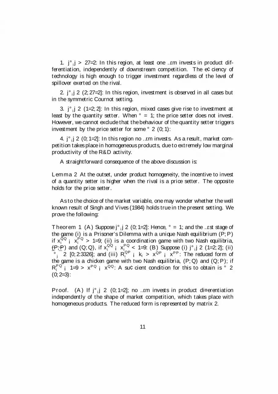
1. j°ij > 27=2: In this region, at least one …rm invests in product dif-ferentiation, independently of downstream competition. The e¢ciency oftechnology is high enough to trigger investment regardless of the level ofspillover exerted on the rival.

2. j°ij 2 (2; 27=2]: In this region, investment is observed in all cases butin the symmetric Cournot setting.

3. j°ij 2 (1=2; 2]: In this region, mixed cases give rise to investment atleast by the quantity setter. When ° = 1; the price setter does not invest.However, we cannot exclude that the behaviour of the quantity setter triggersinvestment by the price setter for some ° 2 (0; 1):

4. j°ij 2 (0; 1=2]: In this region no …rm invests. As a result, market com-petition takes place in homogeneous products, due to extremely low marginalproductivity of the R&D activity.

A straightforward consequence of the above discussion is:

Lemma 2 At the outset, under product homogeneity, the incentive to investof a quantity setter is higher when the rival is a price setter. The oppositeholds for the price setter.

As to the choice of the market variable, one may wonder whether the wellknown result of Singh and Vives (1984) holds true in the present setting. Weprove the following:

Theorem 1 (A) Suppose j°ij 2 (0; 1=2]: Hence, ° = 1; and the …rst stage ofthe game (i) is a Prisoner’s Dilemma with a unique Nash equilibrium (P; P )if xQQi ¡ xPQi > 1=9; (ii) is a coordination game with two Nash equilibria,(P; P ) and (Q;Q), if xQQi ¡ xPQi < 1=9: (B) Suppose (i) j°ij 2 (1=2; 2]; (ii)¯̄°j

¯̄2 [0; 2:3326]; and (iii) RQPi ¡ ki > xQP ¡ xPP : The reduced form of

the game is a chicken game with two Nash equilibria, (P;Q) and (Q;P ); ifRPQi ¡ 1=9 > xPQ ¡ xQQ: A su¢cient condition for this to obtain is ° 2(0; 2=3):

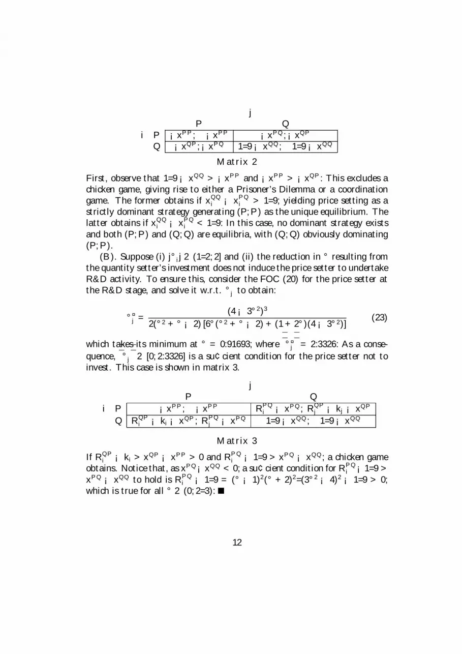
Proof. (A) If j°ij 2 (0; 1=2]; no …rm invests in product di¤erentiationindependently of the shape of market competition, which takes place withhomogeneous products. The reduced form is represented by matrix 2.

11

jP Q

i P ¡xPP ; ¡xPP ¡xPQ;¡xQPQ ¡xQP ;¡xPQ 1=9¡ xQQ; 1=9¡ xQQ

Matrix 2

First, observe that 1=9¡ xQQ > ¡xPP and ¡xPP > ¡xQP : This excludes achicken game, giving rise to either a Prisoner’s Dilemma or a coordinationgame. The former obtains if xQQi ¡ xPQi > 1=9; yielding price setting as astrictly dominant strategy generating (P;P ) as the unique equilibrium. Thelatter obtains if xQQi ¡ xPQi < 1=9: In this case, no dominant strategy existsand both (P; P ) and (Q;Q) are equilibria, with (Q;Q) obviously dominating(P; P ).

(B). Suppose (i) j°ij 2 (1=2; 2] and (ii) the reduction in ° resulting fromthe quantity setter’s investment does not induce the price setter to undertakeR&D activity. To ensure this, consider the FOC (20) for the price setter atthe R&D stage, and solve it w.r.t. °j to obtain:

°¤j =(4¡ 3°2)3

2(°2 + ° ¡ 2) [6°(°2 + ° ¡ 2) + (1 + 2°)(4¡ 3°2)] (23)

which takes its minimum at ° = 0:91693; where¯̄°¤j

¯̄= 2:3326: As a conse-

quence,¯̄°j

¯̄2 [0; 2:3326] is a su¢cient condition for the price setter not to

invest. This case is shown in matrix 3.

jP Q

i P ¡xPP ; ¡xPP RPQi ¡ xPQ; RQPj ¡ kj ¡ xQPQ RQPi ¡ ki ¡ xQP ; RPQj ¡ xPQ 1=9¡ xQQ; 1=9¡ xQQ

Matrix 3

If RQPi ¡ ki > xQP ¡ xPP > 0 and RPQi ¡ 1=9 > xPQ ¡ xQQ; a chicken gameobtains. Notice that, as xPQ¡xQQ < 0; a su¢cient condition for RPQi ¡1=9 >xPQ ¡ xQQ to hold is RPQi ¡ 1=9 = (° ¡ 1)2(° + 2)2=(3°2 ¡ 4)2 ¡ 1=9 > 0;which is true for all ° 2 (0; 2=3):

12

The asymmetry observed at equilibrium in terms of capacity in case Bis driven by the expectation on the part of the price setter of receiving apositive externality from the quantity setter’s decision to invest in productdi¤erentiation at the ensuing R&D stage.3 The above discussion is su¢cientto show that there may exist a non trivial parameter range where quantitysetting is not a dominant strategy, so that the choice of the market variablemay not follow the rule traced by Singh and Vives (1984). Analogous con-siderations hold in the remainder of the range, i.e., for j°ij > 2: E.g., supposethat j°ij 2 (2; 27=2]; in this range, investment is observed in all cases but thesymmetric Cournot one. For the latter to be the unique outcome of the game,as a result of an equilibrium in dominant strategies, the following inequalitiesmust simultaneously hold:

¼QPi ¡ ¼PPi ¸ 0;1

9¡ ¼PQi ¸ xQQ: (24)

If both inequalities above are violated the unique equilibrium is (P; P ): If onlyone of the two inequalities holds we end up with either a chicken game or acoordination game. Our conclusions impinge upon the endogenisation of thedi¤erentiation parameter which is in‡uenced by the nature of downstreamcompetition. The di¤erent incentives to invest in product di¤erentiationdetermine a result which is related to the relative size of revenues and/orcapacities.

3.2 The second game

Consider the alternative game, where the choice of the R&D e¤ort takesplace at the …rst stage of the game, while the choice between P and Q; i.e.,the choice of capacity, is located at the second stage. Suppose, at the …rststage, …rms set a speci…c equilibrium level of ki and kj . In so doing, they …xthe numerical value of ° in the unit interval. Then, the choice between Pand Q is described by matrix 4.

3This resembles the analysis carried out by Fudenberg and Tirole (1984) and Bulow,Geanakoplos and Klemperer (1985) concerning entry deterrence.

13

jP Q

i P RPPi ¡ xPP ; RPPj ¡ xPP RPQi ¡ xPQ; RQPj ¡ xQPQ RQPi ¡ xQP ; RPQj ¡ xPQ RQQi ¡ xQQ; RQQj ¡ xQQ

Matrix 4

Observe that the investment in product di¤erentiation is omitted from ma-trix 4, as it is common to all payo¤s accruing to …rm i; and consequently itis irrelevant as to the choice between P and Q: The inspection of matrix 4reveals that the equilibrium of this game depends on the interplay betweenthe capacity-dominance of price-setting and the revenue-dominance of quan-tity setting. Singh and Vives’s (1984) conclusion, that symmetric Cournotbehaviour should obtain in the unique equilibrium of their game, draws uponthe revenue-dominance of quantity setting, which can be o¤set by the costlyacquisition of capacity. As to the literature on Cournot equilibria under ca-pacity constraints (Levitan and Shubik, 1972; Kreps and Scheinkman, 1983;Davidson and Deneckere, 1986; Osborne and Pitchik, 1986), the above analy-sis highlights the opportunity cost of building up capacity, and its role inshaping endogenously market competition. As an illustration, consider thefollowing inequalities:

xQP ¡ xPP > RQP ¡RPP > 0; xQQ ¡ xPQ > RQQ ¡RPQ > 0: (25)

If the above inequalities hold, the unique equilibrium is (P; P ). Otherwisethe game in matrix 4 can have (Q;Q) as the unique equilibrium or be eithera chicken game, or a coordination game.

4 Welfare analysis

The foregoing analysis of …rms’ behaviour opens the question whether thewell established result that Bertrand competition yields the highest welfarelevel should be expected to carry over to a setting where …rms invest in R&Dand productive capacity. Indeed, some contributions point out that this maynot happen when …rms’ R&D e¤orts are directed towards the attainmentof a process innovation (Delbono and Denicolò, 1990; Qiu, 1997). We showbelow that similar results emerge when capacity is endogenously decided.

14

De…ne social welfare as the sum of consumer surplus plus net pro…ts,i.e., SW IJ = CSIJ + ¦IJ ; where ¦IJ = ¼IJi + ¼IJj : The established wisdomstates that price setting behaviour enhances consumer surplus, with CSPP ¸CSPQ = CSQP > CSQQ 8° 2 (0; 1]. However, from (5-6), we know that

2qPP ¸ qQP + qPQ > 2qQQ 8° 2 (0; 1]; (26)

implying2xPP ¸ xQP + xPQ > 2xQQ 8° 2 (0; 1]: (27)

As a consequence, we can state the following

Lemma 3 From a social standpoint, price setting surplus-dominates quan-tity setting, while quantity setting capacity-dominates price setting.

Although we cannot derive explicit conclusions for both games and allthe relevant parameter subsets, we can unambiguously determine that thereexists at least one case where symmetric Bertrand behaviour is not sociallye¢cient. Consider the …rst game, where the choice of capacity takes place atthe …rst stage. The following obtains:

Proposition 1 Suppose j°ij 2 (0; 1=2]: A necessary and su¢cient conditionfor the social optimality of symmetric Bertrand competition is (xPP ¡xQQ) 2(0; 1=36): Otherwise, symmetric Cournot competition is socially optimal.

Proof. If j°ij 2 (0; 1=2]; we know from the previous section that …rms com-pete in homogeneous products, irrespective of the strategic variables chosenat the …rst stage. Given ° = 1, industry output is equal to one in all casesexcept the symmetric Cournot; as a consequence, the cost of the overallcapacity used in the industry must be the same everywhere except in theCournot setting. Hence, from the social standpoint, relevant welfare levelsare represented in matrix 5.

jP Q

i P 1=2¡ 2xPP 1=2¡ 2xPPQ 1=2¡ 2xPP 4=9¡ 2xQQ

Matrix 5

15

To prove the above Proposition, it su¢ces to observe that

1

2¡ 2xPP > 4

9¡ 2xQQ i¤ xPP ¡ xQQ < 1

36: (28)

If the opposite obtains, i.e., xPP ¡ xQQ > 1=36; the tradeo¤ between con-sumer surplus and the cost of capacity favours Cournot against Bertrandcompetition.

Our next step in the welfare analysis consists in verifying whether thereexists any subset of the space de…ned by the cost of capacity, wherein theprivately optimal equilibrium chosen by …rms is socially e¢cient. We provethe following

Proposition 2 Suppose j°ij 2 (0; 1=2] and xQQ < xPP : If (i) xQQ > xPP ¡1=36; and (ii) xQQ > xPQ+1=9; the unique duopoly equilibrium (P;P ) is alsosocially e¢cient. If (i) xQQ < xPP ¡ 1=36; and (ii) xQQ > xPQ + 1=9; theunique duopoly equilibrium (Q;Q) is socially ine¢cient. If xQQ < xPQ+1=9;…rms play a coordination game with two equilibria, (P; P ) and (Q;Q). WhenxQQ > xPP ¡ 1=36; (P; P ) is socially e¢cient; otherwise (Q;Q) is sociallye¢cient.

Proof. To prove the above Proposition, we resort to a graphical exposition.Figure 2 below is drawn in the space

©xPP ; xQQ

ª; for a given level of xPQ:

² In region ABCD, the duopoly equilibrium fP; Pg coincides with thesocial optimum.

² In region BDE, the duopoly equilibrium is again fP; Pg; while the socialoptimum is fQ;Qg:

16

Figure 2 : Equilibrium analysis

6

-

?

xPP0

xQQ

¡¡¡¡¡¡¡¡¡¡¡¡¡¡¡

xPQ + 1=9

-1/36 ¡¡¡¡¡¡¡¡¡¡¡¡¡¡¡¡¡¡

F

EAB

C D

G

² In region 0ABF, the duopoly game has two equilibria, fP; Pg andfQ;Qg; the former being socially optimal.

² In region BEFG, the duopoly game has two equilibria, fP; Pg andfQ;Qg; the latter being socially optimal.

Consider now the second game where the choice of capacity takes placeat the second stage. On the basis of Lemma 1 and Lemma 3, it can beestablished that a con‡ict between social optimality and private optimalityexists as far as the market variable is concerned.

5 ConclusionsAdopting the same demand structure as in Singh and Vives (1984), we haveendogenised both the choice of capacity and the degree of product substi-tutability by introducing two stages where …rms noncooperatively undertaketechnological commitments before competing on the market. The conse-quences are twofold. First, in both cases the investment behaviour of any

17

given …rm depends upon whether the rival is a quantity or a price setter.Speci…cally, we have established that (i) given the market variable selectedby the rival, being a quantity setter is costlier than being a price setter; and(ii) a quantity setter’s incentive to innovate is higher when the rival is a pricesetter, while the opposite holds for a price setter. Second, a set of equilibriaemerges from the reduced form of the game, where …rms choose between priceand quantity. We have shown that, when the productivity of investment isrelatively low, the game exhibits two asymmetric equilibria in which one …rmis a price setter and the other is a quantity setter, and only the latter investsin di¤erentiation. In the remaining scenarios of innovation technology, theequilibria are determined by the interplay between the level of investmentand the resulting level of di¤erentiation, vis à vis the comparison betweenrevenues and the cost of capacity.

Social welfare analysis suggests two considerations. First, symmetric pricecompetition is more expensive in terms of installed capacity. This impliesthat Bertrand behaviour may not be socially e¢cient. Second, there areconditions under which private incentives may lead …rms to play a sociallyoptimal equilibrium.

18

References

[1] Arrow, K. (1962), “Economic Welfare and the Allocation of Resourcesfor Inventions”, in Nelson, R. (ed.), The Rate and Direction of InventiveActivity, Princeton, NJ, Princeton University Press.

[2] Benoit, J.-P. and V. Krishna (1987), “Dynamic Duopoly: Prices andQuantities”, Review of Economic Studies, 54, 23-35.

[3] Bester, H. and E. Petrakis (1993), “The Incentives for Cost Reductionin a Di¤erentiated Industry”, International Journal of Industrial Orga-nization, 11, 519-34.

[4] Brander, J. and B. Spencer (1983), “Strategic Commitment with R&D:The Symmetric Case”, Bell Journal of Economics, 14, 225-35.

[5] Brock, W. and J. Scheinkman (1985), “Price Setting Supergames withCapacity Constraints”, Review of Economic Studies, 52, 371-82.

[6] Bulow, J., J. Geanakoplos and P. Klemperer (1985), “Holding Idle Ca-pacity to Deter Entry”, Economic Journal, 95, 178-82.

[7] Dasgupta, P. and J. Stiglitz (1980), “Uncertainty, Industrial Structure,and the Speed of R&D”, Bell Journal of Economics, 11, 1-28.

[8] Davidson, C. and R. Deneckere (1986), “Long-run Competition in Ca-pacity, Short-run Competition in Price, and the Cournot Model”, RANDJournal of Economics, 17, 404-15.

[9] Davidson, C. and R. Deneckere (1990), “Excess Capacity and Collu-sion”, International Economic Review, 31, 521-41.

[10] Delbono, F. and V. Denicolò (1990), “R&D Investment in a Symmet-ric and Homogeneous Oligopoly: Bertrand vs Cournot”, InternationalJournal of Industrial Organization, 8, 297-313.

[11] Delbono, F. and V. Denicolò (1991), “Incentives to Innovate in aCournot Oligopoly”, Quarterly Journal of Economics, 106, 951-61.

19

[12] Deneckere, R. and D. Kovenock (1996), “Bertrand-Edgeworth Duopolywith Unit Cost Asymmetry”, Economic Theory, 8, 1-25.

[13] Dixit, A. (1979), “A Model of Duopoly Suggesting a Theory of EntryBarriers”, Bell Journal of Economics, 10, 20-32.

[14] Dixon, H.D. (1985), “Strategic Investment in a Competitive Industry”,Journal of Industrial Economics, 33, 205-12.

[15] Fudenberg, D. and J. Tirole (1984), “The Fat Cat E¤ect, the Puppy DogPloy and the Lean and Hungry Look”, American Economic Review, 74(P&P), 361-68.

[16] Harrington, J.E. (1995), “Experimentation and Learning in aDi¤erentiated-Products Duopoly”, Journal of Economic Theory, 66,275-88.

[17] Hotelling, H. (1929), “Stability in Competition”, Economic Journal, 39,41-57.

[18] Kreps, D. and J. Scheinkman (1983), “Quantity Precommitment andBertrand Competition Yield Cournot Outcomes”, Bell Journal of Eco-nomics, 14, 326-37.

[19] Lambertini, L. and G. Rossini (1998), “Product Homogeneity as a Pris-oner’s Dilemma in a Duopoly with R&D”, Economic Letters, 58, 297-301.

[20] Lee, T. and L. Wilde (1980), “Market Structure and Innovation: AReformulation”, Quarterly Journal of Economics, 94, 429-36.

[21] Levitan, R. and M. Shubik (1972), “Price Duopoly and Capacity Con-straints”, International Economic Review, 13, 111-23.

[22] Loury, G. (1979), “Market Structure and Innovation”, Quarterly Journalof Economics, 93, 395-410.

[23] Osborne, M. and C. Pitchik (1986), “Price Competition in a CapacityConstrained Duopoly”, Journal of Economic Theory, 38, 238-60.

[24] Qiu, L. (1997), “On the Dynamic E¢ciency of Bertrand and CournotEquilibria”, Journal of Economic Theory, 75, 213-29.

20

[25] Reinganum, J. (1989), “The Timing of Innovation: Research, Develop-ment and Di¤usion”, in Schmalensee, R. and R. Willig (eds.), Handbookof Industrial Organization, vol. 1, Amsterdam, North-Holland.

[26] Singh, N. and X. Vives (1984), “Price and Quantity Competition in aDi¤erentiated Duopoly”, RAND Journal of Economics, 15, 546-54.

21