This article appeared in a journal published by Elsevier. The attachedcopy is furnished to the author for internal non-commercial researchand education use, including for instruction at the authors institution

and sharing with colleagues.

Other uses, including reproduction and distribution, or selling orlicensing copies, or posting to personal, institutional or third party

websites are prohibited.

In most cases authors are permitted to post their version of thearticle (e.g. in Word or Tex form) to their personal website orinstitutional repository. Authors requiring further information

regarding Elsevier’s archiving and manuscript policies areencouraged to visit:

http://www.elsevier.com/copyright

Author's personal copy

Neural Networks 21 (2008) 1213–1219

Contents lists available at ScienceDirect

Neural Networks

journal homepage: www.elsevier.com/locate/neunet

Neural networks letter

Emotional balances in experimental consumer choicesGeorge Mengov a,∗, Henrik Egbert b, Stefan Pulov c, Kalin Georgiev da Department of Statistics and Econometrics, Faculty of Economics and Business Administration, Sofia University, 125 Tzarigradsko Chaussee Blvd., Bl. 3, 1113 Sofia, Bulgariab Department of Economics, Behavioral and Institutional Economics VWL VI, 66 Licher Street, 35394 Giessen, Germanyc VMware Bulgaria EAD, 9 Chamkoria Street, 1504 Sofia, Bulgariad Department of Computer Informatics, Faculty of Mathematics and Informatics, Sofia University, 5 James Bourchier Blvd., 1164 Sofia, Bulgaria

a r t i c l e i n f o

Article history:Received 6 January 2008Received in revised form21 August 2008Accepted 29 August 2008

Keywords:Consumer behaviourDecision makingGated dipoleREADSatisfaction treadmill

a b s t r a c t

This paper presents an experiment, which builds a bridge over the gap between neuroscience andthe analysis of economic behaviour. We apply the mathematical theory of Pavlovian conditioning,known as Recurrent Associative Gated Dipole (READ), to analyse consumer choices in a computer-based experiment. Supplier reputations, consumer satisfaction, and customer reactions are operationallydefined and, together with prices, related to READ’s neural dynamics. We recorded our participants’decisions with their timing, and then mapped those decisions on a sequence of events generated bythe READ model. To achieve this, all constants in the differential equations were determined usingsimulated annealing with data from 129 people. READ predicted correctly 96% of all consumer choices ina calibration sample (n = 1290), and 87% in a test sample (n = 903), thus outperforming logit models.The rank correlations between self-assessed and dipole-generated consumer satisfactions were 89% inthe calibration sample and 78% in the test sample, surpassing by a widemargin the best linear regressionmodel.

© 2008 Elsevier Ltd. All rights reserved.

1. Introduction

John Watson, founder of behaviourism, is quoted to have saidin 1922, ‘‘The consumer is to the manufacturer, the departmentstores and the advertising agencies, what the green frog is tothe physiologist’’ (DiClemente & Hantula, 2003). Many decadeslater, we cannot but agree with this provocative insight, althoughwe know a lot more about consumer behaviour, its conditioning,and economic psychology in general. Today fMRI methods helpus discover how brain systems interact when we think abouteconomic decisions (see for example Camerer, Loewenstein, andPrelec (2005)). Yet, these studies still try to locate regions in thecortex involved in forming emotions, judgments, and decisionmaking (cf. Winkielman, Knutson, Paulus, and Trujillo (2007)).It might be advantageous to complement such an observationalapproach, or even step aside from it for a while, by using moreextensively the available theoretical models.In this paper, we present experimental evidence that the math-

ematical theory of Pavlovian conditioning, known as Recurrent As-sociative Gated Dipole (READ) (Grossberg & Schmajuk, 1987) isable to capture essential features of consumer behaviour. A com-puter based experiment showed how a supplier of a fictitious

∗ Corresponding author. Tel.: +359 887765632; fax: +359 28739941.E-mail address: g.mengov@feb.uni-sofia.bg (G. Mengov).

service provoked satisfaction and disappointment, and graduallybuilt its own reputation in the minds of participants as consumers.Accommodated by READ, these factors turned out to be strong pre-dictors of customers’ decisions to retain or abandon their currentsupplier. Our work borrows ideas from affective balance theory(Grossberg & Gutowski, 1987) and the Leven and Levine (1996)neural model of a consumer.

2. Experiment

This experiment investigates the links between (1) monetaryoutcome andmomentary affect, (2) previous emotional experienceand supplier reputation, and (3) provoked emotions and consumerdecisions to retain or abandon the current supplier. It wasconducted in May 2007 and involved 129 students of economicsfrom Sofia University. Its content bears resemblance to theBulgarian market of mobile phone services where two leadingproviders offered indistinguishable quality and prices at the timeof the study. However, similarities with other markets in othercountries would have been just as useful.In each of 17 rounds the participant sees on a computer screen

an advertised price (Pa) offered by the current supplier, whichserves as orientation about what final price (Pf ) might be expected(Fig. 1). No payments with real money are made. Prices Pa wereadjusted to fluctuate slightly around an average monthly billobtained in a survey among another 40 students. Thus, Pa variedwithin 40± 5 Bulgarian leva, and 1 lev is 0.5 euros.

0893-6080/$ – see front matter© 2008 Elsevier Ltd. All rights reserved.doi:10.1016/j.neunet.2008.08.006

Author's personal copy

1214 G. Mengov et al. / Neural Networks 21 (2008) 1213–1219

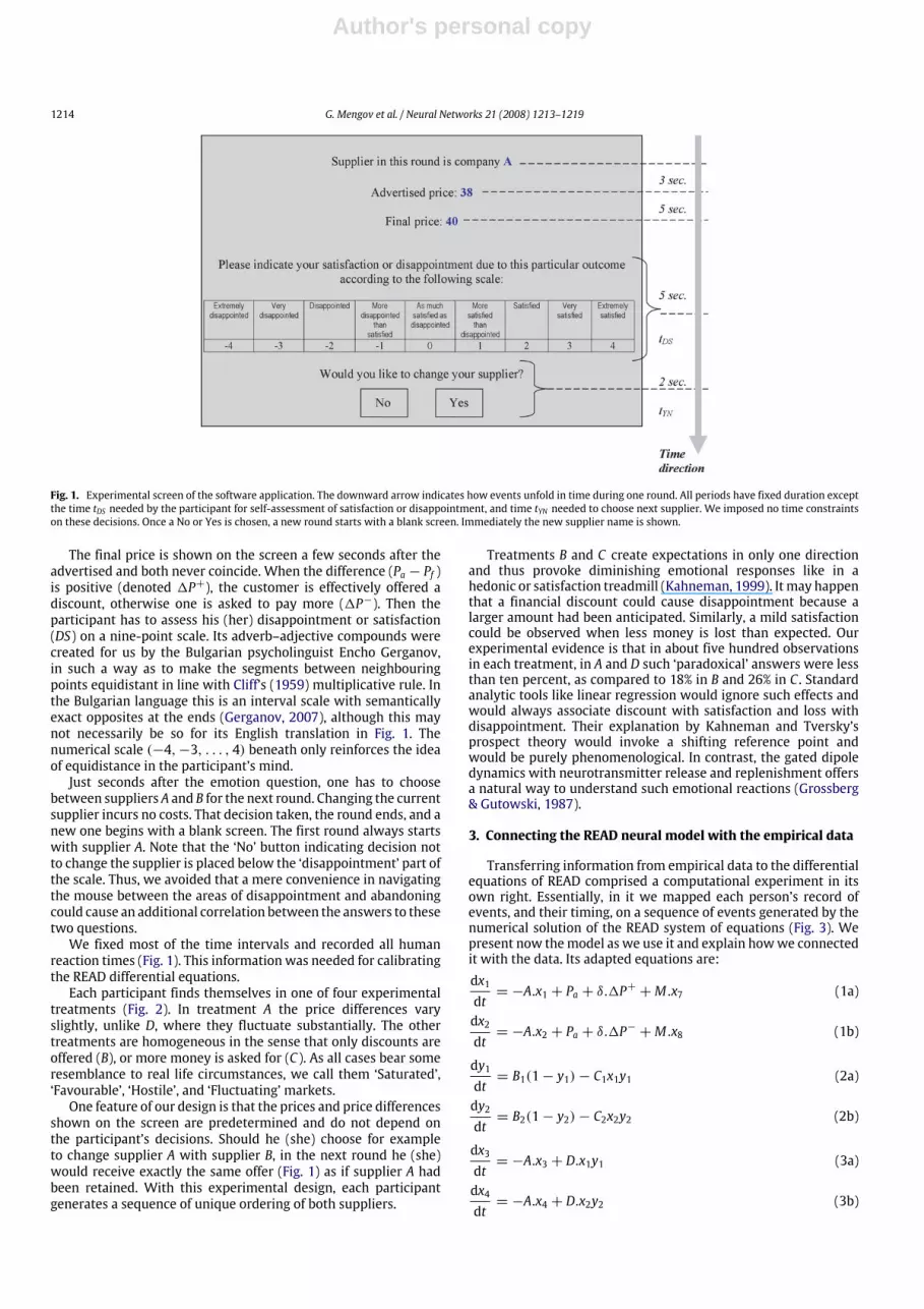
Fig. 1. Experimental screen of the software application. The downward arrow indicates how events unfold in time during one round. All periods have fixed duration exceptthe time tDS needed by the participant for self-assessment of satisfaction or disappointment, and time tYN needed to choose next supplier. We imposed no time constraintson these decisions. Once a No or Yes is chosen, a new round starts with a blank screen. Immediately the new supplier name is shown.

The final price is shown on the screen a few seconds after theadvertised and both never coincide. When the difference (Pa − Pf )is positive (denoted 1P+), the customer is effectively offered adiscount, otherwise one is asked to pay more (1P−). Then theparticipant has to assess his (her) disappointment or satisfaction(DS) on a nine-point scale. Its adverb–adjective compounds werecreated for us by the Bulgarian psycholinguist Encho Gerganov,in such a way as to make the segments between neighbouringpoints equidistant in line with Cliff’s (1959) multiplicative rule. Inthe Bulgarian language this is an interval scale with semanticallyexact opposites at the ends (Gerganov, 2007), although this maynot necessarily be so for its English translation in Fig. 1. Thenumerical scale (−4,−3, . . . , 4) beneath only reinforces the ideaof equidistance in the participant’s mind.Just seconds after the emotion question, one has to choose

between suppliers A and B for the next round. Changing the currentsupplier incurs no costs. That decision taken, the round ends, and anew one begins with a blank screen. The first round always startswith supplier A. Note that the ‘No’ button indicating decision notto change the supplier is placed below the ‘disappointment’ part ofthe scale. Thus, we avoided that a mere convenience in navigatingthe mouse between the areas of disappointment and abandoningcould cause an additional correlation between the answers to thesetwo questions.We fixed most of the time intervals and recorded all human

reaction times (Fig. 1). This information was needed for calibratingthe READ differential equations.Each participant finds themselves in one of four experimental

treatments (Fig. 2). In treatment A the price differences varyslightly, unlike D, where they fluctuate substantially. The othertreatments are homogeneous in the sense that only discounts areoffered (B), or more money is asked for (C). As all cases bear someresemblance to real life circumstances, we call them ‘Saturated’,‘Favourable’, ‘Hostile’, and ‘Fluctuating’ markets.One feature of our design is that the prices and price differences

shown on the screen are predetermined and do not depend onthe participant’s decisions. Should he (she) choose for exampleto change supplier A with supplier B, in the next round he (she)would receive exactly the same offer (Fig. 1) as if supplier A hadbeen retained. With this experimental design, each participantgenerates a sequence of unique ordering of both suppliers.

Treatments B and C create expectations in only one directionand thus provoke diminishing emotional responses like in ahedonic or satisfaction treadmill (Kahneman, 1999). Itmay happenthat a financial discount could cause disappointment because alarger amount had been anticipated. Similarly, a mild satisfactioncould be observed when less money is lost than expected. Ourexperimental evidence is that in about five hundred observationsin each treatment, in A and D such ‘paradoxical’ answers were lessthan ten percent, as compared to 18% in B and 26% in C . Standardanalytic tools like linear regression would ignore such effects andwould always associate discount with satisfaction and loss withdisappointment. Their explanation by Kahneman and Tversky’sprospect theory would invoke a shifting reference point andwould be purely phenomenological. In contrast, the gated dipoledynamics with neurotransmitter release and replenishment offersa natural way to understand such emotional reactions (Grossberg& Gutowski, 1987).

3. Connecting the READ neural model with the empirical data

Transferring information from empirical data to the differentialequations of READ comprised a computational experiment in itsown right. Essentially, in it we mapped each person’s record ofevents, and their timing, on a sequence of events generated by thenumerical solution of the READ system of equations (Fig. 3). Wepresent now themodel as we use it and explain howwe connectedit with the data. Its adapted equations are:dx1dt= −A.x1 + Pa + δ.1P+ +M.x7 (1a)

dx2dt= −A.x2 + Pa + δ.1P− +M.x8 (1b)

dy1dt= B1(1− y1)− C1x1y1 (2a)

dy2dt= B2(1− y2)− C2x2y2 (2b)

dx3dt= −A.x3 + D.x1y1 (3a)

dx4dt= −A.x4 + D.x2y2 (3b)

Author's personal copy

G. Mengov et al. / Neural Networks 21 (2008) 1213–1219 1215

Fig. 2. Four experimental treatments.

dx5dt= −A.x5 + (E − x5)x3 − (x5 + E)x4 (4a)

dx6dt= −A.x6 + (E − x6)x4 − (x6 + E)x3 (4b)

dx7dt= −A.x7 + G[x5]+ + L(SA.z7A + SB.z7B) (5a)

dx8dt= −A.x8 + G[x6]+ + L(SA.z8A + SB.z8B) (5b)

dz7Adt= SA(−K .z7A + H[x5]+) (6a)

dz7Bdt= SB(−K .z7B + H[x5]+) (6b)

dz8Adt= SA(−K .z8A + H[x6]+) (6c)

dz8Bdt= SB(−K .z8B + H[x6]+). (6d)

o1 = [x5]+ (7a)

o2 = [x6]+. (7b)

Here we can afford only a brief discussion on these equationsand refer to the original works of Grossberg and Schmajuk (1987)

and Grossberg, Levine, and Schmajuk (1988) for more detail.The x1, . . . , x8 variables are neuron activities, and y1 and y2 areneurotransmitters. The four z7A, . . . , z8B are memories. Signal SAin Eqs. (5a), (5b) and (6a) and (6c) is equal to one during therounds in which supplier A is active, and is zero otherwise. SignalSB is the opposite. The operator [.]+ denotes rectification [ξ ]+ =max{ξ, 0}. We discuss all equation constants in Section 3.1.We postulate that the dipole’s tonic signal should be the

advertised price Pa, subsuming any other tonic signal. Here it isconstant during a round, but is updated three seconds into eachnew round to match the appearance of Pa on the screen in frontof the participant (Fig. 1). This approach is justified because anadvertised price is shown most of the time, and it is reasonableto assume that in the first three seconds a participant is stillunder the impression of the previous one. Whenever the pricedifference 1P = Pa − Pf is positive, it is submitted to x1 (seeEq. (1a)) eight seconds after the round starts, and is switched offexactly when the round finishes (with Yes or No click), to matchthe unfolding of events with the participant. The same is donewith a negative price difference and x2. Because the experimentalconsumer’s attention focuses on the price difference relativelyindependently from attending Pa and Pf separately, we introduceconstant δ in Eqs. (1a) and (1b).Next, we postulate that the value of o1 in Eq. (7a) and o2 in

Eq. (7b) can represent a participant’s self-assessed emotion (DS).Let us denote by t(i)DS the recorded time moment in round i when

Author's personal copy

1216 G. Mengov et al. / Neural Networks 21 (2008) 1213–1219

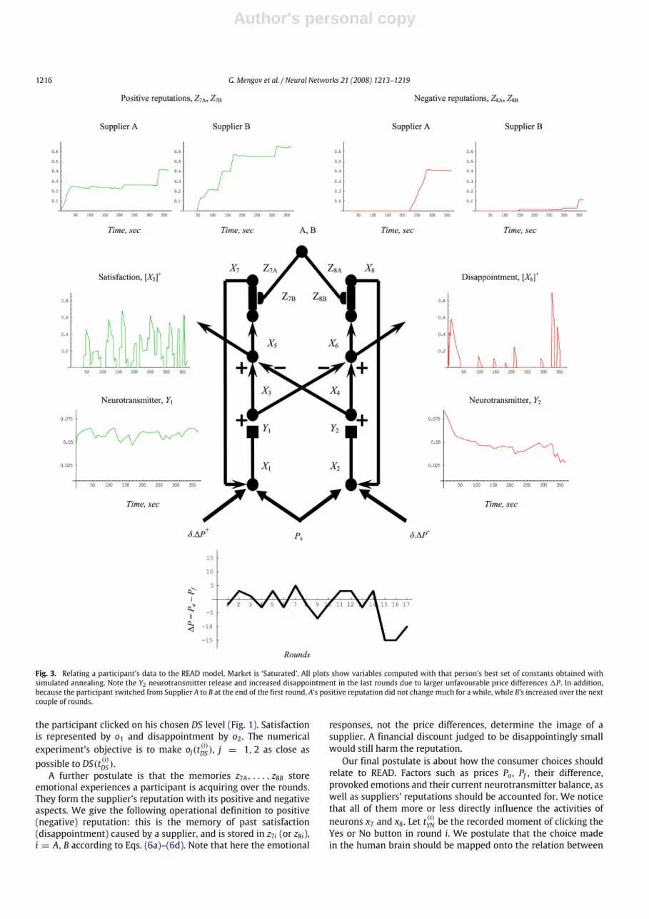
Fig. 3. Relating a participant’s data to the READ model. Market is ‘Saturated’. All plots show variables computed with that person’s best set of constants obtained withsimulated annealing. Note the Y2 neurotransmitter release and increased disappointment in the last rounds due to larger unfavourable price differences 1P . In addition,because the participant switched from Supplier A to B at the end of the first round, A’s positive reputation did not change much for a while, while B’s increased over the nextcouple of rounds.

the participant clicked on his chosen DS level (Fig. 1). Satisfactionis represented by o1 and disappointment by o2. The numericalexperiment’s objective is to make oj(t

(i)DS), j = 1, 2 as close as

possible to DS(t(i)DS).A further postulate is that the memories z7A, . . . , z8B store

emotional experiences a participant is acquiring over the rounds.They form the supplier’s reputation with its positive and negativeaspects. We give the following operational definition to positive(negative) reputation: this is the memory of past satisfaction(disappointment) caused by a supplier, and is stored in z7i (or z8i),i = A, B according to Eqs. (6a)–(6d). Note that here the emotional

responses, not the price differences, determine the image of asupplier. A financial discount judged to be disappointingly smallwould still harm the reputation.Our final postulate is about how the consumer choices should

relate to READ. Factors such as prices Pa, Pf , their difference,provoked emotions and their current neurotransmitter balance, aswell as suppliers’ reputations should be accounted for. We noticethat all of them more or less directly influence the activities ofneurons x7 and x8. Let t

(i)YN be the recorded moment of clicking the

Yes or No button in round i. We postulate that the choice madein the human brain should be mapped onto the relation between

Author's personal copy

G. Mengov et al. / Neural Networks 21 (2008) 1213–1219 1217

neural signals x7 and x8 atmoment t(i)YN . Thus, in round i one chooses

to continue with one’s current supplier iff:

x7(t(i)YN) ≥ x8(t

(i)YN). (8)

Eq. (8) means that, with all factors on the balance, the positivesoutweigh the negatives and the deal is renewed. A supplier whohas just caused disappointment, i.e., o2(t

(i)DS) > 0, may still be

retained, but only on the grounds of a very positive previousreputation. If the inequality in Eq. (8) does not hold, this isinterpreted as decision to change the supplier. Formally, we candefine a variable CS i, which has value 1 if a change was madeand 0 otherwise. An alternative solution could be to introduce athreshold in Eq. (8), but such a complicationwas not really needed.

3.1. Stochastic calibration

Calibrating the READ model in our case meant to make itemulate the human behaviour in the experiment.Wewould like ineach round to have o1(t

(i)DS), o2(t

(i)DS), x7(t

(i)YN), and x8(t

(i)YN) resemble

the participant answers as close as possible. We achieved thisby selecting suitable values for the constants A, δ, M , B1, B2, C1,C2, D, E, G, L, K , and H in Eqs. (1a)–(6d). Their meaning exceptδ (explained in the previous section) is exactly as in Grossbergand Schmajuk (1987) and Grossberg et al. (1988). Because therewas no obvious way for selecting their values, we implementedsimulated annealing. We defined an objective function, optimizedwith respect to both emotional self-assessments and supplierchoices. One possibility was to have a sum of the two criteria withequal weights.

Let DS(tDS) =[DS(t(1)DS ), . . . ,DS(t

(N)DS )

]Tbe the vector of a

participant’s answers to the emotion question, and o(tDS) =[oj(t

(1)DS ), . . . , oj(t

(N)DS )

]T, j = 1, 2 the computed values of o1 in Eq.

(7a) and o2 in Eq. (7b). Here N is the number of sequential roundstaken as calibration sample. Note that the actual emotionDS variesfrom−4 to+4 while READ can have only positive outcomes o1 oro2. Therefore, to relate the empirical and computed scales onemusttake all o2 values (representing disappointment) with negativesigns in o(tDS).We needed a way to put DS(tDS) and o(tDS) in the objective

function. A good choice was to maximize their Spearman rankcorrelation rN (DS(tDS), o(tDS)), and in particular, its variant withcorrections for ties in the data. Other suitable measures ofassociation could be the simple Spearman rank correlation, theKendall rank correlation and, as long as both DS(tDS) and o(tDS)are quantitative, classical correlation could do too.The second term in the objective function should account for

the number of correct choices READmakes. Let Ii(t(i)YN) be indicator

equal to 1 if in round i the READmodel has chosen a supplier in thesense of Eq. (8) exactly as the participant, and 0 otherwise. Thenthe objective function to be maximised was:

J = rN (DS(tDS), o(tDS))+1N

N∑i=1

Ii(t(i)YN). (9)

In Eq. (9) the first term varies within [−1, 1], and the secondwithin [0, 1]. As simulated annealing proceeds, J increases, seekingto reach its maximum of 2 and thereby both terms have equalcontribution. The READ Eqs. (1a)–(7b) were numerically solvedby a Runge-Kutta-Felberg 4–5 method whose implementationby Gammel (2004) offered a suitable trade-off between qualityand speed needed for the many solutions. Of the four milliontimes we solved the READ system several thousand did not finishsuccessfully, but due to the stochastic nature of the optimizationprocess this did not matter.

Each participant’s data of 17 rounds were divided intocalibration sample of the first 10, and validation sample of thelast 7. The former were used to fit Eqs. (1a)–(7b) in an annealingprocess with 6000 solutions. We repeated this computation threetimes and now report the best resultswith respect to the validationsample. An alternative division of 5 calibration and 12 validationrounds achieved slightly lower correlations and predictions forboth samples. In another numerical experiment, only the secondterm in Eq. (9) was used for two runs of 6000 solutions for eachparticipant. Its results were a bit less good, indicating that indeed,emotions should be taken into consideration.

4. Results and discussion

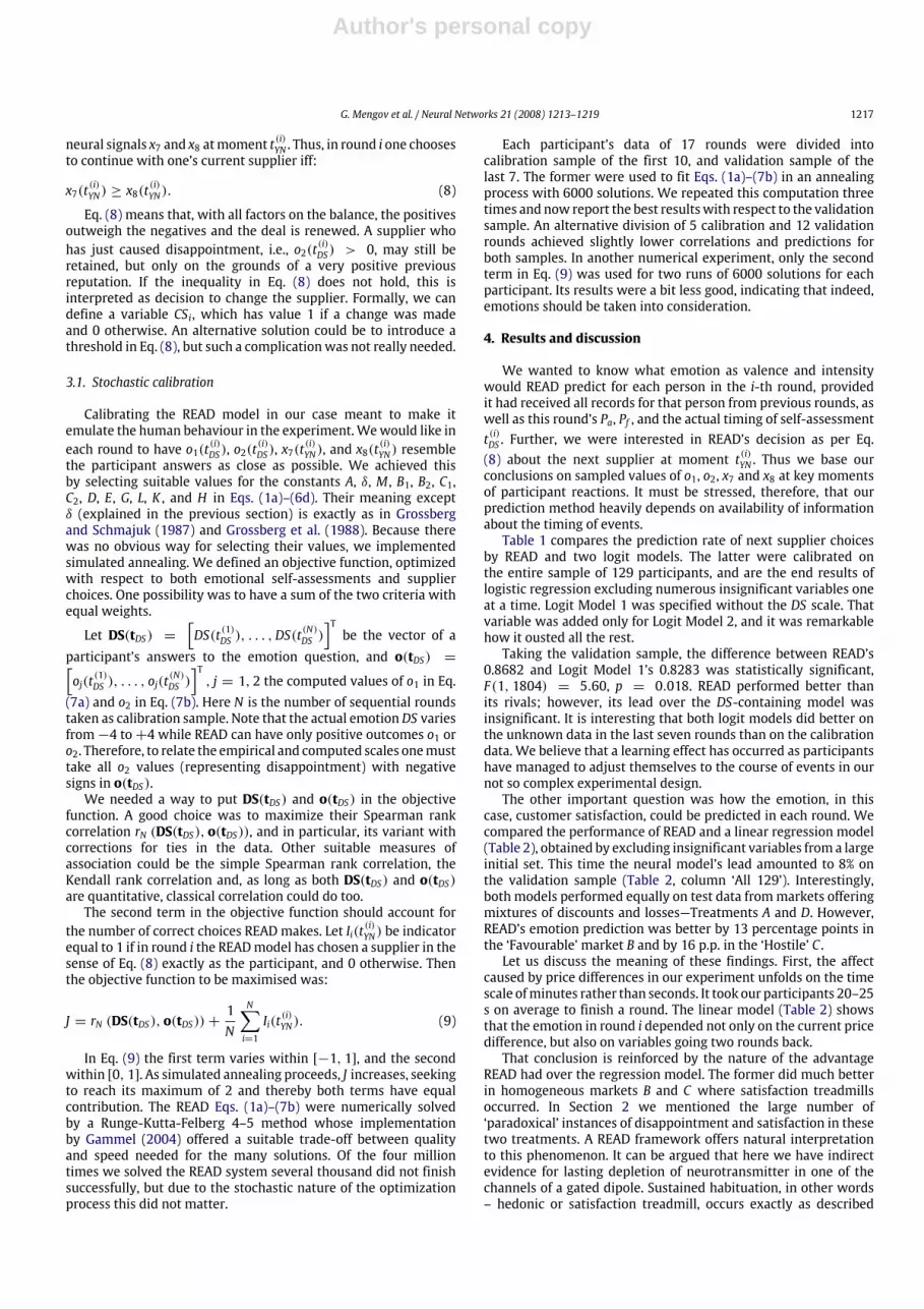
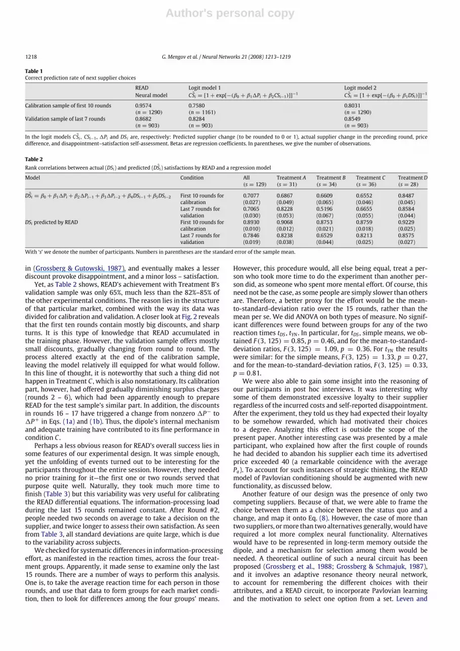
We wanted to know what emotion as valence and intensitywould READ predict for each person in the i-th round, providedit had received all records for that person from previous rounds, aswell as this round’s Pa, Pf , and the actual timing of self-assessmentt(i)DS . Further, we were interested in READ’s decision as per Eq.(8) about the next supplier at moment t(i)YN . Thus we base ourconclusions on sampled values of o1, o2, x7 and x8 at key momentsof participant reactions. It must be stressed, therefore, that ourprediction method heavily depends on availability of informationabout the timing of events.Table 1 compares the prediction rate of next supplier choices

by READ and two logit models. The latter were calibrated onthe entire sample of 129 participants, and are the end results oflogistic regression excluding numerous insignificant variables oneat a time. Logit Model 1 was specified without the DS scale. Thatvariable was added only for Logit Model 2, and it was remarkablehow it ousted all the rest.Taking the validation sample, the difference between READ’s

0.8682 and Logit Model 1’s 0.8283 was statistically significant,F(1, 1804) = 5.60, p = 0.018. READ performed better thanits rivals; however, its lead over the DS-containing model wasinsignificant. It is interesting that both logit models did better onthe unknown data in the last seven rounds than on the calibrationdata. We believe that a learning effect has occurred as participantshave managed to adjust themselves to the course of events in ournot so complex experimental design.The other important question was how the emotion, in this

case, customer satisfaction, could be predicted in each round. Wecompared the performance of READ and a linear regression model(Table 2), obtained by excluding insignificant variables from a largeinitial set. This time the neural model’s lead amounted to 8% onthe validation sample (Table 2, column ‘All 129’). Interestingly,both models performed equally on test data frommarkets offeringmixtures of discounts and losses—Treatments A and D. However,READ’s emotion prediction was better by 13 percentage points inthe ‘Favourable’ market B and by 16 p.p. in the ‘Hostile’ C .Let us discuss the meaning of these findings. First, the affect

caused by price differences in our experiment unfolds on the timescale ofminutes rather than seconds. It took our participants 20–25s on average to finish a round. The linear model (Table 2) showsthat the emotion in round i depended not only on the current pricedifference, but also on variables going two rounds back.That conclusion is reinforced by the nature of the advantage

READ had over the regression model. The former did much betterin homogeneous markets B and C where satisfaction treadmillsoccurred. In Section 2 we mentioned the large number of‘paradoxical’ instances of disappointment and satisfaction in thesetwo treatments. A READ framework offers natural interpretationto this phenomenon. It can be argued that here we have indirectevidence for lasting depletion of neurotransmitter in one of thechannels of a gated dipole. Sustained habituation, in other words– hedonic or satisfaction treadmill, occurs exactly as described

Author's personal copy

1218 G. Mengov et al. / Neural Networks 21 (2008) 1213–1219

Table 1Correct prediction rate of next supplier choices

READ Logit model 1 Logit model 2Neural model CSi = [1+ exp[−(β0 + β11Pi + β2CSi−1)]]−1 CSi = [1+ exp[−(β0 + β1DSi)]]−1

Calibration sample of first 10 rounds 0.9574 0.7580 0.8031(n = 1290) (n = 1161) (n = 1290)

Validation sample of last 7 rounds 0.8682 0.8284 0.8549(n = 903) (n = 903) (n = 903)

In the logit models CSi, CSi−1 , 1Pi and DS i are, respectively: Predicted supplier change (to be rounded to 0 or 1), actual supplier change in the preceding round, pricedifference, and disappointment–satisfaction self-assessment. Betas are regression coefficients. In parentheses, we give the number of observations.

Table 2Rank correlations between actual (DSi) and predicted (DSi) satisfactions by READ and a regression model

Model Condition All Treatment A Treatment B Treatment C TreatmentD(s = 129) (s = 31) (s = 34) (s = 36) (s = 28)

DSi = β0 + β11Pi + β21Pi−1 + β31Pi−2 + β4DSi−1 + β5DSi−2 First 10 rounds forcalibration

0.7077(0.027)

0.6867(0.049)

0.6609(0.065)

0.6552(0.046)

0.8487(0.045)

Last 7 rounds forvalidation

0.7065(0.030)

0.8228(0.053)

0.5196(0.067)

0.6655(0.055)

0.8584(0.044)

DSi predicted by READ First 10 rounds forcalibration

0.8930(0.010)

0.9068(0.012)

0.8753(0.021)

0.8759(0.018)

0.9229(0.025)

Last 7 rounds forvalidation

0.7846(0.019)

0.8238(0.038)

0.6529(0.044)

0.8213(0.025)

0.8575(0.027)

With ‘s’ we denote the number of participants. Numbers in parentheses are the standard error of the sample mean.

in (Grossberg & Gutowski, 1987), and eventually makes a lesserdiscount provoke disappointment, and a minor loss – satisfaction.Yet, as Table 2 shows, READ’s achievement with Treatment B’s

validation sample was only 65%, much less than the 82%–85% ofthe other experimental conditions. The reason lies in the structureof that particular market, combined with the way its data wasdivided for calibration and validation. A closer look at Fig. 2 revealsthat the first ten rounds contain mostly big discounts, and sharpturns. It is this type of knowledge that READ accumulated inthe training phase. However, the validation sample offers mostlysmall discounts, gradually changing from round to round. Theprocess altered exactly at the end of the calibration sample,leaving the model relatively ill equipped for what would follow.In this line of thought, it is noteworthy that such a thing did nothappen in Treatment C , which is also nonstationary. Its calibrationpart, however, had offered gradually diminishing surplus charges(rounds 2 – 6), which had been apparently enough to prepareREAD for the test sample’s similar part. In addition, the discountsin rounds 16 – 17 have triggered a change from nonzero 1P− to1P+ in Eqs. (1a) and (1b). Thus, the dipole’s internal mechanismand adequate training have contributed to its fine performance incondition C .Perhaps a less obvious reason for READ’s overall success lies in

some features of our experimental design. It was simple enough,yet the unfolding of events turned out to be interesting for theparticipants throughout the entire session. However, they neededno prior training for it—the first one or two rounds served thatpurpose quite well. Naturally, they took much more time tofinish (Table 3) but this variability was very useful for calibratingthe READ differential equations. The information-processing loadduring the last 15 rounds remained constant. After Round #2,people needed two seconds on average to take a decision on thesupplier, and twice longer to assess their own satisfaction. As seenfrom Table 3, all standard deviations are quite large, which is dueto the variability across subjects.We checked for systematic differences in information-processing

effort, as manifested in the reaction times, across the four treat-ment groups. Apparently, it made sense to examine only the last15 rounds. There are a number of ways to perform this analysis.One is, to take the average reaction time for each person in thoserounds, and use that data to form groups for each market condi-tion, then to look for differences among the four groups’ means.

However, this procedure would, all else being equal, treat a per-son who took more time to do the experiment than another per-son did, as someone who spent more mental effort. Of course, thisneed not be the case, as some people are simply slower than othersare. Therefore, a better proxy for the effort would be the mean-to-standard-deviation ratio over the 15 rounds, rather than themean per se. We did ANOVA on both types of measure. No signif-icant differences were found between groups for any of the tworeaction times tDS , tYN . In particular, for tDS , simple means, we ob-tained F(3, 125) = 0.85, p = 0.46, and for the mean-to-standard-deviation ratios, F(3, 125) = 1.09, p = 0.36. For tYN the resultswere similar: for the simple means, F(3, 125) = 1.33, p = 0.27,and for the mean-to-standard-deviation ratios, F(3, 125) = 0.33,p = 0.81.We were also able to gain some insight into the reasoning of

our participants in post hoc interviews. It was interesting whysome of them demonstrated excessive loyalty to their supplierregardless of the incurred costs and self-reported disappointment.After the experiment, they told us they had expected their loyaltyto be somehow rewarded, which had motivated their choicesto a degree. Analyzing this effect is outside the scope of thepresent paper. Another interesting case was presented by a maleparticipant, who explained how after the first couple of roundshe had decided to abandon his supplier each time its advertisedprice exceeded 40 (a remarkable coincidence with the averagePa). To account for such instances of strategic thinking, the READmodel of Pavlovian conditioning should be augmented with newfunctionality, as discussed below.Another feature of our design was the presence of only two

competing suppliers. Because of that, we were able to frame thechoice between them as a choice between the status quo and achange, and map it onto Eq. (8). However, the case of more thantwo suppliers, ormore than two alternatives generally, would haverequired a lot more complex neural functionality. Alternativeswould have to be represented in long-term memory outside thedipole, and a mechanism for selection among them would beneeded. A theoretical outline of such a neural circuit has beenproposed (Grossberg et al., 1988; Grossberg & Schmajuk, 1987),and it involves an adaptive resonance theory neural network,to account for remembering the different choices with theirattributes, and a READ circuit, to incorporate Pavlovian learningand the motivation to select one option from a set. Leven and

Author's personal copy

G. Mengov et al. / Neural Networks 21 (2008) 1213–1219 1219

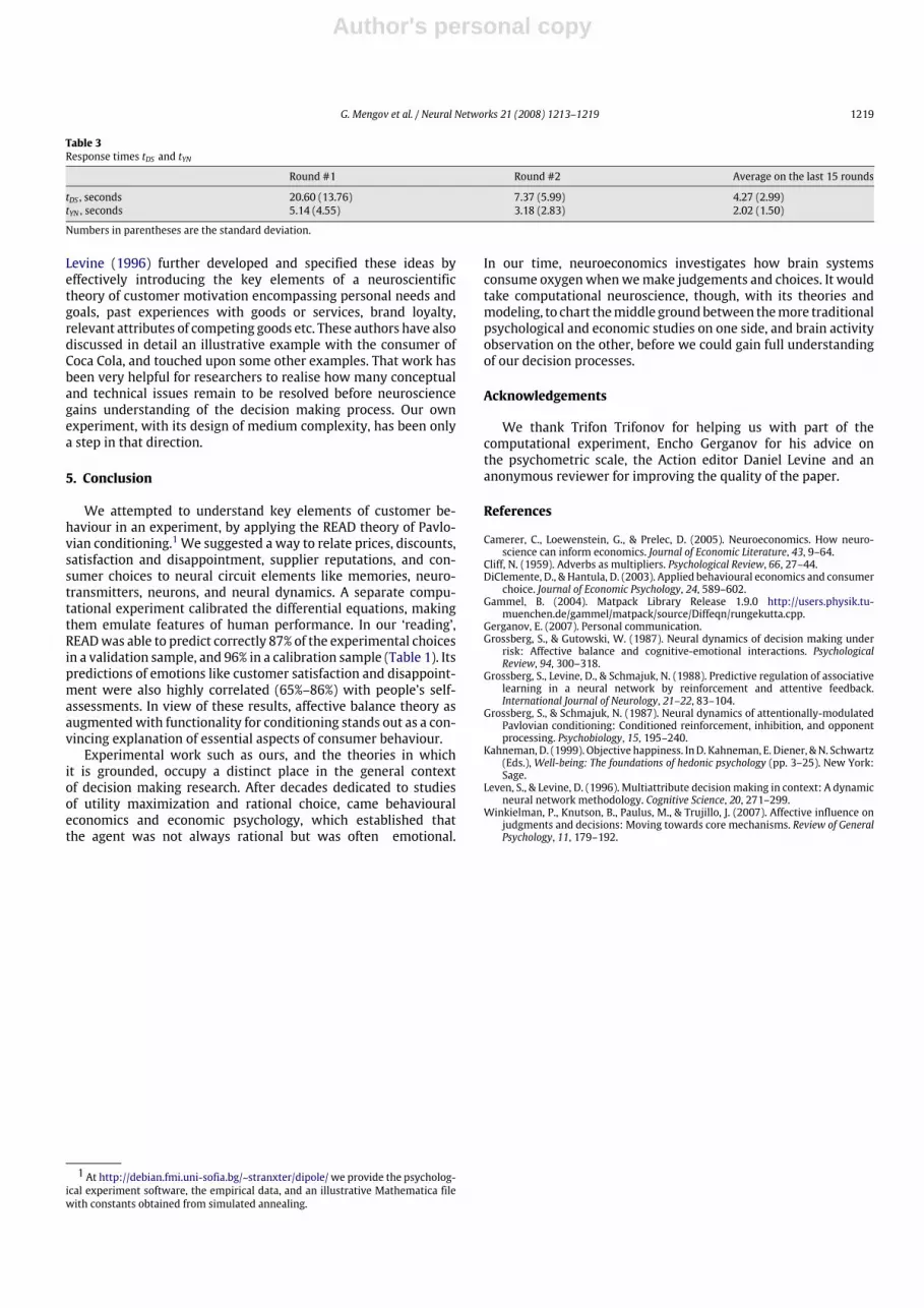
Table 3Response times tDS and tYN

Round #1 Round #2 Average on the last 15 rounds

tDS , seconds 20.60 (13.76) 7.37 (5.99) 4.27 (2.99)tYN , seconds 5.14 (4.55) 3.18 (2.83) 2.02 (1.50)

Numbers in parentheses are the standard deviation.

Levine (1996) further developed and specified these ideas byeffectively introducing the key elements of a neuroscientifictheory of customer motivation encompassing personal needs andgoals, past experiences with goods or services, brand loyalty,relevant attributes of competing goods etc. These authors have alsodiscussed in detail an illustrative example with the consumer ofCoca Cola, and touched upon some other examples. That work hasbeen very helpful for researchers to realise how many conceptualand technical issues remain to be resolved before neurosciencegains understanding of the decision making process. Our ownexperiment, with its design of medium complexity, has been onlya step in that direction.

5. Conclusion

We attempted to understand key elements of customer be-haviour in an experiment, by applying the READ theory of Pavlo-vian conditioning.1We suggested a way to relate prices, discounts,satisfaction and disappointment, supplier reputations, and con-sumer choices to neural circuit elements like memories, neuro-transmitters, neurons, and neural dynamics. A separate compu-tational experiment calibrated the differential equations, makingthem emulate features of human performance. In our ‘reading’,READwas able to predict correctly 87% of the experimental choicesin a validation sample, and 96% in a calibration sample (Table 1). Itspredictions of emotions like customer satisfaction and disappoint-ment were also highly correlated (65%–86%) with people’s self-assessments. In view of these results, affective balance theory asaugmentedwith functionality for conditioning stands out as a con-vincing explanation of essential aspects of consumer behaviour.Experimental work such as ours, and the theories in which

it is grounded, occupy a distinct place in the general contextof decision making research. After decades dedicated to studiesof utility maximization and rational choice, came behaviouraleconomics and economic psychology, which established thatthe agent was not always rational but was often emotional.

1 At http://debian.fmi.uni-sofia.bg/~stranxter/dipole/ we provide the psycholog-ical experiment software, the empirical data, and an illustrative Mathematica filewith constants obtained from simulated annealing.

In our time, neuroeconomics investigates how brain systemsconsume oxygenwhenwemake judgements and choices. It wouldtake computational neuroscience, though, with its theories andmodeling, to chart themiddle groundbetween themore traditionalpsychological and economic studies on one side, and brain activityobservation on the other, before we could gain full understandingof our decision processes.

Acknowledgements

We thank Trifon Trifonov for helping us with part of thecomputational experiment, Encho Gerganov for his advice onthe psychometric scale, the Action editor Daniel Levine and ananonymous reviewer for improving the quality of the paper.

References

Camerer, C., Loewenstein, G., & Prelec, D. (2005). Neuroeconomics. How neuro-science can inform economics. Journal of Economic Literature, 43, 9–64.

Cliff, N. (1959). Adverbs as multipliers. Psychological Review, 66, 27–44.DiClemente, D., & Hantula, D. (2003). Applied behavioural economics and consumerchoice. Journal of Economic Psychology, 24, 589–602.

Gammel, B. (2004). Matpack Library Release 1.9.0 http://users.physik.tu-muenchen.de/gammel/matpack/source/Diffeqn/rungekutta.cpp.

Gerganov, E. (2007). Personal communication.Grossberg, S., & Gutowski, W. (1987). Neural dynamics of decision making underrisk: Affective balance and cognitive-emotional interactions. PsychologicalReview, 94, 300–318.

Grossberg, S., Levine, D., & Schmajuk, N. (1988). Predictive regulation of associativelearning in a neural network by reinforcement and attentive feedback.International Journal of Neurology, 21–22, 83–104.

Grossberg, S., & Schmajuk, N. (1987). Neural dynamics of attentionally-modulatedPavlovian conditioning: Conditioned reinforcement, inhibition, and opponentprocessing. Psychobiology, 15, 195–240.

Kahneman, D. (1999). Objective happiness. InD. Kahneman, E. Diener, &N. Schwartz(Eds.),Well-being: The foundations of hedonic psychology (pp. 3–25). New York:Sage.

Leven, S., & Levine, D. (1996). Multiattribute decisionmaking in context: A dynamicneural network methodology. Cognitive Science, 20, 271–299.

Winkielman, P., Knutson, B., Paulus, M., & Trujillo, J. (2007). Affective influence onjudgments and decisions: Moving towards core mechanisms. Review of GeneralPsychology, 11, 179–192.