Embed Size (px)
Citation preview

Elephant DocumentationRelease 0.6.0
Elephant authors and contributors
Oct 12, 2018


Contents
1 Synopsis 1
2 Table of Contents 3
Bibliography 81
Python Module Index 83
i

ii

CHAPTER 1
Synopsis
Elephant is a toolbox for the analysis of electrophysiological data based on the Neo framework. This manual coversthe installation of Elephant in an existing Python environment, several tutorials to help get you started, information onthe structure and conventions of the library, a list of modules, and help for future contributors to Elephant.
1

Elephant Documentation, Release 0.6.0
2 Chapter 1. Synopsis
CHAPTER 2
Table of Contents
2.1 Overview
2.1.1 What is Elephant?
As a result of the complexity inherent in modern recording technologies that yield massively parallel data streams andin advanced analysis methods to explore such rich data sets, the need for more reproducible research in the neuro-sciences can no longer be ignored. Reproducibility rests on building workflows that may allow users to transparentlytrace their analysis steps from data acquisition to final publication. A key component of such a workflow is a set ofdefined analysis methods to perform the data processing.
Elephant (Electrophysiology Analysis Toolkit) is an emerging open-source, community centered library for the anal-ysis of electrophysiological data in the Python programming language. The focus of Elephant is on generic analysisfunctions for spike train data and time series recordings from electrodes, such as the local field potentials (LFP) orintracellular voltages. In addition to providing a common platform for analysis codes from different laboratories,the Elephant project aims to provide a consistent and homogeneous analysis framework that is built on a modularfoundation. Elephant is the direct successor to Neurotools1 and maintains ties to complementary projects such asOpenElectrophy2 and spykeviewer3.
• Analysis functions use consistent data formats and conventions as input arguments and outputs. Electrophysio-logical data will generally be represented by data models defined by the Neo4 project.
• Library functions are based on a set of core functions for commonly used operations, such as sliding windows,converting data to alternate representations, or the generation of surrogates for hypothesis testing.
• Accepted analysis functions must be equipped with a range of unit tests to ensure a high standard of code quality.
1 http://neuralensemble.org/NeuroTools/2 http://neuralensemble.org/OpenElectrophy/3 http://spykeutils.readthedocs.org/en/0.4.1/4 Garcia et al. (2014) Front.~Neuroinform. 8:10
3

Elephant Documentation, Release 0.6.0
2.1.2 Elephant library structure
Elephant is a standard python package and is structured into a number of submodules. The following is a sketch of thelayout of the Elephant library (0.3.0 release).
Fig. 1: Modules of the Elephant library. Modules containing analysis functions are colored in blue shades, corefunctionality in green shades.
Conceptually, modules of the Elephant library can be divided into those related to a specific category of analysismethods, and supporting modules that provide a layer of various core utility functions. All available modules areavailable directly on the the top level of the Elephant package in the elephant subdirectory to avoid unnecessaryhierarchical clutter. Unit tests for all functions are located in the elephant/test subdirectory and are namedaccording the module name. This documentation is located in the top level doc subdirectory.
In the following we provide a brief overview of the modules available in Elephant.
4 Chapter 2. Table of Contents

Elephant Documentation, Release 0.6.0
Analysis modules
statistics
Statistical measures of spike trains (e.g., Fano factor) and functions to estimate firing rates.
signal_processing
Basic processing procedures for analog signals (e.g., performing a z-score of a signal, or filtering a signal).
spectral
Identification of spectral properties in analog signals (e.g., the power spectrum)
kernels
A class that provides representations for commonly used kernel functions.
spike_train_dissimilarity_measures
Spike train metrics (e.g., the Victor-Purpura measure) to measure the (dis-)similarity between spike trains.
sta
Calculate the spike-triggered average and spike-field-coherence of an analog signal.
spike_train_correlation
Functions to quantify correlations between sets of spike trains.
unitary_event_analysis
Determine periods where neurons synchronize their activity beyond chance level.
cubic
Implements the method Cumulant Based Inference of higher-order Correlation (CuBIC) to detect the presence ofhigher-order correlations in massively parallel data based on its complexity distribution.
asset
Implementation of the Analysis of Sequences of Synchronous EvenTs (ASSET) to detect, in particular, syn-fire chainlike activity.
2.1. Overview 5

Elephant Documentation, Release 0.6.0
csd
Inverse and standard methods to estimate of current source density (CSD) of laminar LFP recordings.
Supporting modules
conversion
This module allows to convert standard data representations (e.g., a spike train stored as Neo SpikeTrain object)into other representations useful to perform calculations on the data. An example is the representation of a spike trainas a sequence of 0-1 values (binned spike train).
spike_train_generation
This module provides functions to generate spike trains according to prescribed stochastic models (e.g., a Poissonspike train).
spike_train_surrogates
This module provides functionality to generate surrogate spike trains from given spike train data. This is particularlyuseful in the context of determining the significance of analysis results via Monte-Carlo methods.
neo_tools
Provides useful convenience functions to work efficiently with Neo objects.
pandas_bridge
Bridge from Elephant to the pandas library.
2.1.3 References
2.2 Prerequisites / Installation
Elephant is a pure Python package so that it should be easy to install on any system.
2.2.1 Dependencies
The following packages are required to use Elephant:
• Python >= 2.7
• numpy >= 1.8.2
• scipy >= 0.14.0
• quantities >= 0.10.1
6 Chapter 2. Table of Contents

Elephant Documentation, Release 0.6.0
• neo >= 0.5.0
The following packages are optional in order to run certain parts of Elephant:
• For using the pandas_bridge module:
– pandas >= 0.14.1
• For using the ASSET analysis
• scikit-learn >= 0.15.1
• For building the documentation:
– numpydoc >= 0.5
– sphinx >= 1.2.2
• For running tests:
– nose >= 1.3.3
All dependencies can be found on the Python package index (PyPI).
Debian/Ubuntu
For Debian/Ubuntu, we recommend to install numpy and scipy as system packages using apt-get:
$ apt-get install python-numpy python-scipy python-pip python-six
Further packages are found on the Python package index (pypi) and should be installed with pip:
$ pip install quantities$ pip install neo
We highly recommend to install these packages using a virtual environment provided by virtualenv or locally in thehome directory using the --user option of pip (e.g., pip install --user quantities), neither of whichrequire administrator privileges.
Windows/Mac OS X
On non-Linux operating systems we recommend using the Anaconda Python distribution, and installing all dependen-cies in a Conda environment, e.g.:
$ conda create -n neuroscience python numpy scipy pip six$ source activate neuroscience$ pip install quantities$ pip install neo
2.2.2 Installation
Automatic installation from PyPI
The easiest way to install Elephant is via pip:
$ pip install elephant
2.2. Prerequisites / Installation 7
Elephant Documentation, Release 0.6.0
Manual installation from pypi
To download and install manually, download the latest package from http://pypi.python.org/pypi/elephant
Then:
$ tar xzf elephant-0.6.0.tar.gz$ cd elephant-0.6.0$ python setup.py install
or:
$ python3 setup.py install
depending on which version of Python you are using.
Installation of the latest build from source
To install the latest version of Elephant from the Git repository:
$ git clone git://github.com/NeuralEnsemble/elephant.git$ cd elephant$ python setup.py install
2.3 Tutorials
2.3.1 Getting Started
In this first tutorial, we will go through a very simple example of how to use Elephant. We will numerically verify thatthe coefficient of variation (CV), a measure of the variability of inter-spike intervals, of a spike train that is modeledas a random (stochastic) Poisson process is 1.
As a first step, install Elephant and its dependencies as outlined in Prerequisites / Installation. Next, start up yourPython shell. Under Windows, you can likely launch a Python shell from the Start menu. Under Linux or Mac, youmay start Python by typing:
$ python
As a first step, we want to generate spike train data modeled as a stochastic Poisson process. Forthis purpose, we can use the elephant.spike_train_generation module, which provides thehomogeneous_poisson_process() function:
>>> from elephant.spike_train_generation import homogeneous_poisson_process
Use the help() function of Python to display the documentation for this function:
>>> help(homogeneous_poisson_process)
As you can see, the function requires three parameters: the firing rate of the Poisson process, the start time and thestop time. These three parameters are specified as Quantity objects: these are essentially arrays or numbers witha unit of measurement attached. We will see how to use these objects in a second. You can quit the help screen bytyping q.
Let us now generate 100 independent Poisson spike trains for 100 seconds each with a rate of 10 Hz for which we laterwill calculate the CV. For simplicity, we will store the spike trains in a list:
8 Chapter 2. Table of Contents
Elephant Documentation, Release 0.6.0
>>> from quantities import Hz, s, ms>>> spiketrain_list = [... homogeneous_poisson_process(rate=10.0*Hz, t_start=0.0*s, t_stop=100.0*s)... for i in range(100)]
Notice that the units s and Hz have both been imported from the quantities library and can be directly attachedto the values by multiplication. The output is a list of 100 Neo SpikeTrain objects:
>>> print(len(spiketrain_list))100>>> print(type(spiketrain_list[0]))<class 'neo.core.spiketrain.SpikeTrain'>
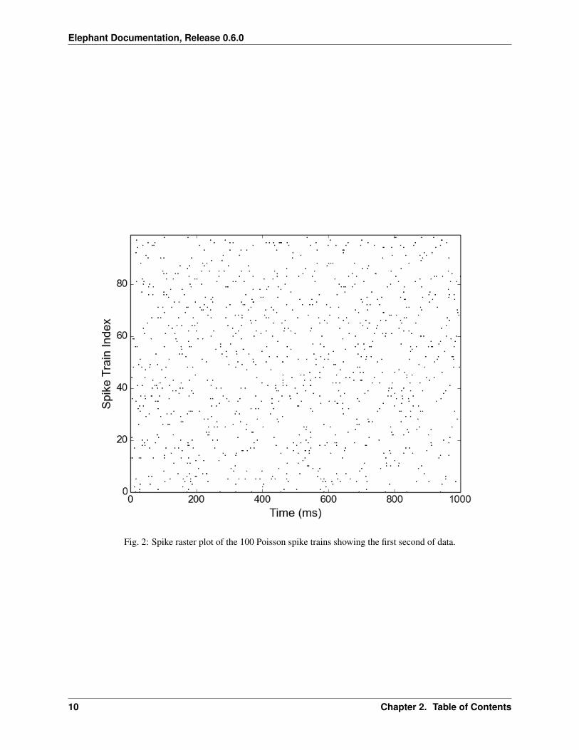
Before we continue, let us (optionally) have a look at the spike trains in a spike raster plot. This can be created, e.g.,using the matplotlib framework (you may need to install this library, as it is not one of the dependencies of Elephant):
>>> import matplotlib.pyplot as plt>>> import numpy as np>>> for i, spiketrain in enumerate(spiketrain_list):
t = spiketrain.rescale(ms)plt.plot(t, i * np.ones_like(t), 'k.', markersize=2)
>>> plt.axis('tight')>>> plt.xlim(0, 1000)>>> plt.xlabel('Time (ms)', fontsize=16)>>> plt.ylabel('Spike Train Index', fontsize=16)>>> plt.gca().tick_params(axis='both', which='major', labelsize=14)>>> plt.show()
Notice how the spike times of each spike train are extracted from each of the spike trains in the for-loop. Therescale() operation of the quantities library is used to transform units to milliseconds. In order to aid the vi-sualization, we restrict the plot to the first 1000 ms (xlim() function). The show() command plots the spike rasterin a new figure window on the screen.
From the plot you can see the random nature of each Poisson spike train. Let us now calculate the distribution ofthe 100 CVs obtained from inter-spike intervals (ISIs) of these spike trains. Close the graphics window to get backto the Python prompt. The functions to calculate the list of ISIs and the CV are both located in the elephant.statistics module. Thus, for each spike train in our list, we first call the isi() function which returns an arrayof all N-1 ISIs for the N spikes in the input spike train (refer to the online help using help(isi)). We then feed thelist of ISIs into the cv() function, which returns a single value for the coefficient of variation:
>>> from elephant.statistics import isi, cv>>> cv_list = [cv(isi(spiketrain)) for spiketrain in spiketrain_list]
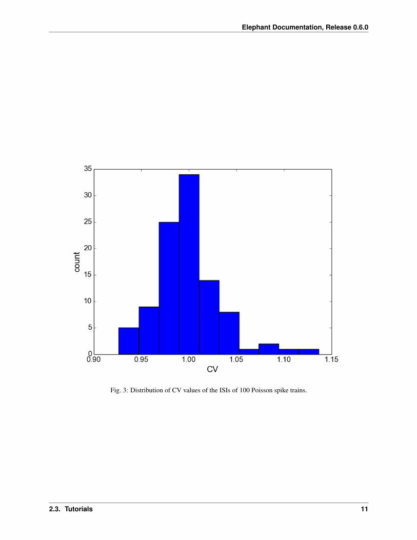
In a final step, let’s plot a histogram of the obtained CVs (again illustrated using the matplotlib framework for plotting):
>>> plt.hist(cv_list)>>> plt.xlabel('CV', fontsize=16)>>> plt.ylabel('count', fontsize=16)>>> plt.gca().tick_params(axis='both', which='major', labelsize=14)>>> plt.show()
As predicted by theory, the CV values are clustered around 1. This concludes our first “getting started” tutorial on theuse of Elephant. More tutorials will be added soon.
2.3. Tutorials 9
Elephant Documentation, Release 0.6.0
Fig. 2: Spike raster plot of the 100 Poisson spike trains showing the first second of data.
10 Chapter 2. Table of Contents
Elephant Documentation, Release 0.6.0
Fig. 3: Distribution of CV values of the ISIs of 100 Poisson spike trains.
2.3. Tutorials 11
Elephant Documentation, Release 0.6.0
2.4 Function Reference by Module
2.4.1 Spike train statistics
Statistical measures of spike trains (e.g., Fano factor) and functions to estimate firing rates.
elephant.statistics.complexity_pdf(spiketrains, binsize)Complexity Distribution [1] of a list of neo.SpikeTrain objects.
Probability density computed from the complexity histogram which is the histogram of the entries of the pop-ulation histogram of clipped (binary) spike trains computed with a bin width of binsize. It provides for eachcomplexity (== number of active neurons per bin) the number of occurrences. The normalization of that his-togram to 1 is the probability density.
Parameters
spiketrains [List of neo.SpikeTrain objects]
Spiketrains with a common time axis (same ‘t_start‘ and ‘t_stop‘)
binsize [quantities.Quantity]
Width of the histogram’s time bins.
Returns
time_hist [neo.AnalogSignal]
A neo.AnalogSignal object containing the histogram values.
‘AnalogSignal[j]‘ is the histogram computed between .
See also:
elephant.conversion.BinnedSpikeTrain
References
[1]Gruen, S., Abeles, M., & Diesmann, M. (2008). Impact of higher-order correlations on coincidence distri-butions of massively parallel data. In Dynamic Brain-from Neural Spikes to Behaviors (pp. 96-114). SpringerBerlin Heidelberg.
elephant.statistics.cost_function(x, N, w, dt)The cost function Cn(w) = sum_{i,j} int k(x - x_i) k(x - x_j) dx - 2 sum_{i~=j} k(x_i - x_j)
elephant.statistics.cv2(v)Calculate the measure of CV2 for a sequence of time intervals between events.
Given a vector v containing a sequence of intervals, the CV2 is defined as:
.math $$ CV2 := frac{1}{N}sum_{i=1}^{N-1}
frac{2|isi_{i+1}-isi_i|} {|isi_{i+1}+isi_i|} $$
The CV2 is typically computed as a substitute for the classical coefficient of variation (CV) for sequences ofevents which include some (relatively slow) rate fluctuation. As with the CV, CV2=1 for a sequence of intervalsgenerated by a Poisson process.
Parameters
v [quantity array, numpy array or list] Vector of consecutive time intervals
Returns
12 Chapter 2. Table of Contents
Elephant Documentation, Release 0.6.0
cv2 [float] The CV2 of the inter-spike interval of the input sequence.
Raises
AttributeError : If an empty list is specified, or if the sequence has less than two entries, anAttributeError will be raised.
AttributeError : Only vector inputs are supported. If a matrix is passed to the function anAttributeError will be raised.
References
..[1] Holt, G. R., Softky, W. R., Koch, C., & Douglas, R. J. (1996). Comparison of discharge variability in vitroand in vivo in cat visual cortex neurons. Journal of neurophysiology, 75(5), 1806-1814.
elephant.statistics.fanofactor(spiketrains)Evaluates the empirical Fano factor F of the spike counts of a list of neo.core.SpikeTrain objects.
Given the vector v containing the observed spike counts (one per spike train) in the time window [t0, t1], F isdefined as:
F := var(v)/mean(v).
The Fano factor is typically computed for spike trains representing the activity of the same neuron over differenttrials. The higher F, the larger the cross-trial non-stationarity. In theory for a time-stationary Poisson process,F=1.
Parameters
spiketrains [list of neo.SpikeTrain objects, quantity arrays, numpy arrays or lists] Spike trainsfor which to compute the Fano factor of spike counts.
Returns
fano [float or nan] The Fano factor of the spike counts of the input spike trains. If an empty listis specified, or if all spike trains are empty, F:=nan.
elephant.statistics.fftkernel(x, w)Function ‘fftkernel’ applies the Gauss kernel smoother to an input signal using FFT algorithm.
Input argument x: Sample signal vector. w: Kernel bandwidth (the standard deviation) in unit of the samplingresolution of x.
Output argument y: Smoothed signal.
MAY 5/23, 2012 Author Hideaki Shimazaki RIKEN Brain Science Insitute http://2000.jukuin.keio.ac.jp/shimazaki
Ported to Python: Subhasis Ray, NCBS. Tue Jun 10 10:42:38 IST 2014
elephant.statistics.instantaneous_rate(spiketrain, sampling_period, kernel=’auto’, cut-off=5.0, t_start=None, t_stop=None, trim=False)
Estimates instantaneous firing rate by kernel convolution.
Parameters
spiketrain [neo.SpikeTrain or list of neo.SpikeTrain objects] Neo object that contains spiketimes, the unit of the time stamps and t_start and t_stop of the spike train.
sampling_period [Time Quantity] Time stamp resolution of the spike times. The same resolu-tion will be assumed for the kernel
2.4. Function Reference by Module 13
Elephant Documentation, Release 0.6.0
kernel [string ‘auto’ or callable object of Kernel from module] ‘kernels.py’. Currently imple-mented kernel forms are rectangular, triangular, epanechnikovlike, gaussian, laplacian, ex-ponential, and alpha function. Example: kernel = kernels.RectangularKernel(sigma=10*ms,invert=False) The kernel is used for convolution with the spike train and its standard devia-tion determines the time resolution of the instantaneous rate estimation. Default: ‘auto’. Inthis case, the optimized kernel width for the rate estimation is calculated according to [1]and with this width a gaussian kernel is constructed. Automatized calculation of the kernelwidth is not available for other than gaussian kernel shapes.
cutoff [float] This factor determines the cutoff of the probability distribution of the kernel, i.e.,the considered width of the kernel in terms of multiples of the standard deviation sigma.Default: 5.0
t_start [Time Quantity (optional)] Start time of the interval used to compute the firing rate. IfNone assumed equal to spiketrain.t_start Default: None
t_stop [Time Quantity (optional)] End time of the interval used to compute the firing rate (in-cluded). If None assumed equal to spiketrain.t_stop Default: None
trim [bool] if False, the output of the Fast Fourier Transformation being a longer vector than theinput vector by the size of the kernel is reduced back to the original size of the consideredtime interval of the spiketrain using the median of the kernel. if True, only the region of theconvolved signal is returned, where there is complete overlap between kernel and spike train.This is achieved by reducing the length of the output of the Fast Fourier Transformation bya total of two times the size of the kernel, and t_start and t_stop are adjusted. Default: False
Returns
rate [neo.AnalogSignal] Contains the rate estimation in unit hertz (Hz). Has a property‘rate.times’ which contains the time axis of the rate estimate. The unit of this property is thesame as the resolution that is given via the argument ‘sampling_period’ to the function.
Raises
TypeError: If spiketrain is not an instance of SpikeTrain of Neo. If sampling_period is nota time quantity. If kernel is neither instance of Kernel or string ‘auto’. If cutoff is neitherfloat nor int. If t_start and t_stop are neither None nor a time quantity. If trim is not bool.
ValueError: If sampling_period is smaller than zero.
References
..[1] H. Shimazaki, S. Shinomoto, J Comput Neurosci (2010) 29:171–182.
elephant.statistics.isi(spiketrain, axis=-1)Return an array containing the inter-spike intervals of the SpikeTrain.
Accepts a Neo SpikeTrain, a Quantity array, or a plain NumPy array. If either a SpikeTrain or Quantity array isprovided, the return value will be a quantities array, otherwise a plain NumPy array. The units of the quantitiesarray will be the same as spiketrain.
Parameters
spiketrain [Neo SpikeTrain or Quantity array or NumPy ndarray] The spike times.
axis [int, optional] The axis along which the difference is taken. Default is the last axis.
Returns
NumPy array or quantities array.
14 Chapter 2. Table of Contents
Elephant Documentation, Release 0.6.0
elephant.statistics.lv(v)Calculate the measure of local variation LV for a sequence of time intervals between events.
Given a vector v containing a sequence of intervals, the LV is defined as:
.math $$ LV := frac{1}{N}sum_{i=1}^{N-1}
frac{3(isi_i-isi_{i+1})^2} {(isi_i+isi_{i+1})^2} $$
The LV is typically computed as a substitute for the classical coefficient of variation for sequences of eventswhich include some (relatively slow) rate fluctuation. As with the CV, LV=1 for a sequence of intervals generatedby a Poisson process.
Parameters
v [quantity array, numpy array or list] Vector of consecutive time intervals
Returns
lvar [float] The LV of the inter-spike interval of the input sequence.
Raises
AttributeError : If an empty list is specified, or if the sequence has less than two entries, anAttributeError will be raised.
ValueError : Only vector inputs are supported. If a matrix is passed to the function a ValueEr-ror will be raised.
References
..[1] Shinomoto, S., Shima, K., & Tanji, J. (2003). Differences in spiking patterns among cortical neurons.Neural Computation, 15, 2823–2842.
elephant.statistics.make_kernel(form, sigma, sampling_period, direction=1)Creates kernel functions for convolution.
Constructs a numeric linear convolution kernel of basic shape to be used for data smoothing (linear low passfiltering) and firing rate estimation from single trial or trial-averaged spike trains.
Exponential and alpha kernels may also be used to represent postynaptic currents / potentials in a linear (current-based) model.
Parameters
form [{‘BOX’, ‘TRI’, ‘GAU’, ‘EPA’, ‘EXP’, ‘ALP’}] Kernel form. Currently implementedforms are BOX (boxcar), TRI (triangle), GAU (gaussian), EPA (epanechnikov), EXP (ex-ponential), ALP (alpha function). EXP and ALP are asymmetric kernel forms and assumeoptional parameter direction.
sigma [Quantity] Standard deviation of the distribution associated with kernel shape. This pa-rameter defines the time resolution of the kernel estimate and makes different kernels com-parable (cf. [1] for symmetric kernels). This is used here as an alternative definition to thecut-off frequency of the associated linear filter.
sampling_period [float] Temporal resolution of input and output.
direction [{-1, 1}] Asymmetric kernels have two possible directions. The values are -1 or 1,default is 1. The definition here is that for direction = 1 the kernel represents the impulseresponse function of the linear filter. Default value is 1.
Returns
2.4. Function Reference by Module 15
Elephant Documentation, Release 0.6.0
kernel [numpy.ndarray] Array of kernel. The length of this array is always an odd numberto represent symmetric kernels such that the center bin coincides with the median of thenumeric array, i.e for a triangle, the maximum will be at the center bin with equal numberof bins to the right and to the left.
norm [float] For rate estimates. The kernel vector is normalized such that the sum of all entriesequals unity sum(kernel)=1. When estimating rate functions from discrete spike data (0/1)the additional parameter norm allows for the normalization to rate in spikes per second.
For example: rate = norm * scipy.signal.lfilter(kernel, 1,spike_data)
m_idx [int] Index of the numerically determined median (center of gravity) of the kernel func-tion.
See also:
elephant.statistics.instantaneous_rate
References
[1], [2]
Examples
To obtain single trial rate function of trial one should use:
r = norm * scipy.signal.fftconvolve(sua, kernel)
To obtain trial-averaged spike train one should use:
r_avg = norm * scipy.signal.fftconvolve(sua, np.mean(X,1))
where X is an array of shape (l,n), n is the number of trials and l is the length of each trial.
elephant.statistics.mean_firing_rate(spiketrain, t_start=None, t_stop=None, axis=None)Return the firing rate of the SpikeTrain.
Accepts a Neo SpikeTrain, a Quantity array, or a plain NumPy array. If either a SpikeTrain or Quantity array isprovided, the return value will be a quantities array, otherwise a plain NumPy array. The units of the quantitiesarray will be the inverse of the spiketrain.
The interval over which the firing rate is calculated can be optionally controlled with t_start and t_stop
Parameters
spiketrain [Neo SpikeTrain or Quantity array or NumPy ndarray] The spike times.
t_start [float or Quantity scalar, optional] The start time to use for the interval. If not specified,retrieved from the‘‘t_start‘ attribute of spiketrain. If that is not present, default to 0. Anyvalue from spiketrain below this value is ignored.
t_stop [float or Quantity scalar, optional] The stop time to use for the time points. If not spec-ified, retrieved from the t_stop attribute of spiketrain. If that is not present, default to themaximum value of spiketrain. Any value from spiketrain above this value is ignored.
axis [int, optional] The axis over which to do the calculation. Default is None, do the calculationover the flattened array.
Returns
16 Chapter 2. Table of Contents
Elephant Documentation, Release 0.6.0
float, quantities scalar, NumPy array or quantities array.
Raises
TypeError If spiketrain is a NumPy array and t_start or t_stop is a quantity scalar.
Notes
If spiketrain is a Quantity or Neo SpikeTrain and t_start or t_stop are not, t_start and t_stop are assumed to havethe same units as spiketrain.
elephant.statistics.nextpow2(x)Return the smallest integral power of 2 that >= x
elephant.statistics.oldfct_instantaneous_rate(spiketrain, sampling_period, form,sigma=’auto’, t_start=None,t_stop=None, acausal=True, trim=False)
Estimate instantaneous firing rate by kernel convolution.
Parameters
spiketrain: ‘neo.SpikeTrain’ Neo object that contains spike times, the unit of the time stampsand t_start and t_stop of the spike train.
sampling_period [Quantity] time stamp resolution of the spike times. the same resolution willbe assumed for the kernel
form [{‘BOX’, ‘TRI’, ‘GAU’, ‘EPA’, ‘EXP’, ‘ALP’}] Kernel form. Currently implementedforms are BOX (boxcar), TRI (triangle), GAU (gaussian), EPA (epanechnikov), EXP (ex-ponential), ALP (alpha function). EXP and ALP are asymmetric kernel forms and assumeoptional parameter direction.
sigma [string or Quantity] Standard deviation of the distribution associated with kernel shape.This parameter defines the time resolution of the kernel estimate and makes different kernelscomparable (cf. [1] for symmetric kernels). This is used here as an alternative definition tothe cut-off frequency of the associated linear filter. Default value is ‘auto’. In this case, theoptimized kernel width for the rate estimation is calculated according to [1]. Note that theautomatized calculation of the kernel width ONLY works for gaussian kernel shapes!
t_start [Quantity (Optional)] start time of the interval used to compute the firing rate, if Noneassumed equal to spiketrain.t_start Default:None
t_stop [Qunatity] End time of the interval used to compute the firing rate (included). If noneassumed equal to spiketrain.t_stop Default:None
acausal [bool] if True, acausal filtering is used, i.e., the gravity center of the filter function isaligned with the spike to convolve Default:None
m_idx [int] index of the value in the kernel function vector that corresponds to its gravity center.this parameter is not mandatory for symmetrical kernels but it is required when asymmetricalkernels are to be aligned at their gravity center with the event times if None is assumed tobe the median value of the kernel support Default : None
trim [bool] if True, only the ‘valid’ region of the convolved signal are returned, i.e., the pointswhere there isn’t complete overlap between kernel and spike train are discarded NOTE: ifTrue and an asymmetrical kernel is provided the output will not be aligned with [t_start,t_stop]
Returns
2.4. Function Reference by Module 17
Elephant Documentation, Release 0.6.0
rate [neo.AnalogSignal] Contains the rate estimation in unit hertz (Hz). Has a property‘rate.times’ which contains the time axis of the rate estimate. The unit of this propertyis the same as the resolution that is given as an argument to the function.
Raises
TypeError: If argument value for the parameter sigma is not a quantity object or string ‘auto’.
See also:
elephant.statistics.make_kernel
References
..[1] H. Shimazaki, S. Shinomoto, J Comput Neurosci (2010) 29:171–182.
elephant.statistics.sskernel(spiketimes, tin=None, w=None, bootstrap=False)Calculates optimal fixed kernel bandwidth.
spiketimes: sequence of spike times (sorted to be ascending).
tin: (optional) time points at which the kernel bandwidth is to be estimated.
w: (optional) vector of kernel bandwidths. If specified, optimal bandwidth is selected from this.
bootstrap (optional): whether to calculate the 95% confidence interval. (default False)
Returns
A dictionary containing the following key value pairs:
‘y’: estimated density, ‘t’: points at which estimation was computed, ‘optw’: optimal kernel bandwidth, ‘w’:kernel bandwidths examined, ‘C’: cost functions of w, ‘confb95’: (lower bootstrap confidence level, upperbootstrap confidence level), ‘yb’: bootstrap samples.
If no optimal kernel could be found, all entries of the dictionary are set to None.
Ref: Shimazaki, Hideaki, and Shigeru Shinomoto. 2010. Kernel Bandwidth Optimization in Spike Rate Esti-mation. Journal of Computational Neuroscience 29 (1-2): 171-82. doi:10.1007/s10827-009-0180-4.
elephant.statistics.time_histogram(spiketrains, binsize, t_start=None, t_stop=None, out-put=’counts’, binary=False)
Time Histogram of a list of neo.SpikeTrain objects.
Parameters
spiketrains [List of neo.SpikeTrain objects] Spiketrains with a common time axis (same t_startand t_stop)
binsize [quantities.Quantity] Width of the histogram’s time bins.
t_start, t_stop [Quantity (optional)] Start and stop time of the histogram. Only events in theinput spiketrains falling between t_start and t_stop (both included) are considered in the his-togram. If t_start and/or t_stop are not specified, the maximum t_start of all :attr:spiketrainsis used as t_start, and the minimum t_stop is used as t_stop. Default: t_start = t_stop = None
output [str (optional)] Normalization of the histogram. Can be one of: * counts’: spike countsat each bin (as integer numbers) * ‘mean: mean spike counts per spike train * rate: meanspike rate per spike train. Like ‘mean’, but the
counts are additionally normalized by the bin width.
18 Chapter 2. Table of Contents
Elephant Documentation, Release 0.6.0
binary [bool (optional)] If True, indicates whether all spiketrain objects should first binned toa binary representation (using the BinnedSpikeTrain class in the conversion module) andthe calculation of the histogram is based on this representation. Note that the output is notbinary, but a histogram of the converted, binary representation. Default: False
Returns
time_hist [neo.AnalogSignal] A neo.AnalogSignal object containing the histogram values.AnalogSignal[j] is the histogram computed between t_start + j * binsize and t_start + (j+ 1) * binsize.
See also:
elephant.conversion.BinnedSpikeTrain
2.4.2 Signal processing
Basic processing procedures for analog signals (e.g., performing a z-score of a signal, or filtering a signal).
elephant.signal_processing.butter(signal, highpass_freq=None, lowpass_freq=None, order=4,filter_function=’filtfilt’, fs=1.0, axis=-1)
Butterworth filtering function for neo.AnalogSignal. Filter type is determined according to how values of high-pass_freq and lowpass_freq are given (see Parameters section for details).
Parameters
signal [AnalogSignal or Quantity array or NumPy ndarray] Time series data to be filtered.When given as Quantity array or NumPy ndarray, the sampling frequency should be giventhrough the keyword argument fs.
highpass_freq, lowpass_freq [Quantity or float] High-pass and low-pass cut-off frequencies,respectively. When given as float, the given value is taken as frequency in Hz. Filter type isdetermined depending on values of these arguments:
• highpass_freq only (lowpass_freq = None): highpass filter
• lowpass_freq only (highpass_freq = None): lowpass filter
• highpass_freq < lowpass_freq: bandpass filter
• highpass_freq > lowpass_freq: bandstop filter
order [int] Order of Butterworth filter. Default is 4.
filter_function [string] Filtering function to be used. Either ‘filtfilt’ (scipy.signal.filtfilt()) or‘lfilter’ (scipy.signal.lfilter()). In most applications ‘filtfilt’ should be used, because itdoesn’t bring about phase shift due to filtering. Default is ‘filtfilt’.
fs [Quantity or float] The sampling frequency of the input time series. When given as float, itsvalue is taken as frequency in Hz. When the input is given as neo AnalogSignal, its attributeis used to specify the sampling frequency and this parameter is ignored. Default is 1.0.
axis [int] Axis along which filter is applied. Default is -1.
Returns
filtered_signal [AnalogSignal or Quantity array or NumPy ndarray] Filtered input data. Theshape and type is identical to those of the input.
elephant.signal_processing.hilbert(signal, N=’nextpow’)Apply a Hilbert transform to an AnalogSignal object in order to obtain its (complex) analytic signal.
2.4. Function Reference by Module 19
Elephant Documentation, Release 0.6.0
The time series of the instantaneous angle and amplitude can be obtained as the angle (np.angle) and absolutevalue (np.abs) of the complex analytic signal, respectively.
By default, the function will zero-pad the signal to a length corresponding to the next higher power of 2. Thiswill provide higher computational efficiency at the expense of memory. In addition, this circumvents a situationwhere for some specific choices of the length of the input, scipy.signal.hilbert() will not terminate.
Parameters
signal [neo.AnalogSignal] Signal(s) to transform
N [string or int]
Defines whether the signal is zero-padded. ‘none’: no padding ‘nextpow’: zero-pad tothe next length that is a power of 2 int: directly specify the length to zero-pad to (indicatesthe
number of Fourier components, see parameter N of scipy.signal.hilbert()).
Default: ‘nextpow’.
Returns
neo.AnalogSignal Contains the complex analytic signal(s) corresponding to the input signals.The unit of the analytic signal is dimensionless.
elephant.signal_processing.wavelet_transform(signal, freq, nco=6.0, fs=1.0,zero_padding=True)
Compute the wavelet transform of a given signal with Morlet mother wavelet. The parametrization of the waveletis based on [1].
Parameters
signal [neo.AnalogSignal or array_like] Time series data to be wavelet-transformed. Whenmulti-dimensional array_like is given, the time axis must be the last dimension of the ar-ray_like.
freq [float or list of floats] Center frequency of the Morlet wavelet in Hz. Multiple center fre-quencies can be given as a list, in which case the function computes the wavelet transformsfor all the given frequencies at once.
nco [float (optional)] Size of the mother wavelet (approximate number of oscillation cycleswithin a wavelet; related to the wavelet number w as w ~ 2 pi nco / 6), as defined in [1]. Alarger nco value leads to a higher frequency resolution and a lower temporal resolution, andvice versa. Typically used values are in a range of 3 - 8, but one should be cautious whenusing a value smaller than ~ 6, in which case the admissibility of the wavelet is not ensured(cf. [2]). Default value is 6.0.
fs [float (optional)] Sampling rate of the input data in Hz. When signal is given as an AnalogSig-nal, the sampling frequency is taken from its attribute and this parameter is ignored. Defaultvalue is 1.0.
zero_padding [bool (optional)] Specifies whether the data length is extended to the least powerof 2 greater than the original length, by padding zeros to the tail, for speeding up the compu-tation. In the case of True, the extended part is cut out from the final result before returned,so that the output has the same length as the input. Default is True.
Returns
signal_wt: complex array Wavelet transform of the input data. When freq was given as a list,the way how the wavelet transforms for different frequencies are returned depends on theinput type. When the input was an AnalogSignal of shape (Nt, Nch), where Nt and Nch arethe numbers of time points and channels, respectively, the returned array has a shape (Nt,
20 Chapter 2. Table of Contents
Elephant Documentation, Release 0.6.0
Nch, Nf), where Nf = len(freq), such that the last dimension indexes the frequencies. Whenthe input was an array_like of shape (a, b, . . . , c, Nt), the returned array has a shape (a,b, . . . , c, Nf, Nt), such that the second last dimension indexes the frequencies. To summa-rize, signal_wt.ndim = signal.ndim + 1, with the additional dimension in the last axis (forAnalogSignal input) or the second last axis (for array_like input) indexing the frequencies.
Raises
ValueError If freq (or one of the values in freq when it is a list) is greater than the half of fs, ornco is not positive.
References
1. Le van Quyen et al. J Neurosci Meth 111:83-98 (2001)
2. Farge, Annu Rev Fluid Mech 24:395-458 (1992)
elephant.signal_processing.zscore(signal, inplace=True)Apply a z-score operation to one or several AnalogSignal objects.
The z-score operation subtracts the mean 𝜇 of the signal, and divides by its standard deviation 𝜎:
𝑍(𝑥(𝑡)) =𝑥(𝑡)− 𝜇
𝜎
If an AnalogSignal containing multiple signals is provided, the z-transform is always calculated for each signalindividually.
If a list of AnalogSignal objects is supplied, the mean and standard deviation are calculated across all objectsof the list. Thus, all list elements are z-transformed by the same values of 𝜇 and 𝜎. For AnalogSignals, eachsignal of the array is treated separately across list elements. Therefore, the number of signals must be identicalfor each AnalogSignal of the list.
Parameters
signal [neo.AnalogSignal or list of neo.AnalogSignal] Signals for which to calculate the z-score.
inplace [bool] If True, the contents of the input signal(s) is replaced by the z-transformed signal.Otherwise, a copy of the original AnalogSignal(s) is returned. Default: True
Returns
neo.AnalogSignal or list of neo.AnalogSignal The output format matches the input format:for each supplied AnalogSignal object a corresponding object is returned containing thez-transformed signal with the unit dimensionless.
Examples
>>> a = neo.AnalogSignal(... np.array([1, 2, 3, 4, 5, 6]).reshape(-1,1)*mV,... t_start=0*s, sampling_rate=1000*Hz)
>>> b = neo.AnalogSignal(... np.transpose([[1, 2, 3, 4, 5, 6], [11, 12, 13, 14, 15, 16]])*mV,... t_start=0*s, sampling_rate=1000*Hz)
2.4. Function Reference by Module 21
Elephant Documentation, Release 0.6.0
>>> c = neo.AnalogSignal(... np.transpose([[21, 22, 23, 24, 25, 26], [31, 32, 33, 34, 35, 36]])*mV,... t_start=0*s, sampling_rate=1000*Hz)
>>> print zscore(a)[[-1.46385011][-0.87831007][-0.29277002][ 0.29277002][ 0.87831007][ 1.46385011]] dimensionless
>>> print zscore(b)[[-1.46385011 -1.46385011][-0.87831007 -0.87831007][-0.29277002 -0.29277002][ 0.29277002 0.29277002][ 0.87831007 0.87831007][ 1.46385011 1.46385011]] dimensionless
>>> print zscore([b,c])[<AnalogSignal(array([[-1.11669108, -1.08361877],
[-1.0672076 , -1.04878252],[-1.01772411, -1.01394628],[-0.96824063, -0.97911003],[-0.91875714, -0.94427378],[-0.86927366, -0.90943753]]) * dimensionless, [0.0 s, 0.006 s],sampling rate: 1000.0 Hz)>,<AnalogSignal(array([[ 0.78170952, 0.84779261],[ 0.86621866, 0.90728682],[ 0.9507278 , 0.96678104],[ 1.03523694, 1.02627526],[ 1.11974608, 1.08576948],[ 1.20425521, 1.1452637 ]]) * dimensionless, [0.0 s, 0.006 s],sampling rate: 1000.0 Hz)>]
2.4.3 Spectral analysis
Identification of spectral properties in analog signals (e.g., the power spectrum).
elephant.spectral.welch_cohere(x, y, num_seg=8, len_seg=None, freq_res=None, overlap=0.5,fs=1.0, window=’hanning’, nfft=None, detrend=’constant’,scaling=’density’, axis=-1)
Estimates coherence between a given pair of analog signals. The estimation is performed with Welch’s method:the given pair of data are cut into short segments, cross-spectra are calculated for each pair of segments, andthe cross-spectra are averaged and normalized by respective auto_spectra. By default the data are cut into 8segments with 50% overlap between neighboring segments. These numbers can be changed through respectiveparameters.
Parameters
x, y: Neo AnalogSignal or Quantity array or Numpy ndarray A pair of time series data, be-tween which coherence is computed. The shapes and the sampling frequencies of x and ymust be identical. When x and y are not of AnalogSignal, sampling frequency should bespecified through the keyword argument fs, otherwise the default value (fs=1.0) is used.
22 Chapter 2. Table of Contents
Elephant Documentation, Release 0.6.0
num_seg: int, optional Number of segments. The length of segments is adjusted so that over-lapping segments cover the entire stretch of the given data. This parameter is ignored iflen_seg or freq_res is given. Default is 8.
len_seg: int, optional Length of segments. This parameter is ignored if freq_res is given. De-fault is None (determined from other parameters).
freq_res: Quantity or float, optional Desired frequency resolution of the obtained coherenceestimate in terms of the interval between adjacent frequency bins. When given as a float, itis taken as frequency in Hz. Default is None (determined from other parameters).
overlap: float, optional Overlap between segments represented as a float number between 0(no overlap) and 1 (complete overlap). Default is 0.5 (half-overlapped).
fs: Quantity array or float, optional Specifies the sampling frequency of the input time series.When the input time series are given as AnalogSignal, the sampling frequency is taken fromtheir attribute and this parameter is ignored. Default is 1.0.
window, nfft, detrend, scaling, axis: optional These arguments are directly passed on to ahelper function elephant.spectral._welch(). See the respective descriptions in the docstringof elephant.spectral._welch() for usage.
Returns
freqs: Quantity array or Numpy ndarray Frequencies associated with the estimates of co-herency and phase lag. freqs is always a 1-dimensional array irrespective of the shape ofthe input data. Quantity array is returned if x and y are of AnalogSignal or Quantity array.Otherwise Numpy ndarray containing frequency in Hz is returned.
coherency: Numpy ndarray Estimate of coherency between the input time series. For eachfrequency coherency takes a value between 0 and 1, with 0 or 1 representing no or perfectcoherence, respectively. When the input arrays x and y are multi-dimensional, coherency isof the same shape as the inputs and frequency is indexed along either the first or the last axisdepending on the type of the input: when the input is AnalogSignal, the first axis indexesfrequency, otherwise the last axis does.
phase_lag: Quantity array or Numpy ndarray Estimate of phase lag in radian between theinput time series. For each frequency phase lag takes a value between -PI and PI, positivevalues meaning phase precession of x ahead of y and vice versa. Quantity array is returned ifx and y are of AnalogSignal or Quantity array. Otherwise Numpy ndarray containing phaselag in radian is returned. The axis for frequency index is determined in the same way as forcoherency.
elephant.spectral.welch_psd(signal, num_seg=8, len_seg=None, freq_res=None, overlap=0.5,fs=1.0, window=’hanning’, nfft=None, detrend=’constant’, re-turn_onesided=True, scaling=’density’, axis=-1)
Estimates power spectrum density (PSD) of a given AnalogSignal using Welch’s method, which works in thefollowing steps:
1. cut the given data into several overlapping segments. The degree of overlap can be specified by pa-rameter overlap (default is 0.5, i.e. segments are overlapped by the half of their length). The numberand the length of the segments are determined according to parameter num_seg, len_seg or freq_res.By default, the data is cut into 8 segments.
2. apply a window function to each segment. Hanning window is used by default. This can be changedby giving a window function or an array as parameter window (for details, see the docstring ofscipy.signal.welch())
3. compute the periodogram of each segment
4. average the obtained periodograms to yield PSD estimate
2.4. Function Reference by Module 23
Elephant Documentation, Release 0.6.0
These steps are implemented in scipy.signal, and this function is a wrapper which provides a proper set ofparameters to scipy.signal.welch(). Some parameters for scipy.signal.welch(), such as nfft, detrend, window,return_onesided and scaling, also works for this function.
Parameters
signal: Neo AnalogSignal or Quantity array or Numpy ndarray Time series data, of whichPSD is estimated. When a Quantity array or Numpy ndarray is given, sampling frequencyshould be given through the keyword argument fs, otherwise the default value (fs=1.0) isused.
num_seg: int, optional Number of segments. The length of segments is adjusted so that over-lapping segments cover the entire stretch of the given data. This parameter is ignored iflen_seg or freq_res is given. Default is 8.
len_seg: int, optional Length of segments. This parameter is ignored if freq_res is given. De-fault is None (determined from other parameters).
freq_res: Quantity or float, optional Desired frequency resolution of the obtained PSD esti-mate in terms of the interval between adjacent frequency bins. When given as a float, it istaken as frequency in Hz. Default is None (determined from other parameters).
overlap: float, optional Overlap between segments represented as a float number between 0(no overlap) and 1 (complete overlap). Default is 0.5 (half-overlapped).
fs: Quantity array or float, optional Specifies the sampling frequency of the input time se-ries. When the input is given as an AnalogSignal, the sampling frequency is taken from itsattribute and this parameter is ignored. Default is 1.0.
window, nfft, detrend, return_onesided, scaling, axis: optional These arguments are di-rectly passed on to scipy.signal.welch(). See the respective descriptions in the docstringof scipy.signal.welch() for usage.
Returns
freqs: Quantity array or Numpy ndarray Frequencies associated with the power estimatesin psd. freqs is always a 1-dimensional array irrespective of the shape of the input data.Quantity array is returned if signal is AnalogSignal or Quantity array. Otherwise Numpyndarray containing frequency in Hz is returned.
psd: Quantity array or Numpy ndarray PSD estimates of the time series in signal. Quantityarray is returned if data is AnalogSignal or Quantity array. Otherwise Numpy ndarray isreturned.
2.4.4 Current source density analysis
‘Current Source Density analysis (CSD) is a class of methods of analysis of extracellular electric potentials recorded atmultiple sites leading to estimates of current sources generating the measured potentials. It is usually applied to low-frequency part of the potential (called the Local Field Potential, LFP) and to simultaneous recordings or to recordingstaken with fixed time reference to the onset of specific stimulus (Evoked Potentials)’ (Definition by Prof.Daniel K.Wójcik for Encyclopedia of Computational Neuroscience)
CSD is also called as Source Localization or Source Imaging in the EEG circles. Here are CSD methods for differenttypes of electrode configurations.
1D - laminar probe like electrodes. 2D - Microelectrode Array like 3D - UtahArray or multiple laminar probes.
The following methods have been implemented so far
1D - StandardCSD, DeltaiCSD, SplineiCSD, StepiCSD, KCSD1D 2D - KCSD2D, MoIKCSD (Saline layer on top ofslice) 3D - KCSD3D
24 Chapter 2. Table of Contents
Elephant Documentation, Release 0.6.0
Each of these methods listed have some advantages. The KCSD methods for instance can handle broken or irregularelectrode configurations electrode
Keywords: LFP; CSD; Multielectrode; Laminar electrode; Barrel cortex
Citation Policy: See ./current_source_density_src/README.md
Contributors to this current source density estimation module are: Chaitanya Chintaluri(CC), Espen Hagen(EH) andMichał Czerwinski(MC). EH implemented the iCSD methods and StandardCSD CC implemented the kCSD methods,kCSD1D(MC and CC) CC and EH developed the interface to elephant.
elephant.current_source_density.estimate_csd(lfp, coords=None, method=None, pro-cess_estimate=True, **kwargs)
Fuction call to compute the current source density (CSD) from extracellular potential recordings(local-fieldpotentials - LFP) using laminar electrodes or multi-contact electrodes with 2D or 3D geometries.
Parameters
lfp [neo.AnalogSignal] positions of electrodes can be added as neo.RecordingChannel coordi-nate or sent externally as a func argument (See coords)
coords [[Optional] corresponding spatial coordinates of the electrodes] Defaults to None Oth-erwise looks for RecordingChannels coordinate
method [string] Pick a method corresonding to the setup, in this implementation For Laminarprobe style (1D), use ‘KCSD1D’ or ‘StandardCSD’,
or ‘DeltaiCSD’ or ‘StepiCSD’ or ‘SplineiCSD’
For MEA probe style (2D), use ‘KCSD2D’, or ‘MoIKCSD’ For array of laminar probes(3D), use ‘KCSD3D’ Defaults to None
process_estimate [bool] In the py_iCSD_toolbox this corresponds to the filter_csd - the param-eters are passed as kwargs here ie., f_type and f_order In the kcsd methods this correspondsto cross_validate - the parameters are passed as kwargs here ie., lambdas and Rs Defaults toTrue
kwargs [parameters to each method] The parameters corresponding to the method chosen Seethe documentation of the individual method Default is {} - picks the best parameters,
Returns
Estimated CSD neo.AnalogSignal object annotated with the spatial coordinates
Raises
AttributeError No units specified for electrode spatial coordinates
ValueError Invalid function arguments, wrong method name, or mismatching coordinates
TypeError Invalid cv_param argument passed
elephant.current_source_density.generate_lfp(csd_profile, ele_xx, ele_yy=None,ele_zz=None, xlims=[0.0, 1.0], ylims=[0.0,1.0], zlims=[0.0, 1.0], res=50)
Forward modelling for the getting the potentials for testing CSD
Parameters
csd_profile [fuction that computes True CSD profile] Available options are (see./csd/utility_functions.py) 1D : gauss_1d_dipole 2D : large_source_2D andsmall_source_2D 3D : gauss_3d_dipole
ele_xx [np.array] Positions of the x coordinates of the electrodes
2.4. Function Reference by Module 25
Elephant Documentation, Release 0.6.0
ele_yy [np.array] Positions of the y coordinates of the electrodes Defaults ot None, use in 2Dor 3D cases only
ele_zz [np.array] Positions of the z coordinates of the electrodes Defaults ot None, use in 3Dcase only
x_lims [[start, end]] The starting spatial coordinate and the ending for integration Defaults to[0.,1.]
y_lims [[start, end]] The starting spatial coordinate and the ending for integration Defaults to[0.,1.], use only in 2D and 3D case
z_lims [[start, end]] The starting spatial coordinate and the ending for integration Defaults to[0.,1.], use only in 3D case
res [int] The resolution of the integration Defaults to 50
Returns
LFP [neo.AnalogSignal object] The potentials created by the csd profile at the electrode posi-tions The electrode postions are attached as RecordingChannel’s coordinate
2.4.5 Kernels
Definition of a hierarchy of classes for kernel functions to be used in convolution, e.g., for data smoothing (low passfiltering) or firing rate estimation.
Examples of usage:
>>> kernel1 = kernels.GaussianKernel(sigma=100*ms)>>> kernel2 = kernels.ExponentialKernel(sigma=8*mm, invert=True)
class elephant.kernels.AlphaKernel(sigma, invert=False)Class for alpha kernels
𝐾(𝑡) =
{(1/𝜏2) 𝑡 exp (−𝑡/𝜏), 𝑡 > 00, 𝑡 ≤ 0
with 𝜏 = 𝜎/√2.
For the alpha kernel an analytical expression for the boundary of the integral as a function of the area under thealpha kernel function cannot be given. Hence in this case the value of the boundary is determined by kernel-approximating numerical integration, inherited from the Kernel class.
Derived from:
This is the base class for commonly used kernels.
General definition of kernel: A function 𝐾(𝑥, 𝑦) is called a kernel function if∫𝐾(𝑥, 𝑦)𝑔(𝑥)𝑔(𝑦) d𝑥 d𝑦 ≥
0 ∀ 𝑔 ∈ 𝐿2
Currently implemented kernels are:
• rectangular
• triangular
• epanechnikovlike
• gaussian
• laplacian
26 Chapter 2. Table of Contents
Elephant Documentation, Release 0.6.0
• exponential (asymmetric)
• alpha function (asymmetric)
In neuroscience a popular application of kernels is in performing smoothing operations via convolution. In thiscase, the kernel has the properties of a probability density, i.e., it is positive and normalized to one. Popularchoices are the rectangular or Gaussian kernels.
Exponential and alpha kernels may also be used to represent the postynaptic current / potentials in a linear(current-based) model.
Parameters
sigma [Quantity scalar] Standard deviation of the kernel.
invert: bool, optional If true, asymmetric kernels (e.g., exponential or alpha kernels) are in-verted along the time axis. Default: False
Attributes
min_cutoff
Methods
__call__(t) Evaluates the kernel at all points in the array t.boundary_enclosing_area_fraction(fraction)Calculates the boundary 𝑏 so that the integral from
−𝑏 to 𝑏 encloses a certain fraction of the integral overthe complete kernel.
is_symmetric() In the case of symmetric kernels, this method is over-written in the class SymmetricKernel, where it re-turns ‘True’, hence leaving the here returned value‘False’ for the asymmetric kernels.
median_index(t) Estimates the index of the Median of the kernel.
class elephant.kernels.EpanechnikovLikeKernel(sigma, invert=False)Class for epanechnikov-like kernels
𝐾(𝑡) =
{(3/(4𝑑))(1− (𝑡/𝑑)2), |𝑡| < 𝑑0, |𝑡| ≥ 𝑑
with 𝑑 =√5𝜎 being the half width of the kernel.
The Epanechnikov kernel under full consideration of its axioms has a half width of√5. Ignoring one ax-
iom also the respective kernel with half width = 1 can be called Epanechnikov kernel. ( https://de.wikipedia.org/wiki/Epanechnikov-Kern ) However, arbitrary width of this type of kernel is here preferred to be called‘Epanechnikov-like’ kernel.
Besides the standard deviation sigma, for consistency of interfaces the parameter invert needed for asymmetrickernels also exists without having any effect in the case of symmetric kernels.
Derived from:
Base class for symmetric kernels.
Derived from:
This is the base class for commonly used kernels.
General definition of kernel: A function 𝐾(𝑥, 𝑦) is called a kernel function if∫𝐾(𝑥, 𝑦)𝑔(𝑥)𝑔(𝑦) d𝑥 d𝑦 ≥
0 ∀ 𝑔 ∈ 𝐿2
2.4. Function Reference by Module 27
Elephant Documentation, Release 0.6.0
Currently implemented kernels are:
• rectangular
• triangular
• epanechnikovlike
• gaussian
• laplacian
• exponential (asymmetric)
• alpha function (asymmetric)
In neuroscience a popular application of kernels is in performing smoothing operations via convolution. In thiscase, the kernel has the properties of a probability density, i.e., it is positive and normalized to one. Popularchoices are the rectangular or Gaussian kernels.
Exponential and alpha kernels may also be used to represent the postynaptic current / potentials in a linear(current-based) model.
Parameters
sigma [Quantity scalar] Standard deviation of the kernel.
invert: bool, optional If true, asymmetric kernels (e.g., exponential or alpha kernels) are in-verted along the time axis. Default: False
Attributes
min_cutoff
Methods
__call__(t) Evaluates the kernel at all points in the array t.boundary_enclosing_area_fraction(fraction)Calculates the boundary 𝑏 so that the integral from
−𝑏 to 𝑏 encloses a certain fraction of the integral overthe complete kernel.
is_symmetric() In the case of symmetric kernels, this method is over-written in the class SymmetricKernel, where it re-turns ‘True’, hence leaving the here returned value‘False’ for the asymmetric kernels.
median_index(t) Estimates the index of the Median of the kernel.
boundary_enclosing_area_fraction(fraction)Calculates the boundary 𝑏 so that the integral from −𝑏 to 𝑏 encloses a certain fraction of the integral overthe complete kernel. By definition the returned value of the method boundary_enclosing_area_fraction ishence non-negative, even if the whole probability mass of the kernel is concentrated over negative supportfor inverted kernels.
Returns
Quantity scalar Boundary of the kernel containing area fraction under the kernel density.
For Epanechnikov-like kernels, integration of its density within
the boundaries 0 and :math:‘b‘, and then solving for :math:‘b‘ leads
to the problem of finding the roots of a polynomial of third order.
28 Chapter 2. Table of Contents

Elephant Documentation, Release 0.6.0
The implemented formulas are based on the solution of this problem
given in https://en.wikipedia.org/wiki/Cubic_function,
where the following 3 solutions are given:
• 𝑢1 = 1: Solution on negative side
• 𝑢2 = −1+𝑖√3
2 : Solution for larger values than zero crossing of the density
• 𝑢3 = −1−𝑖√3
2 : Solution for smaller values than zero crossing of the density
The solution :math:‘u_3‘ is the relevant one for the problem at hand,
since it involves only positive area contributions.
class elephant.kernels.ExponentialKernel(sigma, invert=False)Class for exponential kernels
𝐾(𝑡) =
{(1/𝜏) exp (−𝑡/𝜏), 𝑡 > 00, 𝑡 ≤ 0
with 𝜏 = 𝜎.
Derived from:
This is the base class for commonly used kernels.
General definition of kernel: A function 𝐾(𝑥, 𝑦) is called a kernel function if∫𝐾(𝑥, 𝑦)𝑔(𝑥)𝑔(𝑦) d𝑥 d𝑦 ≥
0 ∀ 𝑔 ∈ 𝐿2
Currently implemented kernels are:
• rectangular
• triangular
• epanechnikovlike
• gaussian
• laplacian
• exponential (asymmetric)
• alpha function (asymmetric)
In neuroscience a popular application of kernels is in performing smoothing operations via convolution. In thiscase, the kernel has the properties of a probability density, i.e., it is positive and normalized to one. Popularchoices are the rectangular or Gaussian kernels.
Exponential and alpha kernels may also be used to represent the postynaptic current / potentials in a linear(current-based) model.
Parameters
sigma [Quantity scalar] Standard deviation of the kernel.
invert: bool, optional If true, asymmetric kernels (e.g., exponential or alpha kernels) are in-verted along the time axis. Default: False
Attributes
min_cutoff
2.4. Function Reference by Module 29
Elephant Documentation, Release 0.6.0
Methods
__call__(t) Evaluates the kernel at all points in the array t.boundary_enclosing_area_fraction(fraction)Calculates the boundary 𝑏 so that the integral from
−𝑏 to 𝑏 encloses a certain fraction of the integral overthe complete kernel.
is_symmetric() In the case of symmetric kernels, this method is over-written in the class SymmetricKernel, where it re-turns ‘True’, hence leaving the here returned value‘False’ for the asymmetric kernels.
median_index(t) Estimates the index of the Median of the kernel.
boundary_enclosing_area_fraction(fraction)Calculates the boundary 𝑏 so that the integral from −𝑏 to 𝑏 encloses a certain fraction of the integral overthe complete kernel. By definition the returned value of the method boundary_enclosing_area_fraction ishence non-negative, even if the whole probability mass of the kernel is concentrated over negative supportfor inverted kernels.
Returns
Quantity scalar Boundary of the kernel containing area fraction under the kernel density.
class elephant.kernels.GaussianKernel(sigma, invert=False)Class for gaussian kernels
𝐾(𝑡) = (1
𝜎√2𝜋
) exp(− 𝑡2
2𝜎2)
with 𝜎 being the standard deviation.
Besides the standard deviation sigma, for consistency of interfaces the parameter invert needed for asymmetrickernels also exists without having any effect in the case of symmetric kernels.
Derived from:
Base class for symmetric kernels.
Derived from:
This is the base class for commonly used kernels.
General definition of kernel: A function 𝐾(𝑥, 𝑦) is called a kernel function if∫𝐾(𝑥, 𝑦)𝑔(𝑥)𝑔(𝑦) d𝑥 d𝑦 ≥
0 ∀ 𝑔 ∈ 𝐿2
Currently implemented kernels are:
• rectangular
• triangular
• epanechnikovlike
• gaussian
• laplacian
• exponential (asymmetric)
• alpha function (asymmetric)
30 Chapter 2. Table of Contents
Elephant Documentation, Release 0.6.0
In neuroscience a popular application of kernels is in performing smoothing operations via convolution. In thiscase, the kernel has the properties of a probability density, i.e., it is positive and normalized to one. Popularchoices are the rectangular or Gaussian kernels.
Exponential and alpha kernels may also be used to represent the postynaptic current / potentials in a linear(current-based) model.
Parameters
sigma [Quantity scalar] Standard deviation of the kernel.
invert: bool, optional If true, asymmetric kernels (e.g., exponential or alpha kernels) are in-verted along the time axis. Default: False
Attributes
min_cutoff
Methods
__call__(t) Evaluates the kernel at all points in the array t.boundary_enclosing_area_fraction(fraction)Calculates the boundary 𝑏 so that the integral from
−𝑏 to 𝑏 encloses a certain fraction of the integral overthe complete kernel.
is_symmetric() In the case of symmetric kernels, this method is over-written in the class SymmetricKernel, where it re-turns ‘True’, hence leaving the here returned value‘False’ for the asymmetric kernels.
median_index(t) Estimates the index of the Median of the kernel.
boundary_enclosing_area_fraction(fraction)Calculates the boundary 𝑏 so that the integral from −𝑏 to 𝑏 encloses a certain fraction of the integral overthe complete kernel. By definition the returned value of the method boundary_enclosing_area_fraction ishence non-negative, even if the whole probability mass of the kernel is concentrated over negative supportfor inverted kernels.
Returns
Quantity scalar Boundary of the kernel containing area fraction under the kernel density.
class elephant.kernels.Kernel(sigma, invert=False)This is the base class for commonly used kernels.
General definition of kernel: A function 𝐾(𝑥, 𝑦) is called a kernel function if∫𝐾(𝑥, 𝑦)𝑔(𝑥)𝑔(𝑦) d𝑥 d𝑦 ≥
0 ∀ 𝑔 ∈ 𝐿2
Currently implemented kernels are:
• rectangular
• triangular
• epanechnikovlike
• gaussian
• laplacian
• exponential (asymmetric)
• alpha function (asymmetric)
2.4. Function Reference by Module 31
Elephant Documentation, Release 0.6.0
In neuroscience a popular application of kernels is in performing smoothing operations via convolution. In thiscase, the kernel has the properties of a probability density, i.e., it is positive and normalized to one. Popularchoices are the rectangular or Gaussian kernels.
Exponential and alpha kernels may also be used to represent the postynaptic current / potentials in a linear(current-based) model.
Parameters
sigma [Quantity scalar] Standard deviation of the kernel.
invert: bool, optional If true, asymmetric kernels (e.g., exponential or alpha kernels) are in-verted along the time axis. Default: False
Methods
__call__(t) Evaluates the kernel at all points in the array t.boundary_enclosing_area_fraction(fraction)Calculates the boundary 𝑏 so that the integral from
−𝑏 to 𝑏 encloses a certain fraction of the integral overthe complete kernel.
is_symmetric() In the case of symmetric kernels, this method is over-written in the class SymmetricKernel, where it re-turns ‘True’, hence leaving the here returned value‘False’ for the asymmetric kernels.
median_index(t) Estimates the index of the Median of the kernel.
boundary_enclosing_area_fraction(fraction)Calculates the boundary 𝑏 so that the integral from −𝑏 to 𝑏 encloses a certain fraction of the integral overthe complete kernel. By definition the returned value of the method boundary_enclosing_area_fraction ishence non-negative, even if the whole probability mass of the kernel is concentrated over negative supportfor inverted kernels.
Returns
Quantity scalar Boundary of the kernel containing area fraction under the kernel density.
is_symmetric()In the case of symmetric kernels, this method is overwritten in the class SymmetricKernel, where it returns‘True’, hence leaving the here returned value ‘False’ for the asymmetric kernels.
median_index(t)Estimates the index of the Median of the kernel. This parameter is not mandatory for symmetrical kernelsbut it is required when asymmetrical kernels have to be aligned at their median.
Returns
int Index of the estimated value of the kernel median.
class elephant.kernels.LaplacianKernel(sigma, invert=False)Class for laplacian kernels
𝐾(𝑡) =1
2𝜏exp(−| 𝑡
𝜏|)
with 𝜏 = 𝜎/√2.
Besides the standard deviation sigma, for consistency of interfaces the parameter invert needed for asymmetrickernels also exists without having any effect in the case of symmetric kernels.
32 Chapter 2. Table of Contents

Elephant Documentation, Release 0.6.0
Derived from:
Base class for symmetric kernels.
Derived from:
This is the base class for commonly used kernels.
General definition of kernel: A function 𝐾(𝑥, 𝑦) is called a kernel function if∫𝐾(𝑥, 𝑦)𝑔(𝑥)𝑔(𝑦) d𝑥 d𝑦 ≥
0 ∀ 𝑔 ∈ 𝐿2
Currently implemented kernels are:
• rectangular
• triangular
• epanechnikovlike
• gaussian
• laplacian
• exponential (asymmetric)
• alpha function (asymmetric)
In neuroscience a popular application of kernels is in performing smoothing operations via convolution. In thiscase, the kernel has the properties of a probability density, i.e., it is positive and normalized to one. Popularchoices are the rectangular or Gaussian kernels.
Exponential and alpha kernels may also be used to represent the postynaptic current / potentials in a linear(current-based) model.
Parameters
sigma [Quantity scalar] Standard deviation of the kernel.
invert: bool, optional If true, asymmetric kernels (e.g., exponential or alpha kernels) are in-verted along the time axis. Default: False
Attributes
min_cutoff
Methods
__call__(t) Evaluates the kernel at all points in the array t.boundary_enclosing_area_fraction(fraction)Calculates the boundary 𝑏 so that the integral from
−𝑏 to 𝑏 encloses a certain fraction of the integral overthe complete kernel.
is_symmetric() In the case of symmetric kernels, this method is over-written in the class SymmetricKernel, where it re-turns ‘True’, hence leaving the here returned value‘False’ for the asymmetric kernels.
median_index(t) Estimates the index of the Median of the kernel.
boundary_enclosing_area_fraction(fraction)Calculates the boundary 𝑏 so that the integral from −𝑏 to 𝑏 encloses a certain fraction of the integral overthe complete kernel. By definition the returned value of the method boundary_enclosing_area_fraction ishence non-negative, even if the whole probability mass of the kernel is concentrated over negative supportfor inverted kernels.
2.4. Function Reference by Module 33
Elephant Documentation, Release 0.6.0
Returns
Quantity scalar Boundary of the kernel containing area fraction under the kernel density.
class elephant.kernels.RectangularKernel(sigma, invert=False)Class for rectangular kernels
𝐾(𝑡) =
{12𝜏 , |𝑡| < 𝜏0, |𝑡| ≥ 𝜏
with 𝜏 =√3𝜎 corresponding to the half width of the kernel.
Besides the standard deviation sigma, for consistency of interfaces the parameter invert needed for asymmetrickernels also exists without having any effect in the case of symmetric kernels.
Derived from:
Base class for symmetric kernels.
Derived from:
This is the base class for commonly used kernels.
General definition of kernel: A function 𝐾(𝑥, 𝑦) is called a kernel function if∫𝐾(𝑥, 𝑦)𝑔(𝑥)𝑔(𝑦) d𝑥 d𝑦 ≥
0 ∀ 𝑔 ∈ 𝐿2
Currently implemented kernels are:
• rectangular
• triangular
• epanechnikovlike
• gaussian
• laplacian
• exponential (asymmetric)
• alpha function (asymmetric)
In neuroscience a popular application of kernels is in performing smoothing operations via convolution. In thiscase, the kernel has the properties of a probability density, i.e., it is positive and normalized to one. Popularchoices are the rectangular or Gaussian kernels.
Exponential and alpha kernels may also be used to represent the postynaptic current / potentials in a linear(current-based) model.
Parameters
sigma [Quantity scalar] Standard deviation of the kernel.
invert: bool, optional If true, asymmetric kernels (e.g., exponential or alpha kernels) are in-verted along the time axis. Default: False
Attributes
min_cutoff
Methods
__call__(t) Evaluates the kernel at all points in the array t.Continued on next page
34 Chapter 2. Table of Contents
Elephant Documentation, Release 0.6.0
Table 7 – continued from previous pageboundary_enclosing_area_fraction(fraction)Calculates the boundary 𝑏 so that the integral from
−𝑏 to 𝑏 encloses a certain fraction of the integral overthe complete kernel.
is_symmetric() In the case of symmetric kernels, this method is over-written in the class SymmetricKernel, where it re-turns ‘True’, hence leaving the here returned value‘False’ for the asymmetric kernels.
median_index(t) Estimates the index of the Median of the kernel.
boundary_enclosing_area_fraction(fraction)Calculates the boundary 𝑏 so that the integral from −𝑏 to 𝑏 encloses a certain fraction of the integral overthe complete kernel. By definition the returned value of the method boundary_enclosing_area_fraction ishence non-negative, even if the whole probability mass of the kernel is concentrated over negative supportfor inverted kernels.
Returns
Quantity scalar Boundary of the kernel containing area fraction under the kernel density.
class elephant.kernels.SymmetricKernel(sigma, invert=False)Base class for symmetric kernels.
Derived from:
This is the base class for commonly used kernels.
General definition of kernel: A function 𝐾(𝑥, 𝑦) is called a kernel function if∫𝐾(𝑥, 𝑦)𝑔(𝑥)𝑔(𝑦) d𝑥 d𝑦 ≥
0 ∀ 𝑔 ∈ 𝐿2
Currently implemented kernels are:
• rectangular
• triangular
• epanechnikovlike
• gaussian
• laplacian
• exponential (asymmetric)
• alpha function (asymmetric)
In neuroscience a popular application of kernels is in performing smoothing operations via convolution. In thiscase, the kernel has the properties of a probability density, i.e., it is positive and normalized to one. Popularchoices are the rectangular or Gaussian kernels.
Exponential and alpha kernels may also be used to represent the postynaptic current / potentials in a linear(current-based) model.
Parameters
sigma [Quantity scalar] Standard deviation of the kernel.
invert: bool, optional If true, asymmetric kernels (e.g., exponential or alpha kernels) are in-verted along the time axis. Default: False
Methods
2.4. Function Reference by Module 35

Elephant Documentation, Release 0.6.0
__call__(t) Evaluates the kernel at all points in the array t.boundary_enclosing_area_fraction(fraction)Calculates the boundary 𝑏 so that the integral from
−𝑏 to 𝑏 encloses a certain fraction of the integral overthe complete kernel.
is_symmetric() In the case of symmetric kernels, this method is over-written in the class SymmetricKernel, where it re-turns ‘True’, hence leaving the here returned value‘False’ for the asymmetric kernels.
median_index(t) Estimates the index of the Median of the kernel.
is_symmetric()In the case of symmetric kernels, this method is overwritten in the class SymmetricKernel, where it returns‘True’, hence leaving the here returned value ‘False’ for the asymmetric kernels.
class elephant.kernels.TriangularKernel(sigma, invert=False)Class for triangular kernels
𝐾(𝑡) =
{1𝜏 (1−
|𝑡|𝜏 ), |𝑡| < 𝜏
0, |𝑡| ≥ 𝜏
with 𝜏 =√6𝜎 corresponding to the half width of the kernel.
Besides the standard deviation sigma, for consistency of interfaces the parameter invert needed for asymmetrickernels also exists without having any effect in the case of symmetric kernels.
Derived from:
Base class for symmetric kernels.
Derived from:
This is the base class for commonly used kernels.
General definition of kernel: A function 𝐾(𝑥, 𝑦) is called a kernel function if∫𝐾(𝑥, 𝑦)𝑔(𝑥)𝑔(𝑦) d𝑥 d𝑦 ≥
0 ∀ 𝑔 ∈ 𝐿2
Currently implemented kernels are:
• rectangular
• triangular
• epanechnikovlike
• gaussian
• laplacian
• exponential (asymmetric)
• alpha function (asymmetric)
In neuroscience a popular application of kernels is in performing smoothing operations via convolution. In thiscase, the kernel has the properties of a probability density, i.e., it is positive and normalized to one. Popularchoices are the rectangular or Gaussian kernels.
Exponential and alpha kernels may also be used to represent the postynaptic current / potentials in a linear(current-based) model.
Parameters
sigma [Quantity scalar] Standard deviation of the kernel.
36 Chapter 2. Table of Contents
Elephant Documentation, Release 0.6.0
invert: bool, optional If true, asymmetric kernels (e.g., exponential or alpha kernels) are in-verted along the time axis. Default: False
Attributes
min_cutoff
Methods
__call__(t) Evaluates the kernel at all points in the array t.boundary_enclosing_area_fraction(fraction)Calculates the boundary 𝑏 so that the integral from
−𝑏 to 𝑏 encloses a certain fraction of the integral overthe complete kernel.
is_symmetric() In the case of symmetric kernels, this method is over-written in the class SymmetricKernel, where it re-turns ‘True’, hence leaving the here returned value‘False’ for the asymmetric kernels.
median_index(t) Estimates the index of the Median of the kernel.
boundary_enclosing_area_fraction(fraction)Calculates the boundary 𝑏 so that the integral from −𝑏 to 𝑏 encloses a certain fraction of the integral overthe complete kernel. By definition the returned value of the method boundary_enclosing_area_fraction ishence non-negative, even if the whole probability mass of the kernel is concentrated over negative supportfor inverted kernels.
Returns
Quantity scalar Boundary of the kernel containing area fraction under the kernel density.
elephant.kernels.inherit_docstring(fromfunc, sep=”)Decorator: Copy the docstring of fromfunc
based on: http://stackoverflow.com/questions/13741998/ is-there-a-way-to-let-classes-inherit-the-documentation-of-their-superclass-with
2.4.6 Spike train dissimilarity / spike train synchrony
In neuroscience one often wants to evaluate, how similar or dissimilar pairs or even large sets of spiketrains are. Forthis purpose various different spike train dissimilarity measures were introduced in the literature. They differ, e.g., bythe properties of having the mathematical properties of a metric or by being time-scale dependent or not. Well knownrepresentatives of spike train dissimilarity measures are the Victor-Purpura distance and the Van Rossum distanceimplemented in this module, which both are metrics in the mathematical sense and time-scale dependent.
elephant.spike_train_dissimilarity.van_rossum_dist(trains, tau=array(1.0) * s,sort=True)
Calculates the van Rossum distance.
It is defined as Euclidean distance of the spike trains convolved with a causal decaying exponential smoothingfilter. A detailed description can be found in Rossum, M. C. W. (2001). A novel spike distance. Neural Compu-tation, 13(4), 751-763. This implementation is normalized to yield a distance of 1.0 for the distance between anempty spike train and a spike train with a single spike. Divide the result by sqrt(2.0) to get the normalizationused in the cited paper.
Given 𝑁 spike trains with 𝑛 spikes on average the run-time complexity of this function is 𝑂(𝑁2𝑛).
Parameters
2.4. Function Reference by Module 37
Elephant Documentation, Release 0.6.0
trains [Sequence of neo.core.SpikeTrain objects of] which the van Rossum distancewill be calculated pairwise.
tau [Quantity scalar] Decay rate of the exponential function as time scalar. Controls for whichtime scale the metric will be sensitive. This parameter will be ignored if kernel is not None.May also be scipy.inf which will lead to only measuring differences in spike count.Default: 1.0 * pq.s
sort [bool] Spike trains with sorted spike times might be needed for the calculation. You canset sort to False if you know that your spike trains are already sorted to decrease calculationtime. Default: True
Returns
2-D array Matrix containing the van Rossum distances for all pairs of spike trains.
elephant.spike_train_dissimilarity.victor_purpura_dist(trains, q=array(1.0) * Hz,kernel=None, sort=True, al-gorithm=’fast’)
Calculates the Victor-Purpura’s (VP) distance. It is often denoted as 𝐷spike[𝑞].
It is defined as the minimal cost of transforming spike train a into spike train b by using the following operations:
• Inserting or deleting a spike (cost 1.0).
• Shifting a spike from 𝑡 to 𝑡′ (cost 𝑞 · |𝑡− 𝑡′|).
A detailed description can be found in Victor, J. D., & Purpura, K. P. (1996). Nature and precision of temporalcoding in visual cortex: a metric-space analysis. Journal of Neurophysiology.
Given the average number of spikes 𝑛 in a spike train and 𝑁 spike trains the run-time complexity of this functionis 𝑂(𝑁2𝑛2) and 𝑂(𝑁2 + 𝑛2) memory will be needed.
Parameters
trains [Sequence of neo.core.SpikeTrain objects of] which the distance will be calcu-lated pairwise.
q: Quantity scalar Cost factor for spike shifts as inverse time scalar. Extreme values 𝑞 = 0meaning no cost for any shift of spikes, or :math: q=np.inf meaning infinite cost for anyspike shift and hence exclusion of spike shifts, are explicitly allowed. If kernel is not None,𝑞 will be ignored. Default: 1.0 * pq.Hz
kernel: :class:‘.kernels.Kernel‘ Kernel to use in the calculation of the distance. If kernelis None, an unnormalized triangular kernel with standard deviation of :math:‘2.0/(q *sqrt(6.0))’ corresponding to a half width of 2.0/𝑞 will be used. Usage of the default valuecalculates the Victor-Purpura distance correctly with a triangular kernel of the suitablewidth. The choice of another kernel is enabled, but this leaves the framework of Victor-Purpura distances. Default: None
sort: bool Spike trains with sorted spike times will be needed for the calculation. You can setsort to False if you know that your spike trains are already sorted to decrease calculationtime. Default: True
algorithm: string Allowed values are ‘fast’ or ‘intuitive’, each selecting an algorithm withwhich to calculate the pairwise Victor-Purpura distance. Typically ‘fast’ should be used,because while giving always the same result as ‘intuitive’, within the temporary structure ofPython and add-on modules as numpy it is faster. Default: ‘fast’
Returns
2-D array Matrix containing the VP distance of all pairs of spike trains.
38 Chapter 2. Table of Contents
Elephant Documentation, Release 0.6.0
2.4.7 Spike-triggered average
Functions to calculate spike-triggered average and spike-field coherence of analog signals.
elephant.sta.spike_field_coherence(signal, spiketrain, **kwargs)Calculates the spike-field coherence between a analog signal(s) and a (binned) spike train.
The current implementation makes use of scipy.signal.coherence(). Additional kwargs will will be directlyforwarded to scipy.signal.coherence(), except for the axis parameter and the sampling frequency, which will beextracted from the input signals.
The spike_field_coherence function receives an analog signal array and either a binned spike train or a spiketrain containing the original spike times. In case of original spike times the spike train is binned according tothe sampling rate of the analog signal array.
The AnalogSignal object can contain one or multiple signal traces. In case of multiple signal traces, the spikefield coherence is calculated individually for each signal trace and the spike train.
Parameters
signal [neo AnalogSignal object] ‘signal’ contains n analog signals.
spiketrain [SpikeTrain or BinnedSpikeTrain] Single spike train to perform the analysis on. Thebinsize of the binned spike train must match the sampling_rate of signal.
Returns
coherence [complex Quantity array] contains the coherence values calculated for each analogsignal trace in combination with the spike train. The first dimension corresponds to thefrequency, the second to the number of the signal trace.
frequencies [Quantity array] contains the frequency values corresponding to the first dimensionof the ‘coherence’ array
elephant.sta.spike_triggered_average(signal, spiketrains, window)Calculates the spike-triggered averages of analog signals in a time window relative to the spike times of acorresponding spiketrain for multiple signals each. The function receives n analog signals and either one or nspiketrains. In case it is one spiketrain this one is muliplied n-fold and used for each of the n analog signals.
Parameters
signal [neo AnalogSignal object] ‘signal’ contains n analog signals.
spiketrains [one SpikeTrain or one numpy ndarray or a list of n of either of these.] ‘spiketrains’contains the times of the spikes in the spiketrains.
window [tuple of 2 Quantity objects with dimensions of time.] ‘window’ is the start time andthe stop time, relative to a spike, of the time interval for signal averaging. If the windowsize is not a multiple of the sampling interval of the signal the window will be extended tothe next multiple.
Returns
result_sta [neo AnalogSignal object] ‘result_sta’ contains the spike-triggered averages of eachof the analog signals with respect to the spikes in the corresponding spiketrains. The lengthof ‘result_sta’ is calculated as the number of bins from the given start and stop time of theaveraging interval and the sampling rate of the analog signal. If for an analog signal nospike was either given or all given spikes had to be ignored because of a too large averaginginterval, the corresponding returned analog signal has all entries as nan. The number of usedspikes and unused spikes for each analog signal are returned as annotations to the returnedAnalogSignal object.
2.4. Function Reference by Module 39
Elephant Documentation, Release 0.6.0
Examples
>>> signal = neo.AnalogSignal(np.array([signal1, signal2]).T, units='mV',... sampling_rate=10/ms)>>> stavg = spike_triggered_average(signal, [spiketrain1, spiketrain2],... (-5 * ms, 10 * ms))
2.4.8 Spike train correlation
This modules provides functions to calculate correlations between spike trains.
elephant.spike_train_correlation.corrcoef(binned_sts, binary=False)Calculate the NxN matrix of pairwise Pearson’s correlation coefficients between all combinations of N binnedspike trains.
For each pair of spike trains (𝑖, 𝑗), the correlation coefficient 𝐶[𝑖, 𝑗] is obtained by binning 𝑖 and 𝑗 at the desiredbin size. Let 𝑏𝑖 and 𝑏𝑗 denote the binary vectors and 𝑚𝑖 and 𝑚𝑗 their respective averages. Then
𝐶[𝑖, 𝑗] =< 𝑏𝑖 −𝑚𝑖, 𝑏𝑗 −𝑚𝑗 > /√< 𝑏𝑖 −𝑚𝑖, 𝑏𝑖 −𝑚𝑖 > * < 𝑏𝑗 −𝑚𝑗 , 𝑏𝑗 −𝑚𝑗 >
where <..,.> is the scalar product of two vectors.
For an input of n spike trains, a n x n matrix is returned. Each entry in the matrix is a real number rangingbetween -1 (perfectly anti-correlated spike trains) and +1 (perfectly correlated spike trains).
If binary is True, the binned spike trains are clipped to 0 or 1 before computing the correlation coefficients, sothat the binned vectors 𝑏𝑖 and 𝑏𝑗 are binary.
Parameters
binned_sts [elephant.conversion.BinnedSpikeTrain] A binned spike train containing the spiketrains to be evaluated.
binary [bool, optional] If True, two spikes of a particular spike train falling in the same bin arecounted as 1, resulting in binary binned vectors 𝑏𝑖. If False, the binned vectors 𝑏𝑖 containthe spike counts per bin. Default: False
Returns
C [ndarrray] The square matrix of correlation coefficients. The element 𝐶[𝑖, 𝑗] = 𝐶[𝑗, 𝑖] isthe Pearson’s correlation coefficient between binned_sts[i] and binned_sts[j]. If binned_stscontains only one SpikeTrain, C=1.0.
Notes
• The spike trains in the binned structure are assumed to all cover the complete time span of binned_sts[t_start,t_stop).
Examples
Generate two Poisson spike trains
>>> from elephant.spike_train_generation import homogeneous_poisson_process>>> st1 = homogeneous_poisson_process(
rate=10.0*Hz, t_start=0.0*s, t_stop=10.0*s)>>> st2 = homogeneous_poisson_process(
rate=10.0*Hz, t_start=0.0*s, t_stop=10.0*s)
40 Chapter 2. Table of Contents
Elephant Documentation, Release 0.6.0
Calculate the correlation matrix.
>>> from elephant.conversion import BinnedSpikeTrain>>> cc_matrix = corrcoef(BinnedSpikeTrain([st1, st2], binsize=5*ms))
The correlation coefficient between the spike trains is stored in cc_matrix[0,1] (or cc_matrix[1,0]).
elephant.spike_train_correlation.covariance(binned_sts, binary=False)Calculate the NxN matrix of pairwise covariances between all combinations of N binned spike trains.
For each pair of spike trains (𝑖, 𝑗), the covariance 𝐶[𝑖, 𝑗] is obtained by binning 𝑖 and 𝑗 at the desired bin size.Let 𝑏𝑖 and 𝑏𝑗 denote the binary vectors and 𝑚𝑖 and 𝑚𝑗 their respective averages. Then
𝐶[𝑖, 𝑗] =< 𝑏𝑖 −𝑚𝑖, 𝑏𝑗 −𝑚𝑗 > /(𝑙 − 1)
where <..,.> is the scalar product of two vectors.
For an input of n spike trains, a n x n matrix is returned containing the covariances for each combination of inputspike trains.
If binary is True, the binned spike trains are clipped to 0 or 1 before computing the covariance, so that the binnedvectors 𝑏𝑖 and 𝑏𝑗 are binary.
Parameters
binned_sts [elephant.conversion.BinnedSpikeTrain] A binned spike train containing the spiketrains to be evaluated.
binary [bool, optional] If True, two spikes of a particular spike train falling in the same bin arecounted as 1, resulting in binary binned vectors 𝑏𝑖. If False, the binned vectors 𝑏𝑖 containthe spike counts per bin. Default: False
Returns
C [ndarrray] The square matrix of covariances. The element 𝐶[𝑖, 𝑗] = 𝐶[𝑗, 𝑖] is the covariancebetween binned_sts[i] and binned_sts[j].
Notes
• The spike trains in the binned structure are assumed to all cover the complete time span of binned_sts[t_start,t_stop).
Examples
Generate two Poisson spike trains
>>> from elephant.spike_train_generation import homogeneous_poisson_process>>> st1 = homogeneous_poisson_process(
rate=10.0*Hz, t_start=0.0*s, t_stop=10.0*s)>>> st2 = homogeneous_poisson_process(
rate=10.0*Hz, t_start=0.0*s, t_stop=10.0*s)
Calculate the covariance matrix.
>>> from elephant.conversion import BinnedSpikeTrain>>> cov_matrix = covariance(BinnedSpikeTrain([st1, st2], binsize=5*ms))
The covariance between the spike trains is stored in cc_matrix[0,1] (or cov_matrix[1,0]).
2.4. Function Reference by Module 41
Elephant Documentation, Release 0.6.0
elephant.spike_train_correlation.cross_correlation_histogram(binned_st1,binned_st2, win-dow=’full’, bor-der_correction=False,binary=False,kernel=None,method=’speed’,cross_corr_coef=False)
Computes the cross-correlation histogram (CCH) between two binned spike trains binned_st1 and binned_st2.
Parameters
binned_st1, binned_st2 [BinnedSpikeTrain] Binned spike trains to cross-correlate. The twospike trains must have same t_start and t_stop
window [string or list of integer (optional)] ‘full’: This returns the crosscorrelation at each pointof overlap, with an output shape of (N+M-1,). At the end-points of the cross-correlogram,the signals do not overlap completely, and boundary effects may be seen. ‘valid’: Modevalid returns output of length max(M, N) - min(M, N) + 1. The cross-correlation productis only given for points where the signals overlap completely. Values outside the signalboundary have no effect. list of integer (window[0]=minimum lag, window[1]=maximumlag): The entries of window are two integers representing the left and right extremes (ex-pressed as number of bins) where the crosscorrelation is computed Default: ‘full’
border_correction [bool (optional)] whether to correct for the border effect. If True, the valueof the CCH at bin b (for b=-H,-H+1, . . . ,H, where H is the CCH half-length) is multipliedby the correction factor:
(H+1)/(H+1-|b|),
which linearly corrects for loss of bins at the edges. Default: False
binary [bool (optional)] whether to binary spikes from the same spike train falling in the samebin. If True, such spikes are considered as a single spike; otherwise they are considered asdifferent spikes. Default: False.
kernel [array or None (optional)] A one dimensional array containing an optional smoothingkernel applied to the resulting CCH. The length N of the kernel indicates the smoothingwindow. The smoothing window cannot be larger than the maximum lag of the CCH. Thekernel is normalized to unit area before being applied to the resulting CCH. Popular choicesfor the kernel are
• normalized boxcar kernel: numpy.ones(N)
• hamming: numpy.hamming(N)
• hanning: numpy.hanning(N)
• bartlett: numpy.bartlett(N)
If None is specified, the CCH is not smoothed. Default: None
method [string (optional)] Defines the algorithm to use. “speed” uses numpy.correlate to calcu-late the correlation between two binned spike trains using a non-sparse data representation.Due to various optimizations, it is the fastest realization. In contrast, the option “memory”uses an own implementation to calculate the correlation based on sparse matrices, which ismore memory efficient but slower than the “speed” option. Default: “speed”
cross_corr_coef [bool (optional)] Normalizes the CCH to obtain the cross-correlation coeffi-cient function ranging from -1 to 1 according to Equation (5.10) in “Analysis of parallelspike trains”, 2010, Gruen & Rotter, Vol 7
42 Chapter 2. Table of Contents
Elephant Documentation, Release 0.6.0
Returns
cch [AnalogSignal] Containing the cross-correlation histogram between binned_st1 andbinned_st2.
The central bin of the histogram represents correlation at zero delay. Offset bins correspondto correlations at a delay equivalent to the difference between the spike times of binned_st1and those of binned_st2: an entry at positive lags corresponds to a spike in binned_st2following a spike in binned_st1 bins to the right, and an entry at negative lags correspondsto a spike in binned_st1 following a spike in binned_st2.
To illustrate this definition, consider the two spike trains: binned_st1: 0 0 0 0 1 0 0 0 0 0 0binned_st2: 0 0 0 0 0 0 0 1 0 0 0 Here, the CCH will have an entry of 1 at lag h=+3.
Consistent with the definition of AnalogSignals, the time axis represents the left bin bordersof each histogram bin. For example, the time axis might be: np.array([-2.5 -1.5 -0.5 0.51.5]) * ms
bin_ids [ndarray of int] Contains the IDs of the individual histogram bins, where the centralbin has ID 0, bins the left have negative IDs and bins to the right have positive IDs, e.g.,:np.array([-3, -2, -1, 0, 1, 2, 3])
elephant.spike_train_correlation.spike_time_tiling_coefficient(spiketrain_1,spiketrain_2,dt=array(0.005)* s)
Calculates the Spike Time Tiling Coefficient (STTC) as described in (Cutts & Eglen, 2014) following Cutts’implementation in C. The STTC is a pairwise measure of correlation between spike trains. It has been proposedas a replacement for the correlation index as it presents several advantages (e.g. it’s not confounded by firingrate, appropriately distinguishes lack of correlation from anti-correlation, periods of silence don’t add to thecorrelation and it’s sensible to firing pattern).
The STTC is calculated as follows:
𝑆𝑇𝑇𝐶 = 1/2((𝑃𝐴− 𝑇𝐵)/(1− 𝑃𝐴 * 𝑇𝐵) + (𝑃𝐵 − 𝑇𝐴)/(1− 𝑃𝐵 * 𝑇𝐴))
Where PA is the proportion of spikes from train 1 that lie within [-dt, +dt] of any spike of train 2 divided by thetotal number of spikes in train 1, PB is the same proportion for the spikes in train 2; TA is the proportion of totalrecording time within [-dt, +dt] of any spike in train 1, TB is the same propotion for train 2.
This is a Python implementation compatible with the elephant library of the original code by C. Cutts writtenin C and avaiable at: (https://github.com/CCutts/Detecting_pairwise_correlations_in_spike_trains/blob/master/spike_time_tiling_coefficient.c)
Parameters
spiketrain_1, spiketrain_2: neo.Spiketrain objects to cross-correlate. Must have the samet_start and t_stop.
dt: Python Quantity. The synchronicity window is used for both: the quantification of thepropotion of total recording time that lies [-dt, +dt] of each spike in each train and theproportion of spikes in spiketrain_1 that lies [-dt, +dt] of any spike in spiketrain_2. Default: 0.005 * pq.s
Returns
index: float The spike time tiling coefficient (STTC). Returns np.nan if any spike train is empty.
2.4. Function Reference by Module 43
Elephant Documentation, Release 0.6.0
References
Cutts, C. S., & Eglen, S. J. (2014). Detecting Pairwise Correlations in Spike Trains: An Objective Comparisonof Methods and Application to the Study of Retinal Waves. Journal of Neuroscience, 34(43), 14288–14303.
2.4.9 Unitary Event (UE) Analysis
Unitary Event (UE) analysis is a statistical method that enables to analyze in a time resolved manner excess spikecorrelation between simultaneously recorded neurons by comparing the empirical spike coincidences (precisionof a few ms) to the expected number based on the firing rates of the neurons.
References:
• Gruen, Diesmann, Grammont, Riehle, Aertsen (1999) J Neurosci Methods, 94(1): 67-79.
• Gruen, Diesmann, Aertsen (2002a,b) Neural Comput, 14(1): 43-80; 81-19.
• Gruen S, Riehle A, and Diesmann M (2003) Effect of cross-trial nonstationarity on joint-spike eventsBiological Cybernetics 88(5):335-351.
• Gruen S (2009) Data-driven significance estimation of precise spike correlation. J Neurophysiology101:1126-1140 (invited review)
elephant.unitary_event_analysis.gen_pval_anal(mat, N, pattern_hash,method=’analytic_TrialByTrial’,**kwargs)
computes the expected coincidences and a function to calculate p-value for given empirical coincidences
this function generate a poisson distribution with the expected value calculated by mat. it returns a functionwhich gets the empirical coincidences, n_emp, and calculates a p-value as the area under the poisson distributionfrom n_emp to infinity
elephant.unitary_event_analysis.hash_from_pattern(m, N, base=2)Calculate for a spike pattern or a matrix of spike patterns (provide each pattern as a column) composed of Nneurons a unique number.
elephant.unitary_event_analysis.inverse_hash_from_pattern(h, N, base=2)Calculate the 0-1 spike patterns (matrix) from hash values
Examples
>>> import numpy as np>>> h = np.array([3,7])>>> N = 4>>> inverse_hash_from_pattern(h,N)
array([[1, 1],[1, 1],[0, 1],[0, 0]])
elephant.unitary_event_analysis.jointJ(p_val)Surprise measurement
logarithmic transformation of joint-p-value into surprise measure for better visualization as the highly significantevents are indicated by very low joint-p-values
44 Chapter 2. Table of Contents
Elephant Documentation, Release 0.6.0
elephant.unitary_event_analysis.jointJ_window_analysis(data, binsize, winsize,winstep, pattern_hash,method=’analytic_TrialByTrial’,t_start=None, t_stop=None,binary=True, **kwargs)
Calculates the joint surprise in a sliding window fashion
data: list of neo.SpikeTrain objects
list of spike trains in different trials 0-axis –> Trials 1-axis –> Neurons 2-axis –> Spike times
binsize: Quantity scalar with dimension time size of bins for descritizing spike trains
winsize: Quantity scalar with dimension time size of the window of analysis
winstep: Quantity scalar with dimension time size of the window step
pattern_hash: list of integers list of interested patterns in hash values (see hash_from_pattern and in-verse_hash_from_pattern functions)
method: string method with which the unitary events whould be computed ‘analytic_TrialByTrial’ – > cal-culate the expectency (analytically) on each trial, then sum over all trials. ‘analytic_TrialAverage’ – >calculate the expectency by averaging over trials. (cf. Gruen et al. 2003) ‘surrogate_TrialByTrial’ – >calculate the distribution of expected coincidences by spike time randomzation in each trial and sum overtrials. Default is ‘analytic_trialByTrial’
t_start: float or Quantity scalar, optional The start time to use for the time points. If not specified, retrievedfrom the t_start attribute of spiketrain.
t_stop: float or Quantity scalar, optional The start time to use for the time points. If not specified, retrievedfrom the t_stop attribute of spiketrain.
elephant.unitary_event_analysis.n_emp_mat(mat, N, pattern_hash, base=2)Count the occurrences of spike coincidence patterns in the given spike trains.
elephant.unitary_event_analysis.n_emp_mat_sum_trial(mat, N, pattern_hash)Calculates empirical number of observed patterns summed across trials
elephant.unitary_event_analysis.n_exp_mat(mat, N, pattern_hash, method=’analytic’,n_surr=1)
Calculates the expected joint probability for each spike pattern
elephant.unitary_event_analysis.n_exp_mat_sum_trial(mat, N, pattern_hash,method=’analytic_TrialByTrial’,**kwargs)
Calculates the expected joint probability for each spike pattern sum over trials
2.4.10 Cumulant Based Inference of higher-order Correlation (CuBIC)
CuBIC is a statistical method for the detection of higher order of correlations in parallel spike trains based on theanalysis of the cumulants of the population count. Given a list sts of SpikeTrains, the analysis comprises the followingsteps:
1) compute the population histogram (PSTH) with the desired bin size
>>> binsize = 5 * pq.ms>>> pop_count = elephant.statistics.time_histogram(sts, binsize)
2) apply CuBIC to the population count
2.4. Function Reference by Module 45
Elephant Documentation, Release 0.6.0
>>> alpha = 0.05 # significance level of the tests used>>> xi, p_val, k = cubic(data, ximax=100, alpha=0.05, errorval=4.):
elephant.cubic.cubic(data, ximax=100, alpha=0.05)Performs the CuBIC analysis [1] on a population histogram, calculated from a population of spiking neurons.
The null hypothesis 𝐻0 : 𝑘3(𝑑𝑎𝑡𝑎) <= 𝑘*3,𝜉 is iteratively tested with increasing correlation order 𝜉 (correspon-dent to variable xi) until it is possible to accept, with a significance level alpha, that 𝜉 (corresponding to variablexi_hat) is the minimum order of correlation necessary to explain the third cumulant 𝑘3(𝑑𝑎𝑡𝑎).
𝑘*3,𝜉 is the maximized third cumulant, supposing a Compund Poisson Process (CPP) model for correlated spiketrains (see [1]) with maximum order of correlation equal to 𝜉.
Parameters
data [neo.AnalogSignal] The population histogram (count of spikes per time bin) of the entirepopulation of neurons.
ximax [int] The maximum number of iteration of the hypothesis test: if it is not possible tocompute the 𝜉 before ximax iteration the CuBIC procedure is aborted. Default: 100
alpha [float] The significance level of the hypothesis tests perfomed. Default: 0.05
Returns
xi_hat [int] The minimum correlation order estimated by CuBIC, necessary to explain the valueof the third cumulant calculated from the population.
p [list] The ordred list of all the p-values of the hypothesis tests that have been performed. Ifthe maximum number of iteration ximax is reached the last p-value is set to -4
kappa [list] The list of the first three cumulants of the data.
test_aborted [bool] Wheter the test was aborted because reached the maximum number ofiteration ximax
References
[1]Staude, Rotter, Gruen, (2009) J. Comp. Neurosci
2.4.11 Analysis of Sequences of Synchronous EvenTs (ASSET)
ASSET is a statistical method [1] for the detection of repeating sequences of synchronous spiking events in parallelspike trains. Given a list sts of spike trains, the analysis comprises the following steps:
1) Build the intersection matrix imat (optional) and the associated probability matrix pmat with the desired binsize:
>>> binsize = 5 * pq.ms>>> dt = 1 * pq.s>>> imat, xedges, yedges = intersection_matrix(sts, binsize, dt, norm=2)>>> pmat, xedges, yedges = probability_matrix_analytical(
sts, binsize, dt)
2) Compute the joint probability matrix jmat, using a suitable filter:
46 Chapter 2. Table of Contents
Elephant Documentation, Release 0.6.0
>>> filter_shape = (5,2) # filter shape>>> nr_neigh = 5 # nr of largest neighbors>>> jmat = joint_probability_matrix(pmat, filter_shape, nr_neigh)
3) Create from pmat and jmat a masked version of the intersection matrix:
>>> alpha1 = 0.99>>> alpha2 = 0.99999>>> mask = mask_matrices([pmat, jmat], [alpha1, alpha2])
4) Cluster significant elements of imat into diagonal structures (“DSs”):
>>> epsilon = 10>>> minsize = 2>>> stretch = 5>>> cmat = asset.cluster_matrix_entries(mask, epsilon, minsize, stretch)
5) Extract sequences of synchronous events associated to each worm
>>> extract_sse(sts, x_edges, y_edges, cmat)
References:
[1] Torre, Canova, Denker, Gerstein, Helias, Gruen (submitted)
elephant.asset.cluster_matrix_entries(mat, eps=10, min=2, stretch=5)Given a matrix mat, replaces its positive elements with integers representing different cluster ids. Each clustercomprises close-by elements.
In ASSET analysis, mat is a thresholded (“masked”) version of an intersection matrix imat, whose values arethose of imat only if considered statistically significant, and zero otherwise.
A cluster is built by pooling elements according to their distance, via the DBSCAN algorithm (seesklearn.cluster.dbscan()). Elements form a neighbourhood if at least one of them has a distance not largerthan eps from the others, and if they are at least min. Overlapping neighborhoods form a cluster.
• Clusters are assigned integers from 1 to the total number k of clusters
• Unclustered (“isolated”) positive elements of mat are assigned value -1
• Non-positive elements are assigned the value 0.
The distance between the positions of two positive elements in mat is given by an Euclidean metric which isstretched if the two positions are not aligned along the 45 degree direction (the main diagonal direction), asmore, with maximal stretching along the anti-diagonal. Specifically, the Euclidean distance between positions(i1, j1) and (i2, j2) is stretched by a factor
1 + (stretch− 1.) * |sin((𝜋/4)− 𝜃)| ,
where 𝜃 is the angle between the pixels and the 45deg direction. The stretching factor thus varies between 1 andstretch.
Parameters
mat [numpy.ndarray] a matrix whose elements with positive values are to be clustered.
eps [float >=0, optional] the maximum distance for two elements in mat to be part of the sameneighbourhood in the DBSCAN algorithm Default: 10
min [int, optional] the minimum number of elements to form a neighbourhood. Default: 2
2.4. Function Reference by Module 47
Elephant Documentation, Release 0.6.0
stretch [float > 1, optional] the stretching factor of the euclidean metric for elements alignedalong the 135 degree direction (anti-diagonal). The actual stretching increases from 1 tostretch as the direction of the two elements moves from the 45 to the 135 degree direction.Default: 5
Returns
cmat [numpy.ndarray of integers]
a matrix with the same shape of mat, each of whose elements is either
• a positive int (cluster id) if the element is part of a cluster
• 0 if the corresponding element in mat was non-positive
• -1 if the element does not belong to any cluster
elephant.asset.extract_sse(spiketrains, x_edges, y_edges, cmat, ids=None)Given a list of spike trains, two arrays of bin edges and a clustered intersection matrix obtained from thosespike trains via worms analysis using the specified edges, extracts the sequences of synchronous events (SSEs)corresponding to clustered elements in the cluster matrix.
Parameters
spiketrains [list of neo.SpikeTrain] the spike trains analyzed for repeated sequences of syn-chronous events.
x_edges [quantities.Quantity] the first array of time bins used to compute cmat
y_edges [quantities.Quantity] the second array of time bins used to compute cmat. Musr havethe same length as x_array
cmat: numpy.ndarray matrix of shape (n, n), where n is the length of x_edges and y_edges,representing the cluster matrix in worms analysis (see: cluster_matrix_entries())
ids [list or None, optional] a list of spike train IDs. If provided, ids[i] is the identity of spike-trains[i]. If None, the IDs 0,1,. . . ,n-1 are used Default: None
Returns
sse [dict] a dictionary D of SSEs, where each SSE is a sub-dictionary Dk, k=1,. . . ,K, where Kis the max positive integer in cmat (the total number of clusters in cmat):
D = {1: D1, 2: D2, . . . , K: DK}
Each sub-dictionary Dk represents the k-th diagonal structure (i.e. the k-th cluster) in cmat,and is of the form
Dk = {(i1, j1): S1, (i2, j2): S2, . . . , (iL, jL): SL}.
The keys (i, j) represent the positions (time bin ids) of all elements in cmat that compose theSSE, i.e. that take value l (and therefore belong to the same cluster), and the values Sk aresets of neuron ids representing a repeated synchronous event (i.e. spiking at time bins i andj).
elephant.asset.intersection_matrix(spiketrains, binsize, dt, t_start_x=None, t_start_y=None,norm=None)
Generates the intersection matrix from a list of spike trains.
Given a list of SpikeTrains, consider two binned versions of them differing for the starting time of the binning(t_start_x and t_start_y respectively; the two times can be identical). Then calculate the intersection matrix Mof the two binned data, where M[i,j] is the overlap of bin i in the first binned data and bin j in the second binned
48 Chapter 2. Table of Contents
Elephant Documentation, Release 0.6.0
data (i.e. the number of spike trains spiking both at bin i and at bin j). The matrix entries can be normalized tovalues between 0 and 1 via different normalizations (see below).
Parameters
spiketrains [list of neo.SpikeTrains] list of SpikeTrains from which to compute the intersectionmatrix
binsize [quantities.Quantity] size of the time bins used to define synchronous spikes in the givenSpikeTrains.
dt [quantities.Quantity] time span for which to consider the given SpikeTrains
t_start_x [quantities.Quantity, optional] time start of the binning for the first axis of the inter-section matrix, respectively. If None (default) the attribute t_start of the SpikeTrains is used(if the same for all spike trains). Default: None
t_start_y [quantities.Quantity, optional] time start of the binning for the second axis of theintersection matrix
norm [int, optional] type of normalization to be applied to each entry [i,j] of the intersectionmatrix. Given the sets s_i, s_j of neuron ids in the bins i, j respectively, the normalisationcoefficient can be:
• norm = 0 or None: no normalisation (row counts)
• norm = 1: len(intersection(s_i, s_j))
• norm = 2: sqrt(len(s_1) * len(s_2))
• norm = 3: len(union(s_i, s_j))
Default: None
Returns
imat [numpy.ndarray of floats] the intersection matrix of a list of spike trains. Has shape (n,n),where n is the number of bins time was discretized in.
x_edges [numpy.ndarray] edges of the bins used for the horizontal axis of imat. If imat is amatrix of shape (n, n), x_edges has length n+1
y_edges [numpy.ndarray] edges of the bins used for the vertical axis of imat. If imat is a matrixof shape (n, n), y_edges has length n+1
elephant.asset.joint_probability_matrix(pmat, filter_shape, nr_largest=None, alpha=0,pvmin=1e-05)
Map a probability matrix pmat to a joint probability matrix jmat, where jmat[i, j] is the joint p-value of thelargest neighbors of pmat[i, j].
The values of pmat are assumed to be uniformly distributed in the range [alpha, 1] (alpha=0 by default). Centereda rectangular kernel of shape filter_shape=(l, w) around each entry pmat[i, j], aligned along the diagonal wherepmat[i, j] lies into, extracts the nr_largest highest values falling within the kernel and computes their jointp-value jmat[i, j] (see [1]).
Parameters
pmat [ndarray] a square matrix of cumulative probability values between alpha and 1. Thevalues are assumed to be uniformly distibuted in the said range
filter_shape [tuple] a pair (l, w) of integers representing the kernel shape. The
nr_largest [int, optional] the number of largest neighbors to collect for each entry in mat IfNone (default) the filter length l is used Default: 0
alpha [float in [0, 1), optional] the left end of the range [alpha, 1] Default: 0
2.4. Function Reference by Module 49

Elephant Documentation, Release 0.6.0
pvmin [flaot in [0, 1), optional] minimum p-value for individual entries in pmat. Each pmat[i,j] is set to min(pmat[i, j], 1-pvmin) to avoid that a single highly significant value in pmat(extreme case: pmat[i, j] = 1) yield joint significance of itself and its neighbors. Default:1e-5
Returns
jmat [numpy.ndarray] joint probability matrix associated to pmat
References
[1] Torre et al (in prep) . . .
elephant.asset.mask_matrices(matrices, thresholds)Given a list of matrices and a list of thresholds, return a boolean matrix B (“mask”) such that B[i,j] is True ifeach input matrix in the list strictly exceeds the corresponding threshold at that position.
Parameters
matrices [list of numpy.ndarrays] the matrices which are compared to the respective thresholdsto build the mask. All matrices must have the same shape.
thresholds [list of floats] list of thresholds
Returns
mask [numpy.ndarray of bools] mask matrix with same shape of the input matrices.
elephant.asset.probability_matrix_analytical(spiketrains, binsize, dt, t_start_x=None,t_start_y=None, fir_rates=’estimate’,kernel_width=array(100.0) * ms, ver-bose=False)
Given a list of spike trains, approximates the cumulative probability of each entry in their intersection matrix(see: intersection_matrix()).
The approximation is analytical and works under the assumptions that the input spike trains are independent andPoisson. It works as follows:
• Bin each spike train at the specified binsize: this yields a binary array of 1s (spike in bin) and 0s (no spikein bin) (clipping used)
• If required, estimate the rate profile of each spike train by convolving the binned array with a boxcar kernelof user-defined length
• For each neuron k and each pair of bins i and j, compute the probability p_ijk that neuron k fired in bothbins i and j.
• Approximate the probability distribution of the intersection value at (i, j) by a Poisson distribution withmean parameter l = sum_k (p_ijk), justified by Le Cam’s approximation of a sum of independent Bernouillirandom variables with a Poisson distribution.
Parameters
spiketrains [list of neo.SpikeTrains] list of spike trains for whose intersection matrix to com-pute the p-values
binsize [quantities.Quantity] width of the time bins used to compute the probability matrix
dt [quantities.Quantity] time span for which to consider the given SpikeTrains
50 Chapter 2. Table of Contents

Elephant Documentation, Release 0.6.0
t_start_x, t_start_y [quantities.Quantity, optional] time start of the binning for the first andsecond axes of the intersection matrix, respectively. If None (default) the attribute t_start ofthe SpikeTrains is used (if the same for all spike trains). Default: None
fir_rates: list of neo.AnalogSignals or ‘estimate’, optional if a list, fir_rate[i] is the firing rateof the spike train spiketrains[i]. If ‘estimate’, firing rates are estimated by simple boxcarkernel convolution, with specified kernel width (see below) Default: ‘estimate’
kernel_width [quantities.Quantity, optional] total width of the kernel used to estimate the rateprofiles when fir_rates=’estimate’. Default: 100 * pq.ms
verbose [bool, optional] whether to print messages during the computation. Default: False
Returns
pmat [numpy.ndarray] the cumulative probability matrix. pmat[i, j] represents the estimatedprobability of having an overlap between bins i and j STRICTLY LOWER THAN the ob-served overlap, under the null hypothesis of independence of the input spike trains.
x_edges [numpy.ndarray] edges of the bins used for the horizontal axis of pmat. If pmat is amatrix of shape (n, n), x_edges has length n+1
y_edges [numpy.ndarray] edges of the bins used for the vertical axis of pmat. If pmat is a matrixof shape (n, n), y_edges has length n+1
elephant.asset.probability_matrix_montecarlo(spiketrains, binsize, dt,t_start_x=None, t_start_y=None,surr_method=’dither_spike_train’,j=None, n_surr=100, verbose=False)
Given a list of parallel spike trains, estimate the cumulative probability of each entry in their intersectionmatrix (see: intersection_matrix())
by a Monte Carlo approach using surrogate data. Contrarily to the analytical version (see: probabil-ity_matrix_analytical()) the Monte Carlo one does not incorporate the assumptions of Poissonianity in the nullhypothesis.
The method produces surrogate spike trains (using one of several methods at disposal, see below) and calculatestheir intersection matrix M. For each entry (i, j), the intersection cdf P[i, j] is then given by:
P[i, j] = #(spike_train_surrogates such that M[i, j] < I[i, j]) / #(spike_train_surrogates)
If P[i, j] is large (close to 1), I[i, j] is statistically significant: the probability to observe an overlap equal to orlarger then I[i, j] under the null hypothesis is 1-P[i, j], very small.
Parameters
sts [list of neo.SpikeTrains] list of spike trains for which to compute the probability matrix
binsize [quantities.Quantity] width of the time bins used to compute the probability matrix
dt [quantities.Quantity] time span for which to consider the given SpikeTrains
t_start_x, t_start_y [quantities.Quantity, optional] time start of the binning for the first andsecond axes of the intersection matrix, respectively. If None (default) the attribute t_start ofthe SpikeTrains is used (if the same for all spike trains). Default: None
surr_method [str, optional] the method to use to generate surrogate spike trains. Can be oneof:
• ‘dither_spike_train’: see spike_train_surrogates.train_shifting() [dt needed]
• ‘spike_dithering’: see spike_train_surrogates.spike_dithering() [dt needed]
• ‘spike_jittering’: see spike_train_surrogates.spike_jittering() [dt needed]
2.4. Function Reference by Module 51

Elephant Documentation, Release 0.6.0
• ‘spike_time_rand’: see spike_train_surrogates.spike_time_rand()
• ‘isi_shuffling’: see spike_train_surrogates.isi_shuffling()
Default: ‘dither_spike_train’
j [quantities.Quantity, optional] For methods shifting spike times randomly around their originaltime (spike dithering, train shifting) or replacing them randomly within a certain window(spike jittering), j represents the size of that shift / window. For other methods, j is ignored.Default: None
n_surr [int, optional] number of spike_train_surrogates to generate for the bootstrap procedure.Default: 100
Returns
pmat [ndarray] the cumulative probability matrix. pmat[i, j] represents the estimated probabil-ity of having an overlap between bins i and j STRICTLY LOWER than the observed overlap,under the null hypothesis of independence of the input spike trains.
See also:
probability_matrix_analytical
elephant.asset.sse_difference(sse1, sse2, difference=’linkwise’)Given two sequences of synchronous events (SSEs) sse1 and sse2, each consisting of a pool of pixel positionsand associated synchronous events (see below), computes the difference between sse1 and sse2. The differencecan be performed ‘pixelwise’ or ‘linkwise’:
• if ‘pixelwise’, it yields a new SSE which contains all (and only) the events in sse1 whose pixel positiondoesn’t match any pixel in sse2.
• if ‘linkwise’, for each pixel (i, j) in sse1 and corresponding synchronous event S1, if (i, j) is a pixel in sse2corresponding to the event S2, it retains the set difference S1 - S2. If (i, j) is not a pixel in sse2, it retainsthe full set S1.
Note that in either case the difference is a non-symmetric operation: intersection(sse1, sse2) != intersection(sse2,sse1).
Both sse1 and sse2 must be provided as dictionaries of the type
{(i1, j1): S1, (i2, j2): S2, . . . , (iK, jK): SK},
where each i, j is an integer and each S is a set of neuron ids. (See also: extract_sse() that extracts SSEs fromgiven spiketrains).
Parameters
sse1, sse2 [each a dict] a dictionary of pixel positions (i, j) as keys, and sets S of synchronousevents as values (see above).
difference [str, optional] the type of difference to perform between sse1 and sse2. Either ‘pix-elwise’ or ‘linkwise’ (see above). Default: ‘linkwise’.
Returns
sse [dict] a new SSE (same structure as sse1 and sse2) which retains the difference betweensse1 and sse2 (see above).
elephant.asset.sse_intersection(sse1, sse2, intersection=’linkwise’)Given two sequences of synchronous events (SSEs) sse1 and sse2, each consisting of a pool of positions (iK,jK) of matrix entries and associated synchronous events SK, finds the intersection among them. The intersectioncan be performed ‘pixelwise’ or ‘linkwise’.
52 Chapter 2. Table of Contents

Elephant Documentation, Release 0.6.0
• if ‘pixelwise’, it yields a new SSE which retains only events in sse1 whose pixel position matches a pixelposition in sse2. This operation is not symmetric: intersection(sse1, sse2) != intersection(sse2, sse1).
• if ‘linkwise’, an additional step is performed where each retained synchronous event SK in sse1 is inter-sected with the corresponding event in sse2. This yields a symmetric operation: intersection(sse1, sse2) =intersection(sse2, sse1).
Both sse1 and sse2 must be provided as dictionaries of the type
{(i1, j1): S1, (i2, j2): S2, . . . , (iK, jK): SK},
where each i, j is an integer and each S is a set of neuron ids. (See also: extract_sse() that extracts SSEs fromgiven spiketrains).
Parameters
sse1, sse2 [each a dict] each is a dictionary of pixel positions (i, j) as keys, and sets S of syn-chronous events as values (see above).
intersection [str, optional] the type of intersection to perform among the two SSEs. Either‘pixelwise’ or ‘linkwise’ (see above). Default: ‘linkwise’.
Returns
sse [dict] a new SSE (same structure as sse1 and sse2) which retains only the events of sse1associated to keys present both in sse1 and sse2. If intersection = ‘linkwise’, such events areadditionally intersected with the associated events in sse2 (see above).
elephant.asset.sse_isdisjoint(sse1, sse2)Given two sequences of synchronous events (SSEs) sse1 and sse2, each consisting of a pool of pixel positionsand associated synchronous events (see below), determines whether sse1 and sse2 are disjoint. Two SSEs aredisjoint if they don’t share pixels, or if the events associated to common pixels are disjoint.
Both sse1 and sse2 must be provided as dictionaries of the type
{(i1, j1): S1, (i2, j2): S2, . . . , (iK, jK): SK},
where each i, j is an integer and each S is a set of neuron ids. (See also: extract_sse() that extracts SSEs fromgiven spiketrains).
Parameters
sse1, sse2 [each a dictionary] a dictionary of pixel positions (i, j) as keys, and sets S of syn-chronous events as values (see above).
Returns
is_disjoint [bool] returns True if sse1 is disjoint from sse2.
elephant.asset.sse_isequal(sse1, sse2)Given two sequences of synchronous events (SSEs) sse1 and sse2, each consisting of a pool of pixel positionsand associated synchronous events (see below), determines whether sse1 is strictly contained in sse2. sse1 isstrictly contained in sse2 if all its pixels are pixels of sse2, if its associated events are subsets of the correspondingevents in sse2, and if sse2 contains events, or neuron ids in some event, which do not belong to sse1 (i.e. sse1and sse2 are not identical)
Both sse1 and sse2 must be provided as dictionaries of the type
{(i1, j1): S1, (i2, j2): S2, . . . , (iK, jK): SK},
where each i, j is an integer and each S is a set of neuron ids. (See also: extract_sse() that extracts SSEs fromgiven spiketrains).
Parameters
2.4. Function Reference by Module 53

Elephant Documentation, Release 0.6.0
sse1, sse2 [each a dict] a dictionary of pixel positions (i, j) as keys, and sets S of synchronousevents as values (see above).
Returns
is_equal [bool] returns True if sse1 is identical to sse2
elephant.asset.sse_issub(sse1, sse2)Given two sequences of synchronous events (SSEs) sse1 and sse2, each consisting of a pool of pixel positionsand associated synchronous events (see below), determines whether sse1 is strictly contained in sse2. sse1 isstrictly contained in sse2 if all its pixels are pixels of sse2, if its associated events are subsets of the correspondingevents in sse2, and if sse2 contains non-empty events, or neuron ids in some event, which do not belong to sse1(i.e. sse1 and sse2 are not identical)
Both sse1 and sse2 must be provided as dictionaries of the type {(i1, j1): S1, (i2, j2): S2, . . . , (iK, jK): SK},
where each i, j is an integer and each S is a set of neuron ids. (See also: extract_sse() that extracts SSEs fromgiven spiketrains).
Parameters
sse1, sse2 [each a dict] a dictionary of pixel positions (i, j) as keys, and sets S of synchronousevents as values (see above).
Returns
is_sub [bool] returns True if sse1 is a subset of sse2
elephant.asset.sse_issuper(sse1, sse2)Given two sequences of synchronous events (SSEs) sse1 and sse2, each consisting of a pool of pixel positionsand associated synchronous events (see below), determines whether sse1 strictly contains sse2. sse1 strictlycontains sse2 if it contains all pixels of sse2, if all associated events in sse1 contain those in sse2, and if sse1additionally contains other pixels / events not contained in sse2.
Both sse1 and sse2 must be provided as dictionaries of the type {(i1, j1): S1, (i2, j2): S2, . . . , (iK, jK): SK},
where each i, j is an integer and each S is a set of neuron ids. (See also: extract_sse() that extracts SSEs fromgiven spiketrains).
Note: sse_issuper(sse1, sse2) is identical to sse_issub(sse2, sse1).
Parameters
sse1, sse2 [each a dict] a dictionary of pixel positions (i, j) as keys, and sets S of synchronousevents as values (see above).
Returns
is_super [bool] returns True if sse1 strictly contains sse2.
elephant.asset.sse_overlap(sse1, sse2)Given two sequences of synchronous events (SSEs) sse1 and sse2, each consisting of a pool of pixel positionsand associated synchronous events (see below), determines whether sse1 strictly contains sse2. sse1 strictlycontains sse2 if it contains all pixels of sse2, if all associated events in sse1 contain those in sse2, and if sse1additionally contains other pixels / events not contained in sse2.
Both sse1 and sse2 must be provided as dictionaries of the type {(i1, j1): S1, (i2, j2): S2, . . . , (iK, jK): SK},
where each i, j is an integer and each S is a set of neuron ids. (See also: extract_sse() that extracts SSEs fromgiven spiketrains).
Note: sse_issuper(sse1, sse2) is identical to sse_issub(sse2, sse1).
Parameters
54 Chapter 2. Table of Contents
Elephant Documentation, Release 0.6.0
sse1, sse2 [each a dict] a dictionary of pixel positions (i, j) as keys, and sets S of synchronousevents as values (see above).
Returns
is_super [bool] returns True if sse1 strictly contains sse2.
2.4.12 Stochastic spike train generation
Functions to generate spike trains from analog signals, or to generate random spike trains.
Some functions are based on the NeuroTools stgen module, which was mostly written by Eilif Muller, or from theNeuroTools signals.analogs module.
elephant.spike_train_generation.compound_poisson_process(rate, A, t_stop,shift=None,t_start=array(0.0) *ms)
Generate a Compound Poisson Process (CPP; see [1]) with a given amplitude distribution A and stationarymarginal rates r.
The CPP process is a model for parallel, correlated processes with Poisson spiking statistics at pre-definedfiring rates. It is composed of len(A)-1 spike trains with a correlation structure determined by the amplitudedistribution A: A[j] is the probability that a spike occurs synchronously in any j spike trains.
The CPP is generated by creating a hidden mother Poisson process, and then copying spikes of the motherprocess to j of the output spike trains with probability A[j].
Note that this function decorrelates the firing rate of each SpikeTrain from the probability for that SpikeTrain toparticipate in a synchronous event (which is uniform across SpikeTrains).
Parameters
rate [quantities.Quantity]
Average rate of each spike train generated. Can be:
• a single value, all spike trains will have same rate rate
• an array of values (of length len(A)-1), each indicating the firing rate of one process inoutput
A [array] CPP’s amplitude distribution. A[j] represents the probability of a synchronous eventof size j among the generated spike trains. The sum over all entries of A must be equal toone.
t_stop [quantities.Quantity] The end time of the output spike trains.
shift [None or quantities.Quantity, optional] If None, the injected synchrony is exact. If shift isa Quantity, all the spike trains are shifted independently by a random amount in the interval[-shift, +shift]. Default: None
t_start [quantities.Quantity, optional] The t_start time of the output spike trains. Default: 0 s
Returns
List of neo.SpikeTrains SpikeTrains with specified firing rates forming the CPP with ampli-tude distribution A.
2.4. Function Reference by Module 55
Elephant Documentation, Release 0.6.0
References
[1] Staude, Rotter, Gruen (2010) J Comput Neurosci 29:327-350.
elephant.spike_train_generation.cpp(rate, A, t_stop, shift=None, t_start=array(0.0) * ms)Generate a Compound Poisson Process (CPP; see [1]) with a given amplitude distribution A and stationarymarginal rates r.
The CPP process is a model for parallel, correlated processes with Poisson spiking statistics at pre-definedfiring rates. It is composed of len(A)-1 spike trains with a correlation structure determined by the amplitudedistribution A: A[j] is the probability that a spike occurs synchronously in any j spike trains.
The CPP is generated by creating a hidden mother Poisson process, and then copying spikes of the motherprocess to j of the output spike trains with probability A[j].
Note that this function decorrelates the firing rate of each SpikeTrain from the probability for that SpikeTrain toparticipate in a synchronous event (which is uniform across SpikeTrains).
Parameters
rate [quantities.Quantity]
Average rate of each spike train generated. Can be:
• a single value, all spike trains will have same rate rate
• an array of values (of length len(A)-1), each indicating the firing rate of one process inoutput
A [array] CPP’s amplitude distribution. A[j] represents the probability of a synchronous eventof size j among the generated spike trains. The sum over all entries of A must be equal toone.
t_stop [quantities.Quantity] The end time of the output spike trains.
shift [None or quantities.Quantity, optional] If None, the injected synchrony is exact. If shift isa Quantity, all the spike trains are shifted independently by a random amount in the interval[-shift, +shift]. Default: None
t_start [quantities.Quantity, optional] The t_start time of the output spike trains. Default: 0 s
Returns
List of neo.SpikeTrains SpikeTrains with specified firing rates forming the CPP with ampli-tude distribution A.
References
[1] Staude, Rotter, Gruen (2010) J Comput Neurosci 29:327-350.
elephant.spike_train_generation.homogeneous_gamma_process(a, b, t_start=array(0.0)* ms,t_stop=array(1000.0) *ms, as_array=False)
Returns a spike train whose spikes are a realization of a gamma process with the given parameters, starting attime t_start and stopping time t_stop (average rate will be b/a).
All numerical values should be given as Quantities, e.g. 100*Hz.
Parameters
a [int or float] The shape parameter of the gamma distribution.
56 Chapter 2. Table of Contents
Elephant Documentation, Release 0.6.0
b [Quantity scalar with dimension 1/time] The rate parameter of the gamma distribution.
t_start [Quantity scalar with dimension time] The beginning of the spike train.
t_stop [Quantity scalar with dimension time] The end of the spike train.
as_array [bool] If True, a NumPy array of sorted spikes is returned, rather than a SpikeTrainobject.
Raises
ValueError [If t_start and t_stop are not of type pq.Quantity.]
Examples
>>> from quantities import Hz, ms>>> spikes = homogeneous_gamma_process(2.0, 50*Hz, 0*ms, 1000*ms)>>> spikes = homogeneous_gamma_process(
5.0, 20*Hz, 5000*ms, 10000*ms, as_array=True)
elephant.spike_train_generation.homogeneous_poisson_process(rate,t_start=array(0.0)* ms,t_stop=array(1000.0)* ms,as_array=False)
Returns a spike train whose spikes are a realization of a Poisson process with the given rate, starting at timet_start and stopping time t_stop.
All numerical values should be given as Quantities, e.g. 100*Hz.
Parameters
rate [Quantity scalar with dimension 1/time] The rate of the discharge.
t_start [Quantity scalar with dimension time] The beginning of the spike train.
t_stop [Quantity scalar with dimension time] The end of the spike train.
as_array [bool] If True, a NumPy array of sorted spikes is returned, rather than a SpikeTrainobject.
Raises
ValueError [If t_start and t_stop are not of type pq.Quantity.]
Examples
>>> from quantities import Hz, ms>>> spikes = homogeneous_poisson_process(50*Hz, 0*ms, 1000*ms)>>> spikes = homogeneous_poisson_process(
20*Hz, 5000*ms, 10000*ms, as_array=True)
elephant.spike_train_generation.inhomogeneous_poisson_process(rate,as_array=False)
Returns a spike train whose spikes are a realization of an inhomogeneous Poisson process with the given rateprofile.
Parameters
2.4. Function Reference by Module 57

Elephant Documentation, Release 0.6.0
rate [neo.AnalogSignal] A neo.AnalogSignal representing the rate profile evolving over time.Its values have all to be >=0. The output spiketrain will have t_start = rate.t_start andt_stop = rate.t_stop
as_array [bool] If True, a NumPy array of sorted spikes is returned, rather than a SpikeTrainobject.
Raises
——
ValueError [If rate contains any negative value.]
elephant.spike_train_generation.peak_detection(signal, threshold=array(0.0) * mV,sign=’above’, format=None)
Return the peak times for all events that cross threshold. Usually used for extracting spike times from a mem-brane potential. Similar to spike_train_generation.threshold_detection.
Parameters
signal [neo AnalogSignal object] ‘signal’ is an analog signal.
threshold [A quantity, e.g. in mV] ‘threshold’ contains a value that must be reached for anevent to be detected.
sign [‘above’ or ‘below’] ‘sign’ determines whether to count thresholding crossings that crossabove or below the threshold. Default: ‘above’.
format [None or ‘raw’] Whether to return as SpikeTrain (None) or as a plain array of times(‘raw’). Default: None.
Returns
result_st [neo SpikeTrain object] ‘result_st’ contains the spike times of each of the events(spikes) extracted from the signal.
elephant.spike_train_generation.single_interaction_process(rate, rate_c, t_stop,n=2, jitter=array(0.0)* ms, coinci-dences=’deterministic’,t_start=array(0.0)* ms,min_delay=array(0.0)* ms, re-turn_coinc=False)
Generates a multidimensional Poisson SIP (single interaction process) plus independent Poisson processes
A Poisson SIP consists of Poisson time series which are independent except for simultaneous events in all ofthem. This routine generates a SIP plus additional parallel independent Poisson processes.
See [1].
Parameters
t_stop: quantities.Quantity Total time of the simulated processes. The events are drawn be-tween 0 and t_stop.
rate: quantities.Quantity Overall mean rate of the time series to be generated (coincidencerate rate_c is subtracted to determine the background rate). Can be: * a float, representingthe overall mean rate of each process. If
so, it must be higher than rate_c.
58 Chapter 2. Table of Contents
Elephant Documentation, Release 0.6.0
• an iterable of floats (one float per process), each float representing the overall mean rateof a process. If so, all the entries must be larger than rate_c.
rate_c: quantities.Quantity Coincidence rate (rate of coincidences for the n-dimensional SIP).The SIP spike trains will have coincident events with rate rate_c plus independent ‘back-ground’ events with rate rate-rate_c.
n: int, optional If rate is a single Quantity value, n specifies the number of SpikeTrains to begenerated. If rate is an array, n is ignored and the number of SpikeTrains is equal to len(rate).Default: 1
jitter: quantities.Quantity, optional Jitter for the coincident events. If jitter == 0, the eventsof all n correlated processes are exactly coincident. Otherwise, they are jittered around acommon time randomly, up to +/- jitter.
coincidences: string, optional Whether the total number of injected coincidences must bedetermin- istic (i.e. rate_c is the actual rate with which coincidences are generated) orstochastic (i.e. rate_c is the mean rate of coincid- ences): * ‘deterministic’: deterministicrate * ‘stochastic’: stochastic rate Default: ‘deterministic’
t_start: quantities.Quantity, optional Starting time of the series. If specified, it must be lowerthan t_stop Default: 0 * ms
min_delay: quantities.Quantity, optional Minimum delay between consecutive coincidencetimes. Default: 0 * ms
return_coinc: bool, optional Whether to return the coincidence times for the SIP process De-fault: False
Returns
output: list Realization of a SIP consisting of n Poisson processes characterized by syn-chronous events (with the given jitter) If return_coinc is True, the coincidence times arereturned as a second output argument. They also have an associated time unit (same ast_stop).
References
[1] Kuhn, Aertsen, Rotter (2003) Neural Comput 15(1):67-101
EXAMPLE:
>>> import quantities as qt>>> import jelephant.core.stocmod as sm>>> sip, coinc = sm.sip_poisson(n=10, n=0, t_stop=1*qt.sec,→˓rate=20*qt.Hz, rate_c=4, return_coinc = True)
elephant.spike_train_generation.spike_extraction(signal, threshold=array(0.0) * mV,sign=’above’, time_stamps=None,extr_interval=(array(-2.0) * ms,array(4.0) * ms))
Return the peak times for all events that cross threshold and the waveforms. Usually used for extracting spikesfrom a membrane potential to calculate waveform properties. Similar to spike_train_generation.peak_detection.
Parameters
signal [neo AnalogSignal object] ‘signal’ is an analog signal.
threshold [A quantity, e.g. in mV] ‘threshold’ contains a value that must be reached for anevent to be detected. Default: 0.0 * mV.
2.4. Function Reference by Module 59
Elephant Documentation, Release 0.6.0
sign [‘above’ or ‘below’] ‘sign’ determines whether to count thresholding crossings that crossabove or below the threshold. Default: ‘above’.
time_stamps: None, quantity array or Object with .times interface if ‘spike_train’ is aquantity array or exposes a quantity array exposes the .times interface, it provides thetime_stamps around which the waveform is extracted. If it is None, the functionpeak_detection is used to calculate the time_stamps from signal. Default: None.
extr_interval: unpackable time quantities, len == 2 ‘extr_interval’ specifies the time intervalaround the time_stamps where the waveform is extracted. The default is an interval of ‘6ms’. Default: (-2 * ms, 4 * ms).
Returns
result_st [neo SpikeTrain object] ‘result_st’ contains the time_stamps of each of the spikes andthe waveforms in result_st.waveforms.
elephant.spike_train_generation.threshold_detection(signal, threshold=array(0.0) *mV, sign=’above’)
Returns the times when the analog signal crosses a threshold. Usually used for extracting spike times from amembrane potential. Adapted from version in NeuroTools.
Parameters
signal [neo AnalogSignal object] ‘signal’ is an analog signal.
threshold [A quantity, e.g. in mV] ‘threshold’ contains a value that must be reached for anevent to be detected. Default: 0.0 * mV.
sign [‘above’ or ‘below’] ‘sign’ determines whether to count thresholding crossings that crossabove or below the threshold.
format [None or ‘raw’] Whether to return as SpikeTrain (None) or as a plain array of times(‘raw’).
Returns
result_st [neo SpikeTrain object] ‘result_st’ contains the spike times of each of the events(spikes) extracted from the signal.
2.4.13 Spike train surrogates
Module to generate surrogates of a spike train by randomising its spike times in different ways (see [1]). Differentmethods destroy different features of the original data:
• randomise_spikes: randomly reposition all spikes inside the time interval (t_start, t_stop). Keeps spike count,generates Poisson spike trains with time-stationary firing rate
• dither_spikes: dither each spike time around original position by a random amount; keeps spike count andfiring rates computed on a slow temporal scale; destroys ISIs, making them more exponentially distributed
• dither_spike_train: dither the whole input spike train (i.e. all spikes equally) by a random amount; keeps spikecount, ISIs, and firing rates computed on a slow temporal scale
• jitter_spikes: discretise the full time interval (t_start, t_stop) into time segments and locally randomise thespike times (see randomise_spikes) inside each segment. Keeps spike count inside each segment andcreates locally Poisson spike trains with locally time-stationary rates
• shuffle_isis: shuffle the inter-spike intervals (ISIs) of the spike train randomly, keeping the first spike time fixedand generating the others from the new sequence of ISIs. Keeps spike count and ISIs, flattens the firingrate profile
60 Chapter 2. Table of Contents
Elephant Documentation, Release 0.6.0
[1] Louis et al (2010) Surrogate Spike Train Generation Through Dithering in Operational Time. Front ComputNeurosci. 2010; 4: 127.
Original implementation by: Emiliano Torre [[email protected]]
elephant.spike_train_surrogates.dither_spike_train(spiketrain, shift, n=1, deci-mals=None, edges=True)
Generates surrogates of a neo.SpikeTrain by spike train shifting.
The surrogates are obtained by shifting the whole spike train by a random amount (independent for each surro-gate). Thus, ISIs and temporal correlations within the spike train are kept. For small shifts, the firing rate profileis also kept with reasonable accuracy.
The surrogates retain the t_start and t_stop of the spiketrain. Spikes moved beyond this range arelost or moved to the range’s ends, depending on the parameter edge.
Parameters
spiketrain [neo.SpikeTrain] The spike train from which to generate the surrogates
shift [quantities.Quantity] Amount of shift. spiketrain is shifted by a random amount uniformlydrawn from the range ]-shift, +shift[.
n [int (optional)] Number of surrogates to be generated. Default: 1
decimals [int or None (optional)] Number of decimal points for every spike time in the surro-gates If None, machine precision is used. Default: None
edges [bool] For surrogate spikes falling outside the range [spiketrain.t_start, spike-train.t_stop), whether to drop them out (for edges = True) or set that to the range’s closestend (for edges = False). Default: True
Returns
list of SpikeTrain A list of spike trains, each obtained from spiketrain by randomly ditheringits spikes. The range of the surrogate spike trains is the same as spiketrain.
Examples
>>> import quantities as pq>>> import neo>>>>>> st = neo.SpikeTrain([100, 250, 600, 800]*pq.ms, t_stop=1*pq.s)>>>>>> print dither_spike_train(st, shift = 20*pq.ms) # doctest: +SKIP[<SpikeTrain(array([ 96.53801903, 248.57047376, 601.48865767,815.67209811]) * ms, [0.0 ms, 1000.0 ms])>]
>>> print dither_spike_train(st, shift = 20*pq.ms, n=2) # doctest: +SKIP[<SpikeTrain(array([ 92.89084054, 242.89084054, 592.89084054,
792.89084054]) * ms, [0.0 ms, 1000.0 ms])>,<SpikeTrain(array([ 84.61079043, 234.61079043, 584.61079043,
784.61079043]) * ms, [0.0 ms, 1000.0 ms])>]>>> print dither_spike_train(st, shift = 20*pq.ms, decimals=0) # doctest: +SKIP[<SpikeTrain(array([ 82., 232., 582., 782.]) * ms,
[0.0 ms, 1000.0 ms])>]
elephant.spike_train_surrogates.dither_spikes(spiketrain, dither, n=1, decimals=None,edges=True)
Generates surrogates of a spike train by spike dithering.
2.4. Function Reference by Module 61
Elephant Documentation, Release 0.6.0
The surrogates are obtained by uniformly dithering times around the original position. The dithering is per-formed independently for each surrogate.
The surrogates retain the t_start and t_stop of the original SpikeTrain object. Spikes moved beyond thisrange are lost or moved to the range’s ends, depending on the parameter edge.
Parameters
spiketrain [neo.SpikeTrain] The spike train from which to generate the surrogates
dither [quantities.Quantity] Amount of dithering. A spike at time t is placed randomly within]t-dither, t+dither[.
n [int (optional)] Number of surrogates to be generated. Default: 1
decimals [int or None (optional)] Number of decimal points for every spike time in the surro-gates If None, machine precision is used. Default: None
edges [bool (optional)] For surrogate spikes falling outside the range [spiketrain.t_start, spike-train.t_stop), whether to drop them out (for edges = True) or set that to the range’s closestend (for edges = False). Default: True
Returns
list of neo.SpikeTrain A list of neo.SpikeTrain, each obtained from spiketrain by ran-domly dithering its spikes. The range of the surrogate spike trains is the same asspiketrain.
Examples
>>> import quantities as pq>>> import neo>>>>>> st = neo.SpikeTrain([100, 250, 600, 800]*pq.ms, t_stop=1*pq.s)>>> print dither_spikes(st, dither = 20*pq.ms) # doctest: +SKIP[<SpikeTrain(array([ 96.53801903, 248.57047376, 601.48865767,815.67209811]) * ms, [0.0 ms, 1000.0 ms])>]
>>> print dither_spikes(st, dither = 20*pq.ms, n=2) # doctest: +SKIP[<SpikeTrain(array([ 104.24942044, 246.0317873 , 584.55938657,
818.84446913]) * ms, [0.0 ms, 1000.0 ms])>,<SpikeTrain(array([ 111.36693058, 235.15750163, 618.87388515,
786.1807108 ]) * ms, [0.0 ms, 1000.0 ms])>]>>> print dither_spikes(st, dither = 20*pq.ms, decimals=0) # doctest: +SKIP[<SpikeTrain(array([ 81., 242., 595., 799.]) * ms,
[0.0 ms, 1000.0 ms])>]
elephant.spike_train_surrogates.jitter_spikes(spiketrain, binsize, n=1)Generates surrogates of a spiketrain by spike jittering.
The surrogates are obtained by defining adjacent time bins spanning the spiketrain range, and randomre-positioning (independently for each surrogate) each spike in the time bin it falls into.
The surrogates retain the t_start and :attr:`t_stop of the spike train. Note that within eachtime bin the surrogate neo.SpikeTrain objects are locally poissonian (the inter-spike-interval are exponentiallydistributed).
Parameters
spiketrain [neo.SpikeTrain] The spike train from which to generate the surrogates
62 Chapter 2. Table of Contents
Elephant Documentation, Release 0.6.0
binsize [quantities.Quantity] Size of the time bins within which to randomise the spike times.Note: the last bin arrives until spiketrain.t_stop and might have width different from binsize.
n [int (optional)] Number of surrogates to be generated. Default: 1
Returns
list of SpikeTrain A list of spike trains, each obtained from spiketrain by randomly replacingits spikes within bins of user-defined width. The range of the surrogate spike trains is thesame as spiketrain.
Examples
>>> import quantities as pq>>> import neo>>>>>> st = neo.SpikeTrain([80, 150, 320, 480]*pq.ms, t_stop=1*pq.s)>>> print jitter_spikes(st, binsize=100*pq.ms) # doctest: +SKIP[<SpikeTrain(array([ 98.82898293, 178.45805954, 346.93993867,
461.34268507]) * ms, [0.0 ms, 1000.0 ms])>]>>> print jitter_spikes(st, binsize=100*pq.ms, n=2) # doctest: +SKIP[<SpikeTrain(array([ 97.15720041, 199.06945744, 397.51928207,
402.40065162]) * ms, [0.0 ms, 1000.0 ms])>,<SpikeTrain(array([ 80.74513157, 173.69371317, 338.05860962,
495.48869981]) * ms, [0.0 ms, 1000.0 ms])>]>>> print jitter_spikes(st, binsize=100*pq.ms) # doctest: +SKIP[<SpikeTrain(array([ 4.55064897e-01, 1.31927046e+02, 3.57846265e+02,
4.69370604e+02]) * ms, [0.0 ms, 1000.0 ms])>]
elephant.spike_train_surrogates.randomise_spikes(spiketrain, n=1, decimals=None)Generates surrogates of a spike trains by spike time randomisation.
The surrogates are obtained by keeping the spike count of the original SpikeTrain object, but placingthem randomly into the interval [spiketrain.t_start, spiketrain.t_stop]. This generates independent Poissonneo.SpikeTrain objects (exponentially distributed inter-spike intervals) while keeping the spike count as inspiketrain.
Parameters
spiketrain [neo.SpikeTrain] The spike train from which to generate the surrogates
n [int (optional)] Number of surrogates to be generated. Default: 1
decimals [int or None (optional)] Number of decimal points for every spike time in the surro-gates If None, machine precision is used. Default: None
Returns
list of neo.SpikeTrain object(s) A list of neo.SpikeTrain objects, each obtained fromspiketrain by randomly dithering its spikes. The range of the surrogate spike trainsis the same as spiketrain.
Examples
>>> import quantities as pq>>> import neo>>>>>> st = neo.SpikeTrain([100, 250, 600, 800]*pq.ms, t_stop=1*pq.s)
(continues on next page)
2.4. Function Reference by Module 63
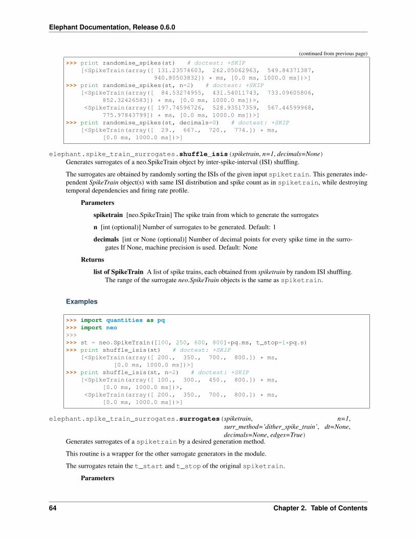
Elephant Documentation, Release 0.6.0
(continued from previous page)
>>> print randomise_spikes(st) # doctest: +SKIP[<SpikeTrain(array([ 131.23574603, 262.05062963, 549.84371387,
940.80503832]) * ms, [0.0 ms, 1000.0 ms])>]>>> print randomise_spikes(st, n=2) # doctest: +SKIP
[<SpikeTrain(array([ 84.53274955, 431.54011743, 733.09605806,852.32426583]) * ms, [0.0 ms, 1000.0 ms])>,
<SpikeTrain(array([ 197.74596726, 528.93517359, 567.44599968,775.97843799]) * ms, [0.0 ms, 1000.0 ms])>]
>>> print randomise_spikes(st, decimals=0) # doctest: +SKIP[<SpikeTrain(array([ 29., 667., 720., 774.]) * ms,
[0.0 ms, 1000.0 ms])>]
elephant.spike_train_surrogates.shuffle_isis(spiketrain, n=1, decimals=None)Generates surrogates of a neo.SpikeTrain object by inter-spike-interval (ISI) shuffling.
The surrogates are obtained by randomly sorting the ISIs of the given input spiketrain. This generates inde-pendent SpikeTrain object(s) with same ISI distribution and spike count as in spiketrain, while destroyingtemporal dependencies and firing rate profile.
Parameters
spiketrain [neo.SpikeTrain] The spike train from which to generate the surrogates
n [int (optional)] Number of surrogates to be generated. Default: 1
decimals [int or None (optional)] Number of decimal points for every spike time in the surro-gates If None, machine precision is used. Default: None
Returns
list of SpikeTrain A list of spike trains, each obtained from spiketrain by random ISI shuffling.The range of the surrogate neo.SpikeTrain objects is the same as spiketrain.
Examples
>>> import quantities as pq>>> import neo>>>>>> st = neo.SpikeTrain([100, 250, 600, 800]*pq.ms, t_stop=1*pq.s)>>> print shuffle_isis(st) # doctest: +SKIP
[<SpikeTrain(array([ 200., 350., 700., 800.]) * ms,[0.0 ms, 1000.0 ms])>]
>>> print shuffle_isis(st, n=2) # doctest: +SKIP[<SpikeTrain(array([ 100., 300., 450., 800.]) * ms,
[0.0 ms, 1000.0 ms])>,<SpikeTrain(array([ 200., 350., 700., 800.]) * ms,
[0.0 ms, 1000.0 ms])>]
elephant.spike_train_surrogates.surrogates(spiketrain, n=1,surr_method=’dither_spike_train’, dt=None,decimals=None, edges=True)
Generates surrogates of a spiketrain by a desired generation method.
This routine is a wrapper for the other surrogate generators in the module.
The surrogates retain the t_start and t_stop of the original spiketrain.
Parameters
64 Chapter 2. Table of Contents
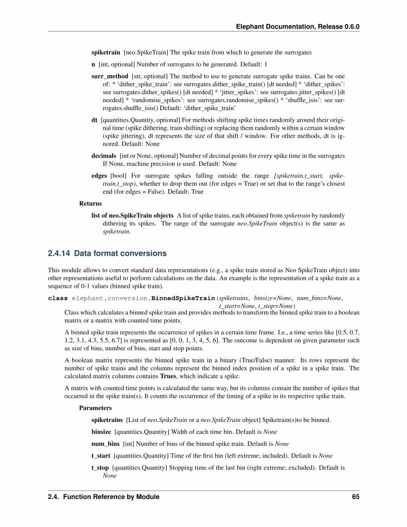
Elephant Documentation, Release 0.6.0
spiketrain [neo.SpikeTrain] The spike train from which to generate the surrogates
n [int, optional] Number of surrogates to be generated. Default: 1
surr_method [str, optional] The method to use to generate surrogate spike trains. Can be oneof: * ‘dither_spike_train’: see surrogates.dither_spike_train() [dt needed] * ‘dither_spikes’:see surrogates.dither_spikes() [dt needed] * ‘jitter_spikes’: see surrogates.jitter_spikes() [dtneeded] * ‘randomise_spikes’: see surrogates.randomise_spikes() * ‘shuffle_isis’: see sur-rogates.shuffle_isis() Default: ‘dither_spike_train’
dt [quantities.Quantity, optional] For methods shifting spike times randomly around their origi-nal time (spike dithering, train shifting) or replacing them randomly within a certain window(spike jittering), dt represents the size of that shift / window. For other methods, dt is ig-nored. Default: None
decimals [int or None, optional] Number of decimal points for every spike time in the surrogatesIf None, machine precision is used. Default: None
edges [bool] For surrogate spikes falling outside the range [spiketrain.t_start, spike-train.t_stop), whether to drop them out (for edges = True) or set that to the range’s closestend (for edges = False). Default: True
Returns
list of neo.SpikeTrain objects A list of spike trains, each obtained from spiketrain by randomlydithering its spikes. The range of the surrogate neo.SpikeTrain object(s) is the same asspiketrain.
2.4.14 Data format conversions
This module allows to convert standard data representations (e.g., a spike train stored as Neo SpikeTrain object) intoother representations useful to perform calculations on the data. An example is the representation of a spike train as asequence of 0-1 values (binned spike train).
class elephant.conversion.BinnedSpikeTrain(spiketrains, binsize=None, num_bins=None,t_start=None, t_stop=None)
Class which calculates a binned spike train and provides methods to transform the binned spike train to a booleanmatrix or a matrix with counted time points.
A binned spike train represents the occurrence of spikes in a certain time frame. I.e., a time series like [0.5, 0.7,1.2, 3.1, 4.3, 5.5, 6.7] is represented as [0, 0, 1, 3, 4, 5, 6]. The outcome is dependent on given parameter suchas size of bins, number of bins, start and stop points.
A boolean matrix represents the binned spike train in a binary (True/False) manner. Its rows represent thenumber of spike trains and the columns represent the binned index position of a spike in a spike train. Thecalculated matrix columns contains Trues, which indicate a spike.
A matrix with counted time points is calculated the same way, but its columns contain the number of spikes thatoccurred in the spike train(s). It counts the occurrence of the timing of a spike in its respective spike train.
Parameters
spiketrains [List of neo.SpikeTrain or a neo.SpikeTrain object] Spiketrain(s)to be binned.
binsize [quantities.Quantity] Width of each time bin. Default is None
num_bins [int] Number of bins of the binned spike train. Default is None
t_start [quantities.Quantity] Time of the first bin (left extreme; included). Default is None
t_stop [quantities.Quantity] Stopping time of the last bin (right extreme; excluded). Default isNone
2.4. Function Reference by Module 65
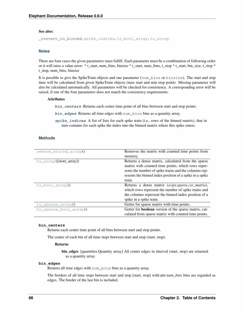
Elephant Documentation, Release 0.6.0
See also:
_convert_to_binned, spike_indices, to_bool_array , to_array
Notes
There are four cases the given parameters must fulfill. Each parameter must be a combination of following orderor it will raise a value error: * t_start, num_bins, binsize * t_start, num_bins, t_stop * t_start, bin_size, t_stop *t_stop, num_bins, binsize
It is possible to give the SpikeTrain objects and one parameter (num_bins or binsize). The start and stoptime will be calculated from given SpikeTrain objects (max start and min stop point). Missing parameter willalso be calculated automatically. All parameters will be checked for consistency. A corresponding error will beraised, if one of the four parameters does not match the consistency requirements.
Attributes
bin_centers Returns each center time point of all bins between start and stop points.
bin_edges Returns all time edges with num_bins bins as a quantity array.
spike_indices A list of lists for each spike train (i.e., rows of the binned matrix), that inturn contains for each spike the index into the binned matrix where this spike enters.
Methods
remove_stored_array() Removes the matrix with counted time points frommemory.
to_array([store_array]) Returns a dense matrix, calculated from the sparsematrix with counted time points, which rows repre-sents the number of spike trains and the columns rep-resents the binned index position of a spike in a spiketrain.
to_bool_array() Returns a dense matrix (scipy.sparse.csr_matrix),which rows represent the number of spike trains andthe columns represent the binned index position of aspike in a spike train.
to_sparse_array() Getter for sparse matrix with time points.to_sparse_bool_array() Getter for boolean version of the sparse matrix, cal-
culated from sparse matrix with counted time points.
bin_centersReturns each center time point of all bins between start and stop points.
The center of each bin of all time steps between start and stop (start, stop).
Returns
bin_edges [quantities.Quantity array] All center edges in interval (start, stop) are returnedas a quantity array.
bin_edgesReturns all time edges with num_bins bins as a quantity array.
The borders of all time steps between start and stop [start, stop] with:attr:num_bins bins are regarded asedges. The border of the last bin is included.
66 Chapter 2. Table of Contents
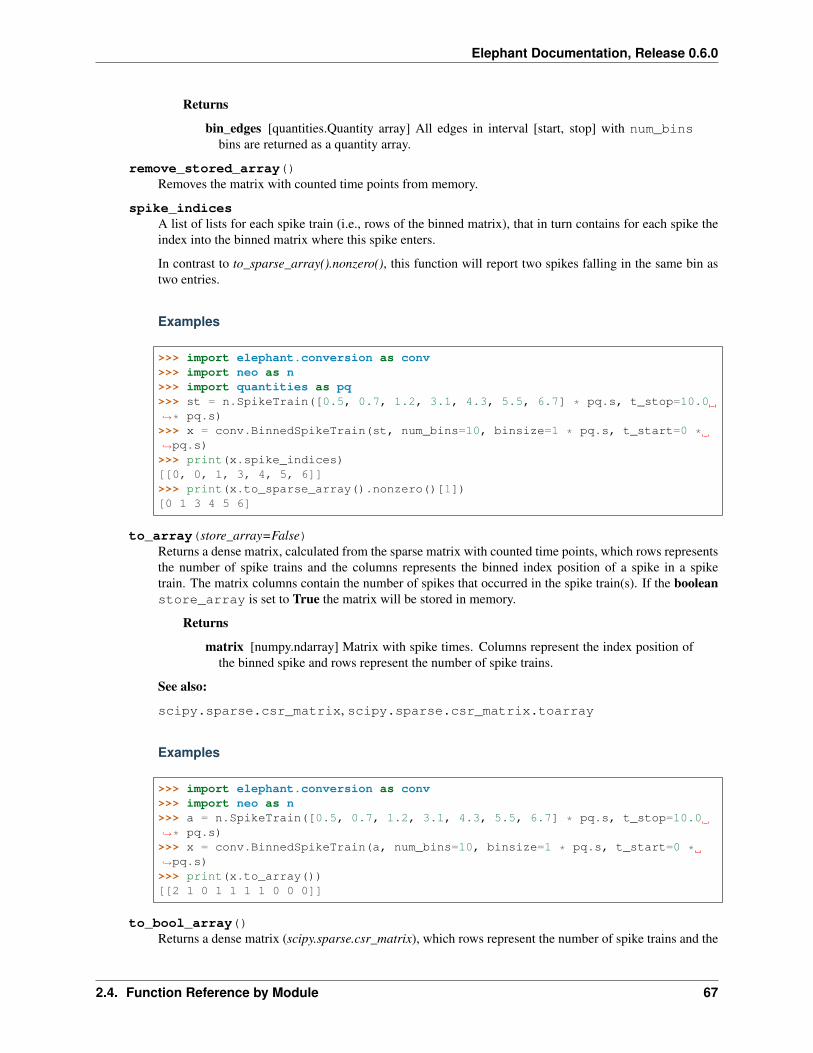
Elephant Documentation, Release 0.6.0
Returns
bin_edges [quantities.Quantity array] All edges in interval [start, stop] with num_binsbins are returned as a quantity array.
remove_stored_array()Removes the matrix with counted time points from memory.
spike_indicesA list of lists for each spike train (i.e., rows of the binned matrix), that in turn contains for each spike theindex into the binned matrix where this spike enters.
In contrast to to_sparse_array().nonzero(), this function will report two spikes falling in the same bin astwo entries.
Examples
>>> import elephant.conversion as conv>>> import neo as n>>> import quantities as pq>>> st = n.SpikeTrain([0.5, 0.7, 1.2, 3.1, 4.3, 5.5, 6.7] * pq.s, t_stop=10.0→˓* pq.s)>>> x = conv.BinnedSpikeTrain(st, num_bins=10, binsize=1 * pq.s, t_start=0 *→˓pq.s)>>> print(x.spike_indices)[[0, 0, 1, 3, 4, 5, 6]]>>> print(x.to_sparse_array().nonzero()[1])[0 1 3 4 5 6]
to_array(store_array=False)Returns a dense matrix, calculated from the sparse matrix with counted time points, which rows representsthe number of spike trains and the columns represents the binned index position of a spike in a spiketrain. The matrix columns contain the number of spikes that occurred in the spike train(s). If the booleanstore_array is set to True the matrix will be stored in memory.
Returns
matrix [numpy.ndarray] Matrix with spike times. Columns represent the index position ofthe binned spike and rows represent the number of spike trains.
See also:
scipy.sparse.csr_matrix, scipy.sparse.csr_matrix.toarray
Examples
>>> import elephant.conversion as conv>>> import neo as n>>> a = n.SpikeTrain([0.5, 0.7, 1.2, 3.1, 4.3, 5.5, 6.7] * pq.s, t_stop=10.0→˓* pq.s)>>> x = conv.BinnedSpikeTrain(a, num_bins=10, binsize=1 * pq.s, t_start=0 *→˓pq.s)>>> print(x.to_array())[[2 1 0 1 1 1 1 0 0 0]]
to_bool_array()Returns a dense matrix (scipy.sparse.csr_matrix), which rows represent the number of spike trains and the
2.4. Function Reference by Module 67
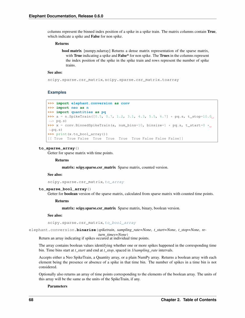
Elephant Documentation, Release 0.6.0
columns represent the binned index position of a spike in a spike train. The matrix columns contain True,which indicate a spike and False for non spike.
Returns
bool matrix [numpy.ndarray] Returns a dense matrix representation of the sparse matrix,with True indicating a spike and False* for non spike. The Trues in the columns representthe index position of the spike in the spike train and rows represent the number of spiketrains.
See also:
scipy.sparse.csr_matrix, scipy.sparse.csr_matrix.toarray
Examples
>>> import elephant.conversion as conv>>> import neo as n>>> import quantities as pq>>> a = n.SpikeTrain([0.5, 0.7, 1.2, 3.1, 4.3, 5.5, 6.7] * pq.s, t_stop=10.0→˓* pq.s)>>> x = conv.BinnedSpikeTrain(a, num_bins=10, binsize=1 * pq.s, t_start=0 *→˓pq.s)>>> print(x.to_bool_array())[[ True True False True True True True False False False]]
to_sparse_array()Getter for sparse matrix with time points.
Returns
matrix: scipy.sparse.csr_matrix Sparse matrix, counted version.
See also:
scipy.sparse.csr_matrix, to_array
to_sparse_bool_array()Getter for boolean version of the sparse matrix, calculated from sparse matrix with counted time points.
Returns
matrix: scipy.sparse.csr_matrix Sparse matrix, binary, boolean version.
See also:
scipy.sparse.csr_matrix, to_bool_array
elephant.conversion.binarize(spiketrain, sampling_rate=None, t_start=None, t_stop=None, re-turn_times=None)
Return an array indicating if spikes occured at individual time points.
The array contains boolean values identifying whether one or more spikes happened in the corresponding timebin. Time bins start at t_start and end at t_stop, spaced in 1/sampling_rate intervals.
Accepts either a Neo SpikeTrain, a Quantity array, or a plain NumPy array. Returns a boolean array with eachelement being the presence or absence of a spike in that time bin. The number of spikes in a time bin is notconsidered.
Optionally also returns an array of time points corresponding to the elements of the boolean array. The units ofthis array will be the same as the units of the SpikeTrain, if any.
Parameters
68 Chapter 2. Table of Contents
Elephant Documentation, Release 0.6.0
spiketrain [Neo SpikeTrain or Quantity array or NumPy array] The spike times. Does not haveto be sorted.
sampling_rate [float or Quantity scalar, optional] The sampling rate to use for the time points.If not specified, retrieved from the sampling_rate attribute of spiketrain.
t_start [float or Quantity scalar, optional] The start time to use for the time points. If notspecified, retrieved from the t_start attribute of spiketrain. If that is not present, default to0. Any value from spiketrain below this value is ignored.
t_stop [float or Quantity scalar, optional] The start time to use for the time points. If not spec-ified, retrieved from the t_stop attribute of spiketrain. If that is not present, default to themaximum value of sspiketrain. Any value from spiketrain above this value is ignored.
return_times [bool] If True, also return the corresponding time points.
Returns
values [NumPy array of bools] A True value at a particular index indicates the presence of oneor more spikes at the corresponding time point.
times [NumPy array or Quantity array, optional] The time points. This will have the same unitsas spiketrain. If spiketrain has no units, this will be an NumPy array.
Raises
TypeError If spiketrain is a NumPy array and t_start, t_stop, or sampling_rate is a Quantity..
ValueError t_start and t_stop can be inferred from spiketrain if not explicitly defined and notan attribute of spiketrain. sampling_rate cannot, so an exception is raised if it is not explic-itly defined and not present as an attribute of spiketrain.
Notes
Spike times are placed in the bin of the closest time point, going to the higher bin if exactly between two bins.
So in the case where the bins are 5.5 and 6.5, with the spike time being 6.0, the spike will be placed in the 6.5bin.
The upper edge of the last bin, equal to t_stop, is inclusive. That is, a spike time exactly equal to t_stop will beincluded.
If spiketrain is a Quantity or Neo SpikeTrain and t_start, t_stop or sampling_rate is not, then the arguments thatare not quantities will be assumed to have the same units as spiketrain.
2.4.15 Utility functions to manipulate Neo objects
Tools to manipulate Neo objects.
elephant.neo_tools.extract_neo_attrs(obj, parents=True, child_first=True, skip_array=False,skip_none=False)
Given a neo object, return a dictionary of attributes and annotations.
Parameters
obj [neo object]
parents [bool, optional] Also include attributes and annotations from parent neo objects (ifany).
2.4. Function Reference by Module 69

Elephant Documentation, Release 0.6.0
child_first [bool, optional] If True (default True), values of child attributes are used over parentattributes in the event of a name conflict. If False, parent attributes are used. This parameterdoes nothing if parents is False.
skip_array [bool, optional] If True (default False), skip attributes that store non-scalar arrayvalues.
skip_none [bool, optional] If True (default False), skip annotations and attributes that have avalue of None.
Returns
dict A dictionary where the keys are annotations or attribute names and the values are the cor-responding annotation or attribute value.
elephant.neo_tools.get_all_epochs(container)Get all neo.Epoch objects from a container.
The objects can be any list, dict, or other iterable or mapping containing epochs, as well as any neo object thatcan hold epochs: neo.Block and neo.Segment.
Containers are searched recursively, so the objects can be nested (such as a list of blocks).
Parameters
container [list, tuple, iterable, dict, neo Block, neo Segment] The container for the epochs.
Returns
list A list of the unique neo.Epoch objects in container.
elephant.neo_tools.get_all_events(container)Get all neo.Event objects from a container.
The objects can be any list, dict, or other iterable or mapping containing events, as well as any neo object thatcan hold events: neo.Block and neo.Segment.
Containers are searched recursively, so the objects can be nested (such as a list of blocks).
Parameters
container [list, tuple, iterable, dict, neo Block, neo Segment] The container for the events.
Returns
list A list of the unique neo.Event objects in container.
elephant.neo_tools.get_all_spiketrains(container)Get all neo.Spiketrain objects from a container.
The objects can be any list, dict, or other iterable or mapping containing spiketrains, as well as any neo objectthat can hold spiketrains: neo.Block, neo.ChannelIndex, neo.Unit, and neo.Segment.
Containers are searched recursively, so the objects can be nested (such as a list of blocks).
Parameters
container [list, tuple, iterable, dict,] neo Block, neo Segment, neo Unit, neo ChannelIndex Thecontainer for the spiketrains.
Returns
list A list of the unique neo.SpikeTrain objects in container.
70 Chapter 2. Table of Contents

Elephant Documentation, Release 0.6.0
2.4.16 Bridge to the pandas library
2.5 Developers’ guide
These instructions are for developing on a Unix-like platform, e.g. Linux or Mac OS X, with the bash shell. If youdevelop on Windows, please get in touch.
2.5.1 Mailing lists
General discussion of Elephant development takes place in the NeuralEnsemble Google group.
Discussion of issues specific to a particular ticket in the issue tracker should take place on the tracker.
2.5.2 Using the issue tracker
If you find a bug in Elephant, please create a new ticket on the issue tracker, setting the type to “defect”. Choose aname that is as specific as possible to the problem you’ve found, and in the description give as much information asyou think is necessary to recreate the problem. The best way to do this is to create the shortest possible Python scriptthat demonstrates the problem, and attach the file to the ticket.
If you have an idea for an improvement to Elephant, create a ticket with type “enhancement”. If you already have animplementation of the idea, open a pull request.
2.5.3 Requirements
See Prerequisites / Installation. We strongly recommend using virtualenv or similar.
2.5.4 Getting the source code
We use the Git version control system. The best way to contribute is through GitHub. You will first needa GitHub account, and you should then fork the repository at https://github.com/NeuralEnsemble/elephant (seehttp://help.github.com/fork-a-repo/).
To get a local copy of the repository:
$ cd /some/directory$ git clone [email protected]:<username>/elephant.git
Now you need to make sure that the elephant package is on your PYTHONPATH. You can do this by installingElephant:
$ cd elephant$ python setup.py install$ python3 setup.py install
but if you do this, you will have to re-run setup.py install any time you make changes to the code. A bettersolution is to install Elephant with the develop option, this avoids reinstalling when there are changes in the code:
$ python setup.py develop
or:
2.5. Developers’ guide 71

Elephant Documentation, Release 0.6.0
$ pip install -e .
To update to the latest version from the repository:
$ git pull
2.5.5 Running the test suite
Before you make any changes, run the test suite to make sure all the tests pass on your system:
$ cd elephant/test
With Python 2.7 or 3.x:
$ python -m unittest discover$ python3 -m unittest discover
If you have nose installed:
$ nosetests
At the end, if you see “OK”, then all the tests passed (or were skipped because certain dependencies are not installed),otherwise it will report on tests that failed or produced errors.
2.5.6 Writing tests
You should try to write automated tests for any new code that you add. If you have found a bug and want to fix it, firstwrite a test that isolates the bug (and that therefore fails with the existing codebase). Then apply your fix and checkthat the test now passes.
To see how well the tests cover the code base, run:
$ nosetests --with-coverage --cover-package=elephant --cover-erase
2.5.7 Working on the documentation
The documentation is written in reStructuredText, using the Sphinx documentation system. To build the documenta-tion:
$ cd elephant/doc$ make html
Then open some/directory/elephant/doc/_build/html/index.html in your browser. Docstrings should conform to theNumPy docstring standard.
To check that all example code in the documentation is correct, run:
$ make doctest
To check that all URLs in the documentation are correct, run:
$ make linkcheck
72 Chapter 2. Table of Contents

Elephant Documentation, Release 0.6.0
2.5.8 Committing your changes
Once you are happy with your changes, run the test suite again to check that you have not introduced any newbugs. Then you can commit them to your local repository:
$ git commit -m 'informative commit message'
If this is your first commit to the project, please add your name and affiliation/employer to doc/source/authors.rst
You can then push your changes to your online repository on GitHub:
$ git push
Once you think your changes are ready to be included in the main Elephant repository, open a pull request on GitHub(see https://help.github.com/articles/using-pull-requests).
2.5.9 Python 3
Elephant should work with Python 2.7 and Python 3.
So far, we have managed to write code that works with both Python 2 and 3. Mainly this involves avoiding the printstatement (use logging.info instead), and putting from __future__ import division at the beginningof any file that uses division.
If in doubt, Porting to Python 3 by Lennart Regebro is an excellent resource.
The most important thing to remember is to run tests with at least one version of Python 2 and at least one version ofPython 3. There is generally no problem in having multiple versions of Python installed on your computer at once:e.g., on Ubuntu Python 2 is available as python and Python 3 as python3, while on Arch Linux Python 2 is python2and Python 3 python. See PEP394 for more on this.
2.5.10 Coding standards and style
All code should conform as much as possible to PEP 8, and should run with Python 2.7 and 3.2-3.5.
2.5.11 Making a release
First, check that the version string (in elephant/__init__.py, setup.py, doc/conf.py, and doc/install.rst) is correct.
Second, check that the copyright statement (in LICENCE.txt, README.md, and doc/conf.py) is correct.
To build a source package:
$ python setup.py sdist
To upload the package to PyPI (if you have the necessary permissions):
$ python setup.py sdist upload
Finally, tag the release in the Git repository and push it:
$ git tag <version>$ git push --tags upstream
2.5. Developers’ guide 73

Elephant Documentation, Release 0.6.0
Here, version should be of the form vX.Y.Z.
2.6 Authors and contributors
The following people have contributed code and/or ideas to the current version of Elephant. The institutional affilia-tions are those at the time of the contribution, and may not be the current affiliation of a contributor.
• Alper Yegenoglu [1]
• Andrew Davison [2]
• Detlef Holstein [2]
• Eilif Muller [3, 4]
• Emiliano Torre [1]
• Espen Hagen [1]
• Jan Gosmann [6, 8]
• Julia Sprenger [1]
• Junji Ito [1]
• Michael Denker [1]
• Paul Chorley [1]
• Pierre Yger [2]
• Pietro Quaglio [1]
• Richard Meyes [1]
• Vahid Rostami [1]
• Subhasis Ray [5]
• Robert Pröpper [6]
• Richard C Gerkin [7]
• Bartosz Telenczuk [2]
• Chaitanya Chintaluri [9]
• Michał Czerwinski [9]
• Michael von Papen [1]
• Robin Gutzen [1]
• Felipe Méndez [10]
1. Institute of Neuroscience and Medicine (INM-6), Computational and Systems Neuroscience & Institute forAdvanced Simulation (IAS-6), Theoretical Neuroscience, Jülich Research Centre and JARA, Jülich, Germany
2. Unité de Neurosciences, Information et Complexité, CNRS UPR 3293, Gif-sur-Yvette, France
3. Electronic Visions Group, Kirchhoff-Institute for Physics, University of Heidelberg, Germany
4. Brain-Mind Institute, Ecole Polytechnique Fédérale de Lausanne, Switzerland
5. NIH–NICHD, Laboratory of Cellular and Synaptic Physiology, Bethesda, Maryland 20892, USA
74 Chapter 2. Table of Contents

Elephant Documentation, Release 0.6.0
6. Neural Information Processing Group, Institute of Software Engineering and Theoretical Computer Science,Technische Universität Berlin, Germany
7. Arizona State University School of Life Sciences, USA
8. Computational Neuroscience Research Group (CNRG), Waterloo Centre for Theoretical Neuroscience, Water-loo, Canada
9. Nencki Institute of Experimental Biology, Warsaw, Poland
10. Instituto de Neurobiología, Universidad Nacional Autónoma de México, Mexico City, Mexico
If we’ve somehow missed you off the list we’re very sorry - please let us know.
2.7 Release Notes
2.7.1 Elephant 0.6.0 release notes
October 12th 2018
New functions
• cell_assembly_detection module
– New function to detect higher-order correlation structures such as patterns in parallel spike trainsbased on Russo et al, 2017.
• wavelet_transform() function in signal_prosessing.py module
– Function for computing wavelet transform of a given time series based on Le van Quyen et al. (2001)
Other changes
• Switched to multiple requirements.txt files which are directly read into the setup.py
• instantaneous_rate() accepts now list of spiketrains
• Minor bug fixes
2.7.2 Elephant 0.5.0 release notes
April 4nd 2018
New functions
• change_point_detection module:
– New function to detect changes in the firing rate
• spike_train_correlation module:
– New function to calculate the spike time tiling coefficient
• phase_analysis module:
– New function to extract spike-triggered phases of an AnalogSignal
2.7. Release Notes 75

Elephant Documentation, Release 0.6.0
• unitary_event_analysis module:
– Added new unit test to the UE function to verify the method based on data of a recent [Re]Sciencepublication
Other changes
• Minor bug fixes
2.7.3 Elephant 0.4.3 release notes
March 2nd 2018
Other changes
• Bug fixes in spade module:
– Fixed an incompatibility with the latest version of an external library
2.7.4 Elephant 0.4.2 release notes
March 1st 2018
New functions
• spike_train_generation module:
– inhomogeneous_poisson() function
• Modules for Spatio Temporal Pattern Detection (SPADE) spade_src:
– Module SPADE: spade.py
• Module statistics.py:
– Added CV2 (coefficient of variation for non-stationary time series)
• Module spike_train_correlation.py:
– Added normalization in cross-correlation histogram() (CCH)
Other changes
• Adapted the setup.py to automatically install the spade modules including the compiled C files fim.so
• Included testing environment for MPI in travis.yml
• Changed function arguments in current_source_density.py to neo.AnalogSignal instead list of neo.AnalogSignalobjects
• Fixes to travis and setup configuration files
• Fixed bug in ISI function isi(), statistics.py module
• Fixed bug in dither_spikes(), spike_train_surrogates.py
• Minor bug fixes
76 Chapter 2. Table of Contents

Elephant Documentation, Release 0.6.0
2.7.5 Elephant 0.4.1 release notes
March 23rd 2017
Other changes
• Fix in setup.py to correctly import the current source density module
2.7.6 Elephant 0.4.0 release notes
March 22nd 2017
New functions
• spike_train_generation module:
– peak detection: peak_detection()
• Modules for Current Source Density: current_source_density_src
– Module Current Source Density: KCSD.py
– Module for Inverse Current Source Density: icsd.py
API changes
• Interoperability between Neo 0.5.0 and Elephant
– Elephant has adapted its functions to the changes in Neo 0.5.0, most of the functionality behaves asbefore
– See Neo documentation for recent changes: http://neo.readthedocs.io/en/latest/whatisnew.html
Other changes
• Fixes to travis and setup configuration files.
• Minor bug fixes.
• Added module six for Python 2.7 backwards compatibility
2.7.7 Elephant 0.3.0 release notes
April 12st 2016
New functions
• spike_train_correlation module:
– cross correlation histogram: cross_correlation_histogram()
• spike_train_generation module:
– single interaction process (SIP): single_interaction_process()
2.7. Release Notes 77

Elephant Documentation, Release 0.6.0
– compound Poisson process (CPP): compound_poisson_process()
• signal_processing module:
– analytic signal: hilbert()
• sta module:
– spike field coherence: spike_field_coherence()
• Module to represent kernels: kernels module
• Spike train metrics / dissimilarity / synchrony measures: spike_train_dissimilarity module
• Unitary Event (UE) analysis: unitary_event_analysis module
• Analysis of Sequences of Synchronous EvenTs (ASSET): asset module
API changes
• Function instantaneous_rate() now uses kernels as objects defined in the kernels module. The previous im-plementation of the function using the make_kernel() function is deprecated, but still temporarily available asoldfct_instantaneous_rate().
Other changes
• Fixes to travis and readthedocs configuration files.
2.7.8 Elephant 0.2.1 release notes
February 18th 2016
Other changes
Minor bug fixes.
2.7.9 Elephant 0.2.0 release notes
September 22nd 2015
New functions
• Added covariance function covariance() in the spike_train_correlation module
• Added complexity pdf complexity_pdf() in the statistics module
• Added spike train extraction from analog signals via threshold detection the in spike_train_generation module
• Added coherence() function for analog signals in the spectral module
• Added Cumulant Based Inference for higher-order of Correlation (CuBIC) in the cubic module for corre-lation analysis of parallel recorded spike trains
78 Chapter 2. Table of Contents

Elephant Documentation, Release 0.6.0
API changes
• Optimized kernel bandwidth in rate_estimation function: Calculates the optimized kernel width when theparamter kernel width is specified as auto
Other changes
• Optimized creation of sparse matrices: The creation speed of the sparse matrix inside the BinnedSpikeTrainclass is optimized
• Added Izhikevich neuron simulator in the make_spike_extraction_test_data module
• Minor improvements to the test and continous integration infrastructure
2.7. Release Notes 79

Elephant Documentation, Release 0.6.0
80 Chapter 2. Table of Contents

Bibliography
[1] Meier R, Egert U, Aertsen A, Nawrot MP, “FIND - a unified framework for neural data analysis”; Neural Netw.2008 Oct; 21(8):1085-93.
[2] Nawrot M, Aertsen A, Rotter S, “Single-trial estimation of neuronal firing rates - from single neuron spike trainsto population activity”; J. Neurosci Meth 94: 81-92; 1999.
81

Elephant Documentation, Release 0.6.0
82 Bibliography
Python Module Index
eelephant.asset, 46elephant.conversion, 65elephant.cubic, 45elephant.current_source_density, 24elephant.kernels, 26elephant.neo_tools, 69elephant.signal_processing, 19elephant.spectral, 22elephant.spike_train_correlation, 40elephant.spike_train_dissimilarity, 37elephant.spike_train_generation, 55elephant.spike_train_surrogates, 60elephant.sta, 39elephant.statistics, 12elephant.unitary_event_analysis, 44
83

Elephant Documentation, Release 0.6.0
84 Python Module Index
Index
AAlphaKernel (class in elephant.kernels), 26
Bbin_centers (elephant.conversion.BinnedSpikeTrain at-
tribute), 66bin_edges (elephant.conversion.BinnedSpikeTrain
attribute), 66binarize() (in module elephant.conversion), 68BinnedSpikeTrain (class in elephant.conversion), 65boundary_enclosing_area_fraction() (ele-
phant.kernels.EpanechnikovLikeKernelmethod), 28
boundary_enclosing_area_fraction() (ele-phant.kernels.ExponentialKernel method),30
boundary_enclosing_area_fraction() (ele-phant.kernels.GaussianKernel method), 31
boundary_enclosing_area_fraction() (ele-phant.kernels.Kernel method), 32
boundary_enclosing_area_fraction() (ele-phant.kernels.LaplacianKernel method),33
boundary_enclosing_area_fraction() (ele-phant.kernels.RectangularKernel method),35
boundary_enclosing_area_fraction() (ele-phant.kernels.TriangularKernel method),37
butter() (in module elephant.signal_processing), 19
Ccluster_matrix_entries() (in module elephant.asset), 47complexity_pdf() (in module elephant.statistics), 12compound_poisson_process() (in module ele-
phant.spike_train_generation), 55corrcoef() (in module elephant.spike_train_correlation),
40cost_function() (in module elephant.statistics), 12
covariance() (in module ele-phant.spike_train_correlation), 41
cpp() (in module elephant.spike_train_generation), 56cross_correlation_histogram() (in module ele-
phant.spike_train_correlation), 41cubic() (in module elephant.cubic), 46cv2() (in module elephant.statistics), 12
Ddither_spike_train() (in module ele-
phant.spike_train_surrogates), 61dither_spikes() (in module ele-
phant.spike_train_surrogates), 61
Eelephant.asset (module), 46elephant.conversion (module), 65elephant.cubic (module), 45elephant.current_source_density (module), 24elephant.kernels (module), 26elephant.neo_tools (module), 69elephant.signal_processing (module), 19elephant.spectral (module), 22elephant.spike_train_correlation (module), 40elephant.spike_train_dissimilarity (module), 37elephant.spike_train_generation (module), 55elephant.spike_train_surrogates (module), 60elephant.sta (module), 39elephant.statistics (module), 12elephant.unitary_event_analysis (module), 44EpanechnikovLikeKernel (class in elephant.kernels), 27estimate_csd() (in module ele-
phant.current_source_density), 25ExponentialKernel (class in elephant.kernels), 29extract_neo_attrs() (in module elephant.neo_tools), 69extract_sse() (in module elephant.asset), 48
Ffanofactor() (in module elephant.statistics), 13
85
Elephant Documentation, Release 0.6.0
fftkernel() (in module elephant.statistics), 13
GGaussianKernel (class in elephant.kernels), 30gen_pval_anal() (in module ele-
phant.unitary_event_analysis), 44generate_lfp() (in module ele-
phant.current_source_density), 25get_all_epochs() (in module elephant.neo_tools), 70get_all_events() (in module elephant.neo_tools), 70get_all_spiketrains() (in module elephant.neo_tools), 70
Hhash_from_pattern() (in module ele-
phant.unitary_event_analysis), 44hilbert() (in module elephant.signal_processing), 19homogeneous_gamma_process() (in module ele-
phant.spike_train_generation), 56homogeneous_poisson_process() (in module ele-
phant.spike_train_generation), 57
Iinherit_docstring() (in module elephant.kernels), 37inhomogeneous_poisson_process() (in module ele-
phant.spike_train_generation), 57instantaneous_rate() (in module elephant.statistics), 13intersection_matrix() (in module elephant.asset), 48inverse_hash_from_pattern() (in module ele-
phant.unitary_event_analysis), 44is_symmetric() (elephant.kernels.Kernel method), 32is_symmetric() (elephant.kernels.SymmetricKernel
method), 36isi() (in module elephant.statistics), 14
Jjitter_spikes() (in module ele-
phant.spike_train_surrogates), 62joint_probability_matrix() (in module elephant.asset), 49jointJ() (in module elephant.unitary_event_analysis), 44jointJ_window_analysis() (in module ele-
phant.unitary_event_analysis), 44
KKernel (class in elephant.kernels), 31
LLaplacianKernel (class in elephant.kernels), 32lv() (in module elephant.statistics), 14
Mmake_kernel() (in module elephant.statistics), 15mask_matrices() (in module elephant.asset), 50mean_firing_rate() (in module elephant.statistics), 16
median_index() (elephant.kernels.Kernel method), 32
Nn_emp_mat() (in module ele-
phant.unitary_event_analysis), 45n_emp_mat_sum_trial() (in module ele-
phant.unitary_event_analysis), 45n_exp_mat() (in module ele-
phant.unitary_event_analysis), 45n_exp_mat_sum_trial() (in module ele-
phant.unitary_event_analysis), 45nextpow2() (in module elephant.statistics), 17
Ooldfct_instantaneous_rate() (in module ele-
phant.statistics), 17
Ppeak_detection() (in module ele-
phant.spike_train_generation), 58probability_matrix_analytical() (in module ele-
phant.asset), 50probability_matrix_montecarlo() (in module ele-
phant.asset), 51
Rrandomise_spikes() (in module ele-
phant.spike_train_surrogates), 63RectangularKernel (class in elephant.kernels), 34remove_stored_array() (ele-
phant.conversion.BinnedSpikeTrain method),67
Sshuffle_isis() (in module ele-
phant.spike_train_surrogates), 64single_interaction_process() (in module ele-
phant.spike_train_generation), 58spike_extraction() (in module ele-
phant.spike_train_generation), 59spike_field_coherence() (in module elephant.sta), 39spike_indices (elephant.conversion.BinnedSpikeTrain at-
tribute), 67spike_time_tiling_coefficient() (in module ele-
phant.spike_train_correlation), 43spike_triggered_average() (in module elephant.sta), 39sse_difference() (in module elephant.asset), 52sse_intersection() (in module elephant.asset), 52sse_isdisjoint() (in module elephant.asset), 53sse_isequal() (in module elephant.asset), 53sse_issub() (in module elephant.asset), 54sse_issuper() (in module elephant.asset), 54sse_overlap() (in module elephant.asset), 54
86 Index
Elephant Documentation, Release 0.6.0
sskernel() (in module elephant.statistics), 18surrogates() (in module elephant.spike_train_surrogates),
64SymmetricKernel (class in elephant.kernels), 35
Tthreshold_detection() (in module ele-
phant.spike_train_generation), 60time_histogram() (in module elephant.statistics), 18to_array() (elephant.conversion.BinnedSpikeTrain
method), 67to_bool_array() (elephant.conversion.BinnedSpikeTrain
method), 67to_sparse_array() (elephant.conversion.BinnedSpikeTrain
method), 68to_sparse_bool_array() (ele-
phant.conversion.BinnedSpikeTrain method),68
TriangularKernel (class in elephant.kernels), 36
Vvan_rossum_dist() (in module ele-
phant.spike_train_dissimilarity), 37victor_purpura_dist() (in module ele-
phant.spike_train_dissimilarity), 38
Wwavelet_transform() (in module ele-
phant.signal_processing), 20welch_cohere() (in module elephant.spectral), 22welch_psd() (in module elephant.spectral), 23
Zzscore() (in module elephant.signal_processing), 21
Index 87