Embed Size (px)
Citation preview
PRESENTED BY
894
(p.£.Q^te^.

ELEMENTS
DIFFERENTIAL AND INTEGRAL
CALCULUS,
EXAMPLES AND APPLICATIONS.
BY
JAMES M: TAYLOR, A.M.,
PROFESSOR OF MATHEMATICS, COLGATE UNIVERSITY.
>^/
BOSTON, U.S.A.:
PUBLISHED BY GINN & COMPANY.
1894.
Entered according to, Act of Congress, in the year 1884, by
JAMES M. TAYLOR,
in the Office of the Librarian of Congress, at Washington.
Entered according to Act of Congress, in the year 1891, by
JAMES M. TAYLOR,
in the Office of the Librarian of Congress, at "Washington.
Sift*
'
Edwn L. Whitney
DEC 8- 1938
Typography by J. S. Cushing & Co., Boston.
Presswork by G-inn & Co., Boston.
PEEFACE
THE object of the following treatise is to present sim-
ply and concisely the fundamental problems of the
Calculus, their solution, and more common applications.
Since variables are its characteristic quantities, the
first fundamental problem of the Calculus is, To find the
ratio of the rates of change of related variables. To ena-
ble the learner most clearly to comprehend cnis problem,
the author has employed the conception of rates, which
affords finite differentials and the simplest demonstration
of many principles. The problem of Differentiation hav-
ing been clearly presented, a general method of its solu-
tion is obtained by the use of limits. This order of
development avoids the use of the indeterminate form -,
and secures all the advantages of the differential nota-
tion. Many principles are proved, both by the method
of rates and that of limits, and thus each is made to
throw light upon the other.
In a final chapter, the method of infinitesimals is briefly
presented; its underlying principles having been previ-
ously established.
The chapter on Differentiation is followed by one on
Integration ; and in each, as throughout the work, there
IV PREFACE.
are numerous practical problems in Geometry and Me-
chanics, which serve to exhibit the power and use of
the science, and to excite and keep alive the interest
of the student.
In writing this treatise, the works of the best Ameri-
can, English, and French authors have been consulted
;
and from these sources the most of the examples and
problems have been obtained.
The author is indebted to Professors J. E. Oliver and
J. McMahon of Cornell University, and Professor O.
Root, Jr., of Hamilton College, for valuable suggestions;
and to Messrs. J. S. Gushing & Co. for the typograph-
ical excellence of the book.
J. M. TAYLOR.Hamilton, N.Y.,
Nov.. 1884.
CONTENTS.
CHAPTER I.
INTRODUCTION.Section. Page.
1. Definition of variable and constant 1
2. Definition of function and independent variable 1
3. Classification of functions 2
4. Definition of continuous variable and continuous function 2
5. Definition of the limit of a variable 3
6. Limits of equal variables 3
7- Limit of the product of a constant and a variable ...,.,. 4
8. Limit of the product of two or more variables ........ 4
9. Limit of the quotient of two variables 4
10. Limit of the sum of two or more variables 4
11. Definition of uniform change 5
12. Definition of increment . 5
13. Definition of differential 5
14. Illustrations of differentials 6
15. Definition of inclination, slope, and tangent 7
16. Geometric signification of -^ 7dx
17. Limit of the ratio of the increments of y and x 8
CHAPTER II.
DIFFERENTIATION.
18. Definition of differentiation. Differentiation of ax2 10
Algebraic Functions.
19. Differential of the product of a constant and variable 10
20. Differential of a constant 11
21. Differential of the sum of two or more variables ...... 11
VI CONTENTS.
Section- Page.
22. Differential of the product of two variables 12
23. Differential of the product of several variables 13
24. Differential of a fraction 14
25. Differential of a variable with a constant exponent 14
26. General symbol for the differential off(x). Examples .... 15
27. Definition of an increasing and a decreasing function 17
28. Definition of derivative 17
29. Measure of rate of change 18
30. Signification of ^ 18dt
31. Signification off'(x) or -1. . 18dx
32. Limit of the ratio of Ay to Ax. Applications 19
33. Definition of velocity and acceleration. Examples 23
Logarithmic and Exponential Functions.
34. Differential of a logarithmic Junction 24
35. The greater the base, the smaller the modulus • . 25
36. Naperian system 25
37. Differential of c* . . 2G
38. Differential of if . 26
39. Logarithmic differentiation. Examples . 26
Trigonometric Functions.
40. Definition of the unit of angular measure 29
41. Differential of sin x and cos x 29
42. Differential of tan x . . 30
43. Differential of cot x 30
44. Differential of sec x 30
45. Differential of cosec x 31
46. Differential of vers x 31
47. Differential of covers x 31
48. Limit of the ratio of an arc to its chord 31
49. Differentiation of sin a: by the method of limits. Examples . . 32
Anti-Trigonometric Functions.
50. Differential of sin-1* 35
51. Differential of cos-1* 35
52. Differential of tan-1* 35
53. Differential of cot-1* 36
54. Differential of sec-1* . 36
CONTENTS, Vll
Section. Page.
55. Differential of cosec" 1^ » . 36
56. Differential of vers _1x 36
57. Differential of covers" 1^. Examples 36
Miscellaneous examples 39
CHAPTER in.
INTEGRATION.
58. Definition of integral and integration. Sign of integration ... 43
59. Elementary principles 43
60. Fundamental formulas 44
61. Statement of formulas 1 and 2. Examples 46
62. Auxiliary formulas. Examples 50
63. Trigonometric differentials. Examples 55
64. Definite integrals. Examples 58
Applications to Geometry and Mechanics.
65. Rectification of curves. Examples 60
6Q. Areas of plane curves. Examples . 61
67. Graphical representation of any integral . , 63
68. Areas of surfaces of revolution. Examples 63
69. Volumes of solids of revolution. Examples 65
70. Fundamental formulas of mechanics. Examples 6Q
1. Formulas for uniformly accelerated motion.
2. Motion down an inclined plane.
3. Motion down a chord of a vertical circle.
4. Values of v and s when a varies directly as t.
5. Geometrical representation of the time, velocity, distance,
and acceleration.
6. Path of a projectile.
7. Path, velocity, and acceleration of a hody whose velocity
in each of two directions is given.
CHAPTER IV.
SUCCESSIVE DIFFERENTIATION.
71. Successive derivatives „ 71
72. Signification oif>'(x),f'"{x),f»(x). Examples 71
73. Successive differentials 73
74. Relations between successive differentials and derivatives.
Examples 73
Vlil CONTENTS.
CHAPTER V.
SUCCESSIVE INTEGRATION AND APPLICATIONS.
Section. Page.
75. Successive integration. Examples 76
76. Problems in mechanics 77
1. Time and velocity of a falling body below the surface of
the earth.
2. Maximum velocity with which a falling body can reach the
earth.
3. Velocity of a body falling from the sun.
4. Velocity of a body falling in the air.
5. Velocity of a body projected into a medium.
6. Velocity of a body sliding down a curve.
7. The cycloidal pendulum isochronal.
8. The length and equation of the catenary.
CHAPTER VI.
INDETERMINATE FORMS.
77. Value of functions assuming an indeterminate form. Examples 86
Evaluation by Differentiation.
78. The form -. Examples 87
79. The form -g. Examples 88
80. The forms • go and co — go. Examples 89
81. Eunctions whose logarithms assume the form ± • go. Examples 91
82. Compound indeterminate forms. Examples 91
83- Evaluation of derivatives of implicit functions. Examples . . 92
CHAPTER VII.
DEVELOPMENT OF FUNCTIONS IN SERIES.
94
84. Definition of series, convergent infinite series, and sum of infinite
series
85. Definition of the development of a function 94
86. Definition of Taylor's formula 95
87. Proof of Taylor's formula 95
88. Proof of Maclaurin's formula 96
CONTENTS. ix
Section. Page.
89. Proof of the binomial theorem . 97
90. Development of loga (:r + y) . . 97
91. Development of ax+'J 98
92. Development of (a -f x) m 98
93. Development of sin x . . . „ . 98
94. Development of cos x 98
95. Exponential series 99
96. Logarithmic series 99
97. Failure of Taylor's and Maclaurin's formulas 102
98. Lemma '. 102
99. Completion of Taylor's and Maclaurin's formulas 103
100. A second complete form 104
101. Proof that $2 = as n = oo 105\n
102. Maclaurin's formula develops ax 105
103. Maclaurin's formula develops sin x and cos x 106
104. The logarithmic series holds for x>—l and <+l 106
105. Development of (I + x)m holds for x>—l and <+l 107
106. One form of the development of (a + x) m always holds .... 108
107. Development of tan-1x, and value of it 109
108. Development of sin-1
^, and value of it 109
109. Geometric proof that/(a + h) =J\a) + hf'{a + Bit). Examples 110
CHAPTER VIII.
MAXIMA AND MINIMA.
110. Definition of maximum and minimvm 112
111. The critical values of a; 112
112. Two methods of examining^x ) at critical values of x . . . . 113
113. Maxima and minima occur alternately 114
114. Principles facilitating the solution of problems ....... 114
Examples and geometric problems 115
CHAPTER IX.
FUNCTIONS OF TWO OR MORE VARIABLES, AND CHANGE OF THEINDEPENDENT VARIABLE.
115. Applicability of previous rules for differentiation 125
116. Definition of partial differential 125
117. Definition of total differential 125
X CONTENTS.
Section. Page,
118. Definition of partial derivative 125
119. Definition of total derivative 125
120. The value of the total differential 126
121. The signification of partial derivatives. Examples ...... 126
122. One method of finding the total derivative 127
123. Formulas for finding the total derivative. Examples .... 128
124. Implicit functions 130
125. Formula for the derivative of an implicit function. Examples 130
126. Successive derivatives of an implicit function. Examples . . 131
127. Successive partial differentials and derivatives ....... 132
128. The order of differentiations is indifferent. Examples .... 133
129. Formulas for successive differentials 134
130. Change of the independent variable 135
131. Forms of successive derivatives, dx being variable. Examples 135
CHAPTER X.
TANGENTS, NORMALS, AND ASYMPTOTES.
132. The equation of a tangent 139
133. The equation of a normal. Examples 139
134. Length of tangent, normal, subtangent, and subnormal. Exam-ples .... 141
135. Important principle in the method of limits 143
136. Length of polar subtangent, subnormal, etc 143
137. A second proof. Examples 145
138. Rectilinear asymptotes. Examples 146
139. Asymptotes determined by inspection or expansion. Examples 149
140. Asymptotes to polar curves. Examples 151
CHAPTER XL
DIRECTION OF CURVATURE, SINGULAR POINTS, AND CURVETRACING.
141. Direction of curvature. Examples 154
142. Definition of singular points 156
143. Points of inflexion. Examples 156
144. Points of inflexion on polar curves 157
145. Definition of multiple point 157
146. At a multiple point -JL has two or more values 158dx
CONTENTS. XI
Section. , ^ Page.
147. At a multiple point -1. assumes the form - 158dx
148. Examination of a curve for multiple points. Examples . . . 159
149. Shooting points and stop points 163
150. Curve tracing. Examples . . . • • 163
151. Tracing polar curves. Examples 168
CHAPTER XII.
CURVATURE, EVOLUTES, ENVELOPES, AND ORDER OF CONTACT.
152. Direction of a curve 170
153. Definition of curvature 170
154. Measure of the curvature of a circle 170
155. Eormula for curvature 171
156. Eadius of curvature 171
157. Eadius of curvature in polar curves 172
158. Intersection of a curve and its circle of curvature ....... 172
159. Exception to § 158 172
160. Definition of an e volute ~
.
174
161. Deduction of the equation of an evolute. Examples 174
162. A normal to an involute is a tangent to its evolute 177
163. Eength of an arc of an evolute 178
164. Tracing an involute from its evolute 179
165. Definition of a variable parameter 180
166. Definition of an envelope 180
167. Deduction of the equation of an envelope . 180
168. An envelope is tangent to each curve of the series. Examples 181
169. Definition of contact of different orders 183
170. Intersection of curves at their point of contact 183
171. Osculating curves , 184
Examples 185
CHAPTER XIII.
INTEGRATION OF RATIONAL FRACTIONS.
172. Decomposition of rational fractions c . . . . 188
173. Simple factors of the denominator real and unequal. Exam-ples . 188
174. Some of the simple factors real and equal. Examples .... 190
175. Some imaginary and unequal Examples 191
176. Some imaginary and equal. Examples , . , . . 193
Xll CONTENTS.
CHAPTER XIV.
INTEGRATION BY RATIONALIZATION.
Section. Page.
177. Rationalization of a differential „ 195c
178. Differentials containing surds of the form xl. Examples . . 195c
179. Surds of the form (a+ bx)a. Examples 196
180. Surds of the form Va + bx + x2 196
181. Surds of the form Va + bx - x2 197
182. Binomial differentials 199
183. Conditions of rationalization of xm(a + bxn )ldx. Examples . 199
CHAPTER XV.
INTEGRATION BY' PARTS AND BY SERIES.
184. Formula for integration by parts. Examples 203
185. Formulas of reduction. Examples 204
186. Integration of (j>(x)(logx) ndx. Examples . 210
187. Integration of xnamxdx. Examples 211
188. Integration of sinTO:r cosw:r dx. Examples 211
189. Integration of xn sin ax dx and xn cos ax dx. Examples . . . 213
190. Integration of eax &m.nxdx and eax cosnxdx. Examples. . . . 213
191. Integration of — 215a -f b cos x
192. Integration off{ x) sin^xdx, etc. Examples ........ 215
193. Integration by series. Examples 216
194. Integration often leads to higher functions 217
CHAPTER XVI.
LENGTH AND AREAS OF PLANE CURVES, AREAS OF SURFACES OF
REVOLUTION, VOLUMES OF SOLIDS.
195. Examples in rectification of plane curves 218
196. Rectification of polar curves. Examples . .- . 219
197. Examples in quadrature of plane curves „ . . 220
198. Quadrature of polar curves. Examples 222
199. Examples in quadrature of surfaces of revolution 223
200. Examples in cubature of solids of revolution 224
201. Equations of curves deduced by aid of the Calculus. Exam-
ples ...... 225
CONTENTS. Xlll
CHAPTER XVn.
THE METHOD OF INFINITESIMALS.
Section, Page.
202. Definition of infinitesimals and infinites 226
203. Orders of products and quotients 227
204. Geometric illustration of infinitesimals of different orders . . 227
205. First fundamental principle of infinitesimals 228
206. Eule for differentiation 229
207. Second fundamental principle of infinitesimals 231
208. Integration as a summation 232
209. Definition of centre of gravity 233
210. Centre Of gravity of any plane surface 233
211. Centre of gravity of any plane curve 234
212. Centre of gravity of any solid of revolution 234
Examples , r . . . . 235

ELEMENTS OP THE CALCULUS

Elements of the Calculus.
CHAPTER I.
INTRODUCTION.
1. In the Calculus there are two kinds of quantities considered,
variables and constants.
A Variable is a quantity that is, or is conceived to be, con-
tinually changing in value. Variables are usually represented
by the final letters of the alphabet.
A Constant is a quantity whose value is fixed or invariable.
Constants are usually represented by figures or the first letters
of the alphabet. Particular values of variables are constants.
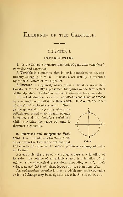
In the Calculus the locus of an equation is conceived as traced
by a moving point called the Generatrix. If a = ob, the locus
of a^-f y2=a2
is the circle abcd. Now,
as the generatrix traces this circle, its
coordinates, x and y, continually change
in value, and are therefore variables;
while a retains the value ob, and is
therefore a constant.
2. Functions and Independent Vari-
ables. One variable is & function of an-
other, when the two are so related that
any change of value in the second produces a change of value
in the first.
For example, the area of a varying square is a function of
its side ; the volume of a variable sphere is a function of its
radius ; all mathematical expressions depending on x for their
values, as ax3, bx^-j-cx2 , sina, log.T, etc., are functions of a?.
An independent variable is one to which any arbitrary value
or law of change may be assigned ; as, x in x?, x in sin$, etc.
Z INTRODUCTION.
The symbol f(x) is used to denote any function of x, and is
read " function of a?." When several functions of x occur in
the same investigation, we employ other symbols, as f'(x),
F(x), <£(#), etc., which are read uf prime function of x"" F function of x" "
</> function of x," etc. According to this
notation, y =f(x) represents any equation between x and y,
when solved for y.
3. Algebraic and Transcendental Functions.— An algebraic
function is one that is expressed in terms of its variable or
variables, by means of algebraic signs, without the use of
variable exponents; as, axs — 2 ex2, ox2 — x, etc.
All functions not algebraic are called transcendental. These
are sub- divided into exponential, logarithmic, trigonometric, and
anti-trigonometric .
An Exponential function is one in which the variable enters
the exponent ; as, acx, y
ax.
A Logarithmic function is one that involves the logarithm of
a variable ; as, log x, log (bx + c).
The sine, cosine, tangent, etc., of a variable angle are called
Trigonometric functions.
The symbol sin-1
a?, read "anti-sine of x," denotes the angle
whose sine is x. Sin-1#, cos""
1^, tan-1^, etc., are called Inverse
Trigonometric, or Anti-Trigonometric, functions.
4. A variable is Continuous, or varies continuously, when, in
passing from one value to another, it passes successively through
all intermediate values.
A Continuous function is one that is constantly real, and
varies continuously, when its variable varies continuously.
Some functions are continuous for all real values of their vari-
ables, others only for those between certain limits. Thus, if
y = ax -f- b, or y = sin x, y is evidently a continuous function of
x for all real values of x ; but, if y = ± Vr2 — x2
, y is continuous
only for values of x between the limits — r and -f- r.
The Calculus treats of variables and functions only between
their limits of continuity ; hence all the values of x and f(x)
that it considers are represented geometrically by the coordi-
nates of the points of the plane curve whose equation is yz=f(x).
'THEORY OF LIMITS. 3
Theory of Limits.
5. For convenience of reference, we give here a brief state-
ment of the theory of limits.
The Limit* of a variable is a constant quantity which the
variable, in accordance with its law of change, approaches
indefinitely near, but which it never reaches. The variable may
be less or greater than its limit.
Thus, if the number of sides of a regular polygon inscribed
in or circumscribed about a circle be indefinitely increased,
the area of the circle will be the limit of the area of either
polygon, and the circumference will be the limit of the peri-
meter of either. When the polygons are inscribed, the6 variable
area and perimeter are less than their limits ; and, when the poly-
gons are circumscribed, the variable area and perimeter are
greater than their limits.
By increasing the number of terms, the sum of the series,
1 -j- -g- + i -f- -J -f- etc. , can be made to approach 2 as nearly as weplease, but it cannot reach 2 ; hence 2 is the limit of the sum.
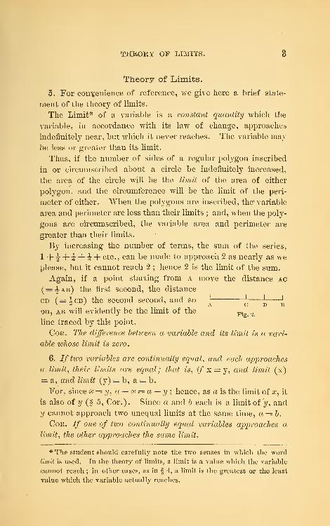
Again, if a point starting from a move the distance ac
(=-Jab) the first second, the distance
cd (=A-cb) the second second, and so '
' ' '
^ z ' A C D Bon, ab will evidently be the limit of the
Fi 2>
line traced by this point.
Cor. The difference between a variable and its limit is a vari-
able whose limit is zero.
6. If two variables are continually equal, and each approaches
a limit, their limits are equal; that is, ?/x = y, and limit (x)
= a, and limit (y) = b, a = b.
For, since x=y, a — x — a — y\ hence, as a is the limit of x, it
is also of y (§ 5, Cor.). Since a and b each is a limit of 'y, and
y cannot approach two unequal limits at the same time, a = b.
Cor. If one of two continually equal variables approaches a
limit, the other approaches the same limit.
* The student should carefully note the two senses in which the word
limit is used. In the theory of limits, a limit is a value which the variable
cannot reach ; in other cases, as in § 4, a limit is the greatest or the least
value which the variable actually reaches.
4 INTRODUCTION.
7. The limit of the product of a constant and a variable is the
product of the constant and the limit of the variable; that is, if
limit (x) = a, limit (ex) = ca.
Let v = a —: x;
then cx= ca — cv.
Now limit (cv) = 0, since limit (v) = ;
hence limit (ex) = limit (ca — cv) = ca.
8. The limit of the variable product of two or more variables
is the product of their limits; that is, if limit (x) = a, and limit
(y) = b, limit (xy) = ab.
Let v== a~x, and vx = b— y ;
then , x= a — v, and y — b — ^ ;
.*. xy = ab — (av±-\- bv — W]) .
Now limit (avx-\- bv -
7-vv i)*=0;
hence limit (xy) = limit \_ab — (a^-f- bv — vv1)~\ = ab.
In like manner, the theorem is proved for n variables.
9. The limit of the variable quotient of two variables is the
quotient of their limits; that is, if limit (x) = a, and limit (y) =b,limit (x -f- y) = (a -r- b) .f
Let z — x-^y,
and c = limit (z) , or limit (x-v-y).
Then a? = y« ; .-. a = bc; §§ G, 8.
.*. limit (x -s-2/)[= c] = a-f- 5.
10. T%e /imrt q/*£7ie variable sum of a finite number of vari-
ables is the sum of their limits ; that is, if limit (x) = a, limit
(y) = b, ZiwiiY (z) = c, etc.,
limit (x+y + z-| ) = a + b + cHLet v = a — x, v1 = b — y, v2 = c — z, etc.
Then x -f y -f z -\
= (a + & + c + .»)-(« + v1 + v, + --);
.-. limit (a) + ?/ + 2 + •••)
= limit[(a + & + c + ...)-(v + ^ + v2 +...)]
= a + 6 -fc H
* When u and vxhave unlike signs, the difference, av
x-\- bv— vvv may be-
come zero for particular values of v and vv but it cannot remain zero, since
xy is variable. The same is true of the difference, v + i\ + v2 + • ••, in § 10.
t This principle does not hold when the limit of the divisor is zero.
INCREMENTS AND DIFFERENTIALS. O
Cor. Wlien the product, quotient, or sum of two or more vari-
ables is equal to a constant, the product, quotient, or sum of their
limits is equal to the same constant.
11. The Change of a variable is Uniform, when its value
changes equal amounts in equal arbitrary portions of time. In
all other cases the change is variable.
Thus, if from a toward b a point move ^—^—J
—
c—^
—
e—
^
equal distances, as aci, ab, be, etc., in equal Fig 3
arbitrary portions of time, the increase of
the line traced will be uniform. Again, if the motion of a point
along a straight line be uniform, the change of each of its
rectilinear coordinates will evidently be uniform.
12. An Increment of a function or variable is the amount of
its increase or decrease in any interval of time, and is found by
subtracting its value at the beginning of the interval from its
value at the end. Hence, if a variable is increasing, its incre-
ment is positive ; and, if it is decreasing, its increment is
negative. An increment of a variable is denoted by writing
the letter A before it; thus, Ax, read "increment of x" is the
symbol for an increment of x. If y =f(x) , Ax and Ay repre-
sent corresponding increments, that is, the increments of x and
y in the same interval of time.
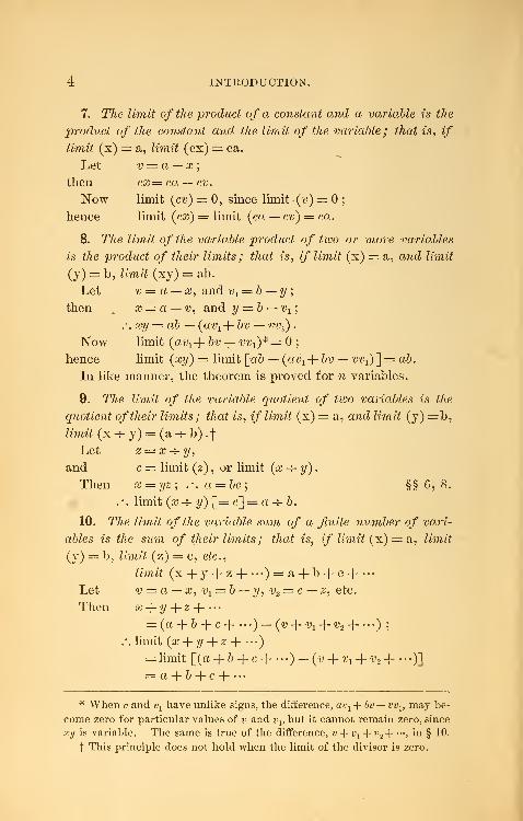
Let oph be the locus of y =f(x) referred to the rectangular
axes ox and or. If, when x = oa,
Ax = ob — oa = ab ; then
Ay =bp f — ap = ep' ; if, when x = oc.
Ax = cf ; then Ay = fh — cd = — xd.
In the last case Ay is negative, but o a b c f
it is properly called an increment, Fig-
4 -
since it is what must be added to the first value to produce
the second.
13. The Differential of a function or variable at any value is
what ivould be its increment in any interval of time, if at that
value its change became uniform. Hence, the differential of a
{ .
p
E
X
Hp \
V
6 INTRODUCTION.
variable is positive or negative, according as the variable is
increasing or decreasing. The interval of time, though arbitrary,
must be the same for a function as for its variable.
If the change of a variable be uniform, any actual increment
may evidently be taken as its differential.
The differential of a variable is represented by writing the
letter d before it ; thus, dx, read " differential x," is the symbol
for the differential of x. When the symbol of a function is not
a single letter, parentheses are used; thus, d(x?) and d(x? — 2x)
denote the differentials of x3 and x2 — 2x.
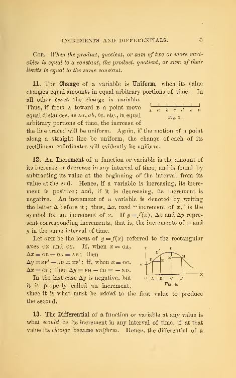
14. Illustrations of Differentials. Conceive a variable right
triangle as generated by the perpendicular moving uniformly to
the right. Let y represent its area, x its
base, and 2 ax its altitude; then y=a>x2. Let
bh be Ax estimated from the value ab (= x'),
then bhmc will be Ay. But, if the increase
of the area became uniform at the value abc,
the increment of the area in the same time
would evidently be bhoc ; hence, bhoc and
bh may be taken as the differentials of y and
x, when x— x'. But bhoc = 2ax'dx, hence,
in general, dy[_= d(ax2)~]=2axdx. lfa=l,y=x2, &nddy=2xdx.
Here Ay = dy-\- triangle com.
The signification of dy=2ax'dx is evidently that, whenx = x\ y, the area, is changing in units of surface 2 ax' times as
fast as x is in linear units.
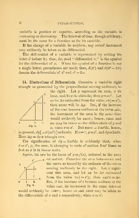
Again, let opn be the locus of y=f(x), referred to the axes
ox and oy. Conceive the area between ox and
the curve as traced by the ordinate of the curve
moving uniformly to the right. Let z repre-
sent this area, and let ab be Ax estimated
from the value oa (=#'); then abp'p = Az.
But, if the increase of z became uniform at the
value oap, its increment in the same interval
would evidently be abdp ; hence ab and abdp may be taken as
the differentials of x and z respectively, when x = x f
.
GEOMETRIC ILLUSTRATIONS OF DIFFERENTIALS. i
Hence dz = abdp =afcIx = y'dx ; or, in general, dz = ydx,
which evidently means that z is changing y times as fast as x.
Area above the axis of x being positive, area below it is
negative ; hence, where the curve lies below the axis of x, the
area decreases as x increases, and ydx is negative as it should be.
Here Az = dz -\- area pdp\
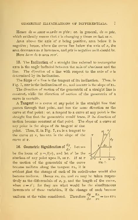
15. The Inclination of a straight line referred to rectangular
axes is the angle included between the axis of abscissas and the
line. The direction of a line with respect to the axis of x is
determined b}~ its inclination.
The Slope of a line is the tangent of its inclination. Thus, in
Fig. 7, hzp is the inclination of za, and tanHzp is the slope of za.
The direction of motion of the generatrix of a straight line is
constant? while the direction of motion of the generatrix of a
curve is variable.
A Tangent to a curve at any point is the straight line that
passes through that point, and has the same direction as the
curve at that point ; or, a tangent to a curve at any point is the
straight line that the generatrix would trace, if its direction of
motion became constant at that point. The slope of a curve at
any point is the slope of its tangent at that
point. Thus, if, in Fig. 7, pa is a tangent to
the curve at p, tanHZA is the slope of the
curve at p.
16. Geometric Signification of JL. Let mndx
be the locus of y=f{x), and let x' be the
abscissa of any point upon it, as p. If at p JTz j- h x .
the motion of the generatrix of the curve Fi§- <•
became uniform along the tangent pa, it is
evident Jthat the change of each of its coordinates would also
become uniform. Hence pe, ea, and pa may be taken respec-
tively as the differentials of x, y, and the length of the curve,
When x= x' ; for they are what would be the simultaneous
increments of these variables, if the change of each became
dll EAUniform at the value considered. Therefore -f- =— — tan epa
dx PE
INTRODUCTION.
= tan hza, which is the slope of the curve at p. Hence, in
general, -JL is the slope of the curve y = f (x) at any point (x, y).dx
Cor. 1. If ea, or dy, be c times as great as pe, or dx, y is
evidently increasing c times as fast as x, when x = 01.
Cor. 2. If s represent the length of the curve mn, PA = ds,
and ds2 = dx2 + dy2, in which ds2 denotes the square of ds.
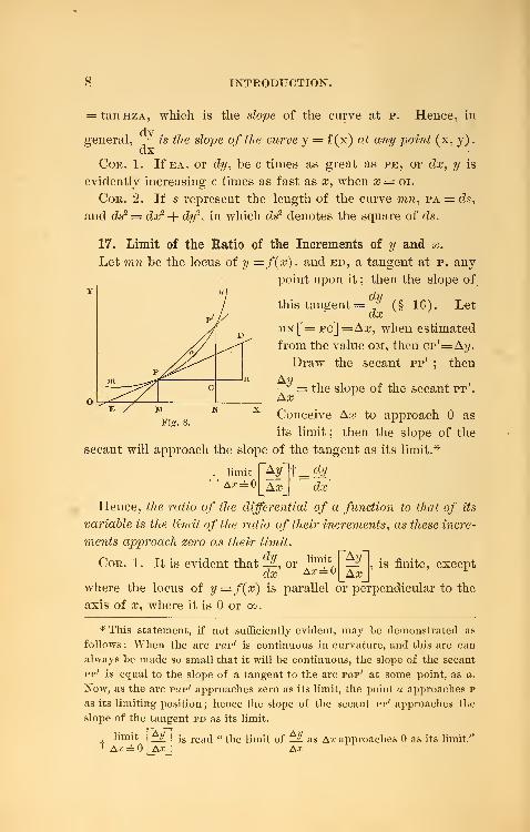
17. Limit of the Ratio of the Increments of y and x.
Let mn be the locus of y =f(x) , and ed, a tangent at p, any
point upon it ; then the slope of
this tangent
mn [= pc] = Ax, when estimated
from the value om, then cp'=A?/.
Draw the secant pp'; then
-^- = the slope of the secant pp'.AxConceive Ax to approach as
its limit ; then the slope of the
secant will approach the slope of the tangent as its limit.*
limit
A.r='Ay
Ax
\= dyt
dx
Hence, the ratio of the differential of a function to that of its
variable is the limit of the ratio of their increments, as these incre-
ments approach zero as their limit.
dy limit Ay
Axis finite, exceptCor. 1. It is evident that — , or
dx Ax= °
where the locus of y=f(x) is parallel or perpendicular to the
axis of x, where it is or go.
* This statement, if not sufficiently evident, may be demonstrated as
follows : When the arc pap' is continuous in curvature, and this arc can
always be made so small that it will be continuous, the slope of the secant
pp' is equal to the slope of a tangent to the arc pap' at some point, as a.
Now, as the arc pap' approaches zero as its limit, the point a approaches p
as its limiting position ; hence the slope of the secant pp' approaches the
slope of the tangent pd as its limit.
xlimit
I A*=read " the limit of — as Ax approaches as its limit.
Ax
LIMIT OF THE RATIO OF INCREMENTS.
AwCor. 2. If —^ be constant, the locus of y=f(x) is evidently
a straight line, in which case — = -^.° Ax dx
Cor. 3. A tangent to ran at p is evidently the limiting posi-
tion of the secant pp' as p' approaches p and arc p'p = 0.
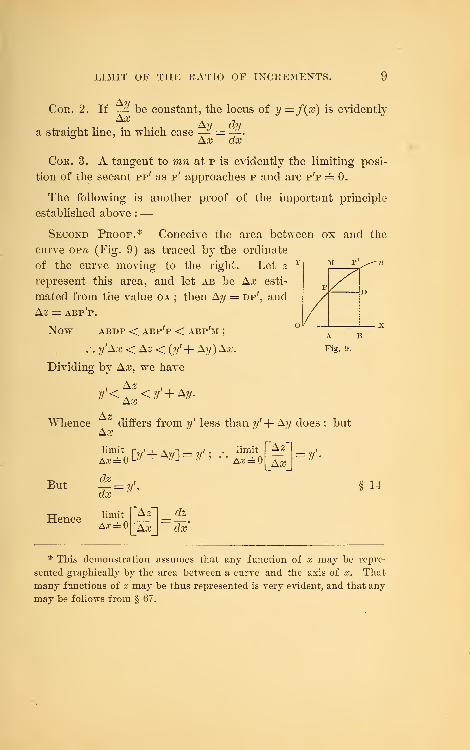
The following is another proof of the important principle
established above :—
Second Proof.* Conceive the area between ox and the
curve opft (Fig. 9) as traced by the ordinate
of the curve moving to the right. Let zT
represent this area, and let ab be Ax esti-
mated from the value oa ; then Ay = dp', and
Az = ABP'P.
NOW ABDP < ABP'P < ABP'M;
.-. y'Ax <Az< (y'+ Ay) Ax.
Dividing by Ax, we have
, Az ,
AzWhence — differs from y' less than y'-\- Ay does ; but
M pv^
p/S\
A B
Fig. 9.
Ax
limit
Ax[7/+A2/] = 2/';
limit
Ax=Az
Ax= y
But
Hence
dz
dx= y § 14
limit Az
Axdz
dx
* This demonstration assumes that any function of x may be repre-
sented graphically by the area between a curve and the axis of x. That
many functions of x may be thus represented is very evident, and that any
may be follows from § 67.
CHAPTER II.
DIFFERENTIATION.
18. Differentiation is the operation of finding the differential
of a function. The sign of differentiation is d ; thus d in d(x3
)
indicates the operation of differentiating x\ while the whole
expression d(x") denotes the differential of x" (see § 13).
To differentiate ax2, let y = ax2
, and let x' and y' be any cor-
responding values of x and y ; then
y'= ax' 2. (1)
Let Ax be any increment of x estimated from the value x\
and Ay the corresponding increment of y ; then
y'+Ay = a(x'+Ax) 2 = ax''2 + 2 ax'Ax + a{Ax) 2
. (2)
Subtracting (1) from (2), we have
Ay = 2 ax'Ax -f a (Ax)2
, or ^ = 2 ax'+ aAx. (3)Ljk-X
. limit' 'A:c =
.dV _
A?/*"**> [2 ooj'+ aAx]. § 6.Ax
= 2 ax', or, in general, dy = 2axdx. § 17.ox
By this general method we could differentiate any other func-
tion, but in practice it is more expedient to use the rules which
we proceed to establish.
Algebraic Functions.
19. The differential of the product of a constant and a vari-
able is the product of the constant and the differential of the
variable.
ALGEBRAIC FUNCTIONS. 11
We are to prove that d (ay) = ady, in which y is some func-
tion of x. Let u = ay, and let x' represent any value of x, and
y! and u' the corresponding values of y and u ; then
u'=ay'. (1)
Let Ax represent any increment of x, estimated from the value
x\ and let Ay and Au represent the corresponding increments
of y and u ; then
u'+Au = a(y'-t-Ay) = ay'+aAy. (2)
Subtracting (1) from (2), member from member, we have
Au = aAy.
AxAuAx
, limit VAu
du dv.— = a—dx dx
limit
Ax =AyAx
(
limit
Ax§§ 6, 7,
§ 17.
Hence, as x' is any value of x, we have in general, by multi-
plying both members by dx,
du[=d (ay) ] = ady.
a \a a
20. The differential of a constant is zero.
This is evident, since the increment of a constant in any
interval of time is zero.
21 . The differential of a polynomial is the algebraic sum ofthe differentials of its several terms.
We are to prove that d (v+y—z+a) = dv+dy— dz, in which
v, y, and z are functions of x.
Let u = v-\-y — z-\-a, and let x' represent any value of x,
and v\ y\ z\ and \0 the corresponding values of v, y, z, and u;
then^'+ 2/'— z'-\-a. (i)
12 DIFFERENTIATION.
Let Ax represent any increment of x, estimated from the value
x', and Av, Ay, Az, and Aw the corresponding increments of #,
y, z, and w ; then
u' + Au = v'+Av+y'+Ay — (zr +Az) + a. (2)
Subtracting (1) from (2) we have
Aw = Aw + Aw — A3.
Aw _ Av Aw Az(
Ax Ax Ax Ax
limit rAw~j_ nmit
Ax= Ax A.r =Aw AwAx Ax
_Az~1
Ax§ 6.
du _dv dy dz
dx dx dx dx§§ 10, 17.
Hence, as x' is any value of x, we have in general
du [= d (v + y — z + a) ] == dw +% — cte.
22. 27te differential of the product of two variables is the first
into the differential of the second, plus the second into the differen-
tial of the first.
We are to prove that d (yz) = ydz + zdy, in which w and z are
functions of x.
Let w = yz, and let x' represent any value of x, and y\ z', and
u' the corresponding values of w, z, and i£ ; then
u'=y'z'. . (1)
Let Ax represent any increment of x estimated from the value
x', and Aw, Az, and Aw the corresponding increments of w, z,
and w ; then
w'+ Aw = (w' -f Aw) (z'+ Az)
= w 'z'+ y'Az + z'Aw + AzAw. (2)
Subtracting (1) from (2) we have
Aw = y'Az + z'Aw + AzAw.
Aw ,
AxAz
Ax+ («' + Az)
Aj/
Ax
ALGEBRAIC FUNCTIONS. 13
limit
A;r=AuAx
limit
Ax=flAz
Ax+ limit
Ax= (s'+A*)^Ax
du ,dz,
,dy
dx dx dx§§7,8.
Hence, as x' is any value of aj, we have in general
d« [= c?(yz)] = yc?» + zdy.
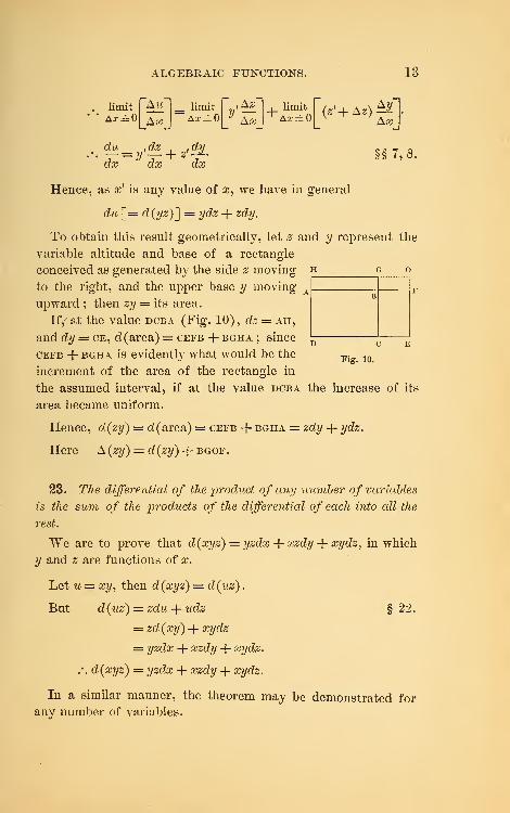
To obtain this result geometrically, let 2 and ?/ represent the
variable altitude and base of a rectangle
conceived as generated by the side z moving h
to the right, and the upper base y moving
upward ; then zy = its area.
If/ at the value dcba (Fig. 10) , dz — ah,
and dy = ce, d(area) = cefb + bgha ; since
cefb + bgha is evidently what would be the
increment of the area of the rectangle in
the assumed interval, if at the value dcba the increase of its
area became uniform.
Hence, d(zy) = d(area) = cefb + bgha = zdy + ydz.
Here A (zy) = d (zy) + bgof.
B
Fig. 10.
23. The differential of the product of any number of variables
is the sum of the products of the differential of each into cdl the
rest.
We are to prove that d(xyz) = yzdx + xzdy + xydz, in which
y and z are functions of x.
Let u = xy, then d(xyz) — d(uz)
.
But d(uz) = zdu + udz § 22.
= zd(xy) -\-xydz
= yzdx + xzdy + xydz.
.-. d(xyz) = yzdx + xzdy + xydz.
In a similar manner, the theorem may be demonstrated for
any number of variables.
14 DIFFERENTIATION.
24. The differential of a fraction is the denominator into
the differential of the numerator, minus the numerator into the
differential of the denominator, divided by the square of the
denominator.
We are to prove that d(K)—_ ? , in which y and z are\zj z\
functions of x.
yLet u == '—•> then uz = y.
z J
.' . udz + zdu = dy.
dy — udz zdy — ydzdy — -dz
,-.du =z z
^ , /a\ xda — adx adx . 7 A ,, , . j7Lor. d I - = ^- = — —-, since da = ; that is, the\xj x2, xz
differential of a fraction with a constant numerator is minus the
numerator into the differential of the denominator divided by
the square of the denominator.
25. The differential of a variable affected with any constant
exponent is the product of the exponent, the variable with its expo-
nent diminished by one, and the differential of the variable.
I. When the exponent is a positive integer.
If n is a positive integer, xn = x • x • x to n factors ; hence
we have
d(xn) = d(x • x • x to n factors)
= xn~ Ydx + xn
~ ldx + etc. to n terms § 23.
= nxn~1dx.
II. When the exponent is a positive fraction.
mLet y = fl5», then y
n == .Tm
. (1)
Differentiating (1), we obtain
nyn~1dy = mxm~ 1dx.
ALGEBRAIC FUNCTIONS. 15
m x"1' 1
7m xm
- ly _ m am T
a;» ,
,\ d?/ = ax— ax — ax* n y
n~l n yu n xm
= _# Jidx,
n
III. When the exponent is negative.
Let y = x~ 7
\ n being integral or fractional ; then
'=? (1)
Differentiating (1), we have
m/y.W— 1
eZy = —^-dx — — ?ia~'l_1da. § 24, Cor.
:ia
For a proof of this theorem, which includes the case of in-
commensurable exponents* see § 39, Ex. 25.
Assuming the binomial theorem, let the student prove this
rule by the general method of differentiation.
Cor. d (Va) = \xr*dx =——
•
2Va
26. The general symbol for the differential off(x) isf'(x)dx ;
hence, if y=f(x), dy =f'(x)dx.
Examples.Differentiate
1. xz + 8x + 2x2. Ans. (3a2 + 8 +4 a?) dx.
d (a3 + 8x + 2 a2) = d (a3
) + d (8a) + d (2a2)
,
§ 21.
d(x3) = 3x2dx, § 25.
d(8x) = 8dx, § 19.
d(2a2) = 4ada, §§ 19, 25.
.'. d (a3 + 8a + 2a2) = (3a2
-f 8 + 4a) da.
2. y=3aa? — 5wsc— 8m. cfa/ = (6aa — 5n)c?a.
dy = d(3axi—5?ia—8m) = c^aa2) — cZ(5?ia) — d(8m).
[The differentials of equals are equal, and § 21.]
16 DIFFERENTIATION.
3. f(x)= Sax2 - 3b2x? - abx\
f'(x)dx= (10ax — 9 62x2 — 4a&x3
) dx.
4. /(x) = a3 + 5 b2xs + 7 a¥.
/'(») da; = (15 62x2 + 35 a¥) dx.
^ r i , ^ 3 ax + b ,
5. 2/ = ax§ + 6x* + c. dy = ^-ax.2Vx
6. y2 =2px. ty—P.
d{y2) — d{2px). dx~ y
7. oV + 6V = a2b2
. dy=-^ dx.
8. f(x) = {b + ax2)*. f'(x)dx = %(b + ax2)iaxdx.
9. ?/= (l+2x2)(l+4x3
). rtj/ = 4x(l+3x + 10x3)ax.
dy = (I + 2x2)d(l + 4xs) + (1 +4x3)a'(l + 2x2
).
. A x + a2, 6 — a2
,
10. ?/ =—! dy = -dx.yx + b .
y(x + 6)
2
dy=i(x + b)d{x + a2)-(x + a2)d{x + b)
{x + by
—• f'(x)dx =—— . .
b-2x* J K J (b-2x2 )''
11- /(*)=—
^
f(x)dx= ^*a*
<fa
a — 3x12. ?/ = (a+ x) Va — x. dy = dx
2Va — x
,o ^/ x 2xA,/s \j 8a¥- 4x5
,
a2 — x2 (a2 — x2
)
dxm+l
(l-x)Vl-x
16-^)=(T^i- ^ = (1^)1
17. v =— •
Vi+*2
DERIVATIVES
.
17
3 a? _ 2 y2
18. 2xy2 — oy2 = or3
. dy =— *— dx.4xy — 2ay
19 . m=¥±± f(x)dx=^+^+v
dx .
±x+ a?v
' {-ix + x2)'
20. y =or — ar
21. f{x)=^/ax+ -\/&f. f'(x) ^ Va "
2V.r
! <ao a 6 ax 722. ^- —•• dx.
23. /(») = —- /'(a)=3a;2 + a;8
./v y (1+a)2 J w(l+ »)
3
24. /(a^-M^L. /'(«) = l +±*
25. (*~ 9y) (ft -te)= («-*) (!-*)dy _ b — 4 x + 6 y — 2 ay
cfee a2— 6#— e+ 26
27. An Increasing function is one that increases when its
variable increases ; hence it decreases when its variable de-
creases.
A Decreasing function is one that decreases when its variable
increases ; hence it increases when its variable decreases.
Thus, ax and ax are increasing, and - and a — x are decreasingx
functions of x.
28. The Derivative of a function is the ratio of the differen-
tial of the function to the differential of its variable. This ratio
is sometimes called the derived function or the differential coeffi-
cient. Hence the derivative of f{x) is /'(a), or the ratio of
f'(x)dx to dx. The derivative of y with respect to x is repre-
sented by ^. If y =f(x) , thencll = f(x) . Thus, ify= x3
,
j
" dx dx— =3x2
; that is, 3 x2is the derivative of ?/, or xJ
; if f(x) = .t6
,
then f(x)= 6ar\
18 DIFFERENTIATION.
29. The Measure of the rate of change of a variable at a
given instant is what ivould be its increment in a unit of time,
if at that instant its change became uniform. This measure
of rate is generally called the rate. Hence, the rate will be
positive or negative, according as the variable is increasing
or decreasing. Thus, when we say that the distance of a train
from the station was changing, at a given instant, at the rate
of -+-30 miles an hour, we mean that this distance would have
increased thirty miles in an hour, if at that instant its increase
had become uniform,
If the change of a variable is uniform, the actual increment
of the variable in a unit of time is the measure of its rate.
30. Signification of — . Let t represent time ; then, any vari-
able, as y, is evidently some function of t. Since time changes
uniformly, dt may represent any increment or interval of time.
If dt equals the unit of time, then by definition cly equals the
measure of the rate of change of y ; and, if dt is n times the unit
of time, dy is n times the rate of change of y ; hence, whatever
be the value of dt, — = the rate of change ofy.
31 . Signification of ^, or /' (x) .
c]l = al^ a== the ratio
dx clx dt dt
of the rate of change of y to that of x (§ 30). f'(x) =/ > '1
at az
= the ratio of the rate of change of f(x) to that of x.
Hence, the derivative ofa function expresses the ratio of the rate
of change of the function to that of its variable; and a function
is an increasing function or a decreasing function, according as
its derivative is positive or negative.
Cor. The same function of x may be an increasing function
for some values of x, and a decreasing one for other values.
Thus, since -, the derivative of — , is -f when x < 0, andx3 ar
— when x > 0, — is an increasing function when x<0, andx2
a decreasing function when x > 0.
APPLICATIONS. 19
32. When the change of y is uniform, it is evident that —6 JAt
is the rate of change of y. When the change of y is variable,
the value of —- evidently lies between the greatest and the least
values of the rate of change of?/ during the time At ; hence, the
Aysmaller At is taken, the nearer — approaches the rate of change
of y at the beginning of At.
Hence limit.rience, A^ Q At
the rate of change of y \ _ dy
at the beginning of At ) dt
~„a limitand A^ Q
Ax __ j the rate of change of x }_dx
At _ I at the beginning of At) dt
Dividing (1) by (2), we obtain, without the aid of a locus,
(i)
(2)
limit
Ax=0 Ax_ dx
Applications.
1. The area of a circular plate of metal expanded by heat
increases how man}' times as fast as its radius ? If, when the
radius is two inches, it is increasing at the rate of .01 inch a
second, how fast is the area increasing at the same time ?
Let x — the radius, and y the area of the plate ; then y = ttx2
.
.'. dy = 2irxdx, or -^- = 2 ttx— ; that is, the area is increas-ed dt
ing in square inches 2ttx times as fast as the radius is in linear
dx dvinches. When x = 2, and — = .01 in., -^= .04 -w sq. in. ; that
dt dtL
is, the area is increasing .04 tt sq. in. a second at the instant
considered.
2. The volume of a spherical soap-bubble increases how manytimes as fast as its radius? When its radius is 3 in., and is
increasing at the rate of 2 in. a second, how fast is its volume
increasing ?
Ans. The volume is increasing in cubic inches 4 ttx2, times as
fast as the radius is in linear inches. The volume is increasing
72-7T cu. in. a second at the instant considered.
20 DIFFERENTIATION.
3. A bo}~ is running on a horizontal plane in a straight line
towards the base of a tower 50 metres in height. He is
approaching the top how many times as fast as he is the foot of
the tower? How fast is he approaching the top, when he is 500
metres from the foot, and running at the rate of 200 metres a
minute ?
Let x and y respectively represent in metres the distances
of the boy from the foot and the top of the tower ; then
y2 = x2
-f- (50)2
, etc. Ans. 199 metres a minute.
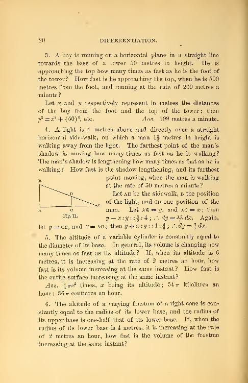
4. A light is 4 metres above and directly over a straight
horizontal side-walk, on which a man If metres in height is
walking away from the light. The farthest point of the man's
shadow is moving how many times as fast as he is walking?
The man's shadow is lengthening how many times as fast as he is
walking? How fast is the shadow lengthening, and its farthest
point moving, when the man is walking
at the rate of 50 metres a minute ?
Let ae be the sidewalk, b the position
of the light, and cd one position of the
man. Let ae = ?/, and ac = x ; then
y — x : y : : % : 4 ;.
' . dy — 1^-- dx. Again,
let 2/ = CE, and o? = ac; then y + x :y : :4 : f ; .\dy = j-dx.
5. The altitude of a variable cylinder is constantly equal to
the diameter of its base. In general, its volume is changing how
many times as fast as its altitude ? If, when its altitude is 6
metres, it is increasing at the rate of 2 metres an hour, how
fast is its volume increasing at the same instant? How fast is
the entire surface increasing at the same instant?
Ans. %ttx2 times, x being its altitude; 54 ?r kilolitres an
hour ; 36 tt centiares an hour.
6. The altitude of a varying frustum of a right cone is con-
stantly equal to the radius of its lower base, and the radius of
its upper base is one-half that of its lower base. If, when the
radius of its lower base is 4 metres, it is increasing at the rate
of 2 metres an hour, how fast is the volume of the frustum
increasing at the same instant?
APPLICATIONS. 21
7. The area of an equilateral triangle increases hew manytimes as fast as each of its sides ? How fast is its area increas-
ing when each of its sides is 10 in., and increasing at the rate
of 3 in. a second? What is the length of each of its sides, when
its area is increasing in square inches 30 times as fast as each
of its sides is in linear inches ?
Ans. 15Vo sq. in. a second; 20V3 in.
8. One end of a ladder 20 ft. long was on the ground 5 ft.
from the foundation of a building, which stood on a horizontal
plane, while the other end rested against the side of the build-
ing. The end on the ground was carried away from the build-
ing on a line perpendicular to it, at the uniform rate of 4 ft. a
minute ; how fast did the other end begin to descend along the
building? How fast was it descending at the end of two
minutes? How far was the foot of the ladder from the building,
when the top was descending at the rate of 4 ft. a minute ?
Ans. 1.03+ ft. a minute ; 3.42 ft. a minute ; 10V2 ft.
9. In the parabola whose parameter is 8, the ordinate
changes how many times as fast as the abscissa? What is its
slope at any point (x, y) ? Find its inclination at the points
whose common abscissa is ^. Is y an increasing or a decreas-
ing function of x? At what points does the ordinate change
numerically four times as fast as the abscissa ?
4In this case, y is a two-valued function; aud - is + or —
,
yaccording as y is + or — ;
.". the + value of?/ is an increasing,
and the — value a decreasing, function of x.
Ans. -; t; 63° 26' 6" and 116° 33' 54"; a, 1) and (1,-1).y y
10. In the ellipse cry2 + b2x2 = a2
b2
, the ordinate increases
how many times as fast as the abscissa ? y changes howmany times as fast as x at the extremities of the axes of the
curve ? How can the points be found at which y changes c times
as fast as x? What is the slope of the ellipse at any point?
What, at the extremities of its axes? Is y an increasing or a
decreasing function of x?
22 DIFFERENTIATION.
dy b2x . , , ,. „
'
&2a?-^= —
;.". when y changes c times as last as a?, — = c.
da? a2?/ , 2 a-?/
When x and 2/ have unlike signs, — is + , and 2/ is an
increasing function ; when x and y have like signs, — is —
,
and y is a decreasing function.
11. What is the slope of y2 = Xs + 2 x4 at (#, y) ? What is it
Ans. ±X + - .. ± i9.VlO.
2Va+2z2 10
12. What is the slope of ?/ = Xs — x2-f- 1 at the point whose
abscissa is 2? 1? 0? -1? Ans. +8; +1; +0; +5.
13. At what point on y2 = 2 Xs
is the slope 3 ? At what point
is the curve parallel to the axis of x? Ans. (2, 4) • (0, 0).
14. At what angles does the line Sy — 2x— 8 = cut the
parabola y2 = Sx?
Find their slopes at their points of intersection ; then find the
angles between the lines having these slopes.
Ans. tan-1
. 2 and tan-1
. 125.
15. One ship was sailing south at the rate of 6 miles an hour;
another, east at the rate of 8 miles an hour. At 4 p.m. the
second crossed the track of the first at a point where the first
was two hours before. How was the distance between the ships
changing at 3 p.m. ? How at 5 p.m. ? When was the distance
between them not changing?
Let t = the time in hours, reckoned from 4 p.m., time after
4 p.m. being +, and time before — . Then 8t and 6£+ 12 will
represent respectively the distances of the two ships from the
point of intersection of their paths, distances south and east
being +, and distances west and north being — . Let y = the
distance between the ships ; then,
2/2 = (80
2 + (6^ + 12)2
.
' '
dt ~[>U 2 + (6£ + 12)2]i' ^ )
VELOCJTY AND ACCELERATION. 28
When y does not change, dy=0. /.from (1), 100 £+ 72= 0;
.-. t= — .72 of 60 minutes =— 43.2 minutes. Therefore, the
distance between them was not changing at 43.2 minutes before
4 p.m., or at 16.8 minutes after 3 p.m.
Ans. Diminishing 2.8 miles an hour; increasing 8.73.
33. Velocity is the rate of change of the distance passed over
b}~ a moving body. Hence, if s = the distance and v = the
velocity, v = — (§ 30). If the unit of s is one foot, and the
dsunit of t one second, v = — ft. a second.
dt
Acceleration is the rate of change of velocity.
dvHence, if a = acceleration, a = — (§ 30).
Examples.
1
.
If s = 2 f, what is the velocity and acceleration ?
Here v = — = 6t2ft. a second ; a =— = 12£ ft. a second
;
dt dt
and the rate of change of acceleration =— = 12 ft. a second.dt
2. If g = 32.17 ft., s =j-t2is the law of falling bodies in
vacuo near the earth's surface ; find the velocity and accelera-
tion in general, also at the end of the third and the eighth
second.
Ans. a = 32.17 ft. a second ; v = 32.172 ft. a second ; 96.51
;
257.36.
3. Given s = aft 9 to find v and a in general, and at the end
of 4 seconds.
Ans. v = and - ft. a second ; a = and ft.
2V* 4 Wf 32
a second ; that is, the A^elocity decreases at the rate of ft.
Wt3
a second.
24 DIFFERENTIATION.
4. Given s3 = 8t2
, to find v and a in general, and at the endof 8 seconds.
Ans. v =—-— and f ft. a second.3-y/t
5. A point moves along a parabola with a velocity v' ; re-
quired the rates of change of its coordinates.
Since y2 — 2px, _^=-£-. (\\
dx y v y
If s represents the length of the curve traversed, by the
conditions of the problem, we have
*="' (2)
But^S •— ^ -
^s —^ -^d°(? + dy2 _ dy L.dx^ .„.
dt dt' dy~dt' dy ~dt\ dy2 ' ^
since ds = -Vdx2-f- dy
2. § 16, Cor. 2.
from (1), (2), and (3), we obtain
dt \ p ^ Vp2-f2/
2
which is the rate of change of y.
In like manner, we obtain
dx _ ydt V/r -f y-
v\ the rate of change of x.
Logarithmic and Exponential Functions.
34. The differential of the logarithm of a variable is the quo-
tient of the differential of the variable divided by the variable
itself, multiplied by a constant.
Let y = nx; (1)
then dy = ndx, (2)
and \ogay*= \oga ii + \oga x. (3)
* loga y is read, "the logarithm of y to the base a"
LOGARITHMIC AND EXPONENTIAL FUNCTIONS. 25
(4)
From (1) and (2),
dy dx
V x
From (3),
d(\oga y) = d(loga x). (5)
From (5) and (4),
d(\oga y) d(\oga x)
dy dx~y
?
dxWhence d(\oga x) bears the same ratio to — that d(\oga y)
does to JL. Let m be this ratio for some particular value of a?,
y
as x 1
; then d(loga #) = m— when a? = x\ and d(logffl?/) = m _~
when y = nx' ; but, as w is an arbitrary constant, nx' may be
any number. Hence, in general, d(\ogn y) = m— , in which m2/
is a constant.*
The constant m is called the Modulus of the system of loga-
rithms whose base is a.
35. Let m and m 1 be the moduli of two systems of loga-
rithms whose bases are a and b respectively. If a > 6,
it is evident that \oga x must change more slowly than logb x;
•'. d(\oga x) < d i\ogh x) ; that is,
dx ' .dx,m— < m'— , or m < m\
Hence, the greater the base of a system of logarithms, the smaller
is its modulus.
36. Naperian System. The system of logarithms whose
modulus is unity is called the Naperian system. The symbol
for the Naperian base is e.
* See Rice and Johnson's Calculus, p. 39 ; Olney's Calculus, p. 25 ; also
Bowser's Calculus, p. 29.
26 DIFFERENTIATION.
The differential of the Naperian logarithm of a variable is,
therefore, the differential of the variable divided by the variable.
Thus we see that Naperian logarithms are the simplest and
most natural for analytic purposes ; and, hereafter, the symbol
log will stand for the Naperian logarithm.
37. The differential of an exponential function with a constant
base is equal to the function itself into the logarithm of the base
into the differential of the exponent, divided by the modulus of the
system of logarithms used.
Let y = cx
, then \oga y = x loga c ;
dy cx \oga c
.'.m— = loga cc£r ; .'. dy\=d(cx)l = dx.
Cor. In the Naperian system, the modulus being unity, wehave
d(cx) = c
x \ogcdx-,
also, d(ex) = e
xdx, since loge = 1.
38. The differential of an exponential function with a variable
base is the sum of the residts obtained by first differentiating as
though the base were constant, and then as though the exponent
were constant.
Let u — yx
, then log u = x logy;
du , , dy. = \ogydx -f- x— ;
u & ^y
:, du = yx\ogydx -f xy
x~ ldy,
which is the result obtained by following the rule given.
39. Logarithmic Differentiation. Exponential functions, as
also those involving products and quotients, are often more
easily differentiated by first passing to logarithms. This method,
which is illustrated in the two preceding demonstrations, is called
logarithmic differentiation.
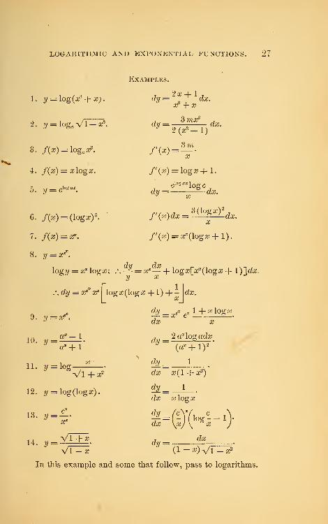
LOGARITHMIC AND EXPONENTIAL FUNCTIONS. 27
Examples.
1. y = \og{xi -\-x)
2. y = \oga -Vl—x\
3. f(x)=\oga x\
4. f(x) = x log x.
5. y = cXosax
.
6. /(*) = (log a)3
.
7. /(*)=**
8. y=-a^.
dy = -—i— dx.x2 -\-x
j 3 mx2
ay = ——
;
: ax.
/'(*)
2(^-1)
3 m
f'(x) = logx+l.
dy =logc
dx.
/'(tt)cfa=3(logg)2
.fa.X
f'(x) = x?(logx + l).
logy = xx log x; .*. ~ = xx— + log a?[af(log a; -f- l)]da?o
logx(loga;+l) +,\dy = x? x*x
dx.
9 . ?/ = a?**.
a2 —
1
% _ xe*ex 1 4-^logx
dx X
10. 2/
az + ld*/
2 a1 log ado;
11. y = log
VlT^12. ?/ = log (log x).
13. 2/ =—
•
(«* + l) 2
dx x(l 4-ic2)
C?iC x log X
da;~~ [xj \ ° x J
14. y = Vl+xVT-a;
dydx
(l-^)Vi-^2
In this example and some that follow, pass to logarithms.
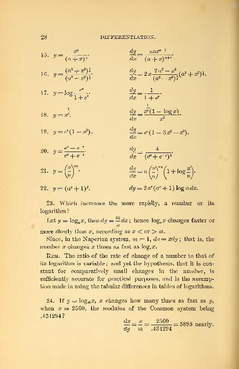
28
15. y =xn
(a + x) n
16. y =(a 2 + z2
)§
DIFFERENTIATION.
dy =dx
1
1 + e*
dy _ xx(1 — logo?)
dx X2
dy =dx
= ex(l-3x2 -x").
dy _ 4
dx (ex + e~ xy
dy =dx ='iT(
1+logf
dy _ naxn~l
. dx~ (a + x) n+1
^ = 2a?2a'-^
(a2 + a?)Kv^u, — jo )* dx (a2 — ar)i
17. ?/ = logJ Sl + e*
i
18. 2/ = of,
19. y = ex(l-x3
).
20. y =^£^
« »-$r-
22. 2/=(aa: +l) 2. dy = 2ax (ax + l)logadaj.
23. Which increases the more rapidly, a number or its
logarithm ?
Let 2/ = loga a?, then dy = —dx\ hence loga# changes faster orx
more slowly than #, according as»< or > m.
Since, in the Naperian sj'stem, m = 1, dx = xc??/ ; that is, the
number a? changes x times as fast as loge a\
Hem. The ratio of the rate of change of a number to that of
its logarithm is variable ; and yet the hypothesis, that it is con-
stant for comparatively small changes in the number, is
sufficiently accurate for practical purposes, and is the assump-
tion made in using the tabular differences in tables of logarithms.
24. If y = log10 x, x changes how many times as fast as ?/,
when x = 2560, the modulus of the Common system being
.434294?da= x = 2560 =5895nearldy ra .434294
J
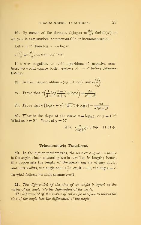
TRIGONOMETRIC FUNCTIONS. 29
dx25. By means of the formula d(\ogx) — — , find d (xn) in
which n is any number, commensurable or incommensurable.
Let u = xn, then log u = n log x
;
dit dx , __!
,
.*. — = n— , or du = nxn l
clx.
u x
If x were negative, to avoid logarithms of negative num-
bers, we would square both members of u = xn before differen-
tiating.
26. In like manner, obtain d(xy), d(xyz), and dl-y
27. Prove that d(— log—- + logc) =2 a " x + a y or — a-
d0728. Prove that d [log (a +Vr ± a 2
) -f log c] =vrift2
29. What is the slope of the curve x = log1Qy, or y = 10 T?
What at x = 0? What at y = 5?
J.?ls . J— • 2.3+; 11.51 + .
.43429
Trigonometric Functions.
40. In the higher mathematics, the tm& of angular measure
is the angle whose measuring arc is a radius in length ; hence,
if x represents the length of the measuring arc of any angle,
xand r its radius, the angle equals -
; or, if r = 1, the angle = x.r
In what follows we shall assume r=l.
41. Tfie differential of the sine of an angle is equal to the
cosine of the angle into the differential of the angle.
TJie differential of the cosine of an angle is equal to minus the
sine of the angle into the differential of the angle.
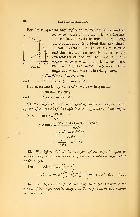
30 DIFFERENTIATION.
For, let x represent any angle, or its measuring arc, and let
ac be any value of this arc. If at c the mo-
tion of the generatrix became uniform along
the tangent cd, it is evident that any simul-
taneous increments of its distances from c
and lines ba and bh may be taken as the
differentials of the arc, the sine, and the
cosine, when x = ac ; that is, if cd = dx,
ed = d(smsc), and — ec = cl (oosx). Nowangle edc = abc = x ; .'.in triangle edc,
ed [= d (sin x) ] = cos x dx,
and — ec[= d(cos x)~\ = — sin xdx.
Hence, as abc is any value of a?, we have in general
dsmx— cos xdx,
and d cos x= — sin xdx.
42. The differential of the tangent of an angle is equal to the
square of the secant of the angle into the differential of the angle.
sin xFor tan& =
.'.dtana;
cos#
cos^dsinx sinit'dcoscc
(cos2# + &m2x)dx
COS2£dx = sec2xdx.
cos-o?
43. TJie differential of the cotangent of an angle is equal to
minus the square of the cosecant of the angle into the differential
of the angle.
For cot x = tan f- — x
.'.dcotx = sec2f—
—
x \d(—x )= cosec2 xdx. §42.
44. The differential of the secant of an angle is equal to the
secant of the angle into the tangent of the angle into the differential
of the angle.
For sec a? =
.'.dsecx =
TRIGONOMETRIC FUNCTIONS.
1
133
sinxdx
31
cos a
dcosx = secxt&nxdx.cos~# COSz£
45. The differential of the cosecant of an angle is equal to
minus the cosecant of the angle into the cotangent of the angle into
the differential of the angle.
For cosec x = secf - — x]
;
.'.d cosec x= sec(
- —# Jtanf- —x \dl - — x\ § 44.
= — cosec x cot a? da?.
46. d vers x = d(l — cos x) = sinxdx.
47. d* covers x = d(l — sin sc) = —cos £ecfcc.
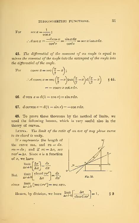
48. To prove these theorems by the method of limits, weneed the following lemma, which is very useful also in the
theory of curves.
Lemma. The limit of the ratio of an arc of any plane curve
to its chord is unity.
If s represents the length of
the curve mw, and pb = dx,
pd = ds ; and if pc = Aaj, arc
pap'= As. Since s is a function
of x, we have
limit |~Ag ~| = ds-
A*= °|_Aa,-J dx
But limit ["chord ppH ds
A*= °|_ Ax dxFig. 13.
limitsince . A Tsec cpp'1 = sec bpd.
Hence, by division, we have limit
As =As
chord—1=:d pp'J
1. §9
32 DIFFERENTIATION.
Cor. Since one-half of the chord of an arc whose radius is
unity is the sine of half the arc,
limit
x^=0 1.
49. To prove that dsin x = cos xdx by the method of limits.
Let y = sin x;
then Ay = sin (x -f- Ax) — sin a?.
But, from Trigonometry, we have
sin a? — sin?/ = 2cos-j-(# -\-.y) sm^-(# — y).
.'. Ay = 2 cos (a? -f -JAa?) sin \ Ax.
Ay , , , A x sinAAa;.-. -^- = cos(# -f- f Ax) *— •
Ax i-Ax
Now
and
[imlo [cos(# -f- ^ Ax)~] = cos a;
;
Ax
limit n j- AaTj
sin ^ Aa?~1. § 48, Cor
dy.'.-?- = cosrc.dx
The other theorems can be proved in like manner.
Examples.Differentiate
:
1. sin ace.
2. ?/ = cos-.a
3. y — cos Xs = cos (cc3)
.
4. /(a) = tanm a = (tanjc)'
5. /(#) = tan x -f- sec cc.
6. y = sin (log x) .
^4?is. acos^da;.
dv 1 . as-^-= sin--dec a a
dy= —3x2 smxidx.
f'(x)dx = m tanTO-1# sec2a; da;
/'(*)=1 + sin x
COS- £
d?/ cos (log x)
dx~~ x
7. y — log (tana?)
TRIGONOMETRIC FUNCTIONS. 33
dy 2 2
dx 2 sin a; cos x sin 2 x
8. y = log(sinx). — = cota\Of a?
9. y = log(cotcc). -^=da? sin 2 #
10. y= 1 ~ tana?[=cosa;-sina;].
seax
11. y = £cnesina:
. cZy = a5n_1
e8ina:(w 4- a? cos x)dx.
12. ?/ = sin-(?ia;)smn
a,*. dy = nsmn~1x sin (nx-{-x)dx.
13. y = ex log sin a;. dy = e
x (cot x + log sin a;) dx.
14. ?/ = tan (log x) .
15. ?/ = logsec#.
1 ^ cos flJ
2 sin2a;
17. i/ = 4 sinm ace. dy = 4 am sinm_Iaa; cos «# da?.
18. y = afin *. ^af*"/— + log x cos a
da? \ x &
19. y = (sina?)tana:
. — = (sina;) tanz(l-f-sec2 a;logsina?).
CiX
J_1
,2,
~
20. y = tanazdy_ aJ sec2 ax log a
->.. tan3 « , . dy , 421. y = tan# + a,\ -^ = tan4 #.^3 da;
22. y = e(a+I '
2
sina;. ^ = e(a+x)2[2(a+tf)sina-f cos a;].
23. y = eax^ cos nc. -*= — e (2 crx* cos ?*a; -f- r sin ra;)
.
dx
^. , /^ dy — (secv 1 — #)2
24. y = tanvl — a;. -£= —^,—*—•
dx 2Vl-a?
34 DIFFERENTIATION.
25. Are sinx, cos a?, and tana? increasing or decreasing func-
tions of x?
d cos x= — sin x dx ; and — sin x is positive when x is of the
third or the fourth quadrant, and negative when x is of the first
or the second ; hence, cos a? is an increasing function when x is of
the third or the fourth quadrant, and a decreasing function when
x is of the first or the second, d tan x = &ec2 xdx, and sec2a; is
always positive ; hence tan x is an increasing function of x
between its limits of continuity ; that is, between x= — - and
x = -, etc.2
26. At what values of x does sin x change as fast as #? Atwhat values does cos x? tan x? cot x?
Ans. sin x does, when x =• and 7r ;
cos x does, when x = - and f w.2
2
27. If the change of x and cos a* became uniform at 30°,
how much would cosx decrease while x increases from 30° to
30° 15'?
Let y = cos x ; then dy = — sin xdx — — Jcfa, when x = 30°.
Let dx = 15' = 3,U159 = .004363 ; then cfy = - .002182.180x4
Hence cos x would decrease .002182. This is evidently less
than the actual decrement.
28. A vertical wheel whose circumference is 20 ft. makes 5
revolutions a second about a fixed axis. How fast is a point
in its circumference moving horizontally, when it is 30° from
either extremity of the horizontal diameter?
Ans. 50 ft. a second.
29. What is the slope of the curve y = sinx? Its inclination
lies between what values ? What is its inclination at x = ?
What at » = -?2
The slope = cos x ; hence, at any point, it must be something
between —1 and +1 inclusive. Hence, the inclination of the
ANTI-TRIGONOMETRIC FUNCTIONS. 35
curve at any point is something" between and -, or something
between f?r and it inclusive.
Ans. -: 0.
30. What is the slope of the curve y = tan x? Its inclination
lies between what values ? What is its inclination at x = 0?
Whatat<B = -?4
Ans. see2#; between - and - inclusive ; -; 63° 26' 6"-
4 2 4
Anti-Trigonometric Functions.
clx50. ^(sin- 1
^) ="V 1 — XT
Let y = sin_1
ic, then x = sin y ;
.*. dx = cosycly = Vl — siirydy = Vl — a^cfa/.
/. d?/[=cZ(sin- 1^)]= ^ •
VI- a?
(
Vi^51. ^(cos- 1^) = d(-- sm *aA = - jf_ - §50.
52. d(tan-1 o,')= '
Let y = tan-1
#, then x = tan ?/
;
.-. dx = sec2ydy = (1 -f- tsm2y)dy — (1 -f- a^cfa/.
.•.%[=d(tan-1a;)]=—fL-
* To avoid the ambiguity of the double sign ±, we shall, in these formu-
las, limit sin- 1 ^, cos-1 x, etc., to values between and -. They maybe
made general, however, by writing the double sign in the second memberof each.
36 DIFFERENTIATION.
53. d(cot-1x)=d(l-tsin- 1x) =
54. d(sec~ 1 x) =
2 J l + x2
dx
xv x2 — 1
Let y == sec" '
1aj, then a? = sec ?/
;
.*. da? = sec y tan ydy = xvx2 — 1 cfa/.
'.•. dy [= d(sec-1 ^)] =a^Va?2 — i
die55. d(cosec" 1
a?) = d( - — sec_1
ic]= —
56. d(vers"_1
aj) =
.2 / a^V^2— 1
da;
V2a> — a?2
Let y = vers-1
a; , then a; = vers ?/
;
/. dx = smydy = Vl — cos2?/ d?/
= Vl — (1 — vers y)2 dy
=V2 vers y — vers2?/ d?/
=V2 x — x2 dy.
/. d?/ [= d (vers-1 a?)] =— •
V2 x — x2
57. d (covers"1 #) = d f|— vers
-1 xi= — dec
V2# — x2
1. Prove that
Examples.
dxd(sin"1)=
Isin - ,
V aJ . U A'V Va2 -x*
Va2 — a?2
aA W da;
v-e50.
ANTI-TRIGONOMETRIC FUNCTIONS. 37
2. Prove that d( cos 1- )=X
; dl tan-1 - )= -r——a \
>*) = ^^; d{sec-i*)= adxd cot"1- =-
a + #"V <V War* — a
,/ iJcN ada^ ,/ _!^\ dxdl cosec- — ; a[ ™« -1 - >
—\ aJ xVa^ — a2
V cv "\Z2ax-x2
-,{ -\%\ dxdl covers - = •
V a/ -\Z2ax-x2
3. ?/ = a? sin 1cc. —^=sin_1aH •^ Vl-arv
j 4._i ^V b 4. -i itana;
4. y = tan a; tan 1a;. -# = sec a; tan" \t H -•
dx 1 H- af
. -i 2a;o. ?/ = tan x -«
~ . _!a;+l6. y — sin 1——
-i 1/. y = sec
2ar2 -l
w = cos *
ar9» +
1
9 . y = tan * (?i tan a;)
.
^2/_ 2(l-ar*)
cfcc l + 6ar9 + a;
4
*/_ 1
da; Vl-2a;-a^
<fy_ 2
da; Vl-ar*
dx
2 na;n_1
ar^+ 1
dy _ ?i
da; cos" x -f- ?i- sin- a;
10 . y^a-.-V. ^= afin-i,/sio_^+ _Jo^_Y
da; V x Vl-arV
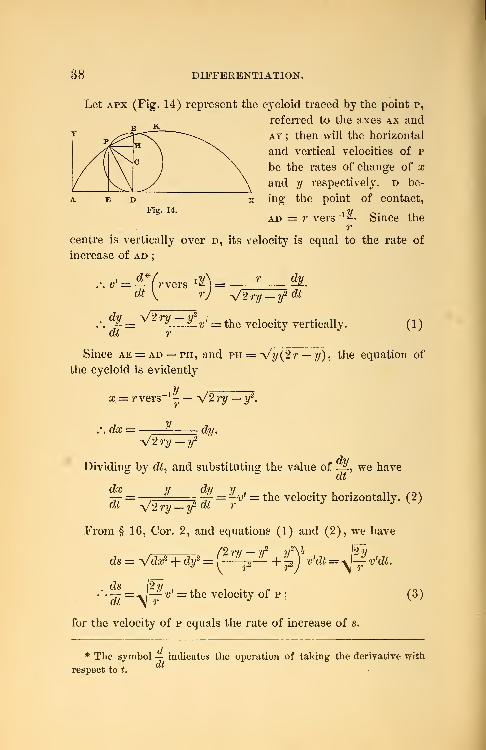
11. A wheel whose radius is r rolls along a horizontal line
with a velocity i>' ; required the velocity of any point p in
its circumference ; also the velocity of p horizontally and
vertically.
38 DIFFERENTIATION.
Let apx (Fig. 14) represent the cycloid traced by the point p,
referred to the axes ax andT ~ •£^T<\ ay ; then will the horizontal
and vertical velocities of p
be the rates of change of x
and y respectively, d be-
x ing the point of contact,
ad = r vers *^- Since ther
centre is vertically over d, its velocity is equal to the rate of
increase of ad;
... v' = ^Yrvers^ = r S.dt \ rj -^2ry-y2 M
~ = y.—9-v' = the velocity vertically. (1)
Since ae = ad — ph, and ph = -\A/(2r — y) , the equation of
the cycloid is evidently
^x = r vers 1 V2 ry — y2
.
,\ dx = ^ dy.
y/2ry-y2
Dividing by dt. and substituting the value of -A we have
dx v dy v , * , . ,i— = - — = -v f = the velocity horizontally. (2)tit V2 ry — y °^ r
From § 16, Cor. 2, and equations (1) and (2), we have
ds = ^/dtf + dy2 =(
2ry
77
2/8
+ pjv'dt =yj^v'dt.
ds (2v.'.— =^-f v' = the velocity of p; (3)
for the velocity of p equals the rate of increase of s.
* The symbol — indicates the operation of taking the derivative with
respect to t.
MISCELLANEOUS EXAMPLES. 39
if
if
if
From (1), (2), and (3), we have,
dy n dxy = o,
dt0,
dt
ds0, and — = :
dt
y = i
dy , dx , , ds rx,
dt
y = 2 r, -^ = 0,
(ft dt
ds= 2v , and — = 2v'.dt dt
Hence, when a point of the circumference is in contact with
the line, its velocit}' is zero ; when it is in the same horizontal
plane as the centre, its velocity horizontally and vertically is the
same as the velocity of the centre ; and when it is at the highest
point, its motion is entirely horizontal, and its velocity is twice
that of the centre.
Sinceds
dt -j?-V2— v'
. ds , /t:—
. .— : v : : v2ry : r.dt
y
Hence the velocity of p is to that of c as the chord dp is
to the radius dc ; that is, p and c are momentarily moving
about d with equal angular velocities.
Miscellaneous Examples.
1. If y =/(#), show that
limit
Ax=0 Aa;
limit f(x + Ax)-f(x)Aa;
2. Find — (
= f(x).
Ans.
3. Finddx .O-^) 1
.
(a2 -x2)i
Sx2
(l-^)f'
40 DIFFERENTIATION.
4. f(x) = (x -3)e2x + 4xex + x + 3.
f'(x) = (2x-b)e2 * + 4:(x+l)ex +l.
5. y = log tan" 1x. $& = L___.
dx (1 +aj2)tan" 1aj
6. Find—[a^-SlogCl + aj8)*].
dx 1 + xJ
x loaf x,
, /1 v dy loarx*
1-x BX }dx (l-x) 2
_ y£2 + a2 + V^+T2
Vcc2 + a2 - Vx2 + &
dy _ 2x /q jo^H? ,Ix
2-j-
6
cta
-a2 -&\ +
\ar + &2 X^ + a
Rationalize the denominator before differentiating.
n V
x
2 + 1 4- a dv / . 2 a?2 + 1 \
V
a
2 + l _ a? dx \ Va^Tl
10. y= 1-ft2. <fr = -2tt(2-s»)
\(14-«2
)3 ^ Vl -x2 V(l+^) 5
/— n dv /i n - 1 Vl — X2 — #
11. 2/= (x+Vl-^2
)M
. ^ = 71(X + Vl-X2) ,
'
dx VI — x2
12. ^wVTT^+VT^). ^y^lfi. J
—
Vdx x\ Vi_W
_ (smnx) m dy _mn{smnx) m ~ 1 aos(mx — nx)
(cosmx) n dx~ (cosmx) n+l
u y_ VH^+VT3^ j
dy _ 2 /X|
1 \
VT+a?- Vl-a? *" A Vl-zV
15. V = tan"'? + log .JEEi dy= 2a^_a \« + a cfcc a;
4 — cr
MISCELLANEOUS EXAMPLES.
16. y = sec— eor> 1
,
vV ;r
41
dy_ 1
da; Va2 --or9
17. /(a) = (a2 -fa2) tarr
1 -. f{x) = 2 a; tan"1- + aa
§1= _x sin l a
dx Vi- a^
dy _ 2
18. y =Vl— a?i
19. w = sin 1-—-•*
. 1+ a? da; 1 + a,-2
20. Find — (eax
sin7" ra)
.
da;
/'(a?) = eax sin
m_1 ra5(a sinrx + mrcosra)
.
21. ?/ = log(2a;-l + 2Vaf'-a;- 1). ^ = *
da; Vaf — a; — 1
ao _i3 + 5cosa; , 4 da;22. ?/ = cos J— dy —
5 -|- 3 cos a; 5 +3 cos a;
23 . f(x) = e(a+x)2
sin x. f (x) = e(a+x)2
[2 (a + ®) sin a; + cos a;]
.
Tito*- 1da;
24. y = log [log (a -f bxn) ]
.
dy(a + bxn ) log (a -f to")
25. 2/= log('^Y-Jtan-1
a;. dy =4
-
K l — x 1 — a;4
nn . l 3-\-2x , da;26. ?/ = sin- 1—
—
dy —Vl3 Vl -Sx-x2
27. y = ex* tan" 1
x. ^ == ex*
|
* - + af tan" 1as(l+ log x)J
dx L 1 + * -
x-y
28. a?= e~!T.
. dy log a;log a;; ,\y=
1 -{- log x da; ( 1 -f- log x)2
42 DIFFERENTIATION.
X2
29. y
1+-S1 +
1 + etc. to infinity.
.'.dy= ±1+2/ Vx2
30. y = \og(x+-Vxi -a2) + sec- 1 -. ^= lJa?+q .
a dsc cc \ # — a
31 „ = logVi - g8 + ^V^
. gy = V^
32. y = logJ^^±
V 1 +A32 — flJ
33. Given/(*)=3x2 -a + 6; to find /(y), /(a), /(2), /(0),
/(^ + 2/)-
When, in connection with the symbol /(a), expressions like
f(y)* /(«) j /(2)> /(°)j f(x +.y) are employed, they denote
respectively the results obtained by substituting y, a, 2, 0, and
x + 2/ f°r * in the value of f(x) . Thus here /(y) = 3y2— y + 6,
/(a) = 3cr-a + 6, /(2) = 16, etc.
34. Given (/>(>) = 4 a3 -a2;find ^(2), <^(6), <^(1), 0(3), 0(0).
Given f{x +y)= <f» ; to find f(x) , /(y) , /(5)
.
35. Find d/(a + ic). /'(« + x)d(a + x), or f'(a + x)dx.
36. Find df(ax). f'(ax)adx.
38. Find df{x + y)
.
/'(a + y) (da + dy)
.
CHAPTER III.
INTEGRATION.
58. A function or variable is called the Integral of its differ-
ential. Thus, x3is the integral of 3x?dx ; and f(x) -f- C, C being
any constant, is the integral of f'(x)dx.
Integration is the operation of finding the integral of a
differential.
The problem of differentiation and the inverse problem of
integration ma}' be stated also as follows
:
That of Differentiation, or of the Differential Calculus, is, To
find the ratio of the rates of change of a function and its variable.
That of Integration, or of the Integral Calculus, is, Having
given the ratio of the rates of change of a function and its vari-
able, to find the fauction.
The sign of integration is J . Thus, J in J ±x\lx indicates
the operation of integrating A:x\lx. Hence, d and J , as signs of
operation, neutralize each other. For example, J cl^x3 ) =x*, and
d J 3 xdx — 3 x^dx. The whole expression J4:X*dx, read '-the
integral of 4or3c?#," represents the integral of ±x?dx.
59. Elementary Principles.
I. Since clC=0< C being any constant,J 0=C.
Hence, as may be added to any differential, the general form
of its integral will contain an indeterminate constant term.
In the Applications of the Calculus, this constant term is
eliminated, or determined from the data of the problem.
II. Since d(ay -\- ac) = ady,
.-.j ady = j d{ay + ac) = a(y+ c)
= a)d(y+c) = ajdy.
44 INTEGRATION.
Hence, a constant factor can be moved from one side of the
sign of integration to the other without changing the value of the
integral.
III. Since d(x — y -f z + c) = dx — dy -f- dz,
.-.J(dx — dy-\-dz)=:x — y-\-z-\-c
—J dx —
J dy -+-J d(z + c)
— j dx — jdy -{- j dz.
Hence, the integral of a sum of terms is equal to the sum of
the integrals of the terms.
60. Fundamental Formulas. Since integration is the inverse
of differentiation, general formulas for integration may be
obtained b}r reversing the general formulas for differentiation.
dx , ,„ dx1. ( — = loga? + logc,* v d(logx-j-\ogc) =—
J X X
2. faafcto =^— -f <7, \'df^^ + C] = axn dx.J n+ 1 U+l J
3. Ja* logacte = ax + (7, •,• d(a* -f- C) = ax \ogadx.
J ex dx = e
x-j- (7.
4. J cos x dx = sin x -\- C\ V d(sinx + C) = cosxdx.
5
.
J— sin xdx = cos x -f (7.
6. J secrxdx = tana; + 0.
7.J— cosec2
#cfce = cotic -+- C.
8. J seccctan#cfcc = seca;-f- C.
* When the integral is a logarithm, it is customary to write the indeter-
minate constant term as a logarithm.
FUNDAMENTAL FORMULAS. 45
9. J— coseco?coticc7ic = cosec# + C.
*10. I s'mxclx= versa; -f (7, or — cosa; -f-C*11. I — cos xdx = coversx + (7, or — sina;-f- (7
f
.
12. fda;
=sin- 1 a;+C.•/ Vi-.t2
*13. f_ZJE_ = cos" 1 a;+ (7, or - sin- 1a; + C.
14. f-^-^taii-^+aJ 1 + ar
*15. fjZ^. = Cot ^ + C, or - tan"1;*; + C.
J 1 + XT
1 6 .f da? =sec-^+G.J x^/x2 — 1
*17. I—~ c,a?
== cosec-1 ^ -f (7, or — sec
-1a; -f C".
J a-Var9 - 1
18. f da; = vers- 1 x 4- C.J V2 x — x2
/— dx—^
= covers-1
a; + (7, or — vers-1
a; -f- C !
.
V2 x — x2
The differentials in these nineteen formulas are the funda-
mental integrable forms, to one of which we endeavor to reduce
* Two integrals having the same or equal differentials must change at
the same rate ; hence they must be equal, or have a constant difference.
The constant difference between the variable terms of the integrals in the
last four starred formulas is evidently - ; for, when x < -,J2 2
cos -1 a: + sin-1 a:=r-, cot _1.r + tan _1 a: = -, etc.
2 2
The starred formulas are not necessary, since the second integral in
each is given by a previous formula.
46 INTEGRATION.
,every differential that is to be integrated. The processes of the
Integral Calculus are largely a succession of transformations
and devices to effect this reduction.
61. To facilitate the application of formulas 1 and 2, the}*
may be stated as follows :
I. The integral of a fraction ivhose numerator is the differen-
tial of its denominator is the Naperian logarithm of the denomi-
nator, plus a constant.
II. Whenever a differential can be resolved into three factors,
— viz., a constant factor, a factor which is a variable with any
constant exponent except — 1, and a factor which is the differential
of the variable without its exponent,— its integral is the product
of the constant factor into the variable ivith its exponent increased
by 1, divided by the new exponent, plus a constant.
Examples.Find
1. (axHx. Ans. — -f C.7
2. jbxhdx. §&#§ + C.
3. $2xidx. f«l.+ C.
4. J (J axi— | bx%) dx. axl — bxl -+- C.
5. C^.= Cix-5 dx. - x -* + a
x2 3x?
7, f^r- 2V5 + CJ Vx
2
-yjx
8. f/W+J-W ^__L + (7.
J \ xi y 4 ^/x
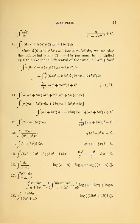
EXAMPLES. 47
a
(1 — ri)xn~ l
q Cadx a ^J xn
10. f&(6«a:2 + 8to3)§(2ax + 4to2)dx.
Since d(6 ax2 + 8 to3) = (12 ax + 24 to2
) ax, we see that
the differential factor (2ax + 4 bx2)dx must be multiplied
by 6 to make it the differential of the variable 6 ax2 + 8 to3.
.'. r6(6ax2 + 8 6or5)i(2ax + 4 6a;
2)cZx
= f-(6a<B2 + 8&arJ)§(12aa; + 2±bx2)dx
=—(6ax2 + 8bxs)% + C. § 61, II.16
11. I \_a(ax -\-bx2)%dx + 2b(ax-{-bx2)*xdx~\.
I \a(ax-\- bx2)?dx + 2b(ax -\-bx2)*xdx~]
= f(aa; + bx2y*{a + 2 to)ox == f (ax + to2)! + C.
12. C(2a + 3bx) 3 dx. —(2a + 3to) 4 + 0.
13. f f
^
, -|(a2 + x3)* + (7.
J (a2 + ar5)i
3 V '
14. f(1 + fx)*dx. ^.(l
.
+ |»)l+ 0.
15. f(6x4+2x2 -5)(3x2 -l)ax. i^_iI^ + 5x-f-<7.
. _. log(x — a) -f-logc, or log [(x — a)c].x — a
17rxn~ l dx
' J a + fcx71
'
/'xn~ 1 dx 1 Cnbxn~ l dx 1 , , , r n \ t i=— I =— log (a 4-ton)+logc.a + ton w6J a + bx11 nb
18-/ToSr5-
log[(10*»+ 15)*c].
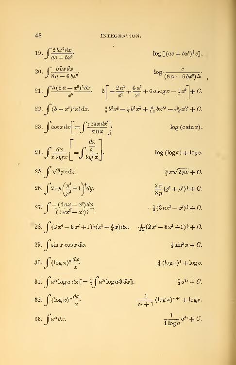
48
19
20
JGSfTEGliATION.
•/;
f.
2bx2 dx
ae -j-foe3
bbxdx
Sa-bbx2
log [(ae + &<*?)*<;].
W £B (8a-6bx2)&
01 f5(2a-a2
)3d« „[" 2a3
, 6a2, „ , x 2
~j, n21J s»
' o^-_ +- + 6alog,-^J+ 0.
23.Jcotajdjc =
|
§&3^
cos x dec"
sin a?
dx
x24. f_*L = r
J xlogx ^ «/ \ogx_
25. C^/2pxdx.
26.f2^yft +1Jdy
ax
(3a^-^3)^
&2icl + •&&»¥ - ^ggft + (7.
log (c sin a).
log (logo?) + logc.
farv/2pa + 0.
g(2/2 +P2)§+0.
97 /*— (2 ax — x2)dx
2* . C(2xi -3x2 +l)h(xs -^x)dx. -^(2xA -3x2 +l)l + C.
29. I sin x cos x da?.
30. f(logcc) 3 ^.J x
31.j a
3xlogadx[=-j-JaMogaScfa;]
.J"(log»)'
. I a4* da.
32,dx
ra + 1
Jsin2aj + C«
£(loga) 4-f logc.
ia^ + C.
(loga^^ + logc.
4 log a
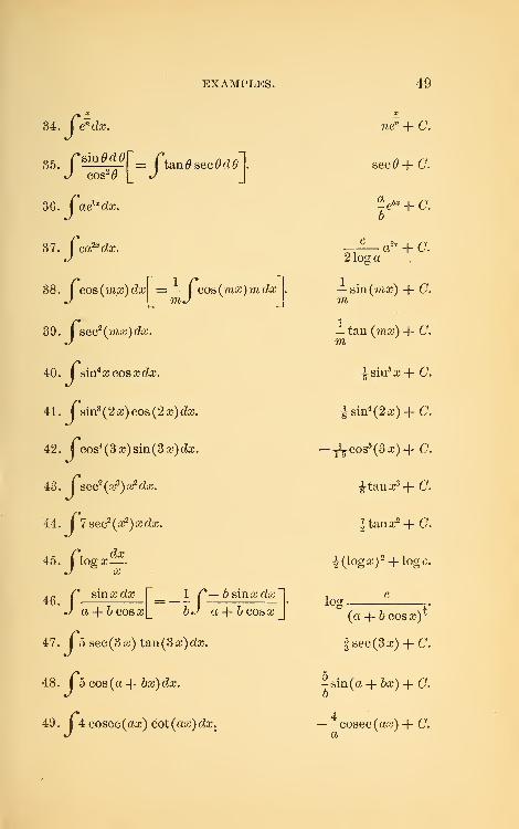
EXAMPLES. 49
34. en dx.
36. Caebx dx.
37. Cca^dx.
38. I cos hnx)dx =—( cos (race)
J [_ m*/
39. I sec2 (mcc)d£c.
40. I sin4x cos x dx.
41. i sin3 (2a?)cos(2#)da3.
42. Jcos4 (3a?)sin(3aj)da;.
43. I sec2(o?
3)^ dx.
44. I 7 sec2(a;
2) a; da?.
45. I logx
mda?
dec
as
46./sin a? da; _ 1 /*— b sin a; cte
a 4- & cos a? bJ a-\-bcosx+ 6 cos x
47. I 5 sec(3a?) tan(3a?)da,\
48. I 5 cos (a •+- bx)dx.
49 .
J4 cosec (aaj) cot (aa?) da;.
wen + C.
sec#-b C.
'eb* + C.
C „2z
2 log; aa2x + C.
— sin (ma?) + C.m
— tan (ma?) + (7.
m
|sin5 a?-{-C.
|sin4 (2a?) + <7.
__L Cos5(3a?)+0.
^ tan xs + (7.
-|tana?2 -f- O.
^(logaj) 2 + logc.
log r(a -\-b cos a?)
5
f sec (3 a?) + (7.
5-sin(a + &a?) -f- (7.
6
cosec (ax) + 0.
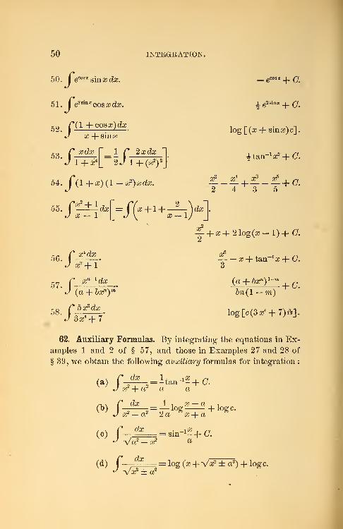
50
50. Cecosx sinxdx.
51. I e2s[nx cosxdx.
/(I +cosx)dx
INTEGRATION.
D'2
x 4- since
532 a* da*r xdx r i r
J 1 4-a-4[_~~2J l + (^)
2
_
54. \(l+x){l —x2)xdx.
±e28inx +C.
log [ (a; 4- sin aj) c] •
£ tan" 1 x2 4-0.
/V»2 /v»* /yid /VH>
y~y y~y
a-V J
56 /a;
4da;
a*2 4-1
57. p
|! + a;4-21og(a--l)4-0.
x 4- tan~* a* 4- O.
a;'1 x dx (a + &aJ*)
:
(a 4- bxny
rr> /^ bXZdX° J 3 a*
4 4-7*
a.&n(l — m)
log [c (3 a;4 +7) A]
62. Auxiliary Formulas. By integrating the equations in Ex-
amples 1 and 2 of § 57, and those in Examples 27 and 28 of
§ 39, we obtain the following auxiliary formulas for integration :
(a)C-te = I tan- 1-+C.J xl 4- a a a
v ' J x2 -a2 2a sa*4-a
B
( C ) fdx = sin-1- 4-0.
J Va2 - x2 a
(d) f dx = log (a* 4- Va*2 ± a2) 4- log c.
J Va,*2 ± a2
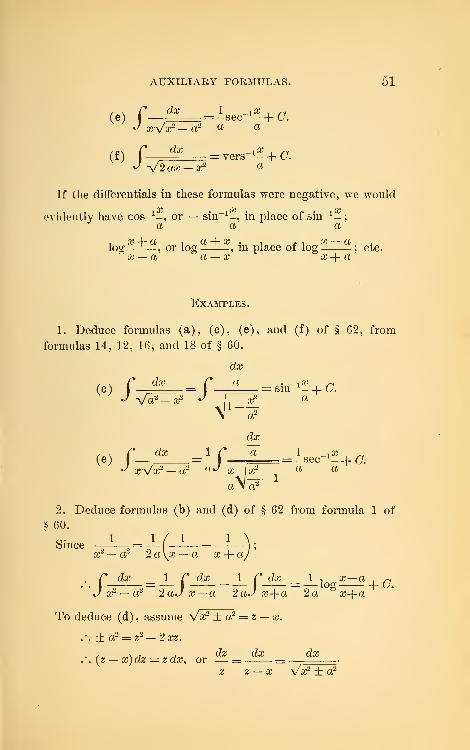
AUXILIARY FORMULAS. 51
(e) f
—
^ = -sec-1-4-Q.J x^/x2 — a2a a
(f) C dx^yers- 1 -
•^ V2 ax — x2 aC.
If the differentials in these formulas were negative, we would
evidently have cos 1-, or — sin
-1-, in place of sin" 1 -
;
a a a
log37 "'
-, or log , in place of log~
; etc.x — a a — x x+ a
Examples.
1. Deduce formulas (a), (c), (e), and (f) of § 62, from
formulas 14, 12, 16, and 18 of § 60.
dx
(0 J^*--/ •=_J V or — xr^ L xr
= sin_1
--|- G.a
dx
a, . C dx 1 C a 1 i#(e) I =- I ^_sec- ]
--fJ x-\Zx? — a2 aJ x x2.
a a
a \ cr
2. Deduce formulas (b) and (d) of § 62 from formula 1 of
§ 60.
Since — -= — f
x2 — a~ 2 a \x — a x + a,
/dx 1 C dx 1 r dx 1 , x—a.px^ — a2 2aJx—a 2aJ x+ a 2 a
ax-\-a
To deduce (d) , assume Vx2 ± a2 = z — x.
.'. ± a2 = z2 — 2xz.
. / N 7 , dz dx dx. . (z — x)dz = zdx, or .— =
x Vx2 ± a2
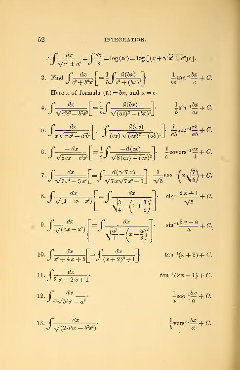
Itan-1^ + C.be c
52 INTEGKATION.
.-. f—^— = f— = log(zc) = log[(a?W^^2)c].
J Va?2 ± a2 J z
3. Find C dx f=-f d(bx)1-* ma
Jc2 + &v[_ &J C2 + (&*)
2
J
Here a? of formula (a) = 6a?, and a = c.
4o r cto nr d(bx) i i sin-i^+0,
J Va2c2 -6VL 6J V(ac) 2 -(6a?) 2J & ac
5. f dxf_ f
d (cx"> 1 J-sec-^ + O.
6 f — ^ r_ i r z^(^) 1 i
' J V^^cV L °J -V8(cx)-(cx) 2J ccovers
-1\- C.
4
, r dx r r d(VixJ V7a?4 — bx'2 \_
J s/lx^Tx1
;. f *! "=f.
i„-.(4D
+0.
>S-: X + IV
/da?
-yJ{CLX — X2
) f-mdx
Vf-f-I
10r dx r r dx
' J a?2 + 4a? + 5[_~J (a? + 2)
2 + l
11
12
13
ji2 a?2 — 2^ + 1
/;dx
x-Vtfx2 - a2
s dx
^(2abx-bV)
V5
sm *\- G.
tfm~\x + 2) + C.
tan- 1(2a?-l)+0.
1 ,bx . n-sec 1f- C.
a a
1 -\bx . -,*
-vers l
h G.6 a
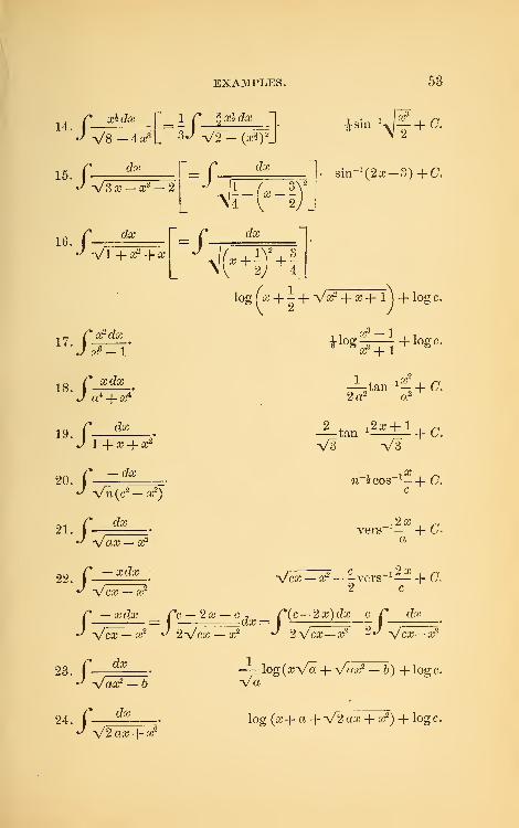
EXAMPLES.
J a/83
15
16
V8 -4arJ
dx
Jdf a4 dx1
3^ V2 - (a;§):
isin-^|
53
V3 x - x2 - 2 f-RVF
3\ 2
siii-1 (2a;-^3)+0.
/:dx
Vl+a^ + aJ
-/-cte
vc-+ar+f
log [a; 4 - 4 V^2 + a?+ 1)+ logc.
ar3 — 1
i log-——-\-logc.x6 4 1
18
19
20
2a :
tan-1-, + 0.
2 . _!2oj + 1-— tan l —V3 V3
a
r^dxJ x6 -l
/' xdxtf + x4
'
r dx' J 1 + x + x2
'
/ —dx
yfn (c2 — x2
)
21. f___^L_.•* ^Jax — x2
n~ /^ —xdx / c -i2x.fi22.
|
- • wcx — x- vers *f- C.
(*_^xdx_ ._ rc — 2x — c , _ r(c-2a;)(?a; cf* da;
J ^/cx — x2 J 2-\/cx — x2 J 2^/cx—x2 2J ^/cx—x2
n~i cos-1-4 (7.
c
vers - \-C-a
23
24
/:dx
s
Vox2 — b
dx
—-\og(xVa +-\/ax2 — b) 4 logc.-\/a
V2 ax 4 a^
log (x-\- a 4 V2 aa; 4 x2
) 4 logc.
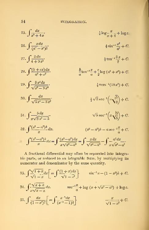
54 IMEGKATION.
25Sidx
x2 -{-Ax
an / X (XX
27 f 3 da;
* J 4+9x2
"J a2 +
log hiogc.
a2
2Jtan-^ + C.
29 f 3ar*c
ar
da;
VV-9;
30. r—^_
31da?
^tan- 1 - + -log (a2 + a?2
) + C.a a '2
Jvers-1(18a^) + 0.
a
/" 5 da:
"^ «V3a^
82r(a^-a2
)^da?.
VSsec-^ajJ-V+O.
(a* -a2)* -a sec"1 - + C.
r(a^-a2
)^a, ==
r (a^-ft2)da;= r a:da; r a2da?
•J a* *^ x-y/x?—a2 J -y/of—a2 ^ xs/x^—a2
A fractional differential may often be separated into integra-
te parts, or reduced to an integrable form, by multiplying its
numerator and denominator by the same quantity.
J Vi - x L J Vi
/:
a?) dxsin- 1a;-(l-a32)§+ C.
-Vx-j-a34. I
y M ^^dx.
x~\/x — asec
-1- -f log (x + Va?2 — a2) + log c.
0f. C dxJ~_ ^_J^da?_
J' J (1 - aj")i \_~J (x~2- l)lj Vl-a?2
<7.
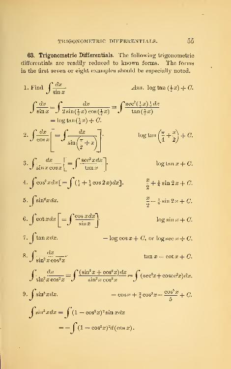
TRIGONOMETRIC DIFFERENTIALS. 55
63. Trigonometric Differentials. The following trigonometric
differentials are readily reduced to known forms. The forms
in the first seven or eight examples should be especially noted.
l.Findr dx
J sin q
Ans. log tan (%%) -\- C.
/ dx _ r dx C sec2{\x)^dx
since J 2 sin (^x) cos (^ x) J tan (-|- as)
= log tan {\x)-\- C.
/ dx ~_ r dx
cos x Jsinf - -f-as U+5
log tan I - 4- - ) -f C.
o C dx T_f*
sec2as c?as ~l
J since cos iu |_ J tana?
4. I cos2asdas[= I
(-J- -J- -Jcos 2 as) das]
5. I sin2as c?as.
6. fcotx^r=fcosa!da;"|.
c/ J sin a;
7. I tan as das.
dx
dx,2^«^o2,suras cos" as
9. I sin5 as das.
log tan a; + (7.
--hi sin 2 as -f (7.
|-i.sin2a?+0.
log sin tc + (7.
— log cos cc 4- (7, or log sec as 4- C.
tan as — cot x -\- C.
/(sin 2as 4- cos2
as) das (*, „ . „ x 7* rV * — = I( see-as+cosec2
as) das.snr as cos- as J
I sin5 as dx = I (1 — cos2as)
2 sin asdx
= — I (1 — cos2as)
2d(cos as)
— cos as + -| cos3as
* cos as + 0.
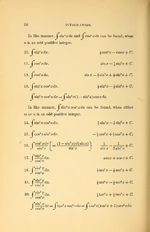
56 INTEGRATION.
In like manner, jsinnxdx and
j cosnxdx can be found, when
n is an odd positive integer.
•/<
. I Qoszxdx.
. I sin5a;
jsin5 x cos3
a; da; =Jsin5 a;(l — sin2x)eosxdx.
In like manner, j sinmxcosn xdx can be found, when either
m or n is an odd positive integer.
14.jsin3 a? cos3 a; die. isin4
a?— -|-sin6£c-|- C.
15. I cos4 a;sin3 a?cfa;. — ieos5 a;+-i-cos7a; -+- (7.
10. i swPxdx.
11
12. | cos5 xdx.
13. I sin5a? cos3
a; da;.
J COS3a; — COSfl? + C.
sin x — isin3#+ 0.
sinx — -|sin3 cc4--|-sin5fl?+ C.
Jsin6a? — ^-sin8 ic -f- C.
16
17
10
/cos3a; cZa;
sin4a?
•/ COS 2£C
/sin3a;
cos8a?
/sin3a;
cos7a;
/sin2 x
cos6a?
(1 — sin2o?)d (sin x)
sin4a?
1 + C.sin x 3 sur a;
seca;-f-cosa;+ C.
dx.
^sec7 x — |-sec5ic+ C.
i sec6a; — ^sec4a;+ C.
±-tan5 a; + -J- tan3a; + C
/'-—-^-dx= I tan2a; sec4
a? da; = ( tan2a; (tan2
a; -f 1) sec2a; da;.
cos6a? J J
20. | ^^dxcos
1
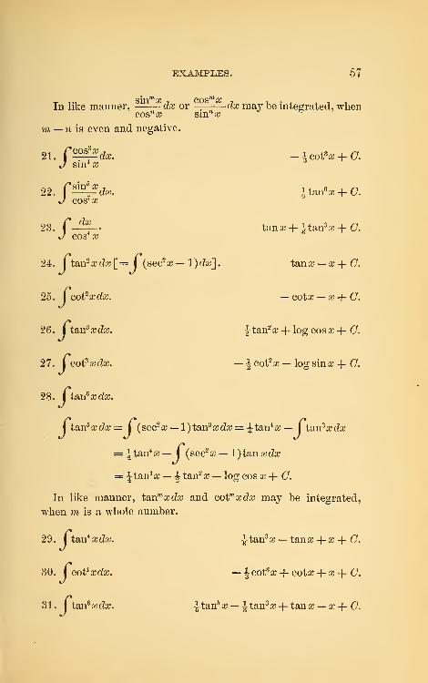
EXAMPLES. 57
In like manner, dx or — dx may be integrated, whencos" a? smn x
m — n is even and negative.
21. C^^dx. _i cot3a;+C.J sin
4a;
22. f^Hlfcfa.. itan6aj + C.
J cos7a?
23. f-^-. tana; + 1tan3a; + 0.
J cos4a;
24.Jtan2
a; daj[=|(sec2 a;— 1) da?], tana? — x + C.
25. I cot2a?da?. — cota? — x-\-C.
26. I tan3a?da?. ^tan2 a?-|-logcosa?-|- O.
27.Jcot3 xdx. — i cot2 x — log sin a; + O.
28.Jtan5 a; da;.
I tan5xdx=J(sec2
a; — l)tan3a?da? = J tan
4a? —
Jtan3xdx
= itan4a? — I (sec2 x — 1) tan xdx
= itan4a? —
-J-tan2
a; — log cos x-\- O.
In like manner, tsiumxdx and cotw a?c?a? may be integrated,
when m is a whole number.
29. I tan4a?da?. |-tan3
a? — tana? -\-x -f- C.
30. I cot4a?da?. — icot3
a? + cota? -f- a? -f 0.
31. I tan6a; da?. J-tan
5a? — itan3
a?-f- tana; — x + C.
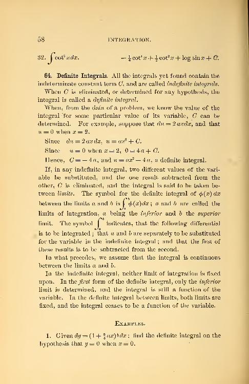
58 INTEGRATION.
32 .
Jcot5 x dx. — \ cot4 x 4- \ cot2 x -f- log sinx+C.
64. Definite Integrals. All the integrals yet found contain the
indeterminate constant term (7, and are called indefinite integrals.
When C is eliminated, or determined for any hypothesis, the
integral is called a definite integral.
When, from the data of a problem, we know the value of the
integral for some particular value of its variable, C can be
determined. For example, suppose that du = 2axdx, and that
u = when x= 2.
Since du — 2 ax dx, u = ax2-f C.
Since u = when x = 2, = 4 a + (7.
Hence, C = — 4 a, and m = ao2 — 4 a, a definite integral.
If, in any indefinite integral, two different values of the vari-
able be substituted, and the one result subtracted from the
other, C is eliminated, and the integral is said to be taken be-
tween limits. The symbol for the definite integral of <j>(x)dx
between the limits a and b isf
cf>(x)dx; a and b are called the
limits of integration, a being the inferior and b the superior
limit. The symbol I indicates, that the following differential
is to be integrated ; that a and b are separately to be substituted
for the variable in the indefinite integral ; and that the first of
these results is to be subtracted from the second.
In what precedes, we assume that the integral is continuous
between the limits a and b.
In the indefinite integral, neither limit of integration is fixed
upon. In the first form of the definite integral, only the inferior
limit is determined, and the integral is still a function of the
variable. In the definite integral between limits, both limits are
fixed, and the integral ceases to be a function of the variable.
Examples.
1. Given dy = (1+ %ax)?dx ; find the definite integral on the
hypothesis that y = when x = 0.
EXAMPLES. 59
Here,- i(l+ *«)• + </; ,.0 =^+0.
* 27aV 4 ; 27a
2. Given dy = (x3 — b2 x)dx-, find the definite integral, if
y = when x= 2.
Ans. 2/ =^l-^ + 262 -4.^4 2
3. Given ay = ~— ; find the definite integral, if y =a; 2 — cc
when a?== 1,
4.
^Ins. 2/ = log (2ce — x2
)
:. Find fnxdx. Ans. -(b2 -a2).
nxdx= -x2-f- (7; irf+0
a^+O = -62 +(7.D
.-.£nxdx = 'p2 + C-(^a2 +C^ = 7
j(b2 -a2).
5. (\x3 dx.
6. I (asr2 — or
3
) aa;.
7 p da;
Jo a2-+- cc
2
8 p dx
Jo Va2 - a2
sin (90*0
. I — = I (cosO) -smOdOJo COS2
(9 \_ JoV
24.
12'
7T
la'
7T
2'
V2-1.
B-x2 + C I denotes the value of -x2 + C when x = a.
2 L 2
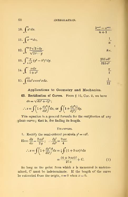
60 INTEGRATION.
10. xn dx.
e~ax dx.
122r2-V2rdy
5»+i _ an+1
71 + 1
1
a
Br.
256 tt69
315 a4'
V2r — y
13- f-^(3/2 -62
)4^.
c/ -6 a4
'Jo 1-f #4*
sin3 # cos3# da;.
Applications to Geometry and Mechanics.
65. Rectification of Curves. From § 16, Cor. 2, we have
7T
4*
J_12*
ds = -ydx2 + (fa/2
;
This equation is a general formula for the rectification of any
plane curve ; that is, for finding its length.
Examples.
1 . Rectify the semi-cubical parabola y2 = asc
3.
Tj dy _ 3 ax2. . d?/
2 _ 9 aa;616
dx~~2y~' ' 'dx>~ 4
,'. s = jYl + ^j£Y(te = J f(4 + 9 ax)hdx
(4 + 9qg)l. e
27a(1)
So long as the point from which s is measured is undeter-
mined, C must be indeterminate. If the length of the curve
be estimated from the origin, s = when x = 0.
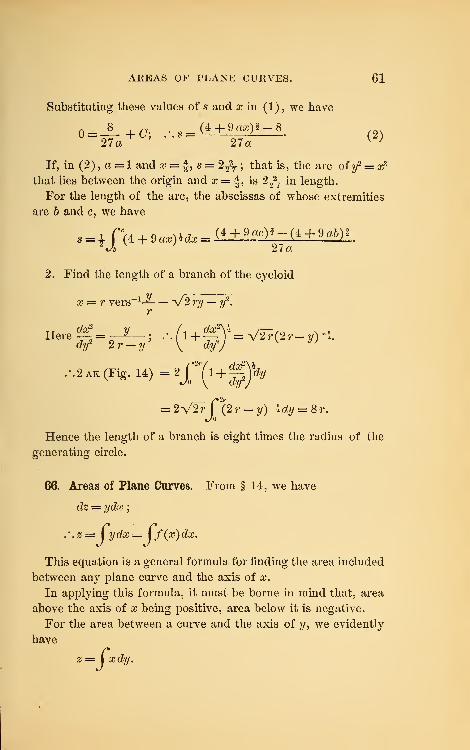
AREAS OF PLANE CURVES. 61
Substituting these values of s and x in (1), we have
27a 27a K }
If, in (2) , a = 1 and x = ±,s= 2^ ; that is, the arc of y2 = x3
that lies between the origin and a; = f , is 2Y2T in length.
For the length of the arc, the abscissas of whose extremities
are b and c, we have
V& y27a
2. Find the length of a branch of the cycloid
x = r vers-1 -^— V2 ?*?/ —
2/2
«
r
dy 2r-y \ dy-J
,.2 AK(Fig.14)=2p(l +^= 2V2r f (2r - ^)"5% = Sa-
lience the length of a branch is eight times the radius of the
generating circle.
66. Areas of Plane Curves. From § 14, we have
dz = ydx;
.-.2= \ydx = \f(x)dx.
This equation is a general formula for finding the area included
between an}r plane curve and the axis of x.
In applying this formula, it must be borne in mind that, area
above the axis of x being positive, area below it is negative.
For the area between a curve and the axis of y, we evidently
have
*%
=Jxdy.
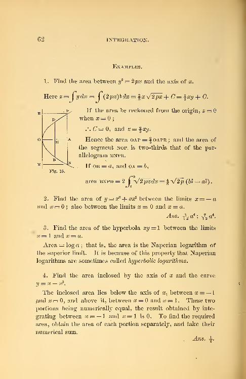
62 INTEG11ATION.
Examples.
1 . Find the area between y2 = 2px and the axis of x.
Here z =Jydx =
J(2p#)2djc = f#V2px -f- C—\xy + 0.
If the area be reckoned from the origin, z =when a; =
;
.-.(7=0, and 2 = %xy.
Hence the area oap = | oapr; and the area of
the segment nop is two-thirds that of the par-
allelogram MNPR.
E
I
H
Fig. 15.
If oh = a, and oa = b,
area bnpd 2 C\/2pxdx = I V2p (61 at).
2. Find the area of y-= x3-f- ax2 between the limits x = — a
and x = ; also between the limits x = and cc = a.
J.71S. yV^4
; T2«4
.
3. Find the area of the hyperbola xy = 1 between the limits
x = 1 and x = a.
Area = log a ; that is, the area is the Naperian logarithm of
the superior limit. It is because of this property that Naperian
logarithms are sometimes called hyperbolic logarithms.
4. Find the area inclosed by the axis of x and the curve
y = x — x3.
The inclosed area lies below the axis of x, between x = — 1
and x = 0, and above it, between x = and x=l. These two
portions being numerical!}- equal, the result obtained by inte-
grating between x = — l and x=l is 0. To find the required
area, obtain the area of each portion separately, and take their
numerical sum.Ans. 1.
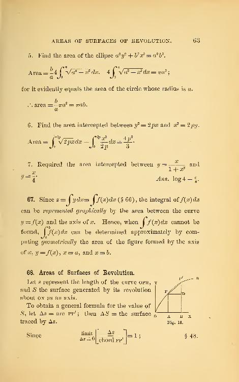
AREAS OF SURFACES OF REVOLUTION. (53
5. Find the area of the ellipse a?y2-j- b
2xr = a2
b2
.
Area = -4JVer — x2 dx.
a Jo4 I Va2 — x2 dx = ira
2;
for it evidently equals the area of the circle whose radius is a.
area = -ira2 = irab.a
6. Find the area intercepted between y2 = 2px and x2 = 2py.
Area = | '^J'lpxdx — j— dx — -^>
Jo Jo 2p 3
7. Required the area intercepted between y = — andJ. -T- XT
_ Xy ~ X Ans. log 4 —
-f
.
67. Since z =jydx=
Jf(x)dx (§ 66) , the integral off{x)dx
can be represented graphically by the area between the curve
y—f{x) and the axis of x. Hence, when ) f(x)dx cannot be
Xb Jf(x)dx can be determined approximately by com-
puting geometrically the area of the figure formed by the axis
of a?, y =f(x) , x = a, and x = b.
68. Areas of Surfaces of Revolution,
Let s represent the length of the curve opn, y
and S the surface generated by its revolution
about ox as an axis.
To obtain a general formula for the value of
#, let As = arc pp'; then AS = the surface
traced by As.
limit f AsAs = ° chord pp'
Since = i; § 4b.
64 1NTEGKATION.
. limit ["surface traced by AsAs =
0[^surface traced b}^ pp', or
, limit
AsiOAs
surface pp'
As
,=i;
limitit [AS1 limit
As = 2 ) As
.-.— = 2tt2/.
as
.-. S = 2 7T Cyds = 2 iz Cyfl +dot?
dx.
When the axis of revolution is the axis of y, we have, simi-
larly,
8 2-rr I xds = 2 7rJx(l-\
2}dy.
Examples.
1
.
Find the surface of the sphere.
Here the generating curve is x2-\-y
2 = r2 .
s = 2€Kl+d£)
idx=2€ii+f)
idx
= 2 itJrdx = 4irr2
.
2. Find the surface of the paraboloid ; that is, of the surface
traced by the revolution of a parabola about its axis.
S = 2 Tf£y (dx2 + dtf) 1 = 2 ttJj (l+ |^*dy
= 2tt
dtf
[(&2+i>
2)^-p3].
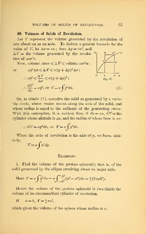
VOLUMES OF SOLIDS OF REVOLUTION. 65
69. Volumes of Solids of Revolution.
Let V represent the volume generated by the revolution of
opw about ox as an axis. To deduce a general formula for the
value of F, let Ax = ab ; then Ay = dp', and
AV = the volume generated by the revolu-
tion Of ABp'p.
Now, volume abdp < AV< volume abp'm;
or Try2 Ax< AV< ir(y-\- Ay) 2 Ax;
AV.-. iry* < -— < TV (y+ Ay) 2
;
AxFig. 17.
dVdx
Try2
, or V— 7T I y2 dx. (i)
Or, to obtain (1), conceive the solid as generated by a varia-
ble circle, whose centre moves along the axis of the solid, and
whose radius is equal to the ordinate of the generating curve.
With this conception, it is evident that, if dx = AB, dV=thecylinder whose altitude is ab, and the radius of whose base is ap.
.-. dV= 7ry2 dx, or V= -n-
| y2 dx.
When the axis of revolution is the axis of?/, we have, simi-
V— TTJx2 dy.
Examples.
1. Find the volume of the prolate spheroid; that is, of the
solid generated by the ellipse revolving about its major axis.
c a r a b2
Here V= tt I y2 dx = ?r I — (a2 — x2)dx f(2«7T&
2).
Hence the volume of the prolate spheroid is two-thirds the
volume of its circumscribed cylinder of revolution.
w,If a = b, V
which gives the volume of the sphere whose radius is a.
66 INTEGRATION.
2. Find the volume generated by the revolution of y5 = ex
about the axis of x, volume being measured from the origin.
Ans. V= \^y2 x = -| the circumscribed cylinder.
3. Find the volume of the oblate spheroid; that is, of the
solid generated by the revolution of the ellipse about its minor
axis.
Ans. V= ^7ra?b = % the circumscribed cylinder of revolution.
4. Find the volume of the paraboloid; that is, of the solid
generated by the revolution of the parabola about its axis.
Ans. V= \-rtxy2
, or \ the circumscribed cylinder.
5. Find the inclosed volume of the solid generated by the
revolution of y2 — b
2 = ax? about the axis of y.
Ans. V=^f\f- bycly = ?§^.crJ-b 3 lo a4
70. From v = — and a =— (§ 33), we have the followingdt dt
v J &
Fundamental Formulas of Mechanics.
I. v== — ; .'.s = I vdt, and t= I — •
dt J J v
II. a =—;.*. v == I adt, and t = (—
dt J J a
Examples.
1. The acceleration of a moviug body is constant; find the
velocity and the distance.
V=fa dt = at+C=at + V, (1)
in which v represents the initial velocity ; that is, the value of
v when £=0.
8=|vdt= I (at -\- v )dt = ± at2
-\- v t -\- SQ , (2)
in which s represents the initial distance ; that is, the value of
s when t = 0.
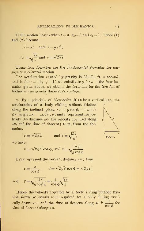
APPLICATIONS TO MECHANICS. 67
If the motion begins when t = 0, v = and s = ; hence (1)
and (2) become
v = at and s = ±-at2
;
.' .t =\i— and v=V2as.
These four formulas are the fundamental formulas for uni-
formly accelerated motion.
The acceleration caused by gravity is 32.17+ ft. a second,
and is denoted by g. If we substitute g for a in the four for-
mulas given above, we obtain the formulas for the free fall of
bodies in vacuo near the earth's surface.
2. By a principle of Mechanics, if ab be a vertical line, the
acceleration of a body sliding without friction a
along the inclined plane ac is #cos<£, in which
$ = angle bac. Let s', v\ and t' represent respec-
tively the distance ac, the velocity acquired along
ac, and the time of descent ; then, from the for-
mulas,
v = V2as, and t =\j—
,
\ a
we have
i| •> s
i
v'.= w2qs' cos<f>, and tf=\ —J
\gcos<f>
Let s represent the vertical distance ab ; then
s'=
an
COS(/>
\ a cos- 6 cos 6 \
v'= ^2 gs 1 cos cf> = V2#s,
2 s.
gcos~cf> coscf> \ g
Fig. 18.
Hence the velocity acquired by a body sliding without fric-
tion down ac equals that acquired by a body falling verti-
cally down ab ; and the time of descent along ac is the
time of descent along ab.COS(£
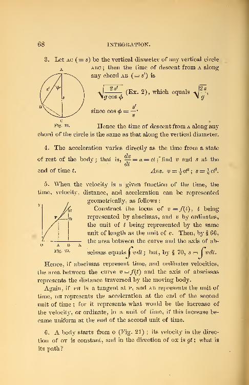
68 INTEGRATION.
3. Let ac (= s) be the vertical diameter of any vertical circle
A abc ; then the time of descent from a along
any chord ab (= s') is
2 s'
\#cos<£
since cos $
(Ex. 2), which equals&Hence the time of descent from a along any
chord of the circle is the same as that along the vertical diameter.
4. The acceleration varies directly as the time from a state
dvof rest of the body ; that is,
end of time t.
dta = ct\ find v and s at the
Ans. v — ^cf; s = ^cf.
5. When the velocity is a given function of the time, the
time, velocit}', distance, and acceleration can be represented
geometrically, as follows
:
Construct the locus of v =f(t), t being-
represented by abscissas, and v by ordinates,
the unit of t being represented by the same
unit of length as the unit of v. Then, bjT § 66,
the area between the curve and the axis of ab-
scissas equals i vdt ; but, by § 70, s == I vdt.
Hence, if abscissas represent time, and ordmates velocities,
the area between the curve y =/(*) and the axis of abscissas
represents the distance traversed by the moving body.
Again, if ph is a tangent at p, and ab represents the unit of
time, dh represents the acceleration at the end of the second
unit of time ; for it represents what would be the increase of
the velocit}7, or ordinate, in a unit of time, if this increase be-
came uniform at the end of the second unit of time.
6. A body starts from o (Fig. 21) ; its velocity in the direc-
tion of oy is constant, and in the direction of ox is gt ; what is
its path?
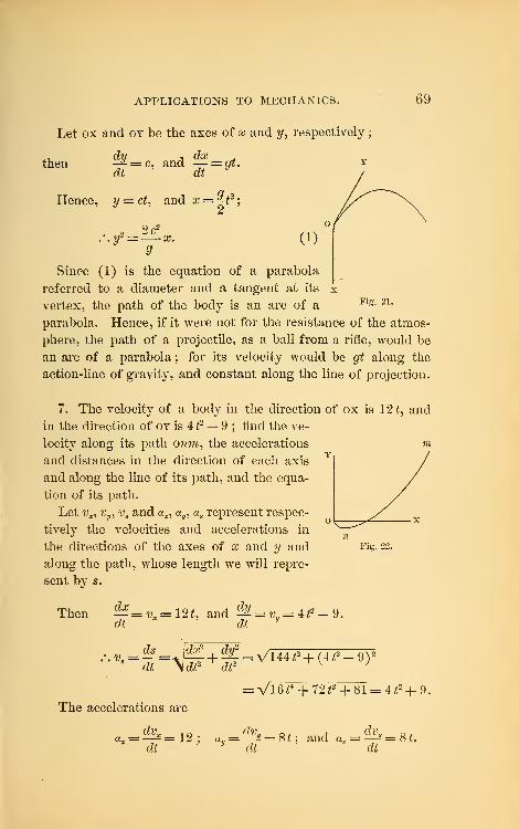
APPLICATIONS TO MECHANICS. 69
Let ox and oy be the axes of x and y, respectively
;
then ^Z-dt
, dxand — =
dt
Hence, y = ct, and x = ^-t2
;
£4
• 2c2
.' .11- =— x.y9
O)
Fig. 21.
Since (1) is the equation of a parabola
referred to a diameter and a tangent at its
vertex, the path of the body is an arc of a
parabola. Hence, if it were not for the resistance of the atmos-
phere, the path of a projectile, as a ball from a rifle, would be
an arc of a parabola ; for its velocity would be gt along the
action-line of gravhVy, and constant along the line of projection.
7. The velocity of a body in the direction of ox is 12 t, and
in the direction of oy is 4£2 — 9 ; find the ve-
locity along its path onm, the accelerations
and distances in the direction of each axis
and along the line of its path, and the equa-
tion of its path.
Let vx1 v9 , vs and aa , 04,, as represent respec-
tively the velocities and accelerations in
the directions of the axes of x and y and
along the path, whose length we will repre-
sent by s.
Fig. 22.
Then ^=v,= 12*, and %l = v=U2
dt dt9.
dt \dt2dt'
2 v ;
Vl6*4 + 72*2 + 81 = 4*2 + 9.
The accelerations are
dvx
dt
dv12 : av
= ~^- = 8t; and asy
dt
dv s
dtSt.
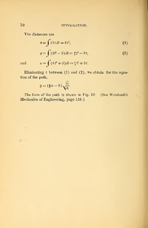
70 INTEGRATION.
The distances are
x = Cl2tdt=6P,
y= C(tt2 -9)dt = ±t3 -9t,
and s= C(±t2 + 9)dt = ±ts + 9t.
(1)
(2)
Eliminating t between (1) and (2), we obtain for the equa-
tion of the path,
y=(i K - 9
>J-The form of the path is shown in Fig. 22. (See Weisbach's
Mechanics of Engineering, page 148.)
CHAPTER IV.
SUCCESSIVE DIFFEBE1STIATI0N.
71. Successive Derivatives. Since f'(x), the derivative of
f(x) , is in general a function of x, it can be differentiated. The
derivative of /' (a?) is called the second derivative of the original
function /(a?) , and is denoted by f"(x). The derivative of
f"(x) is called the third derivative of f(x) , and is represented
by f"'(x) ; and so on. fn (x) represents the nth derivative of
/(#), or the derivative of/n-1 (a;).
Thus, if
f(x)=x*; f>(x)=£(x*) = 4x*;
f"(x) =— (4^) =120?; f'"(x) =— (12a?) = 24aj;
/"(»)= 24; /v(*0=0.
/'(a?), /"(a), f"'(x), etc., are the successive derivatives
of /(*).'
72. Signification of f"(x). Since /"(a;) is obtained from
/""^(a;) in the same way that/' (a?) is from /(#), £7te ntfi deriva-
tive of a function expresses the ratio of the rate of change of its
(n — l)th derivative to that of its variable; and the (n — l)th
derivative is an increasing or a decreasing function, according as
the nth derivative is positive or negative.
Cor. If a is finite, and /(«)*= oo, /'(<x)=cc, /"(a)=oo, etc.
For, when /(a) = oo, f(a + h) is not go, however small h be
taken. Hence, while x changes a very small amount from a,
*/(a) represents the value of f(x) for x = a. The equation /(a)= oo
means that f(x) increases without limit, as x approaches a as its limit.
72 SUCCESSIVE DIFFERENTIATION.
f(x) changes an infinite amount. Therefore, when x = a, f(x)
must change infinitely faster than x does; hence f'(a) = 00.
For like reason, iff (a) = 00, f"(a) = 00, etc.
Examples.
1 . Find the successive derivatives of x%-f 2 x2
-f- x -f- 7.
Let f{x) = x?+2x2 -j-x + 7
;
then /'(a?) =— (ar3 + 2a;
2-f x + 7) = 3a,'
2 + 4a? + 1 •
dec
/"(a) = £ (3a;2 + Ax + 1) = 6 s + 4;
f'"(x)=£(6x + ±) = 6;
and /IV (a;)=0.
2. Find the successive derivatives of cx% -f- aa?2
-j- a.
3 . If f(x) = x3 log as, prove that fiy (x) = —
4. If f(x) == eax
,prove that /"(a?) = a'
l
eaa:
.
/n(a?) is written out in accordance with the law discovered
by inspecting f"(x) and /'"(a;).
5. If f(x)= sin ma?, prove that fiy (x) = m4 sin mx.
6. If /(a?) = x* log cb, prove that/VI(a?) = -^r-
7. If/(aj)=af, prove that/" (aj) = af(l+ log a?)2 + af-1
.
8. If /(a;) = tan x, prove that /'" (x) = 6 sec4 a; — 4 sec2a?.
9 . If f(x) = log (ex + e~")
,prove that /'"(a?) = - 8
e
{f + e-'Y
10. If/(a?)= -^-, prove that/IV(a;):
1 — x (1 — a?)'
[w, read " factorial n," stands for 1 X 2 X 3 X 4 X - X n,
SUCCESSIVE DIFFERENTIALS. 73
11. If f(x) = a2,prove that fn (x) = (log a) n ax
.
(-l) n - l\n-l12. lff(x) = log(l+ x)
,prove that fn (x) =
(1+*)'
(-1) 3|3 x
(_l)»-iU_l
13. If f(x) = ( 1+ x) m,prove that
/»(#) = m(m -1) ••• (m - n +1) (l+x) m~n.
73. Successive Differentials. The clifFerential of the first dif-
ferential of a function is called the second differential of the
function. The differential of the second differential is called
the third differential. In like manner, we have the fourth, fifth,
and nth differentials. d(dy) is written d2y, and read "second
differential of y"; d(d2
y) is written c%, and read "third dif-
ferential of y "; and so on.
dy, d22/, cZ
3?/, etc., are the successive differentials of 2/.
In differentiating 2/ =f(x) successively, dx is usually regarded
as constant ; that is, as having the same value for all values of
x. This greatly simplifies the second and higher differentials,
and also the relations between the successive differentials and
derivatives, and is allowable ; for, when independent, x may be
regarded as changing uniformly.
74. Relations between the Successive Differentials and
Derivatives.
H ,=/(*), !=/'(*); |(f) =/"(*); etc.
dvIf dx is variable, -2 is a fraction with a variable numerator
dx
and denominator, and we have
fiu„\ _ d (dy\ __ dxdhj-dyd2x n ,
7 W ~dx[dxJ- ^ W
74 SUCCESSIVE DIFFERENTIATION.
But, if dx is constant, -^ is the product of the constant —dx dx
and the variable dy, and we have
W-s(*)-.S- wFor the same hypothesis we have
dx\da? J dx3 dx* dxn
Hence dny =fn (x)dxn; whence fn (x) is often called the nth
differential coefficient 6ff(x) .
For the rrypothesis that dx is constant, d2x= 0, and equation
(1) becomes (2), as it evidently should.
Examples.
1. Find the successive differentials of x4.
Let y = x* ; then dy = 4 x?dx.
Differentiating this last equation, regarding dx as constant,
we haved2y — (4:dx)d(x5) = 12a?2 eta2
;
.-. d3y = {\2dx2)d{x2) = 24xdxs
;
.-. cZ4?/ = 24cto4
; .\d5y = 0.
2. Find the successive differentials of 5 or3-f 2 #2 — 3 x.
Ify=5x3 +2x2 -3x, d3y=30dx3.
3. If y = sin a;, prove that d*y = sin a? dx4.
4. If 2/ = log (ao?),prove that cZ
4?/ = ~dx\
x
5. If y = 2 a -y/x, prove that —% =—-•
dx3 4xi
n Tij i 4.14- dsV 2 cos a;
6. If v = log since, prove that —£ = —
•
dx3 snrx
EXAMPLES. 75
7. If y = x2 log a;, prove that —4 = —dar x
d*y8. If y = cos mx, prove that —^ = m^cosma;.
da;4
9. If y2 = 2px, prove that —\ = -±- = ——
•
9 2* dx3 y5
(2a;)§
dy
dy_p. .&y_ = dx = P2.
dx y' " dx2y
2y*
'
32/V ^•
cii. =dx ^sp3 ^ 3ps
"dar3 ~ y6 f ~ {2x)i
10. If ay+ 62ar
9 = a262
,prove that
7= - -%- .
dar a-^8
11. If ar2 + ?/
2 = r2,prove that —
=| =——
•
dec2
2/3
12. If ?/2 = sec 2 x, prove that y + —^ = 3 ^z
5.
dar
13. If ?/ = e* sin a;, prove that ^ — 2^ + 2y == 0.dar da;
14. Given s = 4Z3 ; find i> the velocity, and a the acceleration.
«. - ds dv d fds\ d2s
Since v = — , a =— =— — = —-•
dt dt dt\dt) dt2
Hence v =— — 12 12
, and a = —- = 24 £.
dt dt2
15. If s = ct2 + bt, what is the velocity and acceleration?
d2s
Ans. v =2ct -\-b ; a =— = 2 c.
eft2
16. If ?/2 = 2pa;, prove that —- = —
dy- p
Here x is regarded as the function, and dy is constant.
CHAPTER V.
SUCCESSIVE INTEGRATION, AND APPLICATIONS.
75. The general formulas for integration enable us to obtain
the original function from which a second, third, fourth, or nth
differential has been derived.
For example, let d3y = bbdx2,
; then
d{S)-5bdx - «
Integrating (1), we have
*2L = 5 bx + Gi ;.'\ d(^) = bbxdx + CY dx :
dx- \dxj
dx
.-. y = %bx* + i C,x2 + a2 aj + Os .
Examples.
1. Given dhj = 0, to find 2/.
r.df^^C.dx; .-M=C1x+-G2 \
\dxj dx
.•.y = %C1 x2 +ax + C3 .
2. Given d4y = since dx4, to find ?/.
cq J } = since da; ; .*. —*(-== — cosx + Ci ; etc.\dar/ dor
^.ns. y = sin a? + \C^ -f- -JC^ar2
.-}- C3 x -j- Ct
PROBLEMS IN MECHANICS. 77
3. Given —^ = 32? — x 3, to find y.
dxs
V = to-^5 — i loS x + £ Ci#2 + C2 a; + C3 .
4. Given —^ = sin a;, to find y.da;
3 *
y — cosa; + 1(7^ + C2x+ 3 .
5. Given d3y = 2ar 3 dar?
, to find y.
y = logo; + i C^ar2 + C2 a; + C3 .
76. Problems in Mechanics.
1. If the acceleration of a body moving toward a centre of
force varies directly as its distance from that centre, determine
the velocity and time.
Let fx = the acceleration at a unit's distance from the centre
of force;
x = the varying, and c the initial, distance of the body from
that centre;
then XfM = the acceleration at the distance x.
Here s=c — x: r.v =— =: (1)
dt dt' K }
and X/x = a = —f = ^ • (2)rd£
2d£
2 v 7
Multiplying (2) by —da;, we obtain
—d(— ) = — fjixdx;dt \dt
•••(fjM=-^ +c-
Since « = when x= c, = /xc2
;
da;... v =-^ = V/.(c2 -a^); (3)
tit
,\ £ = /a~5cos-1 -. (4)
c
78 SUCCESSIVE INTEGRATION.
(7=0, since t = when x = c.
If in (3) and (4) we make x = 0, we have
v = cV/x, the velocity at the centre of force;
and t = ^7TfA~*, f 7T/x~5, etc.
Hence the time required for the body to reach the centre of
force is independent of its initial distance from that centre.
Below the surface of the earth, the acceleration due to gravity
varies as the distance from its centre. Hence, from (3) we learn
that if a body could pass freely through the earth, it would fall
with an increasing velocity from the surface to the centre, from
which it would move on with a decreasing velocity, until it
reached the surface on the opposite side. It would then return
to its first position, and thus move to and fro.
The acceleration due to gravity at the surface of the earth
being g}and the radius being r, we have in this case,
a- g •
r
.'.v — rV/x = V#r, the velocity at the centre;
a o, -i \~>'q -lA-ia (20919360
and 2£ = 7nx 5 = tt\ - == o.l416^v sec.r \g \ 32.17
= 42 min. 13.4 sec,
which is the time that would be required for a body to fall
through the earth.
2. Assuming that the acceleration of a falling body above the
surface of the earth varies inversely as the square of its distance
from the earth's centre, find the velocity and time.
Let x = the varying, and c the initial, distance of the body
from the earth's centre;
r = the radius of the earth;
g = the acceleration due to gravity at its surface
;
a = the acceleration due to gravity at the distance x.
PROBLEMS IN MECHANICS. 79
Then s — c — x ; and, from the law of fall, we have
a : g : : r2
: x2;
_ gr2 _ _ drx_
x2 dt2
Multiplying (1) by dec, and integrating, we have
v9 N l/l IVda;
dZ
(1)
(2)
If c = oo ; that is, if the body fall from an infinite distance
to the earth, we have from (2) , when x = i\
v = V'2gr.
Since g = 321 ft., and r = 3962 miles, we have
/_64£ 3962V=6.95-h miles.
V5280 J
Hence, the maximum velocity with which a falling body can
reach the earth is less than seven miles per second.
From (2) , we have
dx /rt _.„a< i fcx — x2\--_ f2gr
2\h (cx — x2)?
m
^c — 2x
2'V-
= -('2 9 r2
)^
V2^-v v^r^2 V2^7
(ca. _ a*) | _ £ vers-1—
"1+ (7,
dx;
c
2gS
Since £= when x = c, C — ^c-rrl -);
£ =2^sy
c# — ar)5 vers x p9 C7ry2 c
2 (3)
3. Assuming that r, the radius of the earth, is 3962 miles;
that the sun is 24,000 r distant from the earth; and that the
moon is 60 r distant ; find the time that it would take a body to
fall from the moon to the earth, and the velocity, at the earth's
80 SUCCESSIVE INTEGRATION.
surface, of a bod}' falling from the sun. The attraction of the
moon and sun, and the resistance of any medium, are not to be
considered.
4. A body falls in the air by the force of gravity ; the resis-
tance of the air varying as the square of the velocity, determine
the velocity on the hypothesis that the force of gravity is
constant.
Let fx = the resistance when the velocity is unity;
and t = the time of falling through the distance s.
Then
and
Hence
that is, —
-
(7\ o
—j= the resistance of the air for any velocity
;
g = the acceleration downward due to gravity alone.
the actual acceleration downward
;
ds\ 2
fds
dt2 9 'V
d(*±\dt
jjl dt— I
—-) , or u dt
V
'ds\ 2
dt) g_fds} 2'
(x \dt
(1)
(2)
Observing that the second member of (2) is of the form
- -, and integrating, we havear
' ah
9h + P*
Ag.l*M
ds
di
(3)
dsC= ; since t = when — |~= v~| = 0.dt
L J
From (3) , by principles of logarithms, we obtain
e2ty/w .
i . idsa* + /x5 •
—
* : dt
i idsq* — u*—U h
dt
PROBLEMS IN MECHANICS. 81
ds fq\\e2t^9-lv.
dt \fij e2*vV<7 -fl
Hence, as t increases, v rapidly approaches the constant value
gP.
5. A bod}' is projected with a velocity v into a medium which
resists as the square of the velocity ; determine the velocity and
distance after t seconds.
Let fx = the resistance of the medium when the velocity
is unity
;
and s = the distance passed over in t seconds.
/dsVThen «,[ — ]= the resistance for any velocity.
\dtj
rj d2s /ds\ 2 \dt)
Hence —— = — a I — , or —i
—
L = — ads:dt
2 r\dt) ds
r
dt
ds.-. log— = — fis + G = — ps + log v .
dt
dsC — log v , since — = v when s — 0.
Hence — fis= log -| - log v = log f-± -*- vj ;
ds „„ ds vi- v = e-^s
,or — = —
^
dt eft e^ s(1)
Hence, the velocity decreases rapidly, but becomes zero only
when s = ex.
Integrating (1), and solving the resulting equation for s, weobtain
s = -log(/x/y £ +1) •
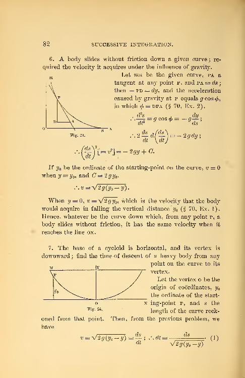
82 SUCCESSIVE INTEGRATION.
6. A body slides without friction down a given curve; re-
quired the velocity it acquires under the influence of gravit}\
Let mn be the given curve, pa a
tangent at any point p, and pa = ds;
then — pd = dy, and the acceleration
caused b}T gravity at p equals g cos<f>,
in which<f>= dpa (§ 70, Ex. 2).
dt2
ds
.'.—- — a cos ct> = Uds
Fig. 23. -d(—)=-2gdy;dt \dt)
y y '
[=v^ = -2gy + C.
If y be the ordinate of the starting-point on the curve, v =when y = y , and C = 2 gry .
•'.v=V2g(y — y).
When ?/ = 0, v=v2gy , which is the velocity that the body
would acquire in falling the vertical distance y (§ 70, Ex. 1).
Hence, whatever be the curve down which, from any point p, a
body slides without friction, it has the same velocity when it
reaches the line ox.
7. The base of a cycloid is horizontal, and its vertex is
downward; find the time of descent of a heavy body from any
point on the curve to. its
vertex.
Let the vertex o be the
origin of coordinates, ythe ordinate of the start-
ing-point p, and s the
length of the curve reck-
oned from that point,
have
Then, from the previous problem, we
v = V2g{y — y) = "111
dtdt = ds
V2^(y -y)(1)
PROBLEMS IN MECHANICS. 83
Since ds is positive, and dy negative,
The equation of the cycloid referred to the axes ox and oy is
x = r vers 1 - +V2 ry — y2
.
r
dx _ /2 r — y\g
.
••*-(S +l)ldir--S)V (2)
From equations (1) and (2), we have
<& = _ f2r\ h dy = _ fr\
k dy.
U / -\/2g(y -y) \9j -\/y y-f
* = - fevers- 52 + (7.
2/o
Since £ = when ?/ = y ?
?=('-Yvers-1 2 = 7iYr
W \ 2/o
£ = 7r( — )", when y = 0.
Hence, the time required to reach the lowest point o will be
the same, from whatever point on om the body starts. Hence,
if a pendulum swings in the arc of a cycloid, the time required
Irfor one oscillation is 2 7ta
J
— The time of an oscillation being
independent of the length of the arc, the cycloidal pendulum is
isochronal.
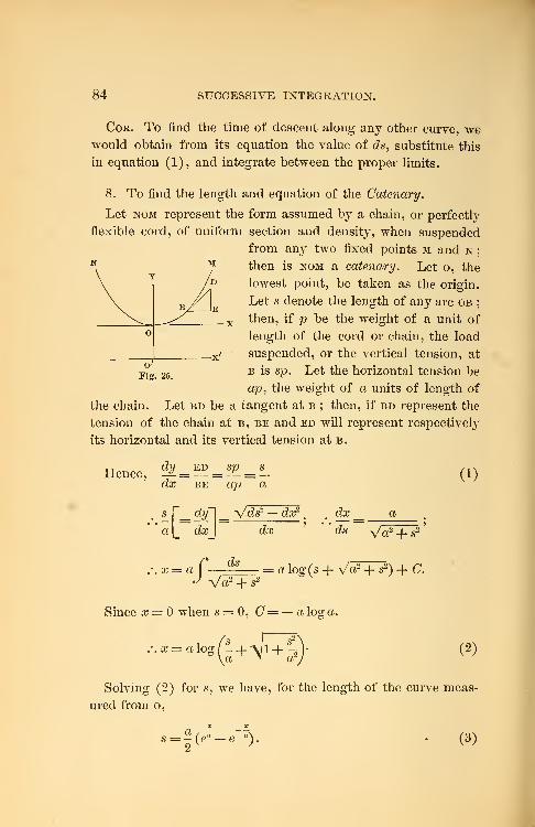
84 SUCCESSIVE INTEGRATION.
Cor. To find the time of descent along any other curve, wewould obtain from its equation the value of c?s, substitute this
in equation (1), and integrate between the proper limits.
8. To find the length and equation of the Catenary.
Let nom represent the form assumed by a chain, or perfectly
flexible cord, of uniform section and density, when suspended
from any two fixed points m and n;
then is nom a catenary. Let o, the
lowest point, be taken as the origin.
Let s denote the length of any arc ob;
then, if p be the weight of a unit of
length of the cord or chain, the load
suspended, or the vertical tension, at
b is sp. Let the horizontal tension be
ap, the weight of a units of length of
the chain. Let bd be a tangent at b ; then, if bd represent the
tension of the chain at b, be and ed will represent respectively
its horizontal and its vertical tension at b.
V 1 >>±
o
V<y
Fig . 25.
TT dy ed sp sHence, -?- = — =— = —
dx be ap a(1)
a[_ dxj
•/:
Vcfc dx2
dx
dx
ds Va2 +
ds
Va2 + s2
Since x = when s = 0, C= — aloga
= o log(s +Vo2+ s2) + O.
(2)
Solving (2) for s, we have, for the length of the curve meas-
ured from o,
s = -(ea — ea), (3)
PROBLEMS IN MECHANICS. 85
To find its equation, we have, from (1) and (3),
-, XXdx
a * -*
Since y = when x = 0, C = — «.
X X
is the equation of the catenary referred to ox and oy.
If o'o = a, and the curve be referred to the axes o'x' and
o'y, its equation will evidently be
X Xa , — . --v
CHAPTER VI.
INDETERMINATE FORMS.
77. When, for any particular value of its variable, a function
assumes any one of the indeterminate forms,
-, — , • 00, 00 - 00, 0°, 00°, 1 ±0°,
<*>
the function, in the usual sense, has no value for this value of
its variable. What we call the value of the function for this
value of its variable is the limit which the function approaches,
as the variable approaches this particular value as its limit.
Often, when a function assumes an indeterminate form, its
value may be found by algebraic methods.
1 . EvaluateXs —
In general,
X3 — 1 x2 -\-x-\-l
Examples.
; that is, findlimit [" or
3 — l "|
x2 -! x + l
limit
x=lar»-r
i
j? - 1
J
limit
x=l'x
2 + x + 1"
x + l
2. Evaluate (x ~ a
}\(x2 — a2
) *
In general,
(x — a)* __(x — a)&
t
(x2 — a2)i (x — a)& (x-\- a)i (aj-f-a)i'
(x— a)&
. limit* x=a
(x — a) 3
(x2 -a2)i_
limit
x^= a
(x—a)h(x + a)i
= 0.
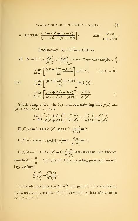
EVALUATION BY DIFFERENTIATION. 87
V2a3. Evaluate
(a2 -x*)k+ (g-x)(a-x)h+(as -xi)h
Ans.1+«V3
Evaluation by Differentiation.
78. To evaluate *& ,ori^i</>(a) <£(x)
when it assumes the form
and
limit
Ax=0
limit
limit
A.r=
~f(x + As) -f(x)Aa;
>(a? + Aa;)-^(a;)
Aa;
7(a? + Aa-)-/(a;)-
<H»+ Aa;) -<£(»)
=/'(»), Ex. 1. p. 39.
(i)
Substituting a for a; in (1), and remembering that /(a) and
<£(«) are each 0. we have
I
Azimit ["/(« + Aa;)
* = °|_<£(a + Aa;)_
If /'(a) = 0, and <f>'(a) is not 0, = 0.
If/'(«) is not 0. and <£'(<*)= 0, 4^7 = °°-
K/'(a) = 0,and«£'(a)= 0, j-^9 V
a )
-' ^''
also assumes the indeter-
minate form - • Applying to it the preceding process of reason-
ing, we have
f'(a) = f"(a)
+' (a) 4>"(a)
If this also assumes the form - , we pass to the next deriva-
tives, and so on, until we obtain a fraction both of whose terms
do not equal 0.
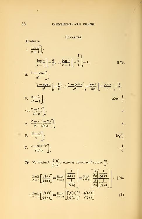
88 INDETERMINATE FORMS.
Examples.Evaluate
1.
2.
log si.
aj — lji
log x~\ _ . .logon _ x
x — lji""0.' "a? — lj!-
1_
1 — cos x~\~~"S Jo"
= 1. §78.
1 — cos a;
ar2
=o
1 — cos af| _ sin cc"1
a? J~^~_
_ cos a?
3.a; -1 1,
tf\-lji
1'
= 1
o~2'
a;
e1 —
2.since
a? — sin a?
!1
6. «^£1a; J
- a? — sin-1
af|
sin3 a; J
79. To evaluatefW
log
, w7ien ££ assumes the form—</>(a) oo
limit r/(g)l _ limit
x = a \J>(x)\ x = a
1
l
LA*) J
_ limit
x = a
d
dx
1 ~]
J>(aj)_
±dx -/(*)JJ
limit fJM1 = limit fL/MT iM~]*=«]_*(»)J
*- aL[*o») ]*'/'(*)J
(1)
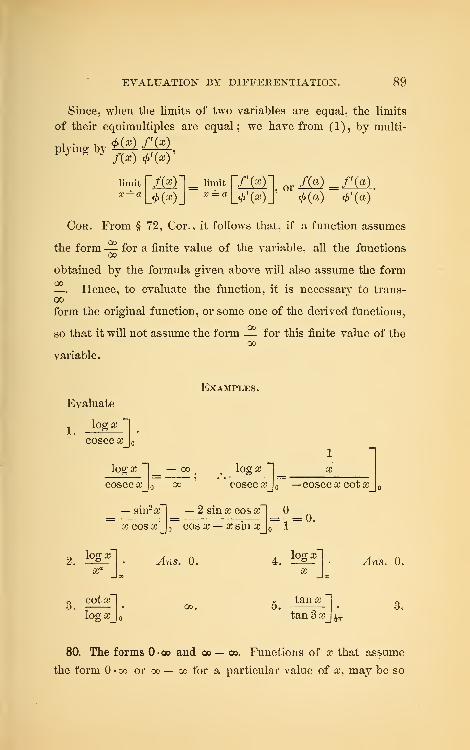
EVALUATION BY DIFFERENTIATION. 89
Since, when the limits of two variables are equal, the limits
of their equimultiples are equal; we have from (1), by multi-
4>{x) f{x)plying by
f{x) *'()'
limit
x~a
'
/(%)'
.*(*).
limit
x = aor /W =ZM
</><» </>'(a)
Cor. From § 72, Cor., it follows that, if a function assumes
the form— for a finite value of the variable, all the functions00
obtained by the formula given above will also assume the form
— Hence, to evaluate the function, it is necessarv to trans-oo
form the original function, or some one of the derived functions,
so that it will not assume the form — for this finite value of the00
variable.
Examples.
Evaluate
1.logo?
~
cosec x
logo;~
cosec x
— sin2 a;'
00> <
log X
X COSiC
» cosec x
— 2 sin x cos x~
cos x — x sin x
cosec £ cotcc
.-! = »•
logon
x° IAns. 0. 4.
logo;"Ans. 0.
3.tana?
tan 3 x
80. The forms 0-oo and oo — oo. Functions of x that assume
the form • oo or oo — oo for a particular value of x, may be so
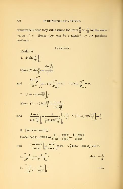
90 INDETERMINATE FORMS.
transformed that they will assume the form - or — for the same
value of x. Hence they can be evaluated by the previous
methods.
Evaluate
1. 2* sin —2*
Examples,
. asin—
a 2rSince 2X sin—=
2* 2~x
and = a cos— = a
:
2. (1 — a?)tan—V ;
2
Since (1 — x) tan— ==
cot
2X sin— = a.2*
_l 00
andl-x
~
, irXcot
2
it oirX- cosecz—
1 2 2 J]
(1 — x) tanttX = 2
c
i t
3. [sec x — tan x]^
.
Since sec x — tan x = sin x 1 — sin x
cosx cos a? COS a
, 1 — sin x~\ _ cos#
cos x J i„. sin a;^
[_log# logajjj
= 0; .*. [sec x — tan a;]|ir= 0.
Arts.2
-1
EVALUATION BY DIFFERENTIATION. 91
81. The Forms 0°, a>°, and l±x . When, for any value of x, a
function of x assumes one of the forms, 0°, oo°, or l±x
, its loga-
rithm assumes the form, ±0«o>, and the function is evaluated
by evaluating its logarithm for this particular value of x.
1. Evaluate af] .
Since log of= x log x
Examples.
x
\ogx
and
2
X -(logxf 2 log x X
1 1 1 1
log X o *£ o *£ _ o «*r
2x
__
.\logaf] = 0, or af] = 1.
2. a^^o.
los" XSince logasin:r= sin a 102^ =—-—
,
cosec x
andlogo; T
cosec x_\ — cosec x cot x
— 2 sin a; cos x~
— sur a;
£COS#
= 0;cos a? — x sin cc
.. logasin*] = 0, or asin
*] = 1.
3. sinasin:,:
] . Ans. 1.
= 0:
4. sino;tan -r]^. ^l?is. 1.
82. Compound Indeterminate Forms. When the given func-
tion can be resolved into factors, some or each of which assumes
the indeterminate form, each factor may be evaluated separately.
Thus, if the function be ^-^? — l) tan2 aT1 we have
92 INDETERMINATE EOHMS.
since
(e»- 1) tan2 aT /'tana
x:i ~\ X
tan af
X1 a e ~ l= 1, and
o X
= 1
= 1,
Examples.
tan a; — x
x — sin a?
= 2.
2.afl 1
Jo 6'
4.
5.
x — sin
x3
ex — e~x
~
|_
log(l+ as)J
ex — e
_x — 2 a;
(e*-l) ;
Jo 3
f].
1 — sin x+ cos
sin a; + cos x — lji^
1.1, as-e*J GO.
G.a:
2+ 2 cos a? — 2"
as3— 3a;-}-2
a;4— 6x2+8x— 3
12
8.<xsinj•'— a
log sin as
= a log a.
9. xi-
10. (cos-mas)* L=l.
12. [as tanas — |-7r sec as] i^ = —1.
13.cos as — cos at
o-x2 d £>-a2 d
eu u sm a i
2a
<-> = efl
83-. Evaluation of Derivatives of Implicit Functions. If an
equation containing as and y is solved for ?/, y is an explicit func-
tion of as ; if it is not so solved, y is an implicit function of x.
EXAMPLES. 93
When y is an implicit function of a?, its derivative, though
containing both x and y, is a function of x. Hence, when the
derivative assumes an indeterminate form for particular values
of x and y, it can be evaluated by the previous methods.
Examples.
1. Find the slope of a2
y2 — a2x2 — x4 = at (0, 0).
TT dv 2a2x+4:X3, nHere — = = -, when x = y = 0.
dx 2a2y
U
TT dy~\ 2a2 x-±-4:XsHence — =
dx^j0|
2a22/ Jo,o
2a2 +12x2~
2<x>dy
dx
1
o.o dx
dx)= 1, or
dec
= ±1.
2. Find the slope o£ys =ax2 — xi at (0,0),
Here -^Sy2
2 a — 6 x
0,0 62/ 0,0
2a — 6a;
6»4da;
?
0,0
2a
o~ " °°'dy~
or -^dx
= ± 00,
3. Find the slope of ar3 — 3 aoy + y
s = at (0, 0)
.
Ans. -^ =0 and oo.
dx
4. Find the slope of x4 - a2xy -f b2
y2 = at (0, 0)
.
Ans. &dx
= and —-•
5. Find the slope of (y2 + a^)
2 — 6 aa;y2 — 2 aar3
-f- a2^ = at
(0,0) and (a, 0)
dxJ 0,0
± 00dy
dx= ±
CHAPTER VII.
DEVELOPMENT OF FUNCTIONS IN SERIES.
84. A Series is a succession of terms following one another
according to some determinate law. The sum of a finite series
is the sum of all its terms. An infinite series is one the number
of whose terms is unlimited.
If the sum of the first n terms of an infinite series approaches
a definite limit as n increases indefinitely, the series is Con-
vergent ; if not, it is Divergent.
The limit of the sum of the first n terms of an infinite con-
vergent series, as n increases, is called the Sum of the series.
An infinite divergent series has no definite sum.
85. To Develop a function is to find a series, the sum of
which shall be equal to the function. Hence the development
of a function is either & finite or an infinite convergent series.
For example, by division, we obtain
1 ~ xn = i + a; + a2 + a3H \-xn~\
1 —x\ xn
This finite series is evidently the development of -—— for
any value of x.
Again, by division, we obtain
1 + x -f x2+ x3 H h af-1 +
1 — X 1 —Xxn 1
Hence is the difference between and the sum of1 —x 1 —x
the first n terms of the series. For x < -f 1 and >— 1, this
difference evidently =0 as n increases, and the series is the
development of the function. But for x> + l or < — 1, this
difference increases numerically as n increases, and the series is
not the development of the function. Thus, the series equals
the function for x = J, but not for x = + 2 or — 2.
taylor's formula. 95
86. Taylor's Formula is a formula for developing a function
of the sum of two variables in a series of terms arranged accord-
ing to the ascending powers of one of the variables, with coeffi-
cients that are functions of the other.
A general symbol for any function of the sum of x and y is
f(x + 2/), of which (x + y)m
i\og(x + y), ax+y , sin(x + y), etc.,
are particular forms.
87. To produce Taylor's Formula.
We are to find the values of A, B, C, etc., when
/(x -h y ) = A + By + Cy2 + Dy5 +W + • • •
,
in which A, _B, (7, i), etc., are functions of x, but independent
of 2/, the series being finite or convergent.
Let x' be amT value of a?, and A', B\ C", etc., the correspond-
ing values of ^4, -B, C, etc. ; then we have
f(x'+y) = A'+B'y + C'y2+ V'yB+ E'yi +-~; (1)
... f(x'+ y ) = B'+ 2 Cy + 3D'y2 + 4£y + -, (2)
/'"(a'+y) = 2 • 3D'+ 2 • 3 • ±Wy + •••, (4)
/-(^+2/) = 2.3.4^'-f---.,etc. (5)
These equations, being true for all values of y, are true when
y = (§ 6) ; hence we have
/(*') = ^'» f{x') = B\ f"(x') = 2C,
f'"(x') = \3D', f"(x') = \±E', etc.
Solving these equations for A', B', C", etc., we have
^'=A«0, B'=f(x'), 0'=£%fK
D'^r^l, E'-^M, etc.
96 DEVELOPMENT OF FUNCTIONS IN SERIES.
Substituting these values in (1), we obtain
f(x<+y) =f{x<) +f'(x')y +/»(«')g +f"(x') £-
+/"(*')j|+ " (6)
Since the coefficients in (6) are equal to f(x), f'(x), /"(#),
etc., for x = x', and since x' is any value of sb, we have, in
general,
f(x + y) =f{x) +f'(x)y +f"(x) £ +/'"(*)£
+/"(*)j£_+- <A >
This development of f(x-\-y) was first published in 1715 by
Dr. Brook Taylor, from whom it is named.
88. When x'= 0, equation (6) of § 87 becomes
Ay) =/(o) +/'(0)2/ +/"(«) =£ +/'"(0) =£
+/"(0-)j| +•• (7)
in which /(0), /'(0), etc., are the values of f(y) and its suc-
cessive derivatives when y = 0.
Letting a? represent the variable in (7), we obtain
f(x)=f(0)+f'(0)x+f"(0)^+f"'(0)^.
+/"(0)g+... (B)
Equation (B) , called Maclaurin's Formula, is a formula for
developing a function of a single variable in a series of terms
arranged according to the ascending powers of that variable,
with constant coefficients.
THE BINOMIAL THEOREM. 97
The completion* of Taylor's and Maclaurin's formulas will be
deferred until we have applied them to the development of a
few functions.
89. To develop (x -f-y)111
, or to deduce the Binomial Theorem.
Here f(x + y) = (x + y)m
; ,:f(x) = x'%
f(x) = mxm-\ f"(x) = m{m — l)xm~\
f'"(x) = m(m - 1) (m - 2)xm~\ etc.
Substituting these values in Taylor's formula, we have
(x + y)m = xm + mxm~ x
y +m
(m ~ 1
) a*-*y
. m(m — 1) (m — 2) m_3 3 .
H—
^
-^J-xm y+ ...
90. To develop log& (x -f y)
.
Here f(x + y) = log, (x + y) ; .-. /(a?) = loga x,
/'(*) = ?, f"(x) =-% f"(x) = *£, etc.a; ar xi
Substituting these values in Taylor's formula, we have
log. (a? + y) = loga « + w/2 -X +X - JL + •••
\x 2ar 3ar 4 ar
which is the logarithmic series.
Cor. If 05= 1, and m = l, we have
log(l + 2/)=^-£ + ^-^+...,
which is the Naperian logarithmic series.
* The series obtained by applying Taylor's or Maclaurin's formula, as
given above, to any given function may or may not be the development of
that function. Their complete forms, however, enable us to determine what
functions can be developed by them-
98 DEVELOPMENT OF FUNCTIONS IN SERIES.
91. To develop ax+y .
Here f(x) — a*, f'(%) = ax log a, etc.
;
.-. a^y = arV 2?r f1 + log a ^ + (log a) 2^- + (log a) 8%- .
92. To develop (a + x) m fo/ Maclaurin's Formula.
Here /(#) = («+^) m;
•'• /(0) = «m .
/'(a;) = m(a+a;) m-1;
/. /'(0) = ma^1.
/"(a?) = m(m-l) (a+a;) m- 2
;
."•'. /"(0) = m(m-l)aw-2.
etc. etc.
Substituting these values in Maclaurin's formula, we have
(a + x) m . m_i . m(m— 1) ™_ 2 9,
93. To develop sin x.
Here f(x) = sin x;
f'(x) = cos a;;
f"(x)= — sin a?;
f'"(x) = — cos a?;
/ IV(a?) = sin a;;
f v (x) = cos a?;
etc.
11
.'. /(0) = 0.
/. /'(0) = 1.
:v/"(o) = a.
.•./'"(.o) = -.i.
.-./~(0) = 0.
• / y(0) = i.
etc.
Substituting these values in the formula, we have
/yv> /y*> ,yti /^,J
sin x = a? — • h , h ; • • •
II li 11 Li
94. To develop cosx.
1w ry& /y»6 /yo
[2_ |4_ [6_ [8_
This result could be obtained by differentiating the value of
sin a; found in § 93.
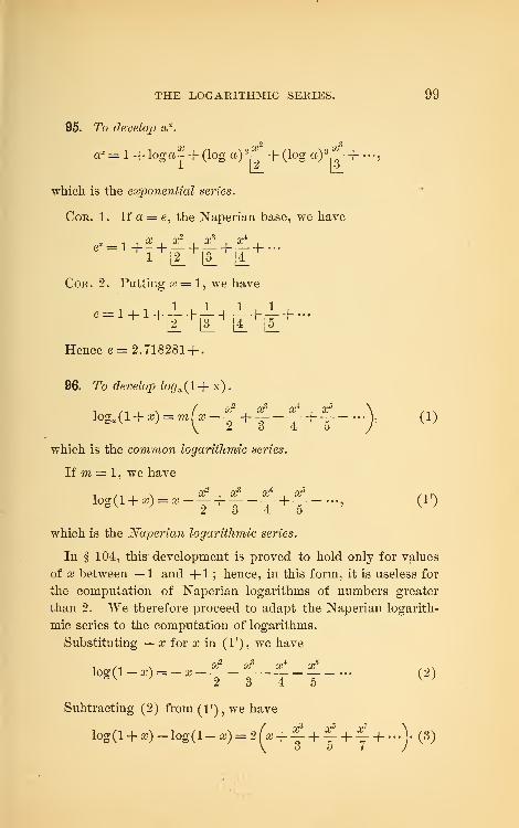
THE LOGARITHMIC SERIES. 99
95. To develop ax .
a^l+loga^4-(loga) 2^+(loga) 3^ + ...5
which is the exponential series.
Cor. 1. If a = e, the Naperian base, we have
Cor. 2. Putting a?= 1, we have
e=l+1+i +
ii+i
+i + -
Hence e =2.718281+ .
96. To develop log,{\ + x)
.
\oga (l+ x)=m(x-^ +y-f+f--} (!)
which is the common logarithmic series.
If m = 1 , we have
log(l + x) = x -— +— -— +— ,(1')oV; 23 45 W
which is the Naperian logarithmic series.
In § 104, this development is proved to hold only for values
of x between —1 and -j-1; hence, in this form, it is useless for
the computation of Naperian logarithms of numbers greater
than 2. We therefore proceed to adapt the Naperian logarith-
mic series to the computation of logarithms.
Substituting — x for x in (1'), we have
/y»* /yi*> /y** /y»0
log(l - x) = - x -— -— -— -— (2)&v }2 3 4 5 V
Subtracting (2) from (1'), we have
l0g(l + ^)-l0g(l-^) = 2^ +^ + y+y4---)-(3)
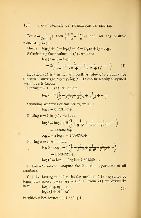
100 DEVELOPMENT OE FUNCTIONS IN SERIES.
I I _i_ x z 4-1Let x — ; then = -
; and, for any positiveu Z -\~ I I — X Z
value of z, x< 1.
Hence log(l + a?) — log(l — a?) = log(2 + 1) — log z.
Substituting these values in (3), we have
log (z + 1) -logz
2z+l+3(2z+l)3+5(2z+l)5+ '"/
Equation (4) is true for any positive value of z ; and, since
the series converges rapidly, log (z + 1) can be readily computed
when \ogz is known.
Putting z = 1 in (4) , we obtain
log2 = 2^+A,+^ +^3 3-33 5-35 7-3 7
Summing six terms of this series, we find
log 2 = 0.693147+ .
Putting 2 = 2 in (4) , we have
108^^2+ 2(1+^+^+^+ ...)
= 1.098612+ .
log 4 = 2 log 2 = 1 .386294+
.
Putting 2 = 4, we obtain
log5 = log4+2(i+3-^+
5-L.
5+ 7-^+...)
= 1.6094379+ .
log 10 = log 5 + log 2 = 2.302585+ .
In this way we can compute the Naperian logarithms of all
numbers.
Cor. 1. Letting m and m' be the moduli of two sj'stems of
logarithms whose bases are a and a', from (1) we evidently
have loga (l+ s) = mT (5)
loga -(l + a) m'
in which # lies between —1 and +1.
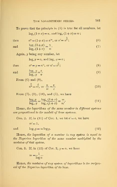
THE LOGARITHMIC SERIES. 101
To prove that the principle in (5) is true for all numbers, let
loga (1+ x) = tt, and loga - ( 1 + x) = w;
w
then aM = (l'+ x) = a'w
, or a'= aw;
(G)
andlog.(l + s) = JL (7 )
loga .(l + a?) lu
Again, y being any number, let
\oga y = 2, and log,,-// = w;
z
then a?= y= a'v, or a'= a*; (8)
and kfeJUL (9 )
From (6) and (8),
aw = «% or — =— (10)to 1'
From (7), (9), (10), and (5), we have
loga y = loga (1+x) = m ^loga .?/ loga .(l + a;) m'
Hence, f/^e logarithms of the same number in different systems
are proportional to the moduli of those systems.
Cor. 2. If, in (11) of Cor. 1, we let a'= e, we have
m'= 1,
and \oga y = mlogy. (12)
Hence, the logarithm of a number in any system is equal to
the Naperian logarithm of the same number multiplied by the
modulus of that system.
Cor. 3. If, in (12) of Cor. 2, y= a, we have
1m =log a
Hence, the modulus of any system of logarithms is the recipro-
cal of the Naperian logarithm of its base.
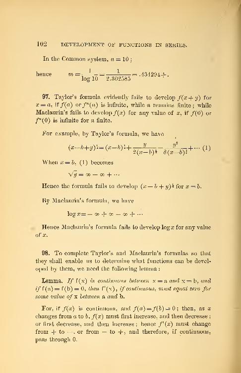
102 DEVELOPMENT OF FUNCTIONS IN SERIES.
In the Common system, a = 10;
hence m — = =.434294+ .
log 10 2.302585T
97. Taylor's formula evidently fails to develop f(x -f- y) for
x = a, if /(a) or /"(a) is infinite, while n remains finite; while
Maclaurin's fails to develop f(x) for any value of x, if /(0) or
fn(0) is infinite for n finite.
For example, by Taylor's formula, we have*
V y) K 2{x-b)h 8(x-b)% K )
Whence =6, (1) becomes
•y/y = go — oo -f-• • •
Hence the formula fails to develop (x — b + y)* for x = b.
By Maclaurin's formula, we have
log£=— oo + oo — oo -f-.-•
Hence Maclaurin's formula fails to develop log x for any value
of ct*.
98. To complete Taylor's and Maclaurin's formulas so that
they shall enable us to determine what functions can be devel-
oped by them, we need the following lemma :
Lemma. If f (x) is continuous betiveen x = a and x = b, and
iff (a) = f (b) = 0, then f'(x), if continuous, must equal zero for
some value of x between a and b.
For, if f(x) is continuous, and f(a) =/(&) = ; then, as x
changes from a to 5, f(x) must first increase, and then decrease;
or first decrease, and then increase; hence f'(x) must change
from + to — . or from — to +, and therefore, if continuous,
pass through 0.
taylor's and maclattrin's formulas. 103
99. Completion of Taylor's and Maclaurin's Formulas. To be
the development of f(x-\-y), the series in Taylor's formula must
be finite or infinite and convergent (§ 85).
Let P^~ be the difference between f(x + y) and the sum of\n
the first n terms of the series ; then we have
/(* + y) =A») +/'(*) \ +/"(f) if +/"'(<»)jf
+ ... +/«-i (a;)jrL + .pj£.( i)
I
?i — 1 \n
We proceed to find the value of P.
Letting y = X — x in (1), and transposing, we have
f(X) -f(x) -f{x) *=* -f'(x){X ~ XY
-p (X~^ n
= 0. (2)[£.
Let i^(z) represent the function of 2 obtained by substituting
2 for x in the first member of (2) ; then
F{z) =/(X) -/(*) -/'(*) *=* -/"(*)i~^
_..._r- I(,)(^z£lr!_p(^I'. (3 )|n — 1 \n
Substituting X for z in (3) , we obtain F{X) = 0.
From (2) we see that the right-hand member of (3) is for
z = x ; hence, by substituting cc for z in (3) , we obtain F(x) =0.
Differentiating (3) to obtain F'(z), we find that the terms of
the second member destroy each other in pairs, with the excep-
tion of the last two, and obtain
104 DEVELOPMENT OF FUNCTIONS IN SERIES.
F'(z) = - (X~ Z"}n~1
fn (z) + (X- Z)
n~1
p.I
71 - 1 \n-l
Whence, P=fn(z) when F'(z)=0. Since F(z) = when
z = X, and also when z = x, F'(z) = for some value of z
between X and x (§ 98) . Now, by giving to some value be-
tween and +1, any value between x and X can evidently be
represented by x -f 0(X— x) .
Hence, P=fn [x 4- 0(X- a;)] =f*(x + By).
Substituting this value of P in (1), we have
\n — 1 [w_
which is one complete form of Taylor's formula.
Cor. Letting x = 0, and putting a? for ?/, we have
/(*) =/(<>) +/'(<>)* +/"(0)£ +/"'(0)j£+ ...
+/"-1(0) r
^l+/»(^)^,I
?i — 1 \n
which is one complete form of Maclaurin's formula.
100. If we had let Pxy be the difference between /(x -\-y) and
the sum of the first n terms of the series in Taylor's formula,
we should have found
\n — 1
Hence a second complete form of Taylor's formula is
A* + v) =/(*)+/»f+/"(«)
jf+ -
n — 1 \n — I
Taylor's and maclaurin's formulas. 105
Cok. 1. The corresponding complete form of Maclaurin's
formula is evidently
j\x) =/(0) +f'{0)x +/"(0)^ +...+/-i(0) J£L|J_ [
n-1
I
71 — 1
All that we know of in any of these formulas is that its
value lies between and +1.
Cor. 2. If, on applying to a given function any one of these
completed formulas, the last term becomes 0, or approaches
as its limit, as n increases, the formula evidently develops this
function ; if not, the formula fails.
101. Since f- = 2- . -£; and since - is very small when y
\n_ nI
n — 1 n
is finite, and n is very large ; each value of — is a very small
llL
part of its preceding value.
yn
Hence ,— = 0, ivhen y is finite and n increases indefinitely.
Cor. 7/*fn (x) does not become infinite with n, Taylor's and
Maclaurin's formulas give the true development of f(x-fy) and
f(x) respectively.
102. To prove that Maclaurin's formula develops ax.
Here fn(x) = (log a) n ax
; .\fn(0 x) = (log a) n a9x
,
and rW*)-= {xl°gaYa.
9'.
\n \n
Since aQx is finite, and ^—-s
—
L = as n increases indefi-\n
nitely (§ 101) ;
L~
(g lo£ a) a0x = On
as n increases, and the formula develops the function (§ 100.
Cor. 2)
.
106 DEVELOPMENT OF FUNCTIONS IN SERIES.
103. To prove that Maclaurin's formula develops sin± and
cosx.
The nth derivative of each of these functions is finite, how-
ever great n may be ; hence Maclaurin's formula develops both
of them (§ 101, Cor.).
104. To determine for what values of x Maclaurin's formula
develops log(l + x.).'
The formula gives (§ 96),
x2. a? x*
, ,
(-i)—"af-1
. -J _ . -+_ ... -X- -^ £ .l g(l + aO=7-^-+lT--T-+--- +12 3 4 n-1
n
The ratio of the nth term to the term before it evidently
approaches — x as n increases. Hence, if x is numerically
greater than 1, the series is divergent, and cannot be the devel-
opment of log(l + x). We need, therefore, to examine the
value of the last term of the formula only for values of x be-
tween — 1 and +1.
(_l)-iu_l
.\f"($x)— = (- 1 )"" 1
\n n \l + 9 xJ
( — \\n-l / x \nFor values of x between and -h 1 ?
- — andf )
n \l + 0xj
each approaches as n increases ; hence the formula develops
log (1 -f- x) for these values of x.
When x lies between and — 1 , let x1 represent its absolute
value ; then X = — x1 , and log(l -+- x) = log(l — a^)
.
Using the second form of the formula, we have, numerically,
ri6Xl)(i-tf)-V = a-ey-w
\n — l {l— 6xx )n
-Ox^- 1
1-OxJ l-$xl
taylor's and maclattrix's formulas. 107
For values of x1 between and -f-1,——— is finite, andl — 0x1
zl Li approaches as n increases. The formula there-\l-0xjfore develops log (l-\-x) when x lies between and — 1.
Hence, Maelaurin's formula develops log(l+ x) for values of
x between — 1 and -f-1.
105. To determine for what values of x Maelaurin's formula
develops (l-f-x)m
.
The formula gives
a i \m -1 r iW (ill 1) a .
-f- x)m = 1 -f- mx -\ ^— L xr -j
,m(m — 1) ••• (m — ?? + 2)
H - ^ :L-¥-xn~1
.
n —1
xn
If m is a positive whole number, fn (0x) — =0 when ?i=m+ l
;
[n_
hence, in this case, Maelaurin's formula develops (l-{-x) min a
finite series of m-\-l terms.
If m is negative or fractional, the series is infinite. The ratio
of the (n + l)th term to the nth is —~ 1
a\ which approachesn
— x as n increases. The series therefore is divergent, and can-
not equal (1 + ®)m when x is numerically greater than 1. Hence
we need examine the value of the last term of the formula only
for values of x between + 1 and — 1
.
Here r(x) = M»i-i)-(m.-
n
+ !)(! +x)"V '
(1+3!)"
[n
= rm(m-l).v(m^W+l)
aftl/_j_YL \n ]\l+dxJ
K }
When x lies between and 1, (1 -f 0x) m is finite,
and| )
= 0, as n increases indefinitely.
108 DEVELOPMENT OF FUNCTIONS IN SERIES.
An increase of 1 in the number of terms multiplies the factor
in brackets by x, which approaches — x as n increases.n +
1
Hence the last term of the formula approaches as n increases;
and the formula develops (l+ x) m for values of x between
and +1.
Using the second form of the formula, we have
-oy-[71-1
fn(ex) ^1~^nlxn
±0xY= m(m-l)...(TO-Hl) f1/ l^ y(l-\n-l ]\l+ 6x) 1
( 1 -4- $x} mFor values of x between and — 1 , ^—— '— is finite
;1-01 n \n
approaches as n increases ; and an increase of 1 inl+ 0x
t
the number of terms multiplies the factor in brackets by x,n
which approaches — x as n increases. Hence Maclaurin's for-
mula develops (l + x) m for all values of x between —1 and +1.
106. The Binomial Theorem. Since (a + x) m = am (l -f -J
,
(x\m14- -) can be developed by Maclaurin's formula, when x
aj
is numerically less than a (§ 105) ; therefore, in this case,
(a + x) m = am -f mam- x x + m(^ -1) am
~ 2 x2+ ••• (1)
For like reason, when x is numerically greater than a,
{x + a)m = xm + mx^a + m<>-l) SB
m-2 a*+ ... (2)11.
Hence one, and only one, form of the development of (a + x) m
holds for any set of values of a and x.
THE COMPUTATION OF 77. 109
107. To develop fcm-1
x, and find the value ofV.
When # lies between — 1 and + 1 •>
——, = (l+^)-1 = l-aP+x'-^+^ ; §105.1 -f-ar
.'.|——
2= I dx— I x2dx + j
x'4<ix — I #6
cfcc
-f- I x?dx — • • •
Hence, if a; is numerically less than 1,
tan" 1 ^ = a; -— +— -— +— (1)3 o / 9
(7=0, since tan_1
cc = when x = 0.
If we put <B=-ij-, equation (1) becomes
tan-Ji = -=JYl-i +^-^ + -..V\3 6 \3V 9 45 189 /
'
.•. 7r = 2V3(/
'l-i + ^ — + .••] = 3.141592+ .
^ 9 45 189 J
108. To develop sin^x, and find the value ofV.
. -, . a;3
, 1-3^ . 1.3.5a?7 ,
sin ±a! = aH ,
2-3 2-4-5 2.4.6.7
when x lies between — 1 and + 1
.
,.- =Yi+-+—+— +6 2 V 24 640 7168
or, 7T = 3.141592+ .
It was by means of this series that Sir Isaac Newton com-
puted the value of 71-,
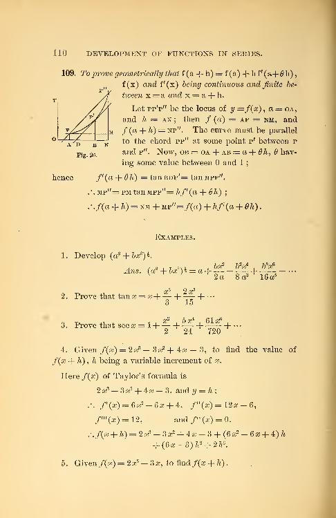
110 DEVELOPMENT OF FUNCTIONS IN SERIES.
109. To prove geometrically that f (a + h) = f (a) + h f ' (a-f h)
,
f (x) and f (x) being continuous and finite be-
tween x =a and x = a -f- h.
Let pp'p" be the locus of y =f(x) , a = oa,
and h = an ; then / (a) = ap = nm, and
f(a + h) = np". The curve must be parallel
to the chord pp" at some point p' between p
and p". Now, ob = oa -j- ab = a -+- Oh, hav-
ing some value between and 1;
hence f'(a -\-0h) = tanBDp'= tanMPp".
.'. mp"= pm tanMPp"= hf'(a + 6h);
,\f(a + h) = nm + Mp"=/(a) + hf(a + 0h).
Examples.
1. Develop (a2 + 5^)5.
A f 2 ,,,, . bx2
b2x4
. bsx6
Ans. (a- -\-bx-)* = a-\ -\v y 2a 8a3 16a5
2. Prove that tan x = x-af 2X5
.
3 15
3. Prove that sec x= l-\ 1 -\
2 24 720
4. Given f(x) = 2 a;3 — 3 a?
2-f- 4 a: — 3, to find the value of
f(x + 7i) , h being a variable increment of x.
Here /(a;) of Taylor's formula is
2x? — 3ar4-4x — 3, and y = h;
.-. /'(») = 6a;2 -6a; + 4, /"(a>)= 12oj — 6,
/"'(a;) = 12, and/IV(a;) = 0.
.-. f(x + 7i) = 2 a;3 - 3 a;
2 + 4 a; - 3 + (6 a;2 - 6 x -f- 4) ft
+ (6a;-3)7i2 + 2/i3 .
5 . Given /(aj) = 2 a;5 - 3 a;, to find f(x + h)
.
EXAMPLES. Ill
6. Develop sin (x -f- y)
.
sin (x -\-y) = sin x ( 1 —li H li /
\ 11 11 \L
= sin x cos 2/+ cos x sin y. §§93,94
7. Prove that cos (x -f- y) = cos a; cos y — s'mx sin ?/.
iar+ 4a^_31a^ +
11 |i
/y»^ /y»o /y»4:
9 . Prove that log ( 1 -f- sin x) = x 1 [-•••&V }2 6 12
10. Developed*. e'inx = 1 + a? + ,— -~ +—-—' +
11 II 11 11
11. DevelopV&2 - cV
12. Develop arV. #V = a;2 + x3 4-— 4-— + •••
[2_ [I
13. Develop log(H-e-). log 2 + |+ |._Jj^ + ...
14. Prove that, if /(a;) =/(— x) , the development of f(x)
contains only even powers of x ; while, if f(x) = —/(— x), the
development of f(x) involves only odd powers of x.
15. What powers of x appear in the development of since,
and why? cos a;? tana;? sec a;? sin-1
a;? tan^x?
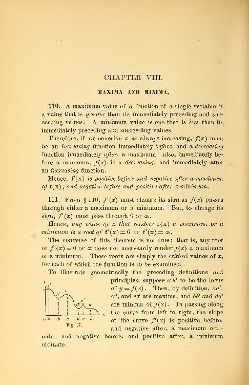
CHAPTER VIII.
MAXIMA AND MINIMA.
110. A maximum value of a function of a single variable is
a value that is greater than its immediately preceding and suc-
ceeding values. A minimum value is one that is less than its
immediately preceding and succeeding values.
Therefore, if we conceive x as always increasing, f(x) must
be an increasing function immediately before, and a decreasing
function immediately after, a maximum ; also, immediately be-
fore a minimum, /(as)- is a decreasing, and immediately after
an increasing function.
Hence, f(x) is positive before and negative after a maximumo/f(x), and negative before and positive after a minimum.
111. From § 110, f'(x) must change its sign as f(x) passes
through either a maximum or a minimum. But, to change its
sign, /'(as) must pass through or go.
Hence, any value of x that renders f (x) a maximum or a
minimum is a root of f (x) = or f (x) = oo.
The converse of this theorem is not true ; that is, any root
of /'(as) = or oo does not necessarily render /(as) a maximumor a minimum. These roots are simply the critical values of x,
for each of which the function is to be examined.
To illustrate geometrically the preceding definitions and
Y principles, suppose a'h' to be the locus
cof y = f(x) . Then, by definition, aa',
VL/Tn . cc', and ee' are maxima, and bb' and dd'; ', \ €
\&AW are minima of f(x) . In passing along
IJ I
i H x the curve from left to right, the slope
oa b c d e h Qf ^e curve f{x) is positive before,
and negative after, a maximum ordi-
nate ; and negative before, and positive after, a minimum
ordinate.
METHODS OF FINDING MAXIMA AND MINIMA. 113
Moreover, at a point whose ordinate f(x) is a maximum or
a minimum, the curve is either parallel or perpendicular to the
axis of 05, and therefore f'(x) = or oo.
At x = oh, f'(x) = Q, but hh' is neither a maximum nor a
minimum of f(x)
.
112. Whether any one of the critical values of a; renders /(a?)
a maximum or a minimum can be determined by one of the
following methods
:
First Method. In this method we determine directly whether
f'(x) changes from positive to negative, or from negative to
positive, as x passes through a critical value.
Let a be a critical value, and h a very small quantity. In
/' (x) substitute a — It and a + h for x.
If f'(a-h) is positive, and f'(a + h) negative,
f(a) is a maximum. § 110
If f'(a-h) is negative, and f'(a-\-h) positive,
f(a) is a minimum.
If f'(a — h) and f (a + h) have the same sign,
/(«) is neither a maximum nor a minimum.
Second Method. This method applies only to the roots of
f'(x) = 0. Let a be a critical value of x. Developing f(x—7i)
and f(x + h) by Taylor's formula, substituting a for x, trans-
posing f(a) , and remembering that f'(a) = 0, we have
/(a-70-/(a)=/^a)|-/'>)^V/-(a)^-..., (1)\± L£ 11
and /(a+ZO-ZC^^/'Ca)^/''^^^/^^^--- (2)
If h be taken very small, the sign of the second member of
either (1) or (2) will be the same as the sign of its first term.
Hence, if /"(«) is negative, f(a) is greater than both /(a — h)
and /(a + 7i), and therefore a maximum; while, if /"(«) is
positive, /(a) is less than both f(a — h) and f(a + h) , and
114 MAXIMA AND MINIMA.
therefore a minimum. If f"(a) is 0, and f'"(a) is not 0,
/(a) is neither greater than both f{a — 7i) and /(a + /*) , nor
less than both, and is therefore neither a maximum nor a mini-
mum. If /'"(a), as well as /"(a), is 0, and/lv (a) is negative,
/(a) is greater than both f(a — li) and f(a + 7i) , and therefore
a maximum; while, if /IV (a) is positive, J\a) is a minimum,and so on. *
Hence, if sl is a critical value obtained from f'(x) = 0, substi-
tute a for x in the successive derivatives of f(x). If the first
derivative that does not reduce to is of an odd order, f (a) is
neither a maximum nor a minimum ; but, if the first derivative
that does not reduce to is of an even order, f (a) is a maximumor a minimum, according as this derivative is negative or positive.
113. Maxima and minima occur alternately.
Suppose that a < 6, and that f(a) and f(b) are maximaof f(x). When x = a + h, f(x) is decreasing; and, whenx = b — h, f(x) is increasing, h being very small. But, in
passing from a decreasing to an increasing state, f(x) must pass
through a minimum. Hence, between two maxima, there must
be at least one minimum.
In like manner, it can be proved that between two minima
there must be at least one maximum.
114. The solution of problems in maxima and minima is
sometimes facilitated by the following considerations
:
(a) Any value of x that renders c -f(x~) a maximum or a minimum, c
being positive, renders f(x) a maximum or a minimum.
(6) Any value of x that renders loga f(x) a maximum or a minimum,
renders f{x) a maximum or a minimum, a being greater than unity.
(c) Any value of x that renders f(x) a maximum or a minimum, renders
a minimum or a maximum.
(d) Any value of x that renders c +f(x) a maximum or a minimum,
renders f(x) a maximum or a minimum.
(e) Any value of x that renders f(x) positive, and a maximum or a
minimum, renders [/(^)]n a maximum or a minimum, n being a positive
whole number.
EXAMPLES. 115
Examples.
1. Find what values of * render 4*' — 15 xr + 12* — 1 a
maximum or a minimum.
Here /(*) = 4*3 - 15*2 + 12*- 1 ;
.\f'(x) =\2xr- 30* + 12, and /"(*) = 24a - 30;
hence the roots of f'(x) = 12*2— 30 x + 12 = 0, which are £ and
2, are the critical values of x (§ 111).
But /"(i) = [24* -30], = -18,
and f"(2) = [24* - 30] 2 = + 18;
hence when * = J, the function is a maximum (§ 112), and
when * = 2, it is a minimum.
2. Find the maxima and minima of Xs — 9 x2 + 15 * — 3.
Here /'(*) = 3*2 - 18* + 15, and /"(*) = 6*- 18;
therefore 5 and 1, the roots of /'(*) = 3*2 — 18* + 15 = 0,
are the critical values (§ 111).
/"(5) = [6*-18] 5 = + 12, and /"(l) = -12;
-\/(5), or [*3 -9*2 +15*-3] 5 , [=-28] isamin.,
and /(l)? or [jx? — 9ar +15* — 3]^ [= 4] is a max.
Let the student construct the locus of y = *3— 9*2+ 15* — 3,
and thus exhibit these results geometrically.
3. Examine *3 — 3*2 +3*+7 for maxima and minima.
Here /'(*) = 3*2-6*+3, /"(*) = 6*-6, and /'"(*) =6;
therefore 1 is the critical value.
But /"(1) = [6*-6] 1 =0, and /'"(1) = 6;
hence the function has neither a maximum nor a minimum (§112).
4. Examine x5 — 5 *4 + 5 *3 — 1 for maxima and minima.
Here /(*) = x5 — 5 *4 + 5 se3 — 1
;
116 MAXIMA AND MINIMA.
.-./'(a?) = 5a?4 -20ar3+ 15a?2
,/"(a?) = 20a?3-60a?2+30a?,
and f'"(x) = 60;x2 - 120 a? + 30;
therefore 1,3, and are the critical values.
Since /"(1) = -10, /(1)[=0] is a maximum.
Since' /"(3) = + 90, /(3)[=-28] is a minimum.
Since /"(0) = 0, and /"'(0) = 30,
/(0) is neither a maximum nor a minimum.
5. Examine (a? — l) 4(a? -f- 2)
3 for maxima and minima.
Here f(x) = (x - l) 3 (x + 2)2(7 x + 5)
,
and the critical values are — 2, —-f-,
and + 1.
In this example, the first method is to be preferred. By in-
spection, we see that
f'(—2 — h) and /'(-— 2 + /i) are both positive;
hence /( — 2) is neither a maximum nor a minimum (§ 112) c
f>(-5- h) is+ , ani /'{_$ + A) is _;
hence /(—"f) *s a maximum (§ 112).
/'(1-A) is -, and f'(l+h) is +;
hence /(I) [=0] is a minimum.
6. Examine & + c(x — a)i for maxima and minima.
Here /'(*)= ,
2°
,, ;
3 (a? — a) s
and the critical value is a, the root of f'(x) = oo.
2c .-i
2c . .
and — is -f ;
3 (a — h— a)s 3(a+/i— a)
.*./(«)[= 6] is a minimum.
(a — x) 3
7. Examine -^-—-
—
'— for maxima and minima.a — 2 x
tt ^/ \ (a — x) 2(4:X — a)
Here /' (a?) = A > v >;
(a — 2 a-)2
EXAMPLES. 117
and the equations fix) = and /'(as) = oo give -, -, and a as4 2
the critical values.
By inspection, we see that f'(x) changes from negative to
positive when x = -; hence ft - )
is a minimum. But, as f\x)
ct fol\does not change its sign when x — a or -, f(a) and /f-] are
neither maxima nor minima.
8. Examine c -\- V4a¥ — 2aas3 for maxima and minima.
By (d), (<?), and (a) of § 114, any value of x that renders
+ V4
a
2;i*- — 2 aas
3 a maximum or a minimum, renders
V4aV — 2 aas3
, 4 eras2 — 2 aa:
3, and 2 aas
2 — as3
a maximum or a minimum.
Hence, let f(x) = 2 aos2 — as
3, etc.
-4ns. When x = 0, c+ v/4a 2as2 — 2 aas3 is a minimum
;
" cc=|a, u " is a maximum.
9. What values of as render 2 as3 — 21 as
2-f- 36 x — 20 a maxi-
mum or a minimum?Ans. /(I) is a max.
; /(6) is a min.
10. Examine 3 as5 — 125 a;
3 + 2 160 as for maxima and minima.
Ans. /(— 4) and/(3) are max.; /(— 3) and/(4) are min.
1 1
.
Examine Xs — Sx2 -\-Qx -f-7 for maxima and minima.
Ans. It has neither a max. nor a min.
12. If /'(as) = as3 (as-l) 2 (as-2) 3(as-3) 4
, what values of x
render /(as) a maximum or a minimum?
Ans. /(0) is a max.; /(2) is a min.
13. Examine x(x -+- a) 2 (a — x) 3 for maxima and minima.
Ans. /(—a) and/(- ) are max.; /( )
is a min.
118 MAXIMA AND MINIMA.
14. Examine -2— for maxima and minima.aj-10
Ans. /(4) is a max.; /(16) is a min.
(x 4- 2) s
15. Examine v yn for maxima and minima.
Ans. /(3) is a max.; /(13) is a min.
16. Prove that sin x + cos x is a maximum when x = —-4
17. Examine for maxima and minima.log a?
-Ans. : is a min.lose
18. Prove that of is a maximum when x = e.
19. Prove that sin #(1+ cos x) is a maximum when x = --o
X20. Prove that is a maximum when x = cos x.
1 + x tan x
21. Examine the curve y = xs — Sx2 — 24 cc + 85 for maxima
and minima ordinates.
^Lns. 113 is a max. ; 5 is a min.
22. Examine y = x3 — 9 x2 + 24a? -f 16 for maxima and min-
ima ordinates.
.Ans. 36 is a max. ; 32 is a min.
23 . Examine y = xs — 3 x2 — 9 x -}- 5 for maxima and minima
ordinates.
A.ns. 10 is a max. ;— 22 is a min.
24. Examine y = x5 — 5jc4 + osc3 + 1 for maxima and minima*
ordinates.
Ans. 2 is a max. ; —26 is a min.
25. Examine y= sin3a? cos a? for maxima and minima ordi-
nates.
Ans. When x =-J 7?, y = T
3FV3, a max.
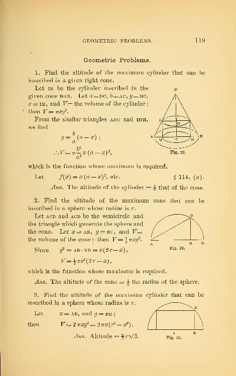
GEOMETRIC PROBLEMS. 119
Geometric Problems.
1. Find the altitude of the maximum cylinder that can be
inscribed in a given right cone.
Let ik be the cylinder inscribed in the d
given cone dab. Let «= dc, 6= ac, y= MC,
x = im, and V= the volume of the cylinder
;
then V— Trxy2
.
From the similar triangles adc and idh,
we find
by (a - x)
h-r.V=^x(a-xy, Fig. 28.
Fig. 29.
which is the function whose maximum is required.
Let f(x) = x (a - x) 2, etc. § 114, (a)
.
Ans. The altitude of the cylinder = ^ that of the cone.
2. Find the altitude of the maximum cone that can be
inscribed in a sphere whose radius is r.
Let acd and acb be the semicircle and
the triangle which generate the sphere and
the cone. Let x = ab, y = bc, and V=the volume of the cone ;
- then V= \irxy2.
Since y2 = ab -bd = x(2r— x),
V=i7rx2(2r-x),
which is the function whose maximum is required.
Ans. The altitude of the cone = |- the radius of the sphere.
3. Find the altitude of the maximum c^ylinder that can be
inscribed in a sphere whose radius is r.
Let x = ab, and y — be;
then V= 2 ivxy2 = 2 irx(f - x2
) .
Ans. Altitude = frV3. Fig. so.
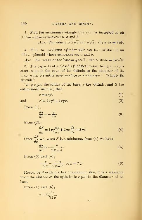
120 MAXIMA AND MINIMA.
4. Find the maximum rectangle that can be inscribed in ah
ellipse whose semi-axes are a and b.
Ans. The sides are <xV2 and &V2 ; the area = 2ab.
5. Find the maximum cylinder that can be inscribed in an
oblate spheroid whose semi-axes are a and b.
Ans. The radius of the base = ^a,-V6-', the altitude == J&V3,
6. The capacity of a closed cylindrical vessel being c, a con-
stant, what is the ratio of its altitude to the diameter of its
base, when its entire inner surface is a minimum? What is its
altitude ?
Let y equal the radius of the base, x the altitude, and S the
entire inner surface ; then
c = 7rxy2
, (1)
and S = 27rif + 2iryx. (2)
From (1),
^ = _JL (3)dx 2x v '
From (2),
^ =4^ + 2^3 + 2^. (4)dx dx dx
d SSince — = when S is a minimum, from (4) we have
dxdy = ydx 2 y -f- x
From (3) and (5),
_V_ = -V orx = 2y. (6)2x 2y + x
v
Hence, as S evidently has a minimum value, it is a minimum
when the altitude of the cylinder is equal to the diameter of its
base.
From (1) and (6),
(5)
\2tt
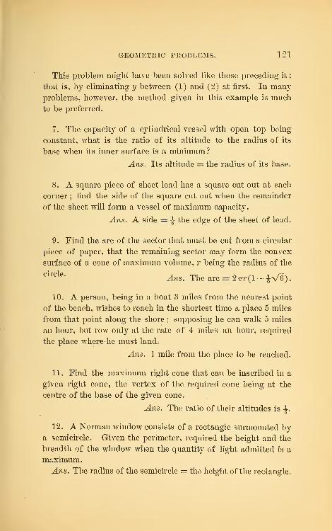
GEOMETRIC PROBLEMS. 121
This problem might have been solved like those preceding it
;
that is, by eliminating y between (1) and (2) at first. In many
problems, however, the method given in this example is much
to be preferred.
7. The capacity of a c}Tlindrical vessel with open top being
constant, what is the ratio of its altitude to the radius of its
base when its inner surface is a minimum?
Arts. Its altitude = the radius of its base.
8. A square piece of sheet lead has a square cut out at each
corner ; find the side of the square cut out when the remainder
of the sheet will form a vessel of maximum capacit}'.
Ans. A side =-J-the edge of the sheet of lead.
9
.
Find the arc of the sector that must be cut from a circular
piece of paper, that the remaining sector may form the convex
surface of a cone of maximum volume, r being the radius of the
circle '
Ans. The arc = 2 ttv (1 - JV6)
.
10. A person, beiug in a boat 3 miles from the nearest point
of the beach, wishes to reach in the shortest time a place 5 miles
from that point along the shore ; supposing he can walk 5 miles
an hour, but row only at the rate of 4 miles an hour, required
the place where he must land.
Ans. 1 mile from the place to be reached.
11. Find the maximum right cone that can be inscribed in a
given right cone, the vertex of the required coue being at the
centre of the base of the given cone.
Ans. The ratio of their altitudes is-J-.
12. A Norman window consists of a rectangle surmounted by
a semicircle. Given the perimeter, required the height and the
breadth of the window when the quantit}r of light admitted is a
maximum.
Ans. The radius of the semicircle = the height of the rectangle.
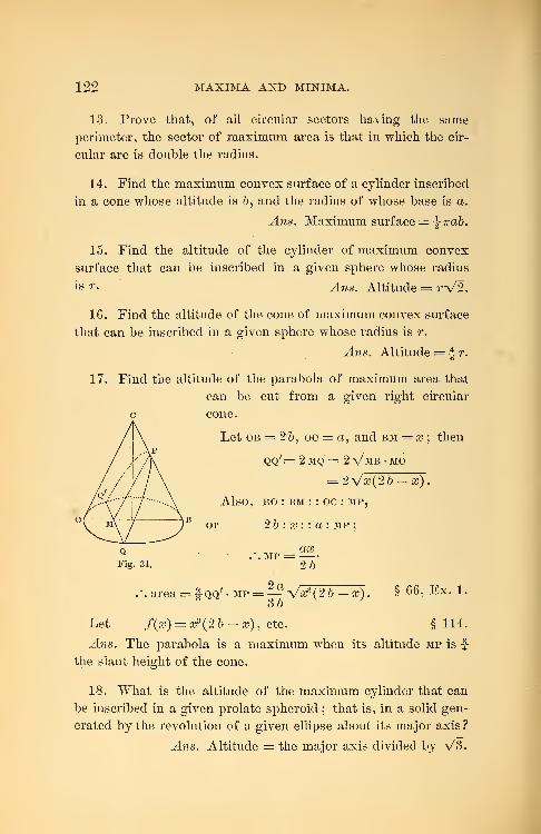
122 MAXIMA AND MINIMA.
13. Prove that, of all circular sectors having the same
perimeter, the sector of maximum area is that in which the cir-
cular arc is double the radius.
14. Find the maximum convex surface of a cylinder inscribed
in a cone whose altitude is 6, and the radius of whose base is a.
Ans. Maximum surface = ^irab.
15. Find the altitude of the cylinder of maximum convex
surface that can be inscribed in a given sphere whose radius
is r. Ans. Altitude = rV2.
16. Find the altitude of the cone of maximum convex surface
that can be inscribed in a given sphere whose radius is r.
Ans. Altitude = |r.
17. Find the altitude of the parabola of maximum area that
can be cut from a given right circular
cone.
Let ob = 2 6, oc = a, and bm = x ; then
qq'= 2 mq = 2 Vmb • MO
= 2^/x(2b-x).
Also, bo : bm : : oc : mp,
2 b : x : : a : mp ;
.*. MP =
2a
ax
Yb
.'. area = f qq'- mp =— -yx^{2b — x).O
§ 66, Ex. 1.
§ 114.Let f(x) = xs(2 b — x) , etc.
Ans. The parabola is a maximum when its altitude mp is fthe slant height of the cone.
18. What is the altitude of the maximum cylinder that can
be inscribed in a given prolate spheroid ; that is, in a solid gen-
erated by the revolution of a given ellipse about its major axis ?
Ans. Altitude = the major axis divided by V3.
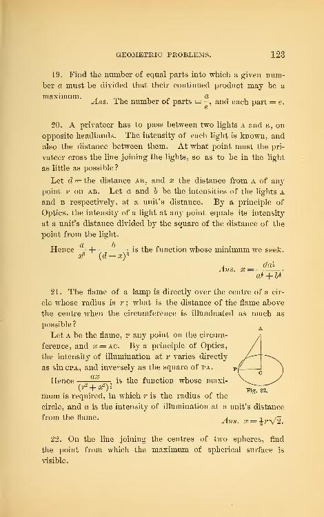
GEOMETRIC PROBLEMS. 123
19. Find the number of equal parts into which a given num-
ber a must be divided that their continued product may be a
maximum. , „. , _ , aAns. I he number of parts = -, and each part = e.
20. A privateer has to pass between two lights a and b, on
opposite headlands. The intensity of each light is known, and
also the distance between them. At what point must the pri-
vateer cross the line joining the lights, so as to be in the light
as little as possible ?
Let d = the distance ab, and x the distance from a of any
point p on ab. Let a and b be the intensities of the lights aand b respectively, at a unit's distance. By a principle of
Optics, the intensity of a light at any point equals its intensity
at a unit's distance divided by the square of the distance of the
point from the light.
Hence 1 is the function whose minimum we seek.x2 (d — xy
Ans. x= dai
as + U
21. The flame of a lamp is directly over the centre of a cir-
cle whose radius is r ; what is the distance of the flame above
the centre when the circumference is illuminated as much as
possible ? ALet a be the flame, p any point on the circum-
ference, and aj = AC. By a principle of Optics,
the intensity of illumination at p varies directly
as sincPA, and inversely as the square of pa.
Hence — is the function whose maxi-(?" + ar
)J
. . Fig. 32.
mum is required, in which r is the radius of the
circle, and a is the intensity of illumination at a unit's distance
from the flame. An^ x= i r^.
22. On the line joining the centres of two spheres, find
the point from which the maximum of spherical surface is
visible.
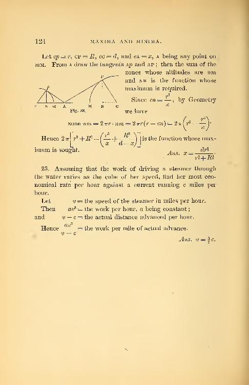
124 MAXIMA AND MINIMA.
Let cp = r, cp = _R, cc = d, and ca = x, a being any point on
mM. From a draw the tangents Ap and ap ; then the sum of the
zones whose altitudes are nmand nm is the function whose
maximum is required.
r2
Since cn =— , by Geometryx
we have
Hence 2-n-
zone nm = 2-kt • nm = 2irr(7 en) = 2 7r ( r2 —
r2 +R2
imum is sought.
d — xis the function whose max-
driAns. x
+ i?i
23. Assuming that the work of driving a steamer through
the water varies as the cube of her speed, find her most eco-
nomical rate per hour against a current running c miles per
hour.
Let v — the speed of the steamer in miles per hour.
Then avs = the work per hour, a being constant
;
and v — c = the actual distance advanced per hour.
avs
Hence — = the work per mile of actual advance.v — c
Ans. ro — \c.
CHAPTER IX.
FUNCTIONS OF TWO OR MORE VARIABLES, AND CHANGE OF
THE INDEPENDENT VARIABLE.
115. Functions of two or more Variables. Since any inde-
pendent variable is some arbitrary function of t, t representing
time, a function of an}' number of independent variables maybe regarded as a function of the single variable £, and therefore
differentiated by the rules already established.
/(a?, ?/), read "function of x and y" represents any function
of x and y\ as, x3-\- xy2
-\- xy and sin(ic -f- y)
.
/(ic, y, z), read "function of jc, y, and z," represents any
and z.
116. A Partial Differential of a function of two or more vari-
ables is the differential obtained on the Irypothesis that only one
of the variables changes.
117. A Total Differential of a function of two or more vari-
ables is the differential obtained on the hypothesis that all its
variables change.
118. A Partial Derivative of a function of two or more vari-
ables is the ratio of the partial differential of the function to
the differential of the variable that is supposed to change.
119. A Total Derivative of a function of two or more vari-
ables, of which only one is independent, is the ratio of the total
differential of the function to the differential of the independent
variable.
If u = f(x, y), the partial differentials of u with respect to
x and y are written dxu and d it, or — dx and — dy; and thedx dy
126 FUNCTIONS OF TWO OR MORE VARIABLES.
partial derivatives, or differential coefficients, are written
dxu -, dvit .A
du -. du-JL- and -1-, or simply — and —dx dy " dx dy
120. The total differential of a function of two or more vari-
ables is equal to the sum of its partial differentials.
For, if u =/(#, y) , it is evident, from the general principles of
differentiation, that du can contain only such terms as are of the
first degree in dx and dy.
Hence du = <£(#, y)dx -f- <f>i(x, y)dy, (1)
in which <£(#, y) and <f>i(x, y) represent the sums of the co-
efficients of dx and dy in the different terms of du.
Let x' and y' be any set of values of x and y ; then we have
du = <f>{x\ y')dx -f faQc'-, y')dy. (2)
Let y be regarded as constant ; then dy = 0, 4>(x', y') remains
unchanged, and (2) becomes
dxu = <f>(V, y')dx. (3)
If x is constant, (2) becomes
dyu=cf, 1 (x\ y')dy. (4)
Adding (3) and (4), and remembering that x' and yf are any
values of x and y, we have in general
dxu -f- dyu = </>(«, y)dx + <f>i(x, y)dy = du.
Since a similar process of reasoning could be extended to a
function of n variables, the theorem is proved.
If x and y were not independent, the demonstration given
above would still hold ; for the idea of a partial differential of a
function sets aside any question concerning the dependence of
its variables.
121. Signification of Partial Derivatives. From § 31 it is
evident that a partial derivative expresses the ratio of the rate
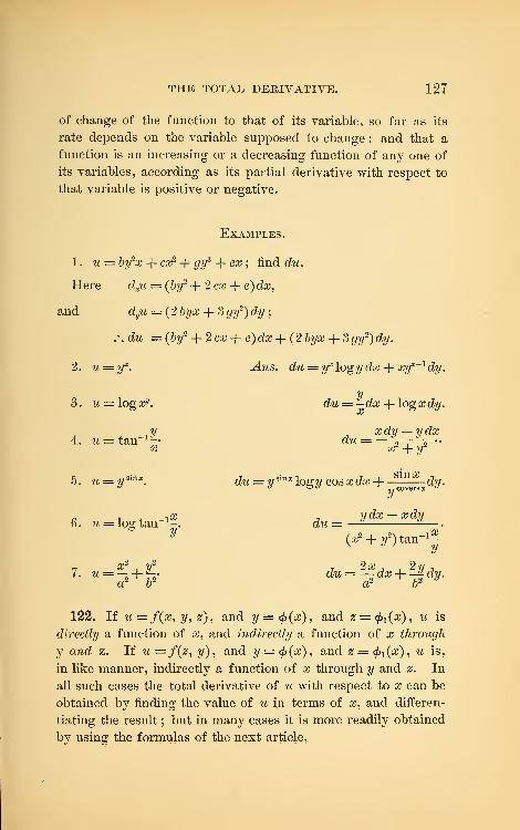
THE TOTAL DERIVATIVE. 127
of change of the function to that of its variable, so far as its
rate depends on the variable supposed to change ; and that a
function is an increasing or a decreasing function of any one of
its variables, according as its partial derivative with respect to
that variable is positive or negative.
Examples.
1
.
u = by2x -j- ex2-f- gy
3-\- ex ; find du.
Here dxu = {by2 + 2 ex -J- e) dx,
and dyu = (2 byx -f 3 a?/
2) cfa/
;
.-. dw = {by2 + 2cx-j-e)dx-\-{'2 byx -f 3 gy2) dy.
2. u = yx
. Ans. du = yx log ydx-\- xyx~ x dy.
y3. ^ = logcc2'. dw = -d#-f-loga?cfa/.
v x dy — y dx4. w = tan~1 -- du = , , 9 •
aj ar + 1/2
5. u = yslnx
. du = ysmx logy cos xdx-\ dy.° iJ tsiJ * overs* •*
: ,aj ydx — xdy6. it = log tan 1-. aw = —
(a^2 + 2/
2)tan- 1
^
7. W = _4-J-. d^ =— cfa + -faya2 62 a2 62
122. If u =f{x, y, z). and y=<j){x), and 2 = <£!(#), it is
directly a function of aj, and indirectly a function of a? through
y and z. If u=f{z, y), and y = <j>(x), and 2! = <^>1 (ic), w is,
in like manner, indirectly a function of x through y and z. In
all such cases the total derivative of u with respect to x can be
obtained by finding the value of u in terms of x, and differen-
tiating the result ; but in man}' cases it is more readily obtained
by using the formulas of the next article.
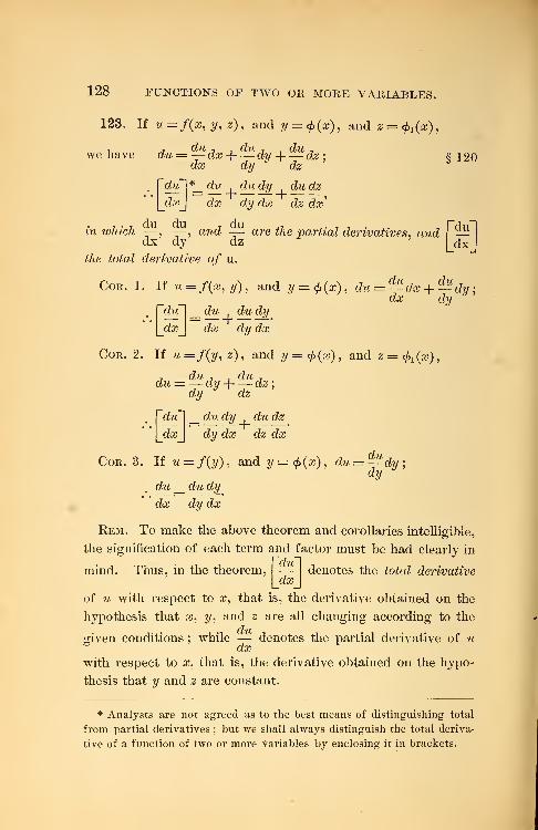
128 FUNCTIONS OF TWO OR MORE VARIABLES.
123. If u=-f(x i y, z), and y = <f>(x), and z =<f>1
(x),
i j du -, du -, . du ,we have du = — dx-\ dy -\ dz; §120
dy dz
du dy du dzVdu~\ *_ du' [_dxj dx
+dy dx dz dx'
in whichdu du du
dx— , and —- are the partial derivatives, anddy dz
the total derivative of u.
du"
dx
Cor. 1. If u=f(x,y), and y = <f>(x), du = —dx + —dy:dx dy
Fdu~\ __du du dy
\_dxj dx dy dx
Cor. 2. If u=f(y, z), and y=<f>(x), and z =<f>1
(x),
, du -, . du -j
du =— dy -\ dz;
dy dz
du
dx
_ du dy du dz
dy dx dz dx
Cor. 3. If u = f(y), and y=<j>(x), du
du _ du dy
dx dy dx
du
dydy;
Rem. To make the above theorem and corollaries intelligible,
the signification of each term and factor must be had clearly in
*~diTmind. Thus, in the theorem,
dxdenotes the total derivative
of u with respect to a?, that is, the derivative obtained on the
hypothesis that x, y, and z are all changing according to the
dugiven conditions ; while — denotes the partial derivative of u
with respect to a?, that is, the derivative obtained on the hypo-
thesis that y and z are constant.
* Analysts are not agreed as to the best means of distinguishing total
from partial derivatives ; but we shall always distinguish the total deriva-
tive of a function of two or more variables by enclosing it in brackets.
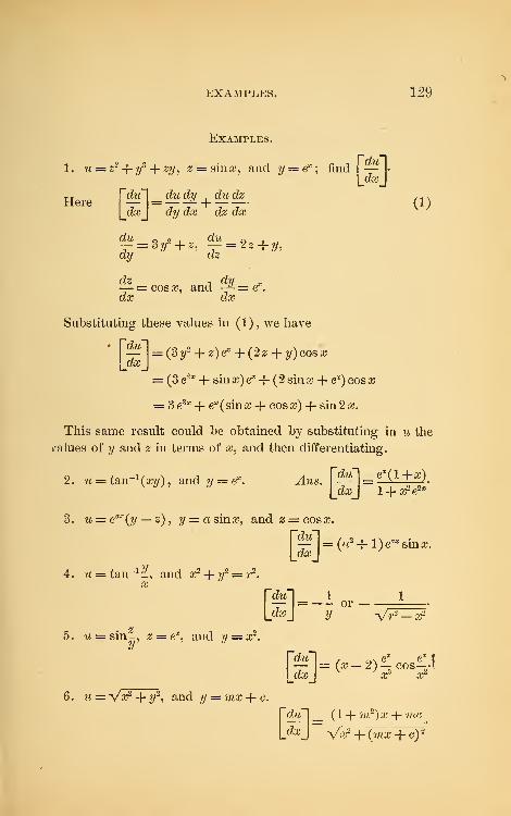
EXAMPLES. 129
Examples.
1. u = z2-r y
s + zy, z = sinx, and y = ex
; find
TT \~du~] dudy . dicdz /iNHere — = *H (1)\_dx_] dy dx dz dx
— = Sy2 + z, — = 2z + y,dy dz
dz , dii ,— = cosoj, and -*-=&'.dx dx
Substituting these values in (1), we have
[^ = (3y*+ z)e* + (2z + y)cos'x
= (3e2x + sin^)ex + (2sinx + ea:)cosa?
= Se3x-\-e
x(sinx-{-cosx) -+- sin 2 x.
This same result could be obtained by substituting in u the
values of y and z in terms of a?, and then differentiating.
2. u = tan" 1 (xy) , and 2/ = ex
. ^4ws. f—1 = g-Ji±g) .
(_(iccj l-j-ar^e2*
3. it = eax(y — z), y = a since, and2=cos#.
r^~| = (a2 + l)e-sin^
4. % = tan _, and #2 4- if = ?-2.
r^i=-ior =1LdajJ y V?-2 -
5. w = sin-, z = ex
, and y = x2.
6. u = -yx2-f- y
2, and y = mx + c.
mc_
— = (x— 2) — cos—-!dx] V J
x* a;2
f^!f~l _ (1 + m2)x + mc
L^J Var -j- (ma? -f- c):
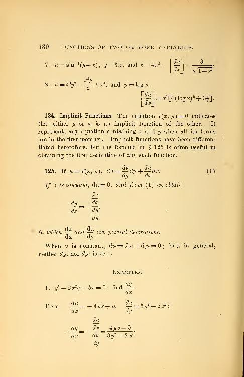
130 FUNCTIONS OF TWO OR MOKE VARIABLES.
7. w = sin 1(y— z), y=3x, and z
a i fdu= 4x3.
—\_clx_ VI -x2
x"yu = a;*?/
2 ^- + x4, and y = logx.
d?£
dxar
1
[4 (log a;)2 + 3£].
124. Implicit Functions. The equation /(oj, y) = indicates
that either y or x is an implicit function of the other. It
represents an}' equation containing x and y when all its terms
are in the first member. Implicit functions have been differen-
tiated heretofore, but the formula in § 125 is often useful in
obtaining the first derivative of an}7 such function.
125. If u=/(a>, ?/), dudu 7 ,
du 7— dy H dx.dy " dx
(i)
If u is constant, du = 0, and from (1) we obtain
du
dy = _dxdx~ du
dy
in which — and — are partial derivatives.dx dy
When u is constant, du = dxu -f- dyw = ; but, in general,
neither dxii nor dyu is zero.
Examples.
1. y3 -2x2
y + bx = 0; find ^-
Here ^=-4^ + 6, ^ = 3 2/2 -2aj2
;
dx d?/
dw-
dy _ dx _ 4yx—bdx~~du
=3y2 -2x2
'
dy
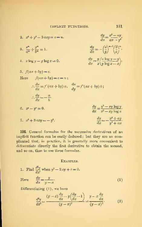
IMPLICIT FUNCTIONS. 131
2. Xs + y3 — 3 axy= c — u.
4. # log y — 2/ logo; = 0.
5. f(ax+by) = c.
Here f(ax -f- 6?/) = c = u;
dy _x2--ay
dx ax -2/2
dy
dx --enSTdy _ 2/ /# log ?/
--.v\
dx a%loga--J
'
' dx/'((MJ + ty) a
dy _t7x
a6*
6. a* — 2/* =
7. a3 + 3 axy == -2/3
-^=f'(ax + by)b;
dv = y2 — qyiogy
,
da; x2 — xy log a;
dy _ cc2 + ay
d"# y2 4- aa;
126. General formulas for the successive derivatives of an
implicit function can be easily deduced ; but they are so com-
plicated that, in practice, it is generally more convenient to
differentiate directly the first derivative to obtain the second,
and so on, than to use these formulas.
Examples.
d2v1 . Find —- when y
2 — 2 xy -j- c = 0.dx2
Here §* = -Z- (1)dx y — x
Differentiating (1), we have
(y — x) ~y~ — y ( -*- — 1) y — x —*-
d2y _ dx
y\dx J _ _
dx
dx2 (y—x) 2 (y-x)~(2)

132 FUNCTIONS OF TWO OR MORE VARIABLES.
From (1), (2), and the given equation, we obtain
d2y _ y
2 — 2 xy _ — c
dtf~\y-xy~ (y-xy
2. Given y2 — 2 axy + x2 — c = 0, to find
a^/#
dx2
d2y _ (a2 - 1) (y
2 - 2 gay + ^2
) = c (a2 - 1)
dx2(y — ctx
)
3( 7/— ax) 3
3. Given y3 + a? — 3 ax?/ = ; show that -~ = —
, 2
a ^x ,*
eta2
(y2 — axy
127. Successive Partial Differentials and Derivatives. If
u—f(x,y), x and y being independent, dBw and dyii are, in
general, functions of both x and ?/. Differentiating dxu and dyw
with respect to either variable, we obtain a class of second par-
tial differentials. Ity differentiating these second partial differ-
entials, we obtain a class of third partial differentials ; and so
on. In finding these successive partial differentials, we regard
dx and dy as constant, since we may suppose x and y to change
uniformly.
The successive partial differentials are represented as follows :
d2u7 I'du 7dx [— dxdx
, ,'du 7
, fd2u 7 .
dj— dy\dy2
A—dy2
dy-
d fdu 7 \ 7
"
= — — ax) dxdx \dx )
=AM dx)dydy\dx J
d fd2u 7 2\ 7
^A(^dy2)dydy\dy2 U
) \
dx2dx2
;
d2u
dxdy
d5u
dy'-dx
dhc
dx dy;
dy2dx;
difdy3 ; etc.
Hence —dxdy2is a symbol for the result obtained by dif-
dxdy2
ferentiating u—f(x,y) three times in succession: first, once
with respect to x, and then twice with respect to y.
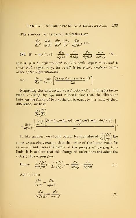
PARTIAL DIFFERENTIALS AND DERIVATIVES. 133
The symbols for the partial derivatives are
dru d2u d2u dht dsu
dor'' dxdy' dy2 ' dar3 ' dx*dy
etc.
1 OR Tf — f( * \^'U
- - ^U < U ^Ut
dydx dxdy' dydx2 dardy'
that is, if u be differentiated m times ivitJi respect to x, and n
times with respect to y, the result is the same, ivhatever be the
order of the differentiations.
Y(x + bx,y)-f(x,y)'
AxFor limit
dx A* = °
Regarding this expression as a function of y, finding its incre-
ment, dividing by Ay, and remembering that the difference
between the limits of two variables is equal to the limit of their
difference, we have
d_(duy
dy\dxj
flimit
[
71*+**, y+Ay)-f(x, y+Ay)-f(x+Ax, y)+f(x, y )
"\
limit \ Ax= o[_ Ax J I
A3/-0^ Ayj
In like manner, we should obtain for the value of — f — ) thedx\dyj
same expression, except that the order of the limits would be
reversed ; but, from the nature of the process of passing to a
limit, it is evident that this change of order does not affect the
value of the expression.
TT d fdu\ d fdu\ d2u d2u , n xHence — — = —f—
], or =
( 1
)
dy\dxj dx\dyj dxdy dydx
Again, since
d2u dru
dxdy dydx"1
d3u d3u
dxdydx dydx2 (2)
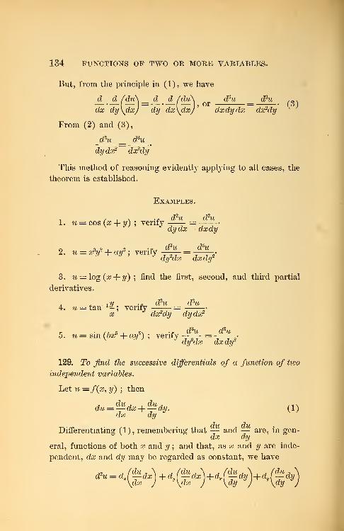
134 FUNCTIONS OF TWO OR MOKE VARIABLES.
But, from the principle in (1), we have
d d (du\ _ d d fdu\ d3u d3u ,„\
dx dy\dx) dy dx\dxj^ dxdydx dx2dy
From (2) and (3),
d3u d3u
dy dx2 dx2dy
This method of reasoning evidently applying to all cases, the
theorem is established.
1
.
u = cos (x -f- y) ; verify
2. u = x'y2-f- ay
5; verify
Examples.
d2u d2u
dydx dxdy
d3u d3u
dy2dx dxdy2
3. u = log (x -\- y) ; find the first, second, and third partial
derivatives.
4. u = tan l ^-; verify
d3u d3u
5. u = sin (bx5 -f ay5) ; verify
dx2dy dy dx2
dhi d3u
dyhlx dx dy*
129. To find the successive differentials of a function of two
independent variables.
Let u =/(#, y) ; then
du =— dx + ^dy. (1)dx dy
du duDifferentiating (1), remembering that — and — are, in gen-
eral, functions of both x and y ; and that, as x and y are inde-
pendent, dx and dy may be regarded as constant, we have
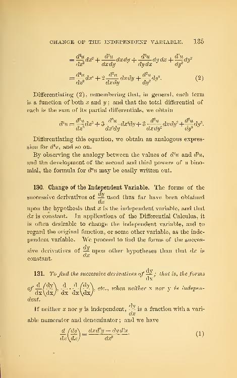
CHANGE OF THE INDEPENDENT VARIABLE. 135
d2u-,o ,dru , , . dru 7 7 . dru , 2=— dor -\ dxdy -\ dydx -\ dy-
dx- dxdy dydx dy
= ^dx* + 2£L dxdy + f^<%2
. (2)
Differentiating (2), remembering that, in general, each term
is a function of both x and y ; and that the total differential of
each is the sum of its partial differentials, we obtain
$u = —da? + 3 -^dx2dy+ 3-^ dxdy2+—dtf.dx? dx2dy dxdy dy2.
Differentiating this equation, we obtain an analogous expres-
sion for dhi, and so on.
B}r observing the analogy between the values of d2u and d3u,
and the development of the second and third powers of a bino-
mial, the formula for dnu may be easily written out.
130. Change of the Independent Variable. The forms of the
successive derivatives of -^ used thus far have been obtaineddx
upon the hypothesis that x is the independent variable, and that
dx is constant. In applications of the Differential Calculus, it
is often desirable to change the independent variable, and to
regard the original function, or some other variable, as the inde-
pendent variable. We proceed to find the forms of the succes-
dusive derivatives of -£ upon other hypotheses than that dx is
constant.
131. To find the successive derivatives of —2 ; that is, the formsdx
of—(— ],— • —f— 1, etc., when neither x nor y is indepen-J
dxVdx/ dx dxVdx/dent.
If neither x nor y is independent, -^ is a fraction with a vari-dx
able numerator and denominator ; and we have
d fdy\ __ dxdry — dydrx ,1
v
dxldx
J
dxs ^j
136 CHANGE OF THE INDEPENDENT VARIABLE.
Differentiating (1), we obtain
d__d_ fdy\ _ _d_ fdxd2
y — dy d2x
dx dx\dxj dx\ dx"
_ ( d"y dx—
d
sx dy) dx—3(
d
2y dx—
d
2x dy ) d2x (i> .
dx5 {' }
In like manner, we obtain the other successive derivatives.
Cor. 1. If y is independent, that is, if dy is constant,
d2y = 0, and dsy = 0,
and (1) and (2) become
d fdy\ = d2xdy(
.
dx\dx) cW ' K }
i sL - f^v\ — - ( c^2a;)2c^ ~ ^x
c
ty ^x (±\dx dx\dxj dx5
Cor. 2. If dx is constant, d2£ = <#U'=0, and (1) and (2)
become
A(dy) = S, and —~(r^\ = ^Vdx\dxj dx2
"1
dx dx\dx) dx^
which agrees with § 74.
Rem. Hence, to transform a differential expression in which
x is independent, into its equivalent in which neither x nor y is
independent, we replace —-,—«, etc., bv their equivalents upon
dx~ dx3
the new hypothesis, which are found in (1), (2), etc.
If, in the transformed expression, a new variable #, of which
x is a function, is to be the independent variable, in the general
result obtained above we replace x, dx, d2x, etc. , by their values
in terms of and its differentials.
If y is to be the independent variable, in the given expression
dry d?vwe replace —~, —^ etc., by their equivalents in (3) , (4) , etc. ; or,
CIX" CIX
in the general result first obtained above, we put d2y = 0, ds
y = 0,
etc.
EXAMPLES. 137
Examples.
1. Given yd2y -f dy2 + dx2 =0, in which x is independent, to
find the transformed equation in which neither x nor y is inde-
pendent ; also the one in which y is independent.
Dividing both members by dx2, substituting for —* the sec-B J to
dx2
ond member of (1), § 131, and multiplying both members by
dx3 , we have
y(d2ydx — d2xdy) + dy2dx-\- dx3 = 0,
in which neither x nor y is independent.
Putting d2y = 0, and dividing by — dy3
, we have
dy2 dy3 dy
in which the position of dy indicates that y is independent.
2. Given —^ -^ + —^— =0, in which x is indepen-dxr 1 —x? dx 1 — x2
dent, to find the transformed equation when x = cos 0, and is
independent.
drySubstituting for —% the second member of (1), we have
dx2
d2ydx — d2xdy x dy V _ q /-i\'
dx31 - x2 dx 1 - x2 ~ ' ^
j
Since a; = cos 0, 1 — #2 = sin20,
cZic = — sin dO, and fe = — cos d62.
Substituting these values in (1), and simplifying, we have
in which 6 is independent.
138 CHANGE OE THE INDEPENDENT VARIABLE.
3. Given B =1 + df
dx2
in which x is independent, to finddry
dx2
the value of R when .T = pcos0, 2/ = psin#, and 6 is inde-
pendent.
From (1), § 131,
R = {dx> + dy2)%
^
_dx d2
y — dy d2x'
in which neither x nor y is independent.
From y = p sin#, and x = p cos 0, we obtain
cfa/ == sin 6dp-\- p cos d#,
dx = cos Odp — ps'mO dO,
d2y = sin 0d2
p + 2 cos (9 d<9 dp - p sin 6 dO2,
and d2# = cos d2p — 2 sin dO dp — p cos d#2
.
Substituting these values in (1), and simplifying, we have
+p2dldO2
p+d02 P
d0>
4. Given —%-\ ^-f2/ = 0, to find the transformed equa-dx2 xdx
tion when x2 — 42, and z is independent.
dz- dz
5. Given (1 - x2)^ - x^- = , to find the transformeddxr dx
equation when x = cos 2, and 2 is independent.
6. Given 2 = '
—
" ~^— , to find the transformed equationydy -f- #dsc
when # = p cos 0, y = p sin 0, and p is independent.
Ans. z= *f-dp
CHAPTER X.
TANGENTS, NORMALS, AND ASYMPTOTES.
132. The Rectangular Equation of the Tangent to any plane
curve at (x\ y') is
dv'*y-y'=-^(v-x')' (a)
For line (a) passes through {x\ y') ; and, by § 16, it has the
slope of the curve at (V, y').
dv'Cor. When the axes are oblique, — is evidently the ratio
dx'
of the sines of the angles which the curve at (V, y') makes with
the axes ; hence, in this case also, («) is the equation of the
tangent.
133. The Rectangular Equation of the Normal to any plane
curve at (V, y') is
y-y'---^-,(x-x'). (b)
For, the axes being rectangular, line (b) is perpendicular to
line (a) of § 132, and therefore to the curve, at (x 1
,y').
Examples.
1. Find the equations of the tangent and normal to the
parabola y2 = 2px.
Here *L=l; .:*>!-?dx y dx' y'
— represents the value ofc-^ at the point (x'
} y').dx' dx
140 TANGENTS, NORMALS, AND ASYMPTOTES.
civ'This value of —
(substituted in (a) of § 132, and (b) of
dx'
§ 133, gives
jf-y'= J(*-«'). (i)
y'
and y-y'=--(x-x'),
as the equations of the tangent and normal respectively.
Since y' 2 = 2px', equation (1) by reduction becomes
yy'=p{x + x').
2. Find the equations of the tangent and normal to the circle9 i 9 9
xr -\-y = r.
vr
Ans. yy' -{- xx f= ^; y = —
fx.
x
3. Find the equations of the tangent and normal to the
ellipse a2
y2 + 6
2ar = orb
2.
Ans. a2yy'-\- b
2xx'= orb2
; y — y'= —f- (x — x')
.
4. Find the equations of the tangent and normal to the
hyperbola a2
y2 — b
2a? = — a2
b2
.
Ans. a2yy'— b
2xx'= — a2b2
; y — y'= — -f- (x — x')
.
b~x'
5. Find the equations of the tangent and normal to the cis-
soid y2 —
2a — x A ,.x'zCSa — x'),
,NAns. y — y' = ± —* —'- (x — x');J J
(2a-x')i V ;
, (2 a — x') i , , x
x'*(3a — x')
6. Find the equation of the tangent to y2 = 2 x2 — x2, at x = 1.
Ans. y = ix + i', y = — \x — \.
7. Find the equation of the normal to y2 — 6 x — 5 at y = 5.
Ans. y = — f»H-^.
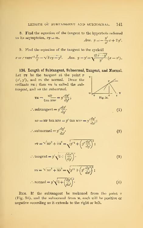
LENGTH OF SUBTANGENT AND SUBNORMAL. 141
8. Find the equation of the tangent to the hyperbola referred
to its asymptotes, xy = m. ^ y =_^x+2y ,_
X
9. Find the equation of the tangent to the cycloid
x = '.* vers-1—— V 2 ry — y
2. Ans. y — ?/'= A/ j-^- (x — x') .
134. Length of Subtangent, Subnormal, Tangent, and NormalLet pt be the tangent at the point p
(x',y'), and ps the normal. Draw the
ordinate pm ; then tm is called the sub-
tangent, and ms the subnormal.
mp , dx f
tm = = y —-
;
tan mtp dy'
dx'subtangent = y'—-• (I)
dy' v '
ms = mp tan mps = y' tan mtp = y' -&-;* J
dx'?
subnormal = y'—' (2)dx' v 7
PT =VMP"' -f- TM2 = Ay' 2
-j-( l
,dxy'
dy'J;
•. tangent =^l+^;j- (3)
ps = V^p2 + ms2
=-\jy'2 + (V j-A ;
.-.normal = 2/^1+^. (4)
Rem. If the subtangent be reckoned from the point t
(Fig. 34), and the subnormal from m, each will be positive or
negative according as it extends to the right or left.
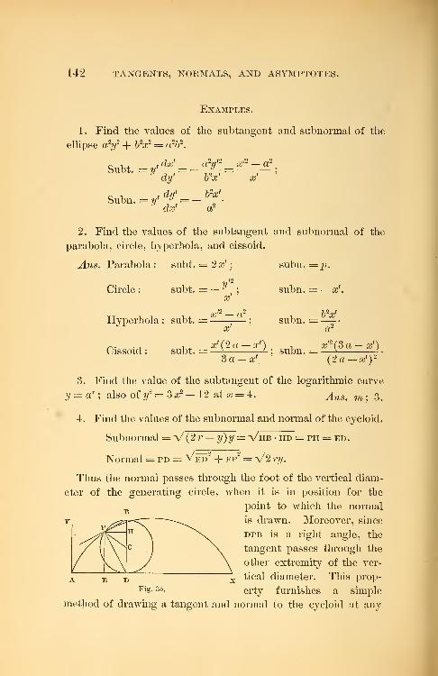
142 TANGENTS, NORMALS, AND ASYMPTOTES.
Examples.
1. Find the values of the subtangent and subnormal of the
ellipse a2
y2 + b
2ar = orb2
.
c , , , dx' cry'2
x'2 — a2
Subt - =?/ ^ =-^v
= ^r- ;
o x. idif b
2x'
2. Find the values of the subtangent and subnormal of the
parabola, circle, hyperbola, and cissoid.
Ans. Parabola : subt. = 2x';
subn. =p.
Circle : subt. = — ^—
;
subn. = — x'.x'
»'2 2 7,2 I
Hyperbola : subt. = —;
subn. =x' or
n . ., ,, x'(2a-x') , x'2(3a-x')
Cissoid : subt. =—* -; subn. =—* '- .
3 a -x[ (2a-x') 2
3. Find the value of the subtangent of the logarithmic curve
y = ax; also of y
2 = Sx2 — 12 at a;= 4. ^ns. m; 3<
4. Find the values of the subnormal and normal of the cycloid.
Subnormal =V (2 r — y)y = Vhb • hd = ph = ed,
Normal = pd= v ed + ep" = a/2 ry.
Thus the normal passes through the foot of the vertical diam-
eter of the generating circle, when it is in position for the
point to which the normal
T, „ /^T*^ ~~~~-\ *s drawn. Moreover, since
dpb is a right angle, the
tangent passes through the
other extremity of the ver-
, tical diameter. This prop-
erty furnishes a simple
method of drawing a tangent and normal to the cycloid at any
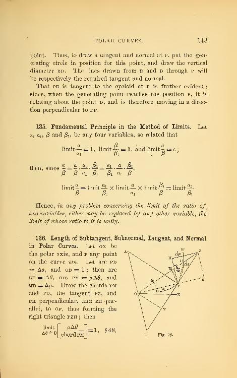
POLAR CURVES. 143
point. Thus, to draw a tangent and normal at p, put the gen-
erating circle in position for this point, and draw the vertical
diameter bd. The lines drawn from b and d through p will
be respectively the required tangent and normal.
That pb is tangent to the cycloid at p is further evident;
since, when the generating point reaches the position p, it is
rotating about the point d, and is therefore moving in a direc-
tion perpendicular to dp.
135. Fundamental Principle in the Method of Limits. Let
a, an /5 and /5 15 be any four variables, so related that
limit— = 1 , limit -=- = 1 , and limit -5 = c :
a a ay fii ax a fi1
limit- = limit -^ X limit— x limit^ = limit-^--
P . Pi - *i P Pi
then, since
Hence, in any problem concerning the limit of the ratio of
two variables, either may be replaced by any other variable, the
limit ofivhose ratio to it is unity.
136. Length of Subtangent, Subnormal, Tangent, and Normal
in Polar Curves. Let ox be
the polar axis, and p an}' point
on the curve mn. Let arc pd
= As, and ob then arc
be = A0, arc pm = pA0, and
md = Ap. Draw the chords pmand pd, the tangent pz, and
ph perpendicular, and zh par-
allel, to op, thus forming the
right triangle pzh ; then
PA0limit
A0 = O chordPM=1, §48.
Fig. 36*
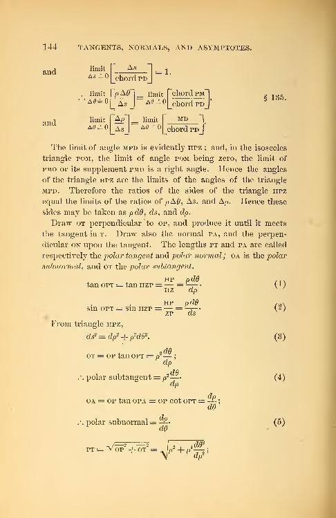
144 TANGENTS, NORMALS, AND ASYMPTOTES.
and
and
limit As —]
As = chord pd
limit
A0=O>A<9~
_ As_,
limit~~ A6 =
limit
A9 =rAp-
Aslimit
~ A9 =
chord pm"
chord pd§ 135.
MDchord pd}
The limit of angle mpd is evidently hpz ; and, in the isosceles
triangle pom, the limit of angle pom being zero, the limit of
pmo or its supplement pmd is a right angle. Hence the angles
of the triangle hpz are the limits of the angles of the triangle
mpd. Therefore the ratios of the sides of the triangle hpz
equal the limits of the ratios of />A0, As, and A,o. Hence these
sides may be taken as pdO, ds, and dp.
Draw ot perpendicular to op, and produce it until it meets
the tangent in t. Draw also the normal pa, and the perpen-
dicular on upon the tangent. The lengths pt and pa are called
respectively the polar tangent and polar normal; oa is the polar
subnormal, and ot the polar sabtangent.
P d0tan opt = tan hzp =— =
hz dp
HP dOsin opt = sin hzp
ZP ds'
From triangle
ds2 =HPZ,
dp2 + PW.
0T = op tan opt = 2 d0
dp
.*. polai subtangent 2 d0= p"—Hdp
OA = op tan opa =- OP COt OPT = dp.
dOJ
.*. polai
PT =
subnormal =_dp.
=
do'
V OP + OT =-Jp2 +,d02
PT-9 j
(1)
(2)
(3)
(4)
(5)
dp2
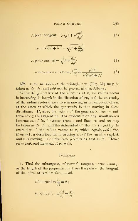
POLAR CURVES. 145
.*. polar tangent = p-v/l + p2
-rr (6)\ dp-
.-. polar normal = -Jp2 + -£ (7)
oup p"Clu /o\« = on = OP Sill OPT = pz— = — r — (o)
137. That the sides of the triangle pzh (Fig. 36) may be
taken as ds, dp, and pdO can be proved also as follows :
When the generatrix of the curve is at p, the radius vector
is increasing in length in the direction of pr, and the extremity
of the radius vector drawn to p is moving in the direction of ph,
at the rates at which the generatrix is then moving in these
directions. If, at p, the motion of the generatrix became uni-
form along the tangent pz, it is evident that any simultaneous
increments of its distances from p and lines ph and or maybe taken as ds, dp, and the differential of the arc traced by the
extremity of the radius vector to p, which equals pdO; for,
if ob = 1, b describes the measuring arc of the variable angle 0,
and p is moving, as op revolves, p times as fast as b. Hence
ph = pdO, and hz = dp, if pz = ds.
Examples.
1. Find the subtangent, subnormal, tangent, normal, and 7?,
or the length of the perpendicular from the pole to the tangent,
of the spiral of Archimedes p = aO.
subnormal =— = a;
dO
subtangent = p2^ =^
;
dp a
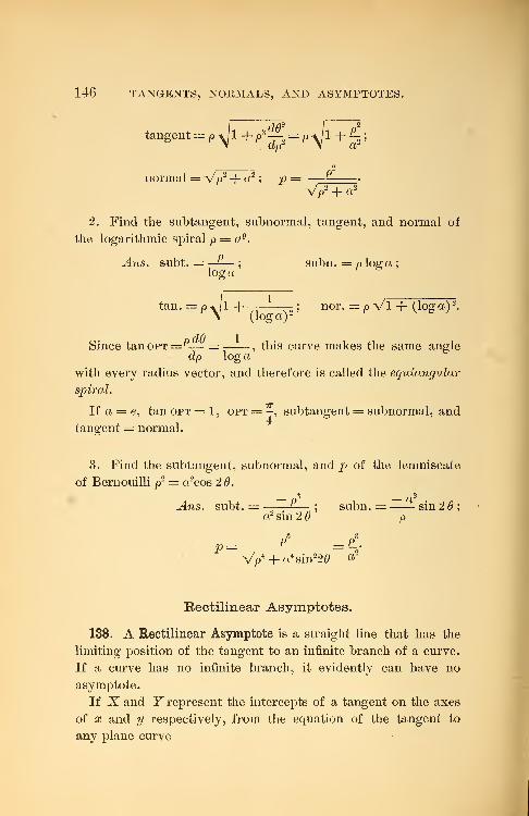
146 TANGENTS, NORMALS, AND ASYMPTOTES.
tangent = p^jl + p2— = pyjl + ^ ;
2
normal = V/o2-\-a2
', j9 = —^—
Vp2 + a2
2. Find the subtangent, subnormal, tangent, and normal of
the logarithmic spiral p = a 9.
Ans. subt. = ——;
subn. = p log a;
log a
tan. = pil + - ; nor. = p VI + (log a) 2.
\ (loga)^
Since tan opt =^— =, this curve makes the same angle
dp log a
with every radius vector, and therefore is called the equiangular
spiral.
If a = e, tan opt == 1, opt = -, subtangent = subnormal, and
tangent = normal.
3. Find the subtangent, subnormal, and p of the lemniscate
of Bernouilli p2 = a 2cos 20.
— os —a2
Ans. subt. = H—; subn. = sin 2
;
a2 sin 2 p
P3
Ps
V^-f «4 sin220 «
Rectilinear Asymptotes.
138. A Rectilinear Asymptote is a straight line that has the
limiting position of the tangent to an infinite branch of a curve.
If a curve has no infinite branch, it evidently can have no
asymptote.
If X and Y represent the intercepts of a tangent on the axes
of x and y respectively, from the equation of the tangent to
any plane curve
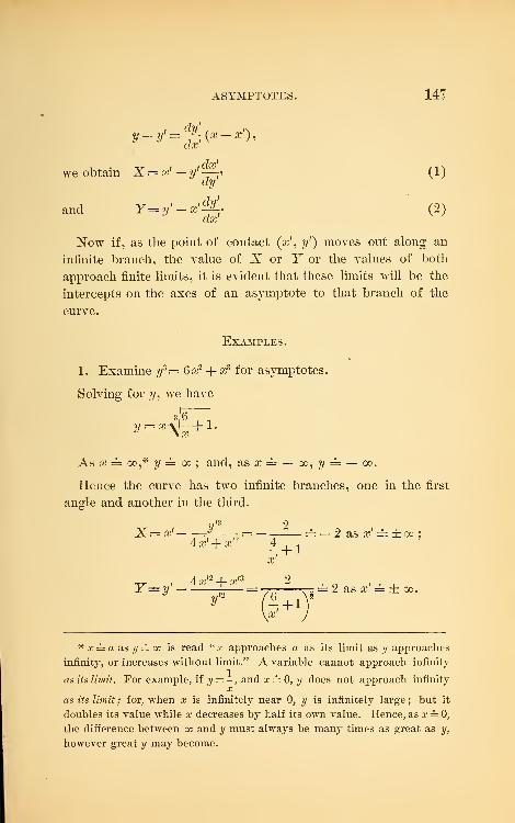
ASYMPTOTES. 147
dx'
dx'we obtain X=x t — y
,-—i (1)dy'
and Y=y'-x' c^. (2)dx
Now if, as the point of contact (V, y') moves out along an
infinite branch, the value of X or Y or the values of both
approach finite limits, it is evident that these limits will be the
intercepts on the axes of an asymptote to that branch of the
curve.
Examples.
1 . Examine ys= 6x? + Xs for asymptotes.
Solving for y, we have
2/ =*% +\x
As x == co,* y = oo ; and, as#= — oc,?/= — oo.
Hence the curve has two infinite branches, one in the first
angle and another in the third.
v'3 2X=x' rf- - = — = — 2 as x' = ± oo
;
Ax'+x'2 liix'
Y= y' ^— = 77 v»= 2 as x' — ± oo.
+1 "
a;
* x = a as y= oo is read "x approaches a as its limit as y approaches
infinity, or increases without limit." A variable cannot approach infinity
as its limit. For example, if y= -, and x = 0, y does not approach infinityx
as its limit ; for, when x is infinitely near 0, y is infinitely large ; but it
doubles its value while x decreases by half its own value. Hence, as x = 0,
the difference between oo and y must always be many times as great as y,
however great y may become.
148 ' TANGENTS, NORMALS, AND ASYMPTOTES.
Therefore, the line y'
— x + 2, whose intercepts on the axes of
x and y are respectively — 2 and 2, is an asymptote to each
branch.
2. Examine the conic sections for asymptotes.
Neither the circle nor the ellipse can have an asymptote, since
neither has an infinite branch.
The parabola has two infinite branches, one in the first angle
and another in the fourth.
v'2
Here X= x' = — x'= — oo as x'= go;
P
,px' y'
and Y=y' r = — = oo as x' = go .
Hence the parabola has no asymptote.
The hyperbola has four infinite branches, one in each angle.
In this curve
X= x' J— =— = ± as x'= ± oo;
IrxJ x'
T-,2 12 7 2
Y= y' ^— = = ± as x' or ?/'= ± co.
cry' y'
Hence the asymptote to each branch passes through the ori-
gin. To determine the direction of these asymptotes, we have
-f-t
=—-- = ± = ± — as x' = ± oo.
clx' cry'| a2 a4-5
b2x'
Since —- is positive for anv point in the first or third angle,a2y'
"
band negative for any point in the second or fourth, y = -x is
the asymptote to the branches in the first and the third angle, and
y — x to those in the second and the fourth. These asymp-
totes are evidently the produced diagonals of the rectangle on
the axes.
3. Prove that y — — x is an asymptote to each of the two
infinite branches of \f = a3 — x3.
ASYMPTOTES. 149
4. Show that y2 = ax" has do asymptotes.
139. Asymptotes Determined by Inspection or Expansion.
From the definition of an asymptote, it follows that it is a line
which an infinite branch of a curve approaches indefinitely
near, but never reaches. From this view of asymptotes, we
can often determine their equations by inspecting the equation
of the curve, or expanding one of its members. Thus, in the
cissoid
x3y2 =
, y = ± oo as x = 2 a.2a — x
Whence, x = 2a is an asymptote to the two infinite branches of
the curve ; for they approach indefinitely near, but never reach,
this line.
In x = loga y, or y = ax,x = — cK as y = 0. The axis of x is
therefore an asymptote to the infinite branch in the second
angle.
Again, the equation xy — ay—bx=0 may be put in the
form,bx ay
y = or x =—£-,x — a y — o
from which we know that x = a and y = b each is an asymptote
to two infinite branches.
The method of examining a curve for asymptotes by solving
its equation for y, and then developing the second member in
descending powers of x, by Maclaurin's formula or some other
means, will be illustrated by a few examples.*
* The following is a brief view of another method of examining a curve
for asymptotes. For a fuller treatment, see Williamson's Differential
Calculus, page 240.
Let the equation of a right line be
y = ixx+v\ (1)
that of a curve of the nth degree,
f(*,y)=0; (2)
that obtained by substituting ux + v for y in (2),
*(x) = 0. (3)
150 TANGENTS, NORMALS, AND ASYMPTOTES.
Examples.
1. Examine x" — xy2 + ay2 = for asymptotes.
Here y=±x( ) == ± x 1 1* \x — aJ \
. /., . a . 3 or .
From the first form of the value of y, x = a is evidently an
asymptote to two branches of the curve that lie to the right of it.
From the last form we see that two branches of the curve ap-
proach infinitely near each of the lines y = ± x ± -, as x = ± go.
The curve therefore has three asymptotes, each of which is
asymptotic to two infinite branches.
Equation (3) is evidently of the nth degree, and its n roots are the
abscissas of the n real or imaginary intersections of (1) and (2). If two
roots of (3) be equal, two points of intersection of (1) and (2) will coincide,
and, in general, (1) will be a tangent to (2). From Algebra, we know that,
as the coefficients of xn and xn~ l approach zero as a limit, two roots of (3)
increase without limit. Hence, if fi and v in (1) have such values as ren-
der these coefficients 0, (1) has the limiting position of a tangent to an
infinite branch, or is an asymptote.
For example, let the curve be
ys= ax1
-f xs. ( 1
)
Substituting /j.x+ v for y, and arranging the terms, we have
(/t8 — l)a:3 + (3^-a)x2 +3
/uj/
2j:+^ = 0. (2)
Two roots of (2) become oo, when ^u8 — 1 — 0, and S/x2v — a = 0; that is,
when fi= 1, and v— \a. Hence, y — x +£ a is an asymptote to ( 1 )
.
From the theory of equations, and this theory of asymptotes, the fol-
lowing are obvious conclusions
:
(a) Any asymptote or tangent to a curve of the third degree intersects
the curve in one, and only one, point.
(b) Any asymptote or tangent to a curve of the nth degree cannot meet
it in more than n — 2 points, exclusive of the point of contact.
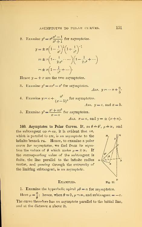
ASYMPTOTES TO POLAR CURVES. 151
2. Examine y2 = x?
&* + !for asymptotes.
l~i)M= ±Xll-2? + "
Hence y = ± x are the two asymptotes.
3. Examine y3 = a a;
2 — x3 for asymptotes.vl?is. y — — x +
4. Examine y = c -f-
(a- ft)1
for asymptotes.
5. Examine ?/2 or
3 + ax2
x — a
Ans. y = c, and x = b.
for asymptotes.
^ws. a; = a, and y = ± (a? + a)
.
140. Asymptotes to Polar Curves. If, as0 = f
,p=oo, and
the subtangent od = os, it is evident that sn,
which is parallel to om, is an asymptote to the
infinite branch pk. Hence, to examine a polar
curve for asymptotes, we find from its equa-
tion the values of which make p = ±oo. If
the corresponding value of the subtangent is
finite, the line parallel to the infinite radius
vector, and passing through the extremity of
the limiting subtangent, is an asymptote.
Examples. Fig. 37.
1. Examine the hyperbolic spiral pO = a for asymptotes.
Here p = -; hence, when = 0, p — oo, and subtangent = — a.
The curve therefore has an asymptote parallel to the initial line,
and at the distance a above it.
152 TANGENTS, NORMALS, AND ASYMPTOTES.
2. Examine p cos = a cos 2 for asymptotes.
Here p = ^L22?L_; hence, when = -, p = ± go, and subtan-
cos# 2
gent = — a.
The line perpendicular to the initial line at the distance a to
the left of the pole is therefore an asymptote to two infinite
branches.
3. Examine p2 cos $ = a2
sin 3 6 for asymptotes.
Ans. The perpendicular to the initial line at the origin is an
asymptote.
4. Show that the initial line is an asymptote to the lituus
pV# = a.
Miscellaneous Examples.
1. At what angle does y2= 10 x intersect x2
-f- y2 — 144 ?
Ans. 71°0'58".
2. Find the subnormal of the curve y2 = 2 a2 log a;.
Ans. —
3. Find the equation of the tangent to the curve
^{x + y) = a2 (x — y) at the origin.
Ans. y = x.
4. Find ad what angle the curve y2 =2ctx cuts the curve
x3 — 3 axy -\-y3 = 0.
Ans. 0, -^-7T, cot_1V4.
5. Find the normal, subnormal, tangent, and subtangent of
X X
the catenary y = - (ea + e ")
.
u2x 2x o
a — VAns. Subn. =-(e a — e
a) : norm. = i_-
4V y a
8Ubt. = ay;
tan.=y2 -
s/tf-a2 -Vy2-a2
6. Find the subtangeut of the curve y
EXAMPLES o 153
Xs
a — x
Ans. M^^lSa-2x
7. Examine y2 (x — 2«) = Xs — a3 for asymptotes.
Ans. x = 2a; y = ±(x-{-a).
8. Examine y(a2 — or) = 62 (2a? -f- e) for asymptotes.
Ans. y = 0; x-\-a = ; x— a.
9. Examine for asymptotes the folium of Descartes,
x? + ys — 3axy = 0.
Ans. y = — x — a.
10. Examine (y2 — l)y = (x2 — 4)<b for asymptotes.
Ans. y = x.
11 t. • c a2(a;-o)(a;-3a) . , ,
11. Examine y*=—* —-*-* - for asymptotes.x~ — 2 a#
^1«.5. a?= 2 a ; a? = ; y = ±a.
12. Examine the hyperbola p =—*———— for asymptotes.e cos 0—1
13. Find the length of the perpendicular from the pole upon
the tangent to the lituus pV# = a. *r
2a 2p
V/o4+ 4a4
14. In the hypocycloid xi -f-yi = at, prove that the portion
of the tangent intercepted between the axes equals a.
15. Give the different methods of drawing a tangent to any
plane curve at a given point.
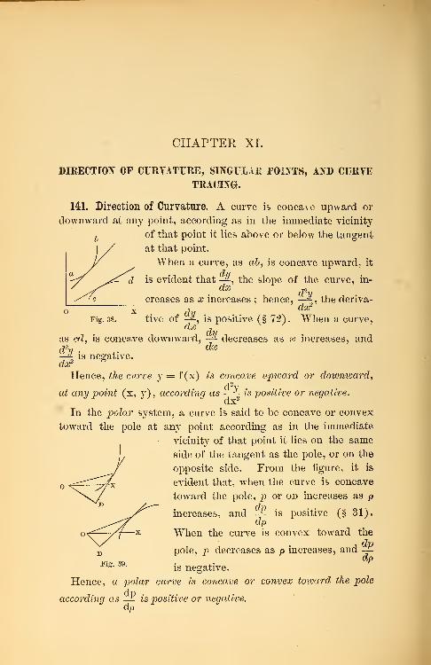
CHAPTER XI.
DIRECTION OF CURYATURE, SINGULAR POINTS, AND CURYETRACING.
141. Direction of Curvature. A curve is concave upward or
downward at any point, according as in the immediate vicinity
of that point it lies above or below the tangent
at that point.
When a curve, as ab, is concave upward, it
is evident that -£, the slope of the curve, in-iXJb -jo
creases as x increases ; hence, —". the deriva-
° x dvFig. 38. tive of -£, is positive (§ 72). When a curve,
dx ,
as cd, is concave downward, —^ decreases as x increases, and
—4 is negative.dx2 &
Hence, the curve y = f(x) is concave upward or downward,
at any point (x, y), according as —^ is positive or negative.
In the polar system, a curve is said to be concave or convex
toward the pole at any point according as in the immediate
vicinity of that point it lies on the same
side of the tangent as the pole, or on the
opposite side. From the figure, it is
evident that, when the curve is concave
toward the pole, p or od increases as p
increases, and -£ is positive (§ 31).dp
When the curve is convex toward the
pole, p decreases as p increases, and -J-
Fig.is negative.
dp
Hence, a polar curve is concave or convex toivard the pole
according as — is positive or negative.
EXAMPLES. 155
When the equation of the curve is given in terms of p and 0,
we findp in terms of p by use of (8) of § 136.
Examples.
1. Find the direction of curvature of y — x2 -}-2x -\- 5.
Here —% = 2 ; hence the curve is concave upward.dx2
2. Find the direction of curvature of y= a + c(x+ b) 3.
d2v
Here —^-— 6c(x -\-b) ; hence the curve is concave upward ordxr
downward at (a,*, y), according asa;> or < — b.
3. Find the direction of curvature of y = x? — Sx2 — 9 # -|- 9.
Ans. Concave upward or downward according as x> or <1.
4. Find the direction of curvature of x = \oga y, and y = sinx.
5. Find the direction of curvature of the lituus p2 — a2
.
Here &= *- =--£•M6iedO 2 P 2 a2 '
p2 2a2
P
ap
cW2
J 2 ,<¥ V4a*+ P*'
\r Tdfi2
• dp = 2a2(4,a
i -Pi)
' 'dp (4a4 +p4)f '
Hence this spiral is concave or convex toward the pole at (0,p)
according as p < or > aV2.
6. Find the direction of curvature of the logarithmic spiral
p = a9.
Here p = —VI + (loga) 2 dP Vl -f (log a)
2
Hence the curve is concave toward the pole.
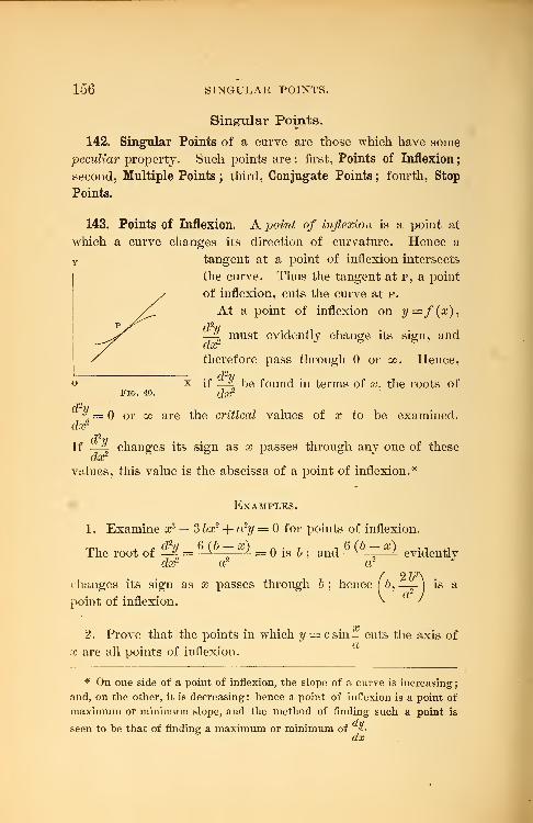
156 SINGULAR POINTS.
Singular Points.
142. Singular Points of a curve are those which have some
peculiar property. Such points are : first, Points of Inflexion;
second, Multiple Points ; third, Conjugate Points ; fourth, Stop
Points.
143. Points of Inflexion. A point of inflexion is a point at
which a curve changes its direction of curvature. Hence a
Y tangent at a point of inflexion intersects
the curve. Thus the tangent at p, a point
of inflexion, cuts the curve at p.
At a point of inflexion on y=f(x),d2v—? must evidently change its sign, and
therefore pass through or oo. Hence,
Fig. 40.if
dx2be found in terms of x. the roots of
dx1
if ^idx2
or oo are the critical values of x to be examined.
changes its sign as x passes through any one of these
values, this value is the abscissa of a point of inflexion.'
Examples.
1 . Examine xJ — Sbx2 + a 2y = for points of inflexion.
rr , , » dhi 6 (b — x) A . , , 6 (b — x)The root of —| = —*—-
—
L = is b ; and —*—-
—
'-
dx2ddently
changes its sign as x passes through b ; hence (b, —_j is a
point of inflexion.
2 b3
x2. Prove that the points in which y = csin- cuts the axis of
a; are all points of inflexion.
* On one side of a point of inflexion, the slope of a curve is increasing
;
and, on the other, it is decreasing : hence a point of inflexion is a point of
maximum or minimum slope, and the method of finding such a point is
seen to be that of finding a maximum or minimum of iii.
dx
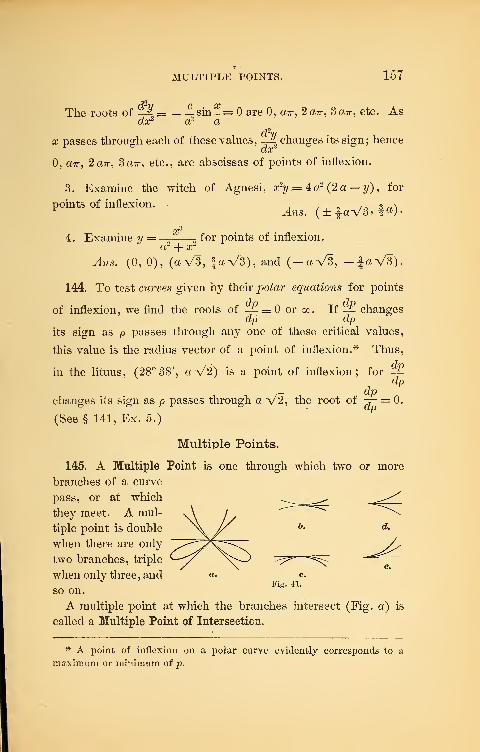
MULTIPLE POINTS. 157
The roots of —^ = — —sm- = are 0, cm-, 2arr, Sair, etc. Asdx2 a" a
x passes through each of these values, —| chauges its sign; hence
0, a7r, 2a7r, 3a7r, etc., are abscissas of points of inflexion.
3. Examine the witch of Agnesi, x2y — 4
a
2(2 a — ?/), for
points of inflexion.^„s . (± |aV3, f «)•
4. Examine ?/ = for points of inflexion.a2
-f- x2
Ans. (0, 0), (a V3, faV3), and (.-a.V8, -faV3).
144. To test curves given by their po/ar equations for points
of inflexion, we find the roots of — = or oo. If -±- changesdp dp
its sign as p passes through any one of these critical values,
this value is the radius vector of a point of inflexion.* Thus,
in the lituus, (28° 38', aV2) is a point of inflexion; for -£dp
- dpchanges its sign as p passes through a V2, the root of -p = 0.
(See § 141, Ex. 5.)
Multiple Points.
145. A Multiple Point is one through which two or more
branches of a curve
pass, or at which
they meet. A mul-
tiple point is double
when there are only
two branches, triple <—/^/ ^^-^when only three, and «• «.
J '
Fig. 41.
so on.
A multiple point at which the branches intersect (Fig. a) is
called a Multiple Point of Intersection.
* A point of inflexion on a polar curve evidently corresponds to a
maximum or minimum of p.
158 SINGULAR POINTS.
A multiple point through which two branches pass, and at
which they are tangent (Figs. b, c) is an Osculating Point.
A multiple point at which two branches terminate, and are
tangent (Figs, d, e) is a Cusp. A cusp or osculating point is
said to be of the first or the second species, according as the
two branches are on opposite sides (Figs, b, d) or the same side
(Figs, c, e) of their common tangent.
A Conjugate Point is one that is entirely isolated from the
rest of the real locus. Hence, in an algebraic curve, a conju-
gate point is a multiple point formed by the intersection or
meeting, in the plane of the axes, of imaginary branches ; that
is, of branches lying outside of the plane of the axes. Since
an odd number of roots of an algebraic equation cannot be
imaginary, an even number of imaginary branches must inter-
sect or touch in a conjugate point of an algebraic curve.
146. From the definitions given above, it follows that, at a
multiple point of intersection, —" must have two or more un-
equal real values ; that, at a point of osculation or a cusp it
must have two equal real values ; that, at a conjugate point on
an algebraic curve, it must have two or more values which .are
imaginary, unless the tangents to the imaginary branches at the
conjugate point lie in the plane of the axes.
Hence at any multiple point -*- has two or more values.dx
147. If f(x, y) = u = be tlie algebraic equation of a curve
freed from radicals and fractions ; at any multiple point upon the
curve,
du
dy__dx_0ydu _du _ ^
dx du 0' dx dy
dy
For, at anv multiple point, — , or the ratio of — to — , mustdx dx dy
have two or more values (§ 146) . But, from the form of the
MULTIPLE POINTS. 159
du duequation of the curve, neither — nor — can contain radicals or
dx dy
fractions ; hence their ratio can have two or more values for the
same values of x and y, only when it assumes the indeterminate
form —
148. Examination of a Curve for Multiple Points. To examine
a curve for multiple points, put its equation in the required form
f(x, y) = u = Q, and find the sets of values of x and y that will
satisfy the equations — = and — = 0. Of these sets, thoseJ ^dx dy
which satisfy the equation of the curve give the points to be
examined.
Let (#', y') be one of these points ; then
du
cit = - — = 9.
dx'~ dw~~0'
dy'
which is evaluated according to the method of § 83.
du'I. If -sL has two or more unequal real values, (x 1
, y') is in(XX
general a multiple point of intersection.
II. If -^- has two equal real values, (V, y') is in generaldx'
either an osculating point or a cusp.
III. If all the values of -^- are imaginary, (x', y') is a con-dx
jugate point.
The following considerations enable us to discover more
exactly the nature of these points :
In Case I., if the values of y or —^ are real for x = x'—hdx
and x = x'-\-h, h being very small, (x\ y') is a multiple point of
intersection ; if real for neither, (V, y') is a conjugate point at
which the imaginary branches are parallel to the plane of th§
axes.
160 SINGULAR POINTS.
In Case II., if the values of y or -^ are real for x = x'—hdx
and x = x'+h, (a?', ?/') is a point of osculation ; if real for only
one of these values of x, (V, 2/') is a cusp ; if real for neither,
(x\ y') is a conjugate point.
In some curves, and especially when— = 00, it is better to7 dx'dx
inspect the values of a? or — for y — y'— h and y = y'-\- h.dy
To determine the species of a cusp or point of osculation,
d2vfind —£, and (x',y') will be of the first or the second species,
according as the two values of —M- have opposite signs or the
same sign. Or we may compare the ordinates or abscissas of
adjacent corresponding points on the branches and on their
common tangent.*
* The following is a brief view of another method of examining a curve
for multiple points. For a fuller treatment, see Williamson's Differential
Calculus or Salmon's Higher Plane Curves.
Let the equation of a curve of the nth degree be
/(*,» = 0; (1)
that of a right line through the origin,
y = (ix; (2)
that obtained by substituting fix for y in (1),
<p(x)=0. (3)
If (1) contains no constant term, its locus evidently passes through the
origin. If (1) contains no constant term nor any term of the first degree,
two roots of (3) are 0. Hence two points of intersection of (1) and (2) are
at the origin; and the origin is a double point. If, in addition, (1) con-
tains no term of the second degree, three roots of (3) are 0, and the origin
is a triple point.
Hence, when the origin is a multiple point, this fact is evident from the
equation of the curve. To examine a curve for multiple points not at the
origin, change the reference of the locus to new parallel axes, using the
formulas x = m -f xv and y = n -f- yv If m and n can be so determined that
the resulting equation will contain no constant term nor any term of the
first degree in xxor yx,
(m, n), or the new origin, is a double point. If mand n can be so determined that the new equation will contain no constant
EXAMPLES. 161
Examples.
1. Examine x* + a^V — aV* = f°r multiple points.
Here u = x4 + a#2?/ — ay3 = ; (1
,'.— = 4-oj8
-+- 2ax#, and — = aar* — 3 ay2;
c?# dy
. dy _ 4 Xs-h 2 aagy
(fa 3 ay2 — ax2 (2)
Placing the partial derivatives equal to zero, we have
x(2? + ay) = 0, (3)
and x2 -3y2 = 0. (4)
Solving (3) and (4), we obtain the following three sets of
values for x and y,
# = 0, i«V3, and —£aV3,
2/ = °> — i«i and -{a.
Only the first set of values will satisfy (1) ; and (0, 0) is the
only point to be examined. From (2) we have
dy~\ _ 4 ar* + 2 axy
dx_ 0j0 Say2 — ax2
Hence the origin is a triple point at which the inclinations of
the branches are respectively 0, ^7r, and f ir.
From (1),
x= ±\— \ay ± \y s/±ay + a2. (5)
From (5) , we see that four values of x are real when?/ = — h,
and two when y = + h ; hence each of the three branches passes
term nor any of the first or second degree in xxor yly
(m, n) is a triple
point.
Erom this method, it is evident that a curve of the third degree can
have only one multiple point ; one of the fourth degree, only two double
points or one triple point ; one of the fifth degree, only two double points
or one triple and one double point,
= and ± 1. § 83.0,0
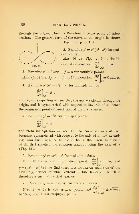
162 SINGULAR POINTS.
through the origin, which is therefore a triple point of inter-
section. The general form of the curve at the origin is shown
in Fig. a on page 157.
2. Examine y'2 — a? (a2—x2) for mul-
tiple points.
Ans. (0, 0), Fig. 42, is a double
Fig. 42.
3- Examine xs
point of intersectiondx
= ±a.0,0
3 axy -f if — for multiple points.
Ans. (0, 0) is a double point of intersection ;-$-
dx
4. Examine y2 (a2 — x2
) = xA for multiple points.
dy
dx
= and oo.
= ±0,
and from its equation we see that the curve extends through the
origin, and is symmetrical with respect to the axis of x\ hence
the origin is a point of osculation of the first species.
5. Examine y2 = a2xs for multiple points.
&~| =±0,dx^
o, o
and from its equation we see that the curve consists of two
branches symmetrical with respect to the axis of x, and extend-
ing from the origin to the right ; hence the origin is a cusp
of the first species, the common tangent being the axis of x
(Fig. 43).
6. Examine y3 = ax2 — x3 for multiple points.
Here (0, 0) is the only critical point. —"
clx
= ±oo, and
y = (ax2 — ar5
)? shows that there is a branch on each side of the
axis of ?/, neither of which extends below the origin, which is
therefore a cusp of the first species.
7. Examine y2 = x (x -f a) 2 for multiple points.
Here (— a, 0) is the critical point,
hence (— a, 0) is a conjugate point,
anddy
dx
= ±0.0,0
CURVE TRACING. 163
8. Examine a3y2 — 2 abafy — x5 = for singular points.
Here (0, 0) is the critical point, and —When x = + h,
bh2,
\b2W + ah5
or \ or
in which both the values of y are real, one greater and the other
less than 0.
When x = — h,
bh2,
/&%* - oh5
or \ cc
m which both the values of y are real and greater than when
li is small.
Hence the origin is a point of osculation, and a point of in-
flexion on one branch.
149. A multiple point at which two or more branches termi-
nate, and have different tangents, is a Shooting Point. A Stop
Point is a point at which a single branch of a curve terminates.
From the law of imaginary roots of algebraic equations,
neither a shooting point nor a stop point can occur on an alge-
braic curve.
150. Curve Tracing. The most rudimentary method of trac-
ing a curve is to find from its equation such a number of its
points that, when located, these points will clearly indicate the
form of the curve.
This method is laborious ; and our present object is to utilize
the principles heretofore developed to determine directly from
its equation the general form of a curve, especially at such points
as present any peculiarity, so that the curve may be traced with-
out the labor of the first method.
To trace a curve from its rectilinear equation, the following
general directions will be found useful.
Solve its equation for y or a?, and determine any lines or points
with respect to which the curve is symmetrical.
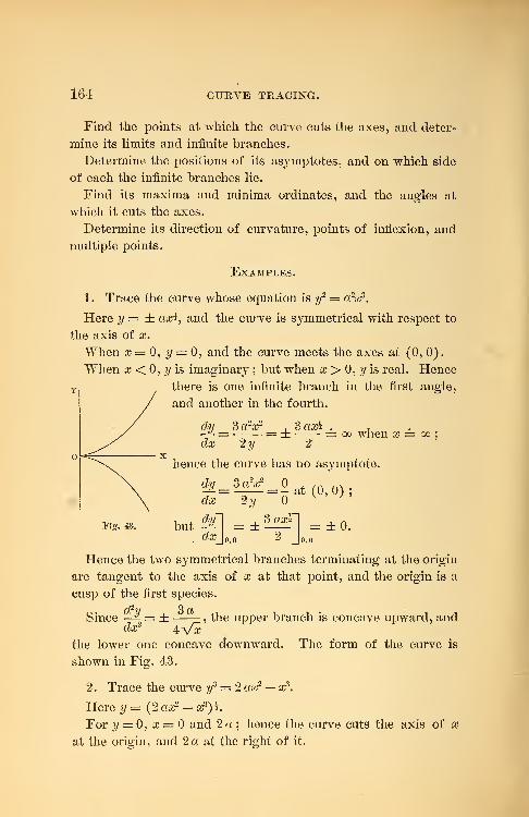
164 CURVE TRACING.
Find the points at which the curve cuts the axes, and deter-
mine its limits and infinite branches.
Determine the positions of its asymptotes, and on which side
of each the infinite branches lie.
Find its maxima and minima ordinates, and the angles at
which it cuts the axes.
Determine its direction of curvature, points of inflexion, and
multiple points.
Examples.
1. Trace the curve whose equation is y2 a2x3
.
Here y = ± aa$, and the curve is symmetrical with respect to
the axis of x.
When x = 0, y — 0, and the curve meets the axes at (0, 0)
.
When x < 0, y is imaginary ; but when x > 0, y is real. Hence
Y /there is one infinite branch in the first angle,
and another in the fourth.
dy=
dx
3 a2x2, 3 axi . ,
= = ± = oo when x = go
2y 2
hence the curve has no asymptote.
dy 3a2x* ,
'
/A AN-£ = = - at (0, 0) ;
dx 2y
but Sfdx
_ , 3 ax^
0,0 "= ±0.
0,0
Fig. 43.
Hence the two symmetrical branches terminating at the origin
are tangent to the axis of x at that point, and the origin is a
cusp of the first species.
3adx2
d uSince —4 , the upper branch is concave upward, and
4Vxthe lower one concave downward. The form of the curve is
shown in Fig. 43.
2. Trace the curve yz —2 ax2 — x3
.
Here y = (2 ax2 — Xs) K
For y = 0, x = and 2 a ; hence the curve cuts the axis of x
at the origin, and 2a at the right of it.
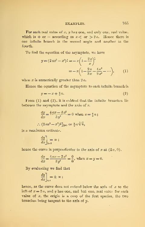
EXAMPLES. 165
For each real value of x, y has one, and only one, real value,
which is + or — according as x< or > 2 a. Hence there is
one infinite branch in the second angle and another in the
fourth.
To find the equation of the asymptote, we have
y = (2 ax2 -xs)h = -x(l-—Y
= — xll _...) (1)V 3a 9a2
Jw
when x is numerically greater than 2 a.
Hence the equation of the asymptote to each infinite branch is
y =--* + !<*. (2)
From (1) and (2), it is evident that the infinite branches lie
between the asymptote and the axis of x.
dy 4: ax — 3 a2n , A-^ = = when x = 4a
;
da 3/ 3
/. (2ax2 -x")%a , orfa^/4,
is a maximum ordinate.
ayda
= 00
2a,
hence the curve is perpendicular to the axis of x at (2 a, 0)
.
dy ^ax — Sx2, n— = = - , when x = y = 0.
dx 3z/2 *
By evaluating we find that
dy
dx= ± oo
;
0,0
hence, as the curve does not extend below the axis of x to the
left of x = 2 a, and y has one, and but one, real value for each
value of a, the origin is a cusp of the first species, the two
branches being tangent to the axis of y.
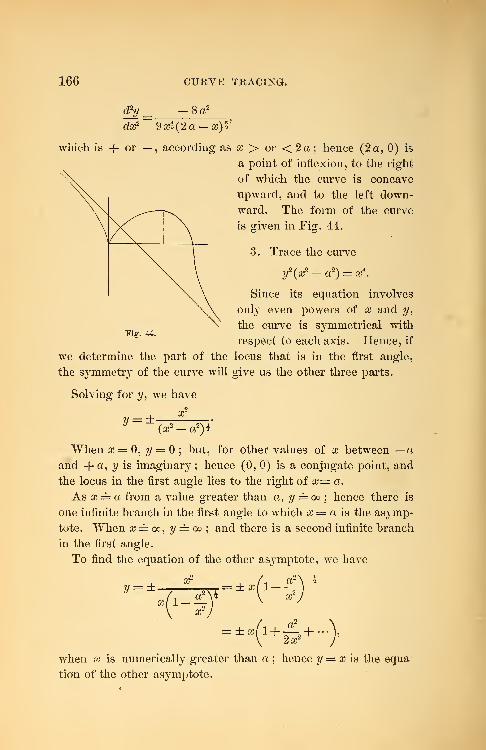
166 CURVE TRACING.
c^/ = -8a2
dx2 9x-3(2a-x)i'
which is + or — , according as x > or < 2 a ; hence (2 a, 0) is
a point of inflexion, to the right
of which the curve is concave
upward, and to the left down-
ward. The form of the curve
is given in Fig. 44.
Fig. 44.
3. Trace the curve
y2 (x2 — a2
) — x*.
Since its equation involves
only even powers of x and y,
the curve is symmetrical with
respect to each axis. Hence, if
we determine the part of the locus that is in the first angle,
the symmetrj- of the curve will give us the other three parts.
Solving for y, we have
x2
y(x2 -a2
)$
When x = 0, y = ; but, for other values of x between —aand + a, y is imaginary ; hence (0, 0) is a conjugate point, and
the locus in the first angle lies to the right of x= a.
As x = a from a value greater than a, y == oo ; hence there is
one infinite branch in the first angle to which x — a is the as}rmp-
tote. When x = oo, y = oo; and there is a second infinite branch
in the first angle.
To find the equation of the other asj-mptote, we have
x2
y = ±.
x 1
= ± X
= ±x
>-f
a?1 +— +
2x2
when x is numerically greater than a ; hence y = x is the equa
tion of the other asymptote.
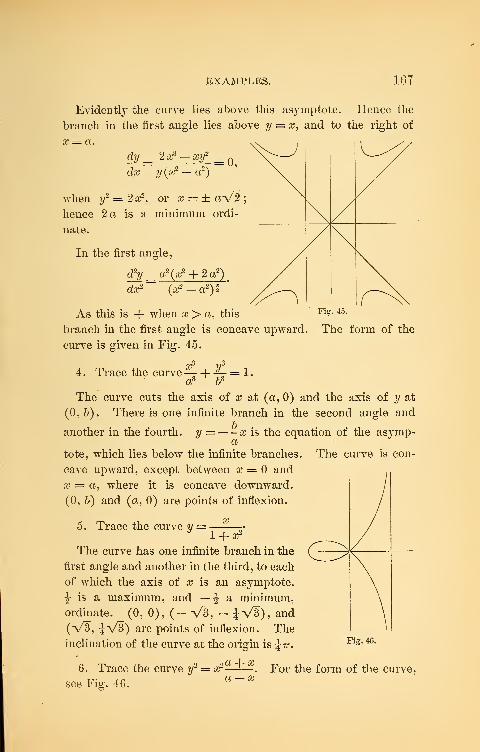
EXAMPLES. 167
Evidently the curve lies above this as3'mptote. Hence the
branch in the first angle lies above y = x, and to the right of
x = a.
dy __ 2x3 -xif _ ny(x2 -a2
)
when ?/2 = 2ar, or a; = ± aV2
;
hence 2 a is a minimum ordi-
nate.
In the first angle,
cl2
y ==a 2 (x2 + 2a2
)
dte2 (ar^-a2
)!
Fig. 45.
The form of the
As this is + when x > a, this
branch in the first angle is concave upward,
curve is given in Fig. 45.
4. Trace the curve—- -f-*— = 1.
as b3
The curve cuts the axis of x at (a, 0) and the axis of y at
(0, b) . There is one infinite branch in the second angle and
another in the fourth, y = a? is the equation of the as}rmp-a
tote, which lies below the infinite branches. The curve is con-
cave upward, except between x = and
x = a, where it is concave downward.
(0, b) and (a, 0) are points of inflexion.
x5. Trace the curve y = -•
1 + ar
The curve has one infinite branch in the
first angle and another in the third, to each
of which the axis of x is an asymptote.
£ is a maximum, and -J a minimum,
ordinate. (0, 0), (- VB, - J-V3), and
(V3, iV3) are points of inflexion. Theinclination of the curve at the origin is \tt.
a 4-x
Fig. 46.
6. Trace the curve y2 =
see Fig. 46.
For the form of the curve,
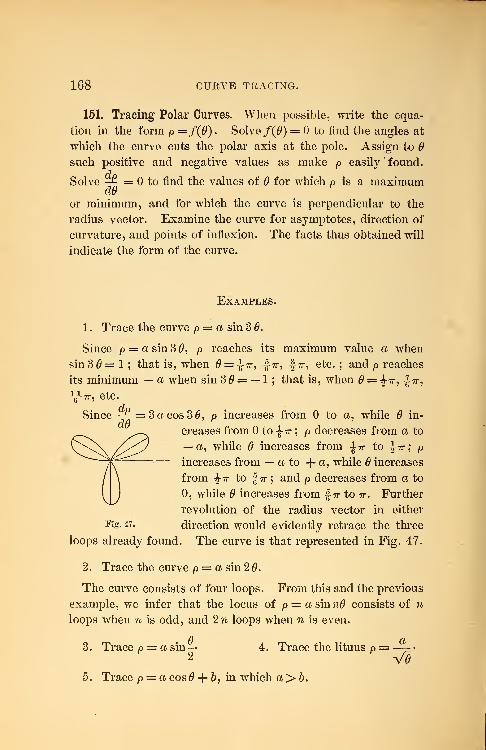
168 CURVE TRACING.
151. Tracing Polar Curves. When possible, write the equa-
tion in the form p =f(0) . Solve f(0) = to find the angles at
which the curve cuts the polar axis at the pole. Assign to
such positive and negative values as make p easily ' found.
Solve -£ = to find the values of for which p is a maximumdO
>
H
or minimum, and for which the curve is perpendicular to the
radius vector. Examine the curve for asymptotes, direction of
curvature, and points of inflexion. The facts thus obtained will
indicate the form of the curve.
Examples.
1
.
Trace the curve p = a sin 3 0.
Since p = a sin 3 0, p reaches its maximum value a when
sin30= 1 ; that is, when = \ir, |-7r, f 77- , etc. ; and p reaches
its minimum — a when sin 30 = — 1 ; that is, when = |-7r, %ir,
-LL-tt, etc.
Since -£=3<xcos30, p increases from to a, while in-
creases from to \tt; p decreases from a to
— a, while 6 increases from -J-7T to J-w; p
increases from — a to -fa, while 6 increases
from \ir to f 7T ; and p decreases from a to
0, while 6 increases from-f
tt to ir. Further
revolution of the radius vector in either
Fjg- 47 « direction would evidently retrace the three
loops already found. The curve is that represented in Fig. 47.
2. Trace the curve p = a sin 20.
The curve consists of four loops. From this and the previous
example, we infer that the locus of p = asin?i0 consists of n
loops when n is odd, and 2 n loops when n is even.
3. Trace p = a sin— 4. Trace the lituus p =
5. Trace p = a cos -}- 6, in which a > 6.
MISCELLANEOUS EXAMPLES. 169
Miscellaneous Examples.
1. Examine x4 — axy2 — ay3 = for multiple points.
The origin, a triple point, is a cusp of the first species, through
which a branch of the curve passes.
2. Examine ax3 -f- by3 — c = for points of inflexion.
3. Prove that (0, 0) is a multiple point of intersection on the
curve x* — a2xy + b2
y2 = 0.
4. Examine xA — a2x2-f- a 3y = for points of inflexion.
An*. fJL.*«\ a.nd f-JL.SaVV6 36/ V V6 36
5. Examine ay2 — x3 — bx2 = for multiple points.
6. Examine ay2 — x3-f- bx
2 = for multiple points.
Ans. (0, 0) is a conjugate point.
7. Trace the curve y2 =——
—
J x+b8. Trace the folium of Descartes y
3 — 3 axy + sc3 = 0.
9. Trace (?/-^) 2 = ^.
10. Trace y2 (x — a) = cc
3.
1 1
.
Trace p cos = a cos 2 0.
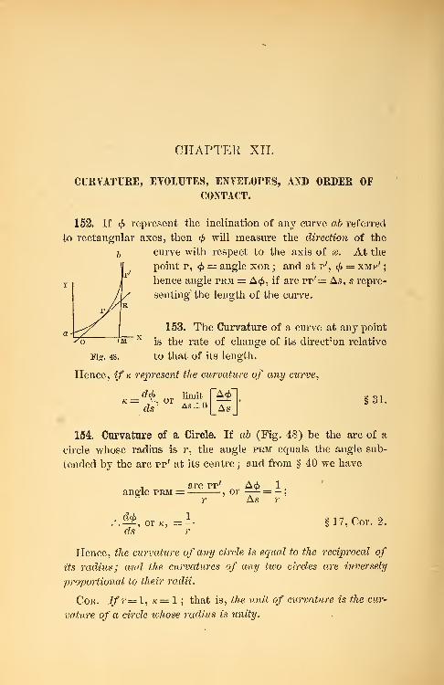
CHAPTER XII.
CURVATURE, EYOLUTES, ENVELOPES, AND ORDER OFCONTACT.
152. If<f>
represent the inclination of any curve ab referred
to rectangular axes, then <£ will measure the direction of the
curve with respect to the axis of x. At the
point p, <£ = angle xor ; and at p', </> = xmp';
hence angle prm = A<£, if arc pp'= As, s repre-
senting the length of the curve.
153. The Curvature of a curve at any point
To 7m~~ a is the rate of change of its direction relative
Fig. 48. to that of its length.
Hence, if k represent the curvature of any curve,
K = ^,or i^r^l §31.ds As = °|_AsJ
154. Curvature of a Circle. If ab (Fig. 48) be the arc of a
circle whose radius is r, the angle prm equals the angle sub-
tended by the arc pp' at its centre ; and from § 40 we have
, arc pp' A(f> 1angle prm = , or —-*- = -
;
r As r
.-.£*, or k, =-. §17, Cor. 2.
ds r
Hence, the curvature of any circle is equal to the reciprocal of
its radius; and the curvatures of any tiuo circles are inversely
proportional to their radii.
Cor. Ifr= l, k = 1 ; that is, the unit of curvature is the cur-
vature of a circle whose radius is unity.
RADIUS OF CURVATURE. 171
155. To find k in terms of the differentials of x and, y.
tan cf> = —?
;
dx
2 , 7 , cZ2?/
.*. sec-<£ a<£ = —-
;
c?#
dcf> =
civ
dx
1 +
c/0"
ds
since sec2<£ = 1 -f-
dx2
sdxj1+f-r-
aY 2
dXj
We take the positive value of the radical so that the curva-
d2v
ture of a curve will be positive or negative according as —- is
dx?
positive or negative ; that is, according as the curve is concave
upward or downward. The sign of curvature, however, is often
neglected.
156. Radius of Curvature. As the radius of a circle varies
from to oo, its curvature varies from go to ; hence there is
alwa}~s a circle whose curvature is equal to that of any curve at
any point. A circle tangent to a curve, and having the same
curvature as the curve at the point of contact, is called the
Circle of Curvature of the curve at that point. Its radius and
centre are the radius of curvature and the centre of curvature of
the curve at that point. Hence, if R represent the radius of
curvature of a curve, from §§151 and 155, we have
K
1 + aYvdx)
dry
dx2
R will be positive or negative, according as the curve is con-
cave upward or downward ; but its sign is often neglected.
172 CTJEVATURE.
157. The radius of curvature in terms of polar coordinates
can be found by transforming the value of R in § 156 to polar
coordinates. We thus obtain
PdO2
' dO2 dO2 l
dO2
in which N is the normal. See § 131, Ex. 3, and § 136, (7).
158. The circle of curvature, in general, cuts the curve at the
point of contact.
For, on one side of the point of contact, the curve changes
its direction more rapidly than the circle of curvature, and hence
lies within the circle ; while on the other side it changes its
direction more slowly than the circle, and hence lies without the
circle.
159. At a point of maximum or minimum curvature,* the cir-
cle of curvature does not cut the curve; and conversely.
For, on either side of a point of maximum curvature, the curve
changes its direction more slowly than at this point ; hence, on
each side of this point, the curve lies without the circle of curva-
ture at this point. On either side of a point of minimum
curvature, the curve changes its direction more rapidly than at
this point ; hence, on each side of this point, the curve lies
within the circle of curvature.
Since the conic sections are symmetrical with respect to nor-
mals at their vertices, it follows that their vertices must be points
of maximum or minimum curvature.
Examples.
1 . Find the curvature of the parabola y2 = 2px.
Here -^=-2-, and —%. = — ^ ;
dx y dx- y3
* By a maximum or minimum curvature, we mean a numerical maxi-
mum or minimum, the sign of curvature not being considered.
EXAMPLES.
dx2 p2
f y2
[i+ &"]
i tf\yz+p\
173
(y2 +P2Y
p2.
The upper or lower sign is to be taken according as —~ is
positive or negative.
At the vertex (0, 0), k = -, which is evidently the maximumcurvature of the parabola. ^
2. Neglecting its sign, find the curvature of the ellipse
a2
y2 + b
2x2 = a 2b2
.
TT dy b2x , d2
y 54
Here -^- — — , and—^ = —;
dx a~y dxr cry5
" * a2f \a,y + Vx2) (a4
y2+ Vx2
) I
At the vertex (a, 0) , k =— ; at the vertex (0, — b) , k =—
;
ft"
hence, the maximum curvature of the ellipse is —- , and the
bb'
minimum-—-a2
3. Find the radius of curvature of the cycloid
x = r vers - — ^J2ry — y2
.
Here ^ = V2ry-^ ^ <%L = _2_,dx y dx- y
z
which equals numerically twice the normal.
1k =
;
— 2^/2 ry
and , the curvature at the highest point, is evidently the
minimum curvature of the cycloid.
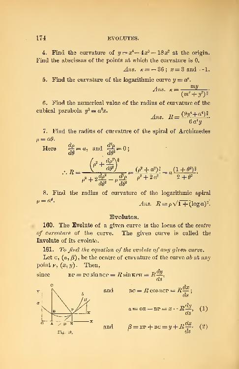
174 EVOLUTES.
4. Find the curvature of y = xi— 4#3 — 18 x2 at the origin.
Find the abscissas of the points at which the curvature is 0.
Ans. k = — 36 ; x = 3 and — 1
.
5. Find the curvature of the logarithmic curve y = ax.
Ans.my
6. Find the numerical value of the radius of curvature of the
cubical parabola ys = a2
x, , Q 4 4 x 3
Ans. B= Vy+a >T
.
Qa'y
7. Find the radius of curvature of the spiral of Archimedes
p = ad.
Here ^=a, and ^ = 0;
.R(*+£
2
YI (i±tf)i_ n (±±f)i
,dP _ d2 -
32 Pp2 + 2 ^tL P
2 + 2a2 2+02
dO2' dO2
8. Find the radius of curvature of the logarithmic spiral
p==ae '
Ans. R = PVl+(loga)2
.
Evolutes.160. The Evolute of a given curve is the locus of the centre
of curvature of the curve. The given curve is called the
Involute of its evolute.
161. To find the equation of the evolute of any given curve.
Let c, (a, f3) , be the centre of curvature of the curve ab at any
point p, (x,y). Then.
since bp = pc sinBCP = R sinKPH = R—,
ds
and
and
bc = R cos bcp = Rdxt
ds'
a = oe — bp = x —R-,ds
= ep + bc = y+Rdx
ds
(1)
(2)
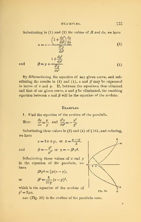
EXAMPLES.
Substituting in (1) and (2) the values of R and ds, we have
x —1 + d£\dy
dx2} dx
1 +and P = y
dx2
dx2
dry
dx2
(3)
W
By differentiating the equation of any given curve, and sub-
stituting the results in (3) and (4), a and (3 may be expressed
in terms of x and y. If, between the equations thus obtained
and that of cue given curve, x and y be eliminated, the resulting
equation between a and /5 will be the equation of the evolute.
Examples.
1. Find the equation of the evolute of the parabola.
Here *=?, and -1 =dx2
P-
dx yJ
dx2 y3
Substituting these values in (3) and (4) of § 161, and reducing,
we have
a = 3x-\-p, or x = a ~-P,
o
and fi= — y or y = — &pi.
Substituting these values of x and yin the equation of the parabola, wehave
which is the equation of the evolute of
tf = 2px.Fig - 50
bac (Fig. 50) is the evolute of the parabola mon.
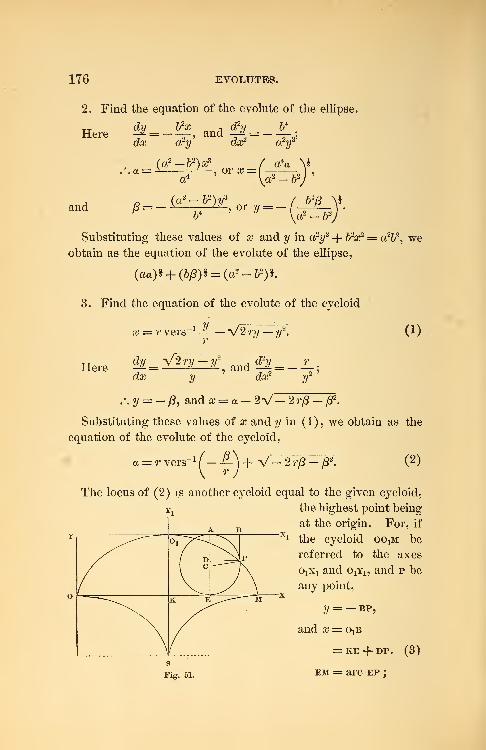
176 EVOLUTES.
2. Find the equation of the evolute of the ellipse.
Here ty _ _ 2?' and ^ = -—;
da? a2?/ dx2 a2y^
(gt-b2)*?
, or x = a4a
^2 -52
and(a2 -52
) 2/
3 _ / &4
ff V^a2 - &y
Substituting these values of a? and y in «y + b2x2 = a2
62
, weobtain as the equation of the evolute of the ellipse,
(aa)* + (ty3)i = (a2 -&*)l.
3. Find the equation of the evolute of the cycloid
x — r vers ry — y% (1)
Heredy
_
-\/2ry-y2, d2
y
_
dx
.-. 2/ = - /?, and a; = a - 2V- 2 r£ - £2
Substituting these values of x and 2/ in (1), we obtain as the
equation of the evolute of the cycloid,
.-i/^A^ y_ 2 r/?-/32.a = r vers (2)
The locus of (2) is another cjxloid equal to the given cycloid,
the highest point being
at the origin. For, if
Xl the cycloid oo2m be
referred to the axes
o^ and 0^, and p be
any point,
y = - bp,
and x = OjB
= ke + dp. (3)
em = arc ep;
PROPERTIES OF THE EVOLUTE. 177
.*. ke = arc ap = r vers-1— = r vers
-11—- )• (4)
dp = Vad-de =V— ?/(2?' + y) =V— 2ry — y2. (5)
From (3), (4), and (5), we obtain
x = r vers-1
(—1
] -f-V— 2ry — y'2. (6)
Comparing (2) with (6), we see that os, the evolute of oo15
must be equal to o^i ; that is, the evolute of a cycloid is an equal
cycloid.
Properties of the Evolute.
162. Any normal to the involute is a tangent to the evolute.
The equation of the normal to y =f(x) at (x'f y') is
y-y'=~(*-*')- (i)
Let (a, /3) be the centre of curvature of y = f(x) at (V,y') ;
then (1) passes through (a, /?), and we have
2/'-^=-S ("''" a); (2)
.•. a,'_a+g!(2,'-
/8)=0. (3)
If (x', y') move along the involute, (a, j3) will move along
the evolute, and a, /?, and y' will be functions of x'. Differen-
tiating (3) on this hypothesis, we have
dx < _ da + dy"-dfdfi + (y. _ ff)it = p.
ax ax
Dividing by dx 1
, and rearranging terms, we have
T<fc'
2T ^ ^cte' 2da;' da;'
2 V ;
178 EVOLUTES.
But, as (a, /?) is on the evolute, we have by § 161, (4),
eto'2
dx' 2
^-"ffg+'+S--* (5)
From (4) and (5) , we obtain
__ da _ dy'dfi _ dx* _ d/3
dx' dx 12 '
dy'~ da
Hence (1) is tangent to the evolute at (a, /?).
163. Any continuous arc of the evolute is equal to the differ
ence between the radii of curvature of the involute that are tangent
to this arc at its extremities.
If (x — a) 2 + (y — j3)2 = R2 be the circle of curvature of any
curve at (x', y1
) , we have
(x'-ay+(y>-py = n2. (i)
Suppose (x f
,y') to move along the curve ; then y
1
, a, /?, and
R will be functions of x\
Differentiating (1) on this hypothesis, we obtain
O'- a) dx'+ (y'- /?) dy'- (x'- a) da
-(y'-f3)d(3 = RdR. (2)
From equation (2) of § 162 we have
,_£=-1^'- .); (3)
da(4)
From (3),
(V- a)da;'+ (?/'- /8)cfo/'= 0. (5)
From (2) and (5),
(V- a)da + (2/'- 0)d0 = - RdR. (6)
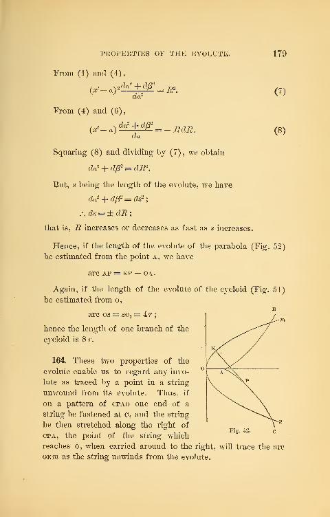
PROPERTIES OF THE EVOLUTE. 179
From (1) and (4),
(?)
(8)
da2
From (4) and (6),
da
Squaring (8) and dividing by (7), we obtain
da2 + cZ/52 = dPi2
.
But, s being the length of the evolute, we have
da2 + dp2 = ds2;
.*. ds = ± dU;
that is, R increases or decreases as fast as s increases.
Hence, if the length of the evolute of the parabola (Fig. 52)
be estimated from the point a, we have
arc ap = kp oa.
Again, if the length of the evolute of the cycloid (Fig. 51)
be estimated from o,
arc os = so! = 4r
;
hence the length of one branch of the
cj^cloid is 8 r.
164. These two properties of the
evolute enable us to regard any invo-
lute as traced by a point in a string
unwound from its evolute. Thus, if
on a pattern of cpao one end of a
string be fastened at c, and the string
be then stretched along the right of
cpa, the point of the string which
reaches o, when carried around to the right, will trace the arc
ok??i as the string unwinds from the evolute.
Fig. 62.
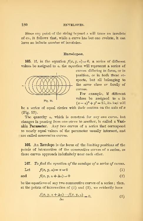
Fig. 53.
180 ENVELOPES.
Since any point of the string beyond a will trace an involute
of ca, it follows that, while a curve has but one evolute, it can
have an infinite number of involutes.
Envelopes.
165. If, in the equation f(x, y, a) = 0, a series of different
values be assigned to a, the equation will represent a series of
curves differing in form, or in
position, or in both these re-
spects, but all belonging to
the same class or family of
curves.
For example, if different
values be assigned to a in
(x — a) 2 + y2 = 25, its loci will
be a series of equal circles with their centres on the axis of x
(Fig. 53).
The quantit}' a, which is constant for any one curve, but
changes in passing from one curve to another, is called a Vari-
able Parameter. Any two curves of a series that correspond
to nearly equal values of the parameter usually intersect, and
are called consecutive curves.
166. An Envelope is the locus of the limiting positions of the
points of intersection of the consecutive curves of a series, as
these curves approach indefinitely near each other.
167. To find the equation of the envelope of a series of curves.
Let f(x, y, a) = u = (1)
and f(x, y, a -f- Aa) = (2)
be the equations of any two consecutive curves of a series ; then,
at the points of intersection of (1) and (2), we evidently have
f(x, y, a + Aa) —f(x, y, a) __ Q> ^Aa
ENVELOPES. 181
Passing to the limit as Aa = 0, we have, at the limiting posi-
tions of these intersections,
f/(*,y,a)= 0, or ff = 0. (4)(La Cla
Since the coordinates of the points on the envelope satisfy
both (4) and (1), its equation is found by eliminating a between
these equations.
168. The envelope is tangent to each curve of the series.
Let cj> (a?, y) represent the value of a obtained from (4) of
§ 167; then, if a =<£(<», y),
f(x,y,a)-u=0 (1)
is the equation of the envelope.
Differentiating (1), a being variable, we obtain
du 7 . die , . du , A— dx-\ ay -\ da = 0.dx dy da
But, at any point on the envelope,
^ = 0; §167, (4)da
.'.^clx +—%= 0, (2)ax ay
which gives the slope of the envelope at an}T point.
Differentiating /(a?, y, a) ==. u = 0, considering a constant, we
have ,7
<^dx + ^dy = 0, (3)dx dy
which gives the slope of any individual curve at any point.
From (2) and (3) we see that the envelope and any curve of
the series have the same slope at their common point.
Examples.
1. Find the envelope of (x — a) 2-f- y
1 — r2, in which a is a
variable parameter.
182 ENVELOPES.
Here f(x, y, a)[= u\ = (x — a) 2 -\-y2 — r2 = ; (1)
.:— = -2(x-a) = 0. (2)da
From (1) and (2), y == ± r ; that is, the envelope is two lines
parallel to the axis of x, as would be inferred from Fig. 53.
2. Find the envelope of y = ax-\— , a being the variable
parameter.
Here /(a?, ?/, a)[= u]=y — ax =0; (1)a
.\—=-x +^ = 0. (2)da a
Eliminating a between (1) and (2) , we obtain y2 = A,mx ; that
is, the envelope is a parabola whose latus rectum is 4m.
3. Find the envelope of the hypotenuse of a right-angled
triangle of constant area.
Let a and j3 be the sides of the right triangle, and assume
them as coordinate axes ; then
a (3
is the equation of the Irypotenuse.
Let c = the constant area ; then
a/? = 2c, or j3 = — •
a
Hence f(x, y, a) = ^+^- 1 = 0, (1)a A C
and ^ = __^_ + J/- =: o. (2)da a2 2c
WEliminating a between (1) and (2), we obtain xy==^c; that
is, the envelope is an hyperbola to which the sides of the tri-
angle are asymptotes.
CONTACT OF DIFFERENT ORDERS. 183
4. Find the envelope of a system of concentric ellipses, the
area and the directions of the axes being constant.
Let the equation of the ellipses be
ay + /5V = a2/3
2, (1)
and c represent the constant area
;
then c = 7ra/?. (2)
Eliminating j3 between (1) and (2), we have
f(cc, y, a) = o.y +^-^ = 0; (3)TT a 77
lu =2ay2 -^4^ = 0. (4)d<a
From (3) and (4) , we obtain
xy= ± —-,92tt
which are the equations of conjugate equilateral hyperbolas
referred to their asymptotes.
169. Contact of Different Orders. Let y—f(x) and y=4>(x)
be an}T two curves referred to the same axes. Iff(a) = <£(«),
the curves have the point [«,/(«)] in common. If f(a) = <j>(a)
and /'(a)= <£'(a), the curves are tangent at [a, /(a)], and are
said to have a contact of the first order. If f(a) = $(a), f'(a)
= <£'(a), and /"(<*) = <f>" (a), the two curves have the same
curvature at their common point, and their contact is of the sec-
ond order. If in addition, /'"(«)= </>"'(a), their contact is of
the third order; and so on. Thus, contact of the nth order im-
poses n + 1 conditions,
170. Two curves intersect or do not intersect at their point of
contact, according as their order of contact is even or odd.
Let y =f(x) and y=cf>(x) be sany two curves having the point
[a, /(a)] in common. Let h be a very small increment of x
By Taylor's formula, we have
184 OEDEB OF CONTACT.
A«+*)=A«) +/(«)*+/'(«) i^+/"'(«)'ir + - W«a+ *) = +(a) + *'(»)* +^(a)i^ + *"'(o)i^+ ...(2)
If. Li.
Subtracting (2) from (1), we obtain
f{a+h) -^a+h)=h[f\a)-<t,\a)^ + ¥-U«(a)-4,»(ay]
which gives the difference between the corresponding ordinates
of the curves on each side of their common ordinate. If the
contact is of an odd order, the first term of the second memberof (3) which does not vanish contains an even power of h
;
hence the sign of the second member is the same whether h be
positive or negative. Therefore, y=zf(x) lies either above or
below y = </>(#) on ^°^n s^es of their common point; and the
curves do not intersect. But, if their contact is of an even
order, the first term of the second member of (3) that does not
vanish contains an odd power of h. Hence, in this case, the
second member changes sign with h ; and y=f(x) lies above
y = (/>(#) on one side of their common point, and below it on the
other ; and the curves intersect.
Cor. At a point of maximum or minimum curvature, the
circle of curvature has contact of the third order with the curve;
for it does not cut the curve at such a point.
The following are obvious conclusions from equation (3) :
(a) Two curves on each side of their common point are
nearer, the higher their order of contact.
(6) If two curves have a contact of the nth order, no curve
having with either of them a contact of a lower order can lie
between them near their common point.
171. Osculating Curves. The curve of a given species, that has
the highest order of contact possible with a given curve at any
point, is called the osculating.curve of that species;
OSCULATING CURVES. 185
Let y =/(#) be the most general form of the equation of a
curve of a given species, and suppose that it contains n-f-1
arbitrary constants. Upon the n +1 constants, n -f-l 5and only
n+1, independent conditions can be imposed. But, in order
that y=f(x) may have contact of the ?ith order with a given
curve at a given point, n +1 conditions must be fulfilled by its
constants ; that is, these constants must have such values that
y=f(x) shall pass through the point, and the first n derivatives
of its ordinate be equal to those of the given curve at this point
(§ 169).
Hence, as y = ax + b has two constants, the osculating straight
line has contact of the first order, and is a tangent.
As (x — a) 2 + (y — b) 2 = r2 has three constants, the osculating
circle has, in general, contact of the second order, and is the circle
of curvature.
The osculating parabola has contact of the third order. T7ie
osculating ellipse or hyperbola has contact of the fourth order.
Miscellaneous Examples.
1. Find the curvature of the hyperbola.
Ans. K=±(6V + aY)i
2. Find the radius of curvature of the equilateral hyperbola
Xy=W -
Ans. B = ±.^+ yy.a 2
3. Find the radius of curvature of y3 = 6 x2
-f x3.
Ans. B = C^ +^ + s2
)2]*
numerically.Sx-y
4. Find the radius of curvature of the lemniscate of Ber-
nouilli,p2=«2 cos 20. at?®2
5. Find the curvature of the cissoid y2 = -
Ans. k= ±
f — x
3(2a-x) 2
aa55(8a — £x)\
186 INVOLUTES AND ENVELOPES.
6. Find the equation of the evolute of the hyperbola.
Ans. (aa) !-(&/?) f = (a2 + &2
)1 -
7. Find the length of ^he evolute of the parabola in terms of
the abscissas of its extremities.
B== (1±P1 == ^±P)!. § 159, Ex.1.
Arc ap (Fig. 52) = kp - oa= (2a; -H>)* _ p-Vp
=^(^)!- §161 -
Ex - 1 -
8. Find the envelope of y2 =a(x — a), in which a is a
variable parameter.
Ans. y = ± \x.
9. One angle of a triangle is constant and fixed in position
;
find the envelope of the opposite side when the area is constant.
Ans. xy ——:— , c being the constant area and w the con-
2 sin wstant angle.
10. Find the envelope of the circles whose diameters are the
double ordinates of the parabola y2 = 2%)x.
Ans. y2 ==p (p -f- 2 x)
.
11. Find the envelope of a line of constant length a, whose
extremities move along two fixed rectangular axes.
Ans. xi -{-y% = a%.
12. Find the envelope of the normals to the parabola y2=2px.
Ans. y2 = (x —p) 3
, which is the evolute of the parabola,27p
as it clearlv should be.
13 . Find the radius of curvature of the catenary y=- ( ea+
fAns. B = —
a
MISCELLANEOUS EXAMPLES. 187
' 14. Find the radius of curvature of the cardioid p—a{l— cosO).
Ans. B = {*«&.3
fie ?/2
15. Find the envelope of the series of ellipses —| ^ =1a2 (k—a) 2
a being a variable parameter.
Ans. #1 -f y^ = &*•
16. Prove that the whole length of the evolute of the ellipse
a3 - bs
is 4ab
17. Find the radius of curvature of the tractrix, having given
^ = -^ §195, Ex.5. 4ns. 2? = - (a8 - y2) 4.
cfo Va2 -2/2 y
18. Show that the evolute of a circle is its centre.
af - — -\19. Prove that the catenary /?=-j e a — e «
jis the evolute
of the tractrix a; = a log —
—
—^-{a2-y2)h. §201, Ex.1.
20. Find the equation of the envelope of y=ax± (<xV-f fr2)*,
in which a is a variable parameter.
Here the equation of the tangent is given, and that of the
curve is required. * x2 y2 _
.
US'
~tf ¥~21. Prove that — + '— = 1 is the envelope of the circles
a2 + b- b2
described on the double ordinates of the ellipse a2
y2-\-b
2x2=a2b2
as diameters.
CHAPTER XIII.
INTEGRATION OF RATIONAL FRACTIONS.
172. Decomposition of Rational Fractions. Any rational frac-
tion whose numerator is not of a lower degree than its denomi-
nator can be separated by division into two parts, the one
rational and entire, and the other a rational fraction whose
numerator is of a lower degree than its denominator. For
example,x* , 5 x2 — 4
x — 2x" -j-2x2 — x— 2 x* -\-2x2 — x — 2
Hence airy rational differential can be considered as com-
posed of an entire part and a fraction whose numerator is of a
lower degree than its denominator. The entire part can be
integrated by previous methods ; and it is our present object to
show that the fractional part, if not directly integrable, can be
resolved into partial fractions which are integrable. These par-
tial fractions differ in form, according as the simple factors of
the denominator of the given fraction are :
I. Real and unequal.
II. Real and some of them equal.
III. Imaginary and unequal.
IV. Imaginary and some of them equal.
To show, in the simplest manner, how the decomposition and
integration is to be effected, we shall apply the process to par-
ticular examples in each of the four cases.
173. Case I. When the simple factors of the denominator are
real and unequal, to every factor, as x — a, there corresponds a
partial fraction of the formx a
CASE I. 189
Let it be required to find ( \ - ~\ ' —+
The roots of x3 -\-x2 —2x = are 0, 1, and — 2; hence, the
factors of Xs + $? — 2 x are x, x — 1 , and x-\- 2.
A 2x + 3 A . B C ,-*Assume ! = (1)x(x—l)(x-j-2) x x-\ x+2 w
Clearing (1) of fractions, we have
2x + 3 = A{x - 1) (a; + 2) + 5 (x + 2)#
+ Cy (^-1)^ (2)
= (^+5+0)a;2+(^+2£-C>-2A (3)
Equating the coefficients of like powers of x in (3) , we have
A+B+C=0, A+2B-C=2, and -2A=B. (4)
Solving equations (4), we find
A = -l £ = f, andC = -l. (5)
Substituting these values in (1), we obtain
2ar+3 _. 3 5 1(Q
,
a?+ x2 -2x 2x 3(a?-l) 60 + 2) 'K)
r (2x + 3)dx = 3 Cdx 5 T dx I T eta
"J x3 + x2 — 2x~ 2J x 3J x — 1 6J x-j-2
= - 1 logx + 1 log (a; - 1) - J log (a + 2) + logc
tc(cc — 1)§= log—^ ^
—
5xi(a; + 2)i
Equation (6) is true ; for the values of A, B, and C given in
(5) satisfy (4), and hence make (3),* and therefore (1), an
identical equation.
* The principle used here is : IfA = A', B = B', C = C, etc., A + Bx+ Cx2 + ••• = A'+ B'x + C'x2
-f ••• is an identical equation.
That the fraction has been correctly decomposed is proved by reasoning
backward through the process. Equation (1) is not assumed as a basis of
proof, but as a basis of operation.
190 INTEGRATION OF RATIONAL FRACTIONS.
The values of A, B, and C may be obtained from (2), as
follows :
Making x — 0, we have 3 = — 2 A; \ A = — f
.
_ 3
Making a; =1, we have 5 = 3B; .\B = %3'
Making x = — 2, we have — 1 = 6 C ; .\ C = — |-.
Examples.
1. Find n*- 1)*8-. ^s . log-^±ilic .
J a;2 + 6a; + 8 " (aj+ 2)#
*J X —\~ X — u
)da? .t
/a;— 2\* . ~
4 °^ + 2
174. Case II. When some of the simple factors of the de-
nominator are real and equal, to every set of equal factors, as
(x — a) 11
, there corresponds a series of n partial fractions of the
, A . B . Lform — — +— -^ + ••• 4
(x-a) n (x-a) 11- 1 x-adx/d
z r.(x—1)'
Assume T7
—
,N2/- -.x= 7~
—
~9 + —:—— + -. , • 0)
'2(a+l)
1 ^1
^1
(a,-l) 2(a, + l) (a;-l) 2 x-1 »+l
Clearing (1) of fractions, we have
1 = .4 (x + 1) + J5(^ - 1) + C (x - l) 2
= (B + C)x2 + (A-2C)x +A-B + C. (2)
Equating the coefficients of like powers of a?, we obtain
£+C=0, .4-20= 0, and ^-£ + (7= 1. (3)
Whence A = £, C=i, and J5= —J. (4)
CASE II. 191
Substituting these values in (1), and integrating, we have
/ dx
J2(x-1) 2 J ±(x-l) J 4(0^+1){)
x+l 1 + c.og(z-iy 2{x-i)
Equation (5) is true ; for the values of A, JB, and C given
in (4) satisfy (3), and hence make (2), and therefore (1), an
identical equation.
Examples.
, va C (2x — 5)dx 7 .11, 35+1 . ^L FmdJ (g + 8)(g +i)'
- i^+T) +T l0g^T3
+ a
+ log(a;+l) + C.+ 8o; + 4J x3
-\- 5 x
3r(2x*+7a?+Gx+2)dx
.
j
'J a*4 + 3^ + 2^ 8
# + 2
x(x+ l)x \i"
^+27-±+0.
a?
175. When the simple factors of its denominator are imagi-
nary, a fraction may then also be decomposed into partial
fractions of the forms in Cases I. and II. ; but, since the inte-
grals obtained from these would involve the logarithms of
imaginaries, we seek other forms for the partial fractions.
Since the imaginary roots of an equation always occur in
conjugate pairs, the imaginary factors of the denominator will
occur in pairs whose products are real quadratic factors of the
form {x — c/)2 + 6
2. Hence, when its simple factors are im-
aginary, the denominator can be resolved into real quadratic
factors.
Case III. When some of the simple factors of the denomina-
tor are imaginary and unequal, to every factor of the form(x — a)
2-f-b
2 there corresponds a partial fraction of the formAx + B
(x-a) 2 -fb2
*
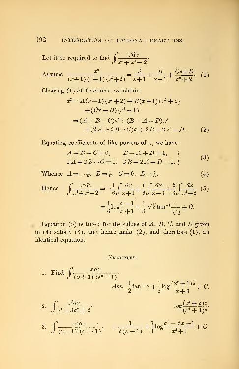
192 INTEGRATION OF RATIONAL FRACTIONS.
Let it be required to find |
J aj* + x2 - 2
Assume* = -JL + -*_ + «*±£ (1)
(x+l){x-l)(a?+2) x-\-l x-l x2 -\-2KJ
Clearing (1) of fractions, we obtain
x2 = A(x - 1) (x2 + 2) + B(x + 1) (a2 + 2)
+ (G* + I>)(ar -1)
= (^L + B + <7)ar3 -{- (5 - .4 + D)a2
+ (2^1 + 2£-0)x + 25-2^4-1). (2)
Equating coefficients of like powers of a?, we have
A + B+C= 0, B-A + D = l,
2A + 2B-C-0, 2B-2A-D = 0.(3)
Whence A = -±, -B = i, (7=0, 7)=f. (4)
Hence f /f =-1 f_^L+ i fj?£L+ 2 fd*_(5)J a;4+iC2_2 QJ x+l 6J x-l 3J x*+2 K J
= ilog— + - V2 tan^ 1— + O.6
&a + 1^3 V2
Equation (5) is true ; for the values of A, B, (7, and D given
in (4) satisfy (3), and hence make (2), and therefore (1), an
identical equation.
Examples.
1. Find f 1^- -•
J (a-f-l)(o;2 + l)
Ans. itan- 1 ^ + ilog (a ^
2 + 1 )i + Q.
2 ^2 ° x + 1 ^
C x*dxm j
(a? + 2)c' J aJ* + 3a^ + 2
s(x2
-f-l)^
J (aj-l^ + l) 20-1) 4&
a2-fl
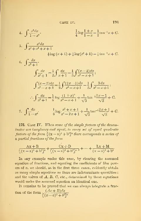
/ ardx
CASE IV. 193
4 *l-x 2
J a3 + a2 + «+ 1
Jlog (a? + 1) +ilog(^2 + 1) - itaa-'x + 0.
G. f-*L.Ja^ + 1
r ja; _ 1 f_efo_ _ 1 /"(a; — 2) eta;.
J a;3 + 1
""3J x + 1 3J a? - a? + 1
.'
r(x — 2)dx _l r(2x—l)dx 1 /" 3 da;
J a^_ ^ J. i
-2J ar-x + 1 2Jx2 — x + l'
A3 + l 6&
a;2 -a;+l V3 V3
/<7a?
1-51, a?-fajr|-l . 1 , _i2a; + l
,~
-loo-——
I
! tan 1h C.
6& ^_2a;+ l V3 V3
176. Case IV. IFAew some of the simple factors of the denom-
inator are imaginary and equal, to every set of equal quadratic
factors of the form [(x — a) 2 + lr] n there corresponds a series of
n partial fractions of the form
Ax + B Cx + D Lx+M[ (x - a)
2 + b2
]11 [(x - a) 2 + b2]*- 1 (x - a) 2 + b2
°
In any example under this case, by clearing the assumed
equation of fractions, and equating the coefficients of like pow-
ers of x, we should, as in the first three cases, evident!}- obtain
as many simple equations as there are indeterminate quantities;
and the values of A, jB, (7, etc., determined by these equations
would make the assumed equation an identical one.
It remains to be proved that we can always integrate a frac-
.. - , T - (Ax-\- B)dxtion of the form —* '
; _ •
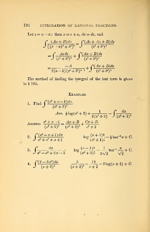
194 INTEGRATION OF RATIONAL FRACTIONS.
Let z = x — a ; then x = z + «> da; = dz, and
J [(a;-a) 2 + 62
]w ~J (z
2 + &2
)w
_ f Azdz r(Aa+B)dzJ (z
2 + b2
)n -J (z
2 + b2
)n
_ —A r(Aa + B)dz
2{n-l){z2-\-b
2
)n~l J (z
2 + b2
)n
The method of finding the integral of the last term is given
in § 185.
Examples.
r(a? + x-l)dxm
J (a;2 + 2)
2
Arts. ilog(a;2 +2) + -? fo
da?•
Assume ^ + x ~ l = Ax + i? + £*±£(a^ + 2)
2 (x2 + 2)2^
a;2 + 2
2# p(s»-s+l)da logi^LDl-jtan-^+a
J ajS + ^ + aj+l B (V + 1)*
3. f _^ tog O- 1)1 L_ tan- 1— + C.
J a?- x* + 2 x -2 *(x2 + 2)h 3V2 V2
J (a;+2) 3(a;+ 2)
2 a;+2 ^ ^ ; ^
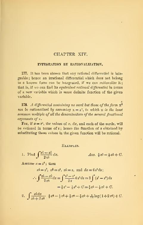
CHAPTER XIV.
INTEGRATION BY RATIONALIZATION.
177. It has been shown that any rational differential is inte-
grate ; hence an irrational differential which does not belong
to a known form can be integrated, if we can rationalize it
;
that is, if we can find its equivalent rational differential in terms
of a new variable which is some definite function of the given
variable.
178. A differential containing no surd but those of the form xd
lan be rationalized by assuming x = zn , in ivhich n is the least
common multiple of all the denominators of the several fractional
exponents o/x.
For, if x = zn
, the values of x, dx, and each of the surds, will
be rational in terms of z\ hence the function of z obtained by
substituting these values in the given function will be rational.
Examples.
1. Find Cxh"f" dx. Ans. |^-Aoi + <7.
J 2x18 3 -r
Assume x = z6
; then
x* = z3, xi = z
4, xi = z, and dx = 6 z?dz
;
.'.Cxl~f dx = Ctzit^dz = 3 f(z7
_
z^ dz
2 * f^Zlh' !^-i^ + |^-f^ + Alog(l+2^)4C.•/ x* -\- zx*
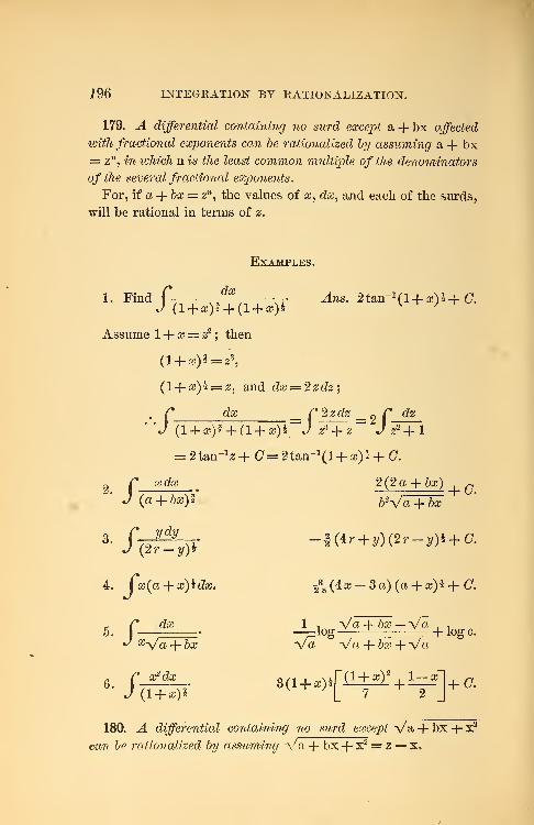
i96 INTEGRATION BY RATIONALIZATION.
179. A differential containing no surd except a + bx affected
with fractional exponents can be rationalized by assuming a + bx= zn , in which n is the least common multiple of the denominators
of the several fractional exponents.
For, if a -f bx = zn
, the values of x, dx, and each of the surds,
will be rational in terms of z.
Examples.
1. Find C- -^ -. Ana. 2tan-1(l+xH + C.
Assume 1+ x — ?} ; then
(l+ x)i=z\
(l-f-#)2 = 2, and dx = 2zdz;
. r dx C 2zdz _ 2 f_dz__"J (l+ x)i + (l + x)l J z*+z~ J z
2 +l
= 2tan~ 1z+ 0= 2tan-1(l-f-«)2 + (7.
dx 2 (2 a + to) „
&»)* bWa + bx2. f-*<J (a +
- C dx It Va + to —Va .
t
5. I • —-log——| = +logc.J xVa -f- bx Va Va+~to -f-Va
+ a) 2 1-x7 2
180. ^4 differential containing no surd except Va + bx -+ x2
can be rationalized by assuming Va -f- bx -f- x2 = z — x.
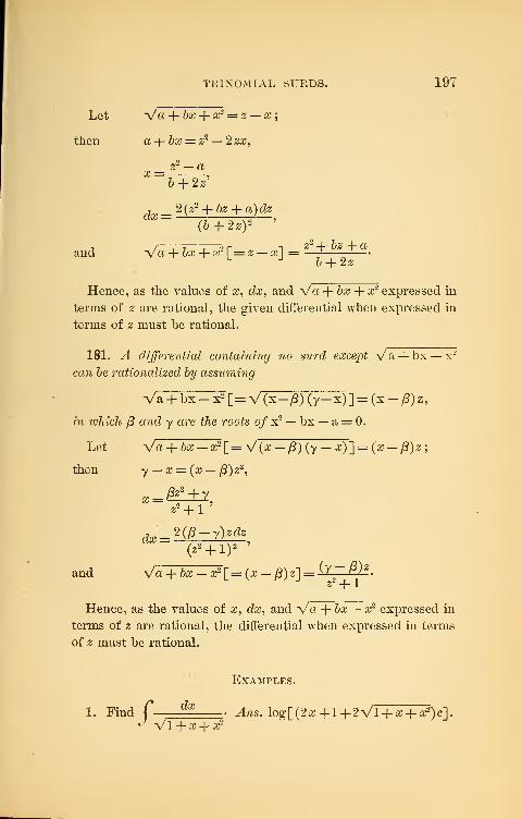
TRINOMIAL iSUBDS. 197
Let Va + bx -f- x2 = z — x;
then a-\-bx = z2 — 2 zx,
z2 — a
x=
and
b + 2z
j _ 2 (z2 +jg-j- a) dz**"(& + 2z) 2
~~'
/—r^—;
—
> r n z2 -\-bz-\-aVa -f 6ic + xr [= z — x] = —! !—
Hence, as the values of x, dx, and V« -\-bx-\-x2 expressed in
terms of z are rational, the given differential when expressed in
terms of z must be rational.
181. A differential containing no surd except Va + bx — x-
can be rationalized by assuming
Va + bx-x2[= V(x-/3)(y-x)] = (x-/?)z,
in which ft and y are the roots of x2 — bx — a = 0.
Let -y/a + bx — oj2 [= V(» — ft) (y — *)]= (x — /3)z
then y — x = (x — ft) z2
,
x^4±y,z2 + l
'
(z2 + l) 2
and Va-h&aJ-aj2 [= (a? - /3)»] = ^~^ g.
z2
-f-
1
Hence, as the values of a?, da?, and V« + &# — &~ expressed in
terms of z are rational, the differential when expressed in terms
of z must be rational.
Examples.
1. Find f dxAns. log[(2aj+l+2Vl+ a?+ «")c].
J Vl + a + cc2
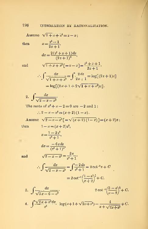
198 INTEGRATION BY RATIONALIZATION.
Assume Vl -\-x-\-x2 = z — x;
2-2 1
then x= - -,2z + l'
(2z + iy '
and Vi +fl; +~^r= z_ar| =g2 + g + 1
.
L J22 + 1
.*. P dx = f_!^-=log[(23 + l)c]^ Vl+aj + ar
2 J 2. + 1bLV T ; J
/:
= log [(2 a; + 1 + 2VI + x -j- x2)c\
dx
V2 — x — x2
The roots of x2-f- x — 2 = are — 2 and 1
;
.-. 2 - x - x2 = (a? + 2) (1 - a?)
.
Assume V2 — a; — x2 [= V(a; + 2) (1— a?)] = (a? + 2)z;
then 1 — x = (x + 2) z2,
l-2z2
a? =
dx =
z2 + l
7
— 6zdz
(^2 + I) 2'
3zand V2 — a? — a?
2
z2 + l
J -W2—X-X2 J * + 1V2 — x — a?2
=3 coir1 /
,x + 22 cot'1f^—^Y
3. f ^ 2cot- 1^Y+ C.J Voa;-6-aj2 V*" 2/
4rV2^+^
# iog(aj+l + V2a?+aj2) ± 4- C.
J x2 ^ + V2a?-j-a;2
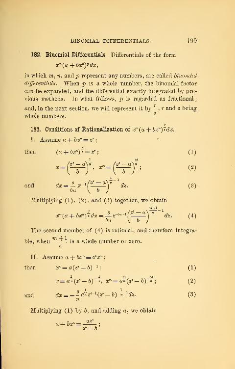
BINOMIAL DIFFERENTIALS. 199
182. Binomial Differentials. Differentials of the form
xm (a + bxn)p dx,
in which ra, n, and p represent any numbers, are called binomial
differentials. When p is a whole number, the binomial factor
can be expanded, and the differential exactly integrated by pre-
vious methods. In what follows, p is regarded as fractional;
and, in the next section, we will represent it by -, r and s being
whole numbers.
r
183. Conditions of Rationalization of xm (a -f- bxn)* dx.
I. Assume a -f- bx11 = z
s
;
then (a + oxn) ~* = zr
; ( 1 )
1 m(z* — a\n fz
s — a\n , .
"=irn '
x {—)
'
(2)
1-1and efcc= —
2
S_1[—H— ] dz. (3)
6>i V h J
Multiplying (1), (2), and (3) together, we obtain
m+l
xm (a + &af)Tda; = JL zr+s-if^zSL\n
dz. (4)bn \ b J
The second member of (4) is rational, and therefore integra-
te, whenm
'
is a whole number or zero.n
II. Assume a -f- focn = z
s#n;
then a;n = a(2s -6)-1
; (1)
1 1 wi m# = a»(zs — &)"*, xm = an(z8 — 6)"»
; (2)
and ^ = --«^s- 1(^- &)~^ 1^- (3 )
Multiplying (1) by 6, and adding a, we obtain
a + bxn =;
z8 — b
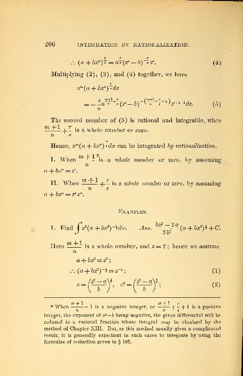
200 INTEGRATION BY RATIONALIZATION.
.-. (a + bxn)T = aJ(zs -by^zr. (4)
Multiplying (2), (3), and (4) together, we have
xm (a + bxnydx
,=: - -a~ +s (z
s-b)~ {~+^ +l
}
zr+s~l
dz. (5)
The second member of (5) is rational and integrable, when771 I I V———f- - is a whole number or zero.n s
Hence, xm (a -f- bxn)^dx can be integrated by rationalization.
I. When —±— is a whole number or zero, by assuming
a -\- bxn = zs
.
n% 1 1 tII. When ———(__ is a whole number or zero, by assuming
n s
a -\-bxn = zs xn .
Examples.
1. Find fx3 (a + bx2)-hdx. Ans.h%* ~ 2 a
(a + bx2) \ + C.
•J o
t)\ I 1Here —— is a whole number, and s = 2 ; hence we assume
a -j- bx2 = 22
;
.\ (a + bx'yh^z- 1; (1)
a=(t=*)\ * = (*=*)*; (2)
wi -4- 1 wi -4- 1 t* When 1 is a negative integer, or -\ 1-1 is a positive
integer, the exponent of zs— b being negative, the given differential will be
reduced to a rational fraction whose integral may be obtained by the
method of Chapter XIII. But, as this method usually gives a complicated
result, it is generally expedient in such cases to integrate by using the
formulas of reduction given in § 185.
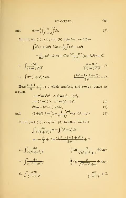
EXAMPLES. 201
and dx=-(— Ydz. (3)b \zL — aJ
Multiplying (1), (2), and (3) together, we obtain
Cx*(a + brf)-ldx =\ C(z2 - a)dz
2 C—^^— 4 — 3 ar2
, ^"J(2-3a^)§" 9(2-3^)5
3. r^(i+^-i^. (2^-i)d+^i +c .
•/ 3 a;3
Here ———f- - is a whole number, and s = 2 ; hence wen s
assume
l+z2 = zV; .-. a? = (z2 -l)-\
x= (?-l)-h, ar^O^-l)", (1)
cfa = -(>2 -l)-izcfe; (2)
and (l + ^)-| = A +_L_Yl= ^(^_i)^ (3)
Multiplying (1), (2), and (3) together, we have
f da; = - f(^-l)^J a;
4 (l + ar9)i J v ;
-* T + c ~3^
+c *
:. I — —-
• ^log
—
""
\-\OQ-C.1
!
)* a ° Va2 + a2 + «
Ti Ki u "lQg / o ; hlo« c -
a; ( cr — ar ) 2 a ,/„2 _ ~2 , „(«2 -^) 5 a Va2 - a? + a
aa;
Jagg ax ^
(l + aj2)!*
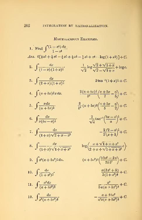
202 INTEGRATION BY RATIONALIZATION.
Miscellaneous Examples.
l.'Find f(lzjA±dx .
J 1 —X3
Ans. 6|>ajS + \xi-\xl + \xl - ±xk + xl- log(l + a#)] + 0.
2. f S J-loaV^ +Vl+ J? +W3 - f^ tt; rr 2tan-1 (l+ ^)^ + C.
4. J(a + &*)**<**2(a + to)l/a^to_a\
+ 0>
J (a+bx) 1* b
2 v J\ 5 2y
!. f ^ - . J- tan-^Mz^Y+ a.
+ 0.. r—^ (i+
(6a;-a)i Va V a
dx 2 /2 — a>\*
dxion(
a+VT+^+#(1 + a) VI + a + ic
2 \2 + a? +VI + x+ a?2
9. f^a + b^idx. (a + 6ffi2)8
(
56
35 y2q
)+a
in f ^ ^(20? + 3) c' J (1+^)1* 3(1 + ^)*
11 /^* v?dx xs
^J (a + 6aj«)l" 3a(a + 6^)i
1 9 f* dx a-\- 'Ibx2 p
' J :${a + bx*)£ a2x(a + bx2)^ '
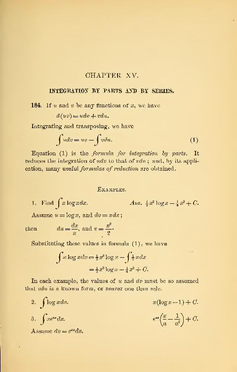
CHAPTER XV.
INTEGRATION BY PARTS AND BY SERIES.
184. If u and v be any functions of x, we have
d(uv) = udv -f vdu.
Integrating and transposing, we have
I udv = uv — I vdu. (1)
Equation (1) is the formula for integration by parts. It
reduces the integration of udv to that of vdu ; and, by its appli-
cation, many useful formulas of reduction are obtained.
Examples.
1. Find I x log xdx. Ans. ^x^logx — ^x2-{- C.
Assume u = log£, and dv = xdx;
then du =— , and v =—x 2
Substituting these values in formula (1), we have
|x log xdx = ^x2 log x —
J\xdx
= ix2 \ogx-ix2 +C.
In each example, the values of u and dv must be so assumed
that vdu is a known form, or nearer one than udv.
2. I log xdx. x(logx — l) + C.
3. fxe^dx. er{- - -V) + G.J \a a1
)Assume dv — e
axdx.
204 INTEGRATION BY PARTS.
4 Cxn log x dx. -^—- Aog x — \-i-C.
5. I sm^xdx. a?sin_1#+ (l— x2)h-\- C.
6.Jtan-1x dx. #tan_1# — log^+ as
2)* -f (7.
7. faf(a - a;2)^. -i^(a - a2
)« -^(a- x2)i + (7.
Assume ?t = x2.
8.J
cc cos xdx. x sin a -f- cos as -f- (7.
185. Formulas of Reduction. We will next apply the formula
for integration by parts to the binomial differential,
xm (a + bxn)pdx*
in which p is any fraction, but m and n are whole numbers, and
n is positive.
I. Let dv = (a + baftyaf^i dx, and w = am
- ,l+1;
then v = ±—
—
-— , and du = (m — n 4- l)xm~n dx.
Hence, by the formula, we have
nb(p-\- 1)J>(« +b*ydx =
^-'+1(» +^r1
m — n
nb(p -\-l)J
* That any binomial differential can be reduced to one of this form is
evident. For, let the given differential be (.r 5— x5)
5 x~*.dx , then, by mul-
tiplying the first factor and dividing the second by (r)s, we obtain
(1— x*)%x~*dx. Putting x = zQ, we have 6 (1 — zb )% dz, which is of the form
required.
The formulas of reduction are true for fractional and negative values
of m and n, but they are not generally useful in leading to known forms,
unless m and n are whole numbers, and n positive.
FORMULAS OF REDUCTION. 205
Now Cxm ~n (a + bxn)p+1 dx = Cri
~n {a -f bxH)p (a + bxn)dx
= a Cxm -'l (a -f bxH)pdx + b Cxm (a + bxnydx.
Substituting this value in (1), we have
Cxm (a + bxnYdx = sm~w+1
(« + fc«H)J,+1
J v yw6(jp+l)
nb(p+l) J
- m ~ n + 1f^(a + bxnYdx.
Transposing the last term to the first member, and solving
for I xm (a -\- bxn)p dx, we obtain
£m (a + bxn) pdx = *
—
! i
—
b(np + m+l)
- a(m - n + 1
\ fx™-n(a + 6aJ»)'da?. (A)6(wp + m + l)J v y v
By formula (A) the integration of xm (a + bxn)p dx is made to
depend upon that of another differential of the same form, in
which m is diminished by n. By a repetition of its use, m maybe diminished by any multiple of n.
Formula (A) evidently fails when np + m + l = ; but in
that case +p == ; hence the method of integration by
rationalization (§183) is applicable, and the formula is not
needed.
II. It is evident that
fxm (a + bxll
)p dx = Cxm (a -f bx
n)p~1 (a + bxll)dx
= aCxm (a + bxny- 1dx
+ b Cxm+n (a + bxny-x dx. (2)
/
206 INTEGRATION BY PARTS.
Applying formula (A) to the last term of (2) , by substituting
in the formula m + n for m, and p —1 for p, we obtain
b fxm+n (a + bar)'-1*/} =xm+\a + hxnY
J np -f- m +
1
np-f- m +USubstituting this in (2) , and uniting similar terms, we have
V(a + 6af)*daj = a*"*1
(<* + &*")*
wp + m -+-
1
H ^ faf,(av+".6afy^1 daB. (B)
np +m+UEach application of formula (B) diminishes p, the exponent
of the binomial, by unity. It fails in the same case that (A)
does.
III. When m and p are negative, we need formulas to increase
rather than to diminish them. To obtain these, we reverse for-
mulas (A) and (B)
.
Solving (A) for I afl-w (a -f- bxn)p dx, and substituting m + n
for m, we obtain
xm+1 (a-\-bxnY+1/xm (a + bxn)p dx
v J a(m+l)
_ 6(np+n+m+l) f^+^+^w*. (C)a(m + l) J V ; V ;
Formula (C) enables us to increase m by n at each applica-
tion. It fails when m -f 1 = ; but in that case the differential
can be rationalized (§ 183).
IV. Solving (B) for I xm (a-j- bxn)p~ 1 dx, and substitutingp-f-1
forp, we obtain
I #m ( a 4- &scn r aa? = —! —
J V Jan(p + l)
np + n + m+1 j^(
^),+i^. (D)
EXAMPLES. 207
Formula (D) enables us to increase p by unity at each appli-
cation .
The mode of applying formulas (A),(B)
,(C) , and (D) will
be illustrated by a few examples.
Examples.
1. Find f fdX
J (a2 — ar)5(a2 -ar°)*
Here m = 4, n = 2, p — — |-, a— a2, and b = — 1 . Hence, by
applying formula (A) twice in succession, this integral will evi-
dently be made to depend upon
dx
fVa2 — x2
Substituting these values of m, n, etc., in formula (A), weobtain
Cx\a2 - x2)-ldx = - ix?(a2 - x>)k
+ %a2 ftf^-tfyhdx. (1)
In like manner, we obtain
I ^{a2 — xPJ-zdx^ — %x(a2 — a?)h
+ i«2 f(a2 -^)-Mx. (2)
Now, C(a2 -x2)-hdx= f f
dx =sm- 1-+C. (3)
From (1), (2), and (3), we obtain
f a *i<to = - (ioj
8 +|
a
2x*) Va2 -^
•^ Va2 — ft2
4- 1 a4 sin-1 - +0.
a C x2 dx A x /— oia2
• i# . >-,2. I — • -4ns. V«" — or H sin
-1- + C.J Va2 - x2 2 2 a
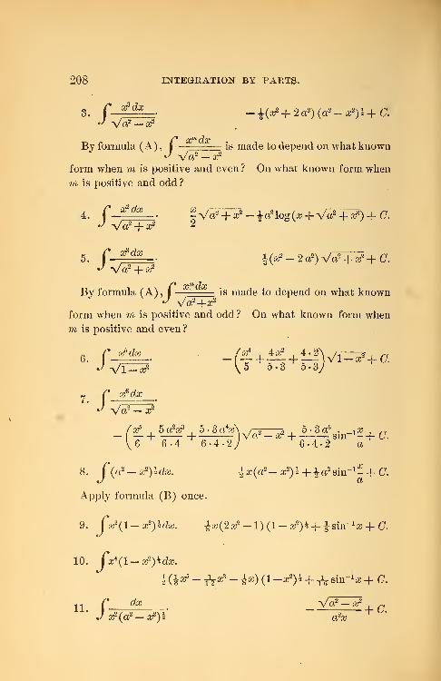
208 INTEGRATION BY PARTS.
3<r tfdx
m _^(^ H.2a2)(a2 -^2)^+C.•^ Va2 — x2
— '
. is made to depend on what knownVa2 — x2
form when m is positive and even ? On what known form when
m is positive and odd?
4. f^ dx -V?T?-ia2log(aj+V?+^) + C.
5>|
" g8^.
i(aj2_2a2)V^4r5+C'.
/* xmdxBy formula (A) , I — '
is made to depend on what knownJ Va2
-{-£C2
form when m is positive and odd ? On what known form when
m is positive and even?
Jvr^5 v.5 5.3 5.3;
7. f-4*^ Va2
;
cte
a?5
. 5aV . 5-3aV\ /-» \ . 5 -3a6. _,« . „
1 (- V<r — ar -\ sin - + C.
x2
6+
6-4 '
6-4-2J' 6-4-2 a
8. f(a2 -x2)hdx. ix(a2-x2)h + ±a2 sm~ 1-+C.
«y CI
Apply formula (B) once.
9. Cx2(l-x2)hdx. ix(2x2 -l)(l-x2)h^.^sm-1x-hC.
10. Cx\l-x2)ldx.
-- C dx Va2-r p' Jrf{a*-a?)h a2x
+
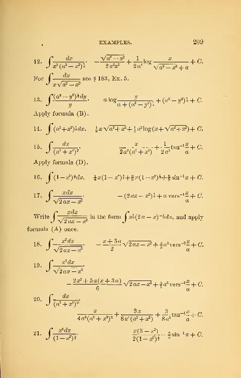
EXAMPLES. 209
12. f *? - Vfl -^ + J-log - + 0.
For f da;see § 183, Ex. 5.
J x~\/a2 — x2
, 8 .Atf-iflMy
. al y +(tt,_^)t + g,
J2/ a+ (a2 -r) 5
Apply formula (B)
.
14. f(a2+x*)*dx. ixVtf^2+ianog(x+Va?+tf)+C.
15. f—^ — * + 1 feur^+ aJ (c^+ ar*)2 2a2(a2 + 2a3 a
Apply formula (D).
16. f(l—sj)*<kr. ia;(l-iB2)i+ta;(l-iB2)5+fsin-1a; + 0.
17. f ^. -(2aaj-ic2)l + avers-1-+0.
*^ V2a«-.T2 a
. /» #da; /»jWrite I , = iu the form | x*(2a — x)~*dx, and apply
J v2ax — x~ Jformula (A) once.
18>J
" a2da. _x±3a^/2ax-x2+ fevers"1-+ O.
J -V2CIX-X2 2 a
-. q U/ C&37
V2 aa; — ft2
!
-J
—
! L V2 a# — x2-f fa3 vers
-1 - -f- C.6
20r dx
J (cf + x2
)
x Sx . 3 , ,£C, ^
4a2 (a2 + ^) 2 Sa^^ + aJ2) 8a5 a
• f****
.x(S-x*) ,21,
(1-z2)* 2(l-ar9)£
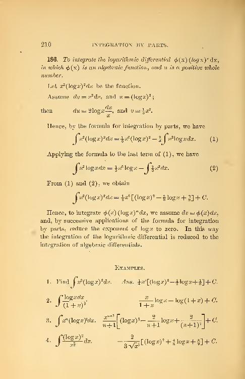
210 INTEGRATION BY PARTS.
186. To integrate the logarithmic differential </>(x) (7o#x) n dx,
in which <£(x) is an algebraic function, and n is a positive ivhole
number.
Let x2 (\ogx) 2 dx be the function.
Assume dv = x2 dx, and u = (logx) 2;
then dw=21oga;— , and v = ^x3.
x
Hence, by the formula for integration by parts, we have
I x2 (logx) 2dx = ^xs (logx) 2 — J Jx2logxdx. (1)
Applying the formula to the last term of (1), we have
I x2 logxdx = \x3 log a? — I ^x2dx. (2)
From (1) and (2), we obtain
Ca?(logx) adx = -Jar3 [(logo?) 2 - f loga; + -§] + C.
Hence, to integrate <jt(x) (logx) n dx, we assume dv — <j>(x)dx.
and, by successive applications of the formula for integration
by parts, reduce the exponent of log a? to zero. In this waythe integration of the logarithmic differential is reduced to the
integration of algebraic differentials.
Examples.
dx x
1. FindJxs (\ogx) 2dx. Ans. i a;
4 [(log a;)2—
-J- logo;+ -J]
+
o r logxdx X
J (l-M) 2'
1+xlog a; — log(l + x) + C.
3. JV (iog^. gi[(iog»)2
-4T log*+(^ir]
+a
4 _ J(M! da; .__i_ [(loga;)2 + |loga;+ |] + o.
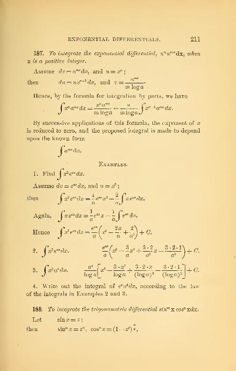
EXPONENTIAL DIFFERENTIALS. 211
187. To integrate the exponential differential, xn amxdx, when
n is a positive integer.
Assume civ = a^dx, and u = xn;
then du = nxn~1 dx, and v =mloga
Hence, by the formula for integration by parts, we have
xn anx dx =-^ — x'^ar^dx.mloga mlogaJ
By successive applications of this formula, the exponent of x
is reduced to zero, and the proposed integral is made to depend
upon the known form
/•a^dx.
Examples.
1. Find Cx-e^dx.
Assume dv = e^dx, and u = x2;
then | or eax dx = ~eax or \xe^ dx.
J - a aj
Again,Jx e°* dx = - e
ax x — -|e™ dx./eax
f 2x 2\x>eax dx = — [x2 -— + — + C-
a \ a a-
J
^ C % ^1 e^/o 3 2 . 3-2 3-2.1\, n
2. I aPe^dx. —I x3 xr -\ x —-
] + C.J a \ a or a° J
3. lx3 ax dx.loo- a
o 3-x2. 3-2 -x 3-2-1
xr — < hloga (log a) 2 (loga) 3
_
4. Write out the integral of exx4 dx, according to the law
of the integrals in Examples 2 and 3.
188. To integrate the trigonometric differential sinm x. cosnxdx.
Let sin x = z;
then sinm x = z
n\ cos'
1 x = (1 — z2)
2",
212 INTEGRATION BY PARTS.
and dx = (l— z2)~^dz.
sinm£ccosM icdic=
jzm{\ — z
2) 2 dz. (1)
Or, letting cos x == 2, we obtain
sinw a;cosMfl?^= I — zw (l— z
2)~2~dz. (2)
Hence, whenever the binomial differential in (1) or (2) can
be integrated, the given differential can be.
This method of integrating sinmxcosnxdx is used in those
cases to which the shorter methods of § 63 are not applicable.
Examples.
1. Find j sm6 xdx.
Put sin x = z\
then dx = ( 1 — z2) ~i dz,
and lsm6xdx = I zG(] — z
2)~* dz
6 6-4 e-4.2/v }
-5^-sin- 1^ + C § 185, Ex. 7.
6-4-2
COS Xf . K , r • Q ,5«3. \snrsc + 4sura5 -\ smo?4 4-2 J
x+C.5-3
5.4.2
2. i $m4 xdx. Ans. — J cos a; (sin3 #-f-f since) -ff x + (7.
3. fcos 4cccte. isin:r(cos3 £ + f cosaj)+fa?+ (7.
4. I sin2 aJCOS2icc?a?. ^sin3 £ccos£c — -§-sina;cosaj + -|-a;+ (7,
or \(x — i sin 4 #) + C.
Let sina? = :<;, and, for j z2(1 — z
2)*dz, see §185, Ex. 9.
TRIGONOMETRIC DIFFERENTIALS. 213
The second form of the integral is obtained from the first by
use of the relations, 2 sin x cos x= sin 2 x, and 2sin2&=l — cos 2x.
By a similar transformation, any differential or integral expressed
in powers of since and cos a; may be found in terms of the sines
and cosines of multiples of x.
C • 2 4 7 sin#/cos3 # cos5a? . cosaA ,
x . no. I sin2 £cos4
#cfa\ [ H \-C.J 2 V 12 3 8 J
T16T
6 . C. ^L_. —l + log tan x + C.J since cos3
a? 2 cos- a;
r r dx
J sin3a^L + ^logtanf+C.2 sin2
a? 2
• -i-cos^a? + cos a; + I02; tan- -f- C.x 3 8
2
189. To integrate xn sm(ax)dx, cmcZ xn cos(ax)dx.
Assume % = a?*, and apply the formula for integration by
parts. Each application of the formula will evidently diminish
n by unity ; hence, when n is a positive integer, the integral
can be made to depend on the known form
Jcos (ax) dx or j sin (ax) dx.
190. To integrate eax smn xdx, and eax cosnxdx.
Put dv = eax dx, and u = sin71
a?
;
then v = -e™,a
and du = n sinn_1 fl7 cos a; da?.
.*.( e™ sin'
1xdx = - eax sinn x
J a
I eax sm n~ 1 XQ,o&xdx.
aJ
Again, put dv = e^dx, and u = sin'l~ 1
a?cosa.
;
then v = -eax,
a
(1)
214 INTEGRATION BY PARTS.
and du = (n — 1) sinn~2# cos2xdx — smn xdx
— (n — 1) sinn~ 2xdx — n $mn xdx.
[Since cos2a; = 1 — sin
2ct\]
Jeax
s[n n-ix Q sxdx — -eax sin"" 1 ^ cos a?
a
n — 1|eax sinn
~2xdx _l. -Jeax smnxdx.
Substituting this result in (1), and solving for j eax sm.n xdx,
we obtain,
> mn*xdx= ^Bin^^Bing-ncosa?)?i
2-f-a
2
w fo~ V feax sinw
- 2x^. (2)?r + ar J
s<
By repeating this process or the application of this formula,
n is reduced to zero or unity ; and the integral is made to de-
pend upon the known form|eax dx or the form
j eax sinxdx.
The value of the latter form is obtained directly from (2) by
making n = 1
.
In like manner I eax cosnxdx can be obtained.
Examples.
1. Find IxPcosxdx.
Here u — x2, dv = cos xdx,
v = since, and du = 2xdx.
.*. I x2 cosxdx = x2 sinx — 2 I x sinxdx
= «2 sin» + 2^cos^— 2 I cosxdx
= x2sinx-f- 2x cosa? — 2 since -f- O.
2. IxPsinxdx. —afcosx+Sx2 sinx-}-6x cosx—6smx-\-C.
TRIGONOMETRIC DIFFERENTIALS
.
215/paxeax sinxdx. — (a sin a; — coso?) + C.
a? + l
ex sm3xdx. — (sin3^ + 3cos3
aj+ 3sin^— 6cos#) +C.X.\J
dx191. To integrate
a -\-b cosx
dxr dx _ rJ a+b cosx- J
a (cQs2x
-/
+sin2- )-\-b cos2 sin2-
V 2 27 \ '2 2
-/
(a + 6) cos2- +(a-6) sin2-
sec2-c?cc
(a + 6) + (a - 6) tan2-
/tan
|
(a + 5) + (a -6) tan2-
which is readily reduced to the known form,
/dx C dx
7+tforJ ^w' aceordiug as a > or < 6>
In like mannerf
can be found.J a
dx
-f- b sin #
192. To integrate the anti-trigonometric differentials,
f (x) sm-1xdx, f(x)cos_1xdx, f (x) fcm^xdx, etc.,
in which f (x) is an algebraic function.
Assume dv =f(x) dx, and apply the formula for integrating
by parts. One application of the formula will evidently makethe integral depend on an algebraic form.
216 INTEGRATION BY SERIES.
Examples.
1. Find f^^-tan-1^J 1+x2
Qu dx dxHere dv =—'—
- — dx , u= tan-1 #,1+x2 1+x2
v = x — tan" 1^, and du = - ••
1+x2
-tan- 1 ^ = x tan_1 # — (tan
-1ic)
2
1+x2 v '
/ xdx rt&rr^xdxl+x2 J l+x2
= x tan" 1^ — (tan-1^)
2
- ilog (1 + a?) + i (tan-^) 2+ G
= tan" 1 ^ {x —-Jtan-1 a;) — log Vl +X2 + C.
2. I xcos^xdx. ^x2 qos~1 x — ix{l — x2)* + ±sm~ 1x+ 0.
3. Cafsm^xdx. i^sm" 1:*; +±(x2 + 2)Vl^x2 + C.
193. Integration by Series. When we cannot, by any of the
preceding methods, integrate a given differential exactly ; or,
when the integral obtained by them is of a complicated form,
we can develop the given differential in a series, and integrate
its terms separately. Moreover, integration by series furnishes
a simple method of developing a function, when we know the
development of its derivative. For examples of this method of
developing functions, see §§ 107, 108.
Examples.
1. Find Cx*{l-x2)ldx.
(l-x^l^l-^x2 - ix* -^—
;
EXAMPLES. 217
.-. Cc£(l-a?)kdx= Cxh(l-^-ia^-^xe )dx
which is the required integral for x < 1 and > — 1
.
2. jx*(l-a?)ldx. i^_^^_J^^__i_^_... + a
3. Prove that log(a+x) = loga + - -^ +^-_^L+ ...,
a 2cr 3a° 4 a4
dxby first integrating directly, and then by series.
a -\-x
dx4. Develop log (a + Vl +X2
) by integrating
Vl^M
r dx
J (l+x*
a i / , /T-T—o\ I*3,l-3af 1.3.5a7
,Ans. log(#+ Vl4-ar)= # —SV '2 3 2-4 5 2-4-6 7
5. Prove that
1 a5, 1 • 3 a9
1 • 3 - 5 x13. . n
(l+x*)h 2 5 2-4 9 2-4-613
194. While we can differentiate any given integral, we can
exactly integrate but a small number of differentials. One
great reason for this seeming difference in the perfection of the
two branches of the Calculus is that the integral is often a
higher or more complex function than its differential. Thus,
the differentials of logo?, sin-1
x, tan" 1
^, etc., are algebraic func-
tions. Moreover, it is evident that certain forms of differentials
do not arise from the differentiation of any known functions.
Hence, to obtain the exact integrals of many differentials, new
and higher functions must be invented and studied. The
integrals of these differentials, as obtained by series, are the
developments of these, as yet, unknown functions.
CHAPTER XVI.
LENGTHS AND AREAS OF PLANE CURVES, AREAS OF SUR-
FACES OF REVOLUTION, VOLUMES OF SOLIDS.
195. Examples in Rectification of Plane Curves. For formulas,
see § 65.
1. Find the length of the parabola y2 = 2px.
Here s =/(i+S)w=/(i+D^=^(y+2'2)4d2/;
.-. s =^EEl+E\og(y+v9+7)+ C. § 185, Ex. 14.
If s be measured from the origin, s = when y = 0, and
G= — iplogp.
2. Rectify the circle a?-{- y2 = r
2.
We use L to represent the entire length of any closed curve.
Here L = 4 fYl + ^fdx = 4r f" dx = 2 rrr.
Jo \ da?
J
Jo Vr2 - x*
For the value of 7r, see § 107.
3. Rectify the ellipse y2= (1- e
2) (a2 - a2
)
.
Here ^ = - (1- e2)* = _^IE?
;
/»« <fcc / e2^ eV 3e6a6 \
= 4JoV^=^V 2 « 2 ' 4 «3 2.4.6a5 "V
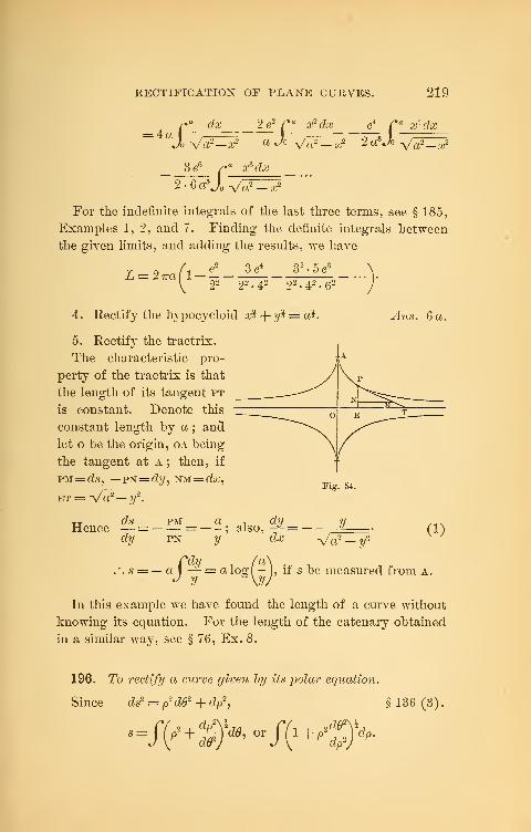
RECTIFICATION OF PLANE CURVES. 219
r*a dx 2e2 r a x2 dx e
4 Ca x'dx
Jo Va2-r a J° Va2 - x2 2 a3Jo ya^3e6
/»tt x6 dx
2 -6a5Jo V^^?
For the indefinite integrals of the last three terms, see § 185,
Examples 1, 2, and 7. Finding the definite integrals between
the given limits, and adding the results, we have
3e4 32 -5e62^1---
22 22• 42 22
• 42• 6
2
4. Rectify the hypocycloid a# -f^ = at.
5. Rectify the tractrix.
The characteristic pro-
perty of the tractrix is that
the length of its tangent pt
is constant. Denote this
constant length by a ; and
let o be the origin, oa being
the tangent at a ; then, if
pm= ds, —T^=dy, NM=C?£,
Ans. 6 a.
et = Va2— 2/
2.
T-rds PM
Hence — = =dy
,'.s
also, -^=dx
Fig. 54.
/ 9Vet"* — 2/"
(1)
— a I — = a if s be measured from a.
In this example we have found the length of a curve without
knowing its equation. For the length of the catenary obtained
in a similar way, see § 76, Ex. 8.
196. To rectify a curve given by its polar equation.
Since ds2 = p2 dO2 + dp2
, § 136 (3)
.
220 LENGTHS AND AREAS OF PLANE CURVES.
Examples.
1. Rectify the spiral of Archimedes, p = a6.
Here — = -;
.* . s = - I (cir 4- p2) * dp.
dp a aJ
Hence, if s be measured from the pole, we have
p(a2 + p2)5 a n
p-j- Va2 + p2 mok r w
2 a 2& a
This is equal to the arc of the parabola, y2 = 2 ax, intercepted
between the vertex and the point whose ordinate equals p
(§195, Ex. 1).
2. Rectify the logarithmic spiral p = ae.
Here s= I (l4-m2)Mp = (l-\-m2)*p,
in which m is the modulus of the system of logarithms whose
base is a, and s is measured from the pole.
3. Construct and rectify the cardioid p = a(l+ cos0).
L = 2 f[a2(l+ cos0) 2 + « 2 sin2 0]sd0
Jo 2 2
since 2(1 + cos (9) = 4 cos2—z
197. Examples in Quadrature of Plane Curves. The quadra-
ture of a figure or surface is the finding of its area. For
formulas, see §66.
1 . Find the area of the circle x2+ y2 = r2
.
Here area = 4J
(r2 — x2)idx
nr=7r?-2
. §185, Ex. 8.=4pr2 — x2
)* , r2. _->x'—4 sm -
2 2 7-
EXAMPLES. 221
For the segment between the lines x = a and x = 6, we have
= 2 I (r2 — x2) h dxarea
= bVr2 — 62 + J*
2 sin-17 —aVr2 — a2— r^sin
-1-
2. Find the area of one branch of the cycloid.
ii
x = r vers-1- — v2ry — y
2.
Area =2 C y' dy = 3^. § 185, Ex. 18.
Jo V2?'2/-2/2
Hence the area of one branch is three times that of the gen-
erating circle.
3. Find the area of the tractrix.
Here &-_, y- ,orcfce=-^-—^cty. §195, Ex. 5.da; Va2 - / 2/
.•.z=jydx =—j Va2— tfdyi
.'. area = - 4 C\/a2 -y2 dy = ira2
. § 185, Ex. 8.
Hence the whole area enclosed by the curve is equal to the
area of a circle whose radius is a.
Xs
4. Find the whole area between the cissoid y2 =— and
., , , 2a — xits asymptote.
Ans. 37T<r.#
5. Fmd the area between the lines xry = a3, x = 5, x = c, and
y = °-Ans. a*
b-^>be
6. Find the area of both loops of the curve tfy2 = aP&aP—tiPx*.
Ans. %ab.
7. Find the area of one loop of the curve aV = x4 (a2 — x2)
.
Ans. ia2.
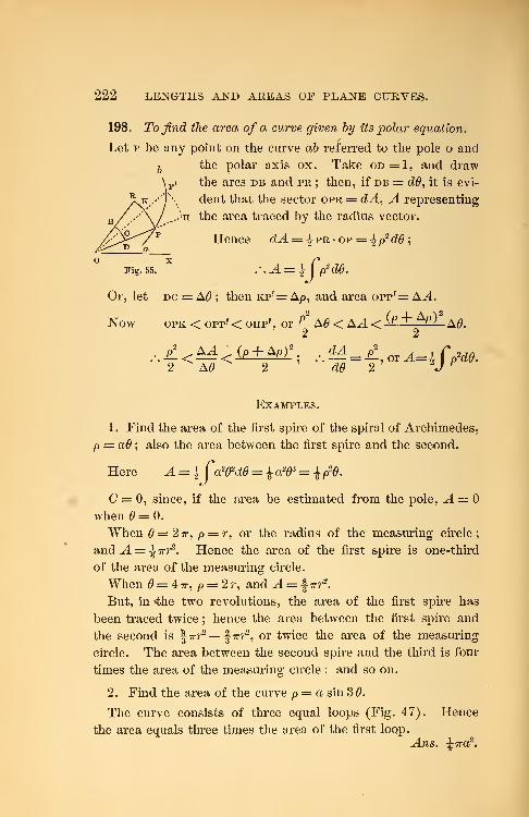
222 LENGTHS AND AREAS OF PLANE CURVES.
198. To find the area of a curve given by its polar equation.
Let p be any point on the curve ab referred to the pole o and
bthe polar axis ox. Take od=1, and draw
the arcs db and pr ; then, if db = dO, it is evi-
dent that the sector opr = cL4, A representing
...;h the area traced by the radius vector.
p Hence dA = ^pr-op = ip2 d0
;
ao x
Fig. 55. .'. A — \ j p2 d$.
Or, let dc = AO ; then kp'= A/>, and area opp'= AA.
Now opk < opp'< OHP f, or £-A0 < AA< ^P + Ap^ AO.
2 AO 2 dO 2' V H
Examples.
1. Find the area of the first spire of the spiral of Archimedes,
p = aO ; also the area between the first spire and the second.
Here A = £ Ca2 2dO = £ a2 3 = ±p2
0.
(7=0, since, if the area be estimated from the pole, A =when = 0.
When0=27r, p = r, or the radius of the measuring circle;
and A = ^irr2. Hence the area of the first spire is one-third
of the area of the measuring circle.
When = 4 ?r, p = 2r, and A = f -rvr2
.
But, in »the two revolutions, the area of the first spire has
been traced twice ; hence the area between the first spire and
the second is \irr2 — \-irr2
, or twice the area of the measuring
circle. The area between the second spire and the third is four
times the area of the measuring circle ; and so on.
2. Find the area of the curve p = a sin 30.
The curve consists of three equal loops (Fig. 47). Hence
the area equals three times the area of the first loop.
Ans. %Tra2 .
QUADRATURE OF SURFACES OF REVOLUTION. 223
3. Find the area of the lemniscate p2 = a2 cos 2 6.
The integral between = and = ^tt is one-fourth of the
whole area. A 2Ans. or.
4. Find the area of the cardioid p = a (cos 6+ 1 )
.
Ans. ^ttcl2
.
199. Examples in Quadrature of Surfaces of Revolution. For
formulas, see § 68.
1
.
Find the area of the surface of the prolate spheroid ; that
is, of the surface traced by the revolution of the ellipse
y' = (l-e2)(a2 -x2
)
about the axis of x.
Area = 2 Clir^l-
e
2)l{a2 -x2)\fl +^fdx
= 4 ve (i _ e2) I fY «j _ aA4d«
= 47re- If— — scM'cfa?
=4^[W^ -tf+fa^ZiY 1 185, Ex.8.
tt62H sin 2
e.
e
2. Find the area of the surface of the prolate spheroid whose
generatrix is 9?/2 + 4a?2 = 36.
3. Find the area of the surface generated by the revolution
of the cycloid about its base.
Area = 2£ 2 iryds= 4 *£y(l +^*dy
= 4ttV27' f y(2r-y)~idy
= 4tt V27 [-f (4r+2/) (2r-y)*]!r
§ 179, Ex.3.
= -§#-7T?'2
.
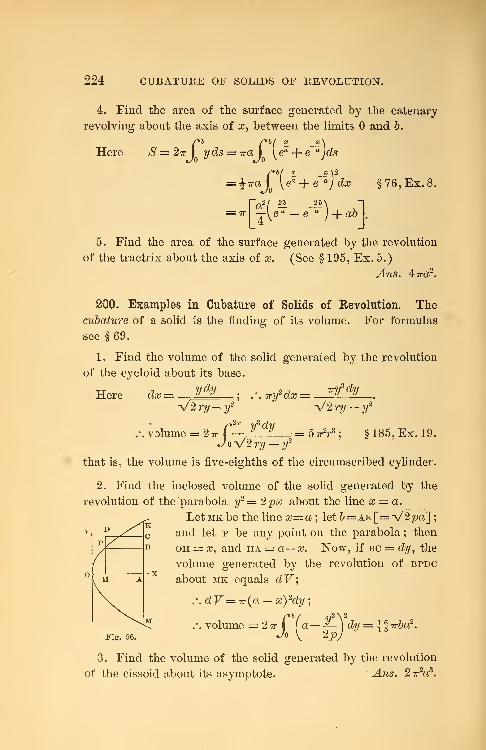
224 CUBATURE OF SOLIDS OF REVOLUTION.
4. Find the area of the surface generated by the catenary
revolving about the axis of x, between the limits and b.
Here S=27rj yds = ira\ [ea-\-e
a]ds
= |7raJo
\ea + e~a)dx §76, Ex. 8.
= 7r
[f(^- e"^)+^].
5. Find the area of the surface generated by the revolution
of the tractrix about the axis of x. (See § 195, Ex. 5.)
Ans. 47ra2.
200. Examples in Cubature of Solids of Revolution. Thecubature of a solid is the finding of its volume. For formulas
see § 69.
1. Find the volume of the solid generated by the revolution
of the cycloid about its base.
ydy . o 7 7ry3 dy
V2 ry— y2 V2 ry — y
2
Here dx
.*. volume = 2tt f-ys dy = 5' §185, Ex. 19.
V2ry-y2
that is, the volume is five-eighths of the circumscribed cylinder.
2. Find the inclosed volume of the solid generated by the
revolution of the parabola y2 = 2px about the line x = a.
LetMKbe the line x=a ; let&=AK[= -y/2pa];
and let p be any point on the parabola ; then
oh — x, and ha = a— x. Now, if bc = dy, the
volume generated by the revolution of bpdc
about mk equals dV\
.'. dV= ?r(a — x) 2dy;
.-. volume = 2?r| (
a— $—)dy = j-f -rrba
2.
Fig. 56.
3. Find the volume of the solid generated by the revolution
of the cissoid about its asymptote. Ans. 2tt2o?.
EXAMPLES. 225
4. Find the volume of the solid generated by the revolution
of the tractrix about the axis of x.
Since y = a when x= 0, and y = when x = oo, and
Va2 -fy
volume = 2 I Try2 dx= — 2 ir j ?/V
a
2 — y2 dy = % -n-a
3.
c/x=0 «/y=a
eta^- V" -ydy;
y»y=0
201. The Calculus is often of great aid in deducing the equa-
tions of curves. The equation of the catenary is obtained by
its use in § 76, Ex.8.
Examples.
1. Find the equation of the tractrix.
Here ^ = -9
V', § 195, Ex. 5.
ax \w — y~)*
J y
.-. x=a loga + (ft2 ~ y2) * - (a2 - y
2)h. §185, Ex. 13.
G— 0, since a?=0 when y= a.
2. Find the equation of the curve whose subtangent is c.
Here y— [=subt.] = c;
dy
.-. dx = c~;y
.-. z = -loga2/+C.mIf c — m^ and the curve pass through the point (0, 1), we
have ,
x= logay.
3. Find the equation of the curve whose subnormal is c times
the square of its abscissa. A 2 ? 3 1 n
CHAPTER XVII.
THE METHOD OF INFINITESIMALS.
202. Infinitesimals and Infinites. A quantity so small that its
value cannot be expressed io terms of a finite unit, is said to be
infinitely small.
An Infinitesimal is an infinitely small variable whose limit is
zero. For example, if y =f(x) , Ax and Ay both become infini-
tesimals as Ax = 0. Again, any variable, when near its limit,
differs from its limit by an infinitesimal.
When we consider several related infinitesimals, we choose
arbitrarily some one of them as the principal infinitesimal, and
adopt the following definitions :
Any infinitesimal, the limit of whose ratio to the principal
infinitesimal is finite, is an infinitesimal of the first order.
Any infinitesimal, the limit of whose ratio to the square of the
principal infinitesimal is finite, is an infinitesimal of the second
order.
Any infinitesimal, the limit of whose ratio to the nth power
of the principal infinitesimal is finite, is an infinitesimal of the
nth order.
Hence, if t represent the principal infinitesimal, vx l, v2 t2, v3 l
3,
and vn in will represent respectively any infinitesimals of the first,
second, third, and nth orders, in which vx , v2 , v3 , and vn are
variables having finite limits, from which they differ by infini-
tesimals. According to this notation, a = i, a = v1 L, and a = v2 t2
are read respectively, " a = the principal infinitesimal," " a = an
infinitesimal of the first order," and "a = an infinitesimal of the
second order."
A quantity so large that its value cannot be expressed in
terms of a finite unit, is said to be infinitely large.
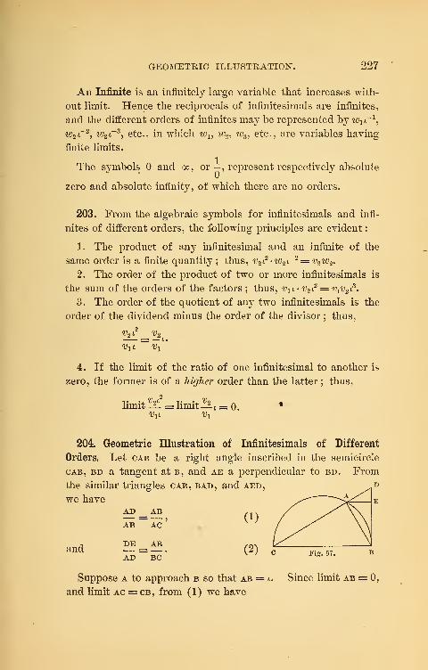
GEOMETRIC ILLUSTRATION. 227
An Infinite is an infinitely large variable that increases with-
out limit. Hence the reciprocals of infinitesimals are infinites,
and the different orders of infinites may be represented by iv1r l,
w2r2, wsr3
yetc., in which w1? w2 , w3 , etc., are variables having
finite limits.
The symbols and oc, or -, represent respectively absolute
zero and absolute infinity, of which there are no orders.
203. From the algebraic symbols for infinitesimals and infi-
nites of different orders, the following principles are evident
:
1. The product of any infinitesimal and an infinite of the
same order is a finite quantity ; thus, v2 t2
• iv2r 2 = v2w2 .
2. The order of the product of two or more infinitesimals is
the sum of the orders of the factors ; thus, vx l'V2 l2 = v1v2 l
3.
3. The order of the quotient of any two infinitesimals is the
order of the dividend minus the order of the divisor ; thus,
V2 L2 v2
4. If the limit of the ratio of one infinitesimal to another is
zero, the former is of a higher order than the latter ; thus,
limit ^i2
= limit-^- t = 0. •
ViL v±
204. Geometric Illustration of Infinitesimals of Different
Orders. Let cab be a right angle inscribed in the semicircle
cab, bd a tangent at b, and ae a perpendicular to bd. Fromthe similar triangles cab, bad, and aed, ^dwe have
AD AB ,1
s=>, (I)
AB AC
and E5 = -^. (2)AD BC Fig. 5
Suppose a to approach b so that ab = t. Since limit ab = 0,
and limit ac = cb, from (1) we have
228 THE METHOD OF INFINITESIMALS,
limit— = limit— =;
AB AC
hence ad is an infinitesimal of a higher order than ab (§ 203, 4).
From (2) we have
limit — = limit — =;
AD BC
hence de is an infinitesimal of a higher order than ad.
Thus, when ab = t, ad = v2 t2
, and de = v3 t3
.
Examples.
1
.
If a = i, of what order is sin a ?
Since HT* ["*Eif] =; 1 , &in« = Vi L.'(§ 202)
,
and limit v1= 1
.
2. If a = t, of what order is tan a?
3. If a = t, of what order is 1 — cos a?
Since ^ P ~ C2
0S al=f, 1 - cos a =V (§ 202)
,
u •-1
and limit v2= -J.
4. If a = t, show that sin a—a=v3 t3
, and that a—tana= /y3 t3
.
205. First Fundamental Principle of Infinitesimals.
Let a — fi= c, in which e is infinitely small in comparison with
a or /5 ; then
2L-— l+.i, andlimit| = 0;P P " ©
\ limit - = limitfl + l~j= 1.
Hence, if the difference between two variables is infinitely small
in comparison with either of them, the limit of their ratio is unity;
RULE FOR DIFFERENTIATION. 229
and, by § 135, either of them may be substituted for the other in
any problem concerning the limit of the ratio of tioo variables.
For convenience of application, this principle may be stated
as follows
:
In problems concerning the limit of the ratio of two variables,
All infinitesimals of the higher orders may be dropped from
sums of infinitesimals of different orders.
All infinitesimals may be dropped from sums offinite quantities
and infinitesimals.
All finite quantities maybe dropped from sums of infinites and
finite quantities.
r limit 1
when € is infinitely small in comparison with (3.
Hence, conversely, if the limit of the ratio of tivo infinitesimals
is unity, their difference is infinitely smcdl in comparison ivith
either.
206. Rule for Differentiation. In this chapter we shall regard
the increments of variables as infinitesimals. Since the differ-
ence between a variable and its limit is an infinitesimal, and
since
Cor. If a = /3 -f-e, limit - , or limit 1+ - is unity only
a[S]-w.•.^=/'(a0 + e , ovAy=f'(x)Ax + e±x, (1)
in which e is an infinitesimal.
Now dy= f'(x)dx. (2)
The value of dx being arbitrary, for convenience we shall, in
this chapter, suppose it to be equal to Aa;.
From (1) and (2) it follows that, if dx = Ax = c, dy and A?/
are infinitesimals whose difference is infinitely small in compari-
son with either, and therefore, in differentiating, dy may be
substituted for Ay (§ 205)
.
230 THE METHOD OF INFINITESIMALS.
From these considerations we have the following simple rule
for differentiating any function :
Find the increment of the function in terms of the increments
of its variables, apply the principles of § 205, and in the terms
remaining replace the increments by differentials.
Thus, to differentiate Xs, let y = x3
; then
Ay = 3 x2Ax + 3 x{Ax) 2-f (Aaj) 3
.
Hence, by the rule,
dy = 3 x2dx.
Rem. We do not drop the infinitesimals of the higher orders,
because the}T are nothing, or comparatively nothing, when added
to an infinitesimal of the first order, but because we know that
they do not appear in the limit of the ratio sought. Thus the
method of limits is the basis of the method of infinitesimals, the
difference being that in the latter we use infinitesimal differen-
tials, and a quantity is dropped as soon as it appears, when it is
known that it will vanish in passing to the limit sought. Anydifferential equation obtained by the infinitesimal method must
evidently be true when the differentials are regarded as finite.
Examples.
1
.
Differentiate u = xy.
Here Au = yAx + xAy -f- AxAy ;.*. du = ydx -f- xdy.
x2. Differentiate u =—
y
Here Au = V**~**y • .-.du =V^-^V .
y2 +yAy y
2
3. Differentiate y = sin.T.
Here Ay — sin (x -j- Ace) — sin x
= cos x sin Ax —{1 — cos Ax) sin x
== cosxAx-t~v2 L2
;
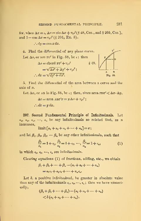
SECOND FUNDAMENTAL PRINCIPLE. 231
for, when Ax = i, Ax = sin Ax + v2 r(§ 48, Cor., and § 205, Cor.),
and l-cosA£C = <y2 i
2(§ 204, Ex. 3).
.•. dy = cos x dx.
4. Find the differential of any plane curve.^J,
Let As, or arc pp' in Fig. 58, be t ; then
As = chord pp'-f- v2 i2
§ 48.
= ^/Ax2 + Ay2-}-v2 l
2;
.-.ds =Vdy2 + dx2.
5. Find the differential of the area between a curve and the
axis of x.
Let Ax, or ab in Fig. 58, be i ; then, since area pdp'< Ax* Ay,
Az = area abp'p = yAx + v2 i2
;
,'.dz = ydx.
207. Second Fundamental Principle of Infinitesimals. Let
ai5 a25 a3? •*•? an t>e anv infinitesimals so related that, as n
increases,
limit [«! + a2 + a3 H |- an] = c
;
and let ft, f32 , (33 ,••» /?„ be any other infinitesimals, such that
^ = l+ q ,£-2 =l-bc2 ,
..-, ^=l+ €n, (1)ttl a2 an
in which et , e2 , •••, cn are infinitesimals.
Clearing equations (1) of fractions, adding, etc., we obtain
/?! + &+••• +/?n-(a1 + a2 +...+an)
= a1 €1 -\-a2 e2 -\ f- a»e».
Let 8, a positive infinitesimal, be greater in absolute value
than any of the infinitesimals e1? e2, •••, en ; then we have numeri-
cally,
< 8 (ai+ a2 H f- an)
.
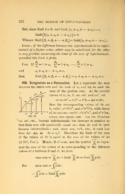
232 THE METHOD OF INFINITESIMALS.
But, since limit 8 = 0, and limit. (ai + «2 H h <0 = c,
limit [8(ai + a2 H 1- «„)] = 0.
Whence limit [ft + ft -\ h ft] = limit [ax + a2 H h an]
.
Hence, if the difference between two infinitesimals is an infini-
tesimal of a higher order, either may be substituted for the other
in any problem concerning the limit of the sum of infinitesimals,
provided this limit is finite.
Cor. If - = !+€!, — =l+ e2 ,•••, — = 1 + e«,
al a2 an
and ax + a2 -\ \-an = C,
then limit [ft 4- ft H h ft] = «i + «2 H h «« = c.
208. Integration as a Summation. Let 2 represent the area
between the curve opd and the axis of x, and let us seek the
area of the portion obd. At the several
values of x, as, 0, oa, oa', and oa", let
oa = aa' = a'a" = a'fB = Ace = dx
;
then the corresponding values of dz are
0, apba', a'p'b'a", and a"p"6"B, while thosex of Az are opa, appV, a'p'p"a", and a"p"DB,
rig. 59. whose sum equals obd. Let the divisions
oct, aa', etc., become infinitesimals, bat increase in number so
that their sum will pontinually equal ob ; then Az and dz both
become infinitesimals; and, since op«, pp'5, etc., is each less
than Ax • Ay, Az — dz = v2 r. Therefore the limit of the sum
of the values of dz is equal to the sum of the values of Azx = x'
(§ 207, Cor.). Hence, if x' =ob, and the symbol ]£ Az repre-ss
sent the sum of the values of Az corresponding to the different
values of x between and x', we have
Xz=X
area obd = ^ Az = limit % dz = limit £ ydx.x=0 x=0
Jydx;
x=0
f*x'
But area obd =
•1ydx = limit J yefce.
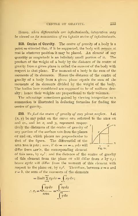
CENTRE OF GRAVITY. 233
Hence, ivhen differentials are infinitesimals, integration maybe viewed as the summation of an infinite series of infinitesimals.
209. Centre of Gravity. The centre of gravity of a body is a
point so situated that, if it be supported, the bocly will remain at
rest in whatever position it may be placed. An element of any
quantity or magnitude is an infinitely small portion of it. The
product of the weight of a body by the distance of its centre of
gravit}' from a given plane is called the moment of the bod}T with
respect to that plane. The moment of a bod}' is the sum of the
moments of its elements. Hence the distance of the centre of
gravity of a body from a given plane equals the sum of the
moments of its elements divided \>y the weight of the body.
The bodies here considered are supposed to be of uniform den-
sity ; hence their weights are proportional to their volumes.
The advantage sometimes gained b}7 viewing integration as a
summation is illustrated in deducing formulas for finding the
centre of gravity.
210. To find the centre of gravity of any plane surface. Let
(x, y) be any point on the curve ovn referred to the axes ox
and oy, and let x and y represent respec-
tively the distances of the centre of gravity of
any portion of the surface xon from the planes
oy and ox, which planes are perpendicular to
that of the figure. The differential of the
area xo?i is ydx ; now. if dx = ab = i, ydx will
differ from abp'p, the corresponding elementFlg ' 60 '
of this area, by v2 c : and the distance of the centre of gravity
of this element from the plane oy will differ from x hyv1 c;
hence xydx will differ from the moment of this element with
respect to the plane oy, by v2 r. Therefore, between x = a and
x = b, the sum of the moments of the elements
= limit % xy dx = j xy dx;
x=a *Ja
area
Xbr*b
xydxjxydx
Jydx
234 THE METHOD OF INFINITESIMALS.
Again, the centre of gravity of ydx is evidently \y from the
plane ox ; hence iy2(lx will differ from the moment of the cor-
responding element with respect to the plane ox, by v2 l2
. Hence,
between x = a and x = b, the sum of the moments of the ele-
ments = \ I y2dx
;
Xb fby
2dx I y2dx
areaJydi
If the curve be symmetrical with respect to ox, x is evidently
the same for the whole area as for the half, and y is zero.
211. To find the centre of gravity of any plane curve. Let
(x01 y ) be the centre of gravity of any arc of a plane curve
whose length is represented by s. Now, when ds = t, xds dif-
fers from the moment of the corresponding element of the curve,
with respect to the plane oy (Fig. 60) , by v2 t2
. Hence, between
x = a and x = b, the sum of the moments of the elements
=Jxds,
and \%dsXn —
In like manner, we obtain
2/o=S)
d'
212. To find the centre of gravity of a solid of revolution.
The differential of a solid of revolution whose axis is the axis
of x, is ny2dx ; hence, if dx = t, irxy2dx will differ from the
moment of the corresponding element of the solid, with respect
to the plane ot, by v2 i2
; and therefore, between x = a and x= b,
the sum of the moments of the elements
= I 7rxy2dx.
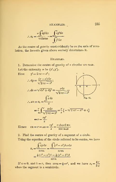
EXAMPLES. 235
7T I xy2dx I xy2dx
I yhlx4/a
Xq —volume
As the centre of gravity must evidently be on the axis of revo-
lution, the formula given above entirely determines it.
Examples.
1. Determine the centre of gravity of a circular arc bad.
Let the extremity d be (x' r y').
Here y2= 2 rx — x2
;
(r—x)dxdy
•\j2rx — x2
= Vcfce2 + dy2 = rdx
V2 rcc
—
xf
,\ ae = a?jf
C?8 Fig. 61.
sJ°V2r£ —
a
2 *
= I[_V2ra'-^'2 + s]
ry
Hence ce = r — aery _ r chord bd
arc bap
2. Find the centre of gravity of a segment of a circle.
Using the equation of the circle referred to its centre, we have
xydxj
(r2— x2)hxdx
area area
area
If a = 0, and b = r, then area == Jtt?*2, and we have # = —
-
when the segment is a semicircle.
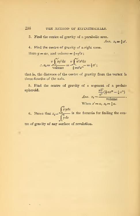
236 THE METHOD OF INFINITESIMALS.
3. Find the centre of gravity of a parabolic area.
Ans. xQ= ^x'.
4. Find the centre of gravity of a right cone.
Here y = ax, and volume = ^iry2x;
7r I xy2dx ttJa2xsdx
volume §Trazx 16
that is, the distance of the centre of gravity from the vertex is
three-fourths of the axis.
5. Find the centre of gravity of a segment of a prolate
spheroid. ^^'-i>)Ans. x — -
volume
When x'= a, x = J- a.
I xyds
6. Prove that # =^ is tne formula for finding the cen-
iyds
tre of gravity of any surface of revolution.