Embed Size (px)
Citation preview
ELECTRIFICATION OF DIESEL-BASED POWERTRAINSFOR HEAVY VEHICLES
by
Tyler Swedes
A Thesis
Submitted to the Faculty of Purdue University
In Partial Fulfillment of the Requirements for the degree of
Master of Science in Mechanical Engineering
School of Mechanical Engineering
West Lafayette, Indiana
August 2021
THE PURDUE UNIVERSITY GRADUATE SCHOOLSTATEMENT OF COMMITTEE APPROVAL
Dr. Greg Shaver, Chair
School of Mechanical Engineering
Dr. Peter Meckl
School of Mechanical Engineering
Dr. Oleg Wasynczuk
School of Electrical and Computer Engineering
Approved by:
Dr. Nicole L. Key
2

To my parents, Dave and Carmen Swedes, and my brother, Christopher Swedes.
3

ACKNOWLEDGMENTS
I would like to thank the Lord for being my foundation and constant source of hope,
and my parents for their love, support, and encouragement in every part of my life. I also
want to recognize my advisor, Dr. Greg Shaver, especially for his guidance in academia and
in transitioning to industry, as well as Dr. Oleg Wasynczuk and Dr. Peter Meckl for their
instruction both in the classroom and in research. Finally I want to thank my colleagues
in Dr. Shaver’s research group for their friendship and their help in completing my work,
especially Harsha Rayasam, Weijin Qui, Chisom Emegoakor, and Shubham Agnihotri.
4

TABLE OF CONTENTS
LIST OF TABLES . . . . . . . . . . . . . . . . . . . . . . . . . . . . . . . . . . . . . 8
LIST OF FIGURES . . . . . . . . . . . . . . . . . . . . . . . . . . . . . . . . . . . . 9
LIST OF SYMBOLS . . . . . . . . . . . . . . . . . . . . . . . . . . . . . . . . . . . . 12
ABBREVIATIONS . . . . . . . . . . . . . . . . . . . . . . . . . . . . . . . . . . . . . 14
ABSTRACT . . . . . . . . . . . . . . . . . . . . . . . . . . . . . . . . . . . . . . . . 16
1 INTRODUCTION . . . . . . . . . . . . . . . . . . . . . . . . . . . . . . . . . . . 18
1.1 Motivation . . . . . . . . . . . . . . . . . . . . . . . . . . . . . . . . . . . . . 18
1.2 Summary and Objectives of Work Presented . . . . . . . . . . . . . . . . . . 19
1.3 Background and Literature Review . . . . . . . . . . . . . . . . . . . . . . . 20
1.3.1 Series Electric Hybrid Powertrain Description . . . . . . . . . . . . . 20
1.3.2 Fuel Savings Due to Hybridization of Class 8 Truck . . . . . . . . . . 21
1.3.3 Electrified Air Handling System Description . . . . . . . . . . . . . . 23
1.3.4 Robust H∞ Multi-Input Multi-Output Control Design . . . . . . . . 24
1.3.5 Mean Value Engine Modeling for Control . . . . . . . . . . . . . . . 26
2 EFFICIENCY ANALYSIS OF SERIES ELECTRIC HYBRID POWERTRAIN . . 27
2.1 System Description . . . . . . . . . . . . . . . . . . . . . . . . . . . . . . . . 27
2.2 Data Collection . . . . . . . . . . . . . . . . . . . . . . . . . . . . . . . . . . 28
2.2.1 Test Routes . . . . . . . . . . . . . . . . . . . . . . . . . . . . . . . . 29
2.2.2 Data Filtering . . . . . . . . . . . . . . . . . . . . . . . . . . . . . . . 32
2.2.3 Distance Traveled Calculation . . . . . . . . . . . . . . . . . . . . . . 35
2.3 Component Energy Inputs and Outputs . . . . . . . . . . . . . . . . . . . . 35
2.3.1 Engine and Generator . . . . . . . . . . . . . . . . . . . . . . . . . . 39
2.3.2 Traction Motor . . . . . . . . . . . . . . . . . . . . . . . . . . . . . . 41
2.3.3 Battery . . . . . . . . . . . . . . . . . . . . . . . . . . . . . . . . . . 45
2.3.4 Contribution of Each Component to Vehicle Work Performed . . . . 47
5

Battery Operation . . . . . . . . . . . . . . . . . . . . . . . . . . . . 48
System Losses . . . . . . . . . . . . . . . . . . . . . . . . . . . . . . . 49
Summary of Component Energy Contributions . . . . . . . . . . . . 50
2.4 Power Electronics Efficiency Analysis . . . . . . . . . . . . . . . . . . . . . . 51
2.4.1 Power Modes . . . . . . . . . . . . . . . . . . . . . . . . . . . . . . . 51
2.4.2 Energy Accumulation in Power Electronics . . . . . . . . . . . . . . . 54
2.4.3 Efficiency Results . . . . . . . . . . . . . . . . . . . . . . . . . . . . . 56
2.5 Summary of Other Efficiency Results . . . . . . . . . . . . . . . . . . . . . . 58
2.5.1 Regeneration Energy Capture Percentage . . . . . . . . . . . . . . . 59
2.5.2 Ratio of Regeneration Energy Capture to Drive Energy Output . . . 60
2.6 Future Work . . . . . . . . . . . . . . . . . . . . . . . . . . . . . . . . . . . 62
3 CONTROL ORIENTED NONLINEAR STATE SPACE MODEL OF DIESEL EN-
GINE WITH ELECTRIFIED AIR HANDLING . . . . . . . . . . . . . . . . . . . 64
3.1 Engine Architecture . . . . . . . . . . . . . . . . . . . . . . . . . . . . . . . 64
3.2 Nonlinear State Space Model . . . . . . . . . . . . . . . . . . . . . . . . . . 65
3.3 Submodels Used in Nonlinear State Space Model . . . . . . . . . . . . . . . 70
3.3.1 eBooster Compressor Flow . . . . . . . . . . . . . . . . . . . . . . . . 72
3.3.2 Turbocharger Compressor Flow . . . . . . . . . . . . . . . . . . . . . 73
3.3.3 Turbocharger Compressor Power . . . . . . . . . . . . . . . . . . . . 75
3.3.4 Turbine Flow . . . . . . . . . . . . . . . . . . . . . . . . . . . . . . . 76
3.3.5 Turbine Power . . . . . . . . . . . . . . . . . . . . . . . . . . . . . . 78
3.3.6 Turbocharger Windage Loss . . . . . . . . . . . . . . . . . . . . . . . 78
3.3.7 Turbine Wastegate . . . . . . . . . . . . . . . . . . . . . . . . . . . . 79
3.3.8 Valve Flow . . . . . . . . . . . . . . . . . . . . . . . . . . . . . . . . 81
3.3.9 Cylinder Charge Flow . . . . . . . . . . . . . . . . . . . . . . . . . . 83
3.3.10 Exhaust Gas Temperature . . . . . . . . . . . . . . . . . . . . . . . . 83
3.3.11 eBooster Outlet Temperature . . . . . . . . . . . . . . . . . . . . . . 87
3.3.12 Engine Torque Coefficient . . . . . . . . . . . . . . . . . . . . . . . . 87
4 STATE SPACE MODEL LINEARIZATION, VALIDATION, AND ANALYSIS . . 89
6

4.1 Nonlinear Model Linearization . . . . . . . . . . . . . . . . . . . . . . . . . . 89
4.2 Linear Models Selected . . . . . . . . . . . . . . . . . . . . . . . . . . . . . . 90
4.3 Model Validation . . . . . . . . . . . . . . . . . . . . . . . . . . . . . . . . . 91
4.3.1 Validation Results from Linear Model 1 . . . . . . . . . . . . . . . . 93
Torque Steps at 1200 rpm . . . . . . . . . . . . . . . . . . . . . . . . 93
Torque Steps at 1400 rpm . . . . . . . . . . . . . . . . . . . . . . . . 99
Torque Steps at 1600 rpm . . . . . . . . . . . . . . . . . . . . . . . . 104
4.3.2 Validation Results from Linear Model 2 . . . . . . . . . . . . . . . . 109
Torque Steps at 1600 rpm . . . . . . . . . . . . . . . . . . . . . . . . 109
Torque Steps at 1800 rpm . . . . . . . . . . . . . . . . . . . . . . . . 115
Torque Steps at 2000 rpm . . . . . . . . . . . . . . . . . . . . . . . . 120
4.3.3 Summary . . . . . . . . . . . . . . . . . . . . . . . . . . . . . . . . . 125
4.3.4 Improvements and Limitations . . . . . . . . . . . . . . . . . . . . . 126
4.4 Relative Gain Array Analysis . . . . . . . . . . . . . . . . . . . . . . . . . . 127
4.4.1 RGA Analysis for Linear Model 1 . . . . . . . . . . . . . . . . . . . . 129
4.4.2 RGA Analysis for Linear Model 2 . . . . . . . . . . . . . . . . . . . . 132
4.4.3 Summary . . . . . . . . . . . . . . . . . . . . . . . . . . . . . . . . . 134
5 CONCLUSIONS AND FUTURE WORK . . . . . . . . . . . . . . . . . . . . . . . 135
5.1 Summary . . . . . . . . . . . . . . . . . . . . . . . . . . . . . . . . . . . . . 135
5.1.1 Series Hybrid Electric Powertrain Analysis for Class 8 Truck . . . . . 135
5.1.2 Control Oriented Modeling of Diesel Engine . . . . . . . . . . . . . . 136
5.2 Future Work . . . . . . . . . . . . . . . . . . . . . . . . . . . . . . . . . . . 136
5.2.1 Series Electric Hybrid Powertrain Analysis for Class 8 Truck . . . . . 136
5.2.2 Control Oriented Modeling of Diesel Engine . . . . . . . . . . . . . . 137
REFERENCES . . . . . . . . . . . . . . . . . . . . . . . . . . . . . . . . . . . . . . . 138
7

LIST OF TABLES
2.1 List of test data sets . . . . . . . . . . . . . . . . . . . . . . . . . . . . . . . . . 29
2.2 Power electronics efficiency results . . . . . . . . . . . . . . . . . . . . . . . . . 57
2.3 Drag and rolling resistance coefficients . . . . . . . . . . . . . . . . . . . . . . . 60
3.1 Nonlinear mean value model states . . . . . . . . . . . . . . . . . . . . . . . . . 66
3.2 Engine actuators . . . . . . . . . . . . . . . . . . . . . . . . . . . . . . . . . . . 68
3.3 State outputs . . . . . . . . . . . . . . . . . . . . . . . . . . . . . . . . . . . . . 68
3.4 Letter assignments . . . . . . . . . . . . . . . . . . . . . . . . . . . . . . . . . . 69
3.5 Subscript definitions . . . . . . . . . . . . . . . . . . . . . . . . . . . . . . . . . 70
3.6 Terms used in state equations . . . . . . . . . . . . . . . . . . . . . . . . . . . . 71
3.7 Parameters in eBooster compressor flow model . . . . . . . . . . . . . . . . . . . 72
3.8 Regression fit coefficients in eBooster compressor flow model . . . . . . . . . . . 73
3.9 Regression fit coefficients in turbocharger compressor flow model . . . . . . . . . 74
3.10 Parameters in turbocharger compressor power model . . . . . . . . . . . . . . . 76
3.11 Parameters in turbine flow model . . . . . . . . . . . . . . . . . . . . . . . . . . 77
3.12 Regression fit coefficients in turbocharger turbine flow model . . . . . . . . . . . 77
3.13 Parameters in turbocharger turbine power model . . . . . . . . . . . . . . . . . 78
3.14 Regression fit coefficients in turbocharger windage loss model . . . . . . . . . . 79
3.15 Regression fit coefficients in wastegate effective valve area model . . . . . . . . . 80
3.16 Parameters in valve model . . . . . . . . . . . . . . . . . . . . . . . . . . . . . . 82
3.17 Parameters in charge flow model . . . . . . . . . . . . . . . . . . . . . . . . . . 83
3.18 Regression fit coefficients exhaust gas temperature model . . . . . . . . . . . . . 85
3.19 Parameters in charge flow model . . . . . . . . . . . . . . . . . . . . . . . . . . 86
3.20 Parameters engine torque coefficient model . . . . . . . . . . . . . . . . . . . . . 88
3.21 Regression fit coefficients for thermal efficiency . . . . . . . . . . . . . . . . . . 88
4.1 Equilibrium states and inputs for linear models . . . . . . . . . . . . . . . . . . 91
8

LIST OF FIGURES
1.1 Series hybrid powertrain architecture. . . . . . . . . . . . . . . . . . . . . . . . . 21
1.2 Average fuel economy over Florence-Cambridge route [ 1 ]. . . . . . . . . . . . . . 22
1.3 Engine air handling system with BorgWarner eBooster [ 5 ]. . . . . . . . . . . . . 23
2.1 Series hybrid system diagram . . . . . . . . . . . . . . . . . . . . . . . . . . . . 27
2.2 Simplified system block diagram and selected reference directions . . . . . . . . 28
2.3 Lexington test route map . . . . . . . . . . . . . . . . . . . . . . . . . . . . . . 30
2.4 Lexington test route grade angle (degrees) . . . . . . . . . . . . . . . . . . . . . 30
2.5 Indianapolis test route grade angle (degrees) . . . . . . . . . . . . . . . . . . . . 31
2.6 Indianapolis test route grade angle (degrees) . . . . . . . . . . . . . . . . . . . . 32
2.7 Grade angle for 10-km stretch of Lexington route on 10 October with and withoutfiltering. . . . . . . . . . . . . . . . . . . . . . . . . . . . . . . . . . . . . . . . . 33
2.8 FFT plots for elevation and grade angle data with and without filtering. . . . . 33
2.9 Acceleration profile for 10-km stretch of Lexington route on 10 October with andwithout filtering. . . . . . . . . . . . . . . . . . . . . . . . . . . . . . . . . . . . 34
2.10 FFT plots for velocity and acceleration data with and without filtering. . . . . . 35
2.11 Power flows and drive cycle conditions for 4 km of Lexington route on 10 October 37
2.12 Power flows and drive cycle conditions for 4 km of Lexington route on 9 January 38
2.13 Generator power output from Lexington test on 10 October . . . . . . . . . . . 39
2.14 Diesel engine rpm and load . . . . . . . . . . . . . . . . . . . . . . . . . . . . . 40
2.15 Generator energy accumulation functions . . . . . . . . . . . . . . . . . . . . . . 41
2.16 Motor power from Lexington from 10 October test run . . . . . . . . . . . . . . 42
2.17 Pbat + Pgen from Lexington from 10 October test run . . . . . . . . . . . . . . . 43
2.18 Motor energy accumulation functions . . . . . . . . . . . . . . . . . . . . . . . . 44
2.19 Battery power, current, voltage, and state of charge from 10 October test run . 45
2.20 Battery energy accumulation functions . . . . . . . . . . . . . . . . . . . . . . . 47
2.21 Component energy accumulation curves for 10 October test run . . . . . . . . . 48
2.22 Work contributed by each component per km for all data sets . . . . . . . . . . 50
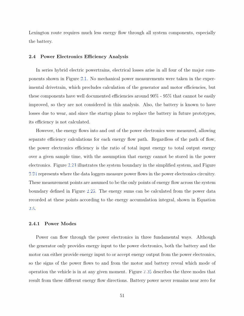
2.23 Power electronics system definition and energy inputs/outputs . . . . . . . . . . 52
2.24 Power electronics diagram . . . . . . . . . . . . . . . . . . . . . . . . . . . . . . 53
9
2.25 Energy flow modes . . . . . . . . . . . . . . . . . . . . . . . . . . . . . . . . . . 54
2.26 Power electronics efficiency versus sample duration Lexington 15 October test . 55
2.27 Power electronics efficiency versus sample duration Indianapolis 9 January test . 56
2.28 Boxplot of average power electronics efficiencies . . . . . . . . . . . . . . . . . . 58
2.29 Measured motor regeneration energy as fraction of calculated available energy . 59
2.30 Energy ratio results summary . . . . . . . . . . . . . . . . . . . . . . . . . . . . 61
3.1 Engine air handling system diagram . . . . . . . . . . . . . . . . . . . . . . . . 64
3.2 Nonlinear state space model simulation framework . . . . . . . . . . . . . . . . 65
3.3 eBooster compressor map . . . . . . . . . . . . . . . . . . . . . . . . . . . . . . 73
3.4 Turbocharger compressor map . . . . . . . . . . . . . . . . . . . . . . . . . . . . 75
3.5 Turbocharger turbine map . . . . . . . . . . . . . . . . . . . . . . . . . . . . . . 77
3.6 Turbocharger windage loss . . . . . . . . . . . . . . . . . . . . . . . . . . . . . . 79
3.7 Wastegate forward discharge coefficient regression fit . . . . . . . . . . . . . . . 81
4.1 Nonlinear and linear model validation method . . . . . . . . . . . . . . . . . . . 92
4.2 Linear model 1 speed and torque profile and actuator responses for torque stepsat 1200 rpm . . . . . . . . . . . . . . . . . . . . . . . . . . . . . . . . . . . . . . 93
4.3 Linear model 1 pressure states for torque steps at 1200 rpm . . . . . . . . . . . 94
4.4 Linear model 1 temperature states for torque steps at 1200 rpm . . . . . . . . . 95
4.5 Linear model 1 turbomachinery speed states for torque steps at 1200 rpm . . . . 96
4.6 Linear model 1 state outputs for torque steps at 1200 rpm . . . . . . . . . . . . 97
4.7 Linear model 1 speed and torque profile and actuator responses for torque stepsat 1400 rpm . . . . . . . . . . . . . . . . . . . . . . . . . . . . . . . . . . . . . . 99
4.8 Linear model 1 pressure states for torque steps at 1400 rpm . . . . . . . . . . . 100
4.9 Linear model 1 temperature states for torque steps at 1400 rpm . . . . . . . . . 101
4.10 Linear model 1 turbomachinery speed states for torque steps at 1400 rpm . . . . 102
4.11 Linear model 1 state outputs for torque steps at 1400 rpm . . . . . . . . . . . . 103
4.12 Linear model 1 speed and torque profile and actuator responses for torque stepsat 1600 rpm . . . . . . . . . . . . . . . . . . . . . . . . . . . . . . . . . . . . . . 104
4.13 Linear model 1 pressure states for torque steps at 1600 rpm . . . . . . . . . . . 105
4.14 Linear model 1 temperature states for torque steps at 1600 rpm . . . . . . . . . 106
4.15 Linear model 1 turbomachinery speed states for torque steps at 1600 rpm . . . . 107
10

4.16 Linear model 1 state outputs for torque steps at 1600 rpm . . . . . . . . . . . . 108
4.17 Linear model 2 speed and torque profile and actuator responses for torque stepsat 1600 rpm . . . . . . . . . . . . . . . . . . . . . . . . . . . . . . . . . . . . . . 110
4.18 Linear model 2 pressure states for torque steps at 1600 rpm . . . . . . . . . . . 111
4.19 Linear model 2 temperature states for torque steps at 1600 rpm . . . . . . . . . 112
4.20 Linear model 2 turbomachinery speed states for torque steps at 1600 rpm . . . . 113
4.21 Linear model 2 state outputs for torque steps at 1600 rpm . . . . . . . . . . . . 114
4.22 Linear model 2 speed and torque profile and actuator responses for torque stepsat 1800 rpm . . . . . . . . . . . . . . . . . . . . . . . . . . . . . . . . . . . . . . 115
4.23 Linear model 2 pressure states for torque steps at 1800 rpm . . . . . . . . . . . 116
4.24 Linear model 2 temperature states for torque steps at 1800 rpm . . . . . . . . . 117
4.25 Linear model 2 turbomachinery speed states for torque steps at 1800 rpm . . . . 118
4.26 Linear model 2 state outputs for torque steps at 1800 rpm . . . . . . . . . . . . 119
4.27 Linear model 2 speed and torque profile and actuator responses for torque stepsat 2000 rpm . . . . . . . . . . . . . . . . . . . . . . . . . . . . . . . . . . . . . . 120
4.28 Linear model 2 pressure states for torque steps at 2000 rpm . . . . . . . . . . . 121
4.29 Linear model 2 temperature states for torque steps at 2000 rpm . . . . . . . . . 122
4.30 Linear model 2 turbomachinery speed states for torque steps at 2000 rpm . . . . 123
4.31 Linear model 2 state outputs for torque steps at 2000 rpm . . . . . . . . . . . . 124
4.32 Linear model 1 RGA element analysis for EGR fraction output . . . . . . . . . 130
4.33 Linear model 1 RGA element analysis for AFR output . . . . . . . . . . . . . . 130
4.34 Linear model 1 RGA element analysis for engine speed output . . . . . . . . . . 131
4.35 Linear model 2 RGA element analysis for EGR fraction output . . . . . . . . . 132
4.36 Linear model 2 RGA element analysis for AFR output . . . . . . . . . . . . . . 133
4.37 Linear model 2 RGA element analysis for engine speed output . . . . . . . . . . 133
11
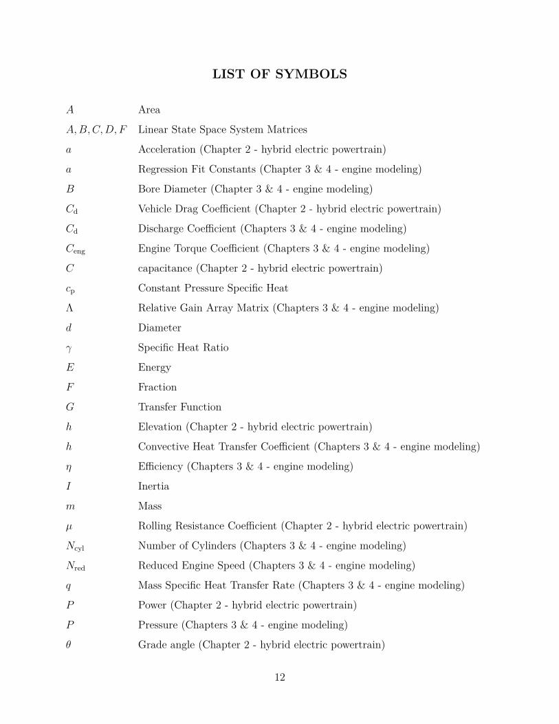
LIST OF SYMBOLS
A Area
A, B, C, D, F Linear State Space System Matrices
a Acceleration (Chapter 2 - hybrid electric powertrain)
a Regression Fit Constants (Chapter 3 & 4 - engine modeling)
B Bore Diameter (Chapter 3 & 4 - engine modeling)
Cd Vehicle Drag Coefficient (Chapter 2 - hybrid electric powertrain)
Cd Discharge Coefficient (Chapters 3 & 4 - engine modeling)
Ceng Engine Torque Coefficient (Chapters 3 & 4 - engine modeling)
C capacitance (Chapter 2 - hybrid electric powertrain)
cp Constant Pressure Specific Heat
Λ Relative Gain Array Matrix (Chapters 3 & 4 - engine modeling)
d Diameter
γ Specific Heat Ratio
E Energy
F Fraction
G Transfer Function
h Elevation (Chapter 2 - hybrid electric powertrain)
h Convective Heat Transfer Coefficient (Chapters 3 & 4 - engine modeling)
η Efficiency (Chapters 3 & 4 - engine modeling)
I Inertia
m Mass
µ Rolling Resistance Coefficient (Chapter 2 - hybrid electric powertrain)
Ncyl Number of Cylinders (Chapters 3 & 4 - engine modeling)
Nred Reduced Engine Speed (Chapters 3 & 4 - engine modeling)
q Mass Specific Heat Transfer Rate (Chapters 3 & 4 - engine modeling)
P Power (Chapter 2 - hybrid electric powertrain)
P Pressure (Chapters 3 & 4 - engine modeling)
θ Grade angle (Chapter 2 - hybrid electric powertrain)
12
R Mass specific gas constant
ρ Density
S Cylinder Stroke Length (Chapter 3 & 4 - engine modeling)
Sp Mean Engine Speed (Chapter 3 & 4 - engine modeling)
s Complex Variable (Chapter 3 & 4 - engine modeling)
T Temperature
T Time Constant
t Time
τ Time (Chapter 2 - hybrid electric powertrain)
τ Torque (Chapters 3 & 4 - engine modeling)
u State Input (Chapters 3 & 4 - engine modeling)
V Voltage (Chapter 2 - hybrid electric powertrain)
V Volume (Chapters 3 & 4 - engine modeling)
v Speed
W Flow Rate (Chapters 3 & 4 - engine modeling)
w Average Cylinder Gas Velocity (Chapters 3 & 4 - engine modeling)
ω Shaft Speed
ω Frequency
x Distance Travelled (Chapter 2 - hybrid electric powertrain)
x State Variable (Chapter 3 - engine modeling)
y State Input (Chapters 3 & 4 - engine modeling)
Z Power (Chapters 3 & 4 - engine modeling)
13
ABBREVIATIONS
AFR Air-Fuel Ratio
aero Aerodynamic (subscript)
amb Ambient conditions (subscript)
bat Battery (subscript)
bd Blowdown (subscript)
bv Bypass Valve (subscript)
BMS Battery Management System
BSFC Brake Specific Fuel Consumption
CAC Charge Air Cooler
comp Compressor (subscript)
compis Compressor interstage (subscript)
cyl Cylinder Inlet (subscript)
cylout Cylinder Outlet (subscript)
ECM Engine Control Module
ECR Effective Compression Ratio
EGR Exhaust Gas Recirculation
EOC End of Combustion
EVO Exhaust Valve Opening
em Exhaust Manifold (subscript)
et Exhaust Throttle (subscript)
ex Exhaust (subscript)
FFT Fast Fourier Transform
gen Generator (subscript)
GPS Global Positioning System
GVW Gross Vehicle Weight
IC Internal Combustion
im Intake Manifold (subscript)
LHV Lower Heating Value
14
MIMO Multi-Input Multi-Output (control method)
mot Motor (subscript)
PR Pressure Ratio
regen Regenerative Braking (subscript)
RGA Relative Gain Array
rpm Revolutions per Minute
rr Rolling Resistance (subscript)
SISO Single-Input Single-Output (control method)
SOC Battery State of Charge
tc Turbocharger (subscript)
TDC Top Dead Center
turb Turbine (subscript)
VFD Variable Frequency Drive
wg Wastegate (subscript)
15
ABSTRACT
In recent decades as environmental concerns and the cost and availability of fossil fuels
have become more pressing issues, the need to extract more work from each drop of fuel has
increased accordingly. Electrification has been identified as a way to address these issues in
vehicles powered by internal combustion engines, as it allows existing engines to be operated
more efficiently, reducing overall fuel consumption. Two applications of electrification are
discussed in the work presented: a series-electric hybrid powertrain from an on-road class
8 truck, and an electrically supercharged diesel engine for use in the series hybrid power
system of a wheel loader.
The first application is an experimental powertrain developed by a small start-up com-
pany for use in highway trucks. The work presented in this thesis shows test results from
routes along (1) Interstate 75 between Florence, KY, and Lexington, KY, and (2) Interstates
74 and 70 east of Indianapolis, during which tests the startup collected power flow data from
the vehicle’s motor, generator, and battery, and three-dimensional position data from a GPS
system. Based on these data, it was determined that the engine-driven generator provided
an average of 15% more propulsive energy than required due to electrical losses in the driv-
etrain. Some of these losses occured in the power electronics, which are shown to be 82% -
92% efficient depending on power flow direction, but the battery showed significant signs of
wear, accounting for the remainder of these electrical losses. Overall, most of the system’s
fuel savings came from its regenerative braking capability, which recaptured between 3% and
12% of the total drive energy output. Routes with significant grade changes maximize this
energy recapture percentage, but it is shown minimizing drag and rolling resistance with a
more modern truck and trailer could further increase this energy capture to between 8% and
18%.
In the second application, an electrified air handling system is added to a 4.5L engine,
allowing it to replace the 6.8L engine in John Deere’s 644K hybrid wheel loader. Most
of the fuel savings arise from downsizing the engine, so in this case an electrically driven
supercharger (eBooster) allows the engine to meet the peak torque requirements of the larger,
original engine. In this thesis, a control-oriented nonlinear state space model of the modified
16
4.5L engine is presented and linearized for use in designing a robust, multi-input multi-output
(MIMO) controller which commands the engine’s fueling rate, eBooster, eBooster bypass
valve, exhaust gas recirculation (EGR) valve, and exhaust throttle. This integrated control
strategy will ultimately allow superior tracking of engine speed, EGR fraction, and air-
fuel ratio (AFR) targets, but these performance gains over independent single-input single-
output control loops for each component demand linear models that accurately represent
the engine’s gas exchange dynamics. To address this, a physics-based model is presented
and linearized to simulate pressures, temperatures, and shaft speeds based on sub-models
for exhaust temperature, cylinder charge flow, valve flow, compressor flow, turbine flow,
compressor power, and turbine power. The nonlinear model matches the truth reference
engine model over the 1200 rpm - 2000 rpm and 100 Nm - 500 Nm speed and torque envelope
of interest within 10% in steady state and 20% in transient conditions. Two linear models
represent the full engine’s dynamics over this speed and torque range, and these models match
the truth reference model within 20% in the middle of the operating envelope. However,
specifically at (1) low load for any speed and (2) high load at high speed, the linear models
diverge from the nonlinear and truth reference models due to nonlinear engine dynamics
lost in linearization. Nevertheless, these discrepancies at the edges of the engine’s operating
envelope are acceptable for control design, and if greater accuracy is needed, additional linear
models can be generated to capture the engine’s dynamics in this region.
17
1. INTRODUCTION
1.1 Motivation
In recent decades as environmental concerns and the cost and availability of fossil fuels
have become more pressing issues, the need to extract more work from each drop of fuel has
increased accordingly. In the on- and off-road commercial vehicle space, no energy source
has been identified which can match diesel fuel’s energy density, ease of distribution, and
ubiquity, so at least for the near term, development efforts have focused on reducing the
amount of fuel required to do the same total work.
Electrification has emerged as one way to reduce total fuel consumption in vehicles pow-
ered by internal combustion (IC) engines, because electrical systems allow the designer to
distance the engine from the inherently non-steady operational profile that characterizes
commercial vehicles’ power requirements. IC engines, and specifically compression ignition
engines, can produce power over a wide range of speeds, which initially suited them for vehi-
cles which operate over a wide speed range, but their efficiency “sweet spot” which maximizes
the energy extracted per unit mass of fuel is a much narrower range of speeds and torques.
As a result, significant fuel savings can be realized by selecting an engine that meets a vehi-
cle’s average power requirement when operating in its sweet spot where brake specific fuel
consumption (BSFC) is minimized. However, an engine selected this way typically cannot
meet a vehicle’s peak transient power requirements, so the electrical system provides addi-
tional assistance, allowing the complete electrified powertrain package to output sufficient
power.
The commercial vehicle industry has successfully employed a variety of electrified drive-
trains, but two common approaches are series-electric powertrain hybridization and engine
air handling electrification. Series-electric powertrains are particularly popular, because they
eliminate the mechanical connection between the engine and drive wheels, they are relatively
simple to understand and design, and they allow braking energy that would normally be lost
in friction brakes to be recaptured. Electrified air handling systems are also straightforward
to implement, because electrically driven compression stages can typically be bolted onto
existing engines to increase torque output, and they typically require smaller, lower voltage
18
electrical systems than those used in full hybrid drivetrains. As a result, these systems are
typically employed to allow smaller engines to replace larger, less efficient engines without
sacrificing power output. However, both approaches can reduce the fuel quantity necessary
to meet a given drivetrain’s required power output.
1.2 Summary and Objectives of Work Presented
The work presented in this thesis covers two distinct applications of hybrid powertrains
in commercial vehicles:
Application 1: The first application is a series electric hybrid class 8 truck designed
and built by a small startup company to provide fuel efficiency gains on a highway drive
cycle. The work on this application, presented in Chapter 2 , builds on the results discussed
in [1 ] with objectives of (1) confirming that electrical components operate as expected, (2)
identifying the mechanisms through which the hybrid drivetrain can provide efficiency im-
provements over a conventional drivetrain, and (3) demonstrating that potential efficiency
improvements from a hybrid drivetrain on a highway drive cycle are significant enough to
merit further development. The modeling and analysis toward objectives 2 and 3 was con-
ducted in cooperation with Shubham Agnihotri, so this work is omitted, but the results are
summarized briefly in Section 2.5 .
Application 2: The second application is a diesel engine with an electrically driven
supercharger for a John Deere 644K hybrid wheel loader. The objective of the work on this
application, presented in Chapters 3 and 4 , is to develop a mean-value, control oriented,
linear state space model of the engine’s gas exchange dynamics which can be used in robust,
multi-input multi-output controller development. The controller design is beyond the scope
of this thesis distribution, but its purpose is to allow coordinated control of the electric
supercharger, valves in the air handling system, and fueling rate to track engine speed,
exhaust gas recirculation fraction, and air-fuel ratio targets.
19
1.3 Background and Literature Review
The automotive industry has implemented numerous hybrid electric drivetrain configu-
rations, but all architectures feature a conventional internal combustion (IC) engine, at least
one electric machine, and an optional electrical energy storage device in the form of batteries
or capacitors. With the exception of plug-in hybrids, all hybrid electric vehicles still rely
on the IC engine to be the source of energy in the powertrain, but the electric machine(s)
provide efficiency gains by allowing the engine’s operation to be optimized. Additionally,
depending on the configuration, an electric machine can act as a generator to recapture
braking energy that would otherwise escape as heat through the friction brakes.
1.3.1 Series Electric Hybrid Powertrain Description
Hybrid drivetrains can be grouped by basic configuration into parallel and series archi-
tectures. In its most basic form, a parallel hybrid drivetrain mechanically connects both
the engine and electric machine to the wheels, effectively summing the electric machine and
IC engine output to meet the vehicle’s mechanical power requirements. This configuration
minimizes the number of electrical components and allows a smaller engine and motor to be
used, but it also requires a complex control system and mechanical linkage to implement [2 ].
In a series hybrid powertrain, shown in Figure 1.1 , no mechanical linkage exists between
the engine and the wheels. This means that the motor must be sized to meet the vehicle’s
mechanical power requirements alone, but the IC engine operation can be optimized much
more readily, since engine operation is mechanically independent of the wheels. In this
configuration, the generator, the battery, or both can provide electrical power to the motor
while driving, and the generator or the drive motor can charge the battery.
Additionally, because this architecture is straightforward to understand, analyze, and
control, it accomodates a wide range of battery and engine sizes. For example, vehicles with
small batteries or even ultracapacitors can use the engine to supply most of the tractive
power. This minimizes battery weight and wear, but requires the engine to supply most of
the vehicle’s transient power requirements. Alternatively, a large battery which can meet
most of the vehicle’s power requirement allows a smaller engine to be selected which primarily
20
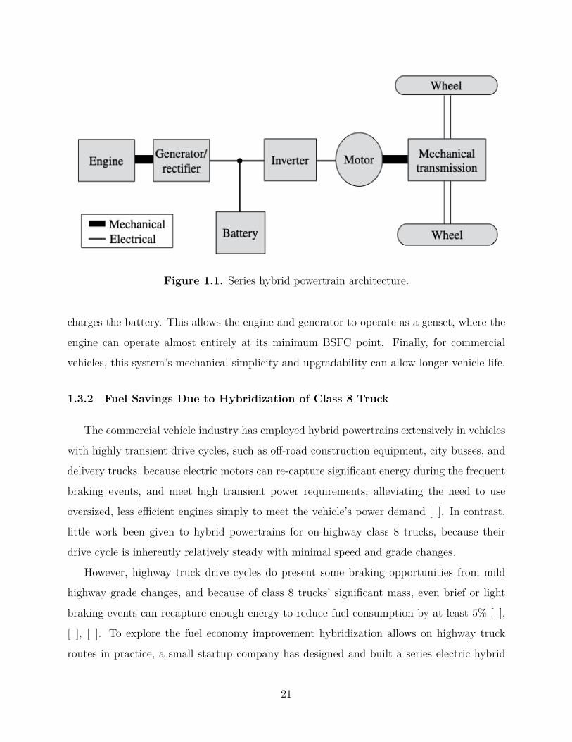
Figure 1.1. Series hybrid powertrain architecture.
charges the battery. This allows the engine and generator to operate as a genset, where the
engine can operate almost entirely at its minimum BSFC point. Finally, for commercial
vehicles, this system’s mechanical simplicity and upgradability can allow longer vehicle life.
1.3.2 Fuel Savings Due to Hybridization of Class 8 Truck
The commercial vehicle industry has employed hybrid powertrains extensively in vehicles
with highly transient drive cycles, such as off-road construction equipment, city busses, and
delivery trucks, because electric motors can re-capture significant energy during the frequent
braking events, and meet high transient power requirements, alleviating the need to use
oversized, less efficient engines simply to meet the vehicle’s power demand [3 ]. In contrast,
little work been given to hybrid powertrains for on-highway class 8 trucks, because their
drive cycle is inherently relatively steady with minimal speed and grade changes.
However, highway truck drive cycles do present some braking opportunities from mild
highway grade changes, and because of class 8 trucks’ significant mass, even brief or light
braking events can recapture enough energy to reduce fuel consumption by at least 5% [1 ],
[3 ], [4 ]. To explore the fuel economy improvement hybridization allows on highway truck
routes in practice, a small startup company has designed and built a series electric hybrid
21
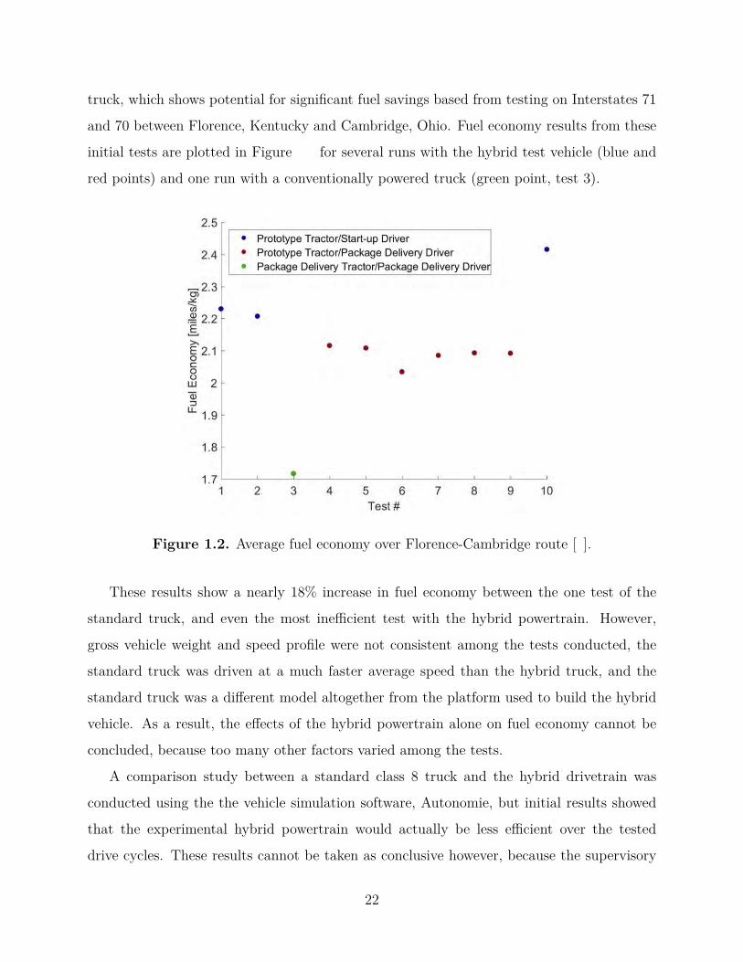
truck, which shows potential for significant fuel savings based from testing on Interstates 71
and 70 between Florence, Kentucky and Cambridge, Ohio. Fuel economy results from these
initial tests are plotted in Figure 1.2 for several runs with the hybrid test vehicle (blue and
red points) and one run with a conventionally powered truck (green point, test 3).
Figure 1.2. Average fuel economy over Florence-Cambridge route [1 ].
These results show a nearly 18% increase in fuel economy between the one test of the
standard truck, and even the most inefficient test with the hybrid powertrain. However,
gross vehicle weight and speed profile were not consistent among the tests conducted, the
standard truck was driven at a much faster average speed than the hybrid truck, and the
standard truck was a different model altogether from the platform used to build the hybrid
vehicle. As a result, the effects of the hybrid powertrain alone on fuel economy cannot be
concluded, because too many other factors varied among the tests.
A comparison study between a standard class 8 truck and the hybrid drivetrain was
conducted using the the vehicle simulation software, Autonomie, but initial results showed
that the experimental hybrid powertrain would actually be less efficient over the tested
drive cycles. These results cannot be taken as conclusive however, because the supervisory
22
control method of controlling power flows in the vehicle was not known, and adjustments
to the hybrid component sizes in Autonomie yielded 5% efficiency improvements over a
standard powertrain for the tested drive cycles. Consequently, this work demonstrates that
hybridization can allow efficiency gains over highway drive cycles, but due to inconsistent
testing and a lack of power flow data from the hybrid drivetrain itself, no conclusions could
be drawn about the experimental vehicle’s efficiency gains over a standard class 8 truck.
1.3.3 Electrified Air Handling System Description
Hybrid powertrains can also be classified by “degree of hybridization”, which is deter-
mined by the size of the electric motor and the vehicle’s dependence on the electric machine
for propulsion. A series electric hybrid for example can be considered a full hybrid, because
the electric motor must provide all of the vehicle’s tractive power requirement at any given
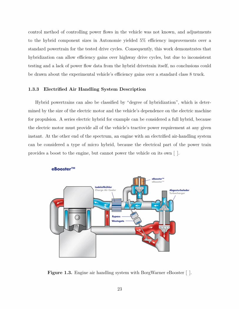
instant. At the other end of the spectrum, an engine with an electrified air-handling system
can be considered a type of micro hybrid, because the electrical part of the power train
provides a boost to the engine, but cannot power the vehicle on its own [2 ].
Figure 1.3. Engine air handling system with BorgWarner eBooster [5 ].
23

Engines with electrified air handling systems are typically standard IC engines with at
least one electrically driven supercharger (eBooster) or turbocharger (eTurbo) providing
additional boost pressure to the intake air supply. An eBooster is simply an electric motor
connected to a compressor, which allows a controller to directly command compressor speed
and by extension intake boost pressure, but unlike a standard supercharger, a valve will
typically allow intake air to bypass the eBooster entirely, allowing the eBooster to idle and
consume minimal power. An air handling system with an eBooster is shown in Figure 1.3 ,
where the eBooster and bypass valve are placed downstream of the standard turbocharger
compressor. An eTurbo is effectively a standard turbocharger with an electric motor attached
to the same shaft as the turbine and compressor. This allows the motor to (a) provide
additional assistance in spinning the compressor if exhaust flow is insufficient to provide the
necessary intake boost pressure, or (b) extract energy from the exhaust flow as electricity if
the turbine is driving more intake boost pressure than necessary.
Both of these components increase engine performance by increasing intake air flow more
quickly than would be possible with an equivalent turbocharger or supercharger, which in
turn allows engine downsizing without sacrificing power output and responsiveness. Addi-
tionally, because eBoosters and eTurbos run on much lower voltage electrical systems than a
typical traction motor, the battery and power electronics necessary are also relatively small.
As a result, electrified air handling offers a convenient drop-in solution for standard IC en-
gines which operate in any kind of standard or hybrid drivetrain, and their performance and
efficiency benefits are widely recognized [6 ]–[17 ].
1.3.4 Robust H∞ Multi-Input Multi-Output Control Design
Electric air handling components will yield performance gains as drop-in components
with standalone single-input single output (SISO) control loops, which typically use intake
manifold pressure ([9 ], [16 ]), intake manifold oxygen fraction ([11 ]), or air-fuel ratio ([12 ]) for
feedback. For many production engine applications, independent, non-model based, SISO
controllers such as PID compensators are good solutions for engine control, because they
are straightforward to implement and intuitive to tune [18 ]. This control approach works
24

well for engines with few actuators to control or decoupled system dynamics, but as more
actuators and tracking parameters are added to an engine, independent SISO loops become
more cumbersome. Non-model based controllers often need to be tuned to every specific
engine, and each SISO control loop’s response effects every other control loop’s performance,
so re-tuning one loop can require a cascade of re-tuning. Additionally, each actuator will only
ever respond based on its particular feedback parameter, so coupling among actuators and
parameters can lead to mediocre overall control performance that does not take full advantage
of the available actuators. Consequently, the coupled nature of engine gas exchange dynamics
calls for a more integrated approach.
A robust H∞ multi-input multi-output (MIMO) controller requires more development
time, but addresses all of these issues. First, a MIMO controller wraps multiple actuators,
feedback parameters, and targets into a single controller, allowing it to coordinate actuators
to track target parameters. Second, an H∞ controller uses a linear plant model as the
foundation for controller design, so for minor engine architecture changes, the controller
can be updated simply by updating the engine model, without necessarily re-tuning the
entire controller. Third, a robust controller accounts for uncertainty around the nominal
plant model, so as long as the physical engine’s response lies within the uncertainty region
specified, the controller will meet its stated performance targets [19 ].
An H∞ controller is a linear controller, K, obtained from the H∞ norm of a controlled
linear plant model. Specifically, an optimization problem is set up to find K, (a matrix in
general), that minimizes the H∞ norm of the closed-loop transfer function from exogenous
(uncontrolled) inputs to exogenous outputs [19 ], [20 ]. The performance of the resulting
controller depends heavily on the accuracy of the linear plant model used in design, and
because an IC engine is a nonlinear system, multiple linear models are often necessary to
represent an engine’s dynamics over its entire operating range. Consequently, the full engine
controller often consists of several linear controllers, each of which governs a portion of the
engine’s operating envelope [21 ].
25
1.3.5 Mean Value Engine Modeling for Control
A wide variety of modeling approaches exist for obtaining a control-oriented engine model,
but they typically fall into three major categories: crank angle resolved, black box, and
mean-value. Crank angle resolved models offer the highest fidelity, and capture high fre-
quency engine dynamics up to 5-15 kHz by modeling in-cylinder dynamics that vary within
each cycle, making them ideal for combustion and emissions analysis, but these models are
complex and computationally intense, making them unsuitable for gas exchange control [18 ],
[22 ]. Black box state models are a much faster option and are widely used for control ([23 ])
because of their simplicity, but they require large amounts of data to generate, and they can-
not be generalized to apply to modified engine architectures, because the internal parameters
have little if any physical significance.
Mean value models offer a flexible alternative however, because they model physical
interactions in the engine, so internal parameters and states represent physical conditions,
making them relatively intuitive to tune, validate, and adjust. Because they typically do not
model combustion dynamics in detail, mean value models are also simpler and faster than
crank angle resolved models, allowing them to capture flow dynamics in the 0.1-50 Hz range,
where gas exchange control is achievable. Finally nonlinear mean value state space models
are relatively straightforward to linearize, making them ideal for designing gas exchange
controllers using the model-based H∞ design method.
26
2. EFFICIENCY ANALYSIS OF SERIES ELECTRIC HYBRID
POWERTRAIN
2.1 System Description
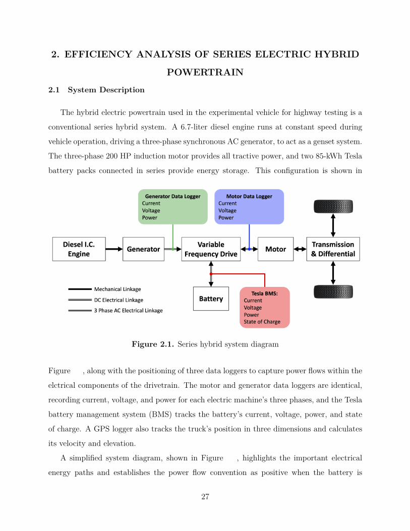
The hybrid electric powertrain used in the experimental vehicle for highway testing is a
conventional series hybrid system. A 6.7-liter diesel engine runs at constant speed during
vehicle operation, driving a three-phase synchronous AC generator, to act as a genset system.
The three-phase 200 HP induction motor provides all tractive power, and two 85-kWh Tesla
battery packs connected in series provide energy storage. This configuration is shown in
Figure 2.1. Series hybrid system diagram
Figure 2.1 , along with the positioning of three data loggers to capture power flows within the
elctrical components of the drivetrain. The motor and generator data loggers are identical,
recording current, voltage, and power for each electric machine’s three phases, and the Tesla
battery management system (BMS) tracks the battery’s current, voltage, power, and state
of charge. A GPS logger also tracks the truck’s position in three dimensions and calculates
its velocity and elevation.
A simplified system diagram, shown in Figure 2.2 , highlights the important electrical
energy paths and establishes the power flow convention as positive when the battery is
27
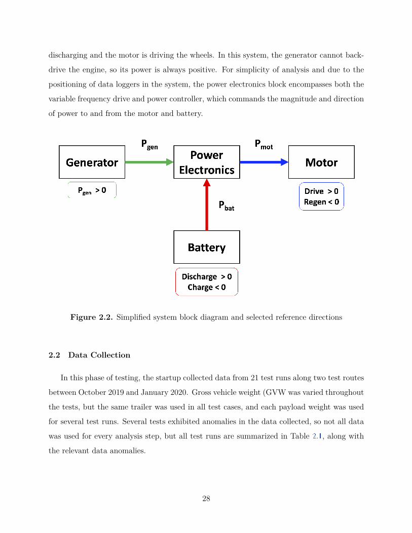
discharging and the motor is driving the wheels. In this system, the generator cannot back-
drive the engine, so its power is always positive. For simplicity of analysis and due to the
positioning of data loggers in the system, the power electronics block encompasses both the
variable frequency drive and power controller, which commands the magnitude and direction
of power to and from the motor and battery.
Figure 2.2. Simplified system block diagram and selected reference directions
2.2 Data Collection
In this phase of testing, the startup collected data from 21 test runs along two test routes
between October 2019 and January 2020. Gross vehicle weight (GVW was varied throughout
the tests, but the same trailer was used in all test cases, and each payload weight was used
for several test runs. Several tests exhibited anomalies in the data collected, so not all data
was used for every analysis step, but all test runs are summarized in Table 2.1 , along with
the relevant data anomalies.
28
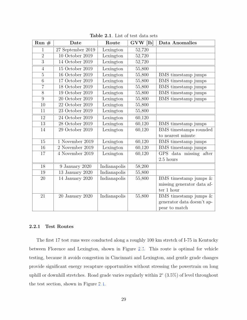
Table 2.1. List of test data setsRun # Date Route GVW [lb] Data Anomalies
1 27 September 2019 Lexington 52,7202 10 October 2019 Lexington 52,7203 14 October 2019 Lexington 52,7204 15 October 2019 Lexington 55,8005 16 October 2019 Lexington 55,800 BMS timestamp jumps6 17 October 2019 Lexington 55,800 BMS timestamp jumps7 18 October 2019 Lexington 55,800 BMS timestamp jumps8 19 October 2019 Lexington 55,800 BMS timestamp jumps9 20 October 2019 Lexington 55,800 BMS timestamp jumps10 22 October 2019 Lexington 55,80011 23 October 2019 Lexington 55,80012 24 October 2019 Lexington 60,12013 28 October 2019 Lexington 60,120 BMS timestamp jumps14 29 October 2019 Lexington 60,120 BMS timestamps rounded
to nearest minute15 1 November 2019 Lexington 60,120 BMS timestamp jumps16 2 November 2019 Lexington 60,120 BMS timestamp jumps17 4 November 2019 Lexington 60,120 GPS data missing after
2.5 hours18 9 January 2020 Indianapolis 58,20019 13 January 2020 Indianapolis 55,80020 14 January 2020 Indianapolis 55,800 BMS timestamp jumps &
missing generator data af-ter 1 hour
21 20 January 2020 Indianapolis 55,800 BMS timestamp jumps &generator data doesn’t ap-pear to match
2.2.1 Test Routes
The first 17 test runs were conducted along a roughly 100 km stretch of I-75 in Kentucky
between Florence and Lexington, shown in Figure 2.3 . This route is optimal for vehicle
testing, because it avoids congestion in Cincinnati and Lexington, and gentle grade changes
provide significant energy recapture opportunities without stressing the powertrain on long
uphill or downhill stretches. Road grade varies regularly within 2◦ (3.5%) of level throughout
the test section, shown in Figure 2.4 .
29
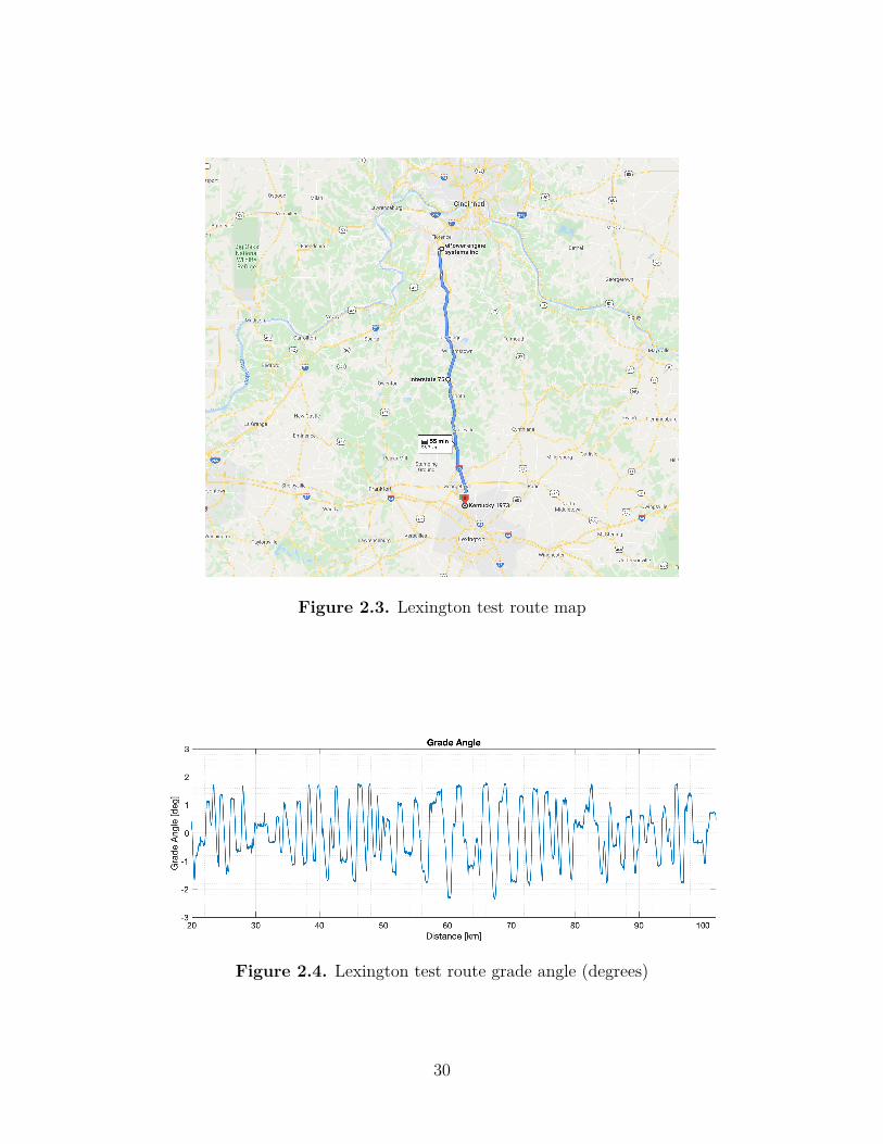
Figure 2.3. Lexington test route map
Figure 2.4. Lexington test route grade angle (degrees)
30
The remaining four tests were conducted along a 140 km section of highway between two
rest stops on I-74 and I-70 in Indiana. Traffic along this route, shown in Figure 2.5 , is busy at
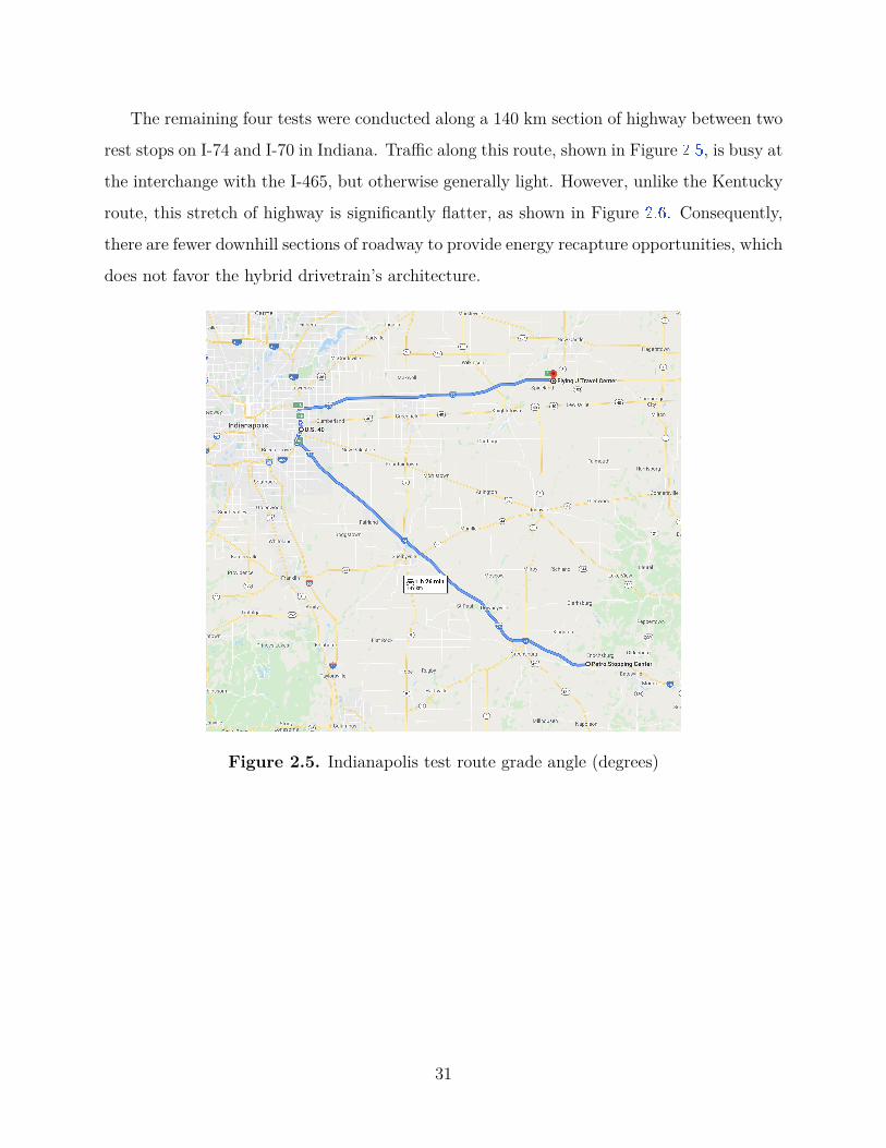
the interchange with the I-465, but otherwise generally light. However, unlike the Kentucky
route, this stretch of highway is significantly flatter, as shown in Figure 2.6 . Consequently,
there are fewer downhill sections of roadway to provide energy recapture opportunities, which
does not favor the hybrid drivetrain’s architecture.
Figure 2.5. Indianapolis test route grade angle (degrees)
31
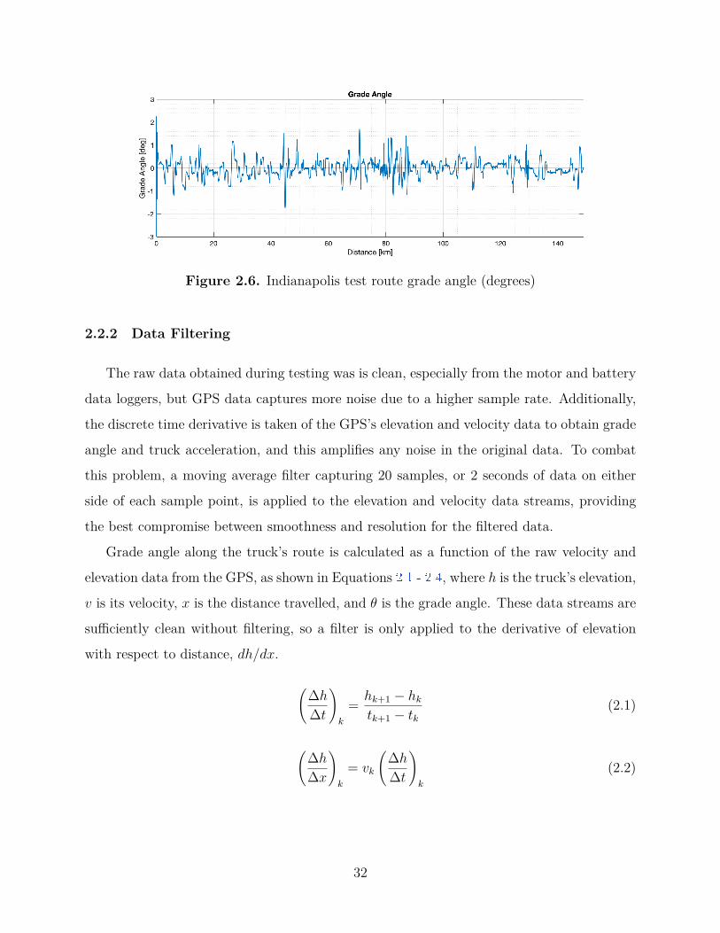
Figure 2.6. Indianapolis test route grade angle (degrees)
2.2.2 Data Filtering
The raw data obtained during testing was is clean, especially from the motor and battery
data loggers, but GPS data captures more noise due to a higher sample rate. Additionally,
the discrete time derivative is taken of the GPS’s elevation and velocity data to obtain grade
angle and truck acceleration, and this amplifies any noise in the original data. To combat
this problem, a moving average filter capturing 20 samples, or 2 seconds of data on either
side of each sample point, is applied to the elevation and velocity data streams, providing
the best compromise between smoothness and resolution for the filtered data.
Grade angle along the truck’s route is calculated as a function of the raw velocity and
elevation data from the GPS, as shown in Equations 2.1 - 2.4 , where h is the truck’s elevation,
v is its velocity, x is the distance travelled, and θ is the grade angle. These data streams are
sufficiently clean without filtering, so a filter is only applied to the derivative of elevation
with respect to distance, dh/dx.
(∆h
∆t
)k
= hk+1 − hk
tk+1 − tk
(2.1)
(∆h
∆x
)k
= vk
(∆h
∆t
)k
(2.2)
32
(∆h
∆x
)k
= average[(
∆h
∆x
)k−20
,
(∆h
∆x
)k−19
, . . . ,
(∆h
∆x
)k+20
](2.3)
Grade Angle = θ = arctan(
∆h
∆x
)k
(2.4)
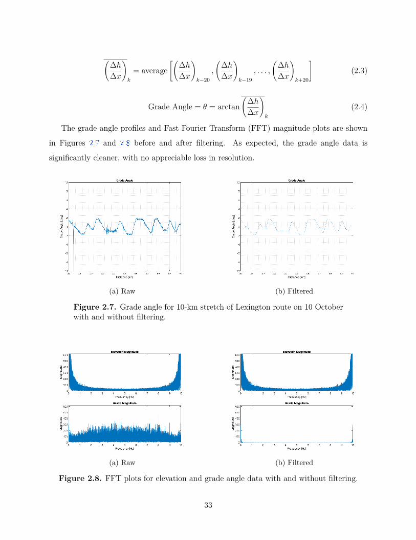
The grade angle profiles and Fast Fourier Transform (FFT) magnitude plots are shown
in Figures 2.7 and 2.8 before and after filtering. As expected, the grade angle data is
significantly cleaner, with no appreciable loss in resolution.
(a) Raw (b) Filtered
Figure 2.7. Grade angle for 10-km stretch of Lexington route on 10 Octoberwith and without filtering.
(a) Raw (b) Filtered
Figure 2.8. FFT plots for elevation and grade angle data with and without filtering.
33
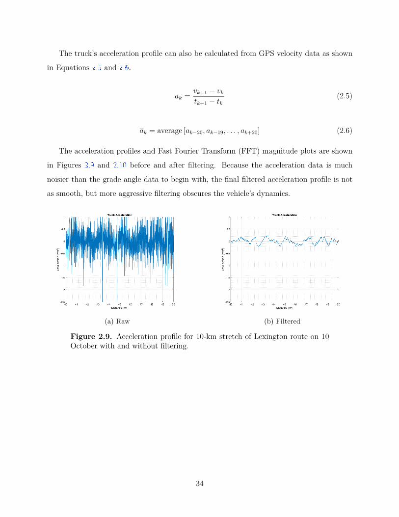
The truck’s acceleration profile can also be calculated from GPS velocity data as shown
in Equations 2.5 and 2.6 .
ak = vk+1 − vk
tk+1 − tk
(2.5)
ak = average [ak−20, ak−19, . . . , ak+20] (2.6)
The acceleration profiles and Fast Fourier Transform (FFT) magnitude plots are shown
in Figures 2.9 and 2.10 before and after filtering. Because the acceleration data is much
noisier than the grade angle data to begin with, the final filtered acceleration profile is not
as smooth, but more aggressive filtering obscures the vehicle’s dynamics.
(a) Raw (b) Filtered
Figure 2.9. Acceleration profile for 10-km stretch of Lexington route on 10October with and without filtering.
34
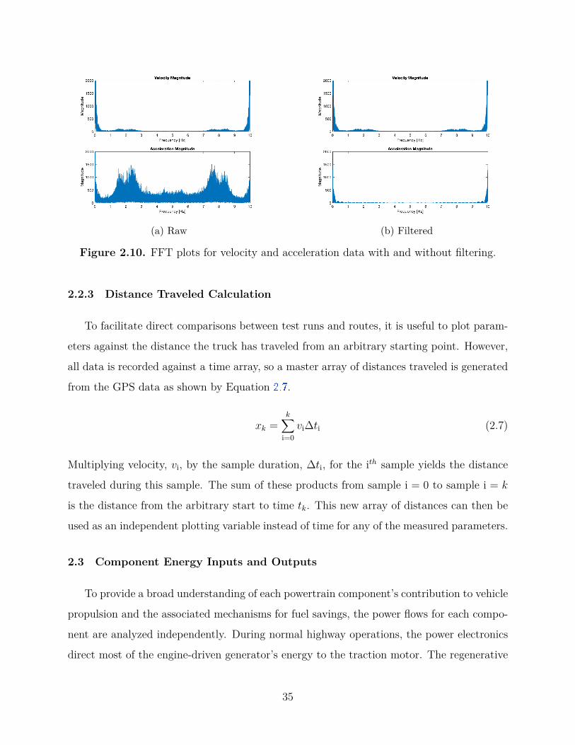
(a) Raw (b) Filtered
Figure 2.10. FFT plots for velocity and acceleration data with and without filtering.
2.2.3 Distance Traveled Calculation
To facilitate direct comparisons between test runs and routes, it is useful to plot param-
eters against the distance the truck has traveled from an arbitrary starting point. However,
all data is recorded against a time array, so a master array of distances traveled is generated
from the GPS data as shown by Equation 2.7 .
xk =k∑
i=0vi∆ti (2.7)
Multiplying velocity, vi, by the sample duration, ∆ti, for the ith sample yields the distance
traveled during this sample. The sum of these products from sample i = 0 to sample i = k
is the distance from the arbitrary start to time tk. This new array of distances can then be
used as an independent plotting variable instead of time for any of the measured parameters.
2.3 Component Energy Inputs and Outputs
To provide a broad understanding of each powertrain component’s contribution to vehicle
propulsion and the associated mechanisms for fuel savings, the power flows for each compo-
nent are analyzed independently. During normal highway operations, the power electronics
direct most of the engine-driven generator’s energy to the traction motor. The regenerative
35
braking energy captured by the traction motor is sufficient to keep the battery charged, so
the generator does not provide power to the battery, other than during low speed stop-and-
go operations. Sample sets of power flow, road grade, and velocity data are shown for 4-km
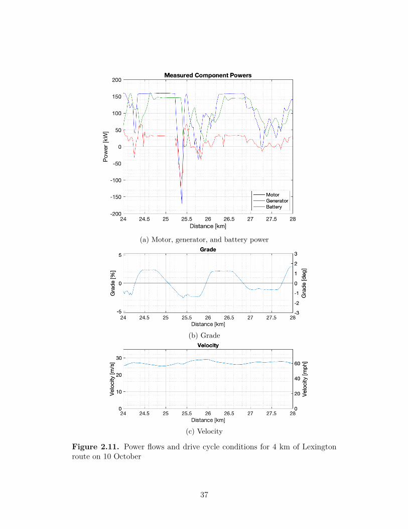
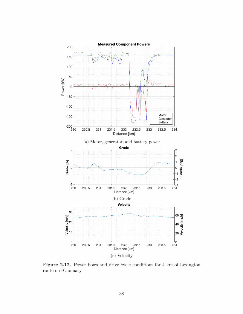
sections of the Lexington route in Figure 2.11 and the Indianapolis route in Figure 2.12 .
Each component’s net energy contribution is then determined from the power flow data
by integration according to Equation 2.8 , where P (τ) is the measured power flow, dτ is the
time step between samples, which was typically 1 second, and E(t) is the cumulative energy
delivery from the beginning of the run to time t.
E(t) =∫ t
0P (τ)dτ (2.8)
36
(a) Motor, generator, and battery power
(b) Grade
(c) Velocity
Figure 2.11. Power flows and drive cycle conditions for 4 km of Lexingtonroute on 10 October
37
(a) Motor, generator, and battery power
(b) Grade
(c) Velocity
Figure 2.12. Power flows and drive cycle conditions for 4 km of Lexingtonroute on 9 January
38
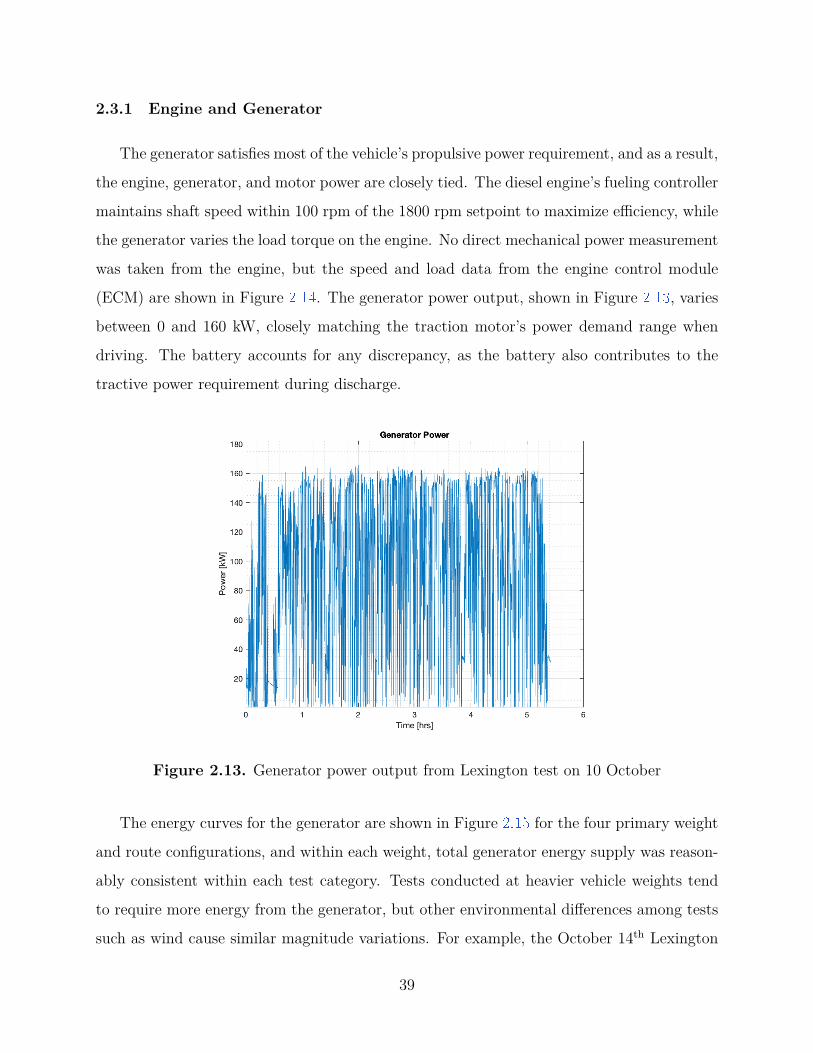
2.3.1 Engine and Generator
The generator satisfies most of the vehicle’s propulsive power requirement, and as a result,
the engine, generator, and motor power are closely tied. The diesel engine’s fueling controller
maintains shaft speed within 100 rpm of the 1800 rpm setpoint to maximize efficiency, while
the generator varies the load torque on the engine. No direct mechanical power measurement
was taken from the engine, but the speed and load data from the engine control module
(ECM) are shown in Figure 2.14 . The generator power output, shown in Figure 2.13 , varies
between 0 and 160 kW, closely matching the traction motor’s power demand range when
driving. The battery accounts for any discrepancy, as the battery also contributes to the
tractive power requirement during discharge.
Figure 2.13. Generator power output from Lexington test on 10 October
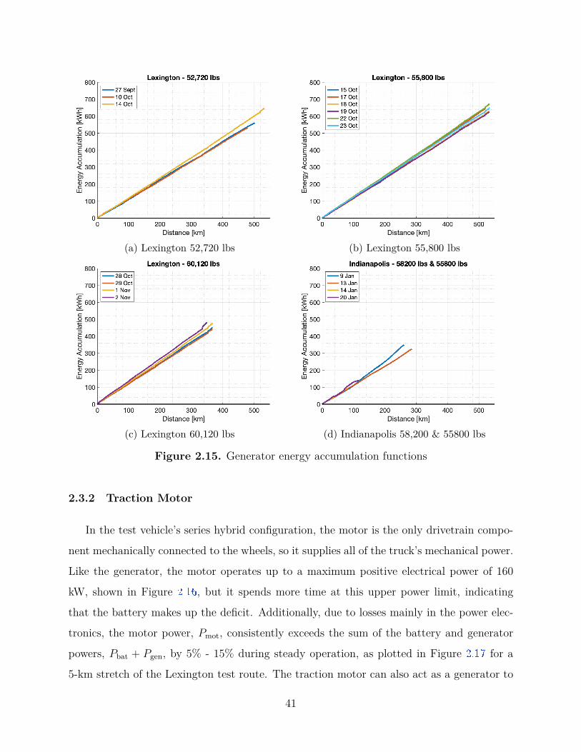
The energy curves for the generator are shown in Figure 2.15 for the four primary weight
and route configurations, and within each weight, total generator energy supply was reason-
ably consistent within each test category. Tests conducted at heavier vehicle weights tend
to require more energy from the generator, but other environmental differences among tests
such as wind cause similar magnitude variations. For example, the October 14th Lexington
39
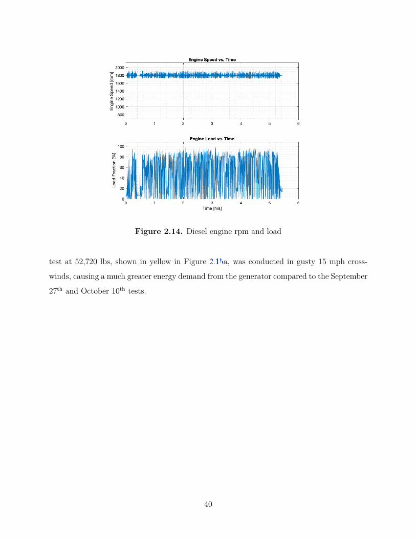
Figure 2.14. Diesel engine rpm and load
test at 52,720 lbs, shown in yellow in Figure 2.15 a, was conducted in gusty 15 mph cross-
winds, causing a much greater energy demand from the generator compared to the September
27th and October 10th tests.
40
(a) Lexington 52,720 lbs (b) Lexington 55,800 lbs
(c) Lexington 60,120 lbs (d) Indianapolis 58,200 & 55800 lbs
Figure 2.15. Generator energy accumulation functions
2.3.2 Traction Motor
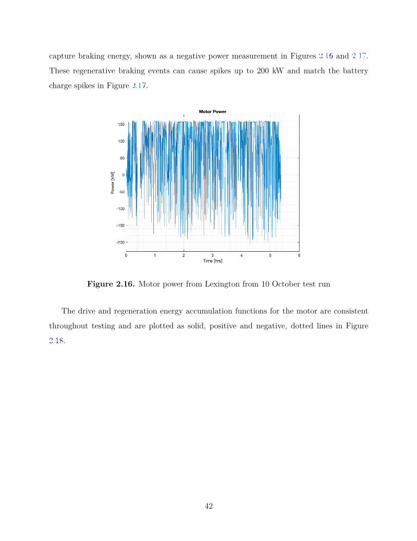
In the test vehicle’s series hybrid configuration, the motor is the only drivetrain compo-
nent mechanically connected to the wheels, so it supplies all of the truck’s mechanical power.
Like the generator, the motor operates up to a maximum positive electrical power of 160
kW, shown in Figure 2.16 , but it spends more time at this upper power limit, indicating
that the battery makes up the deficit. Additionally, due to losses mainly in the power elec-
tronics, the motor power, Pmot, consistently exceeds the sum of the battery and generator
powers, Pbat + Pgen, by 5% - 15% during steady operation, as plotted in Figure 2.17 for a
5-km stretch of the Lexington test route. The traction motor can also act as a generator to
41
capture braking energy, shown as a negative power measurement in Figures 2.16 and 2.17 .
These regenerative braking events can cause spikes up to 200 kW and match the battery
charge spikes in Figure 2.17 .
Figure 2.16. Motor power from Lexington from 10 October test run
The drive and regeneration energy accumulation functions for the motor are consistent
throughout testing and are plotted as solid, positive and negative, dotted lines in Figure
2.18 .
42
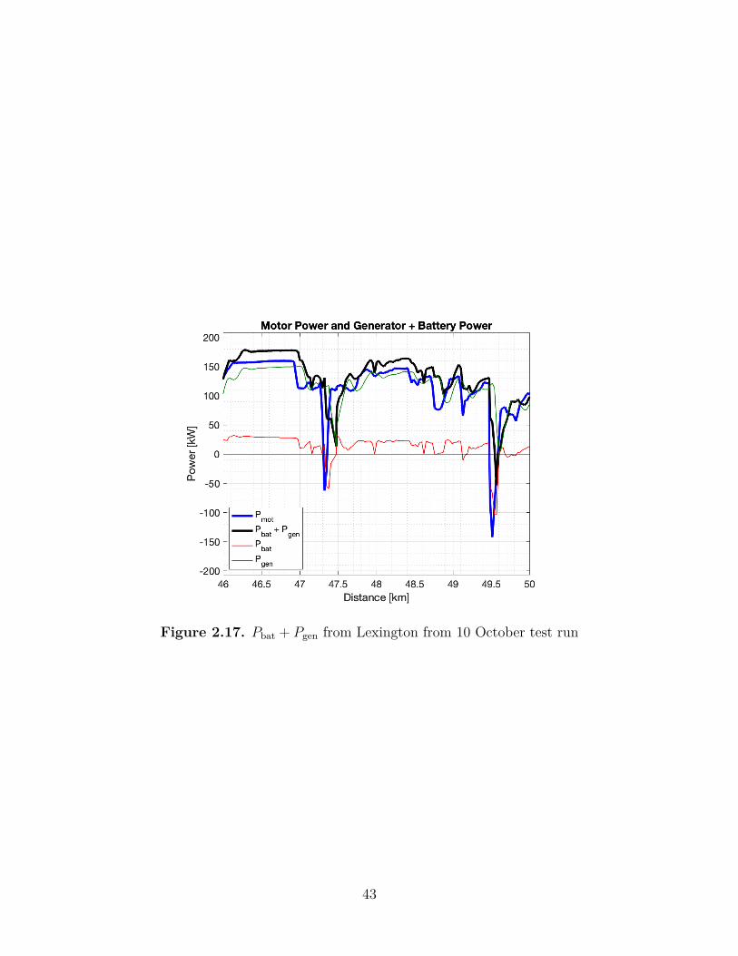
Figure 2.17. Pbat + Pgen from Lexington from 10 October test run
43
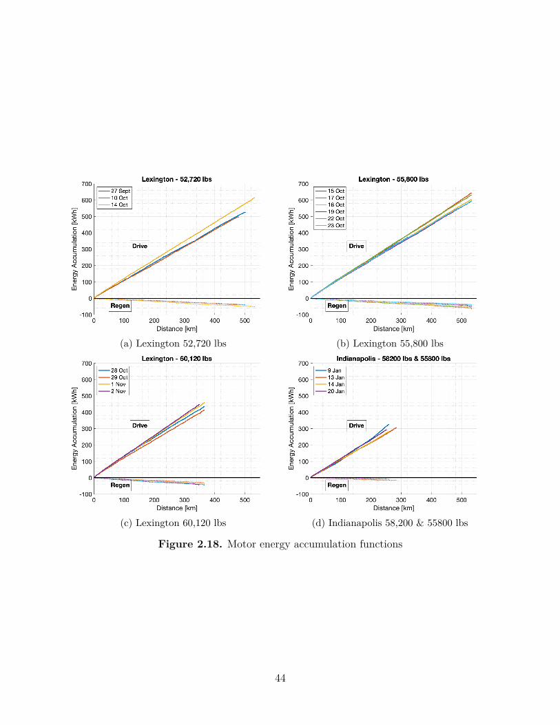
(a) Lexington 52,720 lbs (b) Lexington 55,800 lbs
(c) Lexington 60,120 lbs (d) Indianapolis 58,200 & 55800 lbs
Figure 2.18. Motor energy accumulation functions
44
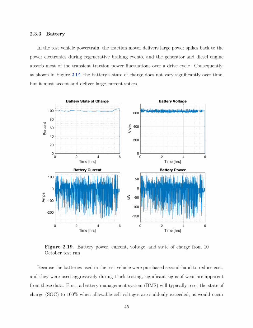
2.3.3 Battery
In the test vehicle powertrain, the traction motor delivers large power spikes back to the
power electronics during regenerative braking events, and the generator and diesel engine
absorb most of the transient traction power fluctuations over a drive cycle. Consequently,
as shown in Figure 2.19 , the battery’s state of charge does not vary significantly over time,
but it must accept and deliver large current spikes.
Figure 2.19. Battery power, current, voltage, and state of charge from 10October test run
Because the batteries used in the test vehicle were purchased second-hand to reduce cost,
and they were used aggressively during truck testing, significant signs of wear are apparent
from these data. First, a battery management system (BMS) will typically reset the state of
charge (SOC) to 100% when allowable cell voltages are suddenly exceeded, as would occur
45
during aggressive use. During some periods of high current charging or discharge in testing,
the BMS recorded physically impossible jumps up to 100% SOC, which is consistent with one
of these reset events. Second, the BMS reported an overall battery SOC consistently near
100%, even though randomly sampled cells were closer to the nominal 3.8 V expected from a
cell at 50% SOC. Third, the measured terminal voltage was approximately 110 V below the
nominal 750 V expected from two Tesla battery packs connected in series, indicating that
some modules in the battery are not contributing to the overall battery voltage.
However, the battery still stores sufficient regenerative braking energy to provide drive
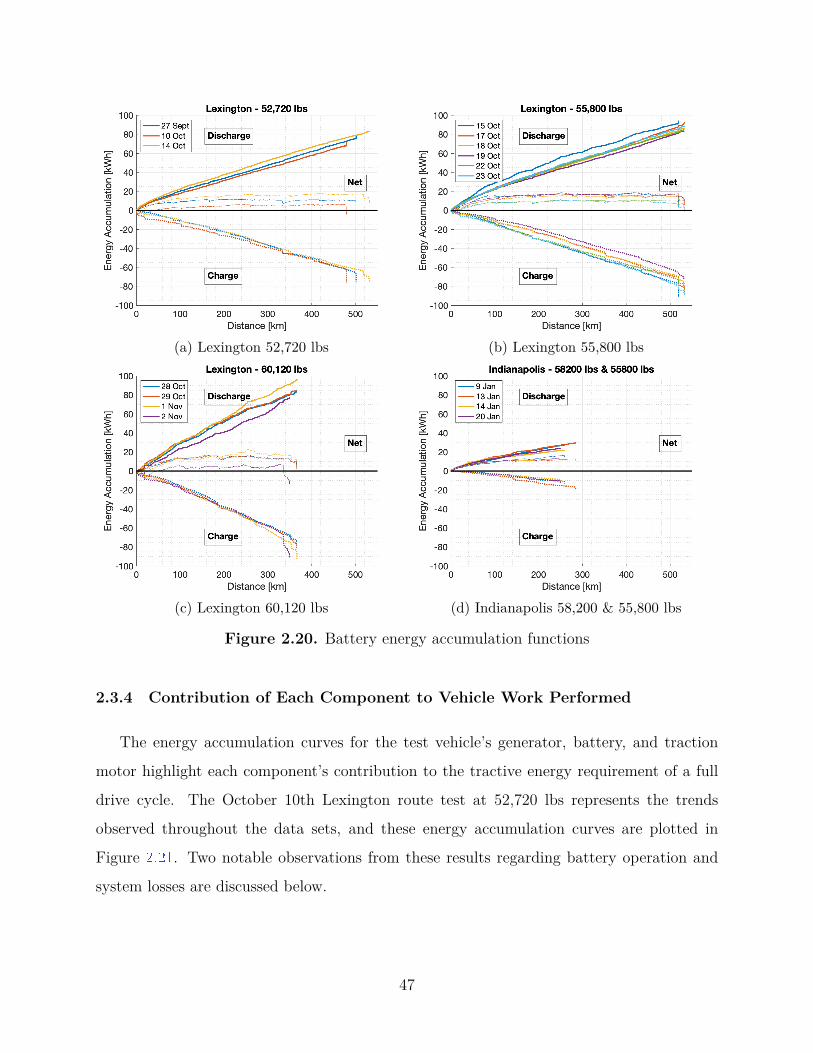
energy and reduce the energy demand on the generator. The battery’s charge (negative),
discharge (positive), and net energy accumulation functions are shown in Figure 2.20 as
dotted, bold, and thin lines respectively. The battery consistently shows a small net discharge
(positive) over most of the test runs, which is consistent with the BMS reported SOC if the
non-physical jumps to 100% are removed. However, gross charge and discharge energy
depends heavily on payload and route. With 15% weight increase of 7,500 lbs, the truck
captures 50% more energy from regenerative braking over the Lexington route, although the
power management algorithm was also adjusted to rely more heavily on the battery for these
runs, accounting for some of these gains (Figures 2.20 a & 2.20 c). In contrast, the shallower
grade of the Indianapolis route provides only half the energy that the battery stores and
returns on the first 250 km of the Lexington route.
46
(a) Lexington 52,720 lbs (b) Lexington 55,800 lbs
(c) Lexington 60,120 lbs (d) Indianapolis 58,200 & 55,800 lbs
Figure 2.20. Battery energy accumulation functions
2.3.4 Contribution of Each Component to Vehicle Work Performed
The energy accumulation curves for the test vehicle’s generator, battery, and traction
motor highlight each component’s contribution to the tractive energy requirement of a full
drive cycle. The October 10th Lexington route test at 52,720 lbs represents the trends
observed throughout the data sets, and these energy accumulation curves are plotted in
Figure 2.21 . Two notable observations from these results regarding battery operation and
system losses are discussed below.
47
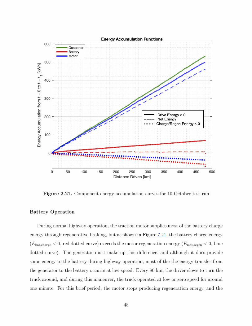
Figure 2.21. Component energy accumulation curves for 10 October test run
Battery Operation
During normal highway operation, the traction motor supplies most of the battery charge
energy through regenerative braking, but as shown in Figure 2.21 , the battery charge energy
(Ebat,charge < 0, red dotted curve) exceeds the motor regeneration energy (Emot,regen < 0, blue
dotted curve). The generator must make up this difference, and although it does provide
some energy to the battery during highway operation, most of the the energy transfer from
the generator to the battery occurrs at low speed. Every 80 km, the driver slows to turn the
truck around, and during this maneuver, the truck operated at low or zero speed for around
one minute. For this brief period, the motor stops producing regeneration energy, and the
48
generator supplies energy to the battery and the motor, causing the total battery charge
energy to exceed the motor regeneration energy.
This behaviour would not matter in a perfect system with no electrical losses, but in
the real powertrain, losses occur in both the battery and the power electronics. As a result,
when the generator charges the battery, power must flow through the power electronics on
its way into and out of the battery, (see Figure 2.2 ) incurring losses in each component. It
is much more efficient for the generator to supply energy straight to the drive motor, and
since the battery’s total capacity of 170 kWh is more than double its discharge energy over
a single test run, the generator arguably does not need to charge the battery, assuming it
can be charged outside the vehicle’s normal drive cycle.
The battery itself is also oversized for the application in order to keep the C-rate near a
reasonable range during aggressive charge and discharge spikes. Even though the battery’s
SOC does not vary significantly, and a fully charged battery would supply more than enough
energy for the entire test without recharging, the Tesla battery pack requires relatively low
charging rates as a fraction of total capacity. A chemistry optimized for power delivery
instead of total capacity would allow a significantly smaller battery to replace the relatively
sensitive Tesla battery, and a battery without the wear signs exhibited in testing would
reduce electrical losses during both charge and discharge modes.
System Losses
In an ideal powertrain with no electrical losses, the generator would deliver precisely
the motor’s net energy requirement, and the battery would return all regenerative braking
energy to the traction motor, satisfying the remaining propulsive energy requirement. This
would place the green line in Figure 2.21 on top of the blue dashed line. However, in
testing, the generator delivers 15% more energy than the net propulsive energy requirement
and actually exceeds the total propulsive energy requirement due to losses primarily in the
battery and power electronics. The power electronics losses, discussed in detail in Section
2.4 , are expected and unavoidable, but a newer battery designed to handle the high charge
and discharge currents observed could substantially improve this efficiency.
49
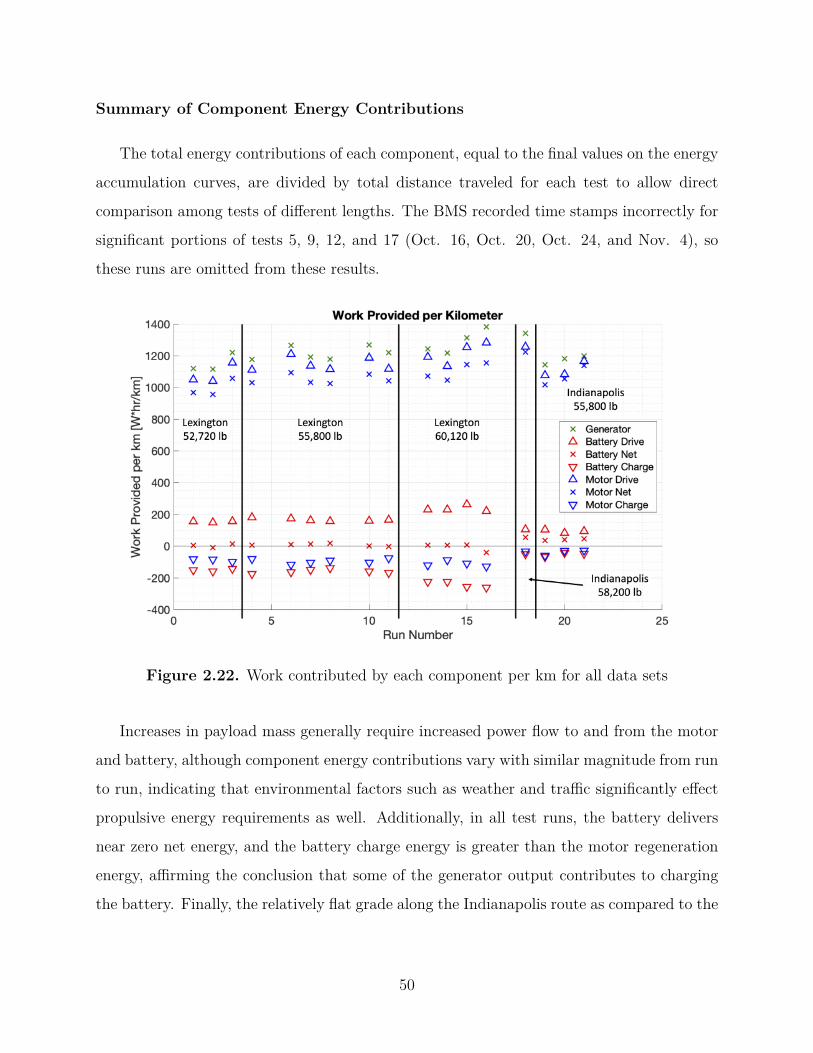
Summary of Component Energy Contributions
The total energy contributions of each component, equal to the final values on the energy
accumulation curves, are divided by total distance traveled for each test to allow direct
comparison among tests of different lengths. The BMS recorded time stamps incorrectly for
significant portions of tests 5, 9, 12, and 17 (Oct. 16, Oct. 20, Oct. 24, and Nov. 4), so
these runs are omitted from these results.
Figure 2.22. Work contributed by each component per km for all data sets
Increases in payload mass generally require increased power flow to and from the motor
and battery, although component energy contributions vary with similar magnitude from run
to run, indicating that environmental factors such as weather and traffic significantly effect
propulsive energy requirements as well. Additionally, in all test runs, the battery delivers
near zero net energy, and the battery charge energy is greater than the motor regeneration
energy, affirming the conclusion that some of the generator output contributes to charging
the battery. Finally, the relatively flat grade along the Indianapolis route as compared to the
50
Lexington route requires much less energy flow through all system components, especially
the battery.
2.4 Power Electronics Efficiency Analysis
In series hybrid electric powertrains, electrical losses arise in all four of the major com-
ponents shown in Figure 2.1 . No mechanical power measurements were taken in the exper-
imental drivetrain, which precludes calculation of the generator and motor efficiencies, but
these components have well documented efficiencies around 90% - 95% that cannot be easily
improved, so they are not considered in this analysis. Also, the battery is known to have
losses due to wear, and since the startup plans to replace the battery in future prototypes,
its efficiency is not calculated.
However, the energy flows into and out of the power electronics were measured, allowing
separate efficiency calculations for each energy flow path. Regardless of the path of flow,
the power electronics efficiency is the ratio of total input energy to total output energy
over a given sample time, with the assumption that energy cannot be stored in the power
electronics. Figure 2.23 illustrates the system boundary in the simplified system, and Figure
2.24 represents where the data loggers measure power flows in the power electronics circuitry.
These measurement points are assumed to be the only points of energy flow across the system
boundary defined in Figure 2.23 . The energy sums can be calculated from the power data
recorded at these points according to the energy accumulation integral, shown in Equation
2.8 .
2.4.1 Power Modes
Power can flow through the power electronics in three fundamental ways. Although
the generator only provides energy input to the power electronics, both the battery and the
motor can either provide energy input to or accept energy output from the power electronics,
so the signs of the power flows to and from the motor and battery reveal which mode of
operation the vehicle is in at any given moment. Figure 2.25 describes the three modes that
result from these different energy flow directions. Battery power never remains near zero for
51
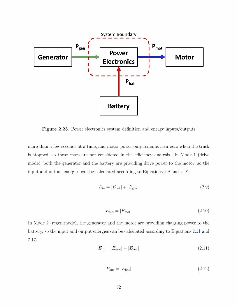
Figure 2.23. Power electronics system definition and energy inputs/outputs
more than a few seconds at a time, and motor power only remains near zero when the truck
is stopped, so these cases are not considered in the efficiency analysis. In Mode 1 (drive
mode), both the generator and the battery are providing drive power to the motor, so the
input and output energies can be calculated according to Equations 2.9 and 2.10 .
Ein = |Ebat| + |Egen| (2.9)
Eout = |Emot| (2.10)
In Mode 2 (regen mode), the generator and the motor are providing charging power to the
battery, so the input and output energies can be calculated according to Equations 2.11 and
2.12 .
Ein = |Emot| + |Egen| (2.11)
Eout = |Ebat| (2.12)
52
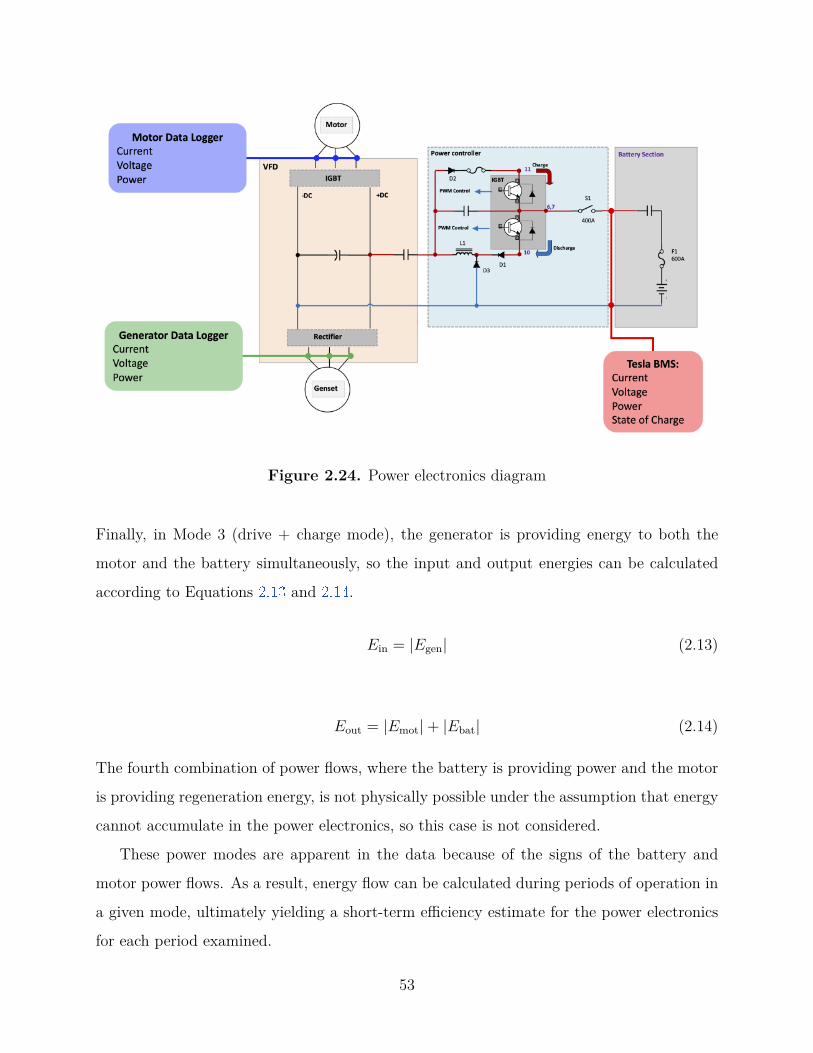
Figure 2.24. Power electronics diagram
Finally, in Mode 3 (drive + charge mode), the generator is providing energy to both the
motor and the battery simultaneously, so the input and output energies can be calculated
according to Equations 2.13 and 2.14 .
Ein = |Egen| (2.13)
Eout = |Emot| + |Ebat| (2.14)
The fourth combination of power flows, where the battery is providing power and the motor
is providing regeneration energy, is not physically possible under the assumption that energy
cannot accumulate in the power electronics, so this case is not considered.
These power modes are apparent in the data because of the signs of the battery and
motor power flows. As a result, energy flow can be calculated during periods of operation in
a given mode, ultimately yielding a short-term efficiency estimate for the power electronics
for each period examined.
53
Figure 2.25. Energy flow modes
2.4.2 Energy Accumulation in Power Electronics
As shown in Figure 2.24 , the variable frequency drive contains a bank of capacitors
between its DC lines to absorb power spikes. The energy stored in this capacitor at any
given moment is described in Equation 2.15 , where C is capacitance and V is the voltage
across the capacitor.
Ecapacitor = 12CV 2 (2.15)
Because the power flow through the DC portion of the VFD, and by extension the voltage
across the capacitor, changes with time, the energy stored in the capacitor also varies with
time, yielding the energy balance relation in Equation 2.16 .
Eout = Ein + ∆Ecapacitor − Elosses (2.16)
However, the voltage across the capacitor was not measured, so the capacitor energy
storage term, ∆Ecapacitor, cannot not be calculated. Over sufficiently long time spans, the
change in energy stored in the capacitor is negligible compared to the magnitude of the energy
flowing in and out of the power electronics, so the ratio of output energy to input energy is a
54
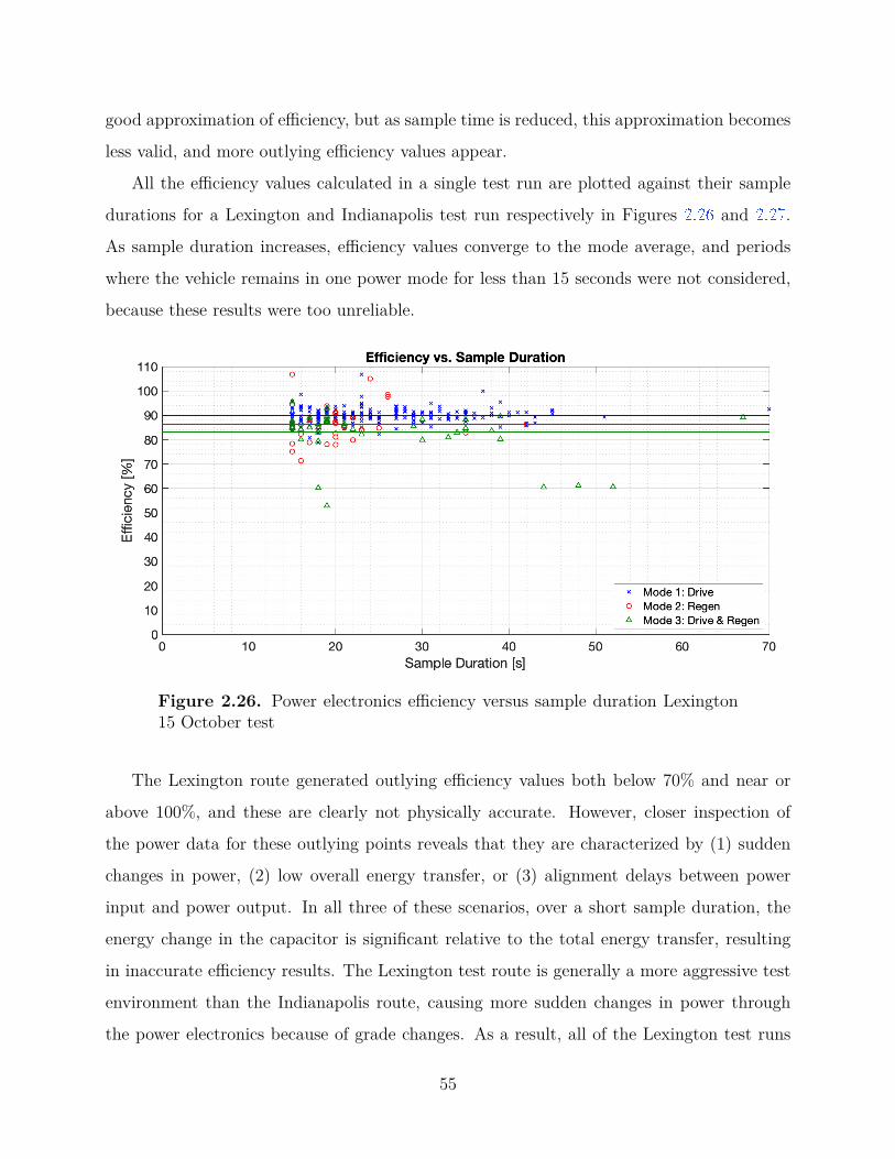
good approximation of efficiency, but as sample time is reduced, this approximation becomes
less valid, and more outlying efficiency values appear.
All the efficiency values calculated in a single test run are plotted against their sample
durations for a Lexington and Indianapolis test run respectively in Figures 2.26 and 2.27 .
As sample duration increases, efficiency values converge to the mode average, and periods
where the vehicle remains in one power mode for less than 15 seconds were not considered,
because these results were too unreliable.
Figure 2.26. Power electronics efficiency versus sample duration Lexington15 October test
The Lexington route generated outlying efficiency values both below 70% and near or
above 100%, and these are clearly not physically accurate. However, closer inspection of
the power data for these outlying points reveals that they are characterized by (1) sudden
changes in power, (2) low overall energy transfer, or (3) alignment delays between power
input and power output. In all three of these scenarios, over a short sample duration, the
energy change in the capacitor is significant relative to the total energy transfer, resulting
in inaccurate efficiency results. The Lexington test route is generally a more aggressive test
environment than the Indianapolis route, causing more sudden changes in power through
the power electronics because of grade changes. As a result, all of the Lexington test runs
55
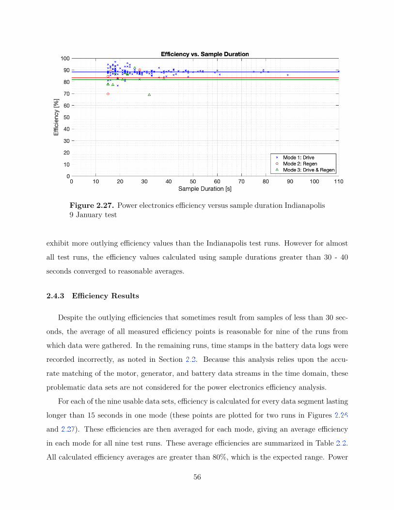
Figure 2.27. Power electronics efficiency versus sample duration Indianapolis9 January test
exhibit more outlying efficiency values than the Indianapolis test runs. However for almost
all test runs, the efficiency values calculated using sample durations greater than 30 - 40
seconds converged to reasonable averages.
2.4.3 Efficiency Results
Despite the outlying efficiencies that sometimes result from samples of less than 30 sec-
onds, the average of all measured efficiency points is reasonable for nine of the runs from
which data were gathered. In the remaining runs, time stamps in the battery data logs were
recorded incorrectly, as noted in Section 2.2 . Because this analysis relies upon the accu-
rate matching of the motor, generator, and battery data streams in the time domain, these
problematic data sets are not considered for the power electronics efficiency analysis.
For each of the nine usable data sets, efficiency is calculated for every data segment lasting
longer than 15 seconds in one mode (these points are plotted for two runs in Figures 2.26
and 2.27 ). These efficiencies are then averaged for each mode, giving an average efficiency
in each mode for all nine test runs. These average efficiencies are summarized in Table 2.2 .
All calculated efficiency averages are greater than 80%, which is the expected range. Power
56
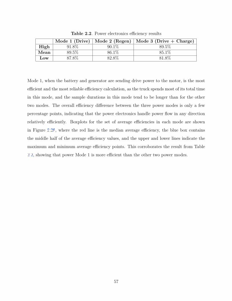
Table 2.2. Power electronics efficiency resultsMode 1 (Drive) Mode 2 (Regen) Mode 3 (Drive + Charge)
High 91.8% 90.1% 89.5%Mean 89.5% 86.1% 85.1%Low 87.8% 82.8% 81.8%
Mode 1, when the battery and generator are sending drive power to the motor, is the most
efficient and the most reliable efficiency calculation, as the truck spends most of its total time
in this mode, and the sample durations in this mode tend to be longer than for the other
two modes. The overall efficiency difference between the three power modes is only a few
percentage points, indicating that the power electronics handle power flow in any direction
relatively efficiently. Boxplots for the set of average efficiencies in each mode are shown
in Figure 2.28 , where the red line is the median average efficiency, the blue box contains
the middle half of the average efficiency values, and the upper and lower lines indicate the
maximum and minimum average efficiency points. This corroborates the result from Table
2.2 , showing that power Mode 1 is more efficient than the other two power modes.
57
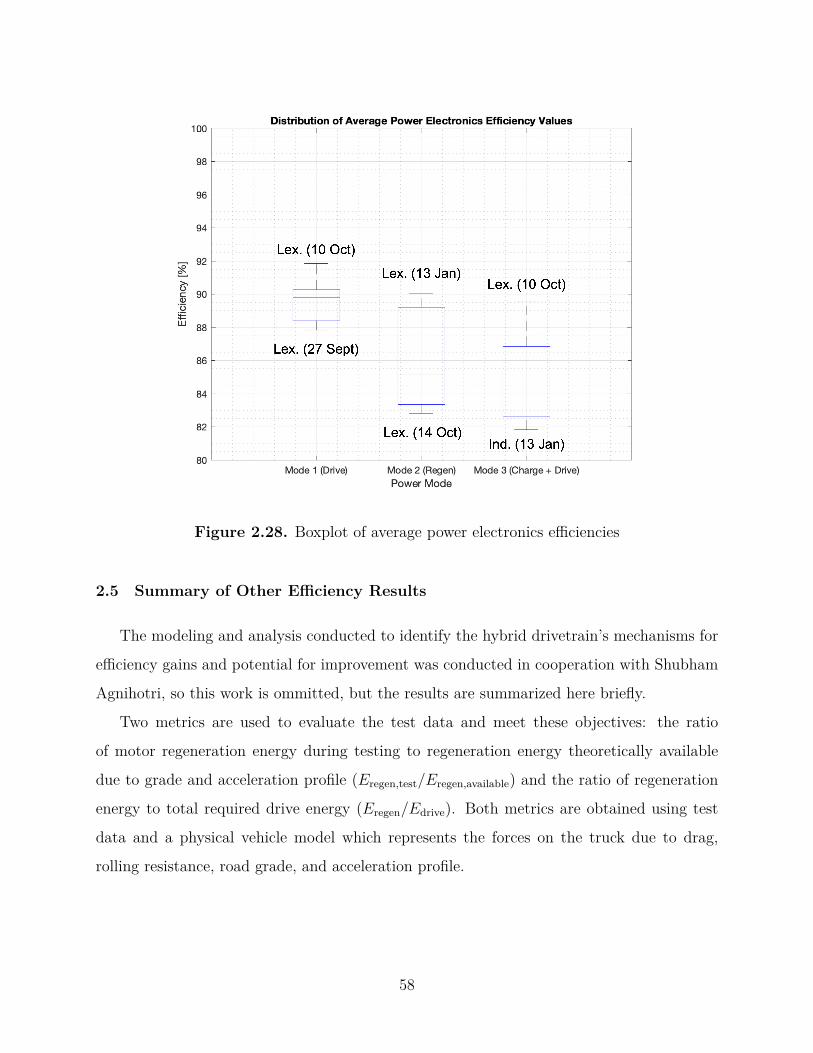
Figure 2.28. Boxplot of average power electronics efficiencies
2.5 Summary of Other Efficiency Results
The modeling and analysis conducted to identify the hybrid drivetrain’s mechanisms for
efficiency gains and potential for improvement was conducted in cooperation with Shubham
Agnihotri, so this work is ommitted, but the results are summarized here briefly.
Two metrics are used to evaluate the test data and meet these objectives: the ratio
of motor regeneration energy during testing to regeneration energy theoretically available
due to grade and acceleration profile (Eregen,test/Eregen,available) and the ratio of regeneration
energy to total required drive energy (Eregen/Edrive). Both metrics are obtained using test
data and a physical vehicle model which represents the forces on the truck due to drag,
rolling resistance, road grade, and acceleration profile.
58
2.5.1 Regeneration Energy Capture Percentage
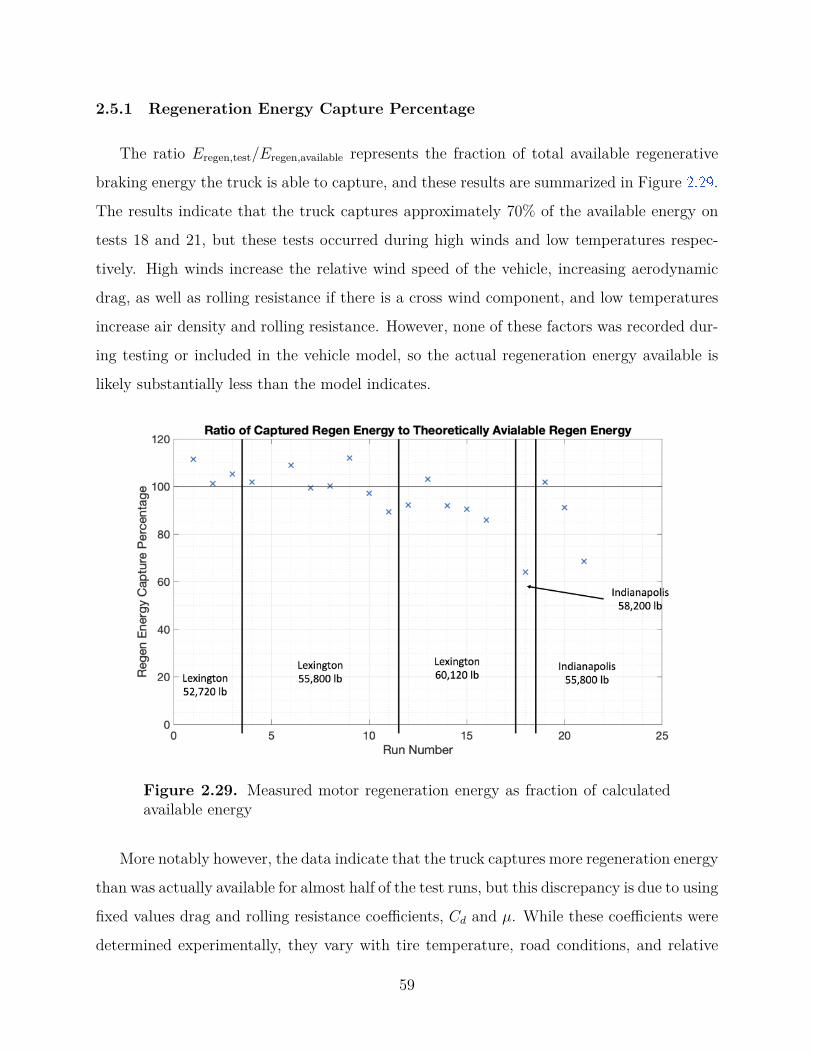
The ratio Eregen,test/Eregen,available represents the fraction of total available regenerative
braking energy the truck is able to capture, and these results are summarized in Figure 2.29 .
The results indicate that the truck captures approximately 70% of the available energy on
tests 18 and 21, but these tests occurred during high winds and low temperatures respec-
tively. High winds increase the relative wind speed of the vehicle, increasing aerodynamic
drag, as well as rolling resistance if there is a cross wind component, and low temperatures
increase air density and rolling resistance. However, none of these factors was recorded dur-
ing testing or included in the vehicle model, so the actual regeneration energy available is
likely substantially less than the model indicates.
Figure 2.29. Measured motor regeneration energy as fraction of calculatedavailable energy
More notably however, the data indicate that the truck captures more regeneration energy
than was actually available for almost half of the test runs, but this discrepancy is due to using
fixed values drag and rolling resistance coefficients, Cd and µ. While these coefficients were
determined experimentally, they vary with tire temperature, road conditions, and relative
59
wind direction, so the values obtained in testing can only accurately be applied to test runs
under the same conditions. Additionally, no tests were performed with the truck traveling
fast enough to obtain a reliable estimate of its drag coefficient, so while the even distribution
around 100% indicates that the truck can capture close to 100% of the available regeneration
energy, no run-specific conclusions can be drawn.
2.5.2 Ratio of Regeneration Energy Capture to Drive Energy Output
The ratio Eregen/Edrive represents the fraction of total drive energy that regenerative
braking provides, which is calculated according to 2.17 , where each energy term is obtained
from the vehicle model using drive cycle data from testing.
Eregen
Edrive= Edecel + Egrade,down
Eaccel + Egrade,up + Err + Eaero(2.17)
These results are summarized in Figure 2.30 for test runs with usable data. Three energy
ratio results are plotted for each test run based on: (1) the experimental truck (calculated
from motor data), (2) the experimental truck (calculated from its theoretical power require-
ment), and (3) a reference 2018 Peterbilt 579 truck (calculated from its theoretical power
requirement). The theoretical power requirements are calculated using the Cd and µ values
shown in Table 2.3 . The analytical results for the experimental truck match the experimental
results fairly well despite some uncertainty around the experimentally determined Cd and µ
coefficients, so it is reasonable to extrapolate the energy ratio calculation to different rolling
resistance and drag coefficients.
Table 2.3. Drag and rolling resistance coefficientsParameter Test Truck New Low Mileage Truck
Cd 0.68 0.58µ 0.007 0.005
In these results, the Lexington profile yields almost double the ratio of regeneration to
drive energy compared to the Indianapolis route, which is expected based on the higher
battery energy transfer (Section 2.3.4 ) and rolling hills on the Lexington cycle. This affirms
60
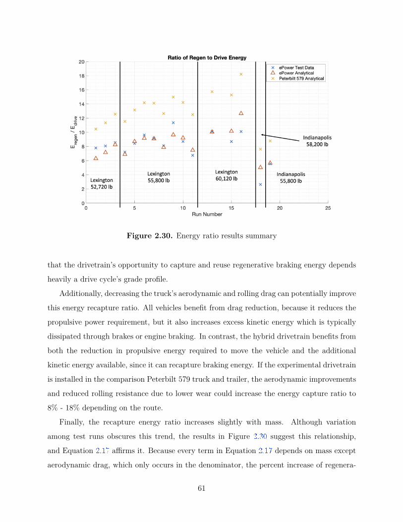
Figure 2.30. Energy ratio results summary
that the drivetrain’s opportunity to capture and reuse regenerative braking energy depends
heavily a drive cycle’s grade profile.
Additionally, decreasing the truck’s aerodynamic and rolling drag can potentially improve
this energy recapture ratio. All vehicles benefit from drag reduction, because it reduces the
propulsive power requirement, but it also increases excess kinetic energy which is typically
dissipated through brakes or engine braking. In contrast, the hybrid drivetrain benefits from
both the reduction in propulsive energy required to move the vehicle and the additional
kinetic energy available, since it can recapture braking energy. If the experimental drivetrain
is installed in the comparison Peterbilt 579 truck and trailer, the aerodynamic improvements
and reduced rolling resistance due to lower wear could increase the energy capture ratio to
8% - 18% depending on the route.
Finally, the recapture energy ratio increases slightly with mass. Although variation
among test runs obscures this trend, the results in Figure 2.30 suggest this relationship,
and Equation 2.17 affirms it. Because every term in Equation 2.17 depends on mass except
aerodynamic drag, which only occurs in the denominator, the percent increase of regenera-
61
tion energy is slightly greater than the percent increase of drive energy, yielding a slightly
better regeneration energy ratio. Nonetheless, the series hybrid system would benefit most
significantly from drag and rolling resistance reductions.
2.6 Future Work
The data from the testbed series hybrid truck shows effective mechanisms for efficiency
gains over a standard drivetrain on highway routes, in particular those with mildly hilly
terrain. However, three components of the powertrain that were not studied would benefit
from further analysis. First, no analysis was conducted on the battery, because its wear and
associated efficiency loss was known, and the startup plans to replace it anyway. Nonetheless,
a drive profile simulation to evaluate round-trip efficiency of the battery would inform the
choice of battery size and chemistry in future powertrain iterations. Battery round-trip
efficiency–the ratio of total charge energy to total discharge energy over a drive cycle with
the battery starting and ending at the same state of charge–would reveal how much of the
captured regeneration energy actually comes back to the motor and how much is lost in the
battery as heat.
Second, no analysis was conducted on the engine, because minimal engine data was
available. However, a comparison of the brake specific fuel consumption (BSFC) of the test
vehicle’s engine and a larger, variable speed, standard drivetrain engine would reveal whether
running the smaller engine at a constant speed but variable load provides any efficiency gains.
Finally, the architecture of the supervisory control system was not available, so no analysis
was conducted on how electrical power is managed. The supervisory control system in a
series hybrid drivetrain commands power flows among the generator, battery, and traction
motor, and adjustments to this control architecture can yield significant gains in powertrain
efficiency and performance. Intuitive rule-based strategies for supervisory control, such as
those presented in [24 ] and [25 ], provide good energy management performance and are easily
tunable, but optimal control methods such as those presented in [26 ] and [27 ] provide better
overall efficiency by continuously adjusting power flows within the drivetrain to minimize a
defined cost function. Additionally, ”look ahead” based on prior knowledge of the vehicle’s
62
route can further reduce fuel consumption and engine emissions, as shown in [28 ]. Even a
few seconds foreknowledge of a power demands, both at the supervisory and engine control
level can yield significant improvements in efficiency and overall performance.
For this experimental system specifically, a review of the existing control architecture
would be useful, particularly with respect to the engine and battery power use. In all vehicle
testing, the load placed on the engine varied from zero to the engine’s maximum load, so
the engine likely spent significant time operating far from its minimum BSFC range. If the
supervisory controller could reduce the fluctuation of the power draw from the generator by
depending more heavily on the battery, the engine could be operated closer to its minimum
BSFC speed and torque range for more of the drive cycle, further improving fuel efficiency,
although the round trip efficiency of the battery would become more significant in this
case. A new battery optimized to withstand the heavy transient power requirements of hilly
highway driving would also enable additional controller optimization in future efforts.
63
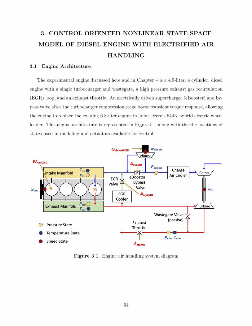
3. CONTROL ORIENTED NONLINEAR STATE SPACE
MODEL OF DIESEL ENGINE WITH ELECTRIFIED AIR
HANDLING
3.1 Engine Architecture
The experimental engine discussed here and in Chapter 4 is a 4.5-liter, 4 cylinder, diesel
engine with a single turbocharger and wastegate, a high pressure exhaust gas recirculation
(EGR) loop, and an exhaust throttle. An electrically driven supercharger (eBooster) and by-
pass valve after the turbocharger compression stage boost transient torque response, allowing
the engine to replace the existing 6.8-liter engine in John Deere’s 644K hybrid electric wheel
loader. This engine architecture is represented in Figure 3.1 along with the the locations of
states used in modeling and actuators available for control.
Figure 3.1. Engine air handling system diagram
64
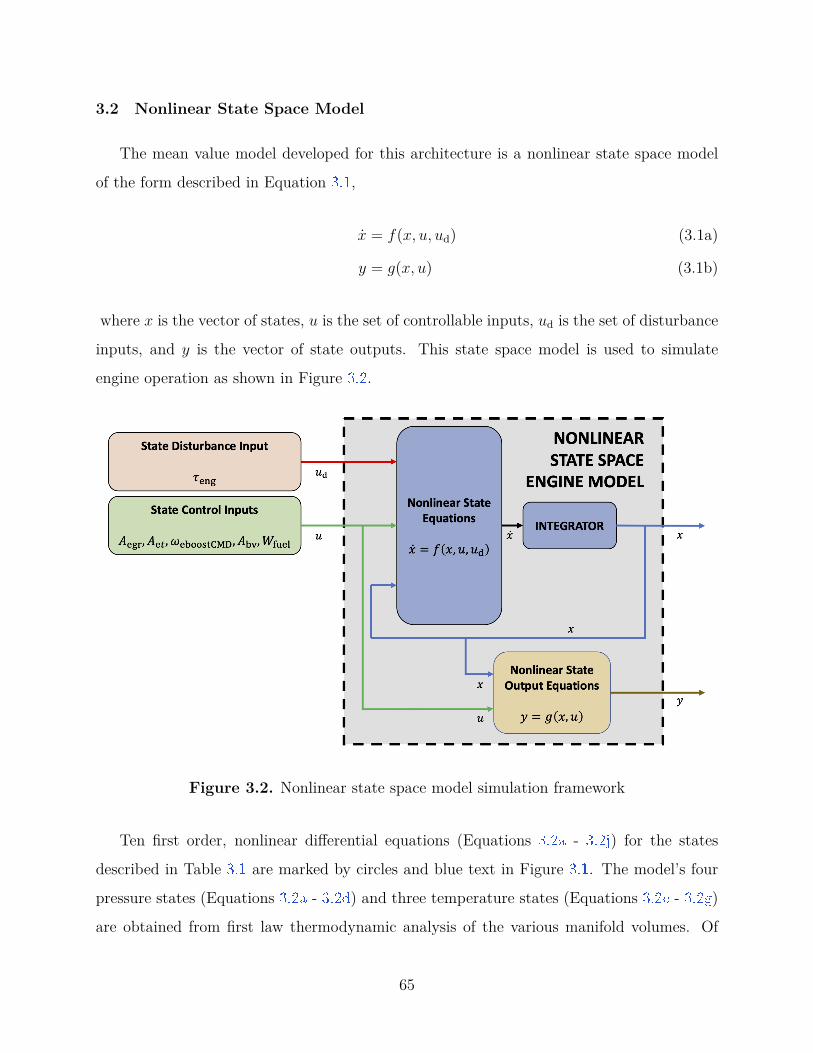
3.2 Nonlinear State Space Model
The mean value model developed for this architecture is a nonlinear state space model
of the form described in Equation 3.1 ,
x = f(x, u, ud) (3.1a)
y = g(x, u) (3.1b)
where x is the vector of states, u is the set of controllable inputs, ud is the set of disturbance
inputs, and y is the vector of state outputs. This state space model is used to simulate
engine operation as shown in Figure 3.2 .
Figure 3.2. Nonlinear state space model simulation framework
Ten first order, nonlinear differential equations (Equations 3.2a - 3.2j ) for the states
described in Table 3.1 are marked by circles and blue text in Figure 3.1 . The model’s four
pressure states (Equations 3.2a - 3.2d ) and three temperature states (Equations 3.2e - 3.2g )
are obtained from first law thermodynamic analysis of the various manifold volumes. Of
65
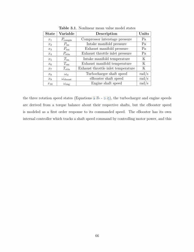
Table 3.1. Nonlinear mean value model statesState Variable Description Units
x1 Pcompis Compressor interstage pressure Pax2 Pim Intake manifold pressure Pax3 Pem Exhaust manifold pressure Pax4 Petin Exhaust throttle inlet pressure Pax5 Tim Intake manifold temperature Kx6 Tem Exhaust manifold temperature Kx7 Tetin Exhaust throttle inlet temperature Kx8 ωtc Turbocharger shaft speed rad/sx9 ωeboost eBooster shaft speed rad/sx10 ωeng Engine shaft speed rad/s
the three rotation speed states (Equations 3.2h - 3.2j ), the turbocharger and engine speeds
are derived from a torque balance about their respective shafts, but the eBooster speed
is modeled as a first order response to its commanded speed. The eBooster has its own
internal controller which tracks a shaft speed command by controlling motor power, and this
66
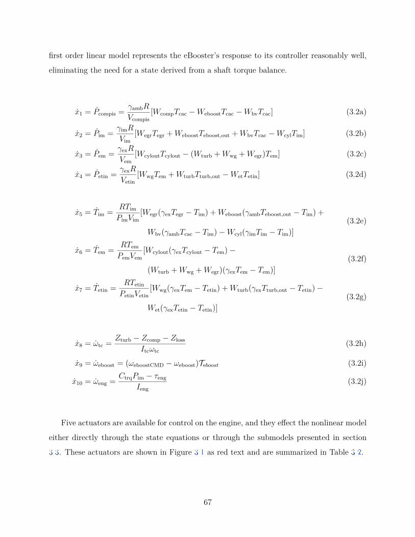
first order linear model represents the eBooster’s response to its controller reasonably well,
eliminating the need for a state derived from a shaft torque balance.
x1 = Pcompis = γambR
Vcompis[WcompTcac − WeboostTcac − WbvTcac] (3.2a)
x2 = Pim = γimR
Vim[WegrTegr + WeboostTeboost,out + WbvTcac − WcylTim] (3.2b)
x3 = Pem = γexR
Vem[WcyloutTcylout − (Wturb + Wwg + Wegr)Tem] (3.2c)
x4 = Petin = γexR
Vetin[WwgTem + WturbTturb,out − WetTetin] (3.2d)
x5 = Tim = RTim
PimVim[Wegr(γexTegr − Tim) + Weboost(γambTeboost,out − Tim) +
Wbv(γambTcac − Tim) − Wcyl(γimTim − Tim)](3.2e)
x6 = Tem = RTem
PemVem[Wcylout(γexTcylout − Tem) −
(Wturb + Wwg + Wegr)(γexTem − Tem)](3.2f)
x7 = Tetin = RTetin
PetinVetin[Wwg(γexTem − Tetin) + Wturb(γexTturb,out − Tetin) −
Wet(γexTetin − Tetin)](3.2g)
x8 = ωtc = Zturb − Zcomp − Zloss
Itcωtc(3.2h)
x9 = ωeboost = (ωeboostCMD − ωeboost)Teboost (3.2i)
x10 = ωeng = CtrqPim − τeng
Ieng(3.2j)
Five actuators are available for control on the engine, and they effect the nonlinear model
either directly through the state equations or through the submodels presented in section
3.3 . These actuators are shown in Figure 3.1 as red text and are summarized in Table 3.2 .
67
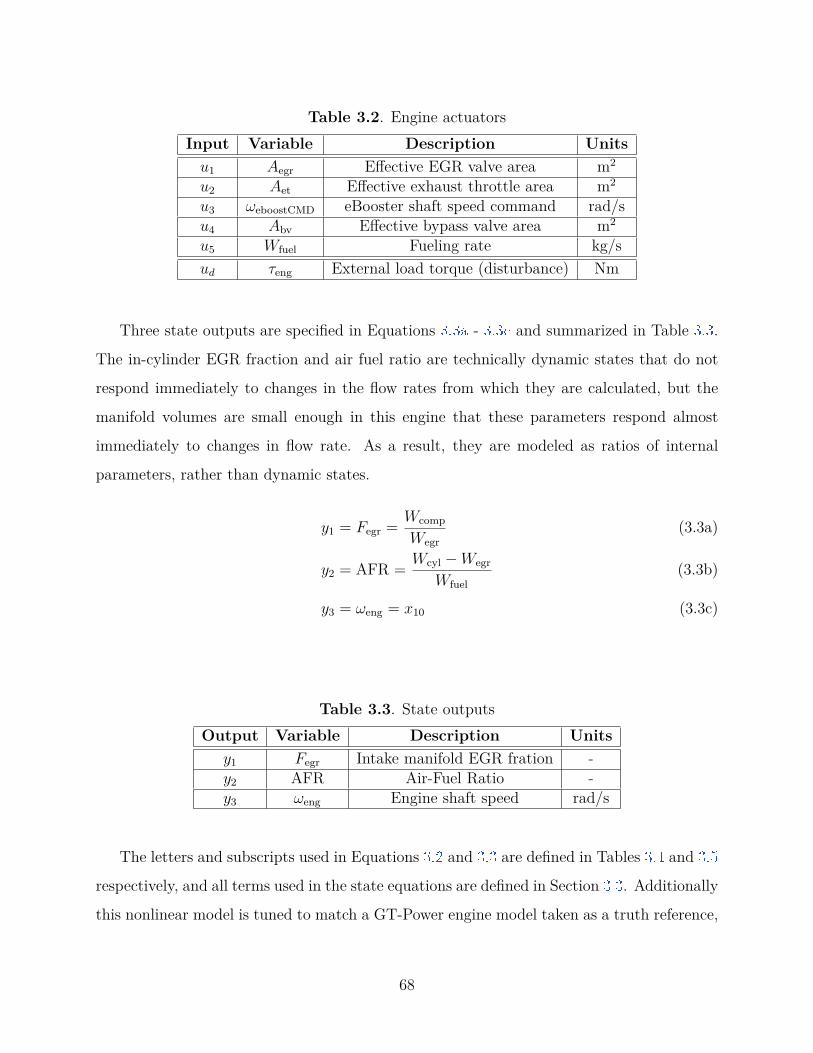
Table 3.2. Engine actuatorsInput Variable Description Units
u1 Aegr Effective EGR valve area m2
u2 Aet Effective exhaust throttle area m2
u3 ωeboostCMD eBooster shaft speed command rad/su4 Abv Effective bypass valve area m2
u5 Wfuel Fueling rate kg/sud τeng External load torque (disturbance) Nm
Three state outputs are specified in Equations 3.3a - 3.3c and summarized in Table 3.3 .
The in-cylinder EGR fraction and air fuel ratio are technically dynamic states that do not
respond immediately to changes in the flow rates from which they are calculated, but the
manifold volumes are small enough in this engine that these parameters respond almost
immediately to changes in flow rate. As a result, they are modeled as ratios of internal
parameters, rather than dynamic states.
y1 = Fegr = Wcomp
Wegr(3.3a)
y2 = AFR = Wcyl − Wegr
Wfuel(3.3b)
y3 = ωeng = x10 (3.3c)
Table 3.3. State outputsOutput Variable Description Units
y1 Fegr Intake manifold EGR fration -y2 AFR Air-Fuel Ratio -y3 ωeng Engine shaft speed rad/s
The letters and subscripts used in Equations 3.2 and 3.3 are defined in Tables 3.4 and 3.5
respectively, and all terms used in the state equations are defined in Section 3.3 . Additionally
this nonlinear model is tuned to match a GT-Power engine model taken as a truth reference,
68
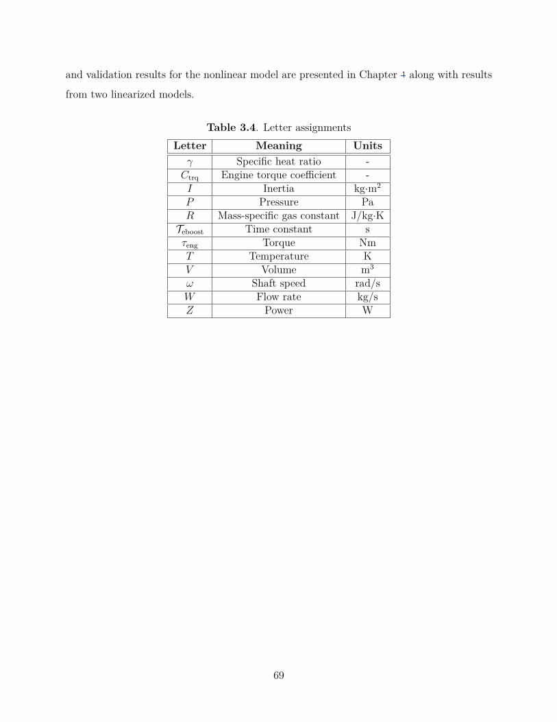
and validation results for the nonlinear model are presented in Chapter 4 along with results
from two linearized models.
Table 3.4. Letter assignmentsLetter Meaning Units
γ Specific heat ratio -Ctrq Engine torque coefficient -
I Inertia kg·m2
P Pressure PaR Mass-specific gas constant J/kg·K
Teboost Time constant sτeng Torque NmT Temperature KV Volume m3
ω Shaft speed rad/sW Flow rate kg/sZ Power W
69
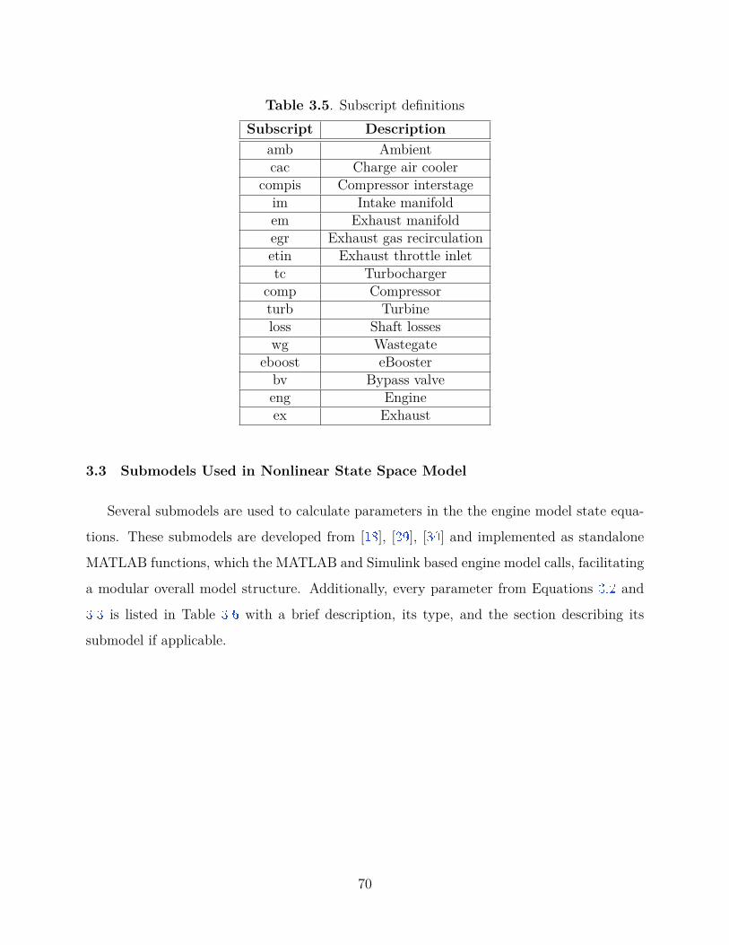
Table 3.5. Subscript definitionsSubscript Description
amb Ambientcac Charge air cooler
compis Compressor interstageim Intake manifoldem Exhaust manifoldegr Exhaust gas recirculationetin Exhaust throttle inlettc Turbocharger
comp Compressorturb Turbineloss Shaft losseswg Wastegate
eboost eBoosterbv Bypass valveeng Engineex Exhaust
3.3 Submodels Used in Nonlinear State Space Model
Several submodels are used to calculate parameters in the the engine model state equa-
tions. These submodels are developed from [18 ], [29 ], [30 ] and implemented as standalone
MATLAB functions, which the MATLAB and Simulink based engine model calls, facilitating
a modular overall model structure. Additionally, every parameter from Equations 3.2 and
3.3 is listed in Table 3.6 with a brief description, its type, and the section describing its
submodel if applicable.
70
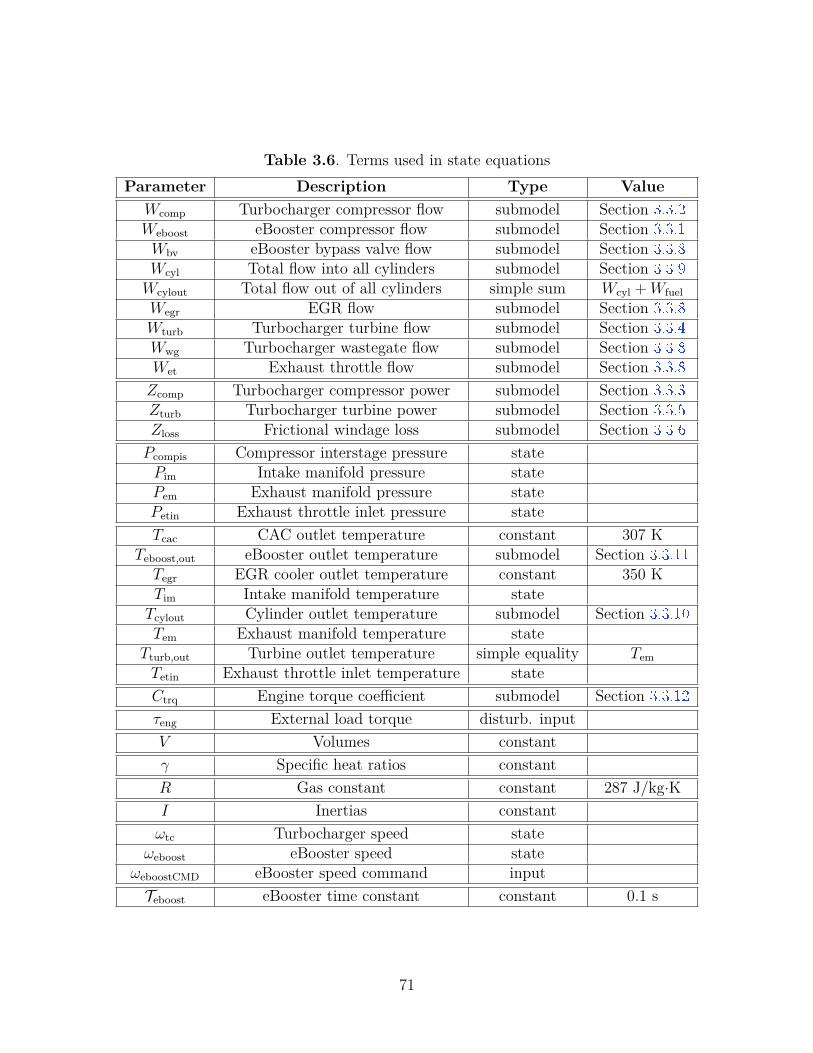
Table 3.6. Terms used in state equationsParameter Description Type Value
Wcomp Turbocharger compressor flow submodel Section 3.3.2
Weboost eBooster compressor flow submodel Section 3.3.1
Wbv eBooster bypass valve flow submodel Section 3.3.8
Wcyl Total flow into all cylinders submodel Section 3.3.9
Wcylout Total flow out of all cylinders simple sum Wcyl + WfuelWegr EGR flow submodel Section 3.3.8
Wturb Turbocharger turbine flow submodel Section 3.3.4
Wwg Turbocharger wastegate flow submodel Section 3.3.8
Wet Exhaust throttle flow submodel Section 3.3.8
Zcomp Turbocharger compressor power submodel Section 3.3.3
Zturb Turbocharger turbine power submodel Section 3.3.5
Zloss Frictional windage loss submodel Section 3.3.6
Pcompis Compressor interstage pressure statePim Intake manifold pressure statePem Exhaust manifold pressure statePetin Exhaust throttle inlet pressure stateTcac CAC outlet temperature constant 307 K
Teboost,out eBooster outlet temperature submodel Section 3.3.11
Tegr EGR cooler outlet temperature constant 350 KTim Intake manifold temperature state
Tcylout Cylinder outlet temperature submodel Section 3.3.10
Tem Exhaust manifold temperature stateTturb,out Turbine outlet temperature simple equality Tem
Tetin Exhaust throttle inlet temperature stateCtrq Engine torque coefficient submodel Section 3.3.12
τeng External load torque disturb. inputV Volumes constantγ Specific heat ratios constantR Gas constant constant 287 J/kg·KI Inertias constant
ωtc Turbocharger speed stateωeboost eBooster speed state
ωeboostCMD eBooster speed command inputTeboost eBooster time constant constant 0.1 s
71
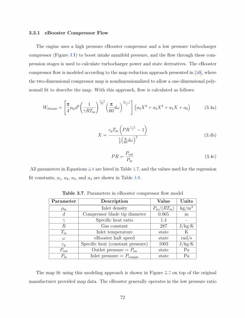
3.3.1 eBooster Compressor Flow
The engine uses a high pressure eBooster compressor and a low pressure turbocharger
compressor (Figure 3.1 ) to boost intake manifold pressure, and the flow through these com-
pression stages is used to calculate turbocharger power and state derivatives. The eBooster
compressor flow is modeled according to the map reduction approach presented in [30 ], where
the two-dimensional compressor map is nondimensionalized to allow a one-dimensional poly-
nomail fit to describe the map. With this approach, flow is calculated as follows:
Weboost =π
4ρind2(
1γRTin
) γ−12γ ( π
60dω) 2γ−1
γ
(a3X3 + a2X
2 + a1X + a0)
(3.4a)
X =cpTin
(PR
γ−1γ − 1
)12
(π
60dω)2 (3.4b)
PR = Pout
Pin(3.4c)
All parameters in Equations 3.4 are listed in Table 3.7 , and the values used for the regression
fit constants, a1, a2, a3, and a4 are shown in Table 3.8 .
Table 3.7. Parameters in eBooster compressor flow modelParameter Description Value Units
ρin Inlet density Pin/(RTin) kg/m3
d Compressor blade tip diameter 0.065 mγ Specific heat ratio 1.4 -R Gas constant 287 J/kg·KTin Inlet temperature state Kω eBooster haft speed state rad/scp Specific heat (constant pressure) 1003 J/kg·K
Pout Outlet pressure = Pim state PaPin Inlet pressure = Pcompis state Pa
The map fit using this modeling approach is shown in Figure 3.3 on top of the original
manufacturer provided map data. The eBooster generally operates in the low pressure ratio
72
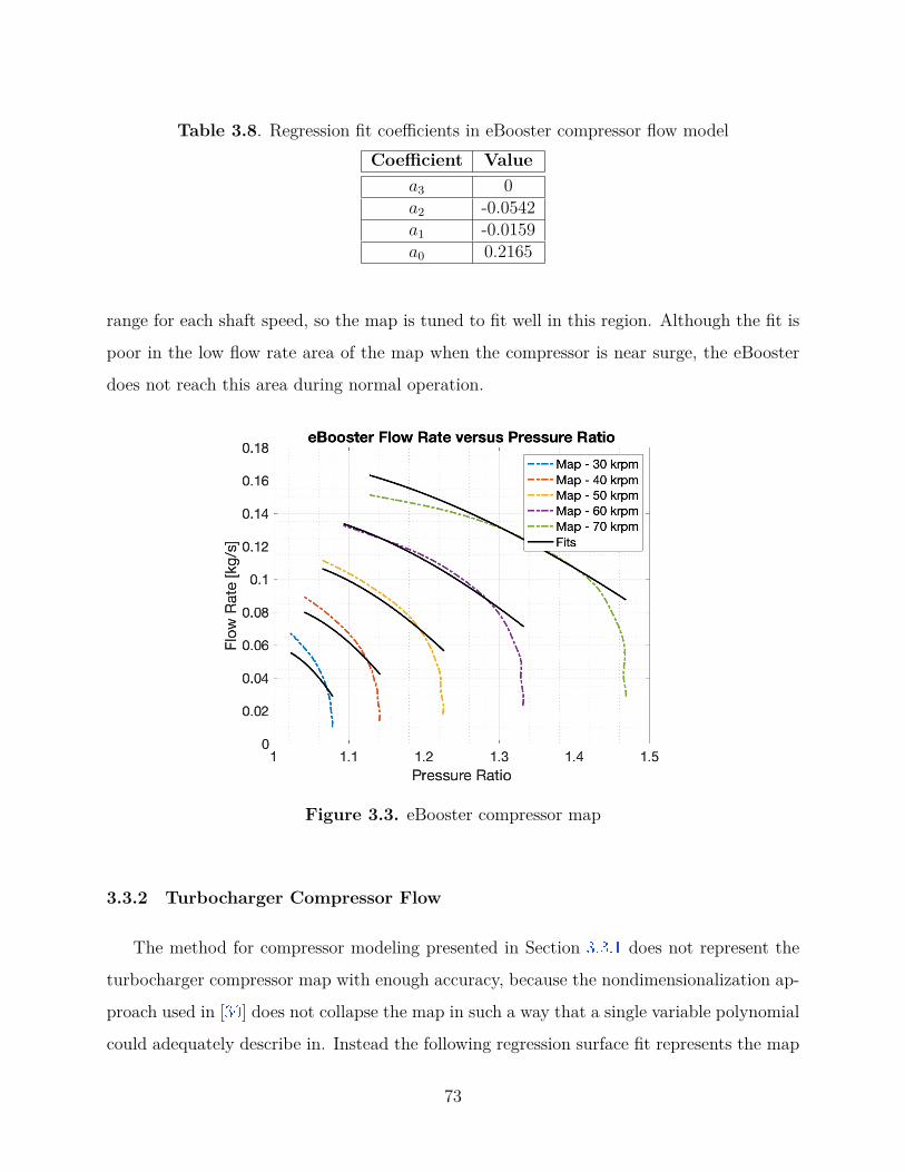
Table 3.8. Regression fit coefficients in eBooster compressor flow modelCoefficient Value
a3 0a2 -0.0542a1 -0.0159a0 0.2165
range for each shaft speed, so the map is tuned to fit well in this region. Although the fit is
poor in the low flow rate area of the map when the compressor is near surge, the eBooster
does not reach this area during normal operation.
Figure 3.3. eBooster compressor map
3.3.2 Turbocharger Compressor Flow
The method for compressor modeling presented in Section 3.3.1 does not represent the
turbocharger compressor map with enough accuracy, because the nondimensionalization ap-
proach used in [30 ] does not collapse the map in such a way that a single variable polynomial
could adequately describe in. Instead the following regression surface fit represents the map
73
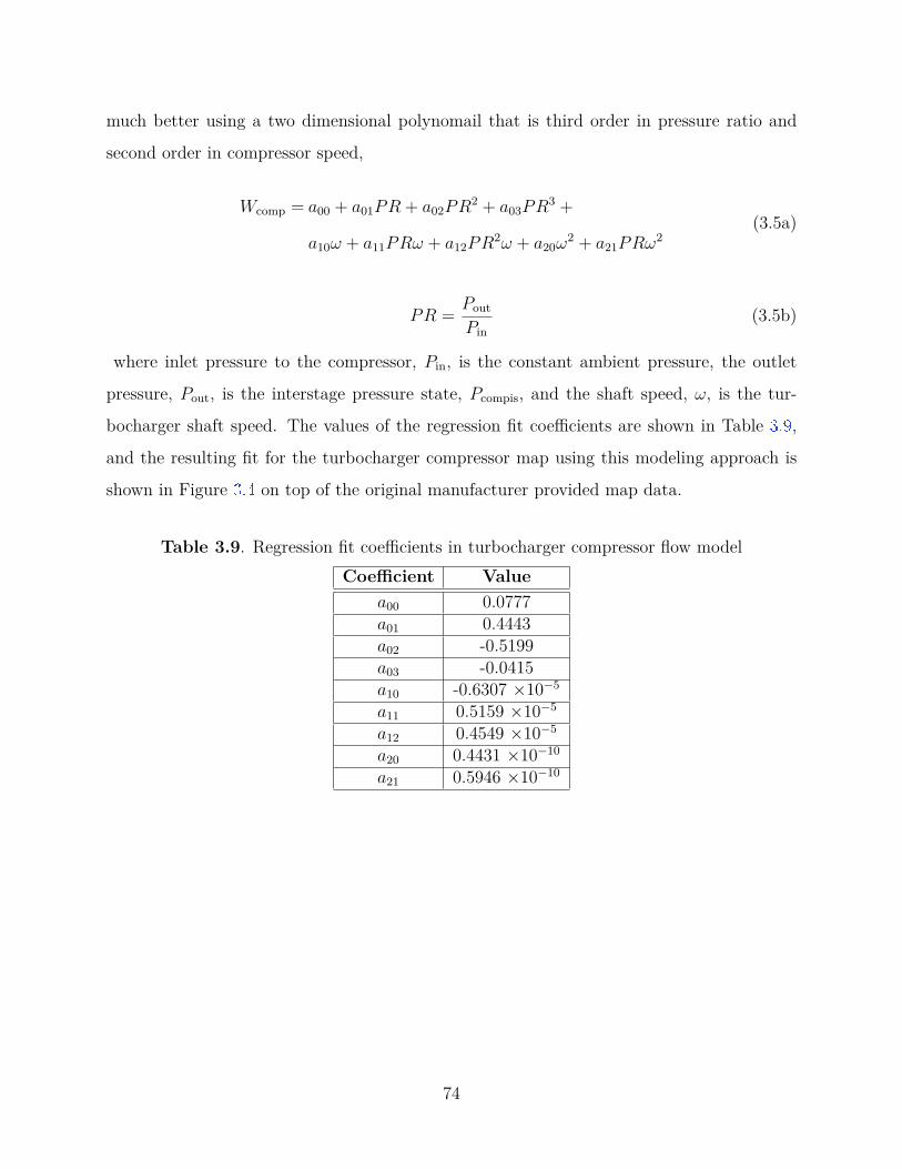
much better using a two dimensional polynomail that is third order in pressure ratio and
second order in compressor speed,
Wcomp = a00 + a01PR + a02PR2 + a03PR3 +
a10ω + a11PRω + a12PR2ω + a20ω2 + a21PRω2
(3.5a)
PR = Pout
Pin(3.5b)
where inlet pressure to the compressor, Pin, is the constant ambient pressure, the outlet
pressure, Pout, is the interstage pressure state, Pcompis, and the shaft speed, ω, is the tur-
bocharger shaft speed. The values of the regression fit coefficients are shown in Table 3.9 ,
and the resulting fit for the turbocharger compressor map using this modeling approach is
shown in Figure 3.4 on top of the original manufacturer provided map data.
Table 3.9. Regression fit coefficients in turbocharger compressor flow modelCoefficient Value
a00 0.0777a01 0.4443a02 -0.5199a03 -0.0415a10 -0.6307 ×10⁻⁵
a11 0.5159 ×10⁻⁵
a12 0.4549 ×10⁻⁵
a20 0.4431 ×10⁻¹⁰
a21 0.5946 ×10⁻¹⁰
74
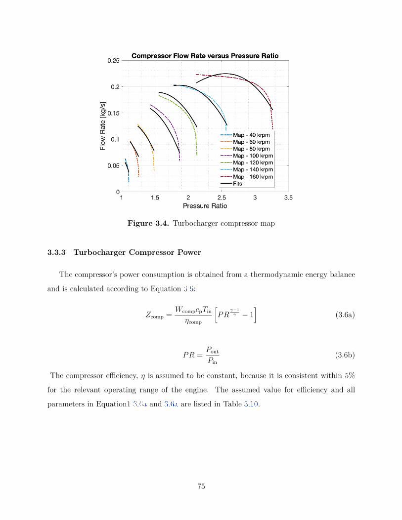
Figure 3.4. Turbocharger compressor map
3.3.3 Turbocharger Compressor Power
The compressor’s power consumption is obtained from a thermodynamic energy balance
and is calculated according to Equation 3.6 :
Zcomp = WcompcpTin
ηcomp
[PR
γ−1γ − 1
](3.6a)
PR = Pout
Pin(3.6b)
The compressor efficiency, η is assumed to be constant, because it is consistent within 5%
for the relevant operating range of the engine. The assumed value for efficiency and all
parameters in Equation1 3.6a and 3.6a are listed in Table 3.10 .
75
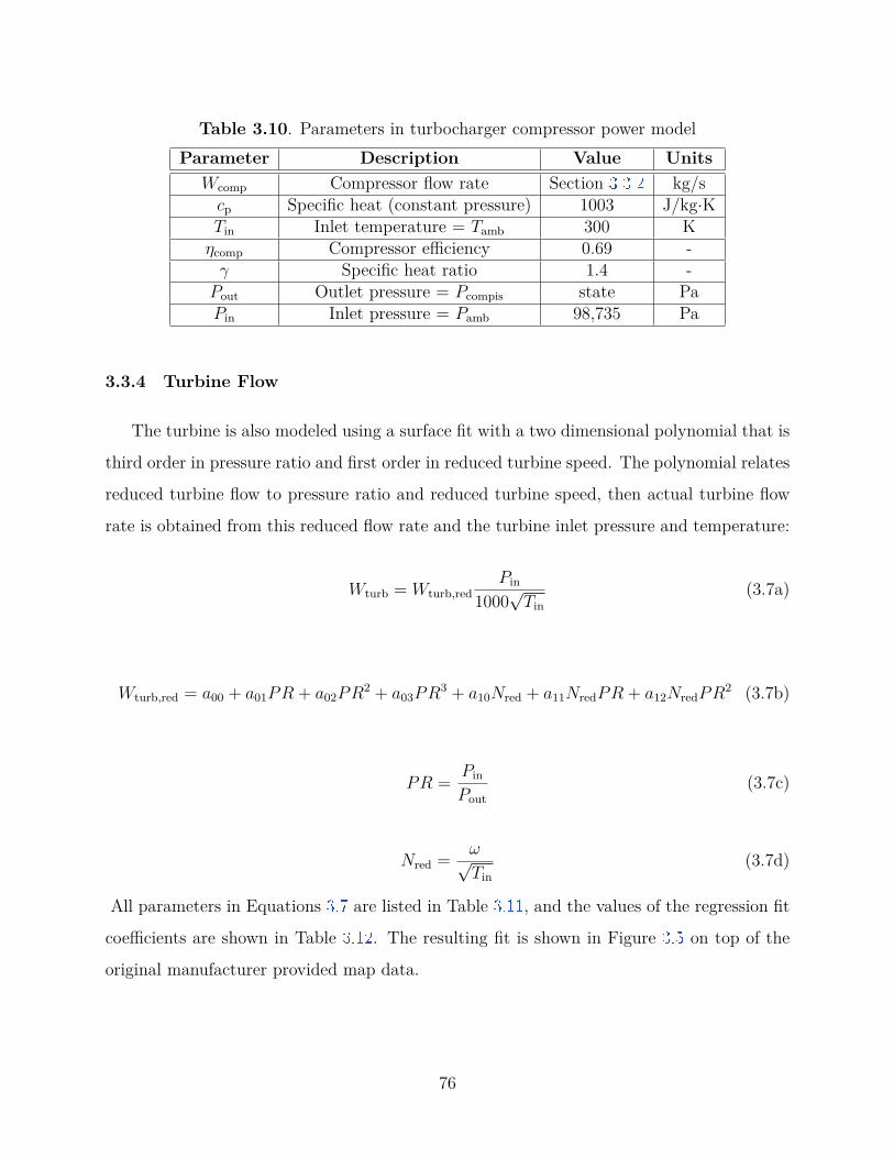
Table 3.10. Parameters in turbocharger compressor power modelParameter Description Value Units
Wcomp Compressor flow rate Section 3.3.2 kg/scp Specific heat (constant pressure) 1003 J/kg·KTin Inlet temperature = Tamb 300 K
ηcomp Compressor efficiency 0.69 -γ Specific heat ratio 1.4 -
Pout Outlet pressure = Pcompis state PaPin Inlet pressure = Pamb 98,735 Pa
3.3.4 Turbine Flow
The turbine is also modeled using a surface fit with a two dimensional polynomial that is
third order in pressure ratio and first order in reduced turbine speed. The polynomial relates
reduced turbine flow to pressure ratio and reduced turbine speed, then actual turbine flow
rate is obtained from this reduced flow rate and the turbine inlet pressure and temperature:
Wturb = Wturb,redPin
1000√
Tin(3.7a)
Wturb,red = a00 + a01PR + a02PR2 + a03PR3 + a10Nred + a11NredPR + a12NredPR2 (3.7b)
PR = Pin
Pout(3.7c)
Nred = ω√Tin
(3.7d)
All parameters in Equations 3.7 are listed in Table 3.11 , and the values of the regression fit
coefficients are shown in Table 3.12 . The resulting fit is shown in Figure 3.5 on top of the
original manufacturer provided map data.
76
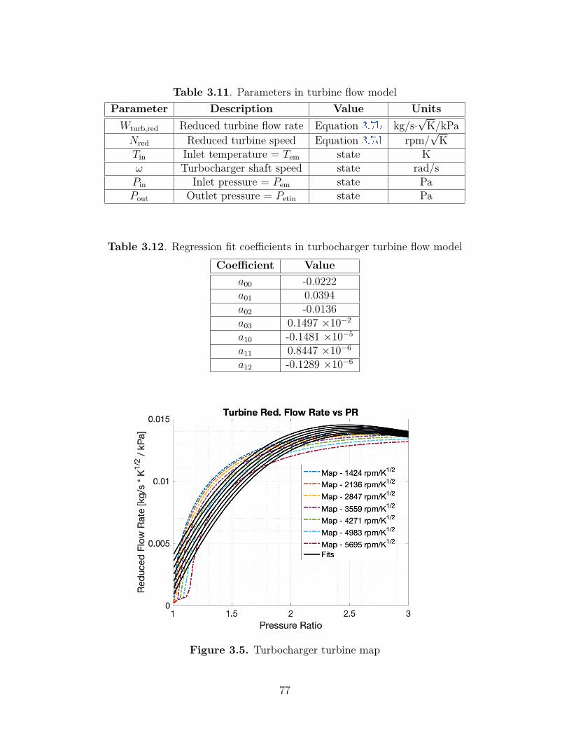
Table 3.11. Parameters in turbine flow modelParameter Description Value Units
Wturb,red Reduced turbine flow rate Equation 3.7b kg/s·√
K/kPaNred Reduced turbine speed Equation 3.7d rpm/
√K
Tin Inlet temperature = Tem state Kω Turbocharger shaft speed state rad/s
Pin Inlet pressure = Pem state PaPout Outlet pressure = Petin state Pa
Table 3.12. Regression fit coefficients in turbocharger turbine flow modelCoefficient Value
a00 -0.0222a01 0.0394a02 -0.0136a03 0.1497 ×10⁻²
a10 -0.1481 ×10⁻⁵
a11 0.8447 ×10⁻⁶
a12 -0.1289 ×10⁻⁶
Figure 3.5. Turbocharger turbine map
77
3.3.5 Turbine Power
The turbine’s power consumption is obtained from a thermodynamic energy balance and
is calculated according to Equation 3.8 :
Zturb = WturbcpTinηcomp
[1 − Pout
Pin
] γ−1γ
(3.8)
Like the compressor efficiency, the turbine efficiency, η is assumed to be constant, because it
is consistent within 5% for the relevant operating range of the engine. The assumed values
for efficiency and all other parameters in Equation 3.8 are listed in Table 3.13 .
Table 3.13. Parameters in turbocharger turbine power modelParameter Description Value Units
Wturb Turbine flow rate Section 3.3.4 kg/scp Specific heat (constant pressure) 1107 J/kg·KTin Inlet temperature = Tem state K
ηturb Turbine efficiency 0.63 -γ Specific heat ratio 1.35 -
Pout Outlet pressure = Petin state PaPin Inlet pressure = Pem state Pa
3.3.6 Turbocharger Windage Loss
The turbocharger windage loss due to friction is modeled as a reduction in power that is
a function of turbocharger shaft speed, ω according to the following equation:
Zloss = a3ω3 + a2ω
2 + a1ω + a0 (3.9)
Data from the GT-Power reference engine model is used to obtain the regression coefficients
shown in Table 3.14 , and the resulting fit is shown in Figure 3.6 .
78
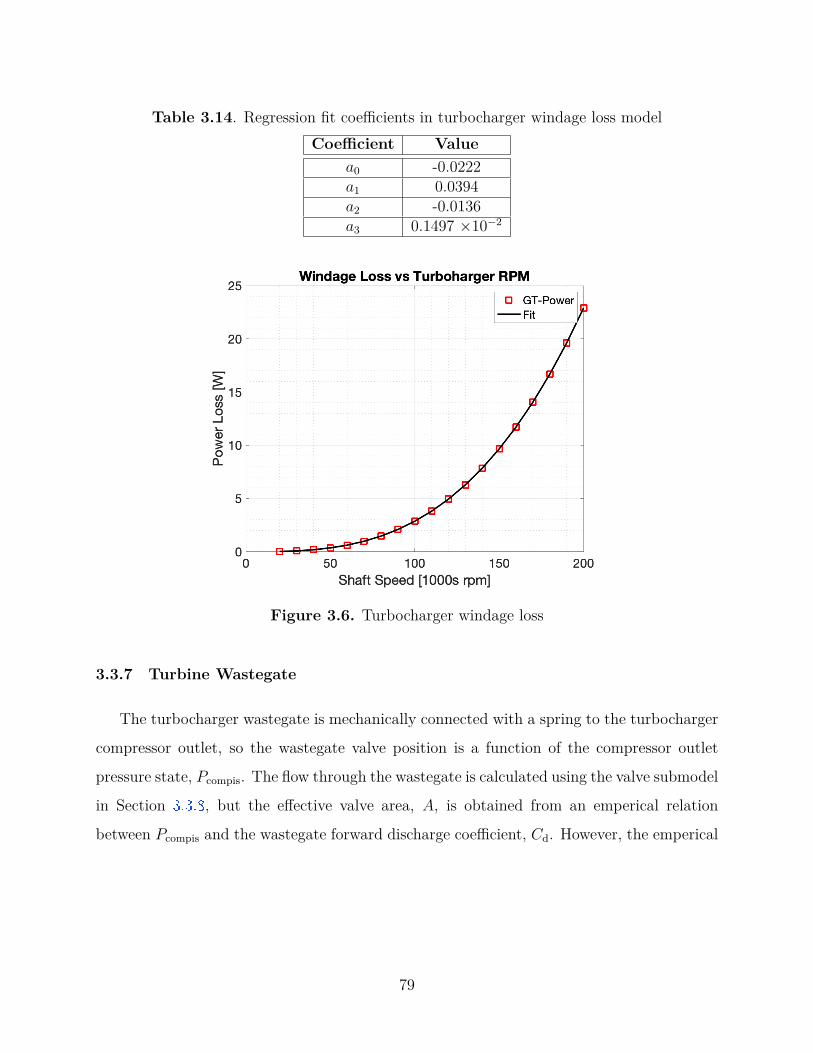
Table 3.14. Regression fit coefficients in turbocharger windage loss modelCoefficient Value
a0 -0.0222a1 0.0394a2 -0.0136a3 0.1497 ×10⁻²
Figure 3.6. Turbocharger windage loss
3.3.7 Turbine Wastegate
The turbocharger wastegate is mechanically connected with a spring to the turbocharger
compressor outlet, so the wastegate valve position is a function of the compressor outlet
pressure state, Pcompis. The flow through the wastegate is calculated using the valve submodel
in Section 3.3.8 , but the effective valve area, A, is obtained from an emperical relation
between Pcompis and the wastegate forward discharge coefficient, Cd. However, the emperical
79
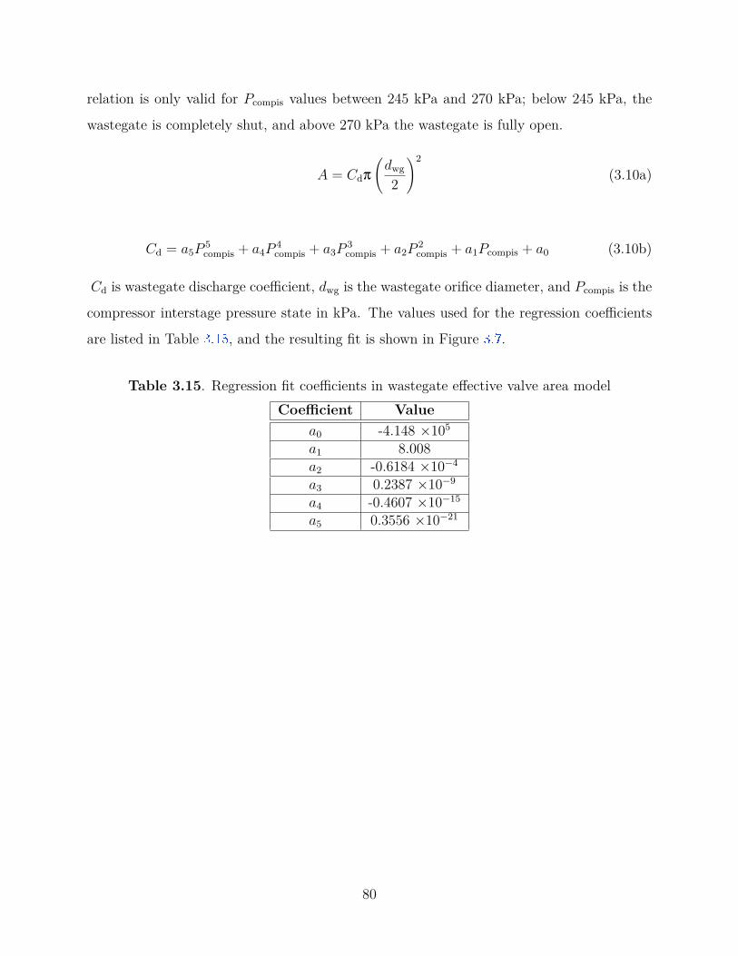
relation is only valid for Pcompis values between 245 kPa and 270 kPa; below 245 kPa, the
wastegate is completely shut, and above 270 kPa the wastegate is fully open.
A = Cdπ
(dwg
2
)2
(3.10a)
Cd = a5P5compis + a4P
4compis + a3P
3compis + a2P
2compis + a1Pcompis + a0 (3.10b)
Cd is wastegate discharge coefficient, dwg is the wastegate orifice diameter, and Pcompis is the
compressor interstage pressure state in kPa. The values used for the regression coefficients
are listed in Table 3.15 , and the resulting fit is shown in Figure 3.7 .
Table 3.15. Regression fit coefficients in wastegate effective valve area modelCoefficient Value
a0 -4.148 ×10⁵
a1 8.008a2 -0.6184 ×10⁻⁴
a3 0.2387 ×10⁻⁹
a4 -0.4607 ×10⁻¹⁵
a5 0.3556 ×10⁻²¹
80
Figure 3.7. Wastegate forward discharge coefficient regression fit
3.3.8 Valve Flow
The mass flow rates through the eBooster bypass valve, EGR valve, wastegate, and
exhaust throttle are all modeled by the standard orifice equation and a linearization of the
orifice equation for pressure ratios near 1 [18 ].
Wvalve = APin√RTin
Ψ (3.11a)
Ψ =
Ψ0 PR < Πlinear
1−Π1−Πlinear
Ψ0 PRlinear < PR
(3.11b)
Ψ0 =√
2γ
γ − 1
(Π
2γ − Π
γ+1γ
)(3.11c)
81
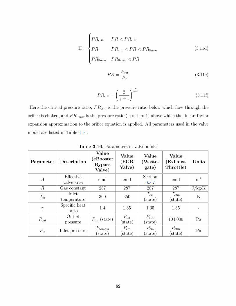
Π =
PRcrit PR < PRcrit
PR PRcrit < PR < PRlinear
PRlinear PRlinear < PR
(3.11d)
PR = Pout
Pin(3.11e)
PRcrit =(
2γ + 1
) γγ−1
(3.11f)
Here the critical pressure ratio, PRcrit is the pressure ratio below which flow through the
orifice is choked, and PRlinear is the pressure ratio (less than 1) above which the linear Taylor
expansion approximation to the orifice equation is applied. All parameters used in the valve
model are listed in Table 3.16 .
Table 3.16. Parameters in valve model
Parameter Description
Value(eBooster
BypassValve)
Value(EGRValve)
Value(Waste-
gate)
Value(ExhaustThrottle)
Units
AEffective
valve area cmd cmd Section3.3.7
cmd m2
R Gas constant 287 287 287 287 J/kg·K
TinInlet
temperature 300 350 Tem(state)
Tetin(state) K
γSpecific heat
ratio 1.4 1.35 1.35 1.35 -
PoutOutlet
pressure Pim (state) Pim(state)
Petin(state) 104,000 Pa
Pin Inlet pressure Pcompis(state)
Pem(state)
Pem(state)
Petin(state) Pa
82
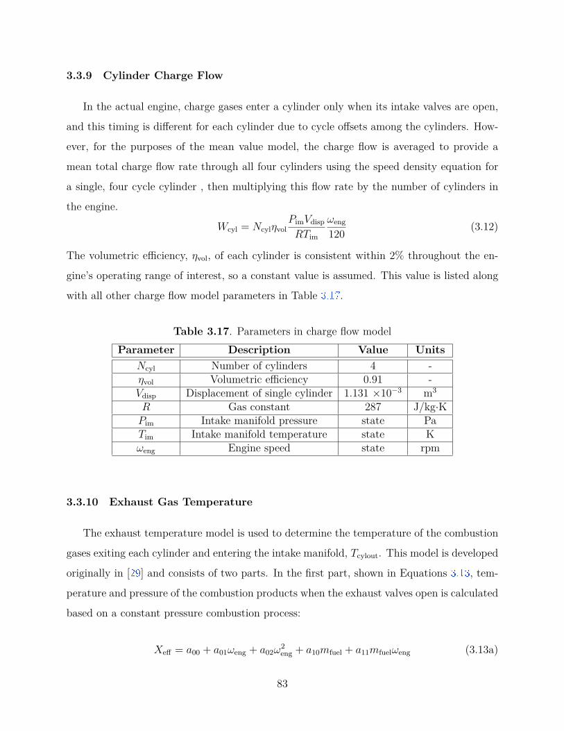
3.3.9 Cylinder Charge Flow
In the actual engine, charge gases enter a cylinder only when its intake valves are open,
and this timing is different for each cylinder due to cycle offsets among the cylinders. How-
ever, for the purposes of the mean value model, the charge flow is averaged to provide a
mean total charge flow rate through all four cylinders using the speed density equation for
a single, four cycle cylinder , then multiplying this flow rate by the number of cylinders in
the engine.
Wcyl = NcylηvolPimVdisp
RTim
ωeng
120 (3.12)
The volumetric efficiency, ηvol, of each cylinder is consistent within 2% throughout the en-
gine’s operating range of interest, so a constant value is assumed. This value is listed along
with all other charge flow model parameters in Table 3.17 .
Table 3.17. Parameters in charge flow modelParameter Description Value Units
Ncyl Number of cylinders 4 -ηvol Volumetric efficiency 0.91 -Vdisp Displacement of single cylinder 1.131 ×10⁻³ m3
R Gas constant 287 J/kg·KPim Intake manifold pressure state PaTim Intake manifold temperature state Kωeng Engine speed state rpm
3.3.10 Exhaust Gas Temperature
The exhaust temperature model is used to determine the temperature of the combustion
gases exiting each cylinder and entering the intake manifold, Tcylout. This model is developed
originally in [29 ] and consists of two parts. In the first part, shown in Equations 3.13 , tem-
perature and pressure of the combustion products when the exhaust valves open is calculated
based on a constant pressure combustion process:
Xeff = a00 + a01ωeng + a02ω2eng + a10mfuel + a11mfuelωeng (3.13a)
83
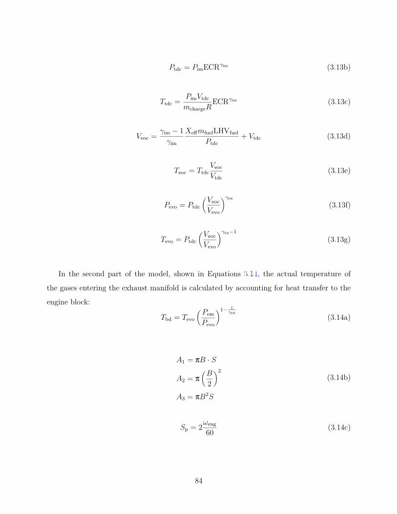
Ptdc = PimECRγim (3.13b)
Ttdc = PimVtdc
mchargeRECRγim (3.13c)
Veoc = γim − 1γim
XeffmfuelLHVfuel
Ptdc+ Vtdc (3.13d)
Teoc = TtdcVeoc
Vtdc(3.13e)
Pevo = Ptdc
(Veoc
Vevo
)γex
(3.13f)
Tevo = Ptdc
(Veoc
Vevo
)γex−1(3.13g)
In the second part of the model, shown in Equations 3.14 , the actual temperature of
the gases entering the exhaust manifold is calculated by accounting for heat transfer to the
engine block:
Tbd = Tevo
(Pem
Pevo
)1− 1γex
(3.14a)
A1 = πB · S
A2 = π
(B
2
)2
A3 = πB2S
(3.14b)
Sp = 2ωeng
60 (3.14c)
84
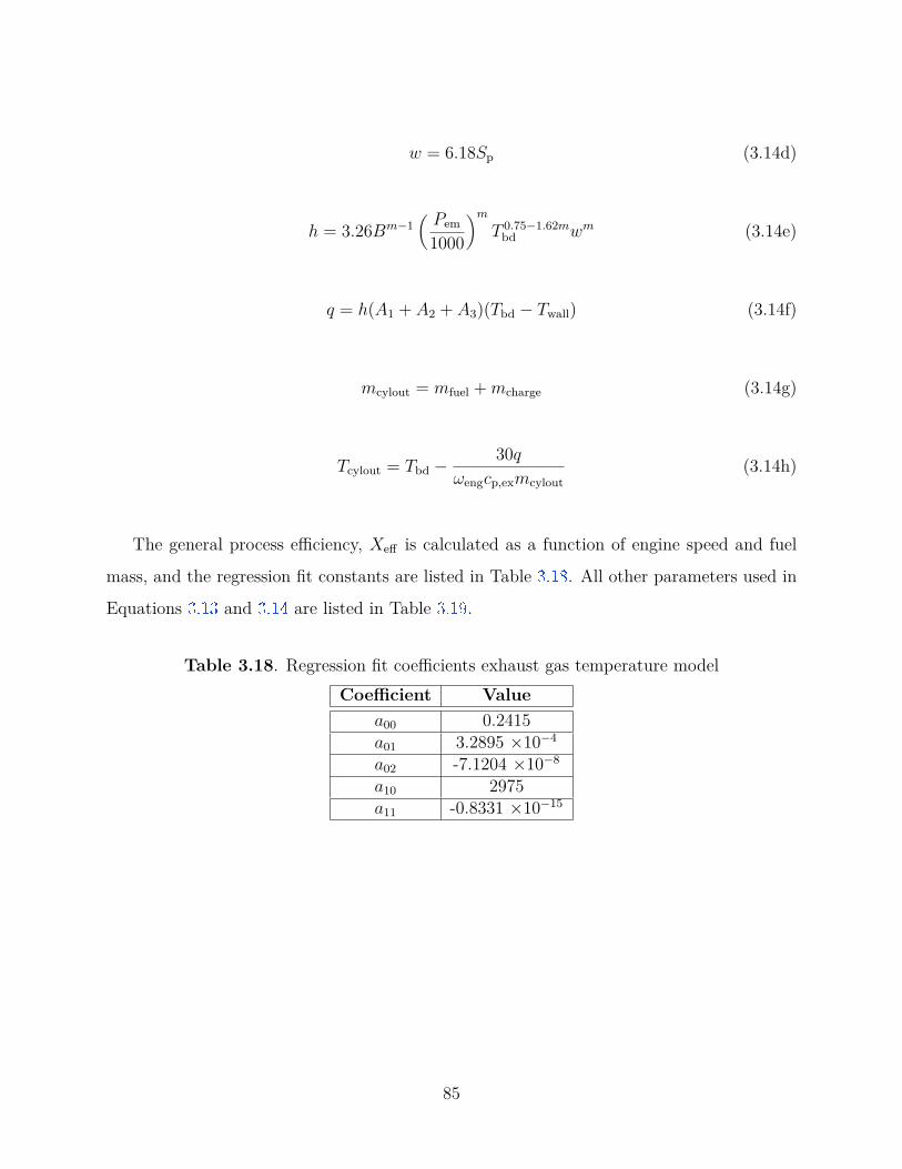
w = 6.18Sp (3.14d)
h = 3.26Bm−1(
Pem
1000
)m
T 0.75−1.62mbd wm (3.14e)
q = h(A1 + A2 + A3)(Tbd − Twall) (3.14f)
mcylout = mfuel + mcharge (3.14g)
Tcylout = Tbd − 30q
ωengcp,exmcylout(3.14h)
The general process efficiency, Xeff is calculated as a function of engine speed and fuel
mass, and the regression fit constants are listed in Table 3.18 . All other parameters used in
Equations 3.13 and 3.14 are listed in Table 3.19 .
Table 3.18. Regression fit coefficients exhaust gas temperature modelCoefficient Value
a00 0.2415a01 3.2895 ×10⁻⁴
a02 -7.1204 ×10⁻⁸
a10 2975a11 -0.8331 ×10⁻¹⁵
85
Table 3.19. Parameters in charge flow modelParameter Description Value Units
Pim Intake manifold pressure state PaPtdc Pressure at TDC Equation 3.13b PaPevo Pressure at EVO Equation 3.13f PaPem Exhaust Manifold Pressure state PaTtdc Temperature at TDC Equation 3.13c KTeoc Temperature at EOC Equation 3.13e KTevo Temperature at EVO Equation 3.13g KTwall Cylinder wall temperature 550 KTbd Blowdown temperature Equation 3.14a KVtdc Volume of 1 cylinder at TDC 7.5423×10⁻⁵ m3
Veoc Volume of 1 cylinder at EOC Equation 3.13d m3
Vevo Volume of 1 cylinder at EVO 6.4107×10⁻⁴ m3
ECR Effective compression ratio 16 -mcharge Mass of gas in 1 cylinder f(Wcyl, ωeng) kgmfuel Fuel mass injected into 1 cylinder in 1 cycle command kg
mcylout Total mass exiting 1 cylinder Equation 3.14g kgR Gas constant 287 J/kg·K
γim Intake manifold specific heat ratio 1.4 -γex Exhaust manifold specific heat ratio 1.35 -Xeff Efficiency Equation 3.13a -
LHVfuel Lower heating value of diesel 42.8 ×10⁶ J/kgA1, A2, A3 Sidewall, cylinder head, & piston head area Equation 3.14b m2
B Cylinder bore diameter 0.1065 mS Cylinder stroke length 0.127 mSp Mean piston speed Equation 3.14c m/s
ωeng Engine speed state rpmw Average cylinder gas velocity Equation 3.14d m/sm Convective heat transfer parameter 0.8 -h Convective heat transfer coefficient Equation 3.14e W/m2·Kq Mass specific heat transfer Equation 3.14f W/kg
cp,ex Constant pressure specific heat 1107 J/kg·K
86
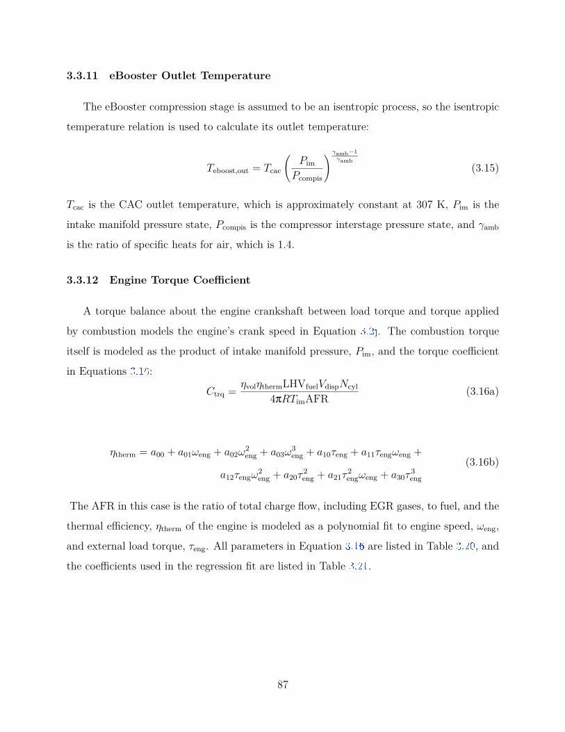
3.3.11 eBooster Outlet Temperature
The eBooster compression stage is assumed to be an isentropic process, so the isentropic
temperature relation is used to calculate its outlet temperature:
Teboost,out = Tcac
(Pim
Pcompis
) γamb−1γamb
(3.15)
Tcac is the CAC outlet temperature, which is approximately constant at 307 K, Pim is the
intake manifold pressure state, Pcompis is the compressor interstage pressure state, and γamb
is the ratio of specific heats for air, which is 1.4.
3.3.12 Engine Torque Coefficient
A torque balance about the engine crankshaft between load torque and torque applied
by combustion models the engine’s crank speed in Equation 3.2j . The combustion torque
itself is modeled as the product of intake manifold pressure, Pim, and the torque coefficient
in Equations 3.16 :
Ctrq = ηvolηthermLHVfuelVdispNcyl
4πRTimAFR (3.16a)
ηtherm = a00 + a01ωeng + a02ω2eng + a03ω
3eng + a10τeng + a11τengωeng +
a12τengω2eng + a20τ
2eng + a21τ
2engωeng + a30τ
3eng
(3.16b)
The AFR in this case is the ratio of total charge flow, including EGR gases, to fuel, and the
thermal efficiency, ηtherm of the engine is modeled as a polynomial fit to engine speed, ωeng,
and external load torque, τeng. All parameters in Equation 3.16 are listed in Table 3.20 , and
the coefficients used in the regression fit are listed in Table 3.21 .
87
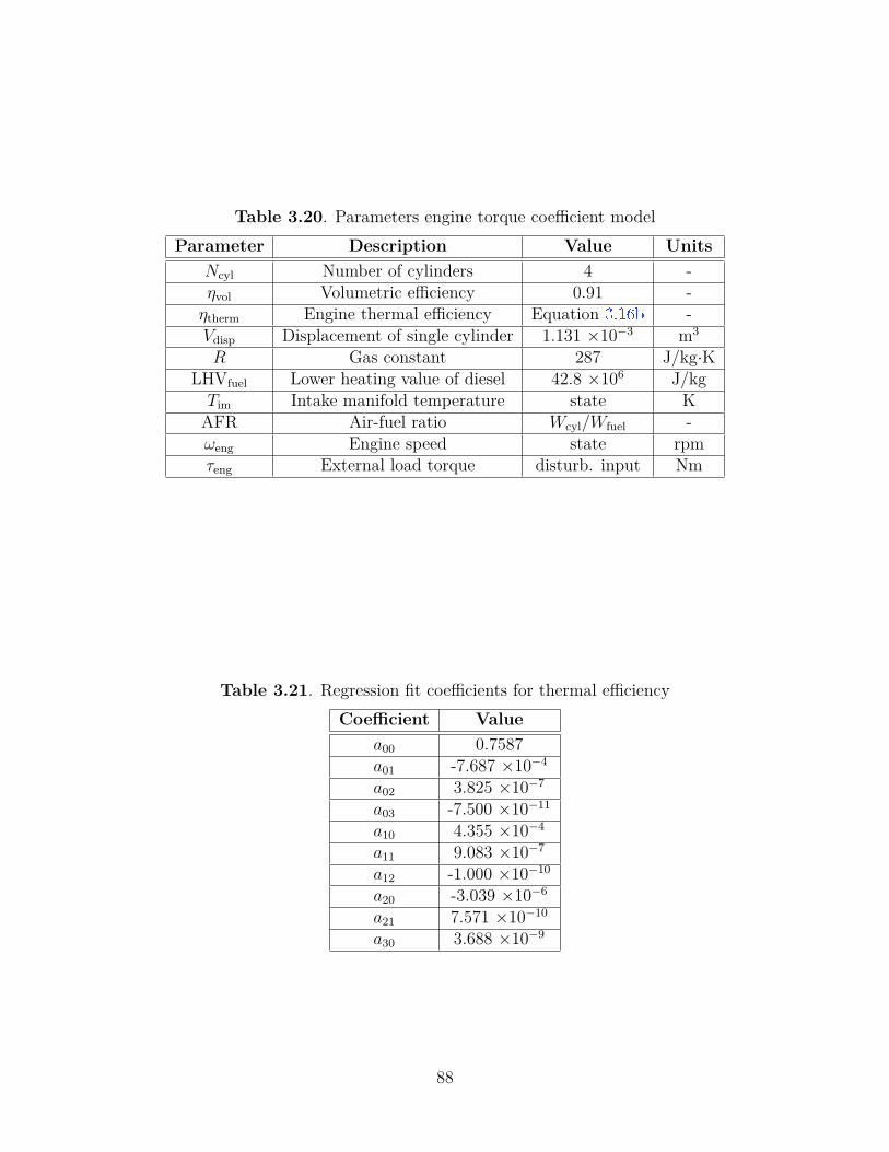
Table 3.20. Parameters engine torque coefficient modelParameter Description Value Units
Ncyl Number of cylinders 4 -ηvol Volumetric efficiency 0.91 -
ηtherm Engine thermal efficiency Equation 3.16b -Vdisp Displacement of single cylinder 1.131 ×10⁻³ m3
R Gas constant 287 J/kg·KLHVfuel Lower heating value of diesel 42.8 ×10⁶ J/kg
Tim Intake manifold temperature state KAFR Air-fuel ratio Wcyl/Wfuel -ωeng Engine speed state rpmτeng External load torque disturb. input Nm
Table 3.21. Regression fit coefficients for thermal efficiencyCoefficient Value
a00 0.7587a01 -7.687 ×10⁻⁴
a02 3.825 ×10⁻⁷
a03 -7.500 ×10⁻¹¹
a10 4.355 ×10⁻⁴
a11 9.083 ×10⁻⁷
a12 -1.000 ×10⁻¹⁰
a20 -3.039 ×10⁻⁶
a21 7.571 ×10⁻¹⁰
a30 3.688 ×10⁻⁹
88
4. STATE SPACE MODEL LINEARIZATION, VALIDATION,
AND ANALYSIS
4.1 Nonlinear Model Linearization
To develop the set of linear H∞ controllers discussed in Section 1.3.4 , linear engine models
are required, which can be obtained by linearizing the nonlinear state space model presented
in Chapter 3 . Each resulting linear model can be represented as:
x = δx = Aδx + Bδu + Fδud (4.1a)
δy = Cδx + Dδu (4.1b)
δx = x − xe δy = y − ye δu = u − ue δud = ud − ud,e (4.1c)
where x, y, u, and ud are the nonlinear model states, outputs, and inputs, δx, δy, δu, and δud
are their linear correlaries, and xe, ye, ue, and ud,e are the equilibrium values around which
the nonlinear model is linearized. The state matrices, A, B, F , C, and D are calculated
from the set of nonlinear differential equations,
x = f(x, u, ud) (3.1a )
y = g(x, u) (3.1b )
89
as the following Jacobian matrices, where each partial derivative is calculated as a function
of xe, ue, and ud,e:
A = A10×10(xe, ue, ud,e) =
∂f1∂x1
· · · ∂f1∂x10
... . . . ...∂f10∂x1
· · · ∂f10∂x10
(4.3a)
B = B10×5(xe, ue, ud,e) =
∂f1∂u1
· · · ∂f1∂u5
... . . . ...∂f10∂u1
· · · ∂f10∂u5
(4.3b)
F = F 10×1(xe, ue, ud,e) =
∂f1∂ud...
∂f10∂ud
(4.3c)
C = C3×10(xe, ue, ud,e) =
∂g1∂x1
· · · ∂g1∂x10
... . . . ...∂g3∂x1
· · · ∂g3∂x10
(4.3d)
D = D3×5(xe, ue, ud,e) =
∂g1∂u1
· · · ∂g1∂u5
... . . . ...∂g3∂u1
· · · ∂g3∂u5
(4.3e)
In practice, the nonlinear state equations are linearized using MATLAB’s symbolic toolbox,
then each linear model is generated by passing the equilibrium states and inputs as arguments
for the symbolic linear matrices.
4.2 Linear Models Selected
The engine operating space of interest for control ranges from 1200 rpm to 2000 rpm,
and no single linear model accurately represents the engine dynamics across this entire speed
range. Instead, two linear models are used which each cover a 400 rpm range around their
respective equilibria, thus covering the complete operating range of interest. The equilibrium
states and input conditions for these linear models are listed in Table 4.1 .
90
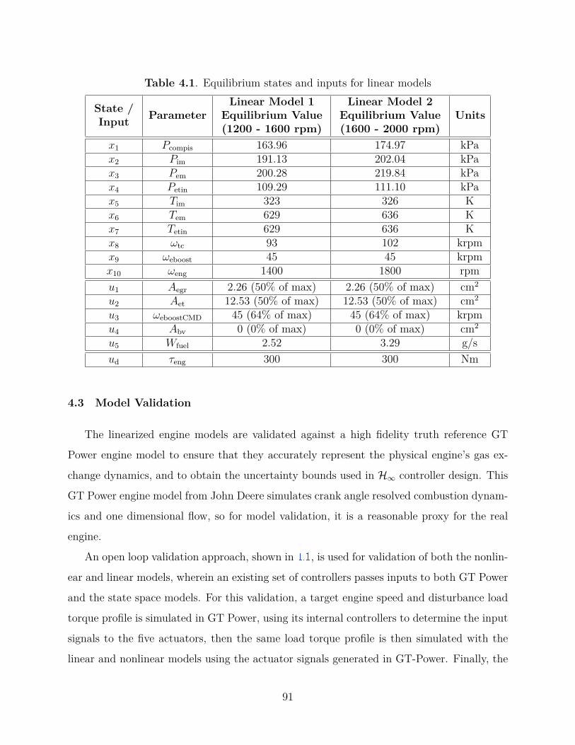
Table 4.1. Equilibrium states and inputs for linear models
State /Input Parameter
Linear Model 1Equilibrium Value(1200 - 1600 rpm)
Linear Model 2Equilibrium Value(1600 - 2000 rpm)
Units
x1 Pcompis 163.96 174.97 kPax2 Pim 191.13 202.04 kPax3 Pem 200.28 219.84 kPax4 Petin 109.29 111.10 kPax5 Tim 323 326 Kx6 Tem 629 636 Kx7 Tetin 629 636 Kx8 ωtc 93 102 krpmx9 ωeboost 45 45 krpmx10 ωeng 1400 1800 rpmu1 Aegr 2.26 (50% of max) 2.26 (50% of max) cm2
u2 Aet 12.53 (50% of max) 12.53 (50% of max) cm2
u3 ωeboostCMD 45 (64% of max) 45 (64% of max) krpmu4 Abv 0 (0% of max) 0 (0% of max) cm2
u5 Wfuel 2.52 3.29 g/sud τeng 300 300 Nm
4.3 Model Validation
The linearized engine models are validated against a high fidelity truth reference GT
Power engine model to ensure that they accurately represent the physical engine’s gas ex-
change dynamics, and to obtain the uncertainty bounds used in H∞ controller design. This
GT Power engine model from John Deere simulates crank angle resolved combustion dynam-
ics and one dimensional flow, so for model validation, it is a reasonable proxy for the real
engine.
An open loop validation approach, shown in 4.1 , is used for validation of both the nonlin-
ear and linear models, wherein an existing set of controllers passes inputs to both GT Power
and the state space models. For this validation, a target engine speed and disturbance load
torque profile is simulated in GT Power, using its internal controllers to determine the input
signals to the five actuators, then the same load torque profile is then simulated with the
linear and nonlinear models using the actuator signals generated in GT-Power. Finally, the
91
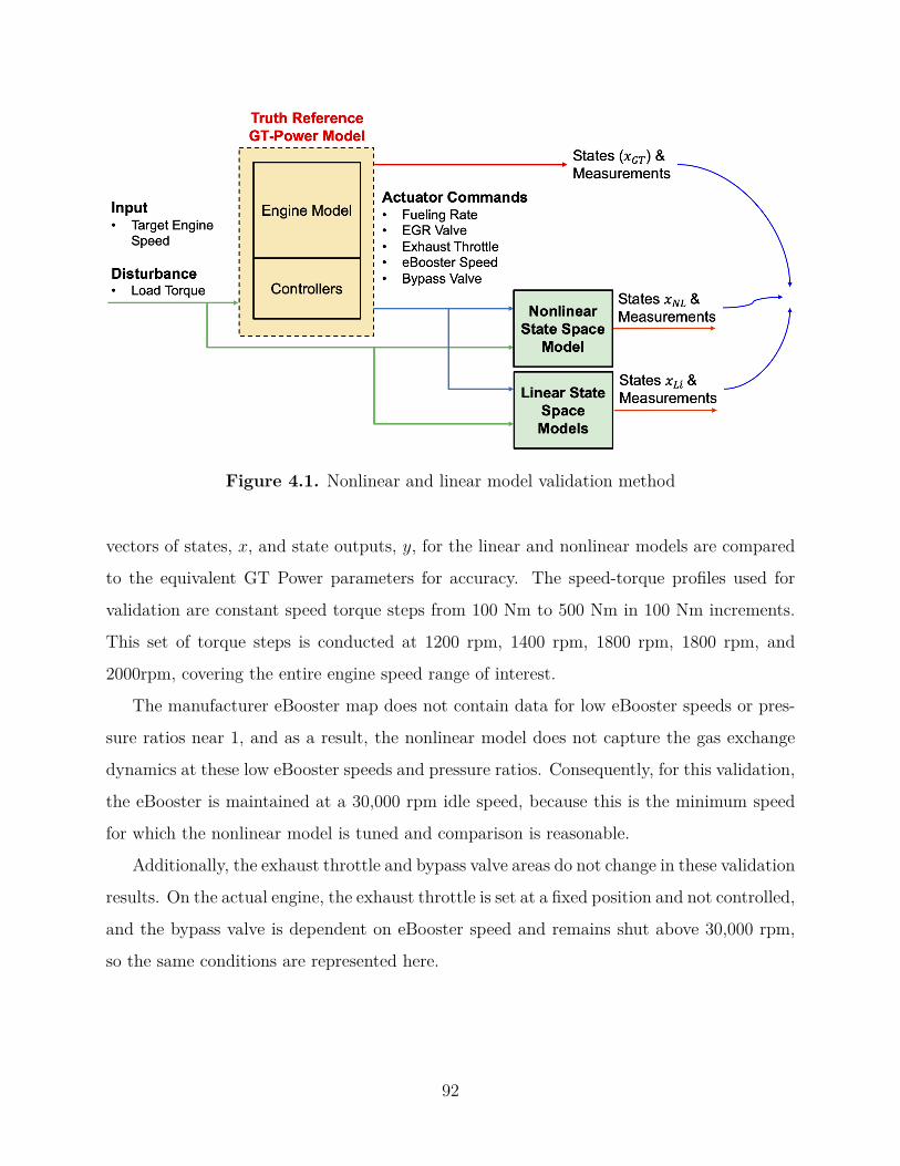
Figure 4.1. Nonlinear and linear model validation method
vectors of states, x, and state outputs, y, for the linear and nonlinear models are compared
to the equivalent GT Power parameters for accuracy. The speed-torque profiles used for
validation are constant speed torque steps from 100 Nm to 500 Nm in 100 Nm increments.
This set of torque steps is conducted at 1200 rpm, 1400 rpm, 1800 rpm, 1800 rpm, and
2000rpm, covering the entire engine speed range of interest.
The manufacturer eBooster map does not contain data for low eBooster speeds or pres-
sure ratios near 1, and as a result, the nonlinear model does not capture the gas exchange
dynamics at these low eBooster speeds and pressure ratios. Consequently, for this validation,
the eBooster is maintained at a 30,000 rpm idle speed, because this is the minimum speed
for which the nonlinear model is tuned and comparison is reasonable.
Additionally, the exhaust throttle and bypass valve areas do not change in these validation
results. On the actual engine, the exhaust throttle is set at a fixed position and not controlled,
and the bypass valve is dependent on eBooster speed and remains shut above 30,000 rpm,
so the same conditions are represented here.
92
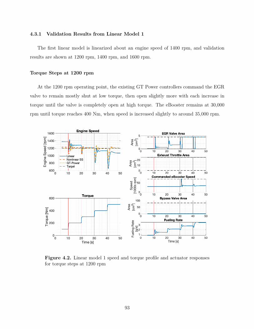
4.3.1 Validation Results from Linear Model 1
The first linear model is linearized about an engine speed of 1400 rpm, and validation
results are shown at 1200 rpm, 1400 rpm, and 1600 rpm.
Torque Steps at 1200 rpm
At the 1200 rpm operating point, the existing GT Power controllers command the EGR
valve to remain mostly shut at low torque, then open slightly more with each increase in
torque until the valve is completely open at high torque. The eBooster remains at 30,000
rpm until torque reaches 400 Nm, when speed is increased slightly to around 35,000 rpm.
Figure 4.2. Linear model 1 speed and torque profile and actuator responsesfor torque steps at 1200 rpm
93
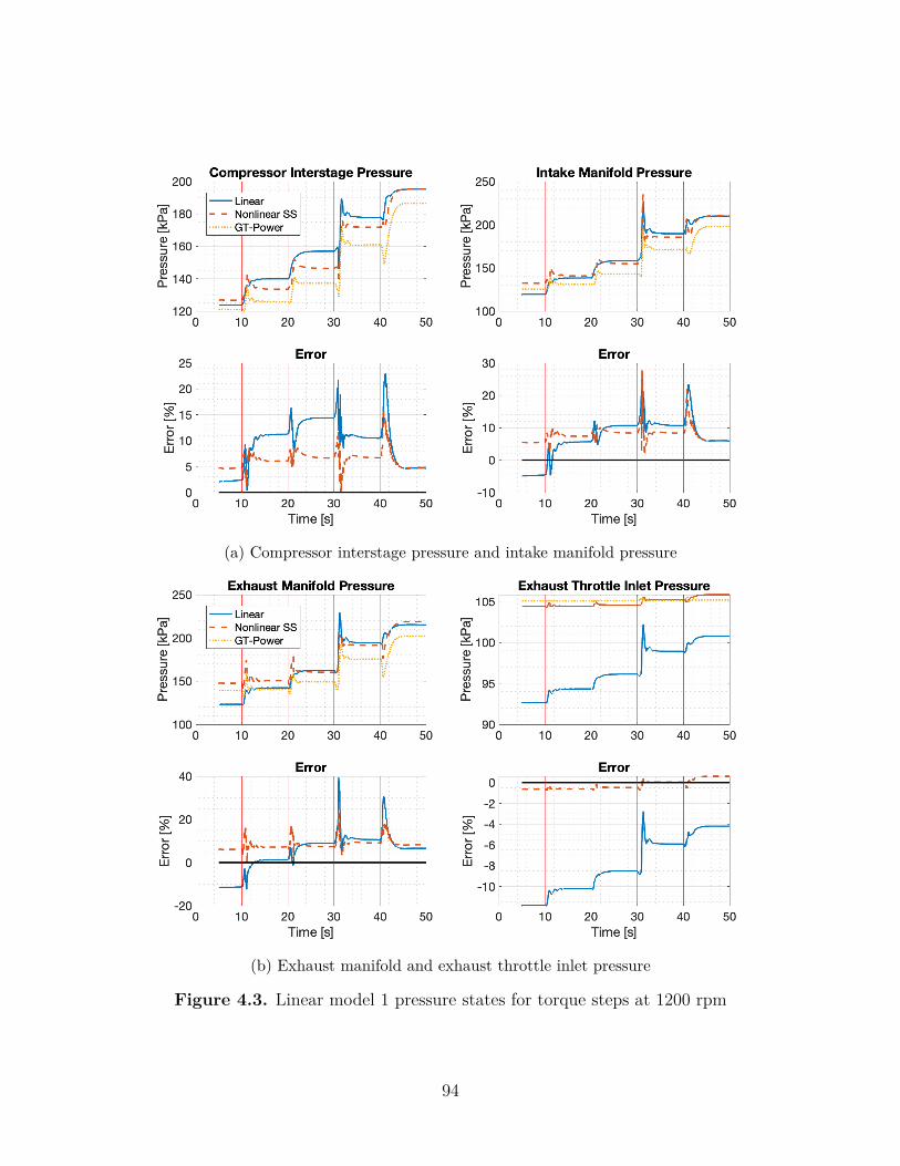
(a) Compressor interstage pressure and intake manifold pressure
(b) Exhaust manifold and exhaust throttle inlet pressure
Figure 4.3. Linear model 1 pressure states for torque steps at 1200 rpm
94
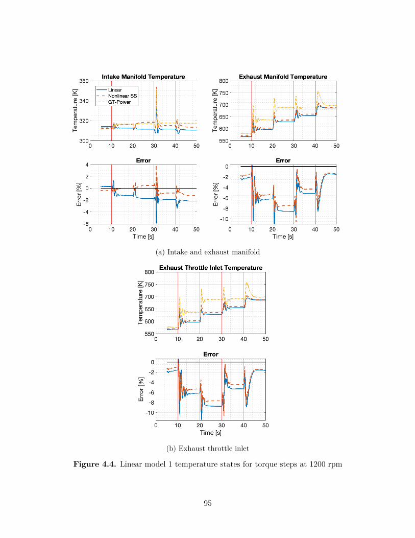
(a) Intake and exhaust manifold
(b) Exhaust throttle inlet
Figure 4.4. Linear model 1 temperature states for torque steps at 1200 rpm
95
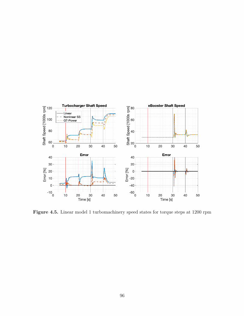
Figure 4.5. Linear model 1 turbomachinery speed states for torque steps at 1200 rpm
96
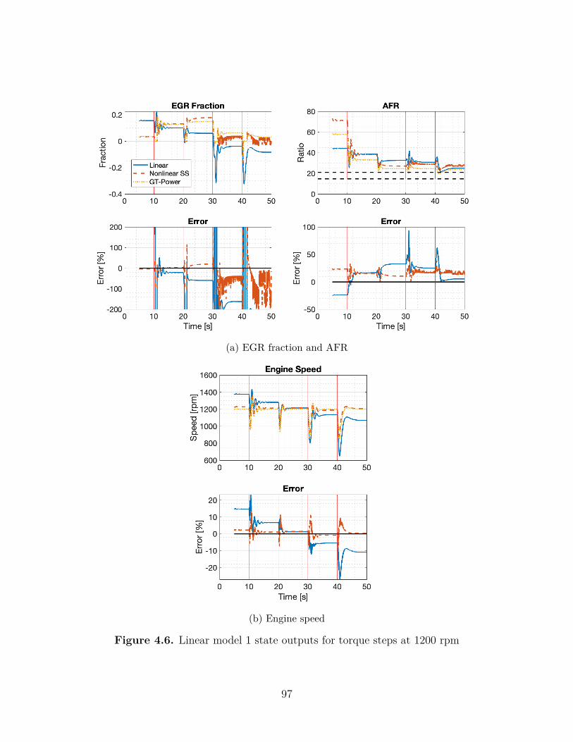
(a) EGR fraction and AFR
(b) Engine speed
Figure 4.6. Linear model 1 state outputs for torque steps at 1200 rpm
97
Under steady state conditions, all linear model states remain within 15% of the GT Power
truth reference, and all nonlinear model states remain within 10%. However, brief transient
errors as high as 40% and 30% are observed for the linear and nonlinear models respectively,
which result primarily from sudden changes in eBooster operation. The eBooster can accel-
erate from its 2000 rpm idle speed to its 70,000 rpm maximum speed within 0.3 seconds,
but the eBooster outlet pressure (intake manifold pressure) in the GT Power model does
not increase as quickly in response to this sudden speed increase as the nonlinear and linear
models predict. This is likely because the GT Power model uses a detailed, proprietary
black box eBooster model, whereas the map data available for the state space model does
not include the high speed, low pressure ratio operating area for the eBooster. As a result,
the eBooster model derived from the available map data likely overestimates air flow in this
regime. Additionally, in the reference engine model, transient pressure spikes are smaller and
much less abrupt, indicating that gas flows in the state space models respond much faster
that they do in the reference model.
State output responses at this low engine speed also show significant error. Engine
speed tracking is good–within 2% and 10% for the nonlinear model under steady state and
transience and within 15% and 25% for the linear model under steady state and transience.
However the linear model’s EGR fraction error appears to be large, especially at low torque
condition of the first few seconds, simply because EGR fraction close to zero. In this region,
the pressure difference across the EGR valve is small–on the order of 20 kPa–so the EGR
flow is sensitive to small errors in intake and exhaust manifold pressure, leading to larger
errors overall. AFR is represented reasonably well, although significant transient errors are
observed, again due to the discrepencies in eBooster flow already noted.
Finally, the linear model predicts significantly lower exhaust throttle inlet pressures than
the nonlinear model suggests. This is because the valve flow model variation with pressure
ratio is highly nonlinear at low pressure ratios like those observed across the exhaust throttle.
Consequently, any given linear model is only accurate for a narrow range of pressure ratios
and exhaust throttle effective areas near the linearization condition, leading to large errors
when conditions are far from the equilibrium used for linearization.
98
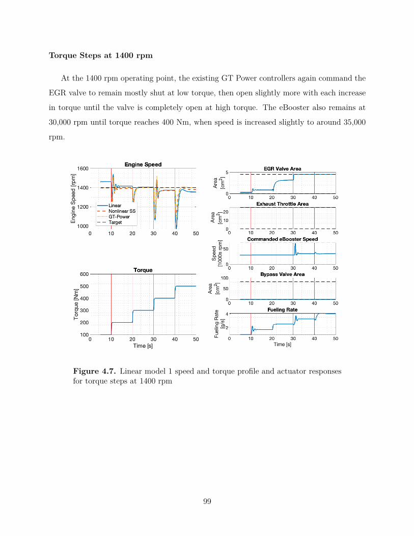
Torque Steps at 1400 rpm
At the 1400 rpm operating point, the existing GT Power controllers again command the
EGR valve to remain mostly shut at low torque, then open slightly more with each increase
in torque until the valve is completely open at high torque. The eBooster also remains at
30,000 rpm until torque reaches 400 Nm, when speed is increased slightly to around 35,000
rpm.
Figure 4.7. Linear model 1 speed and torque profile and actuator responsesfor torque steps at 1400 rpm
99
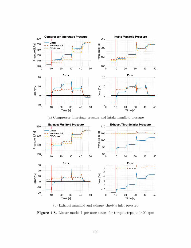
(a) Compressor interstage pressure and intake manifold pressure
(b) Exhaust manifold and exhaust throttle inlet pressure
Figure 4.8. Linear model 1 pressure states for torque steps at 1400 rpm
100
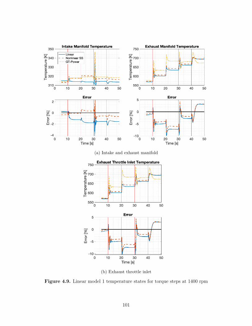
(a) Intake and exhaust manifold
(b) Exhaust throttle inlet
Figure 4.9. Linear model 1 temperature states for torque steps at 1400 rpm
101
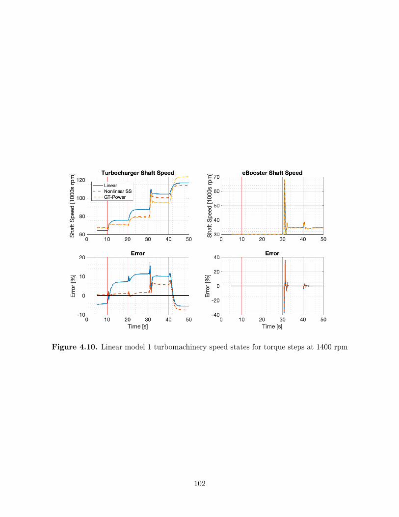
Figure 4.10. Linear model 1 turbomachinery speed states for torque steps at 1400 rpm
102
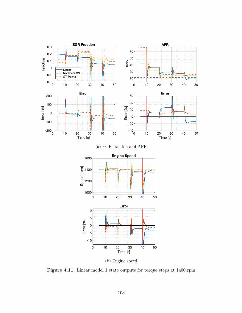
(a) EGR fraction and AFR
(b) Engine speed
Figure 4.11. Linear model 1 state outputs for torque steps at 1400 rpm
103
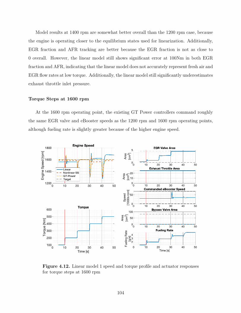
Model results at 1400 rpm are somewhat better overall than the 1200 rpm case, because
the engine is operating closer to the equilibrium states used for linearization. Additionally,
EGR fraction and AFR tracking are better because the EGR fraction is not as close to
0 overall. However, the linear model still shows significant error at 100Nm in both EGR
fraction and AFR, indicating that the linear model does not accurately represent fresh air and
EGR flow rates at low torque. Additionally, the linear model still significantly underestimates
exhaust throttle inlet pressure.
Torque Steps at 1600 rpm
At the 1600 rpm operating point, the existing GT Power controllers command roughly
the same EGR valve and eBooster speeds as the 1200 rpm and 1600 rpm operating points,
although fueling rate is slightly greater because of the higher engine speed.
Figure 4.12. Linear model 1 speed and torque profile and actuator responsesfor torque steps at 1600 rpm
104
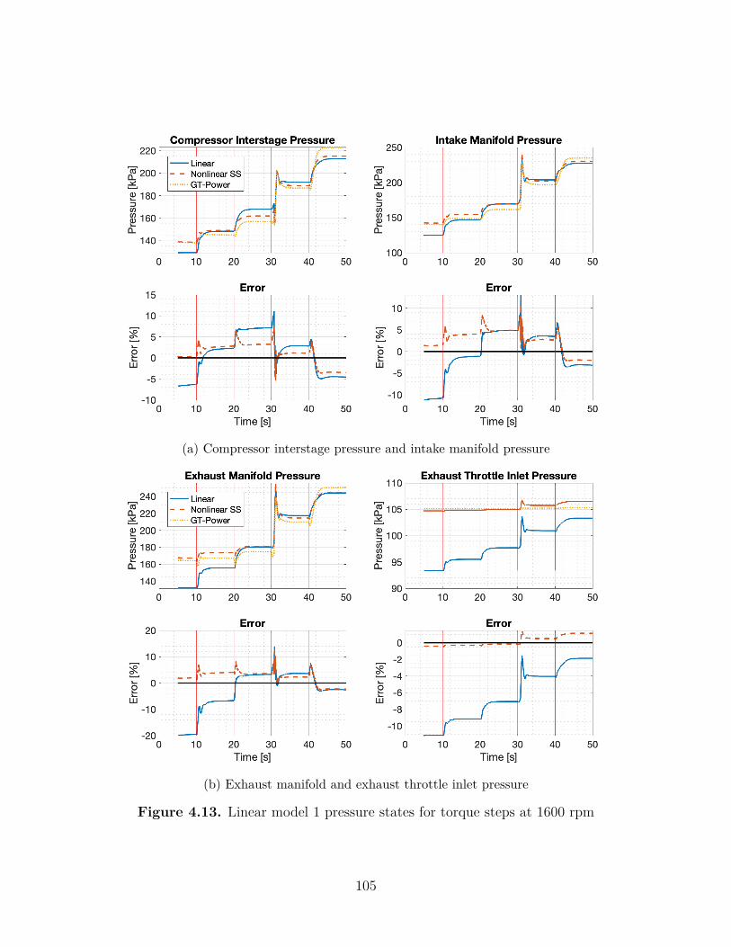
(a) Compressor interstage pressure and intake manifold pressure
(b) Exhaust manifold and exhaust throttle inlet pressure
Figure 4.13. Linear model 1 pressure states for torque steps at 1600 rpm
105
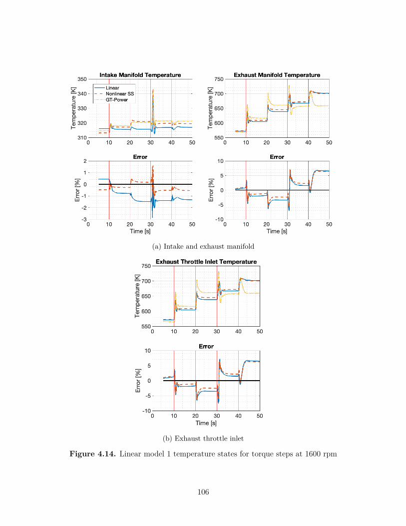
(a) Intake and exhaust manifold
(b) Exhaust throttle inlet
Figure 4.14. Linear model 1 temperature states for torque steps at 1600 rpm
106
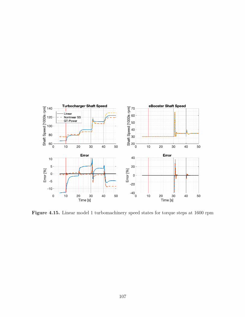
Figure 4.15. Linear model 1 turbomachinery speed states for torque steps at 1600 rpm
107
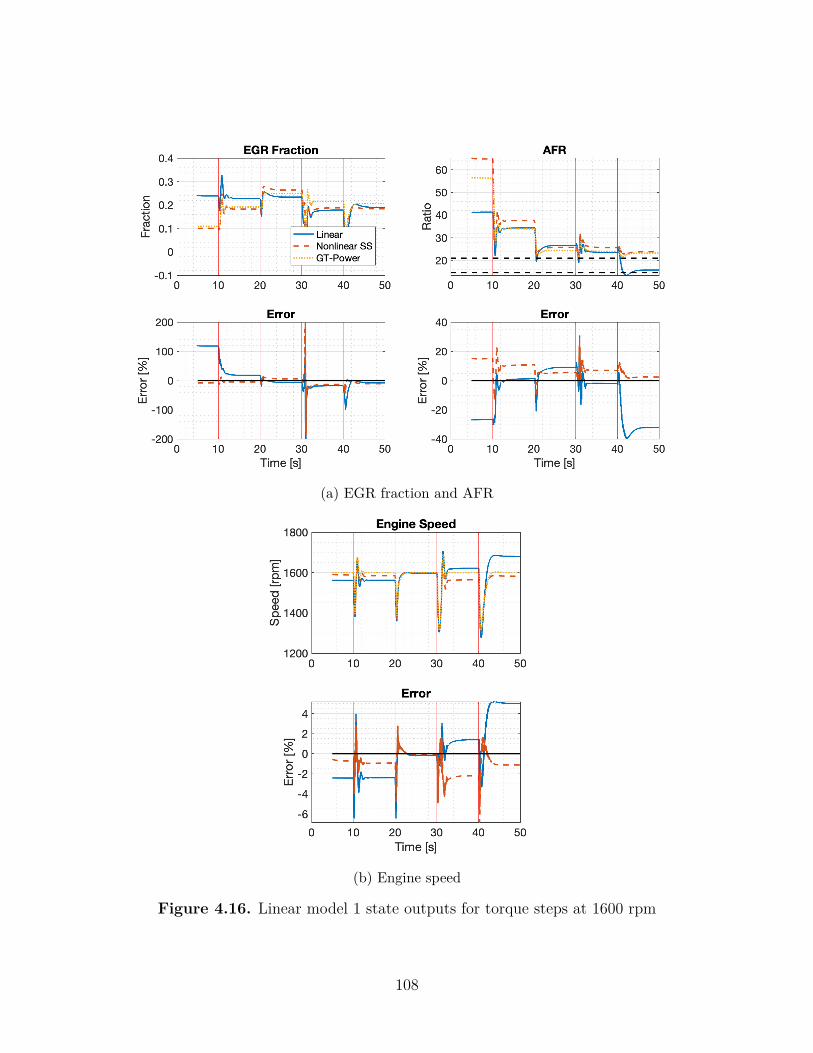
(a) EGR fraction and AFR
(b) Engine speed
Figure 4.16. Linear model 1 state outputs for torque steps at 1600 rpm
108
Improved responses across all states and state outputs are again observed, because the
higher engine speed maintains flow rates that are consistantly in a range that the linear
model can well represent. However, large errors in EGR fraction and AFR are still observed
at low torque due to state conditions that are far away from the linearization equilibrium.
4.3.2 Validation Results from Linear Model 2
The second linear model is linearized about an engine speed of 1800 rpm, and validation
results are shown at 1600 rpm, 1800 rpm, and 2000 rpm.
Torque Steps at 1600 rpm
The 1600 rpm speed-torque profile and actuator commands used to validate linear model
1 are used here to validate linear model 2 at 1600 rpm. This engine speed also represents
the crossover point between the models. Below 1600 rpm, linear model 1 is used, and above
1600 rpm, linear model 2 is used.
109
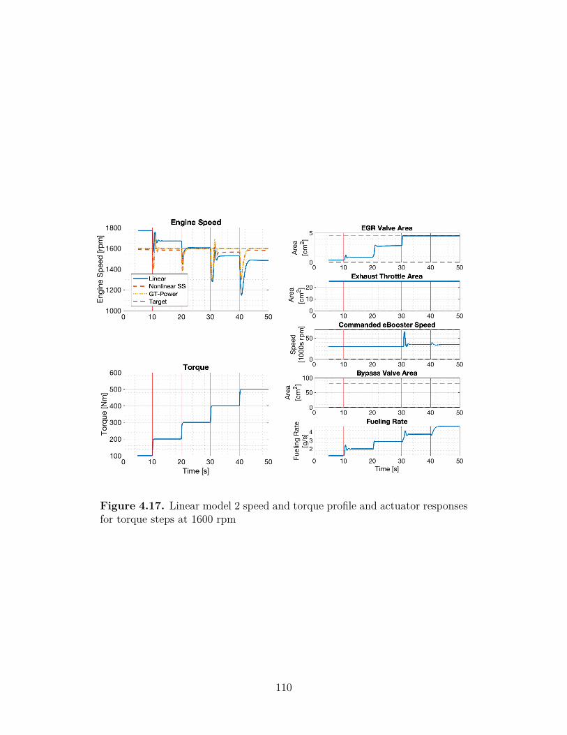
Figure 4.17. Linear model 2 speed and torque profile and actuator responsesfor torque steps at 1600 rpm
110
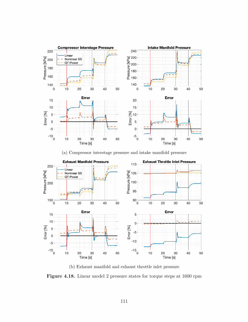
(a) Compressor interstage pressure and intake manifold pressure
(b) Exhaust manifold and exhaust throttle inlet pressure
Figure 4.18. Linear model 2 pressure states for torque steps at 1600 rpm
111
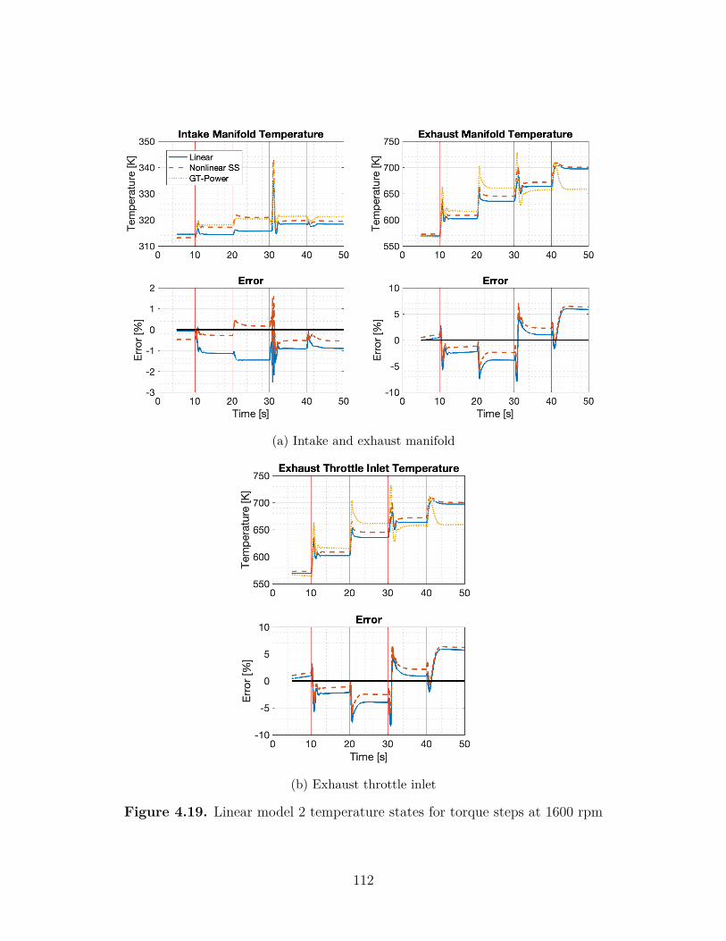
(a) Intake and exhaust manifold
(b) Exhaust throttle inlet
Figure 4.19. Linear model 2 temperature states for torque steps at 1600 rpm
112
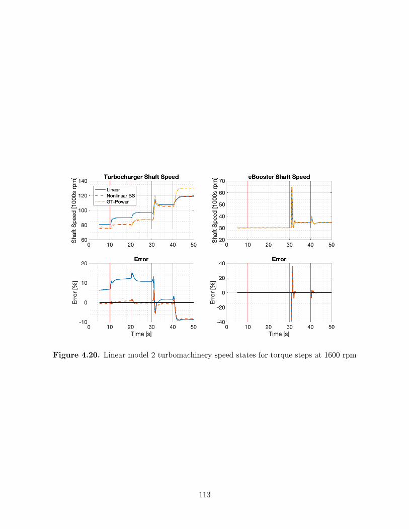
Figure 4.20. Linear model 2 turbomachinery speed states for torque steps at 1600 rpm
113
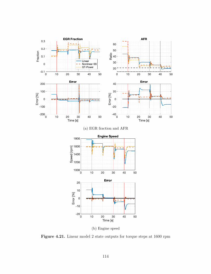
(a) EGR fraction and AFR
(b) Engine speed
Figure 4.21. Linear model 2 state outputs for torque steps at 1600 rpm
114
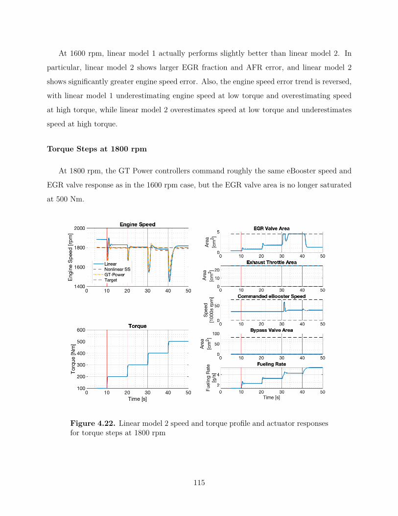
At 1600 rpm, linear model 1 actually performs slightly better than linear model 2. In
particular, linear model 2 shows larger EGR fraction and AFR error, and linear model 2
shows significantly greater engine speed error. Also, the engine speed error trend is reversed,
with linear model 1 underestimating engine speed at low torque and overestimating speed
at high torque, while linear model 2 overestimates speed at low torque and underestimates
speed at high torque.
Torque Steps at 1800 rpm
At 1800 rpm, the GT Power controllers command roughly the same eBooster speed and
EGR valve response as in the 1600 rpm case, but the EGR valve area is no longer saturated
at 500 Nm.
Figure 4.22. Linear model 2 speed and torque profile and actuator responsesfor torque steps at 1800 rpm
115
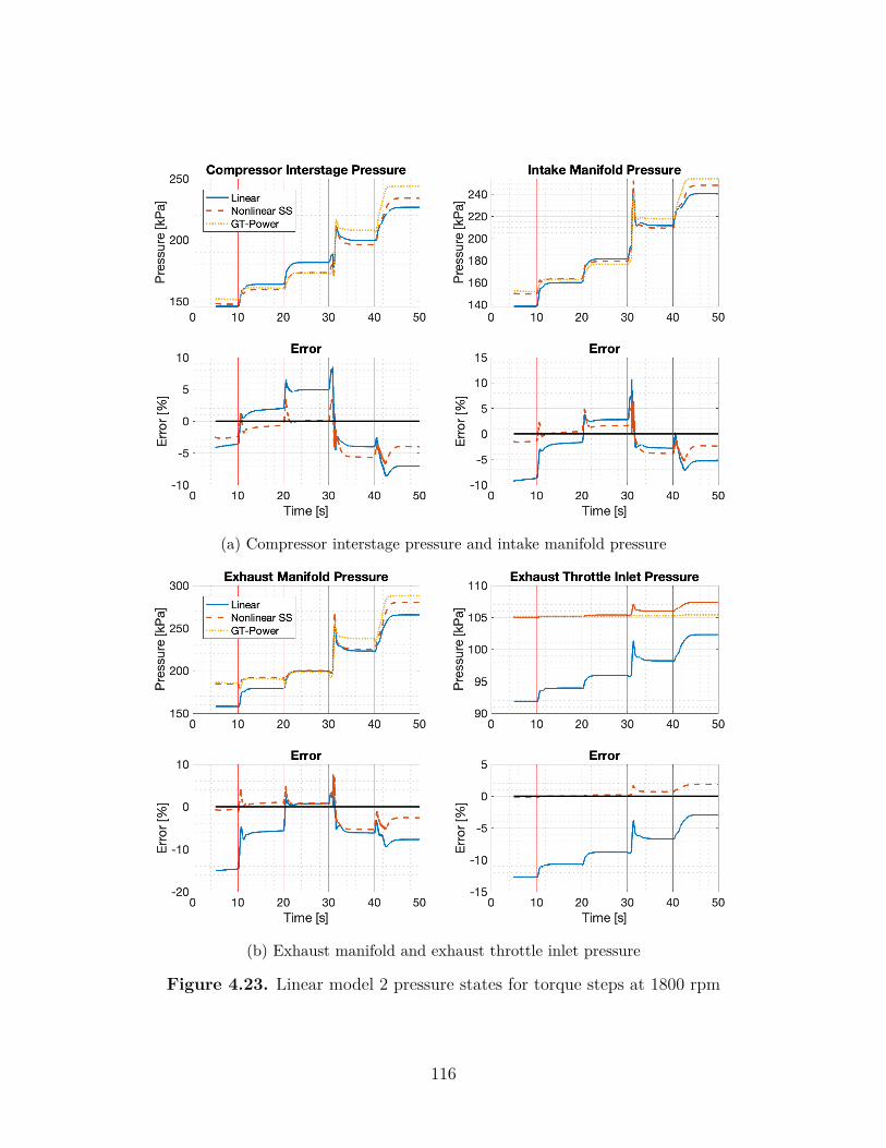
(a) Compressor interstage pressure and intake manifold pressure
(b) Exhaust manifold and exhaust throttle inlet pressure
Figure 4.23. Linear model 2 pressure states for torque steps at 1800 rpm
116
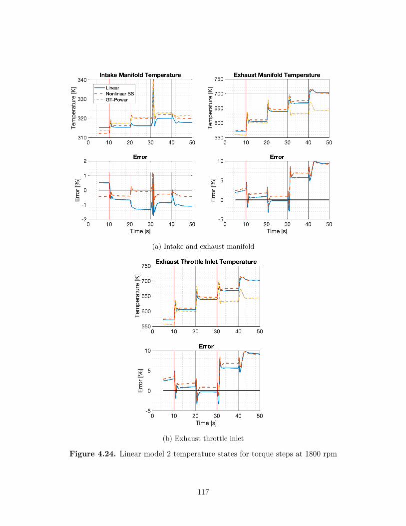
(a) Intake and exhaust manifold
(b) Exhaust throttle inlet
Figure 4.24. Linear model 2 temperature states for torque steps at 1800 rpm
117
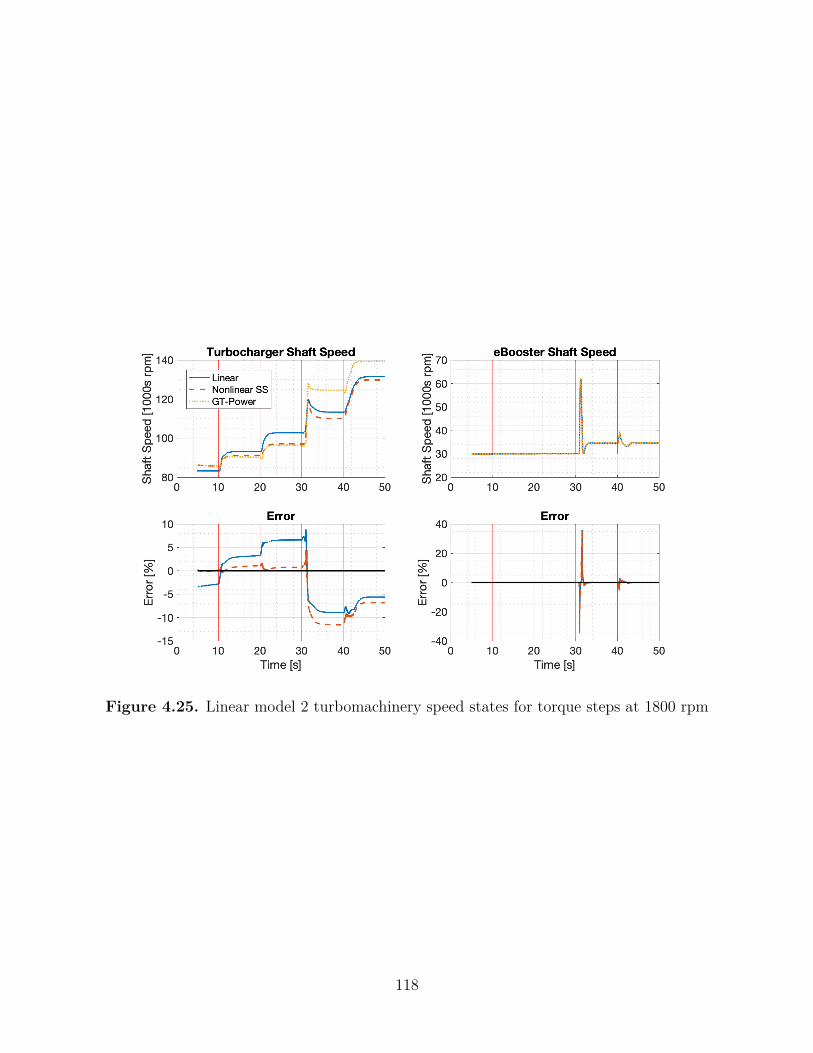
Figure 4.25. Linear model 2 turbomachinery speed states for torque steps at 1800 rpm
118
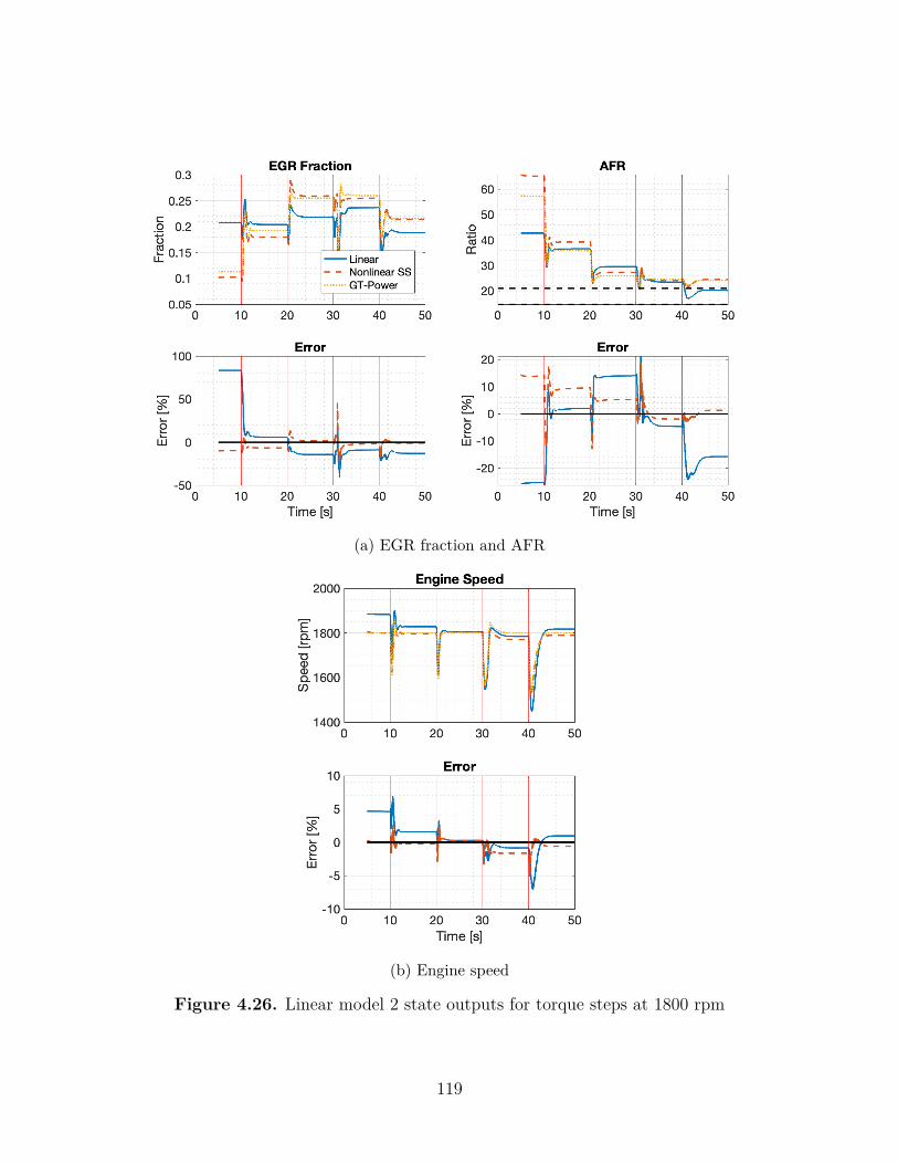
(a) EGR fraction and AFR
(b) Engine speed
Figure 4.26. Linear model 2 state outputs for torque steps at 1800 rpm
119
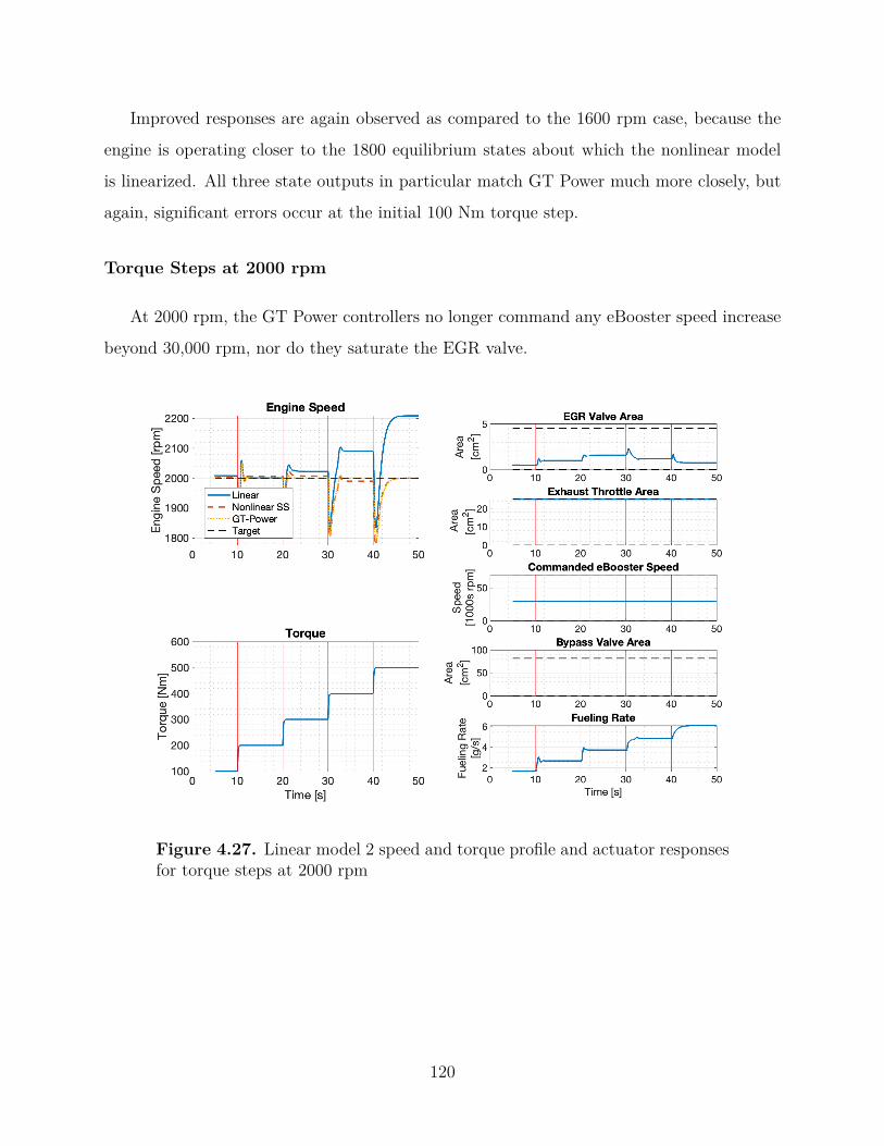
Improved responses are again observed as compared to the 1600 rpm case, because the
engine is operating closer to the 1800 equilibrium states about which the nonlinear model
is linearized. All three state outputs in particular match GT Power much more closely, but
again, significant errors occur at the initial 100 Nm torque step.
Torque Steps at 2000 rpm
At 2000 rpm, the GT Power controllers no longer command any eBooster speed increase
beyond 30,000 rpm, nor do they saturate the EGR valve.
Figure 4.27. Linear model 2 speed and torque profile and actuator responsesfor torque steps at 2000 rpm
120
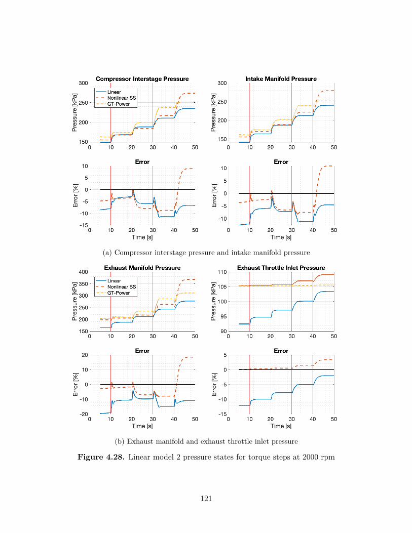
(a) Compressor interstage pressure and intake manifold pressure
(b) Exhaust manifold and exhaust throttle inlet pressure
Figure 4.28. Linear model 2 pressure states for torque steps at 2000 rpm
121
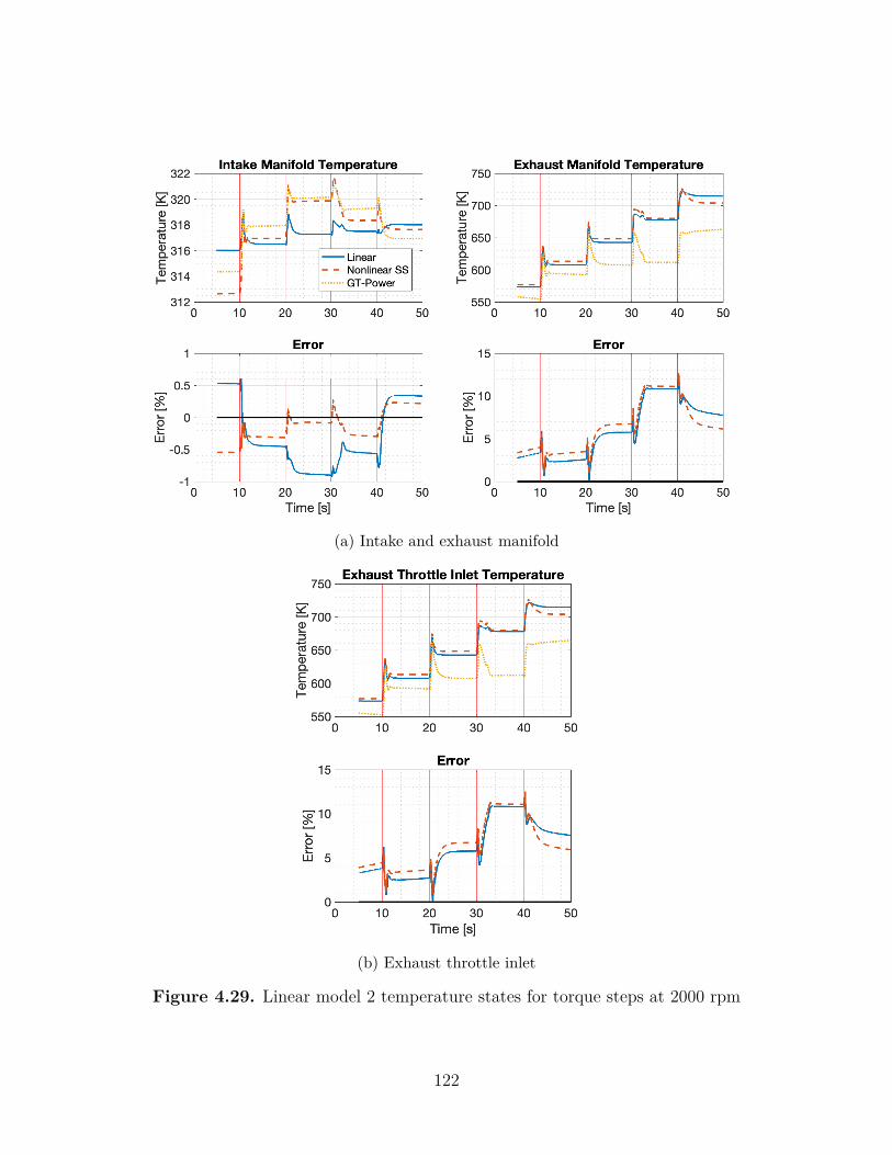
(a) Intake and exhaust manifold
(b) Exhaust throttle inlet
Figure 4.29. Linear model 2 temperature states for torque steps at 2000 rpm
122
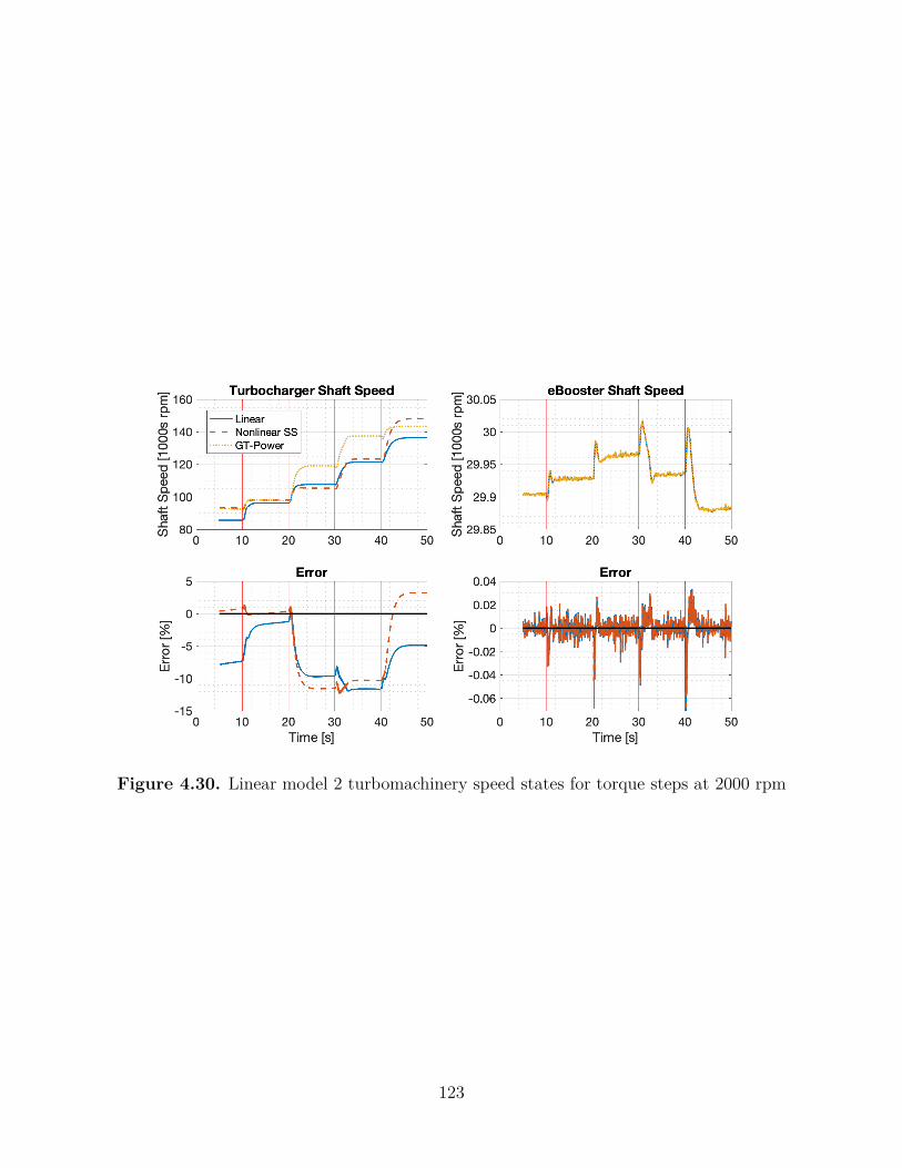
Figure 4.30. Linear model 2 turbomachinery speed states for torque steps at 2000 rpm
123
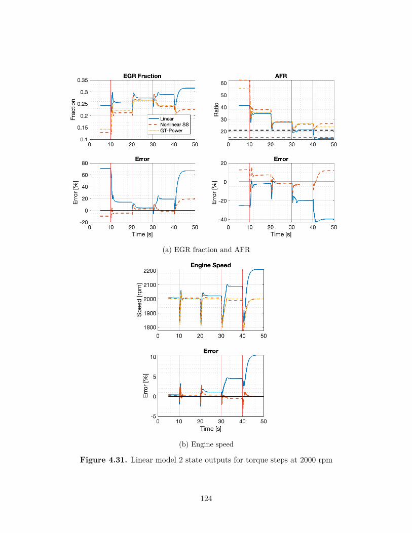
(a) EGR fraction and AFR
(b) Engine speed
Figure 4.31. Linear model 2 state outputs for torque steps at 2000 rpm
124
A notable increase in error is observed across all states and state outputs for the 2000 rpm
test case. This is partly because the test case is relatively far away from the linearization
equilibrium point, and partly because compressor interstage pressure is large enough to
activate the wastegate. The wastegate remains shut for Pcompis < 245 kPa, and the empirical
relation for wastegate discharge coefficient is only valid between 245 kPa and 270 kPa, which
is nonlinear saturation behaviour that cannot be captured in a linear model. As a result,
significant differences in the gas exchange dynamics occur at the 500 Nm torque where the
wastegate is opened. These dynamic differences explain why large steady state error is
observed between 40 and 50 seconds in all state outputs for the linear model. Additionally,
the same problem with large steady state error at low torque is also still observed.
4.3.3 Summary
In summary, the two linear models shown represent the engine’s gas exchange dynamics
reasonably well near the middle of its operating range: 1400 - 1800 rpm and 200 - 400 Nm.
However outside this range, significant deviation from the GT Power truth reference response
is observed because the flow rates through the engine are either higher or lower than those
near the equilibria used for linearization. As a result, different linear dynamics represent the
engine response in these regions.
In particular, the linear models consistently overestimate EGR fraction and underesti-
mate AFR at low torque, indicating that in this region, the fresh air flow is consistently too
low and the EGR flow is consistently too high. Consequently, when using these models for
controller design, better robust performance is possible within the 1400 - 1800 rpm and 200
- 400 Nm speed and torque ranges than is possible outside them, and given the AFR and
EGR fraction errors, robust performance in tracking these gas exchange parameters may not
be possible for low torque conditions. However, engine speed response is reasonably good
across the entire operating range, so a controller should be able to achieve robust engine
speed performance across the entire operating envelope.
125
4.3.4 Improvements and Limitations
Two changes to the engine model may improve these EGR fraction and AFR errors.
First, an eBooster map that includes data for the eBooster near and below a pressure ratio
of 1 would allow better eBooster flow prediction under transient conditions. Second, using
one linear model for the low torque region (100 Nm - 300 Nm) and a different linear model
for the high torque region (300 Nm - 500 Nm) would allow linearization closer to the actual
engine conditions present in these two regimes. However, this approach requires switching
controllers based on both engine speed and load, increasing the complexity of controller and
its tuning.
Significant errors were also observed from the valve flow submodel when pressure ratios
were near 1, which is particularly relevant for this engine, since the bypass valve, EGR
valve, and exhaust throttle all operate with small pressure differences across them. This
is also why all of the validation results shown have the eBooster idling at 30,000 rpm with
the bypass valve shut. The engine’s gas exchange dynamics with the bypass valve open are
completely different from its dynamics with the bypass valve shut, so although the nonlinear
model somewhat captures this difference in dynamics, at least two different linear models
are necessary to capture the region between a shut bypass valve and an open bypass valve.
Furthermore, because the eBooster map does not include data for a pressure ratio near 1,
which is enforced by the bypass valve when it is in any position other than fully shut, even
the nonlinear model does not represent the engine’s dynamics well when the bypass valve is
open.
However, ultimately the bypass valve’s primary purpose is to divert air around the
eBooster, allowing it to idle when not needed. This behaviour can be achieved with an
open loop controller that chooses the bypass valve position based on eBooster speed, so
as long as the MIMO controller can effectively actuate eBooster speed to track EGR frac-
tion and AFR, the bypass valve can be removed as an actuator from the MIMO controller.
Consequently, the linear models used in control design do not need to capture the engine’s
response to the bypass valve.
126
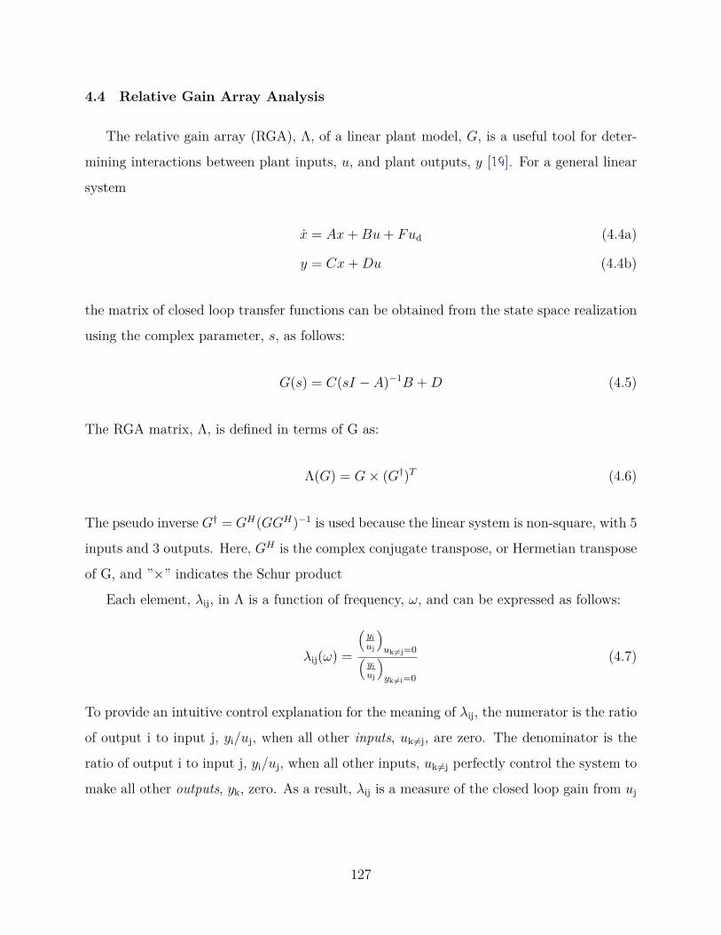
4.4 Relative Gain Array Analysis
The relative gain array (RGA), Λ, of a linear plant model, G, is a useful tool for deter-
mining interactions between plant inputs, u, and plant outputs, y [19 ]. For a general linear
system
x = Ax + Bu + Fud (4.4a)
y = Cx + Du (4.4b)
the matrix of closed loop transfer functions can be obtained from the state space realization
using the complex parameter, s, as follows:
G(s) = C(sI − A)−1B + D (4.5)
The RGA matrix, Λ, is defined in terms of G as:
Λ(G) = G × (G†)T (4.6)
The pseudo inverse G† = GH(GGH)−1 is used because the linear system is non-square, with 5
inputs and 3 outputs. Here, GH is the complex conjugate transpose, or Hermetian transpose
of G, and ”×” indicates the Schur product
Each element, λij, in Λ is a function of frequency, ω, and can be expressed as follows:
λij(ω) =
(yiuj
)uk6=j=0(
yiuj
)yk 6=i=0
(4.7)
To provide an intuitive control explanation for the meaning of λij, the numerator is the ratio
of output i to input j, yi/uj, when all other inputs, uk 6=j, are zero. The denominator is the
ratio of output i to input j, yi/uj, when all other inputs, uk 6=j perfectly control the system to
make all other outputs, yk, zero. As a result, λij is a measure of the closed loop gain from uj
127
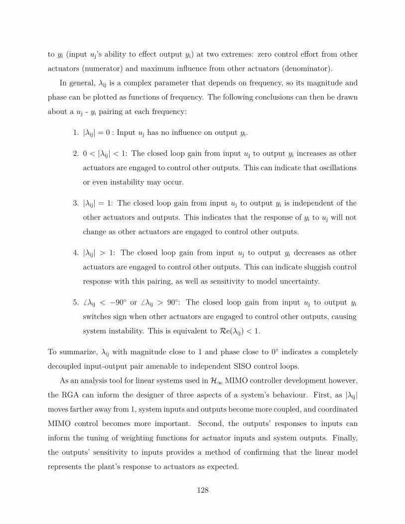
to yi (input uj’s ability to effect output yi) at two extremes: zero control effort from other
actuators (numerator) and maximum influence from other actuators (denominator).
In general, λij is a complex parameter that depends on frequency, so its magnitude and
phase can be plotted as functions of frequency. The following conclusions can then be drawn
about a uj - yi pairing at each frequency:
1. |λij| = 0 : Input uj has no influence on output yi.
2. 0 < |λij| < 1: The closed loop gain from input uj to output yi increases as other
actuators are engaged to control other outputs. This can indicate that oscillations
or even instability may occur.
3. |λij| = 1: The closed loop gain from input uj to output yi is independent of the
other actuators and outputs. This indicates that the response of yi to uj will not
change as other actuators are engaged to control other outputs.
4. |λij| > 1: The closed loop gain from input uj to output yi decreases as other
actuators are engaged to control other outputs. This can indicate sluggish control
response with this pairing, as well as sensitivity to model uncertainty.
5. 6 λij < −90◦ or 6 λij > 90◦: The closed loop gain from input uj to output yi
switches sign when other actuators are engaged to control other outputs, causing
system instability. This is equivalent to Re(λij) < 1.
To summarize, λij with magnitude close to 1 and phase close to 0◦ indicates a completely
decoupled input-output pair amenable to independent SISO control loops.
As an analysis tool for linear systems used in H∞ MIMO controller development however,
the RGA can inform the designer of three aspects of a system’s behaviour. First, as |λij|
moves farther away from 1, system inputs and outputs become more coupled, and coordinated
MIMO control becomes more important. Second, the outputs’ responses to inputs can
inform the tuning of weighting functions for actuator inputs and system outputs. Finally,
the outputs’ sensitivity to inputs provides a method of confirming that the linear model
represents the plant’s response to actuators as expected.
128
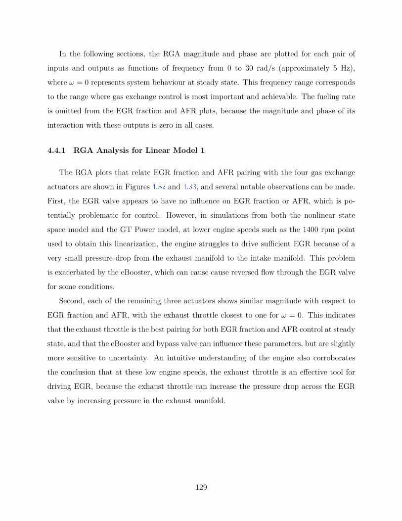
In the following sections, the RGA magnitude and phase are plotted for each pair of
inputs and outputs as functions of frequency from 0 to 30 rad/s (approximately 5 Hz),
where ω = 0 represents system behaviour at steady state. This frequency range corresponds
to the range where gas exchange control is most important and achievable. The fueling rate
is omitted from the EGR fraction and AFR plots, because the magnitude and phase of its
interaction with these outputs is zero in all cases.
4.4.1 RGA Analysis for Linear Model 1
The RGA plots that relate EGR fraction and AFR pairing with the four gas exchange
actuators are shown in Figures 4.32 and 4.33 , and several notable observations can be made.
First, the EGR valve appears to have no influence on EGR fraction or AFR, which is po-
tentially problematic for control. However, in simulations from both the nonlinear state
space model and the GT Power model, at lower engine speeds such as the 1400 rpm point
used to obtain this linearization, the engine struggles to drive sufficient EGR because of a
very small pressure drop from the exhaust manifold to the intake manifold. This problem
is exacerbated by the eBooster, which can cause cause reversed flow through the EGR valve
for some conditions.
Second, each of the remaining three actuators shows similar magnitude with respect to
EGR fraction and AFR, with the exhaust throttle closest to one for ω = 0. This indicates
that the exhaust throttle is the best pairing for both EGR fraction and AFR control at steady
state, and that the eBooster and bypass valve can influence these parameters, but are slightly
more sensitive to uncertainty. An intuitive understanding of the engine also corroborates
the conclusion that at these low engine speeds, the exhaust throttle is an effective tool for
driving EGR, because the exhaust throttle can increase the pressure drop across the EGR
valve by increasing pressure in the exhaust manifold.
129
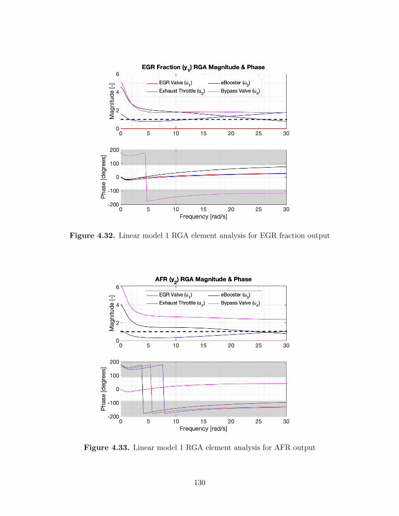
Figure 4.32. Linear model 1 RGA element analysis for EGR fraction output
Figure 4.33. Linear model 1 RGA element analysis for AFR output
130
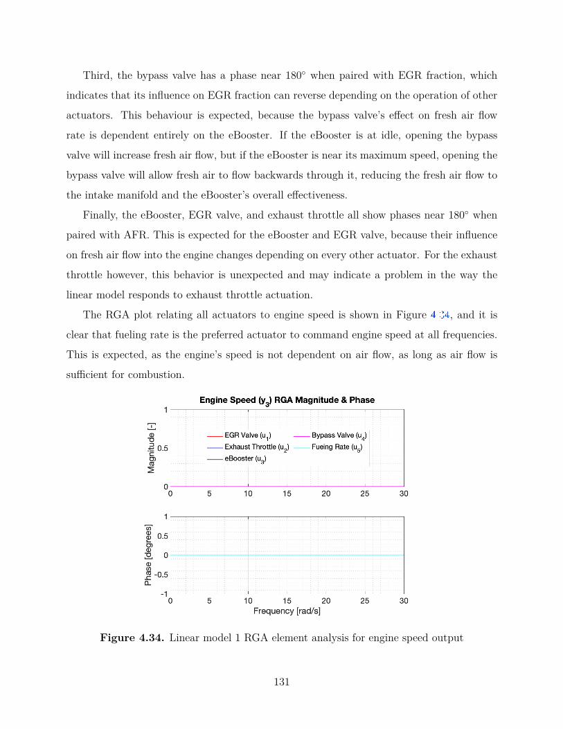
Third, the bypass valve has a phase near 180◦ when paired with EGR fraction, which
indicates that its influence on EGR fraction can reverse depending on the operation of other
actuators. This behaviour is expected, because the bypass valve’s effect on fresh air flow
rate is dependent entirely on the eBooster. If the eBooster is at idle, opening the bypass
valve will increase fresh air flow, but if the eBooster is near its maximum speed, opening the
bypass valve will allow fresh air to flow backwards through it, reducing the fresh air flow to
the intake manifold and the eBooster’s overall effectiveness.
Finally, the eBooster, EGR valve, and exhaust throttle all show phases near 180◦ when
paired with AFR. This is expected for the eBooster and EGR valve, because their influence
on fresh air flow into the engine changes depending on every other actuator. For the exhaust
throttle however, this behavior is unexpected and may indicate a problem in the way the
linear model responds to exhaust throttle actuation.
The RGA plot relating all actuators to engine speed is shown in Figure 4.34 , and it is
clear that fueling rate is the preferred actuator to command engine speed at all frequencies.
This is expected, as the engine’s speed is not dependent on air flow, as long as air flow is
sufficient for combustion.
Figure 4.34. Linear model 1 RGA element analysis for engine speed output
131
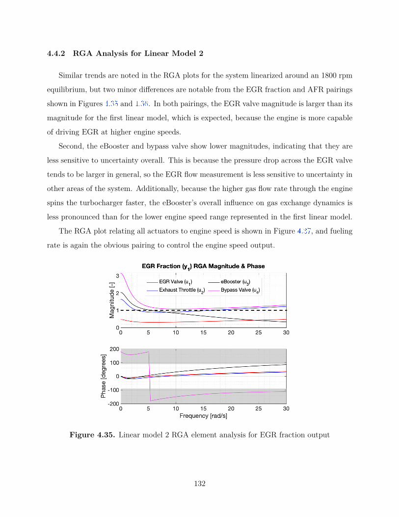
4.4.2 RGA Analysis for Linear Model 2
Similar trends are noted in the RGA plots for the system linearized around an 1800 rpm
equilibrium, but two minor differences are notable from the EGR fraction and AFR pairings
shown in Figures 4.35 and 4.36 . In both pairings, the EGR valve magnitude is larger than its
magnitude for the first linear model, which is expected, because the engine is more capable
of driving EGR at higher engine speeds.
Second, the eBooster and bypass valve show lower magnitudes, indicating that they are
less sensitive to uncertainty overall. This is because the pressure drop across the EGR valve
tends to be larger in general, so the EGR flow measurement is less sensitive to uncertainty in
other areas of the system. Additionally, because the higher gas flow rate through the engine
spins the turbocharger faster, the eBooster’s overall influence on gas exchange dynamics is
less pronounced than for the lower engine speed range represented in the first linear model.
The RGA plot relating all actuators to engine speed is shown in Figure 4.37 , and fueling
rate is again the obvious pairing to control the engine speed output.
Figure 4.35. Linear model 2 RGA element analysis for EGR fraction output
132
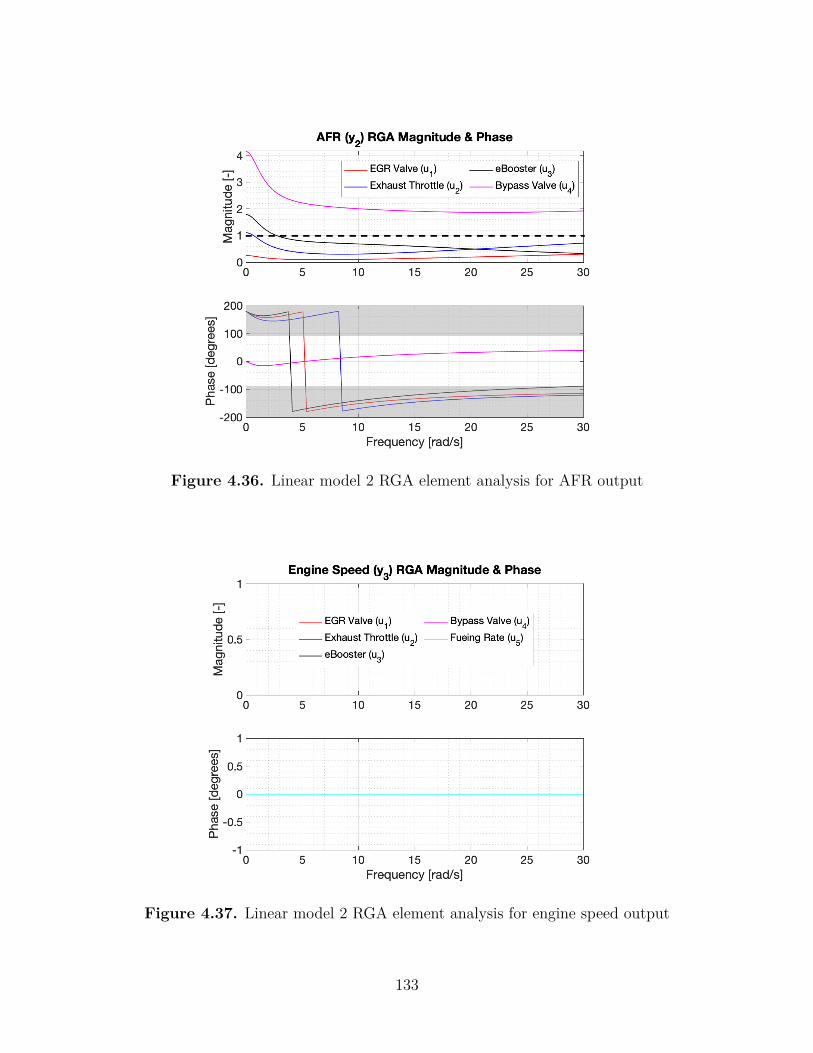
Figure 4.36. Linear model 2 RGA element analysis for AFR output
Figure 4.37. Linear model 2 RGA element analysis for engine speed output
133
4.4.3 Summary
The RGA analysis presented indicates that for EGR fraction and AFR control, no single
actuator is an obvious choice for SISO control. Due to close coupling among these gas
exchange parameters and the EGR valve, exhaust throttle, eBooster, and bypass valve, as
well as the variation in pairing behaviour with frequency, this set of inputs and outputs is
an excellent candidate for a coordinated MIMO control approach.
In contrast, fueling rate and engine speed appear to be an ideal pairing for SISO con-
trol, as fueling rate does not significantly influence EGR fraction and AFR, and the other
actuators do not influence engine speed. However on the actual engine, AFR limits effect
the allowable fueling rate, and a linear model cannot capture these inherently nonlinear
considerations. As a result, during an aggressive torque step from 100 Nm to 500 Nm for
example, the controller must increase airflow before or simultaneous to a fueling increase to
avoid dropping AFR below an allowable bound, and this coupling, while not captured in
the RGA analysis of the linear models, is more effectively handled when the controller can
command fueling in conjunction with the gas exchange process.
Consequently, this analysis indicates that a coordinated MIMO controller is likely to be
superior to independent SISO control loops for performance in tracking all three outputs,
because the MIMO controller can manage both the coupling among actuators, and the
variations in pairing behaviour with frequency.
134
5. CONCLUSIONS AND FUTURE WORK
5.1 Summary
In this thesis, two methods of hybridization are discussed: a series electric powertrain
implemented in an on-highway class 8 truck, and a four cylinder diesel engine with an
electrically driven supercharger for a hybrid wheel loader.
5.1.1 Series Hybrid Electric Powertrain Analysis for Class 8 Truck
The power flows in the series electric hybrid powertrain are analyzed to confirm that elec-
trical components operate as expected, identify mechanisms through which the hybrid driv-
etrain can provide efficiency improvements over a conventional drivetrain, and demonstrate
that potential efficiency improvements of the hybrid drivetrain merit further development.
To this end, power flow data to and from the generator, battery and motor are examined
from test data over highway routes on I-75 between Florence and Lexington, KY and on I-74
and I-70 near Indianapolis. From these data, the total energy contributions provided to and
from each component are calculated and used to study battery operation, power electronics
efficiency, regeneration energy capture percentage, and the fraction of drive energy provided
by regenerative braking.
The power electronics are found to operate between 82% and 92% efficiency, which is
the expected range for power electronics of this type. The battery efficiency is not explicity
determined, but testing results show clear signs of battery wear that can reduce its ability
to store energy with minimal thermal losses. However, it is still able to capture nearly all
of the available regenerative braking energy theoretically available according to the drive
profile test data and a simple physical model of the truck. No exact recapture percentage
is identified, because unmeasured environmental factors such as wind and low temperatures
affect these results significantly, but the model predicts that the recapture percentage is
near 100% on average. Additionally, analysis indicates that during testing, between 2% and
12% of the total drive energy required to propel the vehicle comes from regenerative braking
depending on the route grade and drive profile, and that improvements in rolling resistance
135
and aerodynamic drag consistent with a more modern truck could increase this percentage
to between 8% and 18%.
5.1.2 Control Oriented Modeling of Diesel Engine
A physically-based mean value engine model is also developed for control of a tur-
bocharged diesel engine with a high pressure EGR loop, an exhaust throttle, and an electric
supercharger (eBooster) downstream of the turbocharger compressor. A nonlinear state
space model with ten states is developed to model the effects of the EGR valve, exhaust
throttle, eBooster, eBooster bypass valve, and fueling rate on EGR fraction, AFR, and en-
gine speed, and this model is linearized about two operating points to generate two linear
models which represent the engine over its entire operating range. The linear and nonlinear
models are validated against the truth reference GT Power engine model, and relative gain
array analysis is performed on the linear models which indicates that the engine exhibits sig-
nificant coupling dynamics among actuators and outputs. As a result, it is concluded that
that a SISO control approach is unsuitable for tracking EGR fraction and AFR, and that
the planned MIMO control approach is necessary to take full advantage of the electrified air
handling system to maximize the engine’s transient performance.
5.2 Future Work
Both applications discussed are part of ongoing development efforts to reduce fuel con-
sumption in vehicles with hybrid powertrains, and both applications require additional work
at the supervisory control level.
5.2.1 Series Electric Hybrid Powertrain Analysis for Class 8 Truck
The architecture of the supervisory controller managing power flows in the hybrid class
8 truck powertrain was not accessible for the analysis presented, so further work to optimize
the engine and battery operation will likely further increase its potential for fuel savings.
Specifically, providing the supervisory controller with some indication of its future drive
profile and power needs allows it to optimize power drawn from the genset to keep the IC
136

engine near its minimum BSFC while still providing sufficient power over the operational
cycle. This optimization can also allow the controller to take advantage of a new power-
optimized battery which is planned for the next iteration of the powertrain.
5.2.2 Control Oriented Modeling of Diesel Engine
The diesel engine modeled is ultimately designed as the replacement for a larger engine in
a series electric hybrid wheel loader, and as such, the goal of the engine modeling and robust
MIMO control development is to allow the engine to meet the performance goals of the
larger engine it replaces, while reducing fuel consumption and tracking EGR fraction, AFR,
and engine speed targets. The supervisory controller in this powertrain is also an effective
tool for reducing fuel consumption and helping the engine meet these targets, because it can
manage both the engine’s steady state operating point and the severity of transient speed
and load changes. Rule-based control strategies are an effective way of managing power flows
within a series hybrid powertrain, because they are intuitive to design and tune, so initial
efforts will focus on developing a rule-based supervisory controller, but additional work will
focus on an optimization-based control strategy than can optimize power flows to and from
the generator, battery, and motor, ultimately yielding the best fuel economy for the new
drivetrain.
137
REFERENCES
[1] S. H. Rayasam, “Evaluation of fuel savings due to powertrain electrification of class 8trucks,” Master’s thesis, Purdue University, 2018.
[2] C. Mi and M. Masrur, Hybrid Electric Vehicles: Principles and Applications with Prac-tical Perspectives, Second Edition. John Wiley & Sons Ltd, Oct. 2017.
[3] H. Zhao, A. Burke, and L. Zhu, “Analysis of class 8 hybrid-electric truck technolo-gies using diesel, lng, electricity, and hydrogen, as the fuel for various applications,”presented at the 2013 World Electric Vehicle Symposium and Exhibition, Nov. 2013.
[4] L. Johannesson, N. Murgovski, E. Jonasson, J. Hellgren, and B. Egardt, “Predictiveenergy management of hybrid long-haul trucks,” Control Engineering Practice, vol. 41,pp. 83–97, 2015.
[5] BorgWarner. (2021), [Online]. Available: https://www.borgwarner.com/technologies/electric-boosting-technologies .
[6] D. Zhao, E. Winward, Z. Yang, R. Stobart, B. Mason, and T. Steffen, “An integratedframework on characterization, control, and testing of an electrical turbocharger as-sist,” IEEE transactions on industrial electronics (1982), vol. 65, no. 6, pp. 4897–4908,2018.
[7] M. Alshammari, F. Alshammari, and A. Pesyridis, “Electric boosting and energy re-covery systems for engine downsizing,” Energies (Basel), vol. 12, no. 24, p. 4636, 2019.
[8] P. Dimitriou, R. Burke, Q. Zhang, C. Copeland, and H. Stoffels, “Electric turbocharg-ing for energy regeneration and increased efficiency at real driving conditions,” Appliedsciences, vol. 7, no. 4, p. 350, 2017.
[9] B. Xiao, J. H. Buckland, and A. Karnik, “Frequency separation control of series se-quential boosting system with electric supercharger and turbocharger,” in ASME 2017Dynamic Systems and Control Conference, DSCC 2017, vol. 3, 2017, isbn: 0791858294.
[10] S. Baek, H. Lee, and K. Lee, “Fuel efficiency and exhaust characteristics of tur-bocharged diesel engine equipped with an electric supercharger,” Energy (Oxford),vol. 214, p. 119 049, 2021.
[11] C. Wu, K. Song, S. Li, and H. Xie, “Impact of electrically assisted turbocharger onthe intake oxygen concentration and its disturbance rejection control for a heavy-dutydiesel engine,” Energies (Basel), vol. 14, no. 15, p. 3014, 2019.
138
[12] K. Ekberg and L. Eriksson, “Improving fuel economy and acceleration by electricturbocharger control for heavy duty long haulage,” in IFAC PapersOnLine, vol. 50,Elsevier Ltd, 2017, pp. 11 052–11 057.
[13] N. Terdich, R. F. Martinez-Botas, A. Romagnoli, and A. Pesiridis, “Mild hybridiza-tion via electrification of the air system: Electrically assisted and variable geometryturbocharging impact on an off-road diesel engine,” Journal of engineering for gasturbines and power, vol. 136, no. 3, 31 703–np, 2014.
[14] A. Jain, T. Nueesch, C. Naegele, P. M. Lassus, and C. H. Onder, “Modeling andcontrol of a hybrid electric vehicle with an electrically assisted turbocharger,” IEEEtransactions on vehicular technology, vol. 65, no. 6, pp. 4344–4358, 2016.
[15] D. Zhao, R. Stobart, and B. Mason, “Real-time energy management of the electric tur-bocharger based on explicit model predictive control,” IEEE transactions on industrialelectronics (1982), vol. 67, no. 4, pp. 3126–3137, 2020.
[16] J. Villegas, B. Gao, K. Svancara, W. Thornton, and J. Parra, “Real-time simulationand control of an electric supercharger for engine downsizing,” in 2011 IEEE VehiclePower and Propulsion Conference, IEEE, 2011, pp. 1–6, isbn: 9781612842486.
[17] S. Ebbesen, M. Salazar, P. Elbert, C. Bussi, and C. H. Onder, “Time-optimal con-trol strategies for a hybrid electric race car,” IEEE transactions on control systemstechnology, vol. 26, no. 1, pp. 233–247, 2018.
[18] L. Eriksson and L. Nielsen, Modeling and Control of Engines and Drivelines. JohnWiley & Sons Ltd, 2014.
[19] S. Skogestad and I. Postlethwaite, Multivariable Feedback Control - analysis and design,2nd ed. John Wiley & Sons Ltd, 2005.
[20] D. Gu, P. Petkov, and M. Konstantinov, Robust Control Design with MATLAB, SecondEdition. Springer, 2013.
[21] S.-Y. Cheong and M. G. Safonov, “Slow-fast controller decomposition bumpless trans-fer for adaptive switching control,” IEEE transactions on automatic control, vol. 57,no. 3, pp. 721–726, 2012.
[22] H. Mahabadipour, K. Srinivasan, S. Krishnan, and S. Subramanian, “Crank angle-resolved exergy analysis of exhaust flows in a diesel engine from the perspective ofexhaust waste energy recovery,” Applied energy, vol. 216, pp. 31–44, 2018.
139
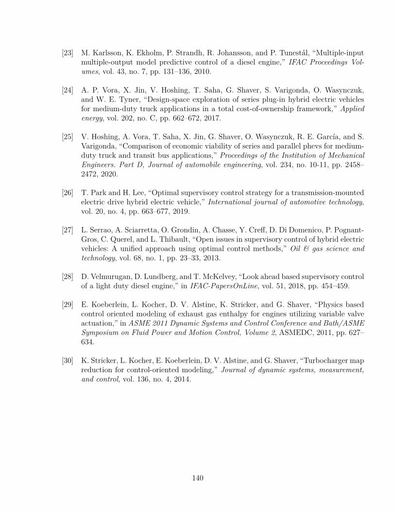
[23] M. Karlsson, K. Ekholm, P. Strandh, R. Johansson, and P. Tunestål, “Multiple-inputmultiple-output model predictive control of a diesel engine,” IFAC Proceedings Vol-umes, vol. 43, no. 7, pp. 131–136, 2010.
[24] A. P. Vora, X. Jin, V. Hoshing, T. Saha, G. Shaver, S. Varigonda, O. Wasynczuk,and W. E. Tyner, “Design-space exploration of series plug-in hybrid electric vehiclesfor medium-duty truck applications in a total cost-of-ownership framework,” Appliedenergy, vol. 202, no. C, pp. 662–672, 2017.
[25] V. Hoshing, A. Vora, T. Saha, X. Jin, G. Shaver, O. Wasynczuk, R. E. García, and S.Varigonda, “Comparison of economic viability of series and parallel phevs for medium-duty truck and transit bus applications,” Proceedings of the Institution of MechanicalEngineers. Part D, Journal of automobile engineering, vol. 234, no. 10-11, pp. 2458–2472, 2020.
[26] T. Park and H. Lee, “Optimal supervisory control strategy for a transmission-mountedelectric drive hybrid electric vehicle,” International journal of automotive technology,vol. 20, no. 4, pp. 663–677, 2019.
[27] L. Serrao, A. Sciarretta, O. Grondin, A. Chasse, Y. Creff, D. Di Domenico, P. Pognant-Gros, C. Querel, and L. Thibault, “Open issues in supervisory control of hybrid electricvehicles: A unified approach using optimal control methods,” Oil & gas science andtechnology, vol. 68, no. 1, pp. 23–33, 2013.
[28] D. Velmurugan, D. Lundberg, and T. McKelvey, “Look ahead based supervisory controlof a light duty diesel engine,” in IFAC-PapersOnLine, vol. 51, 2018, pp. 454–459.
[29] E. Koeberlein, L. Kocher, D. V. Alstine, K. Stricker, and G. Shaver, “Physics basedcontrol oriented modeling of exhaust gas enthalpy for engines utilizing variable valveactuation,” in ASME 2011 Dynamic Systems and Control Conference and Bath/ASMESymposium on Fluid Power and Motion Control, Volume 2, ASMEDC, 2011, pp. 627–634.
[30] K. Stricker, L. Kocher, E. Koeberlein, D. V. Alstine, and G. Shaver, “Turbocharger mapreduction for control-oriented modeling,” Journal of dynamic systems, measurement,and control, vol. 136, no. 4, 2014.
140


