ZENTRUM FÜR ENTWICKLUNGSFORSCHUNG

Economic disruptions, markets and food

security

Dissertation

zur

Erlangung des akademischen Grades

eines

Doktor der Agrarwissenschaften

(Dr. agr.)

der

Landwirtschaftlichen Fakultät

der

Rheinischen Friedrich-Wilhelms-Universität Bonn

Von

Henry Kankwamba

Aus

Bembeke, Dedza, Malawi

Bonn, 2020

ii

Referent: Prof. Dr. Dr. hc. Joachim VON BRAUN

Korreferent: Prof. Dr. Thomas HECKELEI

Tag der mündlichen Prüfung: 5 Oktober 2020

Angefertigt mit Genehmigung der Landwirtschaftlichen Fakultät der Universität

Bonn

iii

Abstract

Idiosyncratic and covariate shocks have considerable impacts on household food se-curity and welfare. While impacts of covariate and idiosyncratic shocks have beenwidely documented, the mitigating role of infrastructure against such events has notbeen widely assessed due to the complexities in quantifying its accrued economicbenefits. Further, traders, who play a significant role in allocating food resourcesamidst idiosyncratic and covariate shocks, their behaviour, motivations and aspira-tions that drive market outcomes have not been well addressed in literature fromsub-Saharan Africa.

Using Malawi as a case, this study first examines impacts of extreme weatherevents and idiosyncratic shocks on food security at household level. Using threewaves of Malawi’s representative panel Integrated Household Surveys (IHS) thestudy estimates impacts of shocks using triple difference fixed effects regressions.In general, having controlled for household socioeconomic factors, the study findsthat weather shocks such as drought and floods during an agricultural season reduceconsumption by 9%. Assuming normal weather conditions, infrastructure scarcityin form of roads, electricity, and service based amenities such as banks, savings andcredit cooperatives and markets – summarized into an infrastructure index – wors-ens economic access to food by 7%. Further, the joint impact of extreme weatherevents and lack of infrastructure is 17% food security reduction.

Considering that social capital can affect market outcomes in the presence ofmarket and government failure, the study assessed the performance and organiza-tion of maize trading by paying attention to the role of social capita and businessformality in Malawi. Benefiting from combining both qualitative and quantitativedata sources, we used Bayes Model Averaging techniques, instrumental variableand control function approaches and found that food markets are concentrated andhighly informal. While there is evidence that social capital is positively associatedwith business profitability, results do not strongly support the hypothesis that othermeasures of social capital such as tribal and religious affiliation have an effect ontraders’ business resilience.

iv

Zusammenfassung

Idiosynkratische und kovariate Schocks haben erhebliche Auswirkungen auf die Er-

nährungssicherheit und das Wohlergehen von Haushalten. Darüber hinaus hat die

Häufigkeit kovariater Schocks, wie beispielsweise extreme Wetterereignisse, in den

meisten Teilen Afrikas südlich der Sahara dramatisch zugenommen. Solche Vor-

kommnisse haben den Zugang zu und die Nutzung von Nahrungsmitteln erheb-

lich beeinträchtigt. Während die Auswirkungen kovariater und idiosynkratischer

Schocks umfassend dokumentiert sind, wurde die Bedeutung der Infrastruktur bei

der Bewältigung solcher Ereignisse aufgrund der Komplexität der Quantifizierung

des daraus erwachsenden Nutzens nicht umfassend bewertet. Darüber hinaus wur-

de die Rolle der Nahrungsmittelhändler, die bei der Zuteilung von Nahrungsmit-

teln inmitten von idiosynkratischen und kovariaten Schocks eine bedeutende Rolle

spielen, ihr Verhalten, ihre Motivationen und Bestrebungen, die die Marktergebnisse

bestimmen, in der Literatur für Afrika südlich der Sahara wenig beachtet.

Anhand des Fallbeispiels Malawi untersucht diese Studie zunächst die Auswir-

kungen extremer Wetterereignisse und idiosynkratischer Schocks auf die Ernäh-

rungssicherheit von Haushalten. Unter Nutzung dreier Befragungswellen der Mala-

wi Integrated Household Surveys (IHS), einer repräsentativen Panelbefragng, schätzt

die Studie die Auswirkungen von Schocks im Rahmen einer Regression mit dreifa-

cher Differenzbildung sowie mit Haushalts-fixed Effekten. Unter Berücksichtigung

der sozioökonomischen Faktoren der befragten Haushalte kommt die Studie zu dem

Ergebnis, dass Wetterschocks, wie Dürre und Überschwemmungen während einer

landwirtschaftlichen Saison, den Konsum im Allgemeinen um 9% reduzieren. Dem-

gegenüber steht, dass eine schlechte Infrastruktur in Form von Straßen, Strom und

der Verfügbarkeit von dienstleistungsorientierten Einrichtungen, wie Banken, Spar-

und Kreditgenossenschaften und Märkten, zusammengefasst in einem Infrastruk-

turindex, bei normalen Wetterbedingungen den wirtschaftlichen Zugang zu Nah-

rungsmitteln um 7% verringert. Die Kombination von extremen Wetterereignissen

und mangelnder Infrastruktur führt zu einer Verschlechterung der Ernährungssi-

cherheit um 17%.

In Anbetracht der Tatsache, dass Sozialkapital bei Markt- und Staatsversagen

v

die Marktergebnisse beeinflussen kann, bewertete die Studie die Funktionsfähig-

keit und Organisation des Maishandels unter Berücksichtigung der Rolle des so-

zialen Kapitals und der Verbreitung formeller Geschäftstätigkeit in Malawi. Wir

nutzen eine Kombination qualitativer und quantitativer Datenquellen und verwen-

deten Bayes-Modell-Mittelwertbildungstechniken, sowie Ansätze für instrumentel-

le Variablen und Kontrollfunktionen und stellten fest, dass Nahrungsmittelmärkte

konzentriert und in hohem Maße informell sind. Es gibt zwar Belege dafür, dass

Sozialkapital positiv mit der Rentabilität der Handelsbetriebe verbunden ist, aller-

dings stützen die Ergebnisse nicht unbedingt die Hypothese, dass andere Indikato-

ren des Sozialkapitals, wie Stammes- und Religionszugehörigkeit, einen Einfluss auf

die wirtschaftliche Widerstandsfähigkeit von Händlern haben.

vii

Acknowledgements

I would like to acknowledge my supervisor Prof. Dr. Dr. hc. Joachim von Braun for

giving me with an opportunity to study under him at the prestigious University of

Bonn at the Center for Development Research (ZEF). I would also like to acknowl-

edge the German Academic Exchange (DAAD) for awarding me with a doctoral stu-

dent scholarship and generous research funding. I recognize Fiat Panis Foundation

for funding my field research in Malawi. I further acknowledge, the Lilongwe Uni-

versity of Agriculture and Natural Resources for providing me with a study leave to

upgrade my academic qualifications. I appreciate countless hours my tutors namely

Dr. Lukas Kornher, Dr. Nicolas Gerber and other senior and junior researchers at

ZEF put into this work. I acknowledge all my classmates from 2016, my family and

friends.

ix

Contents

Abstract iii

Acknowledgements vii

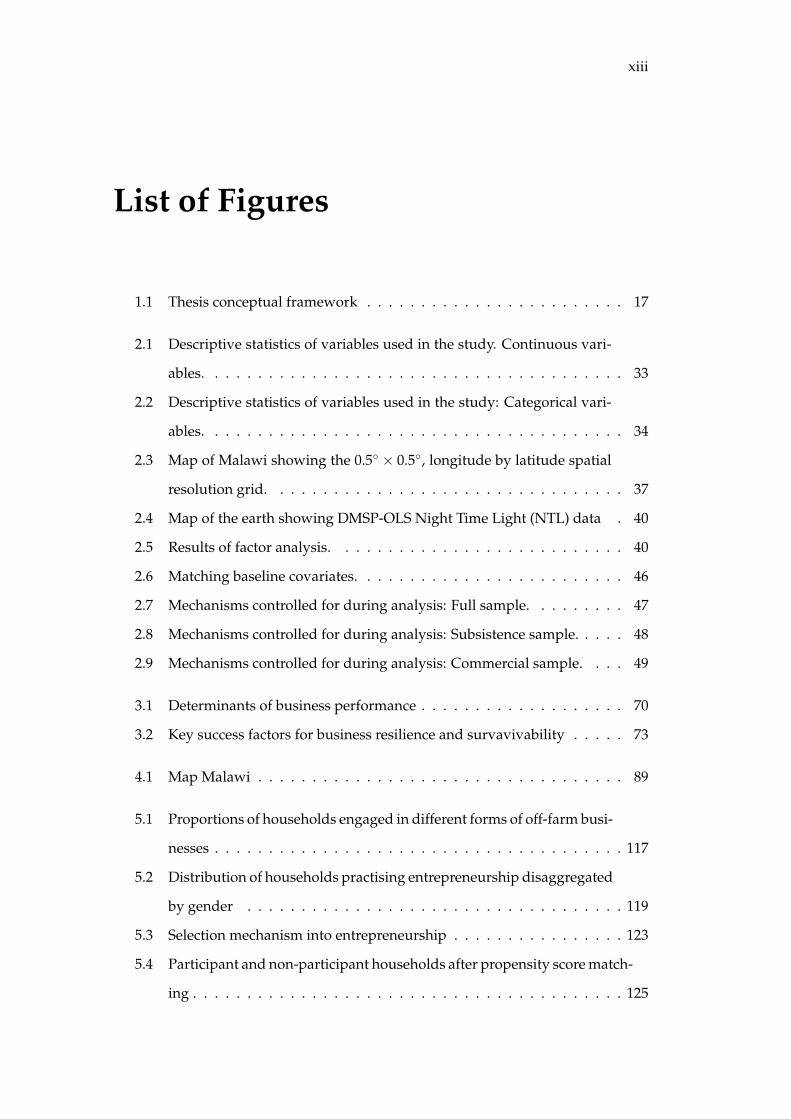
List of Figures xiii

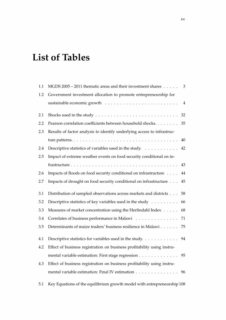
List of Tables xv

List of Abbreviations xvii

1 Introduction 1

1.1 Background . . . . . . . . . . . . . . . . . . . . . . . . . . . . . . . . . . 1

1.1.1 Policy context of the study . . . . . . . . . . . . . . . . . . . . . . 1

1.1.2 External shocks to the economy . . . . . . . . . . . . . . . . . . . 5

1.2 Problem statement . . . . . . . . . . . . . . . . . . . . . . . . . . . . . . 6

1.3 Main research questions . . . . . . . . . . . . . . . . . . . . . . . . . . . 6

1.4 A review of relevant literature . . . . . . . . . . . . . . . . . . . . . . . . 7

1.4.1 Impacts of idiosyncratic and covariate shocks on food and nu-

trition security . . . . . . . . . . . . . . . . . . . . . . . . . . . . 7

1.4.2 Mitigating impacts of climatic shocks: the role of infrastructure 9

1.4.3 Idiosyncratic and covariate shocks, off-farm entrepreneurship,

food and nutrition security . . . . . . . . . . . . . . . . . . . . . 11

1.4.4 Staple food markets, traders, social capital and institutions:

Implications for food and nutrition security . . . . . . . . . . . . 13

1.5 Hypotheses . . . . . . . . . . . . . . . . . . . . . . . . . . . . . . . . . . 15

1.6 Organization and concept of the thesis . . . . . . . . . . . . . . . . . . . 16

x

2 Infrastructure, extreme weather events and food security in Malawi 19

2.1 Introduction . . . . . . . . . . . . . . . . . . . . . . . . . . . . . . . . . . 19

2.1.1 The connection between infrastructure and shocks . . . . . . . . 21

2.2 Methodology . . . . . . . . . . . . . . . . . . . . . . . . . . . . . . . . . 24

2.2.1 Theoretical framework . . . . . . . . . . . . . . . . . . . . . . . . 24

2.2.2 Estimation . . . . . . . . . . . . . . . . . . . . . . . . . . . . . . . 26

2.2.3 Data and descriptive statistics . . . . . . . . . . . . . . . . . . . . 29

Dependent variables considered . . . . . . . . . . . . . . . . . . 29

A typology of self-reported household shocks . . . . . . . . . . 30

Seasonal drought and floods . . . . . . . . . . . . . . . . . . . . 36

Infrastructure availability . . . . . . . . . . . . . . . . . . . . . . 36

Household characteristics . . . . . . . . . . . . . . . . . . . . . . 39

2.3 Results . . . . . . . . . . . . . . . . . . . . . . . . . . . . . . . . . . . . . 42

2.3.1 Proximate impacts of seasonal shocks on food security . . . . . 42

2.3.2 Household dietary diversity and nutrition . . . . . . . . . . . . 44

2.3.3 Potential mechanisms . . . . . . . . . . . . . . . . . . . . . . . . 45

2.4 Discussion . . . . . . . . . . . . . . . . . . . . . . . . . . . . . . . . . . . 50

2.5 Conclusion . . . . . . . . . . . . . . . . . . . . . . . . . . . . . . . . . . . 51

3 Social capital and market performance: Implications for food security 53

3.1 Introduction . . . . . . . . . . . . . . . . . . . . . . . . . . . . . . . . . . 53

3.2 Materials and methods . . . . . . . . . . . . . . . . . . . . . . . . . . . . 56

3.2.1 Study area . . . . . . . . . . . . . . . . . . . . . . . . . . . . . . . 56

3.2.2 Sampling, data and variables . . . . . . . . . . . . . . . . . . . . 56

3.2.3 Theoretical framework . . . . . . . . . . . . . . . . . . . . . . . . 58

3.2.4 Estimation . . . . . . . . . . . . . . . . . . . . . . . . . . . . . . . 61

3.2.5 Industry structure . . . . . . . . . . . . . . . . . . . . . . . . . . 63

Descriptive statistics . . . . . . . . . . . . . . . . . . . . . . . . . 63

3.3 Results . . . . . . . . . . . . . . . . . . . . . . . . . . . . . . . . . . . . . 64

3.3.1 Descriptive statistics . . . . . . . . . . . . . . . . . . . . . . . . . 64

Industry structure . . . . . . . . . . . . . . . . . . . . . . . . . . 67

3.3.2 The role of social capital in determining business performance . 69

xi

3.3.3 The role of social capital in business resilience . . . . . . . . . . 72

3.4 Discussion . . . . . . . . . . . . . . . . . . . . . . . . . . . . . . . . . . . 76

3.5 Conclusion . . . . . . . . . . . . . . . . . . . . . . . . . . . . . . . . . . . 78

4 Business registration and firm performance: A case of maize traders in

Malawi 79

4.1 Background . . . . . . . . . . . . . . . . . . . . . . . . . . . . . . . . . . 79

4.2 Evolution of price policy and agricultural trade informality in Malawi 83

4.3 Methodology . . . . . . . . . . . . . . . . . . . . . . . . . . . . . . . . . 86

4.3.1 Data and measurement . . . . . . . . . . . . . . . . . . . . . . . 86

Study area, data collection and time context . . . . . . . . . . . 86

Empirical Estimation . . . . . . . . . . . . . . . . . . . . . . . . . 88

4.4 Results . . . . . . . . . . . . . . . . . . . . . . . . . . . . . . . . . . . . . 93

4.4.1 Descriptive statistics . . . . . . . . . . . . . . . . . . . . . . . . . 93

4.4.2 Effects of firm registration on performance in form of prof-

itability . . . . . . . . . . . . . . . . . . . . . . . . . . . . . . . . . 93

4.5 Discussion . . . . . . . . . . . . . . . . . . . . . . . . . . . . . . . . . . . 98

4.6 Conclusions . . . . . . . . . . . . . . . . . . . . . . . . . . . . . . . . . . 100

5 Entrepreneurship, food security and welfare in Malawi 103

5.1 Introduction . . . . . . . . . . . . . . . . . . . . . . . . . . . . . . . . . . 103

5.2 Methods . . . . . . . . . . . . . . . . . . . . . . . . . . . . . . . . . . . . 106

5.2.1 Theoretical framework . . . . . . . . . . . . . . . . . . . . . . . . 106

An equilibrium model with endogenous entrepreneurship . . . 106

5.2.2 Identification strategy . . . . . . . . . . . . . . . . . . . . . . . . 107

A counterfactual framework for entrepreneurship and welfare

outcomes . . . . . . . . . . . . . . . . . . . . . . . . . . 107

Adjustments to counterfactual assumptions and estimation . . 111

5.2.3 Data . . . . . . . . . . . . . . . . . . . . . . . . . . . . . . . . . . 113

5.3 Results . . . . . . . . . . . . . . . . . . . . . . . . . . . . . . . . . . . . . 116

5.3.1 Descriptive statistics . . . . . . . . . . . . . . . . . . . . . . . . . 116

Defining and contextualizing entrepreneurship . . . . . . . . . 116

5.3.2 Descriptive statistics of control variables . . . . . . . . . . . . . 118

xii

5.3.3 Mechanism of selection into entrepreneurship . . . . . . . . . . 120

5.3.4 Balancing tests for participants and non-participants . . . . . . 122

5.3.5 Impact of entrepreneurship on food security . . . . . . . . . . . 122

Average treatment effects on the treated . . . . . . . . . . . . . . 122

Quantile treatment effects . . . . . . . . . . . . . . . . . . . . . . 126

5.4 Discussion . . . . . . . . . . . . . . . . . . . . . . . . . . . . . . . . . . . 128

5.4.1 Patterns and drivers of entry into entrepreurship . . . . . . . . 128

5.4.2 Impact of entrepreneurship on food security . . . . . . . . . . . 131

5.5 Conclusion . . . . . . . . . . . . . . . . . . . . . . . . . . . . . . . . . . . 132

6 General conclusions and policy implications 135

6.1 Introduction . . . . . . . . . . . . . . . . . . . . . . . . . . . . . . . . . . 135

6.2 Infrastructure, extreme weather events and food security . . . . . . . . 135

6.2.1 Background . . . . . . . . . . . . . . . . . . . . . . . . . . . . . . 135

6.2.2 Methods . . . . . . . . . . . . . . . . . . . . . . . . . . . . . . . . 136

6.2.3 Key results . . . . . . . . . . . . . . . . . . . . . . . . . . . . . . . 136

6.2.4 Implications . . . . . . . . . . . . . . . . . . . . . . . . . . . . . . 137

6.2.5 Recommendations . . . . . . . . . . . . . . . . . . . . . . . . . . 137

6.3 Social capital and food market performance . . . . . . . . . . . . . . . . 138

6.3.1 Background . . . . . . . . . . . . . . . . . . . . . . . . . . . . . . 138

6.3.2 Methods . . . . . . . . . . . . . . . . . . . . . . . . . . . . . . . . 138

6.3.3 Key results . . . . . . . . . . . . . . . . . . . . . . . . . . . . . . . 138

6.3.4 Implications . . . . . . . . . . . . . . . . . . . . . . . . . . . . . . 139

6.4 Recommendations . . . . . . . . . . . . . . . . . . . . . . . . . . . . . . 139

6.5 Study limitations and recommendations for further studies . . . . . . . 140

References 141

xiii

List of Figures

1.1 Thesis conceptual framework . . . . . . . . . . . . . . . . . . . . . . . . 17

2.1 Descriptive statistics of variables used in the study. Continuous vari-

ables. . . . . . . . . . . . . . . . . . . . . . . . . . . . . . . . . . . . . . . 33

2.2 Descriptive statistics of variables used in the study: Categorical vari-

ables. . . . . . . . . . . . . . . . . . . . . . . . . . . . . . . . . . . . . . . 34

2.3 Map of Malawi showing the 0.5 × 0.5, longitude by latitude spatial

resolution grid. . . . . . . . . . . . . . . . . . . . . . . . . . . . . . . . . 37

2.4 Map of the earth showing DMSP-OLS Night Time Light (NTL) data . 40

2.5 Results of factor analysis. . . . . . . . . . . . . . . . . . . . . . . . . . . 40

2.6 Matching baseline covariates. . . . . . . . . . . . . . . . . . . . . . . . . 46

2.7 Mechanisms controlled for during analysis: Full sample. . . . . . . . . 47

2.8 Mechanisms controlled for during analysis: Subsistence sample. . . . . 48

2.9 Mechanisms controlled for during analysis: Commercial sample. . . . 49

3.1 Determinants of business performance . . . . . . . . . . . . . . . . . . . 70

3.2 Key success factors for business resilience and survavivability . . . . . 73

4.1 Map Malawi . . . . . . . . . . . . . . . . . . . . . . . . . . . . . . . . . . 89

5.1 Proportions of households engaged in different forms of off-farm busi-

nesses . . . . . . . . . . . . . . . . . . . . . . . . . . . . . . . . . . . . . . 117

5.2 Distribution of households practising entrepreneurship disaggregated

by gender . . . . . . . . . . . . . . . . . . . . . . . . . . . . . . . . . . . 119

5.3 Selection mechanism into entrepreneurship . . . . . . . . . . . . . . . . 123

5.4 Participant and non-participant households after propensity score match-

ing . . . . . . . . . . . . . . . . . . . . . . . . . . . . . . . . . . . . . . . . 125

xiv

5.5 Impact of entrepreneurship on welfare . . . . . . . . . . . . . . . . . . . 127

xv

List of Tables

1.1 MGDS 2005 – 2011 thematic areas and their investment shares . . . . . 3

1.2 Government investment allocation to promote entrepreneurship for

sustainable economic growth . . . . . . . . . . . . . . . . . . . . . . . . 4

2.1 Shocks used in the study . . . . . . . . . . . . . . . . . . . . . . . . . . . 32

2.2 Pearson correlation coefficients between household shocks. . . . . . . . 35

2.3 Results of factor analysis to identify underlying access to infrastruc-

ture patterns. . . . . . . . . . . . . . . . . . . . . . . . . . . . . . . . . . . 40

2.4 Descriptive statistics of variables used in the study. . . . . . . . . . . . 42

2.5 Impact of extreme weather events on food security conditional on in-

frastructure . . . . . . . . . . . . . . . . . . . . . . . . . . . . . . . . . . . 43

2.6 Impacts of floods on food security conditional on infrastructure . . . . 44

2.7 Impacts of drought on food security conditional on infrastructure . . . 45

3.1 Distribution of sampled observations across markets and districts . . . 58

3.2 Descriptive statistics of key variables used in the study . . . . . . . . . 66

3.3 Measures of market concentration using the Herfindahl Index . . . . . 68

3.4 Correlates of business performance in Malawi . . . . . . . . . . . . . . 71

3.5 Determinants of maize traders’ business resilience in Malawi . . . . . . 75

4.1 Descriptive statistics for variables used in the study. . . . . . . . . . . . 94

4.2 Effect of business registration on business profitability using instru-

mental variable estimation: First stage regression . . . . . . . . . . . . . 95

4.3 Effect of business registration on business profitability using instru-

mental variable estimation: Final IV estimation . . . . . . . . . . . . . . 96

5.1 Key Equations of the equilibrium growth model with entrepreneurship 108

xvi

5.2 Descriptive Statistics of variables used . . . . . . . . . . . . . . . . . . . 121

5.3 Balancing tests for participants and non-participants . . . . . . . . . . . 124

5.4 Impact of entrepreneurship on food security . . . . . . . . . . . . . . . 126

5.5 Quantile regression model results showing distributional impacts of

entrepreneurship on food security . . . . . . . . . . . . . . . . . . . . . 128

xvii

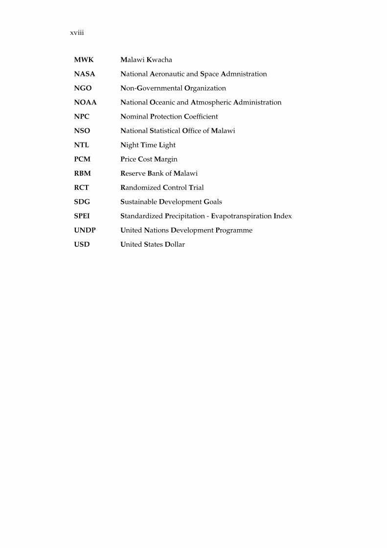
List of Abbreviations

ADMARC Agricultural Development and Marketing Corporation

AIDS Acquired Immune Deficiency Syndrome

BMA Bayes Model Averaging

CAADP Comprehensive Africa Agriculture Development Programme

CEM Coersened Exact Matching

CGE Computable General Equilibrium Model

CII Composite Infrastructure Index

DDD Difference-in-Difference-in-Difference

DMSP-OLS Defense-Meteorological Satellite Program-Optical Line Scanner

DODMA Department of Disaster Management Affairs

ESR Endogenous Switching Regression

FAO Food Agriculture Organization

FEWSNET Famine Early Warning System Network

FISP Farm Input Subsidy Program

GDP Gross Domestic Product

GoM Government of Malawi

HHI Herfindahl Hirschman Index

HHID Household Unique Identifier

HIV Human Immunodeficiency Virus

IFPRI International Food Policy Research Institute

IHS Integrated Household Survey

IPCC Intergovernmental Panel on Climate Change

IPWRA Inverse Probability Weighted Regression Adjustment

LSMS-ISA Living Standards Measurement Surveys - Integrated Surveys on Agriculture

MCMC Monte Carlo Markov Chain

MGDS Malawi Growth and Development Strategy

xviii

MWK Malawi Kwacha

NASA National Aeronautic and Space Admnistration

NGO Non-Governmental Organization

NOAA National Oceanic and Atmospheric Administration

NPC Nominal Protection Coefficient

NSO National Statistical Office of Malawi

NTL Night Time Light

PCM Price Cost Margin

RBM Reserve Bank of Malawi

RCT Randomized Control Trial

SDG Sustainable Development Goals

SPEI Standardized Precipitation - Evapotranspiration Index

UNDP United Nations Development Programme

USD United States Dollar

1

Chapter 1

Introduction

1.1 Background

1.1.1 Policy context of the study

On 1st January, 2016 the world saw the commencement of 17 ambitious Sustainable

Development Goals (SDGs) to make the world a better place by 2030. First among

the goals are to “end poverty in all its forms everywhere” and to “end hunger,

achieve food security and improved nutrition and promote sustainable agriculture”.

Highly connected to these two fore-running goals is another goal to “ensure sus-

tainable consumption and production patterns” (United Nations Development Pro-

gramme, 2016; FAO, 2018). Although quite challenging, these goals call for efficient

allocation of resources in order for them to be attainable.

Operationalizing these goals requires changing the status quo of doing develop-

ment activities. Developing countries, especially those south of the Sahara, where

there is extreme poverty and hunger have been putting together efforts and com-

mitment to achieve these goals. Most often, poverty alleviation policies have been

criticized for lacking clear implementation plans in order to achieve their strategic

goals (United Nations, 2003).

This study takes Malawi, a land locked developing economy in southeast Africa,

as a case on how different circumstances have affected its aspirations towards at-

tainment of the SDGs and other goals that have preceded them. Ranked among

the world’s least developed countries, at purchasing power parity, Malawi’s GDP

is $22.42 billion. It translates to $1200 per capita of its population of 18 million,

of which 7 million comprise its labour force. Slightly over half of its population

2

lives on less than $1.90 per day and inequality is at 0.46 using the Gini index (Cen-

tral Intelligence Agency, 2019). The country faces constraints to economic growth

such as policy inconsistency, poor infrastructure, corruption, poor health and low

education attainment (Central Intelligence Agency, 2019). Agriculture is the main-

stay of Malawi’s economy with smallholder farming comprising 80% of agricultural

GDP. Agriculture employs 77% of the labour force and contributed 28% to GDP for

six consecutive quarters since 2017. Agriculture has strong forward and backward

linkages evidenced by active commodity markets, wholesaling and general trading

which contribute 15% to GDP since 2017 (Reserve Bank of Malawi (RBM), 2019).

During the second and third quarter of 2018 and the first quarter of 2019, inflation

stood around 9.1%. During the same time, food inflation increased by one percent-

age point to 9.5% compared the previous quarters. The mechanism explaining the

food price inflation was a decrease in maize production during the 2017/2018 crop

production season due to fall armyworms and dry spells in some areas (Reserve

Bank of Malawi (RBM), 2019).

From growth strategy point of view, in 1998 the Government of Malawi came

up with a long term strategic plan named "Malawi Vision 2020". The long term

goal of the vision 2020 was that "By the year 2020, Malawi will be secure, demo-

cratically mature, environmentally sustainable, self reliant with equal opportunities

for and active participation by all,having social services, vibrant cultural and reli-

gious values and being a technologically driven middle-income economy" (Govern-

ment of Malawi, 1998). In its attempt to operationalize this long term vision, the

Government of Malawi came up with a number of strategic options to spur eco-

nomic growth which comprised developing the following key sectors 1) agriculture;

2) manufacturing industry, 3) Mining, 4) Tourism and re-orienting Malawi to be a

predominantly exporting country (Government of Malawi, 1998).

As further commitment to economic growth and agricultural development, the

Malawi Government adopted the Comprehensive Africa Agriculture Development

Programme (CAADP) which aimed at increasing the Gross Domestic Product (GDP)

by 6% per year by allocating 10% of its public expenditure in the agricultural sec-

tor (United Nations, 2003). An International Food Policy Research Institute (IFPRI)

commissioned study assessed different investment options to achieve agricultural

3

growth and reduce poverty. The study found that Malawi could not manage to

halve poverty by 2015 by investing 10% in agriculture only. However, it found that

the investment option was worthwhile since historically, agricultural spending as a

share of public spending was much lower (Benin et al., 2008).

The years post-2000 saw increased government commitment to agricultural growth

through introduction of the Farm Input Subsidy Program (FISP) in 2005. In 2006,

the Malawi Government came up with a five throng strategy to move Malawi out

of poverty called the Malawi Growth and Development Strategy (MGDS). As part

of the long term strategy of ending poverty by 2020, the MGDS had five pillars

namely 1) agriculture and food security; 2) irrigation and water development; 3)

Infrastructure development; 4) energy 5)integrated rural development and 6) pre-

vention and management of nutrition disorders and HIV and AIDS (Government of

Malawi, 2006). In its long term food security goal, the MGDS aimed at 1) achieving

no food shortages during times of negative economic disruptions such as drought,

floods, pests and diseases; and 2) increase exports of staples to neighbouring coun-

tries. In its medium term objective on food security, the 2006 – 2011 MGDS aimed

at ensuring that high quality nutritious food was available and accessible to every-

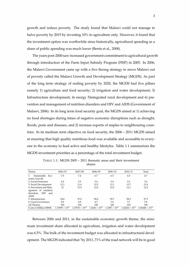
one in the economy to lead active and healthy lifestyles. Table 1.1 summarizes the

MGDS investment priorities as a percentage of the total investment budget.

TABLE 1.1: MGDS 2005 – 2011 thematic areas and their investmentshares

Theme 2006/07 2007/08 2008/09 2009/10 2010/11 Total

1: Sustainable Eco-nomic Growth

7.0 7.4 6.7 6.3 6.5 6.7

2: Social Protection 5.4 5.5 5.4 5.4 5.5 5.43: Social Development 12.1 11.6 12.2 13.1 13.7 12.44: Prevention and Man-agement of nutritiondisorders, HIV andAIDS

12 13.9 12.6 12.0 12.1 12.4

5: Infrastructure 54.8 57.0 58.6 59.7 58.5 57.36: Good Governance 8.8 4.8 4.7 3.6 3.7 5.8All Themes 100 100 100 100 100 100Costs in Million MWK 1.31909× 1011 1.27533× 1011 1.2636× 1011 1.2387× 1011 1.22424× 1011 6.36448× 1011

Between 2006 and 2011, in the sustainable economic growth theme, the mini-

mum investment share allocated to agriculture, irrigation and water development

was 6.5%. The bulk of the investment budget was allocated to infrastructural devel-

opment. The MGDS indicated that "by 2011, 71% of the road network will be in good

4

condition; 18% in fair condition and 11% only in poor condition". On nutrition the

MGDS planned to achieve "active healthy life with reduced burden of diet related,

illness, deaths and disability among men, women, boys and girls living in Malawi".

Noteworthy, much research in Malawi has mainly focused on agricultural growth

and impacts of Farm Input Subsidy Program (FISP). Looking at the investment fig-

ures, infrastructural investments and nutritional impact studies should have equally

taken a leading role to get a whole picture on how these policies fared in the medium

to the long run.

In 2011 the Government of Malawi introduced a second version of the Malawi

Growth and Development Strategy (MGDSII) which prioritized entrepreneurship as

a strategy to encourage all gender groups to participate fully in economic activities

for wealth creation and poverty reduction. The government committed a substantial

amount of resources to ensure that its goal of ensuring economic growth by encour-

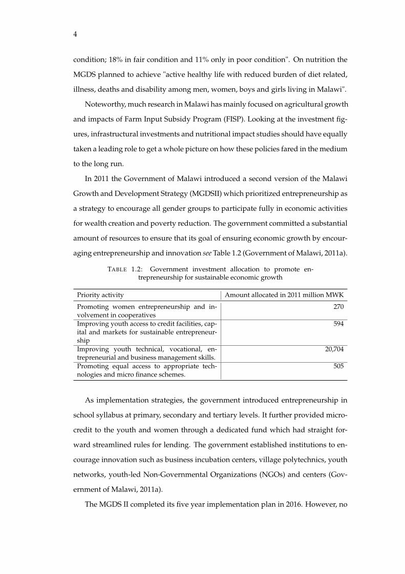
aging entrepreneurship and innovation see Table 1.2 (Government of Malawi, 2011a).

TABLE 1.2: Government investment allocation to promote en-trepreneurship for sustainable economic growth

Priority activity Amount allocated in 2011 million MWK

Promoting women entrepreneurship and in-volvement in cooperatives

270

Improving youth access to credit facilities, cap-ital and markets for sustainable entrepreneur-ship

594

Improving youth technical, vocational, en-trepreneurial and business management skills.

20,704

Promoting equal access to appropriate tech-nologies and micro finance schemes.

505

As implementation strategies, the government introduced entrepreneurship in

school syllabus at primary, secondary and tertiary levels. It further provided micro-

credit to the youth and women through a dedicated fund which had straight for-

ward streamlined rules for lending. The government established institutions to en-

courage innovation such as business incubation centers, village polytechnics, youth

networks, youth-led Non-Governmental Organizations (NGOs) and centers (Gov-

ernment of Malawi, 2011a).

The MGDS II completed its five year implementation plan in 2016. However, no

5

rigorous assessment of the impact of the prioritized strategies was conducted. There-

fore, it is against this background that this study would like to assess the impacts of

some of the strategies of the MGDS such as food and nutrition security, infrastruc-

ture and promotion of entrepreneurship given Malawi market institutions’ structure

and conduct.

1.1.2 External shocks to the economy

Between 2011 and 2016, the MGDS II time frame, a number of macroeconomic, id-

iosyncratic and covariate shocks occured. At macroeconomic level, Malawi expe-

rienced a sudden shift in its exchange rate from a fixed to a market based flexible

regime. Pauw, Dorosh, and Mazunda (2013) documented that the main culprits to

the crisis were a rising import bill mainly attributed fertilizer imports to support

the FISP, a reduction in tobacco exports which reduced its foreign exchange inflows

and withdrawal of budgetary support from the Malawi Governments’ main donors.

These macroeconomic policy shocks could also reflect on domestic markets espe-

cially food markets by altering the structure and conduct of markets and eventually

access to international markets. So far, no study has explored the organization of

food markets during such tumultuous time period.

A number of floods and droughts due to El Nino weather conditions also af-

fected the economy througout the five year period. Using a forward looking Com-

putable General Equilibrium (CGE) model for Malawi, Pauw et al. (2011) found that

income would generally decrease due to extreme weather events but households in

the southern parts of the country will be the ones that lose most. So far, a confirma-

tory or falsifying ex-post externally valid study has not been conducted during the

time period.

Furthermore, household specific shocks could also have perverse economic im-

pacts on households. It is therefore the purpose of this study to explore, using the

lenses of modern microeconomic theory, the impact of idiosyncratic and covariate

shock on household food security.

6

1.2 Problem statement

The challenge of achieving zero hunger calls for a deeper understanding of funda-

mental drivers of food security. While increasing agricultural production is fun-

damental, increasing economic access to food could reduce the prevalence of un-

dernourished people (Von Braun, 2017). Improving food security also requires effi-

ciency of markets (Grote, 2014), institutions (Kirsten, 2009) and provision of physi-

cal support systems such as public infrastructure (Godfray et al., 2010). Notewor-

thy, worldwide, agriculture faces vagaries of climatic shocks. While impacts of

climate change and other weather related shocks have been widely documented

(Parry, 2019; Smit and Skinner, 2002; Adams, 1989), there is a lacuna in literature

on how much soft and hard public infrastructure mitigate against impacts of sea-

sonal shocks. Secondly, whether these shocks drive people out of agriculture to start

new entrepreneurial ventures or people start new businesses while still in agricul-

ture to cushion themselves against seasonal shocks is also not widely understood.

Further, the institutional and behavioural determinants of food market performance

and resilience in an African context are not extensively documented.

Using Malawi, a land locked developing economy in southeast Africa, as a case,

this study is a collection of four distinct essays that relate to determinants of progress

in achieving food security. In the first article, the impacts of seasonal weather and

idiosyncratic shocks and the mitigating role of infrastructure are discussed. The

second essay assesses the role of social capital in determining performance and re-

silience of maize trading businesses. The third paper examines the role of business

registration on business performance. The fourth discourse analyses the distribu-

tional effects of entrepreneurship on food security. It delves into the mechanisms

and implications of entry into entrepreneurial activities on food security.

1.3 Main research questions

The thesis asks the following guiding research questions:

1. What are the impacts of idiosyncratic and covariate shocks on food and nutri-

tion security?

7

2. What is the mitigating role of public physical infrastructure on the the impacts

of extreme weather events on household food security?

3. What is the contribution of off-farm entrepreneurship to food and nutrition

security?

4. What are the food and nutrition security implications of the staple food market

structure and conduct in Malawi? Specifically, what is the role of institutions

and social capital in determining the structure and conduct of food markets?

1.4 A review of relevant literature

In what follows next, a review of the literature to reveal the state of the art and

gaps for further studies regarding these questions is conducted. Thus, the review

follows each question by reviewing closely related literature in order to develop

hypotheses. At the end of each subsection, a summary of contributions this study

makes is provided. The last subsection, therefore, presents the hypotheses guiding

the study.

1.4.1 Impacts of idiosyncratic and covariate shocks on food and nutrition

security

Idiosyncratic and covariate shocks could have significant impacts on food and nu-

trition security. An idiosyncratic shock is an event that a household experiences that

other households in the same area are not experiencing with potential of affecting

production and consumption possibilities (Pradhan and Mukherjee, 2018; Dercon et

al. 2005). For example, death/birth of a family member, debt and sickness in the

household. On the other hand, a covariate shock is an event that affects a number

of households in an area. For instance, droughts, floods, conflict, pests and diseases

(Dercon, Hoddinott, Woldehanna, et al., 2005; Pradhan and Mukherjee, 2018).

In an African setting, idiosyncratic shocks abound and their adverse impacts on

food security and welfare are well documented. One widely documented idiosyn-

cratic shock – with myriad implications – is prevalence of sickness at household level

(see De Waal and Whiteside, 2003; Gillespie and Gillespie, 2006; Conroy et al., 2006).

8

For example, sickness and death of the household head have led to significant loss

of household labour supply, which eventually leads to lower farm productivity, less

output and eventually food insecurity. Sicknesses not only affect household food

security through the production channel but also through the utilization and avail-

ability of nutrients in the body of sick individuals. Individuals’ inability to absorb

nutrients may lead to malnutrition. Compounded by sicknesses, food unavailability

at household level may also lead to mounting debt. Since most households in rural

areas have no access to insurance and credit facilities, the debt servicing premiums

are usually high and lead to deepening food insecurity and poverty (Conroy et al.,

2006).

While idiosyncratic shocks usually have adverse effects on food security, the ef-

fects of covariate shocks on household food security vary from household to house-

hold and have mostly been misunderstood. For instance, a drought in a commu-

nity reduces crop production (Holden and Quiggin, 2016). Resultant food supply at

market level reduces, which in turn raises prices (Timmer et al., 1983; Timmer, 2000).

Households that are net food buyers have to spend more. In worst cases, this could

lead to inability to access food leading to famine and starvation (Ravallion, 1987).

Devereux (2007) called this an entitlement failure. From this view, covariate shocks

could have negative effects on food security. On the other hand, for net food sell-

ing households, a drought, ceteris paribus, could lead to more sales revenue which

could lead to more profits (Timmer, 2000). Higher profits from food sales could in-

crease household total value added which could open up possibilities for more food

consumption and dietary diversity through an income effect. Thus, covariate shocks

could have positive effects on food security.

Covariate shocks could have heterogeneous effects on households. It is there-

fore, important to consider the structure of households when attempting to isolate

their causal effects (see Azeem, Mugera, and Schilizzi, 2016; Harttgen, Klasen, and

Rischke, 2015; Davies, 2010). For example, Foltz et al. (2013) assessed impacts of

weather and temperature on welfare using total household consumption and food

consumption. Using panel data from 1994 to 2004, the authors showed that rainfall

did not have statistically significant effect of household consumption and on food

consumption. However, the authors found that longer degree days had positive

9

effects on both consumption and food security while long dry spells reduced food

and total consumption significantly. In most studies such as the aforementioned,

one estimate for the effect of shocks on a food security outcome is estimated and

conclusions and implications are drawn from such. The problem is that substantive

impacts could be heterogeneous. For a complete understanding of impacts of covari-

ate shocks, a disaggregated approach to the assessment of covariate shocks should

not be overlooked. This study contributes to the understanding of the impacts of

idiosyncratic and covariate shocks by examining different types of households to-

gether and separately to tease out the heterogeneity in the impacts. Treating the

assessment of impacts from this perspective has the advantage of obtaining tailored

policy implications for different households as compared to implications obtained

from single coefficient generalized effects.

Some literature separates idiosyncratic and covariate shocks (Azeem, Mugera,

and Schilizzi, 2016; Günther and Harttgen, 2009) . However, there is an overlap

between idiosyncratic and covariate shocks – i.e. the two are highly correlated. For

example, weather shocks in Tanzania – covariate shocks – lead to reduction in house-

hold incomes and later induced a 13 % probability of migrating – an idiosyncratic

shock – (Miguel, 2005). In addition, Miguel (2005) also found that weather shocks

such as droughts lead to increasing murder rates (idiosyncratic) in Tanzania. Ku-

damatsu, Persson, and Strömberg (2012) also found that droughts increased infant

mortality in Africa. Their results indicated that infants were more likely to die if

they were exposed to drought in utero and are born during hunger episodes. When

a funeral occurs in a household and villagers leave their work to attend, does the is

the shock only idiosyncratic or has it become covariate? Such correlations among

shocks are usually ignored in literature. This paper attempts to bridge this gap.

1.4.2 Mitigating impacts of climatic shocks: the role of infrastructure

Diao and McMillan (2018) indicate that agricultural productivity growth in Africa

will be triggered by deliberate investment. Collier and Dercon (2014) reported that

effects of large investments in agriculture, that is predominantly smallholder farmer

driven, are still unknown. What is clear though is that smallholder farming fails

to be productive because of poor infrastructure which increases transaction costs.

10

However the study advocates building institutions that eliminate market failures

such as insurance before heavily investing in smallholder agriculture. Sonwa et al.

(2017) reported that although climate change has had negative impacts on produc-

tion and consumption, spatially differentiated physical infrastructure plays a key

role in mitigating climatic risks. Donaldson and Hornbeck (2016), using railway data

from the United States from the 1890s and a general equilibrium theory in reduced

econometric form, found that absence of rail roads reduce the value of agricultural

land by 60%. In addition, Dorosh et al. (2012) found that although increasing prox-

imity by opening up remote areas with infrastructure such as roads could increase

crop production, demand constraints and transport costs may not immediately de-

crease if the new regions’ production volumes and markets are not competitive. The

study further advocates for complementing the investments with support institu-

tions such as credit facilities and strong land tenure frameworks. Further, Banerjee,

Duflo, and Qian (2012), using data from China found causal effects between sectoral

per capita GDP but not on per capita GDP growth. They argue that factor mobility

plays an important role in determining economic growth outcomes.

Literature shows that presence of public infrastructure such as roads improves

economic productivity. Burgess and Donaldson (2010), for example, assessed the

mitigating impact of openness to climatic shocks during the famine period in India’s

colonial era. Using railway data as an indicator of openness, the study found that

openness reduced the effects of the famine. Skoufias, Essama-Nssah, and Katayama

(2011) assessed impact of rainfall shocks on welfare in Indonesia using instrumen-

tal variable and propensity score matching techniques. While the authors found

that rainfall shocks had negative effects on welfare, infrastructural projects had pos-

itive contribution to welfare. Noteworthy, Banerjee, Duflo, and Qian (2012), using

data from China, assessed the impact of connectivity to economic growth. The au-

thors’ findings showed that connectivity had a moderately positive effect on GDP

per capita.

As Burgess and Donaldson (2010) contended, openness through presence of in-

frastructure such as means of transportation can exacerbate effects of shocks. The

study observed that a weather shock might affect availability of resources in one

area. Through spatial arbitrage, resources may move from the area of abundance to

11

the area of scarcity. In the end, it may bid up prices in the area that did not experience

a shock. Thus, openness through infrastructure provisioning could also increase ef-

fects of weather shocks. However, their results did not support the assertion.

Further, Arndt et al. (2012), using an economy wide model and a climate infras-

tructure model for Mozambique, found that climatic shocks would destroy physical

infrastructure thereby reducing welfare. The study showed that the rising tempera-

tures and increased rainfall intensity and flooding could lead to quick deterioration

of road stocks. Nevertheless, the authors indicated that “the implications are not

so strong as to drastically diminish development prospects.” The study emphasized

that African countries would continue experiencing increasing marginal productiv-

ity of infrastructural investments due to the scarcity of infrastructure.

While numerous studies show impacts of weather shocks and selected studies

take it further to include infrastructure, none of the studies have analyzed how

food security in form of food consumption expenditure and dietary diversity during

shocks conditional on infrastructure provisioning. Thus, our study extends this nar-

row strand of literature by using novel indicators of infrastructure, weather shocks,

food security and dietary diversity.

1.4.3 Idiosyncratic and covariate shocks, off-farm entrepreneurship, food

and nutrition security

Covariate and idiosyncratic shocks could have significant implications on occupa-

tion choice and labour allocation at household level. Bezu and Holden (2014), con-

ducting a study in Ethiopia, asked whether young people were abandoning agri-

culture. Their study descriptively showed a large proportion (30%) of youth en-

gaging in some form of self-employment or business. Using a probit regression

model, their study showed that when youths lived in areas that frequently experi-

enced rainfall shortages, they were more likely to opt for self-employment or venture

into entrepreneurship. The study is corroborated by Bandyopadhyay and Koufias

(2012) who used nationally represented data from Bangladesh and concluded that

households that live in areas with highly variable rainfall were more likely to di-

versify out of agriculture into other occupations such as businesses as a form of

self-employment. Although the studies clearly showed that productive labour is

12

moving out of agriculture, they did not address implications the shift may have on

food security outcomes. Does the movement result in increased food security and

more diversified diets at household level? A more nuanced look at this question has

not yet been addressed.

Further, Floro and Swain (2013) found that choice of a business is highly cor-

related to food security outcomes among vulnerable households in Bolivia. Using

money shortage as an indicator of food insecurity, the study found that women were

more likely to start a business in the food sector as an adaptation strategy to food

insecurity compared to men. In addition, their study found that social networking,

measured by years spent living in the city, increased the likelihood of starting a busi-

ness in the food sector. Although very informative, several problems arise from the

study. Firstly, money shortage, which proxies lack of purchasing power, may not

be the best indicator of food shortage if the household a farming household. Thus,

the relevance of the study in an African setting may be less since most households

in Africa combine consumption and production decisions. A household that pro-

duces enough food but faces some immediate cash constraints may be reported as a

food insecure household when this indicator is used. As a result more direct mea-

sures of food security which account for the quantity, quality and variation of food

consumed should be accounted for.

Tracing determinants of occupational choice, Blattman, Fiala, and Martinez

(2013) examined the effects of credit constraints on young adults in Northern

Uganda from starting new businesses. The authors used a randomized control trial

which gave participants an unconditional cash transfer. The study then observed

whether the transfer payment led to a proliferation of new business ventures. The

study showed that high ability individuals, who were patient became entrepreneurs

while low skilled individuals remained as labourers. The authors concluded that

when given cash transfers, credit constraints were relaxed and entrepreneurial activ-

ities increased. In addition, the study also found that women were more credit con-

strained than men. A similar study by Brudevold-Newman et al. (2017) conducted in

Nairobi, Kenya provided bundled interventions to reduce credit constraints and di-

rect transfer payments to induce entrepreneurial activity. Using a randomized con-

trol trial, the study found that reducing credit constraints among poor households

13

improved their income levels but did not induce entrepreneurship in years after the

intervention. The study indicated that when women facing savings constraints re-

ceive large cash grants, it does not lead to consumption smoothing. Noteworthy,

the study showed that cash transfers increased total earnings, wealth and expendi-

ture. However, both studies did not attempt to examine the implications on food

and nutrition security among vulnerable households. Noteworthy, the studies did

not consider the nature of businesses. Therefore, without concretely and accurately

describing the types of businesses involved, by simply indicating that they are in

the agricultural/food sector, there remains a wide gap in quantifying and attribut-

ing the impacts. Further, the impacts could be heterogeneous. So far none of the

recent studies reviewed have attempted to quantify such heterogeneity.

This study, therefore, attempts to extend this literature by examining the dis-

tributional impacts of off-farm entrepreneurship on food and nutrition security.

The study presents the sources of heterogeneity by showing the types of off-farm

business enterprises. Then, presents distributional assessment of the entry into en-

trepreneurship in different quantiles of income.

1.4.4 Staple food markets, traders, social capital and institutions: Impli-

cations for food and nutrition security

In the presence of economic disruptions such as climatic and idiosyncratic shocks,

a clear understanding of the food industry structure and institutions that may af-

fect its performance and resilience is required. Numerous studies have assessed the

structure-conduct-and performance of food markets from an industrial organiza-

tion perspective. For example, Beynon, Jones, and Yao (1992) conducted the earliest

African review on the structure, conduct and performance of food markets in East-

ern and Southern region. The review highlighted that public institutions ought to

be reformed to improve performance of food markets. The study found significant

market failures in input markets which eventually affected effective input demand.

Further, the paper found that there were significant entry barriers for smaller firms

into the food industry which undermines performance. In addition, the study ob-

served that remoteness also affected pricing of strategic staple food commodities.

14

Since then, a number of studies have attempted to bridge the gap in literature on

the role of public institutions in liberalizing food markets. For example, Goletti and

Babu (1994), found that liberalization had increased market performance in major

food markets but cautioned that the integration could be slower. Later, after the in-

ternational food crisis in 2007, Minot (2010) found that maize prices in Malawi were

more volatile than international prices and that the volatility in Malawi started much

earlier in 2006. Further, Ochieng et al. (2019) recently found that market integration

is still weak in maize markets and responds slowly to long-run equilibrium values.

In addition, several studies have addressed the role of government intervention

in food markets in Malawi. Baulch (2018) used daily time series data to assess effects

of in-kind food and or cash transfers during a 2017 food crisis in Malawi. Consis-

tent with previous studies, Baulch (2018) found that markets were poorly linked

but showed a structural break due to the food/cash transfers. The study found that

food/cash transfers during the emergency response did not affect daily maize prices

but provided direct entitlement to food despite weak purchasing power of benefi-

ciaries. Further, Edelman and Baulch (2016) assessed impact of trade restrictions on

maize and soya beans in Malawi. The study showed that government interventions

through export bans led to less competitive markets in the country. Further, by limit-

ing trade to only those with licenses the study found that it creates opportunities for

rent seeking behaviour among major traders which could undermine competition.

The aforementioned studies have revealed that although markets were liberal-

ized, food markets in Malawi are still far from efficient. In the absence of efficient

support institutions and policies, adverse market outcomes are inevitable. In such

environments, producers, consumers and traders often resort to informal institu-

tions. As a case in point, during food crises, households often rely on kinship and

social obligations as a source of informal social insurance. Margolies, Aberman, and

Gelli (2017) calls this the subsistence ethic. The authors analysed the impacts of mar-

ket interventions in form of food and cash transfers on food and nutrition security

in Malawi. Their results showed that individuals relied much on their social net-

works in order to obtain resources such as food. While this arrangement is common

among households, little is known about the subsistence ethic’s influence on maize

markets in terms of trader behaviour. In Ethiopia, Eleni (2001) showed significant

15

interactions between traders and brokers from the same origin. Further, De Weerdt

and Fafchamps (2011) found that self-interested individuals are also involved in al-

truistic and unreciprocated transfers and risk sharing between kins. Thus, there is

evidence of partial altruism in support of the subsistence ethic in addition to the

self-interested rational economic agents among households. However, what is not

known is to what extent households and other economic agent are following either

reciprocal or unreciprocated transfers and risk sharing using social norms.

Noteworthy, none of these studies linked the role of social capital on mar-

ket/trader performance. While there has been mention of the effects that trade

restrictions could have on market outcomes, no empirical evidence was given, for

instance, on how licensing through business registration could affect firm perfor-

mance. Thus, there is still a gap in this strand of literature that this study fills by

looking at trade and trader behaviour not only through neo-classical lenses but also

from an industrial organization, institutional and behavioral economic perspectives

to isolate drivers of food instability and pervasive welfare outcomes in the Malawi.

This view would address the substantivist anthropological skepticism that most eco-

nomic models do not fully represent qualitative and behavioural aspects of eco-

nomic agents (Janvry and Sadoulet, 2005). In fact this study uses some ethnographic

ground truthing techniques to substantiate the econometric techniques.

1.5 Hypotheses

In view of the reviewed literature, the following hypotheses have been postulated

for the study:

1. There is food consumption, dietary variety, calorie and micro-nutrient intake

decline among households after negative idiosyncratic and covariate shocks in

Malawi.

2. Public physical infrastructure reduces the impact of agricultural season ex-

treme weather events on food and nutrition security in Malawi.

3. Entrepreneurship has positive distributional effects on food security in

Malawi.

16

4. Staple food markets in Malawi are not perfectly competitive and face signifi-

cant institutional, physical and social capital constraints.

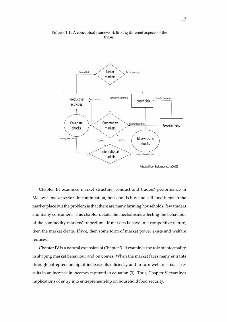
1.6 Organization and concept of the thesis

The thesis uses insights from standard general equilibrium modeling but proceeds

with simpler tractable reduced form econometric techniques. Notable literature has

followed this approach with profound results see (Donaldson and Hornbeck, 2016;

Banerjee, Duflo, and Qian, 2012; Heckman, Lochner, and Taber, 1998). Figure 1.1

summarizes the general equilibrium framework showing households, markets, ac-

tivities, expenditure links and impact pathways of shocks.

Chapter 2 examines economic disruptions, infrastructural investments, food and

nutrition linkages in Malawi. It starts with agricultural households – i.e. the house-

holds box in figure 1.2 – who engage in production using constant returns to scale

technologies. Households use factors of production comprising land, labour, man-

agerial ability or entrepreneurship and capital which takes the form of direct inputs

and public physical infrastructure.

We assume that households get factor payments from factor markets (the factor

market trapezium in figure 1.2) since they are eventual owners of factors of produc-

tion. Thus, the arrow from the factor market trapezium indicates transfer of factor

earnings to households. Of note, any disruption to the factors of production affects

factor earnings. For example a covariate shock (the left circle) such as a drought

may affect factor earnings by reducing output from the productive activities rectan-

gle and later household income. Household income is, therefore, a combination of

factor earnings albeit with varying factor income shares and transfer payments. The

dotted line from the government rectangle indicates transfer payments. Households

can then use their income to purchase food in the commodity market (the outward

going arrow from the households’ rectangle). This simplified circular flow frame-

work guides Chapter II’s assessment of impacts of covariate shocks and the role of

infrastructure to mitigate these impacts. During the analysis, we explicitly show be-

havioural equations and consumption functions that are theoretically consistent and

econometrically estimable.

17

FIGURE 1.1: A conceptual framework linking different aspects of thethesis.

Factor markets

HouseholdsProductive activities

Commodity markets

International markets

Covariate shocks

Idiosyncratic shocks

Government

Transfer paymentsConsumption spending

Value-added Factor earnings

Recurrent spending

Sales income

Imports Exports

Household level shocks

Economy wide shocks

Adapted from Breisinger et al. (2009)

Chapter III examines market structure, conduct and traders’ performance in

Malawi’s maize sector. In continuation, households buy and sell food items in the

market place but the problem is that there are many farming households, few traders

and many consumers. This chapter details the mechanisms affecting the behaviour

of the commodity markets’ trapezium. If markets behave in a competitive nature,

then the market clears. If not, then some form of market power exists and welfare

reduces.

Chapter IV is a natural extension of Chapter 3. It examines the role of informality

in shaping market behaviour and outcomes. When the market faces many entrants

through entrepreneurship, it increases its efficiency and in turn welfare – i.e. it re-

sults in an increase in incomes captured in equation (3). Thus, Chapter V examines

implications of entry into entrepreneurship on household food security.

18

During the analysis, several mechanisms drive our results, we control for demo-

graphic, community, district, rural-urban location, survey round and various forms

of endogeneity. We abstract from explicitly analyzing land and credit markets. This

provides room for further research. The last chapter summarizes the thesis and

presents policy recommendations.

19

Chapter 2

Infrastructure, extreme weather

events and food security in Malawi

2.1 Introduction

We cannot end hunger if we ignore key complementary investments that enable re-

silience to economic disruptions. Investment in public infrastructure is significantly

correlated with increased agricultural growth and welfare (Dorosh et al., 2012; Diao

and Dorosh, 2007; World Bank, 2018). Hirschmann (1958) defined social overhead

capital, hereinafter infrastructure, as resources and services which cannot be owned

privately for social and institutional reasons. Hirschmann (1958) and Uzawa (1975)

expounded that members of society may utilize the resources freely or pay some

nominal charges that are regulated by a public entity. Recently, other quasi-public

service-based structures also known as soft infrastructure are included as part of

social overhead costs (Prud’Home, 2005).

Abundance or scarcity of infrastructure may change allocation of economic re-

sources such as food by altering internal terms of trade and changing the structure of

uncertainty regarding production and factor allocation decisions in rural economies

(Platteau, 1996; World Bank, 2018). Hirschmann (1958) observed that when infras-

tructure is scarce, an increase in direct productive activities such as farming may

exert pressure on infrastructure thereby calling for an increase in its investment.

Christaller’s central place theory and Heinrich von Thünen’s model of agricultural

land use also posit that human settlements would be around places that are ade-

quately endowed with infrastructure. This way, such settlements could minimize

20

distances to access economic resources and also remove the possibility of making

excess profits due to higher transport margins — such excess profits are also known

as Thünen rents (Christaller, 1966; Getis and Getis, 1966; Von Thünen, 2009; Fischer,

2011).

In addition, Banerjee, Duflo, and Qian (2012) observed that proximity to infras-

tructure such as road networks in China had positive causal effects on per capita

Gross Domestic Product (GDP). Therefore, absence of infrastructure such as roads

or markets increase transaction costs which may limit access to economic resources

such as food by increasing prices. Taking this view, absence to infrastructure may

be an implicit tax to economically isolated individuals (Renkow, Hallstrom, and

Karanja, 2004; Nissanke and Aryeetey, 2017). A household lacking access to infras-

tructure may need to pay extra costs in time and resources to access markets making

it less competitive and more inclined to be autarkic and self-sufficient. When this

happens, as earlier reported by Uzawa (1975), it may imply that the marginal pro-

ductivity of social overhead capital is very high.

Using data from Madagascar, Minten et al. (1999) contended that longer dis-

tances to roads were rather associated with lower consumer prices. Minten et al.

(1999) argued that longer distances are associated with higher economies of scale –

making transportation of bulky commodities cheaper. This line of argument, how-

ever, only works when there is considerable connectivity. In most parts of Africa,

however, it is not so. Most bulky commodities are still transported on foot, and by

head load(Riverson, Carapetis, et al., 1991; Barwell et al., 2019). Given these issues,

non-excludable physical infrastructure can, therefore, have positive welfare effects

(Tilman, Dixit, and Levin, 2019).

Mechanisms explaining impacts of infrastructure on income distribution and

hence food security are complex. Among the complexities, Prud’Homme (2005) ob-

served that infrastructure is often viewed from the capital goods perspective rather

than the services and the institutions involved. In fact, earlier policy analysts pre-

ferred to deal with physical availability of infrastructure because monetary invest-

ments were often not available, and if available, mostly questionable. Prud’Homme

(2005) also observed that treating infrastructure by actual observation in this manner

was advantageous because it is lumpy e.g. a bridge is only useful once it is complete.

21

Quantifying effects of infrastructure on economic outcomes is also complicated

by the fact that infrastructure is long-lasting. Donaldson and Hornbeck, (2016) ob-

served that railway instalments had lasting impacts such that a counterfactual sce-

nario of removing them reduced the value of agricultural land in the United States of

America by 60%. Further, although the Roman road network has been in existence

for over two millennia, Garcia-López, Holl, and Viladecans-Marsal (2015) observed

that the investments made by the Romans of old still shape economic activity in Eu-

rope today. The findings on long lasting effects of infrastructure are also confirmed

by studies by (Palei, 2015; Goldsmith, 2014).

Noteworthy, Binswanger, Khandker, and Rosenzweig (1993) and Donaldson

(2018) argued that infrastructure is endogenous such that its placement is often in-

fluenced by region and micro-climatic specific factors. Prud’Homme (2005) also ob-

served that infrastructure is space specific. As an illustration, an irrigation project

may only be restricted to locations that are conducive for such investments making

its assignment a function of location.

Market failures, externalities, and government failure also plague infrastructural

investments (Prud’Homme, 2005). As an example of the latter, Banerjee, Duflo, and

Qian (2012), Guasch, Laffont, and Straub (2007), and Boarnet (1997) reasoned that

government administrators might have their own preferences that guide the politics

of infrastructure delivery. Such decisions result in winners and losers from infras-

tructure investments. In African agriculture, politically strategic investments that

are critical for increasing agricultural productivity and resilient livelihoods in the

long-run such as infrastructure are often not prioritized in favor of meeting immedi-

ate consumption needs of some groups in society for political expediency (Raballand

et al., 2011). Thus, any attempt to assess distributional and welfare effects of infras-

tructure must also adequately account for these sources of endogeneity.

2.1.1 The connection between infrastructure and shocks

Arezki and Sy (2016) reported that the African continent faces risky infrastructure

deficiencies which make it suffer considerable diseconomies of scale. In the absence

of proper infrastructure, effects of extreme events such as weather related shocks and

unusual price fluctuations in addition to household specific idiosyncratic shocks can

22

be deleterious. In fact, the African Development Bank (2014) reported that in Africa,

due to lack of connectivity, costs of service delivery range between 50 – 175% higher

than anywhere in the world.

Further, Arndt et al. (2012) assessed effects of climate change on economic

growth in Mozambique using a computable general equilibrium model. The study

showed that in future – 2050 in particular, climate change in form of high precipita-

tion of drought may destroy existing infrastructure thereby increasing maintenance

costs. In addition Arndt et al., (2012) also indicated that although the study showed

that shocks could reduce economic growth and increase cost of infrastructure in-

vestments, such a future should not deter investments. Noteworthy, the study was

macroeconomic level focused and did not show microeconomic adaptation and im-

pacts on consumption or income distribution.

Chinowsky et al. (2015) assessed the effects of climate change on road infrastruc-

ture in Malawi, Zambia and Mozambique between 2010 and 2050. Using a stressor-

response model under different IPCC scenarios to assess impacts of precipitation,

floods and temperature on paved and unpaved road infrastructure in Malawi, the

authors showed that climatic shocks could raise costs of construction and mainte-

nance by USD21 million discounted 2010 values in Malawi. Chinowsky et al. (2015),

however, omitted social economic impacts.

In addition, Asfaw and Maggio (2018) found that weather shocks were severe

among female headed households. The authors measured shocks as deviations

from the historical average without accurately accounting for crop output responses

which directly links to food security outcomes. Such an omission could overestimate

the actual impacts. To contribute to that inquiry, we use a more novel long term

Standardized Precipitation – Evapotranspiration Index (SPEI) (Vicente-Serrano, Be-

guería, and López-Moreno, 2010; Kubik and Maurel, 2016) drought index that ad-

justs for precipitation, potential evapo-transpiration to determine whether an event

was truly extreme at different monthly intervals. Kubik and Maurel (2016) have re-

vealed that SPEI performed much better that previous methodologies such as the

one used by Asfaw and Maggio.

Malawi has also had a recent history of combined extreme weather and economic

shocks, which due to its low infrastructural investment levels, have undermined its

23

growth prospects (World Bank, 2018). For example, during the 2015/16 agricultural

season, floods, due to extreme El Nino weather, displaced farming communities in

southern Malawi making them unable to both produce and thereafter earn income

for a living (Nation Publication, 2017). According to the Malawi Government’s De-

partment of Disaster Management Affairs (DoDMA) and United Nations Office of

the Resident Coordinator, about 87000 people were affected by floods in 2019 that

were caused by a cylone, named Idai (Government of Malawi (GoM) and United

Nations, 2019). The report showed that nearly 90000 people were displaced, infras-

tructure in form of transport networks, electricity was also destroyed.

This paper, therefore, assesses the impact of household shocks on food security in

Malawi conditional on infrastructural investments using food budget shares, Berry

and Shannon indexes of dietary variety as key dependent variables. Since some

areas are well endowed with infrastructure than others – i.e. the space specificity

of infrastructure – and some experienced extreme weather events within the time

frame, this presents a natural experiment. Therefore, we use a dose-response kind

of difference-in-difference-in-difference approach to identify the effects. That is, we

partial out the changes due to extreme weather, infrastructure and eventually time.

In a panel data setting, this adds value to the growing literature, which has

mostly relied upon cross-section data (Harttgen, Klasen, and Rischke, 2015), small

non-representative samples Harttgen, Klasen, et al., 2012 and computable general

equilibrium (CGE) models (Pauw, Dorosh, and Mazunda, 2013), by bringing evi-

dence from three waves of nationally representative surveys with a simple, theoret-

ically consistent and clearly identified methodology.

The study also triangulates the self-reported drought incidence with high-

resolution long-term gridded weather data at 0.5 × 0.5 longitude-latitude grid

cells. To further triangulate the survey data on access to infrastructure, we use re-

mote sensed Night Time light data at the same grid level as the SPEI data. To the

best of our knowledge, this study is the first to combine high-resolution data and

micro data to assess the mitigating role of infrastructure on food and nutrition secu-

rity during crises in Malawi. Combining big data and representative, country level

data enhances the precision and accuracy of impacts of shocks – which goes a long

way to achieving evidence based policy analysis.

24

The paper is structured as follows: Section 2 presents the methodology and data.

In this section we describe a micro-economic theoretical framework on which our

analysis is based. We use the theory to guide our econometric identification and es-

timation. Then we present sources of data and construction of key variables while

getting insights from literature. In section 3 we present key results of impacts of sea-

sonal shocks on household food security and impacts of community infrastructure

on food security. In Section 4 we present a discussion of key results while in section

5 we provide a summary and conclusion.

2.2 Methodology

2.2.1 Theoretical framework

Public infrastructure could help cushion the household from the impacts of eco-

nomic shocks by smoothing consumption. Following notation from Sadoulet and

De Janvry (1995), Jacoby (2000), and Liu and Henningsen (2016) with modifications,

we assume that households maximize their utility

u = u(X, C, Z, Mh) (2.1)

where X = x1, . . . , xn is a set of home produced crops, C = c1, . . . , ck is a set

of imported commodities; and Z = z1, . . . , zm is a set of other non-imported com-

modities and Mh = m1, . . . , mk is a set of household specific characteristics.

Households engage in production of crops Y = y1, . . . , yn using a well behaved

multi-input multi-output production technology that constrains utility. Thus, for a

unit of output yi the production function is

yi = f (ai, li, qi, Mp) (2.2)

where ai is land; li is labour; qi = q1, . . . , qm is a vector of inputs such as fertil-

izer; and Mp = m1, . . . , mk is a set of farm specific conditions including weather

conditions represented by SPEI.

25

We define crop prices that the households in location τ face as Px = px1 , . . . , px

n.

Due to differences in infrastructure provisioning, e.g. some communities could have

better roads, markets, electricity, among others, prices carry along transaction costs.

For instance, let pix = px

i − bh be the price the net producer household faces in the

market after considering the cost b of traveling h hours to the market. Another con-

sideration might be the case when the household faces electricity power shortages to

process their farm output for the market. Thus, if a household is a net buyer it will

face a price of pix = px

i + bh. Further, input costs are also obtained with transaction

costs, v = v + bh, where v = v1, . . . , vm is a set of input prices; w = w + bh is the

wage and r = r + bh is the land rent (Jacoby, 2000). Thus, a farm household facing

infrastructure constraints will seek to maximize returns to its productive activities

as follows

ρ( pix, w, v, r) = px ·Y− v · qi − w · (l − T)− r · ai (2.3)

which leads to a household budget constraint of the form

Px · X + Pc · C + Z ≤ px ·Y− v · qi − w · (l − T)− r · ai + Ei (2.4)

where the price of commodity Z has been normalized to 1 and Ei is any exogenous

income such as transfer payments or other income from off-farm businesses. Given

first order conditions, we get a set of demand equations X∗ = x∗1 , ..., x∗n; C∗ =

c∗1 , ..., c∗m and Z∗ = z∗1 , ..., z∗n which are functions of prices pix, pi

c, ρ( pix, w, v, r)

and E (Sadoulet and De Janvry, 1995). These demand equation give rise to the indi-

rect utility function

Ψ ( pix∗, pi

c∗, ρ( pix∗, w, v, r)) . (2.5)

Define Ω as a piece of infrastructure such as a road or market, among others1.

Constructing a good road reduces economic isolation by reducing transaction costs.

Let σh(Ω, h) = ρh( pix, w, v, r) be the income situation of the household after the

1While the use of a road infrastructure seems reductionist and overtly simplistic, it serves to makethe model didactic and readable. In practice, infrastructure services that were not captured in earlierstudies such as information, credit, banks, cooperatives, insurance trailing the social overhead capitalare included in the composite infrastructure index. Thus, the simple theoretical model could easilybe extended to other examples of infrastructure. Hirschmann (1958) observed that using roads andpower alone could account for all the other soft and hard infrastructure. During the construction ofthe composite index we will test this hypothesis.

26

infrastructure project in location τ = 1. Thus, due to changes in transaction costs,

profits, incomes and therefore demand for food commodity bundles may change

while in a location without infrastructure τ = 0 the may not (Jacoby, 2000; Jacoby

and Minten, 2008).

In addition, we define G(h, a) as the joint cumulative probability distribution

function for distance from the market and the land endowments, we can define the

social welfare function as

W(Ω, h) =∫

a

∫ h

0Ψ(

pix∗, pi

c∗, ρh( pix∗, w, v, r)

)dG(h, a). (2.6)

Differentiating the welfare function with respect to Ω gets

WΩ =∫

a

∫ h∗

0Ψ′(

pix∗, pi

c∗, ρh′Ω( pi

x∗, w, v, r))

dG(h, a). (2.7)

In this case, WΩ measures the change in welfare with respect to the infrastructural

endowment. On the other hand, if we differentiate the equation 2.7 with the Mp

variable i.e.

WΩ,Mp =∫

a

∫ h∗

0Ψ′′Mp

(pi

x∗, pic∗, ρh′′

ΩMp( pix∗, w, v, r)

)dG(h, a) ≷ 0 (2.8)

is the unknown mitigating role of infrastructure on impact of extreme weather

events.

2.2.2 Estimation

Anand and Harris (1994) and Deaton (2019) reported that food consumption indica-

tors can be used to measure welfare changes. Thus, without losing much details, we

assume that the indirect utility function can be adequately represented by food con-

sumption behaviour at household level. We can econometrically estimate the food

consumption behaviour (see Deaton (2019, Chapt. 4)) for household i in community

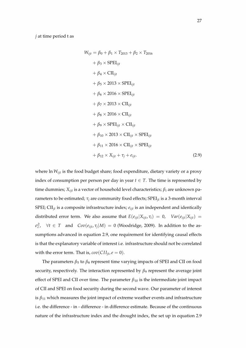
27

j at time period t as

Wijt = β0 + β1 × T2013 + β2 × T2016

+ β3 × SPEIijt

+ β4 ×CIIijt

+ β5 × 2013× SPEIijt

+ β6 × 2016× SPEIijt

+ β7 × 2013×CIIijt

+ β8 × 2016×CIIijt

+ β9 × SPEIijt ×CIIijt

+ β10 × 2013×CIIijt × SPEIijt

+ β11 × 2016×CIIijt × SPEIijt

+ β12 × Xijt + τj + eijt. (2.9)

where ln Wijt is the food budget share; food expenditure, dietary variety or a proxy

index of consumption per person per day in year t ∈ T. The time is represented by

time dummies; Xijt is a vector of household level characteristics; βi are unknown pa-

rameters to be estimated; τj are community fixed effects; SPEIjt is a 3-month interval

SPEI; CIIjt is a composite infrastructure index; eijt is an independent and identically

distributed error term. We also assume that E(eijt|Xijt, τi) = 0, Var(eijt|Xijt) =

σ2e , ∀t ∈ T and Cov(eijt, τj|M) = 0 (Woodridge, 2009). In addition to the as-

sumptions advanced in equation 2.9, one requirement for identifying causal effects

is that the explanatory variable of interest i.e. infrastructure should not be correlated

with the error term. That is, cov(CIIjt, e = 0).

The parameters β5 to β8 represent time varying impacts of SPEI and CII on food

security, respectively. The interaction represented by β9 represent the average joint

effect of SPEI and CII over time. The parameter β10 is the intermediate joint impact

of CII and SPEI on food security during the second wave. Our parameter of interest

is β11 which measures the joint impact of extreme weather events and infrastructure

i.e. the difference - in - difference - in difference estimate. Because of the continuous

nature of the infrastructure index and the drought index, the set up in equation 2.9

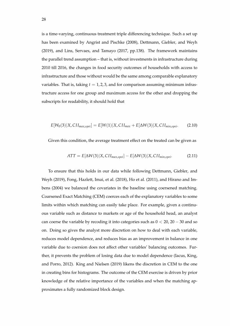
28

is a time-varying, continuous treatment triple differencing technique. Such a set up

has been examined by Angrist and Pischke (2008), Dettmann, Giebler, and Weyh

(2019), and Lins, Servaes, and Tamayo (2017, pp.138). The framework maintains

the parallel trend assumption – that is, without investments in infrastructure during

2010 till 2016, the changes in food security outcomes of households with access to

infrastructure and those without would be the same among comparable explanatory

variables. That is, taking t = 1, 2, 3, and for comparison assuming minimum infras-

tructure access for one group and maximum access for the other and dropping the

subscripts for readability, it should hold that

E[W0(3)|X, CIImax,spei] = E[W(1)|X, CIImax + E[∆W(3)|X, CIImin,spei. (2.10)

Given this condition, the average treatment effect on the treated can be given as

ATT = E[∆W(3)|X, CIImax,spei]− E[∆W(3)|X, CIImin,spei. (2.11)

To ensure that this holds in our data while following Dettmann, Giebler, and

Weyh (2019), Fong, Hazlett, Imai, et al. (2018), Ho et al. (2011), and Hirano and Im-

bens (2004) we balanced the covariates in the baseline using coersened matching.

Coarsened Exact Matching (CEM) coerces each of the explanatory variables to some

limits within which matching can easily take place. For example, given a continu-

ous variable such as distance to markets or age of the household head, an analyst

can coerse the variable by recoding it into categories such as 0 < 20, 20− 30 and so

on. Doing so gives the analyst more discretion on how to deal with each variable,

reduces model dependence, and reduces bias as an improvement in balance in one

variable due to coersion does not affect other variables’ balancing outcomes. Fur-

ther, it prevents the problem of losing data due to model dependence (Iacus, King,

and Porro, 2012). King and Nielsen (2019) likens the discretion in CEM to the one

in creating bins for histograms. The outcome of the CEM exercise is driven by prior

knowledge of the relative importance of the variables and when the matching ap-

proximates a fully randomized block design.

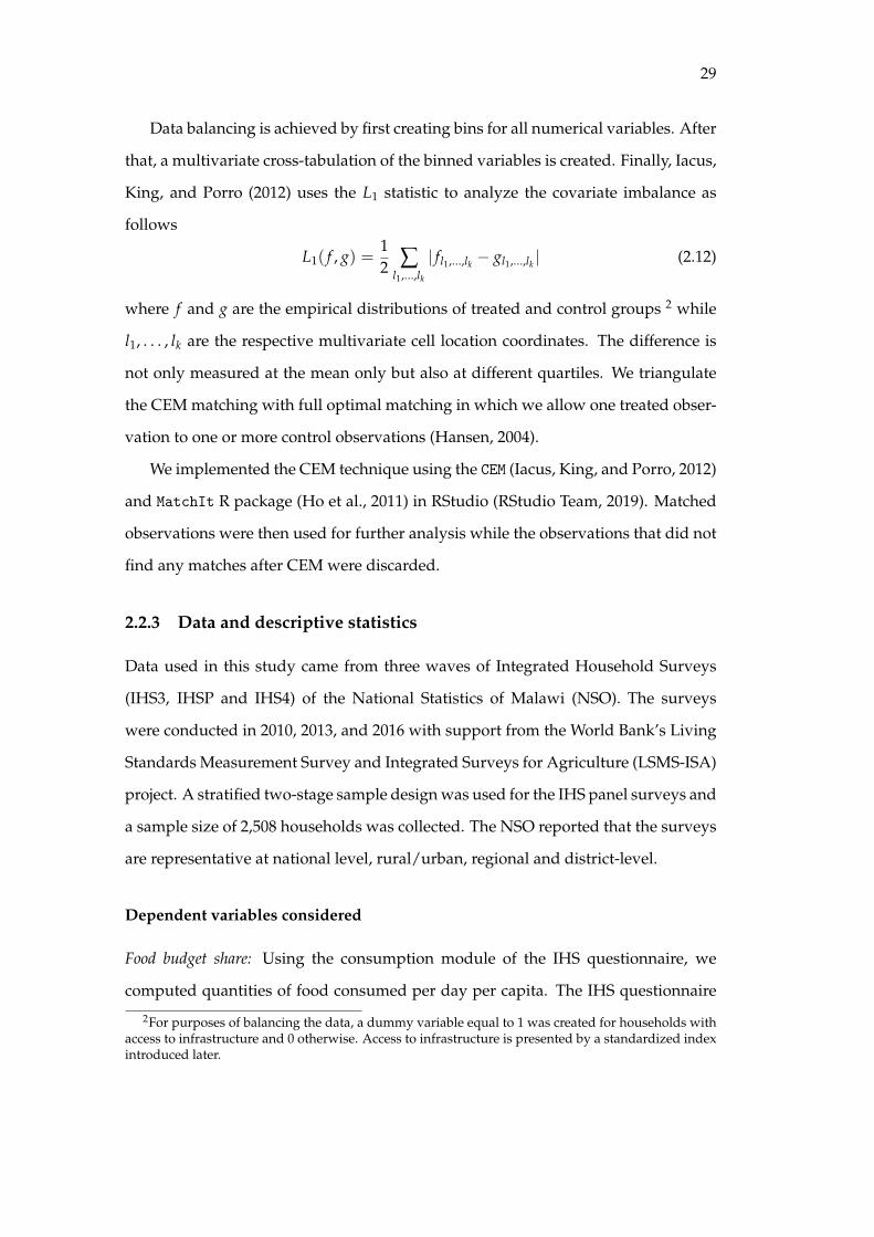
29

Data balancing is achieved by first creating bins for all numerical variables. After

that, a multivariate cross-tabulation of the binned variables is created. Finally, Iacus,

King, and Porro (2012) uses the L1 statistic to analyze the covariate imbalance as

follows

L1( f , g) =12 ∑

l1,...,lk

| fl1,...,lk − gl1,...,lk | (2.12)

where f and g are the empirical distributions of treated and control groups 2 while

l1, . . . , lk are the respective multivariate cell location coordinates. The difference is

not only measured at the mean only but also at different quartiles. We triangulate

the CEM matching with full optimal matching in which we allow one treated obser-

vation to one or more control observations (Hansen, 2004).

We implemented the CEM technique using the CEM (Iacus, King, and Porro, 2012)

and MatchIt R package (Ho et al., 2011) in RStudio (RStudio Team, 2019). Matched

observations were then used for further analysis while the observations that did not

find any matches after CEM were discarded.

2.2.3 Data and descriptive statistics

Data used in this study came from three waves of Integrated Household Surveys

(IHS3, IHSP and IHS4) of the National Statistics of Malawi (NSO). The surveys

were conducted in 2010, 2013, and 2016 with support from the World Bank’s Living

Standards Measurement Survey and Integrated Surveys for Agriculture (LSMS-ISA)

project. A stratified two-stage sample design was used for the IHS panel surveys and

a sample size of 2,508 households was collected. The NSO reported that the surveys

are representative at national level, rural/urban, regional and district-level.

Dependent variables considered

Food budget share: Using the consumption module of the IHS questionnaire, we

computed quantities of food consumed per day per capita. The IHS questionnaire

2For purposes of balancing the data, a dummy variable equal to 1 was created for households withaccess to infrastructure and 0 otherwise. Access to infrastructure is presented by a standardized indexintroduced later.

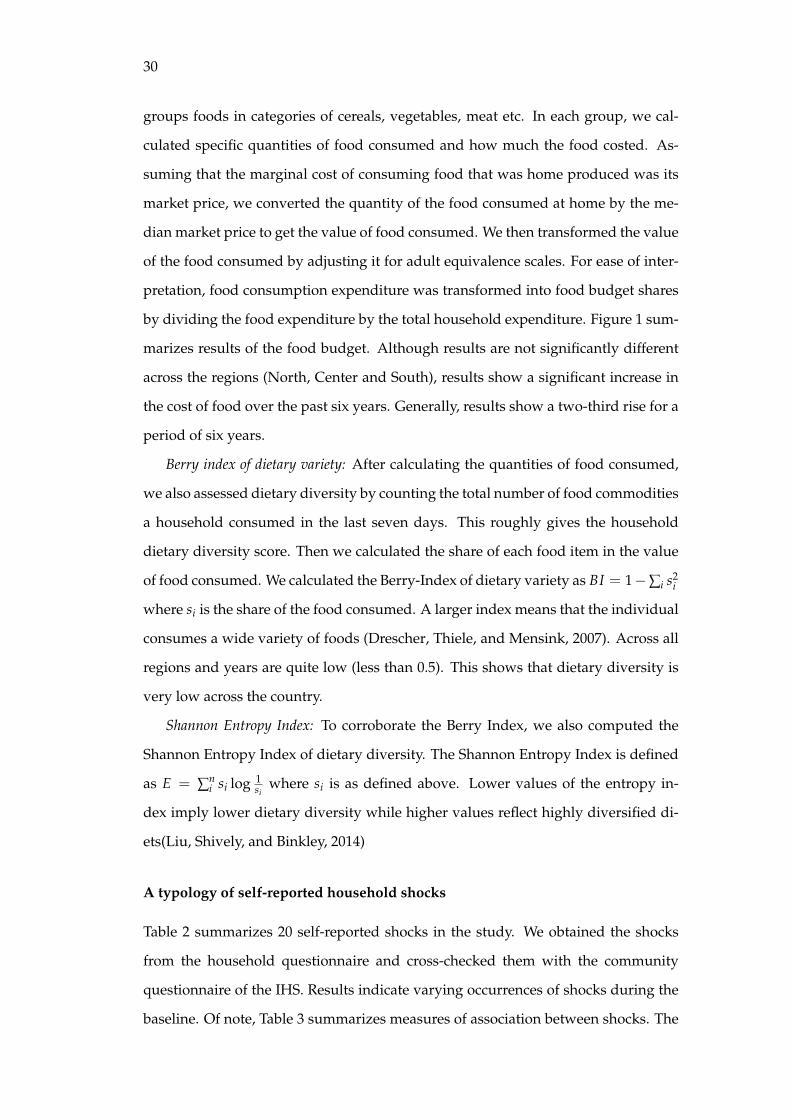
30

groups foods in categories of cereals, vegetables, meat etc. In each group, we cal-

culated specific quantities of food consumed and how much the food costed. As-

suming that the marginal cost of consuming food that was home produced was its

market price, we converted the quantity of the food consumed at home by the me-

dian market price to get the value of food consumed. We then transformed the value

of the food consumed by adjusting it for adult equivalence scales. For ease of inter-

pretation, food consumption expenditure was transformed into food budget shares

by dividing the food expenditure by the total household expenditure. Figure 1 sum-

marizes results of the food budget. Although results are not significantly different

across the regions (North, Center and South), results show a significant increase in

the cost of food over the past six years. Generally, results show a two-third rise for a

period of six years.

Berry index of dietary variety: After calculating the quantities of food consumed,

we also assessed dietary diversity by counting the total number of food commodities

a household consumed in the last seven days. This roughly gives the household

dietary diversity score. Then we calculated the share of each food item in the value

of food consumed. We calculated the Berry-Index of dietary variety as BI = 1−∑i s2i

where si is the share of the food consumed. A larger index means that the individual

consumes a wide variety of foods (Drescher, Thiele, and Mensink, 2007). Across all

regions and years are quite low (less than 0.5). This shows that dietary diversity is

very low across the country.

Shannon Entropy Index: To corroborate the Berry Index, we also computed the

Shannon Entropy Index of dietary diversity. The Shannon Entropy Index is defined

as E = ∑ni si log 1

siwhere si is as defined above. Lower values of the entropy in-

dex imply lower dietary diversity while higher values reflect highly diversified di-

ets(Liu, Shively, and Binkley, 2014)

A typology of self-reported household shocks

Table 2 summarizes 20 self-reported shocks in the study. We obtained the shocks

from the household questionnaire and cross-checked them with the community

questionnaire of the IHS. Results indicate varying occurrences of shocks during the

baseline. Of note, Table 3 summarizes measures of association between shocks. The

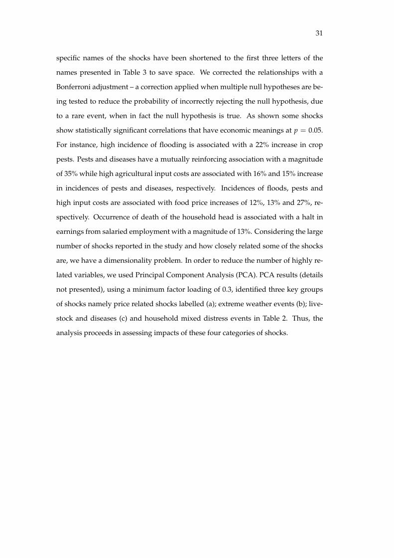
31

specific names of the shocks have been shortened to the first three letters of the

names presented in Table 3 to save space. We corrected the relationships with a

Bonferroni adjustment – a correction applied when multiple null hypotheses are be-

ing tested to reduce the probability of incorrectly rejecting the null hypothesis, due

to a rare event, when in fact the null hypothesis is true. As shown some shocks

show statistically significant correlations that have economic meanings at p = 0.05.

For instance, high incidence of flooding is associated with a 22% increase in crop

pests. Pests and diseases have a mutually reinforcing association with a magnitude

of 35% while high agricultural input costs are associated with 16% and 15% increase

in incidences of pests and diseases, respectively. Incidences of floods, pests and

high input costs are associated with food price increases of 12%, 13% and 27%, re-

spectively. Occurrence of death of the household head is associated with a halt in

earnings from salaried employment with a magnitude of 13%. Considering the large

number of shocks reported in the study and how closely related some of the shocks

are, we have a dimensionality problem. In order to reduce the number of highly re-

lated variables, we used Principal Component Analysis (PCA). PCA results (details

not presented), using a minimum factor loading of 0.3, identified three key groups

of shocks namely price related shocks labelled (a); extreme weather events (b); live-

stock and diseases (c) and household mixed distress events in Table 2. Thus, the

analysis proceeds in assessing impacts of these four categories of shocks.

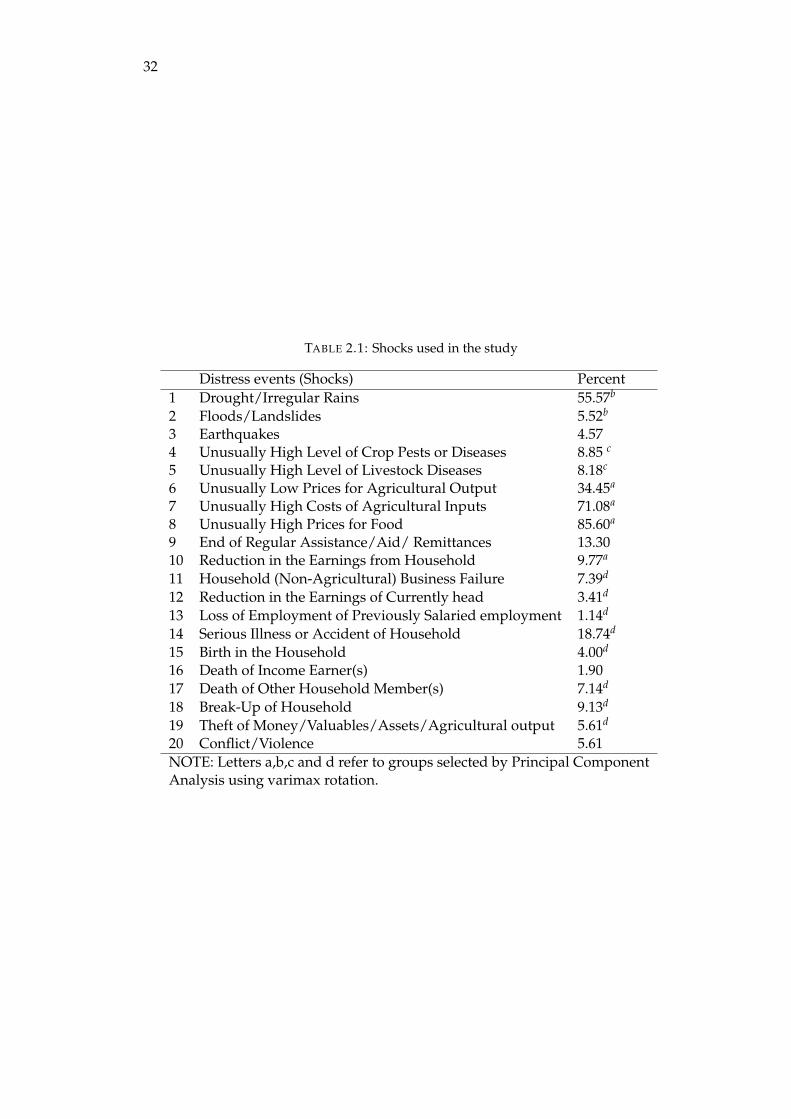
32

TABLE 2.1: Shocks used in the study

Distress events (Shocks) Percent1 Drought/Irregular Rains 55.57b

2 Floods/Landslides 5.52b

3 Earthquakes 4.574 Unusually High Level of Crop Pests or Diseases 8.85 c

5 Unusually High Level of Livestock Diseases 8.18c

6 Unusually Low Prices for Agricultural Output 34.45a

7 Unusually High Costs of Agricultural Inputs 71.08a

8 Unusually High Prices for Food 85.60a

9 End of Regular Assistance/Aid/ Remittances 13.3010 Reduction in the Earnings from Household 9.77a

11 Household (Non-Agricultural) Business Failure 7.39d

12 Reduction in the Earnings of Currently head 3.41d

13 Loss of Employment of Previously Salaried employment 1.14d

14 Serious Illness or Accident of Household 18.74d

15 Birth in the Household 4.00d

16 Death of Income Earner(s) 1.9017 Death of Other Household Member(s) 7.14d

18 Break-Up of Household 9.13d

19 Theft of Money/Valuables/Assets/Agricultural output 5.61d

20 Conflict/Violence 5.61NOTE: Letters a,b,c and d refer to groups selected by Principal ComponentAnalysis using varimax rotation.

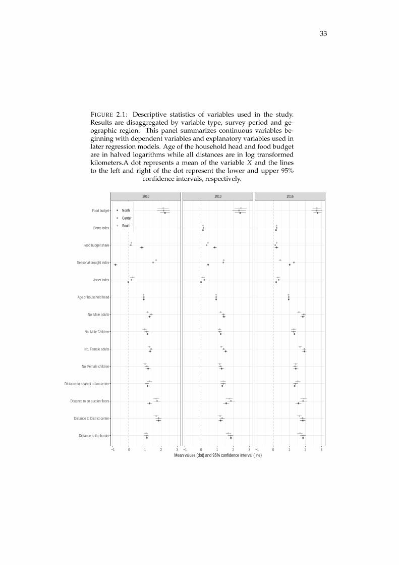
33

FIGURE 2.1: Descriptive statistics of variables used in the study.Results are disaggregated by variable type, survey period and ge-ographic region. This panel summarizes continuous variables be-ginning with dependent variables and explanatory variables used inlater regression models. Age of the household head and food budgetare in halved logarithms while all distances are in log transformedkilometers.A dot represents a mean of the variable X and the linesto the left and right of the dot represent the lower and upper 95%

confidence intervals, respectively.

2010 2013 2016

−1 0 1 2 3 −1 0 1 2 3 −1 0 1 2 3

Distance to the border

Distance to District center

Distance to an auction floors

Distance to nearest urban center

No. Female children

No. Female adults

No. Male Children

No. Male adults

Age of household head

Asset index

Seasonal drought index

Food budget share

Berry Index

Food budget

Mean values (dot) and 95% confidence interval (line)

North

Center

South

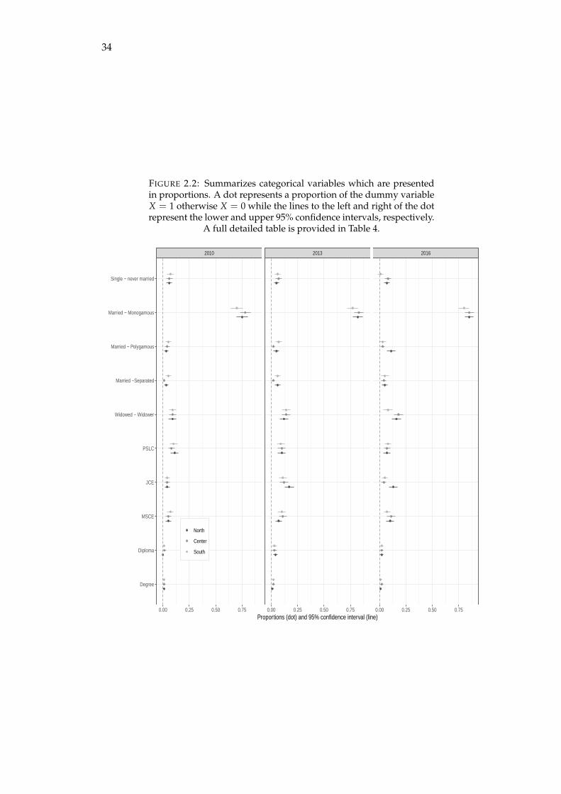
34

FIGURE 2.2: Summarizes categorical variables which are presentedin proportions. A dot represents a proportion of the dummy variableX = 1 otherwise X = 0 while the lines to the left and right of the dotrepresent the lower and upper 95% confidence intervals, respectively.

A full detailed table is provided in Table 4.

2010 2013 2016

0.00 0.25 0.50 0.75 0.00 0.25 0.50 0.75 0.00 0.25 0.50 0.75

Degree

Diploma

MSCE

JCE

PSLC

Widowed − Widower

Married −Separated

Married − Polygamous

Married − Monogamous

Single − never married

Proportions (dot) and 95% confidence interval (line)

North

Center

South

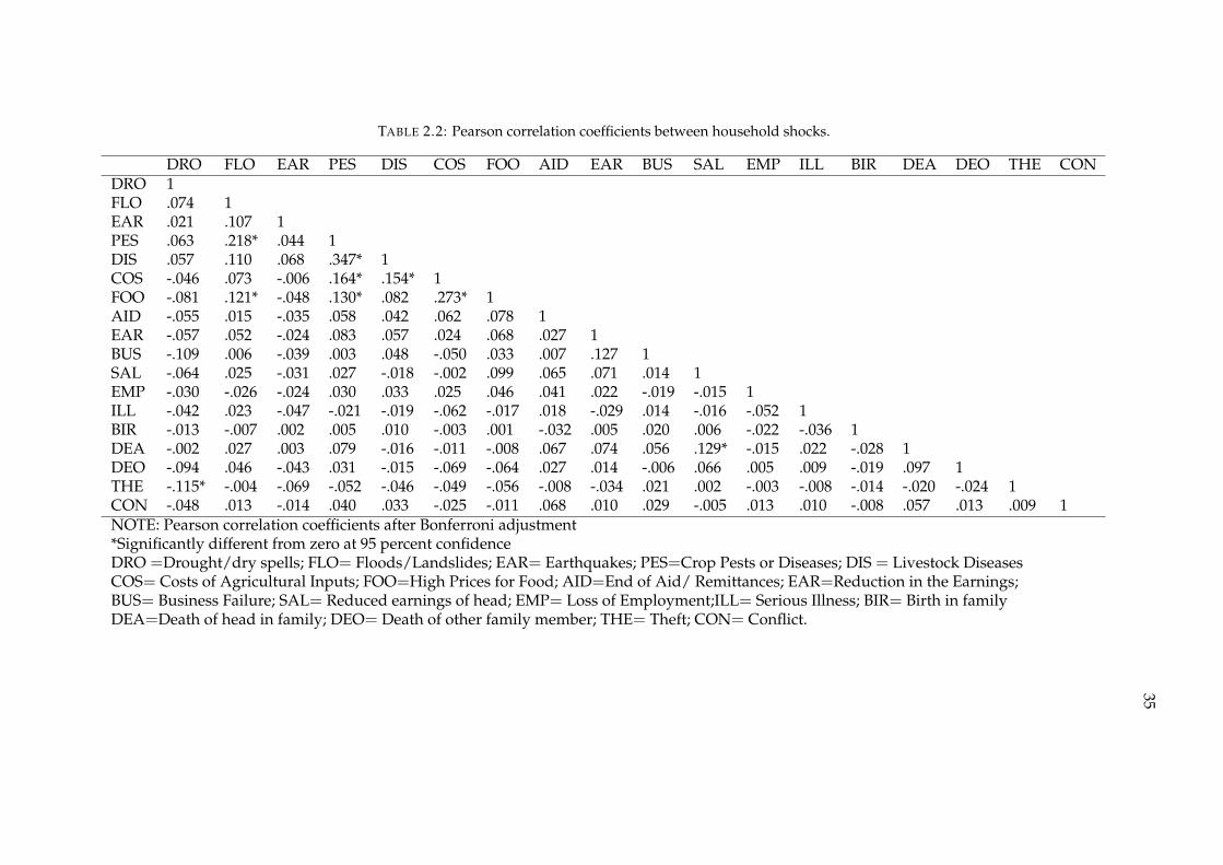
35

TABLE 2.2: Pearson correlation coefficients between household shocks.

DRO FLO EAR PES DIS COS FOO AID EAR BUS SAL EMP ILL BIR DEA DEO THE CONDRO 1FLO .074 1EAR .021 .107 1PES .063 .218* .044 1DIS .057 .110 .068 .347* 1COS -.046 .073 -.006 .164* .154* 1FOO -.081 .121* -.048 .130* .082 .273* 1AID -.055 .015 -.035 .058 .042 .062 .078 1EAR -.057 .052 -.024 .083 .057 .024 .068 .027 1BUS -.109 .006 -.039 .003 .048 -.050 .033 .007 .127 1SAL -.064 .025 -.031 .027 -.018 -.002 .099 .065 .071 .014 1EMP -.030 -.026 -.024 .030 .033 .025 .046 .041 .022 -.019 -.015 1ILL -.042 .023 -.047 -.021 -.019 -.062 -.017 .018 -.029 .014 -.016 -.052 1BIR -.013 -.007 .002 .005 .010 -.003 .001 -.032 .005 .020 .006 -.022 -.036 1DEA -.002 .027 .003 .079 -.016 -.011 -.008 .067 .074 .056 .129* -.015 .022 -.028 1DEO -.094 .046 -.043 .031 -.015 -.069 -.064 .027 .014 -.006 .066 .005 .009 -.019 .097 1THE -.115* -.004 -.069 -.052 -.046 -.049 -.056 -.008 -.034 .021 .002 -.003 -.008 -.014 -.020 -.024 1CON -.048 .013 -.014 .040 .033 -.025 -.011 .068 .010 .029 -.005 .013 .010 -.008 .057 .013 .009 1NOTE: Pearson correlation coefficients after Bonferroni adjustment*Significantly different from zero at 95 percent confidenceDRO =Drought/dry spells; FLO= Floods/Landslides; EAR= Earthquakes; PES=Crop Pests or Diseases; DIS = Livestock DiseasesCOS= Costs of Agricultural Inputs; FOO=High Prices for Food; AID=End of Aid/ Remittances; EAR=Reduction in the Earnings;BUS= Business Failure; SAL= Reduced earnings of head; EMP= Loss of Employment;ILL= Serious Illness; BIR= Birth in familyDEA=Death of head in family; DEO= Death of other family member; THE= Theft; CON= Conflict.

36

Seasonal drought and floods

The IHS data is geo-referenced. We therefore use the GPS coordinates from the sur-

vey and map them on a global Standardized Precipitation-Evapotranspiration Index,

which provides near real-time data on drought conditions with a 0.5 × 0.5, longi-

tude by latitude spatial resolution and a monthly resolution of up to 48 months.

The SPEI index uses Vicente-Serrano et al. (2010) method of calculating deviations

from the mean water balance. Thus, the SPEI calculates drought condition by taking

precipitation subtracting potential evapotranspiration. This method is better than

other methods because it accounts for two important aspects of drought conditions

namely rainfall and temperature conditions which are essential for crop production.

Since the data collection covers the entire year, we use the December to March pe-

riod as a measure of the rain season. Since the historical SPEI is standardized, with

mean zero and standard deviation of one, positive values will refer to high precipi-

tation while negative values will mean dry spells. In general, Malawi covers 16 full

0.5 × 0.5 longitude by latitude spatial resolution (figure 3) which also cover its 8

agro-ecological zones which contain 21 meteorological Stations.

With the exception of the northern region in IHS3, results presented in Figure

1 indicate that, as a country, Malawi experiences a sufficiently wetter agricultural

season. This is evidenced by all mean seasonal drought index values lying to the

right of the zero dotted line across all years. Few districts in the North experienced

some dry spells during the 2010 and 2013 growing season. Importantly, results in-

dicate that seasonal drought incidence varied widely across the country and over

the three survey periods. F-test comparison of means (represented by an asterisk in

Figure 1) shows that seasonal drought conditions were significantly different across

the survey periods (p < 0.01) and also across the regions (p < 0.01).

Infrastructure availability

We obtained infrastructure data from the IHS surveys and US National Oceanic

and Atmospheric Administration. We used the Defense-Meteorological Satellite

Program-Optical Line Scanner (DMSP-OLS) Night Time Light (NTL) data gathered

by NOAA and NASA’s polar orbiting satellites that take pictures which cover the

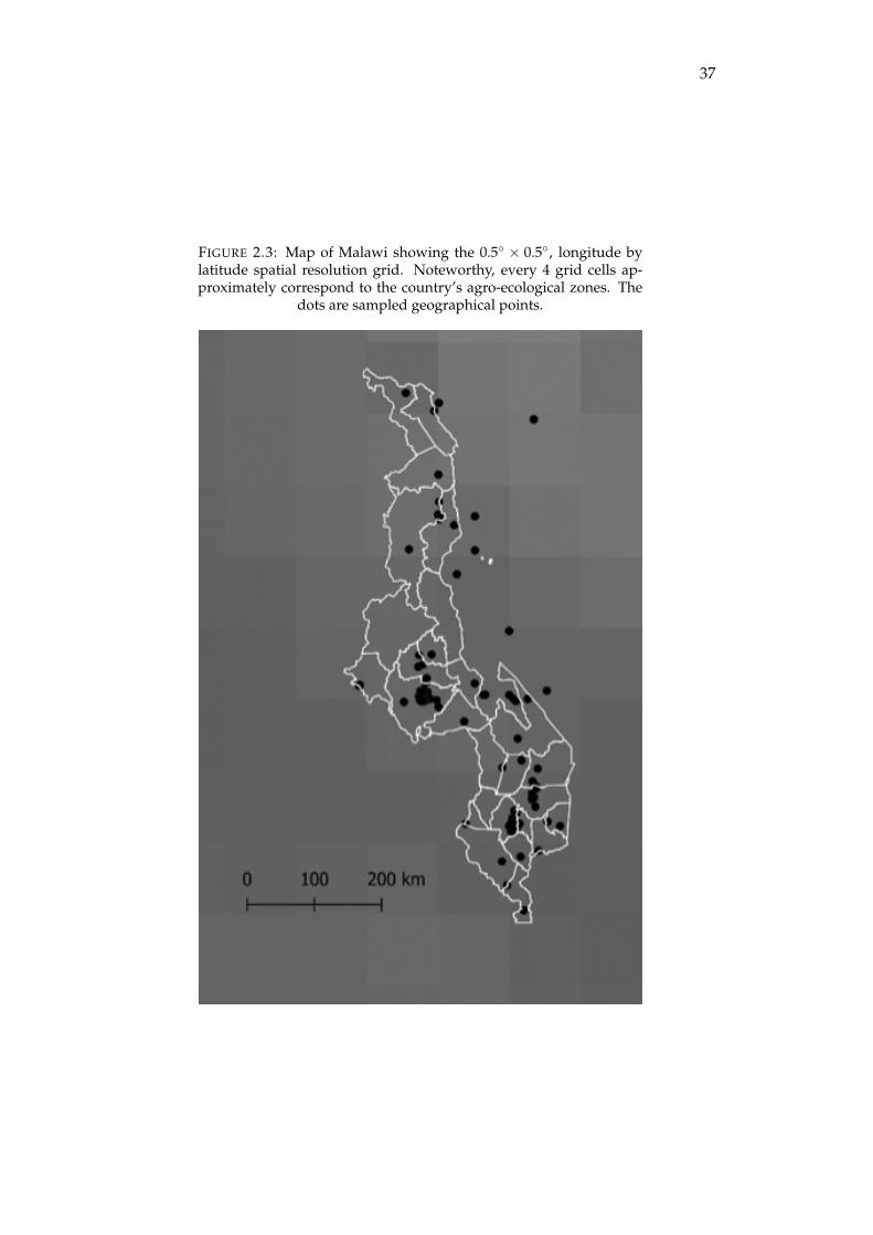
37

FIGURE 2.3: Map of Malawi showing the 0.5 × 0.5, longitude bylatitude spatial resolution grid. Noteworthy, every 4 grid cells ap-proximately correspond to the country’s agro-ecological zones. The

dots are sampled geographical points.

38

entire earth twice per day. The data is presented in form of raster images. The data

presents points illuminated by electricity across the planet in form of near infra-red

radiance. The data is presented in two spatial resolution modes namely full resolu-

tion and smoothed data. We used the smoothed data which was constructed using

a nominal spatial resolution of 2.7 km at 30 arc-seconds, covering 180W to 180E

longitude and 75N to 65S latitude.

Using QGIS 3.6, we extracted a portion of the data corresponding to latitude

−1315′4.38”S and longitude 3418′5.50”E which is the location of Malawi. We ex-

tracted raster values to points corresponding to our survey coordinates at a given

time using QGIS’s processing toolbox. We standardized the radiance such that neg-

ative standard deviations would imply very low lights and positive standard devi-

ations implying availability of light. Radiance greater than or equal to zero meant

that the sample geographic point had electric light and if it was below zero, it did

not.

Community leaders, through the community questionnaire, and respondents at

household level (household questionnaire) reported on the existence of different

types and quality of infrastructure. Further, the enumerators also measured ge-

ographic distances a household was from infrastructural resources such as roads,

markets etc.

Following Christaller’s Central Place theory (Christaller, 1966; Getis and Getis,

1966; Von Thünen, 2009), we measure access to infrastructure as the geographic dis-

tance in kilometers from the center of the district, market, clinic, bank, safe water

amenities and savings and credit cooperation.

Factor analysis based on maximum likelihood was used to extract a composite

infrastructure index using the factanal package in R statistical package. The fac-

tor analysis created a linear combination of the factors in order to identify variables

that explain the underlying structure behind the data. Table shows the three factors

that were extracted from the factor analysis. The factors are independent from each

other. That is, a varimax rotation, which gets orthogonal factors, was used as op-

posed to promax, which provides correlated factors. Factor 1, which is the main fac-

tor, generally shows positive correlations with increasing distances to key hard and

soft infrastructure and is negatively associated with presence of night time lights.

39

Thus, in interpretation we can state that it measures infrastructure inaccessibility or

remoteness to key infrastructure. Since this first factor accounted for most of the

variation in the data (> 0.6), we used it as an indicator of access to infrastructure.

To ease interpretation, we scaled the factor scores to range between 0 and 1 where

0 means that a household had full access to infrastructure and 1 means it is further

away from infrastructure3

Figure 2.5 presents a visual graphic of the factors. Factor 1 is shown on the x-

axis while factor 2 is shown in the y-axis of panel A while factor 3 is shown on

the y-axis of panel B. The results show only factors with significant factor loadings

with correlations of greater than 0.1. Generally, variables namely electricity, distance

to a savings and credit cooperation, ADMARC and the auction floors have high

loadings. Consistent with our guiding theoretical framework, the composite infras-

tructure index (factor 1) shows that remoteness to a main road is associated with

no access to electricity, input, commodity, and financial markets. Also consistent

with Hirschman’s hypothesis these results demonstrate that a road is a precursor

for electricity and soft infrastructure. Thus, our theoretical model’s focus on road

infrastructure as a didactic working model for overall infrastructure is justified. Fac-

tor 2 just features remoteness to central locations, as demonstrated by distances from

the center, which is consistent with Christaller’s central place theory. Factor 3 sum-

marizes access to financial markets since roads, and all financial market indicators

have high factor loadings.

Household characteristics

Figure 1, panel A presents household and community characteristics. A general

pattern shows that both household and community characteristics did not change

much across the regions and also over the subsequent surveys.

Asset index: We calculated an asset index using principle component analysis by

examining the availability at household level (Harttgen and Vollmer, 2013). Using

3Composite Infrastructure Index (CII) was scaled as follows to ease interpretation i.e. 0 ≤ CII ≤ 1.Thus,

CII =Xi −MinXi

MaxXi −MinXi.

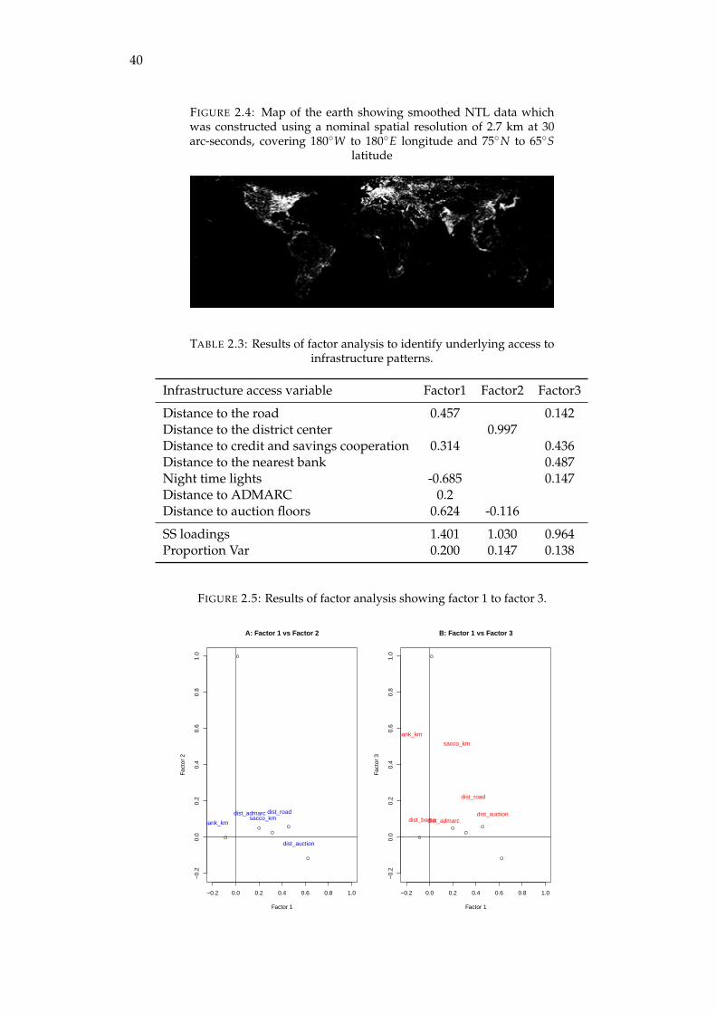
40

FIGURE 2.4: Map of the earth showing smoothed NTL data whichwas constructed using a nominal spatial resolution of 2.7 km at 30arc-seconds, covering 180W to 180E longitude and 75N to 65S

latitude

TABLE 2.3: Results of factor analysis to identify underlying access toinfrastructure patterns.

Infrastructure access variable Factor1 Factor2 Factor3

Distance to the road 0.457 0.142Distance to the district center 0.997Distance to credit and savings cooperation 0.314 0.436Distance to the nearest bank 0.487Night time lights -0.685 0.147Distance to ADMARC 0.2Distance to auction floors 0.624 -0.116

SS loadings 1.401 1.030 0.964Proportion Var 0.200 0.147 0.138

FIGURE 2.5: Results of factor analysis showing factor 1 to factor 3.

−0.2 0.0 0.2 0.4 0.6 0.8 1.0

−0.

20.

00.

20.

40.

60.

81.

0

A: Factor 1 vs Factor 2

Factor 1

Fact

or 2

dist_road

dist_boma

sacco_kmbank_km

dist_admarc

dist_auction

−0.2 0.0 0.2 0.4 0.6 0.8 1.0

−0.

20.

00.

20.

40.

60.

81.

0

B: Factor 1 vs Factor 3

Factor 1

Fact

or 3

dist_road

dist_boma

sacco_km

bank_km

ntl

dist_admarcdist_auction

41

a varimax rotation procedure, we used the component that explained a lot of varia-

tion in the data. Results show no significant changes in the asset index the number

of households with access to irrigation schemes (17%) between 2010 and 2013 but

show a 21-percentage point increase in 2016. However, we notice regional varia-

tions within surveys across regions.

Age of the household head: The average age of the household head in the 2016 sur-

vey was 46. Although we find statistically significant (p < 0.01) results for equality

of means, substantively, the ages do not differ much across the regions. Table 2 sup-

plements Figure 1 and shows that, indeed, the age of the household head does not

change much.

Number of male and female adults and children: Food security is a function of house-

hold composition and gender dynamics. Kennedy and Peters (1992) presents the

oldest reference to gender food security linkage. The study argues that that house-

holds in which women have more discretionary power over expenditure decisions

had better child and overall household nutrition outcomes. Kassie, Ndiritu, and

Stage (2014) however found that female headed households had less food security

outcomes. From a resource needs perspective, a household having more children re-

quires a more nutritionally diverse food consumption bundle that a household that

only has adults. Further, from an econometric perspective, an interaction of time

variant and invariant characteristics makes evaluation of the gender inequality gap

much easier to track. Results show that the distribution of the sexes is between one

and two. A simple count shows that an average household has between two and

five individuals regardless of sex.

Marital status: Panel B of figure 1 summarizes the marital status of the house-

hold. Continuing with the argument from Kennedy and Peters (1992) and Kassie,

Ndiritu, and Stage (2014), the need to account for marital status follows naturally.

Households for single individuals who have never married could have much lower

food security requirements compared to households with married and more diverse

compositions. Results summarized in figure 1 show that the majority of households

were married and monogamous, accounting for about 75% of the sample observa-

tions in 2010. The number proportion increased to 83% in both 2013 and 2016 but

with much variation across the regions. In a similar manner results for the other

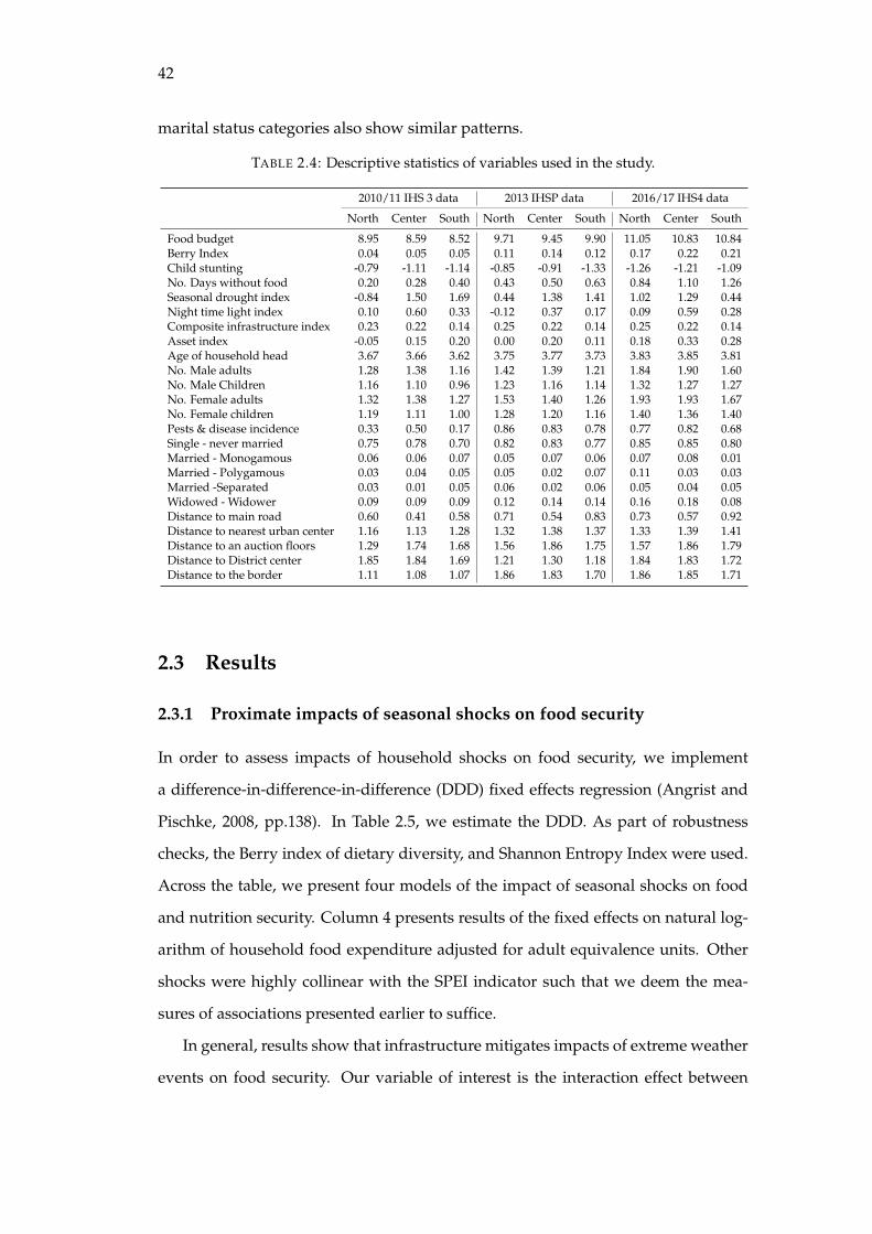
42

marital status categories also show similar patterns.

TABLE 2.4: Descriptive statistics of variables used in the study.

2010/11 IHS 3 data 2013 IHSP data 2016/17 IHS4 data

North Center South North Center South North Center South

Food budget 8.95 8.59 8.52 9.71 9.45 9.90 11.05 10.83 10.84Berry Index 0.04 0.05 0.05 0.11 0.14 0.12 0.17 0.22 0.21Child stunting -0.79 -1.11 -1.14 -0.85 -0.91 -1.33 -1.26 -1.21 -1.09No. Days without food 0.20 0.28 0.40 0.43 0.50 0.63 0.84 1.10 1.26Seasonal drought index -0.84 1.50 1.69 0.44 1.38 1.41 1.02 1.29 0.44Night time light index 0.10 0.60 0.33 -0.12 0.37 0.17 0.09 0.59 0.28Composite infrastructure index 0.23 0.22 0.14 0.25 0.22 0.14 0.25 0.22 0.14Asset index -0.05 0.15 0.20 0.00 0.20 0.11 0.18 0.33 0.28Age of household head 3.67 3.66 3.62 3.75 3.77 3.73 3.83 3.85 3.81No. Male adults 1.28 1.38 1.16 1.42 1.39 1.21 1.84 1.90 1.60No. Male Children 1.16 1.10 0.96 1.23 1.16 1.14 1.32 1.27 1.27No. Female adults 1.32 1.38 1.27 1.53 1.40 1.26 1.93 1.93 1.67No. Female children 1.19 1.11 1.00 1.28 1.20 1.16 1.40 1.36 1.40Pests & disease incidence 0.33 0.50 0.17 0.86 0.83 0.78 0.77 0.82 0.68Single - never married 0.75 0.78 0.70 0.82 0.83 0.77 0.85 0.85 0.80Married - Monogamous 0.06 0.06 0.07 0.05 0.07 0.06 0.07 0.08 0.01Married - Polygamous 0.03 0.04 0.05 0.05 0.02 0.07 0.11 0.03 0.03Married -Separated 0.03 0.01 0.05 0.06 0.02 0.06 0.05 0.04 0.05Widowed - Widower 0.09 0.09 0.09 0.12 0.14 0.14 0.16 0.18 0.08Distance to main road 0.60 0.41 0.58 0.71 0.54 0.83 0.73 0.57 0.92Distance to nearest urban center 1.16 1.13 1.28 1.32 1.38 1.37 1.33 1.39 1.41Distance to an auction floors 1.29 1.74 1.68 1.56 1.86 1.75 1.57 1.86 1.79Distance to District center 1.85 1.84 1.69 1.21 1.30 1.18 1.84 1.83 1.72Distance to the border 1.11 1.08 1.07 1.86 1.83 1.70 1.86 1.85 1.71

2.3 Results

2.3.1 Proximate impacts of seasonal shocks on food security

In order to assess impacts of household shocks on food security, we implement

a difference-in-difference-in-difference (DDD) fixed effects regression (Angrist and

Pischke, 2008, pp.138). In Table 2.5, we estimate the DDD. As part of robustness

checks, the Berry index of dietary diversity, and Shannon Entropy Index were used.

Across the table, we present four models of the impact of seasonal shocks on food

and nutrition security. Column 4 presents results of the fixed effects on natural log-

arithm of household food expenditure adjusted for adult equivalence units. Other

shocks were highly collinear with the SPEI indicator such that we deem the mea-

sures of associations presented earlier to suffice.

In general, results show that infrastructure mitigates impacts of extreme weather

events on food security. Our variable of interest is the interaction effect between

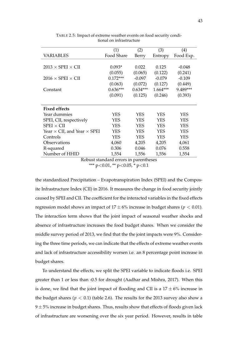
43

TABLE 2.5: Impact of extreme weather events on food security condi-tional on infrastructure

(1) (2) (3) (4)VARIABLES Food Share Berry Entropy Food Exp.

2013 × SPEI × CII 0.093* 0.022 0.125 -0.048(0.055) (0.065) (0.122) (0.241)

2016 × SPEI × CII 0.172*** -0.097 -0.079 -0.109(0.063) (0.072) (0.127) (0.449)

Constant 0.636*** 0.634*** 1.664*** 9.489***(0.091) (0.125) (0.246) (0.393)

Fixed effectsYear dummies YES YES YES YESSPEI, CII, respectively YES YES YES YESSPEI × CII YES YES YES YESYear × CII, and Year × SPEI YES YES YES YESControls YES YES YES YESObservations 4,060 4,205 4,205 4,061R-squared 0.306 0.046 0.076 0.558Number of HHID 1,554 1,556 1,556 1,554

Robust standard errors in parentheses*** p<0.01, ** p<0.05, * p<0.1

the standardized Precipitation – Evapotranspiration Index (SPEI) and the Compos-

ite Infrastructure Index (CII) in 2016. It measures the change in food security jointly

caused by SPEI and CII. The coefficient for the interacted variables in the fixed effects

regression model shows an impact of 17± 6% increase in budget shares (p < 0.01).

The interaction term shows that the joint impact of seasonal weather shocks and

absence of infrastructure increases the food budget shares. When we consider the

middle survey period of 2013, we find that the the joint impacts were 9%. Consider-

ing the three time periods, we can indicate that the effects of extreme weather events

and lack of infrastructure accessibility worsen i.e. an 8 percentage point increase in

budget shares.

To understand the effects, we split the SPEI variable to indicate floods i.e. SPEI

greater than 1 or less than -0.5 for drought (Aadhar and Mishra, 2017). When this

is done, we find that the joint impact of flooding and CII is a 17± 6% increase in

the budget shares (p < 0.1) (table 2.6). The results for the 2013 survey also show a

9± 5% increase in budget shares. Thus, results show that effects of floods given lack

of infrastructure are worsening over the six year period. However, results in table

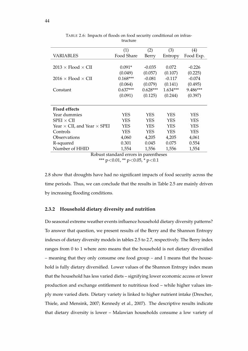
44

TABLE 2.6: Impacts of floods on food security conditional on infras-tructure

(1) (2) (3) (4)VARIABLES Food Share Berry Entropy Food Exp.

2013 × Flood × CII 0.091* -0.035 0.072 -0.226(0.049) (0.057) (0.107) (0.225)

2016 × Flood × CII 0.168*** -0.081 -0.117 -0.074(0.064) (0.079) (0.141) (0.495)

Constant 0.637*** 0.628*** 1.634*** 9.486***(0.091) (0.125) (0.244) (0.397)

Fixed effectsYear dummies YES YES YES YESSPEI × CII YES YES YES YESYear × CII, and Year × SPEI YES YES YES YESControls YES YES YES YESObservations 4,060 4,205 4,205 4,061R-squared 0.301 0.045 0.075 0.554Number of HHID 1,554 1,556 1,556 1,554

Robust standard errors in parentheses*** p<0.01, ** p<0.05, * p<0.1

2.8 show that droughts have had no significant impacts of food security across the

time periods. Thus, we can conclude that the results in Table 2.5 are mainly driven

by increasing flooding conditions.

2.3.2 Household dietary diversity and nutrition

Do seasonal extreme weather events influence household dietary diversity patterns?

To answer that question, we present results of the Berry and the Shannon Entropy

indexes of dietary diversity models in tables 2.5 to 2.7, respectively. The Berry index

ranges from 0 to 1 where zero means that the household is not dietary diversified

– meaning that they only consume one food group – and 1 means that the house-

hold is fully dietary diversified. Lower values of the Shannon Entropy index mean

that the household has less varied diets – signifying lower economic access or lower

production and exchange entitlement to nutritious food – while higher values im-

ply more varied diets. Dietary variety is linked to higher nutrient intake (Drescher,

Thiele, and Mensink, 2007; Kennedy et al., 2007). The descriptive results indicate

that dietary diversity is lower – Malawian households consume a low variety of

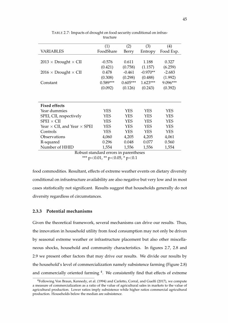
45

TABLE 2.7: Impacts of drought on food security conditional on infras-tructure

(1) (2) (3) (4)VARIABLES FoodShare Berry Entropy Food Exp.

2013 × Drought × CII -0.576 0.611 1.188 0.327(0.421) (0.758) (1.157) (6.259)

2016 × Drought × CII 0.478 -0.461 -0.970** -2.683(0.308) (0.298) (0.488) (1.992)

Constant 0.589*** 0.605*** 1.623*** 9.096***(0.092) (0.126) (0.243) (0.392)

Fixed effectsYear dummies YES YES YES YESSPEI, CII, respectively YES YES YES YESSPEI × CII YES YES YES YESYear × CII, and Year × SPEI YES YES YES YESControls YES YES YES YESObservations 4,060 4,205 4,205 4,061R-squared 0.296 0.048 0.077 0.560Number of HHID 1,554 1,556 1,556 1,554

Robust standard errors in parentheses*** p<0.01, ** p<0.05, * p<0.1

food commodities. Resultant, effects of extreme weather events on dietary diversity

conditional on infrastructure availability are also negative but very low and in most

cases statistically not significant. Results suggest that households generally do not

diversity regardless of circumstances.

2.3.3 Potential mechanisms

Given the theoretical framework, several mechanisms can drive our results. Thus,

the innovation in household utility from food consumption may not only be driven

by seasonal extreme weather or infrastructure placement but also other miscella-

neous shocks, household and community characteristics. In figures 2.7, 2.8 and

2.9 we present other factors that may drive our results. We divide our results by

the household’s level of commercialization namely subsistence farming (Figure 2.8)

and commercially oriented farming 4. We consistently find that effects of extreme

4Following Von Braun, Kennedy, et al. (1994) and Carletto, Corral, and Guelfi (2017), we computea measure of commercialization as a ratio of the value of agricultural sales in markets to the value ofagricultural production. Lower ratios imply subsistence while higher ratios commercial agriculturalproduction. Households below the median are subsistence.

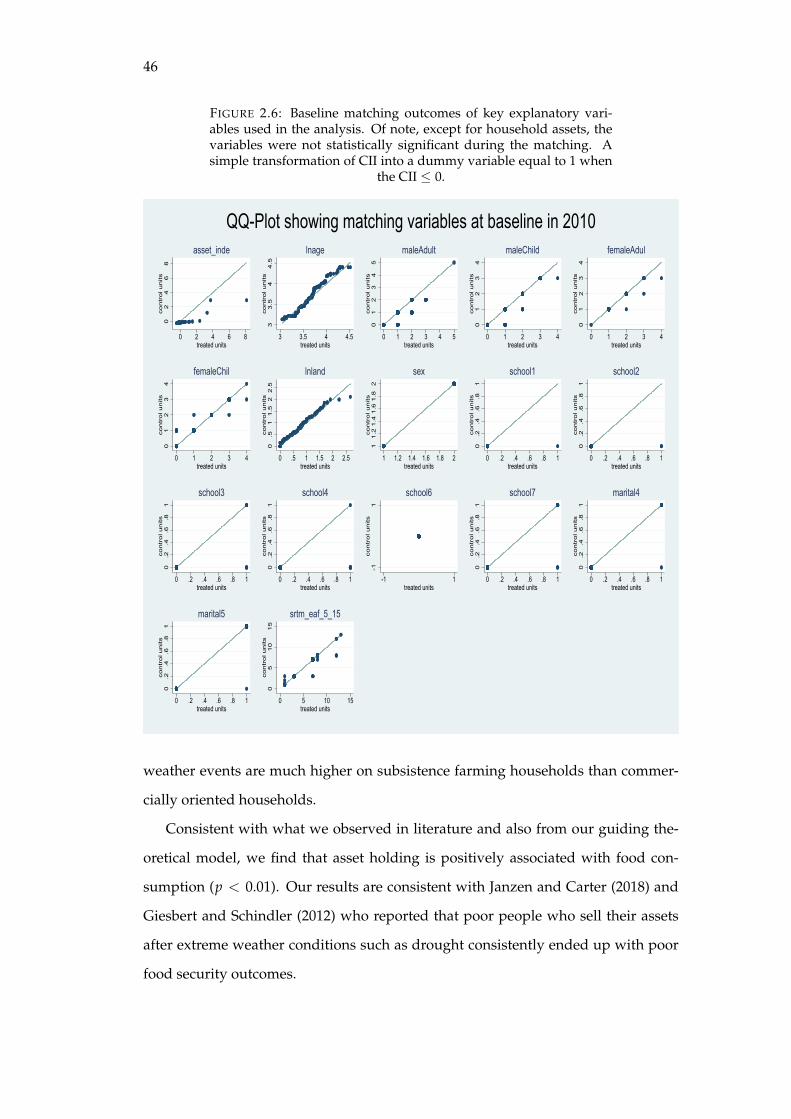
46

FIGURE 2.6: Baseline matching outcomes of key explanatory vari-ables used in the analysis. Of note, except for household assets, thevariables were not statistically significant during the matching. Asimple transformation of CII into a dummy variable equal to 1 when

the CII ≤ 0.0

24

68

co

ntr

ol u

nits

0 2 4 6 8treated units

asset_inde3

3.5

44

.5co

ntr

ol u

nits

3 3.5 4 4.5treated units

lnage

01

23

45

co

ntr

ol u

nits

0 1 2 3 4 5treated units

maleAdult

01

23

4co

ntr

ol u

nits

0 1 2 3 4treated units

maleChild

01

23

4co

ntr

ol u

nits

0 1 2 3 4treated units

femaleAdul

01

23

4co

ntr

ol u

nits

0 1 2 3 4treated units

femaleChil

0.5

11

.52

2.5

co

ntr

ol u

nits

0 .5 1 1.5 2 2.5treated units

lnland1

1.2

1.4

1.6

1.8

2co

ntr

ol u

nits

1 1.2 1.4 1.6 1.8 2treated units

sex

0.2

.4.6

.81

co

ntr

ol u

nits

0 .2 .4 .6 .8 1treated units

school1

0.2

.4.6

.81

co

ntr

ol u

nits

0 .2 .4 .6 .8 1treated units

school2

0.2

.4.6

.81

co

ntr

ol u

nits

0 .2 .4 .6 .8 1treated units

school3

0.2

.4.6

.81

co

ntr

ol u

nits

0 .2 .4 .6 .8 1treated units

school4

-11

co

ntr

ol u

nits

-1 1treated units

school6

0.2

.4.6

.81

co

ntr

ol u

nits

0 .2 .4 .6 .8 1treated units

school7

0.2

.4.6

.81

co

ntr

ol u

nits

0 .2 .4 .6 .8 1treated units

marital4

0.2

.4.6

.81

co

ntr

ol u

nits

0 .2 .4 .6 .8 1treated units

marital5

05

10

15

co

ntr

ol u

nits

0 5 10 15treated units

srtm_eaf_5_15

QQ-Plot showing matching variables at baseline in 2010

weather events are much higher on subsistence farming households than commer-

cially oriented households.

Consistent with what we observed in literature and also from our guiding the-

oretical model, we find that asset holding is positively associated with food con-

sumption (p < 0.01). Our results are consistent with Janzen and Carter (2018) and

Giesbert and Schindler (2012) who reported that poor people who sell their assets

after extreme weather conditions such as drought consistently ended up with poor

food security outcomes.

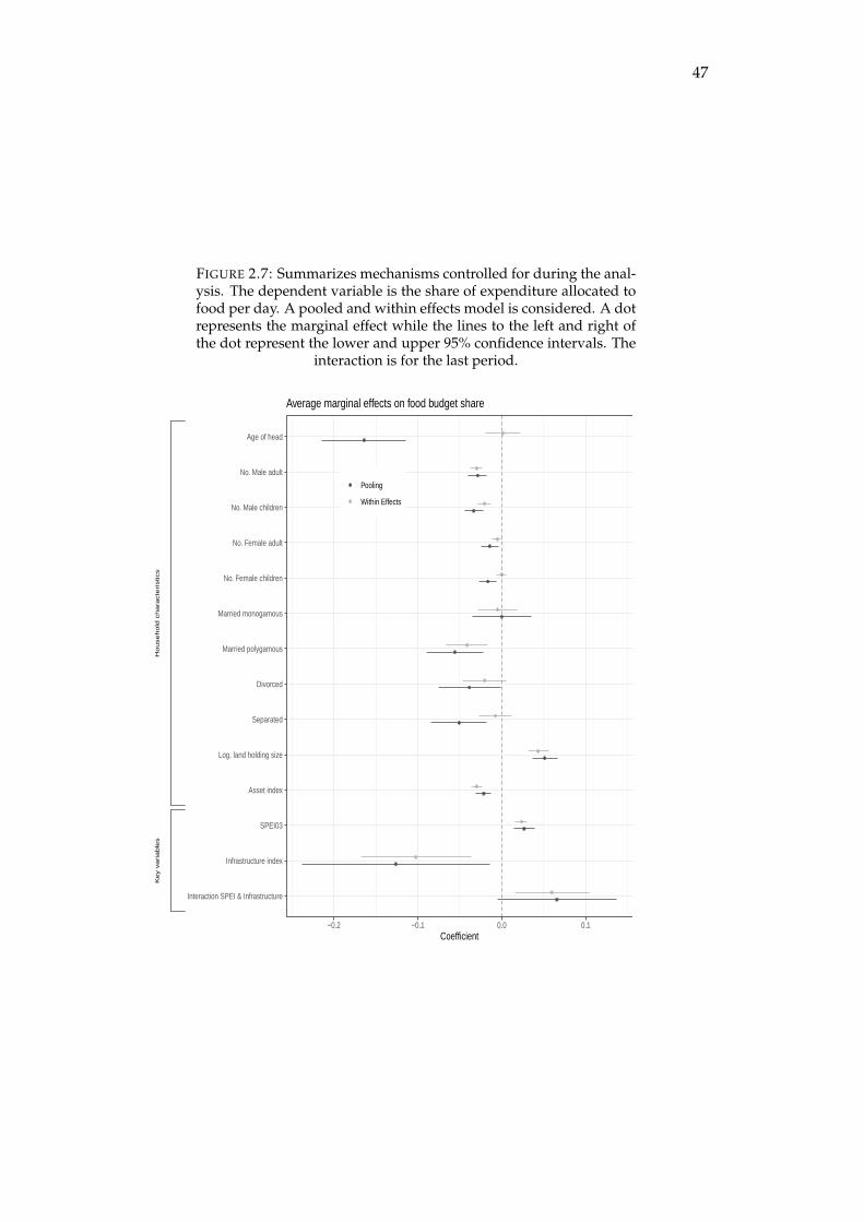
47

FIGURE 2.7: Summarizes mechanisms controlled for during the anal-ysis. The dependent variable is the share of expenditure allocated tofood per day. A pooled and within effects model is considered. A dotrepresents the marginal effect while the lines to the left and right ofthe dot represent the lower and upper 95% confidence intervals. The

interaction is for the last period.

Ho

use

ho

ld c

ha

racte

ristics

Key v

ari

able

s

Interaction SPEI & Infrastructure

Infrastructure index

SPEI03

Asset index

Log. land holding size

Separated

Divorced

Married polygamous

Married monogamous

No. Female children

No. Female adult

No. Male children

No. Male adult

Age of head

−0.2 −0.1 0.0 0.1Coefficient

Pooling

Within Effects

Average marginal effects on food budget share

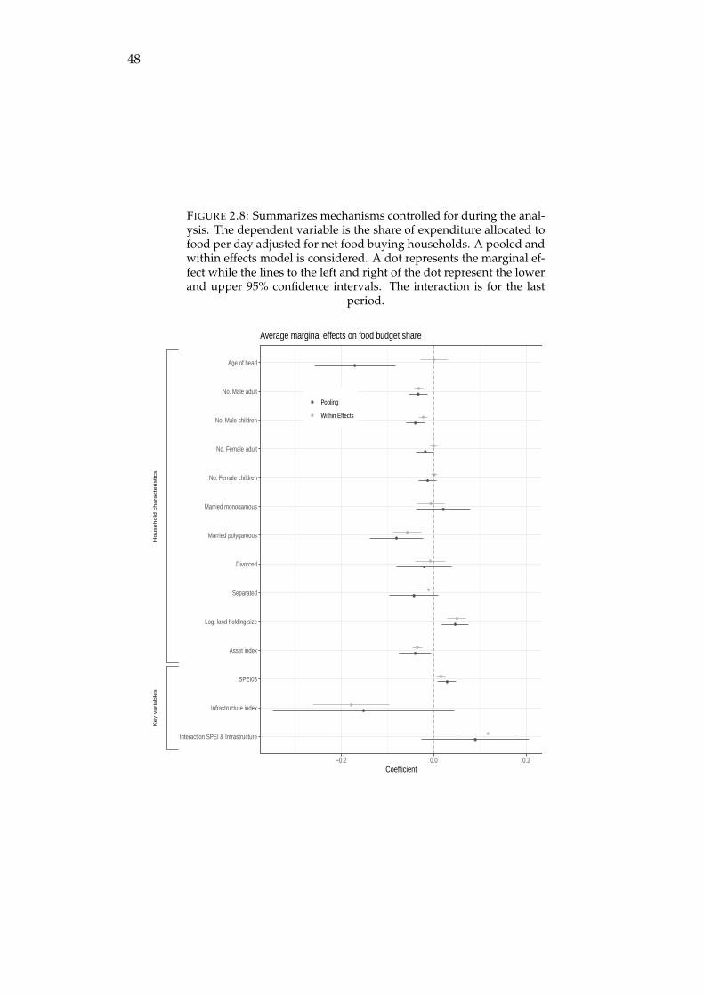
48

FIGURE 2.8: Summarizes mechanisms controlled for during the anal-ysis. The dependent variable is the share of expenditure allocated tofood per day adjusted for net food buying households. A pooled andwithin effects model is considered. A dot represents the marginal ef-fect while the lines to the left and right of the dot represent the lowerand upper 95% confidence intervals. The interaction is for the last

period.

Ho

use

ho

ld c

ha

racte

ristics

Key v

ari

able

s

Interaction SPEI & Infrastructure

Infrastructure index

SPEI03

Asset index

Log. land holding size

Separated

Divorced

Married polygamous

Married monogamous

No. Female children

No. Female adult

No. Male children

No. Male adult

Age of head

−0.2 0.0 0.2Coefficient

Pooling

Within Effects

Average marginal effects on food budget share

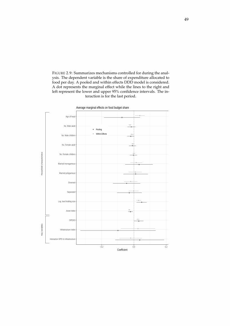
49

FIGURE 2.9: Summarizes mechanisms controlled for during the anal-ysis. The dependent variable is the share of expenditure allocated tofood per day. A pooled and within effects DDD model is considered.A dot represents the marginal effect while the lines to the right andleft represent the lower and upper 95% confidence intervals. The in-

teraction is for the last period.

Ho

use

ho

ld c

ha

racte

ristics

Key v

ari

able

s

Interaction SPEI & Infrastructure

Infrastructure index

SPEI03

Asset index

Log. land holding size

Separated

Divorced

Married polygamous

Married monogamous

No. Female children

No. Female adult

No. Male children

No. Male adult

Age of head

−0.2 0.0 0.2Coefficient

Pooling

Within Effects

Average marginal effects on food budget share

50

Household dynamics, in terms of gender composition, were positively associ-

ated with household consumption expenditure. Although both presence of both

male and female adults was positively correlated with food consumption expendi-

ture shares (p < 0.01). An additional male child was also associated with more

food consumption expenditure. In addition, Kassie, Ndiritu, and Stage (2014), Lit-

tle, Ilbery, and Watts (2009) found that gender plays a significant role in home food

preparation and consumption decisions. Thus, in addition to the gender dispar-

ity in consumption expenditure, household composition may also influence dietary

diversity outcomes. We find that households with more males have lower dietary

diversity compared to households with more females. Further, we also find that

households that were in any form of a civil union had more consumption expendi-

tures compared to household heads who had never married before. This also has to

do with household size and food consumption needs.

2.4 Discussion

Economic disruptions have important implications for welfare and development

policy. A clear identification of the shocks and households that are affected is critical

in order to trace direct causal effects at household and community level. Through-

out the analysis in this study we have addressed both issues and get two consistent

results. First, that seasonal shocks have negatively impacted household food con-

sumption given household characteristics. Second, in the presence of shocks, public

infrastructure plays a pivotal role in smoothing consumption.

The first result – that effects of extreme weather events have deleterious effects

on household consumption expenditure – are consistent with theoretical predictions

of our economic model. Any shock that affects the total household value added

results in reduced indirect utility. Our results show that a supply side shock that

affects earnings – results in significant decrease in consumption per capita. Further,

a supply side shock such as floods (SPEI values in excess of 1) bid up food prices

thereby making households pay more for the same bundle of food items. Of note,

these results were triangulated with the use of the total household expenditure but to

reduce endogeneity, a household asset index was used as a proxy. Due to seasonal

51

shocks, food production may fail thereby reducing household earning capabilities

which in turn may affect food consumption possibilities. Devereux (2007) refers to

this as an entitlement failure.

Accounting for community level infrastructure has clear advantages for welfare.

Our results throughout all the models suggest that infrastructure is associated pos-

itively associated with food security. This observation comes from our theoretical

framework that infrastructure can have positive consumption effect by reducing

transaction costs.

Our results are consistent with findings by Donaldson (2018) who, while assess-

ing effects of road infrastructure in India, found that infrastructure placement de-

creased transaction costs, also further deflated prices, increased trade and raised

income levels. Thus, from a policy planning perspective and owing to the represen-

tativeness of our data, it is important that at household and community level, capital

infrastructure be given priority. At community level, it can fairly be assumed that

returns to infrastructure, being mostly non-excludable, accrue to households and

can therefore be used for current consumption and smoothen future consumption

possibilities. Our observation is consistent with Banerjee, Duflo, and Qian (2012)

who, while assessing impacts of infrastructure on economic growth in China, found

a moderate positive effect on economic growth and income growth.

Although several studies have addressed effects of some of these shocks in isola-

tion (Ellis and Maliro, 2013, Ellis and Manda, 2012, Harttgen et al., 2012, 2015, Pauw

et al., 2013), our study is the first to exploit the combined impact of several shocks

and in a panel data framework combined with triangulated station based and re-

mote sensed data. Thus, not only are our results internally consistent but can also

be generalized at national level considering the representative nature of our data-

set. This is a great advantage considering that other studies which had small sample

sizes, were single cross-sectional surveys or forward-looking simulations.

2.5 Conclusion

This study assessed impacts of shocks on household food security in Malawi us-

ing three indicators namely: food consumption expenditure shares, Berry Index of

52

dietary diversity, and the Shannon Entropy Index of dietary diversity. The study

used fixed effects regression techniques to assess the impact of seasonal weather

shocks on food security. Second, the study assessed the impact of community in-

frastructure on household food security using fixed effects regression techniques.

Three waves of nationally representative integrated household panel surveys ob-

tained from the Malawi National Statistical Office were used. To triangulate the self-

reported shocks conditions in the survey, long term station weather data was used

to come up with the Standardized Precipitation – Evapotranspiration Index from the

Climatic Research Unit of the University of East Anglia. To triangulate infrastruc-

ture conditions, remote sensed Night Time Light data from US National Oceanic and

Atmospheric Administration (NOOA) and National Aeronautics and Space Admin-

istration (NASA) was used. The study finds that extreme weather events result in

increase in food consumption expenditure shares. Second, investment in comple-

mentary infrastructure enable households smoothen their consumption. Therefore,

in attempting to address impacts of shocks on household welfare, it is important to

also account for community level assets and infrastructure.

53

Chapter 3

Social capital and market

performance: Implications for food

security

3.1 Introduction

Industry structure can alter competitiveness and growth prospects of most sectors in

an economy 1. Emergence of highly concentrated industries may deter new entrants

and may lead to inefficient allocation of resources in the market (Poulton, Kydd,

and Dorward, 2006; Porto, Chauvin, Olarreaga, et al., 2011; Sexton and Xia, 2018).

Highly concentrated markets might not be particularly good for food commodities

especially when commodities are heavily consumed by the poor. Concentration can

drive out small firms, scare potential investors and exacerbate avoidable crises (Sex-

ton and Xia, 2018).

Few studies have been conducted to document and assess the complex relation-

ship between industry structure, firm productivity, performance, resilience and the

role of institutions and social capital in the staple food sector markets of develop-

ing economies. For example, Sitko et al., 2018 found no evidence of market con-

centration by entry of large firms into smallholder grain markets but rather found

1This chapter was published as: Kankwamba, H., and Kornher, L. (2019). Performance, be-haviour and organization of maize trading in Malawi. Agricultural and Food Economics, 7(1), 14.https://doi.org/10.1186/s40100-019-0136-6

54

that the retail prices of grain declined due to improved market efficiency. For in-

stance, Gabre-Madhin (2001), using a new institutional economics perspective, as-

sessed market institutions, transaction costs, and social capital in the Ethiopian grain

market and found that social capital enhances firm productivity. Further, Fafchamps

and Minten (2001), using survey data from traders in Madagascar, found high large

social capital effects on firm productivity.

We define social capital as “the structure of informal social relationships con-

ducive to developing cooperation among economic actors aimed at increasing social

product, which is expected to accrue to the group of people embedded in those so-

cial relationships” (Hayami, 2009). Social capital among traders may help reduce

transaction costs if traders interact more with their fellow traders for longer periods

of time (Fafchamps and Minten, 2001). However, such interactions may affect effi-

ciency outcomes as markets may become dominated by small groups of traders that

are well acquainted.

Using structural, relational and cognitive indicators for social capital, most liter-

ature from developed countries suggest a positive association between social capi-

tal and business performance (see Islam, Habes, and Alam, 2018; Liu and Li, 2018;

García-Villaverde et al., 2018; Miao et al., 2017). To illustrate, Islam, Habes, and Alam

(2018) found that a managing director’s cognitive ability, education, experience and

a number of connections had a positive influence on a cooperative’s performance.

Further, Miao et al. (2017) assessed the effect of social capital and business perfor-

mance and found that the link between social capital and performance is mediated

by human capital – education and skills of employees and entrepreneurial orienta-

tion – the strategic, philosophical and behaviours in decision making – of the trader.

In a similar manner, Asiaei and Jusoh (2015) indicated that relational and social cap-

ital improve business perfomance.

Further, other literature asserts that productivity may be reduced if traders trade

and interact with close relatives. For example, Levine et al. (2014) reported that eth-

nic proximity of traders may promote price bubbles and thereby bring about unde-

sirable market outcomes such as market inefficiency. In addition, Atmadja, Su, and

Sharma (2016) found that firms that are run by ethnically cohesive individuals tend

to poorly perform on a indicators such as profitability and survivability – i.e. time

55

in years a business stays profitable before closure. However, Oliveira and Nisbett

(2018) argue that there may not be much differences in outcomes from ethnically di-

verse groups than homogenous groups. In addition, Portes (2014) argued that social

capital might drive marginalism in that individuals without social capital may be

ostracized, face significant barriers to growth and eventually be left out of economic

systems. This becomes particularly difficult when the individuals are poor traders

in developing countries. To a greater extent, the link between business performance

and behavioural aspects of traders such as social capital and informal arrangements

such as trust relationships provide mixed evidence (Van Rijn, Bulte, and Adekunle,

2012). Interestingly, in Africa, where most businesses and, therefore the transactions

therein, are informal do not feature much in the debate on social capital versus per-

formance. As such, it is important to explore on the role of social capital in economic

outcomes.

The main objective of this study is to assess the effect of industry structure and

social capital on maize traders’ behaviour, business resilience and profitability in

Malawi. We use a randomly sampled, market level representative data set involving

small to medium scale maize traders where we ask about trade volumes, value of

stock, proportion of costs, prices, pricing behaviour and whether the enterprise ex-

ports or not to ascertain the structure, conduct and performance of the firm. We also

ask questions about the nature of the traders’ relationship with fellow traders, bro-

kers, lenders and family relations to get information regarding the structure of social

networks which might have a bearing on the nature of transaction costs. Further, the

study also uses key informant interviews, focused observations and group discus-

sions with industry representatives, grain traders’ associations and farmer associa-

tions. We hypothesize that traders who interact more with other traders, brokers and

lenders will have more resilient and profitable businesses. To test our hypothesis, we

econometrically analysed the data using Bayes Model Averaging (BMA) regression

techniques. BMA analysis reduces model uncertainty by taking advantage of the

posterior probability distributions of all competing model parameters conditional

on the observed data and some prior knowledge (see Hoeting et al., 1999; Genell et

al., 2010; Laffineur et al., 2017). In this study, we are able to use the sample data to-

gether with prior knowledge gathered from key informants and available literature

56

to draw inferences about the organization of maize markets and the behaviour of

maize traders.

The study contributes to literature on understanding drivers of business re-

silience, food policy design and industrial organization by bringing recent evidence

from a developing country’s staple food industry and also complementing and tri-

angulating results from methodologically different viewpoints namely qualitative

and Bayesian regression analysis. This would make our interpretation of results

particularly rich and highly informative.

We find two consistent results that social capital enhances business resilience and

that not all forms of social capital make maize trading profitable but when traders

are very close, even to family ties, profits increase.

The rest of the paper is structured as follows. Section two presents materials and

methods used in the paper such as the study area, sampling procedure, theoretical

framework and estimation. Section three presents results where we first present

descriptive and later inferential statistics. Section four presents discussion while

section five presents a summary and conclusion.

3.2 Materials and methods

3.2.1 Study area

The study was carried out in the central region of Malawi. The central region has

nine administrative Districts which have a comparative advantage for producing

maize, the country’s staple food (Chirwa, 2007). In as much as the whole coun-

try trades in maize, the majority of maize traders are situated in the central region

(Messina, Peter, and Snapp, 2017). In order to understand the structure, conduct

and performance of maize markets, the study area is ideal. Second, the region is

logistically cost effective since it contains most of the traders and other stakeholders.

3.2.2 Sampling, data and variables

We assume that the population of traders (N) is sufficiently large but we do not

know the variability among traders’ performance (p). Following Cochran (2007), we

assume maximum variability of (p = 0.5). We further assumed a desired confidence

57

level of 95% - corresponding to a z-value = 1.96. Further, we used ± 10% level of

precision (e). Our sample size is then n = (Z2 p(1− p))/e2 = 96. To account for

uncertainties due to logistics, we adjusted the sample size upwards by 50% to 144.

At the end of the survey, we had interviewed 172 traders, i.e. 28 more traders.

Before drawing the sample we obtained a list of markets that are followed by the

Ministry of Agriculture and Food Security’s Agricultural Statistical Bulletin. From

that list, we picked historical central markets – i.e. markets that had consistent price

and commodity series. We obtained a list of traders in a given market from mar-

ket authorities and listed them in ascending order. In the case where the market

did not have a list of traders, we conducted a linear listing of the traders – usually

traders selling maize are arranged in a line and obtaining a list was simply done

by obtaining their names and assigning numbers to them. Using the lists, the first

trader in the survey was picked using simple random sampling while the second to

the nth trader was picked using systematic random sampling by counting the next

3 traders – where the number three was chosen arbitrarily. For each of the markets

j = 1, . . . , k containing i = 1, . . . , n traders, we draw a systematic sample without

replacement and calculate a market mean, of say profit or resilience – survivability,

as ysys = ∑ yij/nj such that our systematic sampling mean is Y = 1k ∑k

j=1 ysys . The

systematic sampling variance is then calculated as s2 = 1k(n−1) ∑n

i=1 ∑kj=1(yij − yj)

2

Cochran (2007).

The key sources of expert and secondary information were the Ministry of Agri-

culture and Food Security’s (MoAFS) Department of Agricultural Planning Services

(DAPS), where we obtained information on historical prices using their Agricul-

tural Statistical Bulletin. We also obtained information on gross margins and av-

erage prices from the Department of Agricultural Extension Services (DAES). The

second prior data source was the Malawi Strategy Support Program (MASSP) of the

International Food Policy Institute (IFPRI) where we interviewed the IFPRI team of

experts. The IFPRI team provided monthly prices summarized in form of policy

briefs (MASSP, 2018) and indicated their availability for clarifications. We also in-

terviewed other players in the maize marketing industry. Results of the sampled

markets and their respective sample sizes are summarized in Table 3.1.

During the study, we also used simple ethnographic data collection techniques

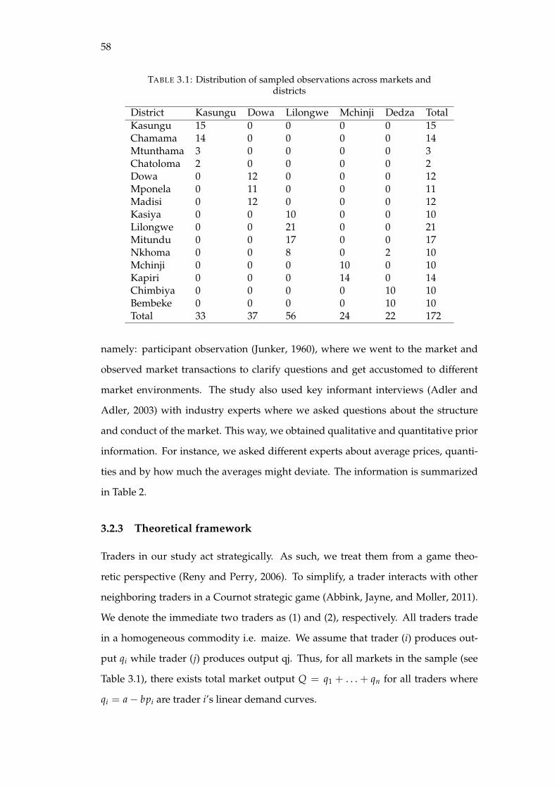
58

TABLE 3.1: Distribution of sampled observations across markets anddistricts

District Kasungu Dowa Lilongwe Mchinji Dedza TotalKasungu 15 0 0 0 0 15Chamama 14 0 0 0 0 14Mtunthama 3 0 0 0 0 3Chatoloma 2 0 0 0 0 2Dowa 0 12 0 0 0 12Mponela 0 11 0 0 0 11Madisi 0 12 0 0 0 12Kasiya 0 0 10 0 0 10Lilongwe 0 0 21 0 0 21Mitundu 0 0 17 0 0 17Nkhoma 0 0 8 0 2 10Mchinji 0 0 0 10 0 10Kapiri 0 0 0 14 0 14Chimbiya 0 0 0 0 10 10Bembeke 0 0 0 0 10 10Total 33 37 56 24 22 172

namely: participant observation (Junker, 1960), where we went to the market and

observed market transactions to clarify questions and get accustomed to different

market environments. The study also used key informant interviews (Adler and

Adler, 2003) with industry experts where we asked questions about the structure

and conduct of the market. This way, we obtained qualitative and quantitative prior

information. For instance, we asked different experts about average prices, quanti-

ties and by how much the averages might deviate. The information is summarized

in Table 2.

3.2.3 Theoretical framework

Traders in our study act strategically. As such, we treat them from a game theo-

retic perspective (Reny and Perry, 2006). To simplify, a trader interacts with other

neighboring traders in a Cournot strategic game (Abbink, Jayne, and Moller, 2011).

We denote the immediate two traders as (1) and (2), respectively. All traders trade

in a homogeneous commodity i.e. maize. We assume that trader (i) produces out-

put qi while trader (j) produces output qj. Thus, for all markets in the sample (see

Table 3.1), there exists total market output Q = q1 + . . . + qn for all traders where

qi = a− bpi are trader i’s linear demand curves.

59

We further assume that each trader maximizes their profits. For example, firm (i)

maximizes its profits as

maxq1 πi = p(Q)qi − ci(qi). (3.1)

Thus, for trader (1), profitability is clearly dependent on trader (2) ’s output on

the market. Thus, assuming an interior optimum for each trader the Cournot Nash

equilibrium must satisfy the following first order necessary conditions

Dq1 πi = p(Q) + p′(Q)qi − c′i(qi) = 0 (3.2)

The second order conditions are

D2qi= 2p′(Q) + p′′(Q)qi − c′′(qi) ≤ 0 ∀i = 1, . . . n. (3.3)

Okuguchi (1993) provided axioms namely p′+ p

′′qi < 0 and p

′< C

′′i to ensure

that the second order sufficient conditions are less than zero. In order to determine

how trader (j) might react we should differentiate the first order conditions with

respect to qj . Thus,

f ′1(qj) =D2π1/Dqi ,qj

D2π1/D2qi

(3.4)

Traders do not play one-off stage games. The interact repeatedly. In a repeated

game, the output of choice for trader i in time t is given by qti = fi(qj)

t−1and profits

will be pit = δt piit where δ is a discount factor to measure the patience of the trader.

The Nash reversion folk theorem states that given a strategy profile in an infinitely

repeatedly game, where the end game reverts to a Nash equilibrium as is the one-off

stage game, then each player’s strategy is to play a consistent outcome until someone

finally defects (see (Mas-Colell, Whinston, Green, et al., 1995). That is, with learning

effects, market out comes can improve since traders will learn the others’ reaction

functions and play consistent strategies.

Proposition 1 Social capital is a parameter that is associated with the trader’s profit func-

tion. Thus, accumulation of social capital will affect profitability.

Proof: Considering a the traders’ first order conditions and ω, a social capital pa-

rameter, we can present the stationarity conditions as

60

Dqi [qi(ω), qj(ω)] = 0 (3.5)

In order to examine the impact of social capital, we take the derivative with re-

spect to ω. That is, D2qi

D2qi ,qj

πi

D2qj,qi

π2 D2qi

Dωqi

Dωqj

=

D2qi ,ωπi

0

.

So using Crammer’s rule, the impact of social capital on a firm’s profitability can

be quantified as

Dω1 q1 =

∣∣∣∣∣∣∣D2

q1,ωπ1 D2q1,q2

π1

0 Dq2 π2

∣∣∣∣∣∣∣∣∣∣∣∣∣∣Dq1 π1 D2π1

Dq1,q2 π2 D2q2

2π2

∣∣∣∣∣∣∣(3.6)

quantifies the effect of a change in social capital on firm’s quantity supplied on

the market – a direct measure of industry share which is a function of arguments

from profits, from firm 1 and 2 and their respective reaction functions.

We learn two things from this quantity. First, if the traders only met once, then it

would make sense for them to use defective strategies, making the D2q1,ωπ1 quantity

negative as it would make one firm take advantage to maximize its own profit at

the expense of the other. Resultant, the other firm would also play a similar move.

Second, if traders would repeatedly interact in the market, and the equilibrium is

mutually beneficial (Dal Bó and Fréchette, 2011), there could be an evolution of co-

operation which could foster learning effects and eventually firm and market per-

formance would increase. It would be optimal for players to play cooperate and it

would be punishable to play defective strategies. This follows the Nash reversion

theorem.

However, as traders keep interacting and learning from each other, it is expected

that they would adopt strategies that work in improving their businesses and aban-

don the strategies that are do not work. Nowak (2006) call a strategy that achieves

this and ultimately dominates an Evolutionary Stable Strategy (ESS). In this study,

traders that tend to play sub-optimal strategies will be left out by the process of

61

evolution and they will go bankrupt. Further, Hamilton (1964) suggested that nat-

ural selection would most certainly favour cooperation and altruistic behaviour in

more genetically related individuals. So on in our context we assume that busi-

nesses would perform much better among related individuals and friends. That is if

a closely related individuals business is falling apart, a relative or a friend they inter-

act with could bail them out in form of a loan or a mere handout. However, we also

take note of Levine et al. (2014) observation that ethnic diversity could also lead to

better market outcomes. We thus, use different indicators of cooperation in traders

interactions namely, 1) kin selection, where individual traders interact more with

genetically related individuals; 2) group selection, where individuals would interact

more among friends doing similar kind of trade and; 3) direct reciprocity where at

first, we observe how firms run as sole trading entities perform and survive. We

also group the traders in ethnicity terms to observe how one ethnic group operates

against another in direct reciprocity (Trivers, 1971).

3.2.4 Estimation

Considering that we used two sources of data namely trader survey and key in-

formant interviews, it is ideal to bring the two data sets together in the process of

drawing inference about the population parameters. For a start, our key informants

i.e. key industry experts, few handpicked traders and government personnel in-

formed us about the distribution of the parameters. We use this prior knowledge

to complement the survey data in the estimation process of the posterior distribu-

tion of parameters and their 95% credible intervals. We thus use Bayesian normal

regression techniques to assess the effects of social capital, on firm profitability and

resilience. Our basic regression framework is presented as

Yijd = βijdX + γj + δd + λt + εijd. (3.7)

where Y is the n × 1 vector of natural logarithm of profits of trader or firm i in

market j and district d. The variable Xijd is an n×m vector of independent variables

that explain the variation in Yijd. The quantity βijd is an m × 1vector of unknown

62

parameters of the explanatory variables,γj is an unknown market specific fixed effect

while δd and λ are a district and seasonal specific fixed effect.

During data collection period, we obtained prior information on the historical

estimates, behaviour and structure of the market. This prior information can be use-

ful in estimating the model parameters and reducing uncertainty. To further reduce

the level of uncertainty, we use Bayes Model Averaging (BMA) estimator (Hoeting

et al., 1999) with market and district specific fixed effects. Considering the lack of

extensive literature on small businesses in Malawi, building an accurate model of

business profitability in the context of geographic, social institutional and physical

capital could be challenging. Thus, given the context, there are many, i.e. the model

space is M = 2m = 230 = 2.684× 1008 where m ∈ M, competing models that can

be estimated from the given variables. Therefore, fitting one Ordinary Least Squares

regression model could result in high measurement and specification errors when

expert knowledge is limited and sample sizes are small (Genell et al., 2010). BMA

fits a regression of the form

Yijd = βijd(X− X) + γj + δd + λt + εijd (3.8)

where the unconditional BMA results’ βijd are weighted average parameters condi-

tional on each of the competing models in the model space, i.e. m ∈ M (Hoeting

et al., 1999; Laffineur et al., 2017). Thus,

ˆβijd = E(βijd|Yijd) =M

∑m=1

ωm βm. (3.9)

Using Bayes’ theorem, we estimate the posterior probability distribution as

ωm = p(M|Data) =P(Mm)× p(Data|Mm)∫ 2m

m=1 P(Mm)× p(Data|Mm)(3.10)

such that p(Mm) is the prior probability distribution of model m while

p(Data|Mm) is the marginal likelihood distribution of the data given the model

Mm where the model space is M such that m ∈ M (Madigan and Raftery, 1994;

Laffineur et al., 2017). We use R statistical package BAS (Bayesian Variable Selection

63

and Model Averaging using Adaptive Sampling) – which samples the models with-

out replacement and outperforms Markov Chain Monte Carlo frameworks – (Clyde,

Ghosh, and Littman, 2011) to estimate the final posterior parameters.

3.2.5 Industry structure

Descriptive statistics

Table 2 summarizes variable descriptions and results of the prior expert information

elicited through the qualitative data collection techniques. The data obtained com-

plements the survey data estimates and are later used in the Bayesian estimation. In

general, results closely match the data such that we can safely deduce that the prior

has similar distributions.

We used the Herfindahl-Hirshmann Index (HHI) to assess market concentration.

The HHI assesses the structure of the market through the lenses of market competi-

tiveness by measuring the size of the firm relative to the size of the industry. Using

two indicators namely value of operating capital and volume of commodities that

the firm handles per month, we computed the HHI as

HHI =n

∑i=1

s2i where si = 1/N, (3.11)

where N is the total number of the firms in the industry. When the HHI is 0.01 or

less, then the market is competitive; when HHI is 0.15 it is unconcentrated; when

HHI is between 0.15 and 0.25, the market is moderately concentrated while an HHI

of 0.25 and above signifies a concentrated industry. We estimate market, district and

regional HHI indicators. However, in the regression estimation we use the log of the

share as an indicator of industry size.

As a qualitative measure of industry size, we used a count of traders in the mar-

ket. A larger number of traders was considered to be a competitive market while

when there are very few traders, then the market is less competitive.

64

3.3 Results

3.3.1 Descriptive statistics

Table summarizes variable descriptions and results of the prior expert information

elicited through the qualitative data collection techniques. The data obtained com-

plements the survey data estimates and are later used in the Bayesian estimation. In

general, results closely match the data such that we can safely deduce that the prior

has similar distributions.

Table 3.2 summarises results of the descriptive statistics of key variables that

are used in the study. The study’s dependent variables are business profitability

and business resilience. The average profit of the maize business was MK30 per

kilogram. Results show that 91% of the traders were male aging between 20 and 71

years old. We found that 92% of the traders in the sample were male. In addition,

when asked about whether they set prices, 39% of traders reported that they discuss

with about 10 colleagues setting market prices. Traders also indicated that it took 14

minutes to get to the market from their home. Results also indicate that 9% have an

export license. Further, traders reported that the market contained between 7 and 54

maize traders.

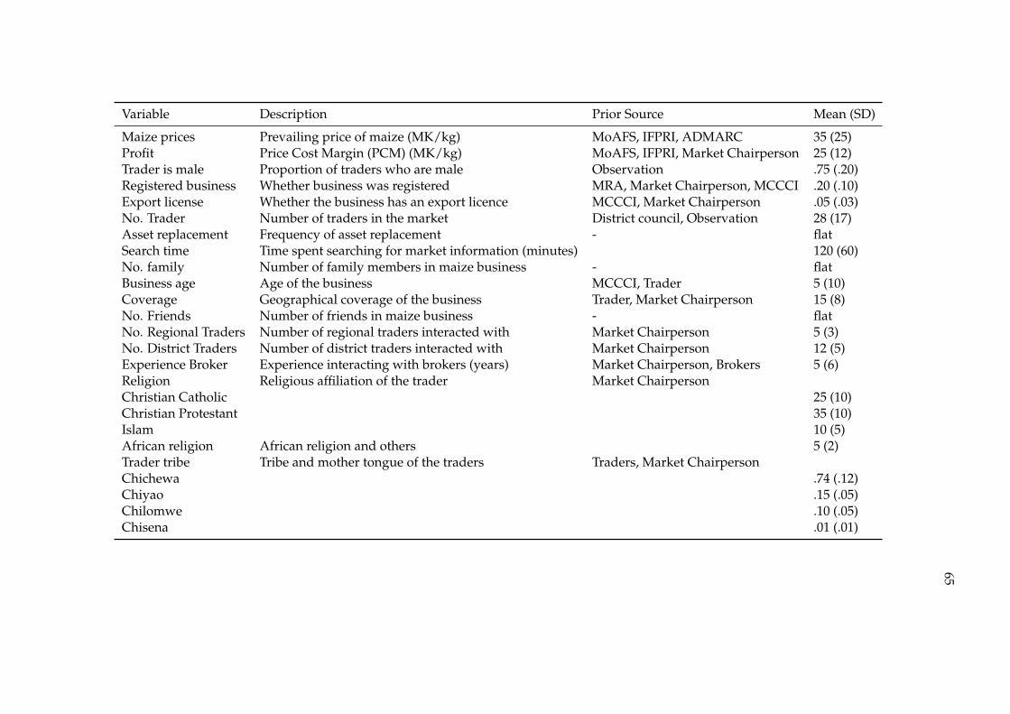
65

Variable Description Prior Source Mean (SD)

Maize prices Prevailing price of maize (MK/kg) MoAFS, IFPRI, ADMARC 35 (25)Profit Price Cost Margin (PCM) (MK/kg) MoAFS, IFPRI, Market Chairperson 25 (12)Trader is male Proportion of traders who are male Observation .75 (.20)Registered business Whether business was registered MRA, Market Chairperson, MCCCI .20 (.10)Export license Whether the business has an export licence MCCCI, Market Chairperson .05 (.03)No. Trader Number of traders in the market District council, Observation 28 (17)Asset replacement Frequency of asset replacement - flatSearch time Time spent searching for market information (minutes) 120 (60)No. family Number of family members in maize business - flatBusiness age Age of the business MCCCI, Trader 5 (10)Coverage Geographical coverage of the business Trader, Market Chairperson 15 (8)No. Friends Number of friends in maize business - flatNo. Regional Traders Number of regional traders interacted with Market Chairperson 5 (3)No. District Traders Number of district traders interacted with Market Chairperson 12 (5)Experience Broker Experience interacting with brokers (years) Market Chairperson, Brokers 5 (6)Religion Religious affiliation of the trader Market ChairpersonChristian Catholic 25 (10)Christian Protestant 35 (10)Islam 10 (5)African religion African religion and others 5 (2)Trader tribe Tribe and mother tongue of the traders Traders, Market ChairpersonChichewa .74 (.12)Chiyao .15 (.05)Chilomwe .10 (.05)Chisena .01 (.01)

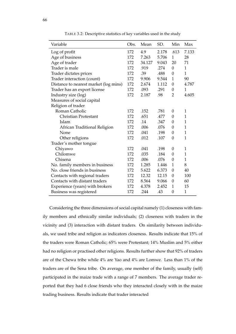
66

TABLE 3.2: Descriptive statistics of key variables used in the study

Variable Obs. Mean SD. Min Max

Log of profit 172 4.9 2.178 .613 7.133Age of business 172 7.263 5.706 1 28Age of trader 172 34.127 9.043 20 71Trader is male 172 .919 .274 0 1Trader dictates prices 172 .39 .488 0 1Trader interaction (count) 172 9.906 9.544 1 90Distance to nearest market (log mins) 172 2.674 1.112 0 4.787Trader has an export license 172 .093 .291 0 1Industry size (log) 172 2.187 .98 2 4.605Measures of social capitalReligion of trader

Roman Catholic 172 .152 .781 0 1Christian Protestant 172 .651 .477 0 1Islam 172 .14 .347 0 1African Traditional Religion 172 .006 .076 0 1None 172 .041 .198 0 1Other religions 172 .012 .107 0 1

Trader’s mother tongueChiyawo 172 .041 .198 0 1Chilomwe 172 .035 .184 0 1Chisena 172 .006 .076 0 1

No. family members in business 172 1.285 1.446 1 8No. close friends in business 172 5.622 6.373 0 40Contacts with regional traders 172 12.32 12.15 0 100Contacts with distant traders 172 8.564 9.066 0 60Experience (years) with brokers 172 4.378 2.452 1 15Business was registered 172 .244 .43 0 1

Considering the three dimensions of social capital namely (1) closeness with fam-

ily members and ethnically similar individuals; (2) closeness with traders in the

vicinity and (3) interaction with distant traders. On similarity between individu-

als, we used tribe and religion as indicators closeness. Results indicate that 15% of

the traders were Roman Catholic; 65% were Protestant; 14% Muslim and 5% either

had no religion or practised other religions. Results further show that 92% of traders

are of the Chewa tribe while 4% are Yao and 4% are Lomwe. Less than 1% of the

traders are of the Sena tribe. On average, one member of the family, usually (self)

participated in the maize trade with a range of 7 members. The average trader re-

ported that they had 6 close friends who they interacted closely with in the maize

trading business. Results indicate that trader interacted

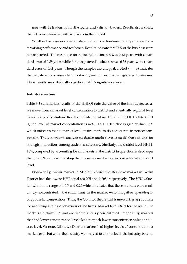
67

most with 12 traders within the region and 9 distant traders. Results also indicate

that a trader interacted with 4 brokers in the market.

Whether the business was registered or not is of fundamental importance in de-

termining performance and resilience. Results indicate that 78% of the business were

not registered. The mean age for registered businesses was 9.32 years with a stan-

dard error of 0.89 years while for unregistered businesses was 6.58 years with a stan-

dard error of 0.41 years. Though the samples are unequal, a t-test (t = 3) indicates

that registered businesses tend to stay 3 years longer than unregistered businesses.

These results are statistically significant at 1% significance level.

Industry structure

Table 3.3 summarizes results of the HHI.Of note the value of the HHI decreases as

we move from a market level concentration to district and eventually regional level

measure of concentration. Results indicate that at market level the HHI is 0.468, that

is, the level of market concentration is 47%. This HHI value is greater than 25%

which indicates that at market level, maize markets do not operate in perfect com-

petition. Thus, in order to analyze the data at market level, a model that accounts for

strategic interactions among traders is necessary. Similarly, the district level HHI is

28%, computed by accounting for all markets in the district in question, is also larger

than the 28% value – indicating that the maize market is also concentrated at district

level.

Noteworthy, Kapiri market in Mchinji District and Bembeke market in Dedza

District had the lowest HHI equal to0.205 and 0.208, respectively. The HHI values

fall within the range of 0.15 and 0.25 which indicates that these markets were mod-

erately concentrated – the small firms in the market were altogether operating in

oligopolistic competition. Thus, the Cournot theoretical framework is appropriate

for analyzing strategic behaviour of the firms. Market level HHIs for the rest of the

markets are above 0.25 and are unambiguously concentrated. Importantly, markets

that had lower concentration levels lead to much lower concentration values at dis-

trict level. Of note, Lilongwe District markets had higher levels of concentration at

market level, but when the industry was moved to district level, the industry became

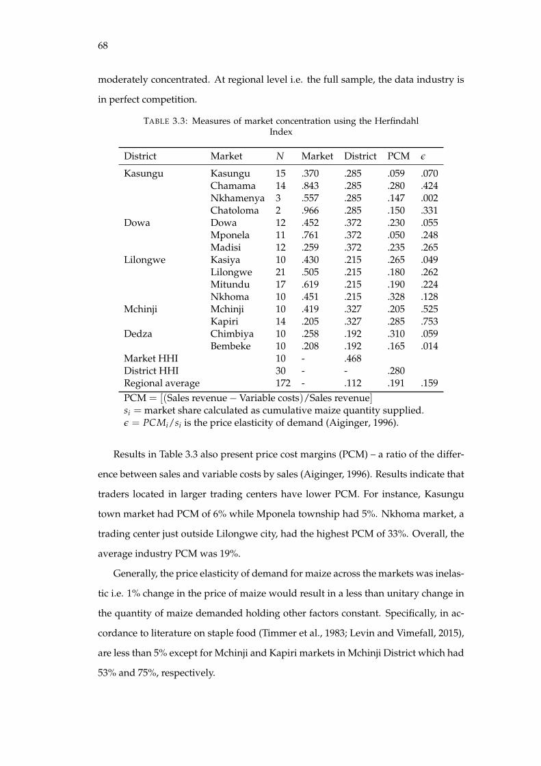
68

moderately concentrated. At regional level i.e. the full sample, the data industry is

in perfect competition.

TABLE 3.3: Measures of market concentration using the HerfindahlIndex

District Market N Market District PCM ε

Kasungu Kasungu 15 .370 .285 .059 .070Chamama 14 .843 .285 .280 .424Nkhamenya 3 .557 .285 .147 .002Chatoloma 2 .966 .285 .150 .331

Dowa Dowa 12 .452 .372 .230 .055Mponela 11 .761 .372 .050 .248Madisi 12 .259 .372 .235 .265

Lilongwe Kasiya 10 .430 .215 .265 .049Lilongwe 21 .505 .215 .180 .262Mitundu 17 .619 .215 .190 .224Nkhoma 10 .451 .215 .328 .128

Mchinji Mchinji 10 .419 .327 .205 .525Kapiri 14 .205 .327 .285 .753

Dedza Chimbiya 10 .258 .192 .310 .059Bembeke 10 .208 .192 .165 .014

Market HHI 10 - .468District HHI 30 - - .280Regional average 172 - .112 .191 .159PCM = [(Sales revenue−Variable costs)/Sales revenue]si = market share calculated as cumulative maize quantity supplied.ε = PCMi/si is the price elasticity of demand (Aiginger, 1996).

Results in Table 3.3 also present price cost margins (PCM) – a ratio of the differ-

ence between sales and variable costs by sales (Aiginger, 1996). Results indicate that

traders located in larger trading centers have lower PCM. For instance, Kasungu

town market had PCM of 6% while Mponela township had 5%. Nkhoma market, a

trading center just outside Lilongwe city, had the highest PCM of 33%. Overall, the

average industry PCM was 19%.

Generally, the price elasticity of demand for maize across the markets was inelas-

tic i.e. 1% change in the price of maize would result in a less than unitary change in

the quantity of maize demanded holding other factors constant. Specifically, in ac-

cordance to literature on staple food (Timmer et al., 1983; Levin and Vimefall, 2015),

are less than 5% except for Mchinji and Kapiri markets in Mchinji District which had

53% and 75%, respectively.

69

3.3.2 The role of social capital in determining business performance

Table 3.4 summarizes results of the Bayesian regression analysis of the effect of social

capital on business profitability. The table presents three models. First, a Bayesian

model with informative prior where we report posterior means, standard devia-

tions and the probability that the posterior mean is not equal to zero i.e. pβ 6= 0).

The model is presented in columns 1 to 3. Second, we present a Bayesian model

with reference priors in columns 4 to 6. This model uses information from the sam-

ple to compute posterior probabilities. In the event that our informative priors are

misleading, this model acts as an objective robustness check. Third, we used an Or-

dinary Least Squares regression model with bootstrapped standard errors replicated

1000 times in columns 7 to 9. Using a frequentist approach with highly conservative

standard errors compared to those produced by normal OLS ensures that the preci-

sion of our estimates is based on actual variation in the information from the sample

and not just chance. The bootstrapped model also shows the level of bias associated

with the resampling. In the informative prior model, we used a normally distributed

prior with mean 12.65 and the model variance from the sample to estimate the pos-

terior distribution of parameters using 20000 Monte-Carlo Markov Chain (MCMC)

simulations. Figure 3.1 summarizes results of the BMA procedure showing 18 best

fitted models.

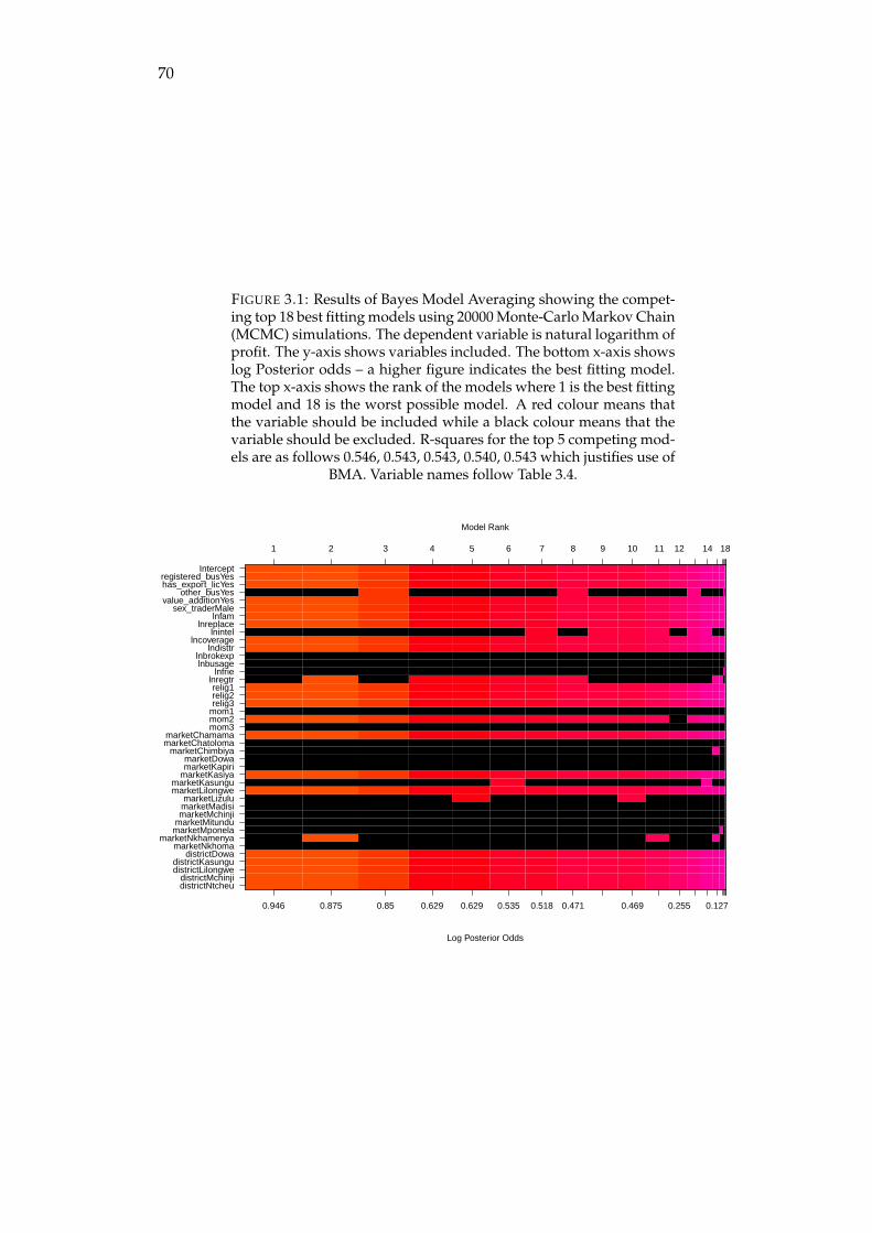
70

FIGURE 3.1: Results of Bayes Model Averaging showing the compet-ing top 18 best fitting models using 20000 Monte-Carlo Markov Chain(MCMC) simulations. The dependent variable is natural logarithm ofprofit. The y-axis shows variables included. The bottom x-axis showslog Posterior odds – a higher figure indicates the best fitting model.The top x-axis shows the rank of the models where 1 is the best fittingmodel and 18 is the worst possible model. A red colour means thatthe variable should be included while a black colour means that thevariable should be excluded. R-squares for the top 5 competing mod-els are as follows 0.546, 0.543, 0.543, 0.540, 0.543 which justifies use of

BMA. Variable names follow Table 3.4.

0.946 0.875 0.85 0.629 0.629 0.535 0.518 0.471 0.469 0.255 0.127

1 2 3 4 5 6 7 8 9 10 11 12 14 18

Model Rank

Log Posterior Odds

districtNtcheudistrictMchinji

districtLilongwedistrictKasungu

districtDowamarketNkhoma

marketNkhamenyamarketMponelamarketMitundumarketMchinjimarketMadisimarketLizulu

marketLilongwemarketKasungu

marketKasiyamarketKapirimarketDowa

marketChimbiyamarketChatolomamarketChamama

mom3mom2mom1relig3relig2relig1

lnregtrlnfrie

lnbusagelnbrokexp

lndisttrlncoverage

lnintellnreplace

lnfamsex_traderMale

value_additionYesother_busYes

has_export_licYesregistered_busYes

Intercept

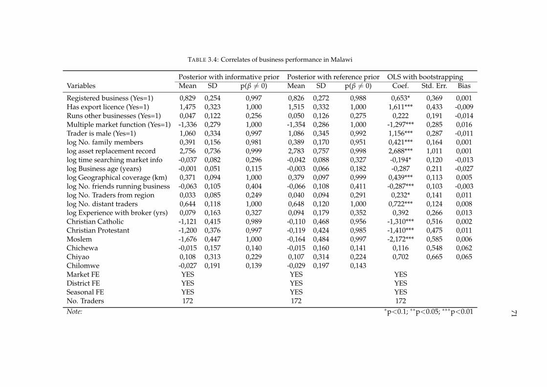
71

TABLE 3.4: Correlates of business performance in Malawi

Posterior with informative prior Posterior with reference prior OLS with bootstrappingVariables Mean SD p(β 6= 0) Mean SD p(β 6= 0) Coef. Std. Err. Bias

Registered business (Yes=1) 0,829 0,254 0,997 0,826 0,272 0,988 0,653* 0,369 0,001Has export licence (Yes=1) 1,475 0,323 1,000 1,515 0,332 1,000 1,611*** 0,433 -0,009Runs other businesses (Yes=1) 0,047 0,122 0,256 0,050 0,126 0,275 0,222 0,191 -0,014Multiple market function (Yes=1) -1,336 0,279 1,000 -1,354 0,286 1,000 -1,297*** 0,285 0,016Trader is male (Yes=1) 1,060 0,334 0,997 1,086 0,345 0,992 1,156*** 0,287 -0,011log No. family members 0,391 0,156 0,981 0,389 0,170 0,951 0,421*** 0,164 0,001log asset replacement record 2,756 0,736 0,999 2,783 0,757 0,998 2,688*** 1,011 0,001log time searching market info -0,037 0,082 0,296 -0,042 0,088 0,327 -0,194* 0,120 -0,013log Business age (years) -0,001 0,051 0,115 -0,003 0,066 0,182 -0,287 0,211 -0,027log Geographical coverage (km) 0,371 0,094 1,000 0,379 0,097 0,999 0,439*** 0,113 0,005log No. friends running business -0,063 0,105 0,404 -0,066 0,108 0,411 -0,287*** 0,103 -0,003log No. Traders from region 0,033 0,085 0,249 0,040 0,094 0,291 0,232* 0,141 0,011log No. distant traders 0,644 0,118 1,000 0,648 0,120 1,000 0,722*** 0,124 0,008log Experience with broker (yrs) 0,079 0,163 0,327 0,094 0,179 0,352 0,392 0,266 0,013Christian Catholic -1,121 0,415 0,989 -0,110 0,468 0,956 -1,310*** 0,516 0,002Christian Protestant -1,200 0,376 0,997 -0,119 0,424 0,985 -1,410*** 0,475 0,011Moslem -1,676 0,447 1,000 -0,164 0,484 0,997 -2,172*** 0,585 0,006Chichewa -0,015 0,157 0,140 -0,015 0,160 0,141 0,116 0,548 0,062Chiyao 0,108 0,313 0,229 0,107 0,314 0,224 0,702 0,665 0,065Chilomwe -0,027 0,191 0,139 -0,029 0,197 0,143Market FE YES YES YESDistrict FE YES YES YESSeasonal FE YES YES YESNo. Traders 172 172 172Note: ∗p<0.1; ∗∗p<0.05; ∗∗∗p<0.01

72

Results indicate that registered businesses were 83% more profitable than un-

registered ones. Further, traders that possessed export licences were twice more

profitable. If a trader ran other businesses apart from the current grain trading, it

resulted in 4% more profits in the maize grain trading business. Results further

show that traders who participated in many marketing functions had profits, which

were lower by a factor of 1.3 than traders who consistently performed one market-

ing function. Traders that were combining multiple functions were mostly small and

itinerant with capacity and credit constraints. We also find that male traders were

twice more profitable than female run businesses. Number of close family relatives

is associated with 40% more profits. We found that traders who were innovative

in changing assets and trying new technologies during trading realized 37% prof-

itable businesses. Results indicate that the larger the geographical coverage of the

business, the more profitable the business i.e. 1% increase in geographical coverage

resulted is 36% increase in profits. As far as social capital is concerned, we found

that the more the trader interacts with traders within the same district but from

other distant markets, the more profitable the business is – 1% increase in interac-

tions resulted in 63% increase in profits. We found higher posterior probabilities

that the other measures of social capital such as religion, and tribe of the trader have

significant effects on profitability.

3.3.3 The role of social capital in business resilience

Taking age of the business as an indicator of business survivability and resilience

(Atmadja, Su, and Sharma, 2016) , In Table 3.5 we estimated a model of key success

factors of business resilience. We used a normally distributed prior with mean 1.6

and the model variance from the sample to estimate the posterior distribution of

parameters using 20000 Monte-Carlo Markov Chain (MCMC) simulations.

Results of the BMA regression model indicates that if a trader has an export li-

cence, it is associated with 9% increase in business resilience. Further, if the business

holds other forms of business apart from the grain trading, it is associated with a 15%

increase in business resilience. Traders that engage in multiple marketing functions

are associated with 11% increase in profitability. A male trader is associated with

30% reduction in business resilience. Traders that often replace assets and actively

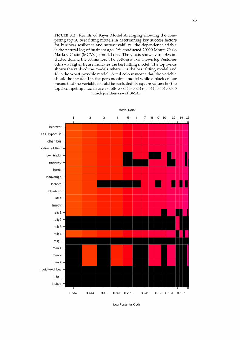
73

FIGURE 3.2: Results of Bayes Model Averaging showing the com-peting top 20 best fitting models in determining key success factorsfor business resilience and survavivability. the dependent variableis the natural log of business age. We conducted 20000 Monte-CarloMarkov Chain (MCMC) simulations. The y-axis shows variables in-cluded during the estimation. The bottom x-axis shows log Posteriorodds – a higher figure indicates the best fitting model. The top x-axisshows the rank of the models where 1 is the best fitting model and16 is the worst possible model. A red colour means that the variableshould be included in the parsimonious model while a black colourmeans that the variable should be excluded. R-square values for thetop 5 competing models are as follows 0.338, 0.349, 0.341, 0.334, 0.345

which justifies use of BMA.

0.562 0.444 0.41 0.398 0.265 0.241 0.19 0.134 0.102

1 2 3 4 5 6 7 8 9 10 12 14 18

Model Rank

Log Posterior Odds

lndisttr

lnfam

registered_bus

mom3

mom2

mom1

relig5

relig4

relig3

relig2

relig1

lnregtr

lnfrie

lnbrokexp

lnshare

lncoverage

lnintel

lnreplace

sex_trader

value_addition

other_bus

has_export_lic

Intercept

74

innovate are associated with 11% increase in business resilience. Traders that spent

more time searching for market information are associated with a 53% reduction in

business resilience. Traders that have a wide geographical coverage are associated

with 11% increase in business resilience. In addition, a 1% increase in friends run-

ning grain trading business results in 14% increase in business resilience. Further, a

1% increase in experience with brokers results in 56% increase in business resilience.

When the trader increases interactions with distant traders within the region by 1%,

business resilience increases by 12%.

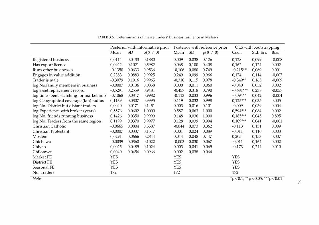
75

TABLE 3.5: Determinants of maize traders’ business resilience in Malawi

Posterior with informative prior Posterior with reference prior OLS with bootstrappingMean SD p(β 6= 0) Mean SD p(β 6= 0) Coef. Std. Err. Bias

Registered business 0,0114 0,0433 0,1880 0,009 0,038 0,126 0,128 0,099 -0,008Has export licence 0,0922 0,1021 0,5982 0,068 0,100 0,408 0,162 0,124 0,002Runs other businesses -0,1350 0,0633 0,9536 -0,106 0,080 0,749 -0,215*** 0,069 0,001Engages in value addition 0,2383 0,0883 0,9925 0,249 0,099 0,966 0,174 0,114 -0,007Trader is male -0,3079 0,1016 0,9965 -0,310 0,115 0,978 -0,349** 0,165 -0,009log No.family members in business -0,0007 0,0136 0,0858 0,000 0,011 0,060 -0,040 0,052 0,002log asset replacement record -0,5291 0,2559 0,9481 -0,457 0,318 0,790 -0,681*** 0,238 -0,057log time spent searching for market info -0,1068 0,0317 0,9982 -0,113 0,033 0,996 -0,094** 0,042 -0,004log Geographical coverage (km) radius 0,1139 0,0307 0,9995 0,119 0,032 0,998 0,125*** 0,035 0,005log No. District but distant traders 0,0040 0,0171 0,1451 0,003 0,016 0,101 -0,009 0,039 0,004log Experience with broker (years) 0,5576 0,0602 1,0000 0,587 0,063 1,000 0,594*** 0,084 0,002log No. friends running business 0,1426 0,0350 0,9999 0,148 0,036 1,000 0,185*** 0,045 0,895log No. Traders from the same region 0,1199 0,0370 0,9977 0,128 0,039 0,994 0,109*** 0,041 -0,001Christian Catholic -0,0665 0,0804 0,5587 -0,044 0,073 0,362 -0,113 0,131 0,009Christian Protestant -0,0007 0,0337 0,1517 0,001 0,024 0,089 -0,011 0,110 0,003Moslem 0,0291 0,0666 0,2844 0,014 0,048 0,147 0,205 0,153 0,007Chichewa -0,0039 0,0360 0,1022 -0,003 0,030 0,067 -0,011 0,164 0,002Chiyao 0,0025 0,0489 0,1024 0,003 0,041 0,069 -0,173 0,244 0,010Chilomwe 0,0040 0,0456 0,0966 0,002 0,038 0,064Market FE YES YES YESDistrict FE YES YES YESSeasonal FE YES YES YESNo. Traders 172 172 172Note: ∗p<0.1; ∗∗p<0.05; ∗∗∗p<0.01

76

3.4 Discussion

In this study we analysed effects of social capital, industry size and firm perfor-

mance in the maize sub-sector in Malawi. Our results explain three important find-

ings. First, trader and industry characteristics shape business performance and re-

silience. Second, the complex nature of business performance and resilience can be

explained by unpacking trader characteristics, closeness and wider social interac-

tions. Our results show that trader and industry characteristics influence profitabil-

ity and resilience of traders businesses in the maize subsector. First, we found that

registered traders were more profitable than unregistered ones. For example, in or-

der for firms to sell to large agencies such as the National Food Reserve Agency

(NFRA), they are required to register their businesses. Having a registered business

therefore guarantees that the trader can access most lucrative markets (McKenzie

and Sakho, 2010). On the other hand, unregistered businesses tend to have a nar-

row base for expanding their business and profitability as they are usually credit

constrained – this observation is consistent with (Fafchamps and Minten, 2001) who

found positive association between formality and performance in Brazil.

We found that at market level, traders behave in an oligopolistic manner but as

one expands to the district and regional levels, the market becomes more competi-

tive. This observation is not surprising as it is usual to find traders who know each

other at market level. Further, traders at market level formed committees of traders

that traded in common commodities. This organization could lead to possibilities for

collusion (Varian, 2014; Mas-Collel and Green, 1995). Our results are in stark con-

trast with (Cai and Szeidl, 2016) who found that when firms interact, performance

increases. However, their finding was based on a sample that had larger businesses

while this study was based on a sample of smaller businesses. Noteworthy, in sup-

port of our result, Levine et al. (2014) explain that when firms interact, it leads to

collusion, which might end up creating price bubbles that eventually depress indus-

try profits. Based on our findings, we tend to subscribe to Levine’s explanation that

at community market, where traders know each other, they can collude to set prices

and therefore create price bubbles which might eventually lower community wel-

fare as consumers would be buying an inefficiently priced maize grain. Of note, in

77

Zambia, Sitko et al., 2018 found that market entry of bigger traders increased mar-

ket performance by decreasing market prices through improved market information

channels and high levels of investment.

We find that social capital exerts an influence in shaping business performance

and resilience. For instance, results show that traders operating within the same

market and district experience an increase in business resilience. We also find that

close ties with family members when running the business encourages business re-

silience. Our results are in agreement with the findings of Islam, Habes, and Alam

(2018), Liu and Li (2018), and Madigan and Raftery (1994) who found that social cap-

ital and business performance and resilience are highly correlated. Our results are

not in agreement with Portes (2014) who indicated that such closeness might reduce

the business into a large family safety net on which family members use the firm’s

resources to the detriment of the business’ performance. Rather, we find that traders

who interact a lot with friends and distant traders have more resilient businesses.

Our results support the narrative that social capital leads to businesses that are

more resilient, they also provide support for business performance. We find strong

posterior probabilities that the association between firm performance and closeness

with friends, religiously affiliated and ethnically close traders in the maize business

is not equal to zero. Our results also strongly support other notions of social capital

such as number of family members in business. Family members, as Portes (2014)

observed would assist in supporting the business with capital and also providing

human resources. This might explain the positive outcomes.

To sum up, results present evidence that long term interaction among traders

leads to resilient businesses. Secondly, interactions among closely related traders

such as family members, and friends lead to more resilient businesses. From the the-

oretical framework, the result that close ties with family and friends and increased

interaction among traders is highly suggestive of both group and kin selection. As

Nowak (2006) put it, natural selection mostly favours some level of altruistic coop-

eration among genetically related individuals. Evidenced by the significant positive

association between relatedness and firm profitability, the Hamiltonian rule Hamil-

ton (1964) would lead us to a conclusion that the relatedness we view in the results

78

outweighs its altruistic cost such that the result is positive firm performance for fam-

ily members.

3.5 Conclusion

This study assessed effects of social capital, industry structure on performance and

resilience of the firm. Results show that characteristics of the industry namely in-

dustry size, market concentration, proportion of registered firms, and proportions

of firms having export licenses affect both firm performance and resilience. Second,

results indicate that ethnically close traders operating within the same area tend to

have more productive businesses. In evolutionary game theory, this suggests strong

group and kin selection. On the other hand, results showed that group selection

prevails as a dominant strategy in building business resilience as close association

with friends in the business led to a more resilient business. In order to foster bet-

ter business performance and resilience, efforts should be put in place to account

for social capital arrangements and industry characteristics. For example, village

banks and savings and credit cooperatives among similar groups could help im-

prove resilience by reducing credit constraints since individuals would have similar

behavioural traits thereby fostering cooperation.

79

Chapter 4

Business registration and firm

performance: A case of maize

traders in Malawi

4.1 Background

Business formality can affect performance by effecting changes in firms’ profitabil-

ity1. From a public finance policy perspective, government entities need to achieve

a highly developed and diversified taxable base of economic activities by registering

informal businesses (Ahmad and Best, 2012). A good tax revenue base would assist

government in its recurrent expenditure and investment spending which have a de-

mand stimulating effect on the commodity markets (Ahmad, Best, and Pöschl, 2012;

Breisinger, Thomas, and Thurlow, 2009; Hausmann, Rodrik, and Velasco, 2008). Fur-

ther, a formalized business environment is more transparent to the activities of both

firms and the government. When more businesses are registered and a market shock

occurs, it is easy to craft interventions to bolster resilience (Dabla-Norris, Gradstein,

and Inchauste, 2008).

On the other hand, businesses characterized by high levels of informality are

difficult to track (Levy, 2010). While it is difficult to cheat in tax returns when a

firm is registered (Ahmad, Best, and Pöschl, 2012), the job of national accounting

becomes not only easier but also more accurate when firms are formally registered

(Dabla-Norris, Gradstein, and Inchauste, 2008).

1This chapter was accepted in the journal of Development in Practice. Routledge. Scopus/SJRranking: Q2. Current status: Awaiting online production.

80

Most African countries are associated with high levels of informality (Auriol and

Warlters, 2012). Thus, they are characterized by small unregistered businesses (Aidis

and Van Praag, 2007). Nevertheless, small firms in Africa generate more revenue

which is unfortunately undocumented (Türkler and Kabatas, 2012). An economy

with a high level of informality is associated with low government revenue, deep-

ening inequality and inequity and low levels of accountability (Kabatas and Türkler,

2012).

While the link between business formality and fiscal policy is well established,

there is mixed evidence on whether informal businesses perform much better

than formally registered businesses. However circumstances and contexts differ

markedly. Literature cites several key issues, such as weak institutional support

(Benhassine et al., 2018), complex tax policies, lack of access to information (De

Giorgi and Rahman, 2013) and opportunities for tax evasion (Mironov, 2013) that

encourage informality. Other literature however, show that under different circum-

stances, performance can improve if businesses are registered (Chow-Chua, Goh,

and Boon Wan, 2003). To adequately understand whether business registration im-

proves performance, we need to critically assess the literature in light of settings,

circumstances, and the quality of tools used to gather such evidence. We start by

evaluating the conceptual literature and later the methodological approaches.

Does business registration increase business performance? Williams and Kedir

(2016), using observational data from India, assessed whether business registra-

tion improved performance. Using variables such as business sales, employment,

and productivity growth, the study found that when the firm was unregistered or

delayed its business registration, there was a positive association with the perfor-

mance indicators except for productivity growth. Thus, the study rejected the con-

trary views of Ahmad et al (2012) and La Porta and Shleifer (2014) that informal-

ity leads to lower performance and hinders economic growth prospects. McKenzie

and Sakho (2008) subjected the same question to Bolivian observational data using

monthly profit as a key dependent variable and indicator of business performance.

The study found mixed results. In terms of performance, smaller and larger firms

benefited from registering while medium firms did not see any growth.

De Giorgi and Rahman (2013) used a randomized control trial in Bangladesh to

81

answer the question. The study embarked on a campaign to increase knowledge

of the benefits of formalizing a business. The study controlled for location, human

capital, sales, ability to export or import and informality. The study found that after

the campaign, awareness of benefits increased but did not increase registration. The

study also reported that registering businesses increased costs, which deterred for-

malization. While the study was internally valid, it does not provide sufficient room

for externally valid inference.

In a similar study using observational panel data from Mexico, Bruhn (2013)

found that unregistered businesses were unwilling to formalize but former employ-

ees started opening up new small businesses after registration rules were reformed.

Contrary to the de Giorgio and Rahman (2013), the study found that it is not true

that small firms, that use low levels of technology, do not register due to high costs of

registration and the complexity of going through the process. A similar randomized

control trial from Benin, after providing information, business services and train-

ing, and controlling for education and firm characteristics found that just providing

information moderately increased formality but when combined with services and

training, formalization increased (Benhassime et al., 2003). So far, evidence for ac-

cess to information and costly registration is mixed and inconclusive for externally

valid inference. Thus, more studies are required.

Noteworthy, Williams and Kedir (2016) and McKenzie and Sakho (2008) differ

on the mechanisms driving business performance. While the latter uses owner

characteristics such as sex, age, education and more abstract variables such as en-

trepreneurial efficacy, the former study emphasizes on firm characteristics such as

firm age, human and physical capital composition of the firm and levels of innova-

tion within the firm. Thus, we find that using completely different albeit important

mechanisms, one can also easily find different results. A better way to ascertain the

mechanisms is to blend the indicators.

Apart from business registration, other mechanisms that explain business perfor-

mance are availability of social economic amenities and location of the business en-

terprise. In an observational study from Kenya, Gulyani and Talukdar (2010) found

that after controlling for the aforementioned factors, income levels increased among

82

owners of microenterprises. Given the critical conceptual literature review, we pos-

tulate the following hypothesis:

- After controlling for other factors, business registration affects business perfor-

mance.

The aim of this study is, therefore, to assess whether business registration leads

to more efficient firms in the tumultuous African environment. We use Malawi as

a case study because the land locked economy has recently been facing high levels

of informality, has a very low tax base, chronically faces revenue shortages, low eco-

nomic integration and has high levels of unemployment (Fontaine, 2010; Campos,

Goldstein, and McKenzie, 2015). Malawi as an economy could benefit from a set

of economic policies that aim at increasing the number of productive activities that

generate more value addition. Our view is in stark contrast to the social transfer pay-

ment stand point that the Malawi government has been using to stimulate effective

demand (Ellis and Maliro, 2013; Baird et al., 2012).

Our study contributes to the growing literature on complexity of economic sys-

tems (Cassata and Marchionatti, 2011), private and public sector reforms such as

Ahmad, Best, and Pöschl (2012). We also complement recent work on fiscal policy

reform by Ahmad, Brosio, and Pöschl (2014) by bringing a more grass-root level

case from micro-enterprises in Africa. Using maize, a staple food, for Malawi, our

study also contributes to the literature on food price policy design. Further, our

results augur well with literature on instrumental variable estimation (Angrist and

Pischke, 2008; Angrist, Imbens, and Rubin, 1996; Angrist and Pischke, 2014; Mason

and Ricker-Gilbert, 2013).

The key message from our study is that, given the current business environment,

if a small business is registered it loses revenue due to taxation, and costly registra-

tion processes our results indicate that, all things being equal, registered businesses

are four times less profitable and efficient. We reiterate Williams and Kedir (2016)

position that, for small businesses, it is much better to delay the registration. Busi-

ness registration could increase if the current institutional environment is reformed

to encourage small business growth.

The remainder of the paper is structured as follows. Section 2 provides the

methodology used in the paper by outlining the data sources, theoretical framework

83

and identifying the causal link between business registration and profitability. Sec-

tion 3 presents results which combine descriptive and inferential statistics. Section 4

presents a discussion of results while section 5 concludes the paper.

4.2 Evolution of price policy and agricultural trade informal-

ity in Malawi

For a long time maize price policy has been synonymous with the whole agricultural

policy in Malawi. Thus, in order to understand trader behaviour, a bit of historical

context on evolution of policy and how it shapes trader perceptions and behaviour

is warranted.

Malawi’s agricultural sector is divided into the smallholder and estate subsec-

tors. Smallholder farmers are the majority of food producers in the country and

produce over 70% of the production (Zeller, Diagne, and Mataya, 1998; Orr, 2000;

Deininger and Xia, 2018). Large farm commercial farmers, locally known as estate

farmers, usually operate under leasehold and freehold.

During pre-colonial times, between the 16th and 17th century, maize was intro-

duced to the region from America. When initial white settlers came, they needed a

cheap source of calories to feed their labourers. Due to its high yielding characteris-

tics, it was readily adopted by smallholder farmers and soon became the staple food

(Matumba et al., 2014; Widgren et al., 2016).

During colonial times, the state sought of ways to enable farmers sell their pro-

duce so that they can earn a living. In order to do this, the colonialists instituted

farmers marketing boards whose agenda was mainly to tax and control smallholder

farmers – that is to ensure that smallholders do not compete with white settlers. In

1971, seven years after attaining its independence from the British Government, the

new Malawi government established the Agricultural Development and Marketing

Corporation (ADMARC) (Harrigan, 2008). ADMARC had three mandates: to en-

courage exports of agricultural produce, establish opportunities for new markets

and make food accessible to the local economy. ADMARC did not abandon all of

the extractive policies from the former agricultural boards. It continued to extract

84

resources from smallholder farmers by offering them low domestic prices as com-

pared to international markets so that it could finance the estate sector (Harrigan,

2003a). This policy resulted in poor performance of the smallholder-sub-sector. To

illustrate, the estate sub-sector grew by 17% while the smallholder sector grew by a

meagre 3%. Further, smallholders were prevented from cultivating high value crops

but were encouraged to grow maize.

Due to some exogenous shocks to the agricultural sector in Malawi, which led

to output reduction of up to 35%, the government took a structural adjustment loan

from the World Bank in 1981 to bail out the agricultural sector. However, the World

Bank loan came with a set of conditions which later came to be known as structural

adjustment conditions. The loan conditions mainly focused on removing the gov-

ernment’s bias against the agricultural sector by improving smallholder prices and

stimulating production of crops, which was predominantly maize and few other

staples. The government implemented the policies against the resistance from the

agricultural sector stakeholders. Resultant, output to sell to ADMARC, then a sole

buyer i.e. a monopsony increased. This stifled private traders participation in the

market.

Smallholders’ production, however, did not increase due to further restrictions

from the government. Further, among the conditions, government was advised to

remove the fertilizer subsidy program which upon its removal, maize production

fell. Demand soared. The government, through the Ministry of Agriculture had

more faith in market interventions while the World Bank believed in the free market

mechanism (Harrigan, 2003b). Due to the uncertainty of private trader participation

in maize markets and food markets in general, formal private traders were virtually

non-existent (Harrigan, 2001).

The latter years of the 1980s lead to poor sequencing and mixing of pricing poli-

cies that led to low maize output and a food shortage crisis. Moreover, due to a lib-

eralization condition, government owned ADMARC failed to purchase output from

smallholder farmers. Coupled with the hunger crisis, farmers had nowhere to sell

their produce and earn income. This pervaded poverty. Resultant, the Malawi gov-

ernment had a policy reversal back to the former price policies but with an increase

in smallholder prices (World Bank, 1990).

85

The year 1992 was a drought year and maize output very low and the situation

from 1980s was aggravated. Following the policy reversals of the latter 80s, the early

1990s saw a re-appraisal of the Washington Consensus to a focus on the Theory of

the Second Best which encouraged investments that were largely non-price inter-

ventions.

The year 1994 saw Malawi change from a dictatorship to a democracy. Note-

worthy, during the dictatorship, successful formal agricultural and non-agricultural

businesses were often expropriated and owners detained indefinitely without trial

which led to local investor fear of entrepreneurship (Mapanje, 2011). The change

in government brought some changes in government policy. Smallholder farmers

were now allowed to grow more lucrative commercial crops such as burley tobacco.

Due to support from donors, the research community were able to come up with

more high yielding maize varieties. Further, to address the hunger and poverty situ-

ation in the country, in 1996, the government called upon an extraordinary meeting

to address the poverty and hunger situation. The main output of the meeting was

that smallholder farmers, generally the country’s poorest should receive a package

of maize seed, fertilizer and legume seed in order to jump start agricultural produc-

tivities. This program was later known as the Starter Pack Program (Conroy, 2006).

Further, as part of the structural adjustment program, traders were allowed to es-

tablish their businesses and to trade freely in all agricultural commodities. In this

climate, the starter pack program was a success due to its appeal to science such that

by 1998, the country was food self-sufficient – it had enough maize and legumes.

Later in 1999 government was ill advised by the World Bank to open up borders and

export the surplus maize. The export, coupled with poor rainfall in the country in

the 1999-2000 agricultural season led to poor agricultural output and hunger. The

Malawi government with donor support imported maize from neighbouring coun-

tries to avert the crisis (Conroy, 2006).

In 2005 the government of Malawi introduced the Farm Input Subsidy Program

FISP to address food security challenges and stimulate effective demand for food

and agricultural inputs (Chibwana, Fisher, and Shively, 2012). The food subsidy

program resulted in surplus agricultural production for several years which main-

tained lower maize prices in the country. Small itinerant traders - often unregistered

86

vendors - play an integral role in distributing grain throughout the country.

Interestingly, during the course of the subsidy program alone, there have been a

number of policy reversals and a lot of interventionist policies (Tchale and Keyser,

2010; Chinsinga, 2011). For instance, the Malawi Government has instituted on-and-

off interventions that were not timed well. The result has been pervasive poverty

as some of the beneficiaries of the much touted FISP have failed to graduate from

the program. To illustrate, the government has been reporting surplus output from

agricultural production but once the output is in the country, the government in-

stitutes trade bans such as export bans (Aberman, Meerman, and Benson, 2018).

Furthermore, the government has institute a number of floor prices which have not

been strictly adhered to. For instance, in 2016/17 season, the government announces

strict price floors when ADMARC and the National Food reserve agency was selling

its maize grain at higher prices. Although the government has a functioning famine

early warning system, its responsiveness is quite lax – it is often associated with

insufficient response strategies.

4.3 Methodology

4.3.1 Data and measurement

Study area, data collection and time context

The study was conducted in five districts in the central region of Malawi namely, Li-

longwe, Mchinji, Kasungu, Dowa, Ntchisi, and Dedza. The central region of Malawi

was selected because it is a major maize producing district and thus has a large pro-

portion of maize traders than the rest of the country (Jones, Shrinivas, and Bezner-

Kerr, 2014; Msowoya et al., 2016). Most traders found within this part of the country

would be representative of other traders who sell maize across the country. Fur-

ther, the study area has had the most consistent market price data over the past two

decades (Sitko et al., 2017).

During the data collection period, we made contact with the market authorities

to obtain permission to collect data during market days. Then we requested a list

of maize traders in the market from which we systematically picked traders in a

87

linear fashion. Usually, the total number of maize traders (N) per j-th market was

Nj ≤ 50. In the case where the market did not have a proper list, we conducted a

market listing of all maize traders in the market to ascertain the number of traders.

We assumed that half of the maize businesses were highly performing. Thus, we

let p =0.5. Assuming a 95% confidence interval which gives a z-value equal to 1.96

and a level of precision (e) of plus or minus 10%, we found that our sample size

n = (z2 p(1 − p))/e2 = 96. We then increased our sample size by half in order

to account for unforeseen circumstances such as individuals who may not want to

respond and other logistic failures.

We visited 5 districts in the central region namely Kasungu, Dowa, Lilongwe

Mchinji and Dedza covering 15 main markets in total. From the initial population

estimates, it means we covered about 750 businesses that sell maize. We numbered

the traders in each list from 1 to Nj per market in ascending order. Then from each

market, we picked a sample of 15 traders in the following way. First, we took a

random number between 1 and 50 in order to pick the first trader. Then we counted

every third trader until our sample was exhausted. Thus, we followed an every third

systematic sample.

We used computer assisted personal interview software called SurveyCTO in or-

der to conduct our trader interviews. In this setting, we coded our semi-structured

questionnaire into the computer server such that every interview was recorded in

real time. Trader basic characteristics, industry structure and social capital data was

collected to form a baseline for further analysis. Later on, traders were visited to

collect data during the harvest season. We mainly collected data on output, revenue

and pricing. In the event that it was not possible, to catch up with the trader, we con-

tacted them using mobile phones. At the end we managed to interview 172 traders

as summarized in Figure 1. We collected 516 data points in 3 waves of panel data

using systematic random sampling following the agricultural season in the country.

Ethical clearance was reviewed and obtained from the University of Bonn’s Cen-

ter for Development Research (ZEF). During the data collection period, we made

contact with the market authorities to obtain permission to collect data during mar-

ket days. Then we requested a list of maize traders in the market from which we

systematically picked traders in a linear fashion. In the case where the market did

88

not have a proper list, we used systematic sampling to pick the traders. Then trader

basic characteristics, industry structure and social capital data was collected to form

a baseline for further analysis. Later on, traders were visited for further seasonal

data mainly on output, revenue and pricing. In the event that it was not possible,

we contacted them using phones.

We collected data using systematic random sampling following the agricultural

season in the country. Thus we collected the data during the warm rainy season in

November of 2017 which is the onset of the planting season. According to Famine

Early Warning System (FEWSNET) (2017), it was a period when prices were low and

stable due to maize supplies which were above average. Atypical of the data col-

lection time, months following this season are historically characterized by scarcity

of grain and higher prices. However, this was not the case in the Central region

as prices were stable as there were sufficient supplies. FEWSNET cited that other

factors that might have led to price stability were informal inflows of maize from

neighbouring Zambia and Mozambique. Our data do not deviate much from the

FEWSNET estimates that prices would range between MK50 and MK105 (Famine

Early Warning System (FEWSNET), 2017). We further, collected data during the

harvest season when food prices were seemingly declining due to increased sup-

ply. Our data during this season are also consistent with the FEWSNET estimates of

maize prices being 8 to 33 percent lower than the other seasons. This is an indicator

of abundant supply. Thus, when interpreting the results, these FEWSNET finding

are also taken into consideration.

Empirical Estimation

Which method is the most suitable to test the null hypothesis that business regis-

tration affects performance? To answer this question we reviewed the relevant liter-

ature for methodological approaches. From an econometric perspective, the best

method to assess causal effects depends on the hypothesis at hand (Deaton and

Cartwright, 2018). Methodological evidence for testing our hypothesis reveals the

following distinct approaches namely, a randomized control trial (RCT) (de Gior-

gio and Rahman, 2013; Benhassime et al., 2008; ), exploiting a natural experiment

through panel data (Bruhn, 2013), observational data using instrumental variable

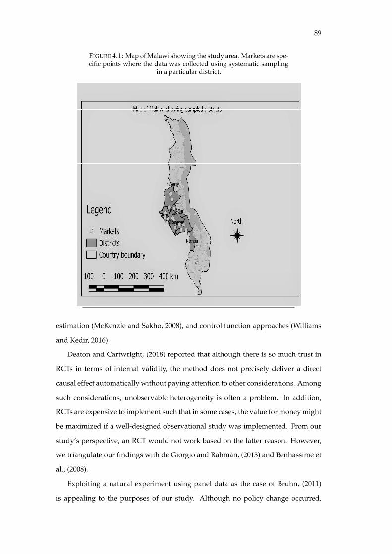
89

FIGURE 4.1: Map of Malawi showing the study area. Markets are spe-cific points where the data was collected using systematic sampling

in a particular district.

estimation (McKenzie and Sakho, 2008), and control function approaches (Williams

and Kedir, 2016).

Deaton and Cartwright, (2018) reported that although there is so much trust in

RCTs in terms of internal validity, the method does not precisely deliver a direct

causal effect automatically without paying attention to other considerations. Among

such considerations, unobservable heterogeneity is often a problem. In addition,

RCTs are expensive to implement such that in some cases, the value for money might

be maximized if a well-designed observational study was implemented. From our

study’s perspective, an RCT would not work based on the latter reason. However,

we triangulate our findings with de Giorgio and Rahman, (2013) and Benhassime et

al., (2008).

Exploiting a natural experiment using panel data as the case of Bruhn, (2011)

is appealing to the purposes of our study. Although no policy change occurred,

90

the appeal of controlling for unobservable heterogeneity in business observations is

important.

McKenzie and Sakho, (2008) subjected their observational data to instrumental

variable (IV) estimation to cleanly identify the causal effects. Noteworthy, Angrist

& Pischke (2008) cautioned that use of IVs should not only follow the study context

and hypothesis at hand but should also be valid and strong. They cautioned that

finding strong instruments is often difficult. Our study context permits the use of

instrumental variable estimation.

Williams and Kedir, (2016) used Heckman’s sample selection procedure. The ap-

proach models the mechanisms that affect business registration through a control

function first, and later models the effects of registration on performance using a ra-

tio of the predicted probability density function to the cumulative density function

i.e. the inverse Mills ratio as an explanatory random variable. The method works

better using observational data but when using panel data, it is advised to use boot-

straped standard errors (Wooldridge, 2010).

To conclude, we adopt a short but rapidly followed observational panel data sur-

vey design and later use instrumental variable estimation techniques. As a robust-

ness check, we implement Wooldridge (2010)’s approach to check our IV approach.

In order to ascertain the effect of registration on business performance, an in-

strumental variable (IV) regression technique is used. The IV regression is a method

that is used to assess direct causal effects in the absence of randomized experiments

(Angrist and Pischke, 2008). For instance, had it been that an external individual

randomly registered maize trading firms and left others unregistered then observed

the performance differences in a controlled manner, then, an ordinary least squares

regression technique would have been used. In that case, given that Dijt is the state

of whether the firm is registered, i.e. Dijt = 1, or the firm is not registered Dijt = 0

and business profitability is Yijt. Then the difference in the business performance

outcomes, i.e. Yijt(1)− Yijt(0) can be estimated by ordinary least squares regression

techniques. That is,

Yijt = β0 + β1Dijt + εijt, (4.1)

where βi are parameters to be estimated. To control for other factors that might affect

91

firm performance, we add a number of variables Xijt which would make our OLS

regression

Yi = β0 + β1Dijt + β3Xijt + εijt, (4.2)

However, since the individual self-selects into registering their firm, we suspect that

firm registration might be correlated with the error term. For instance, while having

controlled for a considerable number of factors, some individuals might have more

aptitude for entrepreneurship and would register their businesses. Aptitude in this

case might be in the error term. We look for a random variable that is correlated with

business registration but is not correlated with the error term. Thus, when clearly

identified, the IV estimate will be of the form

β IV =Cov(xijt, yijt)

Var(xijt). (4.3)

In our study, we use geodetic distances from Lilongwe the capital city, where busi-

ness registration takes place and business age as instruments for business registra-

tion. We argue that while age of the business and distance likely influence the like-

lihood to register, it may not directly influence firm’s profitability. We fitted the

regression using the following form

ln Profitijt = β0 + β1Registration + β2Xijt + δj + γt + εijt, (4.4)

where ln Profit is the natural log of profit of firm i from market j in season t; Registra-

tion is a dummy variable taking the value of 1 if the business is registered and 0 oth-

erwise; Xijt is a vector of control variables; δj are market specific dummies; while γt

is are the seasonal dummies. Then, we tested the robustness of the instrument using

Ordinary Least Squares regression to assess it association, used The Kleibergen-Paap

test for underidentification and the Stock-Watson test for weak instruments.

As a robustness check for our IV estimator, we use an endogenous switching re-

gression model proposed by Maddala (1986). We start by reformulating equation

92

4 by removing the IV and explicitly specifying a selection mechanism that incorpo-

rates as many confounders of business registration as possible. The selection equa-

tion takes the form

D∗ijt = Zijtκ + uijt (4.5)

where Dijt = 1 if the latent variable D∗ijt > 0 and Dijt = 0 if the latent variable

D∗ijt ≤ 0. Using a probit regression model we predict the propensity score – the

probability of registering a business – as

Prob(Dijt = 1|Zijt) = Φ(κZijt) (4.6)

Prob(Dijt = 0|Zijt) = 1−Φ(κZijt) (4.7)

The random variables εijt and uijt and bivariate normally distributed with a zero

mean and a variance covariance matrix equal to

σε ρ

ρ 1

Having explicitly modelled the selection process, we can estimate the potential out-

come model – restate equation 4 – when D = 1 as

log Profitijt = β1(κZijt + uijt) + β2Xij + δj + γt + εijt, (4.8)

and when the business is not registered as

log Profitijt = β2Xijt + δj + γt + εijt, (4.9)

Maddala (1983) provides the joint probability density and likelihood functions

for equations (7a) and (7b) in cross-section form while Wooldridge (2010) provides

detailed exposition on the asymptotic properties.

Since we are operating in a panel data framework, we adopt a dummy variable

fixed effects approach and use bootstrapped standard errors with 250 replications.

Of note, these standard errors are the most conservative in the class of robust stan-

dard errors.

93

4.4 Results

4.4.1 Descriptive statistics

Table 4.1 summarizes results of descriptive statistics of key variables used to asses

the effect of business registration on performance. Results indicate that 76% of

the firms were not registered. The average profit of firms in the sample was

MK600,764.64. Noteworthy, there were marked differences between registered and

unregistered businesses. Using student’s t-test, results were significant at 1% that

registered businesses were twice as profitable. Results further indicate that unregis-

tered firms had less assets than registered firms. In addition, results also show that

registered businesses stay longer in business. Results for this difference is signifi-

cant at 1%. Furthermore, we find that registered firms had more 33% more export

licenses than unregistered firms. Results also indicate that registered firms were cov-

ering a larger geographical area than unregistered firms. Registered firms were 77%

likely to have more businesses than unregistered businesses. The registered firms in

the sample were more likely to sell other commodities apart from maize than unreg-

istered firms. When the market had more firms, then it was more likely that firms

would be unregistered. Furthermore, results also indicate that registered firms are

more likely to have more employees than unregistered ones. In addition, firms that

were registered were more likely to have more interactions with other traders.

4.4.2 Effects of firm registration on performance in form of profitability

Having controlled for the factors in the descriptive statistics, we computed geode-

tic distances i.e. the shortest great circle distances between a given market and Li-

longwe, where business registration takes place, as an instrument for business reg-

istration. We assume that the closer the trader is to the registration center the more

likely they are to be registered and we cannot be certain whether this directly im-

pacts profitability. Even if it were to be correlated, there could be no plausible eco-

nomic explanation. The instrument uses curves between two points using latitudes

and longitudes on the mathematical model of the earth using WGS 1984 datum and

Vincenty’s equations (Vincenty, 1975).

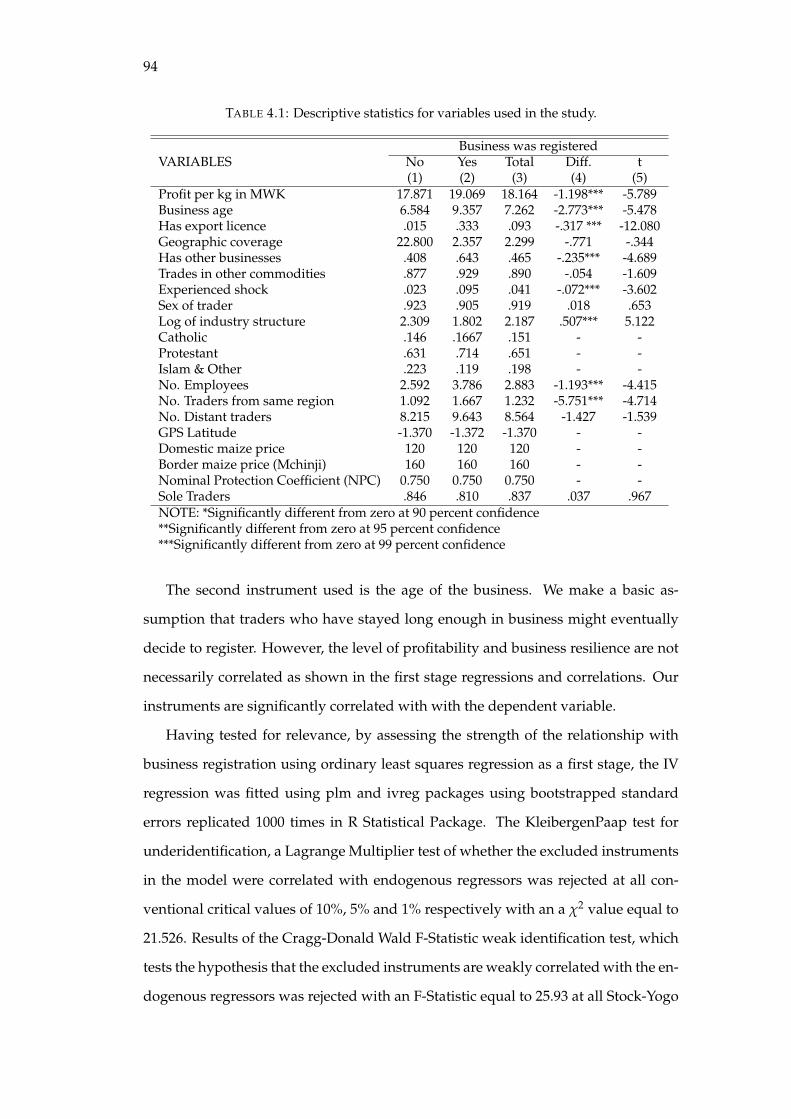
94

TABLE 4.1: Descriptive statistics for variables used in the study.

Business was registeredVARIABLES No Yes Total Diff. t

(1) (2) (3) (4) (5)Profit per kg in MWK 17.871 19.069 18.164 -1.198*** -5.789Business age 6.584 9.357 7.262 -2.773*** -5.478Has export licence .015 .333 .093 -.317 *** -12.080Geographic coverage 22.800 2.357 2.299 -.771 -.344Has other businesses .408 .643 .465 -.235*** -4.689Trades in other commodities .877 .929 .890 -.054 -1.609Experienced shock .023 .095 .041 -.072*** -3.602Sex of trader .923 .905 .919 .018 .653Log of industry structure 2.309 1.802 2.187 .507*** 5.122Catholic .146 .1667 .151 - -Protestant .631 .714 .651 - -Islam & Other .223 .119 .198 - -No. Employees 2.592 3.786 2.883 -1.193*** -4.415No. Traders from same region 1.092 1.667 1.232 -5.751*** -4.714No. Distant traders 8.215 9.643 8.564 -1.427 -1.539GPS Latitude -1.370 -1.372 -1.370 - -Domestic maize price 120 120 120 - -Border maize price (Mchinji) 160 160 160 - -Nominal Protection Coefficient (NPC) 0.750 0.750 0.750 - -Sole Traders .846 .810 .837 .037 .967NOTE: *Significantly different from zero at 90 percent confidence**Significantly different from zero at 95 percent confidence***Significantly different from zero at 99 percent confidence

The second instrument used is the age of the business. We make a basic as-

sumption that traders who have stayed long enough in business might eventually

decide to register. However, the level of profitability and business resilience are not

necessarily correlated as shown in the first stage regressions and correlations. Our

instruments are significantly correlated with with the dependent variable.

Having tested for relevance, by assessing the strength of the relationship with

business registration using ordinary least squares regression as a first stage, the IV

regression was fitted using plm and ivreg packages using bootstrapped standard

errors replicated 1000 times in R Statistical Package. The KleibergenPaap test for

underidentification, a Lagrange Multiplier test of whether the excluded instruments

in the model were correlated with endogenous regressors was rejected at all con-

ventional critical values of 10%, 5% and 1% respectively with an a χ2 value equal to

21.526. Results of the Cragg-Donald Wald F-Statistic weak identification test, which

tests the hypothesis that the excluded instruments are weakly correlated with the en-

dogenous regressors was rejected with an F-Statistic equal to 25.93 at all Stock-Yogo

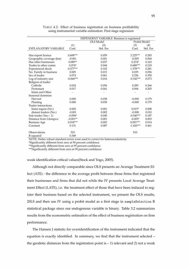
95

TABLE 4.2: Effect of business registration on business profitabilityusing instrumental variable estimation: First stage regression

DEPENDENT VARIABLE: Business is registeredOLS Model Probit Model

(1) (2) (3) (4)EXPLANATORY VARIABLE Coef. Std. Err. Coef. Std. Err

Has export licence 0.608*** 0.059 2.225*** 0.283Geographic coverage (km) -0.001 0.001 -0.005 0.004Has other businesses 0.089** 0.037 0.274* 0.163Trades in other comm 0.074* 0.044 0.688*** 0.218Experienced shock 0.377*** 0.102 1.378*** 0.281No. Family in business 0.005 0.013 0.035 0.056Sex of trader 0.074 0.061 0.256 0.350Log of industry size -0.060*** 0.016 -0.342*** 0.073Religion of trader

Catholic 0.024 0.056 0.285 0.266Protestant 0.017 0.041 0.094 0.205Islam and Other - - - -

Seasonal dummiesHarvest 0.000 0.038 -0.000 0.179Planting 0.000 0.038 -0.000 0.179

Trader interactionsSame region (No.) 0.002 0.001 0.015* 0.008distant traders (No.) -0.001 0.002 -0.008 0.010

Sole trader (Yes= 1) -0.094* 0.049 -0.540*** 0.187Distance from Lilongwe -0.001** 0.001 -0.005* 0.003Business Age 0.018*** 0.003 0.091*** 0.014Constant 0.131 0.087 -1.420*** 0.461

Observations 510 510R-squared 0.349NOTE: Huber robust standard errors were used to correct for heteroscedasticity*Significantly different from zero at 90 percent confidence**Significantly different from zero at 95 percent confidence***Significantly different from zero at 99 percent confidence

weak identification critical values(Stock and Yogo, 2005).

Although not directly comparable since OLS presents an Average Treatment Ef-

fect (ATE) - the difference in the average profit between those firms that registered

their businesses and firms that did not while the IV presents Local Average Treat-

ment Effect (LATE), i.e. the treatment effect of those that have been induced to reg-

ister their business based on the selected instrument, we present the OLS results,

2SLS and then use IV using a probit model as a first stage in sampleSelection R

statistical package since our endogenous variable is binary. Table 3.2 summarizes

results from the econometric estimation of the effect of business registration on firm

performance.

The Hansen J statistic for overidentification of the instrument indicated that the

equation is exactly identified. In summary, we find that the instrument selected –

the geodetic distances from the registration point is – 1) relevant and 2) not a weak

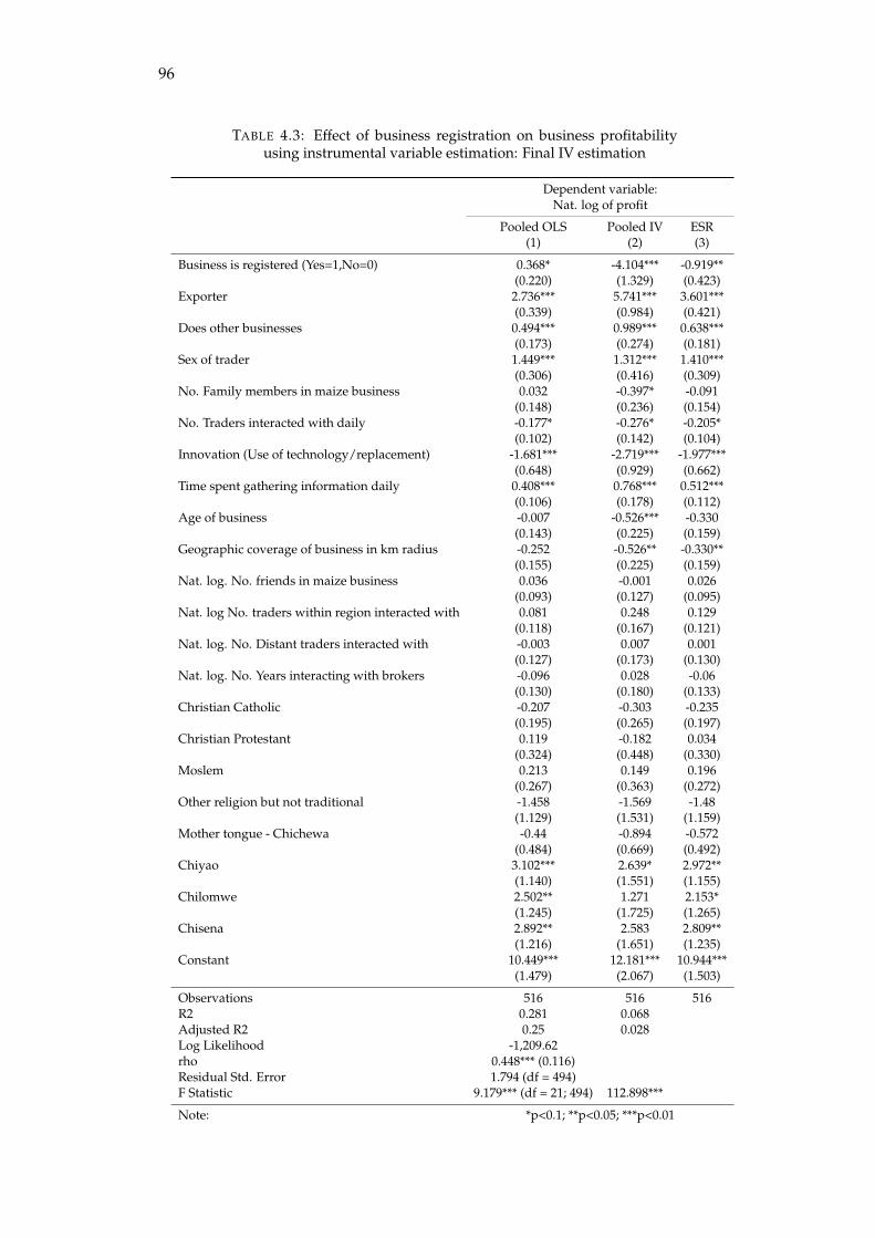
96

TABLE 4.3: Effect of business registration on business profitabilityusing instrumental variable estimation: Final IV estimation

Dependent variable:Nat. log of profit

Pooled OLS Pooled IV ESR(1) (2) (3)

Business is registered (Yes=1,No=0) 0.368* -4.104*** -0.919**(0.220) (1.329) (0.423)

Exporter 2.736*** 5.741*** 3.601***(0.339) (0.984) (0.421)

Does other businesses 0.494*** 0.989*** 0.638***(0.173) (0.274) (0.181)

Sex of trader 1.449*** 1.312*** 1.410***(0.306) (0.416) (0.309)

No. Family members in maize business 0.032 -0.397* -0.091(0.148) (0.236) (0.154)

No. Traders interacted with daily -0.177* -0.276* -0.205*(0.102) (0.142) (0.104)

Innovation (Use of technology/replacement) -1.681*** -2.719*** -1.977***(0.648) (0.929) (0.662)

Time spent gathering information daily 0.408*** 0.768*** 0.512***(0.106) (0.178) (0.112)

Age of business -0.007 -0.526*** -0.330(0.143) (0.225) (0.159)

Geographic coverage of business in km radius -0.252 -0.526** -0.330**(0.155) (0.225) (0.159)

Nat. log. No. friends in maize business 0.036 -0.001 0.026(0.093) (0.127) (0.095)

Nat. log No. traders within region interacted with 0.081 0.248 0.129(0.118) (0.167) (0.121)

Nat. log. No. Distant traders interacted with -0.003 0.007 0.001(0.127) (0.173) (0.130)

Nat. log. No. Years interacting with brokers -0.096 0.028 -0.06(0.130) (0.180) (0.133)

Christian Catholic -0.207 -0.303 -0.235(0.195) (0.265) (0.197)

Christian Protestant 0.119 -0.182 0.034(0.324) (0.448) (0.330)

Moslem 0.213 0.149 0.196(0.267) (0.363) (0.272)

Other religion but not traditional -1.458 -1.569 -1.48(1.129) (1.531) (1.159)

Mother tongue - Chichewa -0.44 -0.894 -0.572(0.484) (0.669) (0.492)

Chiyao 3.102*** 2.639* 2.972**(1.140) (1.551) (1.155)

Chilomwe 2.502** 1.271 2.153*(1.245) (1.725) (1.265)

Chisena 2.892** 2.583 2.809**(1.216) (1.651) (1.235)

Constant 10.449*** 12.181*** 10.944***(1.479) (2.067) (1.503)

Observations 516 516 516R2 0.281 0.068Adjusted R2 0.25 0.028Log Likelihood -1,209.62rho 0.448*** (0.116)Residual Std. Error 1.794 (df = 494)F Statistic 9.179*** (df = 21; 494) 112.898***

Note: *p<0.1; **p<0.05; ***p<0.01

97

instrument.

For robustness checks, we present OLS, Pooled IV and then use an endogenous

switching regression (ESR) (Maddala 1986) to explicitly model the business regis-

tration selection mechanism. The ESR technique is the best way to gauge how well

the selection mechanism has been controlled for through use of propensity scores.

Table 3 summarizes results from the econometric estimation of the effect of business

registration on firm performance.

Since we rejected the use of pooled OLS and establish that there is endogeneity

in our models, we use IV and ESR results. We find that business registration has a

negative effect on firm profitability. Our results indicate that a discrete change from

an unregistered business to a registered one is associated with a -4.104 change in the

natural log of the profits of the business. This result is two-sided statistically dif-

ferent from zero at 99%. From the diagnostic statistics, both models are consistent

and have the same direction. More substantively, when proximity to the registration

center – the instrument – induces traders to register their businesses, it is associated

with a loss in profitability amounting to MWK60 . In addition, when the entire se-

lection mechanism is taken into account –, a shift from and unregistered trader to a

registered one is associated with a MWK2 per kg loss in profits. This is in contrast

to the rejected pooled OLS comparison of expected profits between registered and

unregistered ones which shows registered businesses are 37% more profitable. The

latter estimate ignores self-selection of the registration decision, which biases the re-

sults upwards. Noteworthy, the pooled OLS results are only significantly different

from zero at 90% confidence while the rest are significant at 99% and 95%, respec-

tively. Further, the IV model overestimates the impacts while the ESR is the most

conservative.

Other factors affecting business performance include whether the trader imports

or exports which is associated with an increase in profits by a factor of 5. This re-

sult is statistically significant at 5%. Second, we further find that businesses that

trade in other commodities are associated with a 98% increase in profits. This find-

ing was statistically significant at 1%. We find that if the trader was male, it was

associated with over 100% more profitable businesses. When more family members

are involved in the business, it is associated with less profitability. However, we find

98

that this result is barely robust at p < 0.10. Similarly, interactions with traders also

have a profit reducing effect albeit barely robust at p < 0.10. Frequent replacement

of assets also has a profit reducing effect at p < 0.01.

Indicators of social capital also play a significant role in business performance.

However the magnitudes are mixed. For instance, when endogeneity is controlled

for, tribe has a positive effect while friends’ interactions and religion have no effect.

4.5 Discussion

In this study we assessed the effect of business registration on performance of the

firm in terms of profitability among maize traders in Malawi using an instrumental

variable approach. We find three results. First, from the descriptive analysis, we find

that the informal unregistered businesses are more than the registered businesses.

Second, econometrically, we find a causal path that business registration negatively

affects profitability. Third, social capital plays a, but nevertheless not so robust, role

in business performance.

The result that the informal, unregistered businesses form a majority in the sec-

tor is not surprising as it has also been reported by Chen et al. (2007) who indicated

that the informal sector has a mixture of wage workers, self-employed individuals

and entrepreneurs who produce commodities that are legally acceptable. Chen et

al. (2007) further reported that given favourable conditions such as reduced barriers

to business registration and a suitable regulatory environment, most unregistered

firms would also register. This observation also concurs with our key informant

interviews with informal traders who reported that it was difficult to access infor-

mation about business registration.

Further, it was reported that other barriers were that the registration authorities

were unavailable in the areas where most small businesses operate. If business reg-

istration and regulatory authorities were to set up business registration bureaus at

district level, then the level of informal businesses would reduce. Our finding of sig-

nificant barriers to register the businesses due to distance are also in agreement with

Grimm, Krüger, and Lay (2011) who also found that at the lower level of business ac-

tivity, there are negligible capital costs to running the business among unregistered

99

firms.

However, as firms increase in size, they start facing significant barriers if they

are not registered. One, case in point from our study is the access to export licences.

We found that businesses that are registered were 88% more likely to have an export

license compared to those that were not registered. In addition, businesses that have

export licenses and access international markets make more profits than unregis-

tered ones. As the descriptive statistics show, only 33% of the sample have access to

international markets. This may mean that the industry is highly concentrated at the

export level since only few companies have access to international markets. Resul-

tant, most businesses without export licenses will be forced to sell at depressed do-

mestic market prices, something that does not lead to efficient allocation of resources

as there will be an over-abundance of supply leading to consumers consuming too

much of the inefficiently allocated commodity (Estrades, Flores, Lezama, et al., 2017;

Tsakok, 1990). This may affect firm performance by lowering profits of unregistered

businesses which may negatively affect performance of the entire industry.

The results of large unregistered businesses coupled with lower Nominal Pro-

tection Coefficients (NPC) is suggestive of an agricultural taxation price policy. Ma-

grini, Balié, and Morales-Opazo (2017) reported that price incentives at the border,

such as removal of tariffs on agricultural commodities, repeal of export bans, can

stimulate profitability and eventually sector supply. However, our results which

show large levels of agricultural taxation suggest that as long as large numbers of

unregistered firms who have no access to agricultural licenses exist, performance

and general competitiveness in the industry will remain low.

Our key result that business registration significantly decreases profitability - a

direct measure of business performance - is in agreement with Williams and Kedir;

McKenzie and Sakho (2008) but are not in line with Chen et al. (2007) who found

that firms that have formalized have a high chance of surviving turbulent business

environments. Our results appeal to literature from developing countries where

entrepreneurs face significant registration costs (Benhassime et al., 2018) and lack of

information (de Giorgi and Rahman, 2013). Thus, we reject our null hypothesis that

business registration leads to profitable businesses.

Our results stand in stark contrast to the formality literature such as Aidis and

100

Van Praag (2007) and La Porta (2014). Aidis and Van Praag (2007), in a study from

Lithuania, found that although informal young entrepreneurs might see a surge in

business performance in early stages, setting up legal businesses formally leads to

more stable businesses. We argue that eventually, such opportunities can only be

harnessed by reforming the tax and regulatory environment. Coupled to business

registration, maize trading businesses that are run by males are more profitable com-

pared to their female counterparts.

This result contrasts Chirwa (2008) who found that female run micro-enterprises

in Malawi perform much better than male run businesses. However, Chirwa (2008)

was more general and did not particularly specify whether the firms were formal or

informal as compared to this study, which focuses on maize traders who formalized

their businesses. Further, our result that trader characteristics play an important

role in business performance corroborates Barbieri and Mshenga (2008) who also

found that trader characteristics such as number of employees, length of time doing

business, age of the trader and asset ownership and gender have significant effects

on business performance.

When we control for endogeneity of business registration, we find that measures

of social capital have different effects on business performance. Interactions with

traders, though they had positive effects, were not statistically significant. However,

we found that family based businesses were less profitable – hence low performing.

Diéguez-Soto, López-Delgado, and Rojo-Ramírez (2015) reported that most family

run businesses are often risk averse and would not venture into expansion strategies

such as expanding their businesses by taking in credit for fear of losing a family

business.

4.6 Conclusions

This study assessed the effect of firm registration on business performance in

Malawi’s maize sub-sector. Primary data from the trader survey conducted in the

central region of Malawi was used. The data reports business characteristics, sea-

sonal revenue, variable and transaction costs and profits from 15 markets across five

districts of Kasungu, Dowa, Lilongwe, Mchinji and Dedza, respectively. To assess

101

the effect of firm registration on business performance, an Instrumental Variable es-

timation technique was used. Our study points to three key results. First, we found

that registered businesses comprise 24% of all traders in the sample. Second, results

indicate that firms that were registered were four times less profitable as unregis-

tered businesses. Third, across various indicators, results show that social capital

has significant positive effects on business perfomance.

In order to improve performance of businesses in the agricultural sector, the role

of business registration should not be overlooked. The study recommends reform-

ing the ease of registering businesses, reforming the tax policy and devolving busi-

ness registration processes to district councils so that businesses can register at the

lowest level as this could reduce informality and enhance accountability of firms.

103

Chapter 5

Entrepreneurship, food security

and welfare in Malawi

5.1 Introduction

Entrepreneurship can be a catalyst for economic growth through innovation

(Schumpeter, 1934; Anokhin and Schulze, 2009) 1. While factors, such as choice,

personal characteristics, success and failure, entry and exit mechanisms, that drive

entrepreneurship have been widely studied in management literature (Mwatsika,

2015; Naudé, 2014), there is a huge disconnect on implications of entrpreneurship

on welfare and economic growth (Naudé, 2010). While in the past development eco-

nomics literature largely relegated entrepreneurship to management sciences, it is

only recently that its formalization has taken root. Naudé (2010) pointed out that the

main reasons for the disconnect between entrepreneurship in management sciences

and in mainstream development economics has been that, in the past, entrepreneur-

ship was vaguely defined to be incorporated into formal economic growth theories.

The second reason is that entrepreneurship has commonly been treated as a bind-

ing constraint to economic growth. However, recent advances in economic theory

have made entrepreneurship tractable by formalizing it in modern economic growth

theories (Gries and Naudé, 2010). Using such growth models has enabled devel-

opment research evaluate the implications of venturing into entrepreneurship on

the inequality (Kimhi, 2010), productivity (Audretsch, Keilbach, Lehmann, et al.,

2006), economic transformation (Gries and Naudé, 2010) and welfare (Tamvada,

1An earlier version of this chapter was selected for presentation at the Agricultural and AppliedEconomics Association meeting, Atlanta, GA, July 21 – July 23

104

2010; Henrekson, 2005; Otoo et al., 2011). However, most of the work has been

concentrated in developed countries (see Chowdhury, Audretsch, and Belitski, 2019;

Erken, Donselaar, and Thurik, 2018; Parker, 2018; Audretsch, Keilbach, Lehmann,

et al., 2006; Hamilton, 2000). Of the few studies conducted in developing countries,

none have explored the implications of entrepreneurship on one important indicator

of welfare, food security. In most African countries, achieving food security is one of

the key goals such that evaluating the impact of entrepreneurship on such indicators

would be of much policy relevance.

In the belief that entrepreneurship would induce structural change in economic

activities by creating more value added and, therefore, growth to achieve the Mil-

lennium Development Goals (MDGs) of ending poverty and hunger, the Malawi

Government prioritized promotion of entrepreneurial activities. As a market ori-

ented strategy to ensure that all individuals meaningfully participate in wealth cre-

ation and poverty reduction, the government invested approximately seven million

US Dollars in development of technical, entrepreneurial and business management

skills through various vocational training and all schools across the country between

2011 and 2016 (Government of Malawi, 2011b).

The question of evaluating the effect of entrepreneurship on food security is

complex because of several problems. First, the definition of entrepreneurship it-

self is elusive in literature. Adopting Williams (2008)’s narrow definition, that an

entrepreneur is an individual running a business that is less than 42 months, we can

trace the number of individuals and households that are involved in entrepreneur-

ship. In fact, most businesses in Africa are less than five years.

In the same vain, the government prioritized strategy was nationwide and non-

ignorable as opposed to randomized or sequential exposure. Thus, we can only

observe compliance by individuals who became entrepreneurs. Entrepreneurs can

be systematically different from non-entrepreneurs since we cannot easily describe

the mechanism and motivations that determine entry into entrepreneurship let alone

simply attribute the effect to the government strategy. Dawson and Henley (2012),

in a review of literature on motivations driving individuals to venture into en-

trepreneurship, noted that people chose to start new businesses because of “push”

or “pull” motivations. On one side, individuals are drawn into entrepreneurship

105

because of the need for self-personal efficacy (Pistrui et al., 2001), inability to find

suitable paid employment (Block and Landgraf, 2016) and other pecuniary mo-

tives. Dawson and Henley (2012) reported that individuals would venture into en-

trepreneurship because an external opportunity has availed itself. On the pecuniary

motives, their study noted that women usually venture into entrepreneurship to feel

independent from their spouses and have a feeling that they are in control of their

own lives. The study also noted that when the economic environment is not con-

ducive such as in a recession, individuals, especially men, venture into entrepreneur-

ship. The latter is a push factor while the former were classified as pull factors. Nev-

ertheless, Williams (2009) reported that putting entrepreneurship motives into two

categories obfuscates the reasons for examining motivations. The study advocates

for a holistic take on the mechanisms for venturing into entrepreneurship. This view

is consistent with Wry and York (2019).

While it may not be possible to control for all these motivations, what is clear is

that the decision to venture into entrepreneurship is endogenous and the sample of

entrepreneurs may be systematically different from the entire population. However,

with a proper selection bias correction framework, we can conditionally assess the

treatment effect of entrepreneurship on food security.

This paper, therefore, assesses the distributional impacts of entrepreneurship on

household food and nutrition security. In particular, we examine implications of en-

try into entrepreneurial activities on food consumption, dietary diversity and wel-

fare. We also explore the mechanisms driving entry into entrepreneurship and food

consumption expenditure patterns.

The Government programme to increase entrepreneurial activities is also hard to

evaluate if it increased incomes and reduced hunger. Part of the problem is that it is

ethically and politically difficult to randomize access to program resources mainly

due to the self-selecting nature of individuals getting into entrepreneurship. For

those households that venture into entrepreneurial activities, there could potentially

be general equilibrium effects at population level due to backward and forward link-

ages of multi-sectoral activities.

We specifically assess the distributional impacts of entrepreneurship on house-

hold real consumption expenditure, food and nutrition security. In particular, we

106

examine whether entry into entrepreneurial activities leads to more diverse diets as

incomes change. We also explore the mechanisms driving food consumption expen-

diture patterns among entrepreneur households between 2011 and 2016.

Our study contributes to literature by combining modern economic growth the-

ory with endogenous entrepreneurship assumptions. We further, empirically, apply

a novel quantile regression technique that adjusts for selection bias to a recent three

wave panel Living Standards Measurement Survey (LSMS) from Malawi. Literature

on off-farm entrepreneurship and welfare outcomes in African settings is scarce and

this study aims to bridge that gap.

The rest of the paper is structured as follows. The second section presents the

methodology where the theoretical framework, identification strategy and data are

presented. The third section presents results beginning with descriptive analysis,

then explicitly modeling entry into entrepreneurship to isolate Malawian context

specific drivers. Then propensity score analysis follows to balance the data and

isolate treatment effects on the treated at household level. A quantile regression

model adjusted for selection bias is presented to assess heterogeneous effects of en-

trepreneurship. Section four discusses the results using economic theory and recent

literature to draw policy implications. Section five summarizes and concludes.

5.2 Methods

5.2.1 Theoretical framework

An equilibrium model with endogenous entrepreneurship

Table 5.1 summarizes key equations of the model. Our model starts with en-

trepreneurial firms or people in each of the sector s producing output Q using factors

F using constant returns to scale, equation 1 in Table 5.1. Entrepreneurial and man-

agerial ability are part and parcel of the factors F. The model takes productivity (a)

as endogenous and subject to the entrepreneur’s capabilities and endowments, such

that it determines shares of production technologies. We assume that firms maxi-

mize profits in such a way that factor payments W are equal to production revenues.

107

Labour l is unemployed and fully mobile in the agricultural sector while in non-

agricultural sectors is fully employed and sector specific. That is, unskilled labour

from agriculture can easily move across the sectors i.e. a smallholder farmer can

easily move to be employed or start a business in another sector while it is difficult

for architects or doctors to switch between sectors but they can produce other eco-

nomic activities e.g. entrepreneurial firms within those sectors. Land n, and capital

are fully employed and sector specific. The entrepreneurial firm face investment

demands I – equation 4, Table 5.1.

Households in the model maximize a utility function subject to a budget line

in equation 3, Table 5.1. That is, households pool their resources and livelihood

activities and maximize a common utility function in cooperation (Becker, 1974).

Of note, household income Y is a function of total returns W – equation 2 – from

productive activities of the entrepreneurial firm since they are eventual owners of

factors of production F. Further, households face consumption demands D such that

they utilize their income Y to purchase commodities at given market prices P.

We further assume that product, labour, capital and land markets are in equilib-

rium – equations 7,8,9 in Table 5.1. We also assume that entrepreneurial firms en-

gage in international trade and government collects revenue through various taxes

and levies but to keep the model sufficiently simple we have abstracted from its ex-

plicit modeling. For details see (Lofgren, Harris, and Robinson, 2002; Pauw et al.,

2011). Normally, due to the complexity of linkages in the model, the model is solved

analytically. However, since we have explicitly shown how each of the equations are

linked, it is easier to assess equation (3) econometrically and assume that the other

linkages are implicitly controlled for.

5.2.2 Identification strategy

A counterfactual framework for entrepreneurship and welfare outcomes

The fundamental question of any causal analysis is to find out what would have

happened to treated units had it been that they were not treated or what would have

happened to control units had it been that they were treated. In our case, we would

like to know what would have happened to entrepreneurs’ welfare outcomes had it

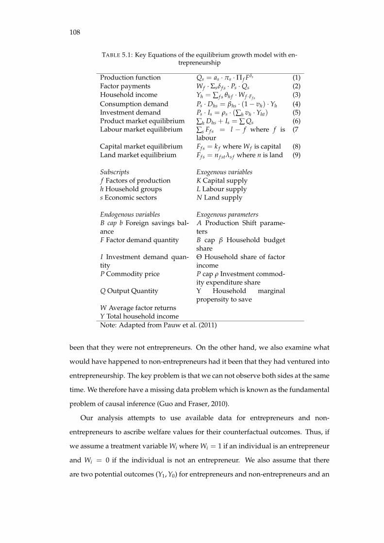
108

TABLE 5.1: Key Equations of the equilibrium growth model with en-trepreneurship

Production function Qs = as · πs ·Π f Fδs (1)Factor payments W f · Σsδ f s · Ps ·Qs (2)Household income Yh = ∑ f s θh f ·W f ·Ff s (3)Consumption demand Ps · Dhs = βhs · (1− vh) ·Yh (4)Investment demand Ps · Is = ρs · (∑h vh ·Yht) (5)Product market equilibrium ∑h Dhs + Is = ∑ Qs (6)Labour market equilibrium ∑s Ff s = l − f where f is

labour(7

Capital market equilibrium Ff s = k f where W f is capital (8)Land market equilibrium Ff s = n f stλs f where n is land (9)

Subscripts Exogenous variablesf Factors of production K Capital supplyh Household groups L Labour supplys Economic sectors N Land supply

Endogenous variables Exogenous parametersB cap b Foreign savings bal-ance

A Production Shift parame-ters

F Factor demand quantity B cap β Household budgetshare

I Investment demand quan-tity

Θ Household share of factorincome

P Commodity price P cap ρ Investment commod-ity expenditure share

Q Output Quantity Υ Household marginalpropensity to save

W Average factor returnsY Total household incomeNote: Adapted from Pauw et al. (2011)

been that they were not entrepreneurs. On the other hand, we also examine what

would have happened to non-entrepreneurs had it been that they had ventured into

entrepreneurship. The key problem is that we can not observe both sides at the same

time. We therefore have a missing data problem which is known as the fundamental

problem of causal inference (Guo and Fraser, 2010).

Our analysis attempts to use available data for entrepreneurs and non-

entrepreneurs to ascribe welfare values for their counterfactual outcomes. Thus, if

we assume a treatment variable Wi where Wi = 1 if an individual is an entrepreneur

and Wi = 0 if the individual is not an entrepreneur. We also assume that there

are two potential outcomes (Y1, Y0) for entrepreneurs and non-entrepreneurs and an

109

actual measured outcome Yi. Rubin (2005) presents the observed outcome as

Yi = W1Yi1 + (1−W1)Yi0. (5.1)

where Wi acts as a switching variable. In order to make statements about causality,

we cannot only use information about individuals who participated Yi1 · (Wi = 1)

but we must also use information about individuals who did not participate Yi0 ·

(Wi = 0) and then eventually compare Yi1 and Yi0. Therefore, to make a causal

statement whether W = 1 causes Y1, we must evaluate the evidence in the data on

potential outcomes under W = 1 and W = 0. Thus, given an arbitrary cut off point

p, where Yi1 > p if Wi = 1 and Yi0 < p if Wi = 0, we can deduce that Wi = 1 causes

Yi1 > p if after evaluating the evidence under Wi = 0, we find that indeed Yi0 < 0.

Under an assumption of perfect randomization, where participants are randomly

assigned W = 1 and non-participants W = 0, Hernan and Robins (2018) and Guo

and Fraser (2010) state that we can compare the average outcome under W = 1 and

that under W = 0. The standard estimator for calculating treatment effect is,

γ = E(Y1|W = 1)− E(Y0|W = 0) (5.2)

where E is an expectation operator and γ is the Average Treatment Effect (ATE) of

participating in entrepreneurship. Thus, E(Y0|W = 0) represents a counterfactual

for E(Y0|W = 1) and E(Y1|W = 1) represents the counterfactual when E(Y1|W = 0).

In a perfectly randomized framework, an ordinary least squares regression can be

used i.e.

Yi = α + γWi + ε (5.3)

where α is a regression constant representing the average effect when Wi = 0, τ

is the ATE and ε is a regression error term (White, 2006). When the assignment

mechanism to participant and non-participant status is not randomized, that is if

either individuals self-select or there appears to be another mechanism, then the

latter and the former do not represent the counterfactuals. Thus, E(Y0|W = 0) 6=

E(Y0|W = 1) and E(Y1|W = 1) 6= E(Y1|W = 0). Estimation of effects using τ in

110

equations 5.2 and 5.3 would lead to biased estimators i.e. effects that are influenced

by outliers. However, given a number of assumption, it is possible to estimate causal

effects using the Rubin counterfactual framework.

In order to estimate the effects, we first assume that conditional on observable

control variables X, assignment to participation and non-participation is indepen-

dent of the potential outcomes (Y1, Y − 0) ⊥ W|X . Thus, we assume that given

the control variables, the selection mechanism into entrepreneurship is independent

of the welfare outcomes. this is known as the conditional independence assump-

tion (CIA) (Huber and Melly, 2015; Guo and Fraser, 2010; Rosenbaum, 1984). To

check the validity off this assumption, we conduct a bivariate comparison of con-

trol variables using student’s t-tests for continuous variables and chi-square tests for

categorical variables. If the control variables are statistically different between the

participants and non-participants, then the correlation is non-zero, ρ(W, X) 6= 0 and

CIA is violated.

Second we assume that the value of the outcome Yi for individual i with par-

ticipation status Wi will not change regardless of the procedure used to assign the

participation status and the participation status of other individuals. This is called

the Stable Unit Treatment Value Assumption (SUTVA) (Rubin, 2005). During the as-

sessment, it helps rule out interactions among individuals and general equilibrium

effects.

Third, w ⊥ ε|X: we assume that the participation status is independent of the

error term given the control variables . In this assumption, we assume that our selec-

tion mechanism has been adequately modeled such that there are no confounding

nor omitted variables and that there are no measurement errors. Thus, all relevant

drivers of selection into entrepreneurship have been thoroughly accounted for.

Fourth, X ⊥ ε: we assume that the control variables are not correlated with the

error term. This assumption rules out that some of the explanatory variables are

independent variables in themselves.

Fifth, X ⊥W: we assume that the treatment status is independent of the explana-

tory variables. This rules out perfect collinearity in our model which would prevent

the model from achieving rank conditions.

111

Sixth, ε ∼ i.i.d, N(0, 1): we assume that the error term is independent and iden-

tically distributed with mean 0 and standard deviation of 1.

Adjustments to counterfactual assumptions and estimation

At the administrative level, the government strategy and efforts to encourage par-

ticipation in entrepreneurship for economic development does not discriminate no

assigns participation status randomly. On the contrary, individuals self select into

program. Thus the randomization assumption is violated and we only observe vol-

untary compliance into entrepreneurship W1 = 1. Therefore, the effect we measure

is a form of intent to treat.

Since we have three time periods, we also have a problem of time varying treat-

ment effects. To illustrate, taking 2010 as time 0, we can have 23 = 8 treatment

situations. For example, it is possible, where W = 1 is represented by 1 otherwise 0,

to have a universal set of

U = (1, 1, 1), (0, 1, 1), (0, 0, 1), (1, 0, 0), (1, 1, 0), (0, 1, 0), (1, 0, 1), (0, 0, 0)

of the static treatment situation. In this case, a an individual drawn randomly from

the population has a one in eight chance of being found in one of the participation

situations. Following Hernan and Robins (2018), we invoke the full sequential ex-

changeability also known as the joint independence assumption that, given the par-

ticipation history a ∈ U of the household in 2010, 2013 and 2016, i.e. t = 0, 1, 2 and

a vector of control variables, the participation into entrepreneurship is independent

of the welfare outcomes. That is

(Ya, Xa) ⊥Wt|Wk−1, Xt ∀k = 0, 1, 2 and a ∈ U. (5.4)

Accordingly, the full sequential exchangeability assumption represents all counter-

factuals of the participation status across the three time periods. Bang and Robins

(2005) provided doubly robust estimators to assess treatment effects. We will use the

doubly robust estimated to draw inference at individual level.

112

There is also a possibility that effects of participation could vary across individ-

uals such that the average treatment effect could not be truly representative. For

example, effects of participating into entrepreneurship could be larger for poorest

households as compared to richest households. To account for this variation in ef-

fects, we use conditional quantile regression models. Using conditional quantile re-

gression models allows us compute quantile specific treatment effects. In this case,

given control variables X, we can express equation 5.3 as

Qτ(Yi|W, X) = X′β + W ′γ + F−1(ε) (5.5)

where Qτ is a quantile analogue of the expectation operator E for quantile τ; β is a

vector of unknown parameters to be estimated and F−1(ε) is the probability distri-

bution of the error term ε (Cameron and Trivedi, 2010; Angrist and Pischke, 2013).

Therefore,

γτ = Qτ(Yi1|W = 1, X)−Qτ(Yi0|W = 0, X) (5.6)

is the Quantile Treatment Effect (QTE). Equation 5.6 is difficult to estimate in the

presence of self selection. Abadie, Angrist, and Imbens (2002) developed an instru-

mental variable estimator for QTE equation 5.6 where in the presence of a suitable

instrument for W, say Z, the QTE can be identified as

(γ, β) = arg minEρτ(Yi − aWi − X′i b)|Wi = 1 − Eκiρτ(Yi − aWi − X′i b)|Wi = 0

(5.7)

where

κi = 1− Wi(1− Zi)

1− P(Zi = 1)|Xi− (1−Wi)Zi

P(Z = 1)|Xi

; where Zi is a dummy instrumental variable (Angrist and Pischke, 2013). However,

since not only one instrument affects W but a vector of variables and the difficulty

of finding a suitable instrument of entrepreneurship, it is proper to explicitly model

the selection mechanism using propensity scores (Heckman, 1977). We, accordingly,

model the selection mechanism using a distribution function of the percentile error

in the food security outcome equation and the error in the entrepreneurship partici-

pation decision using Arellano and Bonhomme, 2017 framework with an adjustment

113

for the extended treatment effects model (Heckman, 1977; Maddala, 1983). Distri-

butional parameters are estimated by a rotated check function method of moments

minimization. Thus, estimates across the percentiles are corrected for selection bias.

The extension of the quantile sample selection model to a generalized treatment ef-

fects model presents a novel methodological contribution of out study. Thus, the

estimated model is

QS(τ, Z) = X′β(τ∗(Z)) (5.8)

where Yit is the outcome of interest for household i at time t (household real con-

sumption expenditure, value of food consumption, dietary variety and nutrient in-

take per capita). The quantity τ∗(Z) = G−1(τ, Φ(Z′γ); ρ) where Z is a vector of all

relevant explanatory variables such that X ⊂ Z and W ⊂ Z. p(Z) = Φ(Z′γ) is the

propensity score and V(Φ(η)) is the rank of unobservable scalar η ∼ U(0, 1) ⊥ Z

and Φ(·) is a normal conditional distribution function (CDF). (U, V) ∼ bivariate

Gaussian copula with a correlation coefficient ρ ⊥ Z and τ is the percentile in ques-

tion τ ∈ (0, 1). Thus, G(τ, p; ρ) and S means conditional on selection Arellano and

Bonhomme, 2017.

5.2.3 Data

We use a panel of Integrated Household Surveys (IHS) from Malawi conducted be-

tween 2010, 2013 and 2016. The IHS is part of the World Bank’s Living Standards

Measurement Surveys which are designed to collect socioeconomic characteristics

of households in order to aid in policy design and evaluation. Use of the IHS to ex-

plore effects of entrepreneurship on food security contributes to a robust discussion

on evidence based development policy design.

The data has household, agriculture, and community modules that are particu-

larly relevant to the study. From the household questionnaire, we obtained a roster

of household characteristics such as household size, sex, age, marital status and ed-

ucation composition of members. We obtained food consumption information, such

as amount of food consumed in the past seven days and expenditure levels if any

114

from the household questionnaire. Due to home production and consumption as-

pects of households, some households reported consumption but no expenditure.

In that case, a nearest neighbour’s unit cost was computed and was triangulated

using a community market questionnaire. A key assumption in imputing the zero

expenditures from their nearest neighbours when the household had actually con-

sumed a food item is that at community level, the marginal cost of producing food

at household level is equal to the prevailing market price. When the value of the

food items consumed was calculated, we aggregated the expenditures to come up

with the food budget. From the aggregated food expenditure, we calculated bud-

get shares as expenditure on a food item divided by total food expenditure. We

also computed total household expenditure by including non-food items. When

the food expenditure and non-food expenditure is combined, we can calculate total

household expenditure per capita.

Using the FAO’s food composition table for use in Africa, nutrient composition

of the food items consumed at household level was computed at and converted to

per capita levels per day. We computed energy (kcal consumed per adult equivalent

as a dependent variable for food security.

We calculate a Berry index of dietary variety as function of shares si = qi/Q

of actual quantities of food consumed where qi is the quantity of the commodity i

consumed and Q = ∑ qi. Hence the Berry index is calculated as BI = 1 − ∑i si.

The BI lies between 0 and 1− 1/n such that as the number of food items increases,

the index approaches 1. The quantity 1 − 1/n describes a case where an individ-

ual household consumes equal shares of each commodity (Drescher, Thiele, and

Mensink, 2007). In a Malawian setting, where there are high poverty levels, this sit-

uation cannot happen. According to Timmer et al. (1983), poor people allocate most

of their expenditure to starchy foods. Malawi’s diets are also predominantly starch

based (Verduzco-Gallo, Ecker, and Pauw, 2014).

Some drivers of food security are whether a household is agricultural or not.

To determine whether a household is agricultural or not, we used the agricultural

household questionnaire and examined whether a household cultivated a non-zero

amount of land during the rainy and dry season. Most agricultural activities are rain

fed and to a certain extent some households practice irrigation during dry season. In

115

addition, we also examined whether a household practiced perennial crop farming

or animal farming. We therefore defined an agricultural household as a household

that fulfilled any one or more of these conditions.

In the same manner, we investigated whether a household was a net food buyer

or seller or autarkic by subtracting the value of food consumption from the value of

food production. If the value of food production was greater than the value of food

consumption, then the household was defined as a net seller of food. If the difference

was negative, we define the household as a net buyer of food. If the difference was

equal to zero, then household was defined as autarkic (Timmer et al., 1983).

Smallholder farmers are usually entrepreneurial in their behavior. They are usu-

ally involved in commercialization – i.e. they buy inputs, and sell agricultural out-

put. Following Von Braun, Kennedy, et al. (1994) and Carletto, Corral, and Guelfi

(2017), we also examined the households’ commercial agricultural orientation. We

took a ratio of the value of agricultural output sold at the market to the value of

agricultural production. The higher the ratio of output sold, the more commercially

oriented the farmer.

Farm size of the household matters in determining whether the household can

engage in off-farm activities. Some landless households may venture into off-farm

entrepreneurship because they have no options in agricultural production. We there-

fore calculated farm size as the total area of land cultivated by the household during

the rainy and dry agricultural seasons. This is calculated as a sum of all parcels

cultivated by the household.

Other variables that were obtained from the agricultural questionnaire relevant

for food security were whether the household adopted improved technology and

had access to inputs. We used adoption of improved seed as an indicator of technol-

ogy adoption. Mutenje et al. (2016) found that adoption of improved technology is

associated with increased food security. Secondly, we also create a dummy variable

whether a household received subsidized farm inputs or not. The Government of

Malawi introduced a farm input subsidy in 2005 to improve effective demand for

agricultural inputs (Kankwamba, Kadzamira, and Pauw, 2018).

Mendola (2007) used institutional factors as control variables in assessing av-

erage causal effects of technology adoption on welfare. In this study, we also use

116

institutional and community variables as control variables. Our community and in-

stitutional control variables include whether a household has access to a savings and

credit cooperation, distance to the main road, distance to the main auction market

and distance to the main population center. In addition, we also control for year,

covariate and idiosyncratic shocks, and location dummies. Location is determined

by district and rural-urban stratification dummies.

5.3 Results

5.3.1 Descriptive statistics

Defining and contextualizing entrepreneurship

It is important to clearly define entrepreneurship and contextualize it. In this sec-

tion we outline the indicators, patterns and some motivations that may contribute

the distribution of microenterprises. The indicators are self-triangulating – i.e. they

may at some points reflect the same information in order to elicit accurate infor-

mation on whether the household participated in an enterprise. As such, multiple

responses are allowed across the indicators. Of note, the analysis abstracts from on-

farm entrepreneurship due to identification issues since most farm households com-

bine production and consumption decisions. However, we control for this aspect by

factoring in a farm commercialization indicator – a ratio of the value of agricultural

sales in markets to the value of agricultural production.

Figure 1 summarizes key variables that were used to come up with an indicator

for off-farm entrepreneurship. The indicators are disaggregated by survey period

and geographical region. Six indicator variables were used, describing varying types

of participation in off-farm enterprises. We find that households that processed and

sold agricultural by-products – i.e. flour, starch, juice, beer, jam, oil, seed, bran, etc.,

in IHS3 in 2010/11, comprised 2.5% of the sample in the Southern region, 2% in

the Northern region and 5% in the Central region. Considering the same indicator

during the IHSP 2013 survey, we find that 5% of the sample in both the Southern

and Central region, respectively and 2% in the Northern region processed and sold

agricultural by-products either from home, along streets or at the market. The 2016

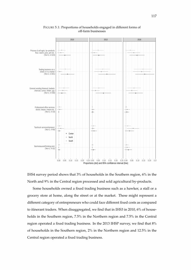
117

FIGURE 5.1: Proportions of households engaged in different forms ofoff-farm businesses

2010 2013 2016

0.00 0.05 0.10 0.15 0.20 0.25 0.00 0.05 0.10 0.15 0.20 0.25 0.00 0.05 0.10 0.15 0.20 0.25

Bar/restaurant/Drinking joint (Yes=1; n=32)

Taxi/truck services/transport (Yes=1; n=69)

Professional office services doctor, lawyer, mason,etc.

(Yes=1; n=19)

General vending firewood, baskets charcoal, curios, timber, juju

(Yes=1; n=258)

Trading business on a street or in a market

(Yes=1; n=501)

Process & sell agric. by−products flour, starch, juice, jam etc.

(Yes=1; n=223)

Proportions (dot) and 95% confidence interval (line)

Center

North

South

IHS4 survey period shows that 3% of households in the Southern region, 6% in the

North and 9% in the Central region processed and sold agricultural by-products.

Some households owned a fixed trading business such as a hawker, a stall or a

grocery store at home, along the street or at the market. These might represent a

different category of entrepreneurs who could face different fixed costs as compared

to itinerant traders. When disaggregated, we find that in IHS3 in 2010, 6% of house-

holds in the Southern region, 7.5% in the Northern region and 7.5% in the Central

region operated a fixed trading business. In the 2013 IHSP survey, we find that 8%

of households in the Southern region, 2% in the Northern region and 12.5% in the

Central region operated a fixed trading business.

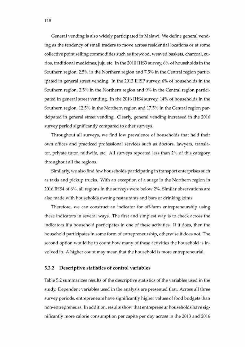
118

General vending is also widely participated in Malawi. We define general vend-

ing as the tendency of small traders to move across residential locations or at some

collective point selling commodities such as firewood, weaved baskets, charcoal, cu-

rios, traditional medicines, juju etc. In the 2010 IHS3 survey, 6% of households in the

Southern region, 2.5% in the Northern region and 7.5% in the Central region partic-

ipated in general street vending. In the 2013 IHSP survey, 6% of households in the

Southern region, 2.5% in the Northern region and 9% in the Central region partici-

pated in general street vending. In the 2016 IHS4 survey, 14% of households in the

Southern region, 12.5% in the Northern region and 17.5% in the Central region par-

ticipated in general street vending. Clearly, general vending increased in the 2016

survey period significantly compared to other surveys.

Throughout all surveys, we find low prevalence of households that held their

own offices and practiced professional services such as doctors, lawyers, transla-

tor, private tutor, midwife, etc. All surveys reported less than 2% of this category

throughout all the regions.

Similarly, we also find few households participating in transport enterprises such

as taxis and pickup trucks. With an exception of a surge in the Northern region in

2016 IHS4 of 6%, all regions in the surveys were below 2%. Similar observations are

also made with households owning restaurants and bars or drinking joints.

Therefore, we can construct an indicator for off-farm entrepreneurship using

these indicators in several ways. The first and simplest way is to check across the

indicators if a household participates in one of these activities. If it does, then the

household participates in some form of entrepreneurship, otherwise it does not. The

second option would be to count how many of these activities the household is in-

volved in. A higher count may mean that the household is more entrepreneurial.

5.3.2 Descriptive statistics of control variables

Table 5.2 summarizes results of the descriptive statistics of the variables used in the

study. Dependent variables used in the analysis are presented first. Across all three

survey periods, entrepreneurs have significantly higher values of food budgets than

non-entrepreneurs. In addition, results show that entrepreneur households have sig-

nificantly more calorie consumption per capita per day across in the 2013 and 2016

119

FIGURE 5.2: Distribution of households practising entrepreneurshipdisaggregated by gender

Full sample

0

20

40

60

IHS3−2010 IHS3P−2013 IHS4−2016

Year

Per

cent

Entrepreneur

Non−Participant

Participant

A

Female household heads

0

20

40

60

80

IHS3−2010 IHS3P−2013 IHS4−2016

Year

Per

cent

BMale household heads

0

20

40

60

IHS3−2010 IHS3P−2013 IHS4−2016

Year

Per

cent

C

survey periods. The Berry and Entropy indexes of dietary variety are higher among

households that ventured into entrepreneurship. Further, results also show that

household that entered into entrepreneurship reported less days of reduced food

production. Similarly, households that entered into entrepreneurship experienced

higher value of food production.

Non-entrepreneur households had significantly larger household sizes as com-

pared to households that practice entrepreneurship. Across the survey periods,

there was 1 male adult in the household. This statistic did not statistically differ

between 2010 and 2013 but moved to 2 in 2016. On average, across all three sur-

veys and between participants and non-participants, there were 2 male children per

household. Between 2010 and 2013, and between participants and non-participants,

there was one female adult in the household. However, in 2016, there were 2 female

adults in the household. Further, the household had 2 female children, between

participants and non-participants across all survey periods.

Most household heads participating in entrepreneurship were in a monogamous

120

marital relationship with 75% in 2010, 83% in 2013 and 88%, respectively. About

7% of households were in a polygamous marital relationship. Results for polyg-

amous marital status do not differ significantly between entrepreneur and non-

entrepreneur households. About 6% of households were separated. However, there

are no statistical differences between entrepreneurs and non-entrepreneurs. About

5% of households are divorced and do not differ significantly between the partici-

pants and non-participants across the 3 survey periods. About 13% of households

are widowed and do not differ markedly across the survey periods and between en-

trepreneurs and non-entrepreneurs. The proportion of single and unmarried house-

hold heads was 3%. However, the number of participants significantly increased

from 2% to 5% and 6% across the survey periods.

About 87% of household heads participating in entrepreneurship in 2010 had

no formal schooling. Another 61% and 62% of household heads participating in

entrepreneurship had no formal schooling in 2013 and 2016 survey periods, respec-

tively. In 2010, 3% of household heads had attained primary school certificate and

participated in entrepreneurship and 12% and 8% had attained primary school. In

2010, about 5% of households participating in entrepreneurship had attained junior

secondary education, while in 2013, 16% had attained primary school. Less than 1%

of households that participated in entrepreneurship across all surveys.

Land holding sizes and adoption of modern farming technology did not vary

substantively across participants and non-participants in all survey periods. Note-

worthy, there are statistically significant differences across the covariates which

means that in absence of modeling the selection process explicitly, our results would

be biased. Thus, based on this assessment, we proceed to model the selection pro-

cess.

5.3.3 Mechanism of selection into entrepreneurship

Figure 5.3 presents results of a probit model that explicitly models the selection pro-

cess into entrepreneurship. Results comprise household, socioeconomic, commu-

nity characteristics, idiosyncratic and covariate shocks that may explain the moti-

vations behind owning an off-farm enterprise. In general, results indicate that the

overall probability of venturing into entrepreneurship is 23%.

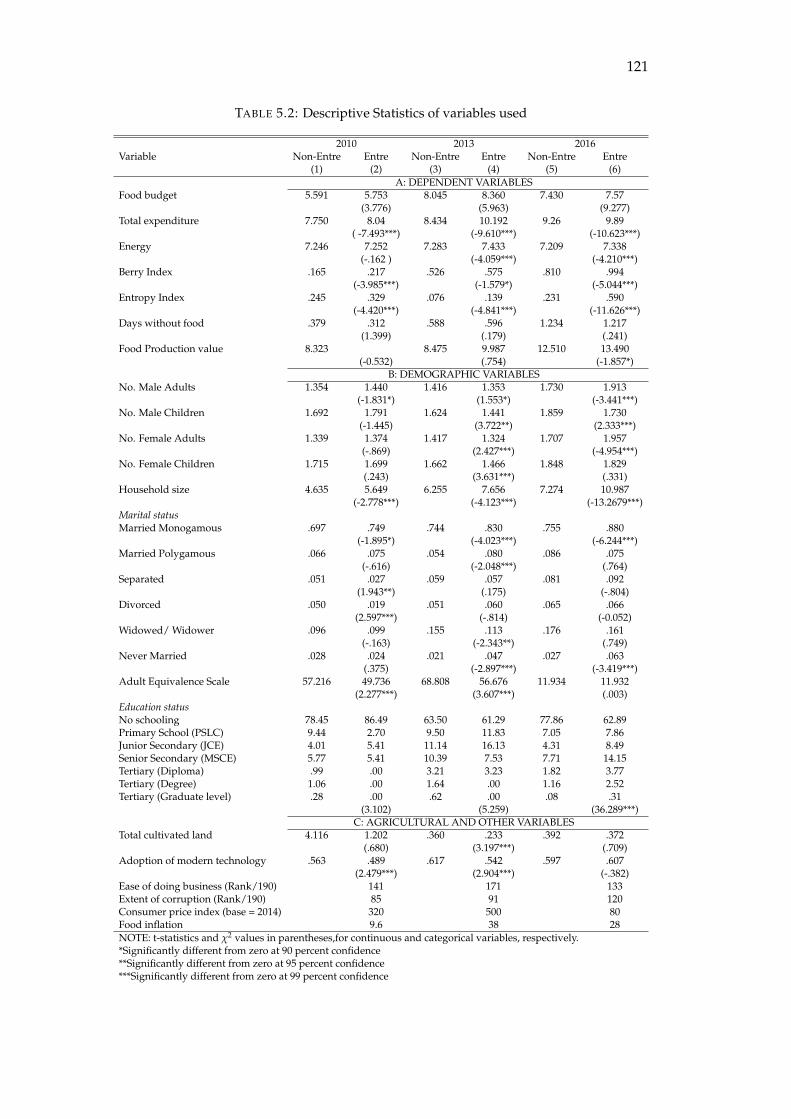
121

TABLE 5.2: Descriptive Statistics of variables used

2010 2013 2016Variable Non-Entre Entre Non-Entre Entre Non-Entre Entre

(1) (2) (3) (4) (5) (6)A: DEPENDENT VARIABLES

Food budget 5.591 5.753 8.045 8.360 7.430 7.57(3.776) (5.963) (9.277)

Total expenditure 7.750 8.04 8.434 10.192 9.26 9.89( -7.493***) (-9.610***) (-10.623***)

Energy 7.246 7.252 7.283 7.433 7.209 7.338(-.162 ) (-4.059***) (-4.210***)

Berry Index .165 .217 .526 .575 .810 .994(-3.985***) (-1.579*) (-5.044***)

Entropy Index .245 .329 .076 .139 .231 .590(-4.420***) (-4.841***) (-11.626***)

Days without food .379 .312 .588 .596 1.234 1.217(1.399) (.179) (.241)

Food Production value 8.323 8.475 9.987 12.510 13.490(-0.532) (.754) (-1.857*)

B: DEMOGRAPHIC VARIABLESNo. Male Adults 1.354 1.440 1.416 1.353 1.730 1.913

(-1.831*) (1.553*) (-3.441***)No. Male Children 1.692 1.791 1.624 1.441 1.859 1.730

(-1.445) (3.722**) (2.333***)No. Female Adults 1.339 1.374 1.417 1.324 1.707 1.957

(-.869) (2.427***) (-4.954***)No. Female Children 1.715 1.699 1.662 1.466 1.848 1.829

(.243) (3.631***) (.331)Household size 4.635 5.649 6.255 7.656 7.274 10.987

(-2.778***) (-4.123***) (-13.2679***)Marital statusMarried Monogamous .697 .749 .744 .830 .755 .880

(-1.895*) (-4.023***) (-6.244***)Married Polygamous .066 .075 .054 .080 .086 .075

(-.616) (-2.048***) (.764)Separated .051 .027 .059 .057 .081 .092

(1.943**) (.175) (-.804)Divorced .050 .019 .051 .060 .065 .066

(2.597***) (-.814) (-0.052)Widowed/ Widower .096 .099 .155 .113 .176 .161

(-.163) (-2.343**) (.749)Never Married .028 .024 .021 .047 .027 .063

(.375) (-2.897***) (-3.419***)Adult Equivalence Scale 57.216 49.736 68.808 56.676 11.934 11.932

(2.277***) (3.607***) (.003)Education statusNo schooling 78.45 86.49 63.50 61.29 77.86 62.89Primary School (PSLC) 9.44 2.70 9.50 11.83 7.05 7.86Junior Secondary (JCE) 4.01 5.41 11.14 16.13 4.31 8.49Senior Secondary (MSCE) 5.77 5.41 10.39 7.53 7.71 14.15Tertiary (Diploma) .99 .00 3.21 3.23 1.82 3.77Tertiary (Degree) 1.06 .00 1.64 .00 1.16 2.52Tertiary (Graduate level) .28 .00 .62 .00 .08 .31

(3.102) (5.259) (36.289***)C: AGRICULTURAL AND OTHER VARIABLES

Total cultivated land 4.116 1.202 .360 .233 .392 .372(.680) (3.197***) (.709)

Adoption of modern technology .563 .489 .617 .542 .597 .607(2.479***) (2.904***) (-.382)

Ease of doing business (Rank/190) 141 171 133Extent of corruption (Rank/190) 85 91 120Consumer price index (base = 2014) 320 500 80Food inflation 9.6 38 28NOTE: t-statistics and χ2 values in parentheses,for continuous and categorical variables, respectively.*Significantly different from zero at 90 percent confidence**Significantly different from zero at 95 percent confidence***Significantly different from zero at 99 percent confidence

122

Results indicate that household characteristics significantly affect the en-

trepreneurship decision. For instance, an additional male adult in the household

increases the probability of venturing into entrepreneurship by 2% (p < .05). Of

note, if a household head is in a monogamous marriage in comparison to a single

non-married head, the probability of venturing into entrepreneurship increases by

17% (p < .05). Asset holdings, represented by the asset index, increased the proba-

bility of venturing into entrepreneurship by 2%.

In addition, entrepreneurial training through formal education significantly af-

fects selection into entrepreneurship. Compared to household heads that had never

attended formal schooling, primary school attendance is associated with 19% in-

crease in the probability of venturing into entrepreneurship. Household heads that

attended junior secondary school and college degree education had 7% higher prob-

abilities of venturing into entrepreneurship, respectively.

However, results show that agricultural variables such as land holding size and

the commercialization indicator deter entry into entrepreneurship.

5.3.4 Balancing tests for participants and non-participants

In order to control for selection bias, we used propensity score analysis. Table 5.3

summarizes results of balancing t-tests after propensity score analysis. Given that

none of the control variables are statistically different between participants and non-

participants, we can assume that the covariates have been well balanced to mimic a

randomized control trial. Figure 5.4 summarizes households on support and those

not after propensity score matching. Hence, assuming that we have controlled for a

sufficient number of covariates, we can now use conventional fixed effects regression

analysis to assess effects of entrepreneurship of welfare variables.

5.3.5 Impact of entrepreneurship on food security

Average treatment effects on the treated

After adjusting our sample for selection bias, we estimate the impact of participating

in entrepreneurship on food security using inverse-probability-weighted regression

adjustment (IPWRA) and nearest neighbour propensity score matching (PSM-NNM)

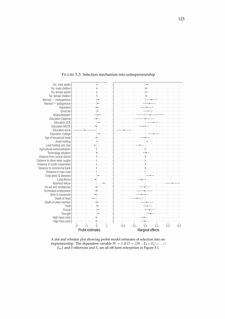
123

FIGURE 5.3: Selection mechanism into entrepreneurship

High food costsHigh input costs

DroughtFloods

TheftDeath of other member

Death of headBirth in household

Terminated employmentNo aid and remittances

Business failureLong illness

Crop pests & diseasesDistance to main road

Distance to commercial bankDistance to credit cooperation

Distance to clean water supplyDistance from central district

Technology adoptionAgricultural comercialization

Land holding size (ha)Asset holding

Age of household headEducation College

Education NoneEducation MSCE

Education JCEEducation Diploma

Widow/widowerDivorced

SeparatedMarried −− polygamous

Married −− monogamousNo. female children

No. female adultsNo. male children

No. male adults

−2 −1 0 1Probit estimates

−0.2 −0.1 0.0 0.1 0.2 0.3Marginal effects

A dot and whisker plot showing probit model estimates of selection into en-trepreneurship. The dependent variable W = 1 if D = W : E1 ∪ E2 ∪ . . . ∪

Em and 0 otherwise and Ei are all off-farm enterprises in Figure 5.1.

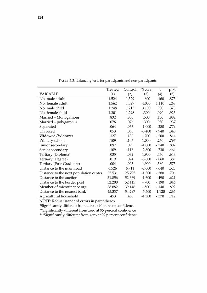
124

TABLE 5.3: Balancing tests for participants and non-participants

Treated Control %bias t p>tVARIABLE (1) (2) (3) (4) (5)No. male adult 1.524 1.529 -.600 -.160 .873No. female adult 1.562 1.527 4.000 1.110 .268No. male child 1.248 1.215 3.100 .900 .370No. female child 1.301 1.298 .300 .090 .925Married – Monogamous .832 .830 .500 .150 .882Married – polygamous .076 .076 .300 .080 .937Separated .064 .067 -1.000 -.280 .779Divorced .053 .060 -3.400 -.940 .345Widowed/Widower .127 .130 -.700 -.200 .844Primary school .109 .106 1.000 .260 .797Junior secondary .097 .099 -1.000 -.240 .807Senior secondary .109 .118 -2.800 -.730 .464Tertiary (Diploma) .035 .032 1.900 .460 .643Tertiary (Degree) .019 .024 -3.600 -.860 .389Tertiary (Post-Graduate) .004 .003 1.900 .560 .573Distance to the main road 6.526 6.711 -2.000 -.640 .525Distance to the next population center 25.531 25.795 -1.300 -.380 .706Distance to the auction 51.856 52.669 -1.600 -.490 .621Distance to the border post 52.200 52.415 -.700 -.190 .846Member of microfinance org. 38.882 39.146 -.500 -.140 .892Distance to the nearest bank 45.337 54.297 -5.500 -1.120 .265Agricultural household .453 .460 -1.300 -.370 .712NOTE: Robust standard errors in parentheses*Significantly different from zero at 90 percent confidence**Significantly different from zero at 95 percent confidence***Significantly different from zero at 99 percent confidence

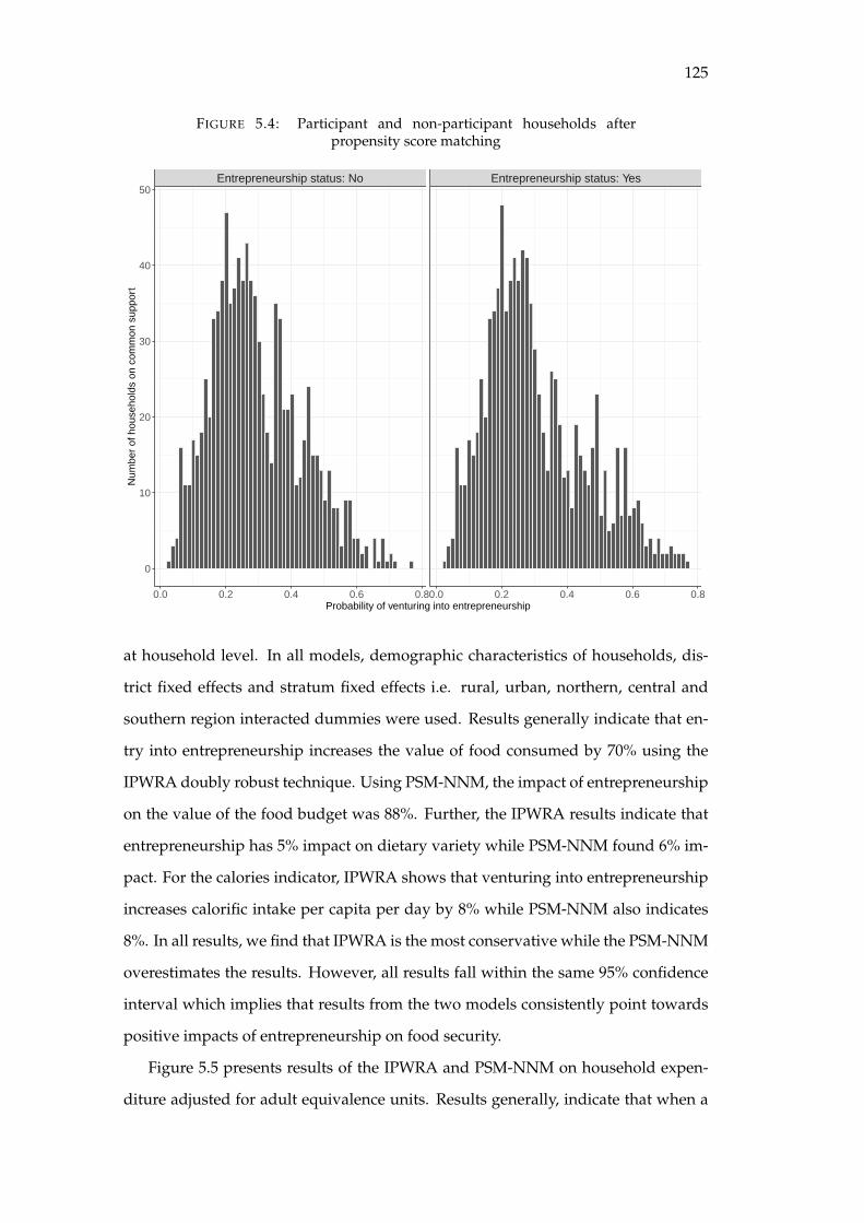
125

FIGURE 5.4: Participant and non-participant households afterpropensity score matching

Entrepreneurship status: No Entrepreneurship status: Yes

0.0 0.2 0.4 0.6 0.80.0 0.2 0.4 0.6 0.8

0

10

20

30

40

50

Probability of venturing into entrepreneurship

Num

ber

of h

ouse

hold

s on

com

mon

sup

port

at household level. In all models, demographic characteristics of households, dis-

trict fixed effects and stratum fixed effects i.e. rural, urban, northern, central and

southern region interacted dummies were used. Results generally indicate that en-

try into entrepreneurship increases the value of food consumed by 70% using the

IPWRA doubly robust technique. Using PSM-NNM, the impact of entrepreneurship

on the value of the food budget was 88%. Further, the IPWRA results indicate that

entrepreneurship has 5% impact on dietary variety while PSM-NNM found 6% im-

pact. For the calories indicator, IPWRA shows that venturing into entrepreneurship

increases calorific intake per capita per day by 8% while PSM-NNM also indicates

8%. In all results, we find that IPWRA is the most conservative while the PSM-NNM

overestimates the results. However, all results fall within the same 95% confidence

interval which implies that results from the two models consistently point towards

positive impacts of entrepreneurship on food security.

Figure 5.5 presents results of the IPWRA and PSM-NNM on household expen-

diture adjusted for adult equivalence units. Results generally, indicate that when a

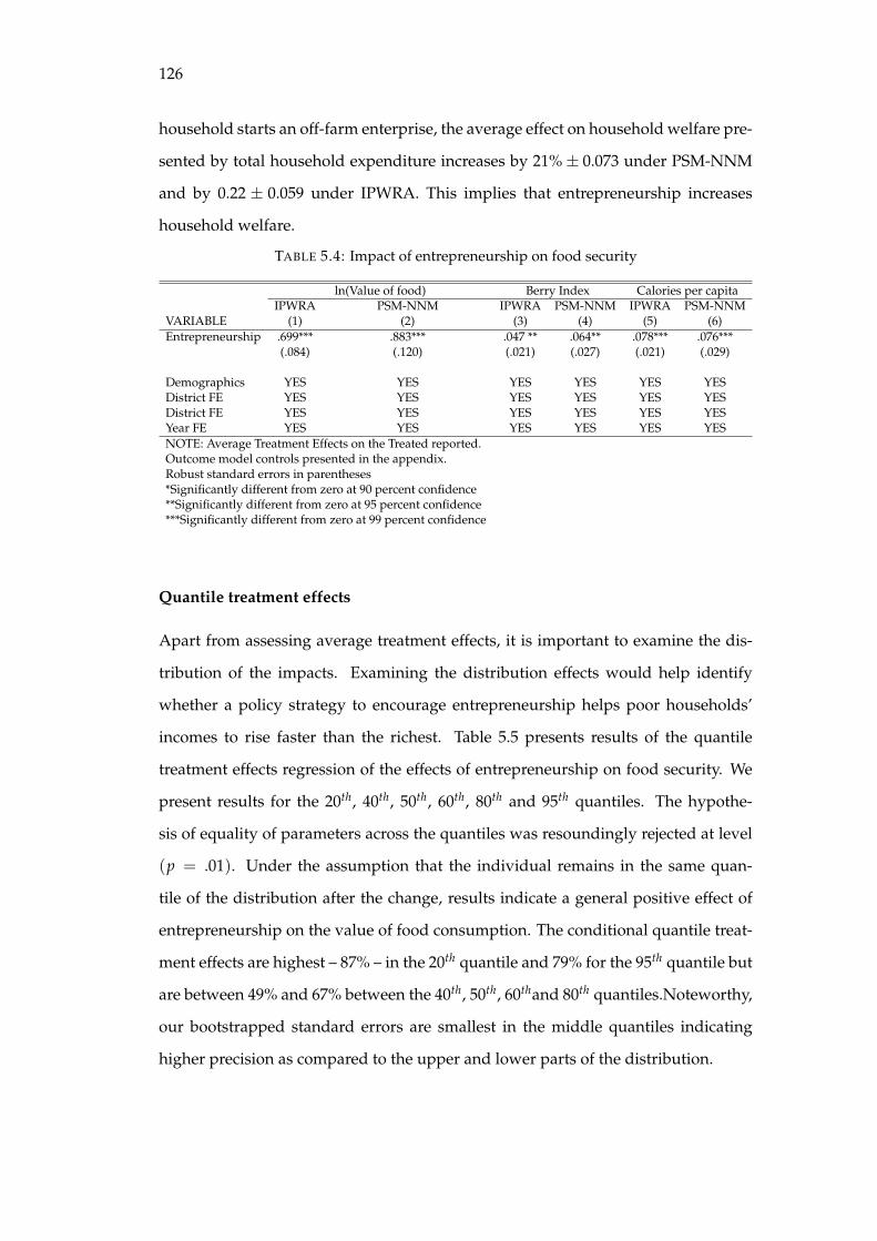
126

household starts an off-farm enterprise, the average effect on household welfare pre-

sented by total household expenditure increases by 21%± 0.073 under PSM-NNM

and by 0.22 ± 0.059 under IPWRA. This implies that entrepreneurship increases

household welfare.

TABLE 5.4: Impact of entrepreneurship on food security

ln(Value of food) Berry Index Calories per capitaIPWRA PSM-NNM IPWRA PSM-NNM IPWRA PSM-NNM

VARIABLE (1) (2) (3) (4) (5) (6)Entrepreneurship .699*** .883*** .047 ** .064** .078*** .076***

(.084) (.120) (.021) (.027) (.021) (.029)

Demographics YES YES YES YES YES YESDistrict FE YES YES YES YES YES YESDistrict FE YES YES YES YES YES YESYear FE YES YES YES YES YES YESNOTE: Average Treatment Effects on the Treated reported.Outcome model controls presented in the appendix.Robust standard errors in parentheses*Significantly different from zero at 90 percent confidence**Significantly different from zero at 95 percent confidence***Significantly different from zero at 99 percent confidence

Quantile treatment effects

Apart from assessing average treatment effects, it is important to examine the dis-

tribution of the impacts. Examining the distribution effects would help identify

whether a policy strategy to encourage entrepreneurship helps poor households’

incomes to rise faster than the richest. Table 5.5 presents results of the quantile

treatment effects regression of the effects of entrepreneurship on food security. We

present results for the 20th, 40th, 50th, 60th, 80th and 95th quantiles. The hypothe-

sis of equality of parameters across the quantiles was resoundingly rejected at level

(p = .01). Under the assumption that the individual remains in the same quan-

tile of the distribution after the change, results indicate a general positive effect of

entrepreneurship on the value of food consumption. The conditional quantile treat-

ment effects are highest – 87% – in the 20th quantile and 79% for the 95th quantile but

are between 49% and 67% between the 40th, 50th, 60thand 80th quantiles.Noteworthy,

our bootstrapped standard errors are smallest in the middle quantiles indicating

higher precision as compared to the upper and lower parts of the distribution.

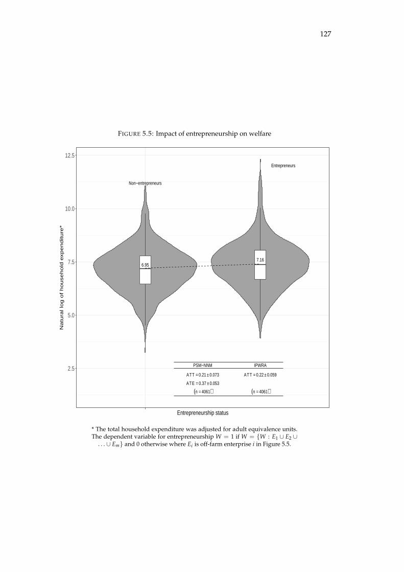
127

FIGURE 5.5: Impact of entrepreneurship on welfare

6.957.16

ATT = 0.21 ± 0.073

ATE = 0.37 ± 0.053

ATT = 0.22 ± 0.059

Non−entrepreneurs

Entrepreneurs

PSM−NNM IPWRA

(n = 4061)(n = 4061)

2.5

5.0

7.5

10.0

12.5

Entrepreneurship status

Na

tura

l lo

g o

f h

ou

se

ho

ld e

xp

en

ditu

re*

* The total household expenditure was adjusted for adult equivalence units.The dependent variable for entrepreneurship W = 1 if W = W : E1 ∪ E2 ∪

. . . ∪ Em and 0 otherwise where Ei is off-farm enterprise i in Figure 5.5.

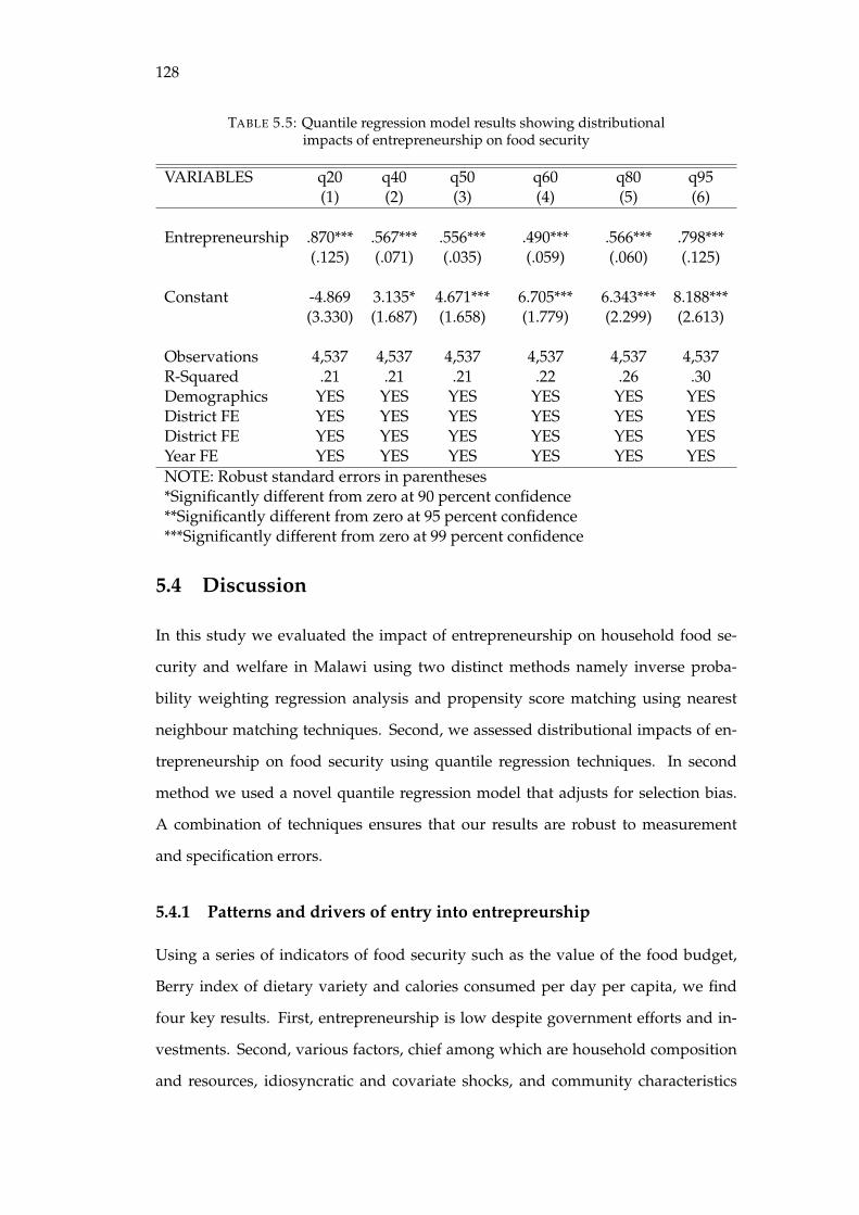
128

TABLE 5.5: Quantile regression model results showing distributionalimpacts of entrepreneurship on food security

VARIABLES q20 q40 q50 q60 q80 q95(1) (2) (3) (4) (5) (6)

Entrepreneurship .870*** .567*** .556*** .490*** .566*** .798***(.125) (.071) (.035) (.059) (.060) (.125)

Constant -4.869 3.135* 4.671*** 6.705*** 6.343*** 8.188***(3.330) (1.687) (1.658) (1.779) (2.299) (2.613)

Observations 4,537 4,537 4,537 4,537 4,537 4,537R-Squared .21 .21 .21 .22 .26 .30Demographics YES YES YES YES YES YESDistrict FE YES YES YES YES YES YESDistrict FE YES YES YES YES YES YESYear FE YES YES YES YES YES YESNOTE: Robust standard errors in parentheses*Significantly different from zero at 90 percent confidence**Significantly different from zero at 95 percent confidence***Significantly different from zero at 99 percent confidence

5.4 Discussion

In this study we evaluated the impact of entrepreneurship on household food se-

curity and welfare in Malawi using two distinct methods namely inverse proba-

bility weighting regression analysis and propensity score matching using nearest

neighbour matching techniques. Second, we assessed distributional impacts of en-

trepreneurship on food security using quantile regression techniques. In second

method we used a novel quantile regression model that adjusts for selection bias.

A combination of techniques ensures that our results are robust to measurement

and specification errors.

5.4.1 Patterns and drivers of entry into entrepreurship

Using a series of indicators of food security such as the value of the food budget,

Berry index of dietary variety and calories consumed per day per capita, we find

four key results. First, entrepreneurship is low despite government efforts and in-

vestments. Second, various factors, chief among which are household composition

and resources, idiosyncratic and covariate shocks, and community characteristics

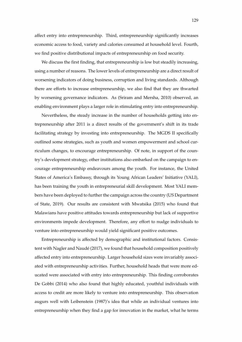
129

affect entry into entrepreneurship. Third, entrepreneurship significantly increases

economic access to food, variety and calories consumed at household level. Fourth,

we find positive distributional impacts of entrepreneurship on food security.

We discuss the first finding, that entrepreneurship is low but steadily increasing,

using a number of reasons. The lower levels of entrepreneurship are a direct result of

worsening indicators of doing business, corruption and living standards. Although

there are efforts to increase entrepreneurship, we also find that they are thwarted

by worsening governance indicators. As (Sriram and Mersha, 2010) observed, an

enabling environment plays a larger role in stimulating entry into entrepreneurship.

Nevertheless, the steady increase in the number of households getting into en-

trepreneurship after 2011 is a direct results of the government’s shift in its trade

facilitating strategy by investing into entrepreneurship. The MGDS II specifically

outlined some strategies, such as youth and women empowerment and school cur-

riculum changes, to encourage entrepreneurship. Of note, in support of the coun-

try’s development strategy, other institutions also embarked on the campaign to en-

courage entrepreneurship endeavours among the youth. For instance, the United

States of America’s Embassy, through its Young African Leaders’ Initiative (YALI),

has been training the youth in entrepreneurial skill development. Most YALI mem-

bers have been deployed to further the campaign across the country (US Department

of State, 2019). Our results are consistent with Mwatsika (2015) who found that

Malawians have positive attitudes towards entrepreneurship but lack of supportive

environments impede development. Therefore, any effort to nudge individuals to

venture into entrepreneurship would yield significant positive outcomes.

Entrepreneurship is affected by demographic and institutional factors. Consis-

tent with Nagler and Naudé (2017), we found that household composition positively

affected entry into entrepreneurship. Larger household sizes were invariably associ-

ated with entrepreneurship activities. Further, household heads that were more ed-

ucated were associated with entry into entrepreneurship. This finding corroborates

De Gobbi (2014) who also found that highly educated, youthful individuals with

access to credit are more likely to venture into entrepreneurship. This observation

augurs well with Leibenstein (1987)’s idea that while an individual ventures into

entrepreneurship when they find a gap for innovation in the market, what he terms

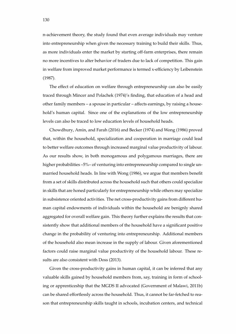
130

n-achievement theory, the study found that even average individuals may venture

into entrepreneurship when given the necessary training to build their skills. Thus,

as more individuals enter the market by starting off-farm enterprises, there remain

no more incentives to alter behavior of traders due to lack of competition. This gain

in welfare from improved market performance is termed x-efficiency by Leibenstein

(1987).

The effect of education on welfare through entrepreneurship can also be easily

traced through Mincer and Polachek (1974)’s finding, that education of a head and

other family members – a spouse in particular – affects earnings, by raising a house-

hold’s human capital. Since one of the explanations of the low entrepreneurship

levels can also be traced to low education levels of household heads.

Chowdhury, Amin, and Farah (2016) and Becker (1974) and Wong (1986) proved

that, within the household, specialization and cooperation in marriage could lead

to better welfare outcomes through increased marginal value productivity of labour.

As our results show, in both monogamous and polygamous marriages, there are

higher probabilities –5%– of venturing into entrepreneurship compared to single un-

married household heads. In line with Wong (1986), we argue that members benefit

from a set of skills distributed across the household such that others could specialize

in skills that are honed particularly for entrepreneurship while others may specialize

in subsistence oriented activities. The net cross-productivity gains from different hu-

man capital endowments of individuals within the household are benignly shared

aggregated for overall welfare gain. This theory further explains the results that con-

sistently show that additional members of the household have a significant positive

change in the probability of venturing into entrepreneurship. Additional members

of the household also mean increase in the supply of labour. Given aforementioned

factors could raise marginal value productivity of the household labour. These re-

sults are also consistent with Doss (2013).

Given the cross-productivity gains in human capital, it can be inferred that any

valuable skills gained by household members from, say, training in form of school-

ing or apprenticeship that the MGDS II advocated (Government of Malawi, 2011b)

can be shared effortlessly across the household. Thus, it cannot be far-fetched to rea-

son that entrepreneurship skills taught in schools, incubation centers, and technical

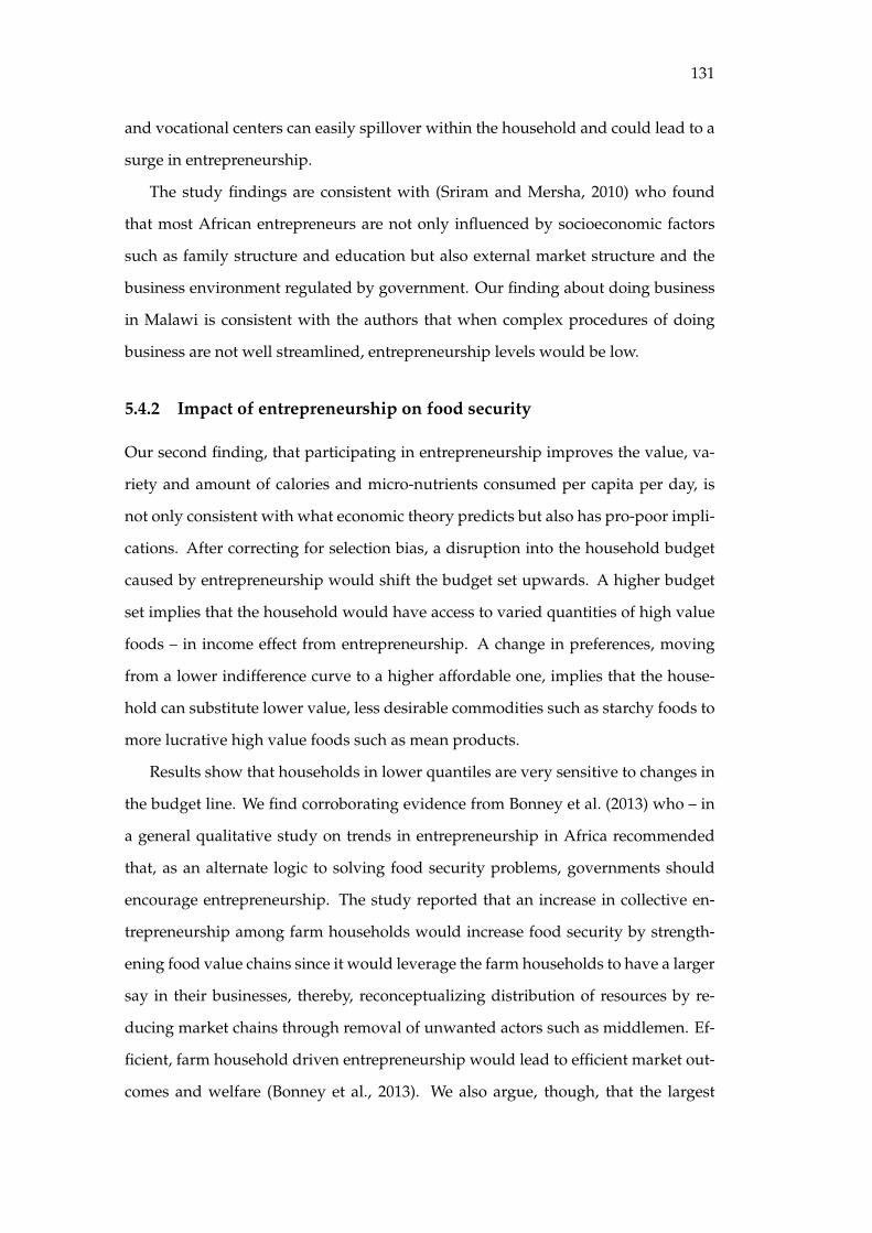
131

and vocational centers can easily spillover within the household and could lead to a

surge in entrepreneurship.

The study findings are consistent with (Sriram and Mersha, 2010) who found

that most African entrepreneurs are not only influenced by socioeconomic factors

such as family structure and education but also external market structure and the

business environment regulated by government. Our finding about doing business

in Malawi is consistent with the authors that when complex procedures of doing

business are not well streamlined, entrepreneurship levels would be low.

5.4.2 Impact of entrepreneurship on food security

Our second finding, that participating in entrepreneurship improves the value, va-

riety and amount of calories and micro-nutrients consumed per capita per day, is

not only consistent with what economic theory predicts but also has pro-poor impli-

cations. After correcting for selection bias, a disruption into the household budget

caused by entrepreneurship would shift the budget set upwards. A higher budget

set implies that the household would have access to varied quantities of high value

foods – in income effect from entrepreneurship. A change in preferences, moving

from a lower indifference curve to a higher affordable one, implies that the house-

hold can substitute lower value, less desirable commodities such as starchy foods to

more lucrative high value foods such as mean products.

Results show that households in lower quantiles are very sensitive to changes in

the budget line. We find corroborating evidence from Bonney et al. (2013) who – in

a general qualitative study on trends in entrepreneurship in Africa recommended

that, as an alternate logic to solving food security problems, governments should

encourage entrepreneurship. The study reported that an increase in collective en-

trepreneurship among farm households would increase food security by strength-

ening food value chains since it would leverage the farm households to have a larger

say in their businesses, thereby, reconceptualizing distribution of resources by re-

ducing market chains through removal of unwanted actors such as middlemen. Ef-

ficient, farm household driven entrepreneurship would lead to efficient market out-

comes and welfare (Bonney et al., 2013). We also argue, though, that the largest

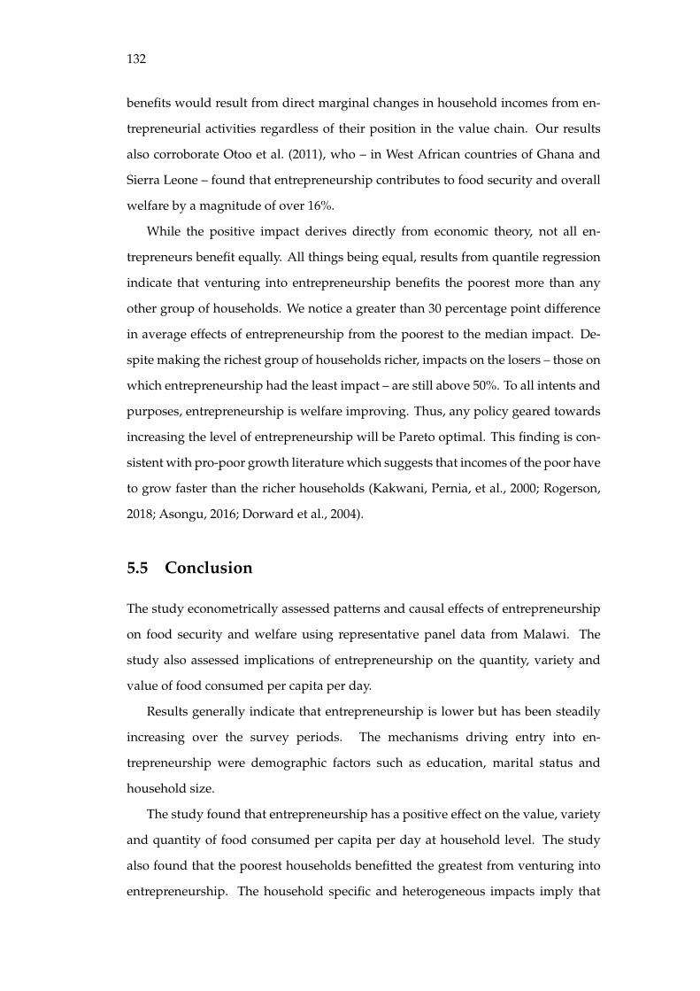
132

benefits would result from direct marginal changes in household incomes from en-

trepreneurial activities regardless of their position in the value chain. Our results

also corroborate Otoo et al. (2011), who – in West African countries of Ghana and

Sierra Leone – found that entrepreneurship contributes to food security and overall

welfare by a magnitude of over 16%.

While the positive impact derives directly from economic theory, not all en-

trepreneurs benefit equally. All things being equal, results from quantile regression

indicate that venturing into entrepreneurship benefits the poorest more than any

other group of households. We notice a greater than 30 percentage point difference

in average effects of entrepreneurship from the poorest to the median impact. De-

spite making the richest group of households richer, impacts on the losers – those on

which entrepreneurship had the least impact – are still above 50%. To all intents and

purposes, entrepreneurship is welfare improving. Thus, any policy geared towards

increasing the level of entrepreneurship will be Pareto optimal. This finding is con-

sistent with pro-poor growth literature which suggests that incomes of the poor have

to grow faster than the richer households (Kakwani, Pernia, et al., 2000; Rogerson,

2018; Asongu, 2016; Dorward et al., 2004).

5.5 Conclusion

The study econometrically assessed patterns and causal effects of entrepreneurship

on food security and welfare using representative panel data from Malawi. The

study also assessed implications of entrepreneurship on the quantity, variety and

value of food consumed per capita per day.

Results generally indicate that entrepreneurship is lower but has been steadily

increasing over the survey periods. The mechanisms driving entry into en-

trepreneurship were demographic factors such as education, marital status and

household size.

The study found that entrepreneurship has a positive effect on the value, variety

and quantity of food consumed per capita per day at household level. The study

also found that the poorest households benefitted the greatest from venturing into

entrepreneurship. The household specific and heterogeneous impacts imply that

133

investing in entrepreneurship is not only a good strategy for economic development

but is also a pro-poor policy strategy.

Since government assignment of treatment was non-ignorable, the study recom-

mends that delivery of investments to increase entrepreneurship levels should be

designed in such a way that attribution can be easily identified. While randomiza-

tion might be unethical, sequential delivery of investments across districts or regions

can ensure cleaner difference-in-difference assessment of impacts.

The finding that entrepreneurship levels are still low calls for focused and in-

creased efforts to encourage entrepreneurship through streamlining and reducing

costs associated with doing business in the country and improving governance ef-

forts such as fighting corruption.

135

Chapter 6

General conclusions and policy

implications

6.1 Introduction

This chapter summarizes key results from the thesis and provides implications for

food policy. Although each chapter provides its own summary and conclusions,

this chapter unifies the results and provides resolutions in line with the general con-

cept presented in Chapter I and tying it to development policy of countries such

as Malawi. We revisit how we have answered the key questions and draw insights

from economic theory to inform policy.

6.2 Infrastructure, extreme weather events and food security

6.2.1 Background

Economic disruptions in form of covariate and idiosyncratic shocks have important

food and nutrition implications. Malawi has for the past six years experienced a

number of covariate shocks with varying impacts. This study assessed assessed the

impact of extreme weather events, price shocks, pest and diseases and miscellaneous

idiosyncratic shocks on food and nutrition security. The study also assesses the im-

pact infrastructure investment on mitigating the impact of economic disruptions.

136

6.2.2 Methods

The study used multiple data sets to triangulate identification of shocks. First

the study used three waves of Integrated Household Survey panel data sets from

Malawi of sample sizes up to 2500 collected between 2010, 2013 and 2016 by the

National Statistical Office. These data sets are geo-referenced and representative

at household and national level. The data contains demographic, production, con-

sumption and incidence of shocks experienced by the households.

The study used high resolution weather data with a 0.5 × 0.5 latitude by lon-

gitude and monthly time resolution of drought incidences during the study time

period. This data is used to objectively triangulate self reported data by households.

The study also used Night Time Light data obtained from the National Oceanic

and Atmospheric Administration of the United States as a proxy for infrastructure.

Another proxy of infrastructure used was the roads GIS shape file obtained from the

World Bank.

Closely following microeconomic theoretic foundations, we exploited a natu-

ral experiment of infrastructure assignment, occurrence of extreme weather events

and time to come up with a triple difference fixed effects regression combined with

propensity matching to assess the impacts. Key dependent variables were food con-

sumption expenditure per day and the Berry dietary diversity index while inde-

pendent variables were Standardized Precipitation - Evapotranspiration Index and

indicator variables for pests and diseases, and price related shocks. We reduced the

dimensionality of the shocks using principal component analysis.

6.2.3 Key results

Results generally indicate that shocks were highly correlated but the major shocks

were extreme weather shocks which were experienced by 56% of the households and

made the principle component. Price related shocks were also widely reported and

made the second component. Results show that extreme weather events have neg-

ative food and nutrition security implications. A standard deviation change in the

mean SPEI in the middle of the agricultural season would reduce food consumption

137

expenditure shares by 17% . Noteworthy, a standard deviation increase in infrastruc-

ture has a food and nutrition security mitigating effect of 9% on food consumption

expenditure .

6.2.4 Implications

An economic disruption such as a drought – the highly significant shock in the study

– reduces market supply i.e. shift the food supply function backwards. Given that

price elasticities of supply are larger than price elasticities of demand, as is the case

in Malawi see (Govindan and Babu, 2001) and (Ecker and Qaim, 2011), in general

welfare reduces due to the shock and consumers are hurt the most. However, net

sellers of food commodities benefit the most due to higher prices.

Infrastructure investments would reduce transaction costs and bring more

traders and commodities to the deficit region under the law of one price such that

the negative effects of the shocks are mitigated. The effects of infrastructure suggest

low endowments and high marginal productivity of social overhead capital.

6.2.5 Recommendations

We find that weather related shocks have negative impacts on food consumption ex-

penditure shares, significantly reduce dietary diversity and micronutrient consump-

tion. In addition, households that sell a larger proportion of their farm produce to

markets and held less assets also experienced higher levels of food insecurity. We

therefore recommend that farmers must ensure that they keep sufficient stocks of

their produce to ensure continued availability of food at household level. Further,

we advocate that households hold tangible assets that could cushion them against

shocks.

Results have shown that infrastructure improves food and nutrition security by

improving access to socioeconomic amenities and also reduces impacts of weather

related shocks. In the construction of the index, results indicated that electricity

availability, proximity to main roads, credit facilities had significant explanatory

power and magnitude. We recommend that policy makers consider increasing in-

vestments towards these forms of infrastructure.

138

Results of low dietary diversity may also signal lack of nutrition education. The

study therefore recommends focused nutrition messages for rural households for

dietary behavioural change. During crises, key messages about dietary diversity

and nutrient rich foods should be widely disseminated.

6.3 Social capital and food market performance

6.3.1 Background

Chapters III and IV analyze different aspects of market structure, conduct and per-

formance of staple food markets using maize as a case study. Considering that

formal contracts in food markets are hard to come by, most contracts, interactions

and transactions are based on trust. As such, we use New Institutional Economics

embedded with Rational Expectations Equilibrium assumptions and evolutionary

game theory to assess the conduct and performance of maize markets. Chapter III

assesses the effect of industry structure, institutional and social capital on maize

trader behaviour, business resilience and profitability. Chapter IV assesses whether

business registration leads to more efficient firms.

6.3.2 Methods

Chapters III and IV use a randomly sampled trader survey of size 172. In Chapter II

we used the Herfindahl Index and key informant interviews to measure market con-

centration and Bayes Model Averaging regression techniques with both informative

and reference priors to analyze key success correlates for business performance and

resilience. Chapter IV uses instrumental variable triangulated with control function

techniques to assess effects of business registration on trader performance.

6.3.3 Key results

Results not only indicate that markets are concentrated but also highly informal with

only 24% of the traders formally registered. Key correlates of business performance

as indicated by profitability were business registration, possession of export licences,

whether the trader performs multiple market functions, number of family members

139

engaged in maize trading, number of contacts with distant traders. Results of causal

effects of business registration on business performance show that registering a busi-

ness reduces performance.

6.3.4 Implications

Results suggest that in the market, traders in an oligopoly will tend to cooperate

until in the last game someone defects. Results bring out evidence of high levels of

interaction and cooperation to fix prices. Such behaviour has welfare reducing impli-

cations. At market level, when traders effectively fix prices they act like a monopoly

such that their quantities are sold at marginal cost, but they generate revenues at av-

erage cost, thereby reducing consumer surplus. Under this arrangement, consumers

always buy their staple food at higher than equilibrium price. This is especially con-

cerning when the consumers are also poor smallholder producers – who are cash

constrained and sell their output to traders at harvest at below long run equilibrium

prices. Due to temporal arbitrage and collusion among genetically close traders,

markets do not perform efficiently.

6.4 Recommendations

Following the results, the study makes the following recommendations:

Our results showed that distance to the registration center was negatively corre-

lated with registration. Registration of major businesses is conducted at major cities

namely Lilongwe and Blantyre. This creates a disincentive for traders that are far

from these areas. When traders do not register the government loses substantial

sums in government revenue.

Due to a large presence of collusion and market concentration from the results,

the study recommends that government institutions should monitor local staple

food markets for anti-competitive behaviour.

A lasting solution for promoting competitive markets would be to ensure con-

tinuous entry of traders into the market by incentivising individuals to venture into

entrepreneurship. Based on our findings, the study therefore suggests entrepreneur-

ship as a means of achieving food security and increased welfare.

140

6.5 Study limitations and recommendations for further stud-

ies

The study of impacts of idiosyncratic and covariate shocks on food security remains

an important area of policy interest. There are some outstanding issues that the

study was not able to address. First, the study’s use of Living Standards Measure-

ment Surveys takes advantage of its representativeness and ease of achieving exter-

nal validity. However, some questions were not as detailed to elicit specific adapta-

tion strategies after shocks. Economic disruption focused primary data longitudinal

surveys are therefore required.

The study has not addressed the public finance aspects of infrastructure provi-

sioning due to data unavailability. Therefore a study building on this quantifying

benefit cost aspects of various infrastructure financing needs is required. Regard-

ing the same manner, public policy design incorporating infrastructure investments

decisions should include baseline socioeconomic surveys and studies where impact

assessment exercises can be built on.

The study managed to assess trader characteristics and behavior with regards to

entry into business, performance and institutional aspects. However, a study based

on laboratory or field games to elicit behavior of traders under given scenarios could

elicit informative insights.

141

References

Aadhar, Saran and Vimal Mishra (2017). “High-resolution near real-time drought

monitoring in South Asia”. In: Scientific data 4, p. 170145.

Abadie, Alberto, Joshua Angrist, and Guido Imbens (2002). “Instrumental variables

estimates of the effect of subsidized training on the quantiles of trainee earnings”.

In: Econometrica 70.1, pp. 91–117.

Abbink, Klaus, Thomas S Jayne, and Lars C Moller (2011). “The relevance of a rules-

based maize marketing policy: an experimental case study of Zambia”. In: The

journal of development studies 47.2, pp. 207–230.

Aberman, Noora-Lisa, Janice Meerman, and Todd Benson (2018). Agriculture, food se-

curity, and nutrition in Malawi: Leveraging the links. Washington, DC: International

Food Policy Research Institute.

Adams, Richard M (1989). “Global climate change and agriculture: an economic per-

spective”. In: American Journal of Agricultural Economics 71.5, pp. 1272–1279.

Adler, Patricia A and Peter Adler (2003). “The reluctant respondent”. In: Inside inter-

viewing: New lenses, new concerns, pp. 153–173.

African Development Bank (2014). Infrastructure financing trends in Africa. African

Development Bank. Tunis Belvedere, Tunisia. URL: https : / / www . icafrica .

org/fileadmin/documents/Annual_Reports/ICA-2013-INFRA-FIN-TRENDS-

AFRICA-2013-FINAL-WEB.pdf.

Ahmad, Ehtisham and Michael Best (2012). Financing social policy in the presence of

informality. Asia Research Centre (ARC), The London School of Economics & Po-

litical Science.

Ahmad, Ehtisham, Michael Best, and Caroline Pöschl (2012). Tax reform in the presence

of informality in developing countries: incentives to cheat in Mexico. Asia Research

Centre (ARC), The London School of Economics & Political Science.

142

Ahmad, Ehtisham, Giorgio Brosio, and Caroline Pöschl (2014). Local Property Taxa-

tion and Benefits in Developing Countries-overcoming political resistance. 65. London

School of Economics, Asia Research Centre Working Paper.

Aidis, Ruta and Mirjam Van Praag (2007). “Illegal entrepreneurship experience: Does

it make a difference for business performance and motivation?” In: Journal of

Business Venturing 22.2, pp. 283–310.

Aiginger, Karl (1996). “Confronting the implications of the Cournot model with in-

dustry and firm data”. In: Small Business Economics 8.5, pp. 365–378.

Anand, Sudhir and Christopher J Harris (1994). “Choosing a welfare indicator”. In:

The American Economic Review 84.2, pp. 226–231.

Angrist, Joshua D, Guido W Imbens, and Donald B Rubin (1996). “Identification of

causal effects using instrumental variables”. In: Journal of the American statistical

Association 91.434, pp. 444–455.

Angrist, Joshua D and Jörn-Steffen Pischke (2008). Mostly harmless econometrics: An

empiricist’s companion. Princeton University Press.

— (2014). Mastering ’metrics: The path from cause to effect. Princeton University Press.

Angrist, Joshua David and Jörn-Steffen Pischke (2013). Mostly harmless econometrics:

an empiricists companion. Princeton University Press.

Anokhin, Sergey and William S Schulze (2009). “Entrepreneurship, innovation, and

corruption”. In: Journal of business venturing 24.5, pp. 465–476.

Arellano, Manuel and Stéphane Bonhomme (2017). “Quantile selection models with

an application to understanding changes in wage inequality”. In: Econometrica

85.1, pp. 1–28.

Arezki, Rabah and Amadou Sy (2016). “Financing Africa’s Infrastructure Deficit:

From Development Banking to Long-term Investing”. In: Journal of African

Economies 25.suppl_2, pp. ii59–ii73.

Arndt, Channing et al. (2012). “Climate change, growth and infrastructure in-

vestment: the case of Mozambique”. In: Review of Development Economics 16.3,

pp. 463–475.

Asfaw, Solomon and Giuseppe Maggio (2018). “Gender, weather shocks and welfare:

Evidence from Malawi”. In: The Journal of Development Studies 54.2, pp. 271–291.

143

Asiaei, Kaveh and Ruzita Jusoh (2015). “A multidimensional view of intellectual

capital: the impact on organizational performance”. In: Management Decision 53.3,

pp. 668–697.

Asongu, Simplice (2016). “Reinventing foreign aid for inclusive and sustainable de-

velopment: Kuznets, Piketty and the great policy reversal”. In: Journal of Economic

Surveys 30.4, pp. 736–755.

Atmadja, Adwin Surja, Jen-Je Su, and Parmendra Sharma (2016). “Examining the im-

pact of microfinance on microenterprise performance (implications for women-

owned microenterprises in Indonesia)”. In: International Journal of Social Eco-

nomics 43.10, pp. 962–981.

Audretsch, David B, Max C Keilbach, Erik E Lehmann, et al. (2006). Entrepreneurship

and economic growth. Oxford University Press.

Auriol, Emmanuelle and Michael Warlters (2012). “The marginal cost of public funds

and tax reform in Africa”. In: Journal of Development Economics 97.1, pp. 58 –72.

ISSN: 0304-3878. DOI: https://doi.org/10.1016/j.jdeveco.2011.01.003. URL:

http://www.sciencedirect.com/science/article/pii/S030438781100006X.

Azeem, Muhammad Masood, Amin W Mugera, and Steven Schilizzi (2016). “Living

on the edge: Household vulnerability to food-insecurity in the Punjab, Pakistan”.

In: Food Policy 64, pp. 1–13.

Baird, Sarah J et al. (2012). “Effect of a cash transfer programme for schooling on

prevalence of HIV and herpes simplex type 2 in Malawi: a cluster randomised

trial”. In: The Lancet 379.9823, pp. 1320–1329.

Bandyopadhyay, Sushenjit and Emmanuel Koufias (2012). Rainfall variability, occupa-

tional choice, and welfare in rural Bangladesh. The World Bank.

Banerjee, Abhijit, Esther Duflo, and Nancy Qian (2012). On the road: Access to trans-

portation infrastructure and economic growth in China. Tech. rep. National Bureau of

Economic Research.

Bang, Heejung and James M Robins (2005). “Doubly robust estimation in missing

data and causal inference models”. In: Biometrics 61.4, pp. 962–973.

Barbieri, Carla and Patience M Mshenga (2008). “The role of the firm and owner

characteristics on the performance of agritourism farms”. In: Sociologia ruralis

48.2, pp. 166–183.

144

Barwell, Ian et al. (2019). Rural transport in developing countries. Routledge.

Baulch, Bob (2018). “Impacts of the 2016-17 Food Insecurity Response Program on

maize prices in Malawi”. In:

Becker, Gary S. (1974). “A Theory of Social Interactions”. In: Journal of Political Econ-

omy 82.6, pp. 1063–1093. DOI: 10.1086/260265. eprint: https://doi.org/10.

1086/260265. URL: https://doi.org/10.1086/260265.

Benhassine, Najy et al. (2018). “Does inducing informal firms to formalize make

sense? Experimental evidence from Benin”. In: Journal of Public Economics 157,

pp. 1–14.

Benin, Samuel et al. (2008). Agricultural growth and investment options for poverty re-

duction in Malawi. International Food Policy Research Institute.

Beynon, Jonathan, Stephen Jones, and Shujie Yao (1992). “Market reform and private

trade in eastern and southern Africa”. In: Food Policy 17.6, pp. 399–408.

Bezu, Sosina and Stein Holden (2014). “Are rural youth in Ethiopia abandoning agri-

culture?” In: World Development 64, pp. 259–272.

Binswanger, Hans P, Shahidur R Khandker, and Mark R Rosenzweig (1993). “How

infrastructure and financial institutions affect agricultural output and investment

in India”. In: Journal of development Economics 41.2, pp. 337–366.

Blattman, Christopher, Nathan Fiala, and Sebastian Martinez (2013). “Credit con-

straints, occupational choice, and the process of development: long run evidence

from cash transfers in Uganda”. In:

Block, Jörn H and Andreas Landgraf (2016). “Transition from part-time en-

trepreneurship to full-time entrepreneurship: the role of financial and non-

financial motives”. In: International Entrepreneurship and Management Journal 12.1,

pp. 259–282.

Boarnet, Marlon G (1997). “Infrastructure services and the productivity of public

capital: the case of streets and highways”. In: National Tax Journal 50 (1), pp. 39–

57.

Bonney, Laurie et al. (2013). “A note on entrepreneurship as an alternative logic to

address food security in the developing world”. In: Journal of Developmental En-

trepreneurship 18.03, p. 1350016.

145

Breisinger, Clemens, Marcelle Thomas, and James Thurlow (2009). Social accounting

matrices and multiplier analysis: An introduction with exercises. Vol. 5. Washington,

DC: International Food Policy Research Institute.

Brudevold-Newman, Andrew et al. (2017). A firm of one’s own: experimental evidence

on credit constraints and occupational choice. The World Bank.

Bruhn, Miriam (2013). “A tale of two species: Revisiting the effect of registration

reform on informal business owners in Mexico”. In: Journal of Development Eco-

nomics 103, pp. 275–283.

Burgess, Robin and Dave Donaldson (2010). “Can openness mitigate the effects of

weather shocks? Evidence from India’s famine era”. In: American Economic Review

100.2, pp. 449–53.

Cai, Jing and Adam Szeidl (2016). “Interfirm relationships and business perfor-

mance”. In: The Quarterly Journal of Economics.

Cameron, Adrian Colin and Pravin K Trivedi (2010). Microeconometrics using stata.

Vol. 2. Stata press College Station, TX.

Campos, Francisco, Markus Goldstein, and David McKenzie (2015). Short-term im-

pacts of formalization assistance and a bank information session on business registration

and access to finance in Malawi. Washington, DC: The World Bank Group.

Carletto, Calogero, Paul Corral, and Anita Guelfi (2017). “Agricultural commercial-

ization and nutrition revisited: Empirical evidence from three African countries”.

In: Food Policy 67, pp. 106–118.

Cassata, Francesco and Roberto Marchionatti (2011). “A transdisciplinary perspec-

tive on economic complexity. Marshall’s problem revisited”. In: Journal of Eco-

nomic Behavior & Organization 80.1, pp. 122–136.

Central Intelligence Agency (2019). The world factbook 2019. Government Printing

Office.

Chen, Martha Alter et al. (2007). Rethinking the informal economy: Linkages with the

formal economy and the formal regulatory environment. Vol. 10. United Nations Uni-

versity, World Institute for Development Economics Research.

Chibwana, Christopher, Monica Fisher, and Gerald Shively (2012). “Cropland Allo-

cation Effects of Agricultural Input Subsidies in Malawi”. In: World Development

146

40.1, pp. 124–133. ISSN: 0305-750X. DOI: 10.1016/j.worlddev.2011.04.022.

URL: http://dx.doi.org/10.1016/j.worlddev.2011.04.022.

Chinowsky, Paul S et al. (2015). “Infrastructure and climate change: a study of im-

pacts and adaptations in Malawi, Mozambique, and Zambia”. In: Climatic Change

130.1, pp. 49–62.

Chinsinga, Blessings (2011). “Seeds and subsidies: The political economy of input

programmes in Malawi”. In: IDS bulletin 42.4, pp. 59–68.

Chirwa, Ephraim W (2008). “Effects of gender on the performance of micro and small

enterprises in Malawi”. In: Development Southern Africa 25.3, pp. 347–362.

Chirwa, Ephraim WT (2007). “Sources of technical efficiency among smallholder

maize farmers in Southern Malawi”. In:

Chow-Chua, Clare, Mark Goh, and Tan Boon Wan (2003). “Does ISO 9000 certifica-

tion improve business performance?” In: International Journal of Quality & Relia-

bility Management 20.8, pp. 936–953.

Chowdhury, Farzana, David B Audretsch, and Maksim Belitski (2019). “Institu-

tions and Entrepreneurship Quality”. In: Entrepreneurship Theory and Practice 43.1,

pp. 51–81.

Chowdhury, M, Shabnaz Amin, and Tazrina Farah (2016). Access to Microcredit and

Women’s Entrepreneurship: Evidence from Bangladesh. Partnership for Economic

Policy.

Christaller, Walter (1966). Central Places in Southern Germany, The Pioneer Work in The-

oretical Economic Geography. Prentice-Hall; Englewood Cliffs,N. J.

Clyde, Merlise A, Joyee Ghosh, and Michael L Littman (2011). “Bayesian adaptive

sampling for variable selection and model averaging”. In: Journal of Computa-

tional and Graphical Statistics 20.1, pp. 80–101.

Cochran, William G (2007). Sampling techniques. John Wiley & Sons.

Collier, Paul and Stefan Dercon (2014). “African agriculture in 50 years: smallholders

in a rapidly changing world?” In: World development 63, pp. 92–101.

Conroy, Anne (2006). “The history of development and crisis in Malawi”. In: Poverty,

AIDS and Hunger. Springer, pp. 14–32.

Conroy, Anne et al. (2006). Poverty, AIDS and hunger: Breaking the poverty trap in

Malawi. Springer.

147

Dabla-Norris, Era, Mark Gradstein, and Gabriela Inchauste (2008). “What causes

firms to hide output? The determinants of informality”. In: Journal of development

economics 85.1-2, pp. 1–27.

Dal Bó, Pedro and Guillaume R Fréchette (2011). “The evolution of cooperation in

infinitely repeated games: Experimental evidence”. In: American Economic Review

101.1, pp. 411–29.

Davies, Simon (2010). “Do shocks have a persistent impact on consumption? The

case of rural Malawi”. In: Progress in Development Studies 10.1, pp. 75–79.

Dawson, Christopher and Andrew Henley (2012). ““Push” versus “pull” en-

trepreneurship: an ambiguous distinction?” In: International Journal of En-

trepreneurial Behavior & Research 18.6, pp. 697–719.

De Giorgi, Giacomo and Aminur Rahman (2013). “SME’s Registration: Evidence

from an RCT in Bangladesh”. In: Economics Letters 120.3, pp. 573–578.

De Gobbi, Maria Sabrina (2014). “Making Youth Entrepreneurship Work in Sub-

Saharan Africa: Some Factors of Success”. In: Open Journal of Business and Man-

agement 2.04, p. 305.

De Waal, Alex and Alan Whiteside (2003). “New variant famine: AIDS and food

crisis in southern Africa”. In: The Lancet 362.9391, pp. 1234–1237.

De Weerdt, Joachim and Marcel Fafchamps (2011). “Social identity and the formation

of health insurance networks”. In: Journal of Development Studies 47.8, pp. 1152–

1177.

Deaton, Angus (2019). The Analysis of Household Surveys (Reissue Edition with a New

Preface): A Microeconometric Approach to Development Policy. The World Bank

Group.

Deaton, Angus and Nancy Cartwright (2018). “Understanding and misunderstand-

ing randomized controlled trials”. In: Social Science & Medicine 210, pp. 2–21.

Deininger, Klaus and Fang Xia (2018). “Assessing the long-term performance of

large-scale land transfers: Challenges and opportunities in Malawi’s estate sec-

tor”. In: World Development 104, pp. 281–296.

Dercon, Stefan, John Hoddinott, Tassew Woldehanna, et al. (2005). “Shocks and con-

sumption in 15 Ethiopian villages, 1999-2004”. In: Journal of African economies 14.4,

p. 559.

148

Dettmann, Eva, Alexander Giebler, and Antje Weyh (2019). flexpaneldid: A stata com-

mand for causal analysis with varying treatment time and duration. Tech. rep. IWH

Discussion Papers.

Devereux, Stephen (2007). “The impact of droughts and floods on food security and

policy options to alleviate negative effects”. In: Agricultural Economics 37, pp. 47–

58.

Diao, Xinshen and Paul Dorosh (2007). “Demand constraints on agricultural growth

in East and Southern Africa: A general equilibrium analysis”. In: Development

Policy Review 25.3, pp. 275–292.

Diao, Xinshen and Margaret McMillan (2018). “Toward an understanding of eco-

nomic growth in Africa: A reinterpretation of the Lewis Model”. In: World Devel-

opment 109, pp. 511–522.

Diéguez-Soto, Julio, Pedro López-Delgado, and A Rojo-Ramírez (2015). “Identifying

and classifying family businesses”. In: Review of Managerial Science 9.3, pp. 603–

634.

Donaldson, Dave (2018). “Railroads of the Raj: Estimating the impact of transporta-

tion infrastructure”. In: American Economic Review 108.4-5, pp. 899–934.

Donaldson, Dave and Richard Hornbeck (2016). “Railroads and American economic

growth: A “market access” approach”. In: The Quarterly Journal of Economics

131.2, pp. 799–858.

Dorosh, Paul et al. (2012). “Road connectivity, population, and crop production in

Sub-Saharan Africa”. In: Agricultural Economics 43.1, pp. 89–103.

Dorward, Andrew et al. (2004). “Institutions and policies for pro-poor agricultural

growth”. In: Development Policy Review 22.6, pp. 611–622.

Doss, Cheryl (2013). Intrahousehold Bargaining and Resource ocation in Developing Coun-

tries. The World Bank.

Drescher, Larissa S, Silke Thiele, and Gert BM Mensink (2007). “A new index to mea-

sure healthy food diversity better reflects a healthy diet than traditional mea-

sures”. In: The Journal of nutrition 137.3, pp. 647–651.

Ecker, Olivier and Matin Qaim (2011). “Analyzing Nutritional Impacts of Policies:

An Empirical Study for Malawi”. In: World Development 39.3, pp. 412–428. ISSN:

149

0305750X. DOI: 10.1016/j.worlddev.2010.08.002. URL: http://dx.doi.org/

10.1016/j.worlddev.2010.08.002.

Edelman, Brent and Bob Baulch (2016). Are Malawi’s maize and soya trade restric-

tions causing more harm than good?: A summary of evidence and practical alternatives.

Vol. 25. Intl Food Policy Res Inst.

Eleni, Gebre-Medhin (2001). “Market institutions, transaction costs, and social capi-

tal in the Ethiopian grain market”. In: IFPRI, Washington, DC.

Ellis, Frank and Dyton Maliro (2013). “Fertiliser subsidies and social cash transfers as

complementary or competing instruments for reducing vulnerability to hunger:

The case of Malawi”. In: Development Policy Review 31.5, pp. 575–596.

Erken, Hugo, Piet Donselaar, and Roy Thurik (2018). “Total factor productivity and

the role of entrepreneurship”. In: The Journal of Technology Transfer 43.6, pp. 1493–

1521.

Estrades, Carmen, Manuel Flores, Guillermo Lezama, et al. (2017). The role of export

restrictions in agricultural trade. Florida: International Agricultural Trade Research

Consortium.

Fafchamps, Marcel and Bart Minten (2001). “Social capital and agricultural trade”.

In: American Journal of Agricultural Economics 83.3, pp. 680–685.

Famine Early Warning System (FEWSNET) (2017). Low staple prices maintained by

above average supplies. Lilongwe: Famine Early Warning System Network.

FAO, Editor (2018). 17 Goals to Transform Our World.

https://www.un.org/sustainabledevelopment/sustainable-development-

goals/. URL: https://www.un.org/sustainabledevelopment/sustainable-

development-goals/.

Fischer, Kathrin (2011). “Central places: the theories of von Thünen, Christaller, and

Lösch”. In: Foundations of location analysis. Springer, pp. 471–505.

Floro, Maria Sagrario and Ranjula Bali Swain (2013). “Food security, gender, and oc-

cupational choice among urban low-income households”. In: World Development

42, pp. 89–99.

Foltz, Jeremy D et al. (2013). “Weather and welfare in Ethiopia”. In:

150

Fong, Christian, Chad Hazlett, Kosuke Imai, et al. (2018). “Covariate balancing

propensity score for a continuous treatment: Application to the efficacy of po-

litical advertisements”. In: The Annals of Applied Statistics 12.1, pp. 156–177.

Fontaine, Thomas (2010). Berechnung eines Investitionsklimaindikators für Auslandsin-

vestitionen in Schwellen-und Entwicklungsländern. Münster, Deutschland: Fach-

hochschule Münster.

Gabre-Madhin, Eleni Zaude (2001). Market institutions, transaction costs, and social cap-

ital in the Ethiopian grain market. Vol. 124. Intl Food Policy Res Inst.

Garcia-López, Miquel-Àngel, Adelheid Holl, and Elisabet Viladecans-Marsal (2015).

“Suburbanization and highways in Spain when the Romans and the Bourbons

still shape its cities”. In: Journal of Urban Economics 85, pp. 52–67.

García-Villaverde, Pedro M et al. (2018). “The role of knowledge absorptive capacity

on the relationship between cognitive social capital and entrepreneurial orienta-

tion”. In: Journal of Knowledge Management.

Genell, Anna et al. (2010). “Model selection in medical research: a simulation study

comparing Bayesian model averaging and stepwise regression”. In: BMC medical

research methodology 10.1, p. 108.

Getis, Arthur and Judith Getis (1966). “Christaller’s central place theory”. In: Journal

of Geography 65.5, pp. 220–226.

Giesbert, Lena and Kati Schindler (2012). “Assets, shocks, and poverty traps in rural

Mozambique”. In: World Development 40.8, pp. 1594–1609.

Gillespie, Stuart and Stuart R Gillespie (2006). AIDS, poverty, and hunger: Challenges

and responses. Intl Food Policy Res Inst.

Godfray, H Charles J et al. (2010). “Food security: the challenge of feeding 9 billion

people”. In: science 327.5967, pp. 812–818.

Goldsmith, Hugh (2014). “The Long-Run Evolution of Infrastructure Services”. In:

Goletti, Francesco and Suresh Babu (1994). “Market liberalization and integration of

maize markets in Malawi”. In: Agricultural Economics 11.2-3, pp. 311–324.

Government of Malawi (1998). Malawi Vision 2020. http://www.sdnp.org.mw/

malawi/vision-2020/. Accessed: 2019-01-09.

— (2006). Malawi Growth and Development Strategy. Malawi Government.

151

— (2011a). Malawi Growth and Development Strategy 2011–2016. Malawi Govern-

ment.

— (2011b). Malawi Growth and Development Strategy II: 2011 – 2016. http://www.

mw . one . un . org / wp - content / uploads / 2014 / 04 / Malawi - Growth - and -

Dedvelopment-Strategy-MGDS-II.pdf. Accessed: 2019-01-15.

Government of Malawi (GoM) and United Nations (2019). Malawi: Floods – Situation

Report No. 3. Department of Disaster Management Affairs (DoDMA) and United

Nations Office of the Resident Coordinator; Lilongwe.

Govindan, Kumaresan and Suresh Chandra Babu (2001). “Supply response under

market liberalisation: A case study of Malawian agriculture”. In: Development

Southern Africa 18.1, pp. 93–106.

Gries, Thomas and Wim Naudé (2010). “Entrepreneurship and structural economic

transformation”. In: Small Business Economics 34.1, pp. 13–29.

Grimm, Michael, Jens Krüger, and Jann Lay (2011). “Barriers To Entry And Returns

To Capital In Informal Activities: Evidence From Sub-Saharan Africa”. In: Review

of Income and Wealth 57.s1.

Grote, Ulrike (2014). “Can we improve global food security? A socio-economic and

political perspective”. In: Food Security 6.2, pp. 187–200.

Guasch, J Luis, Jean-Jacques Laffont, and Stéphane Straub (2007). “Concessions of

infrastructure in Latin America: Government-led renegotiation”. In: Journal of

Applied Econometrics 22.7, pp. 1267–1294.

Gulyani, Sumila and Debabrata Talukdar (2010). “Inside informality: The links be-

tween poverty, microenterprises, and living conditions in Nairobi’s slums”. In:

World Development 38.12, pp. 1710–1726.

Günther, Isabel and Kenneth Harttgen (2009). “Estimating households vulnerability

to idiosyncratic and covariate shocks: a novel method applied in Madagascar”.

In: World Development 37.7, pp. 1222–1234.

Guo, Shenyang and Mark W Fraser (2010). Propensity score analysis: Statistical methods

and analysis. Thousand Oaks, CA: Sage.

Hamilton, Barton H (2000). “Does entrepreneurship pay? An empirical analysis of

the returns to self-employment”. In: Journal of Political economy 108.3, pp. 604–631.

152

Hamilton, William D (1964). “The genetical evolution of social behaviour. II”. In:

Journal of theoretical biology 7.1, pp. 17–52.

Hansen, Ben B (2004). “Full matching in an observational study of coaching for the

SAT”. In: Journal of the American Statistical Association 99.467, pp. 609–618.

Harrigan, Jane (2001). From Dictatorship to Democracy. Economic Policy in Malawi 1964-

2000. Ashgate.

— (2003a). “U-turns and full circles: two decades of agricultural reform in Malawi

1981–2000”. In: World Development 31.5, pp. 847–863.

— (2003b). “U-Turns and Full Circles: Two Decades of Agricultural Reform in

Malawi 1981–2000”. In: World Development 31.5, pp. 847 –863. ISSN: 0305-750X.

DOI: https://doi.org/10.1016/S0305-750X(03)00019-6. URL: http://www.

sciencedirect.com/science/article/pii/S0305750X03000196.

— (2008). “Food insecurity, poverty and the Malawian Starter Pack: Fresh start or

false start?” In: Food Policy 33.3, pp. 237–249.

Harttgen, Kenneth, Stephan Klasen, and Ramona Rischke (2015). Analyzing nutri-

tional impacts of price and income related shocks in Malawi: Simulating household enti-

tlements to food. Tech. rep. Courant Research Centre: Poverty, Equity and Growth-

Discussion Papers.

Harttgen, Kenneth, Stephan Klasen, et al. (2012). “Analyzing Nutritional Impacts of

Price and Income Related Shocks in Malawi and Uganda”. In: Regional Bureau for

Africa (UNDP/RBA) Working Paper 14.

Harttgen, Kenneth and Sebastian Vollmer (2013). “Using an asset index to simulate

household income”. In: Economics Letters 121.2, pp. 257–262.

Hausmann, Ricardo, Dani Rodrik, and Andrés Velasco (2008). Growth diagnostics.

Oxford University Press New York, pp. 324–355.

Hayami, Yujiro (2009). “Social capital, human capital and the community mecha-

nism: Toward a conceptual framework for economists”. In: The Journal of Devel-

opment Studies 45.1, pp. 96–123.

Heckman, James J (1977). Sample selection bias as a specification error (with an application

to the estimation of labor supply functions).

Heckman, James J, Lance Lochner, and Christopher Taber (1998). “Explaining ris-

ing wage inequality: Explorations with a dynamic general equilibrium model of

153

labor earnings with heterogeneous agents”. In: Review of economic dynamics 1.1,

pp. 1–58.

Henrekson, Magnus (2005). “Entrepreneurship: a weak link in the welfare state?” In:

Industrial and Corporate change 14.3, pp. 437–467.

Hernan, Miguel A. and James M. Robins (2018). Causal inference. Harvard University.

Hirano, Keisuke and Guido W Imbens (2004). “The propensity score with continu-

ous treatments”. In: Applied Bayesian modeling and causal inference from incomplete-

data perspectives 226164, pp. 73–84.

Hirschmann, A. O. (1958). The Strategy of Economic Development. Yale University

Press, New Haven.

Ho, Daniel E et al. (2011). “MatchIt: nonparametric preprocessing for parametric

causal inference”. In: Journal of Statistical Software, http://gking. harvard. edu/matchit

42.2, pp. 1–28.

Hoeting, Jennifer A et al. (1999). “Bayesian model averaging: a tutorial”. In: Statistical

science, pp. 382–401.

Holden, Stein T. and John Quiggin (Oct. 2016). “Climate risk and state-contingent

technology adoption: shocks, drought tolerance and preferences”. In: European

Review of Agricultural Economics 44.2, pp. 285–308. ISSN: 0165-1587. DOI: 10.1093/

erae/jbw016. eprint: http://oup.prod.sis.lan/erae/article-pdf/44/2/285/

17051155/jbw016.pdf. URL: https://doi.org/10.1093/erae/jbw016.

Huber, Martin and Blaise Melly (2015). “A test of the conditional independence as-

sumption in sample selection models”. In: Journal of Applied Econometrics 30.7,

pp. 1144–1168.

Iacus, Stefano M, Gary King, and Giuseppe Porro (2012). “Causal inference without

balance checking: Coarsened exact matching”. In: Political analysis 20.1, pp. 1–24.

Islam, Md Mazharul, Essam M Habes, and Md Mahmudul Alam (2018). “The usage

and social capital of mobile phones and their effect on the performance of mi-

croenterprise: An empirical study”. In: Technological Forecasting and Social Change

132, pp. 156–164.

Jacoby, Hanan G (2000). “Access to markets and the benefits of rural roads”. In: The

Economic Journal 110.465, pp. 713–737.

154

Jacoby, Hanan G and Bart Minten (2008). On measuring the benefits of lower transport

costs. The World Bank.

Janvry, Alain de and Elisabeth Sadoulet (2005). “Progress in the Modeling of Rural

Households ’ Behavior under Market Failures”. In: Poverty Inequality and Devel-

opment September 2006, pp. 0–27. DOI: 10.1007/0-387-29748-0.

Janzen, Sarah A and Michael R Carter (2018). “After the drought: The impact of

microinsurance on consumption smoothing and asset protection”. In: American

Journal of Agricultural Economics 101.3, pp. 651–671.

Jones, Andrew D, Aditya Shrinivas, and Rachel Bezner-Kerr (2014). “Farm produc-

tion diversity is associated with greater household dietary diversity in Malawi:

findings from nationally representative data”. In: Food Policy 46, pp. 1–12.

Junker, Buford H (1960). Field work: An introduction to the social sciences. University of

Chicago Press.

Kabatas, Rabia Ceren and Fulya Türkler (2012). “The size of the shadow economy in

GDP”. PhD thesis. uniwien.

Kakwani, Nanak, Ernesto M Pernia, et al. (2000). “What is pro-poor growth?” In:

Asian development review 18.1, pp. 1–16.

Kankwamba, Henry, Mariam Kadzamira, and Karl Pauw (2018). “How diversified

is cropping in Malawi? Patterns, determinants and policy implications”. In: Food

security 10.2, pp. 323–338.

Kassie, Menale, Simon Wagura Ndiritu, and Jesper Stage (2014). “What determines

gender inequality in household food security in Kenya? Application of exoge-

nous switching treatment regression”. In: World Development 56, pp. 153–171.

Kennedy, Eileen and Pauline Peters (1992). “Household food security and child nu-

trition: the interaction of income and gender of household head”. In: World devel-

opment 20.8, pp. 1077–1085.

Kennedy, Gina L et al. (2007). “Dietary diversity score is a useful indicator of mi-

cronutrient intake in non-breast-feeding Filipino children”. In: The Journal of nu-

trition 137.2, pp. 472–477.

Kimhi, Ayal (2010). “Entrepreneurship and income inequality in southern Ethiopia”.

In: Small Business Economics 34.1, p. 81.

155

King, Gary and Richard Nielsen (2019). “Why propensity scores should not be used

for matching”. In: Political Analysis, pp. 1–20.

Kirsten, Johann (2009). Institutional economics perspectives on African agricultural devel-

opment. Intl Food Policy Res Inst.

Kubik, Zaneta and Mathilde Maurel (2016). “Weather shocks, agricultural produc-

tion and migration: Evidence from Tanzania”. In: The Journal of Development Stud-

ies 52.5, pp. 665–680.

Kudamatsu, Masayuki, Torsten Persson, and David Strömberg (2012). “Weather and

infant mortality in Africa”. In:

La Porta, Rafael and Andrei Shleifer (2014). “Informality and development”. In: Jour-

nal of Economic Perspectives 28.3, pp. 109–26.

Laffineur, Catherine et al. (2017). “Active labor market programs’ effects on en-

trepreneurship and unemployment”. In: Small Business Economics 49.4, pp. 889–

918.

Leibenstein, Harvey (1987). “Entrepreneurship, entrepreneurial training, and X-

efficiency theory”. In: Journal of Economic Behavior & Organization 8.2, pp. 191–

205.

Levin, Jörgen and Elin Vimefall (2015). “Welfare impact of higher maize prices when

allowing for heterogeneous price increases”. In: Food Policy 57, pp. 1–12.

Levine, Sheen S et al. (2014). “Ethnic diversity deflates price bubbles”. In: Proceedings

of the National Academy of Sciences 111.52, pp. 18524–18529.

Levy, Santiago (2010). Good intentions, bad outcomes: Social policy, informality, and eco-

nomic growth in Mexico. Washington, DC: Brookings Institution Press.

Lins, Karl V, Henri Servaes, and Ane Tamayo (2017). “Social capital, trust, and firm

performance: The value of corporate social responsibility during the financial

crisis”. In: The Journal of Finance 72.4, pp. 1785–1824.

Little, Jo, Brian Ilbery, and David Watts (2009). “Gender, consumption and the relo-

calisation of food: A research agenda”. In: Sociologia Ruralis 49.3, pp. 201–217.

Liu, Bin and Zhongbin Li (2018). “Director-Generals’ Human and Social Capital,

and Management Performance of Farmers’ Cooperatives: Evidence from China’s

Fujian”. In: International Journal of Management and Economics 54.2, pp. 149–165.

156

Liu, Jing, Gerald E Shively, and James K Binkley (2014). “Access to variety con-

tributes to dietary diversity in China”. In: Food Policy 49, pp. 323–331.

Liu, Zhen and Arne Henningsen (2016). “The effects of China’s Sloping Land Con-

version Program on agricultural households”. In: Agricultural Economics 47.3,

pp. 295–307.

Lofgren, Hans, Rebecca Lee Harris, and Sherman Robinson (2002). A standard com-

putable general equilibrium (CGE) model in GAMS. Vol. 5. Intl Food Policy Res Inst.

Maddala, G.S. (1983). Limited-dependent and qualitative variables in Econometrics. Cam-

bridge University Press.

Madigan, David and Adrian E Raftery (1994). “Model selection and accounting for

model uncertainty in graphical models using Occam’s window”. In: Journal of the

American Statistical Association 89.428, pp. 1535–1546.

Magrini, Emiliano, Jean Balié, and Cristian Morales-Opazo (2017). “Price Signals and

Supply Responses for Staple Food Crops in Sub-Saharan Africa”. In: Applied Eco-

nomic Perspectives and Policy.

Mapanje, Jack (2011). And Crocodiles are Hungry at night. Ayebia Clarke London.

Margolies, Amy, Noora-Lisa Aberman, and Aulo Gelli (2017). Traditional leadership

and social support in Southern Malawi. Vol. 30. Intl Food Policy Res Inst.

Mas-Colell, Andreu, Michael Dennis Whinston, Jerry R Green, et al. (1995). Microe-

conomic theory. Vol. 1. Oxford university press New York.

Mas-Collel, Whinston and D.M Green (1995). JR (1995). Microeconomic Theory.

Mason, Nicole M and Jacob Ricker-Gilbert (2013). “Disrupting demand for com-

mercial seed: Input subsidies in Malawi and Zambia”. In: World Development 45,

pp. 75–91.

MASSP (2018). Malawi Strategy Support Program (IFPRI). http : / / massp . ifpri .

info/. Accessed: 2018-11-16.

Matumba, Limbikani et al. (2014). “A survey of the incidence and level of aflatoxin

contamination in a range of locally and imported processed foods on Malawian

retail market”. In: Food control 39, pp. 87–91.

McKenzie, David and Yaye Seynabou Sakho (2008). Does it pay firms to register for

taxes? The impact of formality on firm profitability. The World Bank.

157

— (2010). “Does it pay firms to register for taxes? The impact of formality on firm

profitability”. In: Journal of Development Economics 91.1, pp. 15–24.

Mendola, Mariapia (2007). “Agricultural technology adoption and poverty reduc-

tion: A propensity-score matching analysis for rural Bangladesh”. In: Food policy

32.3, pp. 372–393.

Messina, Joseph P, Brad G Peter, and Sieglinde S Snapp (2017). “Re-evaluating the

Malawian Farm Input Subsidy Programme”. In: Nature plants 3.4, p. 17013.

Miao, Chao et al. (2017). “The mediating role of entrepreneurial orientation: A meta-

analysis of resource orchestration and cultural contingencies”. In: Journal of Busi-

ness Research 77, pp. 68–80.

Miguel, Edward (2005). “Poverty and witch killing”. In: The Review of Economic Stud-

ies 72.4, pp. 1153–1172.

Mincer, Jacob and Solomon Polachek (1974). “Family investments in human capital:

Earnings of women”. In: Journal of political Economy 82.2, Part 2, S76–S108.

Minot, Nicholas (2010). Staple food prices in Malawi. Tech. rep.

Minten, Bart et al. (1999). Infrastructure, market access, and agricultural prices. Tech. rep.

International Food Policy Research Institute (IFPRI).

Mironov, Maxim (2013). “Taxes, theft, and firm performance”. In: The Journal of Fi-

nance 68.4, pp. 1441–1472.

Msowoya, Kondwani et al. (2016). “Climate change impacts on maize production in

the warm heart of Africa”. In: Water Resources Management 30.14, pp. 5299–5312.

Mutenje, Munyaradzi et al. (2016). “Agricultural innovations and food security in

Malawi: Gender dynamics, institutions and market implications”. In: Technologi-

cal Forecasting and Social Change 103, pp. 240–248.

Mwatsika, Charles (2015). “Entrepreneurship development and entrepreneurial ori-

entation in rural areas in Malawi”. In: African Journal of Business Management 9.9,

pp. 425–436.

Nagler, Paula and Wim Naudé (2017). “Non-farm entrepreneurship in rural sub-

Saharan Africa: New empirical evidence”. In: Food policy 67, pp. 175–191.

Nation Publication (2017). Admarc gets K23 billion bailout. https://mwnation.com/

admarc-gets-k23bn-bailout/. Accessed: 2018-10-25.

158

Naudé, Wim (2010). “Entrepreneurship, developing countries, and development

economics: new approaches and insights”. In: Small business economics 34.1, p. 1.

— (2014). “Entrepreneurship and economic development”. In: International Develop-

ment. Ideas, Experiences and Prospects.

Nissanke, Machiko and Ernest Aryeetey (2017). “Comparative Institutional Analy-

sis: Sub-Saharan Africa and East Asia”. In: Comparative Development Experiences

of Sub-Saharan Africa and East Asia. Routledge, pp. 30–70.

Nowak, Martin A (2006). “Five rules for the evolution of cooperation”. In: science

314.5805, pp. 1560–1563.

Ochieng, Dennis O et al. (2019). “Price volatility and the spatial integration of maize

markets”. In:

Okuguchi, Koji (1993). “Unified approach to Cournot models: Oligopoly, taxation

and aggregate provision of a pure public good”. In: European Journal of Political

Economy 9.2, pp. 233–245.

Oliveira, Stephanie de and Richard E Nisbett (2018). “Demographically diverse

crowds are typically not much wiser than homogeneous crowds”. In: Proceedings

of the National Academy of Sciences 115.9, pp. 2066–2071.

Orr, Alastair (2000). “‘Green Gold’?: Burley tobacco, smallholder agriculture, and

poverty alleviation in Malawi”. In: World Development 28.2, pp. 347–363.

Otoo, Miriam et al. (2011). “Women entrepreneurship in West Africa: The cowpea

street food sector in Niger and Ghana”. In: Journal of Developmental Entrepreneur-

ship 16.01, pp. 37–63.

Palei, Tatyana (2015). “Assessing the impact of infrastructure on economic growth

and global competitiveness”. In: Procedia Economics and Finance 23.2015, pp. 168–

175.

Parker, Simon C (2018). The economics of entrepreneurship. Cambridge University

Press.

Parry, Martin L (2019). Climate change and world agriculture. Routledge.

Pauw, Karl, Paul Dorosh, and John Mazunda (2013). Exchange rate policy and devalu-

ation in Malawi. Vol. 1253. Intl Food Policy Res Inst.

159

Pauw, Karl et al. (2011). “The economic costs of extreme weather events: a hydrom-

eteorological CGE analysis for Malawi”. In: Environment and Development Eco-

nomics 16.2, pp. 177–198.

Pistrui, David et al. (2001). “Entrepreneurship in China: Characteristics, attributes,

and family forces shaping the emerging private sector”. In: Family Business Re-

view 14.2, pp. 141–152.

Platteau, Jean-Philippe (1996). “Physical infrastructure as a constraint on agricul-

tural growth: The case of sub-Saharan Africa”. In: Oxford Development Studies

24.3, pp. 189–219.

Portes, Alejandro (2014). “Downsides of social capital”. In: Proceedings of the National

Academy of Sciences 111.52, pp. 18407–18408.

Porto, Guido Gustavo, Nicolas Depetris Chauvin, Marcelo Olarreaga, et al. (2011).

Supply chains in export agriculture, competition, and poverty in Sub-Saharan Africa.

Centre for Economic Policy Research.

Poulton, Colin, Jonathan Kydd, and Andrew Dorward (2006). “Overcoming market

constraints on pro-poor agricultural growth in Sub-Saharan Africa”. In: Develop-

ment policy review 24.3, pp. 243–277.

Pradhan, Kailash Chandra and Shrabani Mukherjee (2018). “Covariate and Idiosyn-

cratic Shocks and Coping Strategies for Poor and Non-poor Rural Households

in India”. In: Journal of Quantitative Economics 16.1, pp. 101–127. ISSN: 2364-1045.

DOI: 10.1007/s40953-017-0073-8. URL: https://doi.org/10.1007/s40953-

017-0073-8.

Prud’Homme, Remy (2005). “Infrastructure and development”. In: Annual World

Bank Conference on Development Economics, pp. 153–189.

Raballand, Gaël et al. (2011). Are rural road investments alone sufficient to generate trans-

port flows? Lessons from a randomized experiment in rural Malawi and policy implica-

tions. The World Bank.

Renkow, Mitch, Daniel G Hallstrom, and Daniel D Karanja (2004). “Rural infrastruc-

ture, transactions costs and market participation in Kenya”. In: Journal of Devel-

opment Economics 73.1, pp. 349–367.

Reny, Philip J and Motty Perry (2006). “Toward a strategic foundation for rational

expectations equilibrium”. In: Econometrica 74.5, pp. 1231–1269.

160

Reserve Bank of Malawi (RBM) (2019). Monthly Economic Review. Reserve Bank of

Malawi.

Riverson, John, Steve Carapetis, et al. (1991). “Intermediate means of transport in

Sub-Saharan Africa”. In: World Bank technical paper 161.

Rogerson, Christian M (2018). “Towards pro-poor local economic development: the

case for sectoral targeting in South Africa”. In: Local Economic Development in the

Changing World. Routledge, pp. 75–100.

Rosenbaum, Paul R (1984). “Testing the conditional independence and monotonicity

assumptions of item response theory”. In: Psychometrika 49.3, pp. 425–435.

RStudio Team (2019). RStudio: Integrated Development Environment for R. RStudio, Inc.

Boston, MA. URL: http://www.rstudio.com/.

Rubin, Donald B (2005). “Causal inference using potential outcomes: Design, model-

ing, decisions”. In: Journal of the American Statistical Association 100.469, pp. 322–

331.

Sadoulet, Elisabeth and Alain De Janvry (1995). Quantitative development policy anal-

ysis. Vol. 5. Johns Hopkins University Press Baltimore.

Schumpeter, Joseph A (1934). Theory of economic development. Routledge.

Sexton, Richard J and Tian Xia (2018). “Increasing Concentration in the Agricultural

Supply Chain: Implications for Market Power and Sector Performance”. In: An-

nual Review of Resource Economics 0.

Sitko, Nicholas J et al. (2017). “A comparative political economic analysis of maize

sector policies in eastern and southern Africa”. In: Food Policy 69, pp. 243–255.

Sitko, Nicholas J et al. (2018). “An evolution in the middle: examining the rise of

multinational investment in smallholder grain trading in Zambia”. In: Food Secu-

rity 10.2, pp. 473–488.

Skoufias, Emmanuel, Boniface Essama-Nssah, and Roy S Katayama (2011). Too little

too late: welfare impacts of rainfall shocks in rural Indonesia. The World Bank.

Smit, Barry and Mark W Skinner (2002). “Adaptation options in agriculture to cli-

mate change: a typology”. In: Mitigation and adaptation strategies for global change

7.1, pp. 85–114.

Sonwa, Denis J et al. (2017). “Drivers of climate risk in African agriculture”. In: Cli-

mate and Development 9.5, pp. 383–398.

161

Sriram, Ven and Tigineh Mersha (2010). “Stimulating entrepreneurship in Africa”.

In: World Journal of Entrepreneurship, Management and Sustainable Development 6.4,

pp. 257–272.

Stock, James and Motohiro Yogo (2005). “Asymptotic distributions of instrumen-

tal variables statistics with many instruments”. In: Identification and Inference for

Econometric Models. Ed. by Donald W.K. Andrews and James H. Stock. Vol. 6.

Cambridge: Cambridge University Press.

Tamvada, Jagannadha Pawan (2010). “Entrepreneurship and welfare”. In: Small

Business Economics 34.1, pp. 65–79.

Tchale, Hardwick and John Keyser (2010). Quantitative value chain analysis: An appli-

cation to Malawi. Washington, DC: The World Bank Group.

Tilman, Andrew R, Avinash K Dixit, and Simon A Levin (2019). “Localized prosocial

preferences, public goods, and common-pool resources”. In: Proceedings of the

National Academy of Sciences 116.12, pp. 5305–5310.

Timmer, C Peter et al. (1983). Food policy analysis. Vol. 1983. Johns Hopkins University

Press Baltimore.

Timmer, C.Peter (2000). “The macro dimensions of food security: economic growth,

equitable distribution, and food price stability”. In: Food Policy 25.3, pp. 283 –295.

ISSN: 0306-9192. DOI: https://doi.org/10.1016/S0306-9192(00)00007-5. URL:

http://www.sciencedirect.com/science/article/pii/S0306919200000075.

Trivers, Robert L (1971). “The evolution of reciprocal altruism”. In: The Quarterly

review of biology 46.1, pp. 35–57.

Tsakok, Isabelle (1990). Agricultural price policy: a practitioner’s guide to partial-

equilibrium analysis. Cornell University Press.

Türkler, Fulya and Rabia Ceren Kabatas (2012). “The size of the shadow economy in

GDP”. PhD thesis. Viena: University of Vienna.

United Nations (2003). Comprehensive Africa Agriculture Development Programme

(CAADP). http://www.un.org/en/africa/osaa/peace/caadp.shtml. Accessed:

2019-01-10.

United Nations Development Programme (2016). Sustainable Development Goals.

http://www.undp.org/content/undp/en/home/sustainable-development-

goals.html. Accessed: 2019-01-09.

162

US Department of State (2019). Young African Leaders Initiative – Malawi.

https://yali.state.gov/tag/malawi/.

Uzawa, Hirofumi (1975). “Optimum investment in social overhead capital”. In: Eco-

nomic Analysis of Environmental Problems. NBER, pp. 9–26.

Van Rijn, Fédes, Erwin Bulte, and Adewale Adekunle (2012). “Social capital and agri-

cultural innovation in Sub-Saharan Africa”. In: Agricultural Systems 108, pp. 112–

122.

Varian, Hal R (2014). Intermediate Microeconomics: A Modern Approach: Ninth Interna-

tional Student Edition. WW Norton & Company.

Verduzco-Gallo, Iñigo, Olivier Ecker, and Karl Pauw (2014). Changes in food and nu-

trition security in Malawi: Analysis of recent survey evidence. Vol. 6. Intl Food Policy

Res Inst.

Vicente-Serrano, Sergio M, Santiago Beguería, and Juan I López-Moreno (2010). “A

multiscalar drought index sensitive to global warming: the standardized precip-

itation evapotranspiration index”. In: Journal of climate 23.7, pp. 1696–1718.

Vincenty, Thaddeus (1975). “Direct and inverse solutions of geodesics on the ellip-

soid with application of nested equations”. In: Survey review 23.176, pp. 88–93.

Von Braun, Joachim (2017). “Agricultural change and health and nutrition in emerg-

ing economies”. In: Agriculture and Rural Development in a Globalizing World. Rout-

ledge, pp. 273–291.

Von Braun, Joachim, Eileen T Kennedy, et al. (1994). Agricultural commercialization,

economic development, and nutrition. Published for the International Food Policy

Research Institute [by] Johns . . .

Von Thünen, Johann (2009). The isolated state in relation to agriculture and political econ-

omy: part iii: principles for the determination of rent, the most advantageous rotation

period and the value of stands of varying age in pinewoods. Springer.

White, Howard (2006). Impact evaluation: the experience of the Independent Evaluation

Group of the World Bank. World Bank.

Widgren, Mats et al. (2016). “Precolonial agricultural terracing in Bokoni, South

Africa: Typology and an exploratory excavation”. In: Journal of African Archae-

ology 14.1, pp. 33–53.

163

Williams, Colin C (2009). “The motives of off-the-books entrepreneurs: necessity-or

opportunity-driven?” In: International Entrepreneurship and Management Journal

5.2, p. 203.

Williams, Colin C and Abbi M Kedir (2016). “Business registration and firm perfor-

mance: Some lessons from India”. In: Journal of Developmental Entrepreneurship

21.03, p. 1650016.

Wong, Yue-Chim (1986). “Entrepreneurship, marriage, and earnings”. In: The Review

of Economics and Statistics 49, pp. 693–699.

Woodridge, Jeffrey (2009). Introductory econometrics: A modern approach. Cengage

Learning.

World Bank (2018). Malawi’s Recovery and Resilience Efforts Have Major Impact on Edu-

cation. https://www.worldbank.org/en/news/feature/2018/03/14/malawis-

recovery-and-resilience-efforts-have-major-impact-on-education. Ac-

cessed: 2018-09-30.

Wry, Tyler and Jeffrey G York (2019). “Blended Colors or Black and White? Avoiding

Dichotomous Thinking in Identity and Entrepreneurship”. In: Academy of Man-

agement Review 44.1, pp. 215–219.

Zeller, Manfred, Aliou Diagne, and Charles Mataya (1998). “Market access by small-

holder farmers in Malawi: Implications for technology adoption, agricultural

productivity and crop income”. In: Agricultural Economics 19.1-2, pp. 219–229.

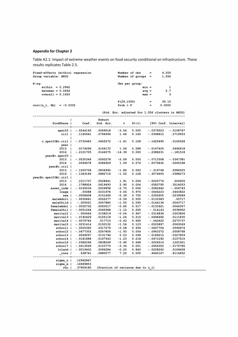
Appendix for Chapter 2

Table A2.1: Impact of extreme weather events on food security conditional on infrastructure. These

results replicates Table 2.5.

Fixed-effects (within) regression Number of obs = 4,205

Group variable: HHID Number of groups = 1,556

R-sq: Obs per group:

within = 0.2962 min = 1

between = 0.0656 avg = 2.7

overall = 0.1920 max = 3

F(29,1555) = 39.15

corr(u_i, Xb) = -0.0332 Prob > F = 0.0000

(Std. Err. adjusted for 1,556 clusters in HHID)

--------------------------------------------------------------------------------------

| Robust

foodShare | Coef. Std. Err. t P>|t| [95% Conf. Interval]

---------------------+----------------------------------------------------------------

spei03 | -.0244145 .0069018 -3.54 0.000 -.0379523 -.0108767

cii1 | .1160561 .0794994 1.46 0.145 -.0398812 .2719933

|

c.spei03#c.cii1 | -.0732483 .0455272 -1.61 0.108 -.1625495 .0160528

year |

2013 | .0174596 .0164172 1.06 0.288 -.0147425 .0496618

2016 | -.2101705 .0146075 -14.39 0.000 -.2388231 -.181518

year#c.spei03 |

2013 | -.0530344 .0093278 -5.69 0.000 -.0713308 -.0347381

2016 | .0094678 .0086929 1.09 0.276 -.0075832 .0265188

year#c.cii1 |

2013 | -.1555728 .0836992 -1.86 0.063 -.319748 .0086025

2016 | -.1343166 .0882716 -1.52 0.128 -.3074605 .0388273

year#c.spei03#c.cii1 |

2013 | .1011737 .0528941 1.91 0.056 -.0025776 .204925

2016 | .1798924 .0619493 2.90 0.004 .0583795 .3014053

asset_inde | -.0165036 .0059958 -2.75 0.006 -.0282642 -.004743

lnage | .00088 .0231978 0.04 0.970 -.0446223 .0463822

sex | -.0058408 .0151669 -0.39 0.700 -.0355905 .0239089

maleAdult | -.0030841 .0052277 -0.59 0.555 -.0133383 .00717

maleChild | -.005021 .0047885 -1.05 0.295 -.0144136 .0043717

femaleAdul | -.0032732 .0050517 -0.65 0.517 -.0131821 .0066357

femaleChil | -.0051264 .0045968 -1.12 0.265 -.014143 .0038902

marital2 | -.000649 .0158219 -0.04 0.967 -.0316836 .0303856

marital3 | -.0192429 .0155118 -1.24 0.215 -.0496692 .0111835

marital4 | -.0076742 .017715 -0.43 0.665 -.042422 .0270737

marital5 | -.0231414 .0150132 -1.54 0.123 -.0525897 .0063069

school1 | -.0025365 .0317279 -0.08 0.936 -.0647704 .0596974

school2 | -.0477302 .0247806 -1.93 0.054 -.0963372 .0008768

school3 | .0069297 .0131794 0.53 0.599 -.0189215 .0327809

school4 | -.0181888 .0147543 -1.23 0.218 -.0471292 .0107515

school6 | -.0382296 .0838249 -0.46 0.648 -.2026514 .1261921

school7 | -.0413569 .0123775 -3.34 0.001 -.0656352 -.0170785

lnland | -.0019402 .0096284 -0.20 0.840 -.0208262 .0169458

_cons | .638741 .0880577 7.25 0.000 .4660167 .8114652

---------------------+----------------------------------------------------------------

sigma_u | .12962867

sigma_e | .16589853

rho | .37909185 (fraction of variance due to u_i)

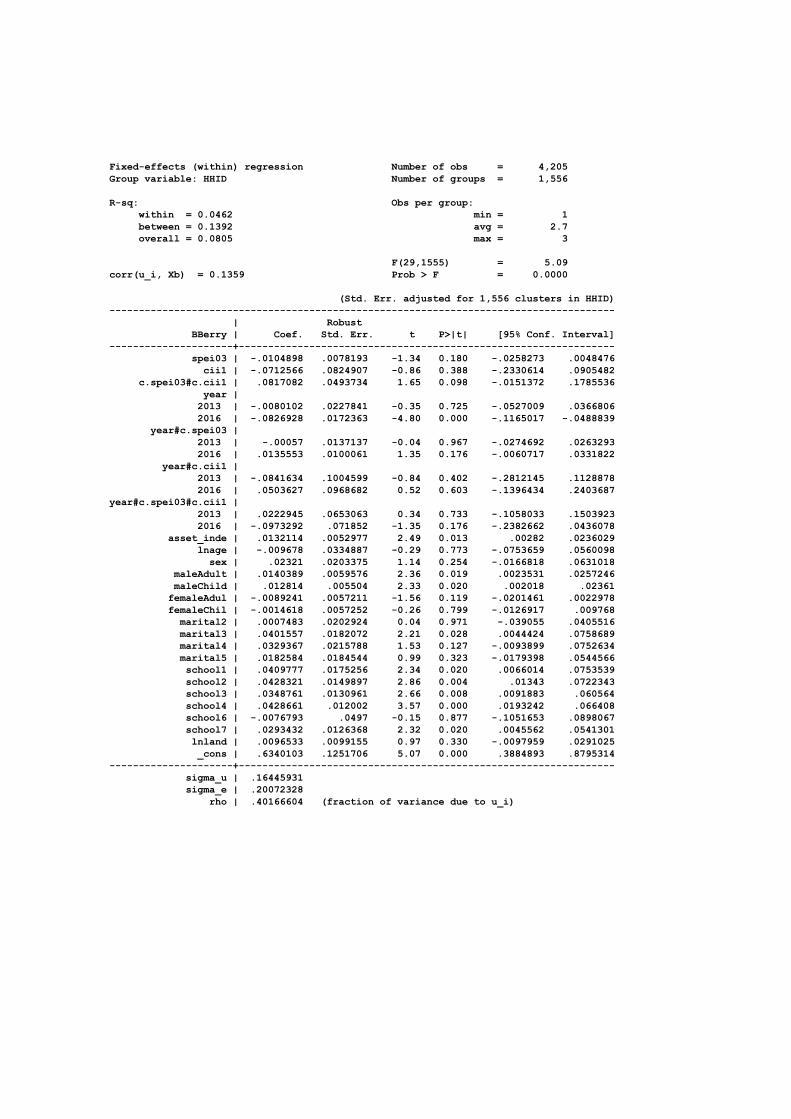
Fixed-effects (within) regression Number of obs = 4,205

Group variable: HHID Number of groups = 1,556

R-sq: Obs per group:

within = 0.0462 min = 1

between = 0.1392 avg = 2.7

overall = 0.0805 max = 3

F(29,1555) = 5.09

corr(u_i, Xb) = 0.1359 Prob > F = 0.0000

(Std. Err. adjusted for 1,556 clusters in HHID)

--------------------------------------------------------------------------------------

| Robust

BBerry | Coef. Std. Err. t P>|t| [95% Conf. Interval]

---------------------+----------------------------------------------------------------

spei03 | -.0104898 .0078193 -1.34 0.180 -.0258273 .0048476

cii1 | -.0712566 .0824907 -0.86 0.388 -.2330614 .0905482

c.spei03#c.cii1 | .0817082 .0493734 1.65 0.098 -.0151372 .1785536

year |

2013 | -.0080102 .0227841 -0.35 0.725 -.0527009 .0366806

2016 | -.0826928 .0172363 -4.80 0.000 -.1165017 -.0488839

year#c.spei03 |

2013 | -.00057 .0137137 -0.04 0.967 -.0274692 .0263293

2016 | .0135553 .0100061 1.35 0.176 -.0060717 .0331822

year#c.cii1 |

2013 | -.0841634 .1004599 -0.84 0.402 -.2812145 .1128878

2016 | .0503627 .0968682 0.52 0.603 -.1396434 .2403687

year#c.spei03#c.cii1 |

2013 | .0222945 .0653063 0.34 0.733 -.1058033 .1503923

2016 | -.0973292 .071852 -1.35 0.176 -.2382662 .0436078

asset_inde | .0132114 .0052977 2.49 0.013 .00282 .0236029

lnage | -.009678 .0334887 -0.29 0.773 -.0753659 .0560098

sex | .02321 .0203375 1.14 0.254 -.0166818 .0631018

maleAdult | .0140389 .0059576 2.36 0.019 .0023531 .0257246

maleChild | .012814 .005504 2.33 0.020 .002018 .02361

femaleAdul | -.0089241 .0057211 -1.56 0.119 -.0201461 .0022978

femaleChil | -.0014618 .0057252 -0.26 0.799 -.0126917 .009768

marital2 | .0007483 .0202924 0.04 0.971 -.039055 .0405516

marital3 | .0401557 .0182072 2.21 0.028 .0044424 .0758689

marital4 | .0329367 .0215788 1.53 0.127 -.0093899 .0752634

marital5 | .0182584 .0184544 0.99 0.323 -.0179398 .0544566

school1 | .0409777 .0175256 2.34 0.020 .0066014 .0753539

school2 | .0428321 .0149897 2.86 0.004 .01343 .0722343

school3 | .0348761 .0130961 2.66 0.008 .0091883 .060564

school4 | .0428661 .012002 3.57 0.000 .0193242 .066408

school6 | -.0076793 .0497 -0.15 0.877 -.1051653 .0898067

school7 | .0293432 .0126368 2.32 0.020 .0045562 .0541301

lnland | .0096533 .0099155 0.97 0.330 -.0097959 .0291025

_cons | .6340103 .1251706 5.07 0.000 .3884893 .8795314

---------------------+----------------------------------------------------------------

sigma_u | .16445931

sigma_e | .20072328

rho | .40166604 (fraction of variance due to u_i)

Fixed-effects (within) regression Number of obs = 4,205

Group variable: HHID Number of groups = 1,556

R-sq: Obs per group:

within = 0.0759 min = 1

between = 0.1441 avg = 2.7

overall = 0.1031 max = 3

F(29,1555) = 8.16

corr(u_i, Xb) = 0.1388 Prob > F = 0.0000

(Std. Err. adjusted for 1,556 clusters in HHID)

--------------------------------------------------------------------------------------

| Robust

EE | Coef. Std. Err. t P>|t| [95% Conf. Interval]

---------------------+----------------------------------------------------------------

spei03 | -.0172309 .014501 -1.19 0.235 -.0456744 .0112126

cii1 | .0471169 .1648491 0.29 0.775 -.2762332 .370467

|

c.spei03#c.cii1 | .0704964 .0924103 0.76 0.446 -.1107654 .2517583

|

year |

2013 | -.1307311 .0408005 -3.20 0.001 -.2107609 -.0507014

2016 | -.186802 .0325129 -5.75 0.000 -.2505758 -.1230282

|

year#c.spei03 |

2013 | -.0004806 .0241682 -0.02 0.984 -.0478863 .046925

2016 | .0575362 .0179888 3.20 0.001 .0222514 .0928211

|

year#c.cii1 |

2013 | -.4900846 .1906531 -2.57 0.010 -.8640489 -.1161202

2016 | -.0580108 .1751596 -0.33 0.741 -.4015847 .2855632

|

year#c.spei03#c.cii1 |

2013 | .1247767 .1220192 1.02 0.307 -.1145628 .3641162

2016 | -.079078 .1270939 -0.62 0.534 -.3283716 .1702155

|

asset_inde | .0270957 .0118607 2.28 0.022 .003831 .0503604

lnage | .0117387 .0666069 0.18 0.860 -.11891 .1423874

sex | -.0129292 .03722 -0.35 0.728 -.0859359 .0600776

maleAdult | .0160272 .0122466 1.31 0.191 -.0079943 .0400488

maleChild | .0212818 .0115428 1.84 0.065 -.0013593 .0439229

femaleAdul | -.0278636 .0115744 -2.41 0.016 -.0505666 -.0051606

femaleChil | -.0177047 .0116786 -1.52 0.130 -.0406122 .0052029

marital2 | .0072636 .0371669 0.20 0.845 -.0656388 .080166

marital3 | .0822321 .0362337 2.27 0.023 .0111601 .1533041

marital4 | .0756194 .0391258 1.93 0.053 -.0011255 .1523643

marital5 | .0151772 .034918 0.43 0.664 -.0533142 .0836686

school1 | .2006522 .0604131 3.32 0.001 .0821524 .319152

school2 | .2136506 .0432306 4.94 0.000 .1288543 .298447

school3 | .1092678 .0287011 3.81 0.000 .0529709 .1655648

school4 | .1623918 .0293346 5.54 0.000 .1048523 .2199313

school6 | .0880682 .1340859 0.66 0.511 -.1749401 .3510764

school7 | .0657791 .0274811 2.39 0.017 .0118751 .1196831

lnland | .0551618 .0202486 2.72 0.007 .0154444 .0948792

_cons | 1.663803 .2458777 6.77 0.000 1.181517 2.14609

---------------------+----------------------------------------------------------------

sigma_u | .39213171

sigma_e | .38324186

rho | .51146375 (fraction of variance due to u_i)

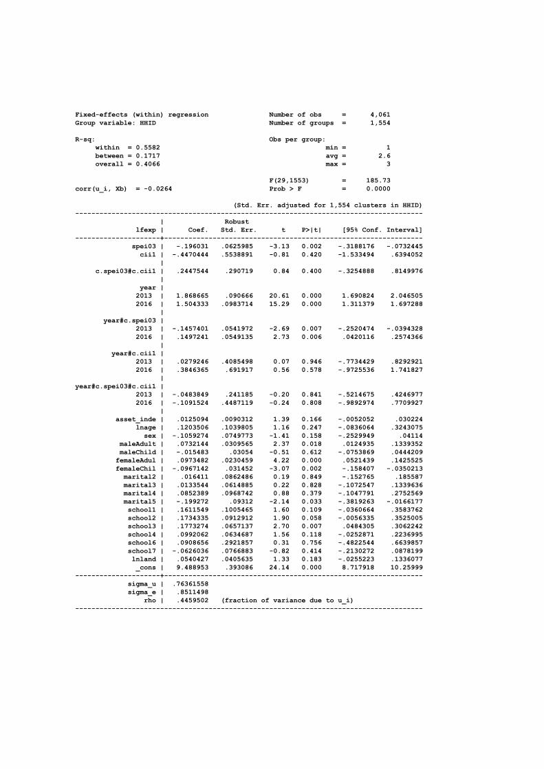
Fixed-effects (within) regression Number of obs = 4,061

Group variable: HHID Number of groups = 1,554

R-sq: Obs per group:

within = 0.5582 min = 1

between = 0.1717 avg = 2.6

overall = 0.4066 max = 3

F(29,1553) = 185.73

corr(u_i, Xb) = -0.0264 Prob > F = 0.0000

(Std. Err. adjusted for 1,554 clusters in HHID)

--------------------------------------------------------------------------------------

| Robust

lfexp | Coef. Std. Err. t P>|t| [95% Conf. Interval]

---------------------+----------------------------------------------------------------

spei03 | -.196031 .0625985 -3.13 0.002 -.3188176 -.0732445

cii1 | -.4470444 .5538891 -0.81 0.420 -1.533494 .6394052

|

c.spei03#c.cii1 | .2447544 .290719 0.84 0.400 -.3254888 .8149976

|

year |

2013 | 1.868665 .090666 20.61 0.000 1.690824 2.046505

2016 | 1.504333 .0983714 15.29 0.000 1.311379 1.697288

|

year#c.spei03 |

2013 | -.1457401 .0541972 -2.69 0.007 -.2520474 -.0394328

2016 | .1497241 .0549135 2.73 0.006 .0420116 .2574366

|

year#c.cii1 |

2013 | .0279246 .4085498 0.07 0.946 -.7734429 .8292921

2016 | .3846365 .691917 0.56 0.578 -.9725536 1.741827

|

year#c.spei03#c.cii1 |

2013 | -.0483849 .241185 -0.20 0.841 -.5214675 .4246977

2016 | -.1091524 .4487119 -0.24 0.808 -.9892974 .7709927

|

asset_inde | .0125094 .0090312 1.39 0.166 -.0052052 .030224

lnage | .1203506 .1039805 1.16 0.247 -.0836064 .3243075

sex | -.1059274 .0749773 -1.41 0.158 -.2529949 .04114

maleAdult | .0732144 .0309565 2.37 0.018 .0124935 .1339352

maleChild | -.015483 .03054 -0.51 0.612 -.0753869 .0444209

femaleAdul | .0973482 .0230459 4.22 0.000 .0521439 .1425525

femaleChil | -.0967142 .031452 -3.07 0.002 -.158407 -.0350213

marital2 | .016411 .0862486 0.19 0.849 -.152765 .185587

marital3 | .0133544 .0614885 0.22 0.828 -.1072547 .1339636

marital4 | .0852389 .0968742 0.88 0.379 -.1047791 .2752569

marital5 | -.199272 .09312 -2.14 0.033 -.3819263 -.0166177

school1 | .1611549 .1005465 1.60 0.109 -.0360664 .3583762

school2 | .1734335 .0912912 1.90 0.058 -.0056335 .3525005

school3 | .1773274 .0657137 2.70 0.007 .0484305 .3062242

school4 | .0992062 .0634687 1.56 0.118 -.0252871 .2236995

school6 | .0908656 .2921857 0.31 0.756 -.4822544 .6639857

school7 | -.0626036 .0766883 -0.82 0.414 -.2130272 .0878199

lnland | .0540427 .0405635 1.33 0.183 -.0255223 .1336077

_cons | 9.488953 .393086 24.14 0.000 8.717918 10.25999

---------------------+----------------------------------------------------------------

sigma_u | .76361558

sigma_e | .8511498

rho | .4459502 (fraction of variance due to u_i)

--------------------------------------------------------------------------------------

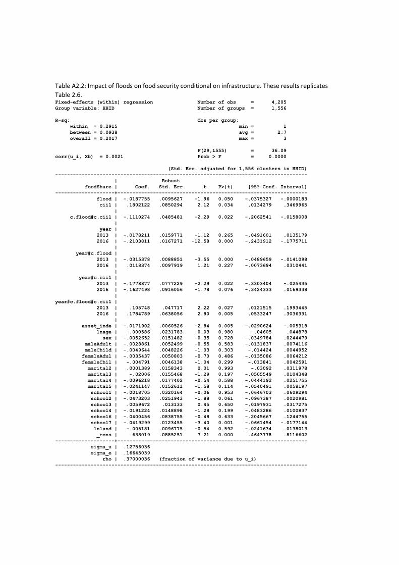
Table A2.2: Impact of floods on food security conditional on infrastructure. These results replicates

Table 2.6. Fixed-effects (within) regression Number of obs = 4,205

Group variable: HHID Number of groups = 1,556

R-sq: Obs per group:

within = 0.2915 min = 1

between = 0.0938 avg = 2.7

overall = 0.2017 max = 3

F(29,1555) = 36.09

corr(u_i, Xb) = 0.0021 Prob > F = 0.0000

(Std. Err. adjusted for 1,556 clusters in HHID)

-------------------------------------------------------------------------------------

| Robust

foodShare | Coef. Std. Err. t P>|t| [95% Conf. Interval]

--------------------+----------------------------------------------------------------

flood | -.0187755 .0095627 -1.96 0.050 -.0375327 -.0000183

cii1 | .1802122 .0850294 2.12 0.034 .0134279 .3469965

|

c.flood#c.cii1 | -.1110274 .0485481 -2.29 0.022 -.2062541 -.0158008

|

year |

2013 | -.0178211 .0159771 -1.12 0.265 -.0491601 .0135179

2016 | -.2103811 .0167271 -12.58 0.000 -.2431912 -.1775711

|

year#c.flood |

2013 | -.0315378 .0088851 -3.55 0.000 -.0489659 -.0141098

2016 | .0118374 .0097919 1.21 0.227 -.0073694 .0310441

|

year#c.cii1 |

2013 | -.1778877 .0777229 -2.29 0.022 -.3303404 -.025435

2016 | -.1627498 .0916056 -1.78 0.076 -.3424333 .0169338

|

year#c.flood#c.cii1 |

2013 | .105748 .047717 2.22 0.027 .0121515 .1993445

2016 | .1784789 .0638056 2.80 0.005 .0533247 .3036331

|

asset_inde | -.0171902 .0060526 -2.84 0.005 -.0290624 -.005318

lnage | -.000586 .0231783 -0.03 0.980 -.04605 .044878

sex | -.0052652 .0151482 -0.35 0.728 -.0349784 .0244479

maleAdult | -.0028861 .0052499 -0.55 0.583 -.0131837 .0074116

maleChild | -.0049644 .0048226 -1.03 0.303 -.014424 .0044952

femaleAdul | -.0035437 .0050803 -0.70 0.486 -.0135086 .0064212

femaleChil | -.004791 .0046138 -1.04 0.299 -.013841 .0042591

marital2 | .0001389 .0158343 0.01 0.993 -.03092 .0311978

marital3 | -.02006 .0155468 -1.29 0.197 -.0505549 .0104348

marital4 | -.0096218 .0177402 -0.54 0.588 -.0444192 .0251755

marital5 | -.0241147 .0152611 -1.58 0.114 -.0540491 .0058197

school1 | -.0018705 .0320164 -0.06 0.953 -.0646703 .0609294

school2 | -.0473203 .0251943 -1.88 0.061 -.0967387 .0020981

school3 | .0059672 .013133 0.45 0.650 -.0197931 .0317275

school4 | -.0191224 .0148898 -1.28 0.199 -.0483286 .0100837

school6 | -.0400456 .0838755 -0.48 0.633 -.2045667 .1244755

school7 | -.0419299 .0123455 -3.40 0.001 -.0661454 -.0177144

lnland | -.005181 .0096775 -0.54 0.592 -.0241634 .0138013

_cons | .638019 .0885251 7.21 0.000 .4643778 .8116602

--------------------+----------------------------------------------------------------

sigma_u | .12756036

sigma_e | .16645039

rho | .37000036 (fraction of variance due to u_i)

-------------------------------------------------------------------------------------

Fixed-effects (within) regression Number of obs = 4,205

Group variable: HHID Number of groups = 1,556

R-sq: Obs per group:

within = 0.0452 min = 1

between = 0.1337 avg = 2.7

overall = 0.0777 max = 3

F(29,1555) = 5.02

corr(u_i, Xb) = 0.1319 Prob > F = 0.0000

(Std. Err. adjusted for 1,556 clusters in HHID)

-------------------------------------------------------------------------------------

| Robust

BBerry | Coef. Std. Err. t P>|t| [95% Conf. Interval]

--------------------+----------------------------------------------------------------

flood | -.0044496 .0107095 -0.42 0.678 -.0254563 .016557

cii1 | -.1094707 .0941793 -1.16 0.245 -.2942026 .0752611

|

c.flood#c.cii1 | .1012825 .0561693 1.80 0.072 -.0088931 .211458

|

year |

2013 | -.0039474 .0195364 -0.20 0.840 -.0422678 .034373

2016 | -.0740331 .0199186 -3.72 0.000 -.1131033 -.034963

|

year#c.flood |

2013 | -.0038809 .0110627 -0.35 0.726 -.0255802 .0178184

2016 | .0067331 .0111882 0.60 0.547 -.0152125 .0286786

|

year#c.cii1 |

2013 | .0136172 .0911285 0.15 0.881 -.1651306 .192365

2016 | .0482883 .1054952 0.46 0.647 -.1586395 .2552161

|

year#c.flood#c.cii1 |

2013 | -.0351189 .0574506 -0.61 0.541 -.1478077 .0775698

2016 | -.0814981 .0786885 -1.04 0.301 -.2358449 .0728487

|

asset_inde | .0132849 .0053499 2.48 0.013 .0027911 .0237787

lnage | -.010292 .0333655 -0.31 0.758 -.0757381 .0551542

sex | .02375 .0203809 1.17 0.244 -.016227 .063727

maleAdult | .0137984 .0059557 2.32 0.021 .0021163 .0254805

maleChild | .0128504 .0055046 2.33 0.020 .0020531 .0236477

femaleAdul | -.0090888 .0057284 -1.59 0.113 -.020325 .0021474

femaleChil | -.0016796 .0057274 -0.29 0.769 -.0129138 .0095546

marital2 | .0009876 .0202462 0.05 0.961 -.0387252 .0407004

marital3 | .0404226 .0182196 2.22 0.027 .0046849 .0761602

marital4 | .0330718 .0216099 1.53 0.126 -.0093158 .0754594

marital5 | .018213 .0184655 0.99 0.324 -.0180069 .0544329

school1 | .0397714 .0176794 2.25 0.025 .0050934 .0744493

school2 | .0423736 .0150732 2.81 0.005 .0128076 .0719397

school3 | .0344136 .0131415 2.62 0.009 .0086367 .0601905

school4 | .0422735 .0120315 3.51 0.000 .0186739 .0658732

school6 | -.0102684 .0509639 -0.20 0.840 -.1102336 .0896967

school7 | .0295186 .0126055 2.34 0.019 .004793 .0542442

lnland | .01085 .0098965 1.10 0.273 -.0085619 .0302619

_cons | .6279794 .1249537 5.03 0.000 .3828838 .8730749

--------------------+----------------------------------------------------------------

sigma_u | .16476545

sigma_e | .2008251

rho | .40231636 (fraction of variance due to u_i)

-------------------------------------------------------------------------------------

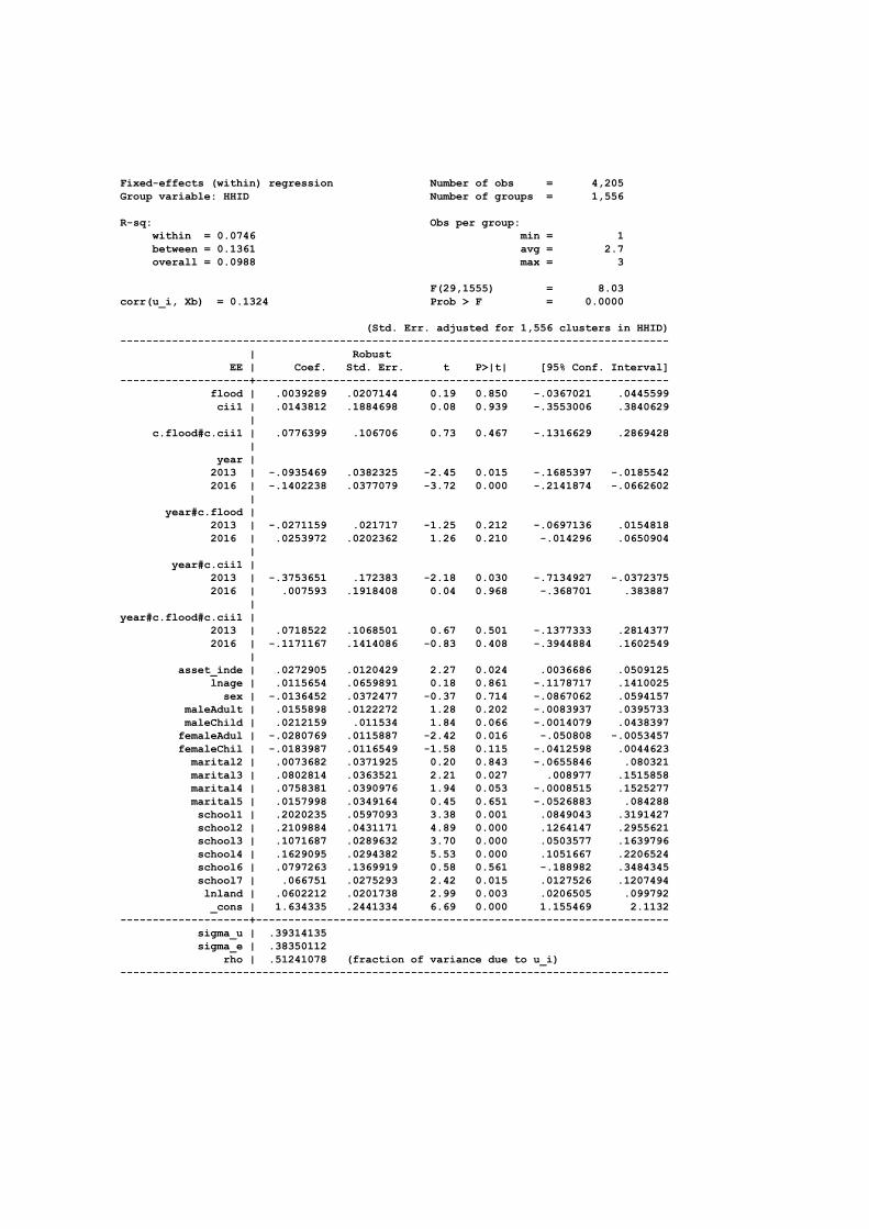
Fixed-effects (within) regression Number of obs = 4,205

Group variable: HHID Number of groups = 1,556

R-sq: Obs per group:

within = 0.0746 min = 1

between = 0.1361 avg = 2.7

overall = 0.0988 max = 3

F(29,1555) = 8.03

corr(u_i, Xb) = 0.1324 Prob > F = 0.0000

(Std. Err. adjusted for 1,556 clusters in HHID)

-------------------------------------------------------------------------------------

| Robust

EE | Coef. Std. Err. t P>|t| [95% Conf. Interval]

--------------------+----------------------------------------------------------------

flood | .0039289 .0207144 0.19 0.850 -.0367021 .0445599

cii1 | .0143812 .1884698 0.08 0.939 -.3553006 .3840629

|

c.flood#c.cii1 | .0776399 .106706 0.73 0.467 -.1316629 .2869428

|

year |

2013 | -.0935469 .0382325 -2.45 0.015 -.1685397 -.0185542

2016 | -.1402238 .0377079 -3.72 0.000 -.2141874 -.0662602

|

year#c.flood |

2013 | -.0271159 .021717 -1.25 0.212 -.0697136 .0154818

2016 | .0253972 .0202362 1.26 0.210 -.014296 .0650904

|

year#c.cii1 |

2013 | -.3753651 .172383 -2.18 0.030 -.7134927 -.0372375

2016 | .007593 .1918408 0.04 0.968 -.368701 .383887

|

year#c.flood#c.cii1 |

2013 | .0718522 .1068501 0.67 0.501 -.1377333 .2814377

2016 | -.1171167 .1414086 -0.83 0.408 -.3944884 .1602549

|

asset_inde | .0272905 .0120429 2.27 0.024 .0036686 .0509125

lnage | .0115654 .0659891 0.18 0.861 -.1178717 .1410025

sex | -.0136452 .0372477 -0.37 0.714 -.0867062 .0594157

maleAdult | .0155898 .0122272 1.28 0.202 -.0083937 .0395733

maleChild | .0212159 .011534 1.84 0.066 -.0014079 .0438397

femaleAdul | -.0280769 .0115887 -2.42 0.016 -.050808 -.0053457

femaleChil | -.0183987 .0116549 -1.58 0.115 -.0412598 .0044623

marital2 | .0073682 .0371925 0.20 0.843 -.0655846 .080321

marital3 | .0802814 .0363521 2.21 0.027 .008977 .1515858

marital4 | .0758381 .0390976 1.94 0.053 -.0008515 .1525277

marital5 | .0157998 .0349164 0.45 0.651 -.0526883 .084288

school1 | .2020235 .0597093 3.38 0.001 .0849043 .3191427

school2 | .2109884 .0431171 4.89 0.000 .1264147 .2955621

school3 | .1071687 .0289632 3.70 0.000 .0503577 .1639796

school4 | .1629095 .0294382 5.53 0.000 .1051667 .2206524

school6 | .0797263 .1369919 0.58 0.561 -.188982 .3484345

school7 | .066751 .0275293 2.42 0.015 .0127526 .1207494

lnland | .0602212 .0201738 2.99 0.003 .0206505 .099792

_cons | 1.634335 .2441334 6.69 0.000 1.155469 2.1132

--------------------+----------------------------------------------------------------

sigma_u | .39314135

sigma_e | .38350112

rho | .51241078 (fraction of variance due to u_i)

-------------------------------------------------------------------------------------

Fixed-effects (within) regression Number of obs = 4,061

Group variable: HHID Number of groups = 1,554

R-sq: Obs per group:

within = 0.5544 min = 1

between = 0.1935 avg = 2.6

overall = 0.4142 max = 3

F(29,1553) = 183.95

corr(u_i, Xb) = -0.0048 Prob > F = 0.0000

(Std. Err. adjusted for 1,554 clusters in HHID)

-------------------------------------------------------------------------------------

| Robust

lfexp | Coef. Std. Err. t P>|t| [95% Conf. Interval]

--------------------+----------------------------------------------------------------

flood | -.1674596 .0699633 -2.39 0.017 -.3046922 -.0302271

cii1 | -.6734308 .6024526 -1.12 0.264 -1.855137 .5082756

|

c.flood#c.cii1 | .3697052 .2986977 1.24 0.216 -.2161881 .9555985

|

year |

2013 | 1.699813 .080419 21.14 0.000 1.542072 1.857555

2016 | 1.521438 .1154014 13.18 0.000 1.295079 1.747797

|

year#c.flood |

2013 | -.0480696 .0410173 -1.17 0.241 -.1285246 .0323855

2016 | .1232376 .0597213 2.06 0.039 .0060947 .2403806

|

year#c.cii1 |

2013 | .3222689 .4260665 0.76 0.450 -.5134575 1.157995

2016 | .4265064 .7154451 0.60 0.551 -.9768339 1.829847

|

year#c.flood#c.cii1 |

2013 | -.2255712 .2248263 -1.00 0.316 -.6665664 .215424

2016 | -.0739923 .4945832 -0.15 0.881 -1.044114 .8961291

|

asset_inde | .0099962 .0091487 1.09 0.275 -.007949 .0279414

lnage | .1122901 .1046471 1.07 0.283 -.0929745 .3175547

sex | -.1000159 .076125 -1.31 0.189 -.2493344 .0493026

maleAdult | .0722676 .031134 2.32 0.020 .0111985 .1333366

maleChild | -.016516 .0308198 -0.54 0.592 -.0769689 .0439368

femaleAdul | .0976411 .0231724 4.21 0.000 .0521887 .1430936

femaleChil | -.0942801 .0314522 -3.00 0.003 -.1559734 -.0325867

marital2 | .0232506 .0886416 0.26 0.793 -.1506193 .1971205

marital3 | .012448 .0621085 0.20 0.841 -.1093774 .1342735

marital4 | .0790902 .0965263 0.82 0.413 -.1102454 .2684258

marital5 | -.202527 .0942155 -2.15 0.032 -.38733 -.017724

school1 | .1611912 .1013577 1.59 0.112 -.0376212 .3600035

school2 | .1759165 .0930886 1.89 0.059 -.006676 .358509

school3 | .1731801 .0659219 2.63 0.009 .0438747 .3024855

school4 | .0970286 .0653668 1.48 0.138 -.031188 .2252451

school6 | .0825266 .2948541 0.28 0.780 -.4958275 .6608808

school7 | -.0602298 .0771419 -0.78 0.435 -.211543 .0910834

lnland | .0498402 .0411155 1.21 0.226 -.0308075 .130488

_cons | 9.485715 .3970297 23.89 0.000 8.706944 10.26449

--------------------+----------------------------------------------------------------

sigma_u | .75298367

sigma_e | .85478146

rho | .43693649 (fraction of variance due to u_i)

-------------------------------------------------------------------------------------

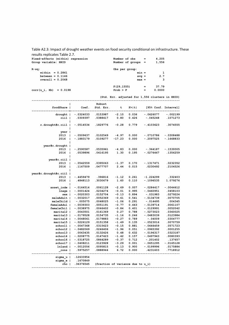
Table A2.3: Impact of drought weather events on food security conditional on infrastructure. These

results replicates Table 2.7. Fixed-effects (within) regression Number of obs = 4,205

Group variable: HHID Number of groups = 1,556

R-sq: Obs per group:

within = 0.2861 min = 1

between = 0.1146 avg = 2.7

overall = 0.2068 max = 3

F(29,1555) = 37.79

corr(u_i, Xb) = 0.0198 Prob > F = 0.0000

(Std. Err. adjusted for 1,556 clusters in HHID)

---------------------------------------------------------------------------------------

| Robust

foodShare | Coef. Std. Err. t P>|t| [95% Conf. Interval]

----------------------+----------------------------------------------------------------

drought | -.0324033 .0153987 -2.10 0.036 -.0626077 -.002199

cii1 | .0309397 .0388417 0.80 0.426 -.045248 .1071273

|

c.drought#c.cii1 | -.0514534 .1829776 -0.28 0.779 -.4103623 .3074555

|

year |

2013 | -.0509637 .0102549 -4.97 0.000 -.0710786 -.0308488

2016 | -.1883179 .0109277 -17.23 0.000 -.2097525 -.1668833

|

year#c.drought |

2013 | -.2590587 .0535961 -4.83 0.000 -.364187 -.1539305

2016 | .0539896 .0416195 1.30 0.195 -.0276467 .1356259

|

year#c.cii1 |

2013 | -.0542559 .0395063 -1.37 0.170 -.1317471 .0232352

2016 | .1167509 .0477707 2.44 0.015 .0230492 .2104526

|

year#c.drought#c.cii1 |

2013 | -.4459479 .396816 -1.12 0.261 -1.224299 .332403

2016 | .4848113 .3030679 1.60 0.110 -.1096535 1.079276

|

asset_inde | -.0164514 .0061128 -2.69 0.007 -.0284417 -.0044612

lnage | -.0001424 .0234274 -0.01 0.995 -.0460951 .0458103

sex | -.0020303 .0152704 -0.13 0.894 -.031983 .0279224

maleAdult | -.0032017 .0052369 -0.61 0.541 -.0134739 .0070705

maleChild | -.005075 .0048025 -1.06 0.291 -.014495 .004345

femaleAdul | -.0039303 .0051191 -0.77 0.443 -.0139714 .0061107

femaleChil | -.0038975 .0046402 -0.84 0.401 -.0129991 .0052042

marital2 | .0043501 .0161369 0.27 0.788 -.0273023 .0360025

marital3 | -.0179528 .0154735 -1.16 0.246 -.0483039 .0123984

marital4 | -.0048061 .0179883 -0.27 0.789 -.04009 .0304777

marital5 | -.0226129 .0151358 -1.49 0.135 -.0523016 .0070759

school1 | -.0047368 .0315623 -0.15 0.881 -.0666459 .0571723

school2 | -.0482069 .0246406 -1.96 0.051 -.0965392 .0001255

school3 | .0063435 .0132426 0.48 0.632 -.0196317 .0323187

school4 | -.0208775 .0147423 -1.42 0.157 -.0497943 .0080393

school6 | -.0318725 .0864289 -0.37 0.712 -.201402 .137657

school7 | -.0408211 .0123928 -3.29 0.001 -.0651295 -.0165128

lnland | -.0012056 .0095815 -0.13 0.900 -.0199996 .0175884

_cons | .5975257 .0888944 6.72 0.000 .4231603 .7718912

----------------------+----------------------------------------------------------------

sigma_u | .12633954

sigma_e | .1670849

rho | .36376545 (fraction of variance due to u_i)

---------------------------------------------------------------------------------------

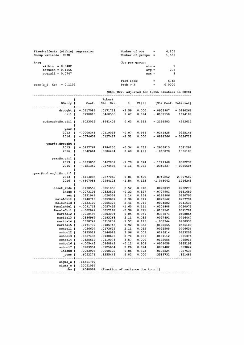
Fixed-effects (within) regression Number of obs = 4,205

Group variable: HHID Number of groups = 1,556

R-sq: Obs per group:

within = 0.0482 min = 1

between = 0.1166 avg = 2.7

overall = 0.0747 max = 3

F(29,1555) = 5.42

corr(u_i, Xb) = 0.1102 Prob > F = 0.0000

(Std. Err. adjusted for 1,556 clusters in HHID)

---------------------------------------------------------------------------------------

| Robust

BBerry | Coef. Std. Err. t P>|t| [95% Conf. Interval]

----------------------+----------------------------------------------------------------

drought | -.0617084 .0171718 -3.59 0.000 -.0953907 -.0280261

cii1 | .0770815 .0460555 1.67 0.094 -.0132558 .1674189

|

c.drought#c.cii1 | .1023015 .1641403 0.62 0.533 -.2196583 .4242612

|

year |

2013 | -.0008341 .0119035 -0.07 0.944 -.0241828 .0225146

2016 | -.0574639 .0127417 -4.51 0.000 -.0824566 -.0324712

|

year#c.drought |

2013 | -.0437762 .1284255 -0.34 0.733 -.2956815 .2081292

2016 | .0342664 .0506474 0.68 0.499 -.065078 .1336108

|

year#c.cii1 |

2013 | -.0833856 .0467039 -1.79 0.074 -.1749948 .0082237

2016 | -.121347 .0574495 -2.11 0.035 -.2340337 -.0086604

|

year#c.drought#c.cii1 |

2013 | .6113085 .7577062 0.81 0.420 -.8749252 2.097542

2016 | -.4607086 .2984125 -1.54 0.123 -1.046042 .1246248

|

asset_inde | .0130559 .0051858 2.52 0.012 .0028839 .0232279

lnage | -.0073106 .0333825 -0.22 0.827 -.0727901 .0581689

sex | .0231944 .020334 1.14 0.254 -.0166906 .0630795

maleAdult | .0140718 .0059687 2.36 0.019 .0023642 .0257794

maleChild | .0133107 .0055328 2.41 0.016 .0024582 .0241633

femaleAdul | -.0091718 .0057452 -1.60 0.111 -.0204408 .0020973

femaleChil | -.002042 .0057161 -0.36 0.721 -.0132541 .0091701

marital2 | .0010496 .0203094 0.05 0.959 -.0387871 .0408864

marital3 | .0386969 .0183268 2.11 0.035 .0027491 .0746447

marital4 | .0338749 .0215239 1.57 0.116 -.008344 .0760938

marital5 | .0171772 .0185745 0.92 0.355 -.0192565 .0536109

school1 | .036607 .0173625 2.11 0.035 .0025505 .0706634

school2 | .0435011 .0146928 2.96 0.003 .0146814 .0723209

school3 | .0357436 .0130678 2.74 0.006 .0101112 .061376

school4 | .0425617 .0119074 3.57 0.000 .0192055 .065918

school6 | -.005443 .0468842 -0.12 0.908 -.0974058 .0865198

school7 | .0283951 .0125654 2.26 0.024 .0037482 .053042

lnland | .0083903 .0098102 0.86 0.393 -.0108524 .027633

_cons | .6052271 .1255443 4.82 0.000 .3589732 .851481

----------------------+----------------------------------------------------------------

sigma_u | .16511799

sigma_e | .20051054

rho | .4040994 (fraction of variance due to u_i)

---------------------------------------------------------------------------------------

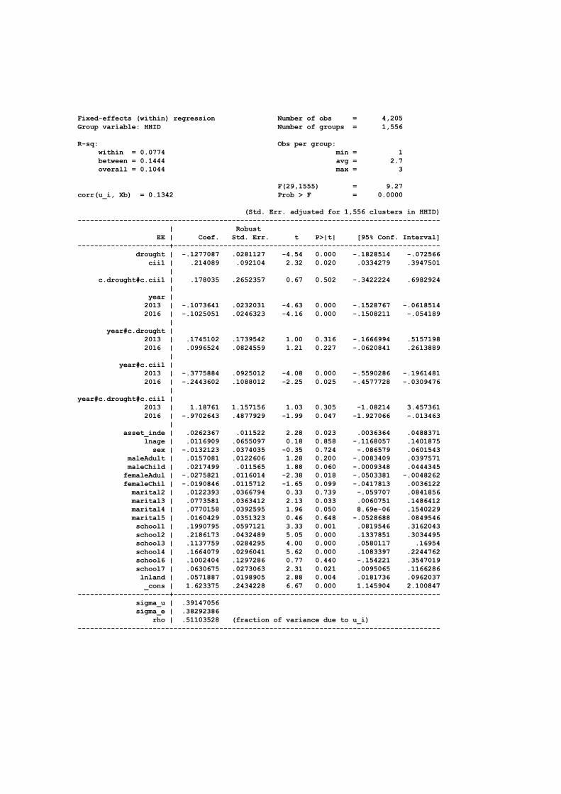
Fixed-effects (within) regression Number of obs = 4,205

Group variable: HHID Number of groups = 1,556

R-sq: Obs per group:

within = 0.0774 min = 1

between = 0.1444 avg = 2.7

overall = 0.1044 max = 3

F(29,1555) = 9.27

corr(u_i, Xb) = 0.1342 Prob > F = 0.0000

(Std. Err. adjusted for 1,556 clusters in HHID)

---------------------------------------------------------------------------------------

| Robust

EE | Coef. Std. Err. t P>|t| [95% Conf. Interval]

----------------------+----------------------------------------------------------------

drought | -.1277087 .0281127 -4.54 0.000 -.1828514 -.072566

cii1 | .214089 .092104 2.32 0.020 .0334279 .3947501

|

c.drought#c.cii1 | .178035 .2652357 0.67 0.502 -.3422224 .6982924

|

year |

2013 | -.1073641 .0232031 -4.63 0.000 -.1528767 -.0618514

2016 | -.1025051 .0246323 -4.16 0.000 -.1508211 -.054189

|

year#c.drought |

2013 | .1745102 .1739542 1.00 0.316 -.1666994 .5157198

2016 | .0996524 .0824559 1.21 0.227 -.0620841 .2613889

|

year#c.cii1 |

2013 | -.3775884 .0925012 -4.08 0.000 -.5590286 -.1961481

2016 | -.2443602 .1088012 -2.25 0.025 -.4577728 -.0309476

|

year#c.drought#c.cii1 |

2013 | 1.18761 1.157156 1.03 0.305 -1.08214 3.457361

2016 | -.9702643 .4877929 -1.99 0.047 -1.927066 -.013463

|

asset_inde | .0262367 .011522 2.28 0.023 .0036364 .0488371

lnage | .0116909 .0655097 0.18 0.858 -.1168057 .1401875

sex | -.0132123 .0374035 -0.35 0.724 -.086579 .0601543

maleAdult | .0157081 .0122606 1.28 0.200 -.0083409 .0397571

maleChild | .0217499 .011565 1.88 0.060 -.0009348 .0444345

femaleAdul | -.0275821 .0116014 -2.38 0.018 -.0503381 -.0048262

femaleChil | -.0190846 .0115712 -1.65 0.099 -.0417813 .0036122

marital2 | .0122393 .0366794 0.33 0.739 -.059707 .0841856

marital3 | .0773581 .0363412 2.13 0.033 .0060751 .1486412

marital4 | .0770158 .0392595 1.96 0.050 8.69e-06 .1540229

marital5 | .0160429 .0351323 0.46 0.648 -.0528688 .0849546

school1 | .1990795 .0597121 3.33 0.001 .0819546 .3162043

school2 | .2186173 .0432489 5.05 0.000 .1337851 .3034495

school3 | .1137759 .0284295 4.00 0.000 .0580117 .16954

school4 | .1664079 .0296041 5.62 0.000 .1083397 .2244762

school6 | .1002404 .1297286 0.77 0.440 -.154221 .3547019

school7 | .0630675 .0273063 2.31 0.021 .0095065 .1166286

lnland | .0571887 .0198905 2.88 0.004 .0181736 .0962037

_cons | 1.623375 .2434228 6.67 0.000 1.145904 2.100847

----------------------+----------------------------------------------------------------

sigma_u | .39147056

sigma_e | .38292386

rho | .51103528 (fraction of variance due to u_i)

---------------------------------------------------------------------------------------

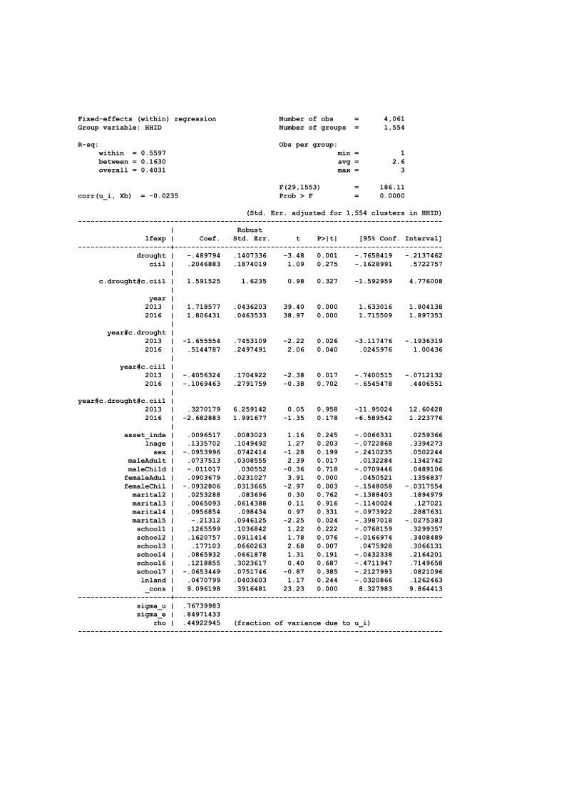
Fixed-effects (within) regression Number of obs = 4,061

Group variable: HHID Number of groups = 1,554

R-sq: Obs per group:

within = 0.5597 min = 1

between = 0.1630 avg = 2.6

overall = 0.4031 max = 3

F(29,1553) = 186.11

corr(u_i, Xb) = -0.0235 Prob > F = 0.0000

(Std. Err. adjusted for 1,554 clusters in HHID)

---------------------------------------------------------------------------------------

| Robust

lfexp | Coef. Std. Err. t P>|t| [95% Conf. Interval]

----------------------+----------------------------------------------------------------

drought | -.489794 .1407336 -3.48 0.001 -.7658419 -.2137462

cii1 | .2046883 .1874019 1.09 0.275 -.1628991 .5722757

|

c.drought#c.cii1 | 1.591525 1.6235 0.98 0.327 -1.592959 4.776008

|

year |

2013 | 1.718577 .0436203 39.40 0.000 1.633016 1.804138

2016 | 1.806431 .0463533 38.97 0.000 1.715509 1.897353

|

year#c.drought |

2013 | -1.655554 .7453109 -2.22 0.026 -3.117476 -.1936319

2016 | .5144787 .2497491 2.06 0.040 .0245976 1.00436

|

year#c.cii1 |

2013 | -.4056324 .1704922 -2.38 0.017 -.7400515 -.0712132

2016 | -.1069463 .2791759 -0.38 0.702 -.6545478 .4406551

|

year#c.drought#c.cii1 |

2013 | .3270179 6.259142 0.05 0.958 -11.95024 12.60428

2016 | -2.682883 1.991677 -1.35 0.178 -6.589542 1.223776

|

asset_inde | .0096517 .0083023 1.16 0.245 -.0066331 .0259366

lnage | .1335702 .1049492 1.27 0.203 -.0722868 .3394273

sex | -.0953996 .0742414 -1.28 0.199 -.2410235 .0502244

maleAdult | .0737513 .0308555 2.39 0.017 .0132284 .1342742

maleChild | -.011017 .030552 -0.36 0.718 -.0709446 .0489106

femaleAdul | .0903679 .0231027 3.91 0.000 .0450521 .1356837

femaleChil | -.0932806 .0313665 -2.97 0.003 -.1548058 -.0317554

marital2 | .0253288 .083696 0.30 0.762 -.1388403 .1894979

marital3 | .0065093 .0614388 0.11 0.916 -.1140024 .127021

marital4 | .0956854 .098434 0.97 0.331 -.0973922 .2887631

marital5 | -.21312 .0946125 -2.25 0.024 -.3987018 -.0275383

school1 | .1265599 .1036842 1.22 0.222 -.0768159 .3299357

school2 | .1620757 .0911414 1.78 0.076 -.0166974 .3408489

school3 | .177103 .0660263 2.68 0.007 .0475928 .3066131

school4 | .0865932 .0661878 1.31 0.191 -.0432338 .2164201

school6 | .1218855 .3023617 0.40 0.687 -.4711947 .7149658

school7 | -.0653449 .0751746 -0.87 0.385 -.2127993 .0821096

lnland | .0470799 .0403603 1.17 0.244 -.0320866 .1262463

_cons | 9.096198 .3916481 23.23 0.000 8.327983 9.864413

----------------------+----------------------------------------------------------------

sigma_u | .76739983

sigma_e | .84971433

rho | .44922945 (fraction of variance due to u_i)

---------------------------------------------------------------------------------------