early dentine erosion assessment with non - UM Students

EARLY DENTINE EROSION ASSESSMENT WITH NON-INVASIVE METHOD

MADIHA HABIB

FACULTY OF DENTISTRY UNIVERSITY OF MALAYA

KUALA LUMPUR

2018

Univers

ity of

Mala

ya

EARLY DENTINE EROSION ASSESSMENT WITH

NON-INVASIVE METHOD

MADIHA HABIB

THESIS SUBMITTED IN FULFILMENT OF THE

REQUIREMENTS FOR THE DEGREE OF DOCTOR OF

PHILOSOPHY

FACULTY OF DENTISTRY

UNIVERSITY OF MALAYA

KUALA LUMPUR

2018

Univers

ity of

Mala

ya

ii

UNIVERSITY OF MALAYA

ORIGINAL LITERARY WORK DECLARATION

Name of Candidate: MADIHA HABIB

Matric No: DHA140014

Name of Degree: DOCTOR OF PHILOSOPHY

Title of Thesis: EARLY DENTINE EROSION ASSESSMENT WITH NON-

INVASIVE METHOD

Field of Study: RESTORATIVE DENTISTRY

I do solemnly and sincerely declare that:

(1) I am the sole author/writer of this Work;

(2) This Work is original;

(3) Any use of any work in which copyright exists was done by way of fair

dealing and for permitted purposes and any excerpt or extract from, or

reference to or reproduction of any copyright work has been disclosed

expressly and sufficiently and the title of the Work and its authorship have

been acknowledged in this Work;

(4) I do not have any actual knowledge nor do I ought reasonably to know that

the making of this work constitutes an infringement of any copyright work;

(5) I hereby assign all and every rights in the copyright to this Work to the

University of Malaya (“UM”), who henceforth shall be owner of the

copyright in this Work and that any reproduction or use in any form or by any

means whatsoever is prohibited without the written consent of UM having

been first had and obtained;

(6) I am fully aware that if in the course of making this Work I have infringed

any copyright whether intentionally or otherwise, I may be subject to legal

action or any other action as may be determined by UM.

Candidate’s Signature Date:

Subscribed and solemnly declared before,

Witness’s Signature Date:

Name:

Designation:

Univers

ity of

Mala

ya

iii

EARLY DENTINE EROSION ASSESSMENT WITH NON-INVASIVE

METHOD

ABSTRACT

Non-invasive assessment of early dentine erosion is required for clinical validation of

therapeutic strategies aiming to reduce or arrest the progression of this condition. The

purpose of this thesis was to seek a non-invasive method suitable for monitoring early

dentine erosion progression with the ultimate goal of using this tool in clinical trials

involving dentine erosion. To achieve this purpose, this thesis aimed to first assess the

potential of optical coherence tomography (OCT) for monitoring early dentine erosion

progression, second, to assess the potential of surface roughness as a method for

measuring early dentine erosion progression in simulated intraoral conditions and

finally to assess if OCT is a sensitive tool to detect early dentine erosion and monitor its

progression in simulated intraoral conditions by correlating OCT data with surface

roughness data. Root dentine samples were first immersed in 0.3% citric acid for a total

of 30 minutes. Measurements with OCT and field-emission scanning electron

microscopy (FE-SEM) were obtained at varying erosion intervals. Integrated OCT

intensity changes were compared with FE-SEM observations. Next, root dentine

samples were subjected to a cycling erosion challenge with 0.3% citric acid for 10

minutes, three times a day interspersed with periods of simulated salivary

remineralisation for three days. Measurements with OCT and non-contact profilometry

were obtained on every cycling day. Fractional change of average roughness and

bearing curve parameters was compared with fractional change of surface loss and FE-

SEM observations. Finally, fractional change of integrated OCT intensity was compared

with fractional change of roughness parameters and FE-SEM observations. Integrated

OCT intensity was able to monitor the progression of early dentine erosion for 30

Univers

ity of

Mala

ya

iv

minutes with a detection threshold of two minutes from baseline. Mean percentage

change in integrated OCT intensity exhibited linear pattern (R2 = .99) with erosion

interval. Integrated OCT intensity changes corresponded with FE-SEM observations.

Average roughness (fRa1) and bearing curve parameters namely core roughness (fRk),

peak roughness (fRpk) and valley roughness (fRvk) were able to longitudinally measure

the progression of early dentine erosion as opposed to fractional change of surface loss.

FE-SEM images supported the surface roughness results. Integrated OCT intensity was

able to longitudinally measure early dentine erosion for three days in simulated intraoral

conditions with a detection threshold of day one from baseline measurement. Fractional

change of integrated OCT intensity correlated moderately but significantly with fRk and

fRa1 (r = .428 and .394 respectively) and showed a weak but significant correlation with

fRpk and fRvk (r = .300 and .217 respectively). Integrated OCT intensity changes

corresponded with ultrastructural changes of early eroded dentine. These studies

suggested that OCT and surface roughness parameters are suited for monitoring the

progression of in vitro early dentine erosion non-invasively and could be possible tools

for monitoring early dentine erosion progression in clinical trials.

Keywords: Early dentine erosion, non-invasive methods, monitoring.

Univers

ity of

Mala

ya

v

EARLY DENTINE EROSION ASSESSMENT WITH NON-INVASIVE METHOD

ABSTRAK

Penilaian yang bukan invasif terhadap hakisan dentine yang awal diperlukan untuk

pengesahan klinikal terhadap strategi terapeutik yang bertujuan untuk mengurangkan

atau memberhentikan perkembangan keadaan ini. Tujuan tesis ini adalah untuk mencari

kaedah pengimejan bukan invasif yang sesuai untuk memantau perkembangan hakisan

dentine awal dengan matlamat menggunakan alat ini dalam ujian klinikal yang

melibatkan hakisan dentine. Untuk mencapai tujuan ini, tesis ini bermatlamat untuk

pertama sekali, menilai potensi tomografi koheren optik (OCT) untuk memantau

progressi erosi dentine yang awal. Kedua, ia bertujuan untuk menilai potensi parameter

kekasaran permukaan untuk memantau perkembangan hakisan dentine awal dalam

keadaan intraoral bersimulasi. Akhir sekali, ia bertujuaan untuk menilai potensi OCT

untuk memantau perkembangan hakisan dentine awal dalam keadaan simulasi intraoral.

Pertama, sampel akar dentine direndam dalam 0.3% asid sitrik selama 30 minit.

Pengukuran menggunakan OCT dan mikroskop elektron pengimbasan-emisi lapangan

(FE-SEM) diperolehi berdasarkan pelbagai tempoh hakisan. Perubahan intensiti OCT

yang bersepadu dibandingkan dengan perubahan ketumpatan mineral dan pemerhatian

FE-SEM. Seterusnya, sampel akar dentine dikenakan cabaran pengitaran hakisan

dengan 0.3% asid sitrik selama 10 minit, tiga kali sehari secara berselang dengan

tempoh remineralisasi saliva bersimulasi selama 3 hari. Pengukuran dengan OCT dan

profilometri tanpa hubungan diperolehi pada setiap hari pengitaran. Perubahan

fraksional pada purata kekasaran dan parameter lengkungan galas dibandingkan dengan

perubahan fraksional kehilangan permukaan dan pemerhatian FE-SEM. Akhir sekali,

perubahan fraksional terhadap intensiti OCT yang berintegrasi dibandingkan dengan

perubahan fraksional parameter kekasaran dan pemerhatian FE-SEM. Intensiti OCT

yang berintegrasidapat memantau perkembangan hakisan dentine awal selama 30 minit

Univers

ity of

Mala

ya

vi

dengan ambang pengesanan selama dua minit dari garis dasar. Perubahan peratusan min

dalam ketumpatan OCT menunjukkan corak linear (R2 = .99) dengan jarak pengesan

hakisan masing-masing. Perubahan intensiti OCT yang berintergrasi berpadanan dengan

pemerhatian FE-SEM. Parameter purata kekasaran (fRa1) dan lengkung galas

terutamanya kekasaran teras (fRk), kekasaran puncak (fRpk) dan kekasaran lembah

(fRvk) dapat memantau perkembangan hakisan dentine awal bertentangan dengan

perubahan fraksional kehilangan permukaan. Imej FE-SEM menyokong keputusan

kekasaran permukaan. Keamatan OCT yang berintegrasi dapat mengukur hakisan

dentine awal secara mendadak selama 3 hari dalam keadaan simulasi intraoral dengan

ambang pengesanan hari pertama dari pengukuran baseline. Perubahan fraksional

intensiti OCT berintegrasi berkorelasi secara sederhana tetapi secara signifikan dengan

fRk dan fRa1 (r = .428 dan .394 masing-masing) dan menunjukkan korelasi yang lemah

tetapi signifikan dengan fRpk dan fRvk (r = .300 dan .177). Perubahan intensiti OCT

berintegrasi sesuai dengan perubahan ultrastruktur dentine yang terhakis awal. Kajian-

kajian ini mencadangkan bahawa parameter OCT dan permukaan kekasaran adalah

sesuai untuk memantau perkembangan in vitro awal hakisan dentine yang bukan invasif

dan berkemungkinan untuk menjadi calon untuk memantau perkembangan hakisan awal

dentine dalam ujian klinikal.

Kata kunci: Hakisan dentine awal, kaedah bukan invasif, memantau perkembangan.

Univers

ity of

Mala

ya

vii

ACKNOWLEDGEMENTS

I am grateful first and foremost to Almighty Allah for making this possible for me

and for everything else.

I would like to express my earnest thanks to my main supervisor, Associate Professor

Dr. Chew Hooi Pin. She has been both an advisor and a mentor. I am truly grateful to

her for the trust she showed in hiring me and for the freedom of decision making during

this journey. She has inspired me in many ways both at a personal and professional

level.

I am grateful to my co-supervisor Dr. Christian Zakian for his arduous efforts in

designing the Matlab programme and for his insights in the analysis part of the study. I

am indebted to him for introducing me to experimental part of research.

I am grateful to Professor Alex Fok and his research team for the use of micro-CT

and scanning electron microscopy in University of Minnesota. My research would not

have been possible without their efforts and input.

Thank you my co-workers and friends in the lab and entire HIR-team for all the

support. I am grateful to Ali for all the troubleshooting. Many thanks to the entire lab

staff especially madam Zarina for facilitating my work in many ways.

I am grateful to University of Malaya for the High Impact Research scholarship and

for the use of many generous resources both at national and international level.

I am grateful to Professor Prabhakaran for showing me this path and to Lakshmi for

introducing me to him.

I owe everything in my life to my mother and father who made me who I am today.

Words cannot express my gratitude for all the selfless and ceaseless support they have

given me throughout my life. Thanks to my brother and sister for their moral support

and love.

Lastly, I would like to thank my husband and son for their encouragement and

unconditional support. I am very fortunate to have you both in my life. Mansoor, I can

never thank you enough for being my pillar of strength throughout this journey. Rayyan,

I love you the most.

This thesis is dedicated to my late father Dr. Habib Ullah Malik, my mother Dr.

Zahida Habib, Mansoor and Rayyan.

Univers

ity of

Mala

ya

viii

TABLE OF CONTENTS

Abstract ....................................................................................................................... iii

Abstrak ......................................................................................................................... v

Acknowledgements ..................................................................................................... vii

Table of Contents ....................................................................................................... viii

List of Figures ............................................................................................................ xvi

List of Tables ............................................................................................................ xxv

List of Symbols and Abbreviations ........................................................................ xxviii

List of Appendices .................................................................................................... xxx

CHAPTER 1: INTRODUCTION............................................................................... 1

1.1 Background and research problem ....................................................................... 1

1.2 Research purpose and questions ........................................................................... 7

1.3 Aims and objectives ............................................................................................. 8

1.4 Significance and scope ......................................................................................... 9

1.5 Thesis structure .................................................................................................. 10

CHAPTER 2: LITERATURE REVIEW ................................................................. 12

2.1 Process of dental erosion .................................................................................... 12

2.1.1 Terminology and definitions ................................................................. 12

2.1.2 Prevalence and incidence of erosion ...................................................... 14

2.1.3 Etiology of dental erosion ..................................................................... 17

2.1.4 Chemical factors ................................................................................... 18

2.1.5 Biological factors .................................................................................. 22

2.1.5.1 Saliva. .................................................................................... 22

2.1.5.2 Pellicle ................................................................................... 24

Univers

ity of

Mala

ya

ix

2.1.6 Behavioral factors ................................................................................. 26

2.1.7 Structural and histopathological aspects of dentine erosion ................... 27

2.2 Clinical assessment ............................................................................................ 30

2.2.1 Diagnosis .............................................................................................. 30

2.2.2 Indices .................................................................................................. 32

2.2.3 Assessment of progression rate ............................................................. 34

2.3 Assessment techniques of dentine erosion .......................................................... 36

2.3.1 Quantitative assessment ........................................................................ 36

2.3.1.1 Surface microhardness ............................................................ 36

2.3.1.2 Nanohardness ......................................................................... 38

2.3.1.3 Surface profilometry ............................................................... 39

2.3.1.4 Chemical analysis of dissolved minerals ................................. 42

2.3.1.5 Atomic force microscopy........................................................ 44

2.3.1.6 Microradiography ................................................................... 45

2.3.1.7 Quantitative light induced florescence .................................... 48

2.3.1.8 Optical coherence tomography ............................................... 49

2.3.1.9 Optical specular and diffuse reflection .................................... 53

2.3.2 Qualitative assessment .......................................................................... 53

2.3.2.1 Scanning electron microscopy ................................................ 53

2.3.3 Conclusion ............................................................................................ 55

CHAPTER 3: MONITORING OF EARLY DENTINE EROSION WITH

OPTICAL COHERENCE TOMOGRAPHY .......................................................... 56

3.1 Introduction ....................................................................................................... 56

3.1.1 Principle of OCT imaging ..................................................................... 57

3.1.2 Assessment of demineralisation with OCT ............................................ 60

3.1.3 Aim....................................................................................................... 64

Univers

ity of

Mala

ya

x

3.2 Materials and Methods ....................................................................................... 65

3.2.1 Pilot studies .......................................................................................... 65

3.2.1.1 Sample preparation ................................................................. 65

3.2.1.2 Speed of agitation ................................................................... 67

3.2.1.3 Drying time of eroded dentine ................................................ 68

3.2.1.4 Reduction of specular reflection ............................................. 69

3.2.1.5 Determination of early erosion before step change .................. 70

3.2.1.6 Protocol verification ............................................................... 72

3.2.1.7 Removal of smear layer .......................................................... 74

3.2.1.8 Effect of smear layer removal on OCT intensity ..................... 76

3.2.1.9 Assessment of early dentine erosion with Micro-CT: .............. 77

3.2.2 Experimental design .............................................................................. 83

3.2.3 OCT ...................................................................................................... 83

3.2.3.1 Sample preparation ................................................................. 83

3.2.3.2 Erosion challenge ................................................................... 85

3.2.3.3 Measurements with OCT ........................................................ 87

3.2.3.4 Data processing ...................................................................... 89

3.2.3.5 Trend of backscattered intensity ............................................. 91

3.2.3.6 Parameters for intensity analysis ............................................. 91

3.2.3.7 Comparison by effect size ....................................................... 94

3.2.4 FE-SEM ................................................................................................ 94

3.2.4.1 Sample Preparation:................................................................ 94

3.2.4.2 Erosion challenge ................................................................... 96

3.2.4.3 Imaging .................................................................................. 97

3.2.5 Statistical Analysis: ............................................................................... 98

3.3 Results. .............................................................................................................. 99

Univers

ity of

Mala

ya

xi

3.3.1 OCT ...................................................................................................... 99

3.3.1.1 Trend of backscattered intensity ............................................. 99

3.3.1.2 Outcomes measures .............................................................. 110

3.3.1.3 Comparison of effect size ..................................................... 125

3.3.2 FE-SEM .............................................................................................. 127

3.4 Discussion ....................................................................................................... 130

3.4.1 OCT .................................................................................................... 131

3.4.2 FE-SEM .............................................................................................. 135

3.5 Conclusions ..................................................................................................... 138


SURFACE ROUGHNESS ...................................................................................... 140

4.1 Introduction ..................................................................................................... 140

4.1.1 Roughness parameters ......................................................................... 141

4.1.1.1 Average roughness ............................................................... 141

4.1.1.2 Bearing area curve ................................................................ 143

4.1.2 Aim..................................................................................................... 147

4.2 Materials and Methods ..................................................................................... 149

4.2.1 Experimental design ............................................................................ 149

4.2.2 Profilometry ........................................................................................ 149

4.2.2.1 Sample preparation ............................................................... 149

4.2.2.2 Erosive pH-cycling ............................................................... 150

4.2.2.3 Measurements with Profilometry .......................................... 152

4.2.2.4 Data extraction ..................................................................... 156

4.2.2.5 Calculation of fractional change ........................................... 162

4.2.2.6 Comparison of effect size ..................................................... 163

4.2.3 FE-SEM .............................................................................................. 164

Univers

ity of

Mala

ya

xii

4.2.3.1 Erosive pH-cycling ............................................................... 164

4.2.3.2 Imaging ................................................................................ 165

4.2.4 Statistical Analysis .............................................................................. 165

4.3 Results. ............................................................................................................ 166

4.3.1 Profilometry ........................................................................................ 166

4.3.1.1 Average roughness: .............................................................. 166

4.3.1.2 Bearing area curve parameters .............................................. 169

4.3.1.3 Tissue loss ............................................................................ 181

4.3.2 FE-SEM .............................................................................................. 182

4.4 Discussion ....................................................................................................... 184

4.4.1 Profilometry ........................................................................................ 185

4.4.1.1 Average roughness ............................................................... 185

4.4.1.2 Bearing area curve parameters .............................................. 186

4.4.1.3 Tissue loss ............................................................................ 188

4.4.2 FE-SEM .............................................................................................. 189

4.5 Conclusions ..................................................................................................... 191


OPTICAL COHERENCE TOMOGRAPHY IN A SIMULATED INTRAORAL

CONDITION…...…………………………………………………………………….193

5.1 Introduction ..................................................................................................... 193

5.1.1 Cycling and non-cycling models ......................................................... 195

5.1.2 Erosion pH-cycling models ................................................................. 195

5.1.3 Substrate ............................................................................................. 196

5.1.4 Polishing and sample preparation ........................................................ 198

5.1.5 Demineralising agent .......................................................................... 199

5.1.6 Remineralising agent ........................................................................... 200

Univers

ity of

Mala

ya

xiii

5.1.7 Time ................................................................................................... 203

5.1.8 Environment ....................................................................................... 204

5.1.9 Temperature ........................................................................................ 205

5.1.10 Timing of measurement ...................................................................... 205

5.1.11 Recommendations / Conclusions ......................................................... 206

5.1.12 Aim..................................................................................................... 207

5.2 Materials and Methods ..................................................................................... 208

5.2.1 Pilot study ........................................................................................... 208

5.2.2 Experimental design ............................................................................ 210

5.2.3 OCT .................................................................................................... 210

5.2.3.1 Measurements with OCT ...................................................... 210

5.2.3.2 Data processing .................................................................... 212

5.2.3.3 Trend of backscattered intensity ........................................... 213

5.2.3.4 Parameters for intensity analysis ........................................... 213

5.2.3.5 Comparison by effect size ..................................................... 215

5.2.3.6 Correction with reference ..................................................... 216

5.2.4 FE-SEM .............................................................................................. 217

5.2.5 Comparison with surface roughness .................................................... 217

5.2.5.1 Calculation of fractional change in intensity ......................... 217

5.2.5.2 Correlation ........................................................................... 218

5.2.6 Statistical Analysis .............................................................................. 218

5.3 Results. ............................................................................................................ 219

5.3.1 OCT .................................................................................................... 219

5.3.1.1 Trend of backscattered intensity ........................................... 219

5.3.1.2 Outcome measures ............................................................... 229

5.3.1.3 Comparison by effect size ..................................................... 240

Univers

ity of

Mala

ya

xiv

5.3.1.4 Correction with reference ..................................................... 240

5.3.2 FE-SEM .............................................................................................. 246

5.3.3 Comparison with surface roughness findings ....................................... 249

5.3.3.1 Fractional change in intensity, fR (I(23µm : 58µm)) ..................... 249

5.3.3.2 Relationship between fR and fRa1 ......................................... 250

5.3.3.3 Relationship between fR and fRk .......................................... 251

5.3.3.4 Relationship between fR and fRpk ......................................... 252

5.3.3.5 Relationship between fR and fRvk ......................................... 253

5.3.3.6 Relationship between fR and fMR1 ...................................... 254

5.3.3.7 Relationship between fR and fMR2 ...................................... 255

5.3.3.8 Significance of difference between correlation coefficients of

fRa and fRk ........................................................................... 257

5.3.3.9 Correlation on day one ......................................................... 257

5.3.3.10 Correlation on day two ......................................................... 257

5.3.3.11 Correlation on day three ....................................................... 258

5.4 Discussion ....................................................................................................... 260

5.4.1 OCT .................................................................................................... 262

5.4.2 FE-SEM .............................................................................................. 267

5.4.3 Comparison with surface roughness findings ....................................... 269

5.5 Conclusions ..................................................................................................... 272

CHAPTER 6: CONCLUSIONS ............................................................................. 274

6.1 Summary and conclusions................................................................................ 274

6.1.1 Aim 1 .................................................................................................. 275

6.1.2 Aim 2 .................................................................................................. 277

6.1.3 Aim 3 .................................................................................................. 279

6.2 Contribution to research ................................................................................... 282

Univers

ity of

Mala

ya

xv

6.3 Limitations of this study .................................................................................. 283

6.4 Future work ..................................................................................................... 284

References ................................................................................................................ 285

List of Publications and Papers Presented ................................................................. 309

Appendix .................................................................................................................. 311

Univers

ity of

Mala

ya

xvi

LIST OF FIGURES

Figure 1.1: Research framework. ............................................................................... 11

Figure 2.1: Salivary factors associated with the control of dental erosion in enamel and

dentine (Buzalaf et al., 2012a). .................................................................................... 26

Figure 3.1: Stereomicroscope image of a root dentine sample used for exploratory

work. The sample was sectioned 1 mm below the cemento-enamel junction. The

demineralisation window was covered with blue adhesive tape. It has been highlighted

by a red box. ............................................................................................................... 67

Figure 3.2: OCT B-scans of root dentine samples taken with SS-OCT at (a) baseline

measurement and (b) after 24 hours of erosive challenge. White line at the center

indicates the border between the reference and eroded areas. The transparent arrows

indicate the backscattered intensity (demineralisation) at the surface of eroded dentine

sample. Minimal increase in backscattered intensity was observed in the B-scan after 24

hours of erosion challenge (b) in comparison to the intensity observed in the B-scan at

baseline measurement (a). ........................................................................................... 67

Figure 3.3: Box plots represent the OCT data acquired after 20 seconds and 10 minutes

of air-drying. ............................................................................................................... 69

Figure 3.4: OCT B-scans of root dentine samples before and after tilting. (a) high

specular reflection was observed in the B-scan of the sample before tilting. Arrows

indicate columnar artefacts of specular reflection (b) OCT B-scan taken after the sample

was tilted at 20 degrees at a plane perpendicular to beam was devoid of specular

reflection..................................................................................................................... 70

Figure 3.5: OCT B-scans of a sample taken at (a) baseline and (b) after 10 minutes of

exposure to hydrochloric acid. Step change (circled in red) was observed at the junction

of reference and eroded areas after 10 minutes of HCL exposure. ............................... 71

Figure 3.6: OCT B-scans of a dentine sample at (a) baseline (b) after 30 minutes of

erosion challenge and (c) after 60 minutes of erosion challenge. White line at the center



sample. No step change was observed at the border between reference and eroded areas

in the OCT B-scan even after 60 minutes of erosion challenge (c). .............................. 72

Figure 3.7: Mean integrated intensity of the reference and eroded areas at different

erosion time points. Arrows indicate the intensity fluctuations in the eroded area. ....... 74

Figure 3.8: Stereomicroscope images of a sample taken after polishing, pre-EDTA

ultrasonication, post-EDTA treatment, post EDTA ultrasonication taken at

Univers

ity of

Mala

ya

xvii

magnification of 1x (1a-1d) 1.6x (2a-2d) 2.5x (3a-3d) respectively. Dentine surface

appeared to be clearer after a combination of ultrasonication and EDTA treatment ..... 75

Figure 3.9: shows (a) sound dentine covered with smear layer (b) Dentine with smear

layer removed by 10 % EDTA treatment for 3 minutes pre- and post ultrasonication.

The dentinal tubules became patent after the smear layer removal without any obvious

gross changes in dentine morphology. ......................................................................... 76

Figure 3.10: shows (a) mean integrated intensity of the reference area of the samples at

various erosion time points. (b) mean integrated intensity of the eroded area of the

samples at various erosion time points. ....................................................................... 77

Figure 3.11: Micro-CT images of samples eroded for (a) 2 minutes, (b) 25 minutes and

(c) 30 minutes. No obvious difference in contrast was observed between the reference

and eroded areas of these samples. .............................................................................. 82

Figure 3.12: Experimental design of the study. ........................................................... 83

Figure 3.13: Sample preparation (a) root of premolar tooth (b) coronal view of root (c)

root sectioned along the long axis buccolingually into two halves (d & e) each half of

root considered as one sample (f) prepared sample. ..................................................... 85

Figure 3.14: Apparatus used for erosion challenge. A beaker containing citric acid

(pH=3.2) was placed on a magnetic stirrer device. A stir bar was added in the solution

(circled in red). The root dentine samples were suspended in the beaker as shown in the

figure. The temperature of citric acid and speed of agitation was controlled by the

magnetic stirrer. .......................................................................................................... 87

Figure 3.15: OCT equipment and repositioning jig. .................................................... 89

Figure 3.16: Data processing of OCT C-scan images (a) graphic user interface (GUI) of

Matlab programme for uploading and processing of data (b) aligned surface view of one

C-scan of one time point. Green and red selections represent the regions of interest

selected for reference and eroded areas respectively (c) mean depth-resolved intensity

profile (A-scan) for the reference and eroded areas represented by green and red plots

respectively (d) data from mean A-scan for one C-scan of one time points exported to

excel files separately for reference and eroded areas.................................................... 90

Figure 3.17: Illustration of the calculation of decay of intensity between optical depths

of 23 µm and 58 µm. Figure shows the mean depth-resolved intensity profile (A-scan)

of the first 120 µm for the eroded area of the sample. Each line plot represents the OCT

intensity (a.u) plotted in optical depth (µm) for all 20 samples at each measurement time

point. The longer black arrow represents the intensity at an optical of 23 µm and shorter

black arrow represents the intensity at 58 µm. The red arrow shows the decay of

intensity between 23 µm and 58 µm. ........................................................................... 92

Univers

ity of

Mala

ya

xviii

Figure 3.18: Illustration of the calculation of integrated intensity from an optical depth

of 23 µm to an optical depth of 58 µm. Figure shows the mean depth-resolved intensity

profile (A-scan) of the first 120 µm for the eroded area of the sample. Each line plot

represents the OCT intensity (a.u) plotted in optical depth (µm) for all 20 samples at

each measurement time point. The longer black arrow represents the intensity at an

optical of 23 µm and shorter black arrow represents the intensity at 58 µm. The red

arrow shows the integrated intensity between 23 µm and 58 µm. Z is the differential

distance between two physical depths. ........................................................................ 93

Figure 3.19: Prepared root dentine sample for FE-SEM imaging. The blue rectangle

indicates the window prepared on the sample. The left half of the window (reference

area) was kept covered with red nail varnish during erosion challenges while the right

half of the window (eroded area) was exposed to erosion challenge ............................ 96

Figure 3.20: Mean depth-resolved intensity profile (A-scan) of the first 120 µm for the

reference area of the sample. Each line plot represents OCT intensity (a.u) plotted in

optical depth (µm) for all 20 samples at each measurement time point. Red, blue and

green dotted lines represent the superficial optical depths chosen for the analysis.

Plateau of intensity is shown by black dotted line. The error bars represent standard

deviation. .................................................................................................................. 101


eroded area of the sample. Each line plot represents OCT intensity (a.u) plotted in




deviation. .................................................................................................................. 101

Figure 3.22: Representative OCT A-scans of one sample at (a) baseline measurement

(b) 2 minutes (c) 4 minutes (d) 6 minutes (e) 8 minutes (f) 10 minutes (g) 12 minutes (h)

14 minutes (i) 16 minutes (j) 20 minutes (k) 25 minutes (l) 30 minutes. Each A-scan

shows the OCT intensity (a.u) plotted in optical depth (µm). The red text box indicates

the OCT intensity at a depth of 23 µm. The chart title of each A-scan indicates the time

interval for which the A-scan was plotted. The increase in intensity at 23 µm is obvious

with time. .................................................................................................................. 102

Figure 3.23: Representative A-scans of a sample at (a) baseline time point and b) after

30 minutes of erosion. Each A-scan shows the OCT intensity (a.u) plotted in optical

depth (µm). The red text box indicates the OCT intensity at a depth of 23 µm. The chart

title of each A-scan indicates the time interval for which the A-scan was plotted. The

increase in intensity from baseline measurement (a) to 30 minutes of erosion (b) at 23

µm is obvious. .......................................................................................................... 104




Univers

ity of

Mala

ya

xix



µm is obvious. .......................................................................................................... 105






µm is obvious. .......................................................................................................... 106






µm is obvious. .......................................................................................................... 107

Figure 3.27: Representative OCT B-scans of a sample at (a) baseline measurement (b)

2 minutes (c) 4 minutes (d) 6 minutes (e) 8 minutes (f) 10 minutes (g) 12 minutes (h) 14

minutes (i) 16 minutes (j) 20 minutes (k) 25 minutes and (l) 30 minutes. A composite

slab was used as reference as shown by the red arrow in the figure. Transparent arrows

indicate the backscattered intensity at the surface of eroded area. .............................. 108

Figure 3.28: Mean decay of intensity of reference and eroded areas at various erosion

intervals between superficial optical depth of 5 µm and intensity plateau at 58 µm. .. 111


intervals between superficial optical depth of 11 µm and intensity plateau at 58 µm. 112



Figure 3.31: Mean integrated intensity of reference and eroded areas at various erosion

intervals. The backscattered intensity was integrated from superficial optical depth of 5

µm to the intensity plateau at 58 µm. ........................................................................ 118





intervals. The intensity was integrated from superficial optical depth of 23 µm to the

intensity plateau at 58 µm. ........................................................................................ 120

Figure 3.34: Mean percentage change in integrated intensity of eroded area for intensity

integrated from superficial optical depth of 23 µm to the intensity plateau at 58 µm. . 121

Univers

ity of

Mala

ya

xx

Figure 3.35: Best fit regression line of backscattered intensity change with erosion

interval...................................................................................................................... 122

Figure 3.36: FE-SEM micrographs (2000x) of eroded areas (a-g) of samples treated

with citric acid for 2, 4, 8, 12, 16, 25 and 30 minutes. ............................................... 127

Figure 3.37: FE-SEM images showing the interface between the reference and eroded

areas of samples eroded for 8 minutes (1a, 1b), 12 minutes (2a, 2b), 16 minutes (3a, 3b),

25 minutes (4a, 4b) and 30 minutes (5a, 5b). ............................................................. 128

Figure 3.38: Cross-section of a sample eroded for 25 minutes at (a) 400x (b) 1000x and

(c) 2000x. ................................................................................................................. 129

Figure 4.1: Three different surfaces having similar Ra values. (a) The first profile has

sharp peaks, (b) the second deep valleys and (c) the third has neither (Bewoor &

Kulkarni, 2009) ......................................................................................................... 143

Figure 4.2: Generation of bearing area curve from roughness profile. Modified from

(Field et al., 2010). Bearing length or tp is the sum of lengths of individual plateaus (L1,

L2), divided by the total assessment length (L) .......................................................... 144

Figure 4.3: Bearing area curve parameters (1) Maximum height (2) Peak area defined

(3) 40% of minimum slope (4) Valley area (5) Minimal height (Infinitefocus, 2009). 145

Figure 4.4: Experimental design of the study ........................................................... 149

Figure 4.5: Photograph of profilometry equipment ................................................... 152

Figure 4.6: 3D model of image captured and displayed by live viewer ..................... 154

Figure 4.7: Repositioning of samples at different measurement time points. (a) custom-

made sample holder pasted on paper (b) sample holder pasted on the stage during

scanning (c) close up of sample-holder with the sample snugly fitted inside .............. 155

Figure 4.8: 3D images acquired by profilometry at the junction of reference and eroded

areas (a) Baseline image (b) Day one image (c) Day two image (d) Day three image 155

Figure 4.9: Measurement of Ra5 (a) Measurement area drawn on the image and its

associated roughness profile displayed (b) Five measurement areas drawn on the image

for calculation of Ra5. Each measurement area was 43 microns wide and was composed

of 100 points. Ra5 was an average of five such areas. ................................................. 158

Figure 4.10: A single measurement area drawn on the image for the calculation of Ra1.

The measurement area was 344 microns wide and was composed of 800 points. ....... 159

Figure 4.11: (a) Roughness profile generated from the single measurement area (b) Ra1

values exported to excel sheet ................................................................................... 159

Univers

ity of

Mala

ya

xxi

Figure 4.12: shows (a) bearing area curve generated from the measurement area (b)

values for bearing area curve parameters automatically exported to excel sheets ....... 160

Figure 4.13: Measurement of tissue loss. Green line represents reference measurement

line and red line represents eroded measurement line. Delta z values are given at the

bottom of the image .................................................................................................. 162

Figure 4.14: Fractional change in average roughness of reference and eroded areas of

fRa5 (a) and fRa1 (b) with erosion interval. ................................................................. 169

Figure 4.15: Fractional change in average core roughness (fRk) of reference and eroded

areas with erosion interval......................................................................................... 170

Figure 4.16: Fractional change in average peak roughness (fRpk) of reference and

eroded areas with erosion interval. ............................................................................ 171

Figure 4.17: Fractional change in average valley roughness (fRvk) of reference and


Figure 4.18: Fractional change in proportion of profile peaks (fMR1) of reference and


Figure 4.19: Fractional change in proportion of profile valleys (fMR2) of reference and

eroded areas with erosion interval ............................................................................. 174

Figure 4.20: Representative profiles (a) and bearing area curves (b) of a sample at

baseline measurement. The excel sheets show the values of Ra and bearing area curve

parameters. ............................................................................................................... 177

Figure 4.21: Representative profiles (a) and bearing area curves (b) of a sample after

one day of cycling erosion challenge. The excel sheets show the values of Ra and

bearing area curve parameters. .................................................................................. 178


two days of cycling erosion challenge. The excel sheets show the values of Ra and



three days of cycling erosion challenge. The excel sheets show the values of Ra and


Figure 4.24: Fractional change in surface loss (fΔZ) with erosion interval. ............... 181

Figure 4.25: FE-SEM micrographs (1000x) of the root dentine samples. a-c show the

reference areas of samples subjected to erosion challenge for one - three days at 1000x.

d-f show the eroded areas of samples subjected to erosion challenge for one - three days

at 1000x .................................................................................................................... 183

Univers

ity of

Mala

ya

xxii

Figure 5.1: OCT B-scans of a root dentine sample at (a) baseline, (b) after three days of

cycling erosion challenge. Red line at the center indicates the border between the

reference and eroded areas. The arrows indicate the backscattered intensity

(demineralisation) at the surface of eroded dentine sample. No visible step change was

discerned at the border between the reference and eroded areas. ................................ 209

Figure 5.2: Experimental design of the study............................................................ 210

Figure 5.3: Illustration of the calculation of decay of intensity between optical depths of

23 µm and 58 µm. Figure shows the mean depth-resolved intensity profile (A-scan) of

the first 120 µm for the eroded area of the sample. Each line plot represents the OCT




intensity between 23 µm and 58 µm. ......................................................................... 214

Figure 5.4: Illustration of the calculation of integrated intensity from an optical depth of

23 µm to an optical depth of 58 µm. Figure shows the mean depth-resolved intensity






distance between two physical depths. ...................................................................... 215

Figure 5.5: Mean depth-resolved intensity profile (mean A-scan) of the first 120 µm for

the reference area of the sample. Each line plot represents the OCT intensity (a.u)

plotted in optical depth (µm) for all 20 samples at each measurement time point. Red,

blue and green dotted lines represent the superficial optical depths chosen for the

analysis. Plateau of intensity is shown by black dotted line. The error bars represent

standard deviation. .................................................................................................... 221


the eroded area of the sample. Each line plot represents the OCT intensity (a.u) plotted

in optical depth (µm) for all 20 samples at each measurement time point. Red, blue and



deviation. .................................................................................................................. 222

Figure 5.7: Representative OCT A-scans of one sample (a - d). Each A-scan shows the

OCT intensity (a.u) plotted in optical depth (µm). The red text box indicates the OCT

intensity at a depth of 23 µm. The chart title of each A-scan indicates the time interval

for which the A-scan was plotted. The increase in intensity at 23 µm is obvious with

time. ......................................................................................................................... 223

Univers

ity of

Mala

ya

xxiii


three days of erosion. Each A-scan shows the OCT intensity (a.u) plotted in optical



increase in intensity from baseline measurement (a) to three days of erosion (b) at 23

µm is obvious. .......................................................................................................... 224






µm is obvious. .......................................................................................................... 225






µm is obvious. .......................................................................................................... 226






µm is obvious. .......................................................................................................... 227

Figure 5.12: Representative OCT B-scans of one sample at (a) baseline measurement

(b) day one (c) day two and (d) day three of cycling erosion challenge. Transparent

arrows indicate the backscattered intensity at the surface of eroded area. .................. 228

Figure 5.13: Mean decay of intensity of reference and eroded areas at cycling erosion

intervals between superficial optical depth of 5 µm and intensity plateau at 58 µm. .. 231





Figure 5.16: Mean integrated intensity of reference and eroded areas at cycling erosion



Univers

ity of

Mala

ya

xxiv

Figure 5.17: Mean integrated intensity of reference and eroded areas at different

cycling erosion intervals. The backscattered intensity was integrated from superficial

optical depth of 11 µm to the intensity plateau at 58 µm............................................ 237




Figure 5.19: Corrected integrated intensity for the reference and eroded areas for

outcome measures (a) I(5µm : 58µm) (b) I(11µm : 58µm) and (c) I(23µm : 58µm). ......................... 242

Figure 5.20: Corrected decay of intensity for the reference and eroded areas for

outcome measures (a) I58µm / I5µm (b) I58µm / I11µm and (c) I58µm / I23µm. ........................ 243

Figure 5.21: Comparison of OCT outcome measures of decay of intensity and

integrated intensity with FE-SEM micrographs (a) The ‘decay of intensity’ outcome

measures plotted in time (b) the ‘integrated intensity’ outcome measures plotted in time

(c) FE-SEM image of sound dentine (d-f) FE-SEM images taken after day one, day two

and day three of cycling erosion challenge respectively............................................. 247

Figure 5.22: Comparison of OCT outcome measure with FE-SEM micrographs (a)

OCT outcome measure of integrated intensity I(23µm : 58µm) plotted in time (b) FE-SEM

image of sound dentine (c-e) FE-SEM images taken after day one, day two and day

three of cycling erosion challenge respectively .......................................................... 248

Figure 5.23: Fractional change in integrated intensity with baseline (fR) of reference

and eroded areas at cycling erosion intervals. The backscattered intensity was integrated

from superficial optical depth of 23 µm to the intensity plateau at 58 µm .................. 250

Figure 5.24: Relationship between fR and fRa .......................................................... 251

Figure 5.25: Relationship between fR and fRk .......................................................... 252

Figure 5.26: Relationship between fR and fRpk ......................................................... 253

Figure 5.27: Relationship between fR and fRvk ......................................................... 254

Figure 5.28: Relationship between fR and fMR1 ...................................................... 255

Figure 5.29: Relationship between fR and fMR2 ...................................................... 256

Univers

ity of

Mala

ya

xxv

LIST OF TABLES

Table 3.1: Specifications of OCS1300SS Swept Source OCT..................................... 59

Table 3.2: OCT parameters and their outcome measures defined. ............................. 110

Table 3.3: Results of repeated measures ANOVA analysis for reference and eroded

areas of outcome measures of decay of intensity. ...................................................... 114

Table 3.4: Post hoc comparisons of all erosion time points with baseline, for the eroded

area of outcome measures of decay of intensity. ........................................................ 114

Table 3.5: Post hoc comparisons of consecutive erosion intervals for the eroded area of

outcome measures of decay of intensity. ................................................................... 115

Table 3.6: Mean and standard deviation (given in brackets) for the eroded area of

outcome measures of decay of intensity. ................................................................... 116


areas of outcome measures of integrated intensity. .................................................... 122

Table 3.8: Post hoc comparisons of all erosion time points with baseline for the eroded

area of outcome measures of integrated intensity....................................................... 123


all outcome measures for integrated intensity. ........................................................... 124

Table 3.10: Mean and standard deviation (given in brackets) for the eroded area of all

outcome measures for integrated intensity. ................................................................ 125

Table 3.11: Comparison of effect sizes of outcome measures used for analysis. ....... 126

Table 4.1: Description of roughness parameters ....................................................... 145

Table 4.2: Calculation methods for surface roughness parameters used in the study.

RaL* was only explored in the pilot study .................................................................. 156

Table 4.3: Results for generalized estimating equations (GEE) for reference and eroded

areas of fRa1 and fRa5................................................................................................. 167

Table 4.4: Post-hoc comparisons of erosion intervals for the eroded areas of fRa1 and

fRa5 ........................................................................................................................... 168

Table 4.5: Effect size comparison of all outcome measures ...................................... 174


areas of bearing area curve parameters. ..................................................................... 175

Univers

ity of

Mala

ya

xxvi

Table 4.7: Results for repeated measures ANOVA for reference and eroded areas of

MR2. ........................................................................................................................ 175

Table 4.8: Post hoc comparisons of erosion intervals for the eroded areas of bearing

area curve parameters................................................................................................ 176

Table 4.9: Results for generalized estimating equations (GEE) for fΔZ .................... 181

Table 4.10: Fractional change in average roughness, bearing area curve parameters and

surface loss with respect to baseline values given at different time points. Standard

deviations are within brackets. Values in bold denote a significant effect. ................. 182

Table 5.1: OCT parameters and their outcome measures defined. ............................. 229


areas of outcome measures of decay of intensity. ...................................................... 233

Table 5.3: Post hoc comparisons for the eroded area of outcome measures for decay of

intensity. ................................................................................................................... 234


outcome measures for decay of intensity ................................................................... 234


areas of all outcome measures for integrated intensity. .............................................. 238

Table 5.6: Post hoc comparisons for the eroded area of outcome measures for integrated

intensity. ................................................................................................................... 239


outcome measures for integrated intensity. ................................................................ 239

Table 5.8: Comparison of effect sizes of all outcome measures used for analysis. .... 240

Table 5.9: Results of repeated measures ANOVA analysis for corrected data of

outcome measures of decay of intensity and integrated intensity. .............................. 243

Table 5.10: Post hoc comparisons for the eroded area of outcome measures of corrected

decay of intensity. ..................................................................................................... 244


integrated intensity. ................................................................................................... 244

Table 5.12: Mean and standard deviation (given in brackets) for the corrected eroded

area of outcome measures of decay of intensity. ........................................................ 245

Univers

ity of

Mala

ya

xxvii


area of outcome measures of integrated intensity....................................................... 245

Table 5.14: Overall relationship between fractional change of OCT outcome measure

(fR) and fractional change of each surface roughness outcome measure .................... 256

Table 5.15: Relationship between fractional change of OCT outcome measure (fR) and

fractional change of surface roughness outcome measures at each time point (day). .. 259

Univers

ity of

Mala

ya

xxviii

LIST OF SYMBOLS AND ABBREVIATIONS

3D : 3-dimensional

A-scan : Depth-resolved intensity profile

BEWE : Basic Erosive Wear Index

D : Decay of intensity

db : Decibel

FE-SEM : Field emission scanning electron microscopy

f : Fractional change

HA : Hydroxyapatite

I : OCT backscattered intensity

I5 : Intensity at a depth of 5 micrometers from tooth-air interface




MR1 : Proportion of profile peaks

MR2 : Proportion of profile valleys

Micro-CT : Micro-computed tomography

OCT : Optical coherence tomography

R : Integrated intensity

Ra : Average roughness

Rk : Core roughness

Rpk : Peak roughness

Rvk : Valley roughness

RaL : Average roughness measured by 5 measurement lines

Ra1 : Average roughness measured by a single measurement area

Univers

ity of

Mala

ya

xxix

Ra5 : Average roughness measured by 5 measurement areas

ΔZ : Surface loss

Univers

ity of

Mala

ya

xxx

LIST OF APPENDICES

Appendix A: Classification of correlation coefficient……………………………... 311

Appendix B: Raw data of surface roughness measurements………………………. 312

Appendix C: Raw data for integrated intensity…………………………………….. 318

Appendix D: Raw data for integrated intensity in simulated intraoral conditions…. 322

Appendix E: Other research activities during candidature………………………… 324

Univers

ity of

Mala

ya

1

CHAPTER 1: INTRODUCTION

1.1 Background and research problem

Dental erosion has been defined as a chemical process that involves the dissolution

of enamel and dentine by acids not derived from bacteria when the surrounding aqueous

phase is undersaturated with respect to tooth mineral (Larsen, 1990). There is evidence

that the prevalence of erosion is growing steadily especially in younger age groups

(Jaeggi & Lussi, 2014). This could be associated with the increase in consumption of

dietary acids which are the main sources of extrinsic erosion (Lussi et al., 2004;

Moazzez et al., 2000). Intrinsic sources of erosion, on the other hand, include those

conditions or habits which expose the dentition to gastric acid by reflux or vomiting

(Johansson et al., 2012).

Initial exposure to acid results in a partial dissolution of mineral or early stage

surface softening (Arends & Tencate, 1981) reaching a few micrometers into enamel or

dentine (Cheng et al., 2009b; Finke et al., 2000; Vanuspong et al., 2002). At this stage,

these acid-softened tissues are remineralisable (Attin et al., 2000; Attin et al., 2001) but

also susceptible to mechanical wear or continued acid attack leading to irreversible

substance loss (Shellis & Addy, 2014; Wiegand et al., 2009) which may be a painful

experience for the patient and require extensive restorative treatment. Timely diagnosis

and appropriate preventive measures are therefore imperative in arresting and reversing

these early erosion lesions by non-operative means and contributing to a better quality

of life for the patient.

Diagnosis of dental erosion is currently limited to subjective interpretation of clinical

inspection because a tool for detection and specific quantification of dental erosion is

absent in routine clinical practice (Ganss & Lussi, 2006). Exposed dentine is diagnosed

on the basis of colour and luster differences from enamel and the diagnosis is not yet

Univers

ity of

Mala

ya

2

validated. In fact, it was found that the accuracy of the diagnosis of exposed dentine in

comparison to the histological findings was poor (Ganss et al., 2006). Accurate

diagnosis of exposed dentine is important for the therapeutic decision making in case of

erosion and for the assessment of progression rate (Ganss & Lussi, 2014).

Contrary to the popular belief, dentine is often exposed in the initial stages of

erosion for instance at the cervical area where the enamel covering is relatively thin

(Ganss et al., 2013) or in cases of cupped cusps in the coronal area (Ganss et al., 2014).

Moreover, gingival recession can also result in loss of cementum which makes the

exposed dentine surfaces prone to dentine erosion (West et al., 2014).Therefore, early

diagnosis of not only enamel erosion but also dentine erosion is imperative and dentine

too should be considered as an important target tissue for anti-erosion strategies (Ganss

et al., 2013).

The effects of anti-erosion strategies for dentine erosion have been investigated

previously (Poggio et al., 2017; Sales-Peres et al., 2007; Steiner-Oliveira et al., 2010).

However, these studies have been conducted mostly in the in vitro and in situ settings

and provide variable and to some extent inconclusive results (Canadian Advisory Board

on Dentin, 2003). This could be attributed to the lack of standardisation in the study

designs especially in terms of erosive parameters employed (Young & Tenuta, 2011).

Moreover, erosion is a multifactorial phenomenon (Lussi & Carvalho, 2014) and the

intraoral conditions, especially the interaction between the saliva and erosive agent or

treatment product is difficult to fully simulate extraorally. Hence, the results of the in

vitro and in situ studies are difficult to extrapolate and generalise to clinical situations.

Additionally, the histology of dentine erosion might differ under experimental or in

vivo conditions (Ganss et al., 2014). Likewise, the efficacy of interventions investigated

for dentine erosion might vary in experimental and clinical conditions. For example in

Univers

ity of

Mala

ya

3

vitro or in situ erosion in dentine results in the formation of a histological feature

marked by a demineralised layer of organic material on the surface (Ganss et al.,

2009b). The fate of this organic matrix is not clear clinically but as it can be digested by

collagenases (Ganss et al., 2004) and proteolytic enzymes (Schlueter et al., 2010), it can

be assumed that it does not survive in vivo (Ganss et al., 2014) and the anti-erosive

effect of fluoride was indeed found less in the absence of organic matrix (Ganss et al.,

2004). Therefore, it is increasingly important to evaluate the efficacies of treatment

modalities meant for treating early dentine erosion in clinical trials.

Clinical trials evaluating the anti-caries products are simpler as compared to those

evaluating the efficacy of anti-erosion products. The reason is that the efficacy of anti-

caries treatments can be confidently assessed in case of cavitated carious lesions. The

erosive wear facet, on the other hand, is characterised by overlapping of wear processes

clinically. Although the effect of erosion is mostly dominant (Addy & Shellis, 2006), it

is difficult to ascertain the degree to which the wear lesion was facilitated by erosion.

The interventions meant to reduce erosion would not be effective if administered for

lesions where erosion had played little or no role. The only cohort of patients where one

would be confident of involvement of erosion would be the patients with confirmed

gastroesophageal reflux disease. However, the erosive wear observed in such patients is

moderate to severe (Moazzez & Bartlett, 2014). For testing the efficacy of interventions

in reducing or preventing early dentine erosion, it would be more reasonable to recruit

patients with gingival recession. However, from an ethical viewpoint, the amount of

erosion induced would have to be clinically small and reversible (Huysmans et al.,

2011). Subsequently, instruments employed in such trials would have to be sensitive

enough to detect and monitor the subtle alterations associated with early

demineralisation over the period of therapy.

Univers

ity of

Mala

ya

4

Monitoring of early dentine erosion over the period of therapy is necessary to

investigate the efficacies of treatment products, ascertain whether therapy is required,

and for the decision making regarding the restoration of worn teeth (Ganss & Lussi,

2014). A suitable method for monitoring of erosion progression should allow for the

exact quantification of erosion. (Schlueter et al., 2005). Monitoring of erosion has

previously been attempted by comparison of sequential study casts or clinical

photographs over time. These methods although suitable for clinical decision making

regarding the restoration of erosive wear, are not sensitive enough to measure exactly

the small changes in surface loss over the period of therapy. Hence, they cannot be

applied for the assessment of effects of preventive measures or the rate of erosive wear

(Azzopardi et al., 2000). Likewise, the currently used tooth wear indices are not

sensitive enough to be employed for longitudinal monitoring of the effect of

interventions (Bardsley, 2008).

Additionally, review of the literature reveals that it is difficult to find an appropriate

method for longitudinal or in vivo assessment of early-stage dentine erosion. Firstly, the

currently used analytical methods in spite of many advantages could be invasive (such

as microradiography), involve destructive measurement effects (such as microhardness,

nanohardness) or require time-consuming sample preparation (such as scanning electron

microscopy, atomic force microscopy) and hence their use is mostly limited to in vitro

assessments. Secondly, the shrinkage-prone nature of exposed organic matrix of dentine

might limit the use of certain techniques (such as surface profilometry) for its

assessment. Finally, due to histological differences between the two tissues, most

methods while applicable for enamel assessment might not be suitable for dentine

assessment (Schlueter et al., 2011). Currently, transverse microradiography is

considered a gold standard technique for determination of mineral content for

assessment of demineralisation and remineralisation in vitro (Hamba et al., 2012).

Univers

ity of

Mala

ya

5

However, it is not suitable for in vivo assessments because of extended X-ray exposure

times and destructive sample preparation (Ganss et al., 2005) whereas longitudinal

microradiography was found to have limited applicability in studies of dentine erosion

(Ganss et al., 2009b).

The two quantitative methods most commonly used to assess dental erosion are

surface profilometry and microhardness (Schlueter et al., 2011). Surface microhardness

is suitable for the measurement of early enamel erosion (Attin, 2006), but not for

dentine erosion because the elastic nature of dentine causes the indentations to shrink

after indentation (Herkstroter et al., 1989). In addition to this, the need to be site-

specific in the indenting process as intertubular and peritubular dentine have distinctly

different hardness values (Kinney et al., 1996) makes surface nanohardness a time

consuming and a non-feasible method for longitudinal erosion study designs.

Profilometry has been used extensively for the assessment of dentine erosion and has

been employed to a limited extent in the in vivo settings (West et al., 1998; Whitehead

et al., 1997). The parameter commonly used for assessment for erosion with

profilometry is surface loss appearing as a step change between the sound and

demineralised surfaces. Although suitable for assessment of advanced stages, it might

not be applicable for initial stages of erosion which do not result in bulk surface loss.

Moreover, assessment of dentine erosion with profilometry (both contact and non-

contact profilometry) may not be accurate because of the organic component of dentine

which forms a layer on the surface of the eroded dentine and interferes with the mineral

loss measurement. Therefore, it has been recommended that organic matrix be removed

from the dentine samples before performing measurements with profilometry (Ganss et

al., 2009b; Ganss et al., 2007). Removal of organic matrix will make profilometry a

Univers

ity of

Mala

ya

6

destructive technique and render it non-suitable for application in longitudinal or in vivo

studies.

Surface roughness measurements with profilometry most commonly in the form of

roughness average (Ra) seem to be useful for assessing early erosion (Schlueter et al.,

2011) and bearing area curve parameters could yield extra information in this regard

(Field et al., 2013). However, this is poorly explored for early dentine erosion. If surface

roughness parameters could be validated for early dentine erosion assessment, then this

non-invasive technique can be applied for assessment of early dentine erosion in vitro

and in vivo studies. Moreover, this method could have the potential of being used to

validate the use of other non-invasive optical techniques.

Another sensitive technique suitable for longitudinal assessment of erosion involves

the quantification of minerals released from dental hard tissues as a result of erosion

process (Hjortsjo et al., 2009). However, the in vivo applicability of this method is

limited because the presence of salivary calcium can interfere with the analysis

(Schlueter et al., 2011).

Optical techniques are non-invasive and could be potentially applicable for clinical

monitoring of early dentine erosion. Quantitative light induced fluorescence while

validated for assessment of enamel demineralisation (Ablal et al., 2009; Chew et al.,

2014; Elton et al., 2009; Pretty et al., 2003, 2004) was found to have limited

applicability for dentine demineralisation (Banerjee & Boyde, 1998). An optical

reflectometer based on the principle of specular reflection measurement was

successfully used for the measurement of early enamel erosion (Carvalho et al., 2016;

Rakhmatullina et al., 2013; Rakhmatullina et al., 2011) but little is known about its

potential for the assessment of dentine erosion.

Univers

ity of

Mala

ya

7

Another non-invasive optical technique which has the potential of evaluating initial

stages of erosion because of its capability of measuring small dimensional changes on

tooth surfaces is optical coherence tomography (OCT) (Chan et al., 2014). While

validated for both early and advanced erosion in enamel (Austin et al., 2017; Chew et

al., 2014; Wilder-Smith et al., 2009), it has only been assessed for dentine erosion

recently (De Moraes et al., 2017). However, only the advanced dentine erosion after the

appearance of surface loss in the OCT images was assessed. Little is known about the

applicability of this method for assessment of early dentine erosion.

As noted above, the problem is that currently the clinical validation of anti-erosion

strategies for preventing early dentine erosion is lacking because of the non-availability

of an in vivo monitoring tool. Although OCT and surface roughness measurements with

profilometry seem to be suitable methods for this task, their sensitivity and potential for

monitoring early dentine erosion have not been investigated previously.

1.2 Research purpose and questions

In view of the research problem discussed immediately above, the purpose of this

thesis was to seek a non-invasive technique suitable for monitoring of early dentine

erosion progression with the ultimate aim of developing it into a tool for clinical trials

involving dentine erosion.

This research purpose was guided by the following research questions,

1. Can optical coherence tomography be used to detect and monitor early dentine

erosion progression?

2. Can surface roughness measurements with profilometry be used to detect and

monitor early dentine erosion progression?

Univers

ity of

Mala

ya

8

1.3 Aims and objectives

These research questions were investigated by the following aims,

Aim 1: To assess the potential of optical coherence tomography in monitoring the

progression of in vitro early dentine erosion

In order to achieve this aim, the research objectives were as follows;

1. To explore the potential of OCT for measuring early dentine erosion and the

quantum.

2. To identify an optimum outcome measure for measuring early dentine erosion.

3. To identify the detection threshold of OCT for measuring early dentine erosion.

4. To compare the OCT backscattered intensity changes of early eroded dentine

with ultrastructural changes.

Aim 2: To assess the potential of surface roughness as a method for longitudinally

measuring in vitro early dentine erosion in simulated intraoral conditions.


1. To explore the use of surface roughness parameters for measuring early dentine

erosion in simulated intraoral conditions.

2. To identify the most sensitive surface roughness parameter for measuring early

dentine erosion in simulated intraoral conditions.

3. To identify the detection threshold of surface roughness parameters for

measuring early dentine erosion in simulated intraoral conditions.

4. To compare the changes of surface roughness parameters in early dentine

erosion with surface ultrastructural changes.

Univers

ity of

Mala

ya

9

Aim 3: To assess if optical coherence tomography is a sensitive tool to detect early

dentine erosion and monitor its progression in simulated intraoral conditions by

correlating OCT data with the surface roughness data.



quantum in simulated intraoral conditions.

2. To identify the optimum outcome measure for measuring early dentine erosion

in simulated intraoral conditions.

3. To identify the detection threshold of OCT for early dentine erosion in simulated

intraoral conditions.

4. To compare the OCT backscattered intensity changes of early eroded dentine in

simulated intraoral conditions with surface ultrastructural changes.


simulated intraoral conditions with surface roughness measurements.

1.4 Significance and scope

This thesis sought to evaluate the suitability of OCT and surface roughness

measurements with profilometry for the longitudinal assessment of early dentine erosion

progression. As no previous study in the existing literature has sought to accomplish

this, the scope of this thesis is innovative. If these methods become available for

monitoring early dentine erosion progression non-invasively, this would enable the

testing of anti-erosion management strategies in clinical trials. It is hoped that it will

serve to eliminate the inevitable variability encountered in the in vitro and in situ study

designs and the efficacies of anti-erosion management strategies would then be assessed

Univers

ity of

Mala

ya

10

more accurately. Effective prevention of dentine erosion progression in the early stages

would save the patients from expensive and extensive restorative treatments.

Development of such an in vivo tool would therefore be a significant contribution to

scientific and clinical research.

A long term benefit would be the use of OCT as a chair-side diagnostic tool for

assessment of early dentine erosion. However, this would require further investigation

which is beyond the scope of this thesis.

1.5 Thesis structure

This thesis has 6 chapters and this chapter is the first. The general body of literature

relevant to this area of research is reviewed in depth in chapter 2 of this thesis. Chapters

3, 4 and 5 deal with the specific investigation of research aims 1, 2 and 3 respectively.

Chapter 6 summarises the most important conclusions drawn in relation to all aims and

includes recommendations for future research. The research framework of this study is

given in Figure 1.1.

Univers

ity of

Mala

ya

11

Figure 1.1: Research framework.

Univers

ity of

Mala

ya

12

CHAPTER 2: LITERATURE REVIEW

This chapter reviews the process of dental erosion and various etiological and risk

factors affecting its outcome. The challenges faced in the clinical assessment of dentine

erosion have been described. In the end, the most frequently employed tools for dental

erosion are presented and critically evaluated regarding their suitability for assessment

of early dentine erosion.

2.1 Process of dental erosion

2.1.1 Terminology and definitions

Erosive wear or erosive tooth wear is a term used to describe the progressive loss of

dental hard tissues by a combination of chemical and mechanical processes. The

mechanical processes are mainly abrasion and attrition. Abrasion is the mechanical

tooth wear resulting from interaction of teeth with other foreign materials, the most

common being tooth brushing. Attrition is the mechanical wear resulting from action of

opposing teeth. Erosion on the other hand refers to demineralisation of dental hard

tissues from chemical action of acids (Shellis & Addy, 2014). Sometimes, a fourth

process called abfraction is included in erosive tooth wear. Abfraction has been

described as the loss of tooth tissue by the stresses induced by abnormal occlusal

biomechanical loading on cervical enamel and dentine at a location away from loading

(Sarode & Sarode, 2013) . However due to lack of appropriate clinical evidence, it is

still considered very much as a theoretical concept (Michael et al., 2009).

It is important to note that tooth wear per se is actually a physiological process and

the term tooth wear would not always refer to pathological wear although it is very

challenging to draw a distinction between both (Schlueter et al., 2012). In fact, physical

Univers

ity of

Mala

ya

13

loss of tooth tissue takes place throughout the duration of a person’s life by erosion and

mechanical wear. For instance, tooth brushing when performed vigorously is the most

common cause of abrasion but it is also an indispensable part of oral health care regime

(Shellis & Addy, 2014). Moreover, consumption of less abrasive diet by Western

population has been considered a causative or exacerbating factor for many dental

problems due to failure of development of attritional occlusion (Kaifu et al., 2003).

Dental erosion by definition is a chemical process that involves the dissolution of

enamel and dentine by acids not derived from bacteria when the surrounding aqueous

phase is undersaturated with respect to tooth mineral (Larsen, 1990). The term

‘softening’ was first employed to describe the loss of structural integrity and mechanical

strength in dental hard tissues followed by acid attack (Koulourides, 1968). Dental

erosion was then described as the chemical process involving softening of enamel and

dentine and erosive wear as the accelerated, pathological wear of dental hard tissues

resulting from the combination of mechanical factors like abrasion and attrition with

softened enamel and dentine (Huysmans et al., 2011). However, tooth tissue loss can

also result exclusively in case of prolonged erosive challenges for instance as a result of

continued vomiting (Lussi & Carvalho, 2014) and is also achieved in experimental

models investigating erosion. Therefore, the term ‘erosion’ was later described as

having a softening phase as well as any surface loss resulting solely from the

continuation of erosive challenge without intervention of any mechanical forces (Shellis

et al., 2011).

From this discussion, it appears that dental erosion can be thought of having two

main phases: Early phase which has been termed as softening phase and a later phase

which involves surface loss due to prolonged acid challenge. This early stage surface

softening or superficial partial dissolution of mineral (Arends & Tencate, 1981) can

Univers

ity of

Mala

ya

14

reach a few micrometers into enamel or dentine (Cheng et al., 2009b; Finke et al.,

2000; Vanuspong et al., 2002). At this stage, this surface can be remineralised or

progress to irreversible tooth structure loss as a result of exposure to prolonged acid

challenge. Enamel softening has been investigated extensively (Cheng et al., 2009b;

Rios et al., 2006). However, limited data is available on softening stage of dentine

erosion.

In this thesis, the terms “dentine softening” and “early dentine erosion” will be used

interchangeably to describe the early stage softening of dentine and primary substance

loss induced by the action of acids before the occurrence of any tooth tissue loss causing

a step change between the eroded and reference areas of sample. The pathophysiology

of this phase will be discussed in more detail in the subsequent sections of the thesis.

2.1.2 Prevalence and incidence of erosion

There is some evidence that the presence of erosion is growing steadily in children.

The prevalence of erosion increased from the time of UK children’ dental health survey

in 1993 to a study involving 4-year old to 18-year-olds in 1996/1997 and a trend

towards a higher prevalence of erosion was observed in children aged 3.5 to 4.5 (Nunn

et al., 2003). Additionally, the prevalence of erosion was assessed in a sample of 987

preschool children (aged 2-5 years) and only primary maxillary incisors were examined.

It was found that 31% of children had evidence of erosion and 13% of children

exhibited dentine and/or pulpal involvement. (Al-Malik et al., 2002). 1,949 Preschoolers

(aged 3-5 years) were examined in China and 5.7% showed signs of erosion on their

primary maxillary incisors. 4.9% of children had their lesions confined to enamel and

0.9% showed involvement of dentine and/or pulp (Luo et al., 2005). More recently, it

was shown that out of 967 children (aged 3 - 4 years), 51.6% had at least one tooth

Univers

ity of

Mala

ya

15

affected by erosive tooth wear. However, 93.9% of lesions were confined to enamel. In

this study, palatal surfaces of upper incisors and occlusal surfaces of lower molar were

examined (Murakami et al., 2011). A higher dentine involvement was found in 5 year

old Irish children. Of the 202 children examined, 21% showed dentine involvement out

of a total of 47% children showing evidence of erosion in primary maxillary incisors.

Interestingly, an association of low-economic status and frequency of fruit squash and

carbonated drink consumption and dentine erosion was found (Harding et al., 2003).

Similarly, another study conducted in rural Switzerland showed that 48% of total 42

children (aged five to nine) showed dentine involvement. Another study examined 463

children (aged two to seven) and found that the prevalence of erosion increased with

increasing age and 13.2 % of children showed dentine involvement with an overall

prevalence of 32%. It is apparent that data from different studies is difficult to compare

because of different sample size and tooth surfaces examined.

Incidence data on tooth erosion among adolescents is rare. The progression of

erosion was assessed in 1308 adolescents at the age of 12 years and two years later. The

incidence of enamel and dentine lesions rose from 5% to 13% and 2% to 9% in two

years respectively. 12% of adolescents without any evidence of erosion developed this

condition in two years of time and a total of 27% of children developed new and

advanced lesions during the study period (Dugmore & Rock, 2003). Another

longitudinal study showed an increased erosion incidence of 24% over a period of 1.5

years with the increase in deep enamel or dentinal erosion from 1.8% to 13.3% (El Aidi

et al., 2008). In 55 adults (aged 26-30years and 46-55 years), the progression of erosion

was assessed over a period of 6 years and no active therapy was given although the

participants were informed about the risk of erosive tooth wear. The results indicated a

distinct progression of erosion on facial and occlusal surfaces. The incidence of occlusal

erosive lesion with dentine involvement rose from 3% to 8% and 8% to 26% in people

Univers

ity of

Mala

ya

16

aged 26-30 years and 46-50 years at the time of first examination (Lussi & Schaffner,

2000).

Dentine hypersensitivity is a common condition and current evidence supports that it

is tooth wear phenomenon (Addy, 2005). Epidemiological studies conducted on dentine

hypersensitivity provides variable data which ranges between 1.34% (Bamise et al.,

2007) to 98% (Chabanski et al., 1997). Interestingly, this prevalence was found to be

higher in patients with periodontal problems ranging from 60% to 98% possibly as a

result of gingival recession associated with periodontal disease, periodontal therapy or

surgery (Mantzourani & Sharma, 2013). Peak incidence of dentine hypersensitivity has

been reported to occur between third and fourth decade of life (Rees, 2000) and in

general, the prevalence of dentine sensitivity is higher in women as compared to men

(Splieth & Tachou, 2013) .

Review of the literature reveals that overall the prevalence data concerning erosion

are not homogeneous. However, a trend for more increasing rate of erosion in younger

age groups is clearly observed which can compromise the child’s dentition and may

require expansive and repeated restorations (Lussi et al., 2006). Therefore, there is a

need to minimise the risk of erosion by early diagnosis and appropriate therapy. The

comparison of different studies in terms of their outcomes is challenging because of the

different scoring systems, sample size and examiners employed in the studies (Jaeggi &

Lussi, 2014) and an immediate standardisation is required in this regard to render the

comparison of prevalence studies possible.

Univers

ity of

Mala

ya

17

2.1.3 Etiology of dental erosion

The etiology of dental erosion is conventionally categorised into extrinsic and

intrinsic factors (Johansson et al., 2012). Any of the acidic products that we consume in

the form of acidic drinks and foodstuff (Cheng et al., 2009a) are considered extrinsic

factors. Also included in this category are the inborn acids that are inhaled or consumed

as a result of regular and continued exposure to acidic environment such as by acid

factory workers (Amin et al., 2001; Johansson et al., 2005) or by professional wine

tasters (Mulic et al., 2011). These factors constitute occupational-related erosion.

Although less investigated, consumption of acidic medications (Bahal & Djemal, 2014;

Lussi et al., 2012) and use of low pH oral hygiene products (Pontefract et al., 2001;

Pretty et al., 2003) have also been known to cause erosion.

Intrinsic factors on the other hand include all those diseases and habits that expose

the teeth to the acidic stomach contents (Johansson et al., 2012). The destruction caused

by intrinsic factors would be expected to be severe as compared to that caused by

extrinsic erosion as the pH and titratability of gastric acid in higher than dietary acids

(Moazzez & Bartlett, 2014). The acid reaches the oral cavity by means of reflux,

recurrent vomiting or regurgitation. Intrinsic causes of somatic origin include

gastroesophageal reflux disease and alcohol consumption (Manarte et al., 2009) .

Pregnancy has also been associated with dental erosion mainly because of unusual

eating habits, vomiting and increased reflux (Moazzez & Bartlett, 2014). Eating

disorders of psychosomatic origin like anorexia nervosa and bulimia (Mehler &

Andersen, 2017) have also been liked to tooth erosion. Sometimes, erosion occurs

without any obvious identifiable cause and is known as Idiopathic erosion (Koch et al.,

2017). In this case an erosion-like pathology is observed as the result of exposure to

acids of unknown sources.

Univers

ity of

Mala

ya

18

Like dental caries, dental erosion is a multifactorial condition. In addition to the

etiological factors explained above, dental erosion results from cumulative interaction

of many other factors. These factors can be categorised as biological, chemical and

behavioral factors.

2.1.4 Chemical factors

Dietary acids are the most dominant cause of dental erosion especially in children

and adolescents (Murakami et al., 2011). The erosive potential of these acids is

modulated by certain parameters inherent to them. It is important to note that the pH of

the acidic drinks is not the only chemical factor determining their erosive potential and

many studies have shown the profound effect of titratable acidity, buffering capacity,

mineral content and calcium-chelation potential of the drinks on their erosive potential

(Jensdottir et al., 2005; West et al., 2001). All these factors constitute the chemical

factors affecting dental erosion.

The critical pH is the pH value at which the solution is just saturated with respect to

dental hard tissues and no dissolution or precipitation of mineral is expected to occur.

During an erosion challenge a solution comes in contact with dental hard tissues. If the

pH of the solution is less than critical pH, it will lead to dissolution of enamel or

dentine. Conversely, if the solution pH is higher than critical pH, it will result in the

precipitation of mineral. Therefore, pH is a crucial factor determining the erosive

potential of solutions (Dawes, 2003). However, it is important to know that unlike

caries, there is no fixed ‘critical pH’ value for erosion. In the case of dental caries, the

critical pH is calculated from the plaque which has a fixed amount of calcium and

phosphate, although it might still vary among individuals. Dental erosion however is the

dissolution of dental hard tissues in the absence of plaque. Hence the critical pH values

Univers

ity of

Mala

ya

19

of enamel and dentine as previously calculated from plaque for dental caries cannot be

extrapolated to erosion. For dental erosion, the pH of the erosive solution itself will

determine the degree of dissolution of tissues which will further depend on the

concentration of mineral constituents of the erosive solution (Lussi & Carvalho, 2014).

The erosive potential of sixty different agents was tested in a study and it was found that

the critical pH values ranged between 3.9 and 6.5 (Lussi et al., 2012). Below the pH of

3.9, erosion will take place irrespective of the mineral status of the solution although the

concentration of minerals is still expected to modulate the rate of dissolution (Lussi &

Carvalho, 2014).

The most important minerals in this context are calcium and phosphate. These salts

determine the erosive potential of acidic drinks by controlling their degree of saturation

with respect to tooth mineral. The dissolution of dental hard tissues will not occur when

the erosive agent is oversaturated with respect to tooth mineral. If it is slightly

undersaturated with respect to tooth mineral, superficial initial demineralisation will

occur until the levels of mineral increase in the fluid layer adjacent to dental hard

tissues. There will result in a local rise in pH and further demineralisation will not take

place. However, swishing of the drink by the patient will increase the dissolution

process because the renewal of ions will readily take place in the solution next to tooth

surface. The addition of calcium and phosphate has been known to decrease the erosive

potential of acidic drinks in dentine (Scaramucci et al., 2011). However, it is important

to understand that the erosion cannot be eliminated completely by the addition of these

salts and only its progression can be retarded to some extent (Lussi & Jaeggi, 2006).

Fluoride is known to form fluorapatite or fluorhydroxyapatite which is more resistant

to dissolution as compared to hydroxyapatite. Therefore, modification of erosive

potential of acidic beverages by addition of fluoride has also been investigated. It was

Univers

ity of

Mala

ya

20

found that fluoride was unable to reduce enamel erosion (Larsen & Richards, 2002). On

the other hand, a significant correlation between erosive potential of drinks and their

fluoride content was found (Mahoney et al., 2003) and it was concluded that in low

concentrations fluoride content of beverages might not exhibit any protection against

enamel softening because the erosion challenge induced by these drinks is severe

(Mahoney et al., 2003). High concentrations of fluoride may be detrimental for health

and thus cannot be added in drinks (Lussi & Jaeggi, 2006). Erosive mineral loss can be

inhibited by intensive fluoridation in erosion softened dentine (Ganss et al., 2001).

However, it was found that the presence of organic matrix is essential for the fluoride

treatment to be effective (Ganss et al., 2004).

In dentine, the chemical events leading to erosion are mainly similar but are rendered

more complex by the presence of organic matrix. The organic matrix once exposed has

been known to protect the dentine from dissolution. It prevents the demineralising agent

from penetrating deeper into the dentine and at the same time prevents the ions from

diffusing out. Degradation of this matrix would increase the demineralisation process. It

can be degraded by Matrix metalloproteinases (MMPs) that are proteolytic enzymes

present in saliva and dentine. Matrix metalloproteinase (MMP) inhibitors reduce the

degradation of organic matrix of dentine and hence reduce erosion in dentine (Buzalaf

et al., 2012b). The effect of adding green tea, a natural matrix metalloproteinase (MMP)

inhibitor in soft drinks was tested in a study and it was postulated that supplementation

of soft drinks with green tea extract might be a method to reduce their erosive potential

against dentine (Barbosa et al., 2011).

Another factor affecting the erosive potential is the chelating property of certain

acids. In this regard, citric acid being the main ingredient of acidic drinks should be

considered. Citric acid has the ability to directly attack the tooth surface by the

Univers

ity of

Mala

ya

21

production of hydrogen ions and also to bind with calcium through its anion. The H+ ion

binds with carbonate and/or phosphate resulting in dissolution of mineral. The citrate

anion indirectly promotes dissolution of minerals by forms complexes with calcium in

the saliva and reducing its degree of supersaturation with respect to tooth mineral or

directly promotes dissolution by removal of calcium from the crystals. Therefore, acids

with chelating properties like citric acid promote demineralisation through dual

mechanisms and as such are more detrimental to the tooth surfaces (Featherstone &

Lussi, 2006; Meurman & Ten Cate, 1996).

In addition, the ability of the acidic food or drink to adhere to the tooth surface and

its potential to be displaced by the film of saliva will also affect the overall erosive

potential (Lussi & Jaeggi, 2006). It was shown that various beverages differed in their

ability to stick to enamel surface which was calculated based on their thermodynamic

properties like surface tension and contact angle of liquid with tooth surface. (Ireland et

al., 1995). The beverages also differed in terms of their degree of displacement by the

saliva. The authors concluded that longer the fluid is in contact with the tooth surface,

the greater will be the intensity of the erosion challenge and drinks with greater ability

to stick to tooth surface as compared to saliva will not be displaced easily by the action

of saliva. Also important in this regard is the buffering capacity of the acidic food. The

higher the buffering capacity of an acidic food or beverage the greater will be the

dissolution because more mineral ions will be required to inactivate it and it will take

saliva longer to neutralise the acid. Different solutions have different buffering

capacities. For instance 124 mmol/l of base is needed to neutralise the pH of orange

juice in contrast to just 34 mmol/l of base required to raise the pH of degassed coca cola

(Zero & Lussi, 2005).

Univers

ity of

Mala

ya

22

In conclusion, the effect of all chemical factors must be taken into account while

determining the erosive potential of acidic drinks or food. It is felt that less work has

been done to explore the erosive potential of food stuff as compared to acidic drinks and

further work is required in this regard. Importantly, there is no fixed critical pH value

for dissolution of dental hard tissues in relation to process of erosion. Moreover, it is felt

that the reported values of these chemical factors in erosion protocols vary immensely

and an immediate standardisation is required in this regard to be able to compare the

findings of different erosion studies.

2.1.5 Biological factors

The biological factors affecting erosion include saliva, acquired pellicle, type and

structure of dental substrate, dental and oral anatomy, occlusion and physiological tooth

movements (Hara et al., 2006b).

2.1.5.1 Saliva

Saliva is the most important biological factor because of its ability to dilute,

neutralise and remove the acids from the oral cavity, form dental pellicle, slow down the

demineralisation and enhance remineralisation with its organic and inorganic

components (Meurman & Ten Cate, 1996). The extent to which saliva modulates the

process of erosion can be judged by the reduction of enamel erosion by the order of 10

times in an in situ study as compared to its similar in vitro counterpart (West et al.,

1998). Also important is the association of low salivary flow rate (Alghilan et al., 2015)

and low buffering capacity (Lussi & Schaffner, 2000) with increased erosion.

Univers

ity of

Mala

ya

23

Before the erosion challenge, the salivary flow is increased by the sight and smell of

food (Keesman et al., 2016). With the increased salivary flow, a favorable environment

is created for prevention and minimisation of initial erosion attack by the increase in

organic and inorganic components of saliva. Inorganic components include calcium and

phosphate which are responsible for maintaining tooth mineral integrity and bicarbonate

ion or hydrogen carbonate is responsible for the buffering capacity of saliva (Buzalaf et

al., 2012a).

Erosive challenge in the form of acidic foodstuff or drinks entering the oral cavity

further increases the salivary flow and output. Three droplets of 4% citric acid applied

to the tongue every 5 minutes increased the salivary flow rate to about 1.87 ml/min

which was significantly higher than unstimulated salivary flow rate of 0.3ml/min

(Engelen et al., 2003). Other factors associated with the salivary flow rate are

mastication (Yeh et al., 2000), stimulation of the mechanoreceptive neurons in gingiva

(Inenaga et al., 2009) and variation in salivary secretion by different salivary glands

(Engelen et al., 2003). Increase in salivary flow rate enhances its ability to neutralise

and remove the acid challenge from the oral cavity and increases its buffering capacity

as the amount of bicarbonate ions in the saliva increases (Lussi & Schaffner, 2000).

Of all the salivary parameters mentioned above, only its flow rate and buffering

capacity have been directly associated with the process of erosion (Zero & Lussi, 2005).

Therefore, the tests for measuring stimulated and unstimulated salivary flow rates and

buffering capacity of saliva are indicators of susceptibility of individuals to dental

erosion (Hara et al., 2006b). The organic components of saliva include various proteins

and glycoproteins and their main role in the process of erosion is exerted through the

formation of pellicle.

Univers

ity of

Mala

ya

24

2.1.5.2 Pellicle

The salivary pellicle is a protein based bacteria-free layer readily formed on the tooth

surfaces after its removal by tooth brushing with dentifrice, chemical dissolution or

prophylaxis (Hara et al., 2006b). It is composed of mucins, glycoproteins and proteins

including several enzymes (Hannig et al., 2005). It was shown that this layer forms in

two distinct stages. The initial stage was detectable after only 2 - 3 minutes after being

exposed to the environment of oral cavity and 30 minutes later reached a thickness 3

times greater as compared to the initial thickness and was maintained for the next 10

hours (Skjorland et al., 1995).

The protection of enamel against erosion by pellicle formation has been investigated

many times (Hannig et al., 2004; Nekrashevych et al., 2004). Only limited data is

available for its effects on dentine erosion and due to differences in composition and

histology of both tissues, protective effect of pellicle might differ for both tissues. The

protective effect of saliva was found greater for enamel erosion as compared to dentine

erosion in an in situ study conducted over a period of 14 days and the protective effect

of pellicle formed in situ was greater for both tissues as compared to that offered by in

vitro storage in saliva (Hall et al., 1999). It was found that the pellicle formed in situ for

120 minutes on dentine eroded for 5 minutes with HCL (pH 2.3) provided limited

protection. Although, it resulted in significantly reduced calcium loss in pellicle coated

dentine samples however thickness of demineralised dentinal surface was similar in

pellicle-coated and pellicle-free dentine samples. (Hannig et al., 2007). In contrast to

this, pellicle formed for two hours was not effective in reducing dentine softening

induced by orange juice (pH = 3.8) for 10, 20 and 30 minutes (Hara et al., 2006a).

The pellicle provides protection against enamel erosion by acting as a diffusion

barrier or a perm-selective membrane thus preventing the contact between tooth surface

Univers

ity of

Mala

ya

25

and acids (Hannig & Balz, 2001) which results in dissolution of hydroxyapatite

(Lendenmann et al., 2000). In dentine, however it was suggested that dentinal pellicle

works like an ion permeable membrane rather than a barrier (Hannig et al., 2007).

Dentine is more soluble and porous than enamel and therefore demineralises at a faster

rate and this prevents the pellicle from acting as a diffusion barrier. It was suggested

that perhaps protective effect of pellicle for dentine could be enhanced by allowing the

pellicle to mature for longer periods of time (Hara et al., 2006a) which will increase its

acid-resistance by the structural modelling with enzymes (Hannig et al., 2005; Yao et

al., 2001).

To summarise, saliva is the most important biological factor affecting the

progression of erosion (Figure 2.1) and enhancement of its protective effects can be

utilised for the prevention and retardation of the process of erosion in cases of mild

erosion challenges. The protective effect of pellicle on enamel erosion is established but

further investigation is required for dentine erosion in this regard. Information gained

from in vitro and in situ studies seems to be contradicting and should be verified

through clinical trials. This will only be possible with the development of non-invasive

tools which can be employed in clinical trials.

Univers

ity of

Mala

ya

26

Figure 2.1: Salivary factors associated with the control of dental erosion in enamel and

dentine (Buzalaf et al., 2012a).

2.1.6 Behavioral factors

Behavioral factors also play a vital role in modulating the process of erosion during

and after and erosion challenge. The most important factors to be considered in this

regard are those habits or lifestyles that increase the contact time of acidic food or

drinks with the tooth surface predisposing it to demineralisation. Excessive and frequent

consumption of soft drinks (Johansson et al., 2002), acidic food juices (Kunzel et al.,

2000) and acidic candies (Carvalho et al., 2017) are included in this category (Kunzel

et al., 2000). The manner in which acidic food is consumed such as by swallowing,

gulping and whether or not a straw is employed will determine which teeth come in

contact with the acidic challenge and also affect the clearance of acidic food / drinks

from the oral cavity (Cheng et al., 2009a; Zero & Lussi, 2006). In addition, the habit of

holding drink in the mouth lowering the pH (Johansson et al., 2004) and drinking acidic

beverages at night when salivary flow is absent (Hamasha et al., 2014) can increase the

risk for erosion.

Healthier lifestyle choices involve regular exercise and consumption of more fruits

and vegetables. Exercise though beneficial for the overall health can increase the risk of

dental erosion (Zero & Lussi, 2006). For instance athletes may be prone to risk of dental

erosion because of frequent consumption of acidic sports drinks, fruit juices and other

carbonated and uncarbonated acidic drinks led by increased energy demands in an

overall dehydrated state with low salivary flow rate (Sirimaharaj et al., 2002). Vigorous

exercise can also induce gastroesophageal reflux in normal subjects (Herregods et al.,

2016). Healthy diets contain more fruits and vegetables. A lactovegetarian diet

Univers

ity of

Mala

ya

27

containing acidic foods has been associated with dental erosion (Staufenbiel et al.,

2015). On the other hand, unhealthy food choices can also cause dental erosion. For

instance, excessive alcohol consumption (Manarte et al., 2009) and use of illegal

designer drugs like ‘ecstasy’ (3,4-methylenedioxy-methamphetamine) have been

associated with dental erosion (Brand et al., 2008).

To summarise, it appears that several habits or lifestyle choices may contribute

significantly to increasing the risk for erosion. Changes in lifestyles via patient

education would be necessary to prevent and retard the progression of dental erosion.

Therefore, it is important for the clinicians to have a thorough understanding of these

factors for appropriate treatment planning. Moreover, there is a need to take into

account the various behavioural factors affecting erosion like those related to drinking

habits of individuals, while designing erosion protocols and interpreting of outcomes.

2.1.7 Structural and histopathological aspects of dentine erosion

Dentine is mainly composed of bulk dentine and dentinal tubules. Bulk dentine is in

turn composed of peritubular and intertubular dentine. The peritubular dentine

surrounds the dentinal tubules and intertubular dentine. The intertubular dentine is

further composed of collagen fibrils and interfibrillar compartments. (Zijp & Bosch,

1993). The peritubular dentine is more mineralised (at least 40%) (Gulabivala & Ng,

2014) and harder than intertubular dentine (Kinney et al., 1996).

Enamel and dentine are different in terms of structure and composition. Dentine is

softer and less brittle than enamel (Scheid & Weiss, 2012). The inorganic component of

dentine is lower (45 vol%), organic component is higher (33 vol%) and amount of

water is considerably higher than enamel (by 22vol%) (Nanci & Cate, 2008). The

Univers

ity of

Mala

ya

28

mineral component in dentine exists in the form of a non-stoichiometric hydroxyapatite

(Ganss et al., 2014) but these crystals are smaller in size in dentine (50 nm x 20 nm x

5nm) as compared to enamel where the crystals are 10 times larger (Abou Neel et al.,

2016). Because of the smaller size and greater solubility of these crystals, the dentine

crystals are dissolved over a shorter distance leaving a narrow zone of partially

demineralised dentine between the demineralised dentine and the sound dentine

(Amaechi, 2015).

When enamel is exposed to an erosive agent, the mineral is partially dissolved and

the roughness of enamel surfaces is increased (Nekrashevych & Stosser, 2003). The

surface structure of eroded enamel closely resembles typical etching pattern

(Eisenburger et al., 2004). This etched or partially demineralised surface is marked by

reduced hardness and is called the early stage softening of erosion (Arends & Tencate,

1981). The loss of hardness progresses with continued acid exposure and makes enamel

susceptible to physical wear (Wiegand et al., 2007) .

When the dentine is exposed to acids, the mineral component of peritubular and

intertubular area is readily dissolved while the organic portion remains intact (Lussi et

al., 2011). Initially the mineral loss occurs at the border between the peritubular and

intertubular dentine. The peritubular dentine is lost and the diameter of dentinal tubules

increases. Subsequently, the intertubular dentine demineralises with the exposure of

organic matrix (Schlueter et al., 2011). Initially, the peritubular and intertubular dentine

recede at comparable rates. However, after the first minute, the intertubular dentine

recedes more slowly while the peritubular dentine continues to dissolve at a linear rate

(Kinney et al., 1995). The demineralised dentine appears rougher at this stage as

compared to the sound dentine (Toledano et al., 2014).

Univers

ity of

Mala

ya

29

It appears that organic matrix is already exposed in early stages of dentine erosion.

Dentine was etched with low pH citric acid and maleic acid (pH 0.7, 1.4) for 30 seconds

and it was found that it resulted in exposure of the complex dentine collagen fibril

network mixed with crystals and debris particularly on the peritubular and intertubular

dentine. (Breschi et al., 2002). The thickness of this organic matrix increases with

increasing erosion time and eventually a fully demineralised zone of collagen matrix

appears. Immediately below this zone of collagen matrix partially demineralised dentine

of roughly constant mineral density is present until sound or fully demineralised dentine

is reached (Kinney et al., 1995). However, this partially demineralised zone is not

always present (Lussi et al., 2011).

This organic matrix has a few important properties in relation to dentine erosion

(Ganss et al., 2014). Firstly, when it reaches a specific thickness, all chemical processes

become diffusion controlled and the process of demineralisation is retarded (Ganss et

al., 2009b; Hara et al., 2005). Secondly, organic matrix is resistant to abrasive forces

(Ganss et al., 2007). Finally, the presence of this organic matrix might interfere with the

quantification of mineral loss in dentine (Schlueter et al., 2011). The level of this

organic tissue remains at the same level as that of adjacent sound tissue as long as it is

kept hydrated but rapidly undergoes shrinkage when exposed to air (Ganss et al., 2007).

Importantly, the histology of dentine erosion in the oral cavity is not clearly

understood. Clinically, dentinal lesions appear hard and shiny but in vitro experiments

show they are resilient and dull. The fate of the organic matrix in vivo is also unclear. It

is assumed because of the presence of proteolytic enzymes (Schlueter et al., 2010) and

collagenases (Tjaderhane et al., 2015) in the oral cavity, organic matrix is digested as

soon as the mineral is dissolved and does not survive. In the absence of organic matrix,

Univers

ity of

Mala

ya

30

the erosion process in dentine would also be surface controlled rather diffusion

controlled. (Ganss et al., 2014).

In short, dentine erosion is different from enamel erosion histologically. Exposure of

dentine to acids result in loss of mineral while organic matrix persists on the surface

leading to formation of a three-zoned tissue with demineralised layer on the surface,

partially demineralised dentine in the middle and sound dentine on the inner side.

Unlike enamel, there is no bulk surface loss in dentine (Ganss et al., 2009b). As a

result, the analytical methods which are applicable for assessment of enamel might not

be suitable for dentine erosion (Schlueter et al., 2011) and will need to be re-assessed

for dentine. The complex histology of dentine and in particular the clinical outcome of

organic matrix needs to be investigated further through clinical studies.

2.2 Clinical assessment

2.2.1 Diagnosis

Early diagnosis of dental erosion is important. To date a clinical device for definitive

diagnosis of dental erosion is lacking in routine clinical practice. Therefore, dentists are

fully dependent on the recognition of clinical appearance for the diagnosis of dental

erosion. Most dentists count the early changes of erosive tooth wear a part of the

physiological process occurring within normal limits and do not start any preventive

therapy at this stage. Consequently, the erosive wear is allowed to progress and is only

diagnosed in later stages when the irreversible tissue loss has occurred and altered the

appearance of the teeth. The ‘early’ signs of erosive wear include smooth silky-glazed

sometimes dull appearing enamel, presence of intact enamel along the gingival margin

and change in color, cupping and grooving on occlusal surfaces. However it is

important to note that by the time these signs become apparent, some tissue loss has

Univers

ity of

Mala

ya

31

already taken place. (Lussi & Carvalho, 2014). Moreover, it is difficult to determine the

exact cause of tooth wear (erosion, abrasion or attrition) which is important from the

view point of timely delivery of preventive measures required to retard the progression

of this condition.

It is very challenging to determine if dentine is exposed or not (Ganss et al., 2006)

and it is important to note that dentine is often exposed in the initial stages of erosion

for instance at the cervical area where the enamel covering is relatively thin (Ganss et

al., 2013) or in cases of cupped cusps in the coronal area (Ganss et al., 2014). The

exposed dentine has a yellowish or brownish appearance and is different from enamel in

terms of luster (Ganss et al., 2006). In the root area, the dentine is exposed by gingival

recession followed by loss of cementum. It was previously found that even the earliest

detectable exposures of root dentine were devoid of cementum (Bevenius et al., 1994)

which suggests that cementum is lost rapidly after root exposure occurs. Causes of

gingival recession include vigorous tooth brushing with improper tooth brushing

technique, periodontal diseases or its treatment (Jati et al., 2016) .

The effect of extrinsic acids from dietary and environmental sources on the dentine

surface would be to initiate and localise dentine hypersensitivity (West et al., 2014)

which might be the first clinical symptom experienced by the patient. Erosion and

gingival recession were found to be the most common causes of dentine hypersensitivity

(Canadian Advisory Board on Dentin, 2003). The exposed dentine either has open

dentinal tubules or is covered by a smear layer composed of oral debris such as calcium

or toothpaste ingredients (West et al., 2014). Removal of this smear layer can take place

by the action of acidic dietary compounds containing organic acids and is accelerated

with brushing after the exposure of dentine to dietary acids (Pinto et al., 2010) . The

progression of dentine erosion can be retarded by institution of appropriate preventive

Univers

ity of

Mala

ya

32

therapy at this stage. However if the erosion process is allowed to proceed it will result

in irreversible mineral loss and require expansive rehabilitation procedures.

It should be borne in mind that dental erosion is a multifactorial condition and a

thorough knowledge of the etiological and risk factors affecting it would be essential for

definitive diagnosis of this condition. Complete diagnosis would therefore require a

though history of the patient with respect to general health, diet, habits, lifestyle,

occupation along with assessment of salivary quantity and quality (Ganss & Lussi,

2006). Moreover, timely diagnosis of not only enamel but also dentine is essential to

arrest the progression of erosive wear by the appropriate preventive measures.

2.2.2 Indices

An ideal index is the one which is simple to understand and use, is clear in its scoring

criteria and is demonstrably reproducible. Over the years many indices have been

introduced for the epidemiological and clinical assessment of erosive wear (Bardsley,

2008). Most of these indices originated from indices published by Eccles (Eccles, 1979)

and Smith and Knight (Smith & Knight, 1984) and combine both qualitative and

quantitative criteria for scoring.

The original index of Eccles classified lesions as early, small and advanced thus

allowing room for wide interpretation (Eccles, 1978). However, later this index was

expanded and description of the grading criteria was included (Eccles, 1979). This idea

was taken one step further and a tooth wear index was proposed to measure and monitor

multifactorial tooth wear. (Smith & Knight, 1984) It was a comprehensive scoring

method which allowed for the scoring of all four visible surfaces (buccal, cervical,

lingual and occlusal-incisal). However, the etiology of wear was not taken into

Univers

ity of

Mala

ya

33

consideration in this index. This tooth wear index was modified to study erosive wear in

the primary and young secondary dentitions (Millward et al., 1994). The cervical

surfaces were not included in the scoring. Later, a qualitative scoring method with listed

diagnostic criteria and a four-scale grading of severity of erosion related to degree of

dentine involvement was introduced (Linkosalo & Markkanen, 1985) This index was

later modified to score labial, lingual and occlusal surfaces of all teeth except the third

molars (Lussi et al., 1991) It is important to remember that indices have been mainly

used as part of epidemiological studies to evaluate prevalence of erosive wear in

population samples rather than for individual assessment (Azzopardi et al., 2000).

Most indices include the diagnostic criteria of quantification of hard tissue loss as

well as the differentiation of dental erosion from abrasion and attrition. Mainly two

criteria are employed for the estimation of tissue loss. The size of the area affected is

calculated in proportion to the sound surface and the depth of defect is estimated by the

criterion of dentine being affected or not. In this way the dentine exposure becomes

related to the tissue loss which might not be always be true as dentine could be exposed

in early stages of erosion. Moreover, the visual assessment of exposed dentine can

prove to be challenging as changes in anatomical form, luster or color assumed to be

easily seen makes this criterion yet to be validated (Ganss & Lussi, 2014). The accuracy

and consistency of visual diagnosis of exposed dentine was investigated (Ganss et al.,

2006). The authors found that the accuracy of the diagnosis of exposed dentine (in

comparison to the histological findings) was poor. Only 65% of areas with exposed

dentine, 88 % of areas with enamel present and 67% of all areas examined had been

diagnosed correctly. Moreover, dentine exposure was not related to significant amounts

of tissue loss. This finding was also found in another study involving primary teeth (Al-

Malik et al., 2001). Dentine was exposed in all cases of cupping or grooving if only

minor tissue loss had occurred. This would suggest that dentine is involved in initial

Univers

ity of

Mala

ya

34

stages of erosion and if cupping is related to dentinal exposure the current grading of

early and advanced occlusal lesions have to be revised. Also, the criterion of ‘dentine

affected or not’ should be reassessed keeping in view the problems encountered in

diagnosing exposed dentine correctly. It is important to note that diagnosing exposed

dentine is important for therapeutic approach in case of erosion or as a prognostic factor

with respect to the progression of wear.

To address these issues, another system for scoring ‘Basic Erosive Wear Index’ was

introduced (Bartlett et al., 2008). It was designed to grade the lesions irrespective of

whether and to what extent the dentine was exposed and aimed to provide a simple

scoring method for use in general practice. In each sextant, the most severely affected

surface is recorded with a four level score. The cumulative score is then associated with

the clinical management of the condition. This index allows the comparison of the

studies and it is hoped that in time it will lead to the development of an internationally

accepted and standardised index.

To summarise, it appears that to date there is no single index which is sensitive

enough to be employed for the clinical staging and longitudinal monitoring of dental

erosion and erosive wear. Moreover, there is a need to regulate the use of these indices

to allow for the comparison between different study-outcomes.

2.2.3 Assessment of progression rate

The clinical signs of erosion progression include frosty appearance and absence of

extrinsic staining. Clinical monitoring of erosion progression is important for

ascertaining the need for treatment, to test the efficacy of preventive measures and/or

Univers

ity of

Mala

ya

35

treatment products and for the decision making regarding the restoration of worn teeth

(Ganss & Lussi, 2014).

A suitable method for monitoring of erosion progression should firstly allow for the

exact quantification of erosion. As the amount of tissue loss that can be induced

clinically should be reversible and small, so the method should be sensitive enough to

measure it. In addition, it should be simple to perform and cost effective (Schlueter et

al., 2005).

One of the challenges of quantification of erosive loss over time is the absence of

stable reference areas as the references areas chosen on tooth surface are liable to

undergo changes with time. The macroscopic estimation of erosion progression has

been performed by usingsequential study casts and photographs. These methods

although inaccurate are sufficient for assisting in clinical decision making regarding the

restoration of erosive wear. However, they are not sensitive enough to measure the

small changes in erosive loss and cannot be applied for the assessment of efficacy of

preventive measures or to assess the rate of erosive wear (Azzopardi et al., 2000).

Moreover, they may be difficult to apply in general dental practice (Bartlett et al.,

2005).

For the quantification of tooth tissue loss, optical methods which generate and

superimpose images of consecutive study casts, surface mapping methods which

generate superimposed 3 D images by usingnull contact stylus Profiler (Pesun et al.,

2000) or 3-D optical scanner (Dai et al., 2015) and electroconductive replicas

(Chadwick & Mitchell, 2001) have been used. These methods are however time

consuming and require extensive equipment. To resolve this issue, a simple approach of

using metal markers on the tooth surface to act as reference areas for profilometric

measurements was used (Schlueter et al., 2005) It was later applied in a clinical trial

Univers

ity of

Mala

ya

36

(Sundaram et al., 2007) to assess the efficacy of bonding agent on dentine wear.

Although this method measured the wear difference between control and resin-coated

dentine surface but it was complicated by the loss of metal discs and changing control

surface height.

All these methods of monitoring erosion employ study casts which are less accurate

and time consuming. Therefore, a non-invasive method which could be applied directly

in the oral cavity would be ideal. Optical coherence tomography and ultrasound are non-

invasive techniques and might prove to be useful in this regard (Ganss & Lussi, 2014).

2.3 Assessment techniques of dentine erosion

Dental erosion can be thought of having two main phases: The early phase which is

marked by softening and later phase which is characterised by the tissue loss resulting

from continued acid exposure resulting in a step change. The choice of the method for

assessment of erosion would be mainly guided by the phase of erosion and the dental

hard tissue being investigated. Over the years many techniques have been introduced for

the assessment of dental erosion. This section will provide an overview of the most

frequently applied methods for investigation of dental erosion and special emphasis will

be placed on their suitability for investigation of dentine erosion particularly the erosion

softening stage.

2.3.1 Quantitative assessment

2.3.1.1 Surface microhardness

Surface microhardness has been extensively used for the assessment of dental

erosion. The effect of an erosive agent would be to cause the tooth substance to get

Univers

ity of

Mala

ya

37

softened or lose its hardness. An indentation made in the softened tissue will easily

penetrate it and reach a greater length as compared to the sound tissue. Using this

principle, an indent is made by microhardness diamond tip in enamel or dentine. Two

types of indenters namely Knop hardness with a rhomboidal shape and Vickers indenter

with a tetra-pyramidal shape can be employed for this purpose. Knoop indenter is

considered more sensitive to early changes of erosion. After making an indentation, the

degree of hardness is then calculated by the length and load of the indentation

(Schlueter et al., 2011) Hardness has been shown to correlate very well with the loss of

mineral induced by the processes of demineralisation (Lippert & Lynch, 2014). Apart

from its usefulness in assessment of erosion softening stage, microhardness has also

been employed for the differentiation of erosion potential of erosion causing beverages

(Lussi et al., 2000).

Microhardness may have a potential of being used for in vivo assessments. The accuracy

of using microhardness on natural surfaces could be limited as flat and polished surfaces

have been recommended for finer indents (Schlueter et al., 2011). Microhardness was

successfully used for assessment of natural surfaces recently. However, the tests were

performed on incisors which have a relatively flatter profile as compared to other teeth

(Chew et al., 2014).

Microhardness is a gold standard assessment technique for the investigation of softening

stage of enamel (Shellis et al., 2011) and was able to detect enamel erosion after a few

minutes of erosion challenge (Hara et al., 2006a). Dentine as opposed to enamel is a

highly elastic tissue. The indentations made in demineralised dentine with a load of 500

gram for 10 seconds were unstable and reversed by about 30% within the first 24 hours

(Herkstroter et al., 1989). Therefore, it has been recommended that indentations in

dentine be measured after 24 hours for the indentations applied with forces as high as

Univers

ity of

Mala

ya

38

500 grams. However, this arrangement would not be feasible for longitudinal study

designs where the measurements may have to be repeated within 24 hours depending on

the study protocol. For lower forces, no clear cut instructions have been given. This

indicates that microhardness might have limited applicability in assessment of early

dentine erosion.

2.3.1.2 Nanohardness

Nanohardness uses the same principle of indentation as microhardness but at a

smaller scale. It typically employs a Berkovich diamond tip which can apply smaller

loads in order of nanonewtons to millinewtons. A load is applied to the substrate which

is being investigated. The substrate is then allowed to relax by reducing the load slowly.

A displacement or load curve is then generated by the continuous measurement of load

and displacement throughout this process. This curve then gives information about

various mechanical properties of that substrate (Attin & Wegehaupt, 2014; Schlueter et

al., 2011).

The ability of nanohardness to create nano-scale indentation makes it a very sensitive

tool. This suggests its applicability in assessment of softening stage of erosion in

enamel and dentine. It can measure hardness, fracture toughness, Young’s modulus,

creep and energy of the test substrate. For the erosion studies, parameters of importance

would be hardness and young’s module of elasticity. Young’s modulus has been

claimed to be a more sensitive parameter than hardness (Attin & Wegehaupt, 2014;

Barbour & Rees, 2004; Schlueter et al., 2011) and might be useful in assessment of

softening stage of erosion. In enamel, it has been reported to detect erosion only after

two seconds of erosion challenge (White et al., 2010).

Univers

ity of

Mala

ya

39

Nanohardness seems to be a more suitable tool than microhardness for assessment of

dentine erosion. Dentine has a complex structure composed of microstructures and each

component has a distinct hardness and elastic modulus value. The size of microhardness

indenter is larger than microstructures of dentine and so it gives only a composite

average of hardness and elastic properties of peritubular dentine, intertubular dentine

and tubular orifices. Nanohardness, because of its smaller size can allow the

measurement of properties of peritubular and intertubular dentine separately rather than

giving only a composite average. This gives a more accurate picture of material

properties of dentine as it eliminates the possibility of competing effects of tubular

morphology and density (Kinney et al., 1996).

However, as each microstructure of dentine has a distinct hardness value, the indent

has to be made at the same component at every measurement. This is especially

important if several measurements are to be taken for instance in a longitudinal study

design. Therefore, for visual control, a combination of atomic force microscopy and

nanoindentation has been proposed for visual control (Schlueter et al., 2011). With

nanohardness, dentine can be measured in hydrated conditions which is an added

advantage (Angker & Swain, 2006). Moreover, nanohardness has the ability to be used

on unpolished, native surfaces and so might have the potential of being employed in the

in vivo conditions (Attin & Wegehaupt, 2014; Schlueter et al., 2011). However, the need

to indent specifically at the same dentinal component repeatedly would be time-

consuming and non-feasible for longitudinal studies.

2.3.1.3 Surface profilometry

Surface profilometry has become the standard technique for quantification of tissue loss

in erosion-related research. After being established for use in in vitro and in situ erosion

Univers

ity of

Mala

ya

40

studies, it was further adopted for in vivo research (Pintado et al., 1997; Sundaram et al.,

2007). With profilometry, the advanced stages of erosion can be quantified by

measuring loss of dental hard tissue between treated and non-treated areas or early

stages of erosion could be assessed by means of surface roughness parameters


A two or three dimensional profile of the specimen is generated by using a contact or

non-contact measuring device. Contact stylus profilometry is an older and more

established technique which measures the tissue loss directly by traversing the surface

with a diamond or steel tipped stylus. The advantage of using this technique is the large

vertical range (2 to 250 µm) which becomes possible because of the intimate contact of

the stylus with the tissue (Field et al., 2010). However, the stylus can also damage the

surface of the specimen by producing scratches as deep as 10-25 nm as measured

previously by atomic force microscopy (Beyer et al., 2012). This disadvantage of

contact profilometer can be overcome by using non-contact profilometers. Non-contact

profilometry uses coaxial white light to perform the measurements instead of a contact

stylus. A light spot typically below 100 µm diameter is directed at the specimen surface.

The surface is profiled by measuring the deflection of light spot on CCD camera by

using triangulation sensor or the profile is recorded by using confocal principle (white

light) (Rodriguez et al., 2009). The vertical range for white light profilometry varies

from 300 µm to 10 mm. With this vertical range, measurement of deep erosion pits and

curved natural surfaces is possible. However flattening of samples increases the

sensitivity and accuracy of measurements. (Schlueter et al., 2011). Using flat samples,

tissue loss of about 0.5 µm could be consistently measured with profilometry (Hara &

Zero, 2008; Hooper et al., 2003).

Univers

ity of

Mala

ya

41

Profilometry has been used in combination with ultrasonication to measure the depth

of softening of enamel (Eisenburger et al., 2000) and dentine (Vanuspong et al., 2002).

The softened enamel surface was removed with ultrasonication and the resulting lesion

depth was measured with profilometry. The same methodology was later applied for

assessment of softening of dentine (Vanuspong et al., 2002) and it was found that

softening zone for dentine was thinner and plateaued in depth at approximately 2 µm at

similar exposure time for enamel (two hours). Interestingly, it was more resistant to

removal and required an extended periods of time of ultrasonication as compared to

enamel. The depth of softening varied with the pH of the citric acid employed.

Softening produced by two hours of erosion increased to 2 µm from pH 2.54 to pH 3.2

and decreased at higher pH values after that. Using similar methodology, it was shown

that this softened zone was susceptible to removal by abrasive action of tongue (Gregg

et al., 2004).

Profilometry has been thoroughly validated for assessment of enamel erosion (Ganss

et al., 2005) and has been used as a gold-standard method for comparison of other

techniques (Hall et al., 1997). Dentine erosion however has a complex histology and

assessment of dentine erosion with profilometry requires a few considerations. Erosion

in dentine results in centripetal loss of peritubular dentine and intertubular dentine until

zone of fully demineralised collagen layer appears on surface which is thick and stable

when hydrated (Kinney et al., 1995). This histological feature indicates that there is no

bulk tissue loss and if mineral loss is the target criterion, it can be difficult to quantify in

the presence of this structure on the surface (Ganss et al., 2009b) . The other target

criterion could be the measurement of level or loss of organic matrix from the surface

which is especially of interest when evaluating degradation of organic matrix by

enzymes. Dentine when demineralised, is prone to shrinkage (Zhang et al., 2009) and

profilometry measurements will reveal a step height difference between treated and

Univers

ity of

Mala

ya

42

non-treated areas which will be absent in controlled moisture conditions. This step does

not represent the true mineral loss or surface level of organic matrix. Similar problems

will be encountered when using a contact profilometry because the mechanical stylus

would cave in the organic matrix to an unknown extent. Therefore, it is critical to scan

dentine samples while wet. However, most profilometry systems are not designed to

scan wet samples and therefore it is recommended that samples be kept wet until before

scanning (Attin et al., 2009; Ganss et al., 2007) or that the drying time be standardised

to 10 minutes to allow for the organic matrix to undergo shrinkage (Steiner-Oliveira et

al., 2010).

Profilometry measurements of eroded dentine in the presence of organic matrix are

not solely related to mineral loss. To resolve this issue, it was recommended that

organic matrix be removed from the dentine samples before performing measurements

with profilometry (Ganss et al., 2009b; Ganss et al., 2007). However, removal of

organic matrix will make profilometry a destructive technique and therefore non-

suitable for application in longitudinal studies. Profilometry is capable of quantifying

erosion by surface roughness parameters (Schlueter et al., 2011) which are reviewed in

chapter 4 of this thesis.

2.3.1.4 Chemical analysis of dissolved minerals

The effect of acid on dental hard tissues is to cause the release of minerals like

calcium and phosphate from dental hard tissues. Quantification of these ions is a well-

established and sensitive technique for assessment of erosion or its treatment (Hjortsjo

et al., 2009). Calcium analysis can be carried out by using ion-selective electrode or

atomic absorption spectroscopy. Ion selective electrode (Hara & Zero, 2008) may be

subject to error because of needing a specific environmental pH to work precisely or by

Univers

ity of

Mala

ya

43

complexation of calcium with certain acid (Attin et al., 2005a) Atomic absorption

spectroscopy is a reliable method for analysis of calcium and has been employed for

assessment of both enamel and dentine erosion (Wiegand et al., 2008) However,

disadvantages of this technique include intensive preparation of solution, the need of

solution to exceed a volume of 100 µl and risk of errors due to contamination (Attin &

Wegehaupt, 2014).

Small amounts of solution i-e 10 µl can be utilised for analysis of both calcium and

phosphate ions by calorimetric methods. The minimum detectable and quantifiable

concentration for calcium was found to be 12.4 µmol/l depending on the acid employed

by using Arsenazo III calorimetric method (Attin et al., 2005a) and 1.9 µl to 9 µ mol/l

for phosphate by using Malachite green procedure (Attin et al., 2005b). The Malachite

green procedure was found to be a reliable method whereas the precision of Arsenazo

III may not be the same with all acids (Attin & Wegehaupt, 2014). Importantly, no

sample preparation is required for these methods. In fact, prepared samples might show

increased concentration of mineral because of presence of smear layer. Not only have

these methods been employed in in vitro and in situ studies but also in vivo (Young et

al., 2006). The presence of saliva in vivo can however cause problems with the analysis


In short, chemical analysis of dissolved minerals are a set of well establish

techniques which are easy to administer. However, they have to be combined with other

techniques since they do not provide any structural information. They are very sensitive

to early changes in erosion (Attin & Wegehaupt, 2014) and might prove useful for the

assessment of early dentine erosion.

Iodide permeability test involves the immersion of enamel samples in potassium

iodide. The iodide is recovered by Millipore prefilter paper discs. The amount of iodide

Univers

ity of

Mala

ya

44

recovered from enamel gives information about the pore volume and hence the

demineralisation and remineralisation status of enamel (Attin & Wegehaupt, 2014).

Although this method is sensitive to detection of early stages of demineralisation and

remineralisation in enamel, it is not suitable for assessment of dentine erosion


2.3.1.5 Atomic force microscopy

Atomic force microscope (AFM) belongs to the family of scanning probe

microscopies and combines the properties of scanning tunneling microscope and the

stylus profilometer (Yang et al., 2018) . A sharp tip attached to a flexible cantilever

moves on the sample and tracks the surface features. Two main modes of AFM are

being used in erosion studies are contacting mode and tapping mode. The tapping mode

is less damaging to the surface of fragile samples as no actual contact is established

between the tip and the sample during scanning. The contacting mode of atomic force

microscopy is similar to stylus profilometry. However it appears that AFM is a better

tool than profilometry in terms of its much higher resolution and imaging capability.

Additionally, AFM provides quantitative information on the surface roughness and step

height difference between the reference and eroded areas at an atomic level which

suggests it usefulness for assessment of early erosion. When compared with scanning

electron microscopy, AFM provides a better qualitative analysis as no sample

preparation is required. Moreover, the scanning can take place in ambient conditions,

air, liquid and vacuum and longitudinal measurements are possible. In spite of all these

advantages, the scanning of AFM is very time-consuming and only a small area can be

scanned at a time. Scan size of < 0.5 X 0.5 mm2

can a employed and it can take up to 60

minutes to scan this area. Several scans have to be taken to make sure that the scanning

Univers

ity of

Mala

ya

45

area is representative of the whole sample (Barbour & Rees, 2004). This might make

AFM non-feasible for longitudinal study designs.

AFM has been used for the assessment of early erosion on native surfaces of enamel

(Cheng et al., 2009b; Finke et al., 2000). Dentine demineralisation has also been

assessed by using atomic force microscopy and it was found that average roughness (Ra)

was significantly different from baseline measurement after only 20 seconds of etching

with 32% phosphoric acid (Ma et al., 2009). In an in situ study, it was found that

dentine demineralised by 10 vol% citric acid for 15 seconds followed by immersion in

6.5vol% sodium hypochlorite for 100 - 200 seconds could be visualised at a level at

which single collagen fibres could be recognised (Habelitz et al., 2002). More recently,

topographical and numerical analysis of dentine surface was performed by AFM to

evaluate the efficacy of a new formulation toothpaste for the prevention of dentine

erosion (Poggio et al., 2014).

It appears that AFM is highly suitable for the assessment of early dentine erosion

because of its ability to qualify and quantify erosion at an atomic level in real time on

native surfaces. However, the time consumed in scanning and its ability to scan only a

small area might limit its usefulness for longitudinal studies.

2.3.1.6 Microradiography

Microradiography is a method that quantifies the mineral loss in dental hard tissues

by the measurement of attenuation of x-rays passing through these tissues (Attin &

Wegehaupt, 2014). A couple of approaches can be used to calculate the mineral mass.

One method is by using X-ray detectors which enable the counting of photons when

appropriate mass attenuation coefficient is known (Anderson & Elliott, 2000). Another

Univers

ity of

Mala

ya

46

approach is by using X-ray sensitive photographic plates or films which calculate

mineral mass by means of gray values acquired by photographic density measurements

calibrated using an aluminium step wedge (Cochrane et al., 2014).

For dental research, microradiography has been categorised as transverse or contact

microradiography (TMR) dealing with assessment of thin sections approximately 200

microns in thickness, longitudinal microradiography (LMR) used for analysing thicker

sections than TMR which are 4 mm in thickness (Joshi et al., 2016) and wavelength-

dependent microradiography for quantification of mineral in whole teeth (Thomas et al.,

2006). Microradiography has mainly been used for assessment of dental caries but has

also been adopted for assessment of mineral loss in erosion studies.

Transverse microradiography has been the most commonly used type of

microradiography been used in dental research. It has been known to calculate both the

lesion depth as well as integrated mineral loss over the depth of lesion (Ablal et al.,

2009; Amaechi & Higham, 2001a, 2001b). However, the tissue loss has to exceed 20

microns for it to be detectable by the microradiography system. For the assessment of

surface softening alone, this equipment is not sensitive enough as 5 - 10 microns of the

edge of tissue samples prepared for TMR can become fuzzy (Attin & Wegehaupt,

2014).

A correlation between transverse microradiography and profilometry was established

and it was shown that transverse microradiography could be used to measure the

mineral loss in both enamel and dentine for erosion challenge of less than 1 hour (Hall

et al., 1997) A correlation between microradiography and chemical analysis of

hydroxyapatite solution was also found (Margolis et al., 1999). Since then it has been

used as a gold standard against which the newer techniques are validated (Elton et al.,

2009; Pretty et al., 2004). The fact that extensive specimen preparation is still required

Univers

ity of

Mala

ya

47

for the analysis makes transverse microradiography inappropriate for longitudinal study

designs.

To overcome this disadvantage of transverse microradiography, longitudinal

microradiography (LMR) was introduced. Sample slices thicker than that used for

transverse microradiography could be prepared for LMR. Moreover, the samples could

be non-destructively analysed multiple times. Therefore this technique can be applied in

longitudinal studies and pH-cycling models of erosion. However, increase in thickness

of sample compromises the sensitivity of the technique. As a result, this method is

unable to measure the minor changes in mineral and might have limited applicability in

studies investigating early erosion (Attin & Wegehaupt, 2014).

It is important to note that for dentine, thicker samples of 800 microns have to be

prepared in contrast to enamel samples for which the recommended thickness is 400

microns which might further compromise the sensitivity of this technique. This could be

the reason why LMR was found to have limited applicability for dentine as the detection

limit for dentine was adjusted to 50 microns which amounts to 25 microns of mineral

loss. In contrast to dentine, mineral loss greater than 20 microns could be reliably

measured in enamel. Interestingly, the organic matrix, due to its low X-ray absorption

property did not affect the LMR measurements significantly in dentine leading to the

conclusion that removal of organic matrix would be unnecessary when LMR is

employed (Ganss et al., 2009a; Ganss et al., 2005; Ganss et al., 2009b). However,

because of having low detection threshold for mineral loss, LMR is not suitable for the


Univers

ity of

Mala

ya

48

2.3.1.7 Quantitative light induced florescence

Quantitative light induced florescence (QLF) is an optical method that was

developed for the longitudinal analysis of early demineralisation in enamel caries (Van

Der Veen & De Josselin De Jong, 2000). The fundamental principle of QLF is described

elsewhere in detail (Angmar-Mansson & Ten Bosch, 2001) Basically, the fluorophores

mainly located at the dentine-enamel junction and underlying dentine, produce natural

florescence of tooth when the tooth is illuminated by filtered blue-violet light. In

demineralised tissue, the mineral content is altered leading to higher scattering and less

absorption of light. Therefore, less light is able to reach the fluorophores decreasing the

intensity of florescence issuing from the demineralised tissue as a result of which the

demineralised tissue appears darker as compared to the surrounding fluorescent sound

tissue. The outcome measure used is the average difference in the fluorescence intensity

[ΔF (%)] of the lesion and the sound area which is calculated by the system software

(Attin & Wegehaupt, 2014) .

Major advantage of QLF for erosion studies would be the non-destructive imaging

and its potential for longitudinal assessment of erosion in in vivo studies. QLF has been

employed for the assessment of enamel erosion in a few studies (Ablal et al., 2009;

Elton et al., 2009; Pretty et al., 2003, 2004) A weak poor correlation was found between

QLF and TMR for measuring the depth of wear but it was concluded that QLF was

reliable for measuring the shallow erosive lesions. It was shown that QLF was able to

detect demineralisation after only 10 minutes of erosive challenge induced by orange

juice (pH = 3.8) in enamel and was suitable for monitoring of early enamel erosion

(Chew et al., 2014). The influence of demineralisation on the fluorescent properties

of dentine was investigated in an in vitro study. ΔF of carious lesions in dentine

measured by micro-Raman spectroscope was correlated with mineral loss profiles of

same lesions by using microradiography and a linear correlation was found between the

Univers

ity of

Mala

ya

49

fluorescence scans and mineral loss (Van Der Veen et al., 1996). On the contrary; the

fluorescence measured by QLF issuing from carious dentine was not found to be linked

to demineralisation which suggests that QLF might not be suitable for assessment of

dentine demineralisation. (Banerjee & Boyde, 1998). For dentine erosion, however the

applicability of QLF remains to be tested.

2.3.1.8 Optical coherence tomography

Optical coherence tomography (OCT) is a non-invasive optical imaging modality

which is based on interference between signals received from the object under

investigation and a local reference and is capable of producing cross-sectional real-time

imaging (Podoleanu, 2012). Basically, OCT is an extension of a technique called low-

coherence interferometry initially used for in vivo assessment of axial length of eye

(Fercher et al., 1988). OCT is comparable to ultrasound because both methods provide

cross-sectional images of tissues by measuring the echo time delay of backscattered

wavelength. However, OCT uses infrared light waves in comparison to ultrasound

which uses sound waves. The use of light waves as a medium by OCT makes it possible

for it to be non-contact for the patient whereas ultrasound needs a transducing medium

such as water along its path to conduct the sound waves. Moreover, OCT provides high

resolution imaging about 10-100 times higher than conventional ultrasound (Joiner &

Van Der Kogel, 2016).

OCT was first presented for in vivo cross-sectional imaging of eye tissues (Huang et

al., 1991). Since then it has been used for the investigation of many aspects of medicine

and dentistry. Its non-invasive, real-time and near-histological imaging makes it highly

suitable for medical imaging. Its main applications in medicine have been in areas of

ophthalmology (Abdolrahimzadeh et al., 2016; Hangai et al., 2007), gastroenterology

Univers

ity of

Mala

ya

50

(Desai et al., 2016; Tsai et al., 2014) and dermatology (Olsen et al., 2016; Von

Braunmuhl et al., 2016).

In dentistry, the use of OCT was first reported in 1998 (Colston et al., 1998). A novel in

vivo optical coherence tomography system was developed for the assessment of oral

hard tissues using which the first in vivo images of oral cavity were presented. Since

then OCT has been used in many fields of dentistry. OCT can be used as a non-invasive

method for high definition visualisation of periodontal structures, calculus and gingival

sulcus which could aid in the early detection of active periodontal disease before bone

loss and help identify the causative factors (Park et al., 2017). Visualisation of soft

tissues in the oral cavity would additionally aid in early diagnosis of soft tissue lesions

including oral tumors (Lee et al., 2012). Recent research in orthodontics has focused on

using OCT for the assessment of demineralisation near the orthodontic bracket base

(Nee et al., 2014), its prevention (Pithon et al., 2015) and for evaluating the enamel

damage after debonding (Leao Filho et al., 2015). However, the principal tissue

evaluated in this regard has only been enamel.

In cariology, numerous applications of OCT have been reported in the recent years.

Of paramount clinical importance is the detection of incipient caries in an attempt to

stabilize and remineralize it. OCT can non-invasively and non-destructively assess early

demineralisation in dental hard tissues (Holtzman et al., 2014; Kang et al., 2010). In

contrast, the conventionally employed X-rays expose the patients to unnecessary

radiation and are unable to detect early demineralisation. Researchers have evaluated

the ability of OCT to detect dental caries on occlusal surfaces (Simon et al., 2017) and

more challenging proximal surfaces (Shimada et al., 2014). Moreover, the potential of

OCT to monitor remineralisation was evaluated (Jones et al., 2006b) and the research is

on-going in this regard. The efficacy of anti-caries agents such as fluoride and different

Univers

ity of

Mala

ya

51

lasers in arresting caries has also been investigated using OCT (Hsu et al., 2008;

Manesh et al., 2009). OCT can additionally detect microleackage and gap formation in

the composite restorations (Nazari et al., 2013). Accurate refractive index of dental hard

tissues would play an important role in the clinical diagnosis of caries as it affects the

light scattering. An attempt was made to understand the impact of different structural

orientations of enamel and dentine structures on the refractive indices of these tissues

and it was found that unlike enamel, refractive index in dentine varies with structural

orientation (Hariri et al., 2012). Moreover, the remaining dentine thickness during caries

removal has been measured using OCT from the viewpoint of preventing accidental

pulp exposures (Majkut et al., 2015).

Since optical coherence tomography is capable of measuring small dimensional

changes non-destructively on tooth surfaces, it appears to be an ideal tool for monitoring

tooth erosion (Chan et al., 2013). When the dental hard tissues get demineralised, they

exhibit increased porosity. This alters the optical property of the tissues resulting in

increased backscattering of light at the surface with reduced depth of penetration in

comparison to sound tissues. Therefore, the eroded areas reflect more light intensity at

the surface in the OCT images. This is the basis on which the sound tissues are

distinguished from the demineralised tissues in case of erosion. On the other hand, the

remineralised areas can be distinguished as having reduced signal intensity as compared

to eroded areas in the OCT images (Attin & Wegehaupt, 2014; Huysmans et al., 2011).

Use of optical coherence tomography for assessment of enamel erosion was first

tested in a double-blind randomised clinical trial and erosive loss in GORD patients

before and after therapy of proton pump inhibitors was measured (Wilder-Smith et al.,

2009). The intensity of backscattered light in treatment area was significantly reduced

as compared to reference area as hypothesized. The OCT was further validated for early

Univers

ity of

Mala

ya

52

enamel erosion in an in vitro study (Chew et al., 2014). Authors were able to detect

demineralisation in enamel after 10 minutes of erosion challenge and the OCT findings

were compared with surface microhardness. This study was followed by a clinical study

in which SS-OCT successfully detected orange juice-induced-demineralisation in

comparison to mineral water rising in enamel of 30 volunteers (Austin et al., 2017).

Recently, OCT was employed for diagnosing and monitoring erosion progression in

dentine (De Moraes et al., 2017).This study aimed to assess the progression of erosive

lesions after irradiation with Nd:YAG laser (Neodymium-doped Yttrium Aluminum

Garnet) and topical fluoride application. The authors were able to measure the amount

of tooth tissue loss over the 20 days of erosive cycle, before and after treatments, and

monitor dentine demineralisation progression with optical coherence tomography.

However, advanced stage dentine erosion was targeted in this study as the criteria set

for development of erosion was visibility of erosive lesions in the OCT images

indicating that bulk tissue loss had taken place. A limitation of this study was that

findings of OCT were not compared with any other qualitative or quantitative

technique.

Because of the histological differences in the enamel and dentine, the information

gathered from studies on enamel erosion cannot be always applicable for dentine

erosion. Therefore, it is felt that further research is needed to assess the applicability of

OCT for measuring early dentine erosion progression. Moreover, there is a need to

develop appropriate algorithms for performing quantitative analysis and for this purpose

optimum outcome measures need to be identified for monitoring erosion progression in

dentine. At the same time, it would be useful if the findings of OCT are compared with

other appropriate qualitative and quantitative reference methods. Optical coherence

tomography is further reviewed in chapter 3 of this thesis.

Univers

ity of

Mala

ya

53

2.3.1.9 Optical specular and diffuse reflection

An optical spectrometer can record specular or diffuse reflection at different

wavelengths and therefore characterise the eroded surface. A reflectometer based on this

principle was successfully used for the measurement of enamel erosion (Rakhmatullina

et al., 2011). It was later developed into a portable optical device and more recently a

Table-top device (Carvalho et al., 2016; Rakhmatullina et al., 2013). These methods

were found suitable for assessment of early enamel erosion and were validated against

calcium loss, surface roughness and hardness measurements. However, these methods

have been only tested for enamel and little is known about their potential for assessment

of dentine.

2.3.2 Qualitative assessment

2.3.2.1 Scanning electron microscopy

Scanning electron microscopy (SEM) is an established technique for qualification of

ultrastructural changes in demineralised tissues. Two main types of scanning electron

microscopy have been used for assessment of dental erosion. The conventional SEM

requires the samples to be coated with gold or other particles like carbon in order to

avoid charging effects. Further, the high vacuum used in the conventional SEM might

cause drying artefacts. This means that the samples cannot be used in longitudinal study

designs. These shortcomings of conventional SEM can be addressed by using

environmental SEM (ESEM). Environment SEM uses a low vacuum which means that

the samples do not need to be dried or coated with any material (Schlueter et al., 2011).

However, the resolution of ESEM is lower as compared to SEM (Attin & Wegehaupt,

2014).

Univers

ity of

Mala

ya

54

In dentine, the process of erosion would result in opening of dentinal tubules which

can then be scored according to its degree. It is believed that ESEM would especially

prove to be useful for qualification of eroded dentine. In eroded dentine, the organic

matrix undergoes considerable shrinkage under dry conditions. Therefore, it is desirable

to keep the dentine samples as hydrated as possible while imaging. ESEM which

allows the samples to be imaged after being dried with air only can be used to assess the

structural alterations following the process of erosion in dentine samples when being

only air-dried (Meurman et al., 1991) However, care should be exercised in drying the

samples as no technique can fully prevent the shrinkage of organic matrix in

demineralised dentine (Carvalho et al., 1996). To assess the sub surface effects of

erosion, the samples have to be fractured or sectioned. In enamel this technique is of

limited value since the fractured enamel surface is irregular. In dentine however, the

linear or areal extent of structural effects can be visualised at the junction of sound and

eroded dentine in fractured and polished sections (Schlueter et al., 2010).

It appears that both of the techniques are suitable for assessment of structural

changes induced by early erosion and ESEM might prove to be more suitable for

imaging erosion softened dentine. Although they provide a subjective and qualitative

assessment, but the fact they allow the visualisation of erosion induced ultrastructural

changes make them a valuable supporting tool when used in combination with

quantitative methods for early erosion studies. Moreover, both techniques can be used

for imaging of native surfaces.

SEM and ESEM have also been used in combination with Energy dispersive X-ray

spectroscopy (EDX, also known as EDS). In EDX, X-rays are emitted when electron

beam comes in contact with the sample surface and causes the atoms and ions in the top

few micrometres of the surface to become excited. These X-rays when analysed give

Univers

ity of

Mala

ya

55

information about the distribution of elements like Calcium, phosphate, stannous or

fluoride within the sample (Barbour & Rees, 2004). EDX was used in in combination

with scanning electron microscopy for the investigation of mechanism of action of tin

containing fluorides for dentine erosion (Ganss et al., 2010). Recent studies also report

the use of EDX for dentine erosion (Flury et al., 2013; Wang et al., 2016).

2.3.3 Conclusion

Review of the literature reveals that overall the assessment of dentine erosion is

challenging because of its complex histology. Although a number of techniques have

been proposed for the qualification and quantification of dental erosion in dentine

however, no single technique in isolation is able to satisfy all the requirements for the

assessment of early dentine erosion. Hence, a combination of techniques is usually

employed for its assessment. However, using a combination of methods is non-feasible

because of specialist and time consuming nature of these techniques. Although good

enough for laboratory experiments, a method which can be used in clinical trials for

direct measurements for monitoring and as a chair side tool is lacking. Optical methods

seem to have the greatest potential in this regard but their validation is lacking for

assessment of early dentine erosion. The next three chapters deal with the qualitative

and quantitative assessment of early dentine erosion with non-invasive methods.

Univers

ity of

Mala

ya

56


OPTICAL COHERENCE TOMOGRAPHY

This chapter details the assessment of early eroded dentine with optical coherence

tomography (OCT) and qualitative assessment with field-emission scanning electron

microscopy (FE-SEM). The findings of OCT were compared with FE-SEM

observations.

3.1 Introduction

Gingival recession is a common occurrence in adults and elderly population leading

to the subsequent exposure of root dentine that is prone to dental erosion (West et al.,

2014). Dental erosion is a chemical process that involves the dissolution of enamel and

dentine by acids not derived from bacteria when the surrounding aqueous phase is

undersaturated with respect to tooth mineral (Larsen, 1990). Initial exposure to acids

results in a partial dissolution of mineral or early stage surface softening of dentine

(Vanuspong et al., 2002). At this stage, dentine is prone to remineralisation (Attin et al.,

2001) or irreversible tooth structure loss by mechanical wear or continued acid

challenge (Shellis & Addy, 2014; Wiegand et al., 2009). Accurate diagnosis at this stage

followed by institution of appropriate management strategies can help to arrest or

reverse these lesions by non-surgical means.

Efficacies of management strategies proposed for dentine erosion have been explored

through a substantial number of in vitro and lesser number of in situ studies (Chiga et

al., 2016; Hannas et al., 2016). However, the multifactorial nature of the erosion process

(Lussi & Jaeggi, 2008) makes the information extracted from these studies inconclusive

and unsafe to extrapolate into clinical settings. Importantly, the in vitro or in situ erosion

in dentine results in formation of a histological feature marked by a demineralised layer

of organic material on the surface (Ganss et al., 2009b). The clinical fate of this organic

Univers

ity of

Mala

ya

57

matrix is not clear, but as it can be digested by collagenases (Ganss et al., 2004) and

proteolytic enzymes (Schlueter et al., 2010), it can be assumed that it does not survive in

vivo (Ganss et al., 2014). The presence and absence of this layer of organic matrix on

eroded dentine could affect the efficacy of anti-erosion treatments (Ganss et al., 2004).

Therefore, clinical validation of the therapeutic methods proposed for reducing dentine

erosion is imperative before implementing them in clinical practice.

Clinical validation of these interventions can only be performed if non-invasive

analytical tools sensitive to early stages of dentine erosion become available. Analytical

techniques being currently used for assessment of dentine erosion are either invasive

(such as microradiography) or require sample preparation (such as scanning electron

microscopy) because of which their use is restricted to in vitro and in situ settings (Attin

& Wegehaupt, 2014). Hence a device which can detect and monitor the progression of

early eroded dentine in a clinical setting would prove to be advantageous in this regard.

One such device is optical coherence tomography which can provide non-invasive

cross-sectional imaging of dental hard tissues at near histological resolution.

3.1.1 Principle of OCT imaging

OCT works on the principle of low-coherence interferometry and uses a device

called white light Michelson interferometer. Non-invasive light and biomedical optics

are combined to provide cross-sectional imaging of internal biological structure in real

time at near histological resolution thus providing microstructural details of tissues up

to 3 mm in depth from the surface. Briefly, near-infrared light from a low coherence

source is split by a fiber-optic splitter into a sample beam and reference beam. Sample

beam passes through the imaging probe and is incident on the sample being imaged. It is

then attenuated by the optical properties of the sample tissue during its forward and

Univers

ity of

Mala

ya

58

reverse course through the sample resulting in either backscattering or absorption of

light. Light backscattered from the sample and reference arm are combined again at the

splitter. The light then passes through the photodetector and is directed to the OCT

monitor (Gimbel, 2008) (Huang et al., 1991). The net difference of the two recombined

echo time delays of the sample beam and the reference beam is then recorded as

interference profile. The backscattered intensity information in the form of reflectivity

profile in depth can then be extracted from this interference profile (Gabriele et al.,

2011).

There are two main types of OCT, time domain OCT (TD-OCT) and spectral domain

OCT (SD-OCT). SD-OCT has the advantage of elimination of need for depth scanning

over TD-OCT in which it is carried out by mechanical means. SD-OCT is further

categorised into two methods (1) Spectrometer-based (SB-OCT) and (2) Swept source-

based (SS-OCT). Each method has its own advantages and disadvantages. SS-OCT, the

OCT system employed in this thesis combines the properties of rapidly sweeping a

narrow linewidth laser through a broad optical bandwidth. This enables a reduced signal

to noise ratio because of an immediate depth scan calculation by Fourier-transform

(Drexler & Fujimoto, 2008; Podoleanu, 2012).

Significant key parameters determining the functioning of an OCT system include

central wavelength, axial and lateral resolution and imaging depth etc. The

specifications of the OCT system used in this study are given in the table 3.1 below,

Univers

ity of

Mala

ya

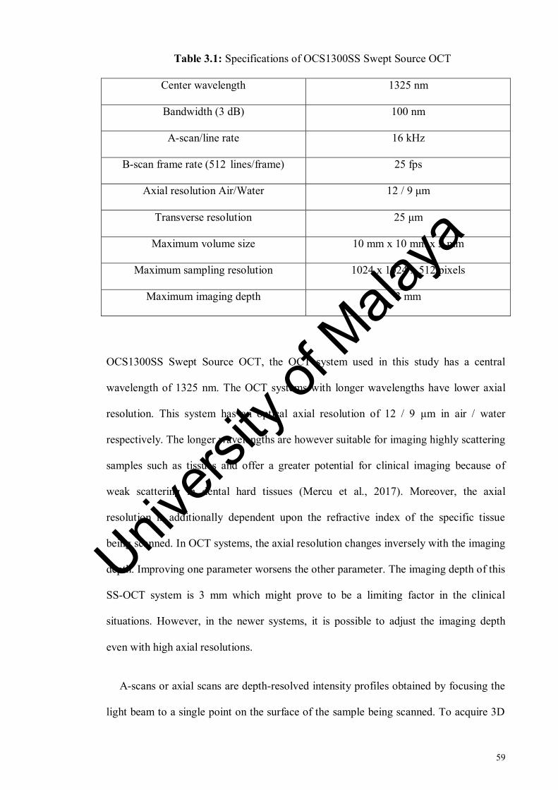
59

Table 3.1: Specifications of OCS1300SS Swept Source OCT

Center wavelength 1325 nm

Bandwidth (3 dB) 100 nm

A-scan/line rate 16 kHz

B-scan frame rate (512 lines/frame) 25 fps

Axial resolution Air/Water 12 / 9 μm

Transverse resolution 25 μm

Maximum volume size 10 mm x 10 mm x 3 mm

Maximum sampling resolution 1024 x 1024 x 512 pixels

Maximum imaging depth 3 mm

OCS1300SS Swept Source OCT, the OCT system used in this study has a central

wavelength of 1325 nm. The OCT systems with longer wavelengths have lower axial

resolution. This system has an optical axial resolution of 12 / 9 μm in air / water

respectively. The longer wavelengths are however suitable for imaging highly scattering

samples such as tissues and offer a greater potential for clinical imaging because of

weak scattering in dental hard tissues (Mercu et al., 2017). Moreover, the axial

resolution is additionally dependent upon the refractive index of the specific tissue

being scanned. In OCT systems, the axial resolution changes inversely with the imaging

depth. Improving one parameter worsens the other parameter. The imaging depth of this

SS-OCT system is 3 mm which might prove to be a limiting factor in the clinical

situations. However, in the newer systems, it is possible to adjust the imaging depth

even with high axial resolutions.

A-scans or axial scans are depth-resolved intensity profiles obtained by focusing the

light beam to a single point on the surface of the sample being scanned. To acquire 3D

Univers

ity of

Mala

ya

60

images, the OCT imaging system is equipped with scanning means to scan the object

both in depth and transversally. As a result, different scan planes can be created

depending on the scanning order and scanning direction. Collection of multiple A-scans

by scanning linearly across the tissue gives rise to one B-scan or longitudinal scan. Each

B-scan has a depth axis and lateral or angular axis. A-scan or line rate determines the

speed with which a B-scan is collected. A-scan rate in turn is related to the sensitivity of

the equipment. A higher A-scan rate results in lower sensitivity of the system. For

Swept-Source OCT systems, the A-scan rate is determined by the sweep speed of the

swept laser source. OCS1300SS Swept Source OCT has an axial scan rate of 16 kHz

with a sensitivity of 100 dB. When the OCT beam is scanned transversally over the

target tissue, T-scans or en-face scans are produced which generate a reflectivity profile

in angular or lateral position. Collection of many T-scans in transverse plane gives rise

to C-scans or transverse slice scans. Different transversal slices are obtained from

different depths (Podoleanu, 2005).

3.1.2 Assessment of demineralisation with OCT

Optical coherence tomography has been used for both the qualitative and quantitative

evaluation of dental caries. Dental erosion is different from dental caries in terms of

being a ‘surface’ or ‘near-surface’ phenomenon rather than a subsurface process (Lussi

& Carvalho, 2014). The backscattered light intensity is therefore expected to present

differently for both processes.

The process of demineralisation causes the loss of mineral from dental hard tissues.

The demineralised dental tissues hence become porous and the pores created differ from

each other in terms of size and shape. Therefore, the structural organisation of the

demineralised tissue becomes complex in comparison to sound tissue. The light

Univers

ity of

Mala

ya

61

travelling through demineralised tissue undergoes two types of interactions. One

interaction is with the regular components of tissue that results in scattering. The other

would be the interaction of light with the newly formed pores which results in (1)

increased intensity of backscattered light because of the change in refractive index and

(2) increased depth of penetration of light in the porous tissue. End result of this would

be the increased backscattering of light received by the OCT system which can then be

qualified or quantified through the OCT images. In the sound tissues, where the pores

are absent, the light only interacts with the regular components of the tissue which

results in less light being transferred to the OCT system as compared to demineralised

tissue. This is the basis on which OCT is able to differentiate the sound tissue from the

demineralised tissues. For dental erosion, this technique is used to quantify the increase

in backscattered intensity at the surface which in turn gives information about the

surface porosity and also the depth of penetration of the region of interest which is

reduced when surface scattering occurs (Huysmans et al., 2011; Wilder-Smith et al.,

2009).

For dentine, the passage of light would be expected to be increasingly complex

because of the presence of organic matrix. However, it was found that dentinal tubules

were the main structures responsible for dentine and organic matrix contributed little to

the overall scattering. Further, both scattering and absorption of light were greater in

dentine as compared to enamel (Zijp & Bosch, 1993).

Use of optical coherence tomography for the assessment of dental erosion was first

tested in a double-blind randomised clinical trial. The erosive loss in GORD (gastro-

esophageal reflux disease) patients before and after therapy with proton pump inhibitors

was measured (Wilder-Smith et al., 2009). The intensity of backscattered light in the

treatment area was significantly reduced as compared to reference area as hypothesized.

Univers

ity of

Mala

ya

62

Although the study was limited to assessment of advanced dental erosions only, it

served to validate OCT as a reliable tool for quantification of dental erosion which had

not been done before. The erosive loss was assessed by measuring the change in enamel

thickness with respect to dentino-enamel junction (DEJ). However, using DEJ as a

reference could prove to be complicated in the presence of saliva or in the case of

erosion-induced roughening or subsurface demineralisation. Irregular boundary of DEJ

can further complicate the analysis (Chan et al., 2013; Chan et al., 2014).

OCT was further validated for monitoring of early enamel erosion in an in vitro

study (Chew et al., 2014). Surface softening stage of enamel erosion before the

occurrence of any surface loss reducing enamel height was targeted in this study.

Authors were able to detect demineralisation in enamel after 10 minutes of erosion

challenge and the OCT findings were compared with surface microhardness. Only 2D

imaging (with B-scans) was employed in this study. The accurate repositioning of B-

scans can be challenging and could result in higher standard deviation. The parameter

used in this study was decay of intensity between two optical depths. One optical depth

was located near the surface and the other optical depth at the intensity plateau where

the backscattered intensity was almost constant. Mean percentage of difference in ratio

of exposed area and ratio of reference area was used as the outcome measure. High

specular reflection near the tooth surface can mask the OCT signal (Chan et al., 2015)

and a systematic way of finding a cut-off level to address the specular reflection by use

of this outcome measure was proposed in this study. In another recent clinical study,

Fresnel reflections near the surface were avoided by using a custom algorithm to

analyse all A-scan profiles instead of using data up to a specific depth. SS-OCT system

used in this study was able to detect statistically significant increase in the OCT signal

post orange juice rinsing in comparison to water rinsing (Austin et al., 2017).

Univers

ity of

Mala

ya

63

A reference area is needed in erosion studies to address the issues of systematic

errors and biological variability among the samples. This reference area is expected to

remain unchanged during the erosion challenges and instrumental measurements at

different measurement time points. The reliability of erosion-induced changes in the

eroded area can then be assessed by comparing the results against this constant

reference. Application of acid-resistant varnish and adhesive tape over the reference

area is common practice in erosion studies. A disadvantage of these methods is that they

cannot be used in the clinical settings. Dentino-enamel junction (DEJ) and CO2 laser

were tested as possible reference methods for erosion studies using OCT (Chan et al.,

2013). It was found that using DEJ can be unreliable in the case of roughness and

subsurface demineralisation. A subablative CO2 laser because of being non-invasive

has a potential of being used in clinical studies and its use as a reference was tested

previously (Chan et al., 2014). The authors however used a pH-cycling model of six

and 12 days indicating that erosion induced was rather aggressive. It implies that this

laser is only applicable in clinical studies investigating advanced erosion and the

usefulness of this subablative laser therefore needs to be explored for early stages of

erosion. A sturdy non-toxic material which can be applied on the tooth surfaces

clinically would be feasible and for this purpose, the use of composites has been

suggested (Chan et al., 2014). Another such material would be the bonding agent which

has the potential of being applied in the in vivo protocols.

Root dentine has been assessed with OCT only in a few studies. The percentage

reflectivity loss in relation to demineralisation on root surfaces was quantified and it

was shown that there was a linear correlation between % reflectivity loss and mineral

loss measured with microradiography (Amaechi et al., 2004). However the

measurement of reflectivity loss could be questionable as the lesion reflectivity would

be expected to increase not decrease with demineralisation. Therefore, the integrated

Univers

ity of

Mala

ya

64

reflectivity was calculated instead of reflectivity loss to assess root dentine caries and

inhibition potential of fluoride for root caries, and a positive correlation was found

between integrated reflectivity and integrated mineral loss (Lee et al., 2009) .

A recent study employed OCT for diagnosing and monitoring erosive wear

progression in dentine (De Moraes et al., 2017). This study aimed to assess the

progression of erosive lesions after irradiation with Nd:YAG laser (Neodymium-doped

Yttrium Aluminum Garnet) and topical fluoride application. Bovine root dentine

samples were exposed to citric acid (pH = 2.3) for a total of 20 days. The authors were

able to measure the amount of tooth tissue loss over 20 days of erosive cycle, before and

after treatments. The dentine demineralisation progression could be monitored with

optical coherence tomography. However, advanced stage dentine erosion was targeted

in this study as the criteria for development of erosion was visibility of erosive lesions

in the OCT images indicating that bulk tissue loss had taken place. To date, the early

stage of dentine erosion before bulk surface loss has not been assessed with OCT.

3.1.3 Aim

The aim of this study was to assess the potential of optical coherence tomography

(OCT) in monitoring the progression of in vitro early dentine erosion.



quantum.

2. To identify an optimum outcome measure for measuring early dentine erosion.

3. To identify the detection threshold of OCT for measuring early dentine erosion.

Univers

ity of

Mala

ya

65

4. To compare the OCT backscattered intensity changes of early eroded dentine

with ultrastructural changes.

The null hypotheses tested were as follows;

1. OCT is not able to detect early dentine erosion in vitro.

2. OCT is not able to measure early dentine erosion progression in vitro.

3.2 Materials and Methods

3.2.1 Pilot studies

Several pilot studies were performed in order to design and test the protocol before

conducting the main experiment. Most of these pilot studies are also applicable to the

research aims discussed in the subsequent chapters 4 and 5. A brief account of these

experiments is given below.

3.2.1.1 Sample preparation

The objective of this pilot study was to identify a suitable sample preparation of root

dentine for the main experiment. Three extracted sound human premolars were

sectioned 1 mm below the cemento-enamel junction using slow-speed microtome

cutting machine (Micracut 125, Metkon Instruments Inc., Bursa, Turkey) and roots were

embedded in self-curing acrylic resin with the sectioned surface facing upwards. The

dentine surface was polished in a water-cooled rotating grinding / polishing machine

(Buehler, USA) under running water to create a flat and smooth surface. A

demineralisation window was created by using a non-residue adhesive tape and bonding

agent as shown in Figure 3.1. The polished dentine surfaces, except for the

Univers

ity of

Mala

ya

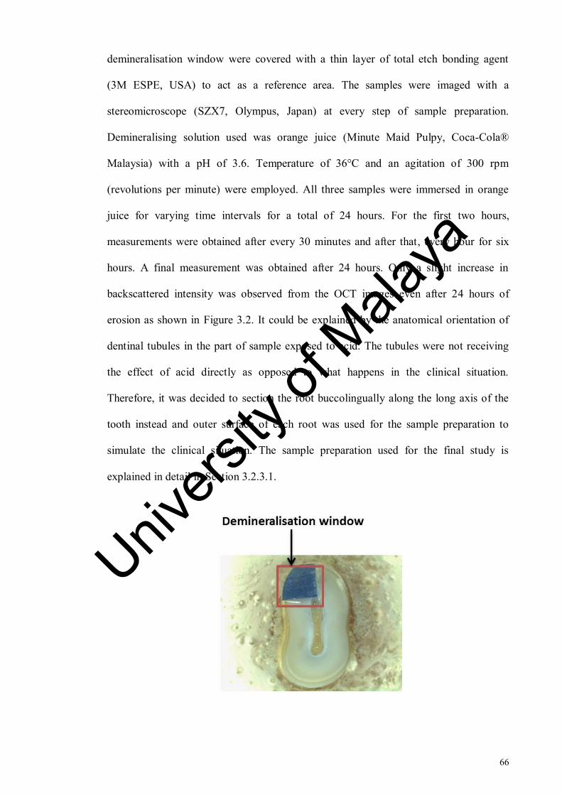
66

demineralisation window were covered with a thin layer of total etch bonding agent

(3M ESPE, USA) to act as a reference area. The samples were imaged with a

stereomicroscope (SZX7, Olympus, Japan) at every step of sample preparation.

Demineralising solution used was orange juice (Minute Maid Pulpy, Coca-Cola®

Malaysia) with a pH of 3.6. Temperature of 36°C and an agitation of 300 rpm

(revolutions per minute) were employed. All three samples were immersed in orange

juice for varying time intervals for a total of 24 hours. For the first two hours,

measurements were obtained after every 30 minutes and after that, every hour for six

hours. A final measurement was obtained after 24 hours. Only a slight increase in

backscattered intensity was observed from the OCT images even after 24 hours of

erosion as shown in Figure 3.2. It could be explained by the anatomical orientation of

dentinal tubules in the part of sample exposed to acid. The tubules were not receiving

the effect of acid directly as opposed to what happens in the clinical situation.

Therefore, it was decided to section the root buccolingually along the long axis of the

tooth instead and outer surface of each root was used for the sample preparation to

simulate the clinical situation. The sample preparation used for the final study is

explained in detail in Section 3.2.3.1.

Univers

ity of

Mala

ya

67

Figure 3.1: Stereomicroscope image of a root dentine sample used for exploratory

work. The sample was sectioned 1 mm below the cemento-enamel junction. The

demineralisation window was covered with blue adhesive tape. It has been highlighted

by a red box.

Figure 3.2: OCT B-scans of root dentine samples taken with SS-OCT at (a) baseline

measurement and (b) after 24 hours of erosive challenge. White line at the center



sample. Minimal increase in backscattered intensity was observed in the B-scan after 24

hours of erosion challenge (b) in comparison to the intensity observed in the B-scan at

baseline measurement (a).

3.2.1.2 Speed of agitation

To simulate the swishing of the drink within the oral cavity in clinical erosion, the

samples are stirred in erosion experiments. The objective of this pilot study was to

determine the optimum speed of stirring for the main experiment. A magnetic stirrer

Univers

ity of

Mala

ya

68

(RCT basic, IKA, Germany) (Figure 3.14) was employed and five root dentine samples

were immersed in 0.3% citric acid solution (A&C American Chemicals Ltd., North

Carolina, USA). The experiment was performed at a constant temperature of 36°C. A

magnetic stirrer is a laboratory device used for stirring a ‘stir bar’ added in the liquid by

employing a magnetic field. The solution is stirred as a result of it.

The speed of solution was increased from 20 rpm (revolutions per minute) to 700

rpm. Lower range of agitation was based on the speed at which the solution was being

stirred uniformly and higher range was based on the speed which the samples did not

move vigorously. The objective was to mimic the intraoral environment in the advent of

clinical erosion challenge when the drink swishes around the teeth whereas the teeth

remain stable. A speed of 300 rpm at a constant temperature of 36 °C was identified as

the optimum stirring speed at which the samples remained stable while the solution was

being stirred uniformly.

3.2.1.3 Drying time of eroded dentine

In a previous OCT validation study, the enamel samples were dried for 20 seconds

before scanning with OCT (Chew et al., 2014). This experiment aimed to assess

whether 20 seconds could also be suitable for drying the dentine samples before OCT

scanning. Five root dentine samples eroded in 0.3% citric acid (A&C American

Chemicals Ltd., North Carolina, USA) for 30 minutes were dried for 20 seconds and

then dried for 10 min. Samples were scanned with OCT at baseline, after 20 seconds

and 10 minutes of drying. Images were analysed with a programme written in Matlab

(The MathWorks, Inc., USA). Between baseline and 20 seconds, OCT signal remained

constant. However, some difference in OCT intensity was observed between 20 seconds

and 10 minutes of dehydration of samples as shown in the Figure 3.3. Based on this

Univers

ity of

Mala

ya

69

experiment, it was decided to restrict drying time of dentine samples to 20 seconds

before scanning them with OCT.

Figure 3.3: Box plots represent the OCT data acquired after 20 seconds and 10

minutes of air-drying.

3.2.1.4 Reduction of specular reflection

Strong specular reflections were observed in the OCT images while scanning and it

was decided that the specimens would be tilted to avoid mirror reflections from the

surface of specimen on the OCT image. The objective of this pilot study was to identify

the optimum tilting angulation and tilting plane to reduce the specular reflection to the

maximum from the OCT images. Tilting was performed 1) on a plane parallel to the

beam and 2) and on a plane perpendicular to the beam. It was found that the specular

reflection reduced significantly if the root dentine specimens were titled at a plane

perpendicular to the beam. In order to identify the tilting angulation, the samples were

tilted at various angles starting from five degrees to 40 degrees. It was found that the

Univers

ity of

Mala

ya

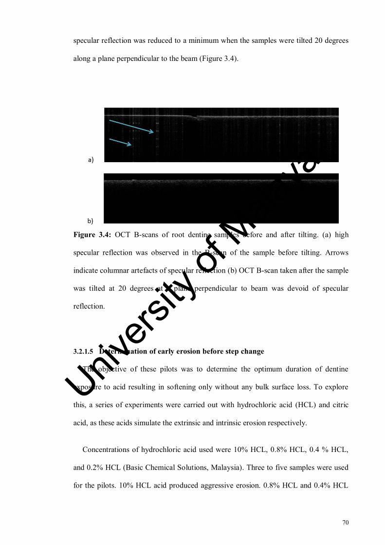
70

specular reflection was reduced to a minimum when the samples were tilted 20 degrees

along a plane perpendicular to the beam (Figure 3.4).

Figure 3.4: OCT B-scans of root dentine samples before and after tilting. (a) high

specular reflection was observed in the B-scan of the sample before tilting. Arrows

indicate columnar artefacts of specular reflection (b) OCT B-scan taken after the sample

was tilted at 20 degrees at a plane perpendicular to beam was devoid of specular

reflection.

3.2.1.5 Determination of early erosion before step change

The objective of these pilots was to determine the optimum duration of dentine

exposure to acid resulting in softening only without any bulk surface loss. To explore

this, a series of experiments were carried out with hydrochloric acid (HCL) and citric

acid, as these acids simulate the extrinsic and intrinsic erosion respectively.

Concentrations of hydrochloric acid used were 10% HCL, 0.8% HCL, 0.4 % HCL,

and 0.2% HCL (Basic Chemical Solutions, Malaysia). Three to five samples were used

for the pilots. 10% HCL acid produced aggressive erosion. 0.8% HCL and 0.4% HCL

Univers

ity of

Mala

ya

71

also resulted in a step change in the OCT images after 10 minutes of erosion challenge

(Figure 3.5). 0.2% HCL did not result in a step change after 10 minutes.

Figure 3.5: OCT B-scans of a sample taken at (a) baseline and (b) after 10 minutes of

exposure to hydrochloric acid. Step change (circled in red) was observed at the junction

of reference and eroded areas after 10 minutes of HCL exposure.

0.3% citric acid (A&C American Chemicals Ltd., North Carolina, USA) (pH = 3.2)

was used for used for this experiment. Samples were immersed in citric acid for 60

minutes and measurements with OCT were taken 10 minutes stepwise. Exposed surface

(eroded) could clearly be distinguished from baseline measurement as well as the

reference surface after only 10 minutes. Surface backscattering increased consistently

up to 40 min and then showed a decline at 50 min and 60 minutes of erosion. However

no step change was observed in the OCT images as shown in Figure 3.6.

Univers

ity of

Mala

ya

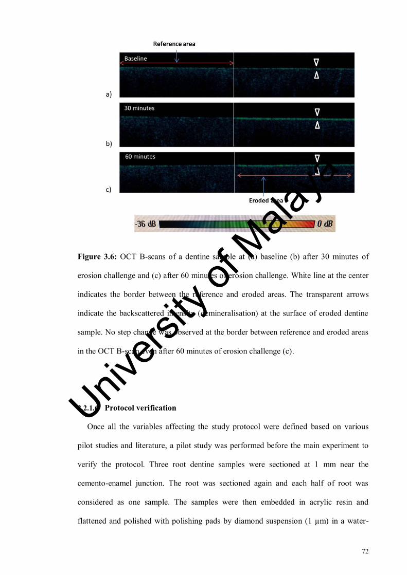
72

Figure 3.6: OCT B-scans of a dentine sample at (a) baseline (b) after 30 minutes of

erosion challenge and (c) after 60 minutes of erosion challenge. White line at the center



sample. No step change was observed at the border between reference and eroded areas

in the OCT B-scan even after 60 minutes of erosion challenge (c).

3.2.1.6 Protocol verification

Once all the variables affecting the study protocol were defined based on various

pilot studies and literature, a pilot study was performed before the main experiment to

verify the protocol. Three root dentine samples were sectioned at 1 mm near the

cemento-enamel junction. The root was sectioned again and each half of root was

considered as one sample. The samples were then embedded in acrylic resin and

flattened and polished with polishing pads by diamond suspension (1 µm) in a water-

Univers

ity of

Mala

ya

73

cooled rotating grinding/polishing machine (Buehler, USA). A window was created on

the sample with an adhesive tape and half of the window was covered with adhesive

tape to act as reference surface. Baseline scanning was performed with OCT. The

samples were then immersed in 0.3 % citric acid (pH 3.2) (A&C American Chemicals

Ltd., North Carolina, USA) and measurements with OCT were taken every two minutes

for the first 16 minutes and then again at 20, 25 and 30 minutes post-demineralisation.

The temperature of the solution was kept constant at 36°C and the speed of agitation

was kept constant at 300 rpm throughout the experiment. After being removed from

acid, the samples were rinsed with deionised water and air dried for 20 seconds. By

using a programme written in Matlab (The MathWorks, Inc., USA), all the images were

aligned horizontally with respect to the tooth-air interface and each aligned image

consisted of a reference and an eroded area (See Figure 3.16 and Section 3.2.3.4 for

details). Regions of interest were selected on each aligned image in the reference and

eroded sections of the image. A-scans were then generated from the regions of interest

selected for both the reference and eroded areas and intensity values were exported

automatically to excel sheets. Integrated intensity was calculated as the sum of pixels

intensities from a superficial optical depth of 23 µm to an optical depth of 58 µm. 58

µm was chosen because at this depth, no further changes in intensity were observed.

(See Section 3.2.3.5 and equation 3.2 for details). The plot is given in the Figure 3.7.

Plot showed that the intensity in the eroded area exhibited fluctuations with time

interval and remained almost constant from baseline measurement to 30 minutes. The

similarity in the intensity fluctuations in the reference and eroded areas suggested that

these were merely instrumental variations in time and the erosion induced was below

the detection threshold of the instrument employed. It was assumed that the presence of

smear layer on the surface had reduced the permeability of dentinal tubules to acid,

Univers

ity of

Mala

ya

74

resulting in very low surface scattering. Therefore, it was decided to conduct another

pilot study and remove the smear layer from the samples.

Figure 3.7: Mean integrated intensity of the reference and eroded areas at different

erosion time points. Arrows indicate the intensity fluctuations in the eroded area.

3.2.1.7 Removal of smear layer

The aim of this pilot study was to assess whether the smear layer was to be removed

by ultrasonication alone or that it would require the use of an agent. The samples were

prepared and polished as described before in Section 3.2.1.6. Samples were imaged with

stereomicroscope (SZX7, Olympus, Japan) at the magnifications of 1x, 1.6x and 2.5x.

The samples were then ultrasonicated with distilled water for 50 seconds. Post-

ultrasonication, the samples were imaged again with stereomicroscope (SZX7,

Olympus, Japan). EDTA is commonly used for removal of smear layer and its chelating

action is used to disintegrate the smear layer and open up the dentine tubules (Serper &

Calt, 2002). Other than the chemical removal of smear layer, ultrasonication has also

been shown to remove smear layer and smear plugs from dentinal tubules(Violich &

Chandler, 2010) . The samples were treated with 10% EDTA for 3 minutes, imaged

with stereomicroscopy and then ultrasonicated for 50 seconds. The imaging was

repeated again. One of the samples was additionally imaged with field-emission

Univers

ity of

Mala

ya

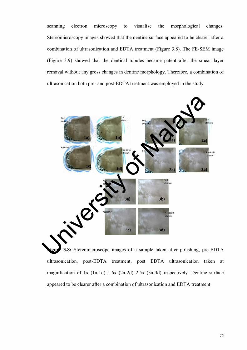
75

scanning electron microscopy to visualise the morphological changes.

Stereomicroscopy images showed that the dentine surface appeared to be clearer after a

combination of ultrasonication and EDTA treatment (Figure 3.8). The FE-SEM image

(Figure 3.9) showed that the dentinal tubules became patent after the smear layer

removal without any gross changes in dentine morphology. Therefore, a combination of

ultrasonication both pre- and post-EDTA treatment was employed in the study.

Figure 3.8: Stereomicroscope images of a sample taken after polishing, pre-EDTA

ultrasonication, post-EDTA treatment, post EDTA ultrasonication taken at

magnification of 1x (1a-1d) 1.6x (2a-2d) 2.5x (3a-3d) respectively. Dentine surface

appeared to be clearer after a combination of ultrasonication and EDTA treatment

Univers

ity of

Mala

ya

76

Figure 3.9: shows (a) sound dentine covered with smear layer (b) Dentine with smear

layer removed by 10 % EDTA treatment for 3 minutes pre- and post ultrasonication.

The dentinal tubules became patent after the smear layer removal without any obvious

gross changes in dentine morphology.

3.2.1.8 Effect of smear layer removal on OCT intensity

The objective of this pilot was to assess the effect of smear layer removal on the

OCT backscattered intensity using the previously employed erosion protocol. Five pre-

molars were prepared and demineralised as described before in Section 3.2.1.7.

However, before inducing demineralisation, smear layer was removed from the samples

by a combination of 50-second ultrasonication before and after treatment with 10%

EDTA solution.

A programme written in Matlab (The MathWorks, Inc., USA) was used for the

intensity analysis as described above (Section 3.2.1.6) and data was plotted. The plot for

the eroded area showed that there was a net increase in erosion from baseline to 30

minutes as shown in Figure 3.10, b). Hence it was decided to remove the smear layer in

the final study. The intensity changes in the reference area as shown in Figure 3.10, a)

suggested that a different reference be used since the residue left by adhesive tape could

be the cause of these fluctuations in intensity. Therefore, it was decided to employ a

Univers

ity of

Mala

ya

77

reference material rather than protecting reference area with adhesive tape during

erosion challenge.

Figure 3.10: shows (a) mean integrated intensity of the reference area of the samples at

various erosion time points. (b) mean integrated intensity of the eroded area of the

samples at various erosion time points.

3.2.1.9 Assessment of early dentine erosion with Micro-CT:

Microradiography is a gold standard technique for determination of mineral content

for assessment of demineralisation and remineralisation in vitro (Hamba et al., 2012).

However, it requires destructive sample preparation and results are inferred from very

thin sections of samples. Longitudinal microradiography has limited applicability in

studies of dentine erosion (Ganss et al., 2009b). Micro-CT is well-known technology

Univers

ity of

Mala

ya

78

with the most notable advantage of offering high resolution and non-destructive 3D

cross-sectional imaging which makes it applicable for in vitro longitudinal studies. This

pilot study aimed to assess if micro-CT is a suitable technique to be employed for


(a) Sample preparation

Fourteen root dentine samples were prepared from seven intact upper or lower

human premolars. The teeth were collected and disinfected as described in Section

3.2.3.1. An ultrasonic scaler (Peizon® Master 400 Switzerland) was employed to

remove the hard deposits and soft tissues from the teeth. After scaling, the crowns were

sectioned horizontally 1 mm below the cemento-enamel junction using slow speed

microtome cutting machine (Micracut 125, Metkon Instruments Inc., Bursa, Turkey)

under copious water irrigation and discarded. Next, the roots were sectioned

longitudinally in the buccolingual direction. Each half of root was considered as one

sample. Resin blocks with dimensions of 30 x 20 x 15 mm were prepared with acrylic

resin (Quick Mount 2 Epoxy resin, Ace Technologies Inc., Arizona) and each sample

was attached to a separate resin block with a removable adhesive material (Tack-it,

Faber Castel, Malaysia) with external part of the root facing the surface. Samples were

ground flat with 600-grit silicon carbide paper (Struers Inc., Ohio, USA) followed by

polishing with polishing pads (8-inch Micropad polishing pad PSA, Pace® technologies,

Arizona) using diamond suspension (1 µm) in a water-cooled rotating

grinding/polishing machine (Buehler, USA) which removed the cementum.

The smear layer was removed from the surface of dentine by a combination of

EDTA and ultrasonication as explained in Section 3.2.3.1. A window with dimensions

of 5 x 3 mm was created on the surface of each sample by using red nail varnish

Univers

ity of

Mala

ya

79

(Revlon, USA). Additionally, the nail varnish was applied on the left half of the window

to create a reference and an eroded area. The reference surface was kept covered with

nail varnish (Revlon, USA) during erosion challenges. After the erosion challenge was

completed, the varnish was removed from the reference surface carefully with acetone

(Sigma-Aldrich, St. Louis, Missouri, USA). A bur mark was made with fissure bur at

the lower end of the window on the reference side of the sample to aid in identification

of reference area in micro-CT images. The prepared sample is shown in Figure 3.19.

(b) Erosion challenge

The prepared samples were suspended in a beaker containing 0.3% citric acid (pH =

3.2) (A&C American Chemicals Ltd., North Carolina, USA) on a movable stand with

wires and plastic clips. The temperature and speed of the solution were controlled by

placing the beakers on a magnetic stirrer (IKA RCT basic, Germany). A magnetic stirrer

is a laboratory device used for stirring a ‘stir bar’ added in the liquid by employing a

magnetic field. The solution is stirred as a result of it. The temperature of the solution

was kept constant at 36°C and the speed was kept constant at 300 rpm during the

experiment (See Figure 3.14).

The samples were not eroded longitudinally and so each sample was eroded for a

defined period of time. Two samples were eroded each for 2, 4, 8, 12, 16, 25 and 30

minutes. After being removed from the beaker containing acid, the samples were rinsed

with deionised water and dried with dental syringe for 20 seconds. The dental syringe

was kept at a distance of 10 cm from the samples. Citric acid was renewed after every

time point. The reference surface was kept covered with nail varnish (Revlon, USA)

during erosion challenges.

Univers

ity of

Mala

ya

80

(c) Measurements with Micro-CT

Micro-CT scanning of the root dentine samples took place in Minnesota Dental

Research for Biomaterials and Biomechanics (MDRCBB) School of Dentistry,

University of Minnesota. To transport the samples, each sample was attached to a

separate resin block with a removable adhesive material (Tack-it, Faber Castel,

Malaysia) with external part of the root facing the surface. Each sample attached to its

resin block was then placed in a separate container. In order to retain humidity, a wet

towel was placed at the bottom of the container avoiding any contact between the towel

and the sample surface (Francescut et al., 2006). Each resin block with the sample was

wrapped in moist gauze and placed in a separate aluminum packet. Fourteen packets

were prepared and placed in one aluminum bag which was air vacuumed. It was then

placed in a thermocol box which was sealed and couriered to reach MDRCBB School of

Dentistry, University of Minnesota for micro-CT scanning.

A high-resolution desktop micro-CT system (HMX-XT 225, X-tek system United

Kingdom) was used to scan the specimens. It had a resolution of 8 µm. Each sample

was placed on the stage inside the Micro-CT chamber using a plastic holder. Scanning

was performed using X-rays produced with tube voltage of 95 kV, tube current of 90

µA, exposure time of 708 m/s with 720 projections and 4 frames per projection. A total

of 14 dentine samples with two samples eroded for 2, 4, 8, 12, 16, 25 and 30 minutes

were scanned. Each sample was kept moist with wet cotton during scanning. Total

scanning time for each sample was 34 minutes. Each tooth was rotated at 360 degrees.

The distances from the x-ray source to the sample and to the detector were 65 and 972

mm respectively. Data was acquired as DICOM image stack for reconstruction of the

3D image of pixel resolution of 8 x 8 µm2 with isotropic voxel sizes of 8 x 8 x 8 µm

3.

Univers

ity of

Mala

ya

81

To minimise ring artefacts, air calibration of the detector was carried out prior to each

scanning. Averaging of 128 frames was applied in the acquisition phase to improve the

signal-to-noise ratio (SNR). The reconstruction of volume data was attempted using the

software CT Pro 3D (Nikon metrology, Inc., Brighton, MI, USA).

(d) Data processing and conclusions

The area of the sample which could be visualised in the DICOM files was the cut

surface of the root sample from where the crown had been sectioned from the root. The

area of interest however was located on the outer surface of the coronal portion of the

root sample. Therefore, a software programme 3D-Doctor (Able Software Corp., USA)

was employed to get the desired orientation of the image to be able to select and analyse

the regions of interest. These 3D images were uploaded in Image J programme (Wayne

Rasband, National Institute of Health, Bethesda, USA). Each image consisted of

approximately 500 micro-CT slices. Demineralised areas appear radiolucent in the

micro-CT images (Espigares et al., 2015). However, in this study visually no apparent

gray scale differences were observed between the sound dentine in the reference and

demineralised dentine in the eroded sides of each sample. Even the samples eroded for

30 minutes showed similar contrast in the reference and eroded areas (Figure 3.11).

Issues of beam hardening and shadow artefacts can sometimes make the detection and

characterisation of lesions with small mineral loss difficult (Espigares et al., 2015). This

coupled with the fact that amount of demineralisation induced in this study was very

low could be the reason that eroded areas did not appear distinct in terms of contrast

from the reference areas in the micro-CT images. Therefore, it could be concluded that

micro-CT had insufficient sensitivity to detect early dentine erosion induced in this

study.

Univers

ity of

Mala

ya

82

Figure 3.11: Micro-CT images of samples eroded for (a) 2 minutes, (b) 25 minutes and

(c) 30 minutes. No obvious difference in contrast was observed between the reference

and eroded areas of these samples.

Univers

ity of

Mala

ya

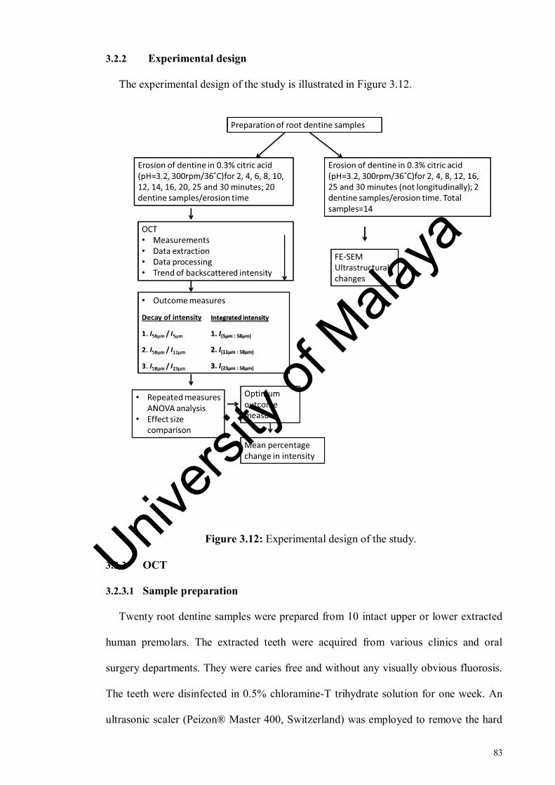
83

3.2.2 Experimental design

The experimental design of the study is illustrated in Figure 3.12.

Figure 3.12: Experimental design of the study.

3.2.3 OCT


Twenty root dentine samples were prepared from 10 intact upper or lower extracted

human premolars. The extracted teeth were acquired from various clinics and oral

surgery departments. They were caries free and without any visually obvious fluorosis.

The teeth were disinfected in 0.5% chloramine-T trihydrate solution for one week. An

ultrasonic scaler (Peizon® Master 400, Switzerland) was employed to remove the hard

Univers

ity of

Mala

ya

84

deposits and soft tissues from the teeth. After scaling, the crowns were sectioned

horizontally 1 mm below the cemento-enamel junction using slow speed microtome

cutting machine (Micracut 125, Metkon Instruments Inc., Bursa, Turkey) and discarded.

Next, the roots were sectioned longitudinally in the buccolingual direction. Fragments

obtained were embedded in separate self-curing resin blocks such that the external part

of the root was kept exposed and inner part of the root was embedded in the resin

(Quick Mount 2 Epoxy resin, Ace Technologies Inc., Arizona, USA). The dentine

surface was then ground flat with 600-grit silicon carbide paper (Struers Inc., Ohio,

USA) which removed the cementum followed by final polishing with polishing pads (8-

inch Micropad polishing pad PSA, Pace® technologies, Arizona, USA) using diamond

suspension (1 µm) in a water-cooled rotating grinding / polishing machine (Buehler,

USA).

Smear layer was removed by a combination of ultrasonication and EDTA treatment.

The dentine samples were placed for ultrasonication for 50-seconds in a stainless steel

basket (UC1-230, Biosonic Ultrasonic Bath, Whaledent, USA) filled with distilled

water without any heat applied. The samples were then removed from the basket and

placed in a beaker containing 0.5 M 10% EDTA (Sigma-Aldrich, St. Louis, Missouri,

USA) for 3 minutes. The samples were then ultrasonicated again with distilled water for

50 seconds.

A window with dimensions of 5 x 3 mm was created on the surface of each sample

with nail varnish (Revlon, New York, USA). A composite slab with dimensions of 1.5 x

1 cm was made with posterior restorative composite material (Filtek™ Bulk Fill, 3M

ESPE, USA). The composite material was placed on a composite slab and shaped by a

plastic instrument into a rectangular slab. This rectangular slab was then cured with

LED curing light system (Demi™ Ultra, Kerr, USA) for 40 seconds. The slab was

Univers

ity of

Mala

ya

85

flattened until it reached a diameter of 0.3 mm and polished with 1200-grit silicon

carbide paper (Struers Inc., Ohio, USA) in a water-cooled rotating grinding / polishing

machine (Buehler, USA). This slab was then used as a reference (Figure 3.13).

Figure 3.13: Sample preparation (a) root of premolar tooth (b) coronal view of root (c)

root sectioned along the long axis buccolingually into two halves (d & e) each half of

root considered as one sample (f) prepared sample.

3.2.3.2 Erosion challenge

Samples were scanned with OCT to acquire 3D images for baseline measurements.

Composite slab was placed on the left side of each sample while scanning the sample

with OCT. The samples were then suspended in a beaker containing 0.3% citric acid

(pH = 3.2) (A&C American Chemicals Ltd., North Carolina, USA) on a movable stand

with wires and plastic clips. A movable stand was used in order to facilitate the

immersion and removal of all samples simultaneously at the beginning or end of erosion

Univers

ity of

Mala

ya

86

challenge to standardise the acid exposure time. Five samples were suspended in 500 ml

of citric acid (A&C American Chemicals Ltd., North Carolina, USA) at one time. The

temperature and speed of the solution were controlled by placing the beakers on a

magnetic stirrer (RCT basic, IKA, Germany). A magnetic stirrer is a laboratory device

used for stirring a ‘stir bar’ added in the liquid by employing a magnetic field. The

solution is stirred as a result of it. The temperature of the solution was kept constant at

36°C and the speed was kept constant at 300 rpm during the erosion challenge

throughout the experiment as shown in the figure 3.14.

After two minutes of erosion challenge, the samples were removed from the beaker

and rinsed with deionised water. With rinsing, the erosion process is expected to be

slowed down or stopped (Lussi & Hellwig, 2014) which helps to avoid any variation in

the acid exposure time during measurements. The samples were then dried with dental

syringe for 20 seconds. The dental syringe was kept at a distance of 10 cm from the

samples. The samples were then scanned again with OCT.

The samples were immersed in citric acid for a total time period of 30 minutes but

they were removed from the acid after every two minutes for the first 16 minutes, then

after 20, 25 and 30 minutes exposure to acid followed by rinsing, drying and scanning

with OCT. Similar protocol of rinsing with deionised water and drying was used at all

time points. Citric acid was renewed after every erosion challenge. Univers

ity of

Mala

ya

87

Figure 3.14: Apparatus used for erosion challenge. A beaker containing citric acid

(pH=3.2) was placed on a magnetic stirrer device. A stir bar was added in the solution

(circled in red). The root dentine samples were suspended in the beaker as shown in the

figure. The temperature of citric acid and speed of agitation was controlled by the

magnetic stirrer.

3.2.3.3 Measurements with OCT

A commercially available OCT system (OCS1300SS Thorlabs Ltd., USA) was used

to capture three dimensional OCT data of the exposed window of the dentine samples.

This OCT system has a high-speed frequency swept laser centered at 1325nm. It has a

transverse resolution of 11 µm and an axial resolution of 9 µm in air according to the

manufacturer. This axial resolution would correspond to about 6 µm in dentine as the

refractive index of dentine is 1.54. The probing head was mounted with the beam facing

downwards. The probe was set at a distance of 1 cm from the sample surface, with the

scanning beam oriented at 0˚ to the surface. The samples were placed on a translational

stage perpendicular to the probe. The stage was fixed with a custom made jig (Figure

3.15) that enabled the samples to be repositioned to the same position and alignment

Univers

ity of

Mala

ya

88

during different measuring time points. This jig was also capable of tilting the samples

to a certain angle to reduce the specular reflection.

The Thorlabs OCT capturing software was used for capturing the images and

controlling the OCT settings and the light beam. The transverse resolution of the X-axis

was set at 1024 pixels in 5 mm and Y-axis at 96 pixels in 2 mm. The axial resolution of

the Z-axis was set at 512 pixels in 3 mm in air or 1.9 mm in dentine (refractive index of

dentine is 1.54). With these settings a total of 96 B-scans were generated for each 3D

image. The (x, y) coordinate of the light beam for each sample was recorded for

replication at consecutive measuring time points. Other parameters such as brightness

and contrast were kept constant for all samples. The inbuilt ruler within the system

software was used for standardising the height of each image and also for repositioning

the reference composite slab. Background noise was removed before the acquisition of

each image.

Each resin-mounted sample was removed from its container (containing deionised

water) immediately before imaging and dried with dental syringe for 20 seconds at a

distance of 10 cm. In order to ensure the repeatability of the OCT scan at various time

points, the specimens were placed at the same orientation as accurately as possible.

After adjusting all the system settings in the B-scan mode, a 3D scan was performed for

the pre-determined area of interest containing both the reference and eroded area within

the exposed window on each sample. All the samples were tilted at 20° to reduce the

specular reflection from the surface of the specimen on the OCT image (Chan et al.,

2015).

The composite slab was placed manually on the left side of the sample during

scanning at each time point. Therefore, each OCT 3D scan had composite slab on the

left side and eroded area on the right side. A bur mark was made on the anterior end of

Univers

ity of

Mala

ya

89

the reference slab to aid in repositioning of slab. Further, an inbuilt ruler within the

Thorlabs OCT software was used to mark the border between the reference and the

eroded side of the image. X and y coordinates of the ruler were recorded and same

values were employed for repositioning in the subsequent scanning.

Figure 3.15: OCT equipment and repositioning jig.

3.2.3.4 Data processing

A program was written in MATLAB (The MathWorks, Inc., USA) to load the OCT

C scan (3D scan) images and analyse the changes of the backscattered light intensity in

time. C scans of each measuring time point of each sample were aligned to reach a

horizontal surface corresponding to the tooth-air interface. Each aligned image

consisted of a reference and an eroded area. Regions of interest were selected on each

aligned image in the reference and eroded sections of the image. Each region of interest

was restricted to 10,500 A-scans in order to standardise the area being analysed. In

Univers

ity of

Mala

ya

90

order to standardise the analysis, all 12 time points of each sample were aligned in a

similar manner and identical regions of interest were loaded for them. A-scans were

then generated from the regions of interest selected for both the reference and eroded

areas and intensity values were exported automatically to excel sheets. Figure 3.16 (a-d)

shows the main steps of data processing through Matlab programme.

Figure 3.16: Data processing of OCT C-scan images (a) graphic user interface (GUI) of

Matlab programme for uploading and processing of data (b) aligned surface view of one

C-scan of one time point. Green and red selections represent the regions of interest

selected for reference and eroded areas respectively (c) mean depth-resolved intensity

profile (A-scan) for the reference and eroded areas represented by green and red plots

respectively (d) data from mean A-scan for one C-scan of one time points exported to

excel files separately for reference and eroded areas.

Univers

ity of

Mala

ya

91

3.2.3.5 Trend of backscattered intensity

In the excel programme, the values of each A-scan generated for the reference or

eroded area of each 3D OCT image was further reduced to single values by averaging

the intensity per pixel. Once the A-scans were averaged for all the samples for each time

point, a mean A-scan was then generated and the standard deviation was also calculated

from the averaged intensity per pixel. The data for the reference and eroded areas was

separately plotted to observe and compare the main trend of backscattered intensity in

both areas.

3.2.3.6 Parameters for intensity analysis

(a) Decay of intensity

Two parameters, ‘decay of intensity’ and ‘integrated intensity’ were employed for

the analysis. Decay of intensity calculates the relationship of the attenuation of

backscattered light between two optical depths of an OCT mean A-scan. It had been

employed in a previous study for the monitoring of early enamel erosion with OCT

(Chew et al., 2014). Integrated intensity had been shown to correlate with the integrated

mineral loss (volume % mineral × µm) ΔZ, in the previous studies (Jones et al., 2006a;

Ngaotheppitak et al., 2005).

The first parameter ‘decay of intensity’ or D is represented by the function below,

𝐷 =𝐼𝑝𝑙𝑎𝑡𝑒𝑎𝑢

𝐼𝑠𝑢𝑝𝑒𝑟𝑓𝑖𝑐𝑖𝑎𝑙

(3.1)

Iplateau is the intensity at an optical depth at which the A-scans had reached a plateau

and were assumed not to be affected further by the erosive challenge. It was observed at

58 µm (physical depth = 38 µm) for this study. Isuperficial is the intensity near the surface

located immediately below the tooth-air interface. For this study, three optical depths 5

Univers

ity of

Mala

ya

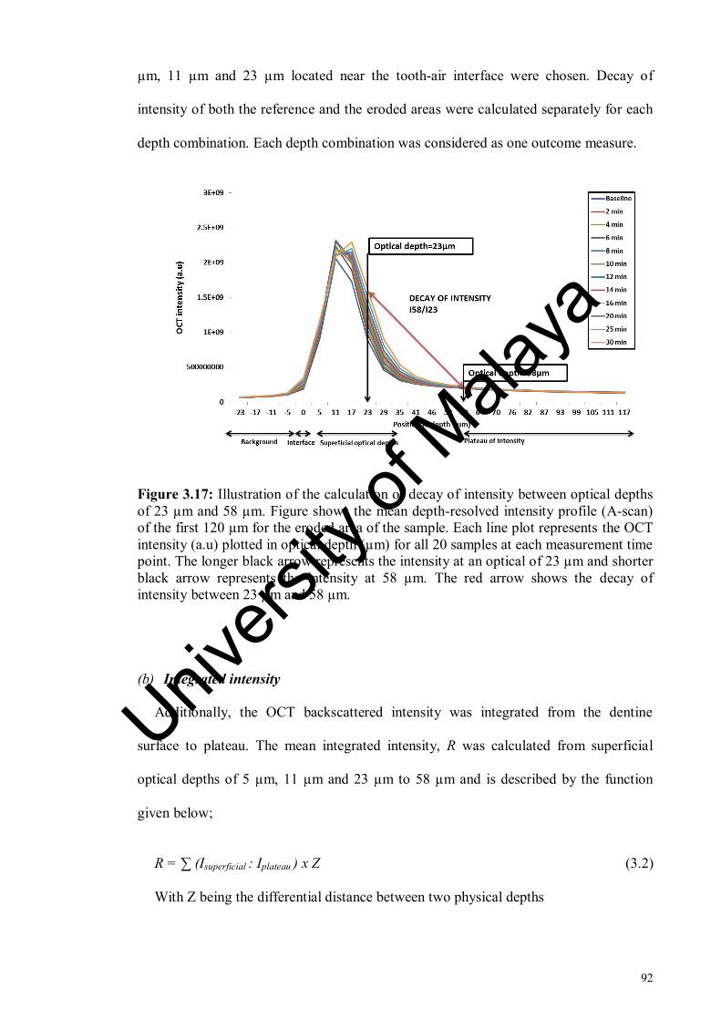
92

µm, 11 µm and 23 µm located near the tooth-air interface were chosen. Decay of

intensity of both the reference and the eroded areas were calculated separately for each

depth combination. Each depth combination was considered as one outcome measure.

Figure 3.17: Illustration of the calculation of decay of intensity between optical depths

of 23 µm and 58 µm. Figure shows the mean depth-resolved intensity profile (A-scan)

of the first 120 µm for the eroded area of the sample. Each line plot represents the OCT




intensity between 23 µm and 58 µm.

(b) Integrated intensity

Additionally, the OCT backscattered intensity was integrated from the dentine

surface to plateau. The mean integrated intensity, R was calculated from superficial

optical depths of 5 µm, 11 µm and 23 µm to 58 µm and is described by the function

given below;

R = ∑ (Isuperficial : Iplateau ) x Z (3.2)

With Z being the differential distance between two physical depths

Univers

ity of

Mala

ya

93

Integrated intensity of both the reference and the eroded areas were calculated

separately for each depth combination. Each depth combination was considered as one

outcome measure.

Figure 3.18: Illustration of the calculation of integrated intensity from an optical depth

of 23 µm to an optical depth of 58 µm. Figure shows the mean depth-resolved intensity






distance between two physical depths.

Further, percentage change in integrated intensity of the eroded area during a

particular time point from baseline time point of eroded area was calculated. ΔR for

each measurement time point is represented by the formula:

∆𝑅(𝑡) = 100 ∗ [𝑅𝐸(𝑡) − 𝑅𝐸(𝑡0)

𝑅𝐸(𝑡0)]

(3.3)

Where RE is mean integrated intensity of the eroded area, 𝑡0 is the baseline time point

and t is the specific measurement time point.

Univers

ity of

Mala

ya

94

The mean percentage change in backscattered intensity was plotted with erosion

interval and line fitting was performed with Microsoft Office Excel® 2010 programme

to observe the trend of ΔR with time. The validity and significance of model was

assessed by R2

value.

3.2.3.7 Comparison by effect size

Effect size is a quantitative measure of strength of a phenomenon. In order to identify

the most suitable outcome measure for analysis, the outcome measures of both

parameters were compared in terms of their effect size to assess their strength. The

effect sizes of all outcome measures were compared by partial eta square values

generated by SPSS, version 22 (IBM SPSS Statistics 22.0 Inc., USA) as part of repeated

measures ANOVA analysis.

3.2.4 FE-SEM

3.2.4.1 Sample Preparation:

Fourteen root dentin samples were prepared from seven intact upper or lower human

premolars. The teeth were collected and disinfected in a similar manner as described in

Section 3.2.3.1. An ultrasonic scaler (Peizon® Master 400 Switzerland) was employed

to remove the hard deposits and soft tissues from the teeth. After scaling, the crowns

were sectioned horizontally 1 mm below the cemento-enamel junction using slow speed

microtome cutting machine (Micracut 125, Metkon Instruments Inc., Bursa, Turkey)

under copious water irrigation and discarded. Next, the roots were sectioned

longitudinally in the buccolingual direction. Each half of root was considered as one

sample. Resin blocks with dimensions of 30 x 20 x 15 mm were prepared with acrylic

Univers

ity of

Mala

ya

95

resin (Quick Mount 2 Epoxy resin, Ace Technologies Inc., Arizona) and each sample

was attached to a separate resin block with a removable adhesive material (Tack-it,

Faber Castel, Malaysia) with external part of the root facing the surface. The fragments

were not embedded in the resin because the presence of resin can act as a confounding

factor during micro-CT scanning as previously determined from a pilot study. Samples

were ground flat with 600-grit silicon carbide paper (Struers Inc., Ohio, USA) which

removed the cementum followed by polishing with polishing pads (8-inch Micropad

polishing pad PSA, Pace® technologies, Arizona) using diamond suspension (1 µm) in a

water-cooled rotating grinding/polishing machine (Buehler, USA).

The smear layer was removed from the surface of dentine by a combination of

EDTA and ultrasonication as explained in Section 3.2.3.1. A window with dimensions

of 5 x 3 mm was created on the surface of each sample with red nail varnish (Revlon,

USA). Additionally, the nail varnish was applied on the left half of the window to create

a reference and an eroded area. The reference surface was kept covered with nail

varnish (Revlon, USA) during erosion challenges. After the erosion challenge was

completed, the varnish was removed from the reference surface carefully with acetone

(Sigma-Aldrich, St. Louis, Missouri, USA). A bur mark was made with fissure bur at

the lower end of the window on the reference side of the sample to aid in identification

of reference area in micro-CT images. The prepared sample is shown in Figure 3.19.

Univers

ity of

Mala

ya

96

Figure 3.19: Prepared root dentine sample for FE-SEM imaging. The blue rectangle

indicates the window prepared on the sample. The left half of the window (reference

area) was kept covered with red nail varnish during erosion challenges while the right

half of the window (eroded area) was exposed to erosion challenge

3.2.4.2 Erosion challenge

The prepared samples were suspended in a beaker containing 0.3% citric acid (pH =

3.2) (A&C American Chemicals Ltd., North Carolina, USA) on a movable stand with

wires and plastic clips. The temperature and speed of the solution were controlled by

placing the beakers on a magnetic stirrer (IKA RCT basic, Germany). A magnetic stirrer

is a laboratory device used for stirring a ‘stir bar’ added in the liquid by employing a

magnetic field. The solution is stirred as a result of it. The temperature of the solution

Univers

ity of

Mala

ya

97

was kept constant at 36°C and the speed was kept constant at 300 rpm during the

experiment as shown in the figure 3.14.

The samples were not eroded longitudinally and so each sample was eroded for a

defined period of time. Two samples were eroded each for 2, 4, 8, 12, 16, 25 and 30

minutes. After being removed from the beaker containing acid, the samples were rinsed

with deionised water and dried with dental syringe for 20 seconds. The dental syringe

was kept at a distance of 10 cm from the samples. Citric acid was renewed after every

time point. The reference surface was kept covered with nail varnish (Revlon, USA)

during erosion challenges.

3.2.4.3 Imaging

High magnification imaging of the surface of dentine samples was performed with

field emission scanning electron microscopy (FE-SEM) to assess the erosion-associated

surface alterations. Two samples exposed to erosion challenge for 2, 4, 8, 12, 16, 25 and

30 minutes (total fourteen samples) were scanned with field emission scanning electron

microscope (FE-SEM; FEI, Quanta 200F, United Kingdom).

Moisture loss within dentine can lead to additional alterations of the surface and

collapse of organic matrix (Attin & Wegehaupt, 2014), therefore, the samples were

dried for only 20 seconds with dental syringe before imaging. The images were captured

at a magnification of 1000x and 2000x at an accelerating voltage of 10 kv. Six images

were obtained in total for each sample. Three images were obtained at a magnification

of 1000x and the other three at a magnification of 2000x. One image was obtained at the

reference side of each sample with healthy dentine, second image was taken at the

Univers

ity of

Mala

ya

98

eroded side of each sample and the third image was taken at the middle of the sample at

the junction of reference surface and the eroded surface.

Additionally, a cross-section of a sample eroded for 25 minutes was obtained to

assess if the demineralisation induced had resulted in a step change between the

reference and eroded areas. The root dentine sample was embedded in epoxy resin and

sectioned at the border between the reference and eroded areas by Isomet™ diamond

saw (Buehler, Lake Bluff, IL, USA) in a transverse plane. The sectioned surfaces were

polished increasingly with sandpapers up to 1200 grits, and then fine polished by a

series of napped cloth impregnates with alumina pastes, finishing with a grain size of

0.1 µm. Imaging was performed at three levels of magnifications i-e 400x, 1000x and

2000x. The sample was air-dried before imaging.

3.2.5 Statistical Analysis:

Statistical data analysis was performed with SPSS, version 22 (IBM SPSS Statistics

22.0 Inc., USA). The level of significance was set at p < 0.05. Shapiro-Wilk test and

skewness were assessed to check the assumption of normality. Outliers were removed

from the data if present. One-way repeated measures ANOVA was performed with post

hoc multiple comparisons. A Bonferroni-Holm correction was performed to reduce risk

of type 1 errors in multiple comparisons using Holm-Bonferroni correction calculator

(Gaetano, 2013). The Bonferroni-Holm correction is a modification of conventionally

used Bonferroni correction. Bonferroni correction addresses the familywise error rates

for multiple comparisons but lacks statistical power. Bonferroni Holm correction not

only addresses the familywise error rates for multiple comparisons but offers more

statistical power at the same time with similar ease of calculation (Mclaughlin &

Sainani, 2014).

Univers

ity of

Mala

ya

99

3.3 Results

3.3.1 OCT


Mean A-scan curve generated from reference (Figure 3.20) and eroded areas (Figure

3.21) showed that initially the light travelled for a certain distance in air without

changing (background intensity, Ibackground). The intensity started to increase from the

tooth-air interface (intensity at interface, Iinterface) observed at approximately at 0 µm,

increased below the interface (Intensity at surface, Isurface) until it reached the maximum

intensity value at approximately 11 µm (maximum intensity, Imax). From Imax onwards,

the intensity then proceeded to decline (Intensity drop, Idrop) until it reached a point

where no further changes in intensity were observed (Intensity plateau, Iplateau). Iplateau

was identified at an optical depth of 58 µm, translated to a physical depth of 38 µm as

the refractive index of the dentine is 1.54 (Natsume et al., 2011).

Each line graph in mean A-scan of reference and eroded area represented the

averaged intensity of all samples for each time point (Figure 3.20 & Figure 3.21). Line

graphs in the mean A-scan of reference area (Figure 3.20) showed little separation at

various depths suggesting that little or no changes in intensity had occurred over time in

the reference area. The mean A-scan of eroded area (Figure 3.21) however showed

separation between line graphs indicating the erosion interval related shift in intensity

from baseline measurement to increasing erosion intervals. Moreover, the line plots in

the eroded area were arranged in increasing order of intensity from baseline

measurement to 30 minutes except for plots of 6 and 10 minutes which were almost

indistinguishable. With the scanning resolution of 512 pixels in 1.90 mm in the z-axis,

there were approximately 21 depth points in the first 120 µm of mean A-scans. The

minimal optical separation of the two adjacent points was about six microns amounting

to 3.8 µm of physical separation.

Univers

ity of

Mala

ya

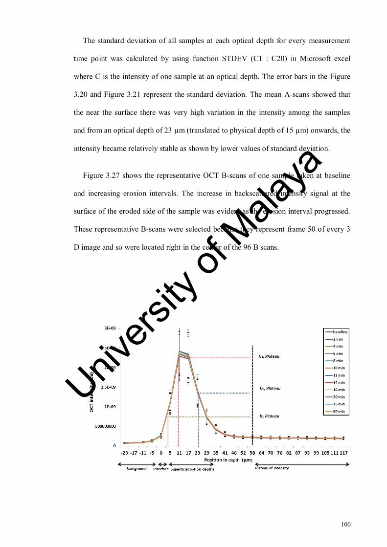
100

The standard deviation of all samples at each optical depth for every measurement

time point was calculated by using function STDEV (C1 : C20) in Microsoft excel

where C is the intensity of one sample at an optical depth. The error bars in the Figure

3.20 and Figure 3.21 represent the standard deviation. The mean A-scans showed that

the near the surface there was very high variation in the intensity among the samples

and from an optical depth of 23 µm (translated to physical depth of 15 µm) onwards, the

intensity became relatively stable as shown by lower values of standard deviation.

Figure 3.27 shows the representative OCT B-scans of one sample taken at baseline

and increasing erosion intervals. The increase in backscattered intensity signal at the

surface of the eroded side of the sample was evident as the erosion interval progressed.

These representative B-scans were selected because they represent frame 50 of every 3

D image and so were located right in the center of the 96 B scans.

Univers

ity of

Mala

ya

101


reference area of the sample. Each line plot represents OCT intensity (a.u) plotted in




deviation.


eroded area of the sample. Each line plot represents OCT intensity (a.u) plotted in




deviation.

Univers

ity of

Mala

ya

102

Figure 3.22: Representative OCT A-scans of one sample at (a) baseline measurement

(b) 2 minutes (c) 4 minutes (d) 6 minutes (e) 8 minutes (f) 10 minutes (g) 12 minutes (h)

14 minutes (i) 16 minutes (j) 20 minutes (k) 25 minutes (l) 30 minutes. Each A-scan

shows the OCT intensity (a.u) plotted in optical depth (µm). The red text box indicates

the OCT intensity at a depth of 23 µm. The chart title of each A-scan indicates the time

interval for which the A-scan was plotted. The increase in intensity at 23 µm is obvious

with time.

Univers

ity of

Mala

ya

103

Figure 3.22 Continued

Univers

ity of

Mala

ya

104






µm is obvious.

Univers

ity of

Mala

ya

105






µm is obvious. Univers

ity of

Mala

ya

106






µm is obvious.

Univers

ity of

Mala

ya

107






µm is obvious.

Univers

ity of

Mala

ya

108

Figure 3.27: Representative OCT B-scans of a sample at (a) baseline measurement (b)

2 minutes (c) 4 minutes (d) 6 minutes (e) 8 minutes (f) 10 minutes (g) 12 minutes (h) 14

minutes (i) 16 minutes (j) 20 minutes (k) 25 minutes and (l) 30 minutes. A composite

slab was used as reference as shown by the red arrow in the figure. Transparent arrows

indicate the backscattered intensity at the surface of eroded area.

Univers

ity of

Mala

ya

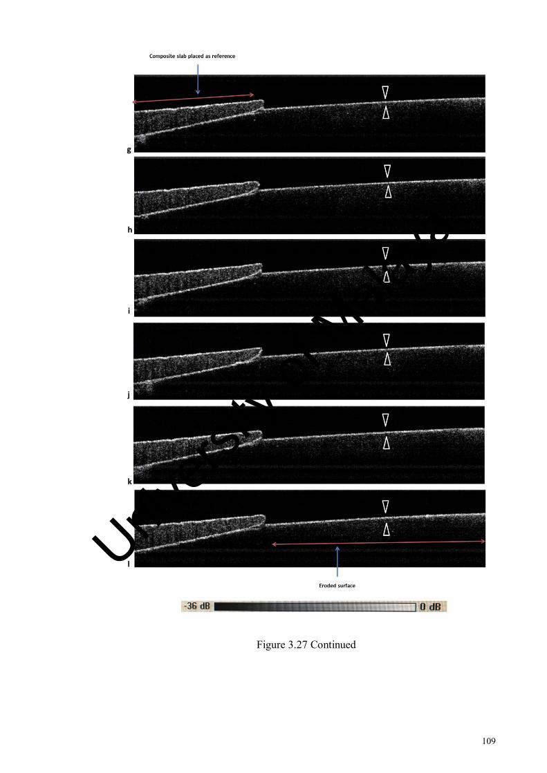
109

Figure 3.27 Continued

Univers

ity of

Mala

ya

110

3.3.1.2 Outcomes measures

OCT parameters and their outcome measures have been summarised in the Table 3.2.

Table 3.2: OCT parameters and their outcome measures defined.

Parameters Symbol Equation Outcome measures

Decay of

intensity

D D = 𝐼𝑝𝑙𝑎𝑡𝑒𝑎𝑢


I58µm / I5µm

I58µm / I11µm

I58µm / I23µm

Integrated

intensity R

R = ∑ Isuperficial : Iplateau ) x Z

I(5µm : 58µm)

I(11µm : 58µm)

I(23µm : 58µm)

Mean %

Integrated

intensity

ΔR

∆𝑅(𝑡) = 100 ∗ [𝑅𝐸(𝑡) − 𝑅𝐸(𝑡0)

𝑅𝐸(𝑡0)]

Where R = I(23µm : 58µm)

Mean % I(23µm : 58µm)

Shapiro-Wilk test and skewness values showed that the data was normally distributed

for the outcome measures I58µm / I5µm, I58µm / I11µm, I(5µm : 58µm), I(11µm : 58µm) and I(23µm :

58µm). Data for I58µm / I23µm did not confirm to a normal distribution. Hence, analysis for

I58µm / I23µm was performed after logarithmic transformation to a normal distribution.

One-way repeated measures ANOVA was performed and Mauchly’s test was used to

evaluate the sphericity assumption. If sphericity was not met, the adjusted F-value of the

Greenhouse-Geisser correction was considered.

Mean and standard deviation (given in brackets) for the eroded area of outcome

measures of decay of intensity and integrated intensity are given in Table 3.6 and Table

3.10 respectively.

Univers

ity of

Mala

ya

111

(a) I58µm / I5µm

Results of Mauchly’s test showed that the sphericity assumption was violated in both

reference (2 = 148.6, p < 0.0001) and eroded areas, (

2 = 196.37, p < 0.0001).

Therefore, the adjusted F-values of the Greenhouse-Geisser correction were considered.

One-way repeated measures ANOVA analysis showed that there was a significant

effect of erosion interval on OCT backscattered intensity of both the reference,

(F(2.61,46.9) = 17.2, p < 0.0001, η2=.489) and eroded areas (F(3.01,54.2) = 8.88, p < 0.0001,

η2 = .331) as shown in table 3.3.

Post hoc comparisons for the eroded area showed that the mean intensity values of

all time points were significantly different with respect to their baseline intensity values

(table 3.4). However, significant differences were only observed among consecutive

time points between baseline and 4 minutes as shown in table 3.5. Data plot is given in

Figure 3.28.


intervals between superficial optical depth of 5 µm and intensity plateau at 58 µm.

Univers

ity of

Mala

ya

112

(b) I58µm / I11µm


reference (2 =206.5, p < 0.0001) and eroded areas (

2 = 215.9, p < 0.0001). Therefore,

the adjusted F-values of the Greenhouse-Geisser correction were considered. One-way

repeated measures ANOVA analysis showed that there was a significant effect of

erosion interval on the OCT backscattered intensity of both the reference, (F(2.1,40.06) =

15.7, p < 0.0001, η2

= .53) and the eroded areas, (F(2.6,49.5) = 6.49, p = 0.001, η2

= .255)

(table 3.3).

Post hoc comparisons for the eroded area showed that mean intensity values of only

4 minutes were significantly different to their baseline intensity values (table 3.4).

However, no significant differences were observed among any of the consecutive time

points (table 3.5). Data plot is given in Figure 3.29.



Univers

ity of

Mala

ya

113

(c) I58µm / I23µm


reference and (2 = 220.27, p < 0.0001) eroded areas (

2 = 181.82, p < 0.0001).


One-way repeated measures ANOVA analysis (table 3.3) showed that there was a

significant effect of erosion interval on the OCT backscattered intensity of both the

reference (F(2.05, 36.9) = 12.1, p < 0.0001, η2

= .403) and the eroded areas (F (3.008, 54.1) =

57.2, p < 0.0001, η2 = .761).

Post hoc comparisons for the eroded area showed that mean intensity values of all

time points were significantly different with respect to their baseline values (p<0.05)

given in table 3.4. Significant differences in mean intensity values were observed

between consecutive time intervals between baseline and 6 minutes of erosion duration

(table 3.5). Plot is given in Figure 3.30.



Univers

ity of

Mala

ya

114


areas of outcome measures of decay of intensity.

Outcome

measure

Reference area Eroded area

Mean

square

F-statistic p-value Mean

square

F-statistic p-value

I58µm / I5µm .005 17.242 <0.0001 .006 8.886 <.0001

I58µm / I11µm .001 15.751 <0.0001 .002 6.496 .001

I58µm / I23µm .021 12.161 <0.0001 .309 57.261 <.0001

Table 3.4: Post hoc comparisons of all erosion time points with baseline, for the eroded

area of outcome measures of decay of intensity.

Time (I) Time(J) Mean difference (I-J)

I58µm / I5µm I58µm / I11µm I58µm / I23µm

Baseline 2min .012** .006 .032**

Baseline 4min .019** .007* .057***

Baseline 6min .022*** .007 .078***

Baseline 8min .020** .004 .093***

Baseline 10min .025*** .005 .121***

Baseline 12min .030*** .006 .143***

Baseline 14min .029*** .004 .151***

Baseline 16min .031*** .002 .161***

Baseline 20min .030*** -.002 .173***

Baseline 25min .031*** -.005 .195***

Baseline 30min .030*** -.008 .214***

*Significant at the 0.05 level

** Significant at the 0.01 level

*** Significant at the 0.001 level.

Univers

ity of

Mala

ya

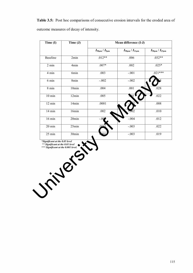
115


outcome measures of decay of intensity.

Time (I) Time (J) Mean difference (I-J)


Baseline 2min .012** .006 .032**

2 min 4min .007* .002 .025*

4 min 6min .003 -.001 .021***

6 min 8min -.002 -.002 .015

8 min 10min .004 .001 .028

10 min 12min .005 .001 .022

12 min 14min .0001 -.002 .008

14 min 16min .002 -.002 .010

16 min 20min -.001 -.004 .012

20 min 25min .0001 -.003 .022

25 min 30min -.001 -.003 .019




Univers

ity of

Mala

ya

116


outcome measures of decay of intensity.

Time point

Outcome measure


Baseline .213

(.054)

.099

(.028)

0.226

(0.058)

2 minutes .201

(.056)

.093

(.028)

0.21

(0.059)

4 minutes .194

(.051)

.091

(.027)

0.198

(0.053)

6 minutes .191

(.052)

.092

(.029)

0.188

(0.049)

8 minutes .193

(.057)

.094

(.03)

0.183

(0.051)

10 minutes .189

(.053)

.094

(.03)

0.172

(0.049)

12 minutes .184

(.048)

.093

(.027)

0.162

(0.041)

14 minutes .184

(.049)

.095

(.028)

0.159

(0.039)

16 minutes .182

(.045)

.097

(.029)

0.154

(0.034)

20 minutes .183

(.045)

.101

(.03)

0.151

(0.038)

25 minutes .182

(.044)

.104

(.03)

0.143

(0.035)

30 minutes .183

(.041)

.107

(.028)

0.136

(0.028)

Univers

ity of

Mala

ya

117

(d) I(5µm : 58µm)


reference (reference, 2 = 192.22, p < 0.0001) and eroded areas (

2 = 196.92, p <

0.0001). Therefore, the adjusted F-values of the Greenhouse-Geisser correction were

considered. One-way repeated measures ANOVA analysis showed that there was a

significant effect of erosion interval on OCT backscattered intensity for the eroded area

(F(3.2, 61.8) = 16.6, p < 0.0001, η2

= .467) whereas no significant effect of erosion interval

on OCT backscattered intensity was found for the reference area (F(3.03, 57.6) = 2.2, p =

0.092, η2 = .106) as shown in Table 3.7.


time points were significantly different with respect to their baseline intensity values (p

< 0.05) (Table 3.8). Significant differences were observed among consecutive time

points from baseline to 6 minutes of erosion challenge (Table 3.9). Data plots for

reference and eroded areas are given in Figure 3.31

Univers

ity of

Mala

ya

118



µm to the intensity plateau at 58 µm.

(e) I(11µm : 58µm)


reference (reference, 2 = 193.209, p < 0.0001) and eroded areas (

2 = 200.914, p <

0.0001). Therefore, the adjusted F-values of the Greenhouse-Geisser correction were

considered. One-way repeated measures ANOVA analysis showed that there was a

significant effect of erosion interval on backscattered intensity of the eroded area (F(3.1,

59.4) = 16.7, p < 0.0001, η2

= .468) whereas no significant effect of erosion interval was

found on backscattered intensity in the reference area (F(2.97, 56.4) = 2.148, p = 0.105, η2

=

.102) as shown in Table 3.7.

Post hoc comparisons for the eroded area showed that mean intensity of all erosion

intervals was significantly different with respect to their baseline intensity values (Table

3.8). However, significant differences in mean intensity values among consecutive time

points were only observed from baseline to 6 minutes of erosion challenge (Table 3.9).

Data plots for reference and eroded areas are given in Figure 3.32. Univers

ity of

Mala

ya

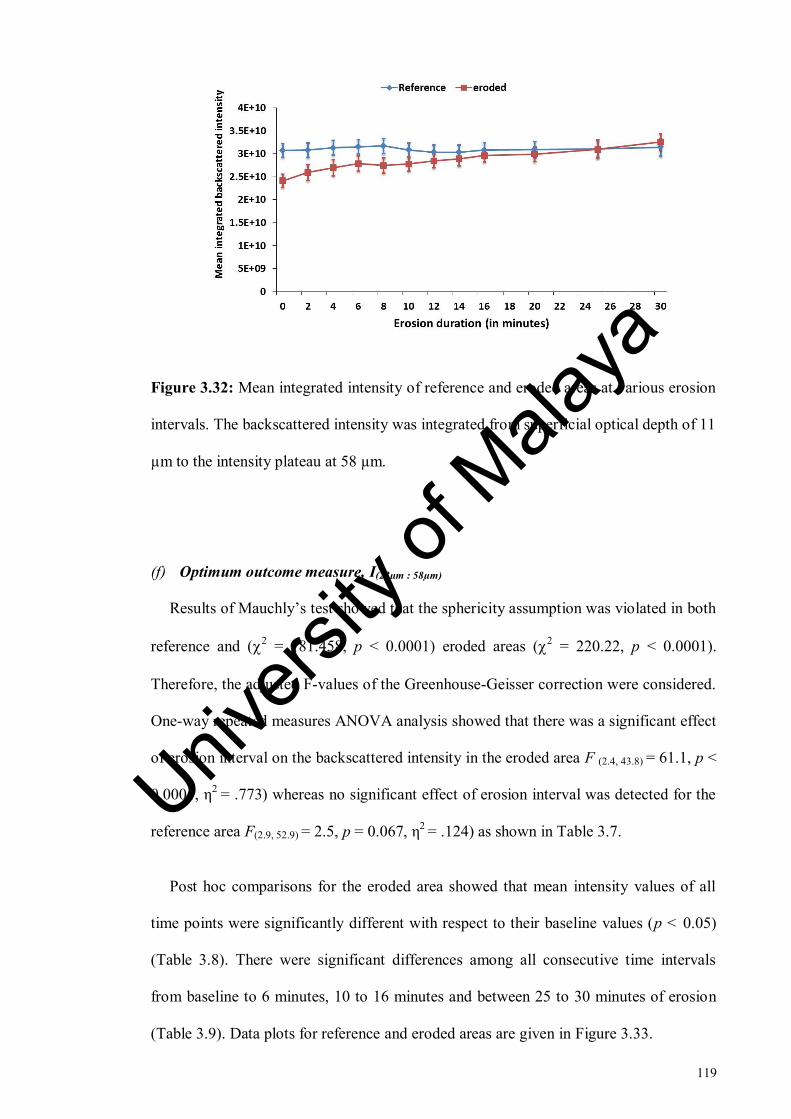
119




(f) Optimum outcome measure, I(23µm : 58µm)


reference and (2 = 181.458, p < 0.0001) eroded areas (

2 = 220.22, p < 0.0001).


One-way repeated measures ANOVA analysis showed that there was a significant effect

of erosion interval on the backscattered intensity in the eroded area F (2.4, 43.8) = 61.1, p <

0.0001, η2

= .773) whereas no significant effect of erosion interval was detected for the

reference area F(2.9, 52.9) = 2.5, p = 0.067, η2 = .124) as shown in Table 3.7.


time points were significantly different with respect to their baseline values (p < 0.05)

(Table 3.8). There were significant differences among all consecutive time intervals

from baseline to 6 minutes, 10 to 16 minutes and between 25 to 30 minutes of erosion

(Table 3.9). Data plots for reference and eroded areas are given in Figure 3.33.

Univers

ity of

Mala

ya

120


intervals. The intensity was integrated from superficial optical depth of 23 µm to the

intensity plateau at 58 µm.

(g) Mean % I(23µm : 58µm)

Results of Mauchly’s test showed that the sphericity assumption was violated (2 =

217.879, p < 0.0001). Therefore, the adjusted F-values of the Greenhouse-Geisser

correction were considered. One-way repeated measures ANOVA analysis showed that

there was a significant main effect of erosion interval on the backscattered intensity F

(2.3, 42.2) = 66.683, p < 0.0001, η2 = .787) as shown in Table 3.7.

Post hoc comparisons showed that mean percentage of integrated intensity of all time

points were significantly different with respect to their baseline values (p < 0.05) (Table

3.8). There were significant differences among all consecutive time intervals from

baseline to 6 minutes, 10 to 16 minutes and between 25 to 30 minutes of erosion (Table

3.9). Data plot is given in Figure 3.34.

Univers

ity of

Mala

ya

121

Almost 20% erosion occurred in the first 10 minutes, 40% by 20 minutes and 60 %

by 30 minutes. Interestingly, almost 17% of erosion occurred in the first 6 minutes.

Figure 3.34: Mean percentage change in integrated intensity of eroded area for intensity

integrated from superficial optical depth of 23 µm to the intensity plateau at 58 µm.

Moreover, a linear line was fitted to the data for ΔR as shown in the Figure 3.35. ΔR

was related to the erosion interval by the equation given below,

𝑦 = 2.17𝑥 + 1.46 (3.8)

Where y is the mean percentage change in backscattered intensity and x is the erosion

interval.

R2 = 0.995 showed that this equation was statistically significant with 99%

confidence interval.

Univers

ity of

Mala

ya

122

Figure 3.35: Best fit regression line of backscattered intensity change with erosion

interval.


areas of outcome measures of integrated intensity.

Outcome

measure


Mean

square

F-statistic p-value Mean

square

F-statistic p-value

I(5µm : 58µm) 1.83E+19 2.248 .092 4.29E+20 16.640 <.0001

I(11µm : 58µm) 1.43E+19 2.148 .105 3.59E+20 16.720 <.0001

I(23µm : 58µm) 2.87E+18 2.55 .067 2.68E+20 61.183 <.0001

Mean %

I(23µm : 58µm)

- - - 3.18E+04 66.683 <.0001

Univers

ity of

Mala

ya

123

Table 3.8: Post hoc comparisons of all erosion time points with baseline for the eroded

area of outcome measures of integrated intensity.

Time (I) Time (J)

Mean difference (I-J)

I(5µm : 58µm) I(11µm : 58µm) I(23µm : 58µm)

Mean %

I(23µm : 58µm)

Baseline 2min -2.096E+9** -1.805E+9** -0.397E+9** -6.164***

Baseline 4min -3.326E+9*** -2.860E+9*** -0.864E+9*** -10.981***

Baseline 6min -4.328E+9*** -3.743E+9*** -1.453E+9*** -16.745***

Baseline 8min -3.804E+9*** -3.306*** -1.544E+9*** -18.355***

Baseline 10min -4.130E+9*** -3.644*** -1.878E+9*** -23.102***

Baseline 12min -4.939E+9*** -4.341E+9*** -2.424E+9*** -27.794***

Baseline 14min -5.448E+9*** -4.792E+9*** -2.818E+9*** -32.436***

Baseline 16min -6.282E+9*** -5.526E+9*** -3.343E+9*** -37.517***

Baseline 20min -6.545E+9*** -5.780E+9*** -3.834E+9*** -43.163***

Baseline 25min -7.713E+9*** -6.864E+9*** -4.620E+9*** -51.679***

Baseline 30min -9.448E+9*** -8.449E+9*** -5.903*** -63.070***




Univers

ity of

Mala

ya

124


all outcome measures for integrated intensity.

Time (I) Time (J)



Mean %

I(23µm : 58µm)

Baseline 2min -2.096E+9** -1.805E+9** -0.397E+9** -6.164***

2min 4min -1.231E+9** -1.055E+9** -0.467E+9*** -4.816***

4min 6min -1.001E+9* -0.882E+9* -0.588E+9*** -5.764***

6min 8min 0.524E+9 0.437E+9 -0.090E+9 -1.610

8min 10min 0.325E+9 0.338E+9 -0.334E+9 -4.747

10min 12min -0.809E+9 0.696E+9 0.334E+9* -4.692*

12min 14min -5.091E+9 -0.450E+9 -0.393E+9** -4.641***

14min 16min -0.834E+9 -0.734E+9 -0.525E+9** -5.081***

16min 20min -0.263E+9 -0.254E+9 -0.490E+9 -5.646

20min 25min -1.166E+9 -1.084E+9 -0.786E+9 -8.515

25min 30min -1.735E+9 -1.084E+9 -1.283E+9* -11.391**

Univers

ity of

Mala

ya

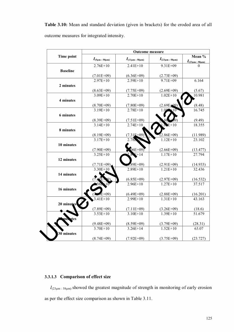
125

Table 3.10: Mean and standard deviation (given in brackets) for the eroded area of all

outcome measures for integrated intensity.

Time point

Outcome measure

I(5µm : 58µm) I(11µm : 58µm) I(23µm : 58µm) Mean %

I(23µm : 58µm)

Baseline

2.76E+10

(7.01E+09)

2.41E+10

(6.36E+09)

9.31E+09

(2.73E+09)

0

2 minutes

2.97E+10

(8.63E+09)

2.59E+10

(7.75E+09)

9.71E+09

(2.69E+09)

6.164

(5.67)

4 minutes

3.09E+10

(8.70E+09)

2.70E+10

(7.80E+09)

1.02E+10

(2.69E+09)

10.981

(8.48)

6 minutes

3.19E+10

(8.39E+09)

2.78E+10

(7.51E+09)

1.08E+10

(2.86E+09)

16.745

(9.49)

8 minutes

3.14E+10

(8.19E+09)

2.74E+10

(7.31E+09)

1.09E+10

(2.86E+09)

18.355

(11.989)

10 minutes

3.17E+10

(7.90E+09)

2.78E+10

(7.06E+09)

1.12E+10

(2.66E+09)

23.102

(13.477)

12 minutes

3.25E+10

(7.71E+09)

2.84E+14

(6.89E+09)

1.17E+10

(2.91E+09)

27.794

(14.933)

14 minutes

3.30E+10

(7.67E+09)

2.89E+10

(6.85E+09)

1.21E+10

(2.97E+09)

32.436

(16.532)

16 minutes

3.38E+10

(7.19E+09)

2.96E+10

(6.49E+09)

1.27E+10

(2.88E+09)

37.517

(16.201)

20 minutes

3.41E+10

(7.89E+09)

2.99E+10

(7.11E+09)

1.31E+10

(3.26E+09)

43.163

(18.6)

25 minutes

3.53E+10

(9.48E+09)

3.10E+10

(8.59E+09)

1.39E+10

(3.79E+09)

51.679

(28.31)

30 minutes

3.70E+10

(8.74E+09)

3.26E+14

(7.92E+09)

1.52E+10

(3.75E+09)

63.07

(23.727)

3.3.1.3 Comparison of effect size

I(23µm : 58µm) showed the greatest magnitude of strength in monitoring of early erosion

as per the effect size comparison as shown in Table 3.11.

Univers

ity of

Mala

ya

126

Table 3.11: Comparison of effect sizes of outcome measures used for analysis.

Parameter Outcome measure Effect size

Decay of intensity

I58µm / I5µm 0.331

I58µm / I11µm 0.255

I58µm / I23µm 0.761

Integrated intensity

I(5µm : 58µm) 0.467

I(11µm : 58µm) 0.468

I(23µm : 58µm) 0.773

Univers

ity of

Mala

ya

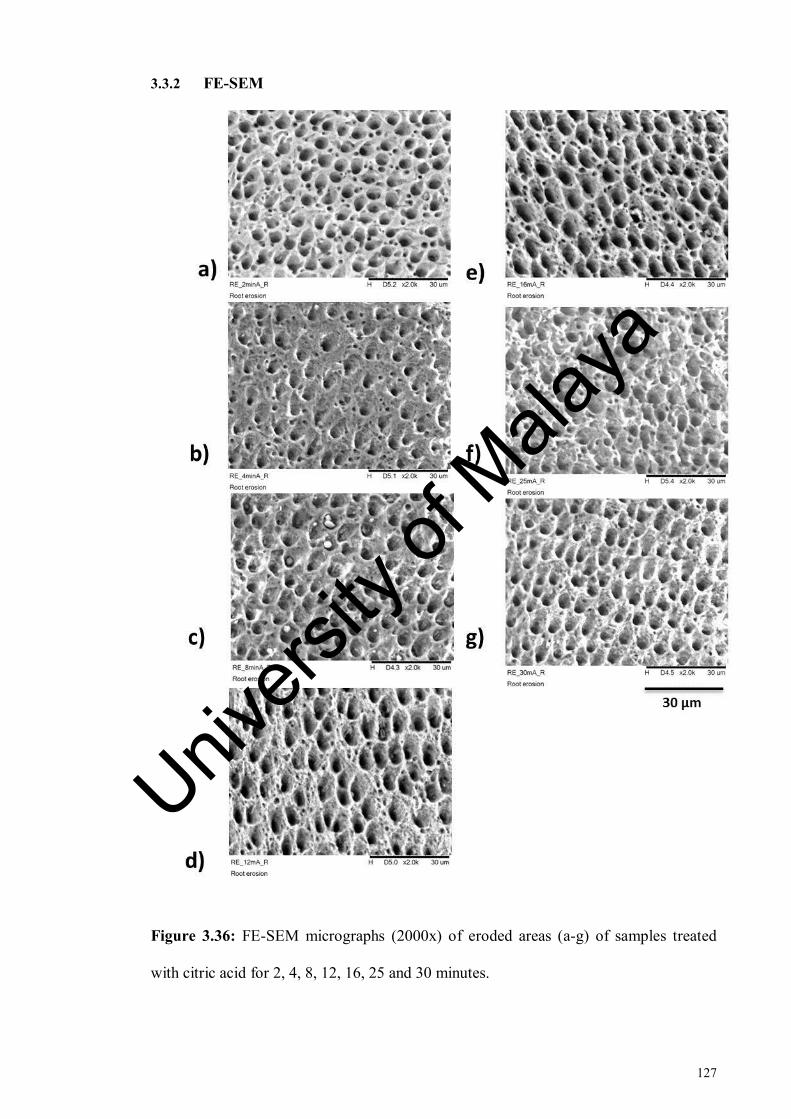
127

3.3.2 FE-SEM

Figure 3.36: FE-SEM micrographs (2000x) of eroded areas (a-g) of samples treated

with citric acid for 2, 4, 8, 12, 16, 25 and 30 minutes.

Univers

ity of

Mala

ya

128

Figure 3.37: FE-SEM images showing the interface between the reference and eroded

areas of samples eroded for 8 minutes (1a, 1b), 12 minutes (2a, 2b), 16 minutes (3a, 3b),

25 minutes (4a, 4b) and 30 minutes (5a, 5b).

FE-SEM images given in Figure 3.36 (a-g) showed the ultrastructural changes of

dentine surface associated with progression of erosion from two to 30 minutes. The

sound dentine (reference areas of same samples) in comparison given in Figure 3.37

(1a-7a) exhibited standard pattern of evenly distributed circular dentinal tubule lumen.

From two to eight minutes, the changes were limited to peritubular dentine as shown in

Figure 3.36 (a-c). Image d (Figure 3.37) representing 12 minutes of erosion showed

marked porosities in the inter-tubular area as compared to the preceding images

Univers

ity of

Mala

ya

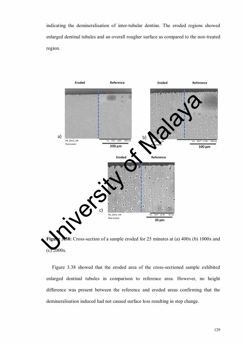
129

indicating the demineralisation of inter-tubular dentine. The eroded regions showed

enlarged dentinal tubules and an overall rougher surface as compared to the non-treated

region.

Figure 3.38: Cross-section of a sample eroded for 25 minutes at (a) 400x (b) 1000x and

(c) 2000x.

Figure 3.38 showed that the eroded area of the cross-sectioned sample exhibited

enlarged dentinal tubules in comparison to reference area. However, no height

difference was present between the reference and eroded areas confirming that the

demineralisation induced had not caused surface loss resulting in step change.

Univers

ity of

Mala

ya

130

3.4 Discussion

This study aimed to assess the applicability of optical coherence tomography for

monitoring the progression of early dentine erosion in vitro. As early stage dentine

erosion was targeted in this study, therefore the demineralisation induced was small,

involving surface-softening only without any evidence of surface loss as ascertained

from FE-SEM images.

A series of pilot studies were performed to determine the optimum duration of

demineralisation required to produce early stage dentine erosion before bulk surface

loss. Citric acid was used instead of commercially available soft drinks to avoid any

potential problems due to variation between the batches in terms of acid concentration

or pH (Shellis et al., 2011). The concentration and pH of the citric acid were kept

similar to that of a commercially available orange juice (Austin et al., 2010; Chiga et al.,

2016) and 10 minutes of erosion was adopted to mimic the consumption of a can of

soda or juice (Faller et al., 2011). Temperature of 36°C was employed to simulate the

intraoral temperature (Shellis et al., 2011). Speed of agitation was pre-determined in a

pilot study. Before the execution of main experiment, the protocol was verified by

performing pilot studies.

Reference area not subjected to erosive challenge is needed in erosion studies to

minimise any systematic errors or biological variability. Previous studies have

employed acid-resistant varnish (Fried et al., 2002), dentino-enamel junction, CO2 laser

(Chan et al., 2013), sub-ablative laser (Chan et al., 2014) and bonding agent to protect

reference areas in erosion-related OCT research. This reference area is expected to

remain unchanged over time against which the changes in the eroded area could be

reliably measured. Use of robust materials like composite would be more applicable for

in vivo research (Chan et al., 2014) and therefore a composite slab was used as a

Univers

ity of

Mala

ya

131

reference in this study. Sectioning of dentine samples creates a smear layer or smear

plugs which can clog the dentinal tubules reducing the permeability of dentine (Ghazali,

2003; Prati et al., 2003). Minimal increase in backscattered intensity was observed in

the OCT images of dentine samples covered with smear layer when eroded in citric acid

for 30 minutes in a pilot study (Section 3.2.1.6). Therefore, to be able to effectively

observe the OCT backscattered intensity changes with erosion interval, it was decided

to remove the smear layer from the root dentine samples before the induction of

demineralisation. The protocol of smear layer removal was adjusted based on pilot

studies and finalised at using a combination of weak chelating agent EDTA in low

concentration and ultrasonication, without significantly affecting the surface

morphology of dentine samples which was confirmed from FE-SEM images. Specular

reflection has been known to mask the information near the tooth-air interface (Fried et

al., 2002). In this study, the issue of specular reflection was addressed by the use of a

custom-made jig attached to the OCT stage which allowed the samples to be inclined to

a certain angle. The samples were inclined at 20 degrees perpendicular to the OCT

beam which effectively reduced the specular reflection from the images. Moreover, the

jig also allowed the samples to be correctly repositioned to the same alignment during

different measurement time points.

3.4.1 OCT

For this study, two different parameters were assessed to determine their potential in

detecting and monitoring the early dentine erosion over time. The first parameter ‘decay

of intensity’ was employed for this study because it has been used to monitor the

progression of early enamel erosion effectively (Chew et al., 2014). However, because

of histological differences between enamel and dentine, the possibility of same

Univers

ity of

Mala

ya

132

parameter of analysis not being applicable for dentine remained. Therefore another

parameter ‘integrated intensity’ was also used for the analysis. Integrated intensity had

been shown to correlate with the integrated mineral loss ΔZ, in the previous studies

involving dental caries (Jones et al., 2006a; Ngaotheppitak et al., 2005).

The outcome measures or depth combinations were selected based on the OCT

backscattered intensity trend observed from mean A-scans. Initially, exploration of data

was performed and many outcome measures were assessed with the both parameters.

Different outcome measures showed different results. In order to standardise the

analysis, it was decided to choose a depth at a subsurface level where the OCT intensity

signal had become constant and did not show any further changes. This depth was

named plateau of intensity. To find an optimal superficial depth to attain maximal

sensitivity of OCT, three superficial depths 5 µm, 11 µm and 23 µm located

immediately below the tooth-air interface were selected for data analysis and

comparison. Their relationship with plateau was assessed by using both ‘decay of

intensity’ and ‘integrated intensity’. The selection of optimum outcome measure was

based on the 1) trend of OCT backscattered intensity 2) repeated measures ANOVA

analysis 3) effect size comparison for assessing the magnitude of strength of outcome

measures and 4) comparison with FE-SEM observations as later discussed in Section

3.4.2

With decay of intensity, significant effect of erosion interval on OCT backscattered

intensity of the reference area was found by all outcome measures employed. Therefore,

the significant differences in backscattered intensity of the eroded area could not be

considered reliable. I58µm / I5µm and I58µm / I23µm were able to monitor intensity changes

for all erosion intervals from baseline whereas I58µm / I11µm was only able to monitor 4

minutes of erosion from baseline. However, with decay of intensity none of the three

Univers

ity of

Mala

ya

133

outcome measures employed was able to detect or monitor intensity between

consecutive erosion intervals beyond 6 minutes of erosion.

In contrast, for integrated intensity, no significant effect of erosion interval on

backscattered intensity of the reference areas was found by all three outcome measures

rendering the outcomes of this parameter for the eroded area more reliable. The

intensity integrated from the first two superficial optical depths I5µm and I11µm to plateau

were sensitive to intensity changes for the initial two to six minutes of erosion challenge

only. I(23µm : 58µm) was the only outcome measure which was able to monitor intensity

changes between consecutive time intervals from baseline to 30 minutes of erosion

challenge. The plotted data for I(23µm : 58µm) showed net increase in intensity from

baseline measurement to 30 minutes of erosion challenge. However, significant

differences were observed between consecutive time points from baseline measurement

to 6 minutes, from six to 12 minutes, from 12 to 16 minutes and from 16 to 30 minutes

of erosion challenge. The results were in line with the trend of intensity observed from

the mean A-scans at this depth where plots of 6 and 10 minutes were indistinguishable

and separation between time points was evident at this depth (23 µm). These

observations were further confirmed by effect size comparison of the outcome

measures. The outcome measure, I(23µm : 58µm) had the largest effect size which indicated

that it had the greatest magnitude of strength in monitoring the early dentine erosion in

comparison to other outcome measures.

At the tooth-air interface, specular reflection is very strong and could be 20dB higher

than OCT backscattered intensity (Fried et al., 2002). . This could lead to scattering

information being masked at or immediately below the tooth-air interface. With both

parameters, the outcome measures near the tooth-air interface did not monitor erosion

beyond 6 minutes of erosion challenge. It could be the result of these outcome measures

Univers

ity of

Mala

ya

134

being influenced by the much stronger specular reflection at superficial optical depths.

Moreover, the mean A-scans for the reference and eroded areas also showed that the

standard deviation near the surface and Imax was very high (Figure 3.20 & Figure 3.21)

which further strengthened this assumption.

The OCT system used in this study (OCS1300SS Thorlabs Ltd., USA) has an axial

resolution of 9 µm in air corresponding to about 6 µm (physical depth) in dentine with

refractive index of dentine being 1.54. Therefore, demineralisation below 6 µm is not

expected to be detected by this OCT system. The plot in Fig 3.21 showed that using this

OCT system, differences in demineralisation over time were detected at about 23 µm

from the surface. This depth would be translated to about 15 µm of physical depth.

Therefore, demineralisation was detected well within the axial optical resolution of this

SS-OCT system however very close to its resolution limit. The earlier depths near the

surface were most probably confounded by the specular reflection. However, the

resolution and penetration depth in the oral cavity will be affected by the presence of

calculus, stain or plaque on the teeth surfaces as well the presence of moisture in the

oral cavity (Park et al., 2013).

Cut-off depths by the exclusion of variety of distances from the surface for different

specimens were identified previously in order to minimise the specular reflection

(Amaechi et al., 2001). In the view of the study results and observation of mean A-

scans, the statistical cut-off depth for monitoring of early dentine erosion would be 23

µm from the tooth-air interface. This is consistent with the statistical cut-off depth of 20

µm determined for monitoring of early enamel erosion previously (Chew et al., 2014).

This is the first study, to the best of our knowledge to examine the ability of OCT for

early stage dentine erosion assessment before the occurrence of any bulk tissue loss

marked by step change. Only one other recent study had examined potential of OCT for

Univers

ity of

Mala

ya

135

dentine erosion but only the advanced stages of dentine erosion after the appearance of

surface loss in the OCT images were explored and only a qualitative analysis was

performed (De Moraes et al., 2017).

This study is a significant step forward since the study findings indicated that

monitoring of erosion progression in root dentine over time was possible with OCT.

This could be used in future for clinical monitoring of progression or regression of early

dentine erosion for testing of treatments products over the period of time. An optimum

outcome measure for the longitudinal monitoring of early dentine erosion was identified

which is currently lacking in literature. Early stage erosion which can be reversed would

have to be induced in clinical trials using healthy subjects (Huysmans et al., 2011). This

study revealed that using the current study protocol, OCT can be employed for

monitoring of dentine erosion starting as early as two minutes. OCT intensity changes

over time (quantum) identified in this study can help in designing the future study

protocols in which the periods of constant intensity can be skipped and measurements

can be taken at fewer intervals. However, a pH-cycling model of erosion was not

applied in this study as the presence of remineralisation step between periods of erosion

challenge could complicate the interpretation of final results. Therefore it was unclear

whether OCT had the potential of being applied to clinical conditions. This was

attempted later and is detailed in chapter 5 of this thesis.

3.4.2 FE-SEM

Scanning electron microscopy (SEM) is a commonly employed method for

qualification of morphological changes in eroded dentine. One of the drawbacks of

conventional SEM is high-vacuum imaging which causes loss of water in biological

samples. Demineralised dentine is prone to shrinkage when dehydrated (Zhang et al.,

Univers

ity of

Mala

ya

136

2009). For this reason, environmental SEM has been recommended for its assessment

(Attin & Wegehaupt, 2014). It allows the samples to be imaged in low-vacuum

conditions thus minimising drying defects. Moreover, environmental SEM as opposed

to conventional SEM does not need any prior metallisation which makes it more

suitable for longitudinal study designs. In this study Field emission scanning electron

microscopy (FE-SEM) was employed to assess the erosion-related surface alterations in

dentine and scanning was performed in low vacuum conditions which did not dehydrate

the samples. The samples were not coated with any metal and were only air-dried before

imaging.

The reference area of each sample was protected with acid-resistant varnish during

the challenges and was not expected to exhibit any demineralisation-associated changes

on surface whereas eroded area of each sample was exposed to citric acid and was

expected to exhibit morphological changes related to erosion. The OCT mean A-scans

extracted for the reference area showed that the backscattered intensity was constant

over time as indicated by the minimal separation between line plots representing various

time points. Mean A-scans for the eroded area showed erosion interval related shift in

backscattered intensity as indicated by the separation of line graphs at various depths.

The FE-SEM images confirmed these findings. The reference areas of the samples

showed the standard pattern of sound dentine without any signs of demineralisation in

comparison to the eroded areas of the same samples which showed signs of progressing

demineralisation with increasing erosion interval.

Repeated measures ANOVA analysis for decay of intensity showed that there were

significant differences in the OCT intensity in the reference area for all outcome

measures employed. Moreover, with this parameter, none of the three outcome

measures employed was able to detect or monitor intensity over consecutive erosion

Univers

ity of

Mala

ya

137

intervals beyond 6 minutes of erosion. In contrast, the reference areas of the samples in

the FE-SEM images did not appear to be demineralised and the eroded areas of the

samples showed progression of erosion. Therefore, SEM images confirmed that decay

of intensity was not suitable for assessment of early dentine erosion within the

limitation of this study protocol.

There were no significant differences in the OCT backscattered intensity over time in

the references areas with integrated intensity. This could be confirmed from the FE-

SEM images. Moreover, I(23µm : 58µm) was the only outcome measure which was able to

monitor intensity changes between consecutive time intervals from baseline to 30

minutes of erosion challenge and showed net increase in intensity from baseline

measurement to 30 minutes of erosion challenge. The suitability of this outcome

measure I(23µm : 58µm) for longitudinal monitoring of early eroded dentine was further

confirmed by FE-SEM images showing signs of progressing erosion with increasing

erosion interval.

OCT outcome measure I(23µm : 58µm) showed an initial increase in backscattered

intensity from baseline measurement to the first 6 minutes of erosion. This could be the

result of the initial rapid dissolution of peritubular dentine as observed in the FE-SEM

images showing 2, 4 and 8 minutes of demineralisation as previously reported (Kinney

et al., 1995). Between 6 and 10 minutes, the OCT intensity remained constant and OCT

could not monitor the erosion progression between these time points. The backscattered

intensity increased from 12 minutes onwards. The increase in OCT backscattered

intensity on the surface of demineralised dentine is associated with increased porosities

which develop as a result of mineral loss (Huysmans et al., 2011). The FE-SEM images

for 12 minutes of erosion showed demineralised intertubular dentine with increased

porosities as previously reported (Meurman et al., 1991). Although there was an

Univers

ity of

Mala

ya

138

increase in backscattered intensity between from 16 to 25 minutes, the changes were not

significantly different. Overall these intensity fluctuations could be attributed to the

changes in the porosity, in structural phase (organic versus mineral-organic) and optical

properties in the demineralised area as previously observed (Natsume et al., 2011)

It has been emphasised that some verification of absence of substance loss should be

given for the protocols dealing with initial erosion (Shellis et al., 2011). One sample

eroded for 25 minutes was embedded in epoxy resin and cross-sectioned in a transverse

plane to see if there was any step change at the border between the reference and eroded

areas. No obvious changes in height were present between reference and eroded areas

confirming the absence of substance loss.

3.5 Conclusions

Within the limitations of the current study design, the following conclusions were

drawn from the study findings,

1. OCT was able to measure early dentine erosion up to 30 minutes. The quantum

of OCT for measuring early dentine erosion varied with different outcome

measures. I(23µm : 58µm) showed significant changes in the first three 2-minute

intervals (0-6 minutes) but not in the subsequent three 2-minute intervals (6-12

minutes). However, in the subsequent eighteen minutes (12-30 minutes), I(23µm :

58µm) detected significant 2-minutes interval change only up to 16 minutes and

significant changes were detected in the consecutive time intervals only between

25 and 30 minutes for the next 14 minutes (16-30 minutes).

2. Integrated intensity was more suitable and sensitive than decay of intensity for

measuring in vitro early dentine erosion. I(23µm : 58µm) was the most sensitive

Univers

ity of

Mala

ya

139

outcome measure for measuring in vitro early dentine erosion. OCT outcome

measure ΔR showed a linear pattern (R2 = 0.995) as goodness of fit model for

measuring in vitro early dentine erosion.

3. The in vitro early dentine erosion detection threshold of OCT varied with

different outcome measures. With I(23µm : 58µm), the detection threshold was 2

minutes of erosion challenge from baseline measurement.

4. FE-SEM images supported the results of OCT backscattered intensity analysis .

With I(23µm : 58µm), continuous increase in backscattered intensity in relation to

incubation time in acid was obvious during erosion progression. The eroded

regions of FE-SEM showed gradually enlarging dentinal tubules with increasing

erosion intervals.

The null hypotheses one and two were rejected as shown below;

1. OCT was able to detect early dentine erosion with a detection threshold of two

minutes from baseline measurement.

2. OCT was able to measure the progression of early dentine erosion up to 30

minutes in vitro.

Univers

ity of

Mala

ya

140


SURFACE ROUGHNESS

This chapter details the profilometric assessment of early eroded dentine in simulated

intraoral environment both with conventional and novel parameters and its qualitative

assessment using field emission scanning electron microscopy.

4.1 Introduction

It is a challenging task to find a suitable method for quantification and monitoring of

early dentine erosion because of the complex histology of these lesions. Surface

microhardness is suitable for the measurement of early enamel erosion (Attin, 2006) but

not for dentine erosion. This could be attributed to the elastic nature of dentine which

causes the indentations to shrink by about 30% within 24 hours after indentation

(Herkstroter et al., 1989). In addition to this, as intertubular and peritubular dentine have

distinctly different hardness values (Kinney et al., 1996) the need to be site-specific in

the indenting process makes surface nanohardness a time consuming and non-feasible

method for longitudinal erosion study designs.

Surface profilometry has been used extensively for the quantification of dental

erosion (Aykut-Yetkiner et al., 2014; Borges et al., 2014; Charone et al., 2014). This

method has been described in more detail in Section 2.3.1.3 of this thesis. The

parameter commonly used is the amount of tissue loss in the form of a step between the

reference and eroded areas (Borges et al., 2014; Paepegaey et al., 2013). However,

initial dental erosion is not marked by bulk surface loss (Young & Tenuta, 2011) and it

is speculated that this parameter might not be effective in measuring the early stages of

erosion.

Univers

ity of

Mala

ya

141

Moreover, measurement of tissue loss in eroded dentine is rendered complicated by

the presence of organic matrix and it has been recommended that organic matrix be

removed from the dentine samples before performing measurements with profilometry

(Ganss et al., 2009b; Ganss et al., 2007). However, the need to remove organic matrix

from dentine samples makes profilometry a destructive technique and therefore non-

suitable for application in longitudinal or in vivo studies. Besides being able to provide

information on height differences between two areas, surface profilometry can also

quantify the surface roughness of dental hard tissues with surface roughness parameters.

Preliminary work has shown that surface roughness parameters seem to be useful for

assessing early erosion (Field et al., 2013; Schlueter et al., 2011).

4.1.1 Roughness parameters

Roughness parameters, depending upon their functionality have normally been

categorised into four groups. These groups are height parameters, amplitude parameters,

spacing parameters and hybrid parameters (Grzesik, 2016). Out of these, amplitude

parameters are the most important in describing the surface topography of a surface and

measure surface characteristics of surface deviations (Gadelmawla et al., 2002). The

most commonly used amplitude parameter in relation to dentistry is surface roughness

average (Ra) (Kukiattrakoon et al., 2011).

4.1.1.1 Average roughness

Ra, the average mean roughness, is defined as the absolute average deviation of

roughness irregularities from the mean line of a sampling length (Gadelmawla et al.,

2002). The mean line is that section through the profile that cuts off equal areas above

Univers

ity of

Mala

ya

142

and below it. It is the mean of the absolute values of the deviations of the profile

(Darvell, 2009). Ra is described by the equation given as follows:

𝑅𝑎 = 1

𝑛∑|𝑦𝑖|

𝑛

𝑖=1

(4.1)

Where n is the number of points at which height measurements are made and 𝑦𝑖 is

the vertical distance from the mean line to the ith data point.

Although Ra is the most commonly reported surface roughness parameter in dentistry

and engineering (Kukiattrakoon et al., 2011), there are a few downsides of reporting Ra

value in isolation. While Ra value furnishes basic information about the relative

departures from the mean line, still it fails to distinguish between these asperities and

valleys in terms of their slopes, sizes, direction or shapes and does not take into account

the frequency of their occurrence. As a result, it is possible to have the same Ra values

for two surfaces with widely different profiles (Rîpă et al., 2003) (Figure 4.1). Other

drawbacks include the inability of Ra value to give any information regarding the

textural characteristics of wear, rate of wear, susceptibility or resistance of a surface

towards future wear or its potential to hold fluids (Field et al., 2010). It is felt that the

description of such surfaces with Ra value alone would be incomplete and more

sophistical parameters could describe such surfaces more efficiently. Univers

ity of

Mala

ya

143

Figure 4.1: Three different surfaces having similar Ra values. (a) The first profile has

sharp peaks, (b) the second deep valleys and (c) the third has neither (Bewoor &

Kulkarni, 2009)

4.1.1.2 Bearing area curve

The bearing area curve or Abott-Firestone curve is obtained by plotting the

cumulative distribution of the lengths of individual plateaus, normalised by the total

assessment length against the sample height (Field et al., 2010). In order to obtain the

bearing area curve from surface profile, a parallel line is drawn at a distance from a

reference line. This parallel line is called the bearing line. Then the length of each

material intercept along this line is calculated and these lengths are summed up. The

proportion of this sum to the total length is then calculated and is called the bearing

length (tp) (figure 4.2). The same procedure is repeated along a number of bearing lines

starting from the highest peak to the lowest valley and the bearing length ratio

(fractional land length) as a function of height of each slice is plotted in the form of a

curve (Bhushan, 2013). The calculation of the bearing area curve from a roughness

profile is shown in Figure 4.2

Univers

ity of

Mala

ya

144

Figure 4.2: Generation of bearing area curve from roughness profile. Modified from

(Field et al., 2010). Bearing length or tp is the sum of lengths of individual plateaus (L1,

L2), divided by the total assessment length (L)

Bearing curve parameters have basically being described in relation to load carrying

surfaces. Peak roughness, Rpk has been described as the top portion of the surface which

will be worn when another surface comes in contact with it. Core roughness, Rk is the

working part of the surface. After the initial running-in period this part of the surface

will carry the load and influence the overall performance of the engine. Valley

roughness, Rvk is the lowest part of the surface that can retain the fluids. Proportion of

peaks, MR1 represents the bearing ratio at which Rpk and Rk meet and forms the upper

part of the core roughness profile. Proportion of valleys, MR2 is the bearing ratio at

which Rvk and Rk meet and represent the lower limit of the core roughness profile

(Menezes et al., 2013). A brief description of the parameters explored in this study in

given in Table 4.1 (Field et al., 2013).

Univers

ity of

Mala

ya

145

Table 4.1: Description of roughness parameters

Parameter Description

Ra

Arithmetic average of all deviations of the profile

from the mean line

Rpk Height of the material peaks

Rk Height of the material core

Rvk Depth of the material valleys

MR1 Proportion of peaks within the sample

MR2 Proportion of valleys within the sample

Figure 4.3: Bearing area curve parameters (1) Maximum height (2) Peak area defined

(3) 40% of minimum slope (4) Valley area (5) Minimal height (Infinitefocus, 2009)

Univers

ity of

Mala

ya

146

Figure 4.3 shows the algorithm for the extraction of bearing curve parameters from

bearing curve. A line segment representing 40% material ratio is fitted in the curve

starting from extreme left point. This is shown by blue line fitting into the red bearing

area curve in the Figure 4.3. The slope of this line matching with the bearing curve

gives an equivalent straight line. This equivalent straight line is extended to meet the

vertical lines drawn at 0% and 100% and difference in height denotes the parameter Rk.

Horizontal lines are drawn to meet the bearing curve at MR1 and MR2. Rpk and Rvk are

represented by the shaded grey areas located above and below the Rk respectively

(Management Association, 2012). .

It has been suggested that bearing area curve parameters can be used to describe

many complex surfaces that cannot be described adequately by simple parameters like

Ra. Among such surfaces are multi-processed surfaces which are treated by more than

one distinct surface processes (Bacova & Draganovska, 2004; Pawlus & Grabon, 2008).

One process may act to remove peaks and the second process may introduce a finer

texture into the resulting plateaus while the deeper valleys may remain unchanged at the

same time. An example of such surfaces is ‘multi-stratified’ surfaces. The assessment of

these surfaces is notoriously difficult as they are negatively skewed (Field et al., 2010;

Whitehouse, 2010). Interestingly, eroded or eroded / abraded surfaces could also be

included in this category. During an erosion challenge, the acid challenge is interspersed

with salivary remineralisation or abrasion (Young & Tenuta, 2011) and the resulting

surfaces could be considered as multi-processed or multi-stratified. Therefore, it could

be assumed that bearing area curve would have the ability of explaining such surfaces

better than other basic surface roughness parameters like Ra. Moreover, tooth wear is

known to occur in two phases, a primary phase described as ‘running-in’ phase followed

by secondary phase called ‘steady-state wear’ (Kaidonis et al., 1998) and bearing area

curve might have a potential of assessing such bi-phasic processes (Field et al., 2010).

Univers

ity of

Mala

ya

147

Bearing curve parameters were successfully employed for the in vivo qualification

and monitoring of changes in enamel surface induced by erosion over a period of 3

months via silicon models. (Whitehead et al., 1997). Moreover, 3D bearing curve

parameters were employed to characterise the topography of native enamel surface with

active erosive wear. (Las Casas et al., 2008). Recently, the usefulness of bearing curve

for evaluation of early enamel erosion was shown in a pilot study and a comparison was

drawn between bovine and human enamel characteristics at baseline and post-erosion

challenge (Field et al., 2013).

Importantly, all of these studies employed enamel as the tissue of interest and the

usefulness of bearing curve parameters for assessment of dentine erosion has not been

evaluated previously. Because of the histopathological differences between enamel and

dentine erosion, the applicability of methods need to be re-assessed for dentine. The

present study therefore sought to achieve the following aim,

4.1.2 Aim

To assess the potential of surface roughness as a method for longitudinally measuring in

vitro early dentine erosion in simulated intraoral conditions.

Research Objectives

In order to achieve this aim, the following research objectives were defined.

1. To explore the use of surface roughness parameters for measuring early dentine

erosion in simulated intraoral conditions.

Univers

ity of

Mala

ya

148

2. To identify the most sensitive surface roughness parameter for measuring early


3. To identify the detection threshold of surface roughness parameters for


4. To compare the changes of surface roughness parameters in early dentine erosion

with surface ultrastructural changes.

The null hypotheses tested were as follows:

1. Surface roughness parameters cannot be used to measure early dentine erosion

progression in simulated intraoral conditions.

2. There is no difference of the sensitivity of Ra and bearing curve parameters in


Univers

ity of

Mala

ya

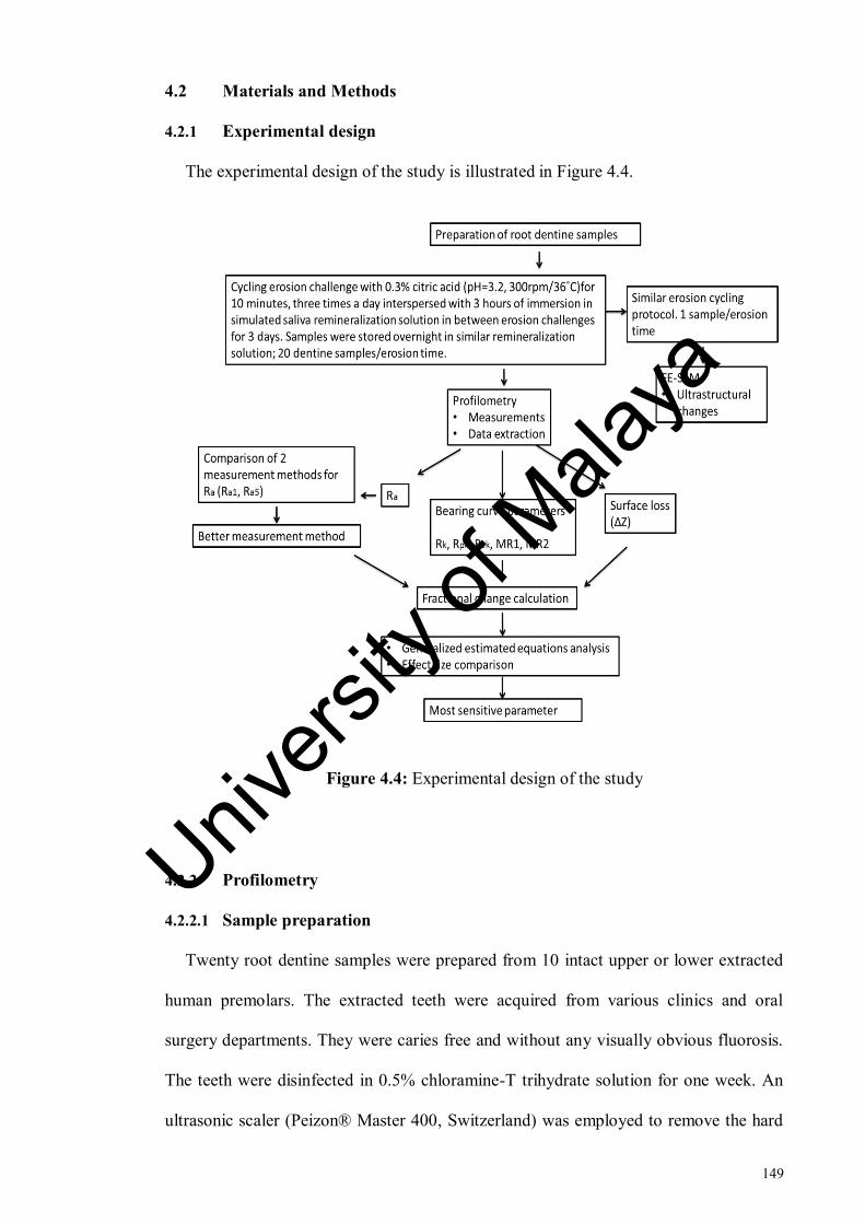
149




Figure 4.4: Experimental design of the study

4.2.2 Profilometry


Twenty root dentine samples were prepared from 10 intact upper or lower extracted

human premolars. The extracted teeth were acquired from various clinics and oral

surgery departments. They were caries free and without any visually obvious fluorosis.

The teeth were disinfected in 0.5% chloramine-T trihydrate solution for one week. An

ultrasonic scaler (Peizon® Master 400, Switzerland) was employed to remove the hard

Univers

ity of

Mala

ya

150

deposits and soft tissues from the teeth. After scaling, the crowns were sectioned

horizontally 1 mm below the cemento-enamel junction using slow speed microtome

cutting machine (Micracut 125, Metkon Instruments Inc., Bursa, Turkey) and discarded.

Next, the roots were sectioned longitudinally in the buccolingual direction. Fragments

obtained were embedded in separate self-curing methyl methacrylate resin blocks such

that the external part of the root was kept exposed and inner part of the root was

embedded in the resin (Quick Mount 2 Epoxy resin, Ace Technologies Inc., Arizona).

The dentine surface was then ground flat with 600-grit silicon carbide paper (Struers

Inc., Ohio, USA) which removed the cementum followed by final polishing with

polishing pads (8-inch Micropad polishing pad PSA, Pace® technologies, Arizona)

using diamond suspension (1 µm) in a water-cooled rotating grinding / polishing

machine (Buehler, USA). The samples were prepared in a flat plane as parallel to the

base of the sample as possible to ensure the surface could be scanned by the

profilometer.

A window with dimensions of 5 x 3 mm was created with non-residue adhesive tape

(3M, United States) on the surface of each sample. Left half of the window was kept

covered with the adhesive tape during the cycling erosion challenges to act as a

reference surface. Middle of the window was marked with a permanent marker on the

resin at the top and bottom part of the each resin embedded sample. This step was

carried out to aid in the identification of the reference and eroded areas in baseline and

subsequent measurements.

4.2.2.2 Erosive pH-cycling

Samples were scanned with a non-contact profilometry (Alicona InfiniteFocus®

Optical 3D Measurement Device G4f, Austria) to acquire images for baseline

Univers

ity of

Mala

ya

151

measurements. The reference area of each sample was covered with non-residue

adhesive tape (3M, United States). The samples were then suspended in a beaker

containing 0.3% citric acid (pH = 3.2) (A&C American Chemicals Ltd., North Carolina,

USA) on a movable stand with wires and plastic clips. Five samples were suspended in

500 ml of citric acid (A&C American Chemicals Ltd., North Carolina, USA) at one

time. The temperature and speed of the solution were controlled by placing the beakers

on magnetic stirrer (RCT basic, IKA, Germany). A magnetic stirrer is a laboratory

device used for stirring a ‘stir bar’ added in the liquid by employing a magnetic field.

The solution is stirred as a result of it (Figure 3.14). The temperature of the solution was

kept constant at 36°C and the speed was kept constant at 300 rpm during the erosion

phase of the cycling throughout the experiment. Temperature of 36°C was employed to

mimic the intraoral temperature. A pilot study was conducted to verify the speed at

which the samples did not move while the solution remained stirred homogeneously as

discussed in Section 3.2.1.2 of Chapter 3. After 10 minutes of erosion challenge,

samples were removed from the beaker and rinsed with deionised water. 10 minutes of

erosion was adopted to mimic the consumption of a can of soda or juice (Faller et al.,

2011). Following this, each sample was stored in a separate plastic container containing

simulated saliva remineralisation solution and kept in incubator at 36°C for 3 hours. The

remineralisation solution (A&C American Chemicals Ltd., North Carolina, USA)

contained 8.38 Millimolar (mM) KCl, 0.29 mM MgCl2.6H2O, 1.13 mM CaCl2.2H2O,

4.62 mM K2HPO4, 2.40 mM KH2PO4, 0.022 ppm fluoride and the pH was adjusted to

7.2 using KOH. After storage in simulated saliva remineralisation solution, samples

were then removed from their respective bottles, dried with dental syringe for 20

seconds at a distance of 10 cm and tapes were reapplied on the reference areas of each

sample. This alternating episode of demineralisation and remineralisation was repeated

three times in one cycling day. At the end of each cycling day, the samples were stored

Univers

ity of

Mala

ya

152

overnight (8 hours) in similar remineralisation solution. Citric acid was renewed after

every exposure and remineralisation solution was refreshed after every 24 hours. This

cycling erosive challenge was repeated for a total of three consecutive days. After every

cycling day, measurements were obtained with both optical coherence tomography and

non-contact profilometry. This chapter details the non-contact profilometric

measurements of these samples whereas the OCT measurements of these samples have

been detailed in chapter 5.

4.2.2.3 Measurements with Profilometry

After every cycling day, a non-contact profilometry device (Alicona InfiniteFocus®

Optical 3D Measurement Device G4f, Austria) in combination with bespoke

measurement software (IFM software) was employed for scanning the samples. Figure

4.5 shows the profilometry equipment used in the experiment.

Figure 4.5: Photograph of profilometry equipment

Univers

ity of

Mala

ya

153

The calibration of the IFM system of the device was performed by the manufacturer

using a gauge block set, alicona calibration tool (known as IF-CalibrationTool), PTB

depth adjustment standard and PTB micro contour standard (known as IF-

VerificationTool) (Infinitefocus, 2009). This equipment uses coaxial white light to

perform the measurements instead of a contact stylus. Each resin-mounted sample was

removed from its container (containing remineralisation solution) before imaging and

tape covering the reference area was removed from the surface of each sample. One

sample at a time was placed on the motorised profilometer stage such that the

experimental surface was parallel to the horizontal plane. A custom-made sample holder

was attached to an A-4 paper which in turn was taped to the stage throughout the study

period as shown in the Figure 4.7. Repositioning of samples at various measurement

time points was achieved by placing the sample in this sample holder. The coaxial white

light was provided by a light source delivered through a beam splitter to a series of

objectives with fixed magnification. The objective lens of 20x magnification was used

for imaging of samples. At this magnification, a lateral resolution of 0.5 µm and a

vertical resolution of ≤100 nm could be achieved. The maximum vertical imaging range

was 100 mm. An area of 0.7 x 0.5 mm (711.46 x 539.73 µm) composed of 1624 x 1232

points was selected for scanning for each image. The sampling distance was kept at

438.09 x 438.09 nm. The stage calibrated itself by moving to the reference position

automatically at startup. The border between the reference and eroded areas for each

sample was identified by using live 3D view function which gives a preview of the

image before capturing. Before capturing the image, a capture range was specified by

using stage control to select a lower bound and an upper bound which represent

different z positions of the stage. Following this, the 3D model of the image was

captured and displayed within an image viewer as shown in the Figure 4.6. Once

captured, the images were then saved for further analysis.

Univers

ity of

Mala

ya

154

Figure 4.6: 3D model of image captured and displayed by live viewer

Non-contact profilometers fail to scan surfaces with steep slopes and highly curved

features. Therefore, each sample was scanned before baseline imaging to ensure that the

surface was smooth and flat. Samples were allowed to dry for 10 minutes before

obtaining measurements in order to address any possible interference by organic

matrix.(Steiner-Oliveira et al., 2010). A total of three images were captured for each

time point for all samples. First image was captured at the reference area, second at the

eroded area and third at the junction between the reference and the eroded areas as

shown in Figure (4.8).

Univers

ity of

Mala

ya

155

Figure 4.7: Repositioning of samples at different measurement time points. (a) custom-

made sample holder pasted on paper (b) sample holder pasted on the stage during

scanning (c) close up of sample-holder with the sample snugly fitted inside

Figure 4.8: 3D images acquired by profilometry at the junction of reference and eroded

areas (a) Baseline image (b) Day one image (c) Day two image (d) Day three image

Univers

ity of

Mala

ya

156

Table 4.2: Calculation methods for surface roughness parameters used in the study.

RaL* was only explored in the pilot study

Parameter Symbol Calculation method

Average roughness RaL* Calculated by an average of 5

measurement lines.

Ra5 Calculated by an average of 5

measurement areas.

Ra1 Calculated from a single measurement area

Core roughness Rk

Calculated from a single measurement area

Peak roughness Rpk

Valley roughness Rvk

Proportion of peaks MR1

Proportion of valleys MR2

4.2.2.4 Data extraction

The saved files were then opened and analysed with the profile analysis software

(IFM 2.1.5 software). The IFM software utilises EN/ISO standards for surface

roughness measurement. Utilising this software, the measurements conform to

ISO4287/ISO4288/. The 3D profile was first activated and levelled using a best-fit

plane. For the roughness measurement, the form of the 3D image was removed. Next,

the extraction parameters were selected and roughness filter was applied to separate the

roughness and waviness from the overall form. A cut-off wavelength of 80 and a profile

length of 500 µm were chosen. Next a red measurement line or area was drawn over the

image at the desired location and values for the parameters were then calculated.

Univers

ity of

Mala

ya

157

(a) Ra

Ra has most commonly been reported as an average of five separately made

measurements rather than a single area. It is believed that a single area that covers most

of the image will be better representative of the overall roughness value. In this study,

Ra was measured with both methods and a comparison was drawn between the both to

find the best method.

For the first method, five measurement areas were drawn on each image and Ra5

value was recorded for each area. One measurement area could be drawn at a time. The

profile viewer displayed the roughness profile of the measurement area as shown in the

Figure 4.9 (a). The Ra5 value for the selected region was recorded. Each measurement

area was composed of 100 points with a width of 43 microns. Next, another

measurement area at a distance of approximately 50 µm from the first area was drawn

on the image. In this manner, five measurement areas were drawn as shown in the

Figure 4.9 (b). Data was entered manually in Microsoft Excel programme. An average

value of Ra5 was calculated as a mean of values recorded from five measurement areas

at every time point. Average Ra5 values were calculated in this manner for both the

reference and eroded images of each sample at every time point.

Univers

ity of

Mala

ya

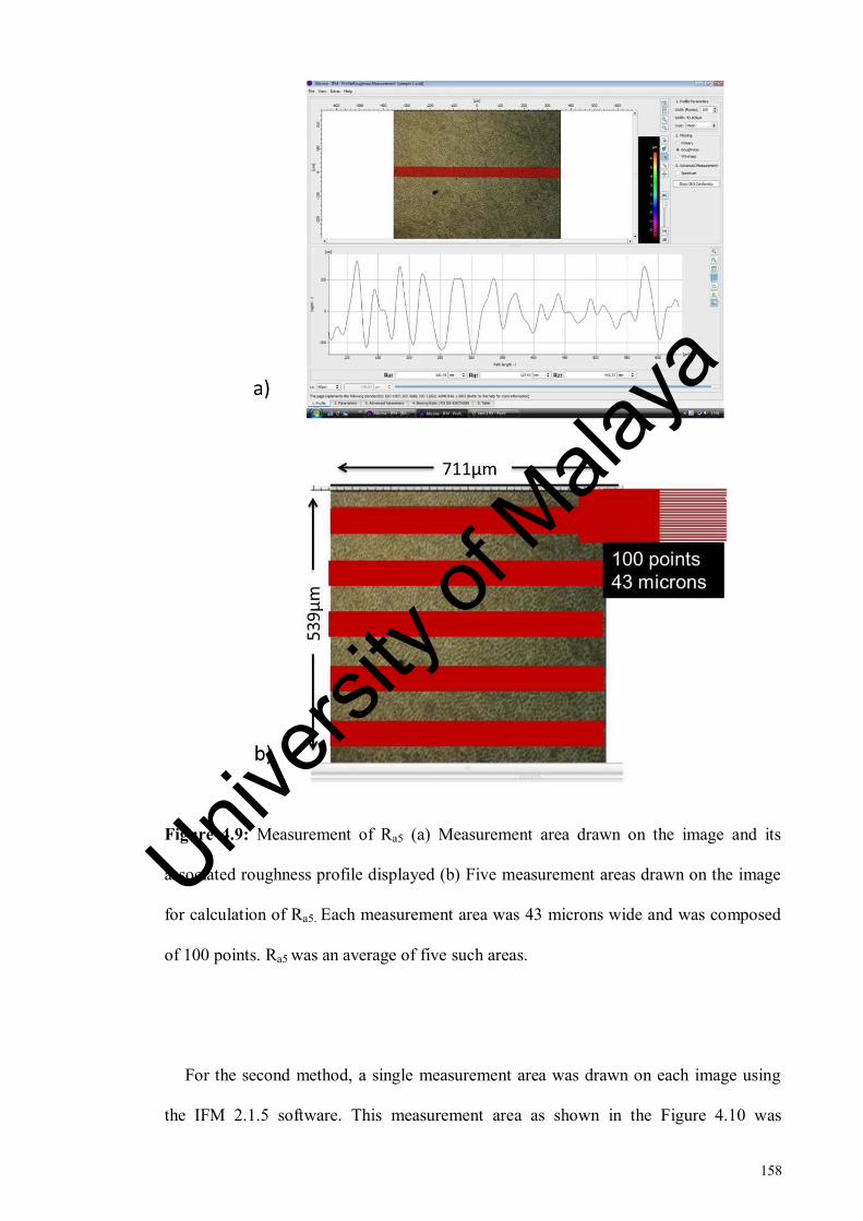
158

Figure 4.9: Measurement of Ra5 (a) Measurement area drawn on the image and its

associated roughness profile displayed (b) Five measurement areas drawn on the image

for calculation of Ra5. Each measurement area was 43 microns wide and was composed

of 100 points. Ra5 was an average of five such areas.

For the second method, a single measurement area was drawn on each image using

the IFM 2.1.5 software. This measurement area as shown in the Figure 4.10 was

Univers

ity of

Mala

ya

159

composed of 800 points and had a width of 334 microns. Average roughness values

(Ra1) were then extracted and exported to Microsoft Excel Programme as shown in

Figure 4.11. The data was measured and exported for both reference and eroded images

of every time point for each sample.

Figure 4.10: A single measurement area drawn on the image for the calculation of Ra1.

The measurement area was 344 microns wide and was composed of 800 points.

Figure 4.11: (a) Roughness profile generated from the single measurement area (b) Ra1

values exported to excel sheet

Univers

ity of

Mala

ya

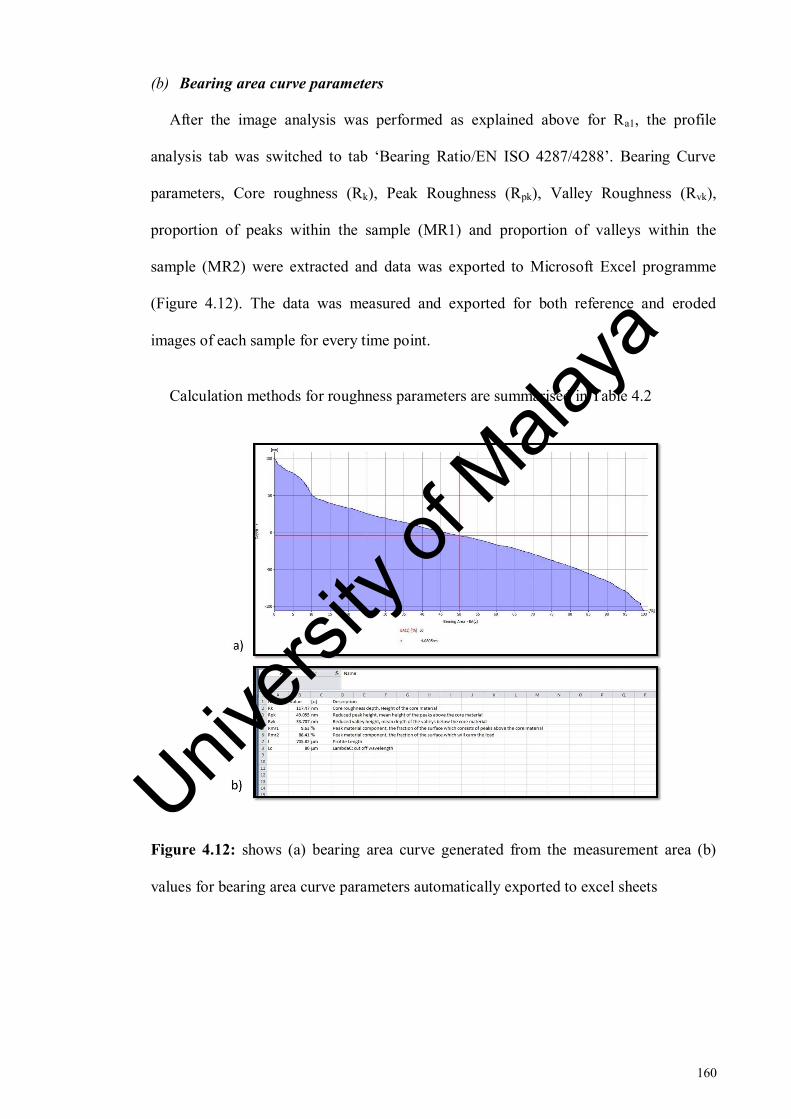
160

(b) Bearing area curve parameters

After the image analysis was performed as explained above for Ra1, the profile

analysis tab was switched to tab ‘Bearing Ratio/EN ISO 4287/4288’. Bearing Curve

parameters, Core roughness (Rk), Peak Roughness (Rpk), Valley Roughness (Rvk),

proportion of peaks within the sample (MR1) and proportion of valleys within the

sample (MR2) were extracted and data was exported to Microsoft Excel programme

(Figure 4.12). The data was measured and exported for both reference and eroded

images of each sample for every time point.

Calculation methods for roughness parameters are summarised in Table 4.2

Figure 4.12: shows (a) bearing area curve generated from the measurement area (b)

values for bearing area curve parameters automatically exported to excel sheets

Univers

ity of

Mala

ya

161

(c) Tissue loss measurement

Tissue loss (ΔZ) of each time point was measured for all samples using the IFM

2.1.5 software. Image taken at the junction of both reference and challenged areas at

each time point was selected for the analysis. Figure 4.13 shows the measurement of the

Z differences between the reference and eroded areas. A profile line was drawn from the

reference area to the eroded area. A green measurement line was positioned on the

reference area and another red measurement line was positioned on the eroded area

along the profile path as shown in Figure 4.13. A small circle on the profile path in the

image viewer indicated correspondence between the measurement line and the position

on the profile path in the image viewer. The vertical distance of these measurement

lines was calculated as tissue loss (ΔZ). At a time only one profile line could be

measured. Following the similar procedure, a total of three measurements at a distance

of 200 µm were made and ΔZ values were recorded. To standardise the measurements,

the reference measurement line was positioned at 100 µm and eroded measurement line

was positioned at 500 µm on the x-axis for all the time points of all samples. The data

was then transferred manually to excel programme and a mean of three measurements

was calculated for each time point for all samples.

Univers

ity of

Mala

ya

162

Figure 4.13: Measurement of tissue loss. Green line represents reference measurement

line and red line represents eroded measurement line. Delta z values are given at the

bottom of the image

4.2.2.5 Calculation of fractional change

The mean data of each parameter was normalised for the reference area (fPR) and

eroded area (fPE) by using the function given below:

𝑓𝑃𝑅 =𝑃𝑅 (𝑡)

𝑃𝑅(𝑡𝑜)

(4.1)

where fPR is the fraction of reference area of each parameter with its baseline, PR (t)

is each time point for the reference area and PR (to) is the baseline time point for the

reference area.

𝑓𝑃𝐸 =𝑃𝐸 (𝑡)

𝑃𝐸(𝑡𝑜)

(4.2)

Univers

ity of

Mala

ya

163

where fPE is the fraction of eroded area of each parameter with its baseline, PE(t) is

the erosive challenge time point for the eroded area and PE (to) is the baseline time point

for the eroded area.

And ΔZ was normalised by the following function:

𝑓𝛥𝑍 =𝛥𝑍(𝑡)

𝛥𝑍(𝑡𝑜)

(4.3)

where fΔZ is the fraction of Z difference with its baseline, ΔZ (t) is the Z difference

at each time point and ΔZ (to) is the Z difference at baseline time point.

4.2.2.6 Comparison of effect size

The effect size and Cohen’s d of all parameters was calculated for each outcome

measure by using means and standard deviations of baseline and day three of the eroded

group. The effect size was computed by using an online calculator (Becker, 2000)

employing the formula given below (Cohen, 2013) ,

Cohen′s d =M1−M2

σpooled. (4.4)

Where M1 and M2 are the means of day three and baseline measurements respectively

and

σpooled = √[(σ1

2 + σ22)

2]

(4.5)

Univers

ity of

Mala

ya

164

4.2.3 FE-SEM

4.2.3.1 Erosive pH-cycling

Another four root dentine samples were prepared from intact human premolar teeth.

The teeth collection and disinfection, the sample preparation was performed as

previously described (Section 4.2.2.1). Three samples were suspended in a beaker

containing 300 ml of 0.3% citric acid (pH = 3.2) (A&C American Chemicals Ltd.,

North Carolina, USA) on a movable stand with wires and plastic clips. The temperature

and speed of the solution were controlled by placing the beakers on a magnetic stirrer

(RCT basic, IKA, Germany). A magnetic stirrer is a laboratory device used for stirring a

‘stir bar’ added in the liquid by employing a magnetic field. The solution is stirred as a

result of it. The temperature of the solution was kept constant at 36°C and the speed was

kept constant at 300 rpm during the erosion phase of the cycling throughout the

experiment as shown in the figure 3.14. After 10 minutes of erosion challenge, samples

were removed from the beaker and rinsed in deionised water. Following this, each

sample was stored in a separate plastic container containing remineralisation solution

(A&C American Chemicals Ltd., North Carolina, USA) and kept in incubator at 36°C

for 3 hours. The samples were then removed from the bottles, dried with dental syringe

for 20 seconds at a distance of 10 cm and tapes were reapplied on the reference areas of

each sample. This alternating episode of demineralisation and remineralisation was

repeated three times during one cycling day. Citric acid was renewed after every

exposure and remineralisation solution was changed after every 24 hours. This cycling

erosive challenge was repeated for a total of three consecutive days. At the end of the

every cycling day, one of the three samples was removed from cycling and was stored

in incubator. Therefore, after three consecutive days of cycling, four representative

samples were imaged with FE-SEM. They included one sound sample which had not

undergone any erosion challenge and was representative of samples at baseline

Univers

ity of

Mala

ya

165

scanning. Three samples, each of which had undergone cycling erosion challenge for

one, two and three cycling days respectively.

4.2.3.2 Imaging

High magnification imaging of the surface was performed to assess the surface

alterations brought about by the cycling erosion challenge using scanning electron

microscopy (SEM). Imaging was performed for four prepared specimens one for each

time point (baseline, day one , day two and day three) using a Field Emission Scanning

Electron Microscope (FESEM; FEI, Quanta 200F, United Kingdom).

As moisture loss within dentine can lead to alterations of the surface and collapse of

organic matrix (Attin & Wegehaupt, 2014), therefore, the samples were dried for only

20 seconds with dental syringe before imaging. The images were captured at

magnifications of 1000x and 2000x and at an accelerating voltage of 10 kv. Six images

were obtained in total for each sample. Three images were obtained at each

magnification. One image was obtained at the reference side of the sample with healthy

dentine, second image at the eroded side of the sample and the third image was taken at

the middle of the sample containing both reference surface and the eroded surface.

4.2.4 Statistical Analysis



skewness values were assessed to check the assumption of normality. Outcome measure

used was the fraction of the roughness parameter values of each time point with baseline

values (fRa1, fRk, fRpk, fRvk, fMR1, fMR2, fΔZ) to account for the biological variation

Univers

ity of

Mala

ya

166

among samples. The data was not normally distributed for fRa1, fRk, fRpk, fRvk,

fMR1and fΔZ. Therefore, Generalized estimating equations was performed with post

hoc multiple comparisons. A Bonferroni-Holm correction within SPSS, version 22

(IBM SPSS Statistics 22.0 Inc., USA) was performed to reduce risk of type 1 errors in

multiple comparisons. Sample 13 was identified as outlier and was removed from the

data of all parameters. Data for fMR2 assumed normal distribution and hence was

analysed using one-way repeated measures ANOVA.

4.3 Results

4.3.1 Profilometry

4.3.1.1 Average roughness:

Generalized estimating equations showed that the effect of erosion interval on the

fRa1 (Ra calculated from a single large area) of the eroded area was statistically

significant (Wald2

= 72.695, p < 0.0001) whereas no significant effect of erosion

interval was detected on fRa1 of the reference area (Wald2

= 4.18, p = 0.243).

There was a significant effect of erosion interval on fRa5 (Ra calculated from five

areas) of both reference (Wald2

= 32.744, p < 0.0001) and eroded areas (Wald2

=

69.702, p < 0.0001) (Table 4.3).

Univers

ity of

Mala

ya

167


areas of fRa1 and fRa5

Area

fRa5 fRa1

Wald Chi-

Square

Degrees

of

freedom

p-value

Wald Chi-

Square

Degrees of

freedom

p-value

Reference 32.744 3 <0.0001 4.180 3 0.243

Eroded 69.702 3 <0.0001 72.695 3 <0.0001

Post hoc comparisons for fRa5 showed that eroded average roughness values of all

time points were significantly different with respect to their baseline roughness values

and significant differences were observed between day one - day two and between day

two - day three roughness values.

Eroded average roughness values (fRa1) of day two and day three were significantly

different with respect to their baseline roughness values whereas fRa1 failed to detect

any significant differences in roughness values between baseline and day 1. Moreover,

fRa1 detected significant difference between day one and day two roughness values only

(Table 4.4).

Univers

ity of

Mala

ya

168

Table 4.4: Post-hoc comparisons of erosion intervals for the eroded areas of fRa1 and

fRa5

Time (I) Time (J)


fRa5 fRa1

Baseline Day 1 .099* -.0751

Baseline Day 2 -.1138* -.4370***

Baseline Day 3 -.3170*** -.6569***

Day 1 Day 2 -.2137*** -.3619**

Day 2 Day 3 -.2031*** -.2199




Although, fRa5 was able to detect differences in roughness values between more time

points than fRa1 but the fact that changes in its reference area were also significant made

the findings of fRa5 unreliable. Hence, it was decided to employ fRa1 (single large area)

for further analysis in this study. Data plots for both fRa5 and fRa1 are given in Figure

4.14.

Univers

ity of

Mala

ya

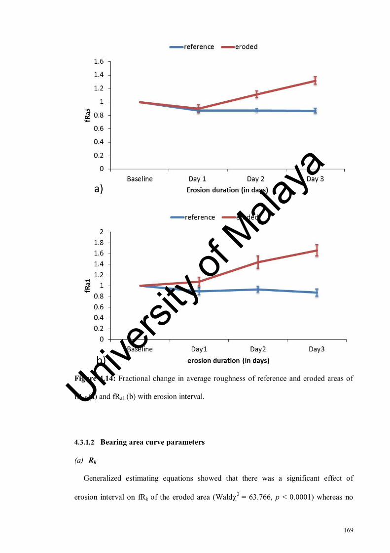
169

Figure 4.14: Fractional change in average roughness of reference and eroded areas of

fRa5 (a) and fRa1 (b) with erosion interval.

4.3.1.2 Bearing area curve parameters

(a) Rk

Generalized estimating equations showed that there was a significant effect of

erosion interval on fRk of the eroded area (Wald2

= 63.766, p < 0.0001) whereas no

Univers

ity of

Mala

ya

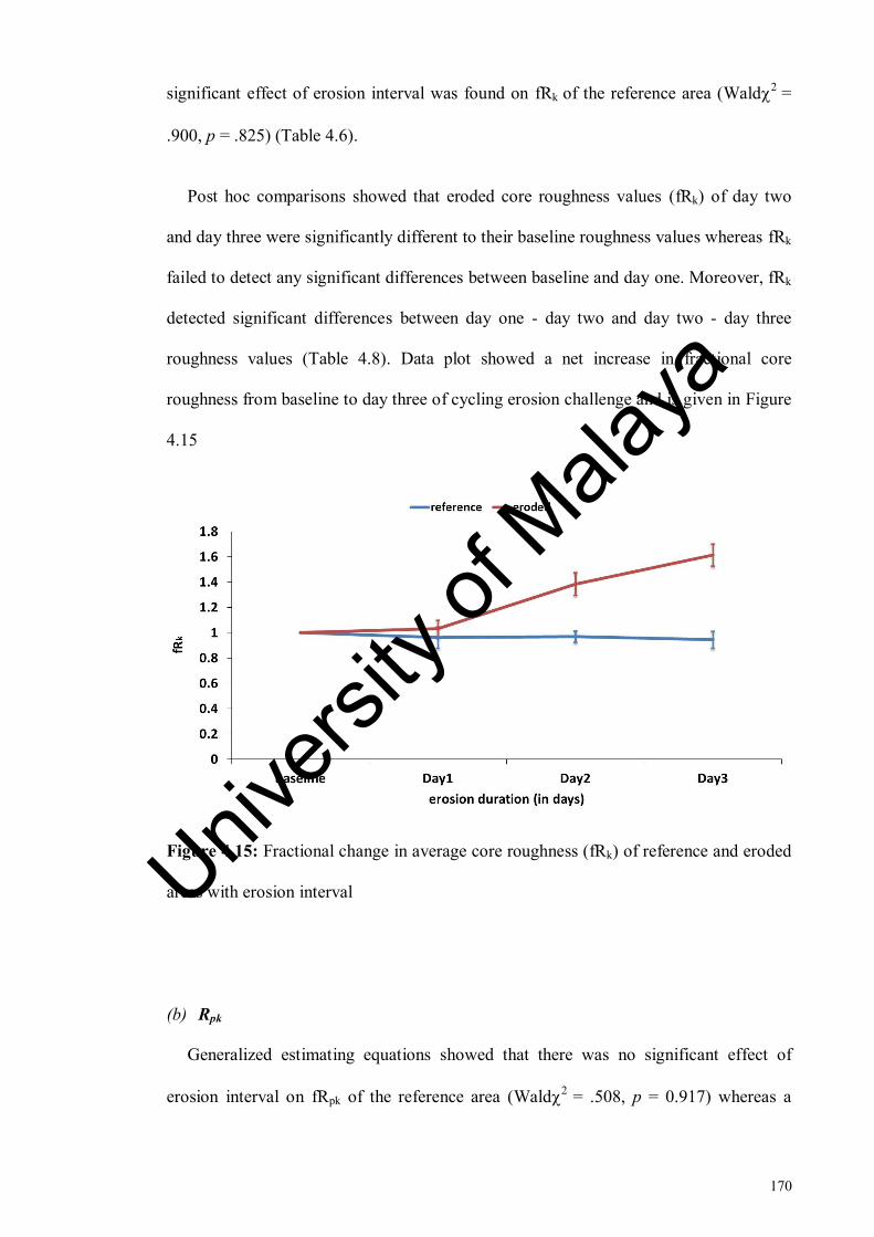
170

significant effect of erosion interval was found on fRk of the reference area (Wald2

=

.900, p = .825) (Table 4.6).

Post hoc comparisons showed that eroded core roughness values (fRk) of day two

and day three were significantly different to their baseline roughness values whereas fRk

failed to detect any significant differences between baseline and day one. Moreover, fRk

detected significant differences between day one - day two and day two - day three

roughness values (Table 4.8). Data plot showed a net increase in fractional core

roughness from baseline to day three of cycling erosion challenge and is given in Figure

4.15

Figure 4.15: Fractional change in average core roughness (fRk) of reference and eroded

areas with erosion interval

(b) Rpk

Generalized estimating equations showed that there was no significant effect of

erosion interval on fRpk of the reference area (Wald2

= .508, p = 0.917) whereas a

Univers

ity of

Mala

ya

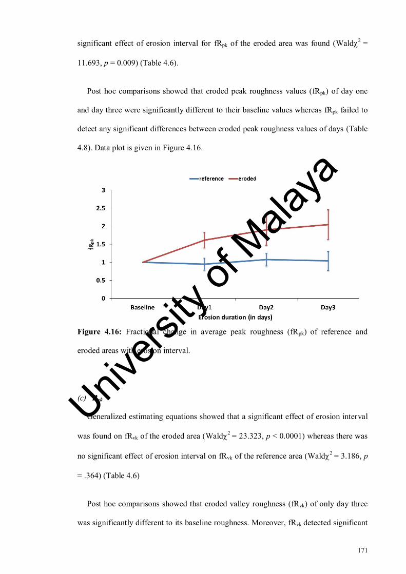
171

significant effect of erosion interval for fRpk of the eroded area was found (Wald2

=

11.693, p = 0.009) (Table 4.6).

Post hoc comparisons showed that eroded peak roughness values (fRpk) of day one

and day three were significantly different to their baseline values whereas fRpk failed to

detect any significant differences between eroded peak roughness values of days (Table

4.8). Data plot is given in Figure 4.16.

Figure 4.16: Fractional change in average peak roughness (fRpk) of reference and

eroded areas with erosion interval.

(c) Rvk

Generalized estimating equations showed that a significant effect of erosion interval

was found on fRvk of the eroded area (Wald2

= 23.323, p < 0.0001) whereas there was

no significant effect of erosion interval on fRvk of the reference area (Wald2

= 3.186, p

= .364) (Table 4.6)

Post hoc comparisons showed that eroded valley roughness (fRvk) of only day three

was significantly different to its baseline roughness. Moreover, fRvk detected significant

Univers

ity of

Mala

ya

172

differences between day two and day three roughness values (Table 4.8). Data plot is

given in Figure 4.17.

Figure 4.17: Fractional change in average valley roughness (fRvk) of reference and


(d) MR1

Generalized estimating equations showed that there was no significant main effect of

erosion interval on fMR1 of eroded area (Wald2

= 2.785, p = 0.426) whereas a

significant effect of erosion interval was detected for the reference area (Wald2

=

11.234, p = 0.011) (Table 4.6). Data plot is given in Figure 4.18.

Univers

ity of

Mala

ya

173

Figure 4.18: Fractional change in proportion of profile peaks (fMR1) of reference and


(e) MR2

Mauchly’s test showed that the assumption of sphericity was not violated for

reference (2 = 5.872, p = .320) and eroded areas (

2 = 2.826, p =.727).

One-way repeated measures ANOVA showed that there was no significant effect of

erosion interval on fMR2 of both the reference (F(3) =.188, p = .904, η2

= .01) and

eroded areas (F(3) = .240, p = .868, η2

= .013) (Table 4.7). Data plot is given in Figure

4.19.

Univers

ity of

Mala

ya

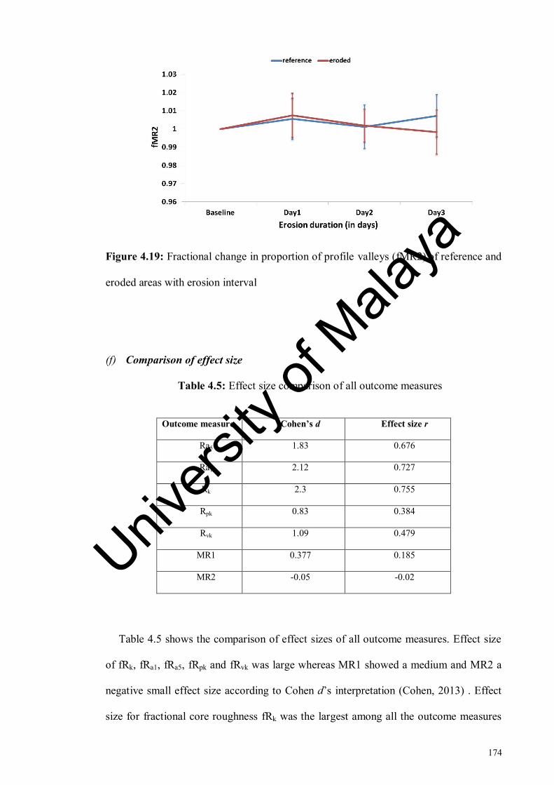
174

Figure 4.19: Fractional change in proportion of profile valleys (fMR2) of reference and

eroded areas with erosion interval

(f) Comparison of effect size

Table 4.5: Effect size comparison of all outcome measures

Outcome measure Cohen’s d Effect size r

Ra5 1.83 0.676

Ra1 2.12 0.727

Rk 2.3 0.755

Rpk 0.83 0.384

Rvk 1.09 0.479

MR1 0.377 0.185

MR2 -0.05 -0.02

Table 4.5 shows the comparison of effect sizes of all outcome measures. Effect size

of fRk, fRa1, fRa5, fRpk and fRvk was large whereas MR1 showed a medium and MR2 a

negative small effect size according to Cohen d’s interpretation (Cohen, 2013) . Effect

size for fractional core roughness fRk was the largest among all the outcome measures

Univers

ity of

Mala

ya

175

with r = 0.755, d = 2.3 followed by effect size of r = 0.727, d = 2.12 for fractional

average roughness fRa1. Moreover, fRa1 showed a larger effect size as compared to fRa5

(r = 0.676, d = 1.83).


areas of bearing area curve parameters.

Outcome

measure

Reference Eroded

Wald Chi-

Square

Degrees of

freedom

p-value

Wald Chi-

Square

Degrees

of

freedom

p-value

fRk .900 3 0.825 63.766 3 <0.0001

fRpk .508 3 0.917 11.693 3 0.009

fRvk 3.186 3 0.364 23.323 3 <0.0001

fMR1 11.234 3 0.011 2.785 3 0.426

Table 4.7: Results for repeated measures ANOVA for reference and eroded areas of

MR2.

Outcome

measure

Reference Eroded

Mean

square

F-statistic p-value

Mean

square

F-statistic p-value

fMR2 <0.0001 0.188 0.904 <0.0001 0.240 0.868

Univers

ity of

Mala

ya

176

Table 4.8: Post hoc comparisons of erosion intervals for the eroded areas of bearing

area curve parameters.

Time (I) Time (J)


fRk fRpk fRvk

Baseline Day 1 -.0306 -.6148* -.0338

Baseline Day 2 -.3851*** -.8993 -.1965

Baseline Day 3 -.6128*** -1.0465* -.8816**

Day 1 Day 2 -.3545*** -.2845 -.1627

Day 2 Day 3 -.2277** -.1473 -.6851*




Univers

ity of

Mala

ya

177

Figure 4.20: Representative profiles (a) and bearing area curves (b) of a sample at

baseline measurement. The excel sheets show the values of Ra and bearing area curve

parameters.

Univers

ity of

Mala

ya

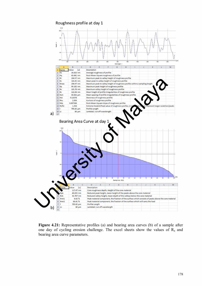
178


one day of cycling erosion challenge. The excel sheets show the values of Ra and

bearing area curve parameters.

Univers

ity of

Mala

ya

179


two days of cycling erosion challenge. The excel sheets show the values of Ra and


Univers

ity of

Mala

ya

180


three days of cycling erosion challenge. The excel sheets show the values of Ra and


Univers

ity of

Mala

ya

181

4.3.1.3 Tissue loss

Generalized estimating equations showed that no main significant effect of erosion

interval on fΔZ was detected (2

= 4.036, p = 0.258) as shown in the Table 4.9. Data

plot is given in Figure 4.24.

Table 4.9: Results for generalized estimating equations (GEE) for fΔZ

Outcome measure Wald Chi-Square Degrees of freedom p-value

fΔZ 4.036 3 0.258

Figure 4.24: Fractional change in surface loss (fΔZ) with erosion interval.

Univers

ity of

Mala

ya

182

Table 4.10: Fractional change in average roughness, bearing area curve parameters and

surface loss with respect to baseline values given at different time points. Standard

deviations are within brackets. Values in bold denote a significant effect.

Time

Point

fRa1 fRa5 fRk fRpk fRvk fMR1 fMR2 fΔZ

Day 1

1.08

(0.3)

0.9

(0.23)

1.03

(0.29)

1.61

(0.95)

1.034

(0.61)

1.16

(0.51)

1.007

(0.05)

-1.2

(6.35)

Day 2

1.44

(0.5)

1.11

(0.21)

1.39

(0.38)

1.89

(1.86)

1.20

(0.49)

1.06

(0.35)

1.001

(0.04)

2.41

(13.67)

Day 3

1.66

(0.44)

1.31

(0.24)

1.61

(0.37)

2.04

(1.78)

1.88

(1.14)

1.07

(0.30)

0.998

(0.05)

-0.29

(4.9)

4.3.2 FE-SEM

FE-SEM images showed that dentine surface in the eroded sides of the samples

(Figure 4.25, d-f), showed an overall rougher appearance. The sound dentine in contrast

was fairly smooth (Figure 4.25, a-c). Eroded side of day one image (Figure 4.25, d)

showed that the surface was partially covered with smear layer but in contrast to the

reference surface (Figure 4.25, a), the dentinal tubules were opened in patches. In day

two image (Figure 4.25, e), the border between the peritubular and intertubular dentine

was demineralised and dentinal tubules were slightly widened as compared to dentinal

tubules in day one image. In day three image (Figure 4.25, f) the dentinal tubules were

further widened. The intertubular dentine appeared to be demineralised although the

peritubular dentine was still intact in most of the tubules. Acid erosion mediated

Univers

ity of

Mala

ya

183

increase in roughness of dentine surface was observed from day one image to day three

image (Figure 4.25, d-f).

Figure 4.25: FE-SEM micrographs (1000x) of the root dentine samples. a-c show

the reference areas of samples subjected to erosion challenge for one - three days at

Univers

ity of

Mala

ya

184

1000x. d-f show the eroded areas of samples subjected to erosion challenge for one -

three days at 1000x

4.4 Discussion

This study investigated the utility of surface roughness parameters for assessment of

early dentine erosion in a clinically relevant model. Traditionally employed parameter

tissue loss (ΔZ) was also measured. Based on the findings, the original null hypothesis

was rejected and it was concluded that surface roughness parameters can be used for

monitoring the progression of early dentine erosion whereas measurement of tissue loss

was not found suitable for its assessment. Moreover, use of bearing area curve enabled

the monitoring of early dentine erosion with sensitive parameters providing a deeper

understanding of overall erosion process which could not be attained by reporting Ra

value alone.

For this study, a pH-cycling model of erosion was employed where erosion

challenges with citric acid were interspersed with periods of simulated salivary

remineralisation. The remineralisation solution employed had a composition similar to

artificial saliva but without methyl p-hydroxybenzoate and sodium carboxymethyl

cellulose. This solution was shown to be more effective than artificial saliva in

remineralising early eroded enamel previously (Amaechi & Higham, 2001b) and was

therefore adopted for this study. Stylus profilometry has the potential of damaging the

specimen surface by producing scratches as deep as 10-25 nm as measured previously

by atomic force microscopy (Beyer et al., 2012). Therefore, a non-contact profilometry

was employed for performing the measurements. It is known that the use of flat samples

increases the accuracy and sensitivity of profilometry (Schlueter et al., 2011). Therefore

the samples were flattened and polished before imaging. The flatness of the samples

Univers

ity of

Mala

ya

185

was further assessed in the baseline scan before scanning. It is critical to reposition a

specimen correctly when monitoring small erosive surface alterations (Attin, 2006).

Hence, a custom made jig was employed to ensure correct repositioning of the samples

at various measurement time points.

4.4.1 Profilometry

4.4.1.1 Average roughness

Ra is traditionally extracted as a line profile through an area and is commonly

reported as an average of several line profiles (Gomez-Lopez, 2012). However, single

line profiles are not representative of the roughness of the entire image as the overall

value may be affected by a single atypical peak or valley (Leach, 2014; Moazzez et al.,

2014). Therefore, it was decided to select areas rather than measurement lines in order

to increase the accuracy of the extraction method of Ra. Although extracted from the

same surface, multiple measurements are known to result in a range of significantly

different Ra values (Wichern & Rasp, 2005). To solve this problem, 3D parameters have

been used (Moazzez et al., 2014). 2D Ra is still the most commonly reported form of

surface roughness in dentistry (Kukiattrakoon et al., 2011) and was therefore employed

in this study. It is felt that a single large area that covers most of the image will be better

representative of the overall roughness value rather than small multiple areas.

Therefore, Ra was measured with 1) a single large measurement area (Ra1) and 2) five

small measurement areas (Ra5) and a comparison was drawn between both measurement

techniques to find the most suitable method. Generalised estimating equation analysis

showed that fRa5 of eroded area was able to monitor roughness over time but the fact

that changes in roughness of its reference area were also significant made the findings

of fRa5 unreliable. Moreover, fRa1 showed a larger effect in monitoring of early dentine

Univers

ity of

Mala

ya

186

erosion as compared to fRa5 as shown by its greater effect size value. Based on these

findings, fRa1 was found most suitable and was employed for further analysis in this

study.

4.4.1.2 Bearing area curve parameters

Bearing area curve can be used to characterise surfaces having different functional

properties at different depths (De Chiffre et al., 2000) called multi-stratified surfaces.

Assessment of multi-stratified surfaces can prove to be challenging and measurement of

these surfaces by simple parameters like Ra might not yield sufficient information (Field

et al., 2010). Dentine erosion likewise is not a simple surface process and its assessment

is a challenging task because of the presence of its organic content. Therefore, same set

of profilometric data was used to extract bearing area curve parameters in adjunct to

average roughness to assess their potential and sensitivity for monitoring of early

dentine erosion.

Results showed that fRpk was most sensitive for detection of early dentine erosion

with detection sensitivity of day one from baseline. fRpk represents the height of the

material peaks or the area which comes in contact with the acidic solution first which

explains its ability to detect erosion by the first day of cycling erosion challenge.

An erosion model is expected to exhibit deeper valleys. The deeper valleys are

expected to result from natural tendency of fluids to deposit in these areas (Las Casas et

al., 2008). The findings of this study supported this assumption. fRvk value, representing

the depth of material valleys was significantly different by day three of erosion

challenge. This would indicate that the valleys had become deeper by the pooling of

citric acid in these areas by third day of cycling erosion challenge. It could be

Univers

ity of

Mala

ya

187

speculated that this acid entrapment might be followed by more aggressive erosion in

case of continued acid challenge. However, it is important to bear in mind that a pH-

cycling model was employed for this study and every erosion challenge was

accompanied by simulated salivary remineralisation of 3 hours. In addition, the samples

were immersed in remineralisation solution overnight. Therefore, significant increase in

valley depths could also be attributed to the pooling of remineralisation solution in these

areas which could aid in resisting demineralisation in the later stages after day three of

erosion. These speculations need further investigation in a prolonged cycling erosion

protocol.

Fraction change in average roughness (fRa1) and fraction change in core roughness

(fRk) showed similar results for the eroded group with detection sensitivity of two days

from baseline. However, unlike fRk, fRa1 was not able to monitor erosion in advanced

stages between day two and day three. Effect size comparison between all roughness

parameters showed that fRk had the greatest effect size and hence could be considered

most effective in monitoring the progression of early erosion in dentine. This could

suggest the possibility of Ra being replaced by a more effective parameter like Rk in

future.

Fractional change in proportion of profile peaks (fMR1) and fractional change in

proportion of profile valleys (fMR2) were not sensitive enough to detect and monitor

early dentinal erosion. The amount of demineralisation induced in this study was

perhaps too low to have brought about a significantly different increase or decrease in

the total number of peaks or valleys between cycling days. At the same time, lesser

degree of remineralisation would be expected from the remineralisation solution

simulating saliva utilised in this study as compared to what would be expected to occur

by a treatment product. It is speculated that MR1 might be more suitable for evaluation

Univers

ity of

Mala

ya

188

of more aggressive erosion in dentine and MR2 might be used for investigation of

efficacy of treatment products or remineralising agents for dentine erosion but this area

undoubtedly requires further investigation. For this particular protocol, these

parameters did not prove to be effective for monitoring early dentine erosion

progression.

4.4.1.3 Tissue loss

Dentine when demineralised is prone to shrinkage (Zhang et al., 2009) and

profilometric measurements of dried eroded dentine will reveal a step height difference

between reference and eroded areas which is absent otherwise in controlled moisture

conditions (Ganss et al., 2009b). This step height does not represent the true mineral

loss or surface level of organic matrix (Schlueter et al., 2011) and it was recommended

that dentine samples be kept wet until measurements are performed (Attin et al., 2009;

Ganss et al., 2007). However, the profilometry system used in this study like most other

systems did not allow the samples to be profiled under wet or moist conditions. This is

because profiling of wet samples can create artifacts by parts of light being reflected by

the water (Attin et al., 2009). The effect of ambient drying on eroded dentine was

assessed and it was found that drying effects reached a plateau after 10 minutes (Ganss

et al., 2007). Therefore, samples were air dried for 10 minutes to standardise the organic

matrix shrinkage for this study as previously employed (Steiner-Oliveira et al., 2010).

Moreover, ΔZ like all other parameters was reported as fractional change with respect to

its baseline measurement (fΔZ) which could address any step height difference between

the reference and eroded areas if present at baseline measurement due to drying.

Tissue loss appearing in the form of a step change between the reference and eroded

areas is conventionally measured by profilometry (Borges et al., 2014; Charone et al.,

Univers

ity of

Mala

ya

189

2014; Paepegaey et al., 2013). However, the initial stage dental erosion is not expected

to produce a step change (Young & Tenuta, 2011) and it is speculated that this

parameter might not be effective in measuring the early stages of erosion. The results of

this study confirmed this assumption and tissue loss was not able to detect or monitor

the early dentinal erosion. This is in accordance with the previous study where non-

contact profilometry was not able to detect changes in surface loss before the digestion

of organic matrix. However, after the removal of organic matrix the mineral loss values

increased (Ganss et al., 2009b). Removal of organic matrix would render non-contact

profilometry a destructive method restricting its use for longitudinal studies and for

clinical trials. Monitoring of early dentine erosion with surface roughness parameters

would be more suitable in this regard.

4.4.2 FE-SEM

FE-SEM images were obtained to visualise the morphological changes in eroded

dentine in comparison to sound dentine in the reference areas. Moreover, the effect of

erosion in time could be visualised by comparing samples eroded for different erosion

intervals. For this study, a field-emission scanning electron microscopy (FE-SEM) was

employed which allowed the samples to be imaged after air-drying only without any

sample preparation or metallisation.

The sound dentine in reference areas of all samples showed a smooth surface covered

with smear layer (Figure 4.25, a-c). Treatment with citric acid resulted in exposure of

dentinal tubules which could be seen in day one image of eroded area (Figure 4.25, d).

However, the tubules were seen partially or completely occluded in the day one image.

It would be tempting to assume that the tubules were occluded with smear plug

remnants due to the partial removal of smear layer by citric acid. However, it is

Univers

ity of

Mala

ya

190

important to bear in mind that a cycling model of erosion was employed for this study

and tubular occlusion observed in the images could also be the result of deposition of

mineral by remineralising solution used in this study. A previous study reported that

artificial saliva deposited mineral on eroded dentine and dentinal tubules were occluded

or partially occluded as result of it (Vanuspong et al., 2002) however authors found that

this deposit was lost after ultrasonication . This is in accordance with our study and it

could be speculated that at day one, the dentinal tubules were opened as a result of

exposure to citric acid. But then the samples were immersed for 3 hours in

remineralising solution after every erosion challenge and overnight. This partially

occluded the opened dentinal tubules as a result of deposition of mineral. However, this

deposit can be assumed to be partially or completely removed with every erosion

challenge until the effect of erosion induced overcame the effect of remineralisation and

deposition of mineral with remineralisation solution could offer little protection. In day

two image of eroded area ((Figure 4.25, d), demineralisation of peritubular dentine at

the border between the peritubular and intertubular dentine was obvious and dentinal

tubules were slightly widened in comparison to reference dentine and eroded dentine in

day one image. In day three image (Figure 4.25, f) the dissolution of peritubular dentine

was obvious and dentine tubules were observed to be further widened as a result of it.

The intertubular dentine appeared to be demineralised and the overall surface appeared

roughened and porous in day three image (Figure 4.25, e) as previously reported

(Meurman et al., 1991).

All the surface roughness parameters except for fMR1 and fMR2 showed an increase

in roughness from baseline to day three of cycling erosion. This was confirmed by the

FE-SEM images which showed considerable roughening on the surface of dentine

especially at day three. This is in line with the previous studies which reported that

Univers

ity of

Mala

ya

191

dentine surface becomes rougher when eroded (Azzopardi et al., 2004; Meurman et al.,

1991; Mirkarimi & Toomarian, 2012).

Surface profilometry has the potential of being employed in clinical studies as shown

previously (West et al., 1998; Whitehead et al., 1997). Use of parameters sensitive to

early changes in erosion process would aid in the assessment of early dentine erosion

and its proposed treatment strategies in clinical trials. Also, the in vivo capability of this

method would make it a potential quantitative reference method to validate the findings

of newer non-invasive techniques in erosion studies. Based on our findings, it is

recommended that a combination of bearing area curve parameters Rpk and Rk be used

for the longitudinal monitoring of early dentine erosion within the limitation of the

current model. Rpk is most suitable for assessment of early erosion challenge and Rk for

monitoring of subsequent erosion challenges between day one- day two and day two –

day three. Rvk might aid in testing the efficacy of anti-erosion treatment products and/or

development of any remineralisation-associated resistance.

4.5 Conclusions



1. Average surface roughness, fRa1 and bearing area curve parameters, fRk (core

roughness), fRpk (peak roughness) and fRvk (valley roughness) were able to

detect and longitudinally measure early dentine erosion. fMR1, fMR2

(Fractional change in proportion of profile peaks and profile valleys

respectively) and fΔZ (surface loss) were not able to detect and measure early

dentine erosion.

Univers

ity of

Mala

ya

192

2. fRk showed the greatest magnitude of strength in measuring early dentine

erosion as determined by its largest effect size.

3. The early dentine erosion detection threshold of surface roughness varied with

different parameters. fRpk showed a detection threshold of day one from baseline

measurement. fRk and fRa1 were able to detect erosion by day two from baseline

measurement. fRvk showed a detection threshold of day three from baseline

measurement.

4. FE-SEM images supported the surface roughness results. FE-SEM images of the

eroded areas of samples showed increase in overall roughness of dentine surface

during erosion progression. Continuous rise of roughness shown by fRa1, fRk,

fRpk and fRvk in relation to the incubation time in acid was obvious.

The null hypotheses were rejected as shown below,

1. Surface roughness parameters fRpk, fRk, fRa1 and fRvk can be used to measure

early dentine erosion progression for three days in simulated intraoral conditions.

2. Bearing curve parameters fRpk and fRk are more sensitive than fRa1 in measuring

early dentine erosion in simulated intraoral conditions.

Univers

ity of

Mala

ya

193


OPTICAL COHERENCE TOMOGRAPHY IN A SIMULATED INTRAORAL

CONDITION

This chapter describes the assessment of early eroded dentine with optical coherence

tomography (OCT) in a simulated intraoral environment and is a continuation of the

study conducted in chapter 4. Same samples were employed in both studies for

comparison purposes. Therefore, the findings of optical coherence tomography were

compared with the surface roughness measurements made with profilometry and

ultrastructural changes acquired with field-emission scanning electron microscopy (FE-

SEM). An introduction to the research purpose is followed by a review of various

conditions necessary for modelling simulated intraoral environment in erosion studies.

5.1 Introduction

Researchers investigate real-world phenomena by creating simulation study models

which enables them to explain the various aspects of those phenomena (Nersessian,

2009). Over the years, extensive research has been carried out to investigate dental

erosion using different study models.

Ideally it is desirable to conduct clinical trials to evaluate the erosion process and its

subsequent prevention. However, due to various challenges encountered in measuring

erosion in the in vivo settings (Attin, 2006) as well as the ethical considerations

involved in the induction of significant levels of erosion clinically (Huysmans et al.,

2011), a number of in vitro and in situ models have been developed and used.

In vitro models are important in erosion studies because they aid in understanding the

process of erosion, help in assessment of measurement techniques and efficacies of the

Univers

ity of

Mala

ya

194

proposed treatment strategies for arresting the progression of erosion. In these models

tightly standardised experimental conditions can be implemented, the effect of variables

can be examined individually or in combination and precise measurement techniques

can be employed to assess the alterations in dental hard tissues caused by the process of

erosion. These models are relatively inexpensive and can be performed in shorter

periods of time (West et al., 2011). Well designed in vitro models provide valuable data

that closely matches with the clinical situation without the fear of causing any harmful

effects to individuals.

Dental erosion is known to interact with the other aspects of tooth wear, which are

attrition and abrasion and it is hard to separate them clinically. Therefore the interaction

of these three processes has been studied widely with in vitro studies in order to

determine the role of each process in the net outcome of wear and their interaction with

each other. Depending on the objective of a study, each component has been studied

either individually or in combination by the help of in vitro or in situ studies (Paepegaey

et al., 2013). During the initial stages of erosive wear, softening caused by initial acid

attack makes the tooth surface vulnerable to mechanical wear. Hence it is important to

understand the process of erosion independently in order to be able to control the

progression of this condition.

OCT showed the potential of monitoring the progression of early dentine erosion as

discussed in chapter 3 of this thesis. However, the potential of OCT in monitoring the

progression of early dentine erosion in simulated erosion conditions was unknown. The

simulated oral environment was created by adopting a cycling model of erosion.

Univers

ity of

Mala

ya

195

5.1.1 Cycling and non-cycling models

The term ‘cycling’ has been used interchangeably in erosion studies to mean either

erosion models in which the acid challenges are interspersed with periods of exposure to

remineralising medium or models with cyclic alternation of erosion with abrasion or

attrition (Addy & Shellis, 2006). The former cycling models have been used to mimic

the intraoral conditions where the erosion process is modulated by the presence of saliva

while the latter cycling models attempt to mimic the clinical interaction between the

mechanical wear processes of attrition and abrasion with erosion. The scope of this

review is the former and in order to differentiate it from the latter, the term ‘pH-cycling’

will be used henceforth and by non pH-cycling models, we mean the erosion models

that do not have a remineralisation phase and only involve the exposure of the substrate

to acid challenges. The primary aim of these pH-cycling models is to simulate the

natural repair process that takes place in the oral cavity during erosion challenges

(Shellis et al., 2011) as results attained from non pH-cycling models, arguably, could

not be extrapolated into the clinical scenario.

Review of literature reveals that there is lack of consistency in the design of erosion

models that makes the comparison of different study outcomes difficult. Although the

use of pH-cycling in dental erosion studies has repeatedly been recommended in the

literature (Shellis et al., 2011; Young & Tenuta, 2011) especially when the phenomenon

of remineralisation related to dental erosion is to be investigated (West et al., 2011),

currently there are no guidelines or consensus as to when and how it should be used.

5.1.2 Erosion pH-cycling models

Generally the in vitro erosion pH-cycling models can be classified into

demineralisation or remineralisation models depending on the loss or gain of minerals

Univers

ity of

Mala

ya

196

occurring in the erosion challenge or treatment respectively. Demineralisation models

are usually employed to analyse the loss of mineral in sound substrate under erosive

conditions or to assess the degree of further demineralisation of lesions which were

already eroded. Remineralisation models deal with the assessment of mineral gain in

eroded lesions as a result of application of different treatment products (Buzalaf et al.,

2010) or assess the ability of various treatment formulations in increasing the resistance

of sound tooth substrate against the initiation and progression of acid induced damage

(Faller et al., 2011; Yamashita et al., 2013). Cycling can be brought about either by

transferring samples manually between the erosive and remineralising media or

automated set-ups such as the artificial mouth models (Attin et al., 2003; Attin et al.,

2005c) which enable intermittent episodes of demineralisation and remineralisation to

be performed more efficiently and meticulously.

The erosion pH-cycling model is made up of a demineralising and a remineralising

arm. Each of these two arms by itself comprises of three components, the de- or

remineralising agent, the time factor and the environment (stirring). Previous

comprehensive reviews had addressed the factors related to demineralising arm in detail

such as for in vitro Erosion / Abrasion studies (West et al., 2011; Wiegand & Attin,

2011; Young & Tenuta, 2011) , however the remineralising arm has been less reviewed.

5.1.3 Substrate

Generally, samples of enamel (Faller et al., 2011; Murakami et al., 2009), or dentine

(Cruz et al., 2012; Karlinsey et al., 2011; Wang et al., 2013) obtained from bovine

incisors, human premolars and third molars have been used as substrates in pH-cycling

erosion studies. Sometimes both enamel and dentine samples have also been assessed in

the same experiment (Piekarz et al., 2008; Scaramucci et al., 2011) which probably

Univers

ity of

Mala

ya

197

offers greater advantage since it aids in making comparisons between these dental hard

tissues simultaneously.

Moreover, sound substrate is usually employed in the in vitro erosion studies which

can then be subjected to a variety of artificially induced erosive challenges depending

on the protocol. This explains the frequent use of human premolars or third molars

which extracted for orthodontic or surgical purposes respectively are available in

relatively conserved state. However, the fact that partially erupted or impacted teeth can

be more porous and hence more susceptible to demineralisation than other permanent

teeth, should be taken into account during comparison of different studies (Buzalaf et

al., 2010).

Primary teeth have rarely been employed in pH-cycling erosion studies probably

because of the difficulty in acquiring them, and the smaller area they present for

handling during experiments (Buzalaf et al., 2010). The erosion rates in primary enamel

as compared to permanent enamel have been reported to be higher by some authors

(Hunter et al., 2000a) whereas others did not find any significant differences (Addy &

Shellis, 2006; Hunter et al., 2000b; Lippert et al., 2004b). However, this conflicting data

may have arisen because substrates of different developmental and post-eruptive ages

were employed in these experiments. Hence, while selecting primary teeth for erosion

experiments, special consideration should be paid to their developmental ages as it is

known to affect the progression of the erosion rate (Murakami et al., 2009).

Ideally, it is preferable to use human teeth in erosion experiments from the

perspective of clinical relevance, but due to the ethical issues involved and difficulties

posed in acquiring sound human teeth, bovine teeth have also been frequently used.

Somewhat inconsistent outcomes have been drawn from the studies investigating and

comparing human and bovine teeth (Yassen et al., 2011). Moreover, bovine teeth have

Univers

ity of

Mala

ya

198

been known to exhibit greater porosity and as a result greater response to erosion

challenge (Wang et al., 2012) . In spite of this, bovine teeth have been considered as

acceptable substitutes for human teeth in erosion experiments (Venasakulchai et al.,

2010; Young & Tenuta, 2011).

5.1.4 Polishing and sample preparation

Although natural surfaces of teeth from the viewpoint of clinical relevance would

make ideal substrates for erosion experiments, yet polished samples have been used in

majority of erosion studies mainly because most of the methods available currently for

measurement of dental erosion (such as profilometry, surface microhardness,

nanohardness) require sample preparation and polishing for maximum precision. But it

should also be considered that during the intraoral erosion challenge, the outer surface

of the natural teeth gets removed by the effect of acid, producing smooth polished

surfaces (Attin, 2006) and the use of polished substrate also aids in reducing the

experimental time by abolishing the more variable natural surface (Young & Tenuta,

2011). However, the fact that polished enamel is more susceptible to erosion than

natural enamel should be taken into consideration while interpreting the study outcomes

(Ganss et al., 2000; Lippert et al., 2004a).

Further, a number of factors need to be considered while preparing the samples for

erosion studies. Structural variations in erosive lesions in enamel specimens prepared

from the same as well as different teeth have been observed (Meurman & Frank, 1991).

This problem can be minimised by random distribution of samples. Additionally, as

radicular dentine has shown to be less susceptible to the effect of acid as compared to

coronal dentine, samples from crown and root dentine should never be combined during

an experiment (Ganss et al., 2000).

Univers

ity of

Mala

ya

199

5.1.5 Demineralising agent

The source of acid causing dental erosion could either be extrinsic or intrinsic in

origin. Extrinsic sources are mainly from food and beverage such as soft drinks, citrus

fruit juices and pickles and less frequently, from occupational exposure to acid vapour

in battery factories or in wine tasters. Intrinsic factors are those chronic diseases or

habits that cause frequent regurgitation of acidic stomach contents. These include

gastroesophageal reflux disease (GORD), eating disorders, chronic vomiting and

rumination (Johansson et al., 2012). Therefore, these acids had been employed as

demineralising agents in erosion studies either in pure form or as inherent acids in soft

drinks (Cheng et al., 2009a). Citric acid being the main inherent acid in acidic beverages

had most frequently been employed for induction of erosion challenge in pH-cycling

erosion models. The other less frequently used acids are phosphoric acid, hydrochloric

acid and maleic acid (Addy, 2005; Addy & Hunter, 2003; Faller et al., 2011). Acids in

inherent form have the advantage of providing more realistic testing but at the same

time are known to vary between batches in terms of pH, concentration and buffering

capacity of the formulation. This could produce variation in the data especially in the

cycling models where the demineralising agent is to be used several times during the

study and standardisation of its formulation is critical. On the other hand, plain acids (in

pure form) are far easier to formulate, reproduce and produce consistent responses

throughout the study (Shellis et al., 2011). Therefore, it is felt that when it comes to

prolonged cycling in erosion pH-cycling models, it is better to use an acid in pure form

rather than a commercial acidic drink.

Further, the inclusion of a standard acid solution for assessment of the employed

methodology has been recommended. The pH and concentration of acid which also

determine the buffering capacity of the acid should fall in clinically relevant ranges

Univers

ity of

Mala

ya

200

according to the type of erosion challenge being simulated (Shellis et al., 2011; Young

& Tenuta, 2011).

5.1.6 Remineralising agent

Dental erosion is a multifactorial condition and involves an interplay of biological,

chemical and behavioural factors (Lussi & Jaeggi, 2008). Saliva is the most important

biological factor affecting dental erosion and influences the rate and progression of

dental erosion through the properties of salivary clearance, pellicle formation, buffering

capacity and its ability to remineralise the eroded tissues by the provision of various

minerals necessary for remineralisation of tissues (Buzalaf et al., 2012a). These

characteristics make the incorporation of saliva in pH-cycling models necessary where

simulation of clinical erosion is critical. The medium used for interim storage of

samples in pH-cycling models can be human natural saliva or simulated salivary fluids

such as artificial saliva and remineralisation solution.

Natural saliva is composed mainly of organic and inorganic components. The

inorganic components include a variety of minerals that play a vital in the process of

erosion. Acid challenge leads to demineralisation and softening of dental hard tissues

and salivary calcium and phosphate serve to remineralise these tissues. They act as

common ions to the tooth mineral and aid in maintenance of tooth integrity by slowing

down the rate of mineral dissolution after an erosive challenge. Moreover, substantial

enhancement of remineralisation is known to occur in the presence of fluoride ions.

Bicarbonate is linked to the buffering capacity of saliva which plays an important role in

neutralisation and buffering of dietary acids (Al-Malik et al., 2002; Buzalaf et al.,

2012a). Neutralisation of acids by saliva directly affects the amount of mineral lost from

dental hard tissues during an erosion challenge. The longer it takes for saliva to buffer

Univers

ity of

Mala

ya

201

the incoming dietary acids, the more mineral loss occurs from the tooth structure (Lussi

et al., 2011).

The storage medium employed in erosion studies should ideally be able to replicate

the intraoral salivary functions modulating the process of erosion. That is why various

recipes of artificial saliva and remineralisation solutions employed in erosion studies

have incorporated the electrolyte component of natural saliva.

The organic component of natural saliva is mainly composed of salivary proteins and

glycoproteins. The main role these proteins play in the process of erosion is through the

formation of pellicle. Pellicle is a protein-based bacteria-free layer formed on the

surfaces of teeth immediately after brushing with dentifrice, prophylaxis or chemical

dissolution (Hara et al., 2006b; Moazzez et al., 2014). It is known to adhere to the tooth

surfaces and provides protection against dental erosion by acting as a perm-selective

membrane hampering the contact of acid with tooth surface, thus preventing dissolution

of dental hard tissues. However, it has also been claimed to reduce the remineralisation

process overall although it might encourage some subsurface remineralisation (Hara et

al., 2006b; Young & Tenuta, 2011). Salivary proteins such as proline-rich proteins,

statherin and histatins play an important role in the formation of salivary pellicle. In

addition, salivary mucins have been known to contribute greatly to provide protection

against enamel erosion by the formation of the acquired pellicle. It is important to note

that the recipes of artificial saliva and remineralisation media do not have an organic

component and hence cannot be expected to allow the adequate formation of salivary

pellicle (Lussi & Carvalho, 2014; Smith & Knight, 1984). Therefore, it is

recommended that if the effect of pellicle is to be investigated in pH-cycling models,

then either natural saliva is to be used or organic component be added to the artificial

storage media.

Univers

ity of

Mala

ya

202

The other important function of salivary proteins is the formation of complexes with

minerals. Statherin and proline-rich proteins are known to bind and prevent the

precipitation of calcium phosphate thus allowing the saliva to maintain its state of

supersaturation with respect to calcium and phosphate salts (Buzalaf et al., 2012a) . This

could lead to greater remineralisation in the in vitro models as compared to in vivo

models. This is because salivary proteins are usually lacking in artificial storage media

employed in the in vitro models. Moreover, some salivary proteins are known to bind

calcium. Recipes of artificial saliva and remineralisation solutions used in erosion pH-

cycling models are based on mineral composition of natural saliva and lack salivary

proteins. Hence, there is always a chance that these artificially formulated solutions

might exhibit too high a degree of supersaturation due to precipitation of calcium

phosphate salts. It has therefore been recommended that the concentration of calcium in

artificial saliva and remineralisation mediums be adjusted accordingly (Shellis et al.,

2011).

Although, exposure of samples to natural saliva in erosion experiments would be the

ideal case scenario, it can also pose a set of problems. Firstly the experiment might

require saliva in large quantities, the collection of which might prove to be quite time

consuming and tedious. Moreover, early decomposition or alteration of natural saliva in

erosion experiments, risk of cross-infection and high intra- / inter-sample variability are

some of the challenges encountered while using natural saliva. Therefore, the use of

artificial saliva has been considered acceptable (West et al., 2011; Wiegand & Attin,

2011).

However, it was shown that a remineralisation solution was better at remineralising

early eroded enamel lesions as compared to artificial saliva (Amaechi & Higham,

2001b) The remineralisation solution used in the study had the same composition as that

Univers

ity of

Mala

ya

203

of artificial saliva with the exception of methyl p-hydroxybenzoate and sodium

carboxymethyl cellulose. The former acts as a preservative whereas the latter is added to

increase the viscosity of artificial saliva to simulate natural saliva. Sodium

carboxymethyl cellulose (CMC) had also been shown to limit the remineralisation

potential of artificial saliva (Ionta et al., 2014). This decrease in remineralisation

potential of artificial saliva had been attributed to the property of CMC to form

complexes with calcium and phosphate ions as well as causing an increase in viscosity

thereby reducing the diffusion rate of solution. Therefore, a properly formulated

remineralisation solution or artificial saliva containing calcium, phosphate and fluoride

in appropriate concentrations at a neutral pH but without CMC could also be used in the

erosion pH-cycling models instead of natural saliva (Amaechi & Higham, 2001b).

5.1.7 Time

The duration of erosion challenge should be in a clinically relevant range. An erosion

challenge of ten minutes has been adopted by researchers to simulate the effect of

extrinsic erosion as it represents the time frame of consumption of a can of soft drink or

juice (Faller et al., 2011) whereas erosion protocols with erosion challenge of five

minutes have mimicked the erosion challenge in individuals at high risk for dental

erosion (Cruz et al., 2012) such as patients with eating disorders involving repeated

vomiting (Schlueter et al., 2010).

It is important to note that for simulation of initial erosion, shorter acid challenges

should be induced to prevent the occurrence of bulk tissue loss keeping in consideration

that erosion caused must always be detectable by the method chosen to measure erosion

(Young & Tenuta, 2011).

Univers

ity of

Mala

ya

204

5.1.8 Environment

Generally, the erosive agents are stirred at a particular rate during erosion

experiments. This is to simulate the swishing of the drink or acid within the oral cavity

in clinical erosion. An increase in agitation of the drink will aid in renewing the solution

on the surface of the layer of liquid lying adjacent to the tooth, thus causing it to become

under saturated with respect to tooth mineral, thereby increasing the dissolution process

of dental hard tissues (Lussi & Jaeggi, 2006). Also, the agitation rate influences the

dissolution rate of tissues by altering the thickness of diffusion layer. Usually an

increase in agitation will decrease the thickness of this layer and also the degree of

saturation at the tooth-tissue interface. Agitation can be achieved with a calibrated

stirrer, rotary mixer, orbital shaker or a chamber pumping the solution at a particular

rate (Barbour et al., 2011; Shellis et al., 2011; West et al., 2011). As stirring rate is

known to greatly influence the outcome of the erosion experiments (Young & Tenuta,

2011) therefore it is recommended that it should be clearly reported in publications in

terms of revolution rate / minute instead of just gentle or continuous agitation.

Moreover, in order to fully simulate the intraoral situation, the stirring rate should be the

value at which the samples do not move whereas the solution remains uniformly stirred

at all times during the experiment. This will help mimic the clinical situation where

drink swishes around the teeth whereas the teeth remain stable.

Since saliva remains stimulated only for short periods clinically when the acid enters

the oral cavity, therefore stirring of storage medium for longer periods should be

avoided. However for in vitro models involving short-term exposures to saliva, (Panich

& Poolthong, 2009) the saliva could be stirred mimicking the intraoral situation where

teeth are exposed to saliva stimulated by the acid challenge.

Univers

ity of

Mala

ya

205

5.1.9 Temperature

Temperature also affects the erosion rate significantly and hence should be controlled

with a water bath, incubator or calibrated devices. Usually the temperature of the

erosive agent is kept constant at 36˚C, mimicking the intraoral temperature or 37˚C,

simulating the body temperature. Since body temperature is known to vary

geographically, a constant temperature of 25˚C has also been suggested. In general,

erosion has been known to increase with increasing temperature (Shellis et al., 2011;

West et al., 2011).

5.1.10 Timing of measurement

In the erosion studies aiming to ascertain the overall changes induced in enamel or

dentine by erosion challenge or by various treatment strategies (Attin et al., 2003; Faller

et al., 2011), the measurements are obtained at the beginning and end of pH-cycling.

However, in monitoring protocols where the progression of loss or gain of mineral is to

be assessed for example to validate new instruments for monitoring of enamel or

dentine erosion or for monitoring of efficacy of treatment products, the measurements

have to be obtained at regular intervals such as after every cycling day.

In this case, it remains questionable whether to obtain measurements directly after

erosion challenge or the next day after the samples had been stored in saliva overnight.

Because clinically the teeth always get exposed to saliva after erosion challenge, it only

makes more sense if the measurements are obtained at the end of one complete erosion

cycle which would include overnight storage in saliva as well. Therefore it is

recommended that the measurements be obtained after the completion of erosion cycle

(including overnight salivary storage) in erosion cycling models.

Univers

ity of

Mala

ya

206

5.1.11 Recommendations / Conclusions

1. It is advisable to employ pH-cycling in erosion studies as these models simulate the

clinical erosion challenge more closely.

2. The experimental details of various parameters employed should be clearly

reported.

3. In order to mimic the intraoral erosion challenge, stirring rate should be the value at

which the samples do not move whereas the solution remains uniformly stirred at

all times during the experiment.

4. Stirring of saliva for longer periods should be avoided; however saliva can be

stirred in models involving short term exposures to saliva after acid challenge.

5. It is better to use a pure (plain) acid for prolonged pH-cycling in erosion models in

order to keep the formulation of acid standardised throughout cycles.

6. Both artificial saliva and remineralisation media can be used in erosion cycling

models instead of natural saliva.

7. If the effect of pellicle is to be investigated in cycling models, then either natural

saliva be used or organic component be added to the artificial storage media.

8. Greater remineralisation is expected to occur in in vitro models as compared in vivo

settings if artificial storage media have been used instead of natural saliva (As in

vivo some salivary proteins inhibit calcium phosphate).

9. The concentration of calcium in artificial saliva and remineralisation solution is to

be adjusted keeping in consideration that certain salivary proteins bind calcium in

vivo.

10. It is advisable to remove sodium carboxymethyl cellulose from the artificial saliva

formulations as it had been shown to limit the remineralisation potential of artificial

saliva.

Univers

ity of

Mala

ya

207

11. Erosion cycle would be incomplete without overnight storage in saliva; therefore it

is recommended that measurements be obtained on the next morning in erosion

cycling models.

5.1.12 Aim

As a necessary step before the clinical trials, this study aimed to assess if optical

coherence tomography is a sensitive tool to detect early dentine erosion and monitor its

progression in simulated intraoral conditions (using salivary simulated remineralisation

solution) by correlating OCT data with surface roughness data.



quantum in simulated intraoral conditions.

2. To identify the optimum outcome measure for measuring early dentine erosion


3. To identify the detection threshold of OCT for early dentine erosion in simulated



simulated intraoral conditions with surface ultrastructural changes.


simulated intraoral conditions with surface roughness measurements.


1. OCT is not able to detect early dentine erosion in simulated intraoral conditions.

Univers

ity of

Mala

ya

208

2. OCT is not able to measure the progression of early dentine erosion in simulated


3. There is no correlation between profilometric surface roughness measurements

and OCT backscattered changes.


5.2.1 Pilot study

A pilot study was performed before the execution of the main experiment. The

objective of this pilot study was to determine the optimum duration of dentine exposure

to acid, producing early dentine erosion without any bulk surface loss. Three root

dentine samples were prepared and polished as explained before (Section 4.2.2.1). The

samples were immersed in 0.3% citric acid (pH = 3.2) (A&C American Chemicals Ltd.,

North Carolina, USA) for 10 minutes three times a day for three days. The temperature

of the solution was kept constant at 36°C and the speed of citric acid was kept constant

at 300 revolutions per minute (rpm) during the erosion phase of the cycling throughout

the experiment. In between erosive challenges and overnight, the samples were stored in

remineralisation solution (A&C American Chemicals Ltd., North Carolina, USA). After

three days of cycling erosion challenge, no visible step change was discerned in the

OCT images as shown in the Figure 5.1. Univers

ity of

Mala

ya

209

Figure 5.1: OCT B-scans of a root dentine sample at (a) baseline, (b) after three days of

cycling erosion challenge. Red line at the center indicates the border between the

reference and eroded areas. The arrows indicate the backscattered intensity

(demineralisation) at the surface of eroded dentine sample. No visible step change was

discerned at the border between the reference and eroded areas.

Univers

ity of

Mala

ya

210



Figure 5.2: Experimental design of the study.

5.2.3 OCT

5.2.3.1 Measurements with OCT

Same 20 root dentine samples were used for the experiments described in chapter 4

and chapter 5. Therefore the details of the sample preparation and erosive pH-cycling

Univers

ity of

Mala

ya

211

have been previously described (Section 4.2.2.1 and Section 4.2.2.2 respectively). After

measurements with non-contact profilometry were performed (detailed in chapter 4), a

commercially available OCT system (OCS1300SS Thorlabs Ltd., USA) was used to

capture three dimensional OCT data of the exposed window of the dentine samples.

This OCT system has a high-speed frequency swept laser centered at 1325 nm. It has a

transverse resolution of 11 µm and an axial resolution of 9 µm in air according to the

manufacturer. This axial resolution would correspond to about 6 µm in dentine as the

refractive index of dentine is 1.54. The probing head was mounted with the beam facing

downwards. The probe was set at a distance of 1 cm from the sample surface, with the

scanning beam oriented at 0 degrees to the sample surface. The samples were placed on

a translational stage perpendicular to the probe. The stage was fixed with a custom

made jig that enabled the samples to be repositioned to the same position and alignment

during the different measuring time points. This jig was also capable of tilting the

samples to a certain angle to reduce the specular reflection.

The Thorlabs OCT capturing software was used for capturing the images and

controlling the OCT settings and the light beam. The transverse resolution of the X-axis

was set at 1024 pixels in 5 mm and Y-axis at 96 pixels in 2 mm as for the previous

study (chapter 3). The axial resolution of the Z-axis was set at 512 pixels in 3 mm in air

or 1.9 mm in dentine (refractive index of dentine is 1.54) . With these settings a total of

96 B-scans were generated for each 3D image. The (x, y) coordinate of the light beam

for each sample was recorded for replication at consecutive measuring time points.

Other parameters such as brightness and contrast were kept constant for all samples.

The inbuilt ruler within the system software was used to standardise the height of each

image. Background noise was removed before the acquisition of each image.

Univers

ity of

Mala

ya

212

Each resin-mounted sample was removed from its container (containing

remineralisation solution) immediately before scanning and dried with dental syringe

for 20 seconds at a distance of 10 cm. In order to ensure the repeatability of the OCT

scan at various time points, the specimens were placed at the same orientation as

accurately as possible. After adjusting all the system settings in the B-scan mode, a 3D

scan was performed for the pre-determined area of interest containing both the reference

and eroded area within the exposed window on each sample. All the samples were tilted

at 20 degrees to reduce the specular reflection from the surface of the specimen on the

OCT image.

The measurements with OCT were performed at baseline and repeated at the end of

every cycling day including the overnight storage in remineralisation solution (A&C

American Chemicals Ltd., North Carolina, USA) for a total of three consecutive days.

5.2.3.2 Data processing

A program was written in MATLAB (The MathWorks, Inc., USA) to load the OCT

C scan (3D scan) images and analyse the changes of the backscattered light intensity in

time. C scans of each sample from different measuring time points were aligned to

reach a horizontal surface corresponding to the tooth-air interface. Each aligned image

consisted of a reference and an eroded area. Regions of interest were selected on each

aligned image in the reference and eroded sections of the image. Each region of interest

was restricted to 7500 A-scans in order to standardise the area being analysed. In order

to standardise the analysis further, all four time points of each sample were aligned in a

similar manner and identical regions of interest were loaded for them. A-scans were

then generated from the regions of interest selected for both the reference and eroded

areas and intensity values were exported automatically to excel sheets.

Univers

ity of

Mala

ya

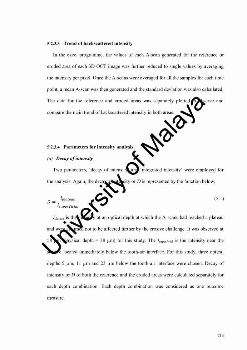
213


In the excel programme, the values of each A-scan generated for the reference or

eroded area of each 3D OCT image was further reduced to single values by averaging

the intensity per pixel. Once the A-scans were averaged for all the samples for each time

point, a mean A-scan was then generated and the standard deviation was also calculated.

The data for the reference and eroded areas was separately plotted to observe and

compare the main trend of backscattered intensity in both areas.

5.2.3.4 Parameters for intensity analysis

(a) Decay of intensity

Two parameters, ‘decay of intensity’ and ‘integrated intensity’ were employed for

the analysis. Again, the decay of intensity or D is represented by the function below,

𝐷 =𝐼𝑝𝑙𝑎𝑡𝑒𝑎𝑢


(5.1)

Iplateau is the intensity at an optical depth at which the A-scans had reached a plateau

and were assumed not to be affected further by the erosive challenge. It was observed at

58 µm (physical depth = 38 µm) for this study. The Isuperficial is the intensity near the

surface located immediately below the tooth-air interface. For this study, three optical

depths 5 µm, 11 µm and 23 µm below the tooth-air interface were chosen. Decay of

intensity or D of both the reference and the eroded areas were calculated separately for

each depth combination. Each depth combination was considered as one outcome

measure.

Univers

ity of

Mala

ya

214

Figure 5.3: Illustration of the calculation of decay of intensity between optical depths of

23 µm and 58 µm. Figure shows the mean depth-resolved intensity profile (A-scan) of

the first 120 µm for the eroded area of the sample. Each line plot represents the OCT




intensity between 23 µm and 58 µm.

(b) Integrated intensity

Additionally, the OCT backscattered intensity was integrated from the dentine

surface to plateau. The mean integrated intensity, R was calculated from superficial

optical depths of 5 µm, 11 µm and 23 µm to 58 µm and is described by the function

below;

R = ∑ (Isuperficial : Iplateau ) x Z (5.2)

With Z being the differential distance between the two physical depths

Univers

ity of

Mala

ya

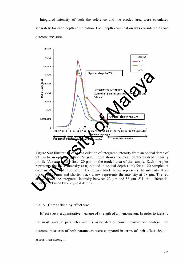
215

Integrated intensity of both the reference and the eroded area were calculated

separately for each depth combination. Each depth combination was considered as one

outcome measure.

Figure 5.4: Illustration of the calculation of integrated intensity from an optical depth of

23 µm to an optical depth of 58 µm. Figure shows the mean depth-resolved intensity






distance between two physical depths.


Effect size is a quantitative measure of strength of a phenomenon. In order to identify

the most suitable parameter and its associated outcome measure for analysis, the

outcome measures of both parameters were compared in terms of their effect sizes to

assess their strength.

Univers

ity of

Mala

ya

216

The effect size of all outcome measures were compared by partial eta square values

generated by SPSS, version 22 (IBM SPSS Statistics 22.0 Inc., USA) as part of repeated

measures ANOVA analysis.

5.2.3.6 Correction with reference

In order to assess the stability of outcome measures (depth combinations) and to

identify any instrumental variations in time, the data for each outcome measure was

corrected for eroded area at each time point with the function given below:

𝐷𝑎𝑡𝑎𝐸 𝑐𝑜𝑟𝑟𝑒𝑐𝑡𝑒𝑑(𝑡) = 𝐷𝑎𝑡𝑎𝐸𝑎𝑏𝑠𝑜𝑙𝑢𝑡𝑒(𝑡)/𝑘(𝑡)

(5.3)

Where 𝐷𝑎𝑡𝑎𝐸 𝑐𝑜𝑟𝑟𝑒𝑐𝑡𝑒𝑑(𝑡) = corrected data for eroded area of the outcome

measure, (t) is the erosion time point, Data E absolute = absolute data of eroded area of

outcome measure and k (t) is the correction factor calculated by the equation below,

𝑘(𝑡) =𝐷𝑎𝑡𝑎𝑅𝑎𝑏𝑠𝑜𝑙𝑢𝑡𝑒(𝑡)

𝐷𝑎𝑡𝑎𝑅𝑎𝑏𝑠𝑜𝑙𝑢𝑡𝑒(𝑡0)

(5.4)

Where 𝐷𝑎𝑡𝑎𝑅𝑎𝑏𝑠𝑜𝑙𝑢𝑡𝑒(𝑡) is the absolute data of the reference area at each time

point and 𝐷𝑎𝑡𝑎𝑅 𝑎𝑏𝑠𝑜𝑙𝑢𝑡𝑒(𝑡0) is the absolute data of the reference area at baseline time

point.

Univers

ity of

Mala

ya

217

5.2.4 FE-SEM

Same root dentine samples were used for the experiments described in chapter 4 and

chapter 5. Therefore, details for FE-SEM imaging and erosive pH-cycling have been

previously described in Section 4.2.3.1 and Section 4.2.3.2 of chapter 4 of this thesis.

5.2.5 Comparison with surface roughness

Same samples were used for pH cycling in chapter 4 and chapter 5. A comparison

between the OCT findings (section 5.3.1.2, f) and surface roughness findings (section

4.3.1) was made in this chapter.

5.2.5.1 Calculation of fractional change in intensity

In order to compare the findings of OCT with surface roughness, fractional change

for the reference and eroded area of the optimum OCT outcome measure was calculated

by the function given below,

f𝑅𝑅 =𝑅𝑅 (𝑡)

𝑅𝑅(𝑡𝑜)

(5.5)

fRR is the fraction of reference area of OCT outcome measure with its baseline, RR(t)

is each time point for the reference area and RR (to) is the baseline time point for the

reference area.

f𝑅𝐸 =𝑅𝐸 (𝑡)

𝑅𝐸(𝑡𝑜)

(5.6)

Univers

ity of

Mala

ya

218

fRE is the fraction of eroded area of each parameter with its baseline, RE(t) is the

erosive challenge time point for the eroded area and RE (to) is the baseline time point for

the eroded area.

5.2.5.2 Correlation

The significance and strength of the relationship between fractional change of the

optimum OCT outcome measure (fR) and fractional change of surface roughness

outcome measures, average roughness (fRa1), core roughness (fRk), peak roughness

(fRpk), valley roughness (fRvk), proportion of peaks (fMR1) and proportion of valleys

(fMR2) was determined by using correlation analysis. Firstly, overall relationship was

determined between fR and each of the surface roughness outcome measures. Moreover,

the correlation was also performed on a day by day basis for each of the surface

roughness outcome measure with fR of OCT.

5.2.6 Statistical Analysis



skewness were assessed to check the assumption of normality. Outliers were removed

from the data if present. One-way repeated measures ANOVA was performed with post

hoc multiple comparisons. A Bonferroni-Holm correction was performed to reduce risk

of type 1 errors in multiple comparisons using Holm-Bonferroni correction calculator

(Gaetano, 2013).

Univers

ity of

Mala

ya

219

Pearson correlation coefficient test was performed to determine the relationship of fR

with fRa, fRk, fRpk, fRvk, fMR1 and fMR2. The table used for the interpretation of

correlation has been added in Appendix A.

5.3 Results

5.3.1 OCT


Mean A-scan curve generated from both reference and eroded areas showed that

initially the light travelled for a certain distance in air without changing (background

intensity, Ibackground). The intensity of light started to increase from approximately 0 µm

at the tooth-air interface, increased below the interface (Intensity at surface, Isurface) until

it reached the maximum intensity value at approximately 11 µm (maximum intensity,

Imax). From Imax onwards, the intensity then proceeded to decline at 23 µm (Intensity

drop, Idrop) until it reached a point where no further changes in intensity were observed

(plateau of intensity, Iplateau).

Each line graph in mean A-scan of reference and eroded area represented the

averaged intensity of all samples for each time point. At a depth of 23 µm, a juncture

between the line plots of all days was observed and the intensity of day three was

observed to be at a higher level than other two line plots whereas it was located at a

lower intensity level than day one intensity at more superficial depths. Moreover at this

depth, the line plots of day one and day two were almost indistinguishable from each

other.

The line graphs of all time points in the mean A-scan of reference area (Figure 5.5)

adhered to one intensity range suggesting that little changes in intensity had occurred

Univers

ity of

Mala

ya

220

over time in the reference area. At the area of maximum intensity (11 µm), separation

between time points was observed even in the mean A-scan of the reference area. The

mean A-scan of eroded area in Figure 5.6 however showed clear separation between

line graphs representing each time point indicating the erosion interval related shift in

intensity from baseline to increasing erosion intervals. The baseline line plot showed a

huge separation from the remaining days at all superficial optical depths. With the

scanning resolution of 512 pixels in 1.90 mm in the z-axis, there were approximately 21

depth points in the first 120 µm. The minimal optical separation of the two adjacent

points was about six microns amounting to 3.8 µm of physical separation.

The standard deviation of samples relative to the mean intensity at each optical depth

was calculated and the error bars in the Figure 5.5 and Figure 5.6 represent the standard

deviation. Similar to what was observed in chapter 3, the mean A-scans showed that the

near the surface there was very high variation in the intensity among the samples and

from an optical depth of 23 µm onwards, the intensity became relatively stable as shown

by lower values of standard deviation.

Also, it was estimated that from an optical depth of 58 µm (translated to physical

depth of 38 microns) onwards the intensity had reached a plateau and did not appear to

be affected by the cycling erosive challenge anymore. The refractive index of the

dentine is 1.54 (Natsume et al., 2011) therefore, these optical depths were translated to

physical depths of 15 µm and 38 µm respectively.

The OCT B-scans of one sample taken at baseline, day one, day two and day three of

cycling erosion challenge are shown in Figure 5.12. The increase in backscattered

intensity signal at the surface of the eroded side of the sample was evident as the erosion

interval progressed. These representative B-scans were selected because they represent

frame 50 of every 3 D image and so were located right in the center of the 96 B scans.

Univers

ity of

Mala

ya

221


the reference area of the sample. Each line plot represents the OCT intensity (a.u)

plotted in optical depth (µm) for all 20 samples at each measurement time point. Red,

blue and green dotted lines represent the superficial optical depths chosen for the

analysis. Plateau of intensity is shown by black dotted line. The error bars represent

standard deviation.

Univers

ity of

Mala

ya

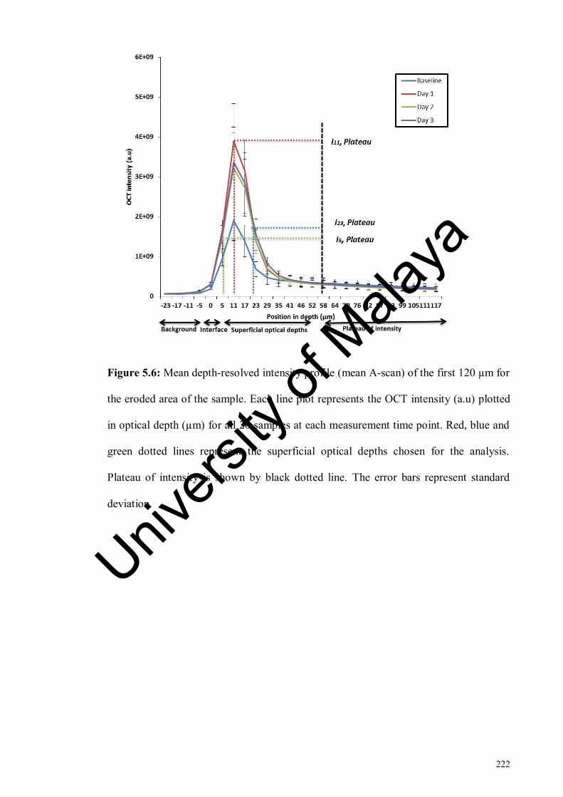
222


the eroded area of the sample. Each line plot represents the OCT intensity (a.u) plotted

in optical depth (µm) for all 20 samples at each measurement time point. Red, blue and



deviation.

Univers

ity of

Mala

ya

223

Figure 5.7: Representative OCT A-scans of one sample (a - d). Each A-scan shows the

OCT intensity (a.u) plotted in optical depth (µm). The red text box indicates the OCT

intensity at a depth of 23 µm. The chart title of each A-scan indicates the time interval

for which the A-scan was plotted. The increase in intensity at 23 µm is obvious with

time.

Univers

ity of

Mala

ya

224






µm is obvious.

Univers

ity of

Mala

ya

225







ity of

Mala

ya

226

Figure 5.10: Representative A-scans of a sample at (a) baseline time point and b)

after three days of erosion. Each A-scan shows the OCT intensity (a.u) plotted in optical




µm is obvious.

Univers

ity of

Mala

ya

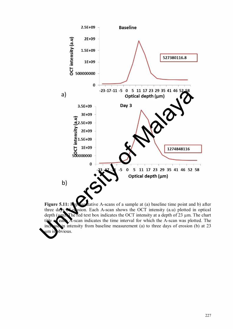
227







ity of

Mala

ya

228

Figure 5.12: Representative OCT B-scans of one sample at (a) baseline measurement

(b) day one (c) day two and (d) day three of cycling erosion challenge. Transparent

arrows indicate the backscattered intensity at the surface of eroded area.

Univers

ity of

Mala

ya

229

5.3.1.2 Outcome measures

OCT parameters and their outcome measures have been summarised in the Table 5.1.

Table 5.1: OCT parameters and their outcome measures defined.

Parameters Symbol Equation Outcome measures

Decay of

intensity

D D = 𝐼𝑝𝑙𝑎𝑡𝑒𝑎𝑢


I58µm / I5µm

I58µm / I11µm

I58µm / I23µm

Integrated

intensity R

R = ∑ Isuperficial : Iplateau ) x Z

I(5µm : 58µm)

I(11µm : 58µm)

I(23µm : 58µm)

Fractional

Integrated

intensity with

baseline

fR

f𝑅𝐸 =𝑅𝐸 (𝑡)

𝑅𝐸(𝑡𝑜)

f (I(23µm : 58µm))

Data correction

for eroded area

DataE

corrected

𝐷𝑎𝑡𝑎𝐸 𝑐𝑜𝑟𝑟𝑒𝑐𝑡𝑒𝑑

= 𝐷𝑎𝑡𝑎𝐸𝑎𝑏𝑠𝑜𝑙𝑢𝑡𝑒(𝑡)/𝑘(𝑡)

Corrected I58µm / I5µm



Corrected I(5µm : 58µm)




for the outcome measures I58µm / I5µm, I58µm / I11µm and I58 µm / I23 µm, I(5µm : 58µm), I(11µm :

58µm) and I(23µm : 58µm). One-way repeated measures ANOVA, with Bonferroni-Holm

correction were performed and Mauchly’s test was used to evaluate the sphericity

assumption. If sphericity was not met, the adjusted F-value of the Greenhouse-Geisser

correction was considered.

Univers

ity of

Mala

ya

230

Mean and standard deviations for eroded areas of I58µm / I5µm, I58µm / I11µm and I58µm /

I23µm are given in Table 5.4 and for eroded areas of I(5µm : 58µm), I(11µm : 58µm) and I(23µm :

58µm) in Table 5.7.

(a) I58µm / I5µm


reference (2 = 11.414, p = .04) and eroded areas (

2 = 49.536, p < 0.0001). Therefore,

the adjusted F-values of the Greenhouse-Geisser correction were considered.

One-way repeated measures ANOVA showed that there was a significant effect of

erosion interval on backscattered intensity in the eroded area (F (1.2, 22.05) = 88.3, p <

0.0001, η2

= .831) whereas no significant effect was found on intensity in the reference

area (F (2.3, 42.07) = 1.13, p = 0.337, η2 = .337) as shown in Table 5.2.


all days were significantly different with respect to their baseline intensity values.

However, significant differences were only observed between day one and day two

intensity values as shown in Table 5.3. Data plot is given in Figure 5.13.

Univers

ity of

Mala

ya

231



(b) I58µm / I11µm

Results of Mauchly’s test showed that the sphericity assumption was violated in

both reference (2 =11.788, p = 0.038) and eroded areas (

2 = 70.734 p < 0.0001).




0.0001, η2

= .782) whereas no significant effect of erosion interval on intensity was

observed in the reference area (F (2.1, 38.2) = 1.43, p = 0.251, η2

= .07) as shown in Table

5.2.



Univers

ity of

Mala

ya

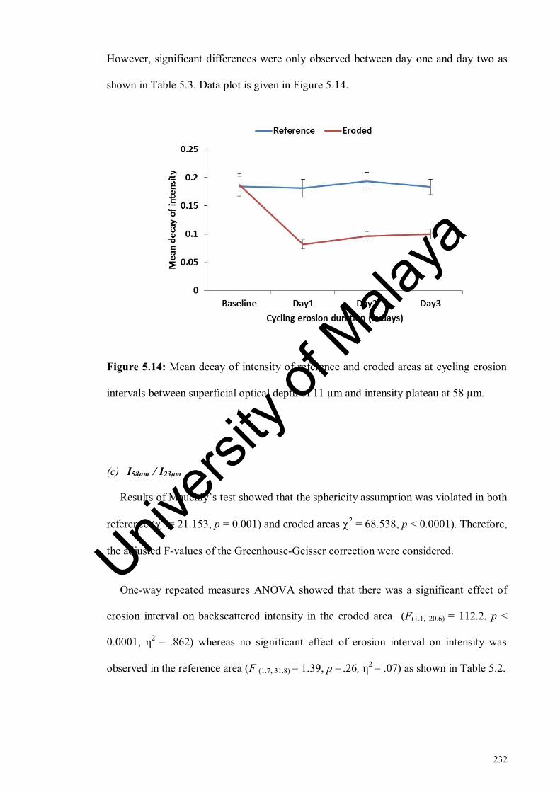
232

However, significant differences were only observed between day one and day two as

shown in Table 5.3. Data plot is given in Figure 5.14.



(c) I58µm / I23µm


reference (2 = 21.153, p = 0.001) and eroded areas

2 = 68.538, p < 0.0001). Therefore,



erosion interval on backscattered intensity in the eroded area (F(1.1, 20.6) = 112.2, p <

0.0001, η2


observed in the reference area (F (1.7, 31.8) = 1.39, p =.26, η2 = .07) as shown in Table 5.2.

Univers

ity of

Mala

ya

233



However, no significant differences were observed between days as shown in Table 5.3.

Data plot is given in Figure 5.15.




areas of outcome measures of decay of intensity.

Outcome

measure


Mean

square

F-statistic p-value

Mean

square

F-statistic p-value

I58µm / I5µm .002 1.135 .337 .257 88.380 <.0001

I58µm / I11µm .001 1.432 .251 .099 64.573 <.0001

I58µm / I23µm .006 1.395 .261 .909 112.268 <.0001

Univers

ity of

Mala

ya

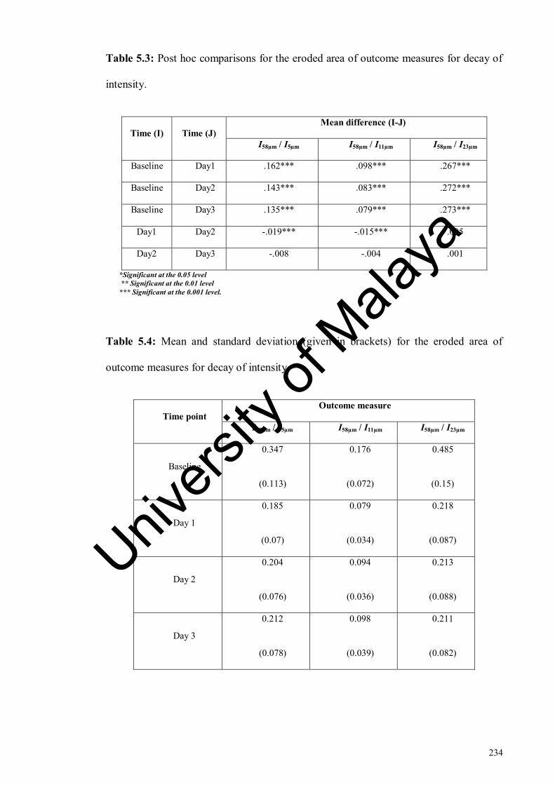
234

Table 5.3: Post hoc comparisons for the eroded area of outcome measures for decay of

intensity.

Time (I) Time (J)



Baseline Day1 .162*** .098*** .267***

Baseline Day2 .143*** .083*** .272***

Baseline Day3 .135*** .079*** .273***

Day1 Day2 -.019*** -.015*** .005

Day2 Day3 -.008 -.004 .001





outcome measures for decay of intensity

Time point

Outcome measure


Baseline

0.347

(0.113)

0.176

(0.072)

0.485

(0.15)

Day 1

0.185

(0.07)

0.079

(0.034)

0.218

(0.087)

Day 2

0.204

(0.076)

0.094

(0.036)

0.213

(0.088)

Day 3

0.212

(0.078)

0.098

(0.039)

0.211

(0.082)

Univers

ity of

Mala

ya

235

(d) I(5µm : 58µm)


reference (2 =25.447, p < 0.0001) and eroded areas (

2 = 25.049 p < 0.0001).



erosion interval on backscattered intensity in the eroded area (F(1.6, 30.08) = 100.1, p <

0.0001, η2


observed in the reference area (F(1.5, 27.4) = 3.5, p = 0.055, η2


5.5.



Moreover, significant differences were observed between all days as shown in Table

5.6. Data plot is given in Figure 5.16.




Univers

ity of

Mala

ya

236

(e) I(11µm : 58µm)


reference (2 = 27.008, p < 0.0001) and eroded areas (

2 = 24.560, p < 0.0001).




0.0001, η2


observed in the reference area (F (1.4, 26.8) = 3.2, p = 0.069, η2


5.5.



Moreover, significant differences were observed between all days as shown in Table

5.6. Data plot is given in Figure 5.17

Univers

ity of

Mala

ya

237

Figure 5.17: Mean integrated intensity of reference and eroded areas at different

cycling erosion intervals. The backscattered intensity was integrated from superficial

optical depth of 11 µm to the intensity plateau at 58 µm.

(f) Optimum outcome measure, I(23µm : 58µm)


reference (2 = 20.618, p<0.001) and eroded areas (

2 = 22.900, p<0.0001). Therefore,



erosion interval on backscattered intensity in the eroded area (F(1.6, 30.5) =39.183, p <

0.0001, η2


observed in the reference area (F(1.5, 26.8) =1.509, p = 0.236, η2


5.5.



Univers

ity of

Mala

ya

238

Moreover, significant differences were observed between day two and day three as

shown in Table 5.6. Data plot is given in Figure 5.18





areas of all outcome measures for integrated intensity.

Outcome

measure


Mean

square

F-statistic p-value

Mean

square

F-

statistic

p-value

I(5µm : 58µm) 4.273E+19 3.507 0.055 2.632E+21 100.105 <0.0001

I(11µm : 58µm) 3.312E+19 3.207 0.069 1.976E+21 99.403 <0.0001

I(23µm : 58µm) 3.539E+18 1.509 0.236 1.602E+20 39.183 <0.0001

fR(I(23µm : 58µm)) 0.03 1.77 0.193 2.057 33.039 <0.0001

Univers

ity of

Mala

ya

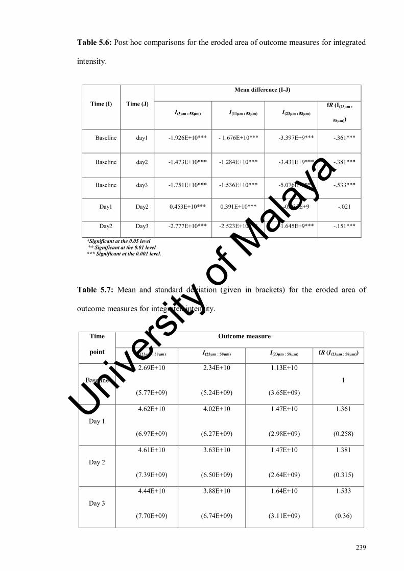
239

Table 5.6: Post hoc comparisons for the eroded area of outcome measures for integrated

intensity.

Time (I) Time (J)



fR (I(23µm :

58µm))

Baseline day1 -1.926E+10*** - 1.676E+10*** -3.397E+9*** -.361***

Baseline day2 -1.473E+10*** -1.284E+10*** -3.431E+9*** -.381***

Baseline day3 -1.751E+10*** -1.536E+10*** -5.076E+9*** -.533***

Day1 Day2 0.453E+10*** 0.391E+10*** -0.033E+9 -.021

Day2 Day3 -2.777E+10*** -2.523E+10*** -1.645E+9*** -.151***





outcome measures for integrated intensity.

Time

point

Outcome measure

I(23µm : 58µm) I(23µm : 58µm) I(23µm : 58µm) fR (I(23µm : 58µm))

Baseline

2.69E+10

(5.77E+09)

2.34E+10

(5.24E+09)

1.13E+10

(3.65E+09)

1

Day 1

4.62E+10

(6.97E+09)

4.02E+10

(6.27E+09)

1.47E+10

(2.98E+09)

1.361

(0.258)

Day 2

4.61E+10

(7.39E+09)

3.63E+10

(6.50E+09)

1.47E+10

(2.64E+09)

1.381

(0.315)

Day 3

4.44E+10

(7.70E+09)

3.88E+10

(6.74E+09)

1.64E+10

(3.11E+09)

1.533

(0.36)

Univers

ity of

Mala

ya

240


The effect sizes of all outcome measures were assessed to find the most sensitive

parameter and outcome measure. I58µm / I23µm was the most powerful outcome measure

as per the effect size comparison as shown in Table 5.8.

Table 5.8: Comparison of effect sizes of all outcome measures used for analysis.

Parameter Outcome measure

Effect size

(partial eta square value)

Decay of intensity

I58µm / I5µm 0.831

I58µm / I11µm 0.782

I58µm / I23µm 0.862

Integrated intensity

I(5µm : 58µm) 0.848

I(11µm : 58µm) 0.847

I(23µm : 58µm) 0.673

5.3.1.4 Correction with reference


for all the outcome measures for both ‘decay of intensity’ and ‘integrated intensity’.

One-way repeated measures ANOVA was performed and Mauchly’s test was used to

evaluate the sphericity assumption.

Mauchly’s test showed that assumption of sphericity was violated for corrected data

for all outcome measures (p < 0.05). Therefore, the adjusted F-value of the Greenhouse-

Geisser correction was considered. One-way repeated measures ANOVA showed that

there was a significant effect of erosion interval on backscattered intensity for all the

Univers

ity of

Mala

ya

241

outcome measures (p < 0.0001). F-values and p-values are given in Table 5.9.

Therefore, post hoc comparisons with Holm-Bonferroni correction were performed to

ascertain where the differences had occurred.

Post hoc comparisons for corrected I58µm / I5µm and corrected I58µm / I11µm showed that

after correction, no significant differences were detected between days as opposed to

their absolute outcome measures where significant differences had been observed

between day one and day two values. Corrected I58µm / I23µm showed that mean intensity

values between day one - day two became statistically significant whereas no significant

differences had been observed in the absolute I58µm / I23µm previously.

Results for corrected I(5µm : 58µm) and corrected I(11µm : 58µm) showed that after day one,

intensity became constant as opposed to their absolute outcome measures where

intensity values were significantly different between all days.

I(23µm : 58µm) was the only outcome measure which showed similar results for corrected

and absolute values showing that it was the most stable outcome measure. Detailed

results are given in Tables 5.10-5.11.

Figures 5.19 (a-c) and 5.20 (a-c) show the corrected integrated intensity and

corrected decay of intensity respectively for the reference and eroded areas for all

outcome measures plotted in time. The reference areas in all plots achieved a horizontal

line in time against which the intensity changes in the eroded area were evaluated. Mean

and standard deviations are given in Tables 5.12 and 5.13.

Univers

ity of

Mala

ya

242

Figure 5.19: Corrected integrated intensity for the reference and eroded areas for

outcome measures (a) I(5µm : 58µm) (b) I(11µm : 58µm) and (c) I(23µm : 58µm).

Univers

ity of

Mala

ya

243

Figure 5.20: Corrected decay of intensity for the reference and eroded areas for

outcome measures (a) I58µm / I5µm (b) I58µm / I11µm and (c) I58µm / I23µm.

Table 5.9: Results of repeated measures ANOVA analysis for corrected data of

outcome measures of decay of intensity and integrated intensity.

Parameter Outcome measure Mean square F-statistic p-value

Corrected decay

of intensity

I58µm / I5µm .252 55.669 <.0001

I58µm / I11µm .101 46.629 <.0001

I58µm / I23µm .990 97.883 <.0001

Corrected

integrated

intensity

I(5µm : 58µm) 3.671E+21 86.030 <.0001

I(11µm : 58µm) 2.743E+21 84.540 <.0001

I(23µm : 58µm) 1.402E+20 30.430 <.0001

Univers

ity of

Mala

ya

244


decay of intensity.

Time (I) Time (J)


Corrected

I58µm / I5µm

Corrected

I58µm / I11µm

Corrected

I58µm / I23µm

Baseline day1 .164*** .101*** .285***

Baseline day2 .160*** .095*** .299***

Baseline day3 .138*** .083*** .296***

Day1 Day2 -.004 -.006 .014*

Day2 Day3 -.026 -.012 -.003





integrated intensity.

Time (I) Time (J) Mean difference (I-J)

Corrected I(5µm :

58µm)

Corrected I(11µm :

58µm)

Corrected

I(23µm : 58µm)

Baseline Day1 -2.134E+10*** -1.871E+10*** -3.267E+9***

Baseline Day2 -1.924E+10*** -1.681E+10*** -3.667E+9***

Baseline Day3 -2.108E+10*** -1.860E+10*** -5.337E+9***

Day1 Day2 0.210E+10 0.189E+10 -0.400E+9

Day2 Day3 -0.184E+10 -0.179E+10 -1.669E+9**




Univers

ity of

Mala

ya

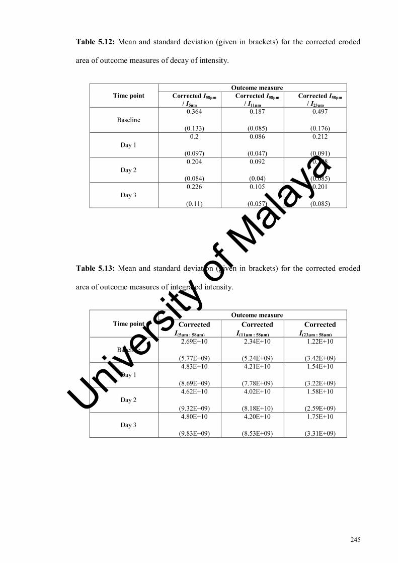
245


area of outcome measures of decay of intensity.

Time point

Outcome measure

Corrected I58µm

/ I5µm

Corrected I58µm

/ I11µm

Corrected I58µm

/ I23µm

Baseline

0.364

(0.133)

0.187

(0.085)

0.497

(0.176)

Day 1

0.2

(0.097)

0.086

(0.047)

0.212

(0.091)

Day 2

0.204

(0.084)

0.092

(0.04)

0.198

(0.085)

Day 3

0.226

(0.11)

0.105

(0.057)

0.201

(0.085)


area of outcome measures of integrated intensity.

Time point

Outcome measure

Corrected

I(5µm : 58µm)

Corrected

I(11µm : 58µm)

Corrected

I(23µm : 58µm)

Baseline

2.69E+10

(5.77E+09)

2.34E+10

(5.24E+09)

1.22E+10

(3.42E+09)

Day 1

4.83E+10

(8.69E+09)

4.21E+10

(7.78E+09)

1.54E+10

(3.22E+09)

Day 2

4.62E+10

(9.32E+09)

4.02E+10

(8.18E+10)

1.58E+10

(2.59E+09)

Day 3

4.80E+10

(9.83E+09)

4.20E+10

(8.53E+09)

1.75E+10

(3.31E+09)

Univers

ity of

Mala

ya

246

5.3.2 FE-SEM

Figure 5.21 shows the comparison of OCT outcome measures with FE-SEM

observations. FE-SEM image representing day one of erosion (Figure 5.21, d) showed

the opened dentinal tubules after the partial removal of smear layer. This phenomenon

was detected by both decay of intensity and integrated intensity. However, after day

one, the intensity of all outcome measures of decay of intensity and I(5µm : 58µm) and I(11µm

: 58µm) of integrated intensity remained almost constant. In the FE-SEM images (Figure

5.21, c-f), the progression of erosion was evident especially in day three image (Figure

5.21, f). Therefore, results for decay of intensity and integrated intensity of the first two

superficial depths were not in accordance with the FE-SEM micrographs.

When compared to FE-SEM micrographs, it is clear that only I(23µm : 58µm) was able to

detect and monitor day three of erosion as shown in the Figure 5.22. Figure 5.22, a)

showed that the intensity between day one and day two was almost constant. From the

FE-SEM images representing day one and day two of cycling erosion, (Figure 5.22, c &

d) it could be observed that the erosion-associated changes were limited to peritubular

dentine. It can be speculated that the overall porosity level was not affected much until

the acid challenge demineralised the intertubular dentine as observed in day three image

of FE-SEM (Figure 5.22, f). Hence, this change was not detected with OCT.

Univers

ity of

Mala

ya

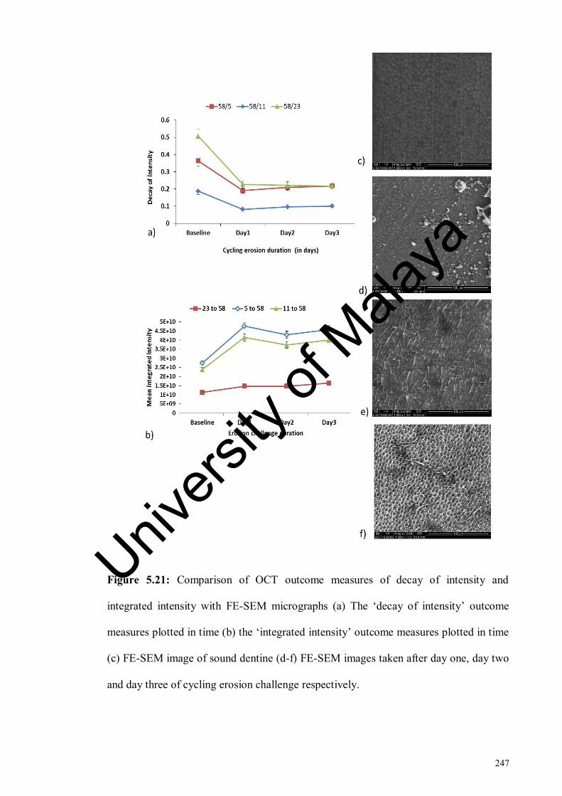
247

Figure 5.21: Comparison of OCT outcome measures of decay of intensity and

integrated intensity with FE-SEM micrographs (a) The ‘decay of intensity’ outcome

measures plotted in time (b) the ‘integrated intensity’ outcome measures plotted in time

(c) FE-SEM image of sound dentine (d-f) FE-SEM images taken after day one, day two

and day three of cycling erosion challenge respectively.

Univers

ity of

Mala

ya

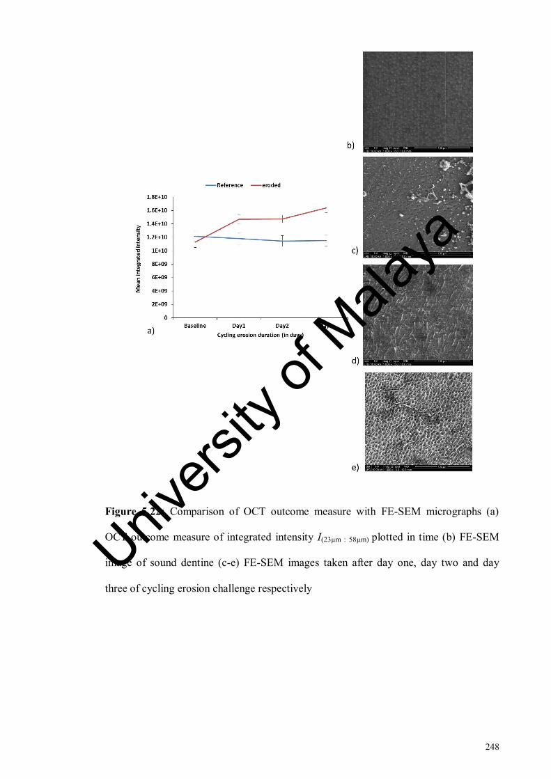
248

Figure 5.22: Comparison of OCT outcome measure with FE-SEM micrographs (a)

OCT outcome measure of integrated intensity I(23µm : 58µm) plotted in time (b) FE-SEM

image of sound dentine (c-e) FE-SEM images taken after day one, day two and day

three of cycling erosion challenge respectively

Univers

ity of

Mala

ya

249

5.3.3 Comparison with surface roughness findings

5.3.3.1 Fractional change in intensity, fR (I(23µm : 58µm))


reference (reference, 2 = 26.975, p<0.0001) and eroded area (

2 = 33.08, p<0.0001).



erosion interval on backscattered intensity in the eroded area (F (1.4, 28.25) = 33.03,

p<0.0001, η2


observed in the reference area (F (1.5, 29.4) = 1.77, p = .193, η2


5.5.



Moreover, significant differences were observed between day two and day three as

shown in Table 5.6. Data plot is given in Figure 5.23

Univers

ity of

Mala

ya

250

Figure 5.23: Fractional change in integrated intensity with baseline (fR) of reference

and eroded areas at cycling erosion intervals. The backscattered intensity was integrated

from superficial optical depth of 23 µm to the intensity plateau at 58 µm

5.3.3.2 Relationship between fR and fRa1

Significance and level of relationship between OCT outcome measure fR (fractional

change in I(23µm : 58µm)) and fractional change in surface roughness outcome measures,

average roughness (fRa1), core roughness (fRk), peak roughness (fRpk), valley roughness

(fRvk), proportion of peaks (fMR1) and proportion of valleys (fMR2) was determined by

Pearson correlation coefficient test. Overall difference and correlation between fR and

surface roughness outcome measures is stated in Table 5.14

Pearson correlation coefficient test showed that there was a significant relationship

between fR of OCT and fRa1 (p<0.0001). Pearson coefficient of r = 0.428 showed a

moderate positive relationship between the two variables. A linear function was fitted to

the variable relationship with a R2 value of 0.161 as shown in Figure 5.24

Univers

ity of

Mala

ya

251

Figure 5.24: Relationship between fR and fRa

5.3.3.3 Relationship between fR and fRk


between fR of OCT and fRk (p<0.0001). Pearson coefficient of r = .394 showed a

moderate positive relationship between the two variables. A linear function was fitted to

the variable relationship with a R2 value of 0.156 as shown in Figure 5.25

Univ

ersity

of M

alaya

252

Figure 5.25: Relationship between fR and fRk

5.3.3.4 Relationship between fR and fRpk


between fR of OCT and fRpk (p = 0.001). However, Pearson coefficient of r = 0.300

showed a weak positive relationship between the two variables. A linear function was

fitted to the variable relationship with a R2 value of 0.068 as shown in Figure 5.26

Univers

ity of

Mala

ya

253

Figure 5.26: Relationship between fR and fRpk

5.3.3.5 Relationship between fR and fRvk


between fR of OCT and fRpk (p = .019). However, Pearson coefficient of r = 0.217


fitted to the variable relationship with R2 value of 0.047 as shown in Figure 5.27

Univers

ity of

Mala

ya

254

Figure 5.27: Relationship between fR and fRvk

5.3.3.6 Relationship between fR and fMR1


between fR of OCT and fMR1 (p = 0.036). However, Pearson coefficient of r = 0.192


fitted to the variable relationship with a R2 value of 0.037 as shown in Figure 5.28

Univers

ity of

Mala

ya

255

Figure 5.28: Relationship between fR and fMR1

5.3.3.7 Relationship between fR and fMR2

Pearson correlation coefficient test showed that the relationship between fR of OCT

and fMR2 was not significant (p = 0.180). Pearson coefficient of r = -.123showed a

weak negative relationship between the two variables. A linear function was fitted to the

variable relationship with a R2 value of 0.015 as shown in Figure 5.29

Univ

ersity

of M

alaya

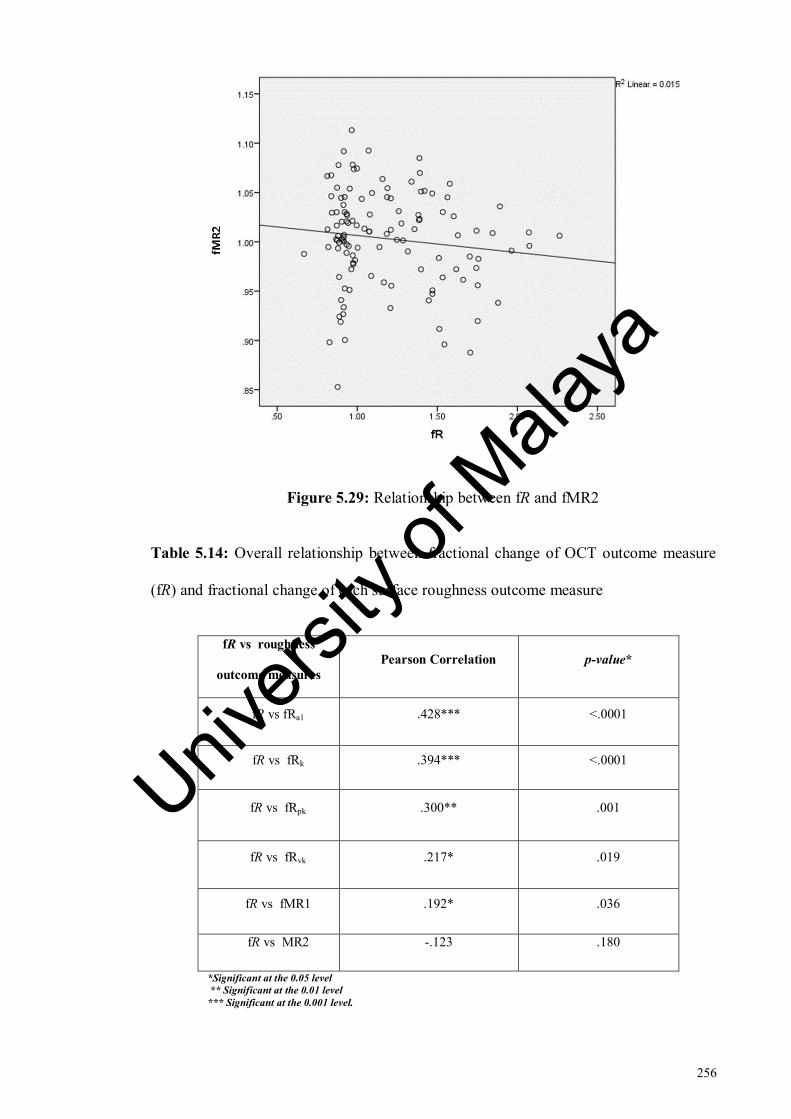
256

Figure 5.29: Relationship between fR and fMR2

Table 5.14: Overall relationship between fractional change of OCT outcome measure

(fR) and fractional change of each surface roughness outcome measure

fR vs roughness

outcome measures

Pearson Correlation p-value*

fR vs fRa1 .428*** <.0001

fR vs fRk .394*** <.0001

fR vs fRpk .300** .001

fR vs fRvk .217* .019

fR vs fMR1 .192* .036

fR vs MR2 -.123 .180




Univers

ity of

Mala

ya

257

5.3.3.8 Significance of difference between correlation coefficients of fRa and fRk

fRa1 showed the highest Pearson correlation coefficient with r = 0.428 closely

followed by fRk with r = 0.394. In order to assess whether the difference between the

two correlation coefficients was significant, Fisher r-to-z transformation was used by

using an online calculator (Soper, 2017).

The Z-value was 0.17 and the p-value was 0.86 showing that there was no

statistically significant difference between the two Pearson correlation coefficients.

5.3.3.9 Correlation on day one

By day one, only fRpk showed a significant relationship with fR (p < 0.003).

Moreover, a moderate positive relationship was found between fRpk and fR (r = .457).

The relationship between fR and all other surface roughness parameters was not

significant. A weak positive Pearson correlation was present between fR and fRa1, fRk,

fRvk and fMR1 whereas a weak negative relationship was found between fR and fMR2

(Table 5.15)

5.3.3.10 Correlation on day two

On day two, Pearson correlation coefficient test showed that fRa1 showed a moderate

positive relationship with fR indicated by r = .320 which was significant (p = .047).

Similarly, fRk also showed a moderate positive relationship with fR as indicated by r =

0.347 which was significant (p = 0.03). Although both surface roughness parameters

showed similar relationship with fR, however the correlation coefficient was slightly

higher for fRk as compared to fRa1.

Univers

ity of

Mala

ya

258

The relationship between fR and all other surface roughness parameters was not

significant on day two. A weak positive Pearson correlation was present between fR and

fRa, fRk, fRvk and fMR1 whereas a weak negative relationship was found between fR

and fMR2. Detailed results are given in Table 5.15.

5.3.3.11 Correlation on day three

On day three, the correlation coefficients of both fRa1 and fRk became higher and

showed a strong positive relationship with fR as indicated by r = 0.578 for fRa1 vs fR

and r = .556 for fRk vs fR. Moreover, the relationship of both fRa1 and fRk was highly

significant by day three (p<0.0001). fRvk also showed a moderate positive relationship

with fR with r = 0.337 which was significant (p = .039). A moderate positive

relationship between fR and fMR1 was found as indicated by r = .444 which was

significant (p = .004).

fRpk showed a weak positive relationship with fR which was not significant. As on

day one and day two, fMR2 showed a weak negative relationship with fR which was not

significant either (Table 5.15).

Univers

ity of

Mala

ya

259

Table 5.15: Relationship between fractional change of OCT outcome measure (fR) and

fractional change of surface roughness outcome measures at each time point (day).

Day fR vs roughness

outcome measures

Pearson correlation p-value

Day 1 fR vs fRa1 .261 .108

fR vs fRk .114 .489

fR vs fRpk .457** .003

fR vs fRvk .079 .632

fR vs fMR1 .182 .260

fR vs fMR2 -.146 .369

Day 2 fR vs fRa1 .320* .047

fR vs Rk .347* .030

fR vs Rpk .225 .169

fR vs Rvk .137 .404

fR vs MR1 .038 .816

fR vs MR2 -.144 .374

Day 3 fR vs Ra1 .578*** <0.0001

fR vs Rk .556*** <0.0001

fR vs Rpk .224 .135

fR vs Rvk .337* .039

fR vs MR1 .444** .004

fR vs MR2 -.094 .564




Univers

ity of

Mala

ya

260

5.4 Discussion

The purpose of this study was to assess whether OCT could be used to monitor the

progression of early dentine erosion in simulated intraoral environment. The OCT

backscattered intensity changes of early eroded dentine were compared with

ultrastructural changes and surface roughness measurements.

A laboratory cycling erosion model was employed in this study to replicate the main

chemical and biological conditions related to extrinsic dental erosion. All the variables

of this study protocol were chosen as much as practically possible to mimic the key

processes occurring in the oral cavity leading to early dentine erosion. In this relation a

literature search was conducted to review the pH-cycling erosion models and the most

frequently employed clinically relevant variables were tabulated and considered.

Observations from previously performed pilot studies explained in chapter 3 were also

taken into account.

Citric acid was used instead of commercially available soft drinks to avoid any

inconsistency in the formulation among the batches which can be problematic in studies

with multiple exposures to acid (Shellis et al., 2011). The concentration and pH of the

citric acid was kept similar to that of a commercially available orange juice (Austin et

al., 2010; Chiga et al., 2016; Eisenburger et al., 2001) and 10 minutes of erosion was

adopted to mimic the consumption of a can of soft drink or juice beverage (Faller et al.,

2011). Temperature of 36°C was employed to simulate the intraoral temperature

(Shellis et al., 2011). The speed of agitation was pre-determined in a pilot study to

mimic the swishing of drink around the teeth at which the samples did not move while

the solution remained stirred homogeneously.

Many formulations of artificial saliva are available and have been used to simulate

the effect of natural saliva in erosion studies (Alexandria et al., 2017; Scaramucci et al.,

Univers

ity of

Mala

ya

261

2011). It was shown that a remineralisation solution was better at remineralising early

eroded enamel lesions as compared to artificial saliva (Amaechi & Higham, 2001b).

This remineralisation solution had the same composition as that of artificial saliva with

the exception of methyl p-hydroxybenzoate and sodium carboxymethyl cellulose.

Sodium carboxymethyl cellulose has been known to limit remineralisation potential of

saliva by forming complexes with calcium and phosphate ions as well as causing an

increase in viscosity (Ionta et al., 2014). Keeping this in view, a remineralisation

solution of similar composition was used in this study. It is felt that overinclusion of

variables in the same protocol can render the interpretation of results difficult.

Previously, the presence of pellicle was speculated to mask the OCT backscattered

intensity on early eroded enamel (H.P.Chew, 2013). Therefore, to keep the effect of

variables to minimum, the organic portion of saliva was not included in the

remineralisation solution at this point.

As dentine is naturally protected by a smear layer in the oral cavity (Cummins,

2009), therefore smear layer was not removed from dentine samples in this study. Each

root was sectioned in a buccolingual direction ensuring that the direction of acid attack

on the dentine samples was similar to that occurring in vivo. Although it is not possible

to use adhesive tape as reference in vivo, the reference surface was still covered with

non-residue adhesive tape during the erosion challenges so that natural surface of the

same tooth could be used as reference for more realistic comparisons during the data

analysis. Moreover, the samples had to be embedded in the resin to aid in repositioning

although the resin cannot be used in vivo conditions.

A pilot study was performed to determine the optimum duration of dentine exposure

to acid resulting in early dentine erosion without any bulk surface loss. After three days

of cycling erosion challenge, no visible step change was discerned in the OCT images.

Univers

ity of

Mala

ya

262

Therefore, the cycling erosion protocol was limited to three cycling days with 0.3%

citric acid three times a day interspersed with periods of simulated salivary

remineralisation of 3 hours in between the erosion challenges followed by overnight

immersion in remineralisation solution.

5.4.1 OCT

Mean depth profiles for the reference and eroded areas of all samples were plotted up

to a depth of 120 µm to observe the general intensity trend. Mean A-scan for the

reference area showed that little changes in intensity had occurred over time. In

contrast, mean A-scan for the eroded area showed erosion interval related shift in

backscattered intensity indicated by the separation of line graphs representing erosion

intervals. The most remarkable separation between line graphs in the eroded area was

observed at a depth of 11 µm (Imax) from tooth-air interface. The intensity increased at

day one at this depth and then dropped back. This could be the effect of smear plugs or

surface deposits of mineral on the surface of dentine (Figure 5.21, d). However, the

surface variation was very high at this depth (shown by high standard deviation) both in

the reference and eroded areas and became relatively moderate at 23 µm (Idrop). Similar

intensity trends had been observed in mean A-scans extracted from the non-pH-cycling

experiment in chapter 3. This could be the result of previously observed phenomenon of

very strong reflection at the tooth surface which can interfere with assessment of early

demineralisation (Lee et al., 2009). Although an attempt was made to minimise the

effect of specular reflection to some extent by inclining the samples to 20 degrees

perpendicular to the OCT beam by a custom made jig, however it was obvious that

complete elimination of this surface reflection was not possible.

Univers

ity of

Mala

ya

263

It would be almost impossible to monitor erosion in early stages solely based on

visual detail contained in OCT images. Therefore, it was important to identify

parameters that could non-subjectively discriminate eroded tissues from sound tissues

and allow the monitoring of erosion over time. The parameters used by other

researchers in OCT-associated research are spectral peak ratio analysis (Sowa et al.,

2007), peak intensity (Bakhsh et al., 2011), area under the curve (Louie et al., 2010) and

attenuations (Mandurah et al., 2013). Previously, two parameters ‘decay of intensity’

and ‘integrated intensity’ were employed to assess the potential of OCT in longitudinal

monitoring of early dentine erosion described in chapter 3. Results had shown that

integrated intensity was more suitable for the analysis. However, the erosion protocol

for this study differed from the previous study by the inclusion of salivary

remineralisation step and intact smear layer. A possibility remained that same parameter

might not prove to be as effective for monitoring of dentinal demineralisation for this

study. Hence, the sensitivity of both parameters was again tested for this study.

A fixed depth value of 200 µm was employed previously and statistically significant

correlations were found between the integrated intensity value and demineralisation

periods (Fried et al., 2002). The demineralisation was induced up to 14 pH-cycling days

as the objective was to simulate artificial caries rather than erosion. In this study, the

demineralisation was induced for three cycling days only and hence a comparatively

more superficially located fixed subsurface optical depth of 58 µm was employed. At

this subsurface depth, the OCT intensity signal had become constant and did not show

any further changes and was called plateau of intensity. To find an optimal superficial

depth to attain maximal sensitivity of OCT, three superficial depths 5 µm, 11 µm and 23

µm located immediately below the tooth-air interface were selected for data analysis

and comparison. Their relationship with plateau of intensity was assessed by using both

parameters. The selection of optimum outcome measure was based on 1) trend of

Univers

ity of

Mala

ya

264

backscattered intensity of mean A-scans 2) repeated measures ANOVA analysis for

sensitivity and 3) effect size comparison for assessing the magnitude of strength of

outcome measures 4) comparison with FE-SEM images (Section 5.4.2) and 5) data

correction with respect to reference.

All outcome measures for decay of intensity were able to monitor OCT backscattered

intensity between each cycling day and baseline measurement. I58µm / I5µm and I58µm /

I11µm were able to monitor dentine demineralisation between day one and day two only

whereas I58µm / I23µm was not able to monitor demineralisation between days. With

integrated intensity, all outcome measures were able to monitor mean backscattered

intensity between each cycling day and baseline measurement. I(5µm : 58µm) and I(11µm :

58µm) were able to monitor mean intensity values between all days. However, I(23µm : 58µm)

was able to monitor intensity from baseline to day one and day two to day three.

The effect size comparison showed that I58µm / I23µm had the greatest magnitude of

strength in monitoring early dentine erosion for this study. It was important to take into

consideration the overall intensity trend of each outcome measure. With decay of

intensity, the intensity is expected to decrease with increasing erosion intervals(Chew et

al., 2014). Unexpectedly, for I58µm / I5µm and I58µm / I11µm day one intensity values of

0.185 and 0.079 increased to .212 and .098 at day three respectively. For I58µm / I23µm, the

intensity was constant after day one of cycling erosion challenge. With integrated

intensity, the backscattered intensity is expected to increase with increasing erosion

intervals. For eroded areas of I(5µm : 58µm) and I(11µm : 58µm) , backscattered intensity at day

one was 4.62E+10 and 4.02E+10 respectively and decreased to 4.44E+10 and 3.88E+10

at day three respectively. For I(23µm : 58µm) the intensity value increased from 1.47E+10 at

day one to 1.64E+10 at day three. It could be ascertained that the first two superficial

depths with either parameter were not able to detect erosion-related intensity change at

Univers

ity of

Mala

ya

265

day three while I(23µm : 58µm) was the only outcome measure to show net increase in

erosion from baseline to day three of cycling erosion challenge. This could be

confirmed from the FE-SEM images as discussed in Section 5.4.2. In the previous study

(chapter 3), I(23µm : 58µm) was identified as the optimum outcome measure for monitoring

of demineralisation in dentine. Moreover, the surface variation in intensity at superficial

depths of I5 and I11 was evident in the mean A-scans.

In order to assess the stability of outcome measures and to identify any instrumental

variations in time, the data for each outcome measure was corrected for eroded area at

each time point by dividing the absolute data of eroded area at each time point by a

correction factor. This correction factor was derived from the absolute data of reference

area. The corrected values were then plotted and statistically analysed. A comparison

was then drawn between the corrected and absolute outcome measures. Corrected I58µm /

I5µm and corrected I58µm / I11µm showed that after correction no statistically significant

differences were detected between days as opposed to their absolute outcome measures

where significant differences had been observed between day one and day two intensity

values. Similarly, corrected I(5µm : 58µm) and corrected I(11µm : 58µm) showed that after day

1, intensity became constant as opposed to their absolute outcome measures where

intensity values were significantly different between all days. Corrected I58µm / I23µm

showed that mean intensity values between day one and day two became statistically

significant whereas it was not significantly different in the absolute I58 µm / I23 µm. I(23µm :

58µm) was the only outcome measure which showed statistically similar results for

corrected and absolute values indicating that it was the most stable outcome measure.

Based on the findings it could be suggested that I(23µm : 58µm) was the optimum

outcome measure for monitoring of early dentine erosion. The statistically determined

cut off depth was therefore 23 µm for this study. This showed that OCT used in this

Univers

ity of

Mala

ya

266

study was most sensitive to the demineralisation activity that occurs at this depth. At the

tooth-air interface, the specular reflection is very strong and could be 20dB higher than

OCT backscattered intensity. This could lead to scattering information being masked at

or immediately below the tooth-air interface (Fried et al., 2002). Apparently,

backscattered intensity of the superficial layers located next to tooth-air interface was

influenced by the much higher specular reflection at these depths. The optical depth of

23 µm could be translated to its physical depth, 15 µm measured from the tooth-air

interface. This would imply that the erosion-linked demineralisation had occurred all the

way into this depth for this study. This concurs with the findings in chapter 3 and

previously reported statistical depth for early enamel erosion (Chew et al., 2014)

This is the first study, to the best of our knowledge to assess the potential of OCT in

measuring the progression of early dentine erosion in simulated oral conditions. Only

one other recent study has examined potential of OCT for dentine erosion but only the

advanced stages of dentine erosion after the appearance of surface loss in the OCT

images were explored in that study (De Moraes et al., 2017). Importantly, pH-cycling

model of erosion was not employed in that study and only a qualitative analysis was

performed.

Within the limitations of this study, it could be established that OCT would very

likely have the ability to longitudinally monitor the progression of early dentine erosion.

With the OCT set up used in this study and the outcome measure selected, it was

possible to measure erosion by day one of cycling erosion challenge and monitoring

was possible between day one and day three of erosion whereas monitoring from

baseline measurement was possible at all cycling days. With this study it was possible

to develop an in vitro model to monitor early dentine erosion with OCT which can

potentially be translated to an in vivo setting. This information could provide a blueprint

Univers

ity of

Mala

ya

267

for testing of treatments products for dentine erosion over the period of time in a clinical

study.

A statistical comparison of non pH-cycling study in chapter 3 and cycling erosion

study explained in this chapter cannot be made as both studies were conducted under

different experimental and acidic challenge conditions. The cumulative erosion induced

was 30 minutes in the non pH-cycling study in chapter 3 as compared to 90 minutes for

this study. The FE-SEM images however showed that the day-three of erosion induced

in the pH cycling was not more aggressive than 30 minutes of erosion induced earlier.

Moreover, the estimated physical depth of demineralisation was 15 µm for both studies.

It could be because of two reasons. A cycling model was employed in this study and

samples were immersed in remineralisation solution for considerable periods of time

which could have offered some degree of remineralisation and resistance against

erosion. Absence of salivary proteins is further expected to have increased the

remineralisation potential of this remineralisation solution (Shellis et al., 2011).

Additionally, as opposed to non pH-cycling study the smear layer was not removed

from the samples before the induction of demineralisation. Both these factors could

have resulted in lesser erosion in this study as would be expected otherwise in a non-

cycling erosion model.

5.4.2 FE-SEM

FE-SEM micrographs served to confirm the OCT findings. Corrected data for I5µm

and I11µm with both parameters showed that the intensity became constant after day one

and I58µm / I23µm was able to monitor erosion between day one and day two only. FE-

SEM images clearly showed that the effects of acid challenge were more pronounced on

day three as compared to day two. Therefore, the intensity trend shown by these

Univers

ity of

Mala

ya

268

outcome measures was not in accordance with the ultrastructural changes as observed in

SEM images. I(23µm : 58µm) on the other hand was the only outcome measure which was

able to monitor intensity from baseline to day one and day two to day three and showed

a net increase in backscattered intensity from baseline to day three which was in line

with the FE-SEM observations. Hence FE-SEM observations further confirmed I(23µm :

58µm) as the optimum outcome measure for the monitoring of early dentine erosion under

the conditions of this study protocol.

The FE-SEM images showed that the effects of acid challenge in the eroded areas of

all samples were evident in comparison to reference areas which appeared smooth.

These observations were in line with those made from mean A-scans. Mean A-scans for

the eroded area showed erosion interval related shift in backscattered intensity as

indicated by the separation of line graphs at various depths in comparison to reference

area which showed little changes in intensity over time. The sequence of events of

dentine erosion observed from the FESEM images from day one to day three of cycling

erosion were similar to those previously reported (Meurman et al., 1991) (Kinney et al.,

1995). One day of cycling erosion challenge resulted in opening of dentinal tubules.

Day two image showed dissolution at the border of peritubular and intertubular dentine

with slight widening of tubules. Day three image showed that the dissolution of

peritubular dentine had taken place. The intertubular dentine was attacked and showed a

roughened and porous surface.

In comparison to the sound dentine, the day one image showed that treatment with

citric acid resulted in exposure of dentinal tubules. The image also showed that the

tubules were partially or completely occluded and there were white spots on the surface.

This could have resulted because of incomplete removal of smear layer from dentine

surface or from mineral deposition (formation of CaF) due to immersion of dentine

Univers

ity of

Mala

ya

269

samples in salivary simulated remineralisation solution as previously observed

(Vanuspong et al., 2002). In a previous study, dentine was exposed to remineralisation

solution for 20 days after being demineralised for six days. PS-OCT images showed the

presence of an intact mineralized layer on the remineralised dentine surface. However,

the overall effect of remineralisation of dentine was reduction in integrated intensity in

the remineralised region in comparison to the demineralized region (Manesh et al.,

2009). The remineralisation induced in this our study was part of a pH cycling regime

only which lasted only for three days. Therefore, it could be speculated that the effect of

these surface deposits would not affect the OCT scattering to the same extent or cause a

reduction in the integrated intensity if at all.

It is known that demineralised dentine becomes porous after the removal of

peritubular dentine (Kinney et al., 1995) (Meurman et al., 1991). OCT was not able to

monitor dentine demineralisation between day one and day two of cycling erosion

challenge. This could be attributed to the almost similar porosity status between day one

and day two as ascertained from the FE-SEM images. On day three images, the

peritubular dentine dissolved and intertubular dentine with increased porosities became

visible which was detected with OCT.

5.4.3 Comparison with surface roughness findings

Process of erosion in dentine results in creation of porosities and increased surface

roughness (Meurman et al., 1991). OCT quantifies erosion by the increase in porosity of

demineralised tissues which brings about a change in reflected backscattered intensity

as compared to sound tissues (Huysmans et al., 2011) whereas increase in erosion-

associated surface roughness can be measured by surface roughness parameters. This

Univers

ity of

Mala

ya

270

would suggest that both of these methods would have the potential of quantifying early

dentine erosion.

In order to compare the findings of OCT with surface roughness measurements,

fractional change, fR for the reference and eroded area of the optimum OCT outcome

measure I(23µm : 58µm) was calculated. Repeated measures ANOVA followed by post hoc

comparisons (Table 5.6) showed that the sensitivity of fR was exactly similar to that to

I(23µm : 58µm). Significance and level of relationship between OCT outcome measure fR

and surface roughness parameters fRa1, fRk, fRpk, fRvk, fMR1 and fMR2 were examined

by Pearson correlation coefficient test. Pearson correlation coefficient test showed that

there was a significant and moderate positive relationship between fR of OCT with fRa1

and fRk. The correlation coefficient of fRa1 (0.428) was higher as compared to fRk

(0.394), however, it was found that there was no statistically significant difference

between the two correlation coefficients.

Moreover, there was a significant weak positive relationship between fR of OCT and

fRpk, fRvk and fMR1. The relationship between fR of OCT and fMR2 was however

weak negative and not statistically significant. This would mean that an increase in OCT

backscattered intensity would result in a lower value for fMR2. This correlation could

be of value in testing of treatment products for erosion. OCT backscattered intensity

would decrease as a result of remineralisation (Manesh et al., 2009). On the other hand

as a result of remineralisation, the profile will be expected to become smoother with

resultant increase in proportion of valleys and MR2 value. However, it warrants further

investigation.

By day one, only fRpk showed a significant moderate positive relationship with fR.

The relationship between fR and all other surface roughness parameters was weak

positive and not statistically significant. This is in accordance with the surface

Univers

ity of

Mala

ya

271

roughness findings (chapter 4) where only fRpk was able to detect dentine

demineralisation by day one from baseline measurement. This would imply that fRpk is

most suited for monitoring of earliest stage of dentine erosion.

On day two, both fRa1 and fRk showed a significant and moderate positive

relationship with fR. The relationship between fR and all other surface roughness

outcome measures was weak positive and not statistically significant. This finding is

also in line with the surface roughness results (chapter 4) where both fRa1 and fRk were

able to monitor erosion by day two whereas Rpk was not able to monitor erosion at day

two from baseline. As would be expected, the correlation coefficients of fRa1 and fRk

with fR became higher and highly significant on day three as compared to day two. By

day three, fRvk was significantly different from baseline value (chapter 4) and also

showed a significant and moderate positive relationship with fR on day three. Although

fMR1 did not show any significantly different results on any of the days (chapter 4), it

still showed a significant and moderate positive relationship with fR on day three. This

would indicate that fMR1 may have a potential of monitoring erosion in more advanced

stages of dentine erosion.

Based on the correlation findings, it could be suggested that fRpk was well-suited to

compare the findings of OCT at day one of erosion from baseline measurement and fRa1

and fRk could be used for comparing the findings of OCT in the more advanced stages

of early dentine erosion. However, fRa1 was not able to monitor erosion between day

two and day three which could be accomplished with fRk. Hence, within the limits of

current study protocol, it could be suggested that a combination of fRpk and fRk are

suitable for comparing the findings of OCT in longitudinal monitoring of early dentine

erosion.

Univers

ity of

Mala

ya

272

In chapter 4, it was shown that surface roughness parameters can be employed for

longitudinal monitoring of early dentine erosion in simulated oral conditions.

Particularly, inclusion of bearing curve parameters provided extra information and

sensitive parameters for its monitoring. This study proves that OCT has the potential of

being employed for early dentine demineralisation in intraoral simulated conditions.

With both methods, day one of demineralisation could be detected and monitored. OCT

was not able to monitor erosion between day one and day two which was possible with

bearing area curve. However, OCT has additional advantage over profilometry in being

non-invasive and can be applied directly in clinical trials. Profilometry requires the use

of indirect impression technique which can cause inaccurate measurements.

5.5 Conclusions



1. OCT was able to measure early dentine erosion for three days in simulated

intraoral conditions. The quantum of OCT for measuring early dentine erosion in

simulated intraoral conditions varied with different outcome measures. I(23µm :

58µm) showed significant changes between baseline - day 1 and between day one -

day three of cycling erosion challenge.


measuring in vitro early dentine erosion in simulated intraoral conditions. I(23µm :

58µm) was the most sensitive outcome measure for measuring in vitro early


Univers

ity of

Mala

ya

273

3. The simulated intraoral early dentine erosion detection threshold of OCT varied

with different outcome measures. With I(23µm : 58µm), the detection threshold was

one day of cycling erosion challenge from baseline measurement.


With I(23µm : 58µm), a net increase of backscattered intensity in relation to

incubation time in acid was observed during erosion progression. The eroded

regions of FE-SEM showed gradually enlarging dentinal tubules and increase in

roughness of dentine surface with increasing erosion intervals.

5. OCT outcome measure fR (fI(23µm : 58µm)) showed a significant and moderate

positive relationship with surface roughness outcome measures fRa1 and fRk.

With fRpk, fRvk and fMR1, fR showed a weak positive but significant

relationship. With fMR2, fR showed a weak negative relationship which was not

significant.

6. On day one, OCT outcome measure fR showed a moderate positive and

significant relationship with fRpk. On day two, fR showed a moderate positive

and significant relationship with fRk and fRa1. On day three, fR showed a

significant and moderate positive relationship with fRk, fRa1, fRvk and fMR1.

The null hypotheses were rejected as shown below;

1. OCT was able to detect early dentine erosion with a detection sensitivity of one

pH-cycling day from baseline.

2. OCT was able to measure the progression of early dentine erosion for three days


3. OCT backscattered intensity changes were correlated with surface roughness

measurements.

Univers

ity of

Mala

ya

274

CHAPTER 6: CONCLUSIONS

6.1 Summary and conclusions

Longitudinal monitoring of early dentine erosion in an in vivo setting is desirable to

evaluate the performance of anti-erosion interventions more accurately as various in

vitro and in situ studies provide contradictory results. Such in vivo studies can only be

materialised by the development of non-invasive methods sensitive to early

demineralisation. The purpose of this thesis was to seek a non-invasive tool which could

be used for detection and monitoring of early dentine erosion in clinical trials to

evaluate the efficacies of treatment strategies meant to reduce the progression of dentine

erosion.

Such a tool is expected to possess a few qualities. It should be a non-destructive and

non-invasive method which is sensitive to early demineralisation and is able to quantify

erosion over time. Review of literature revealed that the currently employed methods do

not meet these criteria. Of the optical methods used in erosion research, optical

coherence tomography (OCT) seemed to be the potential tool for this task. While tested

previously for enamel erosion and advanced staged dentine erosion, its potential in the

assessment of early dentine erosion remained to be tested. Therefore, the first study of

this thesis aimed to assess the applicability of OCT for detection and monitoring of

early dentine erosion. Thirty minutes of erosion was induced in a non pH-cycling model

to assess the potential and the detection capacity of this instrument.

Surface profilometry has been used extensively for the assessment of dentine erosion

and has been employed to a limited extent in the in vivo settings. However, the

conventionally used parameter, surface loss may not be suitable for assessment of early

stage of dentine erosion which is not expected to result in bulk surface loss.

Additionally, in order to compare the findings of newer non-invasive techniques in vivo

Univers

ity of

Mala

ya

275

and in vitro, sensitive and quantitative reference methods are needed. Therefore, the

second study aimed at assessing the potential of surface roughness parameters, in

particular the bearing area curve parameters for monitoring of early dentine erosion in

simulated intraoral conditions.

The potential of OCT to monitor early dentine erosion and its detection capacity had

been identified in chapter 3. Subsequent course of action was to perform an in situ or an

in vivo validation study or proceed with an in vitro study with a simulated intraoral

environment. It was felt that sufficient information about the clinical situation could not

be derived from the first study (chapter 3) and variables like simulated salivary

remineralisation and presence of smear layer could potentially affect the OCT

outcomes. Moreover, from a non-cycling model it is difficult to predict the amount of

erosion that could be induced and monitored in clinical situation. Therefore, it was

decided to evaluate the potential of OCT for monitoring early dentine erosion in

simulated intraoral conditions before testing this tool in more expensive in situ or in

vivo studies.

This multi-aimed study was divided into three main chapters and had the following

aims,

6.1.1 Aim 1

To assess the potential of optical coherence tomography (OCT) in monitoring the

progression of in vitro early dentine erosion


1. OCT is not able to detect early dentine erosion in vitro.

2. OCT is not able to measure early dentine erosion progression in vitro.

Univers

ity of

Mala

ya

276

In order to test these null hypotheses, 20 root dentine samples were subjected to 30

minutes of erosion with 0.3% citric acid and measurements were obtained with OCT at

0, 2, 4, 6, 8, 10, 12, 14, 16, 20, 25 and 30 minutes. A composite slab was used as a

reference during the measurements. Another 14 root dentine samples were imaged with

field emission scanning electron microscopy (FE-SEM) but not longitudinally after 2, 4,

8, 12, 16, 25 and 30 minutes of erosion challenge with similar citric acid. The OCT data

was extracted and processed using a bespoke software programme developed with

MATLAB (The MathWorks, Inc., USA). The OCT data was subsequently analysed

using two parameters ‘decay of intensity’ (D) and ‘integrated intensity’ (R) and their

related outcome measures. The findings of OCT were then compared with

ultrastructural changes.

Based on the data collected and analysed (please refer Sections 3.2 and 3.3), null

hypotheses one and two were rejected as shown below;

1. OCT was able to detect early dentine erosion with a detection threshold of two

minutes from baseline measurement.

2. OCT was able to measure the progression of early dentine erosion up to 30

minutes in vitro.

Following the rejection of the above null hypotheses, further conclusions were drawn

from the study findings;

1. OCT was able to measure early dentine erosion up to 30 minutes. The quantum

of OCT for measuring early dentine erosion varied with different outcome

measures. I(23µm : 58µm) showed significant changes in the first three 2-minutes

intervals (0-6 minutes) but not in the subsequent three 2-minute intervals (6-12

minutes). However, in the subsequent eighteen minutes (12-30 minutes), I(23µm :

Univers

ity of

Mala

ya

277

58µm) detected significant 2-minutes interval change only up to 16 minutes and

significant changes were detected in the consecutive time intervals only between

25 and 30 minutes for the next 14 minutes (16-30 minutes).


measuring in vitro early dentine erosion. I(23µm : 58µm) was the most sensitive

outcome measure for measuring in vitro early dentine erosion. OCT outcome

measure ΔR showed a linear pattern (R2 = 0.995) as goodness of fit model for

monitoring of in vitro early dentine erosion.

3. The in vitro early dentine erosion detection threshold of OCT varied with

different outcome measures. With I(23µm : 58µm), the detection threshold was 2

minutes of erosion challenge from baseline measurement.

4. FE-SEM images supported the results of OCT backscattered intensity analysis.

With I(23µm : 58µm), continuous increase in backscattered intensity in relation to

incubation time in acid was obvious during erosion progression. The eroded

regions of FE-SEM showed gradually enlarging dentinal tubules with increasing

erosion intervals.

6.1.2 Aim 2

To assess the potential of surface roughness as a method for longitudinally

measuring in vitro early dentine erosion in simulated intraoral conditions.

The null hypotheses tested were as follows:

1. Surface roughness parameters cannot be used to measure early dentine erosion

progression in simulated intraoral conditions.

Univers

ity of

Mala

ya

278

2. There is no difference of the sensitivity of Ra and bearing curve parameters in


20 root dentine samples were subjected to a cycling erosion challenge with 0.3%

citric acid for 10 minutes three times a day interspersed with 3-hour long periods of

simulated salivary remineralisation and overnight storage with a remineralisation

solution for three days. Measurements were obtained with non-contact profilometry

after every cycling day. Moreover, three samples were additionally prepared for FE-

SEM imaging using similar demineralisation and remineralisation conditions.

Traditionally used parameter Ra and bearing curve parameters were extracted and

analysed. Different measurement methods for Ra extraction were explored. Moreover,

another conventionally employed parameter, surface loss was also measured.


hypotheses one and two were rejected as shown below;

1. Surface roughness parameters fRa1, fRpk, fRk and fRvk (fractional change of

average roughness, peak roughness, core roughness and valley roughness

respectively) can be used to measure early dentine erosion progression for three

days in simulated intraoral conditions.

2. Bearing curve parameters fRpk and fRk are more sensitive than fRa1 in measuring

early dentine erosion in simulated intraoral conditions.

Following the rejection of the above null hypotheses, further conclusions were

drawn from the study findings;

1. Average surface roughness, fRa1 and bearing area curve parameters, fRk (core

roughness), fRpk (peak roughness) and fRvk (valley roughness) were able to

detect and longitudinally measure early dentine erosion. fMR1, fMR2

Univers

ity of

Mala

ya

279

(Fractional change in proportion of profile peaks and profile valleys

respectively) and fΔZ (surface loss) were not able to detect and measure early

dentine erosion.

2. fRk showed the greatest magnitude of strength in measuring early dentine

erosion as determined by its largest effect size.

3. The early dentine erosion detection threshold of surface roughness varied with

different parameters. fRpk showed a detection threshold of day one from baseline

measurement. fRk and fRa1 were able to detect erosion by day two from baseline

measurement. fRvk showed a detection threshold of day three from baseline

measurement.

4. FE-SEM images supported the surface roughness results. FE-SEM images of the

eroded areas of samples showed increase in overall roughness of dentine surface

during erosion progression. Continuous rise of roughness shown by fRa1, fRk,

fRpk and fRvk in relation to the incubation time in acid was obvious.

6.1.3 Aim 3

To assess if optical coherence tomography is a sensitive tool to detect early dentine

erosion and monitor its progression in simulated intraoral conditions by correlating

OCT data with the surface roughness data.


1. OCT is not able to detect early dentine erosion in simulated intraoral conditions.

2. OCT is not able to measure the progression of early dentine erosion in simulated


Univers

ity of

Mala

ya

280

3. There is no correlation between profilometric surface roughness measurements

and OCT backscattered changes.

As opposed to chapter 3, root dentine samples were eroded in a pH-cycling erosion

model and smear layer was kept intact on the samples. Literature reviewed for the

cycling erosion models helped in molding the design of this study. 20 root dentine

samples (same as employed in chapter 4) were subjected to a cycling erosion challenge

for three days with 0.3% citric acid, three times a day interspersed with periods of

simulated salivary remineralisation of 3 hours in between the erosion challenges

followed by overnight immersion in similar remineralisation solution. The OCT

measurements were obtained at the end of each cycling day. The OCT data was

extracted and processed using a bespoke software programme developed with

MATLAB (The MathWorks, Inc., USA). The data was further analysed using two

parameters ‘decay of intensity’ (D) and ‘integrated intensity’ (R) and their related

outcome measures. The OCT findings were compared with those of surface roughness

and with the ultrastructural changes.


hypotheses one, two and three were rejected as shown below;

1. OCT was able to detect early dentine erosion with a detection sensitivity of one

pH-cycling day from baseline

2. OCT was able to measure the progression of early dentine erosion for three days


3. OCT backscattered intensity changes were correlated with surface roughness

measurements.

Following conclusions could be drawn from the study findings,

Univers

ity of

Mala

ya

281

1. OCT was able to measure early dentine erosion for three days in simulated

intraoral conditions. The quantum of OCT for measuring early dentine erosion in

simulated intraoral conditions varied with different outcome measures. I(23µm :

58µm) showed significant changes between baseline - day one and between day

one - day three of cycling erosion challenge.


measuring in vitro early dentine erosion in simulated intraoral conditions. I(23µm :

58µm) was the most sensitive outcome measure for longitudinal monitoring of in

vitro early dentine erosion in simulated intraoral conditions.

3. The simulated intraoral early dentine erosion detection threshold of OCT varied

with different outcome measures. With I(23µm : 58µm), the detection threshold was

one day of cycling erosion challenge from baseline measurement.


With I(23µm : 58µm), a net increase of backscattered intensity in relation to

incubation time in acid was observed during erosion progression. The eroded

regions of FE-SEM showed gradually enlarging dentinal tubules and increase in

roughness of dentine surface with increasing erosion intervals.

5. OCT outcome measure fR (fI(23µm : 58µm)) showed a significant and moderate

positive relationship with surface roughness outcome measures fRa1 and fRk.

With fRpk, fRvk and fMR1, fR showed a weak positive but significant

relationship. With fMR2, fR showed a weak negative relationship which was not

significant.

6. On day one, OCT outcome measure fR showed a moderate positive and

significant relationship with fRpk. On day two, fR showed a moderate positive

and significant relationship with fRk and fRa1. On day three, fR showed a

significant and moderate positive relationship with fRk, fRa1, fRvk and fMR1.

Univers

ity of

Mala

ya

282

6.2 Contribution to research

The findings made in this thesis make original contributions to the existing

literature on assessment of early dentine erosion. The research contribution of this

study, within its limitations can be summed as,

1. To the best of author’s knowledge, OCT was employed for the first time for

early dentine erosion assessment (before any visible bulk surface loss). The

immediate impact of this research would be the use of this tool for the clinical

validation of management strategies meant to prevent or reduce erosion

progression in dentine. A long term impact would be the use of OCT as a non-

contact chairside tool in routine clinical practice for diagnosing dentine erosion

which to date is dependent on subjective clinical diagnosis.

2. To the best of author’s knowledge, novel bearing curve parameters were used for

the first time as a method for early dentine erosion assessment in simulated

intraoral conditions. This method could be used in the in vivo settings (by

indirect impression technique) for monitoring of early dentine erosion and also

as a quantitative reference method for validation of other newer non-invasive

techniques.

3. The methodologies employed in this study are expected to provide a blueprint

for assessment of early dentine erosion in vivo as;

1. A novel bespoke algorithm developed in Matlab (The Math works, Inc., USA)

for the OCT research under HIR UM.C / 625 / 1 / HIR / MOHE /_Dent_/1 for

OCT data processing with a Graphic Unit interface (GUI) has been used for the

analysis of OCT data. This software was designed by Dr. Christian Zakian

(research collaborator for HIR and co-supervisor for this project).

Univers

ity of

Mala

ya

283

2. An optimum outcome measure has been established for assessment of early

dentine erosion with OCT.

3. An optimum cut-off depth for exclusion of surface effects of specular reflection

for assessment of early dental erosion has been defined in this study.

6.3 Limitations of this study

The limitations of this study are as follows,

1. Use of flat and polished dentine samples in the study. Polished samples were

used in this study to achieve a standardised sample surface and minimize the

natural variability of tooth surface as a new tool (OCT) was being employed.

Moreover, polished samples were required as they increase the accuracy of

profilometry imaging.

2. Absence of organic portion of saliva in the salivary simulated remineralisation

solution. The organic portion of saliva contains salivary enzymes and proteins

which could have an overall impact on salivary remineralisation in vivo. The

organic portion of saliva was not added at this point to keep the effect of

variables to a minimum as potential of a new tool (OCT) was being assessed.

3. Use of adhesive tape to cover reference surfaces in pH-cycling study which

cannot be employed in clinical settings. The reference surface was covered with

non-residue adhesive tape during the erosion challenges so that natural surface of

the same tooth could be used as a reference for more realistic comparisons during

the data analysis.

Univers

ity of

Mala

ya

284

6.4 Future work

This study within its limitations establishes fundaments and is expected to present a

gateway for future research protocols aimed at non-invasive in vivo assessment of early

dentine erosion for the clinical validation of treatment strategies related to its timely

management.

In this direction, future research could aim at,

1. Detection and monitoring of early dentine erosion with OCT using natural

dentine samples instead of polished samples.

2. Assessment of early dentine erosion with polarised sensitive optical coherence

tomography to avoid specular reflection near the tooth-air interface.

3. Assessment of efficacies of anti-erosion products for early dentine erosion with

OCT in vitro or in situ.

4. Assessment of early dentine erosion with OCT and bearing curve parameters in a

clinical trial.

Univers

ity of

Mala

ya

285

REFERENCES

Abdolrahimzadeh, S., Piraino, D. C., Scavella, V., Abdolrahimzadeh, B., Cruciani, F.,

Gharbiya, M., & Recupero, S. M. (2016). Spectral domain optical coherence

tomography and B-scan ultrasonography in the evaluation of retinal tears in

acute, incomplete posterior vitreous detachment. BMC Ophthalmology, 16, 60.

Ablal, M. A., Kaur, J. S., Cooper, L., Jarad, F. D., Milosevic, A., Higham, S. M., &

Preston, A. J. (2009). The erosive potential of some alcopops using bovine

enamel: An in vitro study. Journal of Dentistry, 37(11), 835-839.

Abou Neel, E. A., Aljabo, A., Strange, A., Ibrahim, S., Coathup, M., Young, A. M.,

Bozec, L., & Mudera, V. (2016). Demineralization-remineralization dynamics in

teeth and bone. International Journal of Nanomedicine, 11, 4743-4763.

Addy, M. (2005). Tooth brushing, tooth wear and dentine hypersensitivity--are they

associated? International Dental Journal, 55(4 Suppl 1), 261-267.

Addy, M., & Hunter, M. L. (2003). Can tooth brushing damage your health? Effects on

oral and dental tissues. International Dental Journal, 53 Suppl 3, 177-186.

Addy, M., & Shellis, R. P. (2006). Interaction between attrition,abrasion and erosion in

tooth wear. Monographs in Oral Science, 20, 17-31.

Al-Malik, M. I., Holt, R. D., & Bedi, R. (2002). Erosion, caries and rampant caries in

preschool children in Jeddah, Saudi Arabia. Community Dentistry and Oral

Epidemiology, 30(1), 16-23.

Al-Malik, M. I., Holt, R. D., Bedi, R., & Speight, P. M. (2001). Investigation of an

index to measure tooth wear in primary teeth. Journal of Dentistry, 29(2), 103-

107.

Alexandria, A. K., Vieira, T. I., Pithon, M. M., da Silva Fidalgo, T. K., Fonseca-

Goncalves, A., Valenca, A. M., Cabral, L. M., & Maia, L. C. (2017). In vitro

enamel erosion and abrasion-inhibiting effect of different fluoride varnishes.

Archives of Oral Biology, 77, 39-43.

Alghilan, M. A., Cook, N. B., Platt, J. A., Eckert, G. J., & Hara, A. T. (2015).

Susceptibility of restorations and adjacent enamel/dentine to erosion under

different salivary flow conditions. Journal of Dentistry, 43(12), 1476-1482.

Amaechi, B. T. (2015). Dental Erosion and Its Clinical Management: Springer

International Publishing.

Amaechi, B. T., & Higham, S. M. (2001a). Eroded enamel lesion remineralization by

saliva as a possible factor in the site-specificity of human dental erosion.

Archives of Oral Biology, 46(8), 697-703.

Amaechi, B. T., & Higham, S. M. (2001b). In vitro remineralisation of eroded enamel

lesions by saliva. Journal of Dentistry, 29(5), 371-376.

Univers

ity of

Mala

ya

286

Amaechi, B. T., Higham, S. M., Podoleanu, A. G., Rogers, J. A., & Jackson, D. A.

(2001). Use of optical coherence tomography for assessment of dental caries:

Quantitative procedure. Journal of Oral Rehabilitation, 28(12), 1092-1093.

Amaechi, B. T., Podoleanu, A. G., Komarov, G., Higham, S. M., & Jackson, D. A.

(2004). Quantification of root caries using optical coherence tomography and

microradiography: A correlational study. Oral Health & Preventive Dentistry,

2(4), 377-382.

Amin, W. M., Al-Omoush, S. A., & Hattab, F. N. (2001). Oral health status of workers

exposed to acid fumes in phosphate and battery industries in Jordan.

International Dental Journal, 51(3), 169-174.

Anderson, P., & Elliott, J. C. (2000). Rates of mineral loss in human enamel during in

vitro demineralization perpendicular and parallel to the natural surface. Caries

Research, 34(1), 33-40.

Angker, L., & Swain, M. V. (2006). Nanoindentation: Application to dental hard tissue

investigations. Journal of Materials Research, 21(8), 1893-1905.

Angmar-Mansson, B., & ten Bosch, J. J. (2001). Quantitative light-induced fluorescence

(QLF): a method for assessment of incipient caries lesions. Dento Maxillo

Facial Radiology, 30(6), 298-307.

Arends, J., & Tencate, J. M. (1981). Tooth enamel remineralization. Journal of Crystal

Growth, 53(1), 135-147.

Attin, T. (2006). Methods for assessment of dental erosion. Monographs in Oral

Science, 20, 152-172.

Attin, T., Becker, K., Hannig, C., Buchalla, W., & Hilgers, R. (2005a). Method to detect

minimal amounts of calcium dissolved in acidic solutions. Caries Research,

39(5), 432-436.

Attin, T., Becker, K., Hannig, C., Buchalla, W., & Wiegand, A. (2005b). Suitability of a

malachite green procedure to detect minimal amounts of phosphate dissolved in

acidic solutions. Clinical Oral Investigations, 9(3), 203-207.

Attin, T., Becker, K., Roos, M., Attin, R., & Paque, F. (2009). Impact of storage

conditions on profilometry of eroded dental hard tissue. Clinical Oral

Investigations, 13(4), 473-478.

Attin, T., Buchalla, W., Gollner, M., & Hellwig, E. (2000). Use of variable

remineralization periods to improve the abrasion resistance of previously eroded

enamel. Caries Research, 34(1), 48-52.

Attin, T., Buchalla, W., & Putz, B. (2001). In vitro evaluation of different

remineralization periods in improving the resistance of previously eroded bovine

dentine against tooth-brushing abrasion. Archives of Oral Biology, 46(9), 871-

874.

Univers

ity of

Mala

ya

287

Attin, T., Meyer, K., Hellwig, E., Buchalla, W., & Lennon, A. M. (2003). Effect of

mineral supplements to citric acid on enamel erosion. Archives of Oral Biology,

48(11), 753-759.

Attin, T., & Wegehaupt, F. J. (2014). Methods for assessment of dental erosion.

Monographs in Oral Science, 25, 123-142.

Attin, T., Weiss, K., Becker, K., Buchalla, W., & Wiegand, A. (2005c). Impact of

modified acidic soft drinks on enamel erosion. Oral Diseases, 11(1), 7-12.

Austin, R. S., Haji Taha, M., Festy, F., Cook, R., Andiappan, M., Gomez, J., Pretty, I.

A., & Moazzez, R. (2017). Quantitative Swept-Source Optical Coherence

Tomography of Early Enamel Erosion in vivo. Caries Research, 51(4), 410-418.

Austin, R. S., Rodriguez, J. M., Dunne, S., Moazzez, R., & Bartlett, D. W. (2010). The

effect of increasing sodium fluoride concentrations on erosion and attrition of

enamel and dentine in vitro. Journal of Dentistry, 38(10), 782-787.

Aykut-Yetkiner, A., Wiegand, A., Ronay, V., Attin, R., Becker, K., & Attin, T. (2014).

In vitro evaluation of the erosive potential of viscosity-modified soft acidic

drinks on enamel. Clinical Oral Investigations, 18(3), 769-773.

Azzopardi, A., Bartlett, D. W., Watson, T. F., & Sherriff, M. (2004). The surface effects

of erosion and abrasion on dentine with and without a protective layer. British

Dental Journal, 196(6), 351-354; discussion 339.

Azzopardi, A., Bartlett, D. W., Watson, T. F., & Smith, B. G. (2000). A literature

review of the techniques to measure tooth wear and erosion. The European

Journal of Prosthodontics and Restorative Dentistry, 8(3), 93-97.

Bacova, V., & Draganovska, D. (2004). Analyses of the quality of blasted surfaces.

Materials Science, 40(1), 125-131.

Bahal, P., & Djemal, S. (2014). Dental erosion from an excess of vitamin C. Case

Reports in Dentistry, 2014, 485387.

Bakhsh, T. A., Sadr, A., Shimada, Y., Tagami, J., & Sumi, Y. (2011). Non-invasive

quantification of resin–dentin interfacial gaps using optical coherence

tomography: Validation against confocal microscopy. Dental Materials, 27(9),

915-925.

Bamise, C. T., Olusile, A. O., Oginni, A. O., & Dosumu, O. O. (2007). The prevalence

of dentine hypersensitivity among adult patients attending a Nigerian teaching

hospital. Oral Health & Preventive Dentistry, 5(1), 49-53.

Banerjee, A., & Boyde, A. (1998). Autofluorescence and mineral content of carious

dentine: scanning optical and backscattered electron microscopic studies. Caries

Research, 32(3), 219-226.

Barbosa, C. S., Kato, M. T., & Buzalaf, M. A. (2011). Effect of supplementation of soft

drinks with green tea extract on their erosive potential against dentine.

Australian Dental Journal, 56(3), 317-321.

Univers

ity of

Mala

ya

288

Barbour, M. E., Lussi, A., & Shellis, R. P. (2011). Screening and prediction of erosive

potential. Caries Research, 45 Suppl 1, 24-32.

Barbour, M. E., & Rees, J. S. (2004). The laboratory assessment of enamel erosion: A

review. Journal of Dentistry, 32(8), 591-602.

Bardsley, P. F. (2008). The evolution of tooth wear indices. Clinical Oral

Investigations, 12 Suppl 1, S15-S19.

Bartlett, D., Ganss, C., & Lussi, A. (2008). Basic Erosive Wear Examination (BEWE):

A new scoring system for scientific and clinical needs. Clinical Oral


Bartlett, D. W., Palmer, I., & Shah, P. (2005). An audit of study casts used to monitor

tooth wear in general practice. British Dental Journal, 199(3), 143-145.

Becker, L. A. (2000). Effect size calculators.

Bevenius, J., Lindskog, S., & Hultenby, K. (1994). The micromorphology in vivo of the

buccocervical region of premolar teeth in young adults. A replica study by

scanning electron microscopy. Acta Odontologica Scandinavica, 52(6), 323-334.

Bewoor, A. K., & Kulkarni, V. A. (2009). Metrology and Measurement: Tata McGraw-

Hill Education.

Beyer, M., Reichert, J., Sigusch, B. W., Watts, D. C., & Jandt, K. D. (2012).

Morphology and structure of polymer layers protecting dental enamel against

erosion. Dental Materials, 28(10), 1089-1097.

Bhushan, B. (2013). Introduction to Tribology: Wiley.

Borges, A. B., Scaramucci, T., Lippert, F., Zero, D. T., & Hara, A. T. (2014). Erosion

protection by calcium lactate/sodium fluoride rinses under different salivary

flows in vitro. Caries Research, 48(3), 193-199.

Brand, H. S., Dun, S. N., & Amerongen, A. V. N. (2008). Ecstasy (MDMA) and oral

health. British Dental Journal, 204(2), 77-81.

Breschi, L., Gobbi, P., Mazzotti, G., Falconi, M., Ellis, T. H., & Stangel, I. (2002). High

resolution SEM evaluation of dentin etched with maleic and citric acid. Dental

Materials, 18(1), 26-35.

Buzalaf, M. A., Hannas, A. R., & Kato, M. T. (2012a). Saliva and dental erosion.

Journal of Applied Oral Science, 20(5), 493-502.

Buzalaf, M. A., Hannas, A. R., Magalhaes, A. C., Rios, D., Honorio, H. M., & Delbem,

A. C. (2010). pH-cycling models for in vitro evaluation of the efficacy of

fluoridated dentifrices for caries control: Strengths and limitations. Journal of

Applied Oral Science, 18(4), 316-334.

Univers

ity of

Mala

ya

289

Buzalaf, M. A., Kato, M. T., & Hannas, A. R. (2012b). The role of matrix

metalloproteinases in dental erosion. Advances in Dental Research, 24(2), 72-

76.

Canadian Advisory Board on Dentin, H. (2003). Consensus-based recommendations for

the diagnosis and management of dentin hypersensitivity. The Journal of the

Canadian Dental Association, 69(4), 221-226.

Carvalho, R. M., Yoshiyama, M., Brewer, P. D., & Pashley, D. H. (1996). Dimensional

changes of demineralized human dentine during preparation for scanning

electron microscopy. Archives of Oral Biology, 41(4), 379-386.

Carvalho, T. S., Baumann, T., & Lussi, A. (2016). A new hand-held optical

reflectometer to measure enamel erosion: Correlation with surface hardness and

calcium release. Scientific Reports, 6, 25259.

Carvalho, T. S., Schmid, T. M., Baumann, T., & Lussi, A. (2017). Erosive effect of

different dietary substances on deciduous and permanent teeth. Clinical Oral

Investigations, 21(5), 1519-1526.

Chabanski, M. B., Gillam, D. G., Bulman, J. S., & Newman, H. N. (1997). Clinical

evaluation of cervical dentine sensitivity in a population of patients referred to a

specialist periodontology department: A pilot study. Journal of Oral

Rehabilitation, 24(9), 666-672.

Chadwick, R. G., & Mitchell, H. L. (2001). Conduct of an algorithm in quantifying

simulated palatal surface tooth erosion. Journal of Oral Rehabilitation, 28(5),

450-456.

Chan, K. H., Chan, A. C., Darling, C. L., & Fried, D. (2013). Methods for Monitoring

Erosion Using Optical Coherence Tomography. Proceedings of SPIE--the

International Society for Optical Engineering, 8566, 856606.

Chan, K. H., Chan, A. C., Fried, W. A., Simon, J. C., Darling, C. L., & Fried, D. (2015).

Use of 2D images of depth and integrated reflectivity to represent the severity of

demineralization in cross-polarization optical coherence tomography. Journal of

Biophotonics, 8(1-2), 36-45.

Chan, K. H., Tom, H., & Fried, D. (2014). Monitoring the inhibition of erosion by a

CO2 laser with OCT. Proceedings of SPIE--the International Society for Optical

Engineering, 8929, 89290F.

Charone, S., Cardoso Cde, A., Kato, M. T., Ducati, P., Fukushima, R., Gennaro, G.,

Magalhaes, A. C., & Buzalaf, M. A. (2014). The effect of mouthwashes

containing biguanides on the progression of erosion in dentin. BMC Oral

Health, 14, 131.

Cheng, R., Yang, H., Shao, M. Y., Hu, T., & Zhou, X. D. (2009a). Dental erosion and

severe tooth decay related to soft drinks: A case report and literature review.

Journal of Zhejiang University-Science B, 10(5), 395-399.

Univers

ity of

Mala

ya

290

Cheng, Z. J., Wang, X. M., Cui, F. Z., Ge, J., & Yan, J. X. (2009b). The enamel

softening and loss during early erosion studied by AFM, SEM and

nanoindentation. Biomedical Materials, 4(1), 015020.

Chew, H. P., Zakian, C. M., Pretty, I. A., & Ellwood, R. P. (2014). Measuring initial

enamel erosion with quantitative light-induced fluorescence and optical

coherence tomography: An in vitro validation study. Caries Research, 48(3),

254-262.

Chiga, S., Toro, C. V., Lepri, T. P., Turssi, C. P., Colucci, V., & Corona, S. A. (2016).

Combined effect of fluoride varnish to Er:YAG or Nd:YAG laser on

permeability of eroded root dentine. Archives of Oral Biology, 64, 24-27.

Cochrane, N. J., Iijima, Y., Shen, P., Yuan, Y., Walker, G. D., Reynolds, C., MacRae,

C. M., Wilson, N. C., Adams, G. G., & Reynolds, E. C. (2014). Comparative

study of the measurement of enamel demineralization and remineralization using

transverse microradiography and electron probe microanalysis. Microscopy and

Microanalysis, 20(3), 937-945.

Cohen, J. (2013). Statistical Power Analysis for the Behavioral Sciences (2 ed.): Taylor

& Francis.

Colston, B. W., Sathyam, U. S., DaSilva, L. B., Everett, M. J., Stroeve, P., & Otis, L. L.

(1998). Dental OCT. Optics Express, 3(6), 230-238.

Cruz, J. B., Lenzi, T. L., Tedesco, T. K., Guglielmi, C. D. B., & Raggio, D. P. (2012).

Eroded dentin does not jeopardize the bond strength of adhesive restorative

materials. Brazilian Oral Research, 26(4), 306-312.

Cummins, D. (2009). Dentin hypersensitivity: From diagnosis to a breakthrough therapy

for everyday sensitivity relief. The Journal of Clinical Dentistry, 20(1), 1-9.

Dai, N., Hu, J., & Liu, H. (2015). 3D Simulation Modeling of the Tooth Wear Process.

PLoS One, 10(8), e0134807.

Darvell, B. W. (2009). Materials Science for Dentistry: Elsevier Science.

Dawes, C. (2003). What is the critical pH and why does a tooth dissolve in acid? The

Journal of the Canadian Dental Association, 69(11), 722-724.

De Chiffre, L., Lonardo, P., Trumpold, H., Lucca, D. A., Goch, G., Brown, C. A., Raja,

J., & Hansen, H. N. (2000). Quantitative Characterisation of Surface Texture.

CIRP Annals - Manufacturing Technology, 49(2), 635-652.

de Moraes, M. C., Freitas, A. Z., & Aranha, A. C. (2017). Progression of erosive lesions

after Nd:YAG laser and fluoride using optical coherence tomography. Lasers In

Medical Science, 32(1), 1-8.

Desai, A. P., Tyberg, A., Kedia, P., Smith, M. S., Martinez, G., Zamarripa, F.,

Schneider, Y., Bertani, H., Frazzoni, M., Casas, F., Khanna, L. G., Lambroza,

A., Kumta, N. A., Khan, A., Sharaiha, R. Z., Salgado, S., Gaidhane, M., Sethi,

A., & Kahaleh, M. (2016). Optical coherence tomography (OCT) prior to peroral

Univers

ity of

Mala

ya

291

endoscopic myotomy (POEM) reduces procedural time and bleeding: A

multicenter international collaborative study. Surgical Endoscopy, 30(11), 5126-

5133.

Drexler, W., & Fujimoto, J. G. (2008). Optical Coherence Tomography: Technology

and Applications: Springer Berlin Heidelberg.

Dugmore, C. R., & Rock, W. P. (2003). The progression of tooth erosion in a cohort of

adolescents of mixed ethnicity. International Journal of Paediatric Dentistry,

13(5), 295-303.

Eccles, J. D. (1978). The treatment of dental erosion. Journal of Dentistry, 6(3), 217-

221.

Eccles, J. D. (1979). Dental erosion of nonindustrial origin. A clinical survey and

classification. The Journal of Prosthetic Dentistry, 42(6), 649-653.

Eisenburger, M., Addy, M., Hughes, J. A., & Shellis, R. P. (2001). Effect of time on the

remineralisation of enamel by synthetic saliva after citric acid erosion. Caries

Research, 35(3), 211-215.

Eisenburger, M., Hughes, J., West, N. X., Jandt, K. D., & Addy, M. (2000).

Ultrasonication as a method to study enamel demineralisation during acid

erosion. Caries Research, 34(4), 289-294.

Eisenburger, M., Shellis, R. P., & Addy, M. (2004). Scanning electron microscopy of

softened enamel. Caries Research, 38(1), 67-74.

El Aidi, H., Bronkhorst, E. M., & Truin, G. J. (2008). A longitudinal study of tooth

erosion in adolescents. Journal of Dental Research, 87(8), 731-735.

Elton, V., Cooper, L., Higham, S. M., & Pender, N. (2009). Validation of enamel

erosion in vitro. Journal of Dentistry, 37(5), 336-341.

Engelen, L., de Wijk, R. A., Prinz, J. F., van der Bilt, A., & Bosman, F. (2003). The

relation between saliva flow after different stimulations and the perception of

flavor and texture attributes in custard desserts. Physiology & Behavior, 78(1),

165-169.

Espigares, J., Sadr, A., Hamba, H., Shimada, Y., Otsuki, M., Tagami, J., & Sumi, Y.

(2015). Assessment of natural enamel lesions with optical coherence

tomography in comparison with microfocus x-ray computed tomography.

Journal of Medical Imaging (Bellingham, Wash.), 2(1), 014001.

Faller, R. V., Eversole, S. L., & Tzeghai, G. E. (2011). Enamel protection: A

comparison of marketed dentifrice performance against dental erosion.

American Journal of Dentistry, 24(4), 205-210.

Featherstone, J. D., & Lussi, A. (2006). Understanding the chemistry of dental erosion.


Univers

ity of

Mala

ya

292

Fercher, A. F., Mengedoht, K., & Werner, W. (1988). Eye-length measurement by

interferometry with partially coherent light. Optics Letters, 13(3), 186-188.

Field, J., German, M., & Waterhouse, P. (2013). Using bearing area parameters to

quantify early erosive tooth surface changes in enamel: A pilot study. Journal of

Dentistry, 41(11), 1060-1067.

Field, J., Waterhouse, P., & German, M. (2010). Quantifying and qualifying surface

changes on dental hard tissues in vitro. Journal of Dentistry, 38(3), 182-190.

Finke, M., Jandt, K. D., & Parker, D. M. (2000). The Early Stages of Native Enamel

Dissolution Studied with Atomic Force Microscopy. Journal of Colloid and

Interface Science, 232(1), 156-164.

Flury, S., Koch, T., Peutzfeldt, A., Lussi, A., & Ganss, C. (2013). The effect of a tin-

containing fluoride mouth rinse on the bond between resin composite and

erosively demineralised dentin. Clinical Oral Investigations, 17(1), 217-225.

Francescut, P., Zimmerli, B., & Lussi, A. (2006). Influence of different storage methods

on laser fluorescence values: A two-year study. Caries Research, 40(3), 181-

185.

Fried, D., Xie, J., Shafi, S., Featherstone, J. D., Breunig, T. M., & Le, C. (2002).

Imaging caries lesions and lesion progression with polarization sensitive optical

coherence tomography. Journal of Biomedical Optics, 7(4), 618-627.

Gabriele, M. L., Wollstein, G., Ishikawa, H., Kagemann, L., Xu, J., Folio, L. S., &

Schuman, J. S. (2011). Optical coherence tomography: History, current status,

and laboratory work. Investigative Ophthalmology & Visual Science, 52(5),

2425-2436.

Gadelmawla, E. S., Koura, M. M., Maksoud, T. M. A., Elewa, I. M., & Soliman, H. H.

(2002). Roughness parameters. Journal of Materials Processing Technology,

123(1), 133-145.

Gaetano, J. (2013). Holm-Bonferroni Sequential Correction: An EXCEL Calculator

(1.1) [Microsoft Excel Workbook]. .

Ganss, C., Hardt, M., Blazek, D., Klimek, J., & Schlueter, N. (2009a). Effects of

toothbrushing force on the mineral content and demineralized organic matrix of

eroded dentine. European Journal of Oral Sciences, 117(3), 255-260.

Ganss, C., Hardt, M., Lussi, A., Cocks, A. K., Klimek, J., & Schlueter, N. (2010).

Mechanism of action of tin-containing fluoride solutions as anti-erosive agents

in dentine - An in vitro tin-uptake, tissue loss, and scanning electron microscopy

study. European Journal of Oral Sciences, 118(4), 376-384.

Ganss, C., Klimek, J., & Lussi, A. (2006). Accuracy and consistency of the visual

diagnosis of exposed dentine on worn occlusal/incisal surfaces. Caries

Research, 40(3), 208-212.

Univers

ity of

Mala

ya

293

Ganss, C., Klimek, J., Schaffer, U., & Spall, T. (2001). Effectiveness of two fluoridation

measures on erosion progression in human enamel and dentine in vitro. Caries

Research, 35(5), 325-330.

Ganss, C., Klimek, J., & Schwarz, N. (2000). A comparative profilometric in vitro study

of the susceptibility of polished and natural human enamel and dentine surfaces

to erosive demineralization. Archives of Oral Biology, 45(10), 897-902.

Ganss, C., Klimek, J., & Starck, C. (2004). Quantitative analysis of the impact of the

organic matrix on the fluoride effect on erosion progression in human dentine

using longitudinal microradiography. Archives of Oral Biology, 49(11), 931-

935.

Ganss, C., & Lussi, A. (2006). Diagnosis of erosive tooth wear. Monographs in Oral

Science, 20, 32-43.

Ganss, C., & Lussi, A. (2014). Diagnosis of erosive tooth wear. Monographs in Oral

Science, 25, 22-31.

Ganss, C., Lussi, A., & Klimek, J. (2005). Comparison of calcium/phosphorus analysis,

longitudinal microradiography and profilometry for the quantitative assessment

of erosive demineralisation. Caries Research, 39(3), 178-184.

Ganss, C., Lussi, A., Scharmann, I., Weigelt, T., Hardt, M., Klimek, J., & Schlueter, N.

(2009b). Comparison of calcium analysis, longitudinal microradiography and

profilometry for the quantitative assessment of erosion in dentine. Caries

Research, 43(6), 422-429.

Ganss, C., Lussi, A., & Schlueter, N. (2014). The histological features and physical

properties of eroded dental hard tissues. Monographs in Oral Science, 25, 99-

107.

Ganss, C., Schlueter, N., Hardt, M., von Hinckeldey, J., & Klimek, J. (2007). Effects of

toothbrushing on eroded dentine. European Journal of Oral Sciences, 115(5),

390-396.

Ganss, C., Schulze, K., & Schlueter, N. (2013). Toothpaste and erosion. Monographs in

Oral Science, 23, 88-99.

Ghazali, F. B. (2003). Permeability of dentine. Malaysian Journal of Medical Sciences,

10(1), 27-36.

Gimbel, C. (2008). Optical coherence tomography diagnostic imaging. General

Dentistry, 56(7), 750-757; quiz 758-759, 768.

Gomez-Lopez, V. M. (2012). Decontamination of Fresh and Minimally Processed

Produce: Wiley.

Gregg, T., Mace, S., West, N. X., & Addy, M. (2004). A study in vitro of the abrasive

effect of the tongue on enamel and dentine softened by acid erosion. Caries

Research, 38(6), 557-560.

Univers

ity of

Mala

ya

294

Grzesik, W. (2016). Advanced Machining Processes of Metallic Materials: Theory,

Modelling, and Applications: Elsevier Science.

Gulabivala, K., & Ng, Y. L. (2014). Endodontics E-Book: Elsevier Health Sciences.

H.P.Chew. (2013). Novel Assessments of Early Enamel Erosion. (Doctor of

Philosophy), University of Manchester, Manchester, UK.

Habelitz, S., Balooch, M., Marshall, S. J., Balooch, G., & Marshall, G. W., Jr. (2002).

In situ atomic force microscopy of partially demineralized human dentin

collagen fibrils. Journal of Structural Biology, 138(3), 227-236.

Hall, A. F., Buchanan, C. A., Millett, D. T., Creanor, S. L., Strang, R., & Foye, R. H.

(1999). The effect of saliva on enamel and dentine erosion. Journal of Dentistry,

27(5), 333-339.

Hall, A. F., Sadler, J. P., Strang, R., de Josselin de Jong, E., Foye, R. H., & Creanor, S.

L. (1997). Application of transverse microradiography for measurement of

mineral loss by acid erosion. Advances in Dental Research, 11(4), 420-425.

Hamasha, A. A., Zawaideh, F. I., & Al-Hadithy, R. T. (2014). Risk indicators associated

with dental erosion among Jordanian school children aged 12-14 years of age.

International Journal of Paediatric Dentistry, 24(1), 56-68.

Hamba, H., Nikaido, T., Sadr, A., Nakashima, S., & Tagami, J. (2012). Enamel lesion

parameter correlations between polychromatic micro-CT and TMR. Journal of

Dental Research, 91(6), 586-591.

Hangai, M., Ojima, Y., Gotoh, N., Inoue, R., Yasuno, Y., Makita, S., Yamanari, M.,

Yatagai, T., Kita, M., & Yoshimura, N. (2007). Three-dimensional imaging of

macular holes with high-speed optical coherence tomography. Ophthalmology,

114(4), 763-773.

Hannas, A. R., Kato, M. T., Cardoso Cde, A., Magalhaes, A. C., Pereira, J. C.,

Tjaderhane, L., & Buzalaf, M. A. (2016). Preventive effect of toothpastes with

MMP inhibitors on human dentine erosion and abrasion in vitro. Journal of

Applied Oral Science, 24(1), 61-66.

Hannig, C., Becker, K., Hausler, N., Hoth-Hannig, W., Attin, T., & Hannig, M. (2007).

Protective effect of the in situ pellicle on dentin erosion - an ex vivo pilot study.


Hannig, C., Hannig, M., & Attin, T. (2005). Enzymes in the acquired enamel pellicle.

European Journal of Oral Sciences, 113(1), 2-13.

Hannig, M., & Balz, M. (2001). Protective properties of salivary pellicles from two

different intraoral sites on enamel erosion. Caries Research, 35(2), 142-148.

Hannig, M., Fiebiger, M., Guntzer, M., Dobert, A., Zimehl, R., & Nekrashevych, Y.

(2004). Protective effect of the in situ formed short-term salivary pellicle.


Univers

ity of

Mala

ya

295

Hara, A. T., Ando, M., Cury, J. A., Serra, M. C., Gonzalez-Cabezas, C., & Zero, D. T.

(2005). Influence of the organic matrix on root dentine erosion by citric acid.

Caries Research, 39(2), 134-138.

Hara, A. T., Ando, M., Gonzalez-Canbezas, C., Cury, J. A., Serra, M. C., & Zero, D. T.

(2006a). Protective effect of the dental pellicle against erosive challenges in situ.

Journal of Dental Research, 85(7), 612-616.

Hara, A. T., Lussi, A., & Zero, D. T. (2006b). Biological factors. Monographs in Oral

Science, 20, 88-99.

Hara, A. T., & Zero, D. T. (2008). Analysis of the erosive potential of calcium-

containing acidic beverages. European Journal of Oral Sciences, 116(1), 60-65.

Harding, M. A., Whelton, H., O'Mullane, D. M., & Cronin, M. (2003). Dental erosion in

5-year-old Irish school children and associated factors: a pilot study. Community

Dental Health, 20(3), 165-170.

Hariri, I., Sadr, A., Shimada, Y., Tagami, J., & Sumi, Y. (2012). Effects of structural

orientation of enamel and dentine on light attenuation and local refractive index:

an optical coherence tomography study. Journal of Dentistry, 40(5), 387-396.

Herkstroter, F. M., Witjes, M., Ruben, J., & Arends, J. (1989). Time dependency of

microhardness indentations in human and bovine dentine compared with human

enamel. Caries Research, 23(5), 342-344.

Herregods, T. V., van Hoeij, F. B., Oors, J. M., Bredenoord, A. J., & Smout, A. J.

(2016). Effect of Running on Gastroesophageal Reflux and Reflux Mechanisms.

The American Journal of Gastroenterology, 111(7), 940-946.

Hjortsjo, C., Jonski, G., Thrane, P. S., Saxegaard, E., & Young, A. (2009). The effects

of acidic fluoride solutions on early enamel erosion in vivo. Caries Research,

43(2), 126-131.

Holtzman, J. S., Ballantine, J., Fontana, M., Wang, A., Calantog, A., Benavides, E.,

Gonzalez-Cabezas, C., Chen, Z., & Wilder-Smith, P. (2014). Assessment of

early occlusal caries pre- and post-sealant application--an imaging approach.

Lasers in Surgery and Medicine, 46(6), 499-507.

Hooper, S., West, N. X., Pickles, M. J., Joiner, A., Newcombe, R. G., & Addy, M.

(2003). Investigation of erosion and abrasion on enamel and dentine: A model in

situ using toothpastes of different abrasivity. Journal of Clinical Periodontology,

30(9), 802-808.

Hsu, D. J., Darling, C. L., Lachica, M. M., & Fried, D. (2008). Nondestructive

assessment of the inhibition of enamel demineralization by CO2 laser treatment

using polarization sensitive optical coherence tomography. Journal of

Biomedical Optics, 13(5), 054027.

Huang, D., Swanson, E. A., Lin, C. P., Schuman, J. S., Stinson, W. G., Chang, W., Hee,

M. R., Flotte, T., Gregory, K., Puliafito, C. A., & et al. (1991). Optical

coherence tomography. Science, 254(5035), 1178-1181.

Univers

ity of

Mala

ya

296

Hunter, M. L., West, N. X., Hughes, J. A., Newcombe, R. G., & Addy, M. (2000a).

Erosion of deciduous and permanent dental hard tissue in the oral environment.

Journal of Dentistry, 28(4), 257-263.

Hunter, M. L., West, N. X., Hughes, J. A., Newcombe, R. G., & Addy, M. (2000b).

Relative susceptibility of deciduous and permanent dental hard tissues to erosion

by a low pH fruit drink in vitro. Journal of Dentistry, 28(4), 265-270.

Huysmans, M. C., Chew, H. P., & Ellwood, R. P. (2011). Clinical studies of dental

erosion and erosive wear. Caries Research, 45 Suppl 1, 60-68.

Inenaga, K., Inangaki, T., Hosokawa, R., & Ono, K. (2009). Parotid salivary secretion

induced by stimulation of periodontal regions with toothbrush in humans. The

Journal of Medical Investigation, 56 Suppl, 277.

InfiniteFocus, A. (2009). IFM Manual: Alicona Imaging GmbH.

Ionta, F. Q., Mendonca, F. L., de Oliveira, G. C., de Alencar, C. R., Honorio, H. M.,

Magalhaes, A. C., & Rios, D. (2014). In vitro assessment of artificial saliva

formulations on initial enamel erosion remineralization. Journal of Dentistry,

42(2), 175-179.

Ireland, A. J., McGuinness, N., & Sherriff, M. (1995). An investigation into the ability

of soft drinks to adhere to enamel. Caries Research, 29(6), 470-476.

Jaeggi, T., & Lussi, A. (2014). Prevalence, incidence and distribution of erosion.


Jati, A. S., Furquim, L. Z., & Consolaro, A. (2016). Gingival recession: its causes and

types, and the importance of orthodontic treatment. Dental press journal of

orthodontics, 21(3), 18-29.

Jensdottir, T., Bardow, A., & Holbrook, P. (2005). Properties and modification of soft

drinks in relation to their erosive potential in vitro. Journal of Dentistry, 33(7),

569-575.

Johansson, A. K., Johansson, A., Stan, V., & Ohlson, C. G. (2005). Silicone sealers,

acetic acid vapours and dental erosion: A work-related risk? Swedish Dental

Journal, 29(2), 61-69.

Johansson, A. K., Lingstrom, P., & Birkhed, D. (2002). Comparison of factors

potentially related to the occurrence of dental erosion in high- and low-erosion

groups. European Journal of Oral Sciences, 110(3), 204-211.

Johansson, A. K., Lingstrom, P., Imfeld, T., & Birkhed, D. (2004). Influence of

drinking method on tooth-surface pH in relation to dental erosion. European

Journal of Oral Sciences, 112(6), 484-489.

Johansson, A. K., Omar, R., Carlsson, G. E., & Johansson, A. (2012). Dental erosion

and its growing importance in clinical practice: From past to present.

International Journal of Dentistry, 2012, 632907.

Univers

ity of

Mala

ya

297

Joiner, M. C., & van der Kogel, A. (2016). Basic Clinical Radiobiology, Fifth Edition:

Taylor & Francis.

Jones, R. S., Darling, C. L., Featherstone, J. D., & Fried, D. (2006a). Imaging artificial

caries on the occlusal surfaces with polarization-sensitive optical coherence

tomography. Caries Research, 40(2), 81-89.

Jones, R. S., Darling, C. L., Featherstone, J. D., & Fried, D. (2006b). Remineralization

of in vitro dental caries assessed with polarization-sensitive optical coherence

tomography. Journal of Biomedical Optics, 11(1), 014016.

Joshi, M., Joshi, N., Kathariya, R., Angadi, P., & Raikar, S. (2016). Techniques to

Evaluate Dental Erosion: A Systematic Review of Literature. Journal of Clinical

and Diagnostic Research, 10(10), Ze01-ze07.

Kaidonis, J. A., Richards, L. C., Townsend, G. C., & Tansley, G. D. (1998). Wear of

human enamel: A quantitative in vitro assessment. Journal of Dental Research,

77(12), 1983-1990.

Kaifu, Y., Kasai, K., Townsend, G. C., & Richards, L. C. (2003). Tooth wear and the

"design" of the human dentition: A perspective from evolutionary medicine.

American Journal of Physical Anthropology, Suppl 37, 47-61.

Kang, H., Jiao, J. J., Lee, C., Le, M. H., Darling, C. L., & Fried, D. (2010).

Nondestructive Assessment of Early Tooth Demineralization Using Cross-

Polarization Optical Coherence Tomography. IEEE Journal of Selected Topics

in Quantum Electronics, 16(4), 870-876.

Karlinsey, R. L., Mackey, A. C., Schwandt, C. S., & Walker, T. J. (2011). SEM

evaluation of demineralized dentin treated with professional-strength NaF

topical pastes. American Journal of Dentistry, 24(6), 357-362.

Keesman, M., Aarts, H., Vermeent, S., Hafner, M., & Papies, E. K. (2016).

Consumption Simulations Induce Salivation to Food Cues. PLoS One, 11(11),

e0165449.

Kinney, J. H., Balooch, M., Haupt, D. L., Jr., Marshall, S. J., & Marshall, G. W., Jr.

(1995). Mineral distribution and dimensional changes in human dentin during

demineralization. Journal of Dental Research, 74(5), 1179-1184.

Kinney, J. H., Balooch, M., Marshall, S. J., Marshall, G. W., Jr., & Weihs, T. P. (1996).

Hardness and Young's modulus of human peritubular and intertubular dentine.


Koch, G., Poulsen, S., Espelid, I., & Haubek, D. (2017). Pediatric Dentistry: A Clinical

Approach: Wiley.

Koulourides, T. (1968). Experimental Changes of Mineral Density. In R. Harris (Ed.),

Art and Science of Dental Caries Research (pp. 355-378). New York: Academic

Press.

Univers

ity of

Mala

ya

298

Kukiattrakoon, B., Hengtrakool, C., & Kedjarune-Leggat, U. (2011). Effect of acidic

agents on surface roughness of dental ceramics. Dental Research Journal, 8(1),

6-15.

Kunzel, W., Cruz, M. S., & Fischer, T. (2000). Dental erosion in Cuban children

associated with excessive consumption of oranges. European Journal of Oral

Sciences, 108(2), 104-109.

Larsen, M. J. (1990). Chemical events during tooth dissolution. Journal of Dental

Research, 69 Spec No, 575-580; discussion 634-576.

Larsen, M. J., & Richards, A. (2002). Fluoride is unable to reduce dental erosion from

soft drinks. Caries Research, 36(1), 75-80.

Las Casas, E. B., Bastos, F. S., Godoy, G. C. D., & Buono, V. T. L. (2008). Enamel

wear and surface roughness characterization using 3D profilometry. Tribology

International, 41(12), 1232-1236.

Leach, R. (2014). Fundamental Principles of Engineering Nanometrology: Elsevier

Science.

Leao Filho, J. C., Braz, A. K., de Araujo, R. E., Tanaka, O. M., & Pithon, M. M. (2015).

Enamel Quality after Debonding: Evaluation by Optical Coherence

Tomography. Brazilian dental journal, 26(4), 384-389.

Lee, C., Darling, C. L., & Fried, D. (2009). Polarization-sensitive optical coherence

tomographic imaging of artificial demineralization on exposed surfaces of tooth

roots. Dental Materials, 25(6), 721-728.

Lee, C. K., Chi, T. T., Wu, C. T., Tsai, M. T., Chiang, C. P., & Yang, C. C. (2012).

Diagnosis of oral precancer with optical coherence tomography. Biomedical

Optics Express, 3(7), 1632-1646.

Lendenmann, U., Grogan, J., & Oppenheim, F. G. (2000). Saliva and dental pellicle--a

review. Advances in Dental Research, 14, 22-28.

Linkosalo, E., & Markkanen, H. (1985). Dental erosions in relation to lactovegetarian

diet. Scandinavian Journal of Dental Research, 93(5), 436-441.

Lippert, F., & Lynch, R. J. M. (2014). Comparison of Knoop and Vickers surface

microhardness and transverse microradiography for the study of early caries

lesion formation in human and bovine enamel. Archives of Oral Biology, 59(7),

704-710.

Lippert, F., Parker, D. M., & Jandt, K. D. (2004a). In vitro

demineralization/remineralization cycles at human tooth enamel surfaces

investigated by AFM and nanoindentation. Journal of Colloid and Interface

Science, 280(2), 442-448.

Lippert, F., Parker, D. M., & Jandt, K. D. (2004b). Susceptibility of deciduous and

permanent enamel to dietary acid-induced erosion studied with atomic force

microscopy nanoindentation. European Journal of Oral Sciences, 112(1), 61-66.

Univers

ity of

Mala

ya

299

Louie, T., Lee, C., Hsu, D., Hirasuna, K., Manesh, S., Staninec, M., Darling, C. L., &

Fried, D. (2010). Clinical Assessment of Early Tooth Demineralization Using

Polarization Sensitive Optical Coherence Tomography. Lasers in Surgery and

Medicine, 42(10), 738-745.

Luo, Y., Zeng, X. J., Du, M. Q., & Bedi, R. (2005). The prevalence of dental erosion in

preschool children in China. Journal of Dentistry, 33(2), 115-121.

Lussi, A., & Carvalho, T. S. (2014). Erosive tooth wear: A multifactorial condition of

growing concern and increasing knowledge. Monographs in Oral Science, 25, 1-

15.

Lussi, A., & Hellwig, E. (2014). Risk assessment and causal preventive measures.


Lussi, A., Hellwig, E., Zero, D., & Jaeggi, T. (2006). Erosive tooth wear: Diagnosis,

risk factors and prevention. American Journal of Dentistry, 19(6), 319-325.

Lussi, A., & Jaeggi, T. (2006). Chemical factors. Monographs in Oral Science, 20, 77-

87.

Lussi, A., & Jaeggi, T. (2008). Erosion--diagnosis and risk factors. Clinical Oral


Lussi, A., Jaeggi, T., & Zero, D. (2004). The role of diet in the aetiology of dental

erosion. Caries Research, 38 Suppl 1, 34-44.

Lussi, A., Kohler, N., Zero, D., Schaffner, M., & Megert, B. (2000). A comparison of

the erosive potential of different beverages in primary and permanent teeth using

an in vitro model. European Journal of Oral Sciences, 108(2), 110-114.

Lussi, A., Megert, B., Shellis, R. P., & Wang, X. (2012). Analysis of the erosive effect

of different dietary substances and medications. British Journal of Nutrition,

107(2), 252-262.

Lussi, A., & Schaffner, M. (2000). Progression of and risk factors for dental erosion and

wedge-shaped defects over a 6-year period. Caries Research, 34(2), 182-187.

Lussi, A., Schaffner, M., Hotz, P., & Suter, P. (1991). Dental erosion in a population of

Swiss adults. Community Dentistry and Oral Epidemiology, 19(5), 286-290.

Lussi, A., Schlueter, N., Rakhmatullina, E., & Ganss, C. (2011). Dental erosion--an

overview with emphasis on chemical and histopathological aspects. Caries

Research, 45 Suppl 1, 2-12.

Ma, S., Cai, J., Zhan, X., & Wu, Y. (2009). Effects of etchant on the nanostructure of

dentin: An atomic force microscope study. Scanning, 31(1), 28-34.

Mahoney, E., Beattie, J., Swain, M., & Kilpatrick, N. (2003). Preliminary in vitro

assessment of erosive potential using the ultra-micro-indentation system. Caries

Research, 37(3), 218-224.

Univers

ity of

Mala

ya

300

Majkut, P., Sadr, A., Shimada, Y., Sumi, Y., & Tagami, J. (2015). Validation of Optical

Coherence Tomography against Micro-computed Tomography for Evaluation of

Remaining Coronal Dentin Thickness. Journal of Endodontics, 41(8), 1349-

1352.

Management Association, I. R. (2012). Industrial Engineering: Concepts,

Methodologies, Tools, and Applications: Concepts, Methodologies, Tools, and

Applications: Engineering Science Reference.

Manarte, P., Manso, M. C., Souza, D., Frias-Bulhosa, J., & Gago, S. (2009). Dental

erosion in alcoholic patients under addiction rehabilitation therapy. Medicina

Oral Patologia Oral Y Cirugia Bucal, 14(8), e376-383.

Mandurah, M. M., Sadr, A., Shimada, Y., Kitasako, Y., Nakashima, S., Bakhsh, T. A.,

Tagami, J., & Sumi, Y. (2013). Monitoring remineralization of enamel

subsurface lesions by optical coherence tomography. Journal of Biomedical

Optics, 18(4), 046006.

Manesh, S. K., Darling, C. L., & Fried, D. (2009). Nondestructive assessment of dentin

demineralization using polarization-sensitive optical coherence tomography after

exposure to fluoride and laser irradiation. Journal of Biomedical Materials

Research Part B: Applied Biomaterials, 90(2), 802-812.

Mantzourani, M., & Sharma, D. (2013). Dentine sensitivity: Past, present and future.

Journal of Dentistry, 41 Suppl 4, S3-S17.

Margolis, H. C., Zhang, Y. P., Lee, C. Y., Kent, R. L., Jr., & Moreno, E. C. (1999).

Kinetics of enamel demineralization in vitro. Journal of Dental Research, 78(7),

1326-1335.

McLaughlin, M. J., & Sainani, K. L. (2014). Bonferroni, Holm, and Hochberg

corrections: fun names, serious changes to p values. American academy of

Physical Medicine and Rehabilitation, 6(6), 544-546.

Mehler, P. S., & Andersen, A. E. (2017). Eating Disorders: A Guide to Medical Care

and Complications: Johns Hopkins University Press.

Menezes, P. L., Nosonovsky, M., Ingole, S. P., Kailas, S. V., & Lovell, M. R. (2013).

Tribology for Scientists and Engineers: From Basics to Advanced Concepts:

Springer New York.

Mercu, T. V., Popescu, S. M., Scrieciu, M., Amarascu, M. O., Vatu, M., Diaconu, O.

A., Osiac, E., & Ghelase, S. M. (2017). Optical coherence tomography

applications in tooth wear diagnosis. Romanian Journal of Morphology and

Embryology, 58(1), 99-106.

Meurman, J. H., Drysdale, T., & Frank, R. M. (1991). Experimental erosion of dentin.

Scandinavian Journal of Dental Research, 99(6), 457-462.

Meurman, J. H., & Frank, R. M. (1991). Progression and surface ultrastructure of in

vitro caused erosive lesions in human and bovine enamel. Caries Research,

25(2), 81-87.

Univers

ity of

Mala

ya

301

Meurman, J. H., & ten Cate, J. M. (1996). Pathogenesis and modifying factors of dental

erosion. European Journal of Oral Sciences, 104(2 ( Pt 2)), 199-206.

Michael, J. A., Townsend, G. C., Greenwood, L. F., & Kaidonis, J. A. (2009).

Abfraction: Separating fact from fiction. Australian Dental Journal, 54(1), 2-8.

Millward, A., Shaw, L., Smith, A. J., Rippin, J. W., & Harrington, E. (1994). The

distribution and severity of tooth wear and the relationship between erosion and

dietary constituents in a group of children. International Journal of Paediatric

Dentistry, 4(3), 151-157.

Mirkarimi, M., & Toomarian, L. (2012). Effect of green tea extract on the treatment of

dentin erosion: An in vitro study. Journal of Dentistry (Tehran), 9(4), 224-228.

Moazzez, R., & Bartlett, D. (2014). Intrinsic causes of erosion. Monographs in Oral

Science, 25, 180-196.

Moazzez, R., Smith, B. G., & Bartlett, D. W. (2000). Oral pH and drinking habit during

ingestion of a carbonated drink in a group of adolescents with dental erosion.


Moazzez, R. V., Austin, R. S., Rojas-Serrano, M., Carpenter, G., Cotroneo, E., Proctor,

G., Zaidel, L., & Bartlett, D. W. (2014). Comparison of the possible protective

effect of the salivary pellicle of individuals with and without erosion. Caries

Research, 48(1), 57-62.

Mulic, A., Tveit, A. B., Hove, L. H., & Skaare, A. B. (2011). Dental erosive wear

among Norwegian wine tasters. Acta Odontologica Scandinavica, 69(1), 21-26.

Murakami, C., Bönecker, M., Corrêa, M. S. N. P., Mendes, F. M., & Rodrigues, C. R.

M. D. (2009). Effect of fluoride varnish and gel on dental erosion in primary and

permanent teeth. Archives of Oral Biology, 54(11), 997-1001.

Murakami, C., Oliveira, L. B., Sheiham, A., Nahas Pires Correa, M. S., Haddad, A. E.,

& Bonecker, M. (2011). Risk indicators for erosive tooth wear in Brazilian

preschool children. Caries Research, 45(2), 121-129.

Nanci, A., & Cate, A. R. T. (2008). Ten Cate's Oral Histology: Development, Structure,

and Function: Mosby Elsevier.

Nangolo, C., & Musingwini, C. (2011). Empirical correlation of mineral commodity

prices with exchange-traded mining stock prices. Journal of the Southern

African Institute of Mining and Metallurgy, 111(7), 459-468.

Natsume, Y., Nakashima, S., Sadr, A., Shimada, Y., Tagami, J., & Sumi, Y. (2011).

Estimation of lesion progress in artificial root caries by swept source optical

coherence tomography in comparison to transverse microradiography. Journal

of Biomedical Optics, 16(7), 071408.

Nazari, A., Sadr, A., Shimada, Y., Tagami, J., & Sumi, Y. (2013). 3D assessment of

void and gap formation in flowable resin composites using optical coherence

tomography. The journal of adhesive dentistry, 15(3), 237-243.

Univers

ity of

Mala

ya

302

Nee, A., Chan, K., Kang, H., Staninec, M., Darling, C. L., & Fried, D. (2014).

Longitudinal monitoring of demineralization peripheral to orthodontic brackets

using cross polarization optical coherence tomography. Journal of Dentistry,

42(5), 547-555.

Nekrashevych, Y., Hannig, M., & Stosser, L. (2004). Assessment of enamel erosion and

protective effect of salivary pellicle by surface roughness analysis and scanning

electron microscopy. Oral Health & Preventive Dentistry, 2(1), 5-11.

Nekrashevych, Y., & Stosser, L. (2003). Protective influence of experimentally formed

salivary pellicle on enamel erosion. An in vitro study. Caries Research, 37(3),

225-231.

Nersessian, N. J. (2009). How do engineering scientists think? Model-based simulation

in biomedical engineering research laboratories. Topics in cognitive science,

1(4), 730-757.

Ngaotheppitak, P., Darling, C. L., & Fried, D. (2005). Measurement of the severity of

natural smooth surface (interproximal) caries lesions with polarization sensitive

optical coherence tomography. Lasers in Surgery and Medicine, 37(1), 78-88.

Nunn, J. H., Gordon, P. H., Morris, A. J., Pine, C. M., & Walker, A. (2003). Dental

erosion -- changing prevalence? A review of British National childrens' surveys.

International Journal of Paediatric Dentistry, 13(2), 98-105.

Olsen, J., Themstrup, L., De Carvalho, N., Mogensen, M., Pellacani, G., & Jemec, G. B.

(2016). Diagnostic accuracy of optical coherence tomography in actinic

keratosis and basal cell carcinoma. Photodiagnosis and Photodynamic Therapy.

Paepegaey, A. M., Barker, M. L., Bartlett, D. W., Mistry, M., West, N. X., Hellin, N.,

Brown, L. J., & Bellamy, P. G. (2013). Measuring enamel erosion: A

comparative study of contact profilometry, non-contact profilometry and

confocal laser scanning microscopy. Dental Materials, 29(12), 1265-1272.

Park, J. Y., Chung, J. H., Lee, J. S., Kim, H. J., Choi, S. H., & Jung, U. W. (2017).

Comparisons of the diagnostic accuracies of optical coherence tomography,

micro-computed tomography, and histology in periodontal disease: an ex vivo

study. Journal of Periodontal & Implant Science, 47(1), 30-40.

Park, K. J., Schneider, H., & Haak, R. (2013). Assessment of interfacial defects at

composite restorations by swept source optical coherence tomography. Journal

of Biomedical Optics, 18(7), 076018.

Pawlus, P., & Grabon, W. (2008). The method of truncation parameters measurement

from material ratio curve. Precision Engineering-Journal of the International

Societies for Precision Engineering and Nanotechnology, 32(4), 342-347.

Pesun, I. J., Olson, A. K., Hodges, J. S., & Anderson, G. C. (2000). In vivo evaluation

of the surface of posterior resin composite restorations: a pilot study. The

Journal of Prosthetic Dentistry, 84(3), 353-359.

Univers

ity of

Mala

ya

303

Piekarz, C., Ranjitkar, S., Hunt, D., & McIntyre, J. (2008). An in vitro assessment of the

role of Tooth Mousse in preventing wine erosion. Australian Dental Journal,

53(1), 22-25.

Pintado, M. R., Anderson, G. C., DeLong, R., & Douglas, W. H. (1997). Variation in

tooth wear in young adults over a two-year period. The Journal of Prosthetic

Dentistry, 77(3), 313-320.

Pinto, S. C., Batitucci, R. G., Pinheiro, M. C., Zandim, D. L., Spin-Neto, R., &

Sampaio, J. E. (2010). Effect of an acid diet allied to sonic toothbrushing on root

dentin permeability: an in vitro study. Brazilian dental journal, 21(5), 390-395.

Pithon, M. M., Dos Santos, M. J., Andrade, C. S., Leao Filho, J. C., Braz, A. K., de

Araujo, R. E., Tanaka, O. M., Fidalgo, T. K., Dos Santos, A. M., & Maia, L. C.

(2015). Effectiveness of varnish with CPP-ACP in prevention of caries lesions

around orthodontic brackets: an OCT evaluation. European journal of

orthodontics, 37(2), 177-182.

Podoleanu, A. G. (2005). Optical coherence tomography. The British Journal of

Radiology, 78(935), 976-988.

Podoleanu, A. G. (2012). Optical coherence tomography. Journal Of Microscopy,

247(3), 209-219.

Poggio, C., Gulino, C., Mirando, M., Colombo, M., & Pietrocola, G. (2017). Preventive

effects of different protective agents on dentin erosion: An in vitro investigation.

Journal of Clinical and Experimental Dentistry, 9(1), e7-e12.

Poggio, C., Lombardini, M., Vigorelli, P., Colombo, M., & Chiesa, M. (2014). The role

of different toothpastes on preventing dentin erosion: An SEM and AFM

study(R). Scanning, 36(3), 301-310.

Pontefract, H., Hughes, J., Kemp, K., Yates, R., Newcombe, R. G., & Addy, M. (2001).

The erosive effects of some mouthrinses on enamel. A study in situ. Journal of

Clinical Periodontology, 28(4), 319-324.

Prati, C., Montebugnoli, L., Suppa, P., Valdre, G., & Mongiorgi, R. (2003).

Permeability and morphology of dentin after erosion induced by acidic drinks.

Journal of Periodontology, 74(4), 428-436.

Pretty, I. A., Edgar, W. M., & Higham, S. M. (2003). The erosive potential of

commercially available mouthrinses on enamel as measured by Quantitative

Light-induced Fluorescence (QLF). Journal of Dentistry, 31(5), 313-319.

Pretty, I. A., Edgar, W. M., & Higham, S. M. (2004). The validation of quantitative

light-induced fluorescence to quantify acid erosion of human enamel. Archives

of Oral Biology, 49(4), 285-294.

Rakhmatullina, E., Bossen, A., Bachofner, K. K., Meier, C., & Lussi, A. (2013). Optical

pen-size reflectometer for monitoring of early dental erosion in native and

polished enamels. Journal of Biomedical Optics, 18(11), 117009.

Univers

ity of

Mala

ya

304

Rakhmatullina, E., Bossen, A., Hoschele, C., Wang, X., Beyeler, B., Meier, C., & Lussi,

A. (2011). Application of the specular and diffuse reflection analysis for in vitro

diagnostics of dental erosion: correlation with enamel softening, roughness, and

calcium release. Journal of Biomedical Optics, 16(10), 107002.

Rees, J. S. (2000). The prevalence of dentine hypersensitivity in general dental practice

in the UK. Journal of Clinical Periodontology, 27(11), 860-865.

Rios, D., Honorio, H. M., Magalhaes, A. C., Buzalaf, M. A., Palma-Dibb, R. G.,

Machado, M. A., & da Silva, S. M. (2006). Influence of toothbrushing on

enamel softening and abrasive wear of eroded bovine enamel: An in situ study.

Brazilian Oral Research, 20(2), 148-154.

Rîpă, M., Tomescu, L., Hapenciuc, M., & Crudu, I. (2003). Tribological

characterisation of surface topography using Abbott-Firestone curve. ANNALS,

24, 26.

Rodriguez, J. M., Curtis, R. V., & Bartlett, D. W. (2009). Surface roughness of

impression materials and dental stones scanned by non-contacting laser

profilometry. Dental Materials, 25(4), 500-505.

Sales-Peres, S. H., Pessan, J. P., & Buzalaf, M. A. (2007). Effect of an iron mouthrinse

on enamel and dentine erosion subjected or not to abrasion: An in situ/ex vivo

study. Archives of Oral Biology, 52(2), 128-132.

Sarode, G. S., & Sarode, S. C. (2013). Abfraction: A review. Journal of Oral and

Maxillofacial Pathology, 17(2), 222-227.

Scaramucci, T., Hara, A. T., Zero, D. T., Ferreira, S. S., Aoki, I. V., & Sobral, M. A.

(2011). In vitro evaluation of the erosive potential of orange juice modified by

food additives in enamel and dentine. Journal of Dentistry, 39(12), 841-848.

Scheid, R. C., & Weiss, G. (2012). Woelfel's Dental Anatomy: Wolters

Kluwer/Lippincott Williams & Wilkins Health.

Schlueter, N., Ganss, C., De Sanctis, S., & Klimek, J. (2005). Evaluation of a

profilometrical method for monitoring erosive tooth wear. European Journal of

Oral Sciences, 113(6), 505-511.

Schlueter, N., Hara, A., Shellis, R. P., & Ganss, C. (2011). Methods for the

measurement and characterization of erosion in enamel and dentine. Caries

Research, 45 Suppl 1, 13-23.

Schlueter, N., Hardt, M., Klimek, J., & Ganss, C. (2010). Influence of the digestive

enzymes trypsin and pepsin in vitro on the progression of erosion in dentine.


Schlueter, N., Jaeggi, T., & Lussi, A. (2012). Is dental erosion really a problem?

Advances in Dental Research, 24(2), 68-71.

Serper, A., & Calt, S. (2002). The demineralizing effects of EDTA at different

concentrations and pH. Journal of Endodontics, 28(7), 501-502.

Univers

ity of

Mala

ya

305

Shellis, R. P., & Addy, M. (2014). The interactions between attrition, abrasion and

erosion in tooth wear. Monographs in Oral Science, 25, 32-45.

Shellis, R. P., Ganss, C., Ren, Y., Zero, D. T., & Lussi, A. (2011). Methodology and

models in erosion research: Discussion and conclusions. Caries Research, 45

Suppl 1, 69-77.

Shimada, Y., Nakagawa, H., Sadr, A., Wada, I., Nakajima, M., Nikaido, T., Otsuki, M.,

Tagami, J., & Sumi, Y. (2014). Noninvasive cross-sectional imaging of

proximal caries using swept-source optical coherence tomography (SS-OCT) in

vivo. Journal of Biophotonics, 7(7), 506-513.

Simon, J. C., Kang, H., Staninec, M., Jang, A. T., Chan, K. H., Darling, C. L., Lee, R.

C., & Fried, D. (2017). Near-IR and CP-OCT imaging of suspected occlusal

caries lesions. Lasers in Surgery and Medicine, 49(3), 215-224.

Sirimaharaj, V., Brearley Messer, L., & Morgan, M. V. (2002). Acidic diet and dental

erosion among athletes. Australian Dental Journal, 47(3), 228-236.

Skjorland, K. K., Rykke, M., & Sonju, T. (1995). Rate of pellicle formation in vivo.

Acta Odontologica Scandinavica, 53(6), 358-362.

Smith, B. G., & Knight, J. K. (1984). An index for measuring the wear of teeth. British

Dental Journal, 156(12), 435-438.

Soper, D. S. (2017). Significance of the Difference between Two Correlations

Calculator [Software].

Sowa, M. G., Popescu, D. P., Werner, J., Hewko, M., Ko, A. C., Payette, J., Dong, C.

C., Cleghorn, B., & Choo-Smith, L. P. (2007). Precision of Raman

depolarization and optical attenuation measurements of sound tooth enamel.

Analytical and Bioanalytical Chemistry, 387(5), 1613-1619.

Splieth, C. H., & Tachou, A. (2013). Epidemiology of dentin hypersensitivity. Clinical

Oral Investigations, 17 Suppl 1, S3-8.

Staufenbiel, I., Adam, K., Deac, A., Geurtsen, W., & Gunay, H. (2015). Influence of

fruit consumption and fluoride application on the prevalence of caries and

erosion in vegetarians--a controlled clinical trial. Eur J Clin Nutr, 69(10), 1156-

1160.

Steiner-Oliveira, C., Nobre-dos-Santos, M., Zero, D. T., Eckert, G., & Hara, A. T.

(2010). Effect of a pulsed CO2 laser and fluoride on the prevention of enamel

and dentine erosion. Archives of Oral Biology, 55(2), 127-133.

Sundaram, G., Wilson, R., Watson, T. F., & Bartlett, D. (2007). Clinical measurement

of palatal tooth wear following coating by a resin sealing system. Operative

Dentistry, 32(6), 539-543.

Thomas, R. Z., Ruben, J. L., de Vries, J., ten Bosch, J. J., & Huysmans, M. C. (2006).

Transversal wavelength-independent microradiography, a method for

Univers

ity of

Mala

ya

306

monitoring caries lesions over time, validated with transversal

microradiography. Caries Research, 40(4), 281-291.

Tjaderhane, L., Buzalaf, M. A., Carrilho, M., & Chaussain, C. (2015). Matrix

metalloproteinases and other matrix proteinases in relation to cariology: the era

of 'dentin degradomics'. Caries Research, 49(3), 193-208.

Toledano, M., Osorio, E., Cabello, I., & Osorio, R. (2014). Early dentine

remineralisation: Morpho-mechanical assessment. Journal of Dentistry, 42(4),

384-394.

Tsai, T. H., Lee, H. C., Ahsen, O. O., Liang, K., Giacomelli, M. G., Potsaid, B. M., Tao,

Y. K., Jayaraman, V., Figueiredo, M., Huang, Q., Cable, A. E., Fujimoto, J., &

Mashimo, H. (2014). Ultrahigh speed endoscopic optical coherence tomography

for gastroenterology. Biomedical Optics Express, 5(12), 4387-4404.

van der Veen, M. H., & de Josselin de Jong, E. (2000). Application of quantitative light-

induced fluorescence for assessing early caries lesions. Monographs in Oral

Science, 17, 144-162.

van der Veen, M. H., Tsuda, H., Arends, J., & ten Bosch, J. J. (1996). Evaluation of

sodium fluorescein for quantitative diagnosis of root caries. Journal of Dental

Research, 75(1), 588-593.

Vanuspong, W., Eisenburger, M., & Addy, M. (2002). Cervical tooth wear and

sensitivity: Erosion, softening and rehardening of dentine; effects of pH, time

and ultrasonication. Journal of Clinical Periodontology, 29(4), 351-357.

Venasakulchai, A., Williams, N. A., Gracia, L. H., & Rees, G. D. (2010). A

comparative evaluation of fluoridated and non-fluoridated mouthrinses using a

5-day cycling enamel erosion model. Journal of Dentistry, 38 Suppl 3, S21-29.

Violich, D. R., & Chandler, N. P. (2010). The smear layer in endodontics - a review.

International Endodontic Journal, 43(1), 2-15.

von Braunmuhl, T., Hartmann, D., Tietze, J. K., Cekovic, D., Kunte, C., Ruzicka, T.,

Berking, C., & Sattler, E. C. (2016). Morphologic features of basal cell

carcinoma using the en-face mode in frequency domain optical coherence

tomography. Journal of the European Academy of Dermatology and

Venereology, 30(11), 1919-1925.

Wang, C., Li, Y., Wang, X., Zhang, L., Tiantang, & Fu, B. (2012). The enamel

microstructures of bovine mandibular incisors. The Anatomical Record, 295(10),

1698-1706.

Wang, W., Xie, Q., Xu, T., Wang, Q., Malmstrom, H. S., & Ren, Y. F. (2013). Fluoride

release and anti-erosive effects of dentifrices containing PVM/MA copolymers.


Wang, Z., Maezono, H., Shen, Y., & Haapasalo, M. (2016). Evaluation of Root Canal

Dentin Erosion after Different Irrigation Methods Using Energy-dispersive X-

ray Spectroscopy. Journal of Endodontics.

Univers

ity of

Mala

ya

307

West, N., Seong, J., & Davies, M. (2014). Dentine hypersensitivity. Monographs in

Oral Science, 25, 108-122.

West, N. X., Davies, M., & Amaechi, B. T. (2011). In vitro and in situ erosion models

for evaluating tooth substance loss. Caries Research, 45 Suppl 1, 43-52.

West, N. X., Hughes, J. A., & Addy, M. (2001). The effect of pH on the erosion of

dentine and enamel by dietary acids in vitro. Journal of Oral Rehabilitation,

28(9), 860-864.

West, N. X., Maxwell, A., Hughes, J. A., Parker, D. M., Newcombe, R. G., & Addy, M.

(1998). A method to measure clinical erosion: the effect of orange juice

consumption on erosion of enamel. Journal of Dentistry, 26(4), 329-335.

White, A. J., Yorath, C., ten Hengel, V., Leary, S. D., Huysmans, M. C., & Barbour, M.

E. (2010). Human and bovine enamel erosion under 'single-drink' conditions.

European Journal of Oral Sciences, 118(6), 604-609.

Whitehead, S. A., Lo, L. Y., Watts, D. C., & Wilson, N. H. (1997). Changes of surface

texture of enamel in vivo. Journal of Oral Rehabilitation, 24(6), 449-453.

Whitehouse, D. J. (2010). Handbook of Surface and Nanometrology, Second Edition (2

ed.): CRC Press.

Wichern, C. M., & Rasp, W. (2005). Measuring and quantifying the surface-roughness

anisotropy of modeled and industrially produced surfaces. In M. Geiger, J.

Duflou, H. J. J. Kals, B. Shirvani & U. P. Singh (Eds.), Sheet Metal 2005 (Vol.

6-8, pp. 573-580).

Wiegand, A., & Attin, T. (2011). Design of erosion/abrasion studies--insights and

rational concepts. Caries Research, 45 Suppl 1, 53-59.

Wiegand, A., Bliggenstorfer, S., Magalhaes, A. C., Sener, B., & Attin, T. (2008).

Impact of the in situ formed salivary pellicle on enamel and dentine erosion

induced by different acids. Acta Odontologica Scandinavica, 66(4), 225-230.

Wiegand, A., Kuhn, M., Sener, B., Roos, M., & Attin, T. (2009). Abrasion of eroded

dentin caused by toothpaste slurries of different abrasivity and toothbrushes of

different filament diameter. Journal of Dentistry, 37(6), 480-484.

Wiegand, A., Wegehaupt, F., Werner, C., & Attin, T. (2007). Susceptibility of acid-

softened enamel to mechanical wear--ultrasonication versus toothbrushing

abrasion. Caries Research, 41(1), 56-60.

Wilder-Smith, C. H., Wilder-Smith, P., Kawakami-Wong, H., Voronets, J., Osann, K.,

& Lussi, A. (2009). Quantification of dental erosions in patients with GERD

using optical coherence tomography before and after double-blind, randomized

treatment with esomeprazole or placebo. The American Journal of

Gastroenterology, 104(11), 2788-2795.

Univers

ity of

Mala

ya

308

Yamashita, J. M., Torres, N. M., Moura-Grec, P. G., Marsicano, J. A., Sales-Peres, A.,

& Sales-Peres, S. H. (2013). Role of arginine and fluoride in the prevention of

eroded enamel: An in vitro model. Australian Dental Journal, 58(4), 478-482.

Yang, W., Liu, X., Lu, W., & Guo, X. (2018). Influence of probe dynamic

characteristics on the scanning speed for white light interference based AFM.

Precision Engineering, 51, 348-352.

Yao, Y., Grogan, J., Zehnder, M., Lendenmann, U., Nam, B., Wu, Z., Costello, C. E., &

Oppenheim, F. G. (2001). Compositional analysis of human acquired enamel

pellicle by mass spectrometry. Archives of Oral Biology, 46(4), 293-303.

Yassen, G. H., Platt, J. A., & Hara, A. T. (2011). Bovine teeth as substitute for human

teeth in dental research: A review of literature. Journal of Oral Science, 53(3),

273-282.

Yeh, C. K., Johnson, D. A., Dodds, M. W., Sakai, S., Rugh, J. D., & Hatch, J. P. (2000).

Association of salivary flow rates with maximal bite force. Journal of Dental

Research, 79(8), 1560-1565.

Young, A., & Tenuta, L. M. (2011). Initial erosion models. Caries Research, 45 Suppl

1, 33-42.

Young, A., Thrane, P. S., Saxegaard, E., Jonski, G., & Rolla, G. (2006). Effect of

stannous fluoride toothpaste on erosion-like lesions: An in vivo study. European

Journal of Oral Sciences, 114(3), 180-183.

Zero, D. T., & Lussi, A. (2005). Erosion--chemical and biological factors of importance

to the dental practitioner. International Dental Journal, 55(4 Suppl 1), 285-290.

Zero, D. T., & Lussi, A. (2006). Behavioral factors. Monographs in Oral Science, 20,

100-105.

Zhang, D., Mao, S., Lu, C., Romberg, E., & Arola, D. (2009). Dehydration and the

dynamic dimensional changes within dentin and enamel. Dental Materials,

25(7), 937-945.

Zijp, J. R., & Bosch, J. J. (1993). Theoretical model for the scattering of light by dentin

and comparison with measurements. Applied Optics, 32(4), 411-415.

Univers

ity of

Mala

ya

309

LIST OF PUBLICATIONS AND PAPERS PRESENTED

Habib M., Zakian C.M., H.P. Chew. Longitudinal monitoring of early dentine erosion

with surface roughness, oral presentation at 28th Annual Scientific Meeting,

International Association for Dental Research (IADR) South East Asia and 25th Annual

Scientific Meeting South East Asia Association for dental education, 11th

- 14th

August

2014, IADR-SEA Division (International)

Habib M., Zakian C.M., H.P. Chew. Longitudinal monitoring of early dentine erosion

with bearing curve, oral and poster Presentation at 62nd

Congress of the European

Organisation for Caries Research (ORCA), Brussels Belgium, 2nd

- 5th

July, 2015

(International)

Univers

ity of

Mala

ya

310

Publication submitted to Journal of Applied Optics

Assessing surface characteristics of eroded dentine with optical

coherence tomography: a preliminary in vitro validation study

KUAN MING LEE,1,† MADIHA HABIB,2,† YIH MIIN LIEW,3,* CHRISTIAN ZAKIAN,4

NGIE MIN UNG,5 HOOI PIN CHEW2, 6,*

1 Department of Biomedical Imaging, Faculty of Medicine, University of Malaya, Kuala Lumpur 50603,

Malaysia 2 Department of Restorative Dentistry, Faculty of Dentistry, University of Malaya, Kuala Lumpur 50603,

Malaysia

3 Department of Biomedical Engineering, Faculty of Engineering, University of Malaya, Kuala Lumpur

50603, Malaysia

4 R&D Department, Kevork Instruments, S.A. de C.V., 66450, San Nicolás de los Garza, N.L.Mexico

5 Clinical Oncology Unit, Faculty of Medicine, University of Malaya, Kuala Lumpur 50603, Malaysia

6 Minnesota Dental Research Center for Biomaterials and Biomechanics, University of Minnesota,

Minneapolis 55435, US

*Corresponding author: [email protected] and [email protected]

†Both authors contributed equally to this manuscript.

Received XX Month XXXX; revised XX Month, XXXX; accepted XX Month XXXX; posted XX Month XXXX (Doc. ID XXXXX); published XX Month XXXX

We conducted the first pilot study to investigate using attenuation coefficient from OCT

backscattered signal as a measure of surface roughness changes in eroded dentine. Ten human

premolar root samples were subject to citric acid treatment before scanning by OCT. The extracted

relative attenuation coefficient (μR) from backscattered OCT signal was shown to increase with the

duration of acid challenge. Validated against roughness measurements (rSa) from scanning electron

microscopy (SEM) scans, μR is significantly correlated with rSa indicative of severity of erosion (p

< 0.01, r = 0.9195). We conclude that OCT attenuation coefficient of the immediate sub-surface in

eroded dentine can be a surrogate measure for its surface roughness, of which has been shown to be

able distinguish erosion from other wear processes. © 2015 Optical Society of America

Univers

ity of

Mala

ya

Documents

early dentine erosion assessment with non - UM Students