astr

o-ph

/940

6068

27

Jun

199

4

Dynamics of Silent UniversesMarco BruniAstronomy Unit, School of Mathematical Sciences,Queen Mary & West�eld College, Mile End Road, E1 4NS London, U.K.Dipartimento di Astronomia, Universit�a di Trieste, via Tiepolo 11, 34131 Trieste, ItalySISSA, via Beirut 2{4, Trieste 34013, ItalySabino Matarrese & Ornella PantanoDipartimento di Fisica \Galileo Galilei",Universit�a di Padova, via Marzolo 8, 35131 Padova, ItalyJune 25, 1994AbstractWe investigate the local non{linear dynamics of irrotational dust with vanishing mag-netic part of the Weyl tensor, Hab. Once coded in the initial conditions, this dynamicalrestriction is respected by the relativistic evolution equations. Thus, the outcome of thelatter are exact solutions for special initial conditions with Hab = 0, but with no symme-tries: they describe inhomogeneous triaxial dynamics generalizing that of a uid elementin a Tolman{Bondi, Kantowski{Sachs or Szekeres geometry. A subset of these solutionsmay be seen as (special) perturbations of Friedmann models, in the sense that there aretrajectories in phase{space that pass arbitrarily close to the isotropic ones. We �nd thatthe �nal fate of ever{expanding con�gurations is a spherical void, locally correspondingto a Milne universe. For collapsing con�gurations we �nd a whole family of triaxial at-tractors, with vanishing local density parameter . These attractors locally correspondto Kasner vacuum solutions: there is a single physical con�guration collapsing to a degen-erate pancake, while the generic con�guration collapses to a triaxial spindle singularity.These silent universe models may provide a fair representation of the universe on superhorizon scales. Moreover, one might conjecture that the non{local information carriedby Hab becomes negligible during the late highly non{linear stages of collapse, so thatthe attractors we �nd may give all of the relevant expansion or collapse con�gurations ofirrotational dust.Subject headings: cosmology: theory | large{scale structure of the universe | analyticalmethods | gravitation | relativityRef. SISSA 85/94/A

1 IntroductionA good deal of the work of theoretical physicists is spent in constructing models for naturalphenomena out of their theories, this process perhaps eventually being terminated by anexperimentalist colleague. As a rule, in this practical process some approximation is takenin order to reduce the problem to a tractable one, the hope being that the approximationconsidered is su�ciently reasonable that the results produced are still useful, either becausethey directly give a su�ciently good description of some phenomena or { this goal not beingreached { because through them we nevertheless gain some clue to the next possible steps wecan take to set up a better model.Roughly speaking, we may divide possible approximations in two broad and not necessarilydisjoint classes.1The �rst one we may term the class of exact approximations, where by the deliberate useof this contradictory de�nition we want to indicate all those exact solutions of the theorywe are using that can be derived under some special assumptions regarding, for example, thematter content and/or the boundary conditions. The second class is that of approximationsfor general data: in this we include all those truly approximate solutions of the equations ofthe theory which can be derived by making some ansatz under which the equations noticeablysimplify, but still accept generic boundary conditions.The search for approximate solutions in these two classes outline two strategies: it seems tous that these are equally important and therefore complementary, especially in dealing with nonlinear problems such as those posed by Newtonian and relativistic gravity. In looking for exactapproximations we often �nd solutions with unexpected behaviours, revealing aspects of thefull non linear dynamics, while approximations for general data give us a clue to what can beexpected under general and reasonable circumstances, but only within the range of validity ofthe underlying assumptions. Examples in the �rst class are spherical or axisymmetric solutionsof general relativity with matter, often showing singular behaviour that then deserves furtherstudy. In the second class we have Newtonian and relativistic cosmological perturbations,and the Zel'dovich approximation that reasonably describes pancaking in the �rst stage of thenon{linear regime of Newtonian gravity.Recently, cosmologists's attention has been drawn on relativistic irrotational dust with van-ishing magnetic Weyl tensor, Hab = 0 (Matarrese, Pantano, & Saez 1993, Croudace et al. 1994,Bertschinger & Jain 1994). Having in mind to follow cosmological perturbations in the non{linear regime in the matter dominated era, the assumption of dust is the simplest descriptionone can take for the most interesting case of collisionless matter. The irrotational assumptionis well justi�ed if we take a broad view, i.e. if we think of the resulting description as valid fornot too small scales. Then, the kinematical restriction !ab = 0 is an exact approximation, as itis well known that an initially irrotational ow stays irrotational, in the absence of dissipativee�ects. Moreover, according to the in ationary paradigm for the generation of perturbations,no initial vector modes are present at the onset of cosmological structure formation.1We do not want to give here a formal classi�cation of possible approximations, we merely introduce thesetwo classes for the sake of the following discussion; in particular we do not claim that these two classes are alsoexhaustive. For an extended and somehow related discussion, see (Ellis 1993).1

The assumption of vanishing magnetic Weyl tensor is the most controversial one. Thequestion that was posed and left open by Matarrese, Pantano, & Saez (1993) was if the chosensetting Hab = 0 was su�ciently wide to accept generic initial data for irrotational dust. Morerecent works (Matarrese, Pantano, & Saez 1994a,b; Bertschinger & Hamilton 1994, Kofman &Pogosyan 1994) have indeed proven that generic purely scalar perturbations of a Friedmann{Robertson{Walker (FRW hereafter) universe, although giving Hab = 0 at �rst order (Goode1989; Bruni, Dunsby & Ellis 1992), give rise to a non vanishing magnetic Weyl tensor at secondorder, an e�ect that we may term tidal induction.However, if we want to insert the assumption Hab = 0 (having already assumed !ab = 0) inone of the two classes above, then this is an exact approximation. This was implicitly assumedby Matarrese, Pantano, & Saez (1993) and was in fact proven by Barnes & Rowlingson (1989)in an earlier paper for the more general case of a perfect uid. In other words, Einsteinequations admit exact solutions for an irrotational perfect uid with vanishing magnetic Weyltensor, !ab = Hab = 0. Some of these spacetimes are completely general from the point ofview of the algebraic classi�cation of the Weyl tensor, i.e. they are of Petrov type I, and othersbelong to the degenerate type D or O. The latter are conformally at and all known; type Dspacetimes are those for which the gravitational �eld is purely Coulombian (Szekeres 1965),e.g. as in the case of Scharzschild or Kerr; type I may be characterized by a superposition(because the geodesic deviation equation is linear in the curvature) of purely Coulombian andtransverse �elds (Szekeres 1965). As shown by Barnes & Rowlingson (1989), the dust type Dspacetimes with Hab = 0 are known explicitly, and due to Szekeres (1975a): in the followingwe will refer to them as Szekeres solutions.The assumption Hab = 0 is a dynamical restriction (because is a constraint on the tidal�eld) that has two implications: i) the �rst comes from one of the usual constraint equations(the Hab constraint), which restricts the spatial distribution of the shear �ab (because we alsohave !ab = 0); ii) the second one comes from an additional constraint equation that ariseswhen we impose _Hab = 0, which restricts the spatial variation of the electric tidal �eld Eab.The restriction Hab = 0 may also be regarded as a sort of gauge choice on the curvature(rather than on the metric as it is usually considered in general relativity) that perhaps couldbe dubbed \no induction" or \no radiation", as this, for example, implies atness if imposedon an exact vacuum solution (Petrov type N) for a gravitational wave (Bruni & van der Elst1994); a weaker condition, i.e. the vanishing of Hab at in�nity, was shown to be physicallyequivalent to a certain boundary condition in supergravity (Hawking 1982, 1983).The interesting feature of the !ab = Hab = 0 perfect uid spacetimes is that there is anorthonormal tetrad associated with the matter 4{velocity ua which is the simultaneous eigen-frame for the shear �ab of the matter ow and for the electric Weyl tensor Eab: in all but twospecial cases (Barnes & Rowlingson 1989) the vectors of this tetrad are hypersurface orthog-onal, so that a coordinate system exists in which the metric gab, �ab and Eab are all diagonal.If, in addition to this, the ow is taken to be geodesic, _ua = 0 (as it is the case for dust),the evolution equations simplify a great deal (Matarrese, Pantano, & Saez 1993), reducing toonly six ordinary di�erential equations. Thus, assuming the constraint equations are satis�edby the initial data, the following evolution of each uid element is no more in uenced by theenvironment or, in other words, it proceeds as that of a separate universe, which therefore may2

be dubbed silent universe (Matarrese, Pantano, & Saez 1994a,b).This will be exactly the point of view taken here: assuming the constraint equations aresatis�ed, we will investigate the local dynamics of silent models in complete generality, mainlyusing the theory of dynamical systems (e.g. Arrowsmith & Place 1982, Arnol'd 1992) butalways comparing the outcome of the latter with numerical results. In particular, we will notneed to assume that the initial conditions are necessarily those arising as linear perturbationsof a FRW universe, although a subset of such initial conditions is also a subset of the initialconditions that are accepted by the equations for silent universes (more precisely, there isa subset of perturbed FRW initial conditions that satis�es the constraint equations for thep = !ab = Hab = 0 case exactly, so that these initial conditions are also a subset of allthe possible initial conditions that satisfy the same constraints). Consistently, we will use aset of covariantly de�ned variables, making no reference to a background FRW model. Theperturbative point of view can always be recovered in the end, although in general, in doingthis, there is a problem of gauge choice, basically arising from the fact that in general theinitial singularity does not occur at the same time in inhomogeneous models, as it happens forFRW universes.The formalism we use will be brie y reviewed in Section 2. In Section 3 we will show howthe introduction of a convenient set of �ve dimensionless variables and a new time variabledecouples their evolution equations from that for the expansion � (the Raychaudhuri equation).After a discussion of some general properties of this novel set of �ve equations, we will analyzein Section 4 the subcase of Szekeres models, arising from the simultaneous degeneracy ofthe shear and electric tidal �eld eigenvalues. Because of this degeneracy, the Szekeres uidelement may be said locally axisymmetric, although these models admit no Killing vectors.These models have been extensively discussed in the literature (e.g. Kramer et al. 1980, andreference therein), and retain many of the features of the general case, while only three ofour variables are needed to discuss their dynamics. Thus, the phase{space for these modelsis 3{dimensional, and can be visualized, revealing general properties that also hold in thegeneral 5{dimensional case. In particular, our approach will immediately reveal how there aretwo attracting stationary points for collapsing Szekeres uid elements, one corresponding toa pancake singularity and the other to a spindle singularity, while the �nal fate of an ever{expanding patch of these spacetimes is to fall into an attracting point representing a sphericalvoid (a Milne universe). In Section 5 we will come back to the general triaxial case, and we willshow that silent models in the collapse phase admit an attracting set which is a closed curve inthe 5{dimensional phase{space, corresponding to the Kasner (vacuum Bianchi I) solutions ofgeneral relativity. As it is well known (e.g. Zel'dovich & Novikov 1983, Stephani 1990), thereis a single pancake in this set, while the generic case is that of the cigar or spindle singularity.The pancake is the same as that of the Szekeres models, i.e. is locally axisymmetric, but thegeneric spindle is triaxial. Thus, the �nal fate of a generic silent uid element that stopsexpanding is to collapse to a triaxial spindle singularity, although for perturbed FRW initialconditions the �nal con�guration could be almost locally axisymmetric (Bertschinger & Jain1994). As it is the case for simple homogeneous models (Zel'dovich & Novikov 1983), the �nalstage of collapse (or the generic initial singularity) is dominated by the curvature, and thematter is unimportant, as shown by the vanishing of the local density parameter, . Again,3

the attracting point of ever{expanding con�gurations is that representing a Milne universe.Finally, we will give the asymptotic behaviour of trajectories around the stationary pointsof the phase{space of silent universes. This asymptotic behaviour should be seen as the be-haviour of a perturbation around the background solution given by the stationary point itself.This analysis will further clarify things like the expansion away from a at FRW model, theexpansion toward a spherical void con�guration, and the collapse to a pancake or a spindle.Conclusions are drawn in Section 6, where we also make some conjectures regarding anumber of possible cosmological applications of silent universe models.Throughout this paper we use units c = 8�G = 1; our signature is (�;+;+;+).2 Relativistic dynamicsIn this section we will brie y summarize a formulation of the relativistic dynamics of collision-less matter with zero velocity dispersion (dust) in terms of covariant variables that representobservable kinematical and dynamical (curvature) quantities, focusing on the case of irrota-tional dust with vanishing magnetic Weyl tensor: p = !ab = Hab = 0. We will also givethe set of evolution equations for these variables as derived by Matarrese, Pantano, & Saez(1993) (see also Barnes & Rowlingson 1989). These equations are a specialization to the casep = !ab = Hab = 0 of those presented by Ellis (1971), where a comprehensive presentation tothe approach followed here can be found2.2.1 Hydrodynamical and gravitational �eld variablesLet us consider a perfect uid with four{velocity ua, normalized to uaua = �1. At eachspacetime point we may de�ne a projection tensor into the rest space of an observer movingwith the same four velocity ua (comoving observer): hab � gab+uaub, with habua = 0. With uaand hab the covariant derivative of any tensorial quantity can be split into a time derivative anda spatial derivative. In particular, the spatial part of the derivative ua;b of ua is given by vab �hachbduc;d, with vabub = 0, while its time part is the acceleration _ua � ua;bub, which is a space{like vector, _uaua = 0. An overdot denotes convective di�erentiation with respect to proper timet of comoving observers (for a general n{tensor A, _Aa1;a2:::an � Aa1;a2;:::an;bub). It is standardto split the tensor vab into its trace � � vaa, its symmetric trace{free part �ab � v(ab)� 13hab�,and its skew symmetric part !ab � v[ab] (the symbol [::] stands for skewsymmetrization, (::) forsymmetrization). These are kinematical quantities, as they determine the relative velocity ofneighboring uid elements. In particular, given a uid sphere at an initial time, the expansionscalar � gives its average volume expansion (� > 0) or contraction (� < 0), the shear tensor�ab gives its deformation at �xed volume into an ellipsoid, and the vorticity tensor !ab givesits rotation with respect to a locally inertial frame.It is possible to give an alternative formulation of general relativity (Ellis 1971) using asdynamical variables �, �, �ab, !ab, and the dynamical quantities (in that they determine the2Recently the original 1961 review article by Ehlers has been translated into English by G. F. R. Ellis andP. K. S. Dunsby (Ehlers 1993). 4

relative acceleration of uid elements (Szekeres 1965, Hawking & Ellis 1973) Eab � Cacbducudand Hab = 12�acghCghbducud, where Cabcd is the Weyl tensor, i.e. the trace{free part of thecurvature. The symmetric trace{free tensors Eab and Hab are usually named the electric andmagnetic part of the Weyl tensor, or simply the electric and magnetic tidal �eld; they arealso ow{orthogonal, Eabub = Habub = 0. The electric tidal �eld Eab has a straightforwardNewtonian analogue (E�� = �;�� � 13 ���r2�), while there is no counterpart of Hab having anindependent dynamical role in Newtonian theory (Ellis 1971, Kofman & Pogosyan 1994).In this formulation, the Einstein equations determine a local algebraic relation between the\trace" part of the curvature Rab (the Ricci tensor) and the matter content, as described by theenergy momentumtensor Tab: Rab = (Tab� 12 gabT ). The role of �eld equations is then played bythe Ricci identities for ua, i.e. ua;d;c�ua;c;d = Rabcdub, from which the evolution equations for thekinematical quantities are derived (as well as a set of constraint equations that must be satis�edby the initial data), and by the Bianchi identities in the form Cabcd;d = Rc[a;b]� 16 gc[aR;b]. Thus,the Ricci part of the curvature is locally determined by matter through Einstein equations, andusing these to substitute for Rab in terms of Tab into the Bianchi identities one has a set ofequations in which the trace{free Weyl part of the curvature is determined non{locally bymatter. Splitting the Weyl tensor Cabcd into the electric and magnetic parts Eab and Habthe Bianchi identities become four equations that can be said Maxwell{like, as they resembleMaxwell equations. As usual, the energy and momentum conservation equations T ab;b = 0follow from the contracted Bianchi identities.Here we are interested in a perfect uid with vanishing pressure, p = 0, and with vanishingvorticity, !ab = 0. Two immediate standard results follow from these assumptions: i) sincep = 0, the acceleration vanishes as a consequence of the momentum conservation equation,so that the uid ow is geodesic; ii) since !ab = 0, the uid ow is hypersurface orthogonal,i.e. there exist space{like hypersurfaces of which ua is the normal vector; one can use spatialcoordinates on these surfaces, and proper time along ow lines as coordinate time, thus de�ninga comoving synchronous coordinate system.However, one can also use a frame rather than a coordinate description, i.e. de�ne com-ponents of tensors over a tetrad of vectors. In particular, we can use the orthonormal tetradfua; ea�g, uaea� = 0, ea�e�a = ��� (�; � = 1; 2; 3; here greek indices label these vectors) so thatthe tetrad components of tensors are scalars (e.g. Stephani 1990) that are actually measuredby the comoving observers, as for example the matter density � � Tabuaub.At this point we can make our third fundamental assumption, i.e. we impose the vanishingof the magnetic tidal �eld Hab = 0. As it was shown by Barnes & Rowlingson (1989) itfollows from the �eld equations (the divH equation) that, with this sort of gauge choice on thecurvature, or dynamical restriction, the eigenframe of the shear �ab and of the electric tidal�eld Eab coincide. Thus, taking the ea� aligned with the eigenvectors of �ab and Eab, these twoquantities may be written asEab = 3X�=1E�e�ae�b ; �ab = 3X�=1��e�ae�b ; (1)5

with 3X�=1E� = 3X�=1�� = 0 ; �2 � 12�ab�ab = 12 3X�=1��2 ; E2 � 12EabEab = 12 3X�=1E�2 ; (2)where � and E are the magnitudes of the shear and electric tidal �eld. It was also proven byBarnes & Rowlingson (1989) that (in all but two special cases) the spatial tetrad vectors ea�are also hypersurface orthogonal, so that a coordinate basis exists in which the metric is alsodiagonal together with �ab and Eab. In this case we haveua = ��4a ; e�a = `���a ; (3)and the metric may be written asds2 = �dt2 + 3X�=1 `� 2(~x; t)(dx�)2 ; (4)where the `�'s give the scaling of lengths in the three directions ea�. Then, a local average scalefactor ` may be de�ned, so that the mean expansion rate and the expansion rates in the threedirections ea� are given by _̀̀ = 13� ; _̀�`� = �� + 13� ; (5)that de�ne the `�'s up to a factor which is constant along each ow line. Thus, ` is thegeometric mean of the directional scale factors `�, while 13� is the average of their expansionrates: ` = 3Y�=1 `� 13 ; _̀̀ = 13 3X�=1 _̀�`� : (6)With these de�nitions, we can better see the e�ect of the shear �ab. An initially spherical uidelement tends to a attened con�guration if it has two non{negative shear eigenvalues and astrictly negative one, which corresponds to having one direction whose expansion rate is lowerthan the mean local expansion rate 13�. It tends to an elongated con�guration if it has twonegative shear eigenvalues and a positive one; in this case two directions have expansion rateslower than the local average. When two of the shear eigenvalues are equal, i.e. the shear isdegenerate, the pancake{like con�guration is an oblate spheroid, while the elongated one is aprolate spheroid.Finally, following a standard terminology (MacCallum 1973, Goode & Wainwright 1982),we de�ne singularities as: i) point{like if all three `� ! 0; ii) cigar (or spindle) if two of the`� ! 0 and the other approaches in�nity; iii) pancake if two of the `� approach �nite numbersand the other tends to zero as the singularity is approached. In addition to these, we dub ascylinder the special case of two of the `� ! 0 and the other approaching a constant value.2.2 Silent universesHaving now introduced all the relevant variables we need to describe the dynamics of irrota-tional dust with vanishing magnetic tidal �eld, p = !ab = Hab = 0; they are: �; �; �1; �2; E16

E2. These quantities can be seen as components of a 6{dimensional (6{D) position vector ~X inthe phase{space PS6 = f�; �; �1; �2; E1; E2g. It was indeed shown by Matarrese, Pantano,& Saez (1993) that the dynamics of irrotational dust with zero magnetic tidal �eld is describedby the six �rst{order ordinary di�erential equations giving the evolution of these quantitiesalong each ow line. After the time evolution of � and the ��'s has been determined by theseequations, that of the `�'s will be given by integration of Eq.(5). Thus, the history of each uid element { being given by ordinary di�erential equations { proceeds with no in uencefrom the environment other than those coded in the initial conditions, as in the case of lin-ear perturbations of a matter dominated FRW universe (e.g. Ellis & Bruni 1989), or in thecase of the Zel'dovich approximation in Newtonian theory (Zel'dovich 1970). Since there is nocommunication between neighborhood uid ow lines, we may term these as silent universes(Matarrese, Pantano, & Saez 1994a,b).We may think of the six equations for our variables as a 6{D ow of the form _~X = ~V ( ~X),where ~V at each point ~X is the tangent to the trajectories in the phase{space PS6. The ow~V = ~V ( ~X) is a non linear function of ~X only, i.e. ~V does not depend explicitly on time, sothat the trajectories do not intersect. Thus, we deal with the following autonomous system:_� = �� � ; (7)_� = � 13�2 � 2�12 � 2�1 �2 � 2�22 � 12� ; (8)_�1 = 23 �2 (�1 + �2)� 13�12 � 23 ��1 � E1 ; (9)_�2 = 23 �1 (�1 + �2)� 13�22 � 23 ��2 � E2 ; (10)_E1 = E1 (�1 � �2)� E2 (�1 + 2�2)��E1 � 12� �1 ; (11)_E2 = E2 (�2 � �1)� E1 (�2 + 2�1)��E2 � 12� �2 : (12)The �rst of these equations is the matter conservation, the second is Raychaudhuri equation,while the other two pairs give the time evolution of the shear and the electric tidal �eld. Using(5) and (6) Eq.(7) gives � = M`1`2`3 ; (13)as usual, where M = ��`3�, and from now on a subscript � will label quantities at an arbitrarytime t�. As long as one of the `�'s vanishes, one has a density singularity. In the Newtoniantheory the case of two of the `�'s contemporarily going to zero is regarded as exceptional, thus,the general case is that of Zel'dovich pancaking (e.g. Zel'dovich & Novikov 1983, Shandarin& Zel'dovich 1989, Peebles 1993).However, the relativistic point of view is di�erent, as what really matters are singularitiesin the curvature. Moreover, for simple homogeneous models the collapse phase is Kasner{like,7

so that two of the `�'s go to zero together, and spindle{like singularities are generic, while thepancake is exceptional (e.g. Zel'dovich & Novikov 1983, Stephani 1990).For the inhomogeneous Szekeres models it is known that a cigar singularity can also occur(Goode & Wainwright 1982): however, this is rather obvious: since these models have twoequal shear eigenvalues, the case for the spindle seems to be as likely as that for the pancake.Then, the question is what is the generic collapsing con�guration in the triaxial case: herewe will show that the spindle{like singularity is generic in silent universes, since in the laststage of collapse (as well as close to the initial singularity) they tend to have a Kasner{likebehaviour.Although the �rst work dealing with irrotational uids with vanishing magnetic Weyl ten-sor is that of Barnes & Rowlingson (1989), these authors never discussed their cosmologicalimplications. The �rst cosmological implementation of these models is due to Matarrese, Pan-tano, & Saez (1984), who also showed the existence of spherically symmetric (Tolman{Bondi)and planar (Zel'dovich) pancake solutions, these solutions arising in a special case in which �aband Eab are degenerate, i.e. they have two equal eigenvalues. Later, Croudace et al. (1994)discovered an instability of the pancake solution against non{degenerate perturbations, andsuggested that such an instability could be ascribed to the disregarding of the magnetic tidalcomponent. Bertschinger & Jain (1994) soon realized that this instability was actually causedby the non{linear tide{shear coupling term in the electric tide evolution equation, which isstabilizing for spindle{like collapse but generally destabilizing for pancakes, except for speci�cinitial data. Bertschinger & Jain (1994), however, noticed that this result was in contradictionwith the standard analysis of the Newtonian collapse of isolated ellipsoids (e.g. White & Silk1979). Matarrese, Pantano, & Saez (1994a) argued that the non{linear tide{shear couplingterm is a peculiarity of the relativistic equations, which gives the dominant e�ect wheneverHab is disregarded: by a second{order perturbative calculation (see also Matarrese, Pantano,& Saez 1994b, Kojima 1994) they showed that, on scales smaller than the horizon size, wherethe Newtonian approximation should apply, the magnetic tidal tensor cannot be neglected inthe general case. Only for perturbations on super{horizon scales the Hab = 0 condition wouldapply, leading to the preferential collapse of uid elements to spindles, independently of theenvironmental conditions. The problem has been de�nitely solved by Kofman & Pogosyan(1994), who obtained the Newtonian limit of the covariant general relativistic equations by a1=c expansion. In particular, they showed that the electric tide evolution equation necessitatesa calculation at 1=c3 order, in which case a non{zero magnetic tidal �eld component arisesas a post{Newtonian e�ect, related to non{local gravitational interactions. They also reachedthe important conclusion that the magnetic Weyl component implies non{local terms, and inthe Newtonian limit precisely cancels out the tide{shear coupling term in the tide evolutionequation.Croudace et al. (1994, see also Kasai 1992, 1993, and Salopek, Stewart, & Croudace 1994)pointed out that the planar solution was one of those found by Szekeres (1975a), and examinedthe dynamics arising in the limit �!�1 under the approximation of neglecting linear termsin the equations. They also used a set of variables introduced by Matarrese, Pantano, & Saez(1993), which are de�ned as non{linear perturbations with respect to a at FRW background.This point of view is however rather restrictive, and will not be adopted here: it can always8

be taken at the end of the analysis.As we will show in the next section, it is convenient to introduce a set of new dimensionlessvariables in order to study the dynamics of silent universes. However, some information canbe already extracted from the system above, before introducing these new variables.First, we see that the divergence div~V = �5� of ~V depends just on �, so that the systemis dissipative when the uid element is expanding (� > 0), and exploding otherwise. From theespecially simple form Raychaudhuri equation takes for irrotational dust, Eq.(8), we see that_� < 0: thus, once � < 0 the collapse of the uid element is irreversible. The only stationarypoint3 of the above system is the origin O = f� = 0; � = 0; �1 = 0; �2 = 0; E1 = 0; E2 = 0g,representing an unstable Minkowski vacuum. Therefore, in the collapse j ~Xj ! 1, i.e. themagnitude of all the six variables of the above system grows unbounded.The system above admits various subsystems describing special subcases. The most obviousone is that of the vacuum, � = 0. Another one is that of conformally at models: these are givenby E1 = E2 = 0 (Hab = 0 is our fundamental assumption), a condition that can be maintainedonly in vacuum (� = 0), or if the uid is shear{free (�1 = �2 = 0). Finally, we point out thatthese conformally at vacuum models, � = E1 = E2 = 0, correspond to Minkowski spacetimein a disguised form. The most interesting subcase is that of the simultaneous degeneracy of�ab and Eab, and will be discussed in the next section.3 Dynamics of silent universesIn this section we will reformulate the dynamical problem for silent universes in terms of newvariables that will allow us to simply predict the �nal fate both of expanding voids and ofcollapsing con�gurations, as well as the type of the initial singularity. This formulation willalso make evident a sort of time reversal property of the models.3.1 Dimensionless variablesWe start by making the following linear transformation in the phase{space PS6:�� = 12 (�1 � �2) ; E� = 12 (E1 �E2) : (14)We then have a new ow _~Y = ~V(~Y ) in PS6 = f�; �; �+; ��; E+; E�g, given by the 6{Dsystem _� = �� � ; (15)3A stationary point of a system of di�erential equations such as (7){(12), _~X = ~V ( ~X), is a point ~XS in phase{space such that ~V ( ~XS) = 0. Such a point represents a special solution of the system, and for our purposes herewe may say that it can be asymptotically stable, simply stable, unstable, or a saddle. An asymptotically stablepoint will attract generic solutions of the system, i.e. it will be an attractor for the trajectories in phase{space,while trajectories around a simply stable point would go around it, without falling on it (e.g. the potentialminimum in the mathematical pendulum). A saddle point can be reached if very special initial conditions arechosen (a set of measure zero in phase{space), an unstable point usually represents an asymptotically initialstate, i.e. is a repeller for the trajectories in phase{space (e.g. Arrowsmith & Place 1982, Arnol'd 1992).9

_� = �13�2 � 6�+2 � 2��2 � 12� ; (16)_�+ = �+2 � 13��2 � 23 ��+ � E+ ; (17)_�� = �2�+ �� � 23 ��� � E� ; (18)_E+ = �� E� � 3E+ �+ ��E+ � 12� �+ ; (19)_E� = 3�� E+ + 3E� �+ ��E� � 12� �� : (20)Again, div~V = �5� and the only stationary point is the origin. The interesting subcase isnow apparent, and given by �� = 0, which also implies E� = 0: these degenerate (�1 = �2and E1 = E2) models are those of Szekeres (1975a). The above system is obviously symmetricunder the simultaneous change of sign of �� and E�, corresponding to the exchange of axes1 and 2; it reduces to a 4{D system for �� = E� = 0: the dynamics of these Szekeres modelswill be considered in some detail in the next section. Here, we note that, since this dynamicstakes place on a 4{D subspace SZ4 of the whole phase{space PS6, trajectories in the lattercan \go around" SZ4. Even with the above mentioned symmetry, this means that we cannotrestrict the analysis of the dynamics in PS6 to only a part of it unless we also appropriatelyrestrict the initial conditions. Finally, we point out that the degenerate Szekeres models alsoappear under the less obvious restrictions �+ = �13�� and E+ = �13E� in the system above.These con�gurations are replicas of the case �� = E� = 0 which correspond to either �1 = �3and E1 = E3, or �2 = �3 and E2 = E3.In both cases of the two systems (7){(12) and (15){(20), the interesting dynamics takesplace at in�nity in PS6. One should therefore introduce a 6{D Poincar�e sphere and a relatedset of mathematically convenient variables, but this would make the analysis of the dynamicsrather abstract. Instead, we prefer to introduce a set of new scalar variables ; �+; ��; "+; "�directly related to physical observables ( for example is just the standard density parameter).These quantities are dimensionless, and related to the previous variables by� = 13�2 ; �� = ��� ; E� = "��2 ; (21)similar variables have been used in a perturbative context (Goode 1989, Bruni & Piotrkowska1994). These relations are obviously singular for � = 0, but this is not a fact of major concern:it is just a sign of the turn{around � = 0, as it is the case for example for in a closed FRWmodel. Thus, these new variables will not be very useful to study the turn{around epoch, butthey prove to be a good choice to study the collapse and the initial singularities. Moreover,the advantage of using them is in the simpli�cations occurring in the dynamics, which is nowgiven by a system of the form_� = ��2 �13 + 6�+2 + 2��2 + 16� ; (22)10

_~G = �~F (~G) ; (23)where ~G is a position vector in the 5{D phase{space PS5 = f; �+; ��; "+; "�g. Now theexpansion � is factored out in the system above, with the only exception of the Raychaudhuriequation (22), where we got a �2 factor. The origin is again a stationary point, but in additionto it we now have a whole 5{D stationary hyperplane � = 0. However, we have to cut outthis plane from our analysis, as our new variables ; �+; ��; "+; "� diverge on it. Instead,we will now split the analysis of the dynamics of our models in two parts, one for � > 0 andone for � < 0. In order to achieve this splitting, we introduce a new \time" variable� = � Z �dt = �3 ln ` ; (24)where we use the plus sign in the above de�nition when � > 0, and the minus sign when � < 0.This choice ensures that d�=dt > 0 whatever is the sign of �. Moreover, � is a convenienttime variable in that � ! 1 in getting close to the collapse or the initial singularity, when� ! �1, as ` ! 0. Moreover, � ! 1 also signals the complete evacuation of an ever{expanding con�guration: in such a case � ! 0, but ` ! 1. Denoting by a prime thederivative with respect to � , the evolution equations for our variables for � < 0 read�0 = ��13 + 6�+2 + 2��2 + 16� ; (25)0 = �13 �36�+2 � 1 + 12��2 + � ; (26)�0+ = �+ �13 � �+ (1 + 6�+)� 2��2 � 16 �+ 13��2 + "+ ; (27)�0� = �� �13 � 2�+ (3�+ � 1) � 2��2 � 16 �+ "� ; (28)"0+ = "+ �13 � 3�+ (4�+ � 1)� 4��2 � 13 �� �� "� + 16�+ ; (29)"0� = "� �13 � 3�+ (4�+ + 1)� 4��2 � 13 �� 3�� "+ + 16�� (30)We see that, by the introduction of the dimensionless variables , �� and "� and the time� , we have achieved many important simpli�cations: i) the equations for , �� and "� donot depend on the expansion �; ii) this means that we have achieved a dimensional reduction,since we can now analyse the dynamics of the 5{D ow ~G 0 = �~F (~G) (+ for expansion, �for collapse) given by the subsystem (26){(30); iii) the change of sign of the expansion �corresponds now to a \time reversal" � ! �� , under which the only change in the equationsabove is the sign change of the right hand side; iv) this means that the dynamics is completelyspecular under this time reversal, in the sense that the trajectories in PS5 are exactly the samefor � < 0 and � > 0, as only the direction of the tangent to the trajectories is changed for11

� ! �� , i.e. �! ��, ~G 0 ! �~G 0. As we will see, stationary points in PS5 will now appearfor �nite values of , ��, and "�: because of i) these stationary points will be the same for� > 0 and � < 0, and because of i) and iv) the Jacobian J = @ ~G 0=@ ~G changes sign with�: in particular, the eigenvalues of J change sign, so that stable points (attractors) becomeunstable (repellers), and completely unstable points (repellers) become stable (attractors).Saddle points of course remain saddles. The Raychaudhuri equation (25) is now merely apoint dependent clock in PS5 (i.e. the time � (24) depends on the point ~G in PS5), and itcan be integrated at stationary points. Because of the � factor in the right hand side of(25) and considering the de�nition of � , Eq.(24), �0 will be the same under the time reversal� ! �� , � ! �� at every point ~G of PS5. This is also true for _�, as it is obvious from(22).In synthesis, the phase{space during collapse is a mirror image of the phase{space duringexpansion, with the mirror reversing the arrow of the time � .3.2 Stationary pointsAs we already said, stationary points will now appear for �nite (constant) values of ; �� ; "�;thus, denoting by a subscript S these values, the Raychaudhuri equation (25) at stationarypoints reduces to �0 = ��� ; � = 13 + 2(3�+2S + ��2S) + 16S ; (31)where here and in what follows the top sign holds for the collapse phase � < 0 and the bottomsign for the expansion phase � > 0. This gives� = �� e��(����) ; (32)and e(����) = [1 + ���(t� t�)]� 1� ; (33)this relation between � and t clari�es that � !1 when a singularity is approached. For �, `and the `�'s we have � = ��1 + ���(t� t�) ; (34)` = `�[1 + ���(t� t�)] 13� ; (35)`� = `� �[1 + ���(t� t�)]p� ; (36)where p� = 1� (13+��) and �1 = �++��, �2 = �+���, �3 = �2�+. From these relations wesee that the expanding or contracting behaviour of each model given by a stationary point ismonotonic and �xed by the sign of ��. In dependence of this sign there is a singularity, eitherin the past (initial singularity for �� > 0) at t� t� = �(���)�1, or in the future (�� < 0) att� t� = (�j��j)�1. 12

Before proceeding with the analysis of the more complicated 5{D system (26){(30), weconsider the degenerate case (�� = "� = 0) of Szekeres models. These will now be describedby a 3{D ow ~g 0 = �~f(~g) (again, + for expansion, � for collapse) in the phase{space SZ3 =f; �+; "+g. This ow can be visualized, and this will be instructive also for the most generalcase.4 Dynamics of Szekeres modelsThat the irrotational dust models with vanishing magnetic tidal �eld and with degenerate (twoequal eigenvalues) shear and electric tidal �eld must be the solutions of Szekeres (1975a) wasshown by Barnes & Rowlingson (1989).Szekeres models generalize Kantowski{Sachs, FRW, and Tolman{Bondi solutions (Szek-eres 1975a) and were studied in great detail by many authors because of their interest asinhomogeneous solutions of Einstein equations with no symmetries (Kramer et al. 1980; Mac-Callum 1993). In particular, Szekeres (1975b) considered the collapse of a subclass with �nitemass; Bonnor (1976) showed that these spacetimes can be matched to a spherically symmet-ric Schwarzschild vacuum solution; Bonnor & Tomimura (1976) studied the time evolution ofthe most cosmologically interesting subclass; Lawitzky (1980) gave their Newtonian analogs;Barrow & Silk (1981) considered them in their study of the growth of anisotropic structures inthe universe; Goode & Wainwright (1982) emphasized how these models can be characterizedby the growing and decaying modes of dust{�lled FRW models, and studied the character oftheir singularities in detail (Goode & Wainwright 1992, and references therein).Although Szekeres models are usually divided in two classes, their evolution along owlines is the same in both of them, as noticed by Goode & Wainwright (1982). Since we areprecisely interested in this aspect of the models, we will not need to distinguish between thetwo classes.4.1 An overview of phase{spaceDuring the collapsing phase � < 0 the dynamics of Szekeres models is given by setting �� ="� = 0 in (28), (30). Then, we obtain an autonomous 3{D subsystem in SZ3, ~g 0 = �~f (~g), i.e.0 = �13 �36�+2 � 1 + � ; (37)�0+ = �+ �13 ��+ (1 + 6�+)� 16 �+ "+ ; (38)"0+ = "+ �13 � 3�+ (4�+ � 1)� 13 �+ 16�+ ; (39)while, at each point ~g of SZ3, the Raychaudhuri equation gives � = � (~g):�0 = ��13 + 6�+2 + 16� : (40)13

The divergence div ~f of the ow ~f in SZ3 is such thatdiv ~f < 0 for > 67 �1 + �+ � 42�+2� : (41)Thus, for � < 0 the ow ~f is converging everywhere in SZ3, except below the parabolagiven in (41). Remarkably, we see from (41) that div ~f does not depend on "+. From (37) wesee that the trajectories in SZ3 cannot cross the = 0 plane (because of the factor in theright hand side), which corresponds to the fact that only the � 0 section of SZ3 is physicallymeaningful. Also, from (37) we see that 0 < 0 for > 1� 36�+2, i.e. everywhere (41) is alsosatis�ed. Then, from these three facts we may conclude that for � < 0 generic trajectories inSZ3 converge toward the = 0 plane, i.e. we may expect to �nd stationary points, in particularattracting ones, on this plane.It is immediate to �nd these points ~gS with a computer algebra system: they are listed inTable 1, giving the coordinate of each point in the phase{space SZ3. With a little more workone can easily compute the Jacobian J(~gS) = �[@ ~f=@~g](~gS) at each of these points, and then�nd its eigenvalues �i (i = 1; 2; 3). These eigenvalues are listed in Table 2, with the values theyhave during collapse, � < 0. Points with all �i < 0 are asymptotically stable, i.e. the generictrajectory in SZ3 is attracted by one of these points. Conversely, points with all �i > 0 areunstable. Finally, points with at least two of the �i's having di�erent sign are saddles, and aretherefore unstable.As previously explained in Section 3, the right hand side of Eqs.(37){(39) changes signunder the time reversal � ! �� , i.e. in considering the expanding phase, � > 0. Then, alsothe Jacobian J(~g) changes sign, together with its trace div ~f and eigenvalues �i. Therefore,the inequality (41) is reversed in the expanding phase, and the generic trajectories escape fromthe = 0 plane. Since the �i have di�erent sign during expansion and collapse, the natureof the stationary points also changes. In the last two columns of Table 2 we have thereforegiven the type of each point during collapse and during expansion. To further illustrate thebehaviour of trajectories in phase{space SZ3, we have plotted in Figure 1 the vector ow ~fabove points D II and DV, during the collapse phase, each of these points being at the centerof the bottom of the plotted boxes. From these �gures it is clearly seen how during collapsepoint D II is repelling, although the ow �~f above it is directed downward for �> 1; the ow�~f above point DV is directed toward it, and DV is attracting.Figure 2 (a) represents the Poincar�e disk for the whole = 0 plane 4 during collapse,� < 0, i.e. the bottom of the boxes in Figure 1, and Figure 2 (b) represents the central partof the same plane including all the �ve stationary points D II{DVI, for � > 0. A comparisonbetween the top views in Figure 1 and Figure 2 reveals how, above each point and for smallenough, the trajectories are basically the same as for = 0.4.2 Interpretation of the stationary pointsWe now give an interpretation of the stationary points listed in Table 1; again, we remark thatthey are the same for expansion (� > 0) and collapse (� < 0). As mentioned in Section 3.2,4This disk is a conformal map of the f�+ ; "+g plane, so that its boundary represents in�nity in this plane.14

in general the stationary points represent models that either expand forever from an initialsingularity (when we chose � > 0), or that collapse from in�nity to a future singularity (for� < 0, i.e. the latter are true time reversal of the former ones). The values of � and of theexponents p�'s in (36) are given in Table 3. Then, point D I represents a at FRW model,having zero shear and tidal �eld. Point D II clearly represents an empty conformally at shear{free void, locally equivalent to an empty open FRW model (a Milne universe). Point D III is avacuum solution we have not been able to identify in the literature (see below). Using its � andp� values, it is easy to check that Point D IV represents the degenerate Kasner model with twonon{expanding directions, and a pancake singularity. Similarly, point DV represents anotherdegenerate Kasner model, with two equally expanding directions and a contracting one, witha cigar singularity. Point DVI is the limit of a subclass of Szekeres models (see below, andSection 5). Point DVII is clearly unphysical, having < 0. Notice that the points D II, D IIIand D IV are locally equivalent to Minkowski, (M) in the Tables. In general, con�gurationswith �+ > 0 (< 0) represent prolate (oblate) spheroidal uid elements during collapse (theinequalities must be reversed during expansion).Now, more interesting than the stationary points themselves is the behaviour of trajectoriesin their neighbourhood in phase{space. For Szekeres models, this is given by the eigenvaluesof the Jacobian J(~gS) = �[@ ~f=@~g](~gS) at each of the stationary points ~gS of the system (37){(39): these eigenvalues are listed in Table 2, for the collapsing phase � < 0. Points D I,D III, DVI are saddles, i.e. are unstable in any case, except for special initial conditions. Forexample, during expansion the FRW point, D I, can be approached only by initial conditionscorresponding to the pure decaying mode of linear perturbation theory (see Section 5.2). PointD II is a repeller (an unstable star node) during collapse, and an attractor (a stable star node)during expansion: it represents the �nal fate of ever{expanding voids, locally equivalent to anempty open FRW (Milne) universe. Point D III is a saddle in the f�+ ; "+ g plane, and hasa vanishing eigenvalue for the direction out of this plane: it is a vacuum solution we havenot been able to identify in the literature, but being a saddle and representing Minkowski, itseems of no interest. The Kasner points D IV and DV are repellers (unstable nodes) duringexpansion, and attractors (stable nodes) during collapse. Therefore, point D IV represents the�nal fate of locally axisymmetric pancakes, and point DV that of �laments. Point DVI isa saddle, but during expansion it has only one positive eigenvalue: thus, there is a subset oftrajectories (of measure zero) that fall on it; this point indeed corresponds to the limit t!1of Szekeres models P I by Bonnor & Tomimura (1976), i.e. there is a subset of special Szekeresmodels that expand and asymptotically tend to DVI. The unphysical point DVII is unstable.Let us look again to Figure 2: the two plots show that the trajectories are the same duringcollapse and expansion, but the directions are reversed: the two attractors D IV and DV inthe upper �gure are unstable in the bottom �gure, for � > 0, while the origin is now stable; itrepresents the �nal fate of voids. Note that the "+ = 0 axis is a separatrix between the "+ > 0and the "+ < 0 worlds; since Hab = 0 by assumption, and � = 0 on the plane in �gure, the"+ = 0 line represents Minkowski spacetime: in particular the three points on the line fromleft to right are D IV, D II, and D III. The two points above the "+ = 0 axis are DVI (left)and DV (right).Finally, Figure 3 shows the Poincar�e disk for the the subcase "+ = = 0, i.e. for Minkowski15

models mentioned above, appearing on the "� = 0 line in Figure 2. Since only �+ varies forthese models, one can resort to the variables �+ and �, thus showing the transition from expan-sion to collapse. Although the trajectories in the resulting f�+; �g plane are just Minkowskispacetime in disguised form, they give an idea of the general behaviour.The central stationary point is Minkowski in its standard form (static and shear free). Inthese conformal maps straight lines stay straight: the vertical �+ = 0 axis is Milne universe,point D II (expanding in the upper half, contracting in the lower half); the two lines � =6�+ and � = �3�+ correspond to points D III and DIV respectively. Trajectories enclosedbetween these two lines in the upper half (lower half) of the �gure schematically represent thebehaviour of ever expanding (contracting) voids. Trajectories outside the two lines representcon�gurations that �rst expand, then recollapse. At in�nity all the trajectories asymptoticallyapproach the two lines.4.3 Szekeres trajectoriesIn Section 5 we will give the asymptotic behaviour around points D I{DVI of the generictrajectories representing triaxial con�gurations.In order to show how the solution of the general system of Eqs.(7){(12) could be possiblya�orded, we brie y report here on the solution of the restricted system for the degeneratecase �� = 0 and E� = 0, i.e. for Szekeres models. We will basically follow the analysis byGoode & Wainwright (1982), but we will only focus on the solution of the time evolutionequations, without paying attention to the spatial dependence of the various quantities, i.e.without dealing with the spatial constraint equations. Note that our notation here will beslightly di�erent to that adopted by Goode & Wainwright (1982).Up to a scale change which is constant along the ow lines, we can write`1(~x; t) = `2(~x; t) � S(~x; t) ; (42)and `3(~x; t) � S(~x; t)Z(~x; t) ; (43)which implies � =M=S3Z, with M a generally space{dependent integration constant, and� = 3 _SS + _ZZ ; �+ = �13 _ZZ : (44)Replacing these expressions into the tide evolution equation, we obtainE+ = � M6S3Z + NS3 ; (45)where N is another (generally space{dependent) integration constant. The evolution equationsfor the expansion scalar and the shear are simpli�ed by introducing the function F � Z � M6N ,which leads to the equation �F + 2 _SS _F = 3NS3 F ; (46)16

and �S = �NS2 : (47)The latter equation can be integrated once to give _SS!2 = 2NS3 � kS2 ; (48)where k is an integration constant; by properly rescaling S and N one can renormalize k insuch a way that it can only take the values �1; 0;+1.It is then clear that the function S is equivalent to the scale factor of matter dominatedFRW models, in the sense that, for each uid element, S satis�es the Friedmann equationfor an open, at or closed FRW model, depending on whether k is respectively �1; 0 or +1.The function F , on the other hand, has to satisfy Eq.(46), which is the equation for linearperturbations around FRW; one hasF = ��(+)f (+) � �(�)f (�) ; (49)where f (+) and f (�) represent the growing and decaying modes of linear perturbations aroundFRW and �(+), �(�) set the corresponding (generally space{dependent) amplitudes.The solutions of Eq.(48) and (46) can be found e.g. in Peebles (1980), we neverthelessreport their form here for completeness. As far as the scale factor is concerned one hasS = Nh0(�) ; t� t0 = Nh(�) ; (50)where h(�) = 8>>>><>>>>: sinh � � � ; k = �1 ;16�3 ; k = 0 ;� � sin � ; k = +1 ; (51)here a prime denotes di�erentiation with respect to the development angle � and t0 is a (gen-erally space{dependent) constant. The growing and decaying modes readf (+) = 8>>>><>>>>: 6NS [1� (�=2) coth(�=2)] + 1 ; k = �1 ;110�2; k = 0 ;6NS [1� (�=2) cot(�=2)]� 1 ; k = +1 ; (52)and f (�) = 8>>>><>>>>: 6NS coth(�=2) ; k = �1 ;24�3 ; k = 0 ;6NS cot(�=2) ; k = +1 : (53)Goode & Wainwright (1982) were able to show that, for k = �1 or 0, the �nal singularityin Szekeres models can only be pancake{like and corresponds to Z ! 0; for k = +1 the17

�nal singularity is point{like when �(+) = �(�)=� (in correspondence to S ! 0), cigar when�(+) < �(�)=� (still for S ! 0) and pancake when �(+) > �(�)=� (for Z ! 0).Finally, let us notice that the planar pancake solution obtained by Matarrese, Pantano, &Saez (1993) is recovered in the above formalism, by taking k = 0 = f (�) = 0. This partic-ular trajectory undergoes pancake{like collapse to a shell{crossing singularity, asymptoticallyapproaching our attractor D IV. Indeed, one may argue that the only pancake{like collapseto D IV (with its replicas) always leads to shell{crossing, contrary to the most generic spindleone.5 Triaxial dynamicsIn this section we study the stationary points of the triaxial general system (26){(30), withspecial emphasis on the attracting set, which we will argue to be given by the whole Kasnerfamily of vacuum solutions of general relativity. Then, we will give the asymptotic behaviourof trajectories in the neighborhood of each of the points D I{DVI, for an arbitrary initialcondition in this neighborhood in the 5{D phase{space PS5.5.1 Kasner attractor set for triaxial collapseThe triaxial dynamics is similar to that of Szekeres models; again, during collapse trajectoriesare directed toward the = 0 plane, as (26) implies 0 < 0, anddiv ~G < 0 for > 1 � 12�2 ; (54)where �2 = 3�+2 + ��2 is the dimensionless shear magnitude. There is however a veryimportant di�erence: in addition to the points D I{DVII (which obviously are stationarypoints also for the general case), and their replicas, there is now a whole family of stationarypoints that form a closed curve in PS5, and which are attractors during collapse.The new points are listed in Table 4. Again, these points are the same for expansion andcollapse. For each listed point T there is a specular one T given by the map �� ! ���,"� !�"�. More in general there are six distinct replicas (three in T and three in T) for eachtruly triaxial physical con�guration, corresponding to the 3! permutations of the principal axesof an ellipsoidal uid element; each degenerate spheroidal con�guration, on the other hand,shows up in 3!/2!=3 replicas.The eigenvalues �i of the Jacobian J = �~F (~GS) at each stationary point ~GS of the system(26){(30) are given in Table 5. The value of � in (36), and the exponents p�, are given inTable 3. Points T I and T II are replicas of D III and DVI respectively. Points of the familyT III are parametrized by �1=3 � �+ � 1=3, where the functions in Table 4 read:��(�+) = 1p3q1 � 9�+2 ; (55)"+(�+) = 13�+(6�+ + 1)� 19 ; (56)18

"�(�+) = �p39 (6�+ � 1)q1 � 9�+2 ; (57)therefore, the family T III is a curve in the 5{D phase{space PS5 (actually, it lies on thehyperplane = 0 in PS5) parametrized by �+. Let us callA = A(�+) the curve parametrizedby �+, and including both the T III and the T III family. This curve is projected in thef�+;��g plane on the ellipse3�2 = 9�+2 + 3��2 = 1 , �2 = 13�2 : (58)This ellipse can obviously be represented in parametric form, using the dimensionless shearmagnitude � and the angle � in the plane f�+ ; 1p3 ��g (see Appendix A). Similarly, the curveA in PS5 is projected in the f"+ ; "�g plane through (56){(57), and it may be represented inparametric form using the dimensionless tidal �eld magnitude "2 = 3 "+2 + "�2 and the angle� in the plane f"+; 1p3 "�g. Since this curve is parametrized by �+ only, � is a function of �;using � = �12� we get for these curves (the subscript A labels the values on the curve A):�+ = 1p3 �A cos(�) ;�� = �A sin(�) ; with �A = 1p3 ; (59)"+ = 1p3 "A(�) cos(�) ;"� = "A(�) sin(�) ; with "A(�) = 23p3 cos(3�) : (60)These curves are shown in Figure 4, where that in the f"+ ; "�g plane is a three{lobe curvewith period � (the function "A(�) is itself a symmetric three{leaf curve with period 23�). Thefact that the latter intersect itself is a projection e�ect: the curve A on = 0 in PS5 is closedwith no self{intersections (A can be visualized in the 3{space f "+ ; "� ; �+ g using �+ asparameter along the curve). The curve A include all the six possible replicas of each physicalcon�guration in the family T III, T III, with degenerate (Szekeres) con�gurations appearingthree times (dots in Figure 4, at the intersections with the lines �� = 0, "� = 0, �� = �3�+and "� = �3 "+ (dashed lines in Figure 4. On the curve A, points T IV, T IV are replicas ofDVII: all unphysical stationary points are degenerate. Point T III with �+ = �1=3 is justD IV, and points T III and T III with �+ = 1=6 are its replicas: these are the only solutions ofthe family which end up in a pancake singularity. Point T III with �+ = 1=3 is just DV, andT III, T III, with �+ = �1=6, are its replicas; these solutions end up in a cigar singularity.During collapse (expansion) points in T III represent attened (elongated) ellipsoids for�1=3 � �+ � �1=(2p3) and for 0 � �+ � 1=(2p3), and elongated ( attened) ellipsoids for�1=(2p3) � �+ � 0 and for 1=(2p3) � �+ � 1=3.Using in Eqs.(4) and (36) the values of � and p� given in Tab. 3 it is easy to check thatthe whole family T III, T III locally corresponds to the whole set of Kasner vacuum solutionsof general relativity. As it is well known (Zel'dovich & Novikov 1983, Stephani 1990), there isa single pancake singularity in this set (given by D IV and its replicas), while the singularityfor the generic Kasner model is spindle{like. 19

In Table 5 we give the eigenvalues of the Jacobian J(~GS) at each of the stationary points~GS of the general system (26){(30), for � < 0 (again, the �'s change sign for � > 0). Weinclude here also the points D I{DVII of the degenerate case listed in Table 1, in order to showtheir stability properties in the full 5{D phase{space PS5 (cf. Table 2). In particular, the atFRW point D I is again a saddle, and therefore unstable both during expansion and duringcollapse; the Milne point D II is again the attractor for expanding voids. Points T I, T II andT IV are equivalent to D III, DVI and DVII respectively, as is made clear by inspection oftheir �'s. Also, points D IV and DV are included in the family T III, and their �'s are obtainedby those of T III setting �+ = �1=3, �+ = 1=6 and �+ = �1=6, �+ = 1=3 respectively. Notethat point D II is asymptotically stable in the expanding phase (all �'s are negative in thiscase).All saddle points are degenerate, and have at least two eigenvalues of di�erent sign; thenegative ones correspond to eigenvectors in the direction of special trajectories along whichthat point is approached. For instance, in the collapse phase the closed FRW model and aspecial Szekeres model end up in point D I.Points of the family T III have �2 = 0, and �i < 0 (i 6= 2) during collapse. Thus, theoutcome of linearization stability analysis is that in the collapsing phase the curve A is anattractor. Each point on A given by a value of �+ is asymptotically stable against a perturba-tion in a 4{D subspace in PS5, and it is simply stable in the direction of the nearby point givenby �+ + ��+. In other words, the vanishing of one of the eigenvalue indicates an invariancein the direction tangent to the attractor curve in phase{space, so that for each point of thecurve A there should be a 4{D subspace from which this point is reached. This is in fact theoutcome of any numerical test we have done. Then, this 4{D subspace would be made byall those trajectories that end up on that point. Therefore, we conclude that each point onthe curve A, locally representing the Kasner set of vacuum homogeneous solutions of generalrelativity, is an attractor for a set of generically triaxial con�gurations, which is precisely theset of trajectories forming the 4{D subspace passing through the point. Thus, the generictriaxial con�guration that passes through turn{around tends to one point on the curve A, andcollapses to a Kasner{like triaxial spindle singularity. Caused by our choice of time variable,given by (33), the approach to the singularity is asymptotic in PS5, as expressed by � ! 1,but occurs in a �nite proper time t. This approach will be further clari�ed by the asymp-totic analysis of next section. The fact that close to the singularity matter is unimportant, astesti�ed by ! 0, should not surprise. Close to the singularity density and expansion areunconnected, so that the density is inhomogeneous, with �!1 but ! 0, while the metriccan even be homogeneous, as shown for example by Bonnor & Tomimura (1976) for a specialSzekeres model.We have to point out that the discussion above, although proving the attracting nature ofeach single point of the curve A, is in the following sense incomplete. Indeed, one should beable to demonstrate that there is a conserved quantity Q (i.e. Q0 = 0), parametrized in thesame way as the attractor curve A (e.g. by �+), that foliates the phase{space PS5. Then, foreach point ~GA on A there would be a surface passing through it (the 4{D manifold above), andthe trajectories lying on this surface would asymptotically fall on ~GA (the negative eigenvalues20

at ~GA corresponding to motion in the surface); the eigenvector of J(~GA) corresponding tothe vanishing eigenvalue, being tangent to the curve, would be transverse (not necessarilyorthogonal) to these surfaces, and would map the motion from one surface to the next one.We stress again that, although we have not been able to show the existence of such a conservedquantity Q, numerical tests indicate that it should exist.5.2 Asymptotic behaviour around stationary pointsFrom Eq.(36) one can see that the behaviour of the `�'s is similar to that of Kasner modelsfor point D III, while they all expand or contract for DVI (they are trivially the same for D Iand D II), and all other points are in the T III family, i.e. they are Kasner models.We can now give the asymptotic behaviour of the general solutions of the system (26){(30)in the neighborhood of each of these points. This is achieved by using the Jacobian of thesystem at each stationary point, solving the linear problem ~G 0 = J(~GS)~G with an arbitraryinitial condition ~G�, where however ~G� is supposed to be close to ~GS . In doing so, we solve adirect problem, i.e. we answer the question of where a trajectory starting in the neighborhoodof ~GS is going to end up to. We leave on a side the inverse problem, i.e. that of determining theset of initial data in the neighborhood of ~GS from which trajectories would fall on ~GS itself.For all points except D I, D II and DVI we give here the behaviour for collapse, � < 0,in terms of the time � ; the behaviour in proper time is easily obtained using (33). For D IIwe give the approaching behaviour, i.e. during expansion. Note that the exponents of theexp(� � ��) function are the �i (the eigenvalues of the Jacobian) listed in Tables 2 and 5.In what follows �; ���; "�� are arbitrary initial values for the corresponding variables: thecloser these constants are chosen to the corresponding values of the variables at the stationarypoint, the closer is the asymptotic solution to a true trajectory falling in that point.Point D I � = 12 �� > 0 = 1 + (� � 1)e 13 (����) ; (61)�� = 25 (�� � � 3 "� �) e 13 (����) + 35 (��� + 2 "� �) e� 12 (����) ; (62)"� = �15 (�� � � 3 "� �) e 13 (����) + 15 (��� + 2 "� �) e� 12 (����) : (63)Point D I represents a at FRW universe, and the integration of the linearized system aboutit shows well{known behaviours. It is a 5{D saddle point that repels along the axis, givingthe known instability of the at FRW model among curved ones (the atness problem); then,there is a plane containing the two directions ���3 "� (corresponding to the degeneracy of the� = 13 eigenvalue) from which D I is escaped, and a plane, containing the directions �� + 2 "�(for � = �12), from which is approached. The normals to these two planes give the directionsfor the purely decaying and purely growing perturbation modes about a at matter dominatedFRW universe. It is in fact straightforward to check, using (33) and � = 12 , that the two modes21

above go as t 23 and t�1, as expected.Point D II � = 13 �� > 0 = �e� 13 (����) ; (64)�� = [�� � � "��(� � ��)] e� 13 (����) ; (65)"� = "��e� 13 (����) : (66)Point D II represents a Milne universe: any volume element that falls in its basin of attrac-tion becomes a spherical void. The fact that the fate of ever{expanding con�gurations is aspherical void is a well{known result of Newtonian theory (Icke 1984; see also Bertschinger1985), and it is quite interesting that we recover the same result in the fully relativistic context.Point D III � = 12 �� < 0 = � ; (67)�+ = �16 + ��+ � � "+ � + 19 � + 16� e� 12 (����) ; (68)�� = (�� � + "� �)e 12 (����) � "��e� 12 (����) ; (69)"+ = �"+ � + 118 �� e 12 (����) � 118 � ; (70)"� = "��e� 12 (����) (71)This saddle point is a particular Szekeres solution, which belongs to the subset of trajectoriesobtained by setting M = N = 0 in the solutions of Section 4.3; it corresponds to Minkowskyspace{time in a disguised form. In order not to escape away from it, one has to start with spe-cial initial conditions: ��� = �"�� and "+ � = �18�; further, � = 0 is required to fall in D III.Point D IV � = 1 �� < 0 = �e�(����) ; (72)�+ = �13 + ����+� + 13�+ �"+� + 118��� (73)+ 118 (� � "+�) (� � ��)� e�(����) � �"+� + 118�� e�2(����) ;�� = (��� � "��) e�(����) + "�� ; (74)"+ = �"+� + 118�� e�2(����) � 118�e�(����) ; (75)"� = "�� : (76)22

This point represents the degenerate (Szekeres) pancake. Starting with generic initial con-ditions in its neighborhood, the trajectory ends up in a nearby triaxial point of the familyT III, unless the special initial condition "�� = 0 is chosen, for which the trajectory falls ontoD IV. This result, as well as the asymptotic behaviour of "� near the singularity, is in com-plete agreement with the numerical analysis by Croudace et al. (1994), who �rst noticed theinstability of the planar pancake against general (i.e. non{degenerate) initial perturbations ofthe shear and electric tidal �eld. Taking "�� as small expansion parameter, the nearby T IIIpoint is characterized by �+ ' �13 + 12 "2�� and "+ ' 12"2��, while �� ' "�"��, thus at �rstorder in "�� the di�erence between D IV and the nearby T III point is seen only in �� and "�,as shown above.Point DV � = 1 �� < 0 = �e�(����) ; (77)�+ = 13 � 16�e�(����) + �"+ � � 23 �+ � + 118 �� e� 23 (����) (78)+�53�+ � � "+ � � 13 + 19�� e� 53 (����) ; (79)�� = 23(2�� � + "��)� 15(��� + 3 "� �)e� 53 (����) ; (80)"+ = 29 � 16�e�(����) + 53 �"+ � � 23 �+ � + 118 �� e� 23 (����) (81)+�53�+ � � "+ � � 13 + 19�� e� 53 (����) ; (82)"� = �15(2�� � + "��) + 25(��� + 3 "� �)e� 53 (����) : (83)This point represents the degenerate spindle. The behaviour in its neighborhood is very similarto that around D IV. The generic trajectory falls in a nearby point T III, at �rst order seenonly in �� and "�, and characterized by ��� = �3 "��. The special initial condition requiredto fall onto DV is "�� = �2�� �, explicitly showing that this point is an attractor even for (aset of measure zero of) triaxial con�gurations.Point DVI � = 38 �� > 0 = �e� 14 (����) ; (84)�+ = � 112 + �57 �+ � + 87 "+ � � 2363 � + 142� e� 58 (����) (85)+�27 �+ � � 87 "+ � � 1963 � + 584� e 14 (����) + 23 �e� 14 (����) ; (86)23

�� = "�� � cos p1516 (� � ��)!� 1p15 (16 "� � � 3�� �) sin p1516 (� � ��)!# e� 516 (����) ;(87)"+ = 132 + � 528 �+ � + 27 "+ � � 23252 � + 1168� e� 58 (����) (88)+�� 528 �+ � + 57 "+ � + 95504 � � 25672� e 14 (����) � 772 �e� 14 (����) ; (89)"� = ""� � cos p1516 (� � ��)!� 1p15 �3 "�� � 32 ���� sin p1516 (� � ��)!# e� 516 (����) :(90)This saddle point is also a particular Szekeres solution, which belongs to the subset of trajec-tories obtained by setting M = 0 in the solutions of Section 4.3. It corresponds to a particularmodel obtained by Bonnor & Tomimura (1976) as the t ! 1 limit of a special set (PI intheir paper) of ever{expanding Szekeres models. It is indeed seen from (85) and (88) abovethat there are special initial conditions for which the only growing mode, given by �2 = 14 (inTable 5 the signs are given for � < 0), is suppressed: for this special set, therefore, DVI is anattractor.6 ConclusionsIn this work we have carried out a detailed study of the non{linear dynamics of irrotationaldust with vanishing magnetic tidal �eld. This type of dynamics is completely described by six�rst{order quasi{linear ordinary di�erential equations to which the set of partial di�erentialequations given by Ellis (1971) reduces in the case p = !ab = Hab = 0. From the point ofview of the theory of partial di�erential equations this means that, under the above dynamicalrestrictions, the initial value problem for the general equations is automatically reduced tothe characteristic initial value problem, where the only surviving characteristics are the uid ow{lines. Thus, for these models all the information regarding the environment of each uidelement is that coded in the data on the initial time surface: no sound or gravitational wavesare allowed to exchange information between neighboring uid elements after the initial time,so that these models may be termed silent universes. However, coded in the initial value forEab at each uid element location, there is always an interaction, even beyond the scale of theparticle horizon, given by the Coulombian (type D) �eld generated by distant matter: thisinteraction is ultimately responsible for the spindle{like nature of the singularities we havefound. The di�erence with Newtonian cosmology is precisely in this, i.e. in the arbitrarinessof the boundary conditions for Eab in the Newtonian case (Ellis 1971; Zel'dovich & Novikov1983). With appropriate boundary conditions, one can always �nd a Newtonian solutioncorresponding to the relativistic one, but the vice versa is not necessarily true (Ellis 1971,Matarrese, Pantano, & Saez 1994b).Although the problem we have studied here is by itself an important and fascinating appli-cation of relativistic cosmology, it is tempting to try to interpret our silent universe models asan approximation, useful for more general situations, i.e. beyond those particular cases which24

exactly solve all the constraints required by Hab = 0. In particular, one would be interestedto know if such a formalism can be applied to the non{linear evolution of scalar perturbationsin a matter{dominated FRW universe, i.e. to the general problem of gravitational instabilityof collisionless matter (e.g. Sahni & Coles 1994, for an updated review on the subject). Thiswas indeed the question originally posed and left open by Matarrese, Pantano, & Saez (1993).The obvious question \why should one resort to general relativity in dealing with structureformation in the universe?", can be answered as follows. It is well{known that the standardNewtonian approximation has two main limitations (e.g. Peebles 1980): it cannot be appliedon scales comparable or larger than the universe horizon size, and it cannot be applied duringthe phases of highly non{linear collapse of a perturbation, when the gravitational interactionbecomes too strong and/or relativistic motions are produced. These two limitations of Newto-nian theory lead us to speculate on two possible applications of our formalism: the descriptionof our universe on super{horizon scales, and the study of the highly non{linear collapse ofcosmological perturbations.The �rst application is rather obvious. On scales larger than the Hubble radius, no causalcommunication is possible, so each patch of the universe on that scale is expected to evolveindependently of the surrounding ones, gravitational radiation and sound waves are simplytoo slow to carry any useful signal. This can be understood as the \ultra{relativistic" limit ofEinstein equations. This was in fact proven by Matarrese, Pantano, & Saez (1994a,b) at secondorder in perturbation theory, but is very likely to be valid at any order. What emerges is anew picture of the universe on ultra{large scales, with large patches of the universe evolvingnon{linearly according to our equations: only a small set among these will be approximatelyFRW, while most of them will either expand forever to end up in a spherical void, or undergocollapse toward some Kasner{like con�guration.The second, more speculative application of the present formalism is related to the latephases of expansion, or collapse after turn{around, of scalar perturbations in a FRW back-ground. As far as the fate of ever{expanding con�gurations is concerned, we think that thesituation is almost completely settled down: our attractor for the expansion phase (D II) isthe classical spherical void, already discovered in the Newtonian context (Icke 1984; see alsoBertschinger 1985, Bertschinger & Jain 1994). That during the late, free expansion of an un-derdense region the surrounding matter has no dynamical e�ect should cause no surprise: insuch a case the gravitational �eld does not grow too large, while the overall tendency to makethe perturbation spherical prevents the occurrence of a relevant magnetic component. In sucha case the Newtonian approximation already gives the right answer to the problem.More problematic is the dynamics of collapse. The present status of our understanding ofthe problem leads to the following picture of the history of a scalar perturbation. At early timesthe magnetic component is negligible (Goode 1989; Bruni, Dunsby, & Ellis 1992), as it onlyappears as a second order e�ect (Matarrese, Pantano, & Saez 1994a,b). Later on, however,its presence is generally caused by the spatial gradients of the initial perturbation �eld. Atthis, mildly non{linear stage, the presence of Hab signals a non{zero ux of gravitationalinformation coming from the environment: it tells to the electric tidal �eld that the state ofthe surrounding matter has changed compared to the initial conditions; as a consequence theelectric tide modi�es the shear �eld, which, in turn, acts on the uid expansion and density, as25

prescribed by the Raychaudhuri and mass conservation equations. From this moment onwardsthe evolution of a uid element is a mixture of two competing e�ects: that determined by theimprint of its \private" initial conditions, and that arising later from the in uence of the \restof the world". Which of these two e�ects will be dominant depends on many variables: theform of the particular uid element, the nature of the initial conditions, such as the type ofcollisionless matter, the statistics of primordial perturbations, and so on. For instance, a recentstudy within Newtonian theory (Eisenstein & Loeb 1994) shows that, at least in the case ofthe standard cold dark matter model, the evolution of shapes of uid elements is primarilyinduced by the external tide, and not by their initial triaxiality.What we believe still to be an open problem is what happens much after a uid elementhas turned around and its evolution has detached from the overall expansion of the universe.Maybe, at this stage, neglecting the in uence of the surrounding matter, and thus Hab (in theabsence of pressure gradients), becomes more feasible. In that case, the dynamics we havediscussed so far should apply, and the �nal fate of the uid element should be that of endingup into some member of the triaxial attractor set for collapse (T III and T III), i.e. in someKasner{like singularity.Notice that we are not claiming that there is a one{to{one mapping between the particular�nal con�guration and the speci�c initial condition of the collapsing uid element, becausethis would disregard the in uence of the environment in between. Rather, the picture we havein mind is that of uid elements starting their evolution and ending it according to our localset of equations, but evolving in the middle in a much more complicated and non{local way.There is an important corollary to our conjecture: since the pancake con�guration (D IV andits replicas) only attracts exactly degenerate uid elements, no uid element (actually onlya set of measure zero) would undergo pancake collapse, i.e. no shell{crossing will ever occurwith non{degenerate initial data: the fate of every collapsing element in a pressureless uidshould be a triaxial spindle singularity.However, if the latter conjecture should prove incorrect, then we should wonder in whichsense a non{zero Hab component might modify the above picture. We may try to makesome guess, this problem being related to the more general one of the robustness (Coley &Tavakol 1992) of the p = !ab = Hab� = 0 models. First of all, let us remind that all ourstationary points are also special exact solutions of the most general system, which is obtainedby accounting for the magnetic Weyl tensor and for non{zero pressure. Then, the magnetictensor can only act as follows: i) it can introduce new non{trivial stationary con�gurations, ii)it can stabilize some of our saddle points or repellers, iii) it can destabilize some of our collapseattractors, and iv) it can modify the basin of attraction for some of our stable points, e.g. itcan act in such a way that the pancake singularity also attracts a subset of triaxial trajectories.All these possibilities, except case i), can be studied by considering small perturbations aroundour stationary points, with Hab switched on. In some cases we already know the answer: forinstance, the standard theory of linear perturbations around FRW tells us that point D I is notstabilized by tensor perturbations (i.e. by a linear contribution from the Hab component). Theremaining cases need to be studied, and this will be the aim of our future investigation. In anycase, there is one conclusion we can anticipate: if one had to �nd that the basin of attraction ofour planar pancake (point D IV and its replicas) is enlarged by the presence of a non{zero Hab26

component it would just mean that the shell{crossing singularity of Newtonian theory (e.g.Shandarin & Zel'dovich 1989) only occurs in the non{degenerate relativistic problem becauseof the non{linear interaction with the environment: a non trivial conclusion indeed!Let us conclude with an overview of few more open questions.First, we have attacked here the problem of the time evolution in silent universes, assumingthat suitable initial data exist that satisfy the constraint equations for these models (see Barnes& Rowlingson 1989). Certainly there exists a subset of perturbed FRW initial conditions thatsatisfy these constraints exactly: it will therefore be interesting to further study them, in orderto see how much restricted they are. More generally, it will be enlightening to completely solvethe equations for silent universes, generalizing Szekeres ones, as these solutions will very likelyreveal further interesting features of these models, as well as some intrinsic symmetry theymust possess (cf. Kramer et al. 1980, MacCallum 1993).We have shown that the �nal fate of generic triaxial con�gurations that turn around is torecollapse to one of our spindle singularities of the Kasner attractor. Related to this, thereare at least two open questions we want to point out, namely: if these singularities are real,and, being real, if they are naked. The reality of singularities occurring in the collapse of a uid of dust is a controversial issue, essentially because of the lack of any pressure gradientworking against gravity (e.g. Rendall 1992). On the other hand, what really matters from thepoint of view of cosmological structure formation is not whether the curvature singularitiesstill occur in the presence of pressure gradients, but if the triaxial collapsing con�gurationswe have found give any answer to the question if �lamentary or pancake{like structures arepreferred. Regarding the second point, this clearly goes beyond the scopes of the present work.Further, the \time reversal" property of our formulation of the dynamical problem for silentuniverses shows that the Kasner set is also the repeller for generic expanding trajectories,so that the typical initial singularity is also spindle{like. Related to this are the issues ofthe isotropy of the observed universe, of its initial state, and of the arrow of time. In silentuniverses, as well as in the Szekeres subcase, there are trajectories that spring o� point D I,representing the Einstein{de Sitter model, showing that it is conceivable to think of an initialisotropic singularity: this will be preferred in a quiescent cosmology, according to which theuniverse was initially highly regular, this fact in turn being motived by Penrose's idea of a linkbetween gravitational entropy and the Weyl tensor, selecting the arrow of time (see Goode &Wainwright 1992, and reference therein).Of course, an alternative to this point of view is provided by the in ationary scenario. Wewill show in a forthcoming article (Bruni, Matarrese, & Pantano 1994) that patches of a silentuniverse with non{zero cosmological constant that do not recollapse expand toward a locallyde Sitter universe.AcknowledgementsJ. Miller is acknowledged for useful comments and discussions. MB would like to thank BritishPPARC (grant GR/J 36440) and Universit�a degli Studi di Trieste for �nancial support, andSISSA for hospitality during the preparation of this work. SM and OP acknowledge Italian27

MURST for �nancial support. We have used MapleV to solve for the stationary points ofour systems of di�erential equations, and to compute the eigenvalues of the Jacobian of thesesystems.

28

A Parametric representationIn this paper we have used the variables �� and "� to describe the shear of the uid ow andthe electric tidal �eld. As it was explained in Section 3 this choice is very convenient in orderto select the subsystem describing the degenerate case �� = "� = 0 (the Szekeres models),and also in order to obtain the polynomial character of the ux ~F (~G) in Eq.(23) [the righthand side on the system (26){(30)] which has been used to �nd the stationary points of thesystem. This choice, however, somehow privileges the third axis (or the 1{2 plane orthogonalto it). Another possible choice of variable is that used by Bertschinger & Jain (1994), whichis based on using the magnitude of the shear � � q12�ab�ab and of the electric tidal �eldE = q12EabEab, and two angles � and �. We have used these variables only in the parametricpresentation of the attractor. Here we give the basic de�nitions, and the relations to the workof Bertschinger & Jain (1994). Actually, the quantities used by Bertschinger & Jain (1994)di�er by ours, in that they de�ne the velocity �eld using the conformal time, rather than theproper time; this di�erence is however irrelevant to the present discussion.Bertschinger & Jain (1994) represent the shear by �ab = 23�BJQij, with �BJ < 0 andQij = diag [ cos(�+2�3 ) ; cos(��2�3 ) ; cos(�3 ) ] :One has Q2 = 32 , giving �2 = 12(�21 + �22 + �23) = �21 + �22 + �1�2 = 3�+2 + ��2 = 13�2BJ, i.e.�BJ = �p3�. Similar formulas were given for Eab. In (Bertschinger & Jain 1994) it wasfound that �BJ = � ! �1 at the end of the collapse (with � the peculiar expansion scalar),corresponding to our exact result � = �j�j = 13 (the background FRW part of � is completelynegligible in the phase of advanced collapse, so � = � at this stage).In this work we have used � = �BJ3 ��, and � = �BJ3 , so that the relation �BJ +2�BJ = 3�goes over � = ��2 . The angle � and � are the angles in the planes f�+; 1p3��g and f"+ ; 1p3"�grespectively (measured counterclockwise), and are used for the parametric plots in Figure 4.Using �2 = 3�+2+��2 and "2 = 3"+2+ "�2, (" = E�2 ) the relations between �� and � ; �and "� and " ; � are :�+ = 1p3 �(�) cos(�) ;�� = �(�) sin(�) ; "+ = 1p3"(�) cos(�) ;"� = "(�) sin(�) ; (91)with � and " functions of the point.29

ReferencesArnol'd, V. I. 1992, Ordinary Di�erential Equations (Berlin: Springer)Arrowsmith, D. K., & Place, C. M. 1982, Ordinary Di�erential Equations (London: Chapman& Hall)Barnes, A., & Rowlingson, R. R. 1989, Class. Quantum Grav., 6, 949Barrow, J. D., & Silk, J. 1981, ApJ, 250, 432Bertschinger, E. 1985, ApJS, 58, 1Bertschinger, E., & Jain, B. 1994, ApJ, in pressBertschinger, E., & Hamilton, A. 1994, ApJ, submittedBonnor, W. B. 1976, Comm. Math. Phys., 51, 191Bonnor, W. B., & Tomimura, N. 1976, MNRAS 175, 85Bruni, M., Dunsby, P. K. S., & Ellis, G. F. R. 1992, ApJ, 395, 34 - 53Bruni, M., Matarrese, S., & Pantano, O. 1994, in preparationBruni, M., & Piotrkowska, K. 1994, MNRAS, in pressBruni, M., & van Elst, H. 1994, in preparationColey, A. A., & Tavakol, R. K. 1992, Gen. Rel. Grav., 24, 835Croudace, K. M., Parry, J., Salopek, D. S., & Stewart, J. M. 1994, ApJ, in pressEhlers, J. 1993, Gen. Rel. Grav., 25, 1225Eisenstein, D. J., & Loeb, A. 1994, ApJ, submittedEllis, G. F. R. 1971, in General Relativity and Cosmology, ed. R. K. Sachs (New York:Academic Press)Ellis, G. F. R. 1993, in The Renaissance of General Relativity and Cosmology, eds. G. F. R.Ellis, A. Lanza, & J. Miller (Cambridge: Cambridge University Press)Ellis, G. F. R., & Bruni, M. 1989, Phys. Rev. D, 40, 1804Goode, S. W. 1989, Phys. Rev. D, 39, 2882Goode, S. W., & Wainwright, J. 1982, Phys. Rev. D, 26, 3315Goode, S. W., & Wainwright, J. 1992, Class. Quantum Grav., 9, 445Hawking, S. W. 1982, in Ponti�cia Academi� Scientiarum Scripta Varia, 48, 563Hawking, S. W. 1983, Phys. Lett. B126, 175Hawking, S. W., & Ellis, G. F. R. 1973, The Large Scale Structure of Space{Time (Cambridge:Cambridge University Press)Icke, V. 1984, MNRAS, 206, 1pKasai, M. 1992, Phys. Rev. Lett., 69, 2330Kasai, M. 1993, Phys. Rev. D, 47, 3214Kofman, L., & Pogosyan, D. 1994, ApJ, submittedKojima, Y. 1994, Phys. Rev. D, submitted 30

Kramer, D., Stephani, H., MacCallum, M., & Herlt, E. 1980, Exact Solutions of Einstein'sField Equations (Cambridge: Cambridge University Press)Lawitzky, G. 1980, Gen. Rel. Grav., 12, 903MacCallum, M. 1973, in Carg�ese Lectures in Physics, Vol. VI, ed. E. Schatzmann (New York:Gordon & Breach)MacCallum, M. 1993, in The Origin of Structures in the Universe, eds. E. Gunzig & P. Nardone(Dordrecht: Kluwer Academic Publishers)Matarrese, S., Pantano, O., & Saez, D. 1993, Phys. Rev. D, 47, 1311Matarrese, S., Pantano, O., & Saez, D. 1994a, Phys. Rev. Lett., 72, 320Matarrese, S., Pantano, O., & Saez, D. 1994b, MNRAS, in pressPeebles, P. J. E. 1980, The Large{Scale Structure of the Universe (Princeton: PrincetonUniversity Press)Peebles, P. J. E. 1993, Principles of Physical Cosmology (Princeton: Princeton UniversityPress)Rendall, A. D. 1992, in Approaches to Numerical Relativity, ed. R. D'Inverno (Cambridge:Cambridge University Press)Sahni, V., & Coles, P. 1994, Phys. Rep., in pressSalopek, D. S., Stewart, J. M., & Croudace, K. M. 1994, MNRAS, submittedShandarin, S. F., & Zel'dovich, Ya. B. 1989, Rev. Mod. Phys., 61, 185Stephani, H. 1990, General Relativity (Cambridge: Cambridge University Press)Szekeres, P. 1965, J. Math. Phys., 6, 1387Szekeres, P. 1975a, Comm. Math. Phys., 41, 55Szekeres, P. 1975b, Phys. Rev. D, 12, 2941White, S. D. M., & Silk, J. 1979, ApJ, 231, 1Zel'dovich, Ya. B. 1970, A & A, 5, 84Zel'dovich, Ya. B., & Novikov, I. D. 1983, The Structure and Evolution of the Universe(Chicago: The University of Chicago Press)31

Figure captionsFigure 1: The phase{space ow for Szekeres models during collapse � < 0, above pointsD II and DV, placed at the center of the bottom plane = 0 of the boxes; arrows length isrescaled in each case (Om is , ep is "+, and Sp is �+). From top to bottom, on the left: a)the ow above point D II up to � 2 and including point D I, edge view; b) top view of the ow above point D I; c) edge view of the ow above point D II. On the right (top to bottom):a) the edge view of the ow above point DV up to � 2; b) top view above DV; c) edge view.Figure 2: The = 0 (vacuum) plane for Szekeres model. Top: the Poincar�e disk of theplane �+, "+ (conformal mapping of it) is shown for � < 0. Bottom: the central region of theplane �+, "+ including all the �ve stationary points is shown for � > 0. The trajectories arethe same, but the directions are reversed: the two stable nodes above are unstable for � > 0,while the origin is now stable; it represents the �nal fate of voids. Note that the "+ = 0 axisis a separatrix between the "+ > 0 and the "+ < 0 worlds; since Hab = 0 by assumption, and� = 0 on the plane in �gure, the "+ = 0 line represents Minkowski spacetime: in particularthe three points on the line from left to right are D IV, D II, and D III. The two points abovethe "+ = 0 axis are DVI (left) and DV (right).Figure 3: The Poincar�e disk of the plane �, �+ corresponding the the "+ = 0 axis in Figure2. The behaviour of these Minkowski trajectories simply illustrate that of more complicatedsituations. The central stationary point is Minkowski spacetime in its usual form (static andshear free). In these conformal maps straight lines stay straight: the vertical �+ = 0 axis isMilne universe, point D II (expanding in the upper half, contracting in the lower half); the twostraight lines � = 6�+ and � = �3�+ correspond to points D III and DIV respectively.Figure 4: The whole attractor family fT III;T IIIg as it shows up in the f�+;��g plane(upper left) and in the f"+; "�g plane (upper right). The dashed lines are ��=�+ = 0;�3and "�="+ = 0;�3, corresponding to degenerate con�gurations, and divide the planes in sixphysically equivalent sectors. Dots represent degenerate points of the attractor. The spindleis the �+ = 13 dots, with its two replicas at �+ = �16; the other three points are the pancake.Since this latter is conformally at, it appears at the origin of the f "+ ; "� g plane, where thethree replicas coincide; the other three points in this plane are the spindle. Lower �gures show"+ = "+(�+) and "� = "�(��).32

Table 1: Stationary points for degenerate (D) modelsPoint �+ "+ Collapse Expansion ModelD I 1 0 0 spherical spherical Flat FRWDII 0 0 0 spherical spherical Milne (M)D III 0 1/6 0 prolate oblate Szekeres (M)D IV 0 �1=3 0 oblate prolate Kasner (M)DV 0 1/3 2/9 prolate oblate KasnerDVI 0 �1/12 1/32 oblate prolate SzekeresDVII �3 �1/3 1/6 { { unphysicalTable 2: Eigenvalues of the Jacobian J(~gS;� < 0) for degenerate (D) models, and point typefor � < 0 and � > 0Point �1 �2 �3 Collapse ExpansionD I �1/3 �1/3 1/2 saddle saddleDII 1/3 1/3 1/3 repeller attractorDIII 0 �1/2 1/2 saddle saddleDIV �1 �1 �2 attractor repellerDV �1 �5/3 �2/3 attractor repellerDVI 1/4 �1/4 5/8 saddle saddleDVII �1 �1=2 1 saddle saddle33

Table 3: Exponents and singularity type for the stationary solutionsPoint � p1 p2 p3 SingularityD I 1/2 2/3 2/3 2/3 point-likeDII 1/3 1 1 1 point-likeDIII 1/2 1 1 0 cylinderDIV 1 0 0 1 pancakeDV 1 2/3 2/3 �1=3 spindleDVI 3/8 2/3 2/3 4/3 point-likeT III 1 P p� = P p2� = 1 spindle or pancakeTable 4: Stationary points for the general triaxial (T) systemPoint �+ �� "+ "� Collapse Expansion ModelT I 0 �1/12 1/4 0 0 elongated attened Szekeres (M)T II 0 1/24 1/8 �1/64 �3/64 attened elongated SzekeresT III 0 �+ ��(�+) "+(�+) "�(�+) attened or elongated KasnerT IV �3 1/6 1/2 �1/12 �1/4 { { unphysical

34

Table 5: Eigenvalues of the Jacobian J(vecGS;� < 0) for the general triaxial (T) models, and point typePoint �1 �2 �3 �4 �5 Collapse ExpansionD I �1=3 1/2 1/2 �1=3 �1=3 saddle saddleDII 1/3 1/3 1/3 1/3 1/3 repeller attractorDIII 0 �1=2 �1=2 1/2 1/2 saddle saddleDIV �1 0 �2 �1 �1 attractor repellerDV �1 0 �2=3 �5=3 �5=3 attractor repellerDVI 1/4 �1=4 5/8 5=16 � ip15=16 5=16 + ip15=16 saddle saddleDVII �1 �1=2 1 1=4 � i7=4 1=4 + i7=4 saddle saddleT I 0 �1=2 �1=2 1/2 1/2 saddle saddleT II 1/4 �1=4 5/8 5=16 � ip15=16 5=16 + ip15=16 saddle saddleT III �1 0 �4=3 + 2�+ �4=3 � �+ �q1 � 9�+2=p3 �4=3 � �+ +q1� 9�+2=p3 attractor repellerT IV �1 �1=2 1 1=4 � ip7=4 1=4 + ip7=4 saddle saddle

35

Om

0

0.1

0.08

0.06

0.04

0.02

0

ep0

0.0150.010.0050-0.005-0.01-0.015

Sp

00.04 0.02 0 -0.02 -0.04

Point DII

Om

0

0.01

0.008

0.006

0.004

0.002

0

ep 0.350.30.250.20.150.1

Sp0.5 0.45 0.4 0.35 0.3 0.25 0.2 0.15

Point DV

Om

0

0.1

0.05

0

ep0

0.015

0.01

0.005

0

-0.005

-0.01

-0.015

Sp0

0.04

0.02

0

-0.02

-0.04

Point DII

Om

0

0.01

0.005

0

ep

0.35

0.3

0.25

0.2

0.15

0.1

Sp

0.5

0.45

0.4

0.35

0.3

0.25

0.2

0.15

Point DV

Om

0

2

1.5

1

0.5

0

ep0 0.020.010-0.01-0.02

Sp

00.02 0.01 0 -0.01 -0.02

Points DI & DII

Om

0

2

1.5

1

0.5

0

ep0.340.320.30.280.260.240.220.20.180.160.140.12

Sp0.5 0.45 0.4 0.35 0.3 0.25 0.2

Point DV

36

37

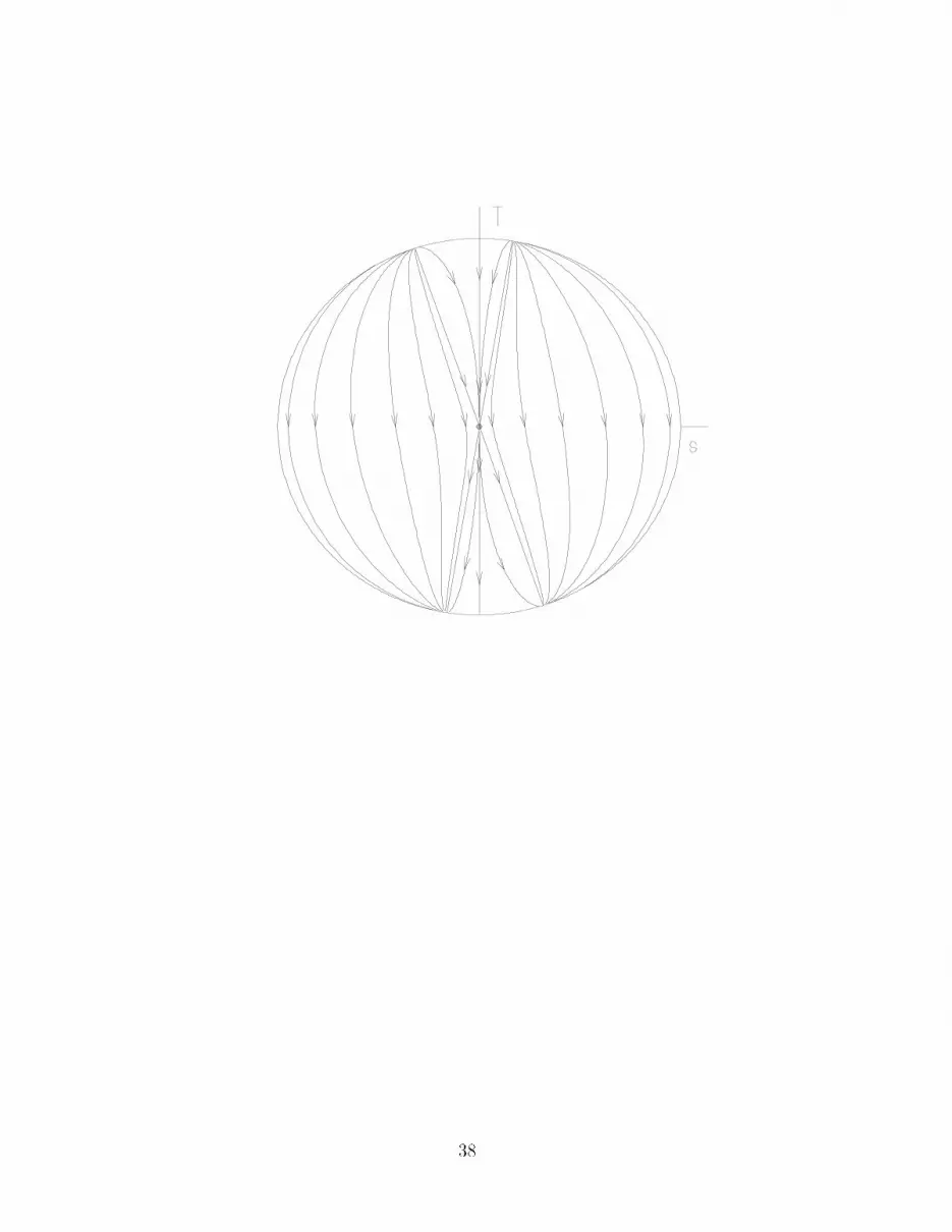
38

-0.6 -0.4 -0.2 0 0.2 0.4 0.6-0.6

-0.4

-0.2

0

0.2

0.4

0.6

-0.4 -0.2 0 0.2 0.4

-0.1

0

0.1

0.2

-0.4 -0.2 0 0.2 0.4-0.4

-0.2

0

0.2

0.4

-0.4 -0.2 0 0.2 0.4-0.4

-0.2

0

0.2

0.4

39