Embed Size (px)
Citation preview


The International Journal on Advances in Networks and Services is published by IARIA.
ISSN: 1942-2644
journals site: http://www.iariajournals.org
contact: [email protected]
Responsibility for the contents rests upon the authors and not upon IARIA, nor on IARIA volunteers,
staff, or contractors.
IARIA is the owner of the publication and of editorial aspects. IARIA reserves the right to update the
content for quality improvements.
Abstracting is permitted with credit to the source. Libraries are permitted to photocopy or print,
providing the reference is mentioned and that the resulting material is made available at no cost.
Reference should mention:
International Journal on Advances in Networks and Services, issn 1942-2644
vol. 4, no. 1 & 2, year 2011, http://www.iariajournals.org/networks_and_services/
The copyright for each included paper belongs to the authors. Republishing of same material, by authors
or persons or organizations, is not allowed. Reprint rights can be granted by IARIA or by the authors, and
must include proper reference.
Reference to an article in the journal is as follows:
<Author list>, “<Article title>”
International Journal on Advances in Networks and Services, issn 1942-2644
vol. 4, no. 1 & 2, year 2011, <start page>:<end page> , http://www.iariajournals.org/networks_and_services/
IARIA journals are made available for free, proving the appropriate references are made when their
content is used.
Sponsored by IARIA
www.iaria.org
Copyright © 2011 IARIA

International Journal on Advances in Networks and Services
Volume 4, Number 1 & 2, 2011
Editor-in-Chief
Tibor Gyires, Illinois State University, USA
Editorial Advisory Board
Jun Bi, Tsinghua University, ChinaMario Freire, University of Beira Interior, PortugalJens Martin Hovem, Norwegian University of Science and Technology, NorwayVitaly Klyuev, University of Aizu, JapanNoel Crespi, Institut TELECOM SudParis-Evry, France
Editorial Board
Networking
Adrian Andronache, University of Luxembourg, Luxembourg Robert Bestak, Czech Technical University in Prague, Czech Republic Jun Bi, Tsinghua University, China Juan Vicente Capella Hernandez, Universidad Politecnica de Valencia, Spain Tibor Gyires, Illinois State University, USA Go-Hasegawa, Osaka University, Japan Dan Komosny, Brno University of Technology, Czech Republic Birger Lantow, University of Rostock, Germany Pascal Lorenz, University of Haute Alsace, France Iwona Pozniak-Koszalka, Wroclaw University of Technology, Poland Yingzhen Qu, Cisco Systems, Inc., USA Karim Mohammed Rezaul, Centre for Applied Internet Research (CAIR) / University of Wales, UK Thomas C. Schmidt, HAW Hamburg, Germany Hans Scholten, University of Twente – Enschede, The Netherlands
Networks and Services
Claude Chaudet, ENST, France Michel Diaz, LAAS, France Geoffrey Fox, Indiana University, USA Francisco Javier Sanchez, Administrador de Infraestructuras Ferroviarias (ADIF), Spain Bernhard Neumair, University of Gottingen, Germany Gerard Parr, University of Ulster in Northern Ireland, UK Maurizio Pignolo, ITALTEL, Italy Carlos Becker Westphall, Federal University of Santa Catarina, Brazil Feng Xia, Dalian University of Technology, China

Internet and Web Services
Thomas Michael Bohnert, SAP Research, Switzerland Serge Chaumette, LaBRI, University Bordeaux 1, France Dickson K.W. Chiu, Dickson Computer Systems, Hong Kong Matthias Ehmann, University of Bayreuth, Germany Christian Emig, University of Karlsruhe, Germany Geoffrey Fox, Indiana University, USA Mario Freire, University of Beira Interior, Portugal Thomas Y Kwok, IBM T.J. Watson Research Center, USA Zoubir Mammeri, IRIT – Toulouse, France Bertrand Mathieu, Orange-ftgroup, France Mihhail Matskin, NTNU, Norway Guadalupe Ortiz Bellot, University of Extremadura Spain Dumitru Roman, STI, Austria Monika Solanki, Imperial College London, UK Vladimir Stantchev, Berlin Institute of Technology, Germany Pierre F. Tiako, Langston University, USA Weiliang Zhao, Macquarie University, Australia
Wireless and Mobile Communications
Habib M. Ammari, Hofstra University - Hempstead, USA Thomas Michael Bohnert, SAP Research, Switzerland David Boyle, University of Limerick, Ireland Xiang Gui, Massey University-Palmerston North, New Zealand Qilian Liang, University of Texas at Arlington, USA Yves Louet, SUPELEC, France David Lozano, Telefonica Investigacion y Desarrollo (R&D), Spain D. Manivannan (Mani), University of Kentucky - Lexington, USA Jyrki Penttinen, Nokia Siemens Networks - Madrid, Spain / Helsinki University of Technology,
Finland Radu Stoleru, Texas A&M University, USA Jose Villalon, University of Castilla La Mancha, Spain Natalija Vlajic, York University, Canada Xinbing Wang, Shanghai Jiaotong University, China Qishi Wu, University of Memphis, USA Ossama Younis, Telcordia Technologies, USA
Sensors
Saied Abedi, Fujitsu Laboratories of Europe LTD. (FLE)-Middlesex, UK Habib M. Ammari, Hofstra University, USA Steven Corroy, University of Aachen, Germany Zhen Liu, Nokia Research – Palo Alto, USA Winston KG Seah, Institute for Infocomm Research (Member of A*STAR), Singapore Peter Soreanu, Braude College of Engineering - Karmiel, Israel

Masashi Sugano, Osaka Prefecture University, Japan Athanasios Vasilakos, University of Western Macedonia, Greece You-Chiun Wang, National Chiao-Tung University, Taiwan Hongyi Wu, University of Louisiana at Lafayette, USA Dongfang Yang, National Research Council Canada – London, Canada
Underwater Technologies
Miguel Ardid Ramirez, Polytechnic University of Valencia, Spain Fernando Boronat, Integrated Management Coastal Research Institute, Spain Mari Carmen Domingo, Technical University of Catalonia - Barcelona, Spain Jens Martin Hovem, Norwegian University of Science and Technology, Norway
Energy Optimization
Huei-Wen Ferng, National Taiwan University of Science and Technology - Taipei, Taiwan Qilian Liang, University of Texas at Arlington, USA Weifa Liang, Australian National University-Canberra, Australia Min Song, Old Dominion University, USA
Mesh Networks
Habib M. Ammari, Hofstra University, USA Stefano Avallone, University of Napoli, Italy Mathilde Benveniste, Wireless Systems Research/En-aerion, USA Andreas J Kassler, Karlstad University, Sweden Ilker Korkmaz, Izmir University of Economics, Turkey //editor assistant//
Centric Technologies
Kong Cheng, Telcordia Research, USA Vitaly Klyuev, University of Aizu, Japan Arun Kumar, IBM, India Juong-Sik Lee, Nokia Research Center, USA Josef Noll, ConnectedLife@UNIK / UiO- Kjeller, Norway Willy Picard, The Poznan University of Economics, Poland Roman Y. Shtykh, Waseda University, Japan Weilian Su, Naval Postgraduate School - Monterey, USA
Multimedia
Laszlo Boszormenyi, Klagenfurt University, Austria Dumitru Dan Burdescu, University of Craiova, Romania Noel Crespi, Institut TELECOM SudParis-Evry, France Mislav Grgic, University of Zagreb, Croatia Hermann Hellwagner, Klagenfurt University, Austria Polychronis Koutsakis, McMaster University, Canada

Atsushi Koike, KDDI R&D Labs, Japan Chung-Sheng Li, IBM Thomas J. Watson Research Center, USA Parag S. Mogre, Technische Universitat Darmstadt, Germany Eric Pardede, La Trobe University, Australia Justin Zhan, Carnegie Mellon University, USA
Additional reviewers
Yunyue Lin, The University of Memphis, USA
International Journal on Advances in Networks and Services
Volume 4, Numbers 1 & 2, 2011
CONTENTS
On two Routing Mechanisms for Wireless Sensor Networks
Adrian Fr. Kacso, University of Siegen, Germany
1 - 12
GeoOLSR: Extension of OLSR to support Geocasting in Mobile Ad Hoc Networks
Volker Köster, TU Dortmund University, Germany
Andreas Lewandowski, TU Dortmund University, Germany
Dennis Dorn, TU Dortmund University, Germany
Christian Wietfeld, TU Dortmund University, Germany
13 - 26
A Traffic Monitoring and Queue Detection System Based on an Acoustic Sensor Network
Barbara Barbagli, Dept. of Electronics and Telecommunications, University of Florence., Italy
Luca Bencini, Dept. of Electronics and Telecommunications, University of Florence., Italy
Iacopo Magrini, Dept. of Electronics and Telecommunications, University of Florence., Italy
Gianfranco Manes, Dept. of Electronics and Telecommunications, University of Florence., Italy
Antonio Manes, Netsens s.r.l., Italy
27 - 37
Enhancing Resiliency Against Routing Layer Attacks in Wireless Sensor Networks:
Gradient-based Routing in Focus
Ochirkhand Erdene-Ochir, Orange Labs, France Telecom Group, France
Apostolos Kountouris, Orange Labs, France Telecom Group, France
Marine Minier, Universite de Lyon, INRIA, INSA-Lyon, CITI, France
Fabrice Valois, Universite de Lyon, INRIA, INSA-Lyon, CITI, France
38 - 54
Reliability Estimation of Mobile Agent System in MANET with Dynamic Topological and
Environmental Conditions
Chandreyee Chowdhury, Jadavpur University, India
Sarmistha Neogy, Jadavpur University, India
55 - 65
Durable Solar Energy Harvesting from Limited Ambient Energy Income
Sebastian Bader, Mid Sweden University, Sweden
Bengt Oelmann, Mid Sweden University, Sweden
66 - 80
TrickleTree: A Gossiping Approach To Fast And Collision Free Staggered Scheduling
Wojciech Bober, University College Dublin, Ireland
Chris J. Bleakley, University College Dublin, Ireland
Xiaoyun Li, University College Dublin, Ireland
81 - 91
Phased Array Satellite Antenna Testing by an Aircraft Borne Emulation Platform 92 - 106

Iwan Kruger, Stellenbosch University, Dept of Electrical & Electronic Engineering, South Africa
Riaan Wolhuter, Stellenbosch University, Dept of Electrical & Electronic Engineering, South Africa
Unifom Generators and Combinatorial Designs
Alexis Bonnecaze, IML/ERISCS, Université de la Méditerranée, France
Pierre Liardet, LATP, Université de Provence, France
107 - 118
CUPID: A Communication Pattern Informed Duty Cycling for Large-scale, Low-delay
Sensor Applications
Daniela Krüger, Institute of Telematics, University of Lübeck, Germany
Stefan Fischer, Institute of Telematics, University of Lübeck, Germany
Dennis Pfisterer, Institute of Telematics, University of Lübeck, Germany
119 - 129
Performance Evaluation of a Disaster Recovery System and Practical Network
Applications in Cloud Compting Envionments
Yoichiro Ueno, Tokyo Denki University, Japan
Noriharu Miyaho, Tokyo Denki University, Japan
Shuichi Suzuki, Tokyo Denki University, Japan
Kazuo Ichihara, Net & Logic Co., Japan
130 - 137
Campus-Wide Indoor Tracking Infrastructure
Heinrich Schmitzberger, Johannes Kepler University Linz, Department of Business Informatics -
Software Engineering, Austria
Wolfgang Narzt, Johannes Kepler University Linz, Department of Business Informatics - Software
Engineering, Austria
138 - 148
Sensor Data Fusion Middleware for Cooperative Traffic Applications
Teemu Leppänen, University of Oulu, Finland
Mikko Perttunen, University of Oulu, Finland
Pekka Kaipio, University of Oulu, Finland
Jukka Riekki, University of Oulu, Finland
149 - 158
A New Wireless Architecture for In-Flight Entertainment Systems Inside Aircraft Cabin
Ahmed Akl, LAAS/CNRS, France
Thierry Gayraud, LAAS/CNRS, France
Pascal Berthou, LAAS/CNRS, France
159 - 175
Exploiting Multimedia Frame Semantics and MAC-layer Enhancements for QoS
Provisioning in IEEE 802.11e Congested Networks
Anastasios Politis, University of Macedonia, Greece
Ioannis Mavridis, University of Macedonia, Greece
Athanasios Manitsaris, University of Macedonia, Greece
176 - 185
AAODV/AAOMDV Routing Protocols: Single and Multipath Routing in WMNs 186 - 198

Horia Ştefănescu, POLITEHNICA University of Bucharest/Orange Romania, Romania
Mariusz Skrocki, Orange Labs, Telekomunikacja Polska/Warsaw University of Technology, Poland
Sławomir Kukliński, Orange Labs, Telekomunikacja Polska/Warsaw University of Technology, Poland
The Analysis of Similarities and Registration Delay in Phonebook Centric Social Networks
Péter Ekler, Budapest University of Technology and Economics, Department of Automation and
Applied Informatics, Hungary
Tamás Lukovszki, Eötvös Loránd University, Faculty of Informatics, Hungary
199 - 208
WLAN IEEE 802.11a/b/g/n Indoor Coverage and Interference Performance Study
Sandra Sendra, Universidad Politécnica de Valencia, Spain
Miguel Garcia, Universidad Politécnica de Valencia, Spain
Carlos Turro, Universidad Politécnica de Valencia, Spain
Jaime Lloret, Universidad Politécnica de Valencia, Spain
209 - 222
Fast Retrieval from Image Databases via Binary Haar Wavelet Transform on the Color
and Edge Directivity Descriptor
Savvas Chatzichristofis, Department of Electrical & Computer Engineering, Democritus University of
Thrace, Xanthi, Greece
Yiannis Boutalis, Department of Electrical & Computer Engineering, Democritus University of
Thrace, Xanthi, Greece
Avi Arampatzis, Department of Electrical & Computer Engineering, Democritus University of Thrace,
Xanthi, Greece
223 - 231
Combining Biometrics Derived from Different Classes of Nonlinear Analyses of Fronto-
Normal Gait Signals
Tracey Lee, Singapore Polytechnic, Singapore
Saeid Sanei, University of Surrey, Surrey, United Kingdom
Mohammed M. Belkhatir, University of Lyon & CNRS, France
232 - 243
On two Routing Mechanisms for Wireless SensorNetworks
Adrian Fr. KacsoComputer Science Department
University of Siegen57068 Siegen, Germany
Email: [email protected]
Abstract—In this paper we extend our previous implementa-tion of the T-MAC protocol inside the sensor network simulatorwith a receiver-based routing (RBR) service and we propose andimplement several performance optimizations. We investigate theimpact of several MAC protocol parameters (listen time, receivercontention window, radio switch time, etc.) on the performanceof routing protocols used in resource constrained wirelesssensornetworks. The main performance criteria we are interested in arethe energy consumption (reflected by the active time the nodeis operational), the throughput and latency of the network indelivering replies to users’ requests.Simulation results have shown that using the proposed opti-mizations improve significantly the performance of the RBR.Moreover, we compare the performance of receiver-based routingagainst the unicast within our implementation of the T-MACprotocol. Although in direct comparison the RBR approach isoutperformed by unicast, we show that RBR can be efficientlyemployed for opportunistic aggregation inside monitoringareaswith many sources or in dynamic network scenarios.
Index Terms—wireless sensor network, simulation framework,MAC and routing protocols, collisions.
I. I NTRODUCTION
A wireless sensor network (WSN) is a communicationnetwork consisting of a large number of sensor nodes thatare randomly and densely deployed in a geographical area.The nodes operate unattended and are forced to self-organizethemselves (in a multihop wireless network) as a result offrequent topology changes (due to node transient failures,addition or depletion) and to adjust their behavior to currentnetwork conditions. Each of the distributed nodes in the WSNsenses individually the environment and they collaborativelypreprocess and communicate the information to a sink.
Typically, a sensor node has limited energy and memory,restricted communication range and computation capabilities.The communication cost is often higher (several orders ofmagnitude) than the computation cost. For optimizing thecommunication cost in order to conserve energy, different data-centric routing protocols and in-network processing techniqueshave been proposed.
In query-driven WSNs, routing protocols determine onwhich routes messages (query and data) are forwarded be-tween the sink and sources (nodes able to deliver the requesteddata) using data-centric approaches. In suchdata-centricrout-ing schemes, the destination node of messages is specified by
tuples of attribute-value pairs of the data carried inside thepackets and not using globally unique identifiers (node addr).
When the distance between source(s) and sink is large,intermediate nodes forward the messages from hop to hopuntil they reach the intended destination. Selecting the nexthop in order to establish a path (to a source or sink) can beeither initiated by the sender or delegated to receiver nodes.In the first approach, the sender decides itself by analysingits internal tables where to send the message, whereas in thesecond approach the sender delegates the decision to all itsneighbors, which distributively elect the best receiver. Thestrategy to select the next hop employs various metrics whichallow to find different paths, e.g., energy-efficient, shorter,rapid, reliable paths, depending on the application goals.
Typically, the information collected in a sensor networkis highly correlated, yielding a spatial and temporal correla-tion between successive measurements. Exploiting the data-centricity and the spatial-temporal correlation characteristicsallows to apply effective in-network data aggregation tech-niques, which further improve the energy-efficiency of thecommunication in WSN. Aggregation can eliminate the in-herent redundancy of the raw data collected and, additionally,it reduces the traffic in the network, avoiding in this waycongestions and induced collisions.
The paper is an extension of [1] and is structured asfollows. Section II presents the state-of-art and the motivationbehind designing energy aware protocols for WSNs usingcross-layer design. Section III describes the basic approachof receiver-based routing (RBR).Section IV presents thedesign (using cross-layering) of the RBR service (RBRS)inside our Timeout-MAC (T-MAC) protocol implementation.Section V discusses several optimizations made to RBRS.Section VI illustrates the performance of the RBR serviceby giving various simulation results and comparing it withunicast. Section gives more comparison results and SectionVIII concludes the paper.
II. RELATED WORK AND OBJECTIVES
The main impact on the energy consumption of the nodes isgiven by the MAC protocol and only secondly by the routingstrategy. A real energy benefit is achieved when using MACprotocols with an active-sleep regime and/or low duty cycles(such as S-MAC [2], B-MAC [3], T-MAC [4]). Considering
1
International Journal on Advances in Networks and Services, vol 4 no 1 & 2, year 2011, http://www.iariajournals.org/networks_and_services/
2011, © Copyright by authors, Published under agreement with IARIA - www.iaria.org
the scarce energy, communication and processing resourcesof WSNs, a joint optimization of the networking layers byemploying a cross-layer design is a promising alternative tomaximize the network performance, while reducing the globalenergy consumption.
Many of the current routing protocols are sender initiated[5][6][7], that is, the decision to which neighbor to routethe just received message is taken by the sender. The sendermaintains some internal neighborhood table (e.g., gradienttable or routing table), which is inspected when messagesneed to be forwarded. Other protocols [8][9][10][11] usethe receiver-based approach; in [9][10][11], the receivercon-tention scheme is used to develop a unified cross-layer protocoland in [8] to build mechanisms that lead to efficient dataaggregation without maintaining a structure, namely the Data-Aware Anycast (DAA) and the Randomized Waiting (RW).
The spare energy and processing resources of battery pow-ered sensor nodes require energy efficient communicationprotocols in order to fulfill the application objectives of WSNs.The use of both cross-layer design techniques [9][11][12] andaggregation [7][8][13] improves the overall network perfor-mance in terms of energy conservation.
The use of cross-layer design aims optimizing jointlyseveral layers of the communication stack. Since for a resourceconstrained node strict layering is inappropriate [14] [15], weemploy [12] a cross-layer design by allowing exchange ofinformation (mainly) across application, routing, MAC andphysical layers in order to optimize them.
Based on the application’s requirements, the network topol-ogy, source placement and the aggregation function, a nearto optimal aggregation structure (tree) can be constructed[16]. Various structured aggregation mechanisms (centralized[13][17] or distributed [7]) have been proposed. For query-driven sensor network applications, where several sourcenodes periodically report data to the sink, structured aggre-gation mechanisms are well suited, since the traffic patternlasts for a long time and the overhead of construction andmaintenance of the structure is low, compared with the energybenefits achieved through aggregation. For sensor networkapplications, where the sources are spread or the networktopology is dynamic, the high construction and maintainanceoverhead for the aggregation structure can outweight thebenefits of data aggregation. In such dynamic scenarios, mech-anisms are required that achieve data aggregation without theconstruction and maintenance of a structure.
Concerning the simulator, we proposed in [18] and extendedin [12] a modular, energy-aware network architecture of asensor node as a flexible approach to design and plug-and-play various protocols at network and MAC layers, and tocombine and analyse the impact of different parameters onthe performance and lifetime of the WSN. We implementedour simulation framework SNF (Sensor Network Framework)using the OMNeT++ 3.4b2 discrete event simulation packageand its Mobility Framework [19].
In the present paper we focus on the implementation of anadditional RBR service to T-MAC for enabling applications
to use both the unicast and the RBR service. An example ofsuch an application is the opportunistic aggregation, wheredata packets are aggregated, if they meet each other on somenode. Inside the source area the data packets are aggregatedusing the RBR service, while outside it the aggregated datapackets are sent usingRTS/CTSunicast ([20]). Source nodeshaving matching data (same type and required timestamp)are potential aggregators.If there is a potential additionalaggregator closer to sink, it gets a higher priority in the RBR-associated transmission than an aggregator that is fartheraway.
III. R ECEIVER-BASED ROUTING (RBR)
The RBR service employs the use ofBRTS (BroadcastRequest-To-Send) control packet to getBCTS (BroadcastClear-To-Send) responses from neighbors, which take initiativeto participate in the transfer of the relevant information to sink.The BRTScontrol packet serves as a negotiation between thesender and all its potential receivers. After receiving theBRTS,each node determines (according to the information carriedinthe packet), wherever it participates in the transfer. In orderto route a packet to destination the next hop should bemoreappropriatethan the sender. Since there are several potentialreceivers, one needs to separate these receivers in prioritygroups, according to the available and propagated routing in-formation. Nodes that achieve anincreasing progress(i.e., arebetter placed or have more energy or data packets to aggregate,etc.) are placed in a higher priority group than others. Thepriority of a receiver node (i.e., its priority group) is estab-lished by the routing component (and communicated throughthe cross-layer to the MAC) and is based on the progress apacket would made if the node forwarded the packet. Thisprioritization is introduced to avoidBCTS-collisions (as morereceivers may try to respond simultaneously). It is performedby a receiver contention mechanism to access the channel andis actually a computation of a random delay for theBCTS.
PriorityGroup 0
PriorityGroup 2
Priority Group 1
BRTS DATA ...
SIFS minislot
sender
receiver 1
receiver 2
receiver 3
(Priority Group 0)
BCTS
cancel BCTS
cancel BCTS
BCTS slot
random delay
SIFS
CTS
RTS
SIFS
DATA ...
receiver
sendera)
b)
(Priority Group 1)
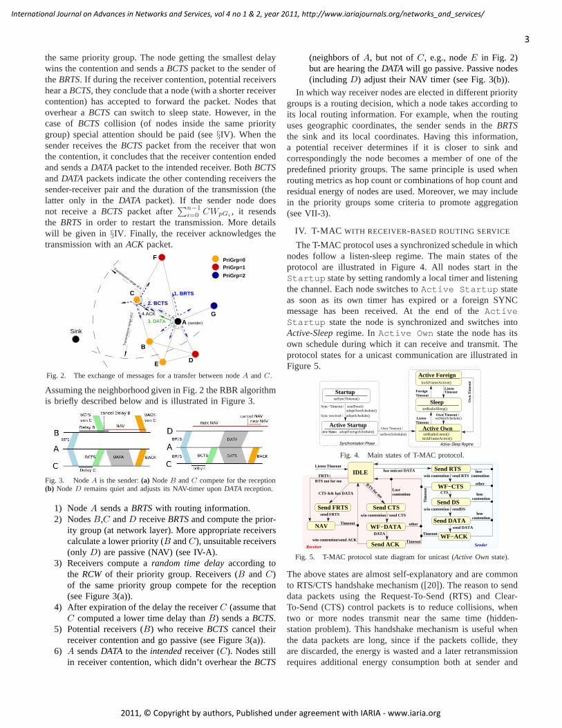
Fig. 1. a) Unicast (using RTS/CTS handshake) b) RBR contention.
Figure 1 shows the difference between the sender initiatednext-hop selection (usingRTS/CTS) and the randomizedBCTSgeneration. According to which priority groupj the nodebelongs, it waits for
∑j−1
i=0CWpGi
+ cwj , where CWpGi
is the contention window corresponding to priority groupi
(j ≤ n−1, assumingn priority groups) andcwj ∈ [0, CWpGj]
is the delay time corresponding toj. This waiting schemedifferentiates nodes of different progress into differentprioritygroups, and attempts to assign different delays to nodes inside
2
International Journal on Advances in Networks and Services, vol 4 no 1 & 2, year 2011, http://www.iariajournals.org/networks_and_services/
2011, © Copyright by authors, Published under agreement with IARIA - www.iaria.org
the same priority group. The node getting the smallest delaywins the contention and sends aBCTSpacket to the sender oftheBRTS. If during the receiver contention, potential receivershear aBCTS, they conclude that a node (with a shorter receivercontention) has accepted to forward the packet. Nodes thatoverhear aBCTScan switch to sleep state. However, in thecase ofBCTS collision (of nodes inside the same prioritygroup) special attention should be paid (see§IV). When thesender receives theBCTSpacket from the receiver that wonthe contention, it concludes that the receiver contention endedand sends aDATApacket to the intended receiver. BothBCTSandDATA packets indicate the other contending receivers thesender-receiver pair and the duration of the transmission (thelatter only in the DATA packet). If the sender node doesnot receive aBCTS packet after
∑n−1
i=0CWpGi
, it resendsthe BRTS in order to restart the transmission. More detailswill be given in §IV. Finally, the receiver acknowledges thetransmission with anACK packet.
C
B
E
F
A
D
G
PriGrp=0PriGrp=1
PriGrp=2
Sink
1. BRTS
3. DATA
2. BCTS
Transmission range of A
Tra
nsm
issi
on r
ange
of C
(sender)
4.ACK
Fig. 2. The exchange of messages for a transfer between nodeA andC.
Assuming the neighborhood given in Fig. 2 the RBR algorithmis briefly described below and is illustrated in Figure 3.
Fig. 3. NodeA is the sender:(a) NodeB andC compete for the reception(b) NodeD remains quiet and adjusts its NAV-timer uponDATA reception.
1) NodeA sends aBRTSwith routing information.2) NodesB,C andD receiveBRTSand compute the prior-
ity group (at network layer). More appropriate receiverscalculate a lower priority (B andC), unsuitable receivers(only D) are passive (NAV) (see IV-A).
3) Receivers compute arandom time delayaccording tothe RCWof their priority group. Receivers (B and C)of the same priority group compete for the reception(see Figure 3(a)).
4) After expiration of the delay the receiverC (assume thatC computed a lower time delay thanB) sends aBCTS.
5) Potential receivers (B) who receiveBCTScancel theirreceiver contention and go passive (see Figure 3(a)).
6) A sendsDATA to the intendedreceiver (C). Nodes stillin receiver contention, which didn’t overhear theBCTS
(neighbors ofA, but not ofC, e.g., nodeE in Fig. 2)but are hearing theDATAwill go passive. Passive nodes(includingD) adjust their NAV timer (see Fig. 3(b)).
In which way receiver nodes are elected in different prioritygroups is a routing decision, which a node takes according toits local routing information. For example, when the routinguses geographic coordinates, the sender sends in theBRTSthe sink and its local coordinates. Having this information,a potential receiver determines if it is closer to sink andcorrespondingly the node becomes a member of one of thepredefined priority groups. The same principle is used whenrouting metrics as hop count or combinations of hop count andresidual energy of nodes are used. Moreover, we may includein the priority groups some criteria to promote aggregation(see VII-3).
IV. T-MAC WITH RECEIVER-BASED ROUTING SERVICE
The T-MAC protocol uses a synchronized schedule in whichnodes follow a listen-sleep regime. The main states of theprotocol are illustrated in Figure 4. All nodes start in theStartup state by setting randomly a local timer and listeningthe channel. Each node switches toActive Startup stateas soon as its own timer has expired or a foreign SYNCmessage has been received. At the end of theActiveStartup state the node is synchronized and switches intoActive-Sleepregime. InActive Own state the node has itsown schedule during which it can receive and transmit. Theprotocol states for a unicast communication are illustrated inFigure 5.
adoptSchedule()
adoptOwnSchedule()sendSync()
Sync received /
Sync−Timeout /
Ow
n T
imeo
ut
Own Timeout /
Own Timeout /
TimeoutForeign Timeout
Listen
TimeoutListen
StartupsetSyncTimeout()
Active−Sleep Regime
rcv Sync: adoptForeignSchedule()
Active Startup
Active Foreign
Active Own
kickFrameActive()
SleepsetRadioSleep()
setRadioListen()kickFrameActive()
setNextSchedule()
setNextSchedule()
Synchronisation Phase
Fig. 4. Main states of T-MAC protocol.
other
contentionlose
other
contentionlose
contentionlose
Losecontention
Send CTS
Send ACK
Send FRTS
WF−DATA
send FRTS
send DATA
CTSCTS && has DATA
WF−ACK
win contention / sendDS
Tim
eout
win contention / send CTS
RTS for me
DATA
Timeout
Timeout
has unicast DATAwin contention / send RTS
NAV
WF−CTS
IDLE
Timeout
win contention/send ACK
RTS not for meFRTS |
Listen Timeout
Receiver Sender
Send RTS
Send DATA
Send DS
Fig. 5. T-MAC protocol state diagram for unicast (Active Ownstate).
The above states are almost self-explanatory and are commonto RTS/CTS handshake mechanism ([20]). The reason to senddata packets using the Request-To-Send (RTS) and Clear-To-Send (CTS) control packets is to reduce collisions, whentwo or more nodes transmit near the same time (hidden-station problem). This handshake mechanism is useful whenthe data packets are long, since if the packets collide, theyare discarded, the energy is wasted and a later retransmissionrequires additional energy consumption both at sender and
3
International Journal on Advances in Networks and Services, vol 4 no 1 & 2, year 2011, http://www.iariajournals.org/networks_and_services/
2011, © Copyright by authors, Published under agreement with IARIA - www.iaria.org
receiver. Broadcast packets are never sent using the RTS/CTShandshake and are not acknowledged (using ACK packets).
In case ofActive Foreign, the node is in active stateof a foreign schedule, where it can only receive. Therefore,the state transitions are the same as in the left side of Figure5. The Future-Request-To-Send (FRTS) packet is an extensionmeant to avoid the early sleeping problem ([4]).
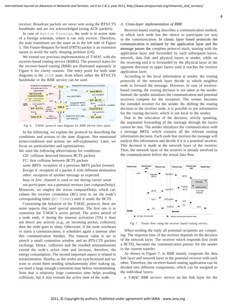
We extend our previous implementation of T-MAC with thereceiver-based routing service (RBRS). The protocol states forthe receiver-based routing (RBR) are illustrated separately inFigure 6 for clarity reasons. The entry point for both statediagrams is theIDLE state, from where either the RTS/CTShandshake or the RBR service can be used.
sameBRTS
Send BRTS
CD && !FC || BRTSTimeout WF−BCTS ||
IDLESend DATA
WF−ACK
free / send BRTS
WF−DATA
busy
NAV
Tim
eout
NA
V
WF−DATATimeout
not participateRTS not for me || CTS ||
free / send DATA
busy ||
RECEIVER
Send ACK
CONTENTION
has msg
BCTS
busy || RTS || BRTS
foreign BCTS || RTS not for me || CTS || DATA
DATA
other ||
Timeout WF−ACK || other
ACK/ delete msg
BRTS
busy
foreign BCTS || foreign DATA
WF−BCTS
CD && FC / send BRTS
foreign BRTS
free / send BCTS
free/send ACK
List
en T
imeo
ut
Receiver Sender
RC−Timer( delay)delay = computeDelay()
Fig. 6. T-MAC protocol state diagram for RBR (Active Ownstate).
In the following, we explain the protocol by describing theconditions and actions of the state diagram. Not mentionedterms/conditions and actions are self-explanatory. Later, wefocus on particularities and optimizations.We used the following abbreviations for conditions:
CD: collision detected betweenBCTSpacketsFC: first collision betweenBCTSpacketssame BRTS: reception of a previousBRTSpacket (resent)foreign X: reception of a packetX with different destinationother: reception of another message as expectedbusyor free: channel is used or not during carrier sensenot participate: not a potential receiver (seecomputeDelay).
Moreover, we employ the actioncomputeDelay, which cal-culates the receiver contention (RC) time to set the node’scorresponding timer (RC-Timer) until it sends theBCTS.
Concerning the behavior of the T-MAC protocol, there aresome aspects that need special attention. The first one is tocustomize the T-MAC’s active period. The active period ofa node ends, if during the timeout activation (TA) it doesnot detect any activity (e.g., an incoming packet, collision);then the node goes to sleep. Otherwise, if the node overhearsor starts a communication, it schedules again a timeout afterthis communication finishes. The timeout value is set tostretch a small contention window and anRTS-CTSpacketsexchange. Hence, collisions and the resulted retransmissionsextend the node’s active time and increase, therefore, theenergy consumption. The second important aspect is relatedtoretransmission. Hereby, as the nodes are synchronized and wewant to avoid them sending simultaneously after waking up,we need a large enough contention time before retransmitting.Note that a relatively large contention time helps avoidingcollisions, but it also extends the active time of the node.
A. Cross-layer implementation of RBR
Receiver-based routing describes a communication method,in which each node has the choice to participate (or not)in the communication.In classic layer based protocols thecommunication is initiated by the application layer and themessage passes thecomplete protocol stack, starting with theapplication layer and forwarded by each subsequent layers,network, data link and physical layers at sender, while onthe receiving end it is forwarded by the physical layer in theopposite direction to upper layers until it reaches the receiverapplication layer.
According to the local information at sender, the routingprotocols of the network layer decide to which neighbornode to forward the message. However, in case of receiver-based routing, the routing decision is not taken at the sender.Instead, the sender initializes the communication and potentialreceivers compete for the reception. The winner becomesthe intended receiver for the sender. By shifting the routingdecision to the receiver node, it is possible to use informationfor the routing decision, which is not local to the sender.
Due to the relocation of the decision, strictly speaking,the sequential forwarding of the message through the layerscannot be met. The sender initializes the communication witha messageBRTS, which contains all the relevant routinginformation decision. Each node that receives the message willanalyze this information and decide if it is a potential receiver.This decision is made at the network layer of the receiver.Thus, the network layer of the receiver is already involved inthe communication before the actual data flow.
Information
(BRTS)
Routing decision
Cross−layerInteraction
(BCTS)(BCTS)
Sender
Wireless communication between nodes
Network layer
Initialization Send BRTS
DATA
Physical Layer Network layerMAC
Physical LayerMAC
Data link layer Data link layer
(BRTS)DATA
Response
Send BCTS
DATA transferDATA
DATAACK
ACKSend ACK
Receiver
inter layer communication
Fig. 7. Packet flow using the receiver based routing service.
When sending the reply all potential recipients are compet-ing. The response time of the receiver depends on the decisionof the network layer. The receiver which responds first (witha BCTS), becomes the communication partner for the senderin the current transfer.
As shown in Figure 7, in RBR mainly cooperate the datalink layer and network layer in the potential receiver with eachother. Therefore, the receiver-based routing applicationcan bedivided into different components, which can be assigned tothe individual layers:
• T-MAC RBR service: service on the link layer for the
4
International Journal on Advances in Networks and Services, vol 4 no 1 & 2, year 2011, http://www.iariajournals.org/networks_and_services/
2011, © Copyright by authors, Published under agreement with IARIA - www.iaria.org
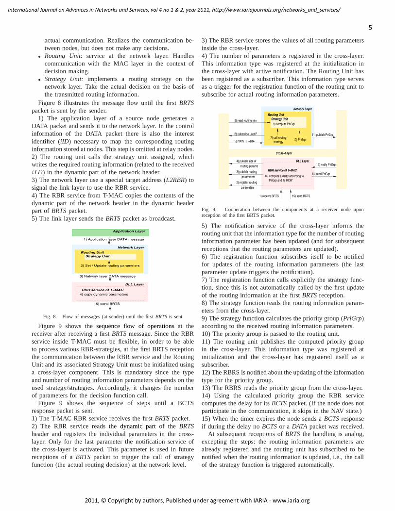
actual communication. Realizes the communication be-tween nodes, but does not make any decisions.
• Routing Unit: service at the network layer. Handlescommunication with the MAC layer in the context ofdecision making.
• Strategy Unit: implements a routing strategy on thenetwork layer. Take the actual decision on the basis ofthe transmitted routing information.
Figure 8 illustrates the message flow until the firstBRTSpacket is sent by the sender.
1) The application layer of a source node generates aDATA packet and sends it to the network layer. In the controlinformation of the DATA packet there is also the interestidentifier (iID ) necessary to map the corresponding routinginformation stored at nodes. This step is omitted at relay nodes.2) The routing unit calls the strategy unit assigned, whichwrites the required routing information (related to the receivediID) in the dynamic part of the network header.3) The network layer use a special target address (L2RBR) tosignal the link layer to use the RBR service.4) The RBR service from T-MAC copies the contents of thedynamic part of the network header in the dynamic headerpart of BRTSpacket.5) The link layer sends theBRTSpacket as broadcast.
DLL Layer
Network Layer
Application Layer
RBR service of T−MAC
4) copy dynamic parameters
Routing Unit
Strategy Unit
2) Set / Update routing parameters
1) Application layer DATA message
3) Network layer DATA message
5) send BRTS
Fig. 8. Flow of messages (at sender) until the firstBRTSis sent
Figure 9 shows thesequence flow of operationsat thereceiver after receiving a firstBRTSmessage. Since the RBRservice inside T-MAC must be flexible, in order to be ableto process various RBR-strategies, at the first BRTS receptionthe communication between the RBR service and the RoutingUnit and its associated Strategy Unit must be initialized usinga cross-layer component. This is mandatory since the typeand number of routing information parameters depends on theused strategy/strategies. Accordingly, it changes the numberof parameters for the decision function call.
Figure 9 shows the sequence of steps until a BCTSresponse packet is sent.1) The T-MAC RBR service receives the firstBRTSpacket.2) The RBR service reads thedynamic partof the BRTSheader and registers the individual parameters in the cross-layer. Only for the last parameter the notification service ofthe cross-layer is activated. This parameter is used in futurereceptions of aBRTSpacket to trigger the call of strategyfunction (the actual routing decision) at the network level.
3) The RBR service stores the values of all routing parametersinside the cross-layer.4) The number of parameters is registered in the cross-layer.This information type was registered at the initializationinthe cross-layer with active notification. The Routing Unit hasbeen registered as a subscriber. This information type servesas a trigger for the registration function of the routing unit tosubscribe for actual routing information parameters.
DLL Layer
Network Layer
Strategy Unit
9) compute PriGrp
5) notify RP−size
14) compute a delay according to
PriGrp and its RCW
1) receive BRTS 15) send BCTS
2) register routing
parameters
parameters
3) publish routing
routing params
4) publish size of
Routing Unit
strategy
7) call routing10) PriGrp
8) read routing info
11) publish PriGrp
12) notify PriGrp
Cross−Layer
6) subscribe Last P
RBR service of T−MAC13) read PriGrp
Fig. 9. Cooperation between the components at a receiver node uponreception of the first BRTS packet.
5) The notification service of the cross-layer informs therouting unit that the information type for the number of routinginformation parameter has been updated (and for subsequentreceptions that the routing parameters are updated).6) The registration function subscribes itself to be notifiedfor updates of the routing information parameters (the lastparameter update triggers the notification).7) The registration function calls explicitly the strategyfunc-tion, since this is not automatically called by the first updateof the routing information at the firstBRTSreception.8) The strategy function reads the routing information param-eters from the cross-layer.9) The strategy function calculates the priority group (PriGrp)according to the received routing information parameters.10) The priority group is passed to the routing unit.11) The routing unit publishes the computed priority groupin the cross-layer. This information type was registered atinitialization and the cross-layer has registered itself as asubscriber.12) The RBRS is notified about the updating of the informationtype for the priority group.13) The RBRS reads the priority group from the cross-layer.14) Using the calculated priority group the RBR servicecomputes the delay for itsBCTSpacket. (If the node does notparticipate in the communication, it skips in the NAV state.)15) When the timer expires the node sends aBCTSresponseif during the delay noBCTSor a DATA packet was received.
At subsequent receptions ofBRTSthe handling is analog,excepting the steps: the routing information parameters arealready registered and the routing unit has subscribed to benotified when the routing information is updated, i.e., the callof the strategy function is triggered automatically.
5
International Journal on Advances in Networks and Services, vol 4 no 1 & 2, year 2011, http://www.iariajournals.org/networks_and_services/
2011, © Copyright by authors, Published under agreement with IARIA - www.iaria.org
V. RBR OPTIMIZATIONS
To design an effective receiver-based service implies toavoid collisions whenever possible and, if they still occur,to handle them efficiently. To that end, we propose in thefollowing several optimizations.
A. First Group Weight optimization
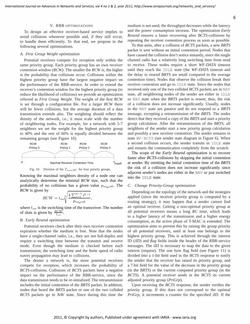
Potential receivers compete for reception only within thesame priority group. Each priority group has an ownreceivercontention window (RCW). The smaller theRCWis, the higheris the probability that collisions occur. Collisions within thehighest priority group have the largest negative impact onthe performance of the RBR-service. In order to extend thereceiver’s contention window for the highest priority group (toreduce the likelihood of collisions) we provide an optimizationreferred asFirst Group Weight. The weight of the firstRCWis set through a configuration file. For a largerRCW therewill be fewer collisions, but the average duration of a datatransmission extends also. The weighting should reflect thedensity of the network, i.e., it must scale with the numberof neighboring nodes. For example, for a network with 5-7neighbors we set the weight for the highest priority groupto 40% and the rest of 60% is equally divided between theremaining groups (see Figure 10).
RCW RCW RCWRCWPriGrp 1 PriGrp 2 PriGrp 3
Maximal Receiver Contention Time0 TmaxRC
PriGrp 0
Fig. 10. Division of theTmaxRC for four priority groups.
Knowing the maximal neighbors density of a node one cananalytically determine the minimalRCW size, such that theprobability of no collisions has a given valuepno coll. TheRCW is given by
RCW = tswk
√
k∑n−1
i=1ik−1
pno coll
,
wheretsw is the switching time of the transceiver. The numberof slots is given byRCW
tsw.
B. Early Resend optimization
Potential receivers check after their ownreceiver contentionexpiration whether the medium is free. Note that the nodeshave a single-channel radio, i.e., they are not full-duplexandrequire a switching time between the transmit and receivemode. Even though the medium is checked before eachtransmission, the switching time and the finite speed of radiowaves propagation may lead to collisions.
The denser a network is, the more potential receiverscompete for reception, which increases the probability ofBCTS-collisions. Collisions ofBCTSpackets have a negativeimpact on the performance of the RBR-service, since thedata transmission needs to be re-initialized. The retransmissionincludes the initial contention of theBRTSpacket. In addition,nodes that heard theBRTSpacket or one of the two collidedBCTS packets go inNAV state. Since during this time the
medium is not used, the throughput decreases while the latencyand the power consumption increase. The optimizationEarlyResendensures a faster recovering afterBCTS-collisions byrepeating the receiver contention process as soon as possible.
To that aims, after a collision ofBCTSpackets, a newBRTSpacket is sent without an initial contention period. Nodes thathave caused the collision don’t notice instantly, since thesinglechannel radio has a relatively long switching time from sendto receive. These nodes require a shortWF-DATA timeoutuntil they reach theIDLE state (theWF-DATA timeout andthe delay to resendBRTSare small compared to the averagecontention time). Nodes that observe the collision break theirreceiver contention and go toIDLE state. Since the nodes thatreceived only one of the two collidedBCTSpackets are inNAVstate, all neighboring nodes of the sender are either inIDLEor NAV state when theBRTSpacket is resent; thus, the riskof a collision does not increase significantly. Usually, nodesin the NAV state are passive and do not respond to aBRTSmessage, excepting a retransmission of theBRTS. The nodesdetect that they received a copy of theBRTSand start a prioritygroup calculation. After the retransmission of theBRTS, allneighbors of the sender start a new priority group calculationand possibly a new receiver contention. The sender remains instateWF-BCTS (see sender state diagram in Figure 6). Whena second collision occurs, the sender transits inIDLE stateand restarts the communication completely from the scratch.
The scope of theEarly Resendoptimization is to recoverfaster afterBCTS-collisions by skipping the initial contentionat sender. By omitting the initial contention time of theBRTSthe risk of a collision does not increase significantly sinceadjacent sender’s nodes are either in theNAV or just switchedinto theIDLE state.
C. Change Priority-Group optimization
Depending on the topology of the network and the strategiesapplied (since the receiver priority group is computed by arouting strategy), it may happen that a sender cannot findan optimal receiver. Getting a non-optimal priority group atall potential receivers means a longRC time, which leadsto a higher latency of the transmission and a higher energyconsumption, as the active phase of T-MAC is extended. Theoptimization aims to prevent this by raising the group priorityof all potential receivers, until at least one belongs to thehighest priority group. This is achieved through the interestID (iID ) andflag fields inside the header of the RBR-servicemessages. TheiID is necessary to map the data to the giveninterest (request). The one byte flag field (see Figure 11) isdivided into a 1-bit field used in theBCTSresponse to notifythe sender that the receiver has raised its priority group, anda 7-bit field for the value of the decrease in the priority group(in the BRTS) or the current computed priority group (in theBCTS). A potential receiver sends in theBCTS its currentadjusted priority group (PriGrp).
Upon receiving theBCTSresponse, the sender verifies thepriority group. If this does not correspond to the optimalPriGrp, it increments a counter for the specifiediID . If the
6
International Journal on Advances in Networks and Services, vol 4 no 1 & 2, year 2011, http://www.iariajournals.org/networks_and_services/
2011, © Copyright by authors, Published under agreement with IARIA - www.iaria.org
counter reaches a threshold (specified in a configuration file),at the next transmission of a data message for the sameinterest, the sender sets in the flag the required decrease (amultiple of the threshold) in order to raise thePriGrp ofall potential receivers. The potential receivers read the flagfrom the sender’sBRTSmessage and, if the value is greaterthan zero, they raise their ownPriGrp with the given value.Receivers send in theirBCTSresponse the newPriGrp and theflag that indicates that they have raised their priority group.
C
A
B0
Sender
10
Transmiss
ion range3. counter++
=0x00
PriGrp=2
a)
2. BCTS
1. BRTSPriGrp=1
Sink
PriGrp=1
C
A
B
Sink
Sender
Transmiss
ion range
=0x80
=0x01
01
1
b)
2. BCTS
1. BRTS
PriGrp=1
PriGrp=0
PriGrp=0
Fig. 11. Change Priority-Group:(a) 1: Sender sendsBRTS2: Node BcomputesPriGrp 1 and since no node has the smallest priority group, it winstheRCand sendsBCTSwith its PriGrp. 3: Sender increments a local counterfor not optimalBCTSresponse.(b) 1: Counter reaches threshold: sender sendsBRTSwith request to adjust thePriGrp. 2: Receivers increase theirPriGrp.B wins theRC and sendsBCTSby setting the first bit, i.e., it has raised thepriority, and its current computedPriGrp (flag = 0x80).
If during the priority increase optimization a new potentialreceiver is added to the neighborhood of the sender, the newnode computes a better priority group that the optimum. Thisreceiver will not set the 1-bit field in theBCTS response,notifying the sender that it has computed the highest prioritygroup, without using the priority group increase request. Inaddition, the receiver contention is reduced by half time, so itis likely that this node wins the contention and this receivercan send itsBCTSresponse. If the sender receives aBCTSwithno flag set, it resets the counter for the corresponding interest.For the next transmission the sender cancels its request forraising the priority group of all its potential receivers.
VI. PERFORMANCE EVALUATION
For the evaluation of the RBR service, we analyze thefollowing performance parameters: active time (which highlyimpacts on the energy consumption), throughput and latency.
Simulator settings: in the simulation we used the ChipconCC1000 (used by MiCA2) and CC2420 (used by Telos) singlechannel radio transceivers with the following parameters:
current [mA] power [mW]SL RX TX SL RX TX Switch
CC1000 0.11 10 8.3 0.33 30 33 25CC2420 0.02 24 14 0.04 48 28 30
switching time [µs]Transceiver SL→RX SL→TX RX,TX→SL RX→TX TX→RX
CC1000 850 850 10 850 850CC2420 580 580 10 580 580
For T-MAC we set the listen time to 30ms and the frametime to 600ms. The overhearing avoidance flag is disabled.
A. Active time
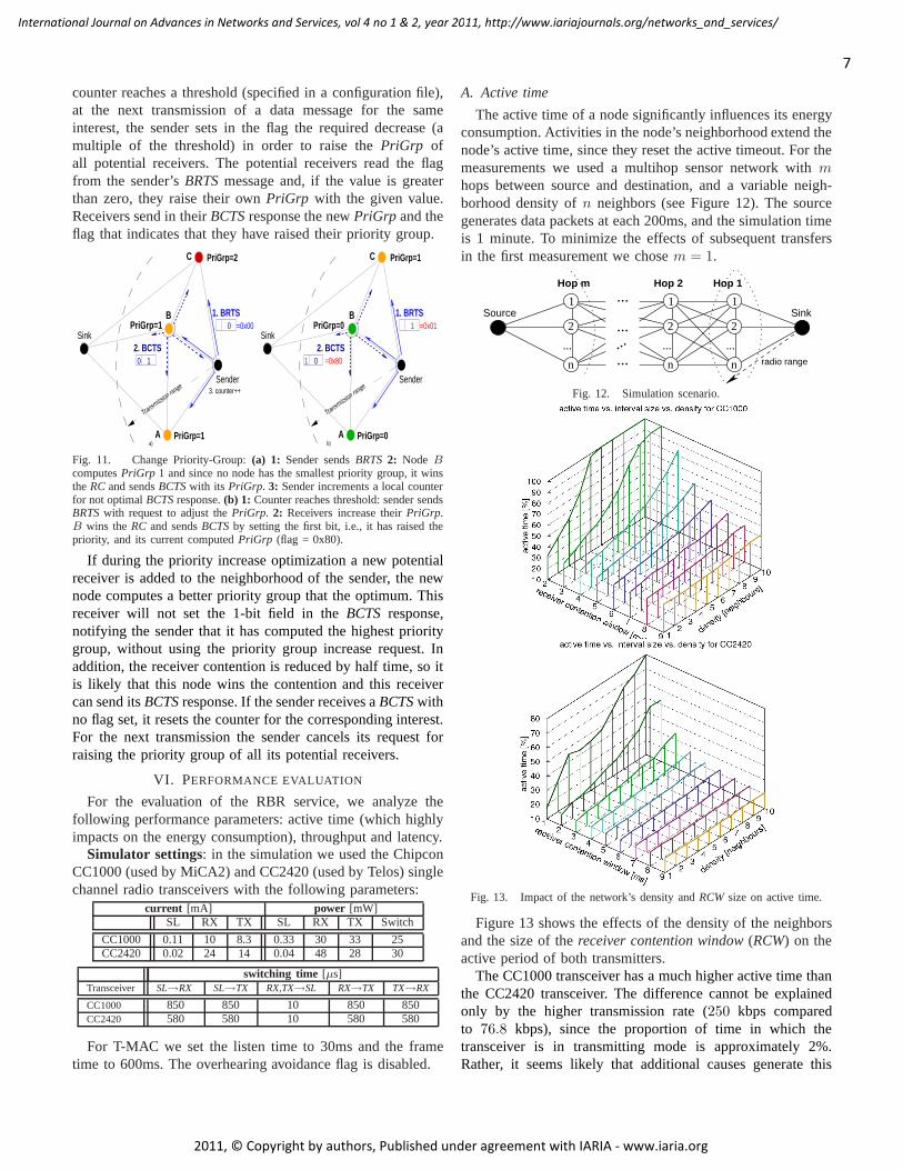
The active time of a node significantly influences its energyconsumption. Activities in the node’s neighborhood extendthenode’s active time, since they reset the active timeout. Forthemeasurements we used a multihop sensor network withm
hops between source and destination, and a variable neigh-borhood density ofn neighbors (see Figure 12). The sourcegenerates data packets at each 200ms, and the simulation timeis 1 minute. To minimize the effects of subsequent transfersin the first measurement we chosem = 1.
Source
Hop m
radio range
Sink
Hop 1Hop 2
2
n
1
...
2
n
2
n
1
...
1
...
...
...
...
...
Fig. 12. Simulation scenario.
Fig. 13. Impact of the network’s density andRCWsize on active time.
Figure 13 shows the effects of the density of the neighborsand the size of thereceiver contention window(RCW) on theactive period of both transmitters.
The CC1000 transceiver has a much higher active time thanthe CC2420 transceiver. The difference cannot be explainedonly by the higher transmission rate (250 kbps comparedto 76.8 kbps), since the proportion of time in which thetransceiver is in transmitting mode is approximately 2%.Rather, it seems likely that additional causes generate this
7
International Journal on Advances in Networks and Services, vol 4 no 1 & 2, year 2011, http://www.iariajournals.org/networks_and_services/
2011, © Copyright by authors, Published under agreement with IARIA - www.iaria.org
behavior. To investigate this closer one needs to analyse thenumber of events that occur during a transfer. Events thatnegatively affect the behavior and extend the active periodare collisions of messages and their consequences.
For small RCW, the active time increases quickly withincreasing of the network’s density. This leads to frequentcollisions ofBCTSresponses, whereby the receiver contentionneeds to be repeated. Therefore, the active timeout is set again.For largeRCW, the active time remains relatively constant.The negative impact on the active time by a long-lastingtransmission (due to the largeRC) will be compensated byrare occurrence ofBCTS-collisions.
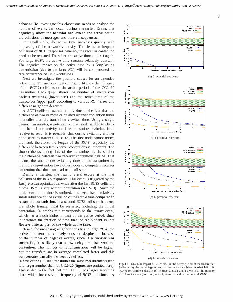
Next we investigate the possible causes for an extendedactive time. The measurements in Figure 14 show the influenceof the BCTS-collisions on the active period of the CC2420transmitter. Each graph shows the number of events (perpacket) occurring (lower part) and the active time of thetransceiver (upper part) according to variousRCWsizes anddifferent neighbors densities.
A BCTS-collision occurs mainly due to the fact that thedifference of two or more calculated receiver contention timesis smaller than the transmitter’s switch time. Using a singlechannel transmitter, a potential receiver node is able to checkthe channel for activity until its transmitter switches fromreceive to send. It is possible, that during switching anothernode starts to transmit itsBCTS. The first node cannot noticethat and, therefore, the length of theRCW, especially thedifference between two receiver contentions is important.Theshorter the switching time of the transmitter is, the smallerthe difference between two receiver contentions can be. Thatmeans, the smaller the switching time of the transmitter is,the more opportunities have other nodes to compute a receivercontention that does not lead to a collision.
During a transfer, theresend eventoccurs at the firstcollision of theBCTSresponses. This event is triggered by theEarly Resendoptimization, when after the firstBCTScollision,a newBRTSis sent without contention(see V-B). Since theinitial contention time is omitted, this event has a relativelysmall influence on the extension of the active timecompared torestart the transmission. If a secondBCTS-collision happens,the whole transfer must be restarted, including the initialcontention. In graphs this corresponds to therestart event,which has a much higher impact on the active period,sinceit increases the fraction of time that the radio spent inIdleReceivestate as part of the whole active time.
Hence, for increasing neighbor density and largeRCW, theactive time remains relatively constant, despite the increaseof the number of negative events, since if a transfer wassuccessful, it is likely that a low delay time has won thecontention. The number of retransmissions will be higher,but the transfers are in average completed faster and thiscompensates partially the negative effect.In case of the CC1000 transmitter the same measurements leadto a larger number than for CC2420 (figures are omitted here).This is due to the fact that the CC1000 has larger switchingtime, which increases the frequency ofBCTS-collisions. A
(a) 2 potential receivers
(b) 4 potential receivers
(c) 6 potential receivers
(d) 8 potential receivers
Fig. 14. CC2420: Impact ofRCWsize on the active period of the transmitter(reflected by the procentage of each active radio state(sleep is what left until100%) for different density of neighbors. Each graph gives also the numberof relevant events (collision, resend, restart) for different size ofRCW.
8
International Journal on Advances in Networks and Services, vol 4 no 1 & 2, year 2011, http://www.iariajournals.org/networks_and_services/
2011, © Copyright by authors, Published under agreement with IARIA - www.iaria.org
larger switching time means that during a node is checkingthe medium and switching to send the probability that anothernode (during this time) starts to transmit is higher and, thus,moreBCTS-collisions occur.
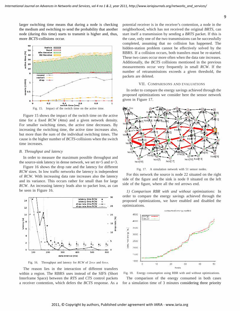
Fig. 15. Impact of the switch time on the active time.
Figure 15 shows the impact of the switch time on the activetime for a fixed RCW (4ms) and a given network density.For smaller switching times, the active time decreases. Byincreasing the switching time, the active time increases also,but more than the sum of the individual switching times. Thecause is the higher number ofBCTS-collisions when the switchtime increases.
B. Throughput and latency
In order to measure the maximum possible throughput andthe source-sink latency in dense network, we set m=5 and n=3.
Figure 16 shows the drop rate and the latency for differentRCWsizes. In low traffic networks the latency is independentof RCW. With increasing data rate increases also the latencyand its variance. This occurs rather for small than for largeRCW. An increasing latency leads also to packet loss, as canbe seen in Figure 16.
Fig. 16. Throughput and latency forRCWof 2ms and6ms.
The reason lies in the interaction of different transferswithin a region. The RBRS uses instead of the SIFS (ShortInterframe Space) between theRTSand CTScontrol packetsa receiver contention, which defers theBCTSresponse. As a
potential receiver is in the receiver’s contention, a node in theneighborhood, which has not received the originalBRTS, canstart itself a transmission by sending aBRTSpacket. If this isthe case, only one of the two transmissions can be successfullycompleted, assuming that no collision has happened. Thehidden-station problem cannot be effectively solved by theRBRS. If a collision occurs, both transfers must be re-started.These two cases occur more often when the data rate increases.Additionally, the BCTScollisions mentioned in the previousmeasurements occur very frequently in smallRCW. If thenumber of retransmissions exceeds a given threshold, thepackets are deleted.
VII. C OMPARISONS AND EVALUATIONS
In order to compare the energy savings achieved through theproposed optimizations we consider here the sensor networkgiven in Figure 17.
Fig. 17. A simulation network with 51 sensor nodes.
For this network the source is node 22 situated on the rightside of the figure and the sink is node 0 situated on the leftside of the figure, where all the red arrows end.
1) Comparison RBR with and without optimizations:Inorder to compare the energy savings achieved through theproposed optimizations, we have enabled and disabled theoptimizations.
Fig. 18. Energy consumption using RBR with and without optimizations.
The comparison of the energy consumed in both casesfor a simulation time of 3 minutesconsidering three priority
9
International Journal on Advances in Networks and Services, vol 4 no 1 & 2, year 2011, http://www.iariajournals.org/networks_and_services/
2011, © Copyright by authors, Published under agreement with IARIA - www.iaria.org
groups and a weight for the highest priority group of 60%)is illustrated in Figure 18. One can observe that with allthree optimizations the energy consumed by some nodesimproves up to 7%, but there are also nodes where the energyconsumption increases. The overall energy consumption isreduced when using optimizations by at least4%.
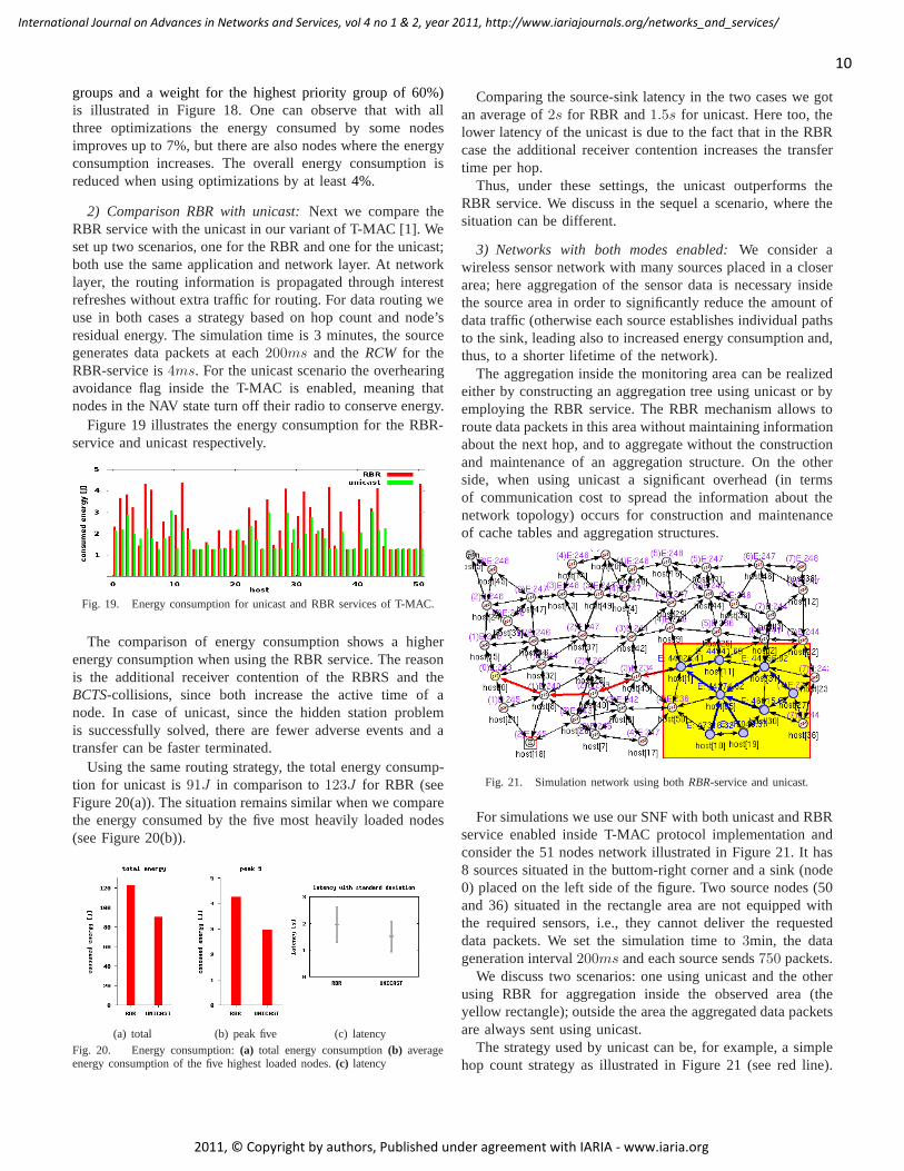
2) Comparison RBR with unicast:Next we compare theRBR service with the unicast in our variant of T-MAC [1]. Weset up two scenarios, one for the RBR and one for the unicast;both use the same application and network layer. At networklayer, the routing information is propagated through interestrefreshes without extra traffic for routing. For data routing weuse in both cases a strategy based on hop count and node’sresidual energy. The simulation time is 3 minutes, the sourcegenerates data packets at each200ms and theRCW for theRBR-service is4ms. For the unicast scenario the overhearingavoidance flag inside the T-MAC is enabled, meaning thatnodes in the NAV state turn off their radio to conserve energy.
Figure 19 illustrates the energy consumption for the RBR-service and unicast respectively.
Fig. 19. Energy consumption for unicast and RBR services of T-MAC.
The comparison of energy consumption shows a higherenergy consumption when using the RBR service. The reasonis the additional receiver contention of the RBRS and theBCTS-collisions, since both increase the active time of anode. In case of unicast, since the hidden station problemis successfully solved, there are fewer adverse events and atransfer can be faster terminated.
Using the same routing strategy, the total energy consump-tion for unicast is91J in comparison to123J for RBR (seeFigure 20(a)). The situation remains similar when we comparethe energy consumed by the five most heavily loaded nodes(see Figure 20(b)).
(a) total (b) peak five (c) latencyFig. 20. Energy consumption:(a) total energy consumption(b) averageenergy consumption of the five highest loaded nodes.(c) latency
Comparing the source-sink latency in the two cases we gotan average of2s for RBR and1.5s for unicast. Here too, thelower latency of the unicast is due to the fact that in the RBRcase the additional receiver contention increases the transfertime per hop.
Thus, under these settings, the unicast outperforms theRBR service. We discuss in the sequel a scenario, where thesituation can be different.
3) Networks with both modes enabled:We consider awireless sensor network with many sources placed in a closerarea; here aggregation of the sensor data is necessary insidethe source area in order to significantly reduce the amount ofdata traffic (otherwise each source establishes individualpathsto the sink, leading also to increased energy consumption and,thus, to a shorter lifetime of the network).
The aggregation inside the monitoring area can be realizedeither by constructing an aggregation tree using unicast orbyemploying the RBR service. The RBR mechanism allows toroute data packets in this area without maintaining informationabout the next hop, and to aggregate without the constructionand maintenance of an aggregation structure. On the otherside, when using unicast a significant overhead (in termsof communication cost to spread the information about thenetwork topology) occurs for construction and maintenanceof cache tables and aggregation structures.
Fig. 21. Simulation network using bothRBR-service and unicast.
For simulations we use our SNF with both unicast and RBRservice enabled inside T-MAC protocol implementation andconsider the 51 nodes network illustrated in Figure 21. It has8 sources situated in the buttom-right corner and a sink (node0) placed on the left side of the figure. Two source nodes (50and 36) situated in the rectangle area are not equipped withthe required sensors, i.e., they cannot deliver the requesteddata packets. We set the simulation time to3min, the datageneration interval200ms and each source sends750 packets.
We discuss two scenarios: one using unicast and the otherusing RBR for aggregation inside the observed area (theyellow rectangle); outside the area the aggregated data packetsare always sent using unicast.
The strategy used by unicast can be, for example, a simplehop count strategy as illustrated in Figure 21 (see red line).
10
International Journal on Advances in Networks and Services, vol 4 no 1 & 2, year 2011, http://www.iariajournals.org/networks_and_services/
2011, © Copyright by authors, Published under agreement with IARIA - www.iaria.org
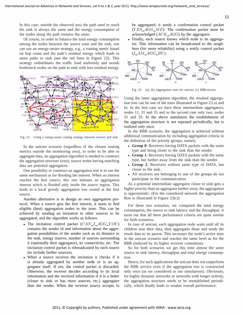
In this case, outside the observed area the path used to reachthe sink is always the same and the energy consumption ofthe nodes along the path remains the same.
Of course, in order to balance the total energy consumptionamong the nodes between the source zone and the sink, onecan use an energy-aware strategy, e.g., a routing metric basedon hop count and the path’s residual energy which leads tomore paths to sink (see the red lines in Figure 22). Thisstrategy redistributes the traffic load uniformly and avoidsbottleneck nodes on the path to sink with less residual energy.
Fig. 22. Using a energy-aware routing strategy between sources and sink.
In the unicast scenario (regardless of the chosen routingmetrics outside the monitoring area), in order to be able toaggregate data, an aggregation algorithm is needed to constructthe aggregation structure (tree); source nodes having matchingdata are potential aggregators.
One possibility to construct an aggregation tree is to use thesame mechanism as for flooding the interest. When an interestreaches the first source, this one initiates an aggregationinterest which is flooded only inside the source region. Thisleads to a local greedy aggregation tree rooted at the firstsource.
Another alternative is to design an own aggregation pro-tocol. When a source gets the first interest, it starts to findeligible (best) aggregation nodes in the zone. This can beachieved by sending an invitation to other sources to beaggregated, and the algorithm works as follows:
• The invitation control packet (CAN I AGG Y OU )contains the sender id and information about the aggre-gation possibilities of the sender such as its distance tothe sink, energy reserve, number of sources surroundingit (optionally their aggregator), its connectivity, etc. Theinvitation control packet is rebroadcasted by each source(to include farther sources).
• When a source receives the invitation it checks if itis already aggregated by another node or is an ag-gregator itself. If yes, the control packet is discarded.Otherwise, the receiver decides according to its localinformation and the received information if it is a better(closer to sink or has more sources, etc.) aggregatorthan the sender. When the receiver source accepts to
be aggregated, it sends a confirmation control packet(Y ES AGG ME). The confirmation packet must beacknowledged (ACK AGG) by the aggregator.
• Finally, each source knows which node is its aggrega-tor. This information can be broadcasted to the neigh-bors (for more reliability) using a notify control packet(I AM AGG BY ).
[30]
[11]
[10] [19]
[31]
[27][35]
[50]
[1]
[30]
[11]
[10] [19]
[31]
[27][35]
[50]
[1]
b)a)
[30]
[11]
[10] [19]
[31]
[27][35]
[50]
[1]
c)
Fig. 23. (a), (b) Aggregation trees for unicast; (c)RBR-service
Using the latter aggregation algorithm, the resulted aggrega-tion tree can be one of the trees illustrated in Figure 23 a) andb). In the first case we have three intermediate aggregators,nodes 11, 31 and 35 and in the second case only two, nodes31 and 35.In the above simulation the establishment ofthe aggregation structure is not repeated periodically, but isrealized only once.
In the RBR scenario, the aggregation is achieved withoutadditional communication by including aggregation criteria inthe definition of the priority groups, namely
• Group 0: Receivers having DATA packets with the sametype and being closer to the sink than the sender.
• Group 1: Receivers having DATA packets with the sametype, but farther away from the sink than the sender.
• Group 2: Receivers without same type of DATA, butcloser to the sink.
• All receivers not belonging to one of the groups do notparticipate in the communication.
As a potential intermediate aggregator closer to sink gets ahigher priority than an aggregator farther away, the aggregationis opportunistic. (For the considered network the aggregationflow is illustrated in Figure 23(c))
For these two scenarios, we compared the total energyconsumption, the source to sink latency and the throughput.Itturns out that all three performance criteria are quite similarfor both scenarios.
In case of unicast, each aggregation node waits until all itschildren sent their data, then aggregates these and sends theresult data to its parent. This increases the node’s active timein the unicast scenario and reaches the same level as for theRBR (induced by its higher receiver contention).
So for both scenarios we get this time almost the samesource to sink latency, throughput and total energy consump-tion.
Hence, for such applications the unicast does not outperformthe RBR service even if the aggregation tree is constructedonly once (as we considered in our simulations). Obviously,for highly dynamic networks or networks with longer activity,the aggregation structure needs to be reestablished periodi-cally, which finally leads to weaker overall performance.
11
International Journal on Advances in Networks and Services, vol 4 no 1 & 2, year 2011, http://www.iariajournals.org/networks_and_services/
2011, © Copyright by authors, Published under agreement with IARIA - www.iaria.org
VIII. C ONCLUSION AND FUTURE WORK
In the present paper, we strive for more modularity atMAC layer, mainly to embed at this layer more customizableservices. We supplement here the sender initiated unicast by areceiver-based contention in order to provide another perspec-tive to the interlayer communication. The RBR service of T-MAC allows (reactive) applications, in which a sender does notknow its potential destination or applications with a dynamicnetwork topology where the construction and maintainanceoverhead for the cache tables and/or aggregation structures isexpensive (in terms of communication cost to spread the infor-mation about the network toplogy). In such dynamic scenariosthe RBR mechanism allows to route, without maintaininginformation about the next hop, and to aggregate, without theconstruction and maintenance of an aggregation structure.
The accurate energy model integrated in our simulator al-lows us to quantify the impact of transceiver’s switch time,theRCWand the occurrence of collisions and their retransmissionson the energy consumption of the sensor node. The possiblecollisions of theBCTSresponses and their consequences mustbe minimized (using transceivers with smaller switching time)for a good performance of the RBR service. Therefore, weproposed and implemented several optimizations of the RBRS.Simulation results have shown that these optimizations im-prove significantly the performance of the RBR.We have ana-lyzed the performance parameters of the RBR service, namelyits energy-efficiency, throughput and latency.Moreover, wecompared (VII-2) the efficiency of both forwarding approachesinside T-MAC: the sender initiated one using unicast versusthereceiver-based routing. For our simulation scenario it turnedout that the RBR approach outperformed by unicast in terms ofenergy consumption, throughput and latency. Nevertheless, theRBR can be efficiently employed for opportunistic aggregationinside monitoring areas with many sources or in dynamicnetwork scenarios (VII-3); here the routing performance ofRBR and unicast are similar.
As future work we intend to build in our simulator dif-ferent simulation scenarios in order tocloser investigate andcompare the performance of RBR versus different aggregationalgorithms using unicast.
REFERENCES
[1] F. Kacso and U. Schipper, “Receiver-based routing service for t-macprotocol,” in Proc. 4th Int. Conf. on on Sensor Technologies andApplications (SENSORCOMM 2010). Venice/Mestre, Italy, July 2010,pp. 489–494.
[2] W. Ye, J. Heidemann, and D. Estrin, “Medium access control withcoordinated, adaptive sleeping for wireless sensor networks,” IEEE/ACMTrans. on Netw., vol. 12, no. 3, pp. 493–506, 2004.
[3] J. Polastre, J. Hill, and D. Culler, “Versatile low powermedia access forwireless sensor networks,” inProc. 2nd ACM Int. Conf. on EmbeddedNetworked SenSys. NY, USA, November 2004, pp. 95–107.
[4] T. Dam and K. Langendoen, “An adaptive energy-efficient mac protocolfor wireless sensor networks,” inProc. 1st Int. Conf. on EmbeddedNetworked SenSys. LA, California, USA, 2003, pp. 171–180.
[5] M. Busse, T. Hanselmann, and W. Effelsberg, “Energy-efficient for-warding schemes for wireless sensor networks,” inProc. Int. Symp. onWoWMoM. New York, USA, June 2006, pp. 125–133.
[6] F. Ye, G. Zhong, S. Lu, and L. Zhang, “Gradient broadcast:A robustdata delivery protocol for large scale sensor networks,”Wireless Net-works/Springer, The Netherlands, vol. 11, no. 2, pp. 285–298, 2005.
[7] C. Intanagonwiwat, R. Govindan, D. Estrin, J. Heidemann, and F. Silva,“Directed diffusion for wireless sensor networking,”IEEE/ACM Trans-actions on Networking, vol. 11, no. 1, pp. 2–16, 2003.
[8] K.-W. Fan, S. Liu, and P. Sinha, “Structure-free data aggregation insensor networks,”IEEE Trans. Mob. Comput, vol. 6, pp. 929–942, 2007.
[9] I. Akyildiz, M. Vuran, and O. Aka, “A cross-layer protocol for wirelesssensor networks,” inProc. CISS. Princeton, NJ, March 2006.
[10] T. Watteyne, A. Bachir, M. Dohler, D. Barthel, and I. Aug-Blum, “1-hopmac: An energy-efficient mac protocol for avoiding 1-hopneighbor-hood knowledge,”Sensor and Ad Hoc Communications and Networks,vol. 2, pp. 639–644, Sept 2006.
[11] P. Skraba, H. Aghajan, and A. Bahai, “Cross-layer optimization for highdensity sensor networks: Distributed passive routing decisions,” inProc.Ad-Hoc Now04. Vancouver, July 2004, pp. 266–279.
[12] F. Kacso and R. Wismuller, “A simulation framework for energy-aware wireless sensor network protocols,” inProc. 18th Int. Conf. onComputer Communications and Networks (ICCCN’09), Workshop onSensor Networks. San Francisco, CA, USA, August 2009, pp. 1–7.
[13] J. Wong, R. Jafari, and M. Potkonjak, “Gateway placement for latencyand efficient data aggregation,” inProc. 29th Annual IEEE Int. Conf. onLocal Computer Networks, Nov 2004, pp. 490–497.
[14] J. Polastre, J. Hui, P. Levis, J. Zhao, D. Culler, S. Shenker, and I. Stoica,“A unifying link abstraction for wireless sensor networks,” in Proc. 3rdACM Int. Conf. SenSys, November 2005, pp. 76–89.
[15] C. Ee, R. Fonseca, S. Kim, D. Moon, A. Tavakoli, D. Culler, S. Shenker,and I. Stoica, “A modular network layer for sensornets,” inProc. 7thSymp. OSDI. Seattle, WA, USA, 2006, pp. 249–262.
[16] C. Intanagonwiwat, R. Govindan, and D. Estrin, “Directed diffusion ascalable and robust communication paradigm for sensor networks,” inProc. ACM MobiCom. Boston, 2000, pp. 56–67.
[17] W. Heinzelman, A. Chandrakasan, and H. Balakrishnan, “Energy-efficient communication protocol for wireless microsensornetworks,” inProc. 33rd Annual Hawaii Int. Conf. on System Sciences (HICSS’00),2000, pp. 3005–3014.
[18] A. Kacso and R. Wismuller, “A framework architectureto simulateenergy-aware routing protocols in wireless sensor networks,” in Proc.IASTED Int. Conf. on Sensor Networks. Greece, 2008, pp. 77–82.
[19] M. Lobbers and D. Willkomm,Mobility Framework for OMNeT++ (APIref.). http://mobility-fw.sourceforge.net: OMNeT++ Ver.3.2,2006.
[20] V. Bharghavan, A. Demers, S. Shenker, and L. Zhang, “Macaw: A mediaaccess protocol for wireless lans,” inProc. of SIGCOMM Conf.London,UK, September 1994, pp. 212–225.
12
International Journal on Advances in Networks and Services, vol 4 no 1 & 2, year 2011, http://www.iariajournals.org/networks_and_services/
2011, © Copyright by authors, Published under agreement with IARIA - www.iaria.org
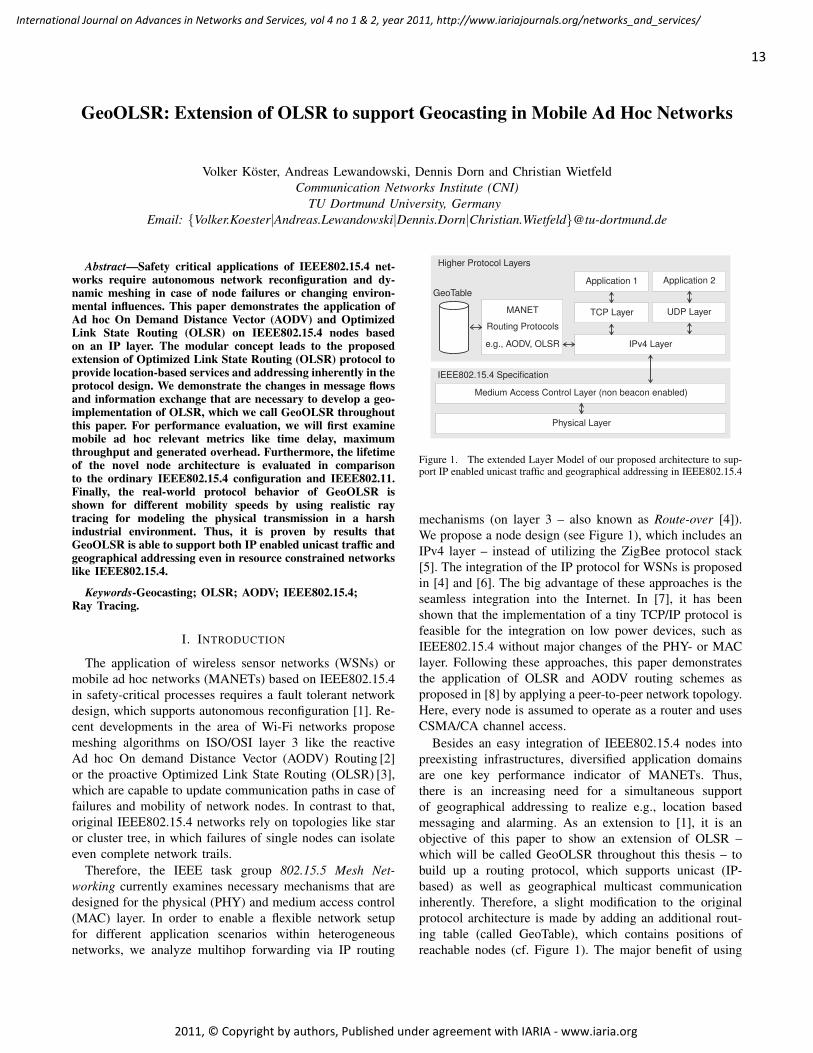
GeoOLSR: Extension of OLSR to support Geocasting in Mobile Ad Hoc Networks
Volker Koster, Andreas Lewandowski, Dennis Dorn and Christian WietfeldCommunication Networks Institute (CNI)
TU Dortmund University, GermanyEmail: Volker.Koester|Andreas.Lewandowski|Dennis.Dorn|[email protected]
Abstract—Safety critical applications of IEEE802.15.4 net-works require autonomous network reconfiguration and dy-namic meshing in case of node failures or changing environ-mental influences. This paper demonstrates the application ofAd hoc On Demand Distance Vector (AODV) and OptimizedLink State Routing (OLSR) on IEEE802.15.4 nodes basedon an IP layer. The modular concept leads to the proposedextension of Optimized Link State Routing (OLSR) protocol toprovide location-based services and addressing inherently in theprotocol design. We demonstrate the changes in message flowsand information exchange that are necessary to develop a geo-implementation of OLSR, which we call GeoOLSR throughoutthis paper. For performance evaluation, we will first examinemobile ad hoc relevant metrics like time delay, maximumthroughput and generated overhead. Furthermore, the lifetimeof the novel node architecture is evaluated in comparisonto the ordinary IEEE802.15.4 configuration and IEEE802.11.Finally, the real-world protocol behavior of GeoOLSR isshown for different mobility speeds by using realistic raytracing for modeling the physical transmission in a harshindustrial environment. Thus, it is proven by results thatGeoOLSR is able to support both IP enabled unicast traffic andgeographical addressing even in resource constrained networkslike IEEE802.15.4.
Keywords-Geocasting; OLSR; AODV; IEEE802.15.4;Ray Tracing.
I. INTRODUCTION
The application of wireless sensor networks (WSNs) ormobile ad hoc networks (MANETs) based on IEEE802.15.4in safety-critical processes requires a fault tolerant networkdesign, which supports autonomous reconfiguration [1]. Re-cent developments in the area of Wi-Fi networks proposemeshing algorithms on ISO/OSI layer 3 like the reactiveAd hoc On demand Distance Vector (AODV) Routing [2]or the proactive Optimized Link State Routing (OLSR) [3],which are capable to update communication paths in case offailures and mobility of network nodes. In contrast to that,original IEEE802.15.4 networks rely on topologies like staror cluster tree, in which failures of single nodes can isolateeven complete network trails.
Therefore, the IEEE task group 802.15.5 Mesh Net-working currently examines necessary mechanisms that aredesigned for the physical (PHY) and medium access control(MAC) layer. In order to enable a flexible network setupfor different application scenarios within heterogeneousnetworks, we analyze multihop forwarding via IP routing
Physical Layer
Medium Access Control Layer (non beacon enabled)
IPv4 Layer
UDP LayerTCP Layer
IEEE802.15.4 Specification
MANET
Routing Protocols
e.g., AODV, OLSR
Application 1 Application 2
Higher Protocol Layers
GeoTable
Figure 1. The extended Layer Model of our proposed architecture to sup-port IP enabled unicast traffic and geographical addressing in IEEE802.15.4
mechanisms (on layer 3 – also known as Route-over [4]).We propose a node design (see Figure 1), which includes anIPv4 layer – instead of utilizing the ZigBee protocol stack[5]. The integration of the IP protocol for WSNs is proposedin [4] and [6]. The big advantage of these approaches is theseamless integration into the Internet. In [7], it has beenshown that the implementation of a tiny TCP/IP protocol isfeasible for the integration on low power devices, such asIEEE802.15.4 without major changes of the PHY- or MAClayer. Following these approaches, this paper demonstratesthe application of OLSR and AODV routing schemes asproposed in [8] by applying a peer-to-peer network topology.Here, every node is assumed to operate as a router and usesCSMA/CA channel access.
Besides an easy integration of IEEE802.15.4 nodes intopreexisting infrastructures, diversified application domainsare one key performance indicator of MANETs. Thus,there is an increasing need for a simultaneous supportof geographical addressing to realize e.g., location basedmessaging and alarming. As an extension to [1], it is anobjective of this paper to show an extension of OLSR –which will be called GeoOLSR throughout this thesis – tobuild up a routing protocol, which supports unicast (IP-based) as well as geographical multicast communicationinherently. Therefore, a slight modification to the originalprotocol architecture is made by adding an additional rout-ing table (called GeoTable), which contains positions ofreachable nodes (cf. Figure 1). The major benefit of using
13
International Journal on Advances in Networks and Services, vol 4 no 1 & 2, year 2011, http://www.iariajournals.org/networks_and_services/
2011, © Copyright by authors, Published under agreement with IARIA - www.iaria.org
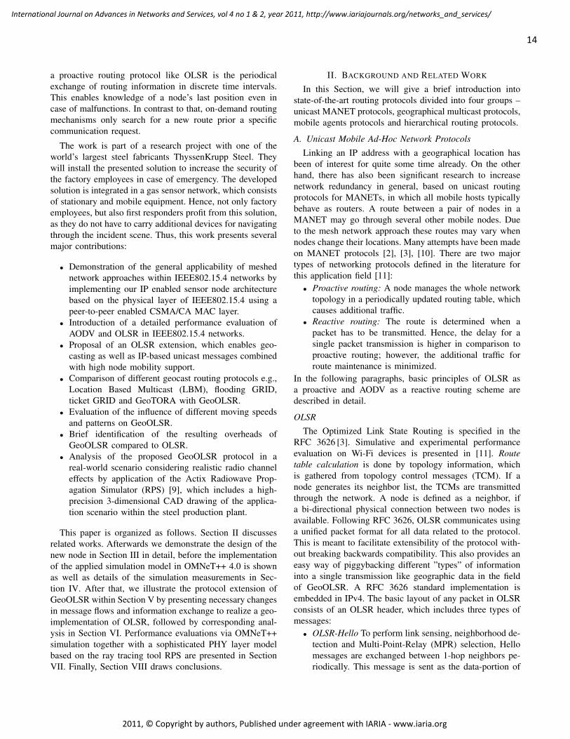
a proactive routing protocol like OLSR is the periodicalexchange of routing information in discrete time intervals.This enables knowledge of a node’s last position even incase of malfunctions. In contrast to that, on-demand routingmechanisms only search for a new route prior a specificcommunication request.
The work is part of a research project with one of theworld’s largest steel fabricants ThyssenKrupp Steel. Theywill install the presented solution to increase the security ofthe factory employees in case of emergency. The developedsolution is integrated in a gas sensor network, which consistsof stationary and mobile equipment. Hence, not only factoryemployees, but also first responders profit from this solution,as they do not have to carry additional devices for navigatingthrough the incident scene. Thus, this work presents severalmajor contributions:
• Demonstration of the general applicability of meshednetwork approaches within IEEE802.15.4 networks byimplementing our IP enabled sensor node architecturebased on the physical layer of IEEE802.15.4 using apeer-to-peer enabled CSMA/CA MAC layer.
• Introduction of a detailed performance evaluation ofAODV and OLSR in IEEE802.15.4 networks.
• Proposal of an OLSR extension, which enables geo-casting as well as IP-based unicast messages combinedwith high node mobility support.
• Comparison of different geocast routing protocols e.g.,Location Based Multicast (LBM), flooding GRID,ticket GRID and GeoTORA with GeoOLSR.
• Evaluation of the influence of different moving speedsand patterns on GeoOLSR.
• Brief identification of the resulting overheads ofGeoOLSR compared to OLSR.
• Analysis of the proposed GeoOLSR protocol in areal-world scenario considering realistic radio channeleffects by application of the Actix Radiowave Prop-agation Simulator (RPS) [9], which includes a high-precision 3-dimensional CAD drawing of the applica-tion scenario within the steel production plant.
This paper is organized as follows. Section II discussesrelated works. Afterwards we demonstrate the design of thenew node in Section III in detail, before the implementationof the applied simulation model in OMNeT++ 4.0 is shownas well as details of the simulation measurements in Sec-tion IV. After that, we illustrate the protocol extension ofGeoOLSR within Section V by presenting necessary changesin message flows and information exchange to realize a geo-implementation of OLSR, followed by corresponding anal-ysis in Section VI. Performance evaluations via OMNeT++simulation together with a sophisticated PHY layer modelbased on the ray tracing tool RPS are presented in SectionVII. Finally, Section VIII draws conclusions.
II. BACKGROUND AND RELATED WORK
In this Section, we will give a brief introduction intostate-of-the-art routing protocols divided into four groups –unicast MANET protocols, geographical multicast protocols,mobile agents protocols and hierarchical routing protocols.
A. Unicast Mobile Ad-Hoc Network Protocols
Linking an IP address with a geographical location hasbeen of interest for quite some time already. On the otherhand, there has also been significant research to increasenetwork redundancy in general, based on unicast routingprotocols for MANETs, in which all mobile hosts typicallybehave as routers. A route between a pair of nodes in aMANET may go through several other mobile nodes. Dueto the mesh network approach these routes may vary whennodes change their locations. Many attempts have been madeon MANET protocols [2], [3], [10]. There are two majortypes of networking protocols defined in the literature forthis application field [11]:• Proactive routing: A node manages the whole network
topology in a periodically updated routing table, whichcauses additional traffic.
• Reactive routing: The route is determined when apacket has to be transmitted. Hence, the delay for asingle packet transmission is higher in comparison toproactive routing; however, the additional traffic forroute maintenance is minimized.
In the following paragraphs, basic principles of OLSR asa proactive and AODV as a reactive routing scheme aredescribed in detail.
OLSR
The Optimized Link State Routing is specified in theRFC 3626 [3]. Simulative and experimental performanceevaluation on Wi-Fi devices is presented in [11]. Routetable calculation is done by topology information, whichis gathered from topology control messages (TCM). If anode generates its neighbor list, the TCMs are transmittedthrough the network. A node is defined as a neighbor, ifa bi-directional physical connection between two nodes isavailable. Following RFC 3626, OLSR communicates usinga unified packet format for all data related to the protocol.This is meant to facilitate extensibility of the protocol with-out breaking backwards compatibility. This also provides aneasy way of piggybacking different ”types” of informationinto a single transmission like geographic data in the fieldof GeoOLSR. A RFC 3626 standard implementation isembedded in IPv4. The basic layout of any packet in OLSRconsists of an OLSR header, which includes three types ofmessages:• OLSR-Hello To perform link sensing, neighborhood de-
tection and Multi-Point-Relay (MPR) selection, Hellomessages are exchanged between 1-hop neighbors pe-riodically. This message is sent as the data-portion of
14
International Journal on Advances in Networks and Services, vol 4 no 1 & 2, year 2011, http://www.iariajournals.org/networks_and_services/
2011, © Copyright by authors, Published under agreement with IARIA - www.iaria.org
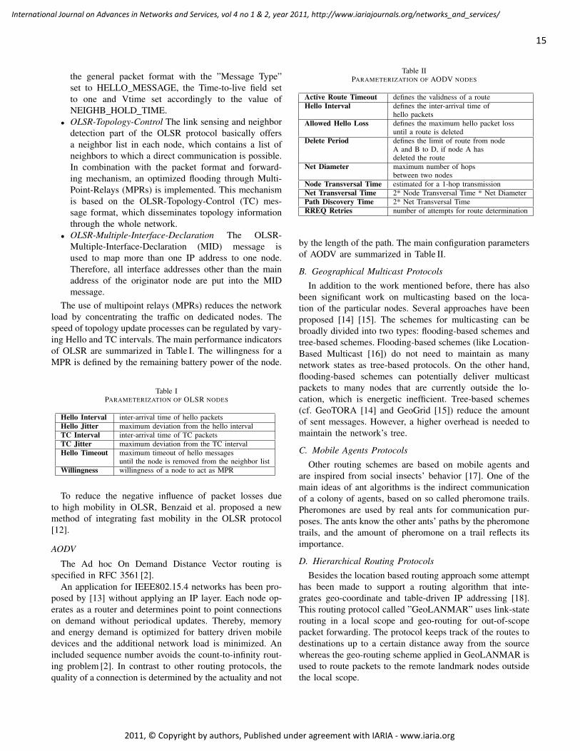
the general packet format with the ”Message Type”set to HELLO MESSAGE, the Time-to-live field setto one and Vtime set accordingly to the value ofNEIGHB HOLD TIME.
• OLSR-Topology-Control The link sensing and neighbordetection part of the OLSR protocol basically offersa neighbor list in each node, which contains a list ofneighbors to which a direct communication is possible.In combination with the packet format and forward-ing mechanism, an optimized flooding through Multi-Point-Relays (MPRs) is implemented. This mechanismis based on the OLSR-Topology-Control (TC) mes-sage format, which disseminates topology informationthrough the whole network.
• OLSR-Multiple-Interface-Declaration The OLSR-Multiple-Interface-Declaration (MID) message isused to map more than one IP address to one node.Therefore, all interface addresses other than the mainaddress of the originator node are put into the MIDmessage.
The use of multipoint relays (MPRs) reduces the networkload by concentrating the traffic on dedicated nodes. Thespeed of topology update processes can be regulated by vary-ing Hello and TC intervals. The main performance indicatorsof OLSR are summarized in Table I. The willingness for aMPR is defined by the remaining battery power of the node.
Table IPARAMETERIZATION OF OLSR NODES
Hello Interval inter-arrival time of hello packetsHello Jitter maximum deviation from the hello intervalTC Interval inter-arrival time of TC packetsTC Jitter maximum deviation from the TC intervalHello Timeout maximum timeout of hello messages
until the node is removed from the neighbor listWillingness willingness of a node to act as MPR
To reduce the negative influence of packet losses dueto high mobility in OLSR, Benzaid et al. proposed a newmethod of integrating fast mobility in the OLSR protocol[12].
AODV
The Ad hoc On Demand Distance Vector routing isspecified in RFC 3561 [2].
An application for IEEE802.15.4 networks has been pro-posed by [13] without applying an IP layer. Each node op-erates as a router and determines point to point connectionson demand without periodical updates. Thereby, memoryand energy demand is optimized for battery driven mobiledevices and the additional network load is minimized. Anincluded sequence number avoids the count-to-infinity rout-ing problem [2]. In contrast to other routing protocols, thequality of a connection is determined by the actuality and not
Table IIPARAMETERIZATION OF AODV NODES
Active Route Timeout defines the validness of a routeHello Interval defines the inter-arrival time of
hello packetsAllowed Hello Loss defines the maximum hello packet loss
until a route is deletedDelete Period defines the limit of route from node
A and B to D, if node A hasdeleted the route
Net Diameter maximum number of hopsbetween two nodes
Node Transversal Time estimated for a 1-hop transmissionNet Transversal Time 2* Node Transversal Time * Net DiameterPath Discovery Time 2* Net Transversal TimeRREQ Retries number of attempts for route determination
by the length of the path. The main configuration parametersof AODV are summarized in Table II.
B. Geographical Multicast Protocols
In addition to the work mentioned before, there has alsobeen significant work on multicasting based on the loca-tion of the particular nodes. Several approaches have beenproposed [14] [15]. The schemes for multicasting can bebroadly divided into two types: flooding-based schemes andtree-based schemes. Flooding-based schemes (like Location-Based Multicast [16]) do not need to maintain as manynetwork states as tree-based protocols. On the other hand,flooding-based schemes can potentially deliver multicastpackets to many nodes that are currently outside the lo-cation, which is energetic inefficient. Tree-based schemes(cf. GeoTORA [14] and GeoGrid [15]) reduce the amountof sent messages. However, a higher overhead is needed tomaintain the network’s tree.
C. Mobile Agents Protocols
Other routing schemes are based on mobile agents andare inspired from social insects’ behavior [17]. One of themain ideas of ant algorithms is the indirect communicationof a colony of agents, based on so called pheromone trails.Pheromones are used by real ants for communication pur-poses. The ants know the other ants’ paths by the pheromonetrails, and the amount of pheromone on a trail reflects itsimportance.
D. Hierarchical Routing Protocols
Besides the location based routing approach some attempthas been made to support a routing algorithm that inte-grates geo-coordinate and table-driven IP addressing [18].This routing protocol called ”GeoLANMAR” uses link-staterouting in a local scope and geo-routing for out-of-scopepacket forwarding. The protocol keeps track of the routes todestinations up to a certain distance away from the sourcewhereas the geo-routing scheme applied in GeoLANMAR isused to route packets to the remote landmark nodes outsidethe local scope.
15
International Journal on Advances in Networks and Services, vol 4 no 1 & 2, year 2011, http://www.iariajournals.org/networks_and_services/
2011, © Copyright by authors, Published under agreement with IARIA - www.iaria.org
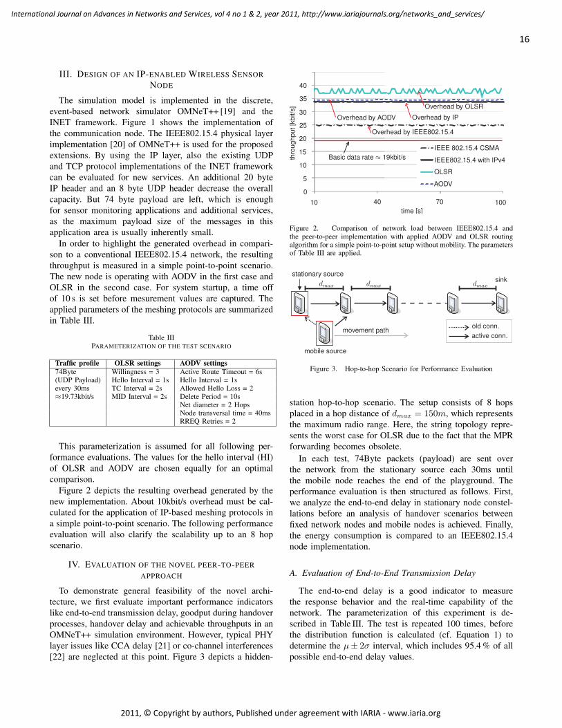
III. DESIGN OF AN IP-ENABLED WIRELESS SENSORNODE
The simulation model is implemented in the discrete,event-based network simulator OMNeT++ [19] and theINET framework. Figure 1 shows the implementation ofthe communication node. The IEEE802.15.4 physical layerimplementation [20] of OMNeT++ is used for the proposedextensions. By using the IP layer, also the existing UDPand TCP protocol implementations of the INET frameworkcan be evaluated for new services. An additional 20 byteIP header and an 8 byte UDP header decrease the overallcapacity. But 74 byte payload are left, which is enoughfor sensor monitoring applications and additional services,as the maximum payload size of the messages in thisapplication area is usually inherently small.
In order to highlight the generated overhead in compari-son to a conventional IEEE802.15.4 network, the resultingthroughput is measured in a simple point-to-point scenario.The new node is operating with AODV in the first case andOLSR in the second case. For system startup, a time offof 10 s is set before mesurement values are captured. Theapplied parameters of the meshing protocols are summarizedin Table III.
Table IIIPARAMETERIZATION OF THE TEST SCENARIO
Traffic profile OLSR settings AODV settings74Byte Willingness = 3 Active Route Timeout = 6s(UDP Payload) Hello Interval = 1s Hello Interval = 1severy 30ms TC Interval = 2s Allowed Hello Loss = 2≈19.73kbit/s MID Interval = 2s Delete Period = 10s
Net diameter = 2 HopsNode transversal time = 40msRREQ Retries = 2
This parameterization is assumed for all following per-formance evaluations. The values for the hello interval (HI)of OLSR and AODV are chosen equally for an optimalcomparison.
Figure 2 depicts the resulting overhead generated by thenew implementation. About 10kbit/s overhead must be cal-culated for the application of IP-based meshing protocols ina simple point-to-point scenario. The following performanceevaluation will also clarify the scalability up to an 8 hopscenario.
IV. EVALUATION OF THE NOVEL PEER-TO-PEERAPPROACH
To demonstrate general feasibility of the novel archi-tecture, we first evaluate important performance indicatorslike end-to-end transmission delay, goodput during handoverprocesses, handover delay and achievable throughputs in anOMNeT++ simulation environment. However, typical PHYlayer issues like CCA delay [21] or co-channel interferences[22] are neglected at this point. Figure 3 depicts a hidden-
0
5
10
15
20
25
30
35
40
45
10 40 70 10010 40 70 100
0
5
10
15
20
25
30
35
40
IEEE802.15.4 with IPv4
OLSR
AODV
thro
ug
hp
ut[k
bit/s
]
time [s]
Overhead by AODV
Overhead by IEEE802.15.4
Overhead by OLSR
Overhead by IP
Basic data rate ≈ 19kbit/s
IEEE 802.15.4 CSMA
Figure 2. Comparison of network load between IEEE802.15.4 andthe peer-to-peer implementation with applied AODV and OLSR routingalgorithm for a simple point-to-point setup without mobility. The parametersof Table III are applied.
stationary source
mobile source
sinkdmax dmax dmax
movement pathold conn.
active conn.
Figure 3. Hop-to-hop Scenario for Performance Evaluation
station hop-to-hop scenario. The setup consists of 8 hopsplaced in a hop distance of dmax = 150m, which representsthe maximum radio range. Here, the string topology repre-sents the worst case for OLSR due to the fact that the MPRforwarding becomes obsolete.
In each test, 74Byte packets (payload) are sent overthe network from the stationary source each 30ms untilthe mobile node reaches the end of the playground. Theperformance evaluation is then structured as follows. First,we analyze the end-to-end delay in stationary node constel-lations before an analysis of handover scenarios betweenfixed network nodes and mobile nodes is achieved. Finally,the energy consumption is compared to an IEEE802.15.4node implementation.
A. Evaluation of End-to-End Transmission Delay
The end-to-end delay is a good indicator to measurethe response behavior and the real-time capability of thenetwork. The parameterization of this experiment is de-scribed in Table III. The test is repeated 100 times, beforethe distribution function is calculated (cf. Equation 1) todetermine the µ± 2σ interval, which includes 95.4 % of allpossible end-to-end delay values.
16
International Journal on Advances in Networks and Services, vol 4 no 1 & 2, year 2011, http://www.iariajournals.org/networks_and_services/
2011, © Copyright by authors, Published under agreement with IARIA - www.iaria.org
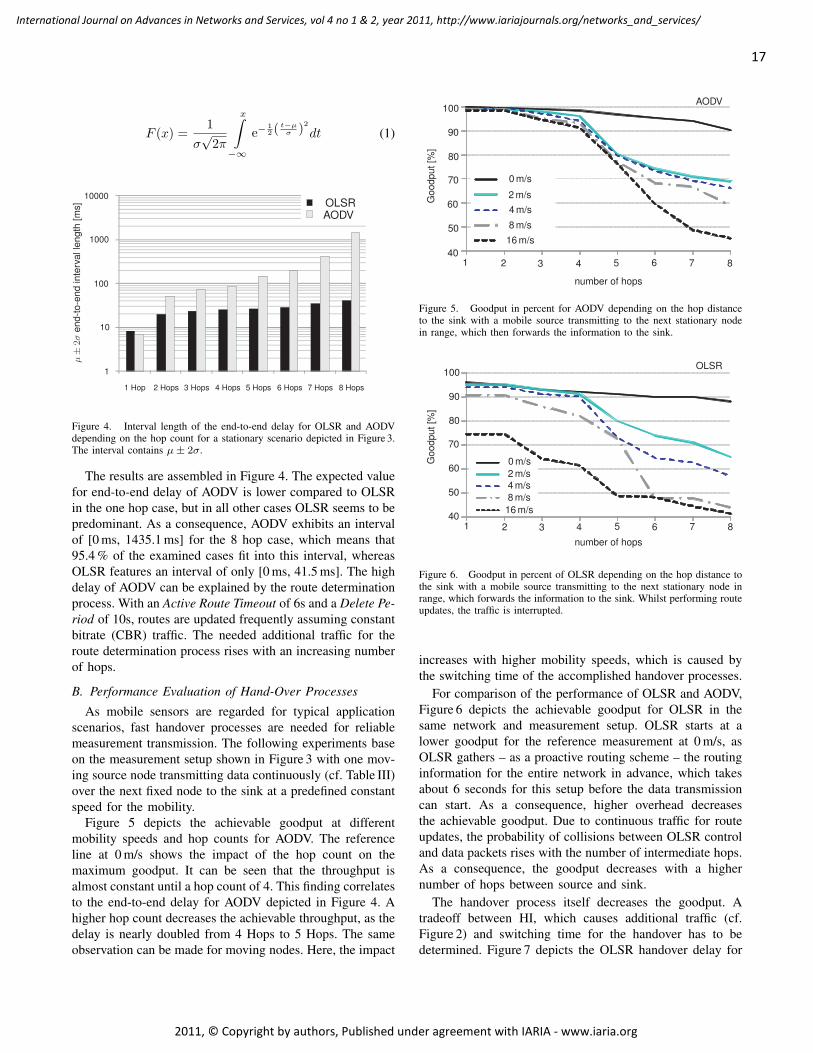
F (x) =1
σ√
2π
x∫−∞
e−12 ( t−µσ )2
dt (1)
OLSRAODV
1 Hop 2 Hops 3 Hops 4 Hops 5 Hops 6 Hops 7 Hops 8 Hops
1
10
100
1000
10000
µ±
2σe
nd
-to
-en
din
terv
alle
ng
th[m
s]
[ms]
Figure 4. Interval length of the end-to-end delay for OLSR and AODVdepending on the hop count for a stationary scenario depicted in Figure 3.The interval contains µ± 2σ.
The results are assembled in Figure 4. The expected valuefor end-to-end delay of AODV is lower compared to OLSRin the one hop case, but in all other cases OLSR seems to bepredominant. As a consequence, AODV exhibits an intervalof [0 ms, 1435.1 ms] for the 8 hop case, which means that95.4 % of the examined cases fit into this interval, whereasOLSR features an interval of only [0 ms, 41.5 ms]. The highdelay of AODV can be explained by the route determinationprocess. With an Active Route Timeout of 6s and a Delete Pe-riod of 10s, routes are updated frequently assuming constantbitrate (CBR) traffic. The needed additional traffic for theroute determination process rises with an increasing numberof hops.
B. Performance Evaluation of Hand-Over Processes
As mobile sensors are regarded for typical applicationscenarios, fast handover processes are needed for reliablemeasurement transmission. The following experiments baseon the measurement setup shown in Figure 3 with one mov-ing source node transmitting data continuously (cf. Table III)over the next fixed node to the sink at a predefined constantspeed for the mobility.
Figure 5 depicts the achievable goodput at differentmobility speeds and hop counts for AODV. The referenceline at 0 m/s shows the impact of the hop count on themaximum goodput. It can be seen that the throughput isalmost constant until a hop count of 4. This finding correlatesto the end-to-end delay for AODV depicted in Figure 4. Ahigher hop count decreases the achievable throughput, as thedelay is nearly doubled from 4 Hops to 5 Hops. The sameobservation can be made for moving nodes. Here, the impact
40
50
60
70
80
90
100
1 2 3 4 5 6 7 8
0 m/s
2 m/s
4 m/s
8 m/s
16 m/s40
50
60
70
80
90
100AODV
1 2 3 4 5 6 7 8
0 m/s
2 m/s
4 m/s
8 m/s
16 m/s
Go
od
pu
t[%
]
number of hops
Figure 5. Goodput in percent for AODV depending on the hop distanceto the sink with a mobile source transmitting to the next stationary nodein range, which then forwards the information to the sink.
40
50
60
70
80
90
100
1 2 3 4 5 6 7 8
0 m/s
2 m/s
4 m/s
8 m/s
16 m/s40
50
60
70
80
90
100OLSR
1 2 3 4 5 6 7 8
0 m/s
2 m/s4 m/s
8 m/s
16 m/s
Go
od
pu
t[%
]
number of hops
Figure 6. Goodput in percent of OLSR depending on the hop distance tothe sink with a mobile source transmitting to the next stationary node inrange, which forwards the information to the sink. Whilst performing routeupdates, the traffic is interrupted.
increases with higher mobility speeds, which is caused bythe switching time of the accomplished handover processes.
For comparison of the performance of OLSR and AODV,Figure 6 depicts the achievable goodput for OLSR in thesame network and measurement setup. OLSR starts at alower goodput for the reference measurement at 0 m/s, asOLSR gathers – as a proactive routing scheme – the routinginformation for the entire network in advance, which takesabout 6 seconds for this setup before the data transmissioncan start. As a consequence, higher overhead decreasesthe achievable goodput. Due to continuous traffic for routeupdates, the probability of collisions between OLSR controland data packets rises with the number of intermediate hops.As a consequence, the goodput decreases with a highernumber of hops between source and sink.
The handover process itself decreases the goodput. Atradeoff between HI, which causes additional traffic (cf.Figure 2) and switching time for the handover has to bedetermined. Figure 7 depicts the OLSR handover delay for
17
International Journal on Advances in Networks and Services, vol 4 no 1 & 2, year 2011, http://www.iariajournals.org/networks_and_services/
2011, © Copyright by authors, Published under agreement with IARIA - www.iaria.org
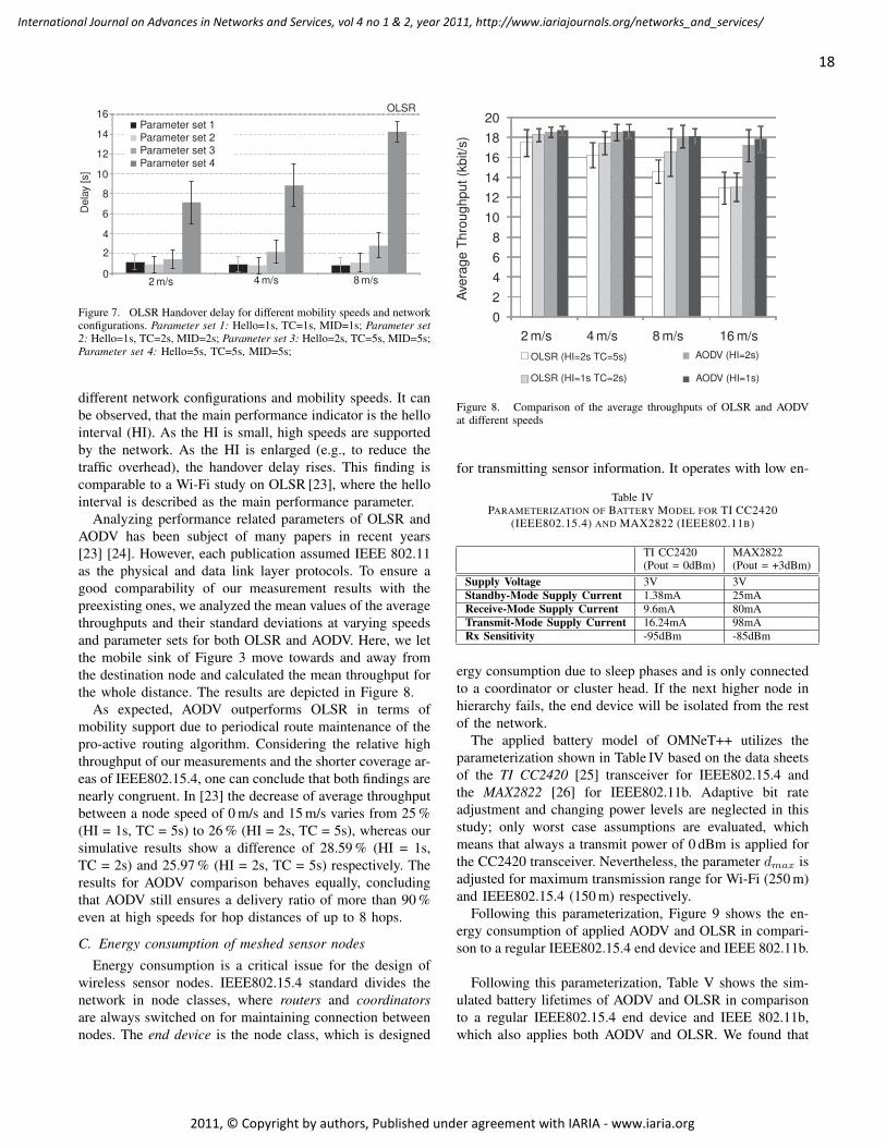
0
2
4
6
8
10
12
14
16
2 m/s 4 m/s 8 m/s
0
2
4
6
8
10
12
14
16
De
lay
[s]
OLSR
2 m/s 4 m/s 8 m/s
Parameter set 1
Parameter set 2
Parameter set 3
Parameter set 4
update
Figure 7. OLSR Handover delay for different mobility speeds and networkconfigurations. Parameter set 1: Hello=1s, TC=1s, MID=1s; Parameter set2: Hello=1s, TC=2s, MID=2s; Parameter set 3: Hello=2s, TC=5s, MID=5s;Parameter set 4: Hello=5s, TC=5s, MID=5s;
different network configurations and mobility speeds. It canbe observed, that the main performance indicator is the hellointerval (HI). As the HI is small, high speeds are supportedby the network. As the HI is enlarged (e.g., to reduce thetraffic overhead), the handover delay rises. This finding iscomparable to a Wi-Fi study on OLSR [23], where the hellointerval is described as the main performance parameter.
Analyzing performance related parameters of OLSR andAODV has been subject of many papers in recent years[23] [24]. However, each publication assumed IEEE 802.11as the physical and data link layer protocols. To ensure agood comparability of our measurement results with thepreexisting ones, we analyzed the mean values of the averagethroughputs and their standard deviations at varying speedsand parameter sets for both OLSR and AODV. Here, we letthe mobile sink of Figure 3 move towards and away fromthe destination node and calculated the mean throughput forthe whole distance. The results are depicted in Figure 8.
As expected, AODV outperforms OLSR in terms ofmobility support due to periodical route maintenance of thepro-active routing algorithm. Considering the relative highthroughput of our measurements and the shorter coverage ar-eas of IEEE802.15.4, one can conclude that both findings arenearly congruent. In [23] the decrease of average throughputbetween a node speed of 0 m/s and 15 m/s varies from 25 %(HI = 1s, TC = 5s) to 26 % (HI = 2s, TC = 5s), whereas oursimulative results show a difference of 28.59 % (HI = 1s,TC = 2s) and 25.97 % (HI = 2s, TC = 5s) respectively. Theresults for AODV comparison behaves equally, concludingthat AODV still ensures a delivery ratio of more than 90 %even at high speeds for hop distances of up to 8 hops.
C. Energy consumption of meshed sensor nodes
Energy consumption is a critical issue for the design ofwireless sensor nodes. IEEE802.15.4 standard divides thenetwork in node classes, where routers and coordinatorsare always switched on for maintaining connection betweennodes. The end device is the node class, which is designed
2 m/s 4 m/s 8 m/s 16 m/s
Ave
rag
eT
hro
ug
hp
ut(k
bit/s
)
OLSR (HI=2s TC=5s)
OLSR (HI=1s TC=2s)
AODV (HI=2s)
AODV (HI=1s)
0
2
4
6
8
10
12
14
16
18
20
Figure 8. Comparison of the average throughputs of OLSR and AODVat different speeds
for transmitting sensor information. It operates with low en-
Table IVPARAMETERIZATION OF BATTERY MODEL FOR TI CC2420
(IEEE802.15.4) AND MAX2822 (IEEE802.11B)
TI CC2420 MAX2822(Pout = 0dBm) (Pout = +3dBm)
Supply Voltage 3V 3VStandby-Mode Supply Current 1.38mA 25mAReceive-Mode Supply Current 9.6mA 80mATransmit-Mode Supply Current 16.24mA 98mARx Sensitivity -95dBm -85dBm
ergy consumption due to sleep phases and is only connectedto a coordinator or cluster head. If the next higher node inhierarchy fails, the end device will be isolated from the restof the network.
The applied battery model of OMNeT++ utilizes theparameterization shown in Table IV based on the data sheetsof the TI CC2420 [25] transceiver for IEEE802.15.4 andthe MAX2822 [26] for IEEE802.11b. Adaptive bit rateadjustment and changing power levels are neglected in thisstudy; only worst case assumptions are evaluated, whichmeans that always a transmit power of 0 dBm is applied forthe CC2420 transceiver. Nevertheless, the parameter dmax isadjusted for maximum transmission range for Wi-Fi (250 m)and IEEE802.15.4 (150 m) respectively.
Following this parameterization, Figure 9 shows the en-ergy consumption of applied AODV and OLSR in compari-son to a regular IEEE802.15.4 end device and IEEE 802.11b.
Following this parameterization, Table V shows the sim-ulated battery lifetimes of AODV and OLSR in comparisonto a regular IEEE802.15.4 end device and IEEE 802.11b,which also applies both AODV and OLSR. We found that
18
International Journal on Advances in Networks and Services, vol 4 no 1 & 2, year 2011, http://www.iariajournals.org/networks_and_services/
2011, © Copyright by authors, Published under agreement with IARIA - www.iaria.org
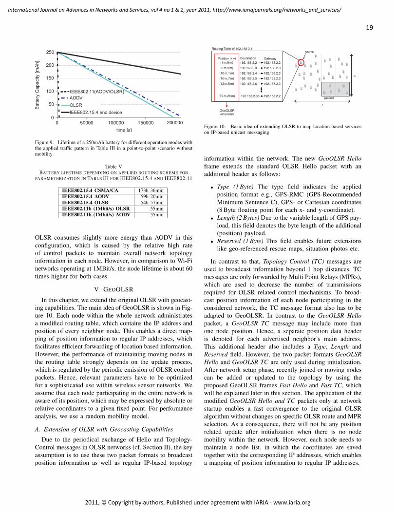
0
50
100
150
200
250
0 50000 100000 150000 200000
AODV
OLSR
IEEE802.15.4
IEEE802.11(AODV/OLSR)
end device0
50
100
150
200
250
0 50000 100000 150000 200000
Ba
tte
ryC
ap
acity
[mA
h]
time [s]
Figure 9. Lifetime of a 250mAh battery for different operation modes withthe applied traffic pattern in Table III in a point-to-point scenario withoutmobility
Table VBATTERY LIFETIME DEPENDING ON APPLIED ROUTING SCHEME FOR
PARAMETERIZATION IN TABLE III FOR IEEE802.15.4 AND IEEE802.11
IEEE802.15.4 CSMA/CA 173h 36minIEEE802.15.4 AODV 59h 20minIEEE802.15.4 OLSR 54h 57minIEEE802.11b (1Mbit/s) OLSR 55minIEEE802.11b (1Mbit/s) AODV 55min
OLSR consumes slightly more energy than AODV in thisconfiguration, which is caused by the relative high rateof control packets to maintain overall network topologyinformation in each node. However, in comparison to Wi-Finetworks operating at 1MBit/s, the node lifetime is about 60times higher for both cases.
V. GEOOLSR
In this chapter, we extend the original OLSR with geocast-ing capabilities. The main idea of GeoOLSR is shown in Fig-ure 10. Each node within the whole network administratesa modified routing table, which contains the IP address andposition of every neighbor node. This enables a direct map-ping of position information to regular IP addresses, whichfacilitates efficient forwarding of location based information.However, the performance of maintaining moving nodes inthe routing table strongly depends on the update process,which is regulated by the periodic emission of OLSR controlpackets. Hence, relevant parameters have to be optimizedfor a sophisticated use within wireless sensor networks. Weassume that each node participating in the entire network isaware of its position, which may be expressed by absolute orrelative coordinates to a given fixed-point. For performanceanalysis, we use a random mobility model.
A. Extension of OLSR with Geocasting Capabilities
Due to the periodical exchange of Hello and Topology-Control messages in OLSR networks (cf. Section II), the keyassumption is to use these two packet formats to broadcastposition information as well as regular IP-based topology
geocast
source
(1 m,9 m)
(9 m,9 m)
(16 m,1 m)
(16 m,7 m)
(12 m,8 m)
(39 m,28 m)
x
y
GeoOLSRextension
192.168.2.2
192.168.2.2192.168.2.2
192.168.2.3
192.168.2.3
192.168.2.3
192.168.2.3192.168.2.3
192.168.2.4
192.168.2.5
192.168.2.6
192.168.2.36
Routing Table of 192.168.2.1
Position (x,y) Destination Gateway
Figure 10. Basic idea of extending OLSR to map location based serviceson IP-based unicast messaging
information within the network. The new GeoOLSR Helloframe extends the standard OLSR Hello packet with anadditional header as follows:
• Type (1 Byte) The type field indicates the appliedposition format e.g., GPS-RMC (GPS-RecommendedMinimum Sentence C), GPS- or Cartesian coordinates(8 Byte floating point for each x- and y-coordinate).
• Length (2 Bytes) Due to the variable length of GPS pay-load, this field denotes the byte length of the additional(position) payload.
• Reserved (1 Byte) This field enables future extensionslike geo-referenced rescue maps, situation photos etc.
In contrast to that, Topology Control (TC) messages areused to broadcast information beyond 1 hop distances. TCmessages are only forwarded by Multi Point Relays (MPRs),which are used to decrease the number of transmissionsrequired for OLSR related control mechanisms. To broad-cast position information of each node participating in theconsidered network, the TC message format also has to beadapted to GeoOLSR. In contrast to the GeoOLSR Hellopacket, a GeoOLSR TC message may include more thanone node position. Hence, a separate position data headeris denoted for each advertised neighbor’s main address.This additional header also includes a Type, Length andReserved field. However, the two packet formats GeoOLSRHello and GeoOLSR TC are only used during initialization.After network setup phase, recently joined or moving nodescan be added or updated to the topology by using theproposed GeoOLSR frames Fast Hello and Fast TC, whichwill be explained later in this section. The application of themodified GeoOLSR Hello and TC packets only at networkstartup enables a fast convergence to the original OLSRalgorithm without changes on specific OLSR route and MPRselection. As a consequence, there will not be any positionrelated update after initialization when there is no nodemobility within the network. However, each node needs tomaintain a node list, in which the coordinates are savedtogether with the corresponding IP addresses, which enablesa mapping of position information to regular IP addresses.
19
International Journal on Advances in Networks and Services, vol 4 no 1 & 2, year 2011, http://www.iariajournals.org/networks_and_services/
2011, © Copyright by authors, Published under agreement with IARIA - www.iaria.org
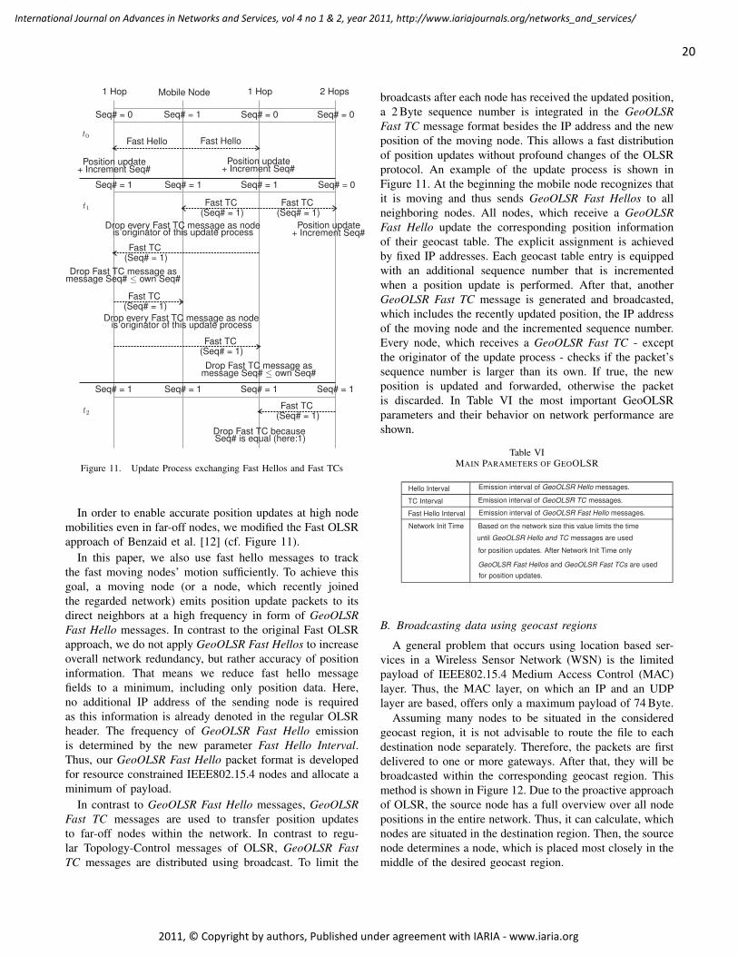
Position update
Position update Position update
+ Increment Seq#
+ Increment Seq# + Increment Seq#
Fast TC
Fast TC
Fast TC
Fast TC
Fast TC Fast TC
(Seq# = 1)
(Seq# = 1)
(Seq# = 1)
(Seq# = 1)
(Seq# = 1) (Seq# = 1)
Drop Fast TC message as
Drop Fast TC message as
message Seq# ≤ own Seq#
message Seq# ≤ own Seq#
Fast Hello Fast Hello
Drop every Fast TC message as node
Drop every Fast TC message as node
is originator of this update process
is originator of this update process
Drop Fast TC becauseSeq# is equal (here:1)
Seq# = 0
Seq# = 0Seq# = 0 Seq# = 0
Seq# = 1Seq# = 1 Seq# = 1Seq# = 1
Seq# = 1 Seq# = 1Seq# = 1
Seq# = 1
t0
t1
t2
Mobile Node1 Hop 1 Hop 2 Hops
Figure 11. Update Process exchanging Fast Hellos and Fast TCs
In order to enable accurate position updates at high nodemobilities even in far-off nodes, we modified the Fast OLSRapproach of Benzaid et al. [12] (cf. Figure 11).
In this paper, we also use fast hello messages to trackthe fast moving nodes’ motion sufficiently. To achieve thisgoal, a moving node (or a node, which recently joinedthe regarded network) emits position update packets to itsdirect neighbors at a high frequency in form of GeoOLSRFast Hello messages. In contrast to the original Fast OLSRapproach, we do not apply GeoOLSR Fast Hellos to increaseoverall network redundancy, but rather accuracy of positioninformation. That means we reduce fast hello messagefields to a minimum, including only position data. Here,no additional IP address of the sending node is requiredas this information is already denoted in the regular OLSRheader. The frequency of GeoOLSR Fast Hello emissionis determined by the new parameter Fast Hello Interval.Thus, our GeoOLSR Fast Hello packet format is developedfor resource constrained IEEE802.15.4 nodes and allocate aminimum of payload.
In contrast to GeoOLSR Fast Hello messages, GeoOLSRFast TC messages are used to transfer position updatesto far-off nodes within the network. In contrast to regu-lar Topology-Control messages of OLSR, GeoOLSR FastTC messages are distributed using broadcast. To limit the
broadcasts after each node has received the updated position,a 2 Byte sequence number is integrated in the GeoOLSRFast TC message format besides the IP address and the newposition of the moving node. This allows a fast distributionof position updates without profound changes of the OLSRprotocol. An example of the update process is shown inFigure 11. At the beginning the mobile node recognizes thatit is moving and thus sends GeoOLSR Fast Hellos to allneighboring nodes. All nodes, which receive a GeoOLSRFast Hello update the corresponding position informationof their geocast table. The explicit assignment is achievedby fixed IP addresses. Each geocast table entry is equippedwith an additional sequence number that is incrementedwhen a position update is performed. After that, anotherGeoOLSR Fast TC message is generated and broadcasted,which includes the recently updated position, the IP addressof the moving node and the incremented sequence number.Every node, which receives a GeoOLSR Fast TC - exceptthe originator of the update process - checks if the packet’ssequence number is larger than its own. If true, the newposition is updated and forwarded, otherwise the packetis discarded. In Table VI the most important GeoOLSRparameters and their behavior on network performance areshown.
Table VIMAIN PARAMETERS OF GEOOLSR
Hello Interval Emission interval of GeoOLSR Hello messages.
TC Interval Emission interval of GeoOLSR TC messages.
Fast Hello Interval Emission interval of GeoOLSR Fast Hello messages.
Network Init Time Based on the network size this value limits the time
until GeoOLSR Hello and TC messages are used
for position updates. After Network Init Time only
GeoOLSR Fast Hellos and GeoOLSR Fast TCs are used
for position updates.
B. Broadcasting data using geocast regions
A general problem that occurs using location based ser-vices in a Wireless Sensor Network (WSN) is the limitedpayload of IEEE802.15.4 Medium Access Control (MAC)layer. Thus, the MAC layer, on which an IP and an UDPlayer are based, offers only a maximum payload of 74 Byte.
Assuming many nodes to be situated in the consideredgeocast region, it is not advisable to route the file to eachdestination node separately. Therefore, the packets are firstdelivered to one or more gateways. After that, they will bebroadcasted within the corresponding geocast region. Thismethod is shown in Figure 12. Due to the proactive approachof OLSR, the source node has a full overview over all nodepositions in the entire network. Thus, it can calculate, whichnodes are situated in the destination region. Then, the sourcenode determines a node, which is placed most closely in themiddle of the desired geocast region.
20
International Journal on Advances in Networks and Services, vol 4 no 1 & 2, year 2011, http://www.iariajournals.org/networks_and_services/
2011, © Copyright by authors, Published under agreement with IARIA - www.iaria.org
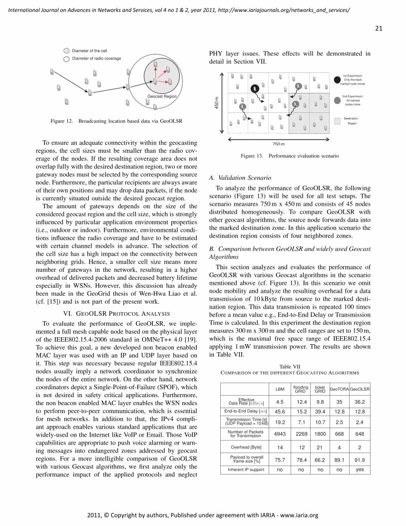
Geocast Region
Diameter of the cell
Diameter of radio coverage
Figure 12. Broadcasting location based data via GeoOLSR
To ensure an adequate connectivity within the geocastingregions, the cell sizes must be smaller than the radio cov-erage of the nodes. If the resulting coverage area does notoverlap fully with the desired destination region, two or moregateway nodes must be selected by the corresponding sourcenode. Furthermore, the particular recipients are always awareof their own positions and may drop data packets, if the nodeis currently situated outside the desired geocast region.
The amount of gateways depends on the size of theconsidered geocast region and the cell size, which is stronglyinfluenced by particular application environment properties(i.e., outdoor or indoor). Furthermore, environmental condi-tions influence the radio coverage and have to be estimatedwith certain channel models in advance. The selection ofthe cell size has a high impact on the connectivity betweenneighboring grids. Hence, a smaller cell size means morenumber of gateways in the network, resulting in a higheroverhead of delivered packets and decreased battery lifetimeespecially in WSNs. However, this discussion has alreadybeen made in the GeoGrid thesis of Wen-Hwa Liao et al.(cf. [15]) and is not part of the present work.
VI. GEOOLSR PROTOCOL ANALYSIS
To evaluate the performance of GeoOLSR, we imple-mented a full mesh capable node based on the physical layerof the IEEE802.15.4-2006 standard in OMNeT++ 4.0 [19].To achieve this goal, a new developed non beacon enabledMAC layer was used with an IP and UDP layer based onit. This step was necessary because regular IEEE802.15.4nodes usually imply a network coordinator to synchronizethe nodes of the entire network. On the other hand, networkcoordinators depict a Single-Point-of-Failure (SPOF), whichis not desired in safety critical applications. Furthermore,the non beacon enabled MAC layer enables the WSN nodesto perform peer-to-peer communication, which is essentialfor mesh networks. In addition to that, the IPv4 compli-ant approach enables various standard applications that arewidely-used on the Internet like VoIP or Email. Those VoIPcapabilities are appropriate to push voice alarming or warn-ing messages into endangered zones addressed by geocastregions. For a more intelligible comparison of GeoOLSRwith various Geocast algorithms, we first analyze only theperformance impact of the applied protocols and neglect
PHY layer issues. These effects will be demonstrated indetail in Section VII.
750 m
45
0m
Destination
Region
1st Experiment:
Only the black
marked node moves
2nd Experiment:
All marked
nodes move
Figure 13. Performance evaluation scenario
A. Validation Scenario
To analyze the performance of GeoOLSR, the followingscenario (Figure 13) will be used for all test setups. Thescenario measures 750 m x 450 m and consists of 45 nodesdistributed homogeneously. To compare GeoOLSR withother geocast algorithms, the source node forwards data intothe marked destination zone. In this application scenario thedestination region consists of four neighbored zones.
B. Comparison between GeoOLSR and widely used GeocastAlgorithms
This section analyzes and evaluates the performance ofGeoOLSR with various Geocast algorithms in the scenariomentioned above (cf. Figure 13). In this scenario we omitnode mobility and analyze the resulting overhead for a datatransmission of 10 kByte from source to the marked desti-nation region. This data transmission is repeated 100 timesbefore a mean value e.g., End-to-End Delay or TransmissionTime is calculated. In this experiment the destination regionmeasures 300 m x 300 m and the cell ranges are set to 150 m,which is the maximal free space range of IEEE802.15.4applying 1 mW transmission power. The results are shownin Table VII.
Table VIICOMPARISON OF THE DIFFERENT GEOCASTING ALGORITHMS
EffectiveData Rate [kBit/s]
End-to-End Delay [ms]
Transmission Time [s](UDP Payload = 10 kB)
Number of Packetsfor Transmission
Overhead [Byte]
Payload to overallframe size [%]
LBM flooding ticketGRIDGRID
GeoTORA GeoOLSR
Inherent IP support
4.5 12.4 9.8 35 36.2
45.6 15.2 39.4 12.812.8
19.2 7.1 10.7 2.5 2.4
4943 2269 1800 668 648
14 12 21 4 2
75.7 78.4 66.2 89.1 91.9
yesnononono
21
International Journal on Advances in Networks and Services, vol 4 no 1 & 2, year 2011, http://www.iariajournals.org/networks_and_services/
2011, © Copyright by authors, Published under agreement with IARIA - www.iaria.org

We observe, that only the route maintaining algorithmssupport high effective data rates and low end-to-end de-lays (cf. Section II-B). However, the resulting differencesbetween GeoTORA and GeoOLSR regarding effective datarate and transmission time are caused by our implementationof GeoTORA on ISO-OSI layer 7 whereas GeoOLSR isimplemented on ISO-OSI layer 3. Thus, GeoOLSR is able tosupport slightly higher effective data rates and a little lowertransmission time for each delivered packet than GeoTORA.Another important fact that can be omitted is the realtime capability of LBM, flooding and ticket based GRID,GeoTORA and GeoOLSR. If we interpret the 10 kByte ofPayload as a 5 s speech packet (16 kBit/s sampling rate andG.726 voice codec), we see that GeoTORA and GeoOLSRneed 2.5 s and 2.4 s respectively to forward this voice alarmmessage into a certain destination area. In comparison tothat LBM and the two GRID derivates show significanthigher transmission times than the original speech lengthcontained in the 10 kByte data packet. Hence, we canconclude that only the two route maintaining algorithmsare able to support real time simplex voice transmissions.Furthermore, GeoTORA and GeoOLSR are able to savebattery lifetime significantly as the overall number of packetsneeded for the transmission is smaller than the values forLBM, flooding GRID and ticket GRID. Finally, GeoGriduses 4 Byte for Next Hop, Message Type and Packet Numbersignaling whereas GeoOLSR uses only 2 Bytes for packetsequence numbering.
Thus, we can postulate that GeoTORA and GeoOLSR areboth suited for an application in Wireless Sensor Networks.However, we neglected node mobility until now, whichis a very important issue for the aimed application insafety critical scenarios where nodes can exhibit relativelyhigh mobilities. Nevertheless, GeoOLSR depicts two mainadvantages in comparison to GeoTORA. First, GeoOLSR asa proactive MANET algorithm is able to send an alarm mes-sage out immediately form a certain control center, whenevera threatening situation occurs without initiating a previouspolling mechanism. Another advantage of GeoOLSR is thesimultaneous support of IP-based traffic and location basedtraffic. That means, no additional geocasting algorithm isneeded and the network management is completely inte-grated in ISO-OSI layer 3.
C. Node Mobility
The previous section neglected nodes’ mobility. However,the knowledge of the correct position of each node has ahigh influence on geocast algorithms. As a quality indicatorwe regard the position deviation of all fixed nodes betweenthe routing table entry and the real position. That meansthe difference of the predicted mobile node’s position andthe real location is calculated for 100 seconds in each node.After that, an overall mean value of the position deviationsof all nodes is computed. To allow easier comparability, we
FH Ival = 0.3 s
FH Ival = 0.3 s
FH Ival = 0.5 s
FH Ival = 0.5 s
Hello Ival = 1 s
Hello Ival = 1 s
Hello Ival = 2 s
Hello Ival = 2 s
TC Ival = 2 s
TC Ival = 2 s
TC Ival = 5 s
TC Ival = 5 s
∆P
os
[m]
2 m/s 4 m/s 8 m/s 10 m/s 16 m/s
0
2
4
6
8
10
12
16
Figure 14. Position Deviation of GeoOLSR depending on varying movingspeeds and parameter sets regarding 1 moving node
FH Ival = 0.3 s
FH Ival = 0.3 s
FH Ival = 0.5 s
FH Ival = 0.5 s
Hello Ival = 1 s
Hello Ival = 1 s
Hello Ival = 2 s
Hello Ival = 2 s
TC Ival = 2 s
TC Ival = 2 s
TC Ival = 5 s
TC Ival = 5 s
∆P
os
[m]
0
2
4
6
8
10
12
2 m/s 4 m/s 8 m/s 10 m/s 16 m/s
Figure 15. Position Deviation of GeoOLSR depending on varying movingspeeds and parameter sets regarding 4 moving nodes
show the same scales for varying motion patterns. In thefirst experiment, we consider only one node moving aroundat different speeds. In the second setup, four nodes movethrough the scenario (cf. Figure 13). The results of the firstexperiment are shown in Figure 14. The overall mean valueof position differences increases as expected with highernode mobility. Here, the same phenomenon can be observedwith standard deviations, which indicate a successive risewith higher speeds. However, we can conclude that theratio of the position deviation to the observed movementspeed is always constant. That means, there is a constantaverage time, in which no communication between nodesis possible due to route maintenance, disconnections etc.Furthermore, we do not see an obvious impact of Helloand TC intervals on position accuracy in contrast to thekey parameter Fast Hello interval. As a consequence, po-sition deviation and standard deviation values using equalparameters for Hello and TC interval show nearly the same∆ positions. In the next step we evaluate the influence ofhigher node mobility within our scenario. Therefore, wecompare position deviations of four moving nodes (Figure15) with those of only one moving node (Figure 14). It isobvious that the increased number of moving nodes does
22
International Journal on Advances in Networks and Services, vol 4 no 1 & 2, year 2011, http://www.iariajournals.org/networks_and_services/
2011, © Copyright by authors, Published under agreement with IARIA - www.iaria.org
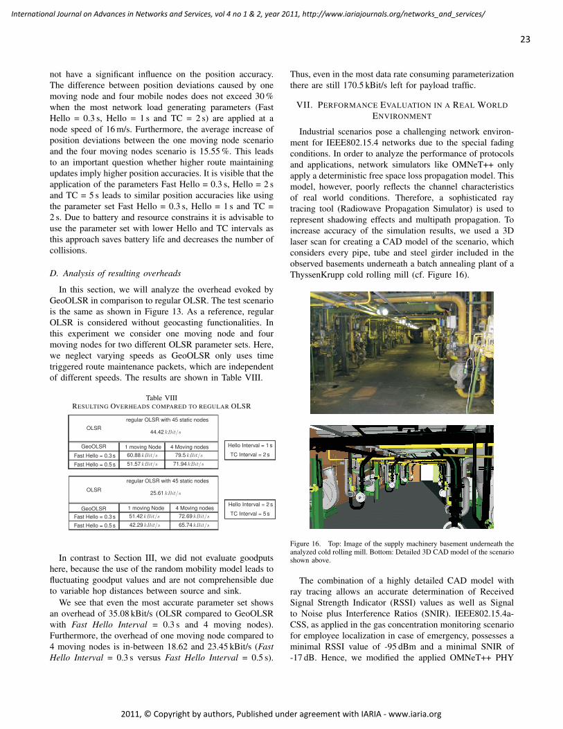
not have a significant influence on the position accuracy.The difference between position deviations caused by onemoving node and four mobile nodes does not exceed 30 %when the most network load generating parameters (FastHello = 0.3 s, Hello = 1 s and TC = 2 s) are applied at anode speed of 16 m/s. Furthermore, the average increase ofposition deviations between the one moving node scenarioand the four moving nodes scenario is 15.55 %. This leadsto an important question whether higher route maintainingupdates imply higher position accuracies. It is visible that theapplication of the parameters Fast Hello = 0.3 s, Hello = 2 sand TC = 5 s leads to similar position accuracies like usingthe parameter set Fast Hello = 0.3 s, Hello = 1 s and TC =2 s. Due to battery and resource constrains it is advisable touse the parameter set with lower Hello and TC intervals asthis approach saves battery life and decreases the number ofcollisions.
D. Analysis of resulting overheads
In this section, we will analyze the overhead evoked byGeoOLSR in comparison to regular OLSR. The test scenariois the same as shown in Figure 13. As a reference, regularOLSR is considered without geocasting functionalities. Inthis experiment we consider one moving node and fourmoving nodes for two different OLSR parameter sets. Here,we neglect varying speeds as GeoOLSR only uses timetriggered route maintenance packets, which are independentof different speeds. The results are shown in Table VIII.
Table VIIIRESULTING OVERHEADS COMPARED TO REGULAR OLSR
OLSR
OLSR
GeoOLSR
GeoOLSR Hello Interval = 1 s
TC Interval = 2 s
Hello Interval = 2 s
TC Interval = 5 sFast Hello = 0.3 s
Fast Hello = 0.3 s
Fast Hello = 0.5 s
Fast Hello = 0.5 s
regular OLSR with 45 static nodes
regular OLSR with 45 static nodes
1 moving Node
1 moving Node
4 Moving nodes
4 Moving nodes
44.42 kBit/s
25.61 kBit/s
60.88 kBit/s 79.5 kBit/s
51.57 kBit/s 71.94 kBit/s
51.42 kBit/s 72.69 kBit/s
42.29 kBit/s 65.74 kBit/s
In contrast to Section III, we did not evaluate goodputshere, because the use of the random mobility model leads tofluctuating goodput values and are not comprehensible dueto variable hop distances between source and sink.
We see that even the most accurate parameter set showsan overhead of 35.08 kBit/s (OLSR compared to GeoOLSRwith Fast Hello Interval = 0.3 s and 4 moving nodes).Furthermore, the overhead of one moving node compared to4 moving nodes is in-between 18.62 and 23.45 kBit/s (FastHello Interval = 0.3 s versus Fast Hello Interval = 0.5 s).
Thus, even in the most data rate consuming parameterizationthere are still 170.5 kBit/s left for payload traffic.
VII. PERFORMANCE EVALUATION IN A REAL WORLDENVIRONMENT
Industrial scenarios pose a challenging network environ-ment for IEEE802.15.4 networks due to the special fadingconditions. In order to analyze the performance of protocolsand applications, network simulators like OMNeT++ onlyapply a deterministic free space loss propagation model. Thismodel, however, poorly reflects the channel characteristicsof real world conditions. Therefore, a sophisticated raytracing tool (Radiowave Propagation Simulator) is used torepresent shadowing effects and multipath propagation. Toincrease accuracy of the simulation results, we used a 3Dlaser scan for creating a CAD model of the scenario, whichconsiders every pipe, tube and steel girder included in theobserved basements underneath a batch annealing plant of aThyssenKrupp cold rolling mill (cf. Figure 16).
it/s
Figure 16. Top: Image of the supply machinery basement underneath theanalyzed cold rolling mill. Bottom: Detailed 3D CAD model of the scenarioshown above.
The combination of a highly detailed CAD model withray tracing allows an accurate determination of ReceivedSignal Strength Indicator (RSSI) values as well as Signalto Noise plus Interference Ratios (SNIR). IEEE802.15.4a-CSS, as applied in the gas concentration monitoring scenariofor employee localization in case of emergency, possesses aminimal RSSI value of -95 dBm and a minimal SNIR of-17 dB. Hence, we modified the applied OMNeT++ PHY
23
International Journal on Advances in Networks and Services, vol 4 no 1 & 2, year 2011, http://www.iariajournals.org/networks_and_services/
2011, © Copyright by authors, Published under agreement with IARIA - www.iaria.org
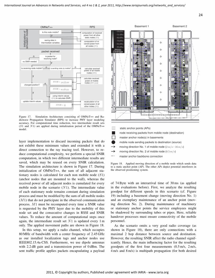
OMNeT++ RPSIn
itia
liza
tio
no
fsim
ula
tio
nm
od
el
Is this node mobile? computation of received
power from all other
static nodes (S1)
saving data in
intermediate variablescomputation of re-
ceived power from
all nodes (N1)
n
n
nn
n
y
y
y
y
y
packet received
is packet for
receiving node?
no SNIR needed
is receiving node mobile? is sending node (s) mobile? calculate receivedpower of all mobile
nodes (M1)
calculate received
power of mobilenodes (M1\s)
changed position?
update interim values recalculation of re-
ceived power of all
other nodes (N1)
using interim values
(N1) to calculate SNIR
SNIR = s(S1\s)∪M1
SNIR = sS1∪(M1\s)
SNIR = sN1
Figure 17. Simulation Architecture consisting of OMNeT++ and Ra-diowave Propagation Simulator (RPS) to increase PHY layer modelingaccuracy. For computational time reduction, two intermediate result sets(S1 and N1) are applied during initialization period of the OMNeT++model.
layer implementation to discard incoming packets that donot exhibit these minimum values and extended it with adirect connection to the ray tracing tool. However, to re-duce computational complexity, we perform a special SNIRcomputation, in which two different intermediate results aresaved, which may be reused on every SNIR calculation.The simulation architecture is shown in Figure 17. Duringinitialization of OMNeT++, the sum of all adjacent sta-tionary nodes is calculated for each non mobile node (S1)(anchor nodes that are mounted to the wall), whereas thereceived power of all adjacent nodes is cumulated for everymobile node in the scenario (N1). The intermediate valueof each stationary node remains constant during simulationprocess and must be modified by the sum of all mobile nodes(M1) that do not participate in the observed communicationprocess. M1 must be recomputed every time a SNIR valueis requested by the PHY layer due to the mobility of thisnode set and the consecutive changes in RSSI and SNIRvalues. To reduce the amount of computational steps onceagain, the intermediate result set N1 is updated every 1 monly. The applied movement paths are shown in Figure 18.
In this setup, we apply a radio channel, which occupies80 MHz of bandwidth with a center frequency of 2.45 GHzas our installed localization tags and anchor nodes useIEEE802.15.4a-CSS. Furthermore, we use dipole antennaswith 2.2 dB gain and a transmission power of 0 dBm. Thesent traffic profile applies packets encapsulating a payload
static anchor points (APs)
node receiving packets from mobile node (destination)
mobile node sending packets to destination (source)
moving direction No. 1 of mobile node (2 m/s - 16 m/s)
moving direction No. 2 of mobile node (0.5 m/s)
master anchor node(s) in basements
master anchor backbone connection
Basement 1 Basement 2
−40 dBm
−51 dBm
−62 dBm
−73 dBm
−84 dBm
−95 dBm
(RSSI)Coverage
Figure 18. Applied moving direction of a mobile node which sends datato a static anchor point (AP). The other APs depict potential interferers inthe observed positioning system.
of 74 Byte with an interarrival time of 30 ms (as appliedin the evaluations before). First, we analyze the resultinggoodput for different speeds in this scenario (cf. Figure19) including a basement change (moving direction No. 1)and an exemplary maintenance of an anchor point (mov-ing direction No. 2). During maintenance of machineryor stationary anchor points the service employees mightbe shadowed by surrounding tubes or pipes. Here, reliablehandover processes must ensure connectivity of the mobilepersonnel.
As the scenario omits a very good radio coverage (asshown in Figure 18), there are only connections with amaximal 2 hop distance between source and destination.However, the resulting SNIR affect the radio channel signif-icantly. Hence, the main influencing factor for the resultinggoodputs of the first four measurements (0.5 m/s, 2 m/s,4 m/s and 8 m/s) is multipath propagation (for both desired
24
International Journal on Advances in Networks and Services, vol 4 no 1 & 2, year 2011, http://www.iariajournals.org/networks_and_services/
2011, © Copyright by authors, Published under agreement with IARIA - www.iaria.org
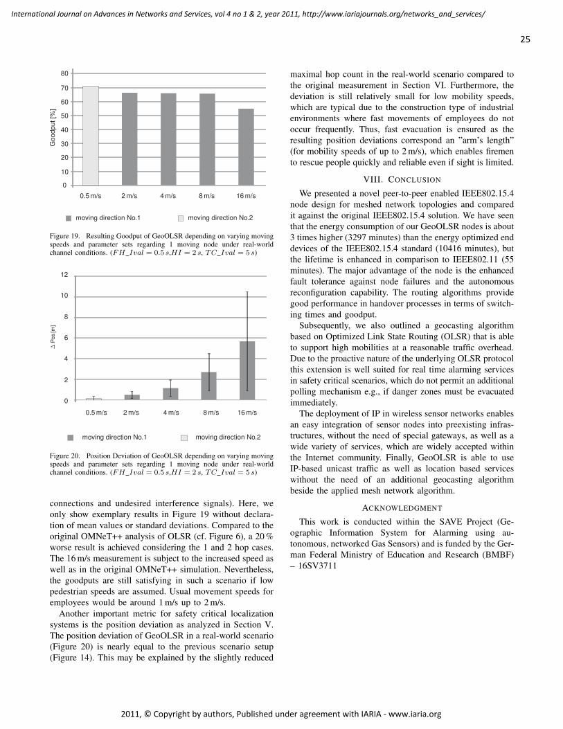
Go
od
pu
t[%
]
2 m/s 4 m/s 8 m/s 16 m/s0.5 m/s
0
10
20
30
40
50
60
70
80
moving direction No.1 moving direction No.2
Figure 19. Resulting Goodput of GeoOLSR depending on varying movingspeeds and parameter sets regarding 1 moving node under real-worldchannel conditions. (FH Ival = 0.5 s,HI = 2 s, TC Ival = 5 s)
∆P
os
[m]
2 m/s 4 m/s 8 m/s 16 m/s0.5 m/s
0
2
4
6
8
10
12
moving direction No.1 moving direction No.2
Figure 20. Position Deviation of GeoOLSR depending on varying movingspeeds and parameter sets regarding 1 moving node under real-worldchannel conditions. (FH Ival = 0.5 s,HI = 2 s, TC Ival = 5 s)
connections and undesired interference signals). Here, weonly show exemplary results in Figure 19 without declara-tion of mean values or standard deviations. Compared to theoriginal OMNeT++ analysis of OLSR (cf. Figure 6), a 20 %worse result is achieved considering the 1 and 2 hop cases.The 16 m/s measurement is subject to the increased speed aswell as in the original OMNeT++ simulation. Nevertheless,the goodputs are still satisfying in such a scenario if lowpedestrian speeds are assumed. Usual movement speeds foremployees would be around 1 m/s up to 2 m/s.
Another important metric for safety critical localizationsystems is the position deviation as analyzed in Section V.The position deviation of GeoOLSR in a real-world scenario(Figure 20) is nearly equal to the previous scenario setup(Figure 14). This may be explained by the slightly reduced
maximal hop count in the real-world scenario compared tothe original measurement in Section VI. Furthermore, thedeviation is still relatively small for low mobility speeds,which are typical due to the construction type of industrialenvironments where fast movements of employees do notoccur frequently. Thus, fast evacuation is ensured as theresulting position deviations correspond an ”arm’s length”(for mobility speeds of up to 2 m/s), which enables firemento rescue people quickly and reliable even if sight is limited.
VIII. CONCLUSION
We presented a novel peer-to-peer enabled IEEE802.15.4node design for meshed network topologies and comparedit against the original IEEE802.15.4 solution. We have seenthat the energy consumption of our GeoOLSR nodes is about3 times higher (3297 minutes) than the energy optimized enddevices of the IEEE802.15.4 standard (10416 minutes), butthe lifetime is enhanced in comparison to IEEE802.11 (55minutes). The major advantage of the node is the enhancedfault tolerance against node failures and the autonomousreconfiguration capability. The routing algorithms providegood performance in handover processes in terms of switch-ing times and goodput.
Subsequently, we also outlined a geocasting algorithmbased on Optimized Link State Routing (OLSR) that is ableto support high mobilities at a reasonable traffic overhead.Due to the proactive nature of the underlying OLSR protocolthis extension is well suited for real time alarming servicesin safety critical scenarios, which do not permit an additionalpolling mechanism e.g., if danger zones must be evacuatedimmediately.
The deployment of IP in wireless sensor networks enablesan easy integration of sensor nodes into preexisting infras-tructures, without the need of special gateways, as well as awide variety of services, which are widely accepted withinthe Internet community. Finally, GeoOLSR is able to useIP-based unicast traffic as well as location based serviceswithout the need of an additional geocasting algorithmbeside the applied mesh network algorithm.
ACKNOWLEDGMENT
This work is conducted within the SAVE Project (Ge-ographic Information System for Alarming using au-tonomous, networked Gas Sensors) and is funded by the Ger-man Federal Ministry of Education and Research (BMBF)– 16SV3711
25
International Journal on Advances in Networks and Services, vol 4 no 1 & 2, year 2011, http://www.iariajournals.org/networks_and_services/
2011, © Copyright by authors, Published under agreement with IARIA - www.iaria.org
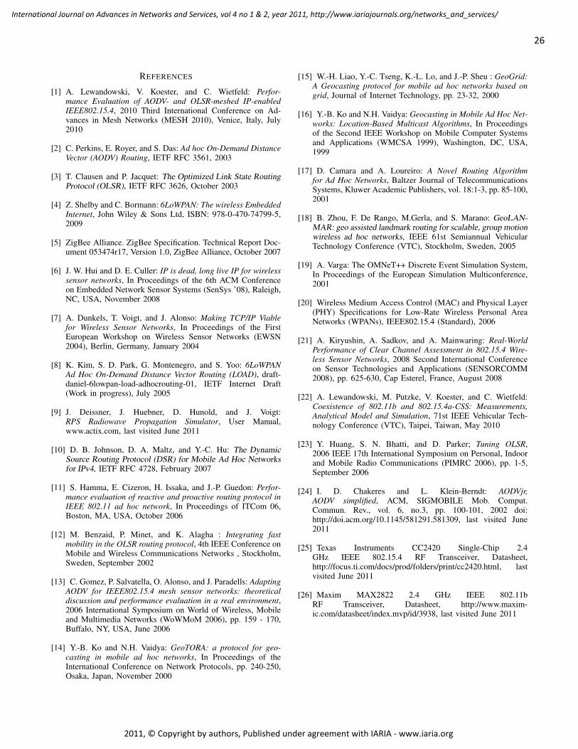
REFERENCES
[1] A. Lewandowski, V. Koester, and C. Wietfeld: Perfor-mance Evaluation of AODV- and OLSR-meshed IP-enabledIEEE802.15.4, 2010 Third International Conference on Ad-vances in Mesh Networks (MESH 2010), Venice, Italy, July2010
[2] C. Perkins, E. Royer, and S. Das: Ad hoc On-Demand DistanceVector (AODV) Routing, IETF RFC 3561, 2003
[3] T. Clausen and P. Jacquet: The Optimized Link State RoutingProtocol (OLSR), IETF RFC 3626, October 2003
[4] Z. Shelby and C. Bormann: 6LoWPAN: The wireless EmbeddedInternet, John Wiley & Sons Ltd, ISBN: 978-0-470-74799-5,2009
[5] ZigBee Alliance. ZigBee Specification. Technical Report Doc-ument 053474r17, Version 1.0, ZigBee Alliance, October 2007
[6] J. W. Hui and D. E. Culler: IP is dead, long live IP for wirelesssensor networks, In Proceedings of the 6th ACM Conferenceon Embedded Network Sensor Systems (SenSys ’08), Raleigh,NC, USA, November 2008
[7] A. Dunkels, T. Voigt, and J. Alonso: Making TCP/IP Viablefor Wireless Sensor Networks, In Proceedings of the FirstEuropean Workshop on Wireless Sensor Networks (EWSN2004), Berlin, Germany, January 2004
[8] K. Kim, S. D. Park, G. Montenegro, and S. Yoo: 6LoWPANAd Hoc On-Demand Distance Vector Routing (LOAD), draft-daniel-6lowpan-load-adhocrouting-01, IETF Internet Draft(Work in progress), July 2005
[9] J. Deissner, J. Huebner, D. Hunold, and J. Voigt:RPS Radiowave Propagation Simulator, User Manual,www.actix.com, last visited June 2011
[10] D. B. Johnson, D. A. Maltz, and Y.-C. Hu: The DynamicSource Routing Protocol (DSR) for Mobile Ad Hoc Networksfor IPv4, IETF RFC 4728, February 2007
[11] S. Hamma, E. Cizeron, H. Issaka, and J.-P. Guedon: Perfor-mance evaluation of reactive and proactive routing protocol inIEEE 802.11 ad hoc network, In Proceedings of ITCom 06,Boston, MA, USA, October 2006
[12] M. Benzaid, P. Minet, and K. Alagha : Integrating fastmobility in the OLSR routing protocol, 4th IEEE Conference onMobile and Wireless Communications Networks , Stockholm,Sweden, September 2002
[13] C. Gomez, P. Salvatella, O. Alonso, and J. Paradells: AdaptingAODV for IEEE802.15.4 mesh sensor networks: theoreticaldiscussion and performance evaluation in a real environment,2006 International Symposium on World of Wireless, Mobileand Multimedia Networks (WoWMoM 2006), pp. 159 - 170,Buffalo, NY, USA, June 2006
[14] Y.-B. Ko and N.H. Vaidya: GeoTORA: a protocol for geo-casting in mobile ad hoc networks, In Proceedings of theInternational Conference on Network Protocols, pp. 240-250,Osaka, Japan, November 2000
[15] W.-H. Liao, Y.-C. Tseng, K.-L. Lo, and J.-P. Sheu : GeoGrid:A Geocasting protocol for mobile ad hoc networks based ongrid, Journal of Internet Technology, pp. 23-32, 2000
[16] Y.-B. Ko and N.H. Vaidya: Geocasting in Mobile Ad Hoc Net-works: Location-Based Multicast Algorithms, In Proceedingsof the Second IEEE Workshop on Mobile Computer Systemsand Applications (WMCSA 1999), Washington, DC, USA,1999
[17] D. Camara and A. Loureiro: A Novel Routing Algorithmfor Ad Hoc Networks, Baltzer Journal of TelecommunicationsSystems, Kluwer Academic Publishers, vol. 18:1-3, pp. 85-100,2001
[18] B. Zhou, F. De Rango, M.Gerla, and S. Marano: GeoLAN-MAR: geo assisted landmark routing for scalable, group motionwireless ad hoc networks, IEEE 61st Semiannual VehicularTechnology Conference (VTC), Stockholm, Sweden, 2005
[19] A. Varga: The OMNeT++ Discrete Event Simulation System,In Proceedings of the European Simulation Multiconference,2001
[20] Wireless Medium Access Control (MAC) and Physical Layer(PHY) Specifications for Low-Rate Wireless Personal AreaNetworks (WPANs), IEEE802.15.4 (Standard), 2006
[21] A. Kiryushin, A. Sadkov, and A. Mainwaring: Real-WorldPerformance of Clear Channel Assessment in 802.15.4 Wire-less Sensor Networks, 2008 Second International Conferenceon Sensor Technologies and Applications (SENSORCOMM2008), pp. 625-630, Cap Esterel, France, August 2008
[22] A. Lewandowski, M. Putzke, V. Koester, and C. Wietfeld:Coexistence of 802.11b and 802.15.4a-CSS: Measurements,Analytical Model and Simulation, 71st IEEE Vehicular Tech-nology Conference (VTC), Taipei, Taiwan, May 2010
[23] Y. Huang, S. N. Bhatti, and D. Parker; Tuning OLSR,2006 IEEE 17th International Symposium on Personal, Indoorand Mobile Radio Communications (PIMRC 2006), pp. 1-5,September 2006
[24] I. D. Chakeres and L. Klein-Berndt: AODVjr,AODV simplified, ACM, SIGMOBILE Mob. Comput.Commun. Rev., vol. 6, no.3, pp. 100-101, 2002 doi:http://doi.acm.org/10.1145/581291.581309, last visited June2011
[25] Texas Instruments CC2420 Single-Chip 2.4GHz IEEE 802.15.4 RF Transceiver, Datasheet,http://focus.ti.com/docs/prod/folders/print/cc2420.html, lastvisited June 2011
[26] Maxim MAX2822 2.4 GHz IEEE 802.11bRF Transceiver, Datasheet, http://www.maxim-ic.com/datasheet/index.mvp/id/3938, last visited June 2011
26
International Journal on Advances in Networks and Services, vol 4 no 1 & 2, year 2011, http://www.iariajournals.org/networks_and_services/
2011, © Copyright by authors, Published under agreement with IARIA - www.iaria.org
A Traffic Monitoring and Queue Detection System Based on an Acoustic SensorNetwork
Barbara Barbagli, Luca Bencini, Iacopo Magrini and Gianfranco ManesDept. of Electronics and Telecommunications
University of FlorenceVia di Santa Marta 3, 50139 Florence, Italy,
Email: [email protected], [email protected],[email protected], [email protected]
Antonio ManesNetsens S.r.l.
Via Tevere 70, 50019 Florence, ItalyEmail: [email protected]
Abstract—Wireless Sensor Networks for real time trafficmonitoring in Intelligent Transportation Systems is currentlyconsidered one of the challenging application area for thisemerging technology. The promise of an unmanaged infras-tructure, with a continuously decreasing cost per unit, attractsthe attention of both final users and system integrator, openingnew business opportunities. This paper describes a TrafficMonitoring Wireless Sensor Network system, based on acousticarrays and powered by an effective post-processing detection.A practical case study is presented starting from a real problemand reaching the best architectural solution with particular fo-cus on hardware implementation and communication protocoldesign. Finally, real experience results are shown to highlightthe reliability of the developed system.
Keywords-wireless sensor network; acoustic sensors; trafficmonitoring; cross-layer routing protocol.
I. INTRODUCTION
Real-time traffic monitoring and early queue detectionis of paramount importance in Intelligent TransportationSystems (ITS). Distributed traffic monitoring on a largescale based on non intrusive/obtrusive solutions are highlydesirable for traffic monitoring.
Conventional traffic surveillance systems make use ofintrusive sensors such as inductive loop detectors or pressuresensors, for high accuracy in vehicle detection. However,these sensors disrupt traffic during installation and repair,and therefore have high installation and maintenance costs.These limitations have pushed towards the development ofnon-intrusive traffic monitoring technologies, including laserradars, passive infrareds, ultrasonics, passive acoustic arraysand video cameras. These systems have high equipmentcosts and their accuracy depends on environmental con-ditions. Moreover video cameras have involved huge datavolume demands for a dedicated wired connection in orderto communicate with the central server. As a result thesesolutions are not suitable for large-scale deployment andhence are restricted to small scale applications, where iso-lated monitoring points are located many kilometers apart.
Passive acoustic transducer-based surveillance systemshave also been developed, featuring vehicle classification
and multi-lane resolution capability; this is based on pro-cessing the characteristic sounds emitted by vehicles [3] [4].Acoustic sensors are attractive especially for their low costand simple and non-intrusive installation, however theyrequire a sophisticated post-processing algorithm for extract-ing useful information.
Another relevant requirement pushing towards the designof an effective traffic monitoring system is to provide highspatial density measurements. A viable solution for achiev-ing that purpose is a system based on a Wireless SensorNetwork (WSN) infrastructure offering advantages in termsof flexibility and a significant reduction of installation costs;therefore making large scale deployment possible.
Several solutions based on wireless sensors have beeninvestigated, including wireless magnetic sensors [5] [6], andcoherent cross-correlated acoustic transducer [8]. Ding etal. [5] demonstrated wireless magnetic sensors embeddedin the road sampling the magnetic field at its front andback ends, and internally processing this data in order tocount vehicles for computing the average speed of passingvehicles.
The requirements that adopting a WSN are expectedto satisfy in effective traffic monitoring monitoring con-cern both system level issues (i.e., unattended operation,maximum network life time, adaptability or even self-reconfigurability of functionalities and protocols) and finaluser needs (i.e., communication reliability and robustness,user friendly, versatile and powerful graphical user inter-faces). The most relevant mainly concerns the supply ofstand-alone operations. To this end, the system must be ableto run unattended for a long period also in the absence ofelectricity. This calls for an optimal energy managementensuring that the energy spent is directly related to theamount of traffic handled and not to the overall workingtime.
An additional requirement is robust operative conditions,which needs fault management, since a node may fail forseveral reasons. Other important properties are scalabilityand adaptability of the network’s topology, in terms of the
27
International Journal on Advances in Networks and Services, vol 4 no 1 & 2, year 2011, http://www.iariajournals.org/networks_and_services/
2011, © Copyright by authors, Published under agreement with IARIA - www.iaria.org
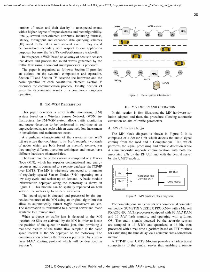
number of nodes and their density in unexpected eventswith a higher degree of responsiveness and reconfigurability.Finally, several user-oriented attributes, including fairness,latency, throughput and enhanced data querying schemes[10] need to be taken into account even if they couldbe considered secondary with respect to our applicationpurposes because the WSN’s cost/performance trade-off.
In this paper, a WSN based on an array of acoustic sensorsthat detect and process the sound waves generated by thetraffic flow using a low-cost microprocessor is proposed.
The paper is organized as follows: Section II providesan outlook on the system’s composition and operation.Section III and Section IV describe the hardware and thebasic operation of each constitutive element. Section Vdiscusses the communication protocol. Finally, Section VIgives the experimental results of a continuous long-termoperation.
II. TM-WSN DESCRIPTION
This paper describes a novel traffic monitoring (TM)system based on a Wireless Sensor Network (WSN) in-frastructure; the TM-WSN system allows traffic monitoringand queue detection to be performed in real-time at anunprecedented space scale with an extremely low investmentin installation and maintenance costs.
A significant characteristic of the system is the WSNinfrastructure that combines, in its basic module, two kindsof nodes which are both based on acoustic sensors, yetthey employ different operation techniques and hence, havedifferent hardware characteristics.
The basic module of the system is composed of a MasterNode (MN), which has superior computational and energyresources and is connected to a remote database via TCP/IPover UMTS. The MN is wirelessly connected to a numberof regularly spaced Sensor Nodes (SNs) operating on alow duty-cycle and woken-up on demand. A basic moduleinfrastructure deployed along the motorway is shown inFigure 1 . This module can be spatially replicated on bothsides of the motorway to cover a wide area.
The sound signal is detected and processed by the em-bedded resource of the MN using an original algorithm thatallow to automatically extract traffic parameters on site.The information is transmitted to a central server and madeavailable to a remote user.
When a queue or traffic jam is detected at the MNlocation the SNs are activated by the MN in order to locatethe position of the queue or traffic jam, thus providing areal-time picture of the traffic flow sampled at the samespace interval as the SN deployed on the motorway. Thecommunication between the devices is performed by a cross-layer MAC Routing protocol which will be described inSection V.
2LWSN
3MN 7SN 6SN10SN 9SN 8SN
UMTS
Server
1SN 2SN
2MN
3SN 5SN4SN
1MN
LWSN-segment1LWSN
Figure 1. Basic system infrastucture.
III. MN DESIGN AND OPERATION
In this section is first illustrated the MN hardware so-lution adopted and then, the procedure allowing automaticextraction on-site of traffic parameters.
A. MN Hardware Design
The MN block diagram is shown in Figure 2. It iscomposed of a Sensor Unit which detects the audio signalcoming from the road and a Computational Unit whichperforms the signal processing and vehicle detection whileit simultaneously supports communication with both theassociated SNs by the RF Unit and with the central serverby the UMTS modem.
MIC 1PROCESSING AND
CONTROL UNIT
UMTS MODEM
RF UNIT
MIC 2
Sensor Unit
Figure 2. MN hardware block diagrams.
The computational unit consists of a commercial computeron module GUMSTIX VERDEX PRO XM-4 with a MarvellPXA270 400 MHz processor equipped with 64 MB RAMand 16 MB flash memory, and operating with a LinuxOS. The audio signals detected by the acoustic sensorsare sampled at 16 KHz and quantized at 16 bit, thenprocessed with a real-time algorithm based on FFT routinesfor estimating the time delay via a coherent cross-correlationmethod.
A TCP-IP over UMTS Modem provides a bidirectionalconnectivity to the central server thus enabling a remote
28
International Journal on Advances in Networks and Services, vol 4 no 1 & 2, year 2011, http://www.iariajournals.org/networks_and_services/
2011, © Copyright by authors, Published under agreement with IARIA - www.iaria.org
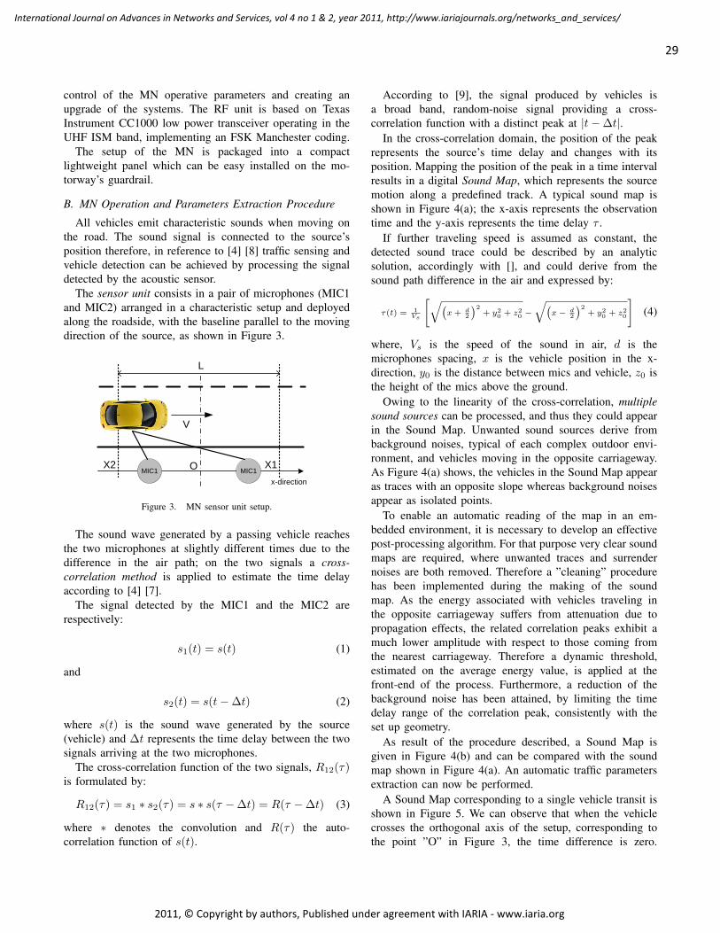
control of the MN operative parameters and creating anupgrade of the systems. The RF unit is based on TexasInstrument CC1000 low power transceiver operating in theUHF ISM band, implementing an FSK Manchester coding.
The setup of the MN is packaged into a compactlightweight panel which can be easy installed on the mo-torway’s guardrail.
B. MN Operation and Parameters Extraction Procedure
All vehicles emit characteristic sounds when moving onthe road. The sound signal is connected to the source’sposition therefore, in reference to [4] [8] traffic sensing andvehicle detection can be achieved by processing the signaldetected by the acoustic sensor.
The sensor unit consists in a pair of microphones (MIC1and MIC2) arranged in a characteristic setup and deployedalong the roadside, with the baseline parallel to the movingdirection of the source, as shown in Figure 3.
MIC1 MIC1
V
x-direction
O X1X2
L
Figure 3. MN sensor unit setup.
The sound wave generated by a passing vehicle reachesthe two microphones at slightly different times due to thedifference in the air path; on the two signals a cross-correlation method is applied to estimate the time delayaccording to [4] [7].
The signal detected by the MIC1 and the MIC2 arerespectively:
s1(t) = s(t) (1)
and
s2(t) = s(t−∆t) (2)
where s(t) is the sound wave generated by the source(vehicle) and ∆t represents the time delay between the twosignals arriving at the two microphones.
The cross-correlation function of the two signals, R12(τ)is formulated by:
R12(τ) = s1 ∗ s2(τ) = s ∗ s(τ −∆t) = R(τ −∆t) (3)
where ∗ denotes the convolution and R(τ) the auto-correlation function of s(t).
According to [9], the signal produced by vehicles isa broad band, random-noise signal providing a cross-correlation function with a distinct peak at |t−∆t|.
In the cross-correlation domain, the position of the peakrepresents the source’s time delay and changes with itsposition. Mapping the position of the peak in a time intervalresults in a digital Sound Map, which represents the sourcemotion along a predefined track. A typical sound map isshown in Figure 4(a); the x-axis represents the observationtime and the y-axis represents the time delay τ .
If further traveling speed is assumed as constant, thedetected sound trace could be described by an analyticsolution, accordingly with [], and could derive from thesound path difference in the air and expressed by:
τ(t) = 1Vs
[√(x+ d
2
)2+ y20 + z20 −
√(x− d
2
)2+ y20 + z20
](4)
where, Vs is the speed of the sound in air, d is themicrophones spacing, x is the vehicle position in the x-direction, y0 is the distance between mics and vehicle, z0 isthe height of the mics above the ground.
Owing to the linearity of the cross-correlation, multiplesound sources can be processed, and thus they could appearin the Sound Map. Unwanted sound sources derive frombackground noises, typical of each complex outdoor envi-ronment, and vehicles moving in the opposite carriageway.As Figure 4(a) shows, the vehicles in the Sound Map appearas traces with an opposite slope whereas background noisesappear as isolated points.
To enable an automatic reading of the map in an em-bedded environment, it is necessary to develop an effectivepost-processing algorithm. For that purpose very clear soundmaps are required, where unwanted traces and surrendernoises are both removed. Therefore a ”cleaning” procedurehas been implemented during the making of the soundmap. As the energy associated with vehicles traveling inthe opposite carriageway suffers from attenuation due topropagation effects, the related correlation peaks exhibit amuch lower amplitude with respect to those coming fromthe nearest carriageway. Therefore a dynamic threshold,estimated on the average energy value, is applied at thefront-end of the process. Furthermore, a reduction of thebackground noise has been attained, by limiting the timedelay range of the correlation peak, consistently with theset up geometry.
As result of the procedure described, a Sound Map isgiven in Figure 4(b) and can be compared with the soundmap shown in Figure 4(a). An automatic traffic parametersextraction can now be performed.
A Sound Map corresponding to a single vehicle transit isshown in Figure 5. We can observe that when the vehiclecrosses the orthogonal axis of the setup, corresponding tothe point ”O” in Figure 3, the time difference is zero.
29
International Journal on Advances in Networks and Services, vol 4 no 1 & 2, year 2011, http://www.iariajournals.org/networks_and_services/
2011, © Copyright by authors, Published under agreement with IARIA - www.iaria.org
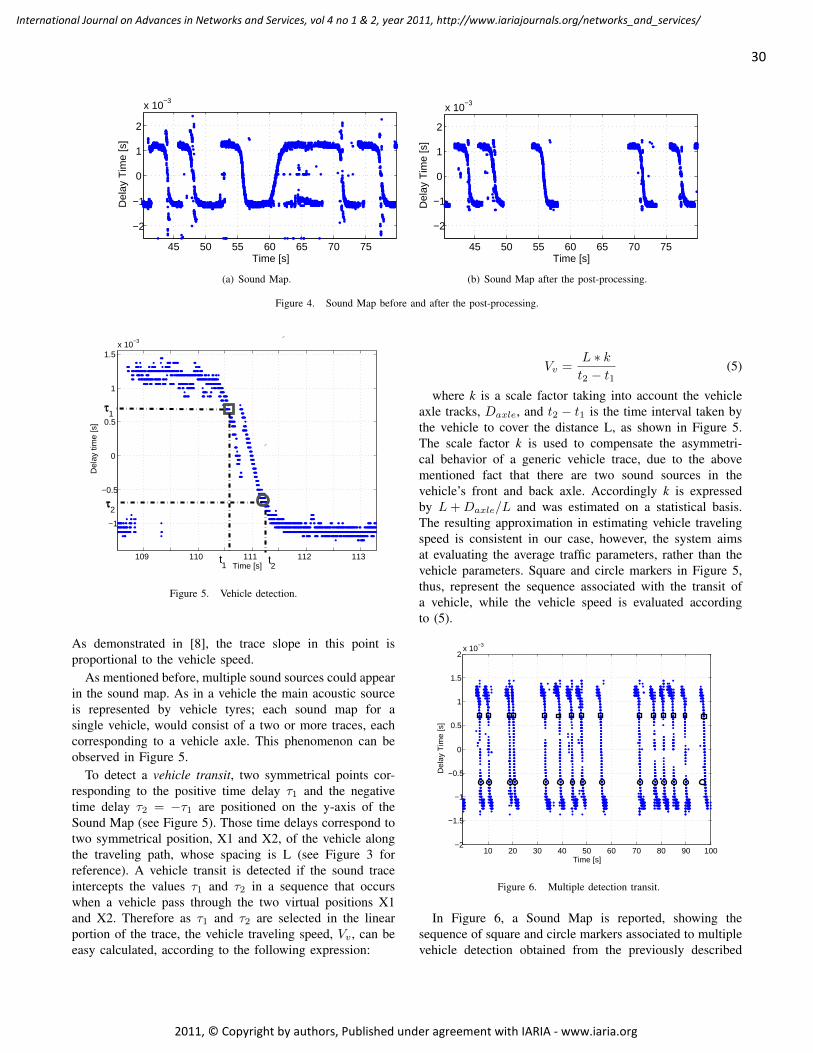
45 50 55 60 65 70 75
−2
−1
0
1
2
x 10−3
Time [s]
Del
ay T
ime
[s]
(a) Sound Map.
45 50 55 60 65 70 75
−2
−1
0
1
2
x 10−3
Time [s]
Del
ay T
ime
[s]
(b) Sound Map after the post-processing.
Figure 4. Sound Map before and after the post-processing.
109 110 111 112 113
−1
−0.5
0
0.5
1
1.5x 10⁻³
Time [s]
Del
ay ti
me
[s]
τ1
τ2
t1 t
2
Figure 5. Vehicle detection.
As demonstrated in [8], the trace slope in this point isproportional to the vehicle speed.
As mentioned before, multiple sound sources could appearin the sound map. As in a vehicle the main acoustic sourceis represented by vehicle tyres; each sound map for asingle vehicle, would consist of a two or more traces, eachcorresponding to a vehicle axle. This phenomenon can beobserved in Figure 5.
To detect a vehicle transit, two symmetrical points cor-responding to the positive time delay τ1 and the negativetime delay τ2 = −τ1 are positioned on the y-axis of theSound Map (see Figure 5). Those time delays correspond totwo symmetrical position, X1 and X2, of the vehicle alongthe traveling path, whose spacing is L (see Figure 3 forreference). A vehicle transit is detected if the sound traceintercepts the values τ1 and τ2 in a sequence that occurswhen a vehicle pass through the two virtual positions X1and X2. Therefore as τ1 and τ2 are selected in the linearportion of the trace, the vehicle traveling speed, Vv , can beeasy calculated, according to the following expression:
Vv =L ∗ kt2 − t1
(5)
where k is a scale factor taking into account the vehicleaxle tracks, Daxle, and t2 − t1 is the time interval taken bythe vehicle to cover the distance L, as shown in Figure 5.The scale factor k is used to compensate the asymmetri-cal behavior of a generic vehicle trace, due to the abovementioned fact that there are two sound sources in thevehicle’s front and back axle. Accordingly k is expressedby L+Daxle/L and was estimated on a statistical basis.The resulting approximation in estimating vehicle travelingspeed is consistent in our case, however, the system aimsat evaluating the average traffic parameters, rather than thevehicle parameters. Square and circle markers in Figure 5,thus, represent the sequence associated with the transit ofa vehicle, while the vehicle speed is evaluated accordingto (5).
10 20 30 40 50 60 70 80 90 100−2
−1.5
−1
−0.5
0
0.5
1
1.5
2x 10⁻³
Time [s]
Del
ay T
ime
[s]
Figure 6. Multiple detection transit.
In Figure 6, a Sound Map is reported, showing thesequence of square and circle markers associated to multiplevehicle detection obtained from the previously described
30
International Journal on Advances in Networks and Services, vol 4 no 1 & 2, year 2011, http://www.iariajournals.org/networks_and_services/
2011, © Copyright by authors, Published under agreement with IARIA - www.iaria.org
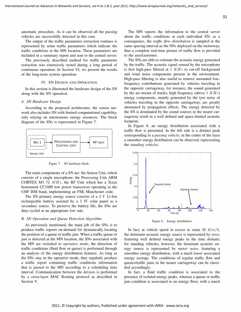
automatic procedure. As it can be observed all the passingvehicles are successfully detected in this case.
The output of the traffic parameters extraction routines isrepresented by some traffic parameters which indicate thetraffic conditions at the MN location. These parameters areincluded in a summary report and sent to the central server.
The previously described method for traffic parameterextraction was extensively tested during a long period ofcontinuous operation. In Section VI, we present the resultsof the long-term system operation.
IV. SN DESIGN AND OPERATION
In this section is illustrated the hardware design of the SNalong with the SN operation.
A. SN Hardware Design
According to the proposed architecture, the sensor net-work also includes SN with limited computational capability,only relying on autonomous energy resources. The blockdiagram of the SNs is represented in Figure 7.
MIC 1 PROCESSING AND
CONTROL UNIT
RF UNIT
Sensor Unit
Figure 7. SN hardware block.
The main components of a SN are: the Sensor Unit, whichconsists of a single microphone, the Processing Unit ARMCORTEX M3 72 MHz, the RF Unit which has a TexasInstrument CC1000 low power transceiver operating in theUHF ISM band, implementing an FSK Manchester code.
The SN primary energy source consists of a 3 V Li-Ionrechargeable battery assisted by a 5 W solar panel as asecondary source. To preserve the battery life, the SNs areduty-cycled at an appropriate low rate.
B. SN Operation and Queue Detection Algorithm
As previously mentioned, the main job of the SNs is toproduce traffic reports on-demand for dynamically locatingthe position of a queue or traffic jam. When a traffic queue orjam is detected at the MN location, the SNs associated withthe MN are switched to operative mode, the detection oftraffic conditions (fluid flow or queue) is performed throughan analysis of the energy distribution features. As long asthe SNs stay in the operative mode, they regularly producea traffic report containing traffic conditions informationthat is passed to the MN according to a scheduling timeinterval. Communication between the devices is performedby a cross-layer MAC Routing protocol as described inSection V.
The MN reports the information to the central serverabout the traffic conditions at each individual SN; as aconsequence, the traffic flow distribution is sampled at thesame spacing interval as the SNs deployed on the motorway,thus a complete real-time picture of traffic flow is providedto the user/customer.
The SNs are able to estimate the acoustic energy generatedby the traffic. The acoustic signal sensed by the microphoneis first high-pass filtered at 1 KHz to cut-off backgroundand wind noise components present in the environment.High-pass filtering is also useful to remove unwanted low-frequency contributions generated by vehicles traveling inthe opposite carriageway, for instance, the sound generatedby the air-stream of trucks; high frequency (above 1 KHz)energy components, mainly generated by the tyre noise ofvehicles traveling in the opposite carriageway, are greatlyattenuated by propagation effects. The energy detected bythe SN is dominated by the sound sources in the nearer car-riageway result in a well defined and space-limited acousticfootprint.
In Figure 8, an energy distribution associated with atraffic flow is presented. In the left side is a distinct peakcorresponding to a passing vehicle; in the center of the tracea smoother energy distribution can be observed, representingthe standing vehicles.
0 20 40 60 80 100 120 1400
0.05
0.1
0.15
0.2
0.25
Time [s]
Ene
rgy
Passing Vehicle
Standing Vehicle
Figure 8. Energy distribution.
In fact, at vehicle speed in excess to some 30 Km/h,the dominant acoustic energy source is represented by tyres,featuring well defined energy peaks in the time domain;for standing vehicles, however, the dominant acoustic en-ergy source is represented by motor noise, featuring asmoother energy distribution, with a much lower associatedenergy average. The conditions of regular traffic flow andqueues/traffic jams in the nearer carriageway can be classi-fied accordingly.
In fact, a fluid traffic condition is associated to thepresence of isolated energy peaks, whereas a queue or trafficjam condition is associated to an energy floor, with a much
31
International Journal on Advances in Networks and Services, vol 4 no 1 & 2, year 2011, http://www.iariajournals.org/networks_and_services/
2011, © Copyright by authors, Published under agreement with IARIA - www.iaria.org
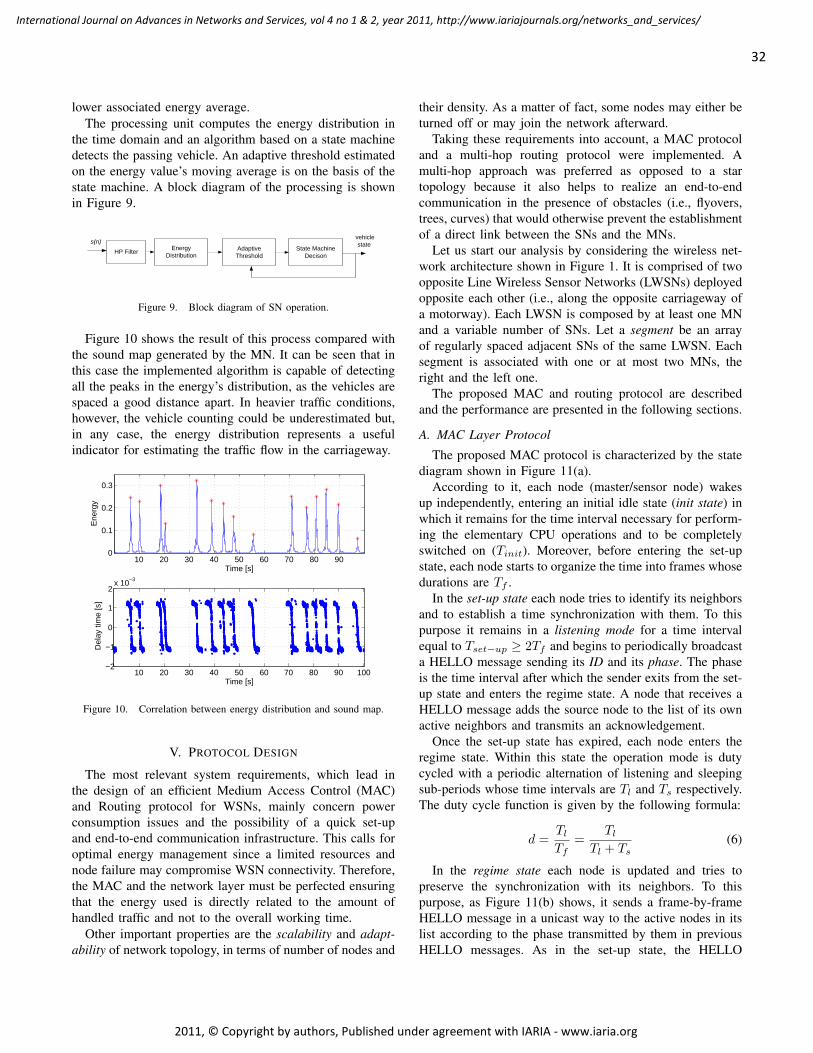
lower associated energy average.The processing unit computes the energy distribution in
the time domain and an algorithm based on a state machinedetects the passing vehicle. An adaptive threshold estimatedon the energy value’s moving average is on the basis of thestate machine. A block diagram of the processing is shownin Figure 9.
HP FilterEnergy
DistributionAdaptive
Threshold
State Machine
Decison
s(n) vehicle
state
Figure 9. Block diagram of SN operation.
Figure 10 shows the result of this process compared withthe sound map generated by the MN. It can be seen that inthis case the implemented algorithm is capable of detectingall the peaks in the energy’s distribution, as the vehicles arespaced a good distance apart. In heavier traffic conditions,however, the vehicle counting could be underestimated but,in any case, the energy distribution represents a usefulindicator for estimating the traffic flow in the carriageway.
10 20 30 40 50 60 70 80 900
0.1
0.2
0.3
Time [s]
Ene
rgy
10 20 30 40 50 60 70 80 90 100−2
−1
0
1
2x 10⁻³
Time [s]
Del
ay ti
me
[s]
Figure 10. Correlation between energy distribution and sound map.
V. PROTOCOL DESIGN
The most relevant system requirements, which lead inthe design of an efficient Medium Access Control (MAC)and Routing protocol for WSNs, mainly concern powerconsumption issues and the possibility of a quick set-upand end-to-end communication infrastructure. This calls foroptimal energy management since a limited resources andnode failure may compromise WSN connectivity. Therefore,the MAC and the network layer must be perfected ensuringthat the energy used is directly related to the amount ofhandled traffic and not to the overall working time.
Other important properties are the scalability and adapt-ability of network topology, in terms of number of nodes and
their density. As a matter of fact, some nodes may either beturned off or may join the network afterward.
Taking these requirements into account, a MAC protocoland a multi-hop routing protocol were implemented. Amulti-hop approach was preferred as opposed to a startopology because it also helps to realize an end-to-endcommunication in the presence of obstacles (i.e., flyovers,trees, curves) that would otherwise prevent the establishmentof a direct link between the SNs and the MNs.
Let us start our analysis by considering the wireless net-work architecture shown in Figure 1. It is comprised of twoopposite Line Wireless Sensor Networks (LWSNs) deployedopposite each other (i.e., along the opposite carriageway ofa motorway). Each LWSN is composed by at least one MNand a variable number of SNs. Let a segment be an arrayof regularly spaced adjacent SNs of the same LWSN. Eachsegment is associated with one or at most two MNs, theright and the left one.
The proposed MAC and routing protocol are describedand the performance are presented in the following sections.
A. MAC Layer Protocol
The proposed MAC protocol is characterized by the statediagram shown in Figure 11(a).
According to it, each node (master/sensor node) wakesup independently, entering an initial idle state (init state) inwhich it remains for the time interval necessary for perform-ing the elementary CPU operations and to be completelyswitched on (Tinit). Moreover, before entering the set-upstate, each node starts to organize the time into frames whosedurations are Tf .
In the set-up state each node tries to identify its neighborsand to establish a time synchronization with them. To thispurpose it remains in a listening mode for a time intervalequal to Tset−up ≥ 2Tf and begins to periodically broadcasta HELLO message sending its ID and its phase. The phaseis the time interval after which the sender exits from the set-up state and enters the regime state. A node that receives aHELLO message adds the source node to the list of its ownactive neighbors and transmits an acknowledgement.
Once the set-up state has expired, each node enters theregime state. Within this state the operation mode is dutycycled with a periodic alternation of listening and sleepingsub-periods whose time intervals are Tl and Ts respectively.The duty cycle function is given by the following formula:
d =TlTf
=Tl
Tl + Ts(6)
In the regime state each node is updated and tries topreserve the synchronization with its neighbors. To thispurpose, as Figure 11(b) shows, it sends a frame-by-frameHELLO message in a unicast way to the active nodes in itslist according to the phase transmitted by them in previousHELLO messages. As in the set-up state, the HELLO
32
International Journal on Advances in Networks and Services, vol 4 no 1 & 2, year 2011, http://www.iariajournals.org/networks_and_services/
2011, © Copyright by authors, Published under agreement with IARIA - www.iaria.org
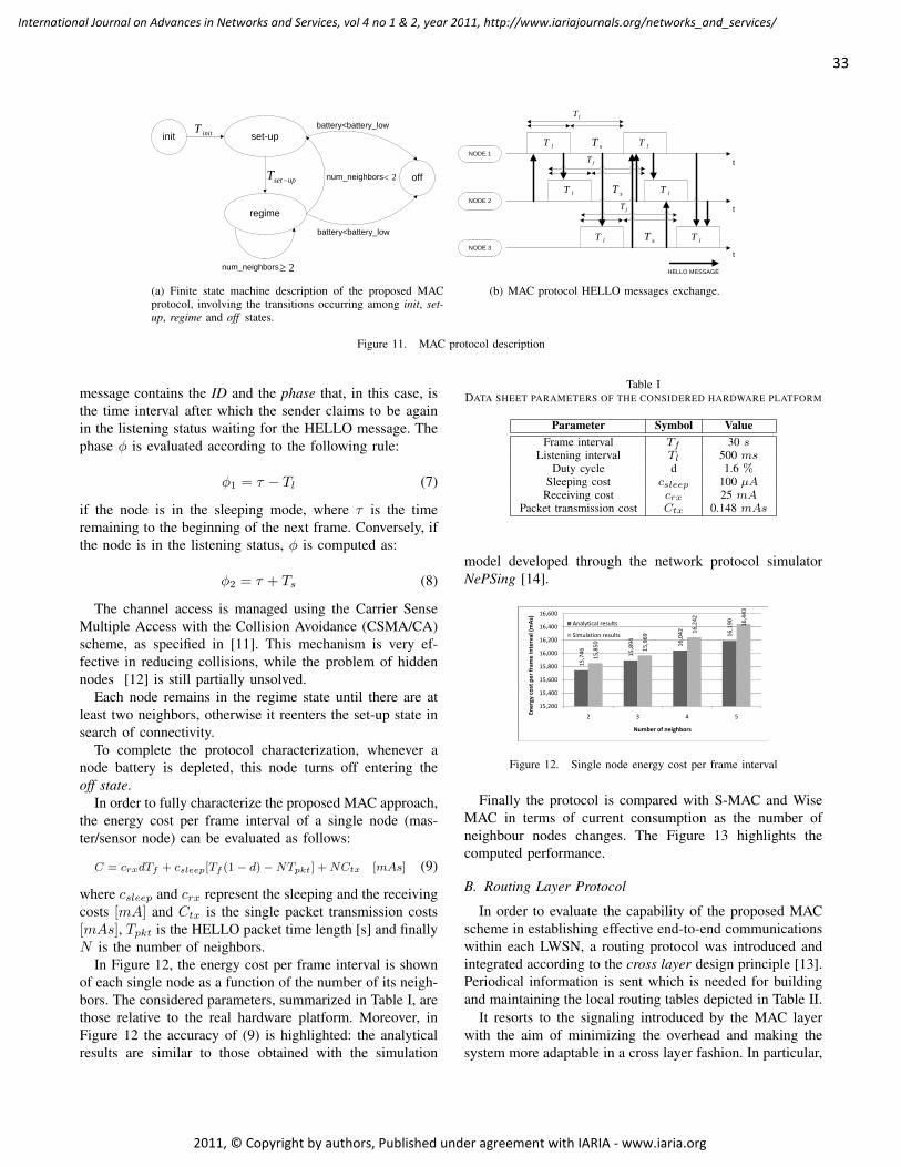
init set-up
regime
off
battery<battery_low
battery<battery_low
num_neighbors 2≥
num_neighbors 2<
initT
upsetT −
(a) Finite state machine description of the proposed MACprotocol, involving the transitions occurring among init, set-up, regime and off states.
NODE 1t
t
t
lT
lT
lT
lT
lTlT
sT
sT
sT
fT
fT
fTNODE 2
NODE 3
HELLO MESSAGE
(b) MAC protocol HELLO messages exchange.
Figure 11. MAC protocol description
message contains the ID and the phase that, in this case, isthe time interval after which the sender claims to be againin the listening status waiting for the HELLO message. Thephase φ is evaluated according to the following rule:
φ1 = τ − Tl (7)
if the node is in the sleeping mode, where τ is the timeremaining to the beginning of the next frame. Conversely, ifthe node is in the listening status, φ is computed as:
φ2 = τ + Ts (8)
The channel access is managed using the Carrier SenseMultiple Access with the Collision Avoidance (CSMA/CA)scheme, as specified in [11]. This mechanism is very ef-fective in reducing collisions, while the problem of hiddennodes [12] is still partially unsolved.
Each node remains in the regime state until there are atleast two neighbors, otherwise it reenters the set-up state insearch of connectivity.
To complete the protocol characterization, whenever anode battery is depleted, this node turns off entering theoff state.
In order to fully characterize the proposed MAC approach,the energy cost per frame interval of a single node (mas-ter/sensor node) can be evaluated as follows:
C = crxdTf + csleep[Tf (1− d)−NTpkt] +NCtx [mAs] (9)
where csleep and crx represent the sleeping and the receivingcosts [mA] and Ctx is the single packet transmission costs[mAs], Tpkt is the HELLO packet time length [s] and finallyN is the number of neighbors.
In Figure 12, the energy cost per frame interval is shownof each single node as a function of the number of its neigh-bors. The considered parameters, summarized in Table I, arethose relative to the real hardware platform. Moreover, inFigure 12 the accuracy of (9) is highlighted: the analyticalresults are similar to those obtained with the simulation
Table IDATA SHEET PARAMETERS OF THE CONSIDERED HARDWARE PLATFORM
Parameter Symbol ValueFrame interval Tf 30 s
Listening interval Tl 500 msDuty cycle d 1.6 %
Sleeping cost csleep 100 µAReceiving cost crx 25 mA
Packet transmission cost Ctx 0.148 mAs
model developed through the network protocol simulatorNePSing [14].
2 443
16,600)
4 6,04
2
16,190
969 16
,242
16,443
16 200
16,400
16,600
rval (m
As)
Analytical results
Simulation results
5,74
6
15,894 16,042 16,190
15,850
15,969
16,242
16,443
16,000
16,200
16,400
16,600
me interval (m
As)
Analytical results
Simulation results
15,746 15,894 16,042 16,190
15,850
15,969
16,242
16,443
15,600
15,800
16,000
16,200
16,400
16,600
t per fram
e interval (m
As)
Analytical results
Simulation results
15,746 15,894 16,042 16,190
15,850
15,969
16,242
16,443
15,200
15,400
15,600
15,800
16,000
16,200
16,400
16,600
nergy cost per fram
e interval (m
As)
Analytical results
Simulation results
15,746 15,894 16,042 16,190
15,850
15,969
16,242
16,443
15,200
15,400
15,600
15,800
16,000
16,200
16,400
16,600
2 3 4 5Energy cost p
er fram
e interval (m
As)
Number of neighbors
Analytical results
Simulation results
15,746 15,894 16,042 16,190
15,850
15,969
16,242
16,443
15,200
15,400
15,600
15,800
16,000
16,200
16,400
16,600
2 3 4 5Energy cost p
er fram
e interval (m
As)
Number of neighbors
Analytical results
Simulation results
15,746 15,894 16,042 16,190
15,850
15,969
16,242
16,443
15,200
15,400
15,600
15,800
16,000
16,200
16,400
16,600
2 3 4 5Energy cost p
er fram
e interval (m
As)
Number of neighbors
Analytical results
Simulation results
Figure 12. Single node energy cost per frame interval
Finally the protocol is compared with S-MAC and WiseMAC in terms of current consumption as the number ofneighbour nodes changes. The Figure 13 highlights thecomputed performance.
B. Routing Layer Protocol
In order to evaluate the capability of the proposed MACscheme in establishing effective end-to-end communicationswithin each LWSN, a routing protocol was introduced andintegrated according to the cross layer design principle [13].Periodical information is sent which is needed for buildingand maintaining the local routing tables depicted in Table II.
It resorts to the signaling introduced by the MAC layerwith the aim of minimizing the overhead and making thesystem more adaptable in a cross layer fashion. In particular,
33
International Journal on Advances in Networks and Services, vol 4 no 1 & 2, year 2011, http://www.iariajournals.org/networks_and_services/
2011, © Copyright by authors, Published under agreement with IARIA - www.iaria.org
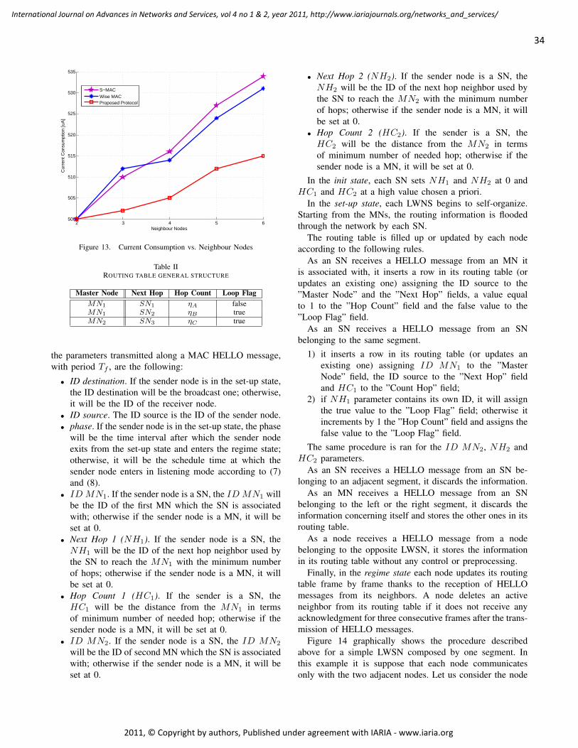
2 3 4 5 6500
505
510
515
520
525
530
535
Neighbour Nodes
Cur
rent
Con
sum
ptio
n [u
A]
S−MACWise MACProposed Protocol
Figure 13. Current Consumption vs. Neighbour Nodes
Table IIROUTING TABLE GENERAL STRUCTURE
Master Node Next Hop Hop Count Loop FlagMN1 SN1 ηA falseMN1 SN2 ηB trueMN2 SN3 ηC true
the parameters transmitted along a MAC HELLO message,with period Tf , are the following:
• ID destination. If the sender node is in the set-up state,the ID destination will be the broadcast one; otherwise,it will be the ID of the receiver node.
• ID source. The ID source is the ID of the sender node.• phase. If the sender node is in the set-up state, the phase
will be the time interval after which the sender nodeexits from the set-up state and enters the regime state;otherwise, it will be the schedule time at which thesender node enters in listening mode according to (7)and (8).
• ID MN1. If the sender node is a SN, the ID MN1 willbe the ID of the first MN which the SN is associatedwith; otherwise if the sender node is a MN, it will beset at 0.
• Next Hop 1 (NH1). If the sender node is a SN, theNH1 will be the ID of the next hop neighbor used bythe SN to reach the MN1 with the minimum numberof hops; otherwise if the sender node is a MN, it willbe set at 0.
• Hop Count 1 (HC1). If the sender is a SN, theHC1 will be the distance from the MN1 in termsof minimum number of needed hop; otherwise if thesender node is a MN, it will be set at 0.
• ID MN2. If the sender node is a SN, the ID MN2
will be the ID of second MN which the SN is associatedwith; otherwise if the sender node is a MN, it will beset at 0.
• Next Hop 2 (NH2). If the sender node is a SN, theNH2 will be the ID of the next hop neighbor used bythe SN to reach the MN2 with the minimum numberof hops; otherwise if the sender node is a MN, it willbe set at 0.
• Hop Count 2 (HC2). If the sender is a SN, theHC2 will be the distance from the MN2 in termsof minimum number of needed hop; otherwise if thesender node is a MN, it will be set at 0.
In the init state, each SN sets NH1 and NH2 at 0 andHC1 and HC2 at a high value chosen a priori.
In the set-up state, each LWNS begins to self-organize.Starting from the MNs, the routing information is floodedthrough the network by each SN.
The routing table is filled up or updated by each nodeaccording to the following rules.
As an SN receives a HELLO message from an MN itis associated with, it inserts a row in its routing table (orupdates an existing one) assigning the ID source to the”Master Node” and the ”Next Hop” fields, a value equalto 1 to the ”Hop Count” field and the false value to the”Loop Flag” field.
As an SN receives a HELLO message from an SNbelonging to the same segment.
1) it inserts a row in its routing table (or updates anexisting one) assigning ID MN1 to the ”MasterNode” field, the ID source to the ”Next Hop” fieldand HC1 to the ”Count Hop” field;
2) if NH1 parameter contains its own ID, it will assignthe true value to the ”Loop Flag” field; otherwise itincrements by 1 the ”Hop Count” field and assigns thefalse value to the ”Loop Flag” field.
The same procedure is ran for the ID MN2, NH2 andHC2 parameters.
As an SN receives a HELLO message from an SN be-longing to an adjacent segment, it discards the information.
As an MN receives a HELLO message from an SNbelonging to the left or the right segment, it discards theinformation concerning itself and stores the other ones in itsrouting table.
As a node receives a HELLO message from a nodebelonging to the opposite LWSN, it stores the informationin its routing table without any control or preprocessing.
Finally, in the regime state each node updates its routingtable frame by frame thanks to the reception of HELLOmessages from its neighbors. A node deletes an activeneighbor from its routing table if it does not receive anyacknowledgment for three consecutive frames after the trans-mission of HELLO messages.
Figure 14 graphically shows the procedure describedabove for a simple LWSN composed by one segment. Inthis example it is suppose that each node communicatesonly with the two adjacent nodes. Let us consider the node
34
International Journal on Advances in Networks and Services, vol 4 no 1 & 2, year 2011, http://www.iariajournals.org/networks_and_services/
2011, © Copyright by authors, Published under agreement with IARIA - www.iaria.org
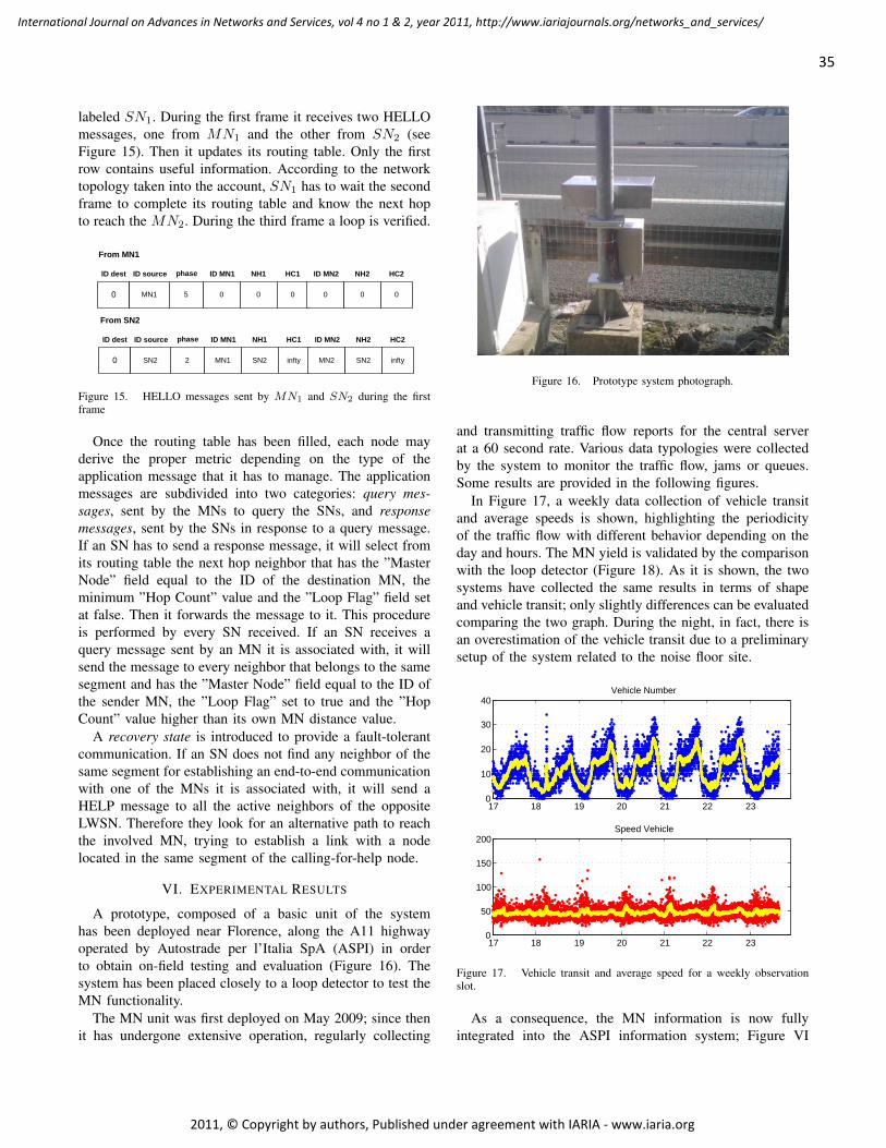
labeled SN1. During the first frame it receives two HELLOmessages, one from MN1 and the other from SN2 (seeFigure 15). Then it updates its routing table. Only the firstrow contains useful information. According to the networktopology taken into the account, SN1 has to wait the secondframe to complete its routing table and know the next hopto reach the MN2. During the third frame a loop is verified.
0 MN1
ID dest ID source phase ID MN1 NH1 HC1
5 0 0 0
ID MN2 NH2 HC2
0 0 0
From MN1
0 SN2
ID dest ID source phase ID MN1 NH1 HC1
2 MN1 SN2 infty
ID MN2 NH2 HC2
MN2 SN2 infty
From SN2
Figure 15. HELLO messages sent by MN1 and SN2 during the firstframe
Once the routing table has been filled, each node mayderive the proper metric depending on the type of theapplication message that it has to manage. The applicationmessages are subdivided into two categories: query mes-sages, sent by the MNs to query the SNs, and responsemessages, sent by the SNs in response to a query message.If an SN has to send a response message, it will select fromits routing table the next hop neighbor that has the ”MasterNode” field equal to the ID of the destination MN, theminimum ”Hop Count” value and the ”Loop Flag” field setat false. Then it forwards the message to it. This procedureis performed by every SN received. If an SN receives aquery message sent by an MN it is associated with, it willsend the message to every neighbor that belongs to the samesegment and has the ”Master Node” field equal to the ID ofthe sender MN, the ”Loop Flag” set to true and the ”HopCount” value higher than its own MN distance value.
A recovery state is introduced to provide a fault-tolerantcommunication. If an SN does not find any neighbor of thesame segment for establishing an end-to-end communicationwith one of the MNs it is associated with, it will send aHELP message to all the active neighbors of the oppositeLWSN. Therefore they look for an alternative path to reachthe involved MN, trying to establish a link with a nodelocated in the same segment of the calling-for-help node.
VI. EXPERIMENTAL RESULTS
A prototype, composed of a basic unit of the systemhas been deployed near Florence, along the A11 highwayoperated by Autostrade per l’Italia SpA (ASPI) in orderto obtain on-field testing and evaluation (Figure 16). Thesystem has been placed closely to a loop detector to test theMN functionality.
The MN unit was first deployed on May 2009; since thenit has undergone extensive operation, regularly collecting
Figure 16. Prototype system photograph.
and transmitting traffic flow reports for the central serverat a 60 second rate. Various data typologies were collectedby the system to monitor the traffic flow, jams or queues.Some results are provided in the following figures.
In Figure 17, a weekly data collection of vehicle transitand average speeds is shown, highlighting the periodicityof the traffic flow with different behavior depending on theday and hours. The MN yield is validated by the comparisonwith the loop detector (Figure 18). As it is shown, the twosystems have collected the same results in terms of shapeand vehicle transit; only slightly differences can be evaluatedcomparing the two graph. During the night, in fact, there isan overestimation of the vehicle transit due to a preliminarysetup of the system related to the noise floor site.
17 18 19 20 21 22 230
10
20
30
40Vehicle Number
17 18 19 20 21 22 230
50
100
150
200Speed Vehicle
Figure 17. Vehicle transit and average speed for a weekly observationslot.
As a consequence, the MN information is now fullyintegrated into the ASPI information system; Figure VI
35
International Journal on Advances in Networks and Services, vol 4 no 1 & 2, year 2011, http://www.iariajournals.org/networks_and_services/
2011, © Copyright by authors, Published under agreement with IARIA - www.iaria.org
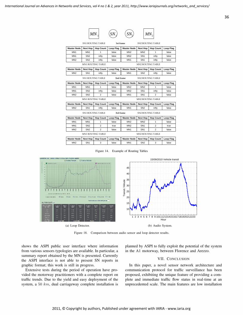
SN1 ROUTING TABLE SN2 ROUTING TABLE
Master Node Next Hop Hop Count Loop Flag
MN1 MN1 1 false
MN1 SN2 infty false
MN2 SN2 infty false
Master Node Next Hop Hop Count Loop Flag
MN2 MN2 1 false
MN2 SN1 infty false
MN1 SN1 infty false
1MN 1SN 2SN 2MN
MN1 ROUTING TABLE MN2 ROUTING TABLE
Master Node Next Hop Hop Count Loop Flag
MN2 SN1 infty false
Master Node Next Hop Hop Count Loop Flag
MN1 SN2 infty false
1st frame
SN1 ROUTING TABLE SN2 ROUTING TABLE
Master Node Next Hop Hop Count Loop Flag
MN1 MN1 1 false
MN1 SN2 infty false
MN2 SN2 2 false
Master Node Next Hop Hop Count Loop Flag
MN2 MN2 1 false
MN2 SN1 infty false
MN1 SN1 2 false
MN1 ROUTING TABLE MN2 ROUTING TABLE
Master Node Next Hop Hop Count Loop Flag
MN2 SN1 infty false
Master Node Next Hop Hop Count Loop Flag
MN1 SN2 infty false
2nd frame
SN1 ROUTING TABLE SN2 ROUTING TABLE
Master Node Next Hop Hop Count Loop Flag
MN1 MN1 1 false
MN1 SN2 2 true
MN2 SN2 2 false
Master Node Next Hop Hop Count Loop Flag
MN2 MN2 1 false
MN2 SN1 2 true
MN1 SN1 2 false
MN1 ROUTING TABLE MN2 ROUTING TABLE
Master Node Next Hop Hop Count Loop Flag
MN2 SN1 3 false
Master Node Next Hop Hop Count Loop Flag
MN1 SN2 3 false
3rd frame
Figure 14. Example of Routing Tables
(a) Loop Detector.
1 2 3 4 5 6 7 8 9 1011121314151617181920212223
10
15
20
25
30
35
40
45
15/09/2010 Vehicle transit
Hour
Tra
nsit
/ Min
ute
(b) Audio System.
Figure 18. Comparison between audio sensor and loop detector results.
shows the ASPI public user interface where informationfrom various sensors typologies are available. In particular, asummary report obtained by the MN is presented. Currentlythe ASPI interface is not able to present SN reports ingraphic format; this work is still in progress.
Extensive tests during the period of operation have pro-vided the motorway practitioners with a complete report ontraffic trends. Due to the yield and easy deployment of thesystem, a 50 km, dual carriageway complete installation is
planned by ASPI to fully exploit the potential of the systemin the A1 motorway, between Florence and Arezzo.
VII. CONCLUSION
In this paper, a novel sensor network architecture andcommunication protocol for traffic surveillance has beenproposed, exhibiting the unique feature of providing a com-plete and immediate traffic flow status in real-time at anunprecedented scale. The main features are low installation
36
International Journal on Advances in Networks and Services, vol 4 no 1 & 2, year 2011, http://www.iariajournals.org/networks_and_services/
2011, © Copyright by authors, Published under agreement with IARIA - www.iaria.org
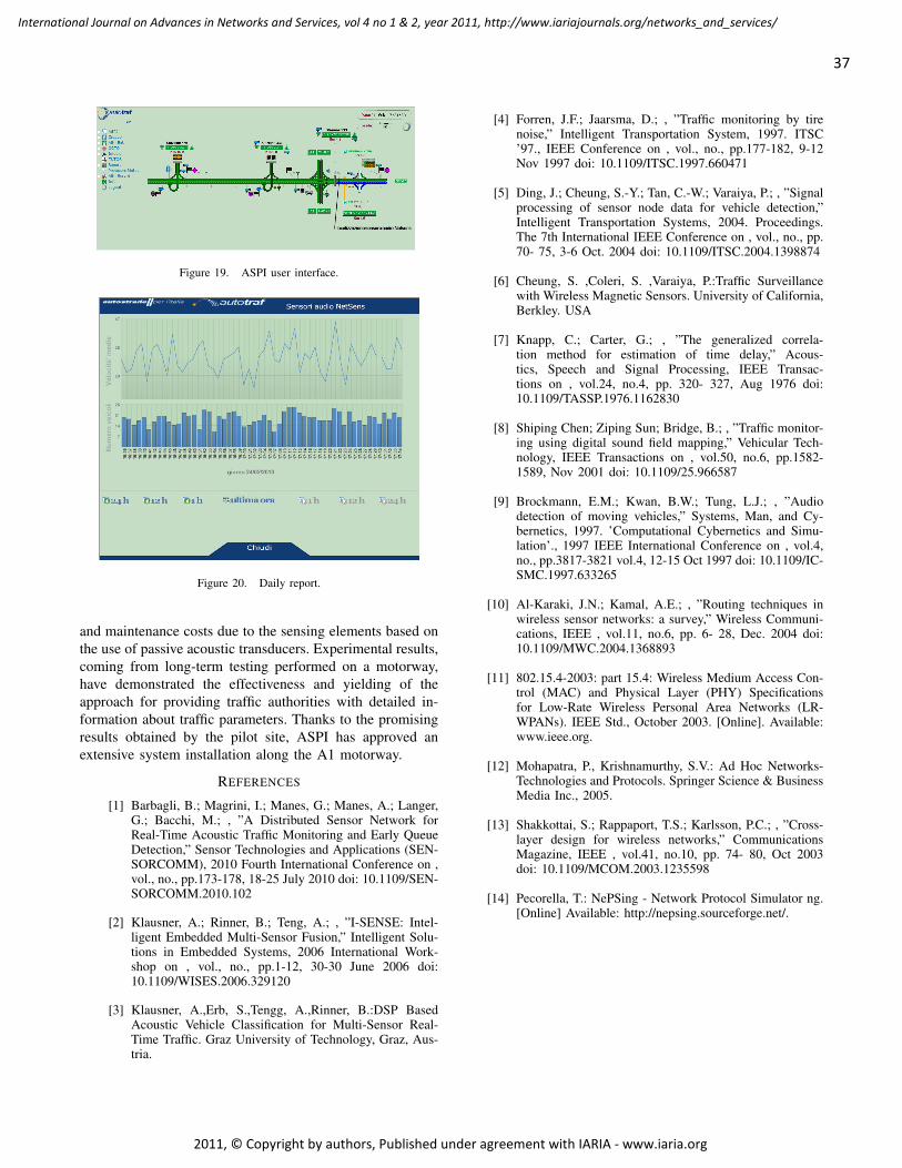
Figure 19. ASPI user interface.
Figure 20. Daily report.
and maintenance costs due to the sensing elements based onthe use of passive acoustic transducers. Experimental results,coming from long-term testing performed on a motorway,have demonstrated the effectiveness and yielding of theapproach for providing traffic authorities with detailed in-formation about traffic parameters. Thanks to the promisingresults obtained by the pilot site, ASPI has approved anextensive system installation along the A1 motorway.
REFERENCES
[1] Barbagli, B.; Magrini, I.; Manes, G.; Manes, A.; Langer,G.; Bacchi, M.; , ”A Distributed Sensor Network forReal-Time Acoustic Traffic Monitoring and Early QueueDetection,” Sensor Technologies and Applications (SEN-SORCOMM), 2010 Fourth International Conference on ,vol., no., pp.173-178, 18-25 July 2010 doi: 10.1109/SEN-SORCOMM.2010.102
[2] Klausner, A.; Rinner, B.; Teng, A.; , ”I-SENSE: Intel-ligent Embedded Multi-Sensor Fusion,” Intelligent Solu-tions in Embedded Systems, 2006 International Work-shop on , vol., no., pp.1-12, 30-30 June 2006 doi:10.1109/WISES.2006.329120
[3] Klausner, A.,Erb, S.,Tengg, A.,Rinner, B.:DSP BasedAcoustic Vehicle Classification for Multi-Sensor Real-Time Traffic. Graz University of Technology, Graz, Aus-tria.
[4] Forren, J.F.; Jaarsma, D.; , ”Traffic monitoring by tirenoise,” Intelligent Transportation System, 1997. ITSC’97., IEEE Conference on , vol., no., pp.177-182, 9-12Nov 1997 doi: 10.1109/ITSC.1997.660471
[5] Ding, J.; Cheung, S.-Y.; Tan, C.-W.; Varaiya, P.; , ”Signalprocessing of sensor node data for vehicle detection,”Intelligent Transportation Systems, 2004. Proceedings.The 7th International IEEE Conference on , vol., no., pp.70- 75, 3-6 Oct. 2004 doi: 10.1109/ITSC.2004.1398874
[6] Cheung, S. ,Coleri, S. ,Varaiya, P.:Traffic Surveillancewith Wireless Magnetic Sensors. University of California,Berkley. USA
[7] Knapp, C.; Carter, G.; , ”The generalized correla-tion method for estimation of time delay,” Acous-tics, Speech and Signal Processing, IEEE Transac-tions on , vol.24, no.4, pp. 320- 327, Aug 1976 doi:10.1109/TASSP.1976.1162830
[8] Shiping Chen; Ziping Sun; Bridge, B.; , ”Traffic monitor-ing using digital sound field mapping,” Vehicular Tech-nology, IEEE Transactions on , vol.50, no.6, pp.1582-1589, Nov 2001 doi: 10.1109/25.966587
[9] Brockmann, E.M.; Kwan, B.W.; Tung, L.J.; , ”Audiodetection of moving vehicles,” Systems, Man, and Cy-bernetics, 1997. ’Computational Cybernetics and Simu-lation’., 1997 IEEE International Conference on , vol.4,no., pp.3817-3821 vol.4, 12-15 Oct 1997 doi: 10.1109/IC-SMC.1997.633265
[10] Al-Karaki, J.N.; Kamal, A.E.; , ”Routing techniques inwireless sensor networks: a survey,” Wireless Communi-cations, IEEE , vol.11, no.6, pp. 6- 28, Dec. 2004 doi:10.1109/MWC.2004.1368893
[11] 802.15.4-2003: part 15.4: Wireless Medium Access Con-trol (MAC) and Physical Layer (PHY) Specificationsfor Low-Rate Wireless Personal Area Networks (LR-WPANs). IEEE Std., October 2003. [Online]. Available:www.ieee.org.
[12] Mohapatra, P., Krishnamurthy, S.V.: Ad Hoc Networks-Technologies and Protocols. Springer Science & BusinessMedia Inc., 2005.
[13] Shakkottai, S.; Rappaport, T.S.; Karlsson, P.C.; , ”Cross-layer design for wireless networks,” CommunicationsMagazine, IEEE , vol.41, no.10, pp. 74- 80, Oct 2003doi: 10.1109/MCOM.2003.1235598
[14] Pecorella, T.: NePSing - Network Protocol Simulator ng.[Online] Available: http://nepsing.sourceforge.net/.
37
International Journal on Advances in Networks and Services, vol 4 no 1 & 2, year 2011, http://www.iariajournals.org/networks_and_services/
2011, © Copyright by authors, Published under agreement with IARIA - www.iaria.org
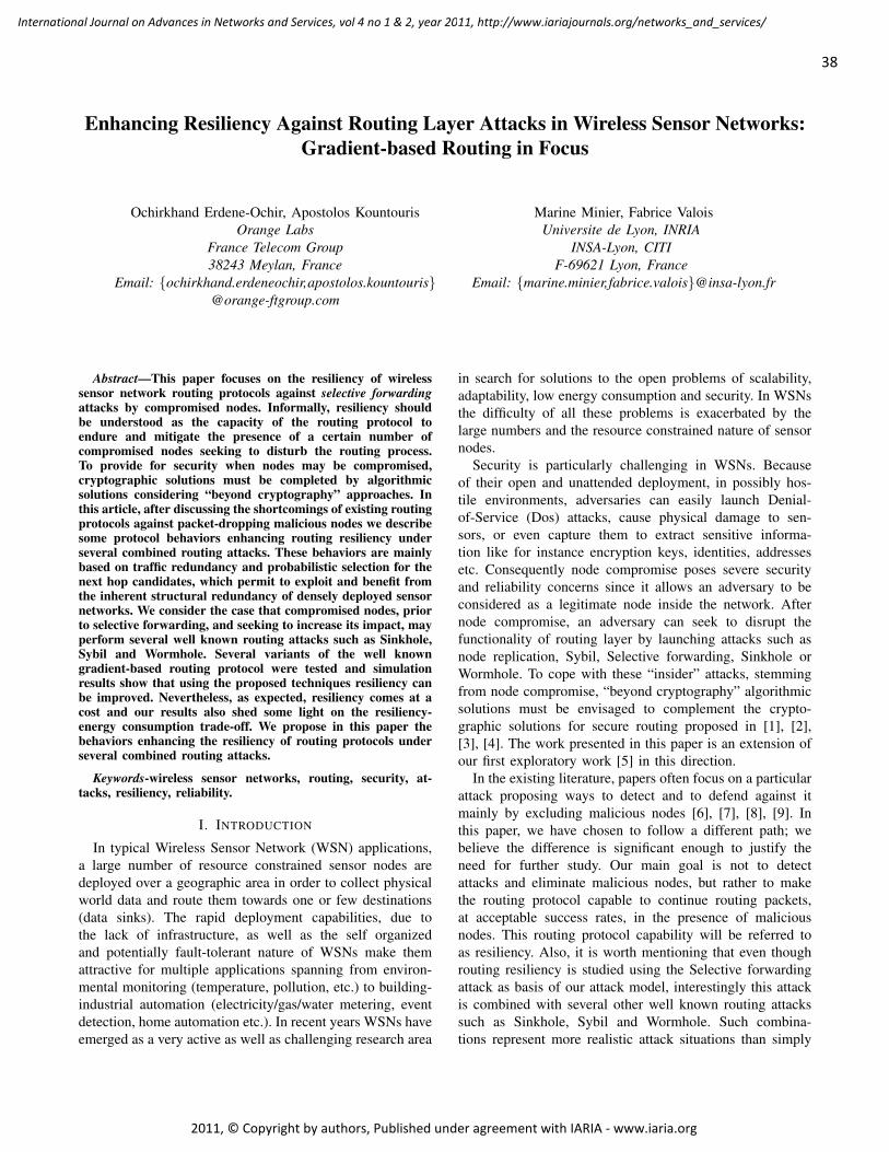
Enhancing Resiliency Against Routing Layer Attacks in Wireless Sensor Networks:Gradient-based Routing in Focus
Ochirkhand Erdene-Ochir, Apostolos KountourisOrange Labs
France Telecom Group38243 Meylan, France
Email: ochirkhand.erdeneochir,[email protected]
Marine Minier, Fabrice ValoisUniversite de Lyon, INRIA
INSA-Lyon, CITIF-69621 Lyon, France
Email: marine.minier,[email protected]
Abstract—This paper focuses on the resiliency of wirelesssensor network routing protocols against selective forwardingattacks by compromised nodes. Informally, resiliency shouldbe understood as the capacity of the routing protocol toendure and mitigate the presence of a certain number ofcompromised nodes seeking to disturb the routing process.To provide for security when nodes may be compromised,cryptographic solutions must be completed by algorithmicsolutions considering “beyond cryptography” approaches. Inthis article, after discussing the shortcomings of existing routingprotocols against packet-dropping malicious nodes we describesome protocol behaviors enhancing routing resiliency underseveral combined routing attacks. These behaviors are mainlybased on traffic redundancy and probabilistic selection for thenext hop candidates, which permit to exploit and benefit fromthe inherent structural redundancy of densely deployed sensornetworks. We consider the case that compromised nodes, priorto selective forwarding, and seeking to increase its impact, mayperform several well known routing attacks such as Sinkhole,Sybil and Wormhole. Several variants of the well knowngradient-based routing protocol were tested and simulationresults show that using the proposed techniques resiliency canbe improved. Nevertheless, as expected, resiliency comes at acost and our results also shed some light on the resiliency-energy consumption trade-off. We propose in this paper thebehaviors enhancing the resiliency of routing protocols underseveral combined routing attacks.
Keywords-wireless sensor networks, routing, security, at-tacks, resiliency, reliability.
I. INTRODUCTION
In typical Wireless Sensor Network (WSN) applications,a large number of resource constrained sensor nodes aredeployed over a geographic area in order to collect physicalworld data and route them towards one or few destinations(data sinks). The rapid deployment capabilities, due tothe lack of infrastructure, as well as the self organizedand potentially fault-tolerant nature of WSNs make themattractive for multiple applications spanning from environ-mental monitoring (temperature, pollution, etc.) to building-industrial automation (electricity/gas/water metering, eventdetection, home automation etc.). In recent years WSNs haveemerged as a very active as well as challenging research area
in search for solutions to the open problems of scalability,adaptability, low energy consumption and security. In WSNsthe difficulty of all these problems is exacerbated by thelarge numbers and the resource constrained nature of sensornodes.
Security is particularly challenging in WSNs. Becauseof their open and unattended deployment, in possibly hos-tile environments, adversaries can easily launch Denial-of-Service (Dos) attacks, cause physical damage to sen-sors, or even capture them to extract sensitive informa-tion like for instance encryption keys, identities, addressesetc. Consequently node compromise poses severe securityand reliability concerns since it allows an adversary to beconsidered as a legitimate node inside the network. Afternode compromise, an adversary can seek to disrupt thefunctionality of routing layer by launching attacks such asnode replication, Sybil, Selective forwarding, Sinkhole orWormhole. To cope with these “insider” attacks, stemmingfrom node compromise, “beyond cryptography” algorithmicsolutions must be envisaged to complement the crypto-graphic solutions for secure routing proposed in [1], [2],[3], [4]. The work presented in this paper is an extension ofour first exploratory work [5] in this direction.
In the existing literature, papers often focus on a particularattack proposing ways to detect and to defend against itmainly by excluding malicious nodes [6], [7], [8], [9]. Inthis paper, we have chosen to follow a different path; webelieve the difference is significant enough to justify theneed for further study. Our main goal is not to detectattacks and eliminate malicious nodes, but rather to makethe routing protocol capable to continue routing packets,at acceptable success rates, in the presence of maliciousnodes. This routing protocol capability will be referred toas resiliency. Also, it is worth mentioning that even thoughrouting resiliency is studied using the Selective forwardingattack as basis of our attack model, interestingly this attackis combined with several other well known routing attackssuch as Sinkhole, Sybil and Wormhole. Such combina-tions represent more realistic attack situations than simply
38
International Journal on Advances in Networks and Services, vol 4 no 1 & 2, year 2011, http://www.iariajournals.org/networks_and_services/
2011, © Copyright by authors, Published under agreement with IARIA - www.iaria.org
considering each attack separately. Finally, since we dealwith “insider” attacks, malicious compromised nodes haveaccess to the same information as honest nodes in agreementwith Shannon’s maxim: “The enemy knows the system”.Therefore, malicious nodes, aware of defensive strategiesagainst attacks, are expected to adapt their own strategies tooptimize the impact of their attacks. From this standpoint ourgoal is also to dissuade an adversary from creating adaptedattack strategies and just settle for basic (random) Selectiveforwarding.
It should be noted that we believe that if an attackerhas decided to break down the network he will succeedby assuming the necessary cost. The required investmentdepends on cost-benefit analysis considerations quantifyingthe adversary’s interest in breaking down the network. Undersuch a worst case scenario protocol resilience will not beeffective. However, this is also the case of other approaches,like for instance detecting and isolating malicious nodes.Even if a source node is capable of detecting and isolatingmalicious neighbors, the packet will not reach the sink ifmost of its neighbors are compromised. We also show in oursimulation results that under Sinkhole attacks where most ofthe compromised nodes are located around the sink, the sinkbecomes almost completely disconnected from the rest of thenetwork which in practice is equivalent to the sink beingcompromised. In what follows we assume that an adversarycan compromise only a limited number of sensor nodes,since compromising a node has some cost. In other words,mass attacks, i.e., a large number of both insider and outsiderattackers, are out of the scope of this paper. Our main goalis to render a network inherently resilient in the presence ofa few malicious nodes, we therefore require that the networkperformance degrades gracefully as the number of compro-mised nodes increases. Numerous business applications suchas periodic monitoring of electricity, gaz, water metering,and environmental monitoring, manipulate some importantbut not highly sensitive data. In these non mission criticalcases, we assume that an adversary has limited power.
The rest of the paper is organized as follows. SectionII, provides an overview of previous work insisting oninformation, which is relevant in the context of this paper;for instance, routing resiliency and its relationship to othersimilar notions such as survivability and robustness arediscussed and it is explained why classical shortest pathrouting protocols are not resilient against insider attacks.In Section III, we illustrate our adversary model includingnetwork assumptions, adversarial definitions and severalrouting attacks considered in this paper. We then propose, inSection IV, several probabilistic node selection and packetreplication strategies, which improve resiliency by makingprotocol behavior dynamic and redundant in order to exploitthe inherent structural redundancy in the topology of denselydeployed WSNs. In Section V we present our approach bymixing and applying these strategies to the well known
Gradient-based routing protocol (GBR) [10]; simulationswere performed for a basic Selective forwarding attack andfor its combination with three other routing attacks, namelySinkhole, Sybil and Wormhole attacks. Finally, Section VIconcludes this paper and outlines future work directions.
II. SCOPE AND RELATED WORK
In this paper, we focus on the Selective forwarding attackwhere compromised nodes drop data packets. This attack isnot only simple but it can be very effective as well. Whenmulti-hop packet routing is considered even a small numberof packet-dropping nodes can significantly deteriorate thepacket delivery rate of the network. Furthermore, when sev-eral routing attacks such as Sinkhole, Sybil and Wormholeare considered in combination with Selective forwarding,this enables adversary nodes to attract more traffic and soamplify the impact of malicious packet dropping.
In this Section a rather rapid overview of previous work isgiven with the purpose of introducing relevant terminology,concepts and open issues. The vastness of the literature fromone side and space limitation from the other do not permitto be more exhaustive but hopefully this brief discussionwill help the reader situate our proposal within this researchcontext.
A. Routing layer attacks and countermeasures
Attacks at the network layer were summarized in [11] asfollows: (a) spoofed, altered or replayed routing information;(b) Selective forwarding, node replication, Sybil, Sinkhole orWormhole and HELLO packets flooding. HELLO packets arespecial control packets sent by each node for neighborhooddiscovery. We are mainly interested on the attacks of thesecond type targeting the routing layer. After node com-promise an adversary can extract all sensitive informationstored in the node. Other attacks such as radio jamming,exhaustion, collisions, link layer jamming or attacks againstdata aggregation are out of the scope of this paper since theydo not directly target the network layer.
In Selective forwarding, malicious nodes simply dropsome packets (Greyhole) or all of them (Blackhole) insteadof forwarding them as they are supposed to. The mainprinciple of the Sinkhole attack is exactly the same exceptthat the compromised nodes are, or pretend to be, near thesink to attract most of the traffic. After a successful Sinkholeattack the adversary performs Selective forwarding. Onepossible solution is to use traffic monitoring to ensure thatneighbor nodes forward the messages. In [7], the authorspropose to use a Watchdog scheme that identifies selfishnodes and a Pathrater scheme that helps routing protocolsavoid such nodes. The Watchdog scheme is further extendedby a reputation based scheme, [12], where the neighborsof any single node collectively rate the node accordingto how well the node executes the functions requested
39
International Journal on Advances in Networks and Services, vol 4 no 1 & 2, year 2011, http://www.iariajournals.org/networks_and_services/
2011, © Copyright by authors, Published under agreement with IARIA - www.iaria.org
upon it. Alternatively an acknowledgment based scheme wasproposed in [6] to detect maliciously packet dropping nodes.
In the Sybil attack, [8], a malicious device illegitimatelytakes on multiple identities. Doing so the malicious nodescan fill up their neighbors’ buffers with non existing neigh-bors and thus create a false topology. Another way to exploitnode capture is the node replication/cloning attack [13],where an adversary replicates several nodes with the sameidentity at different places in the network. To defend againstthe Sybil attack, the network needs some mechanism tovalidate that a particular identity is the only identity beingheld by a given physical node. In [8] the authors describeresource tests and in [13] two distributed algorithms areproposed: randomized multicast and line-selected multicastexploiting the birthday “paradox” to defend against nodereplication.
Finally, the Wormhole attack, [9], occurs when an attackerreceives packets at one location in the network and tunnelsthem to another, via an out-of-band connection, in orderto replay them at this other location. This attack createsa totally false network topology. A Wormhole detectionmechanism, called packet leashes, is introduced in [9] andis based on distance estimation; it consists in two mecha-nisms: geographical leashes and temporal leashes. Anothertechnique to defend against Wormhole attacks consists inusing directional antennas [14].
As a conclusion it can be said that most of the proposedsolutions strive to defend against a single attack adoptinga two stage approach: first, actively detect malicious nodesand second defend against the attack by avoiding routingtraffic through the detected malicious nodes. In contrast ouraim is not to detect and defend against a single attack, aspreviously done, but rather to limit damages when severalrouting attacks are combined together. We propose to do soby enhancing the resiliency of the routing protocols.
B. Resiliency and related notions
According to Webster [15] in mechanics, resiliency is thecapability of a strained body to recover its size and shapeafter deformation caused especially by compressive stress.Hinging upon the general dictionary definition and afterreviewing the multiple definitions of resiliency and othersimilar notions in networking, we define the resiliency in[16] as the ability of a network to “continue to operate” inpresence of k compromised nodes, or in other words, the ca-pacity of a network to endure and overcome internal attacks.Simply put, resiliency is a means to achieve a “gracefuldegradation” in packet delivery rate with increasing numberof compromised nodes.
In the literature, several conceptually similar propertiessuch as survivability [17] and robustness [18], have beendiscussed but mainly focus on system failures from causesof pure statistical nature contrary to attacks where thereis some behind-the-scenes entity with malicious intention.
Furthermore, the notion of enduring and overcoming an at-tack (failure) is not explicitly considered. Finally, resiliencyas discussed in [19], [20], [21] is not applied in securerouting but in contexts like robust data aggregation, fault-tolerant routing and key distribution schemes respectively.Nevertheless it should be noted that as [19] compares theresiliency of aggregation functions, our aim is to comparethe resiliency of several versions of a given routing protocol.
C. Deterministic routing and its limitations
Insofar minimizing power consumption has been con-sidered a top priority in WSNs research. For increasedefficiency, most of the routing protocols use a shortest pathcriterion to route DATA packets the goal being to reachthe sink as quickly as possible. Reactive routing, such asDynamic Source Routing (DSR) [22], geographical routing,such as Greedy Forwarding (GF) [23] and gradient-based,such as Gradient-Based Routing (GBR) [10], all employ ashortest path principle (with some appropriate definition of“short”). Unfortunately this underlying shortest-path opti-mization philosophy is responsible for the severe limitationsof deterministic routing protocols when attacks involvingcompromised nodes are considered.
To facilitate discussion lets suppose that some insiderattacker has compromised a number of nodes, which areuniformly distributed across the network and which dropall DATA packets they receive. If l denotes the path lengthin number of hops from source to destination; pc denotesthe probability that a node is compromised and pn is theprobability that a packet is delivered (i.e., all forwardingnodes on the route are legitimate), we have pn = (1−pc)l. Inthis case, the probability to find a “safe” route exponentiallydecreases with route length; essentially the same applies forSelective forwarding attacks where only part of the traffic isdropped.
In the presence of such attacks, the routing protocols usingshortest paths have better overall delivery ratio. However,they are not resilient. First, as the routes are static all DATApackets from a source node take always the same route toreach a sink. Therefore, if at least one intermediate node iscompromised along a route, all DATA packets will be lostand the source node will be completely disconnected fromthe sink. Second, if a source node has at least one maliciousneighbor who will try to attract the traffic (best delay, bestgradient, geographically closest to the sink etc.), all DATApackets will be engulfed by such a compromised node. Thus,the routing protocol as is will not be able to overcome thissituation since the compromised node will always seem thebest routing choice to make.
In previous work, a configurable secure routing protocol(SIGF) has been proposed in [24], extending geographicalrouting (IGF) [25] with the intention of adding securityand protection against outsider attacks. It advocates for anincremental approach to security. As a basis SIGF uses
40
International Journal on Advances in Networks and Services, vol 4 no 1 & 2, year 2011, http://www.iariajournals.org/networks_and_services/
2011, © Copyright by authors, Published under agreement with IARIA - www.iaria.org
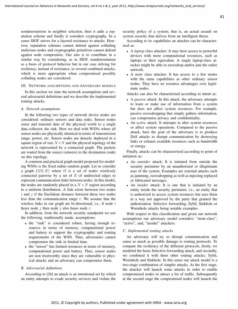
nondeterminism in neighbor selection, then it adds a rep-utation scheme and finally it considers cryptography. In asense SIGF strives for a layered resistance to attacks. How-ever, reputation schemes cannot defend against colludingmalicious nodes and cryptographic primitives cannot defendagainst node compromise. Our aim is to contribute in asimilar way by considering, as in SIGF, nondeterminismas a basis of protocol behavior but in our case striving forresiliency, instead of resistance, to several combined attacks,which is more appropriate when compromised possiblycolluding nodes are considered.
III. NETWORK ASSUMPTIONS AND ADVERSARY MODELS
In this section we state the network assumptions and sev-eral adversarial definitions and we describe the implementedrouting attacks.
A. Network assumptions
In the following two types of network device nodes areconsidered: ordinary sensors and data sinks. Sensor nodessense and transmit data of the physical world to a singledata collector, the sink. Here we deal with WSNs where allsensor nodes are physically identical in terms of transmissionrange, power, etc. Sensor nodes are densely deployed in asquare region of size N×N and the physical topology of thenetwork is represented by a connected graph. The packetsare routed from the source (sensors) to the destination (sink)on this topology.
A common and practical graph model proposed for model-ing WSNs is the fixed radius random graph. Let us considera graph G(Ω, E) where Ω is a set of nodes wirelesslyconnected pairwise by a set of E of undirected edges torepresent communication links between nodes. In this model,the nodes are randomly placed in a N×N region accordingto a uniform distribution. A link exists between two nodesi and j if the Euclidean distance between these two nodesless than the communication range r. We assume that thewireless links in our graph are bi-directional, i.e., if node ihears node j then node j also hears node i.
In addition, from the network security standpoint we usethe following, traditionally made, assumptions:
• the “sink” is considered robust, having enough re-sources in terms of memory, computational powerand battery to support the cryptographic and routingrequirements of the WSN. Thus, adversaries cannotcompromise the sink in limited time.
• the “sensor” has limited resources in terms of memory,computational power and battery. Thus, sensor nodesare non trustworthy since they are vulnerable to phys-ical attacks and an adversary can compromise them.
B. Adversarial definitions
According to [26] an attack is an intentional act by whichan entity attempts to evade security services and violate the
security policy of a system; that is, an actual assault onsystem security that derives from an intelligent threat.
According to its capabilities an attacker can be character-ized as:
• A laptop class attacker: It may have access to powerfuldevices with more computational resources, such aslaptops or their equivalent. A single laptop-class at-tacker might be able to eavesdrop and/or jam the entirenetwork.
• A mote class attacker: It has access to a few moteswith the same capabilities as other ordinary sensornodes. They have no resource advantages over legiti-mate nodes.
Attacks can also be characterized according to intent as:• A passive attack: In this attack, the adversary attempts
to learn or make use of information from a systembut does not affect system resources. For example,passive eavesdropping that simply gathers information,can compromise privacy and confidentiality.
• An active attack: It attempts to alter system resourcesor affect system operations. Compared to the passiveattack, here the goal of the adversary is to produceDoS attacks to disrupt communication by destroyinglinks or exhaust available resources such as bandwidthor energy.
Finally, attacks can be characterized according to point ofinitiation as:
• An outsider attack: It is initiated from outside thesecurity perimeter by an unauthorized or illegitimateuser of the system. Examples are external attacks suchas jamming, eavesdropping as well as injecting replayedor fabricated messages.
• An insider attack: It is one that is initiated by anentity inside the security perimeter, i.e., an entity thatis authorized to access system resources but uses themin a way not approved by the party that granted theauthorization. Selective forwarding, Sybil, Sinkhole orWormhole attacks being notable examples.
With respect to this classification and given our networkassumptions our adversary model considers: “mote-class”,“active”, and, “insider” attackers.
C. Implemented routing attacks
An adversary will try to disrupt communication andcause as much as possible damage to routing protocols. Tocompare the resiliency of the different protocols, firstly, wemodeled the basic Selective forwarding attack, and secondly,we combined it with three other routing attacks; Sybil,Wormhole and Sinkhole. In this sense our attack model is atwo-stage combination of simpler attacks. At the first stage,the attacker will launch some attacks in order to enablecompromised nodes to attract a lot of traffic. Subsequentlyat the second stage the compromised nodes will launch the
41
International Journal on Advances in Networks and Services, vol 4 no 1 & 2, year 2011, http://www.iariajournals.org/networks_and_services/
2011, © Copyright by authors, Published under agreement with IARIA - www.iaria.org
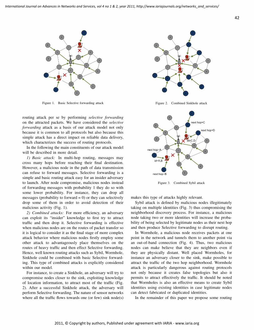
Figure 1. Basic Selective forwarding attack
routing attack per se by performing selective forwardingon the attracted packets. We have considered the selectiveforwarding attack as a basis of our attack model not onlybecause it is common to all protocols but also because thissimple attack has a direct impact on reliable data delivery,which characterizes the success of routing protocols.
In the following the main constituents of our attack modelwill be described in more detail.
1) Basic attack: In multi-hop routing, messages maycross many hops before reaching their final destination.However, a malicious node in the path of data transmissioncan refuse to forward messages. Selective forwarding is asimple and basic routing attack easy for an insider adversaryto launch. After node compromise, malicious nodes insteadof forwarding messages with probability 1 they do so withsome lower probability. For instance, they can drop allmessages (probability to forward = 0) or they can selectivelydrop some of them in order to avoid detection of theirmalicious activity (Fig. 1).
2) Combined attacks: For more efficiency, an adversarycan exploit its “insider” knowledge to first try to attracttraffic and then drop it. Selective forwarding is effectivewhen malicious nodes are on the routes of packet transfer soit is logical to consider it as the final stage of more complexattack behavior where malicious nodes firstly employ someother attack to advantageously place themselves on theroutes of heavy traffic and then effect Selective forwarding.Hence, well known routing attacks such as Sybil, Wormhole,Sinkhole could be combined with basic Selective forward-ing. This type of combined attacks is explicitly consideredwithin our model.
For instance, to create a Sinkhole, an adversary will try tocompromise nodes closer to the sink, exploiting knowledgeof location information, to attract most of the traffic (Fig.2). After a successful Sinkhole attack, the adversary willperform Selective forwarding. The nature of sensor networkswhere all the traffic flows towards one (or few) sink node(s)
Figure 2. Combined Sinkhole attack
Figure 3. Combined Sybil attack
makes this type of attacks highly relevant.Sybil attack is defined by malicious nodes illegitimately
taking on multiple identities (Fig. 3) thus compromising theneighborhood discovery process. For instance, a maliciousnode taking two or more identities will increase the proba-bility of being selected by legitimate nodes as their next hopand then produce Selective forwarding to disrupt routing.
In Wormhole, a malicious node receives packets at onepoint in the network and tunnels them to another point viaan out-of-band connection (Fig. 4). Thus, two maliciousnodes can make believe that they are neighbors even ifthey are physically distant. Well placed Wormholes, forinstance an adversary closer to the sink, make possible toattract the traffic of the two hop neighborhood. Wormholeattack is particularly dangerous against routing protocolsnot only because it creates false topologies but also itpermits to attract effectively the traffic. It should be notedthat Wormholes is also an effective means to create Sybilidentities using existing identities in case legitimate nodescan detect fabricated or duplicated identities.
In the remainder of this paper we propose some routing
42
International Journal on Advances in Networks and Services, vol 4 no 1 & 2, year 2011, http://www.iariajournals.org/networks_and_services/
2011, © Copyright by authors, Published under agreement with IARIA - www.iaria.org
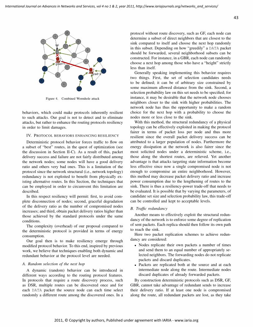
Figure 4. Combined Wormhole attack
behaviors, which could make protocols inherently resilientto such attacks. Our goal is not to detect and to eliminateattacks, but rather to enhance the routing protocols resiliencyin order to limit damages.
IV. PROTOCOL BEHAVIORS ENHANCING RESILIENCY
Deterministic protocol behavior forces traffic to flow ona subset of “best” routes, in the quest of optimization (seethe discussion in Section II-C). As a result of this, packetdelivery success and failure are not fairly distributed amongthe network nodes; some nodes will have a good deliveryratio and others very bad ones. This is a limitation of theprotocol since the network structural (i.e., network topology)redundancy is not exploited to benefit from physically ex-isting alternative routes. In this Section, the techniques thatcan be employed in order to circumvent this limitation aredescribed.
In this respect resiliency will permit: first, to avoid com-plete disconnection of nodes; second, graceful degradationof the delivery ratio as the number of compromised nodesincreases; and third, obtain packet delivery ratios higher thanthose achieved by the standard protocols under the sameconditions.
The complexity (overhead) of our proposal compared tothe deterministic protocol is provided in terms of energyconsumption.
Our goal then is to make resiliency emerge throughmodified protocol behavior. To this end, inspired by previouswork, we believe that techniques enabling both dynamic andredundant behavior at the protocol level are needed.
A. Random selection of the next hop
A dynamic (random) behavior can be introduced indifferent ways according to the routing protocol features.In protocols that require a route discovery process, suchas DSR, multiple routes can be discovered once and foreach DATA packet the source node can each time selectrandomly a different route among the discovered ones. In a
protocol without route discovery, such as GF, each node candetermine a subset of direct neighbors that are closest to thesink compared to itself and choose the next hop randomlyin this subset. Depending on how “greedily” a DATA packetshould be forwarded, several neighborhood subsets can beconstructed. For instance, in a GBR, each node can randomlychoose a next hop among those who have a “height” strictlyless than itself.
Generally speaking implementing this behavior requirestwo things. First, the set of selection candidates needsto be defined; it can be of arbitrary size constrained bysome maximum allowed distance from the sink. Second, aselection probability law on this set needs to be specified; forinstance, it may be desirable that the network node choosesneighbors closer to the sink with higher probabilities. Thenetwork node has thus the opportunity to make a randomchoice for the next hop with a probability to choose thenodes more or less close to the sink.
With this method, the structural redundancy of a physicaltopology can be effectively exploited in making the protocolfairer in terms of packet loss per node and thus moreresilient since the overall packet delivery success can beattributed to a larger population of nodes. Furthermore theenergy dissipation at the network is also fairer since themost solicited nodes under a deterministic scheme, i.e.,those along the shortest routes, are relieved. Yet anotheradvantage is that attacks targeting state information becomeless effective since now a single compromised node is notenough to compromise an entire neighborhood. However,this method may decrease packet delivery ratio and increasepower consumption due to the lengthening of routes to thesink. There is thus a resiliency-power trade-off that needs tobe evaluated. It is possible that by varying the parameters, ofcandidate set size and selection probability law, this trade-offcan be controlled and kept to acceptable levels.
B. Traffic redundancy
Another means to effectively exploit the structural redun-dancy of the network is to enforce some degree of replicationof sent packets. Each replica should then follow its own pathto reach the sink.
Here two packet replication schemes to achieve redun-dancy are considered:
• Nodes replicate their own packets a number of timesand send them to an equal number of appropriately se-lected neighbors. The forwarding nodes do not replicatepackets and discard duplicates.
• Packets are replicated both at the source and at eachintermediate node along the route. Intermediate nodesdiscard duplicates of already forwarded packets.
By construction deterministic protocols such as DSR, GF,GBR, cannot take advantage of redundant sends to increasetheir delivery ratio. If at least one node is compromisedalong the route, all redundant packets are lost, as they take
43
International Journal on Advances in Networks and Services, vol 4 no 1 & 2, year 2011, http://www.iariajournals.org/networks_and_services/
2011, © Copyright by authors, Published under agreement with IARIA - www.iaria.org
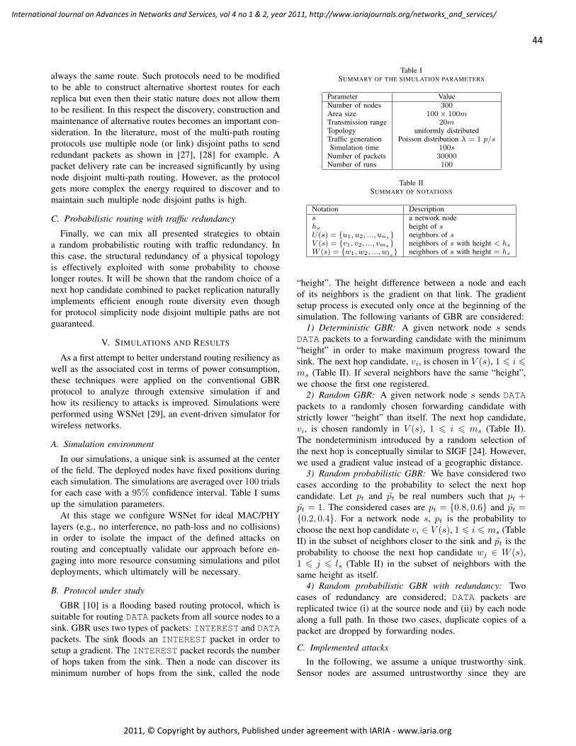
always the same route. Such protocols need to be modifiedto be able to construct alternative shortest routes for eachreplica but even then their static nature does not allow themto be resilient. In this respect the discovery, construction andmaintenance of alternative routes becomes an important con-sideration. In the literature, most of the multi-path routingprotocols use multiple node (or link) disjoint paths to sendredundant packets as shown in [27], [28] for example. Apacket delivery rate can be increased significantly by usingnode disjoint multi-path routing. However, as the protocolgets more complex the energy required to discover and tomaintain such multiple node disjoint paths is high.
C. Probabilistic routing with traffic redundancy
Finally, we can mix all presented strategies to obtaina random probabilistic routing with traffic redundancy. Inthis case, the structural redundancy of a physical topologyis effectively exploited with some probability to chooselonger routes. It will be shown that the random choice of anext hop candidate combined to packet replication naturallyimplements efficient enough route diversity even thoughfor protocol simplicity node disjoint multiple paths are notguaranteed.
V. SIMULATIONS AND RESULTS
As a first attempt to better understand routing resiliency aswell as the associated cost in terms of power consumption,these techniques were applied on the conventional GBRprotocol to analyze through extensive simulation if andhow its resiliency to attacks is improved. Simulations wereperformed using WSNet [29], an event-driven simulator forwireless networks.
A. Simulation environment
In our simulations, a unique sink is assumed at the centerof the field. The deployed nodes have fixed positions duringeach simulation. The simulations are averaged over 100 trialsfor each case with a 95% confidence interval. Table I sumsup the simulation parameters.
At this stage we configure WSNet for ideal MAC/PHYlayers (e.g., no interference, no path-loss and no collisions)in order to isolate the impact of the defined attacks onrouting and conceptually validate our approach before en-gaging into more resource consuming simulations and pilotdeployments, which ultimately will be necessary.
B. Protocol under study
GBR [10] is a flooding based routing protocol, which issuitable for routing DATA packets from all source nodes to asink. GBR uses two types of packets: INTEREST and DATApackets. The sink floods an INTEREST packet in order tosetup a gradient. The INTEREST packet records the numberof hops taken from the sink. Then a node can discover itsminimum number of hops from the sink, called the node
Table ISUMMARY OF THE SIMULATION PARAMETERS
Parameter ValueNumber of nodes 300Area size 100× 100mTransmission range 20mTopology uniformly distributedTraffic generation Poisson distribution λ = 1 p/sSimulation time 100s
Number of packets 30000Number of runs 100
Table IISUMMARY OF NOTATIONS
Notation Descriptions a network nodehs height of sU(s) = u1, u2, ..., uns neighbors of sV (s) = v1, v2, ..., vms neighbors of s with height < hs
W (s) = w1, w2, ..., wls neighbors of s with height = hs
“height”. The height difference between a node and eachof its neighbors is the gradient on that link. The gradientsetup process is executed only once at the beginning of thesimulation. The following variants of GBR are considered:
1) Deterministic GBR: A given network node s sendsDATA packets to a forwarding candidate with the minimum“height” in order to make maximum progress toward thesink. The next hop candidate, vi, is chosen in V (s), 1 6 i 6ms (Table II). If several neighbors have the same “height”,we choose the first one registered.
2) Random GBR: A given network node s sends DATApackets to a randomly chosen forwarding candidate withstrictly lower “height” than itself. The next hop candidate,vi, is chosen randomly in V (s), 1 6 i 6 ms (Table II).The nondeterminism introduced by a random selection ofthe next hop is conceptually similar to SIGF [24]. However,we used a gradient value instead of a geographic distance.
3) Random probabilistic GBR: We have considered twocases according to the probability to select the next hopcandidate. Let pt and pt be real numbers such that pt +pt = 1. The considered cases are pt = 0.8, 0.6 and pt =0.2, 0.4. For a network node s, pt is the probability tochoose the next hop candidate vi ∈ V (s), 1 6 i 6 ms (TableII) in the subset of neighbors closer to the sink and pt is theprobability to choose the next hop candidate wj ∈ W (s),1 6 j 6 ls (Table II) in the subset of neighbors with thesame height as itself.
4) Random probabilistic GBR with redundancy: Twocases of redundancy are considered; DATA packets arereplicated twice (i) at the source node and (ii) by each nodealong a full path. In those two cases, duplicate copies of apacket are dropped by forwarding nodes.
C. Implemented attacks
In the following, we assume a unique trustworthy sink.Sensor nodes are assumed untrustworthy since they are
44
International Journal on Advances in Networks and Services, vol 4 no 1 & 2, year 2011, http://www.iariajournals.org/networks_and_services/
2011, © Copyright by authors, Published under agreement with IARIA - www.iaria.org
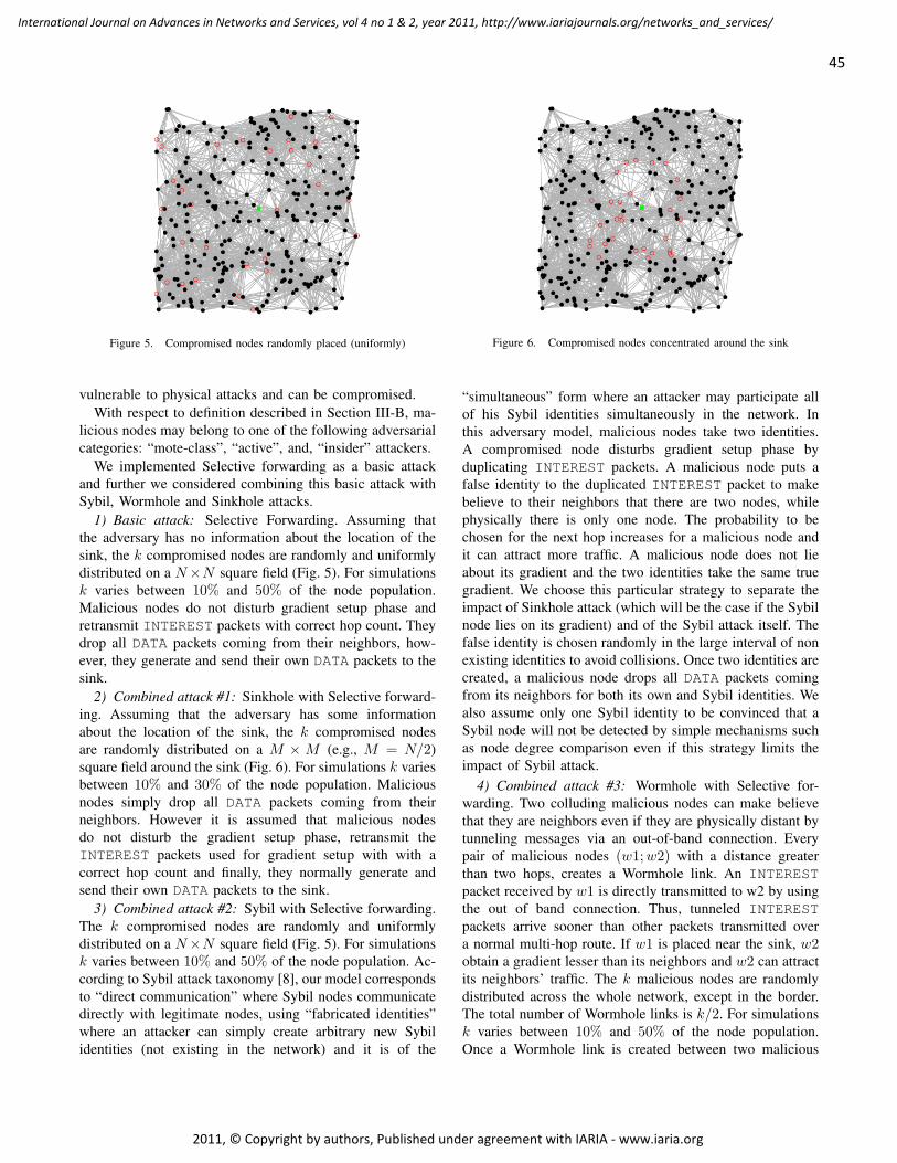
Figure 5. Compromised nodes randomly placed (uniformly)
vulnerable to physical attacks and can be compromised.With respect to definition described in Section III-B, ma-
licious nodes may belong to one of the following adversarialcategories: “mote-class”, “active”, and, “insider” attackers.
We implemented Selective forwarding as a basic attackand further we considered combining this basic attack withSybil, Wormhole and Sinkhole attacks.
1) Basic attack: Selective Forwarding. Assuming thatthe adversary has no information about the location of thesink, the k compromised nodes are randomly and uniformlydistributed on a N×N square field (Fig. 5). For simulationsk varies between 10% and 50% of the node population.Malicious nodes do not disturb gradient setup phase andretransmit INTEREST packets with correct hop count. Theydrop all DATA packets coming from their neighbors, how-ever, they generate and send their own DATA packets to thesink.
2) Combined attack #1: Sinkhole with Selective forward-ing. Assuming that the adversary has some informationabout the location of the sink, the k compromised nodesare randomly distributed on a M × M (e.g., M = N/2)square field around the sink (Fig. 6). For simulations k variesbetween 10% and 30% of the node population. Maliciousnodes simply drop all DATA packets coming from theirneighbors. However it is assumed that malicious nodesdo not disturb the gradient setup phase, retransmit theINTEREST packets used for gradient setup with with acorrect hop count and finally, they normally generate andsend their own DATA packets to the sink.
3) Combined attack #2: Sybil with Selective forwarding.The k compromised nodes are randomly and uniformlydistributed on a N×N square field (Fig. 5). For simulationsk varies between 10% and 50% of the node population. Ac-cording to Sybil attack taxonomy [8], our model correspondsto “direct communication” where Sybil nodes communicatedirectly with legitimate nodes, using “fabricated identities”where an attacker can simply create arbitrary new Sybilidentities (not existing in the network) and it is of the
Figure 6. Compromised nodes concentrated around the sink
“simultaneous” form where an attacker may participate allof his Sybil identities simultaneously in the network. Inthis adversary model, malicious nodes take two identities.A compromised node disturbs gradient setup phase byduplicating INTEREST packets. A malicious node puts afalse identity to the duplicated INTEREST packet to makebelieve to their neighbors that there are two nodes, whilephysically there is only one node. The probability to bechosen for the next hop increases for a malicious node andit can attract more traffic. A malicious node does not lieabout its gradient and the two identities take the same truegradient. We choose this particular strategy to separate theimpact of Sinkhole attack (which will be the case if the Sybilnode lies on its gradient) and of the Sybil attack itself. Thefalse identity is chosen randomly in the large interval of nonexisting identities to avoid collisions. Once two identities arecreated, a malicious node drops all DATA packets comingfrom its neighbors for both its own and Sybil identities. Wealso assume only one Sybil identity to be convinced that aSybil node will not be detected by simple mechanisms suchas node degree comparison even if this strategy limits theimpact of Sybil attack.
4) Combined attack #3: Wormhole with Selective for-warding. Two colluding malicious nodes can make believethat they are neighbors even if they are physically distant bytunneling messages via an out-of-band connection. Everypair of malicious nodes (w1; w2) with a distance greaterthan two hops, creates a Wormhole link. An INTERESTpacket received by w1 is directly transmitted to w2 by usingthe out of band connection. Thus, tunneled INTERESTpackets arrive sooner than other packets transmitted overa normal multi-hop route. If w1 is placed near the sink, w2obtain a gradient lesser than its neighbors and w2 can attractits neighbors’ traffic. The k malicious nodes are randomlydistributed across the whole network, except in the border.The total number of Wormhole links is k/2. For simulationsk varies between 10% and 50% of the node population.Once a Wormhole link is created between two malicious
45
International Journal on Advances in Networks and Services, vol 4 no 1 & 2, year 2011, http://www.iariajournals.org/networks_and_services/
2011, © Copyright by authors, Published under agreement with IARIA - www.iaria.org
nodes (w1; w2), they will drop all DATA packets comingfrom their neighbors. A given malicious node only belongsto one Wormhole link, the case of several Wormhole linkscoming from a single Wormhole node is not treated here.TheWormhole malicious nodes use legitimate traffic to performtheir activity: falsify neighborhood information and attracttraffic; collect node identities and use them as Sybil onesinstead of having to fabricate false ones.
D. Evaluation metrics
To gain insight concerning the WSN routing resiliencysome metrics are needed in order to meaningfully summarizethe information collected by simulations. A single suchmetric is currently lacking and is an object of ongoingresearch. As a provisional substitute we have used thefollowing metrics:
• Average delivery ratio (ADR):
ADR = Nr/Ns, (1)
where Nr, Ns are respectively the total number ofreceived and sent packets.
ADR is an important metric to evaluate the overall successof routing functionality, i.e., packet delivery. To refine overthe information provided by ADR, we also measured thedelivery ratio per node and we grouped the measurementsinto 5 classes.
• ADR classes:– Class c1 : nodes with ADR = 100%
all DATA packets from these nodes are received bythe sink
– Class c2 : nodes with ADR ∈ [66%; 100%[– Class c3 : nodes with ADR ∈ [33%; 66%[– Class c4 : nodes with ADR ∈]0%; 33%[– Class c5 : nodes with ADR = 0%
no DATA packet from these nodes is received bythe sink and so they are totally disconnected fromthe sink
This measure allows to determine the distribution oftransmission success in the node population and the fractureof the network connectivity. In our point of view, the higherthe number of connected source nodes (even if with a lowADR), the more the routing protocol is resilient.
• ADR per distance: The delivery ratio per node ismeasured and grouped according to the distance (innumber of hops) of nodes from the sink.
To get the distance in number of hops, we take the geo-graphical distance between the source nodes and the sink,and we divide it by the transmission range. All source nodeshave the same transmission range. The routing protocols aremore resilient if more distant nodes are able to still reachthe sink and thus successfully transmit packets.
• Average path length (APL): The number of hopscrossed by each received packet.
The end-to-end delay is not explicitly measured in thispaper since for our simulations we configure WSNet forideal MAC/PHY layers which implies no retransmis-sion and no propagation delays. However, the averagepath length (i.e., hop count) is directly proportionalto the average end-to-end delay of the network (seeFig. 11a and Fig. 10) and in this sense it provides anindication of.
• Normalized power consumption (NPC):
NPC = Te/Te (2)
where the total energy consumption (Te) is normalizedby the energy consumption of the deterministic GBRwithout attack and without packet replication sent (Te).
NPC allows to objectively compare energy expenditureunder attacks for each case (including redundancy) withouthaving to enter at this time into low level considerationsrequiring power consumption modeling. The energy modelof WSNet as detailed in the WSNet documentation (see in[30]) is linear: the sleep and idle modes of the MAC layerare not taken into account whereas the basic model considersthat the cost for one bit sent is 1 and the cost for one bitreceived is 2. The total energy is thus computed taking intoaccount the energy cost of each bit received or sent.
E. Results and analysis
The focus of our simulations is on comparing the fourversions of GBR (Deterministic, Random, Random proba-bilistic pt = 0.8 and Random probabilistic pt = 0.6) with asingle and two types of redundant DATA packets under fourimplemented attacks discussed in Section V-C, in term ofmetrics discussed in Section V-D.
An example of the functional flow diagram with trafficredundancy (double sent full path) under a basic Selectiveforwarding attacks is presented in Fig. 7.
1) Results for the basic Selective Forwarding attack:As expected the average delivery ratio (Fig. 8), the averagepath length (Fig. 11) and the total energy consumption (Fig.12) decrease with increasing number of compromised nodesunder the basic Selective forwarding attack. When a singleDATA packet is considered, Deterministic and Random GBRhave a higher delivery ratio than others (Fig. 8(a)). Thepath length is inversely proportional to the average deliveryratio. With probability pt decreasing, the average path length(Fig. 11(a)) and the total energy consumption (Fig. 12(a))increase. However, as the number of the next hop candidatesis increased, the structural redundancy of the network isbetter exploited.
As shown in Fig. 9 in Deterministic GBR only two classesappear. For any source node s either all DATA packetswill be successfully delivered (ADRs = 100%), i.e., nomalicious node is along the route, or all DATA packetswill be lost (ADRs = 0%), i.e., at least one forwardingnode is compromised along the route. In last case, a source
46
International Journal on Advances in Networks and Services, vol 4 no 1 & 2, year 2011, http://www.iariajournals.org/networks_and_services/
2011, © Copyright by authors, Published under agreement with IARIA - www.iaria.org
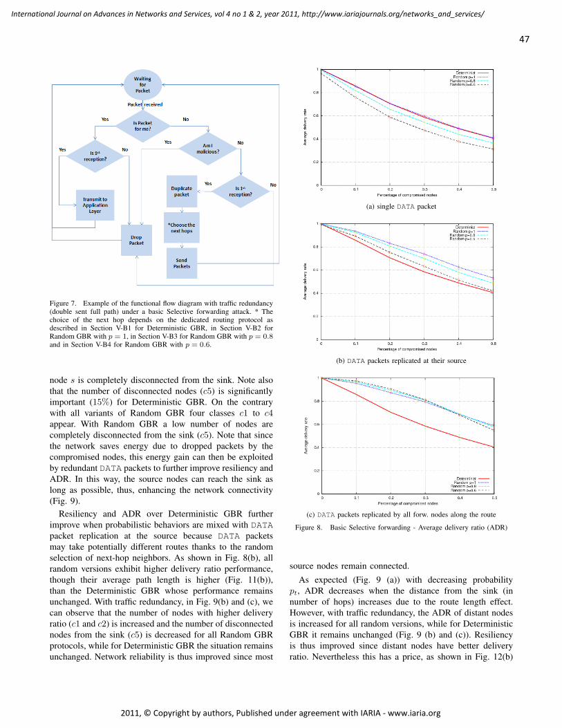
Figure 7. Example of the functional flow diagram with traffic redundancy(double sent full path) under a basic Selective forwarding attack. * Thechoice of the next hop depends on the dedicated routing protocol asdescribed in Section V-B1 for Deterministic GBR, in Section V-B2 forRandom GBR with p = 1, in Section V-B3 for Random GBR with p = 0.8and in Section V-B4 for Random GBR with p = 0.6.
node s is completely disconnected from the sink. Note alsothat the number of disconnected nodes (c5) is significantlyimportant (15%) for Deterministic GBR. On the contrarywith all variants of Random GBR four classes c1 to c4appear. With Random GBR a low number of nodes arecompletely disconnected from the sink (c5). Note that sincethe network saves energy due to dropped packets by thecompromised nodes, this energy gain can then be exploitedby redundant DATA packets to further improve resiliency andADR. In this way, the source nodes can reach the sink aslong as possible, thus, enhancing the network connectivity(Fig. 9).
Resiliency and ADR over Deterministic GBR furtherimprove when probabilistic behaviors are mixed with DATApacket replication at the source because DATA packetsmay take potentially different routes thanks to the randomselection of next-hop neighbors. As shown in Fig. 8(b), allrandom versions exhibit higher delivery ratio performance,though their average path length is higher (Fig. 11(b)),than the Deterministic GBR whose performance remainsunchanged. With traffic redundancy, in Fig. 9(b) and (c), wecan observe that the number of nodes with higher deliveryratio (c1 and c2) is increased and the number of disconnectednodes from the sink (c5) is decreased for all Random GBRprotocols, while for Deterministic GBR the situation remainsunchanged. Network reliability is thus improved since most
(a) single DATA packet
(b) DATA packets replicated at their source
(c) DATA packets replicated by all forw. nodes along the route
Figure 8. Basic Selective forwarding - Average delivery ratio (ADR)
source nodes remain connected.
As expected (Fig. 9 (a)) with decreasing probabilitypt, ADR decreases when the distance from the sink (innumber of hops) increases due to the route length effect.However, with traffic redundancy, the ADR of distant nodesis increased for all random versions, while for DeterministicGBR it remains unchanged (Fig. 9 (b) and (c)). Resiliencyis thus improved since distant nodes have better deliveryratio. Nevertheless this has a price, as shown in Fig. 12(b)
47
International Journal on Advances in Networks and Services, vol 4 no 1 & 2, year 2011, http://www.iariajournals.org/networks_and_services/
2011, © Copyright by authors, Published under agreement with IARIA - www.iaria.org
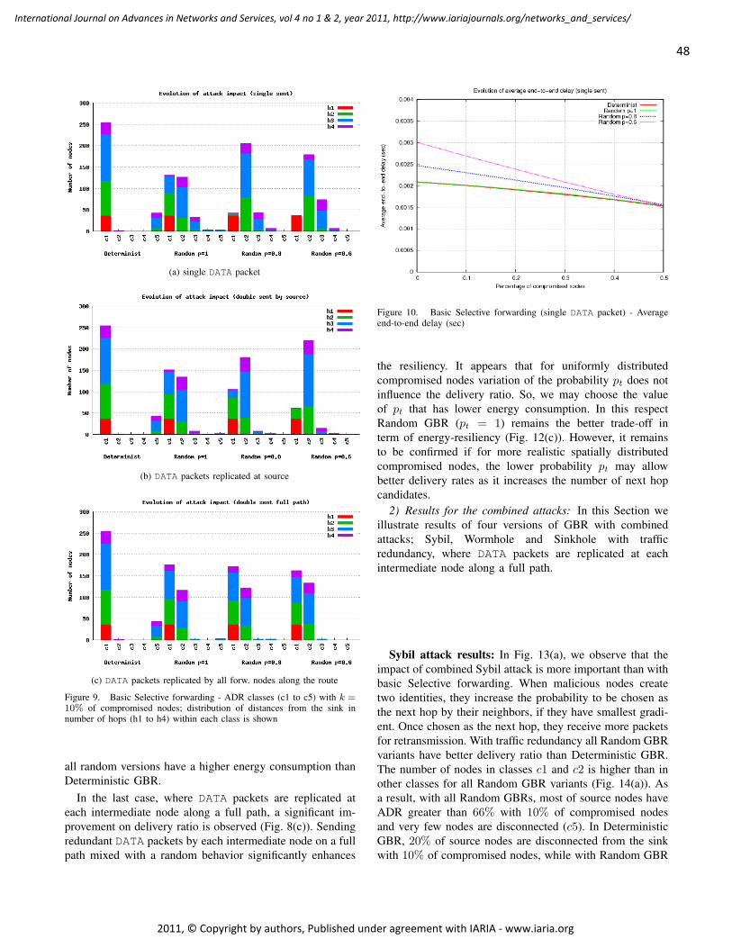
(a) single DATA packet
(b) DATA packets replicated at source
(c) DATA packets replicated by all forw. nodes along the route
Figure 9. Basic Selective forwarding - ADR classes (c1 to c5) with k =10% of compromised nodes; distribution of distances from the sink innumber of hops (h1 to h4) within each class is shown
all random versions have a higher energy consumption thanDeterministic GBR.
In the last case, where DATA packets are replicated ateach intermediate node along a full path, a significant im-provement on delivery ratio is observed (Fig. 8(c)). Sendingredundant DATA packets by each intermediate node on a fullpath mixed with a random behavior significantly enhances
Figure 10. Basic Selective forwarding (single DATA packet) - Averageend-to-end delay (sec)
the resiliency. It appears that for uniformly distributedcompromised nodes variation of the probability pt does notinfluence the delivery ratio. So, we may choose the valueof pt that has lower energy consumption. In this respectRandom GBR (pt = 1) remains the better trade-off interm of energy-resiliency (Fig. 12(c)). However, it remainsto be confirmed if for more realistic spatially distributedcompromised nodes, the lower probability pt may allowbetter delivery rates as it increases the number of next hopcandidates.
2) Results for the combined attacks: In this Section weillustrate results of four versions of GBR with combinedattacks; Sybil, Wormhole and Sinkhole with trafficredundancy, where DATA packets are replicated at eachintermediate node along a full path.
Sybil attack results: In Fig. 13(a), we observe that theimpact of combined Sybil attack is more important than withbasic Selective forwarding. When malicious nodes createtwo identities, they increase the probability to be chosen asthe next hop by their neighbors, if they have smallest gradi-ent. Once chosen as the next hop, they receive more packetsfor retransmission. With traffic redundancy all Random GBRvariants have better delivery ratio than Deterministic GBR.The number of nodes in classes c1 and c2 is higher than inother classes for all Random GBR variants (Fig. 14(a)). Asa result, with all Random GBRs, most of source nodes haveADR greater than 66% with 10% of compromised nodesand very few nodes are disconnected (c5). In DeterministicGBR, 20% of source nodes are disconnected from the sinkwith 10% of compromised nodes, while with Random GBR
48
International Journal on Advances in Networks and Services, vol 4 no 1 & 2, year 2011, http://www.iariajournals.org/networks_and_services/
2011, © Copyright by authors, Published under agreement with IARIA - www.iaria.org
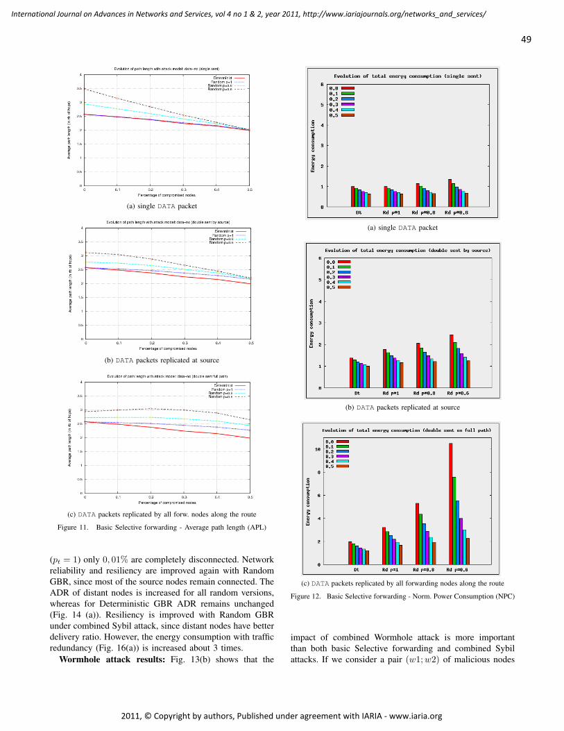
(a) single DATA packet
(b) DATA packets replicated at source
(c) DATA packets replicated by all forw. nodes along the route
Figure 11. Basic Selective forwarding - Average path length (APL)
(pt = 1) only 0, 01% are completely disconnected. Networkreliability and resiliency are improved again with RandomGBR, since most of the source nodes remain connected. TheADR of distant nodes is increased for all random versions,whereas for Deterministic GBR ADR remains unchanged(Fig. 14 (a)). Resiliency is improved with Random GBRunder combined Sybil attack, since distant nodes have betterdelivery ratio. However, the energy consumption with trafficredundancy (Fig. 16(a)) is increased about 3 times.
Wormhole attack results: Fig. 13(b) shows that the
(a) single DATA packet
(b) DATA packets replicated at source
(c) DATA packets replicated by all forwarding nodes along the route
Figure 12. Basic Selective forwarding - Norm. Power Consumption (NPC)
impact of combined Wormhole attack is more importantthan both basic Selective forwarding and combined Sybilattacks. If we consider a pair (w1; w2) of malicious nodes
49
International Journal on Advances in Networks and Services, vol 4 no 1 & 2, year 2011, http://www.iariajournals.org/networks_and_services/
2011, © Copyright by authors, Published under agreement with IARIA - www.iaria.org
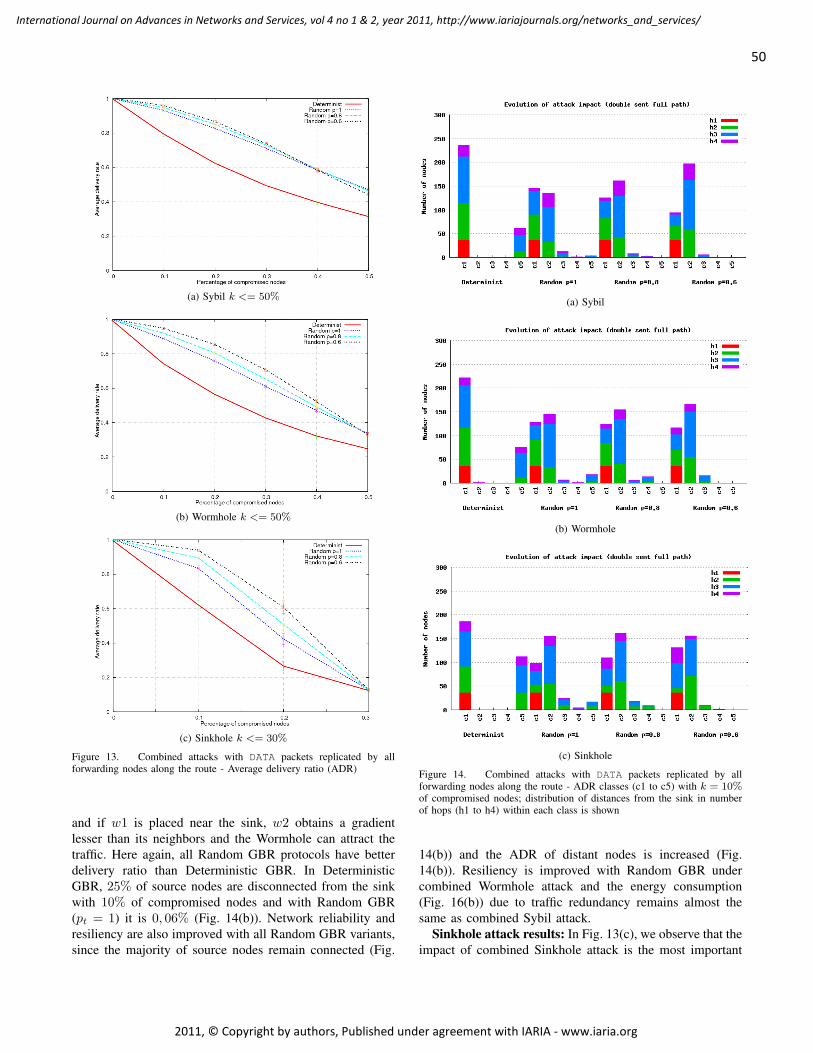
(a) Sybil k <= 50%
(b) Wormhole k <= 50%
(c) Sinkhole k <= 30%
Figure 13. Combined attacks with DATA packets replicated by allforwarding nodes along the route - Average delivery ratio (ADR)
and if w1 is placed near the sink, w2 obtains a gradientlesser than its neighbors and the Wormhole can attract thetraffic. Here again, all Random GBR protocols have betterdelivery ratio than Deterministic GBR. In DeterministicGBR, 25% of source nodes are disconnected from the sinkwith 10% of compromised nodes and with Random GBR(pt = 1) it is 0, 06% (Fig. 14(b)). Network reliability andresiliency are also improved with all Random GBR variants,since the majority of source nodes remain connected (Fig.
(a) Sybil
(b) Wormhole
(c) Sinkhole
Figure 14. Combined attacks with DATA packets replicated by allforwarding nodes along the route - ADR classes (c1 to c5) with k = 10%of compromised nodes; distribution of distances from the sink in numberof hops (h1 to h4) within each class is shown
14(b)) and the ADR of distant nodes is increased (Fig.14(b)). Resiliency is improved with Random GBR undercombined Wormhole attack and the energy consumption(Fig. 16(b)) due to traffic redundancy remains almost thesame as combined Sybil attack.
Sinkhole attack results: In Fig. 13(c), we observe that theimpact of combined Sinkhole attack is the most important
50
International Journal on Advances in Networks and Services, vol 4 no 1 & 2, year 2011, http://www.iariajournals.org/networks_and_services/
2011, © Copyright by authors, Published under agreement with IARIA - www.iaria.org
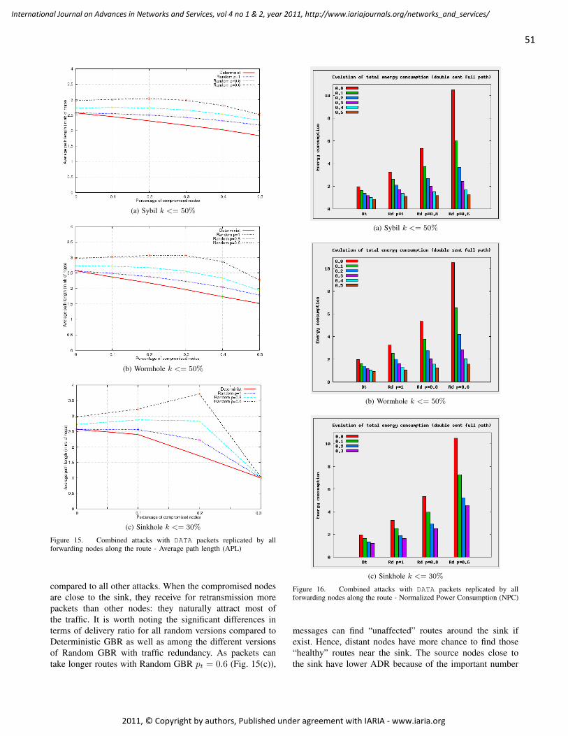
(a) Sybil k <= 50%
(b) Wormhole k <= 50%
(c) Sinkhole k <= 30%
Figure 15. Combined attacks with DATA packets replicated by allforwarding nodes along the route - Average path length (APL)
compared to all other attacks. When the compromised nodesare close to the sink, they receive for retransmission morepackets than other nodes: they naturally attract most ofthe traffic. It is worth noting the significant differences interms of delivery ratio for all random versions compared toDeterministic GBR as well as among the different versionsof Random GBR with traffic redundancy. As packets cantake longer routes with Random GBR pt = 0.6 (Fig. 15(c)),
(a) Sybil k <= 50%
(b) Wormhole k <= 50%
(c) Sinkhole k <= 30%
Figure 16. Combined attacks with DATA packets replicated by allforwarding nodes along the route - Normalized Power Consumption (NPC)
messages can find “unaffected” routes around the sink ifexist. Hence, distant nodes have more chance to find those“healthy” routes near the sink. The source nodes close tothe sink have lower ADR because of the important number
51
International Journal on Advances in Networks and Services, vol 4 no 1 & 2, year 2011, http://www.iariajournals.org/networks_and_services/
2011, © Copyright by authors, Published under agreement with IARIA - www.iaria.org
of compromised nodes in their neighborhood (Fig. 14(c)).When all nodes around the sink are compromised, the sinkreceives packets only from these malicious nodes and noDATA packets are received from the legitimate nodes. Thatis why we observe on Fig. 15(c) a path length that tends to1. Resiliency is improved with a Random GBR under thecombined Sinkhole attack and the energy consumption (Fig.16(b)) due to traffic redundancy remains almost the same aswith other attacks.
VI. CONCLUSION
In this article, we have considered the case of mote-class/active/insider attacks against WSN multi-hop routingprotocols. In this specific context of node compromisecryptography needs to be complemented by algorithmic ap-proaches. We have proposed WSN routing strategies enhanc-ing the protocol resiliency in the presence of maliciouslypacket-dropping compromised nodes. The basic Selectiveforwarding attack as well as its combination with Sinkhole,Sybil and Wormhole attacks was thoroughly investigated inthe context of the well established GBR.
We have started by analyzing the conditions required forresiliency at the routing layer. The two main findings werethat, first, the shortest-path optimization principles thoughgood for energy efficiency are not adapted at all from therouting layer security (i.e., resiliency to insider attacks)standpoint and, second, that the structural redundancy inthe network topology should be effectively exploited byemploying some form of redundant protocol behavior.
In accordance with these findings our proposal consistsin combining random next-hop selection and packet repli-cation; both are needed. A random and probabilistic choiceof the next hop candidates allows a dynamic behavior inroute selection exploiting thus the structural redundancy ofthe network. However, the packet delivery ratio may suffersince packets may take longer routes.
With increasing path length (in terms of packet hopcount), the overall delay across the network increases aswell. The overall delay is directly proportional to the averagepath length (ideal MAC/PHY layers). However, we observedthat under worst attack scenario such as Sinkhole attacks, theaverage path length of successfully delivered packets tendsto one. This can be explained by the fact that with increasingnumber of compromised nodes, the sink ends up receivingpackets only from its direct neighbors. Similarly, in the worstcase mass attack scenario (a large number of both insiderand outsider attackers), the observed overall delay across thenetwork will also decrease since most of the packets fromdistant nodes will be lost.
To counterbalance the longer route effect such dynamic(probabilistic) behavior needs to be combined with someform of packet replication. To validate our ideas we haveextensively simulated the proposed techniques by modifyingin various ways the well-known routing protocol GBR. The
results show that the resiliency of routing protocols can beeffectively enhanced.
The main merits of our proposal compared to the classicaldeterministic protocols are:
• the delivery ratio is improved; “graceful” degradationof the delivery ratio with increasing number of com-promised nodes.
• the delivery success is fairly distributed; more sourcestransmit with a high delivery ratio and distant nodeshave better delivery success.
• the connectivity is improved; more sources are remainconnected to the sink with increasing number of com-promised nodes.
• the structural redundancy of the physical topology isbetter exploited and the energy consumption is fairlydistributed; more nodes participate to the routing.
From simulations, we found that traffic redundancy isextremely energy consuming when no attack, but energyefficiency of the protocol is improved when under attack.Hinging on this observation a future work perspective isthe search of a mechanism to dynamically adapt the degreeof dynamic/redundant behavior to equalize energy cost andso keep the energy consumption-resiliency trade-off at ac-ceptable levels. It also seems that keeping the routes short(in terms of hop count) should be sought but there aresome particular cases (e.g., combined Sinkhole attack) wherelonger routes should be permitted in order to get aroundobstacles. It is worth mentioning that in our simulationstudy we have gone beyond the simple Selective forwardingattack to consider combined attacks (such as Wormhole andSelective forwarding) concluding that these attacks haveextreme impact on routing especially when Sinkhole andselected forwarding are combined together.
From our simulation analysis we conclude that an opera-tional definition resiliency, in the context of network routing,should incorporate the notions of fairness, preservation ofconnectivity and graceful degradation of delivery ratio. Thus,our ongoing research especially concerns the definition of ametric of resiliency that includes all those notions. Such ametric will be a valuable tool in analyzing protocol resilienceand will greatly simplify the process of protocol comparison.
Finally, in a near future, we also need to relax theideal MAC/PHY assumption to validate the performance ofresilient routing techniques when channel imperfections andmedium access limitations are taken into account; to this endit would be interesting to consider modeling packet loss dueto MAC/PHY limitations as a form of unintentional Selectiveforwarding.
ACKNOWLEDGMENT
Ochirkhand Erdene-Ochir is partially supported by a PhDgraduate scholarship through a CIFRE contract betweenFrance Telecom and the French Ministry of Industry.
52
International Journal on Advances in Networks and Services, vol 4 no 1 & 2, year 2011, http://www.iariajournals.org/networks_and_services/
2011, © Copyright by authors, Published under agreement with IARIA - www.iaria.org
REFERENCES
[1] P. Papadimitratos and Z. Haas, “Secure rotuing for mobile adhoc networks,” in Communication Networks and DistributedSystems Modeling and Simulation Conference, San Antonio,Texas, 2002, pp. 27–31.
[2] Y. C. Hu, A. Perrig, and D. B. Johnson, “Ariadne: a secureon-demand routing protocol for ad hoc networks,” WirelessNetworks, vol. 11, no. 1-2, pp. 21–38, January 2005.
[3] K. Sanzgiri, B.Dahill, B. N. Levine, C. Shields, and E. M.Belding-Royer, “A secure routing protocol for ad hoc net-works,” in IEEE International Conference on Network Pro-tocols. Paris, France: IEEE Computer Society, November2002, pp. 78–89.
[4] A. Perrig, R. Szewczyk, V. Wen, D. E. Culler, and J. D. Tygar,“Spins: security protocols for sensor netowrks,” in SeventhAnnual International Conference on Mobile Computing andNetworks, Rome, Italy, July 2001, pp. 189–199.
[5] O.Erdene-Ochir, M.Minier, F. Valois, and A. Kountouris, “To-ward resilient routing in wireless sensor networks: Gradient-based routing in focus,” in 4th International Conference onSensor Technologies and Applications (Sensorcomm), Venice,Italy, July 2010.
[6] B. Xiao, B. Yu, and C. Gao, “Chemas: Identify suspectnodes in selective forwarding attacks,” Journal of ParallelDistributed Computing, vol. 67, no. 11, pp. 1218–1230, June2007.
[7] S. Marti, T. J. Giuli, K. Lai, and M. Baker, “Mitigatingrouting misbehavior in mobile ad hoc networks,” in 6thannual international conference on Mobile computing andnetworking, Boston, USA, August 2000, pp. 255–265.
[8] J. Newsome, E. Shi, D. Song, and A. Perrig, “The sybil attackin sensor networks: analysis & defenses,” in Information Pro-cessing in Sensor Networks, K. Ramchandran, J. Sztipanovits,J. Hou, and T. Pappas, Eds. Berkeley, USA: ACM, April2004, pp. 259–268.
[9] Y.-C. Hu, A. Perrig, and D. B. Johnson, “Packet leashes: Adefense against wormhole attacks in wireless networks,” in22nd Annual Joint Conference of the IEEE Computer andCommunications Societies, San Fransisco, USA, April 2003,pp. 1976–1986.
[10] C. S. Mani and M. B. Srivastava, “Energy efficient routingin wireless sensor networks,” in Military CommunicationsConference Proceedings on Communications for Network-Centric Operations: Creating the Information Force, vol. 1,McLean, USA, October 2001, pp. 357–361.
[11] C. Karlof and D. Wagner, “Secure routing in wireless sensornetworks: attacks and countermeasures,” Ad Hoc Networks,vol. 1, no. 2-3, pp. 293–315, August 2003.
[12] P. Michiardi and R. Molva, “Core: a collaborative reputationmechanism to enforce node cooperation in mobile ad hocnetworks,” in Communications and Multimedia Security, ser.IFIP Conference Proceedings, B. Jerman-Blazic and T. Klobu-car, Eds., vol. 228. Portoroz, Slovenia: Kluwer, September2002, pp. 107–121.
[13] B. Parno, A. Perrig, and V. Gligor, “Distributed detectionof node replication attacks in sensor networks,” in IEEESymposium on Security and Privacy. Oakland, USA: IEEEComputer Society, May 2005, pp. 49–63.
[14] L. Hu and D. Evans, “Using directional antennas to preventwormhole attacks,” in Network and Distributed System Se-curity Symposium. San Diego, USA: The Internet Society,February 2004, pp. 1–11.
[15] “http://www.merriam-webster.com/dictionary/resilience,”July 2011.
[16] O.Erdene-Ochir, M.Minier, F.Valois, and A.Kountouris, “Re-siliency of wireless sensor networks: Definitions and analy-ses,” in IEEE International Conference on Telecommunica-tions (ICT), Doha, Qatar, April 2010.
[17] R. J. Ellison, R. C. Linger, T. Longstaff, and N. R. Mead,“Survivable network system analysis: A case study,” IEEESoftware, vol. 16, no. 4, pp. 70–77, July 1999.
[18] J. P. G. Sterbenz, R. Krishnan, R. Hain, A. Jackson, D. Levin,R. Ramanathan, and J. Zao, “Survivable mobile wirelessnetworks: issues, challenges, and research directions,” inWorkshop on Wireless Security, W. Maughan and N. Vaidya,Eds. Atlanta, USA: ACM, September 2002, pp. 31–40.
[19] D. Wagner, “Resilient aggregation in sensor networks,” inACM Workshop on Security of Ad Hoc and Sensor Networks,S. Setia and V. Swarup, Eds. Washington, USA: ACM,October 2004, pp. 78–87.
[20] D. Ganesan, R. Govindan, S. Shenker, and D. Estrin, “Highly-resilient, energy-efficient multipath routing in wireless sensornetworks,” in 2nd ACM international symposium on Mobilead hoc networking & computing. Long Beach, USA: ACM,October 2001, pp. 251–254.
[21] X. Li and D. Yang, “A quantitative survivability evaluationmodel for wireless sensor networks,” in IEEE InternationalConference on Networking, Sensing and Control, Japan,March 2006, pp. 727–732.
[22] D. B. Johnson and D. A. Maltz, “Dynamic source routing inad hoc wireless networks,” in Mobile Computing, S. US, Ed.,vol. 353, 1996, pp. 153–181.
[23] B. Karp and H. T. Kung, “Gpsr: greedy perimeter statelessrouting for wireless networks,” in Proceedings of the 6thannual international conference on Mobile computing andnetworking, Boston, USA, August 2000, pp. 243–254.
[24] A. D. Wood, L. Fang, J. A. Stankovic, and T. He, “Sigf: afamily of configurable, secure routing protocols for wirelesssensor networks,” in ACM Workshop on Security of ad hocand Sensor Networks (SASN), ACM, Ed., VA, USA, October2006, pp. 35–48.
[25] B. Blum, T. He, S. Son, and J. Stankovic, “Igf : A state-freerobust communication protocol for wireless sensor networks,”Technical report, Univ. of Virginia, Charlottesville, VA, USA,Tech. Rep. CS-2003-11, November 2003.
53
International Journal on Advances in Networks and Services, vol 4 no 1 & 2, year 2011, http://www.iariajournals.org/networks_and_services/
2011, © Copyright by authors, Published under agreement with IARIA - www.iaria.org
[26] E. D. L. Andersson and L. Zhang, “Report from the IABworkshop on Unwanted Traffic March 9-10, 2006,” RFC4948 (Informational), August 2007. [Online]. Available:http://www.ietf.org/rfc/rfc4948.txt
[27] D. Ganesan, R. Govindan, S. Shenker, and D. Estrin, “Highly-resilient, energy-efficient multipath routing in wireless sensornetworks,” Mobile Computing and Communications Review,vol. 5, no. 4, pp. 11–25, 2001.
[28] Y. M. Lu and V. W. S. Wong, “An energy-efficient multi-path routing protocol for wireless sensor networks,” Int. J.Communication Systems, vol. 20, no. 7, pp. 747–766, 2007.
[29] E. Hamida, G. Chelius, and J.-M. Gorce, “Scalable versusaccurate physical layer modeling in wireless network sim-ulations,” in 22nd Workshop on Principles of Advanced andDistributed Simulation, Roma, Italy, June 2008, pp. 127–134.
[30] “http://wsnet.gforge.inria.fr/,” July 2011.
54
International Journal on Advances in Networks and Services, vol 4 no 1 & 2, year 2011, http://www.iariajournals.org/networks_and_services/
2011, © Copyright by authors, Published under agreement with IARIA - www.iaria.org
Reliability Estimation of Mobile Agent System in MANET with Dynamic Topological and Environmental Conditions
Chandreyee Chowdhury Dept. of Computer Sc. and Engg.
Jadavpur University Kolkata, India
email: [email protected]
Sarmistha Neogy Dept. of Computer Sc. and Engg.
Jadavpur University Kolkata, India
email: [email protected]
Abstract—A mobile agent is an agent with the ability to migrate from one host to another where it can resume its execution. Mobile agents can be used in wireless and mobile network applications in order to save bandwidth and time. In this paper we consider reliability issues that need to be addressed before mobile agents can be used in a broad range of applications in Mobile Adhoc Network. We show how a Mobile Agent based System can be made more reliable despite the uncertainties introduced by underlying network environment. Adhoc network brings in new aspects to dependability because the characteristics of such network affect reliability of the services offered by the agent system. Here we propose an algorithm for estimating the task route reliability of a system of agents that is based on the conditions of the underlying network. The system consists of independent agent groups, each group corresponds to a particular application for which these are deployed. The complexity of mobile agent based system combined with the underlying dynamic topology of adhoc network drives us to estimate it using Monte Carlo simulation. Smooth Random Mobility Model is used to estimate node location at a particular time. Environmental factors like multipath propagation that affect the received signal power are also considered. The results achieved demonstrate the robustness of the proposed algorithm. This paper demonstrates a reliability estimation model for mobile agent based system in mobile adhoc network and shows that reliability is heavily dependent on the conditions of the network and on agent heterogeneity.
Keywords- Mobile Ad hoc network; Monte-Carlo; Reliability; Mobility Model; Fault-tolerance;
I. INTRODUCTION A mobile agent is a combination of software program and
data, which migrates from a site to another site to perform tasks assigned by a user according to a static or dynamic route [1]. It can be viewed as a distributed abstraction layer that provides the concepts and mechanisms for mobility and communication [2]. An agent consists of three components: the program, which implements it, the execution state of the program and the data. A mobile agent may migrate in two ways namely weak migration and strong migration [3]. Weak migration occurs when only the code of the agent migrates to its destination, a strong migration occurs when the mobile agent carries out its migrations between different hosts while conserving its data, state and code. The platform is the environment of execution. The platform makes it possible to
create mobile agents; it offers the necessary elements required by them to perform their tasks such as execution, migration towards other platforms and so on.
Typical benefits of using mobile agents include • Bandwidth conservation: sending a complex query
to the database server for processing. • Reduced latency: a lightweight server can move
closer to its clients • Load balancing: loads may move from one machine
to the other within a network etc. The route of the mobile agent can be decided by its
owner or it can decide its next hop destination on the fly. Here, we assume the underlying network to be a Mobile
Ad Hoc Network (MANET) that typically undergoes constant topology changes, which disrupt the flow of information over the existing paths. Mobile agents are nowadays used in MANETs for various purposes like service discovery [4], network discovery, automatic network reconfiguration etc.
Dependability of any computing system may be defined as the trustworthiness of the system, which allows reliance to be justifiably placed on the service it delivers [5]. It is an integrative concept that encompasses attributes like availability (readiness of usage) and reliability (continuity of correct service) [5]. In MANET, like in any other mobile distributed system, mobile nodes access information through wireless data communication at any time and everywhere (motion and location independence) [6]. Therefore, this environment itself introduces new features and aspects to dependability, affecting both availability and reliability of the services of distributed systems.
Hence the reliability of underlying network becomes a factor that may affect the performance, availability, and strategy of mobile agent systems [7] [8].
In this paper, we define a Mobile Agent-based System (MAS) to be a system consisting of a number of different groups of agents where each group accomplishes an independent task.
The connectivity between the nodes is calculated according to the two-ray model [9] for signal propagation reflecting multipath propagation effect of radio signals. The node movements are assumed to be smooth as is the case in most real life scenario. Smooth Random Mobility Model (SRMM) [10] is used for this purpose. We propose a randomized agent planning strategy where an agent selects a destination almost randomly giving preference to a list of nodes over the others and the routes are also updated
55
International Journal on Advances in Networks and Services, vol 4 no 1 & 2, year 2011, http://www.iariajournals.org/networks_and_services/
2011, © Copyright by authors, Published under agreement with IARIA - www.iaria.org
dynamically, in order to incorporate node mobility, as agents roam in the network. We estimate the reliability of such a mobile agent based system using Monte Carlo simulation technique. This technique is used to avoid the typical computational complexity that may arise.
Some contemporary work in this area is discussed in Section II. Our work in reliability estimation is presented in details in the subsequent section (III). The simulation results of our reliability model are summarized in Section IV. Finally, Section V concludes with an indication of our future endeavor in this area.
II. RELATED WORKS Reliability analysis of MAS in adhoc network is a
complicated problem for which little attention has been paid. Most of the work done in this area is related to distributed systems and distributed applications. But as pointed out in [8], features like scalability and reliability becomes critical in challenging environment with wireless networks. However, the scalability/reliability issue of MAS has been highlighted in [11], although the work does not focus on MANET. We did not see any work that considers transient environmental effects (apart from node mobility) into the reliability calculation for MANET.
A. Reliability of Distributed Systems Two reliability measures are introduced in [12],
distributed program reliability and distributed system reliability. Here graph traversal is used in designing an efficient method to evaluate the proposed measures.
In [13], a unified algorithm is proposed to efficiently generate disjoint file spanning trees by cutting different links, and the distributed program reliability and distributed system reliability are computed based on a simple and consistent union operation on the probability space of the file spanning trees.
In [14], two algorithms are proposed for estimating the reliability of a distributed computing system with imperfect nodes. One is called symbolic method (SM), is based on a symbolic approach that consists of two passes of computation, and the other algorithm, called factoring method (FM), and employs a general factoring technique on both nodes and edges.
B. Mobile Ad Hoc Network In [15], Toh et al. describes a MANET as a collection of
two or more devices equipped with wireless communications and networking capability. This definition is expanded further by explaining the method by which their networking capability is realized. Like point to point radios, ad-hoc devices can communicate directly with other devices within their range. They may also communicate with those outside their range by using intermediate nodes to relay or forward the message to the destination node. This second capability, multi-hop communications without the need for network infrastructure is what makes MANET unique.
Research on ad-hoc networks generally focuses on the modification and creation of protocols in the network and transport layer, such as Transmission Control
Protocol/Internet Protocol (TCP/IP) to accommodate the mobility of the nodes and make network performance more robust. In [16], Ye et al. proposed a deployment strategy to increase probability of a ‘reliable path’. The increase in path reliability was accomplished through strategic node placement, limiting the application to instances where node mobility be directed. In [17], a protocol is proposed to accommodate the probabilistic reliability of a MANET but it does not explicitly measure network reliability.
C. Reliability of MANET Due to the analytical complexity and computational cost
of developing a closed-form solution, simulation methods, specifically Monte Carlo (MC) simulation are often used to analyze network reliability. In [18], an approach based on MC method is used to solve network reliability problems. In this case graph evolution models are used to increase the accuracy of the resultant approximation. In [19], a MC method is designed to estimate network reliability in the presence of uncertainty about the reliability of both links and nodes.
But little has been addressed on the reliability estimation of MANETs. In [20], analytical and MC-based methods are presented to determine the two-terminal reliability for the adhoc scenario. Here the existence of links was considered in a probabilistic manner to account for the unique features of the MANET. However, there remains a gap in understanding the exact link between a probability and a specific mobility profile for a node. In [21], MC-based methods are presented to determine the two-terminal reliability for the adhoc scenario. This work is an extension of that in [21], by including directly, mobility models in order to allow mobility parameters, such as maximum velocity, to be varied and therefore analyzed directly. The methods in this paper will now allow for the determination of reliability impacts under specific mobility considerations. As an example, one may consider the different reliability estimate when the same networking radios are used to create a network on two different types of vehicles. Here node mobility is simulated using Random Waypoint mobility model [22]. But this Random Waypoint model of mobility being a very simple one often results in unrealistic conclusions.
D. Reliability of Mobile Agents Little attention has been given to the reliability analysis
of MAS. In [23], two algorithms have been proposed for estimating the task route reliability of MAS depending on the conditions of the underlying computer network. In [24], which is an extension of the previous work, a third algorithm based on random walk generation is proposed. It is used for developing a random static planning strategy for mobile agents. However, in both the works the agents are assumed to be independent and the planning strategy seemed to be static. So this work does not address the scenario where agents can change their routes dynamically. Moreover, it does not address the issue of node mobility in between agent migrations.
56
International Journal on Advances in Networks and Services, vol 4 no 1 & 2, year 2011, http://www.iariajournals.org/networks_and_services/
2011, © Copyright by authors, Published under agreement with IARIA - www.iaria.org
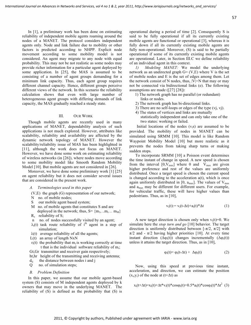
In [1], a preliminary work has been done on estimating reliability of independent mobile agents roaming around the nodes of a MANET. The protocol considers independent agents only. Node and link failure due to mobility or other factors is predicted according to NHPP. Explicit node movement according to some mobility model is not considered. An agent may migrate to any node with equal probability. This may not be not realistic as some nodes may provide richer information for a particular agent deployed by some application. In [25], the MAS is assumed to be consisting of a number of agent groups demanding for a minimum link capacity. Thus, each agent group requires different channel capacity. Hence, different groups perceive different views of the network. In this scenario the reliability calculation shows that even with large number of heterogeneous agent groups with differing demands of link capacity, the MAS gradually reached a steady state.
III. OUR WORK Though mobile agents are recently used in many
applications of MANET, dependability analysis of such applications is not much explored. However, attributes like scalability, reliability and availability are affected by the dynamic network topology of MANET. However the scalability/reliability issue of MAS has been highlighted in [11], although the work does not focus on MANET. However, we have done some work on estimating reliability of wireless networks (in [26]), where nodes move according to some mobility model like Smooth Random Mobility Model [10]. But mobile agents are not considered in [26].
Moreover, we have done some preliminary work [1] [25] on agent reliability but it does not consider several issues that are considered in the present work.
A. Terminologies used in this paper (V,E) the graph (G) representation of our network; N no. of mobile nodes; S our mobile agent based system; M no. of mobile agents that constitutes S and are deployed in the network; thus, S= m1, ..mi… mM Rs reliability of S; n no. of nodes successfully visited by an agent;
λi(t) task route reliability of ith agent in a step of simulation;
λ(t) average reliability of all the agents; L(t) an array of length NxN
ri(t) the probability that mi is working correctly at time t that is the individual software reliability of mi;
Gt,Gr transmitter and receiver gain respectively; ht,hr height of the transmitting and receiving antenna; dij the distance between nodes i and j Q no. of simulation steps;
B. Problem Definition In this paper, we assume that our mobile agent-based
system (S) consists of M independent agents deployed by k owners that may move in the underlying MANET. The reliability of (S) is defined as the probability that (S) is
operational during a period of time [2]. Consequently S is said to be fully operational if all its currently existing mobile agents are functional or operational [3], whereas it is fully down if all its currently existing mobile agents are fully non-operational. Moreover, (S) is said to be partially operational if some of its currently existing mobile agents are operational. Later, in Section III.C we define reliability of an individual agent in this context.
1) Modeling MANET: We model the underlying network as an undirected graph G= (V,E) where V is the set of mobile nodes and E is the set of edges among them. Let the network consist of N nodes, thus, |V|=N that may or may not be connected via bidirectional links (e). The following assumptions are made ([27] [28]):
1) The network graph has no parallel (or redundant) links or nodes.
2) The network graph has bi-directional links. 3) There are no self-loops or edges of the type (vj, vj). 4) The states of vertices and links are mutually
statistically independent and can only take one of the two states: working or failed.
Initial locations of the nodes (vis) are assumed to be provided. The mobility of nodes in MANET can be simulated using SRMM [10]. This model is like Random Waypoint Mobility Model [10] but more realistic as it prevents the nodes from taking sharp turns or making sudden stops.
To incorporate SRMM [10] a Poisson event determines the time instant of change in speed. A new speed is chosen from the interval [0,Vmax] where 0 and Vmax are given higher preference and rest of the values are uniformly distributed. Once a target speed is chosen the current speed is changed according to the acceleration a(t), which is once again uniformly distributed in [0, amax]. The values of Vmax and amax may be different for different users. For example, for vehicular traffic, these will have higher values than pedestrians. Thus, as in [10],
vi(t):= vi(t-Δt)+ai(t)*Δt (1)
A new target direction is chosen only when vi(t)=0. We
simulate here the stop turn and go [10] behavior. The target direction is uniformly distributed between [-π/2, π/2] with π/2 and - π/2 having higher priorities [10]. At every time instant direction (Δφi(t)) changes incrementally (Δφi(t)) unless it attains the target direction. Thus, as in [10],
φi(t)= φi(t-Δt) + Δφi(t) (2)
Now, using this speed at previous time instant,
acceleration, and direction, we can estimate the position (xi,yi) of the node at (t+Δt) as
xi(t+∆t)=xi(t)+∆t*vi(t)*cosφi(t)+0.5*ai(t)*cosφi(t)*Δt2 (3)
57
International Journal on Advances in Networks and Services, vol 4 no 1 & 2, year 2011, http://www.iariajournals.org/networks_and_services/
2011, © Copyright by authors, Published under agreement with IARIA - www.iaria.org
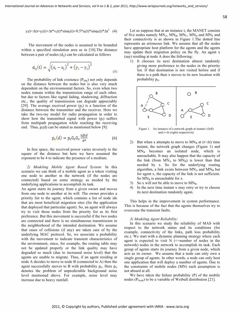
yi(t+∆t)=yi(t)+∆t*vi(t)*sinφi(t)+0.5*ai(t)*sinφi(t)*Δt2 (4)
The movement of the nodes is assumed to be bounded
within a specified simulation area as in [10].The distance between a pair of nodes (dij) can be calculated as follows
(5)
The probability of link existence (Plink) not only depends on the distance between the nodes but is also very much dependent on the environmental factors. So, even when two nodes remain within the transmission range of each other, but due to factors like signal fading, shadowing, diffraction etc., the quality of transmission can degrade appreciably [29]. The average received power (pr) is a function of the distance between the transmitter and the receiver. Here we take the two-ray model for radio propagation in order to show how the transmitted signal with power (pt) suffers from multipath propagation while reaching the receiving end. Thus, pr(d) can be stated as mentioned below [9]:
(6)
In free space, the received power varies inversely to the
square of the distance but here we have assumed the exponent to be 4 to indicate the presence of a medium.
2) Modeling Mobile Agent Based System: In this
scenario we can think of a mobile agent as a token visiting one node to another in the network (if the nodes are connected) based on some strategy as needed by the underlying applications to accomplish its task. An agent starts its journey from a given owner and moves from one node to another at its will. The owner provides a priority list to the agent, which contains a list of node ids that are most beneficial migration sites (for the application that deployed that particular agent). So, an agent will always try to visit those nodes from the priority list as its first preference. But this movement is successful if the two nodes are connected and there is no simultaneous transmission in the neighborhood of the intended destination. We assume that cases of collisions (if any) are taken care of by the underlying MAC protocol. So, we associate a probability with the movement to indicate transient characteristics of the environment, since, for example, the routing table may not be updated properly or the link quality may have degraded so much (due to increased noise level) that the agents are unable to migrate. Thus, if an agent residing at node A decides to move to node B (connected to A) then the agent successfully moves to B with probability ptr. Here ptr denotes the problem of unpredictable background noise level mentioned above. For example, noise level may increase due to heavy rainfall.
Let us suppose that at an instance t, the MANET consists of five nodes namely MNA, MNB, MNC, MND and MNE and their connectivity is as shown in Figure 1.The dotted line represents an erroneous link. We assume that all the nodes have appropriate host platform for the agents and the agents may update their migration policy on the fly. An agent x (say) residing at node A does the following:
1) It chooses its next destination almost randomly giving more preference to the nodes in the priority list. If that destination is not visited before and if there is a path then x moves to its new location with probability ptr.
2) But when x attempts to move to MNB at (t+Δt) time instant, the network graph changes (Figure 1) and MNB becomes an isolated node, which is unreachable. It may also happen that the capacity of the link (from MNA to MNB) is lower than that needed by x. So for the underlying routing algorithm, a link exists between MNA and MNB but for agent x, the capacity of the link is not sufficient. So MNB is unreachable for x.
3) So x will not be able to move to MNB. 4) In the next time instant x may retry or try to choose
its next destination randomly again. This helps in the improvement in system performance.
This is because of the fact that the agents themselves try to overcome the transient faults.
3) Modeling Agent Reliability: In this scenario we study the reliability of MAS with
respect to the network status and its conditions (for example, connectivity of the links, path loss probability etc.). We start with a dynamic planning strategy where each agent is expected to visit N (<=number of nodes in the network) nodes in the network to accomplish its task. Each group of agents starts its journey from a given node, which acts as its owner. We assume that a node can only own a single group of agents. In other words, a node can only host one application that will deploy a number of agents. Due to the constraints of mobile nodes (MN) such assumption is not absurd at all.
We have taken the failure probability (P) of the mobile nodes (PNode) to be a variable of Weibull distribution [21].
Figure 1. An instance of a network graph at instant t (left)
and t+Δt (right) respectively
58
International Journal on Advances in Networks and Services, vol 4 no 1 & 2, year 2011, http://www.iariajournals.org/networks_and_services/
2011, © Copyright by authors, Published under agreement with IARIA - www.iaria.org
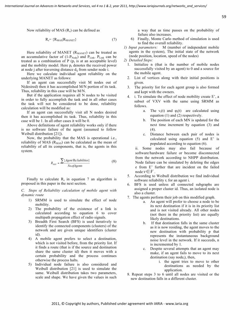
Now reliability of MAS (Rs) can be defined as
Rs= RMAS|RMANET (7)
Here reliability of MANET (RMANET) can be treated as
an accumulative factor of (1-PNode) and PLink. PLink can be treated as a combination of P (pr is at an acceptable level) and the mobility model. Here pr denotes the received power at node j after traversing distance dij from sender node i.
Here we calculate individual agent reliability on the underlying MANET as follows:
If an agent can successfully visit M nodes out of N(desired) then it has accomplished M/N portion of its task. Thus, reliability in this case will be M/N.
But if the application requires all N nodes to be visited in order to fully accomplish the task and in all other cases the task will not be considered to be done, reliability calculation will be modified as:
If an agent can successfully visit all N nodes desired then it has accomplished its task. Thus, reliability in this case will be 1. In all other cases it will be 0.
Above definitions of agent reliability works only if there is no software failure of the agent (assumed to follow Weibull distribution [21]).
Now, the probability that the MAS is operational i.e., reliability of MAS (RMAS) can be calculated as the mean of reliability of all its components, that is, the agents in this system.
(8)
Finally to calculate Rs in equation 7 an algorithm is
proposed in this paper in the next section.
C. Steps of Reliability calculation of mobile agent with dynamic route
1) SRMM is used to simulate the effect of node mobility.
2) The probability of the existence of a link is calculated according to equation 6 to cover multipath propagation effect of radio signals.
3) Breadth First Search (BFS) is used iteratively to identify the connected components (clusters) of the network and are given unique identifiers (cluster id).
4) A mobile agent prefers to select a destination, which is not visited before, from the priority list. If it finds a route (that is if the source and destination share the same cluster id) then it moves with a certain probability and the process continues otherwise the process halts.
5) Individual node failure is also considered and Weibull distribution [21] is used to simulate the same. Weibull distribution takes two parameters, scale and shape. We have given the values in such
a way that as time passes on the probability of failure also increases.
6) Finally, Monte Carlo method of simulation is used to find the overall reliability.
1) Input parameters: M (number of independent mobile agents in the system), The initial state of the network (node position, location, speed of the nodes)
2) Detailed Steps: 1. Initialize n (that is the number of mobile nodes
successfully visited by an agent) to 0 and a source for the mobile agent.
2. List of vertices along with their initial positions is given.
3. The priority list for each agent group is also formed and kept with the owners.
4. i. To simulate the effect of node mobility create E’, a subset of VXV with the same using SRMM as follows.
a. The vi(t) and φi(t) are calculated using equation (1) and (2) respectively.
b. The position of each MN is updated for the next time increment by equation (3) and (4).
c. Distance between each pair of nodes is calculated using equation (5) and E’ is populated according to equation (6).
ii. Some nodes may also fail because of software/hardware failure or become disconnected from the network according to NHPP distribution. Node failure can be simulated by deleting the edges e from E’ further that are incident on the failed node .
5. According to Weibull distribution we find individual software reliability ri for an agent i.
6. BFS is used unless all connected subgraphs are assigned a proper cluster id. Thus, an isolated node is also a cluster.
7. The agents perform their job on this modified graph. a. An agent will prefer to choose a node to be
its next destination if it is in its priority list and is not visited already. All other nodes (not there in the priority list) are equally likely destinations.
b. If that destination falls in the same cluster as it is now residing, the agent moves to the new destination with probability p that represents the instantaneous background noise level in the network. If it succeeds, n is incremented by 1.
c. Despite several attempts that an agent may make, if an agent fails to move to its next destination (say nodei), then,
i. the agent tries to move to other destinations as needed by the application.
8. Repeat steps 3 to 6 until all nodes are visited or the new destination falls in a different cluster.
59
International Journal on Advances in Networks and Services, vol 4 no 1 & 2, year 2011, http://www.iariajournals.org/networks_and_services/
2011, © Copyright by authors, Published under agreement with IARIA - www.iaria.org
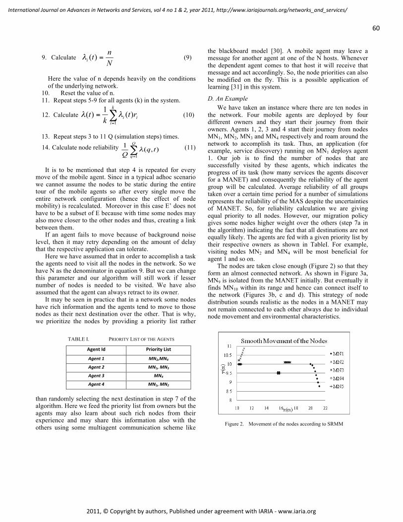
9. Calculate (9)
Here the value of n depends heavily on the conditions of the underlying network.
10. Reset the value of n. 11. Repeat steps 5-9 for all agents (k) in the system.
12. Calculate (10)
13. Repeat steps 3 to 11 Q (simulation steps) times.
14. Calculate node reliability (11)
It is to be mentioned that step 4 is repeated for every
move of the mobile agent. Since in a typical adhoc scenario we cannot assume the nodes to be static during the entire tour of the mobile agents so after every single move the entire network configuration (hence the effect of node mobility) is recalculated. Moreover in this case E’ does not have to be a subset of E because with time some nodes may also move closer to the other nodes and thus, creating a link between them.
If an agent fails to move because of background noise level, then it may retry depending on the amount of delay that the respective application can tolerate.
Here we have assumed that in order to accomplish a task the agents need to visit all the nodes in the network. So we have N as the denominator in equation 9. But we can change this parameter and our algorithm will still work if lesser number of nodes is needed to be visited. We have also assumed that the agent can always retract to its owner.
It may be seen in practice that in a network some nodes have rich information and the agents tend to move to those nodes as their next destination over the other. That is why, we prioritize the nodes by providing a priority list rather
than randomly selecting the next destination in step 7 of the algorithm. Here we feed the priority list from owners but the agents may also learn about such rich nodes from their experience and may share this information also with the others using some multiagent communication scheme like
the blackboard model [30]. A mobile agent may leave a message for another agent at one of the N hosts. Whenever the dependent agent comes to that host it will receive that message and act accordingly. So, the node priorities can also be modified on the fly. This is a possible application of learning [31] in this system.
D. An Example We have taken an instance where there are ten nodes in
the network. Four mobile agents are deployed by four different owners and they start their journey from their owners. Agents 1, 2, 3 and 4 start their journey from nodes MN1, MN2, MN3 and MN4 respectively and roam around the network to accomplish its task. Thus, an application (for example, service discovery) running on MN1 deploys agent 1. Our job is to find the number of nodes that are successfully visited by these agents, which indicates the progress of its task (how many services the agents discover for a MANET) and consequently the reliability of the agent group will be calculated. Average reliability of all groups taken over a certain time period for a number of simulations represents the reliability of the MAS despite the uncertainties of MANET. So, for reliability calculation we are giving equal priority to all nodes. However, our migration policy gives some nodes higher weight over the others (step 7a in the algorithm) indicating the fact that all destinations are not equally likely. The agents are fed with a given priority list by their respective owners as shown in TableI. For example, visiting nodes MN2 and MN4 will be most beneficial for agent 1 and so on.
The nodes are taken close enough (Figure 2) so that they form an almost connected network. As shown in Figure 3a, MN9 is isolated from the MANET initially. But eventually it finds MN10 within its range and hence can connect itself to the network (Figures 3b, c and d). This strategy of node distribution sounds realistic as the nodes in a MANET may not remain connected to each other always due to individual node movement and environmental characteristics.
Figure 2. Movement of the nodes according to SRMM
TABLE I. PRIORITY LIST OF THE AGENTS
AgentId PriorityList
Agent1 MN2,MN4
Agent2 MN1,MN3
Agent3 MN4
Agent4 MN1,MN2
60
International Journal on Advances in Networks and Services, vol 4 no 1 & 2, year 2011, http://www.iariajournals.org/networks_and_services/
2011, © Copyright by authors, Published under agreement with IARIA - www.iaria.org
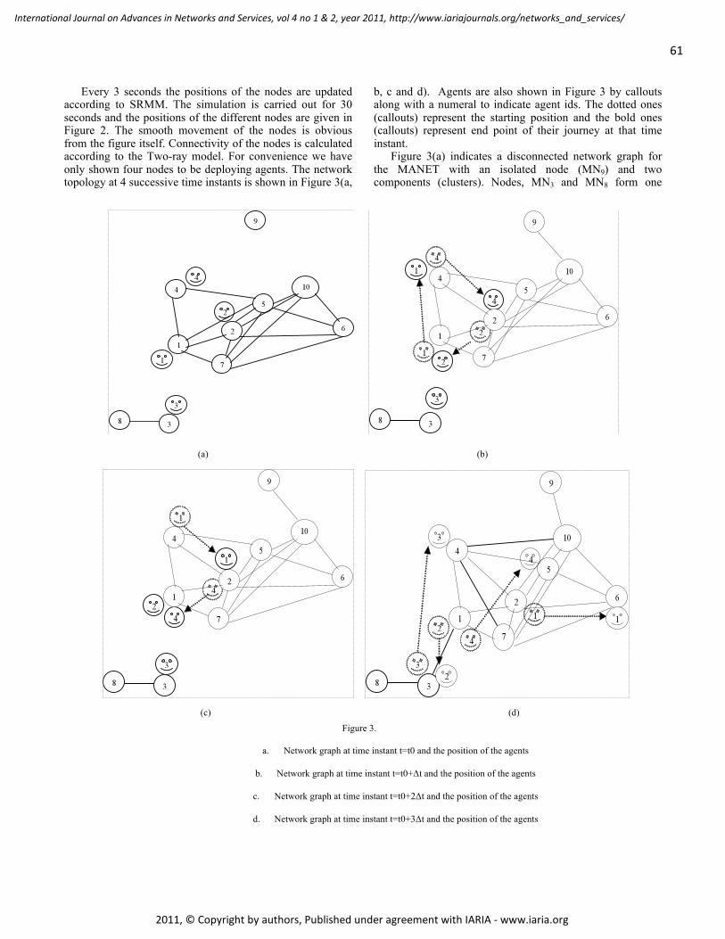
Every 3 seconds the positions of the nodes are updated according to SRMM. The simulation is carried out for 30 seconds and the positions of the different nodes are given in Figure 2. The smooth movement of the nodes is obvious from the figure itself. Connectivity of the nodes is calculated according to the Two-ray model. For convenience we have only shown four nodes to be deploying agents. The network topology at 4 successive time instants is shown in Figure 3(a,
b, c and d). Agents are also shown in Figure 3 by callouts along with a numeral to indicate agent ids. The dotted ones (callouts) represent the starting position and the bold ones (callouts) represent end point of their journey at that time instant.
Figure 3(a) indicates a disconnected network graph for the MANET with an isolated node (MN9) and two components (clusters). Nodes, MN3 and MN8 form one
(a) (b)
(c) (d)
Figure 3.
a. Network graph at time instant t=t0 and the position of the agents
b. Network graph at time instant t=t0+Δt and the position of the agents
c. Network graph at time instant t=t0+2Δt and the position of the agents
d. Network graph at time instant t=t0+3Δt and the position of the agents
e.
61
International Journal on Advances in Networks and Services, vol 4 no 1 & 2, year 2011, http://www.iariajournals.org/networks_and_services/
2011, © Copyright by authors, Published under agreement with IARIA - www.iaria.org
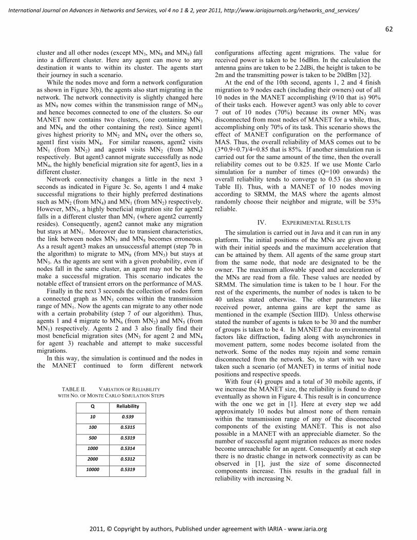
cluster and all other nodes (except MN3, MN8 and MN9) fall into a different cluster. Here any agent can move to any destination it wants to within its cluster. The agents start their journey in such a scenario.
While the nodes move and form a network configuration as shown in Figure 3(b), the agents also start migrating in the network. The network connectivity is slightly changed here as MN9 now comes within the transmission range of MN10 and hence becomes connected to one of the clusters. So our MANET now contains two clusters, (one containing MN3 and MN8 and the other containing the rest). Since agent1 gives highest priority to MN2 and MN4 over the others so, agent1 first visits MN4. For similar reasons, agent2 visits MN1 (from MN2) and agent4 visits MN2 (from MN4) respectively. But agent3 cannot migrate successfully as node MN4, the highly beneficial migration site for agent3, lies in a different cluster.
Network connectivity changes a little in the next 3 seconds as indicated in Figure 3c. So, agents 1 and 4 make successful migrations to their highly preferred destinations such as MN2 (from MN4) and MN1 (from MN2) respectively. However, MN3, a highly beneficial migration site for agent2 falls in a different cluster than MN1 (where agent2 currently resides). Consequently, agent2 cannot make any migration but stays at MN1. Moreover due to transient characteristics, the link between nodes MN3 and MN8 becomes erroneous. As a result agent3 makes an unsuccessful attempt (step 7b in the algorithm) to migrate to MN8 (from MN3) but stays at MN3. As the agents are sent with a given probability, even if nodes fall in the same cluster, an agent may not be able to make a successful migration. This scenario indicates the notable effect of transient errors on the performance of MAS.
Finally in the next 3 seconds the collection of nodes form a connected graph as MN3 comes within the transmission range of MN1. Now the agents can migrate to any other node with a certain probability (step 7 of our algorithm). Thus, agents 1 and 4 migrate to MN6 (from MN2) and MN5 (from MN1) respectively. Agents 2 and 3 also finally find their most beneficial migration sites (MN3 for agent 2 and MN4 for agent 3) reachable and attempt to make successful migrations.
In this way, the simulation is continued and the nodes in the MANET continued to form different network
configurations affecting agent migrations. The value for received power is taken to be 16dBm. In the calculation the antenna gains are taken to be 2.2dBi, the height is taken to be 2m and the transmitting power is taken to be 20dBm [32].
At the end of the 10th second, agents 1, 2 and 4 finish migration to 9 nodes each (including their owners) out of all 10 nodes in the MANET accomplishing (9/10 that is) 90% of their tasks each. However agent3 was only able to cover 7 out of 10 nodes (70%) because its owner MN3 was disconnected from most nodes of MANET for a while, thus, accomplishing only 70% of its task. This scenario shows the effect of MANET configuration on the performance of MAS. Thus, the overall reliability of MAS comes out to be (3*0.9+0.7)/4=0.85 that is 85%. If another simulation run is carried out for the same amount of the time, then the overall reliability comes out to be 0.825. If we use Monte Carlo simulation for a number of times (Q=100 onwards) the overall reliability tends to converge to 0.53 (as shown in Table II). Thus, with a MANET of 10 nodes moving according to SRMM, the MAS where the agents almost randomly choose their neighbor and migrate, will be 53% reliable.
IV. EXPERIMENTAL RESULTS The simulation is carried out in Java and it can run in any
platform. The initial positions of the MNs are given along with their initial speeds and the maximum acceleration that can be attained by them. All agents of the same group start from the same node, that node are designated to be the owner. The maximum allowable speed and acceleration of the MNs are read from a file. These values are needed by SRMM. The simulation time is taken to be 1 hour. For the rest of the experiments, the number of nodes is taken to be 40 unless stated otherwise. The other parameters like received power, antenna gains are kept the same as mentioned in the example (Section IIID). Unless otherwise stated the number of agents is taken to be 30 and the number of groups is taken to be 4. In MANET due to environmental factors like diffraction, fading along with asynchronies in movement pattern, some nodes become isolated from the network. Some of the nodes may rejoin and some remain disconnected from the network. So, to start with we have taken such a scenario (of MANET) in terms of initial node positions and respective speeds.
With four (4) groups and a total of 30 mobile agents, if we increase the MANET size, the reliability is found to drop eventually as shown in Figure 4. This result is in concurrence with the one we get in [1]. Here at every step we add approximately 10 nodes but almost none of them remain within the transmission range of any of the disconnected components of the existing MANET. This is not also possible in a MANET with an appreciable diameter. So the number of successful agent migration reduces as more nodes become unreachable for an agent. Consequently at each step there is no drastic change in network connectivity as can be observed in [1], just the size of some disconnected components increase. This results in the gradual fall in reliability with increasing N.
TABLE II. VARIATION OF RELIABILITY WITH NO. OF MONTE CARLO SIMULATION STEPS
Q Reliability
10 0.539
100 0.5315
500 0.5319
1000 0.5314
2000 0.5312
10000 0.5319
62
International Journal on Advances in Networks and Services, vol 4 no 1 & 2, year 2011, http://www.iariajournals.org/networks_and_services/
2011, © Copyright by authors, Published under agreement with IARIA - www.iaria.org
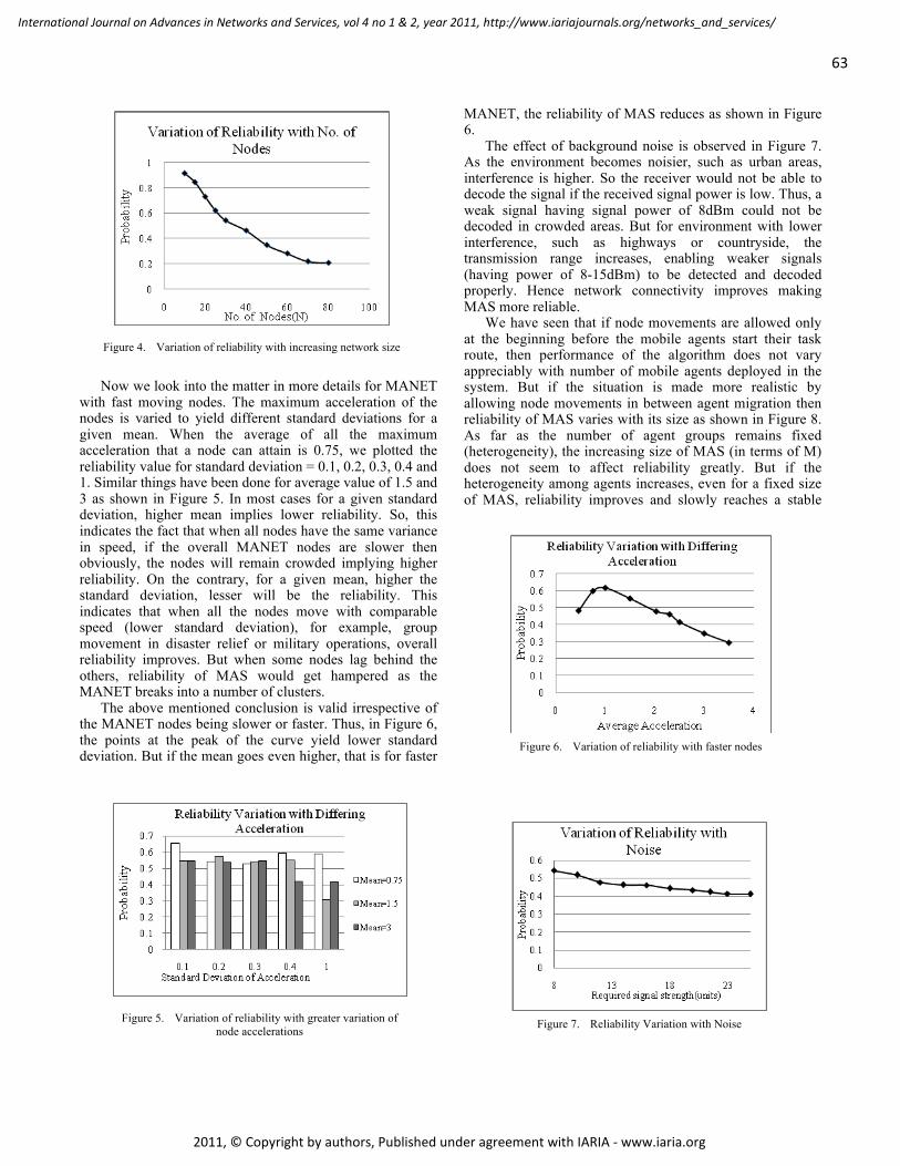
Now we look into the matter in more details for MANET with fast moving nodes. The maximum acceleration of the nodes is varied to yield different standard deviations for a given mean. When the average of all the maximum acceleration that a node can attain is 0.75, we plotted the reliability value for standard deviation = 0.1, 0.2, 0.3, 0.4 and 1. Similar things have been done for average value of 1.5 and 3 as shown in Figure 5. In most cases for a given standard deviation, higher mean implies lower reliability. So, this indicates the fact that when all nodes have the same variance in speed, if the overall MANET nodes are slower then obviously, the nodes will remain crowded implying higher reliability. On the contrary, for a given mean, higher the standard deviation, lesser will be the reliability. This indicates that when all the nodes move with comparable speed (lower standard deviation), for example, group movement in disaster relief or military operations, overall reliability improves. But when some nodes lag behind the others, reliability of MAS would get hampered as the MANET breaks into a number of clusters.
The above mentioned conclusion is valid irrespective of the MANET nodes being slower or faster. Thus, in Figure 6, the points at the peak of the curve yield lower standard deviation. But if the mean goes even higher, that is for faster
MANET, the reliability of MAS reduces as shown in Figure 6.
The effect of background noise is observed in Figure 7. As the environment becomes noisier, such as urban areas, interference is higher. So the receiver would not be able to decode the signal if the received signal power is low. Thus, a weak signal having signal power of 8dBm could not be decoded in crowded areas. But for environment with lower interference, such as highways or countryside, the transmission range increases, enabling weaker signals (having power of 8-15dBm) to be detected and decoded properly. Hence network connectivity improves making MAS more reliable.
We have seen that if node movements are allowed only at the beginning before the mobile agents start their task route, then performance of the algorithm does not vary appreciably with number of mobile agents deployed in the system. But if the situation is made more realistic by allowing node movements in between agent migration then reliability of MAS varies with its size as shown in Figure 8. As far as the number of agent groups remains fixed (heterogeneity), the increasing size of MAS (in terms of M) does not seem to affect reliability greatly. But if the heterogeneity among agents increases, even for a fixed size of MAS, reliability improves and slowly reaches a stable
Figure 4. Variation of reliability with increasing network size
Figure 5. Variation of reliability with greater variation of node accelerations
Figure 6. Variation of reliability with faster nodes
Figure 7. Reliability Variation with Noise
63
International Journal on Advances in Networks and Services, vol 4 no 1 & 2, year 2011, http://www.iariajournals.org/networks_and_services/
2011, © Copyright by authors, Published under agreement with IARIA - www.iaria.org
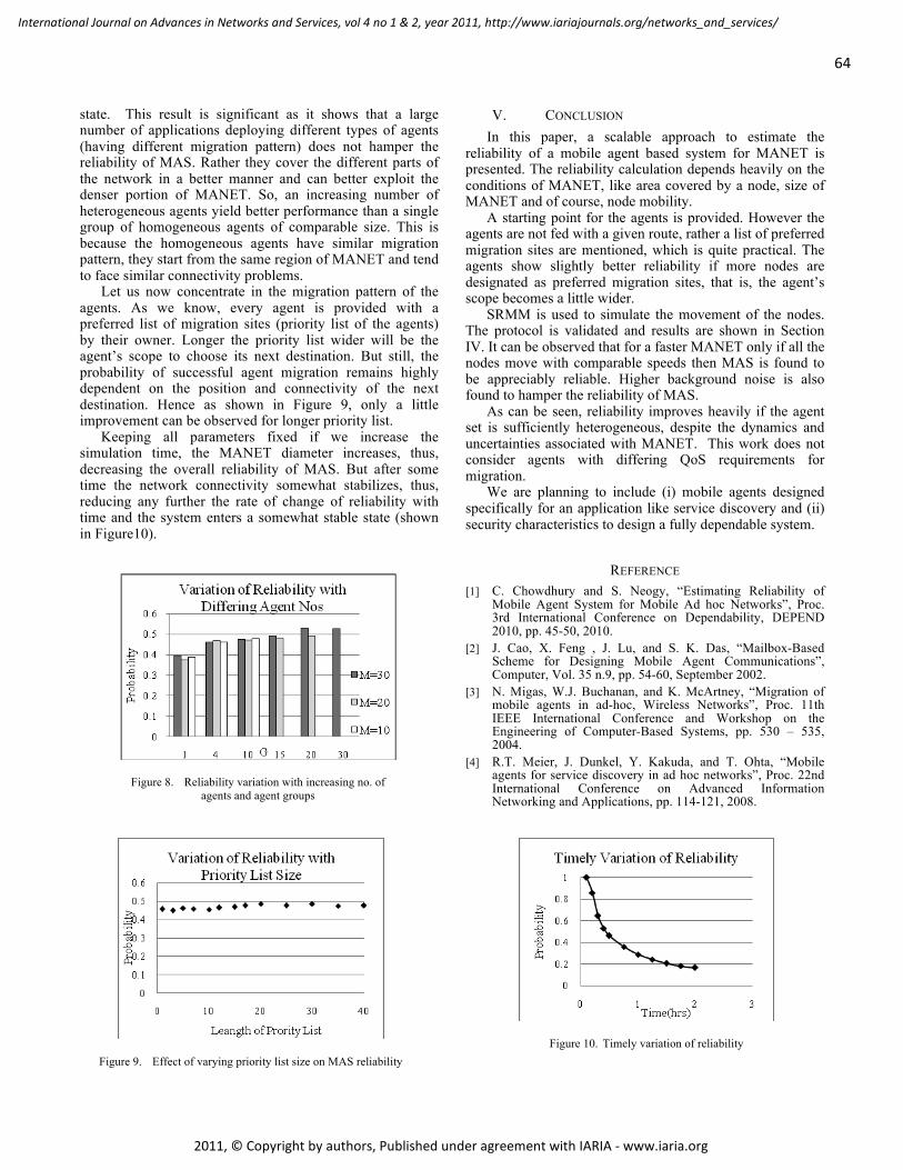
state. This result is significant as it shows that a large number of applications deploying different types of agents (having different migration pattern) does not hamper the reliability of MAS. Rather they cover the different parts of the network in a better manner and can better exploit the denser portion of MANET. So, an increasing number of heterogeneous agents yield better performance than a single group of homogeneous agents of comparable size. This is because the homogeneous agents have similar migration pattern, they start from the same region of MANET and tend to face similar connectivity problems.
Let us now concentrate in the migration pattern of the agents. As we know, every agent is provided with a preferred list of migration sites (priority list of the agents) by their owner. Longer the priority list wider will be the agent’s scope to choose its next destination. But still, the probability of successful agent migration remains highly dependent on the position and connectivity of the next destination. Hence as shown in Figure 9, only a little improvement can be observed for longer priority list.
Keeping all parameters fixed if we increase the simulation time, the MANET diameter increases, thus, decreasing the overall reliability of MAS. But after some time the network connectivity somewhat stabilizes, thus, reducing any further the rate of change of reliability with time and the system enters a somewhat stable state (shown in Figure10).
V. CONCLUSION In this paper, a scalable approach to estimate the
reliability of a mobile agent based system for MANET is presented. The reliability calculation depends heavily on the conditions of MANET, like area covered by a node, size of MANET and of course, node mobility.
A starting point for the agents is provided. However the agents are not fed with a given route, rather a list of preferred migration sites are mentioned, which is quite practical. The agents show slightly better reliability if more nodes are designated as preferred migration sites, that is, the agent’s scope becomes a little wider.
SRMM is used to simulate the movement of the nodes. The protocol is validated and results are shown in Section IV. It can be observed that for a faster MANET only if all the nodes move with comparable speeds then MAS is found to be appreciably reliable. Higher background noise is also found to hamper the reliability of MAS.
As can be seen, reliability improves heavily if the agent set is sufficiently heterogeneous, despite the dynamics and uncertainties associated with MANET. This work does not consider agents with differing QoS requirements for migration.
We are planning to include (i) mobile agents designed specifically for an application like service discovery and (ii) security characteristics to design a fully dependable system.
REFERENCE [1] C. Chowdhury and S. Neogy, “Estimating Reliability of
Mobile Agent System for Mobile Ad hoc Networks”, Proc. 3rd International Conference on Dependability, DEPEND 2010, pp. 45-50, 2010.
[2] J. Cao, X. Feng , J. Lu, and S. K. Das, “Mailbox-Based Scheme for Designing Mobile Agent Communications”, Computer, Vol. 35 n.9, pp. 54-60, September 2002.
[3] N. Migas, W.J. Buchanan, and K. McArtney, “Migration of mobile agents in ad-hoc, Wireless Networks”, Proc. 11th IEEE International Conference and Workshop on the Engineering of Computer-Based Systems, pp. 530 – 535, 2004.
[4] R.T. Meier, J. Dunkel, Y. Kakuda, and T. Ohta, “Mobile agents for service discovery in ad hoc networks”, Proc. 22nd International Conference on Advanced Information Networking and Applications, pp. 114-121, 2008.
Figure 8. Reliability variation with increasing no. of agents and agent groups
Figure 10. Timely variation of reliability
Figure 9. Effect of varying priority list size on MAS reliability
64
International Journal on Advances in Networks and Services, vol 4 no 1 & 2, year 2011, http://www.iariajournals.org/networks_and_services/
2011, © Copyright by authors, Published under agreement with IARIA - www.iaria.org
[5] R. H. Laamanen, T. Alonko, and K. Raatikainen, “Dependability issues in mobile distributed system”, Proc. of the Pacific Rim International Symposium on Dependable Computing, pp. 7-14, 1999.
[6] A. Avizienis, J. Laprie, and B. Randell, “Fundamental concepts of dependability”, LAAS-CNRS, Technical Report N01145, Apr. 2001.
[7] A.L. Murphy and G. P. Picco, “Reliable communication for highly mobile agents”, Autonomous Agents and Multi-Agent Systems, Vol. 5, Issue 1, pp. 81-100, 2002.
[8] O. Urra, S. Ilarri, and E. Mena, “Agents jumping in the air:dream or reality”, Proc. 10th International Work-Conference on Artificial Neural Networks, IWANN’09, Special Session on Practical Applications of Agents and Multi-Agent Systems, pp. 627–634, 2009.
[9] M. Rooryck, “Modelling multiple path propagation- Application to a two ray model”, in the journal of L'Onde Electrique , Vol. 63, pp. 30-34, Aug.-Sept. 1983.
[10] C. Bettstetter, “Smooth is better than sharp: a random mobility model for simulation of wireless networks”, Proc. 4th ACM International Workshop on Modeling, Analysis and Simulation of Wireless and Mobile Systems, pp. 19-25, 2001.
[11] S. Ilarri, R. Trillo, and E. Mena, “SPRINGS: A scalable platform for highly mobile agents in distributed computing environments”, Proc. 4th International WoWMoM 2006, Workshop on Mobile Distributed Computing (MDC 2006), pp. 633–637, 2006.
[12] C. S. Raghavendra, V.K.P. Kumar, and S. Hariri, “Reliability analysis in distributed systems”, in the IEEE Transactions on Computing, Vol. 37, Issue 3, pp.352–358, 1988.
[13] D.J. Chen, and T. H. Huang, “Reliability analysis of distributed systems based on a fast reliability algorithm”, in the IEEE Transactions on Parallel Distributed Systems, Vol. 3, Issue 2, pp.139–154, 1992.
[14] M.S. Lin, D.J. Chen, and M.S. Horng, “The reliability analysis of distributed computing systems with imperfect nodes”, The Computer Journal, Vol. 42, Issue 2, pp. 129–141, 1999.
[15] C-K Toh, “Ad Hoc Mobile Wireless Networks”, Prentice Hall PTR © 2002.
[16] Z. Ye, S. V. Krishnamurthy, and S. K. A Tripathi, “Routing Framework For Providing Robustness to Node Failures in Mobile Ad Hoc Networks”,in Ad Hoc Networks, Vol. 2, No. 1, pp. 87-107, 2004.
[17] M. Abolhasan, T. Wysocki, and E. Dutkiewicz, “A Review of Routing Protocols for Mobile Ad Hoc Networks”, in Ad Hoc Networks, Vol. 2, No. 1, pp.1-22, January 2004.
[18] T.Elperin, I. Gertsbakh, and M. Lomonosov, “Estimation of network reliability using graph evolution models”, in the IEEE Transactions on Reliability, Vol. 40. No. 5. pp 572-581, 1991.
[19] M. Marseguerra, E. Zio, P. Luca, and D. W. Coit, “Optimal Design of Reliable Network Systems in Presence of Uncertainty”, in the IEEE Transactions on Reliability, Vol. 54, No. 2, June 2005.
[20] J. L. Cook and J. E Ramirez-Marquez, “Two-terminal reliability analyses for a mobile ad-hoc wireless network”, in Reliability Engineering and System Safety, Vol. 92, Issue 6, pp. 821-829, June 2007.
[21] J. L. Cook and J. E. Ramirez-Marquez, “Mobility and reliability modeling for a mobile ad-hoc network”, IIE Transactions, Vol. 41, Issue 1, pp. 23 – 31, 2009.
[22] C. Bettstetter and C. Wagner, “The spatial node distribution of the random waypoint mobility model”, Proc 1st German Workshop on Mobile Ad hoc Networks (WMAN), pp. 41-58, 2002.
[23] M. Daoud and Q. H. Mahmoud, “Reliability estimation of mobile agent systems using the Monte Carlo approach”, Proc. 19th IEEE AINA Workshop on Information Networking and Applications, pp. 185–188, 2005.
[24] M. Daoud and Q. H. Mahmoud, “Monte Carlo simulation-based algorithms for estimating the reliability of mobile agent-based systems” Journal of Network and Computer Applications, pp. 19–31, 2008.
[25] C. Chowdhury and S. Neogy, “Reliability Estimate of Mobile Agent Based System for QoS MANET Applications”, Proc. Annual Reliability and Availability Symposium 2011, RAMS 2011, pp.1-6, 2011.
[26] C. Chowdhury and S. Neogy, “Reliability estimation of fault-tolerant wireless and mobile networks”, Proc. 3rd International Conference on Communication Theory, Reliability, and Quality of Service, CTRQ 2010, pp. 67-72 2010.
[27] M. L. Shooman, “Reliability of computer systems and networks: fault tolerance, analysis, and design”. New York: Wiley; 2002.
[28] C. Srivaree-ratana, A. Konak, and A. E. Smith, “Estimation of all-terminal network reliability using an artificial neural network”, Computers and Operations Research, Vol. 29, pp. 849–868, 2002.
[29] H. Taub and D. L. Schilling, “Principles of Communication Systems”, McGraw-Hill, 1986.
[30] S. Li and F. Hu, “Communication between the RoboCup agents based on the blackboard model and observer pattern”, Proc. 5th international conference on Wireless Communications, Networking and Mobile Computing, pp. 5007-5011, 2009.
[31] R. S. Sutton and A. G. Barto, “Reinforcement Learning:An Introduction”, MIT Press, Cambridge, MA,1998.
[32] W. Stallings, “Wireless Communications and Networks”, Pearson, Second Edition, 2009.
65
International Journal on Advances in Networks and Services, vol 4 no 1 & 2, year 2011, http://www.iariajournals.org/networks_and_services/
2011, © Copyright by authors, Published under agreement with IARIA - www.iaria.org
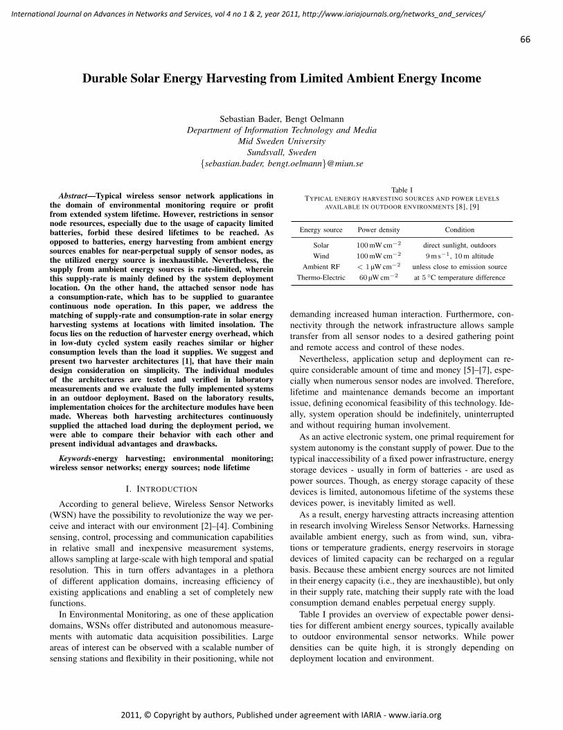
Durable Solar Energy Harvesting from Limited Ambient Energy Income
Sebastian Bader, Bengt OelmannDepartment of Information Technology and Media
Mid Sweden UniversitySundsvall, Sweden
sebastian.bader, [email protected]
Abstract—Typical wireless sensor network applications inthe domain of environmental monitoring require or profitfrom extended system lifetime. However, restrictions in sensornode resources, especially due to the usage of capacity limitedbatteries, forbid these desired lifetimes to be reached. Asopposed to batteries, energy harvesting from ambient energysources enables for near-perpetual supply of sensor nodes, asthe utilized energy source is inexhaustible. Nevertheless, thesupply from ambient energy sources is rate-limited, whereinthis supply-rate is mainly defined by the system deploymentlocation. On the other hand, the attached sensor node hasa consumption-rate, which has to be supplied to guaranteecontinuous node operation. In this paper, we address thematching of supply-rate and consumption-rate in solar energyharvesting systems at locations with limited insolation. Thefocus lies on the reduction of harvester energy overhead, whichin low-duty cycled system easily reaches similar or higherconsumption levels than the load it supplies. We suggest andpresent two harvester architectures [1], that have their maindesign consideration on simplicity. The individual modulesof the architectures are tested and verified in laboratorymeasurements and we evaluate the fully implemented systemsin an outdoor deployment. Based on the laboratory results,implementation choices for the architecture modules have beenmade. Whereas both harvesting architectures continuouslysupplied the attached load during the deployment period, wewere able to compare their behavior with each other andpresent individual advantages and drawbacks.
Keywords-energy harvesting; environmental monitoring;wireless sensor networks; energy sources; node lifetime
I. INTRODUCTION
According to general believe, Wireless Sensor Networks(WSN) have the possibility to revolutionize the way we per-ceive and interact with our environment [2]–[4]. Combiningsensing, control, processing and communication capabilitiesin relative small and inexpensive measurement systems,allows sampling at large-scale with high temporal and spatialresolution. This in turn offers advantages in a plethoraof different application domains, increasing efficiency ofexisting applications and enabling a set of completely newfunctions.
In Environmental Monitoring, as one of these applicationdomains, WSNs offer distributed and autonomous measure-ments with automatic data acquisition possibilities. Largeareas of interest can be observed with a scalable number ofsensing stations and flexibility in their positioning, while not
Table ITYPICAL ENERGY HARVESTING SOURCES AND POWER LEVELS
AVAILABLE IN OUTDOOR ENVIRONMENTS [8], [9]
Energy source Power density Condition
Solar 100mW cm−2 direct sunlight, outdoorsWind 100mW cm−2 9m s−1, 10m altitude
Ambient RF < 1 µW cm−2 unless close to emission sourceThermo-Electric 60 µW cm−2 at 5 C temperature difference
demanding increased human interaction. Furthermore, con-nectivity through the network infrastructure allows sampletransfer from all sensor nodes to a desired gathering pointand remote access and control of these nodes.
Nevertheless, application setup and deployment can re-quire considerable amount of time and money [5]–[7], espe-cially when numerous sensor nodes are involved. Therefore,lifetime and maintenance demands become an importantissue, defining economical feasibility of this technology. Ide-ally, system operation should be indefinitely, uninterruptedand without requiring human involvement.
As an active electronic system, one primal requirement forsystem autonomy is the constant supply of power. Due to thetypical inaccessibility of a fixed power infrastructure, energystorage devices - usually in form of batteries - are used aspower sources. Though, as energy storage capacity of thesedevices is limited, autonomous lifetime of the systems thesedevices power, is inevitably limited as well.
As a result, energy harvesting attracts increasing attentionin research involving Wireless Sensor Networks. Harnessingavailable ambient energy, such as from wind, sun, vibra-tions or temperature gradients, energy reservoirs in storagedevices of limited capacity can be recharged on a regularbasis. Because these ambient energy sources are not limitedin their energy capacity (i.e., they are inexhaustible), but onlyin their supply rate, matching their supply rate with the loadconsumption demand enables perpetual energy supply.
Table I provides an overview of expectable power densi-ties for different ambient energy sources, typically availableto outdoor environmental sensor networks. While powerdensities can be quite high, it is strongly depending ondeployment location and environment.
66
International Journal on Advances in Networks and Services, vol 4 no 1 & 2, year 2011, http://www.iariajournals.org/networks_and_services/
2011, © Copyright by authors, Published under agreement with IARIA - www.iaria.org
Solar energy harvesting is the most frequently used formof energy harvesting in outdoor Wireless Sensor Networks,which might find explanation in several of its properties.(i) Its conversion technology is rather mature and low-cost,because of the use in macro-scale energy production. (ii)Power densities are often sufficiently high. (iii) Availableenergy spreads over a wide area and conversion rate is easilyscalable, and (iv) conversion does not require mechanicalparts, leading to higher maintenance requirements.
Nonetheless, also for solar energy harvesting, achievableconversion rates are highly location specific. This meanswhile there are locations providing good harvesting possi-bilities, there are also those where solar radiation is limitedand insolation unequally distributed over the year. Researchtargeting micro-solar energy harvesting systems for theformer case is documented plentiful in literature. Opposedto that, systems addressing low solar radiation environmentsare strictly limited.
In this paper, we address the issue of limited irradiationconditions for solar energy harvesting based outdoor sensornetworks. The general architecture of solar energy harvestingpower supplies is presented and analyzed towards limitationsfor use in low irradiance situations. Design considerationsare made to allow the sufficient conversion of light into elec-tricity for powering sensor sample-and-send sensor nodes inEnvironmental Wireless Sensor Networks, while at the sametime avoiding lifetime limitations due to battery storagedevices. Herein, the focus of the system lies on providingsufficient energy levels, guaranteeing uninterrupted opera-tion at all times, opposed to optimization towards efficientenergy conversion at times of strong irradiation.
The remainder of the paper is organized as follows. Thenext section summarizes a subset of existing related workin the area of solar energy harvesting systems. After that,Section III provides theory on general solar energy harvest-ing system architecture, location influence and applicationrequirements, leading to the design considerations of solarpower supplies for the intended scenario. Section IV willpresent measurement and evaluation setups, followed bymeasurement results, resulting system architecture and itsevaluation in Section V. Finally, Section VI will concludethe results obtained.
II. RELATED WORK
Plenty of work has been done in Wireless Sensor Net-works for Environmental Monitoring, as typical applicationsin this domain gain from measurement capabilities thistechnology can provide. To mention only a small subsetof the work presented in this area, applications includemonitoring of bird nesting behavior [2], observations ofglacier movement [10], monitoring of volcano activity [5]and analysis of rainforest environments [11].
Nonetheless, while usually large-scale deployments withnumerous sensor nodes are expected, most deployments
are at a proof-of-concept stage with limited coverage andamount of sensing stations. Likely reasons for this are highcost for system setup and maintenance. In turn, a majorpart in maintenance is the replacement of depleting energystorage devices, limiting the period of unattended sensoroperation.
Energy harvesting has gained more attention, as it canreplenish energy reservoirs from ambient energy sources.Types of energy sources cover a broad area, including solar,wind, water flow, vibration, temperature difference and evenpH differences in trees [12]–[15]. While the availabilityof the energy source is highly application dependent, inoutdoor environments (i.e., the typical deployment locationfor environmental monitoring applications) solar energy isalmost ubiquitous.
Existing solar energy harvesting systems are presentedamongst others in [16]–[19]. Distinction exists betweenimplemented storage devices, charge circuitry and systemmanagement (i.e., mainly hardware vs. software control).Typical energy storage devices include Nickel-Metal Hy-dride (NiMH) batteries, Lithium-Ion (Li-Ion) batteries andElectrochemical Double Layer Capacitors (EDLC), comingeach with their advantages and disadvantages.
Systems embedding NiMH batteries include the onesintroduced in [17], [20], [21], while Li-Ion based systemsare presented in [19], [22]. Due to the limitation of chargecycles, several solutions resulted, combining rechargeablebatteries with EDLCs (also known as supercapacitors or ul-tracapacitors), leading to extended system lifetime [16], [23].A set of systems, purely relying on Electrochemical DoubleLayer Capacitors as their storage type, is demonstrated in[1], [18].
Relating to energy extraction, a topic of discussion isMaximum Power Point Tracking (MPPT) for the solar panel.Reference [24] provides a broad overview of different MPPTtechniques, whereas not all of them are applicable in micro-solar energy harvesting systems due to energy overheadconcerns. Most often used are methods such as perturb-and-observe, hill-climbing, as well as fractional open-circuitvoltage and fractional short-circuit current.
Micro-solar energy harvesting systems comprehendingMPPT techniques are those in [18], [21], [25]. However,some of the methods used yield only limited performance.Arguments against the use of Maximum Power Point Track-ers, especially in applications with low power output, areraised in [26].
Work concerning low irradiation conditions is very lim-ited. Reference [11] mentions problems regarding restrictedsolar availability due to shading in their deployment. More-over, in [26] limited power income is a major designconsideration, but the application addressed is indoors andtherefore energy availability is more predictable and con-stant.
67
International Journal on Advances in Networks and Services, vol 4 no 1 & 2, year 2011, http://www.iariajournals.org/networks_and_services/
2011, © Copyright by authors, Published under agreement with IARIA - www.iaria.org
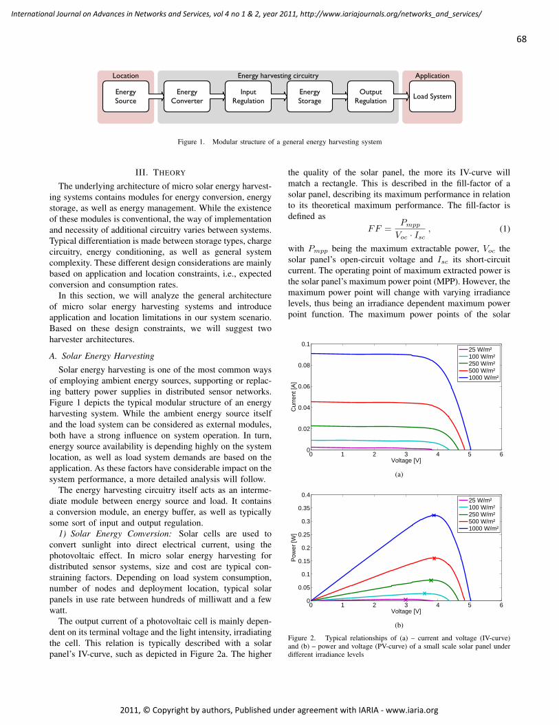
Energy Source
Energy Converter
Energy Storage
Load SystemInput
RegulationOutput
Regulation
Location ApplicationEnergy harvesting circuitry
Figure 1. Modular structure of a general energy harvesting system
III. THEORY
The underlying architecture of micro solar energy harvest-ing systems contains modules for energy conversion, energystorage, as well as energy management. While the existenceof these modules is conventional, the way of implementationand necessity of additional circuitry varies between systems.Typical differentiation is made between storage types, chargecircuitry, energy conditioning, as well as general systemcomplexity. These different design considerations are mainlybased on application and location constraints, i.e., expectedconversion and consumption rates.
In this section, we will analyze the general architectureof micro solar energy harvesting systems and introduceapplication and location limitations in our system scenario.Based on these design constraints, we will suggest twoharvester architectures.
A. Solar Energy Harvesting
Solar energy harvesting is one of the most common waysof employing ambient energy sources, supporting or replac-ing battery power supplies in distributed sensor networks.Figure 1 depicts the typical modular structure of an energyharvesting system. While the ambient energy source itselfand the load system can be considered as external modules,both have a strong influence on system operation. In turn,energy source availability is depending highly on the systemlocation, as well as load system demands are based on theapplication. As these factors have considerable impact on thesystem performance, a more detailed analysis will follow.
The energy harvesting circuitry itself acts as an interme-diate module between energy source and load. It containsa conversion module, an energy buffer, as well as typicallysome sort of input and output regulation.
1) Solar Energy Conversion: Solar cells are used toconvert sunlight into direct electrical current, using thephotovoltaic effect. In micro solar energy harvesting fordistributed sensor systems, size and cost are typical con-straining factors. Depending on load system consumption,number of nodes and deployment location, typical solarpanels in use rate between hundreds of milliwatt and a fewwatt.
The output current of a photovoltaic cell is mainly depen-dent on its terminal voltage and the light intensity, irradiatingthe cell. This relation is typically described with a solarpanel’s IV-curve, such as depicted in Figure 2a. The higher
the quality of the solar panel, the more its IV-curve willmatch a rectangle. This is described in the fill-factor of asolar panel, describing its maximum performance in relationto its theoretical maximum performance. The fill-factor isdefined as
FF =Pmpp
Voc · Isc, (1)
with Pmpp being the maximum extractable power, Voc thesolar panel’s open-circuit voltage and Isc its short-circuitcurrent. The operating point of maximum extracted power isthe solar panel’s maximum power point (MPP). However, themaximum power point will change with varying irradiancelevels, thus being an irradiance dependent maximum powerpoint function. The maximum power points of the solar
0 1 2 3 4 5 60
0.02
0.04
0.06
0.08
0.1
Voltage [V]
Cur
rent
[A]
25 W/m²100 W/m²250 W/m²500 W/m²1000 W/m²
(a)
0 1 2 3 4 5 60
0.05
0.1
0.15
0.2
0.25
0.3
0.35
0.4
Voltage [V]
Pow
er [W
]
25 W/m²100 W/m²250 W/m²500 W/m²1000 W/m²
(b)
Figure 2. Typical relationships of (a) – current and voltage (IV-curve)and (b) – power and voltage (PV-curve) of a small scale solar panel underdifferent irradiance levels
68
International Journal on Advances in Networks and Services, vol 4 no 1 & 2, year 2011, http://www.iariajournals.org/networks_and_services/
2011, © Copyright by authors, Published under agreement with IARIA - www.iaria.org
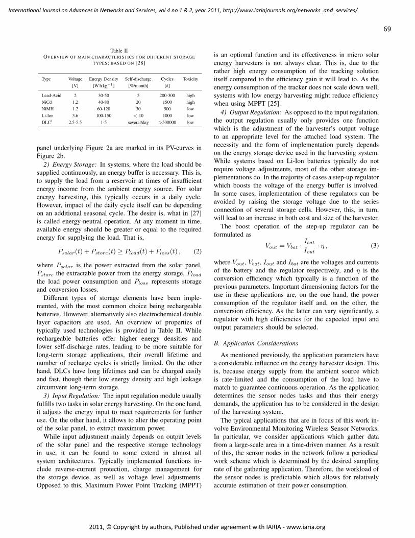
Table IIOVERVIEW OF MAIN CHARACTERISTICS FOR DIFFERENT STORAGE
TYPES; BASED ON [28]
Type Voltage Energy Density Self-discharge Cycles Toxicity[V] [W h kg−1] [%/month] [#]
Lead-Acid 2 30-50 5 200-300 highNiCd 1.2 40-80 20 1500 highNiMH 1.2 60-120 30 500 lowLi-Ion 3.6 100-150 < 10 1000 lowDLC1 2.5-5.5 1-5 several/day >500000 low
panel underlying Figure 2a are marked in its PV-curves inFigure 2b.
2) Energy Storage: In systems, where the load should besupplied continuously, an energy buffer is necessary. This is,to supply the load from a reservoir at times of insufficientenergy income from the ambient energy source. For solarenergy harvesting, this typically occurs in a daily cycle.However, impact of the daily cycle itself can be dependingon an additional seasonal cycle. The desire is, what in [27]is called energy-neutral operation. At any moment in time,available energy should be greater or equal to the requiredenergy for supplying the load. That is,
Psolar(t) + Pstore(t) ≥ Pload(t) + Ploss(t) , (2)
where Psolar is the power extracted from the solar panel,Pstore the extractable power from the energy storage, Pload
the load power consumption and Ploss represents storageand conversion losses.
Different types of storage elements have been imple-mented, with the most common choice being rechargeablebatteries. However, alternatively also electrochemical doublelayer capacitors are used. An overview of properties oftypically used technologies is provided in Table II. Whilerechargeable batteries offer higher energy densities andlower self-discharge rates, leading to be more suitable forlong-term storage applications, their overall lifetime andnumber of recharge cycles is strictly limited. On the otherhand, DLCs have long lifetimes and can be charged easilyand fast, though their low energy density and high leakagecircumvent long-term storage.
3) Input Regulation: The input regulation module usuallyfulfills two tasks in solar energy harvesting. On the one hand,it adjusts the energy input to meet requirements for furtheruse. On the other hand, it allows to alter the operating pointof the solar panel, to extract maximum power.
While input adjustment mainly depends on output levelsof the solar panel and the respective storage technologyin use, it can be found to some extend in almost allsystem architectures. Typically implemented functions in-clude reverse-current protection, charge management forthe storage device, as well as voltage level adjustments.Opposed to this, Maximum Power Point Tracking (MPPT)
is an optional function and its effectiveness in micro solarenergy harvesters is not always clear. This is, due to therather high energy consumption of the tracking solutionitself compared to the efficiency gain it will lead to. As theenergy consumption of the tracker does not scale down well,systems with low energy harvesting might reduce efficiencywhen using MPPT [25].
4) Output Regulation: As opposed to the input regulation,the output regulation usually only provides one functionwhich is the adjustment of the harvester’s output voltageto an appropriate level for the attached load system. Thenecessity and the form of implementation purely dependson the energy storage device used in the harvesting system.While systems based on Li-Ion batteries typically do notrequire voltage adjustments, most of the other storage im-plementations do. In the majority of cases a step-up regulatorwhich boosts the voltage of the energy buffer is involved.In some cases, implementation of these regulators can beavoided by raising the storage voltage due to the seriesconnection of several storage cells. However, this, in turn,will lead to an increase in both cost and size of the harvester.
The boost operation of the step-up regulator can beformulated as
Vout = Vbat ·IbatIout
· η , (3)
where Vout, Vbat, Iout and Ibat are the voltages and currentsof the battery and the regulator respectively, and η is theconversion efficiency which typically is a function of theprevious parameters. Important dimensioning factors for theuse in these applications are, on the one hand, the powerconsumption of the regulator itself and, on the other, theconversion efficiency. As the latter can vary significantly, aregulator with high efficiencies for the expected input andoutput parameters should be selected.
B. Application Considerations
As mentioned previously, the application parameters havea considerable influence on the energy harvester design. Thisis, because energy supply from the ambient source whichis rate-limited and the consumption of the load have tomatch to guarantee continuous operation. As the applicationdetermines the sensor nodes tasks and thus their energydemands, the application has to be considered in the designof the harvesting system.
The typical applications that are in focus of this work in-volve Environmental Monitoring Wireless Sensor Networks.In particular, we consider applications which gather datafrom a large-scale area in a time-driven manner. As a resultof this, the sensor nodes in the network follow a periodicalwork scheme which is determined by the desired samplingrate of the gathering application. Therefore, the workload ofthe sensor nodes is predictable which allows for relativelyaccurate estimation of their power consumption.
69
International Journal on Advances in Networks and Services, vol 4 no 1 & 2, year 2011, http://www.iariajournals.org/networks_and_services/
2011, © Copyright by authors, Published under agreement with IARIA - www.iaria.org
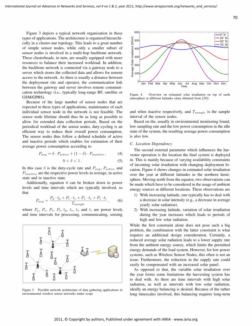
Figure 3 depicts a typical network organization in thesetypes of applications. The architecture is organized hierarchi-cally in a cluster-star topology. This leads to a great numberof simple sensor nodes, while only a smaller subset ofsensor nodes is involved in a multi-hop backbone network.These clusterheads, in turn, are usually equipped with moreresources to balance their increased workload. In addition,the backbone network is connected via a gateway node to aserver which stores the collected data and allows for remoteaccess to the network. As there is usually a distance betweenthe deployment site and operator, the communication linkbetween the gateway and server involves remote communi-cation technology (i.e., typically long-range RF, satellite orGSM/GPRS).
Because of the large number of sensor nodes that areexpected in these types of applications, maintenance of eachindividual sensor node in the network is not feasible. Thesensor node lifetime should thus be as long as possible toallow for extended data collection periods. Based on theperiodical workload of the sensor nodes, duty-cycling is anefficient way to reduce their overall power consumption.The sensor nodes thus follow a defined schedule of activeand inactive periods which enables for estimation of theiraverage power consumption according to
Pavg = δ · Pactive + (1− δ) · Pinactive , (4)
0 < δ < 1 . (5)
In this case δ is the duty-cycle rate and Pavg, Pactive andPinactive are the respective power levels in average, in activestate and in inactive state.
Additionally, equation 4 can be broken down to powerlevels and time intervals which are typically involved, sothat
Pavg =Pp · tp + Pc · tc + Ps · ts + Pi · ti
Tsample, (6)
where Pp, Pc, Ps, Pi, tp, tc, ts and ti are power levelsand time intervals for processing, communicating, sensing
Figure 3. Possible network architecture of data gathering applications inenvironmental wireless sensor networks under scope
Jan Feb Mar Apr May Jun Jul Aug Sep Oct Nov Dec0
100
200
300
400
500
600
Time
Ave
rage
Sol
ar Ir
radi
ance
[W/m
²]
0° N25° N50° N75° N
Figure 4. Overview on estimated solar irradiation on top of earthatmosphere at different latitudes (data obtained from [29])
and when inactive respectively, and Tsample is the sampleinterval of the sensor nodes.
Based on the, usually in environmental monitoring found,low sampling rate and the low power consumption in the idlestate of the system, the resulting average power consumptionis also low.
C. Location Dependency
The second external parameter which influences the har-vester operation is the location the final system is deployedin. This is mainly because of varying availability constraintsof incoming solar irradiation with changing deployment lo-cation. Figure 4 shows changes in estimated solar irradiationover the year at different latitudes in the northern hemi-sphere. Moving north from the equator, two observations canbe made which have to be considered in the usage of ambientenergy sources at different locations. These observations are
1) With increasing latitude, one typically has to deal witha decrease in solar intensity (e.g., a decrease in averageyearly solar radiation).
2) With increasing latitude, variation of solar irradiationduring the year increases which leads to periods ofhigh and low solar radiation.
While the first constraint alone does not pose such a bigproblem, the combination with the latter constraint is whatrequires an additional design consideration. Certainly, areduced average solar radiation leads to a lower supply ratefrom the ambient energy source, which limits the permittedenergy demands of the load system. However, for low powersystems, such as Wireless Sensor Nodes, this often is not anissue. Furthermore, the reduction in the supply rate couldeasily be compensated with an increased solar panel.
As opposed to that, the variable solar irradiation overthe year forms some limitations the harvesting system hasto deal with. As there are time intervals with high solarradiation, as well as intervals with low solar radiation,ideally an energy balancing is desired. Because of the ratherlong timescales involved, this balancing requires long-term
70
International Journal on Advances in Networks and Services, vol 4 no 1 & 2, year 2011, http://www.iariajournals.org/networks_and_services/
2011, © Copyright by authors, Published under agreement with IARIA - www.iaria.org
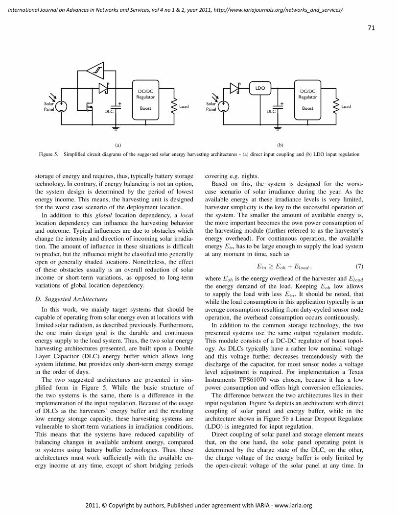
DC/DC Regulator
BoostSolarPanel DLC
+ Load
(a)
DC/DC Regulator
BoostSolarPanel DLC
+ Load
LDO
(b)
Figure 5. Simplified circuit diagrams of the suggested solar energy harvesting architectures - (a) direct input coupling and (b) LDO input regulation
storage of energy and requires, thus, typically battery storagetechnology. In contrary, if energy balancing is not an option,the system design is determined by the period of lowestenergy income. This means, the harvesting unit is designedfor the worst case scenario of the deployment location.
In addition to this global location dependency, a locallocation dependency can influence the harvesting behaviorand outcome. Typical influences are due to obstacles whichchange the intensity and direction of incoming solar irradia-tion. The amount of influence in these situations is difficultto predict, but the influence might be classified into generallyopen or generally shaded locations. Nonetheless, the effectof these obstacles usually is an overall reduction of solarincome or short-term variations, as opposed to long-termvariations of global location dependency.
D. Suggested Architectures
In this work, we mainly target systems that should becapable of operating from solar energy even at locations withlimited solar radiation, as described previously. Furthermore,the one main design goal is the durable and continuousenergy supply to the load system. Thus, the two solar energyharvesting architectures presented, are built upon a DoubleLayer Capacitor (DLC) energy buffer which allows longsystem lifetime, but provides only short-term energy storagein the order of days.
The two suggested architectures are presented in sim-plified form in Figure 5. While the basic structure ofthe two systems is the same, there is a difference in theimplementation of the input regulation. Because of the usageof DLCs as the harvesters’ energy buffer and the resultinglow energy storage capacity, these harvesting systems arevulnerable to short-term variations in irradiation conditions.This means that the systems have reduced capability ofbalancing changes in available ambient energy, comparedto systems using battery buffer technologies. Thus, thesearchitectures must work sufficiently with the available en-ergy income at any time, except of short bridging periods
covering e.g. nights.Based on this, the system is designed for the worst-
case scenario of solar irradiance during the year. As theavailable energy at these irradiance levels is very limited,harvester simplicity is the key to the successful operation ofthe system. The smaller the amount of available energy is,the more important becomes the own power consumption ofthe harvesting module (further referred to as the harvester’senergy overhead). For continuous operation, the availableenergy Ein has to be large enough to supply the load systemat any moment in time, such as
Ein ≥ Eoh + Eload , (7)
where Eoh is the energy overhead of the harvester and Eload
the energy demand of the load. Keeping Eoh low allowsto supply the load with less Ein. It should be noted, thatwhile the load consumption in this application typically is anaverage consumption resulting from duty-cycled sensor nodeoperation, the overhead consumption occurs continuously.
In addition to the common storage technology, the twopresented systems use the same output regulation module.This module consists of a DC-DC regulator of boost topol-ogy. As DLCs typically have a rather low nominal voltageand this voltage further decreases tremendously with thedischarge of the capacitor, for most sensor nodes a voltagelevel adjustment is required. For implementation a TexasInstruments TPS61070 was chosen, because it has a lowpower consumption and offers high conversion efficiencies.
The difference between the two architectures lies in theirinput regulation. Figure 5a depicts an architecture with directcoupling of solar panel and energy buffer, while in thearchitecture shown in Figure 5b a Linear Dropout Regulator(LDO) is integrated for input regulation.
Direct coupling of solar panel and storage element meansthat, on the one hand, the solar panel operating point isdetermined by the charge state of the DLC, on the other,the charge voltage of the energy buffer is only limited bythe open-circuit voltage of the solar panel at any time. In
71
International Journal on Advances in Networks and Services, vol 4 no 1 & 2, year 2011, http://www.iariajournals.org/networks_and_services/
2011, © Copyright by authors, Published under agreement with IARIA - www.iaria.org
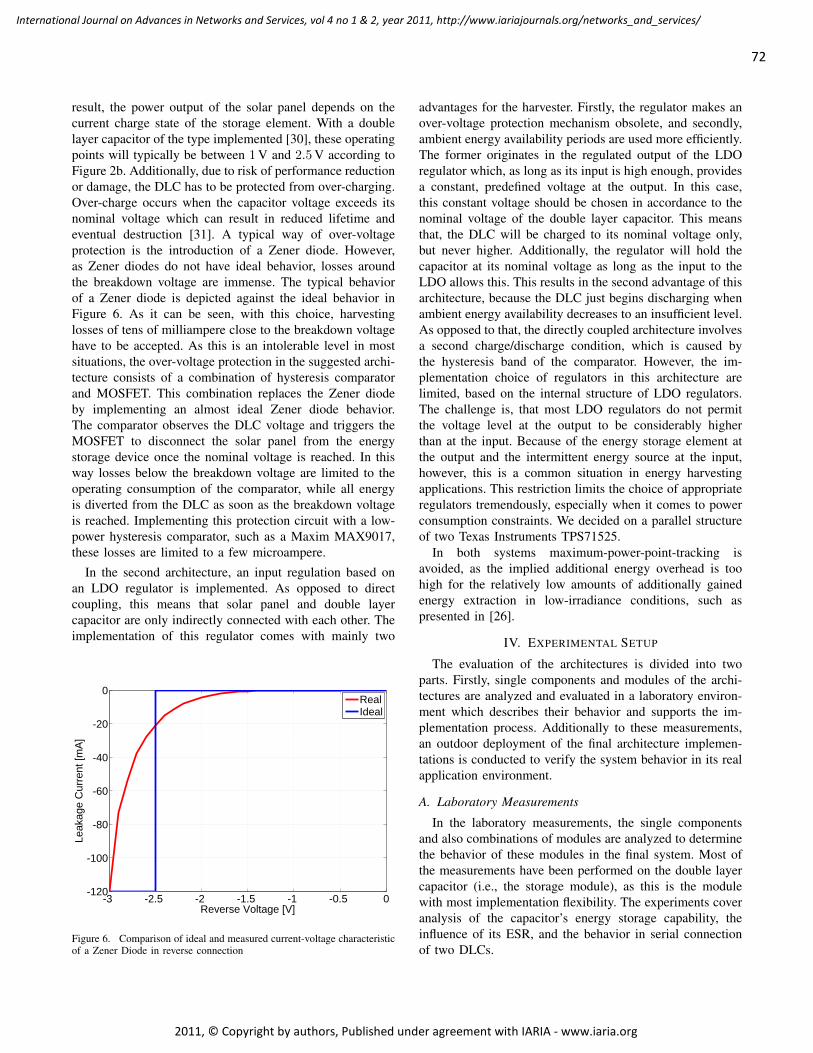
result, the power output of the solar panel depends on thecurrent charge state of the storage element. With a doublelayer capacitor of the type implemented [30], these operatingpoints will typically be between 1V and 2.5V according toFigure 2b. Additionally, due to risk of performance reductionor damage, the DLC has to be protected from over-charging.Over-charge occurs when the capacitor voltage exceeds itsnominal voltage which can result in reduced lifetime andeventual destruction [31]. A typical way of over-voltageprotection is the introduction of a Zener diode. However,as Zener diodes do not have ideal behavior, losses aroundthe breakdown voltage are immense. The typical behaviorof a Zener diode is depicted against the ideal behavior inFigure 6. As it can be seen, with this choice, harvestinglosses of tens of milliampere close to the breakdown voltagehave to be accepted. As this is an intolerable level in mostsituations, the over-voltage protection in the suggested archi-tecture consists of a combination of hysteresis comparatorand MOSFET. This combination replaces the Zener diodeby implementing an almost ideal Zener diode behavior.The comparator observes the DLC voltage and triggers theMOSFET to disconnect the solar panel from the energystorage device once the nominal voltage is reached. In thisway losses below the breakdown voltage are limited to theoperating consumption of the comparator, while all energyis diverted from the DLC as soon as the breakdown voltageis reached. Implementing this protection circuit with a low-power hysteresis comparator, such as a Maxim MAX9017,these losses are limited to a few microampere.
In the second architecture, an input regulation based onan LDO regulator is implemented. As opposed to directcoupling, this means that solar panel and double layercapacitor are only indirectly connected with each other. Theimplementation of this regulator comes with mainly two
-3 -2.5 -2 -1.5 -1 -0.5 0-120
-100
-80
-60
-40
-20
0
Reverse Voltage [V]
Leak
age
Cur
rent
[mA
]
RealIdeal
Figure 6. Comparison of ideal and measured current-voltage characteristicof a Zener Diode in reverse connection
advantages for the harvester. Firstly, the regulator makes anover-voltage protection mechanism obsolete, and secondly,ambient energy availability periods are used more efficiently.The former originates in the regulated output of the LDOregulator which, as long as its input is high enough, providesa constant, predefined voltage at the output. In this case,this constant voltage should be chosen in accordance to thenominal voltage of the double layer capacitor. This meansthat, the DLC will be charged to its nominal voltage only,but never higher. Additionally, the regulator will hold thecapacitor at its nominal voltage as long as the input to theLDO allows this. This results in the second advantage of thisarchitecture, because the DLC just begins discharging whenambient energy availability decreases to an insufficient level.As opposed to that, the directly coupled architecture involvesa second charge/discharge condition, which is caused bythe hysteresis band of the comparator. However, the im-plementation choice of regulators in this architecture arelimited, based on the internal structure of LDO regulators.The challenge is, that most LDO regulators do not permitthe voltage level at the output to be considerably higherthan at the input. Because of the energy storage element atthe output and the intermittent energy source at the input,however, this is a common situation in energy harvestingapplications. This restriction limits the choice of appropriateregulators tremendously, especially when it comes to powerconsumption constraints. We decided on a parallel structureof two Texas Instruments TPS71525.
In both systems maximum-power-point-tracking isavoided, as the implied additional energy overhead is toohigh for the relatively low amounts of additionally gainedenergy extraction in low-irradiance conditions, such aspresented in [26].
IV. EXPERIMENTAL SETUP
The evaluation of the architectures is divided into twoparts. Firstly, single components and modules of the archi-tectures are analyzed and evaluated in a laboratory environ-ment which describes their behavior and supports the im-plementation process. Additionally to these measurements,an outdoor deployment of the final architecture implemen-tations is conducted to verify the system behavior in its realapplication environment.
A. Laboratory Measurements
In the laboratory measurements, the single componentsand also combinations of modules are analyzed to determinethe behavior of these modules in the final system. Most ofthe measurements have been performed on the double layercapacitor (i.e., the storage module), as this is the modulewith most implementation flexibility. The experiments coveranalysis of the capacitor’s energy storage capability, theinfluence of its ESR, and the behavior in serial connectionof two DLCs.
72
International Journal on Advances in Networks and Services, vol 4 no 1 & 2, year 2011, http://www.iariajournals.org/networks_and_services/
2011, © Copyright by authors, Published under agreement with IARIA - www.iaria.org
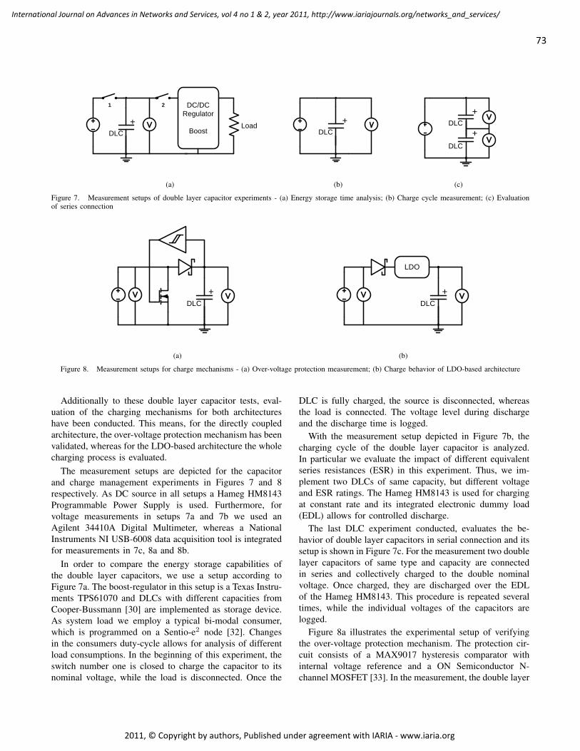
DLC
+
1 DC/DC Regulator
BoostLoad
2
(a)
DLC
+
(b)
DLC
+
DLC
+
(c)
Figure 7. Measurement setups of double layer capacitor experiments - (a) Energy storage time analysis; (b) Charge cycle measurement; (c) Evaluationof series connection
DLC
+
(a)
DLC
+
LDO
(b)
Figure 8. Measurement setups for charge mechanisms - (a) Over-voltage protection measurement; (b) Charge behavior of LDO-based architecture
Additionally to these double layer capacitor tests, eval-uation of the charging mechanisms for both architectureshave been conducted. This means, for the directly coupledarchitecture, the over-voltage protection mechanism has beenvalidated, whereas for the LDO-based architecture the wholecharging process is evaluated.
The measurement setups are depicted for the capacitorand charge management experiments in Figures 7 and 8respectively. As DC source in all setups a Hameg HM8143Programmable Power Supply is used. Furthermore, forvoltage measurements in setups 7a and 7b we used anAgilent 34410A Digital Multimeter, whereas a NationalInstruments NI USB-6008 data acquisition tool is integratedfor measurements in 7c, 8a and 8b.
In order to compare the energy storage capabilities ofthe double layer capacitors, we use a setup according toFigure 7a. The boost-regulator in this setup is a Texas Instru-ments TPS61070 and DLCs with different capacities fromCooper-Bussmann [30] are implemented as storage device.As system load we employ a typical bi-modal consumer,which is programmed on a Sentio-e2 node [32]. Changesin the consumers duty-cycle allows for analysis of differentload consumptions. In the beginning of this experiment, theswitch number one is closed to charge the capacitor to itsnominal voltage, while the load is disconnected. Once the
DLC is fully charged, the source is disconnected, whereasthe load is connected. The voltage level during dischargeand the discharge time is logged.
With the measurement setup depicted in Figure 7b, thecharging cycle of the double layer capacitor is analyzed.In particular we evaluate the impact of different equivalentseries resistances (ESR) in this experiment. Thus, we im-plement two DLCs of same capacity, but different voltageand ESR ratings. The Hameg HM8143 is used for chargingat constant rate and its integrated electronic dummy load(EDL) allows for controlled discharge.
The last DLC experiment conducted, evaluates the be-havior of double layer capacitors in serial connection and itssetup is shown in Figure 7c. For the measurement two doublelayer capacitors of same type and capacity are connectedin series and collectively charged to the double nominalvoltage. Once charged, they are discharged over the EDLof the Hameg HM8143. This procedure is repeated severaltimes, while the individual voltages of the capacitors arelogged.
Figure 8a illustrates the experimental setup of verifyingthe over-voltage protection mechanism. The protection cir-cuit consists of a MAX9017 hysteresis comparator withinternal voltage reference and a ON Semiconductor N-channel MOSFET [33]. In the measurement, the double layer
73
International Journal on Advances in Networks and Services, vol 4 no 1 & 2, year 2011, http://www.iariajournals.org/networks_and_services/
2011, © Copyright by authors, Published under agreement with IARIA - www.iaria.org
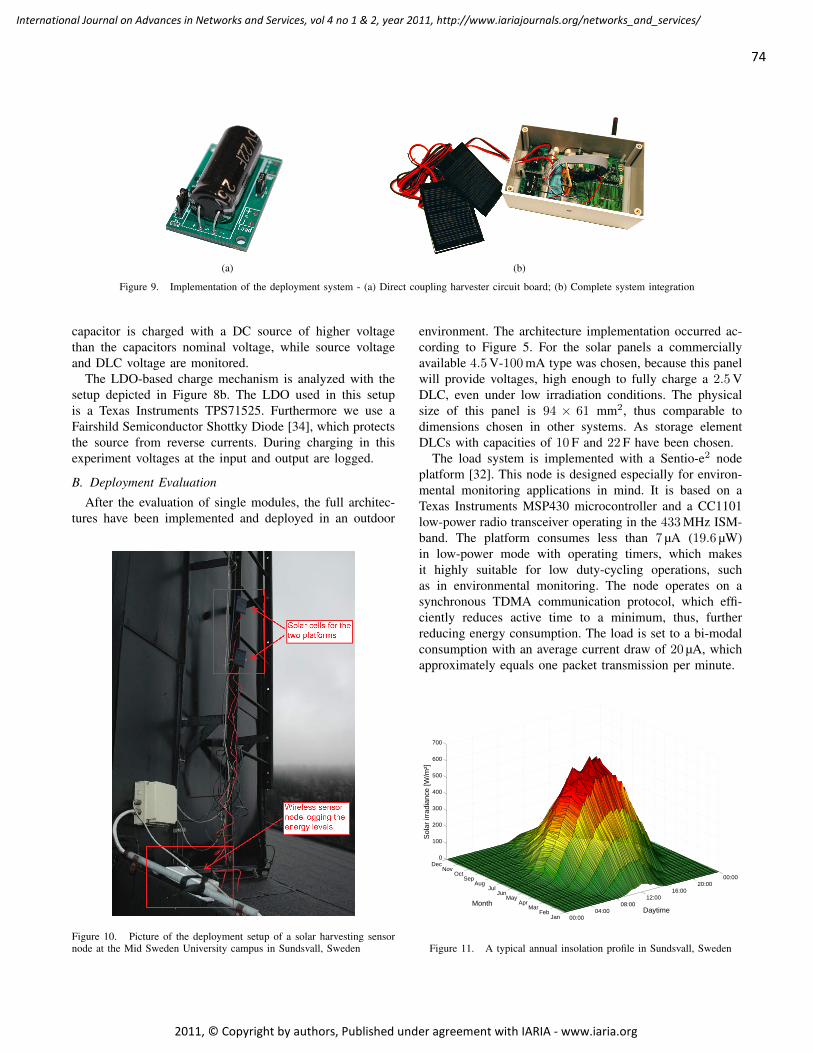
(a) (b)
Figure 9. Implementation of the deployment system - (a) Direct coupling harvester circuit board; (b) Complete system integration
capacitor is charged with a DC source of higher voltagethan the capacitors nominal voltage, while source voltageand DLC voltage are monitored.
The LDO-based charge mechanism is analyzed with thesetup depicted in Figure 8b. The LDO used in this setupis a Texas Instruments TPS71525. Furthermore we use aFairshild Semiconductor Shottky Diode [34], which protectsthe source from reverse currents. During charging in thisexperiment voltages at the input and output are logged.
B. Deployment Evaluation
After the evaluation of single modules, the full architec-tures have been implemented and deployed in an outdoor
Figure 10. Picture of the deployment setup of a solar harvesting sensornode at the Mid Sweden University campus in Sundsvall, Sweden
environment. The architecture implementation occurred ac-cording to Figure 5. For the solar panels a commerciallyavailable 4.5V-100mA type was chosen, because this panelwill provide voltages, high enough to fully charge a 2.5VDLC, even under low irradiation conditions. The physicalsize of this panel is 94 × 61 mm2, thus comparable todimensions chosen in other systems. As storage elementDLCs with capacities of 10F and 22F have been chosen.
The load system is implemented with a Sentio-e2 nodeplatform [32]. This node is designed especially for environ-mental monitoring applications in mind. It is based on aTexas Instruments MSP430 microcontroller and a CC1101low-power radio transceiver operating in the 433MHz ISM-band. The platform consumes less than 7 µA (19.6 µW)in low-power mode with operating timers, which makesit highly suitable for low duty-cycling operations, suchas in environmental monitoring. The node operates on asynchronous TDMA communication protocol, which effi-ciently reduces active time to a minimum, thus, furtherreducing energy consumption. The load is set to a bi-modalconsumption with an average current draw of 20 µA, whichapproximately equals one packet transmission per minute.
00:0004:00
08:0012:00
16:0020:00
00:00
JanFeb
MarApr
MayJun
JulAug
SepOct
NovDec
0
100
200
300
400
500
600
700
DaytimeMonth
Sol
ar ir
radi
ance
[W/m
²]
Figure 11. A typical annual insolation profile in Sundsvall, Sweden
74
International Journal on Advances in Networks and Services, vol 4 no 1 & 2, year 2011, http://www.iariajournals.org/networks_and_services/
2011, © Copyright by authors, Published under agreement with IARIA - www.iaria.org
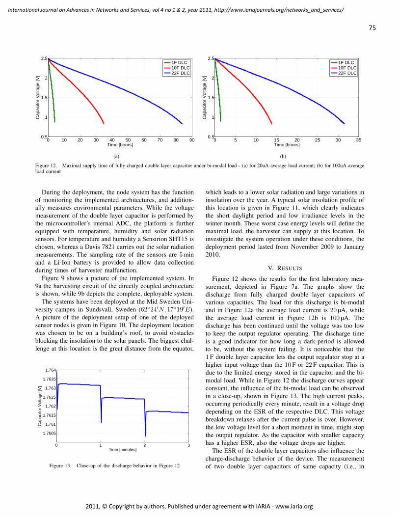
0 10 20 30 40 50 60 70 80 900.5
1
1.5
2
2.5
Time [hours]
Cap
acito
r Vol
tage
[V]
1F DLC10F DLC22F DLC
(a)
0 5 10 15 20 25 30 350.5
1
1.5
2
2.5
Time [hours]
Cap
acito
r Vol
tage
[V]
1F DLC10F DLC22F DLC
(b)
Figure 12. Maximal supply time of fully charged double layer capacitor under bi-modal load - (a) for 20uA average load current; (b) for 100uA averageload current
During the deployment, the node system has the functionof monitoring the implemented architectures, and addition-ally measures environmental parameters. While the voltagemeasurement of the double layer capacitor is performed bythe microcontroller’s internal ADC, the platform is furtherequipped with temperature, humidity and solar radiationsensors. For temperature and humidity a Sensirion SHT15 ischosen, whereas a Davis 7821 carries out the solar radiationmeasurements. The sampling rate of the sensors are 5minand a Li-Ion battery is provided to allow data collectionduring times of harvester malfunction.
Figure 9 shows a picture of the implemented system. In9a the harvesting circuit of the directly coupled architectureis shown, while 9b depicts the complete, deployable system.
The systems have been deployed at the Mid Sweden Uni-versity campus in Sundsvall, Sweden (6224′N, 1719′E).A picture of the deployment setup of one of the deployedsensor nodes is given in Figure 10. The deployment locationwas chosen to be on a building’s roof, to avoid obstaclesblocking the insolation to the solar panels. The biggest chal-lenge at this location is the great distance from the equator,
0 1 2 3
1.7605
1.761
1.7615
1.762
1.7625
1.763
1.7635
1.764
Time [minutes]
Cap
acito
r Vol
tage
[V]
Figure 13. Close-up of the discharge behavior in Figure 12
which leads to a lower solar radiation and large variations ininsolation over the year. A typical solar insolation profile ofthis location is given in Figure 11, which clearly indicatesthe short daylight period and low irradiance levels in thewinter month. These worst case energy levels will define themaximal load, the harvester can supply at this location. Toinvestigate the system operation under these conditions, thedeployment period lasted from November 2009 to January2010.
V. RESULTS
Figure 12 shows the results for the first laboratory mea-surement, depicted in Figure 7a. The graphs show thedischarge from fully charged double layer capacitors ofvarious capacities. The load for this discharge is bi-modaland in Figure 12a the average load current is 20 µA, whilethe average load current in Figure 12b is 100 µA. Thedischarge has been continued until the voltage was too lowto keep the output regulator operating. The discharge timeis a good indicator for how long a dark-period is allowedto be, without the system failing. It is noticeable that the1F double layer capacitor lets the output regulator stop at ahigher input voltage than the 10F or 22F capacitor. This isdue to the limited energy stored in the capacitor and the bi-modal load. While in Figure 12 the discharge curves appearconstant, the influence of the bi-modal load can be observedin a close-up, shown in Figure 13. The high current peaks,occurring periodically every minute, result in a voltage dropdepending on the ESR of the respective DLC. This voltagebreakdown relaxes after the current pulse is over. However,the low voltage level for a short moment in time, might stopthe output regulator. As the capacitor with smaller capacityhas a higher ESR, also the voltage drops are higher.
The ESR of the double layer capacitors also influence thecharge-discharge behavior of the device. The measurementof two double layer capacitors of same capacity (i.e., in
75
International Journal on Advances in Networks and Services, vol 4 no 1 & 2, year 2011, http://www.iariajournals.org/networks_and_services/
2011, © Copyright by authors, Published under agreement with IARIA - www.iaria.org
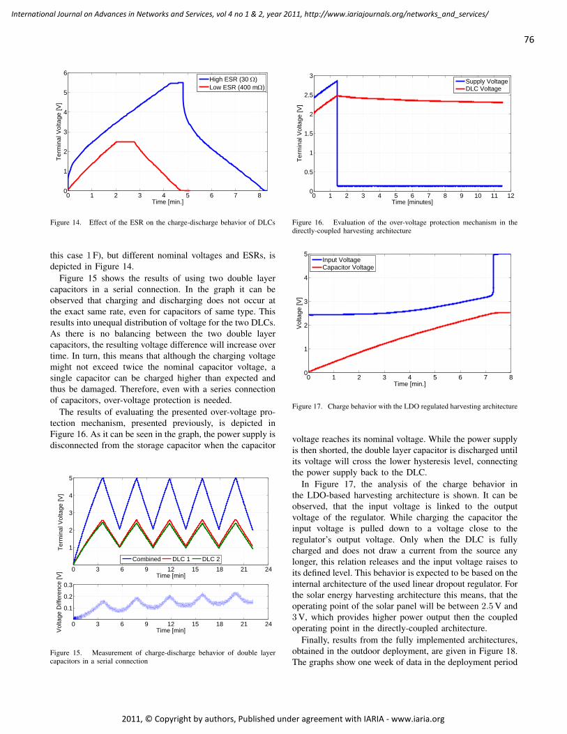
0 1 2 3 4 5 6 7 80
1
2
3
4
5
6
Time [min.]
Term
inal
Vol
tage
[V]
High ESR (30 )Low ESR (400 m)
Figure 14. Effect of the ESR on the charge-discharge behavior of DLCs
this case 1F), but different nominal voltages and ESRs, isdepicted in Figure 14.
Figure 15 shows the results of using two double layercapacitors in a serial connection. In the graph it can beobserved that charging and discharging does not occur atthe exact same rate, even for capacitors of same type. Thisresults into unequal distribution of voltage for the two DLCs.As there is no balancing between the two double layercapacitors, the resulting voltage difference will increase overtime. In turn, this means that although the charging voltagemight not exceed twice the nominal capacitor voltage, asingle capacitor can be charged higher than expected andthus be damaged. Therefore, even with a series connectionof capacitors, over-voltage protection is needed.
The results of evaluating the presented over-voltage pro-tection mechanism, presented previously, is depicted inFigure 16. As it can be seen in the graph, the power supply isdisconnected from the storage capacitor when the capacitor
0 3 6 9 12 15 18 21 24
1
2
3
4
5
Time [min]
Term
inal
Vol
tage
[V]
0 3 6 9 12 15 18 21 24
0.1
0.2
0.3
Time [min]Vol
tage
Diff
eren
ce [V
]
Combined DLC 1 DLC 2
Figure 15. Measurement of charge-discharge behavior of double layercapacitors in a serial connection
0 1 2 3 4 5 6 7 8 9 10 11 120
0.5
1
1.5
2
2.5
3
Time [minutes]
Term
inal
Vol
tage
[V]
Supply VoltageDLC Voltage
Figure 16. Evaluation of the over-voltage protection mechanism in thedirectly-coupled harvesting architecture
0 1 2 3 4 5 6 7 80
1
2
3
4
5
Time [min.]
Vol
tage
[V]
Input VoltageCapacitor Voltage
Figure 17. Charge behavior with the LDO regulated harvesting architecture
voltage reaches its nominal voltage. While the power supplyis then shorted, the double layer capacitor is discharged untilits voltage will cross the lower hysteresis level, connectingthe power supply back to the DLC.
In Figure 17, the analysis of the charge behavior inthe LDO-based harvesting architecture is shown. It can beobserved, that the input voltage is linked to the outputvoltage of the regulator. While charging the capacitor theinput voltage is pulled down to a voltage close to theregulator’s output voltage. Only when the DLC is fullycharged and does not draw a current from the source anylonger, this relation releases and the input voltage raises toits defined level. This behavior is expected to be based on theinternal architecture of the used linear dropout regulator. Forthe solar energy harvesting architecture this means, that theoperating point of the solar panel will be between 2.5V and3V, which provides higher power output then the coupledoperating point in the directly-coupled architecture.
Finally, results from the fully implemented architectures,obtained in the outdoor deployment, are given in Figure 18.The graphs show one week of data in the deployment period
76
International Journal on Advances in Networks and Services, vol 4 no 1 & 2, year 2011, http://www.iariajournals.org/networks_and_services/
2011, © Copyright by authors, Published under agreement with IARIA - www.iaria.org
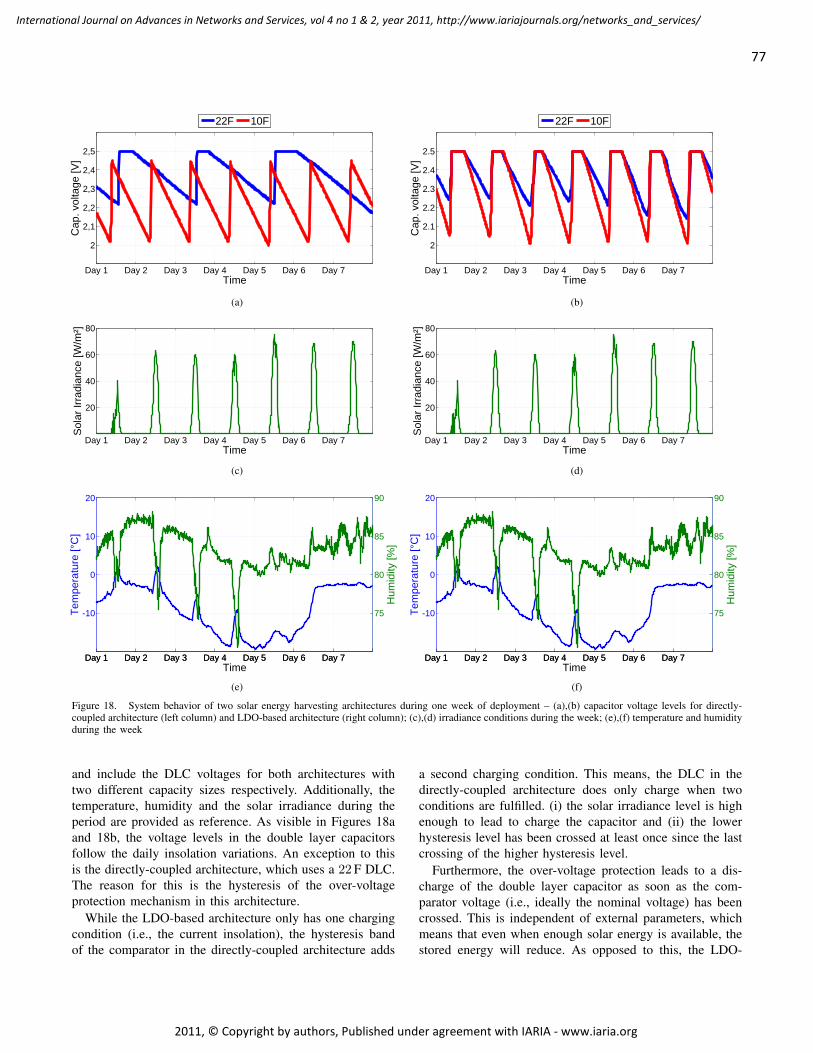
Day 1 Day 2 Day 3 Day 4 Day 5 Day 6 Day 7
2
2,1
2,2
2,3
2,4
2,5
Time
Cap
. vol
tage
[V]
22F 10F
(a)
Day 1 Day 2 Day 3 Day 4 Day 5 Day 6 Day 7
2
2.1
2.2
2.3
2.4
2.5
Time
Cap
. vol
tage
[V]
22F 10F
(b)
Day 1 Day 2 Day 3 Day 4 Day 5 Day 6 Day 7
20
40
60
80
Time
Sol
ar Ir
radi
ance
[W/m
²]
(c)
Day 1 Day 2 Day 3 Day 4 Day 5 Day 6 Day 7
20
40
60
80
Time
Sol
ar Ir
radi
ance
[W/m
²]
(d)
Day 1 Day 2 Day 3 Day 4 Day 5 Day 6 Day 7
-10
0
10
20
Tem
pera
ture
[°C
]
TimeDay 1 Day 2 Day 3 Day 4 Day 5 Day 6 Day 7
75
80
85
90
Hum
idity
[%]
(e)
Day 1 Day 2 Day 3 Day 4 Day 5 Day 6 Day 7
-10
0
10
20
Tem
pera
ture
[°C
]
TimeDay 1 Day 2 Day 3 Day 4 Day 5 Day 6 Day 7
75
80
85
90
Hum
idity
[%]
(f)
Figure 18. System behavior of two solar energy harvesting architectures during one week of deployment – (a),(b) capacitor voltage levels for directly-coupled architecture (left column) and LDO-based architecture (right column); (c),(d) irradiance conditions during the week; (e),(f) temperature and humidityduring the week
and include the DLC voltages for both architectures withtwo different capacity sizes respectively. Additionally, thetemperature, humidity and the solar irradiance during theperiod are provided as reference. As visible in Figures 18aand 18b, the voltage levels in the double layer capacitorsfollow the daily insolation variations. An exception to thisis the directly-coupled architecture, which uses a 22F DLC.The reason for this is the hysteresis of the over-voltageprotection mechanism in this architecture.
While the LDO-based architecture only has one chargingcondition (i.e., the current insolation), the hysteresis bandof the comparator in the directly-coupled architecture adds
a second charging condition. This means, the DLC in thedirectly-coupled architecture does only charge when twoconditions are fulfilled. (i) the solar irradiance level is highenough to lead to charge the capacitor and (ii) the lowerhysteresis level has been crossed at least once since the lastcrossing of the higher hysteresis level.
Furthermore, the over-voltage protection leads to a dis-charge of the double layer capacitor as soon as the com-parator voltage (i.e., ideally the nominal voltage) has beencrossed. This is independent of external parameters, whichmeans that even when enough solar energy is available, thestored energy will reduce. As opposed to this, the LDO-
77
International Journal on Advances in Networks and Services, vol 4 no 1 & 2, year 2011, http://www.iariajournals.org/networks_and_services/
2011, © Copyright by authors, Published under agreement with IARIA - www.iaria.org
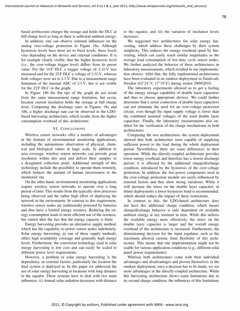
based architecture charges the storage and holds the DLC atfull charge level as long as there is sufficient ambient energy.
In addition, one can observe external influences on theanalog over-voltage protection in Figure 18a. Althoughhysteresis levels have been set to fixed levels, these levelsvary depending on the device and external conditions. It isfor example clearly visible, that the higher hysteresis level(i.e., the over-voltage trigger level) differs from its presetvalue. For the 10F DLC a trigger voltage of 2.45V wasmeasured and for the 22F DLC a voltage of 2.55V, whereasboth voltages were set to 2.5V. Due to a measurement rangelimitation of the internal ADC of 2.5V, this is not visiblefor the 22F DLC in the graph.
In Figure 18b the flat tips of the graph do not resultfrom the same measurement range limitation, but occur,because current insolation holds the storage at full chargelevel. Comparing the discharge rates in Figures 18a and18b, a higher discharge rate can be observed in the LDO-based harvesting architecture, which results from the higherconsumption overhead of this architecture.
VI. CONCLUSIONS
Wireless sensor networks offer a number of advantagesin the domain of environmental monitoring applications,including the autonomous observation of physical, chem-ical and biological values at large scale. In addition toarea coverage, wireless sensor networks can provide greatresolution within this area and deliver their samples toa designated collection point. Additional strength of thistechnology include the possibility to operate them remotely,which reduces the amount of human invasiveness to themonitored site.
On the other hand, environmental monitoring applicationsrequire wireless sensor networks to operate over a longperiod of time. This results from the typically slow processesbeing observed and the rather high effort of deploying thenetwork in the environment. In contrast to this requirement,wireless sensor nodes are traditionally powered by batteriesand thus have a limited energy resource. Reducing the en-ergy consumption leads to more efficient use of the resource,but cannot alter the fact that the energy capacity is finite.
Energy harvesting provides an alternative supply method,which has the capability to power sensor nodes indefinitely.Solar energy harvesting, as one of these supply methods,offers high availability coverage and generally high energylevels. Furthermore, the conversion technology used in solarenergy harvesting is low cost and can easily be scaled todifferent power level requirements.
However, a problem in solar energy harvesting is thedependency on external factors, particularly the location thefinal system is deployed in. In this paper we addressed theuse of solar energy harvesting at locations with long distanceto the equator. These systems have to deal with two maininfluences. (i) Annual solar radiation decreases with distance
to the equator, and (ii) the variation of insolation levelsincreases.
We suggested two architectures for solar energy har-vesting, which address these challenges by their systemsimplicity. This reduces the energy overhead spent by har-vesting, which can easily reach similar magnitudes as theaverage load consumption of low-duty cycle sensor nodes.We further analyzed the behavior of these architectures inlaboratory measurements, which resulted in our implementa-tion choices. After that, the fully implemented architectureshave been evaluated in an outdoor deployment in Sundsvall,Sweden (6224′N, 1719′E) during winter 2009/2010.
The laboratory experiments allowed us to get a feelingof the energy storage capability of double layer capacitorsand thus to choose appropriate devices. We could furtherdetermine that a serial connection of double layer capacitorscan not eliminate the need for an over-voltage protectioncircuit, even though the input supply voltage is lower thanthe combined nominal voltages of the used double layercapacitors. Finally, the laboratory measurements also en-abled for the verification of the charge mechanisms in botharchitectures.
Comparing the two architectures, the system deploymentshowed that both architecture were capable of supplyingsufficient power to the load during the whole deploymentperiod. Nevertheless, there are some differences in theiroperation. While the directly-coupled architecture provideslower energy overhead, and therefore has a slower dischargeperiod, it is affected by the additional charge/dischargecondition, introduced by the hysteresis of the over-voltageprotection. In addition, the low-power components used inthe over-voltage protection module are easily influenced byexternal factors and thus show strong variations. While itwill increase the stress on the double layer capacitor, infuture deployments a lower hysteresis band is recommended,which should reduce the impact of these restrictions.
In contrast to this, the LDO-based architecture doesnot have this additional charge condition, which meanscharge/discharge behavior is only dependent on availableambient energy at any moment in time. While this utilizesthe available energy more effectively, the stress on thedouble layer capacitor is larger and the overall energyoverhead of the architecture is increased. Furthermore, thedimensioning decision for the input regulator, such as themaximum allowed current, limit flexibility of this archi-tecture. This means that one implementation might not beusable for various application conditions (e.g., different solarpanel power requirements).
Whereas both architectures come with their individualadvantages and disadvantages and proven themselves in theoutdoor deployment, once a decision has to be made, we seemore advantages in the directly-coupled architecture. Whilethis harvesting architecture shows some limitations due toits second charge condition, the influences of this limitations
78
International Journal on Advances in Networks and Services, vol 4 no 1 & 2, year 2011, http://www.iariajournals.org/networks_and_services/
2011, © Copyright by authors, Published under agreement with IARIA - www.iaria.org
can be reduced by reducing the hysteresis of its over-voltageprotection. Moreover, the system is more flexible to changesin application and location constraints and thus enables for agreater variety of application cases. Finally, its overall lowerenergy overhead allows for operation during longer dark-periods.
In future work, balancing of annual variations in theambient energy income is a topic of interest. This can beaddressed both, on the hardware and the software level.Furthermore, we will look in more detail into the issueof maximum-power-point-tracking for harvesting from lowambient energy sources.
ACKNOWLEDGMENT
Financial support of the project “Sensible Things thatCommunicate” by KK-foundation is gratefully acknowl-edged. Furthermore we would like to thank Torsten Scholzelfrom Solarwatt AG, Germany, for contributions supportingthe work in this paper.
REFERENCES
[1] S. Bader and B. Oelmann, “Enabling battery-less wirelesssensor operation using solar energy harvesting at locationswith limited solar radiation,” in Fourth International Con-ference on Sensor Technologies and Applications, SENSOR-COMM ’10, 2010.
[2] A. Mainwaring, D. Culler, J. Polastre, R. Szewczyk, andJ. Anderson, “Wireless sensor networks for habitat monitor-ing,” Proceedings of the 1st ACM international workshop onWireless sensor networks and applications, pp. 88–97, 2002.
[3] J. Porter, P. Arzberger, H.-W. Braun, P. Bryant, S. Gage,T. Hansen, P. Hanson, C.-C. Lin, F.-P. Lin, T. Kratz, W. Mich-ener, S. Shapiro, and T. Williams, “Wireless Sensor Networksfor Ecology,” BioScience, vol. 55, no. 7, pp. 561–572, 2005.
[4] J. Hart and K. Martinez, “Environmental Sensor Networks:A revolution in the earth system science?” Earth-ScienceReviews, vol. 78, no. 3-4, pp. 177–191, Oct. 2006.
[5] G. Werner-Allen, J. Johnson, M. Ruiz, J. Lees, and M. Welsh,“Monitoring volcanic eruptions with a wireless sensor net-work,” in Proceeedings of the Second European Workshopon Wireless Sensor Networks, 2005, pp. 108–120.
[6] K. Martinez, P. Padhy, A. Elsaify, G. Zou, A. Riddoch, andJK, “Deploying a sensor network in an extreme environment,”Sensor Networks, Ubiquitous and Trustworthy Computing,June, 2006.
[7] T. Le Dinh, W. Hu, P. Sikka, P. Corke, L. Overs, andS. Brosnan, “Design and deployment of a remote robustsensor network: Experiences from an outdoor water qualitymonitoring network,” in 32nd IEEE Conference on LocalComputer Networks, 2007. LCN 2007, 2007, pp. 799–806.
[8] J. Paradiso and T. Starner, “Energy Scavenging for Mobileand Wireless Electronics,” IEEE Pervasive Computing, vol. 4,no. 1, pp. 18–27, Jan. 2005.
[9] “U.s. energy information administration – website,” http://www.eia.doe.gov, (accessed 02-08-2010).
[10] K. Martinez, R. Ong, and J. Hart, “Glacsweb: a sensornetwork for hostile environments,” 2004 First Annual IEEECommunications Society Conference on Sensor and Ad HocCommunications and Networks, 2004. IEEE SECON 2004.,pp. 81–87, 2004.
[11] T. Wark, W. Hu, P. Corke, J. Hodge, A. Keto, B. Mackey,G. Foley, P. Sikka, and M. Brunig, “Springbrook: Challengesin developing a long-term, rainforest wireless sensor net-work,” 2008 International Conference on Intelligent Sensors,Sensor Networks and Information Processing, pp. 599–604,2008.
[12] R. Morais, S. Matos, M. Fernandes, A. Valente, S. Soares,P. Ferreira, and M. Reis, “Sun, wind and water flow asenergy supply for small stationary data acquisition platforms,”Computers and Electronics in Agriculture, vol. 64, no. 2, pp.120–132, Dec. 2008.
[13] R. Torah, P. Glynne-Jones, J. Tudor, T. O’Donnell, S. Roy, andS. Beeby, “Self-powered autonomous wireless sensor nodeusing vibration energy harvesting,” Measurement Science andTechnology, vol. 19, no. 12, October 2008.
[14] C. J. Love, S. Zhang, and A. Mershin, “Source of sustainedvoltage difference between the xylem of a potted ¡italic¿ficusbenjamina¡/italic¿ tree and its soil,” PLoS ONE, vol. 3, no. 8,p. e2963, 08 2008.
[15] C. Knight and M. Collins, “Results of a water based ther-moelectric energy harvesting device for powering wirelesssensor nodes,” in Proc. SPIE 7288 – Active and Passive SmartStructures and Integrated Systems, 2009.
[16] X. Jiang, J. Polastre, and D. Culler, “Perpetual environmen-tally powered sensor networks,” in Proceedings of the 4thinternational symposium on Information processing in sensornetworks, 2005, pp. 463–468.
[17] V. Raghunathan, A. Kansal, J. Hsu, J. Friedman, and M. Sri-vastava, “Design considerations for solar energy harvestingwireless embedded systems,” in Proceedings of the 4th in-ternational symposium on Information processing in sensornetworks, 2005, pp. 457 – 462.
[18] F. Simjee and P. Chou, “Everlast: long-life, supercapacitor-operated wireless sensor node,” in Proceedings of the 2006international symposium on Low power electronics and de-sign, 2006, pp. 197 – 202.
[19] C. Park and P. Chou, “Ambimax: Autonomous energy har-vesting platform for multi-supply wireless sensor nodes,” in3rd Annual IEEE Communications Society on Sensor and AdHoc Communications and Networks, 2006, pp. 168–177.
[20] P. Corke, P. Valencia, P. Sikka, T. Wark, and L. Overs,“Long-duration solar-powered wireless sensor networks,” inEmNets ’07: Proceedings of the 4th workshop on Embeddednetworked sensors. ACM, 2007, pp. 33–37.
[21] C. Alippi and C. Galperti, “An adaptive system for optimalsolar energy harvesting in wireless sensor network nodes,”Circuits and Systems I: Regular Papers, IEEE Transactionson, vol. 55, no. 6, pp. 1742 –1750, jul. 2008.
79
International Journal on Advances in Networks and Services, vol 4 no 1 & 2, year 2011, http://www.iariajournals.org/networks_and_services/
2011, © Copyright by authors, Published under agreement with IARIA - www.iaria.org
[22] D. Kruger, C. Buschmann, and S. Fischer, “Solar poweredsensor network design and experimentation,” in ISWCS’09:Proceedings of the 6th international conference on Sympo-sium on Wireless Communication Systems. IEEE Press, 2009,pp. 11–15.
[23] J. Alberola, J. Pelegri, R. Lajara, and J. Perez, “Solarinexhaustible power source for wireless sensor node,” inInstrumentation and Measurement Technology ConferenceProceedings, 2008. IMTC 2008. IEEE, 2008, pp. 657 –662.
[24] T. Esram and P. L. Chapman, “Comparison of PhotovoltaicArray Maximum Power Point Tracking Techniques,” IEEETransactions on Energy Conversion, vol. 22, no. 2, pp. 439–449, Jun. 2007.
[25] J. Taneja, J. Jeong, and D. Culler, “Design, modeling, andcapacity planning for micro-solar power sensor networks,” inProceedings of the 7th international conference on Informa-tion processing in sensor networks, 2008, pp. 407–418.
[26] W. S. Wang, T. O’Donnell, L. Ribetto, B. O’Flynn, M. Hayes,and S. C. O’Mathuna, “Energy harvesting embedded wire-less sensor system for building environment applications,”in 1st International Conference on Wireless Communication,Vehicular Technology, Information Theory and Aerospace &Electronic Systems Technology 2009,. IEEE, 2009.
[27] A. Kansal, J. Hsu, S. Zahedi, and M. B. Srivastava, “Powermanagement in energy harvesting sensor networks,” ACMTrans. Embed. Comput. Syst., vol. 6, no. 4, p. 32, 2007.
[28] D. Linden and T. Reddy, Handbook of Batteries. McGraw-Hill Professional, 2001.
[29] “Nasa/giss atmosphere-ocean model – website,” http://aom.giss.nasa.gov/srlocat.htm, (accessed 17-12-2010).
[30] PowerStor B-Series (Datasheet 4307), Cooper Bussmann,2008.
[31] PowerStor Application Guidelines (PS-5006), Cooper Buss-mann, 2007.
[32] “Sentio series of sensor nodes – website,” http://www.miun.se/stc/Sentio, (accessed 14-01-2011).
[33] MGSF1N02ELT1 N-channel Mosfet, ON Semiconductor,2000.
[34] MBR0520L Shottky Rectifier, Fairchild Semiconductor, 2001.
80
International Journal on Advances in Networks and Services, vol 4 no 1 & 2, year 2011, http://www.iariajournals.org/networks_and_services/
2011, © Copyright by authors, Published under agreement with IARIA - www.iaria.org
TrickleTree: A Gossiping Approach To Fast AndCollision Free Staggered Scheduling
Wojciech Bober, Chris J. Bleakley, Xiaoyun LiUCD Complex & Adaptive Systems Laboratory
UCD School of Computer Science and InformaticsUniversity College DublinBelfield, Dublin 4, Ireland
wojciech.bober, xiaoyun.li, [email protected]
Abstract—In recent years, data gathering has received signif-icant attention as an application of Wireless Sensor Networks(WSNs). Staggered data tree based protocols have been shown tobe successful in reducing energy consumption in data gatheringscenarios. An important part of staggered protocols is theprocess of schedule construction. In order to minimize energyconsumption, this process must be fast. In this paper, we presentTrickleTree, a fast distributed protocol for establishing staggeredand collision free communication schedule. TrickleTree has threefunctions: to establish routes, i.e., construct a data gathering tree,to establish a staggered communication schedule, i.e, assign timeslots to links, and to disseminate the maximal tree depth in thenetwork. To minimize network setup time, TrickleTree combinesneighborhood discovery and schedule construction into one step.To ensure that good neighbors are discovered before a node joinsthe network, TrickleTree uses a rating mechanism. Collisionsduring node association are reduced by using association slots. Toincrease the message delivery rate with small message overhead,TrickleTree uses adaptive gossiping. We provide a formal analysisof the protocol properties i.e., collision free scheduling andtermination. The behavior of the proposed approach is evaluatedin simulation. The results show up to 90% in a reduction inschedule setup time and a 50% reduction of duty cycle comparedto a flooding approach.
Index Terms—Wireless sensor networks, staggered schedule,schedule construction, fast association, collisions reduction, asso-ciation ranking
I. INTRODUCTION
This paper is an extended version of [1]. It contains amodified version of the previously proposed algorithm. Itcontains analysis of the algorithm with proofs of terminationand collision free slot assignment. Additional simulations wereadded for in-depth evaluation of the algorithm.
The promise of cheap sensors deployed at large scale isattractive for areas such us microclimate research [1], andhabitat monitoring [2]. Precise observations produce largequantities of data, that must be transmitted via the network.In addition, these networks are often expected to operate forlong periods of time. Although various methods of energyharvesting have been proposed [3], so far using a batteryis the most common method of powering nodes. Dutta etal. [4] have shown that radio operation is the main causeof power consumption. Therefore, communication protocolswhich reduce radio on-time are crucial for achieving the goalof long network lifetime.
Data gathering networks are characterized by a many to onetraffic pattern. A common approach to routing in this class ofnetworks is tree based routing. In tree base routing, a nodeselects a node closer to the sink as its parent. All messagesare forwarded only to this node. In order to improve energy-efficiency and data latency a staggered approach has beenproposed. In this approach, communication between nodes isscheduled according to their level in the tree (i.e., hop countfrom the root). Only two consecutive levels off the tree areactive at any given time. Hence all nodes in the network mustbe aware of the maximal tree depth in order to schedule theircommunication correctly. The quality of wireless links canchange considerably in a short amount of time [5]. This meansa new schedule must be established each time the networktopology changes. Therefore it is important that a staggeredschedule is established quickly, so that the cost of controldoes not exceed the cost of data transmission. We addressthis problem by proposing TrickleTree, a protocol designed toestablish staggered schedule quickly, yet with a small messageoverhead.
TrickleTree differs from existing protocols, in that it com-bines neighborhood discovery and schedule construction intoone step. This reduces the number of messages which must beexchanged. To ensure that a balanced schedule is constructed,TrickleTree carefully selects the time at which a node starts itsassociation process. This is done by delaying the associationprocess accordingly to a ranking function. The function takesinto consideration link quality and the number of potentialparents. To reduce the likelihood of a node becoming anorphan these factors are weighted accordingly to the numberof messages received by the node.
TrickleTree is based on gossiping, which is a simple butrobust and reliable technique of information dissemination.We show how this technique can be applied to establish astaggered schedule. Thanks to adaptive mechanisms derivedfrom the gossiping approach, we are able to balance the delayand communication overhead (energy consumption) requiredto establish the network tree and communication schedule.TrickleTree is able to derive a collision free schedule, thereforeenergy is not wasted resolving collisions during the datagathering phase. To the authors’ knowledge, this is the firstprotocol for establishing staggered communication schedules.
81
International Journal on Advances in Networks and Services, vol 4 no 1 & 2, year 2011, http://www.iariajournals.org/networks_and_services/
2011, © Copyright by authors, Published under agreement with IARIA - www.iaria.org
The contribution of the work is a novel algorithm whichhas three functions: 1) to establish communication routes, i.e,construct data gathering tree, 2) to establish a collision freestaggered communication schedule, i.e., assign time slots tonodes, 3) and to disseminate the maximal tree depth in thenetwork.
The rest of the paper is structured as follows. In section IIwe discuss related work. Section III, describes the proposedprotocol. In Section IV we provide proof of collision freescheduling and algorithm termination. Section V presentssimulation results. We conclude the paper with Section VI.
II. RELATED WORK
In this section, we discuss two categories of protocolsrelated to TrickleTree. The first category are protocols whichcan be used to create staggered schedule. The second, isa category of protocols used to disseminate information inWireless Sensor Networks.
A. Staggered scheduling protocols
Staggered scheduling was first introduced in D-MAC byLu [7]. In D-MAC, transmission times are staggered in veryshort time slots. This reduces latency and end-to-end deliverytime because the receiver is guaranteed to be awake at thetime of the sender’s transmission. Because nodes with at samenetwork depth have the same transmission time offset theymust to compete for the channel. A CSMA scheme is used todeal with collisions. The authors do not discuss many practicalissues related to the protocol. For example, how nodes learnthe maximal routing tree depth in order to calculate their wake-up offset.
A similar concept is used in Merlin [8], a cross-layerprotocol integrating MAC and routing. In Merlin staggeredscheduling is used for up- and down-link traffic.
TIGRA [9] is a protocol designed for periodic collection ofraw data from the network. The authors focus on minimizationof the time required to collect the data from the entire network.The collection time is reduced by two techniques. Firstly,data from separate packets is merged into one packet. Note,this is different from data aggregation, where a single valueis calculated to represent data from a number of sources.Secondly, collisions are eliminated by ensuring interference-free transmission scheduling.
ASLEEP [10] is a data gathering protocol focusing onreducing message latency. ASLEEP, like TIGRA, uses stag-gered data gathering to reduce latency. The protocol is able toadapt to varying bandwidth requirements by run-time scheduleadjustment. ASLEEP adjusts the active radio time at each levelof the tree. Schedule modification is made based on previoustraffic trends. If bandwidth requirements are increasing overa certain period of time, then the active period is extended,otherwise the active period is decreased.
In [6], staggered scheduling was combined with syn-chronous low power listening to reduce energy consumptionin low rate data collection networks. Figure1 illustrates theconcept of a staggered schedule implemented in Bailigh [6].
The network is organized as a tree. Each node has exactlyone parent, which forwards data to the tree root (the sink).Nodes at the same distance from the sink (hop count) are atthe same level. At any time only two consecutive levels of thetree are active. In the example, nodes A, B and C, at Level2 transmit data to nodes D and E, at Level 1, using links1, 2, and 4. This approach reduces delivery latency becausemessages are almost immediately forwarded. When the slotsare guaranteed to be collision and contention free there is nodelay due to backoff, as would occur in a CSMA protocol.However, in the case of distributed scheduling, links 1 and 4sometimes might use the same time slot. If nodes C and Dare in radio communication range this may lead to collision.This is an example of the hidden terminal problem in presentin networks using staggered scheduling.
B. Dissemination protocols
When all nodes in the network must share common in-formation, message dissemination is necessary. Early systemsused packet floods to disseminate common information suchas parameters or commands. Flooding protocols rebroadcastpackets they receive [11]. This is a very simple method,which has many disadvantages. Firstly, flooding is unreliable.Due to collisions, some nodes do not receive the information,so typically flooding is repeated. This leads to excessive re-broadcasting and is energy inefficient. To overcome this prob-lem, adaptive protocols have been introduced. They modifynode behavior depending on the information they receive.Dissemination protocols which have proven to work reliablyin Wireless Sensor Networks are based on gossiping. Trickle[12] was the first proof of concept implementation designed forcode dissemination. Trickle is an adaptive gossiping protocol.When nodes detect inconsistent information in the network,they broadcast new information quickly. When nodes agree,they slow down their communication rate exponentially, suchthat, when in a stable state, they transmit infrequently. Basedon this concept, dissemination protocols have been proposedfor various applications [13], [14]. TrickleTree is a modifica-tion of Trickle used to construct a staggered scheduling tree.We use adaptive beaconing for neighborhood discovery andtree depth dissemination.
TrickleTree is able to minimize collisions between nodes inthe tree by scheduling individual transmission slots. We use2-hop neighborhood information about scheduled time slotsto reduce collisions. This technique is often used in TDMAMAC protocols [15]. Fang-Jing Wu [16] shows how collision-free scheduling can be taken advantage of tree based networks.
III. TRICKLETREE PROTOCOL
TrickleTree uses three types of packets Beacon (BCN), JoinRequest (JREQ) and Join Reply (JREP). Each packet containsa source and destination address. A BCN packet contains thesender’s distance from the sink (hop count), parent address,slot number, and the maximal tree depth known to the node,and number of free slots. A JREQ packet contains the samefields. JREP contains the slot number assigned by the parent
82
International Journal on Advances in Networks and Services, vol 4 no 1 & 2, year 2011, http://www.iariajournals.org/networks_and_services/
2011, © Copyright by authors, Published under agreement with IARIA - www.iaria.org
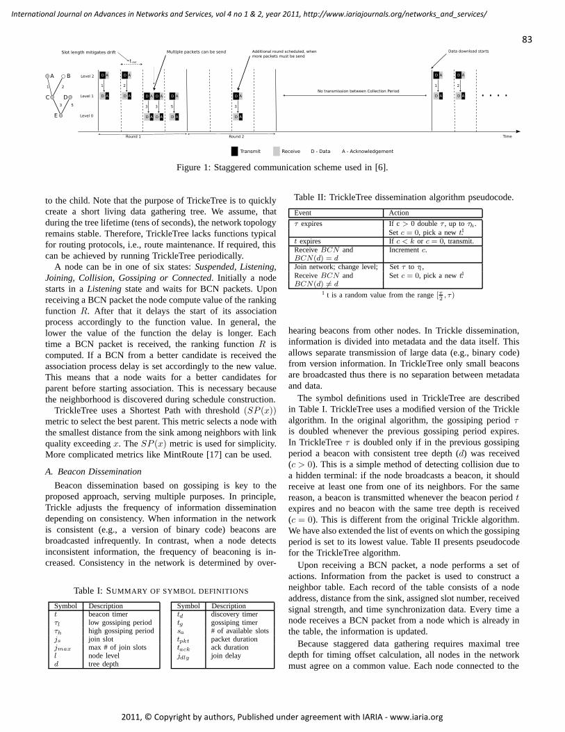
Figure 1: Staggered communication scheme used in [6].
to the child. Note that the purpose of TrickeTree is to quicklycreate a short living data gathering tree. We assume, thatduring the tree lifetime (tens of seconds), the network topologyremains stable. Therefore, TrickleTree lacks functions typicalfor routing protocols, i.e., route maintenance. If required, thiscan be achieved by running TrickleTree periodically.
A node can be in one of six states: Suspended, Listening,Joining, Collision, Gossiping or Connected. Initially a nodestarts in a Listening state and waits for BCN packets. Uponreceiving a BCN packet the node compute value of the rankingfunction R. After that it delays the start of its associationprocess accordingly to the function value. In general, thelower the value of the function the delay is longer. Eachtime a BCN packet is received, the ranking function R iscomputed. If a BCN from a better candidate is received theassociation process delay is set accordingly to the new value.This means that a node waits for a better candidates forparent before starting association. This is necessary becausethe neighborhood is discovered during schedule construction.
TrickleTree uses a Shortest Path with threshold (SP (x))metric to select the best parent. This metric selects a node withthe smallest distance from the sink among neighbors with linkquality exceeding x. The SP (x) metric is used for simplicity.More complicated metrics like MintRoute [17] can be used.
A. Beacon Dissemination
Beacon dissemination based on gossiping is key to theproposed approach, serving multiple purposes. In principle,Trickle adjusts the frequency of information disseminationdepending on consistency. When information in the networkis consistent (e.g., a version of binary code) beacons arebroadcasted infrequently. In contrast, when a node detectsinconsistent information, the frequency of beaconing is in-creased. Consistency in the network is determined by over-
Table I: SUMMARY OF SYMBOL DEFINITIONS
Symbol Description Symbol Descriptiont beacon timer td discovery timerτl low gossiping period tg gossiping timerτh high gossiping period sa # of available slotsjs join slot tpkt packet durationjmax max # of join slots tack ack durationl node level jdly join delayd tree depth
Table II: TrickleTree dissemination algorithm pseudocode.
Event Action
τ expires If c > 0 double τ , up to τh.Set c = 0, pick a new t1.
t expires If c < k or c = 0, transmit.Receive BCN and Increment c.BCN(d) = dJoin network; change level; Set τ to τl ,Receive BCN and Set c = 0, pick a new t1.BCN(d) = d
1 t is a random value from the range [τ2, τ)
hearing beacons from other nodes. In Trickle dissemination,information is divided into metadata and the data itself. Thisallows separate transmission of large data (e.g., binary code)from version information. In TrickleTree only small beaconsare broadcasted thus there is no separation between metadataand data.
The symbol definitions used in TrickleTree are describedin Table I. TrickleTree uses a modified version of the Tricklealgorithm. In the original algorithm, the gossiping period τis doubled whenever the previous gossiping period expires.In TrickleTree τ is doubled only if in the previous gossipingperiod a beacon with consistent tree depth (d) was received(c > 0). This is a simple method of detecting collision due toa hidden terminal: if the node broadcasts a beacon, it shouldreceive at least one from one of its neighbors. For the samereason, a beacon is transmitted whenever the beacon period texpires and no beacon with the same tree depth is received(c = 0). This is different from the original Trickle algorithm.We have also extended the list of events on which the gossipingperiod is set to its lowest value. Table II presents pseudocodefor the TrickleTree algorithm.
Upon receiving a BCN packet, a node performs a set ofactions. Information from the packet is used to construct aneighbor table. Each record of the table consists of a nodeaddress, distance from the sink, assigned slot number, receivedsignal strength, and time synchronization data. Every time anode receives a BCN packet from a node which is already inthe table, the information is updated.
Because staggered data gathering requires maximal treedepth for timing offset calculation, all nodes in the networkmust agree on a common value. Each node connected to the
83
International Journal on Advances in Networks and Services, vol 4 no 1 & 2, year 2011, http://www.iariajournals.org/networks_and_services/
2011, © Copyright by authors, Published under agreement with IARIA - www.iaria.org
network disseminates the maximal tree depth it currently holdsin the BCN packet. If a node overhears a BCN packet whichhas a maximal tree depth field value greater than its currenttree depth value, the node updates its current tree depth to thereceived value. It then resets the counter c, sets τ to τ l andpicks up a new t value. This allows for fast disseminationof a new tree depth in the network. TrickleTree does nothave explicit mechanisms to check the consistency of the treedepth value. We rely on the general convergence property ofdissemination protocols based on gossiping.
Note that a node is allowed to participate in gossiping onlywhen it is in the Gossiping or Connected state, i.e., afterjoining the network. Initially only the sink node is able todisseminate beacons.
B. Node association
Most schedule based data gathering protocols build sched-ules based on data gathering tree. To build such a schedule,a parent - child relationship must be established betweennodes. To establish this relationship a node associates witha node closer to the sink. This node becomes the node’sparent. In the simplest case, a node starts the associationprocedure immediately or shortly after receiving a beaconfrom a potential parent. This method, used in [9], [18], isshown in Figure 2b. Although simple, there are two maindrawbacks of this method. Firstly, it relies on the MAC toresolve collisions. These collisions are caused by multiplenodes requesting association to the same node. Secondly, itdoes not take into consideration the quality of the link to aselected node. To address this issue, a threshold Th on thelink quality is often introduced. In this case, the associationprocess is started only when the link quality is above minimalthreshold. To address the former issue a method based onassociation slots was proposed in [19]. In this method, nodesuse time slots to perform the association process (Figure2b).Whenever a node wants to join the network, it selects a randomslot and starts the association process. Because the length ofthe slot is sufficient for the whole association process, i.e.,exchange of request and reply packets, collisions at the MAClayer are reduced. As in the previous methods, a threshold onlink quality is used to ensure that only good links are used.The method proposed herein improves on the method proposedin [19]. Instead of using a random slot, a node selects a slotaccording to a ranking function (1). The value of the functionis computed each time a BCN packet from a neighboring nodeis received. The function takes into consideration the signalquality σ, the degree of a node δ (defined as a number ofpotential parents), and the total number of beacons receivedβ. The aim of the function is to assign a higher rank i.e.,earlier join slot, to nodes which have a better link to the nodebroadcasting a beacon. It also takes into consideration howmany potential parents a node has, e.g., if a node has onlyone potential parent in its neighborhood its priority will behigher than a node with more potential parents, even if thelink quality is worse. The function uses the number of beaconsreceived from neighboring nodes as a weight for both factors.
As the number of beacons increases, degree of a node δ gainson significance. This is to reduce the number of orphan nodesand forced associations.
qσ =(σ − σL)
σH − σL, qδ =
(δ − δh)
δL − δHqβ =
(β − βL)
βH − βL
R(σ, δ, β) = (1− qβ)qσ + qβqδ (1)
Based on the value of the ranking function, a node calculatesassociation delay (2) and (3).
js = jmax(1−R) (2)
jd = 2(tpkt + tack)js (3)
Each BCN received by a node is an implicit synchronizationpoint. Each join slot is long enough to allow for JREQ andJREP exchange as well to mitigate for clock drift. If the JREQpacket is delivered successfully, the node will set up a JREPtimeout. Setting a timeout on the JREP prevents the node frominfinite waiting in the case that the selected node does notreply. This might happen when the potential parent fails beforeit manages to send a JREP. In the case of delivery failure, JREPtimeout, or join rejection, the node will return to the Listeningstate. It might happen, however, that two nodes will requestassociation in the same slot. This is more probable when nodedensity is high and the value of jmax is low. If both nodes arein the radio range, a node will detect an on going transmission.In this case the node will repeat the association procedureafter receiving the next beacon. If both nodes are not in theradio range, most likely their JREQ packet will collide. This isreported by the MAC layer. A node switches to Random modeand repeats the association procedure after receiving the nextbeacon.
A node accepts JREQ packets only when it is in theGossiping state. A parent node which receives a JREQ packetfrom a node selects an slot using Algorithm 1. The slot ismarked as used by the node which requests the join and aJREP packet is sent back. In the case that there are no freeslots left, the node will refuse to accept the join request andsend a JREP packet with the REFUSED flag set.
Upon receiving the JREP packet, the node cancels the JREPtimeout. If Collision Free (CF) mode is enabled, the nodecompares the assigned slot number with the slot numbersassigned to nodes stored in its neighbor table. If a node withthe same slot number at the same level exists, it indicates a slotcollision. In this case, the node enters the Collision state andinitiates a collision resolution procedure (see Section III-E).If a node with the same slot number does not exist or CFmode is disabled, the node stores the slot number and entersthe Gossiping state. Once connected, the node enables BCNpacket dissemination as described in Section III-A. It also setsa gossiping timer tg. This timer determines how long a nodemaintains in the Gossiping state. After the timer expires thenode enters the Connected state.
84
International Journal on Advances in Networks and Services, vol 4 no 1 & 2, year 2011, http://www.iariajournals.org/networks_and_services/
2011, © Copyright by authors, Published under agreement with IARIA - www.iaria.org
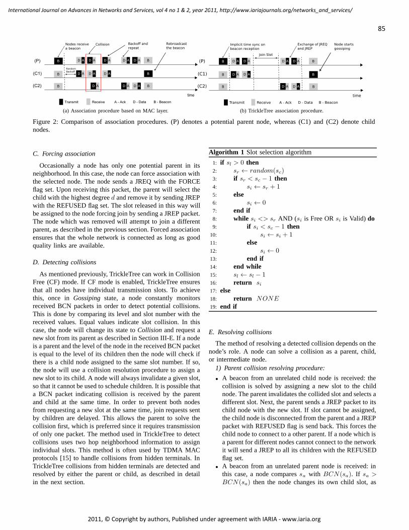
(a) Association procedure based on MAC layer.
Transmit Receive A - Ack D - Data B - Beacontime
(C1)
(P) B
B
(C2) B
B
B
B
D A
D A
D A
D AD A
D A
D A
D A
Implicit time sync onbeacon reception
Join Slot
Exchange of JREQand JREP
Node startsgossiping
(b) TrickleTree association procedure.
Figure 2: Comparison of association procedures. (P) denotes a potential parent node, whereas (C1) and (C2) denote childnodes.
C. Forcing association
Occasionally a node has only one potential parent in itsneighborhood. In this case, the node can force association withthe selected node. The node sends a JREQ with the FORCEflag set. Upon receiving this packet, the parent will select thechild with the highest degree d and remove it by sending JREPwith the REFUSED flag set. The slot released in this way willbe assigned to the node forcing join by sending a JREP packet.The node which was removed will attempt to join a differentparent, as described in the previous section. Forced associationensures that the whole network is connected as long as goodquality links are available.
D. Detecting collisions
As mentioned previously, TrickleTree can work in CollisionFree (CF) mode. If CF mode is enabled, TrickleTree ensuresthat all nodes have individual transmission slots. To achievethis, once in Gossiping state, a node constantly monitorsreceived BCN packets in order to detect potential collisions.This is done by comparing its level and slot number with thereceived values. Equal values indicate slot collision. In thiscase, the node will change its state to Collision and request anew slot from its parent as described in Section III-E. If a nodeis a parent and the level of the node in the received BCN packetis equal to the level of its children then the node will check ifthere is a child node assigned to the same slot number. If so,the node will use a collision resolution procedure to assign anew slot to its child. A node will always invalidate a given slot,so that it cannot be used to schedule children. It is possible thata BCN packet indicating collision is received by the parentand child at the same time. In order to prevent both nodesfrom requesting a new slot at the same time, join requests sentby children are delayed. This allows the parent to solve thecollision first, which is preferred since it requires transmissionof only one packet. The method used in TrickleTree to detectcollisions uses two hop neighborhood information to assignindividual slots. This method is often used by TDMA MACprotocols [15] to handle collisions from hidden terminals. InTrickleTree collisions from hidden terminals are detected andresolved by either the parent or child, as described in detailin the next section.
Algorithm 1 Slot selection algorithm
1: if sl > 0 then2: sr ← random(sc)3: if sr < sc − 1 then4: si ← sr + 15: else6: si ← 07: end if8: while si <> sr AND (si is Free OR si is Valid) do9: if si < sc − 1 then
10: si ← si + 111: else12: si ← 013: end if14: end while15: sl ← sl − 116: return si17: else18: return NONE19: end if
E. Resolving collisions
The method of resolving a detected collision depends on thenode’s role. A node can solve a collision as a parent, child,or intermediate node.
1) Parent collision resolving procedure:
• A beacon from an unrelated child node is received: thecollision is solved by assigning a new slot to the childnode. The parent invalidates the collided slot and selects adifferent slot. Next, the parent sends a JREP packet to itschild node with the new slot. If slot cannot be assigned,the child node is disconnected from the parent and a JREPpacket with REFUSED flag is send back. This forces thechild node to connect to a other parent. If a node which isa parent for different nodes cannot connect to the networkit will send a JREP to all its children with the REFUSEDflag set.
• A beacon from an unrelated parent node is received: inthis case, a node compares sa with BCN(sa). If sa >BCN(sa) then the node changes its own child slot, as
85
International Journal on Advances in Networks and Services, vol 4 no 1 & 2, year 2011, http://www.iariajournals.org/networks_and_services/
2011, © Copyright by authors, Published under agreement with IARIA - www.iaria.org
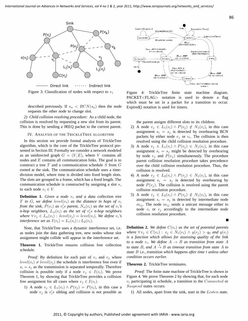
Figure 3: Classification of nodes with respect to vi
described previously. If sa < BCN(sa) then the noderequests the other node to change slot.
2) Child collision resolving procedure: As a child node, thecollision is resolved by requesting a new slot from its parent.This is done by sending a JREQ packet to the current parent.
IV. ANALYSIS OF THE TRICKLETREE ALGORITHM
In this section we provide formal analysis of TrickleTreealgorithm, which is the core of the TrickleTree protocol pre-sented in Section III. Formally we consider a network modeledas an unidirected graph G = (V,E), where V contains allnodes and E contains all communication links. The goal is toconstruct a tree T and a communication schedule S from Grooted at the sink. The communication schedule uses a time-division model, where time is divided into fixed length slots.The slots are grouped in a frame, which has a fixed length. Thecommunication schedule is constructed by assigning a slot s i
to each node vi ∈ V.
Definition 1. Given a node vi and a data collection treeT in G, we define level(vi) as the distance in hops of vifrom the sink, P (vi) as v′is parent, Nn(vi) as the set of vi’sn-hop neighbors, Ln(vi) as the set of v′is n-hop neighborswhere ∀ vj ∈ Ln(vi) : level(vj) = level(vi). We define vi’sinterference set as I(vi) = L1(vi) ∪ L2(vi).
Note, that TrickleTree uses a dynamic interference set, i.e.as nodes join the data gathering tree, new nodes whose slotassignment might collide will appear in the interference set.
Theorem 1. TrickleTree ensures collision free collectionschedule.
Proof: By definition for each pair of vi and vj wherelevel(vi) = level(vj) the schedule is interference free even ifsi = sj as the transmission is separated temporally. Thereforecollision is possible only if a node vj ∈ I(vi). We proveTheorem 1, by showing that TrickleTree provides a collisionfree assignment for all cases where vj ∈ I(vi).
1) A node vj ∈ L1(vi) ∧ P (vj) = P (vi), in this case anode vj is v′is sibling and collision is not possible as
Figure 4: TrickleTree finite state machine diagram.PACKET<FLAG> notation is used to denote a flagwhich must be set in a packet for a transition to occur.Expired() notation is used for timers.
the parent assigns different slots to its children.2) A node vj ∈ L1(vi) ∧ P (vj) /∈ N1(vi), in this case
assignment si = sj is detected by overhearing BCNpackets by either node vj or vi. The collision is thenresolved using the child collision resolution procedure.
3) A node vj ∈ L1(vi) ∧ P (vj) ∈ N1(vi), in this caseassignment si = sj might be detected by overhearingby node vj and P (vj) simultaneously. The procedureparent collision resolution procedure takes precedenceover the child collision resolution procedure. Thus, thecollision is resolved.
4) A node vj ∈ L2(vi) ∧ P (vj) ∈ N1(vi), in this caseassignment si = sj is detected by overhearing bynode P (vj). The collision is resolved using the parentcollision resolution procedure.
5) A node vj ∈ L2(vi) ∧ P (vj) /∈ N1(vi), in this caseassignment si = sj is detected by intermediate nodemij . The node mij sends a unicast message either tonode vi or vj accordingly to the intermediate nodecollision resolution procedure.
Definition 2. We define C(vi) as the set of potential parentswhere ∀ vj ∈ C(vi) : vj ∈ N1(vi) ∧ q(vj) > q0 and q(vi)is a function which allows for assessing quality of the linkto a node vi. We define A → B as transition from state A
to state B, and At→ B as timeout transition from state A to
state B i.e., transition which happens after time t unless othercondition occurs earlier.
Theorem 2. TrickleTree terminates.
Proof: The finite state machine of TrickleTree is shown inFigure 4. We prove Theorem 2 by showing that, for each nodevi participating in schedule, a transition to the Connected orSuspend states occurs.
1) All nodes, apart from the sink, start in the Listen state.
86
International Journal on Advances in Networks and Services, vol 4 no 1 & 2, year 2011, http://www.iariajournals.org/networks_and_services/
2011, © Copyright by authors, Published under agreement with IARIA - www.iaria.org
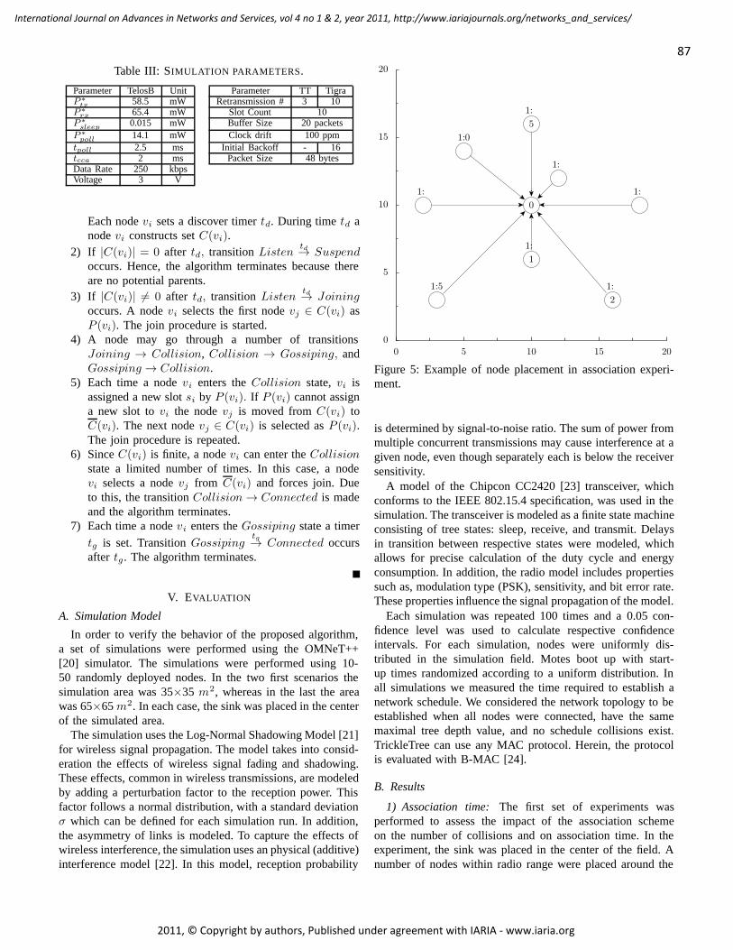
Table III: SIMULATION PARAMETERS.
Parameter TelosB Unit Parameter TT TigraP ∗tx 58.5 mW Retransmission # 3 10
P ∗rx 65.4 mW Slot Count 10
P ∗sleep 0.015 mW Buffer Size 20 packets
P ∗poll 14.1 mW Clock drift 100 ppm
tpoll 2.5 ms Initial Backoff - 16tcca 2 ms Packet Size 48 bytesData Rate 250 kbpsVoltage 3 V
Each node vi sets a discover timer td. During time td anode vi constructs set C(vi).
2) If |C(vi)| = 0 after td, transition Listentd→ Suspend
occurs. Hence, the algorithm terminates because thereare no potential parents.
3) If |C(vi)| = 0 after td, transition Listentd→ Joining
occurs. A node vi selects the first node vj ∈ C(vi) asP (vi). The join procedure is started.
4) A node may go through a number of transitionsJoining → Collision, Collision → Gossiping, andGossiping → Collision.
5) Each time a node vi enters the Collision state, vi isassigned a new slot si by P (vi). If P (vi) cannot assigna new slot to vi the node vj is moved from C(vi) toC(vi). The next node vj ∈ C(vi) is selected as P (vi).The join procedure is repeated.
6) Since C(vi) is finite, a node vi can enter the Collisionstate a limited number of times. In this case, a nodevi selects a node vj from C(vi) and forces join. Dueto this, the transition Collision→ Connected is madeand the algorithm terminates.
7) Each time a node vi enters the Gossiping state a timer
tg is set. Transition Gossipingtg→ Connected occurs
after tg . The algorithm terminates.
V. EVALUATION
A. Simulation Model
In order to verify the behavior of the proposed algorithm,a set of simulations were performed using the OMNeT++[20] simulator. The simulations were performed using 10-50 randomly deployed nodes. In the two first scenarios thesimulation area was 35×35 m2, whereas in the last the areawas 65×65 m2. In each case, the sink was placed in the centerof the simulated area.
The simulation uses the Log-Normal Shadowing Model [21]for wireless signal propagation. The model takes into consid-eration the effects of wireless signal fading and shadowing.These effects, common in wireless transmissions, are modeledby adding a perturbation factor to the reception power. Thisfactor follows a normal distribution, with a standard deviationσ which can be defined for each simulation run. In addition,the asymmetry of links is modeled. To capture the effects ofwireless interference, the simulation uses an physical (additive)interference model [22]. In this model, reception probability
0 5 10 15 200
5
10
15
20
0
:
1
1:
2
1:
1:
1:
5
1:
1:0
1:
1:5
Figure 5: Example of node placement in association experi-ment.
is determined by signal-to-noise ratio. The sum of power frommultiple concurrent transmissions may cause interference at agiven node, even though separately each is below the receiversensitivity.
A model of the Chipcon CC2420 [23] transceiver, whichconforms to the IEEE 802.15.4 specification, was used in thesimulation. The transceiver is modeled as a finite state machineconsisting of tree states: sleep, receive, and transmit. Delaysin transition between respective states were modeled, whichallows for precise calculation of the duty cycle and energyconsumption. In addition, the radio model includes propertiessuch as, modulation type (PSK), sensitivity, and bit error rate.These properties influence the signal propagation of the model.
Each simulation was repeated 100 times and a 0.05 con-fidence level was used to calculate respective confidenceintervals. For each simulation, nodes were uniformly dis-tributed in the simulation field. Motes boot up with start-up times randomized according to a uniform distribution. Inall simulations we measured the time required to establish anetwork schedule. We considered the network topology to beestablished when all nodes were connected, have the samemaximal tree depth value, and no schedule collisions exist.TrickleTree can use any MAC protocol. Herein, the protocolis evaluated with B-MAC [24].
B. Results
1) Association time: The first set of experiments wasperformed to assess the impact of the association schemeon the number of collisions and on association time. In theexperiment, the sink was placed in the center of the field. Anumber of nodes within radio range were placed around the
87
International Journal on Advances in Networks and Services, vol 4 no 1 & 2, year 2011, http://www.iariajournals.org/networks_and_services/
2011, © Copyright by authors, Published under agreement with IARIA - www.iaria.org
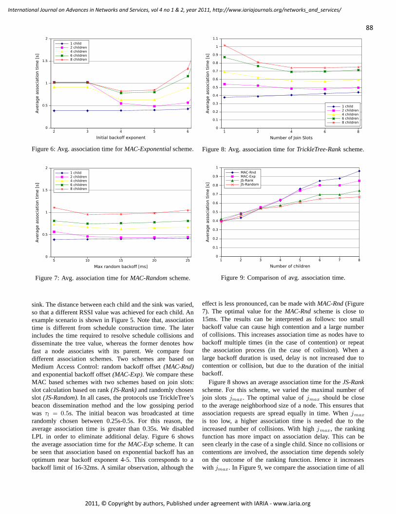
2 3 4 5 6
Initial backoff exponent
0
0.5
1
1.5
2Av
erag
e as
soci
atio
n tim
e [s
]1 child2 children4 children6 children8 children
Figure 6: Avg. association time for MAC-Exponential scheme.
5 10 15 20 25
Max random backoff [ms]
0
0.5
1
1.5
2
Aver
age
asso
ciat
ion
time
[s]
1 child2 children4 children6 children8 children
Figure 7: Avg. association time for MAC-Random scheme.
sink. The distance between each child and the sink was varied,so that a different RSSI value was achieved for each child. Anexample scenario is shown in Figure 5. Note that, associationtime is different from schedule construction time. The laterincludes the time required to resolve schedule collisions anddisseminate the tree value, whereas the former denotes howfast a node associates with its parent. We compare fourdifferent association schemes. Two schemes are based onMedium Access Control: random backoff offset (MAC-Rnd)and exponential backoff offset (MAC-Exp). We compare theseMAC based schemes with two schemes based on join slots:slot calculation based on rank (JS-Rank) and randomly chosenslot (JS-Random). In all cases, the protocols use TrickleTree’sbeacon dissemination method and the low gossiping periodwas τl = 0.5s. The initial beacon was broadcasted at timerandomly chosen between 0.25s-0.5s. For this reason, theaverage association time is greater than 0.35s. We disabledLPL in order to eliminate additional delay. Figure 6 showsthe average association time for the MAC-Exp scheme. It canbe seen that association based on exponential backoff has anoptimum near backoff exponent 4-5. This corresponds to abackoff limit of 16-32ms. A similar observation, although the
1 2 4 6 8
Number of Join Slots
0
0.1
0.2
0.3
0.4
0.5
0.6
0.7
0.8
0.9
1
1.1
Aver
age
asso
ciat
ion
time
[s]
1 child2 children4 children6 children8 children
Figure 8: Avg. association time for TrickleTree-Rank scheme.
1 2 3 4 5 6 7 8
Number of children
0
0.1
0.2
0.3
0.4
0.5
0.6
0.7
0.8
0.9
1
Aver
age
asso
ciat
ion
time
[s]
MAC-RndMAC-ExpJS-RankJS-Random
Figure 9: Comparison of avg. association time.
effect is less pronounced, can be made with MAC-Rnd (Figure7). The optimal value for the MAC-Rnd scheme is close to15ms. The results can be interpreted as follows: too smallbackoff value can cause high contention and a large numberof collisions. This increases association time as nodes have tobackoff multiple times (in the case of contention) or repeatthe association process (in the case of collision). When alarge backoff duration is used, delay is not increased due tocontention or collision, but due to the duration of the initialbackoff.
Figure 8 shows an average association time for the JS-Rankscheme. For this scheme, we varied the maximal number ofjoin slots jmax. The optimal value of jmax should be closeto the average neighborhood size of a node. This ensures thatassociation requests are spread equally in time. When jmax
is too low, a higher association time is needed due to theincreased number of collisions. With high jmax, the rankingfunction has more impact on association delay. This can beseen clearly in the case of a single child. Since no collisions orcontentions are involved, the association time depends solelyon the outcome of the ranking function. Hence it increaseswith jmax. In Figure 9, we compare the association time of all
88
International Journal on Advances in Networks and Services, vol 4 no 1 & 2, year 2011, http://www.iariajournals.org/networks_and_services/
2011, © Copyright by authors, Published under agreement with IARIA - www.iaria.org
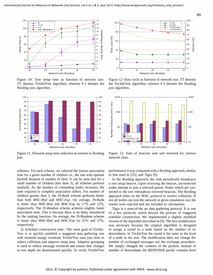
10 20 30 40 50
Network size [#nodes]
0
20
40
60
80
100
120Se
tup
Tim
e [s
]
0
1
2
3
4
5
6
7
8
9
10
11
12
13
Avg.
Num
ber o
f Nei
ghbo
rs
TTTT CFF+JAvg. #Neighbors
Figure 10: Tree setup time as function of network size.TT denotes TrickleTree algorithm, whereas F-J denotes theflooding join algorithm.
10 20 30 40 50
Network size (#nodes)
0
10
20
30
40
50
60
70
80
90
100
0
10
20
30
40
50
60
70
80
90
100
Tim
e Re
duct
ion
[%]
TT CFTT
Figure 11: Network setup time reduction in relation to floodingjoin.
schemes. For each scheme, we selected the lowest associationtime for a given number of children i.e., the one with optimalbackoff duration or number of slots. It can be seen that for asmall number of children (less than 3), all schemes performsimilarly. As the number of contending nodes increases, thetime required to complete association differs. For number ofchildren greater than 3, the JS-Rank scheme performs betterthan both MAC-Rnd and MAC-Exp. On average, JS-Rankis faster than MAC-Rnd and MAC-Exp by 17% and 12%,respectively. The JS-Random scheme achieves slightly fasterassociation time. This is because there is no delay introducedby the ranking function. On average, the JS-Random schemeis faster than MAC-Rnd and MAC-Exp by 21% and 17%,respectively.
2) Schedule construction time: The main goal of Trickle-Tree is to quickly establish a staggered data gathering treewith minimal energy overhead. TrickleTree uses join slots toreduce collisions and improve setup time. Adaptive gossipingis used to reduce message overhead and ensure that changesin tree depth are disseminated quickly. To verify TrickleTree
10 20 30 40 50
Network size [#nodes]
0
20
40
60
80
100
Dut
y cy
cle
[%]
0
10
20
30
40
50
60
70
80
90
100
Fairn
ess
[%]
TT DCF+J DCTT-FairnessF+J Fairness
Figure 12: Duty cycle as function of network size. TT denotesthe TrickleTree algorithm, whereas F-J denotes the floodingjoin algorithm.
10 20 30 40 50
Network size [#nodes]
10
100
1000
10000
10
100
1000
10000
Num
ber o
f bea
cons
sen
t + re
cv
TTTT CFFlooding + Join
Figure 13: Sum of beacons sent and received for variousnetwork sizes.
performance it was compared with a flooding approach, similarto that used in [25], and Tigra [9].
In the flooding approach, the sink periodically broadcastsa tree setup beacon. Upon receiving the beacon, unconnectednodes attempt to join a selected parent. Nodes which are con-nected to the tree rebroadcast received beacons. The floodingapproach relies on the MAC protocol to resolve collisions. Ifnot all nodes can join the network in given simulation run, theresults were rejected and not included in calculations.
Tigra is a state-of-the art data gathering protocol. It is oneof a few protocols which discuss the process of staggeredschedule construction. We implemented a slightly modifiedversion of the algorithm described in [9]. The first modificationwas necessary because the original algorithm is designedto assign a round to a node based on the number of itsdescendants. In TrickleTree the round is the same as the levelof a node in the tree. The modification does not change thenumber of exchanged messages nor the exchange procedure.We simply changed the contents of the packets. Instead ofnumber of descendants the RESPONSE packet contains level
89
International Journal on Advances in Networks and Services, vol 4 no 1 & 2, year 2011, http://www.iariajournals.org/networks_and_services/
2011, © Copyright by authors, Published under agreement with IARIA - www.iaria.org
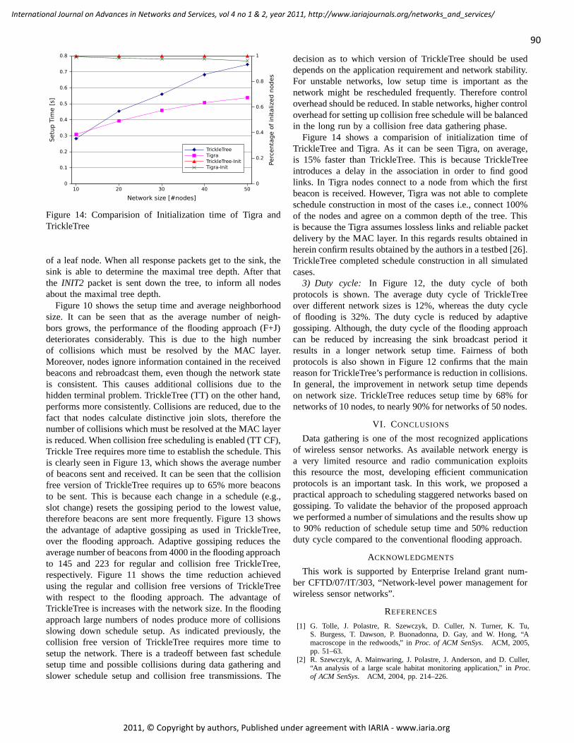
10 20 30 40 50Network size [#nodes]
0
0.1
0.2
0.3
0.4
0.5
0.6
0.7
0.8Se
tup
Tim
e [s
]
0
0.2
0.4
0.6
0.8
1
Perc
enta
ge o
f ini
taliz
ed n
odes
TrickleTreeTigraTrickleTree-InitTigra-Init
Figure 14: Comparision of Initialization time of Tigra andTrickleTree
of a leaf node. When all response packets get to the sink, thesink is able to determine the maximal tree depth. After thatthe INIT2 packet is sent down the tree, to inform all nodesabout the maximal tree depth.
Figure 10 shows the setup time and average neighborhoodsize. It can be seen that as the average number of neigh-bors grows, the performance of the flooding approach (F+J)deteriorates considerably. This is due to the high numberof collisions which must be resolved by the MAC layer.Moreover, nodes ignore information contained in the receivedbeacons and rebroadcast them, even though the network stateis consistent. This causes additional collisions due to thehidden terminal problem. TrickleTree (TT) on the other hand,performs more consistently. Collisions are reduced, due to thefact that nodes calculate distinctive join slots, therefore thenumber of collisions which must be resolved at the MAC layeris reduced. When collision free scheduling is enabled (TT CF),Trickle Tree requires more time to establish the schedule. Thisis clearly seen in Figure 13, which shows the average numberof beacons sent and received. It can be seen that the collisionfree version of TrickleTree requires up to 65% more beaconsto be sent. This is because each change in a schedule (e.g.,slot change) resets the gossiping period to the lowest value,therefore beacons are sent more frequently. Figure 13 showsthe advantage of adaptive gossiping as used in TrickleTree,over the flooding approach. Adaptive gossiping reduces theaverage number of beacons from 4000 in the flooding approachto 145 and 223 for regular and collision free TrickleTree,respectively. Figure 11 shows the time reduction achievedusing the regular and collision free versions of TrickleTreewith respect to the flooding approach. The advantage ofTrickleTree is increases with the network size. In the floodingapproach large numbers of nodes produce more of collisionsslowing down schedule setup. As indicated previously, thecollision free version of TrickleTree requires more time tosetup the network. There is a tradeoff between fast schedulesetup time and possible collisions during data gathering andslower schedule setup and collision free transmissions. The
decision as to which version of TrickleTree should be useddepends on the application requirement and network stability.For unstable networks, low setup time is important as thenetwork might be rescheduled frequently. Therefore controloverhead should be reduced. In stable networks, higher controloverhead for setting up collision free schedule will be balancedin the long run by a collision free data gathering phase.
Figure 14 shows a comparision of initialization time ofTrickleTree and Tigra. As it can be seen Tigra, on average,is 15% faster than TrickleTree. This is because TrickleTreeintroduces a delay in the association in order to find goodlinks. In Tigra nodes connect to a node from which the firstbeacon is received. However, Tigra was not able to completeschedule construction in most of the cases i.e., connect 100%of the nodes and agree on a common depth of the tree. Thisis because the Tigra assumes lossless links and reliable packetdelivery by the MAC layer. In this regards results obtained inherein confirm results obtained by the authors in a testbed [26].TrickleTree completed schedule construction in all simulatedcases.
3) Duty cycle: In Figure 12, the duty cycle of bothprotocols is shown. The average duty cycle of TrickleTreeover different network sizes is 12%, whereas the duty cycleof flooding is 32%. The duty cycle is reduced by adaptivegossiping. Although, the duty cycle of the flooding approachcan be reduced by increasing the sink broadcast period itresults in a longer network setup time. Fairness of bothprotocols is also shown in Figure 12 confirms that the mainreason for TrickleTree’s performance is reduction in collisions.In general, the improvement in network setup time dependson network size. TrickleTree reduces setup time by 68% fornetworks of 10 nodes, to nearly 90% for networks of 50 nodes.
VI. CONCLUSIONS
Data gathering is one of the most recognized applicationsof wireless sensor networks. As available network energy isa very limited resource and radio communication exploitsthis resource the most, developing efficient communicationprotocols is an important task. In this work, we proposed apractical approach to scheduling staggered networks based ongossiping. To validate the behavior of the proposed approachwe performed a number of simulations and the results show upto 90% reduction of schedule setup time and 50% reductionduty cycle compared to the conventional flooding approach.
ACKNOWLEDGMENTS
This work is supported by Enterprise Ireland grant num-ber CFTD/07/IT/303, “Network-level power management forwireless sensor networks”.
REFERENCES
[1] G. Tolle, J. Polastre, R. Szewczyk, D. Culler, N. Turner, K. Tu,S. Burgess, T. Dawson, P. Buonadonna, D. Gay, and W. Hong, “Amacroscope in the redwoods,” in Proc. of ACM SenSys. ACM, 2005,pp. 51–63.
[2] R. Szewczyk, A. Mainwaring, J. Polastre, J. Anderson, and D. Culler,“An analysis of a large scale habitat monitoring application,” in Proc.of ACM SenSys. ACM, 2004, pp. 214–226.
90
International Journal on Advances in Networks and Services, vol 4 no 1 & 2, year 2011, http://www.iariajournals.org/networks_and_services/
2011, © Copyright by authors, Published under agreement with IARIA - www.iaria.org
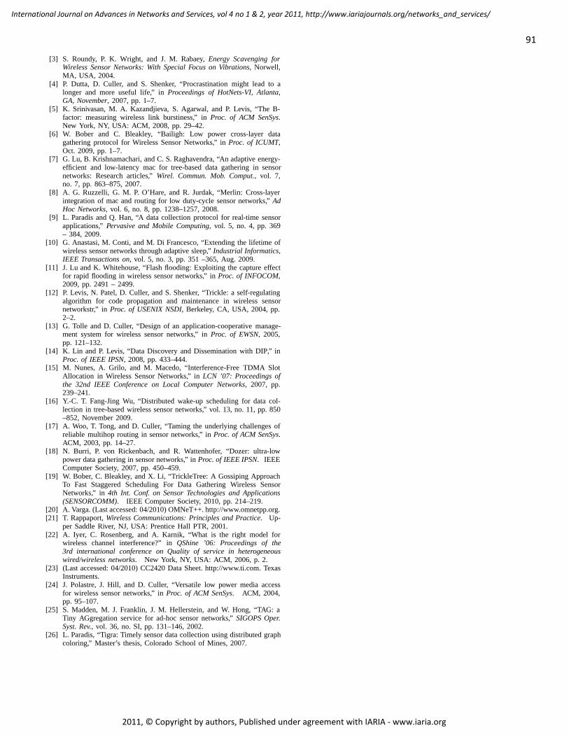
[3] S. Roundy, P. K. Wright, and J. M. Rabaey, Energy Scavenging forWireless Sensor Networks: With Special Focus on Vibrations, Norwell,MA, USA, 2004.
[4] P. Dutta, D. Culler, and S. Shenker, “Procrastination might lead to alonger and more useful life,” in Proceedings of HotNets-VI, Atlanta,GA, November, 2007, pp. 1–7.
[5] K. Srinivasan, M. A. Kazandjieva, S. Agarwal, and P. Levis, “The B-factor: measuring wireless link burstiness,” in Proc. of ACM SenSys.New York, NY, USA: ACM, 2008, pp. 29–42.
[6] W. Bober and C. Bleakley, “Bailigh: Low power cross-layer datagathering protocol for Wireless Sensor Networks,” in Proc. of ICUMT,Oct. 2009, pp. 1–7.
[7] G. Lu, B. Krishnamachari, and C. S. Raghavendra, “An adaptive energy-efficient and low-latency mac for tree-based data gathering in sensornetworks: Research articles,” Wirel. Commun. Mob. Comput., vol. 7,no. 7, pp. 863–875, 2007.
[8] A. G. Ruzzelli, G. M. P. O’Hare, and R. Jurdak, “Merlin: Cross-layerintegration of mac and routing for low duty-cycle sensor networks,” AdHoc Networks, vol. 6, no. 8, pp. 1238–1257, 2008.
[9] L. Paradis and Q. Han, “A data collection protocol for real-time sensorapplications,” Pervasive and Mobile Computing, vol. 5, no. 4, pp. 369– 384, 2009.
[10] G. Anastasi, M. Conti, and M. Di Francesco, “Extending the lifetime ofwireless sensor networks through adaptive sleep,” Industrial Informatics,IEEE Transactions on, vol. 5, no. 3, pp. 351 –365, Aug. 2009.
[11] J. Lu and K. Whitehouse, “Flash flooding: Exploiting the capture effectfor rapid flooding in wireless sensor networks,” in Proc. of INFOCOM,2009, pp. 2491 – 2499.
[12] P. Levis, N. Patel, D. Culler, and S. Shenker, “Trickle: a self-regulatingalgorithm for code propagation and maintenance in wireless sensornetworkstr,” in Proc. of USENIX NSDI, Berkeley, CA, USA, 2004, pp.2–2.
[13] G. Tolle and D. Culler, “Design of an application-cooperative manage-ment system for wireless sensor networks,” in Proc. of EWSN, 2005,pp. 121–132.
[14] K. Lin and P. Levis, “Data Discovery and Dissemination with DIP,” inProc. of IEEE IPSN, 2008, pp. 433–444.
[15] M. Nunes, A. Grilo, and M. Macedo, “Interference-Free TDMA SlotAllocation in Wireless Sensor Networks,” in LCN ’07: Proceedings ofthe 32nd IEEE Conference on Local Computer Networks, 2007, pp.239–241.
[16] Y.-C. T. Fang-Jing Wu, “Distributed wake-up scheduling for data col-lection in tree-based wireless sensor networks,” vol. 13, no. 11, pp. 850–852, November 2009.
[17] A. Woo, T. Tong, and D. Culler, “Taming the underlying challenges ofreliable multihop routing in sensor networks,” in Proc. of ACM SenSys.ACM, 2003, pp. 14–27.
[18] N. Burri, P. von Rickenbach, and R. Wattenhofer, “Dozer: ultra-lowpower data gathering in sensor networks,” in Proc. of IEEE IPSN. IEEEComputer Society, 2007, pp. 450–459.
[19] W. Bober, C. Bleakley, and X. Li, “TrickleTree: A Gossiping ApproachTo Fast Staggered Scheduling For Data Gathering Wireless SensorNetworks,” in 4th Int. Conf. on Sensor Technologies and Applications(SENSORCOMM). IEEE Computer Society, 2010, pp. 214–219.
[20] A. Varga. (Last accessed: 04/2010) OMNeT++. http://www.omnetpp.org.[21] T. Rappaport, Wireless Communications: Principles and Practice. Up-
per Saddle River, NJ, USA: Prentice Hall PTR, 2001.[22] A. Iyer, C. Rosenberg, and A. Karnik, “What is the right model for
wireless channel interference?” in QShine ’06: Proceedings of the3rd international conference on Quality of service in heterogeneouswired/wireless networks. New York, NY, USA: ACM, 2006, p. 2.
[23] (Last accessed: 04/2010) CC2420 Data Sheet. http://www.ti.com. TexasInstruments.
[24] J. Polastre, J. Hill, and D. Culler, “Versatile low power media accessfor wireless sensor networks,” in Proc. of ACM SenSys. ACM, 2004,pp. 95–107.
[25] S. Madden, M. J. Franklin, J. M. Hellerstein, and W. Hong, “TAG: aTiny AGgregation service for ad-hoc sensor networks,” SIGOPS Oper.Syst. Rev., vol. 36, no. SI, pp. 131–146, 2002.
[26] L. Paradis, “Tigra: Timely sensor data collection using distributed graphcoloring,” Master’s thesis, Colorado School of Mines, 2007.
91
International Journal on Advances in Networks and Services, vol 4 no 1 & 2, year 2011, http://www.iariajournals.org/networks_and_services/
2011, © Copyright by authors, Published under agreement with IARIA - www.iaria.org
Phased Array Satellite Antenna Testing by anAircraft Borne Emulation Platform
Iwan KrugerDept. of Electrical and Electronic Engineering
Stellenbosch UniversityStellenbosch, South Africa
Riaan WolhuterDept. of Electrical and Electronic Engineering
Stellenbosch UniversityStellenbosch, South Africa
Abstract—The KU Leuven- and Stellenbosch Universities arejointly developing an electronically beam steerable phased an-tenna array for satellite applications, including all the peripheralground- and space segment subsystems. This paper covers thedevelopment of an Aircraft based Satellite Emulator to facilitateconvenient aircraft based testing of an antenna array, intendedfor Low Earth Orbit satellite deployment. A flight strategy isdeveloped to emulate such a satellite as best possible, with thestrategy subsequently implemented in software on in-flight PChardware. The emulator acts as a full interface between theaircraft avionics and satellite bus system, to enable generation ofthe required antenna steering commands and to create a satellitebus image to the payload. The emulator provides in-flight systemsinformation to the satellite payload, as it would get from an actualsatellite bus during spaceflight. The emulator ensures indifferenceto the payload, regardless of the fact that testing is aircraft based.An embedded control algorithm for the steerable antenna hasalso been developed and resides in the onboard computer of thepayload. Excellent initial test results have been obtained from theaircraft flight simulator and actual flight telemetry data, provingthe viability and cost-effectiveness of the approach. The systemtests as reported on here, stopped just short of full equipmentflight testing, as scheduled for in the near future. This is awaitedwith keen interest, as all results up to the present have beenpositive and in line with expectations.
Index Terms—Satellite Emulator; Phase Array Antenna; BeamSteering; Orbital Calculations; Link Budgets;
I. INTRODUCTION
The feasibility of utilising electronically beam steerableantenna arrays (SAA) in space, is currently jointly beinginvestigated by the ESAT-TELEMIC division of the Depart-ment of Electrical Engineering, Katholieke Universiteit Leu-ven, (KUL) Flanders, in partnership with the Department ofElectrical and Electronic Engineering, Stellenbosch University,South Africa. Successful space implementation of such anantenna array promises a number of significant benefits andthe development of advanced techniques therefor, has beenthe subject of our joint research and development for sometime [1], [2]. Amongst others, it will reduce the cost ofground stations by eliminating tracking antennas and reducingRF chain complexity, while still retaining an acceptable linkbudget. By introducing beam steered satellite antenna trackingof ground stations during overflight, the link budget could beimproved and ground station complexity reduced, particularlywith regard to antenna design and the RF chain. These ground
nodes are typically used for environmental and agriculturaldata acquisition and any improvement regarding the aboveare always beneficial. The Stellenbosch University member ofthis partnership, is responsible for development of the satelliteplatform hosting the SAA, ground station and accompanyingground-space communications link. The payload would bedeployed on a next South African low earth orbit (LEO)satellite. Development and construction of any form of spaceborne system is normally expensive and associated with manyrisks. It was, therefore, decided to introduce an interim testingphase prior to actual space flight, by using a light aircraft asa pseudosatellite test platform. This will offer the obvious ad-vantages of convenient and relatively cheap closed loop systemtesting and debugging. This must, without doubt, enhance thechances of eventual in-flight success. The aircraft itself hasbeen fitted out for experimental use and will house the SAA,the entire satellite payload containing the On Board Computer(OBC), communications link component chain, steerable an-tenna control/status interface, power supplies, as well as anAircraft Satellite Emulator (ASE). In actual deployment, allinteraction with the rest of the satellite is via a system bus forpurposes of telecommand, telemetry and attitude/positioninginformation. The ASE is obviously required to act as translatorand emulator between the payload and aircraft, the latter actingas pseudo-satellite. As far as the payload is concerned, itshould behave as if connected to the actual satellite bus. TheASE and developed emulation strategy can be adapted tovarious LEO satellite payloads and thus provides a generallow cost test platform prior to space deployment. The purposeof this paper is to report on the development of the emulationplatform and SAA control subsystems. Some very encouragingresults have been presented elsewhere [1], which have sincebeen confirmed and expanded by continued pre-flight testing.The paper will describe the required flight path mechanics,the feasibility of an emulation strategy, a brief description ofthe implementation and test results obtained from an aircraftsimulator and aircraft flight telemetry data. The rest of thepaper is structured as follows: An overview of the relevantorbital mechanics in Section II, is followed by the discussionof the required emulation strategy in Section III. Calculationof the aircraft flight path parameters in order to satisfy theemulation strategy, is covered in Section IV. These basic
92
International Journal on Advances in Networks and Services, vol 4 no 1 & 2, year 2011, http://www.iariajournals.org/networks_and_services/
2011, © Copyright by authors, Published under agreement with IARIA - www.iaria.org
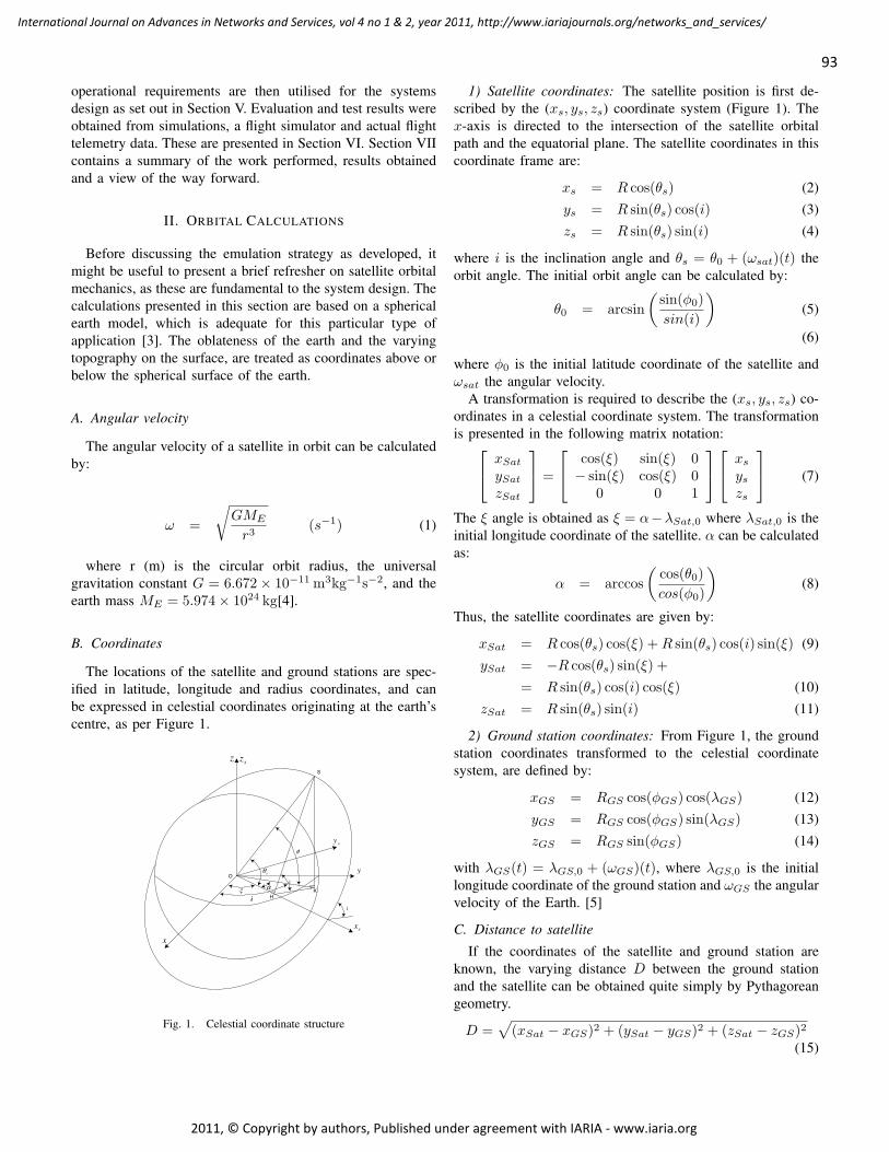
operational requirements are then utilised for the systemsdesign as set out in Section V. Evaluation and test results wereobtained from simulations, a flight simulator and actual flighttelemetry data. These are presented in Section VI. Section VIIcontains a summary of the work performed, results obtainedand a view of the way forward.
II. ORBITAL CALCULATIONS
Before discussing the emulation strategy as developed, itmight be useful to present a brief refresher on satellite orbitalmechanics, as these are fundamental to the system design. Thecalculations presented in this section are based on a sphericalearth model, which is adequate for this particular type ofapplication [3]. The oblateness of the earth and the varyingtopography on the surface, are treated as coordinates above orbelow the spherical surface of the earth.
A. Angular velocity
The angular velocity of a satellite in orbit can be calculatedby:
ω =
√GME
r3(s−1) (1)
where r (m) is the circular orbit radius, the universalgravitation constant G = 6.672× 10⁻¹¹ m3kg−1s−2, and theearth mass ME = 5.974× 1024 kg[4].
B. Coordinates
The locations of the satellite and ground stations are spec-ified in latitude, longitude and radius coordinates, and canbe expressed in celestial coordinates originating at the earth’scentre, as per Figure 1.
λ
sθ
φ
sx
sy
x
szz
ξ
y
α
Fig. 1. Celestial coordinate structure
1) Satellite coordinates: The satellite position is first de-scribed by the (xs, ys, zs) coordinate system (Figure 1). Thex-axis is directed to the intersection of the satellite orbitalpath and the equatorial plane. The satellite coordinates in thiscoordinate frame are:
xs = R cos(θs) (2)ys = R sin(θs) cos(i) (3)zs = R sin(θs) sin(i) (4)
where i is the inclination angle and θs = θ0 + (ωsat)(t) theorbit angle. The initial orbit angle can be calculated by:
θ0 = arcsin(
sin(φ0)sin(i)
)(5)
(6)
where φ0 is the initial latitude coordinate of the satellite andωsat the angular velocity.
A transformation is required to describe the (xs, ys, zs) co-ordinates in a celestial coordinate system. The transformationis presented in the following matrix notation: xSat
ySatzSat
=
cos(ξ) sin(ξ) 0− sin(ξ) cos(ξ) 0
0 0 1
xsyszs
(7)
The ξ angle is obtained as ξ = α−λSat,0 where λSat,0 is theinitial longitude coordinate of the satellite. α can be calculatedas:
α = arccos(
cos(θ0)cos(φ0)
)(8)
Thus, the satellite coordinates are given by:
xSat = R cos(θs) cos(ξ) +R sin(θs) cos(i) sin(ξ) (9)ySat = −R cos(θs) sin(ξ) +
= R sin(θs) cos(i) cos(ξ) (10)zSat = R sin(θs) sin(i) (11)
2) Ground station coordinates: From Figure 1, the groundstation coordinates transformed to the celestial coordinatesystem, are defined by:
xGS = RGS cos(φGS) cos(λGS) (12)yGS = RGS cos(φGS) sin(λGS) (13)zGS = RGS sin(φGS) (14)
with λGS(t) = λGS,0 + (ωGS)(t), where λGS,0 is the initiallongitude coordinate of the ground station and ωGS the angularvelocity of the Earth. [5]
C. Distance to satellite
If the coordinates of the satellite and ground station areknown, the varying distance D between the ground stationand the satellite can be obtained quite simply by Pythagoreangeometry.
D =√
(xSat − xGS)2 + (ySat − yGS)2 + (zSat − zGS)2(15)
93
International Journal on Advances in Networks and Services, vol 4 no 1 & 2, year 2011, http://www.iariajournals.org/networks_and_services/
2011, © Copyright by authors, Published under agreement with IARIA - www.iaria.org
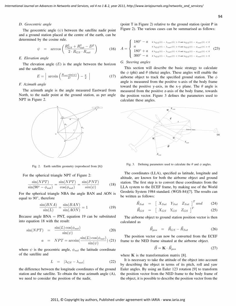
D. Geocentric angle
The geocentric angle (ψ) between the satellite nadir pointand a ground station placed at the centre of the earth, can bedetermined by the cosine rule.
ψ = arccos(R2GS +R2
sat −D2
2 ·RGS ·Rsat
)(16)
E. Elevation angle
The elevation angle (E) is the angle between the horizonand the satellite.
E =∣∣∣ arcsin
(Rsat sin(ψ)
D
)− π
2
∣∣∣ (17)
F. Azimuth angle
The azimuth angle is the angle measured Eastward fromNorth, to the nadir point at the ground station, as per angleNPT in Figure 2.
ψ
satφξ
GSφ
Fig. 2. Earth satellite geometry (reproduced from [6])
For the spherical triangle NPT of Figure 2:
sin(NPT )sin(90 − φsat)
=sin(NPT )cos(φsat)
=sin(PNT )sin(ψ)
(18)
For the spherical triangle NBA the angle BAN and AON isequal to 90, therefore
sin(BNA)sin(L)
=sin(BAN)sin(AON)
= 1 (19)
Because angle BNA = PNT, equation 19 can be substitutedinto equation 18 with the result:
sin(NPT ) =sin(L) cos(φsat)
sin(ψ)(20)
a = NPT = arcsin(sin(L) cos(φsat)
sin(ψ)) (21)
where ψ is the geocentric angle, φsat the latitude coordinateof the satellite and
L = |λGS − λsat| (22)
the difference between the longitude coordinates of the groundstation and the satellite. To obtain the true azimuth angle (A),we need to consider the position of the nadir,
(point T in Figure 2) relative to the ground station (point P inFigure 2). The various cases can be summarised as follows:
A =
180 − a if λGS(t) − λsat(t) > 0 and φGS(t) − φsat(t) < 0
a if λGS(t) − λsat(t) > 0 and φGS(t) − φsat(t) > 0
180 + a if λGS(t) − λsat(t) < 0 and φGS(t) − φsat(t) < 0
360 − a if λGS(t) − λsat(t) < 0 and φGS(t) − φsat(t) > 0
(23)
G. Steering angles
This section will describe the basic strategy to calculatethe φ (phi) and θ (theta) angles. These angles will enable theairborne object to track the specified ground station. The φangle is measured from the positive x-axis of the body frametoward the positive y-axis, in the x-y plane. The θ angle ismeasured from the positive z-axis of the body frame, towardsthe position vector. Figure 3 defines the parameters used tocalculate these angles.
θ
bodyX
bodyY
bodyZ
φ
xW
yWzW
θ
bodyX
bodyY
bodyZ
φ
t
Fig. 3. Defining parameters used to calculate the θ and φ angles.
The coordinates (LLA), specified as latitude, longitude andaltitude, are known for both the airborne object and groundstation. The first step is to convert these coordinates from theLLA system to the ECEF frame, by making use of the WorldGeodetic System 1984 standard. (WGS-84)[7]. The results canbe written as follows:
~RSat =[XSat YSat ZSat
]Tand (24)
~RGS =[XGS YGS ZGS
]T(25)
The airborne object to ground station position vector is thencalculated as
~Rpos = ~RGS − ~RSat (26)
The position vector can now be converted from the ECEFframe to the NED frame situated at the airborne object.
~B = K · ~Rpos (27)
where K is the transformation matrix [8].It is necessary to take the attitude of the object into account
by describing the object in terms of its pitch, roll and yawEuler angles. By using an Euler 123 rotation [9] to transformthe position vector from the NED frame to the body frame ofthe object, it is possible to describe the position vector from the
94
International Journal on Advances in Networks and Services, vol 4 no 1 & 2, year 2011, http://www.iariajournals.org/networks_and_services/
2011, © Copyright by authors, Published under agreement with IARIA - www.iaria.org
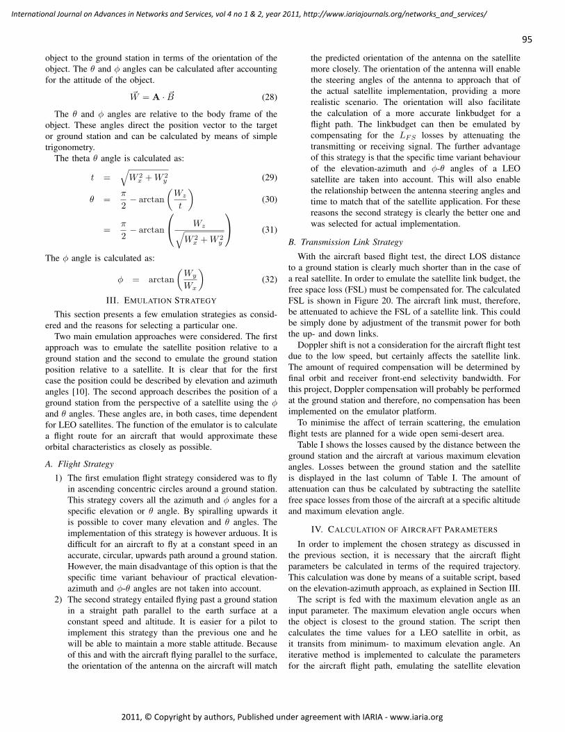
object to the ground station in terms of the orientation of theobject. The θ and φ angles can be calculated after accountingfor the attitude of the object.
~W = A · ~B (28)
The θ and φ angles are relative to the body frame of theobject. These angles direct the position vector to the targetor ground station and can be calculated by means of simpletrigonometry.
The theta θ angle is calculated as:
t =√W 2x +W 2
y (29)
θ =π
2− arctan
(Wz
t
)(30)
=π
2− arctan
Wz√W 2x +W 2
y
(31)
The φ angle is calculated as:
φ = arctan(Wy
Wx
)(32)
III. EMULATION STRATEGY
This section presents a few emulation strategies as consid-ered and the reasons for selecting a particular one.
Two main emulation approaches were considered. The firstapproach was to emulate the satellite position relative to aground station and the second to emulate the ground stationposition relative to a satellite. It is clear that for the firstcase the position could be described by elevation and azimuthangles [10]. The second approach describes the position of aground station from the perspective of a satellite using the φand θ angles. These angles are, in both cases, time dependentfor LEO satellites. The function of the emulator is to calculatea flight route for an aircraft that would approximate theseorbital characteristics as closely as possible.
A. Flight Strategy
1) The first emulation flight strategy considered was to flyin ascending concentric circles around a ground station.This strategy covers all the azimuth and φ angles for aspecific elevation or θ angle. By spiralling upwards itis possible to cover many elevation and θ angles. Theimplementation of this strategy is however arduous. It isdifficult for an aircraft to fly at a constant speed in anaccurate, circular, upwards path around a ground station.However, the main disadvantage of this option is that thespecific time variant behaviour of practical elevation-azimuth and φ-θ angles are not taken into account.
2) The second strategy entailed flying past a ground stationin a straight path parallel to the earth surface at aconstant speed and altitude. It is easier for a pilot toimplement this strategy than the previous one and hewill be able to maintain a more stable attitude. Becauseof this and with the aircraft flying parallel to the surface,the orientation of the antenna on the aircraft will match
the predicted orientation of the antenna on the satellitemore closely. The orientation of the antenna will enablethe steering angles of the antenna to approach that ofthe actual satellite implementation, providing a morerealistic scenario. The orientation will also facilitatethe calculation of a more accurate linkbudget for aflight path. The linkbudget can then be emulated bycompensating for the LFS losses by attenuating thetransmitting or receiving signal. The further advantageof this strategy is that the specific time variant behaviourof the elevation-azimuth and φ-θ angles of a LEOsatellite are taken into account. This will also enablethe relationship between the antenna steering angles andtime to match that of the satellite application. For thesereasons the second strategy is clearly the better one andwas selected for actual implementation.
B. Transmission Link Strategy
With the aircraft based flight test, the direct LOS distanceto a ground station is clearly much shorter than in the case ofa real satellite. In order to emulate the satellite link budget, thefree space loss (FSL) must be compensated for. The calculatedFSL is shown in Figure 20. The aircraft link must, therefore,be attenuated to achieve the FSL of a satellite link. This couldbe simply done by adjustment of the transmit power for boththe up- and down links.
Doppler shift is not a consideration for the aircraft flight testdue to the low speed, but certainly affects the satellite link.The amount of required compensation will be determined byfinal orbit and receiver front-end selectivity bandwidth. Forthis project, Doppler compensation will probably be performedat the ground station and therefore, no compensation has beenimplemented on the emulator platform.
To minimise the affect of terrain scattering, the emulationflight tests are planned for a wide open semi-desert area.
Table I shows the losses caused by the distance between theground station and the aircraft at various maximum elevationangles. Losses between the ground station and the satelliteis displayed in the last column of Table I. The amount ofattenuation can thus be calculated by subtracting the satellitefree space losses from those of the aircraft at a specific altitudeand maximum elevation angle.
IV. CALCULATION OF AIRCRAFT PARAMETERS
In order to implement the chosen strategy as discussed inthe previous section, it is necessary that the aircraft flightparameters be calculated in terms of the required trajectory.This calculation was done by means of a suitable script, basedon the elevation-azimuth approach, as explained in Section III.
The script is fed with the maximum elevation angle as aninput parameter. The maximum elevation angle occurs whenthe object is closest to the ground station. The script thencalculates the time values for a LEO satellite in orbit, asit transits from minimum- to maximum elevation angle. Aniterative method is implemented to calculate the parametersfor the aircraft flight path, emulating the satellite elevation
95
International Journal on Advances in Networks and Services, vol 4 no 1 & 2, year 2011, http://www.iariajournals.org/networks_and_services/
2011, © Copyright by authors, Published under agreement with IARIA - www.iaria.org
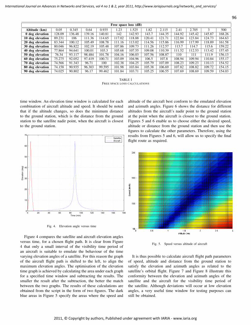
Free space loss (dB)Altitude (km) 0.05 0.345 0.64 0.935 1.23 1.525 1.82 2.115 2.41 2.705 3 5000 deg elevation 128.09 136.48 139.16 140.81 142 142.93 143.7 144.35 144.92 145.42 145.87 168.26
10 deg elevation 89.231 106 111.36 114.65 117.02 118.88 120.41 121.71 122.84 123.84 124.73 164.6320 deg elevation 83.344 100.12 105.49 108.78 111.16 113.02 114.56 115.86 116.99 117.99 118.89 161.5830 deg elevation 80.046 96.822 102.19 105.48 107.86 109.73 111.26 112.57 113.7 114.7 115.6 159.2240 deg elevation 77.864 94.641 100.01 103.3 105.68 107.55 109.08 110.39 111.52 112.53 113.42 157.4550 deg elevation 76.34 93.117 98.484 101.78 104.16 106.03 107.56 108.87 110 111 111.9 156.1360 deg elevation 75.275 92.052 97.419 100.71 103.09 104.96 106.5 107.8 108.94 109.94 110.84 155.1770 deg elevation 74.566 91.343 96.71 100 102.38 104.25 105.79 107.09 108.23 109.23 110.13 154.5280 deg elevation 74.158 90.935 96.303 99.595 101.98 103.84 105.38 106.69 107.82 108.82 109.72 154.1590 deg elevation 74.025 90.802 96.17 99.462 101.84 103.71 105.25 106.55 107.69 108.69 109.59 154.03
TABLE IFREE SPACE LOSS CALCULATIONS
time window. An elevation time window is calculated for eachcombination of aircraft altitude and speed. It should be notedthat if the altitude changes, so does the minimum distanceto the ground station, which is the distance from the groundstation to the satellite nadir point, when the aircraft is closestto the ground station.
0 20 40 60 80 100 120 140 160 1800
10
20
30
40
50
60
70
Time (min)
Ele
vatio
n (d
eg)
SatelliteAircraft
Fig. 4. Elevation angle versus time
Figure 4 compares the satellite and aircraft elevation anglesversus time, for a chosen flight path. It is clear from Figure4 that only a small interval of the visibility time period ofan aircraft is suitable to emulate the behaviour of the timevarying elevation angles of a satellite. For this reason the graphof the aircraft flight path is shifted to the left, to align themaximum elevation angles. The optimisation of the elevationtime graph is achieved by calculating the area under each graphfor a specified time window and subtracting the results. Thesmaller the result after the subtraction, the better the matchbetween the two graphs. The results of these calculations areobtained from the script in the form of two figures. The darkblue areas in Figure 5 specify the areas where the speed and
altitude of the aircraft best conform to the emulated elevationand azimuth angles. Figure 6 shows the distance for differentaltitudes from the aircraft’s nadir point to the ground stationat the point when the aircraft is closest to the ground station.Figures 5 and 6 enable us to choose either the desired speed,altitude or distance from the ground station and then use thefigures to calculate the other parameters. Therefore, using theresults from Figures 5 and 6, will allow us to specify the finalflight route as required.
Fig. 5. Speed versus altitude of aircraft
It is thus possible to calculate aircraft flight path parametersof speed, altitude and distance from the ground station tosatisfy the elevation and azimuth angles as related to thesatellite’s orbital flight. Figure 7 and Figure 8 illustrate thisconformity between the elevation and azimuth angles of thesatellite and the aircraft for the visibility time period ofthe satellite. Although deviations will occur at low elevationangles, a very useful time window for testing purposes canstill be obtained.
96
International Journal on Advances in Networks and Services, vol 4 no 1 & 2, year 2011, http://www.iariajournals.org/networks_and_services/
2011, © Copyright by authors, Published under agreement with IARIA - www.iaria.org
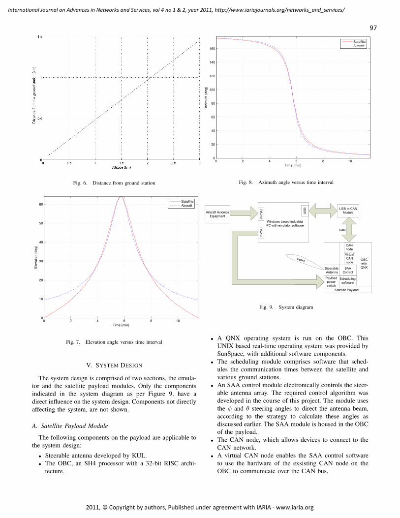
Fig. 6. Distance from ground station
0 2 4 6 8 100
10
20
30
40
50
60
Time (min)
Ele
vatio
n (d
eg)
SatelliteAircraft
Fig. 7. Elevation angle versus time interval
V. SYSTEM DESIGN
The system design is comprised of two sections, the emula-tor and the satellite payload modules. Only the componentsindicated in the system diagram as per Figure 9, have adirect influence on the system design. Components not directlyaffecting the system, are not shown.
A. Satellite Payload Module
The following components on the payload are applicable tothe system design:
• Steerable antenna developed by KUL.• The OBC, an SH4 processor with a 32-bit RISC archi-
tecture.
0 2 4 6 8 100
20
40
60
80
100
120
140
160
Time (min)
Azi
mut
h (d
eg)
SatelliteAircraft
Fig. 8. Azimuth angle versus time interval
!
"
#
$
%!&
!
!
'
(
!
#
Fig. 9. System diagram
• A QNX operating system is run on the OBC. ThisUNIX based real-time operating system was provided bySunSpace, with additional software components.
• The scheduling module comprises software that sched-ules the communication times between the satellite andvarious ground stations.
• An SAA control module electronically controls the steer-able antenna array. The required control algorithm wasdeveloped in the course of this project. The module usesthe φ and θ steering angles to direct the antenna beam,according to the strategy to calculate these angles asdiscussed earlier. The SAA module is housed in the OBCof the payload.
• The CAN node, which allows devices to connect to theCAN network.
• A virtual CAN node enables the SAA control softwareto use the hardware of the exsisting CAN node on theOBC to communicate over the CAN bus.
97
International Journal on Advances in Networks and Services, vol 4 no 1 & 2, year 2011, http://www.iariajournals.org/networks_and_services/
2011, © Copyright by authors, Published under agreement with IARIA - www.iaria.org
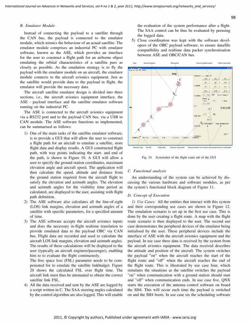
B. Emulator Module
Instead of connecting the payload to a satellite throughthe CAN bus, the payload is connected to the emulatormodule, which mimics the behaviour of an actual satellite. Theemulator module comprises an industrial PC with emulatorsoftware, known as the ASE, which provides an interfacefor the user to construct a flight path for an airborne objectemulating the orbital characteristics of a satellite pass asclosely as possible. As the emulation strategy is to fly thepayload with the emulator module on an aircraft, the emulatormodule connects to the aircraft avionics equipment. Just asthe satellite would provide data to the payload in flight, theemulator will provide the necessary data.
The aircraft satellite emulator design is divided into threesections, i.e., the aircraft avionics equipment interface, theASE - payload interface and the satellite emulator softwarerunning on the industrial PC.
The ASE is connected to the aircraft avionics equipmentvia a RS232 port and to the payload CAN bus, via a USB toCAN module. The ASE software functions as implemented,can be summarised as follows:
1) One of the main tasks of the satellite emulator software,is to provide a GUI that will allow the user to constructa flight path for an aircraft to emulate a satellite, storeflight data and display results. A GUI constructed flightpath, with way points indicating the start- and end ofthe path, is shown in Figure 10. A GUI will allow auser to specify the ground station coordinates, maximumelevation angle and aircraft speed. The application willthen calculate the speed, altitude and distance fromthe ground station required from the aircraft flight tosatisfy the elevation and azimuth angles. The elevationand azimuth angles for the visibility time period ascalculated, are displayed to the user, assisting with flightpath definition.
2) The ASE software also calculates all the line-of-sight(LOS) link margins, elevation and azimuth angles of asatellite with specific parameters, for a specified amountof time.
3) The ASE software accepts the aircraft avionics inputsand does the necessary in-flight realtime translation toprovide emulated data to the payload OBC via CANbus. Flight data are recorded and used to calculate theaircraft LOS link margins, elevation and azimuth angles.The results of these calculations will be displayed to theuser (typically an aircraft engineer/passenger), enablinghim to to evaluate the flight continuously.The free space loss (FSL) parameter needs to be com-pensated for to emulate the satellite linkbudget. Figure20 shows the calculated FSL over flight time. Theaircraft link must thus be attenuated to obtain the correctsatellite link FSL.
4) All the data received and sent by the ASE are logged bya script written in C. The SAA steering angles calculatedby the control algorithm are also logged. This will enable
the evaluation of the system performance after a flight.The SAA control can be thus be evaluated by perusingthe logged data.
5) Close coordination was kept with the software devel-opers of the OBC payload software, to ensure data/filecompatibility and realtime data packet synchronisationbetween ASE and OBC/CAN bus.
Fig. 10. Screenshot of the flight route tab of the GUI
C. Functional analysis
An understanding of the system can be achieved by dis-cussing the various hardware and software modules, as perthe system’s functional block diagram of Figure 11.
D. Concept of Execution
1) Use Cases: All the entities that interact with this systemand their corresponding use cases are shown in Figure 12.The emulation scenario is set up in the first use case. This isdone by the user creating a flight route. A map with the flightroute scenario is then displayed to the user. The second usecase demonstrates the peripheral devices of the emulator beinginitialised by the user. These peripheral devices include theinterface of ASE with the aircraft avionics equipment and thepayload. In use case three data is received by the system fromthe aircraft avionics equipment. The data received describesthe attitude and position of the aircraft. The system switchesthe payload ”on” when the aircraft reaches the start of theflight route and ”off” when the aircraft reaches the end ofthe flight route. This is illustrated by use case four, whichsimulates the situations as the satellite switches the payload”on” when communication with a ground station should startand ”off” when communication ends. In use case five, QNXstarts the execution of the antenna control software on boardthe SH4. This will occur each time the payload is switchedon and the SH4 boots. In use case six the scheduling software
98
International Journal on Advances in Networks and Services, vol 4 no 1 & 2, year 2011, http://www.iariajournals.org/networks_and_services/
2011, © Copyright by authors, Published under agreement with IARIA - www.iaria.org
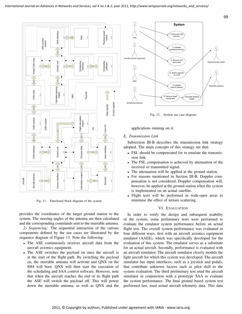
!
"
#
#
$
%
$
%
&
&
'
'
(
(
)
*
)
+
*
#,
+
##
#,
#$
##
#%
#$
#&
#%
#'
#&
#(
#)
#(
#*
#)
#+
#*
#+
#'
Fig. 11. Functional block diagram of the system
provides the coordinates of the target ground station to thesystem. The steering angles of the antenna are then calculatedand the corresponding commands sent to the steerable antenna.
2) Sequencing: The sequential interaction of the variouscomponents defined by the use cases are illustrated by thesequence diagram of Figure 13. Note the following:• The ASE continuously receives aircraft data from the
aircraft avionics equipment.• The ASE switches the payload on once the aircraft is
at the start of the flight path. By switching the payloadon, the steerable antenna will activate and QNX on theSH4 will boot. QNX will then start the execution ofthe scheduling and SAA control software. However, notethat when the aircraft reaches the end of its flight paththe ASE will switch the payload off. This will powerdown the steerable antenna, as well as QNX and the
!
"
#$%
&'
('
Fig. 12. System use case diagram
applications running on it.
E. Transmission Link
Subsection III-B describes the transmission link strategyadopted. The main concepts of this strategy are that:• FSL should be compensated for to emulate the transmis-
sion link.• The FSL compensation is achieved by attenuation of the
received or transmitted signal.• The attenuation will be applied at the ground station.• For reasons mentioned in Section III-B, Doppler com-
pensation is not considered. Doppler compensation will,however, be applied at the ground station when the systemis implemented on an actual satellite.
• Flight tests will be performed in wide-open areas tominimise the effect of terrain scattering.
VI. EVALUATION
In order to verify the design and subsequent usabilityof the system, some preliminary tests were performed toevaluate the emulator system performance before an actualflight test. The overall system performance was evaluated infour different ways, first with an aircraft avionics equipmentemulator (AAEE), which was specifically developed for theevaluation of this system. The emulator serves as a substitutefor an actual aircraft. Secondly, performance is evaluated withan aircraft simulator. The aircraft simulator closely models thelight aircraft for which this system was developed. The aircraftsimulator has input interfaces, such as a joystick and pedals,that contribute unknown factors such as pilot skill to thesystem evaluation. The third preliminary test used the aircraftsimulator in conjunction with a prototype SAA to evaluatethe system performance. The final ground based system testperformed last, used actual aircraft telemetry data. This data
99
International Journal on Advances in Networks and Services, vol 4 no 1 & 2, year 2011, http://www.iariajournals.org/networks_and_services/
2011, © Copyright by authors, Published under agreement with IARIA - www.iaria.org
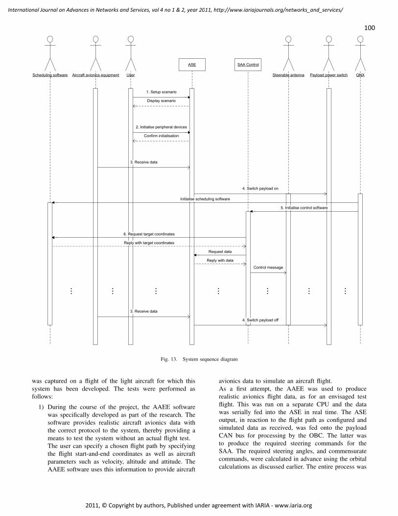
!
"!
"
!
#"
$%& !" ' (
#"
)" "
* "
!"
Fig. 13. System sequence diagram
was captured on a flight of the light aircraft for which thissystem has been developed. The tests were performed asfollows:
1) During the course of the project, the AAEE softwarewas specifically developed as part of the research. Thesoftware provides realistic aircraft avionics data withthe correct protocol to the system, thereby providing ameans to test the system without an actual flight test.The user can specify a chosen flight path by specifyingthe flight start-and-end coordinates as well as aircraftparameters such as velocity, altitude and attitude. TheAAEE software uses this information to provide aircraft
avionics data to simulate an aircraft flight.As a first attempt, the AAEE was used to producerealistic avionics flight data, as for an envisaged testflight. This was run on a separate CPU and the datawas serially fed into the ASE in real time. The ASEoutput, in reaction to the flight path as configured andsimulated data as received, was fed onto the payloadCAN bus for processing by the OBC. The latter wasto produce the required steering commands for theSAA. The required steering angles, and commensuratecommands, were calculated in advance using the orbitalcalculations as discussed earlier. The entire process was
100
International Journal on Advances in Networks and Services, vol 4 no 1 & 2, year 2011, http://www.iariajournals.org/networks_and_services/
2011, © Copyright by authors, Published under agreement with IARIA - www.iaria.org
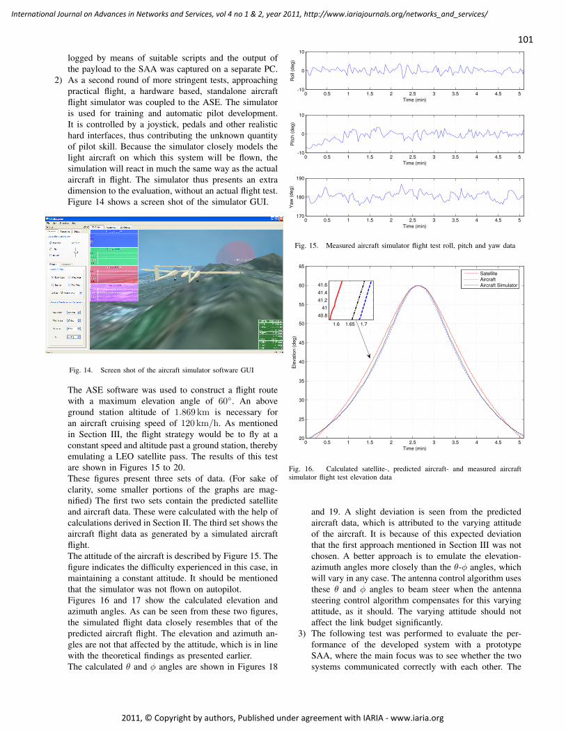
logged by means of suitable scripts and the output ofthe payload to the SAA was captured on a separate PC.
2) As a second round of more stringent tests, approachingpractical flight, a hardware based, standalone aircraftflight simulator was coupled to the ASE. The simulatoris used for training and automatic pilot development.It is controlled by a joystick, pedals and other realistichard interfaces, thus contributing the unknown quantityof pilot skill. Because the simulator closely models thelight aircraft on which this system will be flown, thesimulation will react in much the same way as the actualaircraft in flight. The simulator thus presents an extradimension to the evaluation, without an actual flight test.Figure 14 shows a screen shot of the simulator GUI.
Fig. 14. Screen shot of the aircraft simulator software GUI
The ASE software was used to construct a flight routewith a maximum elevation angle of 60. An aboveground station altitude of 1.869 km is necessary foran aircraft cruising speed of 120 km/h. As mentionedin Section III, the flight strategy would be to fly at aconstant speed and altitude past a ground station, therebyemulating a LEO satellite pass. The results of this testare shown in Figures 15 to 20.These figures present three sets of data. (For sake ofclarity, some smaller portions of the graphs are mag-nified) The first two sets contain the predicted satelliteand aircraft data. These were calculated with the help ofcalculations derived in Section II. The third set shows theaircraft flight data as generated by a simulated aircraftflight.The attitude of the aircraft is described by Figure 15. Thefigure indicates the difficulty experienced in this case, inmaintaining a constant attitude. It should be mentionedthat the simulator was not flown on autopilot.Figures 16 and 17 show the calculated elevation andazimuth angles. As can be seen from these two figures,the simulated flight data closely resembles that of thepredicted aircraft flight. The elevation and azimuth an-gles are not that affected by the attitude, which is in linewith the theoretical findings as presented earlier.The calculated θ and φ angles are shown in Figures 18
0 0.5 1 1.5 2 2.5 3 3.5 4 4.5 5-10
0
10
Time (min)
Rol
l (de
g)
0 0.5 1 1.5 2 2.5 3 3.5 4 4.5 5-10
0
10
Time (min)
Pitc
h (d
eg)
0 0.5 1 1.5 2 2.5 3 3.5 4 4.5 5170
180
190
Time (min)
Yaw
(deg
)
Fig. 15. Measured aircraft simulator flight test roll, pitch and yaw data
0 0.5 1 1.5 2 2.5 3 3.5 4 4.5 520
25
30
35
40
45
50
55
60
65
Time (min)
Ele
vatio
n (d
eg)
1.6 1.65 1.7
40.8
41
41.2
41.4
41.6
SatelliteAircraftAircraft Simulator
Fig. 16. Calculated satellite-, predicted aircraft- and measured aircraftsimulator flight test elevation data
and 19. A slight deviation is seen from the predictedaircraft data, which is attributed to the varying attitudeof the aircraft. It is because of this expected deviationthat the first approach mentioned in Section III was notchosen. A better approach is to emulate the elevation-azimuth angles more closely than the θ-φ angles, whichwill vary in any case. The antenna control algorithm usesthese θ and φ angles to beam steer when the antennasteering control algorithm compensates for this varyingattitude, as it should. The varying attitude should notaffect the link budget significantly.
3) The following test was performed to evaluate the per-formance of the developed system with a prototypeSAA, where the main focus was to see whether the twosystems communicated correctly with each other. The
101
International Journal on Advances in Networks and Services, vol 4 no 1 & 2, year 2011, http://www.iariajournals.org/networks_and_services/
2011, © Copyright by authors, Published under agreement with IARIA - www.iaria.org
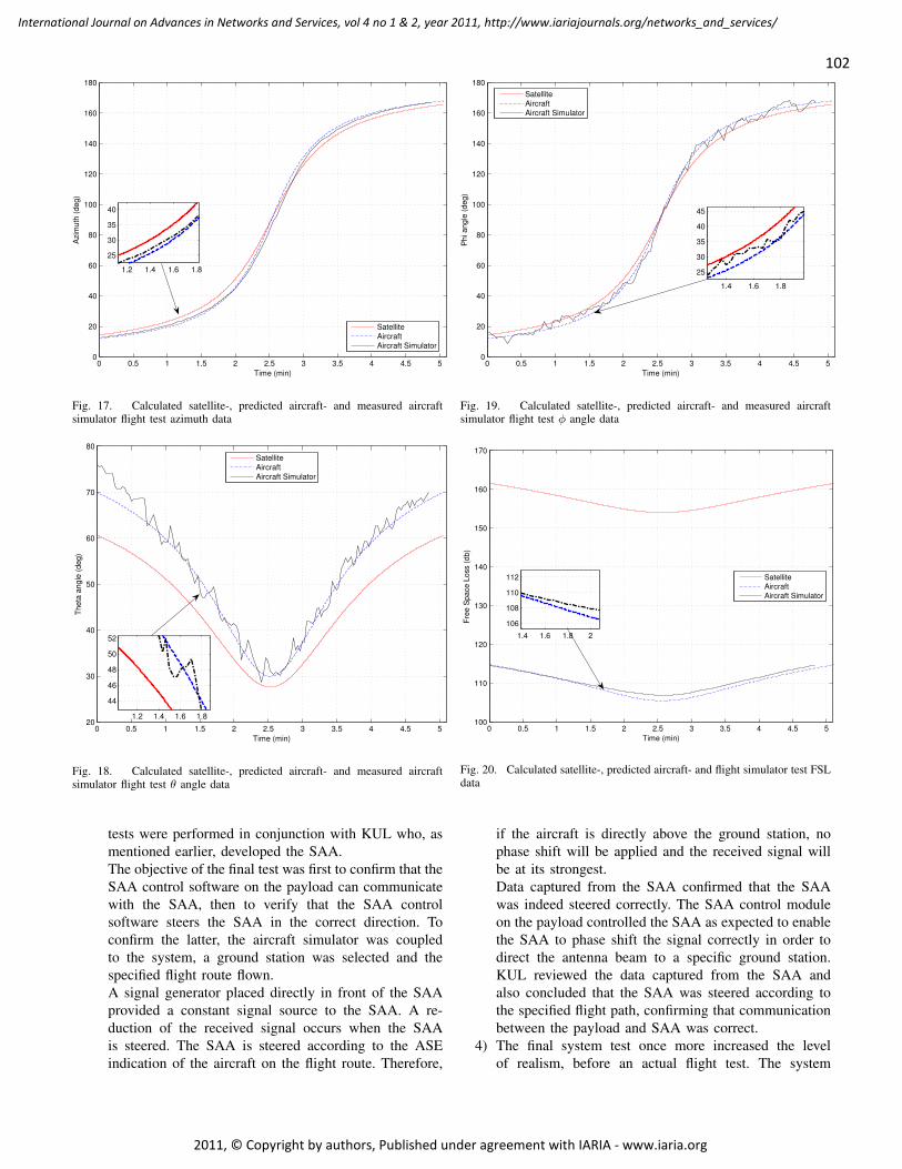
0 0.5 1 1.5 2 2.5 3 3.5 4 4.5 50
20
40
60
80
100
120
140
160
180
Time (min)
Azi
mut
h (d
eg)
1.2 1.4 1.6 1.8
25
30
35
40
SatelliteAircraftAircraft Simulator
Fig. 17. Calculated satellite-, predicted aircraft- and measured aircraftsimulator flight test azimuth data
0 0.5 1 1.5 2 2.5 3 3.5 4 4.5 520
30
40
50
60
70
80
Time (min)
Thet
a an
gle
(deg
)
SatelliteAircraftAircraft Simulator
1.2 1.4 1.6 1.8
44
46
48
50
52
Fig. 18. Calculated satellite-, predicted aircraft- and measured aircraftsimulator flight test θ angle data
tests were performed in conjunction with KUL who, asmentioned earlier, developed the SAA.The objective of the final test was first to confirm that theSAA control software on the payload can communicatewith the SAA, then to verify that the SAA controlsoftware steers the SAA in the correct direction. Toconfirm the latter, the aircraft simulator was coupledto the system, a ground station was selected and thespecified flight route flown.A signal generator placed directly in front of the SAAprovided a constant signal source to the SAA. A re-duction of the received signal occurs when the SAAis steered. The SAA is steered according to the ASEindication of the aircraft on the flight route. Therefore,
0 0.5 1 1.5 2 2.5 3 3.5 4 4.5 50
20
40
60
80
100
120
140
160
180
Time (min)
Phi
ang
le (d
eg)
SatelliteAircraftAircraft Simulator
1.4 1.6 1.8
25
30
35
40
45
Fig. 19. Calculated satellite-, predicted aircraft- and measured aircraftsimulator flight test φ angle data
0 0.5 1 1.5 2 2.5 3 3.5 4 4.5 5100
110
120
130
140
150
160
170
Time (min)
Free
Spa
ce L
oss
(db)
1.4 1.6 1.8 2
106
108
110
112 SatelliteAircraftAircraft Simulator
Fig. 20. Calculated satellite-, predicted aircraft- and flight simulator test FSLdata
if the aircraft is directly above the ground station, nophase shift will be applied and the received signal willbe at its strongest.Data captured from the SAA confirmed that the SAAwas indeed steered correctly. The SAA control moduleon the payload controlled the SAA as expected to enablethe SAA to phase shift the signal correctly in order todirect the antenna beam to a specific ground station.KUL reviewed the data captured from the SAA andalso concluded that the SAA was steered according tothe specified flight path, confirming that communicationbetween the payload and SAA was correct.
4) The final system test once more increased the levelof realism, before an actual flight test. The system
102
International Journal on Advances in Networks and Services, vol 4 no 1 & 2, year 2011, http://www.iariajournals.org/networks_and_services/
2011, © Copyright by authors, Published under agreement with IARIA - www.iaria.org
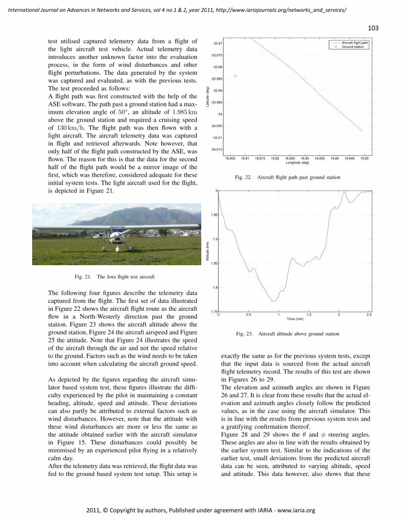
test utilised captured telemetry data from a flight ofthe light aircraft test vehicle. Actual telemetry dataintroduces another unknown factor into the evaluationprocess, in the form of wind disturbances and otherflight perturbations. The data generated by the systemwas captured and evaluated, as with the previous tests.The test proceeded as follows:A flight path was first constructed with the help of theASE software. The path past a ground station had a max-imum elevation angle of 50, an altitude of 1.985 kmabove the ground station and required a cruising speedof 130 km/h. The flight path was then flown with alight aircraft. The aircraft telemetry data was capturedin flight and retrieved afterwards. Note however, thatonly half of the flight path constructed by the ASE, wasflown. The reason for this is that the data for the secondhalf of the flight path would be a mirror image of thefirst, which was therefore, considered adequate for theseinitial system tests. The light aircraft used for the flight,is depicted in Figure 21.
Fig. 21. The Jora flight test aircraft
The following four figures describe the telemetry datacaptured from the flight. The first set of data illustratedin Figure 22 shows the aircraft flight route as the aircraftflew in a North-Westerly direction past the groundstation. Figure 23 shows the aircraft altitude above theground station, Figure 24 the aircraft airspeed and Figure25 the attitude. Note that Figure 24 illustrates the speedof the aircraft through the air and not the speed relativeto the ground. Factors such as the wind needs to be takeninto account when calculating the aircraft ground speed.
As depicted by the figures regarding the aircraft simu-lator based system test, these figures illustrate the diffi-culty experienced by the pilot in maintaining a constantheading, altitude, speed and attitude. These deviationscan also partly be attributed to external factors such aswind disturbances. However, note that the attitude withthese wind disturbances are more or less the same asthe attitude obtained earlier with the aircraft simulatorin Figure 15. These disturbances could possibly beminimised by an experienced pilot flying in a relativelycalm day.After the telemetry data was retrieved, the flight data wasfed to the ground based system test setup. This setup is
18.805 18.81 18.815 18.82 18.825 18.83 18.835 18.84 18.845 18.85
-34.015
-34.01
-34.005
-34
-33.995
-33.99
-33.985
-33.98
-33.975
-33.97
Longitude (deg)
Latit
ude
(deg
)
Aircraft flight pathGround station
Fig. 22. Aircraft flight path past ground station
0 0.5 1 1.5 2 2.51.75
1.8
1.85
1.9
1.95
2
Time (min)
Alti
tude
(km
)
Fig. 23. Aircraft altitude above ground station
exactly the same as for the previous system tests, exceptthat the input data is sourced from the actual aircraftflight telemetry record. The results of this test are shownin Figures 26 to 29.The elevation and azimuth angles are shown in Figure26 and 27. It is clear from these results that the actual el-evation and azimuth angles closely follow the predictedvalues, as in the case using the aircraft simulator. Thisis in line with the results from previous system tests anda gratifying confirmation thereof.Figure 28 and 29 shows the θ and φ steering angles.These angles are also in line with the results obtained bythe earlier system test. Similar to the indications of theearlier test, small deviations from the predicted aircraftdata can be seen, attributed to varying altitude, speedand attitude. This data however, also shows that these
103
International Journal on Advances in Networks and Services, vol 4 no 1 & 2, year 2011, http://www.iariajournals.org/networks_and_services/
2011, © Copyright by authors, Published under agreement with IARIA - www.iaria.org
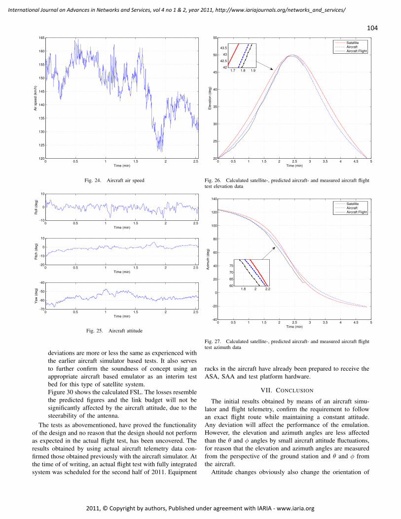
0 0.5 1 1.5 2 2.5120
125
130
135
140
145
150
155
160
165
Time (min)
Air
spee
d (k
m/h
)
Fig. 24. Aircraft air speed
0 0.5 1 1.5 2 2.5-10
0
10
Time (min)
Rol
l (de
g)
0 0.5 1 1.5 2 2.5-20
-10
0
10
Time (min)
Pitc
h (d
eg)
0 0.5 1 1.5 2 2.5-70
-60
-50
-40
Time (min)
Yaw
(deg
)
Fig. 25. Aircraft attitude
deviations are more or less the same as experienced withthe earlier aircraft simulator based tests. It also servesto further confirm the soundness of concept using anappropriate aircraft based emulator as an interim testbed for this type of satellite system.Figure 30 shows the calculated FSL. The losses resemblethe predicted figures and the link budget will not besignificantly affected by the aircraft attitude, due to thesteerability of the antenna.
The tests as abovementioned, have proved the functionalityof the design and no reason that the design should not performas expected in the actual flight test, has been uncovered. Theresults obtained by using actual aircraft telemetry data con-firmed those obtained previously with the aircraft simulator. Atthe time of of writing, an actual flight test with fully integratedsystem was scheduled for the second half of 2011. Equipment
0 0.5 1 1.5 2 2.5 3 3.5 4 4.5 520
25
30
35
40
45
50
55
Time (min)
Ele
vatio
n (d
eg)
SatelliteAircraftAircraft Flight
1.7 1.8 1.942
42.5
43
43.5
Fig. 26. Calculated satellite-, predicted aircraft- and measured aircraft flighttest elevation data
0 0.5 1 1.5 2 2.5 3 3.5 4 4.5 5-40
-20
0
20
40
60
80
100
120
140
Time (min)
Azi
mut
h (d
eg)
SatelliteAircraftAircraft Flight
1.8 2 2.260
65
70
75
Fig. 27. Calculated satellite-, predicted aircraft- and measured aircraft flighttest azimuth data
racks in the aircraft have already been prepared to receive theASA, SAA and test platform hardware.
VII. CONCLUSION
The initial results obtained by means of an aircraft simu-lator and flight telemetry, confirm the requirement to followan exact flight route while maintaining a constant attitude.Any deviation will affect the performance of the emulation.However, the elevation and azimuth angles are less affectedthan the θ and φ angles by small aircraft attitude fluctuations,for reason that the elevation and azimuth angles are measuredfrom the perspective of the ground station and θ and φ fromthe aircraft.
Attitude changes obviously also change the orientation of
104
International Journal on Advances in Networks and Services, vol 4 no 1 & 2, year 2011, http://www.iariajournals.org/networks_and_services/
2011, © Copyright by authors, Published under agreement with IARIA - www.iaria.org
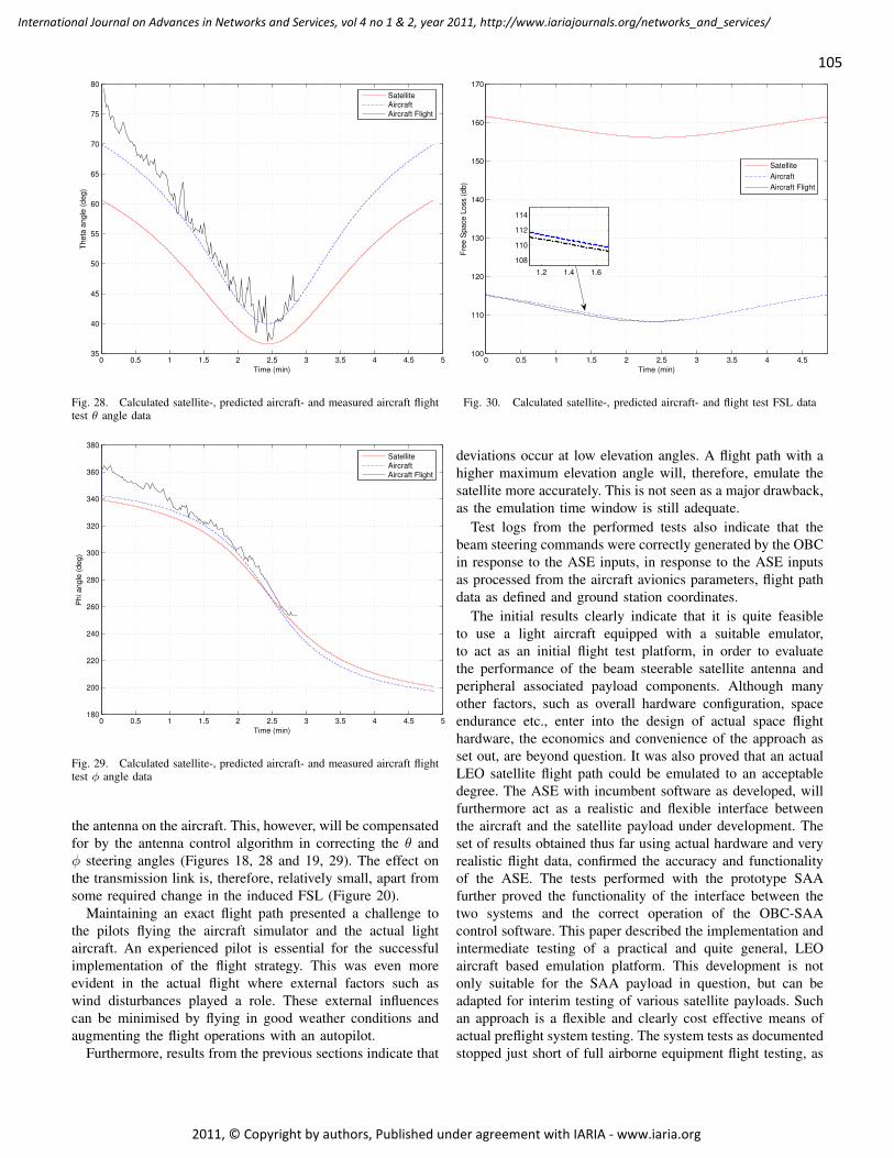
0 0.5 1 1.5 2 2.5 3 3.5 4 4.5 535
40
45
50
55
60
65
70
75
80
Time (min)
Thet
a an
gle
(deg
)
SatelliteAircraftAircraft Flight
Fig. 28. Calculated satellite-, predicted aircraft- and measured aircraft flighttest θ angle data
0 0.5 1 1.5 2 2.5 3 3.5 4 4.5 5180
200
220
240
260
280
300
320
340
360
380
Time (min)
Phi
ang
le (d
eg)
SatelliteAircraftAircraft Flight
Fig. 29. Calculated satellite-, predicted aircraft- and measured aircraft flighttest φ angle data
the antenna on the aircraft. This, however, will be compensatedfor by the antenna control algorithm in correcting the θ andφ steering angles (Figures 18, 28 and 19, 29). The effect onthe transmission link is, therefore, relatively small, apart fromsome required change in the induced FSL (Figure 20).
Maintaining an exact flight path presented a challenge tothe pilots flying the aircraft simulator and the actual lightaircraft. An experienced pilot is essential for the successfulimplementation of the flight strategy. This was even moreevident in the actual flight where external factors such aswind disturbances played a role. These external influencescan be minimised by flying in good weather conditions andaugmenting the flight operations with an autopilot.
Furthermore, results from the previous sections indicate that
0 0.5 1 1.5 2 2.5 3 3.5 4 4.5100
110
120
130
140
150
160
170
Time (min)
Free
Spa
ce L
oss
(db)
1.2 1.4 1.6
108
110
112
114
SatelliteAircraftAircraft Flight
Fig. 30. Calculated satellite-, predicted aircraft- and flight test FSL data
deviations occur at low elevation angles. A flight path with ahigher maximum elevation angle will, therefore, emulate thesatellite more accurately. This is not seen as a major drawback,as the emulation time window is still adequate.
Test logs from the performed tests also indicate that thebeam steering commands were correctly generated by the OBCin response to the ASE inputs, in response to the ASE inputsas processed from the aircraft avionics parameters, flight pathdata as defined and ground station coordinates.
The initial results clearly indicate that it is quite feasibleto use a light aircraft equipped with a suitable emulator,to act as an initial flight test platform, in order to evaluatethe performance of the beam steerable satellite antenna andperipheral associated payload components. Although manyother factors, such as overall hardware configuration, spaceendurance etc., enter into the design of actual space flighthardware, the economics and convenience of the approach asset out, are beyond question. It was also proved that an actualLEO satellite flight path could be emulated to an acceptabledegree. The ASE with incumbent software as developed, willfurthermore act as a realistic and flexible interface betweenthe aircraft and the satellite payload under development. Theset of results obtained thus far using actual hardware and veryrealistic flight data, confirmed the accuracy and functionalityof the ASE. The tests performed with the prototype SAAfurther proved the functionality of the interface between thetwo systems and the correct operation of the OBC-SAAcontrol software. This paper described the implementation andintermediate testing of a practical and quite general, LEOaircraft based emulation platform. This development is notonly suitable for the SAA payload in question, but can beadapted for interim testing of various satellite payloads. Suchan approach is a flexible and clearly cost effective means ofactual preflight system testing. The system tests as documentedstopped just short of full airborne equipment flight testing, as
105
International Journal on Advances in Networks and Services, vol 4 no 1 & 2, year 2011, http://www.iariajournals.org/networks_and_services/
2011, © Copyright by authors, Published under agreement with IARIA - www.iaria.org
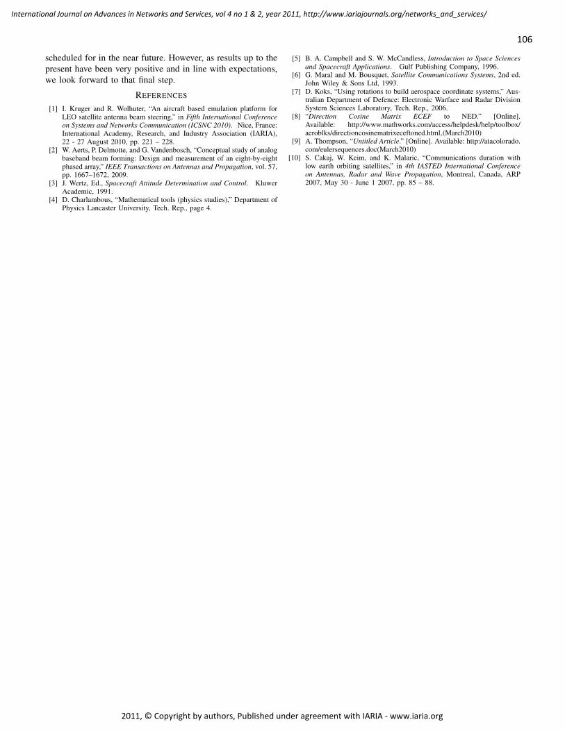
scheduled for in the near future. However, as results up to thepresent have been very positive and in line with expectations,we look forward to that final step.
REFERENCES
[1] I. Kruger and R. Wolhuter, “An aircraft based emulation platform forLEO satellite antenna beam steering,” in Fifth International Conferenceon Systems and Networks Communication (ICSNC 2010). Nice, France:International Academy, Research, and Industry Association (IARIA),22 - 27 August 2010, pp. 221 – 228.
[2] W. Aerts, P. Delmotte, and G. Vandenbosch, “Conceptual study of analogbaseband beam forming: Design and measurement of an eight-by-eightphased array,” IEEE Transactions on Antennas and Propagation, vol. 57,pp. 1667–1672, 2009.
[3] J. Wertz, Ed., Spacecraft Attitude Determination and Control. KluwerAcademic, 1991.
[4] D. Charlambous, “Mathematical tools (physics studies),” Department ofPhysics Lancaster University, Tech. Rep., page 4.
[5] B. A. Campbell and S. W. McCandless, Introduction to Space Sciencesand Spacecraft Applications. Gulf Publishing Company, 1996.
[6] G. Maral and M. Bousquet, Satellite Communications Systems, 2nd ed.John Wiley & Sons Ltd, 1993.
[7] D. Koks, “Using rotations to build aerospace coordinate systems,” Aus-tralian Department of Defence: Electronic Warface and Radar DivisionSystem Sciences Laboratory, Tech. Rep., 2006.
[8] “Direction Cosine Matrix ECEF to NED.” [Online].Available: http://www.mathworks.com/access/helpdesk/help/toolbox/aeroblks/directioncosinematrixeceftoned.html,(March2010)
[9] A. Thompson, “Untitled Article.” [Online]. Available: http://atacolorado.com/eulersequences.doc(March2010)
[10] S. Cakaj, W. Keim, and K. Malaric, “Communications duration withlow earth orbiting satellites,” in 4th IASTED International Conferenceon Antennas, Radar and Wave Propagation, Montreal, Canada, ARP2007, May 30 - June 1 2007, pp. 85 – 88.
106
International Journal on Advances in Networks and Services, vol 4 no 1 & 2, year 2011, http://www.iariajournals.org/networks_and_services/
2011, © Copyright by authors, Published under agreement with IARIA - www.iaria.org
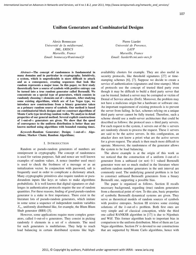
Unifom Generators and Combinatorial Designs
Alexis BonnecazeUniversité de la méditerrané,
IML, ERISCSMarseille, France
Email: [email protected]
Pierre LiardetUniversité de Provence,
LATPMarseille, France
Email: [email protected]
Abstract—The concept of randomness is fundamental inmany domains and in particular in cryptography. Intuitively,a system, which is unpredictable is more difficult to attackand as a consequence, creating sequences that look likerandom represents a major issue. In this paper, we first studytheoretically how a source of symbols with positive entropy canbe turned into a true random generator called Bernoulli. Weconcentrate on a special type of generators, which consists inrandomly choosing k elements out of n elements. After studyingsome existing algorithms, which are of Las Vegas type, weintroduce new constructions from a binary generator takenas a primary random source of symbols. Our method is basedon combinatorial block designs and we construct algorithms ofMonte Carlo type involving random walks. We analyze in detailproperties of our general method. Several explicit constructionsof k-out-of-n generators are given. We show that the speedof convergence to the uniform distribution is better than anyknown method using algorithms with bounded running times.
Keywords-Random Generator; Design; k-out-of-n Algo-rithms; Markov Chain; Random Algorithms;
I. INTRODUCTION
Random or pseudo-random generators of numbers areomnipresent in cryptography. The concept of randomnessis used for various purposes. Salt and nonce are well knownexamples of random values. A nonce (number used once)is used to check the freshness of a message or as aninitialization vector. In conjunction with password, salt isfrequently used in order to complicate a dictionary attack.Many cryptographic primitives also require random or pseu-dorandom inputs like keys or values to make algorithmsprobabilistic. It is well known that digital signatures or chal-lenges in authentication protocols require the use of randomquantities. For these reasons, finding of good pseudo-randomgenerator is a stake in first importance. There exist in theliterature lots of pseudo-random generators, which imitatein some sense a sequence of independent random variablesXn, uniformly distributed like, for example, the Blum BlumShub generator (BBS) [5].
However, some applications require more complex gener-ators, called k-out-of-n generators. They consist in pickingrandomly k elements in a set of n elements. The needfor such generators is multifarious. They help to reachload balancing in certain distributed systems like high-
availability clusters for example. They are also useful insecurity protocols, like threshold signatures [27] or time-stamping schemes [6], [7]. Suppose we decide to create aservice of authentication (signatures and time-stamps). Mostof protocols use the concept of trusted third party eventhough it may be difficult to build a third party server thatcan be trusted. Indeed a server may be corrupted or victim ofDenial of Service attacks (DoS). Moreover, the problem maynot have a malicious origin but a hardware or software one.An important requirement of existing protocols is to preventthe server from failing. In fact, schemes relying on a uniquethird party server cannot be fully trusted. Therefore, such ascheme should use a multi-server architecture that could bedescribed as follows: the protocol uses n third party servers.For each request to the system, k servers out of the n serversare randomly chosen to process the request. These k serversare said to be the active servers. In this configuration, anattacker does not know a priori what are the active serversfor a given request. The attack is then much more difficult tooperate. Moreover, the randomness of the generator allowsthe system to be load balancing.
The above example is at the origin of this work aswe noticed that the construction of a uniform k-out-of-ngenerator from a unbiased (or not) 0-1 valued Bernoulligenerator were not so much studied in the literature whereuniform random number generators in the unit interval arecommonly used. The underlying general problem is in factto construct unbiased Bernoulli generators from a binaryBernoulli one, supporting a possible bias.
The paper is organized as follows. Section II recallsnecessary background, regarding (true) random generatorsfrom a theoretical point of view. To this aim, basic propertiesof symbolic Bernoulli dynamical systems are given. Theyserve as theoretical models of random sources of symbolswith positive entropies. Section III reviews some existingsolutions of the k-out-of-n problem. Both first ones arevery simple and of classical conception, while the thirdone called RANKSB algorithm in [17] is due to Nijenhuisand Wilf. This former algorithm leads to important bias incomparison to the uniform distribution. Most of them are LasVegas algorithms. Section IV is devoted to our constructionsthat are supported by Monte Carlo algorithms, hence with
107
International Journal on Advances in Networks and Services, vol 4 no 1 & 2, year 2011, http://www.iariajournals.org/networks_and_services/
2011, © Copyright by authors, Published under agreement with IARIA - www.iaria.org
a bounded running times. Such algorithms approach theuniform distribution exponentially fast. We first propose agenerator based on the existence of some special combi-natorial objects, namely block t-designs or including someSteiner systems. This construction generates k elementsfrom a set of n elements in a uniform fashion from a binarygenerator. It consists in randomly picking a block, calledword, from the blocks of the design. This word is thenmodified in order to obtain a vector of weight k and lengthn with the desired property. We will see that it can be usefulto introduce the notion of block codes, since codewords ofa fixed Hamming weight in some codes hold a design.
The second type of constructions is based on randomwalks on a finite set following the action of a finite num-ber of generators of a group acting transitively. The firstconstruction uses the permutation group Sn. The secondconstruction is very related to the method based on blockdesigns. The main difference is in the way of randomlypicking a word in the appropriate set. The algorithm makesuse of the automorphism group of the design and executesa random walk on its blocks.
This article is an extended version of [1]. We presentin detail our methods, including mathematical foundations.Compare to the conference version, our construction makesuse of block designs and not just Steiner systems. Indeed,block designs are widespread and, as a consequence, ourconstruction can be applied for a wide range of parametersk and n. In order to illustrate our methods, we give severalexplicit constructions. For each chosen couple of parametersk and n, we exhibit a correct design and calculate the speedof convergence of the generator.
II. RANDOMNESS AND MATHEMATICAL FOUNDATIONS
A. From a binary random number generator to a q-ary one
In [18], the NIST defines a random bit sequence asfollows. “A random bit sequence could be interpreted as theresult of the flips of an unbiased fair coin with sides that arelabeled “0" and “1," with each flip having a probability ofexactly 1/2 of producing a “0" or “1." Furthermore, the flipsare independent of each other: the result of any previous coinflip does not affect future coin flips". Similarly, replacing theset of issues 0, 1 by a given finite set A, one can define arandom A-valued sequence as an A-valued independent andidentically distributed random variables Xn(·) with commonlaw the uniform distribution on A. For our purpose, it isconvenient to translate these notions in term of Bernoullidynamical systems. To this aim, we recall basic definitionsand general results related to symbolic dynamical systemsand entropy.
Assume that A, also called alphabet, is equipped with thediscrete topology, has q elements (or letters) with q ≥ 2, andset Ω(A) = AZ the product space endowed with the usualcompact product topology. Elements ω of Ω(A) are infinite
bilateral sequences
ω = (. . . , ω−3, ω−2, ω−1;ω0, ω1, ω2, . . . )
with origin pointed at ω0. The alphabet A is usuallyendowed with the uniform distribution denoted by U(A)but we also consider other distributions. The space Ω(A)is equipped with the σ-algebra of its Borel subsets. Anyprobability µ on A, induces the infinite product probabilityµ∞ on Ω(A), which is defined from cylinder sets. Moreprecisely, for any a := a0 . . . an−1 in An, let
[a] := ω ∈ Ω ; ∀ i ∈ 0, . . . , n− 1, ωi = ai
be the cylinder set of base a, then
µ∞(σk[a]) = µ(a0) . . . µ(an−1)
for any k ∈ Z. The shift σ : Ω(A) → Ω(A) is defined byσ(ω)n = ωn+1. Now, the triplet B(A, µ) := (Ω(A), σ, µ∞)is by definition the Bernoulli (random generator) on A withsource distribution µ. In case µ = U(A) we set U∞(A)for µ∞ and B(A, U(A)) is simply denoted by B(A). Letπ0 : Ω(A)→ A be the central projection (π0(ω) = ω0), thenthe maps B(A)n := π0σn defined on the probability space(Ω(A), U∞(A)) form an A-valued sequence of independentrandom variables identically distributed with distribution lawU(A). This corresponds to a q-ary random number generatorfor q = #A.
B. Symbolic random sources, entropy and factors
To fix some notations and for convenience of the reader,we recall basic definitions and facts from ergodic theory. Formore details and proofs we refer to the monographs [32]and [25], and specific references below. Our mathematicalmodel of random source of letters in A should be identifiedto a symbolic dynamical system (SDS) with symbols in A,that is to say a triple (Ω(A), σ, ν) where ν is a Borel measureon Ω(A), which is σ-invariant, i.e., ν = ν σ−1. Theentropy of such a system is, by the classical Kolmogorov-Sinai Theorem or by definition,
H(σ, ν) := − limN
1N
∑a∈AN
ν([a]) log ν([a])
with the convention 0. log(0) = 0.Let Ω′ := (Ω(A′), σ′, ν′) and Ω := (Ω(A), σ, ν) be
symbolic dynamical systems. Their direct product is theSDS Ω × Ω′ = (Ω(A × A′), σ × σ′, ν ⊗ ν′) and soH(σ×σ′, ν× ν′) = H(σ, ν) +H(σ′, ν′). This constructionmeans that the source corresponding to Ω and Ω′ are inde-pendent. If there is a measure preserving map f : Ω′ → Ωcommuting with the shifts, i.e.,
ν = ν′ f−1 ,σ f = f σ′ (ν-almost everywhere) , (1)
then Ω is said to be a factor of Ω′ with factor map f . Inthat case H(σ, ν) ≤ H(σ′, ν′). In the following, the value
108
International Journal on Advances in Networks and Services, vol 4 no 1 & 2, year 2011, http://www.iariajournals.org/networks_and_services/
2011, © Copyright by authors, Published under agreement with IARIA - www.iaria.org
H(σ,ν)H(σ′,ν′) will be called entropy rate and denoted by τ(ν, ν′)or simply by τ . If f is invertible (up to negligible sets),with measure preserving inverse map, then Ω is said tobe isomorphic to Ω′ with conjugate map f and if Ω′ isa Bernoulli random generator, then by extension Ω is alsocalled a Bernoulli SDS.
We have H(σ−1, ν) = H(σ, ν) and more generallyH(σ±k, µ) = kH(σ, ν) for any natural number k. In fact thek-th iterate (Ω(A), σk, ν), k 6= 0, is canonically identifiedwith (Ω(Ak), σ(k), ν(k)), where σ(k) is the shift on Ω(Ak)and ν(k) is induced by ν restricted to cylinder sets of Ω(Ak)viewed as particular cylinder sets from Ω(A). ThereforeH(σ(k), ν(k)) = kH(σ, ν).
This construction has the following important conse-quence. Assume that we have got a binary source withpositive entropy h, for example a source extracting fromrandom jitter in an electrical circuit or quantum effects insemiconductors or timing of running current process, or acombination of these sources. Then, we derive a source ofbinary blocks of length k having entropy kh.
In case of a Bernoulli system B(A,µ) (hence ν = µ∞
with the above definition), its entropy is easy to compute:
H(σ, µ∞) = −∑a∈A
λ(a) log λ(a).
In particular H(σ, U∞(A)) = log(#A).As a consequence of a deep result of Y. Sinai (see
[28]), if the entropy H(σ′, ν′) of Ω′ = (Ω(A′), σ′, µ′) isgreater than or equal to log #A then there exists a factor ffrom (Ω(A′), σ′, µ′) onto the uniform Bernoulli generatorB(A). Properties (1) shows that f is determined by thecentral coordinate map f0 = π0 f since we have f =(. . . , f−2, f−1; f0, f1, f2, . . . ) with fk = f0 σk (k ∈ Z).In particular f0 is constant equal to a on Ca := f−1([a]).Moreover, all partitions σ′m(Ca) ; a ∈ A (m ∈ Z) areindependent in between. Hence, building such a partition isusually intractable by computer except in particular casespointed out below. Another consequence of the above con-struction and Sinai’s theorem is that, from any given randombinary source of positive entropy, theoretically there exists afactor built from of a suitable power of this source, which isB(0, 1), the factor map consisting in distributing binarysequences in two parts equally likely and independently inthe time. This is the most hard problem to be solved inpractice for constructing, from a suitable physical randomsource, a binary random generator according to the NISTdefinition.
Following results of D. S. Ornstein [19], we recall that thefamily of Bernoulli dynamical systems is remarkably stable.In particular, they are characterized by their entropy (twosuch systems of equal entropy are isomorphic), any directproduct of Bernoulli systems and any non trivial iterate (andalso any root) of a Bernoulli system are Bernoulli. Moreoverany factor of a Bernoulli system is also Bernoulli. These
properties imply that any probability algorithm that takesin input a Bernoulli source and output a random source ofsymbols always gives rise to a Bernoulli SDS, isomorphicto some B(A, µ). In this paper we propose algorithms thattake as inputs the outcomes of an appropriated Bernoullisource B(0, 1k) and output a random source of letters ina given alphabet A whose distribution of letters is exactlyor approximate accurately the uniform distribution. We maydistinguish three sorts of such random algorithms.
(A1) Algorithms that output the uniform distribution onA in a bounded running time.
(A2) Las Vegas algorithms: they output the uniformdistribution on letters with unbounded running time but witha finite expectation.
(A3) Monte Carlo algorithms: they end in a boundedrunning time, output a distribution usually distinct to theuniform distribution but arbitrarily closed to it in term oftotal variation.
The following theorem depicts the first case.Theorem 1: If an algorithm of type (A1) takes input from
issues of the source B(0, 1k) and produce a uniformBernoulli source of entropy log2 q, then q = 2s with s ≤ k.
Proof: By assumption, the algorithm can be identi-fied to a factor maps f with central coordinate map f0having its values in 0, 1, . . . , q − 1. That leads to thepartition f−1
0 (j) ; 0 ≤ j < q of Ω(0, 1k) withU(Ak)(f−1
0 (j) = 1/q and there exists an integer L ≥ 1such that each f−1
0 (j) is the union of some cylinder sets ofthe form CL(a) := ω ∈ Ω(0, 1k) ; (∀i)(|i| > L or ωi =ai+L), a0 · · · a2L ∈ (0, 1k)2L+1. This implies that qdivides 2kL and since log q ≤ k one has q = 2s with s ≤ k.
Obviously, having in hands a uniform binary source, liketossing an unbiased coin, for cryptographic applications isimpractical. But such an abstract uniform Bernoulli genera-tor of binary sequences serves as a benchmark for evaluationof random generators and pseudo-random generators. Infact, security of most cryptographic algorithms and protocolsusing pseudo-random generators is based on the assumptionthat it is infeasible to distinguish use of a suitable binarypseudo-random number generator (PRNG) from use of a(truly) random number generator (RNG) defined as the SDSB(0, 1). As an example, the pseudorandom generator BBShas been proven secure in the sense that an attacker cannotpredict, in a reasonable time, the next bit of the outcomewith a probability greater than 1/2 (see [5]).
Putting apart the independency, the first major problem isthen to construct generators Gn of elements (called statesor symbols) of a finite set A, such that the distribution lawPn of Gn converges to the uniform distribution U(A) on Aas n tends to infinity. In order to quantify this convergence,we use the total variation distance between Pn and U(A).
109
International Journal on Advances in Networks and Services, vol 4 no 1 & 2, year 2011, http://www.iariajournals.org/networks_and_services/
2011, © Copyright by authors, Published under agreement with IARIA - www.iaria.org
This distance is defined by
d(Pn, U(A)) =12
∑a∈A
∣∣∣Pn(a)− 1#A
∣∣∣where Pn(a) is the probability that the generator Gn out-comes the state a.
A classical method to solve this problem is to introduce atransitive and irreducible Markov chain of transition matrixT , with space of states A, such that the uniform distributionon A is the stationary distribution of the chain. Constraintsof the problem are essentially on the incidence matrix of thechain since each state a can only transit on a number τ(a)of states such that 0 < τ(a) ≤ τmax where τmax is a smallconstant compare to #A. The stationary distribution is thenapproached by considering Markov random walk on a finitegraph. In fact, the general theory of finite Markov chainsshows that (by Perron-Frobenius’s theorem) there exist twoconstants C > 0 and ρ ∈]0, 1[ such that for every pair ofstates (i, j), one has∣∣∣(Tn)ij −
1#A
∣∣∣ ≤ Cρn . (2)
When #A is big, computation of constants C and ρ satis-fying (2) is generally not effective, even if we assume thatn is large enough. In fact, if m0 is an integer such that fora constant c ∈]0, 1] we have (Tm0)ij ≥ c 1
#A for all pairsof states (i, j), then inequality (2) becomes∣∣∣(Tn)ij −
1#A
∣∣∣ ≤ (1− c)bn/m0c . (3)
More details concerning finite Markov chains can be foundin [26] or [13]. Random walks on groups or finite graphs istreated in [23], [10] and a survey on recent results on thesubject can be found in [24].
III. EXISTING ALGORITHMS
Construction of a k-out-of-n generator greatly depends onthe requirements of the applications. They could involve thelevel of security, the amount of resources (CPU, memory,etc.) needed or the generators used as a primary source ofrandomness. In this former case, our reference, the generatorBBS, corresponds to the abstract model B(0, 1). Giventhe set Pnk := F ⊂ E ; #F = k endowed with theuniform distribution, the ultimate goal is then to constructfrom B(0, 1) a sequence of independent random variablesXm of distribution Pm such that d(Pm, U(Pnk )) ≤ Ce−cm
for m ≥ m0, where C, c and m0 are explicit constantsthat can be used in practice. Now we review some standardk-out-of-n generators according to above classification A1–A3.
(1) An algorithm of type (A1) exists if and only if(nk
)is a power of 2. This implies that n = 2s and k = 1. Inthat case, the algorithm is just the identity map: the output
is equal to the input given by the generator B(0, 1s) orby iterating B(0, 1) s times.
(2) The most obvious algorithm is based on the construc-tion of a set of k elements by randomly picking an integerbetween 1 and n, then renew the process to obtain an otherelement between 1 and n but distinct from the first oneand so on. It is typically a Las Vegas algorithm. From aprobabilistic point of view, this process needs an averageof n
(1n + 1
n−1 + · · ·+ 1n−k+1
)random runs (see [14]), an
average, which is O(n) for 1 ≤ k ≤ n/2.(3) The probably oldest probabilistic algorithm to uni-
formly and randomly pick k elements among n elementsrelies to the Fisher-Yates shuffle algorithm for generatinga random permutation σ of En = 1, . . . , n but stopingthe construction as soon as the values σ(1), . . . , σ(k) areconstructed. The Fisher and Yates original method consiststo randomly pick an element e1 from En with the uniformdistribution then pick an element from En \ e1 with theuniform probability and so on, k times. The underlyingprobabilistic model is based on the representation of integersin factorial basis. More precisely, let Ik := 0, . . . , n−1×0, . . . , n − 2 × · · · × 0, . . . , n − k equipped with theuniform probability. Any element i := (i1, i2, . . . , ik) of Ikcorresponds univocally to the integer ni ∈ 0, . . . , n! − 1given by its expansion in the factorial basis:
ni= ik.(n−k)!+ik−1.(n−k+1)!+· · ·+i2.(n−2)!+i1.(n−1)!
and the corresponding subset Pi = pi1 , . . . , pik of Engiven by pi1 = i1 + 1, then pi2 is the (i2 + 1)-thcoordinate of the n-tuple M2 deduced from the n-tupleM1 = (1, 2, . . . , n−1, n) by exchanging the n-th coordinatewith the (i1 + 1)-th one. For 2 ≤ s ≤ k − 1, pis isconstructed by induction as the (is + 1)-th coordinate ofthe n-tuple Ms deduced from Ms−1 by exchanging the(n− s+ 2)-th coordinate with the (is−1 + 1)-th coordinate.Notice that there exist k! integers i, which give the samesubset. The major drawback of this process is that it requiresto have independent uniform generators on s letters, forn − k < s ≤ n. The given construction leads to a factormap from B(A′, µ′) onto B(A,µ) with A′ = Ik and A
equal to Pnk . The entropic rate is thuslog (nk)
logn!−log(n−k)! .A better version of the Fisher-Yates algorithm was in-
troduced by R. Durstenfeld in [11] and later by D. Knuthin [14] with his Algorithm P (Shuffing) on page 145.A random number generator G uniformly distributed in[0, 1] is used in Algorithm P. It can be formally obtainedfrom B(0, 1) by computing G(ω) =
∑∞n=0 ωn2n−1
(ω ∈ Ω(0, 1). G is applied for computing a randominteger k(ω) = 1 + bjG(ω)c, between 1 and j. In thisway, computation of bjG(ω)c could never stop (but onlyfor n particular issues of ω). Nevertheless, the algorithmis of type (A2). Recently, R. Rolland in [22] proposedan algorithm of Las-Vegas type, which is analogous to
110
International Journal on Advances in Networks and Services, vol 4 no 1 & 2, year 2011, http://www.iariajournals.org/networks_and_services/
2011, © Copyright by authors, Published under agreement with IARIA - www.iaria.org
Fisher-Yates algorithm. This algorithm constructs a k-out-of-n random generator involving only a uniform Bernoullirandom generator B(0, 1`) with n ≤ 2`.
(4) RANKSB algorithm proposed in [17] takes into ac-count some algorithmic constraints (in particular in termsof CPU and execution time), which are not verified bythe preceding methods. We give a simplified version ofRANKSB. It consists in subdividing the interval [1, n] ink sub-intervals Rj with approximately the same length,and randomly choose the number rj of elements to beselected in each Rj . If we don’t take into account thatrj ≤ #Rj , the k-tuple (r1, . . . , rk) of integers rj ≥ 0 suchthat r1 + · · · + rk = k follows binomial law constructedfrom k independent runs of integers in 0, . . . , n, withthe uniform law. In order to avoid that rj be greater than#Rj , we recompute the subdivision in sub-intervals Rjthen in each Rj we select rj elements using method (2),(3) or any others. The algorithm uses a source of entropyk log n corresponding to B(1, ..., nk), to obtain the factorcorresponding to a shift of Bernoulli on the set of k-tuples(r1, . . . , rk) as above (distributed according to the binomiallaw), which is of entropy
Hk := −∑
r1+···+rk=k
1kk
(k
r1, . . . , rk
)log( 1kk
(k
r1, . . . , rk
)).
When k is small, let us use (2) to pick the rj elements inRj so that the corresponding entropy rate is (in average)assumed closed to 1. The entropy rate of the algorithm isthen Hk/k log n. Since Hk is less than log kk, this entropyrate is then less than log k/ log n. Notice that if n/k is small,the output distribution has a non negligible bias.
In the sequel we describe k-out-of-n generators, whichare of Monte Carlo type.
IV. PROPOSED ALGORITHMS
In this section, we propose two types of constructions.The first one is based on some remarkable configurationsof points in binary vectors spaces, namely, block designs[15]. It leads to optimal uniform generators and exists for awide range of parameter values k and n since designs arevery common. The second type of constructions is based onrandom walks on some groups or finite sets.
A. Block t-design based constructions
A combinatorial block t-design D with parameters t-(v, k, λ) is an incidence structure (P,B) (where elements ofB, called blocks, are subsets of P) satisfying the followingconditions:
• #P = v,• ∀B ∈ B,#B = k,• ∀S ⊂ P such that #S = t, #B ∈ B ; S ⊂ B = λ.
It is known that a necessary condition for the existenceof a t-design is that
bs = λ
(v−st−s)(
k−st−s) , for all s satisfying 0 ≤ s < t,
and where bs corresponds to the number of blocks thatcontain any s-set (i.e., set of s elements) of points fromP . The Web site [9], maintained and regularly updated byDan Gordon, gives a database of known t-designs.
A Steiner system is a particular case of a block design. Itis simply a block design with parameters t-(v, k, 1) and iscurrently denoted by S(t, k, v). A Steiner system for t = 2is called balanced incomplete block design and for v = s2 +s+1, k = s+1, the system corresponds to the combinatorialnotion of finite projective plane. A necessary condition forthe existence of a Steiner system is that the number(
v−st−s)(
k−st−s)
is an integer for all s satisfying 0 ≤ s < t. This conditionis not sufficient and there is no Steiner system with, forexample, parameters (2, 6, 36), (3, 7, 37) or (5, 6, 18). Infact, there is no known general sufficient condition on theexistence of Steiner systems. For t = 2 and 3, there existinfinitely many families of Steiner systems and for t ≥ 4,we refer to [8] or [31].
There exist many ways to construct a design. The easiestone is probably to consider an error correcting code. Indeed,there exist codes whose words of a fixed weight hold de-signs. For example, words of weight 3 in the Hamming codesyield 2-designs and 5-designs can be constructed from Golaycodes. Quadratic residue codes constitute another example offamily of codes that yield designs. An other way to obtaindesigns is to consider Hadamard matrices. In this article,examples of such constructions are given. Finally, thereexist many other constructions like, for example, recursivemethods [20].
For any design D, its group of automorphisms, denotedby Aut(D), plays a fundamental role to understand thegeometrical structure of D. Elements σ of this group belongto the permutation group S(P) of P and verifies thefollowing condition
Bσ = B
where Bσ denotes the set of σ(B) with B ∈ B.A brief description of our construction of a k-out-of-n
generator from a design can be expressed as follows. First,consider a k-(n, b, λ) design (P,B) and after indexing Pby i, 1 ≤ i ≤ #P identify each block B in B with abinary string of length #P , the place of 1’s indicating theelements of B. Now, choose randomly a block m fromthe blocks of the design. By construction, the Hammingweight of m is b. Then, randomly choose b− k coordinatepositions of 1 in m, replace the corresponding 1 by 0. We
111
International Journal on Advances in Networks and Services, vol 4 no 1 & 2, year 2011, http://www.iariajournals.org/networks_and_services/
2011, © Copyright by authors, Published under agreement with IARIA - www.iaria.org
get the output m′. Since we are only concerned by the setof positions of the 1’s, we may identify it to 1, . . . , b sothat the elimination of b− k digits 1 is done by selecting atrandom, independently of the random choice of m, a subsetof b−k elements in 1, . . . , b, issuing m′ independently ofthe possible λ-blocks m that cover m′. Hence, the algorithmoutputs a random word of length n with Hamming weightk. Notice that finding a k-out-of-n generator is equivalent tofinding a n−k-out-of-n generator. Of course this algorithmneeds uniform random generators on sets of symbols, whichare not necessarily of cardinality a power of 2, hence it isusually of type (A2).
Example 1: As an example, we explain in detail theconstruction of a 5-out-of-24 generator, which is based ona S(5, 8, 24). In this case, the blocks of the design can berepresented as the words of weight 8 in the extended binaryGolay code G24. Our construction is based on the followingproperty [16, page 67]: every binary vector of Hammingweight 5 and length 24 is covered by exactly one word ofG24 of weight 8. It turns out that a random generator in P24
5
is easily obtained from a random generator of the words ofweight 8 of the Golay code (and vice versa).
We recall the main combinatorial properties of G24. Inthe sequel W (m) denotes the Hamming weight of a binarystring m (also called vector as element of the underlyingvector space); the weight distribution of G24 is classical andgiven by the following table:
weights 0 8 12 16 24number of words 1 759 2576 759 1
Table 1: Weight distribution of the words of the Golay code G24
A remarkable property of this code is that the set of wordsof a given weight forms the blocks of a design. Hence, thewords of weight 8, called octads, form the blocks of a 5-(24, 8, 1) design and words of weights 12 form the blocksof a 5-(24, 12, 48) design. It is worth noticing that, in thecase of octads, the parameter λ of the design is equal to 1.This means that a vector of length 24 and Hamming weight5 is covered by exactly one octad of the code. Thus, octadsform a Steiner system with parameters S(5, 8, 24). Note thatthere exist in G24 other Steiner systems like S(4, 7, 23),S(3, 6, 22) or S(2, 5, 21), leading to similar constructionsof generators.
Since G24 decode at most three errors, it happens thatwhen changing three bits from the value 1 to the value 0in an octad, one can construct
(85
)vectors of weight five.
If we repeat this process for every octad, we obtain a totalof 759 ×
(85
)=(245
)vectors of weights five, which is the
cardinal of P248 .
This leads to the following construction:
(a) choose a base b1, . . . , b12 of G24;(b) choose a random generator G on 12 bits (corre-sponding to a 12 iterations of a binary Bernoulli);
(c) pick a binary vector g := g1 · · · g12 from the randomgenerator G;(d) compute the word m(g) :=
⊕12j=1 gjbj ;
(e) if W (m) = 8 then m = 0a110a21 . . . 0a810a9 anddo
(e1) randomly pick a vector x = x1 . . . x8 ofweight three and length eight (there exist
(83
)= 56
such vectors. They can be kept in memory);(e2) computem′′ :=0a1(1⊕ x1)0a2(1⊕ x2) . . . 0a8(1⊕ x8)0a9 ;
(f) if W (m) = 16, then m := m⊕ 124 and go to (e);(g) if W (m) = 0 or W (m) = 24, then go to (c);(h) if W (m) = 12, then ask G a binary vector g′ :=g′1 · · · g′12 and compute m′ := m(g′)if W (m′) = 8 then m := m′ and go to (e)else if W (m′ ⊕m) = 8 then m := m′ ⊕m and go to(e)else go to (c);(i) output m′′.
This algorithm makes use of the generator Γ = B8 ×B(1, . . . , 56) where B8 is the generator induced byB(0, 112) on the set P8 of words of weight eight orsixteen. Since the counting probability of P8 is µ(P8) =2×759
212 = 0, 37 . . . , the entropy of Γ is equal to h(Γ) =(12 log 2+log 56)/µ(P8) = 33.30 . . . . It gives in output theuniform generator B(P24
5 ) with entropy log(245
). Hence we
obtain the entropy rate
log(245
)h(Γ)
= 0, 319 . . . .
In this example, we obtained the blocks of the design byconsidering the words of a fixed weight in the Golay code.This is not the only method as we will show later.
B. Random walks methods
In this section, we show how random walks can leadto a distribution as closed as desired to the uniform k-out-of-n generator. The first construction applies randomwalk on a finite group and in particular on the symmetricgroup Sn. However, this method is not practical for largevalues of n since the size of the group becomes huge. Thesecond construction makes use of a Markov walk on theset of blocks of a k-design. In both case the convergenceto the uniform distribution is exponential. We illustrateour method by some examples. We consider codes, likeHamming, Golay, or quadratic residue codes, in order toobtain the appropriate design. We also give an examplerelated to Hadamard matrices.
1) Random walk on a finite group, generalities: this topicin cryptographic context was investigated by Sloane in a nicesurvey [29]. Let us introduce objects and notations necessaryfor our study.
A random walk on a finite group G is currently definedby a probability Q on G and a homogeneous Markov chain
112
International Journal on Advances in Networks and Services, vol 4 no 1 & 2, year 2011, http://www.iariajournals.org/networks_and_services/
2011, © Copyright by authors, Published under agreement with IARIA - www.iaria.org
Γn, of space of states G, of transition matrix T given byTg,h = Q(gh−1) = P (Γn+1 = g|Γn = h). If the supportof Q generates G, the chain is irreducible and its stationarydistribution is the uniform distribution U(G) on G. From theidentity (Γ0 = e), and a sequence of independent randomvariables Xn, the walk can be described inductively by Γ1 =X1, Γn = XnΓn−1, the law of Γn being given by Q(1) = Qfor Γ1 and convolution product Q(m)(g) = Q∗Q(m−1)(g) =∑h∈GQ
(m−1)(gh−1)Q(h) for Γm (≥ 2). Here, we supposethat the chain is irreducible and aperiodic. Hence there existan integer m0 and a constant c > 0 such that Tm0
g,h ≥ c 1#G
and then inequality (3) can be applied. This inequality canbe translated in terms of distance (2), and can be improvedin the case of symmetric walks (Q(g) = Q(g−1)) or forparticular groups previously analyzed in a probabilistic way.For more details, see [2], [3], [10], [23], [24].
One application in cryptography is the popular stream par-ity de-skewer. Here G is the additive group 0, 1 := Z/2Zand Q(0) = 1
2 − β, Q(1) = 12 + β with 0 ≤ 2β < 1. Then
T = 12J + βS with J :=
(1 1
1 1
)and S :=
(−1 1
1 −1
).
Using JS = SJ = 0, J2 = 2J and S2 = 2S we get theexplicit formula
Tn =12J + (2β)nS
and consequently
d(Qn, U(0, 1)) = e−n log(1/2β).
Moreover, for k ≥ 1 fixed, the sequence of random variables(Γkn)n≥1 defines the Bernoulli SDS B(0, 1, Q(k)) whoseentropy is, after simplification,
Hk = log 2− 12
(1 + (2β)k) log(1 + (2β)k)
+12
(1− (2β)k) log( 1
1− (2β)k).
Hence, Hk − log 2 ∼ (2β)2k as k tends to infinity.2) Random transposition on the symmetric group Sn
and k-out-of-n generators: random walks on the symmetricgroup Sn have been intensely studied (see the precedingreferences). Consider a uniform Bernoulli generator B(Sn)on the group of permutations Sn. This generator definesa sequence of random variables Σn(·) = B(Sn)n. ThenCn = Σn(1, . . . , k) is a sequence of random variablesuniformly distributed in the set Pnk .
An interesting method to construct generators distinctfrom Fisher-Yates shuffle algorithm is to choose a set E ofgenerators of Sn and use a Bernoulli B(E). A result of [10]states that the speed of convergence is in e−γ when the walkhas a sufficiently large number of steps γ: more precisely,for E = Id, (1, 2), (1, 2, . . . , n), (n, n − 1, n − 2, . . . , 1)one has
d(G(36n3(logn+γ)), U(Sn)) ≤ αe−γ , (4)
where α > 0 is a universal constant and for all integersγ ≥ 0. Then, random variables Γm (see above) represent agenerator converging to the Bernoulli generator B(Sn); itoutputs, at each step, a permutation σ and σ(1, . . . , k). LetΓm[k] denotes this generator. Its distribution Q(m)
k on Pnk isgiven, for each set A of k elements of En = 1, . . . , n, by
Q(m)k (A) =
∑σ∈Sn
σ(1,...,k)=A
Q(m)(σ).
We observe that #σ ∈ Sn ; σ(1, . . . , k) = A = k!(n−k)! so that
d(Γm, U(Sn)) =12
∑A∈Pnk
∣∣∣Q(m)k (A)− k!(n− k)!
n!
∣∣∣≤ d(Γm[k], U(Pnk )) .
This last bound validates the construction of Γm[k] withthe same convergence property than that of Γm. However,this generator is not practical for large value of n, and inparticular for n = 24.
3) Homogeneous symmetric random walk on a finite set:Let M be a finite set of elements and let E be a set ofbijections of M. We set
µ := #M and χ := #E.
A general random walk on M with instructions in E isgiven by a distribution law L on M and a sequence of E-valued random variables (Xn)n of given distribution Pn. Anoutcome x = (xk)k of the random sequence (Xk)k≥1 leadsto a walk on M consisting to start from an initial pointm0 in M, selected according to the law L (step 0) and thelocation of the walk after n steps is mn = xn xn−1 · · · x1(m0). In the sequel, we only pay attention to a Markovsymmetric homogeneous and uniform walk, that means awalk satisfying the following properties:
(j) The initial point m0 is fixed.(jj) Symmetry: for all Y in E the inverse map Y −1
belongs to E and the identity map belongs to E.(jjj) The random variables Xn are independent, withuniform distribution Pn := U(E).
Therefore, the space of states of the corresponding Markovchain is M and the stochastic transition matrix T is givenby
Ti,j :=#Y ∈ E ; Y (i) = j
χ((i, j) ∈M2) .
According to property (jj), the matrix T is symmetric and so,has the uniform distribution onM for stationary probability.For our applications we assume that
(jv) The chain is mixing.This assumption is equivalent to the fact that a power of Shas all entries positive. Hence, we may define the followingimportant parameter of the chain
κ := mink ≥ 0 ; ∀ (i, j) ∈M2, (T k)i,j > 0.
113
International Journal on Advances in Networks and Services, vol 4 no 1 & 2, year 2011, http://www.iariajournals.org/networks_and_services/
2011, © Copyright by authors, Published under agreement with IARIA - www.iaria.org
In other words κ is the minimum number of necessary stepsto go from any state to any state.
Our next goal is to estimate the so called spectral holeof S. To this aim we use the symmetry of the chain byconsidering appropriated quadratic forms on the vector spaceRM equipped with the euclidean scalar product denoted by〈ξ|ξ′〉 =
∑(i,j)∈M2 ξiξ
′j , with norm || · ||. Each generator
Y in E, acting on M is identified to an automorphismof RM permuting the canonical basis. It is represented byan orthogonal matrix, still denoted by Y . The action of Yapplies at i will be denoted by Y ·i. Explicitly, Y is given byYi,j = 1 if j = Y ·i and Yi,j = 0 otherwise. The inverse Y −1
of Y corresponds to the transpose matrix Y ∗. The stochastictransition matrix T defined above is now given by
T :=1χ
∑Y ∈E
Y.
By symmetry of T and Perron-Frobenius’s theorem, T has µeigenvalues λν (0 ≤ ν < µ) whose the largest one is equalto 1, with multiplicity 1. Let ρ be the greater eigenvalue ofT distinct from 1, we ordered real eigenvalues as follows:
−1 < λµ−1 ≤ · · · ≤ λ1 = ρ < λ0 = 1 .
Theorem 2: With the preceding definitions and notations,we have
−1 +2χ≤ λµ−1 and ρ ≤ 1− 4
κ(κ+ 1)χ.
Proof.1. The first inequality is easy to prove. By (jj), diagonal
terms of T are equal to 1/χ, hence the matrix χχ−1 (T − 1
χI)is stochastic with eigenvalues χλν−1
χ−1 between −1 and 1. Inparticular −1 ≤ χλµ−1−1
χ−1 , which gives −1 + 2χ ≤ λµ−1, as
expected.2. The second inequality is more complex to prove. It
relies on the comparison of two quadratic forms on RM.To every symmetric matrix A indexed on M we as-
sociate the quadratic form QA(ξ) = 〈Aξ|ξ〉. Eigenvaluesα0 ≤ α1 ≤ · · · ≤ αµ−1 of A are given by Courant-Fishertheorem (also called mini-max theorem) [12]:
αν = minFm(F ) ; dim(F ) = ν + 1, 0 ≤ ν < µ,
the minimum being calculated over the set of all subspacesF of RM of dimension ν + 1 and
m(F ) := max〈Aξ|ξ〉 ; ||ξ|| = 1, and ξ ∈ F.
A straightforward consequence of this theorem isCorollary 1: Let QA and QA′ two quadratic forms on
RM, of symmetric matricesA and A′ and eigenvalues λν , λ′νrespectively (indexed in decreasing order). If for a constantC > 0 we have QA′ ≤ CQA, then λ′ν ≤ Cλν for everyindex ν, 0 ≤ ν < µ.
For our purpose, choose A = I − T . Then we have
QI−T (ξ) =12
∑i,j
(ξi − ξj)2Ti,j
=1
2χ
∑Y∈Ei∈M
(ξi − ξY ·i)2
The bound will result from the following main lemma.Lemma 1: Consider the symmetric matrix B = I − 1
µJwhere J has all its coefficients equal to 1. Then
QB ≤χκ(κ+ 1)
4QI−T . (5)
Proof. For every pair (i, j) of states, let Y i,j =Y i,jk(i,j) · · ·Y
i,j0 with Y i,j0 = I be a composition of elements
of E such that j = Y i,j ·i with k(i, j) minimal. Set|Y i,j | := k(i, j). We have |Y i,j | ≤ κ and
ξi − ξj =|Y i,j |−1∑s=0
(ξYi,js ···Y i,j0 ·i
− ξYi,js+1···Y
i,j0 ·i
).
Applying Cauchy-Schwarz inequality gives
(ξi − ξj)2 = |Y i,j ||Y i,j |−1∑s=0
(ξYi,js ···Y i,j0 ·i
− ξYi,js+1···Y
i,j0 ·i
)2
≤ χ|Y i,j ||Y i,j |−1∑s=0
(ξYi,js ···Y i,j0 ·i
− ξYi,js+1···Y
i,j0 ·i
)2Tλijs
where λijs := Y i,js · · ·Yi,j0 ·i, Y
i,js+1 · · ·Y
i,j0 ·i .
Multiply these inequalities by 1/µ and add all of them, firstby summing on j and then on i. The summation on the leftside simply gives
1µ
∑(i,j)∈M2
(ξi − ξj)2 = 2QB(ξ).
Hence, the summation on the right side is greater than2QB(ξ). By collecting all right terms according to the valuestaking by |Y i,j | for i fixed we get
(χ/2)1µ
κ∑k=1
k(2QI−T )
since by minimality, there is no loop in the path going fromi to j and constructed from Y i,j . Therefore, summing over inow leads to the desired inequality QB(ξ) ≤ κ(κ+1)χ
4 QI−T .Eigenvalues of 1
µJ being 1 and 0, those of B are then1 (with multiplicity µ − 1) and 0. Then Corollary 1 gives1 ≤ κ(κ+1)χ
4 (1 − ρ), which is the second inequality oftheorem 2.Using Theorem 2 and the fact that T is a symmetricstochastic matrix of order µ, we get the following inequality∣∣∣∣∣∣Tn − 1
µJ∣∣∣∣∣∣
2≤(
1− 4κ(κ+ 1)χ
)n,
114
International Journal on Advances in Networks and Services, vol 4 no 1 & 2, year 2011, http://www.iariajournals.org/networks_and_services/
2011, © Copyright by authors, Published under agreement with IARIA - www.iaria.org
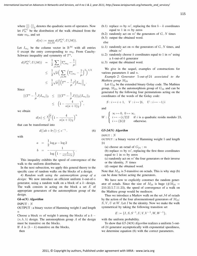
where∣∣∣∣∣∣ ·∣∣∣∣∣∣
2denotes the quadratic norm of operators. Now
let P (n)m be the distribution of the walk obtained from the
state m0, and set
d(n) := maxm∈M
d(P (n)m , U(M)).
Let Im0 be the column vector in RM with all entries0 except the entry corresponding to m0. From Cauchy-Schwarz inequality and symmetry of Tn,
d(P (n)m , U(M)) =
12
∑j∈M
∣∣∣Tni,m0− 1µ
∣∣∣≤ 1
2√µ( ∑j∈M
(Tni,m0
− 1µ
)2)1/2
≤ 12√µ∣∣∣∣∣∣(Tn − 1
µJ)Im0
∣∣∣∣∣∣2.
Since
||(Tn − 1µJ)Im0 ||2 ≤ |||(Tn − 1
µJ)|||2||Im0 ||2
≤(
1− 4κ(κ+ 1)χ
)n,
we obtain
d(n) ≤√µ
2
(1− 4
κ(κ+ 1)χ
)nthat can be transformed into
d(dab+ bγe) ≤ e−γ . (6)
with
a =12
logµ− log 2
b = − 1
log(
1− 4κ(1+κ)χ
) .This inequality exhibits the speed of convergence of the
walk to the uniform distribution.In the next subsection, we apply this general theory to the
specific case of random walks on the blocks of a design.4) Random walk using the automorphism group of a
design: We now introduce an efficient uniform k-out-of-ngenerator, using a random walk on a block of a k−design.The walk consists in acting on the block a set E ofappropriate generators of the automorphism group of thedesign.Gk-n(N) AlgorithmINPUT : NOUTPUT : a binary vector of Hamming weight k and lengthnChoose a block m of weight b among the blocks of a k −(n, b, λ) design. The automorphism group A of the designmust be transitive on the blocks.If A is (b− k)-transitive on the blocks,
then
(b.1) replace m by m′, replacing the first b− k coordinatesequal to 1 in m by zeros
(b.2) randomly act on m′ the generators of G, N times(b.3) output the obtained word.
else(c.1) randomly act on m the generators of G, N times, and
obtain m′
(c.2) randomly choose k coordinates equal to 1 in m′ usinga k-out-of-b generator
(c.3) output the obtained word.
We give in the sequel, examples of constructions forvarious parameters k and n.
Example 2: Generator 5-out-of-24 associated to theMathieu group M24
Let G24 be the extended binary Golay code. The Mathieugroup, M24, is the automorphism group of G24 and can begenerated by the following four permutations acting on thecoordinates of the words of the Golay code:
S : i 7→ i+ 1, V : i 7→ 2i, U : i 7→ −1/i
and
W :
∞ 7→ 0, 0 7→ ∞,i 7→ −(i/2)2 if i is a quadratic residu modulo 23,i 7→ (2i)2 otherwise.
G5-24(N) AlgorihmINPUT : NOUTPUT : a binary vector of Hamming weight 5 and length24
(a) choose an octad of G24 : m(b) replace m by m′, replacing the first three coordinatesequal to 1 in m by zeros(c) randomly act on m′ the four generators or their inverseor the identity, N times(d) output the obtained word.
Note that M24 is 5-transitive on octads. This is why step (b)can be done before acting the generators.
We have now to explicitly construct the random gener-ator of octads. Since the size of M24 is huge (#M24 =210.33.5.7.11.23), the speed of convergence of a walk onthe Mathieu group would be mediocre.
Thus we introduce a Markov walk on the setM of octadsby the action of the four aforementioned generators of M24:S, V , U et W . Let I be the identity. Now we make the walksymmetrical by taking the following transition set
E := I, S, S−1, U, V, V −1,W,W−1,
with the uniform probability.To show that G5-24(N) Algorihm realizes a uniform 5-out-
of-24 generator asymptotically with exponential speediness,we determine equation (6) with the correct parameters.
115
International Journal on Advances in Networks and Services, vol 4 no 1 & 2, year 2011, http://www.iariajournals.org/networks_and_services/
2011, © Copyright by authors, Published under agreement with IARIA - www.iaria.org
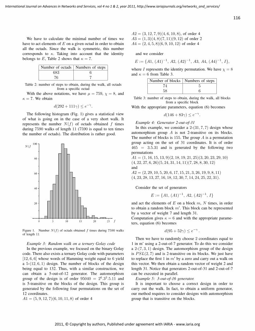
We have to calculate the minimal number of times wehave to act elements of E on a given octad in order to obtainall the octads. Since the walk is symmetric, this numbercorresponds to κ. Taking into account that the identitybelongs to E, Table 2 shows that κ = 7.
Number of octads Numbers of steps683 676 7
Table 2: number of steps to obtain, during the walk, all octadsfrom a specific octad
With the above notations, we have µ = 759, χ = 8, andκ = 7. We obtain
d(292 + 111γ) ≤ e−γ .
The following histogram (Fig. 1) gives a statistical viewof what is going on in the case of a very short walk. Itrepresents the number N(f) of octads obtained f timesduring 7590 walks of length 11 (7590 is equal to ten timesthe number of octads). The distribution is rather good.
N(f)
f
Figure 1. Number N(f) of octads obtained f times during 7590 walksof length 11
Example 3: Random walk on a ternary Golay codeIn the previous example, we focused on the binary Golay
code. There also exists a ternary Golay code with parameters[12, 6, 6] whose words of Hamming weight equal to 6 yielda 5-(12, 6, 1) design. The number of blocks of the designbeing equal to 132. Thus, with a similar construction, wecan obtain a 5-out-of-12 generator. The automorphismgroup of the design is of order 95040 = 26.33.5.11 andis 5-transitive on the blocks of the design. This group isgenerated by the following four permutations on the set of12 coordinates.A1 = (5, 9, 12, 7)(6, 10, 11, 8) of order 4
A2 = (3, 12, 7, 9)(4, 6, 10, 8), of order 4A3 = (1, 3)(4, 8)(7, 11)(9, 12) of order 2A4 = (2, 4, 5, 8)(6, 9, 10, 12) of order 4
and we consider
E := A1, (A1)−1, A2, (A2)−1, A3, A4, (A4)−1, I,
where I represents the identity permutation. We have χ = 8and κ = 6 from Table 3.
Number of blocks Numbers of steps74 558 6
Table 3: number of steps to obtain, during the walk, all blocksfrom a specific block
With the appropriate parameters, equation (6) becomes
d(146 + 83γ) ≤ e−γ .
Example 4: Generator 2-out-of-31In this example, we consider a 2-(31, 7, 7) design whose
automorphism group A is not 2-transitive on its blocks.The number of blocks is 155. The group A is a permutationgroup acting on the set of 31 coordinates. It is of order465 = 3.5.31 and is generated by the following twopermutationsA1 = (1, 16, 15, 13, 9)(2, 18, 19, 21, 25)(3, 20, 23, 29, 10)(4, 22, 27, 6, 26)(5, 24, 31, 14, 11)(7, 28, 8, 30, 12)andA2 = (2, 29, 10, 5, 20, 6, 17, 15, 21, 3, 26, 19, 9, 8, 11)(4, 23, 28, 13, 27, 16, 18, 12, 30, 7, 14, 24, 25, 22, 31).
Consider the set of generators
E := A1, (A1)−1, A2, (A2)−1, I
and act the elements of E on a block m, N times, in orderto obtain a random block m′. This block can be representedby a vector of weight 7 and length 31.Computation gives κ = 6 and with the appropriate parame-ters, equation (6) becomes
d(95 + 52γ) ≤ e−γ .
Then we have to randomly choose 2 coordinates equal to1 in m’ using a 2-out-of-7 generator. To do this we considera 2-(7, 3, 1) design. The automorphism group of the designis PSL(2, 7) and is 2-transitive on its blocks. We just haveto replace the first 1 in m′ by a zero and carry out a walk onthis vector. We then obtain a random vector of weight 2 andlength 31. Notice that generators 2-out-of-31 and 2-out-of-7can be executed in parallel.
Example 5: 3-out-of-16 generator.It is important to choose a correct design in order to
carry out the walk. In fact, to obtain a uniform generator,our method requires to consider designs with automorphismgroup that is transitive on the blocks.
116
International Journal on Advances in Networks and Services, vol 4 no 1 & 2, year 2011, http://www.iariajournals.org/networks_and_services/
2011, © Copyright by authors, Published under agreement with IARIA - www.iaria.org
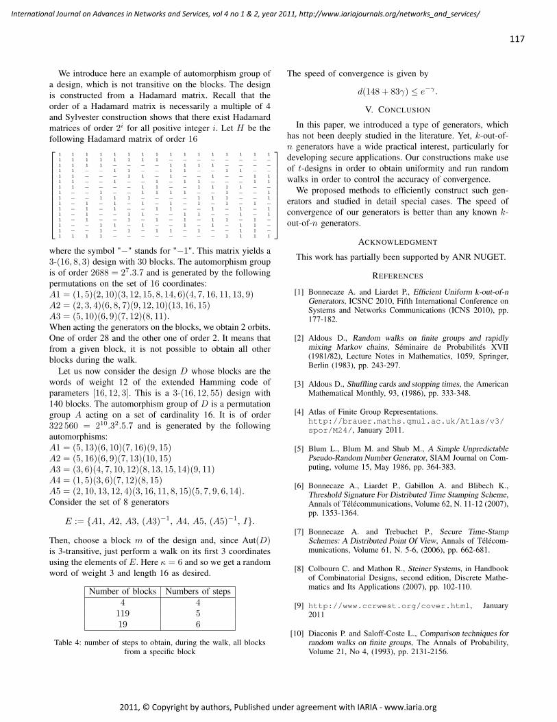
We introduce here an example of automorphism group ofa design, which is not transitive on the blocks. The designis constructed from a Hadamard matrix. Recall that theorder of a Hadamard matrix is necessarily a multiple of 4and Sylvester construction shows that there exist Hadamardmatrices of order 2i for all positive integer i. Let H be thefollowing Hadamard matrix of order 16
1 1 1 1 1 1 1 1 1 1 1 1 1 1 1 11 1 1 1 1 1 1 1 − − − − − − − −1 1 1 1 − − − − 1 1 1 1 − − − −1 1 − − 1 1 − − 1 1 − − 1 1 − −1 1 − − − 1 1 − 1 − − 1 − − 1 11 1 − − 1 − − 1 − 1 1 − − − 1 11 1 − − − − 1 1 − − 1 1 1 1 − −1 − − 1 − − 1 1 1 1 − − 1 − − 11 − − 1 1 1 − − − − 1 1 1 − − 11 − 1 − 1 − 1 − 1 − 1 − 1 − 1 −1 − 1 − 1 − − 1 1 − − 1 − 1 − 11 − 1 − − 1 1 − − 1 1 − − 1 − 11 − 1 − − 1 − 1 − 1 − 1 1 − 1 −1 − − 1 1 − 1 − − 1 − 1 − 1 1 −1 − − 1 − 1 − 1 1 − 1 − − 1 1 −1 1 1 1 − − − − − − − − 1 1 1 1
where the symbol "−" stands for "−1". This matrix yields a3-(16, 8, 3) design with 30 blocks. The automorphism groupis of order 2688 = 27.3.7 and is generated by the followingpermutations on the set of 16 coordinates:A1 = (1, 5)(2, 10)(3, 12, 15, 8, 14, 6)(4, 7, 16, 11, 13, 9)A2 = (2, 3, 4)(6, 8, 7)(9, 12, 10)(13, 16, 15)A3 = (5, 10)(6, 9)(7, 12)(8, 11).When acting the generators on the blocks, we obtain 2 orbits.One of order 28 and the other one of order 2. It means thatfrom a given block, it is not possible to obtain all otherblocks during the walk.
Let us now consider the design D whose blocks are thewords of weight 12 of the extended Hamming code ofparameters [16, 12, 3]. This is a 3-(16, 12, 55) design with140 blocks. The automorphism group of D is a permutationgroup A acting on a set of cardinality 16. It is of order322 560 = 210.32.5.7 and is generated by the followingautomorphisms:A1 = (5, 13)(6, 10)(7, 16)(9, 15)A2 = (5, 16)(6, 9)(7, 13)(10, 15)A3 = (3, 6)(4, 7, 10, 12)(8, 13, 15, 14)(9, 11)A4 = (1, 5)(3, 6)(7, 12)(8, 15)A5 = (2, 10, 13, 12, 4)(3, 16, 11, 8, 15)(5, 7, 9, 6, 14).Consider the set of 8 generators
E := A1, A2, A3, (A3)−1, A4, A5, (A5)−1, I.
Then, choose a block m of the design and, since Aut(D)is 3-transitive, just perform a walk on its first 3 coordinatesusing the elements of E. Here κ = 6 and so we get a randomword of weight 3 and length 16 as desired.
Number of blocks Numbers of steps4 4
119 519 6
Table 4: number of steps to obtain, during the walk, all blocksfrom a specific block
The speed of convergence is given by
d(148 + 83γ) ≤ e−γ .
V. CONCLUSION
In this paper, we introduced a type of generators, whichhas not been deeply studied in the literature. Yet, k-out-of-n generators have a wide practical interest, particularly fordeveloping secure applications. Our constructions make useof t-designs in order to obtain uniformity and run randomwalks in order to control the accuracy of convergence.
We proposed methods to efficiently construct such gen-erators and studied in detail special cases. The speed ofconvergence of our generators is better than any known k-out-of-n generators.
ACKNOWLEDGMENT
This work has partially been supported by ANR NUGET.
REFERENCES
[1] Bonnecaze A. and Liardet P., Efficient Uniform k-out-of-nGenerators, ICSNC 2010, Fifth International Conference onSystems and Networks Communications (ICNS 2010), pp.177-182.
[2] Aldous D., Random walks on finite groups and rapidlymixing Markov chains, Séminaire de Probabilités XVII(1981/82), Lecture Notes in Mathematics, 1059, Springer,Berlin (1983), pp. 243-297.
[3] Aldous D., Shuffling cards and stopping times, the AmericanMathematical Monthly, 93, (1986), pp. 333-348.
[4] Atlas of Finite Group Representations.http://brauer.maths.qmul.ac.uk/Atlas/v3/spor/M24/, January 2011.
[5] Blum L., Blum M. and Shub M., A Simple UnpredictablePseudo-Random Number Generator, SIAM Journal on Com-puting, volume 15, May 1986, pp. 364-383.
[6] Bonnecaze A., Liardet P., Gabillon A. and Blibech K.,Threshold Signature For Distributed Time Stamping Scheme,Annals of Télécommunications, Volume 62, N. 11-12 (2007),pp. 1353-1364.
[7] Bonnecaze A. and Trebuchet P., Secure Time-StampSchemes: A Distributed Point Of View, Annals of Télécom-munications, Volume 61, N. 5-6, (2006), pp. 662-681.
[8] Colbourn C. and Mathon R., Steiner Systems, in Handbookof Combinatorial Designs, second edition, Discrete Mathe-matics and Its Applications (2007), pp. 102-110.
[9] http://www.ccrwest.org/cover.html, January2011
[10] Diaconis P. and Saloff-Coste L., Comparison techniques forrandom walks on finite groups, The Annals of Probability,Volume 21, No 4, (1993), pp. 2131-2156.
117
International Journal on Advances in Networks and Services, vol 4 no 1 & 2, year 2011, http://www.iariajournals.org/networks_and_services/
2011, © Copyright by authors, Published under agreement with IARIA - www.iaria.org
[11] Durstenfeld R., Algorithm 235: Random permutation, Com-munications of the Association for Computing Machinery,volume 7, issue 7, (1964), pp. 420.
[12] Horn R.A. and Johnson R.C., Matrix analysis, CambridgePress, Cambridge, 2nd edition, (2008).
[13] Kemeny J. and Snell L., Finite Markov chains, Van Nostrandcompany, Princeton, (1960).
[14] Knuth D.E., The Art of Computer Programming, Volume2: Seminumerical Algorithms, Addison-Wesley, 2nd edition,(1998).
[15] van Lint J.H. and Wilson R.M, A Course in Combinatorics,Cambridge University Press (1992).
[16] MacWilliams F.J. and Sloane N.J.A., The Theory of Error-Correcting Codes North-Holland, Eight impression, (1993).
[17] Nijenhuis A. and Wilf H.S., Combinatorial Algorithms forComputers and Calculators, Academic Press, Inc., 2nd edi-tion, (1978).
[18] NIST: A Statistical Test Suite for Random and Pseudo-random Number Generators for Cryptographic Applications:http://csrc.nist.gov/publications/nistpubs/800-22-rev1/SP800-22rev1.pdf, January 2011.
[19] Ornstein D.S., Ergodic theory, randomness and dynamicalsystems, Yale Mathematical Monographs No. 5, Yale Univ,(1974).
[20] Ray-Chaudhuri D.K. and Tianbao Z., A recursive methodfor construction of designs, Discrete Mathematics, Volumes106-107, (1992), pp. 399-406.
[21] Rolland R., Sécurité des générateurs pseudo-aléatoires,http ://www.acrypta.fr., January 2011.
[22] Rolland R., Personal communication, April 20, 2010.
[23] Saloff-Coste L., Lectures on finite Markov chains, in Lec-tures on Probability Theory and Statistics, Ecole d’été deProbabilités de Saint-Flour XXVI-1996, E. Giné, G.R. Grim-mett and L. Saloff-Coste (Authors), Lecture Notes in Math,No. 1665, pp. 301-413.
[24] Saloff-Coste L., Random Walks on Finite Groups, Probabilityon discrete structures, 263–346, Encyclopaedia of Mathemat-ical Sciences, 110, Springer, Berlin. Harry Kesten Editor,(2004), pp. 263–346.
[25] Shields P., The Ergodic Theory of Discret Sample Paths,Graduate Studies in Mathematics: 13, American Mathemat-ical Society, (1996).
[26] Seneta E., Non-negative Matrices and Markov Chains,Springer Series in Statistics, Springer, Revised Printing(2006).
[27] Shoup V., Practical Threshold Signatures, EUROCRYPT’00:Proceedings of the 19th international conference on Theoryand application of cryptographic techniques, Springer-Verlag(1999), pp. 207-220.
[28] Sinai Ya. G., On a weak isomorphism of transformationswith invariant measure, Matematidheskii. Sbornik. (N.S.), 63(105), No. 1 (1964), pp. 23-42.
[29] Sloane N.J.A., Encrypting by Random Rotations, ThomasBeth (Ed.): Cryptography, Proceedings of the Workshop onCryptography, Burg Feuerstein, Germany, March 29 - April2, 1982. Lecture Notes in Computer Science 149 Springer(1983), pp. 71-128.
[30] Steiner J., (1853), Combinatorische Aufgabe, Journal fur dieReine und Angewandte Mathematik 45, pp. 181-182 .
[31] Steiner Systems,http://www.ccrwest.org/cover/steiner.html,January 2011.
[32] Walters P., An Introduction to Ergodic Theory, Graduate textsin mathematics: 79, Springer-Verlag (1982).
[33] Yao A., Theory and applications of trapdoor functions. InProceedings of the 23rd IEEE Symposium on Foundationsof Computer Science (1982), pp. 80-91.
118
International Journal on Advances in Networks and Services, vol 4 no 1 & 2, year 2011, http://www.iariajournals.org/networks_and_services/
2011, © Copyright by authors, Published under agreement with IARIA - www.iaria.org
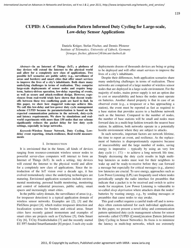
CUPID: A Communication Pattern Informed Duty Cycling for Large-scale,Low-delay Sensor Applications
Daniela Kruger, Stefan Fischer, and Dennis PfistererInstitute of Telematics, University of Lubeck, Germanykrueger, fischer, [email protected]
Abstract—In an Internet of Things (IoT), a plethora oftiny devices will extend the Internet to the physical worldand allow for a completely new class of applications. Twopossible IoT scenarios are public safety (e.g., surveillance ofareas and borders) and smart cities that offer smart servicesto improve the lives of a city’s inhabitants. Both share manyunderlying challenges in terms of realization. They compriselarge-scale deployments of sensor nodes and require long-term, battery-driven operation, low-delay reporting of events,as well as secure and attack-resilient design. However, expe-riences from real-world trials have shown that decent trade-offs between these two conflicting goals are hard to find. Inthis paper, we show how staggered wake-ups achieve this.We call this low-delay and low-power duty cycle managementscheme CUPID because its parameterization is based on theexpected communication patterns in the network, duty-cycleand latency requirements. We show by simulations and real-world experiments with more than 150 nodes that our schemesignificantly reduces the packet delay for low duty cyclesettings, especially in large networks.
Keywords-Wireless Sensor Network, Duty Cycling, Low-delay event reporting, Attack-resilience, Real-world measure-ments
I. INTRODUCTION
It is envisioned that in the future, all kinds of devicesranging from resource-constraint wireless sensor nodes topowerful server-class computers will interact to form anInternet of Things (IoT). In such a setting, tiny deviceswill extend the Internet to the physical world and allowfor a completely new class of applications. Since the in-troduction of the IoT vision over a decade ago, it hasevolved tremendously since the underlying technologies arematuring. Envisioned application scenarios include environ-mental monitoring, personal health monitoring, monitoringand control of industrial processes, public safety, smartspaces and increasingly smart cities.
In the public safety domain, the surveillance of areas (e.g.,for trespasser detection) is a typical application domain ofwireless sensor networks. Examples are [2], [3] and theFleGSens project [4], which realize trespasser detection andlocalization systems for borders and critical areas. Smartcities have recently gained momentum and examples ofsmart cities are projects such as CitySense [5], Oulu SmartCity [6], T-City Friedrichshafen [7] and the recently startedEU FP7-funded SmartSantander [8] project. I such city-scale
deployments dozens of thousands devices are being or goingto be deployed and will offer smart services to improve thelives of a city’s inhabitants.
Despite their differences, both application scenarios sharemany underlying challenges in terms of realization. Thesenetworks are comprised of a large number of wireless sensornodes that are deployed in a large-scale environment. For themajority of nodes, mains power supply is not an option dueto cost or unavailability and hence the nodes must operateon batteries. Another shared property is that in case of anobserved event (e.g., a trespasser or a bus approaching astation), the event must be reported as fast as required toa base station that provides access to a backbone networksuch as the Internet. Compared to the number of nodes,the number of base stations will be small and nodes mustforward data in a multi-hop fashion towards the nearest basestation. In addition, both networks operate in a potentiallyhostile environment where they are subject to attacks.
In such networks, important factors are network lifetime,the time to report an event, and resilience. As the replace-ment of batteries is disproportionately expensive becauseof inaccessibility and the large number of nodes, savingenergy is imperative – typically by using an very lowduty cycle (< 1%) – to achieve a long network life time.Simply decreasing the duty cycle results in high multi-hop latencies as nodes must wait for their neighbors towake up and be ready-to-receive before they can forwarda message but especially for critical messages (e.g., alarms)low latencies are crucial. To save energy, approaches such asLow Power Listening (LPL) are frequently used where nodesperiodically sample the radio interface for preambles thatindicate that a packet is to be received and switch to activemode for reception. Low Power Listening is vulnerable toso-called sleep deprivation where attackers drain the nodes’batteries by wasting energy, e.g., by sending messages orpreambles that cause nodes to stay awake.
This goal conflict requires a careful trade-off and is nowa-days often custom-tailored for each individual application.In this paper, we present a novel delay and communicationpattern optimized duty cycle management scheme for sensornetworks called CUPID (CommUnication Pattern InformedDuty Cycling in Sensor Networks). Its focus is to minimizethe latency in multi-hop networks, which use extremely
119
International Journal on Advances in Networks and Services, vol 4 no 1 & 2, year 2011, http://www.iariajournals.org/networks_and_services/
2011, © Copyright by authors, Published under agreement with IARIA - www.iaria.org
low duty cycles. We picked up the idea of staggeredwakeups [9], [10], [11], [12], which we have extended andgeneralized. In this approach, nodes wake up subsequentlyin the direction where packets are forwarded. In contrastto existing work, CUPID copes with unreliable communi-cation links and hardware constraints, no node redundancy,and with different communication patters (instead of onlyallowing network-to-sink communication). In addition to theaforementioned properties, CUPID is resilient against sleepdeprivation attacks and can therefore be used in securityrelated applications. The work presented in this paper is anextended version of [1].
The remainder of this paper is organized as follows. Inthe next section, we review related approaches. Following,Section III introduces CUPID in detail. Then, Section IVprovides a simulative and Section V an experimental evalu-ation. Section VI concludes the paper with a summary andfuture work.
II. RELATED WORK
In general, there are different types of power managementtechniques. One of the earliest proposals is Low PowerListening (e.g., used in Wisemac [13]), in which nodesare unsynchronized and periodically activate their radiofor a fixed duration. A sender transmits short preamblesbefore sending the actual message causing all addressedreceivers activating their radio at the respective point intime. However, this implies vulnerability to sleep deprivationattacks.
In MAC layer schemes like S-MAC and T-MAC mediaaccess during synchronized active slots is coordinated usingReady-To-Send/Clear-To-Send mechanisms, which impliesthat only unicast communication is possible as well asvulnerability to sleep deprivation attacks.
K-coverage approaches assume that sensing is only pos-sible when a node is active. We do not consider theseapproaches here, since we assume that sensors have thecapability of waking up the node. Also, we don’t compareto on-demand wakeup radios [14] where ultra-low-powerradio interfaces wake up the main radio interface to receivea message. The special hardware required for the first radiosignificantly increases cost.
Scheduled wakeup schemes do not integrate the dutycycling into the MAC layer but they organize their sleep cy-cles using predetermined or random schemes. These can befurther divided into mechanisms with and without time syn-chronization. Asynchronous wakeup methods (e.g., [15]) donot require synchronized clocks, but they increase the end-to-end delay especially over long distances. It is thereforecommon practice to assume (loosely) synchronized clocks.Examples for this approach are staggered wakeups wherenodes wake up subsequently in the packet forward direction.Stankovic et al. [10] call it streamlined wakeup, but assumereliable communication links and high node redundancy.
Moreover, they explain their end-to-end optimization onlyin a short overview and focus on minimizing the detectiondelay of one sensor event instead.
In [9], Li et al. call the approach fast path algorithm.Applying additional wake phases they establish a single pathbetween source and sink, but this is independent from aglobal duty cycle and from other paths. As a node can handleonly a few paths their approach is only appropriate if fewnodes send data to few other nodes. In contrast to them weconcentrate on a solution for the whole network to allow fornetwork-to-sink communication and vice versa.
Bisnik et al. [11] convert the network into a graph, verticesrepresenting nodes and edges representing communicationlinks. The goal is now to assign (awake) slots to all nodesso that the maximum end-to-end communication delay isminimal. Using the graph-theoretical abstraction the authorsprove that this optimization problem is NP-hard given alldata is available at a central station. They derive an optimalsolution for a rectangular topology where nodes are adjustedin a grid and have exactly four neighbors. However, sucha topology can hardly be produced in reality and also as-sumes reliable communication links. Moreover, the smallestconsidered duty cycle is 5% if no messages are sent. Nodessending a message must have knowledge about the wakephases of all destination nodes, which are not necessarily atthe same time, and must be additionally awake during thesetimes. By contrast, we investigated constant duty cycles ofup to 0,1% while enabling broadcast communication at thesame time.
The authors of [16] describe a wave based communica-tion mechanism to deliver sensor information to and from adesignated node without the need of centralized controls.However, they do not consider the resulting duty cyclewhereas we meet the requirement of a constant duty cycle. Inaddition, they base there results exclusively on simulations.
Keshavarzian et al. propose two methods they callcrossed-ladders and multi-parent scheme [12], where nodesare divided into groups depending on their hop baseddistance to a reference node. Each group is awake duringone slot. But their theoretical considerations also assumereliable communication links and disregard the hidden-terminal-problem. Additionally, the authors consider onlysmall networks of at most 4 hops. Their second approachdoes not support broadcast communication as the networkis divided into several partitions, which work independentlyfrom each other. Simulation results refer exclusively to thegeneration of the network partitions. Experimental resultsare not presented.
To summarize, MAC layer schemes are inefficient, vulner-able to sleep-deprivation attacks or do not support broadcastcommunication, k-coverage protocols make different as-sumptions, and on-demand wakeup radios require expensiveadditional hardware. The techniques closest to our approachare scheduled wakeup schemes. Here, we point out that
120
International Journal on Advances in Networks and Services, vol 4 no 1 & 2, year 2011, http://www.iariajournals.org/networks_and_services/
2011, © Copyright by authors, Published under agreement with IARIA - www.iaria.org
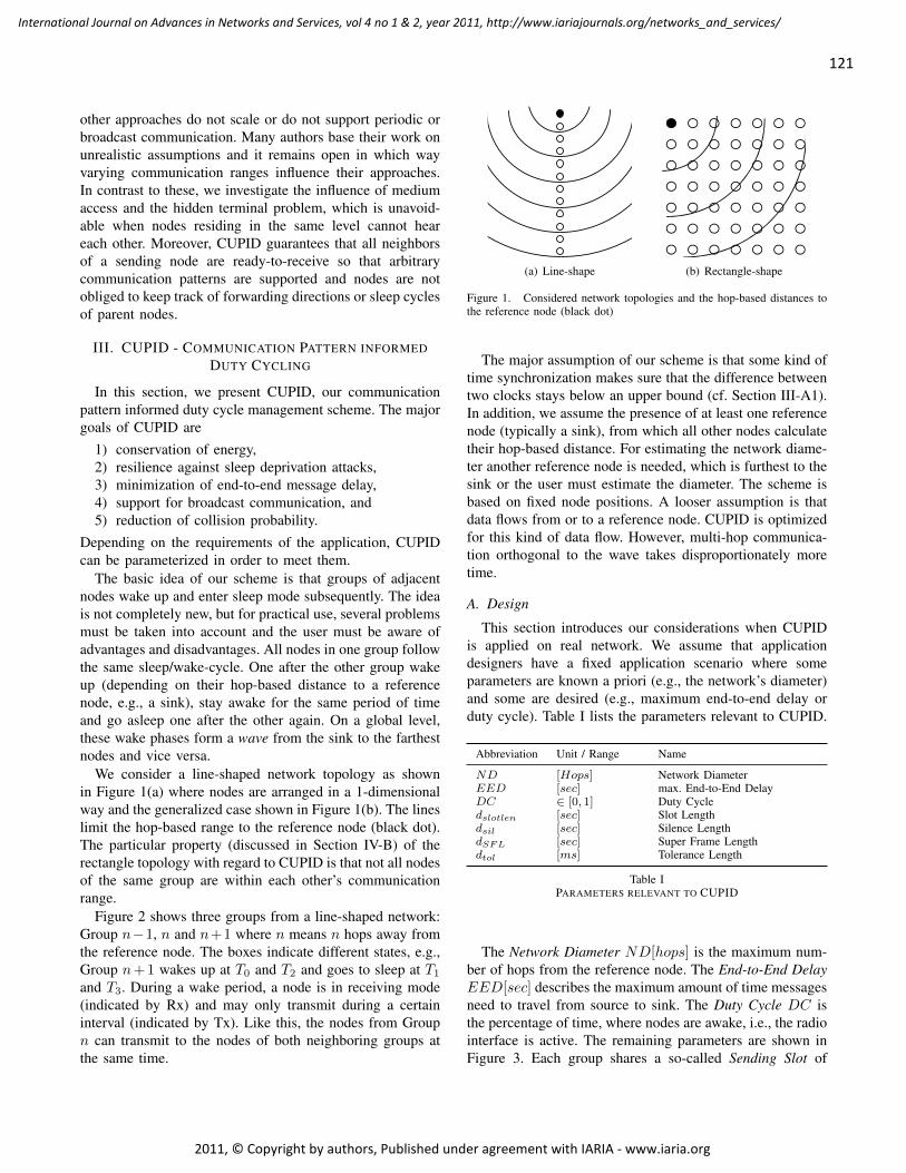
other approaches do not scale or do not support periodic orbroadcast communication. Many authors base their work onunrealistic assumptions and it remains open in which wayvarying communication ranges influence their approaches.In contrast to these, we investigate the influence of mediumaccess and the hidden terminal problem, which is unavoid-able when nodes residing in the same level cannot heareach other. Moreover, CUPID guarantees that all neighborsof a sending node are ready-to-receive so that arbitrarycommunication patterns are supported and nodes are notobliged to keep track of forwarding directions or sleep cyclesof parent nodes.
III. CUPID - COMMUNICATION PATTERN INFORMEDDUTY CYCLING
In this section, we present CUPID, our communicationpattern informed duty cycle management scheme. The majorgoals of CUPID are
1) conservation of energy,2) resilience against sleep deprivation attacks,3) minimization of end-to-end message delay,4) support for broadcast communication, and5) reduction of collision probability.
Depending on the requirements of the application, CUPIDcan be parameterized in order to meet them.
The basic idea of our scheme is that groups of adjacentnodes wake up and enter sleep mode subsequently. The ideais not completely new, but for practical use, several problemsmust be taken into account and the user must be aware ofadvantages and disadvantages. All nodes in one group followthe same sleep/wake-cycle. One after the other group wakeup (depending on their hop-based distance to a referencenode, e.g., a sink), stay awake for the same period of timeand go asleep one after the other again. On a global level,these wake phases form a wave from the sink to the farthestnodes and vice versa.
We consider a line-shaped network topology as shownin Figure 1(a) where nodes are arranged in a 1-dimensionalway and the generalized case shown in Figure 1(b). The lineslimit the hop-based range to the reference node (black dot).The particular property (discussed in Section IV-B) of therectangle topology with regard to CUPID is that not all nodesof the same group are within each other’s communicationrange.
Figure 2 shows three groups from a line-shaped network:Group n−1, n and n+1 where n means n hops away fromthe reference node. The boxes indicate different states, e.g.,Group n+1 wakes up at T0 and T2 and goes to sleep at T1
and T3. During a wake period, a node is in receiving mode(indicated by Rx) and may only transmit during a certaininterval (indicated by Tx). Like this, the nodes from Groupn can transmit to the nodes of both neighboring groups atthe same time.
(a) Line-shape (b) Rectangle-shape
Figure 1. Considered network topologies and the hop-based distances tothe reference node (black dot)
The major assumption of our scheme is that some kind oftime synchronization makes sure that the difference betweentwo clocks stays below an upper bound (cf. Section III-A1).In addition, we assume the presence of at least one referencenode (typically a sink), from which all other nodes calculatetheir hop-based distance. For estimating the network diame-ter another reference node is needed, which is furthest to thesink or the user must estimate the diameter. The scheme isbased on fixed node positions. A looser assumption is thatdata flows from or to a reference node. CUPID is optimizedfor this kind of data flow. However, multi-hop communica-tion orthogonal to the wave takes disproportionately moretime.
A. Design
This section introduces our considerations when CUPIDis applied on real network. We assume that applicationdesigners have a fixed application scenario where someparameters are known a priori (e.g., the network’s diameter)and some are desired (e.g., maximum end-to-end delay orduty cycle). Table I lists the parameters relevant to CUPID.
Abbreviation Unit / Range Name
ND [Hops] Network DiameterEED [sec] max. End-to-End DelayDC ∈ [0, 1] Duty Cycledslotlen [sec] Slot Lengthdsil [sec] Silence LengthdSFL [sec] Super Frame Lengthdtol [ms] Tolerance Length
Table IPARAMETERS RELEVANT TO CUPID
The Network Diameter ND[hops] is the maximum num-ber of hops from the reference node. The End-to-End DelayEED[sec] describes the maximum amount of time messagesneed to travel from source to sink. The Duty Cycle DC isthe percentage of time, where nodes are awake, i.e., the radiointerface is active. The remaining parameters are shown inFigure 3. Each group shares a so-called Sending Slot of
121
International Journal on Advances in Networks and Services, vol 4 no 1 & 2, year 2011, http://www.iariajournals.org/networks_and_services/
2011, © Copyright by authors, Published under agreement with IARIA - www.iaria.org
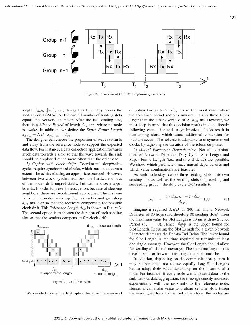
...
Group n-1
Group n
Group n+1 ... t
Rx Tx Rx
Rx Tx Rx
Rx Tx Rx
Rx Tx Rx
Rx Tx Rx
Rx Tx Rx
0T 1T 2T 3T
Figure 2. Overview of CUPID’s sleep/wake-cycle scheme
length dslotlen[sec], i.e., during this time they access themedium via CSMA/CA. The overall number of sending slotsequals the Network Diameter. After the last sending slot,there is a Silence Period of length dsil[sec] where no nodeis awake. In addition, we define the Super Frame LengthdSFL = ND · dslotlen + dsil.
The designer can choose the proportion of waves towardsand away from the reference node to support the expecteddata flow. For instance, a data collection application forwardsmuch data towards a sink, so that the wave towards the sinkshould be employed much more often than the other one.
1) Coping with clock drift: Coordinated sleep/wake-cycles require synchronized clocks, which can – to a certainextent – be achieved using an appropriate protocol. However,between two clock synchronizations, the hardware clocksof the nodes drift unpredictably, but within known upperbounds. In order to prevent message loss because of sleepingneighbors, there are two different approaches: The first oneis to let the nodes wake up dtol ms earlier and go asleepdtol ms later so that the receivers compensate for possibleclock drift. This Tolerance Length dtol is shown in Figure 3.The second option is to shorten the duration of each sendingslot so that the senders compensate for clock drift.
t d = super frame length
d
= silence lengthSILSFL
0
3
4
5 5
2
0
Sending slot
d = tolerance lengthTOL d slotlength
Figure 3. CUPID in detail
We decided to use the first option because the overhead
of option two is 3 · 2 · dtol ms in the worst case, wherethe tolerance period remains unused. This is three timeslarger than the other overhead of 2 · dtol ms. However, wemust keep in mind that this decision results in slots directlyfollowing each other and unsynchronized clocks result inoverlapping slots, which cause additional contention formedium access. The scheme is adaptable to unsynchronizedclocks by adjusting the duration of the tolerance phase.
2) Mutual Parameter Dependencies: Not all combina-tions of Network Diameter, Duty Cycle, Slot Length andSuper Frame Length (i.e., end-to-end delay) are possible.We show, which parameters have mutual dependencies andwhich value combinations are feasible.
As each node stays awake three sending slots – its ownsending slot as well as the sending slots of preceding andsucceeding group - the duty cycle DC results to
DC =3 · dslotlen + 2 · dtol
dSFL· 100. (1)
Imagine a required EED of 300 ms and a NetworkDiameter of 30 hops (and therefore 30 sending slots). Thenthe maximum value for Slot Length is 10 ms with no SilencePeriod (dsil = 0). Hence, dSFL
ND is the upper bound forSlot Length. Reducing the Slot Length for a given NetworkDiameter decreases the End-to-End Delay. The lower boundfor Slot Length is the time required to transmit at leastone single message. However, the Slot Length should allowfor sending all desired messages. The more messages nodeshave to send or forward, the longer the slots must be.
In addition, depending on the communication pattern itmay be beneficial not to use equally long Slot Lengthsbut to adapt their value depending on the location of anode. For instance, if every node wants to send data to thesink without data aggregation, the message density increasesexponentially with the proximity to the reference node.Hence, it can make sense to prolong sending slots (whenthe wave goes back to the sink) the closer the nodes are
122
International Journal on Advances in Networks and Services, vol 4 no 1 & 2, year 2011, http://www.iariajournals.org/networks_and_services/
2011, © Copyright by authors, Published under agreement with IARIA - www.iaria.org
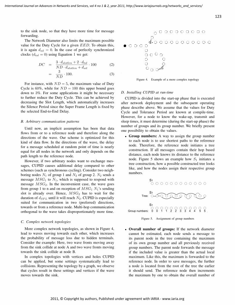
to the sink node, so that they have more time for messageforwarding.
The Network Diameter also limits the maximum possiblevalue for the Duty Cycle for a given EED. To obtain this,it is again dsil = 0. In the case of perfectly synchronizedclocks (dtol = 0) using Equation 1 we get:
DC =3 · dslotlen + 2 · dtolND · dslotlen + dsil
· 100 (2)
=3
ND· 100. (3)
For instance, with ND = 5, the maximum value of DutyCycle is 60%, while for ND = 100 this upper bound goesdown to 3%. For some applications it might be necessaryto further reduce the Duty Cycle. This can be achieved bydecreasing the Slot Length, which automatically increasesthe Silence Period since the Super Frame Length is fixed bythe selected End-to-End Delay.
B. Arbitrary communication patterns
Until now, an implicit assumption has been that dataflows from or to a reference node and therefore along thedirections of the wave. Our scheme is optimized for thiskind of data flow. In the directions of the wave, the delayfor a message scheduled at random point of time is nearlyequal for all nodes in the network and only depends on thepath length to the reference node.
However, if two arbitrary nodes want to exchange mes-sages, CUPID causes additional delay compared to otherschemes (such as synchronous cycling). Consider two neigh-boring nodes N1 of group 1 and N2 of group 2. N2 sends amessage MSG1 to N1, which is supposed to respond withmessage MSG2. In the inconvenient case, the wave goesfrom group 1 to n and on reception of MSG1 N1’s sendingslot is already over. Hence, MSG2 has to wait for theduration of dSFL until it will reach N2. CUPID is especiallysuited for communication in two (preferred) directions,towards or from a reference node. Multi-hop communicationorthogonal to the wave takes disproportionately more time.
C. Complex network topologies
More complex network topologies, as shown in Figure 4,lead to waves moving towards each other, which increasesthe probability of message loss due to hidden terminals.Consider the example: Here, two wave fronts moving awayfrom the sink collide at node A and two wave fronts movingtowards the sink collide at node B.
In complex topologies with vertices and holes CUPIDcan be applied, but some settings systematically lead tocollisions. Representing the topology by a graph, we observethat cycles result in these settings and vertices if the wavemoves towards the sink.
B
Figure 4. Example of a more complex topology
D. Installing CUPID at run-time
CUPID is divided into the start-up phase that is executedafter network deployment and the subsequent operatingphase describe above. We assume that the values for DutyCycle and Tolerance Period are known at compile-time.However, for a node to know the wake-up, transmit andsleep times, it must determine (during the start-up phase) thenumber of groups and its group number. We briefly presentone possibility to obtain the values.
• Group numbers: A way to assign the group numberto each node is to use shortest paths to the referencenode. Therefore, the reference node initiates a treeconstruction. If all messages contain their hop baseddistance, each node knows its distance to the referencenode. Figure 5 shows an example how S1 initiates atree construction, how a possible constructed tree lookslike, and how the nodes assign their respective groupnumbers.
S1
S1Tree:
S1
Group numbers: 0 0 1 1 2 2 3 3 4 4 5 5
Figure 5. Assignment of group numbers
• Overall number of groups: If the network diametercannot be estimated, each node sends a message toits parent node in the tree containing the maximumof its own group number and all previously receivedgroup numbers. The parent node forwards the messageif the included value is greater than the actual localmaximum. Like this, the maximum is forwarded to thereference node. In order to save messages, the furthera node is located from the root of the tree the earlierit should send. The reference node then incrementsthe maximum by one to obtain the overall number of
123
International Journal on Advances in Networks and Services, vol 4 no 1 & 2, year 2011, http://www.iariajournals.org/networks_and_services/
2011, © Copyright by authors, Published under agreement with IARIA - www.iaria.org
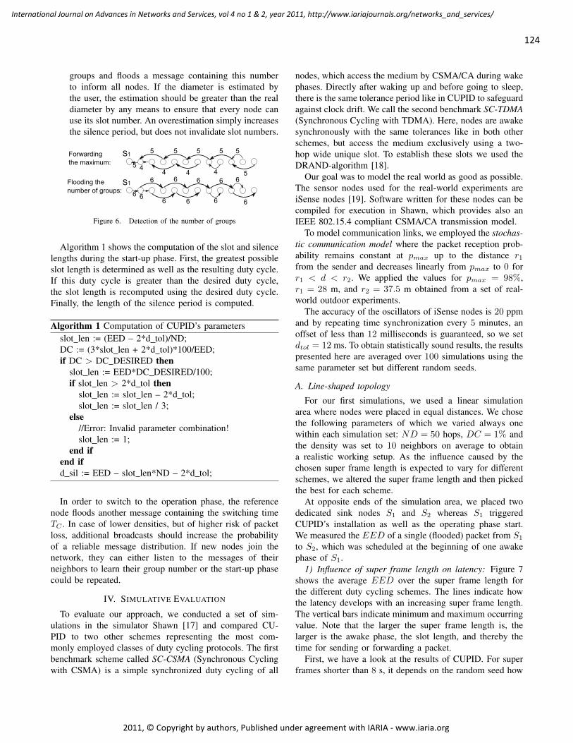
groups and floods a message containing this numberto inform all nodes. If the diameter is estimated bythe user, the estimation should be greater than the realdiameter by any means to ensure that every node canuse its slot number. An overestimation simply increasesthe silence period, but does not invalidate slot numbers.
S1Flooding the
number of groups:
6
66666
66666
S1Forwarding
the maximum:
5
55555
44445
Figure 6. Detection of the number of groups
Algorithm 1 shows the computation of the slot and silencelengths during the start-up phase. First, the greatest possibleslot length is determined as well as the resulting duty cycle.If this duty cycle is greater than the desired duty cycle,the slot length is recomputed using the desired duty cycle.Finally, the length of the silence period is computed.
Algorithm 1 Computation of CUPID’s parametersslot len := (EED – 2*d tol)/ND;DC := (3*slot len + 2*d tol)*100/EED;if DC > DC DESIRED then
slot len := EED*DC DESIRED/100;if slot len > 2*d tol then
slot len := slot len – 2*d tol;slot len := slot len / 3;
else//Error: Invalid parameter combination!slot len := 1;
end ifend ifd sil := EED – slot len*ND – 2*d tol;
In order to switch to the operation phase, the referencenode floods another message containing the switching timeTC . In case of lower densities, but of higher risk of packetloss, additional broadcasts should increase the probabilityof a reliable message distribution. If new nodes join thenetwork, they can either listen to the messages of theirneighbors to learn their group number or the start-up phasecould be repeated.
IV. SIMULATIVE EVALUATION
To evaluate our approach, we conducted a set of sim-ulations in the simulator Shawn [17] and compared CU-PID to two other schemes representing the most com-monly employed classes of duty cycling protocols. The firstbenchmark scheme called SC-CSMA (Synchronous Cyclingwith CSMA) is a simple synchronized duty cycling of all
nodes, which access the medium by CSMA/CA during wakephases. Directly after waking up and before going to sleep,there is the same tolerance period like in CUPID to safeguardagainst clock drift. We call the second benchmark SC-TDMA(Synchronous Cycling with TDMA). Here, nodes are awakesynchronously with the same tolerances like in both otherschemes, but access the medium exclusively using a two-hop wide unique slot. To establish these slots we used theDRAND-algorithm [18].
Our goal was to model the real world as good as possible.The sensor nodes used for the real-world experiments areiSense nodes [19]. Software written for these nodes can becompiled for execution in Shawn, which provides also anIEEE 802.15.4 compliant CSMA/CA transmission model.
To model communication links, we employed the stochas-tic communication model where the packet reception prob-ability remains constant at pmax up to the distance r1from the sender and decreases linearly from pmax to 0 forr1 < d < r2. We applied the values for pmax = 98%,r1 = 28 m, and r2 = 37.5 m obtained from a set of real-world outdoor experiments.
The accuracy of the oscillators of iSense nodes is 20 ppmand by repeating time synchronization every 5 minutes, anoffset of less than 12 milliseconds is guaranteed, so we setdtol = 12 ms. To obtain statistically sound results, the resultspresented here are averaged over 100 simulations using thesame parameter set but different random seeds.
A. Line-shaped topology
For our first simulations, we used a linear simulationarea where nodes were placed in equal distances. We chosethe following parameters of which we varied always onewithin each simulation set: ND = 50 hops, DC = 1% andthe density was set to 10 neighbors on average to obtaina realistic working setup. As the influence caused by thechosen super frame length is expected to vary for differentschemes, we altered the super frame length and then pickedthe best for each scheme.
At opposite ends of the simulation area, we placed twodedicated sink nodes S1 and S2 whereas S1 triggeredCUPID’s installation as well as the operating phase start.We measured the EED of a single (flooded) packet from S1
to S2, which was scheduled at the beginning of one awakephase of S1.
1) Influence of super frame length on latency: Figure 7shows the average EED over the super frame length forthe different duty cycling schemes. The lines indicate howthe latency develops with an increasing super frame length.The vertical bars indicate minimum and maximum occurringvalue. Note that the larger the super frame length is, thelarger is the awake phase, the slot length, and thereby thetime for sending or forwarding a packet.
First, we have a look at the results of CUPID. For superframes shorter than 8 s, it depends on the random seed how
124
International Journal on Advances in Networks and Services, vol 4 no 1 & 2, year 2011, http://www.iariajournals.org/networks_and_services/
2011, © Copyright by authors, Published under agreement with IARIA - www.iaria.org
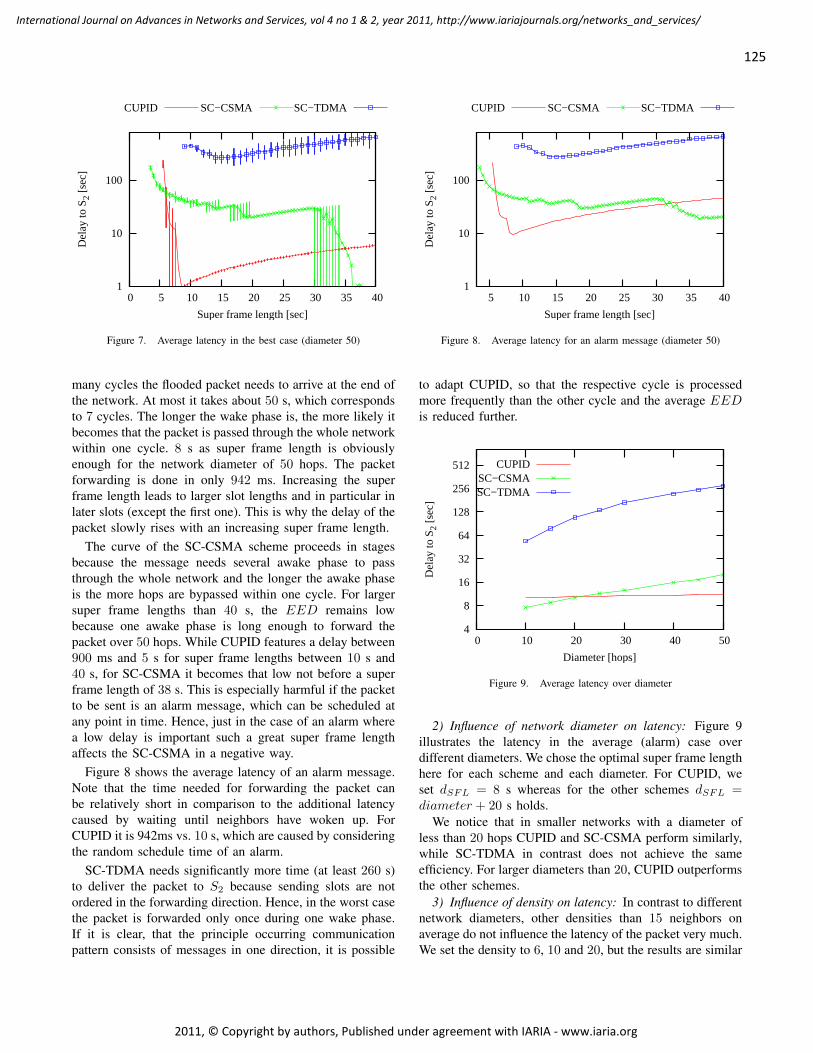
1
10
100
0 5 10 15 20 25 30 35 40
Del
ay to
S 2 [s
ec]
Super frame length [sec]
CUPID SC−CSMA SC−TDMA
Figure 7. Average latency in the best case (diameter 50)
many cycles the flooded packet needs to arrive at the end ofthe network. At most it takes about 50 s, which correspondsto 7 cycles. The longer the wake phase is, the more likely itbecomes that the packet is passed through the whole networkwithin one cycle. 8 s as super frame length is obviouslyenough for the network diameter of 50 hops. The packetforwarding is done in only 942 ms. Increasing the superframe length leads to larger slot lengths and in particular inlater slots (except the first one). This is why the delay of thepacket slowly rises with an increasing super frame length.
The curve of the SC-CSMA scheme proceeds in stagesbecause the message needs several awake phase to passthrough the whole network and the longer the awake phaseis the more hops are bypassed within one cycle. For largersuper frame lengths than 40 s, the EED remains lowbecause one awake phase is long enough to forward thepacket over 50 hops. While CUPID features a delay between900 ms and 5 s for super frame lengths between 10 s and40 s, for SC-CSMA it becomes that low not before a superframe length of 38 s. This is especially harmful if the packetto be sent is an alarm message, which can be scheduled atany point in time. Hence, just in the case of an alarm wherea low delay is important such a great super frame lengthaffects the SC-CSMA in a negative way.
Figure 8 shows the average latency of an alarm message.Note that the time needed for forwarding the packet canbe relatively short in comparison to the additional latencycaused by waiting until neighbors have woken up. ForCUPID it is 942ms vs. 10 s, which are caused by consideringthe random schedule time of an alarm.
SC-TDMA needs significantly more time (at least 260 s)to deliver the packet to S2 because sending slots are notordered in the forwarding direction. Hence, in the worst casethe packet is forwarded only once during one wake phase.If it is clear, that the principle occurring communicationpattern consists of messages in one direction, it is possible
1
10
100
5 10 15 20 25 30 35 40
Del
ay to
S 2 [s
ec]
Super frame length [sec]
CUPID SC−CSMA SC−TDMA
Figure 8. Average latency for an alarm message (diameter 50)
to adapt CUPID, so that the respective cycle is processedmore frequently than the other cycle and the average EEDis reduced further.
4
8
16
32
64
128
256
512
0 10 20 30 40 50
Del
ay to
S 2 [s
ec]
Diameter [hops]
CUPIDSC−CSMASC−TDMA
Figure 9. Average latency over diameter
2) Influence of network diameter on latency: Figure 9illustrates the latency in the average (alarm) case overdifferent diameters. We chose the optimal super frame lengthhere for each scheme and each diameter. For CUPID, weset dSFL = 8 s whereas for the other schemes dSFL =diameter + 20 s holds.
We notice that in smaller networks with a diameter ofless than 20 hops CUPID and SC-CSMA perform similarly,while SC-TDMA in contrast does not achieve the sameefficiency. For larger diameters than 20, CUPID outperformsthe other schemes.
3) Influence of density on latency: In contrast to differentnetwork diameters, other densities than 15 neighbors onaverage do not influence the latency of the packet very much.We set the density to 6, 10 and 20, but the results are similar
125
International Journal on Advances in Networks and Services, vol 4 no 1 & 2, year 2011, http://www.iariajournals.org/networks_and_services/
2011, © Copyright by authors, Published under agreement with IARIA - www.iaria.org
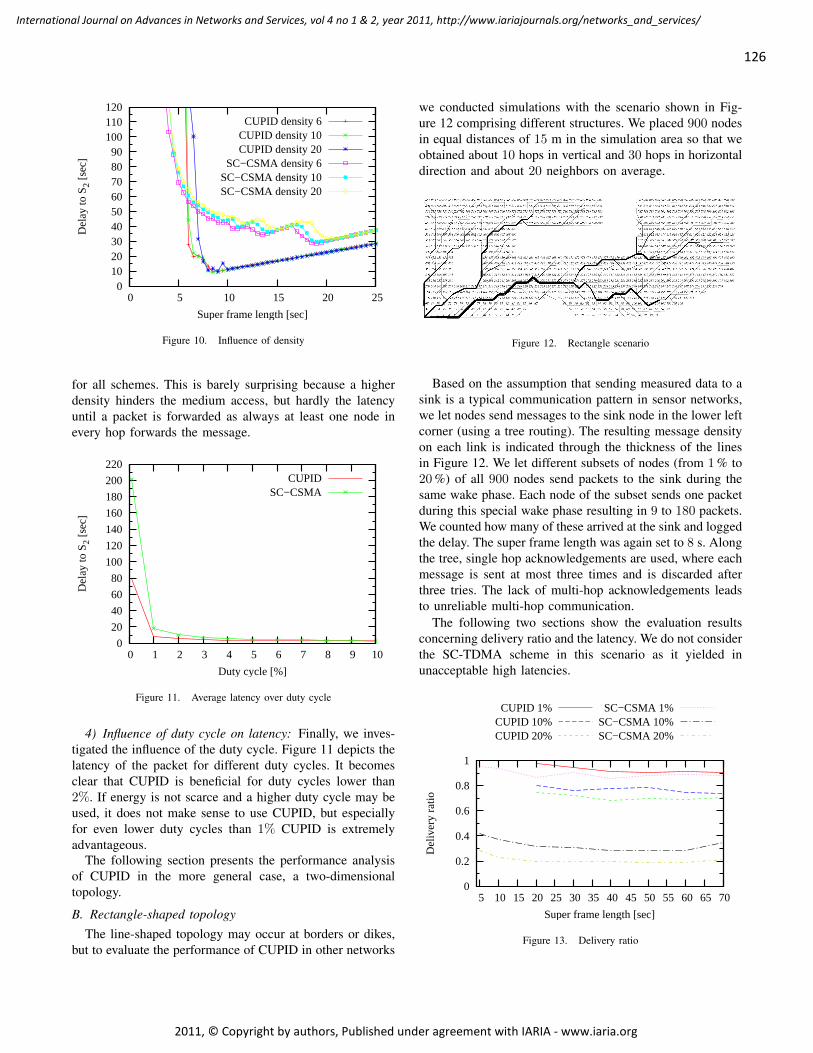
0 10 20 30 40 50 60 70 80 90
100 110 120
0 5 10 15 20 25
Del
ay to
S 2 [s
ec]
Super frame length [sec]
CUPID density 6CUPID density 10CUPID density 20
SC−CSMA density 6SC−CSMA density 10SC−CSMA density 20
Figure 10. Influence of density
for all schemes. This is barely surprising because a higherdensity hinders the medium access, but hardly the latencyuntil a packet is forwarded as always at least one node inevery hop forwards the message.
0
20
40
60
80
100
120
140
160
180
200
220
0 1 2 3 4 5 6 7 8 9 10
Del
ay to
S 2 [s
ec]
Duty cycle [%]
CUPIDSC−CSMA
Figure 11. Average latency over duty cycle
4) Influence of duty cycle on latency: Finally, we inves-tigated the influence of the duty cycle. Figure 11 depicts thelatency of the packet for different duty cycles. It becomesclear that CUPID is beneficial for duty cycles lower than2%. If energy is not scarce and a higher duty cycle may beused, it does not make sense to use CUPID, but especiallyfor even lower duty cycles than 1% CUPID is extremelyadvantageous.
The following section presents the performance analysisof CUPID in the more general case, a two-dimensionaltopology.
B. Rectangle-shaped topologyThe line-shaped topology may occur at borders or dikes,
but to evaluate the performance of CUPID in other networks
we conducted simulations with the scenario shown in Fig-ure 12 comprising different structures. We placed 900 nodesin equal distances of 15 m in the simulation area so that weobtained about 10 hops in vertical and 30 hops in horizontaldirection and about 20 neighbors on average.
Figure 12. Rectangle scenario
Based on the assumption that sending measured data to asink is a typical communication pattern in sensor networks,we let nodes send messages to the sink node in the lower leftcorner (using a tree routing). The resulting message densityon each link is indicated through the thickness of the linesin Figure 12. We let different subsets of nodes (from 1% to20%) of all 900 nodes send packets to the sink during thesame wake phase. Each node of the subset sends one packetduring this special wake phase resulting in 9 to 180 packets.We counted how many of these arrived at the sink and loggedthe delay. The super frame length was again set to 8 s. Alongthe tree, single hop acknowledgements are used, where eachmessage is sent at most three times and is discarded afterthree tries. The lack of multi-hop acknowledgements leadsto unreliable multi-hop communication.
The following two sections show the evaluation resultsconcerning delivery ratio and the latency. We do not considerthe SC-TDMA scheme in this scenario as it yielded inunacceptable high latencies.
0
0.2
0.4
0.6
0.8
1
5 10 15 20 25 30 35 40 45 50 55 60 65 70
Del
iver
y ra
tio
Super frame length [sec]
CUPID 1%CUPID 10%CUPID 20%
SC−CSMA 1%SC−CSMA 10%SC−CSMA 20%
Figure 13. Delivery ratio
126
International Journal on Advances in Networks and Services, vol 4 no 1 & 2, year 2011, http://www.iariajournals.org/networks_and_services/
2011, © Copyright by authors, Published under agreement with IARIA - www.iaria.org
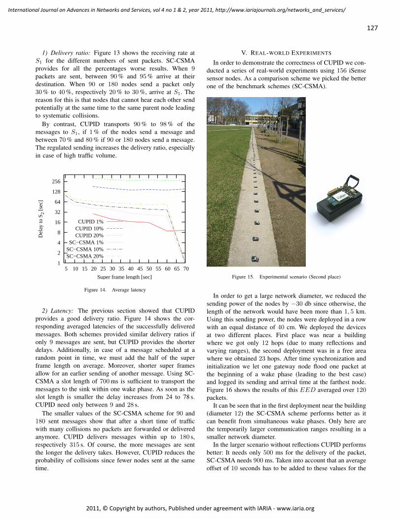
1) Delivery ratio: Figure 13 shows the receiving rate atS1 for the different numbers of sent packets. SC-CSMAprovides for all the percentages worse results. When 9packets are sent, between 90% and 95% arrive at theirdestination. When 90 or 180 nodes send a packet only30% to 40%, respectively 20% to 30%, arrive at S1. Thereason for this is that nodes that cannot hear each other sendpotentially at the same time to the same parent node leadingto systematic collisions.
By contrast, CUPID transports 90% to 98% of themessages to S1, if 1% of the nodes send a message andbetween 70% and 80% if 90 or 180 nodes send a message.The regulated sending increases the delivery ratio, especiallyin case of high traffic volume.
1
2
4
8
16
32
64
128
256
5 10 15 20 25 30 35 40 45 50 55 60 65 70
Del
ay to
S 2 [s
ec]
Super frame length [sec]
CUPID 1%CUPID 10%CUPID 20%
SC−CSMA 1%SC−CSMA 10%SC−CSMA 20%
Figure 14. Average latency
2) Latency: The previous section showed that CUPIDprovides a good delivery ratio. Figure 14 shows the cor-responding averaged latencies of the successfully deliveredmessages. Both schemes provided similar delivery ratios ifonly 9 messages are sent, but CUPID provides the shorterdelays. Additionally, in case of a message scheduled at arandom point in time, we must add the half of the superframe length on average. Moreover, shorter super framesallow for an earlier sending of another message. Using SC-CSMA a slot length of 700ms is sufficient to transport themessages to the sink within one wake phase. As soon as theslot length is smaller the delay increases from 24 to 78 s.CUPID need only between 9 and 28 s.
The smaller values of the SC-CSMA scheme for 90 and180 sent messages show that after a short time of trafficwith many collisions no packets are forwarded or deliveredanymore. CUPID delivers messages within up to 180 s,respectively 315 s. Of course, the more messages are sentthe longer the delivery takes. However, CUPID reduces theprobability of collisions since fewer nodes sent at the sametime.
V. REAL-WORLD EXPERIMENTS
In order to demonstrate the correctness of CUPID we con-ducted a series of real-world experiments using 156 iSensesensor nodes. As a comparison scheme we picked the betterone of the benchmark schemes (SC-CSMA).
Figure 15. Experimental scenario (Second place)
In order to get a large network diameter, we reduced thesending power of the nodes by −30 db since otherwise, thelength of the network would have been more than 1, 5 km.Using this sending power, the nodes were deployed in a rowwith an equal distance of 40 cm. We deployed the devicesat two different places. First place was near a buildingwhere we got only 12 hops (due to many reflections andvarying ranges), the second deployment was in a free areawhere we obtained 23 hops. After time synchronization andinitialization we let one gateway node flood one packet atthe beginning of a wake phase (leading to the best case)and logged its sending and arrival time at the farthest node.Figure 16 shows the results of this EED averaged over 120packets.
It can be seen that in the first deployment near the building(diameter 12) the SC-CSMA scheme performs better as itcan benefit from simultaneous wake phases. Only here arethe temporarily larger communication ranges resulting in asmaller network diameter.
In the larger scenario without reflections CUPID performsbetter: It needs only 500 ms for the delivery of the packet,SC-CSMA needs 900 ms. Taken into account that an averageoffset of 10 seconds has to be added to these values for the
127
International Journal on Advances in Networks and Services, vol 4 no 1 & 2, year 2011, http://www.iariajournals.org/networks_and_services/
2011, © Copyright by authors, Published under agreement with IARIA - www.iaria.org
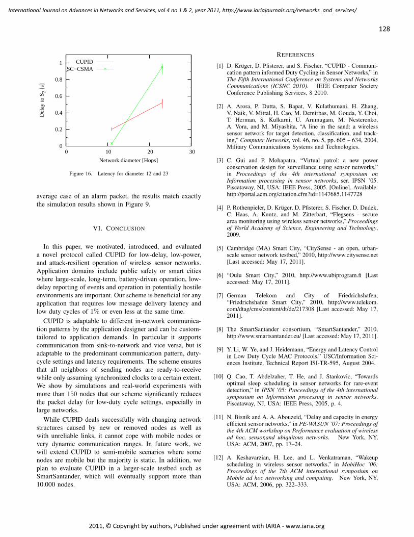
0
0.2
0.4
0.6
0.8
1
0 10 20 30
Del
ay to
S 2 [s
]
Network diameter [Hops]
CUPIDSC−CSMA
Figure 16. Latency for diameter 12 and 23
average case of an alarm packet, the results match exactlythe simulation results shown in Figure 9.
VI. CONCLUSION
In this paper, we motivated, introduced, and evaluateda novel protocol called CUPID for low-delay, low-power,and attack-resilient operation of wireless sensor networks.Application domains include public safety or smart citieswhere large-scale, long-term, battery-driven operation, low-delay reporting of events and operation in potentially hostileenvironments are important. Our scheme is beneficial for anyapplication that requires low message delivery latency andlow duty cycles of 1% or even less at the same time.
CUPID is adaptable to different in-network communica-tion patterns by the application designer and can be custom-tailored to application demands. In particular it supportscommunication from sink-to-network and vice versa, but isadaptable to the predominant communication pattern, duty-cycle settings and latency requirements. The scheme ensuresthat all neighbors of sending nodes are ready-to-receivewhile only assuming synchronized clocks to a certain extent.We show by simulations and real-world experiments withmore than 150 nodes that our scheme significantly reducesthe packet delay for low-duty cycle settings, especially inlarge networks.
While CUPID deals successfully with changing networkstructures caused by new or removed nodes as well aswith unreliable links, it cannot cope with mobile nodes orvery dynamic communication ranges. In future work, wewill extend CUPID to semi-mobile scenarios where somenodes are mobile but the majority is static. In addition, weplan to evaluate CUPID in a larger-scale testbed such asSmartSantander, which will eventually support more than10.000 nodes.
REFERENCES
[1] D. Kruger, D. Pfisterer, and S. Fischer, “CUPID - Communi-cation pattern informed Duty Cycling in Sensor Networks,” inThe Fifth International Conference on Systems and NetworksCommunications (ICSNC 2010). IEEE Computer SocietyConference Publishing Services, 8 2010.
[2] A. Arora, P. Dutta, S. Bapat, V. Kulathumani, H. Zhang,V. Naik, V. Mittal, H. Cao, M. Demirbas, M. Gouda, Y. Choi,T. Herman, S. Kulkarni, U. Arumugam, M. Nesterenko,A. Vora, and M. Miyashita, “A line in the sand: a wirelesssensor network for target detection, classification, and track-ing,” Computer Networks, vol. 46, no. 5, pp. 605 – 634, 2004,Military Communications Systems and Technologies.
[3] C. Gui and P. Mohapatra, “Virtual patrol: a new powerconservation design for surveillance using sensor networks,”in Proceedings of the 4th international symposium onInformation processing in sensor networks, ser. IPSN ’05.Piscataway, NJ, USA: IEEE Press, 2005. [Online]. Available:http://portal.acm.org/citation.cfm?id=1147685.1147728
[4] P. Rothenpieler, D. Kruger, D. Pfisterer, S. Fischer, D. Dudek,C. Haas, A. Kuntz, and M. Zitterbart, “Flegsens - securearea monitoring using wireless sensor networks,” Proceedingsof World Academy of Science, Engineering and Technology,2009.
[5] Cambridge (MA) Smart City, “CitySense - an open, urban-scale sensor network testbed,” 2010, http://www.citysense.net[Last accessed: May 17, 2011].
[6] “Oulu Smart City,” 2010, http://www.ubiprogram.fi [Lastaccessed: May 17, 2011].
[7] German Telekom and City of Friedrichshafen,“Friedrichshafen Smart City,” 2010, http://www.telekom.com/dtag/cms/content/dt/de/217308 [Last accessed: May 17,2011].
[8] The SmartSantander consortium, “SmartSantander,” 2010,http://www.smartsantander.eu/ [Last accessed: May 17, 2011].
[9] Y. Li, W. Ye, and J. Heidemann, “Energy and Latency Controlin Low Duty Cycle MAC Protocols,” USC/Information Sci-ences Institute, Technical Report ISI-TR-595, August 2004.
[10] Q. Cao, T. Abdelzaher, T. He, and J. Stankovic, “Towardsoptimal sleep scheduling in sensor networks for rare-eventdetection,” in IPSN ’05: Proceedings of the 4th internationalsymposium on Information processing in sensor networks.Piscataway, NJ, USA: IEEE Press, 2005, p. 4.
[11] N. Bisnik and A. A. Abouzeid, “Delay and capacity in energyefficient sensor networks,” in PE-WASUN ’07: Proceedings ofthe 4th ACM workshop on Performance evaluation of wirelessad hoc, sensor,and ubiquitous networks. New York, NY,USA: ACM, 2007, pp. 17–24.
[12] A. Keshavarzian, H. Lee, and L. Venkatraman, “Wakeupscheduling in wireless sensor networks,” in MobiHoc ’06:Proceedings of the 7th ACM international symposium onMobile ad hoc networking and computing. New York, NY,USA: ACM, 2006, pp. 322–333.
128
International Journal on Advances in Networks and Services, vol 4 no 1 & 2, year 2011, http://www.iariajournals.org/networks_and_services/
2011, © Copyright by authors, Published under agreement with IARIA - www.iaria.org
[13] A. El-Hoiydi, J.-D. Decotignie, C. Enz, and E. Le Roux,“Poster abstract: wiseMAC, an ultra low power MAC protocolfor the wiseNET wireless sensor network,” in SenSys ’03:Proceedings of the 1st international conference on Embeddednetworked sensor systems. New York, NY, USA: ACM,2003, pp. 302–303.
[14] L. Gu and J. Stankovic, “Radio-triggered wake-up capabilityfor sensor networks,” in RTAS ’04: Proceedings of the 10thIEEE Real-Time and Embedded Technology and ApplicationsSymposium. Washington, DC, USA: IEEE Computer Society,2004, p. 27.
[15] R. Zheng, J. C. Hou, and L. Sha, “Asynchronous wakeupfor ad hoc networks,” in Proceedings of the Fourth ACMInternational Symposium on Mobile Ad Hoc Networking andComputing (MobiHoc), 2003.
[16] Y. Taniguchi, N. Wakamiya, and M. Murat, “A travelingwave based communication mechanism for wireless sensornetworks,” Journal of Networks, vol. 2, pp. 24–32, 2007.
[17] S. P. Fekete, A. Kroller, S. Fischer, and D. Pfisterer, “Shawn:The fast, highly customizable sensor network simulator,”in Proceedings of the Fourth International Conference onNetworked Sensing Systems (INSS’ 07), Jun. 2007.
[18] I. Rhee, A. Warrier, J. Min, and L. Xu, “Drand: distributedrandomized tdma scheduling for wireless ad-hoc networks,”in MobiHoc ’06: Proceedings of the 7th ACM internationalsymposium on Mobile ad hoc networking and computing.New York, NY, USA: ACM, 2006, pp. 190–201.
[19] coalesenses GmbH, “iSense,” http://www.coalesenses.com[Last accessed: May 17, 2011].
129
International Journal on Advances in Networks and Services, vol 4 no 1 & 2, year 2011, http://www.iariajournals.org/networks_and_services/
2011, © Copyright by authors, Published under agreement with IARIA - www.iaria.org
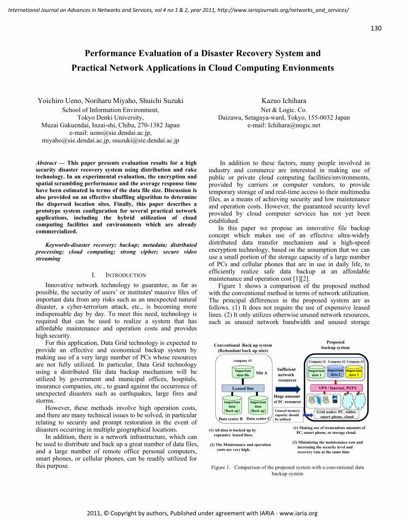
Conventional Back up system(Redundant back up sites)
(1) All data is backed up byexpensive leased lines.
(2) The Maintenance and operation costs are very high.
Proposed backup system
(1) Making use of tremendous amounts of PC, smart phone, or storage cloud.
(2) Minimizing the maintenance cost and increasing the security level and recovery rate at the same time
Importantdata 1
Importantdata
(Back up)
Importantdata
(Back up)
Importantdata 2
Importantdata 3
Sufficient network resources
Huge amount of PC resource
Importantdata file
Leased line
Company #1 Company #2 Company #3
Site A
Data center B Data center C
Unused memorycapacity should be utilized
company #1
Grid nodes: PC, tablet,smart phone, cloud
VPN / Internet, PSTN
Figure 1. Comparison of the proposed system with a conventional data
backup system
Performance Evaluation of a Disaster Recovery System and
Practical Network Applications in Cloud Computing Envionments
Yoichiro Ueno, Noriharu Miyaho, Shuichi Suzuki School of Information Environment,
Tokyo Denki University, Muzai Gakuendai, Inzai-shi, Chiba, 270-1382 Japan
e-mail: [email protected], [email protected], [email protected]
Kazuo Ichihara Net & Logic. Co.
Daizawa, Setagaya-ward, Tokyo, 155-0032 Japan e-mail: [email protected]
Abstract — This paper presents evaluation results for a high security disaster recovery system using distribution and rake technology. In an experimental evaluation, the encryption and spatial scrambling performance and the average response time have been estimated in terms of the data file size. Discussion is also provided on an effective shuffling algorithm to determine the dispersed location sites. Finally, this paper describes a prototype system configuration for several practical network applications, including the hybrid utilization of cloud computing facilities and environments which are already commercialized.
Keywords-disaster recovery; backup; metadata; distributed processing; cloud computing; strong cipher; secure video streaming
I. INTRODUCTION
Innovative network technology to guarantee, as far as possible, the security of users’ or institutes' massive files of important data from any risks such as an unexpected natural disaster, a cyber-terrorism attack, etc., is becoming more indispensable day by day. To meet this need, technology is required that can be used to realize a system that has affordable maintenance and operation costs and provides high security.
For this application, Data Grid technology is expected to provide an effective and economical backup system by making use of a very large number of PCs whose resources are not fully utilized. In particular, Data Grid technology using a distributed file data backup mechanism will be utilized by government and municipal offices, hospitals, insurance companies, etc., to guard against the occurrence of unexpected disasters such as earthquakes, large fires and storms.
However, these methods involve high operation costs, and there are many technical issues to be solved, in particular relating to security and prompt restoration in the event of disasters occurring in multiple geographical locations.
In addition, there is a network infrastructure, which can be used to distribute and back up a great number of data files, and a large number of remote office personal computers, smart phones, or cellular phones, can be readily utilized for this purpose.
In addition to these factors, many people involved in industry and commerce are interested in making use of public or private cloud computing facilities/environments, provided by carriers or computer vendors, to provide temporary storage of and real-time access to their multimedia files, as a means of achieving security and low maintenance and operation costs. However, the guaranteed security level provided by cloud computer services has not yet been established.
In this paper we propose an innovative file backup concept which makes use of an effective ultra-widely distributed data transfer mechanism and a high-speed encryption technology, based on the assumption that we can use a small portion of the storage capacity of a large number of PCs and cellular phones that are in use in daily life, to efficiently realize safe data backup at an affordable maintenance and operation cost [1][2].
Figure 1 shows a comparison of the proposed method with the conventional method in terms of network utilization. The principal differences in the proposed system are as follows. (1) It does not require the use of expensive leased lines. (2) It only utilizes otherwise unused network resources, such as unused network bandwidth and unused storage
130
International Journal on Advances in Networks and Services, vol 4 no 1 & 2, year 2011, http://www.iariajournals.org/networks_and_services/
2011, © Copyright by authors, Published under agreement with IARIA - www.iaria.org
capacity in PCs, smart phones and cellular phones, etc. (3) It can utilize cloud computing facilities/environments as one of the remote Grid nodes to obtain a requested amount of storage and a specific security level in accordance with the customer’s requirements. (4) It can cipher a number of important data files at the same time using spatial scrambling and random dispatching technology. (5) As the number of user companies increases, the security against being deciphered illegally increases accordingly. (6) The maintenance cost can be drastically reduced. In addition, since it uses a stream cipher, the speed of encryption of data is increased, so it can also be applied to secure streaming for video transmission services.
In general, encryption can use two types of technology, that is, block cipher technology or stream cipher technology. In the case of block cipher technology, the data is divided into successive blocks and each block is processed separately for point-to-point systems; as a result, the encryption speed is quite slow. As the data volume increases, the required processor and memory cost increases in an exponential manner.
On the other hand, in case of the stream cipher, the input data is simply operated on bit-by-bit, using a simple arithmetic operation. Therefore, high-speed processing becomes feasible. These are the fundamental differences between the two cipher technologies [3].
When an ultra-widely distributed file data transfer technology, a file fragmentation technology and an encryption technology are used together, then quite different characteristics arise from a point of cipher strength. It is possible to combine the use of technologies, specifically, the spatial scrambling of all data files, the random fragmentation of the data files, and the corresponding encryption and replication of each file fragment using a stream cipher. The corresponding history data, including the encryption key code sequence, which we call "encryption metadata", are used to recover the original data. This mechanism is equivalent to realizing a strong cipher code, comparable to any conventionally developed cipher code, by appropriately assigning affordable network resources [4].
By making use of the proposed combined technology, illegal interception and decoding of the data by a third party becomes almost impossible and an extremely safe data backup system can be realized at reasonable cost. The proposed technology can also increase both the cipher code strength and the data recovery rate.
To realize the proposed disaster recovery mechanism, the following three principal network components are required: (1) a secure data center, (2) several secure supervisory servers, and (3) a number of client nodes such as PCs or cellular phones. We have previously clarified the relationships between data file capacity, the number of file fragments and the number of replications for the case of disaster recovery [5][6].
In this paper, we briefly describe the related work in Section II, and discuss the basic configuration of the system architecture in Section III, and the performance evaluation in Section IV. The practical experimental system is discussed in
Section V. Finally, we provide our conclusions from these studies in Section VI.
II. RELATED WORK
Conventionally, a file data backup system [7] has been realized by duplication of a data center, access lines, etc. However, considering that an earthquake may cause fiber cable failures over a wide area and shut down several communication links, this approach is not fully satisfactory [8].
To take account of this, we have already proposed a disaster recovery concept which can use to realize a reliable file backup system by making use of safe and fast encryption mechanisms, a network distribution mechanism, and a technique for the effective use of secure meta-data containing the history of encryption key code sequences [9][10][11][12]. This technical approach has not yet been implemented elsewhere. Other related studies have included the concept of a distributed file backup system [13][14]. However, in these studies, neither a precise performance evaluation nor practical network service systems are clearly described. In addition, the technological aspects concerning the effective distribution of the fragmented data to establish the required security level are not clearly discussed for conventional systems.
On the other hand, there has been only a little published research on personal disaster recovery systems. A personal disaster recovery system should take account of the cost and the guarantee of security of personal data. So, a personal disaster recovery system may use some kind of cheap storage service for data backup. In recent years, it has become possible to implement data backup using free online storage. However, such low cost storage services are not secure enough for personal information. A persistent file server that should improve security of such storage service has been proposed [15]. This persistent file server system introduced encryption, fragmentation, replication, and scattering. Our proposed system adds more security with spatial scrambling, a second encryption, and an effective shuffling algorithm.
III. BASIC CONFIGURATION OF THE SYSTEM
ARCHITECTURE AND ITS VARIATIONS
This section discusses the basic configuration of the high security distribution and rake technology (HS-DRT).
A. Basic Configuration of the HS-DRT System
The HS-DRT file backup mechanism has three principal components as shown in Figure 2. The main functions of the proposed network components are Data Center, Supervisory Server and various client nodes, and these can be specified as follows.
The client nodes (at the bottom of Fig. 2) are PCs, Smart Phones, Network Attached Storage (NAS) devices, and Storage Services. They are connected to a Supervisory Server in addition to the Data Center via a secure network.
The Supervisory Server (on the right in Fig. 2) acquires the history data, which includes the encryption key code sequence (metadata) from the Data Center (on the left in Fig. 2) via a network.
131
International Journal on Advances in Networks and Services, vol 4 no 1 & 2, year 2011, http://www.iariajournals.org/networks_and_services/
2011, © Copyright by authors, Published under agreement with IARIA - www.iaria.org
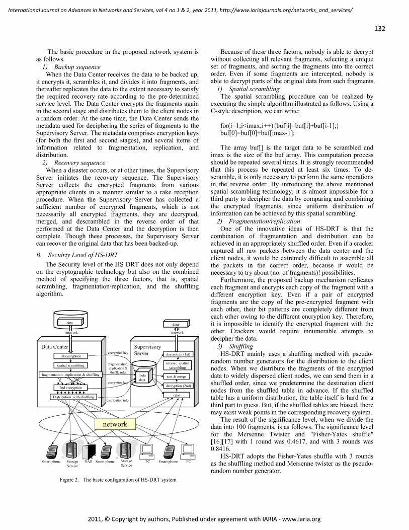
The basic procedure in the proposed network system is as follows.
1) Backup sequence When the Data Center receives the data to be backed up,
it encrypts it, scrambles it, and divides it into fragments, and thereafter replicates the data to the extent necessary to satisfy the required recovery rate according to the pre-determined service level. The Data Center encrypts the fragments again in the second stage and distributes them to the client nodes in a random order. At the sane time, the Data Center sends the metadata used for deciphering the series of fragments to the Supervisory Server. The metadata comprises encryption keys (for both the first and second stages), and several items of information related to fragmentation, replication, and distribution.
2) Recovery sequence When a disaster occurs, or at other times, the Supervisory
Server initiates the recovery sequence. The Supervisory Server collects the encrypted fragments from various appropriate clients in a manner similar to a rake reception procedure. When the Supervisory Server has collected a sufficient number of encrypted fragments, which is not necessarily all encrypted fragments, they are decrypted, merged, and descrambled in the reverse order of that performed at the Data Center and the decryption is then complete. Though these processes, the Supervisory Server can recover the original data that has been backed-up.
B. Secuirty Level of HS-DRT
The Security level of the HS-DRT does not only depend on the cryptographic technology but also on the combined method of specifying the three factors, that is, spatial scrambling, fragmentation/replication, and the shuffling algorithm.
Because of these three factors, nobody is able to decrypt without collecting all relevant fragments, selecting a unique set of fragments, and sorting the fragments into the correct order. Even if some fragments are intercepted, nobody is able to decrypt parts of the original data from such fragments.
1) Spatial scrambling The spatial scrambling procedure can be realized by
executing the simple algorithm illustrated as follows. Using a C-style description, we can write:
for(i=1;i<imax;i++)buf[i]=buf[i]+buf[i-1]; buf[0]=buf[0]+buf[imax-1]; The array buf[] is the target data to be scrambled and
imax is the size of the buf array. This computation process should be repeated several times. It is strongly recommended that this process be repeated at least six times. To de-scramble, it is only necessary to perform the same operations in the reverse order. By introducing the above mentioned spatial scrambling technology, it is almost impossible for a third party to decipher the data by comparing and combining the encrypted fragments, since uniform distribution of information can be achieved by this spatial scrambling.
2) Fragmentation/replication One of the innovative ideas of HS-DRT is that the
combination of fragmentation and distribution can be achieved in an appropriately shuffled order. Even if a cracker captured all raw packets between the data center and the client nodes, it would be extremely difficult to assemble all the packets in the correct order, because it would be necessary to try about (no. of fragments)! possibilities.
Furthermore, the proposed backup mechanism replicates each fragment and encrypts each copy of the fragment with a different encryption key. Even if a pair of encrypted fragments are the copy of the pre-encrypted fragment with each other, their bit patterns are completely different from each other owing to the different encryption key. Therefore, it is impossible to identify the encrypted fragment with the other. Crackers would require innumerable attempts to decipher the data.
3) Shuffling HS-DRT mainly uses a shuffling method with pseudo-
random number generators for the distribution to the client nodes. When we distribute the fragments of the encrypted data to widely dispersed client nodes, we can send them in a shuffled order, since we predetermine the destination client nodes from the shuffled table in advance. If the shuffled table has a uniform distribution, the table itself is hard for a third part to guess. But, if the shuffled tables are biased, there may exist weak points in the corresponding recovery system.
The result of the significance level, when we divide the data into 100 fragments, is as follows. The significance level for the Mersenne Twister and "Fisher-Yates shuffle" [16][17] with 1 round was 0.4617, and with 3 rounds was 0.8416.
HS-DRT adopts the Fisher-Yates shuffle with 3 rounds as the shuffling method and Mersenne twister as the pseudo-random number generator.
Storage Service
bdata
Data Center
1st encryption
spatial scrambling
fragmentation, duplication & shuffling
2nd encryption
Distribution with shuffling
Smart phoneSmart phoneSmart phone Storage Service
NAS PC PC
Supervisory Server
meta data
encryption key
fragmentation, duplication &shuffle info.
distribution info.
encryption key
rake
decryption (2nd)
sort & merge
decryption (1st)
inverse spatial scrambling
data
networknetwork
network
Figure 2. The basic configuration of HS-DRT system
132
International Journal on Advances in Networks and Services, vol 4 no 1 & 2, year 2011, http://www.iariajournals.org/networks_and_services/
2011, © Copyright by authors, Published under agreement with IARIA - www.iaria.org
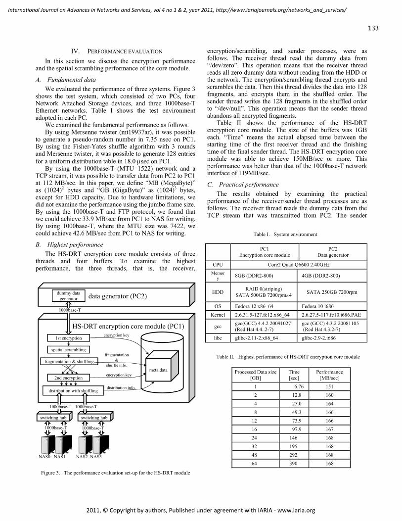
IV. PERFORMANCE EVALUATION
In this section we discuss the encryption performance and the spatial scrambling performance of the core module.
A. Fundamental data
We evaluated the performance of three systems. Figure 3 shows the test system, which consisted of two PCs, four Network Attached Storage devices, and three 1000base-T Ethernet networks. Table I shows the test environment adopted in each PC.
We examined the fundamental performance as follows. By using Mersenne twister (mt19937ar), it was possible
to generate a pseudo-random number in 7.35 nsec on PC1. By using the Fisher-Yates shuffle algorithm with 3 rounds and Mersenne twister, it was possible to generate 128 entries for a uniform distribution table in 18.0 sec on PC1.
By using the 1000base-T (MTU=1522) network and a TCP stream, it was possible to transfer data from PC2 to PC1 at 112 MB/sec. In this paper, we define “MB (MegaByte)” as (1024)2 bytes and “GB (GigaByte)” as (1024)3 bytes, except for HDD capacity. Due to hardware limitations, we did not examine the performance using the jumbo frame size. By using the 1000base-T and FTP protocol, we found that we could achieve 33.9 MB/sec from PC1 to NAS for writing. By using 1000base-T, where the MTU size was 7422, we could achieve 42.6 MB/sec from PC1 to NAS for writing.
B. Highest performance
The HS-DRT encryption core module consists of three threads and four buffers. To examine the highest performance, the three threads, that is, the receiver,
encryption/scrambling, and sender processes, were as follows. The receiver thread read the dummy data from “/dev/zero”. This operation means that the receiver thread reads all zero dummy data without reading from the HDD or the network. The encryption/scrambling thread encrypts and scrambles the data. Then this thread divides the data into 128 fragments, and encrypts them in the shuffled order. The sender thread writes the 128 fragments in the shuffled order to “/dev/null”. This operation means that the sender thread abandons all encrypted fragments.
Table II shows the performance of the HS-DRT encryption core module. The size of the buffers was 1GB each. “Time” means the actual elapsed time between the starting time of the first receiver thread and the finishing time of the final sender thread. The HS-DRT encryption core module was able to achieve 150MB/sec or more. This performance was better than that of the 1000base-T network interface of 119MB/sec.
C. Practical performance
The results obtained by examining the practical performance of the receiver/sender thread processes are as follows. The receiver thread reads the dummy data from the TCP stream that was transmitted from PC2. The sender
HS-DRT encryption core module (PC1)
1st encryption
spatial scrambling
fragmentation & shuffling
2nd encryption
distribution with shuffling
encryption key
fragmentation &
shuffle info.
distribution info.
encryption key
NAS0 NAS1 NAS2 NAS3
meta data
dummy data generator data generator (PC2)
1000base-T
switching hub switching hub
1000base-T 1000base-T
1000base-T 1000base-T
Figure 3. The performance evaluation set-up for the HS-DRT module
Table I. System environment
PC1
Encryption core module PC2
Data generator
CPU Core2 Quad Q6600 2.40GHz
Memory 8GB (DDR2-800) 4GB (DDR2-800)
HDD RAID 0(striping)
SATA 500GB 7200rpm4 SATA 250GB 7200rpm
OS Fedora 12 x86_64 Fedora 10 i686
Kernel 2.6.31.5-127.fc12.x86_64 2.6.27.5-117.fc10.i686.PAE
gcc gcc(GCC) 4.4.2 20091027 (Red Hat 4.4..2-7)
gcc (GCC) 4.3.2 20081105 (Red Hat 4.3.2-7)
libc glibc-2.11-2.x86_64 glibc-2.9-2.i686
Table II. Highest performance of HS-DRT encryption core module
Processed Data size
[GB] Time [sec]
Performance [MB/sec]
1 6.76 151
2 12.8 160
4 25.0 164
8 49.3 166
12 73.9 166
16 97.9 167
24 146 168
32 195 168
48 292 168
64 390 168
133
International Journal on Advances in Networks and Services, vol 4 no 1 & 2, year 2011, http://www.iariajournals.org/networks_and_services/
2011, © Copyright by authors, Published under agreement with IARIA - www.iaria.org
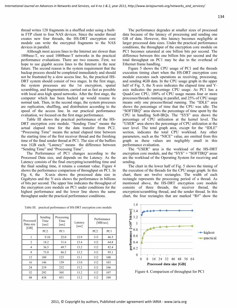
thread writes 128 fragments in a shuffled order using a built-in FTP client to four NAS devices. Since the sender thread creates new four threads, the HS-DRT encryption core module can write the encrypted fragments to the NAS devices in parallel.
Although most access lines to the Internet are slower than 100base-T, we used 1000base-T networks in the practical performance evaluations. There are two reasons. First, we hope to use gigabit access lines to the Internet in the near future. The second reason is the system requirement that the backup process should be completed immediately and should not be frustrated by a slow access line. So, the practical HS-DRT system should consist of two stages. In the first stage, the system processes are the 1st encryption, spatial scrambling, and fragmentation, carried out as fast as possible with local area high speed networks. After the first stage, the computer which has been backed up would resume its normal task. Then, in the second stage, the system processes are replication, shuffling, and distribution according to the speed of the access line. In our practical performance evaluation, we focused on the first stage performance.
Table III shows the practical performance of the HS-DRT encryption core module. “Sending Time” means the actual elapsed time for the data transfer from PC2. “Processing Time” means the actual elapsed time between the starting time of the first receiver thread and the finishing time of the final sender thread at PC1. The size of the buffers was 1GB each. “Latency” means the difference between “Sending Time” and “Processing Time”.
The Performance of PC1 changes according to the Processed Data size, and depends on the Latency. As the Latency consists of the final encrypting/scrambling time and the final sending time, it retains a constant value. Figure 4 shows the performance comparison of throughput on PC1. In Fig. 4, the X-axis shows the processed data size in Gigabytes and the Y-axis shows the performance in billions of bits per second. The upper line indicates the throughput of the encryption core module on PC1 under conditions for the highest performance and the lower line shows the same throughput under the practical performance conditions.
The performance degrades at smaller sizes of processed data because of the latency of processing and sending one GB of data. However, this latency becomes negligible at larger processed data sizes. Under the practical performance conditions, the throughput of the encryption core module on PC1 becomes saturated at one billion bits per second. The difference between this one billion bits per second and the total throughput on PC1 may be due to the overhead of Ethernet frame handling.
Figure 5 shows the CPU usage of PC1 and the threads execution timing chart when the HS-DRT encryption core module executes such operations as receiving, processing, and sending 4GB data. In the CPU usage graph in the upper half of Fig. 5, the X-axis indicates the elapsed time and Y-axis indicates the percentage CPU usage. As PC1 has a Quad-Core CPU, 100% of CPU usage means four or more processes/threads running in parallel, and 25% of CPU usage means only one process/thread running. The “IDLE” area shows the percentage of time that the CPU was idle. The “SOFTIRQ” area shows the percentage of time spent by the CPU in handling Soft-IRQs. The “SYS” area shows the percentage of CPU utilization at the kernel level. The “USER” area shows the percentage of CPU utilization at the user level. The total graph area, except for the “IDLE” section, indicates the total CPU workload. Any other parameters, such as the “NICE” value, are omitted from this graph as these values are negligibly small in this performance evaluation.
The “USER” area is the workload of the HS-DRT encryption core module, and the “SYS” + “SOFTIRQ” areas are the workload of the Operating System for receiving and sending.
The chart in the lower half of Fig. 5 shows the timing of the execution of the threads for the CPU usage graph. In this chart, there are twelve rectangles. The width of each rectangle represents the processing period of a thread. As mentioned above, the HS-DRT encryption core module consists of three threads, the receiver thread, the encryption/scrambling thread, and the sender thread. In this chart, the four rectangles that are marked “R#” show the
Table III. practical performance of HS-DRT encryption core module
Processed Data size
[GB]
Sending Time [sec]
Processing Time [sec]
Latency [sec]
Performance [MB/sec]
PC2 PC1 PC2 PC1
1 9.10 22.0 12.9 113 46.5
2 18.2 31.6 13.4 112 64.8
4 36.5 49.7 13.2 112 82.4
8 73.0 86.2 13.2 112 95.1
12 109 123 13.1 112 100
16 146 159 13.0 112 103
24 219 232 13.2 112 106
32 292 305 13.2 112 107
48 438 451 13.2 112 109
Figure 4. Comparison of throughput for PC1
134
International Journal on Advances in Networks and Services, vol 4 no 1 & 2, year 2011, http://www.iariajournals.org/networks_and_services/
2011, © Copyright by authors, Published under agreement with IARIA - www.iaria.org
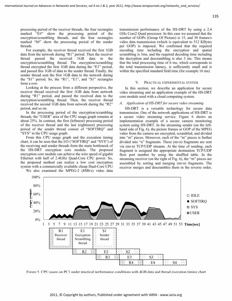
processing period of the receiver threads, the four rectangles marked “E#” show the processing period of the encryption/scrambling threads, and the four rectangles marked “S#” show the processing period of the sender threads.
For example, the receiver thread received the first 1GB data from the network during “R1” period. Then the receiver thread passed the received 1GB data to the encryption/scrambling thread. The encryption/scrambling thread encrypted the first 1GB data during the “E1” period, and passed this 1GB of data to the sender thread. Finally, the sender thread sent the first 1GB data to the network during the “S1” period. So, the “R1”, “E1”, and “S1” rectangles form a row.
Looking at the process from a different perspective, the receiver thread received the first 1GB data from network during “R1” period, and passed the received data to the encryption/scrambling thread. Then, the receiver thread received the second 1GB data from network during the “R2” period, and so on.
In the processing period of the encryption/scrambling threads, the “USER” area of the CPU usage graph remains at about 25%. In contrast, the first (leftmost) processing period of the receiver thread and the last (rightmost) processing period of the sender thread consist of “SOFTIRQ” and “SYS” in the CPU usage graph.
From this CPU usage graph and the execution timing chart, it can be seen that the I/O (“SOFTIRQ” and “SYS”) of the receiving and sender threads form the main bottleneck of the HS-DRT encryption core module. The proposed encryption core module can achieve the wire speed of gigabit Ethernet with half of 2.4GHz Quad-Core CPU power. So, the proposed method can realize a low cost encryption system with a commercially available cheap Dual-Core CPU.
We also examined the MPEG-2 (8Mb/s) video data
transmission performance of the HS-DRT by using a 2.4 GHz Core2 Quad processor. In this case we assumed that the number of GOPs (Group Of Picture) is 15, and 30 frames/s video data transmission (which is equivalent to 512 KBytes per GOP) is imposed. We confirmed that the required encoding time including the encryption and spatial scrambling is 3ms, and the required decoding time including the decryption and descrambling is also 3 ms. This means that the total processing time of 6 ms, which corresponds to the total transmission latency, is sufficiently small and is within the specified standard field time (for example 16 ms).
V. PRACTICAL EXPERIMENTAL SYSTEM
In this section, we describe an application for secure video streaming and an application example of the HS-DRT core module used with a cloud computing system.
A. Application of HS-DRT for secure video streaming
HS-DRT is a versatile technology for secure data transmission. One of the network applications of HS-DRT is a secure video streaming service. Figure 6 shows an implementation example of a secure camera monitoring system using HS-DRT. In the streaming sender (on the left-hand side of Fig. 6), the picture frames or GOP of the MPEG video from the camera are encrypted, scrambled, and divided into “m” pieces. Moreover, each of the “m” pieces is further divided into “n” fragments. These (mn) fragments are sent via (mn) TCP/UDP streams. At the time of sending, each fragment is assigned the appropriate destination TCP/UDP flow port number by using the shuffled table. In the streaming receiver (on the right of Fig. 6), the “m” pieces are assembled by sorting and merging (mn) fragments. The receiver merges and descrambles them in the reverse order,
0%
20%
40%
60%
80%
100%
1 3 5 7 9 11 13 15 17 19 21 23 25 27 29 31 33 35 37 39 41 43 45 47 49 51 53
CPU Usage
Time[sec]
IDLE
SOFTIRQ
SYS
USER
Figure 5. CPU usage on PC1 under practical performance conditions with 4GB data and thread execution timing chart
Receiver thread
processes 1st 1GB
Sender thread
processes 1st 1GB
4th 1GB 4th 1GB
3rd 1GB 3rd 1GB
2nd 1GB 2nd 1GB
E1 Encryption Scrambling
thread
E4E3
E2
R1 Receiver
thread
S1 Sender thread
R4R3
R2
S4 S3
S2
135
International Journal on Advances in Networks and Services, vol 4 no 1 & 2, year 2011, http://www.iariajournals.org/networks_and_services/
2011, © Copyright by authors, Published under agreement with IARIA - www.iaria.org
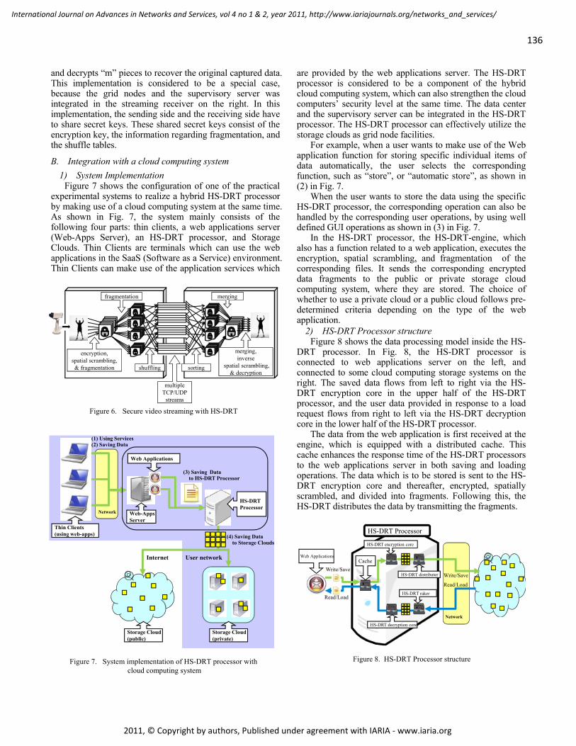
and decrypts “m” pieces to recover the original captured data. This implementation is considered to be a special case, because the grid nodes and the supervisory server was integrated in the streaming receiver on the right. In this implementation, the sending side and the receiving side have to share secret keys. These shared secret keys consist of the encryption key, the information regarding fragmentation, and the shuffle tables.
B. Integration with a cloud computing system
1) System Implementation Figure 7 shows the configuration of one of the practical
experimental systems to realize a hybrid HS-DRT processor by making use of a cloud computing system at the same time. As shown in Fig. 7, the system mainly consists of the following four parts: thin clients, a web applications server (Web-Apps Server), an HS-DRT processor, and Storage Clouds. Thin Clients are terminals which can use the web applications in the SaaS (Software as a Service) environment. Thin Clients can make use of the application services which
are provided by the web applications server. The HS-DRT processor is considered to be a component of the hybrid cloud computing system, which can also strengthen the cloud computers’ security level at the same time. The data center and the supervisory server can be integrated in the HS-DRT processor. The HS-DRT processor can effectively utilize the storage clouds as grid node facilities.
For example, when a user wants to make use of the Web application function for storing specific individual items of data automatically, the user selects the corresponding function, such as “store”, or “automatic store”, as shown in (2) in Fig. 7.
When the user wants to store the data using the specific HS-DRT processor, the corresponding operation can also be handled by the corresponding user operations, by using well defined GUI operations as shown in (3) in Fig. 7.
In the HS-DRT processor, the HS-DRT-engine, which also has a function related to a web application, executes the encryption, spatial scrambling, and fragmentation of the corresponding files. It sends the corresponding encrypted data fragments to the public or private storage cloud computing system, where they are stored. The choice of whether to use a private cloud or a public cloud follows pre-determined criteria depending on the type of the web application.
2) HS-DRT Processor structure Figure 8 shows the data processing model inside the HS-
DRT processor. In Fig. 8, the HS-DRT processor is connected to web applications server on the left, and connected to some cloud computing storage systems on the right. The saved data flows from left to right via the HS-DRT encryption core in the upper half of the HS-DRT processor, and the user data provided in response to a load request flows from right to left via the HS-DRT decryption core in the lower half of the HS-DRT processor.
The data from the web application is first received at the engine, which is equipped with a distributed cache. This cache enhances the response time of the HS-DRT processors to the web applications server in both saving and loading operations. The data which is to be stored is sent to the HS-DRT encryption core and thereafter, encrypted, spatially scrambled, and divided into fragments. Following this, the HS-DRT distributes the data by transmitting the fragments.
encryption,spatial scrambling,& fragmentation
fragmentation
shuffling
multipleTCP/UDP
streams
sorting
merging,inverse
spatial scrambling,& decryption
merging
Figure 6. Secure video streaming with HS-DRT
(1) Using Services(2) Saving Data
(3) Saving Datato HS-DRT Processor
(4) Saving Datato Storage Clouds
User networkInternet
Network
Thin Clients(using web-apps)
Web-AppsServer
Web Applications
HS-DRTProcessor
Storage Cloud(public)
Storage Cloud(private)
Figure 7. System implementation of HS-DRT processor with
cloud computing system
Write/Save
Read/Load
Read/Load
Write/Save
Network
Web Applications
HS-DRT raker
Cache
HS-DRT decryption core
HS-DRT encryption core
HS-DRT Processor
HS-DRT distributer
Figure 8. HS-DRT Processor structure
136
International Journal on Advances in Networks and Services, vol 4 no 1 & 2, year 2011, http://www.iariajournals.org/networks_and_services/
2011, © Copyright by authors, Published under agreement with IARIA - www.iaria.org
When there is a request from the web applications to load data, the cache engine first processes the data. The HS-DRT decryption core engine indicates that the HS-DRT-raker should collect back the distributed data from the relevant storage clouds. The engine then sends the collected data, which can be used for file data recovery if required.
3) Characteristics of HS-DRT processor integrated with the cloud computing system
It is very important to note that the processing efficiency of the HS-DRT processor can easily be improved by increasing the amount of the web cache memory.
We need to consider the scalability of the engine, since it may become a bottleneck in a very large system, owing to the number of clients and the amount of storage. In such cases, the HS-DRT processor may use a key-value database. As the HS-DRT processor can easily work with other HS-DRT processors, the system can be extended. The secrecy of the system can easily be assured because there is no plain raw data stream appearing anywhere in the entire data processing procedure.
On the other hand, we should take the following disadvantageous points into account.
In order to fully utilize the HS-DRT processor, the web applications need to be well adjusted to be used by the HS-DRT engine itself.
If the number of replicated copies of file data increases, the corresponding processor performance for executing the web applications will be degraded accordingly.
As for the HS-DRT processor, it can include the function of the web application server in addition to the encryption, spatial scrambling, and fragmentation of the corresponding file data. Scalability can also be easily attained by making use of conventional technologies for load balancing and multiplexing of the processor.
VI. CONCLUSIONS
We have presented an experimental evaluation of the encryption and the spatial scrambling performance of the proposed data recovery system, and found that the average response time in terms of the file data size is sufficiently practical to realize the corresponding network services.
Discussion has also been provided on an effective shuffling algorithm using Mersenne Twister and "Fisher-Yates shuffle" to determine the dispersed location sites.
Finally, this paper has described a prototype system configuration for several practical network applications, in particular, implementing a hybrid structure by making use of cloud computing facilities and environments which have already been commercialized.
Further studies should address the optimum network utilization technology. We are planning to verify the essential characteristics necessary to fully utilize the network resources to commercialize an ideal disaster recovery system.
ACKNOWLEDGMENTS
This work has been partially supported by the Grants-in-Aid for Scientific Research (Issue number: 21560414), the
Research Institute for Science and Technology of Tokyo Denki University (Q09S-10) and a grant of Strategic Research Foundation Grant-aided Project for Private Universities from Ministry of Education, Culture, Support, Science, and Technology, Japan (MEXT), 2007-2011.
REFERENCES [1] Y. Ueno, N. Miyaho, S. Suzuki, and K. Ichihara, "Performance
Evaluation of a Disaster Recovery System and Practical Network System Applications," ICSNC 2010, pp. 195-200, Aug., 2010.
[2] N. Miyaho, Y. Ueno, S. Suzuki, K. Mori, and K. Ichihara, "Study on a Disaster Recovery Network Mechanism by Using Widely Distributed Client Nodes," ICSNC 2009, pp. 217-223, Sep., 2009.
[3] S. Suzuki, “Additive cryptosystem and World Wide master key,” IEICE technical report ISEC 101(403), pp. 39-46, Nov., 2001.
[4] N. Miyaho, S. Suzuki, Y. Ueno, A. Takubo, Y. Wada, and R. Shibata, “Disaster recovery equipments, programs, and system,” Patent. publication 2007/3/6 (Japan), PCT Patent :No.4296304, Apr. 2009.
[5] Y.Ueno, N.Miyaho, and S.Suzuki, ”Disaster Recovery Mechanism using Widely Distributed Networking and Secure Metadata Handling Technology,” Proceedings of the 4th edition of the UPGRADE-CN workshop, Session II: Networking, pp. 45-48, Jun., 2009.
[6] K. Kokubun, Y. Kawai, Y. Ueno, S. Suzuki, and N. Miyaho, “Performance evaluation of Disaster Recovery System using Grid Computing technology,” IEICE Technical Report 107(403), pp. 1-6, Dec., 2007.
[7] NTT-East “Wide area disaster recovery services”, <http://www.ntt-east.co.jp/business/solution/security/dr/> 23.05.2010
[8] Y. Kitamura, Y. Lee, R. Sakiyama, and K. Okamura, “Experience with Restoration of Asia Pacific Network Failures from Taiwan Earthquake,” IEICE Transactions on Communications E90-B(11), pp. 3095-3103, Nov. , 2007.
[9] S. Kurokawa, Y. Iwaki, and N. Miyaho, “Study on the distributed data sharing mechanism with a mutual authentication and meta-database technology,” APCC 2007, pp. 215-218, Oct., 2007.
[10] J. Yamato, M. Kan, and Y. Kikuchi, “Storage Based Data Protection for Disaster Recovery,” The Journal of the IEICE 89(9), pp. 801-805, Sep. , 2006.
[11] Shanyu Zhao, Virginia Lo, and Chris GauthierDickey, "Result Verification and Trust-Based Scheduling in Peer-to-Peer Grids," p2p, pp. 31-38, Fifth IEEE International Conference on Peer-to-Peer Computing (P2P'05), 2005.
[12] K. Sagara, K. Nishiki, and M. Koizumi, “A Distributed Authentication Platform Architecture for Peer-to-Peer Applications,” IEICE Transactions on Communications E88-B(3), pp. 865-872, 2005.
[13] S. Tezuka, R. Uda, A. Inoue, and Y. Matsushita, “A Secure Virtual File Server with P2P Connection to a Large-Scale Network,” IASTED International Conference NCS2006, pp. 310-315, 2006.
[14] R. Uda, A. Inoue, M. Ito, S. Ichimura, K. Tago, and T. Hoshi, “Development of file distributed back up system,” Tokyo University of Technology, Technical Report, No.3, pp. 31-38, Mar 2008.
[15] Y. Deswarte, L. Blain, J.-C. Fabre, "Intrusion tolerance in distributed computing systems," Research in Security and Privacy, 1991. Proceedings, 1991 IEEE Computer Society Symposium, pp.110-121, 20-22 May 1991
[16] R. A. Fisher and F. Yates, Statistical tables for biological, agricultural and medical research (3rd ed.). London: Oliver & Boyd. pp. 26–27, 1948.
[17] D. E. Knuth, The Art of Computer Programming, Volume 2: Seminumerical algorithms., 3rd edition, Addison Wesley. pp. 142-146, 1998.
137
International Journal on Advances in Networks and Services, vol 4 no 1 & 2, year 2011, http://www.iariajournals.org/networks_and_services/
2011, © Copyright by authors, Published under agreement with IARIA - www.iaria.org
Campus-Wide Indoor Tracking Infrastructure
Heinrich Schmitzberger and Wolfgang Narzt
Department of Business Informatics - Software Engineering
Johannes Kepler University Linz
Altenberger Straße 69, 4040 Linz, Austria
heinrich.schmitzberger, [email protected]
Abstract — In the context of large-scale indoor spaces location-
based services still lack a feasible technology for localization
and tracking in terms of ubiquitous operation. In this article,
we present a tracking system based on wireless local area
network infrastructure that is capable of simultaneously
tracking numerous and diverse mobile clients (i.e., cell phones,
laptops, personal digital assistants and alike) in multistory
buildings within a campus facility at a near real time resolution
and without client software to be installed. In the course of a
real-life project at the campus of the University of Linz we
have been studying deployment issues and environmental
influences on infrastructure-based tracking in a large-scale
setup that comprises various types of building structures and
architecture. We contribute our findings regarding effects of
arbitrary environmental conditions on radio signal based
person tracking and present our current results. Furthermore,
we demonstrate the feasibility of integrating infrastructural
tracking technology into a location-based services platform
called “Digital Graffiti” that handles user and privileges
management while sustaining the privacy of the individual.
Keywords-indoor infrastructural wlan tracking; scalability;
large scale; real time; location-based services.
I. INTRODUCTION
At the core of mobile computing is the most prominent context information about the user: location. The user’s current location as well as the awareness of the location of friends and things of interest have been a decisive driver for the ongoing trend towards smart phones and mobile applications up to date. The integration of the Global Positioning System (GPS) into commercially available mobile devices (smart phones and personal digital assistants for instance) carved the way for a broad variety of location-based services (LBS) covering outdoor spaces and public places in the form of navigation systems, location-based social networks and city guide applications. However, still no convincing counterpart regarding indoor location acquisition has prevailed in real-life LBS scenarios. In the last decade, several approaches towards realizing a ubiquitous indoor localization technology that could compete with the quality and reliability of outdoor GPS have been presented. The underlying sensor technologies were manifold (Bluetooth, Infrared or Ultrasonic, just to name a few). Concluding from the GPS story of success, a key factor of influence is the broad availability of the respective technology in a common mobile device. As we demonstrated in [1], WLAN (Wireless Local Area Network) technology seems to have the most promising potential in this context.
We pointed out that the approach of exerting tracking infrastructure for the localization of a large number of concurrent users has shown feasible, even in terms of large-scale setups covering vast building complexes (e.g., the campus of a university). Using WLAN in this context offers certain benefits concerning costs, accuracy, scalability and deployment compared to other popular radio localization technologies, not least because of its availability in modern mobile phones [2].
Recently, commercial WLAN localization products have been introduced [3][4] following a localization method having the mobile device acting as sensor or even estimating its position itself (client-based). In this article, we propose a converse system where sensor hardware as well as position estimation is decoupled from the client, but achieved by a backend server combined with WLAN infrastructure within a complex of buildings (infrastructure-based).
This setup allows us to look into the subject of indoor localization from a different point of view, being able to support a vast range of client devices. Instead of providing software for different client platforms and sensor arrangements our infrastructure comprises a network of homogeneous, permanently active sensors that assure accurate measurements for convenient location estimation of numerous clients operating on several platforms. By this means we avoid forcing CPU prerequisites since infrastructure bears the processing load. Consequently, power consumption is reduced on the client side.
Another benefit of our setup is its robustness with respect to a constantly changing WLAN environment, a disadvantage that affects accuracy in client-based setups because they mainly rely on stable signal strength fingerprints of access points (APs) in the vicinity. Since the system solely depends on measurements of client signals additional WLAN signal sources have no consequences on the position estimation process.
The system presented in this article meets the following prerequisites: first of all, localization accuracy of room-level granularity is reached. The system is able to provide a mapping of geo-coordinates to symbolic names at detailed spatial level (such as “Office 306, Management Center, University of Linz”), which facilitates users’ perception of location information. In order to attain a ubiquitous user experience, the system operates 24 hours a day, 7 days a week and is open to public access from within the wireless campus network. Accordingly, our architecture has to attend to scalability in terms of providing a near real time service to a potentially unbounded amount of users. Furthermore, we have developed a service based on our LBS framework that
138
International Journal on Advances in Networks and Services, vol 4 no 1 & 2, year 2011, http://www.iariajournals.org/networks_and_services/
2011, © Copyright by authors, Published under agreement with IARIA - www.iaria.org
enables the finding and tracking of friends given their anytime revocable permission. In this context we refer to the notion tracking almost similarly as to localization, with one distinctive exception: localization describes the process in which the current location of a certain client is estimated. Tracking on the other hand uses previously calculated location estimates to create a traceable path that is further used to render the client’s position more precisely and to conclude to the client’s course.
The rest of this article is organized as follows. Section 2 discusses related work to the broad topic of indoor localization with respect to WLAN signal strength based approaches concentrating on infrastructure. In Section 3 we describe the architecture of our system in detail, focusing on its 3 main components in particular. Subsequently, Section 4 deals with our real-life setup in the course of the Smart Information Campus project at the University of Linz, discussing detailed facts of campus-wide deployment as well as the users’ view of the system. In Section 5, we compare tracking results surveyed in different types of buildings at the campus. Finally, Section 6 concludes with a discussion on our efforts to realize the described system and gives a brief outlook on future research questions in context of our setup.
II. RELATED WORK
In the last years, numerous contributions have discussed the subject of indoor localization and tracking on WLAN basis as an alternative to obtaining positions using GPS. Most of them concentrated on signal strength localization algorithms that emphasized a client-based application, i.e., the client device is operated as sensor collecting signal strength information of nearby APs. These systems broadly depend on special hardware in the form of tags [4][5] or native libraries supporting certain network interface card (NIC) features at client-side [6][7][8].
We envision a client-device independent setup in order to not constrain the usage of our system to certain hardware. To this end we have studied an infrastructure-based approach to achieving WLAN signal strength localization. In this context the notion “infrastructure-based” refers to a setup that comprises stationary sensor nodes for measuring client radio transmissions [9][10][11].
Early contributions to this approach are presented in [12]. The RADAR system uses a setup of ordinary PCs as stationary signal strength sensors. This experimental setup showed the feasibility of WLAN for indoor localization. In [9], the LEASE system is proposed, an infrastructure-based framework using sniffers and reference-emitters. The sniffers are constructed as embedded sensor platforms. The emitters were used as signal strength references to constantly rebuild an active radio profile. The main focus of this work concen-trated on deployment issues and consequences of radio propagation for location estimation in potential real life scenarios. A detailed description of the sniffers used for LEASE is given in [13]. In this article, the issues of capturing conventional WLAN traffic as well as the placement of sniffer nodes for convenient location estimation are explored.
Embedded devices have also been the basis for Pinpoint [14], a system that uses the Time-Of-Arrival localization method. In order to achieve accurate estimations, the main functionality of their devices was to maintain high precision clock synchronization. The usage of Linksys WRT54 (the previous generation of the devices used in our work) as platform for localization applications has been a matter of research as well. In [15], customized kismet software is used on a Linksys device to report signal strength measurements. The authors report experiments in a calibration-free localization setup. In [16], another calibration-free fingerprinting system is proposed that applies probabilistic methods for constructing radio profile model and position estimation. Due to heavy computational load it uses PCs as sniffers. In this work another focus lies on WLAN channel characteristics and fluctuations in signal strength.
However, all the systems depicted above discuss the infrastructural localization on a prototypical basis. Most of them solely cover a 2-dimensional area of interest; often a dedicated test bed is constructed to make a proof of concept. The work presented in this article reports experiences of a campus-wide real life setup comprising multistory buildings of various characteristics at the Johannes Kepler University in Linz. In this context we experimented with commercial products as well. Since the campus-wide WLAN network uses Cisco Aironet 1250 devices we evaluated a trial setup of the Cisco Wireless Location Appliance (Version 3.1.35.0) based on RSS fingerprints [17]. Our findings were that the update frequency of the clients’ location was too low (one estimate in 30 seconds up to 1 minute) for our purposes, since it solely listens for client probe request frames. Our system in contrary uses a near real time resolution (updated every 3 seconds). Furthermore, we strongly focus on a scalable, robust system addressed to a public audience in order to provide a convenient LBS experience.
III. WLAN-BASED TRACKING INFRASTRUCTURE
Our main design objective was to implement a system capable of concurrently tracking multiple mobile clients within multistory buildings across a campus areal. We aim at serving a vast variety of mobile devices not requiring specific hardware but a WLAN interface. This had two profound implications on system architecture. First of all, the sensor component of the system is implemented infrastructural to avoid heterogeneity of measuring data. And second, the client’s radio communication with the system can be reused as signal data for position estimation.
Even though indoor WLAN localization systems have been widely studied in the last decade most contributions concentrated on a client-based approach. With few exceptions (cf. Section 2) infrastructure-based WLAN localization has been relegated to a niche existence [13]. This is mainly due to the cost for an area-wide infrastructure deployment (i.e., purchasing sensor hardware, permanent power consumption, setup and maintenance costs and the alike) on the one hand [11], as well as privacy and security concerns on the other hand [18]. In fact, it is easier to sustain user privacy in a client-based localization setup since the respective information is computed on the client side. But if
139
International Journal on Advances in Networks and Services, vol 4 no 1 & 2, year 2011, http://www.iariajournals.org/networks_and_services/
2011, © Copyright by authors, Published under agreement with IARIA - www.iaria.org
client-side contextual data is transmitted to an untrusted server for LBS consumption (as in most public application scenarios), this advantage does not remain existent.
Another important concern is system scalability. If location estimation for each client is calculated on a central backend server and not on each client device individually, the computation load poses an obvious bottleneck. A main focus of our research lies on this aspect. To overcome the scalability issue we explored the potential of the sensor infrastructure itself, further discussed in Section 3B.
Opposing these difficulties that arise as a consequence of our design decisions we have to point out some benefits as well. First and most of all, the system is able to operate without any client pre-requisites but a WLAN communication interface. At the moment we solely support WLAN 802.11b/g/n (802.11a/n support is a work-in-progress at the moment). This implies that every mobile device equipped with such an interface currently on the market is able to use our tracking service. Since consuming the localization service can basically be done via a web request, it poses an energy saving alternative compared to GPS for instance. Furthermore, no additional software needs to be installed at client-side. The system presented in this article consists of three main components (cf. Fig. 1) discussed in the following sections.
Figure 1. System Architecture
A. Tracking Engine
Our architecture bases on a two-phase signal strength fingerprinting system implemented in Java and hosted on a server backend. Every physical position used for location estimation is represented as a vector consisting of several tuples of a certain signal strength paired with a MAC address (cf. Table 1).
TABLE I. POSITION VECTORS
Position Client Fingerprints
LON LAT ALT Sniffer MAC RSS
14.3182073 48.3363918 5.0 00:23:69:3B:2C:A7 -42
00:23:69:3B:2C:FF -62
00:23:69:3B:2E:E7 -78
14.3180591 48.3363577 5.0 00:23:69:3B:2C:FF -58
00:23:69:3B:2E:AF -62
00:23:69:3B:6D:77 -81
Traditionally, the MAC address identifies an AP that is observed by the client. Since the infrastructure-based setup estimates positions observing client transmissions on the contrary, the MAC address identifies the sniffer device that reads the client’s signal strength. A database holding all of these positions (candidate points) is created in the initial training or offline phase, representing a radio profile for the targeted physical space. Fig. 2 (left) shows a clipping of an office floor with its respective candidate points. The colors of the candidate points indicate the quality of the signal level (green: ≥ 5 sniffer receptions, blue: ≥ 3, red: < 3). As the figure illustrates, each office comprises 2 to 4 candidate points with varying signal quality. To cope with several different transmitter characteristics (antenna properties, transmitting power) we created an individual radio profile for each supported device type (laptop, cell phone, PDA).
In the online phase, location estimation is computed with the commonly used Nearest-Neighbor-In-Signal-Space (or kNN) algorithm [12] that queries the database for the k best matches with the least Euclidean distance to the client’s current signal vector. This approach has been discussed and proven feasible for position estimation in numerous publications [19][20][21] and won’t be explained further. An important factor for the estimation quality especially when dealing with large-scale setups in this context is the accurate weighting of both the client’s signal vector entries and the candidate points vector entries, which decisively accounts for the localization result. This weighting has to reflect the density of sensors in the vicinity of the candidate point. Consequently, it uses (i) the amount of different sniffer entries forming one fingerprint vector, (ii) the averaged signal level of the fingerprint and (iii) the actual strength of each entry in the vector to reflect the probability of the appearance of the signal at the respective position. If a vector entry is missing in comparison with the database, it has to be taken into account as well.
Since system scalability is of most importance we don’t use probabilistic localization approaches that might provide better accuracy for account of CPU load, as the HORUS system [8] does for instance.
Figure 2. Candidate points (left), floor sectors (right)
Using signal strength (i.e., the RSSI value of the sensor device’s WLAN NIC) for client localization has practical implications on the tracking engine. First of all, signal strength measurements underlie fluctuations. As [12][16]
140
International Journal on Advances in Networks and Services, vol 4 no 1 & 2, year 2011, http://www.iariajournals.org/networks_and_services/
2011, © Copyright by authors, Published under agreement with IARIA - www.iaria.org
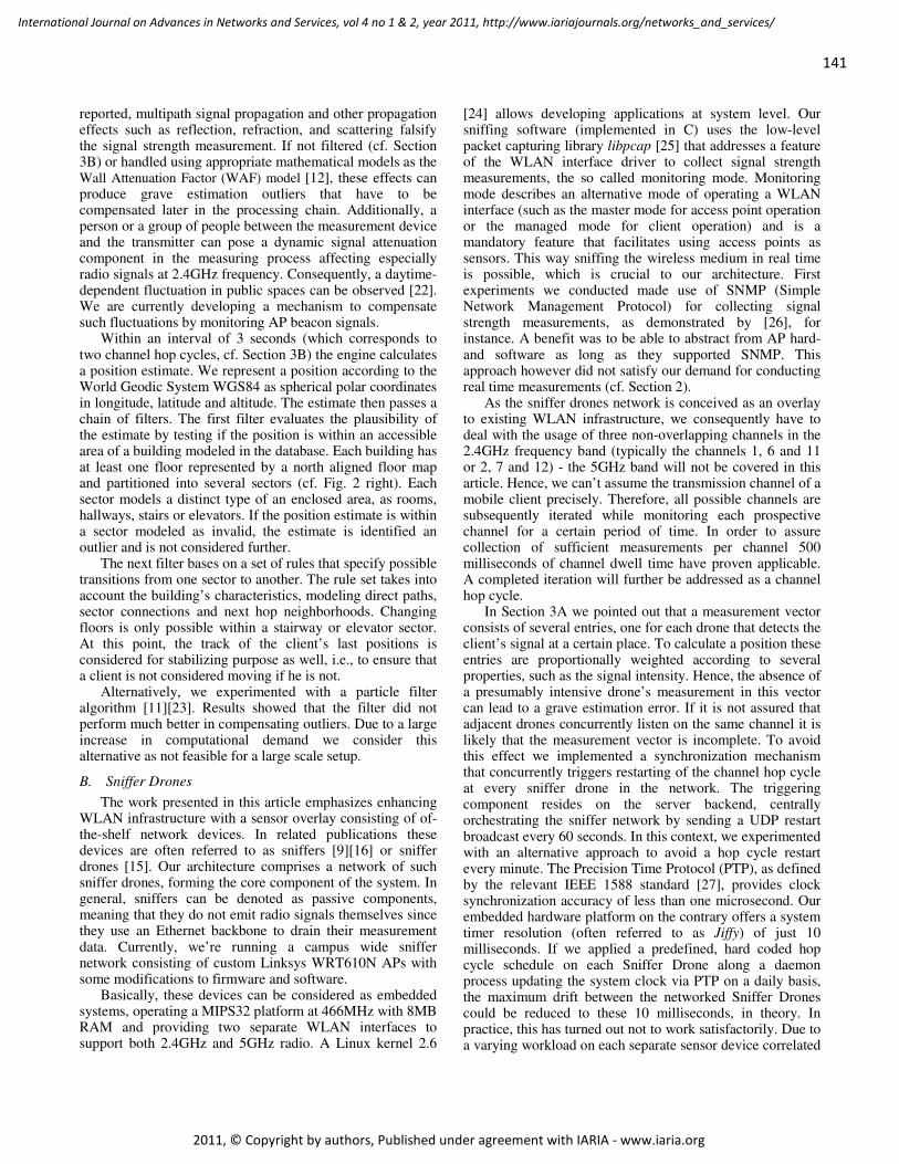
reported, multipath signal propagation and other propagation effects such as reflection, refraction, and scattering falsify the signal strength measurement. If not filtered (cf. Section 3B) or handled using appropriate mathematical models as the Wall Attenuation Factor (WAF) model [12], these effects can produce grave estimation outliers that have to be compensated later in the processing chain. Additionally, a person or a group of people between the measurement device and the transmitter can pose a dynamic signal attenuation component in the measuring process affecting especially radio signals at 2.4GHz frequency. Consequently, a daytime-dependent fluctuation in public spaces can be observed [22]. We are currently developing a mechanism to compensate such fluctuations by monitoring AP beacon signals.
Within an interval of 3 seconds (which corresponds to two channel hop cycles, cf. Section 3B) the engine calculates a position estimate. We represent a position according to the World Geodic System WGS84 as spherical polar coordinates in longitude, latitude and altitude. The estimate then passes a chain of filters. The first filter evaluates the plausibility of the estimate by testing if the position is within an accessible area of a building modeled in the database. Each building has at least one floor represented by a north aligned floor map and partitioned into several sectors (cf. Fig. 2 right). Each sector models a distinct type of an enclosed area, as rooms, hallways, stairs or elevators. If the position estimate is within a sector modeled as invalid, the estimate is identified an outlier and is not considered further.
The next filter bases on a set of rules that specify possible transitions from one sector to another. The rule set takes into account the building’s characteristics, modeling direct paths, sector connections and next hop neighborhoods. Changing floors is only possible within a stairway or elevator sector. At this point, the track of the client’s last positions is considered for stabilizing purpose as well, i.e., to ensure that a client is not considered moving if he is not.
Alternatively, we experimented with a particle filter algorithm [11][23]. Results showed that the filter did not perform much better in compensating outliers. Due to a large increase in computational demand we consider this alternative as not feasible for a large scale setup.
B. Sniffer Drones
The work presented in this article emphasizes enhancing WLAN infrastructure with a sensor overlay consisting of of-the-shelf network devices. In related publications these devices are often referred to as sniffers [9][16] or sniffer drones [15]. Our architecture comprises a network of such sniffer drones, forming the core component of the system. In general, sniffers can be denoted as passive components, meaning that they do not emit radio signals themselves since they use an Ethernet backbone to drain their measurement data. Currently, we’re running a campus wide sniffer network consisting of custom Linksys WRT610N APs with some modifications to firmware and software.
Basically, these devices can be considered as embedded systems, operating a MIPS32 platform at 466MHz with 8MB RAM and providing two separate WLAN interfaces to support both 2.4GHz and 5GHz radio. A Linux kernel 2.6
[24] allows developing applications at system level. Our sniffing software (implemented in C) uses the low-level packet capturing library libpcap [25] that addresses a feature of the WLAN interface driver to collect signal strength measurements, the so called monitoring mode. Monitoring mode describes an alternative mode of operating a WLAN interface (such as the master mode for access point operation or the managed mode for client operation) and is a mandatory feature that facilitates using access points as sensors. This way sniffing the wireless medium in real time is possible, which is crucial to our architecture. First experiments we conducted made use of SNMP (Simple Network Management Protocol) for collecting signal strength measurements, as demonstrated by [26], for instance. A benefit was to be able to abstract from AP hard- and software as long as they supported SNMP. This approach however did not satisfy our demand for conducting real time measurements (cf. Section 2).
As the sniffer drones network is conceived as an overlay to existing WLAN infrastructure, we consequently have to deal with the usage of three non-overlapping channels in the 2.4GHz frequency band (typically the channels 1, 6 and 11 or 2, 7 and 12) - the 5GHz band will not be covered in this article. Hence, we can’t assume the transmission channel of a mobile client precisely. Therefore, all possible channels are subsequently iterated while monitoring each prospective channel for a certain period of time. In order to assure collection of sufficient measurements per channel 500 milliseconds of channel dwell time have proven applicable. A completed iteration will further be addressed as a channel hop cycle.
In Section 3A we pointed out that a measurement vector consists of several entries, one for each drone that detects the client’s signal at a certain place. To calculate a position these entries are proportionally weighted according to several properties, such as the signal intensity. Hence, the absence of a presumably intensive drone’s measurement in this vector can lead to a grave estimation error. If it is not assured that adjacent drones concurrently listen on the same channel it is likely that the measurement vector is incomplete. To avoid this effect we implemented a synchronization mechanism that concurrently triggers restarting of the channel hop cycle at every sniffer drone in the network. The triggering component resides on the server backend, centrally orchestrating the sniffer network by sending a UDP restart broadcast every 60 seconds. In this context, we experimented with an alternative approach to avoid a hop cycle restart every minute. The Precision Time Protocol (PTP), as defined by the relevant IEEE 1588 standard [27], provides clock synchronization accuracy of less than one microsecond. Our embedded hardware platform on the contrary offers a system timer resolution (often referred to as Jiffy) of just 10 milliseconds. If we applied a predefined, hard coded hop cycle schedule on each Sniffer Drone along a daemon process updating the system clock via PTP on a daily basis, the maximum drift between the networked Sniffer Drones could be reduced to these 10 milliseconds, in theory. In practice, this has turned out not to work satisfactorily. Due to a varying workload on each separate sensor device correlated
141
International Journal on Advances in Networks and Services, vol 4 no 1 & 2, year 2011, http://www.iariajournals.org/networks_and_services/
2011, © Copyright by authors, Published under agreement with IARIA - www.iaria.org
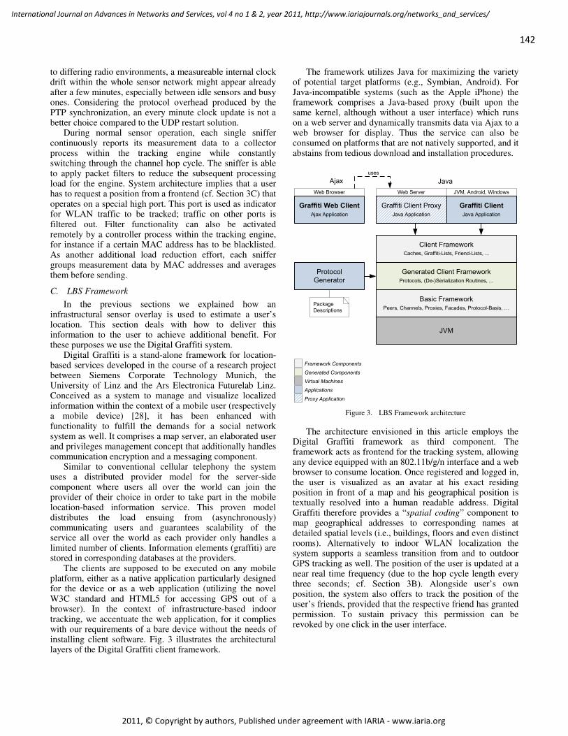
to differing radio environments, a measureable internal clock drift within the whole sensor network might appear already after a few minutes, especially between idle sensors and busy ones. Considering the protocol overhead produced by the PTP synchronization, an every minute clock update is not a better choice compared to the UDP restart solution.
During normal sensor operation, each single sniffer continuously reports its measurement data to a collector process within the tracking engine while constantly switching through the channel hop cycle. The sniffer is able to apply packet filters to reduce the subsequent processing load for the engine. System architecture implies that a user has to request a position from a frontend (cf. Section 3C) that operates on a special high port. This port is used as indicator for WLAN traffic to be tracked; traffic on other ports is filtered out. Filter functionality can also be activated remotely by a controller process within the tracking engine, for instance if a certain MAC address has to be blacklisted. As another additional load reduction effort, each sniffer groups measurement data by MAC addresses and averages them before sending.
C. LBS Framework
In the previous sections we explained how an infrastructural sensor overlay is used to estimate a user’s location. This section deals with how to deliver this information to the user to achieve additional benefit. For these purposes we use the Digital Graffiti system.
Digital Graffiti is a stand-alone framework for location-based services developed in the course of a research project between Siemens Corporate Technology Munich, the University of Linz and the Ars Electronica Futurelab Linz. Conceived as a system to manage and visualize localized information within the context of a mobile user (respectively a mobile device) [28], it has been enhanced with functionality to fulfill the demands for a social network system as well. It comprises a map server, an elaborated user and privileges management concept that additionally handles communication encryption and a messaging component.
Similar to conventional cellular telephony the system uses a distributed provider model for the server-side component where users all over the world can join the provider of their choice in order to take part in the mobile location-based information service. This proven model distributes the load ensuing from (asynchronously) communicating users and guarantees scalability of the service all over the world as each provider only handles a limited number of clients. Information elements (graffiti) are stored in corresponding databases at the providers.
The clients are supposed to be executed on any mobile platform, either as a native application particularly designed for the device or as a web application (utilizing the novel W3C standard and HTML5 for accessing GPS out of a browser). In the context of infrastructure-based indoor tracking, we accentuate the web application, for it complies with our requirements of a bare device without the needs of installing client software. Fig. 3 illustrates the architectural layers of the Digital Graffiti client framework.
The framework utilizes Java for maximizing the variety of potential target platforms (e.g., Symbian, Android). For Java-incompatible systems (such as the Apple iPhone) the framework comprises a Java-based proxy (built upon the same kernel, although without a user interface) which runs on a web server and dynamically transmits data via Ajax to a web browser for display. Thus the service can also be consumed on platforms that are not natively supported, and it abstains from tedious download and installation procedures.
Web Browser Web Server JVM, Android, Windows
Generated Client Framework
Protocols, (De-)Serialization Routines, ...
Protocol
Generator
Client Framework
Caches, Graffiti-Lists, Friend-Lists, ...
Graffiti Client Proxy
Java Application
Graffiti Client
Java Application
Java
Package
Descriptions
JVM
Basic Framework
Peers, Channels, Proxies, Facades, Protocol-Basis, -
Graffiti Web Client
Ajax Application
Ajax
uses
Applications
Framework Components
Generated Components
Virtual Machines
Proxy Application Figure 3. LBS Framework architecture
The architecture envisioned in this article employs the Digital Graffiti framework as third component. The framework acts as frontend for the tracking system, allowing any device equipped with an 802.11b/g/n interface and a web browser to consume location. Once registered and logged in, the user is visualized as an avatar at his exact residing position in front of a map and his geographical position is textually resolved into a human readable address. Digital Graffiti therefore provides a “spatial coding” component to map geographical addresses to corresponding names at detailed spatial levels (i.e., buildings, floors and even distinct rooms). Alternatively to indoor WLAN localization the system supports a seamless transition from and to outdoor GPS tracking as well. The position of the user is updated at a near real time frequency (due to the hop cycle length every three seconds; cf. Section 3B). Alongside user’s own position, the system also offers to track the position of the user’s friends, provided that the respective friend has granted permission. To sustain privacy this permission can be revoked by one click in the user interface.
142
International Journal on Advances in Networks and Services, vol 4 no 1 & 2, year 2011, http://www.iariajournals.org/networks_and_services/
2011, © Copyright by authors, Published under agreement with IARIA - www.iaria.org
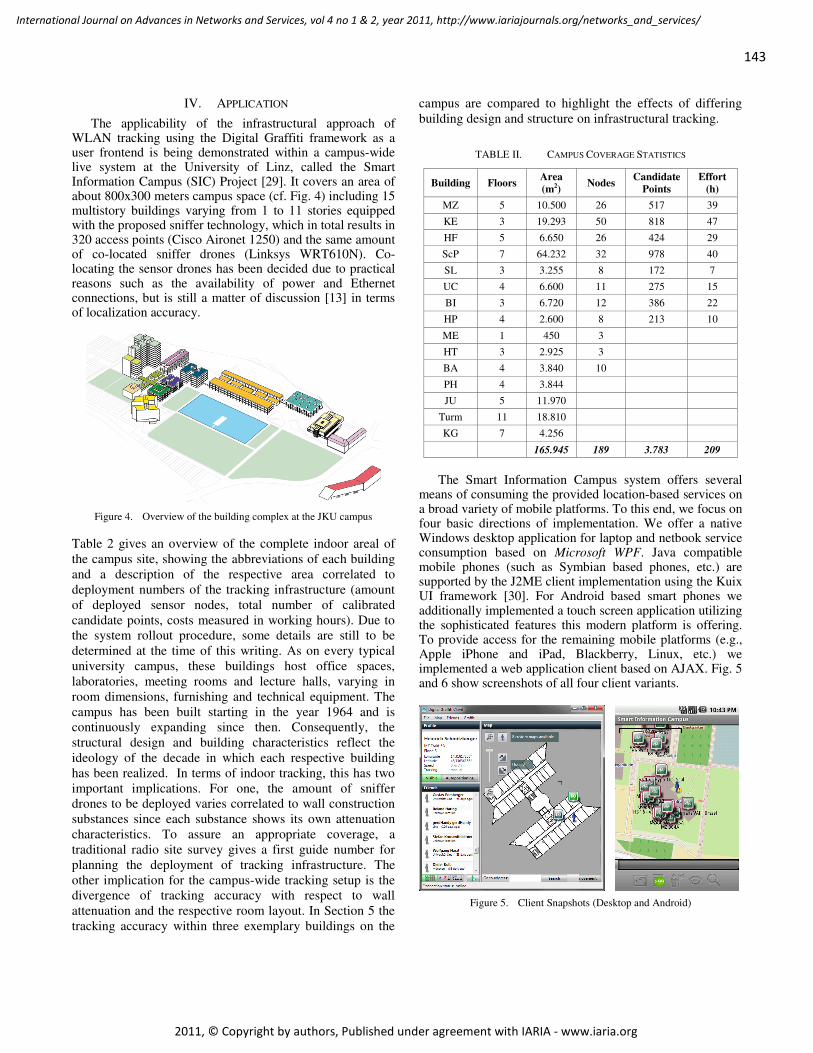
IV. APPLICATION
The applicability of the infrastructural approach of WLAN tracking using the Digital Graffiti framework as a user frontend is being demonstrated within a campus-wide live system at the University of Linz, called the Smart Information Campus (SIC) Project [29]. It covers an area of about 800x300 meters campus space (cf. Fig. 4) including 15 multistory buildings varying from 1 to 11 stories equipped with the proposed sniffer technology, which in total results in 320 access points (Cisco Aironet 1250) and the same amount of co-located sniffer drones (Linksys WRT610N). Co-locating the sensor drones has been decided due to practical reasons such as the availability of power and Ethernet connections, but is still a matter of discussion [13] in terms of localization accuracy.
Figure 4. Overview of the building complex at the JKU campus
Table 2 gives an overview of the complete indoor areal of
the campus site, showing the abbreviations of each building
and a description of the respective area correlated to
deployment numbers of the tracking infrastructure (amount
of deployed sensor nodes, total number of calibrated
candidate points, costs measured in working hours). Due to
the system rollout procedure, some details are still to be
determined at the time of this writing. As on every typical
university campus, these buildings host office spaces,
laboratories, meeting rooms and lecture halls, varying in
room dimensions, furnishing and technical equipment. The
campus has been built starting in the year 1964 and is
continuously expanding since then. Consequently, the
structural design and building characteristics reflect the
ideology of the decade in which each respective building
has been realized. In terms of indoor tracking, this has two
important implications. For one, the amount of sniffer
drones to be deployed varies correlated to wall construction
substances since each substance shows its own attenuation
characteristics. To assure an appropriate coverage, a
traditional radio site survey gives a first guide number for
planning the deployment of tracking infrastructure. The
other implication for the campus-wide tracking setup is the
divergence of tracking accuracy with respect to wall
attenuation and the respective room layout. In Section 5 the
tracking accuracy within three exemplary buildings on the
campus are compared to highlight the effects of differing
building design and structure on infrastructural tracking.
TABLE II. CAMPUS COVERAGE STATISTICS
Building Floors Area
(m2) Nodes
Candidate
Points
Effort
(h)
MZ 5 10.500 26 517 39
KE 3 19.293 50 818 47
HF 5 6.650 26 424 29
ScP 7 64.232 32 978 40
SL 3 3.255 8 172 7
UC 4 6.600 11 275 15
BI 3 6.720 12 386 22
HP 4 2.600 8 213 10
ME 1 450 3
HT 3 2.925 3
BA 4 3.840 10
PH 4 3.844
JU 5 11.970
Turm 11 18.810
KG 7 4.256
165.945 189 3.783 209
The Smart Information Campus system offers several
means of consuming the provided location-based services on a broad variety of mobile platforms. To this end, we focus on four basic directions of implementation. We offer a native Windows desktop application for laptop and netbook service consumption based on Microsoft WPF. Java compatible mobile phones (such as Symbian based phones, etc.) are supported by the J2ME client implementation using the Kuix UI framework [30]. For Android based smart phones we additionally implemented a touch screen application utilizing the sophisticated features this modern platform is offering. To provide access for the remaining mobile platforms (e.g., Apple iPhone and iPad, Blackberry, Linux, etc.) we implemented a web application client based on AJAX. Fig. 5 and 6 show screenshots of all four client variants.
Figure 5. Client Snapshots (Desktop and Android)
143
International Journal on Advances in Networks and Services, vol 4 no 1 & 2, year 2011, http://www.iariajournals.org/networks_and_services/
2011, © Copyright by authors, Published under agreement with IARIA - www.iaria.org
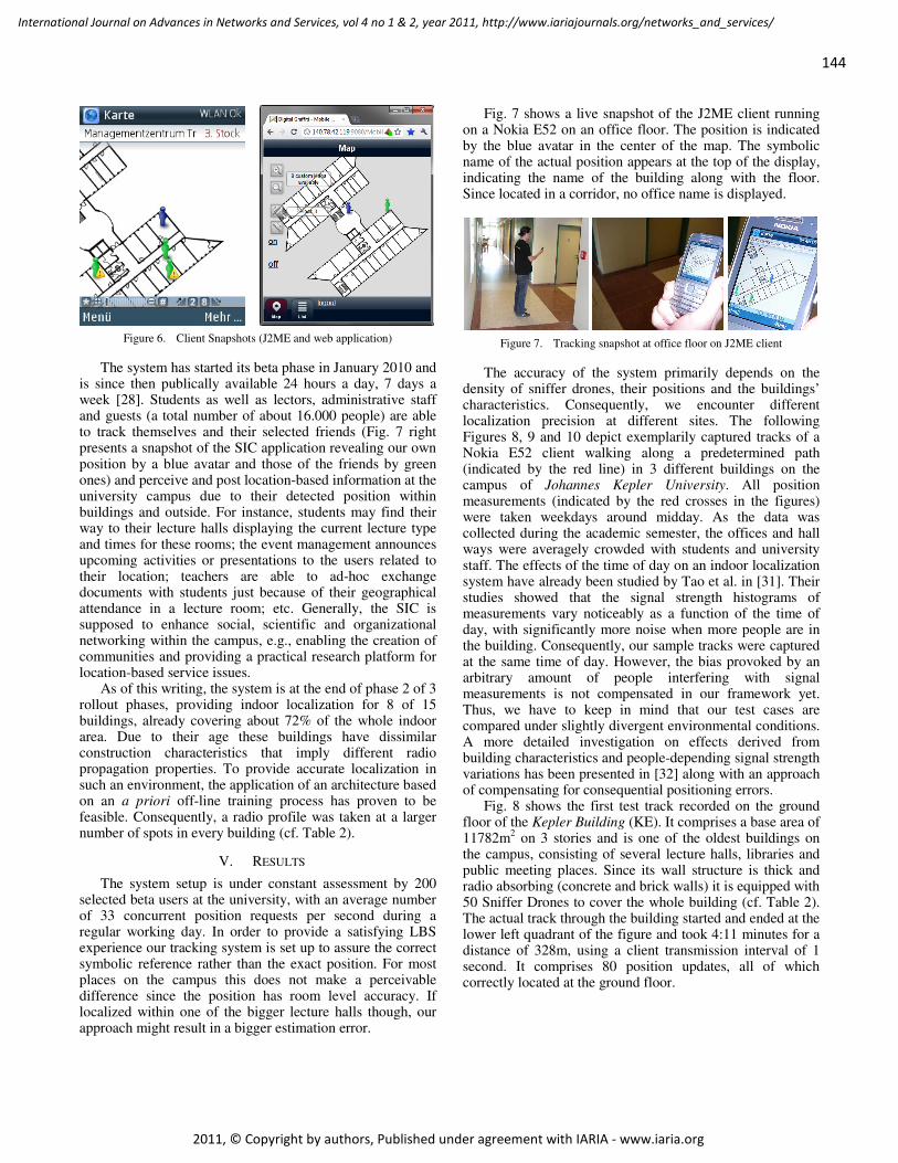
Figure 6. Client Snapshots (J2ME and web application)
The system has started its beta phase in January 2010 and is since then publically available 24 hours a day, 7 days a week [28]. Students as well as lectors, administrative staff and guests (a total number of about 16.000 people) are able to track themselves and their selected friends (Fig. 7 right presents a snapshot of the SIC application revealing our own position by a blue avatar and those of the friends by green ones) and perceive and post location-based information at the university campus due to their detected position within buildings and outside. For instance, students may find their way to their lecture halls displaying the current lecture type and times for these rooms; the event management announces upcoming activities or presentations to the users related to their location; teachers are able to ad-hoc exchange documents with students just because of their geographical attendance in a lecture room; etc. Generally, the SIC is supposed to enhance social, scientific and organizational networking within the campus, e.g., enabling the creation of communities and providing a practical research platform for location-based service issues.
As of this writing, the system is at the end of phase 2 of 3 rollout phases, providing indoor localization for 8 of 15 buildings, already covering about 72% of the whole indoor area. Due to their age these buildings have dissimilar construction characteristics that imply different radio propagation properties. To provide accurate localization in such an environment, the application of an architecture based on an a priori off-line training process has proven to be feasible. Consequently, a radio profile was taken at a larger number of spots in every building (cf. Table 2).
V. RESULTS
The system setup is under constant assessment by 200 selected beta users at the university, with an average number of 33 concurrent position requests per second during a regular working day. In order to provide a satisfying LBS experience our tracking system is set up to assure the correct symbolic reference rather than the exact position. For most places on the campus this does not make a perceivable difference since the position has room level accuracy. If localized within one of the bigger lecture halls though, our approach might result in a bigger estimation error.
Fig. 7 shows a live snapshot of the J2ME client running on a Nokia E52 on an office floor. The position is indicated by the blue avatar in the center of the map. The symbolic name of the actual position appears at the top of the display, indicating the name of the building along with the floor. Since located in a corridor, no office name is displayed.
Figure 7. Tracking snapshot at office floor on J2ME client
The accuracy of the system primarily depends on the density of sniffer drones, their positions and the buildings’ characteristics. Consequently, we encounter different localization precision at different sites. The following Figures 8, 9 and 10 depict exemplarily captured tracks of a Nokia E52 client walking along a predetermined path (indicated by the red line) in 3 different buildings on the campus of Johannes Kepler University. All position measurements (indicated by the red crosses in the figures) were taken weekdays around midday. As the data was collected during the academic semester, the offices and hall ways were averagely crowded with students and university staff. The effects of the time of day on an indoor localization system have already been studied by Tao et al. in [31]. Their studies showed that the signal strength histograms of measurements vary noticeably as a function of the time of day, with significantly more noise when more people are in the building. Consequently, our sample tracks were captured at the same time of day. However, the bias provoked by an arbitrary amount of people interfering with signal measurements is not compensated in our framework yet. Thus, we have to keep in mind that our test cases are compared under slightly divergent environmental conditions. A more detailed investigation on effects derived from building characteristics and people-depending signal strength variations has been presented in [32] along with an approach of compensating for consequential positioning errors.
Fig. 8 shows the first test track recorded on the ground floor of the Kepler Building (KE). It comprises a base area of 11782m
2 on 3 stories and is one of the oldest buildings on
the campus, consisting of several lecture halls, libraries and public meeting places. Since its wall structure is thick and radio absorbing (concrete and brick walls) it is equipped with 50 Sniffer Drones to cover the whole building (cf. Table 2). The actual track through the building started and ended at the lower left quadrant of the figure and took 4:11 minutes for a distance of 328m, using a client transmission interval of 1 second. It comprises 80 position updates, all of which correctly located at the ground floor.
144
International Journal on Advances in Networks and Services, vol 4 no 1 & 2, year 2011, http://www.iariajournals.org/networks_and_services/
2011, © Copyright by authors, Published under agreement with IARIA - www.iaria.org
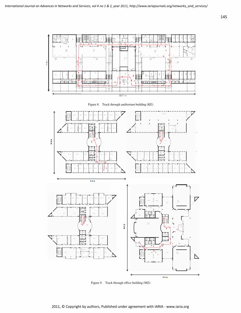
Figure 8. Track through auditorium building (KE)
Figure 9. Track through office building (MZ)
145
International Journal on Advances in Networks and Services, vol 4 no 1 & 2, year 2011, http://www.iariajournals.org/networks_and_services/
2011, © Copyright by authors, Published under agreement with IARIA - www.iaria.org
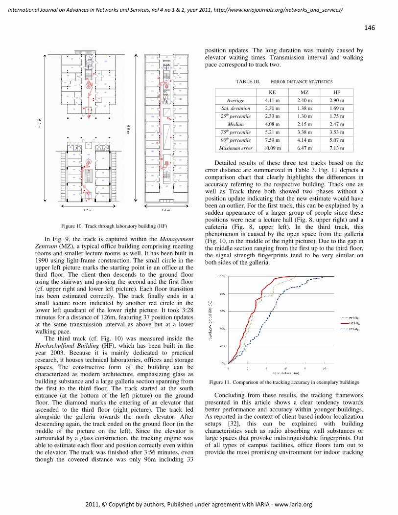
Figure 10. Track through laboratory building (HF)
In Fig. 9, the track is captured within the Management Zentrum (MZ), a typical office building comprising meeting rooms and smaller lecture rooms as well. It has been built in 1990 using light-frame construction. The small circle in the upper left picture marks the starting point in an office at the third floor. The client then descends to the ground floor using the stairway and passing the second and the first floor (cf. upper right and lower left picture). Each floor transition has been estimated correctly. The track finally ends in a small lecture room indicated by another red circle in the lower left quadrant of the lower right picture. It took 3:28 minutes for a distance of 126m, featuring 37 position updates at the same transmission interval as above but at a lower walking pace.
The third track (cf. Fig. 10) was measured inside the Hochschulfond Building (HF), which has been built in the year 2003. Because it is mainly dedicated to practical research, it houses technical laboratories, offices and storage spaces. The constructive form of the building can be characterized as modern architecture, emphasizing glass as building substance and a large galleria section spanning from the first to the third floor. The track started at the south entrance (at the bottom of the left picture) on the ground floor. The diamond marks the entering of an elevator that ascended to the third floor (right picture). The track led alongside the galleria towards the north elevator. After descending again, the track ended on the ground floor (in the middle of the picture on the left). Since the elevator is surrounded by a glass construction, the tracking engine was able to estimate each floor and position correctly even within the elevator. The track was finished after 3:56 minutes, even though the covered distance was only 96m including 33
position updates. The long duration was mainly caused by elevator waiting times. Transmission interval and walking pace correspond to track two.
TABLE III. ERROR DISTANCE STATISTICS
KE MZ HF
Average 4.11 m 2.40 m 2.90 m
Std. deviation 2.30 m 1.38 m 1.69 m
25th percentile 2.33 m 1.30 m 1.75 m
Median 4.08 m 2.15 m 2.47 m
75th percentile 5.21 m 3.38 m 3.53 m
90th percentile 7.59 m 4.14 m 5.07 m
Maximum error 10.09 m 6.47 m 7.13 m
Detailed results of these three test tracks based on the
error distance are summarized in Table 3. Fig. 11 depicts a comparison chart that clearly highlights the differences in accuracy referring to the respective building. Track one as well as Track three both showed two phases without a position update indicating that the new estimate would have been an outlier. For the first track, this can be explained by a sudden appearance of a larger group of people since these positions were near a lecture hall (Fig. 8, upper right) and a cafeteria (Fig. 8, upper left). In the third track, this phenomenon is caused by the open space from the galleria (Fig. 10, in the middle of the right picture). Due to the gap in the middle section ranging from the first up to the third floor, the signal strength fingerprints tend to be very similar on both sides of the galleria.
Figure 11. Comparison of the tracking accuracy in exemplary buildings
Concluding from these results, the tracking framework presented in this article shows a clear tendency towards better performance and accuracy within younger buildings. As reported in the context of client-based indoor localization setups [32], this can be explained with building characteristics such as radio absorbing wall substances or large spaces that provoke indistinguishable fingerprints. Out of all types of campus facilities, office floors turn out to provide the most promising environment for indoor tracking
146
International Journal on Advances in Networks and Services, vol 4 no 1 & 2, year 2011, http://www.iariajournals.org/networks_and_services/
2011, © Copyright by authors, Published under agreement with IARIA - www.iaria.org
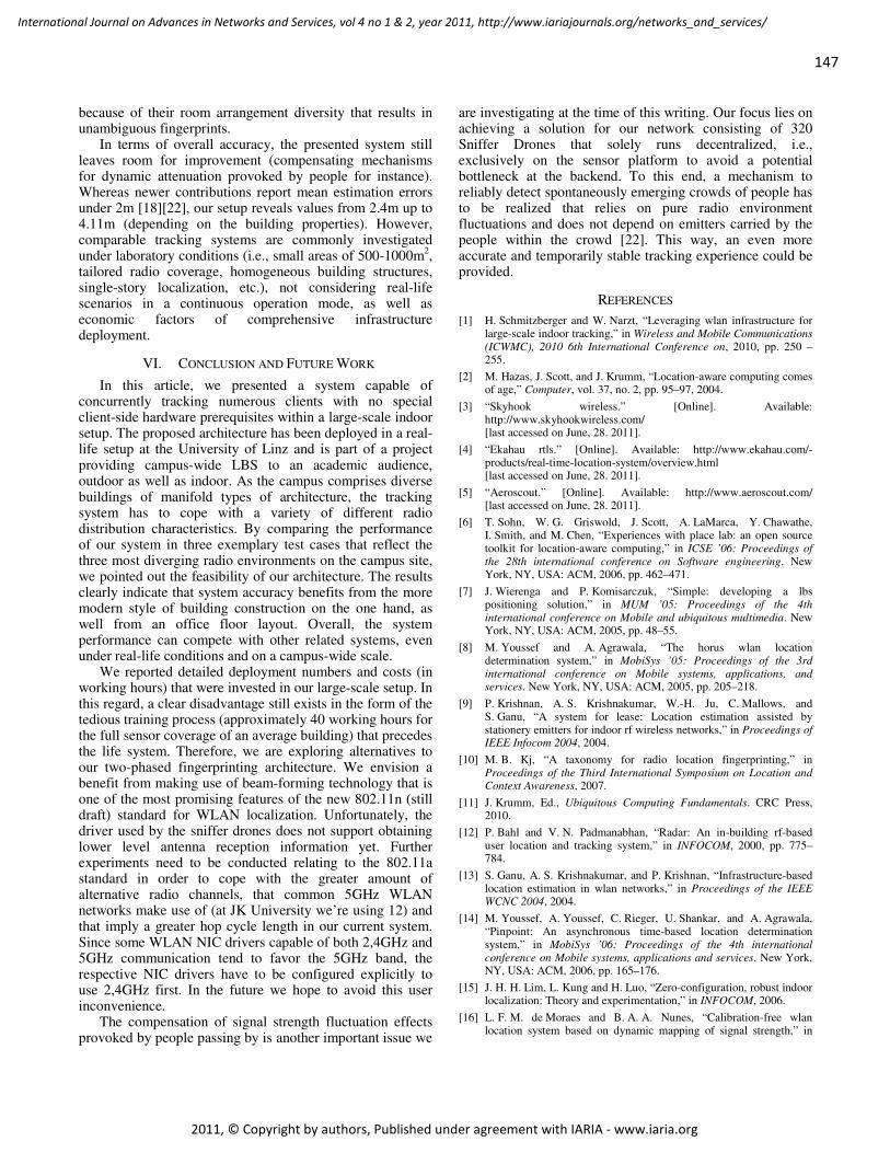
because of their room arrangement diversity that results in unambiguous fingerprints.
In terms of overall accuracy, the presented system still leaves room for improvement (compensating mechanisms for dynamic attenuation provoked by people for instance). Whereas newer contributions report mean estimation errors under 2m [18][22], our setup reveals values from 2.4m up to 4.11m (depending on the building properties). However, comparable tracking systems are commonly investigated under laboratory conditions (i.e., small areas of 500-1000m
2,
tailored radio coverage, homogeneous building structures, single-story localization, etc.), not considering real-life scenarios in a continuous operation mode, as well as economic factors of comprehensive infrastructure deployment.
VI. CONCLUSION AND FUTURE WORK
In this article, we presented a system capable of concurrently tracking numerous clients with no special client-side hardware prerequisites within a large-scale indoor setup. The proposed architecture has been deployed in a real-life setup at the University of Linz and is part of a project providing campus-wide LBS to an academic audience, outdoor as well as indoor. As the campus comprises diverse buildings of manifold types of architecture, the tracking system has to cope with a variety of different radio distribution characteristics. By comparing the performance of our system in three exemplary test cases that reflect the three most diverging radio environments on the campus site, we pointed out the feasibility of our architecture. The results clearly indicate that system accuracy benefits from the more modern style of building construction on the one hand, as well from an office floor layout. Overall, the system performance can compete with other related systems, even under real-life conditions and on a campus-wide scale.
We reported detailed deployment numbers and costs (in working hours) that were invested in our large-scale setup. In this regard, a clear disadvantage still exists in the form of the tedious training process (approximately 40 working hours for the full sensor coverage of an average building) that precedes the life system. Therefore, we are exploring alternatives to our two-phased fingerprinting architecture. We envision a benefit from making use of beam-forming technology that is one of the most promising features of the new 802.11n (still draft) standard for WLAN localization. Unfortunately, the driver used by the sniffer drones does not support obtaining lower level antenna reception information yet. Further experiments need to be conducted relating to the 802.11a standard in order to cope with the greater amount of alternative radio channels, that common 5GHz WLAN networks make use of (at JK University we’re using 12) and that imply a greater hop cycle length in our current system. Since some WLAN NIC drivers capable of both 2,4GHz and 5GHz communication tend to favor the 5GHz band, the respective NIC drivers have to be configured explicitly to use 2,4GHz first. In the future we hope to avoid this user inconvenience.
The compensation of signal strength fluctuation effects provoked by people passing by is another important issue we
are investigating at the time of this writing. Our focus lies on achieving a solution for our network consisting of 320 Sniffer Drones that solely runs decentralized, i.e., exclusively on the sensor platform to avoid a potential bottleneck at the backend. To this end, a mechanism to reliably detect spontaneously emerging crowds of people has to be realized that relies on pure radio environment fluctuations and does not depend on emitters carried by the people within the crowd [22]. This way, an even more accurate and temporarily stable tracking experience could be provided.
REFERENCES
[1] H. Schmitzberger and W. Narzt, “Leveraging wlan infrastructure for large-scale indoor tracking,” in Wireless and Mobile Communications
(ICWMC), 2010 6th International Conference on, 2010, pp. 250 –255.
[2] M. Hazas, J. Scott, and J. Krumm, “Location-aware computing comes of age,” Computer, vol. 37, no. 2, pp. 95–97, 2004.
[3] “Skyhook wireless.” [Online]. Available: http://www.skyhookwireless.com/ [last accessed on June, 28. 2011].
[4] “Ekahau rtls.” [Online]. Available: http://www.ekahau.com/-products/real-time-location-system/overview.html [last accessed on June, 28. 2011].
[5] “Aeroscout.” [Online]. Available: http://www.aeroscout.com/ [last accessed on June, 28. 2011].
[6] T. Sohn, W. G. Griswold, J. Scott, A. LaMarca, Y. Chawathe, I. Smith, and M. Chen, “Experiences with place lab: an open source toolkit for location-aware computing,” in ICSE ’06: Proceedings of
the 28th international conference on Software engineering. New York, NY, USA: ACM, 2006, pp. 462–471.
[7] J. Wierenga and P. Komisarczuk, “Simple: developing a lbs positioning solution,” in MUM ’05: Proceedings of the 4th
international conference on Mobile and ubiquitous multimedia. New York, NY, USA: ACM, 2005, pp. 48–55.
[8] M. Youssef and A. Agrawala, “The horus wlan location determination system,” in MobiSys ’05: Proceedings of the 3rd
international conference on Mobile systems, applications, and services. New York, NY, USA: ACM, 2005, pp. 205–218.
[9] P. Krishnan, A. S. Krishnakumar, W.-H. Ju, C. Mallows, and S. Ganu, “A system for lease: Location estimation assisted by stationery emitters for indoor rf wireless networks,” in Proceedings of IEEE Infocom 2004, 2004.
[10] M. B. Kj, “A taxonomy for radio location fingerprinting,” in Proceedings of the Third International Symposium on Location and Context Awareness, 2007.
[11] J. Krumm, Ed., Ubiquitous Computing Fundamentals. CRC Press, 2010.
[12] P. Bahl and V. N. Padmanabhan, “Radar: An in-building rf-based user location and tracking system,” in INFOCOM, 2000, pp. 775–784.
[13] S. Ganu, A. S. Krishnakumar, and P. Krishnan, “Infrastructure-based location estimation in wlan networks,” in Proceedings of the IEEE WCNC 2004, 2004.
[14] M. Youssef, A. Youssef, C. Rieger, U. Shankar, and A. Agrawala, “Pinpoint: An asynchronous time-based location determination system,” in MobiSys ’06: Proceedings of the 4th international
conference on Mobile systems, applications and services. New York, NY, USA: ACM, 2006, pp. 165–176.
[15] J. H. H. Lim, L. Kung and H. Luo, “Zero-configuration, robust indoor localization: Theory and experimentation,” in INFOCOM, 2006.
[16] L. F. M. de Moraes and B. A. A. Nunes, “Calibration-free wlan location system based on dynamic mapping of signal strength,” in
147
International Journal on Advances in Networks and Services, vol 4 no 1 & 2, year 2011, http://www.iariajournals.org/networks_and_services/
2011, © Copyright by authors, Published under agreement with IARIA - www.iaria.org
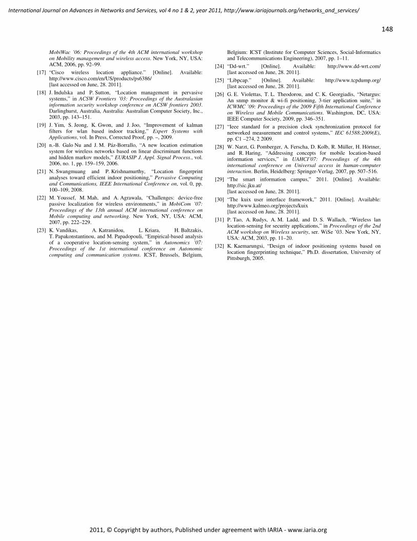
MobiWac ’06: Proceedings of the 4th ACM international workshop
on Mobility management and wireless access. New York, NY, USA: ACM, 2006, pp. 92–99.
[17] “Cisco wireless location appliance.” [Online]. Available: http://www.cisco.com/en/US/products/ps6386/ [last accessed on June, 28. 2011].
[18] J. Indulska and P. Sutton, “Location management in pervasive systems,” in ACSW Frontiers ’03: Proceedings of the Australasian
information security workshop conference on ACSW frontiers 2003. Darlinghurst, Australia, Australia: Australian Computer Society, Inc., 2003, pp. 143–151.
[19] J. Yim, S. Jeong, K. Gwon, and J. Joo, “Improvement of kalman filters for wlan based indoor tracking,” Expert Systems with Applications, vol. In Press, Corrected Proof, pp. –, 2009.
[20] n.-B. Galo Nu and J. M. Páz-Borrallo, “A new location estimation system for wireless networks based on linear discriminant functions and hidden markov models,” EURASIP J. Appl. Signal Process., vol. 2006, no. 1, pp. 159–159, 2006.
[21] N. Swangmuang and P. Krishnamurthy, “Location fingerprint analyses toward efficient indoor positioning,” Pervasive Computing
and Communications, IEEE International Conference on, vol. 0, pp. 100–109, 2008.
[22] M. Youssef, M. Mah, and A. Agrawala, “Challenges: device-free passive localization for wireless environments,” in MobiCom ’07:
Proceedings of the 13th annual ACM international conference on
Mobile computing and networking. New York, NY, USA: ACM, 2007, pp. 222–229.
[23] K. Vandikas, A. Katranidou, L. Kriara, H. Baltzakis, T. Papakonstantinou, and M. Papadopouli, “Empirical-based analysis of a cooperative location-sensing system,” in Autonomics ’07:
Proceedings of the 1st international conference on Autonomic
computing and communication systems. ICST, Brussels, Belgium,
Belgium: ICST (Institute for Computer Sciences, Social-Informatics and Telecommunications Engineering), 2007, pp. 1–11.
[24] “Dd-wrt.” [Online]. Available: http://www.dd-wrt.com/ [last accessed on June, 28. 2011].
[25] “Libpcap.” [Online]. Available: http://www.tcpdump.org/ [last accessed on June, 28. 2011].
[26] G. E. Violettas, T. L. Theodorou, and C. K. Georgiadis, “Netargus: An snmp monitor & wi-fi positioning, 3-tier application suite,” in ICWMC ’09: Proceedings of the 2009 Fifth International Conference
on Wireless and Mobile Communications. Washington, DC, USA: IEEE Computer Society, 2009, pp. 346–351.
[27] “Ieee standard for a precision clock synchronization protocol for networked measurement and control systems,” IEC 61588:2009(E), pp. C1 –274, 2 2009.
[28] W. Narzt, G. Pomberger, A. Ferscha, D. Kolb, R. Müller, H. Hörtner, and R. Haring, “Addressing concepts for mobile location-based information services,” in UAHCI’07: Proceedings of the 4th
international conference on Universal access in human-computer interaction. Berlin, Heidelberg: Springer-Verlag, 2007, pp. 507–516.
[29] “The smart information campus,” 2011. [Online]. Available: http://sic.jku.at/ [last accessed on June, 28. 2011].
[30] “The kuix user interface framework,” 2011. [Online]. Available: http://www.kalmeo.org/projects/kuix [last accessed on June, 28. 2011].
[31] P. Tao, A. Rudys, A. M. Ladd, and D. S. Wallach, “Wireless lan location-sensing for security applications,” in Proceedings of the 2nd
ACM workshop on Wireless security, ser. WiSe ’03. New York, NY, USA: ACM, 2003, pp. 11–20.
[32] K. Kaemarungsi, “Design of indoor positioning systems based on location fingerprinting technique,” Ph.D. dissertation, University of Pittsburgh, 2005.
148
International Journal on Advances in Networks and Services, vol 4 no 1 & 2, year 2011, http://www.iariajournals.org/networks_and_services/
2011, © Copyright by authors, Published under agreement with IARIA - www.iaria.org
Sensor Data Fusion Middleware for Cooperative Traffic Applications
Teemu Leppänen 1)
, Mikko Perttunen 1)
, Pekka Kaipio 2)
, Jukka Riekki 1)
1)
Department of Electrical and Information Engineering
University of Oulu
Oulu, Finland
teemu.leppanen, mikko.perttunen,
2)
Department of Information Processing Science
University of Oulu
Oulu, Finland
Abstract – Recent advancements in information and
communication technology accelerate the development and
deployment of intelligent transportation systems. Cooperative
traffic systems utilize information collected by road users and
traffic operators about their immediate environment sharing it
system-wide, enabling services for all traffic entities. In this
work, we contribute a data processing and data fusion
middleware relying on wireless mobile sensor nodes and public
infrastructure services for traffic data collection for future
cooperative traffic applications and services. The system is
demonstrated with an example application, utilizing mobile
phones with integrated sensors as sensor nodes and producing
the visualization of travelled routes annotated with travel mode
and detected anomalies of road surface. Middleware features
include modular component-based architecture,
reconfigurable and reusable data processing components,
dynamic addition of components and interfaces into the system
in runtime and data fusion of heterogeneous sensor data
through chaining of components into application specific data
fusion levels.
Keywords - Cooperative systems; sensor networks; wireless
sensing; information fusion.
I. INTRODUCTION
Increasing bandwidth and 3G technologies available for wireless communication enable the advancement of intelligent transportation systems towards cooperative traffic systems, where traffic entities collect and share data and become more and more context-aware [1]. In [2], cooperative traffic is given the following description: “Road operators, infrastructure, vehicles, their drivers and other road users will co-operate to deliver the most efficient, safe, secure and comfortable journeys. The vehicle-to-vehicle and vehicle-to-infrastructure cooperative systems will contribute to these objectives beyond the improvements achievable with stand-alone systems.” These actors in traffic can be provided with information, for example, about traffic disorders, road conditions, current weather conditions and usage statistics as well as routes based on dynamic traffic information [3].
The increased need for accurate traffic information has led to the integration of offline traffic information, such as fixed road infrastructure sensor data, with real-time information from supplementary data sources, such as cameras, GPS and cell phone tracking [4]. In addition of providing complementary data, these data sources assist in
decreasing uncertainly of the data from individual sources and enhance the decision maker’s performance [4][5]. This will result in many traffic engineering problems to become data fusion problems, producing estimates or an improved model of the system being observed [4]. Different techniques for data fusion exist: statistical approaches, probabilistic approaches and artificial intelligence [4]. Sensor data fusion techniques can be characterized in several domains [5]. In the application domain, only application relevant concepts are considered. In the fusion objective domain, the objectives of the fusion are considered, for example object recognition. The selected sensor types dictate compatibility and complementary nature of different sensors. The sensor configuration, as in concurrent or temporally separated measurements, defines the sensor usage. Finally, the fusion process is usually described as a three-level hierarchy: data fusion, feature fusion and decision fusion. In any of the three levels spatial or temporal fusion may occur [5]. This model with the hierarchical levels with a varying level of detail in information has been widely accepted [4][5].
Participatory sensing is a method for collecting data from many unknown and independent contributors in collaboration [6]. Cooperation between contributors can take several forms [7]. Informative cooperation occurs when users extend the system range by transmitting their sensory data in one-way communication. In descriptive cooperation, sensory data is augmented with intentions such as the intended direction of movement of the user. Coordinative communication allows objects to reason about and modify their behavior depending on other’s intentions, which requires two-way communication. The key question here is: What information should be shared and in which level of processing and fusion? [7] Performing data processing and fusion refines the data and reduces the amount of data transferred in the system. However, it also reduces the sensor network coverage, reliability and accuracy of the data as fewer samples are available. Communication technology issues, such as wireless channel capacity, also limit coverage and reliability.
Wireless (mobile) sensor networks offer several advantages over fixed sensor networks [8]. First, the coverage of a network can be extended easily with smaller costs. Second, nodes can store data locally and provide data only when requested, which contributes towards scalability and energy saving. Third, if a fixed sensor node fails or
149
International Journal on Advances in Networks and Services, vol 4 no 1 & 2, year 2011, http://www.iariajournals.org/networks_and_services/
2011, © Copyright by authors, Published under agreement with IARIA - www.iaria.org
experiences network failures, mobile data collectors can be used to compensate the data loss. Fourth, localized algorithms in nodes can be utilized in data collection and processing tasks. Khanafer et al. [9] define two main categories for wireless sensor networks for intelligent transportation systems: planar and multi-tiered. Planar architectures utilize mobile sensors and can have infrastructure-less communication paradigm supporting vehicle-to-vehicle networks, forming mobile ad hoc wireless sensor networks. Another paradigm for planar architectures is infrastructure-based supporting vehicle-to-infrastructure and infrastructure-to-vehicle communication by utilizing fixed roadside units. Roadside units relay data to services and can also form clusters of members around them. Some challenges for planar architectures exist, related to network topology and scalability. Furthermore, there are known constrains such as processing capabilities of the nodes, which affects to quality of service among other things. Networks in the second category, multi-tiered architectures, can have better performance by supporting heterogeneous communication, such as wireless local area networks providing more available bandwidth. This means having better quality of service when computations can be relayed to more powerful units in upper layers utilizing the increased bandwidth available. Of course, enabling more communication technologies adds complexity and costs to the system.
As mobile phones are today widely used, equipped with sensors and interfaces to external sensors and they have processor, memory, battery and communication units, they can be also seen as sensor nodes [10]. Mobile data collectors, however, have communication issues when transferring data to the sinks as bandwidth is limited [8]. Also, battery life, processing power and memory capacity are limited. Normal phone usage will limit the data collection capability [10]. Data routing is influenced by the network topology, the quality of the service parameters and contents of the data [8].
The Finnish Cooperative traffic program [11] envisions sustainable traffic using extensive information sharing based on novel technologies and services. In the Sensor Data Fusion and Applications project as a part of this program, our focus is on utilizing new sensor data sources and data fusion methods for generating new potential applications [11]. Our vision in [1] includes the usage of mobile phones with integrated sensors, giving information on the behavior of the actors in traffic. Instead of focusing on tailored applications on the field, our goal is to develop a flexible system that can be used to demonstrate and analyze a variety of cooperative traffic scenarios and applications working cooperatively with little development overhead. To enable this we derive a wide set of requirements from the literature and our example scenarios and take a bottom up approach, contributing a practical data collection system with the ability to integrate heterogeneous sensor data and infrastructure services as data sources, data fusion capabilities and pluggable data processing components. The demonstration system includes a visualization client application that produces annotated maps and enables end-to-end demonstrations. In this paper, we report the system
prototype and an example application featuring real-time travel mode and road surface anomaly detection, with mobile phones with integrated sensor as wireless sensor nodes.
The rest of this paper is organized as follows: Section II reviews the related work in the area. In Section III, we define requirements and scenarios for a cooperative traffic sensor network and describe our system. In Section IV, we compare the developed system against the requirements and represent field test results. Finally, in Section V, thoughts for future work are given.
II. RELATED WORK
We describe here a number of existing applications utilizing mobile traffic-related sensor data and existing solutions for data processing and fusion for intelligent transportation systems.
A. Traffic sensing applications
Several participatory sensing systems have been reported. In the Mobile Millennium project [12], GPS enabled mobile phones are used for the collection of traffic data, which is then fused with data from sensors in the road infrastructure. The system is employed for monitoring and estimating the traffic flow in real-time. The produced estimates are then transferred back to the phones. Google Maps for Mobile [13] offers live traffic conditions monitoring by retrieving the speed of vehicles from the GPS data from the mobile phones. TJam [14] uses GPS receivers to predict traffic jams by measuring the velocity of the vehicles. Users' coordinates are transmitted to the service and the probabilities of congestion in a given region are sent back. In Nericell [10], mobile phones with accelerometer sensors are used in vehicles to detect road bumps, among other features. The detection software is installed in the mobile phone itself and they introduce the concept of triggered sensing where less energy consuming sensors are used to trigger the usage of other sensors.
B. Data fusion platforms
In the following we describe several platforms developed for processing traffic-related information from sensor networks. The hierarchical Content Delivery Network architecture described by Elshenawy and others [15] has network hierarchies to provide scaling. Vehicles contain on-board units acting as clients in the network. Road-side units work as a surrogate servers having storage for the content and self-healing mechanism for communication failures in the network. In the next hierarchy level, geographical areas are grouped into geographical domains, which are controlled by domain managers. It is the manager’s responsibility to dynamically route content to the vehicles under their domain, which should also decrease delivery time. Domain managers can be grouped together recursively. Services sent add and delete messages, which propagate through the network nodes, based on the geographical area the service covers. On
150
International Journal on Advances in Networks and Services, vol 4 no 1 & 2, year 2011, http://www.iariajournals.org/networks_and_services/
2011, © Copyright by authors, Published under agreement with IARIA - www.iaria.org
the other hand, on-board units can send discovery messages to locate available services in a geographical area.
In the Cooperative Vehicle Infrastructure System [16][17] project, OSGi open source platform has been selected as the application platform. Communication is done using the CALM standard, providing both wireless local area and cellular network access, which can be selected dynamically by having better quality of service. The system consists of three layers, in the upper layer is the central management working on the system-wide level. The middle layer represents the roadside infrastructure at the regional level and the lowest level represents the individual vehicles.
Tacconi et al. [18] describe an information retrieval scenario, where mobile sinks, for example vehicles, query data from edge nodes in the wireless sensor network. Sensor nodes and sink nodes are aware of their geographical position or spatial distribution. Data routing from the nodes to mobile sinks is done by predicting the current position of the mobile sink based on its mobility information within the network from the original location of the injected query.
The Telematic Management System [19] component suite has many similarities with our approach. It has three main components: the kernel, communication subsystem and the data module. Framework users provide a set of decision modules accessing the communication system and data module. The decision modules and their dependencies on other modules are defined as graphs in XML documents. With the decision modules, users define a protocol component, which propagates incoming messages to interested modules through the graph. The kernel provides interfaces for the decision modules and initiates them. Data modules define a mechanism to access the data concurrently. The communication subsystem uses TCP/IP asynchronously. For each vehicle there is a local queue in the subsystem, which is used to store messages directed to it. Messages from the vehicles are stored in the general system queue.
Lv et al. [21] define ubiquitous intelligent transportation system architecture as vehicle-to-vehicle or vehicle-to-infrastructure communication with access to large-scale information systems. Their system utilizes multi-source real-time location-based mobile sensor data and fixed sensor data via context-awareness technology. The key idea is the interaction between any devices in any location or time. In their system there are five layers. The resource management layer collects data from the mobile sensors and sensors in the roadside, for example weather stations. Preprocessing of the data and classification is also done in this layer. The information awareness layer fuses the data requested by the services running in the system. Next, the intelligent service layer provides access to data and services from other service providers. These services may be accessed via websites or mobile phones for example. The terminal application layer provides the dynamic system level services such as real-time traffic information or road guidance to personal computers and other terminals. Finally, the ubiquitous network layer provides hybrid network communication models to support usage of multiple communication technologies.
III. SYSTEM AND MIDDLEWARE
We identify various cooperative traffic scenarios to sketch the requirements for the data processing system. In the scenarios, the target users include a car driver, a pedestrian and a traffic operator.
One scenario sketches services supporting efficient responses to traffic accidents. If an intelligent vehicle notices changes in road conditions, or for example detects a traffic accident from abrupt braking, the vehicle can send this information to be added to the real-time situation model of the road segment. The new information can then be disseminated to other traffic entities in the system. The traffic accident location can be inserted to a database. Moreover, a real-time warning can be issued to the drivers planning to drive in that road by updating the route prediction data in their vehicle navigators. A weather service integrated into the system can be used to determine the current local weather and for example lighting conditions when the accident happened. This is useful information at least during the Nordic winter. This information aggregated with the road condition data and on-board diagnostics data from the vehicle can be stored as accident information to the database, where it is available for further analysis by road authorities. In the future, this allows drivers to be warned to avoid accidents when similar weather and road conditions appear. In addition, mobile phone data or roadside sensors, such as cameras, can be used to detect approaching dangerously speeding vehicles. Information about speeding vehicles, aggregated with the real-time road situation information, can produce an alert issued to other entities in that road segment and to the authorities.
Another scenario is warning the driver of a vehicle when approaching a school area where children are walking or bicycling nearby, which can be detected from children’s mobile phone location or roadside sensor data and even aggregated with current time. Additionally, static data for a road segment for improving situation awareness can be requested from a service in the Internet. In Finland, this kind of static road data is available from a public Internet service called DigiRoad [20]. The data includes: road name, entry and exit points, direction, speed limits, number of lanes, traffic signs, location of pedestrian crossings, bus and taxi stops, elements such as illumination, service elements such as car parks and gas stations, and finally even information about scenic locations for tourists.
All this information combined together provides local real-time situation of the traffic in that road segment. Mobile phones with integrated GPS receivers in vehicles without any sensors can provide real-time information to the system, such as the location, speed and direction of the vehicle. This helps detecting the real-time congestion in road segments, which can be used in the system to guide drivers through alternative routes. Eventually the authorities are provided with a real-time situation of traffic in the whole system level. This can be used for real-time traffic monitoring, planning road infrastructure development and in a smaller scale, for planning future heavy transport scenarios.
151
International Journal on Advances in Networks and Services, vol 4 no 1 & 2, year 2011, http://www.iariajournals.org/networks_and_services/
2011, © Copyright by authors, Published under agreement with IARIA - www.iaria.org
Although we identified several scenarios, we do not target the data processing middleware for specific sensors or applications. Thus, services offered by the middleware cannot be tailored and optimized as suggested in [22]. Furthermore, isolated data sources and heterogeneous communication networks set challenges for the systems [22].
A. General Requirements
Ducourthial [23] describes an architecture for vehicular networks and lists unique issues not currently experienced within other networks. These networks are highly dynamic, unreliable, asynchronous, penalized with low bandwidth availability and short communication duration. In spite of this, vehicular networks require robustness, high quality of service and real time operation. Khanafer et al. [9] suggest a number of general requirements for intelligent traffic systems. Fault tolerance and real-time communications are essential to maintain the quality of service. As node deployment is not fixed and network topology can change, a scalable communication network is required. Cost and power consumption of a single sensor node should be minimized. System security should be guaranteed as the data is important real-time data, such as real-time traffic situation.
Furthermore, we adapt several general requirements for sensor networks from [1][8][10][24] to the scope of cooperative traffic data processing middleware: 1) the architecture should be data-centric as we will handle large amounts of heterogeneous sensor data, 2) asynchronous communication should be used because of communication outages, 3) component-based architecture and modular components follow from the diversity of the applications, 4) data processing middleware should have means for self-configuration to achieve runtime scalability with additional modules and to react to dynamic changes in network, 5) means for self-maintenance are required in the case of sensor node failures, 6) support for unknown types of future sensors is required, 7) data processing components should be easily deployable to the system and 8) the system should be able to reconfigure functionality and launch components based on data requests from the client applications. Furthermore, from the project goals we derive the following requirements: 9) component chaining is required to implement a modular system with data fusion capabilities, 10) output interfaces should be well defined and extendable to enable the usage of the resulting information in a wide variety of client applications utilizing common ontology and 11) real-time performance is a major issue when considering the usage of information in traffic.
The middleware running in the system should facilitate rapid application development and deployment as the system is developed constantly [25]. The service access points are provided by the middleware. It should also have means to manage system policies and security and privacy functions. To have a consistent quality of service in applications, the same data should be available to all applications. Thus standardized access to data and storage services need to be provided in the middleware.
B. System Description
The purpose of this prototype system is to demonstrate the chosen applications and test the feasibility of the system. Secondarily, the system functions also as a sensor network test bench for data processing algorithms under development. Currently, we have three main components in the prototype system: 1) mobile phones as mobile sensor nodes with the data collection software and integrated sensors, 2) the middleware for data processing in a remote platform in a public network and 3) a client application showing a map in a web browser on end-user workstation. The system prototype features two-way communications as users can utilize sensory data from other users to assist in decision-making, thus, we have both informative and coordinative cooperation [7].
The developed middleware architecture is data-centric and using a centralized database, as we want all the data to be rapidly propagated for the needs of any client application or data processing component. Our aim is to collect as much as possible raw data in our system. Specifically, we do not want to limit the future use of the collected data sets by applying application specific preprocessing as the level of detail is highest in the lowest level and preserving raw data enables the largest set of applications. We do not consider the level of detail of information and data shared in the system in this work. The data processing functionality can indirectly reduce the reliability and accuracy of the data as the potential loss of details occurs in all processing stages. These are important considerations for the data fusion as well [5]. We do not limit the data acquisition methods available, thus streaming, polling and event-based acquisition all can be used (req. 6). Sensor data producers are decoupled from consumers, because the commonly available sensor nodes in the system, such as mobile phones, should not be concerned about the data processing needs of the client applications. The remote data processing platform provides global endpoints for sensor data producers and infrastructure services to enter data into the system and applications to retrieve it. Global endpoints also allow heterogeneous communication methods, regardless of the physical location of the sensor nodes or the applications (req. 2). Based on these features, when considering architecture categories described by [5], our middleware architecture falls to the multi-tiered category of wireless sensor networks. Multi-tiered architectures avoid the problems with sensor network routing, maintain the quality of service better and also support data fusion in higher levels of processing, and when processing requires more powerful computation platforms [6].
We selected Global Sensor Network (GSN) [26], a sensor network middleware, as a middleware platform for our system [1]. As we are looking for complete open source implementation, for example partially released CarTel [27] cannot be considered. Lightweight Java implementation, possibility to use only a subset of modules and minimal configuration needs make GSN deployable to a large set of system configurations. Simple API and the number of already implemented features reduce the amount of required
152
International Journal on Advances in Networks and Services, vol 4 no 1 & 2, year 2011, http://www.iariajournals.org/networks_and_services/
2011, © Copyright by authors, Published under agreement with IARIA - www.iaria.org
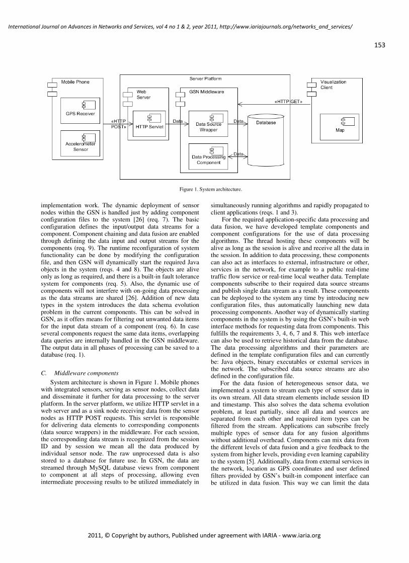
Figure 1. System architecture.
implementation work. The dynamic deployment of sensor nodes within the GSN is handled just by adding component configuration files to the system [26] (req. 7). The basic configuration defines the input/output data streams for a component. Component chaining and data fusion are enabled through defining the data input and output streams for the components (req. 9). The runtime reconfiguration of system functionality can be done by modifying the configuration file, and then GSN will dynamically start the required Java objects in the system (reqs. 4 and 8). The objects are alive only as long as required, and there is a built-in fault tolerance system for components (req. 5). Also, the dynamic use of components will not interfere with on-going data processing as the data streams are shared [26]. Addition of new data types in the system introduces the data schema evolution problem in the current components. This can be solved in GSN, as it offers means for filtering out unwanted data items for the input data stream of a component (req. 6). In case several components request the same data items, overlapping data queries are internally handled in the GSN middleware. The output data in all phases of processing can be saved to a database (req. 1).
C. Middleware components
System architecture is shown in Figure 1. Mobile phones with integrated sensors, serving as sensor nodes, collect data and disseminate it further for data processing to the server platform. In the server platform, we utilize HTTP servlet in a web server and as a sink node receiving data from the sensor nodes as HTTP POST requests. This servlet is responsible for delivering data elements to corresponding components (data source wrappers) in the middleware. For each session, the corresponding data stream is recognized from the session ID and by session we mean all the data produced by individual sensor node. The raw unprocessed data is also stored to a database for future use. In GSN, the data are streamed through MySQL database views from component to component at all steps of processing, allowing even intermediate processing results to be utilized immediately in
simultaneously running algorithms and rapidly propagated to client applications (reqs. 1 and 3).
For the required application-specific data processing and data fusion, we have developed template components and component configurations for the use of data processing algorithms. The thread hosting these components will be alive as long as the session is alive and receive all the data in the session. In addition to data processing, these components can also act as interfaces to external, infrastructure or other, services in the network, for example to a public real-time traffic flow service or real-time local weather data. Template components subscribe to their required data source streams and publish single data stream as a result. These components can be deployed to the system any time by introducing new configuration files, thus automatically launching new data processing components. Another way of dynamically starting components in the system is by using the GSN’s built-in web interface methods for requesting data from components. This fulfills the requirements 3, 4, 6, 7 and 8. This web interface can also be used to retrieve historical data from the database. The data processing algorithms and their parameters are defined in the template configuration files and can currently be: Java objects, binary executables or external services in the network. The subscribed data source streams are also defined in the configuration file.
For the data fusion of heterogeneous sensor data, we implemented a system to stream each type of sensor data in its own stream. All data stream elements include session ID and timestamp. This also solves the data schema evolution problem, at least partially, since all data and sources are separated from each other and required item types can be filtered from the stream. Applications can subscribe freely multiple types of sensor data for any fusion algorithms without additional overhead. Components can mix data from the different levels of data fusion and a give feedback to the system from higher levels, providing even learning capability to the system [5]. Additionally, data from external services in the network, location as GPS coordinates and user defined filters provided by GSN’s built-in component interface can be utilized in data fusion. This way we can limit the data
153
International Journal on Advances in Networks and Services, vol 4 no 1 & 2, year 2011, http://www.iariajournals.org/networks_and_services/
2011, © Copyright by authors, Published under agreement with IARIA - www.iaria.org
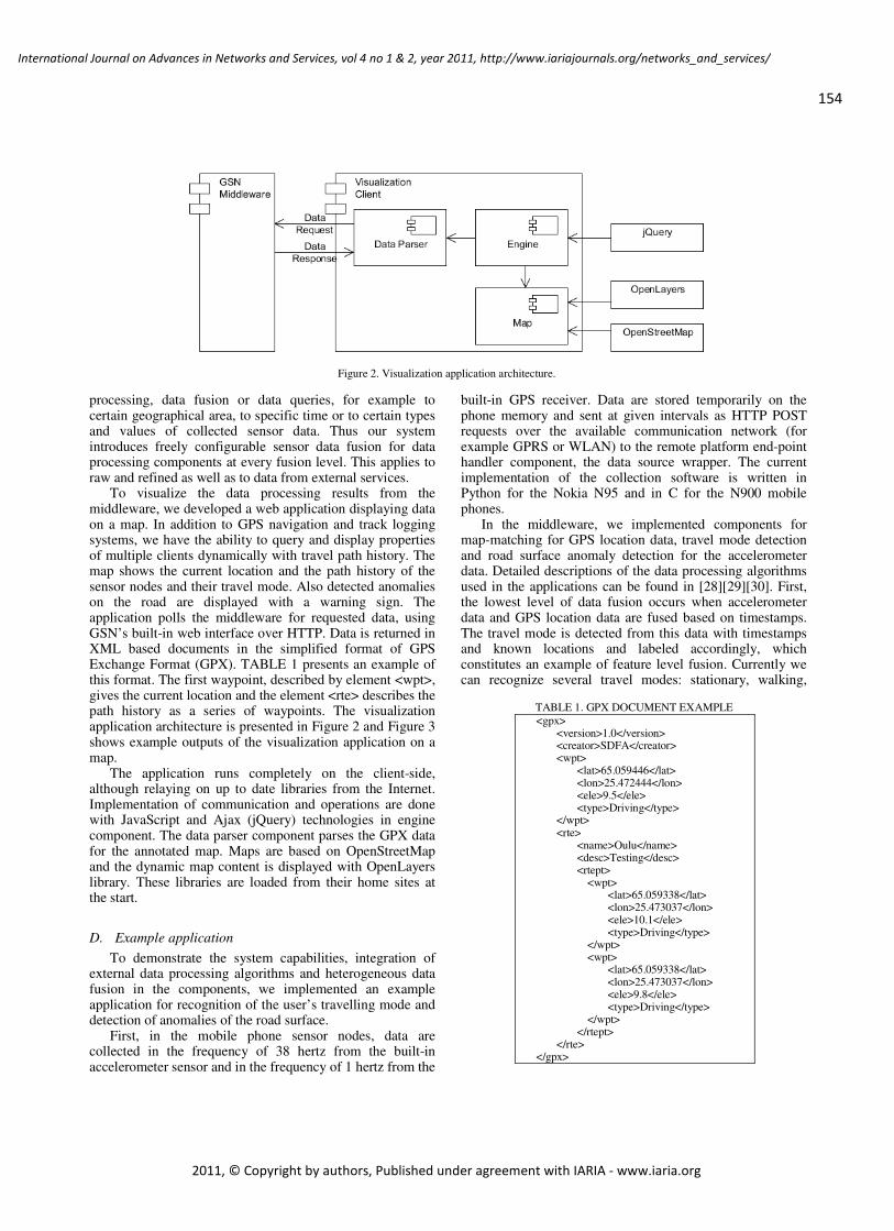
Figure 2. Visualization application architecture.
processing, data fusion or data queries, for example to certain geographical area, to specific time or to certain types and values of collected sensor data. Thus our system introduces freely configurable sensor data fusion for data processing components at every fusion level. This applies to raw and refined as well as to data from external services.
To visualize the data processing results from the middleware, we developed a web application displaying data on a map. In addition to GPS navigation and track logging systems, we have the ability to query and display properties of multiple clients dynamically with travel path history. The map shows the current location and the path history of the sensor nodes and their travel mode. Also detected anomalies on the road are displayed with a warning sign. The application polls the middleware for requested data, using GSN’s built-in web interface over HTTP. Data is returned in XML based documents in the simplified format of GPS Exchange Format (GPX). TABLE 1 presents an example of this format. The first waypoint, described by element <wpt>, gives the current location and the element <rte> describes the path history as a series of waypoints. The visualization application architecture is presented in Figure 2 and Figure 3 shows example outputs of the visualization application on a map.
The application runs completely on the client-side, although relaying on up to date libraries from the Internet. Implementation of communication and operations are done with JavaScript and Ajax (jQuery) technologies in engine component. The data parser component parses the GPX data for the annotated map. Maps are based on OpenStreetMap and the dynamic map content is displayed with OpenLayers library. These libraries are loaded from their home sites at the start.
D. Example application
To demonstrate the system capabilities, integration of external data processing algorithms and heterogeneous data fusion in the components, we implemented an example application for recognition of the user’s travelling mode and detection of anomalies of the road surface.
First, in the mobile phone sensor nodes, data are collected in the frequency of 38 hertz from the built-in accelerometer sensor and in the frequency of 1 hertz from the
built-in GPS receiver. Data are stored temporarily on the phone memory and sent at given intervals as HTTP POST requests over the available communication network (for example GPRS or WLAN) to the remote platform end-point handler component, the data source wrapper. The current implementation of the collection software is written in Python for the Nokia N95 and in C for the N900 mobile phones.
In the middleware, we implemented components for map-matching for GPS location data, travel mode detection and road surface anomaly detection for the accelerometer data. Detailed descriptions of the data processing algorithms used in the applications can be found in [28][29][30]. First, the lowest level of data fusion occurs when accelerometer data and GPS location data are fused based on timestamps. The travel mode is detected from this data with timestamps and known locations and labeled accordingly, which constitutes an example of feature level fusion. Currently we can recognize several travel modes: stationary, walking,
TABLE 1. GPX DOCUMENT EXAMPLE
<gpx> <version>1.0</version> <creator>SDFA</creator> <wpt>
<lat>65.059446</lat> <lon>25.472444</lon> <ele>9.5</ele> <type>Driving</type>
</wpt> <rte>
<name>Oulu</name> <desc>Testing</desc> <rtept>
<wpt> <lat>65.059338</lat> <lon>25.473037</lon> <ele>10.1</ele> <type>Driving</type>
</wpt> <wpt>
<lat>65.059338</lat> <lon>25.473037</lon> <ele>9.8</ele> <type>Driving</type>
</wpt> </rtept>
</rte> </gpx>
154
International Journal on Advances in Networks and Services, vol 4 no 1 & 2, year 2011, http://www.iariajournals.org/networks_and_services/
2011, © Copyright by authors, Published under agreement with IARIA - www.iaria.org
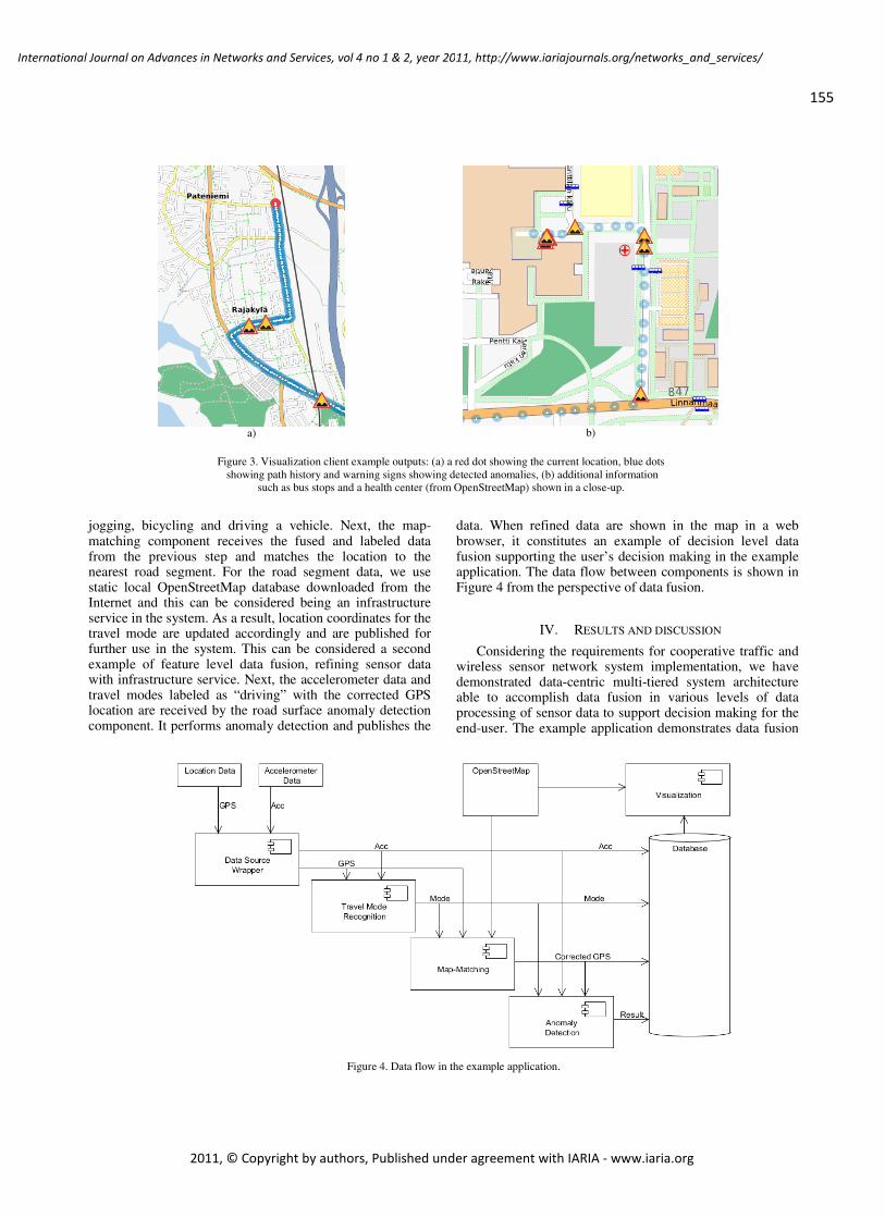
a)
b)
Figure 3. Visualization client example outputs: (a) a red dot showing the current location, blue dots
showing path history and warning signs showing detected anomalies, (b) additional information
such as bus stops and a health center (from OpenStreetMap) shown in a close-up.
jogging, bicycling and driving a vehicle. Next, the map-matching component receives the fused and labeled data from the previous step and matches the location to the nearest road segment. For the road segment data, we use static local OpenStreetMap database downloaded from the Internet and this can be considered being an infrastructure service in the system. As a result, location coordinates for the travel mode are updated accordingly and are published for further use in the system. This can be considered a second example of feature level data fusion, refining sensor data with infrastructure service. Next, the accelerometer data and travel modes labeled as “driving” with the corrected GPS location are received by the road surface anomaly detection component. It performs anomaly detection and publishes the
data. When refined data are shown in the map in a web browser, it constitutes an example of decision level data fusion supporting the user’s decision making in the example application. The data flow between components is shown in Figure 4 from the perspective of data fusion.
IV. RESULTS AND DISCUSSION
Considering the requirements for cooperative traffic and wireless sensor network system implementation, we have demonstrated data-centric multi-tiered system architecture able to accomplish data fusion in various levels of data processing of sensor data to support decision making for the end-user. The example application demonstrates data fusion
Figure 4. Data flow in the example application.
155
International Journal on Advances in Networks and Services, vol 4 no 1 & 2, year 2011, http://www.iariajournals.org/networks_and_services/
2011, © Copyright by authors, Published under agreement with IARIA - www.iaria.org
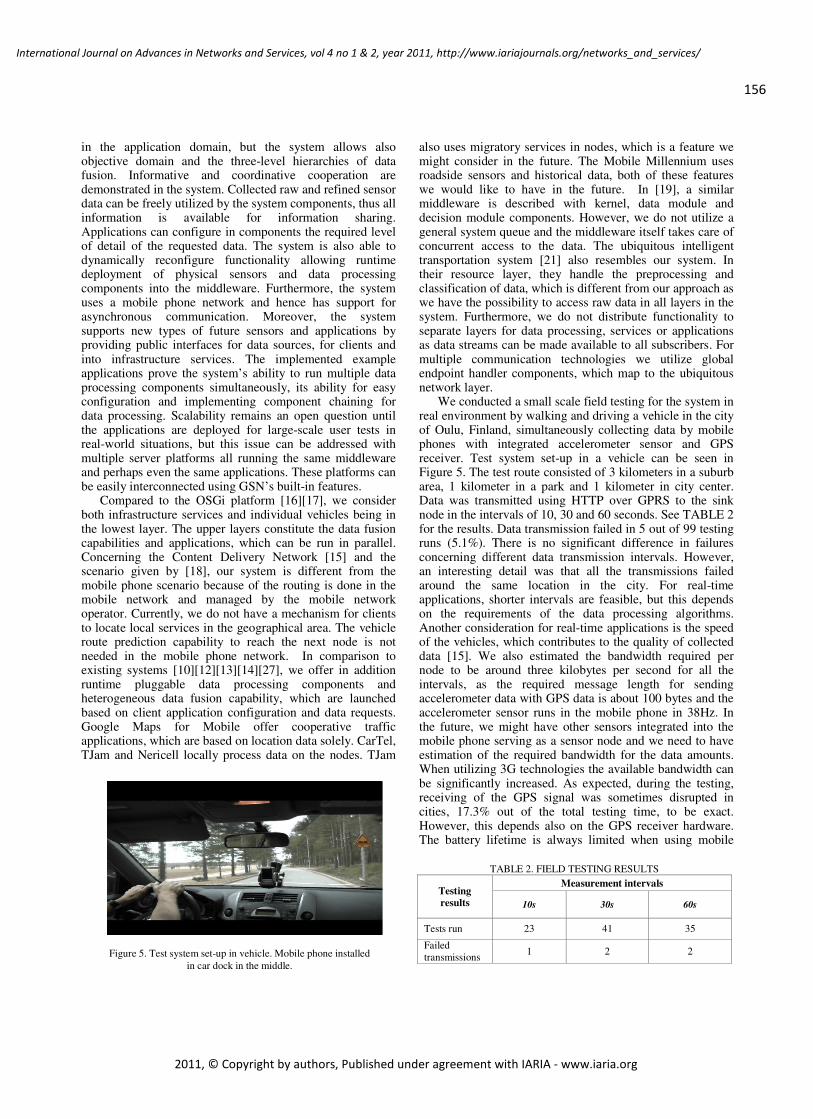
Figure 5. Test system set-up in vehicle. Mobile phone installed
in car dock in the middle.
in the application domain, but the system allows also objective domain and the three-level hierarchies of data fusion. Informative and coordinative cooperation are demonstrated in the system. Collected raw and refined sensor data can be freely utilized by the system components, thus all information is available for information sharing. Applications can configure in components the required level of detail of the requested data. The system is also able to dynamically reconfigure functionality allowing runtime deployment of physical sensors and data processing components into the middleware. Furthermore, the system uses a mobile phone network and hence has support for asynchronous communication. Moreover, the system supports new types of future sensors and applications by providing public interfaces for data sources, for clients and into infrastructure services. The implemented example applications prove the system’s ability to run multiple data processing components simultaneously, its ability for easy configuration and implementing component chaining for data processing. Scalability remains an open question until the applications are deployed for large-scale user tests in real-world situations, but this issue can be addressed with multiple server platforms all running the same middleware and perhaps even the same applications. These platforms can be easily interconnected using GSN’s built-in features.
Compared to the OSGi platform [16][17], we consider both infrastructure services and individual vehicles being in the lowest layer. The upper layers constitute the data fusion capabilities and applications, which can be run in parallel. Concerning the Content Delivery Network [15] and the scenario given by [18], our system is different from the mobile phone scenario because of the routing is done in the mobile network and managed by the mobile network operator. Currently, we do not have a mechanism for clients to locate local services in the geographical area. The vehicle route prediction capability to reach the next node is not needed in the mobile phone network. In comparison to existing systems [10][12][13][14][27], we offer in addition runtime pluggable data processing components and heterogeneous data fusion capability, which are launched based on client application configuration and data requests. Google Maps for Mobile offer cooperative traffic applications, which are based on location data solely. CarTel, TJam and Nericell locally process data on the nodes. TJam
also uses migratory services in nodes, which is a feature we might consider in the future. The Mobile Millennium uses roadside sensors and historical data, both of these features we would like to have in the future. In [19], a similar middleware is described with kernel, data module and decision module components. However, we do not utilize a general system queue and the middleware itself takes care of concurrent access to the data. The ubiquitous intelligent transportation system [21] also resembles our system. In their resource layer, they handle the preprocessing and classification of data, which is different from our approach as we have the possibility to access raw data in all layers in the system. Furthermore, we do not distribute functionality to separate layers for data processing, services or applications as data streams can be made available to all subscribers. For multiple communication technologies we utilize global endpoint handler components, which map to the ubiquitous network layer.
We conducted a small scale field testing for the system in real environment by walking and driving a vehicle in the city of Oulu, Finland, simultaneously collecting data by mobile phones with integrated accelerometer sensor and GPS receiver. Test system set-up in a vehicle can be seen in Figure 5. The test route consisted of 3 kilometers in a suburb area, 1 kilometer in a park and 1 kilometer in city center. Data was transmitted using HTTP over GPRS to the sink node in the intervals of 10, 30 and 60 seconds. See TABLE 2 for the results. Data transmission failed in 5 out of 99 testing runs (5.1%). There is no significant difference in failures concerning different data transmission intervals. However, an interesting detail was that all the transmissions failed around the same location in the city. For real-time applications, shorter intervals are feasible, but this depends on the requirements of the data processing algorithms. Another consideration for real-time applications is the speed of the vehicles, which contributes to the quality of collected data [15]. We also estimated the bandwidth required per node to be around three kilobytes per second for all the intervals, as the required message length for sending accelerometer data with GPS data is about 100 bytes and the accelerometer sensor runs in the mobile phone in 38Hz. In the future, we might have other sensors integrated into the mobile phone serving as a sensor node and we need to have estimation of the required bandwidth for the data amounts. When utilizing 3G technologies the available bandwidth can be significantly increased. As expected, during the testing, receiving of the GPS signal was sometimes disrupted in cities, 17.3% out of the total testing time, to be exact. However, this depends also on the GPS receiver hardware. The battery lifetime is always limited when using mobile
TABLE 2. FIELD TESTING RESULTS
Testing
results
Measurement intervals
10s 30s 60s
Tests run 23 41 35
Failed
transmissions 1 2 2
156
International Journal on Advances in Networks and Services, vol 4 no 1 & 2, year 2011, http://www.iariajournals.org/networks_and_services/
2011, © Copyright by authors, Published under agreement with IARIA - www.iaria.org
phones transmitting data continuously, but as our phones were often mounted in a vehicle, its power system was used. Cost of a single sensor node is not a considerable issue if the user’s personal mobile phones can be utilized. What is more, the cost of air time and available bandwidth also varies locally.
Sometimes, the travel mode recognition did not work accordingly and we needed to abandon its results and publish all data to the anomaly detection component. The two mobile phone models had different accelerometer sensors, the Nokia N900 accelerometer being much more accurate than Nokia N95 accelerometer, so we needed to parameterize recognition components for each phone model. This means that online learning should be utilized to enable adapting the component for different physical sensors.
Also, we tested the feasibility of GSN middleware in a normal desktop PC (2.40 gigahertz processor with one gigabytes of RAM running Windows XP) with randomly generated data sets. We used 50 data sources simultaneously streaming 50 kilobytes of payload to the system at every 20 milliseconds. The delivery time from a data source wrapper to a data processing component was less than one millisecond per payload. This is very a promising result considering real-time capabilities of the system (req. 11). However, these tests have less real-world value as the used hardware components, available network bandwidth and programming skills of the developers largely contribute to the real-time performance in the prototype.
In this work, we have not considered security and privacy issues, which are unavoidable when collecting, fusing and visualizing data from multiple clients and with the integration of roadside infrastructure data and sensors. Koenders et al. [16] give a list of success factors for intelligent transportation systems. There is a need for communication partners in the system to work and penetration of similarly equipped vehicles is critical. This is where vehicle manufacturers need to co-operate by utilizing standards. Authorities can stimulate this, however clear benefits are needed as investments are required. For the individual users, personal privacy and reliability of the services needs to be guaranteed. Security and privacy concerns in the system can be addressed, for example by introducing user groups with restricted access to the data and results. In our prototype, the reliability is largely dependent on mobile phone network reliability and does not require additional investments from the users or traffic operators.
V. CONCLUSION AND FUTURE WORK
We have started with a generic implementation of sensor network middleware for cooperative traffic applications, which meet the given requirements, drawn from the literature and from the project goals. Considering the goals, we have demonstrated modular component-based prototype sensor network implementation capable of sharing traffic related information collected by mobile sensor nodes and realizing the described usage scenarios. In the next phase, the developed prototype system will be deployed to be used with multiple sensor nodes and client applications. Increased
scalability needs may require introducing multiple middleware platforms for distributing the system load. It would be possible to introduce remote interconnected application-specific platforms in the infrastructure providing data fusion featuring separate data sources in remote platforms.
An important goal of our future work is to implement a common ontology and a specific data fusion model in the middleware. This includes information on vehicle type, location, route, event, time, road condition and possible future application-specific parameters. Also, we will develop interfaces to sensors in instrumented vehicles and introduce usage of an on-board diagnostics module installed in test vehicles. These open many new possibilities as more detailed data of the vehicle behavior can be utilized. Usage of GPS data would allow us to feature also descriptive cooperation, such as the user’s intentions or direction of movement, in the system [7]. Furthermore, interfaces to public Finnish government infrastructure services available in the Internet, such as DigiTraffic [31], a real-time traffic flow information service using roadside sensors, and DigiRoad, the static database containing road data and elements, allow us to widen the system perspective to the whole traffic system level. This information can be easily fused with additional local real-time data in the system and provide feedback to road users and operators.
ACKNOWLEDGMENT
The authors would like to thank all the personnel in the Sensor Data Fusion and Applications project. This work was funded by the National Technology Agency of Finland and was carried out in Sensor Data Fusion and Applications project as a part of the Cooperative Traffic research program of the Strategic Centre for Science, Technology and Innovation in the Field of ICT.
REFERENCES
[1] T. Leppanen, M. Perttunen, J. Riekki, and P. Kaipio, "Sensor Network Architecture for Cooperative Traffic Applications," in Proceedings of International Conference on Wireless and Mobile Communications, pp. 400-403, September 20-25, Valencia, Spain, 2010.
[2] F. Minarini, "eSafety for Road Transport: Investing in Preventive Safety and Co-operative Systems, the EU Approach," Advanced Microsystems for Automotive Applications, pp. 487-492, 2005.
[3] Cooperative Vehicle-Inftrastructure Systems. URL: http://www.cvisproject.org/ 12.07.2011.
[4] N. Faouzi, H. Leung, and A. Kurian, "Data fusion in intelligent transportation systems: Progress and challenges - A survey," Information Fusion, Vol. 12, 1, pp. 4, 2011.
[5] B. Dasarathy, "Sensor fusion potential exploitation-innovative architectures and illustrative applications," in Proceedings of the IEEE, Vol. 85, 1, pp. 24, 1997.
[6] C. Haythornthwaite, "Crowds and Communities: Light and Heavyweight Models of Peer Production," in Proceeedings of Hawaii International Conference on System Sciences, pp. 1-10, 2009.
[7] K. Lidstrom, T. Larsson, and L. Stranden, " Safety Considerations for Cooperating Vehicles using Wireless Communication," in
157
International Journal on Advances in Networks and Services, vol 4 no 1 & 2, year 2011, http://www.iariajournals.org/networks_and_services/
2011, © Copyright by authors, Published under agreement with IARIA - www.iaria.org
Proceedings of 5th IEEE International Conference on Industrial Informatics, Vol. 2, pp. 995, June 23-27, 2007.
[8] V. Dyo, "Middleware design for integration of sensor network and mobile devices," in Proceedings of the 2nd international doctoral symposium on Middleware, pp. 1-5, New York, NY, USA, 2007.
[9] M. Khanafer, M. Guennoun, and H. Mouftah, "WSN Architectures for Intelligent Transportation Systems," in Proceedings of 3rd International Conference on New Technologies, Mobility and Security, pp. 1, December 20-23, 2009.
[10] P. Mohan, V. Padmanabhan, and R. Ramjee, "Nericell: rich monitoring of road and traffic conditions using mobile smartphones," in Proceedings of the 6th ACM conference on Embedded network sensor systems, pp. 323-336, New York, NY, USA, 2008.
[11] The Finnish Cooperative Traffic Programme. URL: http://www.cooperativetraffic.fi/ 12.07.2011.
[12] The Mobile Millenium Project. URL: http://traffic.berkeley.edu/, 12.07.2011.
[13] Google Maps for Mobile. URL: http://www.google.com/mobile/products/maps.html, 12.07.2011.
[14] O. Riva, T. Nadeem, C. Borcea, and L. Iftode, "Context-Aware Migratory Services in Ad Hoc Networks," IEEE Transactions on Mobile Computing, Vol. 6, 12, pp. 1313-1328, 2007.
[15] M. Elshenawy, M. El-Darieby, and B. Abdulhai, "Scalable and location-aware its content management in vehicular environments," in proceedings of IEEE Intelligent Vehicles Symposium, pp. 627, June, 2010.
[16] E. Koenders and J. Vreeswijk, "Cooperative infrastructure," in Proceedings of IEEE Intelligent Vehicles Symposium, pp. 721, June, 2008.
[17] O. Brickley, S. Chong, M. Klepal, A. Tabatabaei, and D. Pesch, "A Data Dissemination Strategy for Cooperative Vehicular Systems," in Proceedings of 65th IEEE Vehicular Technology Conference, pp. 2501, April, 2007.
[18] D. Tacconi, D. Miorandi, J. Carreras, F. Chiti, and R. Fantacci, "Using wireless sensor networks to support intelligent transportation systems," Ad Hoc Networks, Vol. 8, 5, pp. 462, 2010.
[19] S. Bengochea, A. Talamona, and M. Parent, " A software framework for vehicle-infrastructure cooperative applications," in Proceeedings of IEEE Intelligent Transportation Systems, pp. 797, September, 2005.
[20] Digiroad – A National Road and Street Database. URL: http://www.digiroad.fi/en_GB/, 12.07.2011.
[21] W. Lv, B. Du, D. Ma, T. Zhu, and C. Wang, "Applied research of data sensing and service to ubiquitous intelligent transportation system," Frontiers of Computer Science in China, Vol. 4, 3, pp. 417-426, 2010.
[22] Y. Yu, B. Krishnamachari, and V. Prasanna, "Issues in Designing Middleware for Wireless Sensor Networks," IEEE Network, Vol. 18, pp. 15-21, 2003.
[23] B. Ducourthial, "About efficiency in wireless communication frameworks on vehicular networks," in Proceedings of The First International Workshop on Wireless Networking for Intelligent Transportation Systems, pp. 3:1-3:9, New York, NY, USA, 2007.
[24] K. Modukuri, S. Hariri, N. Chalfoun, and M. Yousif, "Autonomous Middleware Framework for Sensor Networks," Journal of Pervasive Computing and Communications, Vol. 1, pp. 337-345, 2008.
[25] T. Kosch, I. Kulp, M. Bechler, M. Strassberger, B. Weyl, and R. Lasowski," Communication architecture for cooperative systems in Europe", IEEE Communications Magazine, Vol. 47, 5, pp. 116, May, 2009.
[26] K. Aberer, M. Hauswirth, and A. Salehi, "A middleware for fast and flexible sensor network deployment," in Proceedings of the 32nd international conference on Very large data bases, Seoul, Korea, pp. 1199-1202, 2006.
[27] B. Hull, V. Bychkovsky, Y. Zhang, K. Chen, M. Goraczko, A. Miu, E. Shih, H Balakrishnan, and S. Madden, "CarTel: a distributed mobile sensor computing system," in Proceedings of the 4th international conference on Embedded networked sensor systems, pp. 125-138, New York, NY, USA, 2006.
[28] O. Mazhelis, "Using recursive Bayesian estimation for matching GPS measurements to imperfect road network data," in Proceedings of 13th International IEEE Conference on Intelligent Transportation Systems, pp. 1492, September, 2010.
[29] J. Kantola, M. Perttunen, T. Leppanen, J. Collin, and J. Riekki, "Context Awareness for GPS-Enabled Phones," in Proceedings of ION Technical Meeting, Manassas, VA, USA, 2010.
[30] M. Perttunen, O. Mazhelis, F. Cong, M. Kauppila, T. Leppänen, J. Kantola, J. Collin, S. Pirttikangas, J. Haverinen, T. Ristaniemi, and J. Riekki, "Distributed Road Surface Condition Monitoring Using Mobile Phones," in the 8th International Conference on Ubiquitous Intelligence and Computing, Banff, Canada, September 2-4, 2011.
[31] Digitraffic. URL: http://www.infotripla.fi/digitraffic/english/, 12.07.2011.
158
International Journal on Advances in Networks and Services, vol 4 no 1 & 2, year 2011, http://www.iariajournals.org/networks_and_services/
2011, © Copyright by authors, Published under agreement with IARIA - www.iaria.org
A New Wireless Architecture for In-Flight Entertainment SystemsInside Aircraft Cabin
Ahmed AKL, Thierry GAYRAUD, and Pascal BERTHOUCNRS ; LAAS ; 7 avenue du Colonel Roche, F-31077
Universite de Toulouse ; UPS, INSA, INP, ISAE ; LAAS ; F-31077Toulouse, France
aakl, gayraud, [email protected]
Abstract—A primary difficulty when investigating commu-nication requirements rises when a very specific field as anaircraft cabin is considered. The diverse needs of passengersare often incompatible to the strict constraints inside the cabin.Nowadays, In-Flight Entertainment (IFE) systems, for instance,are widely spread in modern flights. An IFE system usuallyconsists of a Seat Electronic Box, the passengers terminalhardware, plus a Passengers Control Unit, the remote control toselect the service, and a Visual Display Unit, the screen. Usingthe wireless technology in these systems can increase the satis-faction level of both the passengers and the avionics companies.However, the inside of the cabin is not a flexible environment;reliability and safety are two mandatory requirements, sodifferent constrains are imposed. This means that off-shelftechnologies (hardware including antennas, network topology,network protocols and services) are usually not suitable forsuch environment. Consequently, a new architecture has tobe designed and implemented. This paper aims at integratingheterogeneous available communication technologies, showingtheir pros and cons, within this context, while consideringthe imposed communication restrictions inside the aircraftscabin. From that, a new wireless heterogeneous architectureis proposed. In addition, to be able to use such architecture,we propose a new protocol, which utilizes the smart antennastechnology to allow Passenger Control Units to be recognizedand configured autonomously without any external interven-tion.
Keywords-IFE system, Wireless networks, PLC, Smart an-tenna, Protocol engineering and evaluation
I. INTRODUCTION
In recent years, market surveys have revealed a surprisingand growing trend in the importance of In-Flight Entertain-ment (IFE) with regard to choice of airline. With modernlong range aircraft the need for ”stop-over” has been re-duced, so the duration of flights has also been increased. Airflights, especially long distance, may expose passengers todiscomfort and even stress. IFE can provide stress reductionentertainment services to the passenger. The IFE systemis an approach that can utilize the wireless technologyfor the purpose of exchanging data -in both directions-between passengers and the entertainment system. Althoughwired communication gives better performance than wirelesscommunication, but most of modern personal devices are
based on the wireless technology, so providing wireless ca-pabilities is essential for efficient utilization of these devices.Moreover, a wireless headphones is more satisfactory than awired headset attached to the seat arm. We are not targetingto make the system fully wireless, but to emphasize the ideathat different technologies can be used in the IFE system toimprove the passenger’s service satisfaction level [1].
As stated by Niebla [2], users are becoming more andmore familiar to personal equipments, such as mobilephones, laptops, and PDAs. This shows the importance ofproviding aircrafts with facilities that support these equip-ments.
Nowadays, different wireless technologies with differentcapabilities exist in the market such as WiFi, Bluetooth,infrared, and Wirelss Universal Serial Bus (WUSB). How-ever, these technologies may have certain characteristics thatmake them unsuitable for usage inside the cabin. Althoughit was proven that WiFi and Bluetooth can be used insidethe cabin with no fear of interfering with navigationalequipments [3], it is still difficult to use them in largenumbers since performance degrades due to allocating themin a small area inside a metallic tunnel (i.e., cabin), whichis full of different obstacles (i.e., seats). In addition, thenormal way of setting these technologies is usually donethrough predefined identifiers (i.e., IP address) or a user key(i.e., Bluetooth authentication key). Both techniques don’tmatch the constrains inside the cabin, where devices mustbe designed without any predefined identifiers and to beconfigured without any user intervention
However, usage of the wireless technology will help indecreasing the connecting wires; this is a valuable criterionin aircrafts designing. Using off-shelf technologies inside thecabin is usually not applicable when using them in the usualmanner; the environment inside the cabin has very strictconstrains since safety is a major requirement. Consequently,using just one technology can’t be the optimum solution.In fact, using a combination of different technologies canprovide a better service while overcoming the existingconstrains. The way passengers use their Personal ElectronicDevices (PED) (i.e., mobile phones, laptop, etc.) was usuallydone through specialized devices [2], [3]. Nevertheless, there
159
International Journal on Advances in Networks and Services, vol 4 no 1 & 2, year 2011, http://www.iariajournals.org/networks_and_services/
2011, © Copyright by authors, Published under agreement with IARIA - www.iaria.org
is no current research to use a combination of off-shelftechnologies inside the cabin.
The IFE market attracted many companies to submitdifferent IFE solutions. Thales [4], an avionic systemsprovider, introduced its own IFE system that can be tailoredaccording to the needs of the airlines companies. Someother companies provide dedicated solutions for certain partsof the IFE systems; the AeroMobile [5] is a GSM serviceprovider for the aviation industry that allows passengers touse their mobile phones and devices safely during the flight.Passengers can connect to an AeroMobile pico cell locatedinside the craft which relays the text messages and calls toa satellite link which sends them to the ground network.The AeroMobile system manages all the cellular devicesonboard, so signal strength can be ketp at a minimum valueto minimize interference. This system is adopted by Pana-sonic to be part of its in-flight cellular phone component.FlyNet [6] is an onboard communication service providedby Lufthansa to allow passengers to connect to the Internetduring their flight.
In the next section, we will introduce an overview for theIFE system showing its components and requirements. Sec-tion II-C introduces the communication challenges that facethe IFE systems. Section III shows the proposed availabletechnologies that can be used to overcome the challenges insuch environment. Section III-B introduces our approach forintegrating them together. Section IV presents our proposedprotocol that utilizes the smart antenna capabilities to con-nect the IFE devices. Section V shows how the protocol wasverified and validated through a Unified Modeling Language(UML) model and NS2 simulation. Finally, we present theconclusion and future work.
II. BACKGROUND AND RELEVANT WORK
The recognized economics of wireless networks and com-munications systems have made them an attractive targetfor environments where individual wires are cumbersome.An airplane cabin is such an environment. Dwayne [7] saidthat due to the need of rapidly reconfiguring the cabin’sseating, it is further assumed that wireless networking, ratherthan cable or fiber optics, must be used to interconnectpassenger’s entertainment equipment with other elements ofthe system.
The use of wireless communication technologies on boardof an aircraft provides an opportunity to remove wiringand save weight on the aircraft. The weight savings canbe directly measured in terms of fuel savings and improvedoperating economics over the life time of an aircraft. How-ever, there is a need to ensure that there is no interferencewith the aircraft’s communication and navigation systems.
A. The need for IFE systems
Hao [8] mentioned that the enclosed environment ofthe aircraft can cause discomfort or even problems to
passengers. IFE systems can greatly reduce these negativeeffects. This can be done by using e-books, video/audiobroadcasting, games, internet, and On Demand services. Thefact that passengers come from highly heterogeneous pools(such as age, gender, ethnicity, etc.) causes an impact on theadaptive interface systems.
As mentioned by Fariba [9], the IFE systems usuallyinclude screen-based, audio and communication systems.The screen-based products include video systems enablingpassengers to watch movies, news and sports. These systemshad progressed into video-on-demand, allowing passengersto have control when they watch movies. Air map display isanother service that allows them to locate their flight’s route.Exterior-view cameras also enable passengers to have the pi-lot’s forward view on take-off and landing on their personalTV screens. Audio systems include different types of musicchannels and special programs recorded for the airlines.Communication systems include intra-communications withdevices such as telephones, facsimile and in-seat power sup-plies, and inter-communications between the screen-basedsystem and its subsystems (i.e., remote control).
B. The IFE system’s components
In fact, the entertainment starts from the passenger’sseat design where most of the IFE system componentsare embedded. Wiring cables connect together all of theelectronic devices in the seat as well as connecting them tothe whole system in the cabin. They run through the cabin’swalls, floor, and seats. Unfortunately, conveying signals andpower to seats with a connector for each seat would causereliability and maintenance problems, and hinder timelycabin reconfiguration.
Nowadays, IFE systems are interactive systems, so aPassenger Control Unit (PCU) is usually needed to controlthe surrounding devices. The PCU should be compact andeasily held. Moreover, the pocket holding the PCU has tobe placed in a way that makes it reachable and not to affectthe passenger’s comfort. At the beginning, PCUs used to befixed aside to the Visual Display Unit (VDU) at the back ofthe front seat. This orientation introduced a problem whenthe passenger setting beside the window wants to move tothe corridor; where all his neighbors have to replace theirPCUs to allow him to pass. To overcome this problem, PCUsare now connected to their VDUs through wires passing viatheir seat.
A Visual Display Unit (VDU) is usually fixed to the backof the front seat. Depending on the required features of thesystem, ordinary displays can be used to display the visualcontents or touch screens can be installed to act as inputdevices. Another orientation is to be fixed in the ceiling asa shared display for a group of seats.
A Seat Electronic Box (SEB) can be used to connect thesystem’s different components together. It is used to connectthe passenger’s devices and the IFE system instead of having
160
International Journal on Advances in Networks and Services, vol 4 no 1 & 2, year 2011, http://www.iariajournals.org/networks_and_services/
2011, © Copyright by authors, Published under agreement with IARIA - www.iaria.org
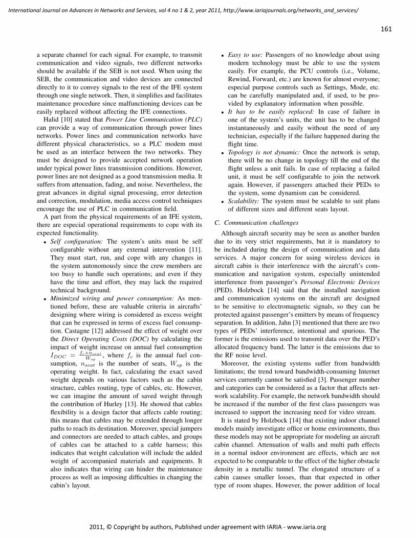
a separate channel for each signal. For example, to transmitcommunication and video signals, two different networksshould be available if the SEB is not used. When using theSEB, the communication and video devices are connecteddirectly to it to convey signals to the rest of the IFE systemthrough one single network. Then, it simplifies and facilitatesmaintenance procedure since malfunctioning devices can beeasily replaced without affecting the IFE connections.
Halid [10] stated that Power Line Communication (PLC)can provide a way of communication through power linesnetworks. Power lines and communication networks havedifferent physical characteristics, so a PLC modem mustbe used as an interface between the two networks. Theymust be designed to provide accepted network operationunder typical power lines transmission conditions. However,power lines are not designed as a good transmission media. Itsuffers from attenuation, fading, and noise. Nevertheless, thegreat advances in digital signal processing, error detectionand correction, modulation, media access control techniquesencourage the use of PLC in communication field.
A part from the physical requirements of an IFE system,there are especial operational requirements to cope with itsexpected functionality.• Self configuration: The system’s units must be self
configurable without any external intervention [11].They must start, run, and cope with any changes inthe system autonomously since the crew members aretoo busy to handle such operations; and even if theyhave the time and effort, they may lack the requiredtechnical background.
• Minimized wiring and power consumption: As men-tioned before, these are valuable criteria in aircrafts’designing where wiring is considered as excess weightthat can be expressed in terms of excess fuel consump-tion. Castagne [12] addressed the effect of weight overthe Direct Operating Costs (DOC) by calculating theimpact of weight increase on annual fuel consumptionIDOC = fc×nseat
Wop, where fc is the annual fuel con-
sumption, nseat is the number of seats, Wop is theoperating weight. In fact, calculating the exact savedweight depends on various factors such as the cabinstructure, cables routing, type of cables, etc. However,we can imagine the amount of saved weight throughthe contribution of Hurley [13]. He showed that cablesflexibility is a design factor that affects cable routing;this means that cables may be extended through longerpaths to reach its destination. Moreover, special jumpersand connectors are needed to attach cables, and groupsof cables can be attached to a cable harness; thisindicates that weight calculation will include the addedweight of accompanied materials and equipments. Italso indicates that wiring can hinder the maintenanceprocess as well as imposing difficulties in changing thecabin’s layout.
• Easy to use: Passengers of no knowledge about usingmodern technology must be able to use the systemeasily. For example, the PCU controls (i.e., Volume,Rewind, Forward, etc.) are known for almost everyone;especial purpose controls such as Settings, Mode, etc.can be carefully manipulated and, if used, to be pro-vided by explanatory information when possible.
• It has to be easily replaced: In case of failure inone of the system’s units, the unit has to be changedinstantaneously and easily without the need of anytechnician, especially if the failure happened during theflight time.
• Topology is not dynamic: Once the network is setup,there will be no change in topology till the end of theflight unless a unit fails. In case of replacing a failedunit, it must be self configurable to join the networkagain. However, if passengers attached their PEDs tothe system, some dynamism can be considered.
• Scalability: The system must be scalable to suit plansof different sizes and different seats layout.
C. Communication challenges
Although aircraft security may be seen as another burdendue to its very strict requirements, but it is mandatory tobe included during the design of communication and dataservices. A major concern for using wireless devices inaircraft cabin is their interference with the aircraft’s com-munication and navigation system, especially unintendedinterference from passenger’s Personal Electronic Devices(PED). Holzbock [14] said that the installed navigationand communication systems on the aircraft are designedto be sensitive to electromagnetic signals, so they can beprotected against passenger’s emitters by means of frequencyseparation. In addition, Jahn [3] mentioned that there are twotypes of PEDs’ interference, intentional and spurious. Theformer is the emissions used to transmit data over the PED’sallocated frequency band. The latter is the emissions due tothe RF noise level.
Moreover, the existing systems suffer from bandwidthlimitations; the trend toward bandwidth-consuming Internetservices currently cannot be satisfied [3]. Passenger numberand categories can be considered as a factor that affects net-work scalability. For example, the network bandwidth shouldbe increased if the number of the first class passengers wasincreased to support the increasing need for video stream.
It is stated by Holzbock [14] that existing indoor channelmodels mainly investigate office or home environments, thusthese models may not be appropriate for modeling an aircraftcabin channel. Attenuation of walls and multi path effectsin a normal indoor environment are effects, which are notexpected to be comparable to the effect of the higher obstacledensity in a metallic tunnel. The elongated structure of acabin causes smaller losses, than that expected in othertype of room shapes. However, the power addition of local
161
International Journal on Advances in Networks and Services, vol 4 no 1 & 2, year 2011, http://www.iariajournals.org/networks_and_services/
2011, © Copyright by authors, Published under agreement with IARIA - www.iaria.org
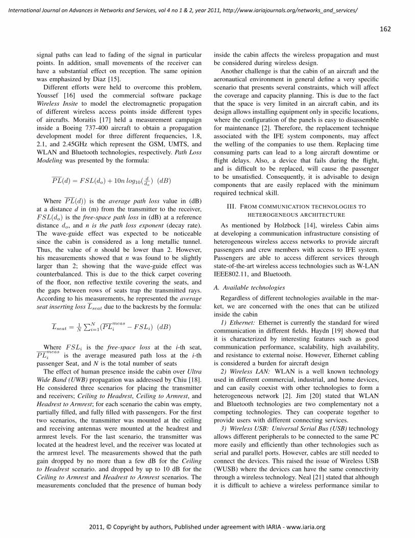
signal paths can lead to fading of the signal in particularpoints. In addition, small movements of the receiver canhave a substantial effect on reception. The same opinionwas emphasized by Diaz [15].
Different efforts were held to overcome this problem,Youssef [16] used the commercial software packageWireless Insite to model the electromagnetic propagationof different wireless access points inside different typesof aircrafts. Moraitis [17] held a measurement campaigninside a Boeing 737-400 aircraft to obtain a propagationdevelopment model for three different frequencies, 1.8,2.1, and 2.45GHz which represent the GSM, UMTS, andWLAN and Bluetooth technologies, respectively. Path LossModeling was presented by the formula:
PL(d) = FSL(do) + 10n log10( ddo
) (dB)
Where PL(d)) is the average path loss value in (dB)at a distance d in (m) from the transmitter to the receiver,FSL(do) is the free-space path loss in (dB) at a referencedistance do, and n is the path loss exponent (decay rate).The wave-guide effect was expected to be noticeablesince the cabin is considered as a long metallic tunnel.Thus, the value of n should be lower than 2. However,his measurements showed that n was found to be slightlylarger than 2; showing that the wave-guide effect wascounterbalanced. This is due to the thick carpet coveringof the floor, non reflective textile covering the seats, andthe gaps between rows of seats trap the transmitted rays.According to his measurements, he represented the averageseat inserting loss Lseat due to the backrests by the formula:
Lseat = 1N
∑Ni=1(PL
meas
i − FSLi) (dB)
Where FSLi is the free-space loss at the i-th seat,PL
meas
i is the average measured path loss at the i-thpassenger Seat, and N is the total number of seats
The effect of human presence inside the cabin over UltraWide Band (UWB) propagation was addressed by Chiu [18].He considered three scenarios for placing the transmitterand receivers; Ceiling to Headrest, Ceiling to Armrest, andHeadrest to Armrest; for each scenario the cabin was empty,partially filled, and fully filled with passengers. For the firsttwo scenarios, the transmitter was mounted at the ceilingand receiving antennas were mounted at the headrest andarmrest levels. For the last scenario, the transmitter waslocated at the headrest level, and the receiver was located atthe armrest level. The measurements showed that the pathgain dropped by no more than a few dB for the Ceilingto Headrest scenario. and dropped by up to 10 dB for theCeiling to Armrest and Headrest to Armrest scenarios. Themeasurements concluded that the presence of human body
inside the cabin affects the wireless propagation and mustbe considered during wireless design.
Another challenge is that the cabin of an aircraft and theaeronautical environment in general define a very specificscenario that presents several constraints, which will affectthe coverage and capacity planning. This is due to the factthat the space is very limited in an aircraft cabin, and itsdesign allows installing equipment only in specific locations,where the configuration of the panels is easy to disassemblefor maintenance [2]. Therefore, the replacement techniqueassociated with the IFE system components, may affectthe welling of the companies to use them. Replacing timeconsuming parts can lead to a long aircraft downtime orflight delays. Also, a device that fails during the flight,and is difficult to be replaced, will cause the passengerto be unsatisfied. Consequently, it is advisable to designcomponents that are easily replaced with the minimumrequired technical skill.
III. FROM COMMUNICATION TECHNOLOGIES TOHETEROGENEOUS ARCHITECTURE
As mentioned by Holzbock [14], wireless Cabin aimsat developing a communication infrastructure consisting ofheterogeneous wireless access networks to provide aircraftpassengers and crew members with access to IFE system.Passengers are able to access different services throughstate-of-the-art wireless access technologies such as W-LANIEEE802.11, and Bluetooth.
A. Available technologies
Regardless of different technologies available in the mar-ket, we are concerned with the ones that can be utilizedinside the cabin
1) Ethernet: Ethernet is currently the standard for wiredcommunication in different fields. Haydn [19] showed thatit is characterized by interesting features such as goodcommunication performance, scalability, high availability,and resistance to external noise. However, Ethernet cablingis considered a burden for aircraft design
2) Wireless LAN: WLAN is a well known technologyused in different commercial, industrial, and home devices,and can easily coexist with other technologies to form aheterogeneous network [2]. Jim [20] stated that WLANand Bluetooth technologies are two complementary not acompeting technologies. They can cooperate together toprovide users with different connecting services.
3) Wireless USB: Universal Serial Bus (USB) technologyallows different peripherals to be connected to the same PCmore easily and efficiently than other technologies such asserial and parallel ports. However, cables are still needed toconnect the devices. This raised the issue of Wireless USB(WUSB) where the devices can have the same connectivitythrough a wireless technology. Neal [21] stated that althoughit is difficult to achieve a wireless performance similar to
162
International Journal on Advances in Networks and Services, vol 4 no 1 & 2, year 2011, http://www.iariajournals.org/networks_and_services/
2011, © Copyright by authors, Published under agreement with IARIA - www.iaria.org
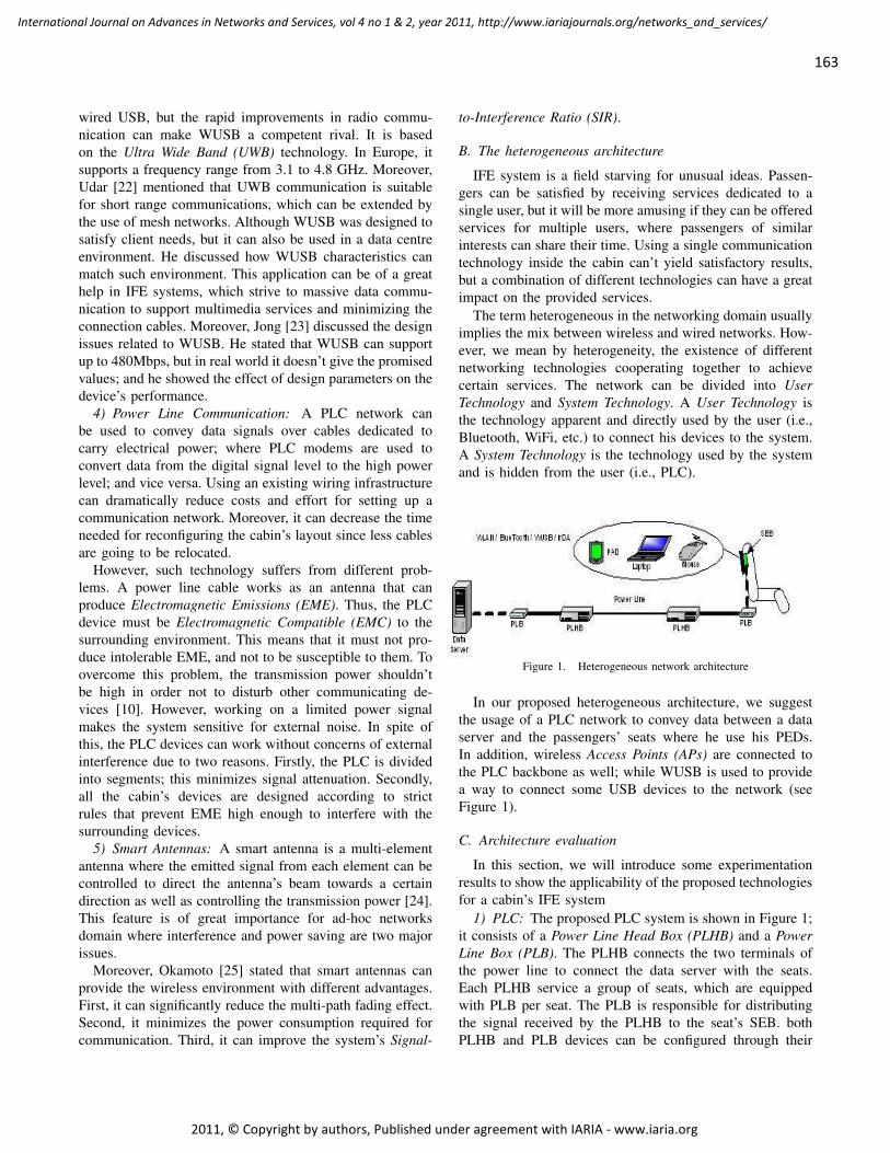
wired USB, but the rapid improvements in radio commu-nication can make WUSB a competent rival. It is basedon the Ultra Wide Band (UWB) technology. In Europe, itsupports a frequency range from 3.1 to 4.8 GHz. Moreover,Udar [22] mentioned that UWB communication is suitablefor short range communications, which can be extended bythe use of mesh networks. Although WUSB was designed tosatisfy client needs, but it can also be used in a data centreenvironment. He discussed how WUSB characteristics canmatch such environment. This application can be of a greathelp in IFE systems, which strive to massive data commu-nication to support multimedia services and minimizing theconnection cables. Moreover, Jong [23] discussed the designissues related to WUSB. He stated that WUSB can supportup to 480Mbps, but in real world it doesn’t give the promisedvalues; and he showed the effect of design parameters on thedevice’s performance.
4) Power Line Communication: A PLC network canbe used to convey data signals over cables dedicated tocarry electrical power; where PLC modems are used toconvert data from the digital signal level to the high powerlevel; and vice versa. Using an existing wiring infrastructurecan dramatically reduce costs and effort for setting up acommunication network. Moreover, it can decrease the timeneeded for reconfiguring the cabin’s layout since less cablesare going to be relocated.
However, such technology suffers from different prob-lems. A power line cable works as an antenna that canproduce Electromagnetic Emissions (EME). Thus, the PLCdevice must be Electromagnetic Compatible (EMC) to thesurrounding environment. This means that it must not pro-duce intolerable EME, and not to be susceptible to them. Toovercome this problem, the transmission power shouldn’tbe high in order not to disturb other communicating de-vices [10]. However, working on a limited power signalmakes the system sensitive for external noise. In spite ofthis, the PLC devices can work without concerns of externalinterference due to two reasons. Firstly, the PLC is dividedinto segments; this minimizes signal attenuation. Secondly,all the cabin’s devices are designed according to strictrules that prevent EME high enough to interfere with thesurrounding devices.
5) Smart Antennas: A smart antenna is a multi-elementantenna where the emitted signal from each element can becontrolled to direct the antenna’s beam towards a certaindirection as well as controlling the transmission power [24].This feature is of great importance for ad-hoc networksdomain where interference and power saving are two majorissues.
Moreover, Okamoto [25] stated that smart antennas canprovide the wireless environment with different advantages.First, it can significantly reduce the multi-path fading effect.Second, it minimizes the power consumption required forcommunication. Third, it can improve the system’s Signal-
to-Interference Ratio (SIR).
B. The heterogeneous architecture
IFE system is a field starving for unusual ideas. Passen-gers can be satisfied by receiving services dedicated to asingle user, but it will be more amusing if they can be offeredservices for multiple users, where passengers of similarinterests can share their time. Using a single communicationtechnology inside the cabin can’t yield satisfactory results,but a combination of different technologies can have a greatimpact on the provided services.
The term heterogeneous in the networking domain usuallyimplies the mix between wireless and wired networks. How-ever, we mean by heterogeneity, the existence of differentnetworking technologies cooperating together to achievecertain services. The network can be divided into UserTechnology and System Technology. A User Technology isthe technology apparent and directly used by the user (i.e.,Bluetooth, WiFi, etc.) to connect his devices to the system.A System Technology is the technology used by the systemand is hidden from the user (i.e., PLC).
Figure 1. Heterogeneous network architecture
In our proposed heterogeneous architecture, we suggestthe usage of a PLC network to convey data between a dataserver and the passengers’ seats where he use his PEDs.In addition, wireless Access Points (APs) are connected tothe PLC backbone as well; while WUSB is used to providea way to connect some USB devices to the network (seeFigure 1).
C. Architecture evaluation
In this section, we will introduce some experimentationresults to show the applicability of the proposed technologiesfor a cabin’s IFE system
1) PLC: The proposed PLC system is shown in Figure 1;it consists of a Power Line Head Box (PLHB) and a PowerLine Box (PLB). The PLHB connects the two terminals ofthe power line to connect the data server with the seats.Each PLHB service a group of seats, which are equippedwith PLB per seat. The PLB is responsible for distributingthe signal received by the PLHB to the seat’s SEB. bothPLHB and PLB devices can be configured through their
163
International Journal on Advances in Networks and Services, vol 4 no 1 & 2, year 2011, http://www.iariajournals.org/networks_and_services/
2011, © Copyright by authors, Published under agreement with IARIA - www.iaria.org
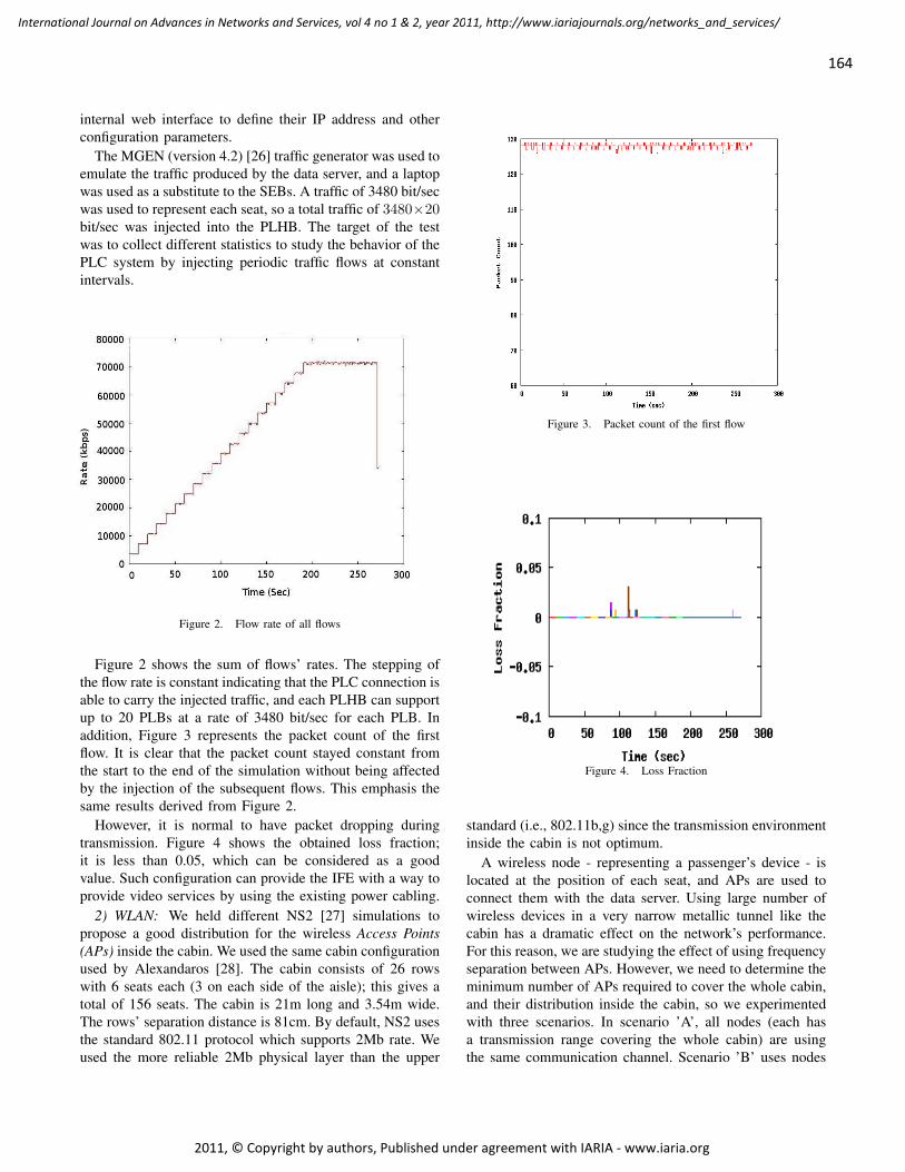
internal web interface to define their IP address and otherconfiguration parameters.
The MGEN (version 4.2) [26] traffic generator was used toemulate the traffic produced by the data server, and a laptopwas used as a substitute to the SEBs. A traffic of 3480 bit/secwas used to represent each seat, so a total traffic of 3480×20bit/sec was injected into the PLHB. The target of the testwas to collect different statistics to study the behavior of thePLC system by injecting periodic traffic flows at constantintervals.
Figure 2. Flow rate of all flows
Figure 2 shows the sum of flows’ rates. The stepping ofthe flow rate is constant indicating that the PLC connection isable to carry the injected traffic, and each PLHB can supportup to 20 PLBs at a rate of 3480 bit/sec for each PLB. Inaddition, Figure 3 represents the packet count of the firstflow. It is clear that the packet count stayed constant fromthe start to the end of the simulation without being affectedby the injection of the subsequent flows. This emphasis thesame results derived from Figure 2.
However, it is normal to have packet dropping duringtransmission. Figure 4 shows the obtained loss fraction;it is less than 0.05, which can be considered as a goodvalue. Such configuration can provide the IFE with a way toprovide video services by using the existing power cabling.
2) WLAN: We held different NS2 [27] simulations topropose a good distribution for the wireless Access Points(APs) inside the cabin. We used the same cabin configurationused by Alexandaros [28]. The cabin consists of 26 rowswith 6 seats each (3 on each side of the aisle); this gives atotal of 156 seats. The cabin is 21m long and 3.54m wide.The rows’ separation distance is 81cm. By default, NS2 usesthe standard 802.11 protocol which supports 2Mb rate. Weused the more reliable 2Mb physical layer than the upper
Figure 3. Packet count of the first flow
Figure 4. Loss Fraction
standard (i.e., 802.11b,g) since the transmission environmentinside the cabin is not optimum.
A wireless node - representing a passenger’s device - islocated at the position of each seat, and APs are used toconnect them with the data server. Using large number ofwireless devices in a very narrow metallic tunnel like thecabin has a dramatic effect on the network’s performance.For this reason, we are studying the effect of using frequencyseparation between APs. However, we need to determine theminimum number of APs required to cover the whole cabin,and their distribution inside the cabin, so we experimentedwith three scenarios. In scenario ’A’, all nodes (each hasa transmission range covering the whole cabin) are usingthe same communication channel. Scenario ’B’ uses nodes
164
International Journal on Advances in Networks and Services, vol 4 no 1 & 2, year 2011, http://www.iariajournals.org/networks_and_services/
2011, © Copyright by authors, Published under agreement with IARIA - www.iaria.org
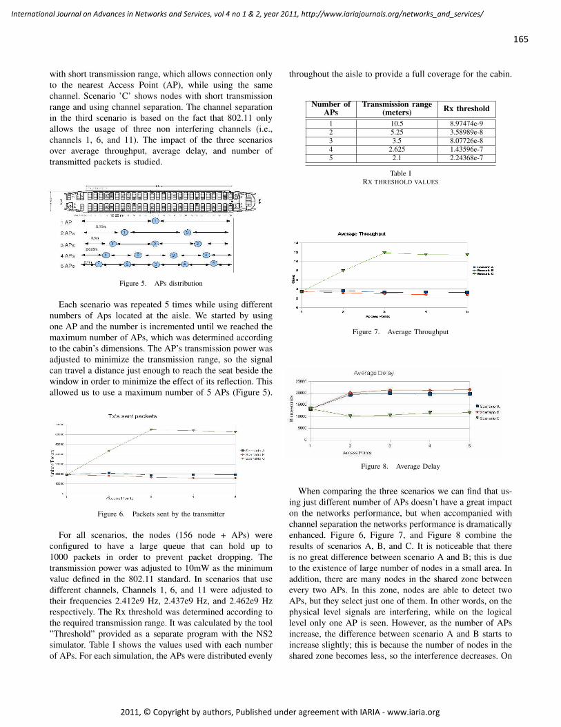
with short transmission range, which allows connection onlyto the nearest Access Point (AP), while using the samechannel. Scenario ’C’ shows nodes with short transmissionrange and using channel separation. The channel separationin the third scenario is based on the fact that 802.11 onlyallows the usage of three non interfering channels (i.e.,channels 1, 6, and 11). The impact of the three scenariosover average throughput, average delay, and number oftransmitted packets is studied.
Figure 5. APs distribution
Each scenario was repeated 5 times while using differentnumbers of Aps located at the aisle. We started by usingone AP and the number is incremented until we reached themaximum number of APs, which was determined accordingto the cabin’s dimensions. The AP’s transmission power wasadjusted to minimize the transmission range, so the signalcan travel a distance just enough to reach the seat beside thewindow in order to minimize the effect of its reflection. Thisallowed us to use a maximum number of 5 APs (Figure 5).
Figure 6. Packets sent by the transmitter
For all scenarios, the nodes (156 node + APs) wereconfigured to have a large queue that can hold up to1000 packets in order to prevent packet dropping. Thetransmission power was adjusted to 10mW as the minimumvalue defined in the 802.11 standard. In scenarios that usedifferent channels, Channels 1, 6, and 11 were adjusted totheir frequencies 2.412e9 Hz, 2.437e9 Hz, and 2.462e9 Hzrespectively. The Rx threshold was determined according tothe required transmission range. It was calculated by the tool”Threshold” provided as a separate program with the NS2simulator. Table I shows the values used with each numberof APs. For each simulation, the APs were distributed evenly
throughout the aisle to provide a full coverage for the cabin.
Number of Transmission range Rx thresholdAPs (meters)1 10.5 8.97474e-92 5.25 3.58989e-83 3.5 8.07726e-84 2.625 1.43596e-75 2.1 2.24368e-7
Table IRX THRESHOLD VALUES
Figure 7. Average Throughput
Figure 8. Average Delay
When comparing the three scenarios we can find that us-ing just different number of APs doesn’t have a great impacton the networks performance, but when accompanied withchannel separation the networks performance is dramaticallyenhanced. Figure 6, Figure 7, and Figure 8 combine theresults of scenarios A, B, and C. It is noticeable that thereis no great difference between scenario A and B; this is dueto the existence of large number of nodes in a small area. Inaddition, there are many nodes in the shared zone betweenevery two APs. In this zone, nodes are able to detect twoAPs, but they select just one of them. In other words, on thephysical level signals are interfering, while on the logicallevel only one AP is seen. However, as the number of APsincrease, the difference between scenario A and B starts toincrease slightly; this is because the number of nodes in theshared zone becomes less, so the interference decreases. On
165
International Journal on Advances in Networks and Services, vol 4 no 1 & 2, year 2011, http://www.iariajournals.org/networks_and_services/
2011, © Copyright by authors, Published under agreement with IARIA - www.iaria.org
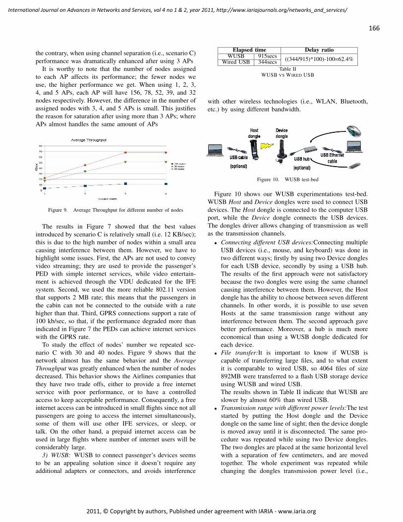
the contrary, when using channel separation (i.e., scenario C)performance was dramatically enhanced after using 3 APs
It is worthy to note that the number of nodes assignedto each AP affects its performance; the fewer nodes weuse, the higher performance we get. When using 1, 2, 3,4, and 5 APs, each AP will have 156, 78, 52, 39, and 32nodes respectively. However, the difference in the number ofassigned nodes with 3, 4, and 5 APs is small. This justifiesthe reason for saturation after using more than 3 APs; whereAPs almost handles the same amount of APs
Figure 9. Average Throughput for different number of nodes
The results in Figure 7 showed that the best valuesintroduced by scenario C is relatively small (i.e. 12 KB/sec);this is due to the high number of nodes within a small areacausing interference between them. However, we have tohighlight some issues. First, the APs are not used to conveyvideo streaming; they are used to provide the passenger’sPED with simple internet services, while video entertain-ment is achieved through the VDU dedicated for the IFEsystem. Second, we used the more reliable 802.11 versionthat supports 2 MB rate; this means that the passengers inthe cabin can not be connected to the outside with a ratehigher than that. Third, GPRS connections support a rate of100 kb/sec, so that, if the performance degraded more thanindicated in Figure 7 the PEDs can achieve internet serviceswith the GPRS rate.
To study the effect of nodes’ number we repeated sce-nario C with 30 and 40 nodes. Figure 9 shows that thenetwork almost has the same behavior and the AverageThroughput was greatly enhanced when the number of nodesdecreased. This behavior shows the Airlines companies thatthey have two trade offs, either to provide a free internetservice with poor performance, or to have a controlledaccess to keep acceptable performance. Consequently, a freeinternet access can be introduced in small flights since not allpassengers are going to access the internet simultaneously,some of them will use other IFE services, or sleep, ortalk. On the other hand, a prepaid internet access can beused in large flights where number of internet users will beconsiderably large.
3) WUSB: WUSB to connect passenger’s devices seemsto be an appealing solution since it doesn’t require anyadditional adapters or connectors, and avoids interference
Elapsed time Delay ratioWUSB 915secs ((344/915)*100)-100=62.4%Wired USB 344secs
Table IIWUSB VS WIRED USB
with other wireless technologies (i.e., WLAN, Bluetooth,etc.) by using different bandwidth.
Figure 10. WUSB test-bed
Figure 10 shows our WUSB experimentations test-bed.WUSB Host and Device dongles were used to connect USBdevices. The Host dongle is connected to the computer USBport, while the Device dongle connects the USB devices.The dongles driver allows changing of transmission as wellas the transmission channels.• Connecting different USB devices:Connecting multiple
USB devices (i.e., mouse, and keyboard) was done intwo different ways; firstly by using two Device donglesfor each USB device, secondly by using a USB hub.The results of the first approach were not satisfactorybecause the two dongles were using the same channelcausing interference between them. However, the Hostdongle has the ability to choose between seven differentchannels. In other words, it is possible to use sevenHosts at the same transmission range without anyinterference between them. The second approach gavebetter performance. Moreover, a hub is much moreeconomical than using a WUSB dongle dedicated foreach device.
• File transfer:It is important to know if WUSB iscapable of transferring large files, and to what extentit is comparable to wired USB, so 4064 files of size892MB were transferred to a flash USB storage deviceusing WUSB and wired USB.The results shown in Table II indicate that WUSB areslower by almost 60% than wired USB.
• Transmission range with different power levels:The teststarted by putting the Host dongle and the Devicedongle on the same line of sight; then the device dongleis moved away until it is disconnected. The same pro-cedure was repeated while using two Device dongles.The two dongles are placed at the same horizontal levelwith a separation of few centimeters, and are movedtogether. The whole experiment was repeated whilechanging the dongles transmission power level (i.e.,
166
International Journal on Advances in Networks and Services, vol 4 no 1 & 2, year 2011, http://www.iariajournals.org/networks_and_services/
2011, © Copyright by authors, Published under agreement with IARIA - www.iaria.org
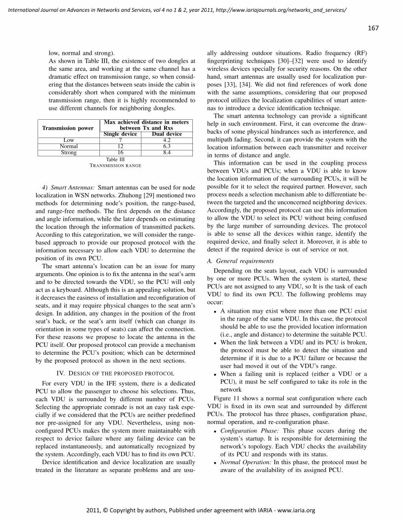
low, normal and strong).As shown in Table III, the existence of two dongles atthe same area, and working at the same channel has adramatic effect on transmission range, so when consid-ering that the distances between seats inside the cabin isconsiderably short when compared with the minimumtransmission range, then it is highly recommended touse different channels for neighboring dongles.
Transmission powerMax achieved distance in meters
between Tx and RxsSingle device Dual device
Low 7 4.2Normal 12 6.3Strong 16 8.4
Table IIITRANSMISSION RANGE
4) Smart Antennas: Smart antennas can be used for nodelocalization in WSN networks. Zhuhong [29] mentioned twomethods for determining node’s position, the range-based,and range-free methods. The first depends on the distanceand angle information, while the later depends on estimatingthe location through the information of transmitted packets.According to this categorization, we will consider the range-based approach to provide our proposed protocol with theinformation necessary to allow each VDU to determine theposition of its own PCU.
The smart antenna’s location can be an issue for manyarguments. One opinion is to fix the antenna in the seat’s armand to be directed towards the VDU, so the PCU will onlyact as a keyboard. Although this is an appealing solution, butit decreases the easiness of installation and reconfiguration ofseats, and it may require physical changes to the seat arm’sdesign. In addition, any changes in the position of the frontseat’s back, or the seat’s arm itself (which can change itsorientation in some types of seats) can affect the connection.For these reasons we propose to locate the antenna in thePCU itself. Our proposed protocol can provide a mechanismto determine the PCU’s position; which can be determinedby the proposed protocol as shown in the next sections.
IV. DESIGN OF THE PROPOSED PROTOCOL
For every VDU in the IFE system, there is a dedicatedPCU to allow the passenger to choose his selections. Thus,each VDU is surrounded by different number of PCUs.Selecting the appropriate comrade is not an easy task espe-cially if we considered that the PCUs are neither predefinednor pre-assigned for any VDU. Nevertheless, using non-configured PCUs makes the system more maintainable withrespect to device failure where any failing device can bereplaced instantaneously, and automatically recognized bythe system. Accordingly, each VDU has to find its own PCU.
Device identification and device localization are usuallytreated in the literature as separate problems and are usu-
ally addressing outdoor situations. Radio frequency (RF)fingerprinting techniques [30]–[32] were used to identifywireless devices specially for security reasons. On the otherhand, smart antennas are usually used for localization pur-poses [33], [34]. We did not find references of work donewith the same assumptions, considering that our proposedprotocol utilizes the localization capabilities of smart anten-nas to introduce a device identification technique.
The smart antenna technology can provide a significanthelp in such environment. First, it can overcome the draw-backs of some physical hindrances such as interference, andmultipath fading. Second, it can provide the system with thelocation information between each transmitter and receiverin terms of distance and angle.
This information can be used in the coupling processbetween VDUs and PCUs; when a VDU is able to knowthe location information of the surrounding PCUs, it will bepossible for it to select the required partner. However, suchprocess needs a selection mechanism able to differentiate be-tween the targeted and the unconcerned neighboring devices.Accordingly, the proposed protocol can use this informationto allow the VDU to select its PCU without being confusedby the large number of surrounding devices. The protocolis able to sense all the devices within range, identify therequired device, and finally select it. Moreover, it is able todetect if the required device is out of service or not.
A. General requirements
Depending on the seats layout, each VDU is surroundedby one or more PCUs. When the system is started, thesePCUs are not assigned to any VDU, so It is the task of eachVDU to find its own PCU. The following problems mayoccur:• A situation may exist where more than one PCU exist
in the range of the same VDU. In this case, the protocolshould be able to use the provided location information(i.e., angle and distance) to determine the suitable PCU.
• When the link between a VDU and its PCU is broken,the protocol must be able to detect the situation anddetermine if it is due to a PCU failure or because theuser had moved it out of the VDU’s range.
• When a failing unit is replaced (either a VDU or aPCU), it must be self configured to take its role in thenetwork
Figure 11 shows a normal seat configuration where eachVDU is fixed in its own seat and surrounded by differentPCUs. The protocol has three phases, configuration phase,normal operation, and re-configuration phase.• Configuration Phase: This phase occurs during the
system’s startup. It is responsible for determining thenetwork’s topology. Each VDU checks the availabilityof its PCU and responds with its status.
• Normal Operation: In this phase, the protocol must beaware of the availability of its assigned PCU.
167
International Journal on Advances in Networks and Services, vol 4 no 1 & 2, year 2011, http://www.iariajournals.org/networks_and_services/
2011, © Copyright by authors, Published under agreement with IARIA - www.iaria.org
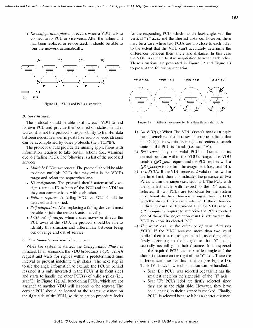
• Re-configuration phase: It occurs when a VDU fails toconnect to its PCU or vice versa. After the failing unithad been replaced or re-operated, it should be able tojoin the network automatically.
Figure 11. VDUs and PCUs distribution
B. Specifications
The protocol should be able to allow each VDU to findits own PCU and provide their connection status. In otherwords, it is not the protocol’s responsibility to transfer databetween nodes. Transferring data like audio or video streamscan be accomplished by other protocols (i.e., TCP/IP).
The protocol should provide the running applications withinformation required to take certain actions (i.e., warningsdue to a failing PCU). The following is a list of the proposedservices:• Multiple PCUs awareness: The protocol should be able
to detect multiple PCUs that may exist in the VDU’srange and select the appropriate one.
• ID assignment: The protocol should automatically as-sign a unique ID to both of the PCU and the VDU sothey can communicate with each other.
• Failure reports: A failing VDU or PCU should bedetected and reported.
• Self adaptation: After replacing a failing device, it mustbe able to join the network automatically.
• PCU out of range: when a user moves or directs thePCU away of the VDU, the protocol should be able toidentify this situation and differentiate between beingout of range and out of service.
C. Functionality and studied use cases
When the system is started, the Configuration Phase isinitiated. In all scenarios, the VDU broadcasts a QRY searchrequest and waits for replies within a predetermined timeinterval to prevent indefinite wait states. The next step isto use the angle information to exclude the PCU(s) behindit (since it is only interested in the PCUs at its front side)and starts to handle the other PCU(s) of valid replies (i.e.,seat ’D’ in Figure 12). All functioning PCUs, which are notassigned to another VDU will respond to the request. Thecorrect PCU should be located at the nearest distance onthe right side of the VDU, so the selection procedure looks
for the responding PCU, which has the least angle with thevertical ”Y” axis, and the shortest distance. However, theremay be a case where two PCUs are too close to each otherto the extent that the VDU can’t accurately determine thedifferences between their angle and distance. In this casethe VDU asks them to start negotiation between each other.These situations are presented in Figure 12 and Figure 13to present the following scenarios:
Figure 12. Different scenarios for less than three valid PCUs
1) No PCU(s): When The VDU doesn’t receive a replyfor its search request, it raises an error to indicate thatno PCU(s) are within its range, and enters a searchstate until a PCU is found. (i.e., seat ’A’).
2) Best case: only one valid PCU is located in itscorrect position within the VDU’s range: The VDUsends a QRY join request and the PCU replies with aQRY accept to confirm the assignment (i.e., seat ’B’).
3) Two PCUs: If the VDU received 2 valid replies withinthe time limit, then this indicates the presence of twoPCUs within the range (i.e., seat ’C’). The PCU withthe smallest angle with respect to the ’Y’ axis isselected. If two PCUs are too close for the systemto differentiate the difference in angle, then the PCUwith the shortest distance is selected. If the differencein distance can’t be determined, then the VDU sends aQRY negotiate request to authorize the PCUs to electone of them. The negotiation result is returned to theVDU to know its elected PCU.
4) The worst case is the existence of more than twoPCUs: If the VDU received more than two validreplies, then it starts to sort them in ascending orderfirstly according to their angle to the ’Y’ axis ,secondly according to their distance. It is expectedthat the required PCU has the smallest angle and theshortest distance on the right of the ’Y’ axis. There aredifferent scenarios for this situation (see Figure 13).Table IV shows how each situation can be handled.• Seat ’E’: PCU1 was selected because it has the
smallest angle on the right side of the ’Y’ axis.• Seat ’F’: PCUs 1&4 are firstly selected since
they are at the right side. However, they haveequal angles, so their distance is checked.. Finally,PCU1 is selected because it has a shorter distance.
168
International Journal on Advances in Networks and Services, vol 4 no 1 & 2, year 2011, http://www.iariajournals.org/networks_and_services/
2011, © Copyright by authors, Published under agreement with IARIA - www.iaria.org
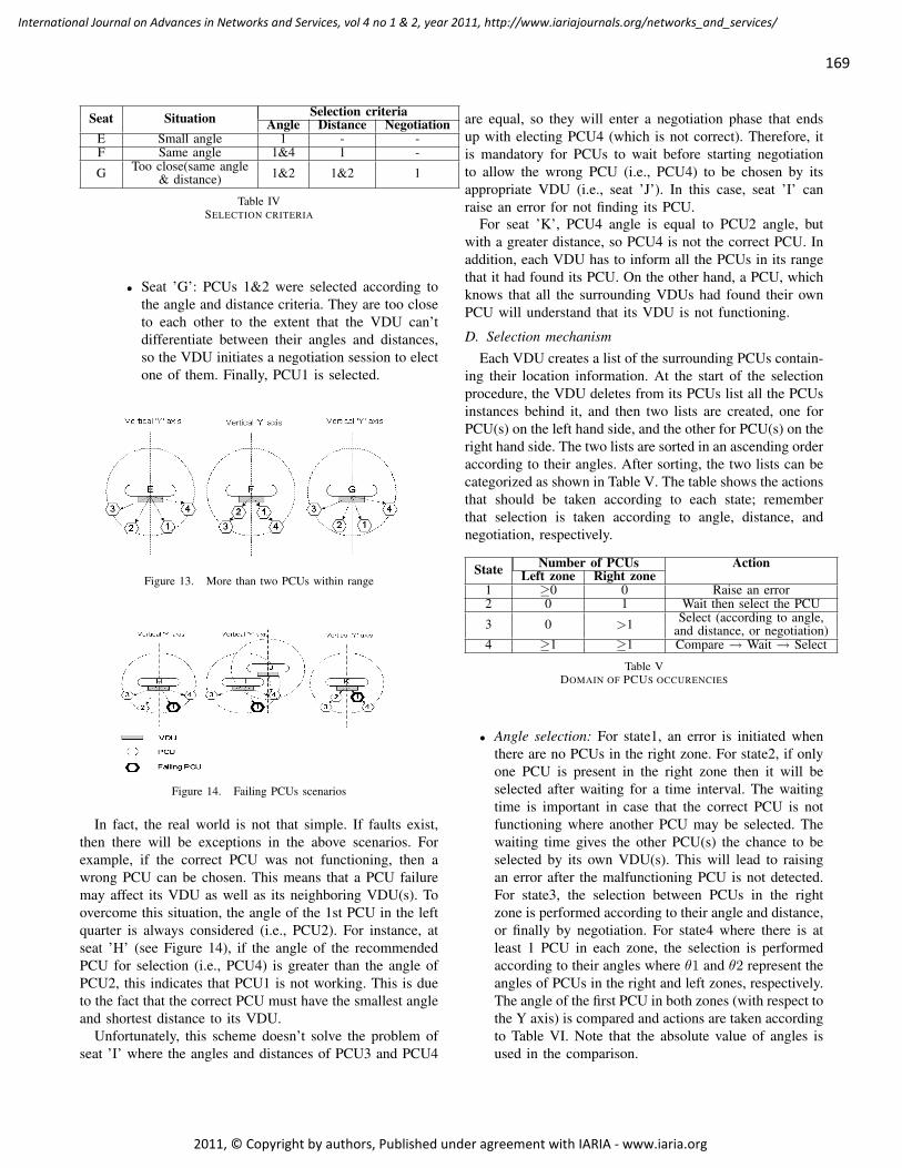
Seat Situation Selection criteriaAngle Distance Negotiation
E Small angle 1 - -F Same angle 1&4 1 -
G Too close(same angle 1&2 1&2 1& distance)
Table IVSELECTION CRITERIA
• Seat ’G’: PCUs 1&2 were selected according tothe angle and distance criteria. They are too closeto each other to the extent that the VDU can’tdifferentiate between their angles and distances,so the VDU initiates a negotiation session to electone of them. Finally, PCU1 is selected.
Figure 13. More than two PCUs within range
Figure 14. Failing PCUs scenarios
In fact, the real world is not that simple. If faults exist,then there will be exceptions in the above scenarios. Forexample, if the correct PCU was not functioning, then awrong PCU can be chosen. This means that a PCU failuremay affect its VDU as well as its neighboring VDU(s). Toovercome this situation, the angle of the 1st PCU in the leftquarter is always considered (i.e., PCU2). For instance, atseat ’H’ (see Figure 14), if the angle of the recommendedPCU for selection (i.e., PCU4) is greater than the angle ofPCU2, this indicates that PCU1 is not working. This is dueto the fact that the correct PCU must have the smallest angleand shortest distance to its VDU.
Unfortunately, this scheme doesn’t solve the problem ofseat ’I’ where the angles and distances of PCU3 and PCU4
are equal, so they will enter a negotiation phase that endsup with electing PCU4 (which is not correct). Therefore, itis mandatory for PCUs to wait before starting negotiationto allow the wrong PCU (i.e., PCU4) to be chosen by itsappropriate VDU (i.e., seat ’J’). In this case, seat ’I’ canraise an error for not finding its PCU.
For seat ’K’, PCU4 angle is equal to PCU2 angle, butwith a greater distance, so PCU4 is not the correct PCU. Inaddition, each VDU has to inform all the PCUs in its rangethat it had found its PCU. On the other hand, a PCU, whichknows that all the surrounding VDUs had found their ownPCU will understand that its VDU is not functioning.
D. Selection mechanismEach VDU creates a list of the surrounding PCUs contain-
ing their location information. At the start of the selectionprocedure, the VDU deletes from its PCUs list all the PCUsinstances behind it, and then two lists are created, one forPCU(s) on the left hand side, and the other for PCU(s) on theright hand side. The two lists are sorted in an ascending orderaccording to their angles. After sorting, the two lists can becategorized as shown in Table V. The table shows the actionsthat should be taken according to each state; rememberthat selection is taken according to angle, distance, andnegotiation, respectively.
State Number of PCUs ActionLeft zone Right zone
1 ≥0 0 Raise an error2 0 1 Wait then select the PCU
3 0 >1 Select (according to angle,and distance, or negotiation)
4 ≥1 ≥1 Compare → Wait → Select
Table VDOMAIN OF PCUS OCCURENCIES
• Angle selection: For state1, an error is initiated whenthere are no PCUs in the right zone. For state2, if onlyone PCU is present in the right zone then it will beselected after waiting for a time interval. The waitingtime is important in case that the correct PCU is notfunctioning where another PCU may be selected. Thewaiting time gives the other PCU(s) the chance to beselected by its own VDU(s). This will lead to raisingan error after the malfunctioning PCU is not detected.For state3, the selection between PCUs in the rightzone is performed according to their angle and distance,or finally by negotiation. For state4 where there is atleast 1 PCU in each zone, the selection is performedaccording to their angles where θ1 and θ2 represent theangles of PCUs in the right and left zones, respectively.The angle of the first PCU in both zones (with respect tothe Y axis) is compared and actions are taken accordingto Table VI. Note that the absolute value of angles isused in the comparison.
169
International Journal on Advances in Networks and Services, vol 4 no 1 & 2, year 2011, http://www.iariajournals.org/networks_and_services/
2011, © Copyright by authors, Published under agreement with IARIA - www.iaria.org
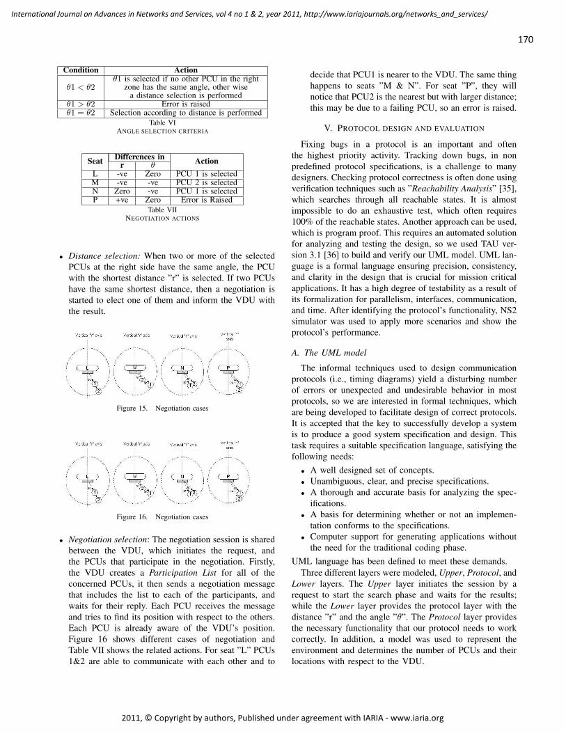
Condition Action
θ1 < θ2θ1 is selected if no other PCU in the right
zone has the same angle, other wisea distance selection is performed
θ1 > θ2 Error is raisedθ1 = θ2 Selection according to distance is performed
Table VIANGLE SELECTION CRITERIA
Seat Differences in Actionr θL -ve Zero PCU 1 is selectedM -ve -ve PCU 2 is selectedN Zero -ve PCU 1 is selectedP +ve Zero Error is Raised
Table VIINEGOTIATION ACTIONS
• Distance selection: When two or more of the selectedPCUs at the right side have the same angle, the PCUwith the shortest distance ”r” is selected. If two PCUshave the same shortest distance, then a negotiation isstarted to elect one of them and inform the VDU withthe result.
Figure 15. Negotiation cases
Figure 16. Negotiation cases
• Negotiation selection: The negotiation session is sharedbetween the VDU, which initiates the request, andthe PCUs that participate in the negotiation. Firstly,the VDU creates a Participation List for all of theconcerned PCUs, it then sends a negotiation messagethat includes the list to each of the participants, andwaits for their reply. Each PCU receives the messageand tries to find its position with respect to the others.Each PCU is already aware of the VDU’s position.Figure 16 shows different cases of negotiation andTable VII shows the related actions. For seat ”L” PCUs1&2 are able to communicate with each other and to
decide that PCU1 is nearer to the VDU. The same thinghappens to seats ”M & N”. For seat ”P”, they willnotice that PCU2 is the nearest but with larger distance;this may be due to a failing PCU, so an error is raised.
V. PROTOCOL DESIGN AND EVALUATION
Fixing bugs in a protocol is an important and oftenthe highest priority activity. Tracking down bugs, in nonpredefined protocol specifications, is a challenge to manydesigners. Checking protocol correctness is often done usingverification techniques such as ”Reachability Analysis” [35],which searches through all reachable states. It is almostimpossible to do an exhaustive test, which often requires100% of the reachable states. Another approach can be used,which is program proof. This requires an automated solutionfor analyzing and testing the design, so we used TAU ver-sion 3.1 [36] to build and verify our UML model. UML lan-guage is a formal language ensuring precision, consistency,and clarity in the design that is crucial for mission criticalapplications. It has a high degree of testability as a result ofits formalization for parallelism, interfaces, communication,and time. After identifying the protocol’s functionality, NS2simulator was used to apply more scenarios and show theprotocol’s performance.
A. The UML model
The informal techniques used to design communicationprotocols (i.e., timing diagrams) yield a disturbing numberof errors or unexpected and undesirable behavior in mostprotocols, so we are interested in formal techniques, whichare being developed to facilitate design of correct protocols.It is accepted that the key to successfully develop a systemis to produce a good system specification and design. Thistask requires a suitable specification language, satisfying thefollowing needs:• A well designed set of concepts.• Unambiguous, clear, and precise specifications.• A thorough and accurate basis for analyzing the spec-
ifications.• A basis for determining whether or not an implemen-
tation conforms to the specifications.• Computer support for generating applications without
the need for the traditional coding phase.UML language has been defined to meet these demands.
Three different layers were modeled, Upper, Protocol, andLower layers. The Upper layer initiates the session by arequest to start the search phase and waits for the results;while the Lower layer provides the protocol layer with thedistance ”r” and the angle ”θ”. The Protocol layer providesthe necessary functionality that our protocol needs to workcorrectly. In addition, a model was used to represent theenvironment and determines the number of PCUs and theirlocations with respect to the VDU.
170
International Journal on Advances in Networks and Services, vol 4 no 1 & 2, year 2011, http://www.iariajournals.org/networks_and_services/
2011, © Copyright by authors, Published under agreement with IARIA - www.iaria.org
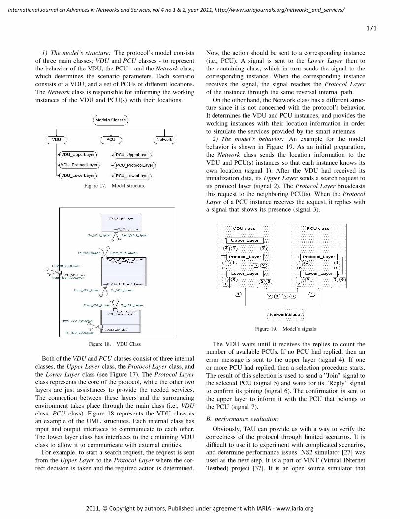
1) The model’s structure: The protocol’s model consistsof three main classes; VDU and PCU classes - to representthe behavior of the VDU, the PCU - and the Network class,which determines the scenario parameters. Each scenarioconsists of a VDU, and a set of PCUs of different locations.The Network class is responsible for informing the workinginstances of the VDU and PCU(s) with their locations.
Figure 17. Model structure
Figure 18. VDU Class
Both of the VDU and PCU classes consist of three internalclasses, the Upper Layer class, the Protocol Layer class, andthe Lower Layer class (see Figure 17). The Protocol Layerclass represents the core of the protocol, while the other twolayers are just assistances to provide the needed services.The connection between these layers and the surroundingenvironment takes place through the main class (i.e., VDUclass, PCU class). Figure 18 represents the VDU class asan example of the UML structures. Each internal class hasinput and output interfaces to communicate to each other.The lower layer class has interfaces to the containing VDUclass to allow it to communicate with external entities.
For example, to start a search request, the request is sentfrom the Upper Layer to the Protocol Layer where the cor-rect decision is taken and the required action is determined.
Now, the action should be sent to a corresponding instance(i.e., PCU). A signal is sent to the Lower Layer then tothe containing class, which in turn sends the signal to thecorresponding instance. When the corresponding instancereceives the signal, the signal reaches the Protocol Layerof the instance through the same reversal internal path.
On the other hand, the Network class has a different struc-ture since it is not concerned with the protocol’s behavior.It determines the VDU and PCU instances, and provides theworking instances with their location information in orderto simulate the services provided by the smart antennas
2) The model’s behavior: An example for the modelbehavior is shown in Figure 19. As an initial preparation,the Network class sends the location information to theVDU and PCU(s) instances so that each instance knows itsown location (signal 1). After the VDU had received itsinitialization data, its Upper Layer sends a search request toits protocol layer (signal 2). The Protocol Layer broadcaststhis request to the neighboring PCU(s). When the ProtocolLayer of a PCU instance receives the request, it replies witha signal that shows its presence (signal 3).
Figure 19. Model’s signals
The VDU waits until it receives the replies to count thenumber of available PCUs. If no PCU had replied, then anerror message is sent to the upper layer (signal 4). If oneor more PCU had replied, then a selection procedure starts.The result of this selection is used to send a ”Join” signal tothe selected PCU (signal 5) and waits for its ”Reply” signalto confirm its joining (signal 6). The confirmation is sent tothe upper layer to inform it with the PCU that belongs tothe PCU (signal 7).
B. performance evaluation
Obviously, TAU can provide us with a way to verify thecorrectness of the protocol through limited scenarios. It isdifficult to use it to experiment with complicated scenarios,and determine performance issues. NS2 simulator [27] wasused as the next step. It is a part of VINT (Virtual INternetTestbed) project [37]. It is an open source simulator that
171
International Journal on Advances in Networks and Services, vol 4 no 1 & 2, year 2011, http://www.iariajournals.org/networks_and_services/
2011, © Copyright by authors, Published under agreement with IARIA - www.iaria.org
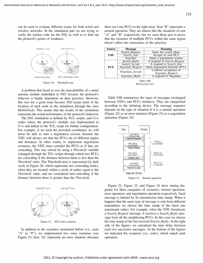
can be used to evaluate different issues for both wired andwireless networks. In the simulation part we are trying toverify the written code for the NS2 as well as to find outthe protocol’s points of weakness.
Figure 20. Threshold area
A problem that faced us was the unavailability of a smartantenna module embedded in NS2 because the protocol’sbehavior is highly dependent on their presence. However,this was not a great issue because NS2 keeps track of thelocation of each node in the simulation through the classMobileNode. This means that the results of the simulationrepresents the actual performance of the protocol’s behavior.
The NS2 simulation is defined by TCL scripts, and C++codes where the protocol’s module was implemented inC++ and linked to the TCL script for further configuration.For example, if we used the provided coordinates we willnever be able to start a negotiation session, because theVDU will always see that the PCUs are of different anglesand distances. In other words, to implement negotiationscenarios, the VDU must consider the PCUs as if they arecoinciding. This was solved by using a Threshold variable(changed through the TCL script) through which two PCUsare coinciding if the distance between them is less than theThreshold value. The Threshold area is represented by darkcircle in Figure 20, which represents two coinciding nodes,when they are located within a circle of radius equal to theThreshold value, and are considered non-coinciding if thedistance between them is greater than the Threshold.
Figure 21. NS2 extra scenarios
In addition to the scenarios mentioned before (i.e., seats”A” to ”P”), we implemented two extra scenarios (seeFigure 21) Seat ”Q” represents an error situation (because
there isn’t any PCUs in the right area). Seat ”R” represents anormal operation. They are almost like the situations of seat”A” and ”B” respectively, but we used them just to provethat the existence of multiple PCUs within the same regiondoesn’t affect the correctness of the selection
Source Message Meaning
VDUSearch Request Starts the search phase
Search Join Accepts its own PCUNegotiate Starts a negotiation session
PCU
Search Reply A respond to Search RequestSearch Accept A respond to Search Join
Negotiate Request Starts negotiation between PCUs
Negotiate Accept Confirms acceptance ofNegotiate Request
Negotiate Reply A respond to Negotiate
Table VIIIMESSAGES LIST
Table VIII summarizes the types of messages exchangedbetween VDUs and PCUs instances. They are categorizedaccording to the initiating device. The message sequencedepends on the type of situation if it is a normal operation(Figure 22) or an error situation (Figure 23) or a negotiationoperation (Figure 24).
Figure 22. Normal operation
Figure 22, Figure 23, and Figure 24 show timing dia-grams for three categories of scenarios, normal operation,error operation, and negotiation operation respectively. Eachmessage is labeled by its transmission time stamp. When ithappens that the same type of message is sent from differenttransmitters we choose the time stamp of the latest one(maximum value). For example, when the VDU broadcastsa Search Request message, it receives a Search Reply mes-sage from all the neighboring PCUs. In this case we choosethe time stamp of the last received Search Reply. At the rightside of the figures, we calculated the time delay betweeneach two successive messages. At the bottom of the figureswe indicated the scenarios (i.e., seats), which match eachoperation.
172
International Journal on Advances in Networks and Services, vol 4 no 1 & 2, year 2011, http://www.iariajournals.org/networks_and_services/
2011, © Copyright by authors, Published under agreement with IARIA - www.iaria.org
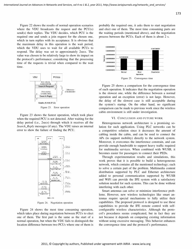
Figure 22 shows the results of normal operation scenarioswhere the VDU broadcasts the request and the PCU(s)send(s) their replies. The VDU decides, which PCU is therequired one and sends a join request for the chosen one,which in turn replies with its acceptance. It is obvious thatthe maximum delay in this operation is the wait period,which the VDU uses to wait for all available PCUs torespond. The delay was set to approximately 2secs. Thevalue was chosen to be relatively large to show its impact onthe protocol’s performance; considering that the processingtime of the requests is trivial when compared to the waittime.
Figure 23. Error operation
Figure 23 shows the fastest operation, which took placewhen the required PCU is not detected. After waiting for thedelay period (i.e., 2secs) through which it receives all theSearch Reply messages (if any). The VDU raises an internalerror to show the failure of finding the PCU.
Figure 24. Negotiation operation
Figure 24 shows the most time consuming operation,which takes place during negotiation between PCUs to electone of them. The first part is the same as the start of anormal operation, but when the VDU fails to distinguish thelocation difference between two PCUs where one of them is
probably the required one, it asks them to start negotiationand elect one of them. The most time consuming parts arethe waiting periods (mentioned above), and the negotiationprocess between the PCUs. Each of them is about 2 s.
Figure 25. Convergence time
Figure 25 shows a comparison for the convergence timeof each operation. It indicates that the negotiation operationis the slowest one, while the difference between a normaloperation and an exception (error) is not large. However,the delay of the slowest case is still acceptable duringthe system’s startup. On the other hand, no significantcomparison can be made to previous work since the wirelesscabin environment is still under investigation.
VI. CONCLUSION AND FUTURE WORK
Heterogeneous network architecture is a promising so-lution for such application. Using PLC networks can bea competitive solution since it decreases the amount ofcabling inside the cabin, and can be used to connect theAPs (to support mobility) directly to the network system.Moreover, it overcomes the interference constrain, and canprovide enough bandwidth to support heavy traffic requiredfor multimedia services. When combined with WUSB, itbecomes easier for passengers to connect their PEDs.
Through experimentation results and simulations, thiswork proves that it is possible to build a heterogeneousnetwork, which contains all the mentioned technology; eachto solve a certain part of the problem. Multimedia contentdistribution supported by PLC and Ethernet architectureadded to personal communication supported by WUSBand WiFi can provide the IFE system with a satisfactorysolution needed for such systems. This can be done withoutinterfering with each other.
Smart antennas can solve or minimize interference prob-lems. However, new wireless technologies like smart an-tennas require special mechanisms to fully utilize theircapabilities. The proposed protocol is designed to use thesecapabilities to provide the IFE remote control with self-configurable wireless characteristics. Although the proto-col’s procedures seems complicated, but in fact they arenot because it depends on comparing existing informationwithout using excessive messaging. This behavior enhancesthe convergence time and the protocol’s performance.
173
International Journal on Advances in Networks and Services, vol 4 no 1 & 2, year 2011, http://www.iariajournals.org/networks_and_services/
2011, © Copyright by authors, Published under agreement with IARIA - www.iaria.org
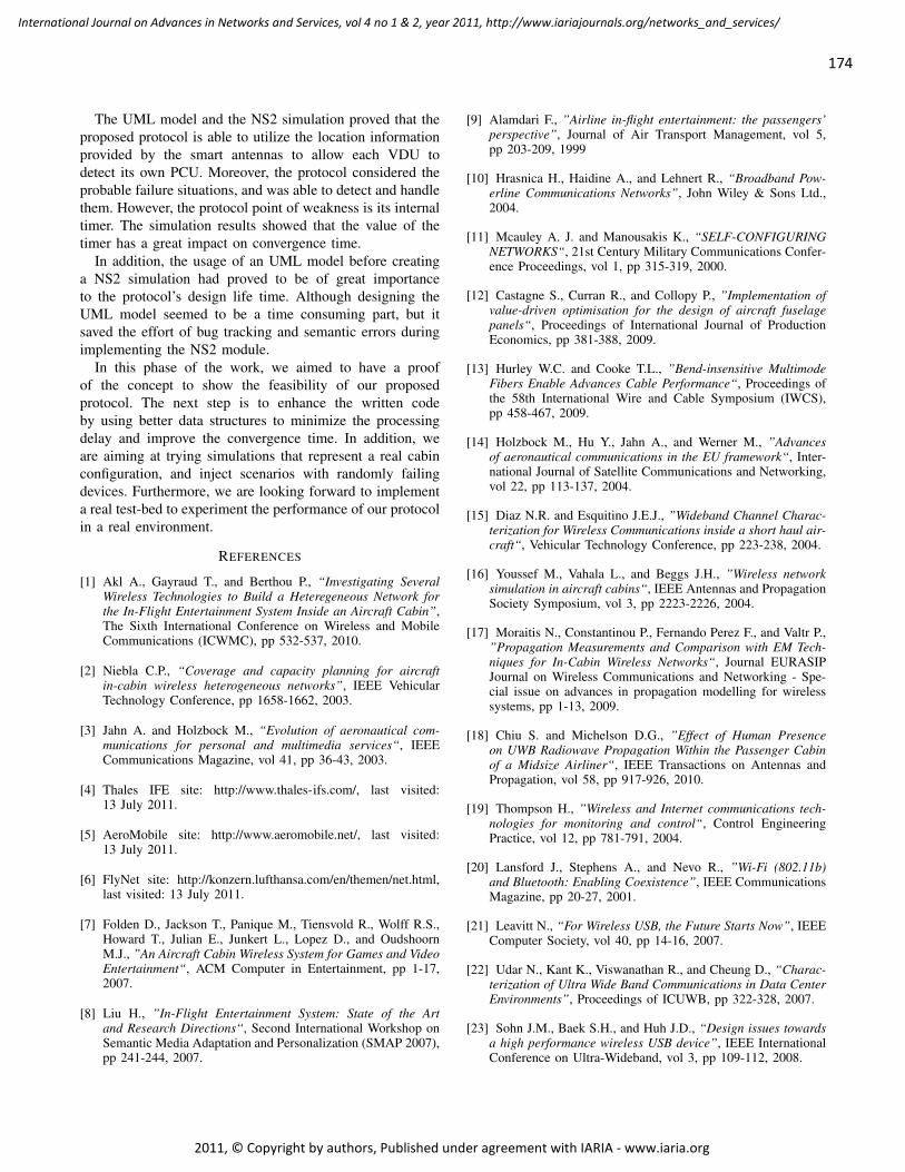
The UML model and the NS2 simulation proved that theproposed protocol is able to utilize the location informationprovided by the smart antennas to allow each VDU todetect its own PCU. Moreover, the protocol considered theprobable failure situations, and was able to detect and handlethem. However, the protocol point of weakness is its internaltimer. The simulation results showed that the value of thetimer has a great impact on convergence time.
In addition, the usage of an UML model before creatinga NS2 simulation had proved to be of great importanceto the protocol’s design life time. Although designing theUML model seemed to be a time consuming part, but itsaved the effort of bug tracking and semantic errors duringimplementing the NS2 module.
In this phase of the work, we aimed to have a proofof the concept to show the feasibility of our proposedprotocol. The next step is to enhance the written codeby using better data structures to minimize the processingdelay and improve the convergence time. In addition, weare aiming at trying simulations that represent a real cabinconfiguration, and inject scenarios with randomly failingdevices. Furthermore, we are looking forward to implementa real test-bed to experiment the performance of our protocolin a real environment.
REFERENCES
[1] Akl A., Gayraud T., and Berthou P., “Investigating SeveralWireless Technologies to Build a Heteregeneous Network forthe In-Flight Entertainment System Inside an Aircraft Cabin”,The Sixth International Conference on Wireless and MobileCommunications (ICWMC), pp 532-537, 2010.
[2] Niebla C.P., “Coverage and capacity planning for aircraftin-cabin wireless heterogeneous networks”, IEEE VehicularTechnology Conference, pp 1658-1662, 2003.
[3] Jahn A. and Holzbock M., “Evolution of aeronautical com-munications for personal and multimedia services“, IEEECommunications Magazine, vol 41, pp 36-43, 2003.
[4] Thales IFE site: http://www.thales-ifs.com/, last visited:13 July 2011.
[5] AeroMobile site: http://www.aeromobile.net/, last visited:13 July 2011.
[6] FlyNet site: http://konzern.lufthansa.com/en/themen/net.html,last visited: 13 July 2011.
[7] Folden D., Jackson T., Panique M., Tiensvold R., Wolff R.S.,Howard T., Julian E., Junkert L., Lopez D., and OudshoornM.J., ”An Aircraft Cabin Wireless System for Games and VideoEntertainment“, ACM Computer in Entertainment, pp 1-17,2007.
[8] Liu H., ”In-Flight Entertainment System: State of the Artand Research Directions“, Second International Workshop onSemantic Media Adaptation and Personalization (SMAP 2007),pp 241-244, 2007.
[9] Alamdari F., ”Airline in-flight entertainment: the passengers’perspective”, Journal of Air Transport Management, vol 5,pp 203-209, 1999
[10] Hrasnica H., Haidine A., and Lehnert R., “Broadband Pow-erline Communications Networks”, John Wiley & Sons Ltd.,2004.
[11] Mcauley A. J. and Manousakis K., “SELF-CONFIGURINGNETWORKS“, 21st Century Military Communications Confer-ence Proceedings, vol 1, pp 315-319, 2000.
[12] Castagne S., Curran R., and Collopy P., ”Implementation ofvalue-driven optimisation for the design of aircraft fuselagepanels“, Proceedings of International Journal of ProductionEconomics, pp 381-388, 2009.
[13] Hurley W.C. and Cooke T.L., ”Bend-insensitive MultimodeFibers Enable Advances Cable Performance“, Proceedings ofthe 58th International Wire and Cable Symposium (IWCS),pp 458-467, 2009.
[14] Holzbock M., Hu Y., Jahn A., and Werner M., ”Advancesof aeronautical communications in the EU framework“, Inter-national Journal of Satellite Communications and Networking,vol 22, pp 113-137, 2004.
[15] Diaz N.R. and Esquitino J.E.J., ”Wideband Channel Charac-terization for Wireless Communications inside a short haul air-craft“, Vehicular Technology Conference, pp 223-238, 2004.
[16] Youssef M., Vahala L., and Beggs J.H., ”Wireless networksimulation in aircraft cabins“, IEEE Antennas and PropagationSociety Symposium, vol 3, pp 2223-2226, 2004.
[17] Moraitis N., Constantinou P., Fernando Perez F., and Valtr P.,”Propagation Measurements and Comparison with EM Tech-niques for In-Cabin Wireless Networks“, Journal EURASIPJournal on Wireless Communications and Networking - Spe-cial issue on advances in propagation modelling for wirelesssystems, pp 1-13, 2009.
[18] Chiu S. and Michelson D.G., ”Effect of Human Presenceon UWB Radiowave Propagation Within the Passenger Cabinof a Midsize Airliner“, IEEE Transactions on Antennas andPropagation, vol 58, pp 917-926, 2010.
[19] Thompson H., ”Wireless and Internet communications tech-nologies for monitoring and control“, Control EngineeringPractice, vol 12, pp 781-791, 2004.
[20] Lansford J., Stephens A., and Nevo R., ”Wi-Fi (802.11b)and Bluetooth: Enabling Coexistence”, IEEE CommunicationsMagazine, pp 20-27, 2001.
[21] Leavitt N., “For Wireless USB, the Future Starts Now”, IEEEComputer Society, vol 40, pp 14-16, 2007.
[22] Udar N., Kant K., Viswanathan R., and Cheung D., “Charac-terization of Ultra Wide Band Communications in Data CenterEnvironments”, Proceedings of ICUWB, pp 322-328, 2007.
[23] Sohn J.M., Baek S.H., and Huh J.D., “Design issues towardsa high performance wireless USB device”, IEEE InternationalConference on Ultra-Wideband, vol 3, pp 109-112, 2008.
174
International Journal on Advances in Networks and Services, vol 4 no 1 & 2, year 2011, http://www.iariajournals.org/networks_and_services/
2011, © Copyright by authors, Published under agreement with IARIA - www.iaria.org
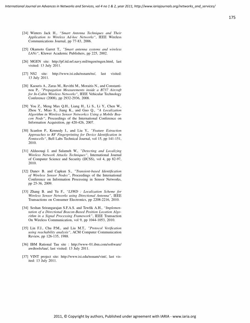
[24] Winters Jack H., “Smart Antenna Techniques and TheirApplication to Wireless Ad-hoc Networks“, IEEE WirelessCommunications Journal, pp 77-83, 2006.
[25] Okamoto Garret T., ”Smart antenna systems and wirelessLANs“, Kluwer Academic Publishers, pp 225, 2002.
[26] MGEN site: http://pf.itd.nrl.navy.mil/mgen/mgen.html, lastvisited: 13 July 2011.
[27] NS2 site: http://www.isi.edu/nsnam/ns/, last visited:13 July 2011.
[28] Kaouris A., Zaras M., Revithi M., Moraitis N., and Constanti-nou P., ”Propagation Measurements inside a B737 Aircraftfor In-Cabin Wireless Networks“, IEEE Vehicular TechnologyConference (2008), pp 2932-2936, 2008.
[29] You Z., Meng Max Q.H., Liang H., Li S., Li Y., Chen W.,Zhou Y., Miao S., Jiang K., and Guo Q., ”A LocalizationAlgorithm in Wireless Sensor Networkcs Using a Mobile Bea-con Node“, Proceedings of the International Conference onInformation Acquisition, pp 420-426, 2007.
[30] Scanlon P., Kennedy I., and Liu Y., ”Feature ExtractionApproaches to RF Fingerprinting for Device Identification inFemtocells“, Bell Labs Technical Journal, vol 15, pp 141-151,2010.
[31] Aldasouqi I. and Salameh W., ”Detecting and LocalizingWireless Network Attacks Techniques“, International Journalof Computer Science and Security (IJCSS), vol 4, pp 82-97,2010.
[32] Danev B. and Capkun S., ”Transient-based Identificationof Wireless Sensor Nodes”, Proceedings of the InternationalConference on Information Processing in Sensor Networks,pp 25-36, 2009.
[33] Zhang B. and Yu F., “LSWD : Localization Scheme forWireless Sensor Networks using Directional Antenna”, IEEETransactions on Consumer Electronics, pp 2208-2216, 2010.
[34] Seshan Srirangarajan S.F.A.S. and Tewfik A.H., “Implemen-tation of a Directional Beacon-Based Position Location Algo-rithm in a Signal Processing Framework”, IEEE TransactionOn Wireless Communication, vol 9, pp 1044-1053, 2010.
[35] Lin F.J., Chu P.M., and Liu M.T., ”Protocol Verificationusing reachability analysis“, ACM Computer CommunicationReview, pp 126-135, 1988.
[36] IBM Rational Tau site : http://www-01.ibm.com/software/awdtools/tau/, last visited: 13 July 2011.
[37] VINT project site: http://www.isi.edu/nsnam/vint/, last vis-ited: 13 July 2011.
175
International Journal on Advances in Networks and Services, vol 4 no 1 & 2, year 2011, http://www.iariajournals.org/networks_and_services/
2011, © Copyright by authors, Published under agreement with IARIA - www.iaria.org
Exploiting Multimedia Frame Semantics and MAC-layer Enhancements for QoS
Provisioning in IEEE 802.11e Congested Networks
Anastasios Politis Dept. of Applied Informatics
University of Macedonia
Thessaloniki, Greece
Ioannis Mavridis
Dept. of Applied Informatics
University of Macedonia
Thessaloniki, Greece
Athanasios Manitsaris
Dept. of Applied Informatics
University of Macedonia
Thessaloniki, Greece
Abstract—Wireless Local Area Networks (WLANs) supporting
modern streaming multimedia applications constitute a very
challenging and rapidly changing field of research. Towards
implementing effective multimedia wireless networks, the
IEEE has published the “state of the art” IEEE 802.11e
standard, which introduced a QoS-aware MAC-layer along
with a series of efficiency enhancements. However, it has been
proven inadequate in handling multimedia traffic optimally in
periods of congestion. For the efficient support of multimedia
applications in high load situations, numerous mechanisms
have emerged, most of them focusing on altering the static
nature of resource allocation specified in IEEE 802.11e.
Nevertheless, traffic characteristics must be taken into
consideration in order to achieve the highest gains. In this
paper, an application-aware MAC-layer mechanism is
developed that exploits multimedia frame semantics and
existing MAC-layer enhancements to adequately cope with
high congestion situations in IEEE 802.11e infrastructure
networks. The proposed algorithm makes use of existing
acknowledgment policies and adaptive resource allocation
techniques depending on multimedia frame significance. The
effectiveness of the algorithm is proven by means of
simulations, where its functionality is evaluated and compared
with other existing schemes.
Keywords- WLANs, Multimedia, IEEE 802.11e, QoS, MAC-layer
I. INTRODUCTION
Wireless Local Area Networks (WLANs) have been established as one of the preferred network technologies by the majority of electronic equipment users. At the same time, networked multimedia applications have penetrated the market with a tremendous success. Hence, the combination of multimedia applications and WLANs has been an extremely interesting research topic for the networking scientific community. The ultimate goal is to design WLANs in a way to support efficiently the incorporated multimedia traffic.
In an attempt to address this challenge, the Institute of Electrical and Electronics Engineers (IEEE) has released a series of amendments, improving the functionality of the initial ΙΕΕΕ 802.11 WLAN standard [2]. The majority of these amendments focused on signal modulation techniques, in an attempt to provide high data rates at the physical (PHY) layer (IEEE 802.11a/b/g) [3], [4], [5]. However, it was soon discovered that MAC layer enhancements were also needed
in order to efficiently utilize the available bandwidth. Furthermore, since multimedia applications demand certain and strict Quality of Service (QoS) levels, it is required that the IEEE 802.11 MAC layer is capable of traffic differentiation.
To this direction, several new mechanisms demonstrated an increased efficiency in multimedia applications support in WLANs, by providing prioritized access to different traffic flows and/or reducing MAC layer overhead [6], [7], [8]. Yet, the final act to these research efforts for providing multimedia support in WLANs, was the standardization of the IEEE 802.11e amendment by the IEEE Standards Committee [9]. Most of the enhancements provided by this standard are also included in the recently released IEEE 802.11n standard [10].
IEEE 802.11e specified a QoS-aware MAC layer protocol capable of service differentiation together with a series of MAC layer enhancements. According to the specification, a new coordinating function is introduced, namely the Hybrid Coordination Function (HCF). Two access methods are defined under HCF: the Enhanced Distributed Channel Access (EDCA) and the HCF Controlled Channel Access (HCCA). EDCA provides service differentiation and thus prioritized access to the wireless medium while HCCA is an enhanced version of legacy PCF (Point Coordination Function) with improved QoS features. Unfortunately, both HCCA and PCF mechanisms are rarely implemented in wireless networking products [11]. Therefore, our main concern focuses on the EDCA distributed channel access method.
Older and recent research studies revealed that EDCA functionality lacks adequate multimedia support in high load conditions in wireless infrastructure networks [1], [12]. This outcome is produced by a very common and critical issue present in these topologies, namely the downlink/uplink asymmetry problem. This phenomenon refers to the fact that, in general, downlink traffic (traffic destined to wireless stations) is, typically, considerably larger than the traffic destined to the wired network. In turn, the Access Point (called QAP in IEEE 802.11e terminology) becomes overcrowded and highly congested suffering from large queuing delays, buffer overflows and low throughput [1]. This has an immediate effect on QoS levels of the downlink multimedia flows. This phenomenon is mainly due to the static nature of resource allocation defined by the IEEE 802.11e standard.
176
International Journal on Advances in Networks and Services, vol 4 no 1 & 2, year 2011, http://www.iariajournals.org/networks_and_services/
2011, © Copyright by authors, Published under agreement with IARIA - www.iaria.org
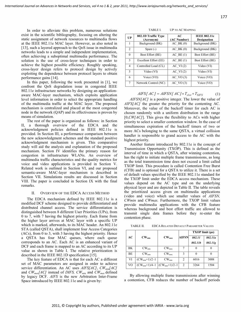
In order to alleviate this problem, numerous solutions exist in the scientific bibliography, focusing on altering the static assignment of network resources to multimedia flows at the IEEE 802.11e MAC layer. However, as also noted in [13], such a layered approach to the QoS issue in multimedia networks leads to a simple and independent implementation, often achieving a suboptimal multimedia performance. The solution is the use of cross-layer techniques in order to achieve the highest possible efficiency. Roughly speaking, cross-layer design refers to protocol design by actively exploiting the dependence between protocol layers to obtain performance gains [14].
In this paper, following the work presented in [1], we confront the QoS degradation issue in congested IEEE 802.11e infrastructure networks by designing an application-aware MAC-layer mechanism, which exploits application level information in order to select the appropriate handling of the multimedia traffic at the MAC layer. The proposed mechanism is centralized and placed at the most congested node in the network (QAP) and its effectiveness is proven by means of simulation.
The rest of the paper is organized as follows: in Section II, a thorough overview of the EDCA and the acknowledgment policies defined in IEEE 802.11e is provided. In Section III, a performance comparison between the new acknowledgment schemes and the standard positive acknowledgment mechanism is given. This comparative study will aid the analysis and explanation of the proposed mechanism. Section IV identifies the primary reason for congestion in infrastructure WLANs. An overview of multimedia traffic characteristics and the quality metrics for voice and video applications is provided in Section V. Related work is outlined in Section VI, and our proposed semantic-aware MAC-layer mechanism is described in Section VII. Simulations results are discussed in Section VIII. The paper is concluded in Section IX with the final remarks.
II. OVERVIEW OF THE EDCA ACCESS METHOD
The EDCA mechanism defined by IEEE 802.11e is a modified DCF scheme designed to provide differentiated and distributed channel access. The service differentiation is distinguished between 8 different User Priorities (UPs), from 0 to 7, with 7 having the highest priority. Each frame from the higher layer arrives at MAC layer with a specific UP which is marked, afterwards, to its MAC header. An 802.11e STA (called QSTA), shall implement four Access Categories (ACs), from 0 to 3, with 3 having the highest priority. Hence a QSTA has four MAC queues, where each queue corresponds to an AC. Each AC is an enhanced variant of DCF and each frame is mapped to an AC according to its UP value as shown in Table I. The relative prioritization is described in the IEEE 802.1D specification [15].
The key feature of EDCA is that for each AC a different set of MAC parameters are assigned in order to achieve service differentiation. An AC uses AIFS[AC], CWmin[AC] and CWmax[AC] instead of DIFS, CWmin and CWmax defined by legacy DCF. AIFS is the new Arbitration Inter-Frame Space introduced by IEEE 802.11e and is given by:
TABLE I. UP TO AC MAPPING
UP 802.1D Traffic Type
(Acronym)
AC
(AC Number)
IEEE 802.11e
Designation
1 Background (BK) AC_BK (0) Background (BK)
2 Spare (-) AC_BK (0) Background (BK)
0 Best Effort (BE) AC_BE (1) Best Effort (BE)
3 Excellent Effort (EE) AC_BE (1) Best Effort (BE)
4 Controlled Load (CL) AC_VI (2) Video (VI)
5 Video (VI) AC_VI (2) Video (VI)
6 Voice (VO) AC_VO (3) Voice (VO)
7 Network Control (NC) AC_VO (3) Voice (VO)
SIFSslot TT]AC[AIFSN]AC[AIFS (1)
AIFSN[AC] is a positive integer. The lower the value of
AIFS[AC] the greater the priority for the contenting AC.
Moreover, the value of the backoff timer for each AC is
chosen randomly with a uniform distribution in the range
[0,CW[AC]]. This gives the flexibility to ACs with higher
priority to select a smaller contention window. In the case of
simultaneous expiration of the backoff timers of two or
more ACs belonging to the same QSTA, a virtual collision
handler is responsible to grand access to the AC with the
highest priority. Another feature introduced by 802.11e is the concept of
Transmission Opportunity (TXOP). This is defined as the interval of time in which a QSTA, after winning contention, has the right to initiate multiple frame transmissions, as long as the total transmission time does not exceed a limit called TXOP limit. This procedure is called Contention Free Burst (CFB) and is optional for a QSTA to utilize it. There is a set of default values specified by the IEEE 802.11e standard for the TXOP limit under the EDCA access mechanism. These values depend on the AC type and on the underlying physical layer and are depicted in Table II. The table reveals the prioritized access given on multimedia applications (video and voice) which use smaller values of AIFSN, CWmin and CWmax. Furthermore, the TXOP limit values provide multimedia applications with the CFB feature whereas background and best effort traffic are allowed to transmit single data frames before they re-enter the contention phase.
TABLE II. EDCA RELATED DEFAULT PARAMETER VALUES
AC CWmin CWmax AIFSN
TXOP limit (μs)
802.11
802.11b
802.11a
802.11g
BK CWmin CWmax 7 0 0
BE CWmin CWmax 3 0 0
VI (CWmin+1)/2–1 CWmin 2 6016 3008
VO (CWmin+1)/4–1 (CWmin+1)/2–1 2 3264 1504
By allowing multiple frame transmissions after winning
a contention, CFB reduces the number of backoff periods
177
International Journal on Advances in Networks and Services, vol 4 no 1 & 2, year 2011, http://www.iariajournals.org/networks_and_services/
2011, © Copyright by authors, Published under agreement with IARIA - www.iaria.org
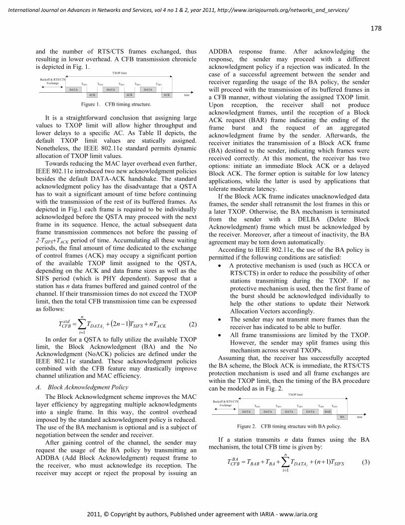
and the number of RTS/CTS frames exchanged, thus
resulting in lower overhead. A CFB transmission chronicle
is depicted in Fig. 1.
DATA
ACK
DATA
ACK
DATA
ACK
TSIFS TSIFS TSIFS TSIFS TSIFS
Backoff & RTS/CTS
Exchange
TXOP limit
time Figure 1. CFB timing structure.
It is a straightforward conclusion that assigning large
values to TXOP limit will allow higher throughput and
lower delays to a specific AC. As Table II depicts, the
default TXOP limit values are statically assigned.
Nonetheless, the IEEE 802.11e standard permits dynamic
allocation of TXOP limit values.
Towards reducing the MAC layer overhead even further,
IEEE 802.11e introduced two new acknowledgment policies
besides the default DATA-ACK handshake. The standard
acknowledgment policy has the disadvantage that a QSTA
has to wait a significant amount of time before continuing
with the transmission of the rest of its buffered frames. As
depicted in Fig.1 each frame is required to be individually
acknowledged before the QSTA may proceed with the next
frame in its sequence. Hence, the actual subsequent data
frame transmission commences not before the passing of
2TSIFSTACK period of time. Accumulating all these waiting
periods, the final amount of time dedicated to the exchange
of control frames (ACK) may occupy a significant portion
of the available TXOP limit assigned to the QSTA,
depending on the ACK and data frame sizes as well as the
SIFS period (which is PHY dependent). Suppose that a
station has n data frames buffered and gained control of the
channel. If their transmission times do not exceed the TXOP
limit, then the total CFB transmission time can be expressed
as follows:
ACKSIFS
n
i
DATAstdCFB nTTnTT
i
12
1
(2)
In order for a QSTA to fully utilize the available TXOP limit, the Block Acknowledgment (BA) and the No Acknowledgment (NoACK) policies are defined under the IEEE 802.11e standard. These acknowledgment policies combined with the CFB feature may drastically improve channel utilization and MAC efficiency.
A. Block Acknowledgment Policy
The Block Acknowledgment scheme improves the MAC
layer efficiency by aggregating multiple acknowledgments
into a single frame. In this way, the control overhead
imposed by the standard acknowledgment policy is reduced.
The use of the BA mechanism is optional and is a subject of
negotiation between the sender and receiver.
After gaining control of the channel, the sender may
request the usage of the BA policy by transmitting an
ADDBA (Add Block Acknowledgment) request frame to
the receiver, who must acknowledge its reception. The
receiver may accept or reject the proposal by issuing an
ADDBA response frame. After acknowledging the
response, the sender may proceed with a different
acknowledgment policy if a rejection was indicated. In the
case of a successful agreement between the sender and
receiver regarding the usage of the BA policy, the sender
will proceed with the transmission of its buffered frames in
a CFB manner, without violating the assigned TXOP limit.
Upon reception, the receiver shall not produce
acknowledgment frames, until the reception of a Block
ACK request (BAR) frame indicating the ending of the
frame burst and the request of an aggregated
acknowledgment frame by the sender. Afterwards, the
receiver initiates the transmission of a Block ACK frame
(BA) destined to the sender, indicating which frames were
received correctly. At this moment, the receiver has two
options: initiate an immediate Block ACK or a delayed
Block ACK. The former option is suitable for low latency
applications, while the latter is used by applications that
tolerate moderate latency.
If the Block ACK frame indicates unacknowledged data
frames, the sender shall retransmit the lost frames in this or
a later TXOP. Otherwise, the BA mechanism is terminated
from the sender with a DELBA (Delete Block
Acknowledgment) frame which must be acknowledged by
the receiver. Moreover, after a timeout of inactivity, the BA
agreement may be torn down automatically.
According to IEEE 802.11e, the use of the BA policy is
permitted if the following conditions are satisfied:
A protective mechanism is used (such as HCCA or
RTS/CTS) in order to reduce the possibility of other
stations transmitting during the TXOP. If no
protective mechanism is used, then the first frame of
the burst should be acknowledged individually to
help the other stations to update their Network
Allocation Vectors accordingly.
The sender may not transmit more frames than the
receiver has indicated to be able to buffer.
All frame transmissions are limited by the TXOP.
However, the sender may split frames using this
mechanism across several TXOPs.
Assuming that, the receiver has successfully accepted
the BA scheme, the Block ACK is immediate, the RTS/CTS
protection mechanism is used and all frame exchanges are
within the TXOP limit, then the timing of the BA procedure
can be modeled as in Fig. 2.
DATA DATA BARDATA
BA
TSIFS TSIFS TSIFS TSIFS
Backoff & RTS/CTS
Exchange
TXOP limit
time
DATA
TSIFS
Figure 2. CFB timing structure with BA policy.
If a station transmits n data frames using the BA mechanism, the total CFB time is given by:
SIFS
n
i
DATABABARBACFB TnTTTT
i)( 1
1
(3)
178
International Journal on Advances in Networks and Services, vol 4 no 1 & 2, year 2011, http://www.iariajournals.org/networks_and_services/
2011, © Copyright by authors, Published under agreement with IARIA - www.iaria.org
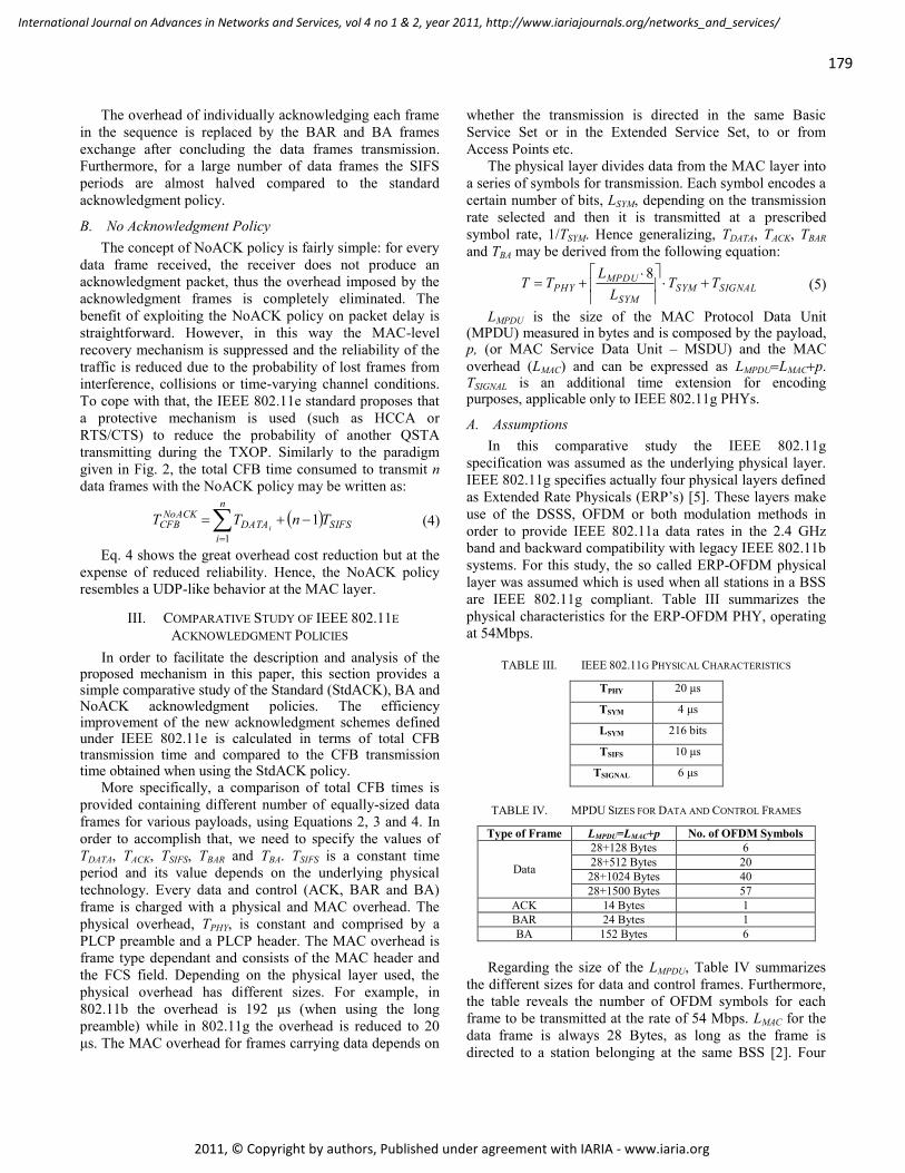
The overhead of individually acknowledging each frame
in the sequence is replaced by the BAR and BA frames
exchange after concluding the data frames transmission.
Furthermore, for a large number of data frames the SIFS
periods are almost halved compared to the standard
acknowledgment policy.
B. No Acknowledgment Policy
The concept of NoACK policy is fairly simple: for every
data frame received, the receiver does not produce an
acknowledgment packet, thus the overhead imposed by the
acknowledgment frames is completely eliminated. The
benefit of exploiting the NoACK policy on packet delay is
straightforward. However, in this way the MAC-level
recovery mechanism is suppressed and the reliability of the
traffic is reduced due to the probability of lost frames from
interference, collisions or time-varying channel conditions.
To cope with that, the IEEE 802.11e standard proposes that
a protective mechanism is used (such as HCCA or
RTS/CTS) to reduce the probability of another QSTA
transmitting during the TXOP. Similarly to the paradigm
given in Fig. 2, the total CFB time consumed to transmit n
data frames with the NoACK policy may be written as:
SIFSn
i
DATANoACKCFB TnTT
i1
1
(4)
Eq. 4 shows the great overhead cost reduction but at the
expense of reduced reliability. Hence, the NoACK policy
resembles a UDP-like behavior at the MAC layer.
III. COMPARATIVE STUDY OF IEEE 802.11E
ACKNOWLEDGMENT POLICIES
In order to facilitate the description and analysis of the proposed mechanism in this paper, this section provides a simple comparative study of the Standard (StdACK), BA and NoACK acknowledgment policies. The efficiency improvement of the new acknowledgment schemes defined under IEEE 802.11e is calculated in terms of total CFB transmission time and compared to the CFB transmission time obtained when using the StdACK policy.
More specifically, a comparison of total CFB times is
provided containing different number of equally-sized data
frames for various payloads, using Equations 2, 3 and 4. In
order to accomplish that, we need to specify the values of
TDATA, TACK, TSIFS, TBAR and TBA. TSIFS is a constant time
period and its value depends on the underlying physical
technology. Every data and control (ACK, BAR and BA)
frame is charged with a physical and MAC overhead. The
physical overhead, TPHY, is constant and comprised by a
PLCP preamble and a PLCP header. The MAC overhead is
frame type dependant and consists of the MAC header and
the FCS field. Depending on the physical layer used, the
physical overhead has different sizes. For example, in
802.11b the overhead is 192 μs (when using the long
preamble) while in 802.11g the overhead is reduced to 20
μs. The MAC overhead for frames carrying data depends on
whether the transmission is directed in the same Basic
Service Set or in the Extended Service Set, to or from
Access Points etc.
The physical layer divides data from the MAC layer into
a series of symbols for transmission. Each symbol encodes a
certain number of bits, LSYM, depending on the transmission
rate selected and then it is transmitted at a prescribed
symbol rate, 1/TSYM. Hence generalizing, TDATA, TACK, TBAR
and TBA may be derived from the following equation:
SIGNALSYMSYM
MPDUPHY TT
L
LTT
8 (5)
LMPDU is the size of the MAC Protocol Data Unit (MPDU) measured in bytes and is composed by the payload, p, (or MAC Service Data Unit – MSDU) and the MAC
overhead (LMAC) and can be expressed as LMPDULMACp. TSIGNAL is an additional time extension for encoding purposes, applicable only to IEEE 802.11g PHYs.
A. Assumptions
In this comparative study the IEEE 802.11g
specification was assumed as the underlying physical layer.
IEEE 802.11g specifies actually four physical layers defined
as Extended Rate Physicals (ERP’s) [5]. These layers make
use of the DSSS, OFDM or both modulation methods in
order to provide IEEE 802.11a data rates in the 2.4 GHz
band and backward compatibility with legacy IEEE 802.11b
systems. For this study, the so called ERP-OFDM physical
layer was assumed which is used when all stations in a BSS
are IEEE 802.11g compliant. Table III summarizes the
physical characteristics for the ERP-OFDM PHY, operating
at 54Mbps.
TABLE III. IEEE 802.11G PHYSICAL CHARACTERISTICS
TPHY 20 μs
TSYM 4 μs
LSYM 216 bits
TSIFS 10 μs
TSIGNAL 6 μs
TABLE IV. MPDU SIZES FOR DATA AND CONTROL FRAMES
Type of Frame LMPDU=LMAC+p No. of OFDM Symbols
Data
28+128 Bytes 6
28+512 Bytes 20
28+1024 Bytes 40
28+1500 Bytes 57
ACK 14 Bytes 1
BAR 24 Bytes 1
BA 152 Bytes 6
Regarding the size of the LMPDU, Table IV summarizes
the different sizes for data and control frames. Furthermore,
the table reveals the number of OFDM symbols for each
frame to be transmitted at the rate of 54 Mbps. LMAC for the
data frame is always 28 Bytes, as long as the frame is
directed to a station belonging at the same BSS [2]. Four
179
International Journal on Advances in Networks and Services, vol 4 no 1 & 2, year 2011, http://www.iariajournals.org/networks_and_services/
2011, © Copyright by authors, Published under agreement with IARIA - www.iaria.org
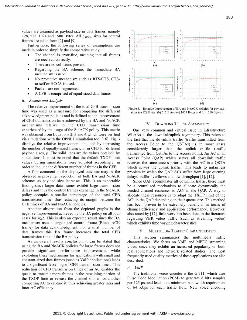
values are assumed as payload size in data frames, namely
128, 512, 1024 and 1500 Bytes. All LMPDU sizes for control
frames are taken from [2] and [9].
Furthermore, the following series of assumptions are
made in order to simplify the comparative study:
The channel is error-free, meaning that all frames
are received correctly.
There are no collisions present.
Regarding the BA scheme, the immediate BA
mechanism is used.
No protective mechanism such as RTS/CTS, CTS-
to-self or HCCA is used.
Packets are not fragmented.
A CFB is comprised of equal-sized data frames.
B. Results and Analysis
The relative improvement of the total CFB transmission
time was used as a measure for comparing the different
acknowledgment policies and is defined as the improvement
of CFB transmission time achieved by the BA and NoACK
mechanisms relative to the CFB transmission time
experienced by the usage of the StdACK policy. This metric
was obtained from Equations 2, 3 and 4 which were verified
via simulations with the OPNET simulation tool [16]. Fig. 3
displays the relative improvement obtained by increasing
the number of equally-sized frames, n, in CFB for different
payload sizes, p. The solid lines are the values obtained by
simulations. It must be noted that the default TXOP limit
values during simulations were adjusted accordingly, in
order to include the different number of frames in the CFB.
A first comment on the displayed outcome may be the
observed improvement reduction of both BA and NoACK
schemes as payload size increases. This is an expectable
finding since larger data frames exhibit large transmission
delays and thus the control frames exchange in the StdACK
policy occupies a smaller percentage of the total CFB
transmission time, thus reducing its margin between the
CFB times of BA and NoACK policies.
Another observation from the depicted graphs is the
negative improvement achieved by the BA policy on all four
cases for n≤2. This is also an expected result since the BA
mechanism uses a large-sized control frame (Block ACK
frame) for data acknowledgment. For a small number of
data frames this BA frame increases the total CFB
transmission time of the BA policy.
As an overall results conclusion, it can be stated that
using the BA and NoACK policies for large frames does not
provide significant performance improvement, while
exploiting these mechanisms for applications with small and
constant-sized data frames (such as VoIP applications) leads
to a significant lessening of CFB transmission times. This
reduction of CFB transmission times of an AC enables the
queue to transmit more frames in the remaining portion of
the TXOP limit or release the channel sooner for another
competing AC to capture it, thus achieving greater intra and
inter-AC efficiency.
(a) (b)
(c) (d)
Figure 3. Relative Improvement of BA and NoACK policies for payload
sizes (a) 128 Bytes, (b) 512 Bytes, (c) 1024 Bytes and (d) 1500 Bytes.
IV. DOWNLINK/UPLINK ASYMMETRY
One very common and critical issue in infrastructure
WLANs is the downlink/uplink asymmetry. This refers to
the fact that the downlink traffic (traffic transmitted from
the Access Point to the QSTAs) is in most cases
considerably larger than the uplink traffic (traffic
transmitted from QSTAs to the Access Point). An AC in an
Access Point (QAP) which serves all downlink traffic
receives the same access priority with the AC in a QSTA
which serves the uplink traffic. This leads to unfairness
problem in which the QAP ACs suffer from large queuing
delays, buffer overflows and low throughput [1], [12].
Since QAP accumulates all downlink traffic, there must
be a centralized mechanism to allocate dynamically the
needed channel resources to ACs in the QAP. A way to
allocate these resources is to adapt the TXOP limit of the
ACs in the QAP depending on their queue size. This method
has been proven to be extremely beneficial in terms of
channel efficiency and application performance. However,
also noted by [17], little work has been done in the literature
regarding VBR video traffic (such as streaming video)
which exhibits time varying characteristics.
V. MULTIMEDIA TRAFFIC CHARACTERISTICS
This section summarizes the multimedia traffic
characteristics. We focus on VoIP and MPEG streaming
video, since they exhibit an increased popularity on both
real applications and network related studies. The most
frequently used quality metrics of these applications are also
described.
A. VoIP
The traditional voice encoder is the G.711, which uses
Pulse Code Modulation (PCM) to generate 8 bits samples
per 125 μs, and leads to a minimum bandwidth requirement
of 64 Kbps for each traffic flow. New voice encoding
180
International Journal on Advances in Networks and Services, vol 4 no 1 & 2, year 2011, http://www.iariajournals.org/networks_and_services/
2011, © Copyright by authors, Published under agreement with IARIA - www.iaria.org
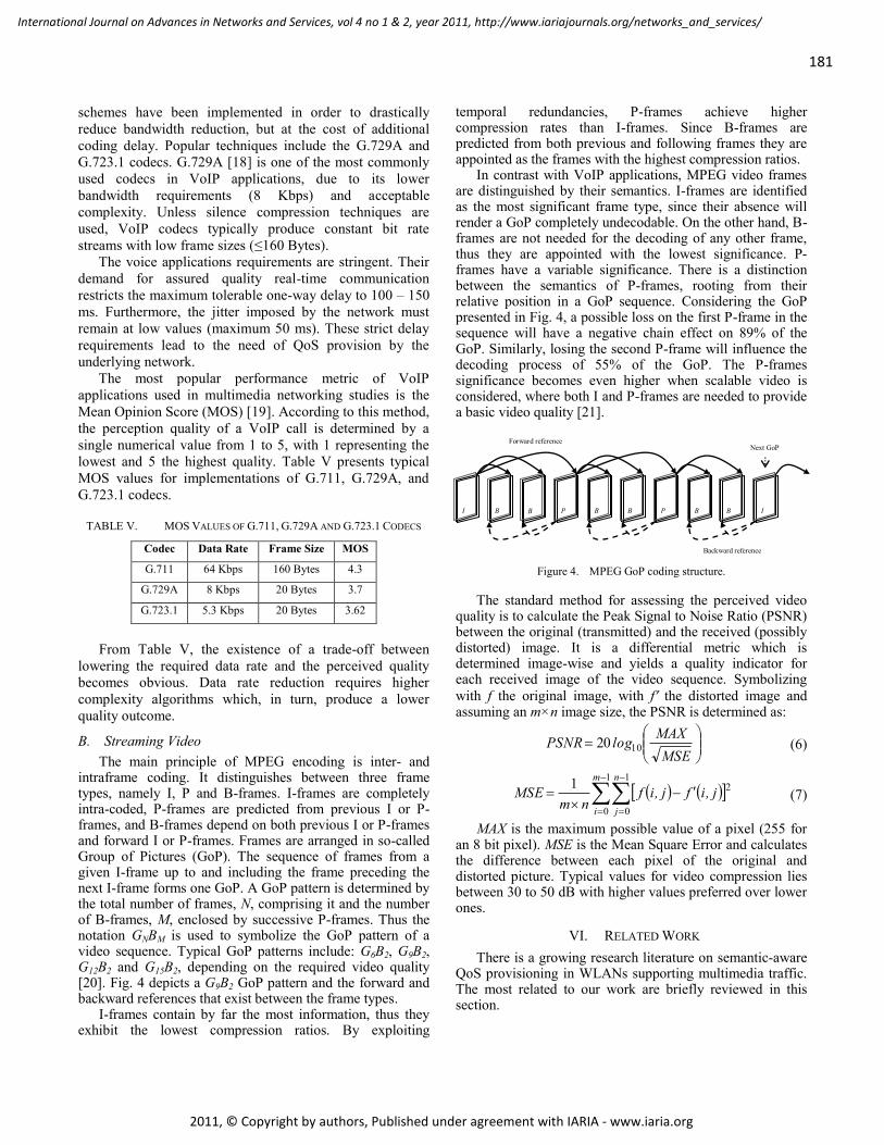
schemes have been implemented in order to drastically
reduce bandwidth reduction, but at the cost of additional
coding delay. Popular techniques include the G.729A and
G.723.1 codecs. G.729A [18] is one of the most commonly
used codecs in VoIP applications, due to its lower
bandwidth requirements (8 Kbps) and acceptable
complexity. Unless silence compression techniques are
used, VoIP codecs typically produce constant bit rate
streams with low frame sizes (≤160 Bytes).
The voice applications requirements are stringent. Their
demand for assured quality real-time communication
restricts the maximum tolerable one-way delay to 100 – 150
ms. Furthermore, the jitter imposed by the network must
remain at low values (maximum 50 ms). These strict delay
requirements lead to the need of QoS provision by the
underlying network.
The most popular performance metric of VoIP
applications used in multimedia networking studies is the
Mean Opinion Score (MOS) [19]. According to this method,
the perception quality of a VoIP call is determined by a
single numerical value from 1 to 5, with 1 representing the
lowest and 5 the highest quality. Table V presents typical
MOS values for implementations of G.711, G.729A, and
G.723.1 codecs.
TABLE V. MOS VALUES OF G.711, G.729A AND G.723.1 CODECS
Codec Data Rate Frame Size MOS
G.711 64 Kbps 160 Bytes 4.3
G.729A 8 Kbps 20 Bytes 3.7
G.723.1 5.3 Kbps 20 Bytes 3.62
From Table V, the existence of a trade-off between
lowering the required data rate and the perceived quality
becomes obvious. Data rate reduction requires higher
complexity algorithms which, in turn, produce a lower
quality outcome.
B. Streaming Video
The main principle of MPEG encoding is inter- and intraframe coding. It distinguishes between three frame types, namely I, P and B-frames. I-frames are completely intra-coded, P-frames are predicted from previous I or P-frames, and B-frames depend on both previous I or P-frames and forward I or P-frames. Frames are arranged in so-called Group of Pictures (GoP). The sequence of frames from a given I-frame up to and including the frame preceding the next I-frame forms one GoP. A GoP pattern is determined by the total number of frames, N, comprising it and the number of B-frames, M, enclosed by successive P-frames. Thus the notation GNBM is used to symbolize the GoP pattern of a video sequence. Typical GoP patterns include: G6B2, G9B2, G12B2 and G15B2, depending on the required video quality [20]. Fig. 4 depicts a G9B2 GoP pattern and the forward and backward references that exist between the frame types.
I-frames contain by far the most information, thus they exhibit the lowest compression ratios. By exploiting
temporal redundancies, P-frames achieve higher compression rates than I-frames. Since B-frames are predicted from both previous and following frames they are appointed as the frames with the highest compression ratios.
In contrast with VoIP applications, MPEG video frames are distinguished by their semantics. I-frames are identified as the most significant frame type, since their absence will render a GoP completely undecodable. On the other hand, B-frames are not needed for the decoding of any other frame, thus they are appointed with the lowest significance. P-frames have a variable significance. There is a distinction between the semantics of P-frames, rooting from their relative position in a GoP sequence. Considering the GoP presented in Fig. 4, a possible loss on the first P-frame in the sequence will have a negative chain effect on 89% of the GoP. Similarly, losing the second P-frame will influence the decoding process of 55% of the GoP. The P-frames significance becomes even higher when scalable video is considered, where both I and P-frames are needed to provide a basic video quality [21].
Figure 4. MPEG GoP coding structure.
The standard method for assessing the perceived video quality is to calculate the Peak Signal to Noise Ratio (PSNR) between the original (transmitted) and the received (possibly distorted) image. It is a differential metric which is determined image-wise and yields a quality indicator for each received image of the video sequence. Symbolizing
with f the original image, with f the distorted image and assuming an m×n image size, the PSNR is determined as:
MSE
MAXlogPSNR 1020 (6)
1
0
1
0
21m
i
n
j
j,ifj,ifnm
MSE
(7)
MAX is the maximum possible value of a pixel (255 for an 8 bit pixel). MSE is the Mean Square Error and calculates the difference between each pixel of the original and distorted picture. Typical values for video compression lies between 30 to 50 dB with higher values preferred over lower ones.
VI. RELATED WORK
There is a growing research literature on semantic-aware QoS provisioning in WLANs supporting multimedia traffic. The most related to our work are briefly reviewed in this section.
Forward reference
I B B P B B P B B I
Backward reference
Next GoP
181
International Journal on Advances in Networks and Services, vol 4 no 1 & 2, year 2011, http://www.iariajournals.org/networks_and_services/
2011, © Copyright by authors, Published under agreement with IARIA - www.iaria.org
In [22], Ksentini et al. propose a QoS cross-layer architecture based on both application and MAC layer features for improving H.264 video transmission over IEEE 802.11e networks. The mechanism relies on a data partitioning technique at the application layer and an appropriate QoS mapping at the IEEE 802.11e MAC layer. More specifically, the authors map the application layer video generated slices to appropriate ACs at the MAC layer according to their significance. AC_VO, AC_VI and AC_BE are used for this purpose while AC_BK is left for serving all other traffic. Furthermore, the retry count parameter at the MAC layer is exploited to unequally protect the high priority information against lower significance frames.
The semantic-aware mechanism presented in [23], follows a similar approach for MPEG-4 video transmission in IEEE 802.11e networks. This scheme introduced a single-video multilevel queue by assigning I-frames to AC_VO, P-frames to AC_VI, B-frames to AC_BE and non-video frames to AC_BK.
In [24], the authors follow a different approach on cross-layer design for H.264 video traffic transmission. At first, they determine the significance of a video frame by using a method called first order estimation. According to this method, the PSNR of all packets in the video sequence is determined by intentionally dropping selected frames. Thus, a frame is more important when its PSNR value is lower. Afterwards, the packets are placed to ACs in the MAC layer according to the access waiting time of an AC and its priority. Hence, the AC with the lowest waiting time is selected for serving a particular video packet.
In [25], Goel and Sarkar propose a mechanism that resides in the interface between LLC and MAC layers to provide QoS for streaming video traffic. The essence of this scheme is to mark I-frames of a video sequence as the Most Valuable Video Packet (MVVP) and en-queue these frames to a higher priority queue called Video Friendly Queue (VFQ) in the interface between LLC and MAC layers. Other frames are en-queued in the so-called Interface Queue (IFQ) and receive FIFO treatment. Whenever frames need to be send to the MAC layer the VFQ receives priority against IFQ. In this way, preferential treatment is provided to MVVP frames ensuring that they get highest priority which minimizes delay.
In [26], a dynamic mapping algorithm of MPEG-4 video frames is proposed. According to this algorithm, the video frames are allocated to ACs according to their significance and network load. When the size of AC_VI reaches a certain threshold, the newly arrived frame is mapped to a lower priority AC (AC_BK or AC_BE). The choice of the AC is determined by the frame significance.
It is clear that the entire semantic-aware mechanisms presented, exploit a mapping technique to allocate video frames to ACs either statically [22], [23], [25] or dynamically [24], [26]. However, with the exception of [26], they disregard the QoS issues of VoIP traffic by allocating voice frames to ACs with lower priority or mixing them with video traffic.
Furthermore, MAC-layer mechanisms, such as dynamic TXOP limit tuning and acknowledgment policies, are left
completely unexploited. The usage of MAC-layer strategies may improve the system efficiency, and thus multimedia application performance, dramatically.
VII. THE PROPOSED SCHEME
Extending the work presented in [1], we propose a semantic-aware MAC-layer mechanism that falls into the cross-layer mechanisms category. The proposed scheme exploits multimedia frame semantics to decide an appropriate MAC-layer strategy for handling these frames. The mechanism is centralized and intends to improve EDCA performance at the QAP in times of congestion. Furthermore, only the functionality of multimedia ACs is affected, leaving the rest of the ACs (AC_BK and AC_BE) uninfluenced.
The essence of the proposed algorithm is to map multimedia frames into AC_VI or AC_VO according to their significance. To this direction, two categories of multimedia frames are introduced: High Priority Multimedia Frames (HPMF) and Low Priority Multimedia Frames (LPMF). I and P video frames are indicated as high significance frames and tagged as HPMFs, while B-frames and voice packets as LPMFs. Every category is linked to a specific AC: HPMF to AC_VO and LPMF to AC_VI. Such a distinction among the multimedia frames can easily be accomplished by manipulating the UP of the multimedia frame:
If UP of packet i (4, 5, 6)
If UP of packet i = 4||5 && packet_type (I, P)
UP of packet i 6 ElseIf UP of packet i = 6
UP of packet i 4
At this point, the appropriate MAC-layer strategy must be selected for both AC_VI and AC_VO. HPMFs belonging to AC_VO, are treated with the maximum protection by using the standard acknowledgment policy. However, regarding the high sizes of these frames, we apply a TXOP limit adaptation algorithm, ensuring the periodical relaxation of this queue.
The TXOP limit adaptation algorithm for the AC_VO traffic class is calculated every Service Interval (SI) which is defined as the time between the start of two subsequent TXOPs. At the beginning of the SI the actual queue length is calculated and the average frame size of all packets contained is determined. Then the TXOP limit is computed as the time needed to successfully transmit the en-queued frames:
frameTNlimitTXOP ×=_ (8)
where N is the number of frames contained in the AC_VO
queue at the start of the SI and Tframe the successful frame
transmission time with the average payload size L. The
Tframe is computed as:
SIFSACKLframe T(r)T(r)TT (9)
where TL(r) and TACK(r) are the transmission times of the
data and acknowledgment frames respectively for a specific
182
International Journal on Advances in Networks and Services, vol 4 no 1 & 2, year 2011, http://www.iariajournals.org/networks_and_services/
2011, © Copyright by authors, Published under agreement with IARIA - www.iaria.org
PHY data rate r and accounting PHY and MAC overhead.
TSIFS is the Short Inter-frame Space. Eq. 9 does not contain
any contention waiting periods (AIFS and backoff time)
since at the start of the SI the contention is already won by
the AC_VO.
Regarding the AC_VI queue, which holds all the LPMF
frames, we propose that no TXOP limit adaptation takes
place, in order to keep complexity as low as possible.
However, taking into consideration the low significance of
B-frames, the loss tolerance of voice frames and the low
sizes of the LPMFs (compared to HPMFs), we propose the
usage of the NoACK scheme as the acknowledgment policy
of this queue. By doing so, we aim at the reduction of the
transmission times of LPMFs (as described in Section III) at
the cost of an increased loss probability. Nevertheless, in
congested networks the usage of this policy is beneficial in
retaining medium quality voice calls, as noted in [27].
Furthermore, the loss of B-frames is acceptable, to a certain
degree, since their absence will not significantly reduce the
video quality.
VIII. SIMULATIONS AND RESULTS
In order to evaluate the proposed algorithm the OPNET
network simulator was used [16]. In this section we provide
a description of the simulation scenarios after which the
results that were obtained are analyzed and explained.
A. Setup
We considered an infrastructure IEEE 802.11e network
with a QAP and four QSTAs in the QBSS. Eight G.729A
(20-Bytes frames transmitted every 20ms) encoded VoIP
streams (UP6) were traversing the network: four in the
downlink direction and four in the uplink direction. Four
MPEG-4 streaming video flows (UP4) were destined to the
QSTAs from the wireline network. Finally, two HTTP
connections (UP0) were representing best effort traffic.
The real video trace “Highway”, available from [28], was
used as the transmitted video sequence. The trace was
encoded in MPEG-4 CIF (Common Intermediate Format)
with a GoP pattern G9B2 (IBBPBBPBB), 2000 frames,
frame rate of 30 frames per second and 67 seconds duration.
The video sequence exhibits a mean bit rate of 0.41 Mbps
and a peak bit rate of 1.89 Mbps.
The wireless channel was assumed to be error-free,
hence no packets were lost due to fading effects. The PHY
data rate was set to 11 Mbps. There were three simulation
scenarios: the first scenario applies standard EDCA default
values as depicted in Table II, the second applies an
implementation of a cross-layer mechanism similar to [25]
(named Cross), and the third scenario implements the
modified version of EDCA according to the proposed
algorithm. The Cross implementation allocates I-frames to
AC_VO, while all other multimedia frames (P, B video
frames and voice frames) are served by the lower priority
AC_VI.
All scenarios had a total simulation time of 120 sec. The starting times of each application with respect to the starting time of simulation run are depicted in Table VI.
TABLE VI. APPLICATION TIMING CHARACTERISTICS
Application Start Time
(sec) Stop Time
(sec) Duration
(sec)
VoIP 5 105 100
Video Streaming
15 80 65
HTTP 7 End of Simulation 113
As depicted in Table VI, for 65 seconds all applications
coexist in the network, creating a highly congested period at
the QAP.
To compare the EDCA performance obtained by all
three scenarios, four performance metrics were considered:
overall network application-level throughput (goodput),
overall network application-level end-to-end delay, average
PSNR for video streaming and MOS for VoIP applications.
B. Simulation Results and Analysis
Fig. 5 shows the overall network application-level
throughput (goodput) in packets/sec for both VoIP and
video streaming applications. The video streaming
application enjoys a large improvement in throughput
performance as show casted in Fig. 5(a). The overall
goodput is almost leveled at 120 packets/sec (for all four
video streams) while both the standard EDCA and the
implemented Cross-layer scheme exhibit a significant
performance degradation due to congestion at the QAP. As
far as VoIP goodput is concerned (Fig. 5(b)), looking
carefully at the graph one can observe that during the
presence of the four video flows, VoIP performance for
standard EDCA and Cross exhibits large oscillations while
the proposed algorithm produces a smoother graph.
Analyzing the overall application level end-to-end delay,
Fig. 6(a) and (b) reveal a significant improvement on the
packet delay that both multimedia applications receive.
Specifically, the VoIP application, that has strict delay
requirements, receives better QoS by applying the proposed
algorithm. Video packet delay oscillates well below the
delay produced by the other schemes as depicted in Fig.
6(a).
Finally, all the benefits of applying the proposed
algorithm are revealed from Fig. 7(a) and (b), where the
average PSNR of streaming video and the MOS values for
VoIP applications are plotted. The majority of PSNR values
are well above 35 dB, indicating an excellent quality of the
received video streams. Regarding the VoIP applications,
both the EDCA and the Cross schemes are outperformed by
the proposed algorithm with acceptable MOS values for
downstream calls.
As an overall simulation results conclusion, it can be
stated that the proposed algorithm clearly produces a
significant EDCA performance improvement. The
exploitation of the multimedia packet semantics combined
183
International Journal on Advances in Networks and Services, vol 4 no 1 & 2, year 2011, http://www.iariajournals.org/networks_and_services/
2011, © Copyright by authors, Published under agreement with IARIA - www.iaria.org
with the appropriate MAC-layer enhancements is capable of
dealing with high congestion periods in infrastructure IEEE
802.11e WLANs.
IX. CONCLUSIONS
This paper addresses the challenge of transporting
multimedia traffic over IEEE 802.11e congested WLANs.
The multimedia frame semantics are exploited to select an
appropriate MAC-layer strategy. A TXOP limit adaptation
scheme is used together with acknowledgment policies in
order to relax the ACs in the congested QAP, and at the
same time protect high significance multimedia frames. The
proposed semantic-aware algorithm is proven extremely
beneficial in terms of application level throughput, end-to-
end delay and QoS metrics for video and voice applications.
REFERENCES
[1] A. Politis, I. Mavridis and A. Manitsaris, “Enhancing Multimedia Traffic Performance in IEEE 802.11e Networks”, in Proc. of the Sixth International Conference in Wireless and Mobile Communications (ICWMC 2010), IEEE Press, Valencia, Spain, pp. 125-130, September 2010.
[2] ISO/IEC and IEEE Std., “Part11: Wireless LAN Medium Access Control (MAC) and Physical Layer (PHY) specifications”, 1999.
[3] IEEE Std. 802.11a, “High-Speed Physical Layer in the 5 GHz Band”, 1999.
[4] IEEE Std. 802.11b, “Higher-Speed Physical Layer (PHY) Extension in the 2.4 GHz Band”, 1999.
[5] IEEE Std. 802.11g, “Further Higher-Speed Physical Layer Extension in the 2.4 GHz Band”, 2003.
[6] F. Cali, M. Conti, and E. Gregori, “IEEE 802.11 Protocol: Design and Performance Evaluation of an Adaptive Backoff Mechanism”, IEEE Journal on Selected Areas in Communications, Vol. 18, No. 3, pp. 1776–1784, 2000.
[7] N. Vaidya, P. Bahl, and S. Gupta, “Distributed Fair Scheduling in a Wireless LAN”, in Proc. Sixth Annual International Conference on Mobile Computing and Networking (MOBICOM), Boston, MA, pp. 167-178, 2000.
[8] J. Sobrinho and A. Krishnakumar, “Quality-of-Service in Ad hoc Carrier Sense Multiple Access Networks”, IEEE Journal on Selected Areas in Communications, Vol. 17, No. 8, pp. 1353–1368, 1999.
[9] IEEE Std. 802.11e, “Part 11: Wireless LAN Medium Access Control (MAC) and Physical Layer (PHY) specifications, Amendment 8: Medium Access Control (MAC) Quality of Service Enhancements”, 2005.
[10] IEEE Std. 802.11n, “Enhancements for Higher Throughput”, 2009.
[11] M. M. Rashid, E. Hossain, V. K. Bhargava, “Controlled Channel Access Scheduling for Guaranteed QoS in 802.11e-Based WLANs”, IEEE Transactions on Wireless Communications, Vol. 7, No.4, pp. 1287-1297, 2008.
[12] A. Andreadis and R. Zambon, “QoS Enhancement for Multimedia Traffics with Dynamic TXOPlimit in IEEE 802.11e”, in Proc. of the 18th IEEE International Symposium in Personal, Indoor and Mobile Radio Communications (PIMRC 07), Athens, Greece, pp. 16-22, 2007.
[13] Μ. van der Schaar and D. Sai Shankar, “Cross-layer wireless multimedia transmission: Challenges, principles and new paradigms”, IEEE wireless Communications, Vol. 12, No. 4, pp. 50- 58, 2005.
[14] C. Bouras, A. Gkamas and G. Kioumourtzis, “Challenges in Cross Layer Adaptation for Multimedia Transmission”, in Proc. of the IADIS International Conference Wireless Applications and Computing 2007, Lisbon, Portugal, pp. 129 – 133, 2007.
[15] IEEE Std 802.1D “IEEE Standard for Local and Metropolitan Area Networks: Media Access Control (MAC) Bridges”, Revised version, 2004.
[16] OPNET Technologies Inc., http://www.opnet.com, accessed 13/1/2011.
[17] H. Liu and Y. Zhao, “Adaptive EDCA Algorithm Using Video Prediction for Multimedia IEEE 802.11e WLAN”, in Proc. of the 2nd International Conference on Wireless and Mobile Communications (ICWMC), Bucharest, Romania, 2006.
[18] ITU-T Annex A to Recommendation G.729, “Coding of Speech at 8 Kbit/s using Conjugate Structure Algebraic-Code-Excited Linear Prediction (CS-CELP)”, November 1996.
[19] ITU-T Recommendation P.800, “Methods for subjective determination of transmission quality”, 1996.
[20] A. Lazaris, P. Koutsakis and M. Paterakis, “A new model for video traffic originating from multiplexed MPEG-4 videoconference streams”, Performance Evaluation, Vol. 65, No. 1, pp. 51-70, 2008.
[21] P. Seeling, M. Reisslein and B. Kulapala, “Network Performance Evaluation Using Frame Size and Quality Traces of Single-Layer and Two-Layer Video: A Tutorial”, IEEE Communications Surveys and Tutorials, Vol.6, No.2, pp. 58-78, Third Quarter 2004.
[22] A. Ksentini, M. Naimi and A. Gueroui, “Toward an improvement of H.264 video transmission over IEEE 802.11e through a cross-layer architecture”, IEEE Commun. Mag., Vol. 44, No. 1, pp.107-114, January 2006.
[23] A. M. Jama, S. Issa and O. O. Khalifa, “Performance evaluation of MPEG-4 video transmission over IEEE 802.11e”, IJCNS, Vol. 2, No. 5, pp. 11-15, May 2010.
[24] C.-H. Mai, Y.-C. Huang and H.-Y. Wei, “Cross-Layer Adaptive H.264/AVC Streaming over IEEE 802.11e Experimental Testbed”, in Proc. of the 71st IEEE Conference on Vehicular Technology (VTC 2010), Taipei, Taiwan, May 2010.
[25] R. Goel and M. Sarkar, “Enhancing QoS of streaming videos over WLANs”, in Proc. of IAENG WCECS ’08, Berkeley, California, 2008.
[26] C.-H. Ke, C.-H. Lin, C.-K. Shieh, N. Chilamkurti and S. Zeadally, "A Novel Cross-Layer Architecture for MPEG-4 Video Stream over IEEE 802.11e Wireless Network", in Special Issue of International Journal of Telecommunications Systems (SPRINGER), Vol. 42, No. 3-4, December 2009.
[27] J. Barcelo, B. Bellalta, A. Sfairopoulou, C. Cano, M. Oliver, “No Ack in IEEE 802.11e single-hop ad-hoc VoIP networks”, in Proc. of MED-HOC-NET ‘08, Mallorca, Spain, 2008.
[28] Video Traces Research Group, http://trace.eas.asu.edu/, accessed 13/1/2011.
184
International Journal on Advances in Networks and Services, vol 4 no 1 & 2, year 2011, http://www.iariajournals.org/networks_and_services/
2011, © Copyright by authors, Published under agreement with IARIA - www.iaria.org
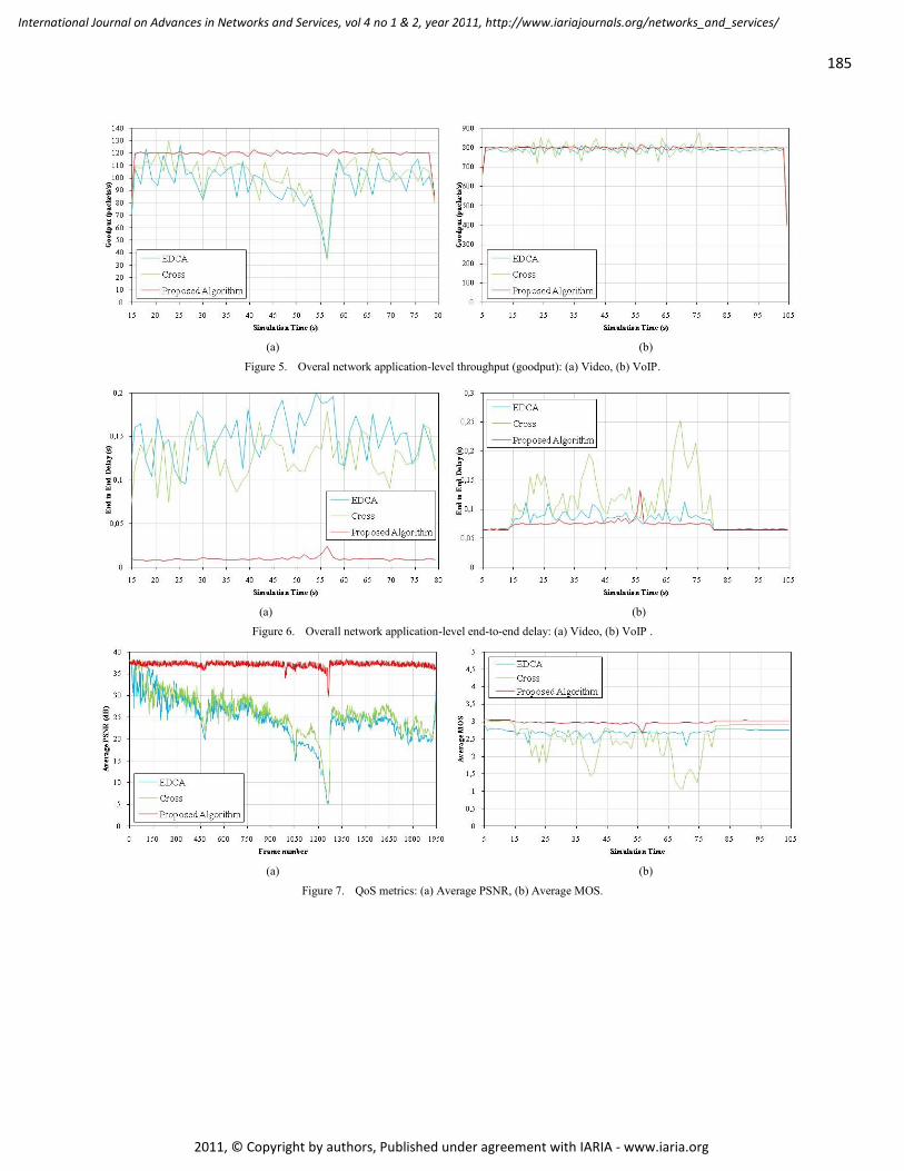
(a) (b)
Figure 5. Overal network application-level throughput (goodput): (a) Video, (b) VoIP.
(a) (b)
Figure 6. Overall network application-level end-to-end delay: (a) Video, (b) VoIP .
(a) (b)
Figure 7. QoS metrics: (a) Average PSNR, (b) Average MOS.
185
International Journal on Advances in Networks and Services, vol 4 no 1 & 2, year 2011, http://www.iariajournals.org/networks_and_services/
2011, © Copyright by authors, Published under agreement with IARIA - www.iaria.org
AAODV/AAOMDV Routing Protocols: Single and Multipath Routing in WMNs
Horia Ştefănescu
POLITEHNICA University of Bucharest
Orange Romania
Bucharest, Romania
Mariusz Skrocki, Sławomir Kukliński
Orange Labs, Telekomunikacja Polska
Warsaw University of Technology
Warsaw, Poland
mariusz.skrocki, [email protected]
Abstract—This paper consists of two parts. In the first part, we
propose a new routing protocol, named Adaptive Ad hoc On-
Demand Distance Vector (AAODV). It is able to establish
routes using any per link calculated routing metric, due to its
ability to separate the monitoring of the quality of the paths
from the routing mechanisms. By using AAODV, the following
widely used metrics: hop count, delay, jitter and Expected
Transmission Count (ETX) are compared using ns-3
simulations performed in eight randomly generated topologies
with different traffic patterns. The results have shown that in
the case of random topologies none of the routing metrics used
provides significantly better results than the other one. In the
second part of our work, the AAODV functionality is enhanced
by adding multipath routing and end-to-end Real-Time
Monitoring (RTM) of the paths. The new improved protocol is
named Adaptive Ad hoc On-Demand Multipath Distance
Vector (AAOMDV). AAOMDV provides multiple paths
between source and destination nodes, therefore it is
mandatory to implement an algorithm that selects the
preferred path and switches the traffic on it when this is
expected. Our simulations performed in ns-3 provide an inside
look into AAOMDV functionality and prove that AAOMDV is
able to enhance network performance when the network load increases.
Keywords-AODV; AAODV; AAOMDV; multipath; routing
metrics; Wireless Mesh Networks
I. INTRODUCTION
The scope of this paper is to analyze and to propose new solutions to overcome some of the routing challenges that appear in Wireless Mesh Networks (WMNs). Typically, the WMNs are based on single path, single metric and single radio. In this paper we will focus on the influence of the new concepts, such as: real-time WMN monitoring, multi-parametric metrics and adaptive path selection in multipath routing.
Our work is composed of two parts. In the first part, we propose a new routing protocol, called AAODV [1], which is based on the well-known Ad hoc On-Demand Distance Vector (AODV) protocol [2]. The main innovation of AAODV is that it can be implemented with any kind of per link calculated routing metric. The routing metrics are used during the routing table building phase in order to select the best path in the network. The impact of AAODV routing metric type on the network performance has been verified by
extensive simulations. In order to obtain generic results, eight randomly generated topologies with random background traffic were used in the simulations. In each simulated case, we monitored Packet Loss Ratio (PLR), delay and jitter of the source traffic, and the results were averaged accordingly.
In the second part of this paper, the Adaptive Ad hoc On-Demand Multipath Distance Vector (AAOMDV) is presented. AAOMDV is the AAODV protocol extended by the multipath routing and real-time path monitoring that is used for the selection of data forwarding path. The end-to-end path monitoring functions are realized by the specially designed component of the routing architecture, named Real-Time Monitoring (RTM). The RTM simultaneously monitors PLR, delay and jitter of the path. To monitor the active path, the RTM uses traffic packets. For all other paths, called inactive paths, probe messages, of size similar to the traffic packets, are sent to evaluate their quality. This way, RTM provides the real values of PLR, delay and jitter of the active paths and just an estimate of delay and jitter values for the inactive paths. Note that for the inactive paths, RTM does not evaluate the PLR value.
The behavior of AAOMDV has been verified by simulations. The results have shown that the AAOMDV protocol combined with the algorithms for path selection and switching increases the network performance in terms of PLR, delay and jitter; thus providing a better user experience. In the simulation scenarios, we used random topologies and considered different traffic patterns. The simulations were performed using ns-3 [3]. The AODV protocol was used as a benchmark.
The paper is structured as follows. This section describes the research motivation and introduces the proposed concept. Section II presents the related work. In Section III, the AAODV protocol is described, whereas Section IV shows the results of the AAODV simulation. Section V describes AAOMDV, the algorithm for discovering multiple link disjoint paths and the RTM implementation. Section VI presents in detail the algorithm applied for the best path selection in the multipath case. In Section VII, an approach used for active path switching is described. In Section VIII AAOMDV simulation results are presented. We conclude this paper in Section IX.
186
International Journal on Advances in Networks and Services, vol 4 no 1 & 2, year 2011, http://www.iariajournals.org/networks_and_services/
2011, © Copyright by authors, Published under agreement with IARIA - www.iaria.org
II. RELATED WORK
It has been shown that the practical performance of a WMN differs from the simulated one [4]. This is the reason for which some modifications of the original protocols have been proposed in the WMN implementations. In [5], a test-WMN (ReMESH) based on Optimized Link State Routing (OLSR) protocol combined with a modified ETX metric (in fact the Minimum Packet Loss Ratio parameter) is proposed. The authors have shown that in comparison to the original OLSR, the performance of the mesh network was improved, leading to more stable routes, lower packet loss rates, smaller delays, and in many cases a small increase in the network throughput. In [6], another test-WMN, called RoofNET, is described. RoofNET is based on a routing protocol named SrcRR that tries to maximize the throughput of the paths. The results presented in both previously cited papers were obtained in a real environment.
In WMNs, the routing metrics greatly impact the network performance. As it has been proved, they should also consider physical layer phenomena, like SINR, interflow interferences or the so-called flow self-interferences, introduced by the hidden and exposed terminal problems [7]. Examples of the most popular WMN routing metrics include: hop count, delay, jitter and ETX. There are approaches, which take into account physical layer processes, e.g., traffic aware metrics like PPTT [8]. However, these metrics are mainly probabilistic ones and they impose quite complex cross-layer operations. It is worth mentioning that the hop count metric does not establish the path according to its actual quality. The other metrics select the routes taking into account parameters of the component links. Therefore the routing protocol adapts to the network state. Routing protocols that use more than one metric can be found in literature. An example of such a protocol is Sharp Hybrid Adaptive Routing Protocol (SHARP) [9]. In the existing approaches, there is no decoupling between the monitoring and routing. This is the reason why it is very difficult to find a comparison of the same routing protocol with different routing metrics used. Nevertheless, some comparisons exist, e.g., in [10], in which the authors compared ETX metric with hop count metric using a grid topology only. Unfortunately, the grid topology is a particular case and it cannot yield relevant results for a wide variety of WMNs. However, a lot of theoretical comparisons exist and the most complete are [11] and [12].
The common approach for routing in both wired and wireless communication systems is the single path approach. However, it has been observed that the reliability and the performance of the network may be improved when more than one path between source and destination nodes is used. There are few scenarios, in which the multipath feature is useful. The simplest one is to discover the additional paths and to use them as a backup when the main route fails (AODV-BR [13], AOMDV [14] and AODVM [15]). This way, it is not necessary to perform the route discovery procedure every time the path breaks, because another path is already available in the routing table. This is the major advantage, especially in the networks with mobile nodes.
When the multiple paths are used simultaneously [16], the traffic may be split among them on per packet or on per flow basis, enabling the load balancing. Another possibility is to replicate the data on each of the discovered paths, thus ensuring enhanced reliability. It has been shown that the improvement of multipath may be achieved only when a limited number of additional paths are kept in the routing table. According to [14] they should be limited to two or three paths, in order to avoid the existence of stale paths in the routing table. In [14] also the disjointness of the paths in the network is considered. Two paths may be either link or node disjoint. In the first case, it is acceptable for two paths to share common nodes. However, if the mutual node fails, both paths will become useless. The second option is much stricter, but at the same time it improves the reliability of the communication. The problem appears in small or sparse networks, because it may be impossible to establish node disjoint routes there.
III. AAODV
There are two main challenges for a routing protocol, i.e., finding the best path and loops avoiding. The “best path” can be defined as the path from the source to the destination that minimizes the end-to-end PLR, delay and jitter. One of the most popular protocols designed for ad-hoc networks, AODV, accomplishes only the second property by using sequence numbers in order to find loop free paths. AODV is relatively simple (see [2]). Every time a node wants to send a packet and does not know a route to the destination, it broadcasts a Route Request (RREQ) message. When any node, including the destination, receives this RREQ, it checks whether it has received a duplicate RREQ within a fixed interval of time. If such RREQ has been received, the node silently discards the newly received RREQ. During the RREQ broadcasting period, the reverse path (from the destination to the source) is established. When the destination receives a new RREQ it responds with a unicast message to the source – Route Reply (RREP). During the transmission of the RREP, the path from source to destination (the forward path) is established. Also, note that in the meantime when RREQ and RREP are sent, the intermediate nodes set their paths to the source and respectively to the destination. AODV will not always find the best path in the network, because for path selection it uses the sequence number as the first criterion and the hop count as the second one. More than one RREQ message can be sent to find a path to a given destination, what has an impact on the AODV control traffic overhead.
In order to make a metric based route selection in AODV, it is necessary that the source node receives more RREPs with the same destination sequence number as the destination sequence number already stored in its routing table. Such an approach is possible if the destination node does not change its sequence number and sends more than one RREP. This simply implies that the source should send more than one RREQ to discover the route to every destination or that more copies of the same RREQ should reach the destination via different paths. In AODV, as long as the source does not have a route to the desired destination,
187
International Journal on Advances in Networks and Services, vol 4 no 1 & 2, year 2011, http://www.iariajournals.org/networks_and_services/
2011, © Copyright by authors, Published under agreement with IARIA - www.iaria.org
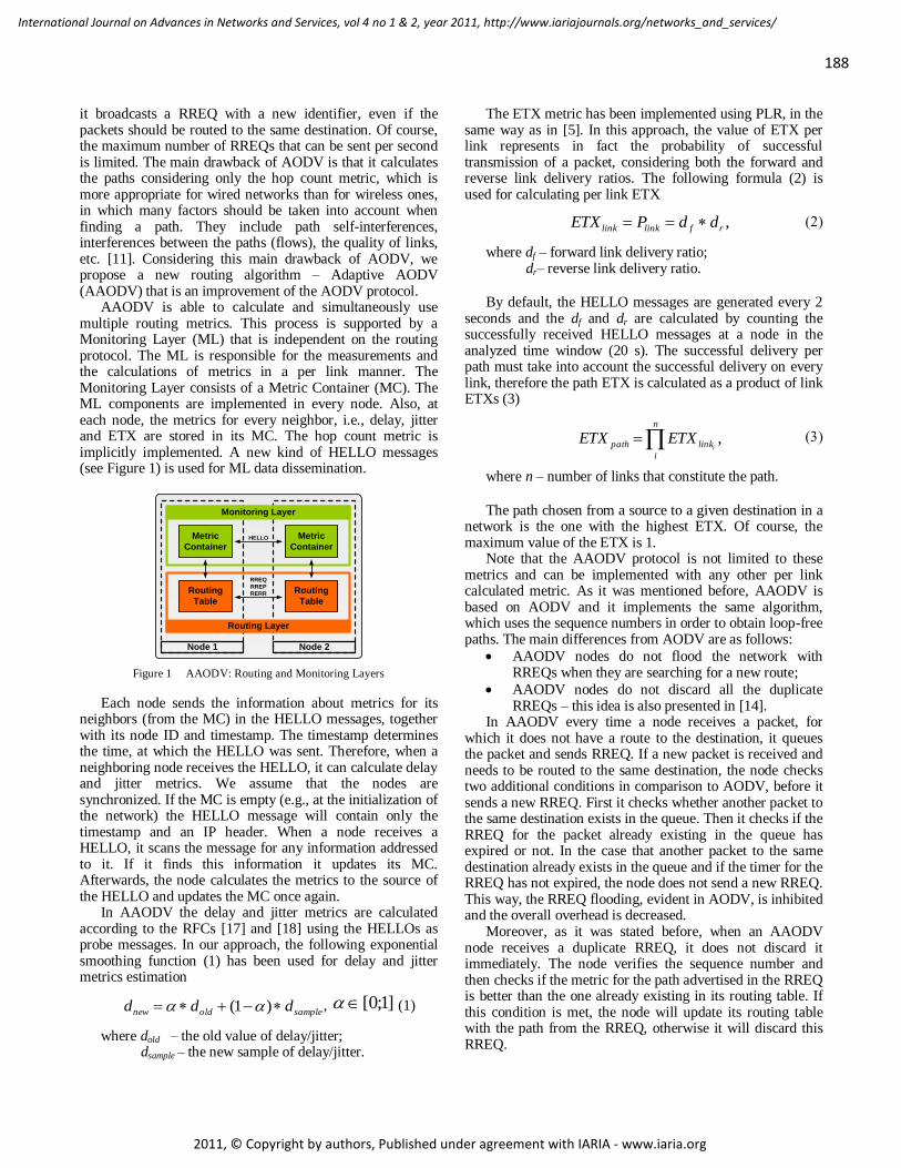
it broadcasts a RREQ with a new identifier, even if the packets should be routed to the same destination. Of course, the maximum number of RREQs that can be sent per second is limited. The main drawback of AODV is that it calculates the paths considering only the hop count metric, which is more appropriate for wired networks than for wireless ones, in which many factors should be taken into account when finding a path. They include path self-interferences, interferences between the paths (flows), the quality of links, etc. [11]. Considering this main drawback of AODV, we propose a new routing algorithm – Adaptive AODV (AAODV) that is an improvement of the AODV protocol.
AAODV is able to calculate and simultaneously use multiple routing metrics. This process is supported by a Monitoring Layer (ML) that is independent on the routing protocol. The ML is responsible for the measurements and the calculations of metrics in a per link manner. The Monitoring Layer consists of a Metric Container (MC). The ML components are implemented in every node. Also, at each node, the metrics for every neighbor, i.e., delay, jitter and ETX are stored in its MC. The hop count metric is implicitly implemented. A new kind of HELLO messages (see Figure 1) is used for ML data dissemination.
Node 1 Node 2
Monitoring Layer
Metric
Container
Metric
Container
Routing Layer
Routing
Table
Routing
Table
HELLO
RREQ
RREP
RERR
Figure 1 AAODV: Routing and Monitoring Layers
Each node sends the information about metrics for its neighbors (from the MC) in the HELLO messages, together with its node ID and timestamp. The timestamp determines the time, at which the HELLO was sent. Therefore, when a neighboring node receives the HELLO, it can calculate delay and jitter metrics. We assume that the nodes are synchronized. If the MC is empty (e.g., at the initialization of the network) the HELLO message will contain only the timestamp and an IP header. When a node receives a HELLO, it scans the message for any information addressed to it. If it finds this information it updates its MC. Afterwards, the node calculates the metrics to the source of the HELLO and updates the MC once again.
In AAODV the delay and jitter metrics are calculated according to the RFCs [17] and [18] using the HELLOs as probe messages. In our approach, the following exponential smoothing function (1) has been used for delay and jitter metrics estimation
sampleoldnew ddd )1( , ]1;0[ (1)
where dold – the old value of delay/jitter; dsample – the new sample of delay/jitter.
The ETX metric has been implemented using PLR, in the same way as in [5]. In this approach, the value of ETX per link represents in fact the probability of successful transmission of a packet, considering both the forward and reverse link delivery ratios. The following formula (2) is used for calculating per link ETX
,rflinklink ddPETX
where df – forward link delivery ratio; dr– reverse link delivery ratio.
By default, the HELLO messages are generated every 2 seconds and the df and dr are calculated by counting the successfully received HELLO messages at a node in the analyzed time window (20 s). The successful delivery per path must take into account the successful delivery on every link, therefore the path ETX is calculated as a product of link ETXs (3)
n
i
linkpath iETXETX ,
where n – number of links that constitute the path.
The path chosen from a source to a given destination in a network is the one with the highest ETX. Of course, the maximum value of the ETX is 1.
Note that the AAODV protocol is not limited to these metrics and can be implemented with any other per link calculated metric. As it was mentioned before, AAODV is based on AODV and it implements the same algorithm, which uses the sequence numbers in order to obtain loop-free paths. The main differences from AODV are as follows:
AAODV nodes do not flood the network with RREQs when they are searching for a new route;
AAODV nodes do not discard all the duplicate RREQs – this idea is also presented in [14].
In AAODV every time a node receives a packet, for which it does not have a route to the destination, it queues the packet and sends RREQ. If a new packet is received and needs to be routed to the same destination, the node checks two additional conditions in comparison to AODV, before it sends a new RREQ. First it checks whether another packet to the same destination exists in the queue. Then it checks if the RREQ for the packet already existing in the queue has expired or not. In the case that another packet to the same destination already exists in the queue and if the timer for the RREQ has not expired, the node does not send a new RREQ. This way, the RREQ flooding, evident in AODV, is inhibited and the overall overhead is decreased.
Moreover, as it was stated before, when an AAODV node receives a duplicate RREQ, it does not discard it immediately. The node verifies the sequence number and then checks if the metric for the path advertised in the RREQ is better than the one already existing in its routing table. If this condition is met, the node will update its routing table with the path from the RREQ, otherwise it will discard this RREQ.
188
International Journal on Advances in Networks and Services, vol 4 no 1 & 2, year 2011, http://www.iariajournals.org/networks_and_services/
2011, © Copyright by authors, Published under agreement with IARIA - www.iaria.org
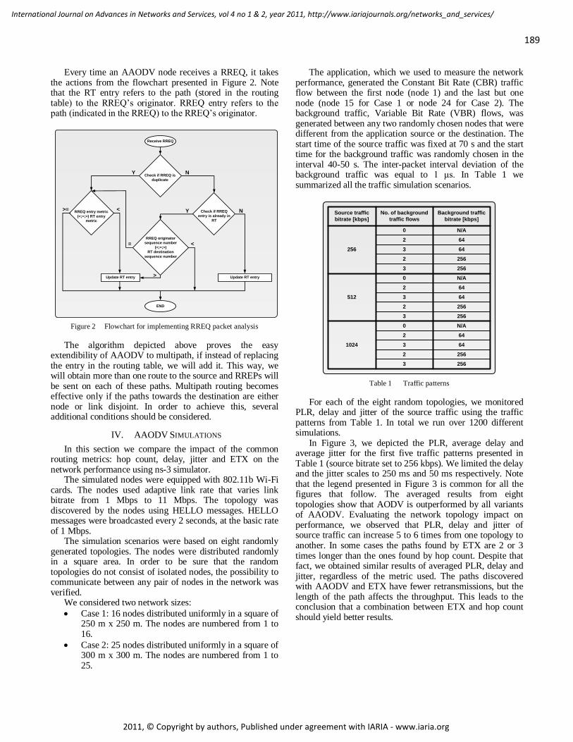
Every time an AAODV node receives a RREQ, it takes the actions from the flowchart presented in Figure 2. Note that the RT entry refers to the path (stored in the routing table) to the RREQ’s originator. RREQ entry refers to the path (indicated in the RREQ) to the RREQ’s originator.
Check if RREQ is
duplicate
Receive RREQ
Check if RREQ
entry is already in
RT
RREQ originator
sequence number
(<;=;>)
RT destination
sequence number
RREQ entry metric
(<;=;>) RT entry
metric
END
Update RT entryUpdate RT entry
NY
NY>= <
<
>
=
Figure 2 Flowchart for implementing RREQ packet analysis
The algorithm depicted above proves the easy extendibility of AAODV to multipath, if instead of replacing the entry in the routing table, we will add it. This way, we will obtain more than one route to the source and RREPs will be sent on each of these paths. Multipath routing becomes effective only if the paths towards the destination are either node or link disjoint. In order to achieve this, several additional conditions should be considered.
IV. AAODV SIMULATIONS
In this section we compare the impact of the common routing metrics: hop count, delay, jitter and ETX on the network performance using ns-3 simulator.
The simulated nodes were equipped with 802.11b Wi-Fi cards. The nodes used adaptive link rate that varies link bitrate from 1 Mbps to 11 Mbps. The topology was discovered by the nodes using HELLO messages. HELLO messages were broadcasted every 2 seconds, at the basic rate of 1 Mbps.
The simulation scenarios were based on eight randomly generated topologies. The nodes were distributed randomly in a square area. In order to be sure that the random topologies do not consist of isolated nodes, the possibility to communicate between any pair of nodes in the network was verified.
We considered two network sizes:
Case 1: 16 nodes distributed uniformly in a square of 250 m x 250 m. The nodes are numbered from 1 to 16.
Case 2: 25 nodes distributed uniformly in a square of 300 m x 300 m. The nodes are numbered from 1 to 25.
The application, which we used to measure the network performance, generated the Constant Bit Rate (CBR) traffic flow between the first node (node 1) and the last but one node (node 15 for Case 1 or node 24 for Case 2). The background traffic, Variable Bit Rate (VBR) flows, was generated between any two randomly chosen nodes that were different from the application source or the destination. The start time of the source traffic was fixed at 70 s and the start time for the background traffic was randomly chosen in the interval 40-50 s. The inter-packet interval deviation of the background traffic was equal to 1 μs. In Table 1 we summarized all the traffic simulation scenarios.
Source traffic
bitrate [kbps]
No. of background
traffic flows
Background traffic
bitrate [kbps]
256
512
1024
0
2
3
3
2
0
2
3
3
2
0
2
3
3
2
N/A
64
64
256
256
N/A
64
64
256
256
N/A
64
64
256
256
Table 1 Traffic patterns
For each of the eight random topologies, we monitored PLR, delay and jitter of the source traffic using the traffic patterns from Table 1. In total we run over 1200 different simulations.
In Figure 3, we depicted the PLR, average delay and average jitter for the first five traffic patterns presented in Table 1 (source bitrate set to 256 kbps). We limited the delay and the jitter scales to 250 ms and 50 ms respectively. Note that the legend presented in Figure 3 is common for all the figures that follow. The averaged results from eight topologies show that AODV is outperformed by all variants of AAODV. Evaluating the network topology impact on performance, we observed that PLR, delay and jitter of source traffic can increase 5 to 6 times from one topology to another. In some cases the paths found by ETX are 2 or 3 times longer than the ones found by hop count. Despite that fact, we obtained similar results of averaged PLR, delay and jitter, regardless of the metric used. The paths discovered with AAODV and ETX have fewer retransmissions, but the length of the path affects the throughput. This leads to the conclusion that a combination between ETX and hop count should yield better results.
189
International Journal on Advances in Networks and Services, vol 4 no 1 & 2, year 2011, http://www.iariajournals.org/networks_and_services/
2011, © Copyright by authors, Published under agreement with IARIA - www.iaria.org
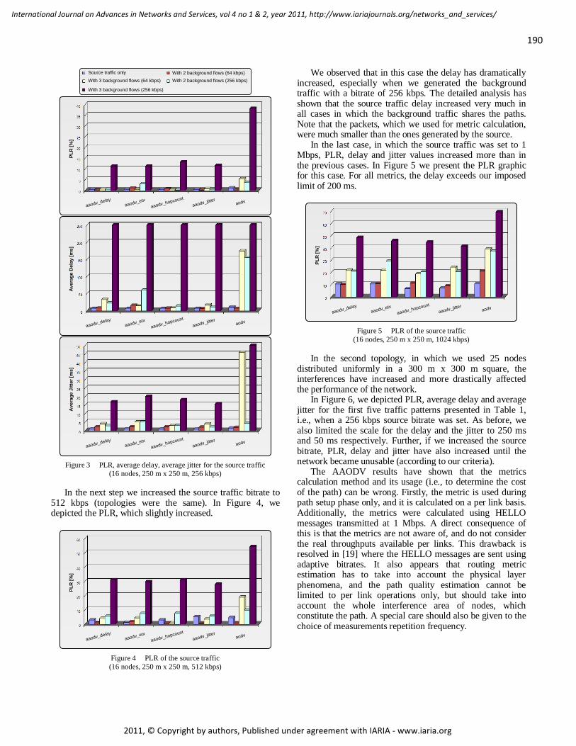
Source traffic only
With 3 background flows (64 kbps)
With 3 background flows (256 kbps)
With 2 background flows (64 kbps)
With 2 background flows (256 kbps)
PL
R [
%]
aaodv_delay
aaodv_etx
aaodv_hopcount
aaodv_jitteraodv
Av
era
ge
De
lay
[m
s]
aaodv_delay
aaodv_etx
aaodv_hopcount
aaodv_jitteraodv
Av
era
ge
Jit
ter
[ms
]
aaodv_delay
aaodv_etx
aaodv_hopcount
aaodv_jitteraodv
Figure 3 PLR, average delay, average jitter for the source traffic
(16 nodes, 250 m x 250 m, 256 kbps)
In the next step we increased the source traffic bitrate to 512 kbps (topologies were the same). In Figure 4, we depicted the PLR, which slightly increased.
PL
R [
%]
aaodv_delay
aaodv_etx
aaodv_hopcount
aaodv_jitteraodv
Figure 4 PLR of the source traffic
(16 nodes, 250 m x 250 m, 512 kbps)
We observed that in this case the delay has dramatically increased, especially when we generated the background traffic with a bitrate of 256 kbps. The detailed analysis has shown that the source traffic delay increased very much in all cases in which the background traffic shares the paths. Note that the packets, which we used for metric calculation, were much smaller than the ones generated by the source.
In the last case, in which the source traffic was set to 1 Mbps, PLR, delay and jitter values increased more than in the previous cases. In Figure 5 we present the PLR graphic for this case. For all metrics, the delay exceeds our imposed limit of 200 ms.
PL
R [
%]
aaodv_delay
aaodv_etx
aaodv_hopcount
aaodv_jitteraodv
Figure 5 PLR of the source traffic
(16 nodes, 250 m x 250 m, 1024 kbps)
In the second topology, in which we used 25 nodes distributed uniformly in a 300 m x 300 m square, the interferences have increased and more drastically affected the performance of the network.
In Figure 6, we depicted PLR, average delay and average jitter for the first five traffic patterns presented in Table 1, i.e., when a 256 kbps source bitrate was set. As before, we also limited the scale for the delay and the jitter to 250 ms and 50 ms respectively. Further, if we increased the source bitrate, PLR, delay and jitter have also increased until the network became unusable (according to our criteria).
The AAODV results have shown that the metrics calculation method and its usage (i.e., to determine the cost of the path) can be wrong. Firstly, the metric is used during path setup phase only, and it is calculated on a per link basis. Additionally, the metrics were calculated using HELLO messages transmitted at 1 Mbps. A direct consequence of this is that the metrics are not aware of, and do not consider the real throughputs available per links. This drawback is resolved in [19] where the HELLO messages are sent using adaptive bitrates. It also appears that routing metric estimation has to take into account the physical layer phenomena, and the path quality estimation cannot be limited to per link operations only, but should take into account the whole interference area of nodes, which constitute the path. A special care should also be given to the choice of measurements repetition frequency.
190
International Journal on Advances in Networks and Services, vol 4 no 1 & 2, year 2011, http://www.iariajournals.org/networks_and_services/
2011, © Copyright by authors, Published under agreement with IARIA - www.iaria.org
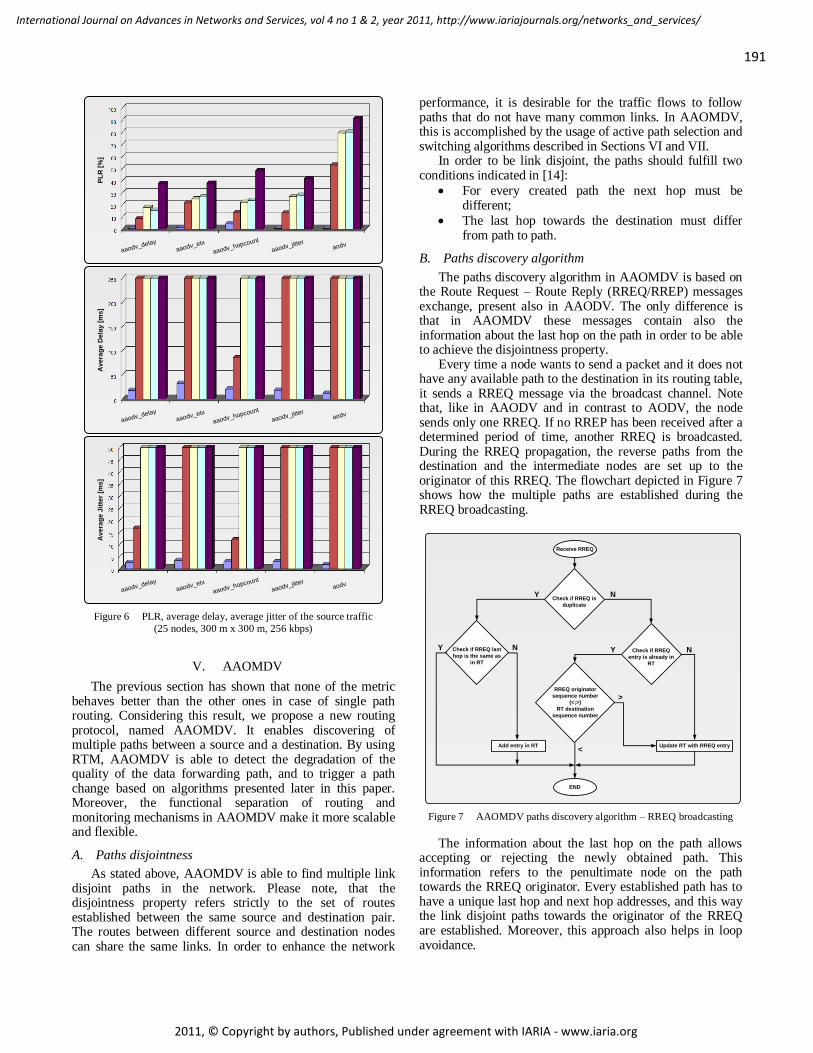
PL
R [
%]
aaodv_delay
aaodv_etx
aaodv_hopcount
aaodv_jitteraodv
Av
era
ge
De
lay
[m
s]
aaodv_delay
aaodv_etx
aaodv_hopcount
aaodv_jitteraodv
Av
era
ge
Jit
ter
[ms
]
aaodv_delay
aaodv_etx
aaodv_hopcount
aaodv_jitteraodv
Figure 6 PLR, average delay, average jitter of the source traffic
(25 nodes, 300 m x 300 m, 256 kbps)
V. AAOMDV
The previous section has shown that none of the metric behaves better than the other ones in case of single path routing. Considering this result, we propose a new routing protocol, named AAOMDV. It enables discovering of multiple paths between a source and a destination. By using RTM, AAOMDV is able to detect the degradation of the quality of the data forwarding path, and to trigger a path change based on algorithms presented later in this paper. Moreover, the functional separation of routing and monitoring mechanisms in AAOMDV make it more scalable and flexible.
A. Paths disjointness
As stated above, AAOMDV is able to find multiple link disjoint paths in the network. Please note, that the disjointness property refers strictly to the set of routes established between the same source and destination pair. The routes between different source and destination nodes can share the same links. In order to enhance the network
performance, it is desirable for the traffic flows to follow paths that do not have many common links. In AAOMDV, this is accomplished by the usage of active path selection and switching algorithms described in Sections VI and VII.
In order to be link disjoint, the paths should fulfill two conditions indicated in [14]:
For every created path the next hop must be different;
The last hop towards the destination must differ from path to path.
B. Paths discovery algorithm
The paths discovery algorithm in AAOMDV is based on the Route Request – Route Reply (RREQ/RREP) messages exchange, present also in AAODV. The only difference is that in AAOMDV these messages contain also the information about the last hop on the path in order to be able to achieve the disjointness property.
Every time a node wants to send a packet and it does not have any available path to the destination in its routing table, it sends a RREQ message via the broadcast channel. Note that, like in AAODV and in contrast to AODV, the node sends only one RREQ. If no RREP has been received after a determined period of time, another RREQ is broadcasted. During the RREQ propagation, the reverse paths from the destination and the intermediate nodes are set up to the originator of this RREQ. The flowchart depicted in Figure 7 shows how the multiple paths are established during the RREQ broadcasting.
Check if RREQ is
duplicate
Receive RREQ
Check if RREQ
entry is already in
RT
RREQ originator
sequence number
(<;>)
RT destination
sequence number
Check if RREQ last
hop is the same as
in RT
END
Update RT with RREQ entryAdd entry in RT
NY
NYY N
>
<
Figure 7 AAOMDV paths discovery algorithm – RREQ broadcasting
The information about the last hop on the path allows accepting or rejecting the newly obtained path. This information refers to the penultimate node on the path towards the RREQ originator. Every established path has to have a unique last hop and next hop addresses, and this way the link disjoint paths towards the originator of the RREQ are established. Moreover, this approach also helps in loop avoidance.
191
International Journal on Advances in Networks and Services, vol 4 no 1 & 2, year 2011, http://www.iariajournals.org/networks_and_services/
2011, © Copyright by authors, Published under agreement with IARIA - www.iaria.org
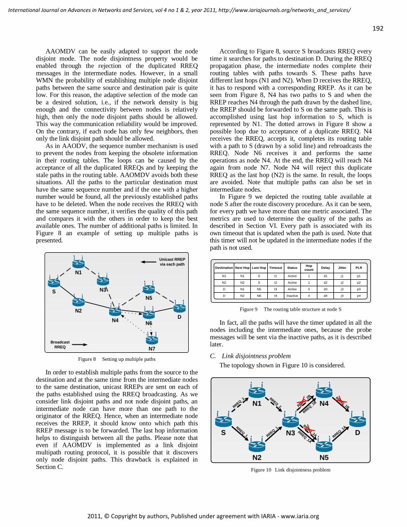
AAOMDV can be easily adapted to support the node disjoint mode. The node disjointness property would be enabled through the rejection of the duplicated RREQ messages in the intermediate nodes. However, in a small WMN the probability of establishing multiple node disjoint paths between the same source and destination pair is quite low. For this reason, the adaptive selection of the mode can be a desired solution, i.e., if the network density is big enough and the connectivity between nodes is relatively high, then only the node disjoint paths should be allowed. This way the communication reliability would be improved. On the contrary, if each node has only few neighbors, then only the link disjoint path should be allowed.
As in AAODV, the sequence number mechanism is used to prevent the nodes from keeping the obsolete information in their routing tables. The loops can be caused by the acceptance of all the duplicated RREQs and by keeping the stale paths in the routing table. AAOMDV avoids both these situations. All the paths to the particular destination must have the same sequence number and if the one with a higher number would be found, all the previously established paths have to be deleted. When the node receives the RREQ with the same sequence number, it verifies the quality of this path and compares it with the others in order to keep the best available ones. The number of additional paths is limited. In Figure 8 an example of setting up multiple paths is presented.
S
N1
N2
N3
N5
D
N7
N4N6
Broadcast
RREQ
Unicast RREP
via each path
Figure 8 Setting up multiple paths
In order to establish multiple paths from the source to the destination and at the same time from the intermediate nodes to the same destination, unicast RREPs are sent on each of the paths established using the RREQ broadcasting. As we consider link disjoint paths and not node disjoint paths, an intermediate node can have more than one path to the originator of the RREQ. Hence, when an intermediate node receives the RREP, it should know onto which path this RREP message is to be forwarded. The last hop information helps to distinguish between all the paths. Please note that even if AAOMDV is implemented as a link disjoint multipath routing protocol, it is possible that it discovers only node disjoint paths. This drawback is explained in Section C.
According to Figure 8, source S broadcasts RREQ every time it searches for paths to destination D. During the RREQ propagation phase, the intermediate nodes complete their routing tables with paths towards S. These paths have different last hops (N1 and N2). When D receives the RREQ, it has to respond with a corresponding RREP. As it can be seen from Figure 8, N4 has two paths to S and when the RREP reaches N4 through the path drawn by the dashed line, the RREP should be forwarded to S on the same path. This is accomplished using last hop information to S, which is represented by N1. The dotted arrows in Figure 8 show a possible loop due to acceptance of a duplicate RREQ. N4 receives the RREQ, accepts it, completes its routing table with a path to S (drawn by a solid line) and rebroadcasts the RREQ. Node N6 receives it and performs the same operations as node N4. At the end, the RREQ will reach N4 again from node N7. Node N4 will reject this duplicate RREQ as the last hop (N2) is the same. In result, the loops are avoided. Note that multiple paths can also be set in intermediate nodes.
In Figure 9 we depicted the routing table available at node S after the route discovery procedure. As it can be seen, for every path we have more than one metric associated. The metrics are used to determine the quality of the paths as described in Section VI. Every path is associated with its own timeout that is updated when the path is used. Note that this timer will not be updated in the intermediate nodes if the path is not used.
Destination Next Hop Last Hop Timeout Delay Jitter PLR
N1
N2
D
D N6
N5
S
S
N2
N1
N2
N1
j3
d4t4
t3 d3
j2
p1
d2t2
j1d1t1
j4 p4
p3
p2
Status
Active
Active
Active
Inactive
Hop
count
4
5
1
1
Figure 9 The routing table structure at node S
In fact, all the paths will have the timer updated in all the nodes including the intermediate ones, because the probe messages will be sent via the inactive paths, as it is described later.
C. Link disjointness problem
The topology shown in Figure 10 is considered.
S
N1
N2
N3 D
N5
N4
RREQ
_1RREQ
_1A
RREQ
_1
RREQ
_2 RREQ
_2 RREQ
_2B
RREQ
_1B
RREQ
_1A
RREQ
_1B
RREQ
_2A
Figure 10 Link disjointness problem
192
International Journal on Advances in Networks and Services, vol 4 no 1 & 2, year 2011, http://www.iariajournals.org/networks_and_services/
2011, © Copyright by authors, Published under agreement with IARIA - www.iaria.org
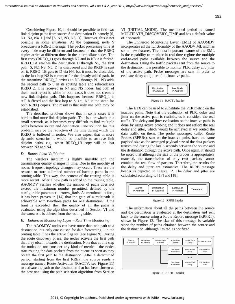
Considering Figure 10, it should be possible to find two link disjoint paths from source S to destination D, namely [S, N1, N3, N4, D] and [S, N2, N3, N5, D]. However, this is not possible in some situations. At the beginning, node S broadcasts a RREQ message. The packet processing time at every node may be different and because of that the RREQ copies arrive at different times in the intermediate nodes. The first copy (RREQ_1) goes through N2 and in N3 it is forked. RREQ_1A reaches the destination D through N5, the first path [S, N2, N3, N5, D] is discovered and the RREP is sent on it. RREQ_1B gets to D via N4, but it must be discarded, as the last hop N2 is common for the already added path. In the meantime RREQ_2 arrives to N3 through N1. N3 adds the second path to S in its routing table and rebroadcasts RREQ_2. It is received in N4 and N5 nodes, but both of them must reject it, while in both cases it does not create a new link disjoint path. This happens, because RREQ_1 is still buffered and the first hop to S, i.e., N3 is the same for both RREQ copies. The result is that only one path may be established.
The described problem shows that in some cases it is hard to find more link disjoint paths. This is a drawback in a small network, as it becomes very difficult to find multiple paths between source and destination. One solution for this problem may be the reduction of the time during which the RREQ is buffered in nodes. We also expect that in more dynamic scenarios it would be possible to achieve link disjoint paths, e.g., when RREQ_1B copy will be lost between N3 and N4.
D. Routes Limit Validation
The wireless medium is highly unstable and the transmission quality changes in time. Due to the mobility of nodes, frequent topology changes may occur. These are the reasons to store a limited number of backup paths in the routing table. This way, the content of the routing table is more recent. After a new path is added to the routing table, AAOMDV verifies whether the number of paths does not exceed the maximum number permitted, defined by the configurable parameter – routes_limit. As mentioned before, it has been proven in [14] that the gain of a multipath is achievable with two/three paths for one destination. If the limit is exceeded, then the quality of all the paths is evaluated using the algorithm described in Section VI and the worst one is deleted from the routing table.
E. Enhanced Monitoring Layer – Real Time Monitoring
The AAOMDV nodes can have more than one path to a destination, but only one is used for data forwarding – in the routing table it has the active flag set (see Figure 9). During the route discovery phase, the nodes activate the first path that they obtain towards the destination. Note that at this step the nodes do not consider any kind of metric – the nodes start routing the data packets from the queue as soon as they obtain the first path to the destination. After a determined period, starting from the first RREP, the source sends a message named Route Activation (RACTV, see Figure 11) to activate the path to the destination that has been chosen as the best one using the path selection algorithm from Section
VI (INITIAL_MODE). The mentioned period is named MULTIPATH_DISCOVERY_TIME and has a default value of 2 seconds.
The Enhanced Monitoring Layer (EML) of AAOMDV incorporates all the functionality of the AAODV ML and has some new features. The most important feature of the EML is the capability to monitor in real-time regime the multiple end-to-end paths available between the source and the destination. Using the traffic packets sent from the source to the destination, it is possible to monitor PLR, delay and jitter of the active path. Probe messages are sent in order to evaluate delay and jitter of the inactive paths.
Destination
IP Address
Last Node
IP Address
Figure 11 RACTV header
The ETX can be used to substitute the PLR metric on the inactive paths. Note that the evaluation of PLR, delay and jitter on the active path is realistic, as it considers the real traffic. The delay and jitter evaluation on the inactive paths is done by using active probing and it does not reflect the real delay and jitter, which would be achieved if we routed the data traffic on them. The probe messages, called Route Probes (RPRBs), sent on the inactive paths, have the same payload size as the averaged payload size of the data packets transmitted during the last 5 seconds between the source and the destination through the active path. Once again, it should be noted that although the size of the probes is appropriately matched, the transmission of only two packets cannot emulate the real flow of packets. Therefore, the results for the delay and jitter are estimative. The RPRB message header is depicted in Figure 12. The delay and jitter are calculated according to [17] and [18].
Source
IP Address
Destination
IP Address
Last Node
IP AddressTimestamp
Figure 12 RPRB header
The information about all the paths between the source and the destination is evaluated at the destination and sent back to the source using a Route Report message (RRPRT), shown in Figure 13. The size of this message is variable since the number of paths obtained between the source and the destination, although limited, is not fixed.
Source
IP Address
Destination
IP Address
Last Node
IP Address
Inactive Path
Delay
Inactive Paths
Counter
Active Path
Counter
Active Path
DelayActive Path Jitter
Inactive Path
Jitter
Last Node
IP Address
Inactive Path
Delay
Inactive Path
Jitter
...
Figure 13 RRPRT header
193
International Journal on Advances in Networks and Services, vol 4 no 1 & 2, year 2011, http://www.iariajournals.org/networks_and_services/
2011, © Copyright by authors, Published under agreement with IARIA - www.iaria.org
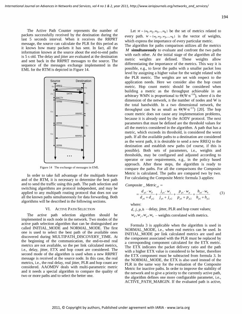
The Active Path Counter represents the number of packets successfully received by the destination during the last 5 seconds interval. When it receives the RRPRT message, the source can calculate the PLR for this period as it knows how many packets it has sent. In fact, all the information known at the source about the end-to-end paths is 5 s old. The delay and jitter are evaluated at the destination and sent back in the RRPRT messages to the source. The sequence of the messages exchange implemented in the EML for the RTM is depicted in Figure 14.
Source Destination
0 s0 s
2 s
5 s
5 s
5 s
5 s
...
RREQ
RREP
DATA
RACTV
RPRB
RRPRT
RPRB
RPRB
RRPRT
Figure 14 The exchange of messages in EML
In order to take full advantage of the multipath feature and of the RTM, it is necessary to determine the best path and to send the traffic using this path. The path selection and switching algorithms are protocol independent, and may be applied to any multipath routing protocol that does not use all the known paths simultaneously for data forwarding. Both algorithms will be described in the following sections.
VI. ACTIVE PATH SELECTION
The active path selection algorithm should be implemented in each node in the network. Two modes of the active path selection algorithm that can be distinguished are called INITIAL_MODE and NORMAL_MODE. The first one is used to select the best path of the available ones discovered during MULTIPATH_DISCOVERY_TIME. At the beginning of the communication, the end-to-end real metrics are not available, so the per link calculated metrics, i.e., delay, jitter, ETX and hop count are considered. The second mode of the algorithm is used when a new RRPRT message is received at the source node. In this case, the real metrics, i.e., the real delay, real jitter, PLR and hop count are considered. AAOMDV deals with multi-parametric metric and it needs a special algorithm to compare the quality of two or more paths and to select the better one.
Let ,...,3,2,1 kmmmmM be the set of metrics related to
every path. ,...,3,2,1 kwwwwW is the vector of weights,
which express the importance of every particular metric. The algorithm for paths comparison utilizes all the metrics
M simultaneously to evaluate and confront the two paths
with each other. At the initial stage of the algorithm all the
metric weights are defined. These weights allow
differentiating the importance of the metrics. This way it is
possible, e.g., to favor the paths with a smaller packet loss
level by assigning a higher value for the weight related with
the PLR metric. The weights are set with respect to the
application needs. Here we consider also the hop count
metric. Hop count metric should be considered when building a metric as the throughput achievable in an
arbitrary WMN is proportional to Θ(W∙n-1/d), where d is the
dimension of the network, n the number of nodes and W is
the total bandwidth. In a two dimensional network, the
throughput can be as small as Θ(W∙n-1/2) [20]. The hop
count metric does not cause any implementation problems,
because it is already used by the AODV protocol. The next
parameters that must be defined are the threshold values for
all the metrics considered in the algorithm. A path that has a
metric, which exceeds its threshold, is considered the worst
path. If all the available paths to a destination are considered
as the worst path, it is desirable to send a new RREQ to the destination and establish new paths (of course, if this is
possible). Both sets of parameters, i.e., weights and
thresholds, may be configured and adjusted according to
operator or user requirements, e.g., in the policy based
approach. After these steps, the algorithm is ready to
compare the paths. For all the comparisons the Composite
Metric is calculated. The paths are compared two by two.
For calculating the Composite Metric formula 3 applies:
1_ pMetricComposite
21
1
21
1
21
1
21
1
pp
hp
pp
pp
pp
jp
pp
dp
hh
wh
pp
wp
jj
wj
dd
wd
where:
hpjd ,,, – delay, jitter, PLR and hop count values;
hpjd wwww ,,, – weights correlated with metrics.
Formula 3 is applicable when the algorithm is used in NORMAL_MODE, i.e., when real metrics can be used. In INITIAL_MODE per link calculated metrics are used and the component associated with the PLR must be replaced by a corresponding component calculated for the ETX metric. The ETX indicates the packet delivery ratio and the path with a higher ETX value is considered to be better, therefore the ETX component must be subtracted from formula 3. In the NORMAL_MODE, the ETX is also used instead of the PLR in the same way for the evaluation of the Composite Metric for inactive paths. In order to improve the stability of the network and to give a priority to the currently active path, the algorithm defines one more configurable parameter, i.e., ACTIVE_PATH_MARGIN. If the evaluated path is active,
194
International Journal on Advances in Networks and Services, vol 4 no 1 & 2, year 2011, http://www.iariajournals.org/networks_and_services/
2011, © Copyright by authors, Published under agreement with IARIA - www.iaria.org
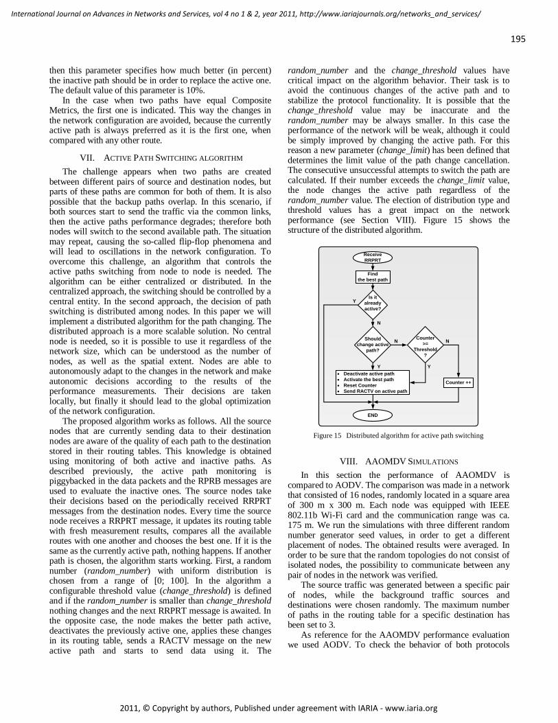
then this parameter specifies how much better (in percent) the inactive path should be in order to replace the active one. The default value of this parameter is 10%.
In the case when two paths have equal Composite Metrics, the first one is indicated. This way the changes in the network configuration are avoided, because the currently active path is always preferred as it is the first one, when compared with any other route.
VII. ACTIVE PATH SWITCHING ALGORITHM
The challenge appears when two paths are created between different pairs of source and destination nodes, but parts of these paths are common for both of them. It is also possible that the backup paths overlap. In this scenario, if both sources start to send the traffic via the common links, then the active paths performance degrades; therefore both nodes will switch to the second available path. The situation may repeat, causing the so-called flip-flop phenomena and will lead to oscillations in the network configuration. To overcome this challenge, an algorithm that controls the active paths switching from node to node is needed. The algorithm can be either centralized or distributed. In the centralized approach, the switching should be controlled by a central entity. In the second approach, the decision of path switching is distributed among nodes. In this paper we will implement a distributed algorithm for the path changing. The distributed approach is a more scalable solution. No central node is needed, so it is possible to use it regardless of the network size, which can be understood as the number of nodes, as well as the spatial extent. Nodes are able to autonomously adapt to the changes in the network and make autonomic decisions according to the results of the performance measurements. Their decisions are taken locally, but finally it should lead to the global optimization of the network configuration.
The proposed algorithm works as follows. All the source nodes that are currently sending data to their destination nodes are aware of the quality of each path to the destination stored in their routing tables. This knowledge is obtained using monitoring of both active and inactive paths. As described previously, the active path monitoring is piggybacked in the data packets and the RPRB messages are used to evaluate the inactive ones. The source nodes take their decisions based on the periodically received RRPRT messages from the destination nodes. Every time the source node receives a RRPRT message, it updates its routing table with fresh measurement results, compares all the available routes with one another and chooses the best one. If it is the same as the currently active path, nothing happens. If another path is chosen, the algorithm starts working. First, a random number (random_number) with uniform distribution is chosen from a range of [0; 100]. In the algorithm a configurable threshold value (change_threshold) is defined and if the random_number is smaller than change_threshold nothing changes and the next RRPRT message is awaited. In the opposite case, the node makes the better path active, deactivates the previously active one, applies these changes in its routing table, sends a RACTV message on the new active path and starts to send data using it. The
random_number and the change_threshold values have critical impact on the algorithm behavior. Their task is to avoid the continuous changes of the active path and to stabilize the protocol functionality. It is possible that the change_threshold value may be inaccurate and the random_number may be always smaller. In this case the performance of the network will be weak, although it could be simply improved by changing the active path. For this reason a new parameter (change_limit) has been defined that determines the limit value of the path change cancellation. The consecutive unsuccessful attempts to switch the path are calculated. If their number exceeds the change_limit value, the node changes the active path regardless of the random_number value. The election of distribution type and threshold values has a great impact on the network performance (see Section VIII). Figure 15 shows the structure of the distributed algorithm.
Receive
RRPRT
Find
the best path
Is it
already
active?
Should
change active
path?
Deactivate active path
Activate the best path
Reset Counter
Send RACTV on active path
END
Counter
>=
Threshold
?
Counter ++
Y
N
Y
N
Y
N
Figure 15 Distributed algorithm for active path switching
VIII. AAOMDV SIMULATIONS
In this section the performance of AAOMDV is compared to AODV. The comparison was made in a network that consisted of 16 nodes, randomly located in a square area of 300 m x 300 m. Each node was equipped with IEEE 802.11b Wi-Fi card and the communication range was ca. 175 m. We run the simulations with three different random number generator seed values, in order to get a different placement of nodes. The obtained results were averaged. In order to be sure that the random topologies do not consist of isolated nodes, the possibility to communicate between any pair of nodes in the network was verified.
The source traffic was generated between a specific pair of nodes, while the background traffic sources and destinations were chosen randomly. The maximum number of paths in the routing table for a specific destination has been set to 3.
As reference for the AAOMDV performance evaluation we used AODV. To check the behavior of both protocols
195
International Journal on Advances in Networks and Services, vol 4 no 1 & 2, year 2011, http://www.iariajournals.org/networks_and_services/
2011, © Copyright by authors, Published under agreement with IARIA - www.iaria.org
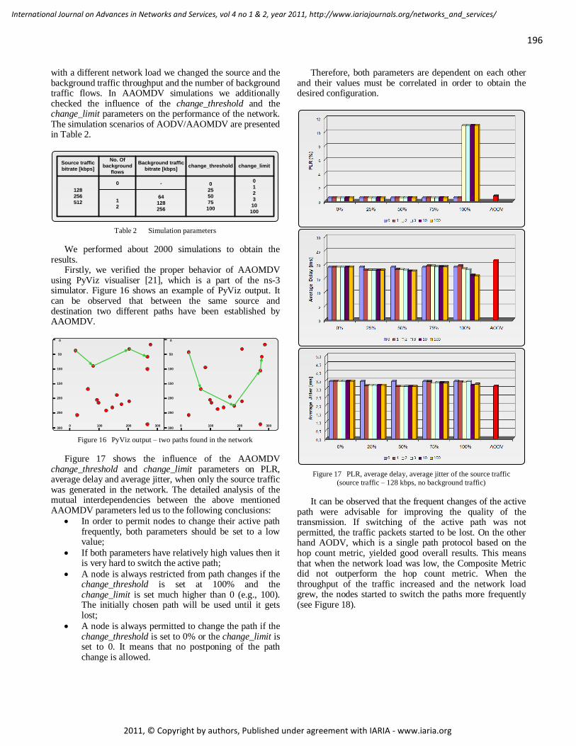
with a different network load we changed the source and the background traffic throughput and the number of background traffic flows. In AAOMDV simulations we additionally checked the influence of the change_threshold and the change_limit parameters on the performance of the network. The simulation scenarios of AODV/AAOMDV are presented in Table 2.
Source traffic
bitrate [kbps]
128
256
512
Background traffic
bitrate [kbps]change_threshold change_limit
0
25
50
75
100
0
1
2
3
10
100
0
64
128
256
No. Of
background
flows
1
2
-
Table 2 Simulation parameters
We performed about 2000 simulations to obtain the results.
Firstly, we verified the proper behavior of AAOMDV using PyViz visualiser [21], which is a part of the ns-3 simulator. Figure 16 shows an example of PyViz output. It can be observed that between the same source and destination two different paths have been established by AAOMDV.
0
50
100
150
200
250
3000 100 200 300
0
50
100
150
200
250
3000 100 200 300
Figure 16 PyViz output – two paths found in the network
Figure 17 shows the influence of the AAOMDV change_threshold and change_limit parameters on PLR, average delay and average jitter, when only the source traffic was generated in the network. The detailed analysis of the mutual interdependencies between the above mentioned AAOMDV parameters led us to the following conclusions:
In order to permit nodes to change their active path frequently, both parameters should be set to a low value;
If both parameters have relatively high values then it is very hard to switch the active path;
A node is always restricted from path changes if the change_threshold is set at 100% and the change_limit is set much higher than 0 (e.g., 100). The initially chosen path will be used until it gets lost;
A node is always permitted to change the path if the change_threshold is set to 0% or the change_limit is set to 0. It means that no postponing of the path change is allowed.
Therefore, both parameters are dependent on each other and their values must be correlated in order to obtain the desired configuration.
Figure 17 PLR, average delay, average jitter of the source traffic
(source traffic – 128 kbps, no background traffic)
It can be observed that the frequent changes of the active path were advisable for improving the quality of the transmission. If switching of the active path was not permitted, the traffic packets started to be lost. On the other hand AODV, which is a single path protocol based on the hop count metric, yielded good overall results. This means that when the network load was low, the Composite Metric did not outperform the hop count metric. When the throughput of the traffic increased and the network load grew, the nodes started to switch the paths more frequently (see Figure 18).
196
International Journal on Advances in Networks and Services, vol 4 no 1 & 2, year 2011, http://www.iariajournals.org/networks_and_services/
2011, © Copyright by authors, Published under agreement with IARIA - www.iaria.org
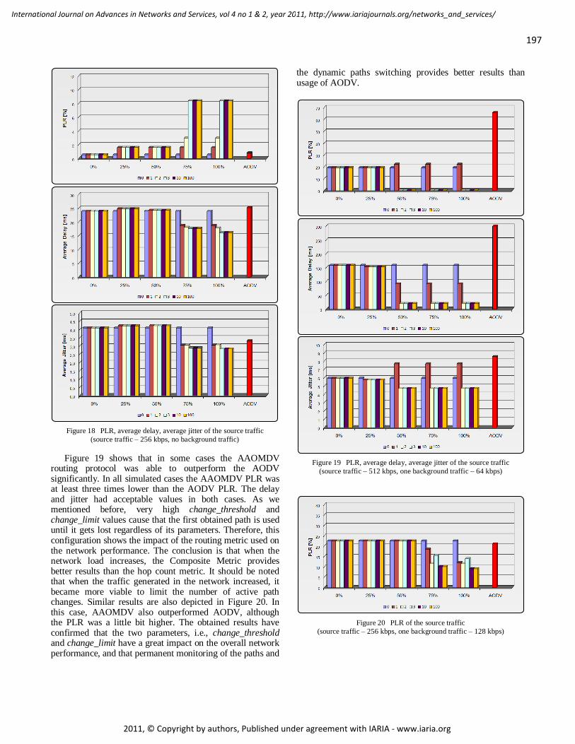
Figure 18 PLR, average delay, average jitter of the source traffic
(source traffic – 256 kbps, no background traffic)
Figure 19 shows that in some cases the AAOMDV routing protocol was able to outperform the AODV significantly. In all simulated cases the AAOMDV PLR was at least three times lower than the AODV PLR. The delay and jitter had acceptable values in both cases. As we mentioned before, very high change_threshold and change_limit values cause that the first obtained path is used until it gets lost regardless of its parameters. Therefore, this configuration shows the impact of the routing metric used on the network performance. The conclusion is that when the network load increases, the Composite Metric provides better results than the hop count metric. It should be noted that when the traffic generated in the network increased, it became more viable to limit the number of active path changes. Similar results are also depicted in Figure 20. In this case, AAOMDV also outperformed AODV, although the PLR was a little bit higher. The obtained results have confirmed that the two parameters, i.e., change_threshold and change_limit have a great impact on the overall network performance, and that permanent monitoring of the paths and
the dynamic paths switching provides better results than usage of AODV.
Figure 19 PLR, average delay, average jitter of the source traffic
(source traffic – 512 kbps, one background traffic – 64 kbps)
Figure 20 PLR of the source traffic
(source traffic – 256 kbps, one background traffic – 128 kbps)
197
International Journal on Advances in Networks and Services, vol 4 no 1 & 2, year 2011, http://www.iariajournals.org/networks_and_services/
2011, © Copyright by authors, Published under agreement with IARIA - www.iaria.org
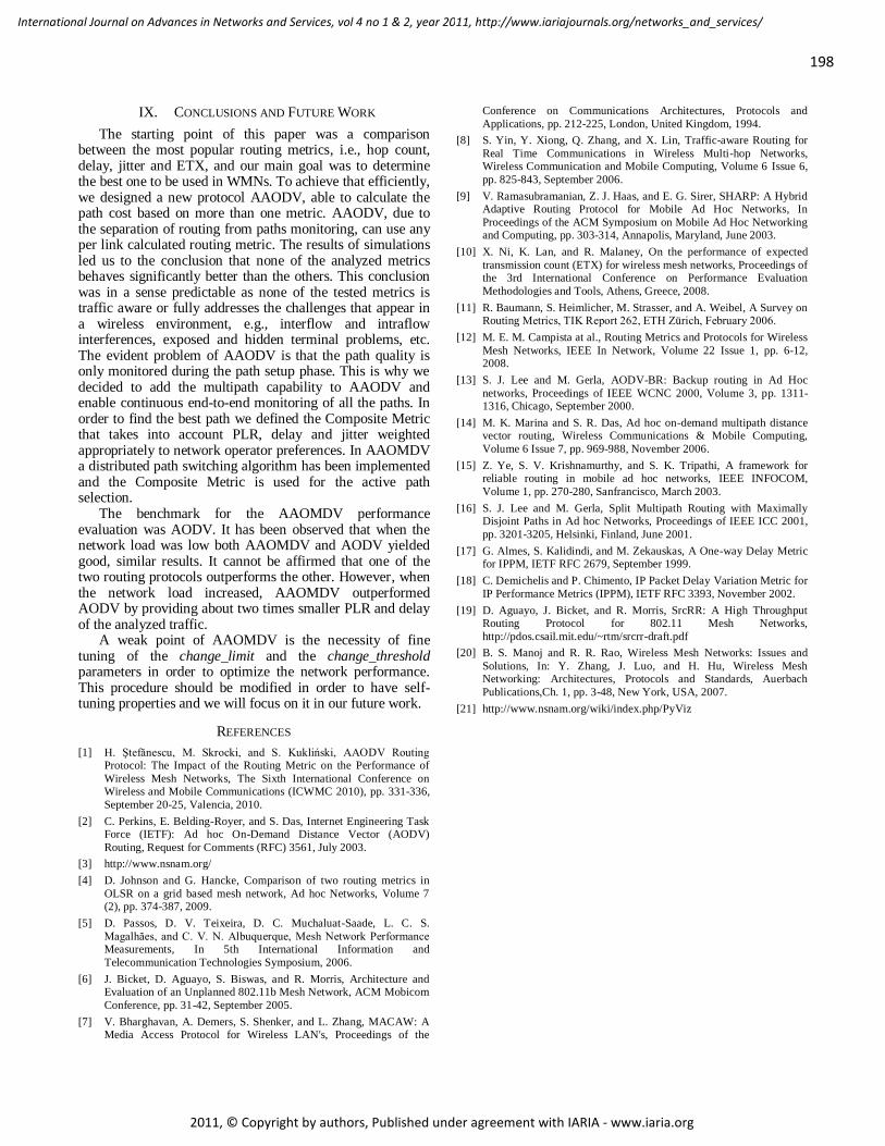
IX. CONCLUSIONS AND FUTURE WORK
The starting point of this paper was a comparison between the most popular routing metrics, i.e., hop count, delay, jitter and ETX, and our main goal was to determine the best one to be used in WMNs. To achieve that efficiently, we designed a new protocol AAODV, able to calculate the path cost based on more than one metric. AAODV, due to the separation of routing from paths monitoring, can use any per link calculated routing metric. The results of simulations led us to the conclusion that none of the analyzed metrics behaves significantly better than the others. This conclusion was in a sense predictable as none of the tested metrics is traffic aware or fully addresses the challenges that appear in a wireless environment, e.g., interflow and intraflow interferences, exposed and hidden terminal problems, etc. The evident problem of AAODV is that the path quality is only monitored during the path setup phase. This is why we decided to add the multipath capability to AAODV and enable continuous end-to-end monitoring of all the paths. In order to find the best path we defined the Composite Metric that takes into account PLR, delay and jitter weighted appropriately to network operator preferences. In AAOMDV a distributed path switching algorithm has been implemented and the Composite Metric is used for the active path selection.
The benchmark for the AAOMDV performance evaluation was AODV. It has been observed that when the network load was low both AAOMDV and AODV yielded good, similar results. It cannot be affirmed that one of the two routing protocols outperforms the other. However, when the network load increased, AAOMDV outperformed AODV by providing about two times smaller PLR and delay of the analyzed traffic.
A weak point of AAOMDV is the necessity of fine tuning of the change_limit and the change_threshold parameters in order to optimize the network performance. This procedure should be modified in order to have self-tuning properties and we will focus on it in our future work.
REFERENCES
[1] H. Ştefănescu, M. Skrocki, and S. Kukliński, AAODV Routing Protocol: The Impact of the Routing Metric on the Performance of
Wireless Mesh Networks, The Sixth International Conference on Wireless and Mobile Communications (ICWMC 2010), pp. 331-336,
September 20-25, Valencia, 2010.
[2] C. Perkins, E. Belding-Royer, and S. Das, Internet Engineering Task Force (IETF): Ad hoc On-Demand Distance Vector (AODV)
Routing, Request for Comments (RFC) 3561, July 2003.
[3] http://www.nsnam.org/
[4] D. Johnson and G. Hancke, Comparison of two routing metrics in
OLSR on a grid based mesh network, Ad hoc Networks, Volume 7 (2), pp. 374-387, 2009.
[5] D. Passos, D. V. Teixeira, D. C. Muchaluat-Saade, L. C. S.
Magalhães, and C. V. N. Albuquerque, Mesh Network Performance Measurements, In 5th International Information and
Telecommunication Technologies Symposium, 2006.
[6] J. Bicket, D. Aguayo, S. Biswas, and R. Morris, Architecture and Evaluation of an Unplanned 802.11b Mesh Network, ACM Mobicom
Conference, pp. 31-42, September 2005.
[7] V. Bharghavan, A. Demers, S. Shenker, and L. Zhang, MACAW: A Media Access Protocol for Wireless LAN's, Proceedings of the
Conference on Communications Architectures, Protocols and
Applications, pp. 212-225, London, United Kingdom, 1994.
[8] S. Yin, Y. Xiong, Q. Zhang, and X. Lin, Traffic-aware Routing for
Real Time Communications in Wireless Multi-hop Networks, Wireless Communication and Mobile Computing, Volume 6 Issue 6,
pp. 825-843, September 2006.
[9] V. Ramasubramanian, Z. J. Haas, and E. G. Sirer, SHARP: A Hybrid Adaptive Routing Protocol for Mobile Ad Hoc Networks, In
Proceedings of the ACM Symposium on Mobile Ad Hoc Networking and Computing, pp. 303-314, Annapolis, Maryland, June 2003.
[10] X. Ni, K. Lan, and R. Malaney, On the performance of expected
transmission count (ETX) for wireless mesh networks, Proceedings of the 3rd International Conference on Performance Evaluation
Methodologies and Tools, Athens, Greece, 2008.
[11] R. Baumann, S. Heimlicher, M. Strasser, and A. Weibel, A Survey on Routing Metrics, TIK Report 262, ETH Zürich, February 2006.
[12] M. E. M. Campista at al., Routing Metrics and Protocols for Wireless
Mesh Networks, IEEE In Network, Volume 22 Issue 1, pp. 6-12, 2008.
[13] S. J. Lee and M. Gerla, AODV-BR: Backup routing in Ad Hoc
networks, Proceedings of IEEE WCNC 2000, Volume 3, pp. 1311-1316, Chicago, September 2000.
[14] M. K. Marina and S. R. Das, Ad hoc on-demand multipath distance vector routing, Wireless Communications & Mobile Computing,
Volume 6 Issue 7, pp. 969-988, November 2006.
[15] Z. Ye, S. V. Krishnamurthy, and S. K. Tripathi, A framework for reliable routing in mobile ad hoc networks, IEEE INFOCOM,
Volume 1, pp. 270-280, Sanfrancisco, March 2003.
[16] S. J. Lee and M. Gerla, Split Multipath Routing with Maximally Disjoint Paths in Ad hoc Networks, Proceedings of IEEE ICC 2001,
pp. 3201-3205, Helsinki, Finland, June 2001.
[17] G. Almes, S. Kalidindi, and M. Zekauskas, A One-way Delay Metric for IPPM, IETF RFC 2679, September 1999.
[18] C. Demichelis and P. Chimento, IP Packet Delay Variation Metric for
IP Performance Metrics (IPPM), IETF RFC 3393, November 2002.
[19] D. Aguayo, J. Bicket, and R. Morris, SrcRR: A High Throughput Routing Protocol for 802.11 Mesh Networks,
http://pdos.csail.mit.edu/~rtm/srcrr-draft.pdf
[20] B. S. Manoj and R. R. Rao, Wireless Mesh Networks: Issues and
Solutions, In: Y. Zhang, J. Luo, and H. Hu, Wireless Mesh Networking: Architectures, Protocols and Standards, Auerbach
Publications,Ch. 1, pp. 3-48, New York, USA, 2007.
[21] http://www.nsnam.org/wiki/index.php/PyViz
198
International Journal on Advances in Networks and Services, vol 4 no 1 & 2, year 2011, http://www.iariajournals.org/networks_and_services/
2011, © Copyright by authors, Published under agreement with IARIA - www.iaria.org
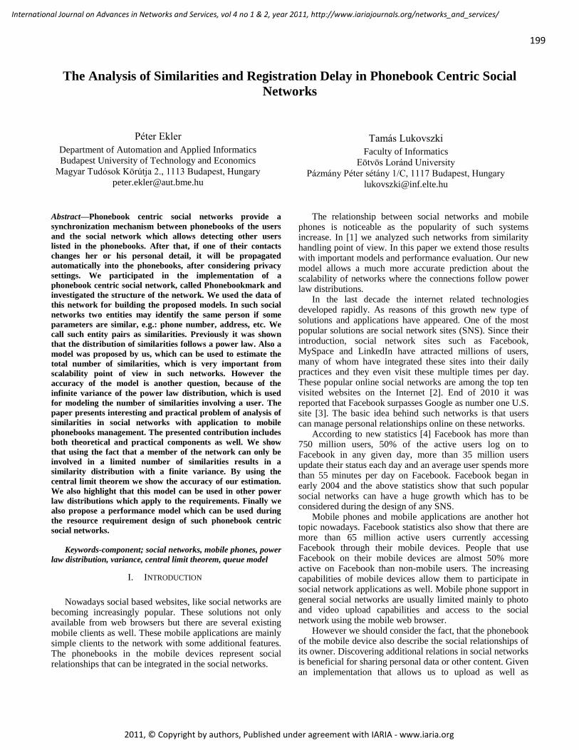
The Analysis of Similarities and Registration Delay in Phonebook Centric Social
Networks
Péter Ekler
Department of Automation and Applied Informatics
Budapest University of Technology and Economics
Magyar Tudósok Körútja 2., 1113 Budapest, Hungary
Tamás Lukovszki
Faculty of Informatics
Eötvös Loránd University
Pázmány Péter sétány 1/C, 1117 Budapest, Hungary
Abstract—Phonebook centric social networks provide a
synchronization mechanism between phonebooks of the users
and the social network which allows detecting other users
listed in the phonebooks. After that, if one of their contacts
changes her or his personal detail, it will be propagated
automatically into the phonebooks, after considering privacy
settings. We participated in the implementation of a
phonebook centric social network, called Phonebookmark and
investigated the structure of the network. We used the data of
this network for building the proposed models. In such social
networks two entities may identify the same person if some
parameters are similar, e.g.: phone number, address, etc. We
call such entity pairs as similarities. Previously it was shown
that the distribution of similarities follows a power law. Also a
model was proposed by us, which can be used to estimate the
total number of similarities, which is very important from
scalability point of view in such networks. However the
accuracy of the model is another question, because of the
infinite variance of the power law distribution, which is used
for modeling the number of similarities involving a user. The
paper presents interesting and practical problem of analysis of
similarities in social networks with application to mobile
phonebooks management. The presented contribution includes
both theoretical and practical components as well. We show
that using the fact that a member of the network can only be
involved in a limited number of similarities results in a
similarity distribution with a finite variance. By using the
central limit theorem we show the accuracy of our estimation.
We also highlight that this model can be used in other power
law distributions which apply to the requirements. Finally we
also propose a performance model which can be used during
the resource requirement design of such phonebook centric
social networks.
Keywords-component; social networks, mobile phones, power
law distribution, variance, central limit theorem, queue model
I. INTRODUCTION
Nowadays social based websites, like social networks are
becoming increasingly popular. These solutions not only available from web browsers but there are several existing mobile clients as well. These mobile applications are mainly simple clients to the network with some additional features. The phonebooks in the mobile devices represent social relationships that can be integrated in the social networks.
The relationship between social networks and mobile phones is noticeable as the popularity of such systems increase. In [1] we analyzed such networks from similarity handling point of view. In this paper we extend those results with important models and performance evaluation. Our new model allows a much more accurate prediction about the scalability of networks where the connections follow power law distributions.
In the last decade the internet related technologies developed rapidly. As reasons of this growth new type of solutions and applications have appeared. One of the most popular solutions are social network sites (SNS). Since their introduction, social network sites such as Facebook, MySpace and LinkedIn have attracted millions of users, many of whom have integrated these sites into their daily practices and they even visit these multiple times per day. These popular online social networks are among the top ten visited websites on the Internet [2]. End of 2010 it was reported that Facebook surpasses Google as number one U.S. site [3]. The basic idea behind such networks is that users can manage personal relationships online on these networks.
According to new statistics [4] Facebook has more than 750 million users, 50% of the active users log on to Facebook in any given day, more than 35 million users update their status each day and an average user spends more than 55 minutes per day on Facebook. Facebook began in early 2004 and the above statistics show that such popular social networks can have a huge growth which has to be considered during the design of any SNS.
Mobile phones and mobile applications are another hot topic nowadays. Facebook statistics also show that there are more than 65 million active users currently accessing Facebook through their mobile devices. People that use Facebook on their mobile devices are almost 50% more active on Facebook than non-mobile users. The increasing capabilities of mobile devices allow them to participate in social network applications as well. Mobile phone support in general social networks are usually limited mainly to photo and video upload capabilities and access to the social network using the mobile web browser.
However we should consider the fact, that the phonebook of the mobile device also describe the social relationships of its owner. Discovering additional relations in social networks is beneficial for sharing personal data or other content. Given an implementation that allows us to upload as well as
199
International Journal on Advances in Networks and Services, vol 4 no 1 & 2, year 2011, http://www.iariajournals.org/networks_and_services/
2011, © Copyright by authors, Published under agreement with IARIA - www.iaria.org
download our contacts to and from the social networking application, we can completely keep our contacts synchronized so that we can see all of our contacts on the mobile phone as well as on the web interface. In addition to that if the system detects that some of our private contacts in the phonebook is similar to another registered members of the social network (i.e. may identify the same person), it can discover and suggest social relationships automatically. In the rest of this paper we refer to this solution as a phonebook centric social network (PCSN). Discovering and handling such similarities in phonebook centric social networks is a key issue. If a member changes some of her or his detail, it should be propagated in every phonebook to which she or he is related after considering privacy settings. In addition to that, with the help of detected similarities the system can keep the phonebooks always up-to-date.
Power law distribution is quite common in social networks and similar internet related graphs as measurements and examples show in Section 2. The number of similarities in phonebook centric social networks is very important from performance and scalability point of view.
We show that the distribution of similarities can be
modeled with a random variable X with cxxX ~]Pr[ , if
nx and 0]Pr[ xX otherwise, where >1 and n is a
relevant upper bound. As a main contribution of this paper, we show that the
distribution of similarities has a finite variance which allows us to use the central limit theorem to prove the accuracy of our estimation of the total number of similarities. This model can be used generally in other similar distributions.
As a practical result, the concept of phonebook centric social networks was applied in the Phonebookmark project at Nokia Siemens Networks. Phonebookmark is a phonebook centric social network implementation by Nokia Siemens Networks. We took part in the implementation and before public introduction it was available for a group of general users from April to December of 2008. It had 420 registered members with more than 72000 private contacts, which is a suitable number for analyzing the behavior of the network. During this period we have collected and measured different type of data related to the social network.
The rest of the paper is organized as follows. Section 2 describes related work in the field of social networks and power law distributions. Section 3 introduces the structure of phonebook centric social networks. Section 4 summarizes our previously published model related to calculating the total number of similarities in the network. Section 5 states a general theorem related to the variance of power law distribution with relevant upper bound and uses it to prove the accuracy of the model described in Section 4. Section 6 shows that the total number of similarities is close to their expected value. Section 7 shows a performance model for calculating the expected queue length for similarity processing. We also show measurements related to Phonebookmark based on this model. The model can be used during the design of any different phonebook centric social networks. Finally, Section 8 concludes the paper and proposes further research plans.
II. RELATED WORK
In [5] the authors have defined social network sites
(SNSs) as web‐based services that allow individuals to (1) construct a public or semi‐public profile within a bounded system, (2) articulate a list of other users with whom they share a connection, and (3) view and traverse their list of connections and those made by others within the system. The nature and nomenclature of these connections may vary from site to site.
According to this definition, the first recognizable social network site launched in 1997. SixDegrees.com allowed users to create profiles, list their Friends and, beginning in 1998, surf the Friends lists. Each of these features existed in some form before SixDegrees, of course. Profiles existed on most major dating sites and many community sites. AIM and ICQ buddy lists supported lists of Friends, although those Friends were not visible to others. Classmates.com allowed people to affiliate with their high school or college and surf the network for others who were also affiliated, but users could not create profiles or list Friends until years later. SixDegrees was the first to combine these features.
After that social networks have developed rapidly and the number of features increased. Nowadays most sites support the maintenance of pre‐existing social networks, but others help strangers connect based on shared interests, political views, or activities. Some sites cater to diverse audiences, while others attract people based on common language or shared racial, sexual, religious, or nationality‐based identities. Sites also vary in the extent to which they incorporate new information and communication tools, such as mobile connectivity, blogging, and photo/video‐sharing.
As the functions of the SNSs flared, the number of users increased rapidly. Handling the extending number of users efficiently in SNSs is a key issue as it was visible in case of Friendster. Friendster was launched in 2002 as a social complement to Ryze. It was designed to help friends‐of‐friends meet, based on the assumption that friends‐of‐friends would make better romantic partners than would strangers. As Friendster's popularity surged, the site encountered technical and social difficulties. Friendster's servers and databases were ill‐equipped to handle its rapid growth, and the site faltered regularly, frustrating users who replaced email with Friendster.
Huge amount of papers and popular books, such as Barabási’s Linked [6] study the structure and principles of dynamically evolving large scale networks like the Internet and networks of social interactions. Many features of social processes and the Internet are governed by power law distributions. Following the terminology in [7] a nonnegative random variable X is said to have a power law distribution if
cxxX ]Pr[ , for constant c>0 and >0. In a power
law distribution asymptotically the tails fall according to the
power , which leads to much heavier tails than other common models.
Distributions with an inverse polynomial tail have been first observed in 1897 by Pareto [8] (see. [9]), while describing the distribution of income in the population. In
200
International Journal on Advances in Networks and Services, vol 4 no 1 & 2, year 2011, http://www.iariajournals.org/networks_and_services/
2011, © Copyright by authors, Published under agreement with IARIA - www.iaria.org
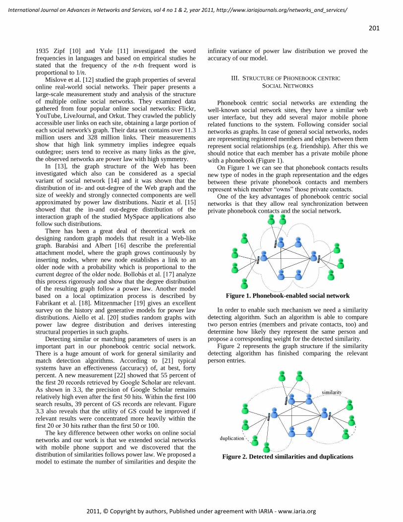
1935 Zipf [10] and Yule [11] investigated the word frequencies in languages and based on empirical studies he stated that the frequency of the n-th frequent word is proportional to 1/n.
Mislove et al. [12] studied the graph properties of several online real-world social networks. Their paper presents a large-scale measurement study and analysis of the structure of multiple online social networks. They examined data gathered from four popular online social networks: Flickr, YouTube, LiveJournal, and Orkut. They crawled the publicly accessible user links on each site, obtaining a large portion of each social network's graph. Their data set contains over 11.3 million users and 328 million links. Their measurements show that high link symmetry implies indegree equals outdegree; users tend to receive as many links as the give, the observed networks are power law with high symmetry.
In [13], the graph structure of the Web has been investigated which also can be considered as a special variant of social network [14] and it was shown that the distribution of in- and out-degree of the Web graph and the size of weekly and strongly connected components are well approximated by power law distributions. Nazir et al. [15] showed that the in-and out-degree distribution of the interaction graph of the studied MySpace applications also follow such distributions.
There has been a great deal of theoretical work on designing random graph models that result in a Web-like graph. Barabási and Albert [16] describe the preferential attachment model, where the graph grows continuously by inserting nodes, where new node establishes a link to an older node with a probability which is proportional to the current degree of the older node. Bollobás et al. [17] analyze this process rigorously and show that the degree distribution of the resulting graph follow a power law. Another model based on a local optimization process is described by Fabrikant et al. [18]. Mitzenmacher [19] gives an excellent survey on the history and generative models for power law distributions. Aiello et al. [20] studies random graphs with power law degree distribution and derives interesting structural properties in such graphs.
Detecting similar or matching parameters of users is an important part in our phonebook centric social network. There is a huge amount of work for general similarity and match detection algorithms. According to [21] typical systems have an effectiveness (accuracy) of, at best, forty percent. A new measurement [22] showed that 55 percent of the first 20 records retrieved by Google Scholar are relevant. As shown in 3.3, the precision of Google Scholar remains relatively high even after the first 50 hits. Within the first 100 search results, 39 percent of GS records are relevant. Figure 3.3 also reveals that the utility of GS could be improved if relevant results were concentrated more heavily within the first 20 or 30 hits rather than the first 50 or 100.
The key difference between other works on online social networks and our work is that we extended social networks with mobile phone support and we discovered that the distribution of similarities follows power law. We proposed a model to estimate the number of similarities and despite the
infinite variance of power law distribution we proved the accuracy of our model.
III. STRUCTURE OF PHONEBOOK CENTRIC
SOCIAL NETWORKS
Phonebook centric social networks are extending the
well-known social network sites, they have a similar web user interface, but they add several major mobile phone related functions to the system. Following consider social networks as graphs. In case of general social networks, nodes are representing registered members and edges between them represent social relationships (e.g. friendship). After this we should notice that each member has a private mobile phone with a phonebook (Figure 1).
On Figure 1 we can see that phonebook contacts results new type of nodes in the graph representation and the edges between these private phonebook contacts and members represent which member “owns” those private contacts.
One of the key advantages of phonebook centric social networks is that they allow real synchronization between private phonebook contacts and the social network.
Figure 1. Phonebook-enabled social network
In order to enable such mechanism we need a similarity
detecting algorithm. Such an algorithm is able to compare two person entries (members and private contacts, too) and determine how likely they represent the same person and propose a corresponding weight for the detected similarity.
Figure 2 represents the graph structure if the similarity detecting algorithm has finished comparing the relevant person entries.
Figure 2. Detected similarities and duplications
201
International Journal on Advances in Networks and Services, vol 4 no 1 & 2, year 2011, http://www.iariajournals.org/networks_and_services/
2011, © Copyright by authors, Published under agreement with IARIA - www.iaria.org
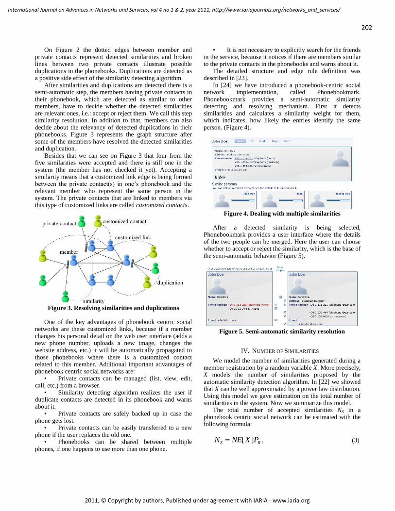
On Figure 2 the dotted edges between member and private contacts represent detected similarities and broken lines between two private contacts illustrate possible duplications in the phonebooks. Duplications are detected as a positive side effect of the similarity detecting algorithm.
After similarities and duplications are detected there is a semi-automatic step, the members having private contacts in their phonebook, which are detected as similar to other members, have to decide whether the detected similarities are relevant ones, i.e.: accept or reject them. We call this step similarity resolution. In addition to that, members can also decide about the relevancy of detected duplications in their phonebooks. Figure 3 represents the graph structure after some of the members have resolved the detected similarities and duplication.
Besides that we can see on Figure 3 that four from the five similarities were accepted and there is still one in the system (the member has not checked it yet). Accepting a similarity means that a customized link edge is being formed between the private contact(s) in one’s phonebook and the relevant member who represent the same person in the system. The private contacts that are linked to members via this type of customized links are called customized contacts.
Figure 3. Resolving similarities and duplications
One of the key advantages of phonebook centric social
networks are these customized links, because if a member changes his personal detail on the web user interface (adds a new phone number, uploads a new image, changes the website address, etc.) it will be automatically propagated to those phonebooks where there is a customized contact related to this member. Additional important advantages of phonebook centric social networks are:
• Private contacts can be managed (list, view, edit, call, etc.) from a browser.
• Similarity detecting algorithm realizes the user if duplicate contacts are detected in its phonebook and warns about it.
• Private contacts are safely backed up in case the phone gets lost.
• Private contacts can be easily transferred to a new phone if the user replaces the old one.
• Phonebooks can be shared between multiple phones, if one happens to use more than one phone.
• It is not necessary to explicitly search for the friends in the service, because it notices if there are members similar to the private contacts in the phonebooks and warns about it.
The detailed structure and edge rule definition was described in [23].
In [24] we have introduced a phonebook-centric social network implementation, called Phonebookmark. Phonebookmark provides a semi-automatic similarity detecting and resolving mechanism. First it detects similarities and calculates a similarity weight for them, which indicates, how likely the entries identify the same person. (Figure 4).
Figure 4. Dealing with multiple similarities
After a detected similarity is being selected,
Phonebookmark provides a user interface where the details of the two people can be merged. Here the user can choose whether to accept or reject the similarity, which is the base of the semi-automatic behavior (Figure 5).
Figure 5. Semi-automatic similarity resolution
IV. NUMBER OF SIMILARITIES
We model the number of similarities generated during a member registration by a random variable X. More precisely, X models the number of similarities proposed by the automatic similarity detection algorithm. In [22] we showed that X can be well approximated by a power law distribution. Using this model we gave estimation on the total number of similarities in the system. Now we summarize this model.
The total number of accepted similarities NS in a phonebook centric social network can be estimated with the following formula:
RS PXNEN ][ , (3)
202
International Journal on Advances in Networks and Services, vol 4 no 1 & 2, year 2011, http://www.iariajournals.org/networks_and_services/
2011, © Copyright by authors, Published under agreement with IARIA - www.iaria.org
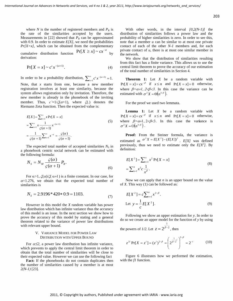
where N is the number of registered members and PR is the rate of the similarities accepted by the users. Measurements in [22] showed that PR can be approximated with 0.9. In order to estimate E[X], we need the probabilities Pr[X=x], which can be obtained from the complementary
cumulative distribution function cxxX ~]Pr[
by derivation:
.'~]Pr[ )1( xcxX (4)
In order to be a probability distribution, .1'1
)1(
xxc
Note, that x starts from one, because a new member
registration involves at least one similarity, because the
system allows registration only by invitation. Therefore, the
new member is already in the phonebook of the inviting
member. Thus, c’=1/(+1), where (.) denotes the
Riemann Zeta function. Then the expected value is:
.)1(
)(
)1(
1
)1(
1
]Pr[][
1
1
)1(
1
x
x
x
x
xx
xXxXE
(5)
The expected total number of accepted similarities NS in
a phonebook centric social network can be estimated with the following formula:
.)1(
)(RMS PNN
(6)
For >1, ()/() is a finite constant. In our case, for
=1.276, we obtain that the expected total number of similarities is
.11039.0420*9196.2 SN (7)
However in this model the X random variable has power
law distribution which has infinite variance thus the accuracy of this model is an issue. In the next section we show how to prove the accuracy of this model by stating and a general theorem related to the variance of power law distributions with relevant upper bound.
V. VARIANCE MODEL FOR POWER LAW
DISTRIBUTION WITH UPPER BOUND
For 2, a power law distribution has infinite variance, which prevents to apply the central limit theorem in order to obtain that the total number of similarities will be close to their expected value. However we can use the following fact
Fact: If the phonebooks do not contain duplicates then the number of similarities caused by a member is at most 2(N-1) [23].
With other words, in the interval [0,2(N-1)] the distribution of similarities follows a power law and the probability of higher similarities is zero. In order to see this, note that a member u can be similar to at most one private contact of each of the other N-1 members and, for each private contact of u, there is at most one similar member in the network.
We show that the distribution of similarities resulting from this fact has a finite variance. This allows us to use the central limit theorem to prove the accuracy of our estimation of the total number of similarities in Section 4.
Theorem 1: Let X be a random variable with cxxX ]Pr[ if nx
and 0]Pr[ xX otherwise,
where =. In this case the variance can be
estimated with 32 nX .
For the proof we used two lemmata.
Lemma 1: Let X be a random variable with
cxxX ]Pr[ if nx and 0]Pr[ xX otherwise,
where =. In this case the variance is
32 nX .
Proof: From the Steiner formula, the variance is
estimated as 222 ])[(][ XEXEX . E[X] was defined
previously, thus we need to estimate only the E[X2]. By
definition:
.1
]Pr[][
1
2
1
22
xcx
xXxXE
n
x
x
(8)
Now we can apply that n is an upper bound on the value
of X. This way (1) can be followed as:
.][1
22
n
xxcXE
Let ][1 2XEc
y . (9)
Following we show an upper estimation for y. In order to
do so we create an upper model for the function of y by using
the powers of 1/2. Let 2
1
2 z , then
ii
iii zzXz
22)(]Pr[
2
2
1
22
(10)
Figure 6 illustrates how we performed the estimation,
with the f1 function.
203
International Journal on Advances in Networks and Services, vol 4 no 1 & 2, year 2011, http://www.iariajournals.org/networks_and_services/
2011, © Copyright by authors, Published under agreement with IARIA - www.iaria.org
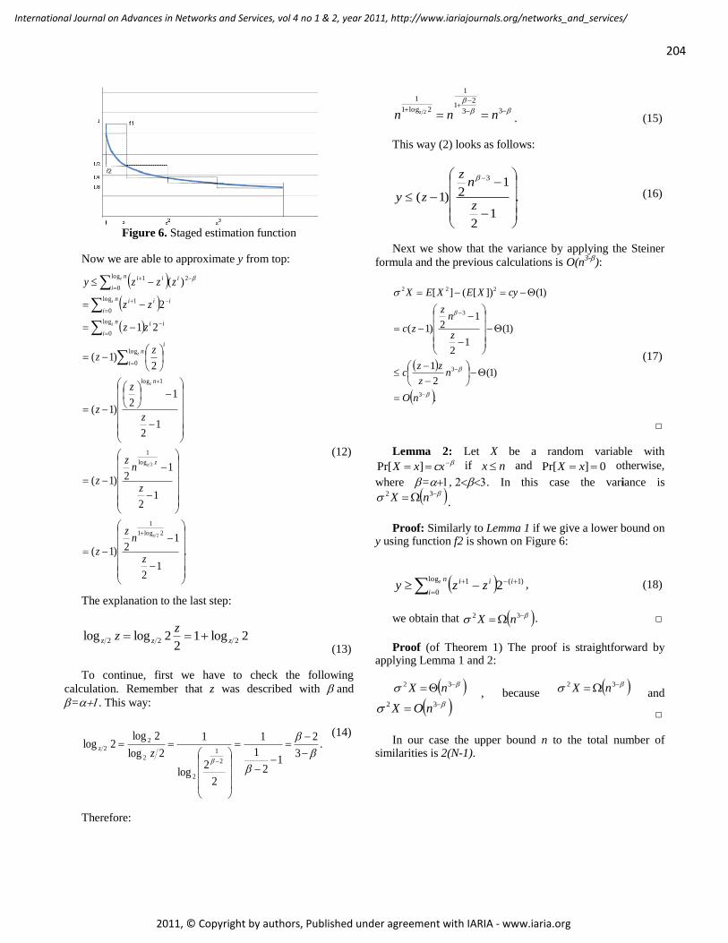
Figure 6. Staged estimation function
Now we are able to approximate y from top:
.
12
12)1(
12
12)1(
12
12
)1(
2)1(
21
2
)(
2log1
1
log
1
1log
log
0
log
0
log
0
1
2log
0
1
2
2
z
nz
z
z
nz
z
z
z
z
zz
zz
zz
zzzy
z
z
z
z
z
z
z
z
n
in
i
iin
i
in
i
ii
in
i
ii
(12)
The explanation to the last step:
2log12
2loglog 222 zzz
zz
(13) To continue, first we have to check the following
calculation. Remember that z was described with and
=. This way:
.3
2
12
1
1
2
2log
1
2log
2log2log
2
1
2
2
2
2
z
z
(14)
Therefore:
33
21
1
2log1
1
2 nnn z
. (15)
This way (2) looks as follows:
.
12
12)1(
3
z
nz
zy
(16)
Next we show that the variance by applying the Steiner
formula and the previous calculations is O(n3-
):
.
)1(2
1
)1(
12
12)1(
)1(])[(][
3
3
3
222
nO
nz
zzc
z
nz
zc
cyXEXEX
(17)
Lemma 2: Let X be a random variable with
cxxX ]Pr[ if nx and 0]Pr[ xX otherwise,
where =. In this case the variance is
32 nX .
Proof: Similarly to Lemma 1 if we give a lower bound on
y using function f2 is shown on Figure 6:
)1(log
0
1 2
in
i
iiz
zzy , (18)
we obtain that 32 nX .
Proof (of Theorem 1) The proof is straightforward by
applying Lemma 1 and 2:
32 nX , because 32 nX and
32 nOX In our case the upper bound n to the total number of
similarities is 2(N-1).
204
International Journal on Advances in Networks and Services, vol 4 no 1 & 2, year 2011, http://www.iariajournals.org/networks_and_services/
2011, © Copyright by authors, Published under agreement with IARIA - www.iaria.org
VI. APPLYING CENTRAL LIMIT THEOREM FOR THE
DISTRIBUTION OF SIMILARITIES
Following we show that the total number of similarities
are close to their expected value. Theorem 2: Let N be the number of members in a
phonebook centric social network and SN=X1+X2+...+XN where Xi , i=1,…,N, is a random variable representing the number of similarities raised by member i, i.e.
xxX i ]Pr[ if nx and 0]Pr[ xX i
otherwise,
where n=(N), = and is a constant. Let = E[Xi]. Then
),(1]Pr[ mNcSN
where 1
21
Ncam and a is an appropriate
constant. Proof: X1, X2, …, XN are N independent and identically
distributed random variables, each having finite values of
expectation and variance 2>0. The central limit theorem
states that the distribution of the sample average of these random variables approaches the normal distribution with a
mean and variance 2/n. Let
N
NSZ N
N
(19)
By the central limit theorem, the distribution of ZN
approaches the standard normal distribution:
x t
N dtexZ 2
2
2
1)(
(20)
The density function looks as follows:
2
2
2
1)(
x
exf
(21)
Now we determine the probability that SN is greater or
equal than c times of its expected value, for a constant c>1.
For SN= cE[SN]=c then
,1
1
)(
1
)(
1
12
21
4
3
Nca
N
c
N
Nc
NN
Nc
N
NNcZN
(22)
where a is an appropriate constant. Therefore:
.1PrPr1
2
NcaZNcS NN (23)
Let 1
21
Ncam . Since, by the central limit
theorem, the distribution of ZN can be approximated by the standard normal distribution, we have
.1
PrPr
m
mZNcS NN
(24)
Theorem 3: For 1
21
Ncam :
,2
1)(1
2
Nem
where = (a(c-1))2/2 is a constant.
Proof:
m t
dtem 2
2
2
11)(1
m
t
dte 2
2
2
1
(25)
22
1 merfc
205
International Journal on Advances in Networks and Services, vol 4 no 1 & 2, year 2011, http://www.iariajournals.org/networks_and_services/
2011, © Copyright by authors, Published under agreement with IARIA - www.iaria.org
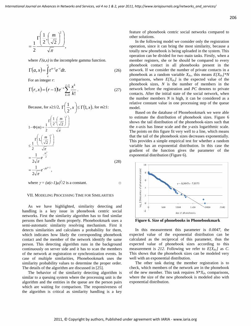
,2
,2
1
2
1
2
m
where a,x) is the incomplete gamma function.
., 1
x
ta dtetxa (26)
For an integer r:
1
0 !!1,
r
k
kx
k
xerxr . (27)
Because, for x1/2, xx ,1,2
1
, for m1:
2
2
2,1
2
1
2,
2
1
2
1)(1
m
m
m
,2
1
2
1
2
2
2
N
m
e
e (28)
where = (a(c-1))2/2 is a constant.
VII. MODELING PROCESSING TIME FOR SIMILARITIES
As we have highlighted, similarity detecting and
handling is a key issue in phonebook centric social
networks. First the similarity algorithm has to find similar
persons then handle them properly. Phonebookmark uses a
semi-automatic similarity resolving mechanism. First it
detects similarities and calculates a probability for them,
which indicates how likely the corresponding phonebook
contact and the member of the network identify the same
person. This detecting algorithm runs in the background
continuously on server side and it has to scan the members
of the network at registration or synchronization events. In
case of multiple similarities, Phonebookmark uses the
similarity probability values to determine the proper order.
The details of the algorithm are discussed in [25].
The behavior of the similarity detecting algorithm is
similar to a queuing system where the processing unit is the
algorithm and the entities in the queue are the person pairs
which are waiting for comparison. The responsiveness of
the algorithm is critical as similarity handling is a key
feature of phonebook centric social networks compared to
other solutions.
In the following model we consider only the registration
operation, since it can bring the most similarity, because a
totally new phonebook is being uploaded in the system. This
operation can be divided for two main tasks. Firstly, when a
member registers, she or he should be compared to every
phonebook contact in all phonebooks present in the
network. If we consider the number of private contacts in a
phonebook as a random variable XPc, this means E[XPc]*N
comparisons, where E[XPc] is the expected value of the
phonebook sizes, N is the number of members in the
network before the registration and PC denotes to private
contacts. After the initial state of the social network, when
the number members N is high, it can be considered as a
relative constant value in one processing step of the queue
model.
Based on the database of Phonebookmark we were able
to estimate the distribution of phonebook sizes. Figure 6
shows the tail distribution of the phonebook-sizes such that
the x-axis has linear scale and the y-axis logarithmic scale.
The points on this figure fit very well to a line, which means
that the tail of the phonebook sizes decreases exponentially.
This provides a simple empirical test for whether a random
variable has an exponential distribution. In this case the
gradient of the function gives the parameter of the
exponential distribution (Figure 6).
Figure 6. Size of phonebooks in Phonebookmark
In this measurement this parameter is 0.0047, the
expected value of the exponential distribution can be
calculated as the reciprocal of this parameter, thus the
expected value of phonebook sizes according to this
measurement is 212. Following we refer to E[XPc] as C.
This shows that the phonebook sizes can be modeled very
well with an exponential distribution.
The other task during the member registration is to
check, which members of the network are in the phonebook
of the new member. This task requires N*XPc comparisons,
where the size of the new phonebook is modeled also with
exponential distribution.
206
International Journal on Advances in Networks and Services, vol 4 no 1 & 2, year 2011, http://www.iariajournals.org/networks_and_services/
2011, © Copyright by authors, Published under agreement with IARIA - www.iaria.org
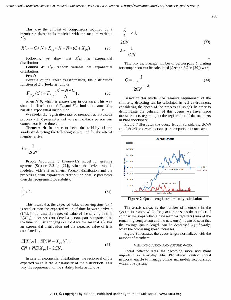
This way the amount of comparisons required by a
member registration is modeled with the random variable
X*
Pc:
)( PcPcPc XCNNXNCX (29)
Following we show that X*
Pc has exponential
distribution.
Lemma 4: X*
Pc random variable has exponential
distribution.
Proof:
Because of the linear transformation, the distribution
function of X*
Pc looks as follows:
)()(N
CNxFxF
PcPc XX
, (30)
when N>0, which is always true in our case. This way
since the distribution of XPc and X*Pc looks the same, X
*Pc
has also exponential distribution.
We model the registration rate of members as a Poisson
process with parameter and we assume that a person pair
comparison is the time unit.
Theorem 4: In order to keep the stability of the
similarity detecting the following is required for the rate of
member arrival:
.2
1
CN
Proof: According to Kleinrock’s model for queuing
systems (Section 3.2 in [26]), when the arrival rate is
modeled with a parameter Poisson distribution and the
processing with exponential distribution with parameter
then the requirement for stability:
.1
(31)
This means that the expected value of serving time (1/)
is smaller than the expected value of time between arrivals
(1/). In our case the expected value of the serving time is
E[X*Pc], since we considered a person pair comparison as
the time unit. By applying Lemma 4 we can see that X*Pc has
an exponential distribution and the expected value of it is
calculated by:
.2][
][][
CNXNECN
NXCNEXE
Pc
PcPc
(32)
In case of exponential distributions, the reciprocal of the
expected value is the parameter of the distribution. This
way the requirement of the stability looks as follows:
CN
CN
2
1
,1
2
1
(33)
This way the average number of person pairs Q waiting
for comparison can be calculated (Section 3.2 in [26]) with:
CN
Q
2
1 (34)
Based on this model, the resource requirement of the
similarity detecting can be calculated in real environment,
considering the speed of the processing unit(s). In order to
demonstrate the behavior of this queue, we have made
measurements regarding to the registration of the members
in Phonebookmark.
Figure 7 illustrates the queue length considering 2C∗N
and 2.5C∗N processed person-pair comparison in one step.
Figure 7. Queue length for similarity calculation
The x-axis shows as the number of members in the
system increases, while the y-axis represents the number of
comparison steps when a new member registers (sum of the
remaining comparison and the new ones). It can be seen that
the average queue length can be decreased significantly,
when the processing speed increases.
Figure 8 illustrates the queue length normalized with the
number of members.
VIII. CONCLUSION AND FUTURE WORK
Social network sites are becoming more and more important in everyday life. Phonebook centric social networks enable to manage online and mobile relationships within one system.
207
International Journal on Advances in Networks and Services, vol 4 no 1 & 2, year 2011, http://www.iariajournals.org/networks_and_services/
2011, © Copyright by authors, Published under agreement with IARIA - www.iaria.org
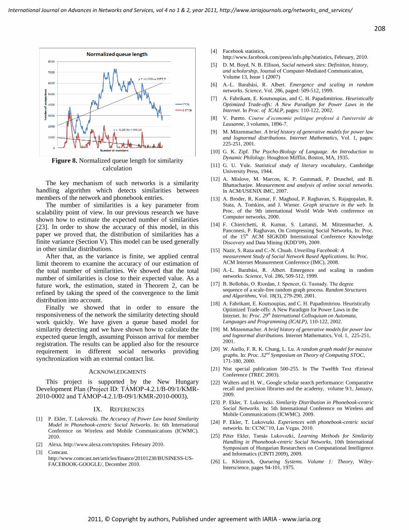
Figure 8. Normalized queue length for similarity
calculation
The key mechanism of such networks is a similarity handling algorithm which detects similarities between members of the network and phonebook entries.
The number of similarities is a key parameter from scalability point of view. In our previous research we have shown how to estimate the expected number of similarities [23]. In order to show the accuracy of this model, in this paper we proved that, the distribution of similarities has a finite variance (Section V). This model can be used generally in other similar distributions.
After that, as the variance is finite, we applied central limit theorem to examine the accuracy of our estimation of the total number of similarities. We showed that the total number of similarities is close to their expected value. As a future work, the estimation, stated in Theorem 2, can be refined by taking the speed of the convergence to the limit distribution into account.
Finally we showed that in order to ensure the responsiveness of the network the similarity detecting should work quickly. We have given a queue based model for similarity detecting and we have shown how to calculate the expected queue length, assuming Poisson arrival for member registration. The results can be applied also for the resource requirement in different social networks providing synchronization with an external contact list.
ACKNOWLEDGMENTS
This project is supported by the New Hungary Development Plan (Project ID: TÁMOP-4.2.1/B-09/1/KMR-2010-0002 and TÁMOP-4.2.1/B-09/1/KMR-2010-0003).
IX. REFERENCES
[1] P. Ekler, T. Lukovszki. The Accuracy of Power Law based Similarity Model in Phonebook-centric Social Networks. In: 6th International Conference on Wireless and Mobile Communications (ICWMC). 2010.
[2] Alexa. http://www.alexa.com/topsites. February 2010.
[3] Comcast. http://www.comcast.net/articles/finance/20101230/BUSINESS-US-FACEBOOK-GOOGLE/, December 2010.
[4] Facebook statistics, http://www.facebook.com/press/info.php?statistics, February, 2010.
[5] D. M. Boyd, N. B. Ellison, Social network sites: Definition, history, and scholarship, Journal of Computer-Mediated Communication, Volume 13, Issue 1 (2007)
[6] A.-L. Barabási, R. Albert. Emergence and scaling in random networks. Science, Vol. 286, paged: 509-512, 1999.
[7] A. Fabrikant, E. Koutsoupias, and C. H. Papadimitriou. Heuristically Optimized Trade-offs: A New Paradigm for Power Laws in the Internet. In Proc. of ICALP, pages: 110-122, 2002.
[8] V. Pareto. Course d’economie politique professé à l'université de Lausanne, 3 volumes, 1896-7.
[9] M. Mitzenmacher. A brief history of generative models for power law and lognormal distributions. Internet Mathematics, Vol. 1, pages: 225-251, 2001.
[10] G. K. Zipf. The Psycho-Biology of Language. An Introduction to Dynamic Philology. Houghton Mifflin, Boston, MA, 1935.
[11] G. U. Yule. Statistical study of literary vocabulary, Cambridge University Press, 1944.
[12] A. Mislove, M. Marcon, K. P. Gummadi, P. Druschel, and B. Bhattacharjee. Measurement and analysis of online social networks. In ACM/USENIX IMC, 2007.
[13] A. Broder, R. Kumar, F. Maghoul, P. Raghavan, S. Rajagopalan, R. Stata, A. Tomkins, and J. Wiener. Graph structure in the web. In Proc. of the 9th international World Wide Web conference on Computer networks, 2000.
[14] F. Chierichetti, R. Kumar, S. Lattanzi, M. Mitzenmacher, A. Panconesi, P. Raghavan, On Compressing Social Networks, In: Proc. of the 15th ACM SIGKDD International Conference Knowledge Discovery and Data Mining (KDD’09), 2009.
[15] Nazir, S. Raza and C.-N. Chuah. Unveiling Facebook: A measurement Study of Social Network Based Applications. In: Proc. ACM Internet Measurement Conference (IMC), 2008.
[16] A.-L. Barabási, R. Albert. Emergence and scaling in random networks. Science, Vol. 286, 509-512, 1999.
[17] B. Bollobás, O. Riordan, J. Spencer, G. Tusnady. The degree sequence of a scale-free random graph process. Random Structures and Algorithms, Vol. 18(3), 279-290, 2001.
[18] A. Fabrikant, E. Koutsoupias, and C. H. Papadimitriou. Heuristically Optimized Trade-offs: A New Paradigm for Power Laws in the Internet. In: Proc. 29th International Colloquium on Automata, Languages and Programming (ICALP), 110-122, 2002.
[19] M. Mitzenmacher. A brief history of generative models for power law and lognormal distributions. Internet Mathematics, Vol. 1, 225-251, 2001.
[20] W. Aiello, F. R. K. Chung, L. Lu. A random graph model for massive graphs. In: Proc. 32nd Symposium on Theory of Computing STOC, 171-180, 2000.
[21] Nist special publication 500-255. In The Twelfth Text rEtrieval Conference (TREC 2003).
[22] Walters and H. W., Google scholar search performance: Comparative recall and precision libraries and the academy, volume 9/1, January, 2009.
[23] P. Ekler, T. Lukovszki. Similarity Distribution in Phonebook-centric Social Networks. In: 5th International Conference on Wireless and Mobile Communications (ICWMC). 2009.
[24] P. Ekler, T. Lukovszki. Experiences with phonebook-centric social networks. In: CCNC’10, Las Vegas. 2010.
[25] Péter Ekler, Tamás Lukovszki, Learning Methods for Similarity Handling in Phonebook-centric Social Networks, 10th International Symposium of Hungarian Researchers on Computational Intelligence and Informatics (CINTI 2009), 2009.
[26] L. Kleinrock, Queueing Systems. Volume 1: Theory, Wiley-Interscience, pages 94-101, 1975.
208
International Journal on Advances in Networks and Services, vol 4 no 1 & 2, year 2011, http://www.iariajournals.org/networks_and_services/
2011, © Copyright by authors, Published under agreement with IARIA - www.iaria.org
WLAN IEEE 802.11a/b/g/n Indoor Coverage and Interference Performance Study
Sandra Sendra1, Miguel Garcia2, Carlos Turro3, Jaime Lloret4 Universidad Politécnica de Valencia
Camino Vera s/n, 46022, Valencia, Spain [email protected], [email protected], [email protected], [email protected]
Abstract—An adequate wireless network plan is needed to replace the traditional wired LANs. A full coverage WLAN offers the flexibility to relocate people and equipment or to reconfigure and add more wireless devices to the network. Usually, an IEEE 802.11 variant is chosen based on their bandwidth and their coverage area. However, sometimes there are special cases where the best technology is not the newest one. In addition, suitable positioning of access points (AP) is crucial to determine the efficiency of the network. E.g. in the case where devices are going to transmit at a maximum of 1 Mbps, any choice is acceptable, but when it is required higher performance, other factors must be considered. In this paper, we compare IEEE 802.11a/b/g/n indoor environments to know what technology is better. This comparison will be taken in terms of RSSI, coverage area, and measuring the interferences between channels. These key factors must be optimum to have high performance in the WLAN. This study will help the researchers to choose the best technology depending of their deploying case, and we will see study the best variant for indoors.
Keywords-WLAN; IEEE 802.11; Coverage; Interferences; Performance measurements.
I. INTRODUCTION This paper is an extended version of the paper presented
by S. Sendra et al. in [1]. One of the major issues in Wireless Local Area Network
(WLAN) indoor environments is the multipath dispersion due to the influence of many signal reflectors and diffusions. Walls, floors and roofs attenuate the signal highly and provoke great variations in the mean received power. Even the furniture and the metallic structures of the walls and roofs have high impact because they enhance the scattering and diffraction. There has been many studies about the signal propagation in indoors [2][3]. Moreover, there are special challenges when designing WLANs in indoors [4].
Because the emitter and the receiver are close, the delay between echoes will enlarge the delay spread. But, temporal variations are slower because of the low mobility of the users. Temporal variations are mainly given by the presence of humans close to the antennas. Moreover, there are other features in indoor environments such as: • Electromagnetic fields provided by electronic devices.
Although the reflection and diffraction can be modeled, there are many things inside the building that introduce a certain grade of variability [3].
• Usually people walking in any corridor or facility close to the emitter or the receiver will cause significant variations [5].
• Because the distances are short, any variation of the direction of the antenna will imply high changes in the signal received.
• Metallic objects reflect the radio signal. The signal will not cross metallic walls and metallic objects will fade.
• Wood, crystal, plastic and bricks reflect part of the signal, but let pass the rest.
• The objects with high humidity have more signal absorption.
There are several indoor propagation models. They can be classified in empirical models (which are based on the measures taken and predict the signal loss), in deterministic models (that simulate the signal propagation in order to characterize the transmission channel), theoretical models, (which are based in the physical laws of the modeled medium) and stochastic models (they are modes which results have a probability distribution) [6]. The appropriate model must be chosen based in the design necessities. Empirical models are used in network design, while deterministic models are used for high precision applications. The first ones are less complex and need lower input parameters, but they do not predict instantaneous signal fainting [7].
The most well known models are the following ones: • Log-Normal Shadowing Path Loss Model [8] • Loss Model based in COST 231 [9] • Linear Path Attenuation Model [10] • Keenan-Motley Model [11] • ITU-R Model [12] • Dual Slope-Model [13] • Multi-Wall Model [14]
Several authors have studied empirically each one of them providing their drawbacks and benefits.
But, when we are setting up a WLAN, it is not practical to model all wireless coverage area for each site where the access point is going to be placed, especially when we are talking about large extension areas [15]. Within the IEEE 802.11 standard [16], there are included several variants like IEEE 802.11a, IEEE 802.11b, IEEE 802.11g and IEEE 802.11n. All of them provide different coverage areas, and even different signal strength inside the coverage area.
The standard uses the CSMA/CA protocol as the medium access method. It is a carrier sense multiple access with collision avoidance used to avoid collisions between wireless data packets. In Europe, the frequency ranges from 2.401 to 2.483 GHz is divided into 13 channels of 22 MHz wide, and spaced 5 MHz between them, where channel 1 is centered on 2.412 GHz and the channel 13 is located at 2.472 GHz.
209
International Journal on Advances in Networks and Services, vol 4 no 1 & 2, year 2011, http://www.iariajournals.org/networks_and_services/
2011, © Copyright by authors, Published under agreement with IARIA - www.iaria.org
Japan adds an additional channel 14, located 12 MHz above channel 13. In an IEEE 802.11 network, the participant significantly reduces the speed of the overall wireless network. Now we are going to introduce each IEEE 802.11 variant [17, 18].
A. IEEE 802.11a IEEE 802.11a was approved in 1999. Although it was
born in 1999, it did not begin to be marketed until 2001. This variant works in the 5 GHz band. Its architecture is based on two types of devices: the Access Points (APs), which are the base station for the wireless network, and the wireless clients, that can be mobile devices such as laptops, PDAs, and fixed devices such as desktops and workstations equipped with a wireless network interface.
IEEE 802.11a uses OFDM (Orthogonal Frequency Division Multiplexing) modulation with 52 subcarriers. This standard has a theoretical maximum speed of 54 Mbps, but the transmission rate decreases when the signal quality decreases. 54 Mbps could be changed to 48, 36, 24, 12, 9 and 6 Mbps. There are 52 subcarriers, 48 of them are used for the data transmission and 4 for pilot tasks, with a separation of 312.5 KHz. Each subcarrier may be modulated by BPSK (Binary Phase Shift Keying), QPSK (Quaternary Phase Shift Keying), 16-QAM (Quadrature Amplitude Modulation) or 64-QAM.
IEEE 802.11a provides 12 non-overlapping channels. As it uses the 5 GHz band, the signal has less interference than the other standards IEEE 802.11. But the equipment must be in the line of sight (LOS) to gain a better efficiency in communications.
B. IEEE 802.11b The 802.11b standard was approved in 1999. IEEE
802.11b data are encoded using the Direct Sequence Spread Spectrum Signal (DSSS). This technology uses CCK (Complementary Code Keying) and QPSK modulation to achieve a maximum transfer raw rate of 11 Mbps. However, it cannot exceed 6 Mbps with TCP (Transmission Control Protocol) and 7 Mbps with UDP (User Datagram Protocol) theoretically.
The protocol can be used in point-to-multipoint or point-to-point topology with links over distances proportional to the features of the antennas and output power. Furthermore, if there is any problem with the signal quality, it is possible to transmit in 5.5, 2 or 1 Mbps, using redundant methods of data encryption.
First devices appeared very quickly because this variant was an extension to the DSSS modulation of the original standard. The higher speed and the low cost of the devices achieved a fast growth of this technology in the market.
C. IEEE 802.11g IEEE 802.11g appeared in 2003. It is an evolution of
IEEE 802.11b. It works on 2.4 GHz frequency band and it is compatible with IEEE 802.11b. Its theoretical transfer is 54 Mbps, although it is reduced to 22 Mbps when the receiver is some meters far from the AP in a real scenario. It uses 52 subcarriers.
The modulation scheme used in 802.11g is orthogonal frequency-division multiplexing (OFDM), such as in 802.11a, with data rates of 6, 9, 12, 18, 24, 36, 48, and 54 Mbps. It reverts to CCK (like the 802.11b standard) for 5.5 and 11 Mbps and to DBPSK and DQPSK + DSSS for 1 and 2 Mbps respectively. In this standard, there is also a speed decrease according to the signal quality.
IEEE 802.11g suffers from the same interference as IEEE 802.11b in the already crowded 2.4 GHz range.
Because IEEE 802.11g uses the same radio signaling (CCK) as 802.11b, at the lower four IEEE 802.11g data rates, it is fully backward compatible with IEEE 802.11b. This enables IEEE 802.11b/g wireless networks to continue supporting only IEEE 802.11b enabled devices. IEEE 802.11g may seem to be the competence of 802.11a, but most products include both technologies because they are complementary.
D. IEEE 802.11n While IEEE 802.11a/b/g WLANs provide adequate
performance for today's networking applications, the wireless applications of next generation require higher data throughput and bigger coverage area. This variant sought to bring the transmission capacity of wireless data transmission at speeds of wired systems.
IEEE 802.11n is a proposed amendment to the IEEE 802.11-2007 standard [16] in order to significantly improve the network performance of the previous standards such as 802.11b and 802.11g. IEEE 802.11n is built based on previous standards of the 802.11 family, adding Multiple-Input Multiple-Output (MIMO) and binding of network interfaces (Channel Bonding). It also adds frames to the MAC layer.
It presents an increase of the theoretical maximum rate of 600 Mbps of data transfer. Currently it supports a PHY rate of 450 Mbps, using 3 spatial streams in a channel width of 40 MHz. Furthermore, IEEE 802.11n uses MIMO based on using multiple transmit and receive antennas to improve system performance. This technology requires a separated radio-frequency chain and an analog to digital converter for each MIMO antenna which increases the implementation costs compared to the systems without MIMO technology.
Table 1 summarizes the main characteristics of the four variants of the IEEE 802.11 standard.
The success of the standard has caused density problems related to crowding in urban areas. So, some issues must be studied such as interference, coverage and used bandwidth in each IEEE 802.11 variant. In our previous work, presented in a conference [1], we carried out coverage measurements of several devices that were capable to work in different IEEE 802.11 variants. In addition, the number of lost packets, bandwidth and throughput when there are interferences, for each IEEE 802.11 variant were measured. In this paper, we have added, on the one hand, some coverage measures that were not performed in the previous work and, on the other hand, we have taken more measurements of lost packets, bandwidth and throughput for each IEEE 802.11 variant. The results will be the mean values for each variant.
210
International Journal on Advances in Networks and Services, vol 4 no 1 & 2, year 2011, http://www.iariajournals.org/networks_and_services/
2011, © Copyright by authors, Published under agreement with IARIA - www.iaria.org
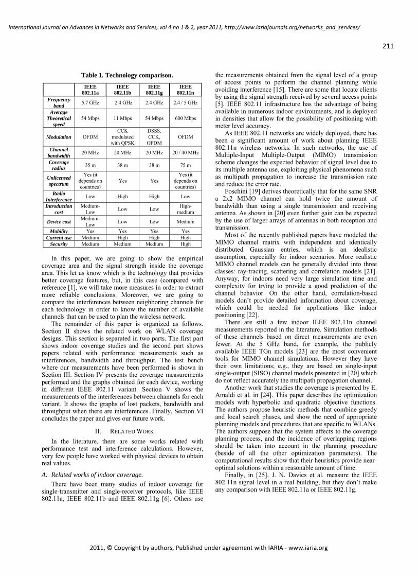
Table 1. Technology comparison.
IEEE 802.11a
IEEE 802.11b
IEEE 802.11g
IEEE 802.11n
Frequency band 5.7 GHz 2.4 GHz 2.4 GHz 2.4 / 5 GHz
Average Theoretical
speed 54 Mbps 11 Mbps 54 Mbps 600 Mbps
Modulation OFDM CCK
modulated with QPSK
DSSS, CCK,
OFDM OFDM
Channel bandwidth 20 MHz 20 MHz 20 MHz 20 / 40 MHz
Coverage radius 35 m 38 m 38 m 75 m
Unlicensed spectrum
Yes (it depends on countries)
Yes Yes Yes (it
depends on countries)
Radio Interference Low High High Low
Introduction cost
Medium-Low Low Low High-
medium
Device cost Medium-Low Low Low Medium
Mobility Yes Yes Yes Yes Current use Medium High High High
Security Medium Medium Medium High In this paper, we are going to show the empirical
coverage area and the signal strength inside the coverage area. This let us know which is the technology that provides better coverage features, but, in this case (compared with reference [1], we will take more measures in order to extract more reliable conclusions. Moreover, we are going to compare the interferences between neighboring channels for each technology in order to know the number of available channels that can be used to plan the wireless network.
The remainder of this paper is organized as follows. Section II shows the related work on WLAN coverage designs. This section is separated in two parts. The first part shows indoor coverage studies and the second part shows papers related with performance measurements such as interferences, bandwidth and throughput. The test bench where our measurements have been performed is shown in Section III. Section IV presents the coverage measurements performed and the graphs obtained for each device, working in different IEEE 802.11 variant. Section V shows the measurements of the interferences between channels for each variant. It shows the graphs of lost packets, bandwidth and throughput when there are interferences. Finally, Section VI concludes the paper and gives our future work.
II. RELATED WORK In the literature, there are some works related with
performance test and interference calculations. However, very few people have worked with physical devices to obtain real values.
A. Related works of indoor coverage. There have been many studies of indoor coverage for
single-transmitter and single-receiver protocols, like IEEE 802.11a, IEEE 802.11b and IEEE 802.11g [6]. Others use
the measurements obtained from the signal level of a group of access points to perform the channel planning while avoiding interference [15]. There are some that locate clients by using the signal strength received by several access points [5]. IEEE 802.11 infrastructure has the advantage of being available in numerous indoor environments, and is deployed in densities that allow for the possibility of positioning with meter level accuracy.
As IEEE 802.11 networks are widely deployed, there has been a significant amount of work about planning IEEE 802.11n wireless networks. In such networks, the use of Multiple-Input Multiple-Output (MIMO) transmission scheme changes the expected behavior of signal level due to its multiple antenna use, exploiting physical phenomena such as multipath propagation to increase the transmission rate and reduce the error rate.
Foschini [19] derives theoretically that for the same SNR a 2x2 MIMO channel can hold twice the amount of bandwidth than using a single transmission and receiving antenna. As shown in [20] even further gain can be expected by the use of larger arrays of antennas in both reception and transmission.
Most of the recently published papers have modeled the MIMO channel matrix with independent and identically distributed Gaussian entries, which is an idealistic assumption, especially for indoor scenarios. More realistic MIMO channel models can be generally divided into three classes: ray-tracing, scattering and correlation models [21]. Anyway, for indoors need very large simulation time and complexity for trying to provide a good prediction of the channel behavior. On the other hand, correlation-based models don’t provide detailed information about coverage, which could be needed for applications like indoor positioning [22].
There are still a few indoor IEEE 802.11n channel measurements reported in the literature. Simulation methods of these channels based on direct measurements are even fewer. At the 5 GHz band, for example, the publicly available IEEE TGn models [23] are the most convenient tools for MIMO channel simulations. However they have their own limitations; e.g., they are based on single-input single-output (SISO) channel models presented in [20] which do not reflect accurately the multipath propagation channel.
Another work that studies the coverage is presented by E. Amaldi et al. in [24]. This paper describes the optimization models with hyperbolic and quadratic objective functions. The authors propose heuristic methods that combine greedy and local search phases, and show the need of appropriate planning models and procedures that are specific to WLANs. The authors suppose that the system affects to the coverage planning process, and the incidence of overlapping regions should be taken into account in the planning procedure (beside of all the other optimization parameters). The computational results show that their heuristics provide near-optimal solutions within a reasonable amount of time.
Finally, in [25], J. N. Davies et al. measure the IEEE 802.11n signal level in a real building, but they don’t make any comparison with IEEE 802.11a or IEEE 802.11g.
211
International Journal on Advances in Networks and Services, vol 4 no 1 & 2, year 2011, http://www.iariajournals.org/networks_and_services/
2011, © Copyright by authors, Published under agreement with IARIA - www.iaria.org
B. Related works of interferences. From the IEEE 802.11 WLAN interference side,
Nicolescu [26] proposed a model for interference in dense wireless networks that enables a low complexity procedure to collect the interference map and can be used to predict the damage from several simultaneous interferers. Unfortunately measurement of the interference map faces asymmetries in the card and channel behavior, which make the complexity still prohibitive for dense multiple card networks, requiring direct measurements in indoor deployments. Also, Fuxjäger et al. [27] show that the assumption of perfect independence between non-overlapping channels does not always hold in practice, by means of simple experiments with commercially available hardware, and found that the level of interference varies with physical distance, concurrent link-load, modulation rate, frame size, transmission power, receiver sensitivity and design, antenna patterns, etc., calling also for more direct measurements.
J. Padhye et al. present in [28] an interference measurement-based study between links in a static, IEEE 802.11, multi-hop wireless network. Then, the authors propose a simple empirical estimation methodology that can predict pair wise interference using only measurements. These tests are based on heuristics methods where the wireless links are defined by their packet loss rate. They state that this methodology could be applicable to any wireless network that uses omni-directional antennas.
Related to interference and throughput measures in WLAN, J. Jun et al. present in [29] an accurate formula to estimate the throughput in IEEE 802.11 networks, for several variants (802.11, 802.11b, 802.11a), in the absence of transmission errors and for various physical layers, data rates and packet sizes. The authors cite some applications where it is very important to know the maximum throughput in order to design them correctly. Theoretical Maximum Throughput can be used to facilitate optimal network provisioning, for example, in multimedia applications. It can influence the topological distribution of the nodes in the case of ad-hoc networks.
Although analytical studies and network simulations may provide valuable insights of the WLANs' operation, they cannot predict the actual performance of practical implementations with high accuracy. Moreover, measurements obtained from file transfer operations are also limited by the need to specify the processor type, processor speed and the network operating system. B. Bing presents in [30], an experimental study to characterize the behavior in terms of throughput and response time of two commercial AP under different degrees of network load. They are WavePOINT, from Lucent Technologies, and Spectrum24, from Symbol Technologies. The tests showed important characteristics such as throughput and response time under various network loads. The author also shows that the length of a data frame and the wireless bit rate also affects to the WLAN’s transmission capabilities. But, the performance of an IEEE 802.11 WLAN is generally unaffected by the type of frame and the use of reservation frames such as RTS and CTS.
III. THE SCENARIO DESCRIPTION In this section, we describe the scenario where the
measures have been taken and the hardware and software used to perform our research.
A. Place of measurement In order to do the measures, we have sought a wide
enclosure with an area of 91 m2, with a length and a width of 12.5 m by 6.68 m. This building is made with walls of different thickness and materials. We have tried to find a scenario that was made from different materials, as can be found in common houses.
Fig. 1 shows the plane of garage. It has rectangular base, divided into two parts by a wall of 9 cm of thick: the garage (left) and the kitchen (right). The enclosure of the staircase is made of bricks with high consistency. All these walls have a layer of plaster and paint on both sides. The bathroom is made with hollow bricks of 9 cm. These walls are covered by ceramic tiles. All external walls are double with a thermic and acoustic insulation of polystyrene. Fig. 1 also shows the APs placement. In red we can see AP, which has been used for the coverage measurements test bench. In green we can see AP1 and AP2, which have been used for the interference test bench. Their placements have been decided randomly in order to avoid having equidistant placements.
B. Hardware used in the test bench Four APs of different brands and models have been used.
All of them are capable to working in different wireless technologies of IEEE 802.11 a/b/g/n (depending on the model). The models used are described below: • Linksys WRT320N: It is a small device that is able to work
in IEEE 802.11a/b/g/n standard variants. It works at frequencies of 2.4 GHz and 5GHz. It has three internal antennas, needed to work in IEEE 802.11n. Its RF power (EIRP) is 17 dBm.
• Dlink DWL-2000AP+: It works on IEEE 802.11g. It can be configured to work as a wireless AP, as a point to point bridge with another access point, as a wireless bridge point to multi-point or as a wireless client configured. Its output power is 16 dBm.
• Cisco Aironet 1130AG: It has been built to provide wireless coverage in offices and workplaces for their services. It is designed to be hung on the wall in a vertical position and it can works in IEEE 802.11a/g but it is also compatible with 802.11 b. It output power in IEEE 802.11a is 17 dBm, and its output power in IEEE 802.11g is 20 dBm.
• Linksys WRT54GL: This device is capable of working in the variants IEEE 802.11b/g, therefore, is only capable of emitting at a frequency of 2.4 GHz. It has 2 external antennas, which are used to correct the multipath effect. His RF power (EIRP) is approximately 18 dBm.
• Linksys WUSB600N: This is a wireless USB interface device that has been used as the capture device for all Laptops and PCs used in the test bench. This wireless card is able to capture IEEE 802.11a/b/g/n signals. It has a transmitting power of 16 dBm in all variants and its receiver sensitivity is approximately -91 dBm.
212
International Journal on Advances in Networks and Services, vol 4 no 1 & 2, year 2011, http://www.iariajournals.org/networks_and_services/
2011, © Copyright by authors, Published under agreement with IARIA - www.iaria.org
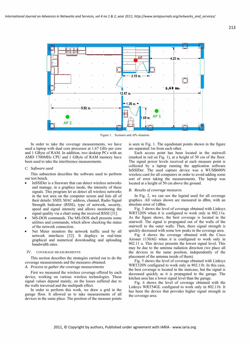
Figure 1. Scenario and APs situation.
In order to take the coverage measurements, we have used a laptop with dual core processor at 1.67 GHz per core and 1 GByte of RAM. In addition, two desktop PCs with an AMD 1700MHz CPU and 1 GByte of RAM memory have been used to take the interference measurements.
C. Software used This subsection describes the software used to perform
our test bench. • InSSIDer is a freeware that can detect wireless networks
and manage, in a graphics mode, the intensity of these signals. This program let us detect all wireless networks in the test area on the computer screen and lists all of their details: SSID, MAC address, channel, Radio Signal Strength Indicator (RSSI), type of network, security, speed and signal intensity and allows monitoring the signal quality via a chart using the received RSSI [31].
• MS-DOS commands. The MS-DOS shell presents some utilities and commands, which allow checking the status of the network connection.
• Net Meter monitors the network traffic used by all network interfaces [32]. It displays in real-time graphical and numerical downloading and uploading bandwidth rates.
IV. COVERAGE MEASUREMENTS This section describes the strategies carried out to do the
coverage measurements and the measures obtained. A. Process to gather the coverage measurements
First we measured the wireless coverage offered by each device, working on various wireless technologies. These signal values depend mainly, on the losses suffered due to the walls traversed and the multipath effect.
In order to perform this work, we draw a grid in the garage floor. It allowed us to take measurements of all devices in the same place. The position of the measure points
is seen in Fig. 1. The equidistant points shown in the figure are separated 1m from each other.
Each access point has been located in the stairwell (marked in red on Fig. 1), at a height of 50 cm of the floor. The signal power levels received at each measure point is collected by a laptop running the application software InSSIDer. The used capture device was a WUSB600N wireless card for all computers in order to avoid adding some sort of error taking the measurements. The laptop was located at a height of 50 cm above the ground.
B. Results of coverage measures In Fig. 2, we can see the legend used for all coverage
graphics. All values shown are measured in dBm, with an absolute error of 1dBm.
Fig. 3 shows the level of coverage obtained with Linksys WRT320N when it is configured to work only in 802.11a. As the figure shows, the best coverage is located in the stairwell. The signal is propagated out of the walls of the stairwell to the outer walls. Then, there signal strength is quickly decreased with some low peaks in the coverage area.
Fig. 4 shows the coverage obtained with the Cisco Aironet 1130AG when it is configured to work only in 802.11 a. This device presents the lowest signal level. This may be due to the antenna radiation direction (we place all the devices in the same position, independently of the placement of the antenna inside of them).
Fig. 5 shows the level of coverage obtained with Linksys WRT320N configured to work only in 802.11b. In this case, the best coverage is located in the staircase, but the signal is decreased quickly as it is propagated to the garage. The kitchen area has a lower signal level than the garage.
Fig. 6 shows the level of coverage obtained with the Linksys WRT54GL configured to work only in 802.11b. It has been the device that provides higher signal strength in the coverage area.
213
International Journal on Advances in Networks and Services, vol 4 no 1 & 2, year 2011, http://www.iariajournals.org/networks_and_services/
2011, © Copyright by authors, Published under agreement with IARIA - www.iaria.org
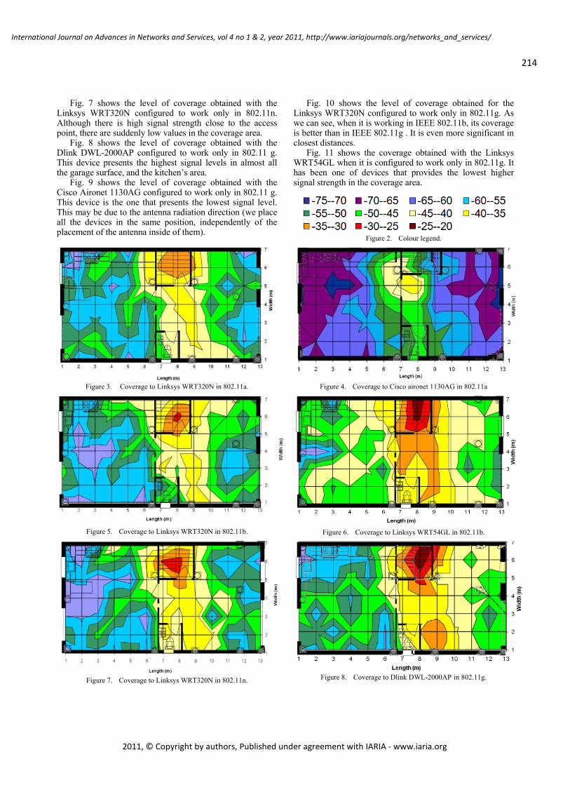
Fig. 7 shows the level of coverage obtained with the Linksys WRT320N configured to work only in 802.11n. Although there is high signal strength close to the access point, there are suddenly low values in the coverage area.
Fig. 8 shows the level of coverage obtained with the Dlink DWL-2000AP configured to work only in 802.11 g. This device presents the highest signal levels in almost all the garage surface, and the kitchen’s area.
Fig. 9 shows the level of coverage obtained with the Cisco Aironet 1130AG configured to work only in 802.11 g. This device is the one that presents the lowest signal level. This may be due to the antenna radiation direction (we place all the devices in the same position, independently of the placement of the antenna inside of them).
Fig. 10 shows the level of coverage obtained for the Linksys WRT320N configured to work only in 802.11g. As we can see, when it is working in IEEE 802.11b, its coverage is better than in IEEE 802.11g . It is even more significant in closest distances.
Fig. 11 shows the coverage obtained with the Linksys WRT54GL when it is configured to work only in 802.11g. It has been one of devices that provides the lowest higher signal strength in the coverage area.
Figure 2. Colour legend.
Figure 3. Coverage to Linksys WRT320N in 802.11a.
Figure 4. Coverage to Cisco aironet 1130AG in 802.11a
Figure 5. Coverage to Linksys WRT320N in 802.11b.
Figure 6. Coverage to Linksys WRT54GL in 802.11b.
Figure 7. Coverage to Linksys WRT320N in 802.11n.
Figure 8. Coverage to Dlink DWL-2000AP in 802.11g.
214
International Journal on Advances in Networks and Services, vol 4 no 1 & 2, year 2011, http://www.iariajournals.org/networks_and_services/
2011, © Copyright by authors, Published under agreement with IARIA - www.iaria.org
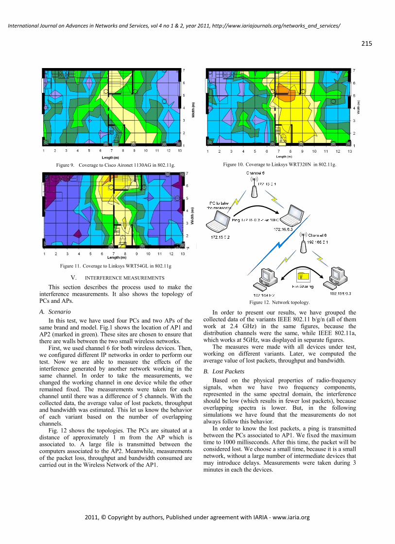
Figure 9. Coverage to Cisco Aironet 1130AG in 802.11g.
Figure 10. Coverage to Linksys WRT320N in 802.11g.
Figure 11. Coverage to Linksys WRT54GL in 802.11g
V. INTERFERENCE MEASUREMENTS This section describes the process used to make the
interference measurements. It also shows the topology of PCs and APs.
A. Scenario In this test, we have used four PCs and two APs of the
same brand and model. Fig.1 shows the location of AP1 and AP2 (marked in green). These sites are chosen to ensure that there are walls between the two small wireless networks.
First, we used channel 6 for both wireless devices. Then, we configured different IP networks in order to perform our test. Now we are able to measure the effects of the interference generated by another network working in the same channel. In order to take the measurements, we changed the working channel in one device while the other remained fixed. The measurements were taken for each channel until there was a difference of 5 channels. With the collected data, the average value of lost packets, throughput and bandwidth was estimated. This let us know the behavior of each variant based on the number of overlapping channels.
Fig. 12 shows the topologies. The PCs are situated at a distance of approximately 1 m from the AP which is associated to. A large file is transmitted between the computers associated to the AP2. Meanwhile, measurements of the packet loss, throughput and bandwidth consumed are carried out in the Wireless Network of the AP1.
Figure 12. Network topology.
In order to present our results, we have grouped the collected data of the variants IEEE 802.11 b/g/n (all of them work at 2.4 GHz) in the same figures, because the distribution channels were the same, while IEEE 802.11a, which works at 5GHz, was displayed in separate figures.
The measures were made with all devices under test, working on different variants. Later, we computed the average value of lost packets, throughput and bandwidth.
B. Lost Packets Based on the physical properties of radio-frequency
signals, when we have two frequency components, represented in the same spectral domain, the interference should be low (which results in fewer lost packets), because overlapping spectra is lower. But, in the following simulations we have found that the measurements do not always follow this behavior.
In order to know the lost packets, a ping is transmitted between the PCs associated to AP1. We fixed the maximum time to 1000 milliseconds. After this time, the packet will be considered lost. We choose a small time, because it is a small network, without a large number of intermediate devices that may introduce delays. Measurements were taken during 3 minutes in each the devices.
215
International Journal on Advances in Networks and Services, vol 4 no 1 & 2, year 2011, http://www.iariajournals.org/networks_and_services/
2011, © Copyright by authors, Published under agreement with IARIA - www.iaria.org
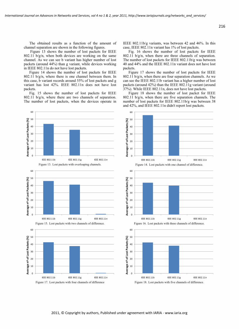
The obtained results as a function of the amount of channel separation are shown in the following figures.
Figure 13 shows the number of lost packets for IEEE 802.11 b/g/n, when both devices are working on the same channel. As we can see b variant has higher number of lost packets (around 44%) than g variant, while devices working in IEEE 802.11n do not have lost packets.
Figure 14 shows the number of lost packets for IEEE 802.11 b/g/n, where there is one channel between them. In this case, b variant records around 55% of lost packets and g variant has lost 42%. IEEE 802.11n does not have lost packets.
Fig. 15 shows the number of lost packets for IEEE 802.11 b/g/n, where there are two channels of separation. The number of lost packets, when the devices operate in
IEEE 802.11b/g variants, was between 42 and 46%. In this case, IEEE 802.11n variant has 1% of lost packets.
Fig. 16 shows the number of lost packets for IEEE 802.11 b/g/n, when there are three channels of separation. The number of lost packets for IEEE 802.11b/g was between 40 and 44% and the IEEE 802.11n variant does not have lost packets.
Figure 17 shows the number of lost packets for IEEE 802.11 b/g/n, when there are four separation channels. As we can see the IEEE 802.11b variant has a higher number of lost packets (around 42%) than the IEEE 802.11g variant (around 37%). While IEEE 802.11n, does not have lost packets.
Figure 18 shows the number of lost packet for IEEE 802.11 b/g/n, when there are five separation channels. The number of lost packets for IEEE 802.11b/g was between 38 and 42%, and IEEE 802.11n didn't report lost packets.
Figure 13. Lost packets with overloaping channels.
Figure 14. Lost packets with one channel of difference.
Figure 15. Lost packets with two channels of difference.
Figure 16. Lost packets with three channels of difference.
Figure 17. Lost packets with four channels of difference
Figure 18. Lost packets with five channels of difference.
0
10
20
30
40
50
60
IEEE 802.11b IEEE 802.11g IEEE 802.11n
Average
nº of Lost P
ackets (%
)
0
10
20
30
40
50
60
IEEE 802.11b IEEE 802.11g IEEE 802.11n
Average
nº of Lost P
ackets (%
)
0
10
20
30
40
50
60
IEEE 802.11b IEEE 802.11g IEEE 802.11n
Average
nº of Lost P
ackets (%
)
0
10
20
30
40
50
60
IEEE 802.11b IEEE 802.11g IEEE 802.11n
Average
nº of Lost P
ackets (%
)
0
10
20
30
40
50
60
IEEE 802.11b IEEE 802.11g IEEE 802.11n
Average
nº of Lost P
ackets (%
)
0
10
20
30
40
50
60
IEEE 802.11b IEEE 802.11g IEEE 802.11n
Average
nº of Lost P
ackets (%
)
216
International Journal on Advances in Networks and Services, vol 4 no 1 & 2, year 2011, http://www.iariajournals.org/networks_and_services/
2011, © Copyright by authors, Published under agreement with IARIA - www.iaria.org
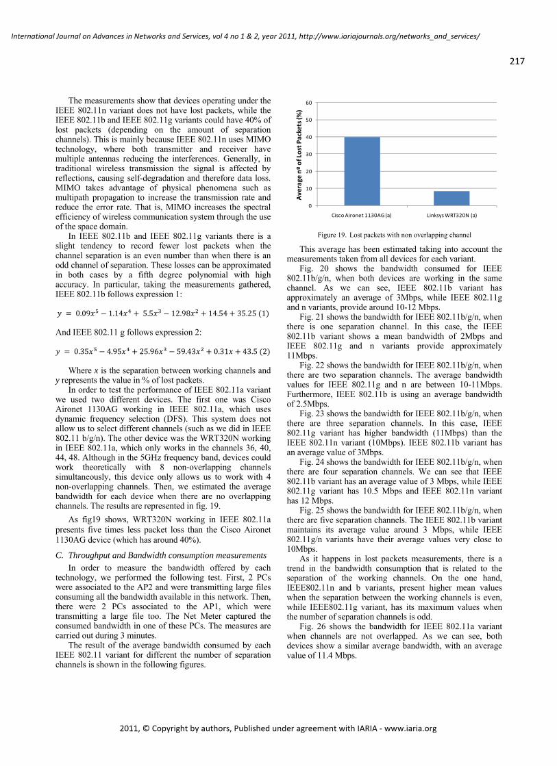
The measurements show that devices operating under the IEEE 802.11n variant does not have lost packets, while the IEEE 802.11b and IEEE 802.11g variants could have 40% of lost packets (depending on the amount of separation channels). This is mainly because IEEE 802.11n uses MIMO technology, where both transmitter and receiver have multiple antennas reducing the interferences. Generally, in traditional wireless transmission the signal is affected by reflections, causing self-degradation and therefore data loss. MIMO takes advantage of physical phenomena such as multipath propagation to increase the transmission rate and reduce the error rate. That is, MIMO increases the spectral efficiency of wireless communication system through the use of the space domain.
In IEEE 802.11b and IEEE 802.11g variants there is a slight tendency to record fewer lost packets when the channel separation is an even number than when there is an odd channel of separation. These losses can be approximated in both cases by a fifth degree polynomial with high accuracy. In particular, taking the measurements gathered, IEEE 802.11b follows expression 1:
0.09 1.14 5.5 12.98 14.54 35.25 1
And IEEE 802.11 g follows expression 2:
0.35 4.95 25.96 59.43 0.31 43.5 2 Where x is the separation between working channels and
y represents the value in % of lost packets. In order to test the performance of IEEE 802.11a variant
we used two different devices. The first one was Cisco Aironet 1130AG working in IEEE 802.11a, which uses dynamic frequency selection (DFS). This system does not allow us to select different channels (such as we did in IEEE 802.11 b/g/n). The other device was the WRT320N working in IEEE 802.11a, which only works in the channels 36, 40, 44, 48. Although in the 5GHz frequency band, devices could work theoretically with 8 non-overlapping channels simultaneously, this device only allows us to work with 4 non-overlapping channels. Then, we estimated the average bandwidth for each device when there are no overlapping channels. The results are represented in fig. 19.
As fig19 shows, WRT320N working in IEEE 802.11a presents five times less packet loss than the Cisco Aironet 1130AG device (which has around 40%).
C. Throughput and Bandwidth consumption measurements In order to measure the bandwidth offered by each
technology, we performed the following test. First, 2 PCs were associated to the AP2 and were transmitting large files consuming all the bandwidth available in this network. Then, there were 2 PCs associated to the AP1, which were transmitting a large file too. The Net Meter captured the consumed bandwidth in one of these PCs. The measures are carried out during 3 minutes.
The result of the average bandwidth consumed by each IEEE 802.11 variant for different the number of separation channels is shown in the following figures.
Figure 19. Lost packets with non overlapping channel
This average has been estimated taking into account the measurements taken from all devices for each variant.
Fig. 20 shows the bandwidth consumed for IEEE 802.11b/g/n, when both devices are working in the same channel. As we can see, IEEE 802.11b variant has approximately an average of 3Mbps, while IEEE 802.11g and n variants, provide around 10-12 Mbps.
Fig. 21 shows the bandwidth for IEEE 802.11b/g/n, when there is one separation channel. In this case, the IEEE 802.11b variant shows a mean bandwidth of 2Mbps and IEEE 802.11g and n variants provide approximately 11Mbps.
Fig. 22 shows the bandwidth for IEEE 802.11b/g/n, when there are two separation channels. The average bandwidth values for IEEE 802.11g and n are between 10-11Mbps. Furthermore, IEEE 802.11b is using an average bandwidth of 2.5Mbps.
Fig. 23 shows the bandwidth for IEEE 802.11b/g/n, when there are three separation channels. In this case, IEEE 802.11g variant has higher bandwidth (11Mbps) than the IEEE 802.11n variant (10Mbps). IEEE 802.11b variant has an average value of 3Mbps.
Fig. 24 shows the bandwidth for IEEE 802.11b/g/n, when there are four separation channels. We can see that IEEE 802.11b variant has an average value of 3 Mbps, while IEEE 802.11g variant has 10.5 Mbps and IEEE 802.11n variant has 12 Mbps.
Fig. 25 shows the bandwidth for IEEE 802.11b/g/n, when there are five separation channels. The IEEE 802.11b variant maintains its average value around 3 Mbps, while IEEE 802.11g/n variants have their average values very close to 10Mbps.
As it happens in lost packets measurements, there is a trend in the bandwidth consumption that is related to the separation of the working channels. On the one hand, IEEE802.11n and b variants, present higher mean values when the separation between the working channels is even, while IEEE802.11g variant, has its maximum values when the number of separation channels is odd.
Fig. 26 shows the bandwidth for IEEE 802.11a variant when channels are not overlapped. As we can see, both devices show a similar average bandwidth, with an average value of 11.4 Mbps.
0
10
20
30
40
50
60
Cisco Aironet 1130AG (a) Linksys WRT320N (a)
Average
nº of Lost P
ackets (%
)
217
International Journal on Advances in Networks and Services, vol 4 no 1 & 2, year 2011, http://www.iariajournals.org/networks_and_services/
2011, © Copyright by authors, Published under agreement with IARIA - www.iaria.org
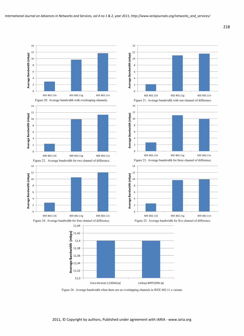
Figure 20. Average bandwidth with overloaping channels.
Figure 21. Average bandwidth with one channel of difference.
Figure 22. Average bandwidth for two channel of difference.
Figure 23. Average bandwidth for three channel of difference.
Figure 24. Average bandwidth for four channel of difference.
Figure 25. Average bandwidth for five channel of difference.
Figure 26. Average bandwidth when there are no overlapping channels in IEEE 802.11 a variant.
0
2
4
6
8
10
12
14
IEEE 802.11b IEEE 802.11g IEEE 802.11n
Average
Ban
dwidth (m
bps)
0
2
4
6
8
10
12
14
IEEE 802.11b IEEE 802.11g IEEE 802.11n
Average
Ban
dwidth (m
bps)
0
2
4
6
8
10
12
14
IEEE 802.11b IEEE 802.11g IEEE 802.11n
Average
Ban
dwidth (m
bps)
0
2
4
6
8
10
12
14
IEEE 802.11b IEEE 802.11g IEEE 802.11n
Average
Ban
dwidth (m
bps)
0
2
4
6
8
10
12
14
IEEE 802.11b IEEE 802.11g IEEE 802.11n
Average
Ban
dwidth (m
bps)
0
2
4
6
8
10
12
14
IEEE 802.11b IEEE 802.11g IEEE 802.11n
Average
Ban
dwidth (m
bps)
11,3
11,32
11,34
11,36
11,38
11,4
11,42
11,44
Cisco Aironet 1130AG (a) Linksys WRT320N (a)
Average
Ban
dwidth (mbp
s)
218
International Journal on Advances in Networks and Services, vol 4 no 1 & 2, year 2011, http://www.iariajournals.org/networks_and_services/
2011, © Copyright by authors, Published under agreement with IARIA - www.iaria.org
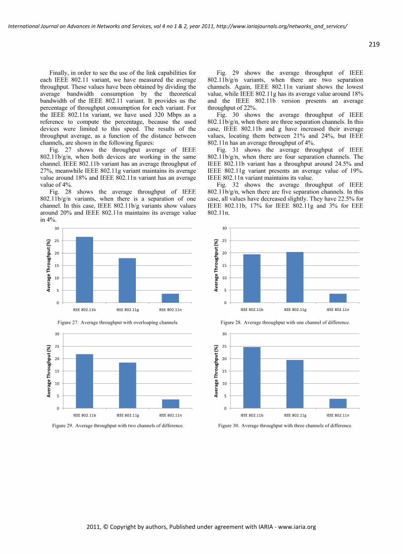
Finally, in order to see the use of the link capabilities for each IEEE 802.11 variant, we have measured the average throughput. These values have been obtained by dividing the average bandwidth consumption by the theoretical bandwidth of the IEEE 802.11 variant. It provides us the percentage of throughput consumption for each variant. For the IEEE 802.11n variant, we have used 320 Mbps as a reference to compute the percentage, because the used devices were limited to this speed. The results of the throughput average, as a function of the distance between channels, are shown in the following figures:
Fig. 27 shows the throughput average of IEEE 802.11b/g/n, when both devices are working in the same channel. IEEE 802.11b variant has an average throughput of 27%, meanwhile IEEE 802.11g variant maintains its average value around 18% and IEEE 802.11n variant has an average value of 4%.
Fig. 28 shows the average throughput of IEEE 802.11b/g/n variants, when there is a separation of one channel. In this case, IEEE 802.11b/g variants show values around 20% and IEEE 802.11n maintains its average value in 4%.
Fig. 29 shows the average throughput of IEEE 802.11b/g/n variants, when there are two separation channels. Again, IEEE 802.11n variant shows the lowest value, while IEEE 802.11g has its average value around 18% and the IEEE 802.11b version presents an average throughput of 22%.
Fig. 30 shows the average throughput of IEEE 802.11b/g/n, when there are three separation channels. In this case, IEEE 802.11b and g have increased their average values, locating them between 21% and 24%, but IEEE 802.11n has an average throughput of 4%.
Fig. 31 shows the average throughput of IEEE 802.11b/g/n, when there are four separation channels. The IEEE 802.11b variant has a throughput around 24.5% and IEEE 802.11g variant presents an average value of 19%. IEEE 802.11n variant maintains its value.
Fig. 32 shows the average throughput of IEEE 802.11b/g/n, when there are five separation channels. In this case, all values have decreased slightly. They have 22.5% for IEEE 802.11b, 17% for IEEE 802.11g and 3% for EEE 802.11n.
Figure 27. Average throughput with overloaping channels.
Figure 28. Average throughput with one channel of difference.
Figure 29. Average throughput with two channels of difference.
Figure 30. Average throughput with three channels of difference.
0
5
10
15
20
25
30
IEEE 802.11b IEEE 802.11g IEEE 802.11n
Average
Throu
ghpu
t (%)
0
5
10
15
20
25
30
IEEE 802.11b IEEE 802.11g IEEE 802.11n
Average
Throu
ghpu
t (%)
0
5
10
15
20
25
30
IEEE 802.11b IEEE 802.11g IEEE 802.11n
Average
Throu
ghpu
t (%)
0
5
10
15
20
25
30
IEEE 802.11b IEEE 802.11g IEEE 802.11n
Average
Throu
ghpu
t (%)
219
International Journal on Advances in Networks and Services, vol 4 no 1 & 2, year 2011, http://www.iariajournals.org/networks_and_services/
2011, © Copyright by authors, Published under agreement with IARIA - www.iaria.org
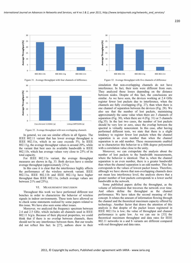
Figure 31. Average throughput with four channels of difference.
Figure 32. Average throughput with five channels of difference
Figure 33. Average throughput with non overlapping channels
In general, we can see similar effects in all figures. The IEEE 802.11 variant that has lower average throughput is IEEE 802.11n, which in no case exceeds 5%. In IEEE 802.11g, the average throughput values is around 20%, while the variant that best uses its available bandwidth is IEEE 802.11b, which has average values very close to 25% of its total capacity.
For IEEE 802.11a variant, the average throughput measures are shown in fig. 33. Both devices have a similar average throughput (approximately 21%).
In this case it is clear that the interference highly affects the performance of the wireless network variant. IEEE 802.11a, IEEE 802.11b and IEEE 802.11g have higher throughput than IEEE 802.11n, (which average values are between 21% and 25%).
VI. MEASUREMENT DISCUSSION Throughout this work we have performed different test
benches in order to characterize the behavior of wireless signals in indoor environments. These tests have allowed us to check some statements realized by some papers related to this issue. We have also seen some other issues.
Moreover, we analyzed the frequency spectrum between 2.4 and 2.5 GHz, which includes all channels used in IEEE 802.11 b/g/n. Because of their physical properties, we could think that if there is no overlap between channels, there should not be any interference between them. But our results did not reflect this fact. In [27], authors show in their
simulation that non-overlapping channels do not have interference. In fact, their tests were different from ours. They analyzed these losses depending on the distance between nodes. Despite of this fact, the conclusions are similar. As we have seen, the devices working at 2.4 GHz register fewer lost packets due to interference, when the channels are fully overlapping (Fig. 27), than when there is one channel of separation between the devices (Fig. 28). We also see that the number of lost packets, maintaining approximately the same value when there are 3 channels of separation (Fig. 30), when there are 4 (Fig. 31) or 5 channels (fig.35). In the last two cases, the number of lost packets should be very low or zero, since the overlap between the spectral is virtually nonexistent. In this case, after having performed different tests, we state that there is a slight tendency to register fewer lost packets when the channel separation is an even number than when the channel separation is an odd number. These measurements enabled us to characterize this behavior to a fifth degree polynomial with a correlation value close to the unity.
Moreover, we can extrapolate the analysis about the number of lost packets to the bandwidth measurements, where the behavior is identical. That is, when the channel separation is an even number, there is a greater bandwidth than when the channel separation is an odd number. This fact corresponds to the values of lowest packet losses. Therefore, although we have shown that non-overlapping channels does not mean less interference level, the analysis shows that a greater number of lost packets corresponds to a lower useful bandwidth in the network.
Some published papers define the throughput, as the volume of information that traverses the network over time. And others define the throughput as the channel performance. We have taken the second meaning of this concept. It relates the amount of information flowing through the channel and the theoretical maximum capacity offered by technology. Another factor that draws the attention of this analysis is that despite of the packet losses registered in IEEE 802.11n is low; the value of throughput and channel performance is quite low. As we can see in [33] the theoretical maximum throughput and data rates for IEEE 802.11 networks in a and b variants are different compared with real throughput and data rates.
0
5
10
15
20
25
30
IEEE 802.11b IEEE 802.11g IEEE 802.11n
Average
Throu
ghpu
t (%)
0
5
10
15
20
25
30
IEEE 802.11b IEEE 802.11g IEEE 802.11n
Average
Throu
ghpu
t (%)
0
5
10
15
20
25
30
Cisco Aironet 1130AG (a) Linksys WRT320N (a)
Average
Throu
ghpu
t (%)
220
International Journal on Advances in Networks and Services, vol 4 no 1 & 2, year 2011, http://www.iariajournals.org/networks_and_services/
2011, © Copyright by authors, Published under agreement with IARIA - www.iaria.org
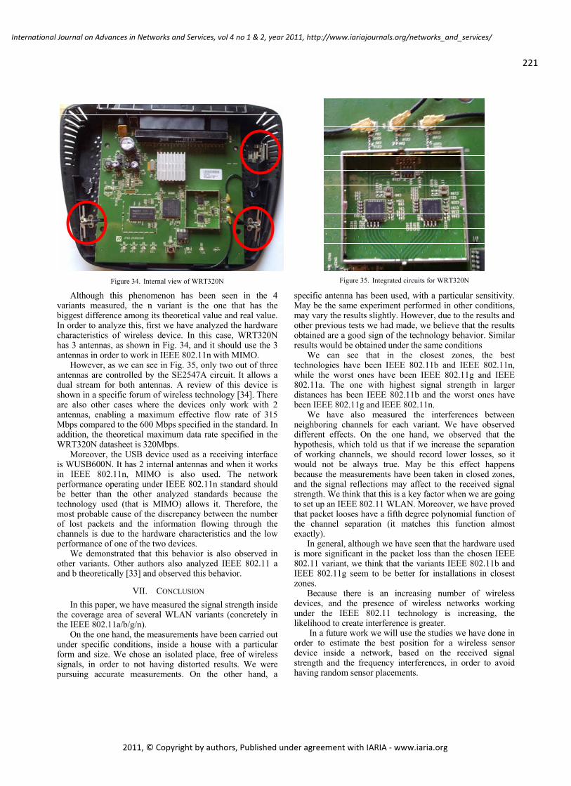
Figure 34. Internal view of WRT320N
Figure 35. Integrated circuits for WRT320N
Although this phenomenon has been seen in the 4 variants measured, the n variant is the one that has the biggest difference among its theoretical value and real value. In order to analyze this, first we have analyzed the hardware characteristics of wireless device. In this case, WRT320N has 3 antennas, as shown in Fig. 34, and it should use the 3 antennas in order to work in IEEE 802.11n with MIMO.
However, as we can see in Fig. 35, only two out of three antennas are controlled by the SE2547A circuit. It allows a dual stream for both antennas. A review of this device is shown in a specific forum of wireless technology [34]. There are also other cases where the devices only work with 2 antennas, enabling a maximum effective flow rate of 315 Mbps compared to the 600 Mbps specified in the standard. In addition, the theoretical maximum data rate specified in the WRT320N datasheet is 320Mbps.
Moreover, the USB device used as a receiving interface is WUSB600N. It has 2 internal antennas and when it works in IEEE 802.11n, MIMO is also used. The network performance operating under IEEE 802.11n standard should be better than the other analyzed standards because the technology used (that is MIMO) allows it. Therefore, the most probable cause of the discrepancy between the number of lost packets and the information flowing through the channels is due to the hardware characteristics and the low performance of one of the two devices.
We demonstrated that this behavior is also observed in other variants. Other authors also analyzed IEEE 802.11 a and b theoretically [33] and observed this behavior.
VII. CONCLUSION In this paper, we have measured the signal strength inside
the coverage area of several WLAN variants (concretely in the IEEE 802.11a/b/g/n).
On the one hand, the measurements have been carried out under specific conditions, inside a house with a particular form and size. We chose an isolated place, free of wireless signals, in order to not having distorted results. We were pursuing accurate measurements. On the other hand, a
specific antenna has been used, with a particular sensitivity. May be the same experiment performed in other conditions, may vary the results slightly. However, due to the results and other previous tests we had made, we believe that the results obtained are a good sign of the technology behavior. Similar results would be obtained under the same conditions
We can see that in the closest zones, the best technologies have been IEEE 802.11b and IEEE 802.11n, while the worst ones have been IEEE 802.11g and IEEE 802.11a. The one with highest signal strength in larger distances has been IEEE 802.11b and the worst ones have been IEEE 802.11g and IEEE 802.11n.
We have also measured the interferences between neighboring channels for each variant. We have observed different effects. On the one hand, we observed that the hypothesis, which told us that if we increase the separation of working channels, we should record lower losses, so it would not be always true. May be this effect happens because the measurements have been taken in closed zones, and the signal reflections may affect to the received signal strength. We think that this is a key factor when we are going to set up an IEEE 802.11 WLAN. Moreover, we have proved that packet looses have a fifth degree polynomial function of the channel separation (it matches this function almost exactly).
In general, although we have seen that the hardware used is more significant in the packet loss than the chosen IEEE 802.11 variant, we think that the variants IEEE 802.11b and IEEE 802.11g seem to be better for installations in closest zones.
Because there is an increasing number of wireless devices, and the presence of wireless networks working under the IEEE 802.11 technology is increasing, the likelihood to create interference is greater.
In a future work we will use the studies we have done in order to estimate the best position for a wireless sensor device inside a network, based on the received signal strength and the frequency interferences, in order to avoid having random sensor placements.
221
International Journal on Advances in Networks and Services, vol 4 no 1 & 2, year 2011, http://www.iariajournals.org/networks_and_services/
2011, © Copyright by authors, Published under agreement with IARIA - www.iaria.org
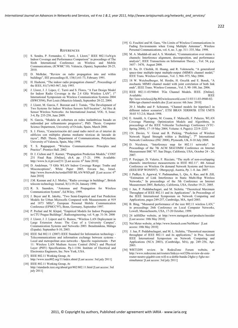
REFERENCES [1] S. Sendra, P. Fernandez, C. Turró, J. Lloret,” IEEE 802.11a/b/g/n
Indoor Coverage and Performance Comparison” in procedings of The Sixth International Conference on Wireless and Mobile Communications, (ICWMC’10). Valencia, (Spain), September 20-25, 2010.
[2] D. Molkdar, “Review on radio propagation into and within buildings”, IEE proceedings-H, 138(1):61-73, February 1991.
[3] H. Hashemi, “The indoor radio propagation channel”, Proceedings of the IEEE, 81(7):943-967, July 1993.
[4] J. Lloret, J. J. López, C. Turró and S. Flores, “A Fast Design Model for Indoor Radio Coverage in the 2.4 GHz Wireless LAN”, 1st International Symposium on Wireless Communication Systems 2004 (ISWCS'04), Port Louis (Mauricio Island), September 20-22, 2004.
[5] J. Lloret, M. Garcia, F. Boronat and J. Tomás, “The Development of Two Systems for Indoor Wireless Sensors Self-location”, Ad Hoc & Sensor Wireless Networks: An International Journal, VOL: 8, Issue: 3-4, Pp. 235-258, June 2009.
[6] N. García, “Modelo de cobertura en redes inalámbricas basado en radiosidad por refinamiento progresivo”, PhD. Thesis. Computer Science Department, University of Oviedo, Spain, March 2006.
[7] S. J. Flores, “Caracterización del canal radio móvil en el interior de edificios con múltiples plantas mediante técnicas de lanzado de rayos”, PhD. Thesis. Department of Communications, Polytechnic University of Valencia, Spain, May 1998.
[8] T. S. Rappapport. "Wireless Communications: Principles and Practice". Prentice Hall. 2002
[9] D. J. Cichon and T. Kurner, “Propagation Prediction Models,” COST 231 Final Rep. [Online], ch.4, pp. 17–21. 1996. Available: http://www.lx.it.pt/cost231/ [Last access: 6th June 2010]
[10] D. Andelman, “5 GHz WLAN Indoor Coverage Range: Truths and Misconceptions'', White Paper 2005, Envara Inc, Israel. http://www.freeweb.hu/tordaif/HIF/RLAN/WSD.pdf [Last access: 6th June 2010]
[11] J.M. Keenan and A.J. Motley, “Radio coverage in buildings”, British telecom technology Journal, 8(1):19-24, January 1990.
[12] R. S. Saunders, “Antennas and Propagation for Wireless Communication System”, Ed.Wiley, 1999.
[13] J. Beyer and R. Jakoby, "Two Semi-Empirical and Fast Prediction Models for Urban Microcells Compared with Measurements at 919 and 1873 MHz", European Personal Mobile Communication Conference (EPMCC'97), Bonn, Germany, September 1997.
[14] P. Pechač and M. Klepal, “Empirical Models for Indoor Propagation in CTU Prague Buildings”, Radioengineering, vol. 9, pp. 31-36. 2000
[15] J. Lloret, J. J. Lópezt and G. Ramos, “Wireless LAN Deployment in Large Extension Areas: The Case of a University Campus”, Communication Systems and Networks 2003. Benalmádena, Málaga (España). September 8-10, 2003.
[16] IEEE Std 802.11 (2007) IEEE Standard for Information technology -Telecommunications and information exchange between systems - Local and metropolitan area networks - Specific requirements - Part 11: Wireless LAN Medium Access Control (MAC) and Physical Layer (PHY) Specifications. Pp.1-1184. Institute of Electrical and Electronics Engineers, Inc. New York, USA.
[17] IEEE 802.11 Working Group, At http://www.ieee802.org/11/index.shtml [Last access: 3rd july 2011]
[18] IEEE 802.11 Working Group, At http://standards.ieee.org/about/get/802/802.11.html [Last access: 3rd july 2011]
[19] G. Foschini and M. Gans, “On Limits of Wireless Communications in Fading Environments when Using Multiple Antennas”, Wireless Personal Communications, vol. 6, no. 3, pp. 311–335, Mar. 1998.
[20] M. A. Maddah-ali and A. S. Motahari, “Communication over mimo x channels: Interference alignment, decomposition, and performance analysis”, IEEE Transactions on Information Theory. , Vol. 54, p.p. 3457 - 3470, August 2008.
[21] H. Xu, D. Chizhik, H. Huang, and R. Valenzuela, “A generalized space-time multiple-input multiple-output (MIMO) channel model,” IEEE Trans. Wireless Commun., Vol. 3, 966–975, May 2004.
[22] 18 W. Weichselberger, M. Herdin, H. Ozcelik and E. Bonek, “A stochastic MIMO channel model with joint correlation of both link ends”, IEEE Trans. Wireless Commun., Vol. 5, 90–100, Jan. 2006.
[23] IEEE 802.11-03/940r4: TGn Channel Models. IEEE. [Online]. Available: IEEE ftp://ieee:[email protected]/11/03/11-03-0940-02-000n-tgn-channel-models.doc [Last access: 6th June 2010] 20 J. Medbo and P. Schramm, “Channel models for hiperlan/2 in different indoor scenarios”, ETSI BRAN 3ERI085B. ETSI UMTS 30.03 V3.2.0, March 1998.
[24] E. Amaldi, A. Capone, M. Cesana, F. Malucelli, F. Palazzo, WLAN Coverage Planning: Optimization Models and Algorithms, in proceedings of the IEEE Vehicular Technology Conference (VTC-Spring 2004), 17–19 May 2004, Volume: 4, Page(s): 2219–2223
[25] J.N. Davies, V. Grout and R. Picking, “Prediction of Wireless Network Signal Strength within a Building”, 7th International Network Conference (INC 2008), Plymouth, UK, 8-10 July 2008.
[26] D. Niculescu, “Interference map for 802.11 networks”. In Proceedings of the 7th ACM SIGCOMM Conference on Internet Measurement IMC '07. San Diego, California, USA, October 24 - 26, 2007.
[27] P. Fuxjager, D. Valerio, F. Ricciato, “The myth of non-overlapping channels: interference measurements in IEEE 802.11”. 4th Annual Conference on Wireless On demand Network Systems and Services (IEEE/IFIP WONS'07). Oberguyrgl, Austria, Pp. 1–8. Jan. 2007.
[28] J. Padhye, S. Agarwal, V. Padmanaban, L. Qiu, A. Rao, and B. Zill, “Estimation of Link Interference in Static Multi-Hop Wireless Networks,” In proceedings of the 5th Conference on Internet Measurement 2005, Berkeley, California, USA, October 19-21, 2005.
[29] J. Jun, P. Peddabachagari, and M. Sichitiu. “Theoretical Maximum Throughput of IEEE 802.11 and its Applications”. In Proceedings of the IEEE International Symposium on Network Computing and Applications, pages 249-257, Cambridge, MA, April 2003.
[30] B. Bing, “Measured performance of the ieee 802.11 wireless LAN,” in proceedings 26th Conference on Local Computer Networks, Lowell, Massachusetts, USA, 17-20 October, 1999.
[31] 24 inSSIDer website, at http://www.metageek.net/products/inssider [Last access: 10th May 2010]
[32] Net Meter website, at http://www.hootech.com/NetMeter/ [Last access: 10th May 2010]
[33] J. Jun, P. Peddabachagari, and M. L. Sichitiu, “Theoretical maximum throughput of IEEE 802.11 and its applications,” in Proc. Second IEEE International Symposium on Network Computing and Applications (NCA 2003), (Cambridge, MA), pp. 249–256, Apr. 2003.
[34] WRT320N review. In RedesZone Forum website, at http://www.redeszone.net/routers/linksys-wrt320n-review-de-este-router-neutro-gigabit-con-wifi-n-a-doble-banda-24ghz-y-5ghz-no-simultanea/ [Last access: 3rd july 2011]
222
International Journal on Advances in Networks and Services, vol 4 no 1 & 2, year 2011, http://www.iariajournals.org/networks_and_services/
2011, © Copyright by authors, Published under agreement with IARIA - www.iaria.org
Fast Retrieval from Image Databases via Binary Haar Wavelet Transform on theColor and Edge Directivity Descriptor
Savvas A. Chatzichristofis1 Yiannis S. Boutalis1,2 Avi Arampatzis11Department of Electrical & Computer Engineering,
Democritus University of Thrace, Xanthi, Greece2Department of Electrical, Electronic and Communication Engineering,
Chair of Automatic Control, University of Erlangen-Nuremberg, Germanyschatzic,ybout,[email protected]
Abstract—In this paper, we are evaluating several accelerat-ing techniques for content-based image retrieval, suitable forthe Color and Edge Directivity Descriptor (CEDD). To date,the experimental results presented in the literature have shownthat the CEDD achieves high rates of successful retrieval inbenchmark image databases. Although its storage requirementsare minimal, only 54 bytes per image, the time required forretrieval may be practically too long when searching on largedatabases. The proposed technique utilizes the Binary HaarWavelet Transform in order to extract from the CEDD asmaller and more efficient descriptor, with a size of less than2 bytes per image, speeding up retrieval from large imagedatabases. This descriptor describes the CEDD, but not neces-sarily the image from which it is extracted. The effectivenessof the proposed method is demonstrated through experimentsperformed on several known benchmarking databases.
Keywords-CEDD; Binary Haar Wavelet Transform; Content-Based Image Retrieval;
I. INTRODUCTION
As the use of computers, internet and cameras is gettingmore popular, efficient content-based image retrieval is moreessential than ever. Any technology that, in principle, helpsto organize digital image archives by their visual contentis defined as content-based image retrieval (CBIR). Bythis definition, anything ranging from an image similarityfunction to a robust image annotation engine falls under thepurview of CBIR [1].
Online image repositories such as Flickr contain hundredsof millions of images and are growing quickly [2]. Therequirements of modern retrieval systems are not limited toproviding good retrieval results, but extend to their abilityfor quick results. The majority of internet users wouldcompromise the partial reduction of result accuracy in orderto save time from searching.
Image retrieval, as well as text retrieval, may be describedby the similarity search paradigm [3]. Efficient approachesthat allow application on generic similarity search problemsstill need to be investigated [4]. A promising directionto address this issue is the approximate similarity searchparadigm [5], [6], [7], [8]. Approximate similarity searchprovides an improvement in search performance at the price
of some imprecision in the results. An interesting approachof approximate similarity search was proposed in [4]. Theidea at the basis of this technique is that when two objectsare very close to each other they ’see’ the world around themin the same way.
In order to achieve image retrieval from large databases,the representation of images by Latent Dirichlet Allocation(LDA) [9] models is studied in [2]. Image representationsare learned in an unsupervised fashion, and each image ismodeled as a mixture of its depicted topics or object parts.
The present paper proposes a different approach forsearching in large databases. First of all, in order to ensurequality of the results, the Color and Edge Directivity De-scriptor (CEDD), proposed in [10], [11], is utilized. The sizeof this descriptor is 54 bytes/image. Subsequently, the BinaryHaar Wavelet Transform [12] is used for the extraction ofa second descriptor, we call Binary CEDD (B-CEDD). Thissecond descriptor is employed during the retrieval procedureinstead of the image. In this way, reduced retrieval timesare achieved. A preliminary version of this work has beenpresented in [13]. Details concerning the CEDD and theBinary Haar Wavelet Transform are given in Sections II andIII, respectively.
In order to shape B-CEDD, we follow and evaluate threedifferent approaches. First, we consider CEDD as a singlevector and apply the Binary Haar Wavelet Transform upto 15 coefficients. Second, we consider CEDD as a resultof early fusion of two independent vectors, one capturingcolor and the other texture information. Also in this case,the resulting compact descriptor consists of 15 coefficients.In final third approach, we again consider CEDD as a resultof early fusion of 6 independent vectors and apply BinaryHaar Wavelet Transform to each of the vectors separately.The length of the resulting descriptor is now 18 coefficients.In Section IV, we will describe these three approaches indetail.
During the search process, an image query is entered andthe system returns images with a similar content. Initially,the similarity/distance between the query and each image inthe database is calculated with the proposed descriptor, and
223
International Journal on Advances in Networks and Services, vol 4 no 1 & 2, year 2011, http://www.iariajournals.org/networks_and_services/
2011, © Copyright by authors, Published under agreement with IARIA - www.iaria.org
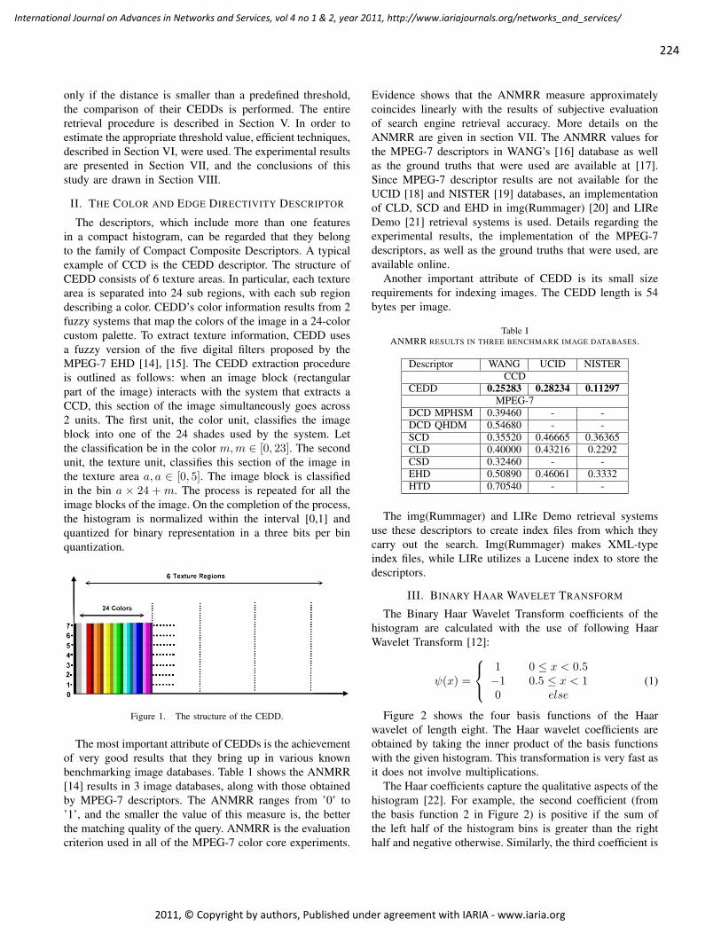
only if the distance is smaller than a predefined threshold,the comparison of their CEDDs is performed. The entireretrieval procedure is described in Section V. In order toestimate the appropriate threshold value, efficient techniques,described in Section VI, were used. The experimental resultsare presented in Section VII, and the conclusions of thisstudy are drawn in Section VIII.
II. THE COLOR AND EDGE DIRECTIVITY DESCRIPTOR
The descriptors, which include more than one featuresin a compact histogram, can be regarded that they belongto the family of Compact Composite Descriptors. A typicalexample of CCD is the CEDD descriptor. The structure ofCEDD consists of 6 texture areas. In particular, each texturearea is separated into 24 sub regions, with each sub regiondescribing a color. CEDD’s color information results from 2fuzzy systems that map the colors of the image in a 24-colorcustom palette. To extract texture information, CEDD usesa fuzzy version of the five digital filters proposed by theMPEG-7 EHD [14], [15]. The CEDD extraction procedureis outlined as follows: when an image block (rectangularpart of the image) interacts with the system that extracts aCCD, this section of the image simultaneously goes across2 units. The first unit, the color unit, classifies the imageblock into one of the 24 shades used by the system. Letthe classification be in the color m,m ∈ [0, 23]. The secondunit, the texture unit, classifies this section of the image inthe texture area a, a ∈ [0, 5]. The image block is classifiedin the bin a × 24 +m. The process is repeated for all theimage blocks of the image. On the completion of the process,the histogram is normalized within the interval [0,1] andquantized for binary representation in a three bits per binquantization.
Figure 1. The structure of the CEDD.
The most important attribute of CEDDs is the achievementof very good results that they bring up in various knownbenchmarking image databases. Table 1 shows the ANMRR[14] results in 3 image databases, along with those obtainedby MPEG-7 descriptors. The ANMRR ranges from ’0’ to’1’, and the smaller the value of this measure is, the betterthe matching quality of the query. ANMRR is the evaluationcriterion used in all of the MPEG-7 color core experiments.
Evidence shows that the ANMRR measure approximatelycoincides linearly with the results of subjective evaluationof search engine retrieval accuracy. More details on theANMRR are given in section VII. The ANMRR values forthe MPEG-7 descriptors in WANG’s [16] database as wellas the ground truths that were used are available at [17].Since MPEG-7 descriptor results are not available for theUCID [18] and NISTER [19] databases, an implementationof CLD, SCD and EHD in img(Rummager) [20] and LIReDemo [21] retrieval systems is used. Details regarding theexperimental results, the implementation of the MPEG-7descriptors, as well as the ground truths that were used, areavailable online.
Another important attribute of CEDD is its small sizerequirements for indexing images. The CEDD length is 54bytes per image.
Table IANMRR RESULTS IN THREE BENCHMARK IMAGE DATABASES.
Descriptor WANG UCID NISTERCCD
CEDD 0.25283 0.28234 0.11297MPEG-7
DCD MPHSM 0.39460 - -DCD QHDM 0.54680 - -SCD 0.35520 0.46665 0.36365CLD 0.40000 0.43216 0.2292CSD 0.32460 - -EHD 0.50890 0.46061 0.3332HTD 0.70540 - -
The img(Rummager) and LIRe Demo retrieval systemsuse these descriptors to create index files from which theycarry out the search. Img(Rummager) makes XML-typeindex files, while LIRe utilizes a Lucene index to store thedescriptors.
III. BINARY HAAR WAVELET TRANSFORM
The Binary Haar Wavelet Transform coefficients of thehistogram are calculated with the use of following HaarWavelet Transform [12]:
ψ(x) =
1−10
0 ≤ x < 0.50.5 ≤ x < 1
else(1)
Figure 2 shows the four basis functions of the Haarwavelet of length eight. The Haar wavelet coefficients areobtained by taking the inner product of the basis functionswith the given histogram. This transformation is very fast asit does not involve multiplications.
The Haar coefficients capture the qualitative aspects of thehistogram [22]. For example, the second coefficient (fromthe basis function 2 in Figure 2) is positive if the sum ofthe left half of the histogram bins is greater than the righthalf and negative otherwise. Similarly, the third coefficient is
224
International Journal on Advances in Networks and Services, vol 4 no 1 & 2, year 2011, http://www.iariajournals.org/networks_and_services/
2011, © Copyright by authors, Published under agreement with IARIA - www.iaria.org
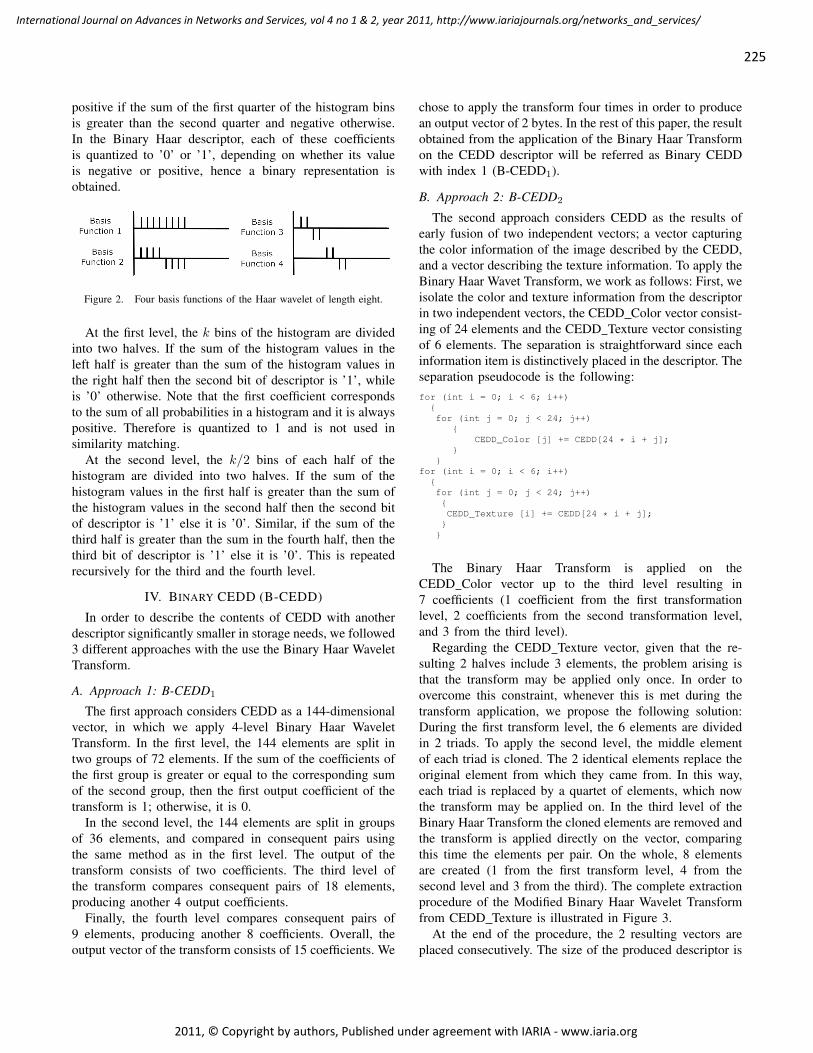
positive if the sum of the first quarter of the histogram binsis greater than the second quarter and negative otherwise.In the Binary Haar descriptor, each of these coefficientsis quantized to ’0’ or ’1’, depending on whether its valueis negative or positive, hence a binary representation isobtained.
Figure 2. Four basis functions of the Haar wavelet of length eight.
At the first level, the k bins of the histogram are dividedinto two halves. If the sum of the histogram values in theleft half is greater than the sum of the histogram values inthe right half then the second bit of descriptor is ’1’, whileis ’0’ otherwise. Note that the first coefficient correspondsto the sum of all probabilities in a histogram and it is alwayspositive. Therefore is quantized to 1 and is not used insimilarity matching.
At the second level, the k/2 bins of each half of thehistogram are divided into two halves. If the sum of thehistogram values in the first half is greater than the sum ofthe histogram values in the second half then the second bitof descriptor is ’1’ else it is ’0’. Similar, if the sum of thethird half is greater than the sum in the fourth half, then thethird bit of descriptor is ’1’ else it is ’0’. This is repeatedrecursively for the third and the fourth level.
IV. BINARY CEDD (B-CEDD)
In order to describe the contents of CEDD with anotherdescriptor significantly smaller in storage needs, we followed3 different approaches with the use the Binary Haar WaveletTransform.
A. Approach 1: B-CEDD1
The first approach considers CEDD as a 144-dimensionalvector, in which we apply 4-level Binary Haar WaveletTransform. In the first level, the 144 elements are split intwo groups of 72 elements. If the sum of the coefficients ofthe first group is greater or equal to the corresponding sumof the second group, then the first output coefficient of thetransform is 1; otherwise, it is 0.
In the second level, the 144 elements are split in groupsof 36 elements, and compared in consequent pairs usingthe same method as in the first level. The output of thetransform consists of two coefficients. The third level ofthe transform compares consequent pairs of 18 elements,producing another 4 output coefficients.
Finally, the fourth level compares consequent pairs of9 elements, producing another 8 coefficients. Overall, theoutput vector of the transform consists of 15 coefficients. We
chose to apply the transform four times in order to producean output vector of 2 bytes. In the rest of this paper, the resultobtained from the application of the Binary Haar Transformon the CEDD descriptor will be referred as Binary CEDDwith index 1 (B-CEDD1).
B. Approach 2: B-CEDD2
The second approach considers CEDD as the results ofearly fusion of two independent vectors; a vector capturingthe color information of the image described by the CEDD,and a vector describing the texture information. To apply theBinary Haar Wavet Transform, we work as follows: First, weisolate the color and texture information from the descriptorin two independent vectors, the CEDD Color vector consist-ing of 24 elements and the CEDD Texture vector consistingof 6 elements. The separation is straightforward since eachinformation item is distinctively placed in the descriptor. Theseparation pseudocode is the following:for (int i = 0; i < 6; i++)for (int j = 0; j < 24; j++)
CEDD_Color [j] += CEDD[24 * i + j];
for (int i = 0; i < 6; i++)for (int j = 0; j < 24; j++)CEDD_Texture [i] += CEDD[24 * i + j];
The Binary Haar Transform is applied on theCEDD Color vector up to the third level resulting in7 coefficients (1 coefficient from the first transformationlevel, 2 coefficients from the second transformation level,and 3 from the third level).
Regarding the CEDD Texture vector, given that the re-sulting 2 halves include 3 elements, the problem arising isthat the transform may be applied only once. In order toovercome this constraint, whenever this is met during thetransform application, we propose the following solution:During the first transform level, the 6 elements are dividedin 2 triads. To apply the second level, the middle elementof each triad is cloned. The 2 identical elements replace theoriginal element from which they came from. In this way,each triad is replaced by a quartet of elements, which nowthe transform may be applied on. In the third level of theBinary Haar Transform the cloned elements are removed andthe transform is applied directly on the vector, comparingthis time the elements per pair. On the whole, 8 elementsare created (1 from the first transform level, 4 from thesecond level and 3 from the third). The complete extractionprocedure of the Modified Binary Haar Wavelet Transformfrom CEDD Texture is illustrated in Figure 3.
At the end of the procedure, the 2 resulting vectors areplaced consecutively. The size of the produced descriptor is
225
International Journal on Advances in Networks and Services, vol 4 no 1 & 2, year 2011, http://www.iariajournals.org/networks_and_services/
2011, © Copyright by authors, Published under agreement with IARIA - www.iaria.org
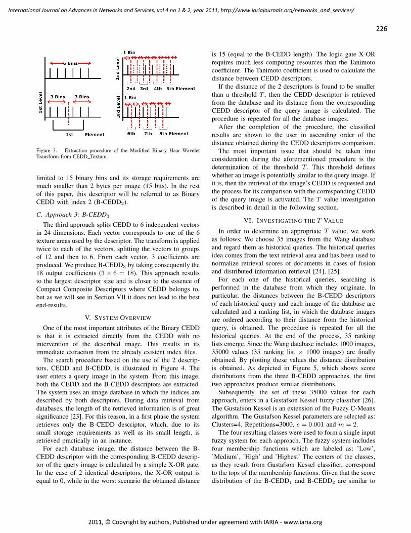
Figure 3. Extraction procedure of the Modified Binary Haar WaveletTransform from CEDD Texture.
limited to 15 binary bins and its storage requirements aremuch smaller than 2 bytes per image (15 bits). In the restof this paper, this descriptor will be referred to as BinaryCEDD with index 2 (B-CEDD2).
C. Approach 3: B-CEDD3
The third approach splits CEDD to 6 independent vectorsin 24 dimensions. Each vector corresponds to one of the 6texture areas used by the descriptor. The transform is appliedtwice to each of the vectors, splitting the vectors to groupsof 12 and then to 6. From each vector, 3 coefficients areproduced. We produce B-CEDD3 by taking consequently the18 output coefficients (3 × 6 = 18). This approach resultsto the largest descriptor size and is closer to the essence ofCompact Composite Descriptors where CEDD belongs to,but as we will see in Section VII it does not lead to the bestend-results.
V. SYSTEM OVERVIEW
One of the most important attributes of the Binary CEDDis that it is extracted directly from the CEDD with nointervention of the described image. This results in itsimmediate extraction from the already existent index files.
The search procedure based on the use of the 2 descrip-tors, CEDD and B-CEDD, is illustrated in Figure 4. Theuser enters a query image in the system. From this image,both the CEDD and the B-CEDD descriptors are extracted.The system uses an image database in which the indices aredescribed by both descriptors. During data retrieval fromdatabases, the length of the retrieved information is of greatsignificance [23]. For this reason, in a first phase the systemretrieves only the B-CEDD descriptor, which, due to itssmall storage requirements as well as its small length, isretrieved practically in an instance.
For each database image, the distance between the B-CEDD descriptor with the corresponding B-CEDD descrip-tor of the query image is calculated by a simple X-OR gate.In the case of 2 identical descriptors, the X-OR output isequal to 0, while in the worst scenario the obtained distance
is 15 (equal to the B-CEDD length). The logic gate X-ORrequires much less computing resources than the Tanimotocoefficient. The Tanimoto coefficient is used to calculate thedistance between CEDD descriptors.
If the distance of the 2 descriptors is found to be smallerthan a threshold T , then the CEDD descriptor is retrievedfrom the database and its distance from the correspondingCEDD descriptor of the query image is calculated. Theprocedure is repeated for all the database images.
After the completion of the procedure, the classifiedresults are shown to the user in ascending order of thedistance obtained during the CEDD descriptors comparison.
The most important issue that should be taken intoconsideration during the aforementioned procedure is thedetermination of the threshold T . This threshold defineswhether an image is potentially similar to the query image. Ifit is, then the retrieval of the image’s CEDD is requested andthe process for its comparison with the corresponding CEDDof the query image is activated. The T value investigationis described in detail in the following section.
VI. INVESTIGATING THE T VALUE
In order to determine an appropriate T value, we workas follows: We choose 35 images from the Wang databaseand regard them as historical queries. The historical queriesidea comes from the text retrieval area and has been used tonormalize retrieval scores of documents in cases of fusionand distributed information retrieval [24], [25].
For each one of the historical queries, searching isperformed in the database from which they originate. Inparticular, the distances between the B-CEDD descriptorsof each historical query and each image of the database arecalculated and a ranking list, in which the database imagesare ordered according to their distance from the historicalquery, is obtained. The procedure is repeated for all thehistorical queries. At the end of the process, 35 rankinglists emerge. Since the Wang database includes 1000 images,35000 values (35 ranking list × 1000 images) are finallyobtained. By plotting these values the distance distributionis obtained. As depicted in Figure 5, which shows scoredistributions from the three B-CEDD approaches, the firsttwo approaches produce similar distributions.
Subsequently, the set of these 35000 values for eachapproach, enters in a Gustafson Kessel fuzzy classifier [26].The Gustafson Kessel is an extension of the Fuzzy C-Meansalgorithm. The Gustafson Kessel parameters are selected as:Clusters=4, Repetitions=3000, e = 0.001 and m = 2.
The four resulting classes were used to form a single inputfuzzy system for each approach. The fuzzy system includesfour membership functions which are labeled as: ’Low’,’Medium’, ’High’ and ’Highest’ The centers of the classes,as they result from Gustafson Kessel classifier, correspondto the tops of the membership functions. Given that the scoredistribution of the B-CEDD1 and B-CEDD2 are similar to
226
International Journal on Advances in Networks and Services, vol 4 no 1 & 2, year 2011, http://www.iariajournals.org/networks_and_services/
2011, © Copyright by authors, Published under agreement with IARIA - www.iaria.org
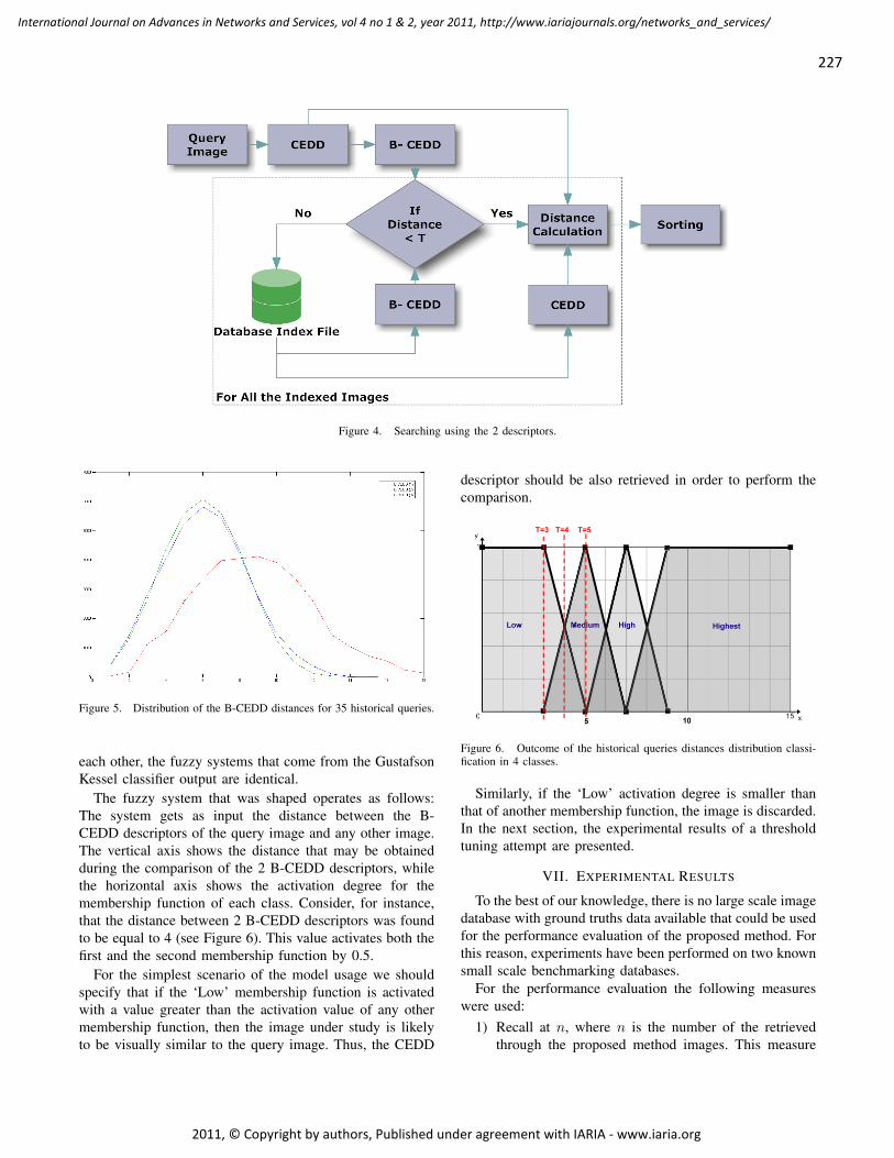
Figure 4. Searching using the 2 descriptors.
Figure 5. Distribution of the B-CEDD distances for 35 historical queries.
each other, the fuzzy systems that come from the GustafsonKessel classifier output are identical.
The fuzzy system that was shaped operates as follows:The system gets as input the distance between the B-CEDD descriptors of the query image and any other image.The vertical axis shows the distance that may be obtainedduring the comparison of the 2 B-CEDD descriptors, whilethe horizontal axis shows the activation degree for themembership function of each class. Consider, for instance,that the distance between 2 B-CEDD descriptors was foundto be equal to 4 (see Figure 6). This value activates both thefirst and the second membership function by 0.5.
For the simplest scenario of the model usage we shouldspecify that if the ‘Low’ membership function is activatedwith a value greater than the activation value of any othermembership function, then the image under study is likelyto be visually similar to the query image. Thus, the CEDD
descriptor should be also retrieved in order to perform thecomparison.
Figure 6. Outcome of the historical queries distances distribution classi-fication in 4 classes.
Similarly, if the ‘Low’ activation degree is smaller thanthat of another membership function, the image is discarded.In the next section, the experimental results of a thresholdtuning attempt are presented.
VII. EXPERIMENTAL RESULTS
To the best of our knowledge, there is no large scale imagedatabase with ground truths data available that could be usedfor the performance evaluation of the proposed method. Forthis reason, experiments have been performed on two knownsmall scale benchmarking databases.
For the performance evaluation the following measureswere used:
1) Recall at n, where n is the number of the retrievedthrough the proposed method images. This measure
227
International Journal on Advances in Networks and Services, vol 4 no 1 & 2, year 2011, http://www.iariajournals.org/networks_and_services/
2011, © Copyright by authors, Published under agreement with IARIA - www.iaria.org
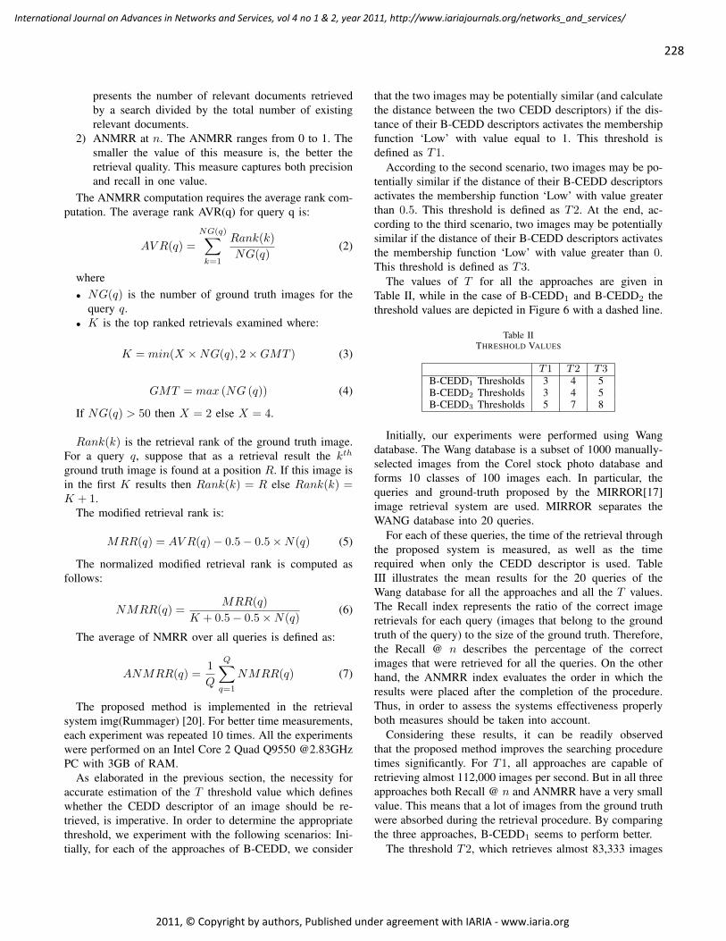
presents the number of relevant documents retrievedby a search divided by the total number of existingrelevant documents.
2) ANMRR at n. The ANMRR ranges from 0 to 1. Thesmaller the value of this measure is, the better theretrieval quality. This measure captures both precisionand recall in one value.
The ANMRR computation requires the average rank com-putation. The average rank AVR(q) for query q is:
AV R(q) =
NG(q)∑k=1
Rank(k)
NG(q)(2)
where• NG(q) is the number of ground truth images for the
query q.• K is the top ranked retrievals examined where:
K = min(X ×NG(q), 2×GMT ) (3)
GMT = max (NG (q)) (4)
If NG(q) > 50 then X = 2 else X = 4.
Rank(k) is the retrieval rank of the ground truth image.For a query q, suppose that as a retrieval result the kth
ground truth image is found at a position R. If this image isin the first K results then Rank(k) = R else Rank(k) =K + 1.
The modified retrieval rank is:
MRR(q) = AV R(q)− 0.5− 0.5×N(q) (5)
The normalized modified retrieval rank is computed asfollows:
NMRR(q) =MRR(q)
K + 0.5− 0.5×N(q)(6)
The average of NMRR over all queries is defined as:
ANMRR(q) =1
Q
Q∑q=1
NMRR(q) (7)
The proposed method is implemented in the retrievalsystem img(Rummager) [20]. For better time measurements,each experiment was repeated 10 times. All the experimentswere performed on an Intel Core 2 Quad Q9550 @2.83GHzPC with 3GB of RAM.
As elaborated in the previous section, the necessity foraccurate estimation of the T threshold value which defineswhether the CEDD descriptor of an image should be re-trieved, is imperative. In order to determine the appropriatethreshold, we experiment with the following scenarios: Ini-tially, for each of the approaches of B-CEDD, we consider
that the two images may be potentially similar (and calculatethe distance between the two CEDD descriptors) if the dis-tance of their B-CEDD descriptors activates the membershipfunction ‘Low’ with value equal to 1. This threshold isdefined as T1.
According to the second scenario, two images may be po-tentially similar if the distance of their B-CEDD descriptorsactivates the membership function ‘Low’ with value greaterthan 0.5. This threshold is defined as T2. At the end, ac-cording to the third scenario, two images may be potentiallysimilar if the distance of their B-CEDD descriptors activatesthe membership function ‘Low’ with value greater than 0.This threshold is defined as T3.
The values of T for all the approaches are given inTable II, while in the case of B-CEDD1 and B-CEDD2 thethreshold values are depicted in Figure 6 with a dashed line.
Table IITHRESHOLD VALUES
T1 T2 T3B-CEDD1 Thresholds 3 4 5B-CEDD2 Thresholds 3 4 5B-CEDD3 Thresholds 5 7 8
Initially, our experiments were performed using Wangdatabase. The Wang database is a subset of 1000 manually-selected images from the Corel stock photo database andforms 10 classes of 100 images each. In particular, thequeries and ground-truth proposed by the MIRROR[17]image retrieval system are used. MIRROR separates theWANG database into 20 queries.
For each of these queries, the time of the retrieval throughthe proposed system is measured, as well as the timerequired when only the CEDD descriptor is used. TableIII illustrates the mean results for the 20 queries of theWang database for all the approaches and all the T values.The Recall index represents the ratio of the correct imageretrievals for each query (images that belong to the groundtruth of the query) to the size of the ground truth. Therefore,the Recall @ n describes the percentage of the correctimages that were retrieved for all the queries. On the otherhand, the ANMRR index evaluates the order in which theresults were placed after the completion of the procedure.Thus, in order to assess the systems effectiveness properlyboth measures should be taken into account.
Considering these results, it can be readily observedthat the proposed method improves the searching proceduretimes significantly. For T1, all approaches are capable ofretrieving almost 112,000 images per second. But in all threeapproaches both Recall @ n and ANMRR have a very smallvalue. This means that a lot of images from the ground truthwere absorbed during the retrieval procedure. By comparingthe three approaches, B-CEDD1 seems to perform better.
The threshold T2, which retrieves almost 83,333 images
228
International Journal on Advances in Networks and Services, vol 4 no 1 & 2, year 2011, http://www.iariajournals.org/networks_and_services/
2011, © Copyright by authors, Published under agreement with IARIA - www.iaria.org
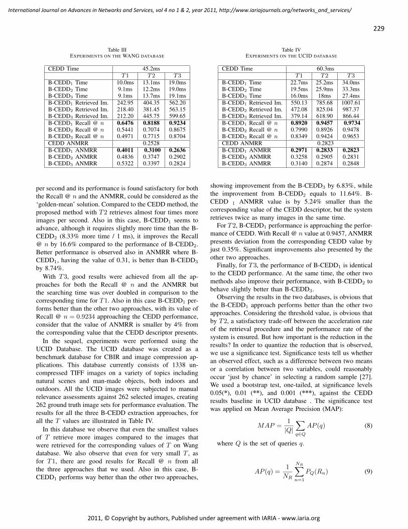
Table IIIEXPERIMENTS ON THE WANG DATABASE
CEDD Time 45.2msT1 T2 T3
B-CEDD1 Time 10.0ms 13.1ms 19.0msB-CEDD2 Time 9.1ms 12.2ms 19.0msB-CEDD3 Time 9.1ms 13.7ms 19.1msB-CEDD1 Retrieved Im. 242.95 404.35 562.20B-CEDD2 Retrieved Im. 218.40 381.45 563.15B-CEDD3 Retrieved Im. 212.20 445.75 599.65B-CEDD1 Recall @ n 0.6476 0.8188 0.9234B-CEDD2 Recall @ n 0.5441 0.7074 0.8675B-CEDD3 Recall @ n 0.4971 0.7715 0.8704CEDD ANMRR 0.2528B-CEDD1 ANMRR 0.4011 0.3100 0.2636B-CEDD2 ANMRR 0.4836 0.3747 0.2902B-CEDD3 ANMRR 0.5322 0.3397 0.2824
per second and its performance is found satisfactory for boththe Recall @ n and the ANMRR, could be considered as the‘golden-mean’ solution. Compared to the CEDD method, theproposed method with T2 retrieves almost four times moreimages per second. Also in this case, B-CEDD1 seems toadvance, although it requires slightly more time than the B-CEDD2 (8.33% more time / 1 ms), it improves the Recall@ n by 16.6% compared to the performance of B-CEDD2.Better performance is observed also in ANMRR where B-CEDD1, having the value of 0.31, is better than B-CEDD3
by 8.74%.With T3, good results were achieved from all the ap-
proaches for both the Recall @ n and the ANMRR butthe searching time was over doubled in comparison to thecorresponding time for T1. Also in this case B-CEDD1 per-forms better than the other two approaches, with its value ofRecall @ n = 0.9234 approaching the CEDD performance,consider that the value of ANMRR is smaller by 4% fromthe corresponding value that the CEDD descriptor presents.
In the sequel, experiments were performed using theUCID Database. The UCID database was created as abenchmark database for CBIR and image compression ap-plications. This database currently consists of 1338 un-compressed TIFF images on a variety of topics includingnatural scenes and man-made objects, both indoors andoutdoors. All the UCID images were subjected to manualrelevance assessments against 262 selected images, creating262 ground truth image sets for performance evaluation. Theresults for all the three B-CEDD extraction approaches, forall the T values are illustrated in Table IV.
In this database we observe that even the smallest valuesof T retrieve more images compared to the images thatwere retrieved for the corresponding values of T on Wangdatabase. We also observe that even for very small T , asfor T1, there are good results for Recall @ n from allthe three approaches that we used. Also in this case, B-CEDD1 performs way better than the other two approaches,
Table IVEXPERIMENTS ON THE UCID DATABASE
CEDD Time 60.3msT1 T2 T3
B-CEDD1 Time 22.7ms 25.2ms 34.0msB-CEDD2 Time 19.5ms 25.9ms 33.3msB-CEDD3 Time 16.0ms 18ms 27.4msB-CEDD1 Retrieved Im. 550.13 785.68 1007.61B-CEDD2 Retrieved Im. 472.08 825.04 987.37B-CEDD3 Retrieved Im. 379.14 618.90 866.44B-CEDD1 Recall @ n 0.8920 0.9457 0.9734B-CEDD2 Recall @ n 0.7990 0.8926 0.9478B-CEDD3 Recall @ n 0.8349 0.9424 0.9653CEDD ANMRR 0.2823B-CEDD1 ANMRR 0.2971 0.2833 0.2823B-CEDD2 ANMRR 0.3258 0.2905 0.2831B-CEDD3 ANMRR 0.3140 0.2874 0.2848
showing improvement from the B-CEDD3 by 6.83%, whilethe improvement from B-CEDD2 equals to 11.64%. B-CEDD 1 ANMRR value is by 5.24% smaller than thecorresponding value of the CEDD descriptor, but the systemretrieves twice as many images in the same time.
For T2, B-CEDD1 performance is approaching the perfor-mance of CEDD. With Recall @ n value at 0.9457, ANMRRpresents deviation from the corresponding CEDD value byjust 0.35%. Significant improvements also presented by theother two approaches.
Finally, for T3, the performance of B-CEDD1 is identicalto the CEDD performance. At the same time, the other twomethods also improve their performance, with B-CEDD2 tobehave slightly better than B-CEDD3.
Observing the results in the two databases, is obvious thatthe B-CEDD1 approach performs better than the other twoapproaches. Considering the threshold value, is obvious thatby T2, a satisfactory trade-off between the acceleration rateof the retrieval procedure and the performance rate of thesystem is ensured. But how important is the reduction in theresults? In order to quantize the reduction that is observed,we use a significance test. Significance tests tell us whetheran observed effect, such as a difference between two meansor a correlation between two variables, could reasonablyoccur ‘just by chance’ in selecting a random sample [27].We used a bootstrap test, one-tailed, at significance levels0.05(*), 0.01 (**), and 0.001 (***), against the CEDDresults baseline in UCID database . The significance testwas applied on Mean Average Precision (MAP):
MAP =1
|Q|∑q∈Q
AP (q) (8)
where Q is the set of queries q.
AP (q) =1
NR
NR∑n=1
PQ(Rn) (9)
229
International Journal on Advances in Networks and Services, vol 4 no 1 & 2, year 2011, http://www.iariajournals.org/networks_and_services/
2011, © Copyright by authors, Published under agreement with IARIA - www.iaria.org
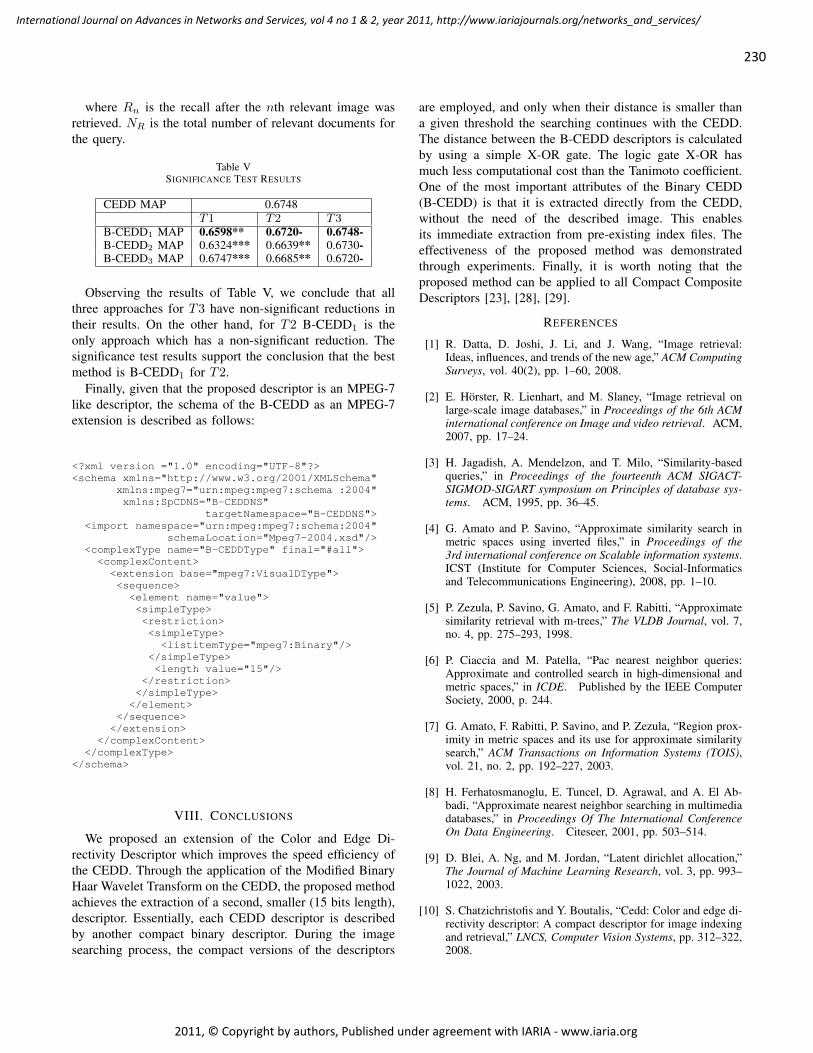
where Rn is the recall after the nth relevant image wasretrieved. NR is the total number of relevant documents forthe query.
Table VSIGNIFICANCE TEST RESULTS
CEDD MAP 0.6748T1 T2 T3
B-CEDD1 MAP 0.6598** 0.6720- 0.6748-B-CEDD2 MAP 0.6324*** 0.6639** 0.6730-B-CEDD3 MAP 0.6747*** 0.6685** 0.6720-
Observing the results of Table V, we conclude that allthree approaches for T3 have non-significant reductions intheir results. On the other hand, for T2 B-CEDD1 is theonly approach which has a non-significant reduction. Thesignificance test results support the conclusion that the bestmethod is B-CEDD1 for T2.
Finally, given that the proposed descriptor is an MPEG-7like descriptor, the schema of the B-CEDD as an MPEG-7extension is described as follows:
<?xml version ="1.0" encoding="UTF-8"?><schema xmlns="http://www.w3.org/2001/XMLSchema"
xmlns:mpeg7="urn:mpeg:mpeg7:schema :2004"xmlns:SpCDNS="B-CEDDNS"
targetNamespace="B-CEDDNS"><import namespace="urn:mpeg:mpeg7:schema:2004"
schemaLocation="Mpeg7-2004.xsd"/><complexType name="B-CEDDType" final="#all">
<complexContent><extension base="mpeg7:VisualDType"><sequence>
<element name="value"><simpleType><restriction><simpleType>
<listitemType="mpeg7:Binary"/></simpleType><length value="15"/>
</restriction></simpleType></element>
</sequence></extension>
</complexContent></complexType>
</schema>
VIII. CONCLUSIONS
We proposed an extension of the Color and Edge Di-rectivity Descriptor which improves the speed efficiency ofthe CEDD. Through the application of the Modified BinaryHaar Wavelet Transform on the CEDD, the proposed methodachieves the extraction of a second, smaller (15 bits length),descriptor. Essentially, each CEDD descriptor is describedby another compact binary descriptor. During the imagesearching process, the compact versions of the descriptors
are employed, and only when their distance is smaller thana given threshold the searching continues with the CEDD.The distance between the B-CEDD descriptors is calculatedby using a simple X-OR gate. The logic gate X-OR hasmuch less computational cost than the Tanimoto coefficient.One of the most important attributes of the Binary CEDD(B-CEDD) is that it is extracted directly from the CEDD,without the need of the described image. This enablesits immediate extraction from pre-existing index files. Theeffectiveness of the proposed method was demonstratedthrough experiments. Finally, it is worth noting that theproposed method can be applied to all Compact CompositeDescriptors [23], [28], [29].
REFERENCES
[1] R. Datta, D. Joshi, J. Li, and J. Wang, “Image retrieval:Ideas, influences, and trends of the new age,” ACM ComputingSurveys, vol. 40(2), pp. 1–60, 2008.
[2] E. Horster, R. Lienhart, and M. Slaney, “Image retrieval onlarge-scale image databases,” in Proceedings of the 6th ACMinternational conference on Image and video retrieval. ACM,2007, pp. 17–24.
[3] H. Jagadish, A. Mendelzon, and T. Milo, “Similarity-basedqueries,” in Proceedings of the fourteenth ACM SIGACT-SIGMOD-SIGART symposium on Principles of database sys-tems. ACM, 1995, pp. 36–45.
[4] G. Amato and P. Savino, “Approximate similarity search inmetric spaces using inverted files,” in Proceedings of the3rd international conference on Scalable information systems.ICST (Institute for Computer Sciences, Social-Informaticsand Telecommunications Engineering), 2008, pp. 1–10.
[5] P. Zezula, P. Savino, G. Amato, and F. Rabitti, “Approximatesimilarity retrieval with m-trees,” The VLDB Journal, vol. 7,no. 4, pp. 275–293, 1998.
[6] P. Ciaccia and M. Patella, “Pac nearest neighbor queries:Approximate and controlled search in high-dimensional andmetric spaces,” in ICDE. Published by the IEEE ComputerSociety, 2000, p. 244.
[7] G. Amato, F. Rabitti, P. Savino, and P. Zezula, “Region prox-imity in metric spaces and its use for approximate similaritysearch,” ACM Transactions on Information Systems (TOIS),vol. 21, no. 2, pp. 192–227, 2003.
[8] H. Ferhatosmanoglu, E. Tuncel, D. Agrawal, and A. El Ab-badi, “Approximate nearest neighbor searching in multimediadatabases,” in Proceedings Of The International ConferenceOn Data Engineering. Citeseer, 2001, pp. 503–514.
[9] D. Blei, A. Ng, and M. Jordan, “Latent dirichlet allocation,”The Journal of Machine Learning Research, vol. 3, pp. 993–1022, 2003.
[10] S. Chatzichristofis and Y. Boutalis, “Cedd: Color and edge di-rectivity descriptor: A compact descriptor for image indexingand retrieval,” LNCS, Computer Vision Systems, pp. 312–322,2008.
230
International Journal on Advances in Networks and Services, vol 4 no 1 & 2, year 2011, http://www.iariajournals.org/networks_and_services/
2011, © Copyright by authors, Published under agreement with IARIA - www.iaria.org
[11] S. A. Chatzichristofis, K Zagoris, Y. S. Boutalis and N.Papamarkos, “Accurate image retrieval based on compactcomposite descriptors and relevance feedback information,”International Journal of Pattern Recognition and ArtificialIntelligence (IJPRAI), vol. 24 (2), pp. 207–244, 2010.
[12] Z. Struzik and A. Siebes, “The haar wavelet transform in thetime series similarity paradigm,” Principles of Data Miningand Knowledge Discovery, pp. 12–22, 1999.
[13] S. A. Chatzichristofis, Y. Boutalis, and A. Arampatzis, “Ac-celerating image retrieval using binary haar wavelet transformon the color and edge directivity descriptor,” in The FifthInternational Multi-Conference on Computing in the GlobalInformation Technology (ICCGI 2010), 2010, pp. 41–47.
[14] B. Manjunath, J. Ohm, V. Vasudevan, A. Yamada et al.,“Color and texture descriptors,” IEEE Transactions on circuitsand systems for video technology, vol. 11, no. 6, pp. 703–715,2001.
[15] C. Won, D. Park, and S. Park, “Efficient use of mpeg-7 edgehistogram descriptor,” Etri Journal, vol. 24, no. 1, pp. 23–30,2002.
[16] J. Wang, J. Li, and G. Wiederholdy, “Simplicity: Semantics-sensitive integrated matching for picture libraries,” Advancesin Visual Information Systems, vol. 1929/2000, pp. 171–193,2000.
[17] K. Wong, K. Cheung, and L. Po, “Mirror: an interactivecontent based image retrieval system,” in IEEE InternationalSymposium on Circuits and Systems, vol. 2. IEEE; 1999,2005, pp. 1541–1544.
[18] G. Schaefer and M. Stich, “Ucid-an uncompressed colourimage database,” Storage and Retrieval Methods and Appli-cations for Multimedia 2004, vol. 5307, pp. 472–480, 2004.
[19] D. Nister and H. Stewenius, “Scalable recognition with a vo-cabulary tree,” in Computer Vision and Pattern Recognition,2006 IEEE Computer Society Conference on, vol. 2. Citeseer,2006, pp. 2161–2168.
[20] S. A. Chatzichristofis, Y. S. Boutalis and M. Lux,“Img(rummager): An interactive content based image retrievalsystem,” in 2nd International Workshop on Similarity Searchand Applications (SISAP), 2009, pp. 151–153.
[21] M. Lux and S. Chatzichristofis, “Lire: lucene image retrieval:an extensible java cbir library,” in Proceeding of the 16thACM international conference on Multimedia. ACM, 2008,pp. 1085–1088.
[22] S. Krishnamachari and M. Abdel-Mottaleb, “Compact colordescriptor for fast image and video segment retrieval,” inIS&T/SPIE Conference on Storage and Retrieval of MediaDatabases, 2000, pp. 581–589.
[23] S. A. Chatzichristofis, Y. S. Boutalis and M. Lux, “Spcd- spatial color distribution descriptor. a fuzzy rule basedcompact composite descriptor appropriate for hand drawncolor sketches retrieval,” in 2nd International Conference onAgents and Artificial Intelligence (ICAART), 2010, pp. 58–63.
[24] A. Arampatzis and J. Kamps, “A signal-to-noise approach toscore normalization,” in Proceeding of the 18th ACM con-ference on Information and knowledge management. ACM,2009, pp. 797–806.
[25] M. Fernandez, D. Vallet, and P. Castells, “Using historicaldata to enhance rank aggregation,” in Proceedings of the 29thannual international ACM SIGIR conference on Research anddevelopment in information retrieval. ACM, 2006, pp. 643–644.
[26] D. Gustafson and W. Kessel, “Fuzzy clustering with a fuzzycovariance matrix,” in 1978 IEEE Conference on Decisionand Control including the 17th Symposium on AdaptiveProcesses, vol. 17, 1978, pp. 761–766.
[27] D. Moore and L. Sorenson, Introduction to the Practice ofStatistics SPSS Manual. WH Freeman, 2005.
[28] S. Chatzichristofis and Y. Boutalis, “Fcth: Fuzzy color andtexture histogram-a low level feature for accurate imageretrieval,” in Image Analysis for Multimedia Interactive Ser-vices, 2008. WIAMIS’08. Ninth International Workshop on,2008, pp. 191–196.
[29] Chatzichristofis, S.A. and Boutalis, Y.S., “Content basedradiology image retrieval using a fuzzy rule based scalablecomposite descriptor,” Multimedia Tools and Applications,vol. 46, pp. 493–519, 2010.
231
International Journal on Advances in Networks and Services, vol 4 no 1 & 2, year 2011, http://www.iariajournals.org/networks_and_services/
2011, © Copyright by authors, Published under agreement with IARIA - www.iaria.org
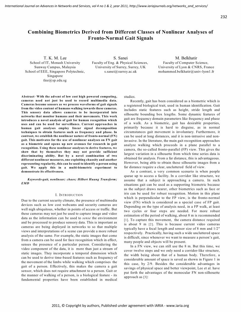
Combining Biometrics Derived from Different Classes of Nonlinear Analyses ofFronto-Normal Gait Signals
T. K. M. LeeSchool of IT, Monash University
Sunway Campus, Malaysia
School of EEE, Singapore Polytechnic,Singapore
S. SaneiFaculty of Eng. & Physical Sciences,
University of Surrey, Surrey, UK
M. BelkhatirFaculty of Computer Science,
University of Lyon & CNRS, France
Abstract!With the advent of low cost high powered computing,
cameras need not just be used to record multimedia data.Cameras become sensors as we process waveforms of gait signals
from the video content of humans walking towards these cameras.
This sensory data allows cameras to be incorporated into
networks that monitor humans and their movements. This workintroduces a novel analysis of gait for human recognition which
uses and can be used for surveillance. Current approaches in
human gait analyses employ linear signal decomposition
techniques to obtain features such as frequency and phase. Incontrast, we establish the nonlinear nature of fronto-normal (FN)
gait. This motivates for the use of nonlinear analyses on FN gait
as a biometric and opens up new avenues for research in gait
recognition. Using these nonlinear analyses to derive features, weshow that by themselves they may not provide sufficient
discriminating ability. But by a novel combination of two
different nonlinear measures, one exploiting chaosity and another
representing regularity, this can be used to identify a person usinggait. We apply this in a multi-biometric experiment to
demonstrate its effectiveness.
Keywords-gait, nonlinear; chaos; Hilbert Huang Transform;EMD
I. INTRODUCTION
Due to the current security climate, the presence of multimediadevices such as low cost webcams and security cameras are
well nigh ubiquitous, whether in points of access or traffic. Butthese cameras may not just be used to capture image and video
data as the information can be used to sense the environmentand be processed to produce sensory data. This is important as
cameras are being deployed in networks to so that multipleviews and interpretations of a scene can provide a more robust
analysis of the same. For example, the static images that comefrom a camera can be used for face recognition which in effect,
senses the presence of a particular person. Considering thevideo component of the data, it is more than just a stream of
static images. They incorporate a temporal dimension whichcan be used to derive time-based features such as frequency of
the movement of the limbs while walking which comprises thegait of a person. Effectively, this makes the camera a gait
sensor, which does not require attachment to a person. Gait orthe manner of walking of a person, is a biological feature - its
fundamental properties have been established in medical
studies. Recently, gait has been considered as a biometric which is
a registered biological trait, used in human identification. Gaitincludes static features such as height, stride length and
silhouette bounding box lengths. Some dynamic features ofgait are frequency domain parameters like frequency and phase
of a walk. As a biometric, gait has desirable properties,primarily because it is hard to disguise, as in normal
circumstances gait movement is involuntary. Furthermore, itcan be used at long distances, and it is non-intrusive and non-
invasive. In the literature, the main gait recognition approachesanalyze walking which proceeds in a plane parallel to a
camera, the so-called fronto-parallel (FP) view. This gives thelargest variation in a silhouette from which time series data is
obtained for analysis. From a far distance, this is advantageous.However, being able to obtain these silhouette images from a
far distance require a clear, uncluttered field of view.As a contrast, a very common scenario is when people
queue up to access a facility. In a corridor like structure, weassume that a subject is approaching a camera. In such
situations gait can be used as a supporting biometric becauseas the subject draws nearer, other biometrics such as face or
iris can be used for robust recognition. Motion in this planewhich is perpendicular to the FP view, is the fronto-normal
view (FN) which is considered as a special case of FP gait.Depending on the type of analysis need, in a FP walk, at least
two cycles or four steps are needed. For more robustestimation of the period of walking, about 8 m is recommended
[1]. To capture this movement, the camera distance requiredis about 9 m [2]. This is because current video cameras
typically have a focal length and sensor size of 8 mm and 1/2"respectively. Practically, having such a wide uncluttered space
is difficult, since whenever we want to measure a person’s gait,many people and objects will be present.
In a FN view, we can still use the 8 m. But this time, wecover twelve steps and we only need a corridor-like structure,
the width being about that of a human body. Therefore, aconsiderable amount of space is saved as shown in Figure 1 in
this case, by 2/9. Besides the considerable advantages insavings of physical space and better viewpoint, Lee et al. have
put forth the advantages of the monocular FN non-silhouetteapproach as [3]:
232
International Journal on Advances in Networks and Services, vol 4 no 1 & 2, year 2011, http://www.iariajournals.org/networks_and_services/
2011, © Copyright by authors, Published under agreement with IARIA - www.iaria.org
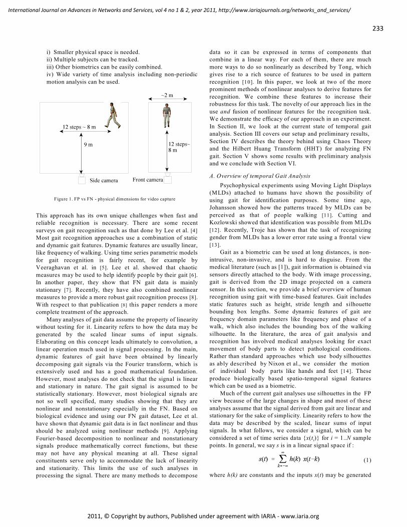
Figure 1. FP vs FN - physical dimensions for video capture
i) Smaller physical space is needed.ii) Multiple subjects can be tracked.
iii) Other biometrics can be easily combined.iv) Wide variety of time analysis including non-periodic
motion analysis can be used.
This approach has its own unique challenges when fast andreliable recognition is necessary. There are some recent
surveys on gait recognition such as that done by Lee et al. [4]
Most gait recognition approaches use a combination of static
and dynamic gait features. Dynamic features are usually linear,like frequency of walking. Using time series parametric models
for gait recognition is fairly recent, for example byVeeraghavan et al. in [5]. Lee et al. showed that chaotic
measures may be used to help identify people by their gait [6].In another paper, they show that FN gait data is mainly
stationary [7]. Recently, they have also combined nonlinearmeasures to provide a more robust gait recognition process [8].
With respect to that publication [8] this paper renders a morecomplete treatment of the approach.
Many analyses of gait data assume the property of linearitywithout testing for it. Linearity refers to how the data may be
generated by the scaled linear sums of input signals.Elaborating on this concept leads ultimately to convolution, a
linear operation much used in signal processing. In the main,dynamic features of gait have been obtained by linearly
decomposing gait signals via the Fourier transform, which isextensively used and has a good mathematical foundation.
However, most analyses do not check that the signal is linearand stationary in nature. The gait signal is assumed to be
statistically stationary. However, most biological signals arenot so well specified, many studies showing that they are
nonlinear and nonstationary especially in the FN. Based onbiological evidence and using our FN gait dataset, Lee et al.
have shown that dynamic gait data is in fact nonlinear and thusshould be analyzed using nonlinear methods [9]. Applying
Fourier-based decomposition to nonlinear and nonstationarysignals produce mathematically correct functions, but these
may not have any physical meaning at all. These signalconstituents serve only to accommodate the lack of linearity
and stationarity. This limits the use of such analyses inprocessing the signal. There are many methods to decompose
data so it can be expressed in terms of components thatcombine in a linear way. For each of them, there are much
more ways to do so nonlinearly as described by Tong, whichgives rise to a rich source of features to be used in pattern
recognition [10]. In this paper, we look at two of the moreprominent methods of nonlinear analyses to derive features for
recognition. We combine these features to increase theirrobustness for this task. The novelty of our approach lies in the
use and fusion of nonlinear features for the recognition task.We demonstrate the efficacy of our approach in an experiment.
In Section II, we look at the current state of temporal gaitanalysis. Section III covers our setup and preliminary results,
Section IV describes the theory behind using Chaos Theoryand the Hilbert Huang Transform (HHT) for analyzing FN
gait. Section V shows some results with preliminary analysisand we conclude with Section VI.
A. Overview of temporal Gait Analysis
Psychophysical experiments using Moving Light Displays(MLDs) attached to humans have shown the possibility of
using gait for identification purposes. Some time ago,Johansson showed how the patterns traced by MLDs can be
perceived as that of people walking [11]. Cutting andKozlowski showed that identification was possible from MLDs
[12]. Recently, Troje has shown that the task of recognizinggender from MLDs has a lower error rate using a frontal view
[13].Gait as a biometric can be used at long distances, is non-
intrusive, non-invasive, and is hard to disguise. From themedical literature (such as [1]), gait information is obtained via
sensors directly attached to the body. With image processing,gait is derived from the 2D image projected on a camera
sensor. In this section, we provide a brief overview of humanrecognition using gait with time-based features. Gait includes
static features such as height, stride length and silhouettebounding box lengths. Some dynamic features of gait are
frequency domain parameters like frequency and phase of awalk, which also includes the bounding box of the walking
silhouette. In the literature, the area of gait analysis andrecognition has involved medical analyses looking for exact
movement of body parts to detect pathological conditions.Rather than standard approaches which use body silhouettes
as ably described by Nixon et al., we consider the motion of individual body parts like hands and feet [14]. These
produce biologically based spatio-temporal signal featureswhich can be used as a biometric.
Much of the current gait analyses use silhouettes in the FPview because of the large changes in shape and most of these
analyses assume that the signal derived from gait are linear andstationary for the sake of simplicity. Linearity refers to how the
data may be described by the scaled, linear sums of inputsignals. In what follows, we consider a signal, which can be
iconsidered a set of time series data x(t ) for i = 1..N samplepoints. In general, we say s is in a linear signal space if :
(1)
where h(k) are constants and the inputs x(t) may be generated
233
International Journal on Advances in Networks and Services, vol 4 no 1 & 2, year 2011, http://www.iariajournals.org/networks_and_services/
2011, © Copyright by authors, Published under agreement with IARIA - www.iaria.org
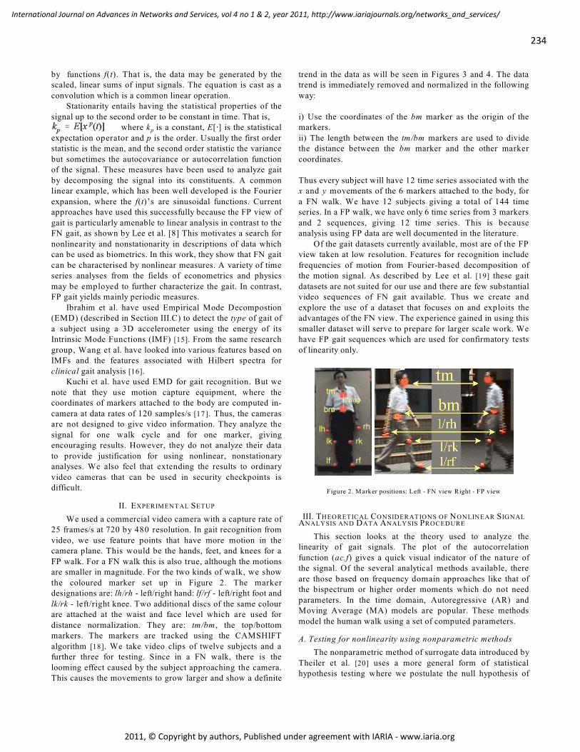
by functions f(t). That is, the data may be generated by thescaled, linear sums of input signals. The equation is cast as a
convolution which is a common linear operation.Stationarity entails having the statistical properties of the
signal up to the second order to be constant in time. That is,
p where k is a constant, E[@] is the statistical
expectation operator and p is the order. Usually the first orderstatistic is the mean, and the second order statistic the variance
but sometimes the autocovariance or autocorrelation functionof the signal. These measures have been used to analyze gait
by decomposing the signal into its constituents. A commonlinear example, which has been well developed is the Fourier
expansion, where the f(t)’s are sinusoidal functions. Currentapproaches have used this successfully because the FP view of
gait is particularly amenable to linear analysis in contrast to theFN gait, as shown by Lee et al. [8] This motivates a search for
nonlinearity and nonstationarity in descriptions of data whichcan be used as biometrics. In this work, they show that FN gait
can be characterised by nonlinear measures. A variety of timeseries analyses from the fields of econometrics and physics
may be employed to further characterize the gait. In contrast,FP gait yields mainly periodic measures.
Ibrahim et al. have used Empirical Mode Decompostion(EMD) (described in Section III.C) to detect the type of gait of
a subject using a 3D accelerometer using the energy of itsIntrinsic Mode Functions (IMF) [15]. From the same research
group, Wang et al. have looked into various features based onIMFs and the features associated with Hilbert spectra for
clinical gait analysis [16].Kuchi et al. have used EMD for gait recognition. But we
note that they use motion capture equipment, where thecoordinates of markers attached to the body are computed in-
camera at data rates of 120 samples/s [17]. Thus, the camerasare not designed to give video information. They analyze the
signal for one walk cycle and for one marker, givingencouraging results. However, they do not analyze their data
to provide justification for using nonlinear, nonstationaryanalyses. We also feel that extending the results to ordinary
video cameras that can be used in security checkpoints isdifficult.
II. EXPERIMENTAL SETUP
We used a commercial video camera with a capture rate of25 frames/s at 720 by 480 resolution. In gait recognition from
video, we use feature points that have more motion in thecamera plane. This would be the hands, feet, and knees for a
FP walk. For a FN walk this is also true, although the motionsare smaller in magnitude. For the two kinds of walk, we show
the coloured marker set up in Figure 2. The markerdesignations are: lh/rh - left/right hand: lf/rf - left/right foot and
lk/rk - left/right knee. Two additional discs of the same colourare attached at the waist and face level which are used for
distance normalization. They are: tm/bm , the top/bottommarkers. The markers are tracked using the CAMSHIFT
algorithm [18]. We take video clips of twelve subjects and afurther three for testing. Since in a FN walk, there is the
looming effect caused by the subject approaching the camera.This causes the movements to grow larger and show a definite
trend in the data as will be seen in Figures 3 and 4. The datatrend is immediately removed and normalized in the following
way:
i) Use the coordinates of the bm marker as the origin of themarkers.
ii) The length between the tm/bm markers are used to dividethe distance between the bm marker and the other marker
coordinates.
Thus every subject will have 12 time series associated with thex and y movements of the 6 markers attached to the body, for
a FN walk. We have 12 subjects giving a total of 144 timeseries. In a FP walk, we have only 6 time series from 3 markers
and 2 sequences, giving 12 time series. This is becauseanalysis using FP data are well documented in the literature.
Of the gait datasets currently available, most are of the FPview taken at low resolution. Features for recognition include
frequencies of motion from Fourier-based decomposition ofthe motion signal. As described by Lee et al. [19] these gait
datasets are not suited for our use and there are few substantialvideo sequences of FN gait available. Thus we create and
explore the use of a dataset that focuses on and exploits theadvantages of the FN view. The experience gained in using this
smaller dataset will serve to prepare for larger scale work. Wehave FP gait sequences which are used for confirmatory tests
of linearity only.
III. THEORETICAL CONSIDERATIONS OF NONLINEAR SIGNALANALYSIS AND DATA ANALYSIS PROCEDURE
This section looks at the theory used to analyze thelinearity of gait signals. The plot of the autocorrelation
function (ac.f) gives a quick visual indicator of the nature ofthe signal. Of the several analytical methods available, there
are those based on frequency domain approaches like that ofthe bispectrum or higher order moments which do not need
parameters. In the time domain, Autoregressive (AR) andMoving Average (MA) models are popular. These methods
model the human walk using a set of computed parameters.
A. Testing for nonlinearity using nonparametric methods
The nonparametric method of surrogate data introduced by
Theiler et al. [20] uses a more general form of statisticalhypothesis testing where we postulate the null hypothesis of
Figure 2. Marker positions: Left - FN view Right - FP view
234
International Journal on Advances in Networks and Services, vol 4 no 1 & 2, year 2011, http://www.iariajournals.org/networks_and_services/
2011, © Copyright by authors, Published under agreement with IARIA - www.iaria.org
(2)
linearity. Then simulated data are generated from the processeswhich are known to have linear and stationary properties. A
discriminating statistic is computed on the simulated data anda critical value determined, based on various levels of
significance for which the hypothesis holds.Using the experimental data now, the discriminating
statistic is again computed and compared with the criticalvalues which now act as threshold values. We seek to reject the
null hypothesis so that the alternative is true - i.e., the presenceof nonlinearity. Surrogate data is one way to obtain simulated
data conforming to the null hypothesis. The steps are:
i. A Fourier transform (FT) is applied to the data. ii. In the transformed data, the phase is randomized.
iii. The data set is converted back to the time domain.
The surrogate data has linear properties and maintains thestationary properties of the original data, like the variance and
autocorrelation. Various modifications on the basic algorithmrefine on how well the stationary properties are kept. Thus the
surrogate data are Gaussian, linear and stationary. Many setsof surrogate data can be generated by changing the random
seed. Using surrogate data requires a suitable discriminatingstatistic to be determined from both experimental and
surrogate data and a comparison made. Schreiber and Schmitzshowed that a statistic based on nonlinear predictor errors
(NPE) gives good results for detecting nonlinearity ascompared to several others [21]. The null hypothesis of
linearity postulates that the NPE computed from the originaldata lies within normal variation limits with the NPE obtained
from sets of surrogate data [22]. Nonlinearity points the way tonovel methods of analysis such as that used in chaos theory.
For the sake of completeness, we include a brief discussionabout the use of prediction as a test of linearity - a fuller
account may be found in [23]. Assuming a signal with adeterministic structure, its predicted values in the short term
may be expressed as a linear weighted sum of its previousvalues in the time domain as described in (1). Of course, we
will use values already in the time series to compute theprediction error. If the previous values are shuffled around as
in the case of surrogate data, there will be a large variation inthe short term predicted values of the surrogate data. However
if we use a suitable nonlinear prediction method which doesnot depend on linear computations, the predicted values should
not vary so much in the surrogate data. This approach usesnonlinear prediction in phase space as explained in Section
III.B.Of the many ways of characterizing nonlinear behaviour,
we select the most widely used from two major categories. Thefirst consists of examining its overall behaviour using phase
space approaches. A widely used method invokes deterministicchaos theory. Another set of approaches is similar to linear
analysis, but this time the signal is split into constituentnonlinear functions. For the sake of completeness, we describe
an earlier work of ours using a measure of chaos, namely the
1Largest Lyapunov Exponent, or ë to characterize gait [8].
B. Measuring Chaos with Lyapunov Exponents
To test for nonlinear chaotic behaviour, a scalar timeseries is subjected to dynamical analysis which assumes that
the time series data x is generated by a vector valued process.The actual state vectors describing this process may never be
known. But we can create a set of phase space vectors whichare topographically equivalent, and can be considered to be a
reconstruction of them. Takens’ "method of delays" is anestablished method for doing this [24]. He also shows that if
the dimension of the phase space vectors m is larger than thedimension of the chaotic attractor D , we can say that the phase
vectors embed the state vectors and m > 2D + 1. Thus thereconstructed trajectory of X is made up of several phase space
vectors as follows:
iwhere X is the state of the system at sample i. Each row of Xis a phase-space vector with a length of the embedding
idimension m . That is, for each X ,
1 2 Nwhere ô is the time lag for a time series x = x , x ,..., x with
N points. So X is an M by m matrix, and we have M the numberof phase space vectors being N ! (m ! 1)ô. The set of phase
vectors describes a path or a trajectory in m dimensional space,and analyzing its behaviour gives a measure of chaos.
For parameter ô, the standard method is to take the timewhen the autocorrelation plot first goes to zero. But in Figure
7 we see that it never reaches zero until the end of the walk, sowe use the time delayed mutual information measure as
proposed by Fraser and Swinney [25]. For parameter m , we usethe method of false nearest neighbours (FNN) proposed by
Kennel et al. in [26].In characterizing chaotic behaviour, the largest Lyapunov
1exponent ë is the most useful and commonly used measure. Ifthe system equations generating the data are known, it is quite
1straightforward to calculate it. ë describes how quicklytrajectories approach or come together, given different initial
conditions. This comes directly from a definition of chaos.
1Then ë is the mean exponential rate of divergence of two
0 iinitially close trajectories from an initial time t to t . The
jdivergence d between the j set of points on the twoth
trajectories is the Euclidean distance between them.
1One of the more recent methods to calculate ë was formulated
by Rosenstein [27] and independently, by Kantz [28]. Thismethod is suitable for small and noisy data sets. Assume a
ifixed sampling time period Ät and that at t the sample number
i 0 iis i so that t - t = iÄt. We substitute the subscripted time t by
its index i. Taking logarithms on both sides of (2), we have:
2 j 1 2 jlog d (i) = ë iÄt + log d (0)
235
International Journal on Advances in Networks and Services, vol 4 no 1 & 2, year 2011, http://www.iariajournals.org/networks_and_services/
2011, © Copyright by authors, Published under agreement with IARIA - www.iaria.org
(3)
(4)
(5)
2 jThe initial separation log d (0) is constant, so we have a groupof j = 1 to M (phase space vectors) approximately parallel
lines for the sample number i. The main feature of this method
2 jis that we average the log d (i) values for all j pairs of sample
points at each sample j. Then
where <A> is the average operator. We average further byfitting a line using Least Squares to the “average line” of (3)
1after which, ë is the slope of the fitted lines. This will beshown in Section V.
C. The Hilbert Huang Transform
Recently, the EMD technique has been used for signalanalysis and decomposition. Huang et al. pioneered its use in
ocean wave studies [29]. It was motivated by the need to studynonlinearity and nonstationarity by obtaining the instantaneous
frequency and amplitude of a signal as defined in (5). Theseallow us to see where the signal is changing, but the difficulty
lies in the scale of the change, for example intermittentbackground noise in a larger say, audio signal. Traditional
time-frequency signal processing methods like the FourierTransform wavelet analysis do not provide a sharp distinction
between the various harmonic components of the signal [30]. The HHT attempts to overcome this problem in a two-step
process. Firstly, EMD decomposes a signal into a set ofconstituent functions, which are the IMFs at suitable scales of
the signal. These functions are then subject to the HilbertTransform which gives amplitude and phase information over
the duration of the signal from which we obtain theinstantaneous frequency and amplitude.
1) IMFs and the sifting process
Assuming the signal is oscillatory, IMFs have two specialproperties - firstly, the number of extrema and zero crossings
must be equal or differ by one. Secondly, the envelope of asignal touching the local maxima and the envelope touching
the local minima of the IMF has a local mean value of zero.The signal x(t) is decomposed into its IMFs through the
process of sifting. Rather than fitting a predefinedmathematical procedure, this works with the signal data
1directly. For the first function IMF :
i. locate all the extrema of x(t)ii. generate the envelope signals touching the maxima and
max minminima e (t) and e (t) respectively
max miniii. obtain the mean signal m(t) = (e (t) + e (t))/2
iv. from the original and mean signal, obtain the residual signal r(t) = x(t) ! m(t)
v. iterate steps i to iv by substituting r(t) into x(t) until a
1 given criterion is met. The residual signal is IMF .
2The next function IMF is derived by using x(t) ! m(t) in place
of x(t) above. The whole process stops when a monotonic IMFis obtained. IMFs may or not have constant amplitude and
frequency and can be used to reconstitute the original signal,
or for further processing. In our case, the Hilbert Transform isapplied to each IMF obtain the instantaneous frequency.
2) The Hilbert Transform
The Hilbert Transform computes the conjugate functiony(t) of any real valued function x(t). By doing so, an analytic
function z(t) = x(t) + iy(t) is defined. In polar form:
where ù(t) and a(t) are the instantaneous frequency andamplitude, respectively at time t. From this, other measures
like the mean instantaneous frequency (MIF) and the weightedmean instantaneous frequency (WMIF) can be derived for each
IMF of the original signal. Then using quantities defined in (4)
for N samples, for a given IMF.
3) Analysis procedure
Since there is such a wide range of data, we perform a
simple data reduction operation for ease of analysis. We usethe simple average of the WIMFs of all the markers of a
subject, looking for those which remain relatively constant forseparate gait sessions. This is done to use as much
idiosyncratic information as possible.
IV. RESULTS FROM PRIOR EXPERIMENTS
This section covers the waveforms obtained from tracking
body parts and the results required for nonlinear analyses ofsignals from previous publications and have been reproduced
here for the sake of completeness. The results concern the testsfor linearity or the lack of it and the derivation of parameters
required for proper embedding of data as explained in SectionIII.B.
As described earlier, the subjects in our dataset aredesignated by symbols such as s01, s02, s04 and so on. Those
having the suffix ‘a ' are the second video sequence of thesubject, as s02a is the second video from s02. The
unnormalized and normalized plots for a FP walk are shownin Figures 3 and 5 respectively. In this figure, the x-axis
motion would seem to swamp out that of the y-axis. This canbe visualized for example, that the horizontal left to right
motion of an arm swing is larger than that of the verticalmotion.
236
International Journal on Advances in Networks and Services, vol 4 no 1 & 2, year 2011, http://www.iariajournals.org/networks_and_services/
2011, © Copyright by authors, Published under agreement with IARIA - www.iaria.org
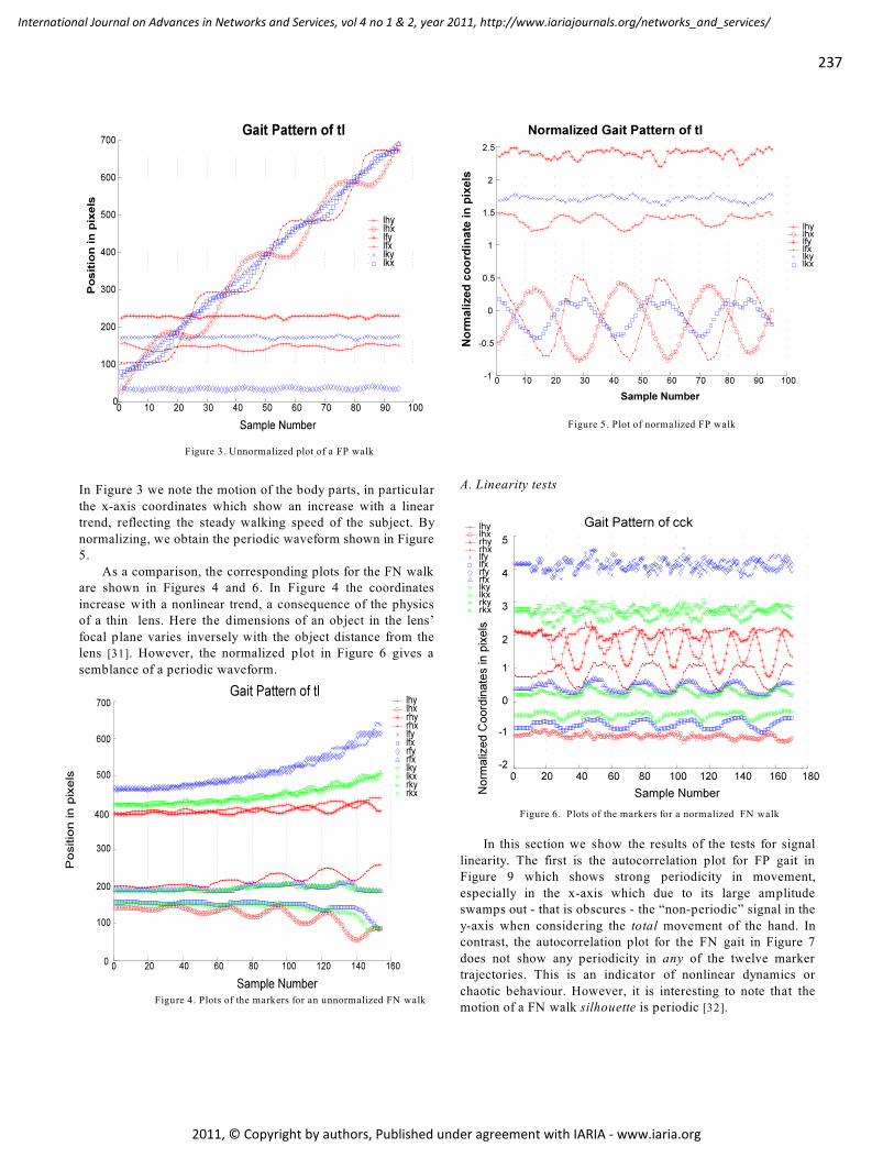
Figure 5. Plot of normalized FP walk
Figure 4. Plots of the markers for an unnormalized FN walk
In Figure 3 we note the motion of the body parts, in particular
the x-axis coordinates which show an increase with a lineartrend, reflecting the steady walking speed of the subject. By
normalizing, we obtain the periodic waveform shown in Figure5.
As a comparison, the corresponding plots for the FN walkare shown in Figures 4 and 6. In Figure 4 the coordinates
increase with a nonlinear trend, a consequence of the physicsof a thin lens. Here the dimensions of an object in the lens’
focal plane varies inversely with the object distance from thelens [31]. However, the normalized plot in Figure 6 gives a
semblance of a periodic waveform.
A. Linearity tests
In this section we show the results of the tests for signal
linearity. The first is the autocorrelation plot for FP gait inFigure 9 which shows strong periodicity in movement,
especially in the x-axis which due to its large amplitudeswamps out - that is obscures - the “non-periodic” signal in the
y-axis when considering the total movement of the hand. Incontrast, the autocorrelation plot for the FN gait in Figure 7
does not show any periodicity in any of the twelve markertrajectories. This is an indicator of nonlinear dynamics or
chaotic behaviour. However, it is interesting to note that themotion of a FN walk silhouette is periodic [32].
Figure 3. Unnormalized plot of a FP walk
Figure 6. Plots of the markers for a normalized FN walk
237
International Journal on Advances in Networks and Services, vol 4 no 1 & 2, year 2011, http://www.iariajournals.org/networks_and_services/
2011, © Copyright by authors, Published under agreement with IARIA - www.iaria.org
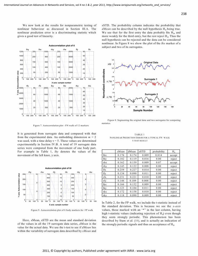
TABLE 1
NONLINEAR PREDICTION ERROR FOR A TYPICAL FN WALK
T-TEST RESULT
We now look at the results for nonparametric testing ofnonlinear behaviour as discussed in Section III.A. The
nonlinear prediction error is a discriminating statistic whichgives a good test of linearity.
It is generated from surrogate data and compared with thatfrom the experimental data. An embedding dimension m = 2
was used, with a time delay ô = 5. These values are determinedexperimentally in Section IV.B. A total of 19 surrogate data
series were computed from the movement of one body part.For example in Table 1, lhy denotes the values of the
movement of the left knee, y axis.
Here, sMean, sSTD are the mean and standard deviationof the values in all the 19 surrogate data series, dMean is the
value for the actual data. We use the t-test to see if dMean lieswithin the variability of surrogate data described by sMean and
sSTD. The probability column indicates the probability that
0dMean can be described by the null hypothesis H being true.
0We see that for the first entry the data probably fits H , and
0more weakly for the third entry, but the rest reject H . Thus the
null hypothesis can be rejected and the data can be considerednonlinear. In Figure 8 we show the plot of the lhx marker of a
subject and two of its surrogates.
0 sMean dMean sSTD probability H
lhx 0.176 0.174 0.009 0.814 accept
lhy 0.182 0.119 0.016 0.00 reject
rhx 0.162 0.159 0.009 0.07 accept
rhy 0.145 0.122 0.008 0.00 reject
lfx 0.259 0.227 0.014 0.00 reject
lfy 0.134 0.090 0.011 0.00 reject
rfx 0.231 0.221 0.010 0.00 reject
rfy 0.146 0.109 0.008 0.00 reject
lkx 0.166 0.152 0.009 0.00 reject
lky 0.123 0.104 0.011 0.00 reject
rkx 0.172 0.158 0.010 0.00 reject
rky 0.118 0.090 0.009 0.00 reject
In Table 2, for the FP walk, we include the t-statistic instead ofthe standard deviation. This is because we see the x-axis
values, those marked with an ‘*” in the last column, having
0high t-statistic values (indicating rejection of H ) even though
they seem strongly periodic. This phenomenon has beendescribed by Stam et al. [33], and is actually an indication of
0the strongly periodic signals and thus an acceptance of H .
Figure 7. Autocorrelation plot - FN walk of 12 markers
Figure 8. Segmenting the original data and two surrogates for computing
statistics
Figure 9. Autocorrelation plot of 6 body markers for FP walk
238
International Journal on Advances in Networks and Services, vol 4 no 1 & 2, year 2011, http://www.iariajournals.org/networks_and_services/
2011, © Copyright by authors, Published under agreement with IARIA - www.iaria.org
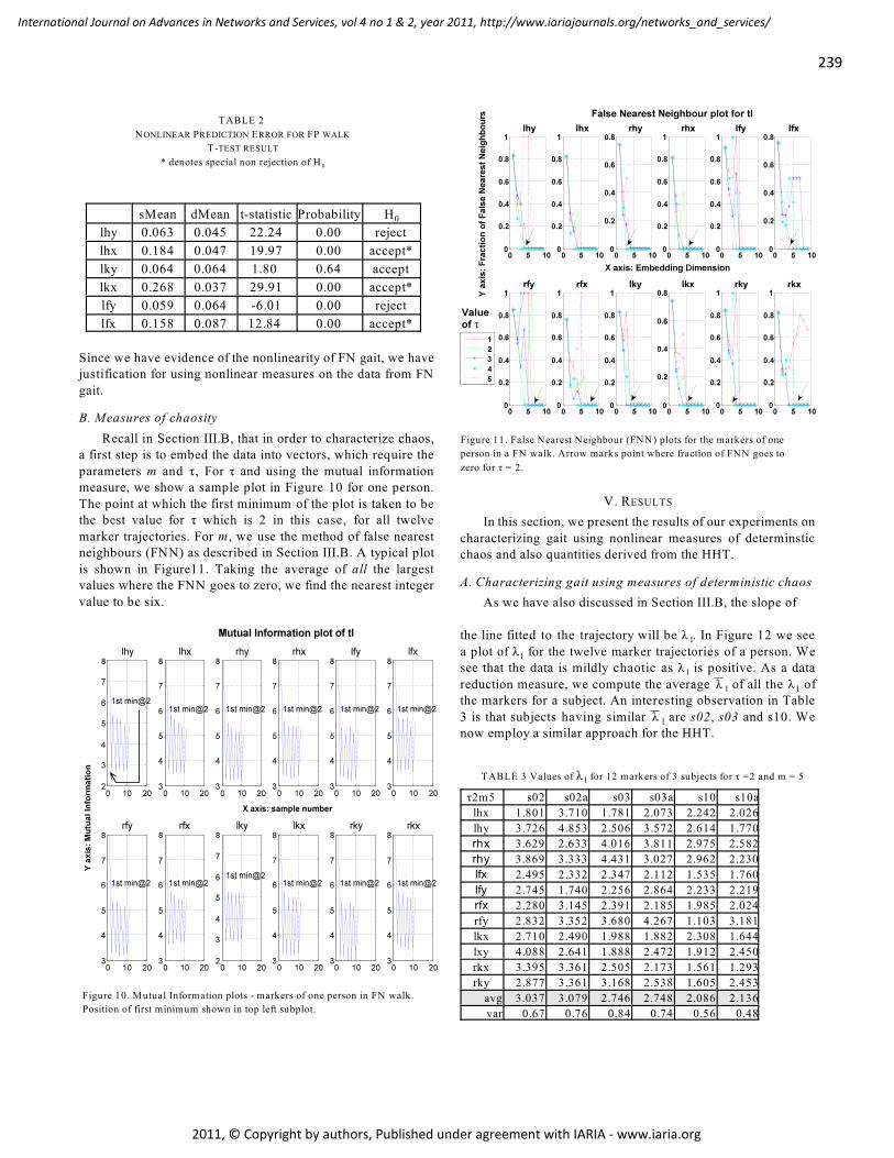
TABLE 2
NONLINEAR PREDICTION ERROR FOR FP WALK
T-TEST RESULT
0* denotes special non rejection of H
Figure 11. False Nearest Neighbour (FNN) plots for the markers of one
person in a FN walk. Arrow marks point where fraction of FNN goes to
zero for ô = 2.
1TABLE 3 Values of ë for 12 markers of 3 subjects for ô =2 and m = 5
0sMean dMean t-statistic Probability H
lhy 0.063 0.045 22.24 0.00 reject
lhx 0.184 0.047 19.97 0.00 accept*
lky 0.064 0.064 1.80 0.64 accept
lkx 0.268 0.037 29.91 0.00 accept*
lfy 0.059 0.064 -6.01 0.00 reject
lfx 0.158 0.087 12.84 0.00 accept*
Since we have evidence of the nonlinearity of FN gait, we havejustification for using nonlinear measures on the data from FN
gait.
B. Measures of chaosity
Recall in Section III.B, that in order to characterize chaos,a first step is to embed the data into vectors, which require the
parameters m and ô, For ô and using the mutual informationmeasure, we show a sample plot in Figure 10 for one person.
The point at which the first minimum of the plot is taken to bethe best value for ô which is 2 in this case, for all twelve
marker trajectories. For m , we use the method of false nearestneighbours (FNN) as described in Section III.B. A typical plot
is shown in Figure11. Taking the average of all the largestvalues where the FNN goes to zero, we find the nearest integer
value to be six.
V. RESULTS
In this section, we present the results of our experiments on
characterizing gait using nonlinear measures of determinsticchaos and also quantities derived from the HHT.
A. Characterizing gait using measures of deterministic chaos
As we have also discussed in Section III.B, the slope of
1the line fitted to the trajectory will be ë . In Figure 12 we see
1a plot of ë for the twelve marker trajectories of a person. We
1see that the data is mildly chaotic as ë is positive. As a data
1 1reduction measure, we compute the average 'ë of all the ë ofthe markers for a subject. An interesting observation in Table
13 is that subjects having similar 'ë are s02, s03 and s10. Wenow employ a similar approach for the HHT.
ô2m5 s02 s02a s03 s03a s10 s10a
lhx 1.801 3.710 1.781 2.073 2.242 2.026
lhy 3.726 4.853 2.506 3.572 2.614 1.770
rhx 3.629 2.633 4.016 3.811 2.975 2.582
rhy 3.869 3.333 4.431 3.027 2.962 2.230
lfx 2.495 2.332 2.347 2.112 1.535 1.760
lfy 2.745 1.740 2.256 2.864 2.233 2.219
rfx 2.280 3.145 2.391 2.185 1.985 2.024
rfy 2.832 3.352 3.680 4.267 1.103 3.181
lkx 2.710 2.490 1.988 1.882 2.308 1.644
lxy 4.088 2.641 1.888 2.472 1.912 2.450
rkx 3.395 3.361 2.505 2.173 1.561 1.293
rky 2.877 3.361 3.168 2.538 1.605 2.453
avg 3.037 3.079 2.746 2.748 2.086 2.136
var 0.67 0.76 0.84 0.74 0.56 0.48
Figure 10. Mutual Information plots - markers of one person in FN walk.
Position of first minimum shown in top left subplot.
239
International Journal on Advances in Networks and Services, vol 4 no 1 & 2, year 2011, http://www.iariajournals.org/networks_and_services/
2011, © Copyright by authors, Published under agreement with IARIA - www.iaria.org
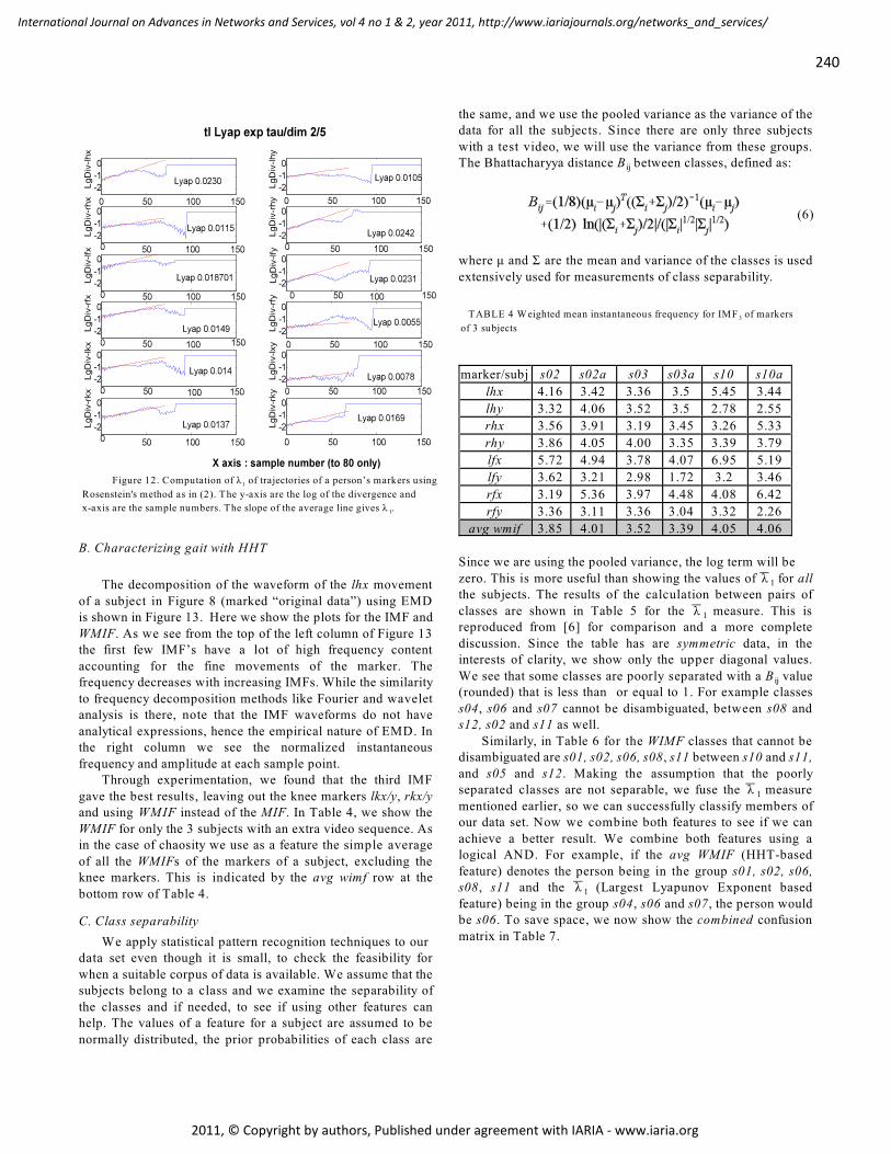
3TABLE 4 Weighted mean instantaneous frequency for IMF of markers
of 3 subjects
(6)
B. Characterizing gait with HHT
The decomposition of the waveform of the lhx movement
of a subject in Figure 8 (marked “original data”) using EMDis shown in Figure 13. Here we show the plots for the IMF and
WMIF. As we see from the top of the left column of Figure 13the first few IMF’s have a lot of high frequency content
accounting for the fine movements of the marker. Thefrequency decreases with increasing IMFs. While the similarity
to frequency decomposition methods like Fourier and waveletanalysis is there, note that the IMF waveforms do not have
analytical expressions, hence the empirical nature of EMD. Inthe right column we see the normalized instantaneous
frequency and amplitude at each sample point.Through experimentation, we found that the third IMF
gave the best results, leaving out the knee markers lkx/y, rkx/yand using WMIF instead of the MIF. In Table 4, we show the
WMIF for only the 3 subjects with an extra video sequence. Asin the case of chaosity we use as a feature the simple average
of all the WMIFs of the markers of a subject, excluding theknee markers. This is indicated by the avg wimf row at the
bottom row of Table 4.
C. Class separability
We apply statistical pattern recognition techniques to our data set even though it is small, to check the feasibility for
when a suitable corpus of data is available. We assume that thesubjects belong to a class and we examine the separability of
the classes and if needed, to see if using other features canhelp. The values of a feature for a subject are assumed to be
normally distributed, the prior probabilities of each class are
the same, and we use the pooled variance as the variance of thedata for all the subjects. Since there are only three subjects
with a test video, we will use the variance from these groups.
ijThe Bhattacharyya distance B between classes, defined as:
where ì and Ó are the mean and variance of the classes is used
extensively used for measurements of class separability.
marker/subj s02 s02a s03 s03a s10 s10a
lhx 4.16 3.42 3.36 3.5 5.45 3.44
lhy 3.32 4.06 3.52 3.5 2.78 2.55
rhx 3.56 3.91 3.19 3.45 3.26 5.33
rhy 3.86 4.05 4.00 3.35 3.39 3.79
lfx 5.72 4.94 3.78 4.07 6.95 5.19
lfy 3.62 3.21 2.98 1.72 3.2 3.46
rfx 3.19 5.36 3.97 4.48 4.08 6.42
rfy 3.36 3.11 3.36 3.04 3.32 2.26
avg wmif 3.85 4.01 3.52 3.39 4.05 4.06
Since we are using the pooled variance, the log term will be
1zero. This is more useful than showing the values of 'ë for allthe subjects. The results of the calculation between pairs of
1classes are shown in Table 5 for the 'ë measure. This isreproduced from [6] for comparison and a more complete
discussion. Since the table has are symmetric data, in theinterests of clarity, we show only the upper diagonal values.
ijWe see that some classes are poorly separated with a B value(rounded) that is less than or equal to 1. For example classes
s04, s06 and s07 cannot be disambiguated, between s08 ands12, s02 and s11 as well.
Similarly, in Table 6 for the WIMF classes that cannot bedisambiguated are s01, s02, s06, s08, s11 between s10 and s11,
and s05 and s12. Making the assumption that the poorly
1separated classes are not separable, we fuse the 'ë measure
mentioned earlier, so we can successfully classify members ofour data set. Now we combine both features to see if we can
achieve a better result. We combine both features using alogical AND. For example, if the avg WMIF (HHT-based
feature) denotes the person being in the group s01, s02, s06,
1s08, s11 and the 'ë (Largest Lyapunov Exponent basedfeature) being in the group s04, s06 and s07, the person wouldbe s06. To save space, we now show the combined confusion
matrix in Table 7.
1Figure 12. Computation of ë of trajectories of a person’s markers using
Rosenstein's method as in (2). The y-axis are the log of the divergence and
1x-axis are the sample numbers. The slope of the average line gives ë .
240
International Journal on Advances in Networks and Services, vol 4 no 1 & 2, year 2011, http://www.iariajournals.org/networks_and_services/
2011, © Copyright by authors, Published under agreement with IARIA - www.iaria.org
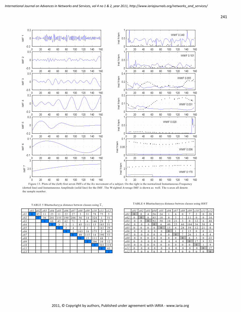
1TABLE 5 Bhattacharyya distance betwen classes using 'ë TABLE 6 Bhattacharyya distance betwen classes using HHT
s01 s02 s03 s04 s05 s06 s07 s08 s09 s10 s11 s12s01 0 85 11 25 11 22 27 3 31 78 75 5
s02 0 36 201 155 190 206 56 14 324 1 51s03 0 68 43 62 71 3 6 146 29 2s04 0 3 1 1 45 111 15 185 51s05 0 2 4 2 2 2 141 29s06 0 1 103 18 175 2 45s07 0 48 115 14 190 53s08 0 15 111 48 1s09 0 206 10 12s10 0 303 119s11 0 43s12 0
s01 s02 s03 s04 s05 s06 s07 s08 s09 s10 s11 s12s01 0 0 4 56 24 1 6 0 7 2 0 20s02 0 0 8 45 18 0 3 1 11 0 0 14s03 0 0 0 92 50 10 21 3 0 12 6 44s04 0 0 0 0 6 40 25 60 104 36 50 8s05 0 0 0 0 0 15 6 28 59 12 21 0s06 0 0 0 0 0 0 1 2 15 0 0 11s07 0 0 0 0 0 0 0 7 26 1 4 4s08 0 0 0 0 0 0 0 0 6 3 0 23s09 0 0 0 0 0 0 0 0 0 17 9 52s10 0 0 0 0 0 0 0 0 0 0 1 9s11 0 0 0 0 0 0 0 0 0 0 0 17s12 0 0 0 0 0 0 0 0 0 0 0 0
Figure 13. Plots of the (left) first seven IMFs of the lhx movement of a subject. On the right is the normalized Instantaneous Frequency
(dotted line) and Instantaneous Amplitude (solid line) for the IMF. The Weighted Average IMF is shown as well. The x-axes all denote
the sample number.
241
International Journal on Advances in Networks and Services, vol 4 no 1 & 2, year 2011, http://www.iariajournals.org/networks_and_services/
2011, © Copyright by authors, Published under agreement with IARIA - www.iaria.org
[1] M. W. Whittle, Gait Analysis: an Introduction , 4 ed., Philadelphia:th
Butterworth-Heinemann, 2007, pg 139.
[2] G. Verhoeven, “Did the digital (r)evolution change the concept of
focal length?” AARGNEWS , vol. 34, pp. 30-35 March 2007.
[3] T . K. M Lee, M. Belkhatir, P.A. Lee and S. Sanei, “Fronto-normal
gait incorporating accurate practical looming compensation,” Proc.
19 Int’l Conf. Pattern Recognition (ICPR 2008), 2008.th
[4] T . Lee, S. Ranganath and S. Sanei, “Patterns in paces: a survey of
current approaches in gait recognition,” Proc. Asian Biometric
Workshop (ABW 2003), pp 421-425, Singapore, Nov. 2003.
[5] A. Veeraraghavan, A. K. Roy-Chowdhury, and Rama Chellapa,
“Matching shape sequences in video with applications in human
movement analysis,” IEEE Transactions on PAMI, vol.27, no.12,
pp.1896-1909, Dec 2005.
[6] T . Lee, S. Ranganath, and S. Sanei, “Fusion of chaotic measure into
a new hybrid face-gait system for human identification,” Proc.
ICPR , Hong Kong, August, 2006.
[7] T . K. M. Lee, K. F. Loe, P. A. Lee and S. Sanei, “A comparison of
the basic temporal features of fronto-normal and fronto-parallel
gait,” DSP 2007 , Cardiff, UK, July 1-4, 2007.
[8] T . K. M. Lee, S. Sanei and B. Clarke, “Fusion of nonlinear measures
in fronto-normal gait recognition,” International Multi-conference
on Computing in the Global Information Technology, Valencia,
Spain, 2010.
[9] T . K. M Lee, M. Belkhatir, P. A. Lee and S. Sanei, “Nonlinear
characterisation of fronto-normal gait for biometric use,” Proc.
Pacific-Rim Conf. On Multimedia (PCM 2008), 2008.
[10] H. Tong, “Non-linear Time Series” 1 ed, Oxford Sciencest
Publications, 1993.
[11] G. Johansson, “Visual perception of biological motion and a model
for its analysis,” Perception & Psychophysics, vol.14, no.2, pp.201-
211, 1973.
[12] J. E. Cutting and L. T . Kozlowski, “Recognizing friends by their
walk: Gait perception without familiarity cues,” Bull of the
Psychonomic Society, vol.9, no.5, pp.353-356, 1977.
[13] N. F. Troje, “Decomposing biological motion: A framework for
analysis and synthesis of human gait patterns,” Journal of Vision ,
vol.2, pp.371-387, 2002.
[14] M.S. Nixon, T . Tan and R. Chellappa , “Human Identification Based
on Gait”, 1st ed, Springer, 2005.
[15] R. K. Ibrahim, E. Ambikairajah, B.G. Celler and N.H. Lovell, “Gait
pattern classification using compact features extracted from Intrinsic
Mode Functions,” 30 Ann. Conf. IEEE Engineering in Medicineth
and Biology Society, 2008.
[16] N. Wang, E. Ambikairajah, B. G. Celler and N. H. Lovell,
“Accelerometry based classification of gait patterns using Empirical
Mode Decomposition,” Proc. 2008 IEEE Int’l Conf. Signals,
Acoustics and Speech Processing (ICASSP), 2008.
[17] P. Kuchi and S. Sethuraman, “Gait recognition using Empirical
Mode Decomposition,” Int’l Conf. Advances In Pattern Recognition ,
2003.
[18] G. R. Bradski, “Computer video face tracking for use in a perceptual
user interface,” Intel Technology Journal, vol.Q2, 1998.
[19] T. K. M. Lee, M. Belkhatir and S. Sanei, “Techniques, issues and
perspectives for gait-based recognition” (in review) by Pattern
Recognition / Elsevier.
[20] J. Theiler, B. Galdrikian, A. Longtin, S. Eubank and J.D. Farmer,
“Using surrogate data to detect nonlinearity in time series,” Proc.
Nonlinear Modeling and Forecasting, Santa Fe Institute Studies in
the Sciences of Complexity, Vol. XII , Santa Fe, 1992.
[21] T. Schreiber and A. Schmitz, “Discrimination power of measures for
nonlinearity in a time series,” Phys. Rev. E , vol.55, no.5, pp.5443 -
5447, May 1997.
[22] D. Kaplan, “Nonlinearity and Nonstationarity: The use of surrogate
data in interpreting fluctuations in heart rate,” Frontiers of Blood
Pressure and Heart Rate Analysis, M. Di Rienzo, et al., IOS Press,
1997.
[23] J. Theiler and D. Prichard, “Constrained-realization Monte-Carlo
method for hypothesis testing,” Physica D , vol.94, pp.221-235,
1996.
TABLE 7 Confusion matrix combining HHT and Largest Lyapunov
Exponent as features.
PREDICTED/ACTUAL in %
s01 s02 s03 s04 s05 s06 s07 s08 s09 s10 s11 s12s01 100 s02 100s03 100s04 100 s05 100s06 100s07 100s08 100s09 100s10 100s11 100s12 100
A useful result is that we are able to separate all classessuccessfully using these two nonlinear measures.
VI. CONCLUSION AND FUTURE WORK
We have used a camera as a sensor to derive the gaitsignals of a person in a multimedia video data stream. The
objective is to see if the data can be used to identify a person.We have shown by using several types of analyses that signals
derived from FN gait is nonlinear in nature. This is in contrastto current approaches which impose linear analyses of gait
signals for convenience. This gives us a basis for usingnonlinear measures of gait. In our experiments, the simple
average of the nonlinear features by themselves are not able todiscriminate completely between the classes of subjects.
However, by combining them, we get a successful result. Thenovelty of our approach lies in the evaluation and use of both
cyclostationarity and nonlinear measures of the gait signal.While our dataset is small, we note that the number of
nonlinear features we can extract from the gait signals ispotentially very large. A more exhaustive search for features
and combinations of signals may yield useful results in termsof deriving new biometrics or improved recognition rates. So
future work will need to test this out for current biometrics ina larger dataset and in a markerless environment. There is also
much scope for investigating other types of signal analysis thatis not based on linearity and stationarity assumptions. By doing
so, we capitalize on the ubiquity of video cameras, from whichwe are able to obtain sensory data which can be used to
augment security networks.
REFERENCES
242
International Journal on Advances in Networks and Services, vol 4 no 1 & 2, year 2011, http://www.iariajournals.org/networks_and_services/
2011, © Copyright by authors, Published under agreement with IARIA - www.iaria.org
[24] F. Takens, “Detecting strange attractors in turbulence,” Lecture
notes in Mathematics, vol. 898, pp. 361-381, Springer-Verlag, 1981.
[25] A. M. Fraser and H.L. Swinney, “Independent coordinates for
strange attractors from mutual information,” Phys. Rev. A , 33, pp.
1134-1140, 1986.
[26] K. B. Kennel, R. Brown and H. D. I. Abarbanel, “Determining
embedding dimension for phase-space reconstruction using a
geometrical construction,” Phys. Rev. A , vol. 45, no. 3403, 1992.
[27] M.T. Rosenstein, J. J. Collins and C. J. De Luca, “A practical
method for calculating largest Lyapunov exponents from small data
sets,” Physica D , vol. 65, pp. 117, 1993.
[28] H. Kantz, “A robust method to estimate the maximal Lyapunov
exponent of a time series,” Physics. Letters A , vol. 185, pp. 77, 1994.
[29] N. E. Huang, Z. Shen, S. R. Long, M. C. Wu, H. H. Shih, Q. Zheng,
N. Yen, C. C. Tung and H. H. Liu, “The empirical mode
decomposition and the Hilbert spectrum for nonlinear and non-
stationary time series analysis,” Proc. R. Soc. Lond. A , 454, pp. 903-
995, 1998.
[30] N. E. Huang, Z. Shen, and S. R. Long, “A new view of nonlinear
water waves: the Hilbert spectrum” Ann. Rev. Fluid Mechanics, pp.
415-457, 1999.
[31] E. Hecht, “Optics” , 4 edition, Addison Wesley, 2001.th
[32] L. Wang, T . Tan, H. Ning and W. Hu, “Silhouette analysis-based
gait recognition for human identification,” IEEE Transactions on
PAMI, vol. 25, no. 12, pp. 1505-1518, Dec 2003.
[33] C. J. Stam, J. P. M. Pijn and W. S. Pritchard, Reliable detection of
nonlinearity in experimental time series with strong periodic
components, Physica D , vol.112, no.3-4, pp.361-380, February
1998.
243
International Journal on Advances in Networks and Services, vol 4 no 1 & 2, year 2011, http://www.iariajournals.org/networks_and_services/
2011, © Copyright by authors, Published under agreement with IARIA - www.iaria.org

www.iariajournals.org
International Journal On Advances in Intelligent Systems
ICAS, ACHI, ICCGI, UBICOMM, ADVCOMP, CENTRIC, GEOProcessing, SEMAPRO,BIOSYSCOM, BIOINFO, BIOTECHNO, FUTURE COMPUTING, SERVICE COMPUTATION,COGNITIVE, ADAPTIVE, CONTENT, PATTERNS, CLOUD COMPUTING, COMPUTATION TOOLS
issn: 1942-2679
International Journal On Advances in Internet Technology
ICDS, ICIW, CTRQ, UBICOMM, ICSNC, AFIN, INTERNET, AP2PS, EMERGING
issn: 1942-2652
International Journal On Advances in Life Sciences
eTELEMED, eKNOW, eL&mL, BIODIV, BIOENVIRONMENT, BIOGREEN, BIOSYSCOM,BIOINFO, BIOTECHNO
issn: 1942-2660
International Journal On Advances in Networks and Services
ICN, ICNS, ICIW, ICWMC, SENSORCOMM, MESH, CENTRIC, MMEDIA, SERVICECOMPUTATION
issn: 1942-2644
International Journal On Advances in Security
ICQNM, SECURWARE, MESH, DEPEND, INTERNET, CYBERLAWS
issn: 1942-2636
International Journal On Advances in Software
ICSEA, ICCGI, ADVCOMP, GEOProcessing, DBKDA, INTENSIVE, VALID, SIMUL, FUTURECOMPUTING, SERVICE COMPUTATION, COGNITIVE, ADAPTIVE, CONTENT, PATTERNS,CLOUD COMPUTING, COMPUTATION TOOLS
issn: 1942-2628
International Journal On Advances in Systems and Measurements
ICQNM, ICONS, ICIMP, SENSORCOMM, CENICS, VALID, SIMUL
issn: 1942-261x
International Journal On Advances in Telecommunications
AICT, ICDT, ICWMC, ICSNC, CTRQ, SPACOMM, MMEDIA
issn: 1942-2601


