A A N K A L A N

Department of Mathematics,

Hansraj College

Volume 2, 2021

FRom tHe PRincipal’s DesK

Aankalan, the Annual Mathematics Journal of Hansraj College is in its second year. It givesme great joy to laud the young minds who have worked assiduously to bring it to fruition.

The Mathematics Department of Hansraj College has always had a legacy of greatness; beit in the sphere of academic performance or innovation and research. Students have alwaysbeen encouraged to think out of the box and apply their learnings in the real world. Theyhave always been given the opportunities to inculcate critical and logical thinking. To thiscount, I congratulate and commend the efforts of the Editorial Board to carry on the legacyand seeking to promote critical thinking and research.

I also thank the faculty advisors Dr. Preeti Dharmarha, Dr. Harjeet Arora, Ms. Amita Ag-garwal, Dr. Mukund Madhav Mishra and Dr. Rakesh Batra for their constant efforts to takethe Department to greater heights and mentoring young minds.

I hope that Aankalan will continue to serve as a learning platform for students and upholdthe sanctity and glory of the Department!

Dr. RamaPRincipalHansRaj College,UniveRsity of Delhi

ii

FRom tHe Head of Faculty AdvisoRs

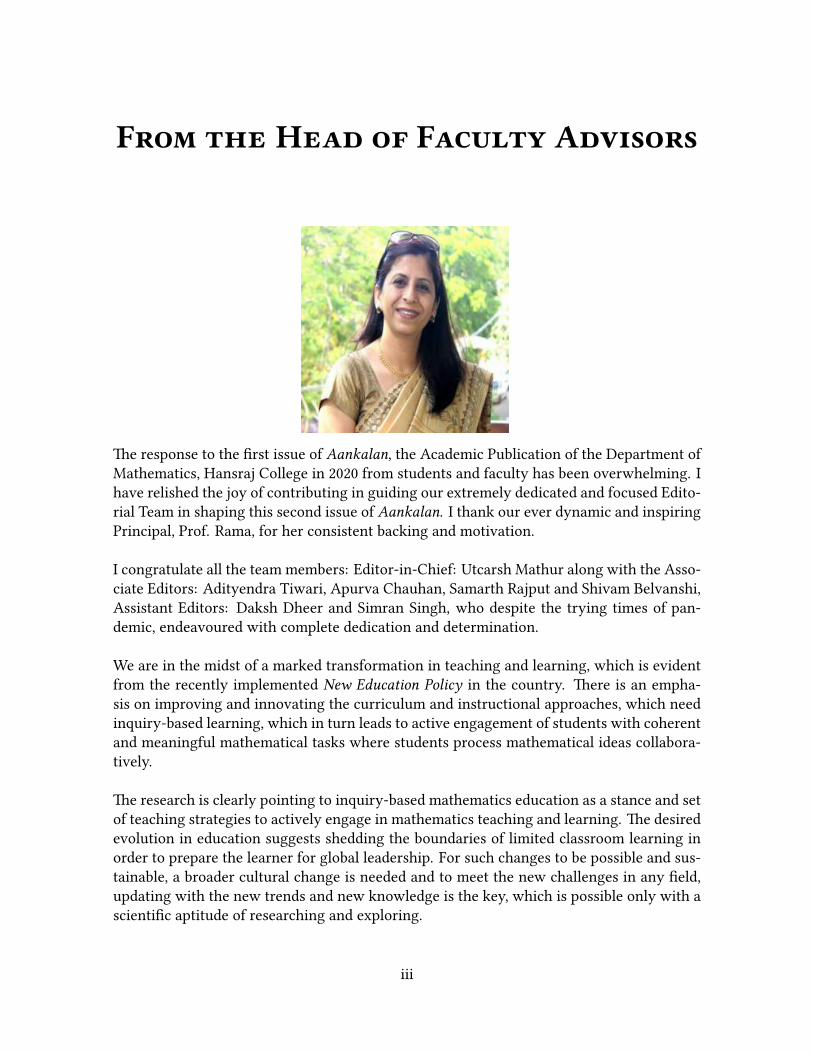
The response to the first issue of Aankalan, the Academic Publication of the Department ofMathematics, Hansraj College in 2020 from students and faculty has been overwhelming. Ihave relished the joy of contributing in guiding our extremely dedicated and focused Edito-rial Team in shaping this second issue of Aankalan. I thank our ever dynamic and inspiringPrincipal, Prof. Rama, for her consistent backing and motivation.

I congratulate all the team members: Editor-in-Chief: Utcarsh Mathur along with the Asso-ciate Editors: Adityendra Tiwari, Apurva Chauhan, Samarth Rajput and Shivam Belvanshi,Assistant Editors: Daksh Dheer and Simran Singh, who despite the trying times of pan-demic, endeavoured with complete dedication and determination.

We are in the midst of a marked transformation in teaching and learning, which is evidentfrom the recently implemented New Education Policy in the country. There is an empha-sis on improving and innovating the curriculum and instructional approaches, which needinquiry-based learning, which in turn leads to active engagement of students with coherentand meaningful mathematical tasks where students process mathematical ideas collabora-tively.

The research is clearly pointing to inquiry-based mathematics education as a stance and setof teaching strategies to actively engage in mathematics teaching and learning. The desiredevolution in education suggests shedding the boundaries of limited classroom learning inorder to prepare the learner for global leadership. For such changes to be possible and sus-tainable, a broader cultural change is needed and to meet the new challenges in any field,updating with the new trends and new knowledge is the key, which is possible only with ascientific aptitude of researching and exploring.

iii

FRom the Head of Faculty AdvisoRs iv

Excellence in academics has always been a hallmark of the Department of Mathematics atHansraj College. Mathematicians par excellence like Shanti Narayan ji, Prof. M.C. Puri, Prof.S. C. Arora and Dr. S. R. Arora; in close association with gurus like Dr. Harbans Lal, Dr. K.L. Bhatla, Dr. N.M. Kapoor, Dr. Satpal, and Sh. J. P. Pruthi as guiding lights brought theDepartment as the most sought after for undergraduate studies, the stepping stone to one’scareer. Our Department has been instrumental in nurturing and creating global leaders byproviding the best of classroom teaching along with co-curricular and practical experiences.

We lost two pillars of our Department, Dr. Satpal and Sh. J. P. Pruthi since the issuanceof our previous issue of Aankalan. Our entire team pays tributes to the stalwarts, whoseable guidance had a significant role in nurturing the Department and our College for manydecades of their association with us.

The inputs and thorough feedback by the Advisory Editorial Board members Dr. HarjeetArora, Mrs. Amita Aggarwal, Dr. Rakesh Batra and Dr. Mukund Madhav Mishra, aidedimmensely in improving the content. A big thanks to them‼

The contents of this edition have also been selected after a careful review by experiencedfaculty. The issue comprises of a rainbow of articles ranging from abstract concepts fromanalysis such as totally bounded sets, ordering in Complex Numbers and Riemann Hypoth-esis to beautiful applications of linear algebra and probability along with the Three UtilityProblem from graph theory and mathematics in plants from bio-mathematics. Apart fromthese, it also includes two problems namely, ‘Mapping’ and ‘The Windmill Process’ alongwith a short piece on lesser-known Mathematical facts.

I am sure that this publication will greatly motivate the students in developing inquisitive-ness to explore new domains, go further deep into the touched upon ideas and build theirinterest in research; inculcating confidence in them. It is also our endeavour in honing thepresentation skills of the readers and prepare them for creating quality academic content.I am confident that this launching pad will open new arenas for the avid learners and em-bolden them to dig out the pearls from the vast ocean of knowledge.

Dr. Preeti DharmarhaAssociate PRofessoR,DepaRtment of Mathematics

EDITORIAL BOARD

Faculty AdvisoRs

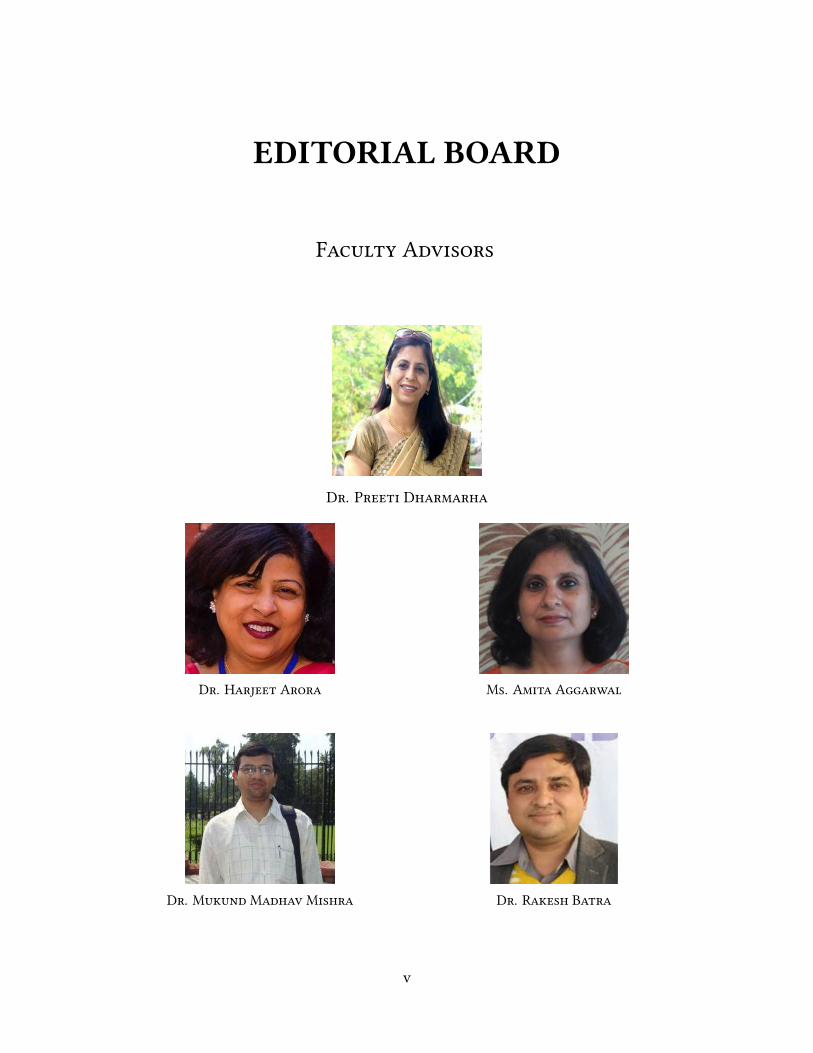
DR. PReeti DhaRmaRha

DR. HaRjeet ARoRa Ms. Amita AggaRwal

DR. MuKund Madhav MishRa DR. RaKesh BatRa

v

EditoRial BoaRd vi

Student EditoRs

EditoR-in-Chief

UtcaRsh MathuR

Associate EditoRs

AdityendRa TiwaRi ApuRva Chauhan

SamaRth Rajput Shivam Belvanshi

Assistant EditoRs

DaKsh DheeR SimRan Singh

FRom tHe EditoRs’ Pen

Aankalan, the Annual Mathematics Journal of Hansraj College was started in 2019 by agroup of Math-enthusiasts, with a view to encourage external learning and inculcate re-search and expository skills at an undergraduate level. It aims at appreciating the signifi-cant presence of the subject in real life. We seek to go beyond the books and explore thevastness of the subject through research, exploration and innovation, something that theDepartment has always encouraged. As Walt Whitman eloquently puts in his 1867 poem‘When I Heard the Learn’d Astronomer’, real knowledge is what comes from exploration andexperiences and this is what the Department of Mathematics at Hansraj stands by.

It is believed by many that all mathematics is concerned with is cumbersome equationsand unnecessary symbols carelessly dispersed over pieces of paper. But that’s far from thetruth. The subject is, in our humble opinion, derived from the universal truths of the world.Every iteration has some logic to it. Perhaps it is in this logic and truth, in a perplexed andasymmetric world, that mathematicians find their peace. Though the wide and all-pervasivenature of this subject has prevented the formulation of a common definition, one can agreethat mathematics is concerned with patterns, certain regularities (or irregularities) that con-stitute nature. Be it the cycle of time, the change of weather, movement of planets or evenour own breathing, patterns can be found everywhere in life. It is these patterns that formthe basis of mathematics.

The Journal encourages students to explore such patterns and try to make them relatablewith topics of higher mathematics. It serves as a learning platform, where students learnfrom each other, through the aggregation of each others’ thoughts.

The initial part of the Journal brings to you the palate of the average math aficionado, withtopics from Real and Complex Analysis, Abstract Algebra and Linear Algebra. These ar-ticles discuss the certain nuances and subtleties of these subjects, from the perspective ofundergraduate students. We also include some clever proofs of well-known theorems.

We thenmove on to discuss the applications of the subject in real life. It is almost impossibleto imagine a world without mathematics. It is involved in almost all aspects of our lives, beit using the internet or managing one’s finances or processing data or even preparing one’sfood! Often, mathematics is applicable in places that we don’t really see. The latter portionof this Journal deals with such observations.

vii

FRom the EditoRs’ Pen viii

Finally, we leave the reader with some food for thought; certain problems that would cap-ture your fancy and some lesser-known facts that can be the subject of further research.We hope that the articles increase the knowledge base of students and encourage them todelve further into the particularities of the discipline. We end with a quote by someone whoalways valued knowledge and power of exploration;

“Reach high, for stars lie hidden in you. Dream deep, for every dream precedes thegoal.”

-Rabindranath Tagore

With that, we present to you, Aankalan 2021.

AcKnowledgements

We thank our Principal, Dr. Rama, who has been a source of encouragement, motivationand inspiration for all of us and who has always supported our efforts to innovate and ex-periment.

A heartfelt gratitude towards Dr. S.C. Arora, for sparing time from his busy schedule andsharing with us his experiences and imparting wisdom. The Department will always followthe path illuminated by him.

We are also grateful to all the professors of the Department for their constant support andguidance. We especially thank Dr. Preeti Dharmarha, Dr. Harjeet Arora, Ms. Amita Ag-garwal, Dr. Mukund Madhav Mishra and Dr. Rakesh Batra (TIC) for their thorough andcomprehensive feedback of the articles, without which the Journal wouldn’t have been pos-sible.

We would like to thank the President of the Department and former Editor-in-Chief, AmanChaudhary, who has always guided us in the right direction. Further, we thank the formerteam of Associate Editors; Ashutosh Maurya, Gaurav Kumar and Ishita Srivastava, for con-sidering us worthy and capable of taking the baton and helping us in all possible ways.

We also thank the technical team comprising Mukesh Kumar, Ujjawal Agarwal, VedantGoyal along with Dushyant Kumar Rohilla, Jivin Vaidya, Ojal Kumar and Vanshika, forworking tirelessly on the Department website that gaveAankalan a platform. We also thankall members of the Mathematics Department Council for their constant support and encour-agement.

Last, but not in anyway the least, we thank the students of theDepartment, for their constantefforts to make the Department reach greater heights and their overwhelming response andparticipation this year.

We thank you all for your support!

ix

InteRview witH DR. S.C. ARoRa

Prof. S.C. Arora is a teacher par excellence and an illustrious and erudite academician. Hecompleted his post-graduation from Hansraj College, University of Delhi in 1967 standingfirst in the University. Subsequently, he was appointed as a lecturer in Hansraj College,where he taught for a period of twenty years. He then joined the Department of Mathemat-ics, University of Delhi, where he also served as Head of the Department.

After superannuation, he remained associated with various academic institutions includ-ing PDM college/University, Haryana and SGTB Institute of Management and Technology,Delhi. He continues to be associated with academic bodies like UGC, AICTE, NCERT, CBSEetc. He is also associated with many Public Service Commissions like Union Public Ser-vice Commission, Himachal Pradesh Service Commission and Jammu and Kashmir ServiceCommission among others. Throughout his teaching career, he was involved in researchand published more than 100 papers in various reputed journals and continues to deliverlectures at national and international conferences. Prof. Arora has also supervised 75M.Philand Ph.D students.

The representatives of the Editorial Board, Daksh Dheer and Simran Singh had a candidtelephonic conversation with this calm and humble personality. Excerpts:

DaKsh: Sir, first of all, we would like you to tell us about your journey at Hansraj. Howwas it like? What were the major highlights?DR ARoRa: I was a student here at Hansraj College in 1961, when it used to be a boys’college, and was not co-educational. Our teachers were great. In fact, it is due to theirteachings, that I became Dr. S.C. Arora. The one thing that they taught us, that I wouldpoint out, was to take our classes regularly. We were always taught to be punctual and“make no excuses”. Hence, we adjusted our time table, programs and fests in such a waythat we didn’t miss any classes. My teaching career at Hansraj began on 28th July, 1967.Throughout my career, I do not remember missing even a single lecture, be it during mystint at Hansraj from 1967-1987, or duringmy days at the University. My students can vouchfor that! It isn’t something worthy of praise, it is our duty to do so. If I speak in very safeterms, we are being paid to do just that!

SimRan: Sir, you said you owe your teachings to your mentors, and so, we would like toknow what was it like having Professor Shanti Narayan as your mentor.DR ARoRa: He was a great man. He did so much for the students. It was because of him

x

xi InteRview with DR. S.C. ARoRa

that people like me became faculty at the Department of Mathematics, University of Delhi.He moulded our careers. To be very frank, I was quite poor. He gave me a place here; I wasliving at college hostel for a year during my masters. He used to help the students so much.I still remember that during my post-graduation, I used to sit in the college library (whichused to close by 12 am in those days), and Prof. Narayan used to come at 11:30 pm to seewhich students were studying. I must say, whatever you all must’ve have heard about him,that is still minuscule compared to what a great man he truly was. I distinctly rememberonce, I had issued a book from the library, Commutative Algebra by Zariski, but somehowit went out of my possession without my knowledge. I had no money to pay for the book. Iwent to him and explained the situation, and he wrote to the college library and waived offthe fine. The years at Hansraj College were the golden years of my life. The past can nevercome back and I miss those days dearly, even today.

SimRan: Yes, sir, hearing your anecdotes, we cannot help getting bittersweet about our ownunique online college life, which brings me to ask you- what changes according to you arerequired in the current teaching patterns?DR ARoRa: A lot of things have changed since I retired in 2010. People have become fasternow, life has become quicker. People are used to online learning, something which we neverhad. I do not know how useful the online mode of education is, but I do believe that thestudents, particularly young ones, are overburdened. Perhaps something should be donein that regard so that the students aren’t always stuck to their laptops and phone screens.Thinking and introspection on one’s own is also required, which is what we used to do.Some balance has to be struck between the online and offline mode. I feel care has to betaken to ensure that students learn to think deeply on their own. There is no replacementof face-to-face teaching. A teacher’s personality is absorbed by their students, and not justin terms of teaching, but the way they tackle problems and talk, which is missing now. Iremember talking to my students who tell me that they try and teach the way I taught them;they try to imitate my methods and teachings towards their students. So, students inheritthe personality of their teachers and pass it on further to their own students.

SimRan: Since we are on this topic, would you tell us how did you end up in the field ofmathematics? Did you choose your profession as a professor for a specific reason?DRARoRa: My parents never planned to sendme to Hansraj College. Out of Physics, Chem-istry and Mathematics, I was more inclined towards maths, even though physics was alsovery interesting. I simply chose mathematics because I enjoyed it. At the time, I neverthought of pursuing engineering or medicine, though there weren’t any competitions toqualify for going into these fields; everyone used to get admission here or there unlike now.I could have just as well gone into the field of physics or chemistry. I came here just becauseit happened, and I don’t want to falsely boast that it was all planned and I always wantedto study mathematics- no, I simply chose it because I was better at it.

SimRan: Sir, now that you have told us about choosing mathematics, could you tell us aboutyour areas of interest? Which field do you find most interesting?DR ARoRa: My specialisation is in analysis, so I was always interested in that. However,

InteRview with DR. S.C. ARoRa xii

I used to like algebra too. Now, before I move further, I want to tell you all to not simplygo by my words because now the scenario has changed. The focus has shifted to appliedmathematics, i.e. people now talk more about its applications. To give you an example,some 15-20 days ago, I delivered an online lecture on the Fundamental Theorem of Alge-bra. I have delivered the same lecture many times, but this instance, for the first time, theyinsisted that I talk not entirely about the theorem, but also on its applications. Nowadays,people mostly talk about how the mathematics they study is applied to real-world problems.

DaKsh: Right, sir, there is now a focus on applied mathematics now, but even so, do youthink that scope for undergraduate research should be provided? How can students be en-couraged in this direction?DR ARoRa: I think they may be shown the places where the knowledge they have learntcan be applied. At the undergraduate level, there is high scope of practicality and applica-tion of concepts, and this ought to be focused upon. Undergraduate study is mostly focusedon mathematical tools; tools of algebra, tools of analysis, in other words, the utility of thesubject. Of course, they may learn on their own terms, at their own pace, but the empha-sis should be on applications and usage of mathematics. Moreover, focus on the real, puremathematics should come at postgraduate and higher levels, when the students have at-tained enough maturity and understanding.

SimRan: On that note sir, how do you view student-teacher bond, and what word of advicewould you like to give to the students?DR ARoRa: Love and respect; they go together. Teachers show love to their students and, inturn, students show respect to their teachers. They are two inseparable aspects. The bondis quite similar to how a father cares for his son or daughter. This sacred bond is importantand ought to be preserved. To all the students, I wish them all the luck and advise them todevelop this love-respect bond deeply with their teachers. I emphasise here once again thenecessity of attending classes regularly without fail, be it a teacher or a student. Learn tothink on your own and don’t let the shortcomings of online classes deter you. Rememberthat these are the golden years of your life that won’t ever come back, so live them to thefullest and work hard!

Contents

From the Principal’s Desk ii

From the Head of Faculty Advisors iii

Editorial Board v

From the Editors’ Pen vii

Acknowledgements ix

Interview with Dr. S.C. Arora x

1 Equivalent Definition of Totally Bounded SetsEkansh Jauhari 1

2 Plausible Orderings of the Complex PlaneAman Chaudhary 5

3 Riemann Hypothesis: the Prime QuestionUtcarsh Mathur 13

4 The Perfect DiceAdityendra Tiwari 19

5 Mathematics and the Rubik’s CubeSamarth Rajput 23

6 On Solving a Cubic EquationDaksh Dheer 28

7 Application of Linear Algebra in Solving GPS EquationsYash Jain 35

8 On Acuteness of Random TrianglesShivam Baurai 42

9 The Three Utility ProblemApurva Chauhan 44

xiii

Contents xiv

10 The Logarithmic SpiralKhushi Agarwal 48

11 Mathematics in PlantsPriyanka Chopra 52

12 Pyramids and MathematicsMir Samreen 56

13 Very Small ProofsShivam Baurai 62

14 One-Step At A Time 64

15 The Windmill Process 66

16 Mathematical Facts 70

EQUIVALENT DEFINITION OFTOTALLY BOUNDED SETS

Ekansh JauhariBatch of 2020

AbstRactThe article aims to provide a more convenient equivalent definition of totallybounded sets in a metric space by establishing that the subset Fϵ ⊂ X (in theusual definition of totally bounded sets in a metric space- also defined in theIntroduction section below) can be chosen from the set A itself, i.e. we can getsome set Gϵ ⊂ A ⊂ X corresponding to any given ϵ > 0.

Notations: (xn) denotes sequence. x(i)n denotes that i is fixed index and n is the running

index. U ⊂ V includes both possibilities, U = V and U ⊊ V . B(x, γ) denotes open ballcentered at x with radius γ.

IntRoductionFor a set in a metric space, the condition of total boundedness is much stronger than that ofboundedness because it gives many important implications, including of course, the bound-edness of the set.

In a metric space (X, d) , A ⊂ X , A ̸= ϕ is said to be totally bounded if ∀ ϵ > 0 ,∃a finite non-empty set Fϵ ⊂ X,Fϵ = {x1, x2, . . . , xn} such that A ⊂

⋃z∈Fϵ

B( z, ϵ) or

A ⊂n⋃

i=1

B(xi, ϵ). Amongst many implications of total boundedness, one important impli-

cation or property is the following:

Lemma. A set is totally bounded if and only if every sequence belonging to the set is a Cauchysequence (the technique involved in its proof deserves another such dedicated article, and is thusskipped here).

1

2 Eivalent Definition of Totally Bounded Sets

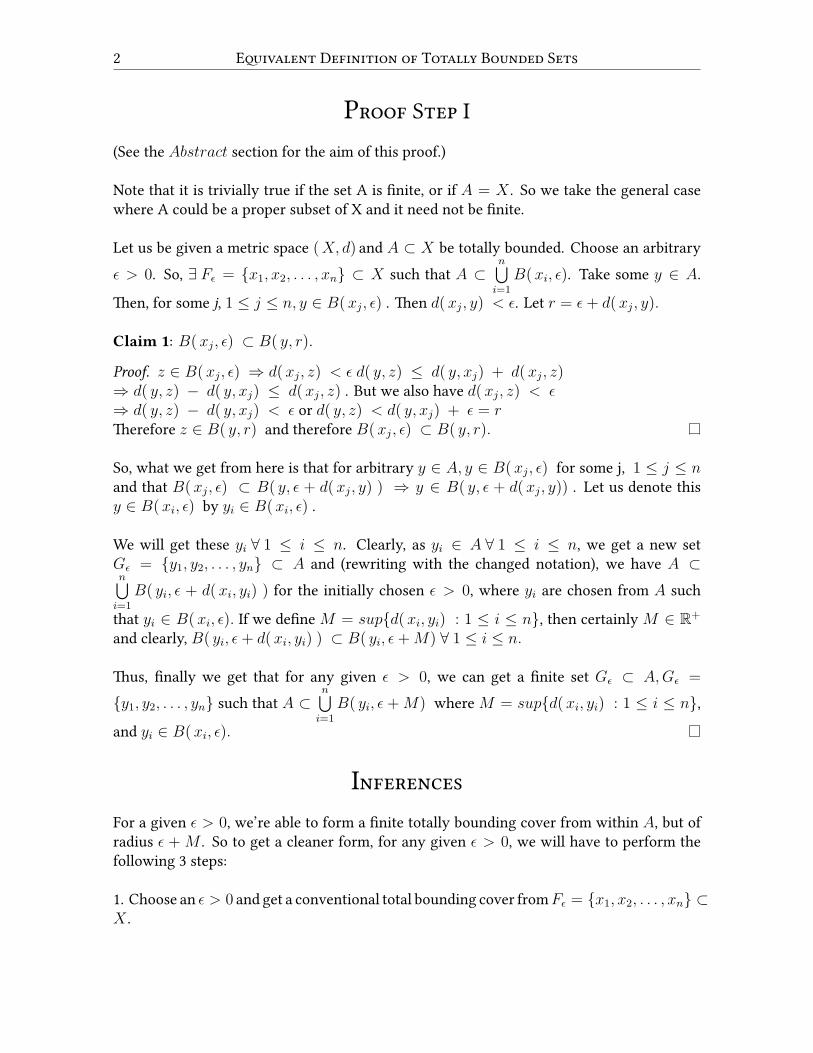
PRoof Step I(See the Abstract section for the aim of this proof.)

Note that it is trivially true if the set A is finite, or if A = X . So we take the general casewhere A could be a proper subset of X and it need not be finite.

Let us be given a metric space (X, d) and A ⊂ X be totally bounded. Choose an arbitraryϵ > 0. So, ∃ Fϵ = {x1, x2, . . . , xn} ⊂ X such that A ⊂

n⋃i=1

B(xi, ϵ). Take some y ∈ A.

Then, for some j, 1 ≤ j ≤ n, y ∈ B(xj, ϵ) . Then d(xj, y) < ϵ. Let r = ϵ+ d(xj, y).

Claim 1: B(xj, ϵ) ⊂ B( y, r).

Proof. z ∈ B(xj, ϵ) ⇒ d(xj, z) < ϵ d( y, z) ≤ d( y, xj) + d(xj, z)⇒ d( y, z) − d( y, xj) ≤ d(xj, z) . But we also have d(xj, z) < ϵ⇒ d( y, z) − d( y, xj) < ϵ or d( y, z) < d( y, xj) + ϵ = rTherefore z ∈ B( y, r) and therefore B(xj, ϵ) ⊂ B( y, r).

So, what we get from here is that for arbitrary y ∈ A, y ∈ B(xj, ϵ) for some j, 1 ≤ j ≤ nand that B(xj, ϵ) ⊂ B( y, ϵ + d(xj, y) ) ⇒ y ∈ B( y, ϵ + d(xj, y)) . Let us denote thisy ∈ B(xi, ϵ) by yi ∈ B(xi, ϵ) .

We will get these yi ∀ 1 ≤ i ≤ n. Clearly, as yi ∈ A ∀ 1 ≤ i ≤ n, we get a new setGϵ = {y1, y2, . . . , yn} ⊂ A and (rewriting with the changed notation), we have A ⊂n⋃

i=1

B( yi, ϵ + d(xi, yi) ) for the initially chosen ϵ > 0, where yi are chosen from A such

that yi ∈ B(xi, ϵ). If we define M = sup{d(xi, yi) : 1 ≤ i ≤ n}, then certainly M ∈ R+

and clearly, B( yi, ϵ+ d(xi, yi) ) ⊂ B( yi, ϵ+M) ∀ 1 ≤ i ≤ n.

Thus, finally we get that for any given ϵ > 0, we can get a finite set Gϵ ⊂ A,Gϵ =

{y1, y2, . . . , yn} such that A ⊂n⋃

i=1

B( yi, ϵ +M) where M = sup{d(xi, yi) : 1 ≤ i ≤ n},

and yi ∈ B(xi, ϵ).

InfeRencesFor a given ϵ > 0, we’re able to form a finite totally bounding cover from within A, but ofradius ϵ + M . So to get a cleaner form, for any given ϵ > 0, we will have to perform thefollowing 3 steps:

1. Choose an ϵ > 0 and get a conventional total bounding cover fromFϵ = {x1, x2, . . . , xn} ⊂X .

EKansh JauhaRi 3

2. Find ( one for each i from 1 to n ) yi ∈ A, yi ∈ B(xi, ϵ) and calculateM = sup{d(xi, yi) :1 ≤ i ≤ n}.

3. Finally, make the total bounding cover Gϵ = {y1, y2, . . . , yn} ⊂ A with radius ϵ − M ,which finally gives us the radius ( ϵ−M) +M = ϵ.

Note 1: the value ϵ−M is justified as a non-negative radius because d(xj, yj) < ϵ ∀ j, 1 ≤j ≤ n whereas M = sup{d(xi, yj) : 1 ≤ i ≤ n}. So by definition of supremum, M ≤ ϵ.

Though the proof is easy, the actual procedure to get Gϵ is unnecessarily lengthy. We canget a better result if we can directly form a total bounding of the same radius ϵ > 0 just afterstep 1. Proving this shall require slightly different arguments and use of the above lemma(see 1).

PRoof Step IIIn continuation with the previous arguments for (possibly infinite) totally bounded A ⊂ X,

and given ϵ > 0, A ⊂n⋃

i=1

B(xi, ϵ). Consider a y1 ∈ A such that for some j, 1 ≤ j ≤ n, y1 ∈

B(xj, ϵ).

Now, let Tc denotec⋃

a=1

B( ya, ϵ) , and thus T1 = B( y1, ϵ).

If (B(xj, ϵ) ∩ A) ⊂ T1, we are done. So assume otherwise. Then, (B(xj, ϵ) ∩ A) \T1 ̸= ϕ,⇒ ∃ y2 ∈ (B(xj, ϵ) ∩ A) \ T1. Now, make T2 = B( y1, ϵ) ∪ B( y2, ϵ) . If(B(xj, ϵ) ∩A) ⊂ T2, we are done, otherwise ∃ y3 ∈ (B(xj, ϵ) ∩A) \ T2 and we form T3

and perform similar check again.

Note 2: Evidently, y2 /∈ B( y1, ϵ) and y3 /∈ B( y1, ϵ) , B( y2, ϵ) and thus, d( y2, y1) ≥ ϵand d( y3, y2) ≥ ϵ, d( y3, y1) ≥ ϵ.

Claim 2: ∃ c ∈ N such that (B(xj, ϵ) ∩ A) ⊂ Tc .

Proof. Let us prove this by themethod of contradiction and assume that ∀ n ∈ N, (B(xj, ϵ)∩A) \ Tn ̸= ϕ, and therefore ∃ yn+1 ∈ (B(xj, ϵ) ∩ A) \ Tn.Clearly then, ∀ n ∈ N, yn+1 /∈

n⋃a=1

B( ya, ϵ).

⇒ yn+1 /∈ B( ya, ϵ) ∀ a, 1 ≤ a ≤ n⇒ d( yn+1, ya) ≥ ϵ ∀ a, 1 ≤ a ≤ n

Since this happens ∀ n ∈ N, in light of Note 2, we get that d( ye, yp) ≥ ϵ ∀ e, p ∈ N wheree ̸= p. Consider the sequence of these terms ( ye) ∈ A ∀ e ∈ N. This sequence ( ye) ∈ A isa Cauchy sequence if and only if ∀ δ > 0,∃ n0 ∈ N, such that ∀ e, p ≥ n0, d( ye, yp) < δ.

4 Eivalent Definition of Totally Bounded Sets

But from above, we obtained, for a particular, (initially chosen for the proof) ϵ > 0 and∀ n ∈ N, that d( ye, yp) ≥ ϵ ∀ e, p ∈ N where e ̸= p.

This, of course, is an absolute negation to the definition of Cauchyness which proves that( ye) ∈ A is NOT a Cauchy sequence. But then this entire derivation is a clear contradictionto the result ( lemma 1 ) seen above⇒ the assumption that we took for this proof is wrong,and hence we get that ∃ some c ∈ N such that (B(xj, ϵ) ∩ A) ⊂ Tc .

This c ∈ N and these {y1, y2, . . . , yc} are for the particular ballB(xj, ϵ) , so better we denotethem as cj ∈ N and {y(j)1 , y

(j)2 , . . . , y

(j)cj }. As the choice of B(xj, ϵ) was arbitrary, we can

get some ci and the corresponding set of points {y(i)1 , y(i)2 , . . . , y

(i)ci } ∀ i, 1 ≤ i ≤ n.

Therefore, ∀ 1 ≤ i ≤ n, (B(xi, ϵ) ∩A) ⊂ Tci for some ci ∈ N, where Tci =ci⋃

ai=1

B( y(i)ai , ϵ) .

Now taking set union on both sides wrt i,n⋃

i=1

(B(xi, ϵ) ∩ A) ⊂n⋃

i=1

(ci⋃

ai=1

B( y(i)ai , ϵ) ) ⇒

A ⊂n⋃

i=1

(ci⋃

ai=1

B( y(i)ai , ϵ) )

Note that y(i)ai ∈ A ∀ 1 ≤ ai ≤ ci, ∀ 1 ≤ i ≤ n.

Therefore, we have found a set, say, Hϵ ⊂ A, such that A ⊂⋃

z∈Hϵ

B( z, ϵ) , where

Hϵ = {y(1)1 , y(1)2 , . . . , y

(1)c1 , y

(2)1 , y

(2)2 , . . . , y

(2)c2 , . . . . . . , y

(n)1 , y

(n)2 , . . . , y

(n)cn }, which is certainly a

finite subset of A of cardinalityn∏

i=1

ci. As our ϵ > 0 was arbitrary, this can be done for anygiven ϵ > 0.

So, given thatA ⊂ X is a totally bounded set, we proved that ∀ ϵ > 0, ∃ a non-empty finitesetHϵ ⊂ A, obtained using its initial covering set Fϵ ⊂ X , such thatA ⊂

⋃z∈Hϵ

B( z, ϵ).

BIBLIOGRAPHY[1] Notes by Dr. Subiman Kundu, Professor, Department of Mathematics (MZ 185), Indian

Institute of Technology Delhi, Delhi.

[2] Sutherland, W. A. (1975), Introduction to metric and topological spaces, Oxford UniversityPress, ISBN: 0-19-853161-3

PLAUSIBLE ORDERINGS OF THECOMPLEX PLANE

Aman ChaudharyYear III

AbstRactThe utility of complex numbers has been fascinating since its evolution withthe help of roots of negative unity. Repeated attempts of ordering the com-plex numbers in the Argand Plane has been a topic of subtle interest to severalmathematicians, unlike the real numbers where a trivial ordering is easily ob-servable. The prime aim of the paper is to illustrate the idea of ordering andfind out if there actually exists any, for the complex numbers. The paper dealswith bringing out not only the conventional orderings like the lexicographicordering or Pseudo-ordering as discussed in various standard books, but alsoan ordering arising through the idea of stereographic projection and its inter-pretation.

Keywords: Ordering relation, Lexicographic ordering, Pseudo-ordering, Stereographic projec-tion

IntRoductionThe idea of complex numbers is believed to have first struck the head of Hero of Alexandriain 1st century CE, referring to the square roots of negative numbers, as per evidences[5].The idea of complex numbers is however credited to the Italian Mathematician G. Cardano(in 1545). Many renowned mathematicians have also put forth great interest in this idea andit proliferated with the support of mathematical minds like R. Descartes (coined the word‘imaginary’), De-Moivre, Euler and many more[2].

Since the beginning, whenArgand suggested to represent the complex numbers in the plane,proceeding with the evolution of Order Theory, the complex numbers’ inability to be an or-dered field, has put to glory the name of many mathematicians who have contributed to thisfield and has always fascinated a freshman in mathematics. It is a very noticeable questionin nearly every standard book meant for undergrads, that ‘The field of complex numbers isnot a completely ordered field’. The article is somewhat inspired from this question, talking

5

6 Plausible ORdeRings of the Complex Plane

in detail not only about, why it isn’t a completely ordered field, but also what it actually is,and is there any ordering possible, if yes then which one?

Section 3, dealing with the central objective of the paper, uses a very salient feature of com-plex numbers, i.e. stereographic projection. It initiates to provide a method that is morevaluable and handy in giving an analogous ordering in C, using the idea of equivalencerelation and equi-radii complex numbers. The article is kept basic without using intensecharacteristics of Complex analysis or Discrete mathematics, to allow the freshmen to feelhandy at it.

The keywork is partitioned into three sections. Section 1 deals with the preliminaries for thearticle from the definition point of view along with the brief discussion of the order theoryand notations used, so that the paper can be followed on smoothly. Section 2 discussesin detail about the inability of complex numbers to become an ordered field, along withaddressing some common ordering relations as discussed in various textbooks and theirpossible reasons for failure. Section 3 represents the chief idea of the paper in connectingthe stereographic projection with a special type of pre-ordering relation in the complexplane, and giving some geometrical interpretation. Section 4 concludes the paper.

PReliminaRiesThe article is specifically centered at the ordering relation, so let’s start with some formaldefinitions of the protagonist viz. ordered sets and ordering relations.

Partial ordering of a set, often simply referred to as ordering, is a binary relation whichis reflexive, antisymmetric and transitive. A set having such a relation is called a ‘poset’(Partial Ordered Set), as was first coined by Garrett Birkhoff [4]. A poset is said to be totallyordered (linear order or chain) if the relation holds for all pairs of elements. Since the articleis concerned with the idea of R and C only, we can simplify the definition of an orderingrelation as: Consider a setA, then a relation onA is said to be an ordering relation, denotedby < (read as: ‘is less than’), if it satisfies the following two properties:

• If x, y ∈ A then either of the following holds

x < y or x = y or x > y

• If x, y, z ∈ A thenx < y and y < z ⇒ x < z

In the same light, a set A is said to be an ordered set, if it holds an ordering relation. In thearticle further, ordering refers only to the total ordering in the set. The ordering relation isof extreme utility in structures like Fields. A field F is said to be an ordered field if it is anordered set, i.e. the following four axioms (order axioms) are satisfied for any x, y, z ∈ F .

Aman ChaudhaRy 7

Axiom 1. Exactly one of x < y, x = y or x > y holds true (‘Law of Trichotomy’).

Axiom 2. If x, y, z ∈ F then x < y and y < z ⇒ x < z (‘Law of Transitivity’).

Axiom 3. If x < y then ∀ z ∈ F , x+ z < y + z.

Axiom 4. If x > 0 and y > 0, then xy > 0.

Some common examples satisfying these properties are the set of real numbersR and ratio-nalsQ. Also, preorder (denoted as◁) is a binary relation that is both reflexive and transitive,but not necessarily antisymmetric. Each preorder on a set A induces an order relation bydefining an equivalence relation ⪯, where a ⪯ b if a◁ b and b◁ a and the so obtained setof equivalence class is often denoted by A/◁.

Pertaining to ordering relation in the article, x ≤ y denotes ‘x < y or x = y’. Alsox < y and y > x denotes the same thing. Often, x > 0 and x < 0 will imply as beingpositive and negative respectively. Re(z) and Im(z) denotes the real part and imaginarypart respectively, of a complex number. The article uses the standard notation of z forthe complex number, and |z| for the modulus of z (length of the line segment joining thecomplex number z to the origin in the Argand plane), arg(z) denotes the principal argumentof the complex number (angle measured from the positive real axis to the line segmentjoining the origin and z).

Is it possible to oRdeR the complex plane?Mathematicians havemade repeated attempts to order the complex plane, but all their effortsin vain, as the answer is (as expected) ‘NO’. Let’s look at why it’s not possible to orderthe complex plane and some possible reasons later on. But before that, a trivial lemma ismentioned below (proof as an exercise to readers), which will help us establish the fact thatwe can’t order the complex plane.

Lemma. If x > 0 ⇒ −x < 0

Now, let’s begin proving, using the concept of proof by contradiction.

Theorem. There doesn’t exist any ordering relation in the field of complex numbers.

Proof. Let (if possible), < be an ordering relation in the field C. Since this ordering relationon R (a subset of C) satisfies −1 < 0, so the ordering on C must also hold this. But beingan ordering relation, < should be able to order any two elements of the complex plane, soconsider the ordering of i and 0. Since i ̸= 0, so by Axiom 1, either of the following casesmust hold:

Case 1: Let 0 < i, then on multiplying by i both sides0 < i2 ⇒ 0 < −1 (By Axiom 4)

8 Plausible ORdeRings of the Complex Plane

which is a contradiction.

Case 2: Now if 0 > i, then by Lemma, 0 < −i.On multiplying by ‘−i’ both sides, we have

0 < (−i)2 ⇒ 0 < −1 (By Axiom 4)

which is a contradiction again.

Since it is a contradiction to a pre-established ordered pair, so our assumption was wrong.Thus, it’s not possible to order 1 and i, i.e. the two elements are incomparable. Similarly, itis clear that there are infinite number of such pairs that can’t be compared. Therefore, nosuch complete ordering exists, and so “C is not an ordered field”.

Since, we now know that there is no complete ordering possible, one may further muzzlehis/her head and ask, “Are there any other types of ordering possible in C? If yes, what arethey ?”

Clearly, C doesn’t feature any complete ordering relation. But, the authors have tried mak-ing C an ordered field either by some sort of extension or relaxation in the conditions. Forinstance, Apostol[1] has mentioned in his Exercise 1.36 (Page no. 29) that is another order-ing style, which does seem to be a proper ordering at once but it fails to satisfy the orderaxioms. This ‘Pseudo-Ordering’ is defined as:We say z1 < z2, if either of the following holds–

1. |z1| < |z2|

2. |z1| = |z2| and arg(z1) < arg(z2)

As the name suggests, it is not a complete ordering property but it does help to disentanglethe complex plane a bit. Upon verification, reader may observe that out of the four orderaxioms, all the axioms hold (an exercise to reader), except Axiom 2. Consider z1 = −1and z2 = 1, then clearly z2 < z1, as |z1| = |z2| and arg(z1) = π > 0 = arg(z2). Ifz3 = −i, then z1 + z3 = −1 − i > 1 − i = z2 + z3 as |z1 + z3| = |z2 + z3| =

√2, and

arg(z1 + z3) = θ1(say) =−3π4

, while arg(z2 + z3) = θ2(say) =−π4. But clearly, |θ1| > |θ2|

contradicts Axiom 2.

Apart from the Pseudo-ordering by Apostol, W. Rudin[6] has mentioned Lexicographic or-dering as follows:We say z1 = a+ ib < z2 = c+ id, if either of the following holds–

1. a < c

2. a = c and b < d

Though this may satisfy the order axioms, but its futility in terms of applications can beeasily inferred from the fact that it is also called as ‘Dictionary ordering’ or ‘Alphabeticalordering’, whereby we just order as per the appearance of alphabets in a dictionary.

Aman ChaudhaRy 9

Existence of a pRe-oRdeRing in C

The ordering that is going to be defined here uses a key feature of ‘Stereographic projection’,so let’s first discuss what exactly it is, and how canwe deploy it to come upwith an ordering.

The Stereographic Projection:

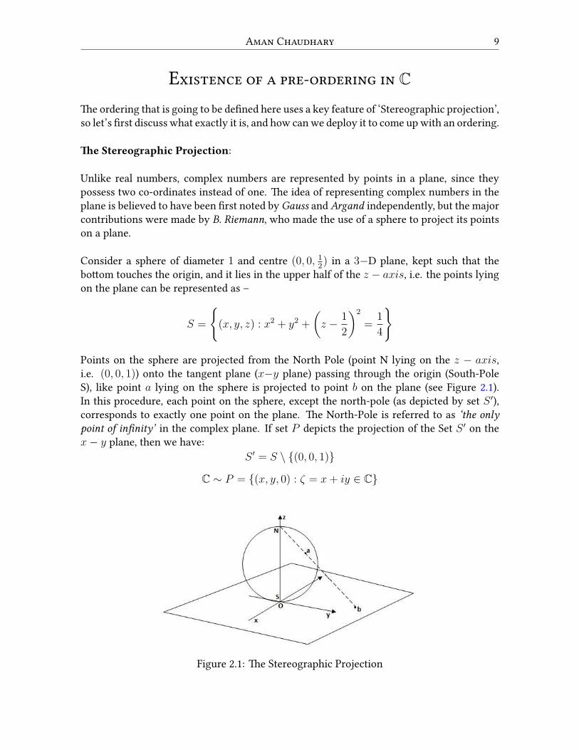
Unlike real numbers, complex numbers are represented by points in a plane, since theypossess two co-ordinates instead of one. The idea of representing complex numbers in theplane is believed to have been first noted by Gauss and Argand independently, but the majorcontributions were made by B. Riemann, who made the use of a sphere to project its pointson a plane.

Consider a sphere of diameter 1 and centre (0, 0, 12) in a 3−D plane, kept such that the

bottom touches the origin, and it lies in the upper half of the z − axis, i.e. the points lyingon the plane can be represented as –

S =

{(x, y, z) : x2 + y2 +

(z − 1

2

)2

=1

4

}

Points on the sphere are projected from the North Pole (point N lying on the z − axis,i.e. (0, 0, 1)) onto the tangent plane (x−y plane) passing through the origin (South-PoleS), like point a lying on the sphere is projected to point b on the plane (see Figure 2.1).In this procedure, each point on the sphere, except the north-pole (as depicted by set S ′),corresponds to exactly one point on the plane. The North-Pole is referred to as ‘the onlypoint of infinity’ in the complex plane. If set P depicts the projection of the Set S ′ on thex− y plane, then we have:

S ′ = S \ {(0, 0, 1)}

C ∼ P = {(x, y, 0) : ζ = x+ iy ∈ C}

Figure 2.1: The Stereographic Projection

10 Plausible ORdeRings of the Complex Plane

This phenomenon is known as stereographic projection, and the sphere is called the ‘Rie-mann Sphere’. Clearly, P corresponds to the complex plane while P ∪{0, 0, 1} correspondsto the Extended Complex Plane (An extended Field that includes all the possible infinitiesof the Field).

Now, if we look carefully and ponder, we will realize that while projecting the points of thesphere to the complex plane, a set of infinite number of concentric circles centered at theorigin (0, 0) are observed, whose radii vary from 0 to+∞. In this way, every complex num-ber lies at the circumference of one of the circles with the origin as its center (the complexnumber 0 + i0 can be regarded as a circle of radius 0 with center at origin).

0 1 2 3 4 5 6−1−2−3−4−5−60

−1−2−3−4−5−6

123456

x

y

z0z1z2z3z4z5z6

Figure 2.2: The concentric circles

So, something like Figure 2.2 is observed such that 0 = |z0| < |z1| < |z2| < |z3| < · · · < ∞,where |zi| = ri and 0 ≤ |ri| < +∞ ∀ i ∈ R+, whereby the subscript of z and r denotesthe radius of the circle here.

Figure 2.3: The Equi-radii complex numbers

Aman ChaudhaRy 11

In a nutshell, we have used the modulus of complex numbers to order them, such that thecomplex numbers lying on the circumference of the circles |zi| = ri are less than those com-plex numbers lying on the circumference of the circles |zj| = rj , for i < j. But the problemremains unresolved for the complex numbers lying on the circumference of the same circle(see Figure 2.3).

For instance, all the roots of unity have the same modulus, but they are unalike, so all thistheory shatters at the very point, and concludes that the ordering is not complete. But, thisallows us to define a pre-ordering by using the equivalence classes of the complex numbersinduced by the equivalence modulus relation, i.e. all the complex numbers lying on thecircumference of the same circle are equi-radii complex numbers and they are equal in amanner that their modulus values are equal and they belong to the same class, representedas [z1] = [z2], where [ ] denotes the equivalence class, which is analogous to saying z1 = z2.

So, we have used the law of trichotomy of real numbers to relate with a feature of com-plex number, which is also real, and this feature allows us to partition the complex plane inclasses with the help of the equivalence modulus relation.

Clearly, for any two complex numbers z1 and z2, exactly one of z1 < z2, z1 > z2, or[z1] = [z2] holds as either of |z1| < |z2|, |z1| > |z2|, or |z1| = |z2| holds in a com-plete ordering. So by the above property, we are able to partition complex numbers inclasses that can be ordered easily. For example, if we have to order the complex numbersa = i, b = −i, c = 1+ i, and d = 2− i. Since |a| = 1, |b| = 1, |c| =

√2 and |d| =

√5,

so we have |a| = |b| < |c| < |d| implying [a] = [b] < [c] < [d], where a and b are equi-radiicomplex numbers.

Geometrically speaking, an ordering relation gives an idea of the position of the elementswhen placed over a line (linear ordering), for instance in R, x < y if x lies on the left of y,or y lies towards the right of x. Here also, this ordering via modulus relation correspondsto the analogous feature as the point on the circumference, whose modulus is greater thanthe other, is farther from the origin of the complex plane while the points which are equi-distant from the origin of the circular plane, belong to the same equivalence class. The sameproperty can be attributed to the areas of the circle constituted by the circumference theylie upon, i.e. if the area of the circle on whose boundary the point lies, is greater than thatof the other point, then it is farther, while if the points lie on the same circle then they havethe same area and therefore belong to the same equivalence class. Similarly, a propertyconcerning the volume of the sphere bounded by the plane x− y plane and a plane parallelto the x − y plane, passing through the pre-image of the complex number on the sphere,can be felt by the readers.

This idea of pre-ordering has comparatively more potential in the sense that it allows us tohave some properties that are prevalent in the real numbers like Linear ordering, Archimedeanproperty, well ordering principle and many more. So in one way or the other, we can say thatthe set C of complex numbers is an ordered field under the equivalence classes of the mod-

12 Plausible ORdeRings of the Complex Plane

ulus relation, or we can say that complex numbers is a pre-ordered field. A very relativequestion that may strike the reader’s mind be: “Why is the ordering in C pretty differentthan that in R ?”. This can be attributed to the fact that the structure of Real and complex isnot exactly the same, for instance R is believed to have two infinities namely+∞ and−∞,while C posses only North Pole as its infinity.

ConclusionsThe paper examines the idea of ordering the complex plane rigorously, in the light of Ordertheory and Complex analysis. The paper gives a brief idea about ordering relations, posets,partial ordering of complex plane and the complete ordering, citing instances from bookswhere authors have tried to extend the idea of ordering to make C an ordered field. Dis-cussing the pseudo-ordering and lexicographic ordering, it begets a way to pre-order thecomplex plane using the sense of stereographic projection and its interpretation.

BIBLIOGRAPHY[1] Apostol Tom M., Mathematical Analysis, 2nd Edition, 1974, Addison-Wesley Publishing

company, ISBN 0-201-00288-4

[2] Burton David M.,TheHistory of Mathematics, 3rd Edition, 1995, New York: McGraw-Hill,ISBN 978-0-07-009465-9

[3] Brown; Churchill, Complex Variables and Applications, 6th Edition, 1995, New York:McGraw-Hill, ISBN 978-0-07-912147-9

[4] Garrett Birkhoff, Lattice Theory, American Mathematical Society Colloquium Publica-tions, vol. 25, revised edition, 1948, American Mathematical Society, New York

[5] Nahin Paul J., An Imaginary Tale: The Story of√−1, 1998, Princeton University Press,

ISBN 978-0-691-12798-9

[6] Rudin Walter, Principles of Mathematical Analysis, 3rd Edition, 1976, McGraw-Hill Edu-cation, ISBN 978-0070856134

[7] Spiegel, Lipschutz and others, Complex Variables, 2nd Edition, 2009, Schaum’s OutlineSeries, McGraw Hill, ISBN 978-0-07-161569-3

[8] Yadav D.K., A New Approach To Ordering Complex Numbers, Int. J. of MathematicalSciences and Engg. Applications, Vol.2, No.3, 211-223 (2008), ISBN 0973-9424, Pune,India

RIEMANN HYPOTHESIS: THE PRIMEQUESTION

Utcarsh MathurYear II

AbstRactOne of the biggest landmarks inMathematical historywas perhaps createdwiththe publication of Georg Friedrich Bernhard Riemann’s 1859 paper titled ‘Onthe Number of Primes Less Than a Given Magnitude’, presented to the BerlinAcademy. The paper had many claims that brought about changes in the studyof Number Theory, Complex Analysis and most importantly theory of PrimeNumbers. The nature of primes continues to be an enigma in Mathematics thatis yet to be understood. It was the RiemannHypothesis that gave us some direc-tion. This paper discusses the Riemann-Zeta Function in brevity and attemptsto explain its consequences on the Prime Number Theorem.

Keywords: Analytic Number Theory, Riemann-Zeta Function, Prime Number Theorem

A BRief IntRoductionThe concept of prime numbers is one that is taught to a student at a very young age, perhapsin the sixth grade itself. Ironically, however, a lot is yet to be known about the nature ofprime numbers. After a point, it is difficult to understand their occurrence and even moredifficult is to interpret their density.

This paper explains the correlation between the Riemann-Zeta function and the Distributionof Primes as theorized by Bernhard Riemann in his 1859 paper. Although numerous math-ematicians such as Eratosthenes, Hadamard, Poussin, Gauss, Hardy have extensively studiedprimes, the most significant contributors to the Theory of Prime Numbers are Euclid (de-scribed their infinite nature), Euler (gave the Euler Product, discussed in a later section) andRiemann[1].

Through the zeroes of the Riemann-Zeta function (sometimes also referred to as the Euler-Riemann-Zeta function), Riemann gave his own prime counting function. However, to un-derstand the essence of this function, certain preliminaries must be established.

13

14 UtcaRsh MathuR

The Riemann-Zeta function is a function of an argument s where s ∈ C. It is defined asfollows:

ζ(s) =∞∑n=1

1

ns= 1 +

1

2s+

1

3s+

1

4s+ · · ·

The argument s = x+ iy such that Re(s) > 1 (i.e. Real part is greater than one).

Lemma. ζ(s) is absolutely convergent ∀Re(s) > 1, but divergent otherwise.

Having clearly defined the nature of the function for Re(s) > 1, we can move on to under-stand its nature outside the half-planeRe(s) > 1. It is apparent that ζ(s) becomes divergentfor any Re(s) ≤ 1.

However, to study the relation between the function and prime numbers, the functionshould be defined in the whole of the complex plane. This may be possible if we definethe function a little differently for Re(s) ≤ 1, while ensuring that its basic properties arepreserved. This is precisely what Riemann did in his paper. This process is called analyticcontinuation, although Riemann does not mention this process explicitly, rather tries to finda function which “remains valid for all s”[2]. The process of analytic continuation tries toextend the definition of a function beyond its domain while preserving its basic propertiessuch that the extended function has a derivative everywhere.

Through analytic continuation, Riemann extended the definition of the function ∀Re(s) >0 except for s = 1, where there is a singularity. He further extends the function in the entirecomplex plane using the functional equation:

ξ(s) = 2sπs−1 sin(πs2

)Γ(1− s)ζ(1− s) (3.1)

whereΓ(s) =

∫ ∞

0

ts−1e−tdt

defined as the gamma function.

Riemann HypothesisHaving established the preliminaries, one canmove on to explain the subject matter at hand;Riemann’s Hypothesis. It can clearly be seen in 3.1 that ξ(s) becomes 0when s = 2n. Whenn is positive, the zeroes get cancelled by the poles of the gamma function. Thus,

ζ(s) = 0 ∀ s = −2n

where n ∈ Z+.

Riemann Hypothesis: the PRime Qestion 15

These are called the trivial zeroes of the Zeta function. In his 1859 paper, Riemann hypoth-esised that the non-trivial zeroes of the zeta function lie in the critical strip (region where0 < Re(s) < 1) and have their real part as 1

2. Thus, s = 1

2+ xi, are the only non-trivial

zeroes of the zeta function. This is called the Riemann Hypothesis and is yet to be proved[3].

EuleR’s IdentityIn his thesis titled ‘Various Observations about Infinite Series’ (published in 1737), Euler gavehis product identity that gave a connection between prime numbers and the Riemann-Zetafunction. This identity, called Euler’s Product is one of the most important results in An-alytic Number Theory and also served as the basis of Riemann’s 1859 paper. The identityis:

∞∑n=1

1

ns=

∏p

1

1− 1ps

. (3.2)

where the product on the right hand side is taken over all the primes.

The above identity may be derived by successively multiplying ζ(s) by 1ps

and subtractingthe resultant from the preceding term. For example:

ζ(s) = 1 +1

2s+

1

3s+ · · · (3.3)

Multiplying by 12s

on both sides:

1

2sζ(s) =

1

2s+

1

4s+

1

6s+ · · · (3.4)

Subtracting 3.4 from 3.3 we get(1− 1

2s

)ζ(s) = 1 +

1

3s+

1

5s+ · · · (3.5)

In a similar manner, onemay successively multiply the Zeta function by a reciprocal of somepower of a prime number and subtract the term obtained from the preceding term. Thus,

ζ(s) =∞∑n=1

1

ns=

∏p

1

1− 1ps

By looking at the identity 3.2 one may also realise that the Riemann-Zeta function cannotbe zero for any Re(s) > 1. Thus, the only zeroes ζ(s) has are:

1. Its trivial zeroes i.e. every negative even integer.

2. Its non-trivial zeroes given by the critical line s = 12+ xi in the Argand plane (as

claimed by Riemann).

16 UtcaRsh MathuR

Riemann’s PRime Counting FunctionThePrime Counting function π(x) is defined as the number of primes less than a given num-ber x. For example, π(3) = 1 as there is only one prime number less than 3. When graphed,this function resembles the step-function as it increases by one unit for each prime. Whileit is easy to compute π(x) for smaller values of x, this cannot be done for arbitrarily largenumbers.

A number of other methods have been proposed by various mathematicians to compute thedensity of prime numbers, the most accurate being the one given by Riemann. He defineshis Prime Counting function as:

J(x) = Li(x)−∞∑ρ

Li(xρ)− log 2 +∫ ∞

x

1

t(t2 − 1) log tdt (3.6)

where

Li(x) =

∫ x

2

1

ln tdt

and ρ represents the non-trivial zeroes of the Riemann-Zeta function[1]. Riemann claimedin his paper that the above function could calculate the number of primes less than a givenmagnitude with the least error.

The accuracy of the Riemann-Prime Counting function may be appreciated with the follow-ing examples. Here, the Prime Counting function and Riemann’s Counting Function havebeen calculated and graphed (using CAS Wolfram Mathematica, due to their large nature)to provide a comparison.

The following commands have been used in the figures below:

1. RiemannR[ ]: for calculating Riemann’s Prime Counting Function.

2. PrimePi[ ]: for computing the Prime Counting Function.

3. Plot[ ]: for plotting the functions mentioned above.

Riemann Hypothesis: the PRime Qestion 17

(a) π(x) and J(x) for x = 100 (b) π(x) and J(x) for x = 10, 000

Figure 3.1

(a) π(x) and J(x) for x = 1013

(b) π(x) and J(x) for x = 1020

Figure 3.2

Remark. In the figures, the following observations can be made:

1. π(x) = J(x) + κ where κ is the error. Thus, J(x) ≈ π(x)

2. The error term increases gradually as x increases.

3. After a point, even the CAS fails to give an accurate value for π(x), forcing one torely on J(x).

Thus, when x is arbitrarily large, no conclusions can be drawn from the Prime Countingfunction. Riemann’s function (accounted for error) is the only way to get a rough picture.Even though this function has given credible results, it can only be considered true whenit is proved that the non-trivial zeroes of the Riemann-Zeta function (denoted by ρ in hisPrime Counting function) have 1

2as their real part.

ConclusionsThe above observations highlight the relevance of the Riemann-Zeta function in modernMathematics. Though his PrimeCounting function has approximated prime number density

18 UtcaRsh MathuR

withmost accurately vis-à-vis other functions, its validity solely depends on the Hypothesis.Riemann himself remarked

“One would, of course, like to have a rigorous proof of this, but I have put asidethe search for such a proof after some fleeting vain attempts because it is notnecessary for the immediate objective of my investigation.”[5]

If solved, the Riemann Hypothesis would not only make us understand the true natureof Prime Numbers, but would also vindicate countless theorems that assume it to be true.Consequently, the Theory of Riemann-Zeta function has emerged as a fascinating branchof study. The Riemann Hypothesis has been checked for the first 1013 values but has notbeen proved as yet. It is enlisted as one of the 7 Millennium Problems in Mathematics bythe Clay Mathematics Institute[4].

In September 2018, British-Lebanese mathematician Sir Michael Atiyah claimed to havesolved the problem. His proof has been derived from the works of John von Neumann andFriedrich Hirzebruch. However, it is yet to be verified.

BIBLIOGRAPHY[1] Derbyshire,J. 2003. Prime Obsession: Bernhard Riemann and the Greatest Unsolved Prob-

lem in Mathematics. Washington, DC, ISBN 978-0-309-51257-2

[2] Edwards,M.H.1974. Riemann’s Zeta function. New York, Academic Press, ISBN 978-0-486-41740-0

[3] Jørgen Veisdal: Cantor’s Paradise: The Riemann Hypothesis, explained

[4] Clay Mathematics Institute: Riemann’s 1859 Manuscript

[5] Riemann,B.On the Number of Prime Numbers less than a Given Quantity Translated byWilkins,David R. December 1998

THE PERFECT DICE

Adityendra TiwariYear II

AbstRactIt has become more of a norm, that the level of sophistication achieved by acivilization determines how progressive it is. This mundanity starts with some-one’s ingenious observation of a very grassroot subject, which is followed bythe employment of our available knowledge and resources to generalise thisobservation and apply this newly acquired wisdom in some other field. But,there are ‘rare’ cases when an object of discovery is left undisturbed in its pris-tine form. One of these rarities is the subject of focus in this paper; a pair ofdice. When numbered from 1 to 6, the probability of obtaining any particularsum with these dice is 1

36for a 2, 2

36for a 3, and so on. On the other hand, if we

number one die with integers 1, 2, 2, 3, 3, 4 and another die with 1, 3, 4, 5, 6, 8then the probability of obtaining any particular sum with these dice remainsthe same! This paper attempts to ensure its validity and prove that this is theonly possible pair with such property.

Keywords: Probability, Group Theory, Ring Theory, Integral Domains, Unique FactorisationDomain

IntRoductionThe game of Ludo has deep-seated roots in the history of our country. Have you ever won-dered why we have numbers only from 1 to 6 on the die only? And even after playing thisgame for more than 5000 years, this game does not seem to have reached any level of so-phistication. Ludo is a game of probabilities and the uncertainty lies on the part of the die.Thinking about probability an American Mathematician, Martin Gardner presented beforeus, the Sicherman Dice[1]. It consists of a pair of dice, one with the integers 1, 2, 2, 3, 3, 4and the other with 1, 3, 4, 5, 6, 8 as its labels. The astounding beauty of these dice lies intheir property of yielding the same probability to achieve a given sum as that with an ordi-nary dice. To understand the proof better, we equip our readers with a few key concepts inmathematics that are used in this paper.

19

20 AdityendRa TiwaRi

What is a Ring?A ring R is a set together with two binary operations, addition and multiplication, whichsatisfy the following axioms:

First, R is an abelian group under addition with zero as identity. Next, multiplication isclosed and associative. At last, we require addition and multiplication are compatible i.e.∀ a, b, c ∈ R, (a+ b)c = ac+ bc.

A ring (R,+, ·) is said to be a ring with zero divisors if for any non-zero a ∈ R, ∃ a non-zero element b ∈ R : ab = 0 or ba = 0, where 0 is the additive identity in R. Here, a and bare called divisors of zero. If e is an element of a ring R: ae = a = ea ∀ a ∈ R, then the ringis called Ring with unity. A commutative ring with unity and no zero-divisors is called anIntegral Domain[2, 3].

What is a Unie FactoRization Domain?Essentially, a U.F.D is an Integral Domain with an additional property. This additional prop-erty may seem to be stuff reserved especially for mathematicians, but in essence, it is easyto understand:

Any element that belongs to a U.F.D can be expressed uniquely as a product of a finite num-ber of irreducible elements of the U.F.D. Now, with the help of the terms mentioned above,we begin with the proof.

Proof. The fact that the set of integersZ[x] has the unique factorization property provides uswith the fuel to begin with our proof. We start with the basics and consider the possibilitiesof getting 6 as the sum with an ordinary pair of dice and they are: (1,5), (2,4), (3,3), (4,2),(5,1).Next we multiply two polynomials formed by the ordinary dice labels as exponents:

(x+ x2 + x3 + x4 + x5 + x6)(x+ x2 + x3 + x4 + x5 + x6).

It is important to notice that the term x6 in this product can be obtained in precisely thefollowing ways:

x1 × x5, x2 × x4, x3 × x3, x4 × x2, x5 × x1.

There is a correspondence between pairs of labels whose sums are 6 and the pairs of termswhose products are x6. This is a one-to-one correspondence and it’s valid for all sums andall dice- including the Sicherman dice and any other dice that yields the desired probabili-ties. Let us supposem1,m2,m3, . . . ,m6 and n1, n2, n3, . . . , n6 be any two arrays of positive

The PeRfect Dice 21

integer labels for the faces of a pair of dice with the property that the probability of rollingany particular sum with these dice (random dice) is same as that of ordinary dice. Using ourobservation about the products of polynomials this means that:

(x+ x2 + x3 + x4 + x5 + x6)(x+ x2 + x3 + x4 + x5 + x6)

= (xm1 + xm2 + xm3 + xm4 + xm5 + xm6)× (xn1 + xn2 + xn3 + xn4 + xn5 + xn6) (4.1)

Now we have to find m′is and n′

is by solving this equation[1]. Here is where the uniquefactorization property of Z[x] helps us.

The polynomial x + x2 + x3 + x4 + x5 + x6 has the factorization into irreducibles asx(x + 1)(x2 − x + 1)(x2 + x + 1). Hence, the L.H.S. of Equation 4.1 has the factoriza-tion: x2(x+ 1)2(x2 − x+ 1)2(x2 + x+ 1)2.

So, this means that these factors are the only possible irreducible factors of P (x) = xm1 +xm2 +xm3 +xm4 +xm5 +xm6 . Thus, P (x) has the form xa(x+1)b(x2−x+1)c(x2+x+1)d,where 0 ≤ a, b, c, d ≤ 2. To narrow down on further possibilities for these four parameters,we evaluate P (1) in given two ways:

P (1) = 1m1 + 1m2 + · · ·+ 1m6 = 6.

and P (1) = 1a2b3c1d.This means that b=1 and c=1. Evaluating P (0) in two ways shows that:

P (0) = 0m1 + 0m2 + · · ·+ 0m6 = 0.

and P (0) = 0a1b1c1d.

Thus, a ̸= 0. If we take a=2, the smallest possible sum one could obtain with the randomdice would be 3. Since this is in contradiction with our assumption, the only possibilitiesleft for a, b, c, d are a=1, b=1, c=1, and d=0,1,2.

For, d=0, P (x) = x+ x2 + x2 + x3 + x3 + x4, hence, die labels are 1, 2, 2, 3, 3, 4 a Sichermandie.For d=1, P (x) = x+ x2 + x3 + x4 + x5 + x6, so, die labels are 1, 2, 3, 4, 5, 6 an ordinary die.For d=2, P (x) = x + x3 + x4 + x5 + x6 + x8, so, die labels are 1, 3, 4, 5, 6, 8 the otherSicherman die.

22 AdityendRa TiwaRi

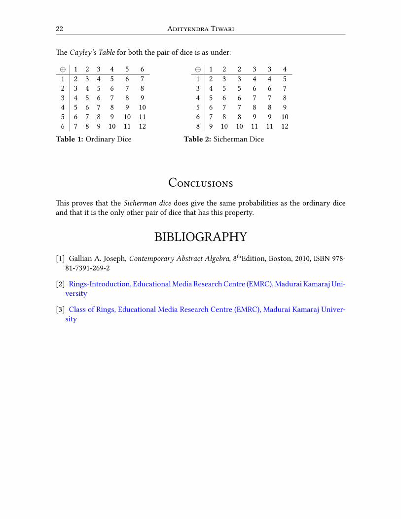
The Cayley’s Table for both the pair of dice is as under:

⊕ 1 2 3 4 5 61 2 3 4 5 6 72 3 4 5 6 7 83 4 5 6 7 8 94 5 6 7 8 9 105 6 7 8 9 10 116 7 8 9 10 11 12

⊕ 1 2 2 3 3 41 2 3 3 4 4 53 4 5 5 6 6 74 5 6 6 7 7 85 6 7 7 8 8 96 7 8 8 9 9 108 9 10 10 11 11 12

Table 1: Ordinary Dice Table 2: Sicherman Dice

ConclusionsThis proves that the Sicherman dice does give the same probabilities as the ordinary diceand that it is the only other pair of dice that has this property.

BIBLIOGRAPHY[1] Gallian A. Joseph, Contemporary Abstract Algebra, 8thEdition, Boston, 2010, ISBN 978-

81-7391-269-2

[2] Rings-Introduction, EducationalMedia Research Centre (EMRC),Madurai Kamaraj Uni-versity

[3] Class of Rings, Educational Media Research Centre (EMRC), Madurai Kamaraj Univer-sity

MATHEMATICS AND THE RUBIK’SCUBE

Samarth RajputYear II

AbstRactRubik’s Cube is a very famous 3-D puzzle invented by Hungarian sculptor andprofessor of architecture Ernö Rubik in 1974. The toy has been in the market fora long time and is still capable of capturing a good sale, which shows the popu-larity and uniqueness of this simple-looking toy. Mathematicians have showna lot of interest in the Rubik’s Cube but they didn’t stop right after solving it.They looked further for the hidden mathematical logic in the cube. After doinga lot of research, they were able to link the plaything with the concept and the-orems of abstract algebra. This paper is concerned with the permutation groupsof a Rubik’s Cube and how they are applicable in search of the maximum num-ber of possible combinations of a Rubik’s Cube that can be solved. In this paper,we’ll be dealing only with a 3× 3 Rubik’s Cube.

IntRoductionA 3 × 3 Rubik’s Cube consists of 6 faces and each one of them is differently coloured. Thecombination of the cube can be changed by rotating the faces of the cube. Each one of the 6faces is composed of 9 facets and on each face the center facet is fixed and can’t be moved.In total, there are 54 facets (9× 6 = 54) and to solve a Rubik’s Cube all the 9 facets of a facemust be of the same colour.

A 3×3 Rubik’s Cube is made up of 26 cubies. There are 6 center cubies, 8 corner cubies and12 edge cubies. Center cubies are fixed with 1 facet each, as mentioned earlier. A cornercubie has 3 facets each and an edge cubie consists of 2 facets each. When a Rubik’s Cubeis rotated, only the edge and corner cubies change their positions in such a way that theymove on to some other edge and corner respectively. The faces of the cube can be rotatedby 90◦, 180◦, 270◦ in clockwise or counter-clockwise direction. A 90◦ turn is considered as1 move and a 180◦ turn makes it 2 moves, and so on[3].

23

24 Mathematics and the RubiK’s Cube

(a) A puzzled 3× 3 Rubik’s Cube: All the9 facets of a face are not of the same colour.

(b) A solved 3 × 3 Rubik’s Cube: All the 9 facetsof each face are of the same colour i.e., each faceis of one colour only.

Figure 5.1

Each move makes a lot of positional changes in the cube. Now, let’s say we have a 3 × 3Rubik’s Cube. Consider a group G of transformations of the Rubik’s Cube. Before movingahead, let’s label the different facets of the Rubik’s Cube and number the non-center facetsfrom 1 to 48 to see that a Rubik’s Group can be regarded as a permutation of the numbers1, 2, 3, 4, . . . , 48, thus forming a symmetric group S48. This will also give us an idea of howa turn changes the positions of the facets. Let:

U = Upper Face of the cubeL = Left Face of the cubeR = Right Face of the cubeD = Downward Face of the cubeF = Front Face of the cubeB = Backward Face of the cube

Note: All the above face labels denote the 90◦ rotation of the respective faces in the clock-wise direction.

On rotating the upper face by 90◦, the edge cubies of U get permuted by 4 → 2 → 5 → 7 →4 and similarly, corner cubies of U are also permuted. Cubies of other faces are also per-muted along with the cubies of U. The permutation of the cubies of U can be written as dis-joint 4-cycles. The disjoint cycle of edge cubies of U is (4, 2, 5, 7). 4-cycles are odd permuta-tions. For example, let’s consider the 4-cycle (4, 2, 5, 7), it can be written as (4, 2)(2, 5)(5, 7),as we can see, there are three transpositions of U which ensure that 4-cycles are odd per-mutations. But, the product of two odd permutations is even, the product of two evenpermutations is also even and the product of an even and an odd permutation is odd andeach face turn is an even permutation of the cubies as each face turn is a composition of4-cycles on the corners and 4-cycles on edges.

U=(4, 2, 5, 7)(1, 3, 8, 6)(9, 33, 25,17)(10, 34 ,26, 18)(11, 35 , 27 ,19)

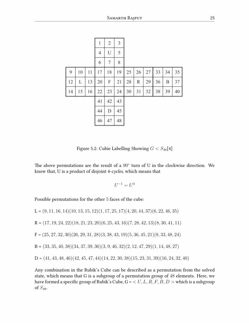
SamaRth Rajput 25

Figure 5.2: Cubie Labelling Showing G < S48[4]

The above permutations are the result of a 90◦ turn of U in the clockwise direction. Weknow that, U is a product of disjoint 4-cycles, which means that

U−1 = U3

Possible permutations for the other 5 faces of the cube:

L = (9, 11, 16, 14)(10, 13, 15, 12)(1, 17, 25, 17)(4, 20, 44, 37)(6, 22, 46, 35)

R = (17, 19, 24, 22)(18, 21, 23, 20)(6, 25, 43, 16)(7, 28, 42, 13)(8, 30, 41, 11)

F = (25, 27, 32, 30)(26, 29, 31, 28)(3, 38, 43, 19)(5, 36, 45, 21)(8, 33, 48, 24)

B = (33, 35, 40, 38)(34, 37, 39, 36)(3, 9, 46, 32)(2, 12, 47, 29)(1, 14, 48, 27)

D = (41, 43, 48, 46)(42, 45, 47, 44)(14, 22, 30, 38)(15, 23, 31, 39)(16, 24, 32, 40)

Any combination in the Rubik’s Cube can be described as a permutation from the solvedstate, which means that G is a subgroup of a permutation group of 48 elements. Here, wehave formed a specific group of Rubik’s Cube, G =< U,L,R, F,B,D >which is a subgroupof S48.

26 Mathematics and the RubiK’s Cube

ORdeR of the gRoupNow, we know about permutations, and we’ll proceed to calculate the order of the Rubik’sCube group or maximum possible combinations of a Rubik’s Cube fromwhere we can bringit to a solved state. Suppose, we have dismantled a Rubik’s Cube and all the edge and cornerpieces are out but the center pieces are at their positions. We have 8 corner pieces and 12edge pieces. Now, we’ll notice that there are 8 corner positions and any of the 8 cornerpieces can be placed at any of them. While placing the first corner piece, we have 8 posi-tions and it can be placed at any one of them, after placing 1 corner piece, we have 7 cornerplaces to position the second piece and so on. In the same way, edge pieces can be placedat 12 different positions.

Total possible positions of edge pieces = 12!Total possible positions of corner pieces = 8!

As mentioned earlier, each edge piece is made up of 2 colours, so any of the 12 edge piecescan be placed in a cube in 2 different ways or simply, by flipping the colours which meanswe have twice as many ways to put those edge pieces at 12 different places. Similarly, anyof the 8 corner pieces can be placed in 3 different ways, as each corner piece is made up of3 different colors.

No. of ways in which edge pieces can be placed (Edge Flips) = 212

No. of ways in which corner pieces can be placed (Corner Twists) = 38

Maximum possible combinations = 12!× 8!× 212 × 38

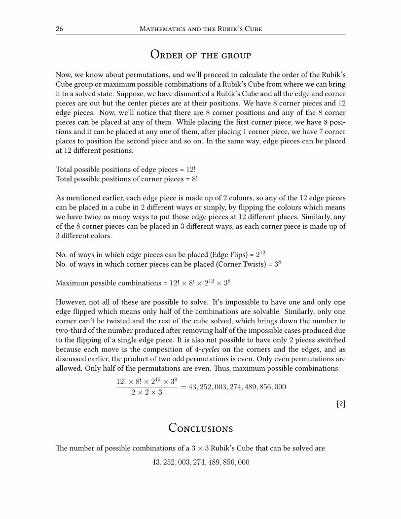
However, not all of these are possible to solve. It’s impossible to have one and only oneedge flipped which means only half of the combinations are solvable. Similarly, only onecorner can’t be twisted and the rest of the cube solved, which brings down the number totwo-third of the number produced after removing half of the impossible cases produced dueto the flipping of a single edge piece. It is also not possible to have only 2 pieces switchedbecause each move is the composition of 4-cycles on the corners and the edges, and asdiscussed earlier, the product of two odd permutations is even. Only even permutations areallowed. Only half of the permutations are even. Thus, maximum possible combinations:

12!× 8!× 212 × 38

2× 2× 3= 43, 252, 003, 274, 489, 856, 000

[2]

ConclusionsThe number of possible combinations of a 3× 3 Rubik’s Cube that can be solved are

43, 252, 003, 274, 489, 856, 000

SamaRth Rajput 27

and this is known only because of the application of mathematics. There are a lot of otherapplications of the permutation groups too which can be useful in solving a scrambled Ru-bik’s Cube, but are out of bounds of this paper.

BIBLIOGRAPHY[1] Gallian A. Joseph, Contemporary Abstract Algebra, 8thEdition, Boston, 2010, ISBN 978-

81-7391-269-2

[2] Article. Group Theory and the Rubik’s Cube

[3] Wikipedia- Rubik’s Cube Group

[4] Article. The Man Who Found God’s Number

[5] Article. Group Theory and the Rubik’s Cube

ON SOLVING A CUBIC EQUATION

Daksh DheerYear I

AbstRactIn the 19th century, Évariste Galois proved that all algebraic equations of de-gree higher than 4 cannot always be solved by radicals, i.e. there does not exista formula that relates the roots of the equations to their coefficients using theoperations of addition, multiplication, subtraction, division, exponentiation andtaking nth roots. However, equations of degree 1, 2, 3 and 4 are solvable by rad-icals. This article attempts to introduce one such formula; specifically, one thatcan solve a cubic equation.

Keywords: Cubic Formula, Cubic Discriminant, Depressed cubic, Cardano’s formula

IntRoductionIn algebra, an equation of the form ax3 + bx2 + cx+ d = 0 such that a, b, c, d ∈ R is calleda cubic equation in one variable. The solutions of the equation are called its roots[6]. Bythe Fundamental Theorem of Algebra and the fact that complex roots occur in conjugatepairs, there always exists a real root of every cubic equation. However, unlike the quadraticformula (which enables one to quickly find roots of a quadratic equation), a cubic formulais rarely discussed in high-school and most undergraduate courses. We attempt to derivesuch a formula in this article[2].

The cubic formula was first published in 1545, byGirolamo Cardano in his book, ‘ArsMagna’.Cardano attributed the formula to Scipione del Ferro. However, another mathematician, Nic-colò Tartaglia, had also independently discovered a formula for solving cubics.

DepRessed FoRm of a CubicAll general cubics can be reduced into a depressed cubic of the form

y3 + py + q = 0

28

On Solving a Cubic Eation 29

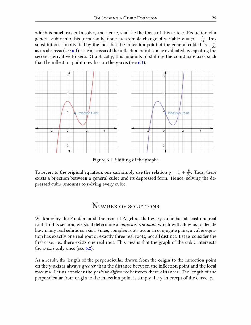
which is much easier to solve, and hence, shall be the focus of this article. Reduction of ageneral cubic into this form can be done by a simple change of variable x = y − b

3a. This

substitution is motivated by the fact that the inflection point of the general cubic has − b3a

as its abscissa (see 6.1). The abscissa of the inflection point can be evaluated by equating thesecond derivative to zero. Graphically, this amounts to shifting the coordinate axes suchthat the inflection point now lies on the y-axis (see 6.1).

Figure 6.1: Shifting of the graphs

To revert to the original equation, one can simply use the relation y = x + b3a. Thus, there

exists a bijection between a general cubic and its depressed form. Hence, solving the de-pressed cubic amounts to solving every cubic.

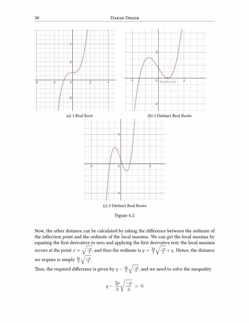
NumbeR of solutionsWe know by the Fundamental Theorem of Algebra, that every cubic has at least one realroot. In this section, we shall determine a cubic discriminant, which will allow us to decidehow many real solutions exist. Since, complex roots occur in conjugate pairs, a cubic equa-tion has exactly one real root or exactly three real roots, not all distinct. Let us consider thefirst case, i.e., there exists one real root. This means that the graph of the cubic intersectsthe x-axis only once (see 6.2).

As a result, the length of the perpendicular drawn from the origin to the inflection pointon the y-axis is always greater than the distance between the inflection point and the localmaxima. Let us consider the positive difference between these distances. The length of theperpendicular from origin to the inflection point is simply the y-intercept of the curve, q.

30 DaKsh DheeR

(a) 1 Real Root (b) 2 Distinct Real Roots

(c) 3 Distinct Real Roots

Figure 6.2

Now, the other distance can be calculated by taking the difference between the ordinate ofthe inflection point and the ordinate of the local maxima. We can get the local maxima byequating the first derivative to zero and applying the first derivative test; the local maximaoccurs at the point x =

√−p3, and thus the ordinate is y = 2p

3

√−p3+ q. Hence, the distance

we require is simply 2p3

√−p3.

Thus, the required difference is given by q − 2p3

√−p3, and we need to solve the inequality

q − 2p

3

√−p

3> 0

On Solving a Cubic Eation 31

which simplifies to (q2

)2

+(p3

)3

> 0

This is the condition for a cubic equation to have one real root.

Note that here p represents the slope of the line tangent to the inflection point, which isnegative, and thus the quantity

√−p3

is real.

Now, let us consider the other case, i.e. there exist three real roots (not necessarily distinct).This means that the graph of the cubic intersects the x-axis thrice (see 6.2). In case of arepeated root, it shall technically intersect the x-axis twice, but for the sake of brevity, wewill consider that equivalent to three intersections. In this case the length of the perpen-dicular drawn from the origin to the inflection point on the y-axis is always smaller thanthe distance between the inflection point and of the local maxima. Hence, we can concludethat the condition for existence of three real roots is given by(q

2

)2

+(p3

)3

≤ 0

Hence, this quantity acts as a discriminant for cubic equations and so we shall henceforthrefer to it as ∆ for ease of writing.

Completing the cubeAs the counterpart to completing the square technique in the derivation of the quadraticformula, let us attempt the same in case of a cubic equation.

Consider the identity(v + u)3 = v3 + u3 + 3vu(v + u)

Re-arranging, we obtain

(v + u)3 − 3vu(v + u)− (v3 + u3) = 0

Comparing this with our depressed cubic, we can deduce the following relations:

p = −3vu

q = −(v3 + u3)

y = v + u

Hence, if we obtain u and v, our original equation is a perfect cube and our equation iseffectively solved.

Solving the above equations, for u and v, and subsequently adding them, we get

32 DaKsh DheeR

y =3

√√√√−q

2+

2

√q2

4+

p3

27+

3

√√√√−q

2− 2

√q2

4+

p3

27

More compactly, the same formula can be written as

y = 3

√−q

2+

2√∆ + 3

√−q

2− 2

√∆

The above is called Cardano’s Formula[1]. Note that we are assuming the existence of asolution by the Fundamental Theorem of Algebra and moreover, the system of equationscan be algebraically reduced to a quadratic equation in v3. Hence, it can be solved using thequadratic formula.

A Complex DetouR and an ExampleOne may notice the fact that the cases of one real root or three non-distinct real roots, i.e.when ∆ > 0 or ∆ = 0, respectively, correspond to cube roots of real numbers and canthus be calculated. However, in the case of existence of three distinct real roots, ∆ < 0and hence we are required to take the sum of two complex numbers. This might seem con-tradictory and impossible; obtaining three real roots by adding up two complex numbers,but it is possible since the two complex numbers being added are conjugates of one another.

Furthermore, a cube root of a complex numbers will result in three different complex num-bers and hence, we shall have three pairs of u and v. Adding corresponding values of u andv in a pair will give us the three required roots.

Now, let us solve an actual cubic equation using this method. Consider the following equa-tion:

x3 − 26x2 + 193x− 420 = 0

Here, a = 1, b = −26, c = 193, and d = −420. Thus, replacing x by y − b3a, i.e., y + 26

3and

simplifying, we get:

y3 − 97

3y − 1330

27= 0

Now,

∆ =(q2

)2

+(p3

)3

=

( −133027

2

)2

+

( −973

3

)3

On Solving a Cubic Eation 33

∆ =442225

729− 912673

729= −470448

729< 0

Thus, there exist 3 real distinct roots.

Now, we know that

y = 3

√−q

2+

2√∆+ 3

√−q

2− 2

√∆

Therefore, putting values we get:

y =3

√−

−133027

2+

2

√−470448

729+

3

√−

−133027

2− 2

√−470448

729

y =3

√1330

54+

√442

3i+

3

√1330

54−√

442

3i

Calculating these cube roots (one method of doing this can be first converting them to theirpolar forms and then carrying out the operations; other methods exist too, but the final an-swers remain the same), we get three different sums of conjugate pairs of complex numbers.Adding them up, we get the following values for y:

y = −5

3, −14

3and 19

3

Now, using the relation, x = y − b3a

= y + 263, we obtain the solutions to our original

equation as:x = 7, 4 and 15

The GeneRal cubic foRmulaWe have seen before that every general cubic can be reduced to a depressed cubic and wederived a formula for solving such a reduced equation[5]. However, since the mappingfrom general cubics to depressed cubics is bijective, we can also derive a direct formula fora general cubic as follows:

34 DaKsh DheeR

x = −b

3a+

3

√√√√(−

b3

27a3+

bc

6a2−

d

2a

)− 2

√(−

b3

27a3+

bc

6a2−

d

2a

)2

+

(c

3a−

b2

9a2

)3

+3

√√√√(−

b3

27a3+

bc

6a2−

d

2a

)+

2

√(−

b3

27a3+

bc

6a2−

d

2a

)2

+

(c

3a−

b2

9a2

)3

ConclusionsWe come to the conclusion that every general cubic equation can be reduced to a depressedcubic and solved using the formula derived above. In case of three real distinct roots, thecubic formula outputs answers as sum of complex conjugates and thus, it is beyond thecurfew of high school mathematics and is rarely discussed at that level, even though it isalgebraically calculable.

BIBLIOGRAPHY[1] G Cardano, Ars Magna or The Rules of Algebra, translated and edited by T.R. Witmer,

Cambridge, MA: MIT Press 1968 and New York, NY: Dover 1993, ISBN 978-0486678115.

[2] Article. Cardano v Tartaglia: The Great Feud Goes Supernatural.

[3] Osler, Thomas. (2021). An easy look at the cubic formula.

[4] Chahal, J.S. Solution of the Cubic. Reson 11, 53–61 (2006).

[5] S Neumark, Solution of Cubic andQuartic Equations, Oxford, etc.: Pergamon 1965, ISBN978-0-08-011220-6.

[6] Wikipedia Cubic Equation.

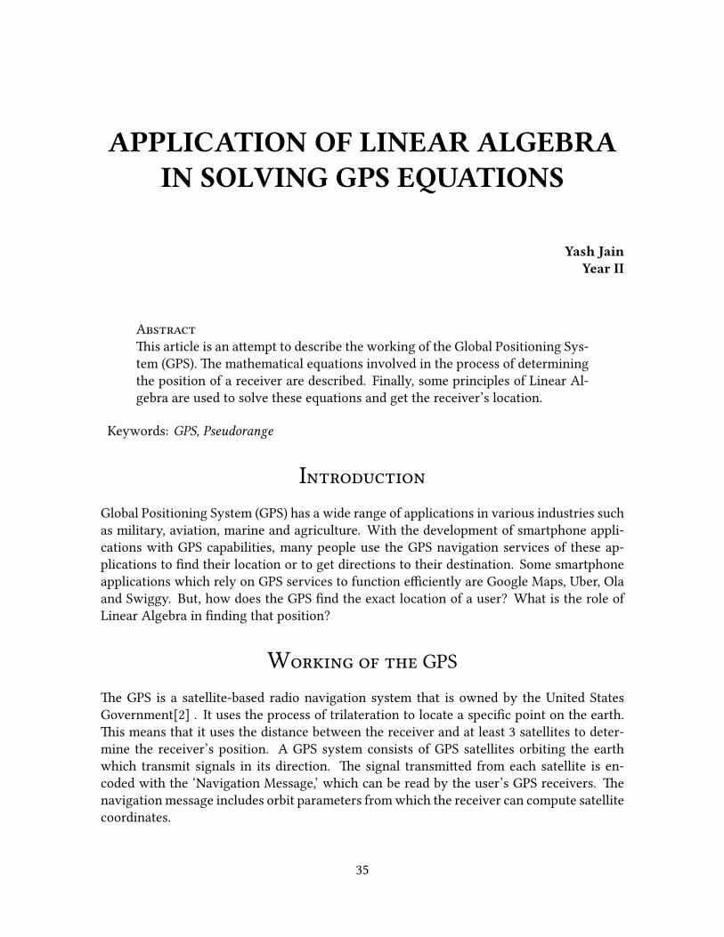
APPLICATION OF LINEAR ALGEBRAIN SOLVING GPS EQUATIONS

Yash JainYear II

AbstRactThis article is an attempt to describe the working of the Global Positioning Sys-tem (GPS). The mathematical equations involved in the process of determiningthe position of a receiver are described. Finally, some principles of Linear Al-gebra are used to solve these equations and get the receiver’s location.

Keywords: GPS, Pseudorange

IntRoductionGlobal Positioning System (GPS) has a wide range of applications in various industries suchas military, aviation, marine and agriculture. With the development of smartphone appli-cations with GPS capabilities, many people use the GPS navigation services of these ap-plications to find their location or to get directions to their destination. Some smartphoneapplications which rely on GPS services to function efficiently are Google Maps, Uber, Olaand Swiggy. But, how does the GPS find the exact location of a user? What is the role ofLinear Algebra in finding that position?

WoRKing of the GPSThe GPS is a satellite-based radio navigation system that is owned by the United StatesGovernment[2] . It uses the process of trilateration to locate a specific point on the earth.This means that it uses the distance between the receiver and at least 3 satellites to deter-mine the receiver’s position. A GPS system consists of GPS satellites orbiting the earthwhich transmit signals in its direction. The signal transmitted from each satellite is en-coded with the ‘Navigation Message,’ which can be read by the user’s GPS receivers. Thenavigationmessage includes orbit parameters fromwhich the receiver can compute satellitecoordinates.

35

36 Yash Jain

These are the Cartesian Coordinates in a geocentric system which has origin at the earthcentre ofmass, Z-axis pointing towards the North Pole, X pointing towards the PrimeMerid-ian, and Y at right angles to X and Z to form a right-handed orthogonal coordinate system.The time at which the signal is transmitted from the satellite is encoded on the signal. Thesatellites carry very stable atomic clocks to record the time. Time of signal reception isrecorded by receiver using an atomic clock. The receiver measures the difference in thesetimes. This is used to calculate the pseudorange, which is defined as[1]:

Pseudorange= (time difference) × (speed of light)

Pseudoranges include clock errors because the receiver clocks are not perfect. Hence, in-cluding the unknown receiver clock error and the coordinates of the unknown station, wehave 4 unknowns. Hence, we need atleast 4 pseudoranges and hence, signals from 4 GPSsatellites[1]. Corresponding to each pseudorange, the following equation can be obtained:

Pseudorange = Range (distance between receiver and satellite) + Clock Error

Hence, we get 4 non-linear equations in 4 unknowns. This system of equations is thenlinearized and solved using linear algebra.

Evaluation of PseudoRangeThe method used in this section to evaluate the pseudorange is adopted from[3]. Let thelocation of the receiver be (X,Y, Z). Let the location of ith satellite be (Xi, Yi, Zi), its signaltravel time be ∆ti, and the range of the receiver from that satellite be Ri, where i variesfrom 1 to 4.

Let ∆t0 denote the clock error and ∆tsati denote the time difference measured by the re-ceiver. Let c denote the speed of light. Then,

Ri = ∆ti.c (7.1)∆tsati = ∆ti +∆t0 (7.2)

Let ρi denote pseudorange for the ith satellite, where i varies from 1 to 4.

ρi = ∆tsati .c

From equation (7.2), we have:

ρi = (∆ti +∆t0).c

⇒ ρi = ∆ti.c+∆t0.c (7.3)

Substituting ∆ti from equation (7.1) in equation (7.3), we have:

ρi = Ri +∆t0.c (7.4)

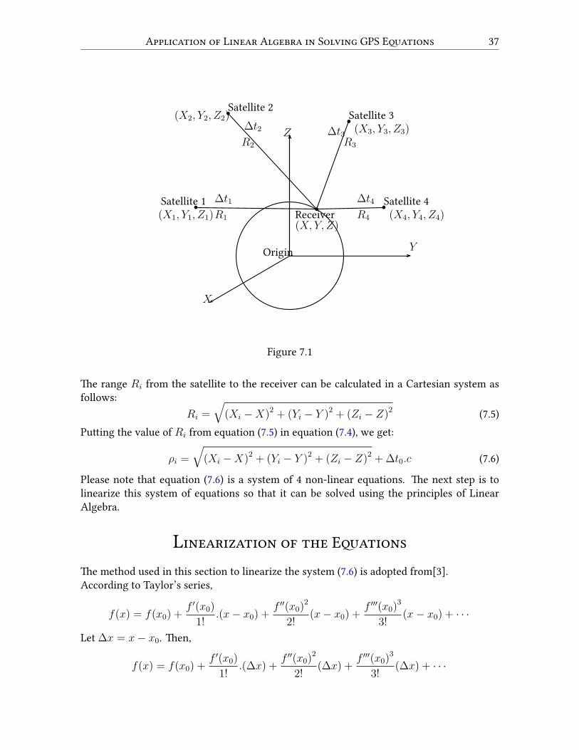
Application of LineaR AlgebRa in Solving GPS Eations 37

b b

bb

b

Y

Z

X

Origin

ReceiverSatellite 4

Satellite 3Satellite 2

Satellite 1 ∆t1

R1

∆t2

R2

∆t3R3

∆t4

R4(X,Y, Z)

(X4, Y4, Z4)

(X3, Y3, Z3)(X2, Y2, Z2)

(X1, Y1, Z1)

Figure 7.1

The range Ri from the satellite to the receiver can be calculated in a Cartesian system asfollows:

Ri =

√(Xi −X)2 + (Yi − Y )2 + (Zi − Z)2 (7.5)

Putting the value of Ri from equation (7.5) in equation (7.4), we get:

ρi =

√(Xi −X)2 + (Yi − Y )2 + (Zi − Z)2 +∆t0.c (7.6)

Please note that equation (7.6) is a system of 4 non-linear equations. The next step is tolinearize this system of equations so that it can be solved using the principles of LinearAlgebra.

LineaRization of the EationsThe method used in this section to linearize the system (7.6) is adopted from[3].According to Taylor’s series,

f(x) = f(x0) +f ′(x0)

1!.(x− x0) +

f ′′(x0)2

2!(x− x0) +

f ′′′(x0)3

3!(x− x0) + · · ·

Let ∆x = x− x0. Then,

f(x) = f(x0) +f ′(x0)

1!.(∆x) +

f ′′(x0)2

2!(∆x) +

f ′′′(x0)3

3!(∆x) + · · ·

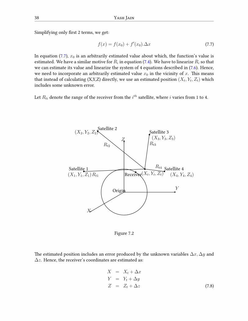
38 Yash Jain

Simplifying only first 2 terms, we get:

f(x) = f(x0) + f ′(x0).∆x (7.7)

In equation (7.7), x0 is an arbitrarily estimated value about which, the function’s value isestimated. We have a similar motive forRi in equation (7.4). We have to linearizeRi so thatwe can estimate its value and linearize the system of 4 equations described in (7.6). Hence,we need to incorporate an arbitrarily estimated value x0 in the vicinity of x. This meansthat instead of calculating (X,Y,Z) directly, we use an estimated position (Xt, Yt, Zt) whichincludes some unknown error.

Let Rti denote the range of the receiver from the ith satellite, where i varies from 1 to 4.

bb

b

bb

b

Y

Z

X

Origin

ReceiverSatellite 4

Satellite 3Satellite 2

Satellite 1Rt1

Rt2Rt3

Rt4

(Xt, Yt, Zt) (X4, Y4, Z4)

(X3, Y3, Z3)(X2, Y2, Z2)

(X1, Y1, Z1)

Figure 7.2

The estimated position includes an error produced by the unknown variables ∆x,∆y and∆z. Hence, the receiver’s coordinates are estimated as:

X = Xt +∆x

Y = Yt +∆y

Z = Zt +∆z (7.8)

Application of LineaR AlgebRa in Solving GPS Eations 39

The range Rti from the ith satellite to the estimated position can be calculated in the sameway as Ri was calculated in equation (7.3):

Rti =

√(Xi −Xt)

2 + (Yi − Yt)2 + (Zi − Zt)

2 (7.9)

Taking Rt from equation (7.3) as the function in equation (7.7), we get:

Ri =

√(Xi −Xt)

2 + (Yi − Yt)2 + (Zi − Zt)

2 +

∂

(√(Xi −Xt)

2 + (Yi − Yt)2 + (Zi − Zt)

2

)∂x

.∆x

+

∂

(√(Xi −Xt)

2 + (Yi − Yt)2 + (Zi − Zt)

2

)∂y

.∆y +

∂

(√(Xi −Xt)

2 + (Yi − Yt)2 + (Zi − Zt)

2

)∂x

.∆z

⇒ Ri =

√(Xi −Xt)

2 + (Yi − Yt)2 + (Zi − Zt)

2 +−2(Xi −Xt)

2√

(Xi −Xt)2 + (Yi − Yt)

2 + (Zi − Zt)2.∆x

+−2(Yi − Yt)

2√

(Xi −Xt)2 + (Yi − Yt)

2 + (Zi − Zt)2.∆y +

−2(Zi − Zt)

2√

(Xi −Xt)2 + (Yi − Yt)

2 + (Zi − Zt)2.∆z

(7.10)

Substituting Rti from equation (7.9) in equation (7.10) we get:

Ri = Rti +Xt −Xi

Rti

.∆x+Yt − Yi

Rti

.∆y +Zt − Zi

Rti

.∆z (7.11)

Now, substituting Ri from equation (7.11) in equation (7.4), we get:

ρi = Rti +Xt −Xi

Rti

.∆x+Yt − Yi

Rti

.∆y +Zt − Zi

Rti

.∆z + c.∆t0 (7.12)

Equation (7.12) now represents a system of 4 linear equations which can be solved usingLinear Algebra.

Solving the EationsThe method used in this section to solve the system (7.12) is adopted from[3]. Equation(7.12) can be rewritten as:

ρi −Rti =Xt −Xi

Rti

.∆x+Yt − Yi

Rti

.∆y +Zt − Zi

Rti

.∆z + c.∆t0 (7.13)

The system of linear equations (7.13) has to be solved for the variables (∆x,∆y,∆z and∆t0). To do so, it can be expressed in the form of matrix equation AX = B, where:

40 Yash Jain

A =

Xt−X1

Rt1

Yt−Y1

Rt1

Zt−Z1

Rt1c

Xt−X2

Rt2

Yt−Y2

Rt2

Zt−Z2

Rt2c

Xt−X3

Rt3

Yt−Y3

Rt3

Zt−Z3

Rt3c

Xt−X4

Rt4

Yt−Y4

Rt4

Zt−Z4

Rt4c

(7.14)

X =

∆x∆y∆z∆t0

(7.15)

B =

ρ1 −Rt1

ρ2 −Rt2

ρ3 −Rt3

ρ4 −Rt4

(7.16)

Using the matrices described in the above equations, AX = B for the system (7.13) is:Xt−X1

Rt1

Yt−Y1

Rt1

Zt−Z1

Rt1c

Xt−X2

Rt2

Yt−Y2

Rt2

Zt−Z2

Rt2c

Xt−X3

Rt3

Yt−Y3

Rt3

Zt−Z3

Rt3c

Xt−X4

Rt4

Yt−Y4

Rt4

Zt−Z4

Rt4c

.

∆x∆y∆z∆t0

=

ρ1 −Rt1

ρ2 −Rt2

ρ3 −Rt3

ρ4 −Rt4

(7.17)

To solve for X , (7.17) is pre-multiplied by A−1 to get X = A−1B, i.e.,∆x∆y∆z∆t0

=

Xt−X1

Rt1

Yt−Y1

Rt1

Zt−Z1

Rt1c

Xt−X2

Rt2

Yt−Y2

Rt2

Zt−Z2

Rt2c

Xt−X3

Rt3

Yt−Y3

Rt3

Zt−Z3

Rt3c

Xt−X4

Rt4

Yt−Y4

Rt4

Zt−Z4

Rt4c

−1

.

ρ1 −Rt1

ρ2 −Rt2

ρ3 −Rt3

ρ4 −Rt4

(7.18)

The system (7.18) gives the value of the matrix X which gives the values of ∆x,∆y,∆zand ∆t0. Using the equations (7.8), we can find (X,Y, Z). However, these values still havesome error (which corresponds to ∆x,∆y and ∆z respectively).

Hence, our aim is to decrease the error component as much as possible so that we canget more accurate value of (X,Y, Z). To accomplish this, we estimate a new set of val-ues, Xnew, Ynew and Znew using the calculated (X,Y, Z) values as Xold, Yold and Zold in thefollowing equations:

Xnew = Xold +∆x

Ynew = Yold +∆y

Znew = Zold +∆z (7.19)

where ∆x,∆y and ∆z are unknown errors.

Application of LineaR AlgebRa in Solving GPS Eations 41

The new estimated position (Xnew, Ynew, Znew) is entered in place ofXt, Yt andZt in the lin-ear system (7.18) to get the values of∆x,∆y and∆z for this new estimation. The same iter-ative process is repeated until the error components are less than the desired error. Hence,in order to determine a position, the receiver will either use the last measurement value,or estimate a new position using (7.19) and calculate error components down to zero byrepeated iteration. After we have satisfactorily low values of ∆x,∆y and ∆z, the finalposition of the receiver is calculated as:

X = Xnew

Y = Ynew

Z = Znew (7.20)

Hence, (7.20) gives the final value of (X,Y, Z). The calculated value of ∆t0 at this pointcorresponds to receiver time error and can be used to adjust the receiver clock.

ConclusionsThese calculations ignore some other sources of GPS errors such as the effect of ionosphere,the effect of troposphere and multipath errors. DGPS, SBAS, A-GPS and HSGPS are someof the improved GPS which give more accurate positions. However, one can appreciate therole of Linear Algebra in the whole process of GPS positioning.

BIBLIOGRAPHY[1] Blewitt, G., 1997.Basics of the GPS Technique: Observation Equations. Geodetic Applica-

tions of GPS, pp.10-54.

[2] Dixon, T.H., 1991.An introduction to the Global Positioning System and some geologicalapplications. Reviews of Geophysics,29(2), pp.249-276.

[3] Zogg, Jean-Marie, 2009.GPS: Essentials of Satellite Navigation: Compendium: Theorie andPrinciples of Satellite Navigation, Overview of GPS/GNSS Systems and Applications.U-bloxISBN 9783033021396

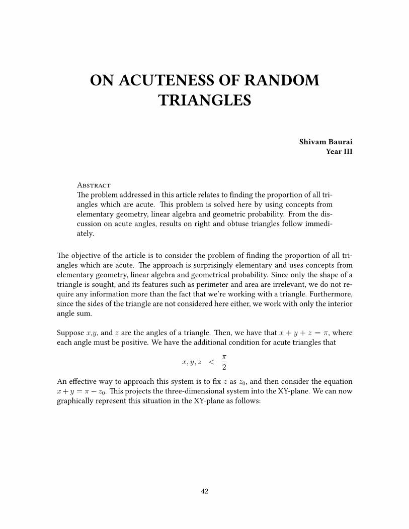
ON ACUTENESS OF RANDOMTRIANGLES

Shivam BauraiYear III

AbstRactThe problem addressed in this article relates to finding the proportion of all tri-angles which are acute. This problem is solved here by using concepts fromelementary geometry, linear algebra and geometric probability. From the dis-cussion on acute angles, results on right and obtuse triangles follow immedi-ately.

The objective of the article is to consider the problem of finding the proportion of all tri-angles which are acute. The approach is surprisingly elementary and uses concepts fromelementary geometry, linear algebra and geometrical probability. Since only the shape of atriangle is sought, and its features such as perimeter and area are irrelevant, we do not re-quire any information more than the fact that we’re working with a triangle. Furthermore,since the sides of the triangle are not considered here either, we work with only the interiorangle sum.

Suppose x,y, and z are the angles of a triangle. Then, we have that x + y + z = π, whereeach angle must be positive. We have the additional condition for acute triangles that

x, y, z <π

2

An effective way to approach this system is to fix z as z0, and then consider the equationx+ y = π− z0. This projects the three-dimensional system into the XY-plane. We can nowgraphically represent this situation in the XY-plane as follows:

42

Shivam BauRai 43

Figure 8.1

Notice that each point in the interior of the triangle ABC contains all the triplets (x, y, z)corresponding to a triangle, as the interior corresponds to x + y < π and thus a suitable zmay be chosen such that x + y + z = π. Meanwhile, each point on the boundary of ABCcannot construct a triangle as one or two angles must be zero; and any point outside ABCdoes not satisfy the interior angle sum property.

Also, observe that the interior of the triangle DEF contains all the triplets (x, y, z) corre-sponding to an acute triangle. Notice that each point on the boundary of DEF correspondsto one of x, y, z equalling π

2. And any point outside DEF corresponds to one of the angles

exceeding π2: x > π

2in region CDF; y > π

2in region BEF; and z > π

2in region AED. Thus,

the probability that a given triangle is acute is:

Pr(x <π

2| y <

π

2| z <

π

2) =

Ar△DEF

Ar△ABC=

12(π2)(π

2)

12(π)(π)

=1

4

It is seen that given a triangle, the probability that it is acute is 14. Additionally, the triplets

corresponding to right triangles lie on the lines DE, EF and FD - as they correspond toz = π

2, y = π

2and x = π

2, respectively. Since lines have zero area, the probability of a

random triangle being right-angled is zero! It also follows now that the proportion of alltriangles which are obtuse is 3

4.

BIBLIOGRAPHY[1] Are random triangles acute or obtuse? - MIT Blossoms

THE THREE UTILITY PROBLEM

Apurva ChauhanYear II

AbstRactHenry Ernest Dudeney was a mathematician who specialised in mathematicalpuzzles. He once stated that the problem discussed in this paper is “as old asthe hills …much older than electric lighting, or even gas”. The utility problem hasbeen a part of many magazines. In this article we will try to find a possiblesolution to our hoary problem using Graph Theory and the Jordan Curve The-orem. We’ll also solve the classical problem using one of the most fascinatingformulas of mathematics, given by Leonhard Euler.

IntRoductionThe utility problem is a sixty-four-thousand-dollar question. It is often referred to as a “veryancient” problem. This problem is one of the most famous maths puzzles and many mathe-maticians have tried to find an answer to this brainstorming puzzle. The problem is quotedas:

“We have three houses and three utilities that are gas, water, and electricity and we need toconnect each house to all three utilities by drawing lines on a paper without any line crossingeach other as shown below:”

First, we need to have a basic idea of Graph Theory, Euler’s formula, and the Jordan CurveTheorem, because that is what we are going to use to find a possible solution to our problem.

44

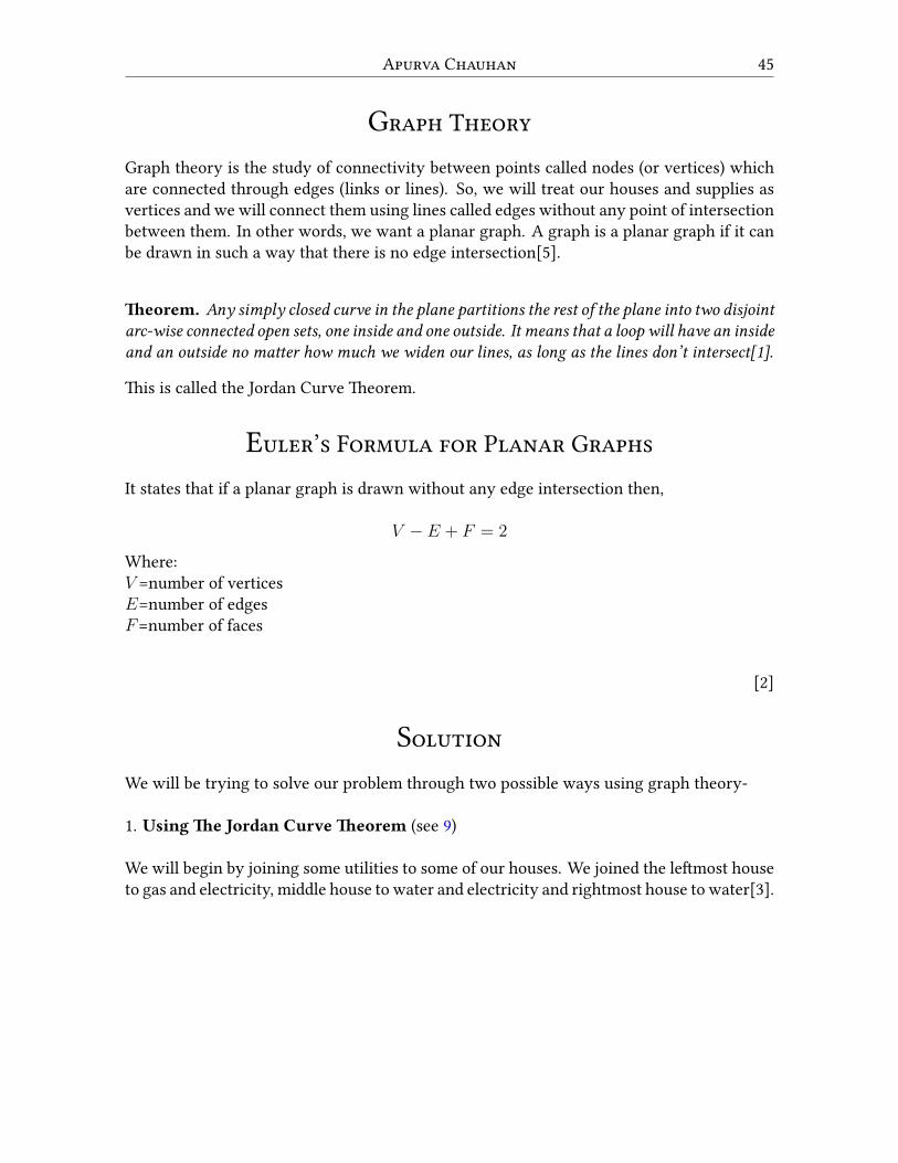
ApuRva Chauhan 45

GRaph TheoRyGraph theory is the study of connectivity between points called nodes (or vertices) whichare connected through edges (links or lines). So, we will treat our houses and supplies asvertices and we will connect them using lines called edges without any point of intersectionbetween them. In other words, we want a planar graph. A graph is a planar graph if it canbe drawn in such a way that there is no edge intersection[5].

Theorem. Any simply closed curve in the plane partitions the rest of the plane into two disjointarc-wise connected open sets, one inside and one outside. It means that a loop will have an insideand an outside no matter how much we widen our lines, as long as the lines don’t intersect[1].

This is called the Jordan Curve Theorem.

EuleR’s FoRmula foR PlanaR GRaphsIt states that if a planar graph is drawn without any edge intersection then,

V − E + F = 2

Where:V =number of verticesE=number of edgesF=number of faces

[2]

SolutionWe will be trying to solve our problem through two possible ways using graph theory-

1. Using The Jordan Curve Theorem (see 9)

We will begin by joining some utilities to some of our houses. We joined the leftmost houseto gas and electricity, middle house to water and electricity and rightmost house to water[3].

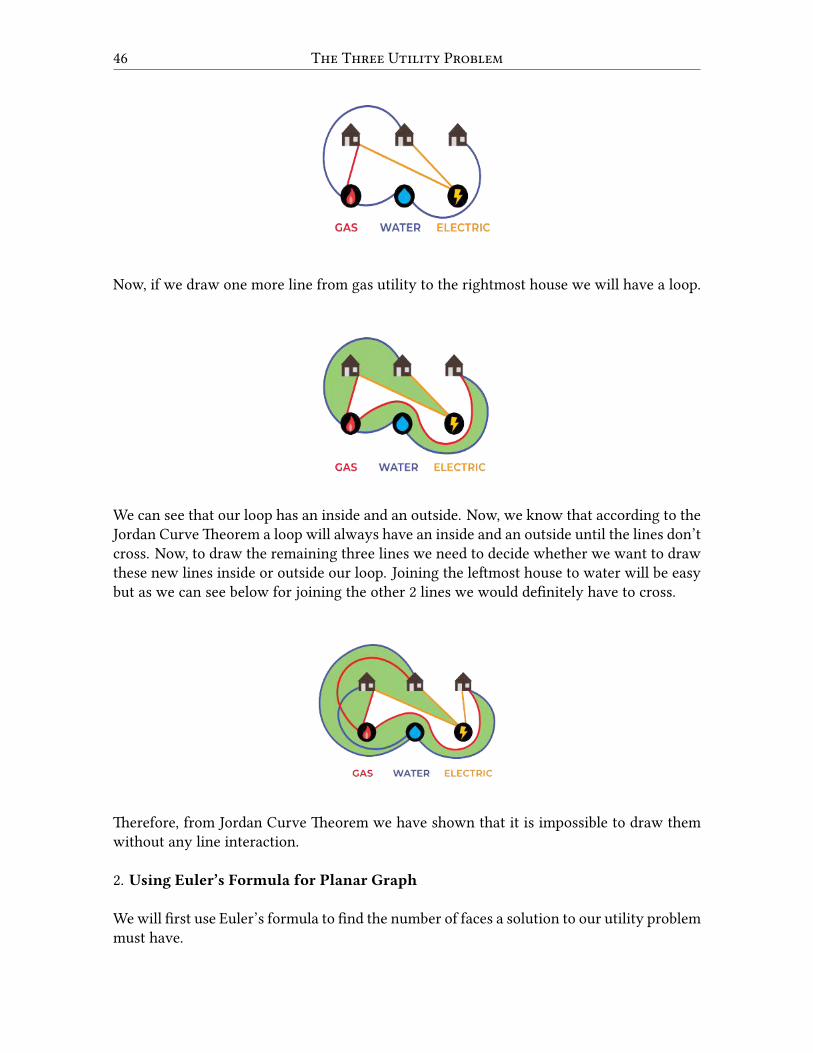
46 The ThRee Utility PRoblem

Now, if we draw one more line from gas utility to the rightmost house we will have a loop.

We can see that our loop has an inside and an outside. Now, we know that according to theJordan CurveTheorem a loop will always have an inside and an outside until the lines don’tcross. Now, to draw the remaining three lines we need to decide whether we want to drawthese new lines inside or outside our loop. Joining the leftmost house to water will be easybut as we can see below for joining the other 2 lines we would definitely have to cross.

Therefore, from Jordan Curve Theorem we have shown that it is impossible to draw themwithout any line interaction.

2. Using Euler’s Formula for Planar Graph

Wewill first use Euler’s formula to find the number of faces a solution to our utility problemmust have.

ApuRva Chauhan 47

We know that;V = number of vertices=6,E=number of edges=9,Using Euler’s formula, we haveF=number of faces

F = 2 + E − V

F = 2 + 9− 6 = 5

So, we have five faces according to our Euler’s formula for planar graphs. We know thatwe can never connect 2 houses or 2 supplies together, that is we can never have 3 edgesto a face. The problem states that connecting lines can only be drawn between houses andutilities. Which means that each face will have at least 4 edges. This implies that 5 faceswill have at least 20 edges (5× 4). But this counts each edge twice because every edge is aboundary for 2 faces. Therefore, we will take the smallest number of edges[4].

E =20

2= 10

But, according to the problem we can have only 9 edges!

ConclusionsThe solution to the three utility problem is ‘impossible’. It is impossible to connect thehouses in the Euclidean plane (a flat sheet stretched to infinity).

BIBLIOGRAPHY[1] Dhruv Gowswami-The Three Utilities Problem

[2] Euler’s Formula and the Utilities Problem

[3] Math Forum-Three Utilities Problem

[4] Wikipedia-Graph Theory

[5] Wikipedia-Three Utilities problem

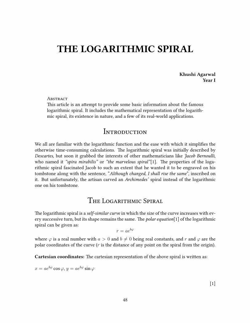
THE LOGARITHMIC SPIRAL

Khushi AgarwalYear I

AbstRactThis article is an attempt to provide some basic information about the famouslogarithmic spiral. It includes the mathematical representation of the logarith-mic spiral, its existence in nature, and a few of its real-world applications.

IntRoductionWe all are familiar with the logarithmic function and the ease with which it simplifies theotherwise time-consuming calculations. The logarithmic spiral was initially described byDescartes, but soon it grabbed the interests of other mathematicians like Jacob Bernoulli,who named it “spira mirabilis” or “the marvelous spiral”[1]. The properties of the loga-rithmic spiral fascinated Jacob to such an extent that he wanted it to be engraved on histombstone along with the sentence, “Although changed, I shall rise the same”, inscribed onit. But unfortunately, the artisan carved an Archimedes’ spiral instead of the logarithmicone on his tombstone.

The LogaRithmic SpiRalThe logarithmic spiral is a self-similar curve in which the size of the curve increases with ev-ery successive turn, but its shape remains the same. The polar equation[1] of the logarithmicspiral can be given as:

r = aebφ

where φ is a real number with a > 0 and b ̸= 0 being real constants, and r and φ are thepolar coordinates of the curve (r is the distance of any point on the spiral from the origin).

Cartesian coordinates: The cartesian representation of the above spiral is written as:

x = aebφ cosφ, y = aebφ sinφ

[1]

48

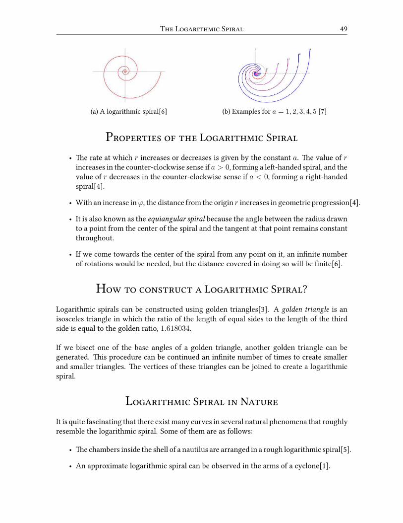
The LogaRithmic SpiRal 49

(a) A logarithmic spiral[6] (b) Examples for a = 1, 2, 3, 4, 5 [7]

PRopeRties of the LogaRithmic SpiRal• The rate at which r increases or decreases is given by the constant a. The value of rincreases in the counter-clockwise sense if a > 0, forming a left-handed spiral, and thevalue of r decreases in the counter-clockwise sense if a < 0, forming a right-handedspiral[4].

• With an increase inφ, the distance from the origin r increases in geometric progression[4].

• It is also known as the equiangular spiral because the angle between the radius drawnto a point from the center of the spiral and the tangent at that point remains constantthroughout.

• If we come towards the center of the spiral from any point on it, an infinite numberof rotations would be needed, but the distance covered in doing so will be finite[6].

How to constRuct a LogaRithmic SpiRal?Logarithmic spirals can be constructed using golden triangles[3]. A golden triangle is anisosceles triangle in which the ratio of the length of equal sides to the length of the thirdside is equal to the golden ratio, 1.618034.

If we bisect one of the base angles of a golden triangle, another golden triangle can begenerated. This procedure can be continued an infinite number of times to create smallerand smaller triangles. The vertices of these triangles can be joined to create a logarithmicspiral.

LogaRithmic SpiRal in NatuReIt is quite fascinating that there existmany curves in several natural phenomena that roughlyresemble the logarithmic spiral. Some of them are as follows:

• The chambers inside the shell of a nautilus are arranged in a rough logarithmic spiral[5].

• An approximate logarithmic spiral can be observed in the arms of a cyclone[1].

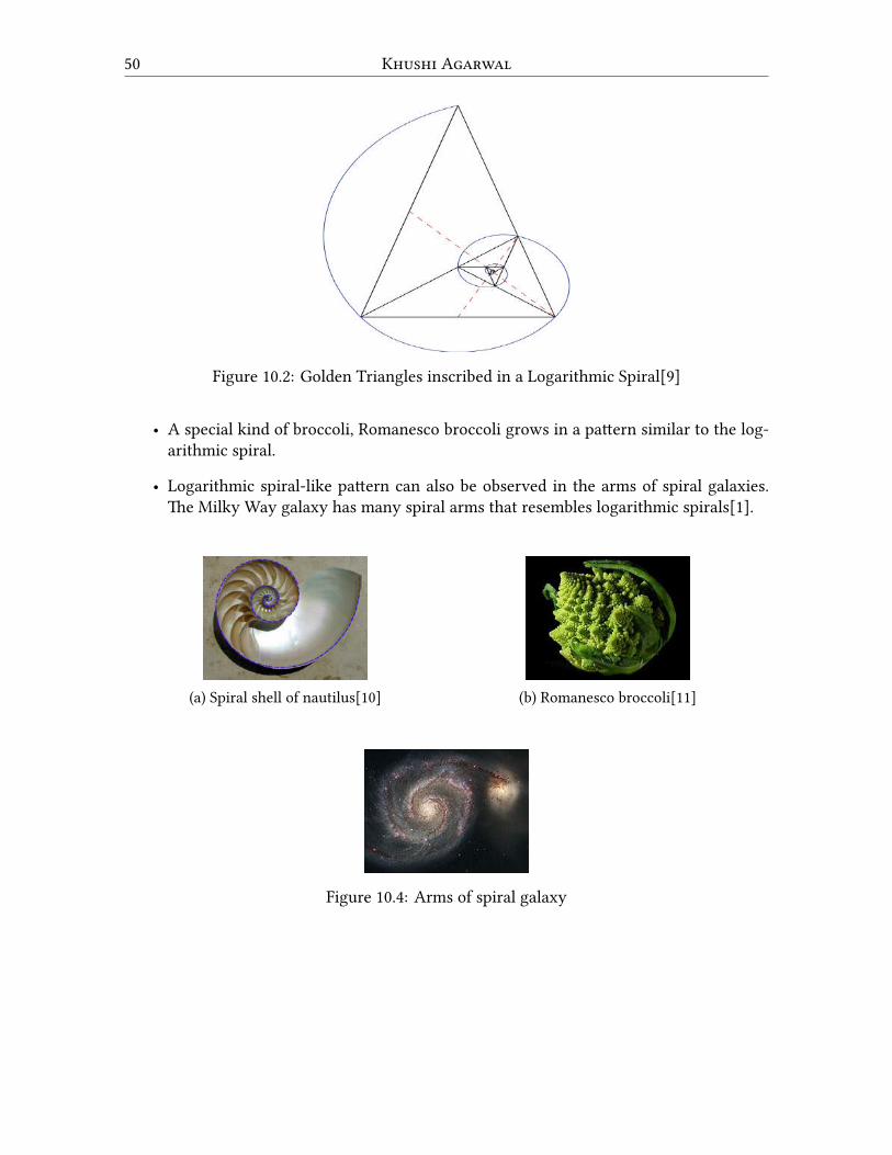
50 Khushi AgaRwal

Figure 10.2: Golden Triangles inscribed in a Logarithmic Spiral[9]

• A special kind of broccoli, Romanesco broccoli grows in a pattern similar to the log-arithmic spiral.

• Logarithmic spiral-like pattern can also be observed in the arms of spiral galaxies.The Milky Way galaxy has many spiral arms that resembles logarithmic spirals[1].

(a) Spiral shell of nautilus[10] (b) Romanesco broccoli[11]

Figure 10.4: Arms of spiral galaxy

The LogaRithmic SpiRal 51

ConclusionsThere are several other spirals like the Archimedean spiral, Euler spiral, Fibonacci spiral,etc. The logarithmic spiral is as fascinating as any one of these. It is used to make spiralbevel gears that are known for their excellent engineering characteristics[1]. It is also usedin frequency-independent spiral antennas. Also, the ways in which it exists in nature aremind-blowing.

BIBLIOGRAPHY[1] Wikipedia- Logarithmic spiral

[2] Logarithmic Spiral: Wolfram Math World

[3] Wikipedia- Golden triangle (mathematics)

[4] Article. Logarithmic Spiral - A Spiral Curve: Utpal Mukhopadhyay

[5] Wikipedia- Logarithm

[6] Logarithmic spiral: David Darling

[7] Image via Wolfram Math World

[8] Image via Wikipedia/Spiral Log

[9] Image via Wikipedia/Fibonacci Spiral

[10] Image via Shallow Sky

[11] Image by Jon Sullivan via Math Images

MATHEMATICS IN PLANTS

Priyanka ChopraYear II

AbstRactThis paper is an attempt to understand how mathematics is applied in plants.Complex calculations happening in plants every day can be well-explained bythe mathematical concepts of Fibonacci Series and Golden Ratio. It focuses onthe Fibonacci Series in particular. The paper discusses few of the applicationsof how mathematics is applied in various plants in brevity.

Keywords: Fibonacci Series, Golden Ratio

IntRoductionMost of us are unaware of the fact that plants apply mathematics every single day to en-sure that they have ample amount of resources to get through nights when sunlight isn’tavailable. According to a recent analysis, plants cannot grow and thrive without mathe-matics. From arrangement of leaves, shape, size, and structure of plants to preparing foodvia photosynthesis, plants perform complex arithmetic calculations regularly. Formationsand patterns in plants are not accidental, rather there is a mathematical logic behind thesestructures. It is commendable how symmetrical patterns can be observed in the arrange-ment of leaves and modeled using DC2 equation which can generate most leaf patterns.

Moreover, it is astonishing how the Fibonacci Series is widely used in predicting the positionof the whorled leaves on stem. The Fibonacci Series can be used not only in studying thespiral pattern of seeds in sunflowers, but also in calculating the number of petals of variousflowers.

While studying the structure of various plants, we get to realise that there is a well-orderedarrangement of leaves. This uniform arrangement of leaves around the stem is termedas phyllotaxis. Usually, the characteristics of this uniform pattern are explained in termsof phyllotactic patterns, including distichous, decussate, tricussate and Fibonacci patternswhere spirally distributed tend to be separated by an angle of 137.5 degrees, also termed asthe Golden Angle, which is the radial equivalent of the golden ratio.

52

Mathematics in Plants 53

(a)(b)

Figure 11.1: Patterns in leaves[4]

It is essential to understand the golden ratio of the Fibonacci Series to unlock the mystery ofthese leaf patterns. Basically, in Fibonacci Series we take the sum of two preceding numbersto calculate the successive number i.e., the series goes like 1, 1, 2, 3, 5, 8, 13, . . . . To calculatethe golden ratio, the ratio of two successive numbers in Fibonacci Series is taken and eachnumber is divided by the preceding number as follows:

1

1= 1,

2

1= 2,

3

2= 1.5,

5

3= 1.666 . . . ,

8

5= 1.6,

13

8= 1.625,

21

13= 1.61538 . . .

Figure 11.2: Graph Plotting of Fibonacci ratios

The ratio appears to be settling down to a particular value, which we call the golden ratio orthe golden number. It has a value of 1.618034 approximately. Actually, the exact value of thegolden ratio comes out to be Φ. As we proceed towards larger numbers in fibonacci series,the ratio turns out to be more close to Φ which can be explained by the basic FibonacciRelationship:

F (i+ 2) = F (i+ 1) + F (i)

Therefore, as the series proceeds, the ratios get closer and closer to this limiting value Φ.

HistoRy of Fibonacci SeRiesFibonacci Series is a significant contribution to mathematics by Sir Leonardo Pisano Bigollo,popularly known as ‘Leonardo of Pisa ’. This series turned out to be an outcome of an arith-metic problem about Rabbit Breeding that was posed in the Liber Abaci. The problem which

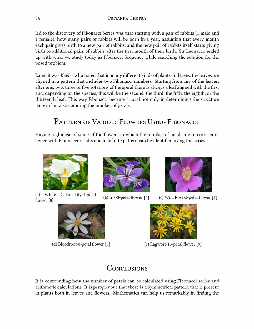
54 PRiyanKa ChopRa

led to the discovery of Fibonacci Series was that starting with a pair of rabbits (1 male and1 female), how many pairs of rabbits will be born in a year, assuming that every montheach pair gives birth to a new pair of rabbits, and the new pair of rabbits itself starts givingbirth to additional pairs of rabbits after the first month of their birth. Sir Leonardo endedup with what we study today as Fibonacci Sequence while searching the solution for theposed problem.

Later, it was Kepler who noted that in many different kinds of plants and trees, the leaves arealigned in a pattern that includes two Fibonacci numbers. Starting from any of the leaves,after one, two, three or five rotations of the spiral there is always a leaf aligned with the firstand, depending on the species, this will be the second, the third, the fifth, the eighth, or thethirteenth leaf. This way Fibonacci became crucial not only in determining the structurepattern but also counting the number of petals.

PatteRn of VaRious FloweRs Using FibonacciHaving a glimpse of some of the flowers in which the number of petals are in correspon-dence with Fibonacci results and a definite pattern can be identified using the series.

(a) White Calla Lily-1-petalflower [8] (b) Iris-3-petal flower [6] (c) Wild Rose-5-petal flower [7]

(d) Bloodroot-8-petal flower [5] (e) Ragwort-13-petal flower [9]

ConclusionsIt is confounding how the number of petals can be calculated using Fibonacci series andarithmetic calculations. It is perspicuous that there is a symmetrical pattern that is presentin plants both in leaves and flowers. Mathematics can help us remarkably in finding the

Mathematics in Plants 55

reasons of existing things in nature. The pattern, size of leaves, number of petals, and pres-ence of recurrent structure in plants are not accidental, rather they have reliable premiseswhich justify the way they are.

BIBLIOGRAPHY[1] Shelley Allen, MASTER FIBONACCI The Man Who Changed Math, ISBN 978-15-3239-

349-5

[2] https://fibonacci.com/nature-golden-ratio/

[3] Klar, A. 2002. Plant mathematics: Fibonacci’s flowers. Nature. 417: 595

[4] Image by Maddie Burakoff via Smithsonian Magazine

[5] Image via Toronto Star

[6] Image via Kaggle

[7] Image by Jasmine Anenberg, Parks Conservancy

[8] Image via Michigan Bulb

[9] Photo taken at Mt. Cuba Center, accessed Mt.Cuba Center.org

PYRAMIDS AND MATHEMATICS

Mir SamreenYear II

AbstRactThis article is an attempt to show a real life application of mathematics asso-ciated with the Great Pyramids of Giza. In this article, Egyptian mathematicsis briefly explained, followed by a reference to pyramids and how they encodeseveral mathematical constants within their geometry and construction. Therelation between Pi and Phi with the Great pyramids is discussed in order tounderstand how these Pyramids are interesting from a mathematical point ofview.

Keywords: Pi, Golden ratio, Fibonacci’s numbers

IntRoductionTheGreat Pyramid of Giza is the oldest monument on the list of seven wonders of the world.It is a marvel of human engineering and construction. Till date, the biggest mystery aboutpyramids is the techniques used in their construction to erect them. It is a standard claimthat the structure of the Great pyramid encodes a number of mathematical and physicalconstants. For example, it is quoted that

“Dimensions of Great Pyramids contain the value of Pi, the principle of thegolden section, Euler’s number, the number of year in tropical year, the relativediameters of the earth at the equator and poles,…, the acceleration of gravityetc”[1].

Mathematics was an inductive discipline of utilitarian nature during the ancient Egyptianera. It was developed as a deductive science by the Greeks. Therefore, there is no evi-dence that Egyptian mathematicians used concept of textual geometry with constructionand proofs. We get most of the information of Egyptian mathematics from the two majormathematical documents that have survived i.e. Rhind and Moscow papyri[2]. However, themathematics involved in the Great Pyramid is so perfect that it is not limited to these twodocuments per se.

56

PyRamids and Mathematics 57

In the coming sections, connections between Pi, Phi, and Great Pyramids is discussed, sincePi and Phi are the two most important mathematical constants. It is fascinating to knowhow the connection between these constants and the pyramid might have been indented,but in a very different methodologies in a much more sophisticated manner.

Pi and the GReat PyRamidThe perimeter of the base of the Great Pyramid divided by twice its height gives 3.150685,which is a remarkably accurate estimate of Pi. However, even though the pyramid givesa fair enough approximation of Pi, there is a reason to doubt that ancient Egyptians evenhad a concept of Pi, since the famous Rhind mathematical papyrus (written during the 13thdynasty) gives the value of Pi (3.160494), less accurate than the value of Pi obtained frompyramids erected in the 4th dynasty. But, there is another side to this conundrum. The rela-tion between slope and Pi is given by the equation:

tan 51.85◦ = 4

π

where 51.85◦ is the slope angle of the pyramid and the value of Pi obtained from this equa-tion is 99.99 % accurate. One may look back at the system of measurements used by Babylo-nians, especially Egyptians, known as the method of seked. Seked is a measure of the slopewhere,

• 1 cubit = 7 palms

• 1 palm = 4 digits

The theory says that the Great Pyramid is based on the application of a gradient of 5.5sekeds. This method of Egyptian mathematicians (based on Rhind papyri), and the waysin which they represented lengths and slopes give a very high probability that they mighthave chosen the angle of at least one of the pyramids to be approximately equal to the value4π, which exhibits the amazing relationship between Pi and the pyramid. Due to this, one

might believe that this relationship can be an accidental resultant of their mathematics.

The importance of Pi was intriguingly represented while seeking a solution to the most fa-mous and intricate problem ever posed in history called “Squaring the Circle”. Egyptianswere also tackling this problem and it was only after the understanding of the nature of Pi,this problem found some lead. With an aid of simple geometry and instruments such ascompass and ruler, it seeks to find area of a square equal to the area of a given circle. Inthe late 19th century we came to know that such a task is impossible to perform as a con-sequence of the Lindemann-Weierstrass theorem which proves that Pi (π) is transcendentaland not like an algebraic irrational number that is the root of any polynomial with rationalcoefficients[?]. But there exists an interesting view to squaring the circle exercise since itwas believed to have symbolic meaning:

58 MiR SamReen

Because the circle is an incommensurable figure based on π, it is impossible todraw a square more than approximately equal to it. Nevertheless, the Squaringof the Circle is of great importance to the geometer-cosmologist because forhim the circle represents pure, un-manifest spirit-space, while the square rep-resents the manifest and comprehensible world. When a near-equality is drawnbetween the circle and square, the infinite is able to express its dimensions orqualities through the finite[3].

Therefore, the accurate approximation gives in itself a sense of aesthetic satisfaction, andthe amazing fact is, the Great Pyramid squares the circle. If a circle is drawn in such a man-ner that its centre lies in the centre of the base of the pyramid, with a radius equal to theheight of the pyramid then we get the circumference of the circle equal to the perimeter ofthe square containing the pyramid. Such geometry approximates the solution of “squaringthe circle” sough by ancient geometers.

Phi and GReat PyRamid

When the slant height of the face of the pyramid is divided by half the length of its base, theanswer is Phi, Golden Ratio (1.61803 . . . ). Phi is the only number which has a very uniqueproperty of its square equal to one more than itself i.e.

ϕ+ 1 = ϕ2.

By observing such property of phi one can apply the Pythagorean equation to this, for ex-ample in the Golden Triangle. One can construct the golden triangle (also called Kepler’striangle) with sides ϕ, 1 and

√ϕ as shown in figure 12.1.

Figure 12.1: Golden Triangle

This can create pyramid constructed with the help of two such triangles placed back to back.Now, the ratio of height to the base is

√ϕ

1= 0.636 . . .

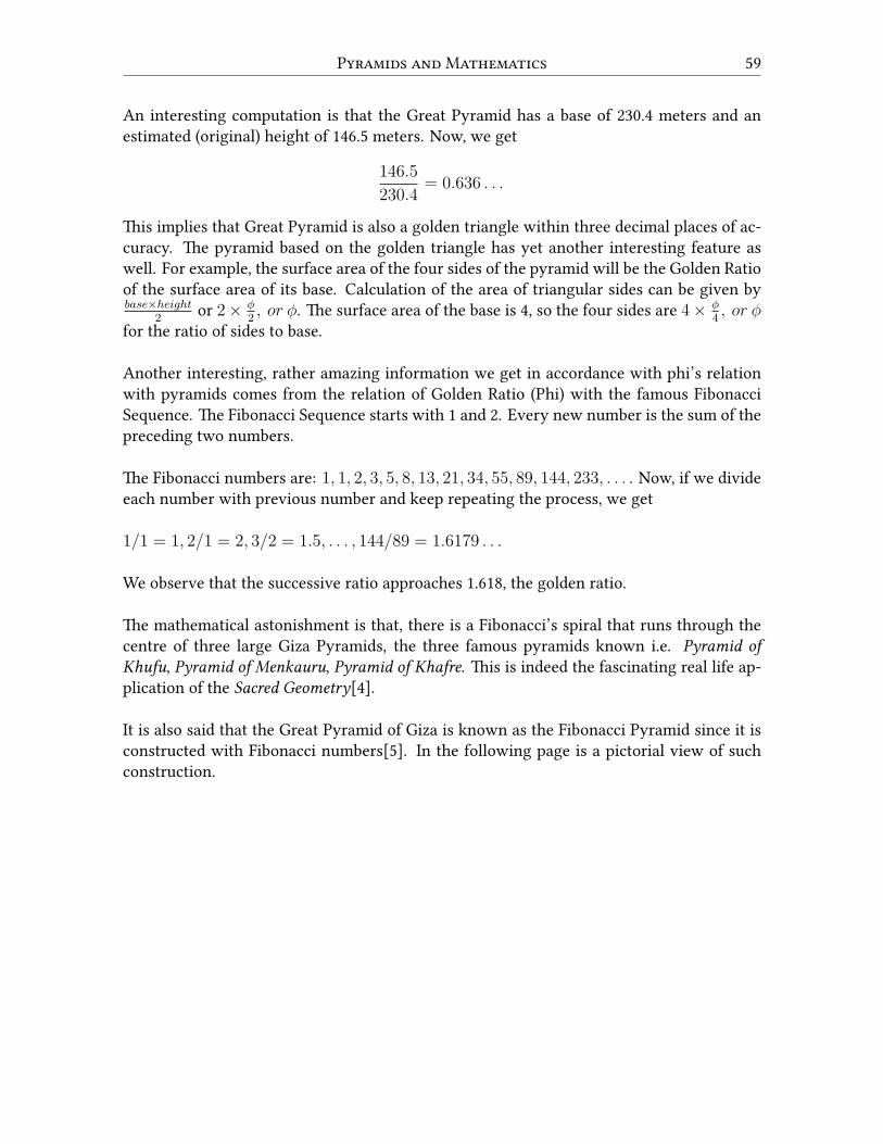
PyRamids and Mathematics 59

An interesting computation is that the Great Pyramid has a base of 230.4 meters and anestimated (original) height of 146.5 meters. Now, we get

146.5

230.4= 0.636 . . .

This implies that Great Pyramid is also a golden triangle within three decimal places of ac-curacy. The pyramid based on the golden triangle has yet another interesting feature aswell. For example, the surface area of the four sides of the pyramid will be the Golden Ratioof the surface area of its base. Calculation of the area of triangular sides can be given bybase×height

2or 2× ϕ

2, or ϕ. The surface area of the base is 4, so the four sides are 4× ϕ

4, or ϕ

for the ratio of sides to base.

Another interesting, rather amazing information we get in accordance with phi’s relationwith pyramids comes from the relation of Golden Ratio (Phi) with the famous FibonacciSequence. The Fibonacci Sequence starts with 1 and 2. Every new number is the sum of thepreceding two numbers.

The Fibonacci numbers are: 1, 1, 2, 3, 5, 8, 13, 21, 34, 55, 89, 144, 233, . . . . Now, if we divideeach number with previous number and keep repeating the process, we get

1/1 = 1, 2/1 = 2, 3/2 = 1.5, . . . , 144/89 = 1.6179 . . .

We observe that the successive ratio approaches 1.618, the golden ratio.

The mathematical astonishment is that, there is a Fibonacci’s spiral that runs through thecentre of three large Giza Pyramids, the three famous pyramids known i.e. Pyramid ofKhufu, Pyramid of Menkauru, Pyramid of Khafre. This is indeed the fascinating real life ap-plication of the Sacred Geometry[4].

It is also said that the Great Pyramid of Giza is known as the Fibonacci Pyramid since it isconstructed with Fibonacci numbers[5]. In the following page is a pictorial view of suchconstruction.

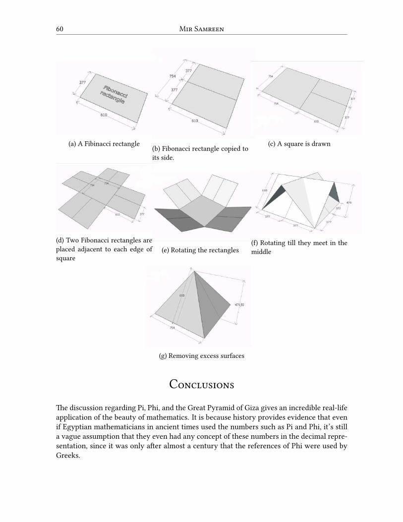
60 MiR SamReen

(a) A Fibinacci rectangle (b) Fibonacci rectangle copied toits side.

(c) A square is drawn

(d) Two Fibonacci rectangles areplaced adjacent to each edge ofsquare

(e) Rotating the rectangles(f) Rotating till they meet in themiddle

(g) Removing excess surfaces

Conclusions

The discussion regarding Pi, Phi, and the Great Pyramid of Giza gives an incredible real-lifeapplication of the beauty of mathematics. It is because history provides evidence that evenif Egyptian mathematicians in ancient times used the numbers such as Pi and Phi, it’s stilla vague assumption that they even had any concept of these numbers in the decimal repre-sentation, since it was only after almost a century that the references of Phi were used byGreeks.

PyRamids and Mathematics 61

It then becomes feasible to believe as some do, that Egyptians might have used the integerapproximation in their designs which resulted in the same relationships. Also, it is quitereasonable to believe this side as we know, both Pi and Phi (it’s square root value) are suchnumbers that can be calculated approximately using simple integers that too with highdegree precision.

π = 227

and ϕ = 196121

Also, one can also claim the possibility that perhaps Egyptians intended to use one of themin the dimensions of the pyramid and the other got automatically included. There are sev-eral questions regarding the construction techniques of pyramids from a mathematical per-spective. No one is completely sure of how were pyramids actually designed. However,whatever is known one can say that the specification of a particular choice of the geometryfor the Great Pyramid was doubtlessly done with some intention since it is different fromthe rest and truly perfect.

The Great Pyramid is one of the exquisite examples of the fact that beautiful, properlyaligned, and coordinated things with nature require such a degree of mathematics in them.

BIBLIOGRAPHY[1] Hunter Havelin Adams 3 in Portland American-African Baseline Essays

[2] Mathematics in Ancient Egypt (Part 1) by Assem Deif, Cairo University, January 2007.

[3] Robert Lawlor, Sacred Geometry Philosophy and Practice in Sacred geometry of the GreatPyramid: squaring the circle, Skypal

[4] The Great Pyramid

[5] The Fibonacci Pyramid of Giza by Ugur Gulcugil, Erasmus University Rotterdam, May2020.

VERY SMALL PROOFS

Shivam BauraiYear III

AbstRactIn this article, ‘clever’or ‘simple’proofs of seemingly abstract problems are pur-sued, which are especially smaller than conventionally quoted proofs of the saidresults.

Wilson’s TheoRem

Lemma. Let G = {a1, a2, . . . , an} be a finite abelian group and suppose that G has only oneelement of order 2, y. Then,

∏ni=1 ai = y.

Theorem. For a prime p, (p− 1)! ≡ −1 mod(p)

Proof. Consider the multiplicative group, U(p).

U(p) = {n ∈ Zp | gcd(n, p) = 1} = {1, 2, 3, . . . , p − 1} is cyclic. Thus, G has ϕ(2) = 1element of order 2, which is p− 1.Then, as per the lemma, (p− 1)! = (1)(2) · · · (p− 1) = p− 1 ≡ −1 mod(p)

The iRRationality of√k

Theorem.√k is irrational ∀ k ∈ N : k is not a perfect square.

Proof. Assume otherwise. Then,√k can be represented in lowest terms as:

√k = m

nwhere

m,n ∈ N and gcd(m,n) = 1. Also note that since k is not a perfect square, ∃ j ∈ N :j <

√k < j + 1. Now:

1. j <√k < j + 1 ⇒ j < m

n< j + 1 ⇒ nj < m < nj + n ⇒ 0 < m− nj < n

62

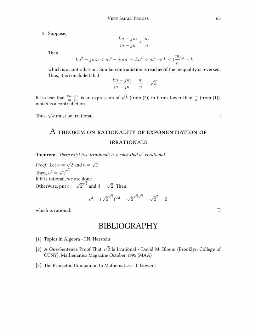
VeRy Small PRoofs 63

2. Suppose,kn− jm

m− jn<

m

n.

Then,kn2 − jmn < m2 − jmn ⇒ kn2 < m2 ⇒ k < (

m

n)2 = k

which is a contradiction. Similar contradiction is reached if the inequality is reversed.Thus, it is concluded that

kn− jm

m− jn=

m

n=

√k

It is clear that kn−jmm−jn

is an expression of√k (from (2)) in terms lower than m

n(from (1)),

which is a contradiction.

Thus,√k must be irrational.

A theoRem on Rationality of exponentiation ofiRRationals

Theorem. There exist two irrationals a, b such that ab is rational.

Proof. Let a =√2 and b =

√2.

Then, ab =√2√2.

If it is rational, we are done.Otherwise, put c =

√2√2 and d =

√2. Then,

cd = (√2√2)√2 =

√2√2√2=

√22= 2

which is rational.

BIBLIOGRAPHY[1] Topics in Algebra - I.N. Herstein

[2] A One-Sentence Proof That√2 Is Irrational - David M. Bloom (Brooklyn College of

CUNY), Mathematics Magazine October 1995 (MAA)

[3] The Princeton Companion to Mathematics - T. Gowers

One-Step At A Time

AbstRactExploring the concept of defining a function between two non-empty sets andusing it to solve a seemingly unrelated puzzle is the main objective of this arti-cle.

Keywords: Function, Bijection

What is a Bijection?A function between two non-empty sets is said to be a bijection if it is both injective and sur-jective. Here, the domain and co-domain have intentionally been disguised because when-ever there exists a bijection from a set to another, then an inverse map can also be definedthe other way around.

Lets take a descriptive figure: Let f be a function f : A → B, such that f is both injectiveand surjective then the mapping looks somewhat like this:

a

b

c

d

1

2

3

4

Figure 14.1

Problem: Determine the number of walks from (0, 0) to (m, n) allowing only unit steps up orto the right.Solution: In this question, we try to morph the situation into something familiar. We tryto symbolize each step and represent a right step by R and an up step by U. As an example,consider the following path:

64

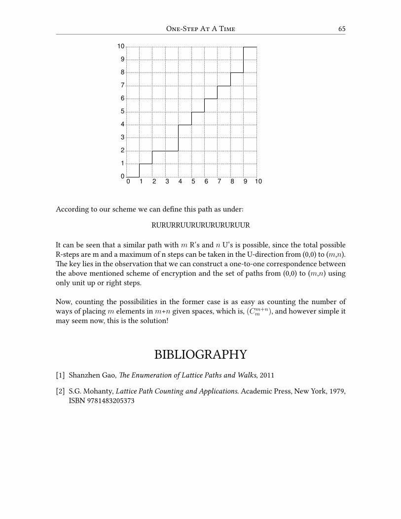
One-Step At A Time 65

0 1 2 3 4 5 6 7 8 9 100

1

2

3

4

5

6

7

8

9

10

According to our scheme we can define this path as under:

RURURRUURURURURURUUR

It can be seen that a similar path with m R’s and n U’s is possible, since the total possibleR-steps are m and a maximum of n steps can be taken in the U-direction from (0,0) to (m,n).The key lies in the observation that we can construct a one-to-one correspondence betweenthe above mentioned scheme of encryption and the set of paths from (0,0) to (m,n) usingonly unit up or right steps.

Now, counting the possibilities in the former case is as easy as counting the number ofways of placing m elements in m+n given spaces, which is, (Cm+n

m ), and however simple itmay seem now, this is the solution!

BIBLIOGRAPHY[1] Shanzhen Gao, The Enumeration of Lattice Paths and Walks, 2011

[2] S.G. Mohanty, Lattice Path Counting and Applications. Academic Press, New York, 1979,ISBN 9781483205373

THE WINDMILL PROCESS

AbstRactWe have reached a phase in this world where everyone fights an identity crisis.And people are appreciated for preserving their traditional and cultural ties.Though abstraction has made its own niche in the realm of art, any work of artis much appreciated and finds an even larger audience when it has a tinge ofsimplicity at its core. It is more of an irony that the questions that are genuinelytough have a cloak of intuitiveness attached to them as a disguise. In this paper,we attempt to discuss a seemingly simple problem that was asked in the world’stoughest math test.

2011 IMO, Qestion 2Let S be a finite set of at least two points in the plane. Assume that no three points of S arecollinear. A windmill is a process that starts with a line ℓ going through a single point P ∈ S .The line rotates clockwise about the pivot P until the first time that the line meets some otherpoint belonging to S . This point,Q, takes over as the new pivot, and the line now rotates clock-wise about Q, until it next meets a point of S . This process continues indefinitely. Show thatwe can choose a point P in S and a line ℓ going through P such that the resulting windmilluses each point of S as a pivot infinitely many times[1].

A Rough SKetchThe fact that a person of any age group or any academic background can understand thequestion makes it even harder to think about a mathematical proof. We begin by attemptingto mathematize this question.

Firstly, to get a feel for what this windmill process is we begin by drawing some diagrams.After progressively increasing the number of points in S , we observe that if the initial pivotof the line ℓ is an outside point then the line keeps on rotating around the perimeter of theplane and it never touches the interior points. But a second look at the question tells us that

66

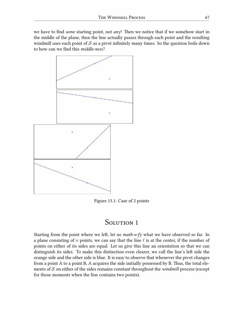
The Windmill PRocess 67

we have to find some starting point, not any! Then we notice that if we somehow start inthe middle of the plane, then the line actually passes through each point and the resultingwindmill uses each point of S as a pivot infinitely many times. So the question boils downto how can we find this middle-ness?

Figure 15.1: Case of 2 points

Solution 1Starting from the point where we left, let us math-o-fy what we have observed so far. Ina plane consisting of n points, we can say that the line ℓ is at the center, if the number ofpoints on either of its sides are equal. Let us give this line an orientation so that we candistinguish its sides. To make this distinction even clearer, we call the line’s left side theorange side and the other side is blue. It is easy to observe that whenever the pivot changesfrom a point A to a point B, A acquires the side initially possessed by B. Thus, the total ele-ments of S on either of the sides remains constant throughout the windmill process (exceptfor those moments when the line contains two points).

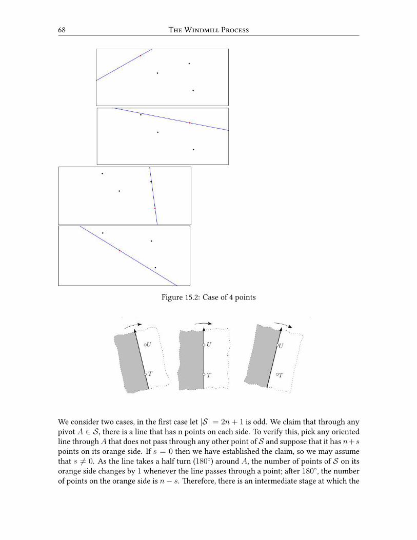
68 The Windmill PRocess

Figure 15.2: Case of 4 points

We consider two cases, in the first case let |S| = 2n+ 1 is odd. We claim that through anypivot A ∈ S , there is a line that has n points on each side. To verify this, pick any orientedline throughA that does not pass through any other point of S and suppose that it has n+spoints on its orange side. If s = 0 then we have established the claim, so we may assumethat s ̸= 0. As the line takes a half turn (180◦) around A, the number of points of S on itsorange side changes by 1 whenever the line passes through a point; after 180◦, the numberof points on the orange side is n− s. Therefore, there is an intermediate stage at which the

The Windmill PRocess 69

orange side, and thus also the blue side, contains n points.

Now, select the point B arbitrarily, and choose a line through B that has n points of Son each side to be the initial state of the windmill. We will show that during a rotation over180◦, the line of the windmill visits each point of S as a pivot. To see this, select any pointA of S and select a line ℓ through A that separates S into equal halves. The point A is theunique point of S through which a line in this direction can separate the points of S intoequal halves (parallel translation would disturb the balance). Therefore, when the windmillline is parallel to ℓ, it must be ℓ itself, and so pass through A.

Next, suppose that |S| = 2n. Similarly to the odd case, for every A ∈ S there is an orientedline throughAwith n−1 points on its orange side and n points on its blue side. Select suchan oriented line through an arbitrary B to be the initial state of the windmill. We will nowshow that during a rotation over 360◦, the line of the windmill visits each point of S as apivot. To see this, select any point A of S and an oriented line ℓ through A that separates Sinto two subsets with n− 1 points on its orange and n points on its blue side. Again, paral-lel translation would change the numbers of points on the two sides, so when the windmillline is parallel to ℓ with the same orientation, the windmill line must pass through A. Thiscompletes the proof.

ConclusionsThis question definitely doesn’t test the number of theorems that students have learnedthroughout their academic curriculum. This unusually pure puzzle has its charm in the in-tuitiveness attached to it that calls for a clever perspective.

BIBLIOGRAPHY[1] 52nd International Mathematical Olympiad, 12-24 July 2011 Amsterdam, the Nether-

lands

MATHEMATICAL FACTS

Ulam SpiRalTheUlam Spiral or prime spiral is a plot of prime numbers, devised bymathematician Stanis-law Ulam. It is constructed by writing all the positive integers in a spiral arrangement on asquare lattice and then by marking the primes[1].

From the spiral, it is clearly visible that most of the primes lie on diagonal straight linesand some on horizontal and vertical lines. Mostly, the number spiral is started with 1 atthe centre but we can also start with any number of our choice. For example, if we startwith 41 at the centre of spiral, we get a diagonal containing an unscathed string of 40 primenumbers (which is the longest example of its kind!).

Explanation. Diagonal, vertical and horizontal lines in the spiral corresponds to the poly-nomial of the form-

f(n) = 4n2 + bn+ c

70

Mathematical Facts 71

where b and c are integer constants. If b is even, then the lines are diagonal, either all of oddor all even depending on the value of c.

However, some polynomials, for example 4n2 + 8n + 3 while producing all odd values,factorize to (2n + 1)(2n + 3) and are therefore never prime other than 1. Such examplescorrosponds to those diagonal lines that are lacking prime numbers.

Hailstone NumbeRsThe Collatz Conjecture is a conjecture that defines a sequence of positive integers in whicheach term is obtained from the previous term as follows:

• If n is even, the next term is n2

• If n is odd, the next term is 3n+ 1

This conjecture was given by Lothar Collatz. It is also known as the 3n + 1 Problem or3n + 1 Conjecture. According to this Conjecture, regardless of the choice of n, eventuallythe sequences converges to 1. The sequence of integers generated by this process are calledHailstone Numbers[2].

Examples

• If n = 7, we get the following sequence:

7, 22, 11, 34, 17, 52, 26, 13, 40, 20, 10, 5, 16, 8, 4, 2, 1

Thus, when n = 7, it takes 17 steps to converge to 1.

• If n = 27, we get the following sequence:27, 82, 41, 124, 62, 31, 94, 47, 142, 71, 214, 107, 322, 161, 484, 242, 121, 364, 182, 91,274, 137, 412, 206, 103, 310, 155, 466, 233, 700, 350, 175, 526, 263, 790, 395, 1186, 593,1780, 890, 445, 1336, 668, 334, 167, 502, 251, 754, 377, 1132, 566, 283, 850, 425, 1276,638, 319, 958, 479, 1438, 719, 2158, 1079, 3238, 1619, 4858, 2429, 7288, 3644, 1822, 911,2734, 1367, 4102, 2051, 6154, 3077, 9232, 4616, 2308, 1154, 577, 1732, 866, 433, 1300, 650,325, 976, 488, 244, 122, 61, 184, 92, 46, 23, 70, 35, 106, 53, 160, 80, 40, 20, 10, 5, 16, 8, 4, 2, 1

When, n = 27, it takes 111 steps to converge to 1.

The Most Beautiful EationEuler’s Identity is considered to be an epitome of mathematical beauty. The equality is

eiπ + 1 = 0

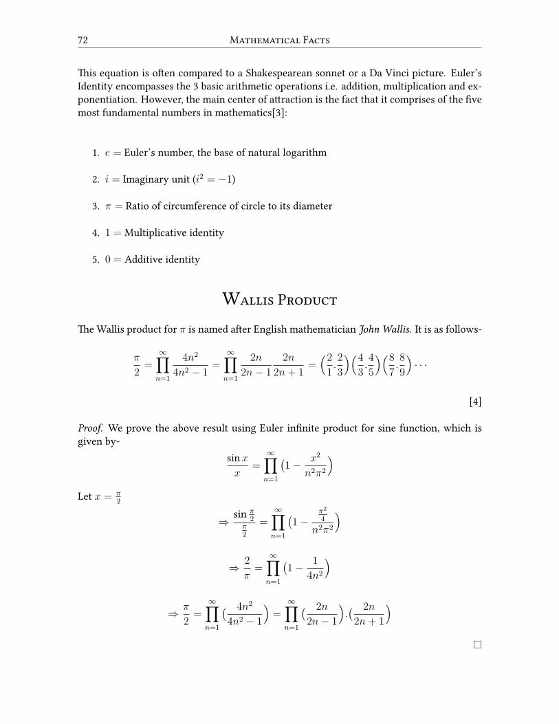
72 Mathematical Facts

This equation is often compared to a Shakespearean sonnet or a Da Vinci picture. Euler’sIdentity encompasses the 3 basic arithmetic operations i.e. addition, multiplication and ex-ponentiation. However, the main center of attraction is the fact that it comprises of the fivemost fundamental numbers in mathematics[3]:

1. e = Euler’s number, the base of natural logarithm

2. i = Imaginary unit (i2 = −1)

3. π = Ratio of circumference of circle to its diameter

4. 1 = Multiplicative identity

5. 0 = Additive identity

Wallis PRoduct

The Wallis product for π is named after English mathematician John Wallis. It is as follows-

π

2=

∞∏n=1

4n2

4n2 − 1=

∞∏n=1

2n

2n− 1

2n

2n+ 1=

(21.2

3

)(43.4

5

)(87.8

9

)· · ·

[4]

Proof. We prove the above result using Euler infinite product for sine function, which isgiven by-

sinxx

=∞∏n=1

(1− x2

n2π2

)Let x = π

2

⇒sin π

2π2

=∞∏n=1

(1−

π2

4

n2π2

)

⇒ 2

π=

∞∏n=1

(1− 1

4n2

)

⇒ π

2=

∞∏n=1

( 4n2

4n2 − 1

)=

∞∏n=1

( 2n

2n− 1

).( 2n

2n+ 1

)

Mathematical Facts 73

The FouR ColouR TheoRemHave you ever got to colour a map for your geography project? How many colours didyou use to colour it? In 1852, Francis Guthrie was trying to colour the map of counties ofEngland. He noticed that the regions could be coloured using at most four colours in such away that no two adjacent regions had the same colour[5]. The first successful proof of thisconjecture came only in 1976, when Kenneth Appel and Wolfgang Haken proved it usingcomputer assistance. They argued that if the four-colour conjecture were false, then therewould be at least one map with minimum regions which needed five colours. Using twoconcepts they proved that such a minimal counterexample could not exist[6].

• Every non-4-colourable map must belong to an unavoidable set of configurations.

• If a configuration does not fall under minimal counterexample then it is called re-ducible configuration. A map can be reduced to a smaller map if it has a reducibleconfiguration. If this smaller map can be coloured with four colours, so could theoriginal one be. So, if the original map could not be coloured with four colours, thesmaller one cannot either. Therefore, the original map is not minimal.

This proof remained contentious due to its extensive usage of computer assistance, but pavedthe path for its upcoming improvements.

GÖdel’s Incompleteness TheoRemsDo you think that mathematics is complete? Can all true statements be proved by a for-mal system (for example a system of natural numbers)? In 1931, Kurt Gödel came up withhis two incompleteness theorems and showed that an axiomatic system cannot exist whichcontains all mathematics. It will only get bigger and bigger as we try to complete it[8].

• First Incompleteness Theorem: Given any consistent formal system S, it will beincomplete, that is, there exists statements in S which are neither provable nor dis-provable in S.

• Second Incompleteness Theorem: Given any consistent formal system S, it is im-possible to prove the consistency of S in S only[7].

GabRiel’s HoRn PaRadox (PainteR’s PaRadox)Gabriel’s Horn is the infinitesimally long surface of revolution obtained after rotating thecurve y = 1

x(for x ≥ 1) about the x− axis. Intuitively, when we think about its volume, it

seems infinite as its length goes on to infinity and thus if we are to fill it with paint, it will

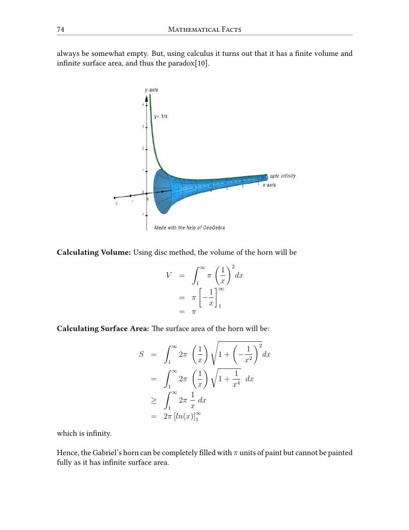
74 Mathematical Facts

always be somewhat empty. But, using calculus it turns out that it has a finite volume andinfinite surface area, and thus the paradox[10].

Calculating Volume: Using disc method, the volume of the horn will be

V =

∫ ∞

1

π

(1

x

)2

dx

= π

[−1

x

]∞1

= π

Calculating Surface Area: The surface area of the horn will be:

S =

∫ ∞

1

2π

(1

x

)√1 +

(− 1

x2

)2

dx

=

∫ ∞

1

2π

(1

x

)√1 +

1

x4dx

≥∫ ∞

1

2π1

xdx

= 2π [ln(x)]∞1

which is infinity.

Hence, the Gabriel’s horn can be completely filledwith π units of paint but cannot be paintedfully as it has infinite surface area.

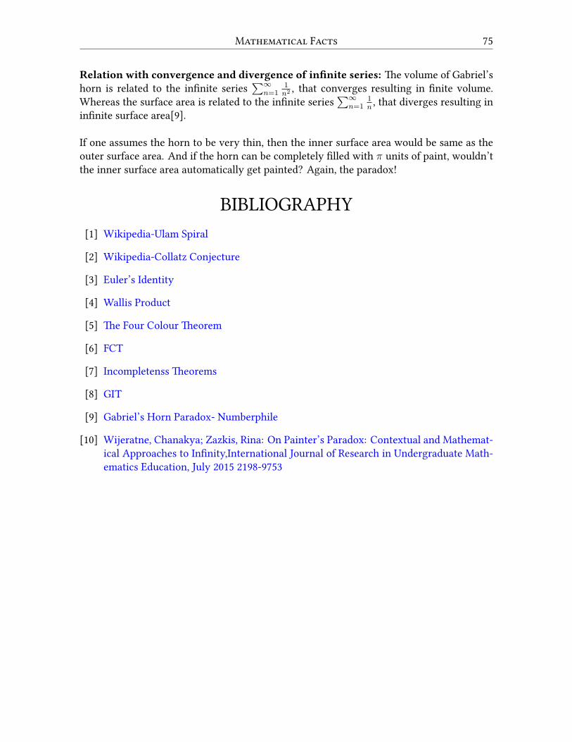
Mathematical Facts 75

Relation with convergence and divergence of infinite series: The volume of Gabriel’shorn is related to the infinite series

∑∞n=1

1n2 , that converges resulting in finite volume.

Whereas the surface area is related to the infinite series∑∞

n=11n, that diverges resulting in

infinite surface area[9].

If one assumes the horn to be very thin, then the inner surface area would be same as theouter surface area. And if the horn can be completely filled with π units of paint, wouldn’tthe inner surface area automatically get painted? Again, the paradox!

BIBLIOGRAPHY[1] Wikipedia-Ulam Spiral

[2] Wikipedia-Collatz Conjecture

[3] Euler’s Identity

[4] Wallis Product

[5] The Four Colour Theorem

[6] FCT

[7] Incompletenss Theorems

[8] GIT

[9] Gabriel’s Horn Paradox- Numberphile

[10] Wijeratne, Chanakya; Zazkis, Rina: On Painter’s Paradox: Contextual and Mathemat-ical Approaches to Infinity,International Journal of Research in Undergraduate Math-ematics Education, July 2015 2198-9753