Embed Size (px)
Citation preview

Journal of Fluid Mechanicshttp://journals.cambridge.org/FLM
Additional services for Journal of Fluid Mechanics:
Email alerts: Click hereSubscriptions: Click hereCommercial reprints: Click hereTerms of use : Click here
Double diffusive effects on pressure-driven miscible displacement flows in a channel
Manoranjan Mishra, A. De Wit and Kirti Chandra Sahu
Journal of Fluid Mechanics / Volume 712 / December 2012, pp 579 - 597DOI: 10.1017/jfm.2012.439, Published online:
Link to this article: http://journals.cambridge.org/abstract_S0022112012004399
How to cite this article:
Manoranjan Mishra, A. De Wit and Kirti Chandra Sahu (2012). Double diffusive effects on pressure-driven miscible displacement flows in a channel. Journal of Fluid Mechanics, 712, pp 579-597 doi:10.1017/jfm.2012.439
Request Permissions : Click here
Downloaded from http://journals.cambridge.org/FLM, IP address: 164.15.129.79 on 29 Nov 2012
J. Fluid Mech. (2012), vol. 712, pp. 579–597.
c�Cambridge University Press 2012 579
doi:10.1017/jfm.2012.439
Double di�usive e�ects on pressure-driven
miscible displacement flows in a channel
Manoranjan Mishra
1, A. De Wit
2and Kirti Chandra Sahu
3†1 Department of Mathematics, Indian Institute of Technology Ropar, Rupnagar 140 001, Punjab, India
2 Nonlinear Physical Chemistry Unit, Service de Chimie Physique et Biologie Theorique,Faculte des Sciences, Universite Libre de Bruxelles (ULB), CP231, 1050 Brussels, Belgium
3 Department of Chemical Engineering, Indian Institute of Technology Hyderabad,Yeddumailaram 502 205, Andhra Pradesh, India
(Received 16 November 2011; revised 27 June 2012; accepted 4 September 2012;first published online 9 October 2012)
The pressure-driven miscible displacement of a less viscous fluid by a more viscousone in a horizontal channel is studied. This is a classically stable system if the moreviscous solution is the displacing one. However, we show by numerical simulationsbased on the finite-volume approach that, in this system, double diffusive effects canbe destabilizing. Such effects can appear if the fluid consists of a solvent containingtwo solutes both influencing the viscosity of the solution and diffusing at differentrates. The continuity and Navier–Stokes equations coupled to two convection–diffusionequations for the evolution of the solute concentrations are solved. The viscosityis assumed to depend on the concentrations of both solutes, while density contrastis neglected. The results demonstrate the development of various instability patternsof the miscible ‘interface’ separating the fluids provided the two solutes diffuse atdifferent rates. The intensity of the instability increases when increasing the diffusivityratio between the faster-diffusing and the slower-diffusing solutes. This brings aboutfluid mixing and accelerates the displacement of the fluid originally filling the channel.The effects of varying dimensionless parameters, such as the Reynolds number andSchmidt number, on the development of the ‘interfacial’ instability pattern are alsostudied. The double diffusive instability appears after the moment when the invadingfluid penetrates inside the channel. This is attributed to the presence of inertia in theproblem.
Key words: convection, double diffusive convection, fingering instability, interfacial flows(free surface), multiphase and particle-laden flows, multiphase flow
1. Introduction
The dynamics of interface patterns and mixing between two miscible fluids is anactive research area (Rashidnia, Balasubramaniam & Schroer 2004; Balasubramaniamet al. 2005) and is of importance in many industrial processes, e.g. in enhanced oilrecovery, fixed bed regeneration, hydrology and filtration. There exist other industrialapplications in which the displacement of one fluid by another miscible/immisciblefluid (Joseph et al. 1997) occurs, e.g. in the oil and gas industry, the transportationof crude oil in pipelines relies on the stability of two-layer flows when the highly
† Email address for correspondence: [email protected]

580 M. Mishra, A. De Wit and K. C. Sahu
viscous fluid is at the wall. In the food processing industries cleaning involves theremoval of a highly viscous fluid by water. The stability of this type of two-phase flowin a channel or pipe has been widely investigated both theoretically (Ranganathan &Govindarajan 2001; Selvam et al. 2007; Sahu et al. 2009a; Sahu & Matar 2010, 2011)and experimentally (Hickox 1971; Hu & Joseph 1989; Joseph & Renardy 1992; Josephet al. 1997).
Linear stability analyses of displacement flows in porous media (Saffman & Taylor1958; Chouke, Van Meurs & Van Der Pol 1959; Tan & Homsy 1986) explain that,if the displacing fluid is less viscous than the displaced one, the interface separatingthem becomes unstable and a fingering pattern develops at the interface. A reviewon such dynamics in porous media and Hele-Shaw cells is given by Homsy (1987).In a pipe flow, when a less viscous miscible fluid displaces a more viscous one, atwo-layer core–annular flow is obtained in most of the channel/pipe as the elongated‘finger’ of the less viscous fluid penetrates into the bulk of the more viscous one.The interface between the two fluids becomes unstable, forming Kelvin–Helmholtz(KH) instabilities and ‘roll-up’ structures (Joseph et al. 1997; Sahu et al. 2009a,b).Experimental studies in miscible core–annular flows (Taylor 1961; Cox 1962; Chen& Meiburg 1996; Petitjeans & Maxworthy 1996; Kuang, Maxworthy & Petitjeans2003) have focused on analysing the thickness of the more viscous fluid layer lefton the pipe walls and the speed of the propagating ‘finger’ tip. The developmentof different instability patterns, like axisymmetric ‘corkscrew’ patterns, in miscibleflows has also been investigated (Lajeunesse et al. 1997, 1999; Scoffoni, Lajeunesse& Homsy 2001; Cao et al. 2003; Gabard & Hulin 2003). Axisymmetric ‘pearl’ and‘mushroom’ patterns were observed in neutrally buoyant core–annular horizontal pipeflows at high Schmidt number and Reynolds number in the range 2 < Re < 60 (d’Olceet al. 2008). By an asymptotic analysis, Yang & Yortsos (1997) studied miscibledisplacement flows (in Stokes flow regime) between parallel plates and in cylindricalcapillaries with large aspect ratio. They found viscous fingering instability for largeviscosity ratio and that the displacement efficiency decreases with increasing viscosityratio.
Goyal, Pichler & Meiburg (2007) performed a linear stability analysis of a miscibledisplacement flow in a vertical Hele-Shaw cell with a less viscous fluid displacing amore viscous one. They found that the flow develops as a result of linear instability.Their nonlinear simulations of the Stokes equations predict that increasing the unstabledensity stratification and decreasing diffusion increase the front velocity. The flowfields obtained by these simulations are qualitatively similar to those observed in theexperiment of Petitjeans & Maxworthy (1996) in capillary tubes and in the theoreticalpredictions of Lajeunesse et al. (1999) for Hele-Shaw cells. The study of Petitjeans& Maxworthy (1996) discussed the formation and propagation of a single finger for amiscible fluid in a capillary tube. Such dynamics was also found by Taylor (1961) forimmiscible fluids.
Thus from the literature discussed above, it has been understood that ahydrodynamic instability of fingering or a KH pattern occur only if the viscosityor density increases along the direction of propagation, i.e. when a less viscous/densefluid displaces a more viscous/dense fluid. The situation of a more viscous fluiddisplacing a less viscous one is being classically understood as a stable situation.This stable displacement flow in a vertical cylindrical tube of small diameter wasexperimentally investigated by Rashidnia et al. (2004) and Balasubramaniam et al.(2005). For downward displacement (with gravity), the ‘interface’ separating the fluidsbecomes unstable and exhibits an asymmetric sinuous shape. On the other hand, in

Double di�usive e�ects on miscible displacement flows 581
the case of upward displacement (against gravity), a stable diffusive finger of themore viscous fluid penetrating the less viscous one is observed for small displacementspeed. At a larger displacement speed, an axisymmetric finger with a needle-shapedspike propagates out from the main finger tip. To the best of our knowledge, theseare the only experiments that have discussed the displacement flow in a classicallystable system. A similar situation in a porous medium or Hele-Shaw cell has beeninvestigated theoretically (Pritchard 2009; Mishra et al. 2010). They found thatdouble diffusive (DD) effects can destabilize the classically stable situation of a moreviscous fluid displacing a less viscous one and affect the viscous fingering dynamics.Therefore, it is interesting to understand whether such a concept of destabilization ofan otherwise stable situation by differential diffusion effects can also occur in pressure-driven channel flows if the solvent at hand contains two different solutes influencingthe viscosity and diffusing at different rates. Recently, Sahu & Govindarajan (2011)found an unstable DD mode in a classically stable system of three-layer pressure-driven channel flow (with highly and less viscous fluids occupying the core andnear-wall regions of the channel, respectively) by conducting a linear stabilityanalysis. The convective and absolute nature of this instability is studied by Sahu& Govindarajan (2012). They assumed that the flow is symmetrical about the channelcentreline.
In this context, the main objective of this present study is to understand theinfluence on the dynamics of differential diffusion between two solutes influencingviscosity when a highly viscous solution of these solutes displaces a less viscousone in a channel without the gravitational force (classically stable system). Thetwo solutions are miscible and their viscosity is a function of the concentration ofthe two solutes, which diffuse at different rates. The flow dynamics is governedby the continuity and Navier–Stokes equations coupled to two convection–diffusionequations for the concentration of both solutes through a concentration-dependentviscosity. We conduct numerical simulations and analyse destabilization of the flowby differential diffusion effects occurring if the two solutes controlling the viscositydiffuse at different rates. The effects of varying the dimensionless parameters, suchas Reynolds number, Schmidt number and ratio of the diffusivity of the species,on the development of interfacial instability patterns are studied. The fundamentalchallenge in the modelling of the flow configuration addressed here is to consider theNavier–Stokes equation for fluid flow in a channel geometry instead of consideringStokes equations in a capillary tube or Darcy’s law in Hele-Shaw geometry.
The rest of this paper is organized as follows. The problem is formulated in § 2, themethod of solution using a finite-volume approach is explained in § 3 and the resultsof the numerical simulations are presented in § 4. Concluding remarks are providedin § 5.
2. Mathematical formulation
Consider a two-dimensional channel initially filled with a stationary Newtonianincompressible fluid containing scalars S and F in quantity S2 and F2 and of viscosityµ2. This solution is displaced by the same solvent in which the scalars are presentwith different values S1 and F1 giving a viscosity µ1 (see figure 1). The inlet fluidis injected with an average velocity V (⌘ Q/H), where Q and H denote the totalflow rate and the height of the channel, respectively. We use a rectangular coordinatesystem (x, y) to model the flow dynamics, where x and y denote the horizontal and

582 M. Mishra, A. De Wit and K. C. Sahu
y
x
H
FIGURE 1. Schematic diagram showing the initial flow configuration: fluid ‘2’ occupies theentire channel and is about to be displaced by fluid ‘1’.
vertical coordinates, respectively. The channel inlet and outlet are located at x = 0and L, respectively. The rigid and impermeable walls of the channel are located aty = 0 and H.
In order to determine the flow dynamics, we consider the incompressibleNavier–Stokes equations along with the convection–diffusion equations for theconservation of both solutes. The governing equations are given by
r ·u = 0, (2.1)
⇢
@u@t
+ u ·ru�
= �rp + r · [µ(ru + ruT)], (2.2)
@S
@t+ u ·rS = Dsr2S, (2.3)
@F
@t+ u ·rF = Df r2F, (2.4)
where u ⌘ (u, v) is the velocity vector with components u and v in the x and ydirections, respectively, p denotes pressure, and S and F are two scalars with diffusioncoefficients Ds and Df , respectively, such that Df > Ds. The density ⇢ is taken tobe constant. In order to keep the model as simple as possible, the effects of cross-diffusion and of possible dependence of diffusion on concentration are neglectedhere.
We assume that the viscosity µ has the following dependence on S and F (Mishraet al. 2010; Sahu & Govindarajan 2011):
µ = µ1 exp
Rs
✓S � S1
S2 � S1
◆+ Rf
✓F � F1
F2 � F1
◆�, (2.5)
where Rs ⌘ (S2 � S1) d(ln µ)/dS and Rf ⌘ (F2 � F1) d(ln µ)/dF are the log-mobilityratios of solutes S and F, respectively. While there is no experimental evidence insupport of (2.5) in a ternary system, it has been widely used to study viscosity-relatedinstabilities (e.g. Chen & Meiburg 1996; Tan & Homsy 1986; Mishra et al. 2010),and will be used here for mathematical convenience, and to allow for comparisonwith previous theoretical work using the same assumption. Since diffusivity andviscosity in a liquid are related approximately inversely through the Stokes–Einsteinequation (Probstein 1994), one cannot conduct an experiment in which viscosityvaries significantly and diffusivity does not. However, in order to avoid discouragingcomplexity of the problem right away and in order to build upon previous works, westart here by assuming the diffusion coefficients to be constant.
Double di�usive e�ects on miscible displacement flows 583
The following scaling is employed to non-dimensionalize equations (2.1)–(2.5)
(x, y) = H(x, y), t = H2
Qt, (u, v) = Q
H(u, v), p = ⇢Q2
H2p,
µ = µµ1, s = S � S1
S2 � S1, f = F � F1
F2 � F1, (2.6)
where the tildes designate dimensionless quantities. After dropping tildes, thedimensionless governing equations become
r ·u = 0, (2.7)@u@t
+ u ·ru�
= �rp + 1Re
r · [µ(ru + ruT)], (2.8)
@s
@t+ u ·rs = 1
Re Scsr2s, (2.9)
@f
@t+ u ·rf = 1
Re Scfr2f , (2.10)
where Re ⌘ ⇢Q/µ1, Scs ⌘ µ1/⇢Ds and Scf ⌘ µ1/⇢Df denote the Reynolds numberand the Schmidt numbers of the slower- and faster-diffusing solutes, respectively, and� ⌘ Df /Ds > 1 is the ratio of the diffusion coefficients of the faster- and slower-diffusing solutes. Thus Scf = Scs/�. The dimensionless viscosity has the followingdependence on f and s:
µ = exp(Rss + Rf f ). (2.11)
The initial conditions for s and f in the dimensionless form are s = f = 0 everywhereinside the channel and s = f = 1 at the inlet. The numerical procedure and boundaryconditions used to solve equations (2.7)–(2.10) are described in § 3. Note that, forthe boundary conditions used here, when one of the log mobility ratios (either Rf
or Rs) is set to zero or � = 1, the above equations (2.7)–(2.11) reduce to a singlesolute model, the flow dynamics of which has been discussed using a Navier–Stokessolver by Sahu et al. (2009a). To have an idea of the order of magnitude of the logmobility ratios for real systems, we note that, if, for instance, the invading fluid ismethanol (kinematic viscosity ⌫ = 0.6704 cSt) and the displaced fluid is a mixture ofethylene glycol, acetone and methanol (⌫ = 0.5472 cSt) (Kalidas & Laddha 1964), weget Rs = 3 and Rf = �3.24. The values of the parameters will thus be chosen in thisorder of magnitude.
3. Numerical solution
3.1. Methods
We use a finite-volume approach similar to the one developed by Ding, Spelt& Shu (2007) in order to solve the system of equations (2.7)–(2.10). Theseequations are discretized using a staggered grid. The scalar variables (the pressureand concentrations of the solutes) are defined at the centre of each cell and thevelocity components are defined at the cell faces. The discretized convection–diffusion

584 M. Mishra, A. De Wit and K. C. Sahu
equations for the conservation of both solutes are given by
32 sn+1 � 2sn + 1
2 sn�1
1t= 1
Re Scsr2sn+1 � 2r · (unsn) + r · (un�1sn�1), (3.1)
32 f n+1 � 2f n + 1
2 f n�1
1t= 1
Re Scfr2f n+1 � 2r · (unf n) + r · (un�1f n�1), (3.2)
where 1t = tn+1 � tn and the superscript n signifies the discretized nth step. In order todiscretize the advective terms, i.e the nonlinear terms in (2.9) and (2.10), a weightedessentially non-oscillatory (WENO) scheme is used. A central difference scheme isused to discretize the diffusive term on the right-hand sides of (2.9) and (2.10).
In order to achieve second-order accuracy in the temporal discretization, theAdams–Bashforth and Crank–Nicolson methods are used for the advective and second-order dissipation terms, respectively, in (2.8). This results in the following discretizedequation:
u⇤ � un
1t= 1
pn+1/2
⇢�
32H (un) � 1
2H (un�1)
�+ 1
2Re[L (u⇤, µn+1) + L (un, µn)]
�,
(3.3)
where u⇤ is the intermediate velocity, and H and L denote the discrete convectionand diffusion operators, respectively. The intermediate velocity u⇤ is then corrected tothe (n + 1)th time level,
un+1 � u⇤
1t= rpn+1/2. (3.4)
The pressure distribution is obtained from the continuity equation at time step n + 1using
r · (rpn+1/2) = r ·u⇤
1t. (3.5)
Solutions of the above discretized equations are subject to no-slip, no-penetration andno-flux conditions at the top and bottom walls. A fully developed velocity profile witha constant flow rate taken to be unity is imposed at the inlet (x = 0), and Neumannboundary conditions are used at the outlet (x = L).
The following steps are employed in our numerical solver in order to solveequations (2.7)–(2.10).
(i) The concentration fields of the solutes are first updated by solving (2.9) and (2.10)with the velocity field at time steps n and n � 1.
(ii) These are then updated to time step n + 1 by solving (2.8) together with thecontinuity equation (2.7).
The numerical procedure described above was developed by Ding et al. (2007)in the context of interfacial flows. Sahu et al. (2009a,b) modified this finite-volumemethod to simulate pressure-driven neutrally buoyant miscible channel flow with highviscosity contrast.
3.2. Validations
An important aspect of numerical methods is to choose the optimum grid size forthe numerical simulations to obtain the results in considerably less computational
Double di�usive e�ects on miscible displacement flows 585
40
60
40
60
20 40 60t
80 20 40 60t
800
100
0
100(a) (b)
20
80
20
80
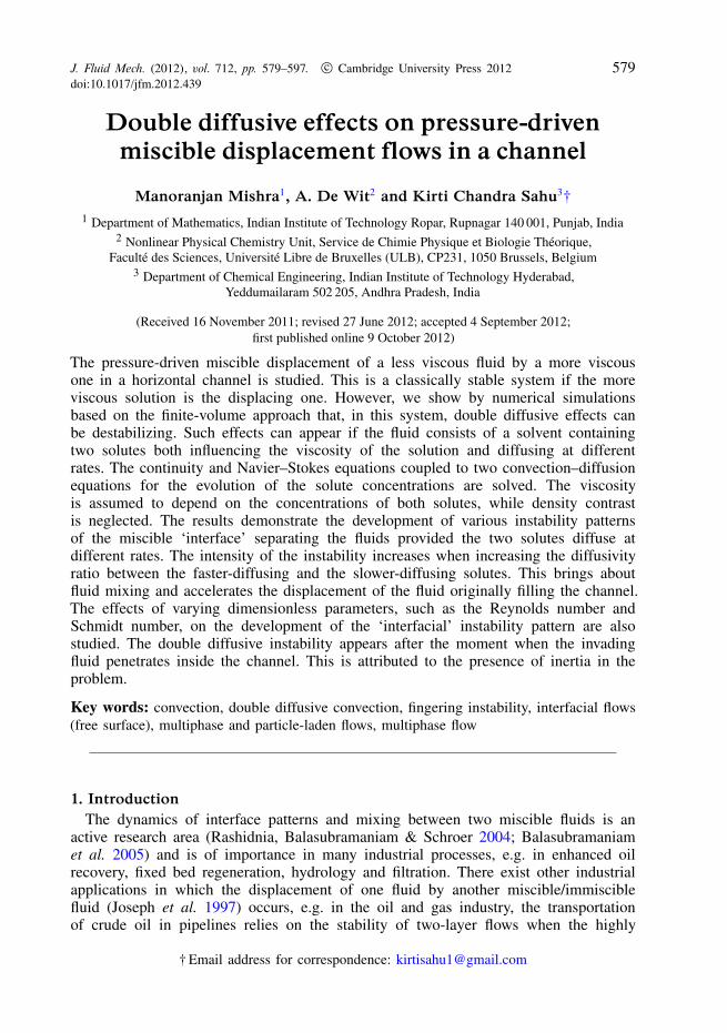
FIGURE 2. Temporal evolution of the position xtip of the leading front separating the twosolutions for (a) s and (b) f obtained using 81 ⇥ 2501 grid points for Re = 500, Scs = 20,Rs = 3, Rf = �3.6 and � = 5.
time. It is essential to perform the numerical simulations with different grid pointsin order to carry out mesh refinement tests and to show convergence of the method.The temporal variations of the spatial location of the leading front separating the twofluids, (xtip), of both solutes s and f are plotted in figure 2(a,b), respectively. Theparameter values chosen are Re = 500, Scs = 20, Rs = 3, Rf = �3.6 and � = 5 inorder to incorporate DD phenomena in the simulation. The results are obtained using81 ⇥ 2501 grid points in a channel of aspect ratio 1 : 100. Numerical simulationsusing 61 ⇥ 2001 and 51 ⇥ 1601 grids are also conducted in the same computationaldomain. We found (not shown) that the results are graphically indistinguishable, with amaximum absolute error less than 0.05 %. On the basis of the spatial variation of xtip,one could measure the speed of the finger tip and study the interfacial dynamics (Sahuet al. 2009a,b). It can be seen that the velocity of the leading front between the twosolutions is constant, as (xtip)s and (xtip)f both vary linearly with time. The rest of thecomputations in this paper are performed using 61 ⇥ 2001 grid points, in a channel ofaspect ratio 1 : 100.
As discussed before, setting Rf = 0 (without DD effects), the present governingequations match those given in Sahu et al. (2010). Thus, to further validate ourcode, we reproduced a result of Sahu et al. (2010) by studying the spatio-temporalevolution of the concentration of the solute s in figure 3. The parameter values areRe = 500, Scs = 100, Rs = 2.3026 and Rf = 0. Note that Rs = 2.3026 corresponds tothe unstable case of a less viscous fluid injected into a more viscous one with aviscosity ratio 10 as considered by Sahu et al. (2010). It can be seen in figure 3 thatthe ‘interface’ becomes unstable, which in turn forms vortical structures and gives riseto intense mixing of the two solutions. During this initial period the flow dynamics isdominated by the formation of KH-type instabilities. At later time (t > 25, for this setof parameters) the remnants of s assume the form of thin layers adjacent to the upperand lower walls. The flow at this stage is dominated by diffusion.
4. Results and discussion
Let us now analyse the role of differential diffusion on the dynamics and, inparticular, investigate how such DD effects can destabilize an otherwise stablesituation.

586 M. Mishra, A. De Wit and K. C. Sahu
0 0.25 0.50 0.75 1.00
FIGURE 3. (Colour online) Spatio-temporal evolution of the concentration field of solute sat successive times (from top to bottom, t = 5, 15, 20, 25 and 40). The rest of the parametervalues are Re = 500, Scs = 100, Rs = 2.3026 and Rf = 0. These results are in excellentagreement with figure 3 of Sahu, Ding & Matar (2010). The greyscale/colour map of all theplots is shown at the bottom.
4.1. E�ects of �
The spatio-temporal evolution of the concentration field of solute s for the parametervalues Re = 100, Scs = 100, Rs = 3 and Rf = �3.6 are plotted in figure 4 for differentvalues of �. In the starting configuration at t = 0, the chosen log mobility ratioscorrespond to a monotonically decreasing viscosity profile at the miscible interfaceof both fluids, which represents a classically stable interface. For � = 1 (whenDf = Ds), it can be seen that the highly viscous fluid initially displaces the lessviscous one like a miscible plug flow and then a fully developed Poiseuille flowregime arises with a pure diffusive miscible interface. Such a stable pattern is termedhere as a ‘pure–Poiseuille–diffusive’ finger (see figure 4a). For � > 1 the miscibleinterface becomes unstable due to the DD mechanism. Figure 4(b) for � = 5 shows thedevelopment of a spike at the tip of the finger and the fact that the miscible interfacedeviates from the ‘pure–Poiseuille–diffusive’ finger. For a larger � (see figure 4c for� = 10), the flow becomes unstable, forming symmetrical wavy interfaces because of aKH-type instability. At later stages the flow dynamics is like a three-layer core–annularflow (Chen & Meiburg 1996; Petitjeans & Maxworthy 1996; Kuang et al. 2003).These instabilities occur at the interface primarily because a viscosity contrast arisesdue to the DD effects. At the tip of the single finger a ‘cap-type’ instability isobserved for the large value of � = 10 (see figure 4c) unlike the spike-like instabilityfor the moderate value of � = 5 (figure 4b). This ‘cap-type’ instability leads to amushroom structure at very late times.
In order to investigate the mechanism of the instability for � > 1, the viscosityfields for the parameter values of figure 4 are plotted in figure 5. It is seen that,at the wall, a highly viscous stenosis region is formed due to the DD effects when� > 1. Such a region does not occur if � = 1. This viscous stenosis region increaseswith increasing �. A highly viscous region behind the wall was also observed in themiscible displacement experiment of Taylor (1961). In figure 5(a), which correspondsto � = 1, a viscosity profile decreasing monotonically along the axial direction isobtained at any fixed transverse axis. But for � > 1 the viscosity profile becomesnon-monotonic in the axial direction and features locally a less viscous fluid layer

Double di�usive e�ects on miscible displacement flows 587
0 0.25 0.50 0.75 1.00
(a)
(b)
(c)
FIGURE 4. (Colour online) Spatio-temporal evolution of the concentration field of solutes at successive times (from top to bottom, t = 20, 30, 40, 50 and t = 75) for (a) � = 1,(b) � = 5 and (c) � = 10. The rest of the parameter values are Re = 100, Scs = 100, Rs = 3 andRf = �3.6.
between two more viscous layers (see figure 5 for � = 5). This is similar to thesituation in DD viscous fingering in porous media (Mishra et al. 2010). For � = 10,rolling structures similar to those in the contours of s (in figure 4) are also observed inthe viscosity contours shown in figure 5(c).
We further analyse the spatial distribution of viscosity by plotting in figure 6the evolution in time of the axial variation of the transverse averaged viscosity,µ =
R 10 µ dy. It can be seen in figure 6(a) that µ varies monotonically in the axial
direction for � = 1. The variation of µ is however non-monotonic for � = 5 and 10.Hence, a local maximum develops such that, locally, the less viscous zone close to

588 M. Mishra, A. De Wit and K. C. Sahu
0.600 0.712 0.824 0.936
0.20 0.92 1.64 2.36 3.08
0.50 1.58 2.66 3.74 4.82
(a)
(b)
(c)
FIGURE 5. (Colour online) The viscosity field at t = 40 for (a) � = 1, (b) � = 5 and(c) � = 10 and the simulations of figure 4.
0.6
0.7
0.8
0.9
1.0
20 40 60 80x
0 100 20 40 60 80x
0 100
0.6
0.8
1.0
1.2
0.4
0.6
0.8
1.0
1.2
1.4
1.6
20 40 60 80x
0 100
0.5
1.4(a) (b)
(c)
204050
FIGURE 6. Variation of transverse average viscosity µ =R 1
0 µ dy in the streamwise directionfor (a) � = 1, (b) � = 5 and (c) � = 10 and parameters of figure 4.
the injection side displaces a more viscous region. This is the main cause of theinstabilities that can occur in pressure-driven displacement flows of a less viscous fluidby a more viscous one in a channel, as studied here. This non-monotonic characterof the viscosity profile due to DD effects was also found in viscous fingering of theclassically stable displacement of a less viscous fluid by a more viscous one in porousmedia (Mishra et al. 2010). At early times, the instability starts here at the axial
Double di�usive e�ects on miscible displacement flows 589
20
30
40
50
60
70
20
25
30
35
40
21
24
27
30
0.2 0.4 0.6 0.8y
0 1.0 0.2 0.4 0.6 0.8y
0 1.0
0.2 0.4 0.6 0.8y
0 1.0
45
18
204050
(a) (b)
(c)
FIGURE 7. Variation of axially averaged viscosity µx =R L/H
0 µ dx in the streamwise directionfor (a) � = 1, (b) � = 5 and (c) � = 10 and parameters of figure 4.
station (after the viscous stenosis region) where there is a change in the slope of theviscosity curve. The spike/cap instability occurs at the tip of the single finger where µdecreases to a value smaller than the initial viscosity at that location (figure 6b,c). For� = 10, the KH instability occurs approximately in the region (35 < x < 60) at t = 40where there is a large zig-zag oscillation in µ. The length of this region increases withtime (see figure 6c).
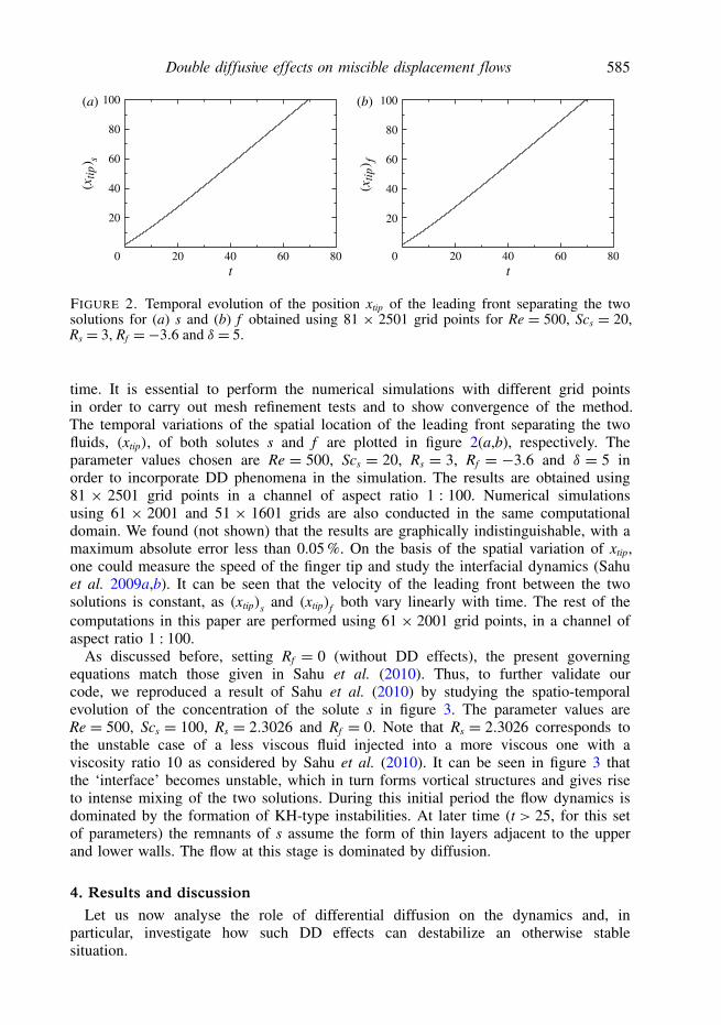
In figure 7, we plot the evolution of the transverse variation of the axially averagedviscosity, µx =
R L/H0 µ dx. For � = 1 it can be seen in figure 7(a) that µx is maximum
at the centreline of the channel. Thus it is similar to a core–annular flow where theless and more viscous fluids occupy the annular and core regions, respectively. Thisis known to be a stable situation in core–annular types of flow (Sahu & Govindarajan2011). Unlike for � = 1, when � = 5 and 10, the viscosity is maximum near thewall regions, which, in the context of core–annular flow, is an unstable situation, asdiscussed in Selvam et al. (2007) and Sahu & Govindarajan (2011). Close inspectionalso reveals that increasing � increases the viscosity near the wall regions, and thus hasa destabilizing effect.
During the displacement process, as the highly viscous fluid displaces the lessviscous one, the total viscosity inside the channel is expected to increase linearly. Thisbehaviour can be seen for � = 1 in figure 8, where the normalized total averagedviscosity, µav ⌘ (1/µ0)
R L0 µ dx, is plotted versus time. Here, µ0 is the total viscosity at
t = 0, when only the displaced solution (solution ‘2’) is present inside the channel.The dotted line in figure 8 represents the analytical solution for the plug-flow

590 M. Mishra, A. De Wit and K. C. Sahu
1.0
1.2
1.4
1.6
10 20 30 40 50t
0 60
5
10
FIGURE 8. Variation of normalized average viscosity µav = (1/µ0)R L
0 µ dx with time fordifferent values of � and parameters of figure 4. The dotted line represents the analyticalsolution for the plug-flow displacement, given by µav = 1 + (t/L)[e�(Rs+Rf ) � 1].
0.2
0.4
0.6
0.8
20 40 60 80t
100
0.2
0.4
0.6
0.8
20 40 60 80t
1000
1.0
0
1.0
510
(a) (b)
FIGURE 9. Measure of the normalized mass of the displaced fluid: (a) Ms = Ms0.98/Ms1 ofsolute ‘s’ and (b) Mf = Mf0.98/Mf 1 of solute ‘f ’, for different values of �. The dotted linesrepresent the analytical solution of plug-flow displacement, given by Ms = Mf = 1 � tH/L.
displacement, given by µav = 1 + t[e�(Rs+Rf ) � 1]/L. It can be seen that, for thisset of parameter values, the line corresponding to � = 1 is close to this analyticalsolution. For � > 1, µav increases at a higher rate than for � = 1. This rate increaseswith increasing �. The rate of increase of viscosity remains the same nearly until thetime t = 5 for all the � values considered, which implies that the onset of DD effectsin the case of channel flows occurs very early (approximately at t = 5 for this setof parameter values). In porous media the DD effects start from the very beginning(Mishra et al. 2010). This delay here of the onset of the DD effects is attributed to thepresence of inertia in the present problem.
In figure 9(a,b), we plot the temporal evolution of the normalized mass of thedisplaced solute s (Ms = Ms0.98/Ms1) and f (Mf = Mf0.98/Mf1), respectively. Here, Ms1and Mf1 are the initial masses of the solutes s and f , respectively, and Ms0.98 andMf0.98 are the masses corresponding concentration labels >0.98 of the solutes s andf , respectively. The parameter values are the same as those used to generate figure 4.
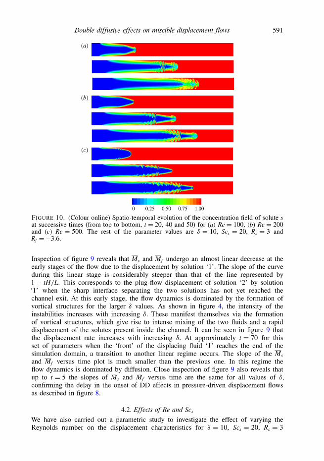
Double di�usive e�ects on miscible displacement flows 591
0 0.25 0.50 0.75 1.00
(a)
(b)
(c)
FIGURE 10. (Colour online) Spatio-temporal evolution of the concentration field of solute sat successive times (from top to bottom, t = 20, 40 and 50) for (a) Re = 100, (b) Re = 200and (c) Re = 500. The rest of the parameter values are � = 10, Scs = 20, Rs = 3 andRf = �3.6.
Inspection of figure 9 reveals that Ms and Mf undergo an almost linear decrease at theearly stages of the flow due to the displacement by solution ‘1’. The slope of the curveduring this linear stage is considerably steeper than that of the line represented by1 � tH/L. This corresponds to the plug-flow displacement of solution ‘2’ by solution‘1’ when the sharp interface separating the two solutions has not yet reached thechannel exit. At this early stage, the flow dynamics is dominated by the formation ofvortical structures for the larger � values. As shown in figure 4, the intensity of theinstabilities increases with increasing �. These manifest themselves via the formationof vortical structures, which give rise to intense mixing of the two fluids and a rapiddisplacement of the solutes present inside the channel. It can be seen in figure 9 thatthe displacement rate increases with increasing �. At approximately t = 70 for thisset of parameters when the ‘front’ of the displacing fluid ‘1’ reaches the end of thesimulation domain, a transition to another linear regime occurs. The slope of the Ms
and Mf versus time plot is much smaller than the previous one. In this regime theflow dynamics is dominated by diffusion. Close inspection of figure 9 also reveals thatup to t = 5 the slopes of Ms and Mf versus time are the same for all values of �,confirming the delay in the onset of DD effects in pressure-driven displacement flowsas described in figure 8.
4.2. E�ects of Re and Scs
We have also carried out a parametric study to investigate the effect of varying theReynolds number on the displacement characteristics for � = 10, Scs = 20, Rs = 3

592 M. Mishra, A. De Wit and K. C. Sahu
0.5
1.0
1.5
2.0
20 40 60 80x
100 20 40 60 80x
100
20 40 60 80x
0 100
0
0.5
1.0
1.5
2.0
1.0
204050
0
2.5
0.5
1.5
(a)
(c)
(b)
FIGURE 11. Variation of transverse average viscosity, µ, in the streamwise direction for(a) Re = 100, (b) Re = 200 and (c) Re = 500 and parameter values of figure 10.
and Rf = �3.6. In figure 10, it is seen that increasing the value of Re from 100to 200 and then to 500, respectively, leads to the rapid development of instabilitiesthat lead to complex dynamics and intricate flow patterns. These are punctuated bymore pronounced roll-up phenomena. Note that, for these parameter values, the flowis in a laminar regime. A close inspection of figure 10 also reveals that the diffusivemixing decreases with increasing Re. This is due to the decrease in effective diffusion,characterized by the Peclet number Pe ⌘ Re Scs, with increasing Re. It can be seenthat a mushroom-like structure appears at the tip of the leading finger. However, it ispersistent only for the intermediate value of Re. The decrease in the effective Pecletnumber (highly diffusive mixing) for the low value Re = 100 destroys this structure atthe nose of the leading finger. For Re = 500 the diffusive mixing is very small and theinterface separating the fluids becomes sharper. It can be seen that the location of theappearance of the KH-type instabilities is shifted towards the tip of the finger whendecreasing the Reynolds number.
The evolution of the corresponding axial variation of the transverse averagedviscosity µ is plotted for Re = 100, 200 and 500 in figure 11. It can be seen thatthe variation of µ is non-monotonic for all values of Re considered. Here, we studya case with highly diffusive mixing (Scs = 20), unlike figure 6, which corresponds toScs = 100 (low diffusion). However like low diffusive flow, the instability starts nearthe viscous stenosis region (not shown) in this case too. The mushroom (spike/cap)type instability occurs at the tip of the single finger when µ decreases to a valuesmaller than the initial viscosity and gradually (suddenly) increases to the initialviscosity (see figure 11). It can be seen that the zig-zag oscillation in µ, whichcorresponds to the KH instability region, moves in the axial direction. The evolution
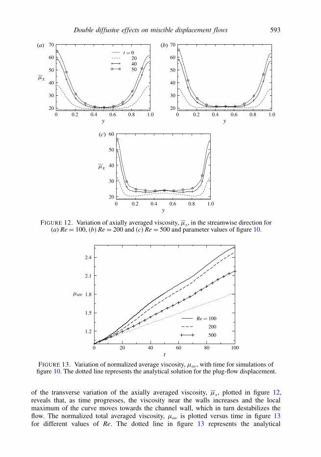
Double di�usive e�ects on miscible displacement flows 593
20
30
40
50
60
70
0.2 0.4 0.6 0.8y
0 1.0
0.2 0.4 0.6 0.8y
0 1.0
20
30
40
50
60
70
0.2 0.4 0.6 0.8y
0 1.0
20
30
40
50
60
204050
(a)
(c)
(b)
FIGURE 12. Variation of axially averaged viscosity, µx, in the streamwise direction for(a) Re = 100, (b) Re = 200 and (c) Re = 500 and parameter values of figure 10.
1.5
1.8
2.1
20 40 60 800 100t
1.2
2.4
200
500
FIGURE 13. Variation of normalized average viscosity, µav , with time for simulations offigure 10. The dotted line represents the analytical solution for the plug-flow displacement.
of the transverse variation of the axially averaged viscosity, µx, plotted in figure 12,reveals that, as time progresses, the viscosity near the walls increases and the localmaximum of the curve moves towards the channel wall, which in turn destabilizes theflow. The normalized total averaged viscosity, µav is plotted versus time in figure 13for different values of Re. The dotted line in figure 13 represents the analytical

594 M. Mishra, A. De Wit and K. C. Sahu
0 0.25 0.50 0.75 1.00
(a)
(b)
FIGURE 14. (Colour online) Spatio-temporal evolution of the concentration field of solutes at successive times (from top to bottom, t = 20, 40, 50, 75 and 95) for (a) Scs = 103 and(b) Scs = 105. Other parameter values are � = 10, Re = 200, Rs = 3 and Rf = �3.6.
solution for the plug-flow displacement. It can be seen that µav increases almostlinearly for all values of Re considered. The slope increases with increasing Re and isconsiderably larger than that of the analytical solution. Close inspection of figure 13also reveals that these lines overlap up to t = 5 (approximately), which confirms thedelay in the onset of DD effects as compared to the phenomena observed in porousmedia.
Finally, we study in figure 14 the flow dynamics for very large Schmidt numbers,i.e. Scs = 103 and 105. The rest of the parameter values are � = 10, Re = 200, Rs = 3and Rf = �3.6. While instabilities due to DD effects can still be seen for Scs = 103,the flow is stable for Scs = 105. In this case the Schmidt number of the faster-diffusingsolute Scf is 104 for � = 10. As the Schmidt numbers of both the solutes are quitelarge (practically in the immiscible limit), the diffusive effects are not destabilizing.This is also evidenced in figure 15, showing that, for Scs = 105, the profiles of theaxially averaged viscosity µx are qualitatively similar to those of the stable single-component system (� = 1) shown in figure 7(a). However, a close inspection offigure 15(b) reveals that, unlike in figure 7(a), µx smoothly approaches a constantvalue just near the wall, which is stabilizing the flow.
5. Concluding remarks
Pressure-driven displacements within a horizontal channel of two different solutionsof two scalars influencing the viscosity and having different diffusion rates are studiedhere numerically. We consider specifically the displacement of a less viscous solution,which occupies the channel initially, by a more viscous one. We show that sucha classically stable displacement can become unstable if the two solutes impactingthe viscosity diffuse at sufficiently different rates. In our simulations, the continuity

Double di�usive e�ects on miscible displacement flows 595
60
70
80
90
50
60
70
80
90
100
0.2 0.4 0.6 0.8y
0 1.0 0.2 0.4 0.6 0.8y
0 1.050
100(a) (b)204050
FIGURE 15. Variation of the axially averaged viscosity, µx, in the streamwise direction for(a) Scs = 103 and (b) Scs = 105. The rest of the parameter values are as in figure 14.
and Navier–Stokes equations coupled to two convection–diffusion equations for theconcentration of both solutes are solved using a finite-volume approach. The viscosityis assumed to be an exponential function of the concentrations of both solutes. Inorder to isolate the effects of viscosity contrast, the density is assumed to be thesame for both the fluids. The numerical code has been validated by conducting a grid-refinement test and also reproducing the results of single-component displacement flow(Sahu & Matar 2010). The results demonstrate the development of various instabilitypatterns of the ‘interface’ separating the fluids when DD effects are present. Theintensity of the instability increases with increasing diffusivity ratio between the faster-diffusing and the slower-diffusing solutes. This instability brings about fluid mixingand accelerates the displacement of the solution originally occupying the channel.The effects of the dimensionless parameters, such as Reynolds number and Schmidtnumber, on the development of the ‘interfacial’ instability pattern are also studied. Amushroom-like structure appears at the tip of the leading finger, which is persistentonly for intermediate values of Re. The DD instability appears after the invadingfluid penetrates inside the channel. This is attributed to the presence of inertia in thepresent problem. These different types of instabilities can be obtained by specifyingthe slow and fast components as mass and heat typically. Experimentally, the predictedinstability can be looked for using two non-reacting chemical species both influencingthe viscosity of the solution and having different diffusion coefficients as in the case oftwo polymers with chains of different length, for instance.
Note that we have here assumed that the diffusion is pseudo-binary and thatthe diffusion coefficients are constant and do not depend on solute concentration.Further developments could be made to include cross-diffusion or concentration-dependent diffusion (Curtiss & Hirschfelder 1949). Moreover, as mentioned above,the Stokes–Einstein relationship (Probstein 1994) shows that, in a solution, it is notpossible that viscosity varies significantly without a correspondingly strong variationin diffusivity. Preliminary computations performed to account for the Stokes–Einsteindependence of diffusivity on viscosity show that, although DD effects still destabilizethe system, some feature of the results are qualitatively different. These aspects shouldbe the focus of additional future studies. Eventually, let us note that we have here alsoused an exponential viscosity–concentration relationship. Other viscosity–concentrationmodels (Iglesias-Silva & Hall 2010) or non-monotonic viscosity profiles (Manickam &Homsy 1993) could be investigated in future studies along the same lines.
596 M. Mishra, A. De Wit and K. C. Sahu
Acknowledgements
Grateful thanks are extended to Professor R. Govindarajan for her valuablesuggestions. K.S. thanks the Department of Science and Technology and the IndianInstitute of Technology Hyderabad, India, for financial support. M.M. acknowledgesthe financial support from the Department of Science and Technology and theIndian Institute of Technology Ropar, India. A.D. acknowledges FNRS and Prodexfor financial support.
R E F E R E N C E S
BALASUBRAMANIAM, R., RASHIDNIA, N., MAXWORTHY, T. & KUANG, J. 2005 Instability ofmiscible interfaces in a cylindrical tube. Phys. Fluids 17, 052103.
CAO, Q., VENTRESCA, L., SREENIVAS, K. R. & PRASAD, A. K. 2003 Instability due to viscositystratification downstream of a centreline injector. Can. J. Chem. Engng 81, 913.
CHEN, C.-Y. & MEIBURG, E. 1996 Miscible displacement in capillary tubes. Part 2. Numericalsimulations. J. Fluid Mech. 326, 57–90.
CHOUKE, R. L., VAN MEURS, P. & VAN DER POL, C. 1959 The instability of slow, immiscible,viscous liquid–liquid displacements in permeable media. Trans. AIME 216, 188.
COX, B. G. 1962 On driving a viscous fluid out of a tube. J. Fluid Mech. 14, 81.CURTISS, C. F. & HIRSCHFELDER, J. O. 1949 Transport properties of multicomponent gas mixtures.
J. Chem. Phys. 17, 550–555.DING, H., SPELT, P. D. M. & SHU, C. 2007 Diffuse interface model for incompressible two-phase
flows with large density ratios. J. Comput. Phys. 226, 2078–2095.D’OLCE, M., MARTIN, J., RAKOTOMALALA, N., SALIN, D. & TALON, L. 2008 Pearl and
mushroom instability patterns in two miscible fluids’ core annular flows. Phys. Fluids 20,024104.
GABARD, C. & HULIN, J.-P. 2003 Miscible displacement of non-Newtonian fluids in a vertical tube.Eur. Phys. J. E 11, 231.
GOYAL, N., PICHLER, H. & MEIBURG, E. 2007 Variable-density miscible displacements in avertical Hele-Shaw cell: linear stability. J. Fluid Mech. 584, 357–372.
HICKOX, C. E. 1971 Instability due to viscosity and density stratification in axisymmetric pipe flow.Phys. Fluids 14, 251.
HOMSY, G. M. 1987 Viscous fingering in porous media. Annu. Rev. Fluid Mech. 19, 271–311.HU, H. H. & JOSEPH, D. D. 1989 Lubricated pipelining: stability of core–annular flows. Part 2.
J. Fluid Mech. 205, 395.IGLESIAS-SILVA, G. A. & HALL, K. R. 2010 Equivalence of the McAllister and Heric equations for
correlating the liquid viscosity of multicomponent mixtures. Ind. Engng Chem. Res. 49,6250–6254.
JOSEPH, D. D., BAI, R., CHEN, K. P. & RENARDY, Y. Y. 1997 Core–annular flows. Annu. Rev.Fluid Mech. 29, 65.
JOSEPH, D. D. & RENARDY, Y. Y. 1992 Fundamentals of Two-Fluid Dynamics. Part II: LubricatedTransport, Drops and Miscible Liquids. Springer.
KALIDAS, R. & LADDHA, S. 1964 Viscosity of ternary liquid mixtures. J. Chem. Engng Data 9,142–145.
KUANG, J., MAXWORTHY, T. & PETITJEANS, P. 2003 Miscible displacements between silicone oilsin capillary tubes. Eur. J. Mech. 22, 271.
LAJEUNESSE, E., MARTIN, J., RAKOTOMALALA, N. & SALIN, D. 1997 3D instability of miscibledisplacements in a Hele-Shaw cell. Phys. Rev. Lett. 79, 5254.
LAJEUNESSE, E., MARTIN, J., RAKOTOMALALA, N., SALIN, D. & YORTSOS, Y. C. 1999 Miscibledisplacement in a Hele-Shaw cell at high rates. J. Fluid Mech. 398, 299.
MANICKAM, O. & HOMSY, G. M. 1993 Stability of miscible displacements in porous media withnonmonotonic viscosity profiles. Phys. Fluids 5, 1356–1367.
MISHRA, M., TREVELYAN, P. M. J., ALMARCHA, C. & DE WIT, A. 2010 Influence of doublediffusive effects on miscible viscous fingering. Phys. Rev. Lett 105, 204501.

Double di�usive e�ects on miscible displacement flows 597
PETITJEANS, P. & MAXWORTHY, T. 1996 Miscible displacements in capillary tubes. Part 1.Experiments. J. Fluid Mech. 326, 37.
PRITCHARD, D. 2009 The linear stability of double-diffusive miscible rectilinear displacements in aHele-Shaw cell. Eur. J. Mech. (B/Fluids) 28 (4), 564–577.
PROBSTEIN, R. F. 1994 Physicochemical Hydrodynamics. Wiley.RANGANATHAN, B. T. & GOVINDARAJAN, R. 2001 Stabilisation and destabilisation of channel flow
by location of viscosity-stratified fluid layer. Phys. Fluids 13 (1), 1–3.RASHIDNIA, N., BALASUBRAMANIAM, R. & SCHROER, R. T. 2004 The formation of spikes in the
displacement of miscible fluids. Ann. N.Y. Acad. Sci. 1027, 311–316.SAFFMAN, P. G. & TAYLOR, G. I. 1958 The penetration of a finger into a porous medium in a
Hele-Shaw cell containing a more viscous liquid. Proc. R. Soc. Lond. A 245, 312–329.SAHU, K. C., DING, H. & MATAR, O. K. 2010 Numerical simulation of non-isothermal
pressure-driven miscible channel flow with viscous heating. Chem. Engng Sci. 65,3260–3267.
SAHU, K. C., DING, H., VALLURI, P. & MATAR, O. K. 2009a Linear stability analysis andnumerical simulation of miscible channel flows. Phys. Fluids 21, 042104.
SAHU, K. C., DING, H., VALLURI, P. & MATAR, O. K. 2009b Pressure-driven miscible two-fluidchannel flow with density gradients. Phys. Fluids 21, 043603.
SAHU, K. C. & GOVINDARAJAN, R. 2011 Linear stability of double-diffusive two-fluid channel flow.J. Fluid Mech. 687, 529–539.
SAHU, K. C. & GOVINDARAJAN, R. 2012 Spatio-temporal linear stability of double-diffusivetwo-fluid channel flow. Phys. Fluids 24, 054103.
SAHU, K. C. & MATAR, O. K. 2010 Three-dimensional linear instability in pressure-driventwo-layer channel flow of a Newtonian and a Herschel–Bulkley fluid. Phys. Fluids 22,112103.
SAHU, K. C. & MATAR, O. K. 2011 Three-dimensional convective and absolute instabilities inpressure-driven two-layer channel flow. Intl J. Multiphase Flow 37, 987–993.
SCOFFONI, J., LAJEUNESSE, E. & HOMSY, G. M. 2001 Interface instabilities during displacementof two miscible fluids in a vertical pipe. Phys. Fluids 13, 553.
SELVAM, B., MERK, S., GOVINDARAJAN, R. & MEIBURG, E. 2007 Stability of misciblecore–annular flows with viscosity stratification. J. Fluid Mech. 592, 23–49.
TAN, C. T. & HOMSY, G. M. 1986 Stability of miscible displacements: rectilinear flow. Phys.Fluids 29, 73549.
TAYLOR, G. I. 1961 Deposition of viscous fluid on the wall of a tube. J. Fluid Mech. 10, 161.YANG, Z. & YORTSOS, Y. C. 1997 Asymptotic solutions of miscible displacements in geometries of
large aspect ratio. Phys. Fluids 9, 286–298.


