Fourier analysis of thermal diffusive wavesMuhammad Sabieh Anwar, Junaid Alam, Muhammad Wasif, Rafi Ullah, Sohaib Shamim, and Wasif Zia

Citation: American Journal of Physics 82, 928 (2014); doi: 10.1119/1.4881608 View online: http://dx.doi.org/10.1119/1.4881608 View Table of Contents: http://scitation.aip.org/content/aapt/journal/ajp/82/10?ver=pdfcov Published by the American Association of Physics Teachers Articles you may be interested in Demonstrating superposition of waves and Fourier analysis with tuning forks and MacScope II Am. J. Phys. 79, 552 (2011); 10.1119/1.3549196 Fourier Analysis of Musical Intervals Phys. Teach. 46, 486 (2008); 10.1119/1.2999065 Speed of Wave Pulses in Hooke's Law Media Phys. Teach. 46, 142 (2008); 10.1119/1.2840977 Kinesthetic Transverse Wave Demonstration Phys. Teach. 43, 344 (2005); 10.1119/1.2033517 WAVES FROM THE LUMBERYARD [Phys. Teach. 12, 366 (Sept. 1974) Phys. Teach. 41, 369 (2003); 10.1119/1.1607810

This article is copyrighted as indicated in the article. Reuse of AAPT content is subject to the terms at: http://scitation.aip.org/termsconditions. Downloaded to IP:

221.120.220.12 On: Wed, 24 Sep 2014 04:46:44

Fourier analysis of thermal diffusive waves

Muhammad Sabieh Anwar,a) Junaid Alam, Muhammad Wasif, Rafi Ullah, Sohaib Shamim,and Wasif ZiaDepartment of Physics, Syed Babar Ali School of Science and Engineering, Lahore University of ManagementSciences (LUMS), Opposite Sector U, D. H. A., Lahore 54792, Pakistan

(Received 18 December 2012; accepted 22 May 2014)

We present details of an experiment that improves earlier attempts to study the propagation of

diffusive thermal waves inside a metal rod. In addition to technical improvements in data

acquisition and heater control, the experiment physically illustrates insightful concepts in Fourier

analysis. For example, the harmonic content and the differential damping of harmonics can be

observed in the thermal domain, thus providing a valuable extension to the standard Fourier

analysis of electric circuits. VC 2014 American Association of Physics Teachers.

[http://dx.doi.org/10.1119/1.4881608]

I. INTRODUCTION

If a metallic sample is periodically heated at one end, ther-mal oscillations will propagate along the sample. This is themainstay of a beautiful experiment performed by Bodas andco-workers,1 where an application of the one-dimensionalheat equation to a propagating thermal disturbance leads tothe estimation of the thermal diffusivity of copper. In that pa-per, it is claimed that various Fourier components of theadvancing disturbance are differentially damped; however,this claim was not experimentally observable as readingswere manually read from a hand-held device while time wasmeasured using a stopwatch. Here we show that by introduc-ing computer-based control and data acquisition this experi-ment can be transformed into an elegant demonstration ofFourier analysis, enabling the harmonic content of a propa-gating disturbance to be visualized with astounding clarity.The key is inputting the data to a computer to allow for nu-merical operations, such as Fast Fourier Transformation(FFT) and the measurement of spectral density. The experi-ment therefore manifests as a beautiful demonstration of amathematical phenomenon, to borrow Berry’s expression,2

something our students thoroughly enjoy.It is interesting to understand the nature of these wave-like

oscillations and to decipher whether they constitute a “wave”or not. The concept of a wave itself is not as simple as itseems,3 although there are physical attributes that help usinfer whether a particular phenomenon qualifies as a wave.First, these wave-like thermal oscillations do not transportenergy.4 Furthermore, they have no wavefronts, do notreflect or refract when encountering an interface, and cannotbe transmitted in a preferred direction in a homogeneous me-dium.5 Thus, these wavy thermal oscillations can by nomeans be regarded as waves similar to those that transmitsound or radio signals. Nevertheless, these oscillations aresometimes referred to in the literature as diffusion-waves,mainly because the accompanying transmission of energy orparticles is diffusion limited.5,6

Being fundamentally different from conventional wavesand having various important applications in different disci-plines of science, diffusion-waves certainly deserve someattention. An in-depth investigation of the phenomena shouldhelp us understand the basic difference between conventionalwaves and diffusion-waves. Moreover, these diffusive thermaloscillations can be used in an undergraduate-level experi-ment1 to measure the thermal properties of a material withhigh efficiency and reasonable accuracy. Although

applications of diffusion-waves are not an immediate concernof this article, it is worth mentioning a few examples. When amodulated laser beam is irradiated on a surface, thermal diffu-sion waves are generated that in turn create a refractive indexgradient. A probe laser moving parallel to the surface willthen be deflected harmonically, a phenomenon known as the“mirage effect” that gives rise to a technique called Photo-thermal Deflection Spectroscopy (PDS). Another example isusing intermittent laser heating and thermal expansion to cre-ate a thermoelastic deformation bump. Blackbody radiationcan then be intercepted from the thermally oscillating surfacein a technique called Photo-Thermal Radiometry (PTR).Lastly, a thermal oscillation can be generated inside a mediumwith a characteristic skin depth; the diffusing oscillation canbe detected using a pyroelectric sensor in a technique knownas Photo-Pyro-Electric Spectroscopy (PPES).6

II. THE EXPERIMENT

A. Apparatus

Our experiment is a modern adaptation of the originalexperiment by Bodas et al.1 We use a 50-cm cylindrical cop-per bar with a homemade 25 -W cartridge heater inserted intoone end. The rod is wrapped inside 4–5 turns of 1/8-in. fiber-glass insulation paper to minimize heat loss. Figure 1 showsthe experimental arrangement. A pulsed dc voltage set at25 V supplies an intermittent current of 1 A to the heater andis switched into the circuit by means of an electromechanicalrelay actuated by a computer-generated signal. The heater isactuated at a frequency of x1/(2p)¼ 5 mHz, applying asquare-wave heating pulse to the bar. Temperatures at fourdifferent points along the bar are measured using K-typethermocouples whose cold-junction temperatures are moni-tored by a thermistor. The actuation pulse and temperaturesare interfaced using National Instrument’s PCI 6221data-acquisition card. Adding computer interfacing providesunique insight into the physics of the problem because wecan (a) accurately measure the oscillation amplitudes at mul-tiple positions simultaneously as a function of time and (b)perform a Fast Fourier Transform (FFT) on the finelysampled numerical data sets.

B. Observations

The temperature variation for the four thermocouples,each separated by 3.3 6 0.2 cm, is shown in Fig. 2 and

928 Am. J. Phys. 82 (10), October 2014 http://aapt.org/ajp VC 2014 American Association of Physics Teachers 928

This article is copyrighted as indicated in the article. Reuse of AAPT content is subject to the terms at: http://scitation.aip.org/termsconditions. Downloaded to IP:

221.120.220.12 On: Wed, 24 Sep 2014 04:46:44

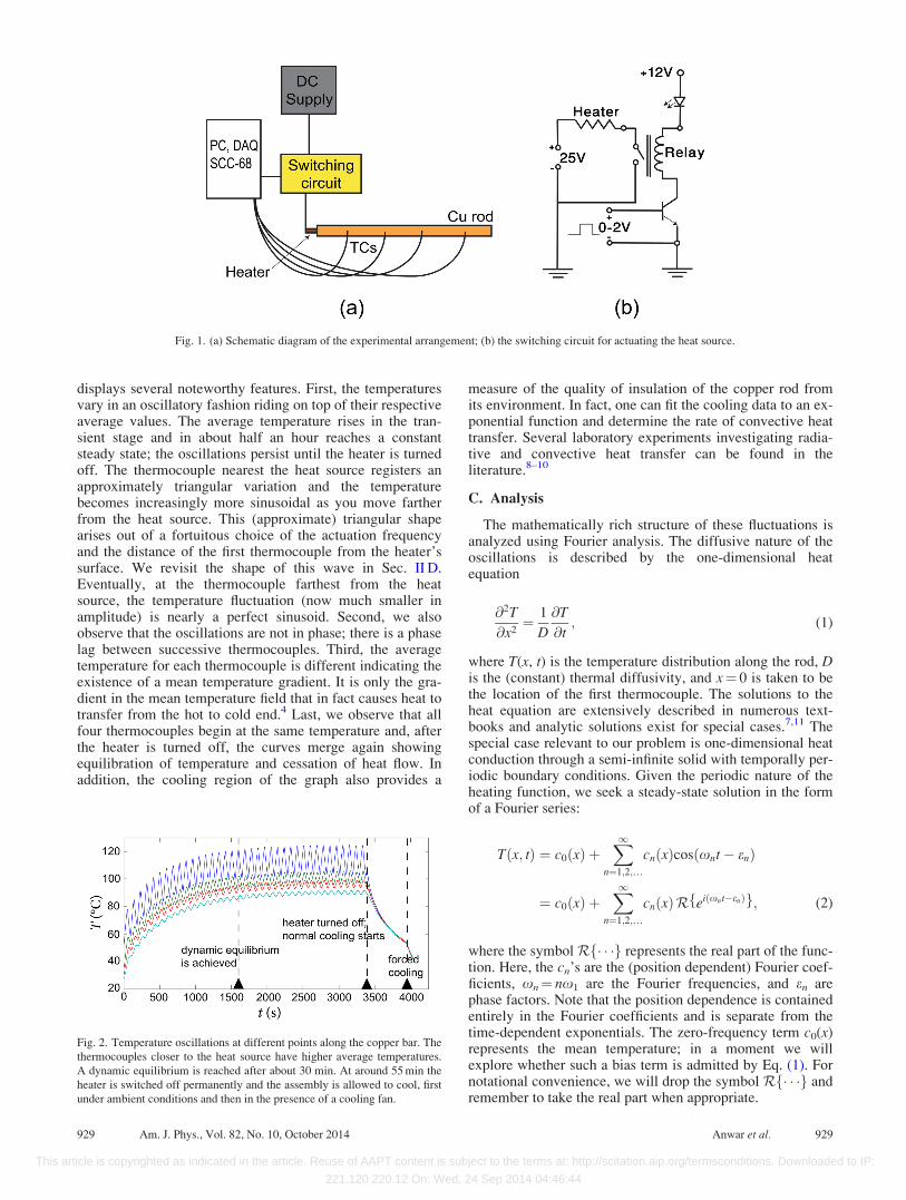
displays several noteworthy features. First, the temperaturesvary in an oscillatory fashion riding on top of their respectiveaverage values. The average temperature rises in the tran-sient stage and in about half an hour reaches a constantsteady state; the oscillations persist until the heater is turnedoff. The thermocouple nearest the heat source registers anapproximately triangular variation and the temperaturebecomes increasingly more sinusoidal as you move fartherfrom the heat source. This (approximate) triangular shapearises out of a fortuitous choice of the actuation frequencyand the distance of the first thermocouple from the heater’ssurface. We revisit the shape of this wave in Sec. II D.Eventually, at the thermocouple farthest from the heatsource, the temperature fluctuation (now much smaller inamplitude) is nearly a perfect sinusoid. Second, we alsoobserve that the oscillations are not in phase; there is a phaselag between successive thermocouples. Third, the averagetemperature for each thermocouple is different indicating theexistence of a mean temperature gradient. It is only the gra-dient in the mean temperature field that in fact causes heat totransfer from the hot to cold end.4 Last, we observe that allfour thermocouples begin at the same temperature and, afterthe heater is turned off, the curves merge again showingequilibration of temperature and cessation of heat flow. Inaddition, the cooling region of the graph also provides a

measure of the quality of insulation of the copper rod fromits environment. In fact, one can fit the cooling data to an ex-ponential function and determine the rate of convective heattransfer. Several laboratory experiments investigating radia-tive and convective heat transfer can be found in theliterature.8–10

C. Analysis

The mathematically rich structure of these fluctuations isanalyzed using Fourier analysis. The diffusive nature of theoscillations is described by the one-dimensional heatequation

@2T

@x2¼ 1

D

@T

@t; (1)

where T(x, t) is the temperature distribution along the rod, Dis the (constant) thermal diffusivity, and x¼ 0 is taken to bethe location of the first thermocouple. The solutions to theheat equation are extensively described in numerous text-books and analytic solutions exist for special cases.7,11 Thespecial case relevant to our problem is one-dimensional heatconduction through a semi-infinite solid with temporally per-iodic boundary conditions. Given the periodic nature of theheating function, we seek a steady-state solution in the formof a Fourier series:

Tðx; tÞ ¼ c0ðxÞ þX1

n¼1;2;…

cnðxÞcosðxnt� enÞ

¼ c0ðxÞ þX1

n¼1;2;…

cnðxÞR eiðxnt�enÞf g; (2)

where the symbolRf� � �g represents the real part of the func-tion. Here, the cn’s are the (position dependent) Fourier coef-ficients, xn¼ nx1 are the Fourier frequencies, and en arephase factors. Note that the position dependence is containedentirely in the Fourier coefficients and is separate from thetime-dependent exponentials. The zero-frequency term c0(x)represents the mean temperature; in a moment we willexplore whether such a bias term is admitted by Eq. (1). Fornotational convenience, we will drop the symbol Rf� � �g andremember to take the real part when appropriate.

Fig. 1. (a) Schematic diagram of the experimental arrangement; (b) the switching circuit for actuating the heat source.

Fig. 2. Temperature oscillations at different points along the copper bar. The

thermocouples closer to the heat source have higher average temperatures.

A dynamic equilibrium is reached after about 30 min. At around 55 min the

heater is switched off permanently and the assembly is allowed to cool, first

under ambient conditions and then in the presence of a cooling fan.

929 Am. J. Phys., Vol. 82, No. 10, October 2014 Anwar et al. 929

This article is copyrighted as indicated in the article. Reuse of AAPT content is subject to the terms at: http://scitation.aip.org/termsconditions. Downloaded to IP:

221.120.220.12 On: Wed, 24 Sep 2014 04:46:44

Inserting the ansatz (2) into Eq. (1), we obtain

d2c0ðxÞdx2

þX1

n¼1;2;…

d2cnðxÞdx2

eiðxnt�enÞ

¼X1

n¼1;2;…

inx1

DcnðxÞeiðxnt�enÞ; (3)

and equating terms with the same time dependence leads to

d2c0ðxÞdx2

¼ 0 andd2cnðxÞ

dx2¼ i

nx1

DcnðxÞ: (4)

These equations can be solved to give

c0ðxÞ ¼ P1xþ P0 (5)

cnðxÞ ¼ An exp ð1þ iÞffiffiffiffiffiffiffiffinx1

2D

rx

" #

þ Bn exp �ð1þ iÞffiffiffiffiffiffiffiffinx1

2D

rx

" #; (6)

where P0, P1, An, and Bn are constants that will be deter-mined from appropriate boundary conditions. We note im-mediately that the bias term c0(x) has a linear positiondependence, as expected. Furthermore, since we require fi-nite temperatures as x ! 1, we must have An¼ 0 for all n.Hence, a possible solution to the heat-equation for ourone-dimensional problem is

Tðx; tÞ ¼ ðP1xþ P0Þ þX1

n¼1;2;…

Bnexp �ffiffiffiffiffiffiffiffinx1

2D

rx

!

� exp i nx1t�ffiffiffiffiffiffiffiffinx1

2D

rx� en

!" #: (7)

As mentioned, the constants are determined from the bound-ary conditions, which are, interestingly, measured andextracted from the experiment itself. As shown below, all ofthe constants except P1 can be determined from the tempera-ture oscillation at the location of the first thermocouple(x¼ 0). Later, we can find P1 by measuring the average tem-perature at any other location within the domain of experi-mental observation.

At x¼ 0, Eq. (7) takes the form

Tð0; tÞ ¼ P0 þX1

n¼1;2;…

Bneiðnx1t�enÞ; (8)

with real part

Tð0; tÞ ¼ P0 þX1

n¼1;2;…

Bncos nx1t� enð Þ: (9)

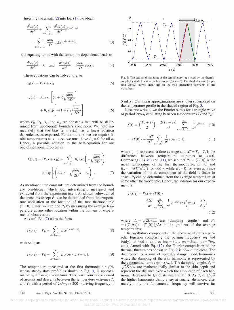
The temperature measured at the first thermocouple f(t),whose steady-state profile is shown in Fig. 3, is approxi-mated by a triangle waveform. This waveform is comprisedof ascents and descents between the temperature extremes Tl

and Th with a period of 2p/x1 � 200 s (driving frequency is

5 mHz). Our linear approximations are shown superposed onthe temperature profile in the shaded region of Fig. 3.

Next, we write down the Fourier series for a triangle waveof period 2p/x1 oscillating between temperatures Tl and Th:

f ðtÞ ¼ Th þ Tl

2

� �� 2ðTh � TlÞ

p2

X1n¼61;63;…

1

n2einx1t (10)

¼ hTð0Þi � 4DT

p2

X1n¼1;3;…

1

n2cosðnx1tÞ; (11)

where h� � �i represents a time average and DT¼Th – Tl is thedifference between temperature extremes at x¼ 0.Comparing Eqs. (9) and (11), we see that P0 ¼ hTð0Þi is themean temperature of the first thermocouple, en¼ 0, andBn¼ –4DT/(p2n2) for odd n while Bn¼ 0 for even n. Sincethe variation of the dc component of the field is linear inspace, P1 can be determined from the average temperature atsome other thermocouple. Hence, the solution for our experi-ment is

Tðx; tÞ ¼ P1xþ hTð0Þi

� 4DT

p2

X1n¼1;3;5;…

1

n2e�x=dn cos nx1t� x

dn

� �;

(12)

where dn ¼ffiffiffiffiffiffiffiffiffiffiffiffiffiffi2D=xn

pare “damping lengths” and P1

¼ hTðDxÞi � hTð0Þið Þ=Dx is the gradient of the averagetemperatures.

The oscillatory component of the above solution is a peri-odic function comprising the pulsing frequency x1 and(only) its odd multiples (x3¼ 3x1, x5¼ 5x1, x7¼ 7x1,etc.). Armed with Eq. (12), the Fourier composition of thethermal fluctuations shown in Fig. 2 is now quite clear. Thedisturbance is a sum of spatially damped odd harmonicswhere the damping of the n’th harmonic is represented bythe exponential term expð�x=dnÞ. The damping lengths dn ¼ffiffiffiffiffiffiffiffiffiffiffiffiffiffi

2D=xn

pare mathematically similar to the skin depth and

represent the distance over which the amplitude of each har-monic decreases to 1/e of its value at x¼ 0. As dn / 1=

ffiffiffinp

the higher harmonics damp away at smaller distances; ulti-mately, only the fundamental frequency will survive far

Fig. 3. The temporal variation of the temperature registered by the thermo-

couple located closest to the heat source (at x¼ 0). The shaded region (of pe-

riod 2p/x1) shows linear fits on the two alternating segments of the

waveform.

930 Am. J. Phys., Vol. 82, No. 10, October 2014 Anwar et al. 930

This article is copyrighted as indicated in the article. Reuse of AAPT content is subject to the terms at: http://scitation.aip.org/termsconditions. Downloaded to IP:

221.120.220.12 On: Wed, 24 Sep 2014 04:46:44

from the heat source. In some sense the material is actinglike the thermal analogue of a low pass filter.

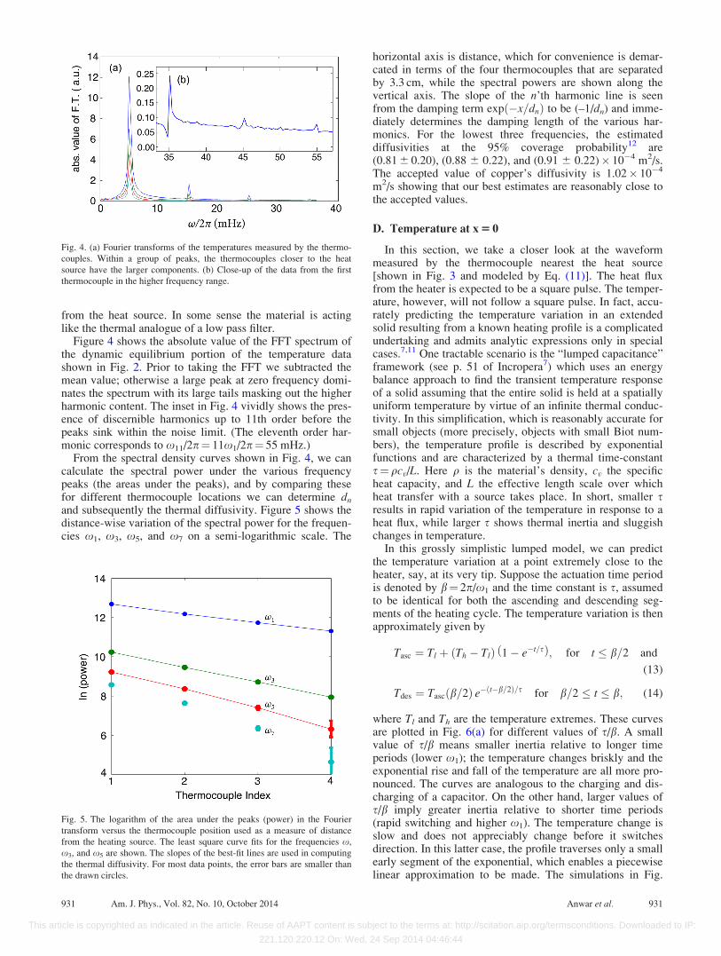
Figure 4 shows the absolute value of the FFT spectrum ofthe dynamic equilibrium portion of the temperature datashown in Fig. 2. Prior to taking the FFT we subtracted themean value; otherwise a large peak at zero frequency domi-nates the spectrum with its large tails masking out the higherharmonic content. The inset in Fig. 4 vividly shows the pres-ence of discernible harmonics up to 11th order before thepeaks sink within the noise limit. (The eleventh order har-monic corresponds to x11/2p¼ 11x1/2p¼ 55 mHz.)

From the spectral density curves shown in Fig. 4, we cancalculate the spectral power under the various frequencypeaks (the areas under the peaks), and by comparing thesefor different thermocouple locations we can determine dn

and subsequently the thermal diffusivity. Figure 5 shows thedistance-wise variation of the spectral power for the frequen-cies x1, x3, x5, and x7 on a semi-logarithmic scale. The

horizontal axis is distance, which for convenience is demar-cated in terms of the four thermocouples that are separatedby 3.3 cm, while the spectral powers are shown along thevertical axis. The slope of the n’th harmonic line is seenfrom the damping term expð�x=dnÞ to be (–1/dn) and imme-diately determines the damping length of the various har-monics. For the lowest three frequencies, the estimateddiffusivities at the 95% coverage probability12 are(0.81 6 0.20), (0.88 6 0.22), and (0.91 6 0.22)� 10�4 m2/s.The accepted value of copper’s diffusivity is 1.02� 10�4

m2/s showing that our best estimates are reasonably close tothe accepted values.

D. Temperature at x 5 0

In this section, we take a closer look at the waveformmeasured by the thermocouple nearest the heat source[shown in Fig. 3 and modeled by Eq. (11)]. The heat fluxfrom the heater is expected to be a square pulse. The temper-ature, however, will not follow a square pulse. In fact, accu-rately predicting the temperature variation in an extendedsolid resulting from a known heating profile is a complicatedundertaking and admits analytic expressions only in specialcases.7,11 One tractable scenario is the “lumped capacitance”framework (see p. 51 of Incropera7) which uses an energybalance approach to find the transient temperature responseof a solid assuming that the entire solid is held at a spatiallyuniform temperature by virtue of an infinite thermal conduc-tivity. In this simplification, which is reasonably accurate forsmall objects (more precisely, objects with small Biot num-bers), the temperature profile is described by exponentialfunctions and are characterized by a thermal time-constants¼qcv/L. Here q is the material’s density, cv the specificheat capacity, and L the effective length scale over whichheat transfer with a source takes place. In short, smaller sresults in rapid variation of the temperature in response to aheat flux, while larger s shows thermal inertia and sluggishchanges in temperature.

In this grossly simplistic lumped model, we can predictthe temperature variation at a point extremely close to theheater, say, at its very tip. Suppose the actuation time periodis denoted by b¼ 2p/x1 and the time constant is s, assumedto be identical for both the ascending and descending seg-ments of the heating cycle. The temperature variation is thenapproximately given by

Tasc ¼ Tl þ ðTh � TlÞ 1� e�t=sð Þ; for t � b=2 and

(13)

Tdes ¼ Tascðb=2Þ e�ðt�b=2Þ=s for b=2 � t � b; (14)

where Tl and Th are the temperature extremes. These curvesare plotted in Fig. 6(a) for different values of s/b. A smallvalue of s/b means smaller inertia relative to longer timeperiods (lower x1); the temperature changes briskly and theexponential rise and fall of the temperature are all more pro-nounced. The curves are analogous to the charging and dis-charging of a capacitor. On the other hand, larger values ofs/b imply greater inertia relative to shorter time periods(rapid switching and higher x1). The temperature change isslow and does not appreciably change before it switchesdirection. In this latter case, the profile traverses only a smallearly segment of the exponential, which enables a piecewiselinear approximation to be made. The simulations in Fig.

Fig. 4. (a) Fourier transforms of the temperatures measured by the thermo-

couples. Within a group of peaks, the thermocouples closer to the heat

source have the larger components. (b) Close-up of the data from the first

thermocouple in the higher frequency range.

Fig. 5. The logarithm of the area under the peaks (power) in the Fourier

transform versus the thermocouple position used as a measure of distance

from the heating source. The least square curve fits for the frequencies x,

x3, and x5 are shown. The slopes of the best-fit lines are used in computing

the thermal diffusivity. For most data points, the error bars are smaller than

the drawn circles.

931 Am. J. Phys., Vol. 82, No. 10, October 2014 Anwar et al. 931

This article is copyrighted as indicated in the article. Reuse of AAPT content is subject to the terms at: http://scitation.aip.org/termsconditions. Downloaded to IP:

221.120.220.12 On: Wed, 24 Sep 2014 04:46:44

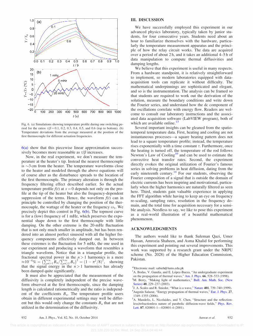
6(a) show that this piecewise linear approximation succes-sively becomes more reasonable as s/b increases.

Now, in the real experiment, we don’t measure the tem-perature at the heater’s tip. Instead the nearest thermocoupleis �3 cm from the heater. The temperature waveforms closeto the heater and modeled through the above equations willof course alter as the disturbance spreads to the location ofthe first thermocouple. The primary alteration is through thefrequency filtering effect described earlier. So the actualtemperature profile f(t) at x¼ 0 depends not only on the pro-file at the tip of the heater but also the frequency-dependentsuppression of the terms. Hence, the waveform f(t) can inprinciple be controlled by changing the position of the ther-mocouple, the wattage of the heater or the frequency x1. Weprecisely depict this control in Fig. 6(b). The topmost curveis for a (low) frequency of 1 mHz, which preserves the expo-nential shape down to the first thermocouple with littledamping. On the other extreme is the 20-mHz fluctuationthat is not only much smaller in amplitude, but has been ren-dered into an almost perfect sinusoid with all the higher fre-quency components effectively damped out. In betweenthese extremes is the fluctuation for 5 mHz, the one used inour experiment and producing a waveform that resembles atriangle waveform. Notice that in a triangular profile, thefractional spectral power in the n> 1 harmonics is a mere�10�4% ¼

P1n>1 Bn=

P1n�1 Bn

� �2 ¼ ð1� p2=8Þ2, showingthat the signal energy in the n> 1 harmonics has alreadybeen damped quite significantly.

It must also be appreciated that the measurement of thediffusivity is completely independent of the precise wave-form observed at the first thermocouple, since the dampinglength is calculated ratiometrically and the ratio is independ-ent of the coefficients Bn. The temperature profile usersobtain in different experimental settings may well be differ-ent but this would only change the constants Bn that are notutilized in the determination of the diffusivity.

III. DISCUSSION

We have successfully employed this experiment in ouradvanced physics laboratory, typically taken by junior stu-dents, for four consecutive years. Students need about anhour to familiarize themselves with the hardware, particu-larly the temperature measurement apparatus and the princi-ple of how the relay circuit works. The data are acquiredover a period of about 2 h, and it takes an additional 4–5 h ofdata manipulation to compute thermal diffusivities anddamping lengths.

We believe that this experiment is useful in many respects.From a hardware standpoint, it is relatively straightforwardto implement, so modern laboratories equipped with data-acquisition tools can replicate it without difficulty. Themathematical underpinnings are sophisticated and elegant,and so is the instrumentation. The analysis can be framed sothat students are required to work out the derivation of thesolution, measure the boundary conditions and write downthe Fourier series, and understand how the dc component ofthe oscillations correlate with energy flow. Readers are wel-come to consult our laboratory instructions and the associ-ated data acquisition software (LabVIEW program), both ofwhich are available online.13

Several important insights can be gleaned from the spatio-temporal temperature data. First, heating and cooling are notinstantaneous processes—a square heating pattern does notlead to a square temperature profile; instead, the temperaturerises exponentially with a time constant s. Furthermore, oncethe heating is turned off, the temperature of the rod followsNewton’s Law of Cooling10 and can be used to estimate theconvective heat transfer rates. Second, the experimentdirectly evokes the original utilization of Fourier’s famousseries in solving problems in heat diffusion, dating from theearly nineteenth century.14 For our students, observing theFourier composition of a signal that is outside the domain ofelectric currents has been inspiring and motivational, particu-larly when the higher harmonics are naturally filtered as seenhere. Third, students gain valuable experience in applyingthe FFT algorithm while having to keep an eye on frequencyre-scaling, sampling rates, resolution in the frequency do-main, and the total time for acquisition necessary for a sensi-ble analysis. Needless to say, we like to pose this experimentas a real-world illustration of a beautiful mathematicalphenomenon.

ACKNOWLEDGMENTS

The authors would like to thank Suleman Qazi, UmerHassan, Amrozia Shaheen, and Asma Khalid for performingthis experiment and pointing out several improvements. Thiswork was supported by a research grant under the NRPUscheme (No. 2028) of the Higher Education Commission,Pakistan.

a)Electronic mail: sabieh@lums.edu.pk1A. Bodas, V. Gand�ıa, and E. L�opez-Baeza, “An undergraduate experiment

on the propagation of thermal waves,” Am. J. Phys. 66, 528–533 (1998).2M. Berry, “Making light of mathematics,” Bull. Am. Math. Soc. (New

Series) 40, 229–237 (2003).3J. A. Scales and R. Snieder, “What is a wave,” Nature 401, 739–740 (1999).4Augst�ın Salazar, “Energy propagation of thermal waves,” Eur. J. Phys. 27,

1349–1355 (2006).5A. Mandelis, L. Nicolaides, and Y. Chen, “Structure and the reflection-

less/refractionless nature of parabolic diffusion-wave fields,” Phys. Rev.

Lett. 87, 020801-1––020801-4 (2001).

Fig. 6. (a) Simulations showing temperature profile during one switching pe-

riod for the ratios s/b¼ 0.1, 0.2, 0.3, 0.4, 0.5, and 0.6 (top to bottom). (b)

Temperature deviations from the average measured at the position of the

first thermocouple for different actuation frequencies.

932 Am. J. Phys., Vol. 82, No. 10, October 2014 Anwar et al. 932

This article is copyrighted as indicated in the article. Reuse of AAPT content is subject to the terms at: http://scitation.aip.org/termsconditions. Downloaded to IP:

221.120.220.12 On: Wed, 24 Sep 2014 04:46:44

6A. Mandelis, “Diffusion waves and their uses”, Phys. Today 66, 29–34

(2000).7F. P. Incropera, D. P. Dewitt, T. L. Bergmann, and A. S. Lavine,

Fundamentals of Heat and Mass Transfer, 7th ed. (Wiley, New Jersey, 2012).8J. E. Spuller and R. W. Cobb, “Cooling of a vertical cylinder by natural con-

vection: An undergraduate experiment,” Am. J. Phys. 61, 568–571 (1993).9M. I. Gonzalez and J. H. Lucio, “Investigating convective heat transfer

with an iron and a hairdryer,” Eur. J. Phys. 29, 263–273 (2008).10M. S. Anwar and W. Zia, “Curie point, susceptibility, and temperature

measurements of rapidly heated ferromagnetic wires,” Rev. Sci. Instrum.

81, 124904–124908 (2010).

11H. S. Carslaw and J. C. Jaeger, Conduction of Heat in Solids, 2nd ed.

(Clarendon Press, Oxford, 1959), pp. 50–92.12L. Kirkup and R. B. Frenkel, An Introduction to Uncertainty in

Measurement (Cambridge U.P., Cambridge, 2006).13See supplementary material at http://dx.doi.org/10.1119/1.4881608 for our

laboratory instructions and the LabVIEW program are available as or at

the author-maintained website <http://physlab.lums.edu.pk/index.php/

Experiment_in_Lab-II> (see the experiment numbered 2.3).14Fourier’s monograph Th�eorie analytique de la chaleur was published in

1822. An original English translation is A. Freeman, The AnalyticalTheory of Heat (Cambridge U.P., Cambridge, 1878).

933 Am. J. Phys., Vol. 82, No. 10, October 2014 Anwar et al. 933

This article is copyrighted as indicated in the article. Reuse of AAPT content is subject to the terms at: http://scitation.aip.org/termsconditions. Downloaded to IP:

221.120.220.12 On: Wed, 24 Sep 2014 04:46:44